LINE SEARCH MULTILEVEL OPTIMIZATION AS COMPUTATIONAL METHODS FOR DENSE OPTICAL FLOW

LINE SEARCH MULTILEVEL OPTIMIZATION ASCOMPUTATIONAL METHODS FOR DENSE OPTICAL FLOW∗

EL MOSTAFA KALMOUN† , LUIS GARRIDO‡ , AND VICENT CASELLES§

Abstract. We evaluate the performance of different optimization techniques developed in thecontext of optical flow computation with different variational models. In particular, based on trun-cated Newton methods (TN) that have been an effective approach for large-scale unconstrainedoptimization, we develop the use of efficient multilevel schemes for computing the optical flow. Moreprecisely, we evaluate the performance of a standard unidirectional multilevel algorithm - calledmultiresolution optimization (MR/Opt), to a bidrectional multilevel algorithm - called full multi-grid optimization (FMG/Opt). The FMG/Opt algorithm treats the coarse grid correction as anoptimization search direction and eventually scales it using a line search. Experimental results onthree image sequences using four models of optical flow with different computational efforts showthat the FMG/Opt algorithm outperforms both the TN and MR/Opt algorithms in terms of thecomputational work and the quality of the optical flow estimation.

Key words. Optical flow, line search multigrid optimization, multiresolution, truncated Newton

1. Introduction. The problem of optical flow computation consists in findingthe 2D-displacement field that represents apparent motion of objects in a sequence ofimages. Many efforts have been devoted to it in computer vision and applied mathe-matics [27, 37, 20, 3, 4, 13, 42, 45, 14, 12, 33, 29, 1, 2, 8, 34, 35, 38]. The computationof optical flow is usually based on the conservation of some property during motion,either the object’s gray level or their shape properties. In a variational setting, theproblem is usually formulated as a minimization of an energy function, which is aweighted sum of two terms: a data term coming from the motion modeling and asmoothing term as a result of the regularization process. For standard optical flowalgorithms, the data term is usually based on a brightness constancy assumption,which assumes that the object illumination does not change along its motion trajec-tory. The regularization process ensures that the optical flow estimation problem iswell-posed. Many regularization terms have been investigated in the last two decadesranging from isotropic to anisotropic. Isotropic smoothers tend to blur motion edgeswhile the anisotropic ones require additional computational resources.

Two strategies might be conducted for the numerical minimization of an energyfunctional arising in a variational framework like above. The first one which is calledoptimize-discretize is achieved by discretizing and solving the corresponding Euler-Lagrange equations. In the second approach called discretize-optimize one can usedirectly numerical optimization methods for solving a discrete version of the problem.While the first approach has been commonly used for variational optical flow compu-tation, the second computational strategy has been less investigated in this context,

∗This research was initiated while the first author was visiting Centre de Recerca Matematica andUniversitat Pompeu Fabra in Barcelona during 2008. The first author was partially supported byFRGS grant UUM/RIMC/P-30 (S/O code 11872) offered by Ministry of Higher Education Malaysia.The second and third authors acknowledge partial support by MICINN project, reference MTM2009-08171, and by GRC reference 2009 SGR 773. The third author also acknowledges partial support by”ICREA Academia” prize for excellence in research funded both by the Generalitat de Catalunya.

†Faculty of Quantitative Sciences, College of Arts and Sciences, Universiti Utara Malaysia, 06010UUM Sintok, Malaysia ([email protected])

‡Departament de Matematica Aplicada i Analisi, Universitat de Barcelona, Barcelona, Spain([email protected])

§Departament de Tecnologia, Universitat Pompeu Fabra, Barcelona, Spain([email protected])

1

2 KALMOUN, GARRIDO AND CASELLES

to the best of our knowledge.

Adopting the first strategy, efficient algorithms have been designed to approximatethe optical flow. In particular, in [1, 2] the authors used a multiscale approximationto solve the corresponding Euler-Lagrange equations using the Nagel-Enkelmann reg-ularization term [38]. Thus, they computed a series of approximations where eachone solves a regularized version of the Euler-Lagrange equations starting from theprevious one while keeping the original grid fixed. A different approach is proposedin [11, 43] where the authors use fixed point iterations to solve the correspondingEuler-Lagrange equations, fully implicit in the smoothness term and semi-implicit inthe data term. Still, this fixed point iteration leads to implicit equations and theylinearize some of their terms using a warping technique. The equations obtained arefully linearized using a lagged diffusivity method [11, 43, 12]. The final linear sys-tem is solved using a linear solver like a Gauss-Seidel type method, or a successiveover-relaxation method (SOR). The connections with warping are detailed in [11, 43].

On the other hand, in order to develop efficient and accurate algorithms workingin real time, there have been recent efforts to improve performance of optical flow al-gorithms using multilevel techniques. We distinguish at this stage between two classesof multilevel algorithms. The first one known as a coarse-to-fine multiresolution usesa sequence of coarse grid subproblems to find a good initialization for the finest gridproblem that avoids possible local minima. We shall refer to this strategy in this paperby multiresolution. The second strategy alternates between solution relaxations usingthe underlying algorithm and solution corrections obtained from a sequence of sub-problems defined on coarse grids. This leads to recursive algorithms like the so-calledV- or W-cycle, which traverse between fine and coarse grids in the mesh hierarchy.We will reserve the term multigrid for it. In the case of elliptic PDEs - and for awide class of problems, multigrid methods are known to outperform multiresolutionmethods [7, 25].

However, being straightforward to implement, multiresolution methods were moreused in computer vision and particularly for motion estimation; e.g. [20, 3, 5, 42, 45,17]. For instance, Enkelmann [20] developed a coarse-to-fine algorithm for orientedsmoothed optical flow. Also, Cohen and Herlin [17] used recently a multiresolutiontechnique with nonuniform sampling for total variation regularization.

For the seek of optimal performance, multigrid schemes were developped to solvethe resulting Euler-Lagrange equations for both isotropic and anisotropic regulariza-tions, see [23, 46, 22, 29, 28, 14, 12] and references therein. The first attempts aredue to Glazer [23] and Terzopoulos [46] using standard multigrid components. Im-provement in performance were reported on simple synthetic images and later on [5]standard multigrids were stated to be not appropriate due to a possible informationconflict between different scales. However, the method was recently better adaptedfor optical flow computation by tuning the multigrid components. In [22], an entirelyalgebraic multigrid approach was developed for a weighted anisotropic regularizationbased model. A geometrical multigrid based on Galerkin coarse grid discretizationapproximation was developped for the classical Horn-Schunck method in [29]. Thisalgorithm was extended and paralelized in [28] for real time computation of vectormotion fields for 3D images. Another recent geometric multigrid investigation waspresented in [14, 12] with anisotropic regularization (a full account of it can be foundin [12]).

All these works have considered data terms based on the brightness constancyassumption, which lead to less accurate optical flow fields when the image sequence

MULTILEVEL OPTIMIZATION FOR OPTICAL FLOW 3

contains illumination variations in the temporal domain, which may be often foundin real images. In [16], a model is proposed for illumination invariant optical flowcomputation, previously introduced in [19] in the context of image registration. Thebrightness constancy assumption is replaced by the assumption that the shapes ofthe image move along the sequence. In this context, the terms of the Euler-Lagrangeequation corresponding to the data attachment term which contains derivatives of theunit normal vector fields are highly nonlinear. They will not produce systems of equa-tions with a symmetric and positive semi-definite matrix (usually after linearisation),the basic systems to which the previous multigrid methods for optical flow have beenapplied.

For that reason we follow in this paper the second strategy of discretize-optimizethat allows to handle such kind of variational problems. Instead of computing theEuler-Lagrange equations of the energy model, discretizing and solving them, our ap-proach is based on the use of numerical optimization methods to solve the discreteversion of the energy, be either based on gray level constancy or shape properties.This leads to the need of developing efficient algorithms for the numerical resolutionof a large scale optimization problem. Therefore only large scale unconstrained op-timization methods are relevant to solve this variational problem. One of them isthe truncated Newton method [18]. It requires only the computation of function andgradient values and has then suitable storage requirements for large-scale problems.However, due to the intensive computations that are required to solve the energyminimization problem, only multilevel versions of the method (multiresolution andmultigrid) are expected to provide suitable performance.

In our context, the bidirectional multigrid scheme should be adapted directly toan optimization problem. Current research is still ongoing in this direction for solvingsome variational problems lacking a governing PDE in different fields. Recently [40,31], the multigrid strategy has been extended to optimization problems for truncatedNewton methods. Motivated by variational problems lacking a governing PDE, themultigrid optimization was derived from the Full Approximation Storage (FAS) [9]for nonlinear PDEs but applied directly in an optimization setting. With regard tononlinear multigrids, the multigrid optimization algorithm (MG/Opt) includes twosafeguards that guarantee convergence: Bounds on the coarse grid correction thatintroduce a constrained optimization subproblem and a line search that eventuallyscales the coarse grid correction treated as a search direction. In [31], it has beenshown that the coarse grid subproblem is a first-order approximation of the fine-grid problem. This justifies somehow the introduction of the two safeguards. Thefirst-order approximation suggests that the correction will be only reliable near therestricted approximation and it relates at the same time the MG/Opt to the steepestdescent method. The latter connection indicates that the coarse grid correction willnot be typically a well-scaled descent direction which, in turn, implies that a linesearch should be performed to adjust the scale of the multigrid search direction. Thismay not be necessary as the MG/Opt is near to convergence since in that case it willprovide a Newton-like search direction for which a search step equal to 1 will be likelyaccepted. These connections to both steepest descent and Newton method suggestthat the MG/Opt will perform well far and near the solution.

Our aim is to develop the MG/Opt method for the computation of optical flow,a problem which is of considerable computational resource requirements. To the bestof our knowledge, the MG/Opt method is studied here for the first time for opticalflow computation. We note here that four different optical flow models are used for


testing the performance of the proposed algorithm combining linear and non-lineardata terms with quadratic (or Tikhononv) and total variation (TV) regularization.Several components of the MG/Opt technique have been tuned for high efficiency andthe algorithm is fully evaluated with respect to one-way multiresolution optimization.The proposed numerical strategy can be adapted to the minimization of other nonlin-ear energy functionals like the illumination invariant model proposed in [16] or depthestimation in stereo problems. Although they are an important motivation for thedevelopment of the present techniques they will not be considered in this paper.

The outline of our paper is as follows. In Section 2, we start off with a reviewof the variational formulation of the optical flow problem. In Section 3, we recallthe basics of the truncated Newton method. In Section 4, we present multilevelalgorithms applied to optimization problems. First, we discuss the coarse-to-finemultiresolution strategy. Then, after recalling the idea of multigrid for linear systems,we describe its application to optimization-based problems. In Section 5, we outlinesome of the implementation details, namely the calculation of the gradient of theobjective functional for each of the four models considered in this paper, of its Hessiancomputation and of the image derivatives. In Section 6, we report our experimentalresults by considering three classical sequences of synthetic images: the translatingtree, the diverging tree and the Yosemite sequences. In Section 7, we conclude thepaper and indicate future research directions.

2. Variational models for optical flow. Let us consider a sequence of graylevel images I(t, x, y), t ∈ [0, T ], (x, y) ∈ Q, where Q denotes the image domain, whichwe assume to be a rectangle in R2. We shall either consider the case where t ∈ [0, T ],and the case where the sequence is sampled at the times tj = j∆t, j = 0, . . . ,K.Assuming that the gray level of a point does not change over time we may write theconstraint

I(t, x(t), y(t)) = I(0, x, y),

where (x(t), y(t)) is the apparent trajectory of the point (x(0), y(0)) = (x, y). Differ-entiating with respect to t and denoting (u(t, x, y), v(t, x, y)) = (x′(t), y′(t)) we obtainthe optical flow constraint

It + uIx + vIy = 0. (2.1)

The vector field w(t, x, y) := (u(t, x, y), v(t, x, y)) is called optic flow and It, Ix, Iy

denote the partial derivatives of I with respect to t, x, y, respectively. Clearly, thesingle constraint (2.1) is not sufficient to uniquely compute the two components (u, v)of the optic flow (this is called the aperture problem) and only gives the componentof the flow normal to the image gradient, i.e., to the level lines of the image. As itis usual, in order to recover a unique flow field a regularization constraint is added.For that, we assume that the optic flow varies smoothly in space, or better, that ispiecewise smooth in Q. This can be achieved by including a smoothness term of theform

R(w) :=

∫Q

G(∇I,∇u,∇v) dxdy, (2.2)

where G : R2 × R2 × R2 → R is a suitable function. The case G = ‖∇u‖2 + ‖∇v‖2corresponds to the Horn-Schunk model [27], the case G = trace((∇w)TD(∇I)∇w)corresponds to the Nagel-Enkelmann model [38], the case G =

√‖∇u‖2 + ‖∇v‖2 or


G = ‖∇u‖ + ‖∇v‖ correspond to total variation regularization models. For a fullaccount of this and the associated taxonomy, we refer to [47, 26].

Both data attachment and regularization terms can be combined into a singleenergy functional∫

Q

(It + uIx + vIy)2 dxdy + α

∫Q

G(∇I,∇u,∇v) dxdy, (2.3)

where α > 0 is the regularization parameter weighting the relative importance of bothterms.

In case of illumination changes, the gray level constancy assumption is violated,and may be substituted by the constancy of the gradient [6, 43] which can be expressedin differential form as

〈w,∇Ix〉 = 0〈w,∇Iy〉 = 0.

(2.4)

Other cases include the constancy of the gradient direction [15] or the assumption thatthe shapes of the image (identified as the level lines) move along the sequence [16](this assumption has been used in [19] in the context of image registration). Higherderivative models have been studied in [43].

The above models (2.3), (2.4) do not take into account that video sequencesare sampled in time so that our data has the form Ij(x, y) := I(tj , x, y), tj = j∆t,j = 0, . . . ,K. Without loss of generality, let us assume that ∆t = 1. In that case, thegray level constancy may be expressed as

Ij−1(x, y) = Ij(x+ uj(x, y), y + vj(x, y)), (2.5)

where (uj(x, y), vj(x, y)) is the optical flow between images Ij−1 and Ij . As argued in[1, 2] the linearized gray level constancy constraint (2.1) may not be a good approx-imation in case of large displacements and the form (2.5) may be more appropriate[12].

A corresponding energy functional can be obtained by combining the non lin-earized form of the brightness constancy assumption and a regularization term. Forconvenience, we assume that we want to compute the optical flow between two imagesI1(x, y) and I2(x, y). We may write the energy∫

Q

Ψ((I1(x, y)− I2(x+ u(x, y), y + v(x, y)))

2)dxdy + α

∫Q

G(∇I,∇u,∇v) dxdy,

(2.6)where Ψ : R → R is an increasing smooth function, and α > 0. Examples of func-tion G have been given above (see [47, 26, 12] for an account of the many differentpossibilities).

Observe that the energy (2.6) is nonlinear and non convex. In order to developthe basic numerical optimization methods, the variational optical flow problem is setinto the simplified minimization form:

minwf(w), (2.7)

where f(w) := D(w) + αR(w). Here D denotes a given data term based on either(2.1) or (2.6) and R denotes a regularization term being either quadratic or the totalvariation. More precisely, we consider in this paper the case of G = ‖∇u‖2 + ‖∇v‖2


or G = ‖∇u‖ + ‖∇v‖. We also consider Ψ(s2) = s2 for |s| ≤ γ and Ψ(s2) = γ2 for|s| > γ.

As discussed in the introduction, we adopt the strategy discretize-optimize. Thismeans that we shall first discretize the objective functional and then solve a finitedimensional but large scale optimization problem. Therefore only large scale uncon-strained optimization methods are relevant to solve this variational problem. One ofthese methods that requires only the computation of function and gradient values andhas suitable storage requirements for large-scale problems is the truncated Newtonmethod [18]. We note that other choices of the underlying optimization procedure -like the BFGS quasi Newton method, are possible. The truncated Newton algorithmis embedded in a multilevel strategy, both multiresolution and multigrid.

3. Truncated Newton optimization. As it is well known, Newton methodsare based on the second order Taylor approximation of the objective function to buildan iterative process for approaching a local minimum. The step sk to move from thecurrent point wk to a new iterate wk+1 is chosen to be a minimum of the quadraticmodel of f given by

qk(s) = fk + gTk s+1

2sTHks. (3.1)

where fk = f(wk) , gk = ∇f(wk) and Hk = ∇2f(wk). The Newton step sk is thenobtained by solving the linear system

Hks = −gk (3.2)

For large-scale problems, solving exactly this linear system will be very expensive.Truncated Newton methods (TN) use rather an iterative method to find an approx-imate solution to (3.2) and truncate the iterates as soon as a required accuracy isreached or whenever (in case when the Hessian matrix Hk is not positive definite), anegative curvature is detected. One of the most well known iterative methods withinTN ones is the Preconditioned Conjugate Gradient algorithm (PCG), see Algorithm2, due to its efficiency and modest memory requirements. In this context, we will referto the process of finding the step sk as inner iterations, while the process of updatingwk using the computed sk will be called outer iterations. Our discussion in the sequeldepends on the use of the PCG method as an inner solver.

Depending on how the step solution sk of the quadratic model (3.1) is exploited,two broad classes of algorithms are distinguished: line search methods and trust regionmethods. Line search methods scale the step sk by a factor αk that approximatelyminimizes f along the line that passes through wk in the direction sk. On the otherhand, trust region methods restrict the search for sk to some region Bk around wk inwhich the algorithm ”trusts” that the model function qk behaves like the objectivefunction f . This paper focuses on the former, the line search method, whereas thecomparison between both methods (line search and trust region) will be the object offuture work.

There are three components in the truncated Newton method related to speedingup the convergence of inner iterations that might have a great impact on its overallefficiency: a) the truncation criterion, b) the preconditioning strategy and c) howto handle the case when the Hessian matrix is not positive definite. Indeed, for thelatter, one of the advantages of trust region over line search is that negative curvaturedirections can be properly exploited. In the PGC algorithm (Algorithm 2), the inner


iterations are truncated as soon as a negative curvature direction is detected, that is,when pTj Hkpj is negative. In our case, we replace the negative curvature test withthe equivalent descent direction test [49], see lines 8-11 of Algorithm 2. From ourpractical experience, the descent direction test has a better numerical behavior thanthe negative curvature test.

For the other two components a) and b), we used a scaled two-step limited mem-ory BFGS [39] with a diagonal scaling for preconditioning the CG method, and wetruncate the inner iterations when the following criterion is satisfied:

||rj ||M−1k

≤ ζk||r0||M−1k,

where rj is the PCG residual at inner iteration j, Mk is the preconditioning matrixand

ζk = max(0.5/(k + 1), ||r0||M−1

k

)(3.3)

which are both being provided at outer iteration k, and where

||rj ||M−1k

=√rTj M

−1k rj .

The matrixM−1k may be computed easily ifMk is updated using the BFGS method [41].

In this case, however, M−1k does not need to be computed since M−1

k rj = vj , andthus rTj M

−1k rj = rTj vj .

Line search TN methods ensure that the new TN step sk provides a good descentby performing a line minimization along this direction and then the new outer iteratebecomes:

wk+1 = wk + αksk.

Exact line search is avoided due to expensive function evaluations and normally asufficient function decrease is obtained by imposing the Wolf’s conditions:

fk+1 ≤ fk + c1αkgTk sk (3.4)

gTk+1sk ≥ c2 gTk sk, (3.5)

where 0 < c1 < c2 < 1. In order to obtain a maximum decrease with a minimumnumber of function evaluations, interpolating polynomials is usually employed. Herein TN a cubic interpolation was used [36].

The algorithm associated to the outer iterations of the line search TN is shown inAlgorithm 1. The algorithm iteratively updates wk by computing a search directionand performing a line search until a given tolerance is reached. In our case we settolerances on the gradient, εg, to detect local minima, and on the function values anditerate values, εf and εx to detect convergence. Note also that the preconditionningmatrix Mk is updated here, which can be easily done from previous values of wk andg(wk), see [41].

4. Multilevel methods. Multilevel methods use a set of subproblems definedon coarser levels of resolution in order to improve the convergence to the global op-timum of (2.7) when compared to using only one level of resolution. Using multiplelevels of resolution allows to deal, in the case of optical flow computation, with largedisplacements and enables the convergence to the global minimum since some localminima may disappear at sufficient coarse resolutions.


Algorithm 1 Line Search Truncated Newton (outer iterations of TN)

1: Initialization w0, M0 = Id, εg, εf , εx2: for k = 0 to max outer do3: gk = ∇f(xk)4: if ||gk|| < εg then5: exit with solution wk6: end if7: Compute sk by calling Algorithm 2.8: Perform a line search to scale the step sk by αk.9: wk+1 = wk + αksk

10: Update Mk+1 by the BFGS formula11: if |fk+1 − fk| < εf or ||wk+1 − wk|| < εx then12: exit with solution wk13: end if14: end for

Algorithm 2 Preconditioned Conjugate Gradient (inner iterations of TN)

1: Initialization: z0 = 0, r0 = −gk, v0 =M−1k r0, p0 = v0, ε = 10−10, ζk(see (3.3))

2: for j = 0 to max inner do3: // Singularity test4: if

(|rTj vj | < ε or |pTj Hkpj | < ε

)then

5: exit with sk = zj (for j = 0 take sk = −gk)6: end if7: αj = rTj vj/p

Tj Hkpj , zj+1 = zj + αjpj

8: // Descent Direction Test replaces Negative Curvature test9: if (gTk zj+1 ≥ gTk zj − ε) then

10: exit with sk = zj (for j = 0 take sk = −gk)11: end if12: rj+1 = rj − αjHkpj , vj+1 =M−1

k rj+1

13: // Truncation test (note that ||rj+1||M−1k

= rTj+1vj+1)

14: if (rTj+1vj+1 ≤ ζkgT0 v0) then

15: exit with sk = zj+1

16: end if17: βj = rTj+1(vj+1 − vj)/r

Tj vj , pj+1 = vj+1 + βjpj .

18: end for19: exit with sk = zj

Let us denote with Ωi the image domain at level i, where i = 0 . . . r, where i = 0corresponds to the finest level of resolution and i = r to the coarsest one. Grid spacingat the coarser grid Ωi+1 is usually twice the spacing at the grid Ωi. Two approachesare currently widely used in the computer vision field, namely the multiresolution andthe multigrid methods. Both are explained below.

4.1. Multiresolution methods. Multiresolution methods have been appliedsuccessfully in many computer vision and image analysis problems where the problemcan be expressed as a global optimization problem [20, 3, 5, 42, 45, 17]. Multiresolutionmethods use a series of coarse to fine resolution levels to obtain an estimate of thesolution to the problem. An initial estimate is obtained at the coarsest level. In our


case, this estimate may be obtained by applying the TN algorithm (see Algorithm 1).The estimate is then extended to the next level of resolution where it is refined.This process is repeated until the finest level is reached, where the final estimate isobtained, see Algorithm 3, where the MR (multiresolution) method is shown. Thisfunction is called with MR(L− 1, xL−1,0), where L is the number of resolution levelsand xL−1,0 is the initial estimate on the coarsest.

The advantage of coarse-to-fine multiresolution is that a good initial guess maybe obtained for the finest grid problem by estimating a solution to the problem usingthe coarser grids. However, for linear systems it is currently known that one-way mul-tilevel methods do not reach the optimal efficiency of standard bidirectional multigridmethods, which are detailed in the next section.

Algorithm 3 Multiresolution method

1: function MR(i, xi,0)2: i = L− 1: coarsest level of resolution3: xi,0: initial estimate4: repeat5: Apply TN with initial estimate xi,06: Let xi,1 be the result7: if i > 0 then8: // Prolonge current estimate to next finer level9: xi−1,0 = Pxi,1

10: end if11: i = i− 112: until i < 013: return x0,1

4.2. Multigrid methods. Multigrid methods were originally developed to solveelliptic PDEs and at present are known to be among the most powerful numericalmethods for improving computational efficiency of a wide class of equations. For aclassical reference on multigrids, we refer to [9, 10]. The main characteristic of multi-grid algorithms is based on the observation that different frequencies are present inthe error of the solution of the finest grid problem. Some algorithms, called smoothers(such as Gauss-Seidel), are known to efficiently reduce the high frequency componentsof the error on a grid (or, in other words, the components whose ”wavelength” is com-parable to the grid’s mesh size). However, these algorithms have a small effect on thelow frequency error components. This is the reason why the application of schemeslike Gauss-Seidel to solve a problem, for a given grid, effectively reduces the error inthe first iterations of the procedure (due to smoothing of the high frequency errors)but then converges slowly to the solution (due to smoothing of the low frequencyerrors).

One may observe that low frequency errors appear as higher frequencies on coarsergrids. The latter may be effectively reduced using a smoother in the coarse grid.Moreover, smoothing at a coarser level has typically a much lower cost than on finerones. The core idea of multigrid is to use a sequence of subproblems defined on coarsergrids as a means to accelerate the solution process (by relaxation such as Gauss-Seidel)on the finest grid. This leads to recursive algorithms like the so-called V- or W-cycle,which traverse between fine and coarse grids in the mesh hierarchy. Since ultimatelyonly a small number of relaxation steps on each level must be performed, multigrid


provides an asymptotically optimal method whose complexity is only O(N), where Nis the number of mesh points.

4.2.1. Multigrid for linear systems. We recall first the basic of multigridtechniques. We consider a sparse linear system which typically results from the dis-cretization of a partial differential equation on a fine grid Ωi with a given grid spacingh.

Aixi = bi. (4.1)

Let xi,0 be an initial approximation of (4.1) and xi be the exact solution. The firststep of the algorithm consists in smoothing the error xi−xi,0 by applyingN0 iterationsof a relaxation scheme S to (4.1) that has the smoothing property [25]. Examplesof the smoother S are Richardson, Jacobi or Gauss-Seidel. The obtained smoothapproximation xi,1 satisfies equation (4.1) up to a residual ri:

Aixi,1 = bi − ri.

The corresponding error equation is therefore given by

Aiei = ri, (4.2)

where ei = xi,1 − xi is the unknown smooth error. Equation (4.2) is then solved ona coarser grid Ωi+1 with a grid spacing that has to be larger than h (typical choiceis 2h but other choices are possible). For this, the fine grid error equation must beapproximated by a coarse grid equation:

Ai+1ei+1 = ri+1. (4.3)

We need therefore to transfer the residual to the coarse grid and construct a coarseversion of the fine matrix. Let R be a restriction operator mapping functions on Ωito functions on Ωi+1 (common examples are injection and full weighting, see [10]).The coarse residual is given then by

ri+1 = Rri.

The coarse grid matrix may be obtained by re-discretization on Ωi+1 or by using theGalerkin coarse grid approximation: Ai+1 = RAi P . Here P is a prolongation (orinterpolation) operator mapping functions from Ωi+1 to Ωi (standard examples arelinear and bilinear interpolation).

The result ei+1,∗ due to solving (4.3) is transferred back to the fine grid to obtain:

ei,∗ = Pei+1,∗.

With this approximation of the fine grid error, the approximate solution is correctedto obtain:

xi,2 = xi,1 + ei,∗.

In order to damp high frequency error components that might arise due to the inter-polation, N1 iterations of the smoother S are applied on the fine grid to get the newiterate xi,3.

The coarse grid problem (4.3) has a lower dimension than the original problem(4.1), but it must be solved accurately for each iteration which can be very costly.


In a typical multigrid with three levels or more, this problem is solved by callingrecursively the algorithm γ times until reaching the coarsest grid, where we solve (4.3)exactly with a negligible cost. The steps of this multigrid algorithm are summarizedin Algorithm 4.

The resulting xi,3 may be injected iteratively as initialization in Algorithm 4 untilthe residual on the finest grid

ri,3 = bi −Aixi,3

is smaller than a given tolerance.

Algorithm 4 Linear Multigrid V-Cycle

1: function MG-cycle(i, Ai, bi, xi,0)2: i: level3: Ai, bi: defines linear system to be solved4: xi,0: initialization5: if i is the coarsest level then6: Solve xi,1 = A−1

i bi // Solve exactly7: else8: xi,1 := S(xi,0, Ai, bi, N0) // Smooth with N0 iterations9: xi+1,0 = 0

10: ri := bi −Aixi,1 // Residual11: ri+1 := Rri // Restrict12: Call MG(i+ 1, Ai+1, ri+1, xi+1,0) γ times // Recursive call13: Let ei+1,∗ be the returned value14: ei,∗ := P ei+1,∗ // Extend15: xi,2 := xi,1 + ei,∗ // Apply correction step16: xi,3 := S(xi,2, Ai, bi, N1) // Postsmooth with N1 iterations17: Return xi,318: end if

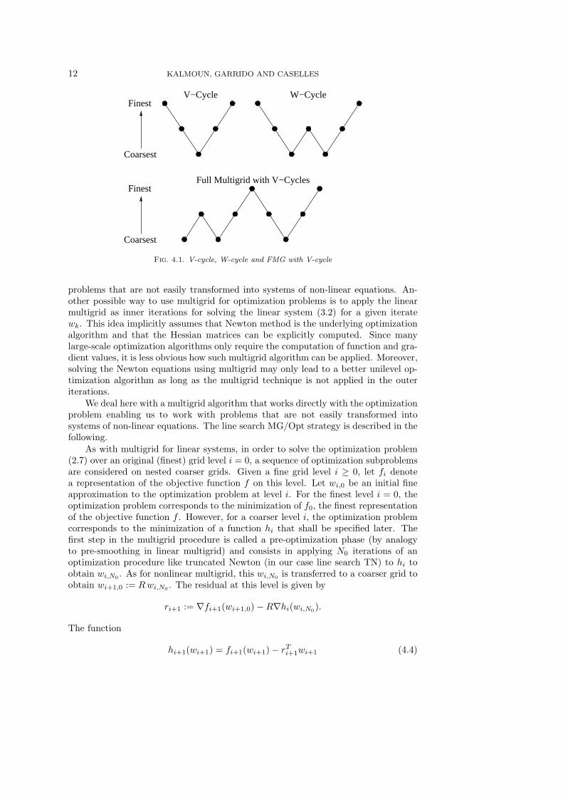
Note that for the smoothing steps N0 and N1, only the sum is important in aconvergence analysis. Typical values for the tuple (N0, N1) are (1, 1) , (2, 1) and (2, 2).For the cycling parameter γ, only the values 1 and 2 are commonly used. The so-calledV-cycle corresponds to γ = 1 and W-cycle corresponds to γ = 2. This is illustratedin Figure 4.1 for three levels.

An important variation of multigrids, which is known as the full multigrid method(FMG) [9] or nested iteration technique [25], combines a multiresolution approach witha standard multigrid cycle. The FMG starts at the coarsest grid level, solves a verylow-dimensional problem, extends the solution to a finer space, performs a multigridcycle, and repeats the process until a multigrid cycle is performed on the finest gridlevel. In this way, a good initialization is obtained to start the multigrid cycle onthe finest level, which usually reduces the total number of iterations required. Themethod is illustrated in Figure 4.1 for three levels and using a V-cycle.

4.2.2. Multigrid for optimization problems. As commented previously, themultigrid strategy has been recently extended to optimization problems for both linesearch methods and trust region problems. Previous works on non-linear multigridmethods applied the techniques directly to systems of non-linear equations obtainedby solving the first-order optimality conditions. This approach is not suitable for


Full Multigrid with V−Cycles

Finest

Coarsest

Finest

Coarsest

V−Cycle W−Cycle

Fig. 4.1. V-cycle, W-cycle and FMG with V-cycle

problems that are not easily transformed into systems of non-linear equations. An-other possible way to use multigrid for optimization problems is to apply the linearmultigrid as inner iterations for solving the linear system (3.2) for a given iteratewk. This idea implicitly assumes that Newton method is the underlying optimizationalgorithm and that the Hessian matrices can be explicitly computed. Since manylarge-scale optimization algorithms only require the computation of function and gra-dient values, it is less obvious how such multigrid algorithm can be applied. Moreover,solving the Newton equations using multigrid may only lead to a better unilevel op-timization algorithm as long as the multigrid technique is not applied in the outeriterations.

We deal here with a multigrid algorithm that works directly with the optimizationproblem enabling us to work with problems that are not easily transformed intosystems of non-linear equations. The line search MG/Opt strategy is described in thefollowing.

As with multigrid for linear systems, in order to solve the optimization problem(2.7) over an original (finest) grid level i = 0, a sequence of optimization subproblemsare considered on nested coarser grids. Given a fine grid level i ≥ 0, let fi denotea representation of the objective function f on this level. Let wi,0 be an initial fineapproximation to the optimization problem at level i. For the finest level i = 0, theoptimization problem corresponds to the minimization of f0, the finest representationof the objective function f . However, for a coarser level i, the optimization problemcorresponds to the minimization of a function hi that shall be specified later. Thefirst step in the multigrid procedure is called a pre-optimization phase (by analogyto pre-smoothing in linear multigrid) and consists in applying N0 iterations of anoptimization procedure like truncated Newton (in our case line search TN) to hi toobtain wi,N0 . As for nonlinear multigrid, this wi,N0 is transferred to a coarser grid toobtain wi+1,0 := Rwi,N0 . The residual at this level is given by

ri+1 := ∇fi+1(wi+1,0)−R∇hi(wi,N0).

The function

hi+1(wi+1) = fi+1(wi+1)− rTi+1wi+1 (4.4)


is the function to be minimized on the coarse grid level i+ 1. We take h0 := f0 = fon the finest level.

Assume that wi+1,∗ is a solution to the optimization of (4.4). The error betweenwi+1,∗ and the initial approximation wi+1,0 is called coarse grid correction. Thiscorrection is extended back to level i,

si,N0 = P (wi+1,∗ − wi+1,0).

In an optimization context, this correction step used to update the current solutionwi,N0 to wi,N0+1 is considered as a search direction called recursive to distinguishit from the direct search direction step that is computed by a given optimizationprocedure on the same grid level.

Finally, in order to remove the oscillatory components that may have been in-troduced by the correction step, one may finish with a post-optimization phase byapplying N1 iterations of the optimization procedure (in our work line search TN) tohi with initial guess wi,N0+1, obtaining wi,N0+N1+1.

The coarse optimization subproblem for hi+1 can be seen as a first order approx-imation to the fine grid problem hi since their gradient coincide on wi+1,0:

∇hi+1(wi+1,0) = ∇fi+1(wi+1,0)− ri+1 = R∇hi(wi,N0).

The first-order approximation suggests that the correction will be only reliable nearthe restricted approximation and it relates at the same time the multigrid optimizationalgorithm to the steepest descent method. The latter connection indicates that thecoarse grid correction will not be typically a well-scaled descent direction which, inturn, implies that a line search should be performed to adjust the scale of the recursivesearch direction. However, it can be demonstrated that the multigrid algorithm isrelated to Newton’s method, in the sense that the recursive search direction si is anapproximate Newton direction [31]. Accordingly, in order to improve computationalefficiency, the line search for a recursive direction step si is performed only if wi,k+αksiwith αk = 1 does not reduce the value of hi. That is, if hi(wi,k + si) < hi(wi,k) weupdate with wi,k+1 = wi,k + si. Otherwise a line search is performed.

In [31] bound constraints are proposed for the optimization subproblem. In thecontext of our work, we have seen that bound contraints may improve robustness ofthe MG/Opt algorithm. These bound constraints may be implemented by means ofactive sets [41]. However, in our case we have seen that we do not need set up suchbounds since the line search TN algorithm used to optimize the subproblem hi+1

already provides with similar constraints. Line search algorithms does restrict thesearch at each iteration wi+1,k to an upper bound which depends on the gradientnorm values and thus ensure that the update wi+1,k+1 is not far away from wi+1,k.

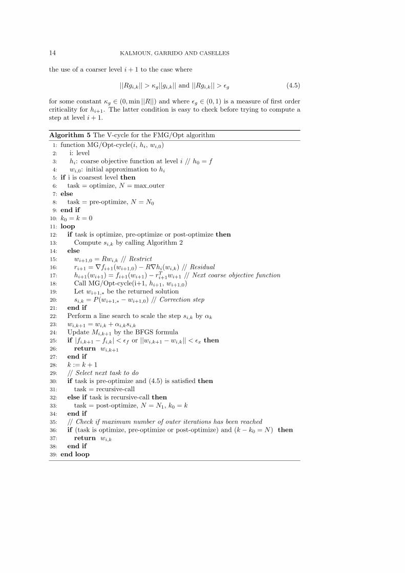
We have implemented the MG/Opt algorithm using a full multigrid method(FMG) to solve the problem and the resulting algorithm will be denoted by FMG/Opt.As for the linear case, the FMG/Opt starts at the coarsest grid level where enoughTN iterations are performed, and prolongates the solution to the next finer level iwhere Vi iterations of the MG/Opt cycle are performed.

Algorithm 5 shows the V-cycle algorithm used for FMG/Opt. At each iterationthe algorithm computes a step si either directly using the inner iteration of the TNmethod (Algorithm 2) on the current level, or recursively by means of the multigridstrategy. However, as noted in [48, 24], the recursive call is useful only if ||Rgi,k|| islarge enough compared to ||gi,k||, where gi,k = hi(wi,k) and k ≤ N0. Thus we restrict


the use of a coarser level i+ 1 to the case where

||Rgi,k|| > κg||gi,k|| and ||Rgi,k|| > εg (4.5)

for some constant κg ∈ (0,min ||R||) and where εg ∈ (0, 1) is a measure of first ordercriticality for hi+1. The latter condition is easy to check before trying to compute astep at level i+ 1.

Algorithm 5 The V-cycle for the FMG/Opt algorithm

1: function MG/Opt-cycle(i, hi, wi,0)2: i: level3: hi: coarse objective function at level i // h0 = f4: wi,0: initial approximation to hi5: if i is coarsest level then6: task = optimize, N = max outer7: else8: task = pre-optimize, N = N0

9: end if10: k0 = k = 011: loop12: if task is optimize, pre-optimize or post-optimize then13: Compute si,k by calling Algorithm 214: else15: wi+1,0 = Rwi,k // Restrict16: ri+1 = ∇fi+1(wi+1,0)−R∇hi(wi,k) // Residual17: hi+1(wi+1) = fi+1(wi+1)− rTi+1wi+1 // Next coarse objective function18: Call MG/Opt-cycle(i+1, hi+1, wi+1,0)19: Let wi+1,∗ be the returned solution20: si,k = P (wi+1,∗ − wi+1,0) // Correction step21: end if22: Perform a line search to scale the step si,k by αk23: wi,k+1 = wi,k + αi,ksi,k24: Update Mi,k+1 by the BFGS formula25: if |fi,k+1 − fi,k| < εf or ||wi,k+1 − wi,k|| < εx then26: return wi,k+1

27: end if28: k := k + 129: // Select next task to do30: if task is pre-optimize and (4.5) is satisfied then31: task = recursive-call32: else if task is recursive-call then33: task = post-optimize, N = N1, k0 = k34: end if35: // Check if maximum number of outer iterations has been reached36: if (task is optimize, pre-optimize or post-optimize) and (k − k0 = N) then37: return wi,k38: end if39: end loop


5. Implementation issues. The numerical algorithms line search TN, MR/Optand FMG/Opt have been implemented in C using MegaWave2 library. In this section,we provide details about derivatives computation for both the objective function andthe image.

5.1. Functional gradient calculation. The gradient of the objective functionin (2.7) is calculated analytically and given by

g = ∇f =

(fu

fv

)=

(Du + αRu

Dv + αRv

).

5.1.1. Horn-Schunck data term. For the linear data term we have

D(u, v) =1

2

∑i,j

ψ([Ixui,j + Iyvi,j + It

]2).

where i (respectively j) corresponds to the discrete column (respectively row) of theimage, being the coordinate origin located in the top-left corner of the image. Thefunction ψ is used to enhance robustness with respect to outliers. In our work wehave used

ψ(x2

)=

x2 if |x| ≤ γγ2 otherwise,

where γ is a given threshold. The gradient D for |x| ≤ γ is therefore given by(Dui,j

Dvi,j

)=

(Ix [Ixui,j + Iyvi,j + It]

Iy [Ixui,j + Iyvi,j + It]

),

where Dui,j and D

vi,j refer to the partial derivative of D(u, v) with respect to variables

ui,j and vi,j , respectively. Here Ix, Iy, It are the spatial and temporal image deriva-tives for which the computation is explained in Section 5.3. Note that for |x| > γ thegradient D is (Du

i,j , Dvi,j)

T = (0, 0)T .

5.1.2. Intensity constancy based data term. The nonlinear data term basedon the constancy assumption is as follows

D(u, v) =1

2

∑i,j

ψ([I2(i+ ui,j , j + vi,j)− I1(i, j)]

2).

The gradient of this functional for |x| ≤ γ is given by(Dui,j

Dvi,j

)=

(Ix2 (i+ ui,j , j + vi,j) [I2(i+ ui,j , j + vi,j)− I1(i, j)]Iy2 (i+ ui,j , j + vi,j) [I2(i+ ui,j , j + vi,j)− I1(i, j)]

).

5.1.3. Quadratic regularization term. Now we consider the regularizationterm and start by the quadratic functional. We have

R(u, v) =1

2

∑i,j

||∇i,j(u, v)||2,

where ||∇i,j(u, v)|| =√(uxi,j)

2 + (uyi,j)2 + (vxi,j)

2 + (vyi,j)2. The partial derivatives of

u, v are computed by forward finite differences with a discretization step h, that is,uxi,j = h−1(ui+1,j − ui,j) and uyi,j = h−1(ui,j+1 − ui,j) (derivatives vx and vy arecomputed similarly). The gradient of this functional is obtained as(

Rui,jRvi,j

)=

1

h2

(4ui,j − ui−1,j − ui,j−1 − ui+1,j − ui,j+1

4vi,j − vi−1,j − vi,j−1 − vi+1,j − vi,j+1

).


5.1.4. Total variation term. In this case we suppose that

R(u, v) =∑i,j

||∇i,j(u, v)||.

To overcome the problem of non-differentiability of the total variation, a widely spreadtechnique consists in approximating R by a differentiable function:

R(u, v) ≈∑i,j

ψi,j ,

where ψi,j =√(uxi,j)

2 + (uyi,j)2 + (vxi,j)

2 + (vyi,j)2 + µ and µ is a small positive param-

eter. Using again forward finite differences, the gradient of the last approximation isgiven by

(Rui,jRvi,j

)=

1

h

uxi−1,j

ψi−1,j+

uyi,j−1

ψi,j−1− ux

i,j+uyi,j

ψi,j

vxi−1,j

ψi−1,j+

vyi,j−1

ψi,j−1− vxi,j+v

yi,j

ψi,j

.

Another approximation of the total variation is given by

R(u, v) ≈∑i,j

ϕµ (||∇i,j(u, v)||) where ϕµ(x) =

|x| if |x| ≥ µ

x2/2µ+ µ/2 otherwise.

Theoretically, this approximation is twice better than the first standard approxima-tion. However, numerically in our implementaion, both approximations lead to almostthe same results.

5.2. Hessian calculation. For computing the Newton direction in the tuncatedNewton method, the linear conjugate gradient is a Hessian-free procedure (see Algo-rithm 2) and needs only to supply a routine for computing the product of the Hessianwith Newton direction p. This matrix-vector product is computed via forward finitedifferences:

H(w) p =g(w + εp)− g(w)

ε

where ε is chosen to be the square root of the machine precision divided by the normof w.

5.3. Image gradient calculation. Differentiation is an ill-posed problem [6]and regularization may be used to obtain good numerical derivatives. Such regu-larization may be accomplished with a low-pass filter such as the Gaussian, and isessential for motion estimation [4, 44]. More recently, [21] proposes to use a matchedpair of low pass and differentiation filters as a gradient operator which are the onesused in this work.

Usually, the derivative at an integer Ixi,j is computed by applying a separablefilter composed by a Gaussian filter (alternatively, a matched low pass filter) in they direction and the derivative of the Gaussian (alternatively, a matched derivative)is applied in the x direction. Conversely, the computation of the derivative in the ydirection at an integer point is performed by applying a separable filter composed by


Shift of0.5 pixels

Filter A

Filter B

0 1−1

−2−3 2 3

0.5Point tointerpolate

54321 6 7 x

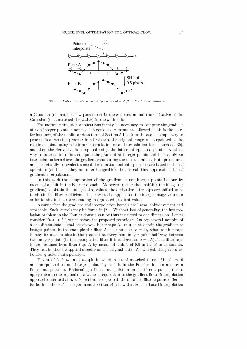
Fig. 5.1. Filter tap interpolation by means of a shift in the Fourier domain.

a Gaussian (or matched low pass filter) in the x direction and the derivative of theGaussian (or a matched derivative) in the y direction.

For motion estimation applications it may be necessary to compute the gradientat non integer points, since non integer displacements are allowed. This is the case,for instance, of the nonlinear data term of Section 5.1.2. In such cases, a simple way toproceed is a two step process: in a first step, the original image is interpolated at therequired points using a bilinear interpolation or an interpolation kernel such as [30],and then the derivative is computed using the latter interpolated points. Anotherway to proceed is to first compute the gradient at integer points and then apply aninterpolation kernel over the gradient values using these latter values. Both proceduresare theoretically equivalent since differentiation and interpolation are based on linearoperators (and thus, they are interchangeable). Let us call this approach as lineargradient interpolation.

In this work the computation of the gradient at non-integer points is done bymeans of a shift in the Fourier domain. Moreover, rather than shifting the image (orgradient) to obtain the interpolated values, the derivative filter taps are shifted so asto obtain the filter coefficients that have to be applied on the integer image values inorder to obtain the corresponding interpolated gradient value.

Assume that the gradient and interpolation kernels are linear, shift-invariant andseparable. Such kernels may be found in [21]. Without loss of generality, the interpo-lation problem in the Fourier domain can be thus restricted to one dimension. Let usconsider Figure 5.1 which shows the proposed technique. On top several samples ofa one dimensional signal are shown. Filter taps A are used to obtain the gradient atinteger points (in the example the filter A is centered on x = 4), whereas filter tapsB may be used to obtain the gradient at every non-integer point half-way betweentwo integer points (in the example the filter B is centered on x = 4.5). The filter tapsB are obtained from filter taps A by means of a shift of 0.5 in the Fourier domain.They can be thus be applied directly on the original data. We will call this procedureFourier gradient interpolation.

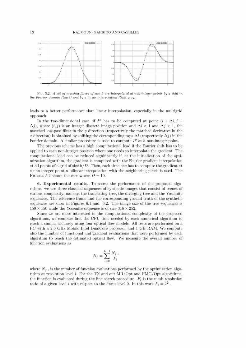
Figure 5.2 shows an example in which a set of matched filters [21] of size 9are interpolated at non-integer points by a shift in the Fourier domain and by alinear interpolation. Performing a linear interpolation on the filter taps in order toapply them to the original data values is equivalent to the gradient linear interpolationapproach described above. Note that, as expected, the obtained filter taps are differentfor both methods. The experimental section will show that Fourier based interpolation


0

0.05

0.1

0.15

0.2

0.25

0.3

0.35

-4 -2 0 2 4

Fourier interpolatedLinear interpolated

-0.15

-0.1

-0.05

0

0.05

0.1

0.15

-4 -2 0 2 4

Fourier interpolatedLinear interpolated

Fig. 5.2. A set of matched filters of size 9 are interpolated at non-integer points by a shift inthe Fourier domain (black) and by a linear interpolation (light gray).

leads to a better performance than linear interpolation, especially in the multigridapproach.

In the two-dimensional case, if Ix has to be computed at point (i + ∆i, j +∆j), where (i, j) is an integer discrete image position and ∆i < 1 and ∆j < 1, thematched low-pass filter in the y direction (respectively the matched derivative in thex direction) is obtained by shifting the corresponding taps ∆i (respectively ∆j) in theFourier domain. A similar procedure is used to compute Iy at a non-integer point.

The previous scheme has a high computational load if the Fourier shift has to beapplied to each non-integer position where one needs to interpolate the gradient. Thecomputational load can be reduced significantly if, at the initialization of the opti-mization algorithm, the gradient is computed with the Fourier gradient interpolationat all points of a grid of size h/D. Then, each time one has to compute the gradient ata non-integer point a bilinear interpolation with the neighboring pixels is used. TheFigure 5.2 shows the case where D = 10.

6. Experimental results. To assess the performance of the proposed algo-rithms, we use three classical sequences of synthetic images that consist of scenes ofvarious complexity; namely, the translating tree, the diverging tree and the Yosemitesequences. The reference frame and the corresponding ground truth of the syntheticsequences are show in Figures 6.1 and 6.2. The image size of the tree sequences is150× 150 while the Yosemite sequence is of size 316× 252.

Since we are more interested in the computational complexity of the proposedalgorithms, we compare first the CPU time needed by each numerical algorithm toreach a similar accuracy using four optical flow models. All tests are performed on aPC with a 2.0 GHz Mobile Intel DualCore processor and 1 GB RAM. We computealso the number of functional and gradient evaluations that were performed by eachalgorithm to reach the estimated optical flow. We measure the overall number offunction evaluations as

Nf =L−1∑i=0

Nf,iFi

where Nf,i is the number of function evaluations performed by the optimization algo-rithm at resolution level i. For the TN and our MR/Opt and FMG/Opt algorithms,the function is evaluated during the line search procedure. Fi is the mesh resolutionratio of a given level i with respect to the finest level 0. In this work Fi = 22i.


Fig. 6.1. On the top one frame of the original sequence is shown. On the bottom the groundtruth for the corresponding translating (left) and diverging (right) is shown. Motion vectors havebeen scaled by a factor of 2.5 for better visibility.

Fig. 6.2. On the left the one frame of the Yosemite sequence is shown. On the right thecorresponding ground truth is depicted where motion vectors have been scaled by a factor of 2.5 forbetter visibility.

The number of gradient evaluations is defined in a similar manner. While thefunction is only evaluated during the line search procedure, the gradient is addi-tionally evaluated during the inner iterations of the TN algorithm (i.e. the Hessiancomputation). Thus, we expect the number of function evaluations to be always lowerthan the gradient evaluations. Note also that the number of gradient evaluations ismore crucial to the overall computational work than that of the objective function.Here one gradient evaluation is approximately equivalent to two function evaluationswhen using quadratic regularization, while it takes almost three times in the case ofTV regularization.

Moreover, we compare the quality of the optical flow estimations of the numericalalgorithms. For this, we measure the average angular error (AAE) and the standard


Table 6.1CPU time needed by the approaches GS, TN1, TN2 and QN to reach similar accuracy for the

Yosemite sequence using the Horn-Schunck model.

Algorithm GS TN1 TN2 QN

CPU Time (s)Unilevel 45.22 8.90 9.36 17.20Multiresolution 10.74 5.21 5.65 9.50

AAE 7.40 6.81 6.82 6.85

deviation (STD) of the estimated flow we with respect to the ground truth wc. Fora given pixel (i, j), the angular error (AE) between the ground truth motion vector,wci,j , and the estimated flow, wei,j , is computed as:

AE(wci,j , wei,j) = cos−1

uci,juei,j + vci,jv

ei,j + 1√

(uci,j)2 + (vci,j)

2 + 1√(uei,j)

2 + (vei,j)2 + 1

.

The average angular error is the mean of the angular error over all pixels Nnp of theimage

AAE(wc, we) =1

Nnp

∑i,j

AE(wci,j , wei,j).

The standard deviation is computed as

STD(wc, we) =

√1

Nnp

∑i,j

(AE(wci,j , w

ei,j)−AAE(wc, we)

)2.

Before going through the performance evaluation of multilevel optimization algo-rithms, we first demonstrate the competitiveness of the adopted discretize-optimizeapproach (numerical optimization) versus the standard optimize-discretize approach(Gauss-Seidel) and also justify the selection of the chosen numerical optimization al-gorithm. To this end, we compare the CPU time needed to reach a similar AAE bythe following algorithms: 1) the proposed line-search two-step preconditionned trun-cated Newton algorithm approach (see Section 3), called here TN1, 2) the line-searchQuasi-Newton L-BFGS approach of [32], called here QN. A positive-definite approxi-mation to the Hessian is obtained at each iteration wk by storing the previous stepswk and the BFGS approach. Instead of solving at each outer iteration the Newtonequation, the L-BFGS method takes advantge from the fact that the obtained BFGSpreconditionning matrix is easily invertible. Thus, in the L-BFGS approach the line7 of Algorithm 1 is substituted by sk =M−1

k gk. The proposed algorithm TN1 is alsocompared against 3) a line-search L-BFGS precondionned truncated Newton method,called here TN2. This corresponds to the same algorithm as TN1 but the L-BFGSpreconditionning approach [32] is used instead the two-step BFGS approach [39].It should be noted that in these three numerical optimization algorithms (TN1, TN2and QN) the same line-search approach is used [36]. The previous algorithms werecompared using the linear data term and quatratic regularization, which correspondsto the classical Horn-Schunck model. Thus we implemented also a Gauss-Seidel Horn-Schunck smoother [27]. We call the latter algorithm GS.The experimental results for the four algorithms (GS, TN1, TN2 and QN) are shownin Table 6.1. Best results for QN were obtained using 4 steps, and TN2 was setup to


the same number of steps for the preconditioner. As expected from a linear relaxationscheme, Gauss-Seidel has problems near the solution and indeed in the tests it canreach an AAE below 8.00 in less than 1 second but will get stuck and does not reach theoptimal solution. Overall, truncated Newton algorithms perform better justifying thechoice of the TN as the underlying optimization smoother within multilevel algorithmsto determine direct search directions. TN1 and TN2 perform almost the same witha slight better performance of TN1. This algorithm will be used in the sequel as thesmoother and will be denoted by Opt.

Now we report the performance evaluation of the unilevel, the multiresolution andthe multigrid optimization algorithms applied to estimate the optical flow betweentwo successive frames of the above three sequences. We have considered four opticalflow models as described above in Section 2 and Subsection 5.1. We note that weuse thresholding in all the data terms to remove outliers. In all experiments we haveconsidered L = 6 levels of resolution for multilevel algorithms (multiresolution andmultigrid) and the initial guess for optical flow was zero. The stopping criteria forall algorithms were set on the relative error of the objective function, the gradientnorm or the solution norm with a tolerance of 10−5. For the MR/Opt algorithm, themaximum number of outer iterations was set to 10 iterations per each resolution forall the optical flow models except when using the nonlinear data term and the TVregularization for which we use a maximum of 15 iterations. For the FMG/Opt, weperform 2 or 3 V-cycles when using the nonlinear data term, while only 1 V-cycle issufficient in the case of the linear data term. We note here that for the purpose of a faircomputational work comparison, we stop the outer iterations once a similar accuracyon the optical flow estimation is reached. For all the algorithms, the maximum numberof innner iterations within the Opt method was set to 20.

In Tables 6.2-6.4, we summarize the quality of the solution and the computationalcosts of the three numerical algorithms for four optical flow models. Model 1 refers tothe linear data term plus the quadratic regularization; Model 2 refers to the nonlineardata term plus the quadratic regularization; Model 3 refers to the linear data termplus the TV regularization; and finally Model 4 refers to the nonlinear data term plusthe TV regularization. The latter is the most accurate for optical flow estimationbut computationally the most expensive among the four models. Indeed, Model 4contains the nonlinear data term as well as the TV regularization which providesaccurate optical flow estimations but it’s numerically more challenging as comparedto the quadratic regularization.

In terms of the quality of the solution, by comparing the unilevel algorithm ver-sus the multilevel algorithms, we note that the optical flow estimation of the fourmodels is more accurate when computed using the latter algorithms for all the testedimages. In this regard, multigrid optimization has shown to provide a more accurateestimation than multiresolution optimization if we take the average angular error asan accuracy measure. In particular, the most accurate optical flow estimations for thethree sequences are obtained with Model 4 using the FMG/Opt algorithm. To illus-trate the results obtained by using multigrid optimization, we show first in Figure 6.3the estimated motion fields of Model 2 and Model 4 for the translating and divergingtree sequences. In Figure 6.4, we plot the estimated motion fields of the four modelsfor the Yosemite sequence. The results obtained with the other methods are visuallysimilar and for reasons of space we do not show them. We refer to Tables 6.2-6.4 forthe quantitative comparison.

We discuss next the computational expense of the FMG/Opt algorithm as com-


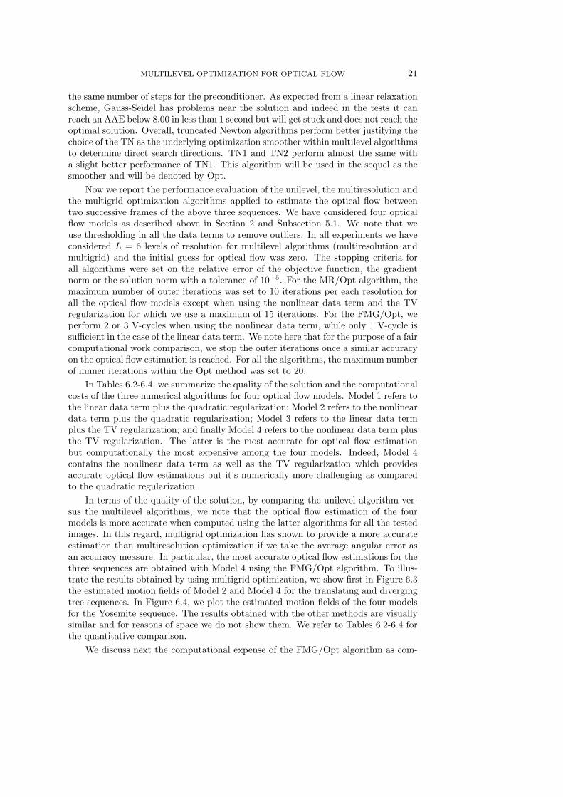
Table 6.2Comparison of computational work and optical flow Estimation for two Frames of the translat-

ing tree sequence using optimization algorithms Opt, MR/Opt and FMG/Opt. Time is CPU timein seconds.

Opt MR/Opt FMG/OptTime 11.91 2.73 0.98Nf 69 15 12

Model 1 Ng 572 133 37AAE 1.83 0.90 0.89STD 1.23 0.55 0.51Time 14.22 5.40 2.07Nf 89 19 25



Model 4 Ng 1130 334 126AAE 0.20 0.20 0.20STD 0.18 0.18 0.17

Fig. 6.3. These plots show the motion fields obtained using the FMG/OPT algorithm for thediverging (top) and translating (bottom) tree. On the left (resp. right) the result for Model 2 (resp.Model 4) is shown superimposed with the ground truth. Motion vectors have been scaled by a factorof 2.5 for better visibility.


Table 6.3Comparison of computational work and optical flow estimation for two frames of the Diverging

Tree sequence using optimization algorithms Opt, MR/Opt and FMG/Opt. Time is CPU time inseconds.





Model 4 Ng 997 492 97AAE 2.09 2.07 1.86STD 1.84 1.89 1.92

Fig. 6.4. These plots show the motion fields obtained using the FMG/OPT algorithm for theyosemite sequence. From left to right, and from top to bottom, Model 1 to 4 are shown superimposedwith the ground truth. Motion vectors have been scaled by a factor of 2.5 for better visibility.


Table 6.4Comparison of computational work and optical flow estimation for two frames of the Yosemite

sequence using line search optimization algorithms (Opt, MR/Opt, FMG/Opt). Time is CPU timein seconds.





Model 4 Ng 1821 223 121AAE 5.75 5.49 5.45STD 8.92 8.57 7.90

pared to Opt and MR/Opt algorithms. From Tables 6.2-6.4, we remark that ouralgorithm outperforms significantly both the two optimization algorithms in terms ofthe CPU running time and the number of function and gradient evaluations for thethree image sequences and the four optical flow models. For Model 1, while linearmultigrid with standard components does not work [5, 29, 28], our FMG/Opt algo-rithm is around eight times faster to run than Opt and two point five times faster thanMR/Opt. The same applies almost for Model 2 that contains a nonlinear data term.As expected, for Model 3 which incorporates a TV regularization term, multilevel op-timization is much more effective than unilevel optimization. In fact, our FMG/Optalgorithm takes thirteen times less CPU time to run than the Opt algorithm. Fi-nally, when used for Model 4, the FMG/Opt algorithm shows a similar signficantimprovement of a factor of twelve over Opt and more than two over MR/Opt.

In overall, the FMG/Opt algorithm performs at least twice better than theMR/Opt algorithm and ten times better than the Opt algorithm; see Table 6.5. Wenotice also that the FMG/Opt algorithm is less independent of the image size becauseit often takes similar number of function and gradient evaluations while comparingacross the same optical flow model.

7. Conclusion. Based on the discretize-optimize approach, we have applied dif-ferent numerical optimization techniques to variational models for optical flow com-putation. First, we have shown the competitiveness of this strategy compared to theclassical optimize-discretize approach. Three Newton-based optimization algorithmswere superior to the Gauss-Seidel method when applied to the classical Horn-Schunck


Table 6.5Global characteristics of Opt, MR/Opt and FMG/Opt for optical flow models on all the three

images. Nfg is the total number of function and gradient evaluations.

Opt MR/Opt FMG/Opt

Model 1Total time (s) 38.54 12.04 4.76Total Nfg 1501 421 106




All modelsTotal time (s) 541.29 117.69 47.86

Total Nfg 9703 2812 933

model. In particular, truncated Newton was shown to be a suitable unilevel opti-mization algorithm and was chosen as the smoother for optimization-based multilevelmethods. We have then implemented the FMG/Opt algorithm based on a line searchstrategy to scale the (direct) Newton or the (recursive) multigrid search direction.Several components of the MG/Opt technique have been tuned for high efficiencyand the algorithm has been fully evaluated with respect to unilevel and (one-way)multiresolution optimization. Our experimental results have demonstrated that theFMG/Opt algorithm can be effectively used for optical flow computation. Using dif-ferent models and images, we have observed the FMG/Opt algorithm was faster andmore accurate than both unilevel and multiresolution truncated Newton. Furtherresearch will investigate the use of line search multigrid versus trust region multigridin the context of dense optical flow computation. The proposed numerical strategycan be adapted to the minimization of other nonlinear energy functionals like theillumination invariant model proposed in [16] or depth estimation in stereo problems.

REFERENCES

[1] L. Alvarez, J. Weickert, and J. Sanchez, A scale-space approach to nonlocal optical flowcalculations, in Scale-Space Theories in Computer Vision, vol. 1682 of Lecture Notes inComputer Science, Springer, 1999, pp. 235–246.

[2] , Reliable estimation of dense optical flow fields with large displacements, InternationalJournal of Computer Vision, 39 (2000), pp. 41–56.

[3] P. Anandan, A computational framework and an algorithm for the measurement of visualmotion, International Journal of Computer Vision, 2 (1989), pp. 283–310.

[4] J. Barron, D. Fleet, and S. Beauchemin, Performance of optical flow techniques, Interna-tional Journal of Computer Vision, 12 (1994), pp. 43–77.

[5] R. Battiti, E. Amaldi, and C. Koch, Computing optical flow across multiple scales: an adap-tive coarse-to-fine strategy, International Journal of Computer Vision, 6 (1991), pp. 133–145.

[6] M. Bertero, T. A. Poggio, and V. Torre, Ill-posed problems in early vision, Proceedingsof the IEEE, 76 (1988), pp. 869–889.

[7] F. A. Bornemann and R. Krause, Classical and cascadic multigrid - a methodogical com-parison, in Domain Decomposition Methods in Sciences and Engineering, P. Bjorstad,M. Espedal, and D. Keyes, eds., Bergen, Norway, 1998, DD Press, pp. 64–71.

[8] A. Borzı, K. Ito, and K. Kunisch, Optimal control formulation for determining optical flow,SIAM Journal on Scientific Computing, 24 (2002), pp. 818–847.

[9] A. Brandt, Multi-level adaptive solutions to boundary-value problems, Mathematics of Com-


putation, 31 (1977), pp. 333–390.[10] W. L. Briggs, V. E. Henson, and S. F. McCormick, A Multigrid Tutorial, 2nd ed., SIAM

Press, Philadelphia, 2000.[11] T. Brox, A. Bruhn, N. Papenberg, and J. Weickert, High accuracy optical flow estimation

based on a theory for warping, in European Conference in Computer Vision, vol. 4, 2004,pp. 25–36.

[12] A. Bruhn, Variational optic flow computation: Accurate modeling and efficient numerics, PhDthesis, Department of Mathematics and Computer Science, Saarland University, 2006.

[13] A. Bruhn, J. Weickert, C. Feddern, T. Kohlberger, and C. Schnorr, Real-time optic flowcomputation with variational methods, in International Conference on Computer Analysisof Images and Patterns, 2003, pp. 222–229.

[14] , Variational optical flow computation in real time, IEEE Transactions on Image Pro-cessing, 14 (2005), pp. 608–615.

[15] P. Y. Burgi, Motion estimation based on the direction of intensity gradient, Image and VisionComputing, 22 (2004), pp. 637–653.

[16] V. Caselles, L. Garrido, and L. Igual, A contrast invariant approach to motion estimation,in Scale Space, Springer Lecture Notes in Computer Science, 2005, pp. 242–253.

[17] I. Cohen and I. Herlin, Non uniform multiresolution method for optical flow and phaseportrait models: Environmental applications, International Journal of Computer Vision,33 (1999), pp. 1–22.

[18] R. S. Dembo and T. Steihaug, Truncated Newton algorithms for large scale unconstrainedoptimization, Mathematical Programming, 26 (1983), pp. 190–212.

[19] M. Droske and M. Rumpf, A variational approach to nonrigid morphological image registra-tion, SIAM Journal of Applied Mathematics, 64 (2004), pp. 668–687.

[20] W. Enkelmann, Investigations of multigrid algorithms for the estimation of optical flow fieldsin image sequences, Computer Vision, Graphics and Image Processing, 43 (1988), pp. 150–177.

[21] H. Farid and E. P. Simoncelli, Differentiation of discrete multidimensional signals, IEEETransactions on Image Processing, 13 (2004), pp. 496–508.

[22] S. Ghosal and P. A. Vanek, Fast scalable algorithm for discontinuous optical flow estimation,IEEE Transactions on Pattern Analysis and Machine Intelligence, 18 (1996), pp. 181–194.

[23] F. Glazer, Multilevel relaxation in low-level computer vision, in Multi-resolution image pro-cessing and Analysis, A. Rosenfeld, ed., Springer-Verlag, 1984, pp. 312–330.

[24] S. Gratton, A. Sartenaer, and P. L. Toint, Recursive trust region method for multiscalenonlinear optimization, SIAM Journal on Optimization, 19 (2008), pp. 414–444.

[25] W. Hackbusch, Multi-Grid Methods and Applications, Springer, Berlin/New York, 1985.[26] W. Hinterberger, O. Scherzer, C. Schnorr, and J. Weickert, Analysis of optical flow

models in the framework of the calculus of variations, Numerical Functional Analysis andOptimization, 23 (2002), pp. 69–89.

[27] B. Horn and B. Schunk, Determining optical flow, Artificial Intelligence, 20 (1981).[28] E. M. Kalmoun, H. Kostler, and U. Rude, 3d optical flow computation using a parallel

variational multigrid scheme with application to cardiac c-arm ct motion, Image and VisionComputing, 25 (2007), pp. 1482–1494.

[29] E. M. Kalmoun and U. Rude, A variational multigrid for computing the optical flow, inProceedings of the Vision, Modeling, and Visualization Conference, Akademische Verlags-gesellschaft, 2003, pp. 577–584.

[30] R. G. Keys, Cubic convolution interpolation for digital image processing, IEEE Trans. Acous-tics, Speech, and Signal Processing, 29 (1981), pp. 1153–1160.

[31] R. M. Lewis and S. G. Nash, Model problems for the multigrid optimization of systems gov-erned by differential equations, SIAM Journal on Scientific Computing, 26 (2005), pp. 1811–1837.

[32] D. C. Liu and J. Nocedal, On the limited memory BFGS method for large scale optimization,Mathematical Programming, 45 (1989), pp. 503–528.

[33] B. D. Lucas and T. Kanade, An iterative image registration technique with an application tostereo vision, in Image Understanding Workshop, 1981, pp. 121–130.

[34] E. Memin and P. Perez, Dense estimation and object-based segmentation of the optical-flowwith robust techniques, IEEE Transactions on Image Processing, 7 (1998), pp. 703–719.

[35] , A multigrid approach for hierarchical motion estimation, in Proceedins of the SixthInternational Conference on Computer Vision, 1998, pp. 933–938.

[36] J. J. More and D. J. Thuente, Line search algorithms with guaranteed sufficient decrease,ACM Transactions on Mathematical Software, 20 (1994), pp. 286–307.

[37] H.-H. Nagel, Constraints for the estimation of displacement vector fields from image se-


quences, in Proceedings of the Eight International Joint Conference on Artificial Intelli-gence, Alan Bundy, ed., Karlsruhe, Germany, Aug. 1983, William Kaufmann, pp. 945–951.

[38] H.-H. Nagel and W. Enkelmann, An investigation of smoothness constraints for the esti-mation of displacement vector fields from image sequences, IEEE Transactions on PatternAnalysis and Machine Intelligence, 8 (1986), pp. 565–593.

[39] S. G. Nash, Preconditioning of truncated-newton methods, SIAM Journal on Scientific andStatistical Computing, 6 (1985), pp. 599–616.

[40] , A multigrid approach to discretized optimization problems, Optimization Methods andSoftware, 14 (2000), pp. 99–116.

[41] J. Nocedal and S. J. Wright, Numerical Optimization, Springer-Verlag, New York, 1999.[42] J. M. Odobez and P. Bouthemy, Robust multiresolution estimation of parametric motion

models, Journal of Visual Communication and Image Representation, 6 (1995), pp. 348–365.

[43] N. Papenberg, A. Bruhn, T. Brox, S. Didas, and J. Weickert, Highly accurate optic flowcomputation with theoretically justified warping, International Journal of Computer Vision,67 (2006), pp. 141–158.

[44] C. Stiller and J. Konrad, Estimating motion in image sequences, IEEE Signal ProcessingMagazine, 16 (1999), pp. 70–91.

[45] R. Szeliski and H. Y. Shum, Motion estimation with quadtree splines, IEEE Trans. PatternAnalysis and Machine Intelligence, 18 (1996), pp. 1199–1210.

[46] D. Terzopoulos, Image analysis using multigrid relaxation methods, IEEE Transactions onPattern Analysis and Machine Intelligence, 8 (1986), pp. 129–139.

[47] J. Weickert and C. Schnorr, A theoretical framework for convex regularizers in PDE-based computation of image motion, International Journal of Computer Vision, 45 (2001),pp. 245–264.

[48] Z. Wen and D. Goldfarb D., A Line Search Multigrid Method for Large-Scale Convex Op-timization, tech. report, Department of IEOR, Columbia University, 2007.

[49] D. Xie and T. Schlick, Efficient implementation of the truncated-Newton algorithm for large-scale chemistry applications, SIAM Journal on Optimization, 10 (1999), pp. 132–154.

LINE SEARCH MULTILEVEL OPTIMIZATION AS COMPUTATIONAL METHODS FOR DENSE OPTICAL FLOW

Documents

Transcript of LINE SEARCH MULTILEVEL OPTIMIZATION AS COMPUTATIONAL METHODS FOR DENSE OPTICAL FLOW