Rochester Institute of Technology Rochester Institute of Technology

RIT Scholar Works RIT Scholar Works

Theses

8-6-2019

Magnetoactive Elastomer Solenoid Development and Magnetoactive Elastomer Solenoid Development and

Implementation in Underwater Jet Propulsion Implementation in Underwater Jet Propulsion

Eric Damm exd7536@rit.edu

Follow this and additional works at: https://scholarworks.rit.edu/theses

Recommended Citation Recommended Citation Damm, Eric, "Magnetoactive Elastomer Solenoid Development and Implementation in Underwater Jet Propulsion" (2019). Thesis. Rochester Institute of Technology. Accessed from

This Thesis is brought to you for free and open access by RIT Scholar Works. It has been accepted for inclusion in Theses by an authorized administrator of RIT Scholar Works. For more information, please contact ritscholarworks@rit.edu.

Rochester Institute of Technology Kate Gleason College of Engineering

Department of Mechanical Engineering

__________________________________________________________ A Thesis submitted in Partial Fulfillment of the Requirements for the Degree of Master of Science in Mechanical Engineering.

_______________________________________________________________________________________________________

August 6, 2019

Magnetoactive Elastomer Solenoid Development and

Implementation in Underwater Jet Propulsion

Eric Damm

ii

Magnetoactive Elastomer Solenoid Development and Implementation in Underwater Jet Propulsion Master’s Thesis

Eric Damm

8/6/2019

Rochester institute of Technology

Under Guidance of Dr. Kathleen Lamkin-Kennard

For Partial Fulfillment of the Requirements of the Degree of Master of Science in

Mechanical Engineering

iii

Magnetoactive Elastomer Solenoid Development and Implementation in

Underwater Jet Propulsion

Master’s Thesis by:

Eric Damm

Faculty

__________________________________________________________________8/6/2019

Dr. Kathleen Lamkin-Kennard, Faculty Advisor

__________________________________________________________________8/6/2019

Dr. Hany Ghoneim, Committee Member

__________________________________________________________________8/6/2019

Dr. Mark Kempski, Committee Member

__________________________________________________________________8/6/2019

Dr. Jason Kolodziej, Committee Member

__________________________________________________________________8/6/2019

Dr. Michael G. Schrlau, Department Representative

iv

Abstract

The objective of this research was to develop and implement an elastomer solenoid capable

of generating underwater jet propulsion for soft robot actuation. This is significant in pushing

forward the progress of soft robotics by proving the viability of a new soft actuation method in

addition to proving the viability of using silicone and magnetic particles as the driving

mechanism for a soft actuator.

The two primary aims were to effectively manufacture an elastomer solenoid core and to

incorporate that core with a flexible diaphragm that actuates when a voltage is applied. This

combination creates a pulse of water that is pumped out of an orifice. In practice, this was a

success. The propagated magnetic field in the elastomer core was very apparent in air and

displacements of 2.7 cm could be achieved for a 100 mm wide diaphragm. Underwater, the

added damping force of the fluid limited the displacement of the diaphragm, however; the final

device was able to pump water at 250 ml/min out of an orifice.

v

Table of Contents

Faculty............................................................................................................................................ iii

Abstract .......................................................................................................................................... iv

Table of Contents ............................................................................................................................ v

List of Figures ............................................................................................................................... vii

List of Tables ................................................................................................................................. ix

List of Equations ............................................................................................................................ ix

Nomenclature .................................................................................................................................. x

Chapter 1 – Introduction ................................................................................................................. 1

1.1 Motivation ............................................................................................................................. 1

1.2 The Research Question.......................................................................................................... 3

Chapter 2 - Background .................................................................................................................. 4

2.1 Literature Review .................................................................................................................. 4

2.1.1 Magnetoactive Elastomer Diaphragms ........................................................................... 4

2.1.2 Magnetic Alignment of Iron Oxide Inside a Silicone Matrix ......................................... 5

2.1.3 Liquid Metal Wire Windings for a Soft Electromagnet ................................................. 8

2.1.4 Soft, Octopus Inspired Pulsing Robot ............................................................................ 9

2.1.5 Underwater Jet Propulsion Via an Orifice .................................................................... 11

2.1.6 Calculations for physical properties of a thin circular plate ......................................... 15

2.1.7 Gaps in the Literature ................................................................................................... 16

Chapter 3 – Methods ..................................................................................................................... 17

3.1 Preliminary Work ................................................................................................................ 17

3.1.1 Basic Speaker Development ......................................................................................... 17

3.1.2 Magnetoactive Elastomer Development ....................................................................... 19

3.2 Theoretical Analysis ............................................................................................................ 25

3.2.1 Magnetic Field Force .................................................................................................... 27

3.3 Electrical Design ................................................................................................................. 29

3.4 Final Manufacturing Methods ............................................................................................. 33

3.4.1 Diaphragm .................................................................................................................... 33

3.4.2 Magnetoactive Core ...................................................................................................... 34

3.4.3 Bonding of Core and Diaphragm.................................................................................. 34

vi

3.5 Initial Testing ...................................................................................................................... 36

3.6 Pump Enclosure Design and Prototyping ........................................................................... 37

3.7 Experimental Results........................................................................................................... 41

3.7.1 Diaphragm Displacement ............................................................................................. 41

3.7.2 Pumping Efficacy ......................................................................................................... 42

Chapter 4 - Data ............................................................................................................................ 43

4.1 Pulsing Circuit ..................................................................................................................... 43

4.2 In-Air Testing ...................................................................................................................... 45

4.2.1 Measured Displacement ............................................................................................... 45

4.3 Underwater Testing ............................................................................................................. 48

4.3.1 Measured Displacement ............................................................................................... 48

Chapter 5 - Discussion .................................................................................................................. 54

5.1.1 Develop an elastomer solenoid core ............................................................................. 54

5.1.2 Develop a diaphragm capable of deformation to create pressure fluctuations ............. 55

5.1.3 Eliminate the need for high voltage and pneumatics .................................................... 55

5.1.4 Develop a device capable of pumping 500ml/min of water ......................................... 55

Chapter 6 - Societal Context ......................................................................................................... 58

Chapter 7 – Future Work .............................................................................................................. 59

7.1 Magnetoactive Diaphragm .................................................................................................. 59

7.2 Inlet Valve ........................................................................................................................... 59

7.3 Soft Enclosure ..................................................................................................................... 60

7.4 Liquid Metal Windings ....................................................................................................... 60

7.5 Diaphragm Tension and Spring Constant ........................................................................... 61

7.6 System Model Accuracy ..................................................................................................... 61

7.6.1 System Model Equation................................................................................................ 61

7.6.2 In-Air Simulation .......................................................................................................... 63

7.6.3 In-Water Simulation ..................................................................................................... 65

Chapter 8 - Acknowledgements .................................................................................................... 66

Appendices .................................................................................................................................... 67

Appendix A: Arduino code for pulsing circuit.......................................................................... 67

Appendix B: MATLAB Code ................................................................................................... 69

In-Air System Model: ............................................................................................................ 69

vii

In-Water System Model ......................................................................................................... 71

Simulation Data ..................................................................................................................... 75

Sphere Cap Formula .............................................................................................................. 76

Data Readings ........................................................................................................................ 77

References ..................................................................................................................................... 78

List of Figures

Figure 1: Elastomer Diaphragm Literature Design [3] ................................................................... 5

Figure 2: Magnetic Alignment Literature Sample [4] The left shows the particle alignment (top:

unaligned, bottom: aligned). The right shows an image of the corresponding experimental result.

......................................................................................................................................................... 6

Figure 3: Film Creation Literature Method [4] ............................................................................... 6

Figure 4: Chained vs. Uniformly Dispersed Particles. Left: Magnetically aligned particles, Right:

Normally dispersed particles. [4] .................................................................................................... 7

Figure 5: Soft Windings Literature [6] ........................................................................................... 8

Figure 6: Soft Mantle Literature Design [1] ................................................................................... 9

Figure 7: Rear and frontal view of the robot from Serchi et al [8] ............................................... 10

Figure 8: Synthetic jet proposed by Thomas et al. [7]. (A) The initial in-stroke sucks water into

the chamber. (B) The out-stroke causes fluid to roll up into a ring. (C) The vortex ring pinches

off. (D) During subsequent in-strokes, water is sucked in from around the departing vortex ring.

[Reproduced from [7]]. ................................................................................................................. 11

Figure 9: Literature Jet Schematic [9] .......................................................................................... 12

Figure 10: Left: Slug model of water exiting the orifice; Right: Slug model turning into vortices

after leaving the orifice [9] ........................................................................................................... 12

Figure 11: Illustration of Paper Cup Speaker [22] ........................................................................ 18

Figure 12: An early design for the jet propulsion device. This was a stepping stone to what would

be the final design (shown later in the section) 1. Displaced Diaphragm, 2. Housing, 3. Solenoid,

4. Outlet valve, 5. Inlet Valve ....................................................................................................... 19

Figure 13: First Iteration Soft Solenoid Core ............................................................................... 22

Figure 14: Second Iteration Soft Solenoid Core ........................................................................... 22

Figure 15: First diaphragm prototype ........................................................................................... 24

Figure 16: Improved diaphragm prototype ................................................................................... 24

Figure 17: Displacement simulation of diaphragm ....................................................................... 25

Figure 18: Sphere Cap [24] ........................................................................................................... 26

Figure 19: Pulsing circuit schematic. C = 60,000 µf; R = 1 Ω. Inductor symbol represents the

coils of the solenoid. ..................................................................................................................... 30

Figure 20: Two 30,000 µf Capacitors ........................................................................................... 31

viii

Figure 21: 4 Channel Mechanical Relay (Note: Only one channel is used) ................................. 32

Figure 22: EcoFlex Diaphragm ..................................................................................................... 33

Figure 23: Core placed in EcoFlex ............................................................................................... 35

Figure 24: Dry prototype .............................................................................................................. 36

Figure 25: Wet prototype; Left: maximum bottom displacement, right: maximum top

displacement. Red line shows centerline. ..................................................................................... 37

Figure 26: Elastomer Core Movement (Left: Max upwards displacement, Right: Max downwards

displacement. ................................................................................................................................ 37

Figure 27: Top view of enclosure. All measurements are in millimeters. .................................... 38

Figure 28: Side view of enclosure, all units are in millimeters. ................................................... 38

Figure 29: Enclosure lid (outlet orifice) ........................................................................................ 39

Figure 30: Enclosure body with inlet valve attached (on right) and orifice (on left) ................... 40

Figure 31: Enclosure with diaphragm attached (Black circle is solenoid core inside enclosure.) 40

Figure 32: Left: Closed check valve; Right: Open Check Valve .................................................. 41

Figure 33: Pumping motor used to vacuum pooled water for measurement. ............................... 42

Figure 34: Single Example Pulse .................................................................................................. 43

Figure 35: Multiple pulse signal ................................................................................................... 44

Figure 36: In-Air Maximum Displacement Values ...................................................................... 46

Figure 37: Time lapse of In-Air displacement (Note: all times are in seconds) ........................... 46

Figure 38: In-Water Maximum Displacement Values .................................................................. 49

Figure 39: Pumping Data .............................................................................................................. 51

Figure 40: Time Until 500 ml Pumped ......................................................................................... 51

Figure 41: Graph indicating the nonlinearity of volume being pumped over time. Each point

shows a mean value of a range of data taken in tests discussed above. ........................................ 52

Figure 42: Frames from slow motion video of in-water pumping test (Note: all times are in

seconds)......................................................................................................................................... 53

Figure 43: Deformed Diaphragm; Red arrows denote downward pressure from enclosure, blue

arrow denotes upward force from magnetic field. ........................................................................ 56

Figure 44: In-Air Displacement MATLAB Simulation................................................................ 63

Figure 45: Spring Constant of Varying thickness SU-8 [20] ........................................................ 64

Figure 46: Underwater Simulation................................................................................................ 65

ix

List of Tables

Table 1: Sylgard 184 Spec Table [11] .......................................................................................... 20

Table 2: Ecoflex Spec Table [12] ................................................................................................. 21

Table 3: In-Air Maximum Displacement Values .......................................................................... 45

Table 4: In-Water Maximum Displacement Values ..................................................................... 48

Table 5: Statistics for 60s, 120s, and 100 pulse trials ................................................................... 50

Table 6: Table of Comparable Pumps [15] [16] [17] [18] [19] .................................................... 57

List of Equations

[1] Intermediate velocity of a fluid moving through an orifice .................................................... 13

[2] Diaphragm velocity ................................................................................................................. 13

[3] Reynolds Number .................................................................................................................... 13

[4] Exit velocity of fluid from an orifice ...................................................................................... 13

[5] Circulation, a measure of vortex strength ............................................................................... 14

[6] Impulse .................................................................................................................................... 14

[7] Average thrust ......................................................................................................................... 14

[8] Plate deflection as a function of radial position ...................................................................... 15

[9] Flexural rigidity ....................................................................................................................... 15

[10] Maximum plate deflection .................................................................................................... 15

[11] Spring constant equation ....................................................................................................... 15

[12] Resonant frequency equation ................................................................................................ 16

[13] Volume of a sphere cap ......................................................................................................... 26

[14] Potential energy equation ...................................................................................................... 27

[15] Power equation ...................................................................................................................... 27

[16] Power equation ...................................................................................................................... 28

[17] Force imparted by magnetic field.......................................................................................... 28

[18] Mass of water in sphere cap .................................................................................................. 28

[19] Natural frequency equation ................................................................................................... 28

[20] Spring constant equation ....................................................................................................... 28

[21] Ohm’s Law ............................................................................................................................ 29

[22] Mass, spring, damper system general equation ..................................................................... 61

[23] State space form of mass, spring, damper system ................................................................. 62

[24] State space form of mass, spring, damper system ................................................................. 62

x

Nomenclature

MMP: Magnetic Microparticle

dorifice: Diameter of jet orifice (m)

dchamber: Diameter of jet chamber (m)

ddisk: Diameter of rigid disk attached to the diaphragm (m)

δ: Maximum diaphragm displacement (m)

Um: Velocity of diaphragm (m/s)

UP: Intermediate velocity (m/s)

Uc: Velocity at the orifice exit (m/s)

RE: Reynolds number

ρ: density (kg/m3)

L: Length of expelled water slug (m)

P0: Pressure (N/m2)

a: Area of plate (m2)

D: Diameter of plate (m)

r: radius of plate (m)

xi

E: Young’s Modulus (N/m2)

v: Poisson ratio

t: Thickness of plate (m)

k: Spring Constant (N/m2)

ω0: Resonant Frequency (Hz)

1

Chapter 1 – Introduction

1.1 Motivation

In the young and emerging field of soft robotics and biomimetics, the most widely used

method of actuation is pneumatics. Pneumatic actuators require an air compressor, air tubes, and

valves, which are made of metal or stiff plastic. The best example of a pneumatic actuator is a

McKibben Muscle, which uses compressed air to create pressure in surgical tubing, causing it to

contract like a bicep. The muscles react quickly and accurately, but there are a lot of extra

components that limit the utility of the actuator for soft robotics.

Another, newer actuator being explored is called a DEA, or Dielectric Elastomer Actuator.

DEAs have great promise as actuators, as they do not require any compressors or tubes to move

fluids. The issue, however; is that they are very inefficient with the amount of force produced

compared to the input power. In the early stages of their research and development, DEAs are

not a particularly viable method of soft actuation for most applications.

This research proposes a new type of soft actuator; one that combines iron oxide

nanoparticles with cross-linked silicone polymers. The goal is to use soft, flexible silicone rubber

as the primary material in a mode of actuation. The motivation to use silicone is that it has many

benefits over other rigid options, such as iron or nickel. Silicone is also useable in a wide range

of temperatures, has low chemical reactivity, and is electrically insulating, waterproof, and flame

retardant. Silicone rubber has also been used in biomedical applications due to its inertness in the

body. The second material, iron oxide microparticles, was chosen because of the small size, the

ease of use, and good magnetic properties of the particles. There has been limited research done

involving mixing silicone and magnetic particles, but no substantial use has come to fruition in

2

the field of soft robotics. Additional motivation for this work is to expand the field of

incorporating magnetic particles with soft robotics, in order to broaden the options for actuators

for future researchers interested in soft robotics.

Furthermore, the development of soft magnetic actuators provides a novel contribution to

the field of soft robotics. Although promising, there has yet to be substantial research into the use

of elastomer solenoid cores as primary sources of actuation. The work illustrated here further

strengthens the viability of using silicone as a solenoid core.

3

1.2 The Research Question

A common actuator used in conventional robotics is the solenoid, which is an electrical

component driven by a current sent through a coil of wire. Solenoids are widely used since these

actuators are robust and can be used in a variety of applications. However, little work has been

done to bring this technology into the field of soft robotics, which leads to the research question:

Can a solenoid be effectively made from an elastomer and successfully utilized for soft robot

actuation? Furthermore: How viable is a magnetoactive elastomer for use in solenoid actuation?

This thesis seeks to address these questions through the following aims:

• Develop an elastomer solenoid core using iron oxide microparticles in combination

with a cross-linked silicone polymer.

• Create an elastomer diaphragm capable of pulsing when an external force is applied.

• Implement the elastomer solenoid core with the diaphragm in a soft actuation device

capable of pumping 500 ml/min of water.

4

Chapter 2 - Background

2.1 Literature Review

The field of soft robotics has expanded greatly in recent years. However, there are currently

few soft actuators that are viable for soft robotic applications. Furthermore, many of the

examples that use magnetic fields or magnetoactive elastomers fail to provide potential

applications for the research. Other examples that do give applications tend to be incredibly

specific, which limits future research to a very small bra [1] [2]nch of pathways.

To give context to the goal of the research and to set a baseline of the knowledge around

the topic, a literature review was performed. The following papers are presented for their

relevance to elastomer actuation using magnetics and soft underwater pumping. The current

research seeks to address the voids identified in the existing literature through creation of an

elastomer solenoid actuator.

2.1.1 Magnetoactive Elastomer Diaphragms

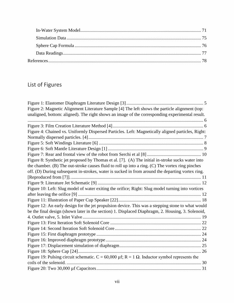
Jayaneththi et al. [3] manipulated a ferrous elastomer diaphragm with an exterior

electromagnet. Figure 1 demonstrates that pulsing motions can be achieved using a magnetic

polymer composite. The diaphragm was 65 mm in diameter and 1.5 mm in thickness. They

achieved a maximum displacement of 2.5mm with an input of 1.5 amps. The study presents a

method for creating the diaphragm and proposed ratios of Ecoflex to Fe3O4 (20% magnetic filler

by weight). The gap in this research is the lack of any clear application of the technology. The

authors propose implanting the diaphragm inside the body and pulsing it with an exterior

electromagnet, but no specific applications are discussed or implemented.

5

More in depth methods for diaphragm creation are outlined by Marchi et al. [4]. To

manufacture the diaphragm films, 10 – 50% by weight of magnetic particles were placed in an

Ecoflex mixture. The mixture was then placed in an ultrasonic bath for a few minutes at a

frequency of 59 kHz. The mixture was then coated on a Teflon substrate and spin-coated at 500

RPM for 30 seconds. Some of the films were subjected to a magnetic field normal to the face of

the samples. A 30% mixture of particles to silicone was determined to have the best physical and

magnetic properties.

2.1.2 Magnetic Alignment of Iron Oxide Inside a Silicone Matrix

In the work done by Marchi et al. [4] iron oxide particles were magnetically aligned inside a

silicone matrix in order to achieve a better magnetic response. Figure 2 shows the effect of

magnetic alignment. On the left side of the image, there is an illustration of what the particles

look like with or without magnetic alignment. The right side shows the difference in

displacement described by Marchi et al. [4].

Figure 1: Elastomer Diaphragm Literature Design [3]

6

According to Marchi et al. [4] the magnetic alignment procedure involved subjecting curing

films to an external magnetic field of 200mT produced by a cylindrical neodymium static magnet

(diameter, D, of 25 mm, thickness, t, of 10 mm) and directed along the normal to the surface of

the films. The films were then placed in an oven at 80 °C overnight. [4].

Ijaz et al. [5] describe using a 30% ratio of particles to Ecoflex by weight and mixing for

five minutes. The authors spin coated the material onto a glass microscope slide at 600 RPM for

30 seconds. The sample was then immediately placed between the poles of an electromagnet at

1000 Oe horizontal magnetic field (equivalent to 0.1 Tesla magnet). Figure 3 illustrates the

Figure 2: Magnetic Alignment Literature Sample [4] The left shows the particle

alignment (top: unaligned, bottom: aligned). The right shows an image of the

corresponding experimental result.

Figure 3: Film Creation Literature Method [4]

7

process [5]. The particles aligned as shown in Figure 4. The authors then cured the mixture in an

oven at 80 degrees Celsius for 3 hours.

Two methods were used for analysis of the magnetic alignment. The first method was a

visual method with a scanning electron microscope at 500x magnification and an acceleration

voltage of 3kV. The results from this analysis are shown in Figure 4. The left side shows the

chained particles and the right shows normally distributed particles. The second method used a

vibrating sample magnetometer to measure the magnetic response from the different samples.

The findings obtained using the second method showed that the higher concentrations led to a

larger displacement during testing.

Song and Cha [6] analyzed how magnetic microparticle concentrations in silicone influence

the magnetic response of the material. Concentrations were determined using field-emission

scanning electron microscopy. Samples were then cooled in liquid nitrogen to preserve the

internal structures. The frozen samples were then broken in half, fixed to the SEM sample holder

using carbon tape, and observed in back-scattered electrons mode in order to analyze the iron

oxide distribution.

Figure 4: Chained vs. Uniformly Dispersed Particles. Left: Magnetically aligned particles,

Right: Normally dispersed particles. [4]

8

2.1.3 Liquid Metal Wire Windings for a Soft Electromagnet

Lazarus and Meyer [7] focused on using a liquid, ferrofluid core in addition to liquid metal

windings as wire for development of a fully soft electromagnet with a liquid magnet core and

windings. The authors then analyzed the physical and magnetic characteristics of the coil and

liquid core. Figure 5 shows the flex testing of the setup. As can be seen in Figure 5, the liquid

windings and core successfully stretched together and proved the viability of this idea.

Figure 5: Soft Windings Literature [6]

9

2.1.4 Soft, Octopus Inspired Pulsing Robot

Serchi et al. [8] designed a device to mimic that of the mantle in octopus. The aim of this

work was to develop an innovative kind of soft underwater robot capable of propelling itself

underwater. Figure 6, from Serchi et al. [8], shows the final design for the mantle in the soft

robot. The most notable parts are number 4, the cables, number 7, the gearmotor, and number 6,

the output nozzle. The driver for this device is the gear motor, which pulls the cables and

compresses the body. The compression pushes water out of the nozzle and creates jet propulsion.

Results from the study suggest that a soft mantle can create enough pressure to propel itself.

Perhaps even more significant is the proven viability of the use of an orifice, instead of a valve,

for creating propulsion.

Figure 6: Soft Mantle Literature Design [1]

10

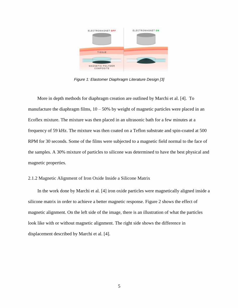
Figure 7 is an image from Serchi et al. [8] showing the rear and frontal view of their robot.

Figure 7: Rear and frontal view of the robot from Serchi et al [8]

One issue with this study is that a motor was used to cause the pressure increase inside the

vessel. Motors are heavy, metal, and certainly not soft. A secondary issue is that the setup seems

very fragile. There are a lot of moving parts that could be damaged if the device propels itself

into a hard surface and the cable detaches.

11

2.1.5 Underwater Jet Propulsion Via an Orifice

Thomas et al. [9] proposed a new idea for underwater jet propulsion, specifically for low

speed vehicles. The authors based their inspiration on locomotion methods from organisms like

jellyfish and squid. Figure 8 shows the actions the authors were attempting to analyze.

Figure 8: Synthetic jet proposed by Thomas et al. [7]. (A) The initial in-

stroke sucks water into the chamber. (B) The out-stroke causes fluid to roll up

into a ring. (C) The vortex ring pinches off. (D) During subsequent in-strokes,

water is sucked in from around the departing vortex ring. [Reproduced from

[7]].

12

The authors further broke down the calculations used to optimize the design of their jet

device. Figure 9 and Figure 10 illustrate the geometries used for the calculations [9].

Figure 10: Left: Slug model of water exiting the orifice; Right: Slug model turning into vortices after leaving the orifice [9]

Figure 9: Literature Jet Schematic [9]

13

According to Thomas et al. [9], the system could be analyzed using a “slug model” that

considers the expelled water as one piece. This is one of the simplest models for this type of

analysis. The intermediate velocity in the small channel created by the outlet orifice can be

calculated using

𝑈𝑝 = 𝑈𝑚 ∗𝑑𝑐ℎ𝑎𝑚𝑏𝑒𝑟

2

𝑑𝑜𝑟𝑖𝑓𝑖𝑐𝑒2

[1]

where Up is velocity through the orifice (m/s), Um is velocity of the diaphragm (m/s), dchamber is

the diameter of the chamber (m), and dorifice is the diameter of the exit orifice (m). The diaphragm

velocity can be calculated using

𝑈𝑚 = 2 ∗ 𝛿 ∗ 𝑓𝑟𝑒𝑞𝑢𝑒𝑛𝑐𝑦 [2]

where 𝛿 is the diameter of the diaphragm (m) and frequency is measured in Hz. From here, the

Reynolds number of the fluid can be calculated using

𝑅𝐸 = 𝑈𝑝 ∗𝑑𝑜𝑟𝑖𝑓𝑖𝑐𝑒

𝑣𝑖𝑠𝑐𝑜𝑠𝑖𝑡𝑦

[3]

After the Reynolds number is calculated, the exit velocity of the fluid can be found using

𝑈𝑒 = 𝑈𝑝 ∗ (1 +8

√𝜋∗

1

√𝑅𝐸∗

√𝐿

√𝐷)

[4]

14

where 𝑈𝑒 is the exit velocity (m/s), L is the length of the slug of ejected fluid (m), and D is the

diameter of the slug of ejected fluid (m). The authors then analyzed the reaction force of the

vortices created from the expulsion of water (shown in Figure 10) using

𝐶𝑖𝑟𝑐𝑢𝑙𝑎𝑡𝑖𝑜𝑛: 𝛤 =1

2∗ 𝐿𝑈𝑝

[5]

The circulation is a measure of vortex strength and an indirect way of measuring thrust.

Using the circulation, the Impulse can then be found using

𝐼𝑚𝑝𝑢𝑙𝑠𝑒: 𝐼 =𝜋 ∗ 𝐷2 ∗ 𝜌

2∗ 𝛤

[6]

The impulse, I, is the impulse imparted on the enclosure by the slug of liquid exiting the

orifice. The final simplification for the average thrust is calculated using

𝑇𝑎𝑣𝑒 =𝐼

𝑡

[7]

where Tave is the average thrust created per pulse of the diaphragm (N) and t is the time of a

single outward push (s).

15

2.1.6 Calculations for physical properties of a thin circular plate

Wygant and Kupnik [10] calculated the diaphragm displacement for circular capacitive

micromachined ultrasonic transducer cells. More specifically, the authors provided detail on how

to calculate the useful constants for a flat plate.

First, the plate deflection is solved for as a function of radial position using

𝜔(𝑟) =𝑃0𝑎4

64𝐷(1 −

𝑟2

𝑎2)

2

= 𝜔𝑝𝑘 (1 −𝑟2

𝑎2)

2

= 𝜔𝑝𝑘 (1 −𝑟2

𝑎2)

2

[8]

where ω is the deflection (m), p is the applied pressure (N/m2), D is the flexural rigidity (N*m2),

r is the radial position on the circle (m), and a is the radius of the circle (m). Then, the Flexural

rigidity is found using

𝐷 =𝐸𝑡3

12(1 − 𝑣2)

[9]

where E is Young’s Modulus, v is Poisson’s Ratio, and D is the flexural rigidity. The maximum

plate deflection can be found using

𝜔𝑝𝑘 =𝑃0 ∗ 𝑎4

64 ∗ 𝐷

[10]

The spring constant can be calculated as

𝑘 =192𝜋𝐷

𝑎2

[11]

16

where k is the spring constant (N/m). The resonant frequency can then be determined using

𝜔0 = √𝑘

𝑚=

10.22

𝑎2 ∗ √(𝜌𝑡𝐷 )

[12]

The resonant frequency equation provided by Wygant and Kupnik [10] is important

because, by pulsing the diaphragm at its resonant frequency, a greater magnitude of displacement

can be achieved since the momentum from each previous pulse is carried into the subsequent

pulse.

2.1.7 Gaps in the Literature

The previous studies in the literature present some information about topics surrounding the

main topic of the current research, but many gaps remain. Serchi et al. [8] presented a concept,

but only the mantle is made of silicone and the compression method is rather rudimentary.

Jayaneththi et al. [3] proposed a flexible and magnetic diaphragm but did not present feasible

applications for their work. Marchi et al. [4] discussed magnetically aligning iron oxide

microparticles during the curing process in order to achieve a better magnetic response.

However, similarly to Jayaneththi et al. [3], the authors do not present a clear application for the

technology. Thomas et al. [9] provided useful equations for key physical characteristics of a

pulsing diaphragm, but the entire proposed device is made of hard plastic and metal. This thesis

utilizes aspects from all this literature to develop a novel soft pulsing diaphragm and an

elastomer solenoid core.

17

Chapter 3 – Methods

In this chapter, the materials and methods for the research are detailed. Section 3.1 describes

the early work performed, leading up to and through the design of the final water pumping

device, described in Chapter 2

3.1 Preliminary Work

The objective of the study was to develop and implement an elastomer solenoid core that

could be integrated into biomedical applications and applications involving harsh conditions

such as environments with extreme temperatures or pH levels. One early source of inspiration for

the design came from audio speakers because they can move small amounts at very high

frequencies with little voltage applied. This idea was stretched into the goal of creating

exaggerated pulses at lower frequencies.

3.1.1 Basic Speaker Development

A simple speaker was created by coiling wire around the bottom of a paper coffee cup,

connecting those wires to the 3.5 mm jack in an mp3 player, and fastening a permanent magnet

to the bottom of the cup. An illustration of this is depicted in Figure 11. This basic prototype was

successful, and the rudimentary speaker projected the signal from the audio jack of the mp3

player. The key finding from this experiment was that small vibrations from a low voltage source

are possible without the need for specialized speaker components.

18

A second source of inspiration for the actuator design was drawn from the archetypal soft

creature: the octopus. An octopus uses an organ called a mantle to draw water through an inlet

and squeezes it out through a nozzle in order to create jet propulsion. Serchi et al. [8] proved that

a synthetic soft mantle can provide adequate propulsion in order to move itself. Robot created by

Serchi et al. [8] involved using pulleys to contract the walls of a soft enclosure in order to

squeeze water out of an orifice. Figure 12 shows an early concept for the jet propulsion device

developed in this thesis work. This is not the final design, merely the original concept for the

water pumping device. In Figure 12, there are four labeled sections of the schematic. 1: The

flexible diaphragm, 2: The stiff housing, 3: The elastomer solenoid core, 4: The outlet orifice, 5:

The inlet valve.

Figure 11: Illustration of Paper Cup Speaker [22]

19

Once the concept for the device was finalized, the next step was to determine the materials

and methods that would be used to develop the final prototype.

3.1.2 Magnetoactive Elastomer Development

Initial samples of magnetic elastomer materials were synthesized using different estimated

ratios of silicone to iron oxide particles. Two different silicone polymers were used – Ecoflex 30

(Smooth-On; Macungie, PA) and Sylgard 184 (Dow Corning; Midland, MI). The best magnetic

response was obtained with a high concentration of particles; however, the physical

characteristics of the polymer, such as the Poisson’s ratio and elasticity, suffered severely.

Samples made from Sylgard 184 were able to cure correctly with higher concentrations of

particles than the Ecoflex 30 samples. Ratios up to 11:10 particles to elastomer by weight could

be used with Sylgard 184, while the maximum ratios that could be obtained using Ecoflex were

Figure 12: An early design for the jet propulsion device. This was a stepping stone to what would be the final design (shown later in the

section) 1. Displaced Diaphragm, 2. Housing, 3. Solenoid, 4. Outlet valve, 5. Inlet Valve

20

4:10 particles to elastomer by weight. Beyond this ratio, the samples did not cure properly.

However, Ecoflex is inherently much more elastic than Sylgard.

Table 1 and Table 2 show the physical properties of raw Sylgard 184 and all Ecoflex

products, respectively. One telling metric is the “% elongation at break”. For the Sylgard, this

elongation is 140%, while the Ecoflex has a minimum of 800% elongation depending on the

mixture. These two tables illustrate the reasoning behind material choices. The defining features

of the Sylgard and Ecoflex are the rigidity and elasticity, respectively. These properties provide

specific functionality for the water pumping mechanism that is described below.

Table 1: Sylgard 184 Spec Table [11]

21

Table 2: Ecoflex Spec Table [12]

Based on the higher stiffness and ability to hold a higher concentration of particles, the

Sylgard 184 was chosen as the base material for the solenoid core. To create this mixture, the

base and curing agent were combined at a 10:1 ratio by weight and manually mixed with a stirrer

for 5 minutes. The mixture was then placed in a vacuum chamber until there were no more

bubbles being released from the mixture. The magnetic particles were then placed in the mixture

at the desired ratio by weight. The particles were mixed for five minutes and the mixture was

placed in a vacuum chamber. Marchi et al. [4] and Ijaz et al. [5] described a mixing method

utilizing an ultrasonic bath, however, these results could not be duplicated. The solution was too

thick and seemed barely affected by the bath at all.

A preliminary investigation using magnetic materials was then done in order to try to

develop an elastomer solenoid core. Figure 13 shows the first iteration of a solenoid core. The

core was approximately 7.5 mm in diameter and 30 mm in total length. The coil had

22

approximately 35 turns of 30 awg magnet wire. For testing purposes, 2.5 amps were applied and

could move a common wood screw across a desk.

A larger core was then created to improve the magnetic properties. With the same applied

current and more turns, the electromagnet was able to pick a screw up off the desk. Figure 14

shows the second iteration of the solenoid core.

One challenge faced during both trials was that, due to settling, the concentration of iron

oxide particles was higher at the bottom of the cylinder than the top. As a result, the magnetic

response was significantly greater at one end than the other. In later iterations, curing the Sylgard

Figure 13: First Iteration Soft Solenoid Core

Figure 14: Second Iteration Soft Solenoid Core

23

184 in the oven led to significantly quicker curing times and very little uneven settling of iron

oxide particles.

The Sylgard 184 was chosen for the base material in the solenoid core because it did not

need to be as flexible as the diaphragm since it did not need to deform. The Sylgard also allowed

for a higher ratio of magnetic particles than the Ecoflex (up to 11:10 as mentioned above).

Although Sylgard 184 is a much stiffer material, the material can still be considered within the

realm of soft actuation.

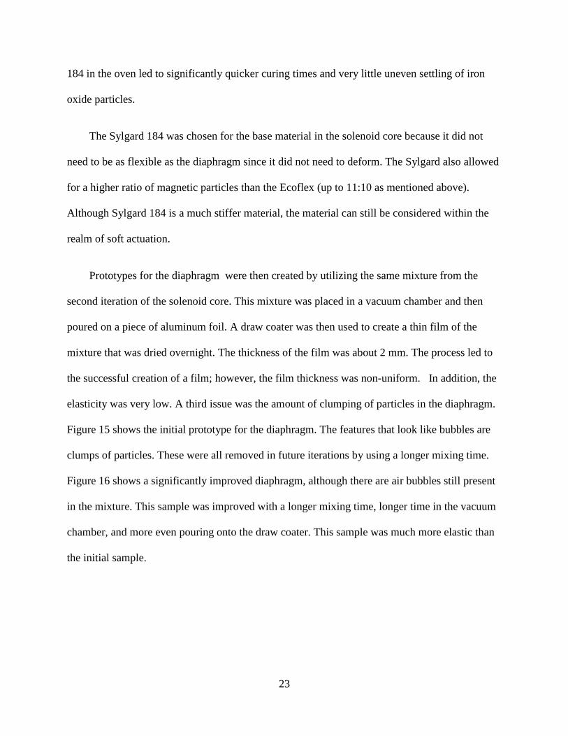
Prototypes for the diaphragm were then created by utilizing the same mixture from the

second iteration of the solenoid core. This mixture was placed in a vacuum chamber and then

poured on a piece of aluminum foil. A draw coater was then used to create a thin film of the

mixture that was dried overnight. The thickness of the film was about 2 mm. The process led to

the successful creation of a film; however, the film thickness was non-uniform. In addition, the

elasticity was very low. A third issue was the amount of clumping of particles in the diaphragm.

Figure 15 shows the initial prototype for the diaphragm. The features that look like bubbles are

clumps of particles. These were all removed in future iterations by using a longer mixing time.

Figure 16 shows a significantly improved diaphragm, although there are air bubbles still present

in the mixture. This sample was improved with a longer mixing time, longer time in the vacuum

chamber, and more even pouring onto the draw coater. This sample was much more elastic than

the initial sample.

24

The first trials done to attract the magnetic diaphragm to the core were unsuccessful. The

best response achieved was no more than a quiver in the material with a total displacement of

less than a millimeter. However, it should be noted that the diaphragm had a very high

displacement when put near a field of stronger neodymium magnets. The use of neodymium

magnets offers potential for future iterations of this work. Three changes were made to address

the limited displacements. The core was attached to the diaphragm causing the two components

to move in tandem through the coil of wire. The wire gauge was also dropped to 17 awg from 30

awg in order to allow for a higher current to be transmitted. Finally, the iron oxide particles were

Figure 15: First diaphragm prototype

Figure 16: Improved diaphragm prototype

25

removed from the diaphragm as their contribution to the magnetic attraction was deemed

negligible, and even deliterious, since the particles decreased the elasticity of the diaphragm.

3.2 Theoretical Analysis

After initial development of the actuator concept and preliminary testing of the materials

was done, parameters for the enclosure were determined. A preliminary goal for the device was

to move one half liter of water per minute using a diaphragm diameter of 10 cm. The diameter of

the diaphragm was set to 10 cm due to the availability of the 10 cm diameter PVC piping that

was used for the wall of the enclosure. Figure 15 shows a simulation of the theoretical maximum

deflection of the pulsing diaphragm.

This simulation reveals that the diaphragm creates a shape called a “sphere cap”. Figure 18

depicts the sphere cap.

Figure 17: Displacement simulation of diaphragm

26

The volume of a sphere cap can be found using

𝑉 =𝜋 ∗ ℎ2

3∗ (3 ∗ 𝑟 − ℎ)

[13]

where h is height of sphere cap (m), r is radius of sphere cap (m), and V is the total volume of the

sphere cap (m3). Using Equation 13, the theoretical volume of water displaced by a single pulse

of water can be found.

Figure 18: Sphere Cap [24]

27

3.2.1 Magnetic Field Force

While there are equations to solve for the strength of the magnetic field, it is difficult to

calculate of the force imparted on an object in Newtons. As a result, the value was determined

experimentally.

In order to find the force imparted on the core by the magnetic field, the core was placed

inside the windings unsecured and allowed to move freely. Next, pulses were sent through the

coil causing a magnetic field to propagate and act on the magnetoactive core. The total vertical

displacement of the core was recorded and used to determine the total force on the material. To

calculate the force, the potential energy was divided by the total time of the impulse of the

magnetic field. In addition, the average velocity of the cylinder was determined by dividing

displacement by time.

The potential energy was calculated using

𝑊 = 𝑚𝑔ℎ [14]

where W is potential energy (J), m is mass of the core (kg), g is acceleration due to gravity

(m/s2), and h is the maximum height displacement (m). Potential energy was then divided by

time to solve for power, such that

𝑃 =𝑊

𝑡

[15]

where P is power (W), W is potential energy (J), and t is total time of displacement (s). A second

power equation was then used where

28

𝑃 = 𝐹 ∗ 𝑉 [16]

In Equation 16, F is the Force imparted by the magnetic field, and V is the average velocity

of the core moving through the windings (m/s). By combining Equations 15 and 16, the force

imparted on the core can be solved for with

𝐹 =𝑚𝑔ℎ

𝑡𝑉

[17]

To find the spring constant, the mass of the water in the sphere cap was solved for by

multiplying the volume of the sphere cap by the density of water using

𝑚𝑤𝑎𝑡𝑒𝑟 = 𝑉𝑐𝑎𝑝 ∗ 𝜌 [18]

The spring constant was solved for experimentally by finding the natural frequency in air

(to eliminate damping from the water) and solving for “k” using

𝜔 = √𝑘

𝑚

[19]

Rearranging yields

𝑘 = 𝜔2 ∗ 𝑚

[20]

where k is the spring constant, ω is the natural frequency in radians/second, and m is the mass.

29

3.3 Electrical Design

The strength of the electromagnetic field produced by a coil is dependent on the current

flowing through the wire. Using Ohm’s law [21], it is apparent that minimizing resistance and

maximizing voltage will lead to the highest possible current flow. Ohm’s law states that

𝐼 =𝑉

𝑅

[21]

where I is the current, V is the voltage and R is the resistance in the circuit. Based on the pulsing

nature of the system, there does not need to be a constant, sustained voltage source. For this

reason, capacitors are used to discharge into the coil. Figure 19 depicts a schematic for the circuit

used to send current through the solenoid coils. A voltage source charges the capacitors which, in

turn, open the circuit when filled. When the switch is closed, the capacitors discharge through the

coil instantaneously. In a perfect circuit, this method has the benefit of a sustained, although

lower, voltage through the coil because the capacitors and voltage source are discharging in

parallel through the wire. Another benefit of using capacitors is that they are not limited in their

power output. Unlike a battery or a power supply, capacitors can instantaneously discharge all

the stored energy, which allows for a higher current in the system.

30

Figure 19: Pulsing circuit schematic. C = 60,000 µf; R = 1 Ω. Inductor symbol represents the coils of the solenoid.

For this thesis, a capacitance value of 60000 uF was chosen. A 30V, 2A power supply was

utilized to drive the system, although the target voltage was 27 V for potential future use with 9V

batteries. Since the power supply was limited to a 3 A output, the capacitors were crucial in

increasing the current as high as possible instantaneously in order to create a strong magnetic

pulse. Figure 20 shows the two capacitors used in the circuit.

31

Figure 20: Two 30,000 µf Capacitors

The coil contains approximately 450 turns of 17 AWG wire evenly distributed over a 5.5

cm long axle. The total resistance of this wire is 1.1 ohms and the inner diameter of the spindle is

2.66 cm.

In order to accurately pulse the circuit, an Arduino Uno was used to send a square wave at

specific frequencies. The code can be found in Appendix A. The frequency was chosen based on

the charge and discharge time of the capacitors (The circuit was closed for 250 ms to discharge

the capacitors and opened for 500 ms to charge the capacitors). This is further explained in

Section 4.1. A signal was sent to a mechanical relay (shown in Figure 21), which acted as the

switch in the circuit described above.

32

Figure 21: 4 Channel Mechanical Relay (Note: Only one channel is used)

The relay shown in Figure 21 is rated for 240 VDC and 120 VAC at 30 A. The mechanical

relay was chosen to add overall robustness to the system. A solid-state relay can switch faster,

but they are more expensive. Another added benefit of the solid-state relay is the clicking noise

that is made every time the internal switch is closed. The noise allowed for easy verification that

the triggering setup was working as intended.

An additional benefit of this specific relay is that it has four channels. Thus, the overall

switching frequency can be increased to four times that of a single channel, assuming each relay

is offset in their triggering. The method of artificially increasing the pulsing frequency is not

necessary in this project but could have potential utility in future studies.

33

3.4 Final Manufacturing Methods

The materials chosen for the final prototype of the water pumping device are Ecoflex 30 for

the diaphragm and Sylgard 184 mixed with iron oxide microparticles for the solenoid core.

3.4.1 Diaphragm

The most reliable way to get a smooth, thin, even diaphragm was to pour the EcoFlex 30 on

a flat piece of aluminum foil, and let gravity spread it out as it cured. Each diaphragm cured to

about 1.5 mm consistently. The only variable was the diameter of the sample, which could be cut

to a workable size. This method was found to be simpler than draw coating, and the thickness of

1.5 mm proved to be acceptable for the diaphragm. Figure 22 shows the EcoFlex curing on a

piece of aluminum foil.

Figure 22: EcoFlex Diaphragm

34

3.4.2 Magnetoactive Core

The magnetic core was made of Sylgard 184 and iron oxide microparticles (0.3 µm in

diameter [13]). The process for creation was as follows:

• Combine Sylgard 184 parts A and B in a cup at a 1:10 ratio by weight.

• Add Iron Oxide particles to the Sylgard 184 at a 1:1 ratio by weight.

• Stir the mixture for five minutes, or until there are no clumps of particles.

• Place the mixture in a vacuum chamber until there are no bubbles leaving the mixture.

The stirring time will vary depending on the dimensions of the container. NOTE: The

mixture will expand significantly in the chamber.

• Evenly pour the mixture into a mold for the necessary dimensions of the core. The mold

used in this project measured 2.2 cm in height and 2.08 cm in diameter. The mold was

made from aluminum foil wrapped around a cylindrical bar of the same size.

• Place the filled mold in the vacuum chamber again until no bubbles are present.

• Bake the mold at 100°C for 45 minutes (or any other temperature/time combination

specified on the Sylgard 184 spec sheet).

• Cool the cured core, then remove the core from the mold using a razor to cleanly cut one

end of the cylinder. Cutting the cylinder should lead to a flat and even surface.

3.4.3 Bonding of Core and Diaphragm

Connecting the magnetoactive cylinder to the diaphragm proved to be a challenge. The first

method tried was a corona-wand plasma treatment to attach the bottom of the cylinder and the

section of the diaphragm that was to be attached. After treatment, the two samples were pushed

together in order to bond the surfaces. This method was not reliable, as it was unpredictable

35

whether the bond would be substantial enough to hold. One issue may have been the slight

difference in materials, with one being EcoFlex 30 (the diaphragm) and the other being Sylgard

184 (the core). The root cause of this unpredictable failure was not further investigated and could

be something for future work.

A much more reliable method for bonding the two components was simply to place the core

in the curing EcoFlex and allow it to bond. The connection was still relatively fragile but was

reliable enough to withstand the separation from the aluminum foil and to undergo testing.

Figure 23 shows an image of the core sitting on the diaphragm as it was curing.

Figure 23: Core placed in EcoFlex

36

3.5 Initial Testing

Figure 24 shows an early prototype of the device created solely for an initial visualization of

the diaphragm pulsing. In this prototype, the coil was placed inside a large glass beaker and the

diaphragm was secured on top of the beaker. When tested with the 27 V pulsing circuit, the

displacement of the diaphragm varied between 2 and 2.5cm. It is important to note that gravity

played a part in this test, with the weight of the magnetic core adding to the downward force

causing deflection.

The same apparatus described above was then placed underwater in order to better mimic

final testing conditions. Figure 25 depicts the deflection of the diaphragm, with the red line

indicating the center mark of the core. The total deflection obtained during this test was 0.5 cm.

It should be noted that in this preliminary test there were no inlet and outlet valves, so there was

a pressure increase in the chamber that caused a decrease in the deflection of the diaphragm.

Figure 24: Dry prototype

37

Figure 26 shows the displacement of the elastomer core in the coil. In this test, both the coil

and the cylinder were placed underwater and individual pulses were sent through the circuit to

test the efficacy of the magnetic field on the core. The total displacement achieved was 1.75 cm.

3.6 Pump Enclosure Design and Prototyping

The final enclosure for the pump was made primarily of PVC tubing. PVC is a readily

available material and is relatively easy to work with. In future iterations, a potential goal may be

to create the enclosure out of a soft material, such as silicone.

Figure 25: Wet prototype; Left: maximum bottom displacement, right: maximum top displacement. Red line

shows centerline.

Figure 26: Elastomer Core Movement (Left: Max upwards displacement, Right: Max downwards displacement.

38

Figure 27: Top view of enclosure. All measurements are in millimeters.

Figure 28: Side view of enclosure, all units are in millimeters.

Silicone Diaphragm

Solenoid Core

Spool for wire

windings

Enclosure Housing Outlet Orifice

Inlet Orifice

(Located in the wall

of the enclosure

housing.)

Enclosure Housing

Spool for wire

windings

39

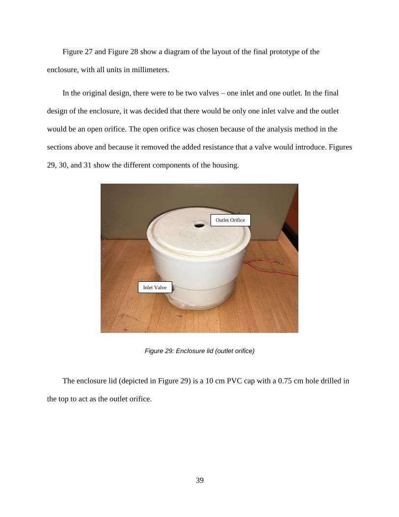
Figure 27 and Figure 28 show a diagram of the layout of the final prototype of the

enclosure, with all units in millimeters.

In the original design, there were to be two valves – one inlet and one outlet. In the final

design of the enclosure, it was decided that there would be only one inlet valve and the outlet

would be an open orifice. The open orifice was chosen because of the analysis method in the

sections above and because it removed the added resistance that a valve would introduce. Figures

29, 30, and 31 show the different components of the housing.

Figure 29: Enclosure lid (outlet orifice)

The enclosure lid (depicted in Figure 29) is a 10 cm PVC cap with a 0.75 cm hole drilled in

the top to act as the outlet orifice.

Outlet Orifice

Inlet Valve

40

Figure 30: Enclosure body with inlet valve attached (on right) and orifice (on left)

Figure 31: Enclosure with diaphragm attached (Black circle is solenoid core inside enclosure.)

Inlet Orifice Inlet Valve

41

The inlet valve is a small aquarium check valve (PS+; Livonia, MI). In addition, there is an

inlet orifice for additional flow. The open orifice greatly improved the performance of the

pumping mechanism. The aquarium check valve was chosen because of its ability to handle very

low flow rates, as well as its overall robustness. The aquarium valve, shown in Figure 32, is a

simple one-way valve that requires no external actuation other than fluid movement.

Figure 32: Left: Closed check valve; Right: Open Check Valve

3.7 Experimental Results

In order to test the efficacy of the device, two different methods were used. The first was to

measure the maximum displacement of the diaphragm during each of twenty pulses, and the

second was to measure the efficacy of the water pumping enclosure by measuring the total water

displaced after certain time intervals.

3.7.1 Diaphragm Displacement

The measurements for diaphragm displacement were done visually. The pulses were

recorded at 240 frames per second using an iPhone 8. The maximum displacement of a pulse was

42

measured in relation to a ruler in the frame. These values are depicted in tabular and graphical

forms in Sections 4.2 and 4.3.

3.7.2 Pumping Efficacy

The pumping efficacy of the device was tested by measuring the total amount of water

being expelled from the orifice of the enclosure. The device was placed with the orifice sitting

0.5 mm above the surface of a pool of water. A pulsing signal was then sent through the coil,

allowing the diaphragm to pulse. The pulsing caused water to be expelled from the orifice and

pool on the surface of the device. The pooled water was then vacuumed into a graduated cylinder

and measured after a specified period of time. Figure 33 shows the motor used to pump the

pooled water into the graduated cylinder.

Figure 33: Pumping motor used to vacuum pooled water for measurement.

43

Chapter 4 - Data

In this section, the results from the testing methods described above are presented. The

pulsing electrical signal is broken down and testing data from in-air and in-water experiments are

shown.

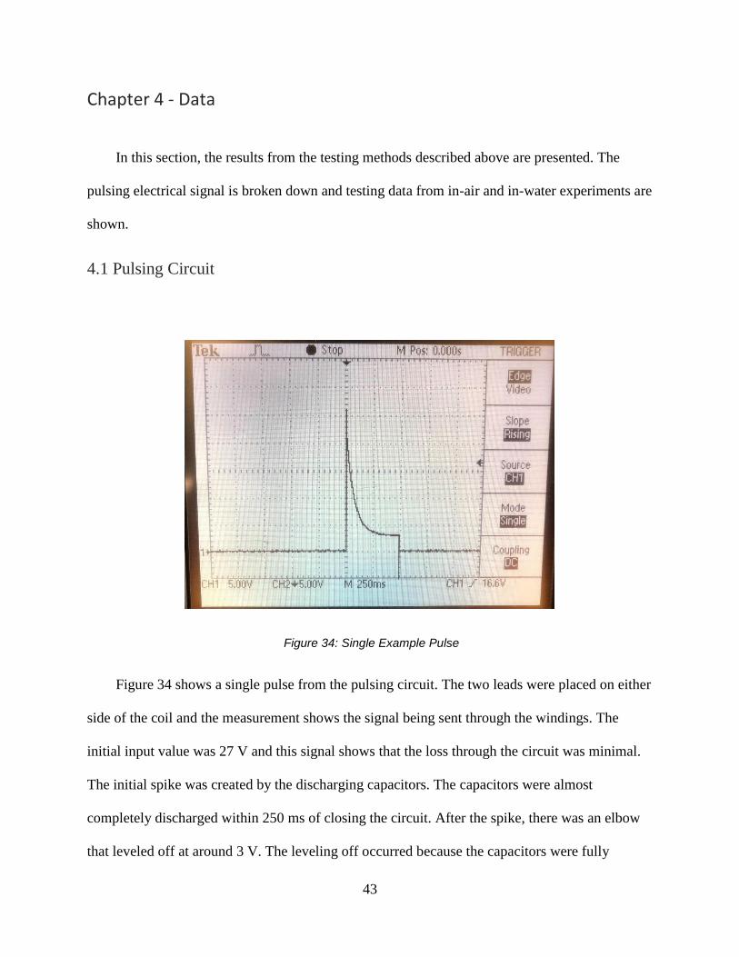
4.1 Pulsing Circuit

Figure 34: Single Example Pulse

Figure 34 shows a single pulse from the pulsing circuit. The two leads were placed on either

side of the coil and the measurement shows the signal being sent through the windings. The

initial input value was 27 V and this signal shows that the loss through the circuit was minimal.

The initial spike was created by the discharging capacitors. The capacitors were almost

completely discharged within 250 ms of closing the circuit. After the spike, there was an elbow

that leveled off at around 3 V. The leveling off occurred because the capacitors were fully

44

discharged and the only voltage through the system was coming from the power supply. The

power supply is limited to 3 A and, following Ohm’s law, the 1 Ohm of resistance through the

coil leads to a limit of 3 V being output from the power supply. After the initial leveling off,

there was a sharp cutoff where the voltage dropped to zero. The drop-off occurred when the

circuit was opened. An open time of around 500 ms was necessary in between pulses to let the

capacitors recharge.

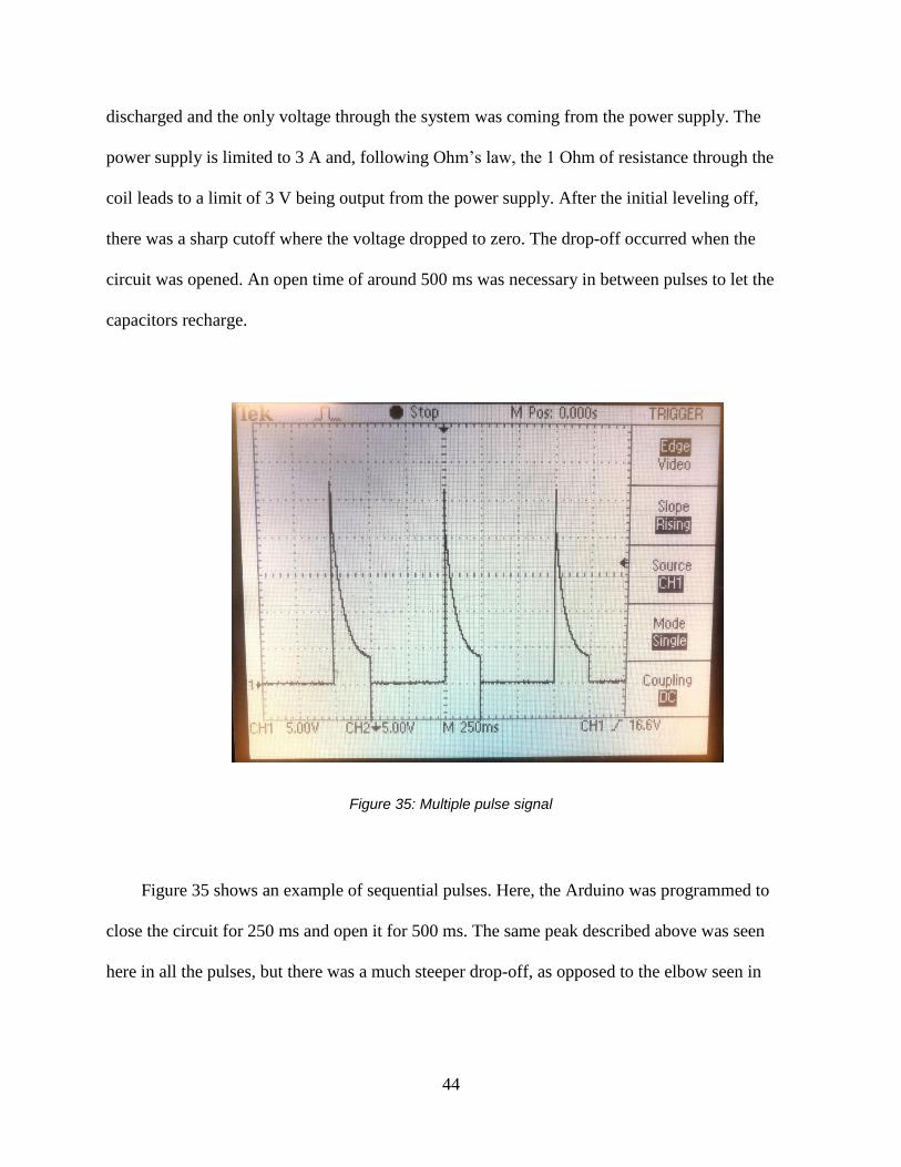
Figure 35: Multiple pulse signal

Figure 35 shows an example of sequential pulses. Here, the Arduino was programmed to

close the circuit for 250 ms and open it for 500 ms. The same peak described above was seen

here in all the pulses, but there was a much steeper drop-off, as opposed to the elbow seen in

45

Figure 34. The off time was therefore set much shorter in order to increase the frequency of the

pulsing.

4.2 In-Air Testing

4.2.1 Measured Displacement

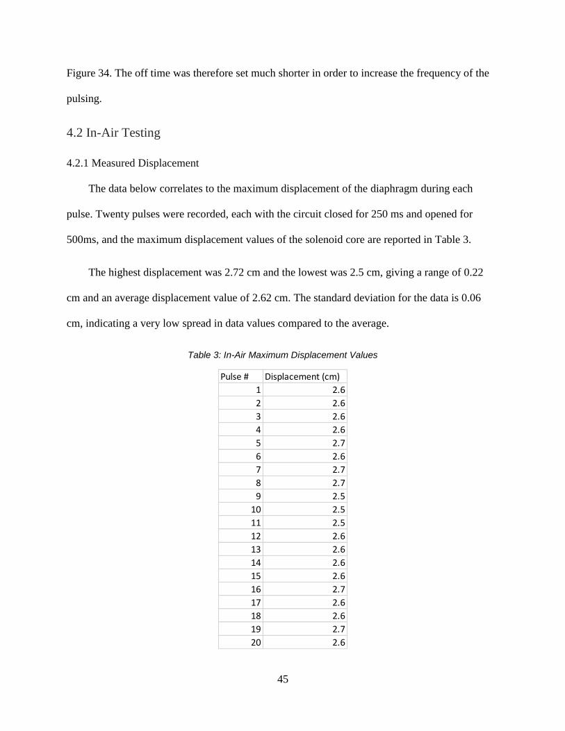
The data below correlates to the maximum displacement of the diaphragm during each

pulse. Twenty pulses were recorded, each with the circuit closed for 250 ms and opened for

500ms, and the maximum displacement values of the solenoid core are reported in Table 3.

The highest displacement was 2.72 cm and the lowest was 2.5 cm, giving a range of 0.22

cm and an average displacement value of 2.62 cm. The standard deviation for the data is 0.06

cm, indicating a very low spread in data values compared to the average.

Table 3: In-Air Maximum Displacement Values

Pulse # Displacement (cm)

1 2.6

2 2.6

3 2.6

4 2.6

5 2.7

6 2.6

7 2.7

8 2.7

9 2.5

10 2.5

11 2.5

12 2.6

13 2.6

14 2.6

15 2.6

16 2.7

17 2.6

18 2.6

19 2.7

20 2.6

46

Figure 33 shows the clustering of the maximum displacement values. Twenty pulses were

measured, and the displacements were recorded in the plot below.

Figure 36: In-Air Maximum Displacement Values

The blue bars on each point are error bars, showing the standard error for each

measurement. This error was found to be 0.013. The red horizontal line indicates the average

value of 2.62 cm.

Figure 37: Time lapse of In-Air displacement (Note: all times are in seconds)

T=0 s T=0.15 s T=0.25 s T=0.45 s T=0.55 s

47

Figure 37 shows a representative series of frames from the slow motion video of the in-air

diaphragm displacement video with the ruler in place. The maximum displacements were

determined visually. In Figure 37, the maximum displacement can be seen at T = 0.25 s.

48

4.3 Underwater Testing

4.3.1 Measured Displacement

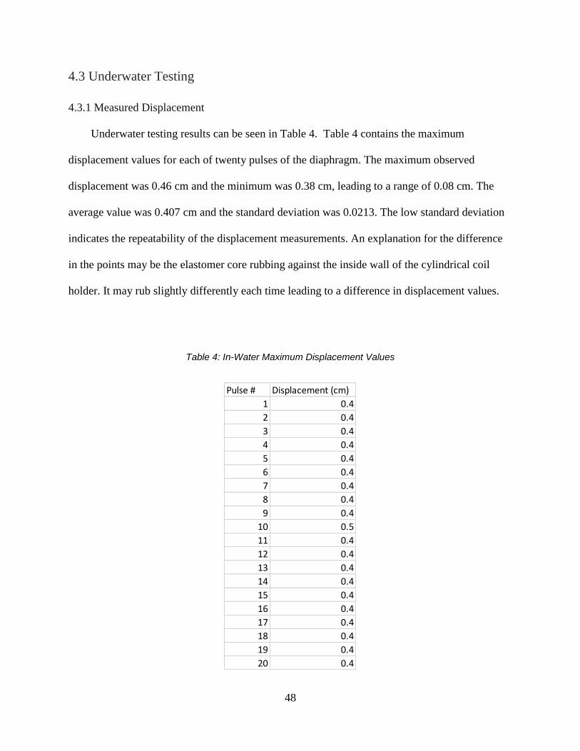
Underwater testing results can be seen in Table 4. Table 4 contains the maximum

displacement values for each of twenty pulses of the diaphragm. The maximum observed

displacement was 0.46 cm and the minimum was 0.38 cm, leading to a range of 0.08 cm. The

average value was 0.407 cm and the standard deviation was 0.0213. The low standard deviation

indicates the repeatability of the displacement measurements. An explanation for the difference

in the points may be the elastomer core rubbing against the inside wall of the cylindrical coil

holder. It may rub slightly differently each time leading to a difference in displacement values.

Table 4: In-Water Maximum Displacement Values

Pulse # Displacement (cm)

1 0.4

2 0.4

3 0.4

4 0.4

5 0.4

6 0.4

7 0.4

8 0.4

9 0.4

10 0.5

11 0.4

12 0.4

13 0.4

14 0.4

15 0.4

16 0.4

17 0.4

18 0.4

19 0.4

20 0.4

49

Figure 38 below shows the spread of maximum displacement values for 20 pulses of the

diaphragm. The range of the data set is 0.08 cm, indicating a tight spread of data points. The bars

on the top and bottom of each point show the error in each measurement. The error is 0.005 cm,

which suggests that consistent displacement measurements are obtained with each pulse of the

circuit. The red line shows the average displacement value and further proves the consistency of

the displacements due to the tight grouping around the average.

Figure 38: In-Water Maximum Displacement Values

50

Figure 39 illustrates the data collected for each of three different tests. The orange points

indicate the total volume of water pumped in 120 seconds (2 minutes). The blue points show the

total volume of water pumped in 60 seconds (1 minute), and the yellow points show the total

volume of water pumped after 100 displacements of the diaphragm. The green, blue, and purple

horizontal lines show the average values for the 120 second, 100 pulse, and 60 second trials,

respectively.

The first notable difference is the change in pumping rate between the 1 and 2 minute trials.

The average total volume pumped for the 1 minute trial was 250 ml, whereas the volume

pumped during the 2 minute trial was 460 ml. This was not a linear pattern and was likely due to

the slight change in the water level of the water bath as water was removed. Another notable

statistic is the range in each set of data. The volume range in the 1 minute trials was 28 ml and

the range for the 2 minute trials was 25 ml. This range is relatively small compared to the total

amount of water pumped and validates the repeatability of the pumping efficacy for set periods

of time. Table 5 shows statistics for the trials, with the most notable statistic being the standard

deviation. The values are very low compared to the averages, indicating a consistent pumping

rate for each trial.

Table 5: Statistics for 60s, 120s, and 100 pulse trials

60 Second (ml) 120 Second (ml) 100 Pulses (ml)

Standard Deviation 8.71 5.49 4.53

Range 28.00 25.00 18.00

Average 252.80 460.05 301.00

Error 1.95 1.23 1.01

51

Figure 39: Pumping Data

Figure 40: Time Until 500 ml Pumped

52

Figure 41: Graph indicating the nonlinearity of volume being pumped over time. Each point shows a mean value of a range of data taken in tests discussed above.

Figure 40 is a graph of the time taken for the device to pump to 500 ml. The blue lines

above and below each point are error bars, with the error being 0.46 seconds. The standard

deviation of the data is 2.04 seconds, deviating from the mean of 131.8 seconds, indicated by the

orange line, only slightly. The small standard deviation indicates a consistent pumping method,

as the total time remains very similar throughout twenty trials.

Figure 41 shows the nonlinearity of the volume being pumped over time. Each point is an

average measurement value of the tests discussed above. When connected, the slope of the

connecting line changes, indicating a change in the pumping rate over different time intervals.

53

Figure 42 below shows an image of the expulsion of water in action. Underneath are small

timestamps indicating when each step occurred.

Figure 42: Frames from slow motion video of in-water pumping test (Note: all times are in seconds)

T=0 s T=0.2 s T=0.3 s T=0.55 s T=0.6 s

Note how the water exits the orifice as a cylindrical slug and turns into a mushroom shape,

like the vortices mentioned in section 2.1.5 by Thomas et al. [9]

54

Chapter 5 - Discussion

The goals of this thesis were to:

• Develop an elastomer solenoid core.

• Create a diaphragm capable of pulsing when subject to an external force.

• Eliminate the need for high voltages and pneumatics.

• Implement the core and diaphragm in a soft actuation device capable of pumping 500

ml/min of water.

Overall, the work performed in this thesis was a success. The elastomer solenoid core

was effective in actuation via a magnetic field. The diaphragm was created using Ecoflex 30

and was also effective in using it to pulse and create pressure differences inside an enclosure.

The maximum voltage used was 27 volts, which is well below threshold to be considered

high voltage. Lastly, the pump was capable of pumping 250 ml of water in a minute. The

original goal was 500 ml/min, meaning the pump fell short by 250 ml, but overall the

development of the prototype was a success. The following sections go into further detail on

these topics.

5.1.1 Develop an elastomer solenoid core

The cornerstone of this work was the development and implementation of an elastomer core

capable of propagating a magnetic field. The development of the core was successful. Utilizing

Sylgard 184 as the elastomer material with which to mix iron oxide particles turned out to be a

much better choice than Ecoflex 30 for the reasons stated previously. Initial tests of adding

windings to the outside of the core and applying a voltage caused the silicone to become a soft

electromagnet.

55

5.1.2 Develop a diaphragm capable of deformation to create pressure fluctuations

The development of the diaphragm was a success. The use of Ecoflex 30 instead of Sylgard

184 proved to be a good choice due to the high elasticity of the Ecoflex compared to the Sylgard.

Using gravity as a method of evening out the membrane also proved to be a success over using a

draw coater because of the simplicity and repeatability.

5.1.3 Eliminate the need for high voltage and pneumatics

The two big fallbacks for the current popular soft actuators are the need for high voltages

and pneumatic tubes/compressors. Eliminating the need for pneumatic tubing to inflate artificial

muscles was a success. The device is self-contained, requiring only an applied voltage.

The elimination of high voltage was also a success. This device is being driven with 27 V; a

value attainable with typical benchtop power supplies. Additionally, the American National

Standard for Electric Power Systems and Equipment defines low voltage as anything below

600V [14]. The device that was developed uses 4.5% of the voltage needed to be classified as

high voltage and is considered low voltage by a large margin. This is advantageous over

electroactive polymers (EAP) which require kilovolts to function properly.

5.1.4 Develop a device capable of pumping 500ml/min of water

The original goal for this device was to pump 500ml/min of water. In final testing, the

device fell short, being able to pump an average of 250ml/min. Although this was the case, it

does prove the viability of the use for an elastomer as a solenoid core for a soft robotic actuator.

Additionally, this goal was secondary to the implementation of the magnetic solenoid core.

The original calculation for the 500 ml came from the formula for a sphere cap, denoted in

Equation 13 above. This original equation called for a perfectly round deformation of the

56

diaphragm to lead to 700 ml/min of water pumped. This number was reduced to 500 ml/min to

account for an imperfect system where the diaphragm would not be completely round. From

experimentation, the observed deformation of the diaphragm was different entirely. Figure 43 is

a cross section of the diaphragm shape. The solenoid pulled upward, creating internal pressure in

the enclosure. The pressure caused the outer edges of the diaphragm to push downwards. The

downward movements on the outer edges of the diaphragm were not accounted for in the initial

calculations. Three things were done to attempt to alleviate the movements: increase tension on

the diaphragm, add a stiff brace on the outer edge of the diaphragm to prevent movement in the

wrong direction, and increase the thickness of the diaphragm. None of the methods increased the

amount of water pumped out of the device.

Figure 43: Deformed Diaphragm; Red arrows denote downward pressure from enclosure, blue arrow denotes upward force from magnetic field.

Another theory for why the calculated volume is incorrect is that the water being pumped is

only the water sitting in the cylinder surrounded by the coil. When the core is pulled through the

coils, it pushes the water out in a cylindrical slug. This slug is independent of the total volume of

the sphere cap and may explain the differences in the data.

57

5.1.4.1 Pump Comparisons

Below is a table of small pumps for comparison to the pump developed in this research.

Table 6: Table of Comparable Pumps [15] [16] [17] [18] [19]

The top three pumps in Table 6 are typical fish tank water pumps for circulating water

through filtration systems or simply creating a current in the water. All three of these have higher

pumping rates than the pump created in this research. They are of similar size and weight to the

soft actuator developed. The bottom two pumps are also of similar size to the pulsing diaphragm

pump developed above, but with much lower flow rates. These pumps are meant to take up less

space and to be fitted to specific heads in specialty scenarios. Their flow rates are much lower

and are much closer to that of the pump developed in this research.

In its current form, the pump developed in this research may be applied to specialty

applications but would require further research and development in order to make it comparable

to current commercial pumps, such as those mentioned above. However, all of the pumps above

are rigid, thus, the progress made is substantial for the field of soft robotics and validates the

notion that further research should be done in this area.

Name Pumping Capacity

Decdeal Ultra-quiet Mini

Brushless Water Pump

4.66L/min

Homasy Submersible

Water Pump 5L/min

VicTsing Submersible

Water Pump 5L/min

GC Series External Gear

Pump .4L/min

GJ Series External Gear

Pump .158L/min

58

Chapter 6 - Societal Context

Soft robotics is an emerging field with many applications from biomedical to underwater

research. The issue with many of the current soft actuation methods is that there is a lot of added

equipment such as air compressors and tubes that take away from the true soft nature of the

devices. Metal components add weight and take up a lot of space. The goal of my research was

to integrate the functionality of metal solenoid-based devices with the development of an

elastomer solenoid. This proof of concept may lead the way to things like elastomer motors in

everyday devices. These motors would be extremely easy to replicate, be lighter, cheaper, and

more versatile than their metal counterparts.

The pulsing action to be mimicked here could also help to further the understanding of the

softest organisms on earth such as jellyfish, octopus, and squid. From this, the technology could

expand to underwater exploration. A hull made from silicone would withstand bumping into a

hard rock wall much better than a metal hull, because of the inherent elastic properties.

A third application of this technology could be to reduce it down to a much smaller scale

and implement it into micro-size applications. This opens the way for new types of pumps in

medical devices and propulsion methods for micro-robots.

59

Chapter 7 – Future Work

7.1 Magnetoactive Diaphragm

Jayaneththi et al. [3] previously developed magnetoactive diaphragms. As described in the

preliminary research section of this paper, the incorporation of this technology was investigated,

but there was difficulty in efficiently including a magnetic diaphragm into final pumping device.

For the purposes of the research, the diaphragm needed to be as elastic as possible and from

experimentation, the inclusion of particles was a detriment to this necessity.

With this being said, extensive research was not performed in this work on the topic of a

magnetic elastomer diaphragm. This topic does not have substantial understanding, and further

developing the relationship between different elastic materials and the inclusion of magnetic

particles for the purposes of a pulsing diaphragm is something that could benefit from more in-

depth research.

7.2 Inlet Valve

The current valve on the enclosure is meant for a low flow aquarium pump. The low flow

rating is the reason it was chosen, but it certainly has flaws. With the pulsing nature of the

enclosure, the valve cannot keep up perfectly. It creates a lot of resistance for water to get into

the enclosure. Further research on an extremely low flow inlet valve is something that, while

seemingly niche, can have further potential use with this project and any other with a similar

rapid pulse and low flow rate fluid movement.

60

7.3 Soft Enclosure

The initial plan for this project was to have the entire enclosure be made of a soft elastomer

material like Ecoflex 30 or Sylgard 184. The PVC was chosen in order to keep the focus on the

crux of the project, the magnetoactive elastomer core. Developing a completely soft enclosure is

something that would further this research and further prove the viability of the technology in the

soft robotics field. This could go even further with bringing the scale of the device down for

potential use in the medical field or in everyday uses.

7.4 Liquid Metal Windings

Lazarus and Meyer [7] discussed the use of a ferrofluid solenoid core. This was the focus of

the paper, but the authors also discussed the use of liquid metal as the wire for a solenoid. A

liquid metal encased in a silicone mold of the proper geometry can act as a wire and, if the mold

is created to make windings like in a solenoid, a completely soft electromagnet can be made.

This concept is something that could greatly increase the viability of the research performed for

this thesis and would allow for a completely soft actuation mechanism.

This would also open new potential avenues with the liquid metal windings. With further

development, these windings could connect to multiple actuators and the same metal could be

recycled to other solenoids, thus saving weight and materials.

61

7.5 Diaphragm Tension and Spring Constant

A big difficulty for this project was finding a reliable way to create even tension across the

diaphragm. As mentioned above, the tension on the diaphragm affects the spring constant of the

material. Finding an easily replicated method of evenly stretching the film is something that

would increase the accuracy of the device and could be incorporated into other areas of research,

such as magnetoactive diaphragms.

7.6 System Model Accuracy

The work done by Thomas et al. [9] in defining the system characteristics is something that

can be further utilized for this project, and even turned into a project in itself. An accurate system

model for this device would cut down on the time needed for testing different parameters. This

model could give optimal dimensions and material properties for this technology to work as well

as possible.

There are two theories laid out in the section above that offer differing thoughts on how the

diaphragm deforms and how the water is being pumped. Both theories would benefit from future

research and could have potential use in other applications. Sections 7.6.2 and 7.6.3 detail

preliminary system model simulations. Section 7.6.1 shows the simplified mathematical model

of the system.

7.6.1 System Model Equation

The flexible pulsing diaphragm can be simplified to a mass, spring and damper system. The

general equation is

𝑚 + 𝑐 + 𝑘𝑥 = 𝑢 [22]

where m is mass, c is the damping constant, and k is the spring constant.

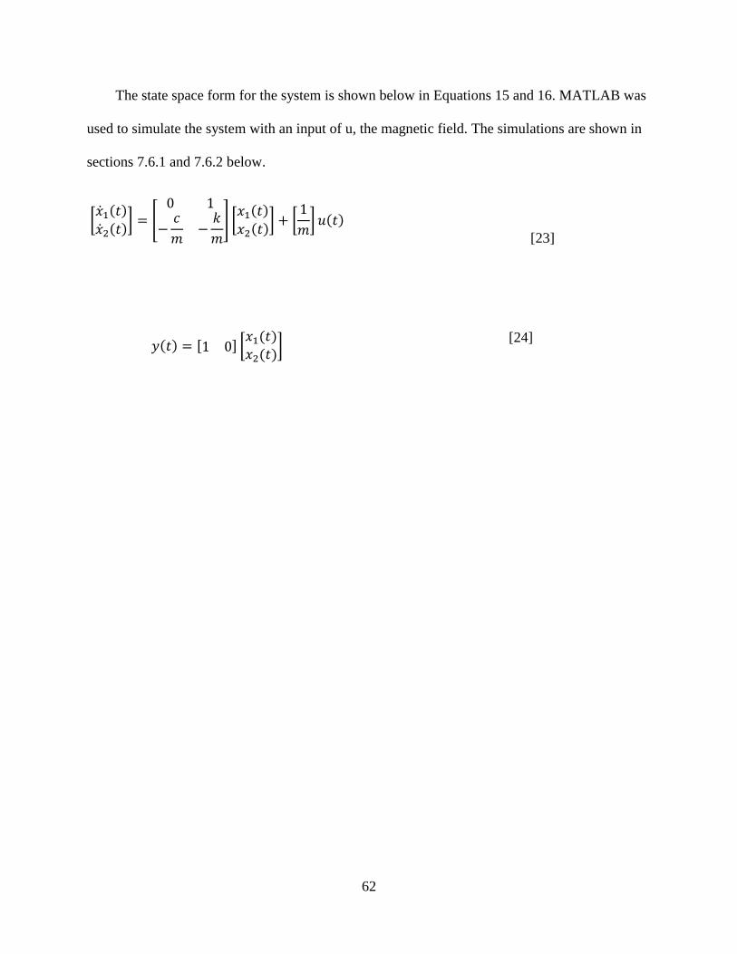
62

The state space form for the system is shown below in Equations 15 and 16. MATLAB was

used to simulate the system with an input of u, the magnetic field. The simulations are shown in

sections 7.6.1 and 7.6.2 below.

[1(𝑡)

2(𝑡)] = [

0 1

−𝑐

𝑚−

𝑘

𝑚

] [𝑥1(𝑡)

𝑥2(𝑡)] + [

1

𝑚] 𝑢(𝑡)

[23]

𝑦(𝑡) = [1 0] [𝑥1(𝑡)𝑥2(𝑡)

] [24]

63

7.6.2 In-Air Simulation

Figure 34 is a MATLAB plot of the in-air simulation of the diaphragm displacement. In the

sections above, the system was simplified down to a mass, spring, and damper system. From

here the system was put into state space form where a specific input was entered. The blue plot

corresponds to the diaphragm displacement and the left axis. The orange plot signifies the input

signal and relates to the right axis.

Figure 44: In-Air Displacement MATLAB Simulation

In order to run this simulation, a few values were needed: c; the damping constant, and k;

the spring constant. The spring constant was found experimentally by stretching the diaphragm

and measuring the force imparted due to displacement. This constant was found to be variable

64

depending on the tension in the diaphragm and is something that could benefit from future

research. The spring constant was determined to be 116 N/m. From here, the damping constant

could be estimated. This value was found to be 2.5. Although it is not applicable to this thesis

because of the slow pulsing frequency ultimately used, the resonant frequency was calculated

using Equation 12 and found to be 32.15 rad/sec, or 5.12 Hz.

The simulated value puts the total vertical displacement of the diaphragm at around 4 cm.

This deviates from the total displacement of the in-air test by about 1.4 cm. This may be due to

the imperfect spring estimation of the silicone diaphragm. It is possible that this circular film has

a nonlinear spring constant that changes at different tensions.

Figure 45: Spring Constant of Varying thickness SU-8 [20]

Figure 45,from Grégoire et al. [20], shows the nonlinear relationship between the thickness

of SU-8, a similar crosslinked polymer, and the spring constant. Figure 42 is included to

demonstrate the point stated above; as the sample of Ecoflex is stretched, the thickness varies.

The variations in thickness have the potential to change the overall spring constant of the

65

material. The combination of constant stretching and relaxing could lead to potential plastic

deformation, which would permanently change the physics of the system.

7.6.3 In-Water Simulation

In the underwater simulation, the two variables that change are the damping constant and

the equivalent mass of the system. The spring constant stays the same, as the material does not

change.

Figure 46: Underwater Simulation

The largest difference in this system is that the total displacement of the diaphragm is

significantly lower than that of the in-air simulation. The simulation places the maximum

displacement at 0.65 cm, varying significantly from the actual displacement value of

approximately 0.2 cm.

66

Chapter 8 - Acknowledgements

I thank my parents for your never-ending support in everything I do, my sister for keeping

me grounded and your genuine aspiration to make the world a better place, and my friends that

continuously push me to be better. Thank you, Dr. Lamkin-Kennard for the use of your lab, your

academic guidance, and your support of my research. I would also like to thank the members of

my thesis committee: Dr. Ghoneim, Dr. Kempski, and Dr. Kolodziej, for your time, interest in

my work, and for your support over the past year.

67

Appendices

Appendix A: Arduino code for pulsing circuit

/*

Blink

Turns an LED on for one second, then off for one second, repeatedly.

Most Arduinos have an on-board LED you can control. On the UNO, MEGA and ZERO

it is attached to digital pin 13, on MKR1000 on pin 6. LED_BUILTIN is set to

the correct LED pin independent of which board is used.

If you want to know what pin the on-board LED is connected to on your Arduino

model, check the Technical Specs of your board at:

https://www.arduino.cc/en/Main/Products

modified 8 May 2014

by Scott Fitzgerald

modified 2 Sep 2016

by Arturo Guadalupi

modified 8 Sep 2016

by Colby Newman

This example code is in the public domain.

http://www.arduino.cc/en/Tutorial/Blink

*/

68

// the setup function runs once when you press reset or power the board

void setup()

// initialize digital pin LED_BUILTIN as an output.

pinMode(LED_BUILTIN, OUTPUT);

// the loop function runs over and over again forever

void loop()

digitalWrite(LED_BUILTIN, HIGH); // turn the LED on (HIGH is the voltage level)

delay(80); // wait for a second

digitalWrite(LED_BUILTIN, LOW); // turn the LED off by making the voltage LOW

delay(170); // wait for a second

69

Appendix B: MATLAB Code

In-Air System Model:

%Code by Eric Damm

%2019

clear;

clc;

close all

ai=.25*pi*.01^2; %inlet orifice area

ao=ai; %outlet orifice area

ad=.25*pi*.1^2; %diaphragm area

k=116;

R1=2;

R2=2;

m=.06;

%q=1/R(dp); %flow rate

M=.011;

G=9.81;

H=.0367;

T=.07;

V1=H/T;

F=(M*G*H)/(T*V1)

%k=770^2*m;

k=116 ;

data1;

U=nV;

t=0:.001:length(U)*.001-.001;

t=t';

%p=kx/ad; %pressure in vessel

c=((k/(ad*ad))*(1/R1-1/R2))/m;

c=2.5;

A=[0 1;-k/m -c/m];

B=[1/m;0];

C=[1 0;0 0];

D=[0;0];

70

sys=ss(A,B,C,D);

[z,y]=lsim(sys,U,t,[0,0]);

xx=length(y);

plot(t(1:xx),z(1:xx))

ylabel('Displacement(m)')

hold on

yyaxis right

plot(t(1:xx),n1)

legend('Membrane Displacement(m)','Input

signal(V)','fontsize',14)

title('In-Air Membrane Displacement

Simulation','fontsize',16)

xlabel('Time(s)','fontsize',16)

ylabel('Input Signal(V)','fontsize',16)

grid on

71

In-Water System Model

%Code by Eric Damm

%2019

clear;

clc;

close all

ai=.25*pi*.01^2; %inlet orifice area

ao=ai; %outlet orifice area

ad=.25*pi*.1^2; %diaphragm area

k=1.16;

R1=2;

R2=2;

m=1.3;

%q=1/R(dp); %flow rate

M=.011;

G=9.81;

H=.0367;

T=.07;

V1=H/T;

F=(M*G*H)/(T*V1)

%k=770^2*m;

k=116;

data1;

U=nV;

t=0:.001:length(U)*.001-.001;

t=t';

%p=kx/ad; %pressure in vessel

c=((k/(ad*ad))*(1/R1-1/R2))/m;

c=14;

A=[0 1;-k/m -c/m];

B=[1/m;0];

C=[1 0;0 0];

D=[0;0];

sys=ss(A,B,C,D);

[z,y]=lsim(sys,U,t,[0,0]);

72

xx=length(y);

READINGS;

plot(t(1:xx),z(1:xx))

hold on

%plot(

ylabel('Displacement(m)','fontsize',16)

yyaxis right

plot(t(1:xx),n1)

legend('Membrane Displacement (m)','Input

signal(V)','fontsize',14)

title('In-Water Membrane Displacement

Simulation','fontsize',16)

xlabel('Time(s)','fontsize',16)

ylabel('Input Signal(V)','fontsize',16)

grid on

figure(2)

plot([1:1:20],readings(:,1),'*',[1:1:20],readings(:,2),'*',

[1:1:20],readings(:,3),'*')

hold on

plot(mean(readings(:,1))*ones(size([1:1:20])))

plot(mean(readings(:,2))*ones(size([1:1:20])))

plot(mean(readings(:,3))*ones(size([1:1:20])))

grid on

xlabel('Trial Number','fontsize',16)

ylabel('Volume(ml)','fontsize',16)

title('Pumping Data','fontsize',16)

legend('Volume/60s','Volume/120s','Volume/100

pulses','Average 60s','Average 120s','Average 100

pulses','fontsize',14)

%Air

figure(3)

AVGair=mean(readings(:,4));

xair=[1:1:20];

yair=readings(:,4);

plot(xair,yair,'*',[1:1:20],AVGair*ones(size([1:1:20])),'r'

,[1:1:20],(AVGair-.01)*ones(size([1:1:20])),'--

r',[1:1:20],(AVGair+.01)*ones(size([1:1:20])),'--r')

%errair=.013*ones(size([1:1:20]));

%errorbar(xair,yair,errair,'*')

73

hold on

%plot(AVGair*ones(size([1:1:20])),'r');

grid on

xlabel('Pulse Number','fontsize',16)

ylabel('Displacement(cm)','fontsize',16)

title('In-Air Maximum Displacement','fontsize',16)

legend('Maximum Displacement Values','Average

Value','Uncertainty (.01 cm)','fontsize',14)

%Water

figure(4)

AVGwater=mean(readings(:,5));

xwater=[1:1:20];

ywater=readings(:,5);

%plot([1:1:20],readings(:,5),'*',[1:1:20],AVGwater*ones(siz

e([1:1:20])),'r')

%errwater=.005*ones(size([1:1:20]));

%errorbar(xwater,ywater,errwater,'*')

hold on

plot(xwater,ywater,'*',xwater,AVGwater*ones(size([1:1:20]))

,'r',xwater,(AVGwater+.01)*ones(size([1:1:20])),'--

r',xwater,(AVGwater-.01)*ones(size([1:1:20])),'--r');

grid on

xlabel('Pulse Number','fontsize',16)

ylabel('Displacement(cm)','fontsize',16)

title('In-Water Maximum Displacement','fontsize',16)

legend('Maximum Displacement Values','Average

Value','Uncertainty (.01 cm)','fontsize',14)

figure(5)

hold on

x500=[1:1:20];

y500=readings(:,6);

%err500=.46*ones(size([1:1:20]));

%errorbar(x500,y500,err500,'*')

plot(x500,y500,'*',x500,mean(readings(:,6))*ones(size([1:1:

20])),'r',x500,(mean(readings(:,6))+.46)*ones(size([1:1:20]

)),'--r',x500,(mean(readings(:,6))-

.46)*ones(size([1:1:20])),'--r')

grid on

74

title('Time Until 500 ml Pumped','fontsize',16)

xlabel('Test Number','fontsize',16)

ylabel('Time (s)','fontsize',16)

legend('Time Until 500 ml','Average Time Until 500

ml','Uncertainty (.46 seconds)','fontsize',14)

xxx=[0,60,75,120];

yyy=[0,mean(readings(:,1)),mean(readings(:,3)),mean(reading

s(:,2))];

figure(6)

hold on

grid on

plot([0,60,75,120],[0,mean(readings(:,1)),mean(readings(:,3

)),mean(readings(:,2))],0,0,'r*',60,mean(readings(:,1)),'r*

',75,mean(readings(:,3)),'r*',120,mean(readings(:,2)),'r*')

title('Average Volume','fontsize',16)

xlabel('Time','fontsize',16)

ylabel('Volume (ml)','fontsize',16)

75

Simulation Data

%Code by Eric Damm

%2019

F;

V=F/25;

n1=[];

for n=[25.1:-.1:.1];

n=n-.1;

n1=[n1;n];

end

for n=[0:.1:49.9];

n=0;

n1=[n1;n];

end

nV=[n1]*V;

nV=[nV;nV;nV;nV;nV];

n1=[nV]/V;

76

Sphere Cap Formula

%Code by Eric Damm

%2019

clear;

clc;

close all

%sphere cap

%V=((pi*h^2)/3)*(3*r-h)

%original calculations

h1=.005;

r1=.1;

V1=((pi*h1^2)/3)*(3*r1-h1)*1000;

f1=1.5;

T1=60*f1;

V1=V1*T1

%Final calcs

V2=.250;

f2=.75;

T2=60*f2;

V2=V2/T2

%r2=.1;

%V2=((pi*h2^2)/3)*(3*r2-h2)*1000;

%h2=.005;

V3=(V1/T1)

n=sqrt(119/((V3+.11)))

%n=n/(pi/2)

77

Data Readings

%Data Collected by Eric Damm

%2019

%1min

%2min

%V/100 pulses

%DisplacementAir

%DisplacementWater

%time to 500ml

readings=[

250 460 300 2.6 0.4 132

248 455 290 2.6 0.4 135

245 465 295 2.6 0.4 131

260 460 298 2.6 0.4 130

265 460 300 2.7 0.4 132

263 470 300 2.6 0.4 132

240 468 305 2.7 0.4 134

243 465 303 2.7 0.4 130

243 460 303 2.5 0.4 135

248 453 305 2.5 0.5 129

250 460 298 2.5 0.4 133

248 463 298 2.6 0.4 129

248 445 303 2.6 0.4 132

263 460 303 2.6 0.4 132

268 455 295 2.6 0.4 136

263 463 303 2.7 0.4 129

263 458 308 2.6 0.4 130

245 458 305 2.6 0.4 132

250 460 308 2.7 0.4 131

253 463 300 2.6 0.4 132

];

78

References

[1] D. L. Frank Daerden, "Pneumatic Artificial Muscles: actuators for robotics and automation," Vrije Universiteit Brussel,

Brussels, 2002.

[2] M. V. D. B. V. P. B. D. L. Daniel Villegas Casi, "Third Generation Pleated Pneumatic Artificial Muscles for Robotic

Applications: Development and Comparison with McKibben Muscle," Advanced Robotics, vol. 26, no. 11-12, pp. 1205-

1227, 2012.

[3] Jayaneththi, Aw and McDaid, "Modelling and Experimental Analysis of a Magnetic Material Actuator: Towards Wireless

Implantable Devices," in Eurosensors, Paris, 2017.

[4] Marchi, Casu, Bertora, Athanassiou and Fragouli, "Highly Magneto-Responsive Elastomeric Films Created by a TwoStep,"

Applied Materials & Interfaces, 2015.

[5] Ijaz, Li, Kim, Cho, Kim, Park and Choi, "Soft Robot Using Magnetic Assembly of Microparticles Into Elastomer Film," in

ISERD International Conference, Rawalpindi, 2018.

[6] Song and Cha, "Fe3O4-Silicone Mixture as Flexible Actuator," MDPI, 2018.

[7] Lazarus and Meyer, "Ferrofluid-based Stretchable Magnetic Core Inductors," Journal of Physics: Conference Series, 2015.

[8] Serchi, Arienti, Baldoli and Laschi, "An elastic pulsed-jet thruster for Soft Unmanned Underwater Vehicles," IEEE

International Conference on Robotics and Automation, 2013.

[9] Thomas, Milano, G'Sell, Fischer and Burdick, "Synthetic Jet Propulsion for Small Underwater Vehicles," in International

Conference on Robotics and Automation, Barcelona, 2005.

[10] K. Wygant, "Analytically Calculating Membrane Displacement and the Equivalent Circuit Model of a Circular CMUT

Cell," in International Ultrasonics Symposium Proceedings, 2008.

[11] D. Corning, "Sylgard 184 Silicone Elastomer," Dow Corning, 1998.

[12] Smooth-On, "Ecoflex Series - Super Soft, Addition Cure Silicone Rubbers," Smooth-On.

[13] A. Chemicals, Black Iron Oxide - Synthetic, Alpha Chemicals, 2019.

[14] B. Brown, "System Voltage Considerations," Square D Engineering Services.

[15] "Amazon," Amazon, 2019. [Online]. Available: https://www.amazon.com/Homasy-Submersible-Aquarium-Fountain-

Powerful/dp/B00EWENMAU/ref=sr_1_3?keywords=fish+tank+pump&qid=1563139854&s=gateway&sr=8-3. [Accessed

14 July 2019].

[16] Amazon, "Amazon," Amazon, 2019. [Online]. Available: https://www.amazon.com/Decdeal-Submersible-Water-Ultra-

quiet-Aquarium/dp/B00JWJIC0K/ref=sr_1_4?keywords=decdeal+fish+tank+pump&qid=1563141228&s=gateway&sr=8-

4. [Accessed 14 July 2019].

[17] Amazon, "Amazon," Amazon, 2019. [Online]. Available: https://www.amazon.com/VicTsing-Submersible-Aquarium-

Fountain-

Hydroponics/dp/B00EWENKXO/ref=sr_1_3?keywords=victsing+fish+tank+pump&qid=1563141354&s=gateway&sr=8-

3. [Accessed 14 July 2019].

79

[18] "MicroPump," MicroPump, 2019. [Online]. Available: http://www.micropump.com/product_detail.aspx?ProductID=55.

[Accessed 14 July 2019].

[19] "MicroPump," MicroPump, 2019. [Online]. Available: http://www.micropump.com/product_detail.aspx?ProductID=57.

[Accessed 14 July 2019].

[20] G. Genolet, J. Brugger, M. Despont, U. Drechsler, P. Vettiger, N. F. d. Rooij and D. Anselmetti, "Soft, entirely

photoplastic probes for scanning force microscopy," Review of scientific instruments, vol. 70, no. 5, pp. 2398-2401, 1999.

[21] H. T. Electric, Director, How does a speaker work. How a speaker works. How a speaker works animation. [Film]. 2016.

[22] Wikihow, "How to Make Your Own Speakers," 2018. [Online]. Available: https://www.wikihow.com/Make-Your-Own-

Speakers.

[23] Korde, "Study of a jet-propulsion method for an underwater vehicle," Ocean Engineering, 2004.

[24] Jhmadden, "Wikipedia," 4 November 2015. [Online]. Available:

https://en.wikipedia.org/wiki/Spherical_cap#/media/File:Spherical_cap_diagram.tiff. [Accessed 6 May 2019].

[25] T. Costa, "Forecasting the Cost of Electricity Generated by Offshore Wind Turbines," University of Massachusetts

Amherst, Amherst, 2019.