
DEVELOPMENT - ESCAP
163
UNITED NATIONS ASIA-PACIFIC DEVELOPMENT JOURNAL Vol. 9, No. 2, December 2002 Economic and Social Commission for Asia and the Pacific
-
Upload
khangminh22 -
Category
Documents
-
view
1 -
download
0
Transcript of DEVELOPMENT - ESCAP

Asia-Pacific Development Journal Vol. 9, No. 2, December 2002
UNITED NATIONS
ASIA-PACIFIC
DEVELOPMENTJOURNAL
Vol. 9, No. 2, December 2002
Economic and Social Commission for Asia and the Pacific
Asia-Pacific Development Journal Vol. 9, No. 2, December 2002
UNITED NATIONS PUBLICATION
Sales No. E.02.II.F.72
Copyright United Nations 2002
ISBN: 92-1-120147-0
ISSN: 1020-1246
ST/ESCAP/2231
This document has been issued without formal editing.The opinions, figures and estimates set forth in this publication are the responsibility of the
authors, and should not necessarily be considered as reflecting the views or carrying the endorsementof the United Nations. Mention of company names and commercial products does not imply theendorsement of the United Nations.
The designations employed and the presentation of the material in this publication do notimply the expression of any opinion whatsoever on the part of the Secretariat of the United Nationsconcerning the legal status of any country, territory, city or area, or of its authorities, or concerningthe delimitation of its frontiers or boundaries.
On 1 July 1997, Hong Kong became Hong Kong, China. Mention of “Hong Kong” in thetext refers to a date prior to 1 July 1997.

Asia-Pacific Development Journal Vol. 9, No. 2, December 2002
Advisory BoardMembers
PROFESSOR KARINA CONSTANTINO-DAVID
Executive Director, School of Social WorkUniversity of the Philippines, Quezon City
PROFESSOR PETER G. WARR
Sir John Crawford, Professor of Agricultural Economics,Research School of Pacific and Asian Studies,Australian National University, Canberra
PROFESSOR SHINICHI ICHIMURA
Counselor,International Centre for the Studyof East Asian Development, Kitakyushu, Japan, 803-0814
PROFESSOR REHMAN SOBHAN
Executive Chairman, Centre for Policy Dialogue
Dhaka
PROFESSOR SYED NAWAB HAIDER NAQVI
President,Institute for Development Research, Islamabad
PROFESSOR SUMAN K. BERY
Director-General, National Council of Applied Economic ResearchNew Delhi
PROFESSOR JOMO K. SUNDARAM
Professor of Economics, University of MalayaKuala Lumpur
PROFESSOR LINDA LOW
Associate Professor, Department of Business PolicyFaculty of Business Administration, National Universityof Singapore
DR CHALONGPHOB SUSSANGKARN
President,Thailand Development Research Institute Foundation, Bangkok
Editors
Chief EditorMR RAJ KUMAR
EditorMR SHAHID AHMED
Asia-Pacific Development Journal Vol. 9, No. 2, December 2002
Editorial Statement
The Asia-Pacific Development Journal is published twice a year by theEconomic and Social Commission for Asia and the Pacific.
Its primary objective is to provide a medium for the exchange of knowledge,experience, ideas, information and data on all aspects of economic and social developmentin the Asian-Pacific region. The emphasis of the Journal is on the publication ofempirically based, policy-oriented articles in the areas of poverty reduction, emergingsocial issues and managing globalization.
The Journal welcomes original articles analysing issues and problems relevantto the region from the above perspective. The articles should have a strong emphasison the policy implications flowing from the analysis. Analytical book reviews willalso be considered for publication.
Manuscripts should be sent to:
Chief EditorAsia-Pacific Development JournalDevelopment Research and Policy Analysis DivisionESCAP, United Nations BuildingRajadamnern AvenueBangkok 10200Thailand
Tel.: (662) 288-1610Fax: (662) 288-1000 or 288-3007Internet: [email protected]
ii
Asia-Pacific Development Journal Vol. 9, No. 2, December 2002
ASIA-PACIFIC DEVELOPMENT JOURNALVol. 9, No. 2, December 2002
CONTENTS
Page
Shahid Ahmed A note from the Editor ........................................ v
Mirza Azizul Islam Exchange rate policy of Bangladesh:not floating does not mean sinking .................... 1
Biswanath Bhattacharyay Leading indicators for monitoringand G. Nerb the stability of asset and financial markets
in Asia and the Pacific ........................................ 17
Sayuri Shirai Banking sector reforms in India and China:does India’s experience offer lessons forChina’s future reform agenda? ........................... 51
H.K. Pradhan and Stock price behaviour in IndiaLakshmi S. Narasimhan since liberalization .............................................. 83
Kakali Mukhopadhyay Economic reforms, energy consumptionand Debech Chakraborty changes and CO2 emissions in India:
a quantitative analysis ......................................... 107
Research Note
Y.H. Mai An analysis of EU anti-dumpingcases against China ............................................. 131
Book Reviews
United Nations-Economic Rejuvenating bank financeand Social Commission for development in Asia andfor Asia and the Pacific the Pacific ............................................................ 151
United Nations-Economic Protecting marginalized groupsand Social Commission during economic downturns:for Asia and the Pacific lessons from the Asian experience ..................... 153
iii
Asia-Pacific Development Journal Vol. 9, No. 2, December 2002
A note from the Editor
The debate on what would be an appropriate exchange rate regime fora developing country operating a semi-open economy, i.e. whether the exchange rateshould be primarily fixed or primarily floating, has never been satisfactorily concluded.During the 1990s there arose a strong body of opinion that prefers a floating to thequasi-fixed crawling peg type regimes that are currently in vogue over much of thedeveloping world. This view is based partly on the premise that markets should determineexchange rates and partly on the contention that any discrepancy between the officialand parallel rates of exchange indicates a hidden subsidy paid to those who can acquireforeign exchange at the official rate by those who cannot. These points of view are notwithout justification. However, on the other side of the coin, freely floating rates,whatever their theoretical merits, have not, at a purely pragmatic level, proved to be thepanacea they were claimed to be. This long-standing policy dilemma is addressedfrom the perspective of Bangladesh, where the Government is currently looking at thetrade-offs involved in pursuing one or the other course. Broadly speaking, the authorfavours the existing arrangements that revolve around an adjustable peg, with little,if anything, to be gained by shifting to a floating rate regime.
Exchange rates do not, of course, exist in isolation. The exchange parity is anintegral element in any macroeconomic framework whose objective is stability in thefinancial and asset markets. Given this background, the problem of devising earlywarning systems that revolve around a system of macroprudential indicators (MPIs) isaddressed in the paper on efforts made by the Asian Development Bank (ADB) todevelop a system for measuring the economic and financial vulnerability of countries toanother 1997-type crisis and its attendant contagion effects. The paper highlights thecentral problem of having either an over-elaborate system with too many numbers orhaving one with only a core set of indicators and thus exposed to the risk of missingsome vital sign in the months prior to the onset of a crisis. The problem of makingfinely balanced policy judgements, often on insufficient information, inevitably creepsin and Governments with an eye on the politics of the situation may opt to do nothingeven in the direst of circumstances, whatever the early warning signals. Early warningsystems are unlikely to override political inertia, one of the reasons for the recurrentfinancial crises in Latin America.
The 1997 crisis left China and India largely unaffected. But both countrieshave State-dominated banking systems that nevertheless have to contend with an arrayof major systemic issues and problems. Both countries had, in fact, been carrying outbanking sector reforms in the 1990s, i.e. both before and after the crisis. Assessing theefficacy of these reforms thus far provides a basis not only for comparing the twocountries but also for forming a view as to the kind of role that the banking system ineach country is likely to play in facilitating growth in a rapidly evolving economicenvironment in the years ahead. One of the important conclusions that the paperreaches is that freeing up the management of banks and reducing State intervention inthe financial system as a whole has to be accompanied by the vital quid pro quo ofinterest rate liberalization if banks are to price risk properly and thus perform theirresource-allocation function effectively.
v

Asia-Pacific Development Journal Vol. 9, No. 2, December 2002
The Indian perspective provides the backdrop for an analysis of stock marketbehaviour in that country since 1990. The paper shows that the years since 1990,coinciding with progressive deregulation of the capital market and other liberalizingmeasures in the economy, have also been a period of unprecedented volatility for thestock markets of India. The volatility has been closely correlated with that in theinternational and the more open regional stock markets. What implications does thiscorrelation have for investors, both individual and institutional? Are they likely tobecome more risk-averse and how will they diversify their portfolios to counter thevolatility? How can the Indian Government deal with the problem? These are cogentissues requiring further discussion.
On the environment front, again from the Indian perspective, the economicreforms of the 1990s are seen to have been closely associated with higher energyconsumption and, hence, higher CO2 emissions. The authors suggest the need for muchgreater stress on a national energy policy for the country with more emphasis on energyconservation. Above all else, there is a need to confront the difficult issues involved inusing the price mechanism for energy conservation and better balance between alternativeenergy sources, on the one hand, versus the need to provide affordable energy to theless well-off members of society on the other. Energy policies became de rigueur allover the world in the 1980s. Their importance declined in the 1990s as oil and gasprices declined. The first decade of the new millennium could well be a repeat of the1980s and developing countries will need to be prepared for the challenges that mightlie ahead.
Finally, a short research note examines the use of anti-dumping measures bythe European Union against imports from China in the three-year period 1995-1998.The author suggests that there is significant evidence that anti-dumping measures havetended to be misused and makes the disquieting allegation that they are in effecttrade-restricting devices. If countries are to be won over to the benefits flowing fromfree trade, such apprehensions are highly damaging and more effort needs to be put atWTO, and bilaterally, into preventing resort to anti-dumping measures on anythingother than the most stringent grounds.
Shahid Ahmed
vi
Asia-Pacific Development Journal Vol. 9, No. 2, December 2002
1
EXCHANGE RATE POLICY OF BANGLADESH –NOT FLOATING DOES NOT MEAN SINKING
Mirza Azizul Islam*
The question of operating a primarily fixed or primarily floating exchangerate regime has long concerned academics and policy makers alike. Thispaper draws upon the literature on the subject and the experiences ofsome of the countries in the Asian and Pacific region that undertook majorchanges in their exchange rate regimes, from the perspective of the currentpolicy choices facing Bangladesh. The paper concludes that Bangladesh’sexperience with an adjustable basket peg policy has been broadly positiveand moving to a floating rate regime is not called for.
Media reports suggest that Bangladesh is under intense pressure by theInternational Monetary Fund (IMF) to change its prevailing exchange rate regime toone in which the nominal exchange rate will be determined primarily, if not solely, bythe market forces of demand for and supply of foreign exchange. There are alsoindications that the Government is willing to comply once the foreign exchange reservesituation improves. In light of these developments, this paper seeks to examine ifthere exists any strong justification to opt for the change that the IMF has beenapparently insisting upon.
The first section of the paper briefly describes the present exchange rateregime in Bangladesh. The second section draws upon literature on the subject toidentify the general economic characteristics suitable for alternative exchange rateregimes and indicates the preferred option for Bangladesh in that light. The thirdsection briefly reviews the experiences of some of the countries in the region thatundertook major changes in their exchange rate regimes in recent years and theimplications of these experiences for Bangladesh. The fourth section evaluates theperformance of the present exchange rate regime of Bangladesh in terms of the keyeconomic objectives that an exchange rate regime is expected to promote. The paperends with concluding observations that summarize the key findings and theirimplications for the choice of the exchange rate regime in Bangladesh.
* Formerly Additional Secretary, Government of Bangladesh, and formerly Chief, Development Researchand Policy Analysis Division, ESCAP.
Asia-Pacific Development Journal Vol. 9, No. 2, December 2002
2
I. EXCHANGE RATE REGIME IN BANGLADESH
The exchange rate regime of Bangladesh can be characterized as one of anadjustable basket peg using a real effective exchange rate target. Given an existingnominal exchange rate, the corresponding real effective exchange rate is estimated. Ifit is observed that the real effective exchange rate (REER) as estimated on the basisof current par value significantly diverges from the desired or targeted REER,a corrective response is initiated in the form of changing the nominal exchange rate.
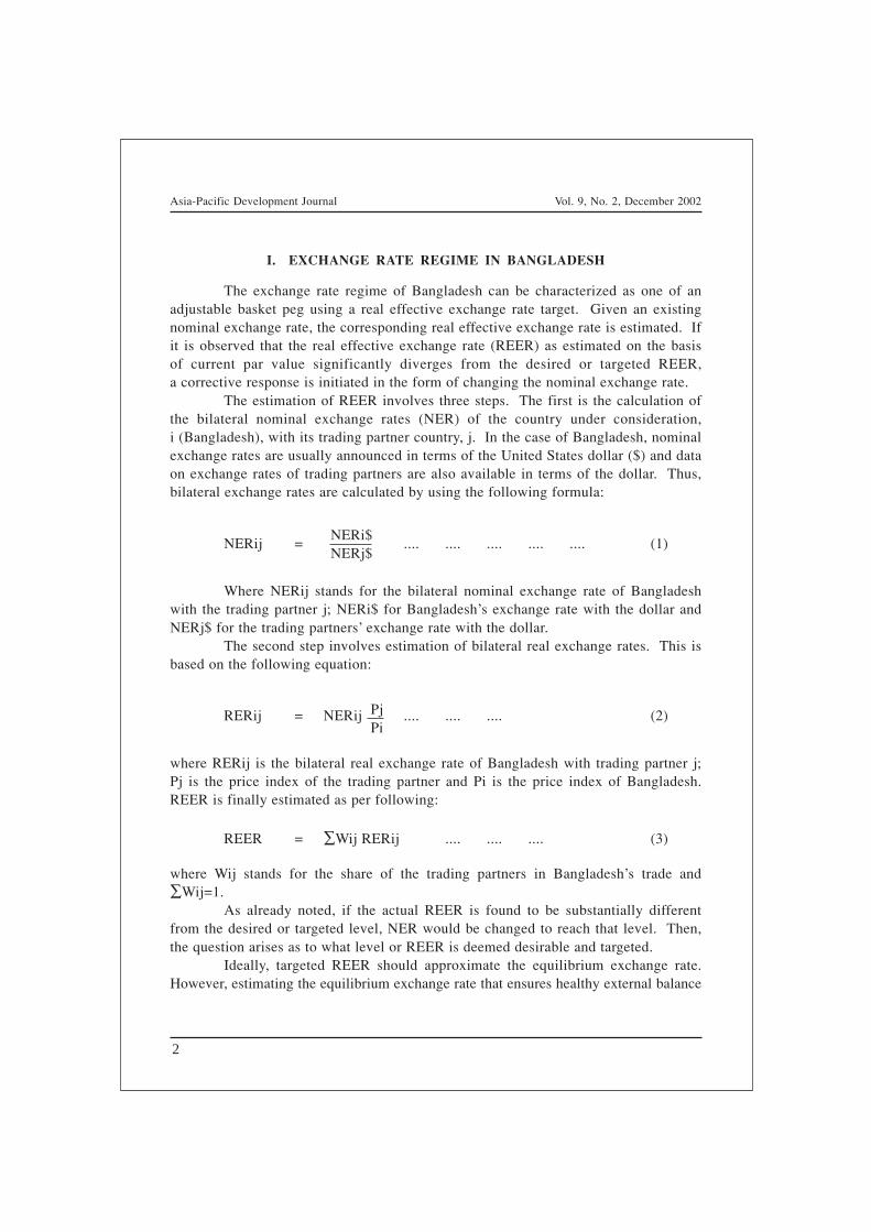
The estimation of REER involves three steps. The first is the calculation ofthe bilateral nominal exchange rates (NER) of the country under consideration,i (Bangladesh), with its trading partner country, j. In the case of Bangladesh, nominalexchange rates are usually announced in terms of the United States dollar ($) and dataon exchange rates of trading partners are also available in terms of the dollar. Thus,bilateral exchange rates are calculated by using the following formula:
NERij = .... .... .... .... .... (1)
Where NERij stands for the bilateral nominal exchange rate of Bangladeshwith the trading partner j; NERi$ for Bangladesh’s exchange rate with the dollar andNERj$ for the trading partners’ exchange rate with the dollar.
The second step involves estimation of bilateral real exchange rates. This isbased on the following equation:
RERij = NERij .... .... .... (2)
where RERij is the bilateral real exchange rate of Bangladesh with trading partner j;Pj is the price index of the trading partner and Pi is the price index of Bangladesh.REER is finally estimated as per following:
REER = ∑Wij RERij .... .... .... (3)
where Wij stands for the share of the trading partners in Bangladesh’s trade and∑Wij=1.
As already noted, if the actual REER is found to be substantially differentfrom the desired or targeted level, NER would be changed to reach that level. Then,the question arises as to what level or REER is deemed desirable and targeted.
Ideally, targeted REER should approximate the equilibrium exchange rate.However, estimating the equilibrium exchange rate that ensures healthy external balance
PjPi
NERi$NERj$
Asia-Pacific Development Journal Vol. 9, No. 2, December 2002
3
as well as desirable levels of domestic economic aggregates is a complex and arduoustask. This cannot be routinely done. It is learnt that the authorities in Bangladeshmonitor the movements of the REER compared to some base year and also qualitativelytake into account several other domestic and external sector variables in determiningthe targeted REER. The external variables include the level of international reserves,current account gap, trends of exchange rate changes in the local interbank foreignexchange market and trends in the exchange rates of major neighbouring trade partners(India and Pakistan). Domestic variables include the domestic inflation rate, creditgrowth in the private and public sector, and the growth of broad money and liquidity.
The exchange rate policy decisions, though notified in all cases by theBangladesh Bank, are made on behalf of and in close consultation with the Ministryof Finance. Bangladesh Bank does not have independent stewardship of exchangerate policy.
The Bangladesh Bank supports the current parity of the taka througha continuous presence in the market in the form of announced readiness to undertakeUnited States dollar purchases and sales at rates decided by itself within the declaredrate band (currently of one taka width) any time an authorized dealer approaches.Any adjustment in the parity is implemented through the announcement by theBangladesh Bank of a revised band for buying and selling rates following which thedealers adjust their rates for transactions with their customers and among themselves.Upto 24 May 2001, Bangladesh Bank used to announce specified buying and sellingrates. From 3 December 2000 Bangladesh Bank adopted the practice of declaringa 50 poisha band within which buying and selling transactions will be undertaken;this band was widened to taka 1.00 from 25 May 2001.
Prima facie, Bangladesh pursues an active exchange rate policy. This activismis reflected in the frequency of nominal exchange rate changes announced by thecentral bank. From 1983 onwards, there have been as many as 89 adjustments in theexchange rate of which 83 were downwards and only six were upward. However, thebehaviour of economic agents is influenced by the impact of policy changes on thereal variables that affect them. In the present context, the relevant variable is the realeffective exchange rate. Table 1 shows the relationship between the nominal exchangerate and the real effective exchange rate during the past twelve years
Data in table 1 suggest that up until 1998, the authorities were basicallypursuing a policy of stable REER. Thus between 1991 and 1998, REER depreciatedby a mere 5 per cent. The subsequent years were marked by stronger depreciations.The mild appreciation of REER in 1998 could be one factor that encouraged policymakers to be more active in the exchange rate policy arena. Another factor could bethat some of the competitor neighbouring countries were apparently depreciating faster.

Asia-Pacific Development Journal Vol. 9, No. 2, December 2002
4
II. CHARACTERISTICS SUITABLE FOR ALTERNATIVE REGIMES
It should be stressed at the outset that the task of identifying economiccharacteristics that dictate the choice of one regime or the other is enormously difficult.The difficulty arises due to several reasons. Much of the literature identifies thesecharacteristics from the standpoint of two polar policy regimes. One of these can bebranded as a regime of “hard peg” in which the value of the local currency isirrevocably fixed in terms of one or more foreign currencies. On the other extremelies the regime of “free float” under which the exchange rate is allowed to fluctuatefreely in response to the market forces of demand for and supply of foreign exchange.The actual practice of either of these regimes is rare. There is a host of other regimeswhich lie in between, variously labelled as “managed float”, “independent float”,“peg with sliding or crawling band”, “flexible peg” etc.
The second difficulty arises from the fact that no single exchange rate regimeis appropriate for all countries in view of differences in levels of economic and financialdevelopment and other aspects of their economic situation. Moreover, the regime thatis appropriate for a particular country may change over time (Mussa and others, 2000).
The third difficulty is that the sustainability of a regime is also conditionedby the capacity of a country to formulate and effectively implement other economicpolicies which can reinforce the beneficial impact of a particular regime and neutralizethe negative consequences. In particular, the credibility and the flexibility of monetaryand fiscal policies are of crucial importance.
Notwithstanding the above difficulties, it is worthwhile to examine theeconomic characteristics that point to the appropriateness of a particular regime asbenchmarks. These can be useful indicators for the choice of a regime in Bangladesh.
Table 1. Indices of NER and REER (1991 = 100)
Year NER NER index REER index
1991 36.60 100.0 100.01992 38.95 106.6 100.21993 39.57 108.1 104.61994 40.21 109.9 102.21995 40.28 110.1 102.91996 41.79 114.2 103.81997 43.89 119.9 105.51998 46.91 128.2 105.41999 48.00 131.4 112.82000 52.00 142.1 116.2
Source: Based on unpublished data from Bangladesh Bank.

Asia-Pacific Development Journal Vol. 9, No. 2, December 2002
5
There is a vast literature on the choice of exchange rate regime.1 Theconditions that generally point to the appropriateness of some form of pegged exchangerate regime are briefly discussed below.
• The degree of involvement with international capital markets is low.This condition ensures that the exchange rate will not be subject tolarge fluctuations in response to volatile inflows and outflows ofshort-term capital. Bangladesh clearly satisfies this criterion witha wide range of controls on capital and money market instruments,credit operations of the commercial banks, and transactions relatedto foreign direct investment and real estate.
• The share of trade with the country/countries to which its currency ispegged is high. As has been explained in the preceding section, thiscondition is fully met in Bangladesh as it follows the policy ofa trade-weighted basket peg.
• The shocks it faces are similar to those facing the country/countriesto which it is pegged. With stringent capital controls in place, theexternal shocks to the Bangladesh economy are transmitted primarilythrough the trade channel. In light of the point made above, thiscondition also holds for Bangladesh.
• Exchange rate based stabilization is considered attractive for thecountry. Given that there are lots of endogenous pressures frompolitical and economic interest groups in Bangladesh to be lax in theconduct of monetary and fiscal policies, maintenance of some sort ofa pegged exchange rate which forces monetary and fiscal disciplineappears to be a desirable nominal anchor for Bangladesh.
• The country is wiling to give up its monetary policy independenceand largely follow the monetary policy of the partner country. Thiscondition is specially relevant for countries which pursue a policy ofhard peg vis a vis a single currency. Since Bangladesh followsa policy of basket peg and the peg itself is adjustable, Bangladeshdoes not have to sacrifice its monetary policy independence entirelyand blindly imitate another country’s monetary policy stance.
• The country has high international reserves. This is an importantrequirement for a pegged exchange rate regime that Bangladesh doesnot adequately meet. However, the rationale for high internationalreserves under a pegged exchange rate regime arises from the factthat should the exchange rate come under pressure the authorities
1 See, for example, Mussa and others (2000); Velasco (2000) and the references cited in note 18 of thepublication by Mussa and others (2000).

Asia-Pacific Development Journal Vol. 9, No. 2, December 2002
6
must have adequate foreign exchange to intervene effectively in themarket to maintain the pegged rate. This condition does not appearto be an indomitable constraint for the present exchange rate policyin Bangladesh as the authorities can exercise two options, in additionto domestic policy instruments, to ease off pressure in the foreignexchange market. First, the exchange control regime can be tightenedsubject to obligations under Article VIII of the IMF Articles ofAgreement. Second, the peg itself can be adjusted, as has been donemany times over the years
The above discussion already suggests that some sort of a pegged exchangerate regime may be the preferred option for Bangladesh. At this point it is worthwhileto examine how does Bangladesh figure in terms of the economic or institutionalrequirements of a floating exchange rate regime.
The literature on the subject clearly highlights the need for a crediblealternative nominal anchor for the conduct of monetary as well as fiscal policies asthe exchange rate fails to provide such an anchor under the floating regime. Thealternative anchor that is most often suggested is inflation targeting. Under the inflationtargeting system, a country is committed to keep inflation within a predeterminedtarget rate. Monetary and fiscal policies have to be tuned to ensure that the target isnot violated. This in turn requires an independent central bank which can refuseaccommodation to the Government if it is apprehended that the latter’s fiscal stance islikely to cause inflation beyond the targeted rate. Furthermore, the central bankshould have the independence to conduct monetary policy in such a manner thatconstrains the Government from financing its deficit through the commercial banksand other ways which may have inflationary consequences. Apart from the requirementof legal independence, the central bank also needs to be staffed by highly competentprofessionals who can predetermine an appropriate target rate of inflation, monitorthe actual behaviour of inflation and implement systematic adjustments in monetarypolicy instruments to ensure that the target is realized in practice. No one wouldseriously doubt that these institutional imperatives for the success of inflation targetingare unlikely to be met in the near future in Bangladesh. Another major problem thatBangladesh is likely to face in this area is that, to a large extent, inflation is mostlikely caused in Bangladesh by supply shocks. In particular, the natural calamitieshave an important bearing on food prices, a major component of inflation inBangladesh. This complicates the task of predicting the behaviour of inflation andalso of controlling it through monetary policy instruments.
Another requirement for a floating exchange rate regime is that the countryshould have a deep and competitive foreign exchange market. If the market is thinand controlled by a small number of operators, free float will inevitably lead toa large degree of volatility. This is likely to inhibit trade as well as investment
Asia-Pacific Development Journal Vol. 9, No. 2, December 2002
7
(both local and foreign) due to greater exposure of economic agents to exchange raterisks. In principle, it can be argued that such risk can be hedged. In practice, thispossibility would be of limited relevance for Bangladesh, given the facts that (a) theforeign exchange market of the country is pretty thin even for spot transactions and(b) no organized markets for currency futures and options exist. In the circumstancesof Bangladesh where non-residents are unwilling to hold local currency exposure,there will be no net capacity to shift foreign exchange risks abroad at a reasonableprice. Therefore, any hedging under a floating exchange rate would basically involveshifting of exchange rate risks of one domestic economic agent to another domesticagent.
A well-regulated, well-supervised and financially sound banking system isalso a crucial requirement for a floating exchange rate regime, particularly so if oneof the objectives behind the adoption of a floating exchange rate regime is tosubstantially open up the capital account. With the opening of the capital account,banks play a critical role in intermediating short-term capital flows. If the inflows arenot invested appropriately, the exchange rate may come under indefensible speculativeattack with disastrous consequences for the economy, as was the case with theEast and South-East Asian economies in 1997. Appropriate investment of short-termexternal capital inflows has to satisfy at least two conditions. First, maturity mismatchhas to be prevented. This means the time profile of the income stream generated byinvestment has to broadly correspond to that of the repayment obligations. Second,currency mismatch has to be avoided. There arises a currency mismatch if most ofthe income from investment is generated in local currency with repayment obligationsinevitably denominated in foreign currency. One need not belabour the point that thebanking system of Bangladesh would be simply incapable of meeting the stringentrequirements of an open capital account.
Finally, the requirement of high international reserves under the peggedexchange rate regime is of no less relevance to the floating exchange rate regimeeither. The reason is that the authorities cannot remain as idle onlookers when theexchange rates fluctuate wildly. The experience of developing countries worldwide(in some cases even developed countries) shows that authorities cannot avoidintervening in foreign exchange markets under floating regimes in order to maintaina reasonable degree of stability in the exchange rate. The need for intervention maybe even stronger for Bangladesh with its thin foreign exchange market which typicallyimplies greater fluctuations. This is precisely the reason why the Finance Ministerhas pronounced many times that he would consider the adoption of floating exchangerate only after the country acquires a high level of reserves.
The upshot of the above arguments is that the ex-ante requirements for theadoption of a floating exchange rate regime are not satisfied in Bangladesh. Thus, thejustification for a change in the present exchange rate regime is by no means obvious.

Asia-Pacific Development Journal Vol. 9, No. 2, December 2002
8
III. EXPERIENCES OF OTHER COUNTRIES
The experiences of some countries in the region which implemented majorchanges in their exchange rate regimes in recent years can provide useful lessons forBangladesh. This section begins with a brief review of the experience of the fiveEast/South-East Asian Countries (Indonesia, Malaysia, Philippines, Republic of Koreaand Thailand) all of which adopted independently floating exchange rate regimesfollowing the Asian crisis in the second half of 1997 with the exception of Malaysiawhich resorted to a fixed exchange rate policy2.
The review here is concerned primarily with the comparison of exchange ratevolatility before and after the crisis. It is well known that, before the crisis, thesecountries were basically pursuing pegged exchange rate policies though their regimes(with the exception of Thailand which officially had a pegged rate) were officiallybranded as managed floats. The post-crisis period is defined as the 24 month periodbeginning January 1999 and the pre-crisis period is defined as 24-month period endingin June 1997. Thus the period of extreme instability resulting from the crisis is leftout of account. The magnitudes of exchange rate variations are captured in thefollowing table.
Table 2 makes it abundantly clear that all the countries experienced muchgreater volatility in their exchange rates as they switched to floating regimes. Andthis happened despite the fact that they did not refrain from intervening in the foreignexchange market as well as using domestic policies to stabilize the exchange rates.
2 This review draws heavily from Hernandedez and Montiel (2001).
Table 2. Monthly exchange rate percentage changes
Country Period Range Standard deviation
Indonesia Pre-crisis .033 .007Post-crisis .230 .063
Malaysia Pre-crisis .027 .007Post-crisis .000 .000
Republic of Korea Pre-crisis .043 .011Post-crisis .066 .017
Philippines Pre-crisis .012 .003Post-crisis .068 .017
Thailand Pre-crisis .016 .004Post-crisis .070 .018
Source: Hernandez and Montiel, 2001.

Asia-Pacific Development Journal Vol. 9, No. 2, December 2002
9
Greater volatility and sharper depreciation have also been the experience ofSouth Asian countries which adopted some sort of floating exchange rate regimes inrecent years. India adopted a unified exchange rate system in March 1993 in whichthe exchange rate is determined by the supply and demand condition in the interbankforeign exchange market. The country’s exchange rate remained fairly stable tillAugust 1995, but then there was a sharp depreciation against the dollar by 12 per centby the end of 1995. There was again a sharp depreciation by about 15 per centbetween September 1997 and July 1998. By November 2001, there was a furtherdepreciation by about 13 per cent and the rupee/dollar exchange rate was 48.0.
The adoption of a floating/flexible regime has not freed the Reserve Bank ofIndia (RBI), the central bank of India, from intervening in the foreign exchange market.In fact, taking note of the fact that the thinness of the foreign exchange market aswell as some large transactions can cause excessive volatility, RBI pursues an explicitpolicy of intervention in the spot market and also undertakes both forward and swaptransactions in support of its exchange rate objectives.
Pakistan can be considered to have adopted a sort of floating exchange ratepolicy since July 2000 when the exchange rate band was abandoned. BetweenNovember 2000 and 2001, the exchange rate depreciated from Rs 57.5 to Rs 60.9 perUS dollar. Exchange rate volatility was relatively high between mid-1998 until October1999 when the fixed peg was adopted for a brief period. With the adoption of thefloating system, volatility increased again to pre-peg level.
The State Bank of Pakistan also intervenes in the foreign exchange market.The interventions take the form of outright sales/purchases of foreign exchange, swaptransactions and provision of foreign exchange to banks to cover certain bulky imports.
Sri Lanka adopted a free float on 23 January 2001. Immediately after thefloat, there arose considerable volatility. The currency fell drastically in two daysfollowing the float to as low as Rs 98/$ compared to Rs 79/$ in November 2000.This forced the authorities to intervene in support of the currency and introducestringent control measures so as to restore the currency to Rs 87/$ by about March2001. By November 2001, the rupee had depreciated to Rs 93/$.
The volatility and the sharp depreciation in Sri Lanka occurred inspite ofputting in place precautionary foreign exchange regulations in conjunction with thefloat. Those regulations, inter alia, imposed limits on banks’ daily net foreign exchangeexposure; enjoined banks to ensure settlement of export credit by using export proceedswithin 90 days (later extended to 120 days) and to impose penalties for overduesettlements; introduced restrictions and deposit requirements for banks’ forward salesof foreign exchange and prohibited prepayment of import bills. The country also hasa set of detailed guidelines for dealing in the foreign exchange market and for conductof intervention by the central bank.
Asia-Pacific Development Journal Vol. 9, No. 2, December 2002
10
IV. HAS THE EXCHANGE RATE REGIME OF BANGLADESHPERFORMED POORLY?
This section examines the performance of Bangladesh in terms of certain keyobjectives that an exchange rate regime is expected to promote. The relevant objectivesare: (a) the prevention of any major misalignment of exchange rate and, in particular,the prevention of appreciation of the real effective exchange rate which can hurtexports; (b) the promotion of exports and containment of the current account deficit;(c) moderation of inflation; and (d) enhancement of remittances – a matter of specialconcern for Bangladesh, given that the remittances financed a significant portion ofthe country’s trade deficit throughout the 1990s (Islam, 2002).
(a) Misalignment of exchange rate
The prevention of misalignment implies that the actual exchange rate shouldcorrespond to the estimate of the equilibrium exchange rate. It is not easy to eitherdefine the equilibrium exchange rate or to estimate it. That would be a complexexercise in itself and is beyond the scope of the present paper. However, a recentstudy has undertaken such an exercise for Bangladesh (ADB, 2002a). The studyconcludes that the misalignment between the actual and equilibrium exchange rate forthe period 1997 to 2001 has been small and has progressively narrowed since 1998.During 2001, the misalignment was only 2.2 per cent.
It will also be recalled from table 1 that the exchange rate policy certainlysucceeded in preventing appreciation of the real effective exchange rate throughoutthe 1990s. In fact there has been more or less consistent depreciation of REER, theindex rising to 116.2 in the year 2000 with 1991 as the base year. There was only oneyear, 1994, in which there was any noticeable appreciation and in that year the indexfell to 102.2 compared to 104.6 in the preceding year.
It can thus be concluded that the exchange rate regime has avoided anymajor misalignment in the exchange rate.
(b) Exports and current account balance
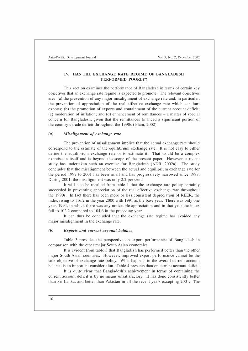
Table 3 provides the perspective on export performance of Bangladesh incomparison with the other major South Asian economics.
It is evident from table 3 that Bangladesh has performed better than the othermajor South Asian countries. However, improved export performance cannot be thesole objective of exchange rate policy. What happens to the overall current accountbalance is an important consideration. Table 4 presents data on current account deficit.
It is quite clear that Bangladesh’s achievement in terms of containing thecurrent account deficit is by no means unsatisfactory. It has done consistently betterthan Sri Lanka, and better than Pakistan in all the recent years excepting 2001. The
Asia-Pacific Development Journal Vol. 9, No. 2, December 2002
11
only country with which Bangladesh compares somewhat unfavourably is India, butthat should not come as a surprise even to a casual observer in view of India’s highsavings rate and level of industrialization.
(c) Inflation
Experience shows that countries have developed with different degrees ofinflation. Nevertheless, a consensus has emerged that high and unstable inflationrates are not conducive to development. High inflation reduces returns to savers andthus acts as a disincentive to save and invest. In particular, saving in financial formis likely to be discouraged. This complicates the task of mobilizing savings forproductive investment. The viability of financial and capital market institutions whichact as crucial intermediaries between savers and investors is impaired. High inflationis also likely to distort the pattern of investment in favour of real estate, gold or otherforms of property as hedging devices without adding much to an economy’s productivecapacity. The international competitiveness of the economy is badly eroded by inflation.It generally encourages capital flight, exacerbates income distribution, gives rise toinequities in income distribution and aggravates poverty. Last but not the least,a high rate of inflation seriously undermines the popularity of the government.
Table 3. Average annual growth rate of export of goods and services
CountryPeriod
1990-1999 2000-2001a
Bangladesh 13.2 10.3
India 11.3 9.3
Pakistan 2.7 8.9
Sri Lanka 8.4 3.5
Sources: World Bank (2001) and ADB (2002 b).a Relates to merchandise exports only
Table 4. Current account deficit as percentage of GDP
CountryYears
1997 1998 1999 2000 2001
Bangladesh 2.1 1.1 1.4 1.0 2.1
India 1.3 1.0 1.1 0.6 0.5
Pakistan 6.4 3.2 4.1 1.9 0.9
Sri Lanka 2.6 1.4 3.6 6.5 3.4
Source: ADB (2002 b).
Asia-Pacific Development Journal Vol. 9, No. 2, December 2002
12
The discussion of inflation in the context of the exchange rate regime becomesrelevant because of two major considerations. First, a change in the exchange rate isalmost certain to cause a change in the domestic prices of tradables. Second, theprices of non-tradables are also likely to be affected because the non-tradables oftenuse tradable inputs and the demand switch generated by an initial change in theexchange rate may not elicit a corresponding supply response from the non-tradablesector to leave prices unchanged.
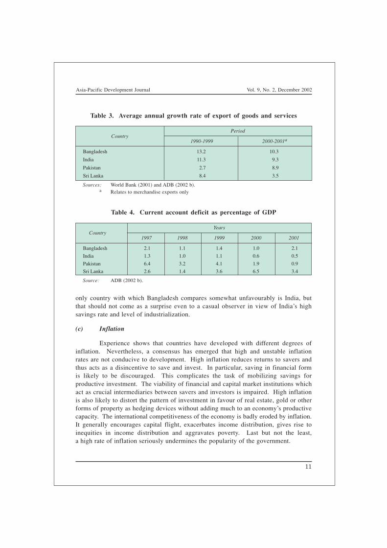
In the backdrop of the above arguments, it is useful to look at the performanceof Bangladesh in respect of inflation. The relevant data are presented in table 5.
Table 5. Inflation in Bangladesh and selected South Asian countries
CountryYears
1996 1997 1998 1999 2000 2001
Bangladesh 6.6 2.5 7.0 8.9 3.4 1.6
India 4.6 4.4 5.9 3.3 7.2 4.7
Pakistan 10.4 11.3 7.8 5.7 3.6 4.4
Sri Lanka 14.6 7.1 6.9 5.9 1.2 11.0
South Asian average 5.8 5.2 6.3 4.2 6.2 4.6
Source: ADB (2002 b).
It is obvious from the data that Bangladesh has done reasonably well interms of the inflation criterion. During the past decade, its inflation rate never reacheddouble-digit level. In every year except 1999, the inflation rate in Bangladesh hasbeen comparable to or lower than the South Asian average.
(d) Remittances
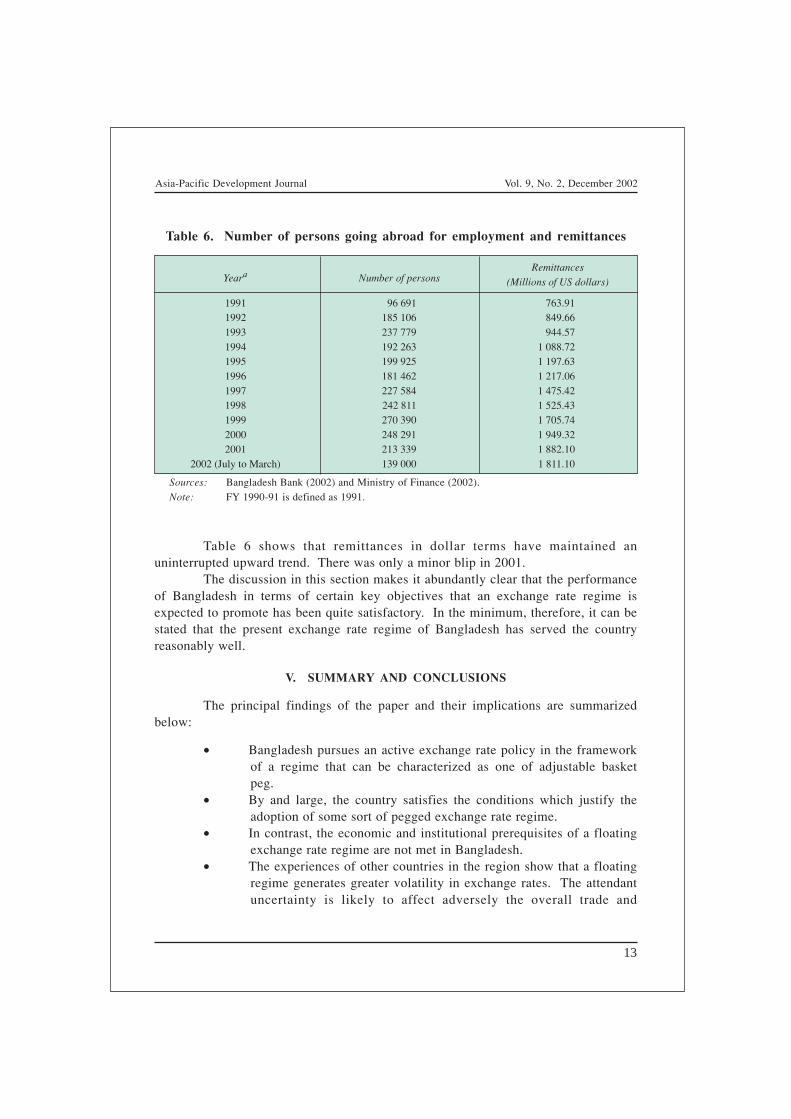
As noted before, remittances by Bangladeshi workers employed abroad playan important role in moderating the country’s trade deficit. The country’s performancein respect of remittances can be gauged from the table below:
Asia-Pacific Development Journal Vol. 9, No. 2, December 2002
13
Table 6 shows that remittances in dollar terms have maintained anuninterrupted upward trend. There was only a minor blip in 2001.
The discussion in this section makes it abundantly clear that the performanceof Bangladesh in terms of certain key objectives that an exchange rate regime isexpected to promote has been quite satisfactory. In the minimum, therefore, it can bestated that the present exchange rate regime of Bangladesh has served the countryreasonably well.
V. SUMMARY AND CONCLUSIONS
The principal findings of the paper and their implications are summarizedbelow:
• Bangladesh pursues an active exchange rate policy in the frameworkof a regime that can be characterized as one of adjustable basketpeg.
• By and large, the country satisfies the conditions which justify theadoption of some sort of pegged exchange rate regime.
• In contrast, the economic and institutional prerequisites of a floatingexchange rate regime are not met in Bangladesh.
• The experiences of other countries in the region show that a floatingregime generates greater volatility in exchange rates. The attendantuncertainty is likely to affect adversely the overall trade and
Table 6. Number of persons going abroad for employment and remittances
Yeara Number of personsRemittances
(Millions of US dollars)
1991 96 691 763.911992 185 106 849.661993 237 779 944.571994 192 263 1 088.721995 199 925 1 197.631996 181 462 1 217.061997 227 584 1 475.421998 242 811 1 525.431999 270 390 1 705.742000 248 291 1 949.322001 213 339 1 882.10
2002 (July to March) 139 000 1 811.10
Sources: Bangladesh Bank (2002) and Ministry of Finance (2002).Note: FY 1990-91 is defined as 1991.

Asia-Pacific Development Journal Vol. 9, No. 2, December 2002
14
investment climate which is already afflicted by many unfavourableelements in Bangladesh.
• The experiences of other countries also show that a floating regimedoes not eliminate the need for intervention in the foreign exchangemarket. Given the thinness of the market in Bangladesh, the needfor intervention may be even greater in Bangladesh as the authoritiescannot remain silent spectators when the exchange rate gyrates wildly.
• The present exchange rate regime in Bangladesh has served thecountry quite well. No major misalignment of the equilibriumexchange rate has occurred and the real effective exchange rate hasnot been allowed to appreciate. There has been satisfactoryperformance in terms of certain key macroeconomic indicators suchas export growth, current account deficit, inflation and remittancesby non-resident Bangladeshis.
Finally, it is instructive to bring to the attention of the readers the conclusionsof a recent study by IMF economists (Mussa and others, 2000). According to thisstudy, it can be safely stated that many developing and transition economies, especiallythose lacking a well-developed financial infrastructure including sophisticated financialinstitutions and broad and deep markets for foreign exchange (Bangladesh certainlybelongs to this category), do not satisfy the requirements for a successful float.
In a different context, another IMF study specifically devoted to Bangladeshstated: “Given such pros and cons, the choice of exchange rate regime is notclear-cut. What matters is a set of sound economic policies that remain consistentwith any chosen exchange rate regime” (Hossain, 2002, p. 23).
At a strictly philosophical level, one can argue that the exchange rate isa price and like any other price, it should be fully flexible. But to compare the priceof foreign exchange which affects virtually all sectors of the economy with, let us say,the price of a pair of socks is both an intellectual absurdity and a practical folly.
Asia-Pacific Development Journal Vol. 9, No. 2, December 2002
15
REFERENCES
Asian Development Bank, 2002a. Quarterly Economic Update, (Dhaka, Bangladesh Resident Office),March.
, 2002b. Asian Development Outlook 2002 (Hong Kong, Oxford University Press).
Bangladesh Bank, 2002. Economic Trends (Dhaka, Statistics Department of Bangladesh Bank), January.
Hern’andez, Leonardo and Peter Montiel, 2001. Post Crisis Exchange Rate Policy in Five Asian Countries:Filling in the “Hollow Middle”? (Washington, D.C., IMF, Working Paper No. WP/01/170).
Hossain, Akhtar, 2002. Exchange Rate Responses to Inflation in Bangladesh (Washington, D.C., IMF,Working Paper No. WP/02/XX).
Islam, Azizul, 2002. “The impact of exchange rate changes on selected economic indictors of Bangladesh”,mimeo.
Ministry of Finance, 2002. Bangladesh Economic Survey, 2002 (Dhaka, Government of Bangladesh).
Mussa, Michael and others, 2000. Exchange Rate Regimes in an Increasingly Integrated World Economy(Washington, D.C., IMF, Occasional Paper No. 193).
Velasco, Andre, 2000. Exchange Rate Policies for Developing Countries: What Have We Learned? WhatDo We Still Not Know? (New York and Geneva, United Nations Conference on Trade andDevelopment).
World Bank, 2001. World Development Report 2000/2001 (Washington, D.C., Oxford University Press).

Asia-Pacific Development Journal Vol. 9, No. 2, December 2002
17
LEADING INDICATORS FOR MONITORING THE STABILITY OFASSET AND FINANCIAL MARKETS
IN ASIA AND THE PACIFIC
Biswanath Bhattacharyay* and G. Nerb**
The Asian economic and financial crisis of 1997 has spawned a considerablebody of analysis as to its origin, causes and resolution. It is generallyrecognized that structural weaknesses of the financial systems of the affectedcountries were at the core of the problem. It follows from this thatmonitoring the stability of financial markets, including asset markets, anddevising early warning systems for problems in these markets would enablethe authorities to deal better with potential crises and to develop moreeffective policy interventions to that end. The Asian Development Bankhas undertaken the development of a system of MPIs macroprudentialindicators (MPIs) to facilitate cross-country comparisons of economic andfinancial vulnerability in the Asian and Pacific region. This paper evaluatesthe significance of the MPIs chosen for this purpose and highlights theneed for a core set of leading indicators for giving early warning offinancial vulnerability.
In 1997, Thailand, Malaysia, Indonesia, the Philippines and the Republic ofKorea reeled from a devastating financial crisis. Following years of robust growth,positive strides in standards of living and export expansion, these economies sufferedfrom crippling devaluations, massive capital flight, corporate and banking failuresand spikes in unemployment. In contrast with the substantial capital inflows in theearly 1990s, close to US$100 billion of capital flew out of the region shortly after theThai baht peg collapsed.
The Asian crisis has spawned a massive literature on the economics of thecrisis that advance numerous hypotheses on the origin, development and resolution ofcrises. Although it is acknowledged that the financial crisis in Asia was multifaceted
* Senior Planning and Policy Officer, Strategy and Policy Department, Asian Development Bank, Manila.** Director, Business Survey Department, IFO Institute for Economic Research, Munich, Germany.
The views expressed in the paper are those of the authors and do not necessarily reflect those ofAsian Development Bank or IFO Institute for Economic Research.

Asia-Pacific Development Journal Vol. 9, No. 2, December 2002
18
and that no single cause can explain the entire phenomena, it is generally recognizedthat structural weaknesses of the financial system were at the core of the problem.
More specifically, at the heart of the currency turmoil and banking crises isthe speculative pressure that economic agents bring to bear on vulnerable financialand economic systems, and the shortcomings of policy responses on the part of nationalauthorities and the international financial institutions alike. In such situations, therole of timely and accurate information is paramount in informing policy officials ofthe probability and potential severity of crises, the specifics of an individual crisisand the policy interventions required. Hence, the immediate aftermath of the crisissaw renewed calls for monitoring the stability of asset and financial markets, earlywarning, international cooperation in policy consultations, coordination, etc. It is inthe context of the need to monitor the strength and vulnerability of financial marketswhere the development of macroprudential indicators (MPI) or financial soundnessindicators acquires greater relevance. MPIs are defined broadly as indicators of thehealth and stability of financial systems.
Because the MPIs are indicators that measure certain attributes of the financialsector (e.g. measures of incidence of non-performing loans), they are appropriatetools for monitoring the stability or vulnerability of the financial system. Inasmuchas the soundness of the financial sector depends critically upon prevailingmacroeconomic conditions (Sundarajan, Marston and Basu 1999), MPIs also includemacroeconomic variables in addition to indicators specific to the financial sector.A number of MPIs are also used in models of early warning (Kaminsky, Lizondo andReinhardt 1998). There is value in developing a common set of indicators to permitcross-country comparisons of experiences and to evaluate regional effects.
The Asian Development Bank (ADB), through a technical assistance project,undertook the development of a system of commonly agreed MPIs for selecteddeveloping member countries or areas, namely Fiji, Indonesia, the Philippines, Thailand,Viet Nam and Taiwan Province of China. This paper aims to evaluate a set ofcommonly agreed ADB MPIs and identify or select a core set of leading indicatorsthat could give early warning signals of vulnerability of financial markets, and supportregular economic and financial monitoring.
I. ASIAN DEVELOPMENT BANK MPIs
The process of identifying and collecting the MPIs is a necessary preconditionfor a comprehensive process of monitoring and responding to financial sector risks.Interpretation and analysis of these indicators is also a major challenge. The MPIsare used in macroprudential analysis, which is a tool that helps to quantify and qualifythe soundness and vulnerabilities of financial systems. Macroprudential analysis canalso be understood as the analytical framework for interpreting the MPIs or theindicators of financial soundness or stability. Clearly, the choice of the MPIs will

Asia-Pacific Development Journal Vol. 9, No. 2, December 2002
19
depend on the level of sophistication of the macroprudential analysis to be employed.For instance, the International Monetary Fund (IMF, 2001) collects not only thetraditional macroeconomic indicators but also includes aggregated microprudentialdata (i.e. data at the firm level) and market-based indicators as well. This combinationof MPIs is used by the IMF in conducting stress tests and scenario analysis to determinethe sensitivity of the financial system to macroeconomic shocks. Alternatively, thevulnerability of the financial system can be assessed using simple benchmarks, criticalor regulatory thresholds, or comparisons with peer group or historical norms.
Work on the MPIs and their interpretation is still recent and there is noconsensus on an optimum set of MPIs nor of the best analytic framework to use. Infact, there is as yet no universally accepted definition of financial soundness or stability.Obviously, the degree of complexity of the macroprudential analysis will depend onfactors such as degree of accuracy of assessing vulnerability that is desired, technicalcapacity of the monitoring agency, cost and availability of data and the structure,openness, and sophistication of the financial system. Although there is a limitedamount of empirical work that has identified some possible MPIs, at this early stagein their development the identification and relative importance of the MPIs remainslargely a matter of judgment given the aforementioned factors.
In general, there are a number of desirable characteristics of MPIs. First,from the point of view of crisis prevention, the MPIs should have early warningcapability. Thus, taken from a statistical perspective, desirable MPIs should be leadingindicators or at least coincident indicators. For short-term monitoring use, the idealfrequency of the indicators should be quarterly or monthly. Also, some capital marketindicators can provide continuous monitoring of some aspects of the financial system.
Secondly, the set of MPIs should include a broad variety of indicators sincecurrency and banking crises seem to be usually preceded by multiple economicproblems. For instance, Kaminsky and Reinhardt (1999) identified 15 early warningvariables whereas Goldstein, Kaminsky and Reinhardt (2000) add another nine variablesto the earlier set. According to this research, the variables that have the best trackrecord in anticipating crises include exports, deviations of the real exchange rate fromtrend, the ratio of broad money to gross international reserves, output and equityprices.
Third, qualitative variables should also be considered in the set of MPIs.Traditionally, MPIs in the literature are quantitative variables. However, the importanceof qualitative variables cannot be underestimated, especially when dealing with financialvariables. In emerging markets, where in the light of contagion, speculative pressurecan be very powerful, qualitative measures can be important. Also, in developingmarkets, the qualitative analysis of possibly underdeveloped financial marketinfrastructures and supervisory institutions could provide important information aboutpossible crisis situations. Thus, there is a need to combine quantitative and qualitativeindicators for assessing the health of a financial market. The qualitative indicators or

Asia-Pacific Development Journal Vol. 9, No. 2, December 2002
20
information should include a judgment on the adequacy of the institutional andregulatory framework of countries.
Under the ADB’s technical assistance project, an inception workshop wasconducted in April 2000 and a follow-up a year later. One major objective of the firstworkshop was agreement on the list of indicators which should be included ina harmonized financial and monetary monitoring system. On this basis, eachparticipating country would develop, compile, analyze and disseminate the commonlyagreed key indicators on a regular basis. During the Inception Workshop, theparticipating countries in consultation with representatives from IMF, the Bank forInternational Settlements (BIS), Deutsche Bundesbank, Bank of Japan, Bank of Korea,Australian Bureau of Statistics, ESCAP, and ADB identified a set of commonly agreedMPIs, with the following subsets of indicators (Bhattacharyay, 2001):
a) External Debt and Financial Flows (8 indicators);b) Money and Credit (17 indicators);c) Banking (14 indicators);d) Interest Rates (12 indicators);e) Stock Markets and Bonds (9 indicators);f) Trade, Exchange and International Reserves (10 indicators); andg) Business Survey Data (9 indicators): mainly Manufacturing but also
Construction, Retail and Wholesale Trade and Services.
The system of ADB MPIs can be classified into three categories, namely,(i) aggregated microprudential indicators of the health of individual financialinstitutions; (ii) macroeconomic indicators concerning the health of financial sectors;and (iii) qualitative business tendency survey indicators. The set is unique as itincludes qualitative and leading business tendency survey indicators as key elements.Of course, as will be covered more fully later, these MPIs should have a clear theoreticallink with the vulnerability and soundness of the financial sector.
The agreed set of indicators is comprised of the core set (commonly agreed)and some additional ones (specific to country needs). Table 1 reports the list of the67 commonly agreed indicators.
It was agreed in the workshop that participating countries should for the timebeing adhere to the list of 67 commonly agreed indicators and the set of voluntaryadditional indicators and gain experience in using this information as an analyticaltool before changing the list of indicators. Countries could compile and analyse anyadditionally agreed indicators for meeting country-specific requirements dependingon data availability. Table 2 presents the 33 additional indicators that are specific tocountry needs.

Asia-Pacific Development Journal Vol. 9, No. 2, December 2002
21
Table 1. ADB commonly agreed macroprudential indicators
External Debt and Financial Flows
1. Total Debt (per cent of GDP) – ratio of total debt to nominal GDP.
a. ...of which public debtb. ...of which private debt
2. Long Term Debt (per cent of total debt) – ratio of long term debt to total debt.
3. Short Term Debt (per cent of GDP) – ratio of short-term debt to nominal GDP.
4. Short Term Debt (per cent of total debt) – ratio of short-term debt to total debt.
5. Foreign Direct Investment (per cent of GDP) – ratio of foreign direct (expressed as flows)investment to nominal GDP.
6. Portfolio Investment (per cent of GDP) – ratio of portfolio investment (expressed as flows) tonominal GDP
Money and Credit
7. M1 Growth (per cent) – per cent difference from previous period. M1 are liabilities of themonetary system consisting of currency and demand deposits.
8. M2 Growth (per cent) – per cent difference from previous period. M2 equals M1 plusquasi-money.
9. Money Multiplier (ratio) – ratio of M2 to money base. Money base is the sum of currency incirculation, reserve requirement and excess reserves (with the central bank).
10. M2 (per cent of International Reserves) – ratio of M2 to international reserves.
11. M2 (per cent of GDP) – ratio of M2 to nominal GDP.
12. M2 to international reserves growth – the growth rate of M2 over international reserves.
13. Quasi money (per cent of GDP) – ratio of quasi money to nominal GDP.
14. Money Base Growth (per cent) – per cent difference from previous period.
15. Central Bank Credit to the Banking System – Central Bank’s credit to the banking system.
16. Growth of Domestic Credit (per cent) – per cent difference from previous period. Consists of netclaims from central government, claims on official entities and state enterprises, and claims ofprivate enterprises and individuals.
17. Domestic Credit (per cent of GDP) – ratio of domestic credit to nominal GDP.
18. Credit to Public Sector (per cent of GDP) – ratio of credit to public sector to nominal GDP.
19. Credit to Private Sector (per cent of GDP) – ratio of credit to private sector to nominal GDP.
20. Capital Adequacy Ratio (per cent) – ratio of total capital to risk weighted assets (threshold value is8 per cent meaning that the ratio should not be less than this value). Ratio of Tier 1 + Tier 2 capitalto risk weighted assets. Tier 1 capital includes issued and paid-up share capital, non-cumulativepreferred stock and disclosed reserves from post-tax retained earnings. Tier 2 capital can includea range of other entities. These are undisclosed reserves that passed through profit and lossaccount, conservatively valued revaluation reserves, revaluation of equities held at historical cost(at a discount), some hybrid instruments, general loan loss reserves (up to 1.25 per cent of riskweighted assets) and subordinated term debt.

Asia-Pacific Development Journal Vol. 9, No. 2, December 2002
22
21. Liquidity Ratio (per cent) – ratio of commercial banks’ liquid assets to total assets: a) domesticliquid asset ratio and b) foreign liquid asset ratio.
Banking
22. Bank Capital (per cent of Total Assets) – ratio of capital equity including reserves, profits and lossto total assets.
23. Total Assets (per cent of GDP) – ratio of total assets (as in Monetary Survey without interbankpositions) to nominal GDP.
24. Growth of Total Assets (per cent) – per cent growth from previous period.
25. Share of 3 Largest Banks (per cent of total assets)
26. Net Operating Profits (per cent of period-average assets)
27. Loan-Loss Provisions (per cent of Non-Performing Loans) – ratio of loan loss provision tonon-performing loans
28. Non-Performing Loans (per cent of total loans) – ratio of non-performing loans
29. Loans to Key Economic Sectors and (per cent of total loans)
30. Real Estate Loans (per cent of total loans) – ratio of real estate loans to total loans.
31. Total Loans (per cent of total deposits) – ratio of total loans to total deposits (i.e., demand deposits,savings deposits and time deposits.)
32. International Liabilities from Banks with Maturities, Total (US$ million) – total internationalliabilities from commercial banks.
a. short term borrowingb. long term borrowing – more than one year
33. International Liabilities with Maturities, one year and less (US$ million) – total internationalliabilities from commercial banks.
Interest Rates (mean rate)(In case of monthly data, average of daily rates; in case of quarterly data, monthly averages are tobe applied)
34. Central Bank Lending Rate (e.o.p.) – end of period; rate at which the monetary authorities lend ordiscount eligible paper for deposit money banks.
35. Commercial Bank Lending Rate (a.o.p.)/Prime Rate – average of period; ratio of commercial banklending rate to prime rate. Prime rate refers to the short and medium term financing needs of theprivate sector.
36. Money Market Rate/Inter-Bank Rate (a.o.p.) – average of period; rate at which short-termborrowings are effected between financial institutions.
37. Short-term (3 mos.) Time Deposit Rates – interest rates of savings account held in a financialinstitution for 3 months or with the understanding that the depositor can withdraw only by givinga notice.
38. Long-term (12 mos.) Time Deposit Rates – interest rates of savings account held in a financialinstitution for 12 months or with the understanding that the depositor can withdraw only by givinga notice.
Table 1. (continued)

Asia-Pacific Development Journal Vol. 9, No. 2, December 2002
23
39. US$ (international market)/Domestic Real Deposit Interest Rate – unweighted averages of offeredrates quoted by at least 5 dealers early in the day for 3-month certificates of deposit in thesecondary market.
40. Bond/Treasury Bill Yield (short term) – yield to maturity of government bonds (short-term)
41. Bond/Treasury Bill Yield (long term) – yield to maturity of government bonds (long-term)
Stock Markets and Bonds
42. Foreign Share in Trading (per cent of total volume of trading) – proportion of foreign share intrading to total volume of trading.
43. Share of 10 Top Stocks in Trading (per cent of total volume of trading) – proportion of top10 stocks in trading to total volume of trading.
44. Composite Stock Price Index (in national currency unit) – equity price index of national capital cityand expressed in national currency unit.
45. Composite Stock Price Index Growth – per cent difference from previous period of equity priceindex; end of period and based on national currency unit.
46. Composite Stock Price Index (in US$) – equity price index of national capital city and expressed inUS$.
47. Market Capitalization (per cent of GDP) – ratio of market capitalization to nominal GDP. MarketCapitalization refers to the total market value of stocks or shares.
48. Stock Price Earnings Ratio
Trade, Exchange and International Reserves
49. Export Growth (per cent) – export growth (fob) per cent difference from previous period.
50. Import Growth (per cent) – import growth (cif) per cent difference from previous period.
51. Trade Balance (US$ million) – difference between exports (fob) and imports (cif)
52. Current account deficit/surplus (US$ million)
53. Exchange Rate (average of period) – national currency unit to the US$
54. Exchange Rate (end of period) – national currency unit to the US$
55. Real Effective Exchange Rate – ratio of an index of the period average exchange rate of a currencyto a weighted geometric average of exchange rate for the currencies of selected countries adjustedfor relative movements in national prices of the home country and the selected countries. Refers tothe definition used in the IMF, IFS series.
56. International Reserves (US$ million) – international reserves include total reserves minus gold plusgold national valuation.
57. Growth of International Reserves (per cent) – per cent difference from previous period.
58. International Reserves (per cent of imports) – ratio of international reserves to total imports.
Table 1. (continued)

Asia-Pacific Development Journal Vol. 9, No. 2, December 2002
24
Table 2. List of additional indicators
External Debt and Financial Flows
1. Short Term Debt (per cent of foreign reserves)
2. Use of IMF credit (per cent of GDP) – ratio of IMF credit to nominal GDP
Money and Credit (data from IFS)
3. Growth of Currency in Circulation (per cent)
4. M3 Growth – per cent difference from previous period. M3 equals M2 plus liabilities of otherfinancial institutions.
Banking
5. Non-Performing Loans (per cent of average assets): simple average of assets over the period
6. Loans to Commercial Real Estate Sector (per cent total loans)
7. Loans to Residential Real Estate (per cent total loans)
8. International Liabilities from Banks, with Maturities over 1 year and up to 2 years (US$ million) –total international liabilities from commercial banks.
9. International Liabilities from Banks, with Maturities over 2 years (US$ million) – totalinternational liabilities from commercial banks.
10. International Liabilities from Banks, with Maturities, unallocated (US$ million) – total internationalliabilities from commercial banks.
11. Gini coefficient of market shares of banks in terms of assets.
Interest Rates
12. Real Deposit Rate (3 mos.) (a.o.p.) – average of period; defined as the difference between depositand inflation rate.
Business Survey Data (Manufacturing, Construction, Trade and Services)
59. Assessment of Current Business Situation
60. Expectations on Business Situation in Next Months/Quarters
61. Limits to Business (present situation)
62. Stocks of Finished Products (present situation)
63. Assessment of Order Books
64. Selling Prices (future tendency)
65. Employment (future tendency)
66. Financial Situation (present situation)
67. Access to Credit (present situation)
Table 1. (continued)

Asia-Pacific Development Journal Vol. 9, No. 2, December 2002
25
13. Real Lending Rate (3 mos.) (a.o.p.) – average of period; defined as the difference betweencommercial bank lending and inflation rate.
14. Real Lending Rate – Real Deposit Rate (each 3 mos.) – difference between commercial banklending rate and deposit rate.
15. Real Lending Rate/Real Deposit Rate (each 3 mos.) – ratio of real lending rate to real deposit rate.
Stock Markets and Bonds
16. Gini Coefficient of Market Share of Stocks in Trading – measure of concentration of marketcapitalization (inequality of market share among the stocks traded during the day). This is the ratioof the actual concentration of total value of stocks among traded companies to the maximumconcentration.
Gini Coefficient =
where:
Pi = is the rank of each company in the stock market counting from the top in terms of stockassets or market capitalization
ai = stock asset of ith companyA = total asset or market capitalization of all securitiesN = total number of companies listed
17. Turnover in stocks (as per cent of market capitalization)
18. Turnover in bonds (as per cent market capitalization)
a. Volume of government bonds traded
b. Volume of corporate bonds traded
19. Turnover in mutual funds (as per cent market capitalization)
20. Foreign investment in stock by sector
Business Survey Data (Manufacturing, Construction, Trade and Services)
21. Production/Turnover (present tendency)
22. Production/Turnover (expected tendency)
23. Capacity Utilization (present situation)
24. Credit Demand by Sector (only for survey of financial sector)
Supervisory Surveys
25. Lending and Credit Standards of Financial Institutions
26. Proportion of Institutions Having License Withdrawn
27. Spreads Between Reference Lending rates and Reference Borrowing Rates
Table 2. (continued)
N
Σi=1
Pi aiN + 1N – 1
2N(N – 1)A
–

Asia-Pacific Development Journal Vol. 9, No. 2, December 2002
26
28. Spreads Between Depository Corporations’ Securities and the Rate of Comparable TreasurySecurities
29. Securities Between Depository Corporations’ Subordinated Debt Securities and the Rate forComparable Treasury Securities
30. Distribution of 3-Month Local Currency Interbank Rates for Different Depository Corporations
31. Average Interbank Bid-Ask Spread for 3-Month Local Currency Deposits
32. Average Maturity of Assets
Others
33. Real Estate Price Index and Its Growth Rate
Table 2. (continued)
The concluding workshop was held in May 2001 in Manila. The objectivesof the concluding workshop were to: (i) present and discuss the country compendiumon commonly agreed MPIs as per the conclusions of the inception workshop as wellas provide an analysis of the indicators; (ii) discuss the various approaches andmethodologies used in producing the MPIs and the problems and issues encounteredin generating them; (iii) appraise participants on the appropriate analysis andinterpretation of the indicators and the usefulness of composite indicators for monitoringthe asset and financial markets; and (iv) provide recommendations and share thecountries’ future plans on compiling, analyzing, interpreting, and disseminating MPIsand other activities related to the monitoring of the vulnerability of the asset andfinancial markets. The concluding workshop was attended by 13 participants fromsix countries and areas: Fiji, Indonesia, the Philippines, Taiwan Province of China,Thailand, and Viet Nam. There was one representative from IMF, one from theEuropean Central Bank, eight from ADB (including an ADB consultant from IFOInstitute, Germany), one from the University of Asia and the Pacific, and five observersfrom the Ministry of Finance, Viet Nam, the Ministry of Economy and Finance,Cambodia, the Ministry of Finance and Revenue, Myanmar, and the Bangko Sentralng Pilipinas.
It needs to be appreciated that the task of macroprudential analysis or theframework for identifying and interpreting MPIs is still work-in-progress. Variousinternational financial institutions such as IMF, ADB, as well as private firms are stillin the process of developing or testing different systems. As such, there is no standardsystem for macroprudential analysis at present. Yet, as the experience of the Asiancrisis shows, systematic monitoring of the financial and economic systems is animportant element in crisis prevention strategies. Regional Technical Assistance(RETA) is thus envisioned to provide a catalytic role in developing macroprudential
Asia-Pacific Development Journal Vol. 9, No. 2, December 2002
27
systems in Asian and Pacific developing member countries. This role takes practicalform in the identification, collection and dissemination of an initial set of MPIs.
All the participating countries have already undertaken the necessary steps toimplement the gathering and dissemination of the commonly agreed MPIs. In fact,arrangements have been made for countries to submit to ADB two types of templates– monthly and quarterly – for eventual posting in the ADB website. The templateorganizes the MPIs according to the following categories: (a) external debt andfinancial flows(b) money and credit; (c) banking; (d) interest rates; (e) stock marketand bonds; (f) trade, exchange and international reserves; and (g) business surveydata. In preparing the core set of MPIs, some countries could not include all items inthe recommended list of MPIs for the reason that the availability of data and collectionproblems varied significantly among the participating countries. For instance, someparticipating DMCs, especially those in transition, do not have fully developed stockmarkets. Hence, they could not report stock market-based MPIs. The MPI data arealready available in the ADB statistics website. Most of the participating countriesare submitting quarterly updates of MPIs. The commitment of the participatingcountries to regularly submit to ADB updates of the MPI is important for the systematicdevelopment and refinement of the MPI analysis. In future, other developing membercountries of ADB will be invited to submit their MPIs on a regular basis to the ADBwebsite. Furthermore, there is an urgent need to strengthen the capacity of thosecountries to analyse and interpret these MPIs.
One of the distinguishing features of the ADB MPIs, as proposed in thisRETA, is the inclusion of information gleaned from business tendency/confidencesurveys (BTS). The use of BTS within the framework of MPI is unique in theliterature on MPIs. The main reason for incorporating BTS information as part of theMPIs is due to the ability of BTS to capture current and future profitability trends inthe corporate sector. Precisely because expectations can play an important role in thebusiness cycle, it can have a significant influence on investments, output andemployment. Inasmuch as the health of the financial sector is tied up withdevelopments in the real sector, e.g. the effect of the profitability in the corporatesector on the loan portfolios of banks and the information gathered from the BTS canhave a bearing on the health of the financial system. More importantly, since BTSare by nature forward looking, the information they convey can augment the earlywarning capabilities of the conventional quantitative MPIs.
All participating countries are conducting business surveys or are in the processof introducing them. However, there is scope for further work on incorporating BTSin the MPI framework. Issues such as harmonization of the survey instrument and itsinterpretation are areas for capacity-building. ADB has recently implemented anotherregional technical assistance project (RETA 5938) jointly with OECD to help selectedcountries develop Business Tendency Surveys using the harmonized set of corequestions used by most OECD countries. The countries or areas involved are China;
Asia-Pacific Development Journal Vol. 9, No. 2, December 2002
28
Hong Kong, China; India; Indonesia; Malaysia; the Philippines, the Lao People’sDemocratic Republic: Singapore; Thailand and Viet Nam. Under this RETA, eachcountry conducted a pilot BTS Survey based on the improved and harmonizedquestionnaire, analyzed and interpreted the results and published a report andcompendium on these qualitative statistics.
II. IDENTIFICATION AND EVALUATION OF CORE SETOF LEADING INDICATORS
Following the selection of the commonly agreed indicators, an attempt wasmade to identify a core set of leading indicators that could give early warning signalsof the vulnerability of financial markets, based on graphical analysis of the series ofMPIs compiled by countries.
One of the main objectives of this exercise is to identify indicators whichappear to be particularly promising for financial and economic monitoring and whichtherefore should be included in a core list of harmonized indicators at ADB. Althougha broad and exhaustive set of indicators could potentially give a more completeassessment of the soundness of financial systems, they can be costly to compile andunwieldy to maintain for the purpose of periodic monitoring. Hence, the workshopsrecommended that a separate core set of MPIs of manageable size be kept and updatedregularly. Apart from this core set of indicators, there will be a number of series ofspecial importance in some countries but not in all.
As indicated earlier, one criterion for inclusion in the core set of MPIs isearly warning capacity. Hence, the MPI should be a leading indicator or, at the veryleast, a coincident one. For a short-term monitoring system, however, only indicatorswhich are available at least on a quarterly basis (even better on a monthly one) can beuseful. However, this requirement is not always fulfilled by all participants.
As the data series provided by the countries participating in RETA 5869 arenot very long (available only from 1995 onward or even later) and are not alwayscomplete over the whole time span, it may not be appropriate at this stage to applyformal statistical methods like regression or factor analysis to identify the bestcandidates for a harmonized set of core MPIs but to use in this first round graphicalinspection of the series. At a later stage, more formal statistical methods should beapplied to identify the exact informational content of those series and to use multivariateanalysis to estimate the joint impact of different subsets of indicators for explainingand forecasting banking and currency crises.
According to this pragmatic approach, the following series have been selectedfor the core set of ADB MPIs. In cases where a clear lead could not be detected thisis labeled with coincident/leading. It appears at this stage that it is not possible togive a range of the lead in months or weeks. For this purpose, observations overa longer time span and the construction of a synthetic curve acting as reference series
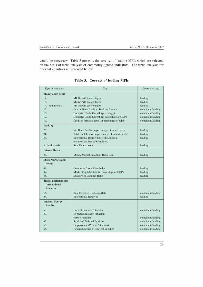
Asia-Pacific Development Journal Vol. 9, No. 2, December 2002
29
would be necessary. Table 3 presents the core set of leading MPIs which are selectedon the basis of trend analysis of commonly agreed indicators. The trend analysis forrelevant countries is presented below.
Table 3. Core set of leading MPIs
Type of indicator Title Characteristics
Money and Credit
7. M1 Growth (percentage) leading8. M2 Growth (percentage) leading4. (additional) M3 Growth (percentage) leading
15. Central Bank Credit to Banking System coincident/leading16. Domestic Credit Growth (percentage) coincident/leading17. Domestic Credit Growth (in percentage of GDP) coincident/leading19. Credit to Private Sector (in percentage of GDP) coincident/leading
Banking
26. Net Bank Profits (in percentage of total assets) leading31. Total Bank Loans (in percentage of total deposits) leading33. International Borrowings with Maturities leading
one year and less (US$ million)6. (additional) Real Estate Loans leading
Interest Rates
36. Money Market Rate/Inter Bank Rate leading
Stock Markets and Bonds
44. Composite Stock Price Index leading47. Market Capitalization (in percentage of GDP) leading48. Stock Price Earnings Ratio leading
Trade, Exchange and International Reserves
55. Real Effective Exchange Rate coincident/leading56. International Reserves leading
Business Survey Results
59. Current Business Situation coincident/leading60. Expected Business Situation
(next 6 months) coincident/leading62. Stocks of Finished Products coincident/leading65. Employment (Present Situation) coincident/leading66. Financial Situation (Present Situation) coincident/leading
Asia-Pacific Development Journal Vol. 9, No. 2, December 2002
30
According to business cycle and economic indicators research, reliableindicators (both coincident and leading) should not only have a sound statistical basis(e.g. broad coverage, representative, no missing data), short delay in publication, limitedex post revisions, a good track record in the reference period and, importantly, a solidtheoretical foundation. Otherwise there exists the problem of measurement withouttheory (“fishing in the data”).
Taking into account these requirements, the main arguments for selecting theabove-mentioned indicators are the following:
Growth rates of M1, M2 and M3: liquidity indicators
The growth rates of money supply aggregates (percentage change from theprevious period) – despite some irregular changes which could be smoothed out witha low-pass filter – signal in advance dangers for financial stability due to excessliquidity which may cause inflation to pick up or create over-exuberance of investment.This again may fuel speculative attacks on the currency, thus leading possibly toa currency crisis.
Excess liquidity can feed into the money financed fiscal deficit basis forcurrency crisis as in the first generation model for currency crises. Alternatively,excessive liquidity can lead to over investment or to real appreciation of the currencieswith the attendant loss in export competitiveness. In such cases, “excess” moneybalances can render an economy vulnerable to shocks.
Apart from this theoretical foundation, the money aggregates have theadvantage of availability in practically all countries on a monthly basis. The publicationlag varies between one and three months; efforts should be made to shorten this timelag to about one month in all countries participating in this harmonized financialmonitoring project.
Figures 1-5 (see appendix) present the trend of growth rates of narrow andbroad money supply, namely, M1 (Thailand and Indonesia), M2 (Thailand andIndonesia), and M3 (Thailand).
Central bank credit to banking system
A large increase in central bank credit to banks and other financial institutionsoften reflects severe liquidity or solvency problems in the financial sector. Althoughcentral bank credit is part and parcel of the functions of the central bank as thefacilitator of the smooth functioning of financial markets or as lender-of-last-resort,a spike in this variable heralds either a severe liquidity problem of a major bank(which can be problematic in itself), or worse, a systemic liquidity problem of thebanking sector. Left unsolved in times of uncertainty a bank run in a particular bankmay turn into a systemic run and unleash a solvency problem, unless the central bank

Asia-Pacific Development Journal Vol. 9, No. 2, December 2002
31
acts immediately to quell liquidity problems. At any rate, a large upward movementof central bank credit may indicate distress in the banking sector. On the other hand,large increases in central bank credit to banks could also be to stimulate bank lendingto revive a sluggish economy, but this can also indicate possible recession-causeddeterioration in the quality of bank lending indicator rather than a leading indicatorindicating a potential crisis. Thus, this indicator should – as empirical evidence hasproved – be more of a coincident nature.
Domestic credit growth (percentage) and domestic credit (percentage) of GDP
The leading character of domestic credit is not as obvious from a theoreticalpoint of view than in the case of money supply aggregates. Nevertheless, sharpincreases in credit demand over a longer time span bear the risk of over-investment(non-productive investment) which as a consequence may cause a deterioration of thecredit portfolio of the banks. As a further argument for the leading character of thesetwo indicators it can be brought forward that high growth rates of domestic credit areas a rule incompatible with a currency peg and could thus signal pending currencyand banking problems. In addition, a persistent increase in domestic credit could leadto deterioration in credit quality. In an environment of euphoria and due toinformational asymmetries, it is not easy to make a more measured assessment ofcredit applications. As the experience of the Asian crisis showed, a credit boompreceded a banking crisis (Evans, Leone, Gill and Hilbers, 2000).
On the other hand, the ratio of domestic credit as a percentage of GDP maystart rising only in the early phase of the onset of a banking crisis. The reason for itis that the central bank – as the crisis unfolds – may be pumping money into thebanks to alleviate their financial situation. This would explain why this series is nota clear-cut leading indicator but shows characteristics of a coincident indicator withregard to currency and banking crises. Furthermore, the construction of this indicatorsuggests that continued expansion of credit – either by momentum or other reasons –during recessionary periods would increase credit risk in the banking system, makingit vulnerable to a banking crisis. Rapid credit growth could also induce unsustainableasset price increases, including for assets used as collateral for lending.
All countries included in RETA 5869 can provide domestic credit growth ona monthly basis. The publication time lag ranges between one and 24 weeks. Theindicator no: 21 (“Domestic Credit in per cent of GDP”) is available as a rule only ona quarterly basis as the GDP figures come out only four times a year. In Fiji andIndonesia, the indicator no: 21 is presented on a monthly basis; the quarterly GDPfigures are obviously interpolated to get monthly estimates.
Figures 6-8 (see appendix) present the trend for domestic credit growth forFiji, Indonesia and Thailand.
Asia-Pacific Development Journal Vol. 9, No. 2, December 2002
32
Credit to private sector (in per cent) of GDP
A sharp increase of this indicator may signal over-investment of the privatesector which could lead to a deterioration in the quality of credit portfolios of thebanking sector and, consequently, in financial institutions’ cash flows, net income andsolvency. An increase in consumer lending, including credit card debt, especially iffinanced by heavy capital flows, can lead easily to a current account deficit. A largecurrent account deficit, accompanied by a loss of competitiveness can put some pressureon the exchange rate. Of course, a massive devaluation can put severe stress on thepaying capability of debtors and undermine the asset quality of the banking system.
Monthly data are available from Fiji and Indonesia, otherwise there existquarterly data with the exception of Viet Nam (only annual data). The publicationtime lag ranges between one and 24 weeks.
Figures 9-12 (see appendix) present the trend for credit to private sector inper cent of GDP for Fiji, Indonesia, Thailand and the Philippines.
Net profits (as per cent of average assets)
The indicator reflects one of the most commonly used measures of profitability.Unusually high profitability may be a sign of excessive risk taking. On the otherhand, bank earnings are a buffer against capital erosion caused by shrinkage in assetvalue. Thus, a steady increase would be the optimal performance of this indicatorfrom a macroeconomic point of view. High profits may also be indicative of protectedor imperfectly competitive banking markets. Thus, a sharp decrease of this indicatoris indicative either of more competition or a deterioration of credit quality.
As empirical evidence has shown, this indicator rose sharply in some placesin 1997 (e.g. Taiwan Province of China) before collapsing in the wake of the financialcrisis in 1998 and only slowly recovering since then. With the exception ofViet Nam, short-term data (at least quarterly) are available in all RETA 5869 countries.The publication time lag ranges between one and 24 weeks. Profitability data aresignificantly affected by practices for provisioning and recognition of impairment ofassets, factors which should always be considered in analyzing these indicators.
Figures 13-15 present the trend for net profits for Taiwan Province of China,Indonesia and Thailand.
Total bank loans (as per cent) of total deposits
The ratio of credit to deposits may give indications of the ability of thebanking system to mobilize deposits to meet credit demand. A high and growing ratiomay indicate stress in the banking system and a low level of liquidity to respond toshocks. Banks that have large outstanding loans relative to the deposit base may berelying on a relatively volatile liability base and could be subject to contagion or to
Asia-Pacific Development Journal Vol. 9, No. 2, December 2002
33
suffer in the event of a slowdown in economic activity. This is particularly true if thebank loans are financed by foreign borrowings. This explains why this indicatorproved to give early warning signals of financial vulnerability.
All countries participating in RETA 5869 can provide this indicator ona monthly basis. The publication lag ranges between one and 24 weeks.
Figures 16-18 (see appendix) present the trend for total bank loans in percent of total deposits for Taiwan Province of China, Indonesia and Thailand.
International borrowings with maturities of one year and less (in US$ million)
A high and growing amount of short-term international borrowing bears therisk that large amounts of foreign capital may be withdrawn rapidly. Central to thejustification of this indicator is the prevalence of maturity mismatches during theAsian crisis. During the banking crisis of 1997-1998, many banks in South-East andEast Asia borrowed from the international capital markets in short maturities butrelent the funds for longer terms. Because of moral hazard and the implicit guaranteesthat exchange rates will continue to be pegged indefinitely, this arrangement provedto be a profitable one for both the banks and their debtors (Corsetti, Pesenti andRoubini, 1999). However, given the shock of the collapse of the Thai baht peg andthe ensuing contagion, many banking systems could not bear the pressure arisingfrom the maturity mismatches and the depreciation of the currencies. Thus, thisindicator appears from a theoretical point of view suited for giving early warningsignals for liquidity crunches, caused e.g. by contagion effects of financial shocks ina neighbouring country.
Figure 19 (see appendix) presents the trend for international borrowings withmaturities of one year and less in US$ million for Thailand.
Real estate loans
Many financial crises have been caused or amplified by downturns in particularsectors of the economy spilling over into the financial system. This has often beenthe case when a concentration of loans occurred in the real estate sector which can besubject to severe boom and bust price cycles. In Asia, for instance, almost all affectedcountries saw rising real estate and equity prices during the early 1990s, then sharpdeclines from around mid-1996. With hindsight, it can easily be said that the bankingsectors of many Asian economies were particularly exposed to a narrow industry.Furthermore, the lack of diversification of the loan portfolio signals vulnerability ofthe banking system. Thus, this indicator when surpassing a certain threshold (definedcountry by country) can act as a leading indicator for financial disturbances.
Not all countries participating in RETA 5869 are providing this information.For Thailand quarterly data are only available since the fourth quarter 2000; prior tothat only annual data existed.

Asia-Pacific Development Journal Vol. 9, No. 2, December 2002
34
Figures 20-21 (see appendix) present the trend for real estate loans forIndonesia and Thailand.
Money market rate/inter-bank rate (average of period)
A sharp increase of this rate signals a tight liquidity situation in the bankingsector, which can possibly lead to solvency problems. Of course, sharp increases ininterest rates could also exacerbate the adverse selection problem in financial markets(Mishkin, 1997). All countries participating in the RETA have provided this indicatoron a monthly basis. The publication time lag is about one month.
Stock market indicators concerning the performance of the composite stock marketindex, market capitalization and the price earnings (PE) ratio
Stock market developments signal changes in market perceptions of capitalinvestors. A steep decline in stock prices – which as a rule is also combined witha sharp drop of market capitalization (in per cent of GDP) – signals tensions in thecapital markets which may spread sooner or later to the real sector of the economy,thus posing the danger to set in force a cumulative downward spiral. Indicatorsnos: 54 and 57 are generally accepted leading indicators for financial markets. Thestock market indicators also reflect confidence in the economy quite broadly. Becausethe price of a stock is theoretically the net present value of the future stream ofincome, its movement reflects the potential profitability of firms. Extended to themacroeconomic plane, movement of the stock market index is taken as the collectiveassessment by stock market analysts of corporate profitability, which is tied up withgeneral economic growth. Thus, the financial literature (Fama, 1981) often links themovements of the stock market index with future economic growth. It has beenobserved that prior to a crisis, stock prices tend to decline. This may indicate that themarket players foresee a weakening of corporate profits or a general economicslowdown in the near future.
The same conclusion holds true for the stock price earnings ratio. If thisindicator is already high and increases further this may signal increasing asset inflation,unsustainable in the medium term. This indicator can also be a measure of euphoriaor speculation in the markets. Astronomical PE ratios can persist for a time (assetbubbles), but a correction invariably happens. The problem with high PE ratios isthat it may falsely lead companies to over-invest and undertake heavy debt positions.Thus, this indicator gives warning signals that the stock asset bubble may burst withall the negative consequences known e.g. from Japan.
Apart from Fiji and Viet Nam, these indicators exist without any significantdelay in all participating countries.
Figures 22-23 (see appendix) present the trend for composite stock priceindex for Indonesia and Thailand.

Asia-Pacific Development Journal Vol. 9, No. 2, December 2002
35
Real effective exchange rate
If real appreciation of a currency is not backed by corresponding productivitygains in the real economy, this implies a loss of international competitiveness whichis possibly a source of increasing vulnerability of a county’s economy. A loss incompetitiveness arising from a peg might put pressure on policy makers to devalue inorder to hit some economic growth targets. The financial markets will recognize thepressure of the policy makers to react to recessionary moves in the face of loss ofcompetitiveness and would engage in speculative actions. If not managed well, thiscould lead to a currency crisis. Indeed, it has been observed that in the run-up toa crisis, the real value of the domestic currency was, on average, significantly higherthan its mean during tranquil periods (IMF 1998).
Until now, monthly data for this indicator are only available for Thailand andFiji and on a quarterly basis for the Philippines.
Figures 24-25 (see appendix) present the trend for the real effective exchangeratio for the Philippines and Thailand.
International reserves (in US$ million)
A low and declining amount of international reserves (central bank and thefinancial sector as a whole) signals possible problems for the country to meetinternational payment requirements. Thus, this series is seen particularly by capitalmarket investors as one of the most important early warning indicators of financialvulnerability. This is an indicator of relative international illiquidity (Sachs, Tornelliand Velasco, 1995). Too low a level of reserves could increase the vulnerability ofa financial system to changes in sentiments.
This indicator is available in all participating countries; Thailand, TaiwanProvince of China and Fiji have provided monthly, Indonesia and the Philippinesquarterly and Viet Nam only annual data.
Figures 26-28 (see appendix) present the trend for international reserves inFiji, Indonesia and Thailand.
Indicators on business survey data
Business survey results in many countries have proved to be good leadingindicators for the real economy. In particular, the business survey results for themanufacturing sector – which is still the cycle maker in most countries – showa significant lead compared with GDP and industrial production. Answers on thecurrent business situation as well as on the expected business trend in the next threeto six months mainly reflects the perceived profit assessment and outlook of managers,which is not only of great importance for the real economy (in particular for futureproduction, investment and employment) but also has implications for the financialsector (soundness of the loan portfolios of banks, share price development).
Asia-Pacific Development Journal Vol. 9, No. 2, December 2002
36
For all these reasons, business survey results play in many countriesa prominent role as leading indicators both for the real economy as well as for thefinancial sector. The majority of countries participating in RETA 5869 have startedregular monthly or at least quarterly business surveys only recently. Thus, a thoroughassessment of the leading character of these variables is not yet possible. The onlyexception is Taiwan Province of China and Indonesia where longer time series areavailable showing that these data give timely signals on economic trends. Also inThailand where business survey data go back only to early 1999 they appear to giveearly information of the recovery phase after the Asian crisis and the slowdown in thefirst half of 2000 followed thereafter by a renewed economic pick-up.
III. CONCLUDING REMARKS
An attempt has been made here to identify a core set of MPIs which can beuseful in monitoring the financial stability of the financial and asset markets. Theabove identification is based on the limited time series of MPIs compiled by theparticipating countries. The length of time series and missing data within the timeseries, frequency and time lag of availability of ADB MPIs vary considerable fromcountry to country. Therefore, the above identification should be considered tentative.A rigorous and sophisticated quantitative analysis based on longer time series andmore data should ideally be conducted by individual countries to identify a set ofleading indicators appropriate for their economic situations and institutionalenvironments. The analysis should be a continuous process as the core set may needinclusion or exclusion of some indicators depending on the forthcoming changes inthe financial sector and in the economy. As monitoring the financial stability ofa country involves both statisticians and financial sector supervisors, and employssupervisory and statistical data, there is a need for a closer collaboration andcoordination among the statistical agencies producing the data and financial sectorsupervisors including central banks and security commissions.
In order to arrive at a smaller number of core leading indicators, one canconsider constructing composite leading indicators. To what extent composite leadingindicators might help in the analysis cannot be assessed at this stage. On the onehand, composite indicators facilitate structuring the vast amount of signals; on theother hand they can lead to an over-simplification of the analysis. Thus, it might beadvisable to construct a group of composite indicators e.g. for each of the five segments(Money and Credit; Banking; Interest Rates; Stock Markets and Bonds; Trade, Exchangeand International Reserves, as well as Business Survey Results), analogous to theweighting methods used in the supervisory CAMELS system (CAMELS is an acronymfor six categories of bank performance: capital adequacy, asset quality, management,earnings and liquidity and sensitivity to market risk). As not enough experience hasbeen gained with the ADB’s MPI’s, it is proposed to concentrate for the time being at
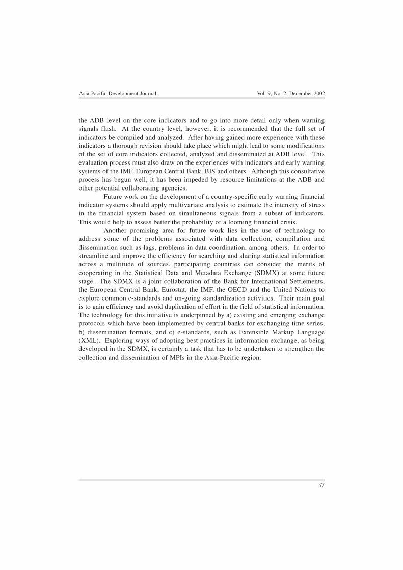
Asia-Pacific Development Journal Vol. 9, No. 2, December 2002
37
the ADB level on the core indicators and to go into more detail only when warningsignals flash. At the country level, however, it is recommended that the full set ofindicators be compiled and analyzed. After having gained more experience with theseindicators a thorough revision should take place which might lead to some modificationsof the set of core indicators collected, analyzed and disseminated at ADB level. Thisevaluation process must also draw on the experiences with indicators and early warningsystems of the IMF, European Central Bank, BIS and others. Although this consultativeprocess has begun well, it has been impeded by resource limitations at the ADB andother potential collaborating agencies.
Future work on the development of a country-specific early warning financialindicator systems should apply multivariate analysis to estimate the intensity of stressin the financial system based on simultaneous signals from a subset of indicators.This would help to assess better the probability of a looming financial crisis.
Another promising area for future work lies in the use of technology toaddress some of the problems associated with data collection, compilation anddissemination such as lags, problems in data coordination, among others. In order tostreamline and improve the efficiency for searching and sharing statistical informationacross a multitude of sources, participating countries can consider the merits ofcooperating in the Statistical Data and Metadata Exchange (SDMX) at some futurestage. The SDMX is a joint collaboration of the Bank for International Settlements,the European Central Bank, Eurostat, the IMF, the OECD and the United Nations toexplore common e-standards and on-going standardization activities. Their main goalis to gain efficiency and avoid duplication of effort in the field of statistical information.The technology for this initiative is underpinned by a) existing and emerging exchangeprotocols which have been implemented by central banks for exchanging time series,b) dissemination formats, and c) e-standards, such as Extensible Markup Language(XML). Exploring ways of adopting best practices in information exchange, as beingdeveloped in the SDMX, is certainly a task that has to be undertaken to strengthen thecollection and dissemination of MPIs in the Asia-Pacific region.

Asia-Pacific Development Journal Vol. 9, No. 2, December 2002
38
REFERENCES
Bhattacharyay, B., 2001. “Strengthening and harmonization of MPIs for monitoring financial asset marketsin Asia and Pacific”, presented at the Concluding Workshop of RETA 5869, Manila, 16-18 May2001.
Corsetti, G., P. Pesenti, and N. Roubini, 1999. “What caused the Asian currency and financial crisis?”Japan and the World Economy, September.
Evans, O., A. Leone, M. Gill and P. Hilbers, 2002. “Macroprudential indicators of financial systemsoundness”, IMF Occasional Paper 192.
Fama, E., 1981. “Stock returns, real activity, inflation and money”, American Economic Review, vol. 71,No. 4, pp. 545-565.
Goldstein, M., G. Kaminsky and C. Reinhardt, 2000. Assessing Financial Vulnerability: An Early WarningSystem for Emerging Markets (Institute for International Economics).
IMF, 1998. World Economic Outlook, May.
, 2001. Macroprudential Analysis: Selected Aspects Background Paper, 7 June 2001.
Kaminsky G., S. Lizondo, and C. Reinhardt, 1998. Leading Indicators of Currency Crisis, IMF StaffPapers, vol. 45, No. 1.
Kaminsky, G., and C. Reinhardt, 1999. “The twin crisis: the causes of banking and balance-of-paymentsproblems”, The American Economic Review, vol. 49, No. 3.
Mishkin, F., 1997. “Understanding financial crises: a developing country perspective”, Annual WorldBank Conference on Development Economics.
Sachs, J., A. Tornelli and A. Velasco, 1995. “Financial crisis in emerging markets”, National Bureau ofEconomic Research, Working Paper No. W5576.
Sundararajan, V., D. Marston, and R. Basu, Financial System Standards and Financial Stability: TheCase of Basel Core Principles, (IMF Working Paper WP/01/62)

Asia-Pacific Development Journal Vol. 9, No. 2, December 2002
39
Appendix

Asia-Pacific Development Journal Vol. 9, No. 2, December 2002
41
1994 1995 1996 1997 1998 1999 2000 2001 2002 2003
-10
0
10
20
30
40
Figure 1. Money supply growth (M1) in Thailand
Indicator 09: M1 growth (per cent)
Figure 2. Money supply growth (M1) in Indonesia
-10
0
10
20
30
40
50
60
70
1994 1995 1996 1997 1998 1999 2000 2001
Indicator 09: M1 growth (per cent)
Figure 3. Money supply growth (M2) in Thailand
1994 1995 1996 1997 1998 1999 2000 2001 2002 2003
-5
0
5
10
15
20
25
Indicator 10: M2 growth (per cent)
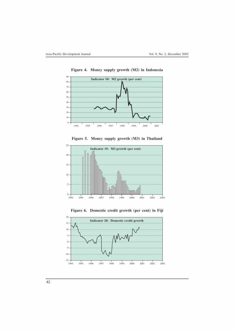
Asia-Pacific Development Journal Vol. 9, No. 2, December 2002
42
1994 1995 1996 1997 1998 1999 2000 2001 2002 2003
0
5
10
15
20
25
Figure 4. Money supply growth (M2) in Indonesia
1994 1995 1996 1997 1998 1999 2000 2001
0
10
20
30
40
50
60
70
80
90Indicator 10: M2 growth (per cent)
Indicator 19: M3 growth (per cent)
Figure 5. Money supply growth (M3) in Thailand
Figure 6. Domestic credit growth (per cent) in Fiji
1994 1995 1996 1997 1998 1999 2000 2001 2002 2003
-15
-10
-5
0
5
10
15
20
Indicator 20: Domestic credit growth

Asia-Pacific Development Journal Vol. 9, No. 2, December 2002
43
Figure 7. Domestic credit growth (per cent) in Indonesia
1994 1995 1996 1997 1998 1999 2000 2001
-40
-20
0
20
40
60
80
100
120
Figure 8. Domestic credit growth (per cent) in Thailand
Indicator 20: Domestic credit growth
1994 1995 1996 1997 1998 1999 2000 2001 2002 2003
-10
0
10
20
30
40
Indicator 20: Domestic credit growth
Figure 9. Credit to the private sector in Fiji
1994 1995 1996 1997 1998 1999 2000 2001 2002 2003
28
30
32
34
36
38
40
42
Indicator 23: Credit to private sector (per cent of GDP)
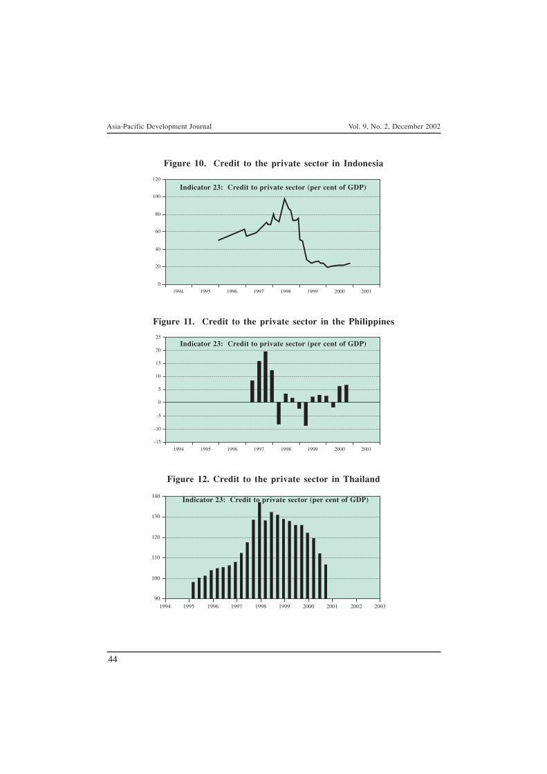
Asia-Pacific Development Journal Vol. 9, No. 2, December 2002
44
Figure 10. Credit to the private sector in Indonesia
1994 1995 1996 1997 1998 1999 2000 2001
0
20
40
60
80
100
120
Indicator 23: Credit to private sector (per cent of GDP)
Figure 11. Credit to the private sector in the Philippines
1994 1995 1996 1997 1998 1999 2000 2001
-15
-10
-5
0
5
10
15
20
25
Indicator 23: Credit to private sector (per cent of GDP)
Figure 12. Credit to the private sector in Thailand
1994 1995 1996 1997 1998 1999 2000 2001 2002 2003
90
100
110
120
130
140 Indicator 23: Credit to private sector (per cent of GDP)

Asia-Pacific Development Journal Vol. 9, No. 2, December 2002
45
Figure 13. Net profits in Taiwan Province of China
1994 1995 1996 1997 1998 1999 2000 2001 2002 2003
0
0.1
0.2
0.3
0.4Indicator 30: Net profits (as per cent of Total Assets)
Figure 14. Net profits in Indonesia
1994 1995 1996 1997 1998 1999 2000 2001
-35
-30
-25
-20
-15
-10
-5
0
5
10Indicator 30: Net profits (as per cent of Total Assets)
Figure 15. Net profits in Thailand
1994 1995 1996 1997 1998 1999 2000 2001 2002 2003
-4
-3
-2
-1
0
1
2Indicator 30: Net profits (per cent of Total Assets)

Asia-Pacific Development Journal Vol. 9, No. 2, December 2002
46
Figure 16. Total credit in Thailand
1994 1995 1996 1997 1998 1999 2000 2001 2002 2003
90
100
110
120
130
140
150Indicator 34: Total credit (per cent of Total deposits)
Figure 17. Total credit in Taiwan Province of China
1994 1995 1996 1997 1998 1999 2000 2001 2002 2003
86
88
90
92
94
96Indicator 34: Total credit (per cent of Total deposits)
Figure 18. Total credit in Indonesia
1994 1995 1996 1997 1998 1999 2000 2001
0
10
20
30
40
50
60
70
80
90
100Indicator 34: Total credit (per cent of Total deposits)
Asia-Pacific Development Journal Vol. 9, No. 2, December 2002
47
1994 1995 1996 1997 1998 1999 2000 2001 2002 2003
0
5 000
10 000
15 000
20 000
0
Figure 19. International borrowings with maturities in Thailand
Indicator 36: International borrowings with maturities(one year and less in Mn US$)
Figure 20. Real estate loans in Indonesia
1994 1995 1996 1997 1998 1999 2000 2001
0
5
10
15
20
25Indicator 37: Real estate loans (per cent of total loans)
Figure 21. Real estate loans in Thailand
1994 1995 1996 1997 1998 1999 2000 2001 2002 2003
15
16
17
18
19
20
21
22
Indicator 37: Real estate credit (per cent of Total Credit)

Asia-Pacific Development Journal Vol. 9, No. 2, December 2002
48
Figure 22. Composite stock price index in Indonesia
1994 1995 1996 1997 1998 1999 2000 2001
0
100
200
300
400
500
600
700
800Indicator 54: composite stock price index (Capital City: NCU)
Figure 23. Composite stock price index in Thailand
1994 1995 1996 1997 1998 1999 2000 2001 2002 2003
200
400
600
800
1 000
1 200
1 400
1 600Indicator 64: Composite Stock Price Index (Capital City: NCU)
Figure 24. Real effective exchange ratio in the Philippines
1994 1995 1996 1997 1998 1999 2000 2001
0
20
40
60
80
100
120
Indicator 67: Real Effective Exchange Rate
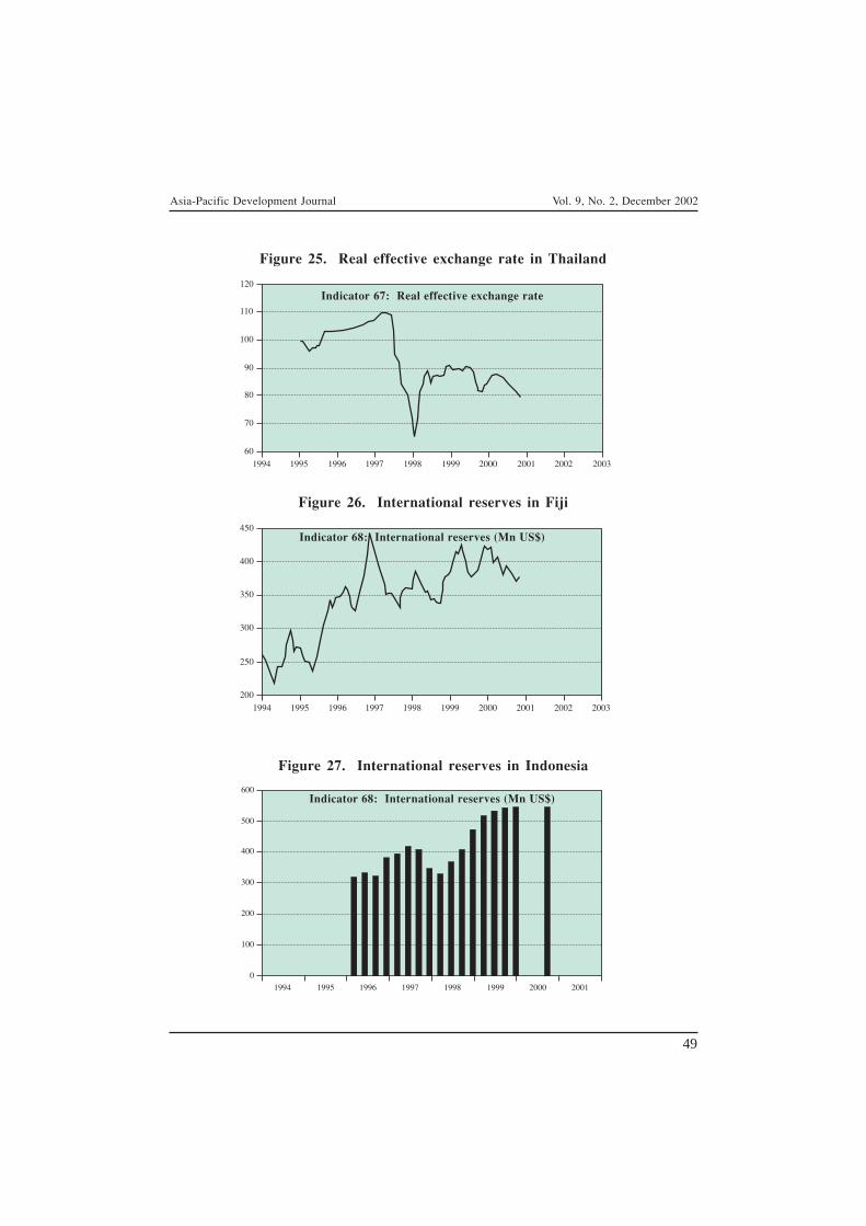
Asia-Pacific Development Journal Vol. 9, No. 2, December 2002
49
1994 1995 1996 1997 1998 1999 2000 2001 2002 2003
200
250
300
350
400
450
Figure 25. Real effective exchange rate in Thailand
1994 1995 1996 1997 1998 1999 2000 2001 2002 2003
60
70
80
90
100
110
120
Indicator 67: Real effective exchange rate
Figure 26. International reserves in Fiji
Indicator 68: International reserves (Mn US$)
Figure 27. International reserves in Indonesia
1994 1995 1996 1997 1998 1999 2000 2001
0
100
200
300
400
500
600Indicator 68: International reserves (Mn US$)
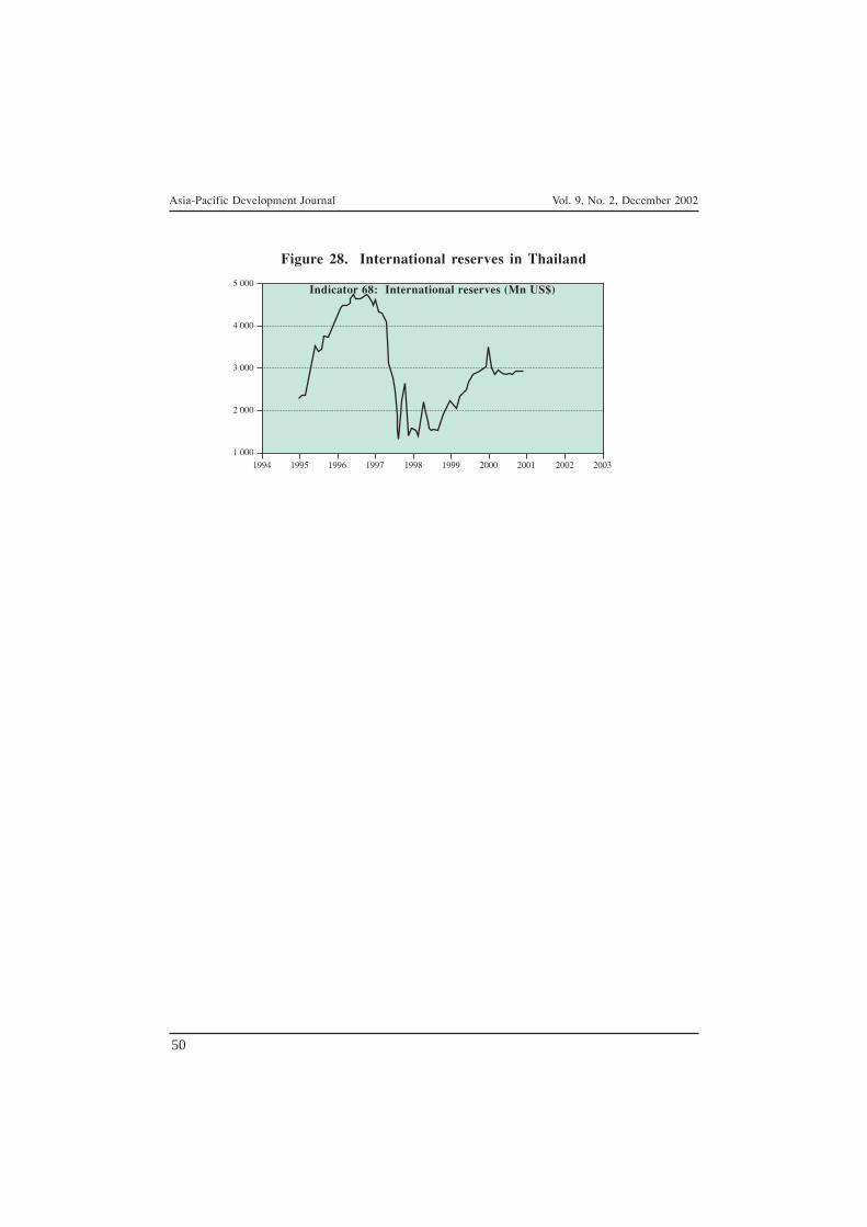
Asia-Pacific Development Journal Vol. 9, No. 2, December 2002
50
Figure 28. International reserves in Thailand
1994 1995 1996 1997 1998 1999 2000 2001 2002 2003
1 000
2 000
3 000
4 000
5 000Indicator 68: International reserves (Mn US$)
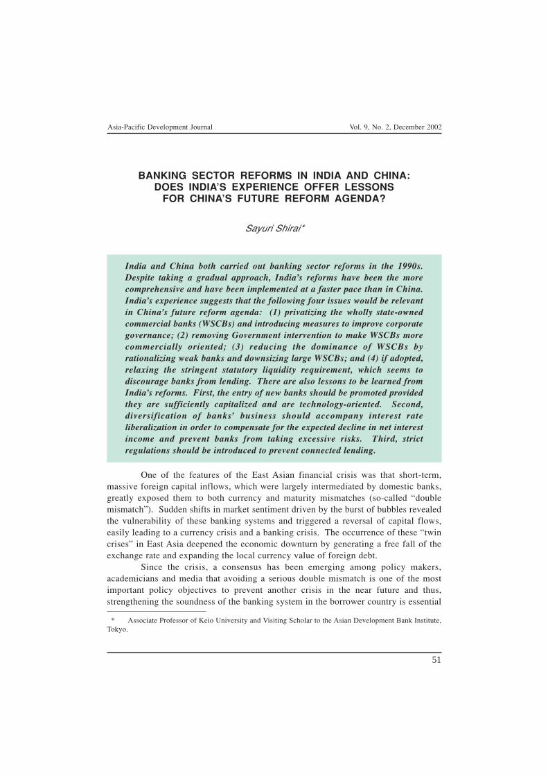
Asia-Pacific Development Journal Vol. 9, No. 2, December 2002
51
BANKING SECTOR REFORMS IN INDIA AND CHINA:DOES INDIA’S EXPERIENCE OFFER LESSONS
FOR CHINA’S FUTURE REFORM AGENDA?
Sayuri Shirai*
India and China both carried out banking sector reforms in the 1990s.Despite taking a gradual approach, India’s reforms have been the morecomprehensive and have been implemented at a faster pace than in China.India’s experience suggests that the following four issues would be relevantin China’s future reform agenda: (1) privatizing the wholly state-ownedcommercial banks (WSCBs) and introducing measures to improve corporategovernance; (2) removing Government intervention to make WSCBs morecommercially oriented; (3) reducing the dominance of WSCBs byrationalizing weak banks and downsizing large WSCBs; and (4) if adopted,relaxing the stringent statutory liquidity requirement, which seems todiscourage banks from lending. There are also lessons to be learned fromIndia’s reforms. First, the entry of new banks should be promoted providedthey are sufficiently capitalized and are technology-oriented. Second,diversification of banks’ business should accompany interest rateliberalization in order to compensate for the expected decline in net interestincome and prevent banks from taking excessive risks. Third, strictregulations should be introduced to prevent connected lending.
One of the features of the East Asian financial crisis was that short-term,massive foreign capital inflows, which were largely intermediated by domestic banks,greatly exposed them to both currency and maturity mismatches (so-called “doublemismatch”). Sudden shifts in market sentiment driven by the burst of bubbles revealedthe vulnerability of these banking systems and triggered a reversal of capital flows,easily leading to a currency crisis and a banking crisis. The occurrence of these “twincrises” in East Asia deepened the economic downturn by generating a free fall of theexchange rate and expanding the local currency value of foreign debt.
Since the crisis, a consensus has been emerging among policy makers,academicians and media that avoiding a serious double mismatch is one of the mostimportant policy objectives to prevent another crisis in the near future and thus,strengthening the soundness of the banking system in the borrower country is essential
* Associate Professor of Keio University and Visiting Scholar to the Asian Development Bank Institute,Tokyo.
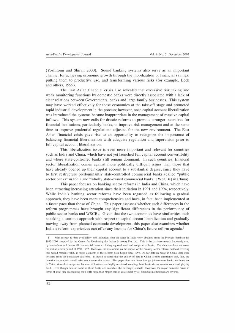
Asia-Pacific Development Journal Vol. 9, No. 2, December 2002
52
(Yoshitomi and Shirai, 2000). Sound banking systems also serve as an importantchannel for achieving economic growth through the mobilization of financial savings,putting them to productive use, and transforming various risks (for example, Beckand others, 1999).
The East Asian financial crisis also revealed that excessive risk taking andweak monitoring functions by domestic banks were directly associated with a lack ofclear relations between Governments, banks and large family businesses. This systemmay have worked effectively for these economies at the take-off stage and promotedrapid industrial development in the process; however, once capital account liberalizationwas introduced the systems became inappropriate in the management of massive capitalinflows. This system now calls for drastic reforms to promote stronger incentives forfinancial institutions, particularly banks, to improve risk management and at the sametime to improve prudential regulations adjusted for the new environment. The EastAsian financial crisis gave rise to an opportunity to recognize the importance ofbalancing financial liberalization with adequate regulation and supervision prior tofull capital account liberalization.
This liberalization issue is even more important and relevant for countriessuch as India and China, which have not yet launched full capital account convertibilityand where state-controlled banks still remain dominant. In such countries, financialsector liberalization comes against more politically difficult issues than those thathave already opened up their capital account to a substantial degree, since they haveto first restructure predominantly state-controlled commercial banks (called “publicsector banks” in India and “wholly state-owned commercial banks” [WSCBs] in China).
This paper focuses on banking sector reforms in India and China, which havebeen attracting increasing attention since their initiation in 1991 and 1994, respectively.While India’s banking sector reforms have been regarded as following a gradualapproach, they have been more comprehensive and have, in fact, been implemented ata faster pace than those of China. This paper assesses whether such differences in thereform programmes have brought any significant differences in the performance ofpublic sector banks and WSCBs. Given that the two economies have similarities suchas taking a cautious approach with respect to capital accout liberalization and graduallymoving away from planned economic development, this paper also examines whetherIndia’s reform experiences can offer any lessons for China’s future reform agenda.1
1 With respect to data availability and limitation, data on banks in India were obtained from the Prowess database for
1993-2000 compiled by the Center for Monitoring the Indian Economy Pvt. Ltd. This is the database mostly frequently used
by researchers and covers all commercial banks excluding regional rural and cooperative banks. The database does not cover
the initial reform period of 1991-1992. However, the assessment on the impact of the banking sector reforms without covering
this period remains valid, as major elements of the reforms have begun since 1993. As for data on banks in China, data were
obtained from the Bankscope data base. It should be noted that the quality of data in China is often questioned and, thus, the
quantitative analysis should take into account this aspect. This paper does not cover foreign joint-venture banks and branches
in China, since their scope and location of business are highly restricted, meaning these banks do not operate on a level playing
field. Even though data on some of these banks are available, the coverage is small. However, the major domestic banks in
terms of asset size (accounting for a little more than 80 per cent of assets held by all financial institutions) are covered.
Asia-Pacific Development Journal Vol. 9, No. 2, December 2002
53
The paper consists of five sections. Section I focuses on India’s and China’sbanking sector reforms. Section II assesses these reforms by examining trends andpatterns of performance over the reform period. Section III discusses six issues relatedto India’s banking sector reforms (privatization, entry deregulation, statutory liquidityrequirement, directed lending, diversification of business, and connected lending) andidentifies lessons that might be applicable to China’s future reforms by analyzing thepolicies adopted in India. Section IV discusses China’s remaining reform agenda.
I. BANKING SECTOR REFORMS IN INDIA AND CHINA
Background of the reforms: India
India’s commercial banking system mainly consists of 27 public sector banks(that are further classified as 19 nationalized banks and eight State Bank of India(SBI) banks (SBI and seven independently capitalized banking subsidiaries); 31 privatesector banks (that are further classified as 23 old private sector banks and eight newprivate sector banks that emerged after 1991; 42 foreign banks; 196 regional ruralbanks; and 67 cooperative banks. The banking system had 959,955 employees and51,267 branches in 2000; of which, public sector banks had a 90 per cent share. TheSBI was originally established in 1806 and acquired its present status through an actof parliament in 1955. Nationalized banks refer to private sector banks that werenationalized (14 banks in 1969 and six in 1980) by the central government. In 1993,Punjab National Bank merged with another nationalized bank, New Bank of India,leading to a decline in the total number of nationalized banks from 20 to 19.
Prior to the 1991 reforms, India’s banking sector had long been characterizedas highly regulated and financially repressed. The prevalence of the reserve requirement(i.e., a cash reserve ratio [CRR] that requires banks to hold a certain amount ofdeposits in the form of deposits with the RBI), liquidity requirement (i.e., statutoryliquidity ratio [SLR] that requires banks to hold a certain amount of deposits in theform of Governmentand eligible securities), interest rate controls and allocation offinancial resources to the so-called priority sectors (i.e., agriculture, small scaleindustries and exports) increased the degree of financial repression and adverselyaffected the country’s financial resource mobilization and allocation. Quantitativeloan targets were imposed on nationalized banks to expand their networks in ruralareas and extend credit to priority sectors. These banks were then increasingly usedto finance fiscal deficits. Although non-nationalized private sector banks and foreignbanks were allowed to coexist with public sector banks at that time, their activitieswere highly restricted through entry regulations and strict branch licensing policies.
As a result of elaborate Government intervention, many banks remainedunprofitable. The average return on assets for public sector banks in the second halfof the 1980s was only about 0.15 per cent and their non-performing assets (NPA)
Asia-Pacific Development Journal Vol. 9, No. 2, December 2002
54
amounted to 24 per cent of credit. Against this background, the first wave of financialliberalization took place in the second half of the 1980s, mainly taking the form ofintroduction of Treasury Bills (TB), development of money markets and partial interestrate deregulation. In 1986, the 182-day TB were introduced through an auction system.In 1988, the Discount and Financial House of India was established as an institutionthat would provide liquidity in the financial market. In 1989, both commercial paperand CDs were introduced. Coupon rates on Government bonds were graduallyincreased to reflect demand and supply conditions. In 1988, the maximum lendingrate and ranges in minimum rates were unified and switched to a minimum lendingrate (MLR) in 1988. As a result, this enabled banks to set interest rates more flexibly.In 1989, the maximum interest rates on call money were liberalized.
Banking sector reforms since 1991
Following most of the recommendations made in the 1991 report of theNarasimham Committee, the Government launched comprehensive banking sectorreforms in that same year. India’s banking sector reforms since 1991 can besummarized in the following six areas: first, the CRR declined from 15 per cent in1991 to 5.5 per cent in 2001. The SLR declined from 38.5 per cent in 1991 to 25 percent in 1997 and has remained at 25 per cent until today. A decline in the CRR andSLR increased banks’ flexibility in allocating credit and hence gave banks anopportunity to improve their profitability. Second, interest rates became flexible withrespect to all term deposits rates and lending rates on advances over Rs 200,000.Interest rate deregulation has encouraged banks to improve their cost efficiency anddiversify into non-traditional business as a result of declining net interst income(table 1). Third, reform in priority sector lending – mainly through the expansion ofcoverage and interest rate decontrols on advances over Rs 200,000 – helped banks tomitigate the negative impact arising from such policy loans, while the targets of40 per cent (of advances) on domestic banks and 33 per cent on foreign banks havenot changed during the reform period.
Fourth, entry barriers were reduced both on private sector and foreign banksand their full ownership was granted. As a result, eight private sector banks and26 new foreign banks entered the banking sector. With respect to branch barriers,public sector banks were allowed to rationalize some branches. Following India’scommitment to the 1995 World Trade Organization (WTO) agreement in respect ofthe services sector, foreign banks have been permitted to open up to 12 branchesa year. Also, these banks can be exempted from meeting branch requirements in ruraland semi-urban areas provided that they, for example, contribute to the RuralInfrastructure Development Fund of the National Bank for Agriculture and RuralDevelopment (NABARD), a refinance institution, or make deposits with the NABARD.Fifth, various prudential norms and more appropriate accounting standards were
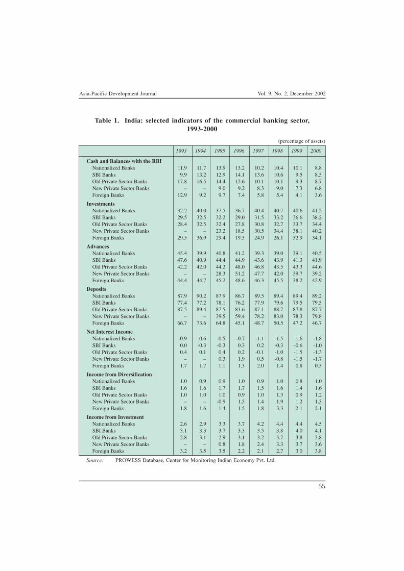
Asia-Pacific Development Journal Vol. 9, No. 2, December 2002
55
Table 1. India: selected indicators of the commercial banking sector,1993-2000
(percentage of assets)
1993 1994 1995 1996 1997 1998 1999 2000
Cash and Balances with the RBINationalized Banks 11.9 11.7 13.9 13.2 10.2 10.4 10.1 8.8SBI Banks 9.9 13.2 12.9 14.1 13.6 10.6 9.5 8.5Old Private Sector Banks 17.8 16.5 14.4 12.6 10.1 10.1 9.3 8.7New Private Sector Banks – – 9.0 9.2 8.3 9.0 7.3 6.8Foreign Banks 12.9 9.2 9.7 7.4 5.8 5.4 4.1 3.6
InvestmentsNationalized Banks 32.2 40.0 37.5 36.7 40.4 40.7 40.6 41.2SBI Banks 29.5 32.5 32.2 29.0 31.5 33.2 36.6 38.2Old Private Sector Banks 28.4 32.5 32.4 27.8 30.8 32.7 33.7 34.4New Private Sector Banks – – 23.2 18.5 30.5 34.4 38.1 40.2Foreign Banks 29.5 36.9 29.4 19.3 24.9 26.1 32.9 34.1
AdvancesNationalized Banks 45.4 39.9 40.8 41.2 39.3 39.0 39.1 40.5SBI Banks 47.6 40.9 44.4 44.9 43.6 43.9 41.3 41.9Old Private Sector Banks 42.2 42.0 44.2 48.0 46.8 43.5 43.3 44.6New Private Sector Banks – – 28.3 51.2 47.7 42.0 39.7 39.2Foreign Banks 44.4 44.7 45.2 48.6 46.3 45.5 38.2 42.9
DepositsNationalized Banks 87.9 90.2 87.9 86.7 89.5 89.4 89.4 89.2SBI Banks 77.4 77.2 78.1 76.2 77.9 79.6 79.5 79.5Old Private Sector Banks 87.5 89.4 87.5 83.6 87.1 88.7 87.8 87.7New Private Sector Banks – – 39.5 59.4 78.2 83.0 78.3 79.8Foreign Banks 66.7 73.6 64.8 45.1 48.7 50.5 47.2 46.7
Net Interest IncomeNationalized Banks -0.9 -0.6 -0.5 -0.7 -1.1 -1.5 -1.6 -1.8SBI Banks 0.0 -0.3 -0.3 0.3 0.2 -0.3 -0.6 -1.0Old Private Sector Banks 0.4 0.1 0.4 0.2 -0.1 -1.0 -1.5 -1.3New Private Sector Banks – – 0.3 1.9 0.5 -0.8 -1.5 -1.7Foreign Banks 1.7 1.7 1.1 1.3 2.0 1.4 0.8 0.3
Income from DiversificationNationalized Banks 1.0 0.9 0.9 1.0 0.9 1.0 0.8 1.0SBI Banks 1.6 1.6 1.7 1.7 1.5 1.6 1.4 1.6Old Private Sector Banks 1.0 1.0 1.0 0.9 1.0 1.3 0.9 1.2New Private Sector Banks – – -0.9 1.5 1.4 1.9 1.2 1.3Foreign Banks 1.8 1.6 1.4 1.5 1.8 3.3 2.1 2.1
Income from InvestmentNationalized Banks 2.6 2.9 3.3 3.7 4.2 4.4 4.4 4.5SBI Banks 3.1 3.3 3.7 3.3 3.5 3.8 4.0 4.1Old Private Sector Banks 2.8 3.1 2.9 3.1 3.2 3.7 3.8 3.8New Private Sector Banks – – 0.8 1.8 2.4 3.3 3.7 3.6Foreign Banks 3.2 3.5 3.5 2.2 2.1 2.7 3.0 3.8
Source: PROWESS Database, Center for Monitoring Indian Economy Pvt. Ltd.
Asia-Pacific Development Journal Vol. 9, No. 2, December 2002
56
introduced. All banks have to meet an 8 per cent capital adequacy requirement.Better accounting standards have revealed part of the true status of NPA problems ofpublic sector banks. This has not only increased pressure on these banks in terms ofimproving their balance sheets, but has also enabled the Government to conductappropriate policies to deal with NPA problems. Sixth, nationalized banks wererecapitalized by the Government and 11 public sector banks have been partiallyprivatized.
However, these reforms should be regarded as a gradual approach for thefollowing reasons. First, India’s banking sector has been highly dominated by publicsector banks, even though entry deregulation has taken place. Based on the assetbase, the share of public sector banks remained more than 80 per cent, despitea decline from 87.2 per cent in 1995 to 80.5 per cent in 2000. The share of foreignbanks remained at 7.5 per cent during 1995-2000, while that of private sector banksincreased from 5.3 per cent in 1995 to 13 per cent in 2000. This suggests that theentry of new banks has exerted competitive pressures only at the lower end.
Second, while the SLR of 25 per cent has remained at a high level, bankscurrently hold Government bonds in excess of the SLR (table 1). Traditionally, banks’holdings of Government securities were heavily affected by the requirement of theSLR. Thus, one would expect that a gradual and steady decline in the SLR wouldhave lowered the ratio of investment in Government securities to assets in line withthe declining pace of the SLR. However, the share of investment has indeed increasedduring 1997-2000 and this phenomenon has taken place regardless of the ownershipof banks. The increased holding of Government securities may reflect that (1) interestrates paid on Government bonds have increasingly become more market-based throughauctions (table 1); (2) greater capital gains are expected as a result of declining interestrates; (3) stringent prudential norms and accounting standards have induced banks tobecome more cautious in terms of lending to the private sector and thus to prefersafer, more liquid Government securities; (4) lack of high-quality borrowers due tomild recession; (5) substitution of a decline in the CRR to maintain sufficient liquidity,and (6) banks’ reluctance to increase advances because banks have to increase advancesto the priority sectors proportionally. Meanwhile, the increase in Government bondsheld by nationalized banks from 32 per cent of assets in 1993 to 40 per cent in 1994can be attributed to the Government’s recapitalization programme. As for the ratio ofcash and balances with the RBI to assets, it has declined steadily owing to the declinein the CRR. The decline has also contributed to the increase in the ratio of investmentto assets.
By contrast, public sector banks have reduced the share of advances to assetsfrom 1992 to 2000, from 45.4 per cent to 40.5 per cent for nationalized banks andfrom 47.6 per cent to 42 per cent for SBI banks generating a shift from lendingactivies to investment in Government securities. Private sector and foreign banksfollowed the same pattern, although the latter increased their share in 2000. At this
Asia-Pacific Development Journal Vol. 9, No. 2, December 2002
57
stage, the issues of credit crunch have not yet become serious social problems thanksto a mild economic recession. Once economic growth accelerates, however, a declinein advances together with excess holdings of Government securities is likely to bebinding and could crowd out the private sector, given that the fiscal deficit remains ata high level.
Third, interest rates on saving deposits as well as other saving schemes– such as, postal savings, public provident funds and national savings certificates –have also remained regulated. To the extent that some of these rates constitute thefloor, an effective monetary policy is rendered more difficult. As for lending rates,those on advances over Rs 200,000 remain subject to the prime lending rate (PLR)and some spread guidelines, despite interest decontrols. The degree of divergenceamong each bank’s lending interest rates is limited, partly because large, dominantpublic sector banks tend to be leaders in setting rates. Many banks offer lending ratesbelow the PLR to high-quality borrowers in the presence of increasing competitionfrom the CP market, making the PLR ineffective. In addition, lending rates on advancesup to Rs 200,000 remain regulated and protected in a sense that rates are set belowthe PLR regardless of the risk and return involved in each lending project. Theseremaining regulations make it difficult for banks to increase lending activities since itis difficult for them to reflect the true credit risk of firms on the rates. Because ofthese factors, net interest income as a share of assets has declined for all banks. Allbanks except foreign banks have maintained negative net interest income.
Fourth, foreign banks do not compete with other banks not only in terms ofcustomer base, but also in terms of deposit acquisition, implying that their impact oncompetition is limited. These banks focus on wholesale business and thus do notcompete with domestic banks that concentrate on retail business. Foreign banks havealso lowered their dependence on deposits from 67 per cent of assets (or equivalently,liabilities and equity) in 1993 to 47 per cent in 2000, while new private sector bankshave increased the ratio from 40 per cent in 1995 to 80 per cent in 2000 and all otherbanks have more or less maintained 80-90 per cent of deposits during 1993-2000.Foreign banks mainly deal with other financial institutions and large corporate firms.This is evident from the fact that deposits per account are much higher in foreignbanks, as compared with SBI banks, or nationalized banks, or private sector banks.Instead, foreign banks have increased equity rapidly from 6.8 per cent of assets in1993 to 20.5 per cent in 2000, and borrowing from 21.8 per cent in 1993 to 28.5 percent in 2000.
Fifth, the pace of partial privatization has been limited owing to the sluggishequity market. Another reason for the slow pace of privatization is that the balancesheets of some nationalized banks as well as their management and operational skillshave remained very weak so that the cost of restructuring these banks would bepresumably prohibitively high. As a result, investors have hardly showed interest ininvesting in these banks.

Asia-Pacific Development Journal Vol. 9, No. 2, December 2002
58
Background of the reforms: China
China’s banking system consists of the four WSCBs, three policy lendingbanks, more than 100 commercial banks (mostly, city commercial banks), about 3,000Urban Credit Cooperatives (UCCs), some 42,000 Rural Credit Cooperatives (RCCs),and about 190 foreign banks with branches or representative offices. The four WSCBsdominate the banking sector in terms of branches (108,507 as of the end of 1998) andemployment (1.67 million staff).
Prior to 1979, China’s banking system played only a limited role in promotingeconomic growth. It reflected the limited role of banks in a highly centralized planningsystem whose primary functions were collecting revenue from SOEs and allocatinginvestment through budgetary grants (Ma, 1997). In these circumstances, banks simplyprovided credit needed by the state-owned enterprises (SOEs) for their productionplans and provided/monitored cash used principally to cover labour costs and purchasesof agricultural products.
The Government has embarked on a series of banking sector reforms since1979. The programmes in the 1980s focused on the establishment of a two-tier bankingsystem comprising primarily of a central bank and four specialized banks that arealready owned fully by the central Government. This is in contrast to India, wherea number of private sector and foreign banks existed in the early 20th century undercolonialism and many of these banks were later nationalized under the plannedeconomic development regime. Further, the reforms replaced direct grants withinterest-bearing loans in an attempt to solve SOEs’ soft-budget problems. From 1986,the People’s Bank of China (PBC) was explicitly made responsible for monetarypolicy and the supervision of the financial system, including the money and capitalmarkets. With the objective of containing inflation, moreover, the PBC tookresponsibility for formulating a credit plan that set an aggregate credit ceiling on eachPBC branch according to the national economic plan and authorized each branch toallocate credit under the ceiling. Autonomy was given to every PBC branch, leavingroom for them to act on behalf of the local governments, who intervened with respectto credit allocation. Moreover, PBC was not an independent regulatory body,functioning more as a line ministry under the State Council and thus its monetarypolicy decisions were subject to the approval of the Council.
Financial reforms since 1994
Once the two-tier banking system was formed, the Government launched thesecond wave of financial reforms. The Government separated policy lending activitiesfrom specialized banks by establishing three policy lending banks and introducing theCommercial Bank Law of 1995. Under the law, the four specialized banks becamecommercial banks (WSCBs) and are now subject to prudential regulations and are
Asia-Pacific Development Journal Vol. 9, No. 2, December 2002
59
supervised by the PBC, while the three policy lending banks are not subject to thelaw and their operations are guided by individual charters. The central Governmentreduced intervention by local governments in WSCB’s credit allocation. For example,the PBC now selects the managers of its local branches at its headquarters.
Other reforms since 1994 are summarized thus: first, the reserve requirementwas lowered from 20 per cent (including an excess reserve requirement of 7 per cent)in 1992 to 8 per cent in 1998. Second, banks were allowed to set lending interestrates freely within the specified range. In 1993, the PBC imposed a lending rateceiling at 20 per cent and floor at 10 per cent on commercial banks, ceiling at 30 percent and floor at 10 per cent on UCCs, and ceiling at 60 per cent and floor at 10 percent on RCCs. In 1996, the PBC set the ceiling and floor both at 10 per cent withrespect to commercial banks, and the ceiling at 40 per cent and floor at 10 per centwith respect to RCCs. In 1998, the ceiling was set at 20 per cent for loans to smalland medium enterprises (SMEs) and at 50 per cent for UCCs. In 1999, the ceiling forSMEs was raised to 30 per cent. Moreover, the interbank markets were unified andthe ceiling on interbank rates was lifted. Third, some private and local banks havebeen established. Fourth, the loan classification system was reformed in 1998 byintroducing an internationally accepted five-tier classification. In 2001, moreover,prudential regulations and accounting standards were tightened in the face of theincreasing challenges from globalization and China’s accession to the WTO. Fifth,the Government recapitalized the WSCBs by injecting Y270 billion in capital in 1998and transferred Y1.4 trillion of assets (about 20 per cent of combined outstandingloans) to the respective asset management companies (AMCs) in 1999. These exerciseshave improved the balance sheets of these banks.
Nevertheless, the speed and coverage of reforms are still very limited for thefollowing reasons. First, the degree of concetration by WSCBs has barely changed,accounting for about 70 per cent of deposits. Even though the number of new bankshas increased, most of them are largely owned by local governments or SOEs.Moreover, tight entry regulations continue to prevail. There are no explicit andtransparent rules set by the Government with respect to entry criteria. Foreign bankshave been closely regulated, since engagement in local currency-denominatedtransactions was largely limited to only Shanghai and Shenzhen and was allowed onlyagainst foreign capital enterprises. Following WTO accession, foreign banks will beallowed to engage in local currency-denominated transactions with resident firms withintwo years, and retail banking business with Chinese citizens will be allowed withinfive years. However, the dominance of WSCBs with an extensive branch networkmakes it difficult for foreign and new banks to penetrate into the retail banking sectorand may have to depend on WSCBs’ networks in some cases (for example, customers’remittance).
Second, all banks have lowered the ratio of advances to assets (for WSCBsin recent years), and instead, increased investment in Government securities, especially
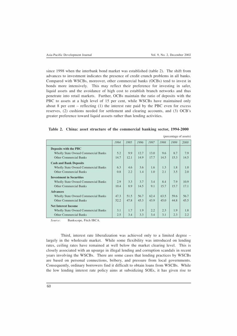
Asia-Pacific Development Journal Vol. 9, No. 2, December 2002
60
since 1998 when the interbank bond market was established (table 2). The shift fromadvances to investment indicates the presence of credit crunch problems in all banks.Compared with WSCBs, moreover, other commercial banks (OCBs) tend to invest inbonds more intensively. This may reflect their preference for investing in safer,liquid assets and the avoidance of high cost to establish branch networks and thuspenetrate into retail markets. Further, OCBs maintain the ratio of deposits with thePBC to assets at a high level of 15 per cent, while WSCBs have maintained onlyabout 8 per cent – reflecting (1) the interest rate paid by the PBC even for excessreserves, (2) cushions needed for settlement and clearing accounts, and (3) OCB’sgreater preference toward liquid asssets rather than lending activities.
Table 2. China: asset structure of the commercial banking sector, 1994-2000
(percentage of assets)
1994 1995 1996 1997 1998 1999 2000
Deposits with the PBCWholly State Owned Commercial Banks 5.2 9.9 12.7 13.0 9.6 8.7 7.9Other Commercial Banks 14.7 12.1 14.9 17.7 14.5 15.3 14.5
Cash and Bank DepositsWholly State Owned Commercial Banks 6.3 4.6 3.6 1.6 1.3 1.8 1.0Other Commercial Banks 0.8 2.2 1.4 1.0 2.1 3.5 2.0
Investment in SecuritiesWholly State Owned Commercial Banks 2.9 3.3 3.7 3.4 8.4 7.9 10.9Other Commercial Banks 10.4 8.9 14.5 9.1 15.7 15.7 17.1
AdvancesWholly State Owned Commercial Banks 47.3 51.5 56.7 62.4 63.5 59.6 56.7Other Commercial Banks 52.2 47.8 45.3 43.9 45.0 44.8 45.5
Net Interest IncomeWholly State Owned Commercial Banks 3.1 1.7 1.9 2.2 2.3 1.9 1.8Other Commercial Banks 2.5 3.4 3.3 3.4 3.1 2.3 2.2
Source: Bankscope, Fitch IBCA.
Third, interest rate liberalization was achieved only to a limited degree –largely in the wholesale market. While some flexibility was introduced on lendingrates, ceiling rates have remained at well below the market clearing level. This isclosely associated with an upsurge in illegal lending and corruption scandals in recentyears involving the WSCBs. There are some cases that lending practices by WSCBsare based on personal connections, bribery, and pressure from local governments.Consequently, ordinary borrowers find it difficult to obtain loans from WSCBs. Whilethe low lending interest rate policy aims at subsidizing SOEs, it has given rise to

Asia-Pacific Development Journal Vol. 9, No. 2, December 2002
61
collusive behaviour among financial institutions despite the penalties faced. The factthat black markets exist and their prevailing lending interest rates are two to threetimes higher than those of regulated lending rates indicates that banks have strongincentives to lend at higher lending rates. Deposit interest rates have remained regulatedand banks have continued to be protected by relatively wide interest rate margins.PBC’s continuation to control official lending and deposit interest rates prevents WSCBsfrom operating according to market principles. Given that banks are able to obtaincheap financing through deposits, interest rate deregulation in the wholesale market isexpected to exert a minimum impact on banks’ behaviour.
Fourth, banks’ decisions to allocate resources are still subject to guidanceand interference from the central Government, even though intervention by localgovernments in banks’ allocation of credit has declined. Given that the Governmentcontinues to face high credit demand for infrastructure projects and development inthe western region, the implicit and explicit influence by the central Government onWSCBs is likely to remain in the foreseeable future. Fifth, recapitalization of WSCBsand transfer of their NPA to the AMCs have been conducted without major reforms inthe corporate governance of these banks and removal of central Governmentintervention. Thus, there are no guarantees that NPA of WSCBs will not increase inthe near future. Even though Y1.4 trillion of NPA was transferred to the AMCs, thefour WSCBs still held 26.6 per cent of NPA as of the end of September 2001. Ifproper accounting methods were applied, moreover, it is believed all WSCBs wouldhave a negative net worth and thus would have been categorized as insolvent.
Between banking sector reforms in India and China, there are thus severalsimilarities. Both countries lowered the statutory reserve requirement. The sequenceof interest rate deregulation was similar: initiated in the wholesale market first,followed by an introduction of flexibility in the lending rates. Both countries madeefforts to mitigate directed lending. Entry deregulation was reformed and prudentialregulations and supervision were improved. The Government attempted to restructurestate-controlled commercial banks through recapitalization programmes in bothcountries.
II. BANKING SECTOR PERFORMANCE IN INDIA AND CHINA
Based on an overview of the two countries’ banking sector reforms, thissection examines developments in the commercial banking sector of each country byevaluating changes in performance in the sector.
Profitability, earnings- and cost-efficiency
India: Foreign banks’ profitability (defined as after-tax profits divided byreturn on average assets [ROA]) exceeded that of public sector banks in 1993-1997(table 3). New private sector banks’ ROA also exceeds that of public sector banks
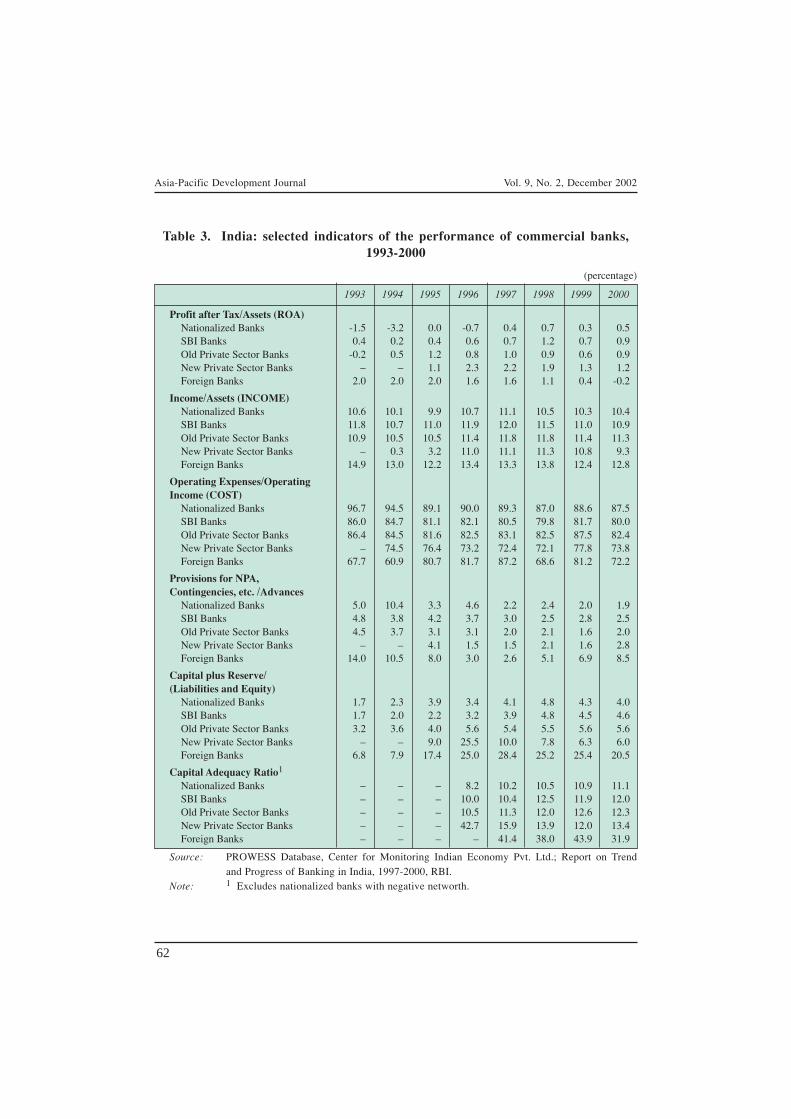
Asia-Pacific Development Journal Vol. 9, No. 2, December 2002
62
Table 3. India: selected indicators of the performance of commercial banks,1993-2000
(percentage)
1993 1994 1995 1996 1997 1998 1999 2000
Profit after Tax/Assets (ROA)Nationalized Banks -1.5 -3.2 0.0 -0.7 0.4 0.7 0.3 0.5SBI Banks 0.4 0.2 0.4 0.6 0.7 1.2 0.7 0.9Old Private Sector Banks -0.2 0.5 1.2 0.8 1.0 0.9 0.6 0.9New Private Sector Banks – – 1.1 2.3 2.2 1.9 1.3 1.2Foreign Banks 2.0 2.0 2.0 1.6 1.6 1.1 0.4 -0.2
Income/Assets (INCOME)Nationalized Banks 10.6 10.1 9.9 10.7 11.1 10.5 10.3 10.4SBI Banks 11.8 10.7 11.0 11.9 12.0 11.5 11.0 10.9Old Private Sector Banks 10.9 10.5 10.5 11.4 11.8 11.8 11.4 11.3New Private Sector Banks – 0.3 3.2 11.0 11.1 11.3 10.8 9.3Foreign Banks 14.9 13.0 12.2 13.4 13.3 13.8 12.4 12.8
Operating Expenses/OperatingIncome (COST)
Nationalized Banks 96.7 94.5 89.1 90.0 89.3 87.0 88.6 87.5SBI Banks 86.0 84.7 81.1 82.1 80.5 79.8 81.7 80.0Old Private Sector Banks 86.4 84.5 81.6 82.5 83.1 82.5 87.5 82.4New Private Sector Banks – 74.5 76.4 73.2 72.4 72.1 77.8 73.8Foreign Banks 67.7 60.9 80.7 81.7 87.2 68.6 81.2 72.2
Provisions for NPA,Contingencies, etc. /Advances
Nationalized Banks 5.0 10.4 3.3 4.6 2.2 2.4 2.0 1.9SBI Banks 4.8 3.8 4.2 3.7 3.0 2.5 2.8 2.5Old Private Sector Banks 4.5 3.7 3.1 3.1 2.0 2.1 1.6 2.0New Private Sector Banks – – 4.1 1.5 1.5 2.1 1.6 2.8Foreign Banks 14.0 10.5 8.0 3.0 2.6 5.1 6.9 8.5
Capital plus Reserve/(Liabilities and Equity)
Nationalized Banks 1.7 2.3 3.9 3.4 4.1 4.8 4.3 4.0SBI Banks 1.7 2.0 2.2 3.2 3.9 4.8 4.5 4.6Old Private Sector Banks 3.2 3.6 4.0 5.6 5.4 5.5 5.6 5.6New Private Sector Banks – – 9.0 25.5 10.0 7.8 6.3 6.0Foreign Banks 6.8 7.9 17.4 25.0 28.4 25.2 25.4 20.5
Capital Adequacy Ratio1
Nationalized Banks – – – 8.2 10.2 10.5 10.9 11.1SBI Banks – – – 10.0 10.4 12.5 11.9 12.0Old Private Sector Banks – – – 10.5 11.3 12.0 12.6 12.3New Private Sector Banks – – – 42.7 15.9 13.9 12.0 13.4Foreign Banks – – – – 41.4 38.0 43.9 31.9
Source: PROWESS Database, Center for Monitoring Indian Economy Pvt. Ltd.; Report on Trendand Progress of Banking in India, 1997-2000, RBI.
Note: 1 Excludes nationalized banks with negative networth.

Asia-Pacific Development Journal Vol. 9, No. 2, December 2002
63
during 1995-2000. However, the profitability of foreign and new private sector bankshas shown a declining trend from the middle of 1990s, in part because of the entry ofnew banks, establishment of new branches, and expansion of business during thisperiod. By contrast, both nationalized and SBI banks have improved their profitabilityin the latter half of the 1990s.
However, caution should be exercised particularly with regard to the improvedperformance of the nationalized banks, since profits of nationalized bonds includeincome from recapitalized bonds. ROA of nationalized banks was only 0.03 per centin 1997, 0.05 per cent in 1998, -0.15 per cent in 1999, and 0.01 per cent in 2000,if income from recapitalized bonds were to be excluded. The ROA excludingincome from recapitalized bonds has remained low and has even deteriorated during1997-2000. This suggests that the improvement in the performance of nationalizedbanks is attributable to holdings of recapitalization bonds, not so much because oftheir efforts to restructure their management and governance systems. On the otherhand, the improvement of the performance of SBI banks, all of which did not getrecapitalized, may reflect an improvement of their management and governance.Overall, a decline in net interest income lowered banks’ ROA, but the decline wasoffset mainly by an increase in income from investment and profits from diversification(defined as income arising from securities and foreign exchange transactions, andcommissions and brokerage).
As for earnings efficiency (defined as income divided by assets or INCOME),foreign banks have been generally better performers. According to INCOME, foreignbanks have consistently performed better than private sector and public sector banks,although foreign banks’ income generating capacity deteriorated somewhat from15 per cent in 1993 to 12.8 per cent in 2000. The poorer performance of domesticbanks relative to foreign banks can be attributed to more stringent requirements imposedon domestic banks with respect to advances to priority sectors, greater Governmentintervention, concentration on the retail market and hence greater competition, poormanagement, and lower interest rate margins. Further, foreign and new private sectorbanks are generally more cost-efficient (defined as operating expenses divided byoperating income or COST) than public sector banks. However, foreign banks havedeteriorated in cost-efficiency during 1995-1997 and 1999, because of expansion ofbusiness. Indeed, nationalized banks and SBI have improved cost-efficiency over thesample period.
China: WSCBs have maintained profitability at a very low level – below0.2 per cent throughout 1994-2000 (table 4). This level of profitability (measured byROA) is remarkably small, especially when compared with OCBs, which achievednearly 2 per cent profitability in 1994-1995. Meanwhile, it should be noted thatOCBs’ profitability has rapidly deteriorated from 1.8 per cent in 1994 to 0.6 per centin 2000 – as against WSCBs, whose profitability has improved slightly in 2000.

Asia-Pacific Development Journal Vol. 9, No. 2, December 2002
64
Interest income is the major source of income, accounting for more than90 per cent of income. Although interest income includes income from investment,the major source of interest income is from advances. This is in sharp contrast toIndian banks, whose income sources are more diversified and interest income fromadvances accounts for only about 50 per cent of income. According to the net interestincome ratio (net interest income divided by average assets), OCBs’ net interest incomeratio has consistently exceeded that of the WSCBs during 1995-2000. This mayreflect the fact that OCBs are more conscious of returns and risk than WSCBs andthus charge higher lending rates that are allowed within the ceiling. However, netinterest income has declined for the OCBs during 1998-2000 and the WSCBs during1999-2000, contributing to a decline in profitability. This happened even thoughinterest rate spreads expanded during this period. This may reflect a delay in interestrate payments on bank loans by borrowers as well as a cautious attitude toward newbank loans and refinancing previous loans. With respect to profitability related tonon-interest income (such as commissions and income from trading), OCBs haveconstantly obtained more returns from non-traditional services than WSCBs. Thus, itcan be said that OCBs have diversified more successfully than WSCBs, even thoughgreater diversification is limited by the Commercial Bank Law.
Table 4. China: selected indicators of the performance of commercial banks,1994-2000
(percentage)
1994 1995 1996 1997 1998 1999 2000
Profit after Tax/Average Assets (ROA)Wholly State Owned Commercial Banks 0.1 0.2 0.1 0.1 0.1 0.1 0.2Other Commercial Banks 1.8 1.7 1.6 1.4 1.2 0.8 0.6
Income/Assets (INCOME)Wholly State Owned Commercial Banks 16.0 12.6 11.2 12.4 6.2 5.0 4.4Other Commercial Banks 6.8 8.3 8.1 8.3 6.3 4.9 3.9
Operating Expenses/Operating Income (COST)Wholly State Owned Commercial Banks 85.9 70.2 69.3 67.5 79.9 78.7 77.0Other Commercial Banks 45.1 43.8 59.9 49.9 56.9 63.6 66.1
Capital plus Reserve/(Liabilities and Equity)Wholly State Owned Commercial Banks 3.5 3.3 3.0 3.2 5.8 5.4 5.3Other Commercial Banks 8.8 6.4 8.2 6.8 9.5 8.4 5.3
Loan Loss Reserves/LoansWholly State Owned Commercial Banks 0.5 1.1 0.9 0.7 0.8 1.2 1.0Other Commercial Banks 0.6 0.7 0.9 1.3 1.6 1.7 1.4
Source: Bankscope, Fitch IBCA.
Asia-Pacific Development Journal Vol. 9, No. 2, December 2002
65
As for the indicator of earnings efficiency proxied by INCOME, WSCBshave performed better than OCBs during 1994-1997. However, the difference wassmall during 1998-2000. Earnings-efficiency of both types of banks has deterioratedin recent years. With respect to the indicator of cost-efficiency proxied by COST,OCBs have been more cost-efficient than WSCBs throughout the reform period.However, OCBs’ cost-efficiency deteriorated in 1998-2000, while that of the WSCBsimproved slightly in 1998-2000. The increase in COST by OCBs during 1998-2000reflects mainly an increase in operating expenditure, such as personnel expenditure.The increase in personnel expenditure is attributable to staff wage rises andan expansion of employment as the number of branches and offices rose.
Capital, asset quality, management and liquidity
India: The overall soundness of the banking sector is assessed from fouraspects: capital adequacy, asset quality, management, and liquidity. In the case ofthe capital adequacy ratio, two indicators were used: equity plus reserves over assetsand risk-weighted capital adequacy ratio. According to the first indicator, the ratio offoreign banks increased from 7 per cent in 1993 to 21 per cent in 2000 (table 3). Interms of the risk-weighted capital adequacy ratios, foreign banks have maintained theratios above 30 per cent during 1997-2000, albeit at a decelerating trend. These ratiosare significantly high not only from the global standard but also compared with otherdomestic banks. While these indicators have reported an increasing trend for oldprivate sector and public sector banks, the scale of increase has been small. Thissuggests that foreign banks have greater incentives to lend prudently and remainwell capitalized than other banks. This reflects in part that foreign banks have steadilyreduced their deposit dependence ratio, while other banks have maintained theirdeposit-dependence ratio throughout the sample period.
Asset quality can be measured by (1) the ratio of contingent liabilities toassets, (2) asset growth, (3) the ratio of investment in Government securities to assets,and (4) the ratio of provisions for NPA to assets. The first indicator reports that theratio of foreign banks (at around 25-30 per cent) has been greater than that of privateand public sector banks (about 10 per cent). While this indicates that foreign banksare more exposed to high potential losses in cases of default, this outcome may simplyreflect that foreign banks provide more complex and sophisticated services thandomestic banks, given that their activities are concentrated in urban areas, wholesalemarkets and large clients. The second indicator reports that foreign banks (about30 per cent) and new private sector banks (about 100 per cent) have faced rapid assetgrowth in 1996-2000 compared with other banks (about 20 per cent), signaling somekind of risk-taking behaviour. However, this may be explained simply by their earlystage of establishment, not necessarily by risk-taking behaviour. The third indicatorshows that all banks invested about 40 per cent of assets in Government securities,

Asia-Pacific Development Journal Vol. 9, No. 2, December 2002
66
which can be used as a large cushion against NPA. The fourth indicator reports thatforeign banks generally allocated greater provisions for NPA. Given that more stringentaccounting and auditing standards of their mother countries are applied to foreignbanks, foreign banks are more resilient to adverse shocks.
With respect to management performance, the ratio of advances to depositswas used. Foreign banks attempt to improve their income by expanding their lendingoperations as compared with other domestic banks. The ratio of foreign banks surgedfrom 56 per cent in 1993 to 94 per cent in 2000, while domestic banks maintained theratio at about 40 per cent over the same period. Given that foreign banks’ ratio ofadvances to assets is similar to other domestic banks (about 40 per cent of assets),this simply suggests that foreign banks lowered the deposit dependency ratio, as pointedout above. Finally, all banks have to maintain sufficient liquidity in terms of cashand balance with banks and the RBI and investment in Government securities,suggesting that they are relatively resilient to systemic banking crises.
China: As measures of soundness, the following four indicators were adopted:capital and reserves divided by assets, loan loss reserves as a share of loans, assetgrowth, and liquidity ratio. With respect to the first indicator, OCBs were morecapitalized than WSCBs in 1994-1999 (table 4). Although WSCBs have increasedcapital from 3.5 per cent of assets in 1994 to 5.3 per cent in 2000, the improvementhas been modest. In addition, OCBs had greater loan loss reserves as a share of loansthan WSCBs in 1997-2000. Even though regulations require banks to set aside only1 per cent of their outstanding credit, this suggests that OCBs have tended to putaside more provisions than WSCBs. As for asset growth, OCBs (44 per cent) werehigher than WSCBs (12 per cent), but like Indian banks, this could be attributed tothe entry of new banks. OCBs also held more liquid assets (proxied as deposits withthe PBC divided by customer deposits) than WSCBs in 1997-2000. In particular,OCBs tended to hold excess reserves during 1998-2000, even after the reserverequirement sharply dropped from 20 per cent in 1993 to 8 per cent in 1998 and to6 per cent in 1999. Moreover, the sum of deposits with PBC and bank depositsdivided by assets shows that OCBs held more liquid assets (about 16 per cent) thanWSCBs (about 10 per cent) during 1998-2000.
Comparison between India and China
There are several common features with respect to the banking sectors inIndia and China. First, in both state-controlled banks are dominant financial institutions.This phenomenon has not changed despite banking sector reforms adopted in bothcountries. While the number of public sector banks is greater in India than in China,the largest public sector bank, the SBI, accounts for over 20 per cent of deposits orassets in India, suggesting that the banking sector is oligopolistic. While Governmentinvolvement in the banking sector can be justified at the initial stage of economic

Asia-Pacific Development Journal Vol. 9, No. 2, December 2002
67
development, the prolonged presence of excessively large public sector banks oftenresults in inefficient resource allocation and concentration of power in a few banks.Further, once entry deregulation takes place, it will put newly established banks in anextremely disadvantageous position.
Second, foreign and private sector banks generally performed better thanpublic sector banks in terms of profitability in India. In China, OCBs were betterperformers than WSCBs. This suggests that state-controlled banks were generallypoor performers than non-state-controlled banks in both countries, suggesting the needfor restructuring state-controlled banks and at the same time promoting the entry ofnew banks. Nevertheless, it should be pointed out that this superiority of non-state-controlled banks was pronounced particularly in the initial reform stage in bothcountries.
Third, foreign banks have been more capitalized and more provisioned thanother banks in India. Similarly, in China, OCBs have been more capitalized and moreprovisioned. This suggests that the balance sheets of state-controlled banks are lesssound than non-state-controlled banks in both countries. Fourth, banks in India andChina have displayed a tendency to increase holdings of Government bonds in recentyears. This has happened in India even though the SLR declined. In China, there isno statutory liquidity requirement applied to Government bonds, but preference towardinvestment in securities was pronounced.
Fifth, both public sector banks as well as other banks in India have reducedthe share of deposits with the RBI in assets, in line with a decline in the CRR.Instead, these banks have increased investment in Government bonds and have doneso even by lowering advances. Similarly, WSCBs in China have lowered the share ofdeposits with the RBI in assets during 1998-2000 in line with a decline in the reserverequirement (to a lesser extent for OCBs). These banks have instead increasedinvestment in securities and has done so even by lowering the share of advances inassets. This suggests that there may be some cases of crowding out the private sector.Indeed, both countries have informal credit markets, where credit is expended byunregulated non-bank financial institutions at substantially higher rates.
Sixth, WSCBs are not illiquid and they are able to operate in practice despitethe weak structure of their balance sheets. This is because households have increasinglydeposited their savings at these banks believing that they are protected by the centralGovernment, which retains full ownership. Also, the underdeveloped state of thefinancial markets has left households no other choice but to save in banks orGovernment bonds. In India, many public sector banks in India have improved theirperformance and have been competing with small savings schemes, provident fundsystems, and the capital market. However, like China, there are still a few weakpublic sector banks and they continue to remain operational. This reflects the publicperception that public sector banks are protected by the Government and are thussafer than private sector banks.

Asia-Pacific Development Journal Vol. 9, No. 2, December 2002
68
Despite these similarities, there are clear differences in terms of performancebetween the two countries. First, public sector banks in India have improved theirperformance measured by profitability and cost-efficiency, and their differencescompared with private sector and foreign banks have diminished over the reformperiod. On the other hand, there was no sign of improvement with respect toprofitability; indeed, there was a decline in earnings-efficiency for WSCBs in China.Moreover, even though WSCBs improved cost-efficiency during 1994-1997, thecost-efficiency has since deteriorated.
Second, the decline in the difference with respect to profitability andcost-efficiency between public sector banks and other banks in India has emerged asa result of an improvement of performance of public sector banks and a deteriorationof performance of foreign and new private sector banks. On the other hand, thedecline in the difference with respect to profitability between WSCBs and OCBs inChina has occurred as a result of a deterioration of performance of OCBs. In themeanwhile, the decline in the difference as for cost-efficiency has happened as WSCBsimproved cost-efficiency while OCBs worsened it. These observations suggest thatthere was a non-negligible impact of the reforms on the performance of public sectorbanks in India (although caution has to be exercised on the interpretation of nationalizedbanks’ performance, as indicated above), while no clear impact of reforms was observedwith respect to the performance of WSCBs in China.
Third, the banking sector reforms have not generated a noticeable improvementin the soundness of WSCBs. Their capital adequacy and loan loss provisions haveremained low. Paid-in capital (comparable to Tier-1) of WSCBs declined relative tobank assets from 12.1 per cent at the end of 1985 to 2.2 per cent at the end of 1997(Lardy, 1999). Meanwhile, the soundness of public sector banks in India has improvedespecially based on the risk-weighted capital adequacy ratio and greater capitalizationover the period.
Fourth, WSCBs continue to be agents of the central Government. Althoughexplicit policy lending practices have been reduced, lending to SOEs still constitutesa large share of WSCBs’ credit. Credit decisions by WSCBs are often influenced bycentral Government guidance. While banks in India are subject to priority sectorlending requirement, the negative impact of this policy lending was reduced throughexpanding the defnition of priority sector lending and liberalizing interest rates onadvances over Rs 200,000. Banks are allowed to choose sectors and projects withmore flexibility under the target and sub-target requirements. While domestic banksare often asked to extend credit to specific individuals and projects under lendingrequirement to the weaker sections, this share accounts for only 10 per cent of advances.
Asia-Pacific Development Journal Vol. 9, No. 2, December 2002
69
III. LESSONS FROM INDIA’S EXPERIENCE
This section focuses on six issues related to India’s banking sector reformsand identifies lessons that could be obtained from them and be applied to China’sfuture reform agenda.
Privatization
The Indian Government did not engage in a drastic privatization of publicsector banks. Rather, it chose a gradual approach toward restructuring these banks byenhancing competition through entry deregulation of foreign and domestic banks. Thisreflects the view of the Narasimham Committee that ensuring integrity and autonomyof public sector banks is the more relevant issue and that they could improveprofitability and efficiency without changing their ownership if competition is enhanced.
Since this approach was introduced, some criticisms have been expressed(Joshi and Little, 1996). First, public sector banks continue to be dominant thanks totheir better branch coverage, customer base and knowledge of the market comparedwith newcomers. Second, public sector banks would find it more difficult to reducepersonnel expenditure because of the strong trade unions. Third, the Governmentwould find it difficult to accept genuine competition within public sector banks. Inresponse to these concerns, the Government decided to gradually expand private sectorequity holdings in public sector banks, but still avoided the transformation of theirownership. However, many public sector banks have remained fully or largely ownedby the Government.
Meanwhile, a consensus is emerging among academicians that state ownershipof banks is bad for financial sector development and growth (World Bank, 2001).Based on data of the 10 largest commercial and development banks in 92 countriesfor 1970-1995, La Porta and others (2000) have found that greater state ownership ofbanks in 1970 was associated with less financial sector development, lower growth,lower productivity and that these effects were greater at lower levels of income.Barth and others (2001) have shown that greater state ownership of banks tends to beassociated with higher interest rate spreads, less private credit, less activity on thestock exchange and less non-bank credit, even after taking into account other factorsthat could influence financial development. This suggests that greater state ownershiptends to be anti-competitive, reducing competition both from banks and non-banks.Barth and others (2001) have also noted that applications for bank licenses are moreoften rejected and there are fewer foreign banks when state ownership is greater.Moreover, Caprio and Martinez-Peria (2000) have shown that greater state ownershipat the start of 1980-1997 was associated with a greater probability of a banking crisisand higher fiscal costs.
Asia-Pacific Development Journal Vol. 9, No. 2, December 2002
70
With respect to privatizing banks, the World Bank (2001) takes the view thatprivatization can yield real benefits to economies provided that an appropriateaccounting, legal and regulatory infrastructure is in place. It should be noted thatpremature privatization may give rise to banking crises. Clarke and Cull (1998) havedemonstrated that Argentina promoted privatization of public sector banks ina reasonably developed regulatory and infrastructure environment, and thus, privatizedbanks improved productivity remarkably.
Based on panel data, Shirai (2002a) has reported the results of regressionestimation that India’s privatization has not produced any significant impact onimproving the performance of public sector banks. Partial privatization has notimproved their corporate governance so far through greater shareholder supervision.This is partly because individual voting rights have remained limited by rules toa maximum of 10 per cent, and partly because the share of the public sector (centralGovernment or the RBI) has remained large. While privatization of viable publicsector banks should be promoted further, information, legal, and judiciary infrastructurethat is needed for developing a sound capital market should be strengthened. Mereprivatization without institutional changes, where external shareholders and independentboards of directors cannot practice corporate governance properly, will not producea favourable impact on the performance of partially privatized public sector banks.
In addition, the Government of India is of the view that the public sectornature of nationalized banks should continue even if the Government stake drops tothe proposed 33 per cent (Raje, 2000). To improve the performance of public sectorbanks, the Government should alter this view and transform public sector banks topurely commercial-oriented banks with greater autonomy with respect to operationsand human resources policies. This is particularly so if it wishes that these bankscould become more profitable and efficient, thereby being able to compete with privatesector and foreign banks in a level playing field and lowering their dependence onGovernment financial support. Moreover, the board of directors should be reformedby increasing the number of competent external directors, guaranteeing independenceof the board from Government and political interference, improving accounting anddisclosure standards and strengthening minority shareholders’ rights. It is importantto ensure a clear separation of management and ownership. The improvement ofcorporate governance in the banking sector would also help increase the price ofinitial public offerings and hence promote privatization.
Entry deregulation
Imposing entry barriers in the banking sector often gives rise to an inefficientresource allocation across sectors and projects and, at the same time, collusive behaviouramong creditor banks and between banks and borrowers. On the other hand, sucha policy can be justified theoretically if it improves banking sector efficiency, provided
Asia-Pacific Development Journal Vol. 9, No. 2, December 2002
71
that commercial banks perform a unique role that cannot be undertaken by non-bankfinancial institutions and capital markets. Commercial banks collect, analyze andprocess internal information about borrowers by forming long-term relationships withthem. With these skills and expertise, banks are able to finance SMEs whoseinformation is largely idiosyncratic (Yoshitomi and Shirai, 2001). Information heldby banks can be idiosyncratic and non-transferable, but cannot and/or need not bestandardized – whereas standardization of information about issuing firms is necessaryfor corporate securities. These features of banks are important especially whendisclosure, auditing, and accounting requirements are loosely or inadequatelyimplemented against borrowers, in the absence of sophisticated legal and institutionalinfrastructures.
This may explain partly why the banking system is likely to dominate at theearly stage of economic development. Further, Rajan and Zingales (1998) have pointedout that in countries where corporate governance is inadequate and bankruptcy lawsare virtually non-existent, the specific expertise of commercial banks – which knowhow to exercise power over borrowers even when explicit protections for the banksare inadequate – is necessary when extending loans to firms. They have alsodemonstrated the existence of a negative correlation between the degree ofsophistication of accounting standards and the size of the banking sector.
When bank regulators determine entry criteria they need to ensure thatcommercial banks have an incentive to perform their information collecting andmonitoring functions. To do so, bank regulators need to balance between allowingbanks to maintain profitability (or earn economic rents that offset risks borne bybanks in the process of providing various financial services) by limiting the entry ofnew banks and preventing them from extracting excessive rents by encouraging theentry. Without sufficient rents, banks may have no choice but to engage in riskyactivities because they need to fight for their market shares or profit margins. Asa result, such risk-taking behaviour would reduce the value of banks’ future earningsand associated incentives to avoid bankruptcy (Allen and Gale, 2000). To maintainsufficient profitability in the banking process, therefore, excessive competition amongbanks needs to be avoided through granting a relatively small number of them theprivilege of offering demand deposits and payment services (Rajan, 1997).
While attempting to maintain adequate rents for banks, nevertheless, regulatorsneed to introduce measures to prevent banks from engaging in excessive risk-takingbehaviour and extracting rents from their borrowers more than is justified by risksthat they bear. Otherwise, borrowers are discouraged from undertaking innovative,profitable ventures, thereby resulting in slower economic growth (Rajan, 1992). Thus,regulators need to carefully consider the extent of competition in the banking sectorby taking account of the trade offs and supplement this policy with other prudentialmeasures, such as capital adequacy requirements, that contribute to limiting excessiverisk-taking by banks.

Asia-Pacific Development Journal Vol. 9, No. 2, December 2002
72
The analysis in section III has indicated that in India, foreign and new privatesector banks were more profitable than public sector banks initially, although theirprofitability has deteriorated in recent years. Based on INCOME and COST indicators,foreign and private sector banks were relatively earnings- and cost-efficient in earlierperiods, but public sector banks have gradually improved their performance in thereform period. This suggests that the performance of public sector banks has becomecomparable to the foreign and private sectors. These results show that ownershipmattered initially in terms of performance differentials, but became less so in the laterpart of the reform period. In other words, entry deregulation has exerted some pressureon public sector banks and has encouraged them to perform better (however, cautionshould be exercised for nationalized banks with respect to this statement since anincrease in their profits comes largely from interest income from recapitalization bonds).
Furthermore, despite entry deregulation, public sector banks have remaineddominant. The SBI, the largest public sector bank, has even increased its share bothin terms of deposits and assets. Given that public sector banks have scale advantageswith nation-wide branch networks (especially as compared with private sector banksthat tend to compete in the retail market), the current approach of improving theirperformance without rationalizing weak public sector banks and downsizing largepublic sector banks may not produce further and substantial benefits for India’s bankingsector. Furthermore, new banks continue to be prevented from competing on thesame level playing field. This would encourage new banks to enter into differentsegments of markets such as niche or wholesale markets, thereby exerting lesscompetitive pressure on existing dominant public sector banks.
Liquidity requirements
Imposing statutory liquidity requirement may be necessary as a policy todevelop a Government bond market. The Asian Policy Forum (2001) has pointed outthat over-dependence on bank-based financing and the underdeveloped state of bondmarkets in Asia have significant adverse implications, such as lack of measurementof the opportunity cost of capital, inefficient use of high savings and excessiveshort-term debt. The development of a local currency-denominated bond market canprovide stable sources of longer-term local currency funding, in the process of helpingto reduce a double mismatch and strengthen financial sector resilience. Moreover,bond markets help to improve the efficiency of resource allocation throughmarket-determined interest rates; spread various borrowers’ credit and market risksamong a large number of dispersed investors; and, serving as a buffer when bankingsector problems occur. Development of a Government bond market is a prerequisitefor developing a corporate bond market. In addition, investment in Governmentsecurities could help to lower the share of high risk-weighted assets and would thusimprove the capital adequacy and liquidity ratios.
Asia-Pacific Development Journal Vol. 9, No. 2, December 2002
73
On the other hand, the diversion of financial resources away from lendingactivities owing to the SLR requirement may increase banks’ cost of operations fromthese activities. This is because banks may be able to reduce the costs of collectingand evaluating information regarding creditworthiness of their borrowers througheconomies of scale. The economies of scale occur in the presence of the fixed cost ofhiring professional staff with special expertise in loan evaluation. Also, the economiesof scale arises from banks’ provision of settlement and checking accounts and otherfinancial services to their borrowers, which gives them an opportunity to monitor theeconomic activities and cash flow movements of their borrowers. Moreover, largeholdings of Government securities may crowd out the private sector. Shirai (2002a)has found that in India, investment in Government securities has tended to lower theperformance of the whole banking sector. The regression estimation has found thatthis investment has affected adversely banks’ profitability (based on ROA) and costefficiency (based on COST).
Based on these factors, the statutory liquidity requirement should not bedismissed. Rather, it might be used not only as a policy to promote the developmentof a Government bond market, but also as a policy to strengthen banks’ ability tomanage with various shocks. However, as the Government bond market develops andbanks’ risk management improves, a reduction of the requirement should be considered.Large holdings of Government bonds, as is the case of banks in India, may not helpthem to improve their risk management in lending activities and give an incentive tobanks in processing and evaluating information about borrowers and monitoring them.
Directed and subsidized lending
India’s Government has attempted to mitigate the adverse impact of directedlending on banks’ performance by expanding the coverage and gradually liberalizinglending interest rates on advances over Rs 200,000. Thus, the adverse impact ofpriority sector lending is expected to decline over the period and to contribute toimproving banks’ performance. Meanwhile, banks continue to be asked to extendcredit to weaker sections, frequently to particular individuals and projects.Shirai (2002a) has reported regression estimation results that while priority sectorlending has contributed to improving cost-efficiency (measured by COST) andearnings-efficiency (measured by INCOME), it has lowered the profitability of publicsector banks, calling for a further reform in priority sector lending.
Also, the current practice of setting lending interest rates below the PLR foradvances less than Rs 2,000,000 appears problematic. Banks should be allowed to setlending interest rates more flexibly by considering returns and risk of each project.The practice of setting below-PLR lending rates indicates the presence of subsidizedlending by banks, making it difficult for banks to improve their performance further.This is particularly so when the Government does not provide explicit compensation

Asia-Pacific Development Journal Vol. 9, No. 2, December 2002
74
for this type of lending. Such lending, if performed by commercial banks, should beexercised at market terms and at banks’ initiatives. In the long run, the Governmentof India should reform existing state-controlled development banks and other financialinstitutions and transfer all policy lending activities to these finiancial institutions. Itis important to ensure a separation of commercial lending and policy lending, whichwould be a prerequisite for enhancing banks’ accountability and management skills.
Scope of business
Financial conglomeration gives banks an opportunity to gain non-interestincome, thereby sustaining profitability. This enables banks to maintain long-termrelationships with clients throughout their life cycles and thus gives them an incentiveto collect and produce internal information and monitor them. Such practices lowerbanks’ incentives to take excessive risks. Also, banks can obtain diversification benefitsby diversifying their activities whose returns are imperfectly correlated, therebystabilizing their profitability. This in turn cuts the costs banks charge their lendingand underwriting customers. Close multi-dimensional relationships between banksand firms can reduce the costs of obtaining funds for firms, improve their performance,make investment decisions less dependent on retained earnings, and make it easier forfirms to resolve financial distress (Yoshitomi and Shirai, 2001).
Financial conglomeration also promotes efficiency by allowing banks to utilizeinternal information. Through long-term lending relationships, banks already possessinternal information about creditworthiness of borrowers and features of theirinvestment projects that are not readily available to outsiders. Thus, banks do notneed to spend a great deal of resources in collecting information about their clientsthat is necessary for underwriting securities issued by them. So banks may be able tounderwrite securities at lower costs than non-bank underwriters. Firms issuinginformation-sensitive securities may receive higher prices when banks underwrite themthan when independent investment firms do so, because of perceived monitoringadvantages of the banks that are a by-product of their lending activities.
Thanks to reputation, moreover, investors may be willing to purchase securitiesunderwritten by bank underwriters rather than independent underwriters. To the extentthat it is easier to gain a reputation in some businesses than in others and to the extentthat there are spillovers in reputation, banks can use the reputation gained in offeringone service to recommend their other services (Rajan, 1996). Banks also enjoyeconomies of scope from the production of financial services. They can spread thefixed costs in terms of physical and human capital needed for managing a clientrelationship over a wider set of products (Steinherr and Huveneers, 1990). Economiesof scope can be exploited by using their branch networks and all their other existingdelivery channels to distribute additional products at low marginal cost (Llewellyn,1996). Also, banks can better handle the shifts in demand for the products they offerby quickly transferring resources within organizations.

Asia-Pacific Development Journal Vol. 9, No. 2, December 2002
75
These advantages, however, can be offset by the following disadvantages.First, public sector banks’ engagement in securities business may promotea concentration of power in the banking sector. This is partly because banks becometoo large and partly because banks have a natural tendency to promote lending oversecurities, thereby indirectly deterring the development of capital markets. Further,the reputation and informational advantages enjoyed by public sector banks put themin an even more advantageous position, preventing other banks and investment firmsfrom competing on a level playing field.
Second, banks’ engagement in underwriting services may lead to conflicts ofinterest between banks and investors. Banks may decide to underwrite securities fortroubled borrowers so that proceeds from the issue of securities can be used to pay offthese banks’ own claims to the companies. Banks may dump into the trust accountsthey manage the unsold part of the securities they underwrite. Further, banks mayimpose tie-in deals on customers by using their lending relationships with firms topressure them to purchase their underwriting services (e.g., using the threat of increasedcredit costs or non-renewal of credit lines). Banks may also use the confidentialinternal information that they possess when they underwrite firms’ securities in a waythat the firms do not contemplate, such as disclosing the information directly orindirectly to the firms’ competitors.
Third, diversification may expose banks to various new risks. For example,banks may end up buying the securities they underwrite. They may also face greatermarket risks as they increase their share of securities holdings and market makingactivities. Further, derivatives involve higher speed and greater complexity, whichmay reduce the solvency and transparency of banking operations.
Given this background, Shirai (2002a) has found that Indian banks’engagement in non-traditional activities and an increase in profits from these activitieshave contributed to improved banks’ performance based on profitability andcost-efficiency as well as the earnings-efficiency of the banking sector. In India,banks have been allowed to engage in diverse activities including securities and foreignexchange transactions, brokerage and dealing activities and other fee-based businesseven before the 1991 reform programmes have been launched. At the same time, theRBI is aware of problems arising from banks’ engagement in non-traditional businessand has tried to cope with them by encouraging banks to engage in this throughsubsidiaries, thereby putting in place firewalls between traditional banking and securitiesservices to some extent. The expansion of the scope of banks’ business has certainlyhelped offset a decline in net interest income from advances, driven by interest ratederegulation. This has an important policy implication for the sequencing of financialliberalization. Namely, regulators should introduce policy measures that wouldsupplement an expected decline in net interest income caused by interest rateliberalization, in order to prevent banks from taking excessive risks in an attempt tomaintain profitability.
Asia-Pacific Development Journal Vol. 9, No. 2, December 2002
76
In China, the Commercial Bank Law prohibited banks from engaging insecurities and related business activities in 1994 after the occurrence of the 1992-93chaos. In 1992, the Government permitted banks to transact some non-traditionalbanking business in 1992. Consequently, all the specialized banks and most of theirmajor branches were encouraged to establish finance companies, which engaged inimprudent or fraudulent operations and led to financial chaos in 1992-1993. Also,many of these banks divested funds earmarked for agriculture and other key projectsinto stock market and real estate market speculation. When monetary policy wastightened in late 1993, many banks and branches lost money from these securitiesactivities, causing instability in the banking system (Ma, 1997). Since then, theGovernment has required all banks to divest themselves of investment banking affiliatesand prohibited commercial banks from engaging in securities trading and underwriting,investment in non-bank financial enterprises and productive enterprises and investmenttrust business under the Commercial Bank Law.
Since 1998, WSCBs have begun to provide money-managing services,including personal investment to individual clients. These banks have since establishedmoney-management offices in major cities. In July 2001, the PBC issued a provisionalregulation on commercial banks’ intermediate business to promote business innovation,improve bank services and competitiveness, and reduce financial risks. The PBC hasdefined intermediate businesses as those that do not constitute scheduled assets andliabilities, and produce non-interest income for banks including settlement, warranty,acceptance and trading. Thus, with PBC’s ratification, commercial banks can engagein financial derivatives business, agency security business, investment bank business,information consultation and financial advisory services. Diversification of banks’business is likely to become an important component of the reform agenda in China,especially when the Government begins to promote further interest rate deregulation.However, it is important that regulators should implement necessary regulatory andlegal systems that are able to cope with problems arising from banks’ engagement innon-traditional business.
Connected lending
The RBI prohibits cross-holdings with industrial groups to minimize“connected lending” – one of the causes of the East Asian crisis. The BankingRegulation Act prohibits loans and advances to directors or to any firm or company inwhich directors are interested or individuals in respect of whom any of its directors isa partner or guarantor. In addition, banks are required to provide loans to their ownsubsidiaries or joint ventures on an arms-length basis. Banks’ investments insubsidiaries are deducted from their Tier I capital. Considering that connectedlending was one of the major problems causing excessive risk-taking by banks inAsian crisis-affected countries, it is appropriate for bank regulators in China to impose
Asia-Pacific Development Journal Vol. 9, No. 2, December 2002
77
this restriction from the beginning when entry deregulation has occurred. Once suchpractices are implemented, it is difficult to remove them later due to strong resistance,as is the case in a few East Asian countries.
IV. REMAINING AGENDA FOR CHINA
In China, the biggest constraint holding back drastic financial reforms arisesclearly from the problems of borrowers – namely, the poor and deterioratingperformance of SOEs. Growing numbers of SOEs have experienced a substantialdecline in profits in the 1990s in spite of overall economic growth. This has not onlycaused a rapid deterioration of WSCBs’ loan assets, but has also limited credit availableto non-state firms by absorbing more than 75 per cent of bank loans, deterringinvestment and output growth of non-state firms. About half of the SOEs incur netlosses nowadays, compared with only 30 per cent just a few years ago. Factorycapacity utilization rates for major industrial products of SOEs have been at a levelbelow 60 per cent.
The poor performance of SOEs is attributable to growing competition,slackening efficiency due to the slow adoption of technological advancement andlarge accumulated debt. Also, SOEs are obliged to provide social services to workersand maintain their employment and, in some cases, continue to pay a salary to retirees.These practices make it difficult for the SOEs to become commercially oriented(Broadman, 1999). Moreover, the absence of clear identification of owners of theSOEs and inadequate property rights undermine corporate governance since it is notclear who should monitor managers. Also, the introduction of non-state shareholdersthrough public listings has not resulted in a clear separation of ownership andmanagement, since few outside shareholders exercise discipline on the managementof the SOEs. In response to the rapidly deteriorating performance of SOEs, theGovernment attempted various experiments in the 1990s, including managementcontracting, providing greater autonomy to managers, corporatization and ownershipdiversification. Moreover, the supervisory capacity over most industrial SOEs (about110,000 firms) has been transferred from the central Government to local governments(Broadman, 1999). Also, a multilayered organizational network has emerged byincluding State asset management bureaus, State asset operating companies and Stateasset supervisory committees. Nevertheless, only a few SOEs have been divested tothe non-state sector and almost all of such firms have been small. It has also becomeincreasingly apparent that the SOE reform strategy has produced problems unanticipatedby the reform’s framers, including asset stripping, decapitalization, wage manipulationand tax evasion. These problems have severely undermined banking sectorperformance.
By contrast, such SOEs’ problems have been less pronounced in India, whichmakes it relatively easier for the Government to cope with banking sector restructuring.
Asia-Pacific Development Journal Vol. 9, No. 2, December 2002
78
In India, there are only about 300 SOEs at the central Government level, as comparedwith China with a few hundred thousand SOEs. Many of these firms have beenalready partially privatized since the early 1990s. Even during the planned economicdevelopment regime, there were already many private firms that operated across sectors.Thus, SOEs are not major borrowers of banks in India and, therefore, not the majorcause of NPA.
China’s second constraint acting against a smooth implementation of financialreforms is that the ownership of WSCBs has not changed and the intervention by thecentral Government in banks’ resource allocation remains. Aware that privatization ofthe WSCBs (as well as SOEs) is a key to successful financial reforms, the Governmentrecently announced that these banks would be gradually restructured by allowingthem to become joint-stock companies listed on the stock exchanges. Immediatelyafter the announcement, however, the stock prices of listed banks (and SOEs) plungedin the expectation that a massive disposal of stocks would lead to a decline in pricesand thus investors would experience a capital loss. In response, the Governmentreversed its decision by suspending state share sales. The PBC Governor, Mr DieXianglong, announced in November 2001 that WSCBs restructuring would be carriedout in several steps: (1) an improvement of management skills with a rationalizationof staff and organizations; (2) allowing WSCBs to become joint-stock companies withcentral Government holding more than 50 per cent of stock; and (3) encouraging themto list on the stock exchange. In addition, the Governor said that WSCBs would beallowed to sell shares to foreign investors.
In the case of India, public sector banks have been gradually and partiallyprivatized in the 1990s. Even though there is no significant impact of partialprivatization on the performance of public sector banks based on regression analysis,it has certainly increased pressure on the management of these banks. Moreover, allpublic sector banks used to be private sector banks prior to the nationalization andhence used to operate on a commercial basis. This makes it easier for public sectorbanks to improve their risk management skills and performance – a sharp contrast toChina, where there were no such private banks prior to the reforms.
The third constraint is that entry of private sector banks is limited. Moreover,other commercial banks need to be restructured through listing shares in stockexchanges and improving their corporate governance. So far, there are only fourpublicly listed commercial banks. Shirai (2002b) has reported that these listed bankshave not necessarily performed better than other banks. These banks have been lessprofitable (in terms of ROA) and less well capitalized than city banks. This suggeststhat the Government policy of approving listings is not necessarily based on theperformance of the bank and the approval process is not transparent.
In India, allowing the entry of private sector and foreign banks that are wellcapitalized and high technology-oriented has certainly increased competitive pressureson public sector banks. Also, all private sector banks are listed on stock exchanges

Asia-Pacific Development Journal Vol. 9, No. 2, December 2002
79
and managers of these banks are very conscious of their performance. The stockmarket in India has developed rapidly since the 1980s. There are about 10,000 listedcompanies and 22 stock exchanges. In 1992, the National Stock Exchange of Indiawas established in order to offer screen-based trading. In 1992, the Securities andExchange Board of India (SEBI) Act was introduced. Pror to 1992, the Controller ofCapital Issues (CCI) used to approve equity issuance based on the requirment ofa debt-equity ratio of 2 versus 1 (higher ratio for capital-intensive industries). Sharescould be issued only once a year. Since 1992, the CCI was abolished and SEBIbecame a special Government entity with the aim to protect investors and develop thecapital market. Foreign institutional investors were also allowed to enter primary andsecondary markets. Thus, the listing requirement is transparent and participation isopen to all private firms. Moreover, the accounting and disclosure standards havebeen strengthened in the 1990s.
The fourth constraint is that the balance sheets of WSCBs have remainedweak despite recapitalization and transfer of NPA to the AMCs. The Government ofChina needs to clean up and restructure the balance sheets of WSCBs more drasticallybefore they become public. Once NPA problems are resolved, the Government mustconsider how to strengthen the capital base of these banks. However, the absence ofsecondary markets for credit and collateral and inadequate property rights makes itdifficult to transfer, sell, or securitize WSCBs’ assets, since the market price of theassets can hardly be realized and the ratio of realized asset values to book values islow. Improving the legal and institutional environment is essential to fulfilling thisgoal. Moreover, the Government should ensure that AMCs are granted the authorityto restructure SOEs and formulate asset resolution procedures. This might includea revision of the bankruptcy law that would provide AMCs with the skills and incentivesto discharge their responsibilities and would ensure that their financial positions aresound (IMF, 2000). Similarly, the balance sheets of OCBs should be cleaned up andrestructured.
At the same time, as a related measure, the Government needs to adopt globalstandards on accounting, auditing and disclosure requirements in order to reveal thetrue status of the NPA problems of WSCBs. The Government had already tightenedprudential regulations in 1998 and 2000. However, existing accounting principlesappear to be problematic, especially as to the calculation of maturities of interestreceivable and the principle of provisioning for NPA. Also, reliable, transparentbusiness records of financial institutions are scarce, making mergers, restructuring, orclosure of any financial institutions difficult. Thus, promoting standardization ofinformation regarding financial institutions as well as enterprises is a prerequisite notonly for successful restructuring of WSCBs and other financial institutions, but alsoto foster sound capital markets.
While prudential norms are still not adequate in India, the strengthening ofthese norms has helped the Government to grasp the true status of NPA of nationalized

Asia-Pacific Development Journal Vol. 9, No. 2, December 2002
80
banks when recapitalization practices were launched. As a result, some nationalizedbanks have improved their balance sheets, thereby enabling them to sell shares in thestock exchanges. Also, strengthening of provisioning requirements has helped thesebanks cope with NPA problems.
Finally, there are three good lessons that could be learnt from the experienceof India’s banking sector reforms and could be applied to China. First, the entry ofnew banks should be promoted provided that they are sufficiently capitalized and aretechnology-oriented. Second, diversification of banks’ business should accompanyinterest rate liberalization in order to supplement an expected decline in net interestincome and prevent banks’ from taking excessive risks in an attempt to maintainprofitability. Third, banks should be prohibited from connected lending. Consideringthat connected lending was one of the major problems causing excessive risk-takingby banks in Asian crisis-affected countries, it is appropriate for bank regulators toimpose this restriction from the beginning when entry deregulation has occurred.

Asia-Pacific Development Journal Vol. 9, No. 2, December 2002
81
REFERENCES
Allen, Franklin, and Douglas Gale, 2000. Comparing Financial Systems, The MIT Press.
Asian Policy Forum, 2000. Policy Recommendations for Preventing Another Capital Account Crisis,Asian Development Bank Institute.
, 2001. Policy Recommendations for Designing New and Balanced Financial Market Structuresin Post-Crisis Asia, Asian Development Bank Institute.
Barth, James, Gerard Caprio, and Ross Levine, 2001. “Banking systems around the globe: do regulationand ownership affect performance and stability?” Forthcoming in Frederic Mishkin, ed.,Prudential Regulation and Supervision: Why it is Important and What are the Issues, Cambridge,Massachusette, National Bureau of Economic Research.
Beck, Thorsten, Ross Levine, and Norman Loayza, 1999. “Finance and the sources of growth”, mimeo.
Broadman, Harry G., 1999. “The Chinese state as corporate shareholder”, vol. 36, No. 3, Finance andDevelopment, International Monetary Fund.
Caprio, Gerald, and Maria Soledad Martinez-Peria, 2000. “Avoiding disaster: policies to reduce the riskof banking crises”, Discussion Paper, Egyptian Center for Economic Studies, Egypt.
Clarke, George R.G., and Robert Cull, 1998. “Why privatize: the case of Argentina’s public provincialbanks”, Policy Research Working Paper No. 1972, World Bank.
International Monetary Fund (IMF), 2000. Article IV Consultation with China, 1 September, PublicInformation Notice (PIN) No. 00/71.
Joshi, Vijay and I.M.D. Little, 1996. India’s Economic Reforms: 1991-2000, Clarenmdon Press, Oxford.
La Porta, Rafael, Florencio Lopez-de-Silanes, and Guillermo Zamarripa, 2000. “Soft lending and hardlending: related lending in Mexico”, mimeo, Harvard University.
Lardy, Nicholas R., 1999. “When will China’s financial system neet China’s needs?”
Conference on Policy Reform in China, Stanford University.
Llewellyn, David. T., 1996. “Universal banking and the public interest: a British perspective”, UniversalBanking: Financial System Design Reconsidered, Anthony Saunders and Ingo Walter eds.,Chicago: Irwin Professional Publishing, pp. 161-204.
Ma, June, 1997. “China’s economic reform in the 1990s”, World Bank, mimeo.
Rajan, Raghuram G., 1992. “Insiders and outsiders: the choice between informed and arm’s-length debt”,Journal of Finance, vol. 47, No. 11, pp. 1,367-1,399.
, 1996. “The entry of commercial banks into the securities business: a selective survey oftheories and evidence”, Universal Banking: Financial System Design Reconsidered, AnthonySaunders and Ingo Walter, eds., Chicago: Irwin Professional Publishing, pp. 282-302.
, 1997. “The past and future of commercial banking viewed through an incomplete contactlens”, mimeo.
Rajan, Raghuram G., and Luigi Zingales, 1998. “Financial systems, industrial structure, and growth”,mimeo.
Raje, Pradeep, 2000. “Where did India miss a turn in banking reform: is there a comeback ?”, CASIWorking Paper, Center for the Advanced Study of India.

Asia-Pacific Development Journal Vol. 9, No. 2, December 2002
82
Shirai, Sayuri, 2001. “Searching for new regulatory frameworks for the intermediate financial marketstructure in post-crisis Asia”, Asian Development Bank Institute Research Paper No. 24.
, 2002a. “Road from state to market-assessing the gradual approach for the banking sectorreforms in India”, Asian Development Bank Institute Research Paper No. 32.
, 2002b. “Banking sector reforms in the case of the People’s Republic of China-progress andconstraints”, in Economic and Social Commission for Asia and the Pacific and AsianDevelopment Bank, Rejuvenating Bank Finance for Development in Asia and the Pacific. UnitedNations publication, Sales No. E.02.II.F.57 (ST/ESCAP/2206).
Steinherr, Alfred, and C. Huveneers, 1990. “Universal banks: the prototype of successful banks in theintegrated European market? A view inspired by the German experience”, Center for EuropeanPolicy Studies, Financial Markets Unit, Working Paper No. 2.
World Bank, 2001. Finance for Growth: Policy Choices in a Volatile World, New York, Oxford UniversityPress.
Yoshitomi, Masaru, and Sayuri Shirai, 2000. Technical Background Paper for Policy Recommendationsfor Preventing Another Capital Account Crisis, Asian Development Bank Institute.
, 2001. “Designing a financial market structure in post-crisis Asia: how to develop corporatebond markets”, Asian Development Bank Institute Working Paper No. 15.
Asia-Pacific Development Journal Vol. 9, No. 2, December 2002
83
STOCK PRICE BEHAVIOUR IN INDIA SINCE LIBERALIZATION
H.K. Pradhan* and Lakshmi S. Narasimhan**
The study investigates the behaviour of Indian stock price indices for the12-year period 1990-2001. This period coincides with major changes inthe Indian capital market and the opening up of the Indian economy. Thestock market witnessed unprecedented swings and volatility during thisperiod, which have had severe repercussions for investors, both individualand institutional. The study also explores other important issues facingthe Indian stock market such as return volatility, including its time varyingpattern, tests of market, efficiency, impact of foreign capital inflows on thevolatility of the indices and correlation of Indian indices with those ofsome Asian and developed country markets.
The study is based upon three Indian stock market indices from the Bombayand National Stock Exchanges, the BSE-30, BSE-100 and NSE-50 indices. It isorganized in six sections. The first section gives a brief overview of the Indian stockmarket. Section II describes the data considered for the study and summarises itsmain features. Discussion of the volatility of returns begins in section III, as volatilityis considered as an important distinguishing feature of emerging markets. Volatilitymeasures are defined and computed as within-month and within-year standarddeviations of continuously compounded daily returns during the period. These arecompared to alternate volatility models widely used in the literature to generatean accurate measure of volatility and to test for the presence of asymmetric volatilityin Indian stock markets.
Section IV deals with the testing of market efficiency using unit root tests aswell as variance ratio tests. A moving window approach to observe the change inmarket efficiency over the period is presented and this is followed by a study on thecharacterization of foreign capital flows to India. Using Granger Causality tests thecausal relationship between domestic returns and world returns is examined, as wellas the relationship between domestic return volatility and foreign portfolio inflowsinto India. In the last section, the increasing correlation of Indian capital markets
* Professor of Finance and Economics at Xavier Labour Relations Institute (XLRI), Jamshedpur, India.** Senior Doctoral Fellow at XLRI, Jamshedpur, India.
Asia-Pacific Development Journal Vol. 9, No. 2, December 2002
84
with important capital markets in the Asia-Pacific region and three developed countrymarkets over time is tested. With Indian capital markets becoming more integratedwith regional and international capital markets, they have become more proneto external shocks. By examining the stock price behaviour during the period1990-2001, the study attempts to draw important lessons relevant to the economic lifeof India from the perspective of an emerging market.
I. AN OVERVIEW OF THE INDIAN STOCK MARKET
The financial sector in India has undergone rapid change in recent years.The deregulation of the securities markets and the gradual reform of the bankingsector have ushered in a new era for the financial sector of the Indian economy.Significant changes have occurred, particularly on the equities side. The repeal of theCapital Issues (Control) Act in 1992 allowing companies to price their issues basedon market conditions, rationalization of the process of price discovery in the primarymarket, enhancing the information content of stock prices through disclosure normsboth at the time of issuance as well as while listing, improved trading and settlementpractices and promotion of international best practices including rolling settlement arethe most important changes in the equity markets. The screen based trading systemintroduced by the National Stock Exchange (NSE) has greatly enhanced the priceformation process and has gradually made market prices reflect the fundamental values.The participation of foreign institutional investors (FIIs) in the capital markets sinceSeptember 1992 and allowing Indian companies to raise funds from the internationalcapital market have helped broaden the investor class.
Table 1 gives important statistics of the secondary market for the time periodcovered in this study for reference. The growth of the Indian capital market is evidentfrom the table. The number of listed companies (9,922) in the country is second onlyto the United States of America. The total market capitalization and the turnover inthe market have increased with a cumulative annual growth rate of 21.43 per cent and46.00 per cent respectively. BSE-Sensex (BSE-30) and S&P CNX-Nifty (NSE-50)are the most popular market indices of the country’s two leading stock exchanges, theBombay Stock Exchange (BSE) and the National Stock Exchange (NSE) respectively.
II. DATA DESCRIPTION AND SUMMARY STATISTICS
The data set comprises of three value weighted market indices: BSE-SENSEX(BSE-30), BSE National Index (BSE-100) and S&P CNX-Nifty (NSE-50) comprising30, 100 and 50 stocks listed in the stock exchanges. We consider monthly return dataon these market indices for the 12 years covering the period 1990-2001 to observe theeffects of financial market liberalization on the stock market. The National StockExchange (NSE) became functional only in 1993; however, the CNX-Nifty has been
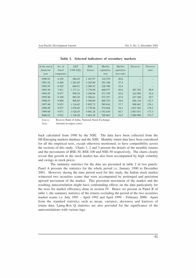
Asia-Pacific Development Journal Vol. 9, No. 2, December 2002
85
back calculated from 1990 by the NSE. The data have been collected from theISI-Emerging markets database and the NSE. Monthly return data have been consideredfor all the empirical tests, except otherwise mentioned, to have compatibility acrossthe sections of this study. Charts 1, 2 and 3 present the details of the monthly returnsand the movements of BSE-30, BSE-100 and NSE-50 respectively. The charts clearlyreveal that growth in the stock market has also been accompanied by high volatilityand swings in stock prices.
The summary statistics for the data are presented in table 2 in two panels.Panel A presents the statistics for the whole period i.e. January 1990 to December2001. However, during the time period used for this study, the Indian stock marketwitnessed two securities scams that were accompanied by prolonged and persistentupward movement of the market. This persistent movement of the market and theresulting autocorrelation might have confounding effects on the data particularly forthe tests for market efficiency done in section IV. Hence we present in Panel B oftable 1, the summary statistics of the returns excluding the period of the two securitiesmarket scams i.e. July 1991 – April 1992 and April 1999 – February 2000. Apartfrom the standard statistics such as mean, variance, skewness and kurtosis ofreturn data, Ljung-Box Q statistics are also provided for the significance of theautocorrelations with various lags.
Table 1. Selected indicators of secondary markets
At the end of No. of S&P BSE- Market Market Turnover Turnover
financial listed CNX-Nifty Sensex capitaliza- capitaliza- ratioyear companies tion tion ratio
1990-91 6 229 366.45 1 167.97 110 279 20.6 – –1991-92 6 480 1 261.65 4 285.00 354 106 57.4 – –1992-93 6 925 660.51 2 280.52 228 780 32.4 – –1993-94 7 811 1 177.11 3 778.99 400 077 45.6 203 703 50.91994-95 9 077 990.24 3 260.96 473 349 45.6 162 905 34.41995-96 9 100 985.30 3 366.61 572 257 47.0 227 368 39.71996-97 9 890 968.85 3 360.89 488 332 34.6 646 116 132.31997-98 9 833 1 116.65 3 892.75 589 816 37.7 908 681 154.11998-99 9 877 1 078.05 3 739.96 574 064 34.1 1 023 382 178.31999-00 9 871 1 528.45 5 001.28 1 192 630 84.7 2 067 031 173.32000-01 9 922 1 148.20 3 604.38 768 863 54.5 2 880 990 374.7
Source: Reserve Bank of India, National Stock Exchange.Note: Amount in rupees cores

Asia-Pacific Development Journal Vol. 9, No. 2, December 2002
86
Chart 1: BSE-30 and its Monthly Return: 1990-2001
Chart 2: BSE-100 and its Monthly Return: 1990-2001
Chart 3: S&P CNX-Nifty and its Monthly Return: 1990-2001
Jan-
90
May
-90
Sep-
90
Jan-
91
May
-91
Sep-
91
Jan-
92
May
-92
Sep-
92
Jan-
93
May
-93
Sep-
93
Jan-
94
May
-94
Sep-
94
Jan-
95
May
-95
Sep-
95
Jan-
96
May
-96
Sep-
96
Jan-
97
May
-97
Sep-
97
Jan-
98
May
-98
Sep-
98
Jan-
99
May
-99
Sep-
99
Jan-
00
May
-00
Sep-
00
Jan-
01
May
-01
Sep-
01
0.5
0.4
0.3
0.2
0.1
0
-0.1
-0.2
-0.3
6 000
5 000
4 000
3 000
2 000
1 000
0
BSE-30Monthly Return
Monthly Return
BSE-100
0.6
0.5
0.4
0.3
0.2
0.1
0
-0.1
-0.2
-0.3
3 500
3 000
2 500
2 000
1 500
1 000
500
0
Jan-
90
May
-90
Sep-
90
Jan-
91
May
-91
Sep-
91
Jan-
92
May
-92
Sep-
92
Jan-
93
May
-93
Sep-
93
Jan-
94
May
-94
Sep-
94
Jan-
95
May
-95
Sep-
95
Jan-
96
May
-96
Sep-
96
Jan-
97
May
-97
Sep-
97
Jan-
98
May
-98
Sep-
98
Jan-
99
May
-99
Sep-
99
Jan-
00
May
-00
Sep-
00
Jan-
01
May
-01
Sep-
01
S&P CNX-NiftyMonthly Return
0.5
0.4
0.3
0.2
0.1
0
-0.1
-0.2
-0.3
1 800
1 600
1 400
1 200
1 000
800
600
400
200
0
30-J
ul-9
0
30-N
ov-9
0
27-M
ar-9
1
31-J
ul-9
1
29-N
ov-9
1
31-M
ar-9
2
31-J
ul-9
2
30-N
ov-9
2
31-M
ar-9
3
30-J
ul-9
3
26-N
ov-9
3
31-M
ar-9
4
29-J
ul-9
4
30-N
ov-9
4
31-M
ar-9
5
31-J
ul-9
5
30-N
ov-9
5
29-M
ar-9
6
31-J
ul-9
6
29-N
ov-9
6
31-M
ar-9
7
31-J
ul-9
7
28-N
ov-9
7
31-M
ar-9
8
31-J
ul-9
8
30-N
ov-9
8
31-M
ar-9
9
30-J
ul-9
9
30-N
ov-9
9
31-M
ar-0
0
31-J
ul-0
0
30-N
ov-0
0
30-M
ar-0
1
31-J
ul-0
1
29-N
ov-0
1
28-M
ar-0
2
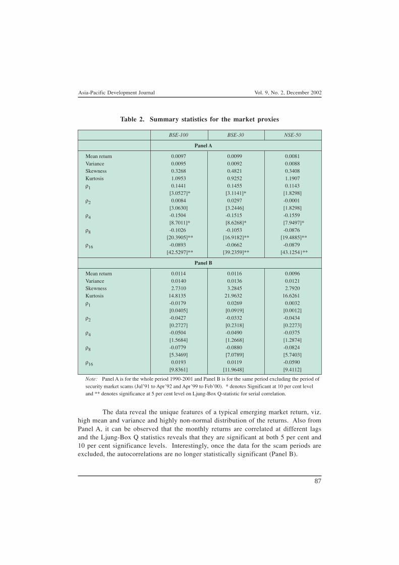
Asia-Pacific Development Journal Vol. 9, No. 2, December 2002
87
The data reveal the unique features of a typical emerging market return, viz.high mean and variance and highly non-normal distribution of the returns. Also fromPanel A, it can be observed that the monthly returns are correlated at different lagsand the Ljung-Box Q statistics reveals that they are significant at both 5 per cent and10 per cent significance levels. Interestingly, once the data for the scam periods areexcluded, the autocorrelations are no longer statistically significant (Panel B).
Table 2. Summary statistics for the market proxies
BSE-100 BSE-30 NSE-50
Panel A
Mean return 0.0097 0.0099 0.0081Variance 0.0095 0.0092 0.0088Skewness 0.3268 0.4821 0.3408Kurtosis 1.0953 0.9252 1.1907ρ1 0.1441 0.1455 0.1143
[3.0527]* [3.1141]* [1.8298]ρ2 0.0084 0.0297 -0.0001
[3.0630] [3.2446] [1.8298]ρ4 -0.1504 -0.1515 -0.1559
[8.7011]* [8.6268]* [7.9497]*ρ8 -0.1026 -0.1053 -0.0876
[20.3905]** [16.9182]** [19.4885]**ρ16 -0.0893 -0.0662 -0.0879
[42.5297]** [39.2359]** [43.1254}**
Panel B
Mean return 0.0114 0.0116 0.0096Variance 0.0140 0.0136 0.0121Skewness 2.7310 3.2845 2.7920Kurtosis 14.8135 21.9632 16.6261ρ1 -0.0179 0.0269 0.0032
[0.0405] [0.0919] [0.0012]ρ2 -0.0427 -0.0332 -0.0434
[0.2727] [0.2318] [0.2273]ρ4 -0.0504 -0.0490 -0.0375
[1.5684] [1.2668] [1.2874]ρ8 -0.0779 -0.0880 -0.0824
[5.3469] [7.0789] [5.7403]ρ16 0.0193 0.0119 -0.0590
[9.8361] [11.9648] [9.4112]
Note: Panel A is for the whole period 1990-2001 and Panel B is for the same period excluding the period ofsecurity market scams (Jul’91 to Apr’92 and Apr’99 to Feb’00). * denotes Significant at 10 per cent leveland ** denotes significance at 5 per cent level on Ljung-Box Q-statistic for serial correlation.
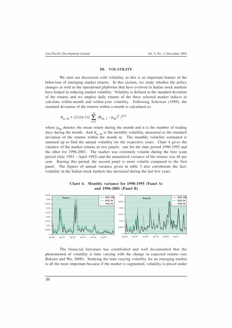
Asia-Pacific Development Journal Vol. 9, No. 2, December 2002
88
III. VOLATILITY
We start our discussion with volatility, as this is an important feature of thebehaviour of emerging market returns. In this section, we study whether the policychanges as well as the operational platforms that have evolved in Indian stock marketshave helped in reducing market volatility. Volatility is defined as the standard deviationof the returns and we employ daily returns of the three selected market indices tocalculate within-month and within-year volatility. Following Schewart (1989), thestandard deviation of the returns within a month is calculated as:
σa, m = {[1/(n-1)] (Rm, t – µm)2 }0.5
where µm denotes the mean return during the month and n is the number of tradingdays during the month. And σa, m is the monthly volatility, measured as the standarddeviation of the returns within the month m. The monthly volatility estimated issummed up to find the annual volatility for the respective years. Chart 4 gives thevariance of the market returns in two panels: one for the time period 1990-1995 andthe other for 1996-2001. The market was extremely volatile during the first scamperiod (July 1991 – April 1992) and the annualized variance of the returns was 48 percent. Barring this period, the second panel is more volatile compared to the firstpanel. The figures of annual variance given in table 3 also corroborate the fact:volatility in the Indian stock markets has increased during the last few years.
n
Σt=1
Chart 4. Monthly variance for 1990-1995 (Panel A)and 1996-2001 (Panel B)
Jan-90 Jan-91 Jan-92 Jan-93 Jan-94 Jan-95
0
0.005
0.01
0.015
0.02
0.025
0.03
0.035
0.04
0.045Panel A BSE-100
BSE-30NSE-50
Jan-96 Jan-97 Jan-98 Jan-99 Jan-00 Jan-01
0
0.005
0.01
0.015
0.02
0.025
0.03
Panel B BSE-100BSE-30NSE-50
The financial literature has established and well documented that thephenomenon of volatility is time varying with the change in expected returns (seeBekaert and Wu, 2000). Studying the time varying volatility for an emerging marketis all the more important because if the market is segmented, volatility is priced under

Asia-Pacific Development Journal Vol. 9, No. 2, December 2002
89
the conditional CAPM framework (Bekaert and Harvey, 1997). Another branch ofvolatility studies that is gaining increased attention in the literature is the asymmetricreaction of volatility to positive and negative news. For the same size of shocks inreturns, negative news increase the volatility more than positive news. This has beenattributed to changes in shocks across the markets. Hence, one would expect anemerging market like India to show a significant asymmetric volatility pattern.In order to investigate the dynamics of Indian stock market volatility and to test forthe presence for asymmetric volatility, we estimate the conditional varianceusing three volatility models that are widely used in the financial literature. We useGARCH (1, 1) of Bollerslev (1986), Exponential GARCH (1, 1) of Nelson (1991) andthe GJR-GARCH model of Glosten, Jagannathan and Rundle (1993). EGARCH andGJR-GARCH are asymmetric volatility models to test the presence of asymmetricvolatility in Indian market. The parameterization of the variance under these modelsis given in table 4 for reference.
Table 3. Annual variance during 1990-2001
Annual1990 1991 1992 1993 1994 1995 1996 1997 1998 1999 2000 2001
variance
BSE-30 0.12 0.07 0.18 0.06 0.04 0.03 0.05 0.06 0.08 0.07 0.11 0.07
BSE-100 0.10 0.04 0.13 0.05 0.03 0.02 0.04 0.06 0.08 0.08 0.14 0.08
NSE-50 0.07 0.05 0.18 0.06 0.04 0.03 0.05 0.08 0.07 0.08 0.10 0.06
Table 4. Variance equations of volatility models
GARCH (1, 1) model (Bollerslev (1986))
EGARCH (1, 1) model (Nelson (1991))
GJR-GARCH model (Glosten, Jagannathan and Runkle, 1993)
log (ht) = ω + β log (ht-1) + γ + α −εt-1
ht-1
2π√
εt-1
ht-1√ √
ht = α0 + α1 εt-1 + β h22t-1
t-1 tht = ω + β ht-1 + α εt-1 + γ S- εt-1 where S- = 1 if εt < 0, S- = 0 otherwiset
2 2

Asia-Pacific Development Journal Vol. 9, No. 2, December 2002
90
For estimating these models, the conditional mean of the returns needs to bespecified. We define the relation between conditional mean and conditional varianceas:
Et [Rt+1] = β σt
where Rt+1 is the nominal returns on the market index and σt is the variance estimated
at time t. This follows the intertemporal relation derived between risk and return.Though the original derivation is for excess returns, we assume that it holds fornominal returns, following Schewart (1989). We fit the models for the daily returnsdata using Maximum Likelihood procedures (see Engle and Ng, 1993). From thedaily variance, monthly variance of the returns is estimated by summing up the dailyvariance for all the trading days of the respective month. Chart 5 plots the actualvariance along with the volatility estimated using the three volatility models.
2
Chart 5. Monthly volatility charts for BSE-30, BSE-100 and NSE-50
2
Jan-90 Jan-93 Jan-96 Jan-99
0
0.005
0.01
0.015
0.02
0.025
0.03
0.035
0.04AVGARCHEGARCHGJR-GARCH
BSE-100
Jan-90 Jan-93 Jan-96 Jan-99
0
0.01
0.02
0.03
0.04
0.05
0.06AVGARCHEGARCHGJR-GARCH
BSE-30
Jul-99 Jul-93 Jul-96 Jul-99
0
0.01
0.02
0.03
0.04
0.05
0.06AVGARCHEGARCHGJR-GARCH
NSE-50
Four standard loss functions viz., Mean Error (ME), Mean Absolute Error(MAE), Root Mean Square Error and Mean Absolute Percentage Error (MAPE) areemployed to find the performance of these models for explaining the return volatility.Table 5 gives the estimation of the standard loss functions.
The error statistics for the three volatility models are provided in table 6 forcomparison. It is evident that asymmetric models outperform the simple GARCHmodel, and GJR-GARCH model generates fewer errors than the other two models.Also the coefficients for the asymmetric component are statistically significant. Wehave not attempted to study the impact of asymmetry for typical shocks that haveoccurred in the Indian stock market on the lines of Bekaert and Wu (2000) and Nelson(1991) as our objective was only to test for the presence of asymmetric volatility.Nevertheless, a detailed study of the asymmetric volatility on Indian stock marketswould offer very interesting insights. Besides, the results of this subsection need tobe read with caution because no out-of-sample forecasting has been done and theforecasting performance of the asymmetric volatility models is not known.

Asia-Pacific Development Journal Vol. 9, No. 2, December 2002
91
IV. MARKET EFFICIENCY
This section is devoted to testing weak form efficiency of the Indian stockmarket using unit root tests and variance ratio tests. We adjust the data for the secondmajor securities market scam that occurred during the study period. Thus we do ourtests for the whole time period as well as excluding scam periods and show thatexcluding the scam periods makes the autocorrelation of the returns statisticallyinsignificant. Next we introduce a moving window approach following Yilmaz (2001)to observe the change in market efficiency over time (see Pant and Bishnoi, 2001).
Table 5. Standard loss functions
ME = (σT – σT)2N
ΣT=1
1N
MAE = σT – σT2
N
ΣT=1
1N
< 2
< 2
RMSE = (σT – σT)2N
ΣT=1
1N
< 2√MAPE = (σT – σT)/σT
2N
ΣT=1
1N
< 22
Table 6. Error statistics of volatility models
Market indices Volatility models ME MAE RMSE MAPE
GARCH (1, 1) 0.00057 0.00205 0.00307 0.48065BSE-30 EGARCH 0.00041 0.00218 0.00253 0.48688
GJR-GARCH 0.00059 0.00207 0.00241 0.48048
GARCH (1, 1) 0.00071 0.00267 0.00489 0.69044BSE-100 EGARCH 0.00049 0.00191 0.00272 0.53793
GJR-GARCH 0.00076 0.00177 0.00241 0.53416
GARCH (1, 1) 0.00051 0.00199 0.00294 0.48319NSE-50 EGARCH 0.00030 0.00224 0.00348 0.49923
GJR-GARCH 0.00053 0.00202 0.00301 0.48528
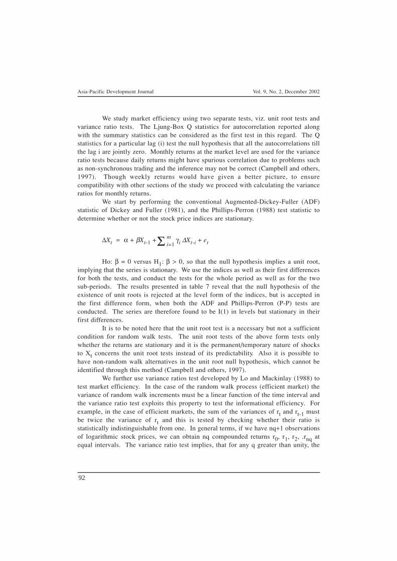
Asia-Pacific Development Journal Vol. 9, No. 2, December 2002
92
We study market efficiency using two separate tests, viz. unit root tests andvariance ratio tests. The Ljung-Box Q statistics for autocorrelation reported alongwith the summary statistics can be considered as the first test in this regard. The Qstatistics for a particular lag (i) test the null hypothesis that all the autocorrelations tillthe lag i are jointly zero. Monthly returns at the market level are used for the varianceratio tests because daily returns might have spurious correlation due to problems suchas non-synchronous trading and the inference may not be correct (Campbell and others,1997). Though weekly returns would have given a better picture, to ensurecompatibility with other sections of the study we proceed with calculating the varianceratios for monthly returns.
We start by performing the conventional Augmented-Dickey-Fuller (ADF)statistic of Dickey and Fuller (1981), and the Phillips-Perron (1988) test statistic todetermine whether or not the stock price indices are stationary.
∆Xt = α + βXt-1 + γi ∆Xt-i + et
Ho: β = 0 versus H1: β > 0, so that the null hypothesis implies a unit root,implying that the series is stationary. We use the indices as well as their first differencesfor both the tests, and conduct the tests for the whole period as well as for the twosub-periods. The results presented in table 7 reveal that the null hypothesis of theexistence of unit roots is rejected at the level form of the indices, but is accepted inthe first difference form, when both the ADF and Phillips-Perron (P-P) tests areconducted. The series are therefore found to be I(1) in levels but stationary in theirfirst differences.
It is to be noted here that the unit root test is a necessary but not a sufficientcondition for random walk tests. The unit root tests of the above form tests onlywhether the returns are stationary and it is the permanent/temporary nature of shocksto Xt concerns the unit root tests instead of its predictability. Also it is possible tohave non-random walk alternatives in the unit root null hypothesis, which cannot beidentified through this method (Campbell and others, 1997).
We further use variance ratios test developed by Lo and Mackinlay (1988) totest market efficiency. In the case of the random walk process (efficient market) thevariance of random walk increments must be a linear function of the time interval andthe variance ratio test exploits this property to test the informational efficiency. Forexample, in the case of efficient markets, the sum of the variances of rt and rt-1 mustbe twice the variance of rt and this is tested by checking whether their ratio isstatistically indistinguishable from one. In general terms, if we have nq+1 observationsof logarithmic stock prices, we can obtain nq compounded returns r0, r1, r2, .rnq atequal intervals. The variance ratio test implies, that for any q greater than unity, the
Σ mi=1
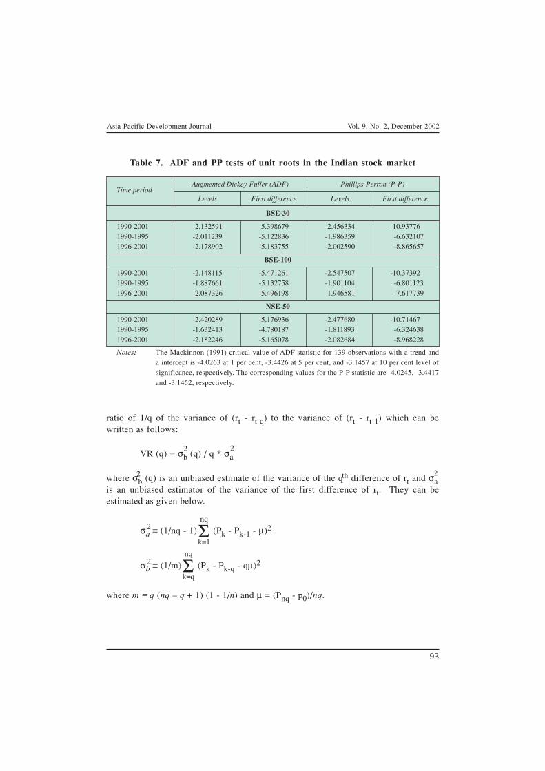
Asia-Pacific Development Journal Vol. 9, No. 2, December 2002
93
ratio of 1/q of the variance of (rt - rt-q) to the variance of (rt - rt-1) which can bewritten as follows:
VR (q) = σb (q) / q * σa
where σb (q) is an unbiased estimate of the variance of the qth difference of rt and σais an unbiased estimator of the variance of the first difference of rt. They can beestimated as given below.
σa ≡ (1/nq - 1) (Pk - Pk-1 - µ)2
σb ≡ (1/m) (Pk - Pk-q - qµ)2
where m ≡ q (nq – q + 1) (1 - 1/n) and µ = (Pnq - p0)/nq.
nq
Σk=1
2
nq
Σk=q
2
2 2
2 2
Table 7. ADF and PP tests of unit roots in the Indian stock market
Time periodAugmented Dickey-Fuller (ADF) Phillips-Perron (P-P)
Levels First difference Levels First difference
BSE-30
1990-2001 -2.132591 -5.398679 -2.456334 -10.937761990-1995 -2.011239 -5.122836 -1.986359 -6.6321071996-2001 -2.178902 -5.183755 -2.002590 -8.865657
BSE-100
1990-2001 -2.148115 -5.471261 -2.547507 -10.373921990-1995 -1.887661 -5.132758 -1.901104 -6.8011231996-2001 -2.087326 -5.496198 -1.946581 -7.617739
NSE-50
1990-2001 -2.420289 -5.176936 -2.477680 -10.714671990-1995 -1.632413 -4.780187 -1.811893 -6.3246381996-2001 -2.182246 -5.165078 -2.082684 -8.968228
Notes: The Mackinnon (1991) critical value of ADF statistic for 139 observations with a trend anda intercept is -4.0263 at 1 per cent, -3.4426 at 5 per cent, and -3.1457 at 10 per cent level ofsignificance, respectively. The corresponding values for the P-P statistic are -4.0245, -3.4417and -3.1452, respectively.

Asia-Pacific Development Journal Vol. 9, No. 2, December 2002
94
Lo and Mckinlay (1988) derive the asymptotic distribution of the varianceratios and offer two test statistics Z (q) and Z*(q). The first test statistic Z (q) is fortesting the random walk process that assumes that the errors are IID and the Z*(q) isfor testing the random walk process allowing for heteroscedasticity in the error term.The test statistics are given as:
Z (q) = [VR(q) - 1]/ [φ (q)] ≈ N (0, 1)
where [φ (q)] = [2(2q - 1)(q - 1)]/[3q (nq)]
Z* (q) = [VR(q) - 1]/ [φ * (q)] ≈ N (0, 1)
where φ* (q) = (θ / nq)
θ = 4 [{1-k / q}δk]
δk = [nq (Pj - Pj-1 - µ)2 (Pj-k - Pj-k-1 - µ)2] / [ (Pj - Pj-1 - µ)2]2
φ (q) and φ* (q) are the homoscedastic and heteroskedastic asymptotic variance of theprocess (see Campbell and others, 1997). Under the null hypothesis, the prices followrandom walk process RW1 or RW3. The test statistics as given by equations (8) and(10) are asymptotically normally distributed and the values obtained from the study ifgreater than the critical value of the standard normal process would mean rejectingthe null hypothesis which is a random walk process and hence signifies marketefficiency.
We start with the testing of the weak form efficiency (both RW1 and RW3)for the full period (1990:01 to 2001:12) as well as after excluding the scam period.The variance ratios and test statistics Z (q) and Z* (q) are provided in table 8. Withboth the test statistics, we could not reject the null hypotheses of random walk forboth the indices for all the four lags considered. The variance ratios estimated for theNSE-50 are more close to unity suggesting that NSE-50 might be more efficientcompared to other market indices. The VR statistics in Panel B, suggest that, asexpected, the variance ratio moves closer to unity on excluding the data during thescam period and the null hypothesis could not be rejected in any of the cases. AlsoVR (16) for Panel B is in the range of 0.58 to 0.75 which suggests mean reversion ofthe returns. This can be corroborated by the significant negative correlation reportedin the summary statistics for the same lag.
In principle, stock market liberalization should improve the efficiency of themarkets. This is because the investor base becomes wider with the participation of
q-1
Σk=1
nq
Σj=1
nq
Σj=k+1
√
√
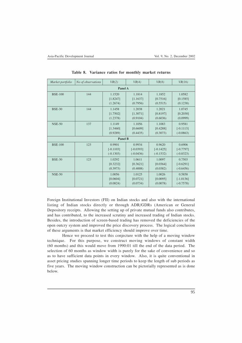
Asia-Pacific Development Journal Vol. 9, No. 2, December 2002
95
Table 8. Variance ratios for monthly market returns
Market portfolio No of observations VR(2) VR(4) VR(8) VR(16)
Panel A
BSE-100 144 1.1520 1.1814 1.1852 1.0582[1.8247] [1.1637] [0.7516] [0.1585](1.2674) (0.7956) (0.5515) (0.1238)
BSE-30 144 1.1458 1.2038 1.2021 1.0745[1.7502] [1.3071] [0.8197] [0.2030](1.2378) (0.9104) (0.6036) (0.0999)
NSE-50 137 1.1149 1.1056 1.1083 0.9581[1.3460] [0.6609] [0.4288] [-0.1113](0.9289) (0.4435) (0.3073) (-0.0863)
Panel B
BSE-100 123 0.9901 0.9934 0.9620 0.6906[-0.1103] [-0.0393] [-0.1425] [-0.7797](-0.1303) (-0.0436) (-0.1532) (-0.8323)
BSE-30 123 1.0292 1.0611 1.0097 0.7503[0.3232] [0.3621] [0.0364] [-0.6291](0.3973) (0.4008) (0.0382) (-0.6456)
NSE-50 1.0056 1.0125 1.0026 0.5858[0.0604] [0.0721] [0.0095] [-1.0136](0.0824) (0.0734) (0.0078) (-0.7578)
Foreign Institutional Investors (FII) on Indian stocks and also with the internationallisting of Indian stocks directly or through ADR/GDRs (American or GeneralDepository receipts. Allowing the setting up of private mutual funds also contributes,and has contributed, to the increased scrutiny and increased trading of Indian stocks.Besides, the introduction of screen-based trading has removed the deficiencies of theopen outcry system and improved the price discovery process. The logical conclusionof these arguments is that market efficiency should improve over time.
Hence we proceed to test this conjecture with the help of a moving windowtechnique. For this purpose, we construct moving windows of constant width(60 months) and this would move from 1990:01 till the end of the data period. Theselection of 60 months as window width is purely for the sake of convenience and soas to have sufficient data points in every window. Also, it is quite conventional inasset pricing studies spanning longer time periods to keep the length of sub periods asfive years. The moving window construction can be pictorially represented as is donebelow.

Asia-Pacific Development Journal Vol. 9, No. 2, December 2002
96
Construction of moving window with constant width
Chart 6. Evidence on increasing market efficiency
BSE-30
BSE-100
NSE-50
BSE-30
BSE-100
NSE-50
BSE-30
BSE-100
NSE-50
BSE-30
BSE-100
NSE-50
1.6
1.4
1.2
1.0
0.8
0.6
0.4
0.2
0
1.6
1.4
1.2
1.0
0.8
0.6
0.4
0.2
0
1.8
1.6
1.4
1.2
1.0
0.8
0.6
0.4
0.2
0
1.4
1.2
1.0
0.8
0.6
0.4
0.2
0
VR(2)
VR(8) VR(16)
VR(4)
1990:02 1995:01
1990:03 1995:02
1997:01 2001:12
........
........
The Z-statistics obtained for the moving windows are plotted against time toobserve the change in informational efficiency. The critical values to reject the nullhypothesis of random walk is 1.96 at a 5 per cent significance level. The movingwindows at the end would contain data for the latest period and the test statistics forthem must be better than the test statistics for the windows at the beginning if themarket is becoming more efficient. Or, in other words, the plot of the test statisticsfor the moving windows should be dropping in case of increasing market efficiency(chart 6). As expected, the test statistics fall smoothly as we consider the latest dataand move away from the critical values. Taken together, the empirical evidencebased on the variance ratio and unit root tests reveal the evolving market efficiency inIndian stock price indices.
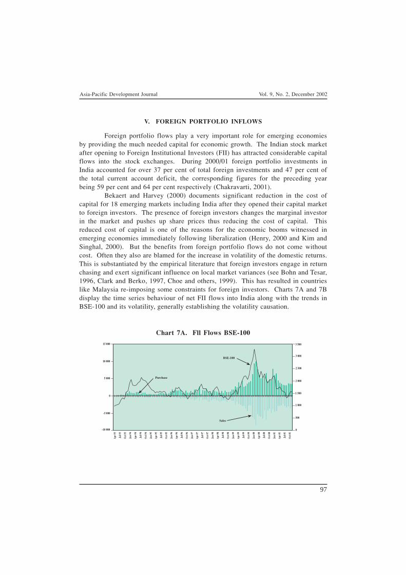
Asia-Pacific Development Journal Vol. 9, No. 2, December 2002
97
V. FOREIGN PORTFOLIO INFLOWS
Foreign portfolio flows play a very important role for emerging economiesby providing the much needed capital for economic growth. The Indian stock marketafter opening to Foreign Institutional Investors (FII) has attracted considerable capitalflows into the stock exchanges. During 2000/01 foreign portfolio investments inIndia accounted for over 37 per cent of total foreign investments and 47 per cent ofthe total current account deficit, the corresponding figures for the preceding yearbeing 59 per cent and 64 per cent respectively (Chakravarti, 2001).
Bekaert and Harvey (2000) documents significant reduction in the cost ofcapital for 18 emerging markets including India after they opened their capital marketto foreign investors. The presence of foreign investors changes the marginal investorin the market and pushes up share prices thus reducing the cost of capital. Thisreduced cost of capital is one of the reasons for the economic booms witnessed inemerging economies immediately following liberalization (Henry, 2000 and Kim andSinghal, 2000). But the benefits from foreign portfolio flows do not come withoutcost. Often they also are blamed for the increase in volatility of the domestic returns.This is substantiated by the empirical literature that foreign investors engage in returnchasing and exert significant influence on local market variances (see Bohn and Tesar,1996, Clark and Berko, 1997, Choe and others, 1999). This has resulted in countrieslike Malaysia re-imposing some constraints for foreign investors. Charts 7A and 7Bdisplay the time series behaviour of net FII flows into India along with the trends inBSE-100 and its volatility, generally establishing the volatility causation.
Chart 7A. Fll Flows BSE-100
3 500
3 000
2 500
2 000
1 500
1 000
500
0
15 000
10 000
5 000
0
-5 000
-10 000
Purchase
Sales
BSE-100
Apr
-93
Jul-9
3
Oct
-93
Jan-
94
Apr
-94
Jul-9
4
Oct
-94
Jan-
95
Apr
-95
Jul-9
5
Oct
-95
Jan-
96
Apr
-96
Jul-9
6
Oct
-96
Jan-
97
Apr
-97
Jul-9
7
Oct
-97
Jan-
98
Apr
-98
Jul-9
8
Oct
-98
Jan-
99
Apr
-99
Jul-9
9
Oct
-99
Jan-
00
Apr
-00
Jul-0
0
Oct
-00
Jan-
01
Apr
-01
Jul-0
1
Oct
-01

Asia-Pacific Development Journal Vol. 9, No. 2, December 2002
98
In this section, we test whether foreign investors have played a role in theincrease in volatility in the Indian stock market. We employ Granger causalitytesting to establish the causal relationship between the FII in flows and the domesticmarket returns and its variance. Additionally we use other important variables suchas rupee-US dollar exchange rates and MSCI indices for the US to characterize foreignportfolio flows to India. Taken together these variables would indicate the primaryfactors that determine the FII flows to India.
Typically the Granger causality test involves the estimation of the bivariateregressions as given below:
Yt = a0 + a1Yt-1 + ..... + alYt-l + β1Xt-1 + .....βlXt-l
Xt = a0 + a1Xt-1 + ..... + alXt-l + β1Yt-1 + .....βlYt-l
We estimate the F-statistics for the test of joint hypothesis β1......βl = 0. Thenull hypothesis set as X does not Granger cause in the first regression, and Y does notGranger cause (GC) X in the second regression. The choice of lag length is restrictedto two months, without stretching the variables too far.
Pair-wise Granger causality tests between monthly net FII flows and variablessuch as monthly return on BSE-30, BSE-100 indices and NSE-50, within-monthvariance in return in these indices, rupee-US dollar exchange rate and return on MSCI-USA are calculated for the period March 1993-December 2001. As revealed fromtable 9, there is evidence of returns causing portfolio inflows and this in turn affectingthe behaviour of returns and their variances in the Indian stock markets. We have
Chart 7B. Net Fll Flows and Varance of BSE-100
Net
VarBSE-100
0.03
0.025
0.02
0.015
0.01
0.005
0
5 000
4 000
3 000
2 000
1 000
0
-1 000
-2 000
Apr
-93
Jul-9
3
Oct
-93
Jan-
94
Apr
-94
Jul-9
4
Oct
-94
Jan-
95
Apr
-95
Jul-9
5
Oct
-95
Jan-
96
Apr
-96
Jul-9
6
Oct
-96
Jan-
97
Apr
-97
Jul-9
7
Oct
-97
Jan-
98
Apr
-98
Jul-9
8
Oct
-98
Jan-
99
Apr
-99
Jul-9
9
Oct
-99
Jan-
00
Apr
-00
Jul-0
0
Oct
-00
Jan-
01
Apr
-01
Jul-0
1
Oct
-01

Asia-Pacific Development Journal Vol. 9, No. 2, December 2002
99
Table 9. Results of the pair-wise Granger Causality tests
Null hypothesis F-statistics Probability
Granger Causality between BSE-30 return and FII flows (net)
Returns on BSE does not GC FII flows (net) 7.08680 0.00133
FII flows (net) does not GC returns on BSE 2.16850 2.16850
BSE return does not GC FII flows (purchase) 2.80657 0.06528
FII flows (purchase) does not GC BSE return 1.35658 0.26233
Granger Causality between variance in BSE-30 return and FII flows (net)
Variance in BSE returns does not GC FII flows (net) 1.41449 0.24797
FII flows (net) does not GC variance in BSE returns 2.34943 0.10078
Variance in BSE return does not GC FII flows (sales) 1.20445 0.30426
FII flows (sales) does not GC variance in BSE return 6.46262 0.00231
Granger Causality between NSE return and FII flows (net)
Returns on NSE does not GC FII flows (net) 4.11977 0.01914
FII flows (net) does not GC returns on NSE 1.34019 0.26655
NSE return does not GC FII flows (purchase) 2.63408 0.07686
FII flows (purchase) does not GC NSE return 0.98209 0.37818
Granger Causality between variance in NSE return and FII flows (net)
Variance in NSE returns does not GC FII flows (net) 0.93118 0.39755
FII flows (net) does not GC variance in NSE returns 1.44817 0.23998
Variance in NSE return does not GC FII flows (sales) 0.89831 0.41058
FII flows (sales) does not GC variance in NSE return 3.27055 0.04217
Granger Causality between the rupee -dollar exchange rate and FII flows
Exchange rate does not GC FII flows (net) 1.58927 0.20929
FII flows (net) does not GC exchange rate 0.99344 0.37400
Granger Causality between the MSCI index and FII flows
Return on MSCI-US index does not GC FII flows (net) 0.78294 0.45990
FII flows (net) does not GC return on MSCI-US index 2.73511 0.06984
also examined the causation between the return and purchases and between variancesand sales. The returns on the indices seem to be causing the FIIs to purchase, and thevariance to cause selling pressures in the Indian stock markets. The causality ofrupee-US dollar exchange rate and MSCI-US to the FII inflows is rather weak in theIndian situation. Taken together the evidence shows the influence of FII inflows onvolatility in Indian stock markets.
Asia-Pacific Development Journal Vol. 9, No. 2, December 2002
100
VI. IMPACT OF FOREIGN SHOCKS
The volatility and correlations in emerging markets have received increasingacademic attention during the last decade. As barriers to foreign investment havebeen dismantled and with the trend towards greater globalization, the stock markets inmany emerging markets have shown stronger co-movements. However, this has alsobeen accompanied by greater volatility. Volatility in the major emerging markets hasbeen traditionally associated with local political and economic events (Aggarwaland others, 1999) or when global factors dominate domestic ones such as oil crises,the Gulf war and the Asian financial crises affecting all financial markets (Longin andSolnik, 1995). Bekaert and Harvey (1995) document the time varying integration of12 emerging markets with the world wherein they find evidence for a movementtowards higher level of integration for India. This would imply that the Indian capitalmarket has become more prone to external shocks.
In this section, we test whether the contemporaneous correlation of Indianstock market returns have increased over time with the returns of eight Asian emergingmarkets and three developed markets. The Morgan Stanley Capital Index (MSCI) hasbeen used for finding the returns of the Asian emerging markets as well as thedeveloped markets. Chart 8 presents the MSCI movements for the whole period forall the countries selected. The correlation between the markets is presented intable 10 for the whole period (1990-2001) as well as for before the Asian crisis(1990-1996) and after the Asian crisis (1998-2001).
It can be observed from table 10 that the correlation based on US dollarreturns are higher among Asian countries, although their values are well below unity.The high correlation among Asian stock market indices suggests the possibility ofincreased market integration in the post-1997 period. With further reduction in barriersto foreign investment, it is possible for stronger co-movements among these markets.
We compute the pair-wise Granger causality tests of the returns to see thedirection of impacts of Asian markets on India. The results of the tests are presentedin table 11. It is interesting to observe that Asian markets do affect Indian stockmarkets, prominent among them are Hong Kong, China; the Republic of Korea;Malaysia; Pakistan; the Philippines; and Thailand. However, the impact of India onthe Asian markets seems to be non-existent.

Asia-Pacific Development Journal Vol. 9, No. 2, December 2002
101
Chart 8. Morgan Stanley Capital Index for various markets
Japan: 31-Dec-69 = 100UK: 31-Dec-69 = 100USA: 31-Dec-69 = 100
Jan-
90Ja
n-91
Jan-
92Ja
n-93
Jan-
94Ja
n-95
Jan-
96Ja
n-97
Jan-
98Ja
n-99
Jan-
00Ja
n-01
Jan-
90Ja
n-91
Jan-
92Ja
n-93
Jan-
94Ja
n-95
Jan-
96Ja
n-97
Jan-
98Ja
n-99
Jan-
00Ja
n-01
Jan-
90Ja
n-91
Jan-
92Ja
n-93
Jan-
94Ja
n-95
Jan-
96Ja
n-97
Jan-
98Ja
n-99
Jan-
00Ja
n-01
1 600
1 400
1 200
1 000
800
600
400
200
0
1 400
1 200
1 000
800
600
400
200
0
4 500
4 000
3 500
3 000
2 500
2 000
1 500
500
0
1 000
Pakistan: 31-Dec-92 = 100India: 31-Dec-92 = 100 Thailand: 31-Dec-87 = 100
Jan-
90
Jan-
91
Jan-
92
Jan-
93
Jan-
94
Jan-
95
Jan-
96
Jan-
97
Jan-
98
Jan-
90
Jan-
91
Jan-
92
Jan-
93
Jan-
94
Jan-
95
Jan-
96
Jan-
97
Jan-
98
Jan-
99
Jan-
00
Jan-
01
Jan-
90
Jan-
91
Jan-
92
Jan-
93
Jan-
94
Jan-
95
Jan-
96
Jan-
97
Jan-
98
250
200
150
100
50
0
700
600
500
400
300
200
100
0
200
180
160
140
120
100
80
60
20
0
40
Hong Kong: 31-Dec-69 = 100Singapore: 31-Dec-69 = 100Philippines: 31-Dec-87 = 100
Jan-
90
Jan-
91
Jan-
92
Jan-
93
Jan-
94
Jan-
95
Jan-
96
Jan-
97
Jan-
98
Jan-
99
Jan-
00
Jan-
01
Jan-
90
Jan-
91
Jan-
92
Jan-
93
Jan-
94
Jan-
95
Jan-
96
Jan-
97
Jan-
98
Jan-
99
Jan-
00
Jan-
01
Jan-
90Ja
n-91
Jan-
92Ja
n-93
Jan-
94Ja
n-95
Jan-
96Ja
n-97
Jan-
98Ja
n-99
Jan-
00Ja
n-01
600
500
400
300
200
100
0
3 500
3 000
2 500
2 000
1 500
1 000
500
0
6 000
5 000
4 000
3 000
2 000
1 000
0
7 000
8 000
Indonesia: 31-Dec-87 = 100Malaysia: 31-Dec-87 = 100 Republic of Korea: 31-Dec-87 = 100
Jan-
90Ja
n-91
Jan-
92Ja
n-93
Jan-
94Ja
n-95
Jan-
96Ja
n-97
Jan-
98Ja
n-99
Jan-
00Ja
n-01
Jan-
90
Jan-
91
Jan-
92
Jan-
93
Jan-
94
Jan-
95
Jan-
96
Jan-
97
Jan-
98
Jan-
99
Jan-
00
Jan-
01
Jan-
90
Jan-
91
Jan-
92
Jan-
93
Jan-
94
Jan-
95
Jan-
96
Jan-
97
Jan-
98
Jan-
99
Jan-
00
Jan-
01
500
450
400
350
300
250
200
150
100
0
50
250
200
150
100
50
0
1 000
900
800
700
600
500
400
200
0
100
300

Asia-Pacific Development Journal Vol. 9, No. 2, December 2002
102
Table 10. Contemporaneous correlation among markets
Panel A: For the time period 1993-2001
Hong Kong, China 1
India 0.22 1
Indonesia 0.53 0.28 1
Japan 0.36 0.14 0.289 1
Korea (Republic of) 0.32 0.21 0.382 0.52 1
Malaysia 0.56 0.28 0.603 0.24 0.31 1
Pakistan 0.25 0.42 0.174 0.04 0.14 0.23 1
Philippines 0.64 0.2 0.594 0.29 0.35 0.62 0.12 1
Singapore 0.77 0.28 0.648 0.42 0.36 0.61 0.27 0.68 1
Thailand 0.62 0.20 0.595 0.35 0.60 0.60 0.27 0.75 0.68 1
UK 0.54 0.10 0.289 0.45 0.29 0.31 0.15 0.33 0.51 0.35 1
USA 0.54 0.20 0.403 0.43 0.35 0.31 0.13 0.42 0.54 0.46 0.67 1
Hon
g K
ong,
Chi
na
Indi
a
Indo
nesi
a
Japa
n
Kor
ea (R
epub
lic o
f)
Mal
aysi
a
Paki
stan
Phili
ppin
es
Sing
apor
e
Thai
land
UK
USA
Panel B: For the time period 1993-1996
Hong Kong, China 1
India 0.03 1
Indonesia 0.7 0.35 1
Japan 0.08 -0.1 0.029 1
Korea (Republic of) 0.22 0.22 0.166 0.34 1
Malaysia 0.72 0.16 0.485 0.18 0.22 1
Pakistan 0.29 0.35 0.283 -0 0.24 0.3 1
Philippines 0.72 0.16 0.528 -0 0.07 0.64 0.44 1
Singapore 0.71 0.21 0.575 0.29 0.37 0.79 0.28 0.68 1
Thailand 0.74 0.15 0.568 0.02 0.29 0.6 0.44 0.79 0.67 1
UK 0.49 0.11 0.365 0.3 0.22 0.44 0.05 0.24 0.51 0.24 1
USA 0.51 -0.1 0.51 0.17 0.05 0.22 -0 0.17 0.3 0.31 0.55 1
Hon
g K
ong,
Chi
na
Indi
a
Indo
nesi
a
Japa
n
Kor
ea (R
epub
lic o
f)
Mal
aysi
a
Paki
stan
Phili
ppin
es
Sing
apor
e
Thai
land
UK
USA
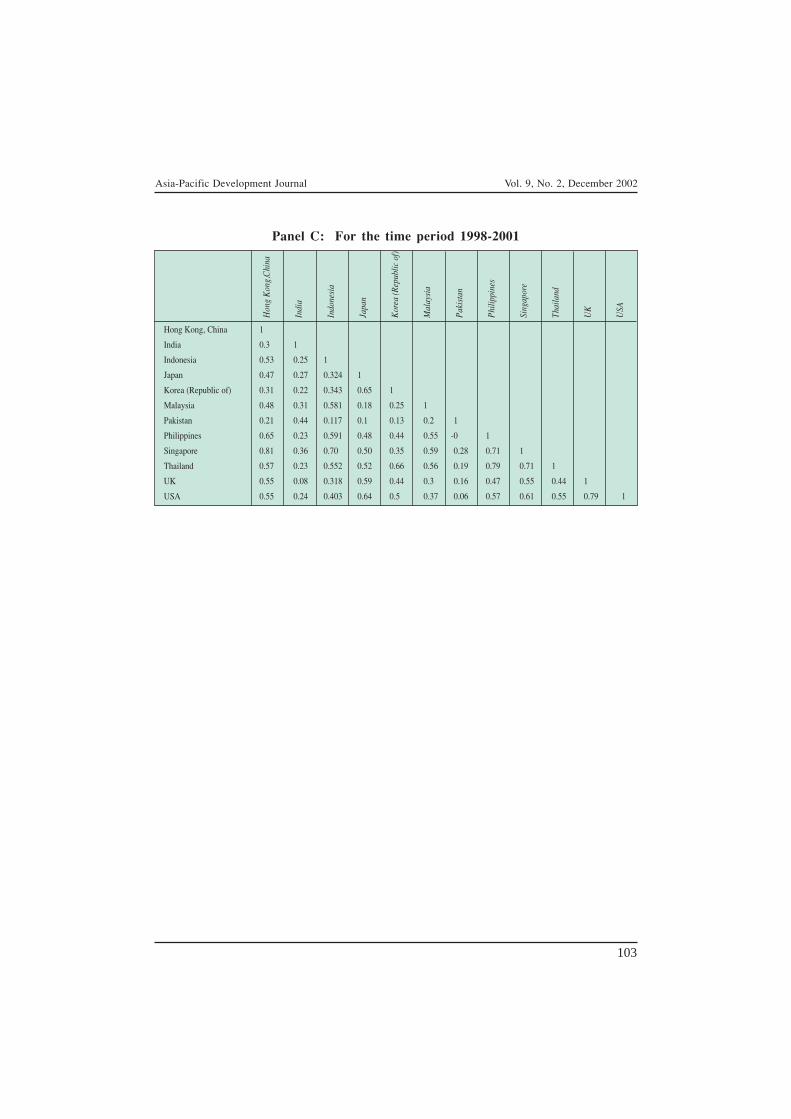
Asia-Pacific Development Journal Vol. 9, No. 2, December 2002
103
Panel C: For the time period 1998-2001
Hong Kong, China 1
India 0.3 1
Indonesia 0.53 0.25 1
Japan 0.47 0.27 0.324 1
Korea (Republic of) 0.31 0.22 0.343 0.65 1
Malaysia 0.48 0.31 0.581 0.18 0.25 1
Pakistan 0.21 0.44 0.117 0.1 0.13 0.2 1
Philippines 0.65 0.23 0.591 0.48 0.44 0.55 -0 1
Singapore 0.81 0.36 0.70 0.50 0.35 0.59 0.28 0.71 1
Thailand 0.57 0.23 0.552 0.52 0.66 0.56 0.19 0.79 0.71 1
UK 0.55 0.08 0.318 0.59 0.44 0.3 0.16 0.47 0.55 0.44 1
USA 0.55 0.24 0.403 0.64 0.5 0.37 0.06 0.57 0.61 0.55 0.79 1
Hon
g K
ong,
Chi
na
Indi
a
Indo
nesi
a
Japa
n
Kor
ea (R
epub
lic o
f)
Mal
aysi
a
Paki
stan
Phili
ppin
es
Sing
apor
e
Thai
land
UK
USA
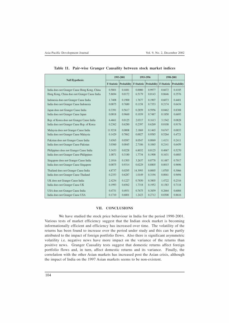
Asia-Pacific Development Journal Vol. 9, No. 2, December 2002
104
Table 11. Pair-wise Granger Causality between stock market indices
Null Hypothesis:1993-2001 1993-1996 1998-2001
F-Statistic Probability F-Statistic Probability F-Statistic Probability
India does not Granger Cause Hong Kong, China 0.5801 0.4481 0.0000 0.9977 0.6672 0.4185
Hong Kong, China does not Granger Cause India 5.8694 0.0172 6.5179 0.0143 0.8646 0.3576
Indonesia does not Granger Cause India 1.7408 0.1900 1.7677 0.1907 0.6073 0.4401
India does not Granger Cause Indonesia 0.0875 0.7680 0.1158 0.7353 0.2174 0.6434
Japan does not Granger Cause India 0.3391 0.5617 0.2859 0.5956 0.0462 0.8308
India does not Granger Cause Japan 0.0018 0.9660 0.1039 0.7487 0.1850 0.6693
Rep. of Korea does not Granger Cause India 6.4661 0.0125 2.0317 0.1613 3.1542 0.0828
India does not Granger Cause Rep. of Korea 0.2362 0.6280 0.2397 0.6269 0.0108 0.9176
Malaysia does not Granger Cause India 11.9218 0.0008 2.1869 0.1465 9.6747 0.0033
India does not Granger Cause Malaysia 0.1429 0.7062 0.0027 0.9585 0.5264 0.4721
Pakistan does not Granger Cause India 3.6565 0.0587 8.0547 0.0069 1.4131 0.2411
India does not Granger Cause Pakistan 3.0360 0.0845 2.7186 0.1065 0.2141 0.6459
Philippines does not Granger Cause India 5.3433 0.0228 6.8032 0.0125 0.4067 0.5270
India does not Granger Cause Philippines 1.0071 0.3180 1.7734 0.1900 0.1631 0.6883
Singapore does not Granger Cause India 2.1016 0.1503 3.2637 0.0778 0.1487 0.7017
India does not Granger Cause Singapore 0.0075 0.9314 0.0229 0.8805 0.0015 0.9696
Thailand does not Granger Cause India 4.8737 0.0295 14.3993 0.0005 1.0705 0.3066
India does not Granger Cause Thailand 0.2353 0.6287 1.0149 0.3194 0.0041 0.9494
UK does not Granger Cause India 2.4234 0.1227 0.7850 0.3805 1.4722 0.2316
India does not Granger Cause UK 0.1993 0.6562 1.7318 0.1952 0.1383 0.7118
USA does not Granger Cause India 0.4731 0.4931 0.7675 0.3859 0.2664 0.6084
India does not Granger Cause USA 0.1710 0.6801 1.2423 0.2712 0.0308 0.8616
VII. CONCLUSIONS
We have studied the stock price behaviour in India for the period 1990-2001.Various tests of market efficiency suggest that the Indian stock market is becominginformationally efficient and efficiency has increased over time. The volatility of thereturns has been found to increase over the period under study and this can be partlyattributed to the impact of foreign portfolio flows. Also there is significant asymmetricvolatility i.e. negative news have more impact on the variance of the returns thanpositive news. Granger Causality tests suggest that domestic returns affect foreignportfolio flows and, in turn, affect domestic returns and its variance. Finally, thecorrelation with the other Asian markets has increased post the Asian crisis, althoughthe impact of India on the 1997 Asian markets seems to be non-existent.

Asia-Pacific Development Journal Vol. 9, No. 2, December 2002
105
REFERENCES
Aggarwal, R., C. Inclan, and R. Leal, 1999. “Volatility in emerging stock markets”, Journal of Financialand Quantitative Analysis, vol. 34, No. 1, pp. 33-55.
Bekaert, G., and C.R. Harvey, 1995. “Time varying world market integration”, Journal of Finance,vol. 50, No. 2, pp. 403-445.
, 1997. “Emerging equity market volatility”, Journal of Financial Economics, vol. 43,pp. 29-77.
Bekaert, G. and G. Wu, 2000. “Asymmetric volatility and risk in equity markets”, Review of FinancialStudies, vol. 13, pp. 1-42.
Bohn, Henning and Linda Tesar, 1996, “US equity investments in foreign markets: portfolio rebalancingor return chasing?” American Economic Review, vol. 86, pp. 77-81.
Bollerslev, T., 1986, “Generalized autoregressive conditional heteroscedasticity”, Journal of Econometrics,vol. 31, pp. 307-27.
Campbell, J., A. Lo, and A.C. Mackinlay, 1997, The Econometrics of Financial Markets, PrincetonUniversity Press, New Jersey.
Chakravarti, R., 2001, “FII flows to India: nature and causes”, ICRA Bulletin of Money and Finance,October-December, pp. 61-79.
Choe, Hyuk, Bong-Chan Kho and Rene M. Stulz, 1999, “Do foreign investors destabilize stock markets?The Korean experience in 1997”, Journal of Financial Economics, vol. 54, pp. 227-264.
Clark, John and Elizabeth Berko, 1997, “Foreign investment fluctuations and emerging market stockreturns”, Federal Reserve Bank of New York Staff Papers, No. 24, May.
Dickey, D. and W. Fuller, 1981, ‘Likelihood ratio statistics for autoregressive time series with a unit root’,Econometrica, vol. 49, pp. 1057-1072.
Engle, Robert and Ng Victor, 1993, “Measuring and testing the impact of news on volatility”, Journal ofFinance, vol. 48, pp. 1749-1778.
Glosten, Lawrence R., Ravi Jagannathan and David E. Rundle, 1993, “On the relation between the expectedvalue and the volatility of the nominal excess return on stocks”, Journal of Finance, vol. 48,pp. 1779-1801.
Henry, Peter B., 2000, “Do stock market liberalizations cause investment booms?”.
Kim, E. Han and Vijay Singhal, 2000, “Stock market openings: experience of emerging economies”,Journal of Business, vol. 73, No. 1, pp. 25-66.
Lo, A. and A.C. Mackinlay, 1988, “Stock market prices do not follow random walks: evidence froma simple specification test”, Review of Financial Studies, vol. 1, No. 1, pp. 41-66.
Longin, F., and B. Solnik, 1995, “Is the correlation in international equity returns constant: 1960-1990?”,Journal of International Money and Finance, vol. 14, No. 1, pp. 3-26.
Nelson, D. 1991, “Conditional heteroscedasticity in asset returns: a new approach”, Econometrica,vol. 59, pp. 347-370.
Pant, Bhanu, and T.R. Bishnoi, 2001, “Testing random walk hypotheses for Indian stock market indices”,Proceedings of the Fifth Capital Markets Conference 2001, UTI institute of capital markets.
Phillips, Peter C.B. and Pierre Perron, 1988, “Testing for a unit root in time series regression” Biometrica,vol. 75, No. 2, pp. 335-346.

Asia-Pacific Development Journal Vol. 9, No. 2, December 2002
106
Schewart, G.W., 1989, “Why does stock market volatility change over time”, Journal of Finance, 44,1115-1153.
Yilmaz, Kamil, 2001, “Market development and efficiency in emerging stock markets”, home.ku.edu.tr/~kyilmaz/papers/emerging.pdf. 27 June 2002.

Asia-Pacific Development Journal Vol. 9, No. 2, December 2002
107
ECONOMIC REFORMS, ENERGY CONSUMPTION CHANGES ANDCO2 EMISSIONS IN INDIA: A QUANTITATIVE ANALYSIS
Kakali Mukhopadhyay* and Debech Chakraborty**
Energy based on fossil fuel consumption is very closely linked withenvironmental pollution in the form of CO2 emissions, a major element inglobal climate change. This paper analyses the changes in India’s energyconsumption and CO2 emissions during the five-year period following the1991 reforms, i.e. 1991/92 to 1996/97. The authors extend the energyInput-Output Structural Decomposition Analysis (SDA) to identify changesin energy consumption during this period. Results indicate that India’senergy consumption, which increased by 5.7 per cent a year in this period,was determined by a number of forces. The most significant role wasplayed by the final demand structure followed by technical change andinteraction between final demand structure and technical change. TheCO2 emission trends reveal that the most dominating sectors have beenpetroleum products and electricity. The paper makes some broad policyrecommendations for the future pattern of energy use in India.
Faced with rising inflation and a balance of payments crisis in mid-1991 theGovernment of India introduced a fairly comprehensive policy reform package,comprising currency devaluation, deregulation, de-licensing and privatization of thepublic sector. The Government of India also initiated new strategies for the energysector in tune with the economic reforms in mid-1991. The energy strategies were:i) to initiate a shift from non-renewable sources of energy to renewable sources and toprovide wider access for the rural and urban poor to adequate energy supplies ataffordable costs, ii) to ensure efficiency in the use of energy in all production processes,iii) to review the use of all energy intensive materials and provide for their substitutionby less energy intensive materials through Rand D, iv) to ensure efficiency in the useof equipment in the energy sector, especially in thermal and nuclear power generationthrough improved plant availability, v) to initiate measures aimed at reducing energyintensity in different sectors, through changes in technology and/or processes, vi) to
* Post-doctorate Research Fellow, Centre for Development and Environment Policy, Indian Institute ofManagement, Joka, Calcutta, India.** Professor of Economics, Department of Economics, Jadavpur University, Calcutta, India.
Asia-Pacific Development Journal Vol. 9, No. 2, December 2002
108
optimise inter-fuel substitution, vii) to propagate renewable resources based ondecentralised and environmentally benign non-conventional technologies and viii) tomaximise the availability of indigenous energy resources such as oil, natural gas, coaland hydroelectric power, as well as non-conventional energy by way of bio-gas, solarenergy and wind energy.
As is known, energy consumption based on fossil fuel consumption is closelylinked with environmental pollution through CO2 emissions, which is contributing toglobal climate change. Global climate change has become one of the most importantissues of recent times. The CO2 emissions from fossil fuel combustion have beenidentified as the single most significant source of GHG (green house gas) emissionsinto the atmosphere from human activities. In the global context, a comparison of theCO2 emissions from India with the global total indicates that the total Indiancontribution from various sources is about 2.2 per cent of the global emissions. Theemissions of CO2 in India are of the order of 1191 tgc (teragram, or 1 million, metrictons of carbon). The energy sector is the largest contributor to GHG emissions inIndia. A large amount of CO2 is emitted from the combustion of fossil fuels in India.Of these, coal accounts for nearly 70 per cent and oil for 26 per cent, while the rest isfrom natural gas. Steel plants, thermal power plants, the cement industry and railwaysare the major industrial consumers of coal.
Considering the above energy problems and aspects of environmental pollution,especially of CO2 emissions, a detailed quantitative analysis of energy consumptionchanges and of the resultant CO2 emissions is called for. The object of this paper isto analyze energy consumption changes and CO2 emissions in India during the period1991-92 to 1996-97 and to draw relevant policy conclusions from the analysis.
As a first step in this exercise a Structural Decomposition Analysis for energyconsumption changes is specified. It is an ideal technique to study “over-period”changes. Similar attempts have been made by Rose and Chen (1991) for TaiwanProvince of China, Lin and Polenske (1995) for China, Han and Lakshmanan(1994) for Japan, and Wier (1998) for Denmark. For CO2 intensities we have usedan input-output technique. The methodology for relating input-output activity to thenatural environment in an input-output framework is familiar and popular forenvironmental studies. Numerous studies have dealt with energy and environmentalanalysis by applying the input-output method. Among them Leontief and Ford (1972)for the U.S., Breuil (1992) for France, Gay and Proops (1993) for the U.K., Hayamiand others (1993) for Japan, Lin (1998) for China, Chang and Lin (1998) for TaiwanProvince of China, Zhang and Folmer (1998) for Germany should be mentioned.Sengupta (1992), Dash and Saxena (1995), Majumdar and Parikh (1995), Chaturvedi(1997), Gupta and others (1997), Mukhopadhyay and Chakraborty (1999, 2000),Mukhopadhyay (2000, 2001) have studied the problems of the energy sector in India.
However, these works have not analysed quantitatively the contribution ofthe different causative factors, for example the role of technology, exports, imports,

Asia-Pacific Development Journal Vol. 9, No. 2, December 2002
109
household consumption and Government consumption in changes in energyconsumption changes during the period under study. This paper will accordinglymake an attempt to understand the changing pattern of energy consumption in theIndian economy after reforms in the early 1990s and the various factors responsiblefor these changes. It will make estimates of CO2 emissions and its intensities basedon a multi-sectoral framework. The paper is organized as follows: the theoreticalmodel adopted for energy consumption changes is outlined in section 1. The data andempirical results are presented in section II. Section III presents the methodology andresults for CO2 emissions and intensities. Section IV concludes the paper with somebroad policy recommendations.
I. THE MODEL
We start our model formulation from a static monetary input-output model.Mathematically, the structure of the input-output model can be expressed as:
X = Ax + Y .......... (1)
The solution of (1) gives
X = (I − A)-1 Y .......... (2)
Where (I − A)-1 is the matrix of total input requirements. For an energy input-outputmodel, the monetary flows in the energy rows in equation (2) are replaced with thephysical flows of energy to construct the energy flows accounting identity, whichconforms to the energy balance condition.
We apply a “hybrid method”. This method always conforms to energyconservation conditions.
In equation (2), X is a hybrid unit total output vector (nx1) in which theoutputs of energy sectors are measured in million tons of coal replacement (MTCR),while the outputs of other sectors are measured in million rupees (M.RS). Y isa hybrid unit final demand vector (nx1), A is a hybrid unit technical coefficient matrix(nxn), I is an identity matrix (nxn).
Next, we develop a Structural Decomposition Analysis (SDA) in this model,which involves analysis of economic changes by means of a set of comparative staticadjustments of key parameters of Input-Output tables.
Now the energy balance equation of an economy can be formed as:
EX = E (I − A)-1 Y .......... (3)
Where E is a selective energy matrix (nxn), which is a diagonal matrix composed ofones and zeros, with ones appearing in the diagonal locations that correspond toenergy sectors and all the other elements of the matrix being zeros.

Asia-Pacific Development Journal Vol. 9, No. 2, December 2002
110
Equation (3) is still under the assumption that energy consumption is entirelysupplied through domestic production. However, energy imports constitute a significantportion of total energy consumption. Conceptually, imports are excluded from GDP,but energy imports are consumed in the economy and energy exports and changes instocks are excluded from the economy. Therefore, the total energy consumption of anopen economy should be the total energy equivalence of domestically produced energyplus energy contained in energy imports minus energy contained in energy exportsand energy contained in changes in stocks.
Now, adding energy imports and subtracting energy exports and changes instocks, equation (3) will be
EX + Em − Eu − Ew = E (I − A)-1Y + Em − Eu − Ew = e .......... (4)
e is the vector (nx1) of total energy consumption in the economy;Em is the energy imports vector (nx1) whose elements are the actual imports forenergy sector and zero for the other sectors;Eu is the energy export vector (nx1) whose elements are the actual exports for theenergy sector and zero for the other sectors;Ew is the energy change in stock vector (nx1) whose elements are the actual changein stock for the energy sector and zero for the other sectors.
The new final demand can be written as
y′ = Y + m − u − w
or y′ − m + u + w = Y
Therefore, using F = (I − A)-1, equation (4) would be
e = EF (y′− m + u + w) + Em − Eu − Ew
= EFy′ − EFm + EFu + EFw + Em − Eu − Ew
= EFy′ − E (F − I)m + E (F − I) u + E (F − I)w .......... (5)
A change in the energy consumption of an economy between any two years(year o and year t ) can be expressed as:
∆e = et − eo
Substituting equation (5), we obtain
∆e = EFt yt′ − E (Ft − I)mt + E (Ft − I)ut + E (Ft − I)wt − [EFo yo′ − E (Fo − I)mo
+ E (Fo − I)uo+ E (Fo − I)wo] .......... (6)
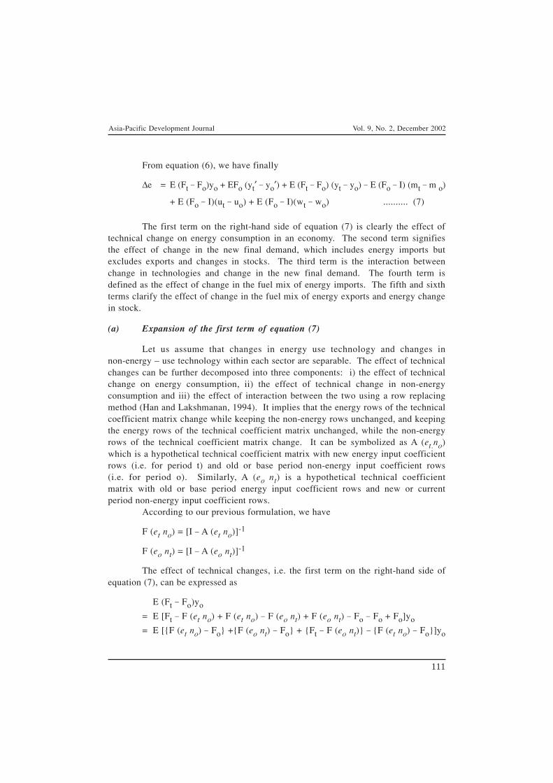
Asia-Pacific Development Journal Vol. 9, No. 2, December 2002
111
From equation (6), we have finally
∆e = E (Ft − Fo)yo + EFo (yt′ − yo′) + E (Ft − Fo) (yt − yo) − E (Fo − I) (mt − m o)
+ E (Fo − I)(ut − uo) + E (Fo − I)(wt − wo) .......... (7)
The first term on the right-hand side of equation (7) is clearly the effect oftechnical change on energy consumption in an economy. The second term signifiesthe effect of change in the new final demand, which includes energy imports butexcludes exports and changes in stocks. The third term is the interaction betweenchange in technologies and change in the new final demand. The fourth term isdefined as the effect of change in the fuel mix of energy imports. The fifth and sixthterms clarify the effect of change in the fuel mix of energy exports and energy changein stock.
(a) Expansion of the first term of equation (7)
Let us assume that changes in energy use technology and changes innon-energy – use technology within each sector are separable. The effect of technicalchanges can be further decomposed into three components: i) the effect of technicalchange on energy consumption, ii) the effect of technical change in non-energyconsumption and iii) the effect of interaction between the two using a row replacingmethod (Han and Lakshmanan, 1994). It implies that the energy rows of the technicalcoefficient matrix change while keeping the non-energy rows unchanged, and keepingthe energy rows of the technical coefficient matrix unchanged, while the non-energyrows of the technical coefficient matrix change. It can be symbolized as A (et.no)which is a hypothetical technical coefficient matrix with new energy input coefficientrows (i.e. for period t) and old or base period non-energy input coefficient rows(i.e. for period o). Similarly, A (eo nt) is a hypothetical technical coefficientmatrix with old or base period energy input coefficient rows and new or currentperiod non-energy input coefficient rows.
According to our previous formulation, we have
F (et no) = [I − A (et no)]-1
F (eo nt) = [I − A (eo nt)]-1
The effect of technical changes, i.e. the first term on the right-hand side ofequation (7), can be expressed as
E (Ft − Fo)yo
= E [Ft − F (et no) + F (et no) − F (eo nt) + F (eo nt) − Fo − Fo + Fo]yo
= E [{F (et no) − Fo} +{F (eo nt) − Fo} + {Ft − F (eo nt)} − {F (et no) − Fo}]yo
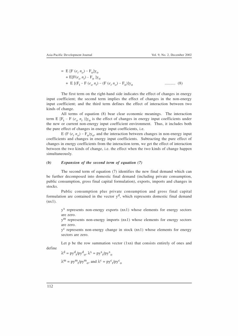
Asia-Pacific Development Journal Vol. 9, No. 2, December 2002
112
= E [F (et no) − Fo]yo
+ E[F(eo nt) − Fo ]yo
+ E [(Ft − F (eo nt) − (F (et no) − Fo)]yo .......... (8)
The first term on the right-hand side indicates the effect of changes in energyinput coefficient; the second term implies the effect of changes in the non-energyinput coefficient; and the third term defines the effect of interaction between twokinds of change.
All terms of equation (8) bear clear economic meanings. The interactionterm E [Ft − F (eo nt )]yo is the effect of changes in energy input coefficients underthe new or current non-energy input coefficient environment. Thus, it includes boththe pure effect of changes in energy input coefficients, i.e.
E (F (et no) − Fo)yo, and the interaction between changes in non-energy inputcoefficients and changes in energy input coefficients. Subtracting the pure effect ofchanges in energy coefficients from the interaction term, we get the effect of interactionbetween the two kinds of change, i.e. the effect when the two kinds of change happensimultaneously.
(b) Expansion of the second term of equation (7)
The second term of equation (7) identifies the new final demand which canbe further decomposed into domestic final demand (including private consumption,public consumption, gross final capital formulation), exports, imports and changes instocks.
Public consumption plus private consumption and gross final capitalformulation are contained in the vector yd, which represents domestic final demand(nx1).
yx represents non-energy exports (nx1) whose elements for energy sectorsare zero.ym represents non-energy imports (nx1) whose elements for energy sectorsare zero.yc represents non-energy change in stock (nx1) whose elements for energysectors are zero.
Let p be the row summation vector (1xn) that consists entirely of ones anddefine
λd = pydt/pyd
o, λx = pyxt/pyx
o
λm = pymt/pym
o, and λc = pyct/pyc
o
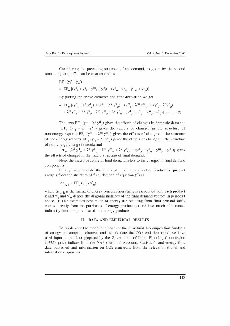
Asia-Pacific Development Journal Vol. 9, No. 2, December 2002
113
Considering the preceding statement, final demand, as given by the secondterm in equation (7), can be restructured as
EFo (yt′ − yo′)
= EFo [(yd
t + yxt − ym
t + yct) − (yd
o+ yxo − ym
o + yco)]
By putting the above elements and after derivation we get
= EFo [(ydt − λd yd
o) + (yxt − λx yx
o) − (ymt − λm ym
o) + (yct − λcyc
o)
+ λd ydo + λx yx
o − λm ymo
+ λc yco
− (ydo + yx
o − ymo+ yc
o)].......... (9)
The term EFo (ydt − λd yd
o) gives the effects of changes in domestic demand; EFo (yx
t − λx yxo) gives the effects of changes in the structure of
non-energy exports; EFo (ymt − λm ym
o) gives the effects of changes in the structure
of non-energy imports EFo (yct − λc yc
o) gives the effects of changes in the structureof non-energy change in stock; and
EFo [(λd ydo + λx yx
o − λm ym
o + λc yc
o) − (ydo + yx
o − ym
o + yco)] gives
the effects of changes in the macro structure of final demand.Here, the macro structure of final demand refers to the changes in final demand
components.Finally, we calculate the contribution of an individual product or product
group k from the structure of final demand of equation (9) as
∆ey, k = EFo (y′t - y′o)
where ∆ey, k is the matrix of energy consumption changes associated with each productk and y′t and y′o denote the diagonal matrices of the final demand vectors in periods tand o. It also estimates how much of energy use resulting from final demand shiftscomes directly from the purchases of energy product (k) and how much of it comesindirectly from the purchase of non-energy products.
II. DATA AND EMPIRICAL RESULTS
To implement the model and conduct the Structural Decomposition Analysisof energy consumption changes and to calculate the CO2 emission trend we haveused input-output data prepared by the Government of India, Planning Commission(1995), price indices from the NAS (National Accounts Statistics), and energy flowdata published and information on CO2 emissions from the relevant national andinternational agencies.
Asia-Pacific Development Journal Vol. 9, No. 2, December 2002
114
Results and Discussion
Energy consumption changes and sources of change
Energy consumption and the causes of changes are presented in table 1.Table 1 records the changes in absolute amounts during the period 1991/92 to1996/97. It is observed from table 1 that during this period India’s total commercialenergy consumption increased by 278.65 mtcr (table 1) or 5.7 per cent p.a. Althoughthe coal sector performed reasonably well in 1991/92 to 1996/97, some majorweaknesses have also emerged. It is observed that during this period coal and ligniteconsumption increased by 58 mtcr (table 1) or 4.83 per cent p.a. from 1991-92 to1996-97, oil and gas sector also recorded an increase at 5.5 per cent p.a., whileelectricity consumption was the highest i.e. 7 per cent p.a during this period an increaseby 79 mtcr.
In fact, electricity, gas and water supply have decelerated sharply from anaverage growth of 9.5 per cent in the Seventh Plan to 7.4 per cent in the Eighth Planperiod. Effective reforms in all these areas have been limited. The rate of growth ofpower generating capacity has declined during 1996/97. During the first half of the1990’s oil production increased at an annual rate of less than 1 per cent p.a. The 19per cent increase in production in 1994/95 arrested the declining trend. The shortfallsare on account of uncertain reservoir behaviour in the Bombay offshore basin, problemsin the north-eastern region and delays in implementation of joint venture projects.On the consumption front it reflects a moderate increment i.e. 5.5 per cent p.a. or141.65 mtcr (table 1) between 1991/92 and 1996/97. Natural gas consumption peakedgradually during the period to 6 per cent p.a. Out of it, 56 per cent of gas wasutilized for energy purposes, mainly for power generation, and 44 per cent was usedas feedstock, mainly for fertilizer plants. More remarkable change occurred between1995/96 and 1996/97: consumption of crude oil picked up at 75.4 mt; being 10.8 percent higher than in 1994/95. This spurt in growth matches with a pick-up in industrialactivity during 1995/96. During 1991/92 to 1996/97, the growth of hsd (high speeddiesel) increased at a rate of 7.3 per cent p.a. The increase in coal consumption in thepower sector has been mainly due to improved PLF (plant load factor) performance ofthe existing plants.
Sources of change
Six different factors can be identified which contributed to the change inenergy use: i) technical change, ii) change in the final demand structure, iii) changein energy imports, iv) change in energy exports, v) change in stocks and vi) interactionbetween technical change and the structure of final demand.

Asia-Pacific Development Journal Vol. 9, No. 2, December 2002
115
Table 1. Structural decomposition analysis of energy consumption changes inIndia from 1991-92 to 1996-97 (Mtcr)
Coal Cr. oil andElectricity Total
and Lignite Natural Gas
Total Energy Consumption Change 58.000 141.650 79.000 278.650Technical change -39.000 -41.860 -5.660 -86.520Changes in energy input coefficient -56.000 -221.000 -19.440 -296.900Changes in non-energy input coefficient 22.570 215.740 15.390 253.700Interaction term -5.370 -35.870 -1.600 -42.840Changes in final dd structure 109.650 139.440 88.350 337.440Effects of changes in str of dom. dd 36.940 83.160 18.440 138.540Effects of changes in str of non-energy export 0.690 9.470 0.930 11.090Non-energy import -2.180 -2.500 -1.750 -6.430Non-energy changes in stock 2.970 -1.300 2.350 4.020Macro structure of final dd 75.740 49.890 68.930 194.560Sector wise contributionCoal and lignite 37.700 2.050 0.670 40.420Crude oil and natural gas 0.000 0.090 0.000 0.090Electricity 13.600 8.260 33.230 55.090Agriculture 7.700 83.940 8.260 99.900Mining and quarrying -2.690 -26.530 -4.930 -34.150Sugar 0.350 3.070 0.290 3.710Food and beverages 3.930 22.170 2.810 28.910Textile and textile products 13.380 54.110 15.430 82.920Wood and wood products 0.040 0.355 0.040 0.435Paper and paper products -0.040 -0.090 -0.020 -0.153Leather and leather products 2.140 13.700 2.090 17.930Rubber and plastic products 0.700 5.100 0.770 6.570Petroleum products -5.040 -284.400 -0.880 -290.300Fertilizer -1.250 -12.630 -1.040 -14.920Chemical and chemical products 2.580 20.490 2.840 25.910Cement -0.750 -0.800 -0.320 -1.870Other metallic and mineral products 0.910 3.160 0.250 4.320Iron and steel -0.100 -0.290 -0.040 -0.430Basic metal products and machinery 8.420 38.070 6.880 53.370Construction 12.360 54.170 8.960 75.490Transport services 5.310 101.500 3.280 110.090Trade and other services 10.340 54.530 9.720 74.590Changes in energy import -0.220 -3.440 -0.280 -3.940Changes in energy export -0.040 -0.060 -0.030 -0.130Changes in energy changes in stock -0.260 -1.050 -0.330 -1.640Interaction of tech ch and final dd structure -12.270 49.990 -3.320 34.400

Asia-Pacific Development Journal Vol. 9, No. 2, December 2002
116
(i) Technical change
During 1991/92 to 1996/97 moderate technical changes took place to reduceenergy consumption. Though the percentage impact was very little small, it wasspearheaded by three sectors (coal, crude oil, and electricity). The contribution inthis respect was 39 mtcr or 3.25 per cent in the case of coal, 41.86 mtcr or 1.64 percent annually in the case of crude oil and natural gas, but electricity shared a smallamount i.e. 5.66 mtcr or 0.44 per cent p.a.
Thus, it would appear that the coal sector has improved technically morethan electricity. The efficient technology in the coal sector is hidden under exploration,exploitation, and benefication for improving the quality and efficient utilization ofcoal. New mining technologies have been introduced during the reform period witha fair degree of success.
The slight technical improvement in the case of oil and natural gas has beenpossible due to the minimization of the flaring of the associated gas, the higheroff-take of natural gas and the minimization of the risks of exploration both by anoptimal mix of exploration in different basins in India and vigorous measures forenergy conservation and inter-fuel substitution.
But, in the case of electricity technical change did not occur as in coal andoil and gas. Agricultural pump sets increased at the rate of 7.7 per cent p.a. andelectricity consumed in the agricultural sector increased at the rate of 13.3 per centp.a. Electricity consumed in agricultural pump sets installed has increased from anaverage of 3,672 kwh to 7,880 kwh in the five years to 1996/97. This has happeneddue to energy inefficiency. The effect of technical change can be classified as(i) change in energy input coefficient, (ii) change in non-energy input coefficient and(iii) interaction between the previous two.
Changes in energy input coefficient reduced energy use by 296.90 mtcr(table 1) or 6.09 per cent annually. The major contribution was by crude oil andnatural gas in this respect, by 221 mtcr or 8.7 per cent p.a. However, changes in thenon-energy portion of production technology increased energy consumption and reducedenergy savings by 253.7 mtcr or 5.2 per cent annually. The changes in non-energyinput coefficient also have an energy impact. Here also the major portion is sharedby crude oil and natural gas. This increased energy consumption by 215.74 mtcr or8.47 per cent p.a.
To minimize flaring the Government had undertaken a major gas flaringreduction programme. During the period 1991/92 to 1996/97 both creation of capacityand its utilisation improved substantially. Due to technical improvement in capacityutilisation the growth rate of crude throughput also performed well at 58.6 per cent in1995/96 which was 4 per cent higher than 1991/92.
The non-energy input coefficient in case of electricity sector increased energyconsumption by 15.39 mtcr (table 1). The flat tariff structure and high level of
Asia-Pacific Development Journal Vol. 9, No. 2, December 2002
117
subsidy provided by the Government and free electricity to farmers has permitted theinefficient use of electricity. Over-used and ill-maintained pump sets cause wastefulconsumption of electricity and also of water. Efficiency in the use of electricitydeclined in the production of newsprint, cotton and blended yarn, polyster-filamentyarn, aluminium and steel. But the interaction between the energy and non-energycoefficients reduced energy use by 42.84 mtcr (table 1) or 0.08 per cent p.a. with thecrude oil sector contributing more.
Changes in energy input coefficients and interactions both worked to drivedown the energy consumption of the Indian economy, while the non-energy inputcoefficient changes have totally offset the negative effect of both energy inputcoefficient changes and interaction that increases energy use. The opposite effects ofthese changes imply that one major characteristic of India’s technical change in thisperiod was the substitution of material inputs for energy inputs. Actually, materialinputs or non-energy inputs embody a large quantity of energy. So smaller energyinput requirement per unit of output worked directly and indirectly to reduce the totalenergy use, while bigger non-energy material input requirement per unit of outputworked indirectly to increase total energy use through increased output levels.
(ii) Changes in final demand structure
These have been an important factor behind the increase in energy consumptionduring 1991/92 to 1996/97. The share of individual sectors are 109.65 mtcr or9.13 per cent p.a. for coal, 139.44 mtcr or 5.47 per cent for crude oil and natural gasand 88.35 mtcr or 7.85 per cent p.a. for electricity in this respect. The demand forcoal during 1991/92 to 1996/97 from the various coal consuming sectors has showna sharp and unanticipated increase. The demand for the power sector alone is210 million tons of coal in the year 1996/97 as against 185.30 million tons indicatedfor the year at the beginning of the Eighth Five Year Plan and 194 million tonsdemanded at the mid-term appraisal carried out in September 1994. At the sametime, as a result of various constraints, including those of finance, land acquisitionand transportation, the coal companies have indicated a domestic production of only288.65 million tons for 1996/97. This implies an increase of 6.8 per cent over actualproduction in 1995/96.
On the electricity front, the pattern of utilisation of electricity from publicutilities has undergone a small change between 1992/93 and 1996/97. The share ofthe domestic sector has increased from 19.37 per cent to 23.52 per cent. The sharesof commercial and miscellaneous sectors have increased very sharply from 10.28 percent in 1992/93 to 13.38 per cent in 1996/97. The demand for electricity in thehousehold sector is expanding rapidly as the pressure of urbanisation continues toincrease and the availability of consumer durables also continues to expand. It isestimated that 40 per cent of the total electricity consumed in the household sector is
Asia-Pacific Development Journal Vol. 9, No. 2, December 2002
118
used for lighting. Fans consumed another 31 per cent of the electricity used whilerefrigerators, air conditioners and televisions account for about 28 per cent of theelectricity consumed by the household sector during our study period. Nearly 50 percent of the total electricity consumed in major power consuming industries was fromcaptive power plants in 1994/95. Several of the relatively newer and faster growingindustries, such as gems and jewellery, garments and electronics, are far more energyintensive; on the other hand, electricity consumption in fertilizer and pesticides andcasting and forging has declined in absolute terms during the study period.
If we separate the final demand structure under five heads like macro structureof final demand, effects of changes in domestic demand, effects of changes in thestructure of non-energy exports, non-energy imports, non-energy change in stocks, weobserve that the lions share goes to macro structure of final demand i.e. 194.56 mtcror 3.99 per cent annually. The positive effect of change in the structure of finaldomestic demand on energy consumption has far reaching significance as the growthof the Indian economy is becoming more domestic demand driven. In the case ofcoal, macro structure of final demand is greater (75.74 mtcr) than the structure ofdomestic demand (36.94 mtcr). But in the case of crude oil, the opposite consequenceshappened, i.e. 83.16 mtcr in domestic demand and 49.89 in macro structure of finaldemand. The electricity sector showed a wide gap between the structure of domesticdemand (18.44 mtcr) and macro structure of final demand (68.93 mtcr). The rapidpace of urbanisation and diverse urban growth patterns involve many structural changesin the economy which have major implications for energy use. Out of the remainingthree heads, the non-energy import sector slightly reduced the energy use of theeconomy during our study period i.e. 6.43 mtcr.
The sector-wise contribution resulting from final demand structure showsthat the contribution made by the energy product is 95.60 mtcr out of 337.44 mtcr andnon-energy products is 241.84 mtcr out of 337.44 mtcr during 1991/92 to 1996/97.Coal and electricity have a major share of energy products. So, the intensity of thesesectors has been rising sharply mainly on account of higher coal consumption bythe power sector and higher electricity consumption by the industrial sector, i.e.33.23 mtcr. During the Eighth Plan period 40 per cent of electricity was consumedby the energy sector itself and the remaining 60 per cent was consumed by energyintensive industries like textiles (15.43 mtcr), agriculture (8.26 mtcr), basic metals,metal products and machinery (6.88 mtcr), construction sector (8.965 mtcr), trade andother (9.72 mtcr) and transport. The consumption of electricity per unit of product inthe above industries is much higher than that in developed countries (Teddy,1995/96). Part of it reflects the dated vintage of the production processes in use.
Consumption of kerosene increased at an annual rate of 1.6 per cent duringthe period 1991/92 to 1996/97. Diesel consumption in the country has almost doubledin the 10 years from 1986/87 to 1996/97. It had a growth of 7.3 per cent p.a. duringthis period. During our study period, consumption of lubes and greases grew by
Asia-Pacific Development Journal Vol. 9, No. 2, December 2002
119
almost 5 per cent p.a. One major agricultural operation is irrigation, which is largelyperformed by using diesel and electric energy. The number of electric and dieselpumps has increased to 10.5 million and 4.9 million respectively by 1993/94. Powerconsumption in the agricultural sector expanded at the rate of 12-13 per cent p.a.during 1971 to 1996. As a result this sector’s share in the total power consumed hasincreased steadily from 10 per cent in 1970/71 to nearly 30 per cent in 1996/97. Theincrease in power consumption in the agricultural sector is the result of an increase inirrigation pump sets in use and a sharp increase in the usage hours of the pump sets.
The industrial sector relies only partly on the utilities for its powerrequirements. Nearly 48 per cent of the total electricity consumed in major powerconsuming industries was from captive power plants. The findings show that productgroups like textile products, petroleum products, chemicals, basic metals etc. are theleading sectors that have increased energy consumption. Chemicals, construction,transport, trade, basic metals, metal products and textile machinery, increased theconsumption of crude petroleum. The share of commercial energy consumed in thetransport sector in the total commercial energy consumed has increased steadily.Besides, the consumption of oil in the transport sector has gradually increased mainlybecause of greater use of private modes of transport. Also oil has gradually replacedcoal as a fuel. This is evident from the declining share of coal from about 30 per centin 1970/71 to 5 per cent in 1994/95, whereas the share of oil increased from 30 percent to 95 per cent in the same period. This change is attributed to greater dependenceon road transport, and shift from steam traction to diesel and electric traction in therailways.
(iii) Change in energy imports
This covers the limited amount of 3.94 mtcr (table 1) in the period 1991/92to 1996/97. The major portion was on account of rise in domestic crude oil andnatural gas production.
(iv) Change in energy exports
During the period 1991/92 to 1996/97 energy consumption increased slightlyi.e. 0.13 mtcr. India is not a major exporter of coal. However, coal exports meet thedemand from neighbouring countries. Coal exports are destined to Bangladesh, Nepal,and Bhutan. The quantity of coal exported during 1995/96 was about 0.098 mt.
(v) Change in energy stocks
This behaved in a similar fashion to imports. It decreased energy consumptionby 1.64 mtcr during 1991/92 to 1996/97.
Asia-Pacific Development Journal Vol. 9, No. 2, December 2002
120
(vi) Interaction between technical change and change in final demand structure
In the period 1991/92 to 1996/97 this interaction has increased energyconsumption by 34.40 mtcr. The lion’s share of it goes to crude petroleum by49.99 mtcr or 1.96 per cent p.a., but two other sectors i.e. coal and electricity sharedvery little (12.27 mtcr and 3.32 mtcr respectively). Thus, the reform period showsthat final demand expansion increased India’s energy consumption by 6.9 per centp.a. while, on the other hand, production technology changes reduced energyconsumption by 1.77 per cent p.a. The consumption of energy produces consequencesfor the environment. The commercial energy activities cause air pollution. Thisincludes the use of fossil fuels (coal and oil), industrial processes etc. The air pollutantsare mainly CO2 emissions. Before any alternative strategies for energy consumptioncan be advanced it is necessary first to try to calculate the level of CO2 emissions andtheir intensity in the next section.
III. THE METHODOLOGY AND RESULTS OF CO2 EMISSIONS
In this section an attempt has been made to estimate carbon dioxideemissions and their intensities in major energy consuming industries with the help ofan input-output model. In reality, CO2 is released mainly from fossil fuel combustionand from bio-mass combustion. The sources of fossil fuel combustion are coal, oiland gas. Here we consider fossil fuel combustion only. The CO2 emissions fromfossil fuel combustion have been estimated by the following IPCC (IntergovernmentalPanel on Climate Change) guideline, wherein total CO2 emissions = (actual fuelconsumption) * (carbon emission factor) * (fraction of carbon oxidized) * (molecularweight ratio of CO2 is to carbon i.e. 44/12 or 3.66).
For an analysis of CO2 emissions we need to extend the above conventionalinput-output framework in one important respect i.e. we have to compute the amountof CO2 emission that takes place in various activities. We apply the fuel specificcarbon emission factors to the row vector of the fossil fuel sector of the respectiveinput-output table to estimate the total CO2 emitted by the coal and oil sectors. Weuse an emission factor of 0.55 (mt of CO2)/mt for coal and 0.79 (mt of CO2)/mt forcrude oil and 0.67 mt of CO2/m.c.m for natural gas to arrive at carbon emissions bydifferent sectors due to coal and oil and natural gas separately. The values of thefraction of carbon oxidized for the fuels are 0.98 for coal and lignite, and 0.99 forcrude oil and natural gas. We then follow the normal convention of measurement ofcarbon dioxide in carbon equivalent units.
For conversion to CO2 units the carbon emission figures are multiplied by3.66. The estimated figures are displayed in tables 2 and 3. The total quantity ofCO2 emitted owing to burning of fossil fuel inputs used by various production sectorsand final demand is shown in table 3. On the basis of the above estimated figure we
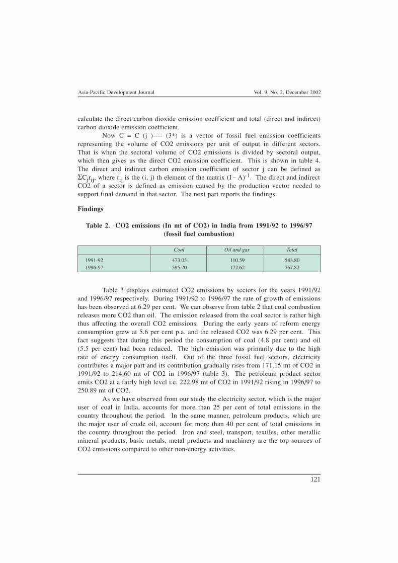
Asia-Pacific Development Journal Vol. 9, No. 2, December 2002
121
calculate the direct carbon dioxide emission coefficient and total (direct and indirect)carbon dioxide emission coefficient.
Now C = C (j )---- (3*) is a vector of fossil fuel emission coefficientsrepresenting the volume of CO2 emissions per unit of output in different sectors.That is when the sectoral volume of CO2 emissions is divided by sectoral output,which then gives us the direct CO2 emission coefficient. This is shown in table 4.The direct and indirect carbon emission coefficient of sector j can be defined asΣCjrij, where rij is the (i, j) th element of the matrix (I − A)-1. The direct and indirectCO2 of a sector is defined as emission caused by the production vector needed tosupport final demand in that sector. The next part reports the findings.
Findings
Table 2. CO2 emissions (In mt of CO2) in India from 1991/92 to 1996/97(fossil fuel combustion)
Coal Oil and gas Total
1991-92 473.05 110.59 583.801996-97 595.20 172.62 767.82
Table 3 displays estimated CO2 emissions by sectors for the years 1991/92and 1996/97 respectively. During 1991/92 to 1996/97 the rate of growth of emissionshas been observed at 6.29 per cent. We can observe from table 2 that coal combustionreleases more CO2 than oil. The emission released from the coal sector is rather highthus affecting the overall CO2 emissions. During the early years of reform energyconsumption grew at 5.6 per cent p.a. and the released CO2 was 6.29 per cent. Thisfact suggests that during this period the consumption of coal (4.8 per cent) and oil(5.5 per cent) had been reduced. The high emission was primarily due to the highrate of energy consumption itself. Out of the three fossil fuel sectors, electricitycontributes a major part and its contribution gradually rises from 171.15 mt of CO2 in1991/92 to 214.60 mt of CO2 in 1996/97 (table 3). The petroleum product sectoremits CO2 at a fairly high level i.e. 222.98 mt of CO2 in 1991/92 rising in 1996/97 to250.89 mt of CO2.
As we have observed from our study the electricity sector, which is the majoruser of coal in India, accounts for more than 25 per cent of total emissions in thecountry throughout the period. In the same manner, petroleum products, which arethe major user of crude oil, account for more than 40 per cent of total emissions inthe country throughout the period. Iron and steel, transport, textiles, other metallicmineral products, basic metals, metal products and machinery are the top sources ofCO2 emissions compared to other non-energy activities.

Asia-Pacific Development Journal Vol. 9, No. 2, December 2002
122
Table 3. Estimated CO2 emissions in India during 1991-92 to 1996-97by sectors (Mt of CO2)
Serial No. Sectors 1991-92 1996-97
1 Coal and lignite 2.34 2.162 Cr. oil and Natural Gas 0.00 0.003 Electricity 171.15 214.604 Agriculture 5.75 4.745 Mining and quarrying 0.04 0.056 Sugar 0.99 1.017 Food and beverages 15.77 16.898 Textile and textile products 24.53 25.539 Wood and wood products 0.32 0.35
10 Paper and paper products 10.53 10.8611 Leather and leather products 0.57 1.0712 Rubber and plastic products 0.94 1.1513 Petroleum products 222.98 250.8914 Fertilizer 12.21 14.8915 Chemical and chemical products 6.90 9.2216 Cement 18.25 17.6817 Other metallic mineral products 16.87 18.5518 Iron and steel 66.30 77.3019 Basic metal, metal products and machinery 20.58 21.9720 Construction 6.15 6.8521 Transport 30.32 31.2522 Trade and other services 22.32 19.0823 Total 656.16 746.0824 Total final -72.36 21.7425 Gross 583.80 767.82
The CO2 emissions from final demand (private consumption + Governmentconsumption + investment demand + net export demand) gradually increased from-72 mt of CO2 in 1991/92 to 21 mt of CO2 in 1996/97 (table 3). Here the sign offinal demand component is negative due to the high import amount of the crude oilsector. One positive aspect from the result of final demand shows that the importedamount has been gradually controlled. The study also reflects that the CO2 emissionsin private consumption were highest during 1991/92 (108.60 mt of CO2).
We now turn to the direct and total CO2 emission coefficient as presented intable 4. The results contained in table 4 show that all the sectors show a more or lesssimilar pattern in case of direct and total coefficients throughout the period. The totalcoefficient is higher in all sectors than the direct coefficient. However, some sectorsdeserve attention. The results reveal that electricity ranks the highest among all
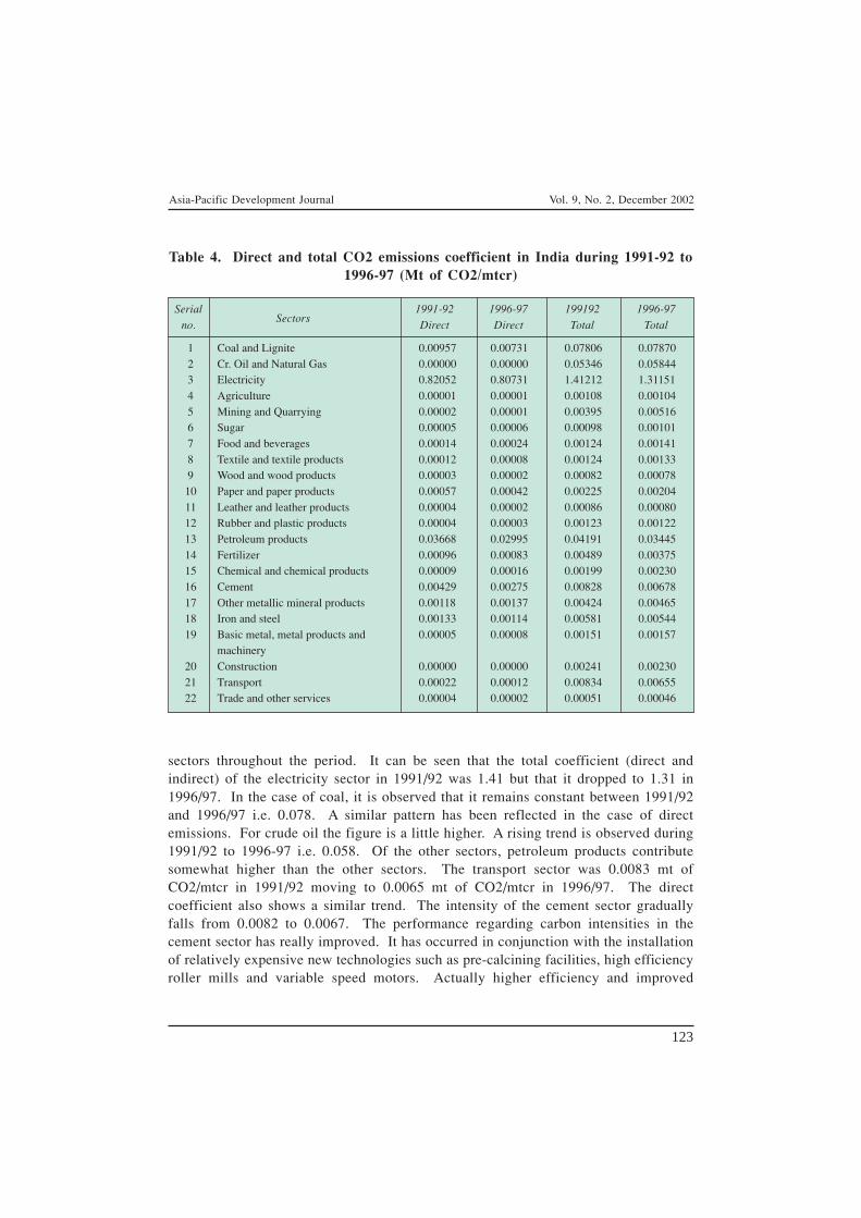
Asia-Pacific Development Journal Vol. 9, No. 2, December 2002
123
sectors throughout the period. It can be seen that the total coefficient (direct andindirect) of the electricity sector in 1991/92 was 1.41 but that it dropped to 1.31 in1996/97. In the case of coal, it is observed that it remains constant between 1991/92and 1996/97 i.e. 0.078. A similar pattern has been reflected in the case of directemissions. For crude oil the figure is a little higher. A rising trend is observed during1991/92 to 1996-97 i.e. 0.058. Of the other sectors, petroleum products contributesomewhat higher than the other sectors. The transport sector was 0.0083 mt ofCO2/mtcr in 1991/92 moving to 0.0065 mt of CO2/mtcr in 1996/97. The directcoefficient also shows a similar trend. The intensity of the cement sector graduallyfalls from 0.0082 to 0.0067. The performance regarding carbon intensities in thecement sector has really improved. It has occurred in conjunction with the installationof relatively expensive new technologies such as pre-calcining facilities, high efficiencyroller mills and variable speed motors. Actually higher efficiency and improved
Table 4. Direct and total CO2 emissions coefficient in India during 1991-92 to1996-97 (Mt of CO2/mtcr)
SerialSectors
1991-92 1996-97 199192 1996-97
no. Direct Direct Total Total
1 Coal and Lignite 0.00957 0.00731 0.07806 0.078702 Cr. Oil and Natural Gas 0.00000 0.00000 0.05346 0.058443 Electricity 0.82052 0.80731 1.41212 1.311514 Agriculture 0.00001 0.00001 0.00108 0.001045 Mining and Quarrying 0.00002 0.00001 0.00395 0.005166 Sugar 0.00005 0.00006 0.00098 0.001017 Food and beverages 0.00014 0.00024 0.00124 0.001418 Textile and textile products 0.00012 0.00008 0.00124 0.001339 Wood and wood products 0.00003 0.00002 0.00082 0.0007810 Paper and paper products 0.00057 0.00042 0.00225 0.0020411 Leather and leather products 0.00004 0.00002 0.00086 0.0008012 Rubber and plastic products 0.00004 0.00003 0.00123 0.0012213 Petroleum products 0.03668 0.02995 0.04191 0.0344514 Fertilizer 0.00096 0.00083 0.00489 0.0037515 Chemical and chemical products 0.00009 0.00016 0.00199 0.0023016 Cement 0.00429 0.00275 0.00828 0.0067817 Other metallic mineral products 0.00118 0.00137 0.00424 0.0046518 Iron and steel 0.00133 0.00114 0.00581 0.0054419 Basic metal, metal products and 0.00005 0.00008 0.00151 0.00157
machinery20 Construction 0.00000 0.00000 0.00241 0.0023021 Transport 0.00022 0.00012 0.00834 0.0065522 Trade and other services 0.00004 0.00002 0.00051 0.00046
Asia-Pacific Development Journal Vol. 9, No. 2, December 2002
124
technology lead to low intensity of carbon emission. The direct intensity of theconstruction sector is lowest among all sectors. This is because it does not makemuch use of fossil fuel based energy to construct a building or a road. However, theconstruction sector uses many energy intensive materials such as bricks, cement, ironand steel, aluminium glass and asbestos. Hence, the indirect part achieves prominencein this respect leading to high value of total intensity. These facts indicate thatsectors like construction, textiles, trade, agriculture and transport emit CO2 at a fairlyhigh level largely due to indirect effects.
Given the higher value of indirect coefficients and the larger volume ofactivity, the above sectors turn out to be the most responsible for CO2 emissions inIndia when they are viewed in terms of total (direct and indirect) emissions due to themagnitude of final demand in each sector.
IV. SUMMARY AND CONCLUSIONS
This paper has shown that India’s energy consumption increased by 5.7 percent p.a or 279.27 mtcr (table 1) from 1991/92 to 1996/97. Six different forcesbehind this increase have been identified. Among them the most significant role, asgarnered from the empirical results, has been played by the structure of final demand,technical change and the interaction between the structure of final demand and technicalchange. The remaining forces had very little impact on energy consumption. TheCO2 emission trends has revealed that the most dominating sectors are petroleumproducts and electricity. This phenomenon is due to the direct effect of crude oil andcoal respectively. The next positions are occupied by the iron and steel and transportsectors respectively. Overall, CO2 emissions have risen gradually from 1991/92 to1996/97. As far as the intensities are concerned, electricity contributes a major part.In actual fact, the increase in emissions is most strongly correlated with fuelconsumption, which, in turn, is influenced by population growth and rising incomelevels.
So far as energy strategies are concerned, specifically strategies to conserveenergy and to minimize CO2 emissions over time, India has not been able to developany credible framework or policy approaches to meet such objectives. The strategiesthat have been adopted by the Government during the period 1991 to 1996 for reducingthe consumption have not been successful. Though the 25 leading industries recordedsignificant energy savings and have received national awards for energy conservationin the year 1996 the performance of major sectors like transport and agriculture havenot been successful in conserving energy.
Considering the above, it would be worthwhile to point out a few importantissues that should get appropriate weightage in any future energy policy. These issuescan be summarised as:

Asia-Pacific Development Journal Vol. 9, No. 2, December 2002
125
(i) The Government of India must adopt an overall policy that promotesthe growth of less energy-intensive components of final demand.
(ii) The Government should develop energy conservation legislation toenforce punitive action under the law and to ensure stricterimplementation.
In the latter context, it is suggested that much higher priority has to be givento the conservation of energy in national policy-making. This will play a significantrole in alleviating the shortage of energy and in reducing environment pollution. TheGovernment must take measures, such as publicity campaigns and differential taxesand subsidies, to promote energy conservation in the country. The enhancement ofnational consciousness in this regard and progress in the understanding of the underlyingscientific and technological issues involved in energy conservation would promoterationalization and greater efficiency in energy consumption in the country.
In this connection it is recommended that efficiency and conservation ofenergy is also possible through inter-fuel substitution. Inter-fuel substitution can helpto mitigate the problem of carbon emissions. Replacing high carbon coal andmid-range oil with lower carbon natural gas, or with zero carbon renewable and nuclearpower can dramatically lower CO2 emissions. In the industrial sector substitutingnatural gas for coal is the most obvious shift. More specifically, in the case ofelectrification, the promotion of biomass-based power plants would be an appropriatepolicy option to mitigate CO2 emissions. The use of plant material as fuel andfeedstock in place of fossil fuels can have a significant effect on the reduction of netCO2 emissions. Alcohol biomass fuels for transport have played a major role inBrazil (Goldenberg and others, 1993) and plantations in other countries, includingIndia, could provide significant quantities of bio fuels (Hall and others, 1993).
Out of the fuel sector electricity emissions show the highest increaseamong energy sources suggesting that local electric plants should increase the shareof non-fossil fuels and natural gas to reduce CO2 emissions in India. Thus pollutioncan be reduced or even prevented by the use of alternative energy sources. Somewind energy, small scale hydro and conversion of waste to energy are alreadycompetitive even with conventional sources of supply. A few other renewabletechnologies may be appropriate for India. Among these are solar hot water systemsfor meeting process heat requirements in industries, solar dryers, fuel cell technologyand the application of hydrogen energy and bioliquid fuels for surface transport.
Reducing emissions by preventive options for pollution control (improvedefficiency and switching to other energy sources) are generally considered advantageousover control options. Furthermore, it is possible to decouple economic growth fromprimary energy consumption by investing in more efficient supply frameworks,improving energy efficiency amongst end-users and substituting renewable energytechnologies for fossil fuels.

Asia-Pacific Development Journal Vol. 9, No. 2, December 2002
126
A proper weightage should be given to the iron and steel industry in India asit is one of the major sources of air pollution as our findings report. It involves notonly upgrading the industry’s processing procedures but also increasing the effectiveutilization of coal consumption in the production of steel.
For energy conservation, efficiency and research and development andtechnological upgradation a suitable national energy price policy has to be framed. Itis a fact that energy prices are low in the country. In India coal, kerosene and naturalgas are subsidized. Ideally, all energy prices should truly reflect the cost of usingfossil fuels including the cost to society from pollution and environmental degradation.Therefore, until there is a realistic consensus on how environmental standards are tobe met, fossil fuel subsidies should not be encouraged. Clearly, such changes are noteasy to implement. Hence, the Government of India should devise appropriate fiscalincentives linked to energy savings and tax concessions, rather than subsidies, inorder to achieve economy in the use of energy over the long term.
A mix of information, market-based tax and investment credits, betterregulations, higher efficiency standards, enhanced use of voluntary agreements likethe energy star programme, removal of trade and investment barriers and resolvingthe international disagreements over intellectual property rights will all be needed forindustry to reduce the problem of CO2 emissions and green house gases further.
For controlling CO2 the use of natural gas is gaining wide popularity acrossthe globe as it is comparatively cleaner than the other fuels and has around half thecarbon content of coal. Its development, coupled with the adoption of suitabletechnology such as combined cycle gas turbines for electricity generation, is likely tolead to natural gas taking a larger share in primary energy requirements. Across theland, pipeline networks would have to be set up to distribute natural gas. Though thehigh cost of transportation makes it presently uncompetitive with other fuels thepossibility of increasing its use has to be explored judiciously.
The Government should consider introducing clean energy technology. Cleanenergy technology (CET) is defined as those technologies that combine more efficientprocesses and reduced pollutant production without necessarily entailing a change inthe form of energy used. Clean coal technologies like integrated gasification combinedcycle (IGCC) plants should be encouraged in industry and power generating plants.These technologies typically reduce emissions of CO2 and provide improvements inenergy efficiency when compared with traditional coal combustion technologies.
One other aspect deserves mention in this context. Emitted gases have thecapacity to be transported over large distances, sometimes many hundreds of kilometers,and may give rise to depositions in another country. The potential for such transboundryair pollution was evident in the recent Indonesian forest fires. The area affected bythe air pollutants from the fire spread for more than 3,200 kilometers east to west,covering six Asian countries and affected around 70 million people. Major weatherpatterns in Asia facilitate the transboundry transport of air pollutants from land to sea

Asia-Pacific Development Journal Vol. 9, No. 2, December 2002
127
and the reverse in summer. Pollutants can thus be carried from country to country inthe region. It is, therefore, not possible for individual countries to solve the associatedproblems alone. There is an obvious and strong need for regional intergovernmentalco-operation in this field (SEI, 2000).
Asia-Pacific Development Journal Vol. 9, No. 2, December 2002
128
REFERENCES
Breuil, J.M., 1992. “Input-output analysis and pollutants emissions in France”, The Energy Journal,vol. 13, No. 3.
Chang, Y.F. and S.J. Lin, 1998. “Structural decomposition of industrial CO2 emission in Taiwan:an input-output approach” Energy Policy, vol. 26 No. 1 pp. 5-12.
Chaturvedi Pradeep, 1997. Energy Management Policy Planning and Utilization, Concept PublishingCompany, New Delhi.
Dash U.K. and K.K. Saxena, 1995. Input-Output Analysis of Energy: An Application to Indian Economy(1979-89), XI International Conference on Input-Output Techniques, Papers for the PlenarySession, 27 November – 2 December.
Gay, S. and J.L.R. Proops, 1993. “CO2 production by the U.K. economy: an input-output assessment”Applied Energy, vol. 44, pp. 113-130.
Goldenberg, J. and others, 1993. “The Brazilian fuel alcohol program” in Johansen, T.B., Kelly, H. andReddy, A.K.N. and Williams, R. (eds.) Renewable Energy: Sources for Fuels and Electricity,Island Press, Washington, D.C.
Gupta, S. and others, 1997. Energy Consumption and GHG Emissions: A Case Study for India, GlobalWarming (Asian Energy Studies) TERI publication.
Hall, D.O. and others, 1993. “Biomass for energy supply prospects” in Johansen, T.B., Kelly, H. andReddy, A.K.N. and Williams, R., eds. Renewable Energy: Sources for Fuels and Electricity,Island Press, Washington, D.C., pp. 593-651.
Han Xiaoli and T.K. Lakshmanan, 1994. “Structural changes and energy consumption in the Japaneseeconomy 1975-85: an input-output analysis”, The Energy Journal, vol. 15, No. 3, pp. 16-188.
Hayami, H., and others, 1993. “Estimation of air pollutions and evaluating CO2 emissions from productionactivities using Japan’s 1985 input-output tables”, Journal of Applied Input-Output Analysis,vol. 1, No. 2, pp. 29-44.
Leontief, W. and D. Ford, 1972. Air pollution and the economic structure: empirical results ofinput-output computation, in A Broody and A.P. Carter, eds. Input-Output Techniques, Amsterdam.
Lin X. and Karen R. Polenske, 1995. “Input-output anatomy of China’s energy use: changes in the 1980,Economic System Research, vol. 7, No. 1, pp. 67-83.
Lin, G., 1998. “Energy development and environmental constraints in China”, Energy Policy, vol. 26,No. 2, pp. 119-128.
Majumdar, S. and Jyoti Parikh, 1995. “Macroeconomic consistency in energy planning: a case study ofIndia, Journal of Quantitative Economics, vol. 11, No. 2, pp. 95-121.
Mukhopadhyay, K., 2000. “Industrial CO2 emissions in India during 1991-92 to 1996-97:an input-output approach”, paper accepted for the 36th Annual Conference of the IndianEconometric Society held at Devi Ahilya University, Indore (4-6 February).
Mukhopadhyay, K. and D. Chakraborty, 1999. “Energy consumption changes in India during 1973-74 to1991-92”. Economic System Research, vol. 13, December.
, 2000. “Energy consumption changes and CO2 emissions in India during 1968-69 to 1996-97,“Paper presented at the 13th International Conference on Input-Output Techniques, MacerataUniversity, Italy (21-25 August).

Asia-Pacific Development Journal Vol. 9, No. 2, December 2002
129
Mukhopadhyay, K., 2001. “Energy consumption changes and CO2 emissions in India during 1968-69 to1996-97: A quantitative approach, Phd. dissertation (Jadavpur University).
Planning Commission, The Eighth Five-year Plan, 1991-96. Government of India, New Delhi.
, 1992. The Eighth Five-year Plan (1992-97), Government of India, New Delhi.
, 1995. A technical note to the Eighth Five-year Plan of India, Input-Output Transaction Tablefor 1991-92, New Delhi, Government of India.
Rose A. and C.Y. Chen, 1991. “Sources of change in energy use in the U.S. economy, 1972-82”. Resourceand Energy, 13, pp. 1-21.
SEI, 2000. Regional Air Pollution in Asia, Stockholm.
Sengupta, R., 1992. Energy Modeling for India, published by the Planning Commission in India.
TEDDY, 1995/96. Tata Energy Data Directory Year Book, “Environmental effects of energy use”,pp. 220-225, TERI publication.
, 1998/99. Tata Energy Data Directory Year Book, TERI Publication.
Wier, M., 1998. “Sources of changes in emissions from energy: A structural decomposition analysis”.Economic System Research, vol. 10, No. 2, pp. 99-112.
World Development Report, 1993. Managing India’s Environment – Selected Aspects Chapter 3, WorldBank, Washington, D.C.
Zhang X.Z. and H. Folmer, 1998. “Economic modeling approaches to cost estimates for the control ofCO2 emissions: a case study of Germany and U.K.”. Energy Economics, February, vol. 20,No. 1, pp. 101-120.

Asia-Pacific Development Journal Vol. 9, No. 2, December 2002
131
AN ANALYSIS OF EU ANTI-DUMPING CASESAGAINST CHINA
Y.H. Mai*
In this study, an analysis of Chinese exports to the European Union (EU)of the products subject to anti-dumping duties shows that anti-dumpingmeasures tend to significantly reduce bilateral trade flows. The rise inChinese exports to EU would have been more than 3 per cent higher withoutthe imposition of 21 anti-dumping duties in 1995-1998. A close investigationof EU anti-dumping cases against China also reveals that calculation ofanti-dumping margins suffers from imperfect information and is thereforehighly likely to lead to biased rulings. The high rate of termination due towithdrawal of complaints poses the question whether the scheme encouragesindustries to use it to fight against “fair” competition as opposed to “unfair”competition.
With the reduction in tariff levels under the General Agreement on Tariffsand Trade (GATT), the predecessor of the World Trade Organization (WTO),import-competing industries in developed countries appear to have turned toanti-dumping for protection since the 1980s. If a company exports a product ata price lower than the price it normally charges on its own home market, it isautomatically said to be “dumping” the product. Such behaviour can be explained interms of exporters tolerating initial losses in order to gain market share in the importingcountry. Under such circumstances, the anti-dumping scheme enables the affectedindustries in the importing country to lodge a complaint. In response to the complaint,the importing country Government may initiate an investigation. If a case of dumpingis established, the importing country Government may take action against the dumping,such as levy a tariff on the concerned products from the exporting country.
For member countries of the WTO, anti-dumping action is governed by theanti-dumping agreement that resulted from the Uruguay Round negotiations. TheWTO agreement disciplines anti-dumping actions by providing rules for calculating theamount of dumping, detailed procedures for initiating and conducting anti-dumpinginvestigations, rules on the implementation and duration of anti-dumping measures,and particular standards for dispute settlement panels to apply in anti-dumping disputes.
* Senior Research Fellow, Centre of Policy Studies, Monash University, Victoria 3800, Australia.

Asia-Pacific Development Journal Vol. 9, No. 2, December 2002
132
A growing body of literature has expressed concern over the explosion inanti-dumping actions since the 1980s (Rugman and Anderson, 1987, Robert and Robert,1991, Finger, 1993, Jones, 1994, and Krueger, 1995). This research concluded thatanti-dumping measures are harmful to the importing country and to the multilateraltrading system. It has negative impacts on competition and consumer welfare andinvolves huge institutional costs for the importing countries. With active anti-dumpingand other administrative protection measures, trade policy that is efficient in promotingincome growth through trade liberalization takes on the role of redistributing income,policy objectives that can be more efficiently carried out by tax and expenditurepolicies (Krueger, 1995). However, much less work has been done in analysing thenegative impact of anti-dumping measures on exporting countries, mostly developingcountries. Lahiri and Sheen (1990) have demonstrated that dumping might not bewelfare improving for the dumper. But some case studies in Finger (1993) havefound that the effects of anti-dumping measures have had little effect on exportingcountry industries.
Despite the growing research confirming the negative effects of anti-dumpingactions on importing countries, Governments in developed importing countries,nevertheless, tend to give way to pressure from interest groups representing importcompeting industries, usually over unemployment concerns. Recently, the debate overanti-dumping issues has gained renewed importance as developing country exportersare questioning the way that anti-dumping measures are used.
China, the largest developing economy, has suffered most from anti-dumpingmeasures adopted by the United States and EU. As a consequence, China has startedto participate more actively in the process of anti-dumping investigations. This hasresulted in some anti-dumping cases terminated without the imposition of duties onChinese exports.
In the new round of WTO negotiation, some WTO members have requesteda review of the anti-dumping regime agreed in the Uruguay Round negotiations. TheDeputy US Trade Representative, Richard Fisher was asked to express views on thisissue during a Worldnet Dialogue with participants from member countries of theAssociation of Southeast Asian Nations (ASEAN) in 1999. He responded that it isimportant to put the anti-dumping issue in perspective. He said less than half per centof trade volume is subject to anti-dumping actions. If the current anti-dumping regimeis removed, its replacement could be even more harmful to the countries concerneddue to rising protectionism in textiles and other import competing industries in theUS. Such sentiment is likely to be even stronger when the economic cycle experiencesone of its periodic downturns in the US. However, he agreed that the current schemeis not perfect and there was a large room for improvement. The EU also claimsthat anti-dumping duties and price undertakings covered only 0.7 per cent of thetotal of EU imports in 1998 and its impact on EU trade should not be exaggerated(EC, 2000b).

Asia-Pacific Development Journal Vol. 9, No. 2, December 2002
133
This study argues that the percentage of imports subject to anti-dumpingmeasures is not a good indicator of the impact of anti-dumping measures on trade, asit tends to underestimate the effects. Even if the impact of anti-dumping measures ontrade is not very big from the perspective of developed countries, the impact can besignificant from the perspective of the developing countries. The negative impacts ofthe anti-dumping scheme on the world trading system therefore cannot be dismissedby adducing the rather small quantities superficially affected by it.
I. AN OVERVIEW OF THE EU ANTI-DUMPING SCHEME
The EU believes that common rules and a general acceptance that certaintypes of behaviour are unfair must underpin the efforts of opening up markets througha multilateral trading system like WTO. While supporting the fundamental principlesof WTO, EU is also determined to see that EU businesses are not disadvantaged bythe unfair trade practices of others. A set of trade policy instruments that is policedby the European Commission (EC) were designed to restore fair internationalcompetition and ensure a level playing field for all producers on the EU and thirdcountry markets. Anti-dumping measures is one such trade policy instrument1
(see appendix 1).During 1992-1998, EU has, on average, around 90 cases of anti-dumping and
anti-subsidy investigations in progress each year. On average about 20 provisionalduties were imposed in the cases under investigation and 30 investigations wereconcluded each year2 (table 1).
Out of the concluded cases, a high percentage (38 per cent) was concludedby terminations (table 1). The most common reason for the termination of cases waswithdrawal of the complaints by EU industries. Other reasons for terminations werede minimis dumping or no injury found. Furthermore, a predominant number of EUanti-dumping and anti-subsidy investigations were against low and middle-incomecountries. About 85 per cent of investigations initiated during 1992-1999 were againstcountries classified by the World Bank as low and middle-income countries (table 2).This evidence supports the claim by some developing countries that anti-dumpingmeasures that cost their companies much time and money during the investigationusually end up without any cases against them.
1 Other EU trade policy instruments include anti-subsidy, trade barriers regulation, and safeguards.
2 Anti-subsidy cases are included in the tables because summary statistics on anti-dumping cases aremixed with statistics on anti-subsidy cases in EU annual reports. However, a dominant number of cases areanti-dumping cases. For example, on the current list of EU anti-dumping and anti-subsidy cases as ofJune 2000, only 33 out of 330 cases were anti-subsidy cases. All the 49 cases concerning China wereanti-dumping cases.

Asia-Pacific Development Journal Vol. 9, No. 2, December 2002
134
Table 1. EU anti-dumping and anti-subsidy cases, 1992-1998
1992 1993 1994 1995 1996 1997 1998 Average 1992-98
Number of investigations 85 78 94 98 102 99 91 92in progress duringthe period
Provisional duties 18 16 25 21 11 33 30 22imposed duringthe period
Total number of 28 27 29 21 48 37 44 33investigations concludedduring the period
Investigations concluded 16 19 21 13 23 24 28 21by imposition ofdefinitive duty oracceptance ofundertakings duringthe period
Investigations concluded 12 8 8 8 25 13 16 13by terminations1 duringthe period
Terminated cases as 43 30 28 38 52 35 36 38a percentage of totalconcluded investigationsduring the period
Source: EC, Annual report from the Commission to the European Parliament on the Community’s
Anti-dumping and Anti-subsidy Activities, 1996, 1998; EC, anti-dumping and anti-subsidystatistics covering the first three months of 2000.
Note: 1 Investigations might be terminated for reasons such as the withdrawal of the complaint,de minimis dumping or injury, etc.
3 China is the fourth largest trading partner of EU in terms of total trade volume. China ranked fourthas a source for EU imports and seventh as a destination for EU exports in 1999.
Although China is not the largest trading partner of EU3, it has been themost frequently investigated trading partner with 46 cases initiated during 1992-1999.India, the Republic of Korea and Taiwan Province of China follow China closely onthe anti-dumping and anti-subsidy list of EU. Three large ASEAN economies, Thailand,Malaysia and Indonesia are also among the top ten most frequently investigatedexporting countries. In terms of regional distribution, Asian countries accounted fortwo thirds of EUs anti-dumping and anti-subsidy investigations during 1992-1999(table 2).
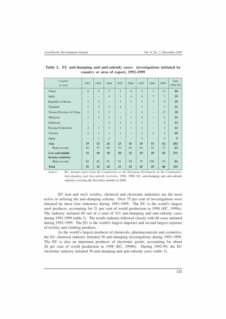
Asia-Pacific Development Journal Vol. 9, No. 2, December 2002
135
Table 2. EU anti-dumping and anti-subsidy cases: investigations initiated bycountry or area of export, 1992-1999
Country1992 1993 1994 1995 1996 1997 1998 1999
Sum
or area 1992-99
China 8 4 5 5 6 5 1 12 46
India – – 4 1 4 6 7 7 29
Republic of Korea 3 2 – 4 1 3 7 9 29
Thailand 1 2 5 4 – 3 – 7 22
Taiwan Province of China 1 1 1 – 1 4 – 12 20
Malaysia 2 2 2 2 1 2 – 4 15
Indonesia – – 4 4 1 1 – 4 14
Russian Federation 3 1 3 1 1 2 – 1 12
Ukraine 2 1 1 1 – 1 2 2 10
Japan – 1 2 – – 2 – 4 9
Asia 19 12 26 23 16 29 15 62 202 Share in total 49 57 60 70 64 64 52 72 63
Low and middle 33 18 39 30 22 35 29 65 271income countries Share in total 85 86 91 91 88 78 100 76 84
Total 39 21 43 33 25 45 29 86 321
Source: EC, Annual report from the Commission to the European Parliament on the Community’s
Anti-dumping and Anti-subsidy Activities, 1996, 1998; EC, anti-dumping and anti-subsidystatistics covering the first three months of 2000.
EU iron and steel, textiles, chemical and electronic industries are the mostactive in utilising the anti-dumping scheme. Over 75 per cent of investigations wereinitiated by these four industries during 1992-1999. The EU is the world’s largeststeel producer, accounting for 21 per cent of world production in 1998 (EC, 1999a).The industry initiated 69 out of a total of 321 anti-dumping and anti-subsidy casesduring 1992-1999 (table 3). The textile industry followed closely with 60 cases initiatedduring 1992-1999. The EU is the world’s largest importer and second largest exporterof textiles and clothing products.
As the world’s largest producer of chemicals, pharmaceuticals and cosmetics,the EU chemical industry initiated 58 anti-dumping investigations during 1992-1999.The EU is also an important producer of electronic goods, accounting for about26 per cent of world production in 1998 (EC, 1999b). During 1992-99, the EUelectronic industry initiated 56 anti-dumping and anti-subsidy cases (table 3).
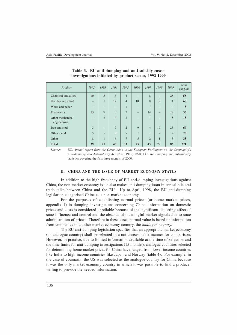
Asia-Pacific Development Journal Vol. 9, No. 2, December 2002
136
II. CHINA AND THE ISSUE OF MARKET ECONOMY STATUS
In addition to the high frequency of EU anti-dumping investigations againstChina, the non-market economy issue also makes anti-dumping loom in annual bilateraltrade talks between China and the EU. Up to April 1998, the EU anti-dumpinglegislation categorised China as a non-market economy.
For the purposes of establishing normal prices (or home market prices,appendix 1) in dumping investigations concerning China, information on domesticprices and costs is considered unreliable because of the significant distorting effect ofstate influence and control and the absence of meaningful market signals due to stateadministration of prices. Therefore in these cases normal value is based on informationfrom companies in another market economy country, the analogue country.
The EU anti-dumping legislation specifies that an appropriate market economy(an analogue country) shall be selected in a not unreasonable manner for comparison.However, in practice, due to limited information available at the time of selection andthe time limits for anti-dumping investigations (15 months), analogue countries selectedfor determining home market prices for China have ranged from lower income countrieslike India to high income countries like Japan and Norway (table 4). For example, inthe case of coumarin, the US was selected as the analogue country for China becauseit was the only market economy country in which it was possible to find a producerwilling to provide the needed information.
Table 3. EU anti-dumping and anti-subsidy cases:investigations initiated by product sector, 1992-1999
Product 1992 1993 1994 1995 1996 1997 1998 1999Sum
1992-99
Chemical and allied 10 5 3 4 – 8 – 28 58
Textiles and allied – 1 17 4 10 8 9 11 60
Wood and paper – – – 1 – 7 – – 8
Electronics 13 7 3 7 – 14 – 12 56
Other mechanical – 2 4 3 – 1 – 5 15 engineering
Iron and steel 3 – 7 2 9 4 19 25 69
Other metal 5 5 3 5 1 1 – – 20
Other 8 1 6 7 5 2 1 5 35
Total 39 21 43 33 25 45 29 86 321
Source: EC, Annual report from the Commission to the European Parliament on the Community’s
Anti-dumping and Anti-subsidy Activities, 1996, 1998; EC, anti-dumping and anti-subsidystatistics covering the first three months of 2000.

Asia-Pacific Development Journal Vol. 9, No. 2, December 2002
137
As many of the analogue countries selected were at a higher stage of economicdevelopment compared with China (table 4), the estimation of home market priceswas likely to be biased towards the finding of dumping. The labour costs in theseanalogue countries tend to be higher than labour costs in China.
Since April 1998, individual companies in China have been givenan opportunity to prove that they operate in market economy conditions in accordancewith certain criteria (see appendix 2). This is to reflect the fact that as a result ofon-going reforms in China, individual companies are likely to be operating in marketeconomic conditions and therefore their prices and costs may be appropriate for the
Table 4. Analogue countries selected for the investigation of anti-dumpingcases against China, 1996-1998
Cases Year of initiationAnalogue countries
or areas used
Refractory chamottees 1993 USA
Coumarin 1994 USA
Powered activated carbon 1994 USA
Iron or steel tube or pipe fittings 1994 Thailand
Colour TV (review) 1995 Singapore
Glyphosphate 1995 Brazil
Footwear with textile uppers 1995 Indonesia
Footwear with leather or plastic uppers 1995 Indonesia
Ring binder mechanisms 1995 Malaysia
Cotton fabrics unbleached 1996 India
Briefcases and school bags 1996 Taiwan Province of China
Luggage and travel goods 1996 Taiwan Province of China
Handbags 1996 Indonesia
Stainless steel fasteners 1996 Taiwan Province of China
Ferro-silico manganese 1996 Brazil
Personal fax machines 1997 Republic of Korea
Cotton grey fabrics 1997 India
Unwrought unalloyed magnesium 1997 Norway
Thiourea dioxide 1997 Japan
Certain laser optical reading systems 1997 Malaysia
Steel stranded ropes and cables 1998 Norway
Source: EC, Annual Report From the Commission to the European Parliament on the Community’s
Anti-dumping and Anti-subsidy Activities, 1996, 1997 and 1998.

Asia-Pacific Development Journal Vol. 9, No. 2, December 2002
138
calculation of normal prices. Indeed, market forces determine about 95 per cent ofindustrial product prices, 90 per cent of retail prices, and 80 per cent of agriculturaland raw material prices in China ( see the South China Morning Post, 17 June 1999).
If a Chinese company can prove that its export activity is not subject to stateinterference, it can apply for individual treatment (for criteria, see appendix 3). Whengranted individual treatment, the anti-dumping margin of the company concerned willbe established by comparing its own export prices and normal prices from the analoguecountry. This is an option open to exporting producers who may not be able to meetall the criteria for full market economy treatment. A full market economy treatmentis granted when a company can show that neither its domestic nor its export activitiesare subject to state interference. While not granted individual treatment, a countrywidedumping margin is normally calculated for all Chinese firms comparing analoguecountry prices and importing prices in EU based on the information available.
To meet the deadline for anti-dumping investigations, the EC requests theChinese exporters concerned to complete a special claim form for market economystatus and return it to the EC within three weeks of the initiation of a proceeding. Ifany information is missing in the completed claim form, or if it is returned late, theclaim is automatically rejected.
The success rate of Chinese firms in claiming market economy status hasbeen low. The amendment to EU anti-dumping legislation became effective on 1 July1998. From July 1998 to October 1999, 27 Chinese companies claimed marketeconomy treatment, but only three were granted the treatment (table 5).
The most common reasons for refusal of market economy treatment were theaccounting and auditing standards. Other accounting issues were the valuation ofstate assets transferred to the companies including land. For those companies withforeign direct investment, the most common reason was prohibition of restriction ondomestic sales. Other reasons for refusal of market economy treatment include statesuppliers of raw materials, state influence in setting prices, barter trade and majoritystate ownership.
In these investigations, different Chinese companies failed to meet differentcriteria of market economy status. In some cases, such as the investigation concerningquarto plates, it was evident that, as a group, the companies that applied for marketeconomy status could in fact meet all the relevant criteria (EC, 2000a).
While the use of Chinese firm’s prices tends to lead to under-estimateddumping margins, the non-market economy way of calculation tends to lead toover-estimated dumping margins for many Chinese firms. The difference between thetwo ways of calculation could be dramatic. For example, in the case of footwear withleather or plastic uppers, individual treatment was granted to one exporter. Thisresulted in zero anti-dumping duty for the particular exporter while a variable duty toensure a minimum price of ECU 5.7 per pair was levied on all other exporters. In thecase of handbags, two companies were granted individual treatment. This resulted in

Asia-Pacific Development Journal Vol. 9, No. 2, December 2002
139
Table 5. Market economy status in anti-dumping investigationsconcerning China
Number of Number ofCases market economy claims Reasons for refusal of market economy status
claims accepted
3 1 • No audited accounts provided
• State holds directly or indirectly 2/3 majority of shares
• One company not an exporter
• Suppliers controlled by the state
3 0 • No audited accounts provided
• Financial situation distorted as a result of impropervaluation of assets transferred to the company fromthe state
• State interference in setting salaries and throughparticular tax rebate
TV tubes 1 0 • No audited accounts
• Majority of suppliers controlled by the state
• No export licence
Coke 80+ 1 0 • Unreliable accounts not prepared in line withinternational accounting standards
CD boxes 3 2 • Domestic sales prohibited
• No legal status in China
• No individual company accounts available
Quarto plates 6 0 • All companies fully or partially owned by the state
• Agreements to purchase raw materials from stateowned suppliers
• Only nominal fees paid for land-use rights
• Barter trade practised
Hair brushes 2 0 • No domestic sales allowed
Glycine 6 0 • Three of the claimants are not exporting producers ofthe product concerned
• Related companies failed to claim market economytreatment
• Incomplete financial statements
• Restrictions on domestic sales
2 0 • Restrictions on domestic sales
• Companies follow pricing law and consequently sell atloss making prices in China
TOTAL 27 3
Source: EC, “Proposal for Council Regulation: amending Regulation (EC) No. 384/96 on protectionagainst dumped imports from countries not members of the European Community”, Brussels,15 June 2000
Yellowphosphorus
Malleablecast ironfittings
Electronicweighingscales
Asia-Pacific Development Journal Vol. 9, No. 2, December 2002
140
0 per cent duty for one company and 7.7 per cent duty for the other, while the rest ofthe exporters were levied 38 per cent duties.
Unfortunately, it is not yet possible to investigate the difference betweenanti-dumping margins for firms with and without market economy status. For thethree Chinese firms that were granted market economy status, their cases (CD boxesand yellow phosphorus) were terminated without definitive measures imposed.
III. THE EFFECTS OF ANTI-DUMPING ONCHINESE EXPORTS TO EU
To understand the effects of anti-dumping measures on trade, bilateral tradestatistics of the products subject to definitive anti-dumping measures are analysed inthis study. On the EU current anti-dumping and anti-subsidy list as of June 2000,49 out of a total of 330 cases were against China4. These cases consisted of:
• 11 cases with definitive measures imposed before 1995;• 21 cases with definitive measures imposed during 1995-19985;• 1 case with definitive measures imposed in 1999;• 10 new cases under investigation with 5 provisional duties imposed;
and• 6 cases initiated since late 1999 terminated without any definitive
measures.
Subject to available information and data, this study is only able to look atthe trade effect of the new measures imposed during 1995-98. The analysis revealsthat anti-dumping measures are generally very trade restrictive. Coincident to theimposition of anti-dumping duties, bilateral trade flows typically reverse their trendof growth from upward to downward. For example, EU initiated an anti-dumpinginvestigation on imports of footwear with textile uppers from China in 1995. Followingthe investigation, a provisional duty of 94.1 per cent was levied between Februaryand October of 1997. From November 1997, a definitive duty of 49.2 per cent wasimposed. Before the imposition of anti-dumping duties, Chinese exports of footwearwith textile uppers to the EU had increased from US$171 million to US$178 million.Coincident to the levy of the anti-dumping duties, Chinese exports of the productsdropped from US$178 million in 1996 to US$95 million in 1997 and US$90 millionin 1998 (table 6).
4 All 49 cases were anti-dumping cases (no anti-subsidy cases).
5 These cases exclude those definitive measures that resulted from reviews of definitive measuresimposed before 1995, unless the review led to increased duty or more restrictive measures.
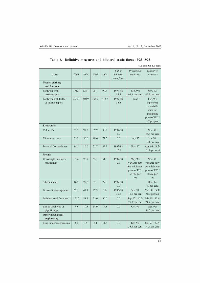
Asia-Pacific Development Journal Vol. 9, No. 2, December 2002
141
Table 6. Definitive measures and bilateral trade flows 1995-1998
(Million US Dollars)
Fall in Provisional DefinitiveCases 1995 1996 1997 1998 bilateral measures measures
trade flows
Textile, clothing and footwear
Footwear with 171.0 178.1 95.1 90.4 1996-98: Feb. 97: Nov. 97: textile uppers 87.7 94.1 per cent 49.2 per cent
Footwear with leather 263.8 360.9 396.2 312.7 1997-98: none Feb. 98: or plastic uppers 83.5 0 per cent
or variableduty for
minimumprice of ECU5.7 per pair
Electronics
Colour TV 67.7 97.5 39.9 38.2 1997-98: Nov. 98:1.7 44.6 per cent
Microwave oven 35.9 36.0 48.6 77.5 0.0 July 95 Jan. 96:12.1 per cent
Personal fax machines 14.5 16.6 52.7 39.9 1997-98: Nov. 97 Apr. 98: 21.2-12.8 51.6 per cent
Metals
Unwrought unalloyed 37.4 28.7 53.1 51.0 1997-98: May 98: Nov. 98: magnesium 2.1 variable duty variable duty
for minimum for minimumprice of ECU price of ECU
2,797 per 2,622 perton ton
Silicon metal 16.5 27.6 37.1 27.8 1997-98: Dec. 97:9.3 49 per cent
Ferro-silico-manganese 63.1 41.1 27.9 1.6 1996-98: Sep. 97: Mar. 98: ECU39.5 19.6 per cent 58.3 per ton
Stainless steel fasteners* 120.5 88.1 75.6 90.6 0.0 Sep. 97: 16.2- Feb. 98: 13.6-75.7 per cent 74.7 per cent
Iron or steel tube or 7.5 10.5 14.9 14.3 0.0 Oct. 95 Apr. 96: pipe fittings 58.6 per cent
Other mechanical engineering
Ring binder mechanisms 3.0 3.5 8.4 11.6 0.0 July 96: Jan. 97: 32.5-35.4 per cent 39.4 per cent
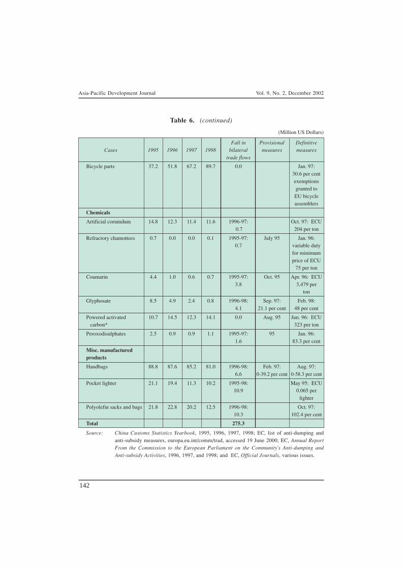
Asia-Pacific Development Journal Vol. 9, No. 2, December 2002
142
Table 6. (continued)
(Million US Dollars)
Fall in Provisional DefinitiveCases 1995 1996 1997 1998 bilateral measures measures
trade flows
Bicycle parts 37.2 51.8 67.2 89.7 0.0 Jan. 97:30.6 per centexemptionsgranted toEU bicycleassemblers
Chemicals
Artificial corumdum 14.8 12.3 11.4 11.6 1996-97: Oct. 97: ECU 0.7 204 per ton
Refractory chamottees 0.7 0.0 0.0 0.1 1995-97: July 95 Jan. 96:0.7 variable duty
for minimumprice of ECU
75 per ton
Coumarin 4.4 1.0 0.6 0.7 1995-97: Oct. 95 Apr. 96: ECU3.8 3,479 per
ton
Glyphosate 8.5 4.9 2.4 0.8 1996-98: Sep. 97: Feb. 98:4.1 21.1 per cent 48 per cent
Powered activated 10.7 14.5 12.3 14.1 0.0 Aug. 95 Jun. 96: ECU carbon* 323 per ton
Peroxodisulphates 2.5 0.9 0.9 1.1 1995-97: 95 Jan. 96:1.6 83.3 per cent
Misc. manufacturedproducts
Handbags 88.8 87.6 85.2 81.0 1996-98: Feb. 97: Aug. 97:6.6 0-39.2 per cent 0-58.3 per cent
Pocket lighter 21.1 19.4 11.3 10.2 1995-98: May 95: ECU10.9 0.065 per
lighter
Polyolefin sacks and bags 21.8 22.8 20.2 12.5 1996-98: Oct. 97:10.3 102.4 per cent
Total 275.3
Source: China Customs Statistics Yearbook, 1995, 1996, 1997, 1998; EC, list of anti-dumping andanti-subsidy measures, europa.eu.int/comm/trad, accessed 19 June 2000; EC, Annual ReportFrom the Commission to the European Parliament on the Community’s Anti-dumping and
Anti-subsidy Activities, 1996, 1997, and 1998; and EC, Official Journals, various issues.

Asia-Pacific Development Journal Vol. 9, No. 2, December 2002
143
Out of the 21 cases with definitive measures imposed between 1995-1998(table 6):
• 15 cases showed a fall in bilateral trade flows coincident to theimposition of duties.
• In four cases, bilateral trade flows continued to rise (in one of thecases, bicycle parts, this was due to exemptions from duties for EUbicycle assemblers). Past experience shows that, when measures areconsidered as insufficient, subsequent reviews are lodged that oftenlead to more restrictive measures.
• In two of the cases, the pattern of change in bilateral trade flows wasnot clear. In one case, the bilateral trade flow fell with a time lag.In the other case, the bilateral trade flow fluctuated.
As bilateral trade flows generally tend to fall following the impositionof anti-dumping duties, the notion of the percentage of trade volume subject toanti-dumping measures almost certainly tends to under-estimate the effects ofanti-dumping on trade. An appropriate estimation of the effects of anti-dumpingduties on trade would be to investigate how the trade flow of the products concernedchanges following the imposition of anti-dumping duties. Ideally, the impact can bemeasured by comparing the actual bilateral trade level with the level it would havegrown to without the imposition of the duties. Such an exercise requires the simulationof the growth trends of trade flows. However, before conducting such an exercise, itis useful to calculate the actual fall in bilateral trade flows coincident to the impositionof duties. While omitting the growing trend in trade flows in many cases, thecalculation can provide a lower-boundary estimation on how anti-dumping duties affectbilateral trade flows of the products concerned.
In this study, the fall in bilateral trade flows coincident with the impositionof anti-dumping duties is calculated based on Chinese customs data. The calculationresults show that the fall in bilateral trade flows coincident to the imposition ofdefinitive measures between 1995-98 amounted to US$275 million6 (table 6). Toobtain a sense of the relative size of this number, it is compared with the change intotal Chinese exports to EU between 1995-1998. Between 1995-1998, total Chineseexports to EU increased by US$9,051 million. The fall in Chinese exports to EUcoincident to the imposition of definitive anti-dumping duties between 1995-1998amount to 3 per cent of the total increase in Chinese exports to EU.
As discussed above, this calculation tends to under-estimate the effects ofanti-dumping duties on trade as it is based on the actual fall in bilateral trade flowswithout taking into account the growing trends before the imposition of duties.However, this calculation at least indicates that without the imposition of the definitive
6 The falls in bilateral trade flows in the two cases where trade flows exhibited an unclear pattern ofchange are counted as zero.

Asia-Pacific Development Journal Vol. 9, No. 2, December 2002
144
duties between 1995-1998, the increase in Chinese exports to EU would have beenmore than 3 per cent higher.
It may be argued that these falls in bilateral trade flows have been caused byother factors. During the period covered in this study (1995-1998), the Asian financialand economic crisis has indeed been identified as the major factor that led to a modestslackening of the export performance of China. However, statistics also show that,while Chinese exports to Asian economies declined during the crisis, Chinese firmsdiversified their exports to the EU and US markets. As a result, Chinese exports toEU and US continued to rise during the Asian crisis.
Even though the 21 cases investigated above are only part of the 49 cases onthe EUs list of anti-dumping cases against China, they have shown that, from theChinese perspective, the effects of anti-dumping measures on trade can be much moresignificant than from EU’s perspective.
IV. CONCLUSION
A close investigation of EU anti-dumping cases against China reveals thatthree issues are important in relation to the impact of anti-dumping measures ontrade. First, the calculation of dumping margins is a challenging task. Although greatefforts have been devoted to make anti-dumping investigation a fair process, the schemesuffers from imperfect information that is highly likely to lead to biased rulings.In particular, the non-market economy way of calculating dumping margins for Chinais a practice that has replaced one set of bias (under-estimation) with another(over-estimation).
Second, the high rates of termination due to withdrawal of complaints alsoposes the question whether the scheme tends to be used by industries to fight againstfair competition as opposed to unfair competition. Investigations and provisionalduties levied can be highly disruptive to exporting firms even if eventually no definitivemeasures are imposed.
Third, as anti-dumping measures tend to significantly change bilateral tradeflows, the percentage of imports subject to anti-dumping measures is not a goodindicator of the effects of anti-dumping duties on trade. A more appropriate measureof the impact of anti-dumping on trade is to estimate the extent that anti-dumpingduties affect bilateral trade flows. In this study, the fall in bilateral trade flowscoincident to the imposition of 21 definitive duties was calculated. The results showthat the rise in Chinese exports to EU would have been more than 3 per cent higherwithout the imposition of the duties in 1995-1998. The actual effects of anti-dumpingmeasures on bilateral trade flows should be much bigger, taking into account theeffects of all 49 cases against China and the upward trend of the trade flows for mostproducts before the imposition of the duties. Thus, from the perspective of developingcountry exporters, the impact of the anti-dumping regime on trade can be much moredramatic than from the perspective of developed country importers.

Asia-Pacific Development Journal Vol. 9, No. 2, December 2002
145
REFERENCES
EC, 1999a. Trade in goods: the steel sector, europa.eu.int/comm/trad/goods, accessed 22 May 2000.
, 1999b. Trade in goods: the electronic sector, europa.eu.int/comm/trad/goods, accessed22 May 2000.
, 2000a. Proposal for Council Regulation: amending Regulation (EC) No. 384/96 on protectionagainst dumped imports from countries not members of the European Community, Brussels.
, 2000b. Trade Policy Instruments, europa.eu.int/comm/trade/policy, accessed 22 May 2000.
Finger, J.M., ed. 1993. Anti-dumping: how it works and who gets hurt, Studies in International TradePolicy (Ann Arbor, University of Michigan Press).
Jones, K.A., 1994. Export Restraint and the New Protectionism: The Political Economy of DiscriminatoryTrade Restrictions (Ann Arbor, University of Michigan Press).
Krueger, A., 1995. American Trade Policy: Tragedy in the Making (Washington, D.C., AEI Press).
Lahiri, S., and J. Sheen, 1990. “On optimal dumping”, The Economic Journal, 100 (Conference 1990),pp. 127-136.
Robert, B., and L. Robert, 1991. Down in the Dumps (Washington, D.C., Brookings Institution).
Rugman, A.M., and A.D.M. Anderson, 1987. Administered Protection in America (London, Croom Helm).

Asia-Pacific Development Journal Vol. 9, No. 2, December 2002
146
Appendix 1. EU anti-dumping and anti-subsidy schemea
EU’s rules to deal with dumping date back to the organization’s earliestdays. They are targeted at dumped imports that cause significant injury to EUproducers. The first anti-dumping and anti-subsidy legislation of EU was enactedin 1968 and has been subsequently modified several times. A new set of rulesgoverning the anti-dumping scheme came into force in 1995 when WTO wasestablished. The new set of rules (updated in 1996) was based on measuresagreed under WTO.
According to the new rules, anti-dumping duties can be levied if thefollowing conditions are met:
• a finding of dumping: the export price at which the product is soldon the EU market is shown to be lower than the price on theproducer’s home market;
• a material injury to EU industry: the imports have caused or threatento cause damage to a substantial part of the industry within the EU,such as loss of market share, reduced prices for producers and resultingpressure on production, sales, profits, productivity etc.;
• the interests of EU: the costs for EU of taking anti-dumping measuresmust not be disproportionate to the benefits.
When an industry in EU considers that dumped imports from non-EUcountries are causing it material injuries, it may submit a complaint to the EC,either directly or through its national government. The EC then has 45 days toexamine the complaint, consult the member states and decide whether or notthere is enough evidence to merit a formal investigation. The case will berejected if there is not enough evidence or if the complainants do not representat least 25 per cent of the total EU production of the product in question.
Once a case is accepted, the EC will conduct a formal investigation within15 months. The investigation covers whether or not dumping is taking place,which can be a complex calculation, and also whether dumped imports are causingmaterial injuries to EU industry. Measures may also be imposed if imports arehindering the establishment of a new industry within EU or there is a clear andimminent threat of material injury.
Anti-dumping measures will only take place if they are shown to be in thebroader EU interest. Producers, importers, users and consumers are able topresent their views.
If the investigation confirms the existence of injurious dumping and if theCommunity interest test is positive, the EC may, after consulting with memberstates, impose provisional duties. The duties levied are within the dumping
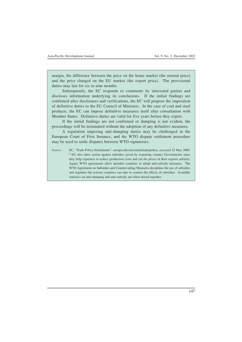
Asia-Pacific Development Journal Vol. 9, No. 2, December 2002
147
margin, the difference between the price on the home market (the normal price)and the price charged on the EU market (the export price). The provisionalduties may last for six to nine months.
Subsequently, the EC responds to comments by interested parties anddiscloses information underlying its conclusions. If the initial findings areconfirmed after disclosures and verifications, the EC will propose the impositionof definitive duties to the EU Council of Ministers. In the case of coal and steelproducts, the EC can impose definitive measures itself after consultation withMember States. Definitive duties are valid for five years before they expire.
If the initial findings are not confirmed or dumping is not evident, theproceedings will be terminated without the adoption of any definitive measures.
A regulation imposing anti-dumping duties may be challenged in theEuropean Court of First Instance, and the WTO dispute settlement proceduremay be used to settle disputes between WTO signatories.
Source: EC, “Trade Policy Instruments”, europa.edu.int/comm/trade/policy, accessed 22 May 2000.a EU also takes action against subsidies given by exporting country Governments sincethey help exporters to reduce production costs and cut the prices of their exports unfairly.Again, WTO agreements allow member countries to adopt anti-subsidy measures. TheWTO Agreement on Subsidies and Countervailing Measures disciplines the use of subsidiesand regulates the actions countries can take to counter the effects of subsidies. Availablestatistics on anti-dumping and anti-subsidy are often mixed together.

Asia-Pacific Development Journal Vol. 9, No. 2, December 2002
148
Appendix 2. Criteria to determine whether or not a company operatesin market economy conditions
• Decisions of firms are taken without significant state interferenceand are made in response to market signals;
• Accounts must be independently audited in line with internationalaccounting standards;
• Production costs and the financial situation of the company is notaffected by distortions carried over from the former state-led economicsystem, barter trade or compensation of debts;
• Companies are subject to bankruptcy and property laws; and• Exchange rate conversations are carried out at market rates.
Source: EC, ‘Proposal for Council Regulation: amending Regulation (EC) No. 384/96 on protectionagainst dumped imports from countries not members of the European Community’,Brussels, 15 June 2000.

Asia-Pacific Development Journal Vol. 9, No. 2, December 2002
149
Appendix 3. Criteria for individual treatment(revised version of the year 2000)
If the following criteria are met, a Chinese company can be grantedindividual treatment that allows anti-dumping margins to be calculated accordingto its own export prices and normal prices in the analogue country.
Old criteria applied before the year 2000:
• The majority of the shares should belong to genuinely privatecompanies and no state officials should appear on the board or ina key management position; the fact that a foreign investor controlsthe company concerned will be considered a relevant indication ofindependence.
• The land on which the facilities of the company are built should berented from the state at conditions comparable to those in a marketeconomy country or purchased (e.g. proper contractual lease).
• The company should have the right to hire and dismiss employeesand the right to fix salaries.
• The company should have full control over its supply of raw materialsand inputs in general.
• The supply of utilities should be guaranteed on the basis of propercontractual terms.
• Proof is given that profit can be exported and capital invested can berepatriated (only in the case of foreign investment, e.g. joint venture).
• The export prices should be determined freely; the fact that exportsales are made to a related party located outside the country in questionwill be a decisive factor.
• Freedom to carry out business activities should be guaranteed, inparticular in respect of the following: there should be no restrictionson selling on the domestic market; the right to do business cannot bewithdrawn outside proper contractual terms; and quantities producedfor export should be determined freely by the company in accordancewith the traditional demand of its export markets.
New criteria following a review in the year 2000:
• Exporters are free to repatriate capital and profits (applicable to whollyforeign owned firms or joint ventures).
• Export prices and quantities, and conditions and terms of sale arefreely determined, and the majority of the shares belong to genuinely

Asia-Pacific Development Journal Vol. 9, No. 2, December 2002
150
private companies. State officials appearing on the board or in keymanagement positions should be in a clear minority. The presumptionis that a state-controlled company cannot guarantee its independencefrom state interference, and the burden rests with the exporter toprove otherwise.
• Exchange rate conversations are carried out at the market rate.• State interference is not such as to permit circumvention of measures
if exporters are given different rates of duty.
Source: EC, “Proposal for Council Regulation: amending Regulation (EC) No. 384/96 on protectionagainst dumped imports from countries not members of the European Community”,Brussels, 15 June 2000.
Asia-Pacific Development Journal Vol. 9, No. 2, December 2002
151
REJUVENATING BANK FINANCE FOR DEVELOPMENTIN ASIA AND THE PACIFIC
United Nations Publication, ST/ESCAP/2206Sales # E.02.II.F.57, ISBN: 92-1-120121-7
pp. viii and 207
The heads of Governments at the United Nations Millennium Summit held inSeptember 2000 adopted the United Nations Millennium Declaration, urging countriesto work towards detailed development goals that include poverty eradication and humandevelopment. The International Conference on Financing for Development held atMonterrey, Mexico in March 2002 underscored the fundamental reality that in orderto achieve these goals the need for mobilizing domestic financial resources in additionto international resources was paramount.
In the ESCAP region, the banking sector remains the primary source ofdomestic resources for private sector development with debt markets for the privatesector in their infancy. However, the operations of the banking system in manycountries in the region remain fragile owing to a variety of factors such as a lowcapital base, excessive government intervention, poor regulations, ineffectivesupervision and insufficient risk-management skills. Fragile banking systems notonly misallocate resources, but are also prone to periodic crises, putting savers’ fundsat risk with serious consequences for economic growth. In several countries in theregion, five years after the Asian financial crisis banks are still suffering from anoverhang of non-performing loans. Even though there has been considerable progressregion-wide with regard to banking sector restructuring, a number of outstandingissues remain to be tackled to rejuvenate banking as one of the main instruments ineconomic development.
Against that background, this volume provides an overview of domesticresource mobilization for development in Asia and the Pacific. It also reviews countrycases in the banking sector and in the related field of microfinance in order todisseminate a range of experiences and lessons for guiding policy in the future. Countrystudies on the banking sector include China, India and Thailand, while those onmicrofinance cover Bangladesh, the Philippines and the Republic of Korea. Policymakers in the region should find the case studies in both fields useful for devisinglong-term strategies to rejuvenate their banking systems.

Asia-Pacific Development Journal Vol. 9, No. 2, December 2002
153
PROTECTING MARGINALIZED GROUPS DURING ECONOMICDOWNTURNS: LESSONS FROM THE ASIAN EXPERIENCE
byUnited Nations Publications, ST/ESCAP/2221
Sales # E.03.II.F.2, ISBN: 92-1-120137-3pp. i and 138
Following the 1997 economic crisis, Governments in East and South-EastAsia expanded several existing employment/income-generating/protecting programmes.This strategy was adopted as the affected countries lacked the automatic stabilizers oruniversal social insurance programmes which could be used to benefit those who hadlost their jobs or other sources of income during the crisis. This timely ESCAPpublication attempts to evaluate the effectiveness of these programmes in benefitingthe target groups. Lessons learned during the evaluation are used to outline an AsianSocial Protection Framework which can be used, among other things, to reassuresociety that the needs of ordinary men and women will not be forgotten during anyfuture economic downturns.
The genre of the programmes evaluated essentially revolves around the publicworks and microcredit programmes in Indonesia and Thailand and the UnemploymentInsurance and the Small and Medium Enterprise credit programme in the Republic ofKorea. Beneficiaries of the programmes, as well as relevant implementing agencies,were approached to provide information on the impact of the programmes on incomeand employment generation. Focus group interviews with the non-beneficiaries whowere eligible, but did not join the programmes, were conducted to identify the reasonsfor their non-participation. The data collected and other relevant information havebeen analysed and the results obtained were then put before a group of senior policymakers from selected Asian countries to ascertain their views. The group recommendedthat the lessons learned from the study could be used to identify the elements of anAsia Social Protection Framework package capable of protecting persons associatedwith the formal, informal and self-employed sectors against income/employment shocksarising out of economic restructuring, downsizing or downturn.
In the light of their recommendations an Asian Social Protection Frameworkcould encompass the following elements:
(1) Implementation of macroeconomic and other policies that promotebroad-based economic growth

Asia-Pacific Development Journal Vol. 9, No. 2, December 2002
154
(2) Recognition of the Government’s responsibility and leadership as the‘social protection provider’ of last resort; hence the need to createa comprehensive social safety system with the active cooperationand participation of the local community
(3) Recognition of the existence of a large self-employed and informalsector and thus the inherent limitations of contributory social insuranceschemes and the need for targeted schemes such as rural public worksprogrammes, and strengthening of the informal sector consistent withthe commitments enshrined in the Copenhagen Declaration andProgramme of Action
(4) In the formal sector, recognition of the need to develop a comprehensivecontributory scheme (funded by employers and workers) to providefor social insurance as well as unemployment insurance
(5) Explicit provision of expenditure on social protection in the budgetary/fiscal framework of the Governments
(6) Effective collaboration between the Government, civil society andthe private sector in designing social safety nets
(7) Harnessing of family ties, human contacts, community self-help and‘other’ philanthropic activities to build “private safety nets”
Such a framework, while undoubtedly ambitious, does provide a basis toenable Governments in the region to look at the full gamut of social protection issues.It also highlights the policy trade-offs involved in their resolution, the opportunitycosts of overemphasizing one or other objective and the clear need to bring theseissues to the forefront of public debate. Without appropriate pressure from publicopinion, social protection issues are unlikely to attract the needed attention ofGovernments in the region. This publication performs a useful service in bringing thecomplex issues of social protection to the attention of a wider audience.

Asia-Pacific Development Journal Vol. 9, No. 2, December 2002
SUBSCRIPTION FORM
(Please type or print)
NAME: ___________________________________________________________
POSITION: ___________________________________________________________
ORGANIZATION: ___________________________________________________________
ADDRESS: ___________________________________________________________
___________________________________________________________
___________________________________________________________
___________________________________________________________
COUNTRY: ______________________ POST-CODE: ____________
TELEPHONE: ____________________ FACSIMILE: ___________ E-MAIL: ____________
----------------------------------------------------------------------------------------------------------------------
SUBSCRIPTION RATES FOR ASIA-PACIFIC DEVELOPMENT JOURNAL (2 ISSUES PER YEAR)
❏ 1 year $US 35.00
❏ 3 years $US 90.00
Please mail this form together with your subscription fee in US dollars to:
Chief, Conference and General Services SectionDivision of AdministrationEconomic and Social Commission for Asia and the Pacific (ESCAP)United Nations Building, Rajadamnern AvenueBangkok 10200, Thailand
✁ ------------------------------------------------------------------------------------------------------------------
This publication may be obtained from bookstores and distributors throughout the world.Please consult your bookstore or write to any of the following:
Sales Section Tel.: (212) 963-8302Room DC2-0853 Fax: (212) 963-4116United Nations Secretariat Telex: 422311 UN UINew York, NY 10017United States of America
Sales Section Tel.: (41) (22) 917-1234United Nations Office at Geneva Fax: (41) (22) 917-0123Palais des Nations Telex: 23711 ONU CHCH-1211 Geneva 10Switzerland
Chief, Conference and General Services SectionDivision of AdministrationEconomic and Social Commission for Asia and the Pacific (ESCAP) Tel.: (662) 288-1234United Nations Building, Rajadamnern Avenue Fax: (662) 288-1000Bangkok 10200, Thailand Telex: 82392 ESCAP TH
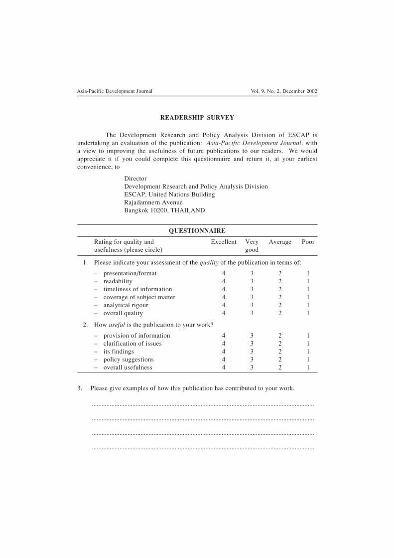
Asia-Pacific Development Journal Vol. 9, No. 2, December 2002
READERSHIP SURVEY
The Development Research and Policy Analysis Division of ESCAP isundertaking an evaluation of the publication: Asia-Pacific Development Journal, witha view to improving the usefulness of future publications to our readers. We wouldappreciate it if you could complete this questionnaire and return it, at your earliestconvenience, to
DirectorDevelopment Research and Policy Analysis DivisionESCAP, United Nations BuildingRajadamnern AvenueBangkok 10200, THAILAND
QUESTIONNAIRE
Rating for quality and Excellent Very Average Poorusefulness (please circle) good
1. Please indicate your assessment of the quality of the publication in terms of:
– presentation/format 4 3 2 1– readability 4 3 2 1– timeliness of information 4 3 2 1– coverage of subject matter 4 3 2 1– analytical rigour 4 3 2 1– overall quality 4 3 2 1
2. How useful is the publication to your work?
– provision of information 4 3 2 1– clarification of issues 4 3 2 1– its findings 4 3 2 1– policy suggestions 4 3 2 1– overall usefulness 4 3 2 1
3. Please give examples of how this publication has contributed to your work.
.........................................................................................................................................
.........................................................................................................................................
.........................................................................................................................................
.........................................................................................................................................

Asia-Pacific Development Journal Vol. 9, No. 2, December 2002
4. Suggestions for improving the publication:
..........................................................................................................................................
..........................................................................................................................................
..........................................................................................................................................
..........................................................................................................................................
5. Your background information, please:
Name: ...............................................................................................................................
Title/position: ..................................................................................................................
Institution: ........................................................................................................................
Office address: .................................................................................................................
..........................................................................................................................................
Please use additional sheets of paper, if required, to answer the questions.
Thank you for your kind cooperation in completing this questionnaire.

Asia-Pacific Development Journal Vol. 9, No. 2, December 2002
Instructions to contributors
1. MANUSCRIPTS
Authors are requested to submit two copies of their manuscripts in English. Contributorsshould indicate in their covering letter to the Editorial Board that the material has not been previouslypublished or submitted for publication elsewhere. The length of manuscripts should not normally exceed25-30 double-spaced A4-size pages. Manuscripts are accepted subject to editorial revision.
The manuscripts should be typed, double-spaced, on one side of white A4 paper. Since all manuscriptswill be refereed by professionals in the field, the name(s) of the author(s), institutional affiliation(s) and otheridentifying information should be placed on the title page only, in order to preserve anonymity.
The title page should contain the following: (a) title; (b) name(s) of the author(s); (c) institutionalaffiliation(s); and (d) complete mailing address, telephone number and facsimile number of the author, or ofthe primary author in the case of joint authors. The second page should contain the title, the name(s) of theauthor(s) and an abstract of approximately 150 words. Acknowledgements (if any) should appear after theabstract.
Once a manuscript is accepted for publication, the author(s) should submit a copy of the manuscripton a computer diskette labelled with the title of the article, the name(s) of the author(s) and the word processingsoftware used. The preferred word processing software is MSWord.
2. FOOTNOTES AND QUOTATIONS
Footnotes, if any, should be numbered consecutively with superscript arabic numerals. They shouldbe typed single-spaced and should be placed at the foot of each page. Footnotes should not be used solely forciting references.
Quotations should be double-spaced. A copy of the page(s) of the original source of the quotation,as well as copy of the cover page of that source, should be provided.
3. TABLES
All tables should be numbered consecutively with arabic numerals. Each table should be typeddouble-spaced on a separate page and should follow the list of references. There should be a clear indicationin the text where the table should be inserted. Full source(s) should appear below the table, followed by notes,if any, in lower-case letters.
4. FIGURES
All figures should be provided as camera-ready copy and numbered consecutively. Figures shouldbe planned to fit the proportions of the printed page. There should be a clear indication in the text whereeach figure should be inserted. Full source(s) should be provided below each figure.
5. REFERENCES
Authors should ensure that there is a complete reference for every citation in the text. Referencesin the text should follow the author-date format followed, if necessary, by page numbers, for example, Becker(1964: 13-24). List only those references that are actually cited in the text or footnotes. References, listedalphabetically, should be typed double-spaced on a separate page in the following style:
Ahmed, E. and N. Stern, 1983. “Effective taxes and tax reform in India”, Discussion Paper 25, University ofWarwick.
Desai, Padma, ed., 1883. Marxism, Central Planning, and the Soviet Economy (Cambridge, MA, MIT Press).Krueger, Alan B. and Lawrence H. Summers, 1987. “Reflections on the inter-industry wage structure”, in
Kevin Lang and Jonathan S. Leonard, eds., Unemployment and the Structure of Labour Markets(London, Basil Blackwell).
Sadorsky, P., 1994. “The behaviour of U.S. tariff rates: comment”, American Economic Review, vol. 84,No. 4, September, pp. 1097-1103.
Terrones, M., 1987. “Macroeconomic policy cycle under alternative electoral structures: a signalling approach”,unpublished.

Asia-Pacific Development Journal Vol. 9, No. 2, December 2002
Printed in Bangkok United Nations publicationFebruary 2003 – 1,380 Sales No. E.02.II.F.72
Copyright United Nations 2002ISBN: 92-1-120147-0ISSN: 1020-1246ST/ESCAP/2231

Asia-Pacific Development Journal Vol. 9, No. 2, December 2002
IN THIS ISSUE:
A note from the Editor
Exchange rate policy of Bangladesh:not floating does not mean sinking
Leading indicators for monitoring thestability of asset and financial marketsin Asia and the Pacific
Banking sector reforms in Indiaand China: does India’sexperience offer lessonsfor China’s future reformagenda?
Stock price behaviour in Indiasince liberalization
Economic reforms, energyconsumption changes and CO2emissions in India:a quantitative analysis
Research Note
An analysis of EU anti-dumpingcases against China
Book Reviews
Rejuvenating bank finance fordevelopment in Asia and the Pacific
Protecting marginalized groupsduring economic downturns:lessons from the Asian experience