Prandtl and Rayleigh number dependence of heat transport in high Rayleigh number thermal convection
Upload
khangminh22Category
view
1download
0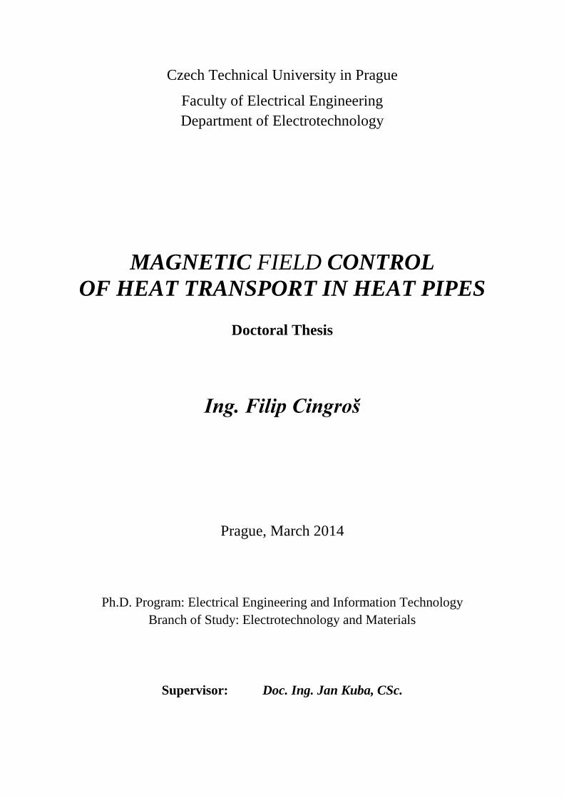
Czech Technical University in Prague
Faculty of Electrical Engineering
Department of Electrotechnology
MAGNETIC FIELD CONTROL
OF HEAT TRANSPORT IN HEAT PIPES
Doctoral Thesis
Ing. Filip Cingroš
Prague, March 2014
Ph.D. Program: Electrical Engineering and Information Technology
Branch of Study: Electrotechnology and Materials
Supervisor: Doc. Ing. Jan Kuba, CSc.


ABSTRACT
i
Abstract
This work deals with magnetic field effects on heat transport in heat pipes. Heat pipes
are two phase thermal devices transporting heat by a close cycle of a working fluid within.
They are able to transport heat over long distances with a low temperature drop and their
efficiency can achieve of several magnitudes higher than that of passive copper systems.
Thus, heat pipes are often used in high tech applications, like cooling of power electronic
components, thermal management of technological processes or in medical devices. However,
heat pipes are getting to be a standard thermal solution also in wide number of consumer
electronics.
Several devices utilizing heat pipes need an active thermal management with some
kind of heat flow regulation. In those cases heat pipes are modified into several constructions
allowing variable heat conductance. Different approaches are available and well established
now, however all with specific limitations. This work ascertains an alternative approach based
on an interaction between a fluid contained within heat pipes and a magnetic field.
The magnetic field regulation of heat transport in heat pipes is still in an early stage of
laboratory research and we do not know about any commercial application utilizing this type
of control. During this work we have designed and realized several experimental heat pipe
systems utilizing magnetic field based regulation and ascertain their behaviors and operation
under magnetic field exposition. According to the experimental results it might be possible to
significantly affect heat transport in selected heat pipe systems by magnetic field.

ABSTRAKT
ii
Abstrakt
Tato disertační práce se zabývá problematikou tepelných trubic ovlivňovaných
magnetickým polem za účelem řízení schopnosti přenášet teplo ve směru jejich podélné osy.
Tepelné trubice umožňují vysoce efektivní přenos tepla a v současné době nacházejí své
uplatnění v celé řadě nejrůznějších aplikací, od chlazení elektronických zařízení a součástek
až po nasazení v rekuperačních výměnících nebo chirurgických nástrojích a kosmické
technice. V poslední době, v souvislosti s hromadnou výrobou tepelných trubic, se tento typ
přenosu tepla stává běžný také ve spotřební elektronice.
Některé z těchto, ale i dalších aplikací vyžadují regulaci přenosu tepla, a proto jsou
v některých případech tepelné trubice modifikovány tak, aby toto umožňovaly. V současné
době je k dispozici několik variant, jak tohoto dosáhnout, každá ale s určitými omezeními.
Tato práce zkoumá alternativní metodu řízení pomocí magnetického pole.
Podle dostupných informací tato technika nebyla zatím v praxi uplatněna a je zatím
zkoumána pouze v laboratorních podmínkách. Popis návrhu a realizace těchto tepelných
trubic, jakož i provedených vybraných experimentů, jejich zdůvodnění a vyhodnocení jsou
uvedeny v této disertační práci a představuje také její hlavní přínos k současnému stavu vědy
a poznání. Na základě výsledků těchto experimentů se zdá být reálné ovlivňovat transport
tepla ve specificky navržených tepelných trubicích pomocí vnějšího statického magnetického
pole.

ACKNOWLEDGEMENTS
iii
Acknowledgements
There are many people who have been more or less involved in this project or just
supported me, the work and the overall research effort in some manner. I would like to thank
you all for your help and contribution to this work. Above all, I would like to express my
gratitude to my supervisor doc. Jan Kuba for his big patient help. Doc. Kuba has been all the
time in a close touch to this project and brought an important contribution to the final
outcome. His marvelous research effort was always motivating me and all the others around
to the further work. Additionally, I would like to appreciate an important support of my home
Department of Electrotechnology and its members. And last, but certainly not least, I thank to
my family for a plenty of time I could spend on this work.

TABLE OF CONTENT
1
Table of Content
1 Introduction .................................................................................................... 3
2 Current State of Knowledge ........................................................................... 5
2.1 Magnetic Field Influence on Free Gas Convection .................................. 6
2.2 Magnetic Field influence on Cryogenic Heat Pipe Performance ............. 7
2.3 Magnetic Coupling Applied on Heat Pipes .............................................. 8
2.4 Magnetic Field Enhancement of Heat Pipe with Ferrofluid .................... 9
3 Goals of the Work ........................................................................................ 10
4 Heat pipes ..................................................................................................... 11
4.1 Heat Pipe Operation ................................................................................ 13
4.1.1 Condensate return ............................................................................. 13
4.1.2 Thermal Resistance Model ............................................................... 14
4.1.3 Heat Transfer in Heat Pipe ............................................................... 16
4.1.4 Limits of Heat Pipe Operation ......................................................... 18
4.2 Construction ............................................................................................ 19
4.2.1 Container .......................................................................................... 19
4.2.2 Working Fluids ................................................................................. 21
4.2.3 Wick Structures ................................................................................ 23
4.3 Cryogenic Heat Pipes Specifics .............................................................. 26
4.3.1 Cryogenic Working Fluids ............................................................... 27
4.3.2 Container and Wick Design ............................................................. 29
5 Variable Conductance Heat Pipes ................................................................ 30
5.1 Thermal Diodes ...................................................................................... 31
5.1.1 Thermosyphon .................................................................................. 31
5.1.2 Inhomogeneous wick ........................................................................ 32
5.1.3 Wick trap .......................................................................................... 32
5.2 Stabilization heat pipes ........................................................................... 33
5.2.1 Gas Loaded Heat Pipes..................................................................... 34
5.3 Active Controlled Heat Pipes ................................................................. 36
5.3.1 Gas Loaded Heat Pipes..................................................................... 37
5.3.2 Vapor channel throttling ................................................................... 37
5.3.3 Magnetic field methods .................................................................... 38
6 Magnetic Field Control ................................................................................ 39
6.1 Magnetic Trap Method ........................................................................... 41
6.2 Theoretic Description ............................................................................. 42
6.2.1 Prerequisites necessary for building the model ................................ 42
6.2.2 Simplified model of the problem ..................................................... 44
6.2.3 Magnetic field in the system ............................................................ 46
6.3 Magnetic Plug Method ........................................................................... 48
6.4 Working fluids ........................................................................................ 50
6.4.1 Conventional Working Fluids .......................................................... 50
6.4.2 Ferrofluids ........................................................................................ 51

TABLE OF CONTENT
2
6.5 Magnetic Field Generation ..................................................................... 54
6.5.1 Electromagnet ................................................................................... 54
6.5.2 Permanent magnets ........................................................................... 56
7 Experimental ................................................................................................. 58
7.1 Design of Experiments ........................................................................... 59
7.1.1 Design and Manufacturing of Experimental Heat Pipes .................. 59
7.1.2 Testing Arrangement and Accessories ............................................. 64
7.1.3 Measurement system ........................................................................ 66
7.2 Magnetic Trap Method Experiments ...................................................... 68
7.2.1 Water and Ethanol Heat Pipes Experiment ...................................... 68
7.2.2 O2 Heat Pipe with Electromagnet Experiment ................................. 74
7.2.3 O2 Heat Pipe with Permanent Magnet source Experiment .............. 80
7.2.4 O2 Heat Pipe - Wick Type Experiment ............................................ 86
7.2.5 Ferrofluid Heat Pipe Experiment ..................................................... 93
7.3 Magnetic Plug Method Experiments ...................................................... 97
7.3.1 Water + Oil-Ferrofluid Heat pipe Experiment ................................. 97
8 Conclusion and Further Work .................................................................... 102
8.1 Conclusion ............................................................................................ 102
8.2 Further Improvement or Applications .................................................. 104
References ......................................................................................................... 105
Publications ....................................................................................................... 108

INTRODUCTION
3
1 Introduction
There is a well-known fact of an interaction between several matters and magnetic
field represented by changes of their physical or chemical properties and behaviors. It was
also experimentally ascertained that by special conditions it is possible to significantly affect
convection of selected fluids, move them or stop. By this work we have applied these
mechanisms and principles on special thermal systems – heat pipes to control their thermal
characteristics.
Heat pipes are two-phase thermal devices allowing a very effective heat transport [20].
Usually, they are in a form of a closed tube with a fluid within continually evaporating at one
end and condensing at the opposite end. So there is a close cycle with a vapor streaming one
way and a liquid flowing back. Magnetic field applied on a heat pipe might be able to
influence this cycle by special conditions.
This work deals with a new approach for the heat transport control in heat pipes based
on magnetic field exposition. The interaction between static magnetic field and a fluid within
a heat pipe may be capable to effectively regulate thermal characteristics of mentioned
systems. This method has not been applied in any commercial application yet and also related
research activities are very limited. Magnetic field control might be an alternative to several
conventional methods currently available for that purpose.
Heat pipes operating under magnetic field exposition are very complex systems from
the theoretical point of view. It is very complicated to create an accurate theoretical
description or a mathematical model of such systems. From this reason we decided to create a
real working heat pipe prototypes controlled by magnetic field and investigate their
behaviours and operation experimentally.
By this work we have developed two basic approaches to the magnetic field control of
heat pipes – Magnetic Trap Method and Magnetic Plug Method. Both methods have been
experimentally ascertained and the effects on heat pipes operation evaluated. Several heat
pipe prototypes were manufactured and tested. Selected results of the performed experiments
are presented within this work. The experimental work represents the main innovative
potential and contribution to the current state of knowledge and is the most important part of
this work.

INTRODUCTION
4
Heat pipes are getting to be widely used in a large number of applications. They are
popular for many reasons. Absence of any moving parts makes them very silent. No need of
any power feeding makes them passive and independent. Since the phase changes are
associated with very high energy exchange and vapor convection is almost lossless, they are
able to transport heat with very high efficiency. Furthermore, heat pipes getting cheaper as the
production grows. Some of the heat pipes applications need a thermal control and hence it is
so important to ascertain various possibilities of the heat transport control in heat pipes.
This work consists of 9 main chapters. It begins with an introduction to the work
(chapter 1), description of current state of knowledge in the field of thermal systems
interacting with some kind of magnetic field (chapter 2) and goals of the work (chapter 3).
Then, general heat pipes characteristics and basic working principles are described
(chapter 4), followed by a chapter focused on variable conductance heat pipes (chapter 5).
The rest of this work deals with the ascertained magnetic field control methods and represents
original theses and experiments. The magnetic field control method principles, its
requirements and possibilities are described in the text (chapter 6). This is followed by
experimental investigation of mentioned effects including description of development of
tested heat pipes prototypes. Setup of realized experiments and selected results are presented
there as well (chapter 7). The work is closed with a final conclusion (chapter 8).

CURRENT STATE OF KNOWLEDGE
5
2 Current State of Knowledge
Current state of knowledge, research and development in the field of heat pipes
utilizing some kind of magnetic field system for their thermal control is summarized in the
following text. Facts and data were obtained from studies and papers published in scientific
literature and available by on-line web portals Science Direct (Elsevier) and Springer Link.
Possibilities of magnetic field application on heat pipes have been investigated from
the very beginning of the heat pipe development. Several examples of such systems and
approaches are presented in the following text. However, we do not know about any
commercial application.
There are two important studies published in the past which are closely related to the
magnetic field control of heat pipes. One of them is focused on static magnetic field influence
on convection of vapours and gases in the free air [14]. The second one deals with a heat pipe
filled with oxygen influenced by an electromagnet [15]. The both are further discussed in the
following text more in detail.
There are also several studies focused on employment of special synthetic fluids with
excellent magnetic behaviours – so called ferrofluids (more details in the section 6.4.2). A
study investigating magnetic field enhancement of heat exchange in evaporator region of a
heat pipe filled with a ferrofluid [19] is presented in the following text.
CURRENT STATE OF KNOWLEDGE
6
2.1 Magnetic Field Influence on Free Gas Convection
A study ascertaining influence of magnetic field on free convection of selected gases
or steam matters [14] is presented in the following text. It has been observed that the fluid
convection was reduced or stopped by interaction with external static magnetic field. It is
important that these experiments were performed in the free space.
Fig. 2.1 Experimental arrangement of the free gas convection experiment
In this experiment gaseous matters flowing up through an air gap of an electromagnet
were ascertained (see the Fig. 2.1). By strong magnetic field the motion of observed matters
was disturbed or fully blocked. The mentioned effects were evaluated by temperature
characteristics measured above the air gap (A).
It was clearly observed that the motion of all tested matters (pure hot air, combustion
products of a spirit flame, water steam, and pure nitrogen steam) was significantly changed by
the magnetic field exposition. It was also observed that the effect of magnetic field strongly
depends on magnetic behaviours of the flowing matter and magnetic field parameters.
CURRENT STATE OF KNOWLEDGE
7
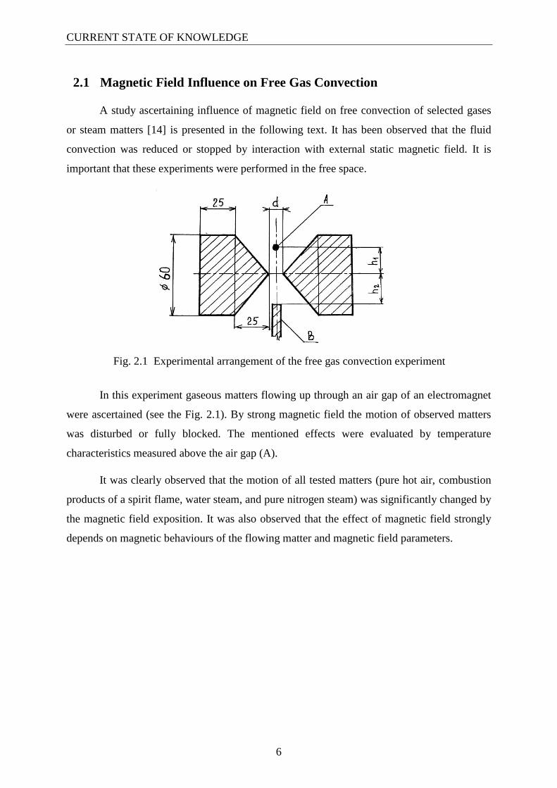
2.2 Magnetic Field influence on Cryogenic Heat Pipe Performance
A study investigating operation of a cryogenic heat pipe filled with liquid oxygen and
operating under static magnetic field generated by an electromagnet [15] is presented in the
following text. The experimental arrangement is shown in the Fig. 2.2. A vertically oriented
gravitational heat pipe was placed in the electromagnet air gap. The top of the heat pipe was
cooled by liquid nitrogen and the rest was exposed to the room temperature. The temperature
of the heat pipe was measured in 7 points during its operation under various conditions.
Fig. 2.2 Experimental arrangement of the cryogenic heat pipe
According to the presented results it was possible to significantly reduce heat flow in
the heat pipe by static magnetic field of B = 1,0 T with gradient 5 to 50 T/m (Fig. 2.3). It was
also found out the heat transport was disturbed when the magnetic induction B was 0,85 T
and higher. This study was limited to the mentioned heat pipe design filled with oxygen and
the electromagnet as a magnetic field source.

CURRENT STATE OF KNOWLEDGE
8
Fig. 2.3 Time dependence of temperature at seven points of cryogenic heat pipe [15]:
without magnetic field exposure (left)
with magnetic field exposure (right)
2.3 Magnetic Coupling Applied on Heat Pipes
There are also examples of mechanical control systems utilizing magnetic field [16].
An example of such system is presented in the Fig. 2.4. A wick inside a heat pipe is movable
by magnetic coupling and can be connected and disconnected by this way. So it is possible
totally stop the working cycle within. Another approach may be some kind of a valve
reducing the vapor channel in a heat pipe. However, commercial applications or more detailed
studies of these systems are not known.
Fig. 2.4 Schema of a heat pipe with movable wick structure by magnetic coupling
Magnet
Fixed Movable
┌ Wick structure ┐

CURRENT STATE OF KNOWLEDGE
9
2.4 Magnetic Field Enhancement of Heat Pipe with Ferrofluid
A study ascertaining heat pipes filled with citric ion stabilized ferrofluids operating
under external static magnetic field [19] is presented in the following text. In the arrangement
(Fig. 2.5) the evaporator region is exposed to a static magnetic field generated by Nd-Fe-B
permanent magnets in various configurations. The magnetic field exposition initiates an
additional liquid convection in the evaporator supporting heat exchange in this region.
Fig. 2.5 Heat pipe with movable wick structure by magnetic coupling
According to the presented results, heat capability of the tested heat pipe operating
under magnetic field exposition increased of up to 30% compared to that without any
magnetic field exposition. At optimal conditions the presented heat pipe was able to achieve
heat transport capability of 10% higher than that of a similar standard heat pipe filled with
water only.

GOALS OF THE WORK
10
3 Goals of the Work
The main aim of this work is development of a method for control of heat transport in
heat pipes by a magnetic field exposition and experimental evaluation of its possibilities. The
work objectives include but are not limited to the followings:
Development of a method for heat transport control in heat pipes based on magnetic
field exposition. The method shall be capable to significantly affect the heat pipe operation
and its thermal characteristics. Additionally, it should be feasible by using passive permanent
magnets systems instead of electromagnet sources with high energy consumption.
Experimental investigation of heat pipes utilizing proposed magnetic field control
methods. Influence of such control systems on heat transport in heat pipes shall be
ascertained. The experiments should be realized for various heat pipe constructions and
overall system arrangements.
Design and manufacturing of heat pipe prototypes. For the experimental investigation
it is necessary to create prototypes capable for operation under standard conditions. Their
construction must also allow ascertaining of mentioned magnetic field effects on heat flow
within. A suitable working fluid should be selected for that purpose as well.
Installation of an experimental arrangement for testing of mentioned effects in heat
pipe prototypes. It shall allow heat pipes operation in selected mode and measurement of
important heat pipe parameters, especially temperature and internal pressure. The
arrangement and tooling shall also allow manufacturing of the prototypes.
Publishing of theses and results of the work. Papers based on this work shall be
published in journals and proceeded at international conferences. Heat pipe prototypes and
arrangements realized during the work might be also registered as Utility Models at Czech
Industrial Property Office in Prague or as Functional Models at Czech Technical University in
Prague. They may be also employed for educational aims.

HEAT PIPES
11
4 Heat pipes
Heat pipes are thermal devices allowing very effective heat transport [15], [16], [17],
[26], [27]. They are based on a two-phase fluid cycle inside a closed tube. First heat pipes are
known from the 19th century as Perkins tubes using gravity for the liquid return (they are also
called thermosyphon). In the 1960s the US space program needed effective and light-weight
cooling systems operating in the 0-g environment. The Perkins tube was an ideal candidate
but it was necessary to solve condensate return independently on the gravity. Thus, a capillary
structure was added inside the tube. So a standard wicked heat pipe was developed (Fig. 4.1).
Fig. 4.1 Several examples of heat pipe applications and solutions
The fluid circulates in heat pipes while continually evaporating at one end and
condensing at the opposite end. Since evaporation and condensation are very effective thermal
processes, heat pipes are able to transport heat with very high efficiency and without any
external power feeding. Currently available heat pipes are able to operate in a wide range of
temperatures from a few Kelvins up to about two thousands Kelvins. Most applications need
to work at ambient temperatures. Typical for this range is water filled heat pipe with effective
thermal conductance up to 104 Wm
1K
1 and temperature drop less than 1 Km
1 (for
example, thermal conductance of copper is 380 Wm1K
1). Since there is a lower pressure
inside a heat pipe, it is able to work from about 20 C up to 250 C.
Heat pipes are very simple in their construction without any moving parts and external
power needs. They are quiet, reliable and needs no maintenance for years. Big advantage is

HEAT PIPES
12
their low weight, important especially for space and avionic applications. Since all the
electronic devices and components are more and more miniaturized, it is also very beneficial
that heat pipes can remove large amount of heat from a small area. On the other hand, they
may have some difficulties at the start-up or with the wick performance. See the typical heat
pipes characteristics in the Tab. 4.1.
Heat pipes are getting to be a common thermal solution in a wide number of
applications. The absolutely most often are cooling of electronic components. Heat pipes can
be found in laptops or other consumer electronic, power semiconductor modules, avionics,
sensor systems or others. However, heat pipes are employed also in more specialized and less
often applications like cryosurgery devices, tight temperature controlled material processing
or cryogenic systems. The mass production of heat pipes reduces their cost and thus, further
increase of heat pipe applications may be expected.
Tab. 4.1 Summary of heat pipe characteristic behaviours
Benefits Negatives
High thermal conductance
(high heat flux)
Operation temperature range limited by a
used working fluid
Almost isothermal along the whole length
(temperature flattening)
Position limitations
Passive device
(No power feeding necessary)
Possible complications at start-up
Can work as a thermal transformer
(small area heat in - large area heat out)
Could be more expensive compared to
conventional systems
Heat source - sink isolation
Simple construction and build in flexibility
Quiet operation, no moving parts
Long life and reliability
(even in a hard environment)
Control possibilities
(can also operate as a thermal diode)

HEAT PIPES
13
4.1 Heat Pipe Operation
Let us discuss basic principles of heat pipes operation in the following text [20]. Heat
is transported by a cycle of a working fluid within a closed tube (Fig. 4.2). Heating one end of
the tube (evaporator with heat source) the fluid is boiling and continuously vaporizing. The
generated vapour streams very fast through the tube and condensates on the colder wall at the
opposite end (condenser with heat sink). The condensed liquid may return to the evaporator
using gravity or through a wick. The working cycle continues as long as the temperature
gradient between the evaporator and condenser is maintained.
Fig. 4.2 Heat pipe operation schema
4.1.1 Condensate Return
Condensate return has a large impact on heat pipes operation and is often the limiting
factor of its power capability. There are two basic types of heat pipes from the condensate
return point of view:
gravitational heat pipes (thermosyphon)
wicked heat pipes (heat pipe with capillary structure)
In gravitational heat pipes the condensate returns back to the evaporator region due to
the gravitational force. This type of heat pipes has a very simple construction but on the other
hand also an important limitation - the evaporator must be always kept below the condenser.

HEAT PIPES
14
Wicked heat pipes with an integrated capillary system are the most common type today. The
wick is able to pump liquid even against gravity and so it allows much more independence in
the heat pipe positioning (more about the wick systems in the section 4.2.3).
Except the above mentioned return systems, there are also some other techniques
including axial rotation, osmotic or magnetic forces, etc. An example of a rotating heat pipe is
presented in the Fig. 4.3. Those are widely used for cooling of electric engines or other
rotating devices.
Q
Q Q
Q
Fig. 4.3 Heat pipe with liquid return based on axial rotation
4.1.2 Thermal Resistance Model
Thermodynamic behaviours and properties of heat pipes can be described by
equivalent thermal resistances. Their values depend on the heat pipe construction and
operation mode. The overall thermal resistance of a simple cylindrical heat pipe is
10
8
2
8
29191
1R
R
R
RRRRRR
i
i
i
i
P
; [KW1
] (4.1)
consisting of 10 partial thermal resistances in serial-parallel combination, as seen in the
Fig. 4.4.

HEAT PIPES
15
Fig. 4.4 Equivalent thermal resistances representing a heat pipe
Each thermal resistance is related to a specific part of a heat pipe with a specific heat transfer
mechanism:
R1 - Thermal resistance of the contact heat source – heat pipe container
R2 - Radial th. resistance of the container wall in the evaporator region
R3 - Radial th. resistance of the condensate film or wick in the evaporator region
R4 - Thermal resistance of the liquid – vapor interface in the evaporator region
R5 - Thermal resistance of the vapor column in the adiabatic section
R6 - Thermal resistance of the vapor – liquid interface in the condenser region
R7 - Radial th. resistance of the condensate film or wick in the condenser region
R8 - Radial th. resistance of the container wall in the condenser region
R9 - Thermal resistance of the contact heat sink – heat pipe container
R10 - Axial th. resistance of the container wall (and wick)
The temperature drop of external resistances R1 and R9 are high, usually comparable
with the rest of the heat pipe resistance (consisting from R2 - R8). They depend on quality of
mechanical contacts heat pipe – heat source and heat pipe – heat sink. On the other hand,
resistances of the liquid – vapor interfaces and of the vapor column (R4 – R6) are very low
(usually not measureable) and thus, they can be usually neglected.
There is also a parallel way for heat transport by axial heat conduction through the
container wall (and wick). However, its thermal resistance R10 is much higher than that of the
standard way provided by the working cycle and thus, it is relevant only when the heat pipe
does not operate (residual heat flow at thermal diodes or variable conductance heat pipes).
R10
R4
R3
R2
R1
R6
R7
R8
R9
R5
T1 T2

HEAT PIPES
16
Fig. 4.5 Partial temperature drops ∆T along the heat pipe (cross-section view)
Every partial thermal resistance, described above, increase the total temperature drop,
as graphically presented in the Fig. 4.5. Heat pipes are able to achieve low thermal resistance
on long ways due to almost lossless convection of the vapour.
4.1.3 Heat Transfer in Heat Pipe
Since there is a difference between the evaporator temperature TE (K) and the
condenser temperature TC (K), the working fluid circulates in the heat pipe and caries out the
heat flux
R
TTLmP CE
V
;
2
2
s
m,
s
kgW; , where (4.2)
m - mass flow of working fluid,
LV - latent heat of evaporation,
R - total thermal resistance of heat pipe.
Heat enters heat pipes at the evaporator region, usually by conduction from a heat
source. Equivalent thermal resistance R1 is related to the heat transfer between the heat source
and the heat pipe surface. It usually depends on the quality of thermal contact between a heat
pipe and a heat source.
Then heat flows through the container wall by radial conduction. To ensure low R2,
container material with high thermal conductance (usually copper if compatible with other
∆T5
∆T4
∆T3
∆T2
∆T1
∆T6
∆T7
∆T8
∆T9
∆T1
0
T1 T2
Adiabatic section Evaporator Condenser
Container wall
Wick
Vapor column

HEAT PIPES
17
heat pipe elements) and low wall thickness (but also respecting the mechanical stress at higher
internal pressure) should be utilized.
Equivalent thermal resistance R3 represents heat transfer through the liquid film
(gravitational heat pipes) or through the wick (wicked heat pipes). This resistance is
significant especially at cryogenic heat pipes with low thermal conductance of fluids. At
wicked heat pipes it depends also on the heat flux. For low values there is only conduction
through the wick and natural convection of the liquid. At higher values bubbles are generated
at the wall and the heat transport is increasing by latent heat of evaporation and supported
liquid convection.
Then, heat is transferred by latent heat of evaporation at vaporization and
condensation (R4 and R6). There is a large energy in this phase changes allowing heat pipe to
work with very high efficiency. These thermal resistances are very low and may be neglected.
Between the evaporator and condenser heat is transported by the vapour convection.
There is a pressure drop along the vapour column represented by the thermal resistance R5.
However, this can be usually neglected. Thanks to this fact, heat pipes are able to transport
heat over long distances with insignificant temperature drop (however, the condensate return
must be assured).
In the condenser region the situation is very similar to that in the evaporator. Vapor
condensates on the condenser surface with a low thermal resistance R6. Then it flows through
the wick/liquid film (R7) and container wall (R8). From the outer surface of the condenser
heat is usually conducted to a heat sink (R9). It may be useful to know typical values of the
equivalent th. resistances - see the Tab. 4.2.
Tab. 4.2 Typical values of thermal resistances of a heat pipe
Resistance Corresponding part Typical value (K/W) Comment
R1, R9 External heat transfer 101 - 10
3
R2, R8 Radial of the wall 10-1
R3, R7 Radial of wick/liquid film 101
R4, R6 Liquid-vapor interfaces 10-5
Usually negligible
R5 Vapor column 10-8
Usually negligible
R10 Axial of the wall 103

HEAT PIPES
18
4.1.4 Limits of Heat Pipe Operation
The heat pipe operation is limited by several factors illustrated in the Fig. 4.6. It is
necessary to consider every single limit. Altogether they define the working area of a heat
pipe and set up its maximal capability. Some of those limits are important at the start-up,
some of them at higher temperatures and some of them are critical across the whole operating
range.
Fig. 4.6 Heat pipe operation limits
The sonic limit may be important at the start-up and also for some high temperature
heat pipes when the vapor streams very fast and may reach the sonic speed.
The viscous limit (vapor pressure limit) is important for wicked heat pipes at the start-
up. At low temperatures the pressure difference is insufficient to overcome the pressure drop
in the wick.
The capillary limit is very critical for all wicked heat pipes and it usually limits the
maximal heat flux across the whole temperature range. However, it can be partially eliminated
by the gravity. Gravitational heat pipes are not limited by this limit at all.
Vapour streaming through the heat pipe can entrain the liquid droplets back to the
condenser and prevent the liquid return. The entrainment limit is critical for the gravitational
heat pipes.
The boiling limit is related to the radial heat flux in the evaporator region. When
exceeding the limit, vapour bubbles are being created around the evaporator and thermal
resistance is increasing.
Boiling limit A
xia
l h
ea
t flu
x (
W)
Sonic limit
Capillary limit Viscous
limit
Entrainment limit
Entrainment limit
Temperature (K)
Working area
T
T
T
C

HEAT PIPES
19
4.2 Construction
Heat pipes are very simple in their construction. They always consist of a closed
container (usually in the form of a cylindrical tube) and a small amount of working fluid
within. Some kind of wick structure may be built-in inside the container. Special heat pipes
may contain also additional components, e.g. some kind of valves in Variable Conductance
Heat Pipes. Very important for heat pipes operation is that all the components must be
chemically compatible and stable. In the Tab. 4.3 there are typical combinations of container
materials and working fluids.
Tab. 4.3 Typical combinations of container materials and working fluids
Working Fluid Container Material
Liquid Nitrogen Stainless Steel
Liquid Ammonia Nickel, Aluminum, Stainless Steel
Methanol Copper, Nickel, Stainless Steel
Water Copper, Nickel
Potassium Nickel, Stainless Steel
Sodium Nickel, Stainless Steel
Lithium Niobium +1% Zirconium
4.2.1 Container
Heat pipe container is a hermetically closed envelope. A cylindrical geometry is most
common, but other geometries are also possible, as seen in the Fig. 4.7. Heat pipes are often
bendable to a specific geometry and may be adapted for several applications (however, not all
wicks are flexible, espec. sintered structures are very fragile). The main container functions
are listed below:
Hermetic closure of internal heat pipe environment
Radial heat flow through its wall (high thermal conductance required)
Mechanical protection
High internal pressure withstanding
Material of the heat pipe container must meet all the above mentioned requirements.
The container must withstand the mechanical stress at the evacuation before filling and then

HEAT PIPES
20
high internal pressure at higher temperatures while being absolutely leak free. Material with
high thermal conductance should be used to obtain low temperature drop.
Fig. 4.7 Heat pipes with various shapes of containers
Typical materials used for heat pipe containers operating at various temperature ranges
are listed in the Tab. 4.3. The most often container material is copper - traditional for water
heat pipes. It has excellent thermal conductance, however, on the other hand the mechanical
strength is relatively low (unsuitable for water heat pipes operating above 200 °C) and the
mass density is also high (unsuitable for space and aircraft applications).
In some special cases, adiabatic section of the heat pipe can be made from different
material with lower thermal conductance than that of evaporator and condenser. So the heat
load and heat sink can be thermally cut off when the heat pipe does not operate. At some of
our experiments the adiabatic section was made from glass to enable visual observation of the
processes inside.

HEAT PIPES
21
4.2.2 Working Fluids
Working fluid is an essential part of the heat pipe system. It must be compatible with
other components (container, wick, event. others) and chemically stable (see typical
combinations in the Tab. 4.3). The fluid choice follows from the heat pipe operation
temperature. It must be in the range between the triple point TT and the critical point TC of the
fluid. Other parameters of working fluid important for the heat pipe operation are shown in
the Tab. 4.4, including their impact on the heat pipe operation. All these aspects must be taken
into account to assure a reliable heat pipe operation.
Tab. 4.4 Working fluid parameters and their impact on the heat pipe operation
Working fluid parameter Required value Related heat pipe parameter
Latent heat high Heat transport capability
Thermal conductance high Radial temp. drop in wick/liquid film
Liquid and vapor viscosity
low Pressure drop of vapor and liquid flow
Wick wettability high Wick filling
Surface tension high Wick capability
Health and safety high Application possibilities
The most common working fluid is water which is suitable for ambient temperatures
(from about 20 °C to 250 °C) and has optimal behaviours for the two phase heat transport. For
lower temperatures methanol, ammonia or some of permanent gases are used (see more in the
4.3.1). Above the water temperature range heat pipes are filled with dowtherm, mercury or
some halides for example. For highest temperatures up to about 2000 °C alkali metals are
used as a working fluid.
Working fluids used for low, ambient and high temperatures are strongly different in
their parameters. Low temperature working fluids are generally less optimal than ambient or
high temperature ones. Power capability comparison of heat pipes filled with various working
fluids is presented in the Tab. 4.5.

HEAT PIPES
22
Tab. 4.5 Power Capability of Heat Pipes with Typical Working Fluids
Working Fluid Axial heat flux
(kW/cm2)
Surface heat flux
(W/cm2)
Liquid Nitrogen 0.067 (-163°C) 1.01 (-163°C)
Liquid Ammonia 0.295 2.95
Methanol 0.45 (100°C) 75.5 (100°C)
Water 0.67 (200°C) 146 (170°C)
Potassium 5.6 (750°C) 181 (750°C)
Sodium 9.3 (850°C) 224 (760°C)
Lithium 2.0 (1250°C) 207 (1250°C)
As mentioned above, every working fluid is able to work only in the limited
temperature range between its triple and critical point. When the needed operating range is
wider than a single working fluid can cover, two or more heat pipes with different working
fluids may be arranged into a cascade. For example in some cryogenic systems it is necessary
to cool down the system from ambient temperature to cryogenic temperature. Typical solution
may be a cascade of an ethane heat pipe (300 K → 140 K) and an oxygen heat pipe (140 K →
60 K). Another way is to fill a single heat pipe with couple of different working fluids.
However, this is not so often, because such customer solutions are much more expensive than
mass produced heat pipes combined into a cascade.

HEAT PIPES
23
Fig. 4.8 Various kinds of wick structures used in water heat pipes
4.2.3 Wick Structures
Most heat pipes have some kind of a built-in wick (wicked heat pipes) providing the
condensate return from the condenser back to the evaporator. The wick is usually some kind
of a fine porous structure or grooves (illustrated in the Fig. 4.8) or capillaries (a fibre wick in
the Fig. 4.9). It can pump the liquid even against the gravity due to the capillary pressure.
Thus, wicked heat pipes bring much more independence in their positioning and orientation.
Moreover, the wick can be assisted by the gravity when the evaporator is below the condenser
(gravity assist mode).
Fig. 4.9 Heat pipe with fiber wick for long way liquid return
HEAT PIPES
24
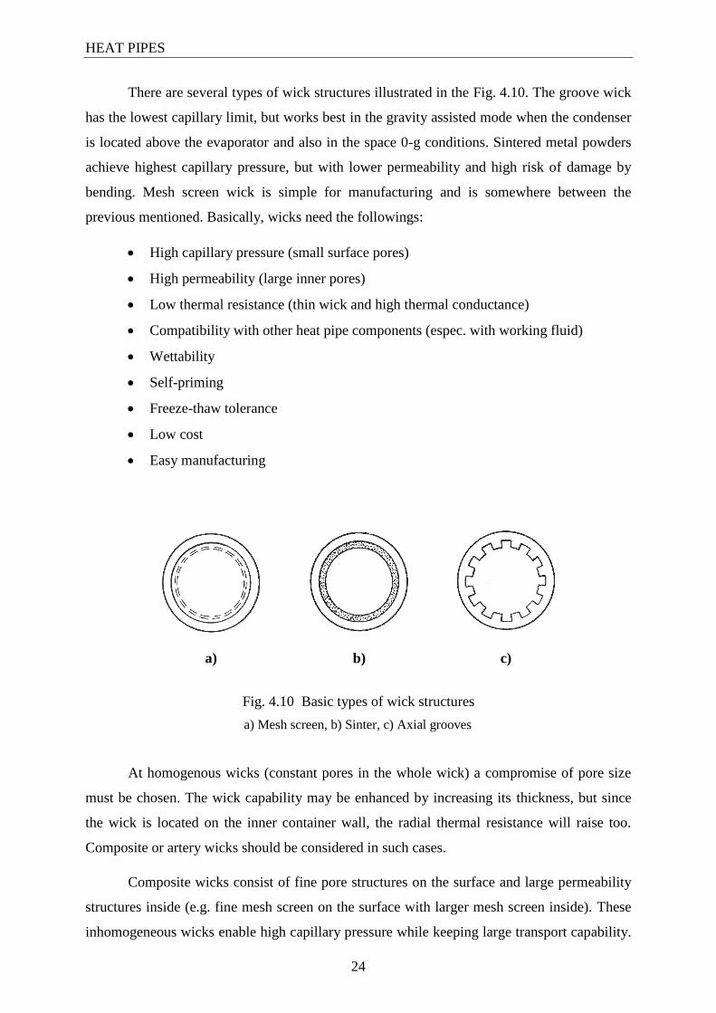
There are several types of wick structures illustrated in the Fig. 4.10. The groove wick
has the lowest capillary limit, but works best in the gravity assisted mode when the condenser
is located above the evaporator and also in the space 0-g conditions. Sintered metal powders
achieve highest capillary pressure, but with lower permeability and high risk of damage by
bending. Mesh screen wick is simple for manufacturing and is somewhere between the
previous mentioned. Basically, wicks need the followings:
High capillary pressure (small surface pores)
High permeability (large inner pores)
Low thermal resistance (thin wick and high thermal conductance)
Compatibility with other heat pipe components (espec. with working fluid)
Wettability
Self-priming
Freeze-thaw tolerance
Low cost
Easy manufacturing
Fig. 4.10 Basic types of wick structures
a) Mesh screen, b) Sinter, c) Axial grooves
At homogenous wicks (constant pores in the whole wick) a compromise of pore size
must be chosen. The wick capability may be enhanced by increasing its thickness, but since
the wick is located on the inner container wall, the radial thermal resistance will raise too.
Composite or artery wicks should be considered in such cases.
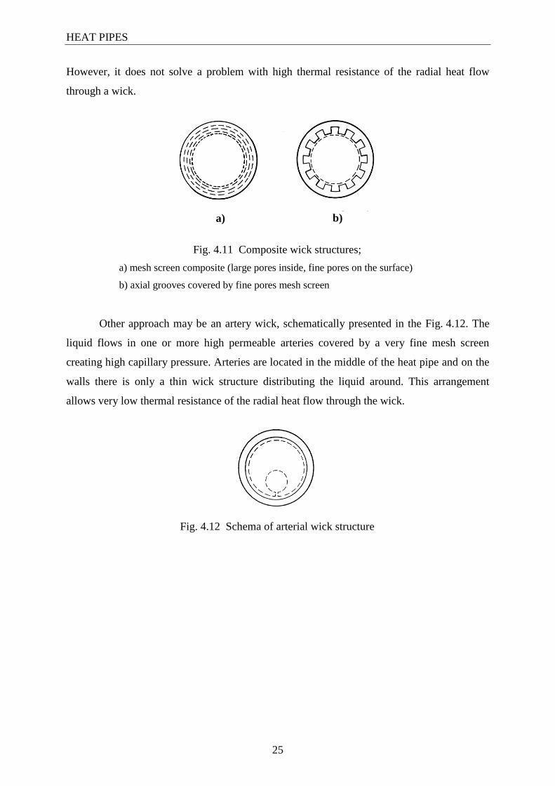
Composite wicks consist of fine pore structures on the surface and large permeability
structures inside (e.g. fine mesh screen on the surface with larger mesh screen inside). These
inhomogeneous wicks enable high capillary pressure while keeping large transport capability.
a) b) c)
HEAT PIPES
25
However, it does not solve a problem with high thermal resistance of the radial heat flow
through a wick.
Fig. 4.11 Composite wick structures;
a) mesh screen composite (large pores inside, fine pores on the surface)
b) axial grooves covered by fine pores mesh screen
Other approach may be an artery wick, schematically presented in the Fig. 4.12. The
liquid flows in one or more high permeable arteries covered by a very fine mesh screen
creating high capillary pressure. Arteries are located in the middle of the heat pipe and on the
walls there is only a thin wick structure distributing the liquid around. This arrangement
allows very low thermal resistance of the radial heat flow through the wick.
Fig. 4.12 Schema of arterial wick structure
a) b)

HEAT PIPES
26
4.3 Cryogenic Heat Pipes Specifics
An important part of this work is focused on experimental ascertaining of magnetic
field influence on cryogenic heat pipes. Thus, cryogenic heat pipes and their specifics will be
discussed more in detail in the following text. Cryogenic heat pipes are used for heat transport
in the lowest temperature range. The upper temperature boundary is not strictly defined,
generally, we speak about temperatures from 123 K (- 150 ˚C) down to about 5 K. Cryogenic
heat pipes are based on the same principles as the others, however, their behaviours are
significantly different.
Tab. 4.6 Working temperature ranges
of selected cryogenic heat pipes
Working fluid Temp. range (K)
Ammonia 200K to 400K
Ethane 120K to 300K
Helium 3K to 5K
Methanol 200K to 400K
Nitrogen 65K to 120K
Oxygen 60K to 140K
Pentane 150K to 400K
Propylene 120K to 335K
Common working fluids employed in cryogenic heat pipes are nitrogen, oxygen,
hydrogen, helium, methane, ethane or others. Some typical low temperature working fluids
are presented in the Tab. 4.6. We have tested oxygen heat pipes operating in the range from
about 60K to 140 K. There are some working fluids parameters which are critical especially
in the low temperature range. Unfortunately those are usually very poor compared to the
higher temperature fluids and furthermore, they also depend on the temperature:
Latent heat of evaporation
Surface tension
Liquid – vapor density ratio
Thermal conductance

HEAT PIPES
27
Another critical factor of cryogenic heat pipes is the container robustness. It must
withstand higher pressure while being stored at ambient temperature (all the working fluid is
in the gaseous state). More robust container increases its weight which is an important
parameter for space and aircraft applications and also the radial thermal resistance.
Finally there can be also a problem how to cool the heat pipe condenser because at
very low temperatures the available methods are quite limited. Because of the above
mentioned facts, cryogenic heat pipes attain lower capability and some additional aspects
must be taken into account.
4.3.1 Cryogenic Working Fluids
Heat pipes are able to operate only in the temperature range between the triple and
critical point of the used working fluid. However, at boundaries of this range heat transport
capability is being reduced due to poor viscosity and surface tension. As mentioned above,
cryogenic working fluids have poor thermophysical and other behaviours important for the
heat pipe performance (see the Tab. 4.7). Impacts on the heat pipe operation will be described
in the following text.
The low latent heat of evaporation and condensation constrain heat transport
capability. Heat removed by a cryogenic fluid vaporization is much smaller than that of
higher temperature fluids.
The low surface tension negatively affects the wick structure filling. This can be
eliminated by smaller pore radius of a wick. However, this is usually not so critical in the 0-g
environment (space applications). For the 1-g applications where the evaporator is placed
above the condenser sintered metal powder wick or fine mesh screen should be utilized.
Cryogenic working fluids have also very low liquid – vapour density ratio. It means,
more liquid is needed for generating the same value of vapour in comparison with water. The
liquid flow passage must be more capable.
Low thermal conductance of cryogenic fluids may increase radial thermal resistance,
especially when there is a thick wick or liquid film on the container surface. From this point
of view, wick should be thin or special arterial structures placed in the middle of a heat pipe
should be used.

HEAT PIPES
28
Tab. 4.7 Thermophysical properties of selected cryogens
(* at 101,3 kPa; ** at 101,3 kPa and 15 C)
Temperatures /
Cryogens
Triple point
Tp (K)
Boiling point* Tb (K)
Critical point
Tc (K)
Critical pressure pC (MPa)
Liq. - vapor density ratio
(-)
Latent heat of vaporization**
LV (Kj/Kg)
Thermal conductance**
λ (mW/m.K)
He4
Helium 4,22 5,2 0,228 748 20,3 142,64
H2
Hydrogen 13,9 20,3 33,19 1,291 844 454,3 168,35
D2
Deuterium 18,7 23,6 38,3 1,665 974 304,4 130,63
Ne Neon
24,559 37,531 44,49 2,651 1434 88,7 45,803
N2 Nitrogen
63,148 77,313 126,19 5,091 691 198,38 24
CO Carbon monox.
68,09 81,624 132,8 3,499 674 214,85 23,027
Ar Argon
83,82 87,281 150,66 5,001 835 168,81 16,36
O2
Oxygen 54,361 90,191 154,58 3,401 854 212,98 24,24
CH4
Methane 90,67 111,685 190,56 4,642 630 510 32,81
Kr Krypton
115,94 119,765 209,43 5,502 699 107,81 8,834
Water 273,16 373,15 674 22,064 1243,78 2257 580

HEAT PIPES
29
4.3.2 Container and Wick Design
Cryogenic heat pipes are usually filled with working fluids in the liquid state (at low
temperature). However, they are usually stored at room temperatures causing an increase of
internal pressure. Hence, stronger material, higher wall thickness or smaller heat pipe
diameter must be utilized.
Several different wick types are well known from ambient temperature heat pipes. For
cryogenic applications a wick must have superior parameters to compensate poor key
properties of working fluids. The most important parameters are:
High capillary pressure (needs small surface pores)
High permeability (needs large inner pores)
Low thermal resistance (needs thin wick made of a material with large thermal
conductance)
Since cryogenic fluids have poor surface tension and low thermal conductance,
composite or artery wicks should be utilized. The composite wick enables higher capillary
pressure while keeping large transport capability. The arterial wick additionally allows
lower temperature drop across the wall since it is located in the middle of the container. More
details about wick structures find in the chapter 4.2.3.

VARIABLE CONDUCTANCE HEAT PIPES
30
5 Variable Conductance Heat Pipes
In the previous text we have discussed heat pipes without any control possibilities,
working with the highest possible efficiency. This chapter deals with variable conductance
heat pipes (VCHPs) [16]. By some kind of modification in heat pipe construction it is possible
to change its heat transport efficiency (thermal conductance) and get some kind of thermal
control - one way heat transport, temperature stabilization, active temperature control etc.
There are three basic groups of VCHPs different in their function, behaviours,
construction and use. Their basic characteristics are presented in the Tab. 5.1 and further
discussed in the following sections.
Tab. 5.1 Characteristics of basic VCHPs groups
Type of VCHP Main Feature Common Design Typical Applications
Thermal Diodes One way heat flow
Thermosyphon
Wick modifications
Liquid flow traps
Heat recuperations,
cryostat systems
Stabilization
Heat Pipes Temp. maintaining
Noncondensable gas
Additional liquid
Cooling of electronic
components (espec.
semiconductors)
Active Control
Heat Pipes
Dynamic temp. control
Thermal switch
(on/off)
Noncondensable gas
Vapour channel valve
Magnetic coupling
Temp. control of
technolog. processes
Thermal key in
cryogenic systems
VARIABLE CONDUCTANCE HEAT PIPES
31
5.1 Thermal Diodes
Thermal diodes are similar to semiconductor ones from the function point of view -
they allow heat transport in one direction only. They have two operation modes - forward and
reverse (see the Tab. 5.2). In the forward mode (higher temperature at the evaporator) the heat
pipe operates standardly with high thermal conductance. When the evaporator temperature
decreases below the condenser temperature the heat pipe switches into the reverse mode. The
working cycle inside is stopped and only the residual heat may be transferred axially by
conduction through the container. Some typical designs of heat pipe diodes are listed below
and discussed in the following sections:
Thermosyphon
Heat pipe with an inhomogeneous wick structure
Heat pipe with a wick trap
Tab. 5.2 Operation modes of heat pipe thermal diodes
Operation mode Evaporator temp. Condenser temp. Eff. thermal conductance
Forward mode higher lower high
Reverse mode lower higher low
5.1.1 Thermosyphon
The simplest heat pipe diode may be a standard gravitational heat pipe
(thermosyphon). It works as a thermal diode because it is able to work only when the
evaporator is placed below the condenser. When the temperature gradient turns over (higher
temperature up) the heat pipe is not able to operate. Gravitational heat pipe diodes are very
simple, however, their positioning is limited.

VARIABLE CONDUCTANCE HEAT PIPES
32
5.1.2 Inhomogeneous Wick
Thermal diode can be realized also by a modification of the wick structure. A common
solution is a wick with special inhomogeneous surface having high capillarity in the
condenser region and low capillarity in the evaporator region. When operating in the reverse
mode, vapor condensates in the evaporator where the wick performance is too poor to feed the
evaporator.
5.1.3 Wick Trap
Another heat pipe diode construction is schematically shown in the Fig. 5.1. In this
case a wicked reservoir is placed in the evaporator region. It is separated from the standard
wick by a barrier with the vapor flow channel. In the forward mode fluid vaporizes from the
reservoir and circulates in the heat pipe. In the reverse mode all the fluid condensates in the
reservoir and no more is available for the heat pipe operation.
standard wick wicked reservoir
Fig. 5.1 Thermal diode with wicked reservoir as a working fluid trap

VARIABLE CONDUCTANCE HEAT PIPES
33
5.2 Stabilization Heat Pipes
Stabilization heat pipes are employed for maintaining stable temperature of devices
mounted at the evaporator. The temperature may be kept at almost constant level even if the
heat input varies in a wide range. The heat pipe effective thermal conductance depends on its
temperature - the stabilization process is simply illustrated in the Fig. 5.2. At the beginning all
parameters are in the stable state (part 1). Then an increase of temperature will cause an
increase of thermal conductance (part 2). Heat pipe is now in the transient state with larger
heat flux and device is cooled with higher efficiency. So the temperature is turning back to the
starting value and thermal conductance will decrease on a new stable state (part 3).
0
50
100
150
200
250
300
350
1 2 3
part of process(-)
ac
tua
l v
alu
e/i
nit
ial
va
lue
(%
)
Heat input
HP temperature
Eff. thermal conductance
Fig. 5.2 Stabilization heat pipe operation;
1 - stable state, 2 - increasing of heat input, 3 - new stable state
Stabilization heat pipes are typically employed for cooling of semiconductors, precise
electronics or detectors sensitive to temperature changes. Stable temperature is important also
at inhomogeneous or multilayer structures made from materials with different temperature
dilatation.
Stabilization heat pipes may be realized in several constructions, however, gas loaded
type is absolutely dominant on the market and thus, it will be described in detail in the
following sections.

VARIABLE CONDUCTANCE HEAT PIPES
34
5.2.1 Gas Loaded Heat Pipes
Gas loaded heat pipes are the absolutely most common in the segment of variable
conductance heat pipes. Simply construction and excellent performance makes them very
popular for thermal designers. This control effect was first observed in standard stainless
steel-sodium heat pipes. After start up a noncondensable gas was generated and pressed by
the vapor stream into the condenser region. A part of the condenser was then filled by the gas
and unavailable for the working cycle anymore. The working fluid could condense on the
reduced surface only and the heat flow proportionally decreased.
Fig. 5.3 Gas loaded heat pipe - basic type
At the Fig. 5.3 there is a schema of the gas loaded heat pipe. In this simple case, the
construction is identical to a standard heat pipe, only some amount of a noncondensable gas
(nitrogen, argon etc.) is added into the heat pipe during the filling. The noncondensable gas
must be compatible with other heat pipe components and must not condense within the
operation temperature range.
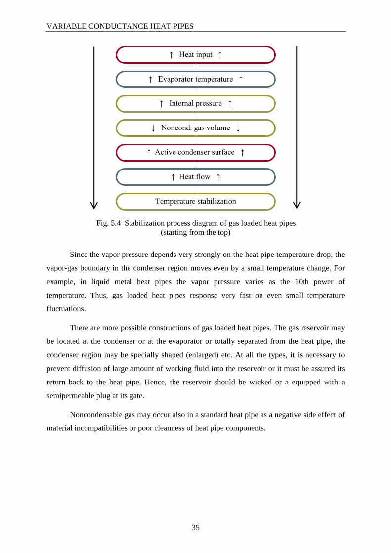
Stabilization process in the gas loaded heat pipe is presented in the Fig. 5.4. During the
operation the noncondensable gas is situated at the end of the condenser region due to the
vapor stream. Its volume negatively depends on the working fluid pressure. When the
pressure is rising the gas is pressed deeper to the condenser. So larger condenser surface is
available for condensation and larger amount of heat can be transported.
vapor
Q Q
Q Q
noncond. gas
VARIABLE CONDUCTANCE HEAT PIPES
35
Fig. 5.4 Stabilization process diagram of gas loaded heat pipes
(starting from the top)
Since the vapor pressure depends very strongly on the heat pipe temperature drop, the
vapor-gas boundary in the condenser region moves even by a small temperature change. For
example, in liquid metal heat pipes the vapor pressure varies as the 10th power of
temperature. Thus, gas loaded heat pipes response very fast on even small temperature
fluctuations.
There are more possible constructions of gas loaded heat pipes. The gas reservoir may
be located at the condenser or at the evaporator or totally separated from the heat pipe, the
condenser region may be specially shaped (enlarged) etc. At all the types, it is necessary to
prevent diffusion of large amount of working fluid into the reservoir or it must be assured its
return back to the heat pipe. Hence, the reservoir should be wicked or a equipped with a
semipermeable plug at its gate.
Noncondensable gas may occur also in a standard heat pipe as a negative side effect of
material incompatibilities or poor cleanness of heat pipe components.
↑ Heat input ↑
↑ Evaporator temperature ↑
↑ Internal pressure ↑
↓ Noncond. gas volume ↓
↑ Active condenser surface ↑
↑ Heat flow ↑
Temperature stabilization

VARIABLE CONDUCTANCE HEAT PIPES
36
5.3 Active Controlled Heat Pipes
Active controlled heat pipes allow absolute temperature regulation because the
effective thermal conductance may be adjusted during their operation. Compared to the
stabilization heat pipes (passive control), they offer some important benefits:
Absolutely free choice of the referential temperature point
(an electronic temperature sensor can be placed long away from the heat pipe)
Simple and operative adjustment (electronic programmable regulator)
Precise control of desired temperature level (faster and tighter response)
These features may be beneficial for some technological processes, electronic devices
or cryogenic adiabatic systems. Gas loaded heat pipes are absolutely major, however, in some
cases this method cannot be employed:
Not enough space for the gas reservoir
Heat flow cut off needs to be realized in the evaporator region
Incompatibility of a noncondensable gas with other components
In those cases alternative control methods needs to be employed. Some of them will be
also discussed in the following sections.

VARIABLE CONDUCTANCE HEAT PIPES
37
5.3.1 Gas Loaded Heat Pipes
Gas loaded active control system is based on the same principles already explained in
the chapter 5.2.1 about stabilization heat pipes. In this case, some kind of the feedback system
must be employed. A representative example is schematically shown in the Fig. 5.5. An
external heater is placed on the gas reservoir and connected to a control unit. The gas volume
depends on its temperature and so the effective thermal conductance can be regulated.
Fig. 5.5 Schema of gas loaded heat pipe with active control
However, the active feedback control needs an external power feeding. This negotiates
one of the most important heat pipes features - power independence.
5.3.2 Vapor Channel Throttling
This method is based on throttling of the vapor channel by a mechanical valve. It is
schematically illustrated in the
Fig. 5.6. The valve is connected with a bellows filled by a liquid. According to the
temperature the bellows varies in its length resulting in changing of the vapor channel cross-
section.
Fig. 5.6 Thermal control by vapor channel throttling
Q Q
Q Bellows with additional liquid
Valve
Q
Q Q
Q
Reservoir
Thermostat Heating

VARIABLE CONDUCTANCE HEAT PIPES
38
5.3.3 Magnetic Field Methods
There are also several methods how to influence heat flow in heat pipes by an external
magnetic field. Most of them are based on magnetic action on movement of mechanical
elements inside a heat pipe. This way it is possible to open and close a mechanic valve in the
vapor channel, connect and disconnect the wick or move some other elements. An example of
a heat pipe with a disconnectable wick is presented in the Fig. 5.7.
Fig. 5.7 Heat pipe with wick structure movable by external magnetic field
This work deals with a new approach for the heat transport control in heat pipes based
on magnetic field interaction with a fluid within a heat pipe. This technique is further
described in the following text in detail.
Magnet
Fixed Movable
┌ Wick structure ┐

MAGNETIC FIELD CONTROL
39
6 Magnetic Field Control
This work deals with a new approach to the heat transport control in heat pipes. It
might be an alternative to several conventional methods discussed in the previous chapter. It
is based on a force interaction between a static magnetic field and a fluid with suitable
magnetic behaviours within a heat pipe. By specific conditions it is possible to catch or move
the fluid by magnetic field or make a barrier for the fluid flow. Furthermore, using special
magnetic fluids, so called ferrofluids, a fluidal seal can be created as well. We assume that
some of these effects have a high potential to significantly reduce heat transport in special
heat pipes.
By this work we have proposed two basic control approaches:
Magnetic Trap Method
(magnetic working fluid + external magnetic field)
Magnetic Plug Method
(conventional working fluid + additional magnetic fluid + internal magnetic field)
The both methods are based on an interaction between static magnetic field and a fluid
within a heat pipe. However, there are important differences between them. Magnetic Trap
Method utilizes an external magnetic field source and can be applied on a heat pipe with
standard composition, only suitable magnetic working fluid must be within. On the other
hand, Magnetic Plug Method has the magnetic field source placed directly in a heat pipe and
furthermore an additional magnetic fluid must be within. The Magnetic Plug Method has been
developed especially for the utilization with ferrofluids – special synthetic liquids with
extraordinary magnetic behaviors.
The both magnetic field control methods need to meet some special requirements.
Very important and usually most difficult is to find a suitable fluid with sufficient magnetic
properties capable to interact with applied magnetic field. The interaction depends also on the
magnetic field – the stronger field, the stronger interaction. Additionally, the heat pipe
container must be made from a nonmagnetic material. The both methods including these
important preconditions are further discussed in the following sections in detail.

MAGNETIC FIELD CONTROL
40
Applying a magnetic field control on a heat pipe we are getting a very complex system
with many variables related to the magnetic field distribution, working fluid properties, heat
pipe construction or its operation mode. Mathematic models and calculations are very
complicated and less accurate because of extreme complexity of such a system. Hence, only a
limited theoretical description is presented in the following text.
MAGNETIC FIELD CONTROL
41
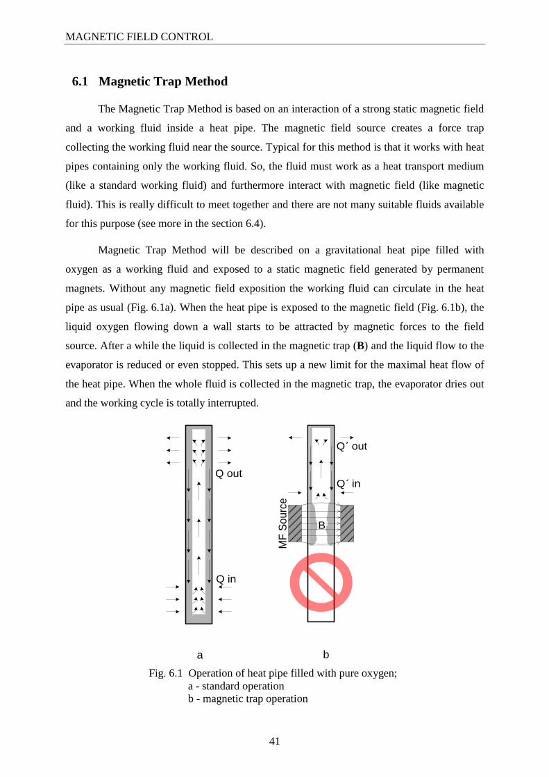
6.1 Magnetic Trap Method
The Magnetic Trap Method is based on an interaction of a strong static magnetic field
and a working fluid inside a heat pipe. The magnetic field source creates a force trap
collecting the working fluid near the source. Typical for this method is that it works with heat
pipes containing only the working fluid. So, the fluid must work as a heat transport medium
(like a standard working fluid) and furthermore interact with magnetic field (like magnetic
fluid). This is really difficult to meet together and there are not many suitable fluids available
for this purpose (see more in the section 6.4).
Magnetic Trap Method will be described on a gravitational heat pipe filled with
oxygen as a working fluid and exposed to a static magnetic field generated by permanent
magnets. Without any magnetic field exposition the working fluid can circulate in the heat
pipe as usual (Fig. 6.1a). When the heat pipe is exposed to the magnetic field (Fig. 6.1b), the
liquid oxygen flowing down a wall starts to be attracted by magnetic forces to the field
source. After a while the liquid is collected in the magnetic trap (B) and the liquid flow to the
evaporator is reduced or even stopped. This sets up a new limit for the maximal heat flow of
the heat pipe. When the whole fluid is collected in the magnetic trap, the evaporator dries out
and the working cycle is totally interrupted.
Q in
Q out
a
Q´ in
Q´ out
MF
So
urc
e
B
b
Fig. 6.1 Operation of heat pipe filled with pure oxygen;
a - standard operation
b - magnetic trap operation
MAGNETIC FIELD CONTROL
42
6.2 Theoretic Description
In the following text Magnetic Trap Method is briefly described from the theoretical point
of view [25]. However, this is a pretty hard business and thus, its scope is limited.
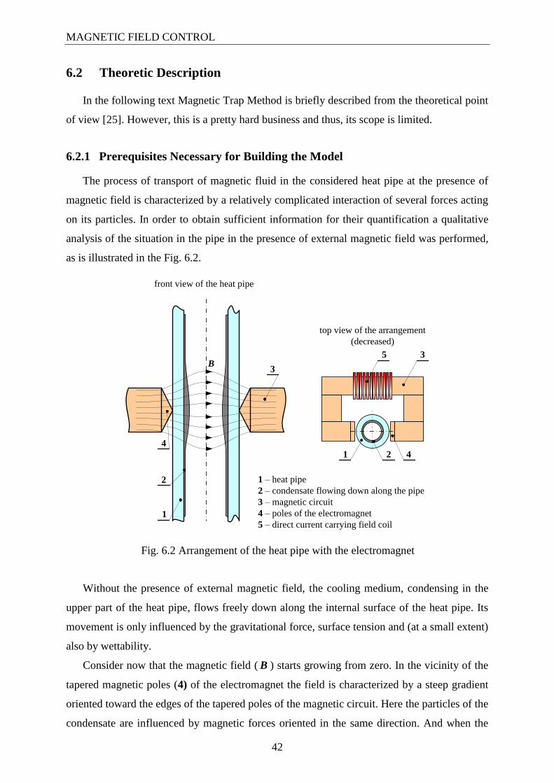
6.2.1 Prerequisites Necessary for Building the Model
The process of transport of magnetic fluid in the considered heat pipe at the presence of
magnetic field is characterized by a relatively complicated interaction of several forces acting
on its particles. In order to obtain sufficient information for their quantification a qualitative
analysis of the situation in the pipe in the presence of external magnetic field was performed,
as is illustrated in the Fig. 6.2.
1 – heat pipe
2 – condensate flowing down along the pipe
3 – magnetic circuit
4 – poles of the electromagnet
5 – direct current carrying field coil
B
top view of the arrangement
(decreased)
35
4
21
front view of the heat pipe
1
2
3
4
Fig. 6.2 Arrangement of the heat pipe with the electromagnet
Without the presence of external magnetic field, the cooling medium, condensing in the
upper part of the heat pipe, flows freely down along the internal surface of the heat pipe. Its
movement is only influenced by the gravitational force, surface tension and (at a small extent)
also by wettability.
Consider now that the magnetic field ( B ) starts growing from zero. In the vicinity of the
tapered magnetic poles (4) of the electromagnet the field is characterized by a steep gradient
oriented toward the edges of the tapered poles of the magnetic circuit. Here the particles of the
condensate are influenced by magnetic forces oriented in the same direction. And when the

MAGNETIC FIELD CONTROL
43
axial component of this magnetic force together with the analogous component of the force
generated by the surface tension exceed the corresponding pressure and gravitational forces,
the particle stops flowing down and takes part in forming a relatively stable droplet. The
volume of the droplet increases with growing magnetic field and after reaching a
predetermined value of magnetic flux density in the axis of the heat pipe the droplet fills in its
whole cross section, preventing the condensate from continuing flowing down. Now, the
operation of the heat pipe is practically stopped because of no transport of heat (provided that
the total weight of the condensate does not exceed the magnetic and tension forces).
B1 = 0
B2 = 0
B3 > B2 B4 > B3
droplet formed by
the condensate
Fig. 6.3 Droplet of condensate formed by forces acting on it for increasing magnetic field
left up: situation without external magnetic field
right up: small external magnetic field, the droplet starts growing
left down: higher magnetic field, the droplet continues growing
right down: high magnetic field, the droplet fills in the whole pipe preventing the
condensate from flowing down

MAGNETIC FIELD CONTROL
44
In the axis of the pipe there the magnetic forces vanish (due to anti-symmetry of the
arrangement). In case that the droplet fills in the whole cross section of the pipe, the column
of the condensate in the axis and its vicinity is kept in balance only by the surface tension.
The magnetic field-dependent evolution of the situation in the heat pipe is shown in the
Fig. 6.3. The distribution of magnetic force lines in particular sub-figures must be considered
only orientative; the presence of magnetic fluid, in fact, leads to changes in their distribution
together with the change of the shape of the droplet.
Mathematical modeling of this dynamic three-dimensional (see Fig. 6.2) coupled problem
would be extremely complicated. The first serious difficulty is to find the shape of the free
surface of the droplet in the given magnetic field. Even when the relative permeability of
magnetic fluid is low (usually r 2 – 5 ), the shape of the droplet affects the local
distribution of magnetic field in the heat pipe and vice versa. Of great importance are also two
more aspects. First, the viscosity of fluid may depend on the applied magnetic field and the
same may hold for its surface tension. Finding these dependences (and their including into the
task) represents a pretty hard business and producers of such fluids often provide only
incomplete information (the above quantities, for example are used to be described by
constants or – in better cases – by simple curves).
Full dynamic models of this kind are still generally insolvable by the existing tools,
although some partial computations could probably be successfully carried out by the
professional code Fluent (whose availability, however, is beyond my possibilities). That is
why it was decided to suggest a simpler 2D model for description of the above phenomena
and verify some important results by experiments.
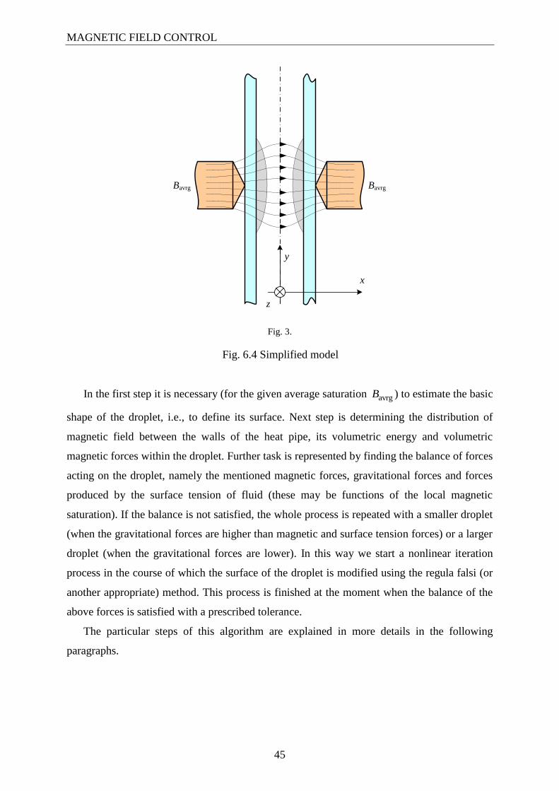
6.2.2 Simplified Model of the Problem
The task will be modeled in the Cartesian coordinates ,x y as a 2D problem, see Fig. 6.4.
Thus, it is considered infinite in the direction of the z -axis. The droplet is considered a static
body, the dynamic phenomena being neglected. This means that its shape is rigid and no fluid
is supposed to flow into it or out of it. In other words, in the course of investigation its curved
surface remains unchanged.
MAGNETIC FIELD CONTROL
45
x
y
z
Bavrg Bavrg
Fig. 3.
Fig. 6.4 Simplified model
In the first step it is necessary (for the given average saturation avrgB ) to estimate the basic
shape of the droplet, i.e., to define its surface. Next step is determining the distribution of
magnetic field between the walls of the heat pipe, its volumetric energy and volumetric
magnetic forces within the droplet. Further task is represented by finding the balance of forces
acting on the droplet, namely the mentioned magnetic forces, gravitational forces and forces
produced by the surface tension of fluid (these may be functions of the local magnetic
saturation). If the balance is not satisfied, the whole process is repeated with a smaller droplet
(when the gravitational forces are higher than magnetic and surface tension forces) or a larger
droplet (when the gravitational forces are lower). In this way we start a nonlinear iteration
process in the course of which the surface of the droplet is modified using the regula falsi (or
another appropriate) method. This process is finished at the moment when the balance of the
above forces is satisfied with a prescribed tolerance.
The particular steps of this algorithm are explained in more details in the following
paragraphs.
MAGNETIC FIELD CONTROL
46
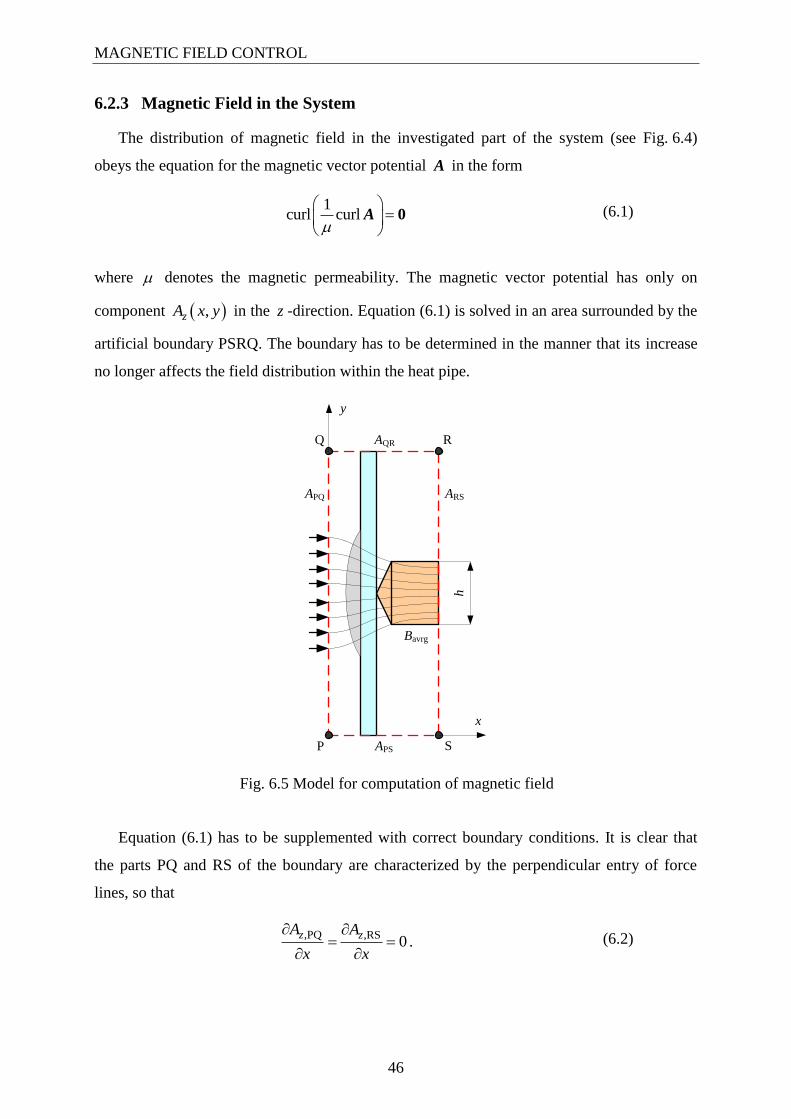
6.2.3 Magnetic Field in the System
The distribution of magnetic field in the investigated part of the system (see Fig. 6.4)
obeys the equation for the magnetic vector potential A in the form
1curl curl
0A (6.1)
where denotes the magnetic permeability. The magnetic vector potential has only on
component ,zA x y in the z -direction. Equation (6.1) is solved in an area surrounded by the
artificial boundary PSRQ. The boundary has to be determined in the manner that its increase
no longer affects the field distribution within the heat pipe.
Bavrg
h
P
RQ
S
ARS
APS
AQR
APQ
x
y
Fig. 6.5 Model for computation of magnetic field
Equation (6.1) has to be supplemented with correct boundary conditions. It is clear that
the parts PQ and RS of the boundary are characterized by the perpendicular entry of force
lines, so that
,PQ ,RS0
z zA A
x x
. (6.2)

MAGNETIC FIELD CONTROL
47
Now we can choose
,PS 0zA , ,QR avrgzA h B . (6.3)
The right condition in (6.3) secures that the average magnetic flux density in the magnetic
core (provided that it is not oversaturated) is really the prescribed value avrgB .
After obtaining the distribution of quantity ,z
A x y we determine the distribution of
magnetic field strength ,H x y following from the formula
2 2, ,1
, z zA x y A x yH x y
x y
(6.4)
and distribution of the volumetric energy m ,w x y of magnetic field
2m
1, ,
2w x y H x y . (6.5)
The volumetric magnetic force m ,x yf acting on a particle of the droplet at point ,x y is
then given as
m m, grad ,x y w x y f , (6.6)
which yields
m , grad gradx x y yx y H H H H f . (6.7)
In order that the magnetic force is high, the field in the droplet should be characterized by
a high gradient. And that high gradient is achieved just by using the tapered magnetic poles.
Further theoretical solving of this coupled problem would be extremely complicated. It is
difficult to find the shape of the free surface of the droplet in the given magnetic field. Even
more, the viscosity and surface tension of fluid may depend on the applied magnetic field.
Due to these facts, the mentioned systems are further ascertained in the experimental way
only.
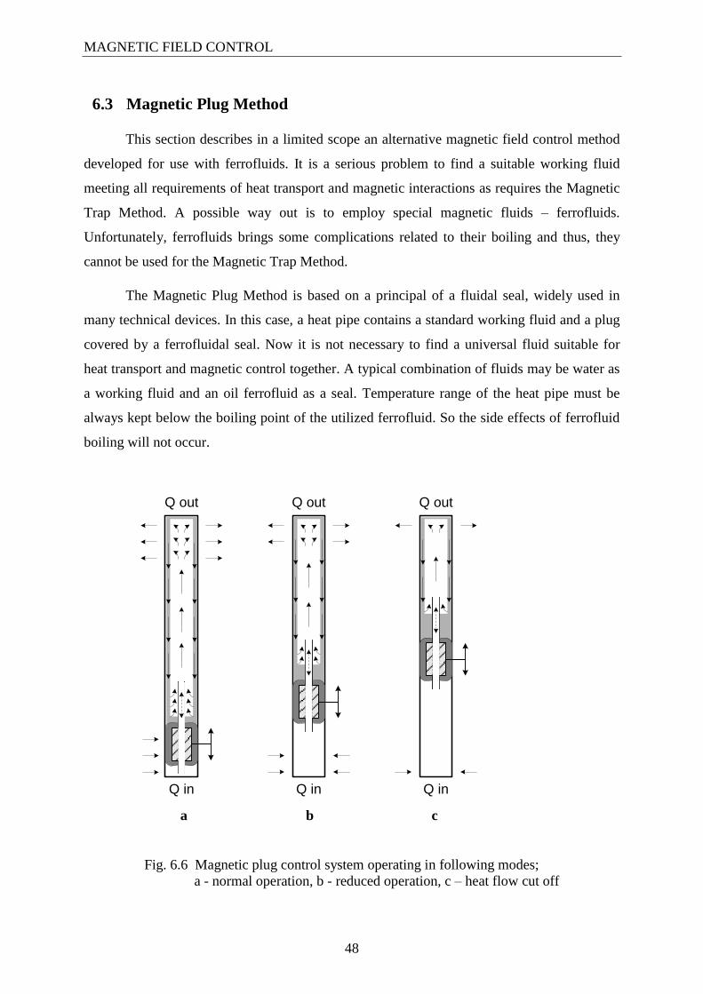
MAGNETIC FIELD CONTROL
48
6.3 Magnetic Plug Method
This section describes in a limited scope an alternative magnetic field control method
developed for use with ferrofluids. It is a serious problem to find a suitable working fluid
meeting all requirements of heat transport and magnetic interactions as requires the Magnetic
Trap Method. A possible way out is to employ special magnetic fluids – ferrofluids.
Unfortunately, ferrofluids brings some complications related to their boiling and thus, they
cannot be used for the Magnetic Trap Method.
The Magnetic Plug Method is based on a principal of a fluidal seal, widely used in
many technical devices. In this case, a heat pipe contains a standard working fluid and a plug
covered by a ferrofluidal seal. Now it is not necessary to find a universal fluid suitable for
heat transport and magnetic control together. A typical combination of fluids may be water as
a working fluid and an oil ferrofluid as a seal. Temperature range of the heat pipe must be
always kept below the boiling point of the utilized ferrofluid. So the side effects of ferrofluid
boiling will not occur.
Q in
Q out
Q in
Q out
Q in
Q out
a b c
Fig. 6.6 Magnetic plug control system operating in following modes;
a - normal operation, b - reduced operation, c – heat flow cut off

MAGNETIC FIELD CONTROL
49
The magnetic plug control system has been also experimentally ascertained by this
work (see more in the section 7.3). A heat pipe arrangement with this control system is
presented in the Fig. 6.6. In the heat pipe, there is a plug open for the vapor stream but closed
for the liquid. By axial positioning of the plug it is possible to control active surface of the
evaporator and regulate the heat flow. In the lowest position (a), the liquid can flow down to
the evaporator and the heat flow is maximal. Pulling up the plug (b, c), the liquid is stopped
above the evaporator and heat flow is more or less reduced. The positioning of the plug may
be simply realized by a magnetic coupling between the permanent magnet inside and a
ferromagnetic object outside the heat pipe.
In the Fig. 6.7 there is a schema of the plug employed in an experimental heat pipe. It
consists of a toroidal permanent magnet(s) covered with a ferrofluid strongly held around by
magnetic field. Thus, a gap between the magnet and container wall is perfectly sealed for the
liquid flow of the working fluid. In the magnet axis there is a channel allowing the vapor
stream to move through. The vapor channel is additionally extended on both sides with a tube
preventing the liquid return.
A-A
Fluid seal
(oil ferrofluid)
Working fluid
(water)
A A
Permanent
magnet
Compensation
channel
Fig. 6.7 Schema of magnetic plug in detail

MAGNETIC FIELD CONTROL
50
6.4 Working Fluids
A suitable fluid with excellent magnetic behaviours is absolutely necessary for all
kinds of magnetic field control. The liquid must allow moving or catching by static magnetic
field, even against gravity or other forces acting in the heat pipe during its operation. The
fluid must also withstand a hard heat pipe internal environment. It must be compatible with
other heat pipe components, long time stable, ecological and health safe.
Unfortunately most of common heat pipe working fluids have poor magnetic
properties, absolutely insufficient for the magnetic field control methods. However, there is
one known exception - oxygen. That is a standard working fluid employed in cryogenic heat
pipes. An alternative might be also some ferrofluid - synthetic liquid compound with strong
magnetic behaviours.
6.4.1 Conventional Working Fluids
There is a large variety of working fluids commonly employed in heat pipes.
Unfortunately, most of them are absolutely unsuitable for magnetic control methods because
of their poor magnetic behaviours, as seen in the Tab. 6.1. The only one exception is oxygen -
standard low temperature working fluid operating from about 60 K to 140 K.
Tab. 6.1 Magnetic susceptibility of selected heat pipe working fluids
Fluid χ (-)
Nitrogen -6,3·10-6
Ammonia -2,6·10-6
Ethanol -7,9·10-6
Water -9,1·10-6
Mercury -29·10-6
Sodium 7,2·10-6
Lithium 14·10-6

MAGNETIC FIELD CONTROL
51
Oxygen has strong magnetic properties, unique among all other natural fluids.
Magnetic properties of oxygen have a strong temperature dependence, as seen in the Tab. 6.2.
The magnetic susceptibility of gaseous oxygen is low but it dramatically grows when
changing into the liquid. Thus, it is suitable for the Magnetic Trap Method and it was also
widely experimentally ascertained during this work.
Tab. 6.2 Magnetic susceptibility of oxygen in dependence on temperature
T (K) χ (-) Phase
10 40·10-6
solid
35 110·10-6
solid
50 300·10-6
liquid
300 2·10-6
gas
Due to the high reactivity of oxygen, it is necessary to keep so called LOX clean. It
means, all components coming into a direct contact with oxygen must be free of any oil,
grease or other organic compounds. Also materials as aluminium, titanium or steel are
incompatible with oxygen. On the other side, copper (Cu), brass (Cu+Sn), bronze (Cu+Zn) or
monel (Ni+Cu) are recommended. The risk grows with higher pressure and is enormous when
the oxygen is in the liquid state (the molecule concentration is maximal). Hence, it is rather
replaced by other permanent gases like nitrogen when possible, however, not suitable for
magnetic field control.
6.4.2 Ferrofluids
Ferrofluids are synthetic colloidal solutions with very interesting behaviours. Their
magnetic susceptibility can reach up to about χ ≈ 10 (several magnitudes higher than that of
oxygen). Ferrofluids can be moved or caught by static magnetic field, even against the gravity
or other forces as seen in the Fig. 6.8. That makes them very interesting for magnetic field
control methods.

MAGNETIC FIELD CONTROL
52
Fig. 6.8 Oil ferrofluid hangs under permanent
magnet
Ferrofluids are made of very fine solid particles (magnetite, maghemite, ferrite etc.;
about 10 nm in diameter) dissolved in a carrier liquid (mineral or silicon oil, kerosene, water
etc.). They behave like very strong paramagnetics (magnetization saturation does not remain
without an external magnetic field) and thus, they are called superparamagnetics.
Unfortunately ferrofluids have some important problems. The particles like to
agglomerate in the liquid. This is prevented by thermal Brown movement, surfactants
additives (long string polymers covering the particles around the particles) or electrostatic
repulsion cause by the same polarity charge. Anyway, their lifetime and stability is lower and
a common ferrofluid is able to work about few years. Furthermore, higher temperatures
(above about 70 °C) and temperature changes deteriorate their function even faster.
There can occur also some other problems in heat pipes. In wicked heat pipes fine
wick pores may be blocked by small particles. Very serious is also boiling of a ferrofluid
which may lead to separation of solid particles in the evaporator. From this point of view
ferrofluids are more suitable for use in gravitational heat pipes using Magnetic Plug System.
In this case the ferrofluid does not boil and utilized as the fluidal seal only. Heat pipes filled
with ferrofluids (see Tab. 6.3) have been also experimentally tested. For more details about
the experiments see the sections 7.2.5 and 7.3.
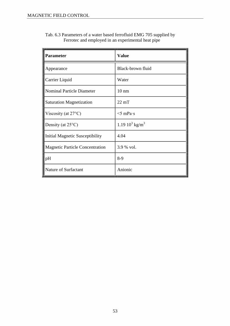
MAGNETIC FIELD CONTROL
53
Tab. 6.3 Parameters of a water based ferrofluid EMG 705 supplied by
Ferrotec and employed in an experimental heat pipe
Parameter Value
Appearance Black-brown fluid
Carrier Liquid Water
Nominal Particle Diameter 10 nm
Saturation Magnetization 22 mT
Viscosity (at 27°C) <5 mPa·s
Density (at 25°C) 1.19 103 kg/m
3
Initial Magnetic Susceptibility 4.04
Magnetic Particle Concentration 3.9 % vol.
pH 8-9
Nature of Surfactant Anionic

MAGNETIC FIELD CONTROL
54
6.5 Magnetic Field Generation
The other essential part of all magnetic control systems is obviously a magnetic field
source. In order to generate a sufficient force interaction with a working fluid, magnetic field
must have relatively high magnetic induction B (approx. 10-1
- 101 T) and its gradient
(approx. 102 A/m). Basically, two types of magnetic field sources may be employed - an
electromagnet or permanent magnets. The both systems have some benefits and negatives,
discussed in the following text in detail. Requirements of the magnetic field source depend on
the type of a used control method (Magnetic Trap / Magnetic Plug) and also on specifics of
the each heat pipe (see the Tab. 6.4). Magnetic field can be also generated by electromagnets
with superconductive coils, however, they are unsuitable for practical applications of the
given systems.
Tab. 6.4 Relation between selected heat pipe parameters and required magnetic field
strengths
Parameter of heat pipe - Value Magnetic field strengths
Outer diameter of container
low low
high high
Magnetic susceptibility
of working fluid
low high
high low
Quantity of working fluid
low low
high high
6.5.1 Electromagnet
Magnetic field generated by an electromagnet allows high magnetic induction and
simple regulation by the current through the coils. It is very useful for laboratory experiments
where the magnetic parameters must be often variably adjusted. Unfortunately, an
electromagnet is usually a very large and heavy device with a high energy consumption. From
this point of view it is not very suitable for practical applications.

MAGNETIC FIELD CONTROL
55
Fig. 6.9 Electromagnet with edge form magnetic poles in longitudinal position
A two coils electromagnet employed in our experiments is presented in the Fig. 6.9.
The electromagnet was provided by columnar poles made from soft carbon steel (60 mm in
diameter), alternatively in the form of an edge (angle 120° and radius 1 mm) or a hollow, as
seen in the Fig. 6.10. The edge poles allow variable position to the heat pipe, from
longitudinal to transversal. Distance between the poles was adjustable from 0 mm to 12 mm.
The magnetic induction in the middle of a 12 mm air-gap achieved up to 1,3 T and was
continuously regulated. The maximal gradient of magnetic induction was about 300 T/m at
the poles edges.
a) b)
Fig. 6.10 Variable magnetic poles in edge (a) and hollow form (b)
There is one more electromagnet system which might be used for the magnetic field
control method. A multisection coil wound up directly on the heat pipe might provide the plug
positioning along the heat pipe. By switching the coil sections one by one in the line it may be
possible to move the plug inside the heat pipe. However, this technique has not been
experimentally ascertained within this work.

MAGNETIC FIELD CONTROL
56
6.5.2 Permanent Magnets
Permanent magnets are now able to challenge with electromagnet systems. New
magnetic materials, based especially on Neodymium-Ferro-Bore compounds (Nd-Fe-B), are
able to generate strong magnetic fields. We have experimentally approved sufficient
behaviours of permanent magnet systems for the magnetic field control methods.
A permanent magnet source is lighter than an electromagnet one does not need the
power feeding. On the other side, regulation is more difficult in this case and must be realized
by the magnets movement, usually realized by a servomotor (or manually during the
laboratory experiments).
A possible arrangement employed for the Magnetic Trap System is schematically
shown in the Fig. 6.11. It consists of two rectangular permanent magnets made from Nd-Fe-B
(dimensions 40 mm x 20 mm x 10 mm and Br = 1,30T Hc = 859 kA/m) and a magnetic
circuit in the U-shape made from a soft carbon steel. Magnetic induction in the middle of the
12 mm air-gap achieved up to 0,6 T, with the maximal gradient about 100 T/m at the magnet
edges.
Fig. 6.11 Magnetic field source in horizontal cross-section and the utilized rectangular
permanent magnet (40mm x 20mm x 10mm)
In the Fig. 6.12 there is an example of the magnetic field source employed in the
Magnetic Plug System. Practically, it may consist of single one or more toroidal permanent
magnets in the line. Outer diameter (OD) of the magnet should be little bit lower than the
inner heat pipe diameter. Hence for a heat pipe with inner diameter (ID) 8 mm, permanent
magnet with OD between 6 and 7 mm is suitable. The length of the magnet should be longer
10mm
N S
Magnetic circuit
Permanent magnets
N S Air gap 2
0m
m

MAGNETIC FIELD CONTROL
57
than its OD to assure the plug stability within the heat pipe. The hole through the magnet must
allow to build in an extension tube preventing the fluid return through the magnet. The tube
should have ID at least 1 mm to allow pressure compensation during the plug positioning or
residual vapour flow.
Fig. 6.12 Permanent magnets suitable for the magnetic plug
EXPERIMENTAL
58
7 Experimental
We have experimentally ascertained the magnetic field influence on heat pipes
operation of various constructions and working fluids. As mentioned in the previous text, we
have worked out two basic approaches to the magnetic field control of heat pipes - Magnetic
Trap Method and Magnetic Plug Method. The both have been implemented into several heat
pipe prototypes and their impact on the operation has been investigated. The experimental
ascertaining is the most important part of this work and it also brings the major contribution to
the improvement of the current state of knowledge.
The major focus of the experimental work was put on ascertaining of the magnetic
field influence on heat pipes operation, however, some related aspects were observed as well.
Heat pipe prototypes of various constructions and working fluids were tested. First
experiments were focused on investigation of a common heat pipe operation and related
processes. This was performed on water and ethanol heat pipes of gravitational type with a
special glass design allowing visual observation. Following experiments were focused
especially on magnetic field effects and required working fluids with strong magnetic
behaviours. Heat pipes filled with oxygen or several types of ferrofluids were tested. Most of
the experiments were performed on gravitational heat pipes, however, several prototypes of
wicked heat pipes were constructed and tested as well.
Before the experiments could be realized we had to do lots of preliminary work. There
were no commercial heat pipes suitable for our aims available on the market. Hence, we had
to design and create our own prototypes. For manufacturing and testing it was also necessary
to adapt or develop some special technologies and procedures and install various experimental
arrangements.
At the beginning of this chapter preliminary setup of experiments, preparation of
tested prototypes and testing arrangements is described. After that, selected experiments with
results are presented, each in a separate section. The experiments are sorted in two groups –
Magnetic Trap Method based and Magnetic Plug Method based.
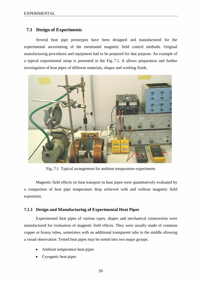
EXPERIMENTAL
59
7.1 Design of Experiments
Several heat pipe prototypes have been designed and manufactured for the
experimental ascertaining of the mentioned magnetic field control methods. Original
manufacturing procedures and equipment had to be prepared for that purpose. An example of
a typical experimental setup is presented in the Fig. 7.1. It allows preparation and further
investigation of heat pipes of different materials, shapes and working fluids.
Fig. 7.1 Typical arrangement for ambient temperature experiments
Magnetic field effects on heat transport in heat pipes were quantitatively evaluated by
a comparison of heat pipe temperature drop achieved with and without magnetic field
exposition.
7.1.1 Design and Manufacturing of Experimental Heat Pipes
Experimental heat pipes of various types, shapes and mechanical construction were
manufactured for evaluation of magnetic field effects. They were usually made of common
copper or brassy tubes, sometimes with an additional transparent tube in the middle allowing
a visual observation. Tested heat pipes may be sorted into two major groups:
Ambient temperature heat pipes
Cryogenic heat pipes

EXPERIMENTAL
60
There is a big difference in construction requirements between these groups.
Cryogenic heat pipes operating at low temperatures were already discussed in the section 4.3
in detail. The most critical factor related to their construction is high pressure (10 MPa or
more) which may occur inside at ambient temperatures. Hence, robustness of the container
must be higher.
On the other hand, construction of ambient temperature heat pipes is quite simple and
allows more flexible arrangement of various components, e.g. combination of copper ends
with a transparent adiabatic part.
7.1.1.1 Ambient Temperature Heat Pipes
A concept of an ambient temperature heat pipe is schematically shown in the Fig. 7.2.
It may consist of a single tube or more tubes coupled by rubber hoses. In the evaporator and
condenser region a material with high thermal conductance is preferred (copper, brass, etc.).
A glass adiabatic section may be integrated for visual observation in between.
1 - Heating wire
2 - Transparent adiabatic part (optional)
3 - Fin radiator
4 - Rubber tubings
5 - Rubber hose with clamp on
Fig. 7.2 Schema of experimental heat pipe for ambient temperature range
4
5
1
2
3
EXPERIMENTAL
61
The evaporator end of heat pipe prototypes was mechanically deformed and
hermetically closed by soldering. The condenser end was usually equipped with a rubber hose
and a clamp allowing repeatable filling, degassing and other procedures. See construction
details in the Fig. 7.3.
Fig. 7.3 The condenser end with a rubber extension and a clamp; fin radiator optionally placed
on the condenser region; the evaporator end
Heat pipes consisting of more parts were coupled by rubber tubings with a silicon
grass for better assembling and tightness. Tightness could be further increased by flexible O-
rings or similar parts put over the tubings.
The heat input was loaded by an isolated copper wire (OD = 0,3 mm) wounded
directly on the heat pipe container. The winding was fixed between rubber outhangs by a
bandage of an adhesive tape. The heat output was realized so that the rest of the heat pipe was
exposed to an external environment. Optionally, fin radiators assisting the heat output might
be fixed on the condenser region.
Fig. 7.4 Evaporator end with a heating wire

EXPERIMENTAL
62
Ambient temperature heat pipes were filled by a specific quantity of a working fluid
from a syringe. The optimal quantity for gravitational heat pipes was about 10 % of its total
volume. Then, the heat pipe was connected to a rotational vacuum pump (Labortechnik
Ilmenau MLW-2DS1) through thick-walled rubber tubes. Internal pressure of the heat pipe
was so decreased to about 2 kPa and continually evacuating for a few minutes by. The
working fluid slowly boiled at lower pressure in the heat pipe and noncondensable gases
contained in the fluid and on the internal container surface were removed out. After finishing
this, the heat pipe was closed by the clamp and it was ready for testing.
Fig. 7.5 Condenser end with fin radiators and clamp closure,
coupled with transparent adiabatic section by rubber tubings and O-rings
7.1.1.2 Cryogenic Heat Pipes
An example of a cryogenic heat pipe with a wick utilized in our experiments is
presented in the Fig. 7.6. In this case, it was made by refilling of a standard wicked heat pipe
for ambient temperatures. Both end of the container were closed by copper plugs
mechanically compressed by hand crimpers and soldered by the Sn-Pb solder. Copper
capillaries passing through the both plugs connected the heat pipe with a filling system and a
manometer.
Experimental gravitational heat pipes were usually made of a standard tube made from
copper or brass which are both compatible with oxygen. Other procedures were identical to
the wicked heat pipe discussed in the previous paragraph. All the components being in contact
with oxygen had to be free of any oil, grease or other organic compounds, as discussed in the
section 6.4.1.

EXPERIMENTAL
63
Fig. 7.6 Cryogenic heat pipe with capillary connections, heat pipe closure in detail
All tested cryogenic heat pipes were filled with pure oxygen from a pressure vessel
(maximal pressure up to about 12 MPa). Heat pipes were connected to the vessel by the filling
capillary with a screw joint. The manometer was coupled to heat pipes by another one
capillary. Before filling heat pipes were flushed through by oxygen for a few seconds to
remove all noncondensable air (the manometer end was open). After that the manometer end
was closed and heat pipes were filled with a desired oxygen quantity, estimated by the filling
pressure. The filling capillary was mechanically deformed and pressed. Then it was cut off
from the pressure vessel and soldered. Finally, heat pipes tightness was tested by the soap
water.

EXPERIMENTAL
64
7.1.2 Testing Arrangement and Accessories
Investigation of heat pipes required a special arrangement consisting of several
components. It was different for ambient temperature heat pipes and cryogenic heat pipes.
Using this arrangement, we were able to simulate heat pipes operation in selected mode and
measure important heat pipe parameters, especially temperature and internal pressure.
A typical arrangement for testing of ambient temperature heat pipes is presented in the
Fig. 7.7. It consisted of the following main parts:
Magnetic field source (see more in the section 6.5)
Two power supplies Mesit MN40V10A (S2) in parallel connection (10 A each)
for feeding the electromagnet (not used with permanent magnets)
A power supply Statron TNG35 (S1) for feeding the heating wire on the heat pipe
evaporator
Axial fan Mezaxial 3112 (optional)
Standard digital multimeters for voltage and DC current measurement
Temperature and pressure measurement (discussed in the following section)
T
A
S1
S2
A
V
p VP
EM
Heat pipe
Heating
Rubber connections
T
T
Manometer
Vacuum
pump
Fig. 7.7 Testing arrangement for ambient temperature heat pipes
EXPERIMENTAL
65
A typical arrangement for testing of cryogenic heat pipes is schematically shown in
the Fig. 7.8. It consisted of the following main parts:
Magnetic field source (see more in the section 6.5)
Two power supplies Mesit MN40V10A (S2) in parallel connection (10 A each)
for feeding the electromagnet (not used with permanent magnets)
Liquid nitrogen reservoir and related accessories
Axial fan Mezaxial 3112 (optional)
Standard digital multimeters for voltage and current measurement
Temperature and pressure measurement devices (discussed in the following
section)
p
Filling capillary
Liquid nitrogene
T = 77 K
Magnetic field
source
Manometer
Capillaries
Thermocouple
Thermocouple
Fig. 7.8 Testing arrangement for cryogenic heat pipes
EXPERIMENTAL
66
7.1.3 Measurement System
The performed experiments were quantitatively evaluated by measurement of selected
heat pipe parameters. Most important was the temperature measurement and additionally also
pressure was monitored within heat pipes. However, the pressure was controlled especially
during filling and degassing procedures. Some aspects were also ascertained by visual
observation in heat pipes with a glass tube in the adiabatic part.
Universal monitoring system Comet MS5 was preferred for the measurement
(Fig. 7.9). However, also single devices with manual data recording were utilized for simple
or short term experiments. The Comet system allowed comfortable monitoring of temperature
in more points along a heat pipe as well as of its internal pressure. It consisted of a
multichannel data logger connected to a PC, five K-type thermocouple inputs (resolution
0,1 °C, accuracy ± 0,3 %) and a voltage input processing a signal from the digital manometer
(resolution 0,01 V, accuracy ± 0,1 %).
Fig. 7.9 Universal measurement system Comet MS5
7.1.3.1 Temperature Monitoring
Temperature along heat pipes was measured by K-type thermocouples placed directly
on the outer container surface. Thermocouples were thermally coupled by silicon grease and
fixed by elastic rubber rings. For low temperature measurement (cryogenic heat pipes) the
thermocouples were calibrated by a Pt thermometer because of their nonlinearity.

EXPERIMENTAL
67
In some cases manual measurement was utilized, especially when temperature was
monitored in two points only. Digital thermometers Greisinger type GTH 1150 and
GTH 1170 (resolution 0,1 °C, accuracy ± 0,05 %) connected to the thermocouples were
employed (Fig. 7.10).
Fig. 7.10 Digital thermometer and manometer Greisinger
7.1.3.2 Pressure Measurement
Pressure within heat pipes was monitored alternatively by the following types of
manometers connected to heat pipes by rubber tubes (ambient temperature heat pipes) or by
copper capillaries (cryogenic heat pipes).
Heat pipes tested in the early experiments were connected to the manual manometer
Prema (range up to 25 MPa, resolution 0,1 MPa , accuracy ± 2,5 %). In the following
experiments digital manometer Greisinger GMH 3151 (Fig. 7.10) was utilized. This
manometer was connected the data logger via digital output. The probe GMSD250BAE for
absolute pressure measurement was utilized (range up to 250 bar resolution 0,1 bar, accuracy
± 0,2 %).
7.1.3.3 Magnetic Field Measurement
Digital gaussmeter Lake Shore, type 410 with a transversal Hall probe was used for all
measurements of magnetic field induction B.

EXPERIMENTAL
68
7.2 Magnetic Trap Method Experiments
The major focus of the experimental work was put on the Magnetic Trap Method. It
was ascertained in several experiments different in the heat pipe construction, magnetic field
source, working fluid or the overall arrangement. Some of the experiments are presented in
the following sections.
7.2.1 Water and Ethanol Heat Pipes Experiment
In the early experiments gravitational heat pipes filled with deionized water or pure
ethanol were tested [12]. The goal was investigation of heat pipes operation principles,
including some start-up or other abnormalities. Manufacturing and adjustment of heat pipes
operation were optimized during this experiment. The magnetic field influence was also
ascertained, but without any expectations in this case, because of weak magnetic properties of
used working fluids. Their magnetic susceptibility is listed below:
Water ....... χ = -9,1·10-6 Ethanol ..... χ = -7,9·10-6
A heat pipe with a special construction allowing visual observation was made for this
purpose. The electromagnet with edge magnetic poles was used as a source of static magnetic
field. The experiment was repeated several times with different setup, selected results of the
measurement are presented in the following text and figures.
Tab. 7.1 Experiment specifications
Parameter Value
Magnetic control method Magnetic Trap
Heat pipe Gravitational
Orientation Vertical
Working fluid Water, ethanol, empty
Operation temperatures Ambient
Container (length x OD/ID) Copper/glass (500 mm x 8/6 mm)
Magnetic field Electromagnet, 0 T / 1,5 T, 300 T/m

EXPERIMENTAL
69
7.2.1.1 Experimental Installation
The overall installation is shown in the Fig. 7.11. The tested gravitational heat pipe
was oriented vertically in the middle between the electromagnet columnar poles in the edge
form. The magnetic induction B in the middle of the electromagnet air-gap was being
adjusted in the range from 0 T to 1,5 T with the gradient up to 300 T/m at the poles edges (for
more details about the electromagnet setup see the section 6.5.1). The heat pipe temperature
was measured by two digital thermometers Greisinger with K-type thermocouples fixed at the
evaporator (T1) and at the condenser (T2). Three power supplies were employed - two in
parallel arrangement feeding the electromagnet and one feeding the evaporator heating. The
pressure inside the heat pipe was adjusted by the rotational vacuum pump connected by a
rubber tube. The condenser was cooled by forced air convection of the axial fan.
Fig. 7.11 Experimental heat pipe with transparent adiabatic section
situated between the electromagnet poles

EXPERIMENTAL
70
The gravitational heat pipe tested in this experiment is schematically shown in the
Fig. 7.12. It consisted of three parts - copper evaporator (1), adiabatic section made of glass
(2) and copper condenser (3). All sections were connected together by rubber tubings (4).
Special construction of the heat pipe allowed visual observation of processes inside and
variability in the heat pipe configuration as well. Total length of the heat pipe was 500 mm,
OD 8 mm and wall thickness 1 mm. The evaporator and the condenser were 80 mm long. The
heating wire (5) was wound directly on the evaporator and the condenser was equipped with
fin radiators. A mechanic valve (6) at the condenser end allowed repeatable filling. The heat
pipe was filled with a small amount of a working fluid - water or ethanol (optimum was 1,0
ml to 1,5 ml).
Fig. 7.12 Schema of the heat pipe
7.2.1.2 Measurement
Due to the absolute beginning of the experimental work lots of parameters important
for the heat pipe operation had to be optimized. Hence, the experiment was repeated many
times until the heat pipe operated appropriately. The processes within the heat pipe were
observed and evaluated also visually.
The evaporator was heated by the power of 10 W and the rest of the heat pipe was
exposed to the forced convection of the room air (23 °C). The magnetic field intensity was
regulated by a current through the electromagnet coils. The temperature was measured in two
5
4
6
1
2
3

EXPERIMENTAL
71
points - at the evaporator and at the condenser - by manual manometers. The heat transport
efficiency was determined from the temperature drop along the heat pipe. The measurement
was repeated for the following configurations:
Water working fluid, without magnetic field exposition
Water working fluid, with static magnetic field of 1,5 T and gradient 300 T/m
Ethanol working fluid, without magnetic field exposition
Ethanol working fluid, with static magnetic field of 1,5 T and gradient 300 T/m
Without any working fluid (empty heat pipe), without magnetic field exposition
7.2.1.3 Results and Discussion
Temperature characteristics of tested heat pipes are presented in the following figures.
In the each figure there are three couples of curves - continuous line for the standard
operation, dash line for the operation with magnetic field and dot line for the empty heat pipe
without any working fluid. The T1 (red lines) represents the evaporator temperature and the T2
(blue lines) represents the condenser temperature.
20
30
40
50
60
70
0 2 4 6 8 10
T ( C
)
t (min)
Water
T1 (B=0T)
T2 (B=0T)
T1 (B=1,5T)
T2 (B=1,5T)
T1 (EMPTY)
T2 (EMPTY)
Fig. 7.13 Heat pipe with water as working fluid

EXPERIMENTAL
72
20
30
40
50
60
70
0 2 4 6 8 10
T ( C
)
t (min)
Ethanol
T1 (B=0T)
T2 (B=0T)
T1 (B=1,5T)
T2 (B=1,5T)
T1 (EMPTY)
T2 (EMPTY)
Fig. 7.14 Heat pipe with ethanol as working fluid
The characteristics are very similar for the both working fluids. It is clearly seen that
the both heat pipes operated correctly with a small temperature drop and high efficiency. The
start-up process, followed by isothermalisation of the whole heat pipe, is well remarkable at
the beginning of curves.
According to our assumptions, performance of the both heat pipes was almost
independent on the magnetic field exposition. The difference between the curves with and
without magnetic field exposition is insignificant, comparable with the measurement error.
The low magnetic field sensitivity of tested heat pipes was caused by weak magnetic
properties of used working fluids. Magnetic field was not able to get over the gravity and
catch the liquid in the magnetic trap.
The operation processes within heat pipes were also visually observed through the
transparent adiabatic part. Intensive boiling effects were observed, mostly during the start-up
phase. The liquid was pushed up high above the evaporator (the higher liquid inventory the
more intensive liquid effects).
About one hour after the start-up a noncondensable gas was detected inside the heat
pipe in the adiabatic part at the condenser region. The vapor-gas boundary was clearly seen
through the glass adiabatic part. The condenser was so closed for the working fluid and heat

EXPERIMENTAL
73
transport which leaded to decreasing of its temperature to the ambient value. Amount of the
noncondensable gas depended on the operation mode (the more intensive operation the faster
gas generation) and also on leakages of the heat pipe (often problematic when utilizing rubber
tubings). The noncondensable gas was being removed from the heat pipe by repeated
evacuation by the vacuum pump.

EXPERIMENTAL
74
7.2.2 O2 Heat Pipe with Electromagnet Experiment
In this experiment [6], possibilities of the Magnetic Trap Method utilizing a
conventional electromagnet have been ascertained. Oxygen was chosen as a working fluid
because of its suitable magnetic properties (find more in the section 6.4.1). Because this was
the first experiment dealing with cryogenic heat pipes, some procedures and adjustments had
to be optimized.
An experimental gravitational heat pipe filled with pure oxygen was made and a
special testing arrangement for the cryogenic temperature range was installed as well. Find
basic parameters and specifications of the experiment in the Tab. 7.2. We have found out that
the heat transport efficiency of the heat pipe was rapidly decreased by the magnetic field
exposition, as presented in the following results.
Tab. 7.2 Experiment specifications
Parameter Value
Magnetic control method Magnetic trap
Heat pipe Gravitational
Orientation Vertical
Working fluid Oxygen
Filling pressure 9 MPa (at 295 K)
Operation temperatures Cryogenic
Container (length x OD/ID) Copper (270 mm x 8/6 mm)
Magnetic field Electromagnet, 0 - 1,25 T, max 300 T/m
EXPERIMENTAL
75
7.2.2.1 Experimental Installation
The experimental installation is shown in the Fig. 7.15. The gravitational heat pipe
was positioned vertically between the electromagnet columnar poles in the edge form. The
upper part of the heat pipe (condenser) was placed in a polystyrene vessel with a liquid
nitrogen (LN2) bath. The middle of the heat pipe was exposed to the static magnetic field with
the magnetic induction B adjusted in steps from 0 T to 1,25 T (in the middle of an air-gap)
and with the gradient up to the 300 T/m at the poles edges (see the section 6.5.1). The heat
pipe temperature was measured in two points (10 mm above the magnetic field zone and
100 mm bellow that) by two digital thermometers Greisinger with K-type thermocouples.
Additionally, the internal pressure of the heat pipe was measured by an analog manometer
Prema connected through a capillary.
Fig. 7.15 Experimental installation of cryogenic heat pipe between electromagnet poles
Arrangement of the tested heat pipe is shown in the Fig. 7.16. The heat pipe was made
of a copper tube (length 270 mm, OD 8 mm, wall thickness 1 mm). The copper capillaries
(OD 2 mm, wall thickness 0,5 mm) on the both ends of the heat pipe provided the connection
with a filling device and the manometer. The filling pressure was 9 MPa at the room
temperature 295 K.
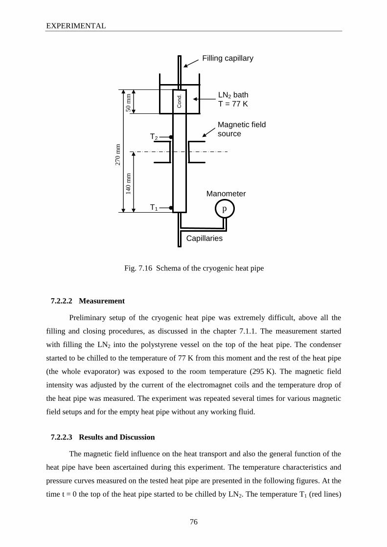
EXPERIMENTAL
76
Fig. 7.16 Schema of the cryogenic heat pipe
7.2.2.2 Measurement
Preliminary setup of the cryogenic heat pipe was extremely difficult, above all the
filling and closing procedures, as discussed in the chapter 7.1.1. The measurement started
with filling the LN2 into the polystyrene vessel on the top of the heat pipe. The condenser
started to be chilled to the temperature of 77 K from this moment and the rest of the heat pipe
(the whole evaporator) was exposed to the room temperature (295 K). The magnetic field
intensity was adjusted by the current of the electromagnet coils and the temperature drop of
the heat pipe was measured. The experiment was repeated several times for various magnetic
field setups and for the empty heat pipe without any working fluid.
7.2.2.3 Results and Discussion
The magnetic field influence on the heat transport and also the general function of the
heat pipe have been ascertained during this experiment. The temperature characteristics and
pressure curves measured on the tested heat pipe are presented in the following figures. At the
time t = 0 the top of the heat pipe started to be chilled by LN2. The temperature T1 (red lines)
p
Filling capillary
LN2 bath T = 77 K
Magnetic field source
Manometer
Capillaries
T1
27
0 m
m
Cond.
50
mm
1
40
mm
T2

EXPERIMENTAL
77
belongs to the lower part of the heat pipe (below the magnetic field zone), the temperature T2
(blue lines) belongs to the upper part (between the magnetic field zone and the LN2 bath), as
illustrated in the Fig. 7.16. The p - curve (black dash lines) represents the pressure inside the
heat pipe, dependent on the phase changes of the oxygen from the gas to the liquid and vice
versa.
0
2
4
6
8
10
100
140
180
220
260
300
0 120 240 360 480p
[M
Pa]
T [
K]
t [s]
T1 [K]
T2 [K]
p (MPa)
Fig. 7.17 Characteristics of standard heat pipe operation
without any magnetic field exposure
Characteristics of the heat pipe without any magnetic field exposure are presented in
the Fig. 7.17. The temperature of the whole heat pipe started to fall immediately after the
condenser cool down. The heat pipe started to operate in about two minutes, when approached
the oxygen operation range. In about four minutes it became almost isothermal along the
whole length with a maximal temperature difference about 5 K.

EXPERIMENTAL
78
0
2
4
6
8
10
100
140
180
220
260
300
0 120 240 360 480
p [M
Pa]
T [
K]
t [s]
T1 [K]
T2 [K]
p (MPa)
B = 1,0 T 0,55T 0,45T 0,35T
Fig. 7.18 Characteristics of heat pipe operating under variable magnetic field
Under the magnetic field exposition, the heat pipe operation was clearly different from
the previous case, as seen in the Fig. 7.18. Initially, the magnetic field induction B was set up
to 1,0 T and the maximal temperature difference was about 56 K. Obviously the heat flow
was restricted by the magnetic field exposition. When decreasing the induction, temperature
difference was slightly decreasing as well but the heat flow was still significantly reduced. A
dramatic change came when the B decreased below 0,4 T - the T1 fell down in a moment and
became equal to the T2. The heat pipe started to operate normally with and insignificant
temperature drop at that moment. Obviously, there is a strong boundary below which the
magnetic field is not able to influence the heat pipe operation any more.
Additionally, the pressure inside the heat pipe was observed during the whole heat
pipe testing. It correlates to the phase changes of oxygen during the cool-down at the
beginning of the experiment. An interruption of decreasing is noticeable on the pressure curve
at the moment of the operation start-up.

EXPERIMENTAL
79
100
140
180
220
260
300
0 120 240 360 480
T [
K]
t [s]
T1 [K]
T2 [K]
Fig. 7.19 Temperature characteristics for empty heat pipe
Thermodynamical behaviors of a heat pipe may be influenced also by thermal
conduction of its container. This is absolutely negligible when the heat pipe operates, but it
becomes relevant when the heat pipe operation is restricted. In such case, even a small
residual heat flow through the container may dramatically affect the temperature characteristic
of a heat pipe.
Hence, the above mentioned cryogenic heat pipe without any working fluid was also
tested. The measured temperature characteristics are shown in the Fig. 7.19. The temperature
difference of the empty heat pipe in the stable state was about 65 K compared to the 56 K
achieved by the magnetic trap. It follows that under the magnetic field exposition heat
transport was provided mostly by thermal conduction of the copper wall with only a small
contribution of the heat pipe working cycle.

EXPERIMENTAL
80
7.2.3 O2 Heat Pipe with Permanent Magnet Source Experiment
In this experiment, the major focus was put on an alternative magnetic field source
based on permanent magnets [8]. Magnetic Trap Method was applied on the gravitational heat
pipe and its performance was investigated. Additionally, an influence of the working fluid
quantity within the heat pipe was ascertained as well.
The experimental setup was very similar to the previous experiment presented in the
section 7.2.2. The main difference was in the utilized magnetic field source. Instead of an
electromagnet, strong permanent magnets were employed now. Additionally, the heat pipe
container was longer and made from brass with lower thermal conductance than that of
copper.
Selected results of the Magnetic Trap Method applied on the gravitational heat pipe
operating with a variable working fluid quantity are presented and discussed in the following
text in detail.
Tab. 7.3 Experiment specifications
Parameter Value
Magnetic control method Magnetic trap
Heat pipe Gravitational
Orientation Vertical
Working fluid Oxygen
Filling pressure 8 / 4,5 / 1,8 MPa (at 297 K)
Operation temperatures Cryogenic
Container (length x OD/ID) Brass (470 mm x 8/6 mm)
Magnetic field Permanent magnets, 0 / 0,6 T, max 100 T/m

EXPERIMENTAL
81
7.2.3.1 Experimental Installation
The experimental installation was very similar to the previous experiment shown in
the Fig. 7.15. But now, the static magnetic field was generated by permanent magnets, already
discussed in the section 6.5.2. Two standard Nd-Fe-B permanent magnets (dimensions in
millimeters – 40 x 20 x 10) were coupled by a magnetic circuit as shown in the Fig. 7.20. The
magnetic induction B achieved about 0,6 T in the middle of an air-gap with the gradient up to
100 T/m at the magnets edges. The magnetic field was regulated by positioning of the
magnets. The temperature and pressure measurement was identical to the previous
experiment, except the thermocouples position - 50 mm above and 200 mm bellow the
magnetic field zone.
Fig. 7.20 Regulation of magnetic field exposition by positioning of permanent magnets;
left – without magnetic field, right – under magnetic field
The tested heat pipe is schematically shown in the Fig. 7.21. It was longer compared to
the previous experiment (length 470 mm, OD 8 mm, wall thickness 1 mm) and with the
container made from brass with lower thermal conductance than those made from copper.
This helped to eliminate residual heat flow through the container wall when the heat pipe
operated under magnetic field exposure. The initial filling pressure was 8 MPa (at 297 K), but
it was slowly decreasing due to some leakages in the container.
N
S
N
S
N
S
N
S

EXPERIMENTAL
82
Fig. 7.21 Schema of the heat pipe
7.2.3.2 Measurement
The heat pipe started to be cooled by LN2 at the time T = 0. The heat pipe was
exposed to the static magnetic field at the beginning and at the end of the experiment, in the
meantime there was no exposure – see the Tab. 7.4.
Tab. 7.4 Definition of experiment periods
Time period Magnetic field exposition
0 - 330 sec B = 0,5 T
330 - 570 sec B = 0 T
570 - 960 sec B = 0,5 T
A series of identical experiments was repeated for three quantities of the liquid oxygen
within the heat pipe (filling pressure resp.):
1,33 cm3 (at 77 K), 8,0 MPa (at room temp.)
0,75 cm3 (at 77 K), 4,5 MPa (at room temp.)
0,30 cm3
(at 77 K), 1,8 MPa (at room temp.)
p
Filling capillary
LN2 bath T = 77 K
Magnetic field source
Manometer
Capillaries
T1
47
0 m
m
Cond.
50
mm
2
40
mm
T2

EXPERIMENTAL
83
The magnetic field intensity varies between two states - maximal value 0,6 T (the heat
pipe situated in the air gap of the magnetic circuit) and minimal value 0 T (the magnetic
circuit moved away). Temperature characteristics of the heat pipe were measured and the
internal pressure was monitored as well. (The pressure curves are not presented in the figures
because of their similarity to the previous experiment).
7.2.3.3 Results and Discussion
The measured characteristics are illustrated in the following three figures, one for the
each working fluid quantity. The temperature T1 (red) belongs to the lower part of the heat
pipe – below the magnetic field zone, T2 (blue) belongs to the upper part – between the
magnetic field zone and the LN2 bath (see Fig. 7.21). The room temperature was 297 K. The
time intervals with and without the magnetic field exposition are marked in the top of the
figures and defined in the Tab. 7.4.
80
120
160
200
240
280
320
0 120 240 360 480 600 720 840 960
T [
K]
t [s]
T1
T2
B = 0,6 T B = 0 T B = 0,6 T
8 MPa
Fig. 7.22 Temperature characteristics of heat pipe with filling pressure 8 MPa

EXPERIMENTAL
84
80
120
160
200
240
280
320
0 120 240 360 480 600 720 840 960
T [
K]
t [s]
T1
T2
B = 0,6 T B = 0 T B = 0,6 T
4,5 MPa
Fig. 7.23 Temperature characteristics of heat pipe with filling pressure 4,5 MPa
80
120
160
200
240
280
320
0 120 240 360 480 600 720 840 960
T [
K]
t [s]
T1
T2
B = 0,6 T B = 0 T B = 0,6 T
1,8 MPa
Fig. 7.24 Temperature characteristics of heat pipe with filling pressure 1,8 MPa

EXPERIMENTAL
85
The performance of heat pipes working with various fluid inventories was very
similar, as seen in the presented figures. The operation was satisfactory in the all cases and the
heat pipe was always isothermal without the magnetic field exposition. However, for the
0,30 cm3
(1,8 MPa) the isothermal temperature without magnetic field exposition was little
bit higher, as seen in the Fig. 7.24. It might be caused by an insufficient fluid inventory
negatively affecting the working cycle in the heat pipe.
The magnetic field influence on the heat transport was significant in the all cases. The
temperature difference under the magnetic field exposition was up to 167 K. Obviously, the
magnetic field of B = 0,6 T was large enough to caught most of working fluid in the magnetic
trap and restrict the heat flow to the lower part of the heat pipe.
Tab. 7.5 Maximal temperature differences for each fluid inventory
Fluid inventory Temperature difference
1,33 cm3 (8,0 MPa ) 165 K
0,75 cm3 (4,5 MPa ) 167 K
0,30 cm3 (1,8 MPa ) 155 K
The efficiency of the magnetic trap was evaluated by a temperature drop at the time
330 sec, as presented in the Tab. 7.5. The highest value was achieved for the filling pressure
0,75 cm3 (4,5 MPa ) – 167 K. For the 1,33 cm3 (8,0 MPa ) it was very similar and the lowest
value was obtained for the 0,30 cm3 (1,8 MPa ). Heat pipe with the lowest fluid inventory had
also a slower dynamic at the magnetic field changes.

EXPERIMENTAL
86
7.2.4 O2 Heat Pipe - Wick Type Experiment
All the experiments presented in the previous sections were based on gravitational heat
pipes. This experiment deals first with wicked heat pipes operating under magnetic field
exposition [1]. Magnetic Trap Method was applied on heat pipes with two different wick
types - sintered and screen. The measurement was realized for variable heat pipe tilting and
for variable working fluid quantity (filling pressure respectively).
Preliminary and testing processes had to be adapted to wicked heat pipes. It was
decided to use oxygen as a working fluid because of its suitable behaviours approved in the
previous experiments. It was practically impossible to find a supplier of an oxygen based heat
pipe. Thus, we decided to modify construction of a standard water heat pipe and refill it with
oxygen. Basic details of the experiment are briefly presented in the Tab. 7.6 and further
discussed in the following text.
Tab. 7.6 Experiment specifications
Parameter Value
Magnetic control method Magnetic trap
Heat pipe Wicked (sintered / screen)
Orientation Variable
Working fluid Oxygen
Filling pressure 8,7 / 12,2 - 12,4 MPa (at 298 K)
Operation temperatures Cryogenic
Container (length x OD/ID) Copper (380 mm x 10/8 mm)
Magnetic field Permanent magnets, 0 / 0,6 T, max 100 T/m

EXPERIMENTAL
87
7.2.4.1 Experimental Installation
The experimental installation is shown in the Fig. 7.25. The heat pipe was fixed in an
arrangement with the tilt angle adjustment. The tilting feature was the main innovation of the
arrangement. One end of the tested heat pipe was chilled by an LN2 and the rest was exposed
to forced air (about 10 m/s perpendicular to the heat pipe) of the room temperature (298 K).
An LN2 reservoir was coupled with the heat pipe by a flexible hose feeding the condenser by
the LN2. The magnetic field source of permanent magnets (B = 0,6 T, grad B = 100 T/m ) was
situated between the points T4 and T5, as seen in the Fig. 7.26. Its regulation was realized by
mechanical positioning similar to the previous experiment shown in the Fig. 7.20. The
temperature measurement was realized by K-type thermocouples fixed in five points along the
heat pipe (see the Fig. 7.26). The pressure was measured by the digital manometer Greisinger
coupled with the heat pipe by a copper capillary. All the measured values were continuously
monitored and recorded by the data logger Comet MS5.
Fig. 7.25 Experimental installation in overview and detail
Two wicked heat pipes were tested in this experiment - sintered heat pipe and screen
heat pipe. They were shape identical (380 mm long, OD 10 mm and wall thickness 1 mm),
different in the wick type only. The both heat pipes were made by a modification of standard
ambient temperature heat pipes with copper container and water as a working fluid. The
container was open at the both ends and emptied. After cleaning it was re-closed by copper

EXPERIMENTAL
88
plugs with copper capillaries for connection with a filling device and a manometer. Finally,
the heat pipes were filled with pure oxygen of a variable quantity:
1,45 cm3 at 77 K, 8,7 MPa at 298 K (sintered heat pipe only)
2,03 cm3 at 77 K, 12,2 MPa at 298 K (sintered heat pipe only)
2,06 cm3 at 77 K, 12,4 MPa at 298 K (screen heat pipe only)
70 70 70 70 50
380
p
T1 T2 T3 T4 T5
B
heat pipe
LN2
resrvoir
condenser
cooling bath
capillary
0°
+30°
-30°
-90°
Heat pipe
LN2
bath
Fig. 7.26 Details of experimental arrangement and heat pipe positioning
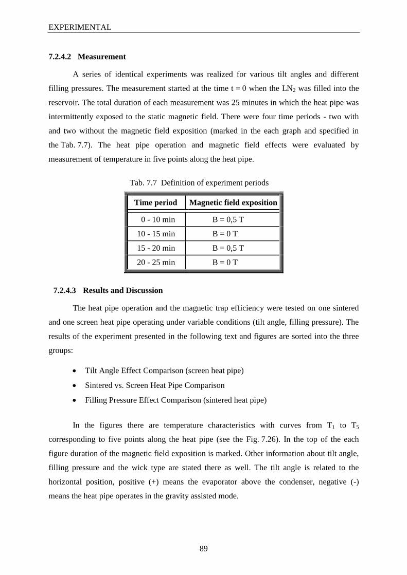
EXPERIMENTAL
89
7.2.4.2 Measurement
A series of identical experiments was realized for various tilt angles and different
filling pressures. The measurement started at the time t = 0 when the LN2 was filled into the
reservoir. The total duration of each measurement was 25 minutes in which the heat pipe was
intermittently exposed to the static magnetic field. There were four time periods - two with
and two without the magnetic field exposition (marked in the each graph and specified in
the Tab. 7.7). The heat pipe operation and magnetic field effects were evaluated by
measurement of temperature in five points along the heat pipe.
Tab. 7.7 Definition of experiment periods
Time period Magnetic field exposition
0 - 10 min B = 0,5 T
10 - 15 min B = 0 T
15 - 20 min B = 0,5 T
20 - 25 min B = 0 T
7.2.4.3 Results and Discussion
The heat pipe operation and the magnetic trap efficiency were tested on one sintered
and one screen heat pipe operating under variable conditions (tilt angle, filling pressure). The
results of the experiment presented in the following text and figures are sorted into the three
groups:
Tilt Angle Effect Comparison (screen heat pipe)
Sintered vs. Screen Heat Pipe Comparison
Filling Pressure Effect Comparison (sintered heat pipe)
In the figures there are temperature characteristics with curves from T1 to T5
corresponding to five points along the heat pipe (see the Fig. 7.26). In the top of the each
figure duration of the magnetic field exposition is marked. Other information about tilt angle,
filling pressure and the wick type are stated there as well. The tilt angle is related to the
horizontal position, positive (+) means the evaporator above the condenser, negative (-)
means the heat pipe operates in the gravity assisted mode.

EXPERIMENTAL
90
Tilt Angle Effect Comparison (screen heat pipe)
Selected temperature characteristics for the screen heat pipe (working fluid quantity
2,06 cm3, 12,4 MPa) operating at various tilt angles and including a comparison with the
empty container are presented in the Fig. 7.27. At the positive tilt angle (+10°) and also in the
horizontal position (0°) the heat pipe has never achieved the isothermal state which is typical
for a standard operation mode. Obviously, the heat pipe could operate only partially in those
positions. The heat pipe operated correctly in the gravity assisted mode only - when tilted
down (-30°). In this position, the magnetic trap effect was significantly observed. Without any
magnetic field exposition the heat pipe was able to achieve the isothermal state. With the
magnetic field exposition the temperature difference ∆ T1, T5 raised up to about 110 K.
Because of the poor heat pipe operation observed in the +10° and 0° positions, the magnetic
trap investigation was limited.
Fig. 7.27 Temperature characteristics of screen heat pipe operating at various tilt angles
and of empty container (heat pipe without any working fluid)

EXPERIMENTAL
91
Sintered vs. Screen Heat Pipe Comparison
The comparison between performance of the sintered heat pipe (2,03 cm3, 12,2 MPa)
and the screen heat pipe (2,06 cm3, 12,4 MPa) operating at tilt angles 0° and -30° is presented
in the Fig. 7.28. The operation without magnetic field in the horizontal position (0°) was very
similar for the both heat pipes. In the gravity assisted mode (-30°), the screen heat pipe
operated significantly better than the sintered one. The screen one was almost isothermal, in
contrast to the temperature difference (∆ T1, T5) at the sintered one - about 95 K. Also the
temperature of the cold end at the screen heat pipe (T4, T5) was higher than that of the sintered
one. We assume that heat flow in the both heat pipes was limited mostly by the wick
capability. From this perspective, the screen wick was significantly better. Hence, also the
magnetic field influence on the heat pipe operation was significantly higher at the screen heat
pipe than at the sintered one.
Fig. 7.28 Comparison of sintered and screen heat pipe characteristics
Filling Pressure Effect Comparison (sintered heat pipe)
The last group of graphs (Fig. 7.29) deals with the fluid inventory effect on the
operation of the sintered heat pipe and Magnetic Trap performance. There are temperature
characteristics for a heat pipe filled with two values of fluid inventory (1,45 cm3, 8,7 MPa in
the left column and 2,03 cm3, 12,2 MPa in the right column) and operation under various tilt
angles (+30°, 0°, -30°, -90°). The effect of the fluid inventory was significantly observed only

EXPERIMENTAL
92
at the gravity assisted modes (-30° and -90°). With more fluid the heat pipe achieved lower
temperature drop compared to the lower fluid inventory.
Fig. 7.29 Comparison of sintered heat pipe characteristics for different filling pressure
EXPERIMENTAL
93
7.2.5 Ferrofluid Heat Pipe Experiment
This experiment deals with a gravitational heat pipe filled with a water based
ferrofluid inside. Its performance under the Magnetic Trap Method was investigated.
Magnetic field was generated by permanent magnets and the heat pipe construction was
similar to the H2O heat pipe, discussed in the section 7.2.1.
Tab. 7.8 Experiment specifications
Parameter Value
Magnetic control method Magnetic trap
Heat pipe Gravitational
Orientation Vertical
Working fluid Water based ferrofluid
Operation temperatures Ambient
Container (length x OD/ID) Copper/glass (500 mm x 8/6 mm)
Magnetic field Permanent magnets, 0 / 0,6 T, max 100 T/m
Magnetic particles contained in ferrofluids might separate from the liquid when it
boils, as already discussed in the section 6.4.2. Thus, the original Magnetic Trap Method had
to be adapted so that the magnetic trap was placed close above the evaporator for this
experiment. This way it was able to catch the ferrofluid droplets streaming up.
7.2.5.1 Experimental Installation
The gravitational heat pipe was tested in a vertical position and magnetic field was
applied on the adiabatic part very close above the evaporator (starting about 2 cm above the
evaporator). Magnetic field was generated by permanent magnets and regulated by the
magnets positioning between two states B = 0 T and B = 0,5 in the middle of the air gap. The
temperature was measured by digital thermometers Greisinger with K-type thermocouples

EXPERIMENTAL
94
fixed in two points - at the copper evaporator (T1) and at the copper condenser (T2). A power
supply Statron was used for feeding a heating wire on the heat pipe evaporator.
Fig. 7.30 Schema of the heat pipe and the arrangement illustration
The gravitational heat pipe tested in this experiment is shown in the Fig. 7.30. It
consisted of three parts - copper evaporator (1), adiabatic section made of glass (2) and copper
condenser (3). The sections were connected by rubber tubings together (4). Total length of the
heat pipe was 350 mm, OD 10 mm and wall thickness 1 mm. The evaporator and the
condenser were 75 mm long each. The heating wire (5) was wound directly on the evaporator
and the condenser was equipped with fin radiators. A mechanic valve (6) at the condenser end
allowed repeatable filling. The heat pipe was filled with a water-based ferrofluid Ferrotec of
amount 2,5 ml.
7.2.5.2 Measurement
The evaporator was heated by the power of 10 W and the rest of the heat pipe was
exposed to the natural convection of the ambient air (23 °C). The total duration of the each
measurement was 25 minutes in which the heat pipe was intermittently exposed to the static
magnetic field. There were four time periods - two with the magnetic field exposition and two
without (marked in the figure and specified in the Tab. 7.9). After 25 minutes the heating was
switched off. The heat pipe operation and magnetic field effects were evaluated by
measurement of temperature in two points along the heat pipe.
MF
Sourc
e
B
5
4
6
1
2
3

EXPERIMENTAL
95
Tab. 7.9 Definition of experiment periods
Time period Magnetic field exposition
0 - 15 min B = 0,5 T
15 - 18 min B = 0 T
18 - 22 min B = 0,5 T
22 - 25 min B = 0 T
7.2.5.3 Results and Discussion
The temperature characteristics of the tested heat pipe are presented in the Fig. 7.31.
The heat pipe started to operate after about 1 minute. Without magnetic field exposition the
heat pipe operated in an almost isothermal mode with the maximum temperature drop
up to 3 °C.
20
30
40
50
60
70
80
0 10 20 30
T [°C
]
t [min]
T1
T2
B = 0 T 0,5T 0,5T0 T B = 0 T
Fig. 7.31 Temperature characteristic of tested heat pipe
under intermittent magnetic field exposition
When the magnetic field was applied on the heat pipe, droplets of the ferrofluid
started to be collected at the magnets. After about one more minute most of the working fluid
was caught in the adiabatic part between the permanent magnets, as seen in the Fig. 7.32.
Insufficiency of the working fluid in the evaporator caused an increase of the temperature
drop up to 20 °C. Dynamic of the control seemed to be slower compared to other
experimental setups.

EXPERIMENTAL
96
Q´ in
Q´ out
MF
So
urc
e
B
Liquid droplet spurt up
by vapor stream
Nonmagnetic
condensate
Magnetic
trap
Ferrofluid
Fig. 7.32 Magnetic trap in schematic illustration and detail of magnetic fluid
caught in trap between permanent magnets

EXPERIMENTAL
97
7.3 Magnetic Plug Method Experiments
The Magnetic Plug Method, discussed in the chapter 6.2, has been developed as an
alternative to the Magnetic Trap Method. It was designed especially for the heat pipes filled
with ferrofluids. It represents an additional part of this work with a limited scope, outlining
the possibilities of this alternative method only. An experimental investigation of the
Magnetic Plug Method was realized and is presented in the following text.
Magnetic plug control is based on reduction of the active surface of the heat pipe
evaporator. Inside the heat pipe is a movable plug consisting of a cylindrical permanent
magnet covered by a ferrofluid around. The ferrofluid works here as a fluidal seal which stops
the condensate flow. Thus, the heat pipe bellow the plug is cut off and the heat flow
efficiency is reduced.
7.3.1 Water + Oil-Ferrofluid Heat pipe Experiment
This experiment was focused on ascertaining of the Magnetic Plug Method applied on
a gravitational heat pipe. Water was used as a working fluid and an oil ferrofluid as a fluidal
seal. In this system, there was no external magnetic field source, only the permanent magnet
of the plug inside the heat pipe.
Tab. 7.10 Experiment specifications
Parameter Value
Magnetic control method Magnetic plug
Heat pipe Gravitational
Orientation Vertical
Fluid Water + Oil ferrofluid
Operation temperatures Ambient
Container (length x OD/ID) Brass (500 mm x 10/8 mm)
Magnetic field Permanent magnet - internal

EXPERIMENTAL
98
7.3.1.1 Experimental Installation
Q in
Q out
T1
T2
T3
T4
Magnetic
coupling
50
0 m
m
x
10
0 m
m1
0 m
m
15
0 m
m5
0 m
m
Heating
Fig. 7.33 Experimental heat pipe with magnetic plug inside
A schema of the tested gravitational heat pipe and its real form are presented in the
Fig. 7.33. Water was used as a working fluid and an oil based ferrofluid formed a liquid seal
around the plug. The heat pipe was positioned vertically during the experiment (evaporator on
the bottom).
The heat pipe was made of a brassy tube 500 mm long, OD 10 mm and wall thickness
1 mm. The bottom end was compressed and soldered, the upper end was equipped with a
rubber extension with a clamp on. A heating wire was wound on the heat pipe in the
evaporator region. The temperature measurement was realized by K-type thermocouples fixed
in four points along the heat pipe. All the measured data were continuously monitored and
recorded by a data logger.

EXPERIMENTAL
99
3 mm
A
Permanent
magnet
Compensation
channel
10
mm
2mm
35
mm
50
mm
A-A
A
Fig. 7.34 Magnetic plug
Magnetic plug placed inside the heat pipe is shown in the Fig. 7.34. It consisted of
4 toroidal permanent magnets in the line and a small copper tube (capillary). The permanent
magnets (each with dimensions: OD = 6 mm, ID = 3,5 mm, length = 2,5 mm) were made
from Nd-Fe-B and achieved magnetic induction of 0,2 T in the hole through with the gradient
max 100 T/m. The copper tube (dimensions: OD = 3 mm, ID = 2 mm, length = 50 mm)
passed through the central hole of the magnets and was tightly glued there.
The plug was inserted into the open heat pipe and the oil ferrofluid of about 0,5 ml
was filled inside. After that, the working fluid of about 1,5 ml was filled in the same way. The
heat pipe was being evacuated by the vacuum pump for 5 minutes (degassing process) and
then closed by the clamp on the rubber extension. The plug inside the heat pipe was
positioned by a common ferrous nut being moved along the heat pipe surface from the
outside.

EXPERIMENTAL
100
7.3.1.2 Measurement
At the time t = 0 the evaporator started to be heated with the power of 5 W, constant
over the whole experiment. The rest of the heat pipe was exposed to the natural convection of
the room air (300 K). The plug was in the lowest position x = 0 at the beginning of the
experiment. Then, the plug was moved up step by step higher according to the Tab. 7.11. The
heat pipe was re-degassed (for about 5 sec) at the time t = 0:05 min and t = 0:50 min. The
temperature characteristics of the heat pipe were measured and recorded.
Tab. 7.11 The plug positioning
Time (h:min) x (mm)
0 : 00 0
0 : 20 50
0 : 55 75
1 : 25 100
1 : 40 150
2 : 05 200
7.3.1.3 Results and Discussion
The temperature characteristic of the tested heat pipe is presented in the Fig. 7.35. The
curves in the figure correspond to the thermocouple points along the heat pipe, as shown in
the Fig. 7.33. The position of the plug “x” is marked in the top of the figure.
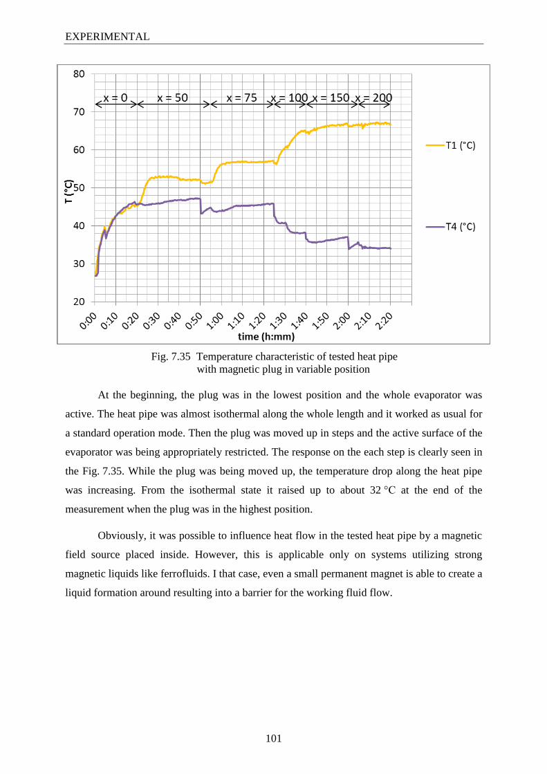
EXPERIMENTAL
101
Fig. 7.35 Temperature characteristic of tested heat pipe
with magnetic plug in variable position
At the beginning, the plug was in the lowest position and the whole evaporator was
active. The heat pipe was almost isothermal along the whole length and it worked as usual for
a standard operation mode. Then the plug was moved up in steps and the active surface of the
evaporator was being appropriately restricted. The response on the each step is clearly seen in
the Fig. 7.35. While the plug was being moved up, the temperature drop along the heat pipe
was increasing. From the isothermal state it raised up to about 32 °C at the end of the
measurement when the plug was in the highest position.
Obviously, it was possible to influence heat flow in the tested heat pipe by a magnetic
field source placed inside. However, this is applicable only on systems utilizing strong
magnetic liquids like ferrofluids. I that case, even a small permanent magnet is able to create a
liquid formation around resulting into a barrier for the working fluid flow.

CONCLUSION AND FURTHER WORK
102
8 Conclusion and Further Work
8.1 Conclusion
This work describes a new approach to the heat transport control in heat pipes based
on magnetic field exposition and it might be an alternative to several conventional methods.
We have worked out two basic magnetic field based control approaches – Magnetic Trap
Method and Magnetic Plug Method. Both are based on an interaction of static magnetic field
with a fluid within a heat pipe, but with different arrangement and construction. Starting at the
page 39 it represents original theories (chapter 6) and results of experimental research
(chapter 7).
Applying the magnetic field control on heat pipe we are getting a very complex system
with many variables related to magnetic field distribution, working fluid properties, heat pipe
construction or its operation mode etc. Mathematic models and calculations are very
complicated and less accurate because of extreme complexity of such systems. Hence, we
decided to investigate this method by experimental ascertaining.
We have experimentally ascertained the magnetic field influence on heat pipes
operation of various constructions and working fluids. The major focus was put on
ascertaining the magnetic field influence on heat pipes operation, however, some related
aspects were observed as well. There were no commercial heat pipes suitable for our aims
available on the market. Hence, we had to design and create our own prototypes and also
adapt or develop some manufacturing technologies, testing arrangements and procedures.
The experimental investigation is the most important part of this work and it also
brings the major contribution to the improvement of the current state of knowledge. We have
observed that it is possible to dramatically reduce the effective thermal conductance of a heat
pipe and regulate the heat flow by this way. At specific conditions it was possible to catch or
move the fluid by magnetic field or make a barrier for the fluid flow. Furthermore, using
special magnetic fluids, so called ferrofluids, it is also possible to create a fluidal seal within
the heat pipe. Additionally, we have successfully approved strong permanent magnets
systems for these aims.
By this work we have experimentally approved that it is possible to significantly affect
heat flow in specially constructed heat pipes by the both investigated approaches - Magnetic
Trap Method and Magnetic Plug Method. The both methods were able to significantly reduce

CONCLUSION AND FURTHER WORK
103
heat flow in selected heat pipes (increase of temperature drop of more than 10 K). The control
effectiveness was affected especially by magnetic properties of working fluids and magnetic
field intensity. Two types of working fluids were successfully approved for the magnetic field
control - oxygen and ferrofluids. Best results were achieved with heat pipes filled with
oxygen and exposed to magnetic field generated by permanent magnets. In that case the
temperature drop increased from almost zero without magnetic field to more than 160 K with
magnetic field.
The magnetic field control might be an alternative to conventional variable
conductance heat pipes based on a noncondensable gas load. In some specific applications it
may bring some desirable benefits like absence of a noncondensable gas (incompatibilities
with other heat pipe components) or possible enhancement of heat exchange in the evaporator
region.
Thesis and results based on this work have been published in several reviewed
journals and presented at several international conferences and journals. Most of them have
been high rated and also often awarded, including The Best Poster Award at the international
conference ISSE 2009, the second place at the international conference POSTER 2009 or the
first place at the CEZ Foundation Award Competition. Some of the prototypes and
arrangements realized during this work were also registered as Utility Models at Czech
Industrial Property Office in Prague and as Functional Models at Czech Technical University
in Prague. They have been also utilized for educational aims at the Faculty of Electrical
Engineering, Czech Technical University in Prague.
Research described in this work has been supported by the research program no. MSM
6840770012 “Transdisciplinary Research in the Area of Biomedical Engineering II” of the
CTU in Prague, sponsored by the Ministry of Education, Youth and Sports of the Czech
Republic. This work was also supported by Student Grant Competition of the Czech
Technical University in Prague no. SGS10/061/OHK3/1T/13 “The Magnetic Field Effect on
Heat Transport” and no. SGS11/055/OHK3/1T/13 “The Magnetic Field Effects on Special
Thermal Systems”.

CONCLUSION AND FURTHER WORK
104
8.2 Further Improvement or Applications
Further research work shall be focused especially on real applications of ascertained
magnetic field control systems. Most of the potential applications are operating at ambient
temperatures and hence this temperature range should be accented. For that purpose it is
necessary to find a working fluid with suitable thermodynamic properties and magnetic
behaviors. Perspective can be also further research of so called ferrofluids, already
investigated and applied during this work. In this case would be necessary to solve their
stability and degradation over longer use in heat pipes. It might be also useful to describe the
mentioned effects theoretically and create a mathematical model for such systems.
REFERENCES
105
References
[1] CINGROŠ, F., KUBA, J.: Investigation and Diagnostic of Magnetic Control of
Cryogenic Heat Pipes, Conference Diagnostika, Kašperské Hory 2011
[2] CINGROŠ, F.: Levitation in Magnetic Fluids, The ČEZ Foundation Competition
about the Best University Research Project, Praha 2011
[3] CINGROŠ, F.: The Magnetic Field Effect on Heat Transport, Conference Workshop
2011, Praha 2011
[4] CINGROŠ, F.: Magnetic Fluids, The ČEZ Foundation Competition about the Best
University Research Project, Praha 2010
[5] CINGROŠ, F.: Magnetic Field Control of Heat Pipes, Conference Elektrotechnologie
2009, Temešvár 2009
[6] CINGROŠ, F., HRON, T., KUBA, J.: Magnetic Field Control of Cryogenic Heat
Pipes, In Proceedings of the International Conference ISSE 2009, Brno 2009
[7] CINGROŠ, F., HRON, T.: Working Fluid Quantity Effect on Magnetic Field Control
of Heat Pipes, International Conference POSTER 2009, Praha 2009
[8] CINGROŠ, F., HRON, T.: Working Fluid Quantity Effect on Magnetic Field Control
of Heat Pipes, Journal Acta Polytechnica, Praha 2009
[9] KUBA, J., CINGROŠ, F., HRON, T.: The Utility Model No. 19045 - Heat Pipe
Controlled by Static Magnetic Field, Czech Industrial Property Office, Praha 2008
[10] CINGROŠ, F., HRON, T.: Electrotechnology Goes to Students, International
Conference POSTER 2008, Praha 2008
[11] KUBA, J., HRON, T., CINGROŠ, F.: Vliv magnetickeho pole na transport tepla, in
proceedings of the International Conference Diagnostika 2007, Plzeň 2007
[12] CINGROŠ, F.: Transport tepla tepelnými trubicemi, the Master‘s Thesis at the Dept.
of Electrotechnology, FEE - CTU in Prague, Praha 2007

REFERENCES
106
[13] CINGROŠ, F., HRON, T., KUBA, J.: Tepelné trubice a ovlivňování transportu tepla
magnetickým polem, the Conference ELEN 2006, Praha 2006
[14] KUBA, J.: Ascertaining of the Effects of Magnetic Curtain, in Proceedings of the
International Conference Diagnostika2005, Plzeň 2005
[15] UENO, S., IWAKI, S., TAZUME, K.: Control of Heat Transport in Heat Pipes by
Magnetic Field. J. Appl. Phys. 69 (8), p. 4925 - 4927, 1991.
[16] Reay, D., A., Kew, P., A.: Heat pipes - Theory and Practice, Elsevier, London 2006
[17] Chi, S., W.: Heat pipe theory and practice: A sourcebook, Hemisphere publishing
corporation, Washington 1976
[18] Silverstein, C., C.: Design and Technology of Heat Pipes for Cooling and Heat
Exchange, CRC Press, 1 edition, 1992
[19] Jeyadevan,B., Koganezawa, H., Nakatsuka, K.: Performance evaluation of citric ion-
stabilized magnetic fluid heat pipe, Journal of Magnetism and Magnetic Materials 289,
p. 253–256, 2005
[20] Sazima, S. a kol.: Sdílení tepla, SNTL, Praha 1993
[21] KUBA, J., CINGROŠ, F., HRON, T.: Heat Pipe Controlled by Static Magnetic Field,
Functional model, CTU in Prague, Prague, 2008
[22] KUBA, J., CINGROŠ, F., HRON, T.: Interactive exposition demonstrating
electromagnetic levitation system and heat transport by heat pipes, Functional model,
CTU in Prague, Prague, 2008
[23] KUBA, J., CINGROŠ, F., HRON, T.: Heat Pipe Controlled by Static Magnetic Field,
Functional model, CTU in Prague, Prague, 2008
[24] KUBA, J., CINGROŠ, F., HRON, T.: Device for Demonstration of Magnetic Curtain
Effect, Functional model, CTU in Prague, Prague, 2009
[25] DOUBEK, J., MUSÁLEK, L., KYNCL, J., JANIŠ, R., KUBA, J.: Behaviour of
Ferrofluidic Liquid in Heat Pipe Affected by External Magnetic Field, In proceedings
of the International Conference ISTET 2013, Pilsen 2013

REFERENCES
107
[26] http://www.thermacore.com
[27] http://www.1-act.com
[28] http://china-heatpipe.net
[29] http://ferrotec.com/

PUBLICATIONS
108
Publications
WoS Publications
CINGROŠ, F., HRON, T., KUBA, J.: Magnetic Field Control of Cryogenic Heat Pipes, In
Proceedings of the International Conference ISSE 2009, Brno 2009
Reviewed Journals Publications
CINGROŠ, F., HRON, T.: Working Fluid Quantity Effect on Magnetic Field Control of Heat
Pipes, Acta Polytechnica, Praha 2009
CINGROŠ, F., KUBA, J.: Investigation and Diagnostic of Magnetic Control of Cryogenic
Heat Pipes, Electroscope, Pilsen 2011
Publications in Proceedings of International Conferences
CINGROŠ, F.: Magnetic Field Control of Heat Pipes, Conference Elektrotechnologie 2009,
Temešvár 2009
CINGROŠ, F., HRON, T.: Working Fluid Quantity Effect on Magnetic Field Control of Heat
Pipes, International Conference POSTER 2009, Praha 2009
CINGROŠ, F., HRON, T.: Electrotechnology Goes to Students, International Conference
POSTER 2008, Praha 2008
KUBA, J., HRON, T., CINGROŠ, F.: Vliv magnetického pole na transport tepla, in
proceedings of the International Conference Diagnostika 2007, Plzeň 2007
Publications in Proceedings of Other Conferences and Symposiums
CINGROŠ, F.: Levitation in Magnetic Fluids, The ČEZ Foundation Competition about the
Best University Research Project, Praha 2011
CINGROŠ, F.: The Magnetic Field Effect on Heat Transport, Conference Workshop 2011,
Praha 2011
CINGROŠ, F.: Magnetic Fluids, The ČEZ Foundation Competition about the Best University
Research Project, Praha 2010
PUBLICATIONS
109
CINGROŠ, F., HRON, T., KUBA, J.: Tepelné trubice a ovlivňování transportu tepla
magnetickým polem, the Conference ELEN 2006, Praha 2006
Intellectual Property Registrations
KUBA, J., CINGROŠ, F., HRON, T.: The Utility Model No. 19045 - Heat Pipe Controlled by
Static Magnetic Field, Czech Industrial Property Office, Praha 2008
Other Publications and Properties
CINGROŠ, F.: Transport tepla tepelnými trubicemi, the Master‘s Thesis at the Dept. of
Electrotechnology, FEE - CTU in Prague, Praha 2007
KUBA, J., CINGROŠ, F., HRON, T.: Heat Pipe Controlled by Static Magnetic Field,
Functional model, CTU in Prague, Prague, 2008
KUBA, J., CINGROŠ, F., HRON, T.: Interactive exposition demonstrating electromagnetic
levitation system and heat transport by heat pipes, Functional model, CTU in Prague, Prague,
2008
The contribution of authors was equal at all the above listed publications.
Copyright © 2022 FDOKUMEN