The Energetics of Ocean Heat Transport
13
The Energetics of Ocean Heat Transport ANAND GNANADESIKAN NOAA/Geophysical Fluid Dynamics Laboratory, Princeton University, Princeton, New Jersey RICHARD D. SLATER AOS Program, Princeton University, Princeton, New Jersey P. S. SWATHI Center for Mathematical Modelling and Computer Simulation, Bangalore, India GEOFFREY K. VALLIS NOAA/Geophysical Fluid Dynamics Laboratory, Princeton University, Princeton, New Jersey (Manuscript received 8 March 2004, in final form 26 January 2005) ABSTRACT A number of recent papers have argued that the mechanical energy budget of the ocean places constraints on how the thermohaline circulation is driven. These papers have been used to argue that climate models, which do not specifically account for the energy of mixing, potentially miss a very important feedback on climate change. This paper reexamines the question of what energetic arguments can teach us about the climate system and concludes that the relationship between energetics and climate is not straightforward. By analyzing the buoyancy transport equation, it is demonstrated that the large-scale transport of heat within the ocean requires an energy source of around 0.2 TW to accomplish vertical transport and around 0.4 TW (resulting from cabbeling) to accomplish horizontal transport. Within two general circulation models, this energy is almost entirely supplied by surface winds. It is also shown that there is no necessary relationship between heat transport and mechanical energy supply. 1. Introduction This paper examines the linkage between mechanical energy supply and thermal energy transport associated with the ocean circulation. The large-scale ocean circu- lation plays an important role in maintaining the earth’s climate. Recent estimates of heat transport show that the oceans export 3.2 petawatts (PW) from the Tropics, as shown by the stars in Fig. 1a (Trenberth and Caron 2001). In the absence of this heat flux, the high latitudes would cool significantly. Indeed, recent work suggests that without this flux of heat, the entire world would freeze over as sea ice spreads equatorward (Winton 2003). In a seminal paper, Munk and Wunsch (1998, here- after MW98) argued that one could use the mechanical energy budget to draw conclusions about what mecha- nisms were responsible for driving this circulation. The abstract of MW98 concludes with the statement, “A surprising conclusion is that the equator-to-pole heat flux of 2000 TW associated with the meridional over- turning circulation would not exist without the com- paratively minute mixing sources. Coupled with the findings that mixing occurs at a few dominant sites, there is a host of questions concerning the maintenance of the present climate state, but also that of paleocli- mates and their relation to detailed continental configu- rations, the history of the Earth–Moon system, and a possible great sensitivity to details of the wind system.” MW98 pose a number of intriguing questions, including whether tidal mixing puts a lower limit on heat trans- port, or whether it is constrained by air–sea fluxes. Wunsch (2002) and Wunsch and Ferrari (2004) extend Corresponding author address: Dr. Anand Gnanadesikan, NOAA/Geophysical Fluid Dynamics Laboratory, Forrestal Cam- pus, U.S. Route 1, P.O. Box 308, Princeton, NJ 08542-0308. E-mail: [email protected] 2604 JOURNAL OF CLIMATE VOLUME 18 JCLI3436
Transcript of The Energetics of Ocean Heat Transport
The Energetics of Ocean Heat Transport
ANAND GNANADESIKAN
NOAA/Geophysical Fluid Dynamics Laboratory, Princeton University, Princeton, New Jersey
RICHARD D. SLATER
AOS Program, Princeton University, Princeton, New Jersey
P. S. SWATHI
Center for Mathematical Modelling and Computer Simulation, Bangalore, India
GEOFFREY K. VALLIS
NOAA/Geophysical Fluid Dynamics Laboratory, Princeton University, Princeton, New Jersey
(Manuscript received 8 March 2004, in final form 26 January 2005)
ABSTRACT
A number of recent papers have argued that the mechanical energy budget of the ocean places constraintson how the thermohaline circulation is driven. These papers have been used to argue that climate models,which do not specifically account for the energy of mixing, potentially miss a very important feedback onclimate change. This paper reexamines the question of what energetic arguments can teach us about theclimate system and concludes that the relationship between energetics and climate is not straightforward.By analyzing the buoyancy transport equation, it is demonstrated that the large-scale transport of heatwithin the ocean requires an energy source of around 0.2 TW to accomplish vertical transport and around0.4 TW (resulting from cabbeling) to accomplish horizontal transport. Within two general circulationmodels, this energy is almost entirely supplied by surface winds. It is also shown that there is no necessaryrelationship between heat transport and mechanical energy supply.
1. Introduction
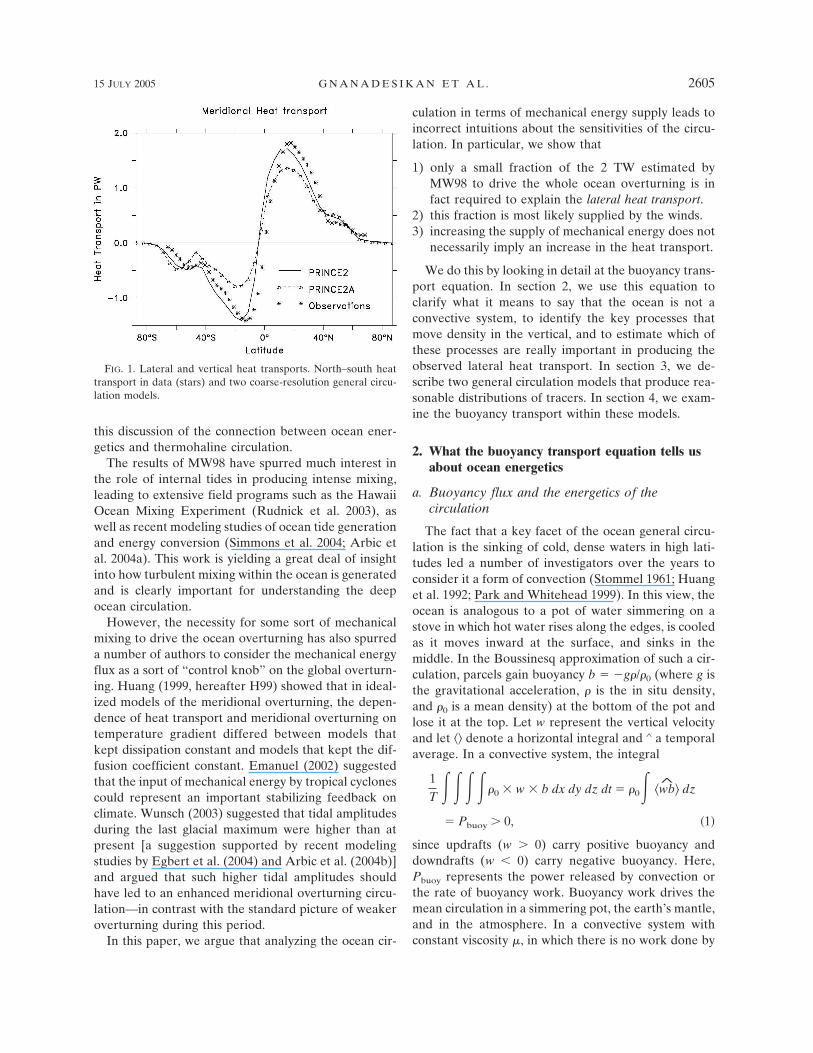
This paper examines the linkage between mechanicalenergy supply and thermal energy transport associatedwith the ocean circulation. The large-scale ocean circu-lation plays an important role in maintaining the earth’sclimate. Recent estimates of heat transport show thatthe oceans export 3.2 petawatts (PW) from the Tropics,as shown by the stars in Fig. 1a (Trenberth and Caron2001). In the absence of this heat flux, the high latitudeswould cool significantly. Indeed, recent work suggeststhat without this flux of heat, the entire world wouldfreeze over as sea ice spreads equatorward (Winton2003).
In a seminal paper, Munk and Wunsch (1998, here-after MW98) argued that one could use the mechanicalenergy budget to draw conclusions about what mecha-nisms were responsible for driving this circulation. Theabstract of MW98 concludes with the statement, “Asurprising conclusion is that the equator-to-pole heatflux of 2000 TW associated with the meridional over-turning circulation would not exist without the com-paratively minute mixing sources. Coupled with thefindings that mixing occurs at a few dominant sites,there is a host of questions concerning the maintenanceof the present climate state, but also that of paleocli-mates and their relation to detailed continental configu-rations, the history of the Earth–Moon system, and apossible great sensitivity to details of the wind system.”MW98 pose a number of intriguing questions, includingwhether tidal mixing puts a lower limit on heat trans-port, or whether it is constrained by air–sea fluxes.Wunsch (2002) and Wunsch and Ferrari (2004) extend
Corresponding author address: Dr. Anand Gnanadesikan,NOAA/Geophysical Fluid Dynamics Laboratory, Forrestal Cam-pus, U.S. Route 1, P.O. Box 308, Princeton, NJ 08542-0308.E-mail: [email protected]
2604 J O U R N A L O F C L I M A T E VOLUME 18
JCLI3436
this discussion of the connection between ocean ener-getics and thermohaline circulation.
The results of MW98 have spurred much interest inthe role of internal tides in producing intense mixing,leading to extensive field programs such as the HawaiiOcean Mixing Experiment (Rudnick et al. 2003), aswell as recent modeling studies of ocean tide generationand energy conversion (Simmons et al. 2004; Arbic etal. 2004a). This work is yielding a great deal of insightinto how turbulent mixing within the ocean is generatedand is clearly important for understanding the deepocean circulation.
However, the necessity for some sort of mechanicalmixing to drive the ocean overturning has also spurreda number of authors to consider the mechanical energyflux as a sort of “control knob” on the global overturn-ing. Huang (1999, hereafter H99) showed that in ideal-ized models of the meridional overturning, the depen-dence of heat transport and meridional overturning ontemperature gradient differed between models thatkept dissipation constant and models that kept the dif-fusion coefficient constant. Emanuel (2002) suggestedthat the input of mechanical energy by tropical cyclonescould represent an important stabilizing feedback onclimate. Wunsch (2003) suggested that tidal amplitudesduring the last glacial maximum were higher than atpresent [a suggestion supported by recent modelingstudies by Egbert et al. (2004) and Arbic et al. (2004b)]and argued that such higher tidal amplitudes shouldhave led to an enhanced meridional overturning circu-lation—in contrast with the standard picture of weakeroverturning during this period.
In this paper, we argue that analyzing the ocean cir-
culation in terms of mechanical energy supply leads toincorrect intuitions about the sensitivities of the circu-lation. In particular, we show that
1) only a small fraction of the 2 TW estimated byMW98 to drive the whole ocean overturning is infact required to explain the lateral heat transport.
2) this fraction is most likely supplied by the winds.3) increasing the supply of mechanical energy does not
necessarily imply an increase in the heat transport.
We do this by looking in detail at the buoyancy trans-port equation. In section 2, we use this equation toclarify what it means to say that the ocean is not aconvective system, to identify the key processes thatmove density in the vertical, and to estimate which ofthese processes are really important in producing theobserved lateral heat transport. In section 3, we de-scribe two general circulation models that produce rea-sonable distributions of tracers. In section 4, we exam-ine the buoyancy transport within these models.
2. What the buoyancy transport equation tells usabout ocean energetics
a. Buoyancy flux and the energetics of thecirculation
The fact that a key facet of the ocean general circu-lation is the sinking of cold, dense waters in high lati-tudes led a number of investigators over the years toconsider it a form of convection (Stommel 1961; Huanget al. 1992; Park and Whitehead 1999). In this view, theocean is analogous to a pot of water simmering on astove in which hot water rises along the edges, is cooledas it moves inward at the surface, and sinks in themiddle. In the Boussinesq approximation of such a cir-culation, parcels gain buoyancy b � �g�/�0 (where g isthe gravitational acceleration, � is the in situ density,and �0 is a mean density) at the bottom of the pot andlose it at the top. Let w represent the vertical velocityand let �� denote a horizontal integral and ∧ a temporalaverage. In a convective system, the integral
1T �����0 � w � b dx dy dz dt � �0� �wb� dz
� Pbuoy � 0, �1�
since updrafts (w 0) carry positive buoyancy anddowndrafts (w 0) carry negative buoyancy. Here,Pbuoy represents the power released by convection orthe rate of buoyancy work. Buoyancy work drives themean circulation in a simmering pot, the earth’s mantle,and in the atmosphere. In a convective system withconstant viscosity �, in which there is no work done by
FIG. 1. Lateral and vertical heat transports. North–south heattransport in data (stars) and two coarse-resolution general circu-lation models.
15 JULY 2005 G N A N A D E S I K A N E T A L . 2605
the boundaries or internal sinks and sources of buoy-ancy,
�0� �wb� dz � �0 � �|��u|2� dz. �2�
This means that an increase in the left side of the equa-tion implies larger dissipation and a faster circulation.The mechanical energy budget of a convective system isthus a useful measure of the circulation.
For many years, however, an argument has ragedabout whether the ocean circulation can in fact bemaintained by surface buoyancy forcing. Sandström(1908) came to a conclusion that is restated in H99 asfollows: “A closed steady circulation can be maintainedin the ocean only if the heating source is situated abovethe cooling source.” As discussed by H99, the applica-bility of this theorem to ocean circulation has been de-bated over many decades. One problem is that Sand-ström’s theorem is derived for a model system that dif-fers in significant ways from the real ocean, ignoringdiffusion, friction, and salinity. Given that Park andWhitehead (1999) present a laboratory model of thethermocline that reproduces many features of modeledoverturning circulations but that violates Sandström’stheorem (heating and cooling being situated at thesame level), it is far from clear that the theorem shouldgive any insight into the real ocean.
In what follows, we point out that the buoyancytransport equation offers a simpler way of thinkingabout the energetics of the large-scale circulation. Webegin by considering the density transport equation
��
�t�
�
�x�u�� �
�
�y���� �
�
�z�w�� � Q�, �3�
where Q� is a source term for density. For our purposes,we will suppose that it includes internal sources due tononlinearities of the equation of state as well as viscousheating and molecular diffusion. All other turbulentfluxes are assumed to be contained in the advectionterms. If we integrate this from the bottom of the oceanto some horizontal surface, the horizontal transportterms drop out and take a temporal average (we areinterested in the steady-state flow), and we obtain
�w�� � �z��D
z0
�Q�^� dz. �4�
Multiplying by �g/�0, we obtain
�wb� ��z��D
z0
� g �Q�^� ��0 dz � �
z��D
z0
�Qb^� dz,
�5�
where Qb includes such terms as geothermal heatingand cabbeling (Huang 2004). In what follows, we willuse both numerical models and data to estimate someof the terms that go into making up both the left- andright-hand sides of this equation.
b. Analyses that assume small interior buoyancysources and sinks
We begin by looking at approximate solutions of thisequation that hold when Qb is taken to be negligible.We note that this assumption is fundamental to previ-ously published results such as MW98 and H99. Then
�wb� 0. �6�
What does this mean? First, it means that the ocean isnot a convective system in the sense that buoyancy workdoes not provide energy to maintain the flow. MW98and H99 also argue that the ocean is not a convectivesystem but do not link it directly to buoyancy transport.If vertical buoyancy transport is zero, then buoyancywork is also zero. While this does not mean that theactual flow is zero (Paparella and Young 2002), it doesimply that there must be compensation between trans-ports associated with different spatial and temporalscales. If the large-scale, time-mean flow brings buoy-ancy upward, some other scales must act to move itdownward. In order for such flows to exist in the pres-ence of dissipation, however, there must be some ex-ternal source of energy to the system. In the laboratoryexperiment of Park and Whitehead (1999), it is the in-ternal energy of the system that is released by molecu-lar diffusion. In the real ocean, the most important ex-ternal source of energy is mechanical work from windsand tides.
This does not mean that buoyancy is unimportant inthe system. Changes in the surface buoyancy distribu-tion resulting from changes in the net freshwater bal-ance can alter the geometry and magnitude of the cir-culation (Bryan 1986; Gnanadesikan 1999; Seidov andHaupt 2003; Saenko et al. 2003; Saenko and Weaver2004). However, as long as the buoyancy flux is notpositive, buoyancy work is not the important source ofenergy for oceanic circulation that it is for atmosphericcirculation.
c. Decomposing the buoyancy transport equation
One can gain more insight into the energetics of thesystem by decomposing the buoyancy transport intofour terms roughly corresponding to the time scalesinvolved in the vertical velocities:
2606 J O U R N A L O F C L I M A T E VOLUME 18
�wb� � �wb� � �webe^� � �wcbc
^� � �wtbt^�
� �z��D
z0
�Qb^� dz
� Mean flow � Mesoscale eddies � Convection
� Small-scale Turbulence
� Buoyancy sinks. �7�
Essentially, the first term is the long-term, large-scalemean; the second is associated with spatial scales of tensof kilometers and temporal scales of days; the third isassociated with spatial scales of tens to hundreds ofmeters and temporal scales of minutes; and the fourth isassociated with spatial scales of centimeters and tem-poral scales of seconds. In the event that Qb � 0 (some-thing that we show is not in fact the case in section 4),any of these terms can be nonzero; only their sum mustvanish. Integrating these terms over the volume of theocean yields the total work associated with each ofthem.
In coarse-resolution general circulation models usedin climate studies (Griffies et al. 2000), these terms areusually represented by separate routines. The first ishandled by the tracer advection routines. The second ishandled by isoneutral diffusion schemes (Gent andMcWilliams 1990; Griffies et al. 1998; Griffies 1998).The third term is dealt with by convective adjustmentand the fourth by parameterizations of small-scale ver-tical diffusion in terms of some mixing coefficient(Bryan and Lewis 1979; Gnanadesikan et al. 2002).
This decomposition can be justified if one thinks ofthe various processes as occupying different locations inwavenumber–frequency space. Insofar as we are look-ing at the long-term mean and globally integrated bud-gets, only those components that have nearly identicalfrequencies and wavenumbers will contribute to a spa-tiotemporal average. This is particularly important in-sofar as we are considering coarse models, which essen-tially assume some separation between advection onscales of the grid and that on scales of the much smallermesoscale eddies. Our decomposition would be muchmore difficult if we were considering models that re-solved the advective flows associated with mesoscaleeddies.
d. Energetic consequences of this decomposition
The argument of MW98 can be recovered from (7)by setting the mesoscale eddy, convective terms, andbuoyancy sink terms to zero. They then assume a cir-culation scheme in which dense water sinks into thedeep ocean, becomes light as a result of downward
buoyancy flux associated with small-scale turbulence,and upwells at a lighter density. Equation (8) then be-comes
Fbuoy � �wb� � � �wtbt^� � K� �N2� � � ����0, �8�
where K� is a turbulent diffusion coefficient, N is thebuoyancy frequency, � 0.2 (Oakey 1982; Polzin et al.1995) is a turbulent efficiency, and � is the turbulentkinetic energy dissipation in W m�3. Given 30 Sv (1 Sv� 106 m3 s�1) of water injected to a depth of 4 km andrising to a depth of 1 km with a density difference of 1kg m�3, it is implied that the buoyancy flux profile Fbuoy
goes from 3 � 105 m4 s�3 at 1 km to 0 at 4 km. Theenergy required to produce such a flux profile (giventhe low efficiency of turbulent mixing) is �0 � Fbuoy �3000 m/2 � 5 � 2.25 TW. This number is so much largerthan the 0.9 TW supplied by the winds working againstthe geostrophic current (Wunsch 1998) that it impliesthat a significant source of mechanical energy is neededto supply �. MW98 use this discrepancy to argue thattides could affect climate. Webb and Suginohara (2001)have criticized this argument on the grounds that muchof the water injected into the deep ocean does not crossisopycnals but is upwelled in other parts of the ocean.We will return to their argument later in this paper.
In the meantime, it is worth asking whether the de-composition of MW98 is the right one for looking at thecirculation that actually accomplishes the transport ofheat within the ocean. In what follows, we argue that adifferent balance is involved, invoking the followingtrain of reasoning:
1) Heat transport must involve the loss of heat in highlatitudes.
2) This heat loss is associated with convection.3) Convection extracts heat from (on average) the
middle of the mixed layer and brings it to the sur-face. This is associated with an upward flux of buoy-ancy.
4) In order for �wb� 0, there must be some compen-sating downward fluxes of buoyancy, either fromturbulence or large-scale advection at other loca-tions or times.
5) These compensating downward fluxes of buoyancyrequire energy.
6) Thus by estimating the upward flux of buoyancy as-sociated with convection, we can estimate the en-ergy required to balance this buoyancy flux and thusto drive the ocean heat transport.
The upward buoyancy flux associated with the con-vective term in (7) can be calculated as follows. By
15 JULY 2005 G N A N A D E S I K A N E T A L . 2607
definition, within a mixed layer the temperature, salin-ity, and buoyancy are well mixed and change coher-ently. Since in one dimension, �b/�t � ��/�z(wb), as-suming that we have a mixed layer is identical to as-suming that the vertical flux divergence is constant in z.Thus within a mixed layer (if one takes an appropriatelocal spatial average—over many individual convectivecells), one can approximate wb as varying linearly be-tween the surface buoyancy flux and zero at the mixedlayer base DML. Then wb � wb|z�0 (z � DML)/DML.The surface buoyancy flux associated with a surfaceheat flux Q is just g�Q/cp, where � � (1/�)��/�T is thecoefficient of thermal expansion and cp is the specificheat. Integrating wb over the mixed layer then gives us(9):
��wb dz �gDML
2cpQ�Qmech, �9�
where Qmech has units of W m�2 and represents a me-chanical energy flux. A standard interpretation ofQmech (see, e.g., Gill and Turner 1976) is that it is theenergy flux required to stir the mixed layer (when Q 0) or released by convection (when Q 0). However,in the context of (7) it represents a nonzero local con-tribution to a global buoyancy budget that must be bal-anced by a buoyancy flux of the opposite sign some-where else within the domain (or potentially at thesame spot, but at a different time). We can thus defineQcon � Qmech (Q 0) as a convective energy demandassociated with the heat transport. The globally inte-grated convective energy demand is then
��Qcon� � ��0��wb� � �webe^� � �wtbt
^�� dz. �10�
We refer to this as an energy demand because it rep-resents a constraint on the energy flux that must be putinto the system to drive the flows on the right-hand sideof (11). These flows move buoyancy downward so thatit can be moved back up again where convection isoccurring.
Similarly, we can define the mixed layer potential en-ergy demand Qmix � �Qmech (Q 0) as the energy fluxneeded to stir heat down into the mixed layer in regionswhere the ocean is gaining heat. Here, Qmix is that partof � �wtbt� dz that is due to wind-driven deepening ofstable mixed layers. Note that when DML is small (say100 m), |Qmech|/|Q| � � 10�5! That is, the mechanicalenergy flux associated with moving heat from point topoint in the ocean is very much smaller than the ther-mal energy flux involved.
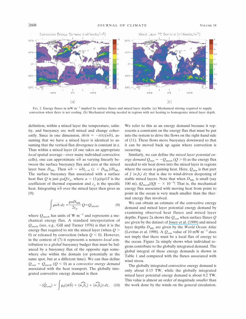
We can obtain an estimate of the convective energydemand and mixed layer potential energy demand byexamining observed heat fluxes and mixed layerdepths. Figure 2a shows the Qcon when surface fluxes Qare given by the dataset of Josey et al. (1999) and mixedlayer depths DML are given by the World Ocean Atlas(Levitus et al. 1998). A Qcon value of 10 mW m�2 doesnot imply that there must be a local flux of energy tothe ocean. Figure 2a simply shows what individual re-gions contribute to the globally integrated demand. Theglobal integral of these energy demands is shown inTable 1 and compared with the fluxes associated withwind stress.
The globally integrated convective energy demand isonly about 0.15 TW, while the globally integratedmixed layer potential energy demand is about 0.2 TW.This value is almost an order of magnitude smaller thanthe work done by the winds on the general circulation.
FIG. 2. Energy fluxes in mW m�2 implied by surface fluxes and mixed layer depths. (a) Mechanical stirring required to supplyconvection when there is net cooling. (b) Mechanical stirring needed in regions with net heating to homogenize mixed layer depth.
2608 J O U R N A L O F C L I M A T E VOLUME 18
Fig 2 live 4/C
In the absence of cabbeling, the convective energy de-mand is a direct estimate of the amount of energyneeded to drive the true circulation. The key point wewould make here is that these numbers do not seem torequire a source of tidal mixing.
The difference between our estimate of 0.15 TW andthe MW98 estimate of 2 TW arises from our focus onthe work associated with the heat transport—which islargely confined to the surface ocean. Recent work byTalley (2003) argues that the deep circulation trans-ports 0.14 PW southward across 30°S, with southwardtransports decreasing as we move northward. This isonly 5% of the tropical heat export. Since MW98 con-sider the buoyancy work only within the deep ocean,they effectively ignore those flows that do most of theheat transport. From (8), the energy flux required todrive the deep circulation Qdeep is
Qdeep � � ��� dz
5 � �0 � �wb�|z�1km � 1500m � A1,
�11�
where A1 is the area of the ocean at a depth of 1 km.The 2 TW associated with the deep circulation comesabout because volume of integration is much largerthan for Qcon and Qmix and because the efficiency � islow. This illustrates why thinking about the ocean cir-culation in terms of energy is not straightforward. Notall energy inputs have equivalent impacts on heat trans-port.
It might be argued that our result is not significantlydifferent from MW98 in that the low mixing efficiency
within the mixed layer demands a large (of order 1 TW)energy flux to satisfy the mixed layer potential energydemand. However, the key point of MW98 is their ar-gument that the mechanical energy be supplied at greatdepths, away from the ocean surface—requiring an in-put of tidal energy. In contrast to the ocean interior,the mixed layer has access to substantial sources ofturbulent kinetic energy. For example, the direct tur-bulent input to waves has been estimated as 100 �u3
*
(Agrawal et al. 1992), where u* � (�/�)1/2 is around0.01 to 0.02 m s�1 for most of the oceans. A roughestimate we made using winds taken from the NationalCenters for Environmental Prediction–National Centerfor Atmospheric Research (NCEP–NCAR) reanaly-sis dataset (Kalnay et al. 1996) showed that this termwas of order 100 TW, much larger than needed tomix the surface ocean. Wang and Huang (2004a,b) es-timate the flux of energy to inertial oscillations at 3 TWand the flux to surface waves at 60 TW. Thus, in con-trast to MW98, our budget thus far does not imply thatthere is “missing mixing” that must be supplied by thetides.
e. Cabbeling and the buoyancy equation
The argument made up to the present point hasone major flaw—namely that it ignores the role of cab-beling. When two water parcels of equal mass aremixed, the resulting water is denser than either one.This means that sources of buoyancy can be asso-ciated with the lateral transport of buoyancy so that ifF x,y
buoy,T,S are the transports of buoyancy, tempera-ture, and salinity in the x and y directions, respectively,then
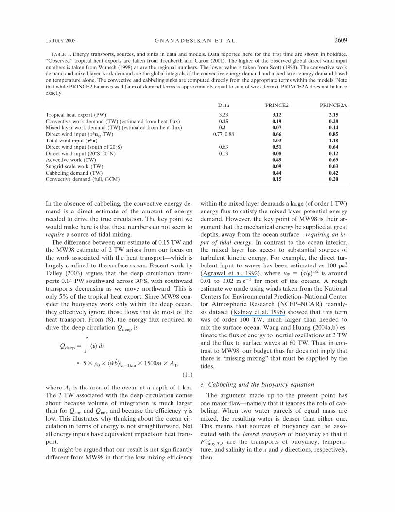
TABLE 1. Energy transports, sources, and sinks in data and models. Data reported here for the first time are shown in boldface.“Observed” tropical heat exports are taken from Trenberth and Caron (2001). The higher of the observed global direct wind inputnumbers is taken from Wunsch (1998) as are the regional numbers. The lower value is taken from Scott (1998). The convective workdemand and mixed layer work demand are the global integrals of the convective energy demand and mixed layer energy demand basedon temperature alone. The convective and cabbeling sinks are computed directly from the appropriate terms within the models. Notethat while PRINCE2 balances well (sum of demand terms is approximately equal to sum of work terms), PRINCE2A does not balanceexactly.
Data PRINCE2 PRINCE2A
Tropical heat export (PW) 3.23 3.12 2.15Convective work demand (TW) (estimated from heat flux) 0.15 0.19 0.28Mixed layer work demand (TW) (estimated from heat flux) 0.2 0.07 0.14Direct wind input (�*ug, TW) 0.77, 0.88 0.66 0.85Total wind input (�*u) 1.03 1.18Direct wind input (south of 20°S) 0.63 0.51 0.64Direct wind input (20°S–20°N) 0.13 0.08 0.12Advective work (TW) 0.49 0.69Subgrid-scale work (TW) 0.09 0.03Cabbeling demand (TW) 0.44 0.42Convective demand (full, GCM) 0.15 0.20
15 JULY 2005 G N A N A D E S I K A N E T A L . 2609
�wb�|z�zr��
�D
zr
� � �
�xFbuoy
x ��
�yFbuoy
y �gQ�^
�0�
� �g�z��D
zr ��
�xFT
x � ��
�xFS
x� �
� ��
�yFT
y � ��
�yFS
y� , �12�
assuming no internal sources of heat and salinity. Inso-far as the horizontal circulation is picking up heat inareas where the temperature is high (and thus � islarge) and losing it in areas where temperature is low(and � is small), the lateral transport of buoyancy canresult in a nonzero buoyancy source. To get a betterestimate of these terms, we now turn to two numericalgeneral circulation models in which all the terms wehave discussed so far can be calculated explicitly.
3. Model description
The models used in this paper are implemented usingthe Geophysical Fluid Dynamics Laboratory (GFDL)Modular Ocean Model, version 3. (Pacanowski andGriffies 1999). The model is run at a nominal resolutionof 4.5° in latitude and 3.75° in longitude with 24 stag-gered vertical levels ranging from 25 m thick at thesurface to 450 m thick at depth. Two implementationsof the model were run.
a. PRINCE2
Model PRINCE2 is built from the KVHISOUTH�AILOW described in Gnanadesikan et al. (2002). Inmodel KVHISOUTH�AILOW, the base topography(adopted from earlier versions of the GFDL coupledclimate model) has a wide Drake Passage. Windstresses are given by the dataset of Hellermann andRosenstein (1983). Surface heat and salt fluxes are de-rived by a combination of applying heat fluxes from thedataset of da Silva et al. (1994) and restoring the surfacetemperature and salinity to the monthly Levitus andBoyer (1994) ocean atlas with a time scale of 30 days.Vertical diffusion is given by the profile of Bryan andLewis (1979), going from 0.15 cm2 s�1 in the surfaceocean to 1.3 cm2 s�1 in the deep ocean with a relativelylarge value (1.0 cm2 s�1) at all depths in the SouthernOcean (Polzin 1999).
Model PRINCE2 makes the following changes toKVHISOUTH�AILOW. First, at four grid pointsaround Antarctica during the winter months, the re-storing salinities are changed so as to ensure that theobserved values of Weddell and Ross Sea bottom wa-
ters are actually found at the surface. Second, the valueof the vertical diffusivity within the pycnocline is in-creased from 0.15 to 0.3 cm2 s�1.
b. PRINCE2A
Model PRINCE2A has the same changes to the sur-face restoring around Antarctica as model PRINCE2,but it does not include the change in vertical diffusivity.Instead, the surface wind stresses are changed from theHellermann wind stress product to the European Cen-tre for Medium-Range Weather Forecasts (ECMWF)analysis (Trenberth et al. 1989), which gives higherwind stresses in the Southern Ocean and lower windstresses in the Tropics. Drake Passage is narrowed byone grid box to make it more realistic. The verticaldiffusivity is increased in the top level of the model toproduce more realistically deep mixed layers. Finally, itwas found that the “flux corrections” computed by re-storing surface salinity and temperature to observationsin many locations were in the opposite direction of theapplied fluxes. This was particularly true in the South-ern Ocean. The (apparently biased) applied fluxes werechanged by adding the restoring correction computedfrom a 400-yr-long run.
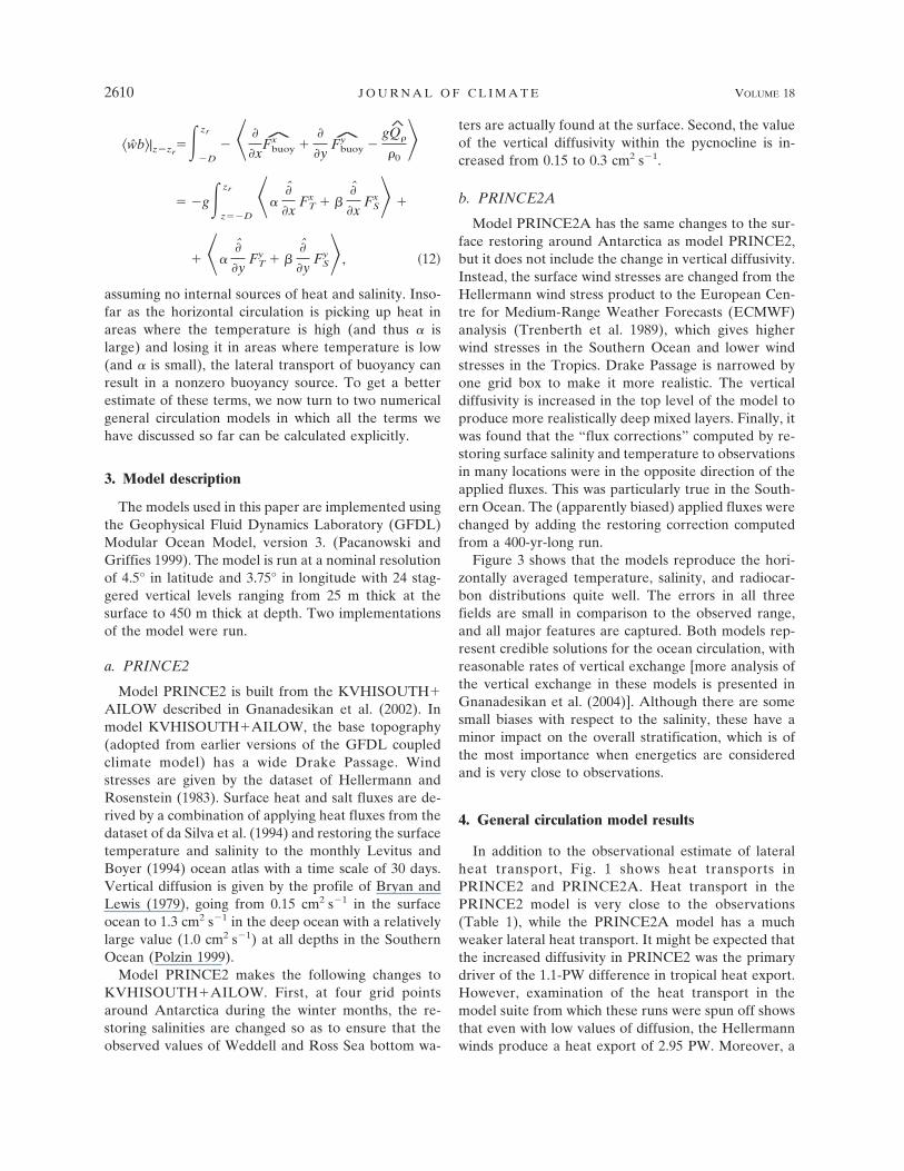
Figure 3 shows that the models reproduce the hori-zontally averaged temperature, salinity, and radiocar-bon distributions quite well. The errors in all threefields are small in comparison to the observed range,and all major features are captured. Both models rep-resent credible solutions for the ocean circulation, withreasonable rates of vertical exchange [more analysis ofthe vertical exchange in these models is presented inGnanadesikan et al. (2004)]. Although there are somesmall biases with respect to the salinity, these have aminor impact on the overall stratification, which is ofthe most importance when energetics are consideredand is very close to observations.
4. General circulation model results
In addition to the observational estimate of lateralheat transport, Fig. 1 shows heat transports inPRINCE2 and PRINCE2A. Heat transport in thePRINCE2 model is very close to the observations(Table 1), while the PRINCE2A model has a muchweaker lateral heat transport. It might be expected thatthe increased diffusivity in PRINCE2 was the primarydriver of the 1.1-PW difference in tropical heat export.However, examination of the heat transport in themodel suite from which these runs were spun off showsthat even with low values of diffusion, the Hellermannwinds produce a heat export of 2.95 PW. Moreover, a
2610 J O U R N A L O F C L I M A T E VOLUME 18
much larger increase in vertical diffusion to 0.6 cm2 s�1
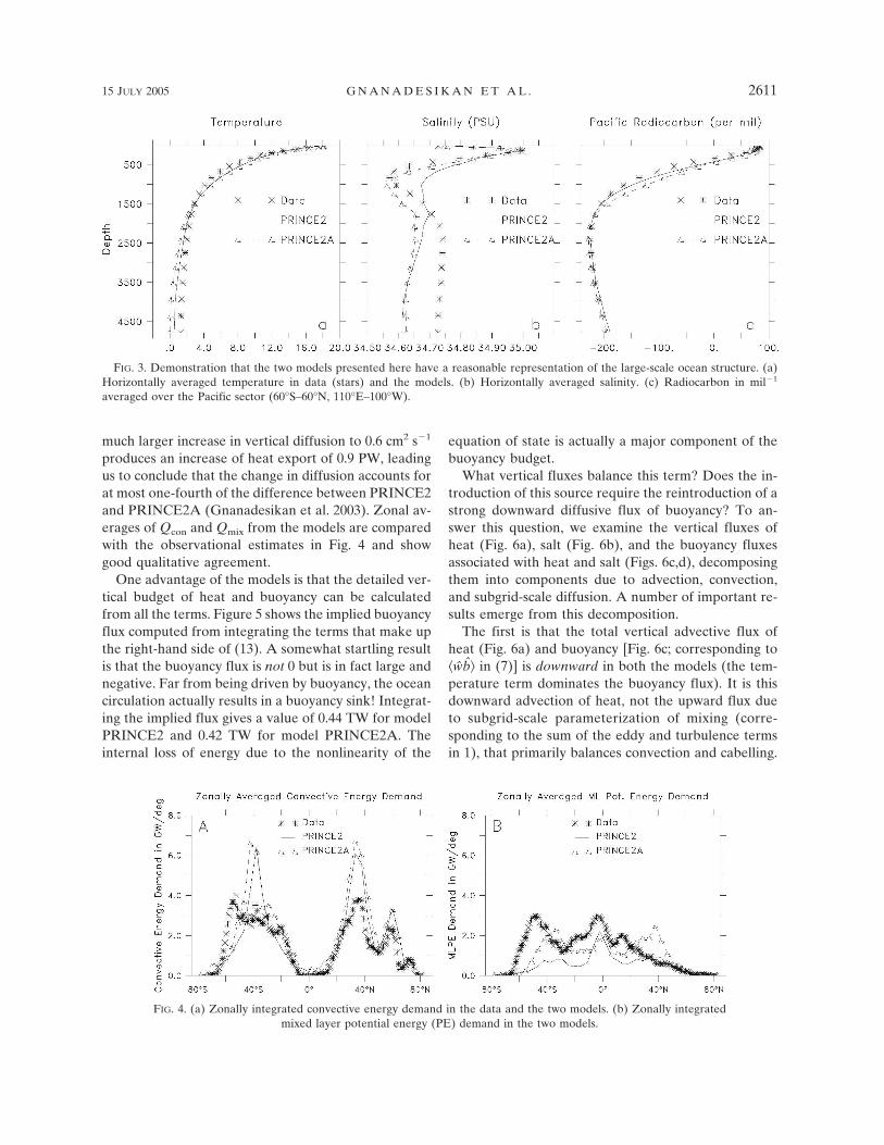
produces an increase of heat export of 0.9 PW, leadingus to conclude that the change in diffusion accounts forat most one-fourth of the difference between PRINCE2and PRINCE2A (Gnanadesikan et al. 2003). Zonal av-erages of Qcon and Qmix from the models are comparedwith the observational estimates in Fig. 4 and showgood qualitative agreement.
One advantage of the models is that the detailed ver-tical budget of heat and buoyancy can be calculatedfrom all the terms. Figure 5 shows the implied buoyancyflux computed from integrating the terms that make upthe right-hand side of (13). A somewhat startling resultis that the buoyancy flux is not 0 but is in fact large andnegative. Far from being driven by buoyancy, the oceancirculation actually results in a buoyancy sink! Integrat-ing the implied flux gives a value of 0.44 TW for modelPRINCE2 and 0.42 TW for model PRINCE2A. Theinternal loss of energy due to the nonlinearity of the
equation of state is actually a major component of thebuoyancy budget.
What vertical fluxes balance this term? Does the in-troduction of this source require the reintroduction of astrong downward diffusive flux of buoyancy? To an-swer this question, we examine the vertical fluxes ofheat (Fig. 6a), salt (Fig. 6b), and the buoyancy fluxesassociated with heat and salt (Figs. 6c,d), decomposingthem into components due to advection, convection,and subgrid-scale diffusion. A number of important re-sults emerge from this decomposition.
The first is that the total vertical advective flux ofheat (Fig. 6a) and buoyancy [Fig. 6c; corresponding to�wb� in (7)] is downward in both the models (the tem-perature term dominates the buoyancy flux). It is thisdownward advection of heat, not the upward flux dueto subgrid-scale parameterization of mixing (corre-sponding to the sum of the eddy and turbulence termsin 1), that primarily balances convection and cabelling.
FIG. 3. Demonstration that the two models presented here have a reasonable representation of the large-scale ocean structure. (a)Horizontally averaged temperature in data (stars) and the models. (b) Horizontally averaged salinity. (c) Radiocarbon in mil�1
averaged over the Pacific sector (60°S–60°N, 110°E–100°W).
FIG. 4. (a) Zonally integrated convective energy demand in the data and the two models. (b) Zonally integratedmixed layer potential energy (PE) demand in the two models.
15 JULY 2005 G N A N A D E S I K A N E T A L . 2611
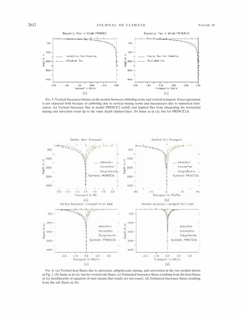
FIG. 6. (a) Vertical heat fluxes due to advection, subgrid-scale mixing, and convection in the two models shownin Fig. 1. (b) Same as in (a), but for vertical salt fluxes. (c) Estimated buoyancy fluxes resulting from the heat fluxesin (a) (nonlinearity of equation of state means that results are not exact). (d) Estimated buoyancy fluxes resultingfrom the salt fluxes in (b).
FIG. 5. Vertical buoyancy balance in the models between cabbeling terms and vertical transport. Exact agreementis not expected both because of cabbeling due to vertical mixing terms and inaccuracies due to numerical trun-cation. (a) Vertical buoyancy flux in model PRINCE2 (solid) and implied flux from integrating the horizontalmixing and advection terms up to the same depth (dashed line). (b) Same as in (a), but for PRINCE2A.
2612 J O U R N A L O F C L I M A T E VOLUME 18
Fig 6 live 4/C
A similar result was noted for heat fluxes in one pre-vious model study (Gregory 2000), but the implicationsfor ocean energetics were not explored.
The fact that the advective heat transport is down-ward (and that as a result, so is the buoyancy transport)has important implications. If the ocean is hydrostaticand velocities vanish on the boundaries (as is the case inthese models), then if p is pressure, the buoyancy workmust be equivalent to the work done by the horizontalpressure gradients on the mean flow:
�� �wb� dz �� �w�p
�z� dz
� �� ��w
�zp� dz
� � ���u
�x�
��
�y� p� dz
� �� � u�p
�x� �
�p
�y� dz. �13�
^
A downward transport of heat and buoyancy impliesthat this must be negative, so that pressure gradientsmust work against the mean flow. Geostrophic flow isby definition along the pressure gradient, and so it doesnot contribute to the pressure work. Frictional flowsdriven by pressure gradients move from high to lowpressure, resulting in positive rather than negative pres-sure work. Only the wind-driven flow in the mixedlayer, which converges water into the subtropical highs,represents a large source of negative pressure work.Ekman pumping is the dominant driver of the buoy-ancy budget in realistic GCMs.
Note that if we integrate over the mixed layer, wherewe assume pressure gradients and Ekman flows are es-sentially constant, we get
��ypx ��f � �xpy ��f � � ���*u�g�, �14�
so that the pressure work is equivalent to the workdone by the winds on the geostrophic current (Wunsch1998). In our models surface winds are not only suffi-ciently energetic to drive the heat transport, they are theonly process that has the correct sign to explain the ad-vective fluxes of heat and buoyancy and to balance con-vection and cabbeling.
A second important result is that the mechanical en-ergy supply is not a good predictor of the lateral heattransport. In fact, the model with the larger verticaltransport of heat (and thus the large convective energydemand) has the smaller lateral transport of heat. Ad-
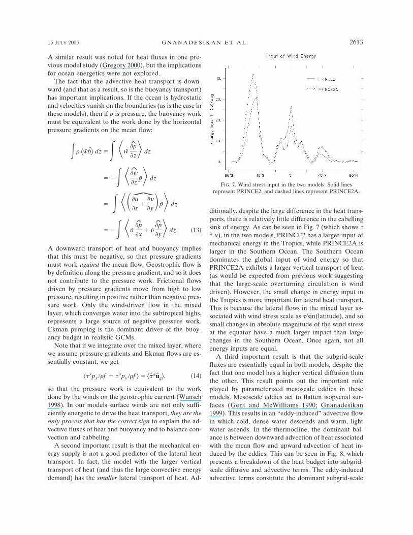
ditionally, despite the large difference in the heat trans-ports, there is relatively little difference in the cabellingsink of energy. As can be seen in Fig. 7 (which shows �* u), in the two models, PRINCE2 has a larger input ofmechanical energy in the Tropics, while PRINCE2A islarger in the Southern Ocean. The Southern Oceandominates the global input of wind energy so thatPRINCE2A exhibits a larger vertical transport of heat(as would be expected from previous work suggestingthat the large-scale overturning circulation is winddriven). However, the small change in energy input inthe Tropics is more important for lateral heat transport.This is because the lateral flows in the mixed layer as-sociated with wind stress scale as �/sin(latitude), and sosmall changes in absolute magnitude of the wind stressat the equator have a much larger impact than largechanges in the Southern Ocean. Once again, not allenergy inputs are equal.
A third important result is that the subgrid-scalefluxes are essentially equal in both models, despite thefact that one model has a higher vertical diffusion thanthe other. This result points out the important roleplayed by parameterized mesoscale eddies in thesemodels. Mesoscale eddies act to flatten isopycnal sur-faces (Gent and McWilliams 1990; Gnanadesikan1999). This results in an “eddy-induced” advective flowin which cold, dense water descends and warm, lightwater ascends. In the thermocline, the dominant bal-ance is between downward advection of heat associatedwith the mean flow and upward advection of heat in-duced by the eddies. This can be seen in Fig. 8, whichpresents a breakdown of the heat budget into subgrid-scale diffusive and advective terms. The eddy-inducedadvective terms constitute the dominant subgrid-scale
FIG. 7. Wind stress input in the two models. Solid linesrepresent PRINCE2, and dashed lines represent PRINCE2A.
15 JULY 2005 G N A N A D E S I K A N E T A L . 2613

mixing terms above 1500 m and essentially compensatethe diffusive fluxes below that depth.
A final important result is that the horizontally av-eraged advective flux of heat and buoyancy is actuallynegative down to 2500 m in the models. The classicpicture of upward advection and downward diffusion ofheat (Munk 1966) holds only over a fraction of theocean and is associated with relatively weak fluxes ofheat. A similar point is made by Gregory (2000), whofinds the classical balance to hold in the tropical ther-mocline, but not globally. The MW98 estimate that 2TW of energy is needed to maintain the deep stratifi-cation against upwelling assumes that a large amount ofwater (30 Sv) upwells through the deep stratification.However, it is not clear that such large fluxes are actu-ally necessary. Webb and Suginohara (2001) make thepoint that the actual buoyancy flux in the deep oceanmay be quite weak, with only 5–6 Sv of deep waterupwelling across isopycnals rather than the 30 Sv ofMW98. Samelson and Vallis (1997) and Vallis (2000)find that an idealized model of ocean circulation cansupport deep stratification as abyssal mixing goes tozero, as the flow across the stratification also goes tozero. Insofar as these pictures actually describe thedeep ocean, tides need not do a lot of work in the deepocean. This implies that winds and eddies, rather thanunresolved tidal processes, play the dominant role inclimate, consistent with the work of investigators suchas Toggweiler and Samuels (1998) and Karsten et al.(2002).
5. Caveats
To keep the argument relatively straightforward, wehave neglected certain aspects of the solution. In thissection, we consider two points that we have neglected.
The first point is the neglect of geothermal heating.How important is this neglect? Estimates of the rate ofgeothermal heating are around 50 mW m�2 (Encyclo-pedia of Energy, s.v. “ocean, energy flows in”) or a heatflux of 18 TW. If we assume this to be injected at4000-m depth (an overestimate as significant amountsof injection occur along ridge crests), the associatedenergy flux is g�/cp � 4000 m � 18TW or 0.036 TW—asignificant number in comparison with the small energyfluxes in the deep ocean but a small contributor to theoverall mechanical energy budget.
A second caveat relates to our use of a linear buoy-ancy flux profile within the mixed layer. In fact, largeeddy simulations (Large et al. 1994) have been used toargue that the buoyancy flux profile actually has theform
wb � wb�z � 0� � �1.2 � z � D��D z � �D
�15a�
wb � �wb�z � 0� � �z � 1.2D��D z � �1.2D,
�15b�
so that the turbulence at the surface entrains lighterwater from below the mixed layer. This reduces theconvective energy demand from 0.5 to 0.42g�QDML/cp.The turbulent kinetic energy generated by convection isable to mix some buoyancy downward, partially satis-fying the convective energy demand.
6. Conclusions
We have presented a decomposition of the verticalbuoyancy equation that casts a new light on the rela-tionship between the mechanical energy supply to theocean and the lateral transport of thermal energy by the
FIG. 8. (a) Decomposition of the subgrid-scale heat flux into the component due to eddy-induced advection(solid) and diffusion (dashed) for model PRINCE2. (b) Same as in (a), but for model PRINCE2A.
2614 J O U R N A L O F C L I M A T E VOLUME 18
ocean. The approximately 3 PW of lateral heat trans-port involves relatively small vertical excursions. As aresult, it requires a very small input of mechanical en-ergy to move buoyancy downward so as to balance con-vection (0.15–0.2 TW) and a surprisingly large input ofmechanical energy to balance cabbeling (0.4 TW). Incomprehensive general circulation models, this energyis efficiently supplied by the winds. This has importantimplications for climate models. Insofar as coupledmodels of climate change capture changes in windstress, they would be expected to capture changes inheat transport as well. The deep circulation, by con-trast, involves very small fluxes of heat that are ineffi-ciently driven by diffusion over large vertical scales.While such circulation may require a significant flux ofenergy (and thus be strongly influenced by tidal mix-ing), it does not directly affect the lateral transport ofheat. Thus, while mechanical energy supply is an inter-esting diagnostic of the ocean circulation, it depends onthe vertical scale of circulation as well as the heat fluxcarried by the circulation. This means that it cannot beused to predict lateral heat transport and its impact onclimate.
It is possible that deep mixing may play a role inclimate, but this role is likely to be indirect. In theSouthern Ocean, upwelling of warmer CircumpolarDeep Waters plays a role in determining sea ice extentand thus surface albedo. The rate of vertical exchangein the Southern Ocean also has important implicationsfor determining atmospheric carbon dioxide (Marinov2005; J. R. Toggweiler, J. L. Russell, and S. R. Carson2005, personal communication). Insofar as deep mixingcan affect the properties of the deep ocean, it may playa role in such climatically important processes—it isimpossible to draw more robust conclusions withoutmore evidence. However, it is clear that the locationand magnitude of the mean wind stress exercises a pri-mary control on the oceanic heat transport, and thus onglobal climate.
Acknowledgments. This work was supported by theCarbon Modeling Consortium, NOAA GrantNA56GP0439 and by the Geophysical Fluid DynamicsLaboratory. We thank A. E. Gnanadesikan, B. Fox-Kemper, R. Hallberg, R. X. Huang, I. Held, R. Scott, H.Simmons, and J. L. Sarmiento for useful discussions.We also thank the editor and three reviewers of thispaper for helping us to clarify our arguments and im-prove our presentation.
REFERENCES
Agrawal, Y. C., E. A. Terray, M. A. Donelan, P. A. Hwang, A. J.Williams, W. M. Drennan, K. K. Kahma, and S. A. Kitaigor-
odskii, 1992: Enhanced dissipation of kinetic energy beneathsurface waves. Nature, 359, 219–220.
Arbic, B. K., S. T. Garner, R. W. Hallberg, and H. L. Simmons,2004a: The uses and accuracy of a forward global tide model:Effects of topographic drag, self-attraction and loading, andstratification. Deep-Sea Res., 51B, 3069–3101.
——, D. MacAyeal, J. X. Mitrovica, and G. A. Milne, 2004b:Ocean tides and Heinrich events. Nature, 432, 460.
Bryan, F., 1986: High latitude salinity effects and interhemisphericthermohaline circulations. Science, 323, 301–304.
Bryan, K., and L. J. Lewis, 1979: A water mass model of the worldocean. J. Geophys. Res., 84, 2503–2517.
da Silva, A. M., A. C. Young, and S. Levitus, 1994: Algorithms andProcedures. Vol. 1, Atlas of Surface Marine Data, NOAAAtlas NESDIS 6, 83 pp.
Egbert, G. D., R. D. Ray, and B. G. Bills, 2004: Numerical mod-eling of the global semidiurnal tide in the present day and inthe last glacial maximum. J. Geophys. Res., 109, C03003,doi:10.1029/2003JC001973.
Emanuel, K., 2002: A simple model of multiple climate regimes. J.Geophys. Res., 107, 4077, doi:10.1029/2001JD001002.
Gent, P., and J. C. McWilliams, 1990: Isopycnal mixing in oceanmodels. J. Phys. Oceanogr., 20, 150–155.
Gill, A. E., and J. S. Turner, 1976: A comparison of seasonal ther-mocline models with observation. Deep-Sea Res., 23, 391–401.
Gnanadesikan, A., 1999: A simple model for the structure of theoceanic pycnocline. Science, 283, 2077–2079.
——, R. D. Slater, N. Gruber, and J. L. Sarmiento, 2002: Oceanicvertical exchange and new production: A comparison be-tween models and observations. Deep-Sea Res., 49B, 363–401.
——, ——, and B. L. Samuels, 2003: Sensitivity of ocean heattransport to subgridscale parameterizations in coarse-resolution ocean models. Geophys. Res. Lett., 30, 1967,doi:10.1029/2003GL018036.
——, J. P. Dunne, R. M. Key, K. Matsumoto, J. L. Sarmiento,R. D. Slater, and P. S. Swathi, 2004: Ocean ventilation andbiogeochemical cycling: Understanding the physical mecha-nisms that give rise to realistic distributions of tracers andproductivity. Global Biogeochem. Cycles, 18, GB4010,doi:10.1029/2003GB002097.
Gregory, J. M., 2000: Vertical heat transports in the ocean andtheir effect on time-dependent climate change. Climate Dyn.,16, 501–515.
Griffies, S. M., 1998: The Gent–McWilliams skew flux. J. Phys.Oceanogr., 28, 831–841.
——, A. Gnanadesikan, R. C. Pacanowski, V. D. Larichev, J. K.Dukowicz, and R. D. Smith, 1998: Isoneutral diffusion in az-coordinate ocean model. J. Phys. Oceanogr., 28, 805–830.
——, and Coauthors, 2000: Developments in ocean climate mod-elling. Ocean Modell., 2, 123–192.
Hellermann, S., and M. Rosenstein, 1983: Normal monthly windstress over the World Ocean with error estimates. J. Phys.Oceanogr., 13, 1093–1107.
Huang, R. X., 1999: Mixing and energetics of the oceanic thermo-haline circulation. J. Phys. Oceanogr., 29, 727–746.
——, 2004: Ocean, energy flows in. Encyclopedia of Energy, C. J.Cleveland, Ed., Vol. 4, Elsevier, 497–509.
——, J. R. Luyten, and H. M. Stommel, 1992: Multiple equilib-rium states in combined thermal and saline circulation. J.Phys. Oceanogr., 22, 231–246.
Josey, S. A., E. C. Kent, and P. K. Taylor, 1999: New insights into
15 JULY 2005 G N A N A D E S I K A N E T A L . 2615

the ocean heat budget closure problem from analysis of theSOC air–sea flux climatology. J. Climate, 12, 2856–2880.
Kalnay, E., and Coauthors, 1996: The NCEP/NCAR 40-Year Re-analysis Project. Bull. Amer. Meteor. Soc., 77, 437–471.
Karsten, R., H. Jones, and J. Marshall, 2002: The role of eddytransfer in setting the stratification and transport of a circum-polar current. J. Phys. Oceanogr., 32, 39–54.
Large, W. G., J. C. McWilliams, and S. C. Doney, 1994: Oceanicvertical mixing: A review and a model with a nonlocal bound-ary layer parameterization. Rev. Geophys., 32, 363–403.
Levitus, S., and T. P. Boyer, 1994: Temperature. Vol. 4, WorldOcean Atlas 1994, NOAA Atlas NESDIS 4, 117 pp.
——, and Coauthors, 1998: Introduction. Vol. 1, World OceanDatabase 1998, NOAA Atlas NESDIS 18, 346 pp.
Marinov, I., 2005: Controls on the air–sea balance of carbon di-oxide. Ph.D. thesis, Princeton University, 224 pp.
Munk, W., 1966: Abyssal recipes. Deep-Sea Res., 13, 707–730.——, and C. Wunsch, 1998: The moon and mixing: Abyssal reci-
pes II. Deep-Sea Res., 45, 1977–2009.Oakey, N. S., 1982: Determination of the dissipation of turbulent
energy from simultaneous temperature and velocity shear mi-crostructure measurements. J. Phys. Oceanogr., 12, 256–271.
Pacanowski, R. C., and S. M. Griffies, 1999: The MOM3 manual.GFDL Ocean Group Tech. Rep. 4, NOAA/GeophysicalFluid Dynamics Laboratory, Princeton, NJ, 680 pp.
Paparella, F., and W. R. Young, 2002: Horizontal convection isnon-turbulent. J. Fluid Mech., 466, 205–214.
Park, Y. G., and J. A. Whitehead, 1999: Rotating convectiondriven by differential bottom heating. J. Phys. Oceanogr., 29,1208–1220.
Polzin, K. L., 1999: A rough recipe for the energy balance ofquasi-steady lee waves. Dynamics of Internal Waves II: Proc.‘Aha Huliko’a Hawaiian Winter Workshop, Honolulu, HI,University of Hawaii at Manoa, 117–128.
——, J. M. Toole, and R. W. Schmitt, 1995: Finescale parameter-izations of turbulent dissipation. J. Phys. Oceanogr., 25, 306–328.
Rudnick, D., and Coauthors, 2003: From tides to mixing along theHawaiian ridge. Science, 301, 355–357.
Saenko, O., and A. J. Weaver, 2004: What drives heat transport inthe Atlantic: Sensitivity to mechanical energy supply andbuoyancy forcing in the Southern Ocean. Geophys. Res. Lett.,31, L20305, doi:10.1029/2004GL020671.
——, ——, and A. Schmittner, 2003: Atlantic deep circulationcontrolled by freshening in the Southern Ocean. Geophys.Res. Lett., 30, 1754, doi:10.1029/2003GL017681.
Samelson, R. M., and G. K. Vallis, 1997: Large-scale circulationwith small diapycnal diffusion: The two-thermocline limit. J.Mar. Res., 55, 223–275.
Sandström, J. W., 1908: Dynamische versuche mit meerwasser.Ann. Hydrogr. Marit. Meteor., 36, 6–23.
Scott, R. B., 1998: Geostrophic energetics and the small viscositybehavior of an idealized ocean circulation model. Ph.D. the-sis, McGill University, 136 pp.
Seidov, D., and B. Haupt, 2003: Freshwater teleconnections andocean thermohaline circulation. Geophys. Res. Lett., 30, 1329,doi:10.1029/2002GL016564.
Simmons, H. L., R. W. Hallberg, and B. K. Arbic, 2004: Internalwave generation in a global barocline tide model. Deep-SeaRes., 51B, 3043–3068.
Stommel, H. M., 1961: Thermohaline convection with 2 stable re-gimes of flow. Tellus, 13, 224–230.
Talley, L. D., 2003: Shallow, intermediate, and deep overturningcomponents of the global heat budget. J. Phys. Oceanogr., 33,530–560.
Toggweiler, J. R., and B. L. Samuels, 1998: On the ocean’s large-scale circulation in the limit of no vertical mixing. J. Phys.Oceanogr., 28, 1832–1852.
Trenberth, K. E., and J. M. Caron, 2001: Estimates of meridionalatmosphere and ocean heat transports. J. Climate, 14, 3433–3443.
——, J. Olson, and W. G. Large, 1989: A global ocean wind stressclimatology based on ECMWF analyses. Tech. Rep. NCAR/TN-388�STR, NCAR, Boulder, CO, 93 pp.
Vallis, G. K., 2000: Large-scale circulation and production ofstratification: Effects of wind, geometry, and diffusion. J.Phys. Oceanogr., 30, 933–954.
Wang, W., and R. X. Huang, 2004a: Wind energy input to theEkman layer. J. Phys. Oceanogr., 34, 1267–1275.
——, and ——, 2004b: Wind energy input to surface waves. J.Phys. Oceanogr., 34, 1276–1280.
Webb, D. J., and N. Suginohara, 2001: The interior circulation ofthe ocean. Ocean Circulation and Climate, G. Siedler, J.Church, and J. Gould, Eds., Academic Press, 205–214.
Winton, M., 2003: On the climatic impact of ocean circulation. J.Climate, 16, 2875–2889.
Wunsch, C., 1998: The work done by wind on the oceanic generalcirculation. J. Phys. Oceanogr., 28, 1425–1430.
——, 2002: What is the thermohaline circulation? Science, 298,1180–1181.
——, 2003: Determining paleoceanographic circulations, with em-phasis on the Last Glacial Maximum. Quat. Sci. Rev., 22,371–385.
——, and R. E. Ferrari, 2004: Energetics and the ocean circula-tion. Annu. Rev. Fluid Mech., 36, doi:10.1146/annurev.fluid.36.050802.122121.
2616 J O U R N A L O F C L I M A T E VOLUME 18