Electrohydrodynamic spraying - Transport, mass and heat ...

ETH Library

Electrohydrodynamic spraying -Transport, mass and heat transferof charged droplets and theirapplication to the deposition of thinfunctional films

Doctoral Thesis

Author(s):Wilhelm, Oliver

Publication date:2004

Permanent link:https://doi.org/10.3929/ethz-a-004718257

Rights / license:In Copyright - Non-Commercial Use Permitted

This page was generated automatically upon download from the ETH Zurich Research Collection.For more information, please consult the Terms of use.

https://doi.org/10.3929/ethz-a-004718257

http://rightsstatements.org/page/InC-NC/1.0/

https://www.research-collection.ethz.ch

https://www.research-collection.ethz.ch/terms-of-use

I

Electrohydrodynamic spraying –

Transport, mass and heat transfer of charged droplets and

their application to the deposition of thin functional films

A dissertation submitted to the

SWISS FEDERAL INSTITUTE OF TECHNOLOGY ZURICH

for the degree of

DOCTOR OF SCIENCES

presented by

OLIVER WILHELM

Dipl. Phys. University of Tübingen

born on September 6th, 1969 in Esslingen, Germany

Accepted on the recommendation of

Prof. Dr. S.E. Pratsinis, examiner Prof. Dr. L.J. Gauckler, co-examiner

PD Dr.-Ing. habil. L. Mädler, co-examiner

Zurich 2004

Diss. ETH No. 15406

III

Acknowledgments

I would like to express my gratitude to Prof. Sotiris E. Pratsinis who supervised

my Ph.D. thesis. He was a continuous source of motivation, encouragement, advice and

enthusiasm. Many thanks also to my co-examiner Prof. Ludwig J. Gauckler for his

interest in my work and the stimulating discussions.

This thesis evolved in close collaboration with Dr. Dainius Perednis and Dr.

Lutz Mädler. I would like to thank both of them for many hours of hard laboratory work

and intense scientific discussions.

But this work would have not been possible without the contribution of the

whole Particle Technology group and the support of the Institute of Process

Engineering. I enjoyed and profited very much from an exceptional working

atmosphere. Thanks a lot to Roger Müller, Susanne Veith and Karsten Wegner, my

long-time companions in the office, further our secretaries Patricia Horn and Illeana

Eugster who have been always a source of understanding in “human problems” and a

source of help in administrative one’s. Many thanks also to the workshop. They helped

a lot with their creativity to find exceptional solutions when I got stuck with a

mechanical problem.

Finally I would like to thank my parents, my family and the wonderful Nanette

Bauer who were a source of continuous support when times became hard and were

always there when I needed them most.

The financial support by the Commision for Technology and Innovation (KTI,

Project No. 4810 and 5487), and the Swiss National Science Foundation (SNF, No.

2160 – 064546.01) is kindly acknowledged.

V

Table of Contents

Acknowledgments III

Table of Contents V

Zusammenfassung VII

Summary XI

1 Electrospraying and its applications 1

1.1 Introduction 1

1.2 Droplet production and charging 3

1.2.1 Atomization techniques 3

1.2.2 Conejet mode 8

1.2.3 Intermittent multijet mode 14

1.3 Electrospray applications 15

1.3.1 Electrospray deposition (ESD) 15

1.3.2 Electrospray ionization 19

1.3.3 Other applications 20

1.4 Summary 21

1.5 References 22

2 Electrospray deposition and evaporation 29

2.1 Introduction 29

2.2 Theory 31

2.2.1 Droplet transport 31

2.2.2 Droplet evaporation 33

2.3 Results 36

2.3.1 Droplet transport 36

2.3.1.1 Validation 36

2.3.1.2 Segregation 39

2.3.2 Droplet transport and evaporation 40

2.4 Summary 47

VI

2.5 References 47

Appendix 1: Background vapor concentration 55

Appendix 2: Estimation of air velocity 57

3 Conejet and multijet electrosprays: transport and evaporation 59

3.1 Introduction 59

3.2 Experiment 61

3.3 Model 63

3.4 Results and discussion 66

3.4.1 Conejet electrospray 66

3.4.2 Multijet electrospray 73

3.5 Summary 78

3.6 References 79

4 Deposition of thin YSZ films by spray pyrolysis 83

4.1 Introduction 83

4.2 Experimental setup 85

4.3 Results 87

4.3.1 SEM/EDX analysis of the deposited film 87

4.3.2 PDA measurements 91

4.3.3 Deposition diagram 94

4.4 Discussion 97

4.5 Conclusion 98

4.6 References 99

5 Research recommendations 101

Appendix 103

A1 Electrical performance of granulated titania nanoparticles 103

A1.1 Introduction 103

A1.2 Experimental procedure 105

A1.3 Results 107

VII

A1.4 Conclusions 111

A1.5 References 111

A2 Dimensionless transport and evaporation equation 113

A2.1 Derivation of the dimensionless version of the transport equation 113

A2.2 Derivation of the dimensionless version of the mass transfer

equation

115

A2.1 Derivation of the dimensionless version of the energy equation 116

A3 Computer code for conejet electrospray 117

A4 Computer code for identifying the conditions of precipitation in Chapter

4 (Figure 7)

135

Curriculum vitae 141

IX

Zusammenfassung

Elektrosprays und ihre Anwendung werden in dieser Studie behandelt. Der

Tropfentransport und die Tropfenverdampfung in elektro-hydrodynamischen Sprays

wird durch Modellierung und Messung von Tropfengrösse und -geschwindigkeit im

Spraykonus untersucht. Ausserdem wird der Einfluss von Sprayparametern auf die

Deposition von dünnen Keramikfilmen und ihrer Morpholgie erforscht.

Das erste Kapitel gibt eine Übersicht über die wichtigen Erkenntnisse der

Grundlagenforschung über elektrisch geladene Sprays und speziell elektro-

hydrodynamischer Sprays. Geladene Tropfen kommen in quasi jedem

Tropfenproduktionsprozess vor. Geladene Tropfen werden für die technische

Anwendung interessant, wenn die Ladung auf dem Tropfen hoch genug ist, um ihren

Transport zu kontrollieren. Elektro-hydrodynamische Sprays werden im Allgemeinen in

der Kapillare-Platten-Konfiguration verwendet. Die zu zerstäubende Flüssigkeit wird

durch die Kapillare gepumpt, an die ein Potential von mehreren Kilovolt angelegt wird.

Unterschiedliche Spraymoden könne durch Anlegen verschiedener Spannungen erzielt

werden. Die Moden unterscheiden sich in der Art wie die Tropfen produziert werden, in

Tropfengrösse und Grössenverteilung, Anzahl der Ladungen auf dem Tropfen und

Sprayeigenschaften (radiale Tropfenverteilung und Massenfluss). Der “beliebteste”

Elektrospray-Modus ist der Conejet-Modus der ausführlich untersucht wurde und sehr

gut verstanden wird bezüglich Konus- und Jetentwicklung und Tropfenaufbruch.

Andere Moden sind immer noch weitgehend unerfoscht. Ausserdem gibt es nur eine

kleine Anzahl an Arbeiten, die sich mit der Tropfenentwicklung nach dem Aufbruch

beschäftigt, obwohl dies einen entscheidenden Faktor im Prozess darstellt. Die Qualität

des Produktes in einem Depositionsprozess kann z.B. von der Tropfengrösse, der

Salzkonzentration im Tropfen oder der Tropfenflussverteilung abhängen. Desweiteren

wird ein Überblick über die wichtigsten Anwendungen, die die aktuelle Forschung

beeinflussen, gegeben. Der Elektrospray-Depositionsprozess ist dabei eines der

Hauptthemen wegen seiner hohen intrinsischen Depositionseffizienz. Diese wird durch

die exakte Kontrolle des Tropfentransportes ermöglicht. Die Tropfen können durch das

elektrische Feld fokusiert werden. Speziell die Deposition von dünnen keramischen

X

Filmen wird untersucht, da Elektrosprays eine vielversprechende Möglichkeit für eine

schnelle und exakte Prozesskontrolle darstellen, um Zusammensetzung und

Morphologie des Produktes zu kontrollieren. Ein weiteres wichtiges Anwendungsgebiet

ist die Elektrospray-Ionisation, die die Massenspektrometrie von grossen Molekülen

und biologischen Zellen revolutioniert hat.

Das zweite Kapitel befasst sich mit der Entwicklung eines Modelles, das den

Tropfentransport und die Tropfenverdampfung in einem Conejet-Elektrospray

beschreibt. Dafür wird ein Modellsystem untersucht und die wichtigen Parameter

herausgefiltert. Das nach dem Aufbruch sehr schmale Spray verbreitert sich durch die

gegenseitige elektrische Abstossung der Tropfen, während die axiale

Geschwindigkeitskomponente durch das externe elektrische Feld dominiert wird. Die

gegenseitige Abstossung der Tropfen ist ausserdem für die räumliche Aufspaltung der

primären und sekundären Tropfen verantwortlich. Der Tropfenmassentransport wird

durch Verdampfung und Rayleigh-Aufbruch in kleine Tropfen kontrolliert. Allerdings

sind hohe Substrattemperaturen notwendig, um eine signifikante Änderung der

Tropfengrösse auf dem Substrat zu erreichen.

Das dritte Kapitel vergleicht zwei Elektrospraymoden, die sich stark bezüglich

ihrer Sprayeigenschaften unterscheiden: Erstens der Conejet-Modus. Er zeichnet sich

durch einen kontrollierten Aufbruch, eine nahezu monodisperse Grössenverteilung und

einen Sprühwinkel von weniger als 45° aus. Zweitens der Multijet-Modus. Er zeichnet

sich durch einen eher chaotischen Tropfenaufbruch, eine polydisperse

Tropfengrössenverteilung und einen Sprühwinkel von nahezu 180° aus. Das Model des

Conejets aus Kapitel 2 wird mit der Messung der Tropfengrössen und

Tropfengeschwindigkeiten durch ein Phasen-Doppler-Anemometer (PDA) verglichen.

Desweiteren wird das Model für die Anwendung auf den Multijet-Modus angepasst.

Auch dieses Model wird mit PDA Messungen verglichen.

Kapitel 4 beschreibt die Anwendung eines Conejet und Multijet Elektrosprays

auf die Deposition eines dünnen Keramikfilmes. Die Parameter, die das Filmwachstum

von Yttria-stabilized Zirconia (YZS) für die Anwendung als Elektrolyt in einer

Feststoffbrennstoffzelle beeinflussen, werden untersucht. Die Resultate werden mit den

Filmen, die mit einer Zweistoffdüse produziert wurden, verglichen. Es wird gezeigt,

dass die anfängliche Tropfengrösse nach dem Tropfenaufbruch und die

XI

Substrattemperatur den grössten Einfluss auf die Filmmorphologie haben. Homogene,

nicht gerissene Filme können nur erzeugt werden, wenn die Tropfen nicht verdampfen,

bevor sie das Substrat erreichen. Die Substrattemperatur muss oberhalb des

Siedepunktes des Lösungsmittels sein, um eine sofortige Verdampfung nach dem

Auftreffen zu garantieren, und damit ein Reissen des Films zu vermeiden.

XIII

Summary

Electrosprays and their applications are examined in this study. The droplet transport

and evaporation of electrohydrodynamic sprays is investigated by modeling and

measurement of droplet size and velocity distribution in spray cones. Further, the

influence of spray parameters on the deposition of ceramic thin films and their

morphology is examined.

The first chapter is reviewing important findings in basic research of charged

sprays in general and electrohydrodynamic sprays in detail. Charged droplets appear

practically in every droplet production process. Charged droplets become technically

interesting when the charge on the droplet is high enough to enable the control of their

transport. This leads to investigation of electrohydrodynamic sprays.

Electrohydrodynamic sprays generally appear in the capillary-plate configuration where

the liquid that shall be atomized is pumped through the capillary that is held at an

electrical potential of several kilovolts versus the grounded plate. Different electrospray

modes can be distinguished with increasing potential. The modes differ in the way the

droplets are produced, droplet size and size distribution, number of charges on the

droplet, spray properties (radial droplet distribution and mass flux). The most “popular”

electrospray mode is the conejet mode which is well investigated and principally

understood concerning cone and jet development and droplet break-up. Other modes are

still a mainly unexplored field for research. Further, there is only a minor number of

works looking into the droplet history after break-up, although this is a decisive part for

the process as for example product quality in deposition processes depends on droplet

size, precursor concentration in the droplet, droplet flux distribution, etc. Also most

influencing applications which are driving recent research are reviewed. Deposition

processes are a main topic as electrosprays have an intrinsic high deposition efficiency

due to their guided droplet deposition by the electric field. Especially deposition of

ceramic thin films is under investigation recently as electrosprays are a promising

technique for a fast and accurate process controlling composition and morphology of the

product. Further, electrospray ionization has revolutionized mass spectroscopy of large

molecules and biological cells.

XIV

The second chapter is focusing on the development of a model describing the

droplet transport and evaporation in a conejet electrospray. Therefore a model system is

investigated and the important parameters are filtered. The narrow spray after jet break-

up is broadening due to mutual electric forces of the droplets, whereas the external

electric field is dominating the axial velocity distribution. The mutual repulsion of the

droplets is also responsible for the spatial segregation of primary and secondary

droplets. The droplet mass transfer is controlled by evaporation and Raleigh breakup

into small secondary droplets. But large substrate temperature changes are necessary to

accomplish a significant change in deposition droplet diameter.

The third chapter compares two electrospray modes which are significantly

different with respect to their spray properties: Firstly, the conejet mode with a

controlled break-up and a nearly monodisperse size distribution with a spraying angle

smaller than 45°, secondly the intermittent multijet mode with a rather chaotic droplet

break-up resulting in a broad droplet size distribution and a spraying angle close to

180°. The model for the conejet introduced in chapter two is compared to droplet size

and velocity measurements with a Phase Doppler Anemometer (PDA). Further the

model is extended to describe also the behavior of the intermittent multijet and is as

well compared to PDA measurements. For the conejet it is found that increasing the

substrate temperature leads to an increase of droplet evaporation and thereby to a

noticeable increase of the solvent background vapor pressure. Chapter four describes the application of conejet and multijet electrospray on the

deposition of ceramic thin films. The parameters influencing the film growth of yttria-

stabilized zirconia (YSZ) films for application in solid oxide fuel cells (SOFC) are

investigated. It is shown that the initial droplet size after droplet break-up and substrate

temperature appear to have the largest influence on film morphology. Homogeneous,

uncracked films only grow if the droplets do not evaporate before reaching the

substrate. The substrate temperature has to be above boiling point of the solvent in order

to guarantee an instant evaporation after impact in order to avoid cracked surfaces.

1

1 Electrospraying and its applications

Abstract

Electrosprays are of great interest for technical application as well as tool for scientific

research. Here the current state-of-the-art in electrospraying is reviewed. The focus is

especially on electrohydrodynamic sprays where the atomization of the bulk liquid is

done by electric forces only. The applications of electrosprays are manifold and range

from ionization techniques for mass spectrometry of large molecules over crop spraying

to spacecraft thrusters. An overview of the different applications is given with a focus

on electrospray deposition techniques.

1.1 Introduction

Electrohydrodynamic spraying is already examined for many years since Zeleny’s first

systematic investigations (Zeleny, 1917). However, recently it is getting more attention

due to a spreading of its applications into diverse scientific and industrial applications.

But electrohydrodynamic spraying is only one aspect of phenomena controlled by

charged droplets. Practically any droplet production process is also generating charges

even without any external electric field applied. The amount of charges produced in a

breakup process depends on the concentration and mobility of free ions in the liquid.

Smoluchowski (1912) proposed the theory that for natural charging the droplet charge

depends on the number of positive and negative ions that happened to be by chance in

the liquid volume forming the droplet. On the other hand the production of charged

droplets with an external electric field present during the breakup process is more

evident and effective than natural charging. This process called induction charging is

illustrated by Lord Kelvin’s water dropping machine (Kelvin, 1867). By backcoupling

of charges eventually produced by water droplets dripping from two nozzles he was

able to establish a mutual potential difference of 10 kV. In 1969 three VLCC’s (very

2

large crude carriers) exploded during washing operation of the cargo tanks when

powerful water jets produced space potentials of several thousand volts in the tanks

having a capacity of over 10000 m3 (Bustin and Dudek, 1983). But charged droplets

have also an impact on natural phenomena. Salt water droplets emanating from the sea

surface (Blanchard, 1958) as well as water fall droplets (Reiter, 1994) are charged due

to the natural electric field of the earth (130 V/m). There is a great influence of droplet

breakup of seawater bubbles bursting on the surface onto electric charging of the

atmosphere (Blanchard, 1958). The droplets are mainly positively charged leaving the

earth with a negative potential. Droplet breakup is also one reason for charge separation

in clouds which is leading to lightning in thunderstorms. Generally the charged droplet

production happens in the form of jet breakup, be it a natural process like a waterfall or

a man-made jet for liquid atomization. The charge production by liquid jet breakup is

called “Lenard effect” named after the German physicist Phillip von Lenard who

discovered the phenomenon by examining the increased electrical charge density near

waterfalls (Lenard, 1892).

There is a number of ways to produce sprays for technical application. Most

practical atomizers are of the pressure, rotary or twin-fluid type (Lefevbre, 1989). They

use mechanical energy to disintegrate the liquid body. It is possible to induce charges

into the mechanically atomized sprays by applying a high voltage to the spraying

device. A pressure spray with high voltage is for example used for fuel jet production in

car engines (Bellan, 1983). In “pure” electrohydrodynamic sprays the liquid is

disintegrated by the applied electric potential only. The typical electrospray setup

consists of the capillary-plate configuration. The liquid is flowing through the metal

capillary exit where the high electric field accelerates the liquid resulting in jets that

break up into droplets. Depending on liquid properties, applied potential and setup

geometry different electrospray modes appear. They are reviewed in Cloupeau and

Prunet-Foch (1990).

The motivation for technical application of charged droplets and electrified

sprays can be found in the possibility to control droplet transport, evaporation and life

time by applying external electric fields. The advantage for deposition purposes is

evident as the droplets can be directed to the wanted location of impact by tailoring the

external electric field. Deposition is one of the main applications due to the intrinsic

3

high deposition efficiency (Siefert, 1984). Since the 40s of the last century there is

ongoing development of devices for crop spraying (Bailey, 1988). Electrospray painting

is an established process e.g. in automotive industry (Domnick, 2003). But as variable

as electrified sprays are their applications. Controlled particle formation (Park and

Burlitch, 1996), application in car engines for fuel injection (Kelly, 1999) or medical

sprays are under investigation (Ijsebaert et al., 2001).

1.2 Droplet production and charging

1.2.1 Atomization techniques

In order to atomize bulk liquid into droplets, energy has to be brought into the system.

Mechanical energy can be added to the liquid by applying high pressure, vibration or

kinetic acceleration. Further, electric energy can be added to the system by applying

high voltage which is disrupting the liquid body into droplets. Even heating the liquid to

boiling point is producing droplets. Air bubbles bursting at the liquid surface lead to the

formation of droplets. For the production of charged droplets mostly the “pure”

electrospray method of applying a high voltage to a capillary is used. But hybrid

electrosprays are applied extensively also, e.g. for production of atomizing charged fuel

sprays (Romat and Badri, 2001) where an electric field is applied to a conventional

pressure nozzle.

The droplet size that is produced with an atomization device is often essential to

the process the spray is applied to. The diameter of droplets which are formed from

liquid which is slowly flowing through a thin circular outlet can be calculated from

(Lefebvre, 1989):

3/1

L

o

gρσd6

d

= ,

where do is the outlet diameter, σ the liquid surface tension, Lρ the liquid density and g

the gravity constant. The size of water droplets dripping from an opening with

4

mm1do = is therefore d = 3.6 mm. This droplet size and volume feed rate are not

suitable for most industrial processes. Therefore the force applied to the droplet has to

be increased with respect to the gravitation force in this example. Atomizers applying

mechanical energy to the liquid body mostly rely on a high relative velocity of liquid

and surrounding gas medium. The influence of the aerodynamic drag force on droplet

breakup is investigated already for a long time and can be summarized in the critical

Weber number:

σdUρWe

2air

crit = ,

where airρ is the gas density and U the relative velocity. Hinze (1955) estimated a Weber

number of 22 for a free falling drop and 13 if the droplet is suddenly exposed to a high

velocity air stream. Taking into acount the equation of settling velocity from Hinds

(1989) the critical breakup diameter of a free falling water droplet in air is d = 5.5 mm

at its settling velocity of v = 15.9 m/s. If the droplet would be exposed to a sudden

increase of air velocity from zero to 15.9 m/s the droplet size shrinks to 3.25 mm.

Assuming a sudden increase from 0 to 100 m/s the critical breakup diameter becomes

78 µm! This simple calculation illustrates the principle of most atomizing devices.

Rotary, pressure as well as air-assisted atomizers produce a high relative velocity

between the liquid that shall be atomized and the gas medium. Pressure atomizers rely

on the conversion of pressure into kinetic energy of the liquid. A liquid jet with a high

velocity is produced e.g. by forcing the liquid through a plain orifice. The liquid jet is

disintegrating into droplets. The air-assisted atomizer is using pressure to produce a gas

jet with high velocity which the liquid body is exposed to. Further information about jet

breakup, droplet disintegration, details of nozzle design by atomizers using mechanical

energy for droplet production can be found in Lefebvre (1989).

The type of atomizer using electric force to overcome the surface tension of the

liquid is called electrostatic or electrohydrodynamic. The two terms are used

exchangeable in literature. Here the acceleration and droplet breakup is induced by the

electric field acting onto the droplet surface. Lord Rayleigh (1879) found that an

electrically charged droplet is becoming instable when the outward electrostatic forces

5

are balancing the surface tension forces. The maximum charge on a droplet with size d

can be described according to Rayleigh (1879):

( ) 5.03oR dσεπ8q = ,

where oε is the dielectric constant, σ the surface tension and d the droplet diameter.

Lord Rayleigh observed that the instability of a droplet resulted in the emission of a

liquid jet. Electrohydrodynamic spraying (EHS) is based on this effect. Duft et. al.

(2003) were able to visualize this effect with a high speed camera (Figure 1.1). An

ethylene glycol droplet with 58 µm initial radius was therefore observed. When the

droplet reached 24 µm due to evaporation it become unstable and emitted liquid jets that

themselves disintegrated into small droplets.

Typically the setup of EHS consists of an electrically conducting capillary to

which a high potential is applied and a grounded counterplate. The liquid is fed through

the capillary and is atomized by the electric field at the capillary exit. Cloupeau and

Prunet-Foch (1990) describe the different spraying modes that can appear depending on

setup geometry (e.g. distance between capillary and plate or capillary radius), volume

feed rate, liquid properties (surface tension, electrical conductivity) and applied

potential (Figure 1.2). Firstly there is the dripping mode. In the absence of an electric

field the liquid flows drop by drop. Increasing the potential from zero increases the

time

Figure 1.1: Rayleigh droplet breakup (after Duft et al., 2003).

100 µm

6

Figure 1.2: Electrospray modes (after Cloupeau and Prunet-Foch, 1990).

droplet dripping frequency and decreases the droplet size. This behavior has two

reasons: The liquid is attracted to the grounded plate due to the action of the external

electric field, further the surface tension is reduced due to the accumulation of charges

on the surface of the pending droplet. Secondly comes the microdripping mode and later

the conejet mode. The liquid droplet at the capillary exit is deformed by the electric

field and takes the shape of a cone. A droplet is formed directly at the droplet apex in

the microdripping mode. In the conejet mode the cone is extended by a jet which is

breaking up into droplets. Clopeau and Prunet-Foch (1989) show that the breakup of the

jet is comparable to the uncharged jet-breakup investigated by Lord Rayleigh. Lord

Rayleigh’s theory proposes a droplet diameter to jet diameter ratio of 1.89. This ratio is

also found for the conejet-breakup for moderately charged jets. The jet-breakup process

leads to micrometer sized droplets as even with the capillary outlet being in the order of

millimeters the diameter of electrospray jets are in the order of micrometers.

Consequently the electrospray mechanism serves as jet miniaturization apparatus.

Variations of the conejet appear at the lower and upper potential limit of the stable

version. If the potential is slightly under the necessary potential for a permanent jet the

intermittent or pulsed conejet is observable. The shape of the liquid at the capillary exit

is alternating between the form of a cone (emitting a jet) and a rounded drop. At

increased potential the conejet becomes unstable and two or more jets appear. This is

the multijet. The number of jets increases with increasing potential. Simple jet, ramified

Electric Potential

Microdrippingmode

Conejet-mode(Taylorcone-mode) Multijet mode

Ramified jet mode

Dripping mode

Electric Potential

Microdrippingmode

Conejet-mode(Taylorcone-mode) Multijet mode

Ramified jet mode

Dripping mode

Electric Potential

MicrodrippingmodeMicrodrippingmode

Conejet-mode(Taylorcone-mode)Conejet-mode(Taylorcone-mode) Multijet modeMultijet mode

Ramified jet mode

Dripping mode

7

jet and spindle mode are modes that appear at even higher electric potentials. Here the

jets emitted by the capillary are highly charged and unstable. They branch into sub-jets

or start wiping. The difference to conejet and multijet mode is mainly the high charge

density on the jets. Whereas for conejet and multijet the breakup is still purely of

mechanical nature, the charge density for ramified jet is so high that the jet gets torn

apart by the mutual repulsion of these charges.

For the electrospray production process Blades et al. (1991) propose the analogy

to the physical processes in an electrolysis cell (Figure 1.3). Assuming a positively

charged metal capillary the negatively charged ions in the solution are attracted to the

metal surface where they become oxidized. The excess of the now positively charged

bulk liquid leads to surface instabilities and droplet production. The positively charged

droplets transport an electric current towards the grounded electrode where the positive

ions are reduced. The electrons required for closing the charge balance are flowing

through the external electric circuit

The conejet and intermittent multijet mode shall be introduced more closely in

the following.

Figure 1.3: Electrolysis cell analogy of electrospray process according to Blades et al. (1991). The

negative ions in the liquid are oxidizing at the capillary electrode. The positive ions are transported via

droplets to the reducing counter plate.

-

+ + +

+ + + + +

+ + +

+ + +

+ + + +

+ + +

+ + +

+ + + +

+ +

++

+ +

+

+ +

++

+ -

+

electrons

electrons

oxidation reduction

-

--

--

-

--

-

-

8

1.2.2 Conjet mode

The first mentioning of the conejet dates back to 1600. Gilbert (1958) (translation into

English) reports in his book “De magnete” that a liquid drop that is subject to strong

electric forces adopts a roughly conical shape. But it took still three hundred years until

Zeleny (1917) was the first to investigate electrosprays systematically in the capillary-

plate configuration. He examined the dripping mode, conejet and multijet of ethanol and

glycerine and was the first to take photographic images of the process. Vonnegut and

Neubauer (1952) investigated electrosprays with D.C. and A.C. voltage and were also

able to see different spraying modes. Among them the dripping mode and the conjet

mode. They produced a monodisperse conejet spray with droplet sizes around 1 µm.

Like Zeleny (1917) they found that it is hard to establish conejets with undistilled water

for its high electrical conductivity. But they were successful with alcohol, lubricating oil

and distilled water. There are a number of works dealing with the stability limits of

conejets but it is hard to give general rules for boundary values of single parameters like

conductivity or surface tension of the liquid as the values are not independently

influencing the spray formation process. For the lower limit of the conductivity the

estimates range from 10-8 to 10-11 S/m (Cloupeau and Prunet-Foch, 1989). The estimates

for the upper limit also vary heavily: According to Mutoh et al. (1979) the upper

conductivity limit is 10-5 S/m, but Smith (1986) could establish a conejet at 10-1 S/m.

The situation is similar with the surface tension parameter. Conejets could be

established with glycerin ( m/N063.0γ = ) and even with water ( m/N073.0γ = ).

Table 1.1 is giving examples of liquids with their properties that were used to establish

the conejet mode.

There are efforts to estimate conejet droplet size and electric current ab initio

from liquid properties and liquid flow rate. The electric current that is produced by this

process and emitted through an electrified jet depending on volume feed rate, liquid

properties, setup geometry and electric potential was examined by Fernandez dela Mora

and Loscertales (1994). They did not find a relevant influence of the applied voltage and

the needle geometry on the electric current if the other parameters (liquid conductivity,

9

volume feed rate) are kept constant. But they found a relation coupling the electric

current I of the spray with the liquid properties and the volume feed rate Q:

( ) 5.0ε/QKγ)ε(fI = .

The function )ε(f is determined experimentally. K is the electric conductivity, ε the

relative permittivity and γ the surface tension. Gañán-Calvo et al. (1997) derived

scaling laws for spray currents and droplet size based on a theoretical model of charge

transport. The results compare very well with the experiments. Their description of

current and droplet size splits in two domains: high and low conductivity and viscosity

liquids. The current in the cone is transported in two ways. There is ion conduction

through the liquid due to the electric field and ion transportation due to fluid convection.

When applying an electric field to a pending droplet it is deformed to a cone. The cone

liquid surface is accelerated towards the apex due to a tangential electric stress on the

free ions in the liquid and a jet is formed which is breaking up into droplets. Cone and

jet shape, electric current and droplet size therefore depend on viscosity and

conductivity of the liquid (Figure 1.4). The domains are separated by a dimensionless

variable incorporating the influence of conductivity and viscosity:

31

23

2o

3

QKµεγG

= ,

where µ is the liquid viscosity. Gañán-Calvo et al. (1997) found a square root

dependence of the current from the liquid feed rate for G < 1 (high conductivity and

viscosity liquids) which is in accordance with Fernandez De la Mora and Loscertales

(1994) and a dependence 31

QI ∝ for G > 1 (low conductivity and viscosity).

The development of the conejet electrospray can be sliced in three parts that can

be examined almost separately. Firstly the development of the cone and its shape,

secondly the droplet breakup of the liquid jet that is emitted at the cone apex, and

thirdly the transport of the droplets to the counter plate. Consequently, many works are

highlighting one of the three aspects:

10

Theoretical description of the conejet started with Taylor (1964) who was the

first to explain the cone shape of the pending droplet at the capillary exit. He calculated

the cone angle to be 49.3°. In his honor the conejet is often called Taylor-cone. Joffre et

al. (1982) proposed a numerical model for shape calculation of a stable droplet at the

capillary exit under the influence of an electric field. Their equations are balancing the

inner liquid pressure with the electrical potential distribution between the capillary and a

plate. The model results show good agreement with the experimental data and are not

restricted to a purely conical shape as Taylor’s analysis. Hayati et al. (1986) were able

to visualize the convection patterns inside the cone by adding tracer particles to the

liquid. They could show that the liquid is flowing towards the apex at the cone surface

Figure 1.4: Cone shape, droplet size and electric current depend on the forces acting on liquid and

dissolved ions: gravity, electric field, surface tension (from Hartman, 1998)

11

and flowing back to the base on the middle axis of the cone. They explain the behavior

with the semiconductive property of the liquids used for conejet spraying. Due to the

low conductivity a potential difference arises between cone base and apex. This induces

the above mentioned tangential electric field on the cone surface which is accelerating

the liquid. This also explains why undistilled water is not showing a conejet. The high

conductivity does not allow a tangential electric field on the surface. Smith (1986)

investigated the stability of the cone with respect to the onset potential, capillary radius,

liquid conductivity, and viscosity. He also developed a theory for the electric field

strength that is necessary to balance surface tension and internal liquid pressure of the

cone. Shtern and Barrero (1994) include the electric Marangoni effect as one of the

driving forced of the swirling motions in the Taylor-cone. Their equations also describe

the vortex generation and breakdown of the cone-liquid flow patterns. Finally, Hartman

et al. (1999a) presented a model that is able to calculate the shape of cone and jet. They

are also able to give values for the electric field inside and outside the cone and the

surface charge density at the cone surface. Further estimations of the liquid velocity at

the cone surface are given. From these results even the electric current of the spray

system could be calculated.

The breakup of a liquid jet was first calculated by Rayleigh (1878) for inviscid

1.0

0.8

0.6

0.4

0.2

0.0Dim

ensi

onle

ss d

ista

nce

from

sub

stra

te, z

*

1.00.80.60.40.20.0Dimensionless distance from centerline, r*

0.4 0.35

0.3

0.25

0.2

0.15

0.1

0.05

1.0

0.8

0.6

0.4

0.2

0.0Dim

ensi

onle

ss d

ista

nce

from

sub

stra

te, z

*


0.4 0.35

0.3

0.25

0.2

0.15

0.1

0.05

1.0

0.8

0.6

0.4

0.2

0.0Dim

ensi

onle

ss d

ista

nce

from

sub

stra

te, z

*


0.4 0.35

0.3

0.25

0.2

0.15

0.1

0.05

Nozzle

Substrate

Figure 1.5: Influence of external electric potential on droplet transport. Conejet picture adopted from

Pantano et al. (1996).

12

jets in vacuum. Schneider et al. (1967) extended the work of Rayleigh by taking the

electric charges on the liquid jet surface into account. But they concluded that the

importance of jet instability due to charging is negligible in comparison to surface

tension. Neukermans (1973) comes to the same conclusion although he states that the

growth rate of charged liquid jet by Schneider et al. (1967) was calculated incorrectly.

Taylor (1969) investigated experimentally the stability of electrified jets from conejet

mode. Also his conclusion is that the breakup mechanism is of mechanical nature.

Cloupau and Prunet-Foch (1989) found in their conejet experiments that the ratio of jet

diameter to mean volume diameter is not changing with electrification of the jet. As

already derived by Rayleigh for uncharged jet the ratio is given as 1.89.

The third part of the EHS system, droplet transport, is only investigated by few

authors. The principle of the process is shown in Figure 1.5. The charged droplets

follow the external electric field that is applied between the nozzle and the counter-

electrode. Gañán-Calvo et al. (1994) developed a Langragian type numerical model for

single droplet tracking between the droplet breakup location and the grounded counter-

plate. The results are compared to experimental droplet size and velocity values

obtained with a Phase Doppler Anemometer (PDA). The axial droplet velocity showed

to be very high close to the capillary exit (~10m/s) and decreasing towards the grounded

plate following the decreasing electric field gradient. Due to the nature of the breakup

the spray is very narrow close to the capillary exit but is spreading towards the plate due

to the mutual repulsion of the charged droplets. Further a size segregation could be seen

in measurement and calculation. The smaller droplets were pushed towards the spray

edges due to their higher mobility. Hartman et al. (1999b) used the model of Gañán-

Calvo et. al (1994) but replaced the electric field approximation of Jones and Thong

(1971) with their own electric field (Hartman et al., 1999a) which is derived from a

numerical calculation including the charge distribution on the cone. The comparison of

the model to the experimental data shows similar underprediction of the axial droplet

velocity as with Gañán-Calvo’s model. The deficiency was explained by both authors

by the entrained air due to momentum transfer from the droplets. Tang and Gomez

(1994) examined the conejet spray with a PDA as well. They found that the axial

droplet velocity is mainly due to the external field whereas the radial spread of the spray

comes from the mutual repulsion of the charged droplets. Their work also includes the

13

only measurement of entrained air velocity in the conejets. By measuring the velocity of

uncharged alumina particles in the air stream they found that the air velocity takes

values of about 30 – 40 % of the droplet velocity close to the capillary. The value is

approaching zero close to the counter-plate. Up to now there is no existing work

including the full process of droplet transport, evaporation, mass and heat transfer,

although it is of great importance in most electrospray applications.

Liquid ρ [kg/m3]

µ [Pa s]

γ [N/m] εr

K [µS/m]

Reference

Acetone 790 0.0032 0.023 20.7 53 Gañán-Calvo et al.(1997) n-Butanol 99%

pure 810 0.00294 0.0246 17.8 15 Rob Hartman (1998)

n-Butanol 99% +LiCl 810 0.00276 0.0252 17.3 101/216 Rob Hartman (1998)

Dioxane + 2/4%

formamide 1030 0.00139 0.03

2.3/2.5 0.24/1.1 Gañán-Calvo et al.

(1997)

Ethylene glycol 1110 0.02 0.046 38.8 1 Jaworek and Krupa (1999)

Dioxane+ 10/25/50/66.7%

water

1027/ 1022/ 1015/ 1010

0.00157/ 0.00205/ 0.00235/ 0.00195

0.033/ 0.037/ 0.043/ 0.044

6.25/14.2/34.5/49.1

4.5/170/ 570/1300 Gañán-Calvo et al.(1997)

Dodecanol 830 0.012 0.028 6.5 2.85 Gañán-Calvo et al.(1997)

Ethanol 789 0.00116 0.022 25 30 Jaworek and Krupa (1999)

Ethylene glycol 1109 0.02 0.048 37 76 Rob Hartman (1998) Ethylene glycol

+ LiCl 1109 0.02 0.048 38 21/72/ 186 Rob Hartman (1998)

Ethylene glycol +

0.96/0.23/0.042/ 10-3/10-4 M LiCl

1110 0.021 0.048 23.7

240000/ 62600/ 16900/

500/ 54

Fernandez De la Mora andLoscertales (1994)

Formamide 1130 0.0037 0.058 111 28400 Fernandez dela Mora and Loscertales (1994)

Formamide + 0.147/0.0147/ 0.00147 M LiCl

1130 0.0037 0.058 111 270000/ 54900/ 31600

Fernandez dela Mora and Loscertales (1994)

Glycerol 1262 0.92(25°C) 0.0063 X 1.57 Ku and Kim (2002)

Glycerol + 0.191/0.338/ 0.398/0.863 M

NaI

1270/ 1285/ 1292/ 1342/ 1390

1400(20°C) 1050(25°C)

X 675(30°C) 690(30°C)

0.0063 X

544/ 1080/ 1200/ 1440/ 1680

Ku and Kim (2002)

Heptane + 0.1/0.4/1.0%

Stadis 684 0.0039 0.021 1.9 0.77/1.9/

4.5 Gañán-Calvo et al. (1997)

Isopropanol X X X X 50 Ragucci et al. (2000) Methanol 795 0.0059 0.021 33.6 85 Gañán-Calvo et al.(1997) Octanol 827 0.0072 0.024 9,93 2.27 Gañán-Calvo et al. (1997)

14

1-Octanol +

0.047/0.13/0.38 M H2SO4

825.5 0.01064 0.026 10.34 116/567/2300


Propylene glycol 1040 0.0511 0.0344 X 1.22 Noymer and Garel

(2000)

Propylen glycol 1036 0.03 0.036 31.23 13.3 Gañán-Calvo et al. (1997)

Sunflower oil +Stadis 920 0.021 0.029 3.4 2.4 Gañán-Calvo et al.

(1997)

Water (distilled) 1000 0.001 0.0725 80.4 110 Jaworek and Krupa (1999)

Water (distilled) 1000 0.00102 0.0740 80.4 140 Jaworek et al. (1999) Water

+ 25/50/75% glycol

1040/ 1080/ 1100

0.002/ 0.0042/ 0.0096

0.071/ 0.061/ 0.055

X 45/42/24 Jaworek et al. (1999)

Water + 10-2/10-3/

10-4/10-5 LiCl

998 0.01 0.072 80.1

830000/ 92600/ 21300/ 2150


Table 1.1: Liquids used for conejet electrospraying.

1.2.3. Intermittent multijet mode

The intermittent multijet mode finds hardly any attention in literature. It is a variation of

the continuous multijet mode and has the same visual appearance. But the breakup

process and droplet size distribution are significantly different. One or several jets are

emitted in an intermittent fashion from the capillary rim. In contrast to the cone- and

stable multijet it shows a broad polydisperse droplet size distribution. Jaworek and

Kruppa (1996) investigated the stability regimes of continuos and intermittent multijet

mode in the capillary-plate configuration regimes with respect to volume flow rate and

electric potential. The continuous multijet showed two to eight stable streams of aerosol

in pulsed light shadow graph pictures. Each of the jets had a thickness of a few tenths of

a micrometer. On the other hand the intermittent conejet mode showed that small

quantities of liquid are ejected in the form of short thick jets alternating at distinct

locations of the capillary rim. The intermittent mode could be established from the

continuous multijet by increasing external electric field and volume flow rate.

Grace and Dunn (1996) made measurements and calculations on, as they call it,

fine sprays which are essentially intermittent multijets. Similar to the conejet also here

15

the axial velocity is high close to the capillary compared to near-plate locations which

seems evident as the electric field gradient is much higher close to the capillary due to

its small dimensions. But this seems to be the only similarity. Near capillary

measurements show a broad spray cross section (6 cm diameter at 0.5 cm distance to the

capillary). The droplet size measurement with a Phase Doppler Anemometer shows a

broad number size distribution for the ethanol spray with diameters between 1 and 30

µm. A size segregation does not appear. The broad size distribution appears in any

location of the spray. The transport model of the droplets that was developed by Grace

and Dunn (1996) matches qualitatively the measured droplet velocity results in the near

capillary region and is able to follow the trends of the axial velocity development in

axial and radial direction.

1.3. Electrospray applications

1.3.1 Electrospray deposition (ESD)

Siefert (1984) has shown that the droplet deposition efficiency of charged sprays is at

least 80%. Preferential landing of charged droplets is another feature of ESD. Tailored

electric fields enable the deposition of charged droplets in desired locations as shown by

Kim and Ryu (1994). They used electrified masks to deposit silica nanoparticles in

geometric micrometer-sized patterns on GaAs substrates. This makes electrosprays

interesting for any kind of layer or film production. Consequently ESD finds application

in processes as diverse as pesticide spraying on crops (Law, 2001) and painting of

automobiles (Domnick et al., 2003).

There is ongoing research in the field of agricultural sprays for pesticide

deposition and product post-treatment since the 1940’s (Bailey, 1988). The excellent

deposition efficiency of electrosprays in combination with increasing demand in

environmental safety is driving the research in the field of crop spraying. Pesticides

have been implicated as being among the top ecological risks worldwide with their 2.25

billion kilograms sprayed annually (Law, 2001). Much inefficiency exists in depositing

pesticides onto target-plant surfaces. This can result in 60-70% off target loss. Therefore

16

the specific problems that have to be addressed in this process are the transport space

between spray source and crop surface and the crop shape. The varying transport space

influences the droplet evaporation time. The crop shape influences deposition efficiency

and possible corona discharges by sharply pointed leaves or hairs (Bailey, 1988).

Devices for crop spraying range from small hand-held units like the Elektrodyn

developed by Coffee (1981) to tractor-mounted systems (Law, 1978).

The challenges facing the automotive finishing industry are to increase the paint

transfer efficiency and to reduce volatile emissions without sacrificing the surface

quality or line speed (Im et al., 2001). The trend goes therefore from the pneumatic

spray guns to rotary cup atomizers with a high voltage applied in order to charge the

droplets. The optimal transfer efficiency for this system is higher than 90% under ideal

operation conditions (Im et al., 2001). But compared to the pneumatic nozzles the rotary

cup gives a darker and duller color appearance which is attributed to the inherent

charges. Therefore research is done to investigate the influence of the electric field (e.g.

Inkpen and Melcher, 1987), the splashing deformation of the charged droplets upon

impact (Fukuta et al., 1993), the concentration of flake content in the droplets (Tachi

and Okuda, 1992).

Ink jet printing has been introduced by Sweet (1965) as modern print

high voltage

capillary

spray

heating device

substrate

syringe pump nozzle

Tnozzle

Tplate

plate

+

H

Figure 1.6: Capillary-platte configuration of ESD setup for film deposition

17

technology. His objective was to deflect charged ink jet droplets for oscillographic

recordings of waveforms. Therefore a vibrating nozzle produced a droplet chain that

was electrostatically charged by a coaxial ring electrode. The charged droplets were

deflected by energizing electrodes with potential differences of several kilovolts and

deposited on the printing paper which was moved transversely to the jet. Nowadays

printers use multiple nozzles in linear arrays. Multicolour ink-jet printers may be used to

print coloured patterns even on fabric surfaces (Bailey, 1988).

Numerous works have been published on the production of ceramic particles and

films via electrospray pyrolysis deposition. The electrospray pyrolysis deposition setup

consist generally of a charged capillary nozzle and a grounded heated substrate (Figure

1.6). A precursor is dissolved in a liquid and sprayed against the substrate. Depending

on the process parameters different film morphologies can appear. Table 1.2 is listing

ceramic materials produced via electrospraying. A major application of the deposited

films can be found e.g. in batteries or fuel cells as electrode (e.g. LiMn2O3) or

electrolyte (e.g. YSZ). Chen et al. (1996) list important parameters for the ESD process

influencing the product quality: spray production, aerosol transport, solvent evaporation

and droplet disruption, preferential landing of droplets on the substrate, discharge and

spreading of droplets on the surface, decomposition and reaction of the solute

(precursor). The droplet impact is illustrated in Figure 1.7. It shows an isopropanol

droplet at t = 0, 1 and 6 ms after substrate contact (Sikalo et al., 2002). The droplet

Weber number is 287. The droplet is spreading on the smooth substrate and does not

show any splashing.

Figure 1.7: Droplet impact of isopropanol droplet (after Sikalo et al., 2002).

18

All of these processes can considerably influence the morphology and

composition of the deposited film. Varying these parameters it was possible to deposit

LiCoO2 films with four distinct morphologies and compositions: A dense non-porous

layer, a dense layer with incorporated particles, a dense bottom layer with a porous top

layer and a fractal-like porous layer.

Further, Choy and Su (2001) propose three different scenarios for the deposition

of a CdS film. For substrate temperatures above 450 °C the droplet solvent and

precursor evaporated and decomposed before impact on the substrate resulting in the

formation of

Material Description Spray Reference

LiCoO2

1. Dense layer 2. Dense layer with

incorporated particles 3. Porous top layer, dense

bottom layer 4. Fractal porous layer

C-P, Ethanol H = 6.0 cm, Φ = 15 kV

TS = 200 – 500°C

Chen et al. (1996)

NiCoO2

Uniform porous layers C-P, Ethanol+Butylcarbitol

H = 3 cm, 0 - 20kV TS = 350 – 400 °C

Lapham et al. (2001)

ZrO2/SiC Dense ZrO2 particle layer Porous SiC particle layer

C-R, Ethanol+Water H = 0.8 cm, Φ = 3.5 – 8 kV

Balachandran et al. (2001)

LiMn2O4 Porous layers C-P, Ethanol+Butylcarbitol H = 2–3 cm, Φ = 8–12 kV

TS = 250 – 450°C

Chen et al. (1997)

YSZ Dense and porous layers C-P, Ethanol+Butylcarbitol H = 3.0 cm, Φ = 14 – 20 kV

TS = 300 – 400°C

Nguyen and Djurado (2001)

CdS CdSe ZnS

Crystalline films UAG, water Φ = 2 – 5 kV

TS = 250 – 500°C

Su and Choy (2000)

SiO2 Particle patterns C-P, Ethanol Φ = 15 – 18 kV

Kim and Ryu (1994)

SnO2 Particles C-R, Ethanol H = 2.0 cm, Φ = 5 – 10 kV

Vercoulen et al. (1993)

Table 1.2: Ceramic materials deposited as films via ESD. (C-P) means capillary-plate configuration, (C-

R) means capillary-ring configuration, (UAG) is an ultrasonic aerosol generator, H is the capillary-plate

distance, Φ the applied potential and TS the substrate temperature.

19

powdery films. For substrate temperatures below 300°C the CdS films were porous

resulting from the evaporation of the solvent on the substrate. The films appeared dense

and adhesive at intermediate substrate temperatures (300 °C – 450 °C) due to

evaporation of the droplets and volatilization of the precursor right above the substrate

which leads to a CVD reaction forming the film.

1.3.2 Electrospray ionization

Electrospray ionization has emerged as a powerful tool for mass spectrometry of large

and complex molecules. Therefore the molecules are dissolved in liquid that is sprayed

via a charged capillary electrode (Fenn et al., 1989). The solvent of the charged solution

droplets evaporates and the charge density on the droplet surface increases. Eventually

the Rayleigh limit of charge density is reached. The surface becomes unstable and starts

emitting charged satellite droplets relaxing the negative pressure produced by the high

charge density on the droplet surface. If the droplet radius is small enough the ions in

the droplet desorb from the droplet into the ambient gas. Attached to the ions are solvent

or solute species that are not ions themselves. This mechanism was proposed by Iribarne

and Thomson (1979). The schematic of the process can be seen in Figure 1.8.

+

+

+ +

+

+ +

+

+ +

+

++

+ +

+

+

+

+

+ +

+

+Evaporation

+ + + +

Evaporation and Rayleigh breakup

++

+

+

++

+

+Desorbing ions and uncharged probe molecules

+

+ +

+

+ + +

Figure 1.8: Evaporation and desorption process according to Iribarne and Thomson (1979).

20

The molecule-ion system is transported via forced convective gas flow and focused by

electrostatic lenses into the mass spectrometer.

Another source of ions is the electrospraying of liquid metal (liquid metal ion

sources – LMIS). The very high conductivity of liquid metals (K ~106 S/m) leads to the

formation of exceedingly sharp tips in the conejet mode which may emit predominantly

single ions (Prewett and Mair, 1991). But due to the large surface tension LMIS is only

applicable in vacuum (Gamero-Castaño et al., 1997).

1.3.3 Other Applications

Electrosprays are always an alternative to other spraying techniques. Consequently there

is research done on fields of liquid atomization that are traditionally dominated by

conventional sprays. The advantages of the different electrospray modes or the

implications of charged droplets have to be evaluated against disadvantages of

electrospraying, e.g. the potential explosion hazard from the presence of a high electric

field.

There is the production of particles often in the nanometer size range. Advantage

of the electrospray is the low agglomeration of the particles and the narrow size

distribution. Park and Burlitch (1996) produced non-agglomerated titania particles in

the size range of 20 nm by spraying an ethanolic solution of titanium alkoxide. Ijsebaert

et al. (2001) spray-dried drug solutions for inhalatation purposes. By using the conejet

mode forming a monodisperse droplet size distribution it was possible to form drug

particles in a very narrow size range which is shown to improve inhaling efficiency e.g.

for antiasthma drug delivery. The disadvantage of the electrospray process is the low

production rate per nozzle which is in the order of g/h or less. Powder production rates

of air assisted spray flames are easily in the kg/h range (Müller et al., 2003).

Consequently the electrospray particle production is only an alternative for niche

products or if direct controlled deposition of the particles on a substrate is of advantage.

One of this niches could be the encapsulation of unstable or labile components for

example in food processing. Loscertales et al. (2002) developed an encapsulation

method by using the conejet electrospray. Two concentric cylinders deliver the

21

components for encapsulation: the inner cylinder the actual product, the outer the

polymer or the polymeric solution that is used to encapsulate the product. The two

immiscible liquids form a compound cone and jet when a voltage is applied to the

capillary cylinders. The breakup of the jet forms compound droplets with the product

solution encapsulated by the polymer.

Due to their aromatic content and high viscosity the so called “logistical fuels”

(jet fuel, diesel) are difficult to burn cleanly (Kelly, 1984). But electrosprays are capable

to disperse the liquid in a way that combustion proceeds in much the same manner as

for a premixed flame with a dispersion energy input of only a few milliwatts (Kelly,

1984). Romat and Badri (2001) investigated how the additional charges are influencing

the hydrodynamic characteristics (droplet dispersion and size) of a diesel oil injector.

The injector is a conventional pressure nozzle atomizing the fuel at 120 bars. The liquid

is electrified by adding a needle brought to a high voltage.

Another application of electrosprays can be found in thruster technology. The

research of the suitability of electrosprays for space propulsion dates back to the 1960s.

The ability to deliver thrust in the range of micro-Newtons is needed for controlling

small satellites and the execution of space missions in which very accurate positioning

of spacecrafts is needed (Gamero-Castaño and Hruby, 2001). The colloid thruster based

on conejet electrospraying that was developped for example by Gamero-Castaño and

Hruby (2001) is able to deliver a force of 0.3 nN at an acceleration voltage of 1300V.

1.4 Summary

Although electrosprays are known for a long time research has virtually exploded

recently due to the new applications found especially in the field of electrospray ion

production. But also other applications which are already standard processes in industry

like paint spraying are still not completely evaluated. Especially in the field of

deposition techniques there is still room for innovation as shown by the establishing of

ESD for ceramic thin film production. This requires also further studies to understand

the mechanisms of electrospraying in its different forms. Therefore basic research on

especially electrohydrodynamic sprays is more active than ever. The more is known

22

about the conejet mode which is well investigated the more the other electrospray

modes come into focus. Further, besides the production process of charged droplets the

control of the droplets after production is important in terms of transport, mass and heat

transfer but is still only little investigated.

1.5 References

Bailey, A.G. (1988) Electrostatic spraying of liquids. John Wiley and Sons, New York.

Balachandran, W., Miao, P. and Xiao, P. (2001) Electrospray of fine droplets of ceramic

suspensions for thin-film preparation. J. Electrostat. 50, 249 – 263.

Bellan, J. (1983) A new approach to soot control in diesel engines by fuel-drop

charging. Comb. Flame 51, 117 – 119.

Blades, A.T., Ikonomou, M.G. and Kebarle, P. (1991) Mechanism of electrospray mass-

spectrometry: electrospray as an electrolysis cell. Anal. Chem. 4, 289 – 295.

Blanchard, D.C. (1958) Electrically charged drops from bubbles in sea water and their

meteorological significance. J. Meteorology 15, 383 – 396.

Bustin, W.M. and Dudek, W.G. (1983) Electrostatic hazards in the petroleum

Industry. John Wiley and Sons, New York.

Chen, C., Kelder, E.M., van der Put, P.J.J.M. and Schoonman, J. (1996) Morphology

control of thin LiCoO2 films fabricated using the electrostatic spray deposition

(ESD) technique. J. Mater. Chem. 6, 765 – 771.

Chen, C.H., Kelder, E.M. and Schoonman, J. (1997) Electrode and solid electrolyte

thin films for secondary lithium-ion batteries. J. Power Sources 68, 377 – 380.

Cloupeau, M. and Prunet-Foch, B. (1989) Electrostatic spraying of liquids in conejet

Mode. J. Electrostat. 22, 135 – 159.

Cloupeau, M. and Prunet-Foch, B. (1990) Electrostatic spraying of liquids: main

functioning modes. J. Electrostat. 25, 165 – 184.

Choy, K.L. and Su, B. (2001) Growth behavior and microstructure of CdS thin films

deposited by an electrostatic spray assisted vapor deposition (ESAVD) process.

Thin Solid Films 388, 9 – 14.

Coffee, R.A. (1981) Electrodynamic crop spraying. Outlook Agr. 10, 350 – 356.

23

Duft, D., Achtzehn, T., Müller, R., Huber, B.A., Leisner, T. (2003) Rayleigh jets from

levitated microdroplets. Nature 421, 128.

Domnick, J., Scheibe, A. and Ye, Q. (2003) The electrostatic spray painting process

with high-speed rotary bell atomizers: Influences of operating conditions and

target geometries. Proc. ICLASS 2003, Sorrento, Italy.

Fenn, J.B., Mann, M., Meng, C.K., Wong, S.F. and Whitehouse, C.M. (1989)

Electrospray ionization for mass spectrometry of large biomolecules. Science

246, 64 – 71.

Fernandez dela Mora, J., Loscertales, I.G. (1994) The current emitted by highly

conducting Taylor cones. J. Fluid Mech. 260, 155 – 184.

Fukuta, K., Murate, M., Ohhashi, Y. and Toda, K. (1993) New electrostatic rotary bell

for metallic paint. Met. Finish. 1, 39 – 42.

Gamero-Castaño, M., Aguirre-de-Carcer, I., de Juan, L. and Fernandez dela Mora, J.

(1997) On the current emitted by Taylor cone-jets of electrolytes in vacuo:

Implications for liquid metal ion sources. J. Appl. Phys. 83, 2428 – 2434.

Gamero-Castaño, M. and Hruby, V. (2001) Electrospray as a source of nanoparticles for

efficient colloid thrusters. J. Prop. Power 17, 977 – 987.

Gañán-Calvo, A.M., Lasheras, J.C., Dávila, J. and Barrero, A. (1994) The electrostatic

spray emitted from an electrified conical meniscus. J. Aerosol Sci. 6, 1121 –

1142.

Gañán-Calvo, A.M., Davila, J. and Barrero, A. (1997) Current and droplet size in the

electrospraying of liquids. J. Aerosol Sci. 28, 249 – 275.

Gilbert, W. (1958) De Magnete. Translation by P. F. Mottelay, Dover Publications

Inc., New York.

Grace, J.M. and Dunn, P.F. (1996) Droplet motion in an electrohydrodynamic fine

Spray. Exp. Fluids 20, 153 – 164.

Hartman, R. (1998) Electrohydrodynamic atomization in the conejet mode. PhD

thesis, Technical University, Delft.

Hartman, R.P.A., Brunner, D.J., Camelot, D.M.A., Marijnissen, J.C.M. and Scarlett, B.

(1999a) Electrohydrodynamic atomization in the conejet mode physical

modeling of the liquid cone and jet. J. Aerosol Sci. 30, 823 – 849.

Hartman, R.P.A., Borra, J.P., Brunner, D.J., Marijnissen, J.C.M. and Scarlett, B.

24

(1999b) The evolution of electrohydrodynamic sprays produced in the conejet

mode, a physical model. J. Electrostat. 47, 143 – 170.

Hayati, I., Bailey, A. and Tadros, T.F. (1986) Investigations into the mechanism of

electrohydrodynamic spraying of liquids. J. Colloid Interf. Sci. 117, 222 – 230.

Hinds, W.C. (1989) Aerosol technology. Wiley Interscience, New York.

Hinze, J.O. (1955) Fundamentals of the hydrodynamic mechanism of splitting in

dispersion processes. AIChE J. 1, 289 – 295.

Ijsebaert, J.C., Geerse, K.B., Marijnissen, J.C.M., Lammers, J.W.J. and Zanen, P.

(2001) Electrohydrodynamic atomization of drug solutions for inhalation

purposes. J. Appl. Physiol. 91, 2735 – 2741.

Im, K.S., Lai, M.C., Sankagiri, N., Loch, T. and Nivi, H. (2001) Visualization and

measurement of automotive electrospray rotary-bell paint spray transfer

processes. J. Fluids Eng. 123, 237 – 245.

Inkpen, S. and Melcher, J.R. (1987) Dominant mechanisms for color differences in the

mechanical and the electrostatic spraying of metallic paint. Ind. Eng. Chem. Res.

26, 1645 – 1653.

Iribarne, J.V. and Thomson, B.A. (1976) Evaporation of small ions from charged

droplets. J. Chem. Phys. 64, 2287 – 2294.

Jaworek, A. and Krupa, A. (1996) Forms of the multijet mode of electrohydrodynamic

spraying. J. Aerosol Sci. 27, 979 – 986.

Jaworek, A., Machowski, W., Krupa, A. and Balachandran, W. (1999) Viscosity effect

on electrohydrodynamic (EHD) spraying of liquids. Inst. Phys. Conf. Ser. 163,

109 – 114.

Joffre, G., Prunet-Foch, B., Berthomme, S. and Cloupeau, M. (1982) Deformation of

liquid menisci under the action of an electric field. J. Electrostat. 13, 151 – 165.

Jones, A.R. and Thong, K.C. (1971) The production of charged monodisperse fuel

droplets by electrical dispersion. J. Phys. D 4, 1159 – 1166.

Kelvin, T.W. (1867) On a self-acting apparatus for multiplying and maintaining

electric charges with applications to illustrate the Voltaic theory. Proc. Roy. Soc.

16, 67 – 72.

Kelly, A.J. (1984) The electrostatic atomization of hydrocarbons. J. Inst. Energy 2,

312 – 320.

25

Kelly, A.J. (1999) Electrostatic atomization – questions and challenges. Inst. Phys.

Conf. Ser. 163, 99 – 107.

Kim, K. and Ryu, C.K. (1994) Generation of charged liquid cluster beam of liquid-mix

precursors and application to nanostructured materials. Nanostruct. Mat. 4, 597

– 602.

Ku, B.K. and Kim, S.S. (2002) Electrospray characteristics of highly viscous liquids.

J. Aersol Sci. 33, 1361 – 1378.

Lapham, D.P., Colbeck, I., Schoonman, J. and Kamlag, Y. (2001) The preparation of

NiCo2O4 films by electrostatic spray deposition. Thin Solid Films 391, 17 – 20.

Law, S.E. (1978) Embedded-electrode electrostatic spray-charging nozzle: Theoretical

and engineering design. Trans. ASAE 21, 1096 – 1104.

Law, S.E. (2001) Agricultural electrostatic spray application: a review of significant

research and development during the 20th century. J. Electrostat. 51 – 52, 25

– 42.

Lefebvre, A.H. (1989) Atomization and sprays. Hemisphere Publishing Corporation,

New York.

Lenard, P. (1892), Ann. Phys. 46, 584.

Loscertales, I.G., Barrero, A., Guerreo, I., Cortijo, R., Marquez, M. and Gañán-Calvo

A.M. (2002) Micro/Nano encapsulation via electrified coaxial liquid jets.

Science 295, 1695 – 1698.

Mutoh, M., Kaieda, S. and Kamimura, K. (1979) Convergence and disintegration of

liquid jets induced by an electric field. J. Appl. Phys. 50, 3174 – 3179.

Müller, R., Mädler, L. and Pratsinis, S.E. (2003) Nanoparticle synthesis at high

production rates by flame spray pyrolysis. Chem. Eng. Sci. 58, 1969 – 1976.

Neukermans, A. (1973) Stability criteria of an electrified liquid jet. J. Appl. Phys. 44,

4769 – 4770.

Nguyen, T. and Djurado, E. (2001) Deposition and characterization of nanocrystalline

tetragonal zirconia films using electrostatic spray deposition. Solid State Ionics

138, 191 – 197.

Nomer, P.D. and Garel, M. (2000) Stability and atomization characteristics of

electrohydrodynmamic jets in the conejet and multijet modes. J. Aerosol Sci. 31,

1165 – 1172.

26

Park, D.G. and Burlitch, J.M. (1996) Electrospray synthesis of titanium oxide

nanoparticles. J. Sol-Gel Sci. Techn. 6, 235 – 249.

Prewett, P.D. and Mair, G.L.R. (1991) Focused ion beams from liquid metal ion

sources. John Wiley Inc., Ney York.

Ragucci, R., Fabiani, F., Cavaliere, A., Muscetta, P. and Noviello, C. (2000)

Characterization of stability regimes of electrohydrodynamically enhanced

atomization. Exp. Therm. Fluid Sci. 21, 156 – 161.

Rayleigh, Lord (1878) On the instability of jets. Proc. London Math. Soc. 11, 4 – 13.

Rayleigh, Lord. (1879) On the conditions of instability of electrified drops. Proc. Roy.

Soc. 29, 71 – 83.

Reiter, R. (1994) Charges on particles of different size from bubbles of mediterranean

sea surf and from waterfalls. J. Geophys. Res. 99, 807 – 812.

Romat, H. and Badri, A. (2001) Internal electrification of diesel oil injectors, J.

Electrostat. 51/52, 481 – 487.

Schneider, J.M., Lindblad, N.R., Hendricks, C.D. and Crowley, J.M. (1967) Stability of

an electrified liquid jet, J. Appl. Phys. 38, 2599 – 2603.

Shtern, V. and Barrero, B. (1994) Striking features of fluid flows in Taylor cones

related to electrosprays. J. Aerosol Sci. 25, 1049 – 1063.

Siefert, W. (1984) Corona spray pyrolysis: a new coating technique with an extremely

enhanced deposition efficiency. Thin Solid Films 120, 267 – 274.

Sikalo, S., Marengo, M., Tropea, C., Ganic, E.N. (2002) Analysis of droplets on

horizontal surfaces. Exp. Therm. Fluid Sci. 25, 503 – 510.

Smith, D.P.H. (1986) The electrohydrodynamic atomization of liquids. IEEE Trans.

Ind. Appl. IA-22, 527 – 534.

Smoluchowski, M. (1912) Experimentell nachweisbare, der üblichen Thermodynamik

widersprechende Molekularphänomene. Physikalische Zeitschrift 11, 1069 –

1080.

Su, B. and Choy, K.L. (2000) Electrostatic assisted aerosol jet deposition of CdS, CdSe

and ZnS thin films. Thin Solid Films 361 – 362, 102 – 106.

Sweet, R.G. (1965) High frequency recording with electrostatically deflected ink jets.

Rev. Sci. Instr. 36, 131 – 136.

Tachi, K. and Okuda, C. (1992) Color variation of automotive metallic finishes. J.

27

Coat. Technol. 64, 64 – 77.

Taylor, G.I. (1964) Disintegration of water drops in an electric field. Proc. Roy.

Soc. London A280, 383 – 397.

Taylor, G.I. (1969) Electrically driven jets. Proc. Roy. Soc. London 313, 453 – 475.

Tang, K and Gomez, A. (1994) On the structure of an eletrostatic spray of monodisperse

droplets. Phys. Fluids 6, 2317 – 2332.

Vonnegut, B. and Neubauer, R.L. (1952) Production of monodisperse liquid particles by

electrical atomization. J. Colloid. Sci. 7, 616 – 626.

Vercoulen, P.H.W., Camelot, D.M.A., Marijnissen, J.C.M., Pratsinis, S.E. and Scarlett,

B. (1993) SnO2 production by an electrostatic spray pyrolysis process. Proc.

Int. Workshop Synth. Meas. Ultrafine Particles, TU Delft, Delft Netherlands, 71

– 81.

Zeleny, J. (1917) Instability of electrified liquid surfaces. Phys. Rev. 10, 1 – 6.

29

2 Electrospray deposition and evaporationa

Abstract

Electrospray transport, evaporation and deposition on a heated substrate is investigated

theoretically by Lagrangian tracking of single droplets. The droplet mass and heat

transfer are calculated under forced convection and compared to limited cases of

electrospray transport only or droplet evaporation only. Segregation of primary and

satellite electrospray droplets is observed also, in agreement with data in the literature.

The arriving droplet diameter and spatial distribution at the substrate show that

evaporation barely affects droplet transport. In contrast, droplet size and salt

concentration can be affected significantly by evaporation. It is shown also how process

parameters such as substrate temperature, initial droplet diameter and vapor transport

may affect the film quality. Accounting for the Rayleigh limit of charged droplets leads

to acceleration of their evaporation when high substrate temperatures or small droplet

diameters are employed.

2.1 Introduction

Compared to other film deposition techniques, Electrostatic Spray Deposition (ESD)

bears the advantage of high deposition efficiency (up to 80%) as the droplets are

transported by electrical forces (Siefert, 1984) and do not need a carrier gas as in

conventional sprays. The simple setup, the wide choice of precursors and an easy

control of product stoichiometry and morphology are additional benefits (Chen et al.,

1999). Applications of ESD are found in production of thin LiMn2O4 films for cathode

material in rechargeable lithium batteries (Van Zomeren et al., 1994). Chen et al. (1999)

used ESD for deposition of ZnO, ZrO2, and Al2O3 from precursor liquid sols. Besides

a This chapter is partly published in J. Aerosol Sci., 34, 815 – 836, (2003).

30

functional films, ceramic powders can be synthesized also such as nanocrystalline SnO2

(Vercoulen et al., 1993).

To improve and control the ESD performance it is important to understand the

key parameters of Electro Hydrodynamic Spraying (EHS). Gañán-Calvo et al. (1994),

Grace and Dunn (1996) and Hartmann et al. (1999) developed numerical models to

describe droplet transport. Their work and that of Tang and Gomez (1994) include

experimental investigations. An extensive review on electrosprays and their different

modes was written by Clopeau and Prunet-Foch (1994).

The use of hot plates as substrates is common for spray processes for drying

and/or pyrolysis of the deposited droplets. Siefert (1984) deposited metal oxides on a

glass substrate by corona spray pyrolysis. The deposition efficiency could be increased

substantially while the electrical and optical properties of the deposited films could be

maintained. The effects of the substrate temperature on CeO2 film properties was

investigated by Konstantinov et al. (2000). They reported cracks in the film for

temperatures above 673 K and large crystallites of CeO2 at low temperatures. The most

uniform film was observed at a substrate temperature of 673 K. Also in a study by

Nguyen and Djurado (2001) the best zirconia films on stainless steel were deposited at

around 673 K. Mahmoud (2001) studied the influence of the substrate temperature on

the structural, electrical and optical properties of a polycrystalline Bi2S3 film.

Here the process of interest is ESD for production of thin electrolyte films of

yttria-stabilized zirconia for fuel cells (Perednis et al., 2001). The general requirements

for an electrolyte are good ionic conductivity, negligible electron conductivity and

impermeability for the fuel gases. Thus, the quality of the film depends on the ratio of

the dissolved precursor salts (yttrium and zirconium salts) to the solvent liquid in the

droplet arriving at the substrate. Solvent evaporation during droplet transport is thereby

an important parameter and has to be controlled carefully. The temperature of the

substrate is varied between 523 K and 723 K to induce the pyrolysis process of

endothermic oxidation reactions of the yttria and zirconia salts. Perednis et al. (2001)

were able to deposit 5 µm thick crack-free coatings with diameters up to 33 mm. They

pointed out that substrate temperature has to be controlled within a narrow range for

best film quality. Operating outside this temperature range results in either small grains

and crystallites (higher temperatures) or cracks (lower temperatures) in the film leading

31

to inhomogeneities. Therefore, the quality of the film depends on the interaction

between the design (nozzle-substrate distance, nozzle radius and substrate temperature)

and spraying parameters (liquid feed rate, electrical potential) as well as material

properties (solution viscosity, conductivity, solubility and density).

Therefore a model is developed to calculate the droplet size distribution of an

electrospray depositing on a heated substrate. This is accomplished by extending the

transport model of Gañán-Calvo et al. (1994) to account for droplet evaporation. That

way, the mean droplet size, velocity and concentration and standard deviation at every

location in the spray are calculated. The model is based on tracking of each droplet

emitted from the electrified nozzle. Droplet mass and heat transfer are calculated for

non-isothermal conditions from the nozzle to the heated substrate. In addition the salt

concentration of the droplets arriving on the substrate is calculated as this is important

for the product film properties.

2.2 Theory

2.2.1 Droplet transport

The migration of droplets emitted from an electrified meniscus towards a grounded

counter electrode is quantitatively described using Lagrangian single-droplet tracking of

a dilute two-phase flow. Thus a force balance for transport of droplet i is written

(Gañán-Calvo et al., 1994):

∑≠πε

++ρπ

=ρπ

ji,ijij3

ij

ji

0extii

2i

2igD

id

3i r

rqq

41Eqevd

8C

dtvdd

6.

(1)

The first term on the right hand side (RHS) of eq. 1 accounts for the drag force by the

surrounding gas. The second RHS term accounts for the force on the droplets by the

external electric field extE between nozzle and substrate. The third RHS term accounts

for the mutual electric forces between the charged droplets and the induced charge on

the conductive substrate by the charged droplets (image force). The drag force is the

32

general form of Newton’s resistance law, where the drag coefficient DC is (Clift et al.,

1978):

)Re15.01(Re24C 687.0

D += , for Re < 800.

(2)

The external electric field is calculated as that between a semi-infinite line of charges

(representing the needle) and an infinite plane (representing the substrate) separated by

distance H (Loeb et al., 1941; Jones and Thong, 1971):

∗Φ∇Φ

=H

E oext ,

(3)

where ∗Φ is a non-dimensional potential:

[ ][ ]

++++

−+−+=Φ

∗∗∗

∗∗∗∗∗∗

)z1()z1(r

)z1()z1(rlog)R/H4log(

K)z,r(

21

22

21

22V ,

(4)

with Hzzand

Hrr == ∗∗ .

In general, VK ranges from 0 to 1 depending on the R/H ratio (Gañán-Calvo et al.,

1994). The path of each droplet can be followed through the velocity vector:

ii v

dtxd

= ,

(5)

by starting with its formation at the nozzle exit until its deposition to the substrate. It is

assumed that the droplets are migrating in still air following Gañán-Calvo et al. (1994)

who calculated the ratio of air to droplet velocity to be far smaller than unity. Equation

1 along with eqs. 2 - 5 are integrated in three dimensions even though the spray has a

symmetry axis through the center of the spraying cone. By using this symmetry it would

have been possible to reduce the necessary spatial dimensions to spare computational

time. However, the location of every single droplet, its diameter and velocity have to be

33

known at each time instant and as such, the spray is not symmetrical. The characteristics

of an electrospray are given by the geometry of the ESD setup, the properties of the

sprayed liquid, the applied electrical potential and the volume feed rate. For the

calculation, additional information is needed for the electrical current between nozzle

and spray and the initial mean droplet size. Based on dimensional analysis and

experimental results, Gañán-Calvo et al. (1997) derived relations for droplet size and

current as a function of liquid properties and flow rate. Two operation regimes can be

distinguished by the dimensionless parameter G:

31r

31

o

l61r

o

3/1

l23

20

3

)1(VV)1(6.1

dd:1

VKGFor −ε−

−ε=<

µ

εγ= (6)

0.2VV

)1(2.6

II

21

o

l41

ro

−

−ε

= (7)

3.0VV2.1

dd:1GforWhile

2/1

o

l

o

−

=> (8)

0.5VV0.11

II

4/1

o

l

o

−

= (9)

with 2/1

d

20

oI

ρ

γε= ;

3/1

2d

20

o Kd

ργε

= ; d

0o K

Vργε

=

2.2.2 Droplet evaporation

Droplets undergo evaporation on their way from the nozzle to the heated substrate. This

determines their size and salt concentration upon deposition and thereby it affects the

quality of the resulting electrolyte film. If low concentrations of the yttrium and

zirconium salts are used, the salts have a negligible influence onto solvent evaporation.

Frössling (1938) described mass transfer from a droplet in forced convection by:

34

[ ])T(c)T(cSh)T(Ddm ,gS,iS,ioref,iii ∞∞−⋅⋅⋅π−= . (10)

Table 2.1 shows various correlations for the Sherwood number in the literature. The

Kelvin and Fuchs effect are neglected as rather large droplets are employed (Hinds,

1998).

Sh0 Re validity range

Frössling (1938) 33.05.0 ScRe552.02 ⋅+ 12800 −

Clift et al. (1978) 077.033.0 Re)ScRe1(2 ++ 4000 −

Beard and Pruppacher (1971) 33.05.0 ScRe616.056.1 ⋅+ 33002 −

Ranz and Marshall (1952) 33.05.0 ScRe6.02 ⋅+ 2000 −

Table 2.1: Mass transfer correlations for an evaporating sphere under forced convection.

A comparison of the evaporation time of a butanol droplet with d = 20 µm at a gas

temperature of K293T ,g =∞ and Re = 10, typical for this process, is plotted in Figure

2.1 as predicted using the correlations of Table 2.1 for zero background butanol vapor

concentration. As the difference between the correlations is rather small, the one by

Ranz and Marshall (1952) is used here.

For a known temperature profile between substrate and nozzle the transient

heating of each droplet is calculated. The correlations for heat transfer are analogous to

mass transfer, where the Schmidt number is replaced by the Prandtl number in the

Sherwood and Nusselt numbers, respectively (Table 2.1):

[ ] iV,gS,ioref,igiS,i mHTTNu)T(dQ ⋅∆−−⋅⋅λ⋅π−= ∞ .

(11)

The second RHS term accounts for droplet evaporation cooling (Frössling, 1938). The

relative velocity of the droplets to the surrounding air is equal to the absolute droplet

velocity, iv , as stagnant air is assumed. Here, heat conduction within the droplet is

much faster compared to the conduction of the surrounding medium (infinite

35

conductivity model). So the temperature inside the droplet is uniformly distributed at all

times (Sirignano, 1999). Abramzon and Sirignano (1989) extended this model by

accounting for Stefan flow:

Mass transfer: m,ieffgii BShDdm ⋅ρ⋅π= (12)

Heat transfer: iV,gS,ieffgiS,i mH)TT(NudQ ⋅∆−−λ⋅π= ∞ (13)

with ( )

m,i

m,i

m,i

oeff B

)B1ln()B(F2Sh

2Sh+

−+= ;

S

S,im,i Y1

YYB

−−

= ∞

and ( )

h,i

h,i

h,i

oeff B

)B1ln()B(F2Nu

2Nu+

−+= ;

eff

S,ih,i L

hhB

−= ∞

where B

)B1ln()B1()B(F 7.0 ++= ;

S,ig

S,iS,i c

cY

+ρ= .

At low vapor concentrations this model reduces to eq. 10 and 11 (Frössling,1938).

The background concentration, ∞c , of the evaporating solvent is an important parameter

for droplet evaporation (see eq. 10 and 12) and depends on the transport of the solvent

vapor by diffusion and convection, and the source strength determined by the

Figure 2.1: Comparison of various droplet evaporation models (Table 2.1) for the evaporation time of

a butanol droplet with initial diameter d = 20 µm at , 293gT K∞ = and zero background concentration

of butanol vapor at p = 1 atm.

20

15

10

5

0

Dro

plet

dia

met

er [µ

m]

200150100500Time [ms]

Frössling (1938) Ranz, Marshall (1952) Clift et al. (1978) Beard, Pruppacher (1971)

36

evaporation rate of the droplets. Here, the extreme cases for the lowest and the highest

possible background concentration are considered and the resulting average droplet

diameters are compared for different substrate temperatures. The lowest possible

background vapor concentration is 0c =∞ while the highest is )T(cc ,g ∞∞∞ = when there

is no convection and only diffusion is considered for vapor transport (see Appendix 2 of

chapter 2). The average vapor concentration over the spray volume can be calculated

from the evaporating droplets and the air exchange rate ψ of the spray volume induced

by convection of the air driven by thermal buoyancy and momentum transfer from the

droplets to the air (Appendix 1 and 2 of chapter 2). The spray volume is the geometrical

space that contains all droplets of the spraying cone.

All properties of the air-solvent gas mixture in the film boundary layer around

the droplet can be assumed constant if they are calculated at reference temperature Ti,ref

and at reference composition Yi,ref. The values for Ti,ref and Yi,ref are evaluated according

to the 1/3 rule of Sparrow and Greg (1958). Non-dimensional versions of equations (1),

(12) and (13) can be found in Appendix 2 of this thesis.

2.3 Results

2.3.1 Droplet transport

2.3.1.1 Validation

The droplet transport model (without evaporation) was validated by comparing the

numerical solution of eq. 1 – 5 to the droplet spatial and velocity distributions as

calculated by Gañán-Calvo et al. (1994). The corresponding computer code is given in

Appendix 3 in this thesis. The mean droplet diameter is m38d µ= with a root mean

square of 4%. The heptane volume feed rate is h/ml64.8Vl = , the electric current is

nA45I = , the nozzle-substrate distance is mm30H = and the applied potential is

kV2.5o =Φ . All these values and the initial droplet velocity and the jet break-up

position are taken from Gañán-Calvo et al. (1994). The break-up location of the liquid

37

jet emitted from the Taylor cone was varied in the radial and transversal directions.

Assuming that the number of droplet charges, iq , is proportional to droplet volume

(Gañán-Calvo et al., 1994): 3

i3

ilii d

dId

qV6qq

=

π==α ,

(14)

the number of elementary charges on a droplet with m38d µ= is 6103.3 ⋅ while the

Rayleigh limit for this droplet can be calculated from (Davies and Bridges, 1994):

( ) 2/130R 8/d8q γεπ= (13)

-0.4

-0.2

0.0

0.2

0.4

Dim

ensi

onle

ss ra

dial

dis

tanc

e, r*

1.00.80.60.40.20.0Dimensionless distance from substrate, z*

a1.2

1.0

0.8

0.6

0.4

0.2

0.0

Dim

ensi

onle

ss d

ropl

et v

eloc

ity, v

*

1.00.80.60.40.20.0 Dimensionless distance from substrate, z*

Ganan-Calvo et al. (1994) This work with KV = 1.0 This work with KV = 0.7

b

0.7

0.6

0.5

0.4

0.3

0.2

Dim

ensi

onle

ss d

ropl

et v

eloc

ity, v

*

0.300.200.100.00Dimensionless distance from centerline, r*

Distance from substrate

z* = 0.66 z* = 0.5 z* = 0.33

c Figure 2.2: Spatial (a) , axial (b) and radial

(c) velocity distributions of electrosprayed

heptane droplets ( 38d mµ= ). The distance

between the needle and the substrate is

30H mm= with an applied potential of

5.2 .o kVΦ = Each data point is representing

a droplet. The solid line represents the present

calculation for the average droplet velocity at a

given axial position while the broken line that

of Gañán-Calvo et al. (1994).

38

which is for this case 6105.5 ⋅ elementary charges.

The calculation was performed for KV = 0.7 in eq. 4 following Gañán-Calvo et

al. (1994). Figure 2.2a shows a snapshot of the spatial distribution of the electrosprayed

droplets. Each point represents an emitted droplet. On the average, there are 552

droplets between nozzle and substrate at these conditions. The spread of the spray

increases with increasing distance from the nozzle because of the mutual repulsion of

the charged droplets. Figure 2.2b shows the corresponding axial velocity, zv , of these

droplets. The thin solid line represents the present calculation at KV = 0.7 for the

average droplet velocity as a function of the axial position while the broken line

represents the corresponding one by Gañán-Calvo et al. (1994). The predictions of the

model by Gañán-Calvo et al. (1994) are matched better if KV = 1 (thick solid line) is

used.

Initially the droplet velocity increases as a strong electric field “pulls” the

droplets out of the nozzle. However the field intensity decreases away from the nozzle

(Figure 2.3) so the droplet velocity exhibits a maximum. After that it decreases

Figure 2.3: External dimensionless ( / oΦ Φ ) electrical potential of a heptane electrospray: the distance

between the needle and the deposition plate is 30H mm= with an applied potential of 5.2 .o kVΦ =

1.0

0.8

0.6

0.4

0.2

0.0Dim

ensi

onle

ss d

ista

nce

from

sub

stra

te, z

*


0.4 0.35

0.3

0.25

0.2

0.15

0.1

0.05

39

monotonically until it almost levels off near the substrate. In fact the velocity starts

increasing as droplets approach the substrate and the mirror “image” forces attract them

to the substrate. Thus equilibrium between drag and electric forces on the droplet is

established resulting in a nearly constant velocity close to the substrate. The results are

sensitive to the selected jet break-up position. Given this uncertainty, both calculations

are in good agreement. Figure 2.2c illustrates the radial velocity profile of the droplets

in the z-direction. Droplets travel faster through the center because of their higher

electric field force. The velocity profiles broaden as the spray approaches the substrate.

The only significant difference is the strong acceleration of the droplets close to the

substrate predicted by Gañán-Calvo et al. (1994) which may be not realistic given the

electric potential distribution (Figure 2.3). There it is shown that the electric potential

close to the substrate is quite low compared to the region close to the nozzle. The

“image” forces of the spray are not compensating for that. The evaporation component

of the model is in excellent agreement with Hinds (1998) for the evolution of the

diameter of a single evaporating droplet.

2.3.1.2 Segregation

The current electrospray transport model can be used to investigate segregation of

droplets according to their size which has been observed experimentally and

theoretically during Taylor-cone electrospraying under certain conditions (Nijman,

2002; Gañán-Calvo et al., 1994). In principle the cone-jet mode results in a highly

monodisperse droplet size distribution. Increasing the liquid flowrate, however,

contributes to the formation of secondary droplets (Camelot, 1999; Nijman, 2002).

Nijman (2002), in particular, observed the segregation of primary and secondary

droplets into clearly distinguishable regions: The bigger, primary droplets are

dominating the inner part of the spraying cone while the secondaries are driven to the

outside of the spray. Here, a bimodal initial droplet size distribution was assumed

having primary droplet diameter of m3.24d µ= and satellite droplet diameter of m2 µ .

Figure 2.4a shows a snapshot of the spatial distribution of this electrospray of a 2 mm

thick central slice of the electrospray cone. The separation of primary and satellite

40

droplets is clearly visible and in excellent agreement with Nijman (2002). It is worth

noting that the droplet separation takes place early on in the cone as the satellites have

high mobility. Figure 2.4b shows the droplet number flux onto the substrate. It can be

seen that the small satellite droplets are confined to the spray edges, whereas the

primary droplets are distributed over the whole spray cross section.

2.3.2. Droplet transport and evaporation

Electrospray simulations accounting for droplet transport and evaporation are presented

here for a nozzle-substrate distance of mm30H = and an applied potential of

kV25.5o =Φ by solving eq. 1 – 13 simultaneously. The liquid properties and setup

parameters are chosen as input for the calculation because they are typical for a conejet.

The corresponding computer code is given in Appendix 3 of this thesis. The liquid

solvent is 2-butanol containing 0.005 mol/l yttrium nitrate and zirconium

acetylactetonate. The yttrium and zirconium salts do not affect the evaporation for their

-0.4

-0.2

0.0

0.2

0.4

Dim

ensi

onle

ss ra

dial

dis

tanc

e, r*


d = 24.3 µm d = 2µm

0.6

0.5

0.4

0.3

0.2

0.1

0.0

Nor

mal

ized

dro

plet

num

ber f

lux

0.300.200.100.00

Dimensionless radial distance, r*

d = 2 µm d = 24.3 µm

b

Figure 2.4: (a) Pattern of a spray with primary and secondary satellite droplets with nozzle-substrate

distance H = 30 mm, volume flowrate 2.67 /lV ml h= and electrical current I = 39.3 nA. The plotted

droplets are taken from a central slice of the spray cone with a thickness of 2 mm. (b) Droplet flux of the

spray onto the substrate. The primaries are distributed over the whole spray cone whereas the small ones

can only be found on the outside of the spray.

a

41

low concentration throughout most of the process so they are neglected. The volume

flowrate of this solution is h/ml67.2 while the substrate temperature ranged between

473 K and 1673 K. Measured axial temperature distributions (thermoelement K-type)

within the spray volume are shown in Figure 2.5 for three substrate temperatures.

Calculations are performed for the two extreme cases of zero background vapor

concentration ( 0c =∞ ) and for )T(cc ,g ∞∞∞ = meaning that there is no convection and

only diffusion is considered for vapor transport. More realistic calculations accounting

for air entrainement into the spray cone were carried out for the mean background vapor

concentration (Appendix 1 of chapter 2).

The initial droplet diameter and the spray electrical current were calculated from

eq. 6 – 9 as m2.19d µ= and nA3.39I = , respectively for 129.7G >= using the

physical properties of butanol: electrical conductivity, m/S105K 6−⋅= , surface tension

m/N02254.0=γ and density 3m/kg806=ρ . As electrosprays are rather

monodisperse, a narrow droplet size distribution is assumed with root mean square

(RMS) of 4 % for a Gaussian droplet size distribution resulting in an arithmetic standard

deviation of m77.0 µ=σ . The initial velocity of the droplet is assumed to be equal to

the capillary jet velocity. Using Rayleigh’s criterion for the breakup of liquid jets, the

1.0

0.8

0.6

0.4

0.2

0.0

Nor

mal

ized

gas

tem

pera

ture


Tsub = 473 K Tsub = 573 K Tsub = 673 K

Figure 2.5: Normalized gas temperature distribution , 273273

g

sub

T KT K

∞ −

−between nozzle and substrate. The

measurements were obtained for substrate temperatures of subT = 473, 573, and 673 K.

42

breakup wavelength of a jet is jetd5.4 ⋅= (Jones and Thong, 1971; Cloupeau and

Prunet-Foch, 1989). Using the liquid volume flowrate, the velocity of the emitted

droplet by the Taylor-cone can be estimated. As a result, the electrospray jet diameter is

m1.10d jet µ= and the initial velocity of the jet (and droplets) is s/m1.9v jet = .

Figure 2.6a shows the spatial distribution of the axial velocity of the droplets as

a function of distance from the substrate with each point representing a droplet for a

substrate temperature of Tsub = 673 K and no solvent vapor background concentration

using the model of Abramzon and Sirignano (1989) and the correlation of Ranz and

Marshall (1952). The solid line is the arithmetic average axial velocity of the droplets.

The droplets are accelerated close to the nozzle ( mm27z > ) by the local high electric

field as shown in Figure 2.2b also. Further away, the droplets are slowed down by the

aerodynamic drag force and the decrease of the electric field. The acceleration of the

droplets that occurs at less than 10 mm from the substrate arises from the forces of the

mirror charges induced on the substrate and the decrease in size of the droplets by

evaporation.

Figure 2.6b shows a snapshot of the droplet diameter (points) from the nozzle to

the substrate as well as the average droplet diameter. Close to the nozzle the air

4.0

3.5

3.0

2.5

2.0

1.5

1.0

Dim

ensi

onle

ss a

xial

vel

ocity

, v*


a 1.1

1.0

0.9

0.8

0.7

0.6

Dim

ensi

onle

ss d

ropl

et d

iam

eter

, d*


b

Figure 2.6: Snapshot of butanol droplet spatial velocity (a) and diameter (b) distributions for electrospray

deposition at a substrate temperature Tsub = 673 K and nozzle-substrate distance H = 30 mm, volume

flowrate 2.67 /lV ml h= and electrical current I = 39.3 nA. Each point represents a single droplet. The

solid line represents the artithmetic average droplet velocity or diameter at a given nozzle-substrate

distance.

43

temperature is low (Figure 2.5) and the droplet velocity is high (Figure 2.6a). Therefore

the droplet diameter is hardly decreasing during the first 15 mm. The low velocity of the

droplets closer to the substrate and the sharp increase of the gas temperature results in

prolonged droplet residence times at high temperatures that reduces sharply the droplet

diameter by evaporation.

The evolution of the dimensionless liquid droplet temperature oS T/TT =∗

( K273To = ) is plotted in Figure 2.7. The nozzle and the liquid inside the nozzle have

the same temperature as the surrounding air. Therefore the initial droplet temperature is

equal to the air temperature at the nozzle tip. Although the surrounding air temperature

is increasing towards the substrate, the droplet temperature is decreasing by evaporation

cooling (release of heat). But closer to the substrate the air temperature gradient is high

and the corresponding wet bulb temperature is considerably higher than the actual

droplet temperature at that point. The wet bulb temperature is the equilibrium

temperature of the droplet at a given air temperature. Thereby the droplet temperature is

increasing again ( mm15z < ). The mass and heat transfer process is transient so an

equilibrium is never reached as has been reported by Sirignano (1983) for droplet

heating during spray combustion. Aihara et al. (1972) measured air velocities along the

1.16

1.14

1.12

1.10

1.08

1.06

1.04Dim

ensi

onle

ss d

ropl

et te

mpe

ratu

re, T

*


673 K 573 K 473 K

Substrate temperature

Figure 2.7: Butanol droplet dimensionless temperature ( / 273 )S o oT T T with T K∗ = = as a function

of the distance from the substrate for different substrate temperatures and no background butanol

vapor ( 0c∞ = ). Nozzle-substrate distance H = 30 mm, flow rate 2.67 /lV ml h= and electrical

current I = 39.3 nA.

44

downward facing surface of a heated horizontal plate 250 mm wide for a maximum

temperature difference between the plate and the surrounding air of 104°C. The

measured air velocities by convection were below 0.1 m/s. Thus the convection velocity

is negligible compared to the droplet velocities imposed by the electric field.

Figure 2.8 illustrates the radial droplet size distribution and the mass at the

substrate of a butanol spray depositing on a substrate at K573Tsub = with 0c =∞

accounting for (solid lines) and neglecting (broken lines) evaporation. For the non-

evaporating spray the average diameter of arriving droplets at the substrate is rather

constant, around 19 µm, across the substrate with small oscillations arising from the

statistics of droplet counting. In contrast, the droplet mass flux decreases by about 30 %

from the outer region to the center of the substrate. The mutual interaction of the

charged droplets results in reduced droplet deposition on the center of the substrate. For

a technical application this effect might make it necessary to rotate the substrate off-

center in order to obtain uniform films. Accounting for evaporation, the radial

distribution of the mass flux hardly changes compared to the non-evaporation case. The

1.0

0.8

0.6

0.4

0.2

0.0

Dim

ensi

onle

ss d

ropl

et d

iam

eter

, d*

0.300.200.100.00Dimensionless radial distance, r*

0.14

0.12

0.10

0.08

0.06

0.04

0.02

0.00

Mass flux [g/h/m

m2]

w/o evaporation w/ evaporation

Figure 2.8: Radial deposition pattern of average droplet diameter and mass flux of a butanol spray

depositing on a substrate of Tsub = 573 K accounting for (solid lines) and neglecting (broken lines)

evaporation. The droplet flux is lower in the center of the spray by the mutual electrostatic repulsion

between the droplets. Evaporation does not change the deposition pattern but decreases the overall

mass deposited by 37 % here.

45

radial droplet size distribution is also constant with a slight decrease in the outer regions

of the spray even though the arriving droplets are smaller now, about m16 µ . Similar

data are obtained at Tsub = 473 K and 673 K. Clearly evaporation does not affect the

radial mass flux distribution across the substrate even though it decreased the average

deposited mass by 23%, 37%, and 47% for Tsub = 473 K, 573 K and 673 K,

respectively.

Figure 2.9a shows the average droplet diameter arriving on the substrate at subT =

473 K – 1673 K, for butanol vapor background conditions of a) zero b) butanol vapor

concentration determined by diffusion only and c) the butanol vapor concentration

determined by the air exchange rate in the spray volume. As expected, smaller droplets

arrive at the substrate with increasing substrate temperatures for a given background

vapor concentration condition. The droplet sizes calculated for cases a) and c) are not

distinguishable so only one curve is shown (circles). The average air velocity is

calculated as 0.4 m/s (Appendix 2 of chapter 2) and contributes to low background

vapor concentration along with the low droplet concentrations typically employed with

electrosprays. This estimation shows that the convection induced by momentum transfer

from the droplets to the air is enough to reduce the background concentration to an

1.0

0.8

0.6

0.4

0.2

0.0

Dim

ensi

onle

ss d

ropl

et d

iam

eter

16001200800400Substrate temperature [K]

Rayleigh limit

c∞= c (T) c∞= 0 c∞= 0, accounting

for Rayeigh limit

Figure 2.9: a) Average diameter and b) salt concentration of depositing droplets as a function of substrate

temperature for background vapor concentration that either is negligible ( 0c∞ = , circles) or at saturation

( ,( )gc c T∞ ∞ ∞= , squares, diffusion only). Realistic systems perform close to 0c∞ = . Open symbols indicate

the droplet diameter when accouting for the Rayleigh limit.

a 1.0

0.8

0.6

0.4

0.2

0.0

Non

-dim

ensi

onal

sal

t con

cent

ratio

n

16001200800400 Substrate temperature [K]

c∞= c (T) c∞= 0 c∞= 0, accounting

for Rayleigh limit

b

46

extent at which the concentration becomes negligible. At high subT there is substantial

reduction of the droplet size by evaporation. As a result, evaporating droplets reach the

Rayleigh limit for charging (eq. 15) for substrate temperatures above Tsub = 773 K

which should lead to a disintegration of the droplets. The rate of satellite emission of the

overall spray in steady state due to Rayleigh breakup for K1073,K873Tsub = and 1273

K is 3200/s, 4800/s and 18600/s, respectively.

Davis and Bridges (1994) showed with dodecanol sprays that the droplets just

keep emitting small satellite droplets (with around 2% mass of the “mother” droplet)

during the evaporation process when reaching the Rayleigh limit. Using these results, an

estimation of the influence of the Rayleigh limit onto the decrease of the droplet size

was calculated also in Figure 2.9a for 0c =∞ (open circles). Clearly, accounting for the

Rayleigh limit accelerates droplet evaporation. In addition these “emitted” droplets can

contribute to the formation of satellite droplets and even submicron or nano dry salt

particles upon deposition.

The resulting salt concentration of the deposited droplets can be seen in Figure

2.9b. The measured concentration threshold for precipitation of these salts is 0.03 mol/l.

If the droplets are shrinking down to 9.4 µm, the precipitation threshold is reached that

can result in the formation of hollow particles and particulate deposits as it has been

observed experimentally by Perednis et al. (2001). Accounting for the Rayleigh effect

hardly alters this picture.

Direct conclusions for film deposition by ESD can be drawn from these

simulations. Typically, the substrate temperature is 473 – 773 K (Perednis et al., 2001).

As Figure 2.9a indicates the bulk of the film is made by direct droplet deposition and

solvent evaporation from the substrate as long as relatively large droplets, e.g. here

larger than m10 µ , are employed. Smaller droplets evaporate and contribute to the

deposition of submicron solid particles that degrade the film quality. These smaller

particles can arise from the satellite droplets that appear during electrospraying at high

rates or multi-cone electrospraying.

47

2.4 Summary

A model for transport and evaporation of electrosprayed droplets was developed. The

model predicts the droplet salt concentrations of sprayed solution droplets which are

used for deposition of electrolyte films for production of solid oxide fuel cells. The

model was in resonably good agreement with a literature model of electrospray

transport alone and droplet evaporation alone. It further predicts the size segregation of

primary and secondary droplets as found experimentally. The performance of the model

was demonstrated for electrospray deposition of a butanol solution containing zirconium

and yttrium salts at various substrate temperatures. In addition, the salt concentration in

the depositing droplets was estimated from the final droplet size during deposition on

the substrate. Evaporation does not dramatically alter electrospray droplet transport but

it can drastically reduce droplet size and increase salt concentration affecting, thus, film

quality. It was shown also that electrospraying may lead to non-uniform deposits

resulting from the mutual repulsion of droplets. Furthermore, accounting for the

Rayleigh limit of charging during evaporation may change the final droplet size and

even contribute to production of ultrafine satellite droplets and fine nanoparticle

deposits that may degrade the film quality.

2.5 References

Abramzon, B. and Sirignano, W.A. (1989) Droplet vaporization model for spray

combustion calculations. Int. J. Heat Mass Transfer 32, 1605 – 1618.

Aihara, T., Yamada, Y. and Endo, S. (1972) Free convection along downward-facing

surface of a heated horizontal plate. Int. J. Heat Mass Transfer 15, 2535 – 2541

Beard, K.V. and Pruppacher, H.R. (1971) A wind tunnel investigation of the rate of

evaporation of small water droplets falling at terminal velocity in air. J.

Atmospheric Sci. 28, 1455 – 1464.

Camelot, D.M.A. (1999) The bipolar coagulation process for powder production. An

application of the electrohydrodynamic atomization of liquids. PhD thesis, Delft

University of Technology, The Netherlands.

48

Chen, C.H., Edmond, M.H.J., Kelder, E.M., Meester, B. and Schoonman, J. (1999)

Electrostatic sol-spray deposition of nanostructured ceramic thin films. J.

Aerosol Sci. 30, 959 – 967.

Clift, R., Grace, J.R. and Weber, M.E. (1978) Bubbles, Drops, and Particles. Academic

Press, New York.

Cloupeau, M. and Prunet-Foch, B. (1989) Electrostatic spraying of liquids in the cone-

jet mode. J. Electrostat. 22, 135 – 159.

Cloupeau, M. and Prunet-Foch, B. (1994) Electrohydrodnamic spraying functioning

modes: a critical review. J. Aerosol Sci. 25, 1021 – 1036.

Cranck, J. (1975) The mathematics of diffusion. Oxford Science Publications, Oxford.

Davis, E.J. and Bridges, M.A. (1994) The Rayleigh limit of charge revisited: light

scattering from exploding droplets. J. Aerosol Sci. 25, 1179 – 1199.

Frössling, N. (1938) Ueber die Verdunstung fallender Tropfen. Gerlands Beiträge zur

Geophysik 52, 170 – 216.

Gañán-Calvo, A.M., Lasheras, J.C., Davila, J. and Barrero, A. (1994) The electrostatic

spray emited from an electrified conical meniscus. J. Aerosol Sci. 25, 1121 –

1142.

Gañán-Calvo, A.M., Dávila, J. and Barrero, A. (1997) Current and droplet size in the

electrospraying of liquids. Scaling laws. J. Aerosol Sci. 28, 249 – 276.


spray. Exp. in Fluids 20, 153 – 164.

Hartmann, R.P.A., Brunner, F.J., Camelot, D.M.A., Marijnissen, J.C.M. and Scarlett, B.

(1999) Electrohydrodynamic atomization in the cone-jet mode and physical

modelling of the liquid cone and jet. J. Aerosol Sci. 30, 823 – 849.

Hinds, W.C. (1998) Aerosol Technoloy Wiley 2nd edition, New York.

Jones, A.R. and Thong, K.C. (1971) The production of charged monodisperse fuel

droplets by electrical dispersion. J. Physics D: Applied Physics 4, 1159 –

1166.

Kanury, A.M. (1975) Introduction to combustion phenomena. Gordon and Breach, New

York.

Konstantinov, K., Stambolova, I., Peshev, P., Darriet, B. and Vassilev, S. (2000)

49

Preparation of ceria films by spray pyrolysis method. Int. J. Inorg. Mater. 2, 277

- 280.

Loeb, L.B., Kip, A.F. and Hudson, G. (1941) Pulses in negative point-to-plane corona.

Phys. Rev. 15, 714 – 722 .

Mahmoud, S.A. (2001) Influence of preparation parameters on physical properties of

Bi2S3 films prepared by the spray pyrolysis method. Physica B 301, 310 –

317.

Nijman, E. (2002) Dynamic light scattering at low concentration and in turbulent flow

PhD thesis, Delft University of Technology, the Netherlands.


tetragonal zirconia films using electrostatic spray deposition. Solid State Ionics

138, 191 – 197.

Perednis, D., Honegger, K. and Gauckler, L.J. (2001) Fabrication of thin YSZ

electrolyte films using spray pyrolysis technique. Proceedings of the 7th

International Symposium on Solid Oxide Fuel Cells, (SOFC-VII), Tsukuba,

Japan, H. Yokokawa, S.C. Singhal (Eds.), The Electrochemical Soc.,

Pennington, NJ, USA, 989.

Ranz, W.E. and Marshall, W.R. (1952) Evaporation from drops. Chem. Eng. Prog.

48, 141–146.



Sirignano, W. A. (1983) Fuel droplet vaporisation and spray combustion theory. Prog.

Energy Combust. Sci. 9, 291 – 322.

Sirignano, W.A. (1999) Fluid Dynamics and Transport of Droplets and Sprays

Cambridge University Press, Cambridge.

Sparrow, E.M. and Gregg, J.L. (1958) The variable fluid-property problem in free

convection. Transactions of the ASME 80, 879 – 886.

Tang, K. and Gomez, A. (1994) On the structure of an electrostatic spray of

monodisperse droplets. Phys. Fluids 6, 2317 – 2332.

Van Zomeren, A.A., Kelder, E.M., Marijnissen, J.C.M. and Schoonman, J. (1994) The

production of thin films of LiMn2O4 by electro spraying. J. Aerosol Sci. 25,

1229 – 1235.

50

Vercoulen, P.H.W., Camelot, D.M.A., Marijnissen, J.C.M., Pratsinis, S.E. and Scarlett,

B. (1993) SnO2 production by an electrostatic spray pyrolysis process. Proc. Int.

Workshop Synth. Meas. Ultrafine Particles, TU Delft, Delft Netherlands, 71 –

81.

51

Notation A Surface of spray perpendicular to spray axis [ 2m ]

sprayA Equivalent area of the spray [ 2m ]

h,iB Heat transfer number of droplet i [ - ]

m,iB Mass transfer number of droplet I [ - ]

S,ic Solvent vapor mass concentration at surface of droplet i [ 3m/kg ]

∞c Solvent vapor mass concentration outside droplet boundary layer [ 3m/kg ]

c Mean solvent vapor concentration [ 3m/kg ]

DC Coefficient of drag [ - ]

D Diffusion coefficient [ s/m 2 ]

id Diameter of droplet i [ m ]

∗d Dimensionless droplet diameter [ - ], d/d

od Characteristic diameter of droplet [ m ]

jetd Jet diameter [ m ]

d Mean droplet diameter [ m ]

ie Unity vector of velocity of droplet i [ - ]

extE External electric field strength [ N / A s ]

elF Electric force acting on a droplet [ N ]

G Dimensionless parameter for different spray operation regimes [ - ]

S,ih Enthalpy of solvent vapor at droplet surface [ J/kg ]

∞h Enthalpy of solvent vapor outside boundary layer[ J/kg ]

H Distance between nozzle and substrate [ m ]

VH∆ Latent heat of vaporization [ J / kg]

I Electric current [ A ]

oI Characteristic electric current [ A ]

J Momentum of jet integrated over cross section [ kg m3/s ]

dJ Momentum of droplets integrated over spray cross section A [ kg m3/s ]

nozzleJ Momentum integrated over area at nozzle exit [ kg m3/s ]

totalJ Total momentum integrated over spray cross section A [ kg m3/s ]

K Mass transfer coefficient [ s/m ]

K Electric conductivity [ mS ]

52

VK Dimensionless value depending on the ratio R/H [ - ]

Breakup wavelength of jet [ m ]

Leff Effective latent heat of vaporisation [ J/kg ]

im Mass of droplet i [ kg ]

m Mean droplet mass [ kg ]

iM Momentum of droplet i [ s/mkg ]

nozzleM Momentum of spray at nozzle exit [ s/mkg ]

totalM Total momentum of spray [ s/mkg ]

N Mean number of droplets in a slice of the spray [ # / 3m ]

Nuo Nusselt number [ - ]

Nueff Effective Nusselt number [ - ]

P Air pressure [ atm ]

Pr Prandtl number [ - ]

iq Charge of droplet i [ A s ]

jq Charge of droplet j [ A s ]

q Average charge of droplets [ A s ]

qR Rayleigh charge limit [ As ]

S,iQ Heat transfer rate of droplet i [ J/s ]

r Radial component of position vector x [ m ]

*r Dimensionless radial component [ - ], r/H

ijr Distance between droplets i and j [ m ]

R Outer radius of the nozzle [ m ]

Re Reynolds number ν

= ii dv [ - ]

Sc Schmitt number [ - ]

Sho Sherwood number [ - ]

Sheff Effective Sherwood number [ - ]

T Time [ s ]

to Characteristic time [s], d

g2o 18/dt

ρ

ρν=

ref,iT Reference temperature of droplet i [ K ]

S,iT Surface temperature of droplet i [ K ]

∞,gT Air temperature outside boundary layer of droplet [ K ]

53

oT Characteristic temperature [ K ]

ST Surface temperature of droplet [ K ]

subT Substrate temperature

*T Dimensionless temperature [ - ], oT/T

V Velocity [ m/s ]

iv Velocity of droplet i [ m / s ]

∗v Dimensionless velocity [ - ] , v/vo

vo Characterisitic velocity [ m/s ], oo t/Hv =

jetv Jet velocity [ s/m ]

gv Air velocity [ s/m ]

gv Mean air velocity [ s/m ]

dv Mean droplet velocity [ s/m ]

zv Axial velocity [ s/m ]

)x(V Volume of grid at location x [ 3m ]

gV Air volume flow rate into and out of the spray volume [ s/m3 ]

sliceV Volume of a slice of the spray with height z∆ [ 3m ]

sprayV Volume of spray [ 3m ]

cylV Volume of air which is pushed away by a droplet on its way from nozzle to substrate [ 3m ]

lV Liquid volume feed rate [ s/m3 ]

oV Characteristic liquid volume flow rate [ 3m /s]

x Location of droplet [ m ]

ref,iY Reference mass fraction of droplet i [ - ]

S,iY Mass fraction of solvent vapor at the surface of droplet i [ - ]

∞Y Mass fraction of solvent vapor out side boundary layer [ - ]

z Axial component of position vector x [ m ]

*z Dimensionless axial component [ - ], H/z

Greek symbols

iα Ratio of charge of droplet i towards mean droplet charge [ - ]

γ Surface tension [ m/N ]

54

0ε Dielectric constant ( m/F10854.8 12−⋅= )

rε Relative dielectric contstant [ - ]

ν Air kinematic viscosity [ s/m 2 ]

ρ Density [ 3m/kg ]

dρ Mass density of droplets [ 3m/kg ]

gρ Mass density of air [ 3m/kg ]

σ Width of Gauss distribution [µm]

gλ Thermal conductivity of air [ Km/W ]

µ Absolute viscosity of liquid [ Pa s ]

ϕ Angle of cylindrical coordinates [ ° ]

Φ Electrical potential [ V ]

oΦ Applied electrical potential between nozzle and substrate [ V ]

∗Φ Dimensionless electrical potential [ - ], o/ ΦΦ

ψ Air exchange rate [ 1 / s ]

55

Appendix 1: Background vapor concentration

a) Air exchange

The change of the mean vapor concentration is induced by the vapor source through

evaporation of droplets and the air exchange rate produced by the air flow in the spray

volume:

cV

m

dtcd

spray

ii ⋅ψ−=

∑.

(16)

The air exchange rate can be estimated from the mean air velocity in the spray volume

induced by momentum transfer from the droplets (Appendix 2 of chapter 2). The

influence of the mean air velocity on the vapor concentration can be described as:

cHv

cV

vAc

VV

dtcd g

spray

gspray

spray

g −=⋅

−=−= ,

(17)

where gV is the air volume flowrate into and out of the spray volume, H is the height of

the spraying cone (distance between nozzle and substrate), Vspray the volume of the

spray, H

VA spray

spray = the equivalent area to the mean air velocity and gv is the mean air

velocity. Comparing the second RHS term side of equation (16) with equation (17) the

air exchange rate can be written as:

Hvg=ψ .

(18)

b) Fickian diffusion only

For the case of diffusion transport only, the butanol vapor background is

calculated from the mass loss of the droplets by evaporation and Fick’s second law. The

equation for a single droplet is analogous to Cranck (1975):

[ ] ∞∞∞ ∇+−⋅−= cD)T(c)r(ckdt

)r(dc 2S,iS,i .

(19)

56

With )x(V

Ddk iπ= a finite volume grid in cylindrical coordinates is chosen for this

calculation to cover the space taken by the spray. The height of each grid cell, having

volume )x(V , in z-direction is 0.5 mm. The radial distance between each cell is also 0.5

mm. The angle ϕ∆ is 6°. The boundary conditions for the vapor concentration are:

0zat0)z,r(ccm6zandcm3rat0)z,r(c

==∇===

∞

∞

for all times. The boundaries were chosen so that they do not affect the calculation. The

initial condition for the vapor concentration in all grid volumes at 0t = is zero. This

leads to a transient calculation. For t > 0 the vapor concentration is increasing and

reaches a steady state after several seconds real time, in which the source for the butanol

vapor and the transport by diffusion are in balance at each location leading to a stable

size distribution of the droplets arriving at the substrate with respect to time. Figure A1

shows the background concentration at Tsub = 573 K assuming diffusion as transport

mechanism for the butanol vapor only. The numerical diffusion calculation was

validated by comparing it to the analytical solution (Crank, 1975) of the diffusion from

a point source.

1.2

1.0

0.8

0.6

0.4

0.2

0.0Dim

ensi

onle

ss d

ista

nce

from

sub

stra

te, z

*

1.00.80.60.40.20.0

Dimensionless radial distance, r*

0.7 0.7

0.65 0.6

0.55 0.5

0.45

0.4

0.35

0.35

0.3 0.25

0.2

0.2

Figure A1: Dimensionless butanol vapor concentration of the background at substrate temperature

573subT K= assuming vapor transport by diffusion only.

57

Appendix 2: Estimation of air velocity

The air velocity in the electrospray is estimated analogous to the derivation of the

velocity of entrainement by Kanury (1975). He shows that the momentum is conserved

over each complete cross-section along the central axis of a gaseous pressurized jet.

This principle is also applied here. In the case of a continuous jet the momentum over

the cross-section is preserved.

dAvJ 2∫ρ= (20)

In the case of an electrospray the momentum induced by the force of the net electric

field acting on the droplets is increased. The total momentum flux of an electrospray is

the momentum flux of the droplets and the momentum flux of the air within the jet area.

dAvdAvJ 2gg

2ddtotal ∫∫ ρ+ρ= (21)

However, the initial momentum of the electrospray at the nozzle exit is inherent only to

the droplets, while the air velocity is zero. Further downstream the droplets’ momentum

is transferred from the droplets to the air by the air resistance acting onto the droplets.

The difference of the total momentum of the spray (air momentum plus droplet

momentum) and the momentum of the droplets at position z is the air momentum. For

the calculation of the air momentum the spray between nozzle and substrate is divided

into 120 slices of cylindrical form with height m105.2z 4−⋅=∆ . The area of the slice is

given by the outer radius of the spray at position z. The droplet momentum at the nozzle

exit is calculated from the mean droplet mass m of the droplets, the mean droplet

velocity dv and the mean number of droplets N in the first slice:

dnozzle vmNM ⋅⋅= . (22)

The momentum integrated over the area is then given by:

58

AvV

MJ dslice

nozzlenozzle ⋅⋅= . (23)

The momentum of the droplets in the following slices can be calculated in the same

fashion. The total momentum of the spray at each position z can be calculated from the

initial momentum at the nozzle exit and the electric forces elF that acted onto the

droplets up to the position z.

)z(v/z)z(F)z(M

)z(F)z(t

Mwith

)z(MM)z(M

deli

eli

iinozzletotal

∆⋅=∆⇔

=∆

∆

∆+= ∑

(24)

The total momentum flux then is calculated as in eq. 24.

The difference between total momentum flux and droplet momentum flux is the

momentum flux of the air in the slice at position z. The air velocity can then be

calculated as:

( )[ ] 5.0gdtotalg )z(A//)z(J)z(J)z(v ρ−= . (25)

59

3 Conejet and multijet electrosprays: transport and evaporationb

Abstract

A numerical model for droplet transport and evaporation of electrosprays in a capillary-

plate configuration is compared to droplet size and velocity measurements. Two distinct

electrospray modes are investigated: the conejet mode with a narrow droplet size

distribution and a spraying angle smaller than 45° and the intermittent multijet with a

broad size distribution and a spraying angle of approximately 180° at the capillary exit.

LiCl/Isopropanol solutions are deposited on a heated plate. The temperature of the plate

is adjusted between 20°C and 215°C. The spray droplet transport and evaporation is

examined with a Phase Doppler Anemometer (PDA) which is able to track the velocity

and size of droplets in the spray. The measurements are compared to the model

predictions. For the first time combined droplet transport and evaporation in the multijet

electrosprays is calculated. Conejet and multijet calculations are in quantitative match

with the measurements. The applicability of the different spraying modes to thin film

deposition and particle production is discussed with reference to electrospray transport

and evaporation behaviour.

3.1 Introduction

Electrosprays find considerable attention in recent years not only because of the noble

prize in chemistry won by John B. Fenn in 2002 for his work on electrospray mass

spectrometry of biomolecules (Fenn et al., 1989). Besides the microdispersing of liquids

the controlled droplet size and the targeted deposition with high efficiency (Siefert,

1984) led to a manyfold of electrospray applications in industry. Electrospray painting

and coating are established processes e.g. in automotive industry (Domnick, 2003).

b This chapter is partly submitted to Atomization and Sprays.

60

Electrospraying is also applied in ink-jet printing (Sweet, 1965) and precise deposition

of pesticides to crops in order to fulfil environmental regulations (Bailey, 1988).

Electrospray deposition (ESD) is a widely used technique for making thin

functional films with applications in batteries, fuel cells, gas sensors, catalysts etc.

Depending on the specific application either porous surfaces or smooth dense layers are

required. Electrospraying nanoparticle suspensions decreases the particle agglomeration

effect and enables the deposition of different materials simultaneously for nano-phase

composite materials (Park and Burlitch, 1996). Even quantum dot structures were

produced via reactive ion etching using ESD (Kim and Ryu, 1994). Thin dense film

formation can also be achieved by ESD from precursor suspensions which pyrolyse

when reaching the hot substrate (electrostatic spray pyrolysis). With this method Chen

et al. (1995) produced a LiCoO2 thin film as cathode for rechargeable lithium batteries

while a NiCo2O4 catalyst film was produced by Lapham et al. (2001). Perednis et al.

(2001) deposited thin yttria-stabilized zirconia (YSZ) electrolyte films on porous anode

substrates for a Solid Oxide Fuel Cell (SOFC). In general, the final film structure

depends on the droplet transport, or precursor concentration in the droplet, solvent

evaporation rate, preferential deposition on the substrate, spreading and discharge of the

liquid, chemical decomposition and reaction (Chen et al., 1996). A very elegant way to

control those properties is the operation in specific electrospray modes. The mode of an

electrospray defines droplet size distribution, spray shape, droplet production rate,

droplet velocity and droplet charge distribution (Cloupeau and Prunet-Foch, 1990).

Most of the fundamental studies investigated the conejet mode for its interesting

feature of having a nearly monodisperse size distribution and for the simplicity of its

structure. The control of narrowly distributed droplet size can for example tailor the

production of drugs for inhalation purposes (Ijsebaert et al., 2001) where the inhaled

drug efficiency depends heavily on the particle size distribution. By adjusting the

aerosol size through conejet spraying to 2-3.5 µm the emitted dose could be reduced by

80% compared to conventional inhalers without loosing any clinical effect.

However, the production of larger droplets (several tens of micrometers) in the

conejet mode is very difficult. This can be a disadvantage for deposition processes of

thin and dense films especially when utilizing high precursor concentrations in order to

gain a high deposition rate. In this case small droplets evaporate too fast leading to

61

precursor precipitation in the droplet and undesired particle production on the substrate.

In the case of heated substrates the droplet evaporation is even enhanced as it was

shown for the deposition of yttria-stabilized zirconia (YSZ) with a conejet configuration

(Perednis, 2003), where even for small precursor concentrations (0.01 M) the droplet

sizes of the ethanol/butylcarbitol spray were too small to reach the substrate without

evaporating. However, changing the mode of the electrospray to the intermittent

multijet electrospray larger droplets can be produced with a broad spectrum. Perednis

(2003) succeeded in producing smooth and homogeneous thin YSZ films with the

multijet electrospray mode which is fundamentally described here. It will be shown that

large droplets reach the substrate surface without significant evaporation. As a

consequence the hot surface evaporates the remaining solvent of the deposited droplet

and the precipitated precursor reacts on the substrate before the next droplet arrives

forming a smooth dense layer. Therefore, the characteristics of the spatial distribution of

droplets, their size, velocity and concentration have to be controlled for conejet and

multijet electrosprays. It will be shown by theoretical analysis and measurement that the

same experimental setup can produce very different sprays just by applying minor

changes highlighting the versatility of the electrospray. There exist separate studies for

conejet (Gañán-Calvo et al., 1994) and multijet (Grace and Dunn, 1996) examining the

transport of the droplets. However, there is still the need for predictive control of the

full process including mass and heat transfer of the droplets for film deposition.

3.2 Experiment

The electrostatic spray setup consists of an aluminum plate with distance either H = 80

mm or 50 mm from the capillary (stainless steel, Hamilton) for the conejet and

intermittent multijet mode, respectively. The spray is facing downward. The outer

capillary diameter is 2.77 mm in the case of the conejet and 0.72 mm for the intermittent

multijet. The aluminum plate can be heated up to 400°C. Isopropanol (Fluka, > 99.5 %)

is used throughout the experiments. In the case of the intermittent multijet mode 0.11

mol/l LiCl (Fluka, > 99.0 %) is added to increase conductivity. The conductivities of

pure isopropanol and with the addition of LiCl at 20 °C are mS103 6−⋅ and

62

mS10220 6−⋅ , respectively. The liquid feed rate through the capillary is 4.95 ml/h for

all experiments which is controlled by a syringe pump (Bioblock Scientific, Model

A99). A positive potential is applied to the capillary, while the plate is grounded. The

potential is obtained by a high voltage supply (Bertan 450, USA). In the case of the

conejet spray 7000 V are applied, while the multijet mode is sprayed with a potential of

9000 V.

A 2D – Phase Doppler Anemometer (PDA) (TSI Inc., USA) operated with an

Argon Ion Laser (Innova 70) is used for the measurement of the droplet sizes and

droplet velocities in the electrospray. The PDA size detection limit is about 1 µm.

Droplets smaller than 1 µm are eliminated from the size and velocity statistic. The mean

velocity (or droplet size) over the cross section for a given distance to the substrate is

calculated by averaging the values obtained from the measurement at discrete radial

distances. If velocity measurements are done at radial positions r = 0, 1, 2, 3, … mm

each value is representing the value for a entire ring area as the spray structure is

symmetric versus rotation (e.g. the value at r = 1 mm represents the velocities in the

ring area between r = 0.5 mm and 1.5 mm). The velocity values are averaged by

weighing them with the ring area.

The air temperature distribution between capillary and plate is measured with a

K-type thermoelement in the absence of the spray. The spray temperature was varied

between 20 °C and 215 °C. Measurement during spraying would cool the element by

deposited droplets and the element itself would serve as a grounded electrode. Further,

the liquid temperature is measured at capillary exit for each substrate temperature

condition.

The images of the droplet production area at the nozzle tip of the intermittent

multijet are taken with a Kodak Ektapro HS Motion Analyzer (Model 4540) using a

working distance of 2 cm and an exposure time of 0.2 ms.

The DC electric spray current is measured via the voltage drop over a Ωk10

resistance between plate and voltage supply.

63

3.3 Model Transport, mass and heat transfer of the droplets in conejet and intermittent multijet is

described according to Wilhelm et al. (2003). When a droplet reaches the Rayleigh limit

(maximum of charges Rq reached by a droplet) ( ) 5.03oR 8/dγεπ8q = (where γ is the

surface tension, 0ε the dielectric constant, and d the droplet diameter), the droplet emits

2% of its mass as a small droplet which carries the number of charges according to its

own Rayleigh limit (Davis and Bridges, 1994; Taflin et al., 1989; Richardson et al.,

1989). The measurement of the electric current produced by the charged conejet

droplets between capillary and plate enables a calculation of the total amount of charges

transported by the spray. Existing studies on the charge distribution of conejet

electrospray droplets with respect to droplet size give size-charge relations between 1qd ≈ (Kelly, 1984) and 3qd ≈ (Gañán-Calvo et al., 1994). In a later work Gañán-

Calvo et al. (1997) reported 5.1qd ≈ in accordance with Tang and Gomez (1994) and

Hartman (1998) which assumes a higher charge density for smaller droplets. As the

value of the power law dependence of 1.5 is postulated by most authors this relation is

also used in the model applied in this work in contrast to the earlier work (Wilhelm et

al., 2003) where the power law dependence of 3 is used following the work of Gañán-

Calvo et al. (1994). As the size distribution of the conejet mode is approximately

monodisperse the influence of the size-charge relations on the droplet transport is not

significant.

This work compares two alternatives to calculate the conejet spray transport and

evaporation. The first method is called “ab initio” since only information on setup

geometry, liquid properties (conductivity, viscosity, dielectricity, surface tension),

volume feed rate and electric current produced by the charged spray is required. The

conditions for droplet velocity after jet breakup is chosen according to Wilhelm et al.

(2003) using the Rayleigh’s jet breakup criterion (Cloupeau and Prunet-Foch, 1989).

The initial size distribution is assumed monodisperse and the primary droplet size is

calculated from the scaling laws of Gañán-Calvo et al. (1997). The ab initio calculation

starts right at jet breakup. The second method is called “initial conditions” since the

initial droplet size and droplet velocity for the model calculation is taken from PDA

64

measurements close to the nozzle (for the conejet: z = 70 mm; 10 mm from the nozzle

exit). The method used by Gañán-Calvo et al. (1994) to calculate droplet transport is

comparable to the one called “initial conditions” here.

For the intermittent multijet location of droplet breakup, initial velocity and size

of the droplets are unknown. Several liquid jets can be emitted at the nozzle rim at the

same time. Further, these jets develop and vanish in a rather chaotic mode. Figure 3.1

shows two images of the breakup area of the multijet. The liquid encloses the capillary

outlet completely and its surface is highly unstable. Waves are running across and liquid

jets are emitted from cone shaped raisings where jets are breaking-up into droplets.

Similar observations have been made by Jaworek and Krupa (1996). An ab initio

calculation of the intermittent multijet mode is not possible today due to its chaotic

nature and here the method of “initial conditions” is applied to investigate and predict

droplet transport and evaporation. As the electric current transported by the spray

cannot be measured due to corona discharge at the capillary rim a different method is

applied in order to estimate the droplet charge distribution at the capillary exit. For this

estimation it is assumed that the forces of air resistance (term on the right side of eq. 1)

and external electric field (term on the left side of eq. 1) acting on a droplet with

diameter d at location zeq in the spray are in equilibrium:

0.72 mm

Figure 3.1: Liquid surface at the outlet of the nozzle during operation in the intermittent multijet mode.

The two photographs show droplet emitting jets produced at the capillary rim which are moving

randomly across the surface.

65

evdρ8πCEq 22

gDext =− (1)

where DC is the drag coefficient, gρ the air density, dρ the droplet density, v the

droplet velocity, e the velocity direction, q the droplet charge and extE the external

electric field. Mutual and image droplet forces do not play a significant role for the axial

velocity as also shown by Tang and Gomez (1994). In this work their contribution is

below 5% for all locations in the spray. With the diameter correlated velocity data from

the PDA measurement it is possible to derive the number of charges for each droplet

size class. This assumption is valid if the effect of initial breakup velocity has decayed

to a velocity value so that the inertia part is negligible at the measurement location zeq.

For intermittent multijets there is no information available on droplet velocity at the

break-up location. But as also the intermittent droplets are a product from jet break-up

like the conejet droplets a velocity smaller than 10 m/s is assumed which is a value

typical for conejet break-up velocity. The location zeq depends on the droplet size as

small droplets have shorter relaxation times and therefore adapt faster to the external

electric field conditions compared to larger ones. At larger distances from the capillary

the droplets will undergo evaporation resulting in a mass loss keeping, however, number

of charges constant. Consequently, the (electric field - air resistance force) equilibrium

is applied at locations zeq where the droplet is not influenced by the initial break-up

velocity as well as by evaporation. The benchmark value therefore is that at least 90 %

of the initial velocity value has decayed and less than 10 % of the droplet mass has

evaporated.

The calculation of the multijet electrospray is split in the transport and

evaporation of the smaller droplets (< 30 µm) and the larger droplets (> 30 µm) in order

to save computational time. But, as the large droplets are rare (< 2 % in number) they do

not have significant influence on the inter-droplet forces. This method is validated by

comparing the results of the separate calculations with a calculation with both size

fractions present shows no significant difference for droplet velocity or evaporation.

Since the PDA instrument has a minimum signal threshold which limits the

detection of droplets smaller than 1 µm, the calculation only accounts for droplets larger

than 1 µm.

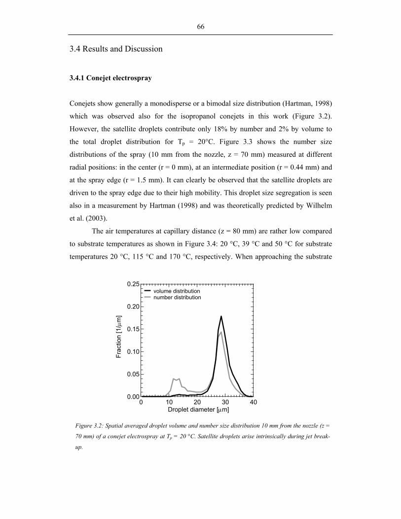
66

3.4 Results and Discussion

3.4.1 Conejet electrospray

Conejets show generally a monodisperse or a bimodal size distribution (Hartman, 1998)

which was observed also for the isopropanol conejets in this work (Figure 3.2).

However, the satellite droplets contribute only 18% by number and 2% by volume to

the total droplet distribution for Tp = 20°C. Figure 3.3 shows the number size

distributions of the spray (10 mm from the nozzle, z = 70 mm) measured at different

radial positions: in the center (r = 0 mm), at an intermediate position (r = 0.44 mm) and

at the spray edge (r = 1.5 mm). It can clearly be observed that the satellite droplets are

driven to the spray edge due to their high mobility. This droplet size segregation is seen

also in a measurement by Hartman (1998) and was theoretically predicted by Wilhelm

et al. (2003).

The air temperatures at capillary distance (z = 80 mm) are rather low compared

to substrate temperatures as shown in Figure 3.4: 20 °C, 39 °C and 50 °C for substrate

temperatures 20 °C, 115 °C and 170 °C, respectively. When approaching the substrate

0.25

0.20

0.15

0.10

0.05

0.00

Frac

tion

[1/µ

m]

403020100Droplet diameter [µm]

volume distribution number distribution

Figure 3.2: Spatial averaged droplet volume and number size distribution 10 mm from the nozzle (z =

70 mm) of a conejet electrospray at Tp = 20 °C. Satellite droplets arise intrinsically during jet break-

up.

67

the temperature increases slowly, while only at about 5 mm in front of the heated plate

the temperature gradient is very steep.

The ab initio calculated droplet diameter from the scaling laws of Gañán-Calvo

0.6

0.5

0.4

0.3

0.2

0.1

0.0

Frac

tion

[1/µ

m]


spray center (r = 0 mm) intermediate position (r = 0.44 mm) spray edge (r = 1.5 mm)

Figure 3.3: Conejet droplet number size distribution measured at 10 mm from the nozzle (z = 70 mm)

in the center of the spray (r = 0 mm), at an intermediate position (r = 0.44 mm) and at the edge (r =

1.5 mm). Spatial size segregation is observed as predicted by the model due to the higher mobility of

smaller droplets.

200

150

100

50

0

Air

tem

pera

ture

[°C

]

806040200Distance from plate [mm]

TP=170°C TP=115°C TP=20°C

Figure 3.4: Air temperature distribution between nozzle and plate for plate temperatures Tp = 20 °C,

115 °C and 170 °C. Between 20 and 80 mm from the plate a plateau temperature is reached (20 °C,

39 °C and 50°C) for each plate temperature condition (20 °C, 115 °C and 170°C, respectively).

68

35

30

25

20

15

Dia

met

er o

f ave

rage

vol

ume

[µm

]

3530252015Calculated droplet diameter [µm]

Figure 3.5: Comparison of the measured droplet diameter of average volume in the center of the conejet

spray 10 mm from the nozzle exit (z = 70 mm) with the droplet sizes obtained from the scaling laws by

Gañán-Calvo et al. (1997).

et al. (1997) are validated with the measured diameter of average volume,

( )1/333,0 0d d q= ∑ , in the center of the spray (r = 0 mm) at nozzle exit (Figure 3.5).

Good agreement is found with the values obtained by the scaling laws of Gañán-Calvo

et al. (1997) for all three plate temperature conditions, and therefore their corresponding

liquid temperature which is about 10 % lower than the air temperature at capillary exit

for the non-ambient conditions: 36 °C and 47 °C for 115 °C and 170 °C substrate

temperature, respectively. Consequently the scaling laws are applied for the ab initio

calculation.

The droplet concentration and mass flux illustrates the structure of the spray

(Figure 3.6). After breakup of the jet into droplets, the droplet number concentration is

higher than 1000 droplets/cm3. At a position 25 mm from the nozzle (z = 55 mm) the

radial expansion of the spray is smaller than 7 mm. The concentration is decreasing

when approaching the plate mainly because of the spatial spread of the spray. The

spatial distribution of the number concentration is more homogeneous close to the plate

and in the middle of the spray (z = 5 mm, z = 30 mm). The width of the spray at z = 5

mm is about 60 mm in diameter which corresponds very well to the capillary-plate

distance of 80 mm which is typical for conejets (Gañán-Calvo et al., 1994). The radial

69

distribution of the mass flux is comparable to the number concentration distribution as

the satellite droplets have hardly an influence. The mass flux at the spray edge still has

about 50% of the center value which is important for homogeneous deposition in spray

deposition in the conejet mode. The droplet size segregation has no large influence for

this configuration due to the negligible volume of the secondary droplets.

Figure 3.7a – c shows the diameter of average volume of the conejet spray

measured with the PDA for the three different plate temperature conditions. The

evaporation is calculated assuming zero background vapor concentration for plate

temperature Tp = 20 °C (Figure 3.7a). The initial conditions (droplet velocity and size

distribution) for the calculation are taken from z = 70 mm (10 mm from the nozzle). The

calculation shows very good agreement for both methods (ab initio and initial

condition). For the conejet spray with a plate temperature Tp = 115 °C the measured

droplet size is underpredicted by the model when assuming zero background vapor

concentration. It takes about 60% of relative isopropanol vapor pressure (100% = 15

kPa) at Tair = 39 °C in order to match the measured values throughout the total spray

distance (Figure 3.7b). For Tp = 170 °C the best match with experimental results is

obtained at 80% of relative vapor pressure (100% = 25 kPa) at Tair = 50°C (Figure 3.7c).

These calculations show clearly that the background concentration must not be

10

2

4

68

100

2

4

68

1000

Dro

plet

con

cent

ratio

n [#

/cm

3 ]

302520151050Radial distance from centerline [mm]

10-5

2

4610-4

2

4610-3

2

4610-2

Volum

e flux [cm3/cm

2/s]

number concentration z = 55mm number concentration z = 30 mm number concentration z = 5 mm volume flux z=55mm volume flux z=30mm volume flux z=5mm

Figure 3.6: Measured droplet concentration and volume flux of conejet electrospray for Tp = 20 °C at

distances z = 5, 30 and 55 mm from the plate. Close to the plate the number concentration and mass flux

is rather homogeneous.

70

neglected. They further suggest that with increasing air temperature the vapour

background concentration is increasing in the spray. In comparison the “ab initio”

calculations show a faster evaporation than the calculation using the “initial conditions”

method but the resulting droplet diameters on the substrate do not differ significantly for

Tp = 20 °C and 115 °C. For Tp = 170 °C the droplets even do not reach the substrate

(Figure 3.7c). This difference results from the larger droplet spectrum of the measured

size distribution which is used in the “initial condition” method. Compared to the

monodisperse assumption in the “ab initio” method the larger droplets in the real

distribution do not evaporate completely. Consequently the “ab initio” calculation can

replace the “initial condition” method if there is no complete evaporation to fear.

Measurement and calculation show that it is possible to control closely the breakup and

impact droplet diameter of conejet sprays for process optimization. The impact

(breakup) diameter is changing here between 24 (26) µm for ambient conditions to 17

(23) µm for 170 °C plate temperature underlining the ability for precise control of the

Figure 3.7: Comparison of measured

and calculated diameter of average

volume for conejet electrosprays at

plate temperatures 20 °C (a), 115 °C

(b) and 170 °C (c). Calculations with

background concentration of

isopropanol vapor are also shown.

30

25

20

15

10

5

0

Dia

met

er o

f ave

rage

vol

ume

[µm

]


0% (initial condition) 0% (ab initio) PDA measurement

30

25

20

15

10

5

0

Dia

met

er o

f ave

rage

vol

ume

[µm

]


80% (initial condition) 60% (initial condition) 40% (initial condition) 0% (initial condition) 0% (ab initio) PDA measurement

30

25

20

15

10

5

0

Dia

met

er o

f ave

rage

vol

ume

[µm

]


80% (initial condition) 60% (initial condition) 40% (initial condition) 0% (initial condition) 0% (ab initio) PDA measurement

Isopropanol vapor background concentration



Tp = 20 °C Tp = 115 °C

Tp = 170 °C

a b

c

71

process. The mass fraction of the diameter of average volume arriving on the plate for

Tp = 20 °C is 68% of the original size whereas the fraction for Tp = 170 °C is 31%. The

important controlling parameters are the liquid properties influencing the initial droplet

size (scaling laws) and the temperature distribution in the process area influencing the

evaporation rate and thereby controlling the final droplet diameter before deposition.

Figure 3.8a - c shows the measured axial velocities averaged over the spray

cross-section and the model predictions for plate temperatures Tp = 20 °C, 115 °C, 170

°C. The droplets have a high velocity after break-up close to the capillary exit compared

to droplet velocity closer to the grounded plate. This is attributed to the higher electric

field close to the capillary exit. The measurements show a nearly constant droplet

velocity close to the plate. Approaching the substrate the match between measured and

calculated values is excellent. The difference close to the nozzle can be explained by an

induced air flow from the momentum transfer of the droplets to the air. This effect will

be largest close to the nozzle where the droplet velocity and concentration is high

12

10

8

6

4

2

0

Dro

plet

axi

al v

eloc

ity [m

/s]


PDA measurement calculation initial condition calculation ab initio

12

10

8

6

4

2

0

Dro

plet

axi

al v

eloc

ity [m

/s]


PDA measurement calculation initial conditions calculation ab initio

Figure 3.8: Mean droplet velocities

for the conejet electrosprays with (a)

Tp = 20 °C, (b) 115 °C and (c) 170

°C. The residence time in the spray is

very similar for all substrate

temperature conditions.

12

10

8

6

4

2

0

Dro

plet

vel

ocity

[m/s

]


PDA measurement calculation initial condition calculation ab initio

a b

c

Tp = 20 °C Tp = 115 °C

Tp = 170 °C

72

(Figure 3.6). The droplet velocity is very high close to the nozzle for the strong electric

field which is induced by the small dimensions of the nozzle tip. Close to the plate, the

electric field is getting weaker and the droplets attain equilibrium between external

electric forces and drag force which leads to a nearly constant velocity. In this region

where the initial velocity has only a very minor influence the calculations using “ab

initio” and “initial conditions” are in very good agreement. For the ab initio calculation

the initial velocity seems to be underestimated due to the slight overestimation of the

diameter of average volume by the scaling law at breakup location (see Figure 3.7a, b,

c). As the diameter of the jet and consequently also the jet velocity (droplet velocity at

breakup) is calculated from the diameter of average volume (Wilhelm et al., 2003) this

leads to a lower jet and droplet velocity at the breakup location (Cloupeau and Prunet-

Foch, 1989).

The conejet enables excellent control of droplet evaporation by spraying under

the moderate temperature conditions. The charged droplets follow the electrical field

lines and they are therefore hardly influenced by radial convection leading to a defined

residence time in the system. The average (calculated) residence time of a droplet in the

6

5

4

3

2

1

0

Dro

plet

axi

al v

eloc

ity [m

/s]

302520151050Distance from centerline [mm]

calculation z = 5mm PDA measurement z = 5mm calculation z = 30mm PDA measurement z = 30mm calculation z = 55mm PDA measurement z = 55mm

Figure 3.9: Radial distribution of axial droplet velocity for the conejet spray with plate temperature Tp

= 20 °C. The large difference between the calculated to the measured axial velocity at (z = 55 mm, r =

0 mm) can be attributed to a background air flow that is induced by momentum transport from the

moving droplets.

73

conejet electrospray is nearly equal for different temperature conditions: t = 0.031 s at

Tp = 20 °C and t = 0.029 s for Tp = 170 °C.

Figure 3.9 shows the axial velocity distribution with the radial distance from the

spray axis for the conejet at Tp = 20 °C. The difference between measured and

calculated velocities at (z = 55 mm, r = 0 mm) in the order of several meters per second

is remarkable. At the edges of the spray the velocity values match. This is another

indication for the existence of an induced air flow. Assuming that the difference

between calculated and measured droplet velocity can be attributed to air flow the

maximum of the air velocity is in the center and approaching zero at the spray edge.

Similar findings have been published by Gañán-Calvo et al. (1994) and Hartman (1998).

However, as it is evident from this work, the resulting difference in residence time of

the droplets does not significantly influence the evaporation as can be seen in Figure

3.6a. A possible underestimation of the electric fields close to the capillary, which could

also lead to this underprediction, does not seem realistic as the external electric fields

used in this work, by Gañan-Calvo et al. (1994) and by Hartman (1998) are derived

from different assumptions.

3.4.2 Multijet electrospray

Figure 3.10a shows an averaged droplet size distribution for an intermittent multijet

electrospray (here Tp = 20 °C) at the nozzle exit. Figures 3.10b and c show the droplet

size distributions measured at the center of the spray (z = 46 mm, r = 0 mm) and at the

spray edge (z = 46 mm, r = 10 mm), respectively. The multijet size distribution is

polydisperse in contrast to the conejet’s monodispersity. Counting by number 1.3%

(10%) of the droplets is larger than 30 µm (10µm) and carries 82% (96%) of the liquid

volume. The number distribution is completely dominated by the small droplets but the

majority of the liquid is transported by the few larger droplets. It is important to note

that there is no segregation of small and large droplets as in the case for the conejet

mode. This results from the droplet distribution after break-up in the intermittent

multijet mode. Droplet producing jets are emitted at the nozzle rim in a random and

intermittent fashion in different directions (Figure 3.1). Consequently large and small

74

droplets are sprayed in a wide spraying angle which leads to a spatial mixing of the

droplets of all sizes and mobilities.

Figure 3.11 shows the number of elementary charges for a given droplet size of

the multijet at TS = 115 °C. The power law dependence is q ~ d1.82. For TS = 20 °C and

215°C the exponent is similar: 1.81 and 1.79, respectively. Thereby the charge density

is approximately scaling with the droplet surface. It is noteworthy that the

proportionality between droplet size and droplet charge for the three sprays is higher

than q ~ d1.5 which is the relation that is often found for conejets (see discussion in

chapter 3.3). Hendricks (1962) measured a diameter-charge relation between q ~ d1.5

and q ~ d2.3 using an electrospray which is producing a polydisperse droplet size

distribution between 0.1 and 10 µm.

The structure of the multijet is different from the conejet. Figure 3.12 shows the

measured and calculated droplet concentrations of the multijet spray for Tp = 20 °C at

different distances from the plate. Already at 4 mm from the nozzle (z = 46 mm) the

0.20

0.15

0.10

0.05

0.00

Num

ber f

ract

ion

[1/µ

m]


30x10-3

25

20

15

10

5

0

Volum

e fraction [1/µm]

number distribution r = 10 mm volume distribution r = 10 mm

0.20

0.15

0.10

0.05

0.00

Num

ber f

ract

ion

[1/µ

m]


30x10-3

25

20

15

10

5

0

Volum

e fraction [1/µm]

number distribution r = 0 mm volume distribution r = 0 mm

Figure 3.10: Droplet size distributions

at (a) z = 46 mm (average over the cross

section ), (b) distribution at z = 46 mm,

r = 0 mm (centerline) and at (c) z = 46

mm, r = 10 mm (spray edge) for multijet

electrospray at Tp = 20 °C. There are

less droplets in the size range above 80

µm at the spray edge.

0.20

0.15

0.10

0.05

0.00

Num

ber f

ract

ion

[1/µ

m]


30x10-3

25

20

15

10

5

0

Volum

e fraction [1/µm]

total number distribution total volume distribution a b

c

75

droplet concentration has shrinked to a value of around 1000 droplets/cm3. Grace and

Dunn (1996) obtained a similar value when investigating an ethanol multijet

electrospray at 5 mm distance from the nozzle. In comparison this concentration

decrease was reached by the conejet 25 mm from the nozzle. The spray width of the

multijet at that distance is already 10 mm. This large spray angle results from the

Figure 3.11: Charge distribution for multijet electrospray for the condition Tp = 115 °C. The line

represents the power law regressed to the droplet size-charge relation. The number of elementray

charge per droplet is proportional to d1.82.

105

2

4

68

106

2

4

68

107

2

Ele

men

tary

cha

rges

[#]

6 7 8 910

2 3 4 5 6 7 8 9100

Droplet diameter [µm]

1

10

100

1000

Dro

plet

con

cent

ratio

n [#

/cm

3 ]

302520151050Distance from centerline [mm]

10-5

2

4610-4

2

4610-3

2

4610-2

Volum

e flux [cm3/cm

2/s]

number concentration = 46 mm number concentration z = 23 mm number concentration z = 3 mm volume flux z = 46 mm volume flux z = 23 mm volume flux z = 3 mm

Figure 3.12: Measured droplet concentration and volume flux of multijet electrospray for Tp = 20 °C at

distances z = 3, 23, and 46 mm from the plate. The mass flux is very homogenous close to the plate.

q ~ d1.82

76

droplet break-up process described above. The droplets are emitted in an angle close to

180°. The concentration is decreasing towards the plate due to increasing spray cross

section and evaporation. Close to the plate the droplet concentration is significantly

higher in the middle due to the shorter residence time of the droplets compared to the

edges of the spray. In contrast to that the mass flux is very homogeneous which is very

important for film deposition. It is even more homogeneous than the conejet mass flux

close to the substrate. The mass flux at the spray edges at r = 30 mm is still 50 % of the

center value.

Figures 3.13a – c show the development of the mean volume diameter with

distance to the substrate. The agreement between theoretical prediction and

measurement is excellent. All calculations show that the diameter of average volume is

increasing with decreasing distance from the plate. Small droplets are evaporating very

fast compared to the larger ones and disappear from the statistics. Therefore, the

diameter of average volume increases although the droplets are evaporating because the

40

30

20

10

0

Dia

met

er o

f ave

rage

vol

ume

[µm

]


PDA measurementcalculation

40

30

20

10

0

Dia

met

er o

f ave

rage

vol

ume

[µm

]


PDA measurement calculation

40

30

20

10

0

Dia

met

er o

f ave

rage

vol

ume

[µm

]




and calculated axial diameter of

average volume of the multijet

electrospray at (a) Tp = 20 °C, (b) 115

°C and (c) 215 °C. Small droplets

evaporate faster and the wide size

distribution narrows leading to an

increase of the diameter of average

volume.

a

c

b

Tp = 20 °C

Tp = 215 °C

Tp = 115 °C

77

size distribution narrows. The calculations assume 0% background vapor pressure. Due

to the large spraying angle of approximately 180° and the resulting low droplet

concentration at the nozzle exit the isopropanol vapor concentration is distributed within

a larger volume and has no influence on the droplet evaporation.

Figures 3.14a – c show the velocity distribution of the multijet spray. The data

show a good qualitative match between measurement and calculation. Grace and Dunn

(1996) who performed their experiments under ambient conditions with pure ethanol as

working fluid in the multijet mode reported similar behavior for the velocity distribution

along the spray axis. The velocity is around 4 m/s close to the capillary after breakup.

Following the central axis towards the plate the velocity is decreasing first to 2.5 m/s

and then increases again to 3 m/s at 5 cm from the plate (capillary-plate distance is 20

cm in their work). The calculation of Grace and Dunn (1996) show only a qualitative

agreement to the measured velocity close to the capillary. In this work, however, the

velocity can be predicted much more accurately. As already observed for the conejet

8

6

4

2

0

Dro

plet

axi

al v

eloc

ity [m

/s]



8

6

4

2

0

Dro

plet

axi

al v

eloc

ity [m

/s]



8

6

4

2

0

Dro

plet

axi

al v

eloc

ity [m

/s]




and calculated axial velocity of droplets

averaged over the cross section for

multijet electrosprays at (a) Tp = 20 °C ,

(b) 115 °C , (c) 215 °C. The calculation

is qualitatively matching the

measurement. The velocities are very

much equal for all three plate

temperature conditions.

a b

c

Tp = 20 °C

Tp = 215 °C

Tp = 115 °C

78

also here the residence time in the system is very similar for the three temperature

conditions. Further, the impact diameter of average mass on the plate can be controlled

very carefully by adjusting the external temperature conditions. However, the multijet

guarantes that the deposition process can be performed without significant droplet

evaporation even at extreme temperature conditions (above 200°C) which are often

necessary for electrospray pyrolysis.

3.5 Summary

The transport and evaporation of electrically charged droplets in conejet and

intermittent multijet in a capillary–plate configuration are investigated by PDA

measurement and simulation. The simulations of the conejet electrospray show an

excellent agreement with the measured velocity and evaporation data assuming a

background concentration of the evaporated solvent. The simulations for the multijet

electrospray are in good qualitative agreement with the velocity data and in good

quantitative agreement with the diameter development along the spray axis. The nearly

monodisperse conejet mode shows excellent control for initial droplet size and

evaporation rate. The final droplet diameter can be controlled very precisely to the

applied external air temperature. The multijet is characterized by its initial broad droplet

size distribution with much larger droplets than in the conejet mode. Also here the

evaporation of the droplets can be controlled carefully by heating the surrounding air.

Due to the larger droplet sizes in the multijet this mode can be applied for film

deposition at more elevated plate temperatures without complete evaporation of the

droplets. Further, the mass flux of the multijet is more homogeneous than the conejet

which is very important for the deposition of homogeneous films. With the present

setup two very distinct sprays that find their applications in many varying production

techniques can be established. The developed theoretical model is able to predict

spatially detailed droplet size and velocity distributions. This makes it an excellent tool

for dimensionalization of ESD setups and helps to evaluate key parameters of the

process.

79

3.6 References

Bailey, A.G. (1988) Electrostatic spraying of liquids. John Wiley and Sons, New York.

Chen, C.H., Buysman, A.A.J., Kelder, E.M. and Schoonman, J. (1995) Fabrication of

LiCoO2 thin film cathodes for rechargeable lithium battery by electrostatic

spray pyrolysis. Solid State Ionics 80, 1 – 4.

Chen, C.H., Kelder, E.M., Van der Put, P.J.J.M. and Schoonman, J. (1996) Morphology

control of thin LiCoO2 films fabricated using the electrostatic spray deposition

(ESD) technique. J. Mater. Chem. 6, 765 – 771.

Clopeau, M. and Prunet-Foch, B. (1989) Electrostatic spraying of liquids in the

conejet mode. J. Electrostat. 22, 135 – 159.

Cloupeau, M. and Prunet-Foch, B. (1990) Electrostatic spraying of liquids – main

functioning modes. J. Electrostat. 25, 165 – 184.

Davis, E.J. and Bridges, M.A. (1994) The Rayleigh limit of charge revisited: light

scattering from exploding droplets. J. Aerosol Sci. 25,1179 – 1199.

Domnick, J., Scheibe, A. and Ye, Q. (2003) The electrostatic spray painting process

with high-speed rotary bell atomizers: influences of operating conditions and

target geometries. 9th International Conference on Liquid Atomization and Spray

Systems (ICLASS), Proceedings, 5-4. Fenn, J.B., Mann, M., Meng, C.K., Wong, S.F. and Whitehouse, C.M. (1989)

Electrospray ionization for mass spectrometry of large biomolecules. Science

246, 64 – 71.

Gañán-Calvo, A.M., Lasheras, J.C., Davila, J. and Barrero, A. (1994) The electrostatic

spray emitted from an electrified conical mensicus. J. Aerosol Sci. 6, 1121 –

1142.


electrospraying of liquids. Scaling laws. J. Aerosol Sci. 28, 249 – 276.


spray. Exp. Fluids 20, 153 – 164.

Hartman, R. (1998) Electrohydrodynamic atomization in the cone-jet mode. PhD thesis,

Delft University of Technology, The Netherlands.

Hendricks, C.D. (1962) Charged droplet experiments. J. Colloid Sci. 17, 249 – 259.

80

Ijsebaert, J.C., Geerse, K.B. and Marijnissen, J.C.M. (2001) Electrohydrodynamic

atomization of drug solutions for inhalation purposes. J. Appl. Physiol. 6, 2735 –

2741.

Jaworek, A. and Krupa, A. (1996) Forms of the multijet mode of electrohydrodynamic

spraying. J. Aerosol Sci. 27, 979 – 986.

Kelly, A.J. (1984) Low charge density electrostatic atomization. IEEE-IA 20,

267 – 273.

Kim, K. and Ryu, C.K. (1994) Generation of charged liquid cluster beam of liquid-mix

precursors and application to nanostructured materials. Nanostruct. Mater. 4,

597 – 602.

Lapham, D.P., Colbeck, I., Schoonman, J. and Kamlag, Y. (2001) The preparation of

NiCo2O4 films by electrostatic spray deposition. Thin Solid Films 391, 17 – 20.

Park, D.G. and Burlitch, J.M. (1996) Electrospray synthesis of titanium oxide

nanoparticles. J. Sol-Gel Sci. Techn. 6, 235 – 249.

Perednis, D., Honegger, K. and Gauckler, L.J. (2001) Fabrication of thin YSZ

electrolyte films using spray pyrolysis technique. Proceedings of the 7th

International Symposium on Solid Oxide Fuel Cells, (SOFC-VII), Tsukuba,

Japan, H. Yokokawa, S.C. Singhal (Eds.), The Electrochemical Soc.,

Pennington, NJ, USA, 989 - 990.

Perednis, D. (2003) Thin film deposition by spray pyrolysis and the application in solid

oxide fuel cells. Ph.D. thesis, ETH Zürich No. 15190.

Richardson, C.B., Pigg, A.L. and Hightower, R.L. (1989) On the stability limit of

charged droplets. Proc. Roy. Soc. London A 422, 319 – 328.



Sweet, R.G. (1965) High frequency recording with electrostatically deflected ink jets.

Rev. Sci. Instr. 36, 131 – 136.

Taflin, D.C., Ward, T.L. and Davis, E.J. (1989) Electrified droplet fission and the

Rayleigh limit. Langmuir 5, 376 – 384.

Tang, K. and Gomez, A. (1994) On the structure of an electrostatic spray of

monodisperse droplets. Phys. Fluids 6, 2317 – 2332.

Wilhelm, O., Mädler, L. and Pratsinis, S.E. (2003) Electrospray evaporation and

81

deposition. J. Aerosol Sci. 34, 815 – 836.

83

4 Electrospray vs. Pressurized Spray Deposition of YSZ Filmsc

Abstract

Yttria-stabilized zirconia (YSZ) films (< 1 µm thickness) were deposited on hot

substrates by electrostatic and pressurized atomization. Droplet transport and

evaporation are examined with a Phase Doppler Anemometer while the film

morphology and composition are investigated by SEM and EDX analysis. The effects of

spraying configuration, solvent/precursor composition and substrate temperature on the

resulting film morphology are examined. Smooth and dense YSZ films can be made at

substrate temperatures above the solvent boiling point while precursor influence is

negligible. Furthermore, the spray droplet has to reach the substrate without solid

precipitation in the droplet or complete evaporation of the solvent. A deposition

diagram for film texture was developed as function of droplet size, precursor

concentration and substrate temperature using a theoretical model for droplet transport

and evaporation.

4.1 Introduction

Spraying precursor droplets on a heated substrate is typically used for thin ceramic film

deposition for its simplicity, low equipment cost and a wide choice of precursors (Gurav

et al., 1993). Yttria-stabilized zirconia (YSZ) is the most commonly used material for

electrolyte films in solid oxide fuel cells (SOFCs) for its chemical and thermal stability

even at 1000 °C. In order to improve the performance of the SOFC and simplify its

fabrication, a lower operation temperature is desired. This can be achieved by

employing new materials that increase the electrolyte ion conductivity or by decreasing

the thickness of the YSZ film. An attractive feature of spray pyrolysis is its ability to

c This chapter is partly submitted to Thin Solid Films.

84

produce YSZ films with a thickness less than a micrometer on substrates with micron-

sized pores (Perednis, 2003).

Siefert (1984) deposited metal oxide films on a glass substrate by corona spray

pyrolysis. Similarly Konstantinov et al. (2000) made uniform CeO2 films at 400 °C

while cracks or large crystallites were formed at higher or lower temperatures,

respectively. Nguyen and Djurado (2001) deposited the best zirconia films on stainless

steel at around 400 °C also. Choy (2002) describes the deposition of films and particles

composed of a variety of materials by electrospray deposition. Different types of

atomization techniques are used for droplet production: ultrasonic, pressurized sprays

and electrosprays (Will et al., 2000). Ruiz et al. (1997) used ultrasonic spray to deposit

zirconia films and pointed out the importance of droplet size for the deposited film

quality. Wang et al. (2000) used a similar setup for deposition of YSZ films but called

their process aerosol-assisted chemical vapor deposition as their droplets are evaporated

before arriving on the substrate. Chen et al. (1995) investigated thin film deposition

(LiCoO2) by electrospray for production of a cathode for rechargeable lithium batteries.

Chen et al. (1998) showed that additives influencing the droplet size in electrosprays

resulted in significant changes in the product. Wilhelm et al. (2003) showed that small

droplets can fully evaporate during transport and deposition on hot substrates altering,

thus, drastically the deposited film quality.

Clearly spray pyrolysis contains several parameters influencing the quality of the

product film: substrate temperature, volume flux, droplet size and velocity, temperature

field, precursor/solvent composition and setup geometry. Here two common spray

pyrolysis techniques are compared and the effect of process parameters on film quality

is evaluated. Droplet size, velocity and volume flux is investigated by a Phase Doppler

Anemometer (PDA) while the film morphology and composition are analysed by

SEM/EDX. Using the model of Wilhelm et al. (2003) the effect of droplet size,

substrate temperature and solution concentration on film texture is summarized on a

design diagram and compared to the above data.

85

4.2 Experimental setup

A YSZ film is deposited by spraying precursor solution (Table 4.1) droplets onto a

heated substrate. The YSZ precursors are zirconium acetylacetonate (Zr(acac)4, Fluka),

zirconium oxinitrate (ZrO(NO2)3, Fluka), and yttrium chloride (YCl3, Fluka). The

solvent is a mixture of 50 vol% ethanol (Fluka) and 50 vol% butylcarbitol

(Diethylenglycol monobutylether, Fluka) or a mixture of 50 vol% ethanol (Fluka) and

50 vol% 1-Methoxy-2-Propanol (Fluka) or pure butylcarbitol (Table 4.1). The films are

deposited on inconel (Ni-alloy) foil with thickness 0.5 mm and diameter 30 mm. The

foil is sucked by a vacuum pump to the surface of a heated aluminum plate.

Solution Solvents, volume ratio Precursor , molar ratio Concentration

A Butylcarbitol/Ethanol (50/50) Zr(acac)4/ YCl3 , 84/16 0.1 mol/l

B Butylcarbitol/Ethanol (50/50) Zr(acac)4/ YCl3 , 84/16 0.01 mol/l

C MethoxyPropanol/Ethanol (50/50) Zr(acac)4/ YCl3 , 84/16 0.1 mol/l

D Butylcarbitol/Ethanol (50/50)

ZrO(NO2)3/ YCl3 , 84/16 0.1 mol/l

E Butylcarbitol Zr(acac)4/ YCl3 , 84/16 0.001 mol/l

The spray droplets containing the precursor are produced either by a downward

pressurized nozzle (“P” – pressurized spray deposition) or by two upward electrospray

configurations: conejet (C) and multijet (M). The pressurized nozzle (Böllhoff, Compact

2000KM) is located 31 cm above the substrate. An air pressure of p = 0.75 bar is

applied to atomize the solution supplied at Q = 30 ml/h by a syringe pump (Bioblock

Scientific, A 99). Table 4.2.1 shows all experimental conditions.

The outlet of the electrospray capillary is 6 cm below the substrate. The

electrosprays are pointing upward to prevent deposition of millimeter-sized droplets

from spraying instability that could destroy the film homogeneity. This is a problem

especially for the conejet mode as the high electric conductivity for liquids containing

salt precursors prevents a strong tangential electric field component along the cone

surface which leads to a low liquid acceleration and consequently to a low volume flux

Table 4.1: Composition of the employed sprayed solutions

86

through the jet emitted at the cone apex (Hayati et al., 1986). As the volume flux Q is

controlled by the syringe pump, more liquid can flow into the cone from the capillary

side than drawn by the electric field through the jet. For upward spraying, surplus liquid

does not disturb the jet as it is just flowing down the outer capillary surface. During

downward spraying, surplus liquid is forming occasionally millimeter-sized droplets

dripping onto the substrate. Steel capillaries are used that have outer/inner diameters of

d = 0.6/0.45 mm (Braun) and 2.7/2.5 mm (Hamilton), respectively. The smaller one is

used for the intermittent multijet mode while the bigger one for the conejet mode of the

electrospray. A syringe pump is used to deliver a precursor solution: Q = 2.8 ml/h for

the multijet (Table 4.2.2: M1 – 4), Q = 5.7 and 1.4 ml/h for the conejet electrospray at

the higher and lower precursor concentration, respectively (Table 4.2.3: C1 – 2).

Exp. P1 P2 P3 P4 P5 P6 P7

Solution

A A A C C D D

TS [°C] 210 250 310 140 180 185 235

Experiment M1

M2 M3 M4

TS [°C] 196 256 310 365

Experiment C1 C2 C3 C4

Solution A

B E E

TS [°C] 260 260 192 260

Q [ml/h] 5.7 1.4 2.12 2.83

Φ [V] 6900 6900 6700 6400

Spray direction Up Up Down Down

As the conejet produces considerably smaller droplets than the multijet electrospray for

Table 4.2.3: Experiments with the conejet electrospray at H = 6 cm.

Table 4.2.1: Deposition experiments with the pressurized spray at p = 0.75 bar, H = 31 cm and Q =

30 ml/h.

Table 4.2.2: Experiments with the multijet electrospray at kV10=Φ , H = 6 cm and Q = 2.8 ml/h

with solution A.

87

As the conejet produces considerably smaller droplets than the multijet electrospray for

the above setup, conditions were identified that can produce comparable droplet sizes

for both electrosprays. So experiments C3 and C4 were carried with a smaller conejet

capillary, 1.47/1.07 mm, and lower salt concentration (Table 4.2.3: C3 – 4) to reduce

electric conductivity and a downward pointing spray to guarantee that all the liquid is

flowing through the jet and droplet size is not decreased by escaping liquid.

The deposited film morphology is investigated by SEM (LEO1530, Field

Emission Gun) while homogeneity and chemical composition by EDX (Noran Vintage).

A 2D – Phase Doppler Anemometer (PDA) by TSI Inc. with an Argon Ion Laser

(Innova 70) is used for measuring spray droplet size (> 1µm) and velocity at each

location. The PDA is measuring single droplets that pass through the volume defined by

the crossing of two coherent laser beams.

The air temperature without spraying between nozzle and substrate is measured

with a K-type thermoelement. It is not possible to measure temperature during spraying

as the droplets cool the element that serves also as a grounded electrode altering the

process when electrospraying.

4.3 Results

4.3.1 SEM/EDX analysis of the deposited film

Figures 4.1a - d show SEM pictures of YSZ films deposited by multijet electrospraying

of solution A at different substrate temperatures, TS (Table 4.2.2). At TS = 196 °C

(Figure 4.1a) the film shows severe cracks while for TS = 256 °C or higher (Figures

4.1b – d) the number of particles deposited on the substrate increases as confirmed by

the EDX spectra (Figures 4.1e – h). Cracks are detected (Figure 4.1a and e) as a

reduction of the zirconium signal and an increase of the nickel-substrate signal. The

enhanced noise-to-signal ratio with increasing substrate temperature indicates increasing

number of particles deposited.

Similar results are obtained when depositing YSZ films by pressurized spraying

of solution A. Figure 4.2 shows the contrast between TS = 210 °C (a) and TS = 250 °C

88

(b). Similar to the multijet electrospray (Figure 4.1a,b), here also the film changes from

a cracked to a crack-free one. This transition point is between TS = 140 °C and 180 °C

using solution C instead of A (Figure 4.2c,d). Spraying solution D (with a different Zr-

precursor compared to solution A) the resulting film is similar to that made with the

original Zr-precursor and solution A (Figure 4.2a,b): the transition from cracked to

crack-free film (Figure 4.2e,f) is between 185 °C and 235 °C.

When using the upward facing conejet electrospray at TS = 260 °C (Table 4.2.3:

C1), the film is a porous structure made of single particles (Figure 4.3a). The same film

texture is obtained when precursor concentration is reduced (Table 4.2.3: C2) though

smaller particles are deposited (Figure 4.3b). But for the downward spraying conejet

employing lower precursor concentrations, the film morphology (Figure 4.3c,d) again

looks similar to that obtained with the multijet electrospray with solution A (Figure 4.1

a,b): At low TS (192 °C) a cracked film forms (Figure 4.3c) whereas at high TS (260 °C)

a rather homogeneous film is obtained (Figure 4.3d).

10 µm

a

250

200

150

100

50

0

Num

ber o

f pho

tons

76543210Scanning distance on substrate [µm]

Zr Ni

e

10 µm

b

250

200

150

100

50

0

Num

ber o

f pho

tons


Zr Ni

f

Figure 4.1: continues next page.

89

c

10 µm 250

200

150

100

50

0

Num

ber o

f pho

tons

76543210 Scanning distance on substrate [µm]

Zr Ni

g

250

200

150

100

50

0

Num

ber o

f pho

tons


Zr Nih

d

10 µm

Figure 4.1: SEM pictures and EDX spectra of the YSZ films on inconel foil sprayed with the

multijet electrospray at (a/e) TS = 196 °C (M1), (b/f) TS = 256 °C (M2), (c/g) TS = 310 °C (M3)

and at (d/h) TS = 365 °C (M4). The Ni line in e – h is for the substrate while the Zr (bold) line

refers to the deposit in the EDX spectra.

90

10 µm

a

10 µm

b

10 µm

c

10 µm

d

10 µm

e

10 µm

f

Figure 4.2: SEM micrographs of YSZ films produced with the pressurized spray at TS = 210°C (a)

and 250°C (b) with solution A (Table 2, exp. P1 and P2), at TS = 140°C (c) and 180°C (d) with

solution C (exp. P4 and P5), and at TS = 185°C (e) and 235°C (f) with solution D (exp. P6 and P7).

91

4.3.2 PDA measurements

Figures 4.4a – c show the initial droplet size distributions for the different

sprays. The number size distribution of the multijet electrospray shows a strong peak for

droplets below 10 µm (Figure 4.4a) but the few big droplets dominate the volume

distribution (experiment M1). The nozzle exit distributions of the other multijet

10 µm

a

10 µm

b

c

10 µm

d

10 µm

Figure 4.3: SEM micrographs of YSZ films deposited with the upward facing conejet electrospray at

TS = 260 °C with solution A (C1) (a) and solution B (C2) (b) and the downward facing conejet at TS =

192 °C with solution E (C3) (c) and TS = 260 °C (C4) (d).

92

experiments are similar (see mean volume diameter in Figure 4.6). Only 5% of the

solution volume is transported by the small droplets (< 10 µm). This is analogous for

the pressurized spray (Figure 4.4c) that forms slightly smaller droplets. The number size

distribution is different for the conejet electrospray (Figure 4.4b). For both conejet

configurations (upward C1/C2 and downward C3/C4) the distribution is very narrow.

But the downward conejet in Figure 4.4b (C4) has a significantly larger mean volume

size (d = 12 µm) than the corresponding upward (d = 3.4 µm) (C1). The C4 droplet size

distribution shows a bimodal number and a unimodal volume distribution. The size

distributions of C2 and C3 are similar to C1 and C4, respectively.

Figure 4.5 shows the droplet axial velocity of the a) pressurized spray and b) two

electrosprays as a function of the distance to the substrate. The pressurized spray droplet

velocity is very high near the nozzle as droplets try to follow the fast dispersion gas

0.25

0.20

0.15

0.10

0.05

0.00

Num

ber f

ract

ion

[1/µ

m]


80x10-3

60

40

20

0

Volum

e fraction [1/µm]

0.8

0.6

0.4

0.2

0.0

Num

ber f

ract

ion

[1/µm

]


0.5

0.4

0.3

0.2

0.1

0.0

Volum

e fracton [1/µm]

0.20

0.15

0.10

0.05

0.00

Num

ber f

ract

ion

[1/µm

]


0.14

0.12

0.10

0.08

0.06

0.04

0.02

0.00

Volume fraction [1/µm

]

Figure 4.4: Initial (nozzle exit) number

and volume size distributions of (a)

multijet electrospray (Table 2.2: exp. M1),

(b) conejet electrospray (C1: solid lines/

C4: dotted lines) and (c) pressurized spray

(exp. P1).

a b

c

C1 = 0.1 mol/l

C4 = 0.001 mol/l

93

stream. Approaching the substrate, the droplets slow down as the gas velocity decreases

roughly proportional to 1/z for a turbulent free jet (Abramovich, 1963). The electrospray

droplets owe their high velocity near the nozzle to their charge and local high electric

field strength (Wilhelm et al., 2003). Closer to the substrate, the electric field is weaker

and the electrospray droplets are decelerated even though they deposit faster than the

pressurized spray ones. For the upward facing conejet electrospray (C1,C2 not shown in

12

10

8

6

4

2

0

Dro

plet

axi

al v

eloc

ity [m

/s]

3 4 5 610

2 3 4 5 6100

2 3

Distance from substrate [mm]

210 °C P1 250 °C P2 300 °C P3

12

10

8

6

4

2

0

Dro

plet

axi

al v

eloc

ity [m

/s]

3 4 5 6 7 8 910

2 3 4 5 6


192 °C C3 196 °C M1 256 °C M2 310 °C M3

Figure 4.5: Mean axial droplet velocity for the pressurized spray (a) and for the multijet and conejet

electrosprays (b) at different substrate temperatures.

30

25

20

15

10

5

0

Dia

met

er o

f ave

rage

vol

ume

[µm]

3 4 5 610

2 3 4 5 6100

2 3


210°C P1 250°C P2 310°C P3

30

25

20

15

10

5

0

Dia

met

er o

f ave

rage

vol

ume

[µm]

3 4 5 6 7 8 910

2 3 4 5 6


196 °C M1256 °C M2310 °C M3192 °C C3

Figure 4.6: Droplet diameter of average volume for pressurized nozzle (a) and for multijet and conejet

electrosprays (b) at different substrate temperatures.

a

a

b

b

94

Figure 4.5) no droplets could be detected in the middle of the spray at z = 3 cm or closer

to the substrate.

Figure 4.6 shows the mean volume droplet diameter along the spray centerline

of the pressurized spray (a) and the multijet and downward facing electrospray (b) as a

function of the distance from the substrate. The most striking characteristic of the mean

volume droplet diameter (for both pressurized spray and multijet electrospray) is its

steep increase close (5 mm) to the substrate as small droplets evaporate much faster than

bigger ones in the hot zone near the substrate (Wilhelm et al., 2003). As soon as the

numerous small droplets cross the detection limit (< 1 µm) of the PDA they are not

counted any more disappearing from the statistics so the mean volume droplet diameter

increases. Outside this hot zone in front of the substrate, the droplet diameter is rather

constant for large distances. The mean volume droplet diameter from the pressurized

nozzle shows an increase at the nozzle exit which can be attributed to droplet

coagulation. This does not happen with the electrospray as the droplets are charged and

mutually repel each other (Wilhelm et al., 2003). The mean volume droplet diameter of

the downward facing conejet changes little throughout the transport to the substrate.

There are not many small droplets that rapidly evaporate within this spray. In addition

butylcarbitol has a rather low equilibrium vapor pressure compared to the mixed solvent

droplets employed during pressurized spraying and multijet electrospraying.

4.3.3 Deposition diagram

It was clearly shown that substrate temperature near or below the solvent boiling

point leads to cracked films. Too high TS can lead, however, to grainy films (Figure

4.1c,d) that result from particle formation prior to droplet deposition. In other words,

the onset of solid precipitation in the droplet defines the upper limit for deposition of

thin films. This takes place when solvent evaporation has increased the solute

concentration C above its saturation value, CS. Mathematical models (Wilhelm et al.,

2003) can be used to identify optimal conditions for droplet evaporation during spray

deposition that could lead to design and operation diagrams for spray deposition of

smooth or grainy films. Using the measured droplet velocity (Figure 4.5a,b) and initial

precursor (solute) concentration, Co, and droplet diameter, dp0, the evolution of droplet

95

diameter, solute concentration and subsequently the onset of solute precipitation, C =

CS, can be calculated from the nozzle to the substrate at temperature TS (Wilhelm et al.,

2003).

Figure 4.7a shows the onset of solid precipitation for solution A in

electrosprayed initially monodisperse droplets of dp0 = 5 (broken line), 7 (dot line), 9

(solid line) and 13 µm (dot-broken line) for various initial solute concentrations. For

each droplet diameter, the corresponding line signifies the onset of precipitation. To the

left and below each line, the sprayed droplets have not started precipitating indicating

the region for optimal film deposition. In other words these lines indicate the upper limit

of TS for deposition of smooth films. Given that the boiling point of the heavy solvent

(butylcarbitol) 231 °C, one would need a TS above 240 °C to avoid cracked films and

below 300 °C to avoid grainy films for dp0 = 9 µm and solvent concentrations less than

0.02 mol/l. The upper TS can increase to 450 °C when monodisperse droplets of dp0 = 13

µm are used for these concentrations. For faster deposition, the solute concentration can

increase nearly up to 0.2 mol/l at these conditions. Figure 4.7a labels also these curves

with the geometric standard deviation of the initial spray assuming it is polydisperse

with dp0= 5 µm. The broader the spray size distribution, the larger is the upper TS for

non-grainy films. For the polydisperse spray, the line corresponds to the point where

precipitation took place in 80 % of the droplets by number.

The employed size distribution in Figure 4.1 and 4.4a corresponds to the dp0= 5

µm and σg = 2 in Figure 4.7a (solid line) for initial solute concentration of 0.1 mol/l and

are shown with square symbols. The data points that are to the left of that line, TS = 196

and 256 °C (open squares), do not show precipitation (Figure 4.1a,b) while the ones to

the right of it, TS = 300 and 350 °C (filled squares), show grainy deposits (Figure

4.2c,d). It is worth pointing out that an increased number of smaller particles are

obtained with increasing TS as rapid precipitation will take place in more droplets where

many small particles will nucleate and deposit on the substrate. Of course the present

model cannot predict the formation of cracked films (Figure 4.1a) as this is determined

by film drying so droplet evaporation has little, if anything, to do with it.

An analogous calculation can be done for the pressurized spray (Figure 4.7b).

The employed size distribution in Figure 4.2a,b and 4.4c corresponds to dp0 = 5 µm and

96

Figure 7: The precipitation conditions of multijet electrospray (a) and pressurized spray (b) droplets

composed of solution A are shown. Each line corresponds to a constant (monodisperse) geometric

standard deviation, σg, and variable average droplet diameter or to a constant droplet diameter (5 µm)

and variable σg. To the left and below each line there is no precipitation of precursor material in the

droplets by number for the given substrate temperature TS and initial precursor concentration. Process

conditions to the right or above the lines will result in non-uniform, grainy deposits, as solid

precipitation has occurred to more than 80 % of the droplets. The M1 – 4 experiments (Table 2.2)

correspond to the solid line (d1,0 = 5 µm, σg = 2) and are in excellent agreement with this analysis

(Wilhelm et al., 2003) for smooth (open squares) and grainy films (filled squares).

0.001

0.01

0.1

Initi

al s

olut

e co

ncen

tratio

n [m

ol/l]

6005004003002001000Substrate temperature [°C]

σg = 1.0 d1,0 = 5 7 9 13 µm

d1,0 = 5.0 µm σg = 1.0 1.5 2.0 3.0

0.001

2

4

68

0.01

2

4

68

0.1

2

Initi

al p

recu

rsor

con

cent

ratio

n [m

ol/l]

6005004003002001000Substrate temperature [°C]

σg = 1.0 d1,0 = 5 7 9 13 µm

d1,0 = 5.0 µm σg = 1.0 1.5 2.0 3.0

a

b

97

σg = 2 in Figure 4.7b. As well here the data points that are to the left of that line, TS =

210 and 250 °C (open squares), do not show precipitation.

4.4 Discussion

YSZ films are deposited with three different sprays on an inconel substrate. The

SEM and EDX analysis of the deposited films show that film texture is similar

regardless if droplets are deposited with an intermittent multijet electrospray or a

pressurized spray (Figure 4.1a,b and 4.2a,b). When spraying butylcarbitol/ethanol as

solvent, the film shows a cracked surface for low substrate temperatures between (185

°C, Figure 4.1a/2a) and a crackfree surface for higher temperatures (250 °C, Figure

4.1b/2b). When exchanging the butylcarbitol with methoxy-propanol the transition

between cracked and crack-free film is between 140 °C and 180 °C (Figures 4.2c,d). For

both solutions this temperature range is close to the boiling point of the less volatile

solvent, butylcarbitol (Tb = 231 °C) and methoxy-propanol (Tb = 120 °C), respectively.

This indicates that for crackfree film deposition of YSZ, the substrate temperature

should be higher than the boiling point of the solvents in the mixture. Exchanging the

zirconium precursor does not alter the result as its concentration is rather small in these

solutions (Figure 4.2e,f).

The upward conejet deposited films show a porous structure for both applied

precursor concentrations (Figure 4.3a,b). The particle sizes are smaller for lower

precursor concentration. The precursor content induces an increased electrical

conductivity of the solution which is decreasing the initial droplet size compared to the

pure solvent (Gañán-Calvo et al., 1997). The droplets seem to need a minimum initial

size to overcome the high temperature area in front of the substrate otherwise the

droplets evaporate before their arrival on the substrate. So the solid is precipitating in

the droplets during transport and deposits in the form of particles (Figures 4.3a,b). By

lowering the precursor concentration and using a low volatility solvent, butylcarbitol, it

is possible to obtain a conejet spray whose droplets are able to “survive” during

transport through the hot zone in front of the substrate without complete evaporation or

solid precipitation. The resulting film morpholgies look similar to the ones obtained

98

with pressurized spray or multijet electrospray deposition. For a substrate temperature

around 200 °C the film shows cracks and inhomogeneity. The cracks disappear for a

substrate temperature above 250 °C.

The most important parameters for the film morphology are substrate

temperature and initial droplet size. Firstly, the substrate temperature has to be above

the boiling point of the solvent. This guarantees a fast and effective evaporation of the

solvent after droplet deposition. If the temperature is lower, the liquid remains too long

on the substrate and a slurry film develops which is drying after the spray deposition

process is stopped. The drying of the slurry will result in cracked structures (Figures

4.1a, 4.2a, 4.3c). So it is essential that the substrate is dry at all times during the

spraying process. Secondly, the initial droplets have to be large enough so they can

reach the substrate without complete evaporation. This is related to setup geometry

(transport distance of droplets), droplet velocity and air temperature. For the pressurized

spray and intermittent multijet electrospray the initial droplet sizes are sufficiently large

(Figure 4.4) as only a small droplet fraction is evaporating that increases by increasing

substrate temperature (Figure 4.1e – h). This fraction results in aerosol ceramic particles

whose number increases as shown in Figure 4.1c,d. This is undesirable as it ruins the

surface smoothness (Figure 4.1f – h).

4.5 Conclusion

YSZ films are deposited by spray pyrolysis with intermittent multijet electrospray and

pressurized spray that result in similar droplet size distributions and YSZ film quality.

The films become crackfree if the substrate temperature is above the boiling point of the

employed solvents. The substrate temperature may not exceed the solvent boiling point

by more than 50 °C as with increasing temperature more and more of the smaller

droplets are evaporating resulting in the deposition of dry precipitated particles on the

substrate that increases film roughness. The importance of the initial droplet size is

shown by applying conejets with solutions containing different precursor

concentrations. High concentrations induce high electrical conductivity and lead to

small droplets (< 10 µm) in conejets. The droplets evaporate during transport and

99

ceramic aerosol is deposited as porous structure on the substrate. By increasing the

initial conejet droplet size by decreasing precursor content similar morpholgies as for

pressurized spray deposition and multijet electrospray deposition can be obtained. This

hypothesis is supported by modelling the onset of solid precipitation conditions in the

droplets during evaporation and transport to the film substrate.

4.6 References

Abramovich, G.N. (1963) The theory of turbulent jets. M.I.T. Press, Cambridge

Massachusetts.

Chen, C.H., Buysman, A.A.J., Kelder, E.M. and Schoonman, J. (1995) Fabrication of

LiCoO2 thin film cathodes for rechargeable lithium battery by electrostatic

spray pyrolysis. Solid State Ionics 80, 1 – 4.

Chen, C.H., Kelder, E.M. and Schoonman, J. (1998) Effects of Additives in

Electrospraying for Materials Preparation. J. Euro. Ceramic

Society 18, 1439 –1443.

Choy, K.L. (2002) Innovative processing of films and nanocrystalline powders.

Imperial College Press, England.


electrospraying of liquids. Scaling laws. J. Aerosol Sci. 28, 249 –

276.

Gurav, A., Kodas, T., Pluym, T. and Xiong, Y. (1993) Aerosol Processing of Materials,

Aerosol Sci. Technol. 19, 411 – 452.

Hayati, I., Bailey, A. and Tadros, T.F. (1986) Investigations into the mechanism of

electrohydrodynamic spraying of liquids. J. Colloid Interf. Sci. 117, 222 – 230.

Konstantinov, K., Stambolova, I., Peshev, P., Darriet, B. and Vassilev, S. (2000)

Preparation of ceria films by spray pyrolysis method. Int. J. Inorg. Mat. 2, 277 –

280.


tetragonal zirconia films using electrostatic spray deposition. Solid State

Ionics 138, 191 – 197.

100

Perednis, D. (2003) The film deposition by spray pyrolysis and the application in

solid oxide fuel cells. PhD thesis ETH Zürich, No. 15190.

Ruiz, H., Vesteghem, H., Di Giampaolo, A.R. and Lira, J. (1997) Zirconia coatings by

spray pyrolysis. Surf. Coat. Technol. 89, 77 – 81.

Siefert, W. (1984) Corona spray pyrolysis: a new coating technique with an

extremely enhanced deposition efficiency. Thin Solid Films 120, 267 – 274.

Wang, H.B., Xia, C.R., Meng, G.Y and Peng, D.K. (2000) Deposition and

characterization of YSZ thin films by aerosol-assisted CVD. Mat. Let. 44, 23 –

28.

Wilhelm, O., Mädler, L. and Pratsinis, S.E. (2003) Electrospray evaporation and

deposition. J. Aerosol Sci. 34, 815 – 836.

Will, J., Mitterdorfer, A., Kleinlogel, C., Perednis, D. and Gauckler, L.J. (2000)

Fabrication of thin electolytes for second-generation solid oxide fuel cells. Solid

State Ionics 131, 79 – 96.

101

5 Research recommendations A model for droplet transport and evaporation was developed and successfully applied

to conejet and intermittent multijet. But there is still the open question if the axial

velocity difference between the measured and calculated data close to the capillary exit

for electrospraying in the conejet mode is due to air movement induced by momentum

transfer from droplets to air. This problem could be modeled by solving Navier-Stokes

equations together with the transport and evaporation equations applied here. The

measurement of the air velocity by adding tracer particles to the spray as done by Tang

and Gomez (1994) does not seem to be a proper way as the particles might get charged

somehow which is hard to confute. Further there is the gaseous solvent background

concentration that has to be accounted for especially in highly volatile conejet sprays.

As the concentration is depending on gaseous sources (evaporating droplets) and gas

transport (convection/diffusion) this problem is linked to the previous one. But anyway

it would be of great importance to measure the background concentration directly. A

feasible way might be to use a mass spectrometer that is fed by air from the spray

interior over a ceramic capillary that is not influencing the spray performance.

The conejet spray is well investigated and still nowadays studies are done. As

has been shown multijets might be a very versatile tool especially for deposition

processes. The practical advantage is, besides the intrinsic features of the multijet, its

stability versus external disturbances in contrast to the conejet. An extension of the

conejet knowledge in terms of scaling laws, charge distribution etc. to multijet,

intermittent multijet and electrosprays at higher potentials is still to come.

The deposition of (uncharged) droplets is extensively studied, as well the

decomposition and crystallization of precursors by pyrolysis. But still the complicated

mechanism between droplet deposition (how do the charges affect the deposition and

spreading of the liquid ?), drying of the solvent and solidification of the precursor

(effect of surface tension and surface roughness, diffusion of precursor out of the drying

porous precursor material) up to the final pyrolysis (is the precursor precipitated and

pyrolised on the substrate or deposited in a CVD process from the drying droplets ?) is

predominantly unclear.

103

Appendix A1 Electrochemical performance of granulated titania nanoparticlesd

Abstract

The electrochemical performance of Li-ion insertion into electrodes made of various

sizes of anatase titania nanoparticles embedded in larger granulated entities (1 - 10 µm)

is investigated. The granules are formed by spray drying of a suspension containing

titania nanoparticles made by hydrolyzing titanium tetraisopropoxide. Depending on the

three process steps, i.e. hydrolysis-condensation, hydrothermal processing and spray

drying, different properties for the electrode made from these granules can be achieved

in terms of phase composition, specific surface area (SSA) and specific charge capacity.

Hydrothermally processed particles are more resistant to calcination than sol-gel

precipitated ones and have a higher SSA which leads to a better performance with

respect to specific charge capacity. Electrodes made from granulated nanoparticles have

superior specific charge capacity than from non-granulated ones as the former have

more inter-particle contacts.

A1.1 Introduction

Titania (TiO2) electrodes are used in solar cells (Hagdeldt, 1995), electrochromic

devices (Granquist et al., 1997) and lithium-ion batteries (Huang et al., 1995). By

replacing the carbon at the negative electrode with titanium based oxide materials

working at more than 1 Volt, the thermodynamic stability of the electrolyte is

guaranteed, which saves 15% energy loss during the first cycles and is expected to

improve safety. In order to maintain the cell energy, positive electrode materials with

working voltage 1Volt higher than LiCoO2 can be used. Anatase TiO2 is a prospective

d This chapter will partly be published in the Journal of Power Sources.

104

interesting negative electrode material for 2V lithium ion batteries due to its convenient

formal potential around 1.8 V (vs.Li/Li+). Although there are eight existing polymorphs

of titania (Kavan et al., 1996) only the anatase and rutile phase are examined more

closely for their electrochemical performance. But rutile shows only a weak

intercalation of Li-ions into the titania crystal at room temperature (Kavan et al., 1999).

Anatase phase accommodates the charged Li-ions by a first-order phase transformation

(Van de Krol, 1999):

TiO2 + 0.5 e- +0.5 Li+ → Li0.5 TiO2 .

Many authors report the existence of the orthorombic Li0.5 TiO2 phase (Kavan et al.,

2001). Others report maximum electrochemical insertion for Lix TiO2 with x = 0.7 – 1

(e.g. Ebina et al., 1999). The ability of the anatase phase to intercalate a large number of

Li-ions together with relatively fast kinetics makes it a good candidate for an

application in high density lithium-ion batteries (Van de Krol, 1999).

Especially the morphology plays an important role in the kinetics of the

charge/discharge process. Several authors report the influence of organised or ordered

mesorporous films (Kavan et al., 2001) on the electrochemical performance. Other

works mention the importance of the dimension of the crystals in porous electrodes for

the intercalation kinetics (Exnar et al., 1997). Supposing that the intercalation time t can

be estimated based on the effective diffusion D we get DπRt 2= (Exnar et al. 1997).

The square root dependence of the intercalation time from the radius R of the crystals

makes the use of nanostructured mesoporous electrodes for Li-ion batteries evident.

This is a new approach to organize the electrode in nanoparticles embedded in

larger granulated entities in order to increase their interconnectivity. The influence of

titania phase, specific surface area and granule morphology on the electrochemical

behaviour of the powder is examined. The nanoparticles are derived from a sol-gel

process and granulated in a spray drier. The particle size is influenced by hydrothermal

treatment and calcination.

105

A1.2 Experimental procedure

The sol-gel and spray drying processes for production of the colloid suspension

and the packaged nanoparticles were described in an earlier paper (Kim et al., 2001) and

are only summarized here. A titania suspension is synthesised by hydrolysis and

condensation of titanium tetraisopropoxide (TTIP; Ti(OC3H7)4 97 % Aldrich) in ethanol

and water as solvent liquids. In order to form granules out of the sol-gel precipitate

(SGP) the suspension is fed into a co-current spray drier. After spray drying, the

powders are annealed at 300°C, 450°C, and 600°C, respectively, for 2 hours in an oven

3 µm

300 nm

5 µm 500 nm

a

c

b

d

Figure A1.1: SEM micrographs of spray-dried granules from (a,b) hydrothermally processed (HP) and

(c,d) sol-gel precipitated (SGP) granules. The SGP granules consist of numerous hard aggregates

whereas the substructure of HP granules appears less compact.

106

at ambient pressure. Hydrothermally processed (HP) granules are produced by aging the

SGP slurry in an autoclave for 12h at 80°C and spray drying the resulting suspension

(Kim et al., 2003). As well the HP granules are calcined as well at 300°C, 450°C and

600°C.

The specific surface area (SSA) of the powder is obtained by nitrogen gas

adsorption/desorption at 77 K by the multipoint Brunauer-Emmett-Teller (BET)

method. X-ray diffraction (XRD, Model D5000, Siemens) was used to evaluate the

crystallite structure of the powder samples with Ni-filtered CuKα radiation. The

software tool TOPAS was used to evaluate crystallite sizes and crystallite fractions.

Scanning electron microscopy is used to get information about the granule morphology

(Hitachi, H-900).

The electrochemical analysis is done in a cell with one lithium electrode. For

electrochemical measurements, the synthesized samples are mixed with 10% carbon

black and 5% PVDF are coated on Al foil using the doctor blade technique. The foils

were pressed at 2000 kg/cm2 and dried at 150°C for 24h under vacuum. The

electrochemical test is performed versus Li-metal in a two electrode cell using EC/DEC

1 M LiPF6 electrolyte in a Arbin battery test system.

a b

Inte

nsity

60504030202 theta

600°C/2h

450°C/2h

300°C/2h

A

A

A

RB In

tens

ity

60504030202 theta

600°C/2h

450°C/2h

300°C/2h

A

A

Figure A1.2: XRD spectra at different calcination temperatures of the granulated HP (a) and SGP

powder (b): A stands for anatase phase, R for rutile and B for brookite.

107

A1.3 Results

Figure A1.1 shows SEM micrographs of HP (1a and b) and SGP (1c and d)

granules after spray drying. The SGP granules consist of hard agglomerates of

nanoparticles which can be seen in Figure A1.1d. This kind of granule substructure

cannot be seen for the HP granules. The granule size distribution is between 1 and 10

µm consistent with Kim et al. (2002).

Figure A1.2 shows the XRD patterns of HP a) and SGP b) granules at different

calcination temperatures. Most samples show clearly the anatase peak at

°= 3.25θ2 . Οnly the sample of SGP granules at 300°C calcination temperature appears

to be largely amorphous but it is transformed to anatase at higher calcination

temperatures (Song et al., 2000). The HP granules which were calcined at 300°C show

already a distinct anatase peak. At 600°C the HP granules contain small fractions of

rutile and brookite phase.

Figure A1.3a illustrates the dependence of the specific surface area (SSA) with

respect to calcination temperature of SGP (full symbols) and HP (open symbols) titania

granules. Increasing the calcination temperature is decreasing the SSA for all

investigated powders. The SSA results are within about 10% for the SGP (Kim et al.,

200

150

100

50

0

Spe

cific

sur

face

are

a [m

2 /g]

700600500400300200Calcination temperature [°C]

HP SGP

60

50

40

30

20

10

0

Dia

met

er [n

m]

700600500400300200Calcination temperature [°C]

100

90

80

70

60

50

Anatase fraction [%]

BET_HP BET_SGP XRD_HP XRD_SGP HP_anatase SGP_anatase

Figure A1.3: a) Specific surface area (SSA) and b) BET diameter (circles), anatase size (squares) and

fraction (triangles) of SGP (filled symbols) and HP (open symbols) granules after calcination at 300°C,

450°C and 600°C for 2 hours. There is no value for the crystallite size of the SGP granule at 300°C

because it is mostly amorphous.

a b

108

2002) and HP (Kim et al., 2003) granules. For calcination temperatures above 300°C

the SGP powders show a distinctly smaller SSA and bigger particle size than the HP

granules. This indicates the higher thermal stability of HP granules. The anatase

crystallite size is comparable to the BET primary particle size of the HP granules for

calcination temperatures at 300°C, 450°C and 600°C (Figure A1.3b) and in agreement

with Kim et al. (2003). The fraction of anatase phase is around 70% for all three

calcinations temperatures. The other 30% are brookite phase. The brookite crystalls

have about the same size (7.8 µm, 10.0 µm, 20.2 µm at 300°C, 450°C and 600°C,

respectively) as the anatase crystalls. This suggests that the primary particles are single

crystals, either anatase or brookite. The sample at 600°C also shows a small rutile peak,

3.7 % by weight. There is no value given for the anatase crystallite size of the SGP

granules at 300°C where titania is still largely amorphous. At 450°C and 600°C the

anatase phase dominates with 95% by weight. Also here the crystallite size is close to

the primary particle size calculated from BET indicating single crystallites.

Figures A1.4a and b show the specific charge capacity of granulated

hydrothermally processed and SGP titania electrodes at different C-rates. 1 C

corresponds to complete charging of the electrode within 1h. The specific capacity

shows good values for charging rates up to C for all electrodes except the SGP which

was calcined at 300°C. As a large fraction of this powder is amorphous, it is not active

140

120

100

80

60

40

20

0

Spe

cifu

c ca

paci

ty (m

Ahg

-1)

20151050Cycle number

C/2

C

2C

5C10C

C/10

C/2

300°C 450°C 600°C

140

120

100

80

60

40

20

0

Spec

ific

capa

city

[mA

hg-1

]

20151050Cycle number

C/2

C

2C

5C 10C

C/10

C/2

300°C 450°C 600°C

Figure A1.4: Specific charge capacity at different calcination temperatures for 2 hours of the electrode

made from granulated HP (a) and SGP (b) powders.

a b

109

for Li-ion intercalation and therefore lost for charging. At low charging rates (C/10 –

charging of electrode in 10h) the specific capacity can be up to 140 mAh/g (HP granules

at 300°C calcination temperature) which corresponds to x = 0.42 being close to the

value of a completely filled octahedral lattice where x = 0.5. All powders show good

cycling stability. After 20 cycles, the capacity at C/2 (corresponding to charging in 2h)

is still more than 90% of the original specific capacity. Higher charge/discharge rates

lead to lower specific capacities. The HP granules show in general a better performance

compared to the SGP powder at the same charging rate. Only at very low charging rates

(C/10) the specific capacity is comparable. The primary particle size of HP primary

particles is smaller than the one of SGP primary particles, so a faster Li-exchange is

possible between titania lattice and surrounding electrolyte. The best performance is

given by the HP granules calcined at 300°C which also have the smallest primary

particle size of all powders (dBET = 8 nm). Increasing the particle size by calcination

lowers the specific charge capacity. Exnar et al. (1997) found that the optimal anatase

particle size in practical TiO2/LiCo0.5Ni0.5O2 button cells is about 10 – 15 nm. Kavan et

al. (2003) investigated Li insertion into Li4Ti5O12 spinel structures and also saw a

decrease of charge capacity with decreasing SSA (meaning increasing particle size).

This experiment was performed on thin film electrodes in absence of any supporting

additives.

3.0

2.8

2.6

2.4

2.2

2.0

1.8

1.6

1.4

Vol

tage

[V]

100806040200Specific capacity [mAhg-1]

300°C 450°C 600°C

3.0

2.8

2.6

2.4

2.2

2.0

1.8

1.6

1.4

Vol

tage

[V]

806040200Specific capacity [mAhg-1]

300°C 450°C 600°C

Figure A1.5: Galvanostatic chronopotentiometry at different calcination temperatures for 2 hours of

the granulated HP (a) and SGP (b) electrode.

a b

110

Figures A1.5a and b show the galvanostatic charge/discharge characteristics of

the HP and SGP titania electrodes against lithium metal at 1C rate charge and discharge.

The examples were chosen to demonstrate behaviour of electrode with thickness and

composition usual in conventional electrodes. Hence, the polarization of electrodes is

relatively high and the maximum reversible capacity is in expected range (ca 90 mAh/g)

as shown in Fig. A1.4. Despite of high polarization of electrodes due to high ohmic

losses can we observe significant difference between HP and SGP electrode.

The performance of an ordered electrode consisting of HP granules concerning

the specific capacity is compared to an unstructured (ungranulated) nanoparticle

electrode in Figure A1.6. The comparison of SSA of granulated and ungranulated

powders show a difference in the range of 10% or less. Figure A1.6 a and b show the

specific capacity of granulated and ungranulated electrode for calcination temperature

300°C (a) and 450°C (b) at different charging and discharging rates. The specific

capacity is about 20% higher for the granulated nanoparticle electrode at charging rates

higher than C for both calcination temperatures. At low charging rate (C/10) the specific

capacity has the same value for granulated and ungranulated electrodes. This effect

cannot be attributed to the negligible difference in SSA. Presumably it is the increased

number of contacts in the granules which facilitates current flow resulting in higher

charging capacity. Again at low charging rates the electrode structure has less influence

on the intercalation kinetics.

Figure A1.6: Specific charge capacity at different charging rates of granulated and ungranulated HP

powders at calcination temperatures 300°C (a) and 450°C (b).

120

100

80

60

40

20

0

spec

ific

capa

city

[mA

h/g]

2015105cycle

C/2

C

2C

5C10C

C/10

C/2 granulated_300°C ungranulated_300°C

120

100

80

60

40

20

spec

ific

capa

city

[mA

h/g]

2015105cycle

C/2

C

2C

5C10C

C/10

C/2 granulated_450°C ungranulated_450°C

a b

111

A1.4 Conclusions

The electrochemical performance of nanosized, granulated anatase titania was

investigated. The influence of the primary particle size on the ability of the titania

electrode to intercalate Li-ions was clearly shown. With decreasing size of the primary

particles down to 8 nm an increase in charge capacity at different charging rate could be

found. The maximum charge capacity is 140 mAh/g (at C/10 charging rate) which is

close to the value in the orthorombic structure (Kavan et al., 2001). Ordering the

primary nanoparticles to larger entities by granulation enhanced the charge capacity of

the electrodes as a higher number of bonds or contacts were formed between the

nanoparticles during spray drying.

A1.5 References

Ebina, T., Iwasaki, T., Onodera, Y., Hayashi, H., Nagase, T., Chatterjee, A. and

Chiba, K. (1999) Ab initio study on the topological Li insertion in titanium

oxide. J. Power Sources 81 – 82, 393 – 396.

Exnar, I., Kavan, L., Huang, S.Y. and Grätzel, M. (1997) Novel 2V rocking chair

lithium battery based on nano-crystalline titanium dioxide. J. Power Sources 68,

720 – 722.

Granqvist, C.G., Azens, A., Issidorson, J., Kharrayi, M., Kullman, L., Lindström, T.,

Niklasson, G.A., Ribbing, C.G., Rönnow, D., Stromme Mattsson, M. and

Veszelei, M. (1997) Towards the smart window: progress in electrochromics. J.

Non-Cryst. Solids 218, 273 – 279.

Hagfeldt, A. and Grätzel, M. (1995) Light-induced redox reactions in nanocrystalline

systems. Chem. Rev. 95, 49 – 68.

Huang, S.Y., Kavan, L., Grätzel, M. and Exnar, I. (1995) Rocking chair lithium

battery based on nanocrystalline TiO2 (anatase). J. Electrochem. Soc. 143,

L142 – L144.

Kavan, L., Grätzel, M., Gilbert, S.E., Klemenz, C. and Scheel, H.J. (1996)

112

Electrochemical and photoelectrochemical investigation of single-crystal

anatase. J. Am. Chem. Soc. 118, 6716 – 6723.

Kavan, L., Fattakhova, D. and Krtil, P. (1999) Lithium insertion into mesoscopic and

single-crystal TiO2 (rutile) electrodes. J. Electrochem. Soc. 146, 1375 – 1379.

Kavan, L., Rathousky, J., Grätzel, M., Shklover, V. and Zuhal, A. (2001) Mesoporous

thin film TiO2 electrodes. Micropor. Mesopor. Mat. 44 – 45, 653 – 659.

Kavan, L., Procházka, J., Spitler, T.M., Kalbác, M., Zukalová and Drezen, M. (2003) Li

insertion into Li4Ti5O12 p(Spinel) - Charge capability vs. particle size in the thin-

film electrodes. J. Electrochem. Soc. 150, A1000 – A1007.

Kim, J., Song, K.C., Wilhelm, O. and Pratsinis, S.E.(2001) Sol-gel synthesis and spray

granulation of porous titania powder. Chem. Ing. Tech. 73, 461 – 468.

Kim, J., Wilhelm, O. and Pratsinis, S.E. (2002) Nanoparticle packaging. Adv. Eng. Mat.

4, 494 – 496.

Kim, J., Wilhelm, O. and Pratsinis, S.E.(2004) Nanostructured titania powders by

hydrothermal processing and spray drying. J. Nanosci. Nanotechnol., in press.

Song, K.C. and Pratsinis, S.E. (2000) Synthesis of bimodally porous titania powders by

hydrolysis of titanium tetraisopropoxide. J. Mater. Res. 15, 2322 – 2329.

Van de Krol, R., Goossens, A. and Meulenkamp, E. A. (1999) In Situ X-ray

diffraction of lithium intercalation in nanostructured and thin film anatase

TiO2. J. Electrochem. Soc. 146, 3150 – 3154.

113

A2 Dimensionless transport and evaporation equation All variables that are not defined here can be found in the notation list in chapter 2. A2.1 Derivation of the dimensionless version of transport equation (eq. 1, chapter 2):

ij3ij

ji

0ii

2i

2igD

id

3i r

rqq

πε41Eqevdρ

8πC

dtvdρd

6π ∑++=

with ( )687.0D Re15.01

Re24C += and Φ∇

Φ=

HE o .

The derivation is done here for the z-direction. The derivation for other directions is analogous:

( ) ∑ρεπ+φ∇

ρΦ

π++

ρρ

=⇔ 2ijz

ji3ido

2z3i

i

d

oi

i

2iz687.0

d

giz

rqq

d11

23

dq

H6e

dvRe15.01

Re18

dtdv

with ∗∞

∗∞

∗∞

∞

=

ρ

ρν

=

ρν

=

ρν

=

ρ

ρν

= TtT18

dT

RTpM18

d

RTpM18

d

18

dt co

d

go

2

od

2

d

2

d

g

2

c ;

3ii

dd

qq

= ;

Hxx =∗ ;

cttt =∗ ;

ddd i

i =∗ ;

o

ii v

vv =∗ ; c

o tHv = ;

oTT

T =∗ :

∑

∑

∑

∗

∗∗∞

∗∗

∗∗∗

∗

∗

∗

∗

∗

∗∗∗

∗∗∗

∗

∗

∗∗

∗

∗

∗∗∗

∗∗∗

∗

+

Φ∇+

+=⇔

+

Φ∇+

+=⇔

+

Φ∇+

+=⇔

2ijz

3j2

i

2

3do

2co

3

z2

iod

2

2coo

2i

iz

687.0

iizd

giz

2ijz

3j

3

2

3

2c

do2

zd

2

2co

i

2iz

687.0

iiz

cd

g

iiz2

ciz

2ijz

3j

3i

3i

3

2

2do

2

z3d

o

i

2iz

2c

2687.0

iiz

cd

g

iiz

ciz2c

rd

TQI

Hρεtd

241

TQI

ρHtφ

dv

dvρdρH18

15.01dtdv

rd

dq

Ht

ρεπ1

23

Vq

ρHtφ

dv

νdv

tdH15.01

ρρ

dvdtν18

dtdv

rdd

ddq

H1

ρεπ1

23

dq

ρHφ

π6e

dv

tdH

νdv

tdH15.01

ρρ

dvdHtν18

dtdv

tH

114

∑ ∗

∗∗∞

∗∞∗

∗

∗

∗∗

∗

∗

+

Φ∇+

+=⇔

2ijz

3j2

i

2

3do

2co

3

z2

id

2

2coo

2i

iz

687.0

i

iiz

omd

iz

rd

TQI

Hρεtd

241

TQI

ρHtφ

dv

Tdv

TRpM

ρdH1815.01

dtdv

2

3do

2co

3

d2

2coo

687.0

i

iiz

omd

2ijz

3j2

iz2

i2i

iziz

QI

Hρεtd

241γ;

QI

ρHt

β;T

dvTR

pMρdH1815.01αwith

rd

TγTβdv

αdtdv

=

Φ=

+=

⋅+Φ∇⋅+⋅=⇔

∗

∗∗

∗

∗∗∞

∗∞∗

∗

∗

∗

∑

Interpretation:

omgo

687.0

i

iiz

d

go

TRpMρwith

Tdv

ρdρH18

15.01α =

+= ∗

∗∗

.

d

go

d

go

d

gocyl

d

go

pp

27mm

27V

V27

dH18

==ρρ

=ρρ

with p momentum→ .

The ratio describes the ratio of momentum transfer from the droplet to the air.

kin

el

d

o2od

2

2co

WW2

Vq

v1

QI

Ht

=ρφ

=ρ

φ=β .

This is the ratio of the electric energy versus the kinetic energy of a droplet in the spray.

kin

mut2

3d

2o

2

o2

3do

2co

3

WW

81

621

141

d6

v21

Hq

41

241

QI

Htd

241

π=

ππ

πρ

πε=

ρε

=γ .

This is the ratio of the mutual droplet force to the kinetic force.

115

A2.2 Derivation of the dimensionless version of the mass transfer equation (eq. 10, chapter 2):

meffgi BShDρdπdtdm

=

with m

m

m

oeff B

)B1ln()B(F2Sh

2Sh+

−+= ;

S

Sm Y1

YYB−−

= ∞ ;

B)B1ln()B1()B(F 7.0 +

+= and S SS gas

S gas

c cY c air concentrationc c c

= = →+

)B1ln()B(F2Sh

2Tν

D31

dtdd

)B1ln()B(F2Sh

2Td

tDρρ

6dtdd

)B1ln()B(F2Sh

2Td

Dρρ

6dt

ddtd

d1)B1ln(

)B(F2Sh

2TT

dD

ρρ

6dt

dd

d1BShD

ρρ

6dt

dd

BShDρdπdt

ddd

6πρ

BShDρdπdt

d6πρd

mm

o5.1iref

oi

mm

o5.1iref2

co

d

gi

mm

o5.1iref

o

d

gi

c

*i

mm

o5.1

o

5.1irefo

d

gi

imeff

d

gi

meffgii2

id

meffgi

3id

+

−+=⇔

+

−+=⇔

+

−+=⇔

+

−+=⇔

=⇔

=⇔

=

⇔

∗∗

∗

∗∗

∗

∗

( )( ) ( )

( )( ) ( )

( )( ) ( )SgasSS

SS

gasSgasSS

SS

S

sm

o

mm

o5.1iref

i

TcTcTc

1

TcTcTc

TcTcTc

Y1YY

Bandν

D31δwith

)B1ln()B(F2Sh

2Tδdt

dd

+−

+−

+=

−−

==

+

−+⋅=⇔

∞∞∞

∞∞

∞

∗∗

Interpretation:

Sc1

31D

31 o =ν

=δ .

This is the mean droplet size divided by the Schmitt number.

116

A2.3 Derivation of the dimensionless version of the energy equation (eq. 11, chapter 2):

( ) mHTTNuddtdQ

Seffgi ∆−−λπ= ∞

with ( )H

TTCBandB

)B1ln()B(F2Nu2Nu S

hh

h

h

0eff ∆

−=

+

−+= ∞

( )

( )

( )

( )

∗

∗

∗∗∗∗

∞

∗

∗

∗

∗∗∗

∗

∗

∗

∗∗

∗

∗

∗

∗∗∞

∗

∞

∞

∞

∆−+

−+

∆=⇔

∆−+

−+

∆=⇔

∆−+

−+

∆=⇔

∆−−

+

−+=⇔

∆−−=⇔

∆−−=⇔

∆−−=⋅⋅

⇔

dtdd

d1

CTH

d1TT)B1ln(

)B(F2Nu

2TdρCHtλ

π6

dtdT

dtdd

d1

CTH

d1T)B1ln(

)B(F2Nu

2TdρCHtλ

π6

dtdT

dtdd

d1

CTH

d1)B1ln(

)B(F2Nu

2TdρCHtλ

π6

dtdT

dtdd

d1

t1

CTH

d1TT

B)B1ln(

)B(F2Nu

2d1

ρCλ

π6

dtdT

tT

dtdd

d1

CH

d1TTNu

ρCλ

π6

dtdT

dtdd

dρ6πHTTNuλd

dtdT

d6πρC

mHTTNuλdπdt

dTmC

i

io2

i

5.0irefih

h

0

o2

d2

co0g*i

i

io2

i

5.0irefh

h

0

o2

d2

c0g*i

i

io2

ih

h

0

o2

d2

cg*i

i

ico2

iS

h

h

h

02

d

g*i

c

o

i

i2i

Seffd

gi

i2idSeffgi

i3id

Seffgiii

CTHφ;

TdρCHtλ

π6εmit

dtdd

d1φ

d1TT)B1ln(

)B(F2Nu

2εdtdT

oo2

d2

co0g

i

i2

irefih

h

0*i

∆=

∆=

−+

−+⋅=⇔ ∗

∗

∗∗∗∗

∞

∗

Interpretation:

oogaso

0g

o2

d2

co0g

CTH

Pr1

31

CTH

C31

TdCHt6 ∆

π=

∆νρ

λ

π=

ρ

∆λ

π=ε

Pr is the Prandtl number. oCT

H∆ is the ratio of the gasous and liquid energy content.

117

A3 Computer code for conejet electrospray Line 1 – 34 Definitions Line 35 – 507 Main programm Line 36 – 110 Variable definitions and space allocation Line 112 – 129 Material properties and constants Line 131 – 147 Input of initial droplet size distribution Line 149 – 176 Starting values of variables Line 178 – 595 Iteration over time, Integration of transport and evaporation equations Line 181 – 197 A droplet that has reached the substrate is erased from the calculation and reentered at the break up point with the parameter values given here Line 201 – 231 Initial droplet size, location and velocity of droplet after breakup Line 239 – 259 Forces of external electric field on droplet Line 261 – 293 Mutual forces on droplets Line 300 – 346 Acceleration of droplets Line 360 – 439 Evaporation and Rayleigh breakup of droplets Line 441 – 520 Statistical evaluation of droplet size, velocity and concentration Line 522 – 594 Output of data Line 599 – 750 Subroutines 1 #include <stdio.h> #include <stddef.h> #include <stdlib.h> #include <string.h> 5 #include <math.h> #include "NR.H" #include "NRUTIL.H" #define NRANSI 10 #define IM1 2147483563 #define IM2 2147483399 #define AM (1.0/IM1) #define IMM1 (IM1-1) #define IA1 40014 15 #define IA2 40692 #define IQ1 53668 #define IQ2 52774 #define IR1 12211 #define IR2 3791 20 #define NTAB 32 #define NDIV (1+IMM1/NTAB) #define EPS 1.2e-7 #define RNMX (1.0-EPS) 25 /***************** Subroutines **** Start **********************/ int dropsize(float *dvert, float *nd,int t); float ran2(long *idum); float ran2(long *idum1); 30 float ran2(long *idum2);

118

/**************** Subroutines ** End ****************************/ /**************** Main programm ** Start ************************/ 35 int main(void) /************ Definition of Variable ***** Start ****************/ FILE *infile,*outfile; 40 long data2pow,i,j,k,kk,gg,x,xx,r1,z1,idum,idum1,idum2,ff; long start_fit,end_fit,totalcount2; double dd,zzz; char filename[80]; int t,ds,gh,ii,x1,x2,x3,minz,min1,min2,ghh,minx,numbd,ttt,count; 45 int xgreat,xgreath,totalcount; float *nkl,*da1,daaa,*dp1,*tempa1,*tempd1,no,*n5,*daa,sc cd,re; float *zz,tempa,da,z2,du,*ur,ulo,dv,nu,m,rog,row,dp,dx,*ul,dt,h; float p1,p2,p3,dep,la,de,fe,sw,fr,pi,h1,q1,q2,q3,q4,**n,*d*rm1; float cu,cdr,diff,lam,kd,tempdt,*cu1,*cdr1,net,*oz,*o1,*o2; 50 float *uz,*u1,*u2,*ozz,*o1z,*o2z,*uzz,*u1z,*u2z,*fez,*fer; float omega,z,r,uges,nrfz,nrf1,nrf2,mp,dz,d1,d2,eo,qo,*ela,ela1; float tt,tt1,*fe1,*fe2,*fdz,rm,nges,pu,pd,tu2,a,b,c,l,*dtt; float *ofz,*of1,*of2,cf[41][41][41],cfn[41][41][41],*mges,*dcol; float *upr,*upz,br,up1,difup,*dcu,*fd1,*fd2,*fb,*duz,*du1,*du2; 55 float zaez,zaer,nenz,nenr,phiz,phir,zae,nen,kv,phio,uzh,u1h,u2h; float fdz1,alpha,beta,rr,g,g1,g2,g11,gamma,dminz,dmin1,dmin2; float diffz,diff1,diff2,dmh,min,cc,dmo,dmu,dmr,dml,dmv,dmhi,dve; float nex1,nex2,pe_innen,pe_out,times,*num,*dvert,z11,r11,*ofr; float rez,re1,re2,cdz,cd1,cd2,rr2,*fdz2,*fd12,*fd22,minr,dminr; 60 float **davc,**dav,**dave1,**dave2,**dave3,**dave4,next,ra,rg; float dave1g,*dave2g,*dave3g,daveh1,daveh2,ddd1,ddd2,ddd3,ddd4; float **vavc,**vav,**vave,vvv1,vvv2,*mm,*fmm,*vm,diffr,or,ant; float *vmz,*mzz,*fmz,f1,f,f2,*dmz,*ddz,cgas,cet,next1,next2,*dm;

float cpgas,cpet,cpmix,*mtempd,*mtempdz,numbdc,td2,tempd2,*vv; 65 float pe_0,pe_1,pe_2,pe_3,pe_4,pe_5,pe_6,pe_7,pe_8,pe_9,*num2; float cpf,yvs,yvu,bm,cor,fb1,pr,sho,nuo,dw,cp,*tempd,cref,ww; float qsec, dsec,gamm,*dr,*mz,*mmz, totalcount2,tempref,*nd;

/******** Definition of Variable ***** End ********************/ 70 /******* Allocation of Vectors and Matrices *** Start *********/ dr=vector(1,8000); tempd=vector(1,8000); ofr=vector(0,200); 75 d=vector(1,8000); oz=vector(1,8000); o1=vector(1,8000); o2=vector(1,8000); uz=vector(1,8000); u1=vector(1,8000); u2=vector(1,8000); ozz=vector(1,8000); o1z=vector(1,8000); o2z=vector(1,8000); uzz=vector(1,8000); u1z=vector(1,8000); u2z=vector(1,8000); 80 fez=vector(1,8000); fer=vector(1,8000); fe1=vector(1,8000); fe2=vector(1,8000); fdz=vector(1,8000); fd1=vector(1,8000); fd2=vector(1,8000); fdz2=vector(1,8000); fd12=vector(1,8000); fd22=vector(1,8000); fb=vector(1,8000); 85 duz=vector(1,8000); du1=vector(1,8000); du2=vector(1,8000); ofz=vector(1,8000); of1=vector(1,8000); of2=vector(1,8000); dm=vector(1,8000); mges=vector(1,8000); dcol=vector(1,100000);

119

90 dvert=vector(1,8000); num=vector(1,8000); num2=vector(1,8000); ela=vector(1,8000); nkl=vector(1,8000); dmz=vector(0,200); 95 dave1g=vector(0,200); dave2g=vector(0,200); dave3g=vector(0,200); davc=matrix(0,200,0,200); dav=matrix(0,200,0,200); dave1=matrix(0,200,0,200); dave2=matrix(0,200,0,200); dave3=matrix(0,200,0,200); dave4=matrix(0,200,0,200); 100 vavc=matrix(0,200,0,200); vav=matrix(0,200,0,200);

vave=matrix(0,200,0,200); mm=vector(0,200); mmz=vector(0,200); mz=vector(0,200); vm=vector(0,200); mtempd=vector(0,200); mtempdz=vector(0,200); 105 vmz=vector(0,200); fmm=vector(0,200); fmz=vector(0,200); mzz=vector(0,200); nd=vector(0,200); ddz=vector(0,200); 110 /***** Allocation of Vectors and Matrices ***** End ***********/

/***** Material properties and constants ****** Start *********/ pi=3.1415927; 115 dve=0.0000099; /*** Diffusioncoefficient ***/ rg=8.31; /******Gasconstant*****/ m=0.06; /**** molar weight *****/ rog=1.29; /*** air density *****/ row=780; /****liquid (solvent) density *****/ 120 lam=734000; /***** latente heat *****/ kd=0.025; /***** thermal conductivity of air *****/ nu=1.5/100000; /*** viscosity of air ****/ eo=8.854*pow(10,-12); /* dielectric constant */ qo=1.6*pow(10,-19); /* elementary charge */ 125 phio=7025; /* applied Potential in Volt */ h=0.078; /* Distance between noozle and plate in [m] */ kv=1; /* coefficient for potential equation in GC paper*/ gamm=0.021; z=0; x=1; rm=1;numbd=500;r=0;z=0;dz=0;

/**** Material properties and constants *** End ***************/ 130

/**** Input of droplet size distribution ***** Start **********/ printf("#Bitte geben Sie mir das zu konvertierende File an\n"); scanf("%s",filename); 135 if (NULL!=(infile=fopen(filename,"r"))) count=0; while (((fscanf(infile,"%f",&times))!=EOF)&&(count<200)) fscanf(infile,"%f %f",&pe_innen,&pe_out); num[count]=times; 140 dvert[count]=pe_innen; ela[count]=pe_out; printf("%f %f %f\n",num[count],dvert[count],ela[count]); count++; 145 totalcount=count; /**** Input of droplet size distribution ***** End ***********/

120

/****** Starting values of variables ******* Start ************/ 150 for(x1=0;x1<81;x1=x1+1) mm[x1]=0; mz[x1]=0; vm[x1]=0; 155 fmm[x1]=0; mzz[x1]=0; mtempd[x1]=0; for(z1=0;z1<81;z1=z1+1) 160 for(r1=0;r1<40;r1=r1+1) davc[z1][r1]=0; dave1[z1][r1]=0; dave2[z1][r1]=1; dave3[z1][r1]=0; 165 dave4[z1][r1]=0; dav[z1][r1]=0; vavc[z1][r1]=0; vave[z1][r1]=0; vav[z1][r1]=0; 170 for(z1=0;z1<100;z1=z1+1)nd[z1]=dvert[z1]*1000000; for(z1=0;z1<6000;z1=z1+1)tempd[z1]=20;

ghh=0; ttt=1; numbd=0;numbdc=0;kk=0; next=1; next1=5; next2=9; 175 idum1=5; idum2=9; idum=1; /******* Starting values of variables ******* End *************/ /******** Time iteration ********* Start **********************/ 180 for(t=4;t<50000;t=t+1) if(kk>0.1) for(xx=0;xx<kk;xx=xx+1) gg=nkl[xx]; minx=numbd-1; 185 d[gg]=d[minx]; mges[gg]=row*pi/6*pow(d[gg],3); oz[gg]=oz[minx]; o1[gg]=o1[minx]; o2[gg]=o2[minx]; 190 uz[gg]=uz[minx]; u1[gg]=u1[minx]; u2[gg]=u2[minx]; ela[gg]=ela[minx]; tempd[gg]=37; 195 numbd=numbd-1; dt=0.00000267; /** iteration time **/ 200 /******** Initial values of droplet after breakup ** Start **/ g1=1.0*t; g=(g1)/2; /* Droplet release at every second time step */ 205 gh=t/2; g2=g-gh; if(g2<0.001)

121

next=ran2(&idum); next1=ran2(&idum1); 210 next2=ran2(&idum2); minx=numbd; numbd=numbd+1; oz[minx]=0.074+(0.00008*next); /* z-location of breakup */ o1[minx]=0.0001*(next1-0.5); /* x-location of breakup */ 215 o2[minx]=0.0001*(next2-0.5); /* y-location of breakup */ if(oz[minx]==0)oz[minx]=0.000001; u1[minx]=0.0; /* x-velocity at breakup */ u2[minx]=0.0; /* y-velocity at breakup */ uz[minx]=10.75; /* z-velocity at breakup */ 220 xgreath=dropsize(dvert,nd,t); d[minx]=num[xgreath]/1000000; nd[xgreath]=nd[xgreath]+1; dcol[ttt]=d[minx]; ela[minx]=(-10.297*pow(d[minx]*1000000,3)+ 225 +1469.3*pow(d[minx]*1000000,2)

+20942*d[minx]*1000000-28910); mges[minx]=row*pi/6*pow(d[minx],3); ttt=ttt+1; tempd[minx]=37; 230 /******** Initial values of droplet after breakup ** END ****/ /********* Forces acting on droplets**** Start **************/ 235 x=0;kk=0; for(x=0;x<numbd;x=x+1) if(oz[x]<h) /************ External Field ******* Start **************/ 240 z=oz[x]/h; r=pow(o1[x]*o1[x]+o2[x]*o2[x],0.5)/h; if(o1[x]==0)o1[x]=o1[x]+0.000001; zae=pow(r*r+(1-z)*(1-z),0.5)+(1-z); 245 nen=pow(r*r+(1+z)*(1+z),0.5)+(1+z); zaez=-pow(r*r+(1-z)*(1-z),-0.5)*(1-z)-1; nenz=-pow(pow(r*r+(1+z)*(1+z),0.5)+(1+z),-2) *(pow(r*r+(1+z)*(1+z),-0.5)*(1+z)+1); zaer=pow(r*r+(1-z)*(1-z),-0.5)*r; 250 nenr=-pow(pow(r*r+(1+z)*(1+z),0.5)+(1+z),-2) *pow(r*r+(1+z)*(1+z),-0.5)*r; phiz=kv/5.46*nen/zae*(zaez/nen+zae*nenz); phir=kv/5.46*nen/zae*(zaer/nen+zae*nenr); 255 fez[x]=phio/h*phiz; /** Feldkraft in z-Richtung **/ fer[x]=phio/h*phir; /** Feldkraft in r-Richtung **/ fe1[x]=fer[x]*o1[x]/r*h; /** Feldkraft in 1-Richtung **/ fe2[x]=fer[x]*o2[x]/r*h; /** Feldkraft in 2-Richtung **/ /************ External Field ******* End **************/ 260 /************** Mutual field ****** Start *********/ f1=1.0*t; ww=1; if(oz[x]<h-0.01)ww=10; 265 f=(f1)/ww; ff=t/ww; f2=f-ff; if(f2<0.0005)

122

fdz[x]=0; fd1[x]=0; fd2[x]=0; fdz2[x]=0; fd12[x]=0; fd22[x]=0; for(xx=0;xx<numbd;xx=xx+1) 270 if(xx!=x) rr=pow((oz[x]-oz[xx])*(oz[x]-oz[xx]) +(o1[x]-o1[xx])*(o1[x]-o1[xx]) +(o2[x]-o2[xx])*(o2[x]-o2[xx]),0.5); if(rr<0.01) 275 fdz[x]=fdz[x]+0.25/pi/eo*qo*qo *ela[xx]*ela[x]/(rr*rr*rr)*(oz[x]-oz[xx]); fd1[x]=fd1[x]+0.25/pi/eo*qo*qo *ela[xx]*ela[x]/(rr*rr*rr)*(o1[x]-o1[xx]); fd2[x]=fd2[x]+0.25/pi/eo*qo*qo 280 *ela[xx]*ela[x]/(rr*rr*rr)*(o2[x]-o2[xx]); rr2=pow((oz[x]+oz[xx])*(oz[x]+oz[xx]) +(o1[x]-o1[xx])*(o1[x]-o1[xx]) +(o2[x]-o2[xx])*(o2[x]-o2[xx]),0.5); fdz2[x]=fdz2[x]+0.25/pi/eo*qo*qo*ela[xx]*ela[x] 285 /(rr2*rr2*rr2)*(oz[x]+oz[xx]); fd12[x]=fd12[x]+0.25/pi/eo*qo*qo*ela[xx]*ela[x] /(rr2*rr2*rr2)*(o1[x]-o1[xx]); fd22[x]=fd22[x]+0.25/pi/eo*qo*qo*ela[xx]*ela[x] /(rr2*rr2*rr2)*(o2[x]-o2[xx]); 290 /************** Mutual field ****** End *********/ 295 /****************** Imageforce **************************/ fb[x]=0.25/pi/eo*qo*qo*ela[x]*ela[x]/(2*oz[x]*2*oz[x]); 300 /******** Acceleration of droplet *** Start *************/ uges=pow(uz[x]*uz[x]+u1[x]*u1[x]+u2[x]*u2[x],0.5); re=uges*d[x]/nu; /* Reynoldszahl */ rez=uz[x]*d[x]/nu; 305 re1=u1[x]*d[x]/nu; re2=u2[x]*d[x]/nu; sc=nu/dve; cd=24/re*(1+0.15*pow(re,0.687)); /* Widerstandsbeiwert */ 310 if(rez>0)cdz=24/rez*(1+0.15*pow(rez,0.687)); elsecdz=0; if(re1==0)cd1=0; elsecd1=fabs(24/re1*(1+0.15*pow(fabs(re1),0.687))); if(re2==0)cd2=0; 315 elsecd2=fabs(24/re2*(1+0.15*pow(fabs(re2),0.687))); if(uz[x]>0)nrfz=cdz*pi/8*rog*d[x]*d[x]*uz[x]*uz[x]; elsenrfz=-cdz*pi/8*rog*d[x]*d[x]*uz[x]*uz[x]; if(u1[x]>0)nrf1=cd1*pi/8*rog*d[x]*d[x]*u1[x]*u1[x]; elsenrf1=-cd1*pi/8*rog*d[x]*d[x]*u1[x]*u1[x]; 320 if(u2[x]>0)nrf2=cd2*pi/8*rog*d[x]*d[x]*u2[x]*u2[x]; elsenrf2=-cd2*pi/8*rog*d[x]*d[x]*u2[x]*u2[x]; mp=pi/6*d[x]*d[x]*d[x]*row; /* Masse des Tropfens */ 325 duz[x]=(-fez[x]*qo*ela[x]-fdz[x]+fdz2[x]+fb[x]-nrfz)

123

/mp*dt; du1[x]=(fe1[x]*qo*ela[x]+fd1[x]-nrf1)/mp*dt; du2[x]=(fe2[x]*qo*ela[x]+fd2[x]-nrf2)/mp*dt; 330 uzh=uz[x]+duz[x]; u1h=u1[x]+du1[x]; u2h=u2[x]+du2[x]; dz=(uz[x]+uzh)/2*dt; 335 d1=(u1[x]+u1h)/2*dt; d2=(u2[x]+u2h)/2*dt; uzz[x]=uzh; u1z[x]=u1h; 340 u2z[x]=u2h; ozz[x]=oz[x]-dz; o1z[x]=o1[x]+d1; o2z[x]=o2[x]+d2; 345 if(ozz[x]<0.00001)nkl[kk]=x;kk=kk+1; if(oz[x]>0.09)oz[x]=0.02; /********* Forces acting on droplets**** END **************/ 350 for(x=0;x<numbd;x=x+1) uz[x]=uzz[x]; u1[x]=u1z[x]; u2[x]=u2z[x]; 355 oz[x]=ozz[x]; o1[x]=o1z[x]; o2[x]=o2z[x]; 360 /******** Evaporation of droplets ******* Start ***********/ for(x=0;x<numbd;x=x+1) if(oz[x]<0.09) 365 if(oz[x]<0.003)tempa=115-(115-49)*oz[x]/0.003; elsetempa=49-(49-39)*(oz[x]-0.003)/0.076; tempref=tempd[x]+(-tempd[x]+tempa)/3; 370 kd=0.025/pow(273,0.5)*pow((tempd[x]+tempa)/3+273,0.5); dve=0.0000099*pow((tempa+tempd[x])/3+273,1.5) /pow(289.1,1.5); td2=1-(tempd[x]+273)/508; 375 pd=exp(1/(1-td2)*(-8.16927*td2-0.09432*pow(td2,1.5) -8.1*pow(td2,3)+7.85*pow(td2,6)))*51.7*100000; cdr=m/rg/(273+tempd[x])*pd; cu=0.5*15200*m/rg/(273+tempa); cref=cdr+(cu-m/rg/(273+tempa)*pd)/3; 380 cgas=100000*28/8314/(tempref+273); cet=cdr*0.66666; uges=pow(uz[x]*uz[x]+u1[x]*u1[x]+u2[x]*u2[x],0.5); re=uges*d[x]/nu;

124

385 sc=nu/dve; cpgas=(31.15-1.357/100*tempref +2.68/100000*tempref*tempref -1.168*pow(10,-8)*pow(tempref,3))/28*1000; 390 cpet=(32.43+0.1885*tempref +6.406/10000*tempref*tempref -9.261*pow(10,-8)*pow(tempref,3))/60*1000; cpmix=cgas/(cgas+cet)*cpgas+cet/(cgas+cet)*cpet; cpf=3016; 395 cgas=100000*28/8314/(tempd[x]+273); yvs=cdr/(cdr+cgas); cgas=100000*28/8314/(tempa+273); yvu=cu/(cu+cgas); 400 bm=(yvs-yvu)/(1-yvs); cor=log(1+bm)/bm; fb1=pow(1+bm,0.7)*log(1+bm)/bm; 405 pr=cpmix*nu*1/kd; sho=2+0.6*pow(re,0.5)*pow(sc,0.33); nuo=2+0.6*pow(re,0.5)*pow(pr,0.33); /*** Rayleigh limit ** Start ******/ 410 dr[x]=2*pow(pow(ela[x]*qo/8/pi,2)/0.02/eo,0.3333); if(dr[x]>d[x]) mges[x]=mges[x]-0.02*mges[x]; d[x]=pow(6/pi*mges[x]/row,0.333333); 415 dsec=pow(6/pi*0.02*mges[x]/row,0.33333); qsec=8*pi*pow(gamm*eo*dsec*dsec*dsec/8,0.5) /1.6*pow(10,19); ela[x]=ela[x]-qsec; 420 /*** Rayleigh limit ** End ******/ cgas=100000*28/8314/(tempref+273); dm[x]=pi*dve*d[x]*(cref+cgas)*(2+(sho-2)/fb1)*cor*bm*dt; dw=pi*kd*d[x]*(tempa-tempd[x])*(2+(nuo-2)/fb1)*cor*dt 425 -lam*dm[x]; tempd[x]=tempd[x]+dw/mges[x]/cpf; dmh=dm[x]; if(d[x]>0.000001)mges[x]=mges[x]-dmh; 430 if(d[x]<0.000001)nkl[kk]=x;kk=kk+1; d[x]=pow(6/pi*mges[x]/row,0.333333); /****** Evaporation of droplets *** End *******************/ 435 /******* Statistical evaluation ******* Start **************/ if(t>15) f1=1.0*t; 440 f=(f1)/10; //* Start an jedem 5ten Zeitschritt */ ff=t/10; /* ganze Zahl */ f2=f-ff; if(f2<0.001)

125

for(gg=0;gg<numbd;gg=gg+1) 445 i=0; for(z1=0;z1<81;z1=z1+1) z11=z1*1.0; if(oz[gg]>z11*0.001) if(oz[gg]<(z11*0.001)+0.001) 450 if(t>4) dmz[z1]=dmz[z1]+d[gg]*(dt/(0.001/uz[gg])); ddd1=1000000000000*d[gg]*d[gg]*d[gg]*d[gg] *(dt/(0.001/uz[gg])); ddd2=1000000000000*d[gg]*d[gg]*d[gg] 455 *(dt/(0.001/uz[gg])); ddd3=dave1g[z1]; ddd4=dave2g[z1]; dave1g[z1]=ddd3+ddd1; dave2g[z1]=ddd4+ddd2; 460 mm[z1]=mm[z1]+mges[gg]*(dt/(0.001/uz[gg])); mz[z1]=mz[z1]+1*(dt/(0.001/uz[gg])); vm[z1]=vm[z1]+uz[gg]*(dt/(0.001/uz[gg])); fmm[z1]=fmm[z1]-fez[gg]*qo*ela[gg] -fdz[gg]+fdz2[gg]+fb[gg]; 465 mtempd[z1]=mtempd[z1]+tempd[gg]; for(r1=0;r1<40;r1=r1+1) r11=r1*1.0; r=pow(o1[gg]*o1[gg]+o2[gg]*o2[gg],0.5); 470 if(r>r11*0.001) if(r<(r11*0.001)+0.001) davc[z1][r1]=davc[z1][r1]+1; ddd1=1000000000000*d[gg]*d[gg]*d[gg]*d[gg] *(dt/(0.001/uz[gg])); 475 ddd2=1000000000000*d[gg]*d[gg]*d[gg] *(dt/(0.001/uz[gg])); ddd3=dave1[z1][r1]; ddd4=dave2[z1][r1]; dave1[z1][r1]=ddd3+ddd1; 480 dave2[z1][r1]=ddd4+ddd2; ddd1=d[gg]; ddd2=dave4[z1][r1]; dave4[z1][r1]=ddd2+ddd1; dav[z1][r1]=dave4[z1][r1]/davc[z1][r1]; 485 vavc[z1][r1]=vavc[z1][r1]+1; vvv1=uz[gg]; vvv2=vave[z1][r1]; vave[z1][r1]=vvv2+vvv1; vav[z1][r1]=vave[z1][r1]/vavc[z1][r1]; 490 495 for(z1=0;z1<81;z1=z1+1) 500 if(mz[z1]>0) ddz[z1]=dmz[z1]/mz[z1]; mmz[z1]=mm[z1]/mz[z1];

126

vmz[z1]=vm[z1]/mz[z1]; fmz[z1]=fmm[z1]/mz[z1]; 505 mtempdz[z1]=mtempd[z1]/mz[z1]; dave3g[z1]=dave1g[z1]/dave2g[z1]; 510 for(z1=0;z1<81;z1=z1+1) for(r1=0;r1<40;r1=r1+1) dave3[z1][r1]=dave1[z1][r1]/dave2[z1][r1]; 515 **** Statistical evaluation ******* End ************/

/******** Output to files ******** Start ****************/ f1=1.0*t; 520 f=(f1)/1000; ff=t/1000; f2=f-ff; if(f2<0.001) outfile=fopen("drergebnis_200","w"); 525 for(x=0;x<numbd;x=x+1) fprintf(outfile,"%d %f %f %.12f %f %f %f %f %f %f %.12f %.12f %.12f %.12f %.12f %.12f \n",x,nd[x],ela[x],d[x], oz[x],o1[x],o2[x],uz[x],u1[x],u2[x],fdz[x],fd1[x], fd2[x],fez[x],fe1[x],fe2[x]); 530 fclose(outfile); outfile=fopen("impuls_200","w"); for(x1=0;x1<81;x1=x1+1) 535 fprintf(outfile,"%.10f %.10f %.15f %.10f %.10f %.10f %.15f %.15f %.15f",dave3g[x1],ddz[x1],mmz[x1],vmz[x1],fmz[x1], mz[x1],mm[x1],fmm[x1],mzz[x1]); fprintf(outfile," \n"); 540 fclose(outfile); outfile=fopen("drergebnis3_200","w"); for(x1=0;x1<5000;x1=x1+1) fprintf(outfile,"%.20f\n ",dcol[x1]); 545 fclose(outfile); outfile=fopen("drergebnis4_200","w"); for(x1=0;x1<81;x1=x1+1) 550 for(x2=0;x2<40;x2=x2+1) fprintf(outfile,"%.20f ",dave3[x1][x2]); fprintf(outfile,"\n"); 555 fclose(outfile); outfile=fopen("drergebnis4_2_200","w"); for(x1=0;x1<81;x1=x1+1) for(x2=0;x2<40;x2=x2+1) 560 fprintf(outfile,"%.20f ",dav[x1][x2]);

127

fprintf(outfile,"\n"); fclose(outfile); 565 outfile=fopen("drergebnis5_200","w"); for(x1=0;x1<81;x1=x1+1) for(x2=0;x2<40;x2=x2+1) fprintf(outfile,"%.20f ",davc[x1][x2]); 570 fprintf(outfile,"\n"); fclose(outfile); 575 outfile=fopen("drergebnis6_200","w"); for(x1=0;x1<81;x1=x1+1) for(x2=0;x2<40;x2=x2+1) fprintf(outfile,"%.20f ",vav[x1][x2]); 580 fprintf(outfile,"\n"); fclose(outfile); /******** Output to files ********** End ******************/ 585 ******* Time iteration ************* End ******************/ /********** Main programm ************** End ******************/ /************ Subroutines ************** Start *************/ 590 #if defined(__STDC__) || defined(ANSI) || defined(NRANSI) /*ANSI*/ #define NR_END 1 #define FREE_ARG char* 595 float ran2(long *idum) int j; long k; static long idum2=123456789; 600 static long iy=0; static long iv[NTAB]; float temp; if (*idum <= 0) if (-(*idum) < 1) *idum=1; 605 else *idum = -(*idum); idum2=(*idum); for (j=NTAB+7;j>=0;j--) k=(*idum)/IQ1; *idum=IA1*(*idum-k*IQ1)-k*IR1; 610 if (*idum < 0) *idum += IM1; if (j < NTAB) iv[j] = *idum; iy=iv[0]; 615 k=(*idum)/IQ1; *idum=IA1*(*idum-k*IQ1)-k*IR1; if (*idum < 0) *idum += IM1; k=idum2/IQ2; idum2=IA2*(idum2-k*IQ2)-k*IR2;

128

620 if (idum2 < 0) idum2 += IM2; j=iy/NDIV; iy=iv[j]-idum2; iv[j] = *idum; if (iy < 1) iy += IMM1; 625 if ((temp=AM*iy) > RNMX) return RNMX; else return temp; int dropsize(float dvert[], float nd[],int t) 630 int x,xgreat; float great,*dvert1,nextaux1,t1; unsigned long int nextaux=1; dvert1=vector(1,5000); 635 t1=t/2+1; for(x=0;x<99;x=x+1) dvert1[x]=fabs(((nd[x]+1)/dvert[x])); great=dvert1[0]; 640 xgreat=0; for(x=0;x<99;x=x+1) if(dvert1[x]<great) great=dvert1[x]; xgreat=x; 645 return xgreat; 650 void nrerror(char error_text[]) /* Numerical Recipes standard error handler */ fprintf(stderr,"Numerical Recipes run-time error...\n"); fprintf(stderr,"%s\n",error_text); 655 fprintf(stderr,"...now exiting to system...\n"); exit(1); float *vector(long nl, long nh) 660 /* allocate a float vector with subscript range v[nl..nh] */ float *v; v=(float *)malloc((size_t) ((nh-nl+1+NR_END)*sizeof(float))); 665 if (!v) nrerror("allocation failure in vector()"); return v-nl+NR_END; int *ivector(long nl, long nh) 670 /* allocate an int vector with subscript range v[nl..nh] */ int *v; v=(int *)malloc((size_t) ((nh-nl+1+NR_END)*sizeof(int))); 675 if (!v) nrerror("allocation failure in ivector()"); return v-nl+NR_END;

129

float **matrix(long nrl, long nrh, long ncl, long nch) 680 /* allocate a float matrix with subscript range m[nrl..nrh][ncl..nch] */ long i, nrow=nrh-nrl+1,ncol=nch-ncl+1; float **m; 685 /* allocate pointers to rows */ m=(float **) malloc((size_t)((nrow+NR_END)*sizeof(float*))); if (!m) nrerror("allocation failure 1 in matrix()"); m += NR_END; 690 m -= nrl; /* allocate rows and set pointers to them */ m[nrl]=(float *) malloc((size_t)((nrow*ncol+NR_END)*sizeof(float))); 695 if (!m[nrl]) nrerror("allocation failure 2 in matrix()"); m[nrl] += NR_END; m[nrl] -= ncl; for(i=nrl+1;i<=nrh;i++) m[i]=m[i-1]+ncol; 700 /* return pointer to array of pointers to rows */ return m; 705 void free_vector(float *v, long nl, long nh) /* free a float vector allocated with vector() */ free((FREE_ARG) (v+nl-NR_END)); 710 void free_ivector(int *v, long nl, long nh) /* free an int vector allocated with ivector() */ 715 free((FREE_ARG) (v+nl-NR_END)); void free_matrix(float **m, long nrl, long nrh, long ncl, long nch) 720 /* free a float matrix allocated by matrix() */ free((FREE_ARG) (m[nrl]+ncl-NR_END)); free((FREE_ARG) (m+nrl-NR_END)); 725 #undef IM1 #undef IM2 #undef AM #undef IMM1 730 #undef IA1 #undef IA2 #undef IQ1 #undef IQ2 #undef IR1 735 #undef IR2 #undef NTAB #undef NDIV #undef EPS

130

#undef RNMX 740 #endif /* ANSI */ Line 1 – 7 Include library functions Line 9 – 23 Definition of variables necessary for subroutines Line 25 – 30 Definition of Subroutines (Explanation of subroutines see below after

main program) Line 35 Start of main program Line 39 – 67 Definition of main program variables Line 70 – 110 Allocation of storage space for vectors and matrices Line 112 – 129 Definition of constants Line 131 – 147 Input of initial (discrete) droplet size distribution.

num[count] - mean droplet size of a section, dvert[count] - number fraction of this size section, ela[count] is not used here, totalcount - total number of size sections.

Line 149 – 176 Starting values of time dependent variables. In order to calculate the average values of droplet mass, droplet velocity and so on, the values are summed in each slice x1 representing a cross-section of the spray. The spray is divided in 80 slices along the spray axis. mm[x1] - sum of droplet mass in slice z1, mz[x1] – number of droplets, vm[x1] - sum of droplet velocities, fmm[x1] – sum of electrical forces on droplets (external and mutual electric force), mtempd[x1] – sum of droplet temperatures, mzz[x1] – not used here. A more detailed statistic over the radius is derived as well. The step size of z1 (axial direction) is 1mm. The step size of r1 (radial direction) is 1mm. davc – sum of droplet number, dave1 – sum of droplet diameter^4, dave2 – sum of droplet diameter^3, dave3 – dave1/dave2, dave4 – sum of droplet diameter, dav – dave4/davc, vavc – number of droplets, vave – sum of velocities, vav – vave/vavc. nd – dvert * 1000000 (dvert is the number fraction), tempd - initial value of droplet temperature.

Line 178 Start of time iteration Line 182 – 197 Each droplet has a number. If a droplet reaches the substrate it has to

“disappear”. Its number is given to a droplet that is just produced at the nozzle. The new droplet size (d[gg]), velocity (uz[gg] – droplet axial z-velocity, u1 – velocity in x-direction, u2 – velocity in y-direction), charge (ela[gg]) and temperature (tempd[gg]) values have to be “switched” to that number.

Line 199 The iteration time dt. Line 201 – 231 Initial values of a droplet after breakup. The parameter g2 guarantees that

each second time step a droplet is released. The x, y, and z-location of the droplet breakup is chosen as a fixed distance from the substrate +/- a randomized value. The initial velocity in x and y-direction are zero. The axial velocity is calculated from the Rayleigh jet breakup laws (see chapter 2). The charge of a droplet ela is calculated from its size. The procedure how the number of charges per time (which is the electric current) are distributed over the droplet size distribution is described in chapter 2 and 3. The initial temperature tempd is

131

defined as well. All variables (size, velocity, …) are attributed to a single droplet until it hits the surface. The values are obviously not constant, they change over time.

Line 233 – 349 Calculation of the total force on one droplet and the resulting acceleration. This procedure is repeated for every droplet x. The total number of droplets at the given time instant is numbd.

Line 241 – 259 Calculation of the external field on a single droplet. z and r are the dimensionless cylindrical coordinates of the droplet. They are needed to calculate the electrical potential acting on the droplet at its given location. Phiz is the dimensionless external electric force in z-direction, phir is the dimensionless form of the force in radial direction. The formula for the external electric potential is given in chapter 2. fez and fer are the dimensional forms of the forces. fe1 and fe2 are the forces in x and y direction. h is the distance between nozzle exit and substrate.

Line 261 – 294 Calculation of the mutual droplet and mirror force on a single droplet. The forces of the other droplet acting on a certain droplet in x, y, and z-direction are fd1, fd2 and fdz. They are calculated from the droplet-droplet distance rr and the charges ela of the droplets. The same is done for the mirror charges of the droplets. The forces here are called in x,y, and z-direction: fdz12, fd22, and fdz2.

Line 296 – 300 The image force of the droplet itself is calculated. Line 300 – 348 The acceleration and the movement of the droplets in time dt. The total

velocity of a droplet is uges. Re, rez, re1, and re2 are the total Reynolds number, the Reynolds number in z, x, and y-direction. sc is the Schmitt number. Cd is the total drag. cd1, cd2, and cdz are the drag in x, y, and z-direction. nrfz, nrf1, and nrf2 are the air forces acting on the droplet in x, y, and z-direction. mp is the droplet mass. Row is the liquid density. du1, du2 and duz are the velocity increase of the droplet due to the external electric force, the mutual force and the image forces during time dt. d1, d2 and dz are the space steps the droplets made during the time dt. In Line 345 it is tested if the droplet has hit the substrate. If yes it is removed in the next time step and reinserted again at the breakup location.

Line 351 – 358 The new droplet velocities and locations are moved from the interim variable to the actual variable. It was necessary to store these values in intermediate variables until the new values are calculated for each droplet.

Line 360 – 439 The droplet evaporation is calculed. Analog to the droplet transport one droplet after the other is calculated.

Line 365 – 366 Definition of the background air temperature tempa at the droplet location.

Line 368 Definition of the reference air temperature tempref as described in chapter

2. This temperature is a kind of a mean value between the backround air temperature and the temperature on the droplet surface tempd.

Line 370 Temperature dependent heat conductivity of air kd (calculated at reference temperature).

Line 370 – 371 Diffusion coefficient of isopropanol in air calculated at reference temperature.

Line 374 – 376 Isopropanol vapor pressure pd at droplet surface.

132

Line 377 Isopropanol mass concentration cdr at droplet surface. Line 378 Isopropanol background mass concentration cu. Line 379 Isopropanol reference mass concentration cref in the film. Line 380 Air mass concentration cgas at the droplet surface. Line 381 Isopropanol reference mass concentration in the film. Line 383 Absolute droplet velocity uges. Line 384 Reynolds number for the droplet Re. Line 385 Schmitt number Sc. Line 387 Heat capacity of Isopropanol gas. Line 390 Heat capacity of air. Line 393 Mixed gas heat capacity cpmix. Line 394 Heat capacity of fluid. Line 397 Relative isopropanol mass fraction yvs at droplet surface. Line 399 Relative isopropanol background mass fraction yvu. Line 401 Mass transfer number bm. Line 403 Correction factor fb1. Line 405 Prandtl number pr. Line 406 – 407 Conventional Sherwood and Nusselt numbers derived by Ranz and

Marshall. Line 409 – 420 Calculation of the Rayleigh limit influence. Line 411 Calculation of Rayleigh diameter dr. Line 412 – 419 If the actual droplet diameter d[x] is bigger than dr the mass and charge

of the secondary droplet and the mass and charge loss of the mother droplet is calculated according to the Davis and Bridges (1994).

Line 423 Mass loss dm of droplet during time step dt. The equation follows the theory of Abramzon and Sirignano and is also described in Chapter 2 of this thesis.

Line 424 Heat energy loss (or gain) dw during time step dt. As well described in Chapter 2.

Line 426 Calculation of droplet temperature tempd[x] change from the heat energy

flow calculated in Line 424. Line 429 If the droplet is bigger than 1 µm the mass reduction is calculated. Line 430 If the droplet shrinks below 1 µm diameter the droplet is taken out of the

spray. This border had to be included for technical reasons. Line 436 – 515 Statistical evaluation of the data. Line 439 – 443 The evaluation is done every 10th time step. Line 444 The evaluation is done for every droplet (numbd is number of droplets in

spray). Line 446 – 449 The droplet axial z-location of droplet [gg] is searched. Line 451 The droplet total size dmz[z1] at position [z1] is calculated (just summing

all droplets that are found at that z-location). The droplet size is weighed by (dt/….) with the ratio of time step dt over total expected time of droplet flight through the slice (0.001/uz[gg]), so each droplet is counted only once in the slice z1 and not twice, three times … for slow droplets (which would give them a higher weight).

133

Line 460 Same as in Line 451, here for the droplet mass mm. Line 461 Same as before. Here the droplets are counted mz with the weight. Line 462 Same as before. Here for the velocity. Line 463 Same as before. Here for electric forces acting on the droplet. But this is

done without weighing here! Line 465 Same as before. Here for droplet temperature tempd. Again without

weighing. Line 467 – 470 The droplet radial location is searched. The statistical parameters

evaluated now are taken for a specific location in the spray and not only an average over the cross-section.

Line 472 Count of droplets davc. Line 480 Average count diameter dav. Line 489 Average droplet velocity vav. Line 501 Average count diameter in a spray cross-section. Line 502 Average mass in a spray cross-section Line 503 Average velocity in a spray cross-section. Line 504 Average electric force in a spray cross-section. Line 505 Average droplet temperature in a spray cross-section. Line 506 Diameter of average mass in a spray cross-section. Line 512 Diameter of average mass at location [z1,r1]. Line 517 – 583 Output of results. Line 525 – 531 Parameters of each single droplet when the code stops (location, velocity, …) Line 534 – 540 Ouput of mean values (across cross-section): Droplet diameter, velocity, forces, … Line 548 – 554 Output of averaged diameters in the given grid. Line 575 – 582 Output of averaged velocities in the given grid. Line 690 – 740 Subroutines necessary for matrix definition, …

135

A4 Computer code for identifying the conditions of precipitation in chapter 4 (Figure 7) Line 1 – 23 Definitions Line 25 – 268 Main programm Line 27 – 55 Variable definitions and space allocation Line 57 – 78 Material properties and constants Line 80 – 94 Routine to calculate the droplet diameter which is bigger than 80 % of

the droplets (by number) Line 97 – 266 Routine to calculate the evaporation of the droplet with the above

found diameter and identify the temperature and initial precursor concentration conditions for precipitation.

1 #include <stdio.h> #include <stddef.h> #include <stdlib.h> #include <string.h> 5 #include <math.h> #include "NR.H" #include "NRUTIL.H" #define NRANSI 10 #define IM1 2147483563 #define IM2 2147483399 #define AM (1.0/IM1) #define IMM1 (IM1-1) #define IA1 40014 15 #define IA2 40692 #define IQ1 53668 #define IQ2 52774 #define IR1 12211 #define IR2 3791 20 #define NTAB 32 #define NDIV (1+IMM1/NTAB) #define EPS 1.2e-7 #define RNMX (1.0-EPS) 25 int main(void) /*************** definition of variables **********************/ FILE *infile,*outfile; long data2pow,i,j,k,x,s; 30 float *nkl,xx; double dd,zzz; float *rm1,tu2,pu,pd,cu,cdr,diff,tempd2,lam,kd,tempdt,*cu1, *cdr1,net,rm,ds; float sc,cd,re,*dtt,*zz,tempa,nu,m,rog,row,dp,dx, 35 dt,h,pi,h1,d,rg; char filename[80]; float oz,uz,t; float omega,z,r,uges,nrfz,nrf1,nrf2,mp,dz,d1,d2,eo,qo,tt,tt1, ela,ela1,uzh,u1h,u2h,fdz1,rr; 40 float gamma,dminz,dmin1,dmin2,diffz,diff1,diff2,dmh,min; int gh,ii,x1,x2,x3,minz,min1,min2,minx,numbd,ttt,count,

136

totalcount,xgreat,xgreath; float *ofz,*of1,*of2,cf[41][41][41],cfn[41][41][41], dm,mges,*dcol,numbdc; 45 float cc,dmo,dmr,dml,dmv,dmhi,dve,td2,nex1,nex2,pe_innen,

pe_out,times,*num,*dvert,z11; float tempref,cgas,cet,cpgas,cpet,cpmix,cpf,yvs,bm,cor, fb1,pr,sho,nuo,dw,cp,tempd,cref; float dve2,pd2,cdr2,cref2,cpet2,cpmix2,cpf2,yvs2,bm2,bm3, 50 cor2,pr2,nuo2,dm2,dw2,dmh2; float mges2,lam2,m2,cet2,cgas2,mges1,verh1,row2,temps; float sg1,sg2,dg,prop,prop1,prop2,dpm[20][20],tempsm[20][20],

conc1,massexit,concprep,tempaux,flag; float fb11,fb12,fb13,sho1,sho2,sc1,sc2,dr,dsec,qsec,gamm; 55 int sg,conc; /*********************** material properties *********/ pi=3.1415927; rg=8.31; /******gas constant*****/ 60 m=0.046; /**** molar weight *****/ m2=0.162; rog=1.29; /*** density of air *****/ row=952; /****density ethanol*****/ row2=997; /****density butylcarbitol *****/ 65 lam=920000; /***** latent heat ethanol*****/ lam2=2515000; /***** latent heat butylcarbitol *****/ kd=0.025; /***** heat conducitvity of air *****/ nu=1.5/100000; /*** viscosity of air ****/ eo=8.854*pow(10,-12); 70 gamm=0.021; qo=1.6*pow(10,-19); z=0; x=1; 75 rm=1; r=0; z=0; dz=0; 80 for(x=5;x<6;x=x+1) dg=x; for(sg=2;sg<3;sg=sg+1) sg2=sg; sg1=sg2/2+0.5; 85 if(sg==1)sg1=1.01; prop2=0; dp=0.2; for(dp=0.2;dp<50000;dp=dp+0.1) prop1=1/(2.5*log(sg1)*dp)*exp(-(pow(log(dp)- 90 log(dg),2))/(2*pow(log(sg1),2))); prop2=prop2+prop1*0.1; prop=0; dp=0.2; 95 while(prop<0.8) dp=dp+0.1; prop1=1/(2.5*log(sg1)*dp)*exp(-(pow(log(dp)-

log(dg),2))/(2*pow(log(sg1),2))); prop=prop+prop1*0.1/prop2; 90

137

pm[x][sg]=dp; printf(" %d %f %f \n",sg,sg1,dpm[x][sg]); 95 outfile=fopen("drergebnis_200","w"); for(x=5;x<6;x=x+1) for(sg=2;sg<3;sg=sg+1) for(conc=0;conc<1;conc=conc+1) 100 for(temps=40;temps<600;temps=temps+1) flag=0; conc1=0.001*pow(2,conc); if(conc==7)conc1=0.1; tt=0; 105 xx=dpm[x][sg]; d=xx/1000000; ela=457.28*pow(dpm[x][sg],2)+23041*dpm[x][sg]

+567.26; mges=row*pi/6*pow(d,3); concprep=1; 110 while(concprep>conc1*(massexit/mges)) temps=temps+2; xx=dpm[x][sg]; d=xx/1000000; mges=row*pi/6*pow(d,3); 115 mges1=mges*0.1/1949; mges2=mges*1949/1949; dm=0; dm2=0; tempd=25; 120 ds=0.0001; oz=0.06; while(oz>0.0) if(mges1/dm<100)if(mges1>mges/1000)

ds=ds*0.1; 125 if(mges2/dm2<100)ds=ds*0.1; if(ds<0.00000001)ds=0.00000001; /****** location *******************/ oz=oz-ds; 130 /******** velocity ***********/ uz=1.62; if(oz>0.004)uz=(2.03-1.62)*(oz-0.004)/(0.006- 0.004)+1.62; 135 if(oz>0.006)uz=(2.04-2.03)*(oz-0.006)/(0.008- 0.006)+2.03; if(oz>0.008)uz=(2.32-2.04)*(oz-0.008)/(0.01- 0.008)+2.04; if(oz>0.01)uz=(2.57-2.32)*(oz-0.01)/(0.03- 140 0.01)+2.32; if(oz>0.03)uz=(3.85-2.57)*(oz-0.03)/(0.05- 0.03)+2.57; if(oz>0.05)uz=(5-3.85)*(oz-0.05)/(0.06- 0.05)+3.85; 145 dt=ds/uz; tt=tt+dt; /*********** air temperature ************/ if(oz<0.06)tempa=temps*(0.2-(((oz-

138

150 0.014)/0.046)*(0.2-0.15))); if(oz<0.014)tempa=temps*(1-(oz/0.014)*0.8); if(tempa<20)tempa=20; /*** reference temperatur ***/ 155 tempref=tempd+(-tempd+tempa)/3; /*** heat conductivity of air ***/ kd=0.025/pow(273,0.5)*pow(tempref+273,0.5); 160 /*** diffusionskoefficient of solvent in air ***/ dve=0.0000102*pow(tempref+273,1.5) /pow(273,1.5); 165 dve2=0.00000134*pow(tempref+273,1.5) /pow(273,1.5); /*** vapor pressure und -concentration on droplet

surface ***/ td2=1-(tempd+273)/513.9; 170 pd=exp(1/(1-td2)*(8.51838*td2+0.34163 *pow(td2,1.5)-5.73683*pow(td2,3) +8.32581*pow(td2,6)))*61.4*100000; if(pd>100000)pd=100000; if(mges1>0)cdr=m/rg/(273+tempd)*pd 175 *mges1/mges; cref=cdr-cdr/3; pd2=exp(7.68-2581.87/(tempd+273- 167.589))*100000; if(tempd<66.8)pd2=(100-10)*(tempd-37)/(66.8- 180 37)+10; if(tempd<37)pd2=(10-1)*(tempd-14)/(37-14)+1; if(tempd<14)pd2=1; cdr2=m2/rg/(273+tempd)*pd2*mges2/mges; 185 cref2=cdr2-cdr2/3; /*** heat capacity of gas and liquid ***/ cgas=100000*28/8314/(tempref+273); 190 cpgas=(31.15-1.357/100*tempref+2.68/100000

*tempref*tempref-1.168*pow(10,8) *pow(tempref,3))/28*1000;

cpf=2441.3; cpf2=1732.43; 195 /*** Vereinfachungen für Diffgleichungen ***/ cgas=100000*28/8314/(tempd+273); yvs=cdr/(cdr+cgas); yvs2=cdr2/(cdr2+cgas); 200 bm=yvs/(1-yvs); bm2=yvs2/(1-yvs2); cor=log(1+bm)/bm; 205 cor2=log(1+bm2)/bm2; fb11=pow(1+bm,0.7)*log(1+bm)/bm; fb12=pow(1+bm2,0.7)*log(1+bm2)/bm2;

139

fb13=(fb11+fb12)/2; 210 re=uz*d/nu; pr=cpgas*nu*1/kd; sc1=nu/dve; sc2=nu/dve2; sho1=2+0.6*pow(re,0.5)*pow(sc1,0.33); 215 sho2=2+0.6*pow(re,0.5)*pow(sc2,0.33); nuo=2+0.6*pow(re,0.5)*pow(pr,0.33); /*** Diffgleichungen für Massen- und Wärmetransport ***/ dr=2*pow(pow(ela*qo/8/pi,2)/0.02/eo,0.3333); 220 if(dr>d) mges=mges-0.02*mges; mges1=mges1-0.02*mges1; mges2=mges2-0.02*mges2; d=pow(6/pi*mges/row,0.333333); dsec=pow(6/pi*0.02*mges/row,0.33333); 225 qsec=8*pi*pow(gamm*eo*dsec*dsec*dsec

/8,0.5)/1.6*pow(10,19); ela=ela-qsec; cgas=100000*28/8314/(tempref+273); 230 verh1=mges1/mges; if(verh1>0.0000001)dm=pi*dve*d*(cref+cgas) *(2+(sho1-2)/fb11)*cor*bm*dt; elseif(mges1<=pow(10,-18))dm=0; elsedm=0; 235 dm2=pi*dve2*d*(cref2+cgas)*(2+(sho2- 2)/fb12)*cor2*bm2*dt; dw=pi*kd*d*(tempa-tempd)*(2+(nuo2)/fb13) *(mges1/mges*cor+mges2/mges*cor2)* 240 dt-lam*dm-lam2*dm2; if(fabs(tempa-tempd)<1)dw=0.1*dw;; tempd=tempd+dw/mges/cpf2; dmh=dm; dmh2=dm2; 245 concprep=(mges1/mges)*(0.0045*tempd+0.169) +(mges2/mges)*(0.0067*tempd+0.0254); if(mges1>pow(10,-18))mges1=mges1-dmh; mges2=mges2-dmh2; 250 mges=mges1+mges2; d=pow(6/pi*mges/row,0.333333); massexit=row*pi/6*pow(dpm[x][sg]/1000000,3); 255 if(concprep<conc1*(massexit/mges))oz=0.0; if(oz<0.000)oz=0;flag=1; printf("%d %f %f %f \n",x,dpm[x][sg],temps,conc1); 260 fprintf(outfile,"%d %d %f %f %f %f %f\n" ,x,sg,dpm[x][sg],temps,conc1, concprep,conc1*(massexit/mges)); 265 fclose(outfile);

140

Line 80 – 94 Here the droplet diameter which is larger than 80 % of the doplets in a

log-normal distribution is calculated. “x” is the mean diameter of the distribution and “sg” the geometric standard deviation. The way to find the 80 % - value is done by integrating the distribution and stopping at 80 %. This calculation can be done for different mean diameters and standard deviations as indicated by the loop.

Line 97 – 100 The identification of the precipitation conditions for a given distribution are done by iterating the temperature (Line 100).

Line 102 The initial precursor concentration is given here (“conc1”) Line 107 The amount of charges per droplet. Line 115 – 116 The ratio of Ethanol (mges1) versus Butylcarbitol (mges2). Line 121 Initial location of droplet “oz”. Line 131 – 146 Measured droplet velocities. Line 149 Measured air temperature. Line 155 – 251 Evaporation routine analogous to A3. Here the calculation is performed

for two components (Butylcarbitol and Ethanol). Line 245 Precipitation ratio of precursor “concprep“ at given droplet

temperature “tempd”.

141

Curriculum vitae

Oliver Wilhelm

Date of birth September 6th, 1969

Place of birth Esslingen, Germany

Education and Professional Experience:

10/1999 – 4/2004 Research and Teaching Associate, Particle Technology

Laboratory, Department of Mechanical and Process Engineering,

Swiss Federal Institute of Technology (ETH Zurich),

Switzerland.

7/1997 – 9/1999 Research and Teaching Associate, Chair of Building Physics,

Department of Architecture, Swiss Federal Institute of

Technology (ETH Zurich), Switzerland.

4/1996 – 5/1997 Diploma Thesis, Institute of Physics, University of Tübingen,

Germany.

Title: Double pionic charge exchange at the nuclei 16O and 93Nb.

10/1990 – 5/1997 Studies of Physics at the University of Tübingen, Germany.

Graduation as Dipl. Phys.

2/1994 – 7/1994 Exchange student at the University of Salerno, Italy.

6/1989 – 8/1990 Military Service in the German Bundeswehr.

8/1980 – 6/1989 Abitur at the Schlossgymnasium in Kirchheim/Teck, Germany.

8/1976 – 7/1980 Grundschule in Altbach, Baden Württemberg, Germany.

Refereed articles: Wilhelm, O., Perednis, D., Gauckler, L.J., Pratsinis, S.E.(2004) Electrospray vs.

pressurized spray deposition of YSZ films, submitted to Thin Solid Films.

142

Kaelin, M., Zogg, H., Tiwari, A.N., Wilhelm, O., Pratsinis, S.E., Meyer, T., Meyer, A.

(2004) Electrosprayed and selenized Cu/In metal particle films, Thin Solid

Films, in press.

Wilhelm, O., Mädler, L. (2004) Conejet and multijet electrosprays: transport and

evaporation, submitted to Atomization and Sprays.

Wilhelm, O., Exnar, I., DeChambrier, E., Crouzet, M., Pratsinis, S.E. (2004) Electrochemical

performance of granulated titania nanoparticles, J. Power Sources, in press.

Wilhelm, O., Mädler, L., Pratsinis, S.E. (2003) Electrospray evaporation and deposition, J.

Aerosol Sci. 34, 815 – 836.

Kim, J., Wilhelm, O., Pratsinis, S.E. (2003) Nanoparticle Packaging, Adv. Eng. Mater. 4, 494 –

496.

Kim, J., Wilhelm, O., Pratsinis, S.E. (2002) Packaging of sol-gel-made porous nanostructured

titania particles by spray drying, J. Am. Ceram. Soc. 84, 2802 – 2808.

Kim, J., Song, K.C., Wilhelm, O., Pratsinis, S.E. (2001) Sol-gel synthesis and granulation of

porous titania powder, Chem-Ing-Tech 73, 461 – 468.

Draeger, J., Bilger, R., Clement, H., Croni, M., Denz, H., Gräter, J., Meier, R., Paetzold, J.,

Schapler, D., Wagner, J., Wilhelm, O., Föhl, K., Schepkin, M. (2000) Systematics of the

low-energy pionic double charge exchange in nuclei, Phys. Rev. C 62, art. no. 064615.

Paetzold, J., Bilger, R., Clement, H., Denig, A., Föhl, K., Gräter, J., Kluge, W., Meier, R.,

Schepkin, M., Wagner, G.J., Wilhelm, O. (1998) Pionic double charge exchange on Nb-

93 at low energies, Physics letters B 428, 18 – 22.

Electrohydrodynamic spraying - Transport, mass and heat ...

Documents

Transcript of Electrohydrodynamic spraying - Transport, mass and heat ...