Macroeconomic Fluctuations in Emerging Economies: An Unobserved Components Approach

ISSN 1833-4474

Macroeconomic Fluctuations in Emerging Economies:

An Unobserved Components Approach

Sinchan Mitra† School of Economics

University of Queensland St Lucia, QLD 4072 [email protected]

Tara M. Sinclair Department of Economics And the Elliott School of

International Affairs The George Washington University

Washington, DC 20005 [email protected]

April 11, 2010

Abstract We employ a multivariate correlated unobserved components model to investigate the interaction between the permanent and transitory movements in output for two groups of emerging economies: one group in Asia and the other in Latin America. Our empirical framework enables us to assess the relative importance of permanent versus transitory shocks in driving output growth rate correlations across countries, providing an alternative to dynamic factor models for analyzing international co-movements. Our results suggest that GDP in all the emerging economies have highly variable stochastic permanent components with innovations that are negatively correlated with their respective transitory movements. We also find that the Asian countries in our sample share a significant fraction of innovations to output whereas output disturbances are largely idiosyncratic for the Latin American countries. These results lead us to conclude that Asia may be a plausible candidate for a monetary union, whereas Latin American countries do not seem similar enough in terms of macroeconomic fluctuations to gain from sharing a common currency. JEL Classifications: C32, E32, 057

Keywords: International Business Cycles, Latin America, Asia, Monetary Unions

†Corresponding author. The authors wish to thank Gaetano Antinolfi, Shahe Emran, Steve Fazzari, James Morley, Gennaro Zezza, and seminar participants in the GWU Trade and Development workshop. Aashna Sinha provided excellent research assistance. All remaining errors are our own.

Macroeconomic Fluctuations in Emerging Economies:

An Unobserved Components Approach

Sinchan Mitra† School of Economics

University of Queensland St Lucia, QLD 4072 [email protected]

Tara M. Sinclair Department of Economics And the Elliott School of International Affairs

The George Washington University Washington, DC 20005

[email protected]

April 11, 2010

JEL Classifications: C32, E32, 057

Keywords: International Business Cycles, Latin America, Asia, Monetary Unions

Abstract

We employ a multivariate correlated unobserved components model to investigate the interaction between the permanent and transitory movements in output for two groups of emerging economies: one group in Asia and the other in Latin America. Our empirical framework enables us to assess the relative importance of permanent versus transitory shocks in driving output growth rate correlations across countries, providing an alternative to dynamic factor models for analyzing international co-movements. Our results suggest that GDP in all the emerging economies have highly variable stochastic permanent components with innovations that are negatively correlated with their respective transitory movements. We also find that the Asian countries in our sample share a significant fraction of innovations to output whereas output disturbances are largely idiosyncratic for the Latin American countries. These results lead us to conclude that Asia may be a plausible candidate for a monetary union, whereas Latin American countries do not seem similar enough in terms of macroeconomic fluctuations to gain from sharing a common currency.

†Corresponding author. The authors wish to thank Gaetano Antinolfi, Shahe Emran, Steve Fazzari, James Morley, Gennaro Zezza, and seminar participants in the GWU Trade and Development workshop. Aashna Sinha provided excellent research assistance. All remaining errors are our own.

1 Introduction

Most of the existing research on business cycles has concentrated on the U.S. and

G-7 economies. One major reason for this has been limitations on the availability and

reliability of data. However, studying the nature of macroeconomic fluctuations in

emerging market economies is a useful exercise. Compared to developed economies,

emerging market countries have grown faster, their output volatility has been higher, and

external shocks have played a bigger role in their macroeconomic fluctuations as

compared to developed countries. Consequently, analyzing macroeconomic fluctuations

in developing countries allows us to understand whether or not key business cycle

features differ based on the level of development of the country.

In this paper, we apply similar techniques to those used in Mitra and Sinclair

(forthcoming) to investigate output co-movements for two sets of countries. The analysis

is conducted separately for a group of Asian countries and a group of Latin American

countries. However, all countries within the Asian group were modeled jointly, and

likewise for Latin America. Our principal objective is to assess the relative importance

of permanent versus transitory innovations as sources of variation in real GDP. A second

objective of our paper is to investigate the feasibility and desirability of establishing a

common currency area in a set of Asian and Latin American countries by assessing the

degree of correlation in output shocks among these economies. The literature on an

optimal currency area (OCA) identifies several criteria for a common currency area in a

region: the extent of trade linkages and financial integration, correlation of shocks and

cycles across countries, the degree of mobility in factor markets, etc. One major cost of

joining a currency area is foregoing the possibility of dampening short-run output

fluctuations through independent counter-cyclical monetary policy. Therefore, countries

which have more highly correlated output disturbances are more likely to join and benefit

from a common currency area.

In summary, we find that all the emerging economies in our study have highly

variable stochastic permanent components and negative correlation between innovations

to the permanent and transitory components within each country. As is the case for the

developed country analysis in Mitra and Sinclair (forthcoming), innovations to the

permanent component are found to play a significant role in explaining short-run

aggregate fluctuations in both the Asian and Latin American emerging economy samples.

Innovations in the permanent and transitory components for the East Asian countries in

our sample have high positive correlations that match, and in some cases exceed the

correlation between the G-7 economies. In contrast, output shocks are largely

idiosyncratic in the Latin American countries. Based on this and related evidence, East

Asia seems to be a plausible candidate for a monetary union,1 while the gains from co-

operative currency arrangements in Latin America do not appear to be high.

2 Literature Review

A number of recent studies investigate the major characteristics of

macroeconomic fluctuations in emerging economies. Agénor et al (2000) find evidence

of considerable persistence in output fluctuations in a set of 12 developing countries.

Output volatility, as measured by the standard deviations of the filtered cyclical

components of industrial production, varies substantially across developing countries, but

1 There are many other economic and non-economic factors that determine suitability for a common currency area and we do not address the whole range of factors relevant to this decision in this paper.

is higher than the level observed for developed countries.2 They also find that there are

several quantitative features of the data that are not robust across detrending methods.

Kim, Kose, and Plummer (2003) analyze the extent of similarities and differences in

business cycle characteristics of the Asian countries. They define business cycles as

fluctuations that simultaneously take place in the components of aggregate output

(consumption, investment expenditure etc). They argue that, in this sense, there are

business cycles in the Asian countries and that these cycles are similar to those observed

in the G-7 economies in terms of co-movement and persistence properties. They also

document a high degree of co-movement between the individual country business cycles

and different measures of the Asian business cycle, indicating a regional business cycle

specific to the Asian countries. Calderon and Fuentes (2006) characterize the business

cycles of a set of Asian and Latin American countries in terms of amplitude, duration,

and cumulative changes in output. They identify peaks and troughs in the business cycle

based on the widely used method of Harding and Pagan (2002). They find that the cost

of recessions, as measured by cumulative output loss, is higher in Latin America than in

Asia and the developed economies. Expansions are stronger and larger in the Asian

countries than in other groups. Additionally, Latin American cycles are not highly

correlated with cycles in Asia or the developed economies.

All the results discussed in these papers are based on unconditional correlations

between different macroeconomic variables. Such correlations do not imply causal

relationships, however. Reduced-form relationships often depend crucially on the

sources of macroeconomic shocks (Agenor and Prasad 1999). Hoffmaster and Roldos

2 The Asian economies are less volatile than other developing countries. They are, however, 35 percent more volatile on average than developed economies. See Kim , Kose, and Plummer (2003).

(1997) compare business cycles in Asia and Latin America using a structural vector

autoregression approach. They analyze the relative importance of different factors or

shocks that drive business fluctuations in developing countries. They find that the main

source of output fluctuations is supply shocks, even in the short run. Additionally, in

Latin America, world interest rate shocks and demand shocks affect output fluctuations

more than in Asia. Nominal shocks affect these developing countries differently, but in

general play a small role in GDP fluctuations. Aguiar and Gopinath (2007) argue that a

standard real business cycle model can explain business cycle features of both emerging

and developed economies. They use the method of King, Plosser, Stock, and Watson

(1991) to perform a variance decomposition of output into permanent and transitory

shocks. They find that shocks to trend growth are the primary source of fluctuations in

emerging economies rather than transitory fluctuations around a stable trend.

ASEAN (Association of South-East Asian Nations) aims to create a single

regional market by 2015. It is also studying the feasibility of a common currency and

exchange rate system to promote greater trade integration and monetary cooperation in

the region. There have been a number of recent studies analyzing the economic benefits

and costs of a common monetary framework in Asia. Lee, Park, and Shin (2002) assess

the feasibility and desirability of a currency union in East Asia using a dynamic factor

model. After decomposing macroeconomic shocks into world, regional, and country-

specific components, they compare the estimates between the Asian and European

countries. They find that region-wide shocks play a significant role in the fluctuations of

national outputs in the European and Asian regions. The common regional factor

accounts for close to 50% of output fluctuations in a number of South-East Asian

economies. Sato and Zhang (2005) use co-integration tests and Vahid and Engle (1993)

employ a common-cycles test to examine the long-run relationship and short-run

interactions in real output of the East Asian countries.3 They find that some countries in

the region share long-run as well as short-run synchronous movements in real output. In

particular, Singapore, Thailand, Malaysia and Indonesia appeared to share a short-run

common business cycle.

Most of the earlier research in this area relies on either detrended or first

differenced data.4 This approach creates potential problems, as discussed in Mitra and

Sinclair (forthcoming). By modeling the permanent and transitory unobserved

components explicitly, the method employed here avoids these problems.

Another principal feature of our empirical framework is that we estimate the

correlation parameter between the permanent and transitory innovations, rather than

assuming that it is zero-as had been done in many previous papers. Estimating the

correlation parameter between the innovations to the trend function and the cyclical

component is important because it helps to distinguish between alternative

macroeconomic theories.5 Morley, Nelson, and Zivot (2003, hereafter MNZ), Morley

(forthcoming), Sinclair (2009), and others find that when the correlation between shocks

to the trend component and the cyclical component is a free parameter to be estimated, it

is significantly negative for U.S. data, rejecting the restriction implied by the assumption

3 Most of these studies concentrate on the economic benefits and costs of a common currency area, and abstract from other relevant considerations about political climate and institutional framework. 4 An exception is Sato and Zhang (2005) who use cointegration analysis, but this requires the strict assumption that all long run movements are shared across countries. For more details on how an unobserved components framework, which jointly models the non-stationary (permanent) and stationary (transitory) components, avoids certain limitations of the detrending/first-differencing approach, see Mitra and Sinclair (2007). 5 Real business cycle theories might imply a negative relationship between innovations to the permanent and transitory unobserved components of GDP, whereas some other macroeconomic theories imply a positive relationship (see Mitra and Sinclair, 2007, for a more detailed discussion).

of zero correlation. MNZ interpret this negative correlation as suggestive of the

dominance of real shocks in the macroeconomy, with much of the movement of the

transitory component being explained as adjustment dynamics to permanent shocks.6

One additional objective of our paper is to test whether this result holds true for emerging

economies.

Our research design seeks to improve upon the existing empirical research in

several ways. First, our analysis allows for cross-country growth rate correlations to be

driven by correlations between innovations to the trend component and correlations

between innovations to the cyclical component across countries enabling us to capture

more accurately the factors driving international co-movements. Other modeling

approaches which rely on a prior transformation of the GDP series through first

differencing or detrending focus only on the cyclical aspects of economic interaction

among countries. Second, most studies for emerging economies use annual GDP data for

their empirical analysis. However, quarterly data may be more appropriate for analyzing

output fluctuations at business cycle frequencies. Some studies also use quarterly

industrial production figures, but GDP is the best single indicator of aggregate economic

activity. We use quarterly GDP data spanning the period from 1970-2004 for our

empirical analysis. Third, we estimate correlations between each pair of countries, but

within a model that uses all countries to identify these parameters, thus increasing

statistical efficiency. Finally, our approach is more general than the common factor

models because we do not make prior assumptions about the existence of a common

regional or world factor.

6 For example, suppose the economy receives a permanent positive technology shock, but it takes time for the capital stock to adjust so that the full positive effect of the shock is reflected in output only after a transition period. Then, the positive permanent shock will be associated with a negative transitory shock.

3 The Model and Data

The output model for each country is represented as the sum of a “trend”

component (τ) and a “cycle” component(c).

nicy ititit to1, =+=τ (1)

A random walk with drift (µ) for each of the trend components allows for

permanent movements in the series:

ititiit ητµτ ++= −1 (2)

Each transitory component is modeled as an autoregressive process of order p

(AR(p)):

it

p

jjitjiit cc εφ +=∑

=−

1

(3)

We assume the innovations (ηit, and εit) are jointly normally distributed random

variables with mean zero and a general covariance matrix (allowing possible correlation

between any of the unobserved innovations). We also assume that each transitory

component is a second order auto-regressive process AR(2). (p =2). 7 Traditionally,

unobserved components models have imposed restrictions on the variance-covariance

matrix. Generally they have assumed that the off-diagonal elements were equal to zero.

Our model, however, imposes no restrictions on the variance-covariance matrix and thus

we have estimates for all potential contemporaneous within-series and across-series

correlations. The two key identifying assumptions of this model are that the permanent

component is a random walk with drift and that the remaining stationary part has only

7 Univariate specification tests were performed which suggested that an AR(2) model for each individual country would be appropriate. Including additional lags did not qualitatively change the results. Note that an AR(2) transitory component implies that the first difference of each series is an ARMA(2,2). See the discussion of this issue in Morley, Nelson, and Zivot (2003).

autoregressive dynamics (but the reduced form growth rates also have MA dynamics).

We cast the model into state-space form (available from the authors upon request) and

apply the Kalman filter for maximum likelihood estimation (MLE) of the parameters

using prediction error decomposition and to estimate the permanent and transitory

components.8

We use quarterly GDP data for the period from 1970-2004.9 Dos Santos, Shaikh, and

Zezza (2003) have constructed a new dataset for quarterly real GDP of major trading

partners of USA (which includes many emerging economies of Asia and Latin America)

using a variety of sources.10 Our sample of Asian countries includes the four high-

performing ‘Asian Tigers’- Hong Kong, South Korea, Singapore, and Taiwan and the

three newly industrializing economies-Indonesia, Malaysia, and Thailand.11 Our sample

of Latin American countries includes Argentina, Brazil, Chile, Colombia, and Mexico.

4 The Results

Tables 1 and 2 report the maximum likelihood estimates for the Asian countries

and Tables 3 and 4 report the estimates for the Latin American countries. Figures 1 and 2

present the estimated permanent component along with the GDP series for each country.

Figures 3 and 4 present the estimated transitory component of GDP for each country.

8See chapter 3 of Kim and Nelson (1999a) or chapter 4 of Harvey (1993) for a discussion of the implementation of the Kalman filter. All estimation was done in GAUSS version 6.0. To ensure that the estimates represent the global maximum, estimates of all models were repeated using different starting values approximating a coarse grid search. The appropriateness of MLE in the case of random walk components has been examined in Chang, Miller, and Park (2009). 9 We thank Gennaro Zezza (University of Naples/Levy Economics Institute) for providing us with the dataset. 10 The major data sources consulted were International Financial Statistics (IFS) CD-ROM, IMF’S World Economic Outlook (WEO), The World Bank’s World Development Indicators (WDI) and official national sources. The authors argue that their dataset is complete enough to subsume all data currently in use in the literature as special cases. For details about the method for constructing this dataset using disparate sources, see Dos Santos, Shaikh, and Zezza (2003). 11 ASEAN was established in 1967 with five countries: Indonesia, Malaysia, the Philippines, Thailand, and Singapore. Our sample includes all the founding members of ASEAN except the Philippines.

4.1 The Permanent and Transitory Components

It is interesting to observe that the estimated permanent and transitory innovations

are roughly similar in magnitude for the Asian countries, while they differ more widely

for the Latin American economies. Additionally, the estimated innovations are generally

larger in magnitude for the Latin American economies (particularly for Argentina and

Chile) suggesting greater variability for the Latin American economies as compared to

the U.S. as well as the Asian emerging economies.

Within countries, the correlations between the permanent and transitory

innovations (the diagonal entries in Tables 3.1c and 3.3c) are found to be negative for

each country. These findings demonstrate that the MNZ result that shows a negative

correlation between innovations to the two components of GDP for U.S. data extends to

many different kinds of economies.12

Tables 3.2 and 3.4 present the drift terms and the AR parameters for our estimated

model. It should be noted that the autoregressive process in the transitory component

does not have complex roots for some of the countries in our sample. We may expect the

“cycle” to be periodic, but there is nothing in the model that requires it. Our estimated

transitory component is simply the stationary part of the data, as identified based on the

model.

The permanent components are found to be highly variable for every country in

our sample. For 9 of the 13 countries in our sample, the standard deviation for the

innovation to the permanent component exceeds the standard deviation for the innovation

12 See Mitra and Sinclair (forthcoming) for a more detailed discussion on the interpretation of a negative correlation between innovations to the permanent and transitory components.

to the transitory component.13 Generally, a substantial part of the variability in output is

captured by our estimated permanent component. This is quite similar to the results of

multivariate studies for developed economies, where many researchers using different

methods have found that permanent innovations in output play an important role in

determining the movements of GDP in horizons typically associated with the business

cycle.14

4.2 The Cross-Country Relationships: Asia

We find that correlations between innovations to the permanent and transitory

components are both important in driving international co-movements. Table 3.1 lists the

estimated correlations between the permanent and transitory innovations across the Asian

countries. We should emphasize here that we directly estimate the correlation between

the innovations rather than first estimating the components and then computing their

correlation as has been done in many previous papers.

High positive correlations are found between the transitory components of Hong

Kong, Singapore, and Taiwan and between Singapore, Malaysia, Thailand and

Indonesia. 15 Of the 21 correlation parameters between innovations to the transitory

component, 15 are greater than 0.5. This suggests that the Asian countries share a large

fraction of innovations to the transitory component.16 Many explanations have been

advanced for the high degree of output co-movements among the Asian economies.

13 The exceptions are Brazil, South Korea, Malaysia, and Singapore. 14 Many studies which assign a much greater role to the transitory component assume that the correlation between shocks to the permanent and transitory components is zero, which biases their results towards finding a bigger role for the transitory component. See Stock and Watson (1988), Nelson, (1988), and Morley, Nelson, and Zivot (2003). 15 We primarily consider correlations among the innovations to the transitory component as these fluctuations could be counteracted by an independent monetary policy. 16 A number of other researchers have found that the Asian countries experience similar correlation patters to the Eurozone countries. See Bayoumi and Eichengreen (1999), Xinpeng Xu (2004), Sato and Zhang (2005).

First, most of these countries went through a similar development path. They had an

outward oriented trade strategy which emphasized exports and foreign direct investment

and this seems to have played a role in their spectacular growth success (The World Bank

1993). Cooperation through regional associations such as ASEAN and APEC might also

have played a role. Additionally, the extent of regional economic integration has also

increased markedly in the recent decades. For example, for the East Asian economies,

the share of intra-regional trade in total trade increased from 18.9 % in 1980, to 27.4 % in

2000.17 (These figures for trade shares include Philippines along with the East Asian

countries in our sample, McKinnon and Schnabl 2002). In contrast, East Asian trade

with the industrial countries other than USA has declined in this period.

McKinnon and Schnabl (2002) argue that industry-specific random shocks are

unlikely to generate the highly synchronous output co-movements observed in the East

Asian countries.18 Instead, they emphasize macroeconomic shocks that affect aggregate

demand and broad industrial competitiveness across the board in East Asia. They show

that fluctuations in the yen-dollar exchange rate are an important macroeconomic shock

that can account for output co-movements in East Asia. In these countries, dollar

pegging both before and after the East Asian crisis of 1997-98 implies that as the yen-

17 Imbs (2001) provides evidence that the extent of specialization in industry structure is a good predictor of output co-movements in a sample of 49 countries. Lee, Park, and Shin (2002) find a strong positive association between the initial intra-regional trade share and subsequent output co-movements. They show that once similarities in trade structure are taken into account, the variable capturing similarities in industrial structure becomes insignificant. Shin and Wang (2004) find, that for the East Asian countries, increased trade leads to greater synchronization of output movements only if it is accompanied by an increase in intra-industry trade. These findings imply that industry-specific shocks play an important role in explaining output co-movements among the East Asian economies. 18 They argue that the newly industrialized club of Hong Kong, Korea, Singapore, and Taiwan has highly developed and capital-intensive industries, where intra-industry trade could be important. However, Indonesia, Malaysia, Philippines, and Thailand focus more on agricultural products, raw materials, and labor-intensive products, where intra-industry trade is less important. Additionally, between these two groups of countries, inter-industry trade is likely to predominate. So, both types of trade patterns are observed in the East Asian economies.

dollar rate fluctuates, the asymmetry between Japan that does not peg to the dollar and

the others that do sets the stage for the synchronized East Asian business cycle.

4.3 The Cross-Country Relationships: Latin America

Table 3.2 lists the estimated correlations between the permanent and transitory

innovations across the Latin American economies. The correlations among innovations

to the transitory components for Latin American economies suggest a very different

general pattern than that for East Asian countries. Only the country pair of Brazil and

Mexico shares more than 50% of the innovations to the transitory component.19 Thus

output disturbances seem largely idiosyncratic across the Latin American countries.

Similar conclusions have been reached by researchers who investigate synchronization of

output movements in Latin America using a variety of approaches.20 Low levels of

regional economic integration appear to be an important explanation for this pattern. The

proportion of exports from Latin American countries to Latin America was below 20%

over the period 1970-1995. The volume of intra-regional investment is low and does not

appear to be significant as a transmission mechanism. (Mejia-Reyes 2001).21 Thus, the

benefits from joining a regional common currency area may not be high for Latin

American economies.

19 For innovations to the permanent component, only 3 country pairs (Brazil-USA, Brazil-Columbia, Brazil-Mexico) have correlations greater than 0.5 as opposed to 11 country pairs for the East Asian countries. 20 By using a classical business cycle approach, Mejia-Reyes (1999) finds that business cycle regimes are synchronized only for a few countries (Brazil and Peru, and Argentina and Brazil). Similar results are obtained from the application of Markov-switching models (Mejia-Reyes 2000). 21 The Latin American economies traditionally share closer trading linkages with the U.S. But our estimated correlation parameters between innovations to the permanent and transitory components among the Latin American economies and the U.S. indicate that output disturbances are largely idiosyncratic.

5 Conclusions and Extensions

In this paper we estimated a multivariate correlated unobserved components

model for two sets of countries: one Asian grouping and one Latin American grouping.

The model examines the correlations between permanent innovations and transitory

movements within countries and across countries for this period. We find that permanent

innovations play a significant role in explaining GDP fluctuations, even at short run

horizons typically associated with the business cycle. Additionally, the permanent

component is found to be variable and stochastic. These results are remarkably

consistent across all the countries in our sample. We also find that the Asian countries in

our sample share a significant fraction of innovations to output whereas output

disturbances are largely idiosyncratic for the Latin American countries in our sample.

Additionally, correlations between permanent innovations across countries are found to

be at least as important as correlated transitory innovations in driving international output

co-movements.

A future direction for this research is to investigate international linkages across

other macroeconomic aggregates. Sinclair (2009) and Basistha (2005) both argue that

inference is greatly augmented by including additional variables in a correlated

unobserved components model. Possible variables include the unemployment rate

(Sinclair 2009), the inflation rate (Basistha 2005), and consumption and investment

(Gregory et al, 1997).

References Aguiar, M. and G. Gopinath (2007). “Emerging Market Business Cycles: The Cycle is the Trend,” The Journal of Political Economy 115(1): 69-102. Allan, W. G., A. C. Head, and J. Raynauld (1997). “Measuring World Business Cycles.” International Economic Review 38(3): 677-701. Blanchard, O. J. and D. Quah (1989). "The Dynamic Effects of Aggregate Demand and Supply Disturbances." The American Economic Review 79(4): 655-673. Caballero, J. R. and L. M. Hammour (1994). “The Cleansing Effect of Recessions.” American Economic Review 84(5): 1350-1368. Calderon, Cesar and Rodrigo Fuentes (2006). “Characterizing the Business Cycles of Emerging Economies;” Working Paper, The World Bank. Campbell, J. Y. and N. G. Mankiw (1987). “Are Output Fluctuations Transitory?” Quarterly Journal of Economics 102(4): 857-880. Clark, P. K. (1987). “The Cyclical Component of U.S Economic Activity.” Quarterly Journal of Economics 102(4): 797-814. Clark, P. K. (1989) "Trend Reversion in Real Output and Unemployment." Journal of Econometrics 40(1): 15-32. Chang, Y., Z. Miller, and J. Y. Park (2009). “Extracting Common Stochastic Trend: Theories with Some Applications,” Journal of Econometrics. Diebold, F. X. and G. D. Rudebusch (1996). “Measuring Business Cycles: A Modern Perspective.” The Review of Economics and Statistics, 78(1): 67-77. Dos Santos, C. H., A. Shaikh and G. Zezza (2003). "Measures of the Real GDP of U.S. Trading Partners: Methodology and Results." The Levy Institute Working Paper No. 387. Gregory, Allan W., Allen C. Head, and Jacques Raynauld (1997). “Measuring World Business Cycles,” International Economic Review, 38(3): 677-701. Hamilton, J. D. (1994). Time Series Analysis. Princeton, NJ, Princeton University Press. Harding, Don and Adrian Pagan (2002). “Dissecting the Cycle: A Methodological Investigation,” Journal of Monetary Economics, 49(2):365-381. Harvey, A. C. (1993). Time Series Models. Cambridge, MA, MIT Press.

Hoffmaister, Alexander and Jorge Roldos (1997). “Are Business Cycles Different in Asia and Latin America?” International Monetary Fund Working Paper No. 97/9. Kim, Sunghyn, Ayhan Kose, and Michael Plummer (2003). “Dynamics of Business Cycles in Asia: Differences and Similarities,” Review of Development Economics 7(3): 462-477. Kim, C.-J. and C. R. Nelson (1999). State-Space Models with Regime Switching: Classical and Gibbs-Sampling Approaches with Applications. Cambridge, MA, MIT Press. King, Robert, Charles Plosser, James Stock, and Mark Watson (1991). “Stochastic Trends and Economic Fluctuations,” American Economic Review, 81(4): 819-840. Kose, M. A., C. Otrok, and C. H. Whiteman (2003). “International Business Cycles: World, Region, and Country-Specific Factors.” American Economic Review 93(4): 1216-1239. Kydland, F. E. and E. C. Prescott (1982). "Time to Build and Aggregate Fluctuations." Econometrica 50(6): 1345-1370. Lee, Jong, Yung Chul Park, and Kawanho Shin (2002). “A Currency Union in East Asia,” Manuscript, Korea University. McKinnon, Ronald and Gunther Schnabl (2002). “Synchronized Business Cycles in East Asia: Fluctuations in the Yen-Dollar Exchange Rate and China’s Stabilizing Role,” Working Paper, Stanford University. Mejía-Reyes, P. (1999). “Classical Business Cycles in Latin America: Turning Points, Asymmetries and International Synchronisation”, Estudios Económicos. El Colegio de México, Mexico, 14(2): 265-297. Mejía-Reyes, P. (2000). “Asymmetries and Common Cycles in Latin America: Evidence from Markov Switching Models”, Economía Mexicana. Nueva época. CIDE, Mexico, IX(2): 189-225. Mejía-Reyes, P. (2001). “Why Individual Business Cycles are Largely Idiosyncratic in Latin America? Evidence from Intra-Regional Trade and Investment”, Documento de Investigación. Núm. 58. El Colegio Mexiquense. Mitra, S. and T. M. Sinclair (forthcoming). “Output Fluctuations in the G-7: An Unobserved Components Approach.” Macroeconomic Dynamics Morley, J. C. (forthcoming). "The Slow Adjustment of Aggregate Consumption to Permanent Income." Journal of Money, Credit, and Banking.

Morley, J. C., C. R. Nelson, and E. Zivot (2003). "Why Are the Beveridge-Nelson and Unobserved-Components Decompositions of GDP So Different?" The Review of Economics and Statistics 85(2): 235-243. Nelson, C. R. and C. I. Plosser (1982). "Trends and Random Walks in Macroeconomic Time Series." Journal of Monetary Economics 10(2): 139-162. Nelson, C. R. (1988). "Spurious Trend and Cycle in the State Decomposition of a Time Series with a Unit Root." Journal of Economic Dynamics and Control 12(2/3): 475-88. Agénor, Pierre-Richard, C. John McDermott, and Eswar S. Prasad (2000). "Macroeconomic Fluctuations in Developing Countries: Some Stylized Facts," The World Bank Economic Review 14(2): 251-85. Prescott, E. C. (1987). "Theory Ahead of Business Cycle Measurement." Carnegie-Rochester Conference on Public Policy 25:11-44. Sato, Kiyataka and Zhaoyang Zhang (2005). “Real Output Co-movements in East Asia: Any Evidence for a Monetary Union?” CITS Working Paper, Center for International Trade Studies. Sinclair, T. M. (2009). “The Relationship Between Permanent and Transitory Movements in U.S. Output and the Unemployment Rate.” Journal of Money, Credit and Banking, 41, 529-542. Stock, J. H. and M. W. Watson (1988). "Variable Trends in Economic Time Series." Journal of Economic Perspectives 2: 147-174. Stock, J. H. and M. W. Watson (2003). “Understanding Changes in International Business Cycle Dynamics.” NBER Working Paper No. 9859. Vahid, F. and R. F. Engle (1993). “Common Trends and Common Cycles.” Journal of Applied Econometrics 8(4): 341-360.

http://ideas.repec.org/p/imf/imfwpa/99-35.html

Table A: Growth Rate Correlations

1.A.: Growth Rate Correlations Among Latin American Countries

Argentina Brazil Chile Colombia Mexico USA

Argentina 1

Brazil 0.08 1

Chile 0.11 0.00 1

Colombia 0.18 0.34 0.23 1

Mexico 0.11 0.20 0.02 0.11 1

USA 0.17 0.10 0.23 0.11 0.15 1

1.B: Growth Rate Correlations Among Asian Countries

Hong Kong Indonesia South

Korea Malaysia Singapore Taiwan Thailand USA

Hong Kong 1

Indonesia 0.41 1

South Korea 0.18 0.30 1

Malaysia 0.40 0.52 0.35 1

Singapore 0.28 0.42 0.15 0.47 1

Taiwan 0.53 0.23 0.18 0.31 0.28 1

Thailand 0.36 0.53 0.35 0.40 0.25 0.24 1

USA 0.27 0.07 0.05 0.10 0.16 0.35 0.10 1

Table 1

Asia: Estimated Standard Deviations and Cross-Country Correlations

Maximum Likelihood: -1456.59

Table 1a: Permanent Innovations ( ηΣ )

Std. Dev.

Correlations Across Countries


Korea Malaysia Singapore Taiwan Thailand

Hong Kong 2.90 (0.26) 1

Indonesia 2.13

(0.15) 0.48

(0.06) 1

South Korea 1.75 (0.11)

0.17 (0.07)

0.08 (0.01) 1

Malaysia 2.56 (0.07)

0.53 (0.05)

0.41 (0.05)

0.40 (0.03) 1

Singapore 2.50 (0.09)

0.79 (0.03)

0.31 (0.07)

0.18 (0.02)

0.76 (0.08) 1

Taiwan 2.79

(0.38) 0.75

(0.07) 0.18

(0.07) 0.22

(0.02) 0.27

(0.02) 0.76

(0.05) 1

Thailand 2.10 (0.10)

0.20 (0.01)

0.39 (0.03)

0.68 (0.03)

0.70 (0.03)

0.29 (0.03)

0.08 (0.01) 1

Table1b: Transitory Innovations ( εΣ )

Std. Dev.




Hong Kong 2.83 (0.22) 1

Indonesia 1.23

(0.10) 0.55

(0.06) 1


0.42 (0.10)

0.37 (0.04) 1


0.53 (0.06)

0.58 (0.05)

0.83 (0.09) 1


0.88 (0.02)

0.47 (0.06)

0.73 (0.05)

0.70 (0.04) 1

Taiwan 2.66 (0.33)

-0.64 (0.09)

0.32 (0.06)

0.64 (0.05)

0.35 (0.04)

0.75 (0.05) 1


0.34 (0.03)

0.75 (0.10)

0.72 (0.03)

0.78 (0.02)

0.50 (0.02)

0.23 (0.03) 1

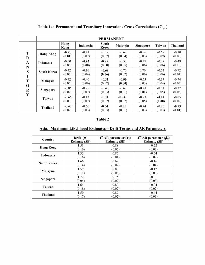
Table 1c: Permanent and Transitory Innovations Cross-Correlations ( ηεΣ )

PERMANENT

T R A N S I T O R Y



Hong Kong -0.91 (0.01)

-0.41 (0.07)

-0.19 (0.02)

-0.62 (0.04)

-0.86 (0.03)

-0.68 (0.09)

-0.10 (0.08)

Indonesia -0.60 (0.05)

-0.95 (0.00)

-0.25 (0.00)

-0.53 (0.05)

-0.47 (0.06)

-0.37 (0.06)

-0.49 (0.10)

South Korea -0.42 (0.07)

-0.16 (0.04)

-0.68 (0.06)

-0.70 (0.02)

0.70 (0.06)

-0.63 (0.06)

-0.72 (0.04)

Malaysia -0.42 (0.05)

-0.40 (0.06)

-0.51 (0.02)

-0.90 (0.00)

-0.73 (0.03)

-0.37 (0.04)

-0.74 (0.03)

Singapore -0.86 (0.02)

-0.25 (0.07)

-0.40 (0.03)

-0.69 (0.01)

-0.90 (0.01)

-0.81 (0.05)

-0.37 (0.03)

Taiwan -0.66 (0.08)

-0.13 (0.07)

-0.31 (0.02)

-0.24 (0.02)

-0.73 (0.05)

-0.97 (0.00)

-0.05 (0.02)

Thailand -0.43 (0.02)

-0.66 (0.03)

-0.64 (0.03)

-0.75 (0.01)

-0.44 (0.03)

-0.26 (0.03)

-0.93 (0.01)

Table 2

Asia: Maximum Likelihood Estimates – Drift Terms and AR Parameters

Country Drift (µµµµi) Estimate (SE)

1st AR parameter (φφφφ1t) Estimate (SE)

2nd AR parameter (φφφφ2t) Estimate (SE)

Hong Kong 1.51 (0.16)

0.88 (0.05)

-0.22 (0.03)

Indonesia 1.35 (0.16)

0.86 (0.01)

-0.64 (0.02)


0.62 (0.07)

-0.16 (0.04)


0.89 (0.03)

-0.12 (0.03)


0.75 (0.02)

-0.01 (0.03)

Taiwan 1.64 (0.18)

0.80 (0.02)

-0.04 (0.02)


0.89 (0.02)

-0.44 (0.01)

Table 3

Latin America: Estimated Standard Deviations and Cross-Country Correlations

Maximum Likelihood: -1292.97

Table 3a: Permanent Innovations ( ηΣ )

Std. Dev.



Argentina 3.34 (0.48) 1

Brazil 2.38

(0.26) 0.29

(0.12) 1

Chile 4.05 (0.46)

0.10 (0.2)

0.00 (0.08) 1

Colombia 1.51 (0.08)

0.17 (0.02)

0.57 (0.05)

0.25 (0.05) 1

Mexico 2.20 (0.18)

0.17 (0.00)

0.40 (0.10)

-0.02 (0.00)

0.27 (0.04) 1

USA 0.74

(0.04) -0.08 (0.01)

0.57 (0.09)

0.21 (0.03)

-0.02 (0.11)

-0.27 (0.02) 1

Table 3.3b: Transitory Innovations ( εΣ )

Std. Dev.



Argentina 2.69 (0.24) 1

Brazil 2.70

(0.25) -0.01 (0.00) 1

Chile 3.89 (0.30)

0.30 (0.01)

-0.30 (0.03) 1


0.02 (0.05)

0.45 (0.06)

0.13 (0.04) 1

Mexico 1.62 (0.16)

0.20 (0.03)

0.55 (0.14)

-0.31 (0.05)

0.41 (0.06) 1

USA 0.36

(0.04) -0.15 (0.04)

-0.18 (0.00)

-0.09 (0.08)

-0.28 (0.06)

-0.69 (0.03) 1

Table 3c: Permanent and Transitory Innovations Cross-Correlations ( ηεΣ )

PERMANENT

T R A N S I T O R Y


Argentina -0.85 (0.03)

-0.04 (0.14)

-0.24 (0.04)

-0.13 (0.06)

-0.20 (0.06)

0.29 (0.05)

Brazil -0.19 (0.07)

-0.90 (0.01)

0.26 (0.02)

-0.42 (0.06)

-0.49 (0.11)

-0.43 (0.08)

Chile -0.16 (0.03)

0.07 (0.01)

-0.91 (0.02)

-0.20 (0.05)

0.17 (0.04)

-0.17 (0.03)

Colombia -0.05 (0.02)

-0.59 (0.04)

-0.16 (0.05)

-0.97 (0.02)

-0.29 (0.03)

0.00 (0.12)

Mexico 0.68 (0.07)

-0.45 (0.14)

0.15 (0.02)

0.40 (0.07)

-0.90 (0.02)

-0.29 (0.07)

USA 0.16 (0.03)

0.10 (0.02)

0.21 (0.06)

0.31 (0.04)

0.72 (0.09)

-0.37 (0.08)

Table 4 Maximum Likelihood Estimates: Drift Terms and AR Parameters

Country Drift (µµµµi) Estimate (SE)

1st AR parameter (φφφφ1t) Estimate (SE)

2nd AR parameter (φφφφ2t) Estimate (SE)

Argentina 0.45 (0.29)

0.59 (0.10)

-0.07 (0.06)

Brazil 0.95 (0.20)

0.92 (0.04)

-0.13 (0.03)

Chile 0.87 (0.34)

0.83 (0.03)

-0.10 (0.03)


0.90 (0.04)

-0.32 (0.03)

Mexico 0.89 (0.18)

0.72 (0.06)

-0.24 (0.04)

USA 0.77 (0.06)

1.65 (0.06)

-0.76 (0.03)

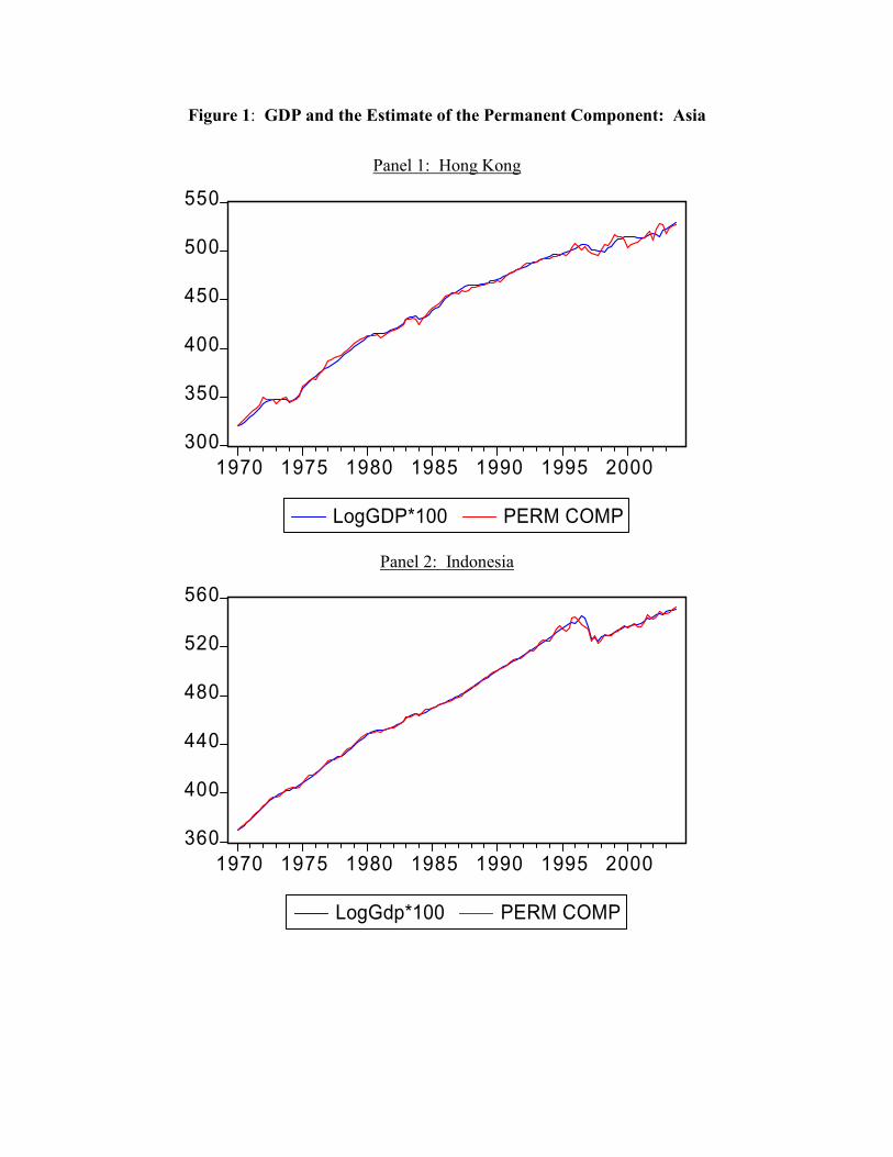
Figure 1: GDP and the Estimate of the Permanent Component: Asia

Panel 1: Hong Kong

300

350

400

450

500

550

1970 1975 1980 1985 1990 1995 2000

LogGDP*100 PERM COMP

Panel 2: Indonesia

360

400

440

480

520

560

1970 1975 1980 1985 1990 1995 2000

LogGdp*100 PERM COMP

Panel 3: South Korea

400

450

500

550

600

650

700

1970 1975 1980 1985 1990 1995 2000


Panel 4: Malaysia

250

300

350

400

450

500

1970 1975 1980 1985 1990 1995 2000


Panel 5: Singapore

200

300

400

500

1970 1975 1980 1985 1990 1995 2000


Panel 6: Taiwan

360

400

440

480

520

560

600

1970 1975 1980 1985 1990 1995 2000


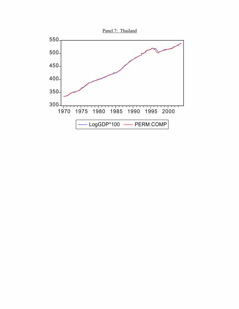
Panel 7: Thailand

300

350

400

450

500

550

1970 1975 1980 1985 1990 1995 2000


Figure 1: GDP and the Estimate of the Permanent Component: Latin America and

U.S.

Panel 1: Argentina

500

520

540

560

580

1970 1975 1980 1985 1990 1995 2000


Panel 2: Brazil

520

560

600

640

680

1970 1975 1980 1985 1990 1995 2000


Panel 3: Chile

280

320

360

400

440

480

1970 1975 1980 1985 1990 1995 2000


Panel 4: Colombia

320

360

400

440

480

1970 1975 1980 1985 1990 1995 2000


Panel 5: Mexico

440

480

520

560

600

640

1970 1975 1980 1985 1990 1995 2000


Panel 6: USA

800

840

880

920

960

1970 1975 1980 1985 1990 1995 2000

LogGDP*100 PERMCOMP

Figure 3: Estimate of the Transitory Component: Asia

Panel 1: Hong Kong Transitory Component

-20

-10

0

10

20

1970 1975 1980 1985 1990 1995 2000

Panel 2: Indonesia Transitory Component

-8

-4

0

4

8

1970 1975 1980 1985 1990 1995 2000

Panel 3: South Korea Transitory Component

-4

0

4

8

1970 1975 1980 1985 1990 1995 2000

Panel 4: Malaysia Transitory Component

-10

0

10

20

1970 1975 1980 1985 1990 1995 2000

Panel 5: Singapore Transitory Component

-10

-5

0

5

10

15

1970 1975 1980 1985 1990 1995 2000

Panel 6: Taiwan Transitory Component

-8

-4

0

4

8

12

1970 1975 1980 1985 1990 1995 2000

Panel 7: Thailand Transitory Component

-4

0

4

8

12

1970 1975 1980 1985 1990 1995 2000

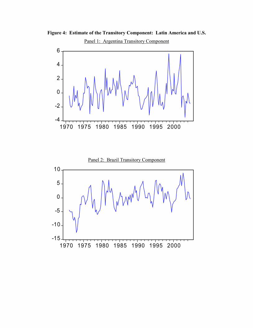
Figure 4: Estimate of the Transitory Component: Latin America and U.S.

Panel 1: Argentina Transitory Component

-4

-2

0

2

4

6

1970 1975 1980 1985 1990 1995 2000

Panel 2: Brazil Transitory Component

-15

-10

-5

0

5

10

1970 1975 1980 1985 1990 1995 2000

Panel 3: Chile Transitory Component

-10

-5

0

5

10

15

1970 1975 1980 1985 1990 1995 2000

Panel 4: Colombia Transitory Component

-4

-2

0

2

4

6

1970 1975 1980 1985 1990 1995 2000

Panel 5: Mexico Transitory Component

-4

-2

0

2

4

6

1970 1975 1980 1985 1990 1995 2000

Panel 6: USA Transitory Component

-4

-2

0

2

4

1970 1975 1980 1985 1990 1995 2000

Macroeconomic Fluctuations in Emerging Economies: An Unobserved Components Approach

Documents

Transcript of Macroeconomic Fluctuations in Emerging Economies: An Unobserved Components Approach