buildings

Review

Macro-Impacts of Air Quality on Property Values in China—AMeta-Regression Analysis of the Literature

Jianing Wang *, Chyi Lin Lee and Sara Shirowzhan

�����������������

Citation: Wang, J.; Lee, C.L.;

Shirowzhan, S. Macro-Impacts of Air

Quality on Property Values in

China—A Meta-Regression Analysis

of the Literature. Buildings 2021, 11,

48. https://doi.org/10.3390/

buildings11020048

Academic Editor: Benedetto

Manganelli

Received: 28 December 2020

Accepted: 26 January 2021

Published: 30 January 2021

Publisher’s Note: MDPI stays neutral

with regard to jurisdictional claims in

published maps and institutional affil-

iations.

Copyright: © 2021 by the authors.

Licensee MDPI, Basel, Switzerland.

This article is an open access article

distributed under the terms and

conditions of the Creative Commons

Attribution (CC BY) license (https://

creativecommons.org/licenses/by/

4.0/).

Faculty of Built Environment, University of New South Wales, Sydney, NSW 2052, Australia;chyilin.lee@unsw.edu.au (C.L.L.); s.shirowzhan@unsw.edu.au (S.S.)* Correspondence: jianing.wang1@student.unsw.edu.au

Abstract: Air pollution has received increasing attention in recent years, particularly in China, dueto the rapid industrialisation that has wrought intense levels of air pollution. A number of studies,therefore, have been devoted to quantifying the impacts of air pollution on property value in China.However, the empirical results are somewhat mixed. This naturally raises questions of whether thereis a significant relationship between air quality and housing prices and the plausible reasons forthe mixed results in previous studies. This study aims to fill this gap by explaining the variationsin the findings by a meta-regression analysis. To control for heterogeneity, a weighted least squaremodel was used to explore the factors influencing the magnitude and significance of the air qualityeffect based on empirical estimates from 117 observations. This study confirms that air quality doeshave a discernible impact on housing prices beyond the publication bias. Besides, the types of airquality indicator and the air data source do significantly influence estimates through affecting boththe magnitude of the elasticity and the partial correlation coefficient (PCC). Further, the selections ofcontrol variables and estimation approaches also have significant impacts on estimates. This studyalso finds that published papers tend to be biased towards more economically significant estimates.The implications of the findings have also been discussed.

Keywords: air pollution; housing prices; meta-regression analysis; China

1. Introduction

Megacities all around the world have struggled with severe air pollution in recentdecades [1], especially cities in developing countries [2]. China is one of the develop-ing countries that has been experiencing severe air pollution due to its rapid economicgrowth in which it heavily relies on coal burning to meet the energy demand from themanufacturing industry.

Since China’s economic reform in the 1980s, China has been keeping a relatively fastspeed of economic growth, with an annual average rate of over 7% in the last decade [3].China’s Gross Domestic Product (GDP) accounts for 16% of the world’s GDP in 2018, whichmakes China the engine of economic growth, the largest industrial country and the largesttrader of goods across the globe [4]. However, those great achievements are accomplishedbased on substantial energy consumption and at the sacrifice of the environment, whichconsequently results in the hover of notorious ambient air pollution over the majority ofthe urban areas in China. The air pollution problem in China has become worse and hasraised the attention of the public since 2005, whilst it has deteriorated continuously overtime [5].

Although China’s central and local governments have introduced numerous relevantpolicies and regulations to combat the ambient air pollution, such as the Air PollutionPrevention and Control Action Plan, traffic restriction and environmental tax, etc., no no-ticeable improvement in air quality is evident [6]. Approximately over half of China’s urbanpopulation are under severe pernicious air pollution with the concentrations of PM2.5 and

Buildings 2021, 11, 48. https://doi.org/10.3390/buildings11020048 https://www.mdpi.com/journal/buildings

Buildings 2021, 11, 48 2 of 24

PM10 five times exceeding the guideline set by the World Health Organisation (WHO) [7].The air quality in some specific areas is even worse. For example, the air pollution index inBeijing was beyond the measurable capacities in 2013, and the PM2.5 concentration reachedthe level of over 1000 µg/m3 in 2015 [6], while the standard concentration of PM2.5 thataffects human health is 10 µg/m3 set by the WHO.

According to the previous literature, air pollution has substantial effects on the risein mortality rate and the decline of average lifespan [8,9]; respiratory diseases and cardio-vascular diseases including lung cancer, asthma, respiratory allergy, inflammation, heartdisease, thromboembolic and sclerosis [10–14]. Due to the significant adverse impacts ofair pollution on human health and lifespan [9,11,12,14], it has received increasing attentionfrom scholars and governments as well as residents. Many scholars have assessed theinfluences of air pollution on various aspects, including climates [15], the health of plantsand animals [16–18], telecommunication and traffic [19–21] and buildings [22]. Thesestudies generally found that ambient air pollution threatens the suitability of habitats andbreaks the balance of healthy ecosystems [23]. It also causes decreases in the biodiversity ofplants and animals and reduces crop yield [16–18,24,25]. The pollutants in the air restrictthe transmission of telecommunication signals and traffic and decrease the sustainabilityof buildings [19,21,26–28].

Given the significant multidimensional adverse effects of air pollution and the increas-ing public awareness of a better living environment [29], the demand for clean air has alsoincreased over time. The residents are willing to pay for a reduction in air pollution leveland move to a place with better air quality if they can afford it [30–32]. Such demand hasresulted in emerging studies to explore the relationship between air quality and housingprices. The impacts of air quality on housing prices are commonly addressed with a hedo-nic price model (HPM), which considers air quality as one of the environmental attributesof the property and calculates the price of air quality based on the observations of realestate values [33].

Following the pioneering work of Ridker and Henning [34] on the influences of airquality on housing value, scholars continue to contribute to this topic by introducingextra key variables, comparing different function forms, applying spatial econometricapproaches, using instrument variables, testing the theory with macro-housing data andmicro-housing data as well as subjective and objective indicators for air quality [35–37].Most of the studies confirm that air quality is significantly associated with housing values,and the improvement of air quality would lead to an increase in local housing prices.

In recent years, the association between air quality and real estate values has attractedclose attention from Chinese scholars with respect to the heightened level of air pollution inChina. Several attempts have been conducted to assess the relationship between air qualityand housing prices, applying both micro and macro hedonic empirical studies. However,the empirical results from these Chinese studies are somewhat mixed in that some studiesindicate a weak relationship between air quality and housing prices [38] and other studiesdocument the strong impact of air quality on housing values [6,39,40]. Further, there arehuge variations among the results reported by studies, which find significant impacts ofair quality on housing prices and that the percentage change in housing value caused by a1% change in air quality ranges from 0.0365 to 1.3% [6,41].

Some researchers attempted to identify influential factors to explain the variationsamong environmental hedonic empirical studies [42,43]. Nevertheless, it is difficult todistinguish the influential factors only relying on a systematic review with respect todescriptive analyses, which could be subjective in study selection and result interpreta-tion [44]. To offer objective and persuasive explanations about the mixed results amongempirical studies, quantitative approaches are needed. In this case, a meta-regressionanalysis can be a powerful tool to identify influential factors and to extract additional infor-mation on how those influential factors affect the results of the estimates. By employingeconometric specifications, a meta-regression analysis can objectively and accurately esti-

Buildings 2021, 11, 48 3 of 24

mate the real effects of air quality on macro housing prices and enhance our understandingof why the impacts of air quality vary across the previous studies [44].

Several meta-regression analyses [45–48] have been conducted, exploring the rela-tionship between housing price and environmental contamination including air pollution,landfills, underground water contaminant, pipeline, nuclear power plant and airborneradioactive release. However, previous meta-regression analyses focused on exploring thecritical factors in micro-level hedonic studies, which quantify the impacts of air qualityon housing prices based on the housing price data of individual properties and largelyignore macro variables. Compared with micro-level studies, macro studies tend to applya panel dataset. Besides, the influential factors affecting micro and macro housing pricesare different; therefore, the control variables in micro and macro studies are considerablydifferent. Instead of employing housing characteristics such as locational and structuralcharacteristics as control variables, macro studies apply macroeconomic features, demo-graphic characteristics, housing supply, infrastructure and public service level to control theinfluences on macro housing prices. As macro hedonic air quality studies are significantlydifferent from micro hedonic air quality studies, whether the results of the macro-levelmeta-regression analysis are consistent with the previous findings of micro-level studies isstill an open question.

This study aims to explore the factors affecting the impacts of air quality on macrohousing prices with a focus on the Chinese context. We confined our study to China as itoffers a unique dataset for a number of reasons. Firstly, the majority of Chinese cities havesuffered from severe air pollution in the last decade. Given the high level of air pollution inChina, a dedicated study of China is required to offer a comprehensive explanation of theimpact of air quality in China. Secondly, China has experienced a rapid industrialisationand urbanisation process in the last three decades, and the development is based onsubstantial energy consumption and the sacrifice of the environment. Thus, a dedicatedstudy of China would provide some empirical evidence of how the environment will bepriced by households. Further, almost all macro hedonic air pollution studies selectedChina as a study case. The relatively small sample size for studies conducted in otherregions might lack the explanatory ability for the variations among studies. Therefore,a dedicated meta-regression analysis study of air pollution on Chinese housing prices ismore capable of delivering a comprehensive explanation of the fluctuations of the estimatesin the Chinese context. Finally, the macro analysis of air quality on property value onlycommenced in 2000. This reduces the potential bias of the time, as most studies wereconducted since 2000.

This study contributes to the literature in a number of ways. Firstly, to the bestof our knowledge, this is the first meta-regression analysis focusing on air pollutionimpacts on macro-level housing markets. This study provides a systematic review ofthe macro hedonic air quality studies in China. This may guide policymakers to have acomplete understanding of the effects of air quality and to make a more balanced policyin terms of economic growth and air quality. Secondly, the publication bias conducted inthis meta-regression analysis confirms that air quality does have a noticeable impact onhousing prices, excluding the influence of publication bias. This assists policymakers andhomeowners in making a more informed decision. Thirdly, this meta-regression analysisalso provides us with a fuller understanding of the reasons for the variations of previousstudies, which help scholars on data, estimation methods and control variables selections.Further, it can be referred to as a benchmark for researchers to understand how theirresults fit with others. Fourthly, as previous meta-regression analyses use samples before2000, this study will supplement previous research by applying a more recent dataset.Finally, through identifying critical factors affecting estimates of macro hedonic air qualitystudies, this study enables a comparison between macro and micro hedonic studies. This isexpected to offer a complete understanding of the impact of air quality from both macroand micro perspectives.

Buildings 2021, 11, 48 4 of 24

This paper is structured as follows. Section 2 presents the literature review aboutprevious meta-regression analyses in the topic of environmental impacts on housing prices.Section 3 demonstrates our method of data collection and the design for the meta-regressionanalysis. The publication bias test is also reported in this section. Section 4 reports theregression results of the meta-regression analysis, and Section 5 discusses the strength andweakness of the study. Finally, Section 6 draws the conclusion of the overall study.

2. Literature Review

Hedonic price model (HPM) was first formally coined by Court in 1941 [49] to reportthe price index for automotive and investigate the link between functions and pricesby employing regression models [50]. Then, the theory of HPM was developed by thetwo major approaches: utility theory and revealed preference theory [34,51]. These twomethods aim to quantify the implicit prices of attributes through empirical studies based onthe products’ characteristics and prices [52]. The modern HPM is based on the assumptionsthat the property is a set of goods, and individuals are free to move according to theirdemands [53]. A house is considered as a set of immovable and local attributes, includingthe conditions of the entire urban area where it is located [54], the accessibility to otherfacilities and travel convenience and the quality of the neighbourhood [55–57] such as thequality of public services, the quality of the residents and the quality of the neighbourhoodenvironment [58–60]. HPM is commonly applied to understand the real estate pricedynamics in general or to estimate the variation caused by a specific factor [61]. Estimatingneighbourhood characteristics’ impacts on housing prices has always been a popular topicamong HPM studies [61]. Among neighbourhood characteristics, there are three categoriesincluding social factors (race and crime rate), infrastructure (school, park and public goods)and environmental factors (air pollution, forest and wetlands). Recently, with the rise inthe public awareness of the importance of the environment, the effects of environmentalexternalities arouse more extensive attention from scholars. A number of environmentalfactors, both amenities and disamenities, have been investigated, including landscape andurban water bodies [62,63], urban trees [64], noise [65], hazardous waste site [66], wildfirerisk [67], flood risk [68,69], etc.

Ridker and Henning [34] carried out probably the first empirical study to investigatethe influence of air pollution on housing prices; afterwards, scholars continue to explorethe variations in housing values caused by the changes in air quality. A number of studieshave been devoted to gauging the linkage between air pollution and housing prices inChina. The results have frequently observed that the interlinkage is mixed and dependenton the markets examined. Wang and Cai [70] found a negative and statistically significantassociation between air pollution and housing prices; reflecting that homebuyers arewilling to pay a premium for better air quality. Comparable evidence is also documentedby Kong [41], Dong, Zeng [71], Chen and Jin [72], Chen [73], Zou [74], Shen [75] andDong, Zeng [76]. Chen and Chen [6] and Sun and Yang [77] suggested that the findingsare intuitively appealing, as the demand for clean air has increased over time in Chinawith respect to the heightened level of air pollution and the increasing awareness on theimportance of air quality.

However, a number of empirical studies found contradictory results. Chen andChen [6], Zheng, Kahn [37], Jia [39], Wang and Shi [40], Sun and Yang [77], Zhang andHuang [78], Huang and Lanz [79] and Yu [80] found mixed results in that they did notfind a strong relationship between air quality and Chinese housing prices in some specificcases, for example, study period, submarket, etc. Further, Chen and Chen [6] and Wangand Shi [40] indicated that air pollution had been paid more attention by residents wholived in developed regions or high-ranking cities than homebuyers who reside in lessdeveloped areas or low-ranking cities. In fact, the documented positive and statisticallyinsignificant association could be attributed to omitted variable bias [6,40,79,80]. This isfurther exacerbated by the fact that there is no consensus on the magnitude of air pollution’simpact on housing price. The elasticity (the change in housing price with one percentage

Buildings 2021, 11, 48 5 of 24

change in air quality) varies across these studies, ranging from 0.3679 (a premium for airpollution) to −1.3038 (a discount for air pollution). To sum up, the empirical evidence onthe interlinkage between air quality and Chinese housing prices are mixed. This naturallyraises questions of whether air quality is priced by home buyers and what are the plausiblereasons for the mixed results that have been documented by previous studies.

Several scholars had conducted research by reviewing the literature to identify the in-fluential factors and to explore further and explain the reasons why different environmentalhedonic studies come up with different results with the focus on US studies. These includetwo review papers concerning the broad areas of environmental contamination conductedby Jackson [42] and Boyle and Kiel [43]. Jackson [42] reviewed 21 papers focusing on theimpacts of environmental factors (including landfills, underground water contaminant,pipeline, nuclear power plant and airborne radioactive release) on housing prices andfound that the impacts on residential and commercial housing are stronger in urban areasand the regions with greater market demands. Boyle and Kiel [43] compared the empiricalresults of the impacts of environmental pollutants on residential property value based on39 studies, which pay attention to several different pollutants, including air and waterquality, undesirable land use, neighbourhood variables and multiple pollutants. The au-thor suggested that the coefficients of air pollution impacts are influenced by the controlvariables included in the models. In terms of water contamination, water measurementsare crucial to the results of the estimates. The measurement, which can be easily observed,results in the best estimate, while multiple measurements are problematic because of themulticollinearity between different measurements.

Considering these two review papers compare the empirical results through simpledescriptive methods; the results might by subjective and inadequate for identifying theinfluential factors resulting in the mixed regression results. In this case, the approach ofmeta-regression analysis can be applied to provide objective and persuasive explanationsabout the variations among empirical studies. The term “meta-analysis” was coined byGlass [81] and was defined as a statistical analysis method with the purpose of synthesisingexisting findings based on individual studies. Glass [81] conducted the first meta-analysisin the area of psychology and first proposed the term “effect sizes”—the dependent variablein meta-analysis. Meta-analysis is a commonly applied review method in medicine andsocial science; then, given the difference between economic research and medicine studies,Stanley and Jarrell [44] came up with the concept of “meta-regression analysis”, which isdeveloped based on meta-analysis and enabled the application of meta-regression analysisin other study areas such as business and economics. Stanley and Jarrell [44] introduceddifferent possible effect sizes (including elasticity, t-value, partial correlation coefficient,F-value, etc.) in meta-regression analysis to replace the odds ratio and risk ratio, whichare commonly applied in psychological and clinical studies. Meta-regression analysis wasdefined by Stanley and Doucouliagos [82] as an evidence-based multivariate investigation,exploring the influential factors affecting the estimates reported by previous studies.

Following Stanley’s work, meta-regression analysis had been applied on businessand economics [83–85], and it has become increasingly popular in environmental eco-nomics recently [86]. Some researchers applied the approach of meta-regression analysisto understand the factors affecting estimates of environmental hedonic studies compre-hensively [45–48]. Smith and Huang [45] conducted a meta-analysis to estimate how dataand model specification influence the results of Hedonic price model regression and airpollution with the data collected from 37 studies with overall 167 observations from 1976to 1990 with the focus on major American cities; the author found that the impact of airpollution on housing price is influenced by modelling decision, air pollution measurementsand the condition of the local housing market. Specifically, using sales prices reduces thesignificant effects of air pollution compared with census data, and the linear model alsoreduces the significance of air pollution. Moreover, the number of air pollution measure-ments in models reduces the prospects for finding a significant relationship. Then, Smithand Huang [46] further analysed some of those studies (with 86 observations) through

Buildings 2021, 11, 48 6 of 24

applying the following two approaches: minimum absolute deviation and ordinary leastsquare. After reconstructing the data, this study draws the following conclusion that 1 unitreduction in PM10 concentration is related to a USD 110 increase in property value, whichequals to 0.1% of the property value.

Simons and Saginor [47] addressed the effects of several environmental contaminationsources on housing prices in the United States. This study estimates the effects of the con-textual and methodological variables; the regression results show that contamination type,amenities, region, distance from the contamination source, information of announcementand research methods are significantly associated with regression results of the reductionon property value.

Chen, Li [48] identified the influential scenario, modelling and contextual variablesthat affect the impacts of urban rivers on residential property values through conductinga meta-analysis with 30 studies (with 53 observations). Employing the random-effectmodel with the data of contextual variables, scenario variables and modelling variables,estimate results indicate that the effect size is affected by the abovementioned three typesof variables. Specifically, in terms of environmental amenity scenarios, the view of theriver is the most significant factor, while the proximity that received the widest attention inprevious studies has the lowest relative value. As for modelling variables, the study yearand whether the result is significant shows significant positive influences on effect size;however, whether the model considers spatial factors is not statistically significant to effectsize. Among contextual factors, GDP per capita and the average housing price, whichreflect the income level of the case, have significant positive influences on willingness topay for river amenity. Moreover, the population density is negatively related to the impactof urban river impacts, and the regional difference shows insignificant effects.

However, previous literature only paid attention to micro-hedonic studies whichfocus on the influences of environmental factors on individual housing prices, while thecritical factors in macro-level studies have been neglected. Therefore, this paper looks intomacro-scale hedonic price model and environmental contamination of air pollution, fillingthe gap of meta-regression analysis and macro-hedonic price studies.

3. Method

Meta-regression analysis serves as an important tool for a systematic explanationof differences in the previous empirical findings [46,82]. The meta-regression analysisinvolves three major stages. The first stage is to identify the related studies in the literature.One of the primary tasks for identifying relevant studies is to move out systematic biases byconducting searches comprehensively [87]. To be more specific, we need to include as manyof the relevant studies in the meta-regression analysis, instead of only covering some of theseminal studies. All studies, including unpublished papers, can be valuable for identifyinginfluential factors affecting the estimates [88]; a more inclusive sample of a paper canalso address publication bias in the analysis [89]. In addition, to explain the variations insome specific context, it is of great importance to access non-English studies to get a morethorough overview of the studies in this area. After identifying the relevant literature, thesecond stage involves identifying and coding differences as the critical groups of factorsamong selected studies. In general, according to the previous meta-regression analysesabout environmental impacts on housing prices [47,48], three factor groups, includingscenario, methodology and context factors, were identified and used in the meta-regression.Lastly, through undertaking an econometric model to estimate the impacts of each factor,influential factors explaining the variations among empirical studies were finally identified.Except for the abovementioned three steps, we also conducted a publication bias test assuggested by Stanley and Doucouliagos [82] to test whether air quality has genuine effectson real estate price beyond the publication bias. The specific methodology strategies ofdata searching, publication bias test, factors identification, effect size and econometricmethod selection will be elaborated on in the following subsections.

Buildings 2021, 11, 48 7 of 24

3.1. Data

To comprehensively identify the studies investigating the impacts of air quality onmacro housing prices, this study applies the following processes (the specific proceduresare presented in Figure 1): Firstly, in the stage of identification, the original case study dataare assembled through searching in the online bibliographical database—Scopus—andutilising Google Scholar and the reference of the returned studies as a complimentary.Given that the scope of this study is macro-level hedonic price method empirical studiesexploring the relationships between the residential property market and air quality levelin China, the keywords employed for searching are the most representative keywords:“air pollution” or “air quality” or “environmental quality” or “environmental pollution”or “environmental factor” or “living environment” or “soft power” or habitability orcompetitiveness and “housing price” or “housing value” or “property price” or “propertyvalue” or “real estate price” or “real estate value” and China or Chinese. This meta-regression analysis covers papers within all types to reduce the effects of publicationbias, including journal articles, conference articles, book chapters, books, dissertations,conference proceedings, the essays in press and business articles. To further reduce thelanguage bias and to have a more comprehensive understanding of the Chinese context,this research also includes studies written in Chinese. These studies are collected froma Chinese online bibliographical database—Chinese National Knowledge Infrastructure(CNKI). The total number of 65 papers (from Scopus) and 633 studies (from CNKI) werereturned (the search was conducted on 4 December 2020).

Buildings 2021, 11, x FOR PEER REVIEW 8 of 25

Figure 1. Prisma flow diagram [90].

Secondly, in the screening stage, the returned studies were first screened to remove repeated literature. Thirteen repeated papers were removed, and 685 papers remained to be evaluated by title and abstract reviewing following the criterion: the study must have a focus on understanding the impacts of air quality on the housing market. Specifically, studies focussing on the following topics were identified as irrelevant studies and were removed: indoor air quality; cause of air pollution; the tendency of air pollution in a par-ticular region; air pollution improvement and control strategies; air pollution and policy-making; predicting, detecting, processing and recovering air quality data; air pollution caused by construction; air pollution's impacts on house materials; the relationship be-tween air quality and health risk and life quality; factors affecting real estate market or property value; household energy's influence on housing price; factors impacting both air quality and real estate market; the relationships between air pollution and aerosol optical properties.

Thirdly, 55 studies moved to the next stage of eligibility to be further filtered through full-text reviewing, and only studies that satisfied the following criteria were finally in-cluded as the meta-sample: (1) The study must be a macro-level study instead of micro-level study applying individual housing transactions as the dependent variable. (2) The impacts of air quality in the study must be quantified based on the hedonic price method.

Figure 1. Prisma flow diagram [90].

Buildings 2021, 11, 48 8 of 24

Secondly, in the screening stage, the returned studies were first screened to removerepeated literature. Thirteen repeated papers were removed, and 685 papers remained tobe evaluated by title and abstract reviewing following the criterion: the study must havea focus on understanding the impacts of air quality on the housing market. Specifically,studies focussing on the following topics were identified as irrelevant studies and wereremoved: indoor air quality; cause of air pollution; the tendency of air pollution in aparticular region; air pollution improvement and control strategies; air pollution and policy-making; predicting, detecting, processing and recovering air quality data; air pollutioncaused by construction; air pollution’s impacts on house materials; the relationship betweenair quality and health risk and life quality; factors affecting real estate market or propertyvalue; household energy’s influence on housing price; factors impacting both air quality andreal estate market; the relationships between air pollution and aerosol optical properties.

Thirdly, 55 studies moved to the next stage of eligibility to be further filtered throughfull-text reviewing, and only studies that satisfied the following criteria were finally in-cluded as the meta-sample: (1) The study must be a macro-level study instead of micro-levelstudy applying individual housing transactions as the dependent variable. (2) The impactsof air quality in the study must be quantified based on the hedonic price method. Studiesthat use other econometric approaches such as the travel cost method and contingentvaluation method are excluded, as their studies focus on the willingness to pay for airpollution, but their willingness to pay might not necessarily be reflected on housing prices.Although the results that are estimated by different approaches can also reflect the associa-tions between air quality and housing markets, herein, we only focus on the HPM to buildthe consistency that the estimates are based on the same theory and methodology. (3) Theresearch must focus on the residential property market (housing price, rental price andland price are included), and cases that pay attention to the commercial property or othertypes of property are excluded. This criterion is another strategy employed in this study tosatisfy the commodity consistency of the meta-regression analysis [91]. (4) The study mustreport the primary estimations, and the estimates must be capable of being expressed andcompared (after standardisation). Specifically, the study must report the sample size andt-value or standard error of the coefficient.

Finally, there were 17 papers looking into the relationship between air quality andhosing prices from a macro perspective. The specific list of the dataset is shown in Table 1;Figure 2 maps the cities covered by previous studies. Given some of the studies donot provide the detailed information about the cities covered by their studies, the mappresented in Figure 2 only shows the cities included in [6,37,39,71,72,74,77,78].

Table 1. The list of meta-samples.

Reference Air pollution Indicator StudyYear

Number ofCities

Sign andSignificance Elasticity

[70] PM2.5 2006–2016 70 −; sig −0.187 to −0.881%

[77] PM2.52005, 2009and 2013 286 −; mixed −0.0245 to −0.1986%

[76] AQI 2013–2015 74 −; sig −0.209%[71] PM2.5 2002–2016 280 −; sig −0.109 to −0.134%[72] PM2.5 2005–2013 286 −; sig −0.0612 to −0.2416%[40] PM10 2005–2017 30 − and +; mixed 0.3679 to −0.5806%[73] PM2.5 2009–2017 62 −; sig −0.0612 to −0.1217%[74] PM2.5 2015 282 −; sig −0.2759%[41] SO2 2003–2011 104 −; sig −0.0365%[80] SO2 and PM10 2010–2012 74 − and +; mixed 0.025 to −0.35078%[75] Index (SO2, NO2 and PM) 2013 31 −; sig −0.142 to −0.217%[79] PM10 2011 288 − and +; mixed −0.71 to −1.09%[6] PM2.5 2004–2013 286 − and +; mixed 0.34443 to −1.3038%[38] SO2 2003–2015 283 − and +; insig 0.00336 to −0.00117%[78] PM10 and SO2 2015 288 −; mixed −0.09 to −0.68%[39] API 2009–2012 35 −; mixed −0.1918 to −0.7826%[37] PM10 2003–2006 30 −; mixed −0.167 to 0.388%

Notes: AQI refers to air quality index. API refers to air pollution index. − and + refer to whether the study reportsthat air quality has a negative and a positive effect on housing prices, respectively. Mixed refers to the mixedresults reported in which the results are either statistically significant and insignificant.

Buildings 2021, 11, 48 9 of 24Buildings 2021, 11, x FOR PEER REVIEW 10 of 25

Figure 2. The map of the cities covered by sample studies (notes: Yellow dots refer to cities cov-ered by less than 4 studies; green dots denote cities explored by 4 to 6 studies; black dots are cities investigated by more than 6 studies.).

Then, all relevant estimates reported in the selected studies that satisfy the standard-isation criterion were included in the dataset, providing 117 observations in total. The reasons for applying all-set are [82]: Firstly, it greatly expands the sample size for the meta-regression analysis, which helps to explore the explanations for the heterogeneity between studies and within studies. Furthermore, it is sometimes not appropriate or un-available to apply the best set, which only consists of the key regression result reported by the author, because not all studies present clear view about the best estimate. In this case, we need to make some judgements based on personal preferences, which might re-sult in bias of the meta-regression analysis.

3.2. Publication Bias Test Publication selection is the process of selecting and reporting statistically significant

results, and it is a commonly known fact in social science, natural science, political sci-ence and medical research [92–94]. Publication selection can be found between both re-searchers and reviewers [92]. For researchers, they tend to report the models with ex-pected results; for reviewers, they are more likely to accept studies reporting statistically significant results and confirming conventional theories. As the majority of the studies tend to choose for statistical significance, the effects are overstated with larger and more significant estimates. Neglecting the publication selection bias will distort the literature review, including meta-regression analyses [95]. Therefore, a publication bias test is con-ducted to test whether publication bias exists in the empirical studies exploring the macro-impacts of air quality on housing prices.

To test for publication selection bias, a funnel plot is presented in Figure 3. The funnel plot is a scatter diagram, depicting the relationship between estimates and the precision of the estimates, which is commonly used for publication bias detection [96]. Then, a fun-nel asymmetry test (FAT) is performed through a regression model to further test for pub-

Figure 2. The map of the cities covered by sample studies (notes: Yellow dots refer to cities coveredby less than 4 studies; green dots denote cities explored by 4 to 6 studies; black dots are citiesinvestigated by more than 6 studies.).

Then, all relevant estimates reported in the selected studies that satisfy the standard-isation criterion were included in the dataset, providing 117 observations in total. Thereasons for applying all-set are [82]: Firstly, it greatly expands the sample size for the meta-regression analysis, which helps to explore the explanations for the heterogeneity betweenstudies and within studies. Furthermore, it is sometimes not appropriate or unavailable toapply the best set, which only consists of the key regression result reported by the author,because not all studies present clear view about the best estimate. In this case, we need tomake some judgements based on personal preferences, which might result in bias of themeta-regression analysis.

3.2. Publication Bias Test

Publication selection is the process of selecting and reporting statistically significantresults, and it is a commonly known fact in social science, natural science, political scienceand medical research [92–94]. Publication selection can be found between both researchersand reviewers [92]. For researchers, they tend to report the models with expected results;for reviewers, they are more likely to accept studies reporting statistically significant resultsand confirming conventional theories. As the majority of the studies tend to choose forstatistical significance, the effects are overstated with larger and more significant estimates.Neglecting the publication selection bias will distort the literature review, including meta-regression analyses [95]. Therefore, a publication bias test is conducted to test whetherpublication bias exists in the empirical studies exploring the macro-impacts of air qualityon housing prices.

To test for publication selection bias, a funnel plot is presented in Figure 3. The funnelplot is a scatter diagram, depicting the relationship between estimates and the precisionof the estimates, which is commonly used for publication bias detection [96]. Then, afunnel asymmetry test (FAT) is performed through a regression model to further test for

Buildings 2021, 11, 48 10 of 24

publication bias. Stanley and Doucouliagos [82] suggested that FAT, which reflects therelationship between t-statistics and the standard error reported by the studies, can beapplied to test the publication bias. The specification of FAT is shown in Equation (1):

ti = β0 + β1

(1

SEi

)+ µi, (1)

where ti is the t-statistics, and SEi refers to the standard error. Evidence for publicationbias will be judged by the value of β0. If β0 is significantly not 0, there exists publicationbias; otherwise, publication bias does not exist. Additionally, β1 provides an estimate ofwhether there is a genuine effect beyond the potential distortion caused by publicationselection bias [87,88].

Buildings 2021, 11, x FOR PEER REVIEW 11 of 25

lication bias. Stanley and Doucouliagos [82] suggested that FAT, which reflects the rela-tionship between t-statistics and the standard error reported by the studies, can be applied to test the publication bias. The specification of FAT is shown in Equation (1): t = β + β 1SE + μ ,

(1)

where t is the t-statistics, and SE refers to the standard error. Evidence for publication bias will be judged by the value of β . If β is significantly not 0, there exists publication bias; otherwise, publication bias does not exist. Additionally, β provides an estimate of whether there is a genuine effect beyond the potential distortion caused by publication selection bias [87,88].

Figure 3. Funnel plot.

Figure 3 plots the estimated elasticities for air quality impacts on housing prices. As shown in Figure 3, the funnel plot is asymmetric, suggesting that there exists publication bias towards negative elasticities. The results of FAT are shown in Table 2. According to the estimation presented in Table 2, although FAT has limited power to reflect the exist-ence of publication bias [88,97], 𝛽 estimation value rejects the null hypothesis (𝛽 = 0) at 1% significance level, suggesting that publication bias in the effects of air quality on hous-ing prices exists. This result further confirms the interpretation of the funnel plot. With regards to 𝛽 , the result also indicates that 𝛽 is significantly not zero, demonstrating that air quality does affect the property value beyond the publication selection bias.

Table 2. Results of the funnel asymmetry test (FAT).

Variables t 1/SE −0.00224***

(−6.33) Constant −2.395***

(−12.19) Observations 117

R-squared 0.258 Notes: t-statistics in parentheses (*** p < 0.01, ** p < 0.05, * p < 0.1).

Figure 3. Funnel plot.

Figure 3 plots the estimated elasticities for air quality impacts on housing prices. Asshown in Figure 3, the funnel plot is asymmetric, suggesting that there exists publicationbias towards negative elasticities. The results of FAT are shown in Table 2. According tothe estimation presented in Table 2, although FAT has limited power to reflect the existenceof publication bias [88,97], β0 estimation value rejects the null hypothesis (β0 = 0) at 1%significance level, suggesting that publication bias in the effects of air quality on housingprices exists. This result further confirms the interpretation of the funnel plot. With regardsto β1, the result also indicates that β1 is significantly not zero, demonstrating that airquality does affect the property value beyond the publication selection bias.

Table 2. Results of the funnel asymmetry test (FAT).

Variables t

1/SE −0.00224 ***(−6.33)

Constant −2.395 ***(−12.19)

Observations 117R-squared 0.258

Notes: t-statistics in parentheses (*** p < 0.01, ** p < 0.05, * p < 0.1).

Buildings 2021, 11, 48 11 of 24

3.3. Effect Sizes of the Impacts of Air Quality on Housing Prices

There are two types of effect size commonly used in the meta-regression analysis ineconomics and business studies; they are elasticity and partial correlation coefficient (PCC).Each type of the abovementioned effect size has its strength and weakness. PCC refers tothe coefficient between two variables in the multivariate regression model after eliminatingthe effects of other variables [98]. The advantages of applying PCC as the effect size in meta-regression analysis are shown as following [82]: Firstly, PCC is a unitless measure, and itreflects the direction and strength of the relationship between two variables. Therefore,it enables the comparison between different results in various units. Besides, it can beaccessed easily and is more capable of compiling a comprehensive dataset into comparabledata, because most of the studies report the t-value or standard error, which enables thecalculation of PCC. However, as PCC cannot measure the economic effect between twovariables, it is inappropriate to employ PCC in benefit transfer meta-regression analyses [82].Elasticity means the percentage change in the dependent variable when the independentvariable change in 1%, and it measures the economic effects of two variables. As nostandard for functional form selection exists, different estimates might apply differentfunctional forms including linear, semi-log and double-log. To transform all the estimatesinto elasticity, the mean value of housing data and air quality data are needed. However,not all researchers report those mean values in their paper, and this will significantlydecrease the sample size for meta-regression analysis [82].

In this study, both PCC and elasticity are employed as the effect sizes to identifyinfluential factors affecting statistical significance and economic significance between airquality and housing prices. Although PCC is not always directly reported in the research,it can be easily calculated [82] through Equation (2):

PCC =t√

t2 + df(2)

PCC is the partial correlation coefficient; t refers to the t-statistics of regression coefficientreported in the original study; df denotes the degree of freedom of the t-statistics. Thedescriptive statistics of elasticity and PCC are shown in Table 3.

Table 3. The descriptive statistics of the two effect sizes.

Variables Obs Mean Std. Dev. Min Max

Elasticity 117 −0.2289675 0.2697816 −1.303818 0.3679Partial correlation coefficient 117 −0.1383982 0.1448643 −0.8152795 0.1669264

3.4. Independent Variables

According to the three examples of literature reviewed and the consideration ofthe concept of the effects of air pollution on real estate market, several factors can poseimpacts on the final regression results, these including the elements in the two broadcategories: scenario variables and methodological variables [48,99]. In this meta-analysis,we try to identify and code any of the possible influential factors, which might haveeffects on regression results to explain the heterogeneity among estimates. We introducetwo additional types of factors, namely, data source factors and modelling factors, to obtaina more comprehensive understanding of the influence of those factors on the empiricalvalues. In this study, three groups of variables including scenario and data variables(the combination of scenario variables and data variables), methodology variables andmodelling variables will be considered to identify influential factors for the mixed results.The contextual variable of average housing price is initially considered. As suggestedby Stanley and Doucouliagos [82], we applied a general-to-specific approach to identifyinfluential factors. However, the average housing price was found to be insignificant.Further, when employing the stepwise method to introduce each group of factors, addingthe variable of housing price results in inconsistency among models; dropping this variable

Buildings 2021, 11, 48 12 of 24

will lead to a more robust result. This could also be attributed to the high correlation ofhousing supply in which this is intuitively appealing, as higher supply might lead to alower housing price [59,60]. Table 4 shows the definition of each variable, and the resultsof the variance inflation factor (VIF) test of these variables are shown in Appendix A. Thevariables included in the abovementioned three groups will be explained below.

Table 4. The definition of meta-variables.

Variables Dimension Definition Reference Case

Scenario and data factors

D_ai Air index = 1 if the study using air index as airquality indicator

The study using single air pollutant as airquality indicator

D_ie Industrial_emission = 1 if the air pollution data are based onindustrial emission

The air pollution data are based onmonitoring station reading

D_sp Source_published = 1 if the sample is a publishedacademical article The sample is an unpublished dissertation

Methodological factorsD_p Panel = 1 if the data type is panel data The data type is cross-sectional data

D_s Spatial = 1 if the spatial effects are controlled in theregression model

Spatial effects are not considered inthe study

D_iv IV = 1 if the estimate introducesinstrument variable

The study does not includeinstrument variable

Modelling factors

D_i Infrastructure = 1 if the model applies infrastructurevariable(s) as the independent variable(s) -

D_hs Housing_supply = 1 if the model applies housing supplyvariable(s) as the independent variable(s) -

D_oe Other environmental = 1 if the model applies other environmentvariable(s) as the independent variable(s) -

3.4.1. Scenario and Data Factors

Scenario and data factors consist of variables related to the scenario of air qualityindicator and the source of the data. In terms of the air quality indicators, there are twobroad categories included in our dataset: single air pollutant and the index of severalcombined air pollutants. Compared with the level of a single air pollutant, air indexescan reflect the air quality level more comprehensively with respect to it measures the airquality by considering the level of all six types of the major air pollutants. It should benoted that studies that consider the concentration of a single air pollutant as air qualityindicators usually select the major source of air pollution, such as PM2.5, PM10, SO2, andthese air pollutants might be more sensible and noticeable compared with the air indexesand might receive closer attention from the residents. In this study, we introduce a dummyvariable of “air index”, which represents the studies applying air indexes as air qualityindicators to test the impacts of different scenarios on estimates.

Two data factors are considered in this study: the source of air quality data and thesource of the original case studies. According to the selected studies, most of them utilise thereadings from the monitoring stations to measure the air quality level, while others take theindustrial emission data from city-level official census tracts as the city air quality indicators.Monitoring station readings, which reflect the air quality in specific locations, might bebiased in representing the air quality of the entire city. Fortunately, most of the cities inChina have several monitoring stations in different districts and counties. It is appropriateto apply the average value of the readings of all monitoring stations in a specific region toreflect the air quality condition for the entire region. Compared with monitoring stationreadings, industrial emission data only measure the air pollutant generated by factoriesand ignore the air pollutant emitted by other sources such as transportation emission.Therefore, monitoring station readings are capable of representing the actual air quality

Buildings 2021, 11, 48 13 of 24

level for the city. “Industrial_emission” is added as a dummy variable in the meta-variableto test whether different air pollution data sources have influences on estimates.

As for the source of the original case studies, the sample cases are a mix of pub-lished journals and unpublished dissertations. Undoubtedly, papers published in thepeer-reviewed journal are mostly of a high quality but tend to report significant results.The unpublished dissertations are theses to fulfil the requirement of completing a Masterdegree or a Doctoral degree; therefore, we just assume that these dissertations are also of ahigh quality. To test whether published papers tend to report more meaningful results, weintroduce the variable of “source-published” in this meta-regression analysis. To measureand control the quality of the study, precision (inverse of standard error) is applied as theweight of the model to control the influence of the study quality.

3.4.2. Methodological Factors

Methodological factors refer to the variables related to the methodology of the originalempirical studies, including the type of data used and the estimation approaches applied.There are two types of data included in the meta-sample—panel data and cross-sectionaldata. To testify impacts of data type on regression results, a dummy variable of “panel”is set.

As researchers continue contributing to investigate the relationship between air qualityand housing prices, some studies apply advanced approaches to come up with morecomprehensive explanations about air quality and property value. Some studies applyspatial econometrics to control the effects of spatial factors (spatial dependence, spatialheterogeneity or both), while some studies apply instrument variables with a two-stagemethod to address the endogenous problem. Overlooking spatial or endogenous factorsmight affect the estimates or result in biased estimates. Two dummy variables are set as“spatial” and “IV” in this study to understand the effects of using spatial econometrics andinstrument variable on estimates.

3.4.3. Modelling Factors

Modelling factors reflect the selections of control variables included in hedonic models.Undoubtedly, the selection of independent variables is critical to the regression results andthe goodness-of-fit of the model. There are four types of control variables included in theselected studies, including infrastructure characteristics, housing supply characteristics,demography and socioeconomics characteristics and other environmental characteristics.These factors have been widely seen as a key factor in explaining housing markets asdocumented by Liang, Koo [56], Lee and Locke [57], Bangura and Lee [59], Bangura andLee [60], Bangura and Lee [100] and Shih, Li [101]. Infrastructure characteristics reflect theinfrastructural level of the region, such as the number of universities, hospitals, libraries,road area, etc. Housing supply characteristics represent the supply of the property throughthe supply of residential land, the total area for sale, etc. Other environmental characteristicsrefer to other neighbourhood and environmental factors except for air quality, such as greenland area, rainfall, temperature, etc. All studies include demographic and socioeconomicfactors in their models; therefore, we focus on the influences of the other three types ofvariables, which are not included in all studies, on the regression results. A set of themodelling variables are introduced to examine the role of controlling different types ofvariables in the hedonic model specifications.

3.5. Meta-Regression Analysis Model Specification

As mentioned above, we introduce three groups of the factors, which might affect theestimate in this meta-regression analysis as the meta-regressors to systematically addressthe heterogeneity. A typical meta-regression analysis model is shown in Equation (3): [82]

pi = α0 + ∑kαkDik + µi (3)

Buildings 2021, 11, 48 14 of 24

where i refers to the individual estimate(s), pi is the dependent variable, which refers tothe effect size of observation i, Dik is the meta-regressor k of the observation i, αk refers tothe model parameter related to meta-regressor k. α0 is the constant of the model, and µi isthe residual.

However, µi in different estimates are significantly different; this results in the dissat-isfaction of the independent distribution condition. Therefore, it is inappropriate to applyordinary least square. In this case, the random-effect model is a popular approach formeta-regression analyses and widely used in previous studies [48,99]. Compared with therandom-effect model, the fixed-effect model only allows for within-study variations, whichis likely to neglect the characteristics of different studies [102], for example, the differencesbetween housing markets. Further, Braden, Feng [103] argued that the fixed-effect modelsgenerate inefficient results in meta-regression analyses. Therefore, it is more appropriateto employ the random-effect model. However, Stanley and Doucouliagos [82] stated thatusing random-effect models in meta-regression analyses increases bias, because it is likelyto reintroduce the publication bias into the models. To filter the publication selectionbias, it is more appropriate to apply a weighted least square (WLS) method to identifyinfluential factors in this meta-regression analysis [82]. When publication selection biasis detected, the publication selection effects are correlated with the standard errors [82].Thus, the inverse of the standard error is employed as the analytic weight to correct for thedetected publication bias; the model can be expressed as Equations (4) and (5). To ensurethe robustness of our baseline results, we re-ran our PCC model by fixing market levelsas suggested by Lee, Stevenson and Lee [104]. The results are fairly robust in which wefound that scenario and data factors, methodological factors and modelling factors havesignificant effects on estimates. In other words, the results did not alter the conclusion.

PCCi/sei = α0/sei + ∑kαkDik/sei + εi (4)

Ei/SEi = α0/SEi + ∑kαkDik/SEi + εi (5)

where PCCi and Ei refer to the effect size PCC and elasticity of observation i; sei and SEiare the standard error of PCCi and Ei; Dik is the meta-regressor k; αk refers to the modelparameter related to meta-regressor k; α0 is the constant of the model.

4. Results

The correlation coefficient of each meta-variable is reported in Table 5. According tothe results reported in Table 5 and the VIF value (reported in Appendix A), there is nomulticollinearity issue among the variables. The results of the meta-regression analysis areshown in Tables 6 and 7.

Table 5. Correlation coefficient matrix.

D_ai D_ie D_sp D_i D_hs D_oe D_p D_s D_iv

D_ai 1.0000 - - - - - - - -D_ie −0.1526 1.0000 - - - - - - -D_sp −0.3039 0.1254 1.0000 - - - - - -D_i −0.4705 −0.2910 0.0244 1.0000 - - - - -

D_hs 0.4208 −0.1526 −0.1161 −0.1094 1.0000 - - - -D_oe −0.2495 −0.2404 0.3100 0.3202 0.1928 1.0000 - - -D_p −0.2676 0.0461 −0.2314 −0.0332 −0.5269 −0.1523 1.0000 - -D_s −0.086 −0.1526 −0.4291 0.3034 −0.1584 −0.2495 0.1862 1.0000 -D_iv −0.1282 −0.1235 0.1593 0.0633 0.0423 −0.0718 −0.0020 −0.1282 1.0000

Buildings 2021, 11, 48 15 of 24

Table 6. Meta-regression analysis results (elasticity).

(1) (2) (3)

Variables E E E

Scenario and data factorsD_ai −0.107 *** −0.105 *** −0.128 ***

(−2.909) (−2.630) (−2.836)D_ie 0.121 *** 0.101 *** 0.0832 ***

(9.067) (4.735) (3.278)D_sp 0.0612 *** 0.0623 *** 0.0643 ***

(6.007) (6.179) (6.495)Methodological factors

D_p - 0.0389 0.0469- (1.330) (1.406)

D_s - −0.0237 −0.0598 **- (−1.280) (−2.566)

D_iv - −0.136 ** −0.153 **- (−2.040) (−2.308)

Modelling factorsD_i - - 0.0238

- - (0.950)D_hs - - 0.0440

- - (0.836)D_oe - - −0.108 ***

- - (−2.751)Constant −0.184 *** −0.201 *** −0.198 ***

(−20.46) (−6.443) (−4.433)Observations 117 117 117

R-squared 0.569 0.592 0.620F test 0 0 0

F 49.7 26.65 19.38Note: t-statistics in parentheses (*** p < 0.01, ** p < 0.05, * p < 0.1).

Table 7. Meta-regression analysis results (PCC).

(1) (2) (3)

Variables PCC PCC PCC

Scenario and data factorsD_ai −0.222 *** −0.202 *** −0.238 ***

(−5.769) (−5.707) (−6.068)D_ie 0.0951 *** 0.0837 *** 0.0765 ***

(5.102) (4.738) (3.867)D_sp 0.00223 −0.0117 −0.00269

(0.104) (−0.550) (−0.125)Methodological factors

D_p - 0.120 *** 0.153 ***- (4.837) (4.868)

D_s - −0.0585 *** −0.0609 ***- (−2.967) (−2.835)

D_iv - 0.0285 0.0183- (1.379) (0.854)

Modelling factorsD_i - - −0.00226

- - (−0.127)D_hs - - 0.0890 **

- - (2.263)D_oe - - −0.0287

- - (−1.269)Constant −0.107 *** −0.197 *** −0.229 ***

(−5.372) (−6.008) (−5.264)Observations 117 117 117

R-squared 0.381 0.529 0.554F test 0 0 0

F 23.18 20.63 14.74Note: t-statistics in parentheses (*** p < 0.01, ** p < 0.05, * p < 0.1).

Buildings 2021, 11, 48 16 of 24

Tables 6 and 7 report the meta-regression results based on the effect size of elasticityand PCC, respectively. As mentioned in Section 3, we consider three groups of factors in themeta-regression analysis. Therefore, three models are reported in Tables 6 and 7, stepwiseintroducing scenario and data factors, methodology factors and modelling factors intoModels 1, 2 and 3. The R-squared of Models 1, 2 and 3 increases gradually; the R-squaredof Model 3 in Tables 6 and 7 is 0.62 and 0.554, suggesting that it is able to explain 62%and 55.4% of the variation in elasticity or PCC. Further, the results of the F test indicatethat all six models reject the null hypothesis; all six models are significant. Consideringthe results of elasticity and PCC are robust, and Model 3 in both Tables 6 and 7 has thehighest R-squared, the results will be explained and discussed based on Model 3 in thefollowing part.

4.1. Influences of Scenario and Data Variables

For scenario and data factors, “air index” and “industrial_emission” are significant inboth models, while “source_published” is found to be significant only in elasticity. Thenegative and statistically significant coefficients of “air index” indicate that using air indexas an air quality indicator has negative effects on the percentage change in housing pricesand the strength of the correlation between air quality and property values that “air index”is found to be significant at the 1% in both elasticity and PCC. This confirms that air quality,in general, is priced by households in China. These results are intuitively appealing inwhich the rapid industrialisation has wrought intense levels of air pollution in China;thereby, it is reasonable to document that Chinese households are willing to pay a premiumfor clean air. Compared with applying the level of a single air pollutant as air qualityindicator, utilising the air index leads to a more significant result in both elasticity and PCCwith a 0.128 and 0.238 increase in the absolute value of elasticity and PCC, respectively. Thisresult is in line with the finding of Smith and Huang [45] in that air quality measurementcan affect the estimated results. Jackson [42] also found that the measurement, which iseasier for residents to notice and distinguish, changes to best estimates with higher statisticand economic significance. Our finding further compliments Jackson’s finding that themeasurement, which can reflect residents’ subjective sense comprehensively, generates bestestimates. Although studies quantifying a single air pollutant’s impact on housing pricetend to apply PM2.5, PM10, SO2, which are more sensible either visually or olfactory, airindexes are more capable of reflecting the residents’ perceptions of the air quality in boththe visual sense and olfaction.

Different from the air index, “industrial emission” shows significant positive signsfor both elasticity and PCC with the significances both at 1%. Instead of applying thedata collected from the real-time readings of the monitoring stations, using the data oftotal industrial emission results in smaller elasticity with lower statistical significance.Specifically, compared with the model using monitoring station readings, the model em-ploying industrial emission generates results with a 0.0832 decrease in the absolute valueof elasticity and a 0.0765 decrease in the absolute value of PCC. Industrial emission isthe primary source of air pollutants in China and can partly reflect the total air qualitylevel. However, compared with the actual readings represent the air pollution level in nomatter what sources. Therefore, monitoring station readings can better reflect the actual airpollution level and the residents’ perceptions about air quality.

In terms of the last variable in scenario and data factors, different from “air index” and“industrial emission”, “source_published” demonstrates significant effects on elasticity butshows the insignificant influence on PCC. This finding suggests that the estimates frompublished samples are 0.0643 higher in the absolute value of elasticity than the estimatesof unpublished observations. It indicates that published papers tend to report the studiesfinding more significant impacts of air quality on housing prices to show their researchsignificance, and it is also the source of publication bias [89]. However, no remarkabledifference in PCC is identified between published and unpublished samples.

Buildings 2021, 11, 48 17 of 24

4.2. Influences of Methodological Variables

Finally, as for methodological factors, each variable shows different impacts on effectsizes of elasticity and PCC. “Spatial” demonstrates significant influences on both elasticityand PCC, while “panel” and “IV” are found to be significant to PCC and elasticity, respec-tively. Controlling spatial effects of air pollution impacts result in larger coefficients withhigher statistical significance in hedonic models that the estimates would be 0.06 larger inthe absolute value of elasticity and 0.06 larger in the absolute value of PCC. This findingreconfirms that ignoring spatial effects might generate biased or even inconsistent estimatesargued by Anselin and Lesage [105,106]. Therefore, spatial effects should be consideredwhen quantifying the impacts of air quality on real estate values.

In addition, utilising panel data versus cross-sectional data generates estimates withlower statistical significance that the PCC for models applying panel data present a 0.153 de-crease in PCC (absolute value). It might be because panel data are able to reduce the omittedvariable bias. In this case, this finding can be interpreted as failing to control the effects ofomitted variables through applying panel data, which will lead to biased estimates whenquantifying the price of air quality based on housing prices. Furthermore, the applica-tion of the instrument variable poses a negative impact on elasticity that the estimatesgenerated by models utilising instrument variable present a 0.153 increase in percentagechange (absolute value) in housing prices. Applying instrument variables is also helpful forcontrol-omitted variable bias, and this finding suggests that overlooking the bias caused byomitted variables will lead to a decrease in percentage change but will not make remarkabledifferences in statistical significance.

4.3. Influences of Modelling Variables

With regard to modelling factors, different results can be found in “housing_supply”and “other_enviromental”. “Housing_supply” has a significant positive impact on PCCand an insignificant effect on elasticity, while “other_enviromental” has a significantnegative influence on elasticity and an insignificant impact on PCC. For models introducinghousing supply characteristics as control variables, the results of the impacts of air qualityon property values are less significant, with a 0.089 reduction in the absolute value ofPCC. For models applying other environmental factors as control variables, the estimatesof the effects of air pollution on housing prices are 0.108 larger in the magnitude ofthe elasticity. However, “infrastructure” demonstrates insignificant influences on bothmodels. It is consistent with Smith and Huang [45] that the model selection will affectestimates. Therefore, to come to results with less bias, other environmental characteristicsand housing supply characteristics are important control variables and need to be controlledin quantifying the impacts of air quality based on housing prices.

5. Discussion

This study attempts to explain the variation of the statistical significance and economicsignificance of air quality impacts on macro housing prices across the previous literature. Itis the first study to examine macro-level hedonic air quality studies and compares two typesof effect sizes of the effects of air pollution on housing prices. Applying the quantitativemethod of meta-regression analysis, this study provides a comprehensive understandingof how empirical estimates are influenced by study-design factors. Further, the findingsof this study also provide researchers who try to quantify the price of air based on HPMwith some suggestions on how to generate less biased estimates. With two types of effectsizes reflecting the statistical and economic significance of the relationship between airquality and housing prices, this study offers a more comprehensive explanation of themixed results of previous empirical studies in two perspectives and enables comparisonsbetween them.

In terms of the finding of this study, given the differences between micro and macrohedonic air quality studies, the influential factors for micro studies and macro studies areheterogeneous. Based on the results reported in Section 4, we find that factors, including

Buildings 2021, 11, 48 18 of 24

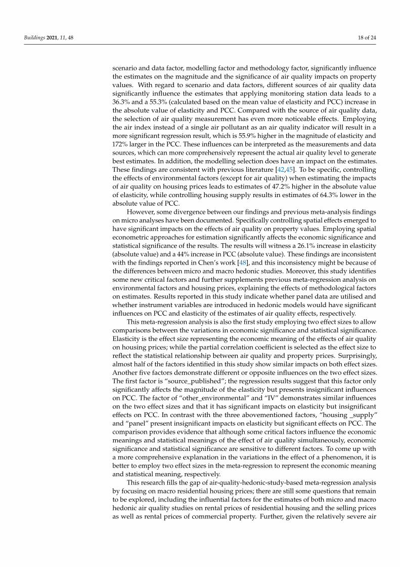
scenario and data factor, modelling factor and methodology factor, significantly influencethe estimates on the magnitude and the significance of air quality impacts on propertyvalues. With regard to scenario and data factors, different sources of air quality datasignificantly influence the estimates that applying monitoring station data leads to a36.3% and a 55.3% (calculated based on the mean value of elasticity and PCC) increase inthe absolute value of elasticity and PCC. Compared with the source of air quality data,the selection of air quality measurement has even more noticeable effects. Employingthe air index instead of a single air pollutant as an air quality indicator will result in amore significant regression result, which is 55.9% higher in the magnitude of elasticity and172% larger in the PCC. These influences can be interpreted as the measurements and datasources, which can more comprehensively represent the actual air quality level to generatebest estimates. In addition, the modelling selection does have an impact on the estimates.These findings are consistent with previous literature [42,45]. To be specific, controllingthe effects of environmental factors (except for air quality) when estimating the impactsof air quality on housing prices leads to estimates of 47.2% higher in the absolute valueof elasticity, while controlling housing supply results in estimates of 64.3% lower in theabsolute value of PCC.

However, some divergence between our findings and previous meta-analysis findingson micro analyses have been documented. Specifically controlling spatial effects emerged tohave significant impacts on the effects of air quality on property values. Employing spatialeconometric approaches for estimation significantly affects the economic significance andstatistical significance of the results. The results will witness a 26.1% increase in elasticity(absolute value) and a 44% increase in PCC (absolute value). These findings are inconsistentwith the findings reported in Chen’s work [48], and this inconsistency might be because ofthe differences between micro and macro hedonic studies. Moreover, this study identifiessome new critical factors and further supplements previous meta-regression analysis onenvironmental factors and housing prices, explaining the effects of methodological factorson estimates. Results reported in this study indicate whether panel data are utilised andwhether instrument variables are introduced in hedonic models would have significantinfluences on PCC and elasticity of the estimates of air quality effects, respectively.

This meta-regression analysis is also the first study employing two effect sizes to allowcomparisons between the variations in economic significance and statistical significance.Elasticity is the effect size representing the economic meaning of the effects of air qualityon housing prices; while the partial correlation coefficient is selected as the effect size toreflect the statistical relationship between air quality and property prices. Surprisingly,almost half of the factors identified in this study show similar impacts on both effect sizes.Another five factors demonstrate different or opposite influences on the two effect sizes.The first factor is “source_published”; the regression results suggest that this factor onlysignificantly affects the magnitude of the elasticity but presents insignificant influenceson PCC. The factor of “other_environmental” and “IV” demonstrates similar influenceson the two effect sizes and that it has significant impacts on elasticity but insignificanteffects on PCC. In contrast with the three abovementioned factors, “housing _supply”and “panel” present insignificant impacts on elasticity but significant effects on PCC. Thecomparison provides evidence that although some critical factors influence the economicmeanings and statistical meanings of the effect of air quality simultaneously, economicsignificance and statistical significance are sensitive to different factors. To come up witha more comprehensive explanation in the variations in the effect of a phenomenon, it isbetter to employ two effect sizes in the meta-regression to represent the economic meaningand statistical meaning, respectively.

This research fills the gap of air-quality-hedonic-study-based meta-regression analysisby focusing on macro residential housing prices; there are still some questions that remainto be explored, including the influential factors for the estimates of both micro and macrohedonic air quality studies on rental prices of residential housing and the selling pricesas well as rental prices of commercial property. Further, given the relatively severe air

Buildings 2021, 11, 48 19 of 24

pollution in China, this study focuses on the impacts of air quality on housing prices inChina. Researchers who are interested in this topic can expand the study scope to a globalscale and testify whether some country-level factors such as socioeconomic condition andair pollution condition affect the estimates of the impacts of air quality on housing prices.

6. Conclusions

Given the mixed empirical results concerning the impacts of air pollution on housingvalue in China, this study investigates whether air quality significantly affects housingprices in China with a meta-regression analysis. Further, this study explores the variationin the estimated effects of air quality on property values and provides a comprehensive ex-planation of the mixed results in previous studies by identifying and comparing influentialfactors, which significantly affect the magnitude of the elasticity and the strength of thecorrelation coefficient.

The study found several important findings. Firstly, the study found that air qualitydoes have a profound impact on housing prices. This suggests that air pollution is pricedby Chinese households. Secondly, the impact of air quality is diverse in the followingaspects: scenario and data factors, modelling factors and methodology factors. Half ofthe variables show significant influences on both effect sizes, including two scenario anddata variables, one modelling variables and a methodology variable. With regard to thescenario variable, the selection of the type of air pollution and the source of air pollutiondata negatively and positively affects both elasticity and PCC, separately.

This finding suggests that the air pollutant and data source, which is more capableof comprehensively reflecting the residents’ real perceptions, lead to more significantestimates. Moreover, addressing spatial effects using spatial econometric approaches resultsin more accurate regression estimates, which is higher in both economic and statisticalmeanings. Thus, to come up with less biased estimates, spatial econometric approachescan be helpful tools. The modelling factor of “infrastructure” demonstrates insignificanteffects on both elasticity and PCC.

Except for the four abovementioned variables, there are five factors that only presentsignificant impacts on either elasticity or PCC. This meta-regression analysis finds thatpublished studies included in the meta-sample tend to report estimates with higher eco-nomic meaning. In terms of modelling variables, applying housing supply characteristicsand other environmental factors as control variables in the hedonic models will lead toestimates with smaller elasticity and higher statistical significance, respectively. In otherwords, housing supply characteristics and other environmental characteristics are impor-tant control variables in hedonic models when quantifying macro impacts of air quality,and the ignorance of these two types of control variables will lead to biased estimates.Besides, utilising panel data and instrument variables, helping to reduce omitted variablebias, decreases the strength of the correlation between air pollution and property values.Therefore, in macro-level hedonic air quality studies, employing panel data and instrumentvariables can significantly reduce estimated biases.

The above-listed findings of this study have several profound implications and canbe of interest to not only researchers but also policymakers. Firstly, this study providesa systematic review of the macro hedonic air quality studies in China, so policymakersand researchers would have an enhanced understanding of the impacts of air quality. Thisoffers a rigorous foundation for policy formulation; thereby, Chinese and internationalpolicymakers, particularly in cities or countries where no empirical evidence is available forthe effect of air quality on housing values, are able to formulate a better policy in relationto air quality and economic development.

In addition, the significant results in the meta-regression analysis might guide scholarson the choice of control variables for their analyses, such as infrastructure characteristicsand housing supply characteristics. This study also gives some suggestions on the choice ofdata type and estimation approaches. For example, applying spatial econometric methodsgenerates more significant results with higher statistical significance; introducing the

Buildings 2021, 11, 48 20 of 24

instrument variable leads to larger coefficients. These suggest that the ignorance of spatialeffects and endogeneity will lead to biased estimates. Furthermore, this study can bereferred to as a benchmark for scholars who would like to find how their results fit withother studies; the results may also be used to explain different estimates obtained fromdifferent research.

Recognising the uniqueness of the Chinese market (e.g., the imperfections of theChinese financial market [107] and the high level of air pollution in China), the abovemen-tioned contributions can, to a certain extent, be limited to China. To better understand thevariations among the impacts of air quality on property prices globally or in other markets,future studies of air pollution impacts on other housing markets are necessary. However,this study also helps scholars (not restricted to Chinese researchers) to get a comprehensiveoverview of the variations in how the air quality impacts in the following two perspectives.Firstly, different findings in elasticity and PCC models give reasonable suggestions on effectsize selection in meta-regression analysis. Although half of the factors in this study havecomparable effects on both elasticity and PCC, elasticity and PCC are still sensitive to someof the different factors. Therefore, to better understand the relationship between air qualityand housing prices, we need to understand the critical factors for economic significance andstatistical significance, respectively. Additionally, some of the inconsistent findings withprevious micro-level studies demonstrate that the macro hedonic air quality studies areaffected by different factors (e.g., spatial effects). Given most previous literature focused onthe meta-regression analysis with micro-hedonic studies, further meta-regression analysesconsidering macro studies and comparisons are of great importance to understand themixed results of air quality impacts.

Author Contributions: Conceptualization, C.L.L. and J.W.; writing—original draft preparation, J.W.;writing—review and editing, C.L.L. and S.S.; supervision, C.L.L. and S.S. All authors have read andagreed to the published version of the manuscript.

Funding: This research received no external funding.

Institutional Review Board Statement: Not applicable (study not involving humans).

Informed Consent Statement: Not applicable (study not involving humans).

Data Availability Statement: Not applicable (No new data were created or analysed in this study).

Conflicts of Interest: The authors declare no conflict of interest.

Appendix A

Table A1. Variance inflation factor (VIF) of meta-variables.

Variable VIF 1/VIF

D_ai 2.21 0.452671D_i 1.90 0.527032

D_hs 1.88 0.530586D_sp 1.77 0.564519D_p 1.75 0.571473D_oe 1.73 0.578003D_s 1.63 0.618269D_ie 1.42 0.703426D_iv 1.19 0.843061

Mean VIF 1.72

Buildings 2021, 11, 48 21 of 24

References1. Kanakidou, M.; Mihalopoulos, N.; Kindap, T.; Im, U.; Vrekoussis, M.; Gerasopoulos, E.; Dermitzaki, E.; Unal, A.; Koçak, M.;

Markakis, K.; et al. Megacities as hot spots of air pollution in the East Mediterranean. Atmos. Environ. 2011, 45, 1223–1235.2. Du, H.; Kong, L.; Cheng, T.; Chen, J.; Du, J.; Li, L.; Xia, X.; Leng, C.; Huang, G. Insights into summertime haze pollution events

over Shanghai based on online water-soluble ionic composition of aerosols. Atmos. Environ. 2011, 45, 5131–5137.3. National Bureau of Statistics of China. Indicators of gross and speed of national economic and social development. In China

Statistical Yearbook; Ning, J., Ed.; China Statistics Press: Beijing, China, 2019; pp. 4–11.4. XinhuaNews. China’s GDP Grows over 170 Times in 70-Year Period. Available online: http://www.xinhuanet.com/politics/201

9-09/21/c_1125022721.htm (accessed on 15 December 2019).5. Wang, B.; Hong, G.; Qin, T.; Fan, W.R.; Yuan, X.C. Factors governing the willingness to pay for air pollution treatment: A case

study in the Beijing-Tianjin-Hebei region. J. Clean. Prod. 2019, 235, 1304–1314.6. Chen, D.; Chen, S. Particulate air pollution and real estate valuation: Evidence from 286 Chinese prefecture-level cities over

2004–2013. Energy Policy 2017, 109, 884–897.7. Du, X.; Mendelsohn, R.O. Estimating the value of the reduction in air pollution during the Beijing Olympics. Environ. Dev. Econ.

2011, 16, 735–749.8. Warburton, D.; Warburton, N.; Wigfall, C.; Chimedsuren, O.; Lodoisamba, D.; Lodoysamba, S.; Jargalsaikhan, B. Impact of

seasonal winter air pollution on health across the lifespan in Mongolia and some putative solutions. Ann. Am. Thorac. Soc. 2018,15, S86–S90.

9. Tran, H.; Kim, J.; Kim, D.; Choi, M.; Choi, M. Impact of air pollution on cause-specific mortality in Korea: Results from BayesianModel Averaging and Principle Component Regression approaches. Sci. Total Environ. 2018, 636, 1020–1031.

10. Almakhanova, K.K.; Zhussupova, A.S.; Nurmanova, S.A.; Alzhanova, D.S.; Kozhakanova, S.T.; Balgayeva, M.S.; Baltayeva, Z.S.;Zharkinbayeva, N.A. Comparative evaluation of air pollution impact on severity of multiple sclerosis in patients of northern andsouthern cities of Kazakhstan: Astana, Shymkent. Res. J. Med. Sci. 2015, 9, 229–232.

11. Gibelin, P. Cardiovascular diseases and pollution. Bulletin de l’Academie Nationale de Medecine 2019, 203, 201–208.12. Dales, R.E.; Cakmak, S.; Vidal, C.B. Air pollution and hospitalization for venous thromboembolic disease in Chile. J. Thromb.

Haemost. 2010, 8, 669–674.13. He, S.; Tang, S.; Xiao, Y.; Cheke, R.A. Stochastic Modelling of Air Pollution Impacts on Respiratory Infection Risk. Bull. Math. Biol.

2018, 80, 3127–3153. [PubMed]14. Dauchet, L.; Hulo, S.; Cherot-Kornobis, N.; Matran, R.; Amouyel, P.; Edmé, J.L.; Giovannelli, J. Short-term exposure to air

pollution: Associations with lung function and inflammatory markers in non-smoking, healthy adults. Environ. Int. 2018, 121,610–619. [PubMed]

15. Raoufi, S.S.; Goharnejad, H.; Niri, M.Z. Air Pollution Effects on Climate and Air Temperature of Tehran City Using RemoteSensing Data. Asian J. Water Environ. Pollut. 2018, 15, 79–87.

16. Burney, J.; Ramanathan, V. Recent climate and air pollution impacts on Indian agriculture. Proc. Natl. Acad. Sci. USA 2014, 111,16319–16324. [PubMed]

17. Sanderfoot, O.V.; Holloway, T. Air pollution impacts on avian species via inhalation exposure and associated outcomes. Environ.Res. Lett. 2017, 12, 083002.

18. Fan, X.Y.; Gao, J.F.; Pan, K.L.; Li, D.C.; Dai, H.H.; Li, X. More obvious air pollution impacts on variations in bacteria than fungiand their co-occurrences with ammonia-oxidizing microorganisms in PM2.5. Environ. Pollut. 2019, 251, 668–680. [PubMed]

19. Adisasmita, S.A. Air pollution effects on aircrafts movement in and around airport: Solutions and recommendations (case study:Djalaluddin airport, Gorontalo, Indonesia). J. Eng. Appl. Sci. 2014, 9, 176–181.

20. Ahmad, A.; Abdullah, M.M.; Quegan, S.; Sufahani, S.F.; Sakidin, H. Haze effects on satellite remote sensing imagery and theircorrections. Int. J. Adv. Comput. Sci. Appl. 2019, 10, 69–76.

21. Gong, Y.; Zhang, J.; Lan, J.H. A road network model in haze and haze situation influence on traffic networks. Jiaotong YunshuXitong Gongcheng Yu Xinxi (J. Transp. Syst. Eng. Inf. Technol.) 2015, 15, 114–122.

22. Vidorni, G.; Sardella, A.; De Nuntiis, P.; Volpi, F.; Dinoi, A.; Contini, D.; Comite, V.; Vaccaro, C.; Fermo, P.; Bonazza, A. Airpollution impact on carbonate building stones in Italian urban sites?. Eur. Phys. J. 2019, 134, 1–10.

23. Dirnböck, T.; Djukic, I.; Kitzler, B.; Kobler, J.; Mol-Dijkstra, J.P.; Posch, M.; Reinds, G.J.; Schlutow, A.; Starlinger, F.; Wamelink,W.G.W. Climate and air pollution impacts on habitat suitability of Austrian forest ecosystems. PLoS ONE 2017, 12, e0184194.[CrossRef] [PubMed]

24. Sterzynska, M.; Nicia, P.; Zadrozny, P.; Fiera, C.; Shrubovych, J.; Ulrich, W. Urban springtail species richness decreases withincreasing air pollution. Ecol. Indic. 2018, 94, 328–335. [CrossRef]

25. Solazzo, E.; Riccio, A.; Van Dingenen, R.; Valentini, L.; Galmarini, S. Evaluation and uncertainty estimation of the impact of airquality modelling on crop yields and premature deaths using a multi-model ensemble. Sci. Total Environ. 2018, 633, 1437–1452.[CrossRef] [PubMed]

26. Lo Sciuto, G. Air pollution effects on the intensity of received signal in 3G/4G mobile terminal. Int. J. Energy Environ. Eng. 2019,10, 221–229.

Buildings 2021, 11, 48 22 of 24

27. Lamhasni, T.; El-Marjaoui, H.; El Bakkali, A.; Lyazidi, S.A.; Haddad, M.; Ben-Ncer, A.; Benyaich, F.; Bonazza, A.; Tahri, M. Airpollution impact on architectural heritage of Morocco: Combination of synchronous fluorescence and ATR-FTIR spectroscopiesfor the analyses of black crusts deposits. Chemosphere 2019, 225, 517–523. [CrossRef]

28. Vidal, F.; Vicente, R.; Mendes Silva, J. Review of environmental and air pollution impacts on built heritage: 10 questions oncorrosion and soiling effects for urban intervention. J. Cult. Herit. 2019, 37, 273–295. [CrossRef]

29. Li, J.; Hu, Y.; Liu, C. Exploring the Influence of an Urban Water System on Housing Prices: Case Study of Zhengzhou. Buildings2020, 10, 44. [CrossRef]

30. Nourse, H.O. The Effect of Air Pollution on House Values. Land Econ. 1967, 43, 181–189. [CrossRef]31. Tan, J.; Zhao, J. The value of clean air in China: Evidence from Beijing and Shanghai. Front. Econ. China 2014, 9, 109–137.32. Wang, X.J.; Zhang, W.; Li, Y.; Yang, K.Z.; Bai, M. Air quality improvement estimation and assessment using contingent valuation

method, a case study in Beijing. Environ. Monit. Assess. 2006, 120, 153–168. [CrossRef]33. Chau, K.; Yiu, C.; Wong, S.; Lai, L.W.C. Hedonic price modelling of environmental attributes: A review of the literature and

a Hong Kong case study. In Understanding and Implementing Sustainable Development; Lawrence, W.C.L., Frank, L., Eds.; NovaScience Publication: New York, NY, USA, 2003; pp. 87–110.

34. Ridker, R.G.; Henning, J.A. The determinants of residential property values with special reference to air pollution. Rev. Econ. Stat.1967, 49, 246–257. [CrossRef]

35. Kim, C.W.; Phipps, T.T.; Anselin, L. Measuring the benefits of air quality improvement: A spatial hedonic approach. InProceedings of the AAEA Annual Meeting, Salt Lake City, UT, USA, 2–5 August 1998.

36. Berezansky, B.; Portnov, B.A.; Barzilai, B. Objective vs. perceived air pollution as a factor of housing pricing: A case study of thegreater Haifa metropolitan area. J. Real Estate Lit. 2010, 18, 99–122.

37. Zheng, S.; Kahn, M.E.; Liu, H. Towards a system of open cities in China: Home prices, FDI flows and air quality in 35 major cities.Reg. Sci. Urban Econ. 2010, 40, 1–10. [CrossRef]

38. Wang, Y. Environmental pollution and urban housing prices. Mod. Manag. Sci. 2017, 000, 50–52.39. Jia, Y. An Empirical Study on the Relationship between Urban Air Quality and Commerical Housing Price. Master’s Thesis,

Tianjin Normal University, Tianjin, China, 2014.40. Wang, S.; Shi, J. Study on regional difference of air quality’s impact on urban housing price. Prices Mon. 2019, 10, 14–21.41. Kong, N. Empirical Research on the Impact of Air Pollution on China’s Real Estate Market. Master’s Thesis, Xiamen University,

Xiamen, China, 2018.42. Jackson, T. The effects of environmental contamination on real estate: A literature review. J. Real Estate Lit. 2001, 9, 91–116.43. Boyle, M.; Kiel, K. A survey of house price hedonic studies of the impact of environmental externalities. J. Real Estate Lit. 2001, 9,

117–144.44. Stanley, T.D.; Jarrell, S.B. Meta-regression analysis: A quantitative method of literature surveys. J. Econ. Surv. 2005, 19, 299–308.

[CrossRef]45. Smith, V.K.; Huang, J.C. Hedonic models and air pollution: Twenty-five years and counting. Environ. Resour. Econ. 1993, 3,

381–394. [CrossRef]46. Smith, V.K.; Huang, J.-C. Can markets value air quality? A meta-analysis of hedonic property value models. J. Political Econ. 1995,

103, 209–227. [CrossRef]47. Simons, R.A.; Saginor, J.D. A meta-analysis of the effect of environmental contamination and positive amenities on residential

real estate values. J. Real Estate Res. 2006, 28, 71–104.48. Chen, W.Y.; Li, X.; Hua, J. Environmental amenities of urban rivers and residential property values: A global meta-analysis. Sci.

Total Environ. 2019, 693, 133628. [CrossRef] [PubMed]49. Court, L.M. Entrepreneurial and consumer demand theories for commodity spectra: Part I. Econom. J. Econom. Soc. 1941, 135–162.

[CrossRef]50. Bartik, T. The estimation of demand parameters in hedonic price models. J. Political Econ. 1987, 95, 81–88. [CrossRef]51. Lancaster, K.J. A new approach to consumer theory. J. Political Econ. 1966, 74, 132–157. [CrossRef]52. Muhammad, I. Disamenity impact of Nala Lai (open sewer) on house rent in Rawalpindi city. Environ. Econ. Policy Stud. 2017, 19,

77–97. [CrossRef]53. Nelson, J.P. Highway noise and property values. J. Transp. Econ. Policy 1982, 16, 117–138.54. Follain, J.R.; Jimenez, E. Estimating the demand for housing characteristics: A survey and critique. Reg. Sci. Urban Econ. 1985, 15,

77–107. [CrossRef]55. Kiel, K. Environmental Contamination and House Values; College of the Holy Cross, Department of Economics Faculty Working

Papers Series, no. 06-01; Dept. of Economics College of the Holy Cross: Worcester, MA, USA, 2006.56. Liang, J.; Koo, K.M.; Lee, C.L. Transportation Infrastructure Improvement and Real Estate Value: Impact of Level Crossing

Removal Project on Housing Prices. Transportation 2021, 1–43. [CrossRef]57. Lee, C.L.; Locke, M. The effectiveness of passive land value capture mechanisms in funding infrastructure. J. Prop. Invest. Financ.

2020. [CrossRef]58. Dubin, R.A. Predicting House Prices Using Multiple Listings Data. J. Real Estate Financ. Econ. 1998, 17, 35–59. [CrossRef]59. Bangura, M.; Lee, C.L. The differential geography of housing affordability in Sydney: A disaggregated approach. Aust. Geogr.

2019, 50, 295–313. [CrossRef]

Buildings 2021, 11, 48 23 of 24

60. Bangura, M.; Lee, C.L. House price diffusion of housing submarkets in Greater Sydney. Hous. Stud. 2020, 35, 1110–1141.[CrossRef]

61. Herath, S.; Maier, G. The Hedonic Price Method in Real Estate and Housing Market Research. A Review of the Literature; SRE-DiscussionPapers Series 2010/03; WU Vienna University of Economics and Business: Vienna, Austria, 2010.

62. Wen, H.; Zhang, Y.; Zhang, L. Assessing amenity effects of urban landscapes on housing price in Hangzhou, China. Urban For.Urban Green. 2015, 14, 1017–1026. [CrossRef]

63. Mahan, B.L.; Polasky, S.; Adams, R.M. Valuing Urban Wetlands: A Property Price Approach. Land Econ. 2000, 76, 100–113.[CrossRef]

64. Donovan, G.H.; Butry, D.T. Trees in the city: Valuing street trees in Portland, Oregon. Landsc. Urban Plan. 2010, 94, 77–83.[CrossRef]

65. Del Giudice, V.; De Paola, P.; Manganelli, B.; Forte, F. The Monetary Valuation of Environmental Externalities through the Analysisof Real Estate Prices. Sustainability 2017, 9, 229. [CrossRef]

66. Zuindeau, B.; Letombe, G. Hazardous waste sites and property values: A French case study in the light of US analyses. Int. J.Environ. Pollut. 2008, 32, 387–409. [CrossRef]

67. Donovan, G.H.; Butry, C.D.T. Wildfire Risk and Housing Prices: A Case Study from Colorado Springs. Land Econ. 2007, 83,217–233. [CrossRef]

68. Bekes, G.; Horvath, A.; Sapi, Z. Flood Risk and Housing Prices: Evidence from Hungary; Discussion Papers Series, MT-DP—2016, 20;Centre for Economic and Regional Studies, Hungarian Academy of Sciences: Budapest, Hungary, 2016.

69. Pilla, F.; Gharbia, S.S.; Lyons, R. How do households perceive flood-risk? The impact of flooding on the cost of accommodation inDublin, Ireland. Sci. Total Environ. 2019, 650, 144–154. [CrossRef]

70. Wang, S.; Cai, Q. Are home buyers in Chinese cities concerned about air quality? Using panel data for 70 large and medium-sizedcities from 2006 to 2016 as an example. J. Hous. Built Environ. 2020, 1–20. [CrossRef]

71. Dong, J.; Zeng, X.; Mou, X.; Li, X. The impact of smog on real estate prices. Sci. Technol. Dev. 2020, 16, 138–144.72. Chen, S.; Jin, H. Pricing for the clean air: Evidence from Chinese housing market. J. Clean. Prod. 2019, 206, 297–306. [CrossRef]73. Chen, X. Environmental pollution, housing prices. Contemp. Econ. 2019, 12–15. Available online: https://kns.cnki.net/kcms/deta

il/detail.aspx?dbcode=CJFD&dbname=CJFDLAST2019&filename=DAJJ201910004&v=hQ%25mmd2BzqWfWNbhBWymHhVy5kaIIq2psjT6MnxJe1ChuQf52n%25mmd2B3IzUJjwdn%25mmd2BArIeCz7I (accessed on 4 December 2020).

74. Zou, Y. Air Pollution and Housing Prices across Chinese Cities. J. Urban Plan. Dev. 2019, 145, 04019012. [CrossRef]75. Shen, S. The impacts of urban air pollution on housing prices. China Civil Entrep. 2018, 181–182. Available online:

https://kns.cnki.net/kcms/detail/detail.aspx?dbcode=CJFD&dbname=CJFDLASN2018&filename=MISH201801150&v=ahh62pXBOwXAcnSdcFRt7r2zwpwThZxB9MByNvrXTDu0%25mmd2F0w%25mmd2FOYazDeHpJ3uSKAT7 (accessed on 4December 2020).

76. Dong, J.; Zeng, X.; Mou, X.; Li, X. Pay for clean air or not? The impact of air quality on China’s real estate price. Syst. Eng. TheoryPract. 2020, 40, 1613–1626.

77. Sun, B.; Yang, S. Asymmetric and Spatial Non-Stationary Effects of Particulate Air Pollution on Urban Housing Prices in ChineseCities. Int. J. Environ. Res. Public Health 2020, 17, 7443. [CrossRef]

78. Zhang, B.; Huang, X. A Price Evaluation of Air Quality in China. Res. Econ. Manag. 2017, 38, 94–103.79. Huang, X.; Lanz, B. The Value of Air Quality in Chinese Cities: Evidence from Labor and Property Market Outcomes. Environ.

Resour. Econ. 2017, 71, 849–874. [CrossRef]80. Yu, J. The Study on Air Quality Valuation Based on The Hedonic Price Model. Master’s Thesis, Xiamen University, Xiamen,

China, 2018.81. Glass, G.V. Primary, secondary, and meta-analysis of research. Educ. Res. 1976, 5, 3–8. [CrossRef]82. Stanley, T.D.; Doucouliagos, H. Meta-Regression Analysis in Economics and Business; Routledge: London, UK, 2012.83. Egert, B.; Halpern, L. Equilibrium exchange rates in Central and Eastern Europe: A meta-regression analysis. J. Bank. Financ.

2006, 30, 1359–1374. [CrossRef]84. Bom, P.R.D.; Ligthart, J.E. How Productive is Public Capital? A Meta-Regression Analysis; Working Paper Series, 0912; International

Center for Public Policy, Andrew Young School of Policy Studies, Georgia State University: Atlanta, GA, USA, 2009.85. Brander, L.M.; Koetse, M.J. The value of urban open space: Meta-analyses of contingent valuation and hedonic pricing results. J.

Environ. Manag. 2011, 92, 2763–2773. [CrossRef] [PubMed]86. Nelson, J.P.; Kennedy, P.E. The use (and abuse) of meta-analysis in environmental and natural resource economics: An assessment.

Environ. Resour. Econ. 2009, 42, 345–377. [CrossRef]87. Stanley, T.D. Beyond publication bias. J. Econ. Surv. 2005, 19, 309–345. [CrossRef]88. Stanley, T.D. Meta-regression methods for detecting and estimating empirical effects in the presence of publication selection. Oxf.

Bull. Econ. Stat. 2008, 70, 103–127. [CrossRef]89. Zelmer, J. Linear Public Goods Experiments: A Meta-Analysis. Exp. Econ. 2003, 6, 299–310. [CrossRef]90. Moher, D.; Liberati, A.; Tetzlaff, J.; Altman, D. Preferred Reporting Items for Systematic Reviews and Meta-Analyses: The

PRISMA Statement. Open Med. 2009, 3, 123–130.91. Pattanayak, S.K.; Smith, V.L.; Smith, V.K. Is Meta-Analysis a Noah’s Ark for Non-Market Valuation? Environ. Resour. Econ. 2002,

22, 271–296.

Buildings 2021, 11, 48 24 of 24

92. Card, D.; Krueger, A.B. Time-series minimum-wage studies: A meta-analysis. Am. Econ. Rev. 1995, 85, 238–243.93. Begg, C.B.; Berlin, J.A. Publication bias: A problem in interpreting medical data. J. Roy. Stat. Soc. 1988, 151, 419–445. [CrossRef]94. Gerber, A.S.; Green, D.P.; Nickerson, D. Testing for publication bias in political science. Political Anal. 2001, 9, 385–392. [CrossRef]95. Stanley, T.D. Wheat from chaff: Meta-analysis as quantitative literature review. J. Econ. Perspect. 2001, 15, 131–150. [CrossRef]96. Sutton, A.J.; Abrams, K.R.; Jones, D.R.; Jones, D.R.; Sheldon, T.A.; Song, F. Methods for Meta-Analysis in Medical Research; Wiley:

Chichester, UK, 2000; Volume 348.97. Egger, M.; Smith, G.D.; Schneider, M.; Minder, C. Bias in meta-analysis detected by a simple, graphical test. Br. Med. J. 1997, 315,

629–634. [CrossRef]98. Peng, Y.; Gu, L. Meta-regression analysis in economics. Econ. Perspect. 2014, 2, 126–131.99. Mohammad, S.I.; Graham, D.J.; Melo, P.C.; Anderson, R.J. A meta-analysis of the impact of rail projects on land and property

values. Transp. Res. Part A Policy Pract. 2013, 50, 158–170. [CrossRef]100. Bangura, M.; Lee, C.L. Housing price bubbles in Greater Sydney: Evidence from a submarket analysis. Hous. Stud. 2020, 1–36.

[CrossRef]101. Shih, Y.N.; Li, H.C.; Qin, B. Housing price bubbles and inter-provincial spillover: Evidence from China. Habitat Int. 2014, 43,

142–151. [CrossRef]102. Klemick, H.; Griffiths, C.; Guignet, D.; Walsh, P. Improving Water Quality in an Iconic Estuary: An Internal Meta-analysis of

Property Value Impacts Around the Chesapeake Bay. Environ. Resour. Econ. 2018, 69, 265–292. [CrossRef]103. Braden, J.B.; Feng, X.; Won, D. Waste Sites and Property Values: A Meta-Analysis. Environ. Resour. Econ. 2011, 50, 175–201.

[CrossRef]104. Lee, C.L.; Stevenson, S.; Lee, M.L. Low-frequency volatility of real estate securities and macroeconomic risk. Account. Financ.

2018, 58, 311–342. [CrossRef]105. Anselin, L. Spatial Externalities, Spatial Multipliers, And Spatial Econometrics. Int. Reg. Sci. Rev. 2003, 26, 153–166. [CrossRef]106. LeSage, J.P. An introduction to spatial econometrics. Revue d’Economie Industrielle 2008, 123, 19–44. [CrossRef]107. Zhang, J.; Lee, C.L.; Chan, N. The asymmetric effect of institutional quality on Chinese outward real estate investment. Int. J.

Strateg. Prop. Manag. 2019, 23, 435–449. [CrossRef]