MACRO ECONOMICS: THEORIES AND POLICIES II ...
172
School of Distance Education Macro Economics : Theories and Policies II Page 1 MACRO ECONOMICS: THEORIES AND POLICIES II (ECO2C06) STUDY MATERIAL II SEMESTER CORE COURSE MA ECONOMICS (2019 Admission ONWARDS) UNIVERSITY OF CALICUT SCHOOL OF DISTANCE EDUCATION Calicut University P.O, Malappuram Kerala, India 673 635. 190306
-
Upload
khangminh22 -
Category
Documents
-
view
3 -
download
0
Transcript of MACRO ECONOMICS: THEORIES AND POLICIES II ...

School of Distance Education
Macro Economics : Theories and Policies II Page 1
MACRO ECONOMICS:
THEORIES AND POLICIES II
(ECO2C06)
STUDY MATERIAL
II SEMESTER
CORE COURSE
MA ECONOMICS(2019 Admission ONWARDS)
UNIVERSITY OF CALICUTSCHOOL OF DISTANCE EDUCATION
Calicut University P.O, Malappuram Kerala, India 673 635.
190306

School of Distance Education
Macro Economics : Theories and Policies II Page 2
UNIVERSITY OF CALICUTSCHOOL OF DISTANCE EDUCATION
STUDY MATERIALSECOND SEMESTER
MA ECONOMICS (2019 ADMISSION)CORE COURSE : ECO2C06 : MACRO ECONOMICS :
THEORIES AND POLICIES II
Prepared by : SUJIN K N,
Assistant Professor,PG & Research Department of Economics,Government College,Kodanchery,Kozhikode - 673 580.
Scrutinized by : Dr.K.X Joseph,
Professor (Retd.),Dr.John Matthai Centre,Thrissur.
School of Distance Education
Macro Economics : Theories and Policies II Page 3
CONTENTS
I Classical Vs Keynes 5
II Monetarism 79
IIINew Classical Macro Economics, RealBusiness cycle School and Supply sideEconomics
93
IV The New Keynes School 126
V New Political Macroeconomics 151

School of Distance Education
Macro Economics : Theories and Policies II Page 4

School of Distance Education
Macro Economics : Theories and Policies II Page 5
MODULE I
CLASSICAL VS KEYNES
“Economics is an easy subject in which few excel”-- John Maynard Keynes
INTRODUCTION TO MACROECONOMICS
Macro economics is the branch of economics studying the behaviour of the aggregate
economy – at the regional, national or international level. In other words Macroeconomics is the
study of the behavior of the whole economy or economy as a whole. It is concerned with the
determination of the broad aggregates in the economy, in particular the national output,
unemployment, inflation and the balance of payments position.
The way in which we nowadays study macroeconomics largely owes its origins to John
Maynard Keynes’s “The General Theory of Employment, Interest and Money”. Published in
1936, “The General Theory” was regarded by its author, and by many others since, as a
revolutionary work. In it Keynes set out to challenge the mainstream neoclassical economic
thought of his day, which he castigated as unable to explain or offer policy solutions for the high
level of unemployment which, in Britain between 1921 and 1939, was just under 10 per cent at
its lowest level and rose to 22 per cent at the depth of the depression in 1930.
The term ‘macroeconomics’ was coined and used by a Norwegian economist, Ragnar
Frisch in 1933 in his paper “Propagation Problems and Impulse Problems in Dynamic
Economics” in ‘Economic Essays in the Honor of Gustav Cassel’(London, 1933). The prefix
‘macro’ meaning large has been derived from Greek language.
What is macroeconomics?The aim of studying macroeconomics is to understand how an economy works, and
identifying the levers that can be pulled to put the overall economy on the right path of growth.
The system that is a result of different economic agents coming into contact is much more
complex than the sum of its independent and often disjoint parts.

School of Distance Education
Macro Economics : Theories and Policies II Page 6
Moreover, it is strictly “non-experimental” as we do not have the luxury of conducting
controlled experiments like in the field of science. We can just wait and observe the effects of
broader policy measures with a certain level of accuracy and a tinge of hope.
It usually deals with goals that are conflicting; ensuring growth, taming inflation, full
employment and fair income distribution at the same time!
Classical macroeconomics
The term “classical economics” was firstly coined by KARL MARX to refer the economic
theories of David Ricardo and his predecessors including Adam Smith. Classical economics
covered almost a period of 150 years (1776-1929). The leaders of this school were David Ricardo,
Malthus, J.S Mill, J.B Say and A.C Pigou.
Classical economics is that body of thought which existed prior to the publication of
Keynes’s (1936) General Theory. For Keynes the classical school not only included Adam Smith,
David Ricardo and John Stuart Mill, but also ‘the followers of Ricardo, those, that is to say, who
adopted and perfected the theory of Ricardian economics’ (Keynes, 1936, p. 3). Keynes was
therefore at odds with the conventional history of economic thought classification, particularly
with his inclusion of both Alfred Marshall and Arthur Cecil Pigou within the classical school.
However, given that most of the theoretical advances which distinguish the neoclassical from the
classical period had been in microeconomic analysis, Keynes perhaps felt justified in regarding
the macroeconomic ideas of the 1776–1936 period, such as they existed, as being reasonably
homogeneous in terms of their broad message. This placed great faith in the natural market
adjustment mechanisms as a means of maintaining full employment equilibrium.
Before moving on to examine the main strands of macroeconomic thought associated with
the classical economists, the reader should be aware that, prior to the publication of the General
Theory, there was no single unified or formalized theory of aggregate employment, and
substantial differences existed between economists on the nature and origin of the business cycle
(see Haberler, 1963). The structure of classical macroeconomics mainly emerged after 1936 and
did so largely in response to Keynes’s own theory in order that comparisons could be made. Here
we take the conventional approach of presenting a somewhat artificial summary of classical
macroeconomics, a body of thought that in reality was extremely complex and diverse.
Although no single classical economist ever held all the ideas presented below, there are
certain strands of thought running through the pre-Keynes literature which permit us to
characterize classical theory as a coherent story with clearly identifiable building-blocks. To do
so will be analytically useful, even if ‘historically somewhat inaccurate’ (see Ackley, 1966, p.
109). Even an ‘Aunt Sally’ version of the classical theory can, by comparison, help us better

School of Distance Education
Macro Economics : Theories and Policies II Page 7
understand post-1936 developments in macroeconomic theory. We accept that, whilst the major
presentations of the ‘Keynes v. Classics’ debate consist of ahistorical fictions – especially those
of Hicks (1937) and Leijonhufvud (1968) – and serve as straw men, they aid our understanding
by overtly simplifying both the Keynes and the classics positions.
Classical economists were well aware that a capitalist market economy could deviate from
its equilibrium level of output and employment. However, they believed that such disturbances
would be temporary and very short-lived. Their collective view was that the market mechanism
would operate relatively quickly and efficiently to restore full employment equilibrium. If the
classical economic analysis was correct, then government intervention, in the form of activist
stabilization policies, would be neither necessary nor desirable. Indeed, such policies were more
than likely to create greater instability. As we shall see later, modern champions of the old
classical view (that is, new classical equilibrium business cycle theorists) share this faith in the
optimizing power of market forces and the potential for active government intervention to create
havoc rather than harmony. It follows that the classical writers gave little attention to either the
factors which determine aggregate demand or the policies which could be used to stabilize
aggregate demand in order to promote full employment. For the classical economists full
employment was the normal state of affairs. That Keynes should attack such ideas in the 1930s
should come as no surprise given the mass unemployment experienced in all the major capitalist
economies of that era. But how did the classical economists reach such an optimistic conclusion?
In what follows we will present a ‘stylized’ version of the classical model which seeks to explain
the determinants of an economy’s level of real output (Y), real (W/P) and nominal (W) wages,
the price level (P) and the real rate of interest (r) (see Ackley, 1966). In this stylized model it is
assumed that:
1. All economic agents (firms and households) are rational and aim to maximize their profits or
utility; furthermore, they do not suffer from money illusion;
2. All markets are perfectly competitive, so that agents decide how much to buy and sell on the
basis of a given set of prices which are perfectly flexible;
3. All agents have perfect knowledge of market conditions and prices before engaging in trade;
4. Trade only takes place when market-clearing prices have been established in all markets, this
being ensured by a fictional Walrasian auctioneer whose presence prevents false trading;
5. Agents have stable expectations.
These assumptions ensure that in the classical model, markets, including the labour market,
always clear. To see how the classical model explains the determination of the crucial macro
variables, we will follow their approach and divide the economy into two sectors: a real sector

School of Distance Education
Macro Economics : Theories and Policies II Page 8
and a monetary sector. To simplify the analysis we will also assume a closed economy, that is, no
foreign trade sector.
In examining the behaviour of the real and monetary sectors we need to consider the
following three components of the model: (i) the classical theory of employment and output
determination, (ii) Say’s Law of markets, and (iii) the quantity theory of money. The first two
components show how the equilibrium values of the real variables in the model are determined
exclusively in the labour and commodity markets. The third component explains how the nominal
variables in the system are determined. Thus in the classical model there is a dichotomy. The real
and monetary sectors are separated. As a result, changes in the quantity of money will not affect
the equilibrium values of the real variables in the model. With the real variables invariant to
changes in the quantity of money, the classical economists argued that the quantity of money was
neutral.
The Classical Revolution
Classical economics emerged as a revolution against a body of economic doctrines known
as mercantilism. Mercantilist thought was associated with the rise of the nation state in Europe
during the sixteenth and seventeenth centuries. Two tenets of mercantilism were (1) bullionism,
a belief that the wealth and power of a nation were determined by its stock of precious metals,
and (2) the belief in the need for state action to direct the development of the capitalist system.
Adherence to bullionism led countries to attempt to secure an excess of exports over imports to
earn gold and silver through foreign trade. Methods used to secure this favorable balance of trade
included export subsidies, import duties, and development of colonies to provide export markets.
State action was believed to be necessary to cause the developing capitalist system to further the
interests of the state. Foreign trade was carefully regulated, and the export of bullion was
prohibited to serve the ends of bullionism. The use of state action was also advocated on a broader
front to develop home industry, to reduce consumption of imported goods, and to develop both
human and natural resources.
In contrast to the mercantilists, classical economists emphasized the importance of real
factors in determining the “wealth of nations” and stressed the optimizing tendencies of the free
market in the absence of state control. Classical analysis was primarily real analysis; the growth
of an economy was the result of increased stocks of the factors of production and advances in
techniques of production. Money played a role only in facilitating transactions as a means of
exchange. Most questions in economics could be answered without analyzing the role of money.
Classical economists mistrusted government and stressed the harmony of individual and national

School of Distance Education
Macro Economics : Theories and Policies II Page 9
interests when the market was left unfettered by government regulations, except those necessary
to ensure that the market remained competitive. Both of these aspects of classical economics—
the stress on real factors and the belief in the efficacy of the free-market mechanism—developed
in the course of controversies over long-run questions concerning the determinants of economic
development. These classical positions on long-run issues were, however, important in shaping
classical economists’ views on short-run questions.
The attack on bullionism led classical economists to stress that money had no intrinsic
value. Money was important only for the sake of the goods it could purchase. Classical economists
focused on the role of money as a means of exchange. Another role money had played in the
mercantilist view was as a spur to economic activity. In the short run, mercantilists argued, an
increase in the quantity of money would lead to an increase in demand for commodities and would
stimulate production and employment. For classical economists to ascribe this role to money in
determining real variables, even in the short run, was dangerous in light of their de-emphasis of
the importance of money.
The classical attack on the mercantilist view of the need for state action to regulate the
capitalist system also had implications for short-run macroeconomic analysis. One role for state
action in the mercantilist view was to ensure that markets existed for all goods produced.
Consumption, both domestic and foreign, must be encouraged to the extent that production
advanced. The classical response is stated by John Stuart Mill: “In opposition to these palpable
absurdities it was triumphantly established by political economists that consumption never needs
encouragement. “
As in other areas, classical economists felt that the free-market mechanism would work
to provide markets for any goods that were produced: “The legislator, therefore, need not give
himself any concern about consumption.” The classical doctrine was that, in the aggregate,
production of a given quantity of output will generate sufficient demand for that output; there
could never be a “want of buyers for all commodities.” Consequently, classical economists gave
little explicit attention to factors that determine the overall demand for commodities.
Thus, two features of the classical analysis arose as part of the attack on mercantilism:
1. Classical economics stressed the role of real as opposed to monetary factors in determining
output and employment. Money had a role in the economy only as a means of exchange.
2. Classical economics stressed the self-adjusting tendencies of the economy. Government
policies to ensure an adequate demand for output were considered by classical economists to be
unnecessary and generally harmful.

School of Distance Education
Macro Economics : Theories and Policies II Page 10
Production
A central relationship in the classical model is the aggregate production function. The
production function, which is based on the technology of individual firms, is a relationship
between the level of output and the level of factor inputs. For each level of inputs, the production
function shows the resulting level of output and is written as
Y = F( , N)
where Y is output, is the stock of capital (plant and equipment), and N is the quantity of the
homogeneous labor input.
For the short run, the stock of capital is assumed to be fixed, as indicated by the bar over
the symbol for capital. The state of technology and the population are also assumed to be constant
over the period considered. For this short-run period, output varies solely with variations in the
labor input (N ) drawn from the fixed population. Classical economists assumed that the quantity
of labor employed would be determined by the forces of demand and supply in the labor market.
Say’s Law of Market
Say’s law of market can be stated as simply “supply creates its own demand”. In other
words, every supply of output creates an equivalent demand for output so that there can never be
a problem of general over production. According to this law, every supply creates its own demand
because the very fact that a good is offered for sale implies that something is being demanded in
return.
The law denies any possibility of deficiency of aggregate demand. Say’s law was
basically formulated in terms of barter economy. What Say had in mind was that people work
not for the sake of doing work but only to obtain goods and services that give the required
satisfaction. The very act of production therefore constitutes demand for other goods. Thus
supply creates automatically its own demand. Under these conditions it is evident that there can
be no general over production of goods and hence the aggregate must equal the aggregate supply.
The classical economists believed that the law also held true for an economy using money,
because they believed that people do not desire money for its own sake. This implies that they
sell their output or services for money, the money so earned would in turn be promptly spent on
other goods. They assume that money is merely a medium of exchange. As such the law formed
in terms of barter economy would hold true in an economy using money.
Implications of Say’s Law

School of Distance Education
Macro Economics : Theories and Policies II Page 11
1. Since there is automatic adjustment between production and consumption, there is no need for
the government to interfere in the functioning of the economic system.
2. So long as there exist unemployed resources in the economy, it is profitable to employ them.
Hence the economy will operate at the level of full employment.
3. The mechanism of interest flexibility brings about equality between savings and investment.
4. The mechanism of wage flexibility brings about full employment of labour.
Classical System
The classical theory is the theory of full employment. It simply outlines a model which
will ensure the maintenance of equilibrium at full employment level. According to the classical
economists, the economy consists of three markets: (i) Labour market; (ii) Money market; and
(iii) Goods market. The classical economists assumed that the operation of the forces of supply
and demand in each of these markets would finally result in full employment. We shall deal these
markets separately in the following sections.
I. Labour Market
The equilibrium level of aggregate output and employment in the labour market,
according to the classical economists, is determined by the aggregate production function and the
demand and supply schedules of labour.
The aggregate production function depicts the relationship between aggregate inputs and
aggregate output. According to classical, the aggregate output is a function of the economy’s
capital stock, technology and the amount of labour employed. In equation form, the relationship
is
Q = f ( N, K, T)
Where Q denotes the level of output, N denotes the level of employment, K denotes the
stock of capital and T denotes the level of technology.
Output is assumed to be positively related to the capital stock, technology and the amount of
labour employed. If the capital stock and technology are assumed constant, the relationship Q –
f (N, K, T) may be written as
Q = f ( N )
The demand for labour
The demand curve for labour is derived from the production function. It is the slope of
the production function because it consists of the marginal product of labour. Under perfect
competition firms hire labourers until the money wage is equal to the general price level
multiplied by the marginal physical product of labour. That is,
W = P x MPPL

School of Distance Education
Macro Economics : Theories and Policies II Page 12
Where W represents the cost of hiring an additional worker (money wage) and P x MPPL
represents the revenue associated with the employment of an additional worker (Marginal revenue
product).
We can state the same idea in terms of real wages by dividing both sides of the equation
by the general price level ‘P’ = × =Where is the real wage and is the marginal physical product of labour.
Since the demand for labour is determined by the and the real wage ( ), the demand for
labour function is also a function of real wages.
DN = F ( )Where DN is the amount of labour demanded and is the real wage rate.
The demand function of labour varies inversely with the real wage rate. In other words,
more and more employment is offered only as the wage rate is lowered. This is so because the
marginal product of labour decreases as output increases with the increase in employment.
The supply of labour
As in the case of demand for labour function, the real wage plays a key role in the
supply of labour function. In fact the amount of labour supplied is assumed to be a function of
the real wage by the classical economists. The supply of labour function can be written as
SN = f ( )
Where SN is the amount of labour supplied and is the real wage rate. The amount of
labour supplied is assumed to be positively related to the real wage rate, that is, at higher real
wages more labour will be supplied.
Equilibrium
For the labour market to be in equilibrium the amount of labour demanded must equal
the amount of labour supplied. Thus the equilibrium in the labour market occurs at the
intersection of demand and supply curves.
The equilibrium level of employment represents a state of full employment. At this
position all the persons who are willing and able to work at the existing wage rate have been
employed. There may be some voluntary unemployment, but there will be no involuntary

School of Distance Education
Macro Economics : Theories and Policies II Page 13
unemployment at this point. According to classical economists, involuntary unemployment can
arise only when real wages are high. If there are flexible wages the market forces allow the wages
to fall till all workers are employed and the economy will have its stable equilibrium at full
employment level. Thus wage flexibility will automatically bring back the economy to the level
of full employment where there is no involuntary unemployment.
Money Market (Quantity Theory of Money)
One of the important features of the classical system is the well known quantity theory of
money. According to the quantity theory of money, the price level is a function of money supply.
Changes in the price level are directly proportional to changes in the quantity of money. This
functional relationship between the price level and supply of money can be algebraically put as
MV = PQ
i.e., supply of money = demand for money
The equality between MV and PQ refers to an equilibrium situation where the demand for
money is equal to supply of money. In other words, it implies that entire amount of money is
spent on the purchase of goods and services. Assuming the magnitudes of velocity (V) and output
(Q) as constant, at least in the short run, any additional amount of money will raise the price level
in a direct proportionate manner. Suppose the economy is in full employment and if at this
position the supply of money increases by 15%, the price level would also rise by 15%. Thus the
changes in the supply of money cause similar changes in the price level.
Goods Market (Savings and Investment in the classical system)
The goods market is in a state of equilibrium when saving and investment are equal or the
aggregate demand for goods just equals the aggregate supply. If the amount of saving exceeds
investment or the aggregate supply is greater than aggregate demand, the level of income in the
community will have a tendency to decline. On the opposite, if the volume of investment exceeds
savings, or, the aggregate demand for goods is greater than their aggregate supply, the level of
income tends to expand.
The Classical system postulates both saving and investment as the function of rate of
interest and gives the following goods market relationships
S = f ( r ) -------------------------- Savings function
I = f ( r ) -------------------------- Investment function
S = I ---------------Equilibrium in the goods market

School of Distance Education
Macro Economics : Theories and Policies II Page 14
Saving is assumed as a direct function of the rate of interest and investment as an inverse
function of the rate of interest. Equilibrium represents the equilibrium condition in the goods
market. In the classical goods market, the equilibrating mechanism of the rate of interest always
ensures savings and investment equality.
The Quantity Theory of Money
To understand the determination of the price level in the classical system, we analyze
the role of money. In the classical theory, the quantity of money determines aggregate demand,
which in turn determines the price level.
Fisher’s Quantity Theory of Money: The Transaction Approach (THE EQUATION OF
EXCHANGE)
Irving Fisher presented his transaction version of quantity theory of money in his famous
book ‘The Purchasing Power of Money’ published in 1911. In his theory, he establishes a direct
and proportionate relationship between the changes in the quantity of money and the resultant
price level. This basic proposition is established by Fisher in his equation of exchange which is
MV=PT
Where; M represents the total quantity of money in circulation
V indicates the velocity of circulation of money. i.e., the average number of times the
money is spent on the purchase of goods and services
P represents the general price level or average price per unit of T
T represents the total volume of transactions against money
Prof. Fisher’s theory is based on an essential function of money, namely, that money is a medium
of exchange. It is not needed for its own sake, but to exchange for goods and services
The above equation has two sides, namely MV and PT. The MV, the product of M and V
on the left hand side of the equation of exchange gives the aggregate effective supply of money
or total money expenditure during a given period of time. M is the total quantity of money in
existence at a moment of time. But the supply of money over a period of time is the total quantity
of money (M) multiplied by the velocity of its circulation (V).
PT, the product of P and T on the right hand side of the equation of exchange represents
the money value of all goods and services bought during a given period of time. It indicates the
total demand for money. The demand for money is equal to the total value of all goods and
services transacted during a given period of time. It is indicated by PT. fisher pointed out that in
a country, during any given period of time, the total quantity, during any given period of time, the

School of Distance Education
Macro Economics : Theories and Policies II Page 15
total quantity of money (i.e., MV) will be equal to the total value of all goods and services bought
and sold(i.e., PT)
Hence, MV (supply of money) = PT (Demand for money)
The above equation is referred to as the ‘Cash Transaction Equation’. It could also be expressed
as
P =
This equation implies that the quantity of money determines the price level; the price level
varies directly with the quantity of money, provided V and T remains constant.
In the above equation of exchange only primary money or currency money has been included.
But money in the modern economy includes banks’ demand deposits or credit. It was on account
of the growing importance of bank deposits or credit money, Fisher later on modified his equation
of exchange to include credit money. The modified form of equation of exchange presented by
Fisher is in the form
MV+M’V’ = PT
P =
Where, M’ represents the total amount of credit money or bank money
V’ velocity of circulation of credit money
From the above equation, it is evident that the price level is determined by the M, M’,V V’ & T.
and price level is directly related to M, V, M’ & V’. It is inversely related to T.
The basic proposition which Prof. Irving Fisher establishes in his equation of exchange is that the
price level or the value of money is a function of the supply of money, provided other variables
M’, V & V’ remain constant. Then P will change in direct proportion to M. Prof. Fisher thus
established a direct and proportionate relationship between the changes in the quantity of money
and the resultant price level.
The equation of exchange is a truism and does not explain the variables it contains. Fisher
and other quantity theorists, however, postulated that the equilibrium values of the elements in
the equation of exchange, with the exception of the price level, are determined by other forces.
Thus, the equation of exchange determines the price level. As Fisher put it:
“We find that, under the conditions assumed, the price level varies (1) directly as the
quantity of money in circulation (M), (2) directly as the velocity of its circulation (V), (3) inversely
as the volume of trade done by it (T). The first of these three relations is worth emphasis. It
constitutes the “quantity theory of money.”

School of Distance Education
Macro Economics : Theories and Policies II Page 16
Assumptions of Fisher’s Equation of Exchange.
Fisher’s equation of exchange is based on the following assumptions.
1. The price level P is a passive element in the equation of exchange
‘P’ is affected by other factors in the equation but does not affect those factors, P is purely an
inactive element. P is the resultant and not the cause. The relationship between P and other factors
in the equation is one-sided. In the words of Fisher, “The price level is normally the one absolutely
passive element in the equation of exchange. It is controlled solely by other elements but exerts
no control over them”
2. The volume of trade (T) is an independent and constant element in the equation of
exchange. It is independent of other factors such as M, M’, V and V’
Fisher assumes the volume of trade to be an independent factor in his equation of exchange.
According to Fisher, T is not affected by any change of other elements in the equation of exchange
say M, V, M’ and V’. It is independent of these elements. On the contrary, T is determined by
certain outside factors such as natural resources, climatic condition, population, technique of
production etc. which do not change in the short period. Hence, T is not subjected to rapid
fluctuations. T remains constant is also based on other assumption which lies implicit in the
equation of exchange. The assumption is that there exists full-employment of resources in the
economy. Fisher therefore assumes T to be constant
3. The velocity of circulation of money (V) is an independent and constant element in the
equation of exchange
Fisher assumed that V is independent and is not affected by changes in M or P. and change in M
or P has no effect on V, for V depends on external factors such as commercial customs of the
country, banking habits of the people, trade activities, interest rates, facilities for investment etc.
Since these factors do not change in the short period, V may be taken to be more or less constant
during this period. Thus change in M will have no effect on V, similarly, V’ too would not be
affected by M
4. The ratio of credit money (M’) to legal tender money (M) remains constant.
Fisher assumes that the ratio of credit or bank money to legal tender money remains constant. In
the words of Fisher, “Under any given conditions of industry and civilizations, deposits tend to
hold a fixed normal ratio to money in circulation”. Thus, the inclusion of M’ does not normally
disturb the quantitative relation between M and P.
5. The supply of money is assumed as an exogenously determined constant.
6. The theory is applicable in the long-run

School of Distance Education
Macro Economics : Theories and Policies II Page 17
7. It is based on the assumption of the existence of full-employment in the economy
Criticisms of the Fisher’s Equation of Exchange
1. Quantity Theory of Money is based on unrealistic assumptions
2. The theory offers us a long-term analysis of the value of money and it ignores the short
period. But in reality, people are more interested in the short period.
3. The Quantity Theory does not tell us precisely how changes in money supply influence
the price level.
4. In actual life, there is no direct and proportional relationship between the quantity of
money and the price level.
5. The Quantity Theory is based on wrong assumptions of full employment
6. This theory of money is not comprehensive. The theory assumes that there is no hoarding
of money and that people spend immediately whatever they earn. This is indeed a
very serious handicap.
7. The Quantity Theory does not furnish a comprehensive explanation of price changes.
8. According to critics, the theory is incomplete and one-sided as it introduces only
transactions approach of the demand for money. It neglects the store of value
function of money
9. The Theory is mechanical and neglects the human element in the analysis of price
changes.
10. The theory ignores the rate of interest as determinant of the price level.
11. The Fisher’s theory offers no discussion on the velocity of circulation of money and it is
difficult to measure the velocity of circulation of money
12. The theory offers no explanation of cyclical fluctuations in prices.
13. According to Prof. Nicholson, this theory expresses only an elementary truth with which
most of us are familiar. It tells us nothing new, therefore, it is not proper to call
this as a theory
14. The quantity theory does not take into account the effect of changes in the price level.
15. The theory neglects the real balance effect of money.
It is true that the theory is subjected to lots of criticism, yet as an expression of a tendency,
the theory is perfectly all right and the theory occupies an important place in economics

School of Distance Education
Macro Economics : Theories and Policies II Page 18
The Cambridge Version of Quantity Theory of Money: The Cash-Balance Approach
The Cambridge Version of the quantity theory of money was first developed by the great
Cambridge economist Alfred Marshall. It was later modified by his followers A.C Pigou, D.H
Robertson, and J.M. Keynes, all at Cambridge University. That is why this version of quantity
theory of money is known as Cambridge Version. It is also often referred to
According to Marshall, the total demand for money is a function of the annual income and
the size of assets and the demand function for money can be expressed as
M = KY + K’A
Where M is the total supply of money which consists of currency and demand deposits with the
banks; Y is the money income; K is that proportion of money income which the people intend to
hold in the form of cash; A is the money value of the assets or wealth; and K’ is proportion of the
total assets which people intend to hold in form of cash.
The above Marshallian equation came to be modified at the hands of the successors of
Marshall, when they dropped the assets part of the equation and re-stated the money demand
function as
M = KY
The money income of the community is equal to the value of the total output, that is
Y = P.O
Substituting Y in the equation, it can be stated as
M = KPO
The Marshallian cash balance approach was further developed by A.C. Pigou and it was
expressed as
P = KR/M
Where P represents purchasing power of the value of money, which is the reciprocal of P
in Fisher’s equation. R represents total real income, K stands for the proportion of real income
that the people hold in the form of cash and M represents the number of units of legal tender.
Another noted advocate of the Cambridge approach is D.H. Robertson. He gave the
following cash balance equation:
M = KTP or P = M/KT
Where P is the price level, M is the supply of money and T is the amount of goods and
services which is to be purchased during a year and K is f\the fraction of T over which people
want to hold command in the form of cash balance.

School of Distance Education
Macro Economics : Theories and Policies II Page 19
Features of Cash-Balance Approach
The important features of neo-classical monetary theory is summarized as follows
1. Unlike Fisher’s transaction equation, neo-classical monetary theory links prices to the
demand for money, not the supply of money, because idle cash balances does not in reality
create demand and affect prices.
2. Cambridge equation links demand for money to money income. In other words, it
hypothesizes that demand for money is a function of money income
3. By linking prices to demand for money, Cambridge version of monetary theory brings out
the mechanism by which change in the demand for money affects the general price level
4. According to Fisher, the demand for money serves as a medium of exchange. The
Cambridge economists, on the contrary consider the demand for money as arising from
its function as a store of value
5. The cash-balance approach considers the demand for and supply of money at a particular
point of time rather than over a period of time. The supply of money according to them is
its stocks at a particular point of time rather than its flow over a given period of time
Criticism of the Cash-Balance Approach
The various Cambridge equations under cash-balance approach suffer from the following defects
and short-comings
1. The cash-balance theory does not discuss the demand for money in its entirety. The theory
does not analyse all the determinants of demand for money. In particular, the cash-balance
theory does not discuss the speculative motive for holding money.
2. A serious defect in the Cambridge equations is that they seek to explain the purchasing
power in terms of consumption goods only. In the actual market, there are not only
consumption goods but also investment goods.
3. Cash-Balance theory is based on the assumption that the demand for money has uniform
unitary elasticity or the demand for money is unity.
4. The cash-balance theory has taken a narrow view of ‘k’. This theory has assigned an
unduly large weight to real income as the sole determinant of ‘k’.
5. According to the theory, k determines the price level. The larger the cash holding (demand
for money), lower shall be the price level. ‘k’ thus, exerts its influence on ‘p’. but ‘k’ is
inturn influenced by ‘p’
6. It is difficult to have an accurate measurement of the real income of the country.
7. Cambridge equation assumed ‘k’ and T as given. In a dynamic setup, neither ‘k’ nor T
could be assumed constant.

School of Distance Education
Macro Economics : Theories and Policies II Page 20
8. Cash-balance theory does not offer a comprehensive treatment of the various forces which
lead to changes in the price level. For example, rate of interest is an important determinant
of prices. But it does not figure at all in the cash-balance approach.
9. It is difficult to visualize in terms of the cash-balance approach the extent to which prices
and output will change consequent upon a given change in the supply of money. The
theory lacks quantitative exactness.
10. The theory neglects important factors such as income, saving and investment which
according to present day economists have an important bearing on the price level of the
country.
11. The cash-balance theory ignores those bank deposits which come into existence
consequent upon the lending operations of the commercial banks
Despite the above defects, and shortcomings, the cash-balance theory is not entirely
useless. The great merit of this theory lies in the fact that it has emphasized the importance of the
demand for money as the main determinant of the value of money.
Comparison of Fisher’s Transaction Approach and Cash-Balance Approach
There are similarities as well as dissimilarities between the two versions of the quantity
theory of money.
Similarities
The important similarities between the two approaches are
1. Both the approaches to the quantity theory of money lead to the same destination, namely,
the price level or the value of money depends upon the quantity of money
2. M in Fisher’s equation as well as Cash-balance equation refer to the same thing namely,
the total quantity of money.
3. The cash-balance equation of Robertson, P = closely resembles the Fisher’s equation
of P = . the symbols in the two equations convey almost the same meaning. The only
difference relate to V and k. But, even V and k tend to be the reciprocals of each other. In
other words, k= , while V = . There is no fundamental difference between the two
equations. By substituting for V in the Fisher’s equation MV = PT, we arrive at M=kPT
which is nothing but the Cambridge equation. By substituting for k in the Cambridge
equation M=kPT, we arrive at MV = PT which is simply Fisher’s equation.

School of Distance Education
Macro Economics : Theories and Policies II Page 21
Dissimilarities
Though the two approaches have some similarities, both are different. The differences between
the two versions of the quantity theory of money are as follows.
1. ‘P’ in the Fisher’s equation is not identical with ‘P’ in the Cambridge equation. In the
Fisher’s equation, ‘P’ refers to the general price level. But the price level in the Cambridge
equation relates only to the prices of consumption goods.
2. The Fisher’s version stresses the medium of exchange function of money, while the
Cambridge version stresses the store of value function of money.
3. Fisher’s equation emphasises the importance of velocity of circulation of money (V),
while the Cambridge version emphasises that part of the community’s income which is
held in the form of cash balances (k)
4. Fisher’s equation presents money as a flow concept, while Cambridge equation present
money as a stock concept.
5. Fisher’s equation explains the value of money over a period of time, while the Cambridge
equation explains the value of money at a particular point of time.
6. Nature of money has been interpreted differently by the two approaches. Fisher’s
approach stresses the spending of money on goods and services and the Cambridge
approach emphasizes the holding of money by the people.
Superiority of Cash Balance Approach over Cash transaction approach
The Cambridge version of the quantity theory of money is superior to the Fisher’s version
on the following grounds.
1. The Fisher’s version is mechanical while the Cambridge version is more realistic. Fisher’s
version is mechanical in the sense that it treats price level is the exclusive function of the
quantity of money in circulation. This version accords no place to human motives as the
determinants of price level. The Cambridge version by emphasizing ‘k’ brings human
motives as important factors determining the price level.
2. Fisher’s version is incomplete because it considers quantity of money in circulation to be
the determinant of price level or the value of money. The Cambridge version on the
contrary considers both the supply as well as the demand for money as the real
determinants of the value of money. Thus, the Cambridge version is more comprehensive.
3. The Cambridge version is wider and more comprehensive than the Fisher’s version. It
takes into account the income level as well as the changes in it as an important determinant

School of Distance Education
Macro Economics : Theories and Policies II Page 22
of price level. The Fisher’s version neglected income level as a determinant of the price
level.
4. The Cambridge equation P = is more valuable than the Fisher’s equation P = while
explaining the value of money. The reason is being that it is easier to know the cash
balance of the individual than to gain information about the expenditure on various types
of transaction.
5. The symbol ‘k’ in the Cambridge version proves to be a better tool in the analysis of
cyclical fluctuations than V in Fisher’s equation.
6. The Cambridge version is more realistic than the Fisher’s version because the former
stresses subjective factors as the main determinants of the demand for money. The Fisher’s
version takes into account purely objective factors while discussing the demand for money
7. Lastly, the Cambridge version of the quantity theory has provided the foundation for the
building up of the Keynesian liquidity preference theory of interest
It is on these grounds that the Cambridge version enjoys a superiority over the Fisher’s
approach to the quantity theory.
General equilibrium analysis or Classical theory of Employment and Output Determination
The Classical economists disagreed with the Mercantilist view who emphasized State
interference and money factors, for the determination of real variables like output and
employment.
According to Adam Smith, “it is the real factor which is more important.” Money was
used only as a medium of exchange.
Assumptions
1. Long –Run Analysis
2. Full Employment
3. No State Interference
4. Price Mechanism
5. State of Technology and population is constant
The Classical model of employment consists of 2 components:
I. Aggregate Production Function:

School of Distance Education
Macro Economics : Theories and Policies II Page 23
Production function shows the relationship between input and output. Assume there are two
inputs—Labour and capital. Due to the assumption of short-run, output will be a function of
Labour (N) with capital constant (K), that is, output can be increased only by increasing the
variable factor (N) with fixed factor (K) constant.
Y = F(K, N) …(2.1)
Where K → Constant capital stock
N → Quantity of homogeneous Labour Input
Y → Real Output.
II. Labour supply and demand function:
With the help of these two functions output and employment is determined. As capital is constant
in the short-run, output will change only with change in the labour input.
As MPN represents addition to output when the Labour input is increased, MPN curve represents
the slope of production function.
MPN = ∆Y/∆N
The slope of the production function (MPN) is positive but decreases as we move along the curve.
Characteristics of Production Function:
In short run, production function shows technological relationship between the output level (Y)
and the level of employment (N).
1. At low level of Labour input before N1

School of Distance Education
Macro Economics : Theories and Policies II Page 24
The Production function is a straight line which exhibits constant returns to scale.
Therefore, MPN curve is flat which represents constant MPN.
It shows at very low level of output as we employ more labour to the given capital, productivity
of the last worker added does not fall.
Therefore, MPN does not fall.
2. After N, till N2
As we add more labour, output increases but at a decreasing rate (i.e., increment to the output
decreases) MPN decreases but is positive.
3. Beyond N2
The additional Labour employed will not lead to additional production/ output i.e, MPN = 0.
Therefore, MPN curve touches X-axis at N2.
Employment:
The Amount of Labour employed will be determined at the point where: Aggregate Demand for
Labour (Nd) = Aggregate Supply of Labour (Ns)
Assumptions:
1. Market works well.
2. Firms and individual workers optimize.
3. Both the firms and workers have perfect knowledge about the prices.
4. Money wage is adjusted automatically by the market.
5. Perfect competition.
II. (a) Demand for Labour:
Demand for labour is negatively related to the real wages (W/P). This is because real
wages are the cost of production for the firms. Therefore, an increase in real wages due to increase
in wages will lead to an increase in the cost of production. This in turn will decrease the profits
of the firm because profit is equal to Revenue minus cost (Profit = Revenue – Cost). Due to
decrease in the profit level, firm will demand less labour.

School of Distance Education
Macro Economics : Theories and Policies II Page 25
Aggregate Demand for Labour (Nd):
It is a horizontal summation of individual firm’s demand curve for Labour. Aggregate demand
for labour is negatively related to the real wages (W/P)
ND = f (W/P) (Aggregate labour demand function) …(2.4)

School of Distance Education
Macro Economics : Theories and Policies II Page 26
II. (b) Supply of Labour:
Supply of labour is positively related to the real wages (W/P). This is because wages are
the income of the labourer. Increase in wages implies increase in income, therefore, a labourer is
willing to work more at higher wages. Thus, the supply curve of labour is positively sloped.
Derivation of supply curve of labour:
Labour supply curve is derived from the income-leisure trade-off curve which shows the trade-
off between leisure and work.
At lower income level, labour prefers work to leisure → Substitution Effect (SE) > Income Effect
(IE)
At ‘extremely’ higher income level, labour prefers leisure to work → IE > SE. Thus, we get
backward bending supply curve of labour.
However ‘extremely’ high wages are rare. Therefore, it is assumed that the Aggregate labour
supply curve has a positive slope. SE is strong enough to offset the IE. (SE > IE)
Aggregate Supply Curve of Labour (Ns):
It is a horizontal summation of all individual labour supply curves. It gives the total labour
supplied at each level of real wages. It is positively related to the real wages.

School of Distance Education
Macro Economics : Theories and Policies II Page 27
Therefore, Equilibrium level of employment → N*, as here Nd = Ns shown by point ‘e’
Real wage → (W/P)* (Fig. 2.4a)
Equilibrium level of output →Y* (Fig. 2.4b)
Thus, Y* is the full employment level.
Note: In the classical model → The endogenous variables are Output, Employment, Real Wage
(they are determined within or by the model).
It is the exogenous variable (determined outside the model) which leads to changes in output and
employment. The factors which are operating on the supply side determines the level of output

School of Distance Education
Macro Economics : Theories and Policies II Page 28
and employment. Thus, it is the supply of labour which plays an important role in the
determination of labour market equilibrium and thus the employment and output level.
Conclusion:
Thus, in the classical model the factors that determine the output and employment are the factors
which determine the positions of:
(a) Labour supply curve,
(b) Labour demand curve, and
(c) Aggregate Production Function.
The Classical Theory of Employment: Assumption and Criticism
John Maynard Keynes in his General Theory of Employment, Interest and Money
published in 1936, made a frontal attack on the classical postulates. He developed a new
economics which brought about a revolution in economic thought and policy.
The General Theory was written against the background of classical thought. By the “classicists”
Keynes meant “the followers of Ricardo, those, that is to say, who adopted and perfected the
theory of Ricardian economics.” They included, in particular, J.S. Mill, Marshall and Pigou.
Keynes repudiated traditional and orthodox economics which had been built up over a century
and which dominated economic thought and policy before and during the Great Depression. Since
the Keynesian Economics is based on the criticism of classical economics, it is necessary to know
the latter as embodied in the theory of employment
1. The Classical Theory of Employment:
The classical economists believed in the existence of full employment in the economy. To
them, full employment was a normal situation and any deviation from this regarded as something
abnormal. According to Pigou, the tendency of the economic system is to automatically provide
full employment in the labour market when the demand and supply of labour are equal.
Unemployment results from the rigidity in the wage structure and interference in the
working of free market system in the form of trade union legislation, minimum wage legislation
etc. Full employment exists “when everybody who at the running rate of wages wishes to be
employed.”
Those who are not prepared to work at the existing wage rate are not unemployed because
they are voluntarily unemployed. Thus full employment is a situation where there is no possibility

School of Distance Education
Macro Economics : Theories and Policies II Page 29
of involuntary unemployment in the sense that people are prepared to work at the current wage
rate but they do not find work.
The basis of the classical theory is Say’s Law of Markets which was carried forward by
classical economists like Marshall and Pigou. They explained the determination of output and
employment divided into individual markets for labour, goods and money. Each market involves
a built-in equilibrium mechanism to ensure full employment in the economy.
It’s Assumptions:
The classical theory of output and employment is based on the following assumptions:
1. There is the existence of full employment without inflation.
2. There is a laissez-faire capitalist economy without government interference.
3. It is a closed economy without foreign trade.
4. There is perfect competition in labour and product markets.
5. Labour is homogeneous.
6. Total output of the economy is divided between consumption and investment expenditures.
7. The quantity of money is given and money is only the medium of exchange.
8. Wages and prices are perfectly flexible.
9. There is perfect information on the part of all market participants.
10. Money wages and real wages are directly related and proportional.
11. Savings are automatically invested and equality between the two is brought about by the rate
of interest
12. Capital stock and technical knowledge are given.
13. The law of diminishing returns operates in production.
14. It assumes long run.
It’s Explanation:
The determination of output and employment in the classical theory occurs in labour, goods and
money markets in the economy.
Say’s Law of Markets:
Say’s law of markets is the core of the classical theory of employment. An early 19th century
French Economist, J.B. Say, enunciated the proposition that “supply creates its own demand.”
Therefore, there cannot be general overproduction and the problem of unemployment in the
economy.
If there is general overproduction in the economy, then some labourers may be asked to
leave their jobs. The problem of unemployment arises in the economy in the short run. In the long

School of Distance Education
Macro Economics : Theories and Policies II Page 30
run, the economy will automatically tend toward full employment when the demand and supply
of goods become equal.
When a producer produces goods and pays wages to workers, the workers, in turn, buy
those goods in the market. Thus the very act of supplying (producing) goods implies a demand
for them. It is in this way that supply creates its own demand.
Determination of Output and Employment:
In the classical theory, output and employment are determined by the production function
and the demand for labour and the supply of labour in the economy. Given the capital stock,
technical knowledge and other factors, a precise relation exists between total output and amount
of employment, i.e., number of workers. This is shown in the form of the following production
function: Q=f (K, T, N)
where total output (Q) is a function (f) of capital stock (K), technical knowledge (T), and the
number of workers (N)
Given K and T, the production function becomes Q = f (AO which shows that output is a
function of the number of workers. Output is an increasing function of the number of workers,
output increases as the employment of labour rises. But after a point when more workers are
employed, diminishing marginal returns to labour start.
This is shown in Fig. 1 where the curve Q = f (N) is the production function and the total
output OQ1 corresponds to the full employment level NF. But when more workers NfN2 are
employed beyond the full employment level of output OQ1, the increase in output Q1Q2 is less
than the increase in employment N1N2.
Labour Market Equilibrium:
In the labour market, the demand for labour and the supply of labour determine the level of output
and employment. The classical economists regard the demand for labour as the function of the
real wage rate: DN =f (W/P)

School of Distance Education
Macro Economics : Theories and Policies II Page 31
Where DN = demand for labour, W = wage rate and P = price level. Dividing wage rate (W) by
price level (P), we get the real wage rate (W/P).
The demand for labour is a decreasing function of the real wage rate, as shown by the
downward sloping DN curve in Fig. 2. It is by reducing the real wage rate that more workers can
be employed.
The supply of labour also depends on the real wage rate: SN =f (W/P), where SN is the
supply of labour. But it is an increasing function of the real wage rate, as shown by the upward
sloping SN curve in Fig. 2. It is by increasing the real wage rate that more workers can be
employed.
When the DN and SN curves intersect at point E, the full employment level NF is
determined at the equilibrium real wage rate W/P0. If the wage rate rises from WP0 to WP1 the
supply of labour will be more than its demand by ds.
Now at W/P1 wage rate, ds workers will be involuntary unemployed because the demand for
labour (W/P1-d) is less than their supply (W/P1-s). With competition among workers for work,
they will be willing to accept a lower wage rate. Consequently, the wage rate will fall from W/P1
to W/P0.
The supply of labour will fall and the demand for labour will rise and the equilibrium
point E will be restored along with the full employment level Nr On the contrary, if the wage rate
falls from W/P0 to WP2 the demand for labour (W/P2-d1) will be more than its supply (W/P2-
s1). Competition by employers for workers will raise the wage rate from W/ P2 to W/P0 and the
equilibrium point E will be restored along with the full employment level NF.
Wage Price Flexibility:
The classical economists believed that there was always full employment in the economy.
In case of unemployment, a general cut in money wages would take the economy to the full
employment level. This argument is based on the assumption that there is a direct and proportional
relation between money wages and real wages.

School of Distance Education
Macro Economics : Theories and Policies II Page 32
When money wages are reduced, they lead to reduction in cost of production and
consequently to the lower prices of products. When prices fall, demand for products will increase
and sales will be pushed up. Increased sales will necessitate the employment of more labour and
ultimately full employment will be attained.
Pigou explains the entire proposition in the equation: N = qY/W. In this equation, N is the
number of workers employed, q is the fraction of income earned as wages, Y is the national
income and W is the money wage rate. N can be increased by a reduction in W. Thus the key to
full employment is a reduction in money wage. When prices fall with the reduction of money
wage, real wage is also reduced in the same proportion.
As explained above, the demand for labour is a decreasing function of the real wage rate.
If W is the money wage rate, P is the price of the product, and MPN is the marginal product of
labour, we have W=P X MPN or W/P = MPN
Since MPN declines as employment increases, it follows that the level of employment
increases as the real wage (W/P) declines. This is explained in Figure 3. In Panel (A), SN is the
supply curve of labour and DN is the demand curve for labour. The intersection of the two curves
at E shows the level of full employment NF and the real wage W/P0.
If the real wage rises to W/P1, supply exceeds the demand for labour by sd and N1N2
workers are unemployed. It is only when the wage is reduced to W/P0 that unemployment
disappears and the level of full employment is attained.
This is shown in Panel (B), where MPN is the marginal product of labour curve which
slopes downward as more labour is employed. Since every worker is paid wages equal to his

School of Distance Education
Macro Economics : Theories and Policies II Page 33
marginal product, therefore the full employment level NF is reached when the wage rate falls
from W/P1 to W/P0.
Contrariwise, with the fall in the wage from W/P0 to W/P2, the demand for labour
increases more than its supply by s1d1, the workers demand higher wage. This leads to the rise
in the wage from W/P2 to W/P0 and the full employment level NF is attained.
Goods Market Equilibrium:
The goods market is in equilibrium when saving equals investment. At that point of time,
total demand equals total supply and the economy is in a state of full employment. According to
the classicists, what is not spent is automatically invested.
Thus saving must equal investment. If there is any divergence between the two, the
equality is maintained through the mechanism of the rate of interest. To them, both saving and
investment are the functions of the interest rate.
S=f(r) …(1)
I=f(r) …(2)
S = I
Where S = saving, I = investment, and r = interest rate.
To the classicists, interest is a reward for saving. The higher the rate of interest, the higher
the saving, and lower the investment. On the contrary, the lower the rate of interest, the higher
the demand for investment funds, and lowers the saving. If at any given period, investment
exceeds saving, (I > S) the rate of interest will rise.
Saving will increase and investment will decline till the two are equal at the full
employment level. This is because saving is regarded as an increasing function of the interest rate
and investment as a decreasing function of the rate of interest.
Assuming interest rates are perfectly elastic, the mechanism of the equality between
saving and investment is shown in Figure 4 where S is the saving curve and I is the investment
curve. Both intersect at E which is the full employment level where at Or interest rate S = I. If the
interest rate rises to Or1 saving is more than investment by ha which will lead to unemployment
in the economy.

School of Distance Education
Macro Economics : Theories and Policies II Page 34
Since S > I, the investment demand for capital being less than its supply, the interest rate
will fall to Or, investment will increase and saving will decline. Consequently, S = I equilibrium
will be re-established at point E.
On the contrary, with a fall in the interest rate from Or to Or2 investment will be more
than saving (I > S) by cd, the demand for capital will be more than its supply. The interest rate
will rise, saving will increase and investment will decline. Ultimately, S = I equilibrium will be
restored at the full employment level E.
Money Market Equilibrium:
The money market equilibrium in the classical theory is based on the Quantity Theory of
Money which states that the general price level (P) in the economy depends on the supply of
money (M). The equation is MV= PT, where M = supply of money, V= velocity of circulation of
M, P = Price level, and T = volume of transaction or total output.
The equation tells that the total money supply MV equals the total value of output PT in
the economy. Assuming V and T to be constant, a change in the supply of money (M) causes a
proportional change in the price level (P). Thus the price level is a function of the money supply:
P = f (M).
The relation between quantity of money, total output and price level is depicted in Figure
5 where the price level is taken on the horizontal axis and the total output on the vertical axis. MV
is the/money supply curve which is a rectangular hyperbola.
This is because the equation MV = PT holds on all points of this curve. Given the output
level OQ, there would be only one price level OP consistent with the quantity of money, as shown
by point M on the MV curve. If the quantity of money increases, the MV curve will shift to the
right as M1V curve.

School of Distance Education
Macro Economics : Theories and Policies II Page 35
As a result, the price level would rise from OP to OP1 given the same level of output OQ.
This rise in the price level is exactly proportional to the rise in the quantity of money, i.e., PP1 =
MM1 when the full employment level of output remains OQ.
Summery of classical Macroeconomics
The classical theory of employment was based on the assumption of full employment
where full employment was a normal situation and any deviation from this was regarded as an
abnormal situation. This was based on Say’s Law of Market.
According to this, supply creates its own demand and the problem of overproduction and
unemployment does not arise. Thus there is always full employment in the economy. If there is
overproduction and unemployment, the automatic forces of demand and supply in the market will
bring back the full employment level.
In the classical theory, the determination of output and employment takes place in labour,
goods and money markets of the economy, as shown in Fig. 6. The forces of demand and supply
in these markets will ultimately bring full employment in the economy.

School of Distance Education
Macro Economics : Theories and Policies II Page 36
In the classical analysis, output and employment in the economy are determined by the
aggregate production function, demand for labour and supply of labour. Given the stock of capital,
technical knowledge and other factors, there is a precise relation between total output and
employment (number of workers).
This is expressed as Q = f (K, T, N). In other words, total output (Q) is a function (f) of
capital stock (K), technical knowledge T, and number of workers (TV). Given K and T, total
output (Q) is an increasing function of the number of workers (N): Q=f (N) as shown in Panel
(B). At point E, ONF workers produce OQ output. But beyond point E, as more workers are
employed, diminishing marginal returns start.
Labour Market Equilibrium:
In the labour market, the demand for and supply of labour determine output and
employment in the economy. The demand for labour depends on total output. As production
increases, the demand for labour also increases.
The demand for labour, in turn, depends on the marginal productivity (MP) of labour
which declines as more workers are employed. The supply of labour depends on the wage rate,
SL = f (W/P), and is an increasing function of the wage rate.
The demand for labour also depends on the wage rate, DL =f (W/P), and is a decreasing
function of the wage rate. Thus both the demand for and supply of labour are the functions of real

School of Distance Education
Macro Economics : Theories and Policies II Page 37
wage rate (W/P). The intersection point E of DL and SL curves at W/ P wage rate in Panel (C) of
the figure determines the full employment level ONF.
Goods Market Equilibrium:
In the classical analysis, the goods market is in equilibrium when saving and investment
are in equilibrium (S=I). This equality is brought about by the mechanism of interest rate at the
full employment level of output so that the quantity of goods demanded is equal to the quantity
of goods supplied. This is shown in Panel (A) of the figure where S=I at point E when the interest
rate is Or.
Money Market Equilibrium:
The money market is in equilibrium when the demand for money equals the supply of
money. This is explained by the Quantity Theory of Money which states that the quantity of
money is a function of the price level, P=f (MV). Changes in the general price level are
proportional to the quantity of money.
The equilibrium in the money market is shown by the equation MV = PT where MV is
the supply of money and PT is the demand for money. The equilibrium of the money market
explains the price level corresponding to the full employment level of output which relates Panel
(E) and Panel (B) with MQ line.
The price level OP is determined by total output (Q) and the quantity of money (MV), as
shown in Panel (E). Then the real wage corresponding with the money wage is determined by the
(W/P) curve, as shown in Panel (D).
When the money wage increases, the real wage also increases in the same proportion and
there is no effect on the level of output and employment. It follows that the money wage should
be reduced in order to attain the full employment level in the economy. Thus the classicists
favoured a flexible price-wage policy to maintain full employment.
Keynes criticism of classical theory
Keynes vehemently criticized the classical theory of employment for its unrealistic
assumptions in his General Theory.
(1) Underemployment Equilibrium:
Keynes rejected the fundamental classical assumption of full employment equilibrium in
the economy. He considered it as unrealistic. He regarded full employment as a special situation.
The general situation in a capitalist economy is one of underemployment.

School of Distance Education
Macro Economics : Theories and Policies II Page 38
This is because the capitalist society does not function according to Say’s law, and supply
always exceeds its demand. We find millions of workers are prepared to work at the current wage
rate, and even below it, but they do not find work.
Thus the existence of involuntary unemployment in capitalist economies (entirely ruled
out by the classicists) proves that underemployment equilibrium is a normal situation and full
employment equilibrium is abnormal and accidental.
(2) Refutation of Say’s Law:
Keynes refuted Say’s Law of markets that supply always created its own demand. He
maintained that all income earned by the factor owners would not be spent in buying products
which they helped to produce.
A part of the earned income is saved and is not automatically invested because saving and
investment are distinct functions. So when all earned income is not spent on consumption goods
and a portion of it is saved, there results in a deficiency of aggregate demand.
This leads to general overproduction because all that is produced is not sold. This, in turn,
leads to general unemployment. Thus Keynes rejected Say’s Law that supply created its own
demand. Instead he argued that it was demand that created supply. When aggregate demand rises,
to meet that demand, firms produce more and employ more people.
(3) Self-adjustment not Possible:
Keynes did not agree with the classical view that the laissez-faire policy was essential for
an automatic and self-adjusting process of full employment equilibrium. He pointed out that the
capitalist system was not automatic and self-adjusting because of the non-egalitarian structure of
its society. There are two principal classes, the rich and the poor.
The rich possess much wealth but they do not spend the whole of it on consumption. The
poor lack money to purchase consumption goods. Thus there is general deficiency of aggregate
demand in relation to aggregate supply which leads to overproduction and unemployment in the
economy. This, in fact, led to the Great Depression.
Had the capitalist system been automatic and self-adjusting, this would not have occurred.
Keynes, therefore, advocated state intervention for adjusting supply and demand within the
economy through fiscal and monetary measures.
(4) Equality of Saving and Investment through Income Changes:
The classicists believed that saving and investment were equal at the full employment
level and in case of any divergence the equality was brought about by the mechanism of rate of
interest. Keynes held that the level of saving depended upon the level of income and not on the
rate of interest.

School of Distance Education
Macro Economics : Theories and Policies II Page 39
Similarly investment is determined not only by rate of interest but by the marginal
efficiency of capital. A low rate of interest cannot increase investment if business expectations
are low. If saving exceeds investment, it means people are spending less on consumption.
As a result, demand declines. There is overproduction and fall in investment, income,
employment and output. It will lead to reduction in saving and ultimately the equality between
saving and investment will be attained at a lower level of income. Thus it is variations in income
rather than in interest rate that bring the equality between saving and investment.
(5) Importance of Speculative Demand for Money:
The classical economists believed that money was demanded for transactions and
precautionary purposes. They did not recognise the speculative demand for money because
money held for speculative purposes related to idle balances.
But Keynes did not agree with this view. He emphasised the importance of speculative
demand for money. He pointed out that the earning of interest from assets meant for transactions
and precautionary purposes may be very small at a low rate of interest.
But the speculative demand for money would be infinitely large at a low rate of interest.
Thus the rate of interest will not fall below a certain minimum level, and the speculative demand
for money would become perfectly interest elastic. This is Keynes ‘liquidity trap’ which the
classicists failed to analyse.
(6) Rejection of Quantity Theory of Money:
Keynes rejected the classical Quantity Theory of Money on the ground that increase in
money supply will not necessarily lead to rise in prices. It is not essential that people may spend
all extra money. They may deposit it in the bank or save.
So the velocity of circulation of money (V) may slow down and not remain constant. Thus
V in the equation MV = PT may vary. Moreover, an increase in money supply, may lead to
increase in investment, employment and output if there are idle resources in the economy and the
price level (P) may not be affected.
(7) Money not Neutral:
The classical economists regarded money as neutral. Therefore, they excluded the theory
of output, employment and interest rate from monetary theory. According to them, the level of
output and employment and the equilibrium rate of interest were determined by real forces.
Keynes criticised the classical view that monetary theory was separate from value theory. He
integrated monetary theory with value theory, and brought the theory of interest in the domain of
monetary theory by regarding the interest rate as a monetary phenomenon. He integrated the value
theory and the monetary theory through the theory of output.
School of Distance Education
Macro Economics : Theories and Policies II Page 40
This he did by forging a link between the quantity of money and the price level via the
rate of interest. For instance, when the quantity of money increases, the rate of interest falls,
investment increases, income and output increase, demand increases, factor costs and wages
increase, relative prices increase, and ultimately the general price level rises. Thus Keynes
integrated monetary and real sectors of the economy.
(8) Refutation of Wage-Cut:
Keynes refuted the Pigovian formulation that a cut in money wage could achieve full
employment in the economy. The greatest fallacy in Pigou’s analysis was that he extended the
argument to the economy which was applicable to a particular industry.
Reduction in wage rate can increase employment in an industry by reducing costs and increasing
demand. But the adoption of such a policy for the economy leads to a reduction in employment.
When there is a general wage-cut, the income of the workers is reduced. As a result, aggregate
demand falls leading to a decline in employment.
From the practical view point also Keynes never favoured a wage cut policy. In modern
times, workers have formed strong trade unions which resist a cut in money wage. They would
resort to strikes. The consequent unrest in the economy would bring a decline in output and
income. Moreover, social justice demands that wages should not be cut if profits are left
untouched.
(9) No Direct and Proportionate Relation between Money and Real Wages:
Keynes also did not accept the classical view that there was a direct and proportionate
relationship between money wages and real wages. According to him, there is an inverse relation
between the two. When money wages fall, real wages rise and vice versa.
Therefore, a reduction in the money wage would not reduce the real wage, as the
classicists believed, rather it would increase it. This is because the money wage cut will reduce
cost of production and prices by more than the former.
Thus the classical view that fall in real wages will increase employment breaks down.
Keynes, however, believed that employment could be increased more easily through monetary
and fiscal measures rather than by reduction in money wage. Moreover, institutional resistances
to wage and price reductions are so strong that it is not possible to implement such a policy
administratively.
(10) State Intervention Essential:
Keynes did not agree with Pigou that “frictional maladjustments alone account for failure
to utilise fully our productive power.” The capitalist system is such that left to itself it is incapable
of using productive powerfully. Therefore, state intervention is necessary.

School of Distance Education
Macro Economics : Theories and Policies II Page 41
The state may directly invest to raise the level of economic activity or to supplement
private investment. It may pass legislation recognising trade unions, fixing minimum wages and
providing relief to workers through social security measures.
“Therefore”, as observed by Dillard, “it is bad politics even if it should be considered good
economics to object to labour unions and to liberal labour legislation.” So Keynes favoured state
action to utilise fully the resources of the economy for attaining full employment.
(11) Long-Run Analysis Unrealistic:
The classicists believed in the long-run full employment equilibrium through a self-
adjusting process. Keynes had no patience to wait for the long period for he believed that “In the
long-run we are all dead”.
As pointed by Schumpeter, “His philosophy of life was essentially a short-term
philosophy.” His analysis is confined to short-run phenomena. Unlike the classicists, he assumes
tastes, habits, techniques of production, supply of labour, etc. to be constant during the short
period and so neglects long-run influences on demand.
Assuming consumption demand to be constant, he lays emphasis on increasing investment
to remove unemployment. But the equilibrium level so reached is one of underemployment rather
than of full employment. Thus the classical theory of employment is unrealistic and is incapable
of solving the present day economic problems.
Keynesian Economics
John Maynard Keynes the most influential economist of the 20th century. When
unemployment and over production was a common phenomenon in most of the capitalist
economies at that time he came as a representative of god to solve these problems. In 1936 he
published his magnum opus called “ General theory of employment interest and money”
which brought a revolution in the realm of economics popularly known as Keynesian revolution
and it give birth to a new branch of economics called ‘Macroeconomics’. He is undoubtedly a
brilliant economist. His greatness is not merely in demolishing the classical theory during the eve
of great depression, but also provided an alternative theory to help the capitalist economy.
Keynesian economics is an economic theory of total spending in the economy and its
effects on output and inflation. Keynesian economics was developed by the British economist
John Maynard Keynes during the 1930s in an attempt to understand the great depression. Keynes
advocated for increased government expenditures and lower taxes to stimulate demand and pull
the global economy out of the depression. Subsequently, Keynesian economics was used to refer

School of Distance Education
Macro Economics : Theories and Policies II Page 42
to the concept that optimal economic performance could be achieved—and economic
slumps prevented—by influencing aggregate demand through activist stabilization and economic
intervention policies by the government. Keynesian economics is considered a "demand-side"
theory that focuses on changes in the economy over the short run.
Main propositions of Keynes
Classical economists were of the view that there is always full employment in the
economy, or there is always a tendency towards full employment in the economy. This view of
them was based upon their belief in says law of market. In this background, Keynes wrote his
book “General Theory of Employment Interest and Money”. In which he challenged the validity
of the classical theory of employment. Keynes invented new tools and concepts of economic
analysis in terms of which he propounded his theory of income and employment. These new
tools and concepts are propensity to consume, multiplier, marginal efficiency of capital, liquidity
preference....in his analysis the effective demand plays an important role.
Assumptions of Keynes’s General Theory:
To simplify his theory considerably, Keynes employed a few assumptions which must be noted
to avoid any confusion or misunderstanding.These assumptions are:
1. Short period:
Keynes was writing about the short-period problem of depression. Therefore, he made the
specific assumption of short-period so as to concentrate on the problem at hand. Keynes assumed
that the techniques of production and the amount of fixed capital used remain constant in the
model of his theory. In his view, short period is that in which new investments do not change the
technique, the organisation and equipment. This considerably simplified his analysis, for he could
thereby take employment and output as moving together in the same direction.
2. Perfect competition:
He assumed that there is a fairly high degree of competition in the markets. Or if there is
some monopoly clement somewhere, then its degree remains unchanged.
3. Law of Diminishing returns to scale:
Further, directly flowing from his assumption of unchanging techniques was his
assumption of the operation of diminishing returns to productive resources or increasing cost.
4. Absence of Governmental Part in Economic Activity:
The government is assumed to play no (significant) part either as a taxer or as a spender.
He ignored the fiscal operations of the government in his analysis to highlight the causes of and
remedies for the instability of the pure capitalist economy.

School of Distance Education
Macro Economics : Theories and Policies II Page 43
5. A Closed Economy:
Keynes further assumed that the economy under analysis is a closed one; that is, he did
not explicitly recognise in his analysis the influence of exports and imports. This considerably
simplified his work.
6. Heroic Aggregation:
Keynes in his general theory dealt with aggregates like the national income, saving,
investment, etc. and measured them in wage units to be able to ignore the questions arising out of
changes in relative prices of resources.
7. Static Analysis:
The ‘General Theory’ does not trace out the effect of the future on the present economic
events clearly. Its analysis remains comparatively static, though at times Keynes introduced
expectations in his analysis.
Apparatus of Keynes’s General Theory:
His theory is built up on the basic idea that ‘Effective Demand’ determines employment.
The effective demand in turn depends upon:
(1) Consumption, and
(2) Investment, which depends upon marginal efficiency of capital and the rate of interest.
Consumption C and Investment I further depend on a large number of other influences in the
economy. Some of these are controllable by policy, others are not so. We have to select the more
easily manageable factors influencing aggregate income and employment. All this requires
detailed study of Keynes’s General Theory. Before we do so, it will help us to know the general
framework or apparatus of Keynes’s theory.
The general apparatus of the Keynesian theory of employment can be briefly summarized in the
following form:

School of Distance Education
Macro Economics : Theories and Policies II Page 44
start explaining the concepts from the top of the format given above. It conveys the impression
that there are several factors on which employment depends. In the short period, employment,
income and aggregate output are interrelated.
Keynes’s first proposition was that total income depends upon the volume of total
employment, which depends upon effective demand (D), which in turn, depends upon
consumption expenditure (D1) and investment expenditure (D2): therefore, Effective Demand D
= D1 + D2. Consumption depends upon the size of income and the propensity to consume while
investment depends upon marginal efficiency of capital and the rate of interest.
The rate of interest depends upon the quantity of money and liquidity preference while
the marginal efficiency of capital depends upon the expected profitability (M.E.C.) and
replacement cost of capital assets. These propositions contain the essentials of the general theory’
of employment. Let us study the concepts and relations one by one.
1. Effective Demand:
Effective demand manifests itself in the spending of income. It is judged from the total
expenditure in the economy. The demand in the economy is ordinarily for two types of goods –
consumption goods and investment goods. The demand for consumption goods forms a major
part of the total demand and it goes on increasing with increase in income and employment. At
various levels of income and employment, there will be different levels of aggregate demand, but
all the levels of demand are not effective.

School of Distance Education
Macro Economics : Theories and Policies II Page 45
Effective demand is the demand for goods and services in the economy as a whole which
is fully satisfied by the supply of the output as a whole. It was this theory of demand and supply
of output as a whole which was neglected for more than 100 years and which Keynes analysed.
He divided effective demand into two components – consumption and investment. Consumption
depends upon propensity to consume and investment is determined by inducement to invest.
2. Propensity to Consume:
Propensity to consume, also called the consumption function, is a key concept to
Keynesian theory of employment. The equation Y= C+I, expresses the relationship between C
and Y. We can write this relation as C=f(Y). It tells us that there is a direct relation between
income and consumption. Consumption function is written as a schedule of various amounts of
consumption expenditure that consumers will incur at different levels of income.
It simply lays down that as our incomes increase; consumption will also increase though not in
the same proportion as the increase in income. Propensity to consume refers to the actual
consumption that takes place at different levels of income. An important fact about the
consumption function is that it is stable in the short run because the consumption habits of the
community remain more or less stable in the short run. According to Prof. Hansen, Consumption
Function is the most important contribution of J.M. Keynes.
3. Saving (S):
In Keynesian Economics saving is defined as the excess of income over consumption, i.e.,
S = Y – C. The fundamental fact about saving is that its volume depends upon income. A man’s
saving is that part of his money income that is not spent on consumption goods. Generally
speaking, saving is done in the form of cash or in buying shares and stocks, bonds etc. Community
saving is simply an aggregate of individual saving. Classical economists believed that saving was
a great private and social virtue.
Keynes, however, called it a social vice, as more saving on the part of an individual will
mean less saving on the part of another individual, leaving the total savings of the community
unaffected. Thus, according to Keynes, during a period of depression or recession encourage
spending more to increase effective demand.
4. Investment (I):
In Keynesian economics, investment does not mean financial investment i.e., investing
money in buying existing stocks and shares, bonds or equities. Here, it means real investment in
new capital goods Investment in Keynesian economics is that expenditure which should result in
an increase of employment of the factors of production in new factories and consumption.

School of Distance Education
Macro Economics : Theories and Policies II Page 46
In practical life the exact line of demarcation between investment and consumption is
easily drawn; for example, expenditures on food and clothing are clearly consumption while those
on buildings, factories and transportation facilities are easily investment.
Investment also includes additions to stocks of manufactured and semi-manufactured
goods (inventories) as well as in fixed capital. Production in excess of what is currently-consumed
is called investment. The distinction between consumption and investment is fundamental to
Keynes’ General Theory.
Since consumption expenditures in the short run remain stable, Keynes’s theory stated in
simple terms maintains that employment depends upon investment. This may be great
simplification of facts but it brings forth the crucial importance of investment in Keynesian theory
of employment. The fact of the matter is that employment fluctuates on account of the fluctuations
in investment. Therefore, it is important to understand what determines the amount of investment.
5. Marginal Efficiency of Capital (MEC):
Investment depends upon the marginal efficiency of capital on the one hand and the rate
of interest on the other. Marginal efficiency of capital refers to the expected profitability of an
additional capital asset; it may be defined as the highest rate of return over cost accruing from an
additional unit of a capital asset. In other words, it is the highest rate of return over cost expected
from producing one more unit (marginal unit) of a particular type of capital asset.
In Keynes’s view, fluctuations in the marginal efficiency of capital are the fundamental
cause of the business cycle. Its importance lies in the fact that in a private enterprise economy
investment depends upon it. If the expected rate of profitability (MEC) of an additional unit of
capital asset is high, private investors would be prepared to invest, otherwise not. There are a
large number of short-run and long-run influences which affect the marginal efficiency of capital.
6. Liquidity Preference (LP):
Liquidity preference is a new concept used by Keynes. His theory of interest depends upon
it. Interest, in turn, affects investment and employment. Liquidity preference means preference
for liquidity or cash. Keynes’s view was that money offers ready purchasing power for
commodities and bonds. To guard against the risks of uncertain and vague future, people want to
hold some of their assets in cash. In order to carry daily transactions, to meet unforeseen
contingencies and in order to take advantage of the market movements of bond prices, people
want to hold cash; this constitutes the demand side of the Keynesian theory of the rate of interest.
The desire to hold cash, however, is not an absolute desire; it can be easily overcome by offering
sufficiently high reward in the form of interest. The higher the liquidity preference i.e., the desire
of the people to hold cash, the higher the rate of interest which must be offered to overcome their

School of Distance Education
Macro Economics : Theories and Policies II Page 47
liquidity preference. Keynes considered government as the sole supplier of money in the short
period.
7. Multiplier (K):
Multiplier is the key concept of Keynes. Keynes’ multiplier is investment multiplier in the
sense that a small increase in investment (A1) is expected to lead to a much higher increase in
income (Ay). Investment multiplier (Income multiplier) expresses the relationship between an
initial investment and the ultimate increase in national income.
It shows that an initial increase in investment increases the national income by a multiple
of it. Keynes believed that whenever an investment is made in an economy, the national income
increases not only by the amount of investment, but by something much more than the original
investment.
Suppose in order to cure unemployment an investment of Rs. 5 crores is made in public
works, the effect of this original investment would be to increase the national income several fold.
If the national income is increased by an amount of say Rs. 15 crores then investment multiplier
is 15/5 = 3. In the analysis of trade cycle, theory of multiplier is an important tool Keynes’s policy
of public works was based on his belief in the working of the multiplier vigorously in the
depression phase.
8. Underemployment Equilibrium:
The concept of underemployment equilibrium is the most revolutionary idea put forth by
Keynes. Classical economists always believed that the economy was in equilibrium at full
employment level only, but in his general theory Keynes could show successfully that the free
enterprise market economy could be in equilibrium at less than full employment-to this, he gave
the name of underemployment equilibrium.
According to Keynes, this was the normal situation of a free-enterprise market economy
and economists hailed this idea of Keynes as the most significant gift to economics. Keynes
disputed the classical assumption of automaticity of full employment and the classical
prescription that in the event of an economic depression wage cuts would bring about full
employment in the economy.
According to him what actually existed in the capitalist society was under-employment
and not full employment. Underemployment equilibrium was the result of private under-
investment in relation to the savings available in the capitalist economy at the given income level.
The Keynesian Theory of Income, Output and Employment!
In the Keynesian theory, employment depends upon effective demand. Effective demand
results in output. Output creates income. Income provides employment. Since Keynes assumes

School of Distance Education
Macro Economics : Theories and Policies II Page 48
all these four quantities, viz., effective demand (ED), output (Q), income (Y) and employment
(N) equal to each other, he regards employment as a function of income.
Effective demand is determined by two factors, the aggregate supply function and the aggregate
demand function. The aggregate supply function depends on physical or technical conditions of
production which do not change in the short-run.
Since Keynes assumes the aggregate supply function to be stable, he concentrates his
entire attention upon the aggregate demand function to fight depression and unemployment. Thus
employment depends on aggregate demand which in turn is determined by consumption demand
and investment demand.
According to Keynes, employment can be increased by increasing consumption and/or
investment. Consumption depends on income C(Y) and when income rises, consumption also
rises but not as much as income. In other words, as income rises, saving rises.
Consumption can be increased by raising the propensity to consume in order to increase income
and employment. But the propensity to consume depends upon the psychology of the people, their
tastes, habits, wants and the social structure which determine the distribution of income.
All these elements remain constant during the short-run. Therefore, the propensity to consume is
stable. Employment thus depends on investment and it varies in the same direction as the volume
of investment.
Investment, in turn, depends on the rate of interest and the marginal efficiency of capital
(MEC). Investment can be increased by a fall in the rate of interest and/or a rise in the MEC. The
MEC depends on the supply price of capital assets and their prospective yield.
It can be raised when the supply price of capital assets falls or their prospective yield
increases. Since the supply price of capital assets is stable in the short- run, it is difficult to lower
it. The second determinant of MEC is the prospective yield of capital assets which depends on
the expectations of yields on the part of businessmen. It is again a psychological factor which
cannot be depended upon to increase the MEC to raise investment. Thus there is little scope for
increasing investment by raising the MEC.
The other determinant of investment is the rate of interest. Investment and employment
can be increased by lowering the rate of interest. The rate of interest is determined by the demand
for money and the supply of money. On the demand side is the liquidity preference (LP) schedule.
The higher the liquidity preference, the higher is the rate of interest that will have to be paid to
cash holders to induce them to part with their liquid assets, and vice versa. People hold money
(M) in cash for three motives: transactions, precautionary and speculative.

School of Distance Education
Macro Economics : Theories and Policies II Page 49
The transactions and precautionary motives (M) are income elastic. Thus the amount held
under these two motives (M1) is a function (L1) of the level of income (Y), i.e. M=L (Y). But the
money held for speculative motive (M2) is a function of the rate of interest (r), i.e. M=L2 (r). The
higher the rate of interest, the lower the demand for money, and vice versa.
Since LP depends on the psychological attitude to liquidity on the part of speculators with
regard to future interest rates, it is not possible to lower the liquidity preference in order to bring
down the rate of interest. The other determinant of interest rate is the supply of money which is
assumed to be fixed by the monetary authority during the short-run.
The relation between interest rate, MEC and investment is shown in Figure 1, where in
Panels (A) and (B) the total demand for money is measured along the horizontal axis from M
onward. The transactions (and precautionary) demand is given by the L1 curve at OY1 and OY2
levels of income in Panel (A) of the figure.
Thus at OY1 income level, the transactions demand is given by OM1 and at OY2 level of
income it is OM2. In Panel (B), the L2 curve represents the speculative demand for money as a
function of the rate of interest.
When the rate of interest is R2, the speculative demand for money is MM2. With the fall
in the rate of interest to R1, the speculative demand for money increases to MM1. Panel (C) shows
investment as a function of the rate of interest and the MEC. Given the MEC, when the rate of
interest is R2, the level of investment is OI1. But when the rate of interest falls to R1, investment
increases to OI2.

School of Distance Education
Macro Economics : Theories and Policies II Page 50
“In the Keynesian analysis, the equilibrium level of employment and income is
determined at the point of equality between saving and investment. Saving is a function of
income, i.e. S=f (Y). It is defined as the excess of income over consumption, S=Y-C and income
is equal to consumption plus investment.
Thus Y = C + I
Or Y-C = I
Y-C = S
I = S
So the equilibrium level of income is established where saving equals investment. This is
shown in Panel (D) of Figure 1 where the horizontal axis from O toward the right represents
investment and saving, and OY axis represents income. S is the saving curve.
The line I1E1 is the investment curve (imagine that it can be extended beyond E as in an S
and I diagram) which touches the S curve at E1. Thus OY1 is the equilibrium level of employment
and income. This is the level of underemployment equilibrium, according to Keynes. If OY2 is
assumed to be the full employment level of income then the equality between saving and
investment will take place at E2 where I2E2 investment equals Y2E2 saving.
The Keynesian theory of employment and income is also explained in terms of the equality
of aggregate supply (C+S) and aggregate demand (C+I). Since unemployment results from the
deficiency of aggregate demand, employment and income can be increased by increasing
aggregate demand.
Assuming the propensity to consume to be stable during the short-run, aggregate demand
can be increased by increasing investment. Once investment increases, employment and income
increase. Increased income leads to a rise in the demand for consumption goods which leads to
further increase in employment and income.
Once set in motion, employment and income tend to rise in a cumulative manner through
the multiplier process till they reach the equilibrium level. According to Keynes, the equilibrium
level of employment will be one of under-employment equilibrium because when income
increases consumption also increases but by less than the increase in income.
This behaviour of the consumption function widens the gap between income and
consumption which ordinarily cannot by filled up due to the lack of required investment. The full
employment income level can only be established if the volume of investment is increased to fill
the income-consumption gap corresponding to full employment.
The Keynesian cross model of under-employment equilibrium is explained in Figure 2
where income and employment are taken on the horizontal axis and consumption and investment

School of Distance Education
Macro Economics : Theories and Policies II Page 51
on the vertical axis. Autonomous investment is taken as a first approximation. C+I is the aggregate
demand curve plotted by adding to consumption function C an equal amount of investment at all
levels of income.
The 45° line is the aggregate supply curve. The economy is in equilibrium at point E where
the aggregate demand curves C+I intersects the 45° line. This is the point of effective demand
where the equilibrium level of income and employment OY1 is determined.
This is the level of underemployment equilibrium and not of full employment. There are
no automatic forces that can make the two curves cross at a full employment income level. If it
happens to be a full employment level, it will be accidental. Keynes regarded the under-
employment equilibrium level as a normal case and the full employment income level as a special
case.
Suppose OYF is the full employment income level. To reach this level, autonomous
investment is increased by I1 so that the C+I curve shifts upward as C+I+I1, curve. This is the new
aggregate demand curve which intersects the 45° line (the aggregate supply curve) at E1, the
higher point of effective demand corresponding to the full employment income level OYF.
This also reveals that to get a desired increase in employment and income of Y1YF, it is the
multiplier effect of an increase in investment by I1 (=I2 in Panel C of Figure 1) which leads to an
increase in employment and income by Y1YF through successive rounds of investment.
KEYNESIAN THEORY OF EMPLOYMENT, OUTPUT AND INCOME
Introduction:
The starting point of Keynes’s theory of employment is the principle of effective demand.
In a capitalist economy the level of employment depends on effective demand. It attributes
School of Distance Education
Macro Economics : Theories and Policies II Page 52
unemployment to a lack of effective demand, i.e., to a deficiency of outlay on consumption and
investment.
Concept of Effective Demand
The principle of effective demand is basic to Keynes analysis of income, output and
employment. Effective demand manifests itself in the spending of income and is judged from the
total expenditure in the economy. The total demand in the economy consists of consumption and
investment. It goes on increasing with an increase in income and investment. At various levels
of income and employment, there are corresponding level of demand. But all levels of demand
are not effective, only that level of demand which is fully met with corresponding supply is
effective. In other words, out of the various levels of demand, the one which is brought in
equilibrium with supply is called effective demand.
In any community, effective demand represents the money actually spent by the people
on the products. The money which entrepreneurs receive is paid in the form of wages, rent,
interest and profit. As such, effective demand (actual expenditure) equals national income; the
receipts of all members of the community. It also represents the value of the output of community.
Further, since all goods are consumption goods or investment goods, effective demand is equal
to national expenditure on consumption and investment. Thus
Effective demand = National Income = Value of national output = Total expenditure
Hence it is the effective demand which determines employment at a particular time.
Determinants of Effective Demand:
Effective demand is determined by the aggregate demand function and aggregate supply
function and their interrelationships.
Aggregate Demand Function:
Aggregate demand function (ADF), according to Keynes, relates to any given level of
employment and to the expected proceeds from the volume of employment. The expected
proceeds will be depended upon the expected expenditures on consumption and investment.
Every producer in a free enterprise economy tries to maximize his proceeds. The sum total of
income payments made to the factors of production constitutes the factor costs. Thus the factor
cost and the entrepreneurs’ profit taken together give us the total amount of proceeds resulting
from a given amount of employment. This aggregate income or aggregate proceeds expected
from a given amount of employment is called the aggregate demand price of the output of that
amount of employment. A schedule of the proceeds expected from the sale of output resulting
from varying amount of employment is called the aggregate demand schedule or aggregate
demand function. The aggregate demand function shows the increase in the aggregate demand

School of Distance Education
Macro Economics : Theories and Policies II Page 53
price as the amount of employment increases. Thus aggregate demand schedule is an increasing
function of the amount of employment. If D represents the proceeds expected by entrepreneurs
from the employment of N men, the ADF can be written as
D = f(N)
which shows a relationship between D and N. The ADF is shown by the curve DD.
Aggregate Supply Function:
On the other hand, there are some proceeds of the output which the entrepreneurs expect
will just make it worthwhile to provide a certain amount of employment. The minimum expected
proceeds arising from the sale of the output resulting from a given amount of employment are
called the “aggregate supply price”. In other words, these are the minimum expected proceeds
which are considered just necessary to induce entrepreneurs to provide a certain amount of
employment. A schedule of the minimum amount of proceeds required to induce entrepreneurs
to give varying amounts of employment is called aggregate supply function. This is also an
increasing function of the amount of employment.
It is pertinent to observe here that in the aggregate demand function it is the expected sale
proceeds that we consider and in the aggregate supply function it is the minimum sale proceeds.
ASF slopes upward from left or right because the minimum sale proceeds will go on increasing
with increase in employment. If Z is the aggregate supply price of the employment of N men, the
ASF can be written as
Z = g (N )
Effective demand is determined at a point of intersection between the aggregate demand
curve and the aggregate supply curve. It may be noted that there are many points on the aggregate
demand function, but all these points are not effective demand. Only the point of intersection of
aggregate demand function and the aggregate supply function is considered as effective demand.
It may, however, be noted that the economy is in equilibrium at the point of intersection
for here the entrepreneurs do not have the tendency either to increase or decrease employment,
but this may or may not be a point of full employment equilibrium, in that case, it will be known
as underemployment equilibrium or unemployment equilibrium.
KEYNESIAN CONSUMPTION FUNCTION
The Keynesian rejection of the classical assumptions about the consumption function
marks the starting point of modern economic theory. Classical economists argued that the level
of consumption was determined by the rate of interest. Variations in consumption and savings
are due to variations in the rate of interest. Keynes, however, refuted this theory of consumption
of the classical and held the view that the consumption expenditures are determined primarily by

School of Distance Education
Macro Economics : Theories and Policies II Page 54
the level of income. Keynesians argued that consumption is relatively unaffected by interest rate.
They say that MPC is positive and less than unity and that APC declines as income increases.
Fundamental Psychological Law of Consumption
Keynes’s psychological law of consumption is an important tool of economic analysis in
Keynesian economics. This law is a statement of a very common tendency that when income
increases, consumption also increases but not the same extent as the increase in income. The
psychology of the community is such that the aggregate real income is increased, the aggregate
consumption is increased but not by as much as income. Keynes remarked in his ‘General
Theory’: “men are disposed, as a rule and on the average, to increase their consumption as their
income increases but not by as much as the increase in their income.” This law is popularly
known as Propensity to Consume or Fundamental Psychological Law of Consumption.
Keynes’s psychological law depends upon three related prepositions:
1. When the aggregate income increases, consumption expenditure will also increase, but by
somewhat smaller amount.
2. An increment of income will be divided in some ratio between saving and spending.
3. An increase in income is unlikely to lead either to less spending or less saving than before.
The first preposition is vital to Keynes’s law of consumption. All this means that consumption
essentially depends upon income or net income (disposable income) and the income receivers
always have a tendency to spend less on consumption than the increment in income.
Consumption Function
Consumption function is simply a name for the general income-consumption relationship.
The consumption function shows what consumers will wish to make on consumer goods and
services at each possible level of disposable income. Thus consumption function expresses the
relationship between income (Y) and consumption (C). As the relationship between income and
consumption is a functional one, we represent it as
C = f ( Y )
Keynesian Consumption Function
Keynesian consumption function can be written as
C = a + bY
Where ‘a’ is the autonomous consumption, ‘b’ represents the marginal propensity to consume,
‘C’ and ‘Y’ represents income and consumption respectively. According to Keynes, the
relationship between consumption and income are direct and non-proportional.

School of Distance Education
Macro Economics : Theories and Policies II Page 55
Marginal Propensity to Consume:
Marginal propensity to consume is the ratio of change in consumption to a small change
in income. In other words, it refers to marginal increase in consumption as a result of marginal
increase in income and is expressed as
MPC = Y
C
where ∆C is the change in consumption and ∆Y is the change in income.
The ratio of increase in consumption to increase in income is always less than one, i.e., MPC<1
(less than unity). There is a double restriction for MPC which is written as 0 < MPC < 1. It
implies that MPC lies between the values zero and one.
Marginal Propensity to Save:
The complement of MPC is MPS. It can be easily derived from MPC because MPC + MPS = 1.
Therefore,
MPS = 1 – MPC
i.e., MPS = 1 - Y
C
i.e., MPS = ∆Y - Y
C
= Y
S
where ∆S is the change in savings. Thus if MPC is known, MPS can be easily find out without
any difficulty as the income of the community is divided between saving and spending. The value
of MPS also lies between zero and one. That is,
0 < MPS < 1
Average Propensity to Consume:
APC is the ratio of absolute consumption to absolute income and is expressed as
APC = Y
C
Where C is the absolute consumption and Y is the absolute income. For example, if income is
Rs.100 crore and consumption expenditure Rs.60 crore, then APC = C/Y = 60/100 = 0.6 or 60 %.
Thus the value of APC for any income level may be found by dividing consumption by income.
Assumptions of Keynes’s Psychological Law
1. It assumes that consumption depends upon income alone and other institutional and
psychological factors such as income distribution, price level, population growth, fashion,
taste, habit, etc. do not change (constant psychological institutional complex).

School of Distance Education
Macro Economics : Theories and Policies II Page 56
2. The second assumption is that there exist normal circumstances and no extra ordinary
circumstances like war, revolution, hyper inflation, etc.
3. Another assumption on which Keynes’s law depends is that it presumes a socio-economic
set up based on laissez-faire.
Paradox of Thrift
The paradox of thrift (or paradox of saving) is a paradox of economics, popularized by
John Maynard Keynes, though it had been stated as early as 1714 in The Fable of the Bees, and
similar sentiments date to antiquity. The paradox states that if everyone tries to save more money
during times of recession, then aggregate demand will fall and will in turn lower total savings in
the population because of the decrease in consumption and economic growth. The paradox is,
narrowly speaking, that total savings may fall even when individual savings attempt to rise, and,
broadly speaking, that increases in savings may be harmful to an economy. Both the narrow and
broad claims are paradoxical within the assumption underlying the fallacy of composition, namely
that what is true of the parts must be true of the whole. The narrow claim transparently contradicts
this assumption, and the broad one does so by implication, because while individual thrift is
generally averred to be good for the economy, the paradox of thrift holds that collective thrift may
be bad for the economy.
Suppose people decide to become thrifty, that is, they decide to save more at each level of
income. One might expect that this would increase the total amount of savings, but the simple
Keynesian multiplier model predicts a paradox of thrift, that total savings will remain the same
and income will decline.
If people become thrifty, they consume less at each level of expected income. On a graph
increased thriftiness can be illustrated as a shift downward of the consumption function or a shift
upward of the savings function. If you draw in these shifted lines, you will see that equilibrium
income will fall. But since in equilibrium savings plus taxes must equal investment plus
government spending, and because by assumption investment, taxes, and government spending
are fixed, in equilibrium savings cannot change. In fact, if we allowed investment to increase a
bit with income (but not by too much, or the model has an unstable equilibrium), then the
investment line would slope upwards a bit. At the new equilibrium caused by increased thriftiness,
savings would actually be less.
Another way to illustrate the logic of the paradox of thrift uses the analogy of the leaky
bucket. Consider what will happen if the savings hole in the bucket is made a little larger, which
corresponds to people becoming thrifty. Initially there will be a larger flow of water out. But this
cannot continue indefinitely. Equilibrium exists when the inflow equals the outflow, and the

School of Distance Education
Macro Economics : Theories and Policies II Page 57
inflow has not changed. This means that the water level must drop so that the pressure forcing
water out the bottom will be reduced. Less pressure means less outflow, and at some lower level
of water equilibrium will be reestablished. It is illustrated in the figure.
S’’ S’
I
Y’’ Y’ Y
Paradox of Thrift
Because Y=C + I and the level of investment has not changed, if in the aggregate everyone
tries to save more, i.e. S increases, which means a fall in C, income will adjust downward (Y will
fall) to preserve equilibrium. Paradoxically, an attempt to save more (shift from S’ to S’’) leads
to declining consumption, (declining effective demand) and declining income. Saving and
investment are the same but now the total level of income is lower. If lower income gives a signal
to investors that demand will decline in the near future, investors may in turn decide to lower
investment (not shown on graph) which will further reduce aggregate income and reduce saving!
So paradoxically a desire to save more in the aggregate could lead to lower savings in the future
if the resulting fall in income produces falling investment. In sum, saving more for the individual
may be good for him or her, but if everyone in the economy tries to do so, the cumulative effect
is negative. The only way to increase savings in the economy as a whole is to increase investment
and therefore income.
Contrast this with the neoclassical story: In the neoclassical model, greater savings make
available more funds for investment. Here it is the exact opposite. Greater saving means lower
consumption, demand, profit expectations and therefore investment.
MULTIPLIER
The concept of multiplier occupies an important place in Keynesian theory. Keynesian
concept of multiplier was known as investment or income multiplier. Keynes’s theory of
investment multiplier was inspired by the work of R.F.Kahn (who introduced the concept of
employment multiplier).
S, I

School of Distance Education
Macro Economics : Theories and Policies II Page 58
The multiplier expresses the relationship between an initial increment in investment and
final increment in aggregate income. To be more precise, multiplier is the ratio of the total change
in income to the initial change in investment. It tells us how many times the income increases as
a result of an initial increase investment. Mathematically, it can be expressed as
k = X
Y
where k denotes multiplier, ∆Y is the change in income and ∆I is the change in investment.
The value of multiplier is determined by the marginal propensity to consume (MPC).
Higher the MPC higher will be the value of multiplier. The relationship between multiplier and
MPC can be shown as
k = MPC1
1
or MPS
1
Thus, multiplier is the reciprocal of 1 – MPC or MPS. If the value of MPC or MPS is
known, we can calculate the value of multiplier. Suppose MPC = 0.8, then multiplier is
k = 8.01
1
= 2.0
1
= 5
Greater the MPC, higher will be the size of multiplier and vice versa. According to the
Psychological Law of Consumption, the value of MPC lies between 0 and 1. Therefore, the value
of multiplier is always greater than one or it lies between 1 and ∞ (infinity).
INCOME DETERMINATION
The net national product or income in a country is the aggregate of consumption, net
investment, government expenditure and the net foreign balance or net export, that is,
Y = C + I + G + ( X – M )
Where Y is the income, C denotes consumption, I denotes net investment, G denotes government
expenditure and X – M denotes net export.
The change in the income of a country can be attributed to the changes in any one or all
these variables. Let us now examine income determination in an economy with two sectors,
namely, household and business sectors.
TWO SECTOR MODEL (SIMPLE KEYNESIAN MODEL)
This was the model originally presented by Keynes in his celebrate work ‘The General
Theory of Employment, Interest and Money’ (1936). This model assumes a free enterprise
economy without government activity and foreign transactions. So in a closed economy without
government participation in economic activities, there are only two sectors, namely, firms and

School of Distance Education
Macro Economics : Theories and Policies II Page 59
households. Private firms are investors and producers and the households are consumers and
savers.
In a two sector model equilibrium level of income takes place when aggregate demand is
equal to aggregate supply. Aggregate demand consists of consumption and investment spending
(AD = C + I). Aggregate supply is the quantity of goods and services available for sale or it is
the income of the country.
Equilibrium level of income can be examined in two ways:
1. Income—Expenditure approach:
According to this approach, equilibrium is attained when aggregate supply (income) is equal to
aggregate demand (expenditure), that is,
Y = C + I
Or
Income = Expenditure
2. Savings—Investment Approach:
In this approach, equilibrium occurs when saving is equal to investment, that is,
S = I
Assumptions:
The model of income determination is based on the following assumptions:
1. A two sector economy consisting household and business sectors.
2. Constant level of investment ( I = I )
3. No saving by business sectors.
4. Consumption function remains constant.
5. There is no government and foreign trade.
Determination of National Income – An Algebraic Determination:
The condition for equilibrium in a two sector model is that output or income equals aggregate
demand.
Y = C + I
Where Y = income or output, C = consumption and I = Investment.
From the Psychological Law of Consumption, we know that C = a + b Y and from the second
assumption we know that
I = I
Where ‘a’ is the autonomous consumption and ‘b’ is the MPC. Therefore the equilibrium
condition can be rewritten as

School of Distance Education
Macro Economics : Theories and Policies II Page 60
Y = a + b Y + I …………………. (1)
Solving for Y we get
Y – b Y = a + I
i.e., Y ( 1 – b ) = a + I ………………(2)
Therefore,
Y = b1
1
(a + I) …………………….(3)
If there is a change in investment or autonomous consumption (a) income will change. Suppose
investment rises to a new level I + ∆I. Then the income will also rise by an amount, ∆Y, so that
the new level of income may be expressed as follows:
Y + ∆Y = b1
1
(a + I) + b1
1
(∆I) ……………(4)
Subtracting equation (3) from equation (4) we get
∆Y = b1
1
∆I ……………………..(5)
Thus the change in income (∆Y) is b1
1
times change in investment. Now dividing both sides
of equation (5) by ∆I we get
I
Y
= b1
1
The term b1
1
is called the multiplier.
THREE SECTOR KEYNESIAN THEORY (DETERMINATION OF THE
EQUILIBRIUM LEVEL OF INCOME AND OUTPUT, INCLUDING GOVERNMENT
EXPENDITURE AND TAXATION)
In the two sector economy in which we assume there was no government, disposable
personal income is found to be equal to net national product. In the three sector economy,
however, taxes absorb a portion of income. Therefore, disposable personal income is less than
net national product or national income by the amount of taxes. Let Y represent national income
and Yd disposable personal income. We now have Yd identically equal to Y – T, that is,
Yd Y – T
where T denotes taxes (direct taxes).
Now with Yd less than Y, the consumption function becomes

School of Distance Education
Macro Economics : Theories and Policies II Page 61
C = a + b Yd or
C = a + b (Y – T) ………………… (1)
In this model we assume that investment is entirely autonomous (I = I) and government
expenditure is constant (G = G). The equilibrium level of income is given as
Y = C + I + G ……………………… (2)
i.e., Y = a + b (Y – T) + I + G
i,e., Y = a + bY – bT + I + G
i.e., Y – bY = a – bT + I + G ……….. (3)
Therefore,
Y = b1
1
(a – bT + I + G) …………… (4)
Equation (4) shows the equilibrium level of income in a three sector economy.
Expressed in terms of saving and investment, equilibrium will be found at that level of
income and output at which planned saving plus taxes equal to planned investment plus
government expenditure, that is,
S + T = I + G
DETERMINATION OF EQUILIBRIUM INCOME AND OUTPUT IN A FOUR SECTOR
ECONOMY
In a four sector economy we have the following identity for the net national product
Y = C + I + G + (X – M) ……………………. (1)
where X and M are exports and imports respectively. X – M represents the net export.
As always, corresponding to the flow of expenditure on the right is an equal flow of
income on the left which is split up into S, C, and T. To show the break down on both the
expenditures and income sides we now have C + S + T identically equal to C + I + G + (X – M).
If C is dropped from both sides we have
S + T = I + G + (X – M) ……………………. (2)
in the explanation of the determination of the equilibrium level of income in a four sector
economy.
Import Function:
All else be equal as the income level rises, we expect an induced rise in spending. We
may also expect aht some portion of the rise in spending will be for imported goods and services.
As a rough approximation, we will assume that there is a linear relationship between income and
imports which gives us the import function
M = Ma + mY ………………………………… (3)

School of Distance Education
Macro Economics : Theories and Policies II Page 62
Here Ma represents autonomous expenditure for imports and m is the marginal propensity to
import (MPM). Ma is the amount of expenditure on imports at the zero level of income, or the
amount of import expenditure that is independent of the level of income. ‘m’ is simply the
fraction of any change in income that will be devoted to expenditure on imports, that is,
M = Y
M
……………………………………… (4)
Exports
Exports are assumed to be externally determined. The level of exports depends on the whole
complex of external conditions.
The equilibrium level of income:
In the four sector economy, the equilibrium level of income is that at which aggregate spending
is equal to income. This gives us the general equation for the equilibrium level of income.
Y = C + I + G + (X – M) ………………………. (5)
It can also be said that because C + S + G = C + I + G + (X – M), the equilibrium level of income
is that at which
S + T = I + G + (X – M) or
S + T + M = I + G + X
Now substituting equation (3) in the equilibrium equation, we get
Y = C + I + G + X – (Ma + mY)
Rearranging we get,
Y = a + b Y – b T + I + G + X – Ma – mY
i.e., Y – bY + m Y = a – b T + I + G + X – Ma
Therefore,
Y = mb 1
1
(a – b T + I + G + X – Ma) ……………………………. (6)
Equation (6) shows the equilibrium level of income. Here mb 1
1
is the foreign trade
multiplier for a system in which consumption expenditure and import expenditure are linear
functions of the level of domestic income.
Marginal Efficiency of Capital (MEC) Approach to Investment
In the present value method, the present value of the future returns on capital was
compared to the supply price of capital. An alternative but similar approach to the evaluation of
investment decisions was developed by Keynes in his “General Theory”. Using Keynesian
terminology, we shall define MEC as that discount rate, if which, if applied to the stream of

School of Distance Education
Macro Economics : Theories and Policies II Page 63
returns on capital would equate the present value of the returns to the supply price of capital.
More mechanically, the MEC is the discount rate which satisfies the equation
C = MEC
R
11
+ 22
1 MEC
R
+ 33
1 MEC
R
+ . . . + nn
MEC
R
1
Where C is the cost of capital.
According to the Keynesian approach, the MEC could be compared to the market rate of
interest and the comparison would yield a decision rule for firms considering the purchase of
capital goods. The appropriate decision rule would be
If MEC > rate of interest -- buy the capital good
If MEC < rate of interest -- do not buy the capital good
If MEC = rate of interest -- indifferent situation
The analysis of the investment behaviour of an individual firm should allow us to
formulate a theory of investment. We should first attempt to show how the business sector
determines the desired level of its capital stock.
In the process we shall assume that, given the state of technology and the general level of
demand for the products of business sector, the MEC declines as the stock of capital increases.
This is happening because
(1) If the labour force is already fully employed, then the increased use of capital would
eventually bring about diminishing marginal productivity of capital. Thus the physical
returns on capital would decline as the capital stock increased.
(2) If some firms try to hire more labour, then it is possible only through the incentive of
higher wages—this leads to decline in returns.
(3) If neither of these influences were present, the expanded use of capital stock would tend
to reduce the product price—therefore MEC declines
These factors taken together allow us to specify a downward sloping MEC schedule.
Keynes’s Theory of Rate of Interest or Monetary Theory of Rate of Interest (Liquidity
Preference Theory)
To Keynes, money interest rate is determined by the demand for and supply of money.
Keynes’s theory based on liquidity preference (prefer to hold cash) is called monetary theory of
rate of interest as against the classical real theory of rate of interest.
According to Keynes, money is not only a medium of exchange but also a store of value.
He laid more emphasis on the latter function of money. In his opinion people have great liquidity

School of Distance Education
Macro Economics : Theories and Policies II Page 64
preference on account of the fact that it gives them ready command over goods and services.
People need a lot of cash to meet the transaction, precautionary and speculative motives.
Transaction motives:
The demand for money a medium of exchange is called the transaction demand for money. It is
the money demanded in order to meet day to day expenses. The demand for money for transaction
purposes depends upon income (it is income elastic).
Md = f (Y)
Precautionary motive:
Demand for money in order to take proper precautions against unforeseen future
contingencies like sickness, unemployment, accidents, fire, etc is called precautionary demand
for money. This is also determined by income (income elastic). Keynes has taken transaction and
precautionary demand for money together as they both are income determined.
Mt = f ( )
Where Mt = Md + Mp
Speculative motive:
Keynes emphasized speculative demand for money as he felt that people kept cash to take
advantage of the rise and fall of prices of bonds and securities. The speculative demand for money
arises on account of the uncertainty regarding the future rate of interest. Given the amount of
wealth and uncertainty regarding future, the speculative demand for money is related inversely
with the rate of interest.
Ms = g ( r )
At high rate of interest people will hold no money in speculative balances. At very low
rate of interest, the demand for money curve becomes perfectly elastic (parallel to horizontal
axis), that is, they will not hold any bond or securities – speculative balance is the highest or
maximum – this situation is explained as liquidity trap.
Total demand for money:
All the three motives taken together give us the total demand for money.
MD = MD ( Y, r )
Supply of money:
By supply of money we simply mean the sum total of currency and bank deposit held by
the non-bank public. The monetary authority is responsible for determining the supply of money
in an economy. It is therefore clear that the supply of money is exogenously determined by the
monetary authority and is not responsive to changes in the rate of interest (money supply curve is
completely interest inelastic and is therefore vertical or parallel ot Y-axis).

School of Distance Education
Macro Economics : Theories and Policies II Page 65
Determination of interest rate:
Rate of interest is determined at that point where demand for money is equal to supply of money.
Keynes and classical (comparison)
(1) classical – long term & Keynes – short term
(2) Keynes opposed saving, thrift and frugality – Keynes advocated spending and thriftless
ness during depression – while spending was a virtue, saving was an evil
(3) Classicals favoured wage cutting for increasing the volume of employment
Keynes opposed wage cutting and favoured wage rigidity
(4) Classicals – full employment equilibrium
Keynes – under employment equilibrium
(5) As against the classicals, Keynes succeeded in linking the general theory with the theory
of money.
(6) Classicals – no dynamic elements
Keynes – included dynamic elements, particularly in the form of expectations which
play an important role in the determination of MEC.
(7) Classicals – micro approach
Keynes – macro ting to the economic theory
(8) Classical theory applicable only to the full employment situation
Keynesian theory applicable to all situations – full employment, less than full
employment
(9) Classicals – interest rate is the reward for waiting & it is determined by savings and
investment
Keynes – interest rate determined by demand for money (liquidity preference) and
supply of money
(10) Classical economists favoured balanced budget
Keynes believed that budgeting should be adjusted to the requirements of the economy
(11) Classicals – whenever money supply increases the general price level would go up in the
same proportion, without affecting real variables as there is full employment – monetary
policy is ineffective
Keynes – no full employment – increase in money supply increases output – monetary
policy effective
(12) Classicals – laissez faire policy
Keynes – government intervention required

School of Distance Education
Macro Economics : Theories and Policies II Page 66
Keynes’s analysis of the labour market
Unemployment is an emotive issue and this is reflected in the terminology adopted in the
economic analysis of unemployment. The fundamental principle of the classical theory is that the
economy is self‐regulating. Classical economists maintain that the economy is always capable
of achieving the natural level of real GDP or output, which is the level of real GDP that is obtained
when the economy's resources are fully employed. While circumstances arise from time to time
that cause the economy to fall below or to exceed the natural level of real GDP, self‐adjustment
mechanisms exist within the market system that work to bring the economy back to the natural
level of real GDP. The classical doctrine—that the economy is always at or near the natural level
of real GDP—is based on two firmly held beliefs: Say's Law and the belief that prices, wages,
and interest rates are flexible. Flexibility of the wage rate keeps the labor market or the market
for workers, in equilibrium all the time. If the supply of workers exceeds firms' demand for
workers, then wages paid to workers will fall so as to ensure that the work force is fully employed.
Classical economists believe that any unemployment that occurs in the labor market or in other
resource markets should be considered voluntary unemployment. Voluntarily unemployed
workers are unemployed because they refuse to accept lower wages. If they would only accept
lower wages, firms would be eager to employ them.
Keynes rejected the classical conclusion of full employment in a capitalist economy. The
worldwide depression of the 1930s gave birth to Keynesian economics.
The entire capitalist world now experienced massive unemployment problem. Keynes now
forcefully argued that a capitalist economy can never reach full employment. Keynes Rejected
the Fundamental Classical Assumption of Normal, Automatic Full Employment Equilibrium in
the Economy. He considered it as unrealistic. He regarded full employment as a special situation.
He observed that the general situation in a capitalist economy is one of underemployment.
Keynes's Analysis of Labour Market
Labour Market
A labour market is the place where workers and employees interact with each other. In
the labour market, employers compete to hire the best, and the workers compete for the best
satisfying job. A labour market in an economy functions with demand and supply of labour. In
this market, labour demand is the firm's demand for labour and supply is the worker's supply of
labour.
Keynes based his own analysis of unemployment on the neo classical theory of the labour
market. In the past Keynesians and Neo classicists have adopted the same approach to the demand
side of the labour market but have differed over specifying the supply side of that market.

School of Distance Education
Macro Economics : Theories and Policies II Page 67
First of all we have to understand the views of Keynes regarding employment. The Keynes theory
of employment was based on the view of the short run. The main point related to starting point of
Keynes theory of employment is the principle of effective demand. Keynes propounded that the
level of employment in the short run is dependent on the aggregate effective demand of products
and services.
According to Keynes, full employment situation is a sort of astrological coincidence. What
is reality is underemployment. Thus, Keynes developed his underemployment equilibrium
hypothesis rather than full employment equilibrium. If, at the going wage rate, people do not find
employment a situation of unemployment emerges. Such unemployment has been called
‘involuntary unemployment’ by Keynes. In Keynesian theory, involuntary unemployment is
associated with insufficient aggregate demand and so is closely related to demand deficient
unemployment. If aggregate demand falls, this leads to involuntary unemployment because
wages are ‘sticky downwards.’ Cutting real wages will not solve this unemployment because
cutting real wages will lead to further fall in aggregate demand. The solution is to increase
aggregate demand. The below graph shows how the process of involuntary unemployment occur
in the economy when wage rate increases.
The labour market is one of the major components which determine employment and related
aggregates.
Full employment guaranteed in the classical model providing that the competition prevails
in the labour market, and prices and wages are perfectly flexible. In sharp contrast, Keynes did
not accept that the labour market worked in a way that would always ensure market clearing.
Involuntary unemployment is likely to be a feature of the labour market if money wages are rigid.
But Keynes went further than this and argued that flexibility of nominal wages would be unlikely
to generate powerful enough forces which could lead the economy back to full employment.

School of Distance Education
Macro Economics : Theories and Policies II Page 68
Rigidity of nominal wages
The workers are rendered unemployed because at a given wage rate supply of labour
exceeds demand for labour. Keynes believed that money wage would not change sufficiently in
the short run to keep the economy at full employment. To understand money wage rigidity which
results in unemployment we have to examine why labour market does not clear through reduction
in money wages, Keynes gave three reasons for the stickiness of money wage rate. It may be
noted that stickiness or rigidity of money wage implies that money wage rate will not quickly
change.
1. Money Illusion:
The first reason why firms fail to cut wages despite an excess supply of labour is that
workers will resist any move for cut in money wages though they might accept fall in real wages
brought about by rise in prices of commodities.
2. Wage Fixation through Contracts:
In most of the free market economies such as those of USA and Great Britain, wages are
fixed by the firms through contracts made with the workers for a year or two. There is little
possibility of changing money wages fixed through contracts.
3. Minimum Wage Laws:
Another reason for money wage rigidity or, what is also called money wage stickiness, is
the intervention by the Government in fixing minimum wages below which employers are not
permitted to pay wages to the workers.
Price Flexibility and Money Wage Rigidity: Keynes’ View of Involuntary Unemployment:
In Keynes’ contractual view of labour market, it is assumed that whereas prices are free
to vary, the money wage is fixed. It is important to note that Keynesians do not believe that money
wage rate is completely fixed or sticky. What they actually mean by sticky wages is that money
wages do not fall quickly to bring demand for and supply of labour in equilibrium at full
employment.
In their view money wages are very slow to adjust sufficiently to ensure full employment
of labour when there is a decline in aggregate demand resulting in lowering of prices of products.
As a consequence, involuntary unemployment comes into existence. It may be further noted that
Keynes was particularly concerned with downward rigidity of money wages at which the demand
for labour exceeds the supply of labour and consequently unemployment or excess supply of
labour emerges.

School of Distance Education
Macro Economics : Theories and Policies II Page 69
It is important to note that Keynes accepted the classical theory of labour demand
according to which firms demand labour up to the point at which real wage rate (that is, money
wage rate divided by the price level or, W/P) is equal to the marginal product of labour.
At a higher real wage rate, less amount of labour will be demanded and, at a lower real
wage rate, more labour will be demanded or employed. In other words, demand curve of labour
is downward sloping. Keynes’ theory of involuntary unemployment based on price flexibility and
money wage rigidity is depicted in Figure 12.2.
In panel (b) of Figure. 12.2 short-run aggregate supply curve AS and aggregate demand
curve AD0have been drawn and through their interaction determine price level P0 and the level of
real GNP equal to Y0. It is important to note that short-run aggregate supply curve AS has been
drawn with a given fixed money wage rate, say W0.
In panel (a) of Figure 12.2 the level of labour employment N0 shows the number of jobs
when the economy is producing Y0 level of national output in panel (b) corresponding to the
equilibrium between aggregate supply AS and aggregate demand AD0 at price level P0, with a
fixed money wage and the level of GNP equal to Y0.
The labour market must be in equilibrium at point E0 or at real wage rate W0/P0 at which
N0 workers are demanded and employed. All those who are willing to get jobs at the real wage
rate W0/P0 are in fact demanded and employed. Thus, equilibrium at E0 or at level of employment
N0 represents full-employment equilibrium.
Now consider again panel (b) of Figure 12.2. Suppose due to fall in marginal efficiency
of capital there is reduction in investment demand which along with its multiplier effect causes a
leftward shift in the aggregate demand curve AD. Since Keynes believed that with a fixed money
wage rate aggregate Supply curve AS is given and remains unchanged, it will be seen from panel

School of Distance Education
Macro Economics : Theories and Policies II Page 70
(b) of Figure 12.2 that new aggregate demand curve AD1 and the fixed aggregate supply curve
AS intersect at point K determining new equilibrium lower price P1 and smaller real GNP equal
to Y1.
Keynes asserted that the economy would remain stuck at point K with less than full-
employment level of output Y1 and lower price level P1. Now, a glance at panel (a) of Figure 12.2
shows that with fixed money image W0 and lower price level P1 (P1 < P0), the real wage rate rises
to W0/P1. It will be seen from panel (a) of Figure 12.2 that at this higher real wage rate W0/P1 the
smaller amount of labour N1 will be demanded and employed by all firms in the economy.
However, at this higher wage rate W0/P1 (with money wage rate fixed at W0), RT number of
workers are rendered unemployed. It is in this way that Keynes explained that with money wage
rate remaining fixed at the level W0 and with flexible prices, the fall in aggregate demand results
in persistent involuntary unemployment.
Thus, by explaining the emergence of persistent involuntary unemployment Keynes made
a fundamental departure from the classical view of a free market economy which denied the
existence of involuntary unemployment except for a short time.
Keynes vehemently opposed the classical position of automatic adjustment and the
Pigovian formulation of Say’s Law because the same had become obsolete in the conditions of
contemporary capitalist world. Keynes particularly objected to the notion that unemployment
would disappear, if workers will just accept sufficiently low money wage rates. According to
Keynes’ this type of classical reasoning turned out to be extremely disastrous both from the
theoretical and practical points of views.
He contended that collective bargaining by trade unions, minimum wage laws,
unemployment benefits, etc. have become an integral part of the modern advanced and democratic
economists possessing increased productivity and technology and the classical theory of
employment though quite logical on account of strong basic postulates yet is unacceptable owing
to the unrealistic nature of its assumptions.
Thus, by explaining the emergence of persistent involuntary unemployment Keynes made
a fundamental departure from the classical view of a free market economy which denied the
existence of involuntary unemployment except for a short time.
KEYNES AND INTERNATIONAL MACRO ECONMICS
The publication of the General Theory in 1936 had an enormous impact on both economic
theory and policy. Keynes’s contribution has been very influential in the field of macroeconomic
policy-making.

School of Distance Education
Macro Economics : Theories and Policies II Page 71
Keynes described his premise in “The General Theory of Employment, Interest, and
Money.”4 Published in February 1936, it was revolutionary. First, it argued that government
spending was a critical factor driving aggregate demand. That meant an increase in spending
would increase demand. Second, Keynes argued that government spending was necessary to
maintain full employment.
Keynesian economics served as the standard economic model in the developed
nations during the later part of the Great Depression, World War II, and the post-war economic
expansion (1945–1973), though it lost some influence following the oil shock and
resulting stagflation of the 1970s. The advent of the financial crisis of 2007–08 caused resurgence
in Keynesian thought, which continues as new Keynesian economics.
Keynesian economists generally argue that as aggregate demand is volatile and unstable,
a market economy often experiences inefficient macroeconomic outcomes in the form of
economic recessions (when demand is low) and inflation (when demand is high), and that these
can be mitigated by economic policy responses, in particular, monetary policy actions by
the central bank and fiscal policy actions by the government, which can help stabilize output over
the business cycle. Keynesian economists generally advocate a managed market economy –
predominantly private sector, but with an active role for government intervention during
recessions and depressions
FISCAL POLICY
Keynes argued that the solution to the Great Depression was to stimulate the country ("incentive
to invest") through some combination of two approaches:
1. A reduction in interest rates (monetary policy), and
2. Government investment in infrastructure (fiscal policy).
If the interest rate at which businesses and consumers can borrow decreases, investments that
were previously uneconomic become profitable, and large consumer sales normally financed
through debt (such as houses, automobiles, and, historically, even appliances like refrigerators)
become more affordable. A principal function of central banks in countries that have them is to
influence this interest rate through a variety of mechanisms collectively called monetary policy.
This is how monetary policy that reduces interest rates is thought to stimulate economic activity,
i.e., "grow the economy"—and why it is called expansionary monetary policy.
Expansionary fiscal policy consists of increasing net public spending, which the government
can effect by a) taxing less, b) spending more, or c) both. Investment and consumption by
government raises demand for businesses' products and for employment, reversing the effects of
the aforementioned imbalance. If desired spending exceeds revenue, the government finances the

School of Distance Education
Macro Economics : Theories and Policies II Page 72
difference by borrowing from capital markets by issuing government bonds. This is called deficit
spending. Two points are important to note at this point. First, deficits are not required for
expansionary fiscal policy, and second, it is only change in net spending that can stimulate or
depress the economy. For example, if a government ran a deficit of 10% both last year and this
year, this would represent neutral fiscal policy. In fact, if it ran a deficit of 10% last year and 5%
this year, this would actually be contractionary. On the other hand, if the government ran a surplus
of 10% of GDP last year and 5% this year, which would be expansionary fiscal policy, despite
never running a deficit at all.
Keynes's ideas influenced Franklin D. Roosevelt's view that insufficient buying-power
caused the Depression. During his presidency, Roosevelt adopted some aspects of Keynesian
economics, especially after 1937, when, in the depths of the Depression, the United States
suffered from recession yet again following fiscal contraction. But to many the true success of
Keynesian policy can be seen at the onset of World War II, which provided a kick to the world
economy, removed uncertainty, and forced the rebuilding of destroyed capital. Keynesian ideas
became almost official in social-democratic Europe after the war and in the U.S. in the 1960s.
Keynesian economists believe that adding to profits and incomes during boom cycles
through tax cuts, and removing income and profits from the economy through cuts in spending
during downturns, tends to exacerbate the negative effects of the business cycle. This effect is
especially pronounced when the government controls a large fraction of the economy, as
increased tax revenue may aid investment in state enterprises in downturns, and decreased state
revenue and investment harm those enterprises.
Keynesian Economics and Monetary Policy
Keynesian economics focuses on demand-side solutions to recessionary periods. The
intervention of government in economic processes is an important part of the Keynesian arsenal
for battling unemployment, underemployment, and low economic demand. The emphasis on
direct government intervention in the economy places Keynesian theorists at odds with those who
argue for limited government involvement in the markets. Lowering interest rates is one way
governments can meaningfully intervene in economic systems, thereby generating active
economic demand. Keynesian theorists argue that economies do not stabilize themselves very
quickly and require active intervention that boosts short-term demand in the economy. Wages and
employment, they argue, are slower to respond to the needs of the market and require
governmental intervention to stay on track.
Prices also do not react quickly, and only gradually change when monetary policy
interventions are made. This slow change in prices, then, makes it possible to use money supply

School of Distance Education
Macro Economics : Theories and Policies II Page 73
as a tool and change interest rates to encourage borrowing and lending. Short-term demand
increases initiated by interest rate cuts reinvigorate the economic system and restore employment
and demand for services. The new economic activity then feeds continued growth and
employment. Without intervention, Keynesian theorists believe, this cycle is disrupted and market
growth becomes more unstable and prone to excessive fluctuation. Keeping interest rates low is
an attempt to stimulate the economic cycle by encouraging businesses and individuals to borrow
more money. When borrowing is encouraged, businesses and individuals often increase their
spending. This new spending stimulates the economy. Lowering interest rates, however, does not
always lead directly to economic improvement.
Keynesian economists focus on lower interest rates as a solution to economic woes, but
they generally try to avoid the zero-bound problem. As interest rates approach zero, stimulating
the economy by lowering interest rates becomes less effective because it reduces the incentive to
invest rather than simply hold money in cash or close substitutes like short term Treasuries.
Interest rate manipulation may no longer be enough to generate new economic activity if it cannot
spur investment, and the attempt at generating economic recovery may stall completely. This is
know as a liquidity trap.
When lowering interest rates fails to deliver results, Keynesian economists argue that
other strategies must be employed, primarily fiscal policy. Other interventionist policies include
direct control of the labor supply, changing tax rates to increase or decrease the money supply
indirectly, changing monetary policy, or placing controls on the supply of goods and services
until employment and demand are restored.
Views on trade imbalance
In the last few years of his life, John Maynard Keynes was much preoccupied with the
question of balance in international trade. He was the leader of the British delegation to the United
Nations Monetary and Financial Conference in 1944 that established the Bretton Woods system of
international currency management. He was the principal author of a proposal – the so-called
Keynes Plan – for an International Clearing Union. The two governing principles of the plan were
that the problem of settling outstanding balances should be solved by 'creating' additional
'international money', and that debtor and creditor should be treated almost alike as disturbers of
equilibrium. In the event, though, the plans were rejected, in part because "American opinion was
naturally reluctant to accept the principle of equality of treatment so novel in debtor-creditor
relationships".
School of Distance Education
Macro Economics : Theories and Policies II Page 74
The new system is not founded on free-trade (liberalization of foreign trade ) but rather on
regulating international trade to eliminate trade imbalances. Nations with a surplus would have a
powerful incentive to get rid of it, which would automatically clear other nations deficits Keynes
proposed a global bank that would issue its own currency - the banker - which was exchangeable
with national currencies at fixed rates of exchange and would become the unit of account between
nations, which means it would be used to measure a country's trade deficit or trade surplus. Every
country would have an overdraft facility in its banker account at the International Clearing Union.
He pointed out that surpluses lead to weak global aggregate demand – countries running surpluses
exert a "negative externality" on trading partners, and posed far more than those in deficit, a threat
to global prosperity. Keynes thought that surplus countries should be taxed to avoid trade
imbalances. In "National Self-Sufficiency" The Yale Review, Vol. 22, no. 4 (June 1933), he already
highlighted the problems created by free trade.
His view, supported by many economists and commentators at the time, was that creditor
nations may be just as responsible as debtor nations for disequilibrium in exchanges and that both
should be under an obligation to bring trade back into a state of balance. Failure for them to do
so could have serious consequences. In the words of Geoffrey Crowther, then editor of The
Economist, "If the economic relationships between nations are not, by one means or another,
brought fairly close to balance, then there is no set of financial arrangements that can rescue the
world from the impoverishing results of chaos." These ideas were informed by events prior to
the Great Depression when – in the opinion of Keynes and others – international lending,
primarily by the U.S., exceeded the capacity of sound investment and so got diverted into non-
productive and speculative uses, which in turn invited default and a sudden stop to the process of
lending.
Influenced by Keynes, economic texts in the immediate post-war period put a significant
emphasis on balance in trade. For example, the second edition of the popular introductory
textbook, An Outline of Money, devoted the last three of its ten chapters to questions of foreign
exchange management and in particular the 'problem of balance'. However, in more recent years,
since the end of the Bretton Woods system in 1971, with the increasing influence of Monetarist
schools of thought in the 1980s, and particularly in the face of large sustained trade imbalances,
these concerns – and particularly concerns about the destabilizing effects of large trade surpluses
– have largely disappeared from mainstream economics discourse and Keynes' insights have
slipped from view They are receiving some attention again in the wake of the financial crisis of
2007–08.

School of Distance Education
Macro Economics : Theories and Policies II Page 75
POSTWAR KEYNESIANISM
Keynes's ideas became widely accepted after World War II, and until the early 1970s,
Keynesian economics provided the main inspiration for economic policy makers in Western
industrialized countries. Governments prepared high quality economic statistics on an ongoing
basis and tried to base their policies on the Keynesian theory that had become the norm. In the
early era of social liberalism and social democracy, most western capitalist countries enjoyed low,
stable unemployment and modest inflation, an era called the Golden Age of Capitalism.
In terms of policy, the twin tools of post-war Keynesian economics were fiscal policy and
monetary policy. While these are credited to Keynes, others, such as economic historian David
Colander, argue that they are, rather, due to the interpretation of Keynes by Abba Lerner in his
theory of functional finance, and should instead be called "Lernerian " rather than "Keynesian"
.Through the 1950s, moderate degrees of government demand leading industrial development,
and use of fiscal and monetary counter-cyclical policies continued, and reached a peak in the "go
go" 1960s, where it seemed to many Keynesians that prosperity was now permanent. In 1971,
Republican US President Richard Nixon even proclaimed "I am now a Keynesian in economics."
Beginning in the late 1960s, a new classical macroeconomics movement arose, critical of
Keynesian assumptions (see sticky prices), and seemed, especially in the 1970s, to explain certain
phenomena better. It was characterized by explicit and rigorous adherence to micro foundations,
as well as use of increasingly sophisticated mathematical modelling. With the oil shock of 1973,
and the economic problems of the 1970s, Keynesian economics began to fall out of favour. During
this time, many economies experienced high and rising unemployment, coupled with high and
rising inflation, contradicting the Phillips curve's prediction. This stagflation meant that the
simultaneous application of expansionary (anti-recession) and contractionary (anti-inflation)
policies appeared necessary. This dilemma led to the end of the Keynesian near-consensus of the
1960s, and the rise throughout the 1970s of ideas based upon more classical analysis,
including monetarism, supply-side economics, and new classical economics.
INFLUENCE OF KEYNESIAN THEORYS
In July 1944 representatives from 45 countries met at Bretton Woods in New Hampshire,
USA, to discuss the post-war establishment of major international institutions whose purpose
would be to facilitate international cooperation and increasing international economic integration
and development, thereby improving the stability of the world economy. A major concern of the
Bretton Woods delegates was to help prevent a recurrence of the disastrous events and
consequences of economic mismanagement that had occurred during the interwar years. The

School of Distance Education
Macro Economics : Theories and Policies II Page 76
outcome of the meeting was the creation of what John Maynard Keynes labelled the ‘Bretton
Woods twins’, the International Monetary Fund (IMF) and the International Bank for
Reconstruction and Development (IBRD), now known as the World Bank.
While the main objective of the World Bank is to focus on long-term economic
development and poverty reduction issues, the main objective of the IMF, as originally set out in
its Articles of Agreement (Charter), is the shortrun stabilization of the international monetary
system. In December 1945, the IMF officially came into existence when 29 countries joined, and
it finally began financial operations on 1 March 1947. The World Bank began formal operations
on 25 June 1946. In addition, the General Agreement on Tariffs and Trade (GATT) was
established in 1947, with the main purpose to promote trade liberalization by encouraging and
facilitating the lowering of trade barriers. In a series of eight negotiating rounds before the current
Doha Round, GATT succeeded in significantly cutting tariffs and reducing other barriers to trade.
The GATT was never established as a formal institution but was set up as an interim device which
would operate until the establishment of an international trade organization (ITO). In 1995 this
was finally achieved with the establishment of the World Trade Organization (WTO).
Keynes’s work on British war finance and his quest to ‘save Britain from financial ruin at
the hands of the US at the end of the war’ pushed him towards a sophisticated understanding of
the emerging post-war international economic system. By 1945 Britain’s economic and financial
position was catastrophic. In response to this crisis Keynes’s work during the last few years of
his life created international macroeconomics and this contribution is ‘as important as any of
Keynes’s achievements as an economist’ (Vines, 2003, p. 339). Keynes’s wartime work builds
on his earlier contributions to international finance contained in Indian Currency and Finance
(1913), A Tract on Monetary Reform (1923), The Economic Consequences of the Peace (1919),
The Economic Consequences of Mr. Churchill (1925), and A Treatise on Money (1930).
Keynes’ advice on ending the Great Depression was rejected. President Roosevelt tried
countless other approaches, all of which failed. Almost all economists agree that World War II
cured the Great Depression; Keynesians believe this was so because the U.S. finally began
massive public spending on defence. This is a large part of the reason why “wars are good for the
economy.” Although no one knows the full secret to economic growth (the world’s top
economists are still working on this mystery), wars are an economic boon in part because
governments always resort to Keynesian spending during them. Of course, such spending need
not be directed only towards war — social programs are much more preferable.
In seven short years, under massive Keynesian spending, the U.S. went from the greatest
depression it has ever known to the greatest economic boom it has ever known. The success of

School of Distance Education
Macro Economics : Theories and Policies II Page 77
Keynesian economics was so resounding that almost all capitalist governments around the world
adopted its policies. And the result seems to be nothing less than the extinction of the economic
depression! Before World War II, eight U.S. recessions worsened into depressions (as happened
in 1807, 1837, 1873, 1882, 1893, 1920, 1933, and 1937). Since World War II, under Keynesian
policies, there have been nine recessions (1945-46, 1949, 1954, 1956, 1960-61, 1970, 1973-75,
1980-83, 1990-92), and not one has turned into a depression. The success of Keynesian economics
was such that even Richard Nixon once declared, “We are all Keynesians now.”
After the war, economists found Keynesianism a useful tool in controlling unemployment
and inflation. And this set up a theoretical war between liberals and conservatives that continues
to this day, although it appears that Keynesianism has survived the conservatives’ attacks and has
emerged the predominant theory among economists. Before describing this battle, however, we
should take a look at how the money supply is expanded or contracted.
In the U.S., there are several ways to expand the money supply. The most common is for
Federal Reserve banks to buy U.S. debt from commercial banks. The money that commercial
banks collect from the sale of these government securities increases the amount they can lend. A
second way is to loosen credit requirements, thereby increasing the amount of money generated
by the banking system. A third way is to cut the prime lending rate, which is the rate the Federal
Reserve loans to commercial banks. To reduce money in the economy, the Fed commits all the
opposite actions.

School of Distance Education
Macro Economics : Theories and Policies II Page 78
MODULE II:
MONETARISM
Introduction
Monetarism is a school of thought in monetary economics that emphasizes the role of
governments in controlling the amount of money in circulation. Monetarist theory asserts that
variations in the money supply have major influences on national output in the short run and on
price levels over longer periods. Monetarists assert that the objectives of monetary policy are best
met by targeting the growth rate of the money supply rather than by engaging in discretionary
monetary policy.
Monetarism today is mainly associated with the work of Milton Friedman, who was
among the generation of economists to accept Keynesian economics and then criticise Keynes's
theory of fighting economic downturns using fiscal policy (government spending). Friedman and
Anna Schwartz wrote an influential book, A Monetary History of the United State, 1867–1960,
and argued "inflation is always and everywhere a monetary phenomenon"
Monetarism is a macroeconomic school of thought that emphasizes (1) long-run monetary
neutrality, (2) short-run monetary non neutrality, (3) the distinction between real and nominal
interest rates, and (4) the role of monetary aggregates in policy analysis. It is particularly
associated with the writings of Milton Friedman, Anna Schwartz, Karl Brunner, and Allan
Meltzer, with early contributors outside the United States including David Laidler, Michael
Parkin, and Alan Walters. Some journalists—especially in the United Kingdom—have used the
term to refer to doctrinal support of free-market positions more generally, but that usage is
inappropriate; many free-market advocates would not dream of describing themselves as
monetarists.
An economy possesses basic long-run monetary neutrality if an exogenous increase of Z
percent in its stock of money would ultimately be followed, after all adjustments have taken place,
by a Z percent increase in the general price level, with no effects on real variables (e.g.,
consumption, output, relative prices of individual commodities). While most economists believe
that long-run neutrality is a feature of actual market economies, at least approximately, no other
group of macroeconomists emphasizes this proposition as strongly as do monetarists. Also, some
would object that, in practice, actual central banks almost never conduct policy so as to involve
exogenous changes in the money supply. This objection is correct factually but irrelevant: the
crucial matter is whether the supply and demand choices of households and businesses reflect
concern only for the underlying quantities of goods and services that are consumed and produced.

School of Distance Education
Macro Economics : Theories and Policies II Page 79
If they do, then the economy will have the property of long run neutrality, and thus the above-
described reaction to a hypothetical change in the money supply would occur. Other neutrality
concepts, including the natural-rate hypothesis, are mentioned below.
Short-run monetary non neutrality obtains, in an economy with long-run monetary
neutrality, if the price adjustments to a change in money take place only gradually, so that there
are temporary effects on real output (GDP) and employment. Most economists consider this
property realistic, but an important school of macroeconomists, the so-called real business cycle
proponents, denies it.
Continuing with our list, real interest rates are ordinary (“nominal”) interest rates adjusted
to take account of expected inflation, as rational, optimizing people would do when they make
trade-offs between present and future. As long ago as the very early 1800s, British banker and
economist Henry Thornton recognized the distinction between real and nominal interest rates,
and American economist Irving fisher emphasized it in the early 1900s. However, the distinction
was often neglected in macroeconomic analysis until monetarists began insisting on its
importance during the 1950s. Many Keynesians did not disagree in principle, but in practice their
models often did not recognize the distinction and/or they judged the “tightness” of monetary
policy by the prevailing level of nominal interest rates. All monetarists emphasized the
undesirability of combating inflation by nonmonetary means, such as wage and price control or
guidelines, because these would create market distortions. They stressed, in other words, that
ongoing inflation is fundamentally monetary in nature, a viewpoint foreign to most Keynesians
of the time.
Finally, the original monetarists all emphasized the role of monetary aggregates—such as
M1, M2, and the monetary base—in monetary policy analysis, but details differed between
Friedman and Schwartz, on the one hand, and Brunner and Meltzer, on the other. Friedman’s
striking and famous recommendation was that, irrespective of current macroeconomic conditions,
the stock of money should be made to grow “month by month, and indeed, so far as possible, day
by day, at an annual rate of X per cent, where X is some number between 3 and 5.” Brunner and
Meltzer also favored monetary policy rules but recognized the attractiveness of activist rules that
relate money growth rates to prevailing economic conditions. Also, they typically concentrated
on the monetary base, adjusted to reflect changes in reserve requirements, whereas Friedman was
more concerned with M2 or M1 and, indeed, sought major changes in banking legislation, such
as 100 percent reserve requirements on deposits, designed to make the chosen aggregate precisely
controllable.

School of Distance Education
Macro Economics : Theories and Policies II Page 80
Friedman’s constant-money-growth rule, rather than other equally fundamental aspects of
monetarism, attracted the most attention, thereby detracting from the understanding and
appreciation of monetarism. In particular, this led to the comparative neglect of Friedman’s
crucial “accelerationist” or “natural-rate” hypothesis, according to which there is no long-run
trade-off between inflation and unemployment; that is, the long-run Phillips curve is vertical. The
no-trade-off view was also promoted by Brunner and Meltzer. Accordingly, it might be argued
that the two fundamental monetarist propositions are (1) that cyclical movements in nominal
income are primarily attributable to movements in the stock of money, and, (2) that there is no
permanent trade-off between unemployment and inflation. Together, these lead to monetarist-
style policy positions.
Monetarism’s rise to intellectual prominence began with writings on basic monetary
theory by Friedman and other University of Chicago economists during the 1950s, writings that
were influential because of their adherence to fundamental neoclassical principles. The most
outstanding in this series was Friedman’s presidential address to the American Economic
Association in 1967, published in 1968 as “The Role of Monetary Policy.” In this paper Friedman
developed the natural-rate hypothesis (which he had clearly stated two years earlier) and used it
as a pillar in the argument for a constant-growth-rate rule for monetary policy. Almost
simultaneously, Edmund Phelps, who was not a monetarist, developed a similar no-trade-off
theory, and, within a few years, events in the world economy apparently provided dramatic
empirical support.
In the late 1970s and early 1980s, after a decade of increasing influence, monetarism’s
reputation began to decline for three main reasons. One was the growing belief, based on plausible
interpretations of experience that money demand is in practice highly “unstable,” shifting
significantly and unpredictably from one quarter to the next. The second was the rise of rational
expectations economics, which split analysts antagonistic to Keynesian activism into distinct
camps. (A majority of monetarists themselves soon embraced the rational expectations
hypothesis.) The third was the Federal Reserve’s famous “monetarist experiment” of 1979–1982.
The latter episode warrants an extended discussion.
During the 1970s, inflation rose in the United States, as well as in many other industrial
nations, to levels unprecedented on a multiyear basis during periods of relative peace. This
occurred as a consequence of various “shocks”—oil price increases, the Vietnam War, and
especially the 1971–1973 demise of the Bretton Woods system of fixed exchange rates (itself
caused largely by the failure of the United States to maintain the gold value of the dollar). This
demise left central bankers with a major new responsibility; namely, to provide a nominal anchor

School of Distance Education
Macro Economics : Theories and Policies II Page 81
for national fiat currencies to replace the gold standard. The Federal Reserve announced several
times during the 1970s that it intended to bring inflation under control, but various attempts were
unsuccessful. Then, on October 6, 1979, the Fed, under Paul Volcker’s chairmanship, announced
and put into effect a new attempt involving drastically revised operating procedures that had some
prominent features in common with monetarist recommendations. In particular, the Fed would
try to hit specified monthly targets for the growth rate of M1, with operating procedures that
emphasized control over a narrow and controllable monetary aggregate, nonborrowed reserves
(i.e., bank reserves minus borrowings from the Fed). The M1 targets were intended to bring
inflation down from double-digit levels to unspecified but much lower values.
In retrospect, the events that occurred from October 1979 to September 1982 are widely
viewed as the crucial beginning of a necessary and successful attack on inflation that led,
eventually, to the worldwide low-inflation environment of the 1990s. At the time, however, the
“experiment” seemed anything but successful to many Americans. Short-term interest rates
jumped dramatically in late 1979 under the tightened conditions, and 1980 witnessed a major fall
in output in one quarter followed by a major jump in the next, due primarily to the imposition,
and then removal, of credit controls. Finally, in 1981 and into the middle of 1982, a sustained
period of monetary stringency brought about the deepest recession since the Great Depression of
the 1930s and began to bring inflation down, more rapidly than many economists anticipated,
toward acceptable values.
Many critics characterized the “experiment” as a macroeconomic disaster. Some believed,
moreover, that it provided strong and definitive evidence invalidating monetarism—partly by
showing how undesirable it was to have money growth targets and partly in showing how poor
are operating procedures for controlling M1 money growth by means of tight control of a narrow
monetary aggregate. Monetarists argued that the episode was actually not monetarist in its design
because growth rates of M1 fluctuated very widely on a month-to-month basis; the operating
procedures in place were, because of lagged reserve requirements, extremely poorly designed for
the control of M1; and the Fed never forswore discretionary responses to current cyclical
conditions. It now seems clear that the Fed’s use of a narrow monetary aggregate for week-to-
week control was highly effective in terms of public relations. The reason was that it permitted
the Fed to escape political responsibility for the resulting high and, therefore, unpopular interest
rate levels by claiming that these were simply the consequence of market forces. At the same
time, by adopting a putatively monetarist approach, the Fed could at least, even if the episode was
a failure, discredit monetarism and the Fed’s annoying monetarist critics. As matters played out,

School of Distance Education
Macro Economics : Theories and Policies II Page 82
the episode was soon seen as a strategic success, despite temporary unhappiness, and monetarism
was discredited as well!
What is left today of monetarism? While some disagreement remains, certain things are
clear. Interestingly, most of the changes to Keynesian thinking that early monetarists proposed
are accepted today as part of standard macro/monetary analysis. After all, the main proposed
changes were to distinguish carefully between real and nominal variables, to distinguish between
real and nominal interest rates, and to deny the existence of a long-run trade-off between inflation
and unemployment. Also, most research economists today accept, at least tacitly, the proposition
that monetary policy is more potent and useful than fiscal policy for stabilizing the economy.
There is some academic support, and a bit in central bank circles, for the real-business-cycle
suggestion that monetary policy has no important effect on real variables, but this idea probably
has marginal significance. It is hard to believe that the major recession of 1981–1983 in the United
States was not caused largely by the Fed’s deliberate tightening of 1981—a tightening that shows
up in ex-post real interest rates and in M1B growth rates as adjusted by the Fed at the time to
take account of major institutional changes.
In 2005, most academic specialists in monetary economics would probably describe their
orientation as new Keynesian. Also, monetary aggregates currently play a small or nonexistent
role in the monetary policy analysis of academic and central-bank economists. In terms of its
underlying scientific rationale, however, today’s mainstream analysis is much closer to that of the
monetarist than the Keynesian position of, for example, 1956–1978. In addition to the points
noted above, current thinking clearly favors policy rules in contrast to “discretion,” however
defined, and stresses the central importance of maintaining inflation at quite low rates. It is only
in its emphasis on monetary aggregates that monetarism is not being widely espoused and
practiced today.
The following are the important theories and arguments of the monetarists.
FRIEDMAN’S RESTATEMENT OF THE QUANTITY THEORY OF MONEY
The pure theory of the demand for money put forward by Friedman is in his essay “The
Quantity Theory of Money: A Restatement”. Friedman considered the question of demand for
money to be a highly significant aspect of the new quantity theory, or as itself being the quantity
theory.
The theory is based on the principle that an individual’s demand for money is constrained
by his or her resources and is determined by equating at the margin the returns on money holdings
with the returns on alternative assets. The return on money derives from its intangible services

School of Distance Education
Macro Economics : Theories and Policies II Page 83
in facilitating exchanges and providing security against bankruptcy; the returns on other assets
are, in general, measurable in nominal or real terms. Friedman makes several simplifying
assumptions to arrive at a demand function for nominal money balances of the following form
MD = p f(rB, rE, p•, h, y, u)
The variables have the following meaning and rationale: MD is planned demand for
nominal money balances and p is the absolute price level. By dividing through with p, the
equation can be expressed as a demand function for real balances with the same variables within
the brackets. The variables rB, rE and p• reflects the nominal yields on assets that could be held
as alternative to money. The variable rB is the rate of interest on bonds, and rE is the market
yield of equities. The variable p• is the percentage rate of change of the price level. It therefore
reflects the nominal rate of returns on holdings of goods as assets. These goods may include
automobiles, houses, or machinery.
The existence of the first three variables (rB, rE, p•) arises because it is assumed that for
households, the alternative forms in which wealth can be held are money, bonds, equities and
goods. The demand for nominal money balances is determined by equating the returns on each
at the margin. If the rate of returns on bonds, equities, and goods rises, the demand for nominal
balances would fall to the point at which their marginal return would equal the new returns on
these three alternative assets.
Comparing the returns on alternative assets only enables the individual to decide on the
proportion of total wealth to be held in the form of money. It does not determine the level of
desired money balances. Introduction of the wealth does permit this. Real income, y, enters as a
representative of this wealth constraint.
An important point to be noted is that an individual’s income does not only consist of the
yield on financial and physical assets. For vast majority of persons, income is derived from work.
Consequently, the return on human wealth should enter the demand function for money.
Friedman, however, argues that the possibilities of substituting between human wealth and other
assets (including money) are severely restricted, at least in the short run. Therefore the return on
human wealth is not a relative return that is relevant to the decision at any instant on how much
money one should hold. Instead, the variable ‘h’ is introduced as a measure of the ratio between
human wealth and all other forms of wealth, a ratio that is fixed and not, at any instant, the subject
of a choice relevant to money holdings.
Finally, the variable ‘u’ reflects the change in tastes and preferences, and these, to some
extent, may be linked to objective circumstances, such as uncertainty and geographic mobility.
Friedman’s theory of the individual’s demand for money is, therefore, constructed on the principle

School of Distance Education
Macro Economics : Theories and Policies II Page 84
of utility maximization. Given tastes, individuals maximize utility subject to their budget
constraints (approximated by y) and the relative returns on feasible assets.
This demand function can also be written in the form of a velocity equation
V =DM
py
= g(rB, rE, p•, h, y, u)
Indicating that the desired velocity of money is a stable function of those same variables.
THE NATURAL RATE OF UNEMPLOYMENT HYPOTHESIS
Cynics have observed that whenever an apparently stable economic relationship is
discovered and then used for policy purposes, it promptly breaks down! The most famous
example of this is probably the Phillips curve. The relationship between inflation and
unemployment in the United Kingdom from 1960 to 1981 had shown pretty conclusively that the
Phillips curve has not been a stable relationship; over the last fifteen years inflation and
unemployment have both shown a marked secular increase. Other industrialized economies have
displayed a similar tendency, though the levels of inflation and unemployment of some of these
economies have remained below British rates.
The breakdown of the empirical Phillips relationship in the late 1960s coincided with new
theoretical work, notably by Friedman ['The Role of Monetary Poliey', American Economic
Review, 58 (March 1968)] and Phelps ['Phillips Curves, Expectations of Inflation, and Optimal
Unemployment over Time', Economica, 34 (August 1967)], which denied the existence of a
permanent trade-off between inflation and unemployment. The starting-point of this analysis is
that microeconomic theory posits a relationship between the level of excess labour demand and
the rate of change of real wages, not money wages as suggested by Phillips.
Instead, the Phillips relation should be
where w w⁄ = (1 w⁄ )(dw dt⁄ ) = rate of increase of the real wage rate. By definition, the
actual rate of change of real wages equals the rate of change of money wages, W/W, minus the
rate of inflation, P P⁄ :
When workers and employers set the money wage rate, each party is really concerned
with the real wage rate at which labour will be hired. The perceived real wage rate implied by a
particular money wage rate depends on what is the expected rate of inflation. Unless the economy
is in long-run equilibrium so that expectations are always realised, there will be some divergence

School of Distance Education
Macro Economics : Theories and Policies II Page 85
between the expected rate of inflation and the actual rate of inflation. This means that the
appropriate relationship between the rate of change of the real wage rate anticipated by a worker
and the rate of change in the money wage rate is
where E(P P⁄ ) = the expected rate of inflation. If workers are rational, they fully adjust the
increase in money wages for the expected increase in prices to obtain the resulting change in the
real wage rate upon which they base their decision as to whether to remain in their present
employment or to continue job search if unemployed, as the case may be. If workers do not fully
take into account the inflation that they expect to occur when estimating their real income from
their money income, they are said to have 'money illusion'. Behaviour due to money illusion is
quite distinct from incorrect expectations. One can overestimate one's future real income because
a higher rate of inflation occurs than one expected. This is distinct from money illusion, which
would cause one not to act in response to one's future real income, even though one is correctly
anticipating the rate of inflation that will occur. A coefficient, (∝, is subsequently attached to the
price expectations variable. It will equal 1.0 if employees are both rational (that is, they do not
suffer from money illusion) and can adjust fully their money wages to compensate for expected
price increases.
If from equation we substitute for and rearrange terms we get
where (∝ = 1 if, given the rate of unemployment, workers completely adjust their money
wage to compensate for expected inflation, and 0≤∝ < 1 if they only partially adjust their money
wage. This equation is known as the expectations-augmented Phillips curve. The original Phillips
relationship, shown in Figure 18.1, did not contain the ∝ E (P P⁄ ) term since it was based on the
implicit assumption of a zero expected rate of inflation. When the rate of inflation was very low
such an assumption was reasonably plausible. Once a positive rate of inflation becomes
anticipated and given that ∝≠ 0, then the rate of increase of money wage rates at all levels of
employment will adjust to reflect anticipations about inflation. In terms of the Phillips-curve
diagram, this means an upward shift in the entire relationship. There is therefore a whole family
of short-run Phillips curves, each one corresponding to a given rate of expected inflation.
Friedman proceeded to argue that the expectations-augmented Phillips curve would shift in such
a way that in the long run a higher rate of inflation would result in no change in unemployment.

School of Distance Education
Macro Economics : Theories and Policies II Page 86
This argument is explained in Figure 18.4 and it assumes that ∝ = 1. We start with an economy
which has a stable price level and constant real and money wages. We are simplifying by
assuming no growth in labour productivity. The short run Phillips curve for a zero rate of expected
inflation is PCo. Since the price level is stable the unemployment level is UN. This level of
unemployment is termed the natural rate of unemployment. It is defined as that rate of
unemployment which is consistent with labour-market equilibrium and at which the price level
could be stable. The natural rate of unemployment is determined by the real factors which affect
the amount of frictional and structural unemployment in the economy.
The government has been told that there is a trade-off between unemployment and
inflation. It therefore chooses to keep the economy at point A of the short -run Phillips curve PCo
by expansionary policies which increase the money supply. The rate of inflation now rises to 5
per cent and the level of unemployment falls to U l. We need an explanation of why
unemployment falls and output rises when the rate of inflation increases. In the neoclassical
interpretation of the Phillips relationship this occurs only because the inflation is unanticipated.
Since demand has increased firms start raising prices and bidding up the money wage rate to
attract more labour. Because workers' expectations of inflation are below the actual rate of
inflation, they think that the higher money wages now being offered means that real wages have
risen. The supply of labour therefore increases. When inflation increases but expected inflation
lags behind workers are deceived into offering to work for a lower real wage. The demand for
labour increases as firms moves down the demand for labour schedule. Unemployment falls and
output rises as the economy moves up the short-run Phillips curve PCo.
As expectations adjust towards the actual rate of inflation, workers realize that real wages
are lower than they had anticipated and therefore require a more rapid increase in the money wage
rate. The supply of labour schedule shifts back up until it regains its initial long-run position once
expected and actual inflation are equal. As the supply of labour shifts back to its original position,

School of Distance Education
Macro Economics : Theories and Policies II Page 87
the short-run Phillips curve also shifts outwards because the expected rate of inflation is rising.
When expectations have fully adjusted to the new higher rate of inflation the short-run Phillips
curve in Figure 18.4 has shifted up to PC1 which is its position when the expected rate of inflation
is 5 per cent. The economy is now at point B in Figure 18.4. Unemployment is back to its natural
rate but there is now a 5 per cent rate of inflation. (This requires a permanently higher rate of
increase in the money supply.) The idea that there is no way in which the rate of unemployment
can be permanently held at a different level to the natural rate of unemployment is known as the
natural-rate hypothesis (NRH). Another way of stating the same point is that the long-run Phillips
curve is vertical.
The Monetary Approach to Balance of Payments and Exchange Rates
The PPP theory indicates that the exchange rates are closely related to the level of prices
in different countries. But it does not explain what determines national price level or the rate at
which it changes, that is, the inflation rate. Many economists believe that the money supply and
its growth rate determine the price level and inflation rate. They suggests that money supplies in
different countries, through their links to national price levels and inflation rates are closely linked
to exchange rate in the long run
Monetary approach was started towards the end of the 1960s by Robert Mundell and Harry
Johnson and became fully developed during 1970s. The monetary approach views the balance of
payment as an essentially a monetary phenomenon. Not only balance of payment is measured in
monetary terms, money plays the crucial role in the long run both as a disturbance and as an
adjustment in the country’s balance of payments.
The Monetary Approach under Fixed Exchange Rates
The relationship between money and national price level and inflation rate follows from
the relationship between many supply and money demand. The monetary approach begins by
postulating that the demand for nominal money balances is positively related to the level of
nominal national income and is stable in long run. The monetarist use the quantity theory of
money as the basis of money demand function, which can be written as,
Md = kPy
Where ‘Md’ is the demand for nominal money balances, ‘P’ is the domestic price level,
‘y’ is the real national income and ‘k’ is a parameter that measures the sensitivity of money
demand to changes in national income. k is also equal to 1/v, where v is the velocity of circulation
of money. With v and thus k is assumed to be constant, Md is a stable and positive function of
the domestic price level and real national income
On the other hand, the country’s supply of money is given by

School of Distance Education
Macro Economics : Theories and Policies II Page 88
MS = m (D + F)
Where ‘MS’ is the nation’s total supply of money, ‘m’ is the money multiplier, ‘D’ is the
domestic component of the country’s monetary base and ‘F’ is the foreign component of the
country’s monetary base. In fact, ‘D’ is the domestic credit created by the country’s monetary
authorities or the domestic assets backings in the country’s money supply. ‘F’ refers to the foreign
reserves of the country. ‘D + F’ is called the monetary base of the country or high-powered
money. For simplicity, ‘m’ is assumed to be constant.
Starting from a condition of equilibrium where Md = MS, an increase in the demand for
money can be satisfied either by an increase in the country’s domestic monetary base (D) or an
inflow of an international reserves or BoP surplus (F). If the country’s monetary authorities do
not increase D, the excess demand for money will be satisfied by an increase in F. On the other
hand, an increase in the domestic component of the country’s monetary base (D) and money
supply (MS), in the face of unchanged money demand (Md) flows out of the country leading to a
fall in F and a deficit in the country’s BoP.
Thus, a surplus in the country’s BoP results from an excess in the stock of money
demanded that is not satisfied by the domestic monetary authorities. On the other hand, a deficit
in BoP results from an excess in the stock of money supplied that is not eliminated or corrected
by the country’s monetary authorities. Thus, the country’s BoP surplus or deficit is temporary and
self correcting in long run. That is, after the excess demand or supply of money is eliminated
through an inflow or outflow of funds. Therefore, a country has no control over its money supply
under fixed exchange rate system in the long run. That is, the size of country’s money supply will
the one that is consistent with equilibrium in its BoP in the long run.
The Monetary Approach under Flexible Exchange Rates
Under flexible exchange rate system, BoP disequilibrium are immediately corrected by
automatic changes in exchange rates without any international flow of money. Thus, under
flexible exchange rate system, the country retains dominant control over its money supply and
monetary policy.
Adjustment takes place as a result of the change in domestic prices that accompanies the
change in the exchange rate. For example, a deficit in the BoP resulting from an excess money
supply leads to an automatic depreciation of the country’s currency which causes domestic prices
to rise. Therefore, the demand for money will rise sufficiently to absorb the excess supply of
money and automatically eliminate the BoP deficit. On the other hand, a surplus in the BoP
resulting from an excess demand for money automatically leads to an appreciation of the
country’s currency. This leads to a reduction in the domestic prices, thus eliminating the excess

School of Distance Education
Macro Economics : Theories and Policies II Page 89
demand for money and BoP surplus. Thus, under flexible exchange rate system, BoP
disequilibrium is immediately corrected by an automatic change in exchange rates and without
any international flow of money or reserves so that the country retains dominant control over its
money supply and domestic monetary policy.
According to the monetary approach, a currency depreciation results from excessive
money growth in the country over time, while appreciation results from an inadequate money
growth in the country. In other words, a country facing greater inflationary pressure than other
countries will find its currency depreciating or its exchange rate rising and vice versa. This is
shown below.
Line OC shows the relationship between the money supply in India relative to the money
supply in the United States and Rupees-Dollar exchange rate. It shows that as relative money
supply in India increases from S1 to S2, the exchange rate changes from R1 to R2 leading to a
depreciation in the value of Rupee against Dollar.
Monetary Approach to Exchange Rate Determination
The monetary model is based on three key assumptions. Firstly, there is a stable money
demand function. Secondly, prices are flexible and markets operate perfectly so that there is
vertical aggregate supply schedule reflecting full employment. Thirdly, there is purchasing power
parity theory so that exchange rate adjusts to the ratio of domestic prices level and foreign price
level.
The equation for the demand for money in the home country is given by
Md = kPy ………….………………. (1)

School of Distance Education
Macro Economics : Theories and Policies II Page 90
This being the case we can postulate the demand for money in the foreign economy as
Md* = k*P*y*…………………………. (2)
Where Md* denotes the foreign money demand, k* is the foreign nominal income elasticity of
demand for money, P* is the foreign price level and y* is the real foreign income.
The equilibrium exchange rate is determined by PPP, so that
R = P (3)
P*
In equilibrium, money demand is equal to money supply in each country so that
Ms = Md and Ms* = Md* ………………………………. (4)
This being the case we can substitute Ms for Md in equation (1) and Ms* for Md* in equation
(2) and dividing equation (1) and equation (2) to get the relative money supply function as
Ms* = kPy (5)
Ms* k*P*y*
Since P/P* = R because of PPP, we can rewrite equation (5) as
Ms* = kRy (6)
Ms* k* y*
Solving the equation (6) for the exchange rate (R), we have
R = Ms/ Ms* or R = Msk*y* (7)
ky/k*y* Ms*ky
The equation (7) says that the exchange rate is determined by the relative supply and
demand for the different national money stock. An increase in the domestic money stock (Ms)
relative to the foreign money stock (Ms*) will lead to a rise in the exchange rate or depreciation
of the home currency. An increase in the domestic income (y) relative to the foreign income leads
to a fall in exchange rate or appreciation of home currency. This is because of the reason that an
increase in the domestic income leads to an increased transaction demand for the home currency
leading to an appreciation.
Several important things are needed to noted with equation (7). Firstly, it depends on the
PPP theory and law of one price (equation 3). Secondly, it is derived from the demand for nominal
money balances (equations 1&2). Thirdly, the exchange rate adjusts to clear money markets in
each country without any flow or change in reserves.
Expectations, Interest Differentials and Exchange Rates

School of Distance Education
Macro Economics : Theories and Policies II Page 91
Exchange rate depends not only on the relative growth of the money supply and real
income in various countries but also on the inflation expectations and expected changes in
exchange rates. An expected change in exchange rate will also lead to an immediate actual change
in the exchange rate by an equal percentage.
Monetarists assume that domestic and foreign bonds are perfect substitutes so that there
is no additional risk of holding the foreign bond with respect of holding the domestic bond. The
interest rate differentials between two countries will always equal the expected change in
exchange rate between the two currencies. That is
i - i*= EA
Where, ‘i’ is the interest rate in the home country (say, India), ‘i*’ is the interest rate in
the foreign country (say, US) and ‘EA’ is the expected percentage appreciation per year of the
foreign currency with respect to the home currency. For example, if i = 6% and i*= 5%, then
expectation must be that the Dollar will appreciate by 1% at an annual basis in order to make the
returns on investing in US equal to the return on investing in India and thus be at “uncovered
interest parity”. Like the PPP theory and the law of one price, the uncovered interest arbitrage
condition is an integral part of the monetary approach and exchange rate determination.
Conclusion
Monetarism has therefore made several important and lasting contributions to modern
macroeconomics. First, the expectations-augmented Phillips curve analysis, the view that the
long-run Phillips curve is vertical and that money is neutral in the long run are all now widely
accepted and form an integral part of mainstream macroeconomics. Second, a majority of
economists and central banks emphasize the rate of growth of the money supply when it comes
to explaining and combating inflation over the long run. Third, it is now widely accepted by
economists that central banks should focus on controlling inflation as their primary goal of
monetary policy. Interestingly, since the 1990s inflation targeting has been adopted in a number
of countries. What has not survived the monetarist counter- revolution is the ‘hard core’ belief
once put forward by a number of leading monetarists that the authorities should pursue a non-
contingent ‘fixed’ rate of monetary growth in their conduct of monetary policy. Evidence of
money demand instability (and a break in the trend of velocity, with velocity becoming more
erratic), especially since the early 1980s in the USA and elsewhere, has undermined the case for
a fixed monetary growth rate rule. Finally, perhaps the most important and lasting contribution of
monetarism have been to persuade many economists to accept the idea that the potential of activist
discretionary fiscal and monetary policy is much more limited than conceived prior to the
monetarist counter-revolution.

School of Distance Education
Macro Economics : Theories and Policies II Page 92
Monetarist view of Fiscal and Monetary policy
Monetarists believe monetary policy is more effective than fiscal policy (government
spending and tax policy). Stimulus spending adds to the money supply, but it creates a deficit
adding to a country's sovereign debt. That will increase interest rates. Monetarists say that central
banks are more powerful than the government because they control the money supply. They also
tend to watch real interest rates rather than nominal rates. Most published rates are nominal rates,
while real rates remove the effects of inflation. Real rates give a truer picture of the cost of money.

School of Distance Education
Macro Economics : Theories and Policies II Page 93
MODULE III
NEW CLASSICAL MACROECONOMICS, REAL BUSINESS
CYCLE SCHOOL AND SUPPLY SIDE ECONOMICS
Introduction
During the early 1970s there was a significant renaissance of the belief that a market
economy is capable of achieving macroeconomic stability, providing that the visible hand of
government is prevented from conducting misguided discretionary fiscal and monetary policies.
In particular the ‘Great Inflation’ of the 1970s provided increasing credibility and influence to
those economists who had warned that Keynesian activism was both over-ambitious and, more
importantly, predicated on theories that were fundamentally flawed. To the Keynesian critics the
events of the Great Depression together with Keynes’s theoretical contribution had mistakenly
left the world ‘deeply sceptical about self-organising market systems’ the orthodox Keynesian
insistence that relatively low levels of unemployment are achievable via the use of expansionary
aggregate demand policies was vigorously challenged by Milton Friedman, who launched a
monetarist ‘counter-revolution’ against policy activism during the 1950s and 1960s. During the
1970s another group of economists provided a much more damaging critique of Keynesian
economics. Their main argument against Keynes and the Keynesians was that they had failed to
explore the full implications of endogenously formed expectations on the behaviour of economic
agents. Moreover, these critics insisted that the only acceptable way to incorporate expectations
into macroeconomic models was to adopt some variant of John Muth’s (1961) ‘rational
expectations hypothesis’.
Following Thomas Sargent’s (1979) contribution, rational expectationists, who also
adhered to the principle of equilibrium theorizing, became known collectively as the new classical
school. As the label infers, the new classical school has sought to restore classical modes of
equilibrium analysis by assuming continuous market clearing within a framework of competitive
markets. The assumption of market clearing, which implies perfectly and instantaneously flexible
prices, represents the most controversial aspect of new classical theorizing. According to Hoover
(1992), the incorporation of this assumption represents the classical element in their thinking,
namely a firm conviction ‘that the economy should be modelled as an economic equilibrium’.
Thus, to new classical theorists, ‘the ultimate macroeconomics is a fully specified general
equilibrium micro economics’. As Hoover notes, this approach implies not only the revival of
classical modes of thought but also ‘the euthanasia of macroeconomics!

School of Distance Education
Macro Economics : Theories and Policies II Page 94
The Structure of New Classical Models
The new classical school emerged as a distinctive group during the 1970s and, as we have
already noted, the key figure in this development was Robert E. Lucas Jr. The new classical
approach as it evolved in the early 1970s exhibited several important features:
1. a strong emphasis on underpinning macroeconomic theorizing with neoclassical choice-
theoretic micro foundations within a Walrasian general equilibrium framework;
2. the adoption of the key neoclassical assumption that all economic agents are rational; that
is, agents are continuous optimizers subject to the constraints that they face, firms
maximize profits and labour and households maximize utility;
3. agents do not suffer from money illusion and therefore only real magnitudes (relative
prices) matter for optimizing decisions;
4. Complete and continuous wage and price flexibility ensure that markets continuously
clear as agents exhaust all mutually beneficial gains from trade, leaving no unexploited
profitable opportunities. Given these assumptions, changes in the quantity of money
should be neutral and real magnitudes will be independent of nominal magnitudes.
However, empirical evidence shows that there are positive correlations (at least in the
short run) between real GDP and the nominal price level (an upward-sloping aggregate
supply curve), between changes in the nominal money supply and real GDP, and negative
correlations between inflation and unemployment (a Phillips curve); that is, empirically
money does not appear to be neutral in the short run. Solving this puzzle between the
neutrality of money predicted by classical/neoclassical theory and empirical evidence
showing non-neutralities would be a considerable intellectual achievement (Zijp, 1993,
refers to this as the ‘Lucas problem’). Lucas’s (1972a) seminal paper, ‘Expectations and
the Neutrality of Money’, was just such an achievement. Lucas’s key insight was to
change the classical assumption that economic agents have perfect information to an
assumption that agents have imperfect information.
We can sum up the main elements of the early new classical approach to macroeconomics as
the joint acceptance of three main sub-hypotheses involving (i) the rational expectations
hypothesis; (ii) the assumption of continuous market clearing; and (iii) the Lucas (‘surprise’)
aggregate supply hypothesis. In the discussion of these hypotheses individually in what follows,
the reader should bear in mind that although new classicists accept all three hypotheses (see
Figure 5.1), it is possible for economists of different persuasions to support the rational
expectations hypothesis without necessarily accepting all three together.

School of Distance Education
Macro Economics : Theories and Policies II Page 95
The rational expectations hypothesis
One of the central tenets underlying new classical macroeconomics is the rational
expectations hypothesis (REH) associated with the work of John Muth (1961) initially in the
context of microeconomics. It is, however, interesting to note that Keuzenkamp (1991) has
suggested that Tinbergen was a precursor to Muth, having presented a model of rational
expectations nearly 30 years earlier. We should also note that it was Alan Walters (1971) who
first applied the idea of what he called ‘consistent expectations’ to macroeconomics. However, it
was John Muth’s (1961) seminal paper that proved to be most influential on the research of the
young new classical Turks during the early 1970s. In his seminal article, Muth suggested ‘that
expectations since they are informed predictions of future events are essentially the same as the
predictions of the relevant economic theory’. Expectations, which are subjective, are fundamental
to the behaviour of economic agents and all economic activities have an
informational/expectational dimension. For example, expectations of the future value of
economic variables will clearly influence demand and supply decisions. As Carter and Maddock
(1984) note, ‘since virtually all economic decisions involve taking actions now for uncertain
rewards in the future, expectations of the future are crucial in decision making’. An obvious
example where expectations of inflation will influence behaviour concerns wage negotiations
between trade unions and employers. Should a trade union negotiator underestimate the rate of

School of Distance Education
Macro Economics : Theories and Policies II Page 96
inflation prevailing over the period of the negotiated wage contract, then workers are likely to
find that they have suffered a nominal wage increase, but a real wage cut.
An expectation of the future value of some key economic variable need not be confined to a
single predicted value but can more realistically take the form of a probability distribution of
outcomes. Therefore, there are two key questions facing macroeconomists with respect to
incorporating expectations into macroeconomic models:
1. How do individuals acquire, process and make use of information in order to form
expectations of key variables?
2. What form of expectations hypothesis should we use in macroeconomic models?
During the 1970s, the rational expectations hypothesis replaced the adaptive expectations
hypothesis as the dominant way of modelling endogenous expectations (in his General Theory,
published in 1936, Keynes had stressed the importance of expectations for understanding
macroeconomic instability, but in Keynes’s theory expectations were exogenous, being driven by
‘animal spirits’). One great appeal of the rational expectations hypothesis is that alternative (non-
rational) hypotheses of expectations formation involve systematic errors, a situation that does not
sit comfortably with the rational calculating agents that populate orthodox neoclassical models.
The rational expectations hypothesis has over the years been presented in the literature in a
number of different forms and versions. At the outset it is important to note the distinction
between weak and strong versions of the hypothesis. The main idea behind the weak version of
the hypothesis is that, in forming forecasts or expectations about the future value of a variable,
rational economic agents will make the best (most efficient) use of all publicly available
information about the factors which they believe determine that variable. In other words,
expectations are assumed to be formed ‘rationally’ in line with utility-maximizing behaviour on
the part of individual economic agents. For example, if economic agents believe that the rate of
inflation is determined by the rate of monetary expansion, they will make the best use of all
publicly available information on rates of monetary expansion in forming their expectations of
future rates of inflation.
The strong version of the rational expectations hypothesis is taken from Muth’s (1961)
article and it is the Muthian version that has been taken up by leading exponents of the new
classical school and incorporated into their macroeconomic models. In the Muthian ‘strong’
version, economic agents’ subjective expectations of economic variables will coincide with the
true or objective mathematical conditional expectations of those variables. Using the example of
economic agents’ expectations of inflation ( ), the rational expectations hypothesis may be
expressed algebraically in the following way:

School of Distance Education
Macro Economics : Theories and Policies II Page 97
Where is the actual rate of inflation; E( |Ω t−1) is the rational expectation of the rate
of inflation subject to the information available up to the previous period (Ωt−1). It is important to
emphasize that rational expectations does not mean that agents can foresee the future exactly.
Rational expectations are not the same as perfect foresight. In order to form a rational expectation
of inflation, agents will need to take into account what they believe to be the ‘correct’
macroeconomic model of the economy. Agents will make errors in their forecasts, since available
information will be incomplete. Indeed, this is an essential element of Lucas’s monetary surprise
model. However, such forecast errors will be unrelated to the information set at the time the
expectation (for example of inflation) was formed. With rational expectations, agents’
expectations of economic variables on average will be correct, that is, will equal their true value.
Furthermore, the hypothesis implies that agents will not form expectations which are
systematically wrong (biased) over time. If expectations were systematically wrong, agents
would, it is held, learn from their mistakes and change the way they formed expectations, thereby
eliminating systematic errors. More formally, the strong version of the rational expectations
hypothesis implies that:
where = expected rate of inflation from t to t + 1; = actual rate of inflation from t to
t + 1; and εt = random error term, which (i) has a mean of zero, and (ii) is uncorrelated with the
information set available at the time when expectations are formed, otherwise economic agents
would not be fully exploiting all available information.
In summary, the forecasting errors from rationally formed expectations will (i) be essentially
random with a mean of zero; (ii) be unrelated to those made in previous periods, revealing no
discernible pattern: that is, they will be serially uncorrelated over time; and (iii) have the lowest
variance compared to any other forecasting method. In other words, rational expectations is the
most accurate and efficient form of expectations formation.
A number of criticisms have been raised against the rational expectations hypothesis and
we now consider three common ones. The first of these concerns the costs (in time, effort and
money) of acquiring and processing all publicly available information in order to forecast the
future value of a variable, such as inflation. Given the costs involved in acquiring and processing
information, it is unlikely that agents would ever use all publicly available information. What
proponents of the weak version of the hypothesis suggest is that ‘rational’ economic agents will
have an incentive to make the ‘best’ use of all publicly available information in forming their

School of Distance Education
Macro Economics : Theories and Policies II Page 98
expectations. In other words, agents will have an incentive to use information up to the point
where the marginal benefit (in terms of improved accuracy of the variable being forecast) equals
the marginal cost (in terms of acquiring and processing all publicly available information). In this
case, expectations would be less efficient than they would be if all available information were
used. Furthermore, the weak version of the hypothesis does not require, as some critics have
suggested, that all individual agents directly acquire and process available information personally.
Economic agents can derive information indirectly from, for example, published forecasts and
commentaries in the news media. Given that forecasts frequently differ, the problem then arises
of discerning which is the ‘correct’ view. A far more serious objection concerns the problem of
how agents actually acquire knowledge of the ‘correct’ model of the economy, given that
economists themselves display considerable disagreement over this. The issue of whether
individual agents operating in decentralized markets will be able to ‘learn’ the true model of the
economy has been the subject of considerable debate. With regard to this particular criticism, it
is important to note that the strong version of the hypothesis does not require that economic agents
actually know the correct model of the economy. What the hypothesis implies is that rational
agents will not form expectations which are systematically wrong over time. In other words,
expectations, it is suggested, will resemble those formed ‘as if’ agents did know the correct model
to the extent that they will be unbiased and randomly distributed over time. Critics of the
hypothesis are not, however, convinced by arguments such as these and suggest that, owing to
such problems as the costs of acquiring and processing all available information, and uncertainty
over which is the correct model, it ‘is’ possible for agents to form expectations which are
systematically wrong. There is some evidence that agents do make systematic errors in
expectations.
A third important criticism, associated in particular with the Post Keynesian school,
relates to the problems of expectations formation in a world of fundamental uncertainty. To
Keynesian fundamentalists, a major achievement of Keynes was to place the problem of
uncertainty at the centre stage of macroeconomics. In the Post Keynesian vision, the world is non-
ergodic; that is, each historical event is unique and non-repetitive. In such situations the rules of
probability do not apply. We are in a world of ‘kaleidic’ change and fundamental discontinuities.
Accordingly, Post Keynesians argue that it is important to follow both Keynes (1921) and Knight
(1933) and distinguish between situations involving risk and situations involving uncertainty. In
situations of risk the probability distribution is known. In contrast, in situations of uncertainty
there is no possibility of formulating any meaningful probability distribution. Because the rational
expectations hypothesis assumes that economic agents can formulate probability distributions of
School of Distance Education
Macro Economics : Theories and Policies II Page 99
outcomes of various economic changes and situations, it belongs to the world of risk. In new
classical models the problem of fundamental uncertainty is ignored since Lucas (1977) interprets
business cycles as repeated instances of essentially similar events. Hence, in Lucas’s ergodic
world, meaningful probability distributions of outcomes can be gauged by intelligent and rational
economic agents. Unfortunately, according to Post Keynesians, the real world is one characterized
by fundamental uncertainty and this means that conclusions built on models using the rational
expectations hypothesis are useless. Likewise, the Austrian school are also very critical of the
rational expectations hypothesis.
One final point is worth making. The use of the word ‘rational’ in the presentation of the
hypothesis proved to be an important ‘rhetorical’ weapon in the battle to win the minds of
macroeconomists during the 1970s.
Continuous market clearing
A second key assumption in new classical models is that all markets in the economy
continuously clear, in line with the Walrasian tradition. At each point of time all observed
outcomes are viewed as ‘market-clearing’, and are the result of the optimal demand and supply
responses of economic agents to their perceptions of prices. As a result the economy is viewed as
being in a continuous state of (short- and long-run) equilibrium. New classical models are in
consequence often referred to as ‘equilibrium’ models, where equilibrium is interpreted to mean
that all economic agents within a market economy have made choices that optimize their
objectives subject to the constraints that they face.
In market-clearing models economic agents (workers, consumers and firms) are ‘price
takers’; that is, they take the market price as given and have no market power that could be used
to influence price. Firms are operating within a market structure known as ‘perfect competition’.
In such a market structure firms can only decide on their optimal (profit-maximizing) output
(determined where marginal revenue = marginal cost) given the market determined price. In the
absence of externalities the competitive equilibrium, with market prices determined by the forces
of demand and supply, is Pareto optimal and leads to the maximization of total surplus (the sum
of producer and consumer surplus). In Figure 5.2(a) we can see that a competitive market-clearing
equilibrium (P*, Q*) maximizes the total of consumer and producer surplus (equal to area BCE)
whereas non-market-clearing prices (output), such as P1(Q1) or P2 (Q2 ), indicated in Figure
5.2(b), result in a welfare loss indicated by the areas FEI and GEH respectively.

School of Distance Education
Macro Economics : Theories and Policies II Page 100
In Figure 5.2(a) all the mutual gains from trade have been exhausted by economic agents
and there are ‘no dollar bills left on the sidewalk’. It is important to note that the position of supply
and demand curves, and hence market-clearing prices and equilibrium output, will be influenced
by the expectations of economic agents. Since even rationally formed expectations can turn out
to be wrong due to incomplete information, this means that, at least until agents acquire more
accurate information, a currently observed market-clearing equilibrium will differ from a full
information equilibrium. Nevertheless, since agents are doing the best they can with the
information they have acquired, they are seen to be in a state of equilibrium at all times, as
illustrated below.
RATIONALITY⇒ ⇒ OPTIMIZATION EQUILIBRIUM
The assumption of continuous market clearing is the most critical and controversial
assumption underlying new classical analysis and is highly contentious, as it implies that prices
are free to adjust instantaneously to clear markets.
The aggregate supply hypothesis
As with the rational expectations hypothesis, various explanations of the aggregate supply
hypothesis can be found in the literature. Having said this, two main approaches to aggregate
supply can be identified. Underlying these approaches are two orthodox microeconomic
assumptions: (i) rational decisions taken by workers and firms reflect optimizing behaviour on
their part; and (ii) the supply of labour/output by workers/firms depends upon relative prices.

School of Distance Education
Macro Economics : Theories and Policies II Page 101
The first new classical approach to aggregate supply focuses on the supply of labour and
derives from the work of Lucas and Rapping (1969). During any period, workers have to decide
how much time to allocate between work and leisure. Workers, it is assumed, have some notion
of the normal or expected average real wage. If the current real wage is above the normal real
wage, workers will have an incentive to work more (take less leisure time) in the current period
in the anticipation of taking more leisure (working less) in the future, when the real wage is
expected to be lower. Conversely, if the current real wage is below the norm, workers will have
an incentive to take more leisure (work less) in the current period in the anticipation of working
more (taking less leisure) in the future, when the real wage is expected to be higher. The supply
of labour is postulated, therefore, to respond to perceived temporary changes in the real wage.
This behavioural response of substituting current leisure for future leisure and vice versa is
referred to as ‘intertemporal substitution’. Within the intertemporal substitution model, changes
in employment are explained in terms of the ‘voluntary’ choices of workers who change their
supply of labour in response to perceived temporary changes in the real wage.
The second new classical approach to aggregate supply again derives from the highly
influential work of Lucas (1972a, 1973). An important element of Lucas’s analysis concerns the
structure of the information set available to producers. It is assumed that, while a firm knows the
current price of its own goods, the general price level for other markets only becomes known with
a time lag. When a firm experiences a rise in the current market price of its output it has to decide
whether the change in price reflects (i) a real shift in demand towards its product, in which case
the firm should respond (rationally) to the increase in the price of its output relative to the price
of other goods by increasing its output, or (ii) merely a nominal increase in demand across all
markets, producing a general increase in prices which would not require a supply response. Firms
are faced by what is referred to as a ‘signal extraction’ problem, in that they have to distinguish
between relative and absolute price changes. Indeed, the greater the variability of the general price
level, the more difficult it will be for a producer to extract a correct signal and the smaller the
supply response is likely to be to any given change in prices. The analysis of the behaviour of
individual agents in terms of the supply of both labour and goods has led to what is referred to as
the Lucas ‘surprise’ supply function, the simplest from of which is given by equation (5.3):
Since in new classical models expectations are formed rationally, we can replace (5.3) with (5.4):

School of Distance Education
Macro Economics : Theories and Policies II Page 102
Equation (5.4) states that output (Yt) deviates from its natural level (YNt) only in response
to deviations of the actual price level (Pt) from its (rational) expected value [E(Pt |Ωt−1)], that is,
in response to an unexpected (surprise) increase in the price level. For example, when the actual
price level turns out to be greater than expected, individual agents are ‘surprised’ and mistake the
increase for an increase in the relative price of their own output, resulting in an increase in the
supply of output and employment in the economy. In the absence of price surprises, output will
be at its natural level. For any given expectation of the price level, the aggregate supply curve
will slope upwards in P–Y space, and the greater the value of α, the more elastic will be the
‘surprise’ aggregate supply curve and the bigger will be the impact on real variables of an
unanticipated rise in the general price level.
An alternative specification of the Lucas surprise function states that output only deviates
from its natural level in response to a deviation of actual from expected inflation (that is, in
response to errors in inflation expectations):
In equation (5.5) t is the actual rate of inflation, E( t |Ω t−1) is the rational expectation of
rate of inflation subject to the information available up to the previous period, and εt is a random
error process. According to Lucas, countries where inflation has been relatively stable should
show greater supply response to an inflationary impulse and vice versa. In his famous empirical
paper, Lucas (1973) confirmed that: In a stable price country like the United States … policies
which increase nominal income tend to have a large initial effect on real output, together with a
small positive effect on the rate of inflation … In contrast, in a volatile price county like
Argentina, nominal income changes are associated with equal, contemporaneous price
movements with no discernible effect on real output.
INTERTEMPORAL SUBSTITUTION MODEL
The Inter temporal nature of condition choice at the micro level of the household will be
treated more formally, using analysis that originated in the work of Irving Fisher. It is the process
by which people make decisions about what and how much to do at various points in time, when
choices at one time influence the possibilities available at other points in time. Most choices
require decision makes to trade off costs and benefits at different points in time
INTERTEMPORAL CHOICE
Irving Fisher developed the theory of inter temporal model in his book “Theory of
Interest” in the year 1930.
School of Distance Education
Macro Economics : Theories and Policies II Page 103
What is inter temporal choice?
Inter temporal choice is an economic term describing how an individual’s current
decisions affect what options become available in the future .
Theoretically, by not consuming today, consumption levels could increase significantly in
the future and vice versa.
According to Keynes Absolute income hypothesis current consumption depends only on
current income. But this analysis is not always true. In reality while taking consumption and
saving decisions people consider both the present and the future.
The more people consume in the current period and less they save, then they will be able
to consume less in the next period. There is always a trade off between current consumption and
future consumption.
The present consumption is based on the value of future income from bot human and non
human source. Wealth is consider as the important income generating source for both human and
non human.
Fishers model of Intertemporal choice illustrates at least three things.
(1) Budget constraint faced by the consumer
(2) Their preferences between current and future consumption.
(3) Households decision regarding optimal consumption and saving over an extended
period of time.
We know that, consumption is the ultimate purpose of all economic activity , household utility is
taken to be a function of the time profile of its consumption.
We can derive the total utility,
U = f ( c0, c1, c2,…..cN )
The household is assumed to choose that time profile of consumption which maximise it’s
utility , subject to the constraint imposed by the households wealth.
Then the total wealth is derived as,
W = y1/1+i + y2 / ( 1+i )^2 +……+yN/ (1+i)^N
Yt = Disposable income in period t .
W = wealth
I = Market rate of interest
ASSUMPTIONS
●future income in each of the future years and the future market rate of interest are assumed to
be known with a 100% probability.
● The household can borrow or lend at the going market rate of interest as much as it wants.

School of Distance Education
Macro Economics : Theories and Policies II Page 104
● Transaction costs involved in borrowing and lending activities are taken to be zero.
Given the above assumption we can consider the problem of inter temporal choice over
two period, present and next period (future period).
Then the utility function as,
U = f ( c0 , c1 )
The wealth constraint is,
W = y0 + y1 / (1+i )
The wealth constraint is in the income or consumption base so,
y0 + y1 = c0 + c1
ie,. c0 + c1 / ( i+1 ) = W
c0 + c1 = ( 1+i ) W
c1 = 1+i [ W - c0 ]
c1 = W ( 1+i ) –c0 (1+I )
Which is the equation of the budget line AB in the figure 12.3 . This is the constraint subject to
which utility is maximised. The slope of AB is –( 1+i ).
The graphical representation of inter temporal model is below,
Figure: 12.3

School of Distance Education
Macro Economics : Theories and Policies II Page 105
There are many combinations of present and future that will give the wealth constraint
imposed by budget line AB . The ‘ x ‘ axis represent the present income and consumption and the
‘ y ‘ axis represent the future income and consumption.
Two of the combinations, y^j 0, y^j 1 and y^k 0, are shown in figure 12.3. in the case of
income stream y^ j 0, y^j 1, utility is maximised by consuming less than current income in the
present, and thus by consuming more than the next periods income in the future. In the income
stream y^k 0, y^k 1, utility is maximised by consuming less than the income which will accrue in
the next period. This is financed by borrowing an amount equal to the distance y^k 0 c^k 0, on
which the market rate of interest, i , must be paid.
CONCLUSION
From this analysis one can deduce that, given this type of household behaviour, current
household consumption plans depend not only on current income but also on the future expected
income stream, the market rate of interest at which this income stream id discounted and the time
preference of the consumer. A further important deduction is that the decision to save is inherently
linked with the consumption decision, since the decision to save out of current income is a
decision to postpone consumption, whereas dissaving involves consuming in the present at the
expense of future consumption.
The Influence of Robert E. Lucas Jr
Professor Robert E. Lucas Jr is widely acknowledged as the originator and central figure
in the development of the new classical approach to macroeconomics and has been described by
Michael Parkin (1992) as ‘the leading macro mountaineer of our generation’. In recognition of
Lucas’s seminal research in macroeconomics, in October 1995 the Royal Swedish Academy of
Sciences announced its decision to award him the Nobel Memorial Prize in Economics ‘for having
developed and applied the hypothesis of rational expectations, and thereby having transformed
macroeconomic analysis and deepened our understanding of economic policy’. The award of this
prestigious prize to Lucas came as no surprise to economists since, without doubt, his important
contributions have made him the most influential macroeconomist during the last quarter of the
twentieth century. While some commentators see Lucas’s contributions to business cycle analysis
as ‘part of the natural progress of economics’ (Chari, 1998), or as ‘part of the steady accumulation
of knowledge’ (Blanchard, 2000), others make frequent reference to ‘revolution’ or counter-
revolution when discussing the influence of Lucas’s contributions to macroeconomics (Tobin,
1996; Snowdon and Vane, 1999b; Woodford, 2000).

School of Distance Education
Macro Economics : Theories and Policies II Page 106
Although Lucas made explicit use of the rational expectations hypothesis in analysing
optimal investment policy as early as 1965, it was not until he began to wrestle with aggregate
supply issues, within a Walrasian general equilibrium framework, that the real significance of this
hypothesis for macroeconomics became clear (Fischer, 1996a). While the Lucas and Rapping
(1969) paper is perhaps the first ‘new classical’ paper in spirit, because of its emphasis on the
equilibrium (voluntary) nature of unemployment and its utilization of the intertemporal labour
substitution hypothesis (see Hoover, 1988 and Chapter 6), it was the series of papers written by
Lucas and published in the period 1972–8 that established the analytical base of the rational
expectations equilibrium approach to research into aggregate economic fluctuations (business
cycles). Collectively these papers had an immense influence on the direction of macroeconomic
research during the last quarter of the twentieth century.
Equilibrium Business Cycle Theory
Before Keynes’s (1936) General Theory many economists were actively engaged in
business cycle research (see Haberler, 1963). However, one of the important consequences of the
Keynesian revolution was the redirection of macroeconomic research towards questions relating
to the level of output at a point in time, rather than the dynamic evolution of the economy over
time. Nevertheless, within mainstream macroeconomics, before the 1970s, the main approach to
the analysis of business cycles after 1945 was provided by Keynesians and monetarists (see
Mullineux, 1984). During the 1970s a new approach to the study of aggregate fluctuations was
initiated by Lucas, who advocated an equilibrium approach to business cycle modelling (Kim,
1988). Lucas’s equilibrium theory was a significant departure from Keynesian business cycle
analysis where fluctuations of GDP were viewed as disequilibrium phenomena. Keynesian
macroeconomic models are typically characterized by various rigidities and frictions that inhibit
wage and price flexibility. Consequently, in the short run, markets fail to clear and GDP can
depart significantly from its potential level for extended periods of time. Milton Friedman also
criticized Keynesian models for their downplaying of the importance of monetary disturbances
as a major source of aggregate instability. The Friedman and Schwartz (1963) study proved to be
highly influential to a whole generation of economists. In particular Friedman and Schwartz
argued that the Great Depression was ‘a tragic testimonial to the importance of monetary factors’.
While Lucas was very much influenced by Friedman’s monetarist ideas, he preferred to utilize a
Walrasian research methodology rather than build on Friedman’s Marshallian approach when
analysing business cycles (see Hoover, 1984).

School of Distance Education
Macro Economics : Theories and Policies II Page 107
The foundations of Lucas’s approach to business cycle modelling can be found in his
seminal Journal of Economic Theory paper (Lucas, 1972a), where his objective is clearly stated
in the opening paragraphs:
This paper provides a simple example of an economy in which equilibrium prices and quantities exhibit what may
be the central feature of the modern business cycle: a systematic relation between the rate of change of nominal
prices (inflation) and the level of real output. The relationship, essentially a variant of the wellknown Phillips curve,
is derived within a framework from which all forms of ‘money illusion’ are rigorously excluded: all prices are market
clearing, all agents behave optimally in light of their objectives and expectations, and expectations are formed
optimally … In the framework presented, price movement results from a relative demand shift or a nominal
(monetary) one. This hedging behaviour results in the non neutrality of money, or broadly speaking a Phillips curve,
similar in nature to that we observe in reality. At the same time, classical results on the long-run neutrality of money,
or independence of real and nominal magnitudes, continue to hold.
Lucas demonstrated that within this Walrasian framework, monetary changes have real
consequences, but ‘only because agents cannot discriminate perfectly between monetary and real
demand shifts’ so ‘there is no usable trade-off between inflation and real output’. In Lucas’s 1972
model ‘the Phillips curve emerges not as an unexplained empirical fact, but as a central feature
of the solution to a general equilibrium system’. Building on this insight, Lucas proceeded to
develop an equilibrium approach to the analysis of aggregate fluctuations. Lucas (1975) defines
business cycles as the serially correlated movements about trend of real output that ‘are not
explainable by movements in the availability of factors of production’. Associated with
fluctuations in GDP are co-movements among different aggregative time series, such as prices,
consumption, business profits, investment, monetary aggregates, productivity and interest rates
(see Abel and Bernanke, 2001). Such are the regularities that Lucas (1977) declares that ‘with
respect to the qualitative behaviour of co-movements among series, business cycles are all alike’
(the Great Depression being an exception). To Lucas the ‘recurrent character of business cycles
is of central importance’. As Lucas (1977) explains:Insofar as business cycles can be viewed as repeated instances of essentially similar events, it will be reasonable to
treat agents as reacting to cyclical changes as ‘risk’, or to assume their expectations are rational, that they have
fairly stable arrangements for collecting and processing information, and that they utilise this information in
forecasting the future in a stable way, free of systematic and easily correctable biases.
Building on his path-breaking 1972 and 1973 papers, Lucas (1975, 1977) provides a ‘new
classical’ monetarist explanation of the business cycle as an equilibrium phenomenon. As Kevin
Hoover (1988) observes, ‘to explain the related movements of macroeconomic aggregates and
prices without recourse to the notion of disequilibrium is the desideratum of new classical

School of Distance Education
Macro Economics : Theories and Policies II Page 108
research on the theory of business cycles’. As Lucas (1975) puts it, ‘the central problem in
macroeconomics’ is to find a theoretical framework where monetary disturbances can cause real
output fluctuations which at the same time does not imply ‘the existence of persistent, recurrent,
unexploited profit opportunities’ such as occur in Keynesian models characterised by price
rigidities and non-rational expectations. Hayek (1933) had set forth a research agenda where ‘the
crucial problem of Trade Cycle Theory’ was to produce a solution that would allow ‘incorporation
of cyclical phenomena into the system of economic equilibrium theory, with which they are in
apparent contradiction’. By equilibrium theory Hayek meant that which had been ‘most perfectly
expressed by the Lausanne School of theoretical economics’. While Keynesian economists
regarded the quest for an equilibrium theory of the business cycle as unattainable, it is one of
Lucas’s most notable achievements to demonstrate that it is possible to develop an equilibrium
account of aggregate instability. Although initially Lucas claimed some affinity, via the notion of
equilibrium theorizing, with the work of Hayek on business cycles, it is now clear that new
classical and Austrian theories of the business cycle are very different. While the Austrian theory
views business cycles as an equilibrating process, in new classical models the business cycle is
viewed as a ‘continuum of equilibrium’ (Kim, 1988; see also Chapter 9; Lucas, 1977; Hoover,
1984, 1988; Zijp, 1993).
Lucas’s monetary equilibrium business cycle theory (MEBCT) incorporates Muth’s
(1961) rational expectations hypothesis, Friedman’s (1968a) natural rate hypothesis, and
Walrasian general equilibrium methodology. With continuous market clearing due to complete
wage and price flexibility the fluctuations in the MEBCT are described as competitive equilibria.
But how can monetary disturbances create fluctuations in such a world? In the stylized classical
model where agents have perfect information, changes in the money supply should be strictly
neutral, that is, have no impact on real variables such as real GDP and employment. However,
the leading and procyclical behaviour of money observed empirically by researchers such as
Friedman and Schwartz (1963), and more recently by Romer and Romer (1989), suggests that
money is non-neutral (ignoring the possibility of reverse causation). The intellectual challenge
facing Lucas was to account for the non-neutrality of money in a world inhabited by rational
profit maximizing agents and where all markets continuously clear. His main innovation was to
extend the classical model so as to allow agents to have ‘imperfect information’. As a result
Lucas’s MEBCT has come to be popularly known as the ‘misperceptions theory’, although the
idea of instability being the result of monetary-induced misperceptions is also a major feature of
Friedman’s (1968a) analysis of the Phillips curve. In Lucas’s (1975) pioneering attempt to build

School of Distance Education
Macro Economics : Theories and Policies II Page 109
a MEBCT his model is characterized by: prices and quantities determined in competitive
equilibrium; agents with rational expectations; and imperfect information, ‘not only in the sense
that the future is unknown, but also in the sense that no agent is perfectly informed as to the
current state of the economy’.
The hypothesis that aggregate supply depends upon relative prices is central to the new
classical explanation of fluctuations in output and employment. In new classical analysis,
unanticipated aggregate demand shocks (resulting mainly from unanticipated changes in the
money supply) which affect the whole economy cause errors in (rationally formed) price
expectations and result in output and employment deviating from their long-run (full information)
equilibrium (natural) levels. These errors are made by both workers and firms who have
incomplete/imperfect information, so that they mistake general price changes for relative price
changes and react by changing the supply of labour and output, respectively.
THE REAL BUSINESS CYCLE SCHOOL
In the model developed during the early 1980s by Kydland and Prescott (1982) a purely
supply-side explanation of the business cycle is provided. This paper marked the launch of a
‘mark II’ version of new classical macroeconomics. Indeed, the research of Kydland and Prescott
represented a serious challenge to all previous mainstream accounts of the business cycle that
focused on aggregate demand shocks, in particular those that emphasized monetary shocks.
Particularly shocking to conventional wisdom is the bold conjecture advanced by real business
cycle theorists that each stage of the business cycle (peak, recession, trough and recovery) is an
equilibrium! As Hartley et al. (1998) point out, ‘to common sense, economic booms are good and
slumps are bad’. This ‘common sense’ vision was captured in the neoclassical synthesis period
with the assumption that ‘full employment’ represented equilibrium and that recessions were
periods of welfare-reducing disequilibrium implying market failure and the need for stabilization
policy. Real business cycle theorists reject this market failure view. While recessions are not
desired by economic agents, they represent the aggregate outcome of responses to unavoidable
shifts in the constraints that agents face. Given these constraints, agents react optimally and
market outcomes displaying aggregate fluctuations are efficient. There is no need for economists
to resort to disequilibrium analysis, coordination failure, price stickiness, monetary and financial
shocks, and notions such as fundamental uncertainty to explain aggregate instability. Rather,
theorists can make use of the basic neoclassical growth model to understand the business cycle
once allowance is made for randomness in the rate of technological progress. In this setting, the

School of Distance Education
Macro Economics : Theories and Policies II Page 110
business cycle emerges as the aggregate outcome of maximizing decisions made by all the agents
populating an economy.
Real Business Cycle Theory
The modern new classical research programme starts from the position that ‘growth and
fluctuations are not distinct phenomena to be studied with separate data and different analytical
tools’ (Cooley, 1995). The REBCT research programme was initiated by Kydland and Prescott
(1982), who in effect took up the challenge posed by Lucas (1980a) to build an artificial imitation
economy capable of imitating the main features of actual economies. The artificial economy
consists of optimizing agents acting in a frictionless perfectly competitive environment that is
subject to repeated shocks to productivity. Although the second phase of new classical
macroeconomics has switched emphasis away from monetary explanations of the business cycle,
the more recently developed equilibrium models have retained and refined the other new classical
building blocks.
Following Frisch (1933) and Lucas (1975, 1977), real business cycle theorists distinguish
between impulse and propagation mechanisms. An impulse mechanism is the initial shock which
causes a variable to deviate from its steady state value. A propagation mechanism consists of
those forces which carry the effects of the shock forward through time and cause the deviation
from the steady state to persist. The more recent brand of new classical equilibrium theories has
the following general features (Stadler, 1994):
1. REBCT utilizes a representative agent framework where the agent/household/firm aims to
maximize their utility or profits, subject to prevailing resource constraints.
2. Agents form expectations rationally and do not suffer informational asymmetries. While
expected prices are equal to actual prices, agents may still face a signal extraction problem in
deciding whether or not a particular productivity shock is temporary or permanent.
3. Price flexibility ensures continuous market clearing so that equilibrium always prevails. There
are no frictions or transaction costs.
4. Fluctuations in aggregate output and employment are driven by large random changes in the
available production technology. Exogenous shocks to technology act as the impulse mechanism
in these models.
5. A variety of propagation mechanisms carry forward the impact of the initial impulse. These
include the effect of consumption smoothing, lags in the investment process (‘time to build’), and
intertemporal labour substitution.
6. Fluctuations in employment reflect voluntary changes in the number of hours people choose to
work. Work and leisure are assumed to be highly substitutable over time.

School of Distance Education
Macro Economics : Theories and Policies II Page 111
7. Monetary policy is irrelevant, having no influence on real variables, that is, money is neutral.
8. The distinction between the short run and the long run in the analysis of economic fluctuations
and trends is abandoned.
It can be seen from the above that the major changes from MEBCT are with respect to: (i) the
dominant impulse factor, with technological shocks replacing monetary shocks; (ii) the
abandonment of the emphasis given to imperfect information as regards the general price level
which played such a crucial role in the earlier monetary misperception models inspired by Lucas;
and (iii) the breaking down of the short-run/long-run dichotomy in macroeconomic analysis by
integrating the theory of growth with the theory of fluctuations. The lack of clear supporting
evidence from econometric work on the causal role of money in economic fluctuations was
generally interpreted as providing a strong case for shifting the direction of research towards
models where real forces play a crucial role. As we have already seen, this case was further
strengthened by the findings of Nelson and Plosser (1982) that most macroeconomic time series
are better described as a random walk, rather than as fluctuations or deviations from deterministic
trends.
The Policy Implications of Real Business Cycle Theory
Before 1980, although there was considerable intellectual warfare between
macroeconomic theorists, there was an underlying consensus relating to three important issues.
First, economists viewed fluctuations in aggregate output as temporary deviations from some
underlying trend rate of growth. An important determinant of this trend was seen to be an
exogenously determined smooth rate of technological progress. Second, aggregate instability in
the form of business cycles was assumed to be socially undesirable since they reduced economic
welfare. Instability could and therefore should be reduced by appropriate policies. Third,
monetary forces are an important factor when it comes to explaining the business cycle. Orthodox
Keynesian, monetarist and new classical economists accepted all three of these pillars of
conventional wisdom. Of course these same economists did not agree about how aggregate
instability should be reduced. Neither was there agreement about the transmission mechanism
which linked money to real output. In Keynesian and monetarist models, non-neutralities were
explained by adaptive expectations and the slow adjustment of wages and prices to nominal
demand shocks.
In the new classical market-clearing models of the 1970s, non-neutralities were explained
as a consequence of agents having imperfect information. When it came to policy discussions
about how to stabilize the economy, monetarists and new classical economists favoured a fixed
(k per cent) monetary growth rate rule, whereas Keynesian economists argued in favour of

School of Distance Education
Macro Economics : Theories and Policies II Page 112
discretion (see Modigliani, 1986; Tobin, 1996). The main impact of the first wave of new classical
theory on policy analysis was to provide a more robust theoretical case against activism (see
Kydland and Prescott, 1977). The political business cycle literature also questioned whether
politicians could be trusted to use stabilization policy in order to reduce fluctuations, rather than
as a means for maximizing their own interests.
During the 1980s everything changed. The work of Nelson and Plosser (1982) and
Kydland and Prescott (1982) caused economists to start asking the question ‘Is there a business
cycle?’ Real business cycle theorists find the use of the term ‘business cycle’ unfortunate
(Prescott, 1986) because it suggests there is a phenomenon to explain that is independent of the
forces determining economic growth. Real business cycle theorists, by providing an integrated
approach to growth and fluctuations, have shown that large fluctuations in output and employment
over relatively short time periods are ‘what standard neoclassical theory predicts’. Indeed, it
‘would be a puzzle if the economy did not display large fluctuations in output and employment’
(Prescott, 1986). Since instability is the outcome of rational economic agents responding
optimally to changes in the economic environment, observed fluctuations should not be viewed
as welfare-reducing deviations from some ideal trend path of output. In a competitive theory of
fluctuations the equilibria are Pareto-optimal (see Long and Plosser, 1983; Plosser, 1989). The
idea that the government should in any way attempt to reduce these fluctuations is therefore
anathema to real business cycle theorists. Such policies are almost certain to reduce welfare. As
Prescott (1986) has argued, ‘the policy implication of this research is that costly efforts at
stabilisation are likely to be counter-productive. Economic fluctuations are optimal responses to
uncertainty in the rate of technological progress.’ Business cycles trace out a path of GDP that
reflects random fluctuations in technology. This turns conventional thinking about economic
fluctuations completely on its head. If fluctuations are Pareto-efficient responses to shocks to the
production function largely resulting from technological change, then monetary factors are no
longer relevant in order to explain such instability; nor can monetary policy have any real effects.
Money is neutral. Since workers can decide how much they want to work, observed
unemployment is always voluntary. Indeed, the observed fluctuating path of GNP is nothing more
than a continuously moving equilibrium. In real business cycle theory there can be no meaning
to a stated government objective such as ‘full employment’ because the economy is already there!
Of course the real business cycle view is that the government can do a great deal of harm if it
creates various distortions through its taxing and spending policies. However, as we have already
noted, in real business cycle models a temporary increase in government purchases will increase

School of Distance Education
Macro Economics : Theories and Policies II Page 113
output and employment because the labour supply increases in response to the higher real interest
rate brought about by higher (real) aggregate demand.
If technological change is the key factor in determining both growth and fluctuations, we
certainly need to develop a better understanding of the factors which determine the rate of
technological progress, including institutional structures and arrangements (see Chapter 11). To
real business cycle theorists the emphasis given by Keynesian and monetarist economists to the
issue of stabilization has been a costly mistake. In a dynamic world instability is as desirable as
it is inevitable.
Finally, Chatterjee (1999) has pointed out that the emergence of REBCT is a legacy of
successful countercyclical policies in the post-Second World War period. These policies, by
successfully reducing the volatility of GDP due to aggregate demand disturbances compared to
earlier periods, has allowed the impact of technological disturbances to emerge as a dominant
source of modern business cycles.
SUPPLY-SIDE ECONOMICS
The term “supply-side economics” is used in two different but related ways. Some use the
term to refer to the fact that production (supply) underlies consumption and living standards. In
the long run, our income levels reflect our ability to produce goods and services that people value.
Higher income levels and living standards cannot be achieved without expansion in output.
Virtually all economists accept this proposition and therefore are “supply siders.”
“Supply-side economics” is also used to describe how changes in marginal tax rates
influence economic activity. Supply-side economists believe that high marginal tax rates strongly
discourage income, output, and the efficency of resource use. In recent years, this latter use of the
term has become the more common of the two and is thus the focus of this article.
The marginal tax rate is crucial because it affects the incentive to earn. The marginal tax
rate reveals how much of one’s additional income must be turned over to the tax collector as well
as how much is retained by the individual. For example, when the marginal rate is 40 percent,
forty of every one hundred dollars of additional earnings must be paid in taxes, and the individual
is permitted to keep only sixty dollars of his or her additional income. As marginal tax rates
increase, people get to keep less of what they earn.
An increase in marginal tax rates adversely affects the output of an economy in two ways.
First, the higher marginal rates reduce the payoff people derive from work and from other taxable
productive activities. When people are prohibited from reaping much of what they sow, they will
sow more sparingly. Thus, when marginal tax rates rise, some people—those with working

School of Distance Education
Macro Economics : Theories and Policies II Page 114
spouses, for example—will opt out of the labor force. Others will decide to take more vacation
time, retire earlier, or forgo overtime opportunities. Still others will decide to forgo promising but
risky business opportunities. In some cases, high tax rates will even drive highly productive
citizens to other countries where taxes are lower. These adjustments and others like them will
shrink the effective supply of resources, and therefore will shrink output.
Second, high marginal tax rates encourage tax-shelter investments and other forms of tax
avoidance. This is inefficient. If, for example, a one-dollar item is tax deductible and the
individual has a marginal tax of 40 percent, he will buy the item if it is worth more than sixty
cents to him because the true cost to him is only sixty cents. Yet the one-dollar price reflects the
value of resources given up to produce the item. High marginal tax rates, therefore, cause an item
with a cost of one dollar to be used by someone who values it less than one dollar. Taxpayers
facing high marginal tax rates will spend on pleasurable, tax-deductible items such as plush
offices, professional conferences held in favorite vacation spots, and various fringe benefits (e.g.,
a company luxury automobile, business entertainment, and a company retirement plan). Real
output is less than its potential because resources are wasted producing goods that are valued less
than their cost of production.
Critics of supply-side economics point out that most estimates of the elasticity of labor
supply indicate that a 10 percent change in after-tax wages increases the quantity of labor supplied
by only 1 or 2 percent. This suggests that changes in tax rates would exert only a small effect on
labor inputs. However, these estimates are of short-run adjustments. One way to check the long-
run elasticity of labor supply is to compare countries, such as France, that have had high marginal
tax rates on even middle-income people for a long time with countries, such as the United States,
where the marginal rates have been persistently lower. Recent work by Edward Prescott,
corecipient of the 2004 Nobel Prize in economics, used differences in marginal tax rates between
France and the United States to make such a comparison. Prescott found that the elasticity of the
long-run labour supply was substantially greater than in the short-run supply and that difference
in tax rates between France and the United States explained nearly the entire 30 percent shortfall
of labour inputs in France compared with the United States. He concluded:
I find it remarkable that virtually all of the large difference in labour supply between
France and the United States is due to differences in tax systems. I expected institutional
constraints on the operation of labour markets and the nature of the unemployment benefit system
to be more important. I was surprised that the welfare gain from reducing the intratemporal tax
wedge is so large. (Prescott 2002, p. 9)

School of Distance Education
Macro Economics : Theories and Policies II Page 115
The supply-side economic policy of cutting high marginal tax rates, therefore, should be
viewed as a long-run strategy to enhance growth rather than a short-run tool to end recession.
Changing market incentives to increase the amount of labor supplied or to move resources out of
tax-motivated investments and into higher-yield activities takes time. The full positive effects of
lower marginal tax rates are not observed until labor and capital markets have time to adjust fully
to the new incentive structure.
Because marginal tax rates affect real output, they also affect government revenue. An
increase in marginal tax rates shrinks the tax base, both by discouraging work effort and by
encouraging tax avoidance and even tax evasion. This shrinkage necessarily means that an
increase in tax rates leads to a less than proportional increase in tax revenues. Indeed, economist
Arthur Laffer (of “Laffer curve” fame) popularized the notion that higher tax rates may actually
cause the tax base to shrink so much that tax revenues will decline, and that a cut in tax rates may
increase the tax base so much that tax revenues increase.
How likely is this inverse relationship between tax rates and tax revenues? It is more likely
in the long run when people have had a long time to adjust. It is also more likely when marginal
tax rates are high, but less likely when rates are low. Imagine a taxpayer in a 75 percent tax bracket
who earns $300,000 a year. Assume for simplicity that the 75 percent tax rate applies to all his
income. Then the government collects $225,000 in tax revenue from this person. Now the
government cuts tax rates by one-third, from 75 percent to 50 percent. After the tax cut, this
taxpayer gets to keep $50, rather than $25, of every $100, a 100 percent increase in the incentive
to earn. If this doubling of the incentive to earn causes him to earn 50 percent more, or $450,000,
then the government will get the same revenue as before. If it causes him to earn more than
$450,000, the government gets more revenue.
Now consider a taxpayer paying a tax rate of 15 percent on all his income. The same 33
percent rate reduction cuts his rate from 15 percent to 10 percent. Here, take-home pay per $100
of additional earnings will rise from $85 to $90, only a 5.9 percent increase in the incentive to
earn. Because cutting the 15 percent rate to 10 percent exerts only a small effect on the incentive
to earn, the rate reduction has little impact on the amount earned. Therefore, in contrast with the
revenue effects in high tax brackets, tax revenue will decline by almost the same percentage as
tax rates in the lowest tax brackets. The bottom line is that cutting all rates by a third will lead to
small revenue losses (or even revenue gains) in high tax brackets and large revenue losses in the
lowest brackets. As a result, the share of the income tax paid by high-income taxpayers will rise.
As the Keynesian perspective triumphed following World War II, most economists believed tax
reductions affect output through their impact on total demand. The potential supply-side effects

School of Distance Education
Macro Economics : Theories and Policies II Page 116
of taxes were ignored. However, in the 1970s, as inflation pushed more and more Americans into
high tax brackets, a handful of economists challenged the dominant Keynesian view. Led by Paul
Craig Roberts, Norman Ture, and Arthur Laffer, they argued that high taxes were a major drag
on the economy and that the top rates could be reduced without a significant loss in revenue. They
became known as supply-side economists. During the presidential campaign of 1980, Ronald
Reagan argued that high marginal tax rates were hurting economic output, but contrary to what
many people think, neither Reagan nor his economic advisers believed that cuts in marginal tax
rates would increase tax revenue.
The 1975–1985 periods were an era of great debate about the impact of supply-side
policies. The supply siders highlighted the positive evidence from two earlier major tax cuts—
the Coolidge-Mellon cuts of the 1920s and the Kennedy tax cut of the 1960s. Between 1921 and
1926, three major tax cuts reduced the top marginal rate from 73 percent to 25 percent. The
Kennedy tax cut reduced rates across the board, and the top marginal rate was sliced from 91
percent to 70 percent. Both of these tax cuts were followed by strong growth and increasing
prosperity. In contrast, the huge Hoover tax increase of 1932—the top rate was increased from
25 percent to 63 percent in one year—helped keep the economy depressed. As the economy grew
slowly in the 1970s and the unemployment rate rose, supply-side economists argued that these
conditions were the result of high tax rates due to high inflation.
Keynesian economists were not impressed with the supply-side argument. They continued
to focus on the demand-side effects, charging that it was irresponsible to cut taxes at a time when
inflation was already high. They expected the rate cuts to lead to larger budget deficits, which
they did, but also that these deficits would increase demand and push the inflation rate to still
higher levels. As Walter Heller, chairman of the Council of Economic Advisers under President
John F. Kennedy put it, “The [Reagan] tax cut would simply overwhelm our existing productive
capacity with a tidal wave of demand.” But this did not happen. Contrary to the Keynesian view,
the inflation rate declined substantially from 9 percent during the five years prior to the tax cut to
3.3 percent during the five years after the cut.
Economists continue to debate the precise effects of the 1980s tax cuts. After extensive
analysis of the 1986 rate reductions, both Lawrence Lindsey and Martin Feldstein concluded that
for taxpayers previously facing marginal tax rates of 40 percent or more, the drop in tax rates
caused such a large increase in taxable income that the government was collecting even more
revenue from taxpayers in these top brackets. This would mean that tax rates of 40 percent had
had a highly destructive impact on economic activity. Joel Slemrod argued that Lindsey’s and
Feldstein’s estimates of the extra income due to tax rate cuts are too high because they

School of Distance Education
Macro Economics : Theories and Policies II Page 117
inadequately reflect people’s shifting of personal income from high-tax-rate years to low-tax-rate
years and of business income from regular corporations to partnerships and Sub-S corporations
in response to the lower personal tax rates. According to Slemrod, only a small portion of the
increase in the tax base resulted from improvements in efficiency and expansion in the supply of
labor and other resources.
Even though economists still disagree about the size and nature of taxpayer response to
rate changes, most economists now believe that changes in marginal tax rates exert supply-side
effects on the economy. It is also widely believed that high marginal tax rates—say, rates of 40
percent or more—are a drag on an economy. The heated debates are now primarily about the
distributional effects. Supply-side critics argue that the tax policy of the 1980s was a bonanza for
the rich. It is certainly true that taxable income in the upper tax brackets increased sharply during
the 1980s. But the taxes collected in these brackets also rose sharply. Measured in 1982–1984
dollars, the income tax revenue collected from the top 10 percent of earners rose from $150.6
billion in 1981 to $199.8 billion in 1988, an increase of 32.7 percent. The percentage increases in
the real tax revenue collected from the top 1 and top 5 percent of taxpayers were even larger. In
contrast, the real tax liability of other taxpayers (the bottom 90 percent) declined from $161.8
billion to $149.1 billion, a reduction of 7.8 percent.
Since 1986, the top marginal personal income tax rate has been less than 40 percent,
compared with 70 percent prior to 1981. Nonetheless, those with high incomes are now paying
more. For example, more than 25 percent of the personal income tax has been collected from the
top 0.5 percent of earners in recent years, up from less than 15 percent in the late 1970s. These
findings confirm what the supply siders predicted: the lower rates, by increasing the tax base
substantially in the upper tax brackets, would increase the share of taxes collected from these
taxpayers.
Supply-side economics has exerted a major impact on tax policy throughout the world.
During the last two decades of the twentieth century, there was a dramatic move away from high
marginal tax rates. In 1980, the top marginal rate on personal income was 60 percent or more in
forty-nine countries. By 1990, only twenty countries had such a high top tax rate, and by 2000,
only three countries—Cameroon, Belgium, and the Democratic Republic of Congo—had a top
rate of 60 percent or more. In 1980, only six countries levied a personal income tax with a top
marginal rate of less than 40 percent. By 2000, fifty-six countries had a top marginal income tax
rate of less than 40 percent.
The former socialist economies have been at the forefront of those moving toward supply-
side tax policies. Following the collapse of communism, most of these countries had a

School of Distance Education
Macro Economics : Theories and Policies II Page 118
combination of personal income and payroll taxes that generated high marginal tax rates. As a
result, the incentive to work was weak and tax evasion was massive. Russia was a typical case.
In 2000, Russia’s top personal income tax rate was 30 percent and a 40.5 percent payroll tax was
applied at all earnings levels. If Russians with even modest earnings complied with the law, the
tax collector took well over half of their incremental income. Beginning in January 2001, the
newly elected Putin administration shifted to a 13 percent flat-rate income tax and also sharply
reduced the payroll tax rate. The results were striking. Tax compliance increased and the inflation-
adjusted revenues from the personal income tax rose more than 20 percent annually during the
three years following the adoption of the flat-rate tax. Further, the real growth rate of the Russian
economy averaged 7 percent during 2001–2003, up from less than 2 percent during the three years
prior to the tax cut.
Ukraine soon followed Russia’s lead and capped its top personal income tax rate at 13
percent. Beginning in 2004, the Slovak Republic imposed a flat-rate personal income tax of 19
percent. Latvia and Estonia also have flat-rate personal income taxes.
Supply-side economics provided the political and theoretical foundations for what became
a remarkable change in the tax structure of the United States and other countries throughout the
world. The view that changes in tax rates exert an impact on total output and that marginal rates
in excess of 40 percent exert a destructive influence on the incentive of people to work and use
resources wisely is now widely accepted by both economists and policymakers. This change in
thinking is the major legacy of supply-side economics.
The Supply Shocks (With Diagram)
Any change in the AD and the AS will lead to fluctuations in the economy as a whole.
These changes are called shocks to the economy.
A supply shock is a disturbance to the economy whose first impact is a shift in the AS curve.
Shock may be adverse or favourable. In a case of an adverse supply shock.
It will have 2 effect:
(i) Increase in P
(ii) Decrease in the output level
e.g. Oil Price Shock. It is a case of adverse supply shock there is a sudden and significant rise in
prices. An increase in the oil price implies an increase in the cost of production. As a result, firms
will be willing to supply output only at a higher price. The AS curve will shift upwards to the left.

School of Distance Education
Macro Economics : Theories and Policies II Page 119
If we incorporate supply shock into AS curve by including price of raw materials then price (AS)
equation will be written as:
Equation (3) shows that given the (a) wage (b) profit margin and (c) the labour
productivity, an increase in the real price of materials will lead to an increase in the cost of
production and thus in an increase in the price level.
Thus, AS curve will shift to the left.

School of Distance Education
Macro Economics : Theories and Policies II Page 120
Initially the economy is at full employment level (Y*) at point E
Price level – P0.
Due to an adverse supply shock caused by an increase in the price of material (oil), at a given
wage, AS curve shifts upwards to the left from AS0 to AS1 (Fig. 13.5).
Reason:
Increase in the cost of production.
Equilibrium of economy moves from point E to E1.
Immediate effect:
(i) Increase in the price level from P0 to P1 (P1 > P0)
(ii) Decrease in the output level from Y* to Y1 (Y1 < Y*)
(iii) Real wages will fall.
As Y1 <Y*
Unemployment takes place because of decrease in the demand for labour.
Result: Wages will fall.
Increase in price level and fall in wages implies fall in:
Real wages (W/P):
Due to decrease in real wage (W/P), on the one hand labour cost falls and on the other
hand fall in real wage (W/P) will lead to a decrease in the AD, and thus the price level will fall.
The adjustment continues till the economy does not come back to the same price level and full
employment level as it was before the shock.
The economy moves from point E] to E and the full employment output level (Y*) is
reached. This is called automatic adjustment process. Thus, an adverse supply shock gives dual
blow to the economy, that is, higher price and low output level. There is thus inflation with
recession known as stagflation. Increase in price is accompanied by higher unemployment. This
leads to the break-down of Phillips curve.
How to accommodate a supply shock?
As the automatic adjustment process is slow because wages adjust downward slowly,
therefore the economy will have to tolerate prolonged recession. Thus, expansionary monetary
and fiscal policies are used which will lead to an increase in AD and, thus can be used in case of
adverse supply shock. Such policies which increase AD are called accommodating policies as it
will prevent the price from falling. Price will rise by the full extent by which the AS curve shifts
upwards.
In Fig. (13.5) Due to expansionary monetary and fiscal policy AD curve will shift to the
right from AD0 to AD1. Equilibrium is attained at point E2, at a higher price level – P2 but at the

School of Distance Education
Macro Economics : Theories and Policies II Page 121
full employment output level – Y*. However accommodating policies are not undertaken because
of trade off between inflationary impact of supply shock and its recessionary effect.
Stagflation
Stagflation is a new terminology added to economics only after 1970’s. The word
stagflation is the combination of two words stag and flation. Stag means stagnation and flation
means inflation. So stagflation is a contradictory situation in which an economy experience high
unemployment along with high rate of inflation.
Stagflation is a period of rising inflation but falling output and rising unemployment.
Stagflation is often caused by a rise in the price of commodities, such as oil. Stagflation occurred
in the 1970s following the tripling in the price of oil. A degree of stagflation occurred in 2008,
following the rise in the price of oil and start of the global recession.
Higher oil prices increase costs of firms causing SRAS to shift to the left.
AD/AS diagram showing stagflation (higher price level P1 to P2 and lower real GDP Y1 to Y2)
Causes of stagflation
Oil price rise Stagflation is often caused by a supply-side shock. For example, rising
commodity prices, such as oil prices, will cause a rise in business costs (transport more
expensive) and short-run aggregate supply will shift to the left. This causes a higher
inflation rate and lower GDP.
Powerful trade unions. If trade unions have strong bargaining power – they may be able
to bargain for higher wages, even in periods of lower economic growth. Higher wages are
a significant cause of inflation.
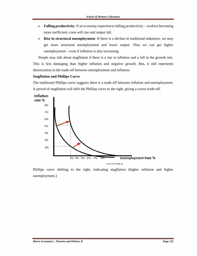
School of Distance Education
Macro Economics : Theories and Policies II Page 122
Falling productivity. If an economy experiences falling productivity – workers becoming
more inefficient; costs will rise and output fall.
Rise in structural unemployment. If there is a decline in traditional industries, we may
get more structural unemployment and lower output. Thus we can get higher
unemployment – even if inflation is also increasing.
People may talk about stagflation if there is a rise in inflation and a fall in the growth rate.
This is less damaging than higher inflation and negative growth. But, it still represents
deterioration in the trade-off between unemployment and inflation.
Stagflation and Phillips Curve
The traditional Phillips curve suggests there is a trade-off between inflation and unemployment.
A period of stagflation will shift the Phillips curve to the right, giving a worse trade-off.
Phillips curve shifting to the right, indicating stagflation (higher inflation and higher
unemployment.)

School of Distance Education
Macro Economics : Theories and Policies II Page 123
Stagflation in the 1970s
Solutions to stagflation
There are no easy solutions to stagflation.
Monetary policy can generally try to reduce inflation (higher interest rates) or increase
economic growth (cut interest rates). Monetary policy cannot solve both inflation and
recession at the same time.
One solution to make the economy less vulnerable to stagflation is to reduce the
economies dependency on oil. Rising oil prices are the major cause of stagflation.
The only real solution is supply-side policies to increase productivity; this enables higher
growth without inflation.
Laffer curve
The Laffer Curve is a theory developed by supply-side economist Arthur Laffer to show the
relationship between tax rates and the amount of tax revenue collected by governments. The curve
is used to illustrate Laffer’s argument that sometimes cutting tax rates can increase total tax
revenue.
The Laffer Curve describes the relationship between tax rates and total tax revenue, with
an optimal tax rate that maximizes total government tax revenue.
If taxes are too high along the Laffer curve, then they will discourage the taxed activities,
such as work and investment, enough to actually reduce total tax revenue. In this case,
cutting tax rates will both stimulate economic incentives and increase tax revenue.

School of Distance Education
Macro Economics : Theories and Policies II Page 124
The Laffer curve was used as a basis for tax cuts in the 1980's with apparent success, but
criticized on practical grounds on the basis of its simplistic assumptions, and on economic
grounds that increasing government revenue might not always be optimal.
Understanding the Laffer curve
The Laffer curve is based on the economic idea that people will adjust their behaviour in
the face of the incentives created by income tax rates. Higher income tax rates decrease the
incentive to work and invest compared lower rates. If this effect is large enough, it means that at
some tax rate, and further increase in the rate will actually lead to decrease in total tax revenue.
For every type of tax, there is a threshold rate above which the incentive to produce more
diminishes, thereby reducing the amount of revenue the government receives.
At a 0% tax rate, tax revenue would obviously be zero. As tax rates increase from low
levels, tax revenue collected by the also government increases. Eventually, if tax rates reached
100 percent, shown as the far right on the Laffer Curve, all people would choose not to work
because everything they earned would go to the government. Therefore it is necessarily true that
at some point in the range where tax revenue is positive, it must reach a maximum point. This is
represented by T* on the graph below. To the left of T* an increase in tax rate raises more revenue
than is lost to offsetting worker and investor behaviour. Increasing rates beyond T* however
would cause people not to work as much or not at all, thereby reducing total tax revenue.

School of Distance Education
Macro Economics : Theories and Policies II Page 125
Therefore at any tax rate to the right of T*, a reduction in tax rate will actually increase
total revenue. The shape of the Laffer Curve, and thus the location of T* is dependent on worker
and investor preferences for work, leisure, and income, as well as technology and other economic
factors. Governments would like to be at point T* because it is the point at which the government
collects maximum amount of tax revenue while people continue to work hard. If the current tax
rate is to the right of T*, then lowering the tax rate will both stimulate economic growth by
increasing incentives to work and invest, and increase government revenue because more work
and investment means a larger tax base.

School of Distance Education
Macro Economics : Theories and Policies II Page 126
MODULE IV
THE NEW KEYNESIAN SCHOOL
Introduction
New Keynesian economics is a school of contemporary macroeconomics that strives to
provide microeconomic foundations for Keynesian economics. It developed partly as a response
to criticisms of Keynesian macroeconomics by adherents of new classical macroeconomics.
New Keynesian Economics is a modern macroeconomic school of thought that evolved
from classical Keynesian economics. This revised theory differs from classical Keynesian
thinking in terms of how quickly prices and wages adjust.
New Keynesian advocates maintain that prices and wages are "sticky," meaning they
adjust more slowly to short-term economic fluctuations. This, in turn, explains such economic
factors as involuntary unemployment and the impact of federal monetary policies.
This way of thinking became the dominant force in academic macroeconomics from the
1990s through to the financial crisis of 2008.
British economist John Maynard Keynes' idea in the aftermath of the Great Depression
that increased government expenditures and lower taxes can stimulate demand and pull the global
economy out of a downturn became the dominant way of thinking for much of the 20th century.
The new Keynesian theory attempts to address, among other things, the sluggish behavior of
prices and its cause, and how market failures could be caused by inefficiencies and might justify
government intervention. The benefits of government intervention remains a flashpoint for
debate. New Keynesian economists made a case for expansionary monetary policy, arguing that
deficit spending encourages saving, rather than increasing demand or economic growth.
The Fall and Rise of Keynesian Economics
Dennis Robertson, one of Keynes’s most articulate critics, once wrote that ‘high brow
opinion is like the hunted hare; if you stand in the same place, or nearly the same place, it can be
relied upon to come around to you in a circle’ (Robertson, 1956). Good examples that illustrate
Robertson’s observation have been provided by the revival of both classical and Keynesian ideas
in their ‘new’ guise. In Chapters 5 and 6 we have seen how classical ideas have been given new
form through the technically impressive and imaginative contributions inspired, in particular, by
Robert Lucas and Edward Prescott. In this chapter we survey how Keynesian economics has also
undergone a ‘renaissance’ during the last 20 years.

School of Distance Education
Macro Economics : Theories and Policies II Page 127
We have seen in the previous chapters how the orthodox Keynesian model associated with
the neoclassical synthesis came under attack during the 1970s. It soon became apparent to the
Keynesian mainstream that the new classical critique represented a much more powerful and
potentially damaging challenge than the one launched by the monetarists, which was of longer
standing. Although orthodox monetarism presented itself as an alternative to the standard
Keynesian model, it did not constitute a radical theoretical challenge to it (see Laidler, 1986).
While Lucas’s new classical monetary theory of aggregate instability had its roots in Friedman’s
monetarism, the new classical real business cycle school represents a challenge to Keynesianism,
monetarism and Lucas’s monetary explanations of the business cycle. The poor performance of
Keynesian wage and price adjustment equations, during the ‘Great Inflation’ of the 1970s, based
on the idea of a stable Phillips curve, made it imperative for Keynesians to modify their models
so as to take into account both the influence of inflationary expectations and the impact of supply
shocks. This was duly done and once the Phillips curve was suitably modified, it performed
‘remarkably well’ (Blinder, 1986; Snowdon, 2001a). The important work of Gordon (1972,
1975), Phelps (1968, 1972, 1978) and Blinder (1979), all of whom are ‘Keynesians’, was
particularly useful in creating the necessary groundwork which has subsequently allowed the
Keynesian model to adapt and evolve in a way that enabled monetarist influences to be absorbed
within the existing framework (Mayer, 1997; DeLong, 2000). Moreover, this transition towards
a synthesis of ideas did not require any fundamental change in the way economists viewed the
economic machine. For example, Gordon (1997) argues that his ‘resolutely Keynesian’ model of
inflation, introduced in the mid-1970s and based on inertia, demand and supply shocks, within an
expectations-augmented Phillips curve framework, performs very well in explaining the
behaviour of output, unemployment and inflation during the ‘Great Inflation’ period. By
introducing supply shocks into the Phillips curve framework, Gordon’s ‘triangle’ model proved
capable of explaining the positive correlation between inflation and unemployment observed
during the 1970s. Meanwhile, debate continues on the relative importance of demand and supply
shocks as causes of the ‘Great Inflation’ (see Bernanke et al., 1997; Barsky and Kilian, 2001).
Despite these positive developments within Keynesian economics, by 1978 Lucas and
Sargent were contemplating life ‘After Keynesian Macroeconomics’. In their view the Keynesian
model could not be patched up. The problems were much more fundamental, and related in
particular to: (i) inadequate micro foundations which assume non-market clearing; and (ii) the
incorporation in both Keynesian and monetarist models of a hypothesis concerning the formation
of expectations which was inconsistent with maximizing behaviour, that is, the use of an adaptive
rather than rational expectations hypothesis. In an article entitled ‘The Death of Keynesian

School of Distance Education
Macro Economics : Theories and Policies II Page 128
Economics: Issues and Ideas’, Lucas (1980b) went so far as to claim that ‘people even take
offence if referred to as Keynesians. At research seminars people don’t take Keynesian theorising
seriously anymore; the audience starts to whisper and giggle to one another’ (cited in Mankiw,
1992). In a similar vein, Blinder (1988b) has confirmed that ‘by about 1980, it was hard to find
an American academic macroeconomist under the age of 40 who professed to be a Keynesian.
That was an astonishing intellectual turnabout in less than a decade, an intellectual revolution for
sure.’ By this time the USA’s most distinguished ‘old’ Keynesian economist had already posed
the question, ‘How Dead is Keynes’? (see Tobin, 1977). When Paul Samuelson was asked
whether Keynes was dead he replied, ‘Yes, Keynes is dead; and so are Einstein and Newton’ (see
Samuelson, 1988).
A Keynesian Resurgence
Lucas’s obituary of Keynesian economics can now be seen to have been premature
because Robert Barro’s ‘bad guys’ have made a comeback (Barro, 1989a). By the mid-1980s
Howitt (1986) was commenting on ‘The Keynesian Recovery’, and Blinder was discussing
‘Keynes After Lucas’ (1986) and ‘The Fall and Rise of Keynesian Economics’ (1988b). By the
early 1990s Blinder had announced that ‘A Keynesian Restoration is Here’ (1992b), Mankiw
(1992) proclaimed that Keynesian economics had been ‘reincarnated’ and Thirlwall (1993)
enthusiastically discussed the ‘Keynesian Renaissance’. While in the late 1980s the Keynesian
Promised Land was not yet in sight, Blinder (1988a) believed that ‘we may at long last be
emerging from the arid desert and looking over the Jordan’. In answering his own (1977) question
about the ‘death’ of Keynesian economics, Tobin (1987) later provided an unequivocal answer in
his essay, ‘The Future of Keynesian Economics’:
“One reason Keynesian economics has a future is that rival theories of economic
fluctuations do not … I hazard the prediction that neither of the two species of business cycle
theory offered by new classical macroeconomics will be regarded as serious and credible
explanations of economic fluctuations a few years from now. Whatever cycle theory emerges in
a new synthesis will have important Keynesian elements … Yes, Keynesian economics has a
future because it is essential to the explanation and understanding of a host of observations and
experiences past and present, that alternative macroeconomic approaches do not illuminate”.
Tobin (1996) was particularly critical of the ‘elegant fantasies’ of the ‘Robinson Crusoe
macroeconomics’ of real business cycle theory because it ignores the coordination question in
macroeconomics. To economists such as Akerlof, Stiglitz, Tobin and Leijonhufvud, an essential
task for macroeconomic theory is to explain in what circumstances the invisible hand does, and
does not, efficiently coordinate the economic behaviour of numerous diverse agents.

School of Distance Education
Macro Economics : Theories and Policies II Page 129
Certainly the persistence of high unemployment in Europe during the 1980s and 1990s
also called into question the plausibility of equilibrium explanations of the business cycle while
also providing increasing ‘credibility to Keynesian theory and policy’.
The central analytical message of the orthodox Keynesian school comprised the following main
propositions:
1. an unregulated market economy will experience ‘prolonged’ periods of excess supply of output
and labour in contradiction to ‘Say’s Law’ of markets; that is, in Keynes’s terminology, market
economies will exhibit ‘unemployment equilibrium’;
2. aggregate macroeconomic instability (business cycles) are mainly caused by aggregate demand
disturbances;
3. ‘money matters’ most of the time, although in very deep recessions monetary policy may be
ineffective (Blanchard, 1990a; Krugman, 1998);
4. government intervention in the form of stabilization policy has the potential to improve
macroeconomic stability and economic welfare.
While ‘new’ Keynesian economists would agree with these ‘old’ Keynesian propositions,
we shall see that the new Keynesian models are very different in many aspects from their distant
(1960s) cousins. While new Keynesians disagree with the new classical explanations of
instability, they do share two new classical methodological premises. First, macroeconomic
theories require solid microeconomic foundations. Second, macroeconomic models are best
constructed within a general equilibrium framework. However, as Greenwald and Stiglitz (1993a)
point out, real business cycle theorists adopt micro foundations that describe a world of perfect
information, perfect competition, zero transactions costs, and the existence of a complete set of
markets. Problems associated with asymmetric information, heterogeneous agents and imperfect
and incomplete markets are assumed away. The essence of the new Keynesian approach is to
recognize the importance of a whole variety of real world imperfections. By rebuilding the micro
foundations of Keynesian economics utilizing the findings of modern microeconomic theory, new
Keynesian theorists have established a research programme aimed at rectifying the theoretical
flaws which permeated the supply side of the ‘old’ Keynesian model. Because the typical market
economy is riddled with numerous imperfections, aggregate supply does respond to changes in
aggregate demand.
Although the term ‘new Keynesian’ was first used by Parkin and Bade in 1982 in their
textbook on modern macroeconomics (1982b), it is clear that this line of thought had been
conceived in the 1970s during the first phase of the new classical revolution. The burgeoning new
Keynesian literature since then has been primarily concerned with the ‘search for rigorous and

School of Distance Education
Macro Economics : Theories and Policies II Page 130
convincing models of wage and/or price stickiness based on maximising behaviour and rational
expectations’ (Gordon, 1990). New Keynesian economics developed in response to the perceived
theoretical crisis within Keynesian economics which had been exposed by Lucas during the
1970s. The paramount task facing Keynesian theorists is to remedy the theoretical flaws and
inconsistencies in the old Keynesian model. Therefore, new Keynesian theorists aim to construct
a coherent theory of aggregate supply where wage and price rigidities can be rationalized.
Both the old and new versions of classical economics assume continuous market clearing and in
such a world the economy can never be constrained by a lack of effective demand. To many
economists the hallmark of Keynesian economics is the absence of continuous market clearing.
In both the old (neoclassical synthesis) and new versions of Keynesian models the failure of prices
to change quickly enough to clear markets implies that demand and supply shocks will lead to
substantial real effects on an economy’s output and employment. In a Keynesian world,
deviations of output and employment from their equilibrium values can be substantial and
prolonged, and are certainly interpreted as damaging to economic welfare. As Gordon (1993)
points out, ‘the appeal of Keynesian economics stems from the evident unhappiness of workers
and firms during recessions and depressions. Workers and firms do not act as if they were making
a voluntary choice to cut production and hours worked.’ New Keynesians argue that a theory of
the business cycle based on the failure of markets to clear is more realistic than the new classical
or real business cycle alternatives. The essential difference between the old and new versions of
Keynesian economics is that the models associated with the neoclassical synthesis tended to
assume nominal rigidities, while the attraction of the new Keynesian approach is that it attempts
to provide acceptable microfoundations to explain the phenomena of wage and price stickiness.
New Keynesian economists are an extremely heterogeneous group, so much so that the use of the
term ‘school’ is more convenient than appropriate. Nevertheless, economists who have made
significant contributions to the new Keynesian literature, even if some of them may object to the
label ‘new Keynesian’, include Gregory Mankiw and Lawrence Summers (Harvard); Olivier
Blanchard (MIT), Stanley Fischer (Citigroup, and formerly at MIT); Bruce Greenwald, Edmund
Phelps and Joseph Stiglitz (Columbia); Ben Bernanke (Princeton); Laurence Ball (Johns
Hopkins); George Akerlof, Janet Yellen and David Romer (Berkeley); Robert Hall and John
Taylor (Stanford); Dennis Snower (Birkbeck, London) and Assar Lindbeck (Stockholm). The
proximity of US new Keynesians to the east and west coasts inspired Robert Hall to classify these
economists under the general heading of ‘Saltwater’ economists. By a strange coincidence new
classical economists tend to be associated with ‘Freshwater’ academic institutions: Chicago,
Rochester, Minnesota and Carnegie-Mellon.

School of Distance Education
Macro Economics : Theories and Policies II Page 131
Core Propositions and Features of New Keynesian Economics
New Keynesian economics emerged mainly as a response to the theoretical crisis facing
Keynesian economics that emerged during the 1970s. In their brief survey of new Keynesian
economics Mankiw and Romer (1991) define new Keynesian economics with reference to the
answer a particular theory gives to the following pair of questions:
Question 1 Does the theory violate the classical dichotomy? That is, is money non-neutral?
Question 2 Does the theory assume that real market imperfections in the economy are crucial for
understanding economic fluctuations?
Of the mainstream schools only new Keynesians answer both questions in the affirmative.
Non-neutralities arise from sticky prices, and market imperfections explain this behaviour of
prices. Thus, according to Mankiw and Romer, it is the ‘interaction of nominal and real
imperfections’ that distinguishes new Keynesian economics from the other research programmes
in macroeconomics. In contrast, the early real business cycle models gave a negative response to
both questions.
80s new Keynesian developments had a distinctly non-empirical flavour. Those younger-
generation economists seeking to strengthen the Keynesian model did so primarily by developing
and improving the microfoundations of ‘Fort Keynes’ which had come under theoretical attack.
A crucial difference between new classical and new Keynesian models arises with regard to price-
setting behaviour. In contrast to the price takers who inhabit new classical models, new Keynesian
models assume price making monopolistic, rather than perfectly competitive, firms.
Most new Keynesian models assume that expectations are formed rationally. This is
clearly one area where the new classical revolution of the 1970s has had a profound effect on
macroeconomists in general. However, some prominent Keynesians (Blinder, 1987b; Phelps,
1992), as well as some economists within the orthodox monetarist school (Laidler, 1992b) remain
critical of the theoretical foundations and question the empirical support for the rational
expectations hypothesis. Hence, although the incorporation of rational expectations in new
Keynesian models is the norm, this need not always be the case.
Although new Keynesian economists share an interest in improving the supply side of
Keynesian models, they hold a wide diversity of views relating to policy issues such as the debate
over the importance of discretion, rather than rules, in the conduct of fiscal and monetary policy.
New Keynesians regard both supply and demand shocks as potential sources of instability but
part company with real business cycle theorists particularly when it comes to an assessment of a
market economy’s capacity to absorb such shocks so that equilibrium (full employment) is

School of Distance Education
Macro Economics : Theories and Policies II Page 132
maintained. Many new Keynesians (but not all) also share Keynes’s view that involuntary
unemployment is both possible and likely.
New Keynesian economists inhabit a brave new theoretical world characterized by
imperfect competition, incomplete markets, heterogeneous labour and asymmetric information,
and where agents are frequently concerned with fairness. As a result the ‘real’ macro world, as
seen through new Keynesian eyes, is characterized by the possibility of coordination failures and
macroeconomic externalities.
Because the literature reviewed here is so wide-ranging, it is convenient to divide the
explanations of rigidities between those that focus on nominal rigidities and those that focus on
real rigidities. A nominal rigidity occurs if something prevents the nominal price level from
adjusting so as exactly to mimic nominal demand disturbances. A real rigidity occurs if some
factor prevents real wages from adjusting or there is stickiness of one wage relative to another, or
of one price relative to another.
Nominal Rigidities
Both orthodox and new Keynesian approaches assume that prices adjust slowly following
a disturbance. But, unlike the Keynesian cross or IS–LM approaches, which arbitrarily assume
fixed nominal wages and prices, the new Keynesian approach seeks to provide a microeconomic
underpinning for the slow adjustment of both wages and prices.
Nominal wage rigidity
In traditional Keynesian models the price level is prevented from falling to restore
equilibrium by the failure of money wages (costs) to adjust. In the new classical models developed
by Lucas, Sargent, Wallace and Barro during the 1970s, any anticipated monetary disturbance
will cause an immediate jump of nominal wages and prices to their new equilibrium values, so
preserving output and employment. In such a world, systematic monetary policy is ineffective.
Initially it was widely believed that this new classical policy ineffective proposition was a direct
implication of incorporating the rational expectations hypothesis into macroeconomic models.
Fischer (1977) and Phelps and Taylor (1977) showed that nominal disturbances were capable of
producing real effects in models incorporating rational expectations, providing the assumption of
continuously clearing markets was dropped. Following these contributions it became clear to
everyone that the rational expectations hypothesis did not imply the end of Keynesian economics.
The crucial feature of new classical models was shown to be the assumption of continuous market
clearing, that is, perfect and instantaneous wage and price flexibility.
The early Keynesian attempts to fortify their theoretical structure concentrated on nominal
wage rigidities and the models developed by Fischer (1977) and Taylor (1980) introduced

School of Distance Education
Macro Economics : Theories and Policies II Page 133
nominal inertia in the form of long-term wage contracts. In developed economies wages are not
determined in spot markets but tend to be set for an agreed period in the form of an explicit (or
implicit) contract. The existence of these long-term contracts can generate sufficient nominal
wage rigidity for monetary policy to regain its effectiveness. It should be noted, however, that
neither Fischer nor Phelps and Taylor pretend to have a rigorous microfoundation for their price-
and wage-setting assumptions. Instead they take it for granted that there is a ‘revealed preference’
for long-term wage contracts reflecting the perceived disadvantages that accompany too frequent
adjustments to wages and prices.
According to Phelps (1985, 1990) there are private advantages to both firms and workers
from entering into long-term wage contracts:
1. Wage negotiations are costly in time for both workers and firms. Research must be carried out
with respect to the structure of wage relativities both within and outside the negotiating
organization. In addition, forecasts are required with respect to the likely future paths of key
variables such as productivity, inflation, demand, profits and prices. The longer the period of the
contract, the less frequently are such transaction costs incurred and in any case management will
always tend to prefer a pre-set schedule for dealing with the complex issues associated with pay
negotiations.
2. There always exists the potential for such negotiations to break down, with workers feeling
that they may need to resort to strike action in order to strengthen their bargaining position. Such
disruption is costly to both firms and workers.
3. It will not be an optimal strategy for a firm to ‘jump’ its wage rates to the new ‘ultimate’
equilibrium following a negative demand stock because if other firms do not do likewise the firm
will have reduced its relative wage, which would be likely to increase labour turnover, which is
costly to the firm.
Thus the responsiveness of wage rates during a recession does not follow the new classical
‘precision drill process’; rather we observe a ‘ragged, disorderly retreat’ as new information
becomes available.
Nominal price rigidity
Keynesian models based on nominal wage contracting soon came in for considerable
criticism (see Barro, 1977b). Critics pointed out that the existence of such contracts is not
explained from solid microeconomic principles. A further problem relates to the countercyclical
path of the real wage in models with nominal wage contracts.
As a result of these and other criticisms, some economists sympathetic to the Keynesian
view that business cycles can be caused by fluctuations of aggregate demand switched their

School of Distance Education
Macro Economics : Theories and Policies II Page 134
attention to nominal rigidities in the goods market, rather than continue with research into nominal
wage inertia. Indeed, the term ‘new Keynesian’ emerged in the mid-1980s as a description of
those new theories that attempted to provide more solid microfoundations for the phenomenon of
nominal price rigidity. From this standpoint, the ‘fundamental new idea behind new Keynesian
models is that of imperfect competition’. This is the crucial innovation which differentiates new
Keynesians from Keynes, orthodox Keynesians, monetarists and new classicals.
If the process of changing prices were a costless exercise and if the failure to adjust prices
involved substantial changes in a firm’s profitability we would certainly expect to observe a high
degree of nominal price flexibility. A firm operating under conditions of perfect competition is a
price taker, and prices change automatically to clear markets as demand and supply conditions
change. Since each firm can sell as much output as it likes at the going market price, a perfectly
competitive firm which attempted to charge a price above the market clearing level would have
zero sales. There is also no profit incentive to reduce price independently, given that the firm’s
demand curve is perfectly elastic at the prevailing market price. Thus in this world of perfect price
flexibility it makes no sense to talk of the individual firm having a pricing decision.
When firms operate in imperfectly competitive markets a firm’s profits will vary
differentially with changes in its own price because its sales will not fall to zero if it marginally
increases price. Price reductions by such a firm will increase sales but also result in less revenue
per unit sold. In such circumstances any divergence of price from the optimum will only produce
‘second-order’ reductions of profits. Hence the presence of even small costs to price adjustment
can generate considerable aggregate nominal price rigidity. This observation, due to Akerlof and
Yellen (1985a), Mankiw (1985) and Parkin (1986), is referred to by Rotemberg (1987) as the
‘PAYM insight’.
The PAYM insight makes a simple but powerful point. The private cost of nominal
rigidities to the individual firm is much smaller than the macroeconomic consequences of such
rigidities. A key ingredient of the PAYM insight is the presence of frictions or barriers to price
adjustment known as ‘menu costs’. These menu costs include the physical costs of resetting
prices, such as the printing of new price lists and catalogues, as well as expensive management
time used up in the supervision and renegotiation of purchase and sales contracts with suppliers
and customers. To illustrate how small menu costs can produce large macroeconomic
fluctuations, we will review the arguments made by Mankiw and by Akerlof and Yellen.
In imperfectly competitive markets a firm’s demand will depend on (i) its relative price
and (ii) aggregate demand. Suppose following a decline in aggregate demand the demand curve
facing an imperfectly competitive firm shifts to the left. A shift of the demand curve to the left
School of Distance Education
Macro Economics : Theories and Policies II Page 135
can significantly reduce a firm’s profits. However, faced with this new demand curve, the firm
may gain little by changing its price.
If the presence of menu costs and/or near rational behaviour causes nominal price rigidity,
shocks to nominal aggregate demand will cause large fluctuations in output and welfare. Since
such fluctuations are inefficient, this indicates that stabilization policy is desirable. Obviously if
money wages are rigid (because of contracts) the marginal cost curve will be sticky, thus
reinforcing the impact of menu costs in producing price rigidities.
Real Rigidities
Sources of real price rigidity
1. mild sensitivity of marginal cost to variations in output and procyclical elasticity of demand
(implying a countercyclical markup) will contribute towards real price rigidity.
2. Thick market externalities In the real world buyers and sellers are not brought together without
incurring search costs. Consumers must spend time searching the market for the goods they desire
and firms advertise in order to attract customers. Workers and employers must also spend time
and resources searching the market. When markets are thick during periods of high economic
activity it seems plausible that search costs will be lower than is the case in a thin market
characterized by a low level of trading activity. It may also be the case that people are much more
willing to participate in thick markets where a lot of trade is taking place and this leads to strategic
complementary; that is, the optimal level of activity of one firm depends on the activity of other
firms. If these thick market externalities help to shift the marginal cost curve up in recessions and
down in booms, then this will contribute to real price rigidity.
3. Customer markets The distinction between auction and customer markets has been developed
by Okun (1975, 1981). The crucial characteristic of a customer market is a low frequency of
search relative to the frequency of purchase (McDonald, 1992). Most products are sold through a
process of shopping and, providing the costs of searching the market are non-trivial, the buyer
will always have imperfect (limited) information concerning the lowest price in the marketplace.
Because of the search costs associated with the shopping process, sellers have some monopoly
power even though there may be a large number of firms in the market, each selling a similar
product. Since a large number of customers make repetitive purchases it is in the interests of any
firm to discourage its customers from searching the market in order to find a better deal. Firms
are therefore discouraged from frequently changing their prices, a practice which will provide an
incentive for customers to look elsewhere. Whereas an increase in price will be noticed
immediately by customers, a decrease in price will produce a much smaller initial response as it
takes time for this new information to reach the buyers at other firms. This difference in the

School of Distance Education
Macro Economics : Theories and Policies II Page 136
response rates of customers to price increases and decreases, and the desire of a firm to hold on
to its regular customers, will tend to produce relative price stickiness.
4. Price rigidity and the input–output table Gordon (1981, 1990) has drawn attention to the
complexity of decision making in a world where, typically, thousands of firms buy thousands of
components containing thousands of ingredients from numerous other firms, many of which may
reside overseas. ‘Once decentralisation and multiplicity of supplier–producer relationships are
recognised, no single firm can perform an action that would eliminate the aggregate business
cycle’. Because a firm is linked to thousands of other firms via a complex input– output table, it
is impossible for it to know the identity of all the other agents linked together in the web of
supplier–producer relationships. Because of this complexity there is no certainty that marginal
revenue and marginal cost will move in tandem following an aggregate demand shock. There is
no certainty for an individual firm that, following a decline in aggregate demand, its marginal
cost will move in proportion to the decline in demand for its products. Many of its suppliers may
be firms in other countries facing different aggregate demand conditions. To reduce price in these
circumstances is more likely to produce bankruptcy for the particular firm than it is to contribute
to the elimination of the business cycle because a typical firm will be subject to both local and
aggregate demand shocks as well as local and aggregate cost shocks. As Gordon (1990) argues,
in such a world no firm would be likely to take the risk of nominal GNP indexation that would
inhibit its freedom and flexibility of action in responding to the wide variety of shocks which can
influence the position of its marginal revenue and cost curves. Since indexation is undesirable
when there is substantial independence of marginal cost and aggregate demand, Gordon’s input–
output theory not only provides an explanation of real price rigidity but also translates into a
theory of nominal rigidity. The fundamental reason for the gradual adjustment of prices is that
this represents the safest course of action for firms operating in an uncertain world where
information is inevitably imperfect.
5. Capital market imperfections An important obstacle to firms seeking external finance is the
problem of asymmetric information between borrowers and lenders; that is, borrowers are much
better informed about the viability and quality of their investment projects than lenders. One
consequence of this will be that external finance will be more expensive to a firm than internal
finance. During booms when firms are making higher profits there are more internal funds to
finance various projects. Hence during recessions the cost of finance rises as the result of a greater
reliance on external sources. If the cost of capital is countercyclical, this too will tend to make a
firm’s costs rise during a recession.

School of Distance Education
Macro Economics : Theories and Policies II Page 137
6. Judging quality by price Stiglitz (1987) has emphasized another reason why firms may be
reluctant to reduce price when faced with a decline in demand. In markets where customers have
imperfect information about the characteristics of the products which they wish to buy, the price
may be used as a quality signal. By lowering price a firm runs the risk that its customers (or
potential customers) may interpret this action as a signal indicating a deterioration of quality.
Real wage rigidity
New Keynesian explanations of real wage rigidity fall into three main groups: (i) implicit contract
theories; (ii) efficiency wage theories; and (iii) insider–outsider theories.
Implicit contract models The original implicit (non-union) contract models were provided by
Bailey (1974), D.F. Gordon (1974) and Azariadis (1975). Implicit contract theory seeks to
understand what it is that forms the ‘economic glue’ that keeps workers and firms together in
long-term relationships since such arrangements, rather than the Walrasian auctioneer, dominate
the labour market. Because firms seek to maintain the loyalty of their workforce they find it
necessary to enter into unwritten (implicit) understandings with their workers. This ‘invisible
handshake’ provides each worker with assurances concerning the terms of the working
relationship under a variety of working circumstances. The models of Bailey, Gordon and
Azariadis examine the consequences of optimal labour contracts established between risk-neutral
firms and risk-averse workers. In these circumstances the wage rate not only represents payment
for labour services but also serves as an insurance against the risk of variable income in the face
of shocks. A constant real wage smooths the individual worker’s consumption stream and firms
provide this ‘insurance’ since they are in a better position than workers to weather economic
fluctuations, given their better access to capital and insurance markets. Because firms provide
stable wages over time, workers, for their part, accept a real wage which is lower on average than
the highly varying rates that would be dictated by market forces.
Efficiency wage models Any acceptable account of involuntary unemployment must explain why
unemployed workers are unable to bid down wages to a level that will generate full employment.
Efficiency wage theories suggest that it is not in a firm’s interest to lower real wages because the
productivity (effort or efficiency) of workers is not independent of the wage, rather real wages
and worker effort are interdependent, at least over some meaningful range. Efficiency wage
theory, described by Gordon (1990) as the ‘rage of the 80s’, is surveyed by Yellen (1984), Akerlof
and Yellen (1986), Katz (1986, 1988), Haley (1990), and Weiss (1991); see also Akerlof (1979,
2002), and Stiglitz (2002).
Solow (1979) provides the basic structure of efficiency wage models. In Solow’s model, wage
stickiness is in the employer’s interest because wage cutting would lower productivity and raise

School of Distance Education
Macro Economics : Theories and Policies II Page 138
costs. Because the wage enters a firm’s short-run production function in a labour-augmenting
way, a cost minimizing firm will favour real wage rigidity.
The modern efficiency wage theories which have been put forward relate in general to the issues
of selection and incentives and four categories of efficiency wage theory can be identified: (i) the
adverse selection model (for example, Weiss, 1980); (ii) the labour turnover model (for example,
Salop, 1979); (iii) the shirking model (for example, Shapiro and Stiglitz, 1984); and (iv) the
fairness model (for example, Akerlof, 1982).
The adverse selection model In the adverse selection model, firms that offer higher wages will
attract the best workers. Because the labour market is populated by heterogeneous individuals,
firms have imperfect information about the productivity characteristics of job applicants; the
labour market is an excellent example of a market where asymmetric information predominates.
When there is asymmetric information one party to a transaction has more information than the
other party. In this case workers have more information about their own abilities, honesty and
commitment than employers before they are hired and will attempt to send signals to potential
employers that convey information about their qualities, such as educational qualifications,
previous employment record and current wage if employed. Because of the non-trivial hiring and
firing costs firms prefer not to hire workers and then find they need to fire those with low
productivity. The firm may also need to invest considerable resources in training new employees
before it becomes clear that they are not up to scratch. One way of avoiding this problem is for
the firm to send a signal to the labour market in the form of offers of high wages. In the model
presented by Weiss (1980) the wage offered by a firm influences both the number and quality of
job applicants. If workers’ abilities are closely connected to their reservation wage, then higher
wage offers will attract the most productive job applicants and any applicant who offers to work
for less than the efficiency wage will be regarded as a potential ‘lemon’. Firms will also be
reluctant to lower wage rates even if faced with an excess supply of labour wishing to work at the
prevailing wage offer because this would in all likelihood induce the most productive workers to
quit voluntarily. As a result of these influences an under employment equilibrium is attained. To
avoid adverse selection problems firms will attempt to introduce screening devices, but these
measures involve costs, as will the continuous monitoring of workers after they have been
appointed.
The labour turnover model A second reason why firms may offer an efficiency wage in excess
of the market-clearing wage is to reduce costly labour turnover. This approach received
inspiration from the pioneering work of Phelps (1968) and Phelps et al. (1970) in the development
of explanations of the natural rate of unemployment and search behaviour. The idea here is that

School of Distance Education
Macro Economics : Theories and Policies II Page 139
workers’ willingness to quit a job will be significantly reduced if a firm pays above the going
rate. With quitting rates a decreasing function of the real wage, firms have an incentive to pay an
efficiency wage to reduce costly labour turnover. In the model developed by Salop (1979), labour
market equilibrium entails involuntary unemployment since all firms need to raise their wages to
deter workers from quitting. In situations where unemployment increases, the wage premium
necessary to deter labour turnover will fall.
The shirking model In most occupations labour contracts are incomplete, which allows workers
to exercise discretion with respect to their effort levels. Because contracts cannot specify every
aspect of a worker’s performance and duties there is ‘effort discretion’. Since the collection of
information relating to the productivity of individual workers and the continual monitoring of
workers is very costly to the firm, the payment of an efficiency wage in excess of the market-
clearing equilibrium wage can act as an incentive which will deter the worker from shirking. The
threat of dismissal is not an effective deterrent in a labour market where workers can quickly find
a new job at the same wage rate. However, if a firm pays a wage in excess of that available
elsewhere, or if there is unemployment, workers have an incentive not to shirk, since there is now
a real cost to being fired and shirking becomes more risky for each worker. In the Shapiro–Stiglitz
(1984) model, the payment of an efficiency wage acts as a disincentive to shirking, and
involuntary unemployment in equilibrium is an outcome of the problems firms face when
monitoring is imperfect: ‘With imperfect monitoring and full employment workers will choose
to shirk.’ By being paid more than the going rate, workers now face a real penalty if they are
caught shirking.
The fairness model Several economists have examined the adverse effects of ‘unfair wages’ and
wage cuts on worker effort via the impact such cuts will have on the morale of the workforce.
Sociological models stress such factors as the importance of wage relativities, status, relative
deprivation, loyalty, trust and equity. In a series of papers, Akerlof (1982, 1984) and Akerlof and
Yellen (1987, 1988, 1990) responded to Solow’s (1979, 1980) ‘piece of home-made sociology’
and developed models where feelings about equity and fairness act as a deterrent to firms to offer
too low wages in the labour market.
Insider–outsider models Why don’t unemployed workers offer to work for lower wages than
those currently paid to employed workers? If they did so, wages would be bid down and
employment would increase. There appears to be an unwritten eleventh commandment: ‘Thou
shalt not permit job theft by underbidding and stealing the jobs of thy comrades.’ The insider–
outsider theory also attempts to explain why wage rigidity persists in the face of involuntary
unemployment. The insider–outsider approach to real wage rigidity was developed during the

School of Distance Education
Macro Economics : Theories and Policies II Page 140
1980s in a series of contributions by Lindbeck and Snower (1985, 1986, 1988a, 1988b). In this
model the insiders are the incumbent employees and the outsiders are the unemployed workers.
Whereas in efficiency wage models it is firms that decide to pay a wage higher than the market-
clearing wage, in the insider–outsider approach the focus shifts to the power of the insiders who
at least partially determine wage and employment decisions. No direct effects of wages on
productivity are assumed. Where does the insider power come from? According to Lindbeck and
Snower, insider power arises as a result of turnover costs (Vetter and Andersen, 1994). These
include hiring and firing costs such as those associated with costs of searching the labour market,
advertising and screening, negotiating conditions of employment, mandatory severance pay and
litigation costs. Other important costs are production-related and arise from the need to train new
employees. In addition to these well-known turnover costs, Lindbeck and Snower (1988a) also
emphasize a more novel form of cost – the insider’s ability and incentive to cooperate with or
harass new workers coming from the ranks of the outsiders. If insiders feel that their position is
threatened by outsiders, they can refuse to cooperate with and train new workers, as well as make
life at work thoroughly unpleasant. By raising the disutility of work, this causes the outsiders’
reservation wage to rise, making it less attractive for the firm to employ them. To the extent that
cooperation and harassment activities lie within the control of workers, they can have a significant
influence on turnover costs by their own behaviour. Because firms with high rates of turnover
offer both a lack of job security and few opportunities for advancement, workers have little or no
incentive to build reputations with their employers. Low motivation damages productivity and
this represents yet another cost of high labour turnover. Because it is costly to exchange a firm’s
current employees for unemployed outsiders, the insiders have leverage which they can use to
extract a share of the economic rent generated by turnover costs (the firm has an incentive to pay
something to avoid costly turnover). Lindbeck and Snower assume that workers have sufficient
bargaining power to extract some of this rent during wage negotiations. Although unions are not
necessary for insider power, they enhance it with their ability to threaten strikes and work-to-rule
forms of non-cooperation.
Policy Implications
Following the contributions of Fischer (1977), Phelps and Taylor (1977), it was clear that
the new classical conclusion that government demand management policy was ineffective did not
depend on the assumption of rational expectations but rather on the assumption of instantaneous
market clearing. In new Keynesian models which emphasize sticky prices, money is no longer
neutral and policy effectiveness is, at least in principle, re-established. Since in the Greenwald–

School of Distance Education
Macro Economics : Theories and Policies II Page 141
Stiglitz model greater price flexibility exacerbates the problems of economic fluctuations, new
Keynesians have also demonstrated the potential role for corrective demand management policies
even if prices are flexible (but not instantaneously so). In a world where firms set prices and
wages in an uncoordinated way, and where they are uncertain of the consequences of their actions,
it is not surprising that considerable inertia with respect to prices and wages results. In a market
economy endogenous forces can frequently amplify the disturbing impact of exogenous shocks.
While new Keynesians tend to be more concerned with the way an economy responds to shocks
than with the source of the shocks, experience during the past quarter-century has confirmed that
economies can be disturbed from the supply side as well as the demand side. Indeed, as Benjamin
Friedman (1992) has observed, it is often practically and conceptually difficult to draw a clear
distinction between what is and what is not the focal point of any disturbance. Because in new
Keynesian models fluctuations are irregular and unpredictable, new Keynesians are not
enthusiastic supporters of government attempts to ‘fine-tune’ the macro economy. Many new
Keynesians (such as Mankiw) accept the monetarist criticisms relating to old-style Keynesianism
as well as several of the criticisms raised by new classical economists, such as those related to
dynamic consistency. There is no unified new Keynesian view on the extent of discretionary fiscal
and monetary action that a government may take in response to aggregate fluctuations. However,
most new Keynesians do see a need for activist government action of some form because of
market failure, especially in the case of a deep recession. For example, Taylor (2000a) argues that
while fiscal policy should normally be used to achieve long-term objectives such as economic
growth, there is a strong case for the explicit use of fiscal expansionary policy in ‘unusual
situations such as when nominal interest rates hit a lower bound of zero’.
Because of uncertainty with respect to the kinds of problems an economy may confront
in the future, new Keynesians do not support the fixed-rules approach to monetary policy
advocated by Friedman (1968a) and new classical equilibrium theorists such as Lucas, Sargent,
Wallace, Barro, Kydland and Prescott during the 1970s. If the monetarists and new classicists
successfully undermined the case for fine-tuning, new Keynesians have certainly championed the
case for what Lindbeck (1992) has referred to as ‘coarsetuning’ – policies designed to offset or
avoid serious macro-level problems.
New Keynesian Business Cycle Theory
New Keynesian economists accept that the source of shocks which generate aggregate
disturbances can arise from the supply side or the demand side. However, new Keynesians argue
that there are frictions and imperfections within the economy which will amplify these shocks so

School of Distance Education
Macro Economics : Theories and Policies II Page 142
that large fluctuations in real output and employment result. The important issue for new
Keynesians is not so much the source of the shocks but how the economy responds to them.
Within new Keynesian economics there have been two strands of research relating to the issue of
aggregate fluctuations. The predominant approach has emphasized the importance of nominal
rigidities. The second approach follows Keynes (1936) and Tobin (1975), and explores the
potentially destabilizing impact of wage and price flexibility.
The impact of an aggregate demand shock in the new Keynesian model
Consider above Figure. In panel (a) we illustrate the impact of a decline in the money
supply which shifts aggregate demand from AD0 to AD1. If a combination of menu costs and real
rigidities makes the price level rigid at P0, the decline in aggregate demand will move the
economy from point E0 to point E1 in panel (a). The decline in output reduces the effective
demand for labour. In panel (c) the effective labour demand curve (DLe) shows how much labour
is necessary to produce different levels of output. As the diagram shows, L1 amount of labour is

School of Distance Education
Macro Economics : Theories and Policies II Page 143
required to produce Y1 amount of output. With prices and the real wage fixed at P0 and w0,
respectively, firms move off the notional demand curve for labour, DL, operating instead along
their effective labour demand curve indicated by NKL1 in panel (d). At the rigid real wage of w0,
firms would like to hire L0 workers, but they have no market for the extra output which would be
produced by hiring the extra workers. The aggregate demand shock has produced an increase in
involuntary unemployment of L0 – L1. The new Keynesian short run aggregate supply curve
SRAS (P0) is perfectly elastic at the fixed price level. Eventually downward pressure on prices
and wages would move the economy from point E1 to E2 in panel (a), but this process may take
an unacceptably long period of time. Therefore new Keynesian economists, like Keynes, advocate
measures which will push the aggregate demand curve back towards E0. In the new Keynesian
model, monetary shocks clearly have non-neutral effects in the short run, although money remains
neutral in the long run, as indicated by the vertical long-run aggregate supply curve (LRAS).
The failure of firms to cut prices even though this would in the end benefit all firms is an
example of a ‘coordination failure’. A coordination failure occurs when economic agents reach
an outcome that is inferior to all of them because there are no private incentives for agents to
jointly choose strategies that would produce a much better (and preferred) result. The inability of
agents to coordinate their activities successfully in a decentralized system arises because there is
no incentive for a single firm to cut price and increase production, given the assumed inaction of
other agents. Because the optimal strategy of one firm depends on the strategies adopted by other
firms, a strategic complementary is present, since all firms would gain if prices were reduced and
output increased. To many Keynesian economists the fundamental causes of macroeconomic
instability relate to problems associated with coordination failure.
Hysteresis and NAIRU
Hysteresis and NAIRU are two words adopted by economists from physics. By the topic
'hysteresis and the NAIRU, policy implications', it is dealing with the two terms hysteresis and
NAIRU in economics, and trying to find out the relationship between these two terms.
RELATION BETWEEN INFLATION AND UNEMPLOYMENT
The traditional economics since the time of Classist David Hume[1752] emphasizes
that the supply of money influences both inflation and employment. The same argument even
motivated modern theorist like Milton Friedman and Robert Lucas.
But business cycle theorists like Prescott laid emphasis on technological advancement
and argued that money had no role in production and employment fluctuations. But this theory
did not get much support. There is a wide agreement about monetary fluctuations push inflation

School of Distance Education
Macro Economics : Theories and Policies II Page 144
and unemployment in opposite direction. That is economy face trade off between inflation and
unemployment.
As per David Hume and others, monetary policy has a big say in the trade off between
inflation and unemployment. But still the problem of trade off between these two in the opposite
direction is not explained. For this, many blamed on imperfect information, long term labour
contracts, costs of price adjustment etcetera leading into theoretical and empirical questions.
This trade off is written as follows.
II=k-aU
Where, II=inflation
U=unemployment
k, a=parameters>0
This relationship only indicates that II and U are negatively related. This trade off between
inflation and unemployment is shown by Philips curve.
PHILLIPS CURVE
The Phillips curve is an economics concept developed by A. W. Phillips stating that
inflation and unemployment have a stable and inverse relationship. The concept behind the
Phillips curve states the change in unemployment within an economy has a predictable effect on
price inflation. The inverse relationship between unemployment and inflation is depicted as a
downward sloping, concave curve, with inflation on Y- axis and unemployment on X- axis.
Increasing inflation decreases unemployment, and vice versa. Alternatively, a focus on decreasing
unemployment also increases inflation, and vice versa.

School of Distance Education
Macro Economics : Theories and Policies II Page 145
EXPECTATIONS-AUGMENTED PHILLIPS CURVE
The expectations- augmented Phillips curve introduces adaptive expectations into the
Phillips curve and first used to explain the monetarist’s view of the Phillips curve.

School of Distance Education
Macro Economics : Theories and Policies II Page 146
Initially, unemployment and inflation are at point A. The government decides to embark
on an expansionist monetary policy, which floods the markets with inexpensive credit,
incentivising consumption. Expectations shift to point B along the Phillips curve, unemployment
is reduced through economic stimulus with a trade off in the form of inflation. However, after a
short period, agents will begin to associate expansionist policies with inflation, which means a
drain on their resources, and they will push for higher wages. This will stop the consumption
stimulus and also deincentivise hiring. Eventually, agents will shift their expectations curve to
point C. This is why, in the long run inflation has little effect on unemployment.
NAIRU
NAIRU is an acronym for non-accelerating inflation rate of unemployment, and refers to a
theoretical level of unemployment below which inflation would be expected to rise. In other
words it is a specific level of unemployment that does not cause inflation. If unemployment is at
NAIRU level, inflation is constant.

School of Distance Education
Macro Economics : Theories and Policies II Page 147
HYSTERESIS
Hysteresis was a term used by Sir James Alfred Ewing, a Scottish physicist and engineer
to refer systems, organisms and other things that have memory. For example, an iron piece
exposed to the magnetic field a long time will have the magnetization even after removing from
the field.
In the field of economics, hysteresis refers to an event in the economy that persist into
the future, even after that led the event have been removed. An example of hysteresis in
economics is that a delayed effect of unemployment, a characteristic of recession will persist in
the economy even after started recovery. In short, hysteresis refers to
an event in the economy that the unemployment persist even after the removal of recession.

School of Distance Education
Macro Economics : Theories and Policies II Page 148
That can be a delayed effect, as some times the rate of unemployment continue to rise even after
the commencement of recovery.
To indicate a permanent change in the attitude and skill of the work force even after the
commencement recovery.
Hysteresis is the term which was used to explain the process in the expectations- augmented
Phillips curve. The following table explains the above.
Unemployment in UK in the period of recession and after.
YEAR UNEMPLOYMENT
Recession/Deflation 1980 1.5 million
1981 2.0 million
Recovery/Inflation 1985 2.0 million
1986 3.0 million
During 1980-81, the UK entered a recession with falling output, falling inflation rate and
rising unemployment. In the year 1981, unemployment increased from 1.5 million to 2.0 million.
After 1981, UK started to recover from the recession, but unemployment remains the same (2.0
million) even after four years. And in the year 1986, the unemployment increased to 3.0 million.
POLICY IMPLICATIONS
If there is no hysteresis in unemployment, then for example if the central bank wishes to
lower the inflation rate it may shift to a contractionary monetary policy, which if not fully
anticipated and believed will temporarily increase the unemployment rate; if the contractionary
policy persists, the unemployment rise will eventually disappear as the unemployment rate returns
to the natural rate. Then the cost of the anti- inflation policy will have been temporary
unemployment. But if there is hysteresis, the unemployment rise initiated by the contractionary
policy will never completely go away, and in this case the cost of anti- inflation policy will have
been permanently higher unemployment, making the policy less likely to have greater benefits
than costs.
It is important to note that hysteresis is more serious than that of unemployment relates to
business cycles. It can not be over took by simple expansionary monetary or fiscal policies, but
policies including that of job training and counselling is necessary.

School of Distance Education
Macro Economics : Theories and Policies II Page 149
Hysteresis and NAIRU are two terms taken from the subject physics and used to show
the relationship between inflation and unemployment. NAIRU is a specific level of
unemployment that does not cause inflation. If unemployment is at NAIRU level, inflation is
constant. Hysteresis refers to an event in the economy that persist into the future, even after that
led the event have been removed.
The common belief in the case of inflation and unemployment is that when inflation
increases, unemployment decreases. There is an inverse relation between inverse and
unemployment. But hysteresis shows that, when economy started to move towards inflation after
the time of recession, or after the NAIRU level of unemployment, unemployment remains
constant or inflation increases. It can not be over took by simple expansionary monetary or fiscal
policies, but policies including that of job training and counselling is necessary in order to
improve employment.
Empirical evidence - Hysteresis and the NAIRU
Since the early 1970s the natural rate of unemployment ‘seems to have taken a wild ride’
in OECD countries. For OECD countries in general, unemployment in the 1980s and 90s was
higher than during the ‘Golden Age’ of the 1950–73 period. The steadily rising unemployment
rates appear to have their origins in the two OPEC oil price shocks in 1973 and 1979 respectively
and in the case of the European OECD countries, unemployment that averaged 1.7 per cent in the
early 1960s rose to 11 per cent by the mid-1990s. This high average also hides the large dispersion
of unemployment rates across the European countries estimates show that the US natural rate of
unemployment has also varied during this same period although the long-run unemployment
repercussions of the 1980s recessions appear to have been much more persistent in Europe than
in the USA. While the problem of inflation was a major policy concern during the 1970s and early
1980s, by the mid-1980s economists were once again turning their attention to the problem of
unemployment, in particular the rise in the estimated NAIRU.
Hysteresis in the field of economics refers to an event in the economy that persists into
the future, even after the factors that led to that event have been removed. Hysteresis can occur
following a recession when the unemployment rate continues to increase despite growth in the
economy.
Hysteresis was a term coined by Sir James Alfred Ewing, a Scottish physicist, and
engineer (1855-1935), to refer to systems, organisms, and fields that have memory. In other
words, the consequences of an input are experienced with a certain time lag or delay. One example
is seen with iron: iron maintains some magnetization after it has been exposed to and removed

School of Distance Education
Macro Economics : Theories and Policies II Page 150
from a magnetic field. Hysteresis is derived from the Greek term meaning "a coming short, a
deficiency."
Hysteresis in economics arises when a single disturbance affects the course of the
economy. An example of hysteresis is the delayed effects of unemployment, whereby the
unemployment rate can continue to rise even after the economy has begun recovering. The current
unemployment rate is a percentage of the number of people in an economy who are looking for
work but can't find any. In order to understand hysteresis, we must first explore the types of
unemployment. In a recession, which is two consecutive quarters of contracting growth,
unemployment rises.
Cyclical Unemployment
When a recession occurs, cyclical unemployment rises as the economy experiences
negative growth rates. Cyclical unemployment rises when the economy performs poorly and
falls when the economy is in expansion.
Natural Unemployment
Natural unemployment is not the result of a recession but instead, the result of a natural
flow of workers to and from jobs. Natural unemployment explains why unemployed people exist
in a growing, expansionary economy. Also called the natural rate of unemployment, it represents
people, including college graduates or those laid off because of technological advances. The
constant, ever-present movement of labor in and out of employment makes up natural
unemployment. However, natural unemployment can be from both voluntary and involuntary
factors.
Structural Unemployment
When workers are laid off due to a factory relocating or technology replaces their job,
structural unemployment exists. Structural unemployment, which is a portion of natural
unemployment, occurs even when an economy is healthy and expanding. It can be due to a
changing business environment or economic landscape and last for many years. Structural
unemployment is typically due to business changes such as factories moving overseas,
technological changes, and lack of skills for new jobs.

School of Distance Education
Macro Economics : Theories and Policies II Page 151
MODULE V
NEW POLITICAL MACROECONOMICS
“Most economists have now come to the realization that good economic advice requires
an understanding of the political economy of the situation”. (Rodrik, 1996)
That’s why we incorporate this module to our syllabus
Political Distortions and Macroeconomic Performance
The relationship between the economy and the political system has always attracted the
interest of economists since it is obvious that politics will influence the choice of economic
policies and consequently economic performance. During the last quarter of the twentieth century
research into the various forms of interaction between politics and macroeconomics has become
a major growth area, giving rise to a field known as ‘the new political macroeconomics’, a
research area which has developed at the interface of macroeconomics, social choice theory and
game theory. This burgeoning field makes specific use of the modern technical apparatus of
economic analysis to investigate numerous key public policy issues. Of particular interest to
macroeconomists is the influence that the interaction of political and economic factors has on
such issues as business cycles, inflation, unemployment, the conduct and implementation of
stabilization policies, the relationship between dictatorship, democracy, inequality and economic
growth, instability and conflict, the origin of persistent budget deficits, international integration
and the size of nations. Major contributions to this field of activity, both in terms of theoretical
analysis and empirical investigation, have come from the research of economists such as Daron
Acemoglu, Alberto Alesina, Alan Drazen, Bruno Frey, Douglass Hibbs, William Nordhaus,
Douglass North, Mancur Olson, Kenneth Rogoff, Fredrich Schneider, and Andrei Shleifer. In
this module we will examine some of the progress that has been made with regard to the
development of the ‘new political macroeconomics.
Political Influences on Policy Choice
Keynes (1926) believed that capitalism ‘can probably be made more efficient for attaining
economic ends than any alternative yet in sight’. However, for that to be the case would
necessarily involve an extension of government intervention in the economy. Classical
economists did not deny that fluctuations in aggregate economic activity could occur, but they
firmly believed that the self-correcting forces of the price mechanism would prevail and restore
the system to full employment within an acceptable time period. By the mid-1920s Keynes was
already expressing his disillusionment with this classical laissez-faire philosophy which
presented a vision of capitalist market economies where order and stability were the norm. For

School of Distance Education
Macro Economics : Theories and Policies II Page 152
Keynes the wise management of capitalism was defended as the only practicable means of
‘avoiding the destruction of existing economic forms in their entirety’. Hence the orthodox
Keynesian view evolved out of the catastrophic experience of the Great Depression and suggested
that market economies are inherently unstable. Such instability generates welfare-reducing
fluctuations in aggregate output and employment. As a result, ‘old’ Keynesians argue that this
instability can and should be corrected by discretionary monetary and fiscal policies (see
Modigliani, 1977; Tobin, 1996). Implicit in this orthodox Keynesian view is the assumption that
governments actually desire stability.
Michal Kalecki (1943) was one of the first economists to challenge this rather naive
assumption by presenting a Marxo-Keynesian model where a partisan government, acting on
behalf of capitalist interests, deliberately creates politically induced recessions in order to reduce
the threat to profits resulting from the enhanced bargaining power of workers. This increased
bargaining power is acquired as a direct result of prolonged full employment. In Kalecki’s model
it is the dominance of capitalists’ interests which, by generating an unrepresentative political
mechanism, causes the political business cycle.
Akerman (1947), anticipating later developments, suggested that the electoral cycle, by
influencing economic policies, would also contribute to aggregate instability. This of course runs
counter to traditional Keynesian models which treat the government as exogenous to the circular
flow of income and in which politicians are assumed to act in the interests of society. According
to Harrod (1951), Keynes was very much an élitist who assumed that economic policy should be
formulated and implemented by enlightened people drawn from an intellectual aristocracy. These
‘presuppositions of Harvey road’ imply that Keynes thought that economic policies would always
be enacted in the public interest. This benevolent dictator image of government acting as a
platonic guardian of social welfare has increasingly been questioned by economists.
In particular the work of public choice economists has called into question the assumption
that elected politicians will always pursue policies aimed at maximizing net social benefit (see
Buchanan et al., 1978). During the early days of the Keynesian revolution Joseph Schumpeter
also recognized that, since capitalist democracies are inhabited by politicians who compete for
votes, this will inevitably influence policy decisions and outcomes (see Schumpeter, 1939, 1942).
For example, from a public choice perspective Keynesian economics is seen to have
fundamentally weakened the fiscal constitutions of industrial democracies by giving
respectability to the idea that budget deficits should be accepted as a method of reducing the risk
of recessions. Buchanan etal. (1978) argue that such a philosophy, operating within a democratic
system where politicians are constantly in search of electoral favour, inevitably leads to an

School of Distance Education
Macro Economics : Theories and Policies II Page 153
asymmetry in the application of Keynesian policies. Because voters do not understand that the
government faces an intertemporal budget constraint, they
Under estimate the future tax liabilities of debt-financed expenditure programmes, that is,
voters suffer from ‘fiscal illusion’ (see Alesina and Perotti, 1995a). Instead of balancing the
budget over the cycle (as Keynes intended), in accordance with Abba Lerner’s (1944) principle
of functional finance, stabilization policies become asymmetric as the manipulation of the
economy for electoral purposes generates a persistent bias towards deficits. A deficit bias can also
result from strategic behaviour whereby a current government attempts to influence the policies
of future governments by manipulating the debt (Alesina, 1988). Given these considerations, it
would seem that macroeconomists ought to consider the possibility that elected politicians may
engage in ‘economic manipulation for political profit’ (Wagner, 1977). In the neoclassical
political economy literature government is no longer viewed as exogenous; rather it is (at least)
partially endogenous and policies will reflect the various interests in society (Colander, 1984).
This is certainly not a new insight, as is evident from the following comment taken from Alexis
de Tocqueville’s famous discussion of Democracy in America (1835):
(It is impossible to consider the ordinary course of affairs in the United States without
perceiving that the desire to be re-elected is the chief aim of the President… and that especially
as [the election] approaches, his personal interest takes the place of his interest in the public good.)
Although Keynes had an extremely low opinion of most politicians, in the context of his era it
never really crossed his mind to view the political process as a marketplace for votes. What
Keynes had in mind was what can be described as a linear model of the policy-making process
whereby the role of the economist is to offer advice, predictions and prescriptions, based on sound
economic analysis, to role-oriented politicians responsible for policy making. In turn, it is
assumed that that because politicians are looking for efficient solutions to major economic
problems, they will automatically take the necessary actions to maximize social welfare by
following the impartial and well-informed advice provided by their economic advisers. The
traditional economist’s view of the policy-making process is illustrated in the upper part of Figure
5.1.

School of Distance Education
Macro Economics : Theories and Policies II Page 154
5.1 Influence on policy choice
The conventional approach to the analysis of policy making traditionally adopted the
approach of Tinbergen (1952) and Theil (1956). For example, in the traditional optimizing
approach pioneered by Theil the policy maker is modelled as a ‘benevolent social planner’ whose
only concern is to maximize social welfare. Thus the conventional normative approach to the
analysis of economic policy treats the government as exogenous to the economy. Its only interest
is in steering the economy towards the best possible outcome. Economic policy analysis is
reduced to a technical exercise in maximization subject to constraint. From a new political
economy perspective policy makers will be heavily influenced by powerful societal and state-
centred forces rather than acting impartially on the advice of economists. Therefore the theoretical
insights and policy advice based on those insights that economists can offer are mediated through
a political system that reflects a balance of conflicting interests that inevitably arise in a country
consisting of heterogeneous individuals.
In the society-centred approach, various groups exert pressure on the policy maker to
‘supply’ policies that will benefit them directly or indirectly. While neo-Marxists typically focus
on class struggle and the power of the capitalist class, the new political economy literature
highlights the influence of interest groups (for example farmers), political parties and voters. In
the state-centred approach, emphasis on the role of technocrats is equivalent to accepting the
‘benevolent dictator’ assumption. In contrast, the new political economy literature focuses on the
impact that bureaucrats and state interests exert on the policy maker. The traditional approach to
the policy-making process adopted by economists was neatly summarized by Tony Killick (1976)
many years ago, in a critique of ‘The Possibilities of Development Planning’:
Economists have adopted a rational actor model of politics. This would have us see
governments as composed of publicly-spirited, knowledgeable, and role-oriented politicians:
clear and united in their objectives; choosing those policies which will achieve optimal results for
the national interest; willing and able to go beyond a short-term point of view. Governments are

School of Distance Education
Macro Economics : Theories and Policies II Page 155
stable, in largely undifferentiated societies; wielding a centralized concentration of power and a
relatively unquestioned authority; generally capable of achieving the results they desire from a
given policy decision.
In reality, societies are often fragmented and heterogeneous, especially if there are
significant religious, ethnic, linguistic and geographical divides compounded by extreme
inequalities of income and wealth. As a result governments will frequently be preoccupied with
conflict management, representing particular rather than general interests, responding to a
constantly shifting balance of preferences. In such a world concepts such as the ‘national interest’
and ‘social welfare function’ have little operational meaning? ‘Decision making in the face of
major social divisions becomes a balancing act rather than a search for optima; a process of
conflict resolution in which social tranquility and the maintenance of power is a basic concern
rather than the maximization of the rate of growth’ (Killick, 1976).
In modelling politico-economic relationships the new political macroeconomics views the
government as standing at the centre of the interaction between political and economic forces.
Once this endogenous view of government is adopted, the welfare-maximizing approach to
economic policy formulation associated with the normative approach ‘is no longer logically
possible’ (see Frey, 1978). Incumbent politicians are responsible for the choice and
implementation of economic policy, and their behaviour will clearly be shaped by the various
institutional constraints that make up the political system. Accordingly, a politico-economic
approach to the analysis of macroeconomic phenomena and policy highlights the incentives
which confront politicians and influences their policy choices.
Role of government
What governments do, or do not do, will obviously have an important impact on economic
growth and stability. Fiscal, monetary and exchange rate policies, along with policies towards
international trade, competition, regulation, the labour market, education, technology, healthcare
and the provision of key institutions such as property rights, all have a profound influence on
economic performance. During the nineteenth century the economic role of government, as
measured by government expenditure as a percentage of GDP, was around 10 per cent. By 1996
the government expenditure/GDP ratio had risen to an average of 45 per cent in developed OECD
countries (see Tanzi and Schuknecht, 2000).
This expanding role of government activity in all countries during the twentieth century
reflects the influence of several factors, in particular:
1. The impact of two world wars;

School of Distance Education
Macro Economics : Theories and Policies II Page 156
2. The Great Depression and subsequent Keynesian revolution;
3. The initial post-1945 influence of the Soviet state-led model of development;
4. Rising military expenditures associated with the cold war and global ideological competition
between the USA and the USSR;
5. The influence of socialist/humanitarian thinking and a growing concern for greater equity via
income redistribution;
6. The rise of welfare state capitalism;
7. The general recognition by economists of a wider range of important market failures beyond
those initially identified by Adam Smith, particularly widespread distortions created by
externalities, imperfect information and the problems of aggregate instability (Stiglitz, 2000,
2002).
At the beginning of the twentieth century the role of the state in the economic sphere was
minimal. However, over the past one hundred years we have witnessed a dramatic change in the
balance of economists’ vision of the appropriate role of government in economic affairs. For the
first 75 years of the twentieth century the role of the state expanded but during the last quarter of
the twentieth century there has been a marked change in economists’ thinking on the desirability
of this trend. This change, in large part, reflects the fact that over the past 25 years there has been
an unmistakable convergence of beliefs among economists in the power of a market economy to
deliver rising living standards compared to any known alternative.
What should be the role of government in an economy? This important question has been
debated throughout history and permeates all important public policy issues. The current borders
of the state have been mainly determined by historical events combined with developments in
economic analysis that recognized the importance of both market failure and government failure.
While the 1950s and 1960s represent the high-water mark of economists’ belief in the capacity
of governments to correct market failures, the 1970sand 1980s witnessed increasing scepticism
about the expanding role for government and saw a return of economists’ faith in markets. Among
economists there was a growing recognition of various forms of government failure. The state
was doing much more, but doing it less well. Even in the case where a government is attempting
to act as a benevolent social planner and intervenes to correct market failures, it must do so via
the use of agents (bureaucrats) who actually implement the strategy. Because these agents are
likely to be self-interested and difficult to monitor, government interventions invariably provide
opportunities for rent-seeking behaviour and corruption. From the 1970s onwards, the debate on
market failure versus government failure gathered momentum and became a key feature of the
economics literature. Many economists, influenced by the critiques of economists such as Peter

School of Distance Education
Macro Economics : Theories and Policies II Page 157
Bauer, Milton Friedman, James Buchanan, Friedrich von Hayek, Robert Lucas Jr and Anne
Krueger, began to accept that the state was trying to do too much. In many countries this had
deleterious effects on the efficient functioning of markets, economic growth and stability. The
idea of government acting as a ‘benevolent social guardian’ and the dubious assumption that state
agencies are populated by ‘selfless bureaucrats’ had been severely eroded by experience. This
does not imply that capitalism is a perfect system, that markets always work efficiently, or that
there is not an important role for government. But it does mean that throughout the world
‘governments have come to plan less, to own less, and to regulate less, allowing instead the
frontiers of the market to expand’ (Yergin and Stanislaw, 1999). Markets and effective
accountable government is complementary (see World Bank, 1997; Snowdon, 2001b; Stiglitz,
2002).
Politicians and Stabilization Policy
This ‘Downsian’ view of politicians indicates that government should be viewed as
endogenous in macroeconomic models (see Downs, 1957). According to Frey (1978), the
traditional Keynesian circular flow model needs to be modified to take account of self-interested
government behaviour. The politico-economic system resulting from this modification is
illustrated in Figure 5.2. There is no doubt that following the Keynesian revolution voters have
increasingly held governments responsible for the state of the economy. But in choosing to whom
they will delegate decision-making power, voters are faced with a principal–agent problem since
the agent (government) may have different preferences which it can conceal from the imperfectly
informed voters. As is evident from Figure 5.2, in the politico-economic circular flow model
politicians are seen to be driven by a balance of both ideological and re-election considerations.
Voters evaluate politicians on the basis of how successful they have been in achieving desirable
economic goals such as high employment, low inflation and rapid growth of real disposable
incomes. The state of the economy in the immediate pre-election period is crucial and politicians
are obviously aware that in order to survive in government it is preferable to have a buoyant
economy. If economic conditions are unfavourable, voters may well choose to elect the opposition
party and the incumbents lose office. Meanwhile the opposition party makes attractive promises
to the electorate (recall, for example, George Bush Sr’s famous 1988 pre-election pledge. ‘Read
my lips, no new taxes’). Hence economic conditions influence election results and the incentive
to get elected directly influences the choice and use of macroeconomic policies.

School of Distance Education
Macro Economics : Theories and Policies II Page 158
Figure 5.1
Politicians are also driven by partisan considerations, but ideological programmes cannot
be implemented unless parties first of all win or maintain power. During the past 25 years a
considerable amount of empirical work has been undertaken to test the importance of key
macroeconomic variables (such as inflation, unemployment and the growth of disposable income)
for the popularity of governments. This work indicates that such macroeconomic variables are
statistically significant and have an important influence on election outcomes (see Kramer, 1971;
Tufte, 1975, 1978; Mosley, 1978; Fair, 1988; Schneider and Frey, 1988). Given that incumbent
politicians occupy a position similar to that of a monopolist with respect to the supply of policies,
it is hardly surprising that they may often succumb to temptation and use discretionary policies
in order to maximize their re-election prospects. During the past 20 years or so economists have
produced a rich array of politico-economic models which incorporate many of these
considerations. The interdependence between the economy and the polity is now a well
established area of research for economists interested in identifying the underlying causes of
aggregate instability.
This research has attempted to answer a number of interesting questions, for example:

School of Distance Education
Macro Economics : Theories and Policies II Page 159
1. How important are economic factors in influencing voter choice? (Frey and Schneider, 1978a,
1978b);
2. Do opportunistic politicians manipulate the economy for political profit? (Nordhaus, 1975);
3. Do ideological (partisan) considerations lead to political parties producing a differentiated
product? (Hibbs, 1977);
4. Can political cycles exist in a world of rational non-myopic voters and economic agents?
(Alesina, 1987; Rogoff and Sibert, 1988);
5. Does the empirical evidence provide support for politico-economic models? (Alesina and
Roubini with Cohen, 1997);
6. What are the policy implications of such models? (Alesina, 1989; Drazen, 2000a).
In what follows we shall show how economists have attempted to answer these and other
questions.
Alternative Approaches to the ‘Political Business Cycle’: An Overview
In the theoretical literature on the political business cycle, which has developed since the
mid-1970s, we can distinguish four main approaches which have evolved in two separate phases.
The assumptions underlying these four different approaches are summarized in Table 5.1 (see
Alesina, 1988). During the first phase, in the mid- to late 1970s, Nordhaus (1975) reawakened
interest in this area by developing an opportunistic model of the political business cycle. This was
followed by Hibbs (1977), who emphasized ideological rather than office-motivated
considerations. However, both the Nordhaus and Hibbs models (the ‘old’ political
macroeconomics) were swept aside somewhat during the so-called rational expectations
revolution which dominated macroeconomic discussions during the mid- to late 1970s. After a
period of relative neglect a second phase of politicoeconomic models emerged in the mid-1980s
and research in this area has continued to flourish ever since. Due to the influence of new classical
theorists these new models incorporate the assumption of rational economic agents and voters.
While economists such as Rogoff and Sibert (1988) developed rational opportunistic models,
Alesina (1987) produced a rational partisan theory (the ‘new’ political macroeconomics). In what
follows we shall examine all four of these approaches (plus the hybrid model of Frey and
Schneider, 1978a, 1978b), each of which attempts to endogenize the influence of political
behaviour on the macroeconomy.

School of Distance Education
Macro Economics : Theories and Policies II Page 160
Table 5.1
The Nordhaus Opportunistic Model
The modern literature on political business cycles was stimulated by the seminal paper of
Nordhaus (1975). In the electoral model popularized by Nordhaus the party in power ‘chooses
economic policies during its incumbency which maximize its plurality at the next election’. Since
voters are influenced by a government’s macroeconomic performance before an election,
politicians will be tempted to manipulate policy instruments so that policy outcomes are most
favourable around the election period. The important consequence of such behaviour is that
policies are implemented in democracies which are biased against future generations (see also
Lindbeck, 1976; MacRae, 1977). Thus while elections and electoral competition are necessary
to increase the accountability of government, they are also likely to introduce potentially
damaging distortions into the policy-making process. In producing this result Nordhaus makes a
number of important assumptions, namely:
N1 The political system contains two parties between which there has been complete
policy convergence as predicted by the median voter theorem of Downs (1957).
N2 Both parties are interested in maximizing political profit rather than engaging in ideological
programmes. Only election outcomes matter to these opportunistic non-partisan politicians.
N3 The timing of elections is exogenously fixed.
N4 Individual voters are identical and have aggregate unemployment (Ut) and inflation
(P˙t ) in their preference functions and low inflation and unemployment rates are preferred. Policy
makers are fully informed of voters’ preferences but have no specific preferences with respect to
inflation and unemployment.

School of Distance Education
Macro Economics : Theories and Policies II Page 161
N5 Voters make political choices based on the past performance of incumbent politicians
in managing the economy during their term of office. Not only are voters retrospective in their
voting behaviour (they have no foresight); they also have a decaying memory (a high discount
rate on past economic performance), that is, they are myopic.
N6 The macroeconomic system can be described by an expectations-augmented Phillips
curve where the short-run trade-off is less favourable than the long-run trade-off. Voters are
ignorant of the macroeconomic framework.
N7 Expectations of inflation (P˙t ) e are formed adaptively, that is, agents are backward-
looking. N8 Policy makers can control the level of unemployment by manipulating aggregate
demand via fiscal and monetary policies. Nordhaus assumes (N4) that policy decisions will be
based on the observed aggregate voting function (Vt) which reflects individual preferences; this
is described by equation (10.1):
Vt g(Ut ,P˙t ), where g′(Ut ) 0, andg′(P˙t ) 0 (10.1)
In equation (5.1) votes are a decreasing function of ˙P and U. Figure 5.3 shows the
contours (iso-vote lines) of the aggregate voting function (V1, V2 and so on), which indicate the
percentage of votes acquired by the incumbents for a given policy outcome. Since inflation and
unemployment are ‘bads’, V1 > V2 > V3 > V4. Voters prefer any point on V1 to any point on V2
but are indifferent between points on the same contour. Governments seeking to win elections
will endeavour to manipulate the economy towards the highest feasible vote contour so as to
coincide with the election period.
The macroeconomic framework adopted by Nordhaus involves an expectations-
augmented Phillips curve framework summarized by equations (10.2)– (10.5).

School of Distance Education
Macro Economics : Theories and Policies II Page 162
Nordhaus assumes that 1 > > 0 which yields a long-run Phillips curve which is less
favourable (steeper) than the short-run relationship. In Figure 10.3 the short-run curves are
indicated by SG, SW and SM and the position of each curve depends on the expected rate of
inflation. The long-run Phillips curve is labelled LRPC. If the coefficient is unity, the
Phillips curve becomes a vertical line at the natural rate of unemployment (see Friedman, 1968a).
However, as Nordhaus (1975, p. 176) notes, ‘a vertical long-run Phillips curve makes no
difference in principle’ to the substantial conclusions of the model.
The Hibbs Partisan Model
In the Nordhaus model there is policy convergence in that all governments behave in the
same opportunistic way, and all voters are assumed to have identical preferences over inflation
and unemployment. An alternative approach is to view voters and politicians as ideological or
partisan. Politicians view winning elections as a means of putting into action their partisan
programme and heterogeneous voters will clearly have different preferences over inflation and
unemployment. Hibbs (1977) examined the post-war patterns of economic policies and outcomes
in 12 advanced capitalist democracies for the period 1945–69 in order to test the proposition that
left- and rightwing governments have different preferences with respect to the trade-off between
inflation and unemployment. In particular, Hibbs argues that his evidence supports the
proposition that left-wing governments prefer a lower U, higher ˙P outcome than right-wing
governments. We can represent this difference in preferences in terms of differences in loss
functions. Equations (10.8) and (10.9) show the loss (cost) functions in terms of unemployment
and inflation for two parties, a right-wing party = CR, and a left-wing party = CL (see Alesina,
1987).

School of Distance Education
Macro Economics : Theories and Policies II Page 163
Here UR * and P˙R* are the unemployment and inflation targets of the right wing party and R
is the relative weight placed on deviations of inflation from target (P˙t −P˙R* ) relative to
deviations of unemployment from target (UR – UR * ). The partisan differences can be summed
up as follows.
Partisan effects are further illustrated in Figure 10.5, where RR and LL indicate the respective
preferences of right- and left-wing politicians. Given the assumption of a stable exploitable
Phillips curve trade-off, left-wing governments will choose a combination of ˙PL and UL,
indicated by point L*, and right-wing governments will choose a combination of ˙PR and UR,
indicated by point R*.
Figure 5.5

School of Distance Education
Macro Economics : Theories and Policies II Page 164
Figures 5.5
According to Hibbs, ‘different unemployment/inflation outcomes have important class-
linked effects on the distribution of national income’. The revealed preference of policy makers
reflects the interests of the social groups who typically provide support for different parties. Since
macroeconomic policies have distributional consequences, Hibbs rejects Nordhaus’s assumption
(N1) ofpolicy convergence. According to Hibbs, the empirical evidence supports the partisan
view that ‘a relatively low unemployment–high inflation macroeconomic configuration is
associated with substantial relative and absolute improvements in the economic well-being of the
poor’. Because tight labour markets tend to generate income-equalizing effects, we should expect
left-wing governments to favour a point on the Phillips curve trade-off indicated by L*. Right-
wing parties view inflation as more damaging to their constituency of upper middle-class voters
and choose a position such as R*. According to Hibbs, the empirical evidence supports the
ideological view of macroeconomic policy making. The differing interests of various
occupational groups is reflected in the policy preferences of left- and right-wing political parties.
In an examination of 12 Western European and North American countries over the period 1945–
69 Hibbs found strong support for the proposition that the mean inflation rate is higher and the
mean unemployment rate lower, the greater the percentage of years that labour/socialist parties
have been in office. In addition to the static aggregated evidence, Hibbs also found that the time
series evidence for the USA and the UK supports the proposition that Democratic and Labour
administrations have usually reduced unemployment while Republican and Conservative

School of Distance Education
Macro Economics : Theories and Policies II Page 165
governments have tended to increase unemployment. Hibbs (1987) also reports significant
partisan effects on the distribution of income and Bartels and Brady (2003) conclude that the
‘consistent partisan differences in economic performance identified by Hibbs remain alive and
well two decades later’ and partisan influences have had a ‘profound influence on the workings
of the US economy’. These influences are summarized in Table 5.2.
Partisan influence on macroeconomic outcomes, USA, 1948–2001
Hence there is evidence supporting the Hibbs model that systematic differences exist in
the policy choices and outcomes of partisan governments. Hibbs argues that this is in line with
the subjective preferences of the class based political constituencies of right- and left-wing
political parties.
The Decline and Renaissance of Opportunistic and Partisan Models
The 1970s were a turbulent time for the capitalist democracies as the ‘Golden Age’ of low
inflation, low unemployment and above average growth came to an end. The stagflation crisis of
the 1970s also brought to an end the Keynesian consensus which had dominated macroeconomic
theory and policy making in the quarter-century following the Second World War. In the wake of
the monetarist counter-revolution, Lucas inspired a rational expectations revolution in
macroeconomics. By the mid-1970s models which continued to use the adaptive expectations
hypothesis were coming in for heavy criticism from new classical theorists, as the hypothesis
implies that economic agents can make systematic errors. In market-clearing models with rational
expectations the assumption that economic agents are forward-looking makes it more difficult for
the policy maker to manipulate real economic activity. There is no exploitable short-run Phillips
curve which policy makers can use. Pre election monetary expansions, for example, will fail to
surprise rational agents because such a manoeuvre will be expected. The rational expectations
hypothesis also implies that voters will be forward- looking and will not be systematically fooled
School of Distance Education
Macro Economics : Theories and Policies II Page 166
in equilibrium. According to Alesina (1988), ‘the theoretical literature on political business cycles
made essentially no progress’ after the contributions of Nordhaus (1975), Lindbeck (1976) and
MacRae (1977) because of the ‘devastating’ effect of the rational expectations critique. The
Nordhaus model involves an exploitable short-run Phillips curve trade-off combined with myopic
voters. Once the rational expectations hypothesis is introduced, however, voters can be expected
to recognize the incentives politicians have to manipulate the economy for electoral profit. Given
that US presidential elections are held on a regular four-year basis, it is difficult to believe that
rational voters and economic agents would allow themselves to be systematically duped by the
macroeconomic manipulations of self-interested politicians. Moreover, it is difficult to reconcile
the predictions of the Nordhaus model with situations where monetary policy is conducted by an
independent central bank, unless government can in some way pressurize the central bank to
accommodate the incumbent government’s preferred monetary policy (on this see Havrilesky,
1993; Woolley, 1994). However, Blinder, in discussing this issue, denies that political pressure
was an issue during his period as Vice Chairman at the US Federal Reserve, 1994–6. In his
experience the political influence on monetary policy was ‘trivial, next to zero’, although he
agrees that this was not the case during the Richard Nixon–Arthur Burns era (see Snowdon,
2001a).
The Hibbs model also has major theoretical shortcomings, especially with respect to the
stability of the Phillips curve trade-off implicit in his analysis. Remarkably, Hibbs makes no
mention of the expectations-augmented Phillips curve in his 1977 paper even though the
Friedman–Phelps theory was a decade old and by then a well-established idea, even among
Keynesians (see Gordon, 1975, 1976; Blinder, 1988b, 1992a; Laidler, 1992a). The assumption of
rationality also has implications for the Hibbs model. Since the output and employment effects of
expansionary and contractionary demand management policies are only transitory in new
classical models, the identification of partisan influences on macroeconomic outcomes will be
harder to detect (see Alesina, 1989).
Alt (1985) concluded that partisan effects are not permanent but occur temporarily after a
change of government.
In addition to the theoretical shortcomings of the early political business cycle literature,
the Nordhaus model also failed to attract strong empirical support, with the econometric literature
yielding inconclusive results (see Mullineux et al., 1993). While McCallum (1978) rejected the
implications of the Nordhaus model for US data, Paldam (1979) could only find weak evidence
of a political business cycle in OECD countries. Later studies, such as those conducted by Hibbs
(1987), Alesina (1988, 1989), Alesina and Roubini (1992), Alesina and Roubini with Cohen

School of Distance Education
Macro Economics : Theories and Policies II Page 167
(1997) and Drazen (2000a, 2000b), also find little evidence of a political business cycle in data
on unemployment and GNP growth for the US and other OECD economies. This also applies
where the timing of elections is endogenous (see Alesina et al., 1993). More favourable results
for the Nordhaus model are reported by Soh (1986), Nordhaus (1989), Haynes and Stone (1990)
and Tufte (1978), who found some evidence of pre election manipulation of fiscal and monetary
policy for the USA. In addition,
Drazen (2000a) distinguishes between empirical predictions that focus on policy
outcomes (inflation, unemployment, growth) and those that focus on policy instruments (taxes,
government expenditure interest rates) and concludes that ‘the evidence for opportunistic
manipulation of macroeconomic policies is stronger than for macroeconomic outcomes’. With
respect to policy outcomes there is more support for the opportunistic political business cycle
theory coming from post-electoral inflation behaviour than can be found in the pre electoral
movement of real GDP and unemployment. Drazen also concludes that the evidence in favour of
opportunistic manipulation of policy instruments is much stronger for fiscal policy than it is for
monetary policy.
A significant problem for partisan theories in general is the argument and evidence
presented by Easterly and Fischer (2001) that low inflation helps the poor more than the rich.
Inflation acts as a financial tax that hits the poor disproportionately because they tend to hold
more of their wealth in cash relative to their income than the rich, whereas the rich are more likely
to have access to various financial instruments that allow them to hedge against inflation. In
addition the poor obviously depend more on minimum wages and state-determined income
payments that are not always indexed to protect against the effects of inflation (see Snowdon,
2004b). Easterly and Fischer present evidence drawn from an international poll of over 30 000
respondents from 38 countries and the responses indicate that the poor themselves are more
strongly averse to inflation than those with higher incomes. This undermines a key assumption of
Hibbs’s model that the rich are more inflation-averse than the poor.
By the mid-1980s the politico-economic literature had reached a new ebb. Zarnowitz
(1985), in his survey of business cycle research, devotes one footnote to the idea of an electoral
cycle and refers critically to the ‘strong’ and ‘questionable’ assumptions of such models as well
as the lack of supporting evidence. The same neglect is also a feature of Gordon’s (1986) edited
survey of The American Business Cycle. Following a period of relative neglect, the literature on
the relationship between politics and the macroeconomy underwent a significant revival since the
mid-1980s (see Willet, 1988). Economists responded to the rational expectations critique by
producing a new generation of rational politico-economic models. Like the first phase in the

School of Distance Education
Macro Economics : Theories and Policies II Page 168
1970s, the second phase of politicoeconomic models consisted of opportunistic and partisan
versions of the interaction between politics and the macroeconomy. In the next two sections we
examine the main features of rational political business cycle models and the rational partisan
theory.
Rational Political Business Cycles
Recent work in the political business cycle tradition has shown that some of the insights
of Nordhaus (1975) can survive even in a model with rational expectations, providing there is
asymmetric information between voters and policy makers. In other words, voters need not be
myopic in order for politicians to generate political business cycles. Optimal policies are only
likely in a world of political competition when there is unanimity about social objectives and
symmetric information between agents, voters and politicians. Since these conditions are unlikely
ever to hold, politicians have the opportunity to follow non-optimal policies. Providing there is
some element of imperfect information, so that forward-looking voters are not fully informed
about some characteristics of the political and economic environment, incumbents have the
opportunity of creating ‘a temporary illusion of prosperity’ (Alesina, 1989) in order to gain favour
with the electorate.
In the rational opportunistic models proposed by Cukierman and Meltzer (1986), Rogoff
and Sibert (1988), Rogoff (1990) and Persson and Tabellini (1990), electoral cycles are created
in policy variables such as government spending, taxes and monetary growth, and such cycles are
made possible by temporary information asymmetries. Although rational voters aim to choose
politicians who they believe can deliver the highest utility, they lack information on the
competence of different policy makers. Voters acquire information on competence by observing
outcomes. Therefore before elections the incumbents engage in a ‘signalling process’ which aims
to persuade voters that the politicians in power are competent. Such signalling is always observed
in the UK during the Chancellor of the Exchequer’s annual budget speech, especially just before
an election.
Rogoff and Sibert define competence as the ability to reduce waste in the budget process;
that is, competent governments can produce more public goods and transfers for a given amount
of tax revenue. Incumbents have the potential to create a temporary fiscal boost (or fail to impose
necessary tax increases), which is popular with voters. Because the budgetary process is so
complicated the inevitable post-election tax increases needed to finance the pre-election boost are
not foreseen even by rational voters, due to their incomplete information. Rather than generating
a regular inflation–unemployment cycle as in the Nordhaus model, rational political business

School of Distance Education
Macro Economics : Theories and Policies II Page 169
cycle theories predict the manipulation of various policy instruments before and after the election.
The temptation of incumbents to cut taxes and increase spending before an election in order to
appear competent clearly generates departures from optimality. Hence opportunistic behaviour
survives in rational opportunistic models, although such models give rise to a different set of
empirical predictions compared to the original Nordhaus model. In particular, because of rational
expectations, any cycles resulting from the manipulation of monetary and fiscal policies will be
predicted to be less regular and of shorter duration. Finally, we should note that developing-
country governments appear to behave in a similar way to their counterparts in richer countries.
In a study of 35 developing countries Schuknecht (1996) found ‘considerable evidence’ in favour
of election generated fiscal policy cycles although the opportunities for self-interested political
behaviour are less in more open economies.
Policy Implications of Politico-Economic Models: An Independent Central Bank?
In introducing ‘The New Monetary Policy Framework’ for the UK economy on 6 May
1997, which established ‘operational independence’ for the Bank of England, Chancellor Gordon
Brown, in an official statement, provided the following rationale for the government’s strategy
(Brown, 1997, emphasis added):
We will only build a fully credible framework for monetary policy if the long term needs
of the economy, not short-term political considerations guide monetary decision-making. We must
remove the suspicion that short-term party political considerations are influencing the setting of
interest rates.
Chancellor Brown’s decision to grant much greater independence to the Bank of England
had its origins in a 1992 Fabian Society paper entitled ‘Euro Monetarism’, written by Ed Balls,
Brown’s economic adviser. As a former student of Larry Summers at Harvard, Balls was familiar
with the empirical work on central bank independence produced by Alesina and Summers (1993).
In a visit to the USA in March 1997, Shadow Chancellor Brown and his economic adviser met
both Alan Greenspan and Larry Summers. And so was born the strategy to go for immediate
greater central bank independence if elected. The general debate on the relative merits of rules
versus discretion in the conduct of fiscal and monetary policy was given a new stimulus by the
research surveyed in Chapters 5 and 7. Since the non-optimal use of monetary and fiscal
instruments lies at the heart of the various strands of the political business cycle literature, most
of this work points towards the desirability of establishing a policy regime which curtails the
incentives policy.

School of Distance Education
Macro Economics : Theories and Policies II Page 170
The Political Economy of Debt and Deficits
During the mid-1970s several OECD countries accumulated large public debts. This rise
in the debt/GNP ratios during peacetime among a group of relatively homogeneous economies is
unprecedented and difficult to reconcile with the neoclassical approach to optimal fiscal policy
represented by the ‘tax smoothing’ theory. While countries such as Greece, Italy and Ireland had
accumulated public debt ratios in excess of 95 per cent in 1990, other countries such as Germany,
France and the UK had debt ratios in 1990 of less than 50 per cent .
In order to explain the variance of country experience and the timing of the emergence of these
rising debt ratios, Alesina and Perotti (1995b) argue that an understanding of politico-institutional
factors is ‘crucial’. In explaining such wide differences Alesina and Perotti conclude that the two
most significant factors are:
1. The various rules and regulations which surround the budget process; and
2. The structure of government; that is, does the electoral system tend to generate coalitions or
single party governments?
In the face of large economic shocks weak coalition governments are prone to delaying
necessary fiscal adjustments. While a ‘social planner’ would react quickly to an economic shock,
in the real world of partisan and opportunistic politics a ‘war of attrition’ may develop which
delays the necessary fiscal adjustment (see Alesina and Drazen, 1991). Persson and Tabellini
(2004) have investigated the relationship between electoral rules, the form of government and
fiscal outcomes. Their main findings are that: (i) majoritarian elections lead to smaller
government and smaller welfare programmes than elections based on proportional representation;
and (ii) presidential democracies lead to smaller governments than parliamentary democracies.
Research by Alesina and Perotti (1996b, 1997a) also indicates that the ‘composition’ of a fiscal
adjustment matters for its success in terms of its sustainability and macroeconomic outcome. Two
types of adjustment are identified: Type 1 fiscal adjustments rely on expenditure cuts, reductions
in transfers and public sector wages and employment; Type 2 adjustments depend mainly on
broad-based tax increases and cuts in public investment. Alesina and Perotti (1997a) find that
Type 1 adjustments ‘induce more lasting consolidation of the budget and are more expansionary
while Type 2 adjustments are soon reversed by further deterioration of the budget and have
contractionary consequences for the economy’. Hence any fiscal adjustment that ‘avoids dealing
with the problems of social security, welfare programs and inflated government bureaucracies is
doomed to failure’ (see Alesina, 2000). Type 1 adjustments are also likely to have a more
beneficial effect on ‘competitiveness’ (unit labour costs) than policies which rely on distortionary
increases in taxation (see Alesina and Perotti, 1997b).

School of Distance Education
Macro Economics : Theories and Policies II Page 171
Political and Economic Instability:
A further related area of research in the politico-economic sphere concerns the relationship
between political and economic stability. There are good reasons to believe that economic
performance will suffer if a country is politically unstable. Frequent riots, politically motivated
violence and revolution inevitably have a negative impact on a country’s economic performance.
As Keynes always highlighted, uncertainty has a depressing effect on investment and productive
entrepreneurship. Alesina’s partisan theory predicts that instability will increase the greater the
partisan effects because widely divergent policies create uncertainty and destabilize expectations.
It is also unlikely that reputational considerations will be important to a government which feels
that it has little chance of being re-elected. In this situation an incumbent has an ‘incentive to
follow particularly shortsighted policies, since it is not concerned with a future in which it is likely
to be out of office’ (Alesina, 1989). A further destabilizing influence on policy arising from
political instability derives from the inability of fragile coalition governments to carry through
the tough but necessary economic policies crucial for long-run stability. Alesina (1989) finds a
positive correlation between an index of political instability and Okun’s misery index (inflation
+ unemployment) for the period 1973–86. An exception in his 20-country sample is the UK,
which managed to combine relatively poor economic performance during this period despite
having a high degree of political stability. In Alesina and Drazen’s (1991) analysis of why
necessary stabilization policies are frequently delayed, they consider a situation where two parties
with different ideologies engage in a war of attrition as they each attempt to pass on the burden
of fiscal reform to the other party’s supporters. The resultant delay and government inaction in
the reform process leads to debt accumulation and crisis before one of the parties is forced to
accept a larger share of the fiscal burden. As Drazen (2000a) notes, ‘the failure to adopt socially
beneficial economic reforms or their adoption only after long delays is a leading example of the
divergence between the simple textbook models of economic policymaking and real world
experience’. Considerable cross-country evidence now exists which indicates that seigniorage
(the inflation tax) is positively related to the degree of political instability. In a study of 79
developed and developing countries for the period 1971–82, Cukierman et al. (1992) found
evidence in support of their hypothesis that ‘more unstable countries rely relatively more on
seigniorage to finance the government budget than do stable and homogenous societies’. These
conclusions are also supported by Edwards (1994), who found that the incentive to use
inflationary finance is closely related to the volatility of the political system. In the extreme,
hyperinflation may erupt (see Capie, 1991; Siklos, 1995; Fischer et al., 2002).
School of Distance Education
Macro Economics : Theories and Policies II Page 172
References
1. Gregory Mankiw (2008): Macroeconomics- Worth Publishers NY, 6th ed.
2. Richard T Froyen (2008): Macroeconomics: Theories and Policies- Pearson (LPE), Seventh
ed.
3. Brian Snowdown and Howard Vane (2005): Modern Macroeconomics: Its Origin,
Development and Current State- Edward Elgar pub., Cheltenham, UK. Northampton, MA,
USA.
4. Levacic, Rosalind and Rebman, Alexander (1982): Macroeconomics: An Introduction to
Keynesian-Neoclassical Controversies- 2nd ed. Macmillan.
5. Eric Pentacost: Macroeconomics-An Open Economy Approach- Macmillan.
6. Rudiger Dornbusch: Stanley Fisher and Richard Startz (2004) Macroeconomics- Tata Mc
Graw Hill, 9th ed.
7. Hargreaves Heap S.P (1992): The New Keynesian Macroeconomics: Time, Belief and Social
Independence Edward Elgar Publishing.
8. D’Souza, Errol (2008): Macroeconomics- Pearson Education.
9. Fred R Glahe, (1985): Macroeconomics: Theory and Policy- Harcourt Publishers, New Delhi.
10. Veneries and Sebold, (1977): Macroeconomics: Models and Policies- John Wiley & Sons.
11. Samuelson and Nordhaus (1998): Macroeconomics- 16th ed. Irwin McGraw Hill.
12. Robert J Gordon: Macroeconomics- Eastern Economy Edition.
13. Edward Shapiro: Macroeconomics- Golgotha Publications, New Delhi.
14. Brian Showdown, Howard Vane and Peter Wynarczyk (2001): A Modern Guide to
Macroeconomics: An Introduction to Competing Schools of Thought- Edward Elgar.
15. Mervyn K.Lewis and Paul D Mizen (2000): Monetary Economics- Oxford University Press.
16. Jagdish Handa (2000):Monetary Economics- Routledge
17. Economic discussion –on line source