Nitrates and Property Values: Evidence from a FrenchMarket Intervention

Henrik Andersson∗

Toulouse School of Economics, University of Toulouse Capitole,Toulouse, France

Emmanuelle Lavaine†

Montpellier University, CEEM, Montpellier, France

March 21, 2018

Abstract

This paper examines the effect of properties being located in vulnerable zones in

term of nitrates on the property prices using a change in the classification of vulnerable

zones in France in 2012. Using an identification strategy based on a spatial difference-

in-differences specification, we show that the revision of the classification significantly

decreased not only property prices in zones that became classified as vulnerable after

the revision, but also those of properties already classified as vulnerable. However,

the effect was stronger for the former, 10% vs. 5%, and this differences may reflect a

difference in how zones are classified. The risks covered in the 2012 classification cover

a broader range of risks, and hence the larger price effect may reflect this additional

perceived risk exposure.

Keywords: Hedonic Price Analysis, difference in difference, water pollution

∗Email: henrik.andersson@tse-fr.eu†Email: emmanuelle.lavaine@umontpellier.fr

1

Work in progress. Do not quote. Comments welcome.

2

1 Introduction

Nitrates in drinking water, which may come from nitrogen fertilizers applied to crops, are a

potential health risk (Crutchfield et al., 1997). In Europe, Council Directive 91/676/EEC

(EEC, 1991) has been implemented to protect water sources against pollution caused by

nitrates from agricultural sources through a number of measures incumbent on the Euro-

pean Union (EU) member states. These measures concern monitoring surface water and

groundwater, designating vulnerable zones, introducing codes of good agricultural prac-

tice, adopting action programs, and evaluating the actions implemented. The measures

provide benefits in the form of reducing the potential health risk, but since they are costly

to implement the evaluation of them is important. Benefit-cost analysis (BCA) provides

a powerful, and transparent, tool for policy evaluations, but it requires that both benefits

and costs are measured in a common metric. The standard approach is to use money as

this common metric and since health effects do not have easily available prices it means

that non-market valuation techniques are required to monetize the social value of reducing

the health risks reductions from measures like the ones above.

Broadly speaking there exists two approaches to monetize health risk reductions, as well

as other “non-market goods”, i.e. stated- (SP) and revealed-preference (RP) methods (see,

e.g., Freeman et al., 2014). The former approach, i.e. SP methods, is based on respondents’

choices in hypothetical situations, whereas the latter, i.e. RP methods, is based on actual

decisions in markets related to the non-market good of interests. Both approaches have

their strengths and weaknesses, but economists have historically preferred the RP approach

since it is based on actual decisions. Regarding water quality it has been shown with market

data that it can have a significant effect on property values (Leggett and Bockstael, 2000).

Hence, market data can be used to estimate the marginal willingness to pay (WTP) for

access to clean and safe water. However, the literature underlines the need to improve

current and to develop novel methods to improve our ability to estimate the marginal

WTP for environmental improvements with market data (e.g., Bento, 2013; Guignet et al.,

2018).

A wide range of studies on this topic use quasi-experimental techniques. For instance,

Davis (2004) measures the effect of health risk on housing values by exploiting a severe

increase in pediatric leukemia in an isolated county in Nevada as a natural experiment.

In addition, Currie et al. (2015) recently examined the effect of health impacts of 1,600

openings and closings of industrial plants that emit toxic pollutants on the housing market.

3

Chay and Greenstone (2005) exploit the quasi-random assignment of air pollution changes

across counties induced by federally mandated air pollution regulations to identify the

impact of particulate matter on property values. Greenstone and Gallagher (2008) use the

Superfund cleanups to analyze its local welfare impacts.

In this study we are interested in the effect on property prices from exposure to ni-

trates. We are concerned with examining the impact on property prices from being located

in vulnerable zones, which are all known areas of land which drain into surface waters

and groundwater which are affected by pollution or at risk of being so. Zones classified as

vulnerable zones were revised in December 2012 in France due to pollution concentration

from surface waters and groundwater observed in 2010-2011. Before 2012, areas of land

were classified as being at risk if the population was exposed to contaminated drinking

water. The first delimitation was completed in July 1997 and was revised several times

since then in 2000, 2003, 2007, 2012, and most recently in 2014.1 The 2012 boundary

revision was mainly concerned with eutrophication risk, and was due to a litigation initi-

ated by the European Commission (EC) against France for misapplication of the Nitrates

Directive (EEC, 1991). France was sentenced by the European Court of Justice (ECJ) on

June 13, 2013, because of the 2007 boundary revision. The ECJ considered that a wider

classification would have been justified given the excessive levels of nitrates or eutrophica-

tion in surface and groundwater bodies. In short, the EC considered that France did not

take into account eutrophication risk into zoning and did not include enough areas as vul-

nerable located in the four following basins: Adour-Garonne, Loire-Bretagne, Rhin-Meuse

et Rhone-Mediterranee.2 The nitrates threshold for safe drinking water that is frequently

used in regulatory texts is 50mg/l3, even if this level is not enough to protect from eutroph-

ication.4 A difference between the EC and France was that the EC used the maximum

value relative to nitrates concentration to define contaminated water, whereas France used

the mean of the concentration. The French Circular related to the 2012 reclassification

instead use the 90th percentile resulting from the 2010-2011 monitoring campaign to evalu-

ate nitrate pollution.5 When its value exceeds 40mg/l, the Circular states it is necessary to

1Due to data limitation our analysis do not cover the 2014 delimitation.2http://www.donnees.centre.developpement-durable.gouv.fr/zv/comite bassin/Rapport Comite bassin.pdf3An area is vulnerable if surface and groundwater, particularly for drinking water supply, have or may

have a nitrate content greater than 50 mg/l and/or if the waters of estuaries, coastal or marine waters andsurface freshwaters show a tendency to eutrophication that can be reduced by decreasing nitrogen inputs.

4http://www.cnrs.fr/inee/communication/breves/docs/Eutrophisation resume.pdf5http://www.centre.developpement-durable.gouv.fr/IMG/pdf/Circulaire ZoneVulnerable 191211 cle7f77b8.pdf

4

analyze its inter-annual evolution at least since 2004-2005 to define its evolution; if increas-

ing, the zone has to be considered as vulnerable, whereas if stable or decreasing, nearby

measurement points should be checked (points not included in the surveillance network)

to confirm the non-classification or to invalidate it. This 2012 reclassification partly meets

the delimitation deficiencies recognized by the ECJ in the context of the litigation. To-

day, nearly 55% of France is classified as vulnerable, which corresponds to regions where

agricultural land is dominating.

In the same vein as Chay and Greenstone (2005), to mitigate selection and endogeneity

problems and to infer the impact of a new directive on property prices, we use the 2012

boundary revision of vulnerable zones as a quasi-experimental approach. While this is not

the first difference in difference (DiD) study to use the effect of an environmental policy on

hedonic prices as a natural experiment, this study aims to analyze the consequences of new

information that may have altered the risk perception. That is, the study examines the

effects on housing markets from the new information, not only in areas directly concerned

by a policy change, but also in areas indirectly concerned by this policy change. In fact,

the study focus, in addition to areas never classified as vulnerable, on two types of areas:

(i) areas of land that have been classified as being sensitive in term of nitrates before

2012, and (ii) areas of land considered as sensitive from December 2012. Thus, the paper

aims to shed light on people’s WTP for perceived differences in nitrates risk on health

and eutrophication. The analysis of this paper focuses on municipalities in the Centre and

Poitou Charentes region, where residents recently were considered to be living in a sensitive

geographical area in terms of nitrates, though this is not the only place in France. The

geographic region for the control group is then represented by all towns not classified as

vulnerable zones. House prices in new sensitive areas are compared before and after the

2012 designation of vulnerable zones with the nearby municipalities. The conditions of

supply and demand for housing are relatively similar in both groups, so that we can expect

a similar set of implicit prices in vulnerable zones and in its surroundings.

The article is structured as follows. In section 2 we first describe the data used and

then we outline the empirical strategy. We then in section 3 present the findings from the

regression results with a focus on the impact from vulnerable zones on the property prices.

Section 4 provides a discussion of our findings and some concluding comments.

5

2 Data and empirical strategy

2.1 Data sources

Property transactions are drawn from the data source PERVAL, compiled by the Chambre

of Notaires (that in France records property transactions), that provides us the exact

address of all property transactions between 2011 and 2014 together with the sales price

and all publicly recorded housing characteristics. Hence, we have access to a very unique

and rich data set on property transactions and in this study we focus our analysis on the

Centre-Val de Loire and Poitou Charentes regions. In these two regions we selected four

departments, i.e. Vienne (86) and Charente Maritime (17) for the Poitou Charente region,

and Loiret (45) and Indre et Loire (37) for the Centre Val de Loire region.6

The classification of whether an area is a nitrate sensitive, or a vulnerable, area is

at the municipality level. Information on which municipality that is considered to be

vulnerable is provided by the DRIEA, subordinated to the Ministry for an Ecological and

Inclusive Transition, and responsible for the environment, town planning and housing at

the regional level in France.7 The matching of the data from PERVAL and the info on

vulnerable zones was done using GPS coordinates for the municipalities of our four French

departments, i.e. Loiret, Indre et Loire, Vienne and Charentes Maritime. Hence, each

property is defined as vulnerable, and if so at what point in time, or not at the municipality

level. This is illustrated Figure 1 that shows the selected areas for our analysis. We have

classified municipalities at three levels with respect to the date they have been considered

as vulnerable. The first year that municipalities were considered as vulnerable was in

2007 and then in December of 2012 there was the reclassification mentioned above. Thus,

municipalities have therefore been classified as: (i) never being nitrates sensitive, shown as

white in Figure 1, (ii) nitrate sensitive before December 2012, shown as grey in Figure 1,

and (iii) nitrate sensitive from December 2012, shown as black in Figure 1. Hence, the

different colors indicate whether and when municipalities were considered as vulnerable,

and out of 676 municipalities, 135 have never been classified as nitrate sensitive, 456 have

been classified as nitrate sensitive since before December 2012 and 85 are classified as

6Department is a French geographical level below the regional level. There exist 96 departments inFrance, and the numbers in the parentheses refer to the official “department INSEE code”. For our clas-sification, see below, we will use municipalities which is a French geographical level below the departmentlevel.

7For info (in French only), http://www.driea.ile-de-france.developpement-durable.gouv.fr/.

6

nitrate sensitive since December 2012.

[Figure 1 about here.]

Table 1 presents summary statistics of the property transactions that took place be-

tween 2011-2014 in the Centre and Poitou Charentes Region. The unit of analysis is the

transaction - month - year and Panel A of Table 1 shows the average price. Transactions

occurred between 2011 and 2014, but all property price have been converted to the 2014

level using the INSEE property price index.8 Also shown is the number of transactions

per municipalities by year. The number of observations is 15,390.9 One concern with our

analysis is that a change of a sensitive area can affect the number of property transactions,

potentially leading to sample selection bias.

[Table 1 about here.]

The key variables of the PERVAL data set are, in addition to the property prices, the

number of rooms, the type of apartment or house, the property surface, the presence of

an attic, a parking space, a balcony, and a variable which indicates if the property is less

than 5 years old. We add the floor level for apartments while we add the presence of a

pool or a terrace for houses. We also include specific variables to distinguish houses and

apartments. We construct type of house as a dummy which is coded as 1 if it is a standard

house (detached house), considered as the most popular type of houses in the data set (it

represents more than 50% of all transactions) versus a farmhouse, a chalet, a city house,

a rural house or a villa. We construct type of apartment as a dummy which is coded as 1

if it is a standard apartment (two rooms in one floor with possible mezzanine), considered

as the most popular type of apartment in the data set (it represents nearby 78% of all

transactions), versus a studio or a duplex, or apartments with more than two rooms. All

these dwelling characteristics will appear as control variables in the regression analyzes.

2.2 Empirical Methodology

Our goal is to assess the impact of vulnerable zone boundaries on property prices. We

estimate DiD models to exploit the change in the boundaries in December 2012. Hous-

8Annual price index calculated as mean of year (quarter info) from INSEE,https://www.insee.fr/fr/statistiques/series/102770558?INDICATEUR=2770594.

9The unit of observation is the transaction-month-year. We have 8138, 4139, 2614 and 499 transactionsin 2011, 2012, 2013 and 2014, respectively. The number of transactions in 2014 is less as we do not haveobservations for the entire year.

7

ing prices are compared before and after the geographical boundary change with nearby

municipalities acting as a control group. We implement this by estimating the following

equation:

Yimt = βnitratesim ∗ policyt + δXimt + σt + αm + εimt (1)

where Y is the log of property price with subscripts i, m, and t, defining the individual

transaction, the municipality, and the time period (month-year), respectively. Turning to

the independent variables, policy is an indicator variable for the month and year of the

new boundary of vulnerable areas that corresponds to December 2012, and nitrate is an

indicator variable for whether the municipality is classified as vulnerable. The coefficient

for interaction variable β is the DiD parameter. The property controls are represented by

the vector Ximt that includes year of construction, the surface of the property, the surface

of the parking, the surface of the main room, the number of rooms, the presence of an

attic and the presence of a balcony. It also differentiates specific attributes for house and

apartment such as the type of house and the presence of a pool and a terrace or the type

of apartment and the floor level. Property characteristics are added to control for any

differences in the evolution of property characteristics between the treatment and control

group. We also control for temporal patterns by including year and month dummies in

σt. Because many properties were sold repeatedly during the sample period it is possible

to control for unobserved municipalities-characteristics. Thus, we include municipalities

fixed effects (αm) to control for time-invariant characteristics of the municipality. Finally,

εimy represents the error term, which consists of an idiosynchratic component and a term

clustered on the municipality and year.10 This approach is in line with the suggestion

in Kuminoff et al. (2010) that large gains in accuracy can be realized by moving from the

standard linear specifications for the price function to a more flexible framework that would

use a combination of spatial fixed effects, quasi-experimental identifications, and temporal

controls for housing market adjustment.

The different treatments with their treated and control observations are described in

Table 2. As with any DiD design, the key underlying assumption for identification is that

the control group serves as a valid counterfactual for the treatment group with parallel

10We cluster on the municipality because this is the unit of boundary for vulnerable zones, and on the yearsince this is the unit of measurement for the price. This yields a total of 2704 clusters (676 municipalities*4years). By clustering on the municipality we are also accounting for potential serial correlation within amunicipality.

8

trends. Although we cannot explicitly verify this assumption, we feel this threat is limited

in this setting for several reasons. Firstly, we vary the definition of treatment to test the

robustness of our results in the next section. Because the boundary of a sensitive zone could

be anticipated, we also could expect sorting of households according to preferences prior to

the boundary. Using our really rich and exhaustive data set for property transactions, we

are able to distinguish municipalities that were already considered as vulnerable in 2012 to

municipalities that will become vulnerable in 2012. The issue of sorting, following the 2012

policy, is limited in municipalities considered vulnerable before 2012 as households may

have already sorted themselves at the time of the old geographical boundary. Secondly, as

is illustrated in Figure 2 in the result section, prices in both groups reveal a similar pattern

before the 2012 revision of boundary areas.

[Table 2 about here.]

3 Results

In this section we provide the results from the hedonic DiD models. Since the main focus

is on the effect on property prices from the boundary classifications the tables with the

regression output are available in the appendix, and in this section we instead only present

a summary of the effects from the reclassification. However, the regression output is an

important validity test of the results and we therefore briefly discuss them here.

Table 4 shows the results from the regressions on Treatment 1 and 2. Regarding the

other property characteristics, i.e. all characteristics expect nitrates ∗ policy, overall we

find the expected effects on the property prices. That is, properties with more of attractive

characteristics are prized higher in the market. For instance, we find that the size of surface

of the house or the apartment and access to a parking space have a positive effect on the

property price. There are also findings that are different for houses and apartments, but

in line with our expectations. For instance, having access to a balcony has a positive effect

on the price of an apartment, but not on a house price, whereas the number of rooms has

a positive effect on the house, but not on the apartment price. Regarding the former it is

reasonable that having access to a balcony in an apartment is more important than a house

that usually provides some outdoor area even without a balcony, and hence the different

findings are in line with our expectations. The latter finding could be a result of that once

9

surface is reflected in the apartment price, then the number of rooms has no statistically

significant effect on the apartment price. The results are similar between treatments. The

exception is Attic that is positive and statistically significant in the apartment subsample

in Treatment 2, which is against our expectations.

The equivalent regression results for Treatment 3 and 4 are shown in Table 5. Results

are similar to the ones in Table 4 for Treatments 1 and 2. Again, the only finding that

is not in line with our expectations is Attic, which is positive and statistically significant

in the apartment subsample in Treatment 3. Based on the available information on this

variable, it is not possible for us to explain why it has a positive effect on the apartment

prices in two of our treatments. However, there are no other findings that are contrary

to the expectations, and hence the standard validity requirements of a hedonic model are

fulfilled. An interesting finding from the regressions in Table 4 and 5 is the importance of

taking into account the heterogeneity that exists in a sample consisting of both houses and

apartments. Hence, when examining the effect on the property prices from the classification

of vulnerable zones we will use the results from all regressions including when they are run

separately for apartments and houses.

Figure 2 provides a graph of monthly adjusted prices levels from 2011 to 2014 for the

treated and control group in Treatment 2, with prices levels adjusted by δXimt, σt and αm

using the results from Table 4. It can be seen that prior to the December 2012 reclassifi-

cation, the prices follow a similar pattern, with levels slightly higher in the municipalities

that were going to become classified as vulnerable. Immediately after the reclassification,

prices levels in vulnerable areas decrease whereas prices levels in non-vulnerable areas stay

constant. Thus, after the 2012 revision, prices level in municipalities that are not classified

as nitrates sensitive exceed those of nitrate sensitive areas. Hence, these visual illustration

clearly demonstrates that prices follow the same pattern before the reclassification, and a

strong, temporal effect on the prices levels after the reclassification.

[Figure 2 about here.]

Table 3 summarizes the effect on the property price from being located in a municipality

classified as nitrate vulnerable by focusing on the DiD coefficient, i.e. β, from Eq. (1), which

empirical estimates are found in Table 4 and 5. The three columns with results show the

findings with the first one providing the results from the overall sample, and column 2

and 3 showing the results for apartments and houses separately. By first examining the

10

effect in Treatment 1, i.e. vulnerable before or after 2012 compared to never vulnerable,

on the overall property market we find that there is no effect on property prices from the

classification of being located in a vulnerable zone. This absence of significant results for the

overall sample suggests, as for the other property characteristics, that taking into account

a potential heterogeneity among houses and apartments in the effect from vulnerable zones

on the prices may be important. Indeed, when we split the market according to whether

the properties are houses or apartments we find a statistically significant effect on the house

prices. For houses we find a 6.7% decrease in the price from being in a nitrate sensitive

area.

[Table 3 about here.]

As shown in Table 3 the results for Treatment 2 differ from those of Treatment 1.

In Treatment 2 the treated group consists of those properties than became classified as

vulnerable in December 2012, and the control group is those properties that have never

been classified as located in vulnerable zones. The second block of Table 3 reveals a

negative and statistically relationship for both the overall sample and when it has been

separated into houses and apartments (for apartments at the 10% level). The decrease in

the property price from the December 2012 revision of municipalities is about 10% in the

three different samples. We further extended our analysis by examining the effect of the

2012 revision on prices of properties already classified as vulnerable before 2012, by using

never vulnerable as the control group, i.e. Treatment 3. Results from Treatment 3 show no

significant effect in the overall market and for apartments whereas house prices decrease

by 5.2% after the December 2012 reclassification. We finally repeat once again the exercise

using the group that became classified as vulnerable in December 2012 as treated, and

restricting the control group to properties that were considered as vulnerable before 2012

only. The results are shown in the last block of Table 3 and the DiD estimator is again

negative and significant for the overall sample and for house prices. Again, the effect on

apartment prices is not statistically significant. Results show that house prices for those

properties that became classified as vulnerable in 2012 decrease by 5.7% compared to those

that were classified as vulnerable already in 2007.

To summarize, the findings that being located in a vulnerable zone is robust for houses,

but not for apartments. The effect is negative and statistically significant in all 4 regressions

for houses, but only in the regression for Treatment 2 for apartments. The monetary value

11

can be obtained by using the mean of the house prices from Table 1, i.e. 183,278e. This

results in a price reduction of ca. 10,000e for properties classified as in vulnerable zones

in 2007 compared to those never classified as vulnerable (Treatment 3), and a reduction

of ca. 20,000e for those classified as vulnerable in 2012 compared to never vulnerable. As

mentioned previously, before 2012 areas of land classified as vulnerable were concerned with

contaminated drinking water risk, whereas the ones classified as vulnerable in December

2012 were concerned with eutrophication risk. One interpretation of the results is therefore

that, if the December 2012 reclassification reminded the market of the previous classifica-

tion, the difference between the two would reflect the WTP to reduce eutrophication risk,

and hence, the marginal WTP to reduce health risk due to contaminated drinking water is

close to equal to the marginal WTP to reduce eutrophication risk.

4 Discussion

The goal of this paper was to examine the effect on property prices from nitrate exposure.

To account for the endogeneity of nitrate exposure, we exploit the change in boundary

areas in term of nitrates that occurred in 2012 in France. To do so, the empirical model

compares property prices in municipalities considered as vulnerable (the treatment group)

to municipalities considered as not vulnerable (the control group).

Overall we find a decrease in property prices in municipalities classified as vulnerable

(the treatment group) compared to municipalities classified as not vulnerable (the control

group). The findings differ, though, depending on the definition of the treatment and the

control groups. As expected we find a negative effect from the classification in Treatment

2, i.e. treated = Vulnerable 2012 and control = Never Vulnerable. More surprisingly,

we also find a negative and significant effect of the policy on house prices that are not

concerned by the new zone boundary, i.e. Treatment 3 where already classified as sensitive

were treated. One potential explanation for this effect is that the reclassification acts as a

reminder about the potential nitrate risk faced by municipalities also in those areas that

were already classified as vulnerable. The effect on the property prices is, however, larger in

the areas classified as vulnerable in 2012 compared with those that were classified in 2007.

This relationship corresponds to the more comprehensive risk classification in 2012. Hence,

the findings could be interpreted as a combination of a risk reminder and a understanding

12

that the new classification is more comprehensive in the sense that it covers more risks.

That is, if property owners/buyers are well informed about the risk classification then the

larger effect from the new classification could be a measure of the risk premium of the

additional risks covered in the new classification.

Feitelson et al. (1996) noted that in theory, hedonic price studies do not require the

segmentation of housing markets if all attributes are adequately taken into account. How-

ever, in practice, several types of market segmentation are likely to exist in most markets.

This is because housing markets are not uniform (Adair et al., 1994; Fletcher et al., 2000).

Hence, the literature highlights that it is unrealistic to treat the housing market in any

geographical location as a single entity. Unfortunately, the definition, composition, and

structure of sub-markets have not been given much attention in hedonic price literature,

although this is an important empirical issue (Fletcher et al., 2000). This study examines

the effect from taking into account the heterogeneity in the market. The lack of significant

results in Table 3 compared to the following tables is in line with the literature highlighting

the importance of market segmentation in empirical work. In the same vein, the literature

highlights that examining the full housing value distribution can have important policy

implications for the results of a hedonic analysis (Gamper-Rabindran and Timmins, 2013).

Gamper-Rabindran and Timmins (2013)’s valuation of superfund cleanups shows that a

focus on the median housing value would have understated the larger effects at the lower

tails of the housing value distribution. In this paper, the distinction between houses and

apartments acts as a proxy of the property value distribution.

This study provides empirical estimates of relevance for policy use in France. Moreover,

it confirms the importance of taking into account heterogeneity in the property market

when using the hedonic regression technique. Further, an important contribution is the

finding that not only properties that were reclassified due to the new policy were affected

by it, but also those already classified. The data in this study does not allow for examining

whether individuals are not well-informed about the risks when acting in the property

markets, or if risk perception may change of over time, i.e. the perception declines with

time and a reminder is necessary to keep it accurate. We believe this to be an interesting

and important line of research to better understand decisions when using the revealed

preference approach.

13

Appendix – Regression output

[Table 4 about here.]

[Table 5 about here.]

14

References

Adair, A., J. N. Berry, and W. S. McGreal (1994). Investment and private residential

development in inner city dublin. Journal of Property Valuation and Investment 12,

47–56.

Bento, A. M. (2013). Equity impacts of environmental policy. Annu. Rev. Resour.

Econ. 5 (1), 181–196.

Chay, K. Y. and M. Greenstone (2005). Does air quality matter? evidence from the housing

market. Journal of Political Economy 113 (2), 376–424.

Crutchfield, S. R., J. C. Cooper, and D. Hellerstein (1997). Benefits of safer drinking

water: the value of nitrate reduction. Technical report, United States Department of

Agriculture, Economic Research Service.

Currie, J., L. Davis, M. Greenstone, and R. Walker (2015). Environmental health risks and

housing values: Evidence from 1,600 toxic plant openings and closings. The American

Economic Review 105 (2), 678–709.

Davis, L. W. (2004). The effect of health risk on housing values: Evidence from a cancer

cluster. American Economic Review , 1693–1704.

EEC (1991). Council directive 91/676/eec of 12 december 1991 concerning the protection

of waters against pollution caused by nitrates from agricultural sources. The Council of

European Communities, Official Journal L 375 , 31/12/1991 P. 0001 - 0008, http://eur-

lex.europa.eu/legal-content/en/TXT/?uri=CELEX:31991L0676.

Feitelson, E. I., E. H. Robert, and R. R. Mudge (1996). The impact of airport noise

on willingness to pay for residences. Transportation Research Part D: Transport and

Environment 1 (1), 1–14.

Fletcher, M., P. Gallimore, and J. Mangan (2000). Heteroscedasticity in hedonic house

price models. Journal of Property Research 17 (2), 93–108.

Freeman, A., J. Herriges, and C. Kling (2014). The Measurement of Environmental and

Resource Values: Theory and Methods. Taylor & Francis.

15

Gamper-Rabindran, S. and C. Timmins (2013). Does cleanup of hazardous waste sites

raise housing values? evidence of spatially localized benefits. Journal of Environmental

Economics and Management 65 (3), 345–360.

Greenstone, M. and J. Gallagher (2008). Does hazardous waste matter? evidence from the

housing market and the superfund program. The Quarterly Journal of Economics 123 (3),

951–1003.

Guignet, D., R. Jenkins, M. Ranson, and P. J. Walsh (2018). Contamination and incomplete

information: Bounding implicit prices using high-profile leaks. Journal of Environmental

Economics and Management 88, 259–282.

Kuminoff, N. V., C. F. Parmeter, and J. C. Pope (2010). Which hedonic models can we

trust to recover the marginal willingness to pay for environmental amenities? Journal

of Environmental Economics and Management 60 (3), 145–160.

Leggett, C. G. and N. E. Bockstael (2000). Evidence of the effects of water quality on

residential land prices. Journal of Environmental Economics and Management 39 (2),

121–144.

16

Figures and tables

Figure 1: Geographical boundaries of nitrate sensitive areas

Note: This figure corresponds to the geographical boundaries of nitrate sensitive areas. Property trans-actions are plotted thanks to their GPS coordinates. It corresponds to 4 regions: Loiret, Indre et Loire,Vienne and Charentes Maritime. White corresponds to a property which is not in a vulnerable zone,whereas grey and black correspond to a property which belongs to a zone classified as vulnerable eitherbefore or from December 2012.

17

Figure 2: Adjusted yearly price level by nitrate sensitive municipalities

Note: Figure illustrates the price effect for Treatment 2 (see Table 2 for a description of the treatments) withthe darker and dashed line showing the price development for municipalities classified as never vulnerableand as vulnerable in December 2012, respectively. Prices levels are adjusted by property characteristics,year dummy variables and municipalities characteristics (FE). The solid vertical lines indicates the date ofthe regulation.

18

Table 1: Summary Statistics

All time period Before 2012 After 2012Variables Description N= 15,390 N=12,277 N=3,113

A. Dependent variablePrice Euros (e) in 2014 price level

Overall 154,125 155,349 149,301(121,058) (121,244) (120,225)

Houses 183,278 183,573 181,827(138,208) (136,456) (146,554)

Flats 112,956 111,233 118,145(74,043) (73,369) (75,826)

B. Property characteristics

B.1 HousesDetached Dummy = 1 if detached 0.30 0.32 0.28Pool Dummy = 1 if pool 0.02 0.03 0.02Terrace Dummy = 1 if terrace 0.10 0.09 0.11Attic Dummy = 1 if non-convertiblea 0.19 0.19 0.20Balcony Dummy = 1 if balcony 0.01 0.01 0.01Less-5-years Dummy = 1 if less than 5 years old 0.05 0.05 0.04Parking Parking space in m2 0.20 0.14 0.42

(2.89) (2.18) (4.06)Surface Surface in m2 110.29 109.95 110.75

(98.35) (95.54) (100.256)Rooms Number of rooms 4.66 4.51 4.79

(2.03) (1.94) (2.10)

B.2 Apartments2-room-flat Dummy = 1 if 2 rooms 0.76 0.80 0.71Attic See above 0.02 0.02 0.02Balcony See above 0.26 0.24 0.27Less-5-years See above 0.17 0.17 0.17Parking See above 0.89 0.54 1.94

(4.17) (3.11) (6.27)Surface See above 52.59 50.96 54.16

(76.61) (27.06) (104.03)Rooms See above 2.35 2.29 2.42

(1.23) (1.23) (1.22)Floor Floor of apartment 2.11 2.16 2.08

(3.40) (1.72) (3.90)

Notes: Means with standard deviations in brackets. Let mean= x, Std.dev.(dummy)=√

x(1− xThe time period covered is 2011-2014, and the unit of analysis is the transaction - month - year.The dataset has 6,390 apartments and 9,010 houses.a: Attic = 1 if the attic has not or cannot be converted to to a room.

19

Table 2: Treatment classificationTreatment Treated Control

1 Vulnerable 2007 and/or 2012 Never vulnerable2 Vulnerable 2012 Never vulnerable3 Vulnerable 2007 Never vulnerable4 Vulnerable 2012 Vulnerable 2007

Table 3: The impact of vulnerable zones revision on property prices with respect to treat-ment

Description Overall Apartment House

Treatment 1nitrates*policy -0.027 -0.050 -0.067***

(0.024) (0.032) (0.023)N 15,390 4,777 9,010R2 0.652 0.362 0.651

Treatment 2nitrates*policy -0.095*** -0.096* -0.109***

(0.030) (0.052) (0.030)N 7,772 3,122 3,681R2 0.620 0.543 0.653

Treatment 3nitrates*policy 0.003 -0.017 -0.052**

(0.022) (0.029) (0.024)N 12,618 3,907 7,480R2 0.672 0.716 0.651

Treatment 4nitrates*policy -0.087*** -0.079 -0.057**

(0.028) (0.051) (0.028)N 10,390 2,525 6,859R2 0.672 0.707 0.633

House Characteristics Yes Yes YesMunicipalities FE Yes Yes YesYear FE Yes Yes YesMonth FE Yes Yes Yes

Notes: This table provides a summary of the reduced form coefficient estimates of the effect of vulnerablezone boundary on the log of property prices from Table 4 and 5.Robust standard errors in parentheses. Standard errors clustered at the year and municipality level.Statistical significance is denoted by: *** p<0.01. ** p<0.05. * p<0.1See Table 2 for a description of the treatments.

20

Table 4: Regression results treatments 1 and 2: Dependent variable log of the priceTreatment 1 Treatment 2

Variables Overall Apartment House Overall Apartment House

nitrates*policy -0.027 -0.050 -0.067*** -0.095*** -0.096* -0.109***(0.024) (0.032) (0.023) (0.030) (0.052) (0.030)

Attic -0.055*** -0.078 -0.046*** -0.021 0.062*** -0.010(0.016) (0.076) (0.012) (0.027) (0.014) (0.020)

Balcony 0.109*** 0.060*** 0.004 0.113*** 0.006*** 0.033(0.012) (0.010) (0.032) (0.016) (0.002) (0.033)

Parking 0.005*** 0.006*** 0.002* 0.006*** 0.014*** 0.002*(0.001) (0.001) (0.001) (0.001) (0.001) (0.001)

Surface 0.004*** 0.014*** 0.003*** 0.003** 0.456*** 0.002**(0.001) (0.001) (0.001) (0.001) (0.048) (0.001)

Less-5-years 0.342*** 0.459*** 0.179*** 0.331*** -0.002 0.166***(0.023) (0.042) (0.014) (0.023) (0.025) (0.020)

Rooms 0.127*** -0.014 0.101*** 0.145*** -0.002 0.108***(0.023) (0.018) (0.020) (0.028) (0.025) (0.023)

House 0.240*** 0.230***(0.020) (0.029)

2-room-flat -0.185*** -0.014***(0.023) (0.004)

Floor -0.014*** -0.075(0.003) (0.104)

Detached 0.093*** 0.047***(0.013) (0.017)

Pool 0.246*** 0.254***(0.031) (0.041)

Terrace 0.095*** 0.097***(0.013) (0.019)

Municipalities FE Yes Yes Yes Yes Yes YesYear FE Yes Yes Yes Yes Yes YesMonth FE Yes Yes Yes Yes Yes Yes

N 15,390 4,777 9,010 7,772 3,122 3,681R2 0.652 0.362 0.651 0.620 0.543 0.653

Notes: Robust standard errors in parentheses. Standard errors clustered at the year and municipality level.Statistical significance is denoted by: *** p<0.01, ** p<0.05, * p<0.1See Table 2 for a description of the treatments.

21

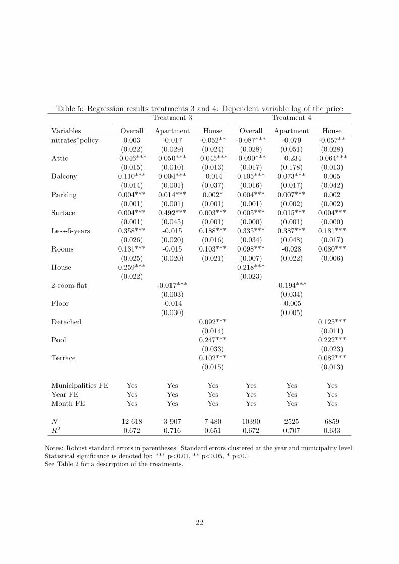
Table 5: Regression results treatments 3 and 4: Dependent variable log of the priceTreatment 3 Treatment 4

Variables Overall Apartment House Overall Apartment House

nitrates*policy 0.003 -0.017 -0.052** -0.087*** -0.079 -0.057**(0.022) (0.029) (0.024) (0.028) (0.051) (0.028)

Attic -0.046*** 0.050*** -0.045*** -0.090*** -0.234 -0.064***(0.015) (0.010) (0.013) (0.017) (0.178) (0.013)

Balcony 0.110*** 0.004*** -0.014 0.105*** 0.073*** 0.005(0.014) (0.001) (0.037) (0.016) (0.017) (0.042)

Parking 0.004*** 0.014*** 0.002* 0.004*** 0.007*** 0.002(0.001) (0.001) (0.001) (0.001) (0.002) (0.002)

Surface 0.004*** 0.492*** 0.003*** 0.005*** 0.015*** 0.004***(0.001) (0.045) (0.001) (0.000) (0.001) (0.000)

Less-5-years 0.358*** -0.015 0.188*** 0.335*** 0.387*** 0.181***(0.026) (0.020) (0.016) (0.034) (0.048) (0.017)

Rooms 0.131*** -0.015 0.103*** 0.098*** -0.028 0.080***(0.025) (0.020) (0.021) (0.007) (0.022) (0.006)

House 0.259*** 0.218***(0.022) (0.023)

2-room-flat -0.017*** -0.194***(0.003) (0.034)

Floor -0.014 -0.005(0.030) (0.005)

Detached 0.092*** 0.125***(0.014) (0.011)

Pool 0.247*** 0.222***(0.033) (0.023)

Terrace 0.102*** 0.082***(0.015) (0.013)

Municipalities FE Yes Yes Yes Yes Yes YesYear FE Yes Yes Yes Yes Yes YesMonth FE Yes Yes Yes Yes Yes Yes

N 12 618 3 907 7 480 10390 2525 6859R2 0.672 0.716 0.651 0.672 0.707 0.633

Notes: Robust standard errors in parentheses. Standard errors clustered at the year and municipality level.Statistical significance is denoted by: *** p<0.01, ** p<0.05, * p<0.1See Table 2 for a description of the treatments.

22