Operational methods in semantics - Archive ouverte HAL
288
HAL Id: cel-01422101 https://hal.archives-ouvertes.fr/cel-01422101v2 Submitted on 3 May 2017 HAL is a multi-disciplinary open access archive for the deposit and dissemination of sci- entific research documents, whether they are pub- lished or not. The documents may come from teaching and research institutions in France or abroad, or from public or private research centers. L’archive ouverte pluridisciplinaire HAL, est destinée au dépôt et à la diffusion de documents scientifiques de niveau recherche, publiés ou non, émanant des établissements d’enseignement et de recherche français ou étrangers, des laboratoires publics ou privés. Operational methods in semantics Roberto Amadio To cite this version: Roberto Amadio. Operational methods in semantics. Master. Paris, France. 2016. cel-01422101v2
-
Upload
khangminh22 -
Category
Documents
-
view
2 -
download
0
Transcript of Operational methods in semantics - Archive ouverte HAL

HAL Id: cel-01422101https://hal.archives-ouvertes.fr/cel-01422101v2
Submitted on 3 May 2017
HAL is a multi-disciplinary open accessarchive for the deposit and dissemination of sci-entific research documents, whether they are pub-lished or not. The documents may come fromteaching and research institutions in France orabroad, or from public or private research centers.
L’archive ouverte pluridisciplinaire HAL, estdestinée au dépôt et à la diffusion de documentsscientifiques de niveau recherche, publiés ou non,émanant des établissements d’enseignement et derecherche français ou étrangers, des laboratoirespublics ou privés.
Operational methods in semanticsRoberto Amadio
To cite this version:
Roberto Amadio. Operational methods in semantics. Master. Paris, France. 2016. cel-01422101v2
Operational methods in semantics
Roberto M. Amadio
Universite Paris-Diderot
May 3, 2017

2
Contents
Preface 7
Notation 11
1 Introduction to operational semantics 131.1 A simple imperative language . . . . . . . . . . . . . . . . . . . . . . . . . . . . . . . . . . . . . 131.2 Partial correctness assertions . . . . . . . . . . . . . . . . . . . . . . . . . . . . . . . . . . . . . 171.3 A toy compiler . . . . . . . . . . . . . . . . . . . . . . . . . . . . . . . . . . . . . . . . . . . . . 211.4 Summary and references . . . . . . . . . . . . . . . . . . . . . . . . . . . . . . . . . . . . . . . . 25
2 Rewriting systems 272.1 Basic properties . . . . . . . . . . . . . . . . . . . . . . . . . . . . . . . . . . . . . . . . . . . . . 272.2 Termination and well-founded orders . . . . . . . . . . . . . . . . . . . . . . . . . . . . . . . . . 292.3 Lifting well-foundation . . . . . . . . . . . . . . . . . . . . . . . . . . . . . . . . . . . . . . . . . 302.4 Termination and local confluence . . . . . . . . . . . . . . . . . . . . . . . . . . . . . . . . . . . 322.5 Term rewriting systems . . . . . . . . . . . . . . . . . . . . . . . . . . . . . . . . . . . . . . . . 332.6 Summary and references . . . . . . . . . . . . . . . . . . . . . . . . . . . . . . . . . . . . . . . . 35
3 Syntactic unification 373.1 A basic unification algorithm . . . . . . . . . . . . . . . . . . . . . . . . . . . . . . . . . . . . . 373.2 Properties of the algorithm . . . . . . . . . . . . . . . . . . . . . . . . . . . . . . . . . . . . . . 383.3 Summary and references . . . . . . . . . . . . . . . . . . . . . . . . . . . . . . . . . . . . . . . . 39
4 Termination of term rewriting systems 414.1 Interpretation method . . . . . . . . . . . . . . . . . . . . . . . . . . . . . . . . . . . . . . . . . 414.2 Recursive path order . . . . . . . . . . . . . . . . . . . . . . . . . . . . . . . . . . . . . . . . . . 444.3 Recursive path order is well-founded . . . . . . . . . . . . . . . . . . . . . . . . . . . . . . . . . 474.4 Simplification orders are well-founded . . . . . . . . . . . . . . . . . . . . . . . . . . . . . . . . 484.5 Summary and references . . . . . . . . . . . . . . . . . . . . . . . . . . . . . . . . . . . . . . . . 52
5 Confluence and completion of term rewriting systems 535.1 Confluence of terminating term rewriting systems . . . . . . . . . . . . . . . . . . . . . . . . . . 535.2 Completion of term rewriting systems . . . . . . . . . . . . . . . . . . . . . . . . . . . . . . . . 545.3 Summary and references . . . . . . . . . . . . . . . . . . . . . . . . . . . . . . . . . . . . . . . . 57
6 Term rewriting systems as functional programs 596.1 A class of term rewriting systems . . . . . . . . . . . . . . . . . . . . . . . . . . . . . . . . . . . 596.2 Primitive recursion . . . . . . . . . . . . . . . . . . . . . . . . . . . . . . . . . . . . . . . . . . . 606.3 Functional programs computing in polynomial time . . . . . . . . . . . . . . . . . . . . . . . . . 626.4 Summary and references . . . . . . . . . . . . . . . . . . . . . . . . . . . . . . . . . . . . . . . . 66
7 λ-calculus 677.1 Syntax . . . . . . . . . . . . . . . . . . . . . . . . . . . . . . . . . . . . . . . . . . . . . . . . . . 677.2 Confluence . . . . . . . . . . . . . . . . . . . . . . . . . . . . . . . . . . . . . . . . . . . . . . . 707.3 Programming . . . . . . . . . . . . . . . . . . . . . . . . . . . . . . . . . . . . . . . . . . . . . . 737.4 Combinatory logic . . . . . . . . . . . . . . . . . . . . . . . . . . . . . . . . . . . . . . . . . . . 75
3

4
7.5 Summary and references . . . . . . . . . . . . . . . . . . . . . . . . . . . . . . . . . . . . . . . . 75
8 Weak reduction strategies, closures, and abstract machines 77
8.1 Weak reduction strategies . . . . . . . . . . . . . . . . . . . . . . . . . . . . . . . . . . . . . . . 77
8.2 Static vs. dynamic binding . . . . . . . . . . . . . . . . . . . . . . . . . . . . . . . . . . . . . . 80
8.3 Environments and closures . . . . . . . . . . . . . . . . . . . . . . . . . . . . . . . . . . . . . . . 82
8.4 Summary and references . . . . . . . . . . . . . . . . . . . . . . . . . . . . . . . . . . . . . . . . 84
9 Contextual equivalence and simulation 85
9.1 Observation pre-order and equivalence . . . . . . . . . . . . . . . . . . . . . . . . . . . . . . . . 85
9.2 Fixed points . . . . . . . . . . . . . . . . . . . . . . . . . . . . . . . . . . . . . . . . . . . . . . . 86
9.3 (Co-)Inductive definitions . . . . . . . . . . . . . . . . . . . . . . . . . . . . . . . . . . . . . . . 88
9.4 Simulation . . . . . . . . . . . . . . . . . . . . . . . . . . . . . . . . . . . . . . . . . . . . . . . . 90
9.5 Summary and references . . . . . . . . . . . . . . . . . . . . . . . . . . . . . . . . . . . . . . . . 94
10 Propositional types 95
10.1 Subject reduction . . . . . . . . . . . . . . . . . . . . . . . . . . . . . . . . . . . . . . . . . . . . 98
10.2 A normalizing strategy for the simply typed λ-calculus . . . . . . . . . . . . . . . . . . . . . . . 99
10.3 Termination of the simply typed λ-calculus . . . . . . . . . . . . . . . . . . . . . . . . . . . . . 100
10.4 Summary and references . . . . . . . . . . . . . . . . . . . . . . . . . . . . . . . . . . . . . . . . 102
11 Type inference for propositional types 103
11.1 Reduction of type-inference to unification . . . . . . . . . . . . . . . . . . . . . . . . . . . . . . 103
11.2 Reduction of unification to type inference . . . . . . . . . . . . . . . . . . . . . . . . . . . . . . 105
11.3 Summary and references . . . . . . . . . . . . . . . . . . . . . . . . . . . . . . . . . . . . . . . . 107
12 Predicative polymorphic types and type inference 109
12.1 Predicative universal types and polymorphism . . . . . . . . . . . . . . . . . . . . . . . . . . . . 109
12.2 A type inference algorithm . . . . . . . . . . . . . . . . . . . . . . . . . . . . . . . . . . . . . . 112
12.3 Reduction of stratified polymorphic typing to propositional typing . . . . . . . . . . . . . . . . 114
12.4 Summary and references . . . . . . . . . . . . . . . . . . . . . . . . . . . . . . . . . . . . . . . . 115
13 Impredicative polymorphic types 117
13.1 System F . . . . . . . . . . . . . . . . . . . . . . . . . . . . . . . . . . . . . . . . . . . . . . . . 117
13.2 Inductive types and iterative functions . . . . . . . . . . . . . . . . . . . . . . . . . . . . . . . . 119
13.3 Strong normalization . . . . . . . . . . . . . . . . . . . . . . . . . . . . . . . . . . . . . . . . . . 125
13.4 Summary and references . . . . . . . . . . . . . . . . . . . . . . . . . . . . . . . . . . . . . . . . 127
14 Program transformations 129
14.1 Continuation passing style form . . . . . . . . . . . . . . . . . . . . . . . . . . . . . . . . . . . . 129
14.2 Value named form . . . . . . . . . . . . . . . . . . . . . . . . . . . . . . . . . . . . . . . . . . . 134
14.3 Closure conversion . . . . . . . . . . . . . . . . . . . . . . . . . . . . . . . . . . . . . . . . . . . 135
14.4 Hoisting . . . . . . . . . . . . . . . . . . . . . . . . . . . . . . . . . . . . . . . . . . . . . . . . . 138
14.5 Summary and references . . . . . . . . . . . . . . . . . . . . . . . . . . . . . . . . . . . . . . . . 139
15 Typing the program transformations 141
15.1 Typing the CPS form . . . . . . . . . . . . . . . . . . . . . . . . . . . . . . . . . . . . . . . . . 142
15.2 Typing value-named closures . . . . . . . . . . . . . . . . . . . . . . . . . . . . . . . . . . . . . 142
15.3 Typing the compiled code . . . . . . . . . . . . . . . . . . . . . . . . . . . . . . . . . . . . . . . 145
15.4 Summary and references . . . . . . . . . . . . . . . . . . . . . . . . . . . . . . . . . . . . . . . . 146
16 Records, variants, and subtyping 147
16.1 Records . . . . . . . . . . . . . . . . . . . . . . . . . . . . . . . . . . . . . . . . . . . . . . . . . 147
16.2 Subtyping . . . . . . . . . . . . . . . . . . . . . . . . . . . . . . . . . . . . . . . . . . . . . . . . 148
16.3 Variants . . . . . . . . . . . . . . . . . . . . . . . . . . . . . . . . . . . . . . . . . . . . . . . . . 151
16.4 Summary and references . . . . . . . . . . . . . . . . . . . . . . . . . . . . . . . . . . . . . . . . 152

5
17 References 153
17.1 References and heaps . . . . . . . . . . . . . . . . . . . . . . . . . . . . . . . . . . . . . . . . . . 153
17.2 Typing . . . . . . . . . . . . . . . . . . . . . . . . . . . . . . . . . . . . . . . . . . . . . . . . . . 155
17.3 Typing anomalies . . . . . . . . . . . . . . . . . . . . . . . . . . . . . . . . . . . . . . . . . . . . 157
17.4 Summary and references . . . . . . . . . . . . . . . . . . . . . . . . . . . . . . . . . . . . . . . . 157
18 Object-oriented languages 159
18.1 An object-oriented language . . . . . . . . . . . . . . . . . . . . . . . . . . . . . . . . . . . . . . 159
18.2 Objects as records . . . . . . . . . . . . . . . . . . . . . . . . . . . . . . . . . . . . . . . . . . . 164
18.3 Typing . . . . . . . . . . . . . . . . . . . . . . . . . . . . . . . . . . . . . . . . . . . . . . . . . . 165
18.4 Summary and references . . . . . . . . . . . . . . . . . . . . . . . . . . . . . . . . . . . . . . . . 168
19 Introduction to concurrency 169
19.1 A concurrent language with shared memory . . . . . . . . . . . . . . . . . . . . . . . . . . . . . 170
19.2 Equivalences: a taste of the design space . . . . . . . . . . . . . . . . . . . . . . . . . . . . . . . 172
19.3 Summary and references . . . . . . . . . . . . . . . . . . . . . . . . . . . . . . . . . . . . . . . . 174
20 A compositional trace semantics 175
20.1 Fixing the observables . . . . . . . . . . . . . . . . . . . . . . . . . . . . . . . . . . . . . . . . . 175
20.2 Towards compositionality . . . . . . . . . . . . . . . . . . . . . . . . . . . . . . . . . . . . . . . 176
20.3 A trace-environment interpretation . . . . . . . . . . . . . . . . . . . . . . . . . . . . . . . . . . 178
20.4 Summary and references . . . . . . . . . . . . . . . . . . . . . . . . . . . . . . . . . . . . . . . . 180
21 A denotational presentation of the trace semantics 181
21.1 The interpretation domain . . . . . . . . . . . . . . . . . . . . . . . . . . . . . . . . . . . . . . . 181
21.2 The interpretation . . . . . . . . . . . . . . . . . . . . . . . . . . . . . . . . . . . . . . . . . . . 182
21.3 Summary and references . . . . . . . . . . . . . . . . . . . . . . . . . . . . . . . . . . . . . . . . 186
22 Implementing atomicity 187
22.1 An optimistic strategy . . . . . . . . . . . . . . . . . . . . . . . . . . . . . . . . . . . . . . . . . 187
22.2 A pessimistic strategy . . . . . . . . . . . . . . . . . . . . . . . . . . . . . . . . . . . . . . . . . 188
22.3 A formal analysis of the optimistic strategy . . . . . . . . . . . . . . . . . . . . . . . . . . . . . 189
22.4 Summary and references . . . . . . . . . . . . . . . . . . . . . . . . . . . . . . . . . . . . . . . . 192
23 Rely-guarantee reasoning 193
23.1 Rely-guarantee assertions . . . . . . . . . . . . . . . . . . . . . . . . . . . . . . . . . . . . . . . 193
23.2 A coarse grained concurrent garbage collector . . . . . . . . . . . . . . . . . . . . . . . . . . . . 197
23.3 Summary and references . . . . . . . . . . . . . . . . . . . . . . . . . . . . . . . . . . . . . . . . 199
24 Labelled transition systems and bisimulation 201
24.1 Labelled transition systems . . . . . . . . . . . . . . . . . . . . . . . . . . . . . . . . . . . . . . 201
24.2 Bisimulation . . . . . . . . . . . . . . . . . . . . . . . . . . . . . . . . . . . . . . . . . . . . . . . 202
24.3 Weak transitions . . . . . . . . . . . . . . . . . . . . . . . . . . . . . . . . . . . . . . . . . . . . 205
24.4 Proof techniques for bisimulation . . . . . . . . . . . . . . . . . . . . . . . . . . . . . . . . . . . 206
24.5 Summary and references . . . . . . . . . . . . . . . . . . . . . . . . . . . . . . . . . . . . . . . . 207
25 Modal logics 209
25.1 Modal logics vs. equivalences . . . . . . . . . . . . . . . . . . . . . . . . . . . . . . . . . . . . . 209
25.2 A modal logic with fixed points: the µ-calculus . . . . . . . . . . . . . . . . . . . . . . . . . . . 211
25.3 Summary and references . . . . . . . . . . . . . . . . . . . . . . . . . . . . . . . . . . . . . . . . 215
26 Labelled transition systems with synchronization 217
26.1 CCS . . . . . . . . . . . . . . . . . . . . . . . . . . . . . . . . . . . . . . . . . . . . . . . . . . . 217
26.2 Labelled transition system for CCS . . . . . . . . . . . . . . . . . . . . . . . . . . . . . . . . . . 218
26.3 A reduction semantics for CCS . . . . . . . . . . . . . . . . . . . . . . . . . . . . . . . . . . . . 222
26.4 Value-passing CCS . . . . . . . . . . . . . . . . . . . . . . . . . . . . . . . . . . . . . . . . . . . 226
26.5 Summary and references . . . . . . . . . . . . . . . . . . . . . . . . . . . . . . . . . . . . . . . . 227

6
27 Determinacy and confluence 22927.1 Determinism in lts . . . . . . . . . . . . . . . . . . . . . . . . . . . . . . . . . . . . . . . . . . . 22927.2 Confluence in lts . . . . . . . . . . . . . . . . . . . . . . . . . . . . . . . . . . . . . . . . . . . . 23227.3 Kahn networks . . . . . . . . . . . . . . . . . . . . . . . . . . . . . . . . . . . . . . . . . . . . . 23627.4 Reactivity and local confluence in lts . . . . . . . . . . . . . . . . . . . . . . . . . . . . . . . . . 23827.5 Summary and references . . . . . . . . . . . . . . . . . . . . . . . . . . . . . . . . . . . . . . . . 241
28 Synchronous/Timed models 24328.1 Timed CCS . . . . . . . . . . . . . . . . . . . . . . . . . . . . . . . . . . . . . . . . . . . . . . . 24328.2 A deterministic calculus based on signals . . . . . . . . . . . . . . . . . . . . . . . . . . . . . . . 24628.3 Summary and references . . . . . . . . . . . . . . . . . . . . . . . . . . . . . . . . . . . . . . . . 247
29 Probability and non-determinism 24929.1 Preliminaries . . . . . . . . . . . . . . . . . . . . . . . . . . . . . . . . . . . . . . . . . . . . . . 24929.2 Probabilistic CCS . . . . . . . . . . . . . . . . . . . . . . . . . . . . . . . . . . . . . . . . . . . 25029.3 Measuring transitions . . . . . . . . . . . . . . . . . . . . . . . . . . . . . . . . . . . . . . . . . 25229.4 Summary and references . . . . . . . . . . . . . . . . . . . . . . . . . . . . . . . . . . . . . . . . 254
30 π-calculus 25730.1 A π-calculus and its reduction semantics . . . . . . . . . . . . . . . . . . . . . . . . . . . . . . . 25730.2 A lts for the π-calculus . . . . . . . . . . . . . . . . . . . . . . . . . . . . . . . . . . . . . . . . . 25930.3 Variations . . . . . . . . . . . . . . . . . . . . . . . . . . . . . . . . . . . . . . . . . . . . . . . . 26230.4 Summary and references . . . . . . . . . . . . . . . . . . . . . . . . . . . . . . . . . . . . . . . . 262
31 Processes vs. functions 26331.1 From λ to π notation . . . . . . . . . . . . . . . . . . . . . . . . . . . . . . . . . . . . . . . . . . 26331.2 Adding concurrency . . . . . . . . . . . . . . . . . . . . . . . . . . . . . . . . . . . . . . . . . . 26431.3 Summary and references . . . . . . . . . . . . . . . . . . . . . . . . . . . . . . . . . . . . . . . . 270
32 Concurrent objects 27132.1 Review of concurrent programming in Java . . . . . . . . . . . . . . . . . . . . . . . . . . . . . 27232.2 A specification of a fragment of concurrent Java . . . . . . . . . . . . . . . . . . . . . . . . . . 27432.3 Summary and references . . . . . . . . . . . . . . . . . . . . . . . . . . . . . . . . . . . . . . . . 277
Bibliography 279
Index 285

Preface
The focus of these lecture notes is on abstract models and basic ideas and results that re-late to the operational semantics of programming languages largely conceived. The approachis to start with an abstract description of the computation steps of programs and then tobuild on top semantic equivalences, specification languages, and static analyses. While otherapproaches to the semantics of programming languages are possible, it appears that the op-erational one is particularly effective in that it requires a moderate level of mathematicalsophistication and scales reasonably well to a large variety of programming features. In prac-tice, operational semantics is a suitable framework to build portable language implementationsand to specify and test program properties (see, e.g., [MTH90]). It is also used routinely totackle more ambitious tasks such as proving the correctness of a compiler or a static analyzer(see, e.g., [Ler06]).
These lecture notes contain a selection of the material taught by the author over severalyears in courses on the semantics of programming languages, foundations of programming,compilation, and concurrency theory. They are oriented towards master students interestedin fundamental research in computer science. The reader is supposed to be familiar with themain programming paradigms (imperative, functional, object-oriented,. . .) and to have beenexposed to the notions of concurrency and synchronization as usually discussed in a courseon operating systems. The reader is also expected to have attended introductory courses onautomata, formal languages, mathematical logic, and compilation of programming languages.
Our goal is to provide a compact reference for grasping the basic ideas of a rapidly evolvingfield. This means that we concentrate on the simple cases and we give a self-containedpresentation of the proof techniques. Following this approach, we manage to cover a ratherlarge spectrum of topics within a coherent terminology and to shed some light, we hope, onthe connections among apparently different formalisms.
Chapter 1 introduces, in the setting of a very simple imperative programming language,some of the main ideas and applications of operational semantics. A sequential programminglanguage is a formalism to define a system of computable functions; the closer the formalismto the notion of function, the simpler the semantics. The first formalism we consider is theone of term rewriting systems (chapters 2–6). On one hand, (term) rewriting is ubiquitousin operational semantics and so it seems to be a good idea to set on solid foundations thenotions of termination and confluence. On the other hand, under suitable conditions, termrewriting is a way of defining first-order functions on inductively defined data structures.
The second formalism we introduce (chapters 7–9) is the λ-calculus, which is a notation torepresent higher-order functions. In this setting, a function is itself a datum that can be passedas an argument or returned as a result. We spend some time to explain the mechanisms neededfor correctly implementing the λ-calculus via the notion of closure. We then address the issueof program equivalence (or refinement) and claim that the notion of contextual equivalence
7

8 Preface
provides a natural answer to this issue. We also show that the co-inductively defined notionof simulation provides an effective method to reason about contextual equivalence.
Chapters 10–13 introduce increasingly expressive type systems for the λ-calculus. Thegeneral idea is that types express properties of program expressions which are invariant underexecution. As such, types are a way of documenting the way a program expression can be usedand by combining program expressions according to their types we can avoid many run-timeerrors. In their purest form, types can be connected with logical propositions and this leads toa fruitful interaction with a branch of mathematical logic known as proof theory. Sometimestypes lead to verbose programs. To address this issue we introduce type inference techniqueswhich are automatic methods discharging the programmer from the task of explicitly writingthe types of the program expressions. Also sometimes types are a bit of a straight jacket inthat they limit the way programs can be combined or reused. We shall see that polymorphictypes (and later subtyping) address, to some extent, these issues.
Chapters 14–15, introduce various standard program transformations that chained to-gether allow to compile a higher-order (functional) language into a basic assembly language.We also show that the type systems presented in the previous chapters shed light on theprogram transformations.
Chapters 16–18 consider the problem of formalizing the operational semantics of imper-ative and object-oriented programming languages. We show that the notion of higher-ordercomputable function is still useful to understand the behavior of programs written in theselanguages. We start by enriching the functional languages considered with record and variantdata types. This is an opportunity to discuss the notion of subtyping which is another wayof making a type system more flexible. Concerning functions with side-effects, we show thatthey can be compiled to ordinary functions by expliciting the fact that each computationtakes a memory as argument and returns a new memory as result. Concerning objects, weshow that they can be understood as a kind of recursively defined records.
Starting from chapter 19, we move from sequential to concurrent programming modelswhere several threads/processes compete for the same resources (e.g. write a variable or achannel). Most of the time, this results into non-deterministic behavior which means thatwith the same input the system can move to several (incomparable) states. Chapters 20–23focus on a concurrent extension of the simple model of imperative programming introducedin chapter 1. In particular, we introduce a compositional trace semantics, rely-guaranteeassertions, and mechanisms to implement atomic execution.
Chapters 24–27 take a more abstract look at concurrency in the framework of labelled tran-sition systems. We develop the notion of bisimulation and we consider its logical characteriza-tion through a suitable modal logic. Labelled transition systems extended with a rendez-voussynchronization mechanism lead to a simple calculus of concurrent systems known as CCS .We rely on this calculus to explore the connections between determinacy and confluence.
Chapters 28 and 29 describe two relevant extensions of CCS . In the first one, we considerthe notion of timed (or synchronous) execution where processes proceed in lockstep (at thesame speed) and the computation is regulated by a notion of instant. In the second one, weconsider systems which exhibit both non-deterministic and probabilistic behaviors.
Chapters 30–31 introduce another extension of CCS , known as π-calculus, where processescan communicate channel names. We show that the theory of equivalence developed for CCScan be lifted to the π-calculus and that the π-calculus can be regarded as a concurrentextension of the λ-calculus.
Finally, chapter 32 builds on chapter 18 to formalize a fragment of the concurrency avail-

Preface 9
able in the Java programming language and to discuss the notion of linearization of concurrentdata structures.
While the choice of the topics is no doubt biased by the interests of the author, it stillprovides a fair representation of the possibilities offered by operational semantics. Linksbetween operational semantics and more ‘mathematical’ semantics based, e.g., on domainand/or category theory are not developed at all in these lecture notes; we refer the interestedreader to, e.g., [AC98, Gun92, Win93].
Most topics discussed in these lecture notes can form the basis of interesting programmingexperiences such as the construction of a compiler, a static type analyzer, or a verificationcondition generator. The proofs sketched in these lecture notes can also become the object ofa programming experience in the sense that they can be formalized and checked in suitableproof assistants (experiments in this direction can be found, e.g., in the books [Chl13, NK14,PCG+15]).
Each chapter ends with a summary of the main concepts and results introduced and a fewbibliographic references. These references are suggestions for further study possibly leadingto research problems. Quite often we prefer to quote the ‘classic’ papers that introduced aconcept than the most recent ones which elaborated on it. Reading the ‘classics’ is a veryvaluable exercise which helps in building some historical perspective especially in a disciplinelike computer science where history is so short.
These lecture notes contain enough material for a two semesters course; however, there aremany possible shortcuts to fit just one semester course. The chapters 1–18 cover sequentiallanguages. Chapters 1, 2, and some of 4 are a recommended introduction and the chapters7–10 constitute the backbone on the λ-calculus. The remaining chapters can be selectedaccording to the taste of the instructor and the interests of the students. Topics coveredinclude: term rewriting systems (chapters 3, 5, 6), type systems (chapters 12, 13, 16), typeinference (chapters 3, 11, 12), program transformations (chapters 14, 15), and imperativeand object-oriented languages (chapters 17, 18). The chapters 19–32 focus on concurrentlanguages and assume some familiarity with the basic material mentioned above. Chapter 19is a recommended introduction to concurrency. Chapters 20–23 cover a simple model of sharedmemory concurrency while chapters 24–26 lead to the calculus CCS , a basic model of messagepassing concurrency. The following chapters explore the notions of deterministic (chapter27), timed (chapter 28), and probabilistic (chapter 29) computation. The final chapters movetowards models of concurrency that integrate the complexity of a sequential language. Inparticular, we discuss the π-calculus (chapters 30, 31) which relates to the λ-calculus and aconcurrent object oriented language (chapter 32) which extends the object-oriented languagepresented in chapter 18.

10 Preface
Notation
Set theoretical
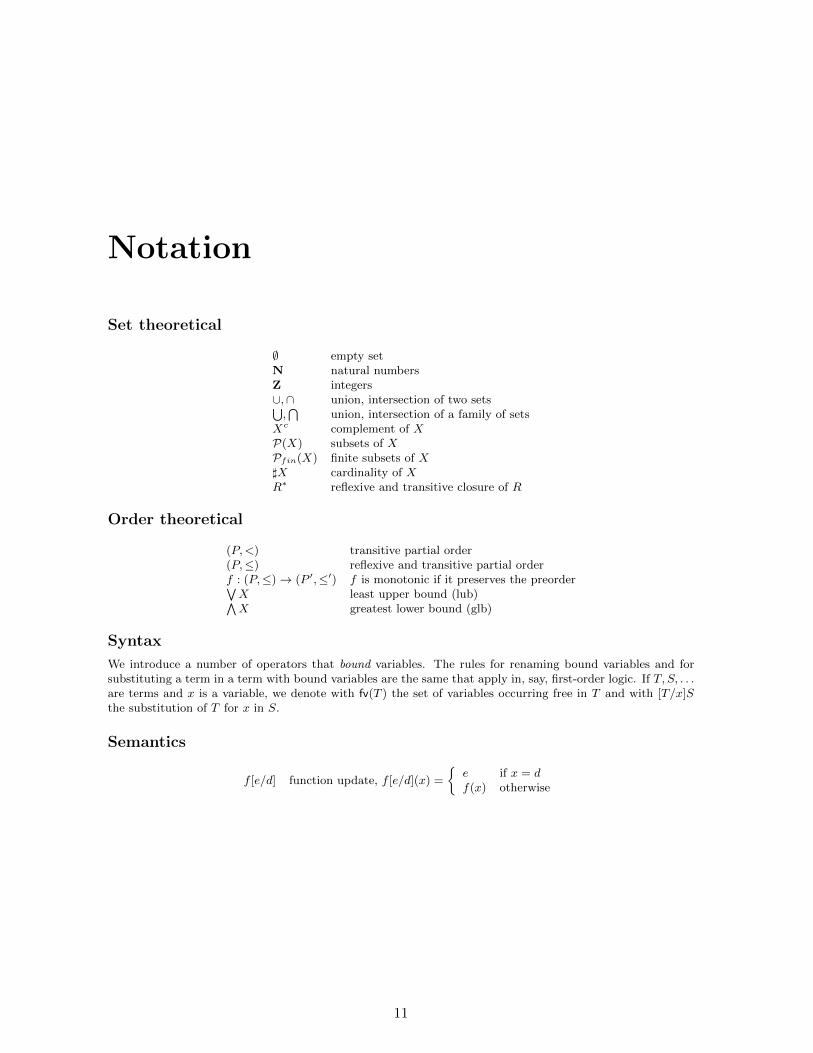
∅ empty setN natural numbersZ integers∪,∩ union, intersection of two sets⋃,⋂
union, intersection of a family of setsXc complement of XP(X) subsets of XPfin(X) finite subsets of X]X cardinality of XR∗ reflexive and transitive closure of R
Order theoretical
(P,<) transitive partial order(P,≤) reflexive and transitive partial orderf : (P,≤)→ (P ′,≤′) f is monotonic if it preserves the preorder∨X least upper bound (lub)∧X greatest lower bound (glb)
Syntax
We introduce a number of operators that bound variables. The rules for renaming bound variables and forsubstituting a term in a term with bound variables are the same that apply in, say, first-order logic. If T, S, . . .are terms and x is a variable, we denote with fv(T ) the set of variables occurring free in T and with [T/x]Sthe substitution of T for x in S.
Semantics
f [e/d] function update, f [e/d](x) =
e if x = df(x) otherwise
11

12 Notation

Chapter 1
Introduction to operationalsemantics
The goal of this introductory chapter is to present at an elementary level some ideas of theoperational approach to the semantics of programming languages and to illustrate some oftheir applications.
To this end, we shall focus on a standard toy imperative language called Imp. As a firststep we describe formally and at an abstract level the computations of Imp programs. Indoing this, we identify two styles known as big-step and small-step. Then, based on thisspecification, we introduce a suitable notion of pre-order on statements and check that thispre-order is preserved by the operators of the Imp language.
As a second step, we introduce a specification formalism for Imp programs that relies onso called partial correctness assertions (pca’s). We present sound rules for reasoning aboutsuch assertions and a structured methodology to reduce reasoning about pca’s to ordinaryreasoning in a suitable theory of (first-order) logic. We also show that the pre-order previouslydefined on statements coincides with the one induced by pca’s.
As a third and final step, we specify a toy compiler from the Imp language to an hypothet-ical virtual machine whose semantics is also defined using operational techniques. We thenapply the developed framework to prove the correctness of the compiler.
1.1 A simple imperative language
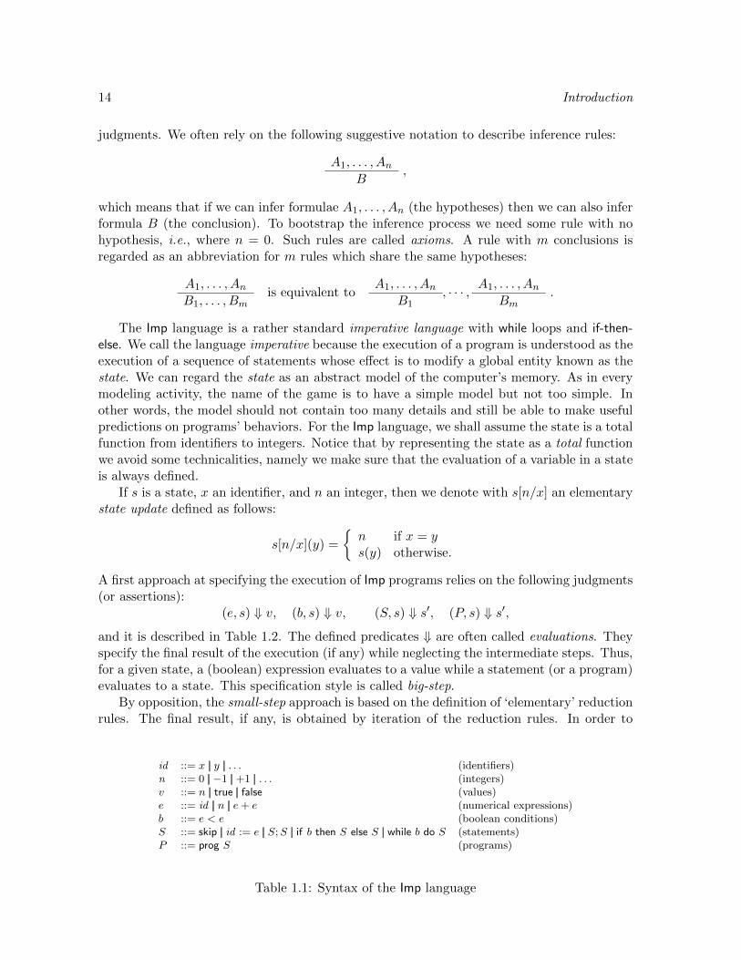
We assume the reader is familiar with the idea that the syntax of a programming languagecan be specified via a context-free grammar. The syntax of the Imp language is described inTable 1.1 where we distinguish the syntactic categories of identifiers (or variables), integers,values, numerical expressions, boolean conditions, statements, and programs. We shall notdwell on questions of grammar ambiguity and priority of operators. Whenever we look at asyntactic expression we assume it contains enough parentheses so that no ambiguity arises onthe order of application of the operators.
We also assume the reader is familiar with the notion of formal system. A formal systemis composed of formulae specified by a certain syntax and inference rules to derive formulaefrom other formulae. Depending on the context, the formulae may be called assertions or
13
14 Introduction
judgments. We often rely on the following suggestive notation to describe inference rules:
A1, . . . , AnB
,
which means that if we can infer formulae A1, . . . , An (the hypotheses) then we can also inferformula B (the conclusion). To bootstrap the inference process we need some rule with nohypothesis, i.e., where n = 0. Such rules are called axioms. A rule with m conclusions isregarded as an abbreviation for m rules which share the same hypotheses:
A1, . . . , AnB1, . . . , Bm
is equivalent toA1, . . . , An
B1, · · · , A1, . . . , An
Bm.
The Imp language is a rather standard imperative language with while loops and if-then-else. We call the language imperative because the execution of a program is understood as theexecution of a sequence of statements whose effect is to modify a global entity known as thestate. We can regard the state as an abstract model of the computer’s memory. As in everymodeling activity, the name of the game is to have a simple model but not too simple. Inother words, the model should not contain too many details and still be able to make usefulpredictions on programs’ behaviors. For the Imp language, we shall assume the state is a totalfunction from identifiers to integers. Notice that by representing the state as a total functionwe avoid some technicalities, namely we make sure that the evaluation of a variable in a stateis always defined.
If s is a state, x an identifier, and n an integer, then we denote with s[n/x] an elementarystate update defined as follows:
s[n/x](y) =
n if x = ys(y) otherwise.
A first approach at specifying the execution of Imp programs relies on the following judgments(or assertions):
(e, s) ⇓ v, (b, s) ⇓ v, (S, s) ⇓ s′, (P, s) ⇓ s′,
and it is described in Table 1.2. The defined predicates ⇓ are often called evaluations. Theyspecify the final result of the execution (if any) while neglecting the intermediate steps. Thus,for a given state, a (boolean) expression evaluates to a value while a statement (or a program)evaluates to a state. This specification style is called big-step.
By opposition, the small-step approach is based on the definition of ‘elementary’ reductionrules. The final result, if any, is obtained by iteration of the reduction rules. In order to
id ::= x || y || . . . (identifiers)n ::= 0 || −1 || +1 || . . . (integers)v ::= n || true || false (values)e ::= id || n || e+ e (numerical expressions)b ::= e < e (boolean conditions)S ::= skip || id := e || S;S || if b then S else S || while b do S (statements)P ::= prog S (programs)
Table 1.1: Syntax of the Imp language

Introduction 15
(v, s) ⇓ v (x, s) ⇓ s(x)
(e, s) ⇓ v (e′, s) ⇓ v′(e+ e′, s) ⇓ (v +Z v
′)
(e, s) ⇓ v (e′, s) ⇓ v′(e < e′, s) ⇓ (v <Z v
′)
(skip, s) ⇓ s(e, s) ⇓ v
(x := e, s) ⇓ s[v/x]
(S1, s) ⇓ s′ (S2, s′) ⇓ s′′
(S1;S2, s) ⇓ s′′
(b, s) ⇓ true (S, s) ⇓ s′(if b then S else S′, s) ⇓ s′
(b, s) ⇓ false (S′, s) ⇓ s′(if b then S else S′, s) ⇓ s′
(b, s) ⇓ false
(while b do S, s) ⇓ s(b, s) ⇓ true (S;while b do S, s) ⇓ s′
(while b do S, s) ⇓ s′
(S, s) ⇓ s′(prog S, s) ⇓ s′
Table 1.2: Big-step reduction rules of Imp
(x := e,K, s) → (skip,K, s[v/x]) if (e, s) ⇓ v
(S;S′,K, s) → (S, S′ ·K, s)
(if b then S else S′,K, s) →
(S,K, s) if (b, s) ⇓ true(S′,K, s) if (b, s) ⇓ false
(while b do S,K, s) →
(S, (while b do S) ·K, s) if (b, s) ⇓ true(skip,K, s) if (b, s) ⇓ false
(skip, S ·K, s) → (S,K, s)
Table 1.3: Small-step reduction rules of Imp statements
describe the intermediate steps of the computation, we introduce an additional syntacticcategory of continuations. A continuation K is a list of statements which terminates with aspecial symbol halt:
K ::= halt || S ·K (continuation).
A continuation keeps track of the statements that still need to be executed. Table 1.3 definessmall-step reduction rules for Imp statements whose basic judgment has the shape:
(S,K, s)→ (S′,K ′, s′) .
Note that we still rely on the big-step reduction of (boolean) expressions; the definition of asmall step reduction for (boolean) expressions is left to the reader. We define the reduction ofa program prog S as the reduction of the statement S with continuation halt. We can derivea big-step reduction from the small-step one as follows:
(S, s) ⇓ s′ if (S, halt, s)∗→ (skip, halt, s′) ,
where∗→ denotes the reflexive and transitive closure of the relation →.
Let us pause to consider some properties of both the big-step and the small-step reductions.In both cases, reduction is driven by the syntax of the object (program, statement,. . .) under
16 Introduction
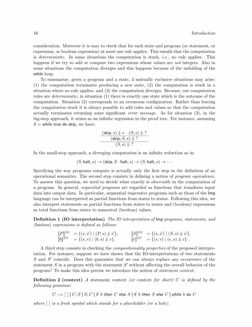
consideration. Moreover it is easy to check that for each state and program (or statement, orexpression, or boolean expression) at most one rule applies. This entails that the computationis deterministic. In some situations the computation is stuck, i.e., no rule applies. Thishappens if we try to add or compare two expressions whose values are not integers. Also insome situations the computation diverges and this happens because of the unfolding of thewhile loop.
To summarize, given a program and a state, 3 mutually exclusive situations may arise:(1) the computation terminates producing a new state, (2) the computation is stuck in asituation where no rule applies, and (3) the computation diverges. Because, our computationrules are deterministic, in situation (1) there is exactly one state which is the outcome of thecomputation. Situation (2) corresponds to an erroneous configuration. Rather than leavingthe computation stuck it is always possible to add rules and values so that the computationactually terminates returning some significant error message. As for situation (3), in thebig-step approach, it arises as an infinite regression in the proof tree. For instance, assumingS = while true do skip, we have:
(skip, s) ⇓ s (S, s) ⇓ ?
(skip;S, s) ⇓ ?
(S, s) ⇓ ?
In the small-step approach, a diverging computation is an infinite reduction as in:
(S, halt, s)→ (skip, S · halt, s)→ (S, halt, s)→ · · ·
Specifying the way programs compute is actually only the first step in the definition of anoperational semantics. The second step consists in defining a notion of program equivalence.To answer this question, we need to decide what exactly is observable in the computation ofa program. In general, sequential programs are regarded as functions that transform inputdata into output data. In particular, sequential imperative programs such as those of the Implanguage can be interpreted as partial functions from states to states. Following this idea, wealso interpret statements as partial functions from states to states and (boolean) expressionsas total functions from states to numerical (boolean) values.
Definition 1 (IO interpretation) The IO interpretation of Imp programs, statements, and(boolean) expressions is defined as follows:
[[P ]]IO = (s, s′) | (P, s) ⇓ s′, [[S]]IO = (s, s′) | (S, s) ⇓ s′,[[b]]IO = (s, v) | (b, s) ⇓ v, [[e]]IO = (s, v) | (e, s) ⇓ v .
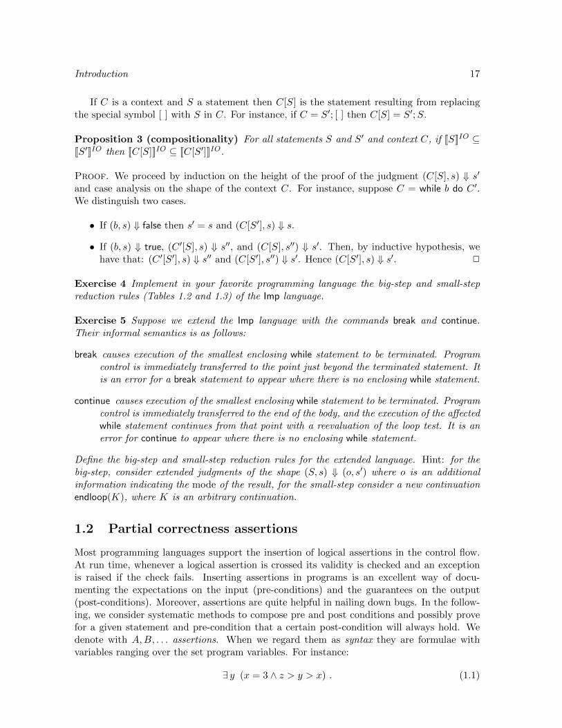
A third step consists in checking the compositionality properties of the proposed interpre-tation. For instance, suppose we have shown that the IO-interpretations of two statementsS and S′ coincide. Does this guarantee that we can always replace any occurrence of thestatement S in a program with the statement S′ without affecting the overall behavior of theprogram? To make this idea precise we introduce the notion of statement context.
Definition 2 (context) A statement context (or context for short) C is defined by thefollowing grammar:
C ::= [ ] || C;S || S;C || if b then C else S || if b then S else C || while b do C
where [ ] is a fresh symbol which stands for a placeholder (or a hole).
Introduction 17
If C is a context and S a statement then C[S] is the statement resulting from replacingthe special symbol [ ] with S in C. For instance, if C = S′; [ ] then C[S] = S′;S.
Proposition 3 (compositionality) For all statements S and S′ and context C, if [[S]]IO ⊆[[S′]]IO then [[C[S]]]IO ⊆ [[C[S′]]]IO.
Proof. We proceed by induction on the height of the proof of the judgment (C[S], s) ⇓ s′and case analysis on the shape of the context C. For instance, suppose C = while b do C ′.We distinguish two cases.
• If (b, s) ⇓ false then s′ = s and (C[S′], s) ⇓ s.
• If (b, s) ⇓ true, (C ′[S], s) ⇓ s′′, and (C[S], s′′) ⇓ s′. Then, by inductive hypothesis, wehave that: (C ′[S′], s) ⇓ s′′ and (C[S′], s′′) ⇓ s′. Hence (C[S′], s) ⇓ s′. 2
Exercise 4 Implement in your favorite programming language the big-step and small-stepreduction rules (Tables 1.2 and 1.3) of the Imp language.
Exercise 5 Suppose we extend the Imp language with the commands break and continue.Their informal semantics is as follows:
break causes execution of the smallest enclosing while statement to be terminated. Programcontrol is immediately transferred to the point just beyond the terminated statement. Itis an error for a break statement to appear where there is no enclosing while statement.
continue causes execution of the smallest enclosing while statement to be terminated. Programcontrol is immediately transferred to the end of the body, and the execution of the affectedwhile statement continues from that point with a reevaluation of the loop test. It is anerror for continue to appear where there is no enclosing while statement.
Define the big-step and small-step reduction rules for the extended language. Hint: for thebig-step, consider extended judgments of the shape (S, s) ⇓ (o, s′) where o is an additionalinformation indicating the mode of the result, for the small-step consider a new continuationendloop(K), where K is an arbitrary continuation.
1.2 Partial correctness assertions
Most programming languages support the insertion of logical assertions in the control flow.At run time, whenever a logical assertion is crossed its validity is checked and an exceptionis raised if the check fails. Inserting assertions in programs is an excellent way of docu-menting the expectations on the input (pre-conditions) and the guarantees on the output(post-conditions). Moreover, assertions are quite helpful in nailing down bugs. In the follow-ing, we consider systematic methods to compose pre and post conditions and possibly provefor a given statement and pre-condition that a certain post-condition will always hold. Wedenote with A,B, . . . assertions. When we regard them as syntax they are formulae withvariables ranging over the set program variables. For instance:
∃ y (x = 3 ∧ z > y > x) . (1.1)

18 Introduction
We write s |= A if the assertion A holds in the interpretation (state) s. Thus a syntacticassertion such as (1.1) is semantically the set of states that satisfy it, namely:
s | s(x) = 3, s(z) ≥ 5 .
Definition 6 (pca) A partial correctness assertion (pca) is a triple A S B. We saythat it is valid and write |= A S B if:
∀ s (s |= A and (P, s) ⇓ s′ implies s′ |= B) .
The assertion is partial because it puts no constraint on the behavior of a non-terminating,i.e., partial, statement. Table 1.4 describes the so called Floyd-Hoare rules (logic). The rulesare formulated assuming that A,B, . . . are sets of states. It is possible to go one step furtherand replace the sets by predicates in, say, first-order logic, however this is not essential tounderstand the essence of the rules.
We recall that if S is a statement then [[S]]IO is its input-output interpretation (definition1). This is a binary relation on states which for Imp statements happens to be the graph ofa partial function on states. In particular, notice that for an assignment x := e we have:
[[x := e]]IO = (s, s[v/x]) | (e, s) ⇓ v ,
which is the graph of a total function. In the assertions, we identify a boolean predicate bwith the set of states that satisfy it, thus b stands for s | s |= b. We denote with A,B, . . .unary relations (predicates) on the set of states and with R,S, . . . binary relations on the setof states. We combine unary and binary relations as follows:
A;R = s′ | ∃ s s ∈ A and (s, s′) ∈ R (image)R;A = s | ∃ s′ s′ ∈ A and (s, s′) ∈ R (pre-image).
The first rule in Table 1.4 allows to weaken the pre-condition and strengthen the post-condition while the following rules are associated with the operators of the language. Therules are sound in the sense that if the hypotheses are valid then the conclusion is valid too.
Proposition 7 (soundness pca rules) The assertions derived in the system described inTable 1.4 are valid.
A ⊆ A′ A′ S B′ B′ ⊆ BA S B
A S1 C C S2 BA S1;S2 B
A ∩ b S1 B A ∩ ¬b S2 BA if b then S1 else S2 B
A ⊆ BA skip B
A; [[x := e]]IO ⊆ BA x := e B
(A ∩ ¬b) ⊆ B A ∩ b S AA while b do S B
Table 1.4: Floyd-Hoare rules for Imp

Introduction 19
Proof. We just look at the case for the while rule. Suppose s ∈ A and (while b do S, s) ⇓ s′.We show by induction on the height of the derivation that s′ ∈ B. For the basic case, wehave s ∈ ¬b and we know A ∩ ¬b ⊆ B. On the other hand, suppose s ∈ b and
(S; while b do S, s) ⇓ s′ .
This means (S, s) ⇓ s′′ and (while b do S, s′′) ⇓ s′. By hypothesis, we know s′′ ∈ A and byinductive hypothesis s′ ∈ B. 2
Exercise 8 Suppose A is a first-order formula. Show the validity of the pca [e/x]A x :=e A. On the other hand, show that the pca A x := e [e/x]A is not valid.
Interestingly, one can read the rules bottom up and show that if the conclusion is validthen the hypotheses are valid up to an application of the first ‘logical’ rule. This allows toreduce the proof of a pca A S B to the proof of a purely set-theoretic/logical statement.The task of traversing the program S and producing logical assertions can be completelyautomated once the loops are annotated with suitable invariants. This is the job of so-calledverification condition generators.
Proposition 9 (inversion pca rules) The following properties hold:
1. If A S1;S2 B is valid then A S1 C and C S2 B are valid where C =(A; [[S1]]IO) ∩ ([[S2]]IO;B).
2. If A if b then S1 else S2 B is valid then A ∩ b S1 B and A ∩ ¬b S2 B arevalid.
3. If A skip B is valid then A ⊆ B holds.
4. If A x := e B is valid then A; [[x := e]]IO ⊆ B holds.
5. If A while b do S B is valid then there is A′ ⊇ A such that (i) A′ ∩ ¬b ⊆ B and(ii) A′ ∩ b S A′ is valid.
Proof. The case for while is the interesting one. We define:
A0 = A An+1 = (An ∩ b); [[S]]IO A′ =⋃n≥0An .
We must have: ∀n ≥ 0 An ∩ ¬b ⊆ B. Then for the first condition, we notice that:
A′ ∩ ¬b = (⋃n≥0An) ∩ ¬b =
⋃n≥0(An ∩ ¬b)
⊆⋃n≥0B = B .
For the second, we have:
(A′ ∩ b); [[S]]IO = (⋃n≥0An ∩ b); [[S]]IO = (
⋃n≥0(An ∩ b)); [[S]]IO
=⋃n≥0(An ∩ b); [[S]]IO =
⋃n≥1An
⊆⋃n≥0An = A′ .
An assertion such as A′ is called an invariant of the loop. In the proof, A′ is defined asthe limit of an iterative process where at each step we run the body of the loop. While in

20 Introduction
theory A′ does the job, in practice it may be hard to reason on its properties; finding a usableinvariant may require some creativity. 2
Given a specification language on, say, statements, we can consider two statements logicallyequivalent if they satisfy exactly the same specifications. We can apply this idea to pca’s.
Definition 10 (pca interpretation) The pca interpretation of a process P is:
[[P ]]pca = (A,B) | |= A P B .
So now we have two possible notions of equivalence for statements: one based on theinput-output behavior and another based on partial correctness assertions. However, it is nottoo difficult to show that they coincide.
Proposition 11 (IO vs. pca) Let S1, S2 be statements. Then:
[[S1]]IO = [[S2]]IO iff [[S1]]pca = [[S2]]pca .
Proof. (⇒) Suppose (A,B) ∈ [[S1]]pca, s |= A, (S2, s) ⇓ s′. Then (s, s′) ∈ [[S2]]IO = [[S1]]IO.Hence s′ |= B and (A,B) ∈ [[S2]]pca.
(⇐) First a remark. Let us write s =X s′ if ∀x ∈ X s(x) = s′(x). Further suppose X ⊇ fv(S)and (S, s) ⇓ s′. Then:
1. The variables outside X are untouched: s =Xc s′.
2. If s =X s1 then (S, s1) ⇓ s′1 and s′ =X s′1.
We now move to the proof. Given a state and a finite set of variables X, define:
IS(s,X) =∧x∈X
(x = s(x)) .
Notice that: s′ |= IS(s,X) iff s′ =X s. We proceed by contradiction, assuming (s, s′) ∈ [[S1]]IO
and (s, s′) /∈ [[S2]]IO. Let X be the collection of variables occurring in the commands S1 orS2. Then check that:
(IS(s,X),¬IS(s′, X)) ∈ [[S2]]pca .
On the other hand: (IS(s,X),¬IS(s′, X)) /∈ [[S1]]pca. 2
Exercise 12 Let S be a statement and B an assertion. The weakest precondition of S withrespect to B is a predicate that we denote with wp(S,B) such that: (i) wp(S,B) S Bis valid and (ii) if A S B is valid then A ⊆ wp(S,B). Let us assume the statement Sdoes not contain while loops. Propose a strategy to compute wp(S,B) and derive a method toreduce the validity of a pca A S B to the validity of a logical assertion.
Introduction 21
Rule C[i] =
C ` (i, σ, s)→ (i+ 1, n · σ, s) cnst(n)C ` (i, σ, s)→ (i+ 1, s(x) · σ, s) var(x)C ` (i, n · σ, s)→ (i+ 1, σ, s[n/x]) setvar(x)C ` (i, n · n′ · σ, s)→ (i+ 1, (n+Z n
′) · σ, s) add
C ` (i, σ, s)→ (i+ k + 1, σ, s) branch(k)C ` (i, n · n′ · σ, s)→ (i+ 1, σ, s) bge(k) and n <Z n
′
C ` (i, n · n′ · σ, s)→ (i+ k + 1, σ, s) bge(k) and n ≥Z n′
Table 1.5: Small-step reduction rules of Vm programs
1.3 A toy compiler
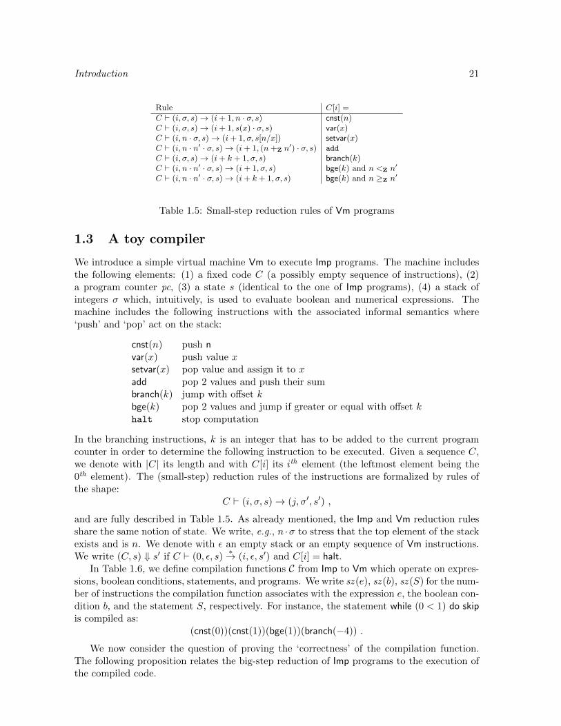
We introduce a simple virtual machine Vm to execute Imp programs. The machine includesthe following elements: (1) a fixed code C (a possibly empty sequence of instructions), (2)a program counter pc, (3) a state s (identical to the one of Imp programs), (4) a stack ofintegers σ which, intuitively, is used to evaluate boolean and numerical expressions. Themachine includes the following instructions with the associated informal semantics where‘push’ and ‘pop’ act on the stack:
cnst(n) push nvar(x) push value xsetvar(x) pop value and assign it to xadd pop 2 values and push their sumbranch(k) jump with offset kbge(k) pop 2 values and jump if greater or equal with offset khalt stop computation
In the branching instructions, k is an integer that has to be added to the current programcounter in order to determine the following instruction to be executed. Given a sequence C,we denote with |C| its length and with C[i] its ith element (the leftmost element being the0th element). The (small-step) reduction rules of the instructions are formalized by rules ofthe shape:
C ` (i, σ, s)→ (j, σ′, s′) ,
and are fully described in Table 1.5. As already mentioned, the Imp and Vm reduction rulesshare the same notion of state. We write, e.g., n ·σ to stress that the top element of the stackexists and is n. We denote with ε an empty stack or an empty sequence of Vm instructions.We write (C, s) ⇓ s′ if C ` (0, ε, s)
∗→ (i, ε, s′) and C[i] = halt.In Table 1.6, we define compilation functions C from Imp to Vm which operate on expres-
sions, boolean conditions, statements, and programs. We write sz (e), sz (b), sz (S) for the num-ber of instructions the compilation function associates with the expression e, the boolean con-dition b, and the statement S, respectively. For instance, the statement while (0 < 1) do skipis compiled as:
(cnst(0))(cnst(1))(bge(1))(branch(−4)) .
We now consider the question of proving the ‘correctness’ of the compilation function.The following proposition relates the big-step reduction of Imp programs to the execution ofthe compiled code.

22 Introduction
C(x) = var(x) C(n) = cnst(n) C(e+ e′) = C(e) · C(e′) · add
C(e < e′, k) = C(e) · C(e′) · bge(k)
C(skip) = ε C(x := e) = C(e) · setvar(x) C(S;S′) = C(S) · C(S′)
C(if b then S else S′) = C(b, k) · C(S) · (branch(k′)) · C(S′)where: k = sz (S) + 1, k′ = sz (S′)
C(while b do S) = C(b, k) · C(S) · branch(k′)where: k = sz (S) + 1, k′ = −(sz (b) + sz (S) + 1)
C(prog S) = C(S) · halt
Table 1.6: Compilation from Imp to Vm
Proposition 13 (soundness, big-step) The following properties hold:
(1) If (e, s) ⇓ v then C · C(e) · C ′ ` (i, σ, s)∗→ (j, v · σ, s) where i = |C| and j = |C · C(e)|.
(2) If (b, s) ⇓ true then C ·C(b, k)·C ′ ` (i, σ, s)∗→ (j+k, σ, s) where i = |C| and j = |C ·C(b, k)|.
(3) If (b, s) ⇓ false then C · C(b, k) ·C ′ ` (i, σ, s)∗→ (j, σ, s) where i = |C| and j = |C · C(b, k)|.
(4) If (S, s) ⇓ s′ then C · C(S) · C ′ ` (i, σ, s)∗→ (j, σ, s′) where i = |C| and j = |C · C(S)|.
Proof. All proofs are by induction on the derivation of the evaluation judgment. We detailthe proof of property (4) in the case the command is a while loop while b do S whose booleancondition b is satisfied. So we have:
(b, s) ⇓ true, (S, s) ⇓ s′′, (while b do S, s′′) ⇓ s′ .
By definition of the compilation function, we have a code C ′′ of the shape:
C · C(b, k) · C(S) · branch(k′) · C ′ .
By property (2), we have for any σ, s:
C ′′ ` (i, σ, s)∗→ (j, σ, s) ,
where i = |C|, j = |C · C(b, k)|. By inductive hypothesis on property (4), we have:
C ′′ ` (j, σ, s)∗→ (j′, σ, s′′) ,
where j′ = |C · C(b, k) · C(S)|. Since k′ = −(|C(b, k) · C(S)|+ 1), we have:
C ′′ ` (j, σ, s′′)→ (i, σ, s′′) .
Again, by inductive hypothesis on property (4) we have:
C ′′ ` (i, σ, s′′)∗→ (j′′, σ, s′) ,
where j′′ = |C · C(while b do S)|. 2

Introduction 23
We can prove similar results working with the small-step reduction of the Imp language.
To this end, given a Vm code C, we define an ‘accessibility relation’C; as the least binary
relation on 0, . . . , |C| − 1 such that:
iC; i
C[i] = branch(k) (i+ k + 1)C; j
iC; j
.
Thus iC; j if in the code C we can go from i to j following a sequence of unconditional
jumps. We also introduce a ternary relation R(C, i,K) which relates a Vm code C, a numberi ∈ 0, . . . , |C| − 1, and a continuation K. The intuition is that relative to the code C, theinstruction i can be regarded as having continuation K.
Definition 14 The ternary relation R is the least one that satisfies the following conditions:
iC; j C[j] = halt
R(C, i, halt)
iC; i′ C = C1 · C(S) · C2
i′ = |C1| j = |C1 · C(S)| R(C, j,K)
R(C, i, S ·K)
.
We can then state the correctness of the compilation function as follows.
Proposition 15 (soundness, small-step) If (S,K, s)→ (S′,K ′, s′) and R(C, i, S ·K) then
C ` (i, σ, s)∗→ (j, σ, s′) and R(C, j, S′ ·K ′).
Proof. Preliminary remarks:
1. The relationC; is transitive.
2. If iC; j and R(C, j,K) then R(C, i,K).
The first property can be proven by induction on the definition ofC; and the second by
induction on the structure of K. Next we can focus on the proof of the assertion. The
notation Ci· C ′ means that i = |C|. Suppose that:
(1) (S,K, s)→ (S′,K ′, s′) and (2) R(C, i, S ·K) .
From (2), we know that there exist i′ and i′′ such that:
(3) iC; i′, (4) C = C1
i′· C(S)i′′· C2, and (5) R(C, i′′,K) .
And from (3) it follows that:
(3′) C ` (i, σ, s)∗→ (i′, σ, s) .
We are looking for j such that:
(6) C ` (i, σ, s)∗→ (j, σ, s′), and (7) R(C, j, S′ ·K ′) .
We proceed by case analysis on S. We just detail the case of the conditional statement as theremaining cases have similar proofs. If S = if e1 < e2 then S1 else S2 then (4) is rewritten asfollows:
C = C1i′· C(e1) · C(e2) · bge(k1)
a· C(S1)b· branch(k2)
c· C(S2)i′′· C2 ,
where c = a+ k1 and i′′ = c+ k2. We distinguish two cases according to the evaluation of theboolean condition. We describe the case (e1 < e2, s) ⇓ true. We set j = a.

24 Introduction
C[i] = Conditions for C : h
cnst(n) or var(x) h(i+ 1) = h(i) + 1add h(i) ≥ 2, h(i+ 1) = h(i)− 1setvar(x) h(i) = 1, h(i+ 1) = 0branch(k) 0 ≤ i+ k + 1 ≤ |C|, h(i) = h(i+ 1) = h(i+ k + 1) = 0bge(k) 0 ≤ i+ k + 1 ≤ |C|, h(i) = 2, h(i+ 1) = h(i+ k + 1) = 0halt i = |C| − 1, h(i) = h(i+ 1) = 0
Table 1.7: Conditions for well-formed code
• The instance of (1) is (S,K, s)→ (S1,K, s).
• The reduction required in (6) takes the form C ` (i, σ, s)∗→ (i′, σ, s)
∗→ (a, σ, s′), and itfollows from (3′), the fact that (e1 < e2, s) ⇓ true, and proposition 13(2).
• Property (7), follows from the preliminary remarks, fact (5), and the following prooftree:
jC; j b
C; i′′ R(C, i′′,K)
R(C, b,K)
R(C, j, S1 ·K)
2
Remark 16 We have already noticed that an Imp program has 3 possible behaviors: (1) itreturns a (unique) result, (2) it is stuck in an erroneous situation, (3) it diverges. Proposition13 guarantees that the compiler preserves behaviors of type (1). Using the small-step reductionrules (proposition 15), we can also conclude that if the source program diverges then thecompiled code diverges too. On the other hand, when the source program is stuck in anerroneous situation the compiled code is allowed to have an arbitrary behavior. The followingexample justifies this choice. Suppose at source level we have an error due to the addition ofan integer and a boolean. Then this error does not need to be reflected at the implementationlevel where the same data type may well be used to represent both integers and booleans.
Exercise 17 (stack height) The Vm code coming from the compilation of Imp programs hasvery specific properties. In particular, for every instruction of the compiled code it is possibleto predict statically, i.e., at compile time, the height of the stack whenever the instructionis executed. We say that a sequence of instructions C is well formed if there is a functionh : 0, . . . , |C| → N which satisfies the conditions listed in Table 1.7 for 0 ≤ i ≤ |C| − 1. Inthis case we write C : h.
The conditions defining the predicate C : h are strong enough to entail that h correctlypredicts the stack height and to guarantee the uniqueness of h up to the initial condition. Showthat: (1) If C : h, C ` (i, σ, s)
∗→ (j, σ′, s′), and h(i) = |σ| then h(j) = |σ′|. (2) If C : h,C : h′ and h(0) = h′(0) then h = h′.
Next prove that the result of the compilation is a well-formed code. Namely, for anyexpression e, statement S, and program P the following holds. (3) For any n ∈ N there is aunique h such that C(e) : h, h(0) = n, and h(|C(e)|) = h(0) + 1. (4) For any S, there is aunique h such that C(S) : h, h(0) = 0, and h(|C(e)|) = 0. (5) There is a unique h such thatC(P ) : h.

Introduction 25
1.4 Summary and references
The first step in defining the operational semantics of a programming language amountsto specify the way a program computes. The following steps are the specification of theobservables (of a computation) and the definition of a compositional pre-order (or equivalence)on programs.
An alternative and related approach amounts to introduce (partial) correctness assertionson programs and deem two programs equivalent if they satisfy the same assertions. Alsothe validity of a program’s assertion can be reduced to the validity of an ordinary logicalstatement in a suitable theory of first order logic.
The formal analysis of compilers is a natural application target for operational semantics.Each language in the compilation chain is given a formal semantics and the behavior of thesource code is related to the behavior of its representation in intermediate languages, anddown to object code.
The lecture notes [Plo04] are an early (first version appeared in 1981) systematic pre-sentation of an operational approach to the semantics of programming languages. Rules forreasoning on partial correctness assertions of simple imperative programs are presented in[Flo67] and [Hoa69] while [MP67] is an early example of mechanized verification of a simplecompiler. The presented case study builds on that example and is partially based on [Ler09].

26 Introduction
Chapter 2
Rewriting systems
In computer science, a set equipped with a binary reduction relation is an ubiquitous structurearising, e.g., when formalizing the computation rules of an automaton, the generation step ofa grammar, or the reduction rules of a programming language (such as the rules for the Implanguage in Table 1.3).
Definition 18 A rewriting system is a pair (A,→) where A is a set and →⊆ A × A is areduction relation. We write a→ b for (a, b) ∈→.
If we regard the reduction relation as an edge relation, we can also say that a rewritingsystem is a (possibly infinite) directed graph.
Next we introduce some notation. If R is a binary relation we denote with R−1 its inverseand with R∗ its reflexive and transitive closure. In particular, if → is a reduction relation wealso write ← for →−1,
∗→ for (→)∗ and∗← for (←)∗. Finally,
∗↔ is defined as (→ ∪ →−1)∗.This is the equivalence relation induced by the rewriting system.
2.1 Basic properties
Termination and confluence are two relevant properties of rewriting systems. Let us startwith termination, namely the fact that all reduction sequences terminate.
Definition 19 (termination) A rewriting system (A,→) is terminating if all sequences ofthe shape a0 → a1 → a2 → · · · are finite.
In this definition, we require the sequence (not the set) to be finite. In particular, arewriting system composed of a singleton set A where →= A×A is not terminating.
When the rewriting system corresponds to the reduction rules of a programming languagethe termination property is connected to the termination of programs. This is a fundamentalproperty in program verification. As a matter of fact, the verification of a program is oftendecomposed into the proof of a partial correctness assertion (cf. section 1.2) and a proof oftermination.
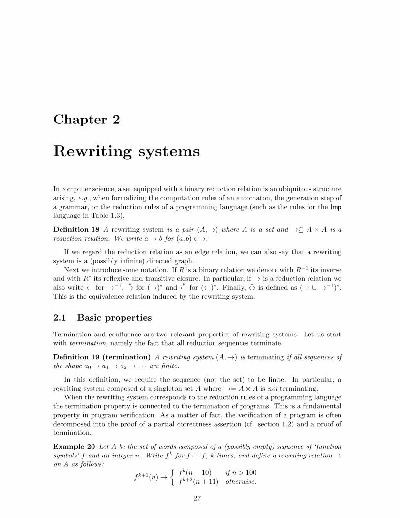
Example 20 Let A be the set of words composed of a (possibly empty) sequence of ‘functionsymbols’ f and an integer n. Write fk for f · · · f , k times, and define a rewriting relation →on A as follows:
fk+1(n)→fk(n− 10) if n > 100fk+2(n+ 11) otherwise.
27

28 Rewriting systems
This is known as McCarthy’s function 91. For instance:
f(100)→ f(f(111))→ f(101)→ 91 6→
Proving its termination is not trivial, but the name of the function gives a hint. For anotherexample, let N+ be the collection of non-negative natural numbers with the following rewritingrelation:
n→n/2 if n > 1, n even3n+ 1 if n > 1, n odd.
This is known as Collatz’s function and its termination is a long standing open problem.
Exercise 21 Consider the following Imp command (extended with integer addition and divi-sion) where b is an arbitrary boolean condition:
while (u > l + 1) do (r := (u+ l)/2 ; if b then u := r else l := r) .
Show that the evaluation of the command starting from a state satisfying u, l ∈ N terminates.
Definition 22 (normalizing) We say that a ∈ A is a normal form if 6 ∃b (a → b). Wealso say that the rewriting system is normalizing if for all a ∈ A there is a finite reductionsequence leading to a normal form.
A terminating rewriting system is normalizing, but the converse fails. For instance, con-sider: A = a, b with a→ a and a→ b. In some contexts (e.g., proof theory), a terminatingrewriting system is also called strongly normalizing. A second property of interest is conflu-ence.
Definition 23 (confluence) A rewriting system (A,→) is confluent if for all a ∈ A:
∀ b, c (b∗← a
∗→ c)
∃ d (b∗→ d
∗← c).
We also write b ↓ c if ∃ d (b∗→ d
∗← c).
A property related to confluence is the property called Church-Rosser, after the logicianswho introduced the terminology in the framework of the λ-calculus (cf. chapter 7).
Definition 24 (Church-Rosser) A rewriting system (A,→) is Church-Rosser if for all
a, b ∈ A, a∗↔ b implies a ↓ b.
Proposition 25 A rewriting system is Church-Rosser iff it is confluent.
Proof. (⇒) If a∗→ b and a
∗→ c then b∗↔ c. Hence ∃ d b
∗→ d, c∗→ d.
(⇐) If a∗↔ b then a and b are connected by a finite sequence of ‘picks and valleys’. For
instance:a∗→ c1
∗← c2∗→ c3 · · ·
∗← cn∗→ b .
Using confluence, we can then find a common reduct. To show this, proceed by induction onthe number of picks and valleys. 2
Let us look at possible interactions of the introduced properties.

Rewriting systems 29
Proposition 26 Let (A,→) be a rewriting system.
1. If the rewriting system is confluent then every element has at most one normal form.
2. If moreover the rewriting system is normalizing then every element has a unique normalform.
Proof. (1) If an element reduces to two distinct normal forms then we contradict confluence.
(2) By normalization, there exists a normal form and by (1) there cannot be two differentones. 2
Exercise 27 Let (A,→1) and (A,→2) be two rewriting systems. We say that they commute
if a∗→1 b and a
∗→2 c implies ∃ d (b∗→2 d and c
∗→1 d). Show that if→1 and→2 are confluentand commute then →1 ∪ →2 is confluent too.
2.2 Termination and well-founded orders
Terminating rewriting systems and well-founded orders are two sides of the same coin.
Definition 28 A partial order (P,>) is a set P with a transitive relation >. A partial order(P,>) is well-founded if it is not possible to define a sequence xii∈N ⊆ P such that:
x0 > x1 > x2 > · · ·
Notice that in a well-founded system we cannot have an element x such that x > x forotherwise we can define a sequence x > x > x > · · · (a similar remark concerned the definitionof terminating rewriting system).
Exercise 29 Let N be the set of natural numbers, Nk the cartesian product N × · · · ×N,k-times, and A =
⋃Nk | k ≥ 1. Let > be a binary relation on A such that :
(x1, . . . , xm) > (y1, . . . , yn) iff ∃ k (k ≤ min(n,m), x1 = y1, . . . , xk−1 = yk−1, xk > yk) .
Prove or disprove the assertion that > is a well-founded order.
Clearly, every well-founded partial order is a terminating rewriting system if we regardthe order > as the reduction relation. Conversely, every terminating rewriting system, say
(P,→), induces the well-founded partial order (P,+→) where
+→ is the transitive (but notreflexive) closure of →.
Proposition 30 (induction principle) Let (P,>) be a well-founded partial order and forx ∈ P let ↓ (x) = y | x > y. Then the following induction principle holds where ⊃ standsfor the logical implication:
∀x ((↓ (x) ⊆ B) ⊃ x ∈ B)
B = P(2.1)
Proof. If x is minimal then the principle requires x ∈ B. Otherwise, suppose x0 is notminimal and x0 /∈ B. Then there must be x1 < x0 such that x1 /∈ B. Again x1 is not minimaland we can go on to build: x0 > x1 > x2 > · · · which contradicts the hypothesis that P iswell-founded. 2

30 Rewriting systems
Exercise 31 Explain why the principle fails if P is a singleton set and > is reflexive.
Remark 32 On the natural numbers the induction principle can be stated as:
∀n (∀n′ < n n′ ∈ B ⊃ n ∈ B)
∀n n ∈ B ,
which is equivalent to the usual reasoning principle:
0 ∈ B ∧ (∀n (n ∈ B ⊃ (n+ 1) ∈ B))
∀n n ∈ B .
We have shown that on a well-founded order the induction principle holds. The converseholds too in the following sense.
Proposition 33 Let (P,>) be a partial order for which the induction principle (2.1) holds.Then (P,>) is well-founded.
Proof. Define: Z = x ∈ P | there is no infinite descending chain from x and ↓ (x) = y |y < x. The set Z satisfies the condition: ∀x (↓ (x) ⊆ Z ⊃ x ∈ Z). Hence by the inductionprinciple Z = P . Thus P is well-founded. 2
2.3 Lifting well-foundation
We examine three ways to lift an order to tuples so as to preserve well-foundation, namelythe product order, the lexicographic order, and the multi-set order.
Definition 34 Let (P,>) be a partial order and let Pn = P×· · ·×P , n times, be the cartesianproduct (n ≥ 2). The product order on Pn is defined by (x1, . . . , xn) >p (y1, . . . , yn) if:
xi ≥ yi, i = 1, . . . , n and ∃ j ∈ 1, . . . , n xj > yj .
The lexicographic order (from left to right) on Pn is defined by (x1, . . . , xn) >lex (y1, . . . , yn)if:
∃ j ∈ 1, . . . , n x1 = y1, . . . , xj−1 = yj−1, xj > yj .
Notice that (x1, . . . , xn) >p (y1, . . . , yn) implies (x1, . . . , xn) >lex (y1, . . . , yn) but that theconverse fails.
Proposition 35 If (P,>) is well-founded and n ≥ 2 then (Pn, >p) and (Pn, >lex ) are well-founded.
Proof. For the product order, suppose there is an infinite descending chain in the productorder. Then one component must be strictly decreasing infinitely often which contradicts thehypothesis that (P,>) is well-founded. As for the lexicographic order, we proceed by induc-tion on n. For the induction step, notice that the first component must eventually stabilizeand then apply induction on the remaining components. 2
A third way to compare a finite collection of elements is to consider them as multi-setswhich we introduce next.

Rewriting systems 31
Definition 36 A multi-set M over a set A is a function M : A → N. If M(a) = k then aoccurs k times in the multi-set. A finite multi-set is a multi-set M such that a |M(a) 6= 0is finite.
Definition 37 Let Mfin(X) denote the finite multi-sets over a set X.
Definition 38 Assume (X,>) is a partial order and M,N ∈Mfin(X). We write M >1,m Nif N is obtained from M by replacing an element by a multi-set of elements which are strictlysmaller.
Example 39 If X = N then |1, 3| >1,m |1, 2, 2, 1| >1,m |0, 2, 2, 1| >1,m |0, 1, 1, 2, 1|.
Exercise 40 Find an example where the relation >1,m is not transitive.
Definition 41 Let (X,>) be a partial order. We define the multi-set order >m on Mfin(X).as the transitive closure of >1,m.
We want to show that if (X,>) is well-founded then >m is well-founded. First we recalla classical result known in the literature as Konig’s lemma.
Proposition 42 A finitely branching tree with an infinite number of nodes admits an infinitepath.
Proof. First let us make our statement precise. A tree can be seen as a subset D of N∗
(finite words of natural numbers) satisfying the following properties.
1. If w ∈ D and w′ is a prefix of w then w′ ∈ D.
2. If wi ∈ D and j < i then wj ∈ D.
Notice that this representation is quite general in that it includes trees with a countablenumber of nodes and even trees with nodes having a countable number of children (e.g., N∗
is a tree). We say that a tree is finitely branching if every node has a finite number of children(this is strictly weaker than being able to bound the number of children of every node!).
Now suppose D is a finitely branching tree with infinitely many nodes. If π ∈ N∗ let ↑ (π)be the set of paths that start with π. We show that it is always possible to extend a path πsuch that ↑ (π) ∩D is infinite to a longer path π · i with the same property, i.e., ↑ (π · i) ∩Dis infinite. Indeed, the hypothesis that D is finitely branching entails that there are finitelymany i1, . . . , ik such that πij ∈ D. Since ↑ (π) ∩ D is infinite one of these branches, say i,must be used infinitely often. So we have that ↑ (π · i) ∩D is infinite. 2
Proposition 43 If (P,>) is well-founded then (Mfin(P ), >m) is well-founded.
Proof. By contradiction suppose we have an infinitely descending chain:
X0 >m X1 >m · · ·
Because >m is the transitive closure of >1,m this gives an infinitely descending chain:
Y0 >1,m Y1 >1,m · · ·

32 Rewriting systems
where X0 = Y0. By definition of >1,m, the step from Yi to Yi+1 consists in taking an elementof Yi, say y, and replacing it by a finite multi-set of elements |y1, . . . , yk| which are strictlysmaller. Suppose we have drawn a tree whose leaves correspond to the elements of Yi (ifneeded we may add a special root node). Then to move to Yi+1 we have to take a leaf of Yi,which corresponds to the element y, and add k branches labelled with the elements y1, . . . , yk(if k = 0 we may just add one branch leading to a special ‘sink node’ from which no furtherexpansion is possible). The tree we build in this way is finitely branching and is infinite. Thenby Konig’s lemma (proposition 42) there must be an infinite path in it which corresponds toan infinitely descending chain in (P,>). This is a contradiction since (P,>) is supposed tobe well-founded. 2
Exercise 44 Does the evaluation of the following Imp commands terminate assuming initiallya state where m,n are positive natural numbers?
while (m 6= n) do (if (m > n) then m := m− n; else n := n−m; ) ,while (m 6= n) do (if (m > n) then m := m− n; else (h := m;m := n;n := h; )) .
Exercise 45 Let (A,→) be a rewriting system and let N be the set of natural numbers. Amonotonic embedding is a function µ : A → N such that if a → b then µ(a) >N µ(b).Define the set of immediate successors of a ∈ A as: suc(a) = b | a → b, and say that Ais finitely branching if for all elements a ∈ A, suc(a) is a finite set. Prove that: (1) If arewriting system has a monotonic embedding then it terminates. (2) If a rewriting systemis finitely branching and terminating then it has a monotonic embedding. (3) The followingrewriting system (N×N,→) where: (i+ 1, j)→ (i, k) and (i, j + 1)→ (i, j), for i, j, k ∈ N,is terminating, not finitely branching, and does not have a monotonic embedding.
2.4 Termination and local confluence
In general, it is hard to prove confluence because we have to consider arbitrary long reductions.It is much simpler to reason locally.
Definition 46 A rewriting system (A,→) is locally confluent if for all a ∈ A:
∀ b, c ∈ A (b← a→ c)
∃ d ∈ A (b∗→ d
∗← c).
Proposition 47 If a rewriting system (A,→) is locally confluent and terminating then it isconfluent.
Proof. We apply the principle of well-founded induction to (A,+→) ! Suppose:
c1∗← b1 ← a→ b2
∗→ c2 .
By local confluence: ∃ d (b1∗→ d
∗← b2). Also, by induction hypothesis on b1 and b2 we have:
∃ d′ (c1∗→ d′
∗← d) , ∃ d′′ (d′∗→ d′′
∗← c2) .
But then c1 ↓ c2. Thus by the principle of well-founded induction, the rewriting system isconfluent. 2

Rewriting systems 33
Example 48 Let A = N ∪ a, b and → such that for i ∈ N: i → i + 1, 2 · i → a, and2 · i+ 1→ b. This rewriting system is locally confluent and normalizing, but not terminatingand not confluent.
Exercise 49 Let Σ∗ denote the set of finite words over the alphabet Σ = f, g1, g2 withgeneric elements w,w′, . . . As usual, ε denotes the empty word. Let → denote the smallestbinary relation on Σ∗ such that for all w ∈ Σ∗:
(1) fg1w → g1g1ffw , (2) fg2w → g2fw , (3) fε → ε ,
and such that if w → w′ and a ∈ Σ then aw → aw′. This is an example of word rewriting; amore general notion of term rewriting will be considered in the following section 2.5. Proveor give a counter-example to the following assertions:
1. If w∗→ w1 and w
∗→ w2 then there exists w′ such that w1∗→ w′ and w2
∗→ w′.
2. The rewriting system (Σ∗,→) is terminating.
3. Replacing rule (1) with the rule fg1w → g1g1fw, the answers to the previous questionsare unchanged.
2.5 Term rewriting systems
When rewriting systems are defined on sets with structure, we can exploit this structure, e.g.,to represent in a more succinct way the reduction relation and to reason on its properties.A situation of this type arises when dealing with sets of first-order terms (in the sense offirst-order logic). Let us fix some notation. A signature Σ is a finite set of function symbolsf1, . . . , fn where each function symbol has an arity, ar(fi), which is a natural numberindicating the number of arguments of the function. Let V denote a countable set of variableswith generic elements x, y, z, . . . If V ′ ⊆ V then TΣ(V ′) is the set of first order terms over thevariables V ′ with generic elements t, s, . . . (respecting the arity). So TΣ(V ′) is the least setwhich contains the variables V ′ and such that if f ∈ Σ, n = ar(f), and t1, . . . , tn ∈ TΣ(V ′)then f(t1, . . . , tn) ∈ TΣ(V ′). If t is a term we denote with var(t) the set of variables occurringin the term.
A natural operation we may perform on terms is to substitute terms for variables. Formally,a substitution is a function S : V → TΣ(V ) which is the identity almost everywhere. Werepresent with the notation [t1/x1, . . . , tn/xn] the substitution S such that S(xi) = ti fori = 1, . . . , n and which is the identity elsewhere. Notice that we always assume xi 6= xj ifi 6= j. We use id to denote a substitution which is the identity everywhere. We extend S toTΣ(V ) by defining, for f ∈ Σ:
S(f(t1, . . . , tn)) = f(S(t1), . . . , S(tn)) (extension of substitution to terms).
Thanks to this extension, it is possible to compose substitutions: (T S) is the substitutiondefined by the equation:
(T S)(x) = T (S(x)) (composition of substitutions).
As expected, composition is associative and the identity substitution behaves as a left andright identity: id S = S id = S.

34 Rewriting systems
Example 50 If t = f(x, y), S = [g(y)/x], and T = [h/y] then:
(T S)(t) = T (S(t)) = T (f(g(y), y)) = f(g(h), h) .
Next we aim to define the reduction relation schematically exploiting the structure offirst-order terms. A context C is a term with exactly one occurrence of a special symbol [ ]called hole and of arity 0. We denote with C[t] the term resulting from the replacement ofthe hole [ ] by t in C. A term-rewriting rule (or rule for short) is a pair of terms (l, r) thatwe write l→ r such that var(r) ⊆ var(l); the variables on the right hand side of the rule mustoccur on the left hand-side too.
Definition 51 A set of term rewriting rules R = l1 → r1, . . . , ln → rn, where li, ri, i =1, . . . , n are terms over some signature Σ, induces a rewriting system (TΣ(V ),→R) where →R
is the least binary relation such that is l → r ∈ R is a rule, C is a context, and S is asubstitution then:
C[Sl]→R C[Sr] .
Example 52 Assume the set of rules R is as follows:
f(x) → g(f(s(x))) , i(0, y, z) → y , i(1, y, z) → z .
Then, for instance:
f(s(y)) →R g(f(s(s(y)))) →R g(g(f(s(s(s(y)))))) →R · · ·i(0, 1, f(y)) →R 1i(0, 1, f(0)) →R i(0, 1, g(f(s(0)))) →R · · ·
There is a natural interplay between equational and term rewriting systems. We illustratethis situation with a few examples.
Example 53 Suppose we have a set of equations dealing with natural numbers:
+(x, Z) = +(Z, x) = x, +(S(x), y) = +(x, S(y)) = S(+(x, y)),+(+(x, y), z) = +(x,+(y, z)) .
Here the numbers are written in unary notation with a zero Z and a successor S functionsymbols, and the equations are supposed to capture the behavior of a binary addition symbol +.Now it is tempting to orient the equations so as to simplify the expression. E.g. +(x, Z)→ x ,but this is not always obvious! For instance, what is the orientation of:
+(S(x), y) = S(+(x, y)) or + (+(x, y), z) = +(x,+(y, z)) ?
One proposal could be:
+(x, Z)→ x, +(Z, x)→ x, +(S(x), y)→ S(+(x, y)),+(x, S(y))→ S(+(x, y)), +(+(x, y), z)→ +(x,+(y, z)) .
Thus we have defined a term rewriting system and some interesting and natural questionsarise. Is there a reduction strategy always leading to a normal form? Does any reductionstrategy reach a normal form? Suppose we apply different reduction strategies, is it alwayspossible to reach a common reduct?

Rewriting systems 35
In our case we are lucky. Termination (and therefore normalization) is guaranteed. More-over the system is confluent and therefore each term has a unique normal form. These proper-ties can be verified automatically by state of the art tools dealing with term rewriting systems.Once these properties are verified, we have a strategy to decide the equality of two terms: wereduce the terms to their normal forms and check whether they are identical.
Example 54 In this example we look at the equations of group theory:
∗(e, x) = x, ∗(x, e) = x, ∗(i(x), x) = e, ∗(x, i(x)) = e, ∗(∗(x, y), z) = ∗(x, ∗(y, z)) .
Here e is the identity, i is the inverse function, and ∗ is the binary operation of a group.If we orient the equations from left to right we obtain a term rewriting system and againautomatic tools can check that the system is terminating. However the system as it standsis not confluent. In this case, a procedure known as completion tries to add rewriting rulesto the system which are compatible with the equations and preserve termination. A possibleoutcome of this analysis is to add the following rules:
i(e)→ e, ∗(i(x), ∗(x, y))→ y, i(i(x))→ x,∗(x, ∗(i(x), y))→ y , i(∗(x, y))→ ∗(i(y), i(x)) .
The previous examples may give the impression that checking termination and confluenceis a task that can be automatized. While this is true in many practical cases, the readershould keep in mind that in general these properties are undecidable. Term rewriting systemsconstitute a powerful computational model and it is easy to reduce, e.g., the halting problemfor Turing machines to a termination problem for term rewriting systems.
2.6 Summary and references
We have shown that the following concepts are ‘equivalent’: (1) terminating rewriting sys-tem, (2) well-founded set, and (3) partial order with well-founded induction principle. Also,whenever working in a terminating rewriting system we have shown that to prove confluenceit suffices to prove local confluence. We have also introduced the notion of term rewritingsystem which is a way of presenting schematically a rewriting system using first-order terms.Term rewriting systems are tightly connected to equational theories and can provide proce-dures to decide when two expressions are equated. The book [BN99] is a standard and quitereadable introduction to term rewriting. Proposition 42 is a special case of a theorem due toKonig [K26] while proposition 47 is due to Newman [New42].

36 Rewriting systems

Chapter 3
Syntactic unification
Syntactic unification is about solving equations on terms, or equivalently on finite labelledtrees. We introduce some notation and terminology. We write t = s if the terms t and s aresyntactically equal. We define a pre-order on substitutions as follows:
R ≤ S iff ∃T T R = S .
Thus R ≤ S if S is an instance of R or, equivalently, if R is more general than S (note thatid ≤ S, for any S).
Exercise 55 Give an example of two substitutions S, T such that: S 6= T , S ≤ T , and T ≤ S.
A system of equations E is a finite set of pairs t1 = s1, . . . , tn = sn. A substitution Sunifies a system of equations E, written S |= E, if St = Ss (here = means identity on TΣ(V ))for all t = s ∈ E. Notice that we are abusing notation by using = both for the identity onterms (semantic level) and for a constraint relation (syntactic level).
Exercise 56 Show that if S is a substitution unifying the system s1 = s2, x = t then Sunifies [t/x]s1 = [t/x]s2 too.
3.1 A basic unification algorithm
A basic algorithm for unification is presented in table 3.1 as a rewriting system over pairs(E,S) and a special symbol ⊥ (the symmetric rules for (vti), i = 1, 2, are omitted). This‘abstract’ presentation of the algorithm is instrumental to the proof of its properties. Theidea is that we transform the system leaving the set of its solutions unchanged till eitherthe solution is explicit or it appears that no solution exists. This is a standard methodologyfor solving systems of constraints, e.g., consider Gaussian elimination for solving systems oflinear equations.
Example 57 Applying the unification algorithm to the system:
f(x) = f(f(z)), g(a, y) = g(a, x) ,
leads to the substitution: S = [f(z)/y] [f(z)/x].
Exercise 58 Apply the unification algorithm to the systems of equations: f(x, f(x, y)) =f(g(y), f(g(a), z)), a constant, and f(x, f(y)) = f(y, f(f(x))).
37
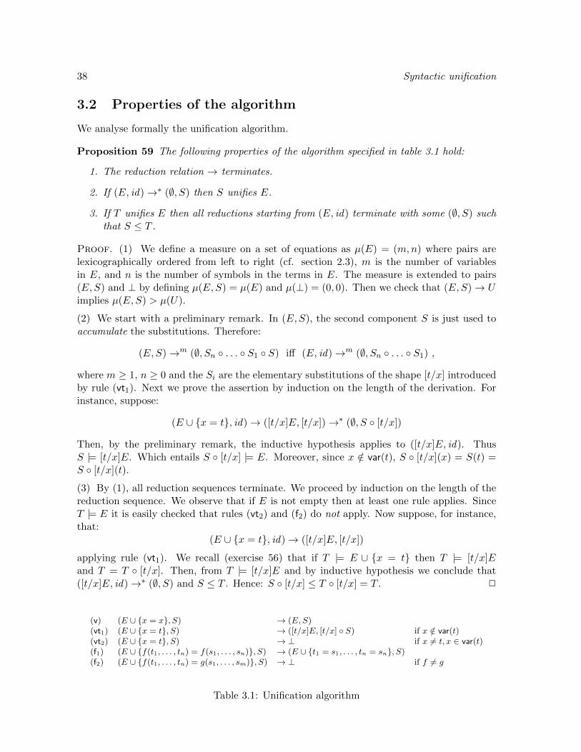
38 Syntactic unification
3.2 Properties of the algorithm
We analyse formally the unification algorithm.
Proposition 59 The following properties of the algorithm specified in table 3.1 hold:
1. The reduction relation → terminates.
2. If (E, id)→∗ (∅, S) then S unifies E.
3. If T unifies E then all reductions starting from (E, id) terminate with some (∅, S) suchthat S ≤ T .
Proof. (1) We define a measure on a set of equations as µ(E) = (m,n) where pairs arelexicographically ordered from left to right (cf. section 2.3), m is the number of variablesin E, and n is the number of symbols in the terms in E. The measure is extended to pairs(E,S) and ⊥ by defining µ(E,S) = µ(E) and µ(⊥) = (0, 0). Then we check that (E,S)→ Uimplies µ(E,S) > µ(U).
(2) We start with a preliminary remark. In (E,S), the second component S is just used toaccumulate the substitutions. Therefore:
(E,S)→m (∅, Sn . . . S1 S) iff (E, id)→m (∅, Sn . . . S1) ,
where m ≥ 1, n ≥ 0 and the Si are the elementary substitutions of the shape [t/x] introducedby rule (vt1). Next we prove the assertion by induction on the length of the derivation. Forinstance, suppose:
(E ∪ x = t, id)→ ([t/x]E, [t/x])→∗ (∅, S [t/x])
Then, by the preliminary remark, the inductive hypothesis applies to ([t/x]E, id). ThusS |= [t/x]E. Which entails S [t/x] |= E. Moreover, since x /∈ var(t), S [t/x](x) = S(t) =S [t/x](t).
(3) By (1), all reduction sequences terminate. We proceed by induction on the length of thereduction sequence. We observe that if E is not empty then at least one rule applies. SinceT |= E it is easily checked that rules (vt2) and (f2) do not apply. Now suppose, for instance,that:
(E ∪ x = t, id)→ ([t/x]E, [t/x])
applying rule (vt1). We recall (exercise 56) that if T |= E ∪ x = t then T |= [t/x]Eand T = T [t/x]. Then, from T |= [t/x]E and by inductive hypothesis we conclude that([t/x]E, id)→∗ (∅, S) and S ≤ T . Hence: S [t/x] ≤ T [t/x] = T . 2
(v) (E ∪ x = x, S) → (E,S)(vt1) (E ∪ x = t, S) → ([t/x]E, [t/x] S) if x /∈ var(t)(vt2) (E ∪ x = t, S) → ⊥ if x 6= t, x ∈ var(t)(f1) (E ∪ f(t1, . . . , tn) = f(s1, . . . , sn), S) → (E ∪ t1 = s1, . . . , tn = sn, S)(f2) (E ∪ f(t1, . . . , tn) = g(s1, . . . , sm), S) → ⊥ if f 6= g
Table 3.1: Unification algorithm

Syntactic unification 39
Exercise 60 Let the size of a term be the number of nodes in its tree representation. Considerthe following unification problem:
x1 = f(x0, x0), x2 = f(x1, x1), . . . , xn = f(xn−1, xn−1) . (3.1)
Compute the most general unifier S. Show that the size of S(xn) is exponential in n.
In view of exercise 60, you could expect unification algorithms to be hopelessly inefficient.However a closer look at the solution of the unification problem (3.1) reveals that the solutioncan be represented compactly as soon as we move from a tree representation to a directedacyclic graph (dag) representation. This change of perspective allows to share terms and keepthe size of S(xn) linear in n. Indeed, unification algorithms based on a dag representationcan be implemented to run in quasi-linear time.
Exercise 61 Propose a method to transform a unification problem of the shape:
E = t1 = s1, . . . , tn = sn
over a signature Σ = g1, . . . , gm with n,m ≥ 1 into a unification problem E′ with thefollowing properties:
1. The problem E′ contains exactly one equation.
2. The terms in E′ are built over a signature Σ′ containing exactly one binary symbol f .
3. The problem E has a solution if and only if the problem E′ has a solution.
4. Apply the method to the system: E = x = h(y), g(c, x, z) = g(y, z, z), where x, y, zare variables.
Exercise 62 Let t, s, . . . be terms over a signature Σ. We say that t is a filter (or pattern)for s if there is a substitution S such that St = s. In this case we write: t ≤ s. Show or givea counter-example to the following assertions:
1. If t ≤ s then t and s are unifiable.
2. If t and s are unifiable then t ≤ s and s ≤ t.
3. If t ≤ s and s ≤ t then s and t are unifiable.
4. For all t, s one can find r such that r ≤ t and r ≤ s.
5. For all t, s one can find r such that r ≥ t and r ≥ s.
3.3 Summary and references
We have shown that there is a simple algorithm to solve the unification problem on first-orderterms. The algorithm either shows that no solution exists or computes a most general one.Moreover the algorithm is efficient as soon as terms are represented as directed acyclic graphs.The unification algorithm was brought to the limelight by Robinson’s work on the resolutionprinciple and its application to theorem proving [Rob65].

40 Syntactic unification
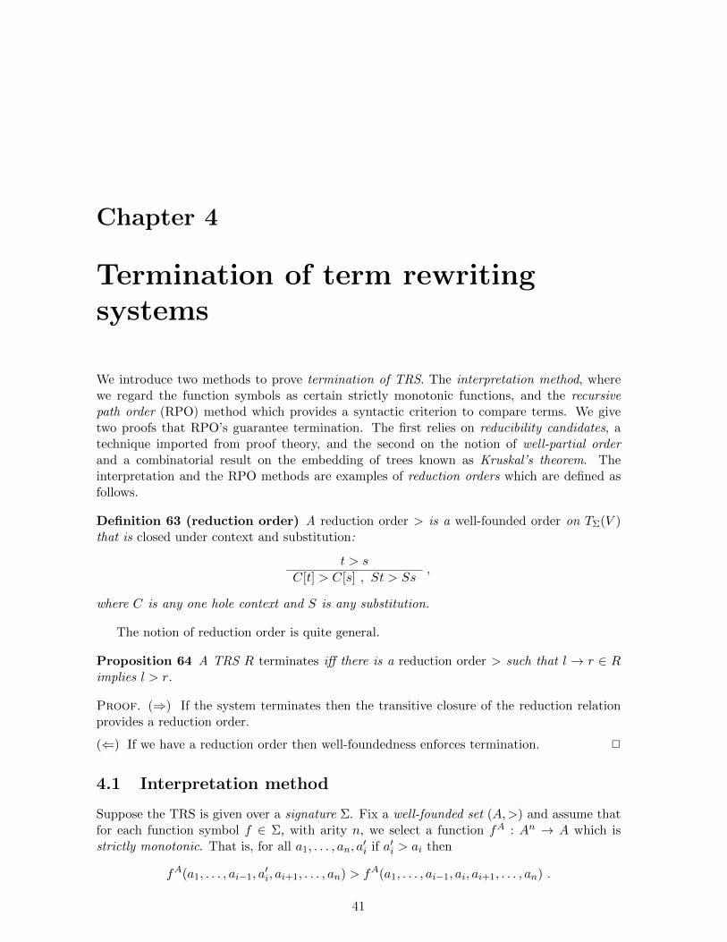
Chapter 4
Termination of term rewritingsystems
We introduce two methods to prove termination of TRS. The interpretation method, wherewe regard the function symbols as certain strictly monotonic functions, and the recursivepath order (RPO) method which provides a syntactic criterion to compare terms. We givetwo proofs that RPO’s guarantee termination. The first relies on reducibility candidates, atechnique imported from proof theory, and the second on the notion of well-partial orderand a combinatorial result on the embedding of trees known as Kruskal’s theorem. Theinterpretation and the RPO methods are examples of reduction orders which are defined asfollows.
Definition 63 (reduction order) A reduction order > is a well-founded order on TΣ(V )that is closed under context and substitution:
t > s
C[t] > C[s] , St > Ss,
where C is any one hole context and S is any substitution.
The notion of reduction order is quite general.
Proposition 64 A TRS R terminates iff there is a reduction order > such that l → r ∈ Rimplies l > r.
Proof. (⇒) If the system terminates then the transitive closure of the reduction relationprovides a reduction order.
(⇐) If we have a reduction order then well-foundedness enforces termination. 2
4.1 Interpretation method
Suppose the TRS is given over a signature Σ. Fix a well-founded set (A,>) and assume thatfor each function symbol f ∈ Σ, with arity n, we select a function fA : An → A which isstrictly monotonic. That is, for all a1, . . . , an, a
′i if a′i > ai then
fA(a1, . . . , ai−1, a′i, ai+1, . . . , an) > fA(a1, . . . , ai−1, ai, ai+1, . . . , an) .
41
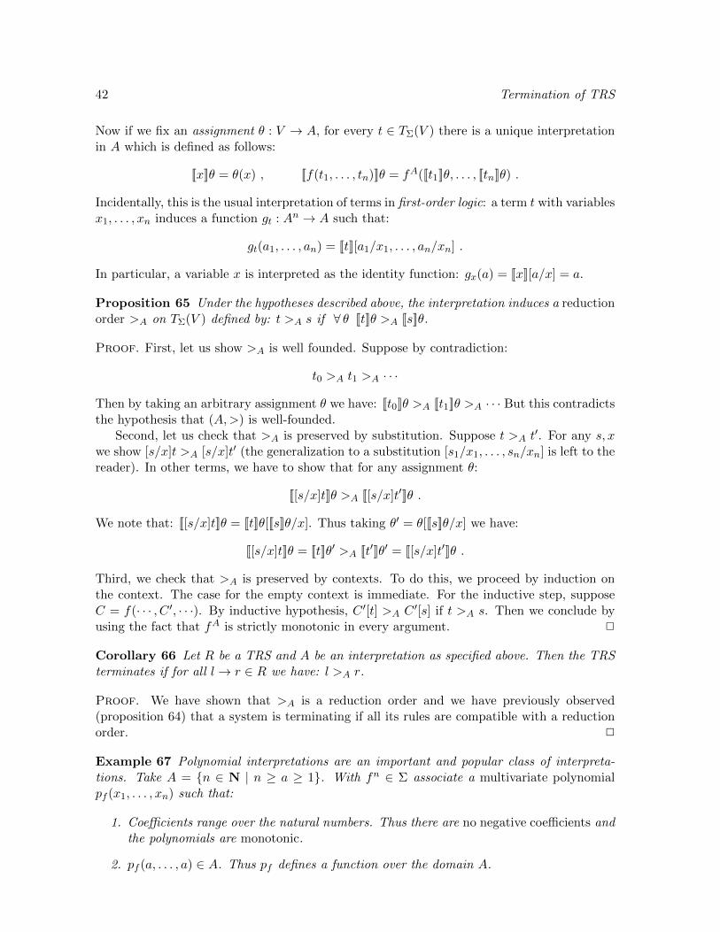
42 Termination of TRS
Now if we fix an assignment θ : V → A, for every t ∈ TΣ(V ) there is a unique interpretationin A which is defined as follows:
[[x]]θ = θ(x) , [[f(t1, . . . , tn)]]θ = fA([[t1]]θ, . . . , [[tn]]θ) .
Incidentally, this is the usual interpretation of terms in first-order logic: a term t with variablesx1, . . . , xn induces a function gt : An → A such that:
gt(a1, . . . , an) = [[t]][a1/x1, . . . , an/xn] .
In particular, a variable x is interpreted as the identity function: gx(a) = [[x]][a/x] = a.
Proposition 65 Under the hypotheses described above, the interpretation induces a reductionorder >A on TΣ(V ) defined by: t >A s if ∀ θ [[t]]θ >A [[s]]θ.
Proof. First, let us show >A is well founded. Suppose by contradiction:
t0 >A t1 >A · · ·
Then by taking an arbitrary assignment θ we have: [[t0]]θ >A [[t1]]θ >A · · · But this contradictsthe hypothesis that (A,>) is well-founded.
Second, let us check that >A is preserved by substitution. Suppose t >A t′. For any s, x
we show [s/x]t >A [s/x]t′ (the generalization to a substitution [s1/x1, . . . , sn/xn] is left to thereader). In other terms, we have to show that for any assignment θ:
[[[s/x]t]]θ >A [[[s/x]t′]]θ .
We note that: [[[s/x]t]]θ = [[t]]θ[[[s]]θ/x]. Thus taking θ′ = θ[[[s]]θ/x] we have:
[[[s/x]t]]θ = [[t]]θ′ >A [[t′]]θ′ = [[[s/x]t′]]θ .
Third, we check that >A is preserved by contexts. To do this, we proceed by induction onthe context. The case for the empty context is immediate. For the inductive step, supposeC = f(· · · , C ′, · · ·). By inductive hypothesis, C ′[t] >A C ′[s] if t >A s. Then we conclude byusing the fact that fA is strictly monotonic in every argument. 2
Corollary 66 Let R be a TRS and A be an interpretation as specified above. Then the TRSterminates if for all l→ r ∈ R we have: l >A r.
Proof. We have shown that >A is a reduction order and we have previously observed(proposition 64) that a system is terminating if all its rules are compatible with a reductionorder. 2
Example 67 Polynomial interpretations are an important and popular class of interpreta-tions. Take A = n ∈ N | n ≥ a ≥ 1. With fn ∈ Σ associate a multivariate polynomialpf (x1, . . . , xn) such that:
1. Coefficients range over the natural numbers. Thus there are no negative coefficients andthe polynomials are monotonic.
2. pf (a, . . . , a) ∈ A. Thus pf defines a function over the domain A.
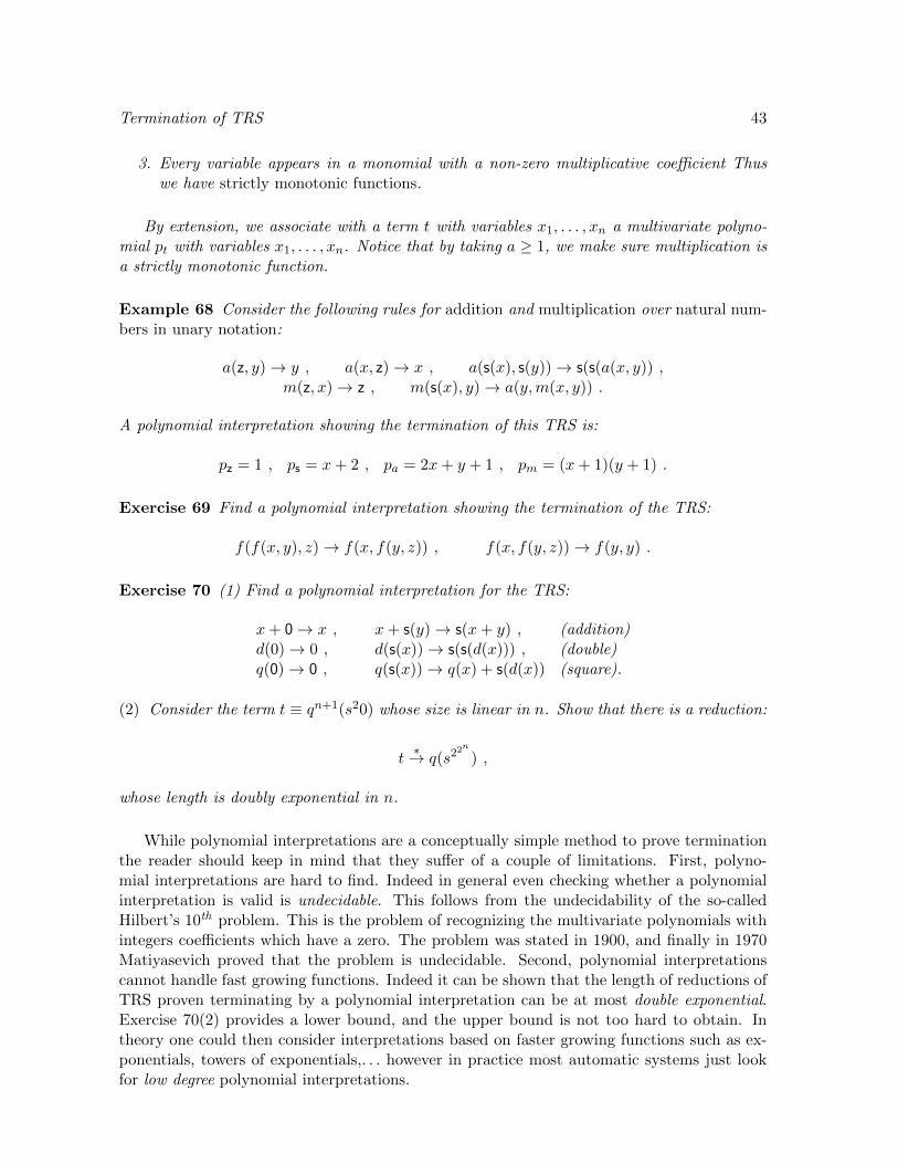
Termination of TRS 43
3. Every variable appears in a monomial with a non-zero multiplicative coefficient Thuswe have strictly monotonic functions.
By extension, we associate with a term t with variables x1, . . . , xn a multivariate polyno-mial pt with variables x1, . . . , xn. Notice that by taking a ≥ 1, we make sure multiplication isa strictly monotonic function.
Example 68 Consider the following rules for addition and multiplication over natural num-bers in unary notation:
a(z, y)→ y , a(x, z)→ x , a(s(x), s(y))→ s(s(a(x, y)) ,m(z, x)→ z , m(s(x), y)→ a(y,m(x, y)) .
A polynomial interpretation showing the termination of this TRS is:
pz = 1 , ps = x+ 2 , pa = 2x+ y + 1 , pm = (x+ 1)(y + 1) .
Exercise 69 Find a polynomial interpretation showing the termination of the TRS:
f(f(x, y), z)→ f(x, f(y, z)) , f(x, f(y, z))→ f(y, y) .
Exercise 70 (1) Find a polynomial interpretation for the TRS:
x+ 0→ x , x+ s(y)→ s(x+ y) , (addition)d(0)→ 0 , d(s(x))→ s(s(d(x))) , (double)q(0)→ 0 , q(s(x))→ q(x) + s(d(x)) (square).
(2) Consider the term t ≡ qn+1(s20) whose size is linear in n. Show that there is a reduction:
t∗→ q(s22n
) ,
whose length is doubly exponential in n.
While polynomial interpretations are a conceptually simple method to prove terminationthe reader should keep in mind that they suffer of a couple of limitations. First, polyno-mial interpretations are hard to find. Indeed in general even checking whether a polynomialinterpretation is valid is undecidable. This follows from the undecidability of the so-calledHilbert’s 10th problem. This is the problem of recognizing the multivariate polynomials withintegers coefficients which have a zero. The problem was stated in 1900, and finally in 1970Matiyasevich proved that the problem is undecidable. Second, polynomial interpretationscannot handle fast growing functions. Indeed it can be shown that the length of reductions ofTRS proven terminating by a polynomial interpretation can be at most double exponential.Exercise 70(2) provides a lower bound, and the upper bound is not too hard to obtain. Intheory one could then consider interpretations based on faster growing functions such as ex-ponentials, towers of exponentials,. . . however in practice most automatic systems just lookfor low degree polynomial interpretations.

44 Termination of TRS
(R1)s ≥r t
f(. . . s . . .) >r t
(R2)f >Σ g f(s1, . . . , sm) >r ti i = 1, . . . , n
f(s1, . . . , sm) >r g(t1, . . . , tn)
(R3)(s1, . . . , sm) >
τ(f)r (t1, . . . , tm)
f(s1, . . . , sm) >r ti i = 1, . . . ,mf(s1, . . . , sm) >r f(t1, . . . , tm)
Table 4.1: Recursive path-order
4.2 Recursive path order
Recursive path orders are a family of reduction orders which are defined by induction on thestructure of the terms. The way to compare terms is rather simple. First we assume a strictpartial order >Σ on the function symbols in Σ (since Σ is supposed finite, >Σ is well-founded).If f >Σ g, proving that:
t = f(t1, . . . , tn) >r g(s1, . . . , sm) = s ,
reduces to proving: t >r si for i = 1, . . . ,m. On the other hand, proving that:
t = f(t1, . . . , tn) >r f(s1, . . . , sm) = s ,
reduces to proving that: (t1, . . . , tn) >r (s1, . . . , sm), according to one of the orders thatpreserve well-foundation we have considered in chapter 2, namely product order, lexicographicorder, or multi-set order. What we have described is almost the official definition of recursivepath order which is given in Table 4.1.
In this definition, we assume that every function symbol f is assigned a status τ(f) whichdetermines how f ’s arguments are to be compared (product, lexicographic, multi-set,. . .)Indeed, this is necessary to guarantee termination. For instance, consider the non-terminatingTRS:
f(a, b)→ f(b, a) , f(b, a)→ f(a, b) ,
with Σ = f, a, b. Assume a >Σ b. If f ’s arguments could be compared with a lexicographicorder from left to right or from right to left then we could prove both f(a, b) >r f(b, a) andf(b, a) >r f(a, b).
Exercise 71 Consider the TRS:
(x+ y) + z → x+ (y + z) , x ∗ s(y) → x+ (y ∗ x) .
Find a status for the function symbols that allows to prove:
(x+ y) + z >r x+ (y + z) , x ∗ s(y) >r x+ (y ∗ x) .

Termination of TRS 45
Another point that deserves to be stressed is that in the rule (R3) we also require that theterm on the left is larger than all the arguments of the term on the right. To see the necessityof this condition, consider the non-terminating TRS:
f(a, y)→ f(b, f(a, y)) ,
where Σ = f, a, b, a >Σ b, and the status of f is lexicographic from left to right.Finally, we notice that there is an additional rule (rule R1) that entails that a term is
larger than all its proper subterms. This ‘subterm property’ is characteristic of an importantclass of orders known as simplification order that we define next.
Definition 72 A strict order > on TΣ(V ) is a simplification order if it is closed under contextand substitution and moreover for all functions f ∈ Σ it satisfies:
f(x1, . . . , xn) > xi for i = 1, . . . , n .
Exercise 73 Show that if > is a simplification order and C is a one hole context with C 6= [ ]then C[t] > t.
We prove next that the recursive path order is a simplification order. Further it will beproven in section 4.4 that every simplification order is well-founded. This proof relies on aclassical combinatorial argument known as Kruskal’s theorem. This is enough to guaranteethat the recursive path order is a reduction order and therefore can be used to prove thetermination of TRS. We will also give in section 4.3 a direct proof of the fact that therecursive path order is well-founded that avoids the detour through Kruskal’s theorem byusing a so called reducibility argument (a standard method to prove termination of typedλ-calculi introduced in chapter 10).
Proposition 74 The recursive path order is a simplification order on TΣ(V ).
Proof. To fix the ideas, we consider a particular case where we always compare tuplesvia the product order. We prove the following properties: (1) > is strict, (2) s > t impliesvar(s) ⊇ var(t), (3) transitivity, (4) subterm property, (5) closure under substitution, and (6)closure under context.
Before proceeding, we formulate in Table 4.2 a simplified definition of recursive path orderfor functions having product status. Notice that in (R3) we drop the condition f(s1, . . . , sm) >rti for i = 1, . . . ,m. It turns out that in this case the condition can be derived from thetransitivity property and the fact that for i = 1, . . . ,m: f(s1, . . . , sm) >r si ≥r ti.
> is strict By induction on s show that s > s is impossible. Note in particular that x > tand f > f are impossible.
s > t implies var(s) ⊇ var(t). By induction on the proof of s > t.
Transitivity Suppose s1 > s2 and s2 > s3. Show s1 > s3 by induction on |s1| + |s2| + |s3|analyzing the last rules applied in the proof of s1 > s2 and s2 > s3 (9 cases).
Subterm property We check that f(x1, . . . , xn) > xi for i = 1, . . . , n.
Closure under substitution Show that t > r implies [s/x]t > [s/x]r by induction on|t|+ |r|.

46 Termination of TRS
(R1)s ≥r t
f(. . . s . . .) >r t
(R2)f >Σ g f(s1, . . . , sm) >r ti i = 1, . . . , n
f(s1, . . . , sm) >r g(t1, . . . , tn)
(R3)si ≥ ti for i ∈ 1..m, and ∃ j ∈ 1..m sj > tj
f(s1, . . . , sm) >r f(t1, . . . , tm).
Table 4.2: RPO, for functions with product status
Closure under context Show by induction on the structure of a one hole context that t > simplies C[t] > C[s]. 2
Exercise 75 Consider the following TRS:
ack(z, n) → s(z) , ack(s(z), z) → s2(z) ,ack(s2(m), z) → s2(m) , ack(s(m), s(n)) → ack(ack(m, s(n)), n) .
This TRS corresponds to a very fast growing function known as Ackermann’s function. Forinstance, this function grows faster than any tower of exponentials1 and no polynomial inter-pretation can prove its termination. In practice, running ack(4 , 4 ) will produce an out-of-memory exception on most computers. Prove the termination by RPO.
Exercise 76 The previous exercise 75 marks a point for RPO. However, sometimes the (poly-nomial) interpretation method beats the RPO method. Consider the TRS:
b(x) → r(s(x)) , r(s(s(x))) → b(x) .
(1) Show that the TRS terminates by polynomial interpretation. (2) Show that there is noRPO on Σ that can prove its termination. (3) RPO is a particular type of simplificationorder. Is there a simplification order that shows termination of the TRS above?
Exercise 77 The previous exercise 76 shows that the termination of certain TRS cannot beproven by RPO. It turns out that using an arbitrary simplification order does not change thisstate of affairs. Consider the TRS:
f(f(x))→ f(g(f(x))) .
(1) Show that the TRS is terminating. (2) Show that there is no simplification order > thatcontains →.
We terminate with a few remarks concerning the complexity of working with RPO. Oncethe order on the signature and the status of the function is fixed, deciding whether t >r s canbe done in time polynomial in the size of the terms. However, it is possible to come out withrather artificial examples where the choice of the order on the signature is not obvious. Infact it can be shown that deciding whether t >r s with respect to some order on the signatureis an np-complete problem.
1Technically, Ackermann showed that this function cannot be defined by primitive recursion.

Termination of TRS 47
s ≥r tf(. . . s . . .) >r t
f >Σ g f(s1, . . . , sm) >r ti i = 1, . . . , n
f(s1, . . . , sm) >r g(t1, . . . , tn)
(s1, . . . , sm) >lexr (t1, . . . , tm)
f(s1, . . . , sm) >r ti i = 1, . . . ,m
f(s1, . . . , sm) >r f(t1, . . . , tm)
Table 4.3: RPO for functions with lexicographic, left-to right status
4.3 Recursive path order is well-founded
We know that RPO is a simplification order, i.e., a strict order, closed under context andsubstitution. We want to show that it is well-founded (and therefore a reduction order).To this end, we apply the reducibility candidates method: a proof technique developed firstto prove termination of typed λ-calculi. To simplify the argument, we shall assume thatfunction arguments are always compared with the lexicographic order from left to right. Thecorresponding specialized definition of RPO is given in Table 4.3.
Definition 78 We work on the set of terms TΣ(V ) and define:
WF = t ∈ TΣ(V ) | there is no infinite sequence t = t0 >r t1 >r · · · ,Red(t) = s | t >r s .
Exercise 79 Show that:
1. (WF , >r) is a well-founded set.
2. If Red(t) ⊆WF then t ∈WF .
3. If s ∈WF and s >r t then t ∈WF .
Let >lexr be the lexicographic ordered induced by >r on vectors of n terms in WF . Thekey property follows.
Proposition 80 If s1, . . . , sn ∈WF and f(s1, . . . , sn) >r t then t ∈WF .
Proof. By induction on the triple:
(f, (s1, . . . , sn), |t|) ,
with the lexicographic order from left to right where:
• The first component is a function symbol ordered by >Σ.
• The third is the size of the term with the usual order on natural numbers.

48 Termination of TRS
• For the second, consider the set⋃f∈Σ WF ar(f) ordered by:
(s1, . . . , sn) > (t1, . . . , tm) iff n = m and (s1, . . . , sn) >lexr (t1, . . . , tm) .
Notice that two vectors of different lengths are incomparable. Also, (WF,>r) well-founded implies (WFn, >lexr ) is well-founded too.
Case f(s1, . . . , sn) >r t as si = t or si >r t.
• If si = t the conclusion is immediate as si ∈WF by hypothesis.
• If si >r t then t ∈WF as si ∈WF .
Case t = g(t1, . . . , tm), f >Σ g, f(s1, . . . , sn) >r ti for i = 1, . . . ,m.
• We notice that (f, (s1, . . . , sn), |t|) > (f, (s1, . . . , sn), |ti|) for i = 1, . . . ,m. Hence,by inductive hypothesis, ti ∈WF .
• Suppose g(t1, . . . , tm) >r u. We remark (f, (s1 . . . , sn), |t|) > (g, (t1, . . . , tm), |u|).Hence, by inductive hypothesis, u ∈WF , and by exercise 79, g(t1, . . . , tm) ∈WF .
Case t = f(t1, . . . , tn), f(s1, . . . , sn) >r ti for i = 1, . . . , n, (s1, . . . , sn) >lexr (t1, . . . , tn). Thiscase is similar to the previous one.
• We remark that (f, (s1, . . . , sn), |t|) > (f, (s1, . . . , sn), |ti|) for i = 1, . . . , n. Hence,by inductive hypothesis, ti ∈WF .
• Suppose f(t1, . . . , tn) >r u. We notice (f, (s1 . . . , sn), |t|) > (f, (t1, . . . , tn), |u|)(second component decreases!). By inductive hypothesis, u ∈WF , and by exercise79, f(t1, . . . , tn) ∈WF . 2
Corollary 81 All terms are in WF .
Proof. By induction on the structure of the terms. 2
4.4 Simplification orders are well-founded
We prove that all simplification orders (in particular RPO) are well-founded. As alreadymentioned, the proof goes through a classical combinatorial result known as Kruskal’s the-orem. This result concerns a natural binary relation on terms (or labelled trees), known ashomeomorphic embedding, that we denote .; we also denote with . the reflexive closure of ..The appearance of the embedding relation is justified by the simple observation that everysimplification order contains it.
Kruskal’s theorem states that when considering the embedding relation on the collection ofterms built out of a finite signature and a finite set of variables there is no infinite descendingchain t0 . t1 . · · · (the order is well-founded) and moreover it is not possible to find an infiniteset of terms which are all incomparable (an infinite anti-chain). Technically, one says thatthe collection of terms with the embedding relation is a well partial order (wpo).
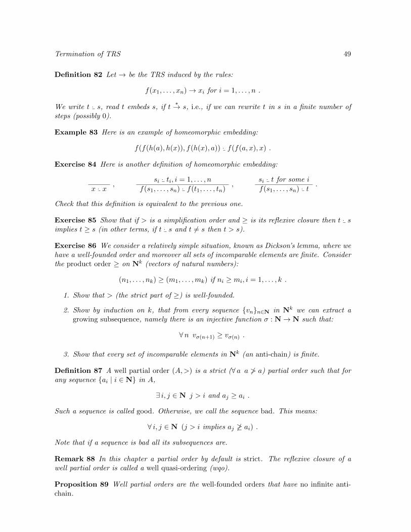
Termination of TRS 49
Definition 82 Let → be the TRS induced by the rules:
f(x1, . . . , xn)→ xi for i = 1, . . . , n .
We write t . s, read t embeds s, if t∗→ s, i.e., if we can rewrite t in s in a finite number of
steps (possibly 0).
Example 83 Here is an example of homeomorphic embedding:
f(f(h(a), h(x)), f(h(x), a)) . f(f(a, x), x) .
Exercise 84 Here is another definition of homeomorphic embedding:
x . x,
si . ti, i = 1, . . . , n
f(s1, . . . , sn) . f(t1, . . . , tn),
si . t for some i
f(s1, . . . , sn) . t.
Check that this definition is equivalent to the previous one.
Exercise 85 Show that if > is a simplification order and ≥ is its reflexive closure then t . simplies t ≥ s (in other terms, if t . s and t 6= s then t > s).
Exercise 86 We consider a relatively simple situation, known as Dickson’s lemma, where wehave a well-founded order and moreover all sets of incomparable elements are finite. Considerthe product order ≥ on Nk (vectors of natural numbers):
(n1, . . . , nk) ≥ (m1, . . . ,mk) if ni ≥ mi, i = 1, . . . , k .
1. Show that > (the strict part of ≥) is well-founded.
2. Show by induction on k, that from every sequence vnn∈N in Nk we can extract agrowing subsequence, namely there is an injective function σ : N→ N such that:
∀n vσ(n+1) ≥ vσ(n) .
3. Show that every set of incomparable elements in Nk (an anti-chain) is finite.
Definition 87 A well partial order (A,>) is a strict (∀ a a 6> a) partial order such that forany sequence ai | i ∈ N in A,
∃ i, j ∈ N j > i and aj ≥ ai .
Such a sequence is called good. Otherwise, we call the sequence bad. This means:
∀ i, j ∈ N (j > i implies aj 6≥ ai) .
Note that if a sequence is bad all its subsequences are.
Remark 88 In this chapter a partial order by default is strict. The reflexive closure of awell partial order is called a well quasi-ordering (wqo).
Proposition 89 Well partial orders are the well-founded orders that have no infinite anti-chain.

50 Termination of TRS
Proof. (⇒) A wpo must be well-founded for a strictly descending chain gives a bad sequence.For the same reason, a wpo cannot contain an infinite anti-chain.
(⇐) Vice versa, take a well-founded set without infinite anti-chain. Given an infinite se-quence, the set of minimal elements of the sequence must be finite. Therefore there is aminimal element such that the sequence is infinitely often above it. 2
Proposition 90 Given a sequence in a wpo, it is always possible to extract an ascendingsubsequence.
Proof. Consider a sequence aii∈N. We want to show that there is an ascending subse-quence:
i1 < i2 < i3 < . . . and ai1 ≤ ai2 ≤ ai3 ≤ · · ·
We notice that in a good sequence there are finitely many ai such that ∀ j j > i implies aj 6≥ai. Otherwise, the sequence composed of all such elements is bad. Thus starting from acertain point i1, if i ≥ i1 then ∃ j > i aj ≥ ai. Now starting from i1 we can inductively builda sequence i1 < i2 < . . . such that ai1 ≤ ai2 ≤ · · · 2
Proposition 91 The product A×B of wpo’s A,B, ordered component-wise (product order)is a wpo.
Proof. Consider (ai, bi) | i ∈ N and suppose ai | i ∈ N and bi | i ∈ N are bothinfinite (otherwise it is easy). Then consider the subsequence i0 < i1 < i2 < · · · such thatai0 ≤ ai1 ≤ ai2 ≤ · · · (cf. previous proposition 90). Then find k > l such that bik ≥ bil . 2
Recall that . is the homeomorphic embedding and that the strict part of ., say ., iscontained in every simplification order.
Proposition 92 (Kruskal) Suppose Σ and V finite. Then the strict homeomorphic embed-ding . on TΣ(V ) is a well partial order.
Proof. We pause to notice that if Σ or V are infinite then (TΣ(V ), .) contains an infiniteanti-chain and the proposition does not hold. The proof proceeds by contradiction. Supposethere is a bad sequence in TΣ(V ). Extract from the bad sequence a minimal one with respectto the size of the terms, say t1, t2, . . . This means that having built the sequence t1, . . . , ti, wepick a term ti+1 of minimal size among those that follow ti. Define:
Si =
∅ if ti variables1, . . . , sn if ti = f(s1, . . . , sn)
S =⋃i≥0 Si .
For the time being, assume (S, .) is a wpo; this is a tricky point whose proof is postponed.Since Σ and X are finite, there must be a symbol that occurs infinitely often as the root ofthe minimal bad sequence t1, t2, . . . If it is a variable or a constant we derive a contradiction.Otherwise, we have i0 < i1 < . . . with:
tik = f(sik1 , . . . , sikn ) .
Now (S, .) is a wpo and the product of wpo’s is a wpo (proposition 91). Therefore, thesequence:
(sik1 , . . . , sikn )k≥0

Termination of TRS 51
is good. So ∃ p, q q > p and siql. s
ipl , l = 1, . . . , n. And this entails tiq . tip . Contradiction!
We now come back to the tricky point. Suppose (S, .) is not a wpo, and let s1, s2, s3 . . .be a bad sequence. The si must be all distinct. Suppose s1 ∈ Sk. This entails tk . s1. LetS<k = S1 ∪ · · · ∪ Sk−1. There is an index l such that si /∈ S<k for i ≥ l. Consider:
t1, . . . , tk−1, s1, sl, sl+1, . . .
Since s1 is smaller than tk, by minimality (!) this sequence must be good. Since t1, t2, . . . ands1, s2, . . . are bad, this entails sj . ti for some i ∈ 1, . . . , k − 1 and j ∈ 1, l, l + 1, . . .. Wedistinguish two cases, both leading to a contradiction.
j = 1 tk . sj . ti. Contradiction!
j ≥ l Suppose sj ∈ Sm\S<k. Thus m ≥ k > i and tm . sj . ti. Contradiction! 2
Remark 93 The presented result is an interesting case study for logicians. First, the proof wehave presented is non-constructive (two nested arguments by contradiction). The literaturecontains proposals for constructive versions of the proof. Second, the theorem is a simpleexample of a combinatorial statement that cannot be proved in Peano’s Arithmetic (a standardformalization of arithmetic in first-order logic).
Exercise 94 The following is a special case of Kruskal’s theorem on words known as Hig-man’s lemma. Let Σ be a finite set (alphabet). Given two words w,w′ ∈ Σ∗ we say that w′
is a subsequence of w, and write w > w′, if the word w′ can be obtained from the word w byerasing some (at least one) of its characters. Apply Kruskal’s theorem to conclude that > isa well partial order.
Incidentally, there is also a famous generalization of Kruskal’s theorem to graphs knownas the graph minor theorem. An edge contraction of a graph consists in removing an edgewhile merging the two vertices. A graph G is a minor of the graph H if it can be obtainedfrom H by a sequence of edge contractions. It turns out that the minor relation is a wellpartial order.
Next, we present two relevant applications of Kruskal’s theorem to the termination prob-lem of TRS. The first one is another proof that RPO is well-founded.
Proposition 95 Every simplification order on TΣ(V ) is well founded. Hence, every simpli-fication order (in particular RPO) is a reduction order.
Proof. By contradiction, suppose t1 > t2 > . . . First, we prove by contradiction thatvar(t1) ⊇ var(t2) ⊇ . . . Suppose x ∈ var(ti+1)\var(ti) and consider the substitution S = [ti/x].Then Sti = ti > Sti+1. By the subterm property, we have Sti+1 ≥ ti. Thus ti > ti whichcontradicts the hypothesis that > is strict.
Thus we can take X = var(t1) which is finite. Then we can apply Kruskal’s theorem tothe sequence and conclude:
∃ i, j j > i and tj . ti .
Thus we have both ti > tj and tj ≥ ti. Hence, ti > ti, which contradicts the hypothesis thata simplification order is strict. Notice that we used the fact that (TΣ(X), .) is a wpo, not justa well-founded set. 2

52 Termination of TRS
The second application concerns the introduction of the interpretation method over thereals. Take as domain A = r ∈ R+ | r ≥ a ≥ 1. This may appear as a wrong start as the setA is not well founded! However, suppose that we associate with every fn ∈ Σ a multivariatepolynomial pf (x1, . . . , xn) such that:
1. Coefficients range over the non-negative reals.
2. pf (a, . . . , a) ∈ A: thus pf defines a function over the domain A.
3. pf (a1, . . . , an) > ai for i = 1, . . . , n (the new condition!).
Write s >A t if over the domain A the polynomial associated with the term s is strictly largerthan the one associated with the term t. It is easily checked that this is a simplificationorder, hence a reduction order. The fact that we move from integers to real has an interestingconsequence as the first-order theory of reals is decidable (e.g., it is decidable whether afirst-order assertion in analytic geometry is valid).
A corollary of this result is that we can decide whether there is a polynomial interpretationover the reals where the polynomials have a bounded degree. However, we stress that this isa rather theoretical advantage because of the high complexity of the decision procedures.
4.5 Summary and references
Proving the termination of a TRS amounts to find a reduction order that is compatible withthe rules of the TRS. One method consists in interpreting the function symbols as functionsover the positive integers with certain strictness properties. Another method consists inapplying the rules of the recursive path orders. It turns out that the recursive path ordersare an instance of the simplification orders and that the latter are well-founded. Many othermethods for proving termination of TRS have been proposed and their implementation isavailable in several tools. Recursive path orders were introduced in [Der82] and the presentedtermination proof is based on [vR01]. Kruskal’s tree theorem is in [Kru60] with a shorter proofin [NW63] which is the one we present. Its special case for words is presented in [Hig52] and itsgeneralization to graphs is presented in a long series of papers starting with [RS83]. Hilbert’s10th problem was among 23 open problems put forward at a 1900 international conference onmathematics. The problem was eventually shown to be undecidable by Matiyasevich in 1970.The decidability of the first-order theory of real numbers was shown by Tarski around 1950.
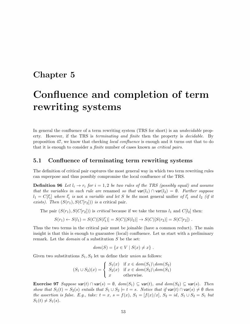
Chapter 5
Confluence and completion of termrewriting systems
In general the confluence of a term rewriting system (TRS for short) is an undecidable prop-erty. However, if the TRS is terminating and finite then the property is decidable. Byproposition 47, we know that checking local confluence is enough and it turns out that to dothat it is enough to consider a finite number of cases known as critical pairs.
5.1 Confluence of terminating term rewriting systems
The definition of critical pair captures the most general way in which two term rewriting rulescan superpose and thus possibly compromise the local confluence of the TRS.
Definition 96 Let li → ri for i = 1, 2 be two rules of the TRS (possibly equal) and assumethat the variables in each rule are renamed so that var(l1) ∩ var(l2) = ∅. Further supposel1 = C[l′1] where l′1 is not a variable and let S be the most general unifier of l′1 and l2 (if itexists). Then (S(r1), S(C[r2])) is a critical pair.
The pair (S(r1), S(C[r2])) is critical because if we take the terms l1 and C[l2] then:
S(r1)← S(l1) = S(C)[S(l′1)] = S(C)[S(l2)]→ S(C)[S(r2)] = S(C[r2]) .
Thus the two terms in the critical pair must be joinable (have a common reduct). The maininsight is that this is enough to guarantee (local) confluence. Let us start with a preliminaryremark. Let the domain of a substitution S be the set:
dom(S) = x ∈ V | S(x) 6= x .
Given two substitutions S1, S2 let us define their union as follows:
(S1 ∪ S2)(x) =
S1(x) if x ∈ dom(S1)\dom(S2)S2(x) if x ∈ dom(S2)\dom(S1)x otherwise.
Exercise 97 Suppose var(t) ∩ var(s) = ∅, dom(S1) ⊆ var(t), and dom(S2) ⊆ var(s). Thenshow that S1(t) = S2(s) entails that S1 ∪ S2 |= t = s. Notice that if var(t) ∩ var(s) 6= ∅ thenthe assertion is false. E.g., take: t = x, s = f(x), S1 = [f(x)/x], S2 = id, S1 ∪ S2 = S1 butS1(t) 6= S1(s).
53
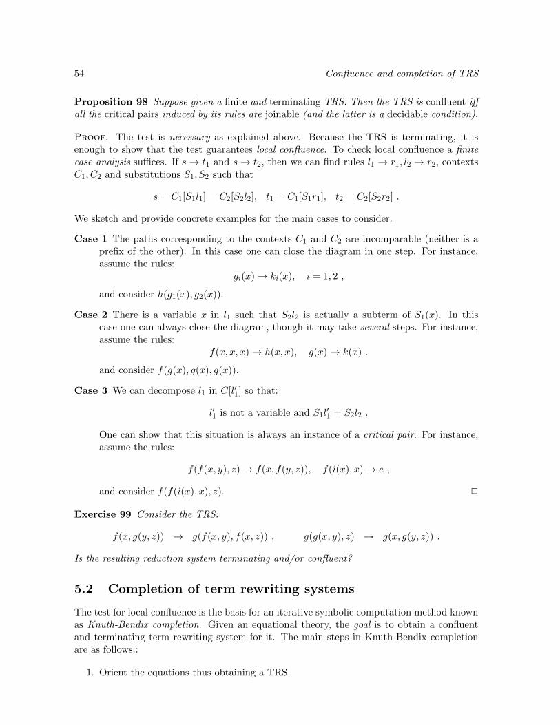
54 Confluence and completion of TRS
Proposition 98 Suppose given a finite and terminating TRS. Then the TRS is confluent iffall the critical pairs induced by its rules are joinable (and the latter is a decidable condition).
Proof. The test is necessary as explained above. Because the TRS is terminating, it isenough to show that the test guarantees local confluence. To check local confluence a finitecase analysis suffices. If s→ t1 and s→ t2, then we can find rules l1 → r1, l2 → r2, contextsC1, C2 and substitutions S1, S2 such that
s = C1[S1l1] = C2[S2l2], t1 = C1[S1r1], t2 = C2[S2r2] .
We sketch and provide concrete examples for the main cases to consider.
Case 1 The paths corresponding to the contexts C1 and C2 are incomparable (neither is aprefix of the other). In this case one can close the diagram in one step. For instance,assume the rules:
gi(x)→ ki(x), i = 1, 2 ,
and consider h(g1(x), g2(x)).
Case 2 There is a variable x in l1 such that S2l2 is actually a subterm of S1(x). In thiscase one can always close the diagram, though it may take several steps. For instance,assume the rules:
f(x, x, x)→ h(x, x), g(x)→ k(x) .
and consider f(g(x), g(x), g(x)).
Case 3 We can decompose l1 in C[l′1] so that:
l′1 is not a variable and S1l′1 = S2l2 .
One can show that this situation is always an instance of a critical pair. For instance,assume the rules:
f(f(x, y), z)→ f(x, f(y, z)), f(i(x), x)→ e ,
and consider f(f(i(x), x), z). 2
Exercise 99 Consider the TRS:
f(x, g(y, z)) → g(f(x, y), f(x, z)) , g(g(x, y), z) → g(x, g(y, z)) .
Is the resulting reduction system terminating and/or confluent?
5.2 Completion of term rewriting systems
The test for local confluence is the basis for an iterative symbolic computation method knownas Knuth-Bendix completion. Given an equational theory, the goal is to obtain a confluentand terminating term rewriting system for it. The main steps in Knuth-Bendix completionare as follows::
1. Orient the equations thus obtaining a TRS.

Confluence and completion of TRS 55
2. Check termination of the TRS.
3. Then check local confluence.
4. If a critical pair cannot be joined, then we add the corresponding equation and we repeatthe process.
Notice that there is no guarantee that the process terminates! At various places, onemay require a human intervention: orientation of the rules, well-founded order to checktermination, selection of the rules to add,. . .
Example 100 The following law describes so called ‘central grupoids’:
(x ∗ y) ∗ (y ∗ z) = y .
Any simplification ordering > will satisfy:
(x ∗ y) ∗ (y ∗ z) > y ,
so we orient the equation from left to right. A critical pair is:
((x′ ∗ y′) ∗ (y′ ∗ z′)) ∗ ((y′ ∗ z′) ∗ z)→ (y′ ∗ z′), y′ ∗ ((y′ ∗ z′) ∗ z) .
Any simplification ordering satisfies: y′ ∗ ((y′ ∗ z′) ∗ z) > (y′ ∗ z′). Another critical pair is:
(x ∗ (x′ ∗ y′)) ∗ ((x′ ∗ y′) ∗ (y′ ∗ z′))→ (x′ ∗ y′), (x ∗ (x′ ∗ y′)) ∗ y′ .
Again any simplification ordering satisfies:
(x ∗ (x′ ∗ y′)) ∗ y′ > (x′ ∗ y′) .
Thus we get a terminating TRS with three rules. In the next iteration all critical pairs turnout to be joinable and thus the completion terminates successfully.
Example 101 The equations for left/right distributivity of ∗ over + are:
x ∗ (y + z) = (x ∗ y) + (x ∗ z) , (u+ v) ∗ w = (u ∗ w) + (v ∗ w) .
Ordering from left to right, a critical pair is:
(u+ v) ∗ (y + z)→ ((u+ v) ∗ y) + ((u+ v) ∗ z), (u ∗ (y + z)) + (v ∗ (y + z)) .
If we normalize the two terms on the left-hand-side we get:
((u ∗ y) + (v ∗ y)) + ((u ∗ z) + (v ∗ z), ((u ∗ y) + (u ∗ z)) + ((v ∗ y) + (v ∗ z)) ,
and there is no reasonable way to order them.
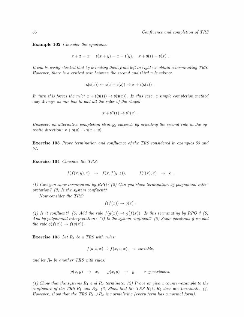
56 Confluence and completion of TRS
Example 102 Consider the equations:
x+ z = x, s(x+ y) = x+ s(y), x+ s(z) = s(x) .
It can be easily checked that by orienting them from left to right we obtain a terminating TRS.However, there is a critical pair between the second and third rule taking:
s(s(x))← s(x+ s(z))→ x+ s(s(z)) .
In turn this forces the rule: x + s(s(z)) → s(s(x)). In this case, a simple completion methodmay diverge as one has to add all the rules of the shape:
x+ sn(z)→ sn(x) .
However, an alternative completion strategy succeeds by orienting the second rule in the op-posite direction: x+ s(y)→ s(x+ y).
Exercise 103 Prove termination and confluence of the TRS considered in examples 53 and54.
Exercise 104 Consider the TRS:
f(f(x, y), z) → f(x, f(y, z)), f(i(x), x) → e .
(1) Can you show termination by RPO? (2) Can you show termination by polynomial inter-pretation? (3) Is the system confluent?
Now consider the TRS:
f(f(x))→ g(x) .
(4) Is it confluent? (5) Add the rule f(g(x)) → g(f(x)). Is this terminating by RPO ? (6)And by polynomial interpretation? (7) Is the system confluent? (8) Same questions if we addthe rule g(f(x))→ f(g(x)).
Exercise 105 Let R1 be a TRS with rules:
f(a, b, x)→ f(x, x, x), x variable,
and let R2 be another TRS with rules:
g(x, y) → x, g(x, y) → y, x, y variables.
(1) Show that the systems R1 and R2 terminate. (2) Prove or give a counter-example to theconfluence of the TRS R1 and R2. (3) Show that the TRS R1 ∪ R2 does not terminate. (4)However, show that the TRS R1 ∪R2 is normalizing (every term has a normal form).

Confluence and completion of TRS 57
5.3 Summary and references
The critical pair test is a practical test to check the (local) confluence of TRS and the basisof an iterative method known as Knuth-Bendix completion [KB70]. The method starts with aTRS which is typically derived from a set of equations. It then checks the TRS for terminationand local confluence. If local confluence fails, then we try to orient the critical pairs and startthe verification again. Many sophisticated refinements of the completion procedure havebeen proposed and implemented in a variety of tools. Also similar ideas have been developedin parallel and independently in the area of computer algebra where a technique known asGrobner bases is used to solve decision problems in rings of polynomials. Examples in thischapter are based on [BN99] and the reader is invited to check them with one of the toolsavailable online.

58 Confluence and completion of TRS
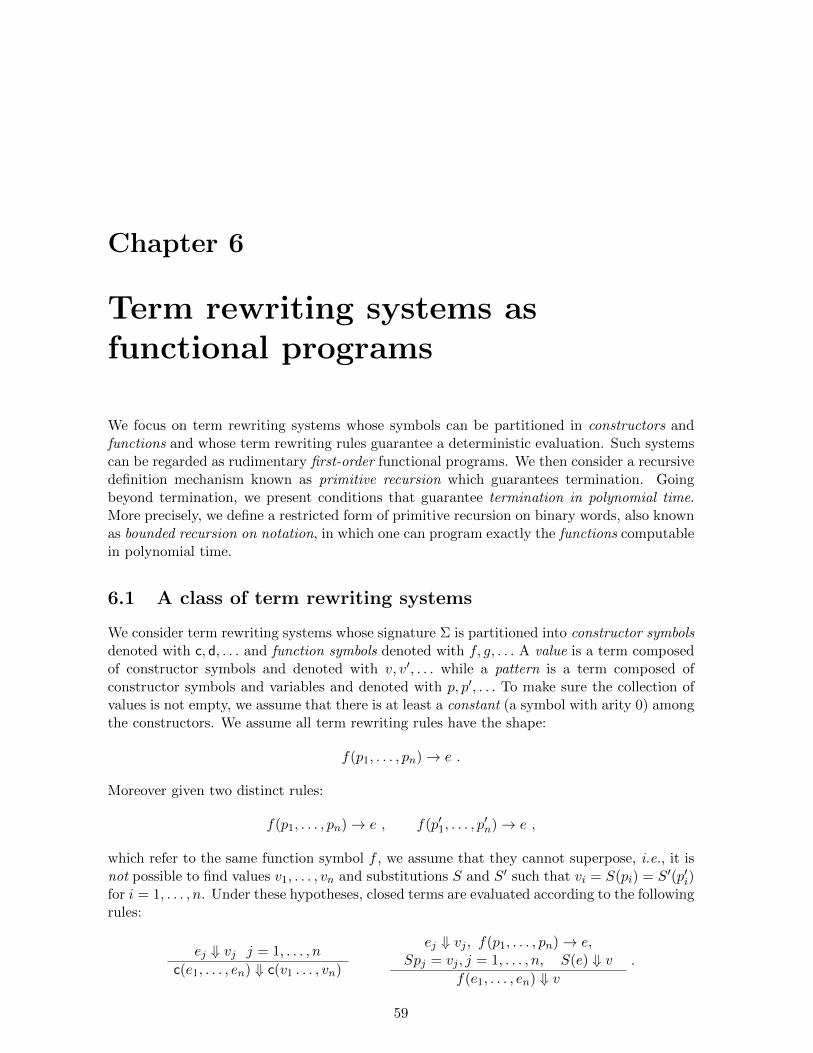
Chapter 6
Term rewriting systems asfunctional programs
We focus on term rewriting systems whose symbols can be partitioned in constructors andfunctions and whose term rewriting rules guarantee a deterministic evaluation. Such systemscan be regarded as rudimentary first-order functional programs. We then consider a recursivedefinition mechanism known as primitive recursion which guarantees termination. Goingbeyond termination, we present conditions that guarantee termination in polynomial time.More precisely, we define a restricted form of primitive recursion on binary words, also knownas bounded recursion on notation, in which one can program exactly the functions computablein polynomial time.
6.1 A class of term rewriting systems
We consider term rewriting systems whose signature Σ is partitioned into constructor symbolsdenoted with c, d, . . . and function symbols denoted with f, g, . . . A value is a term composedof constructor symbols and denoted with v, v′, . . . while a pattern is a term composed ofconstructor symbols and variables and denoted with p, p′, . . . To make sure the collection ofvalues is not empty, we assume that there is at least a constant (a symbol with arity 0) amongthe constructors. We assume all term rewriting rules have the shape:
f(p1, . . . , pn)→ e .
Moreover given two distinct rules:
f(p1, . . . , pn)→ e , f(p′1, . . . , p′n)→ e ,
which refer to the same function symbol f , we assume that they cannot superpose, i.e., it isnot possible to find values v1, . . . , vn and substitutions S and S′ such that vi = S(pi) = S′(p′i)for i = 1, . . . , n. Under these hypotheses, closed terms are evaluated according to the followingrules:
ej ⇓ vj j = 1, . . . , n
c(e1, . . . , en) ⇓ c(v1 . . . , vn)
ej ⇓ vj , f(p1, . . . , pn)→ e,Spj = vj , j = 1, . . . , n, S(e) ⇓ v
f(e1, . . . , en) ⇓ v.
59

60 TRS as functional programs
Notice that the first rule guarantees that for all values v, we have: v ⇓ v. If the term is nota value, then we look for the innermost-leftmost term of the shape f(v1, . . . , vn) and look fora rule f(p1, . . . , pn) → e which applies to it (by hypothesis, there is at most one). If no ruleapplies then the evaluation is stuck. If v is a value its size |v| is a natural number defined by:
|c(v1, . . . , vn)| = 1 + Σi=1,...,n|vi| .
By extension, if t ⇓ v then |t| = |v|. Thus, in this chapter, the notation |t| denotes the size ofthe unique value to which the closed term t evaluates (if any).
Example 106 We introduce some constructors along with their arity.
t0, f0 (boolean values)z0, s1 (tally (unary) natural numbers)nil0, c1 (lists)ε0, 01, 11 (binary words)
and some functions:
ite(t, x, y) → x (if-then-else)ite(f, x, y) → y
leq(z, y) → t (less-equal)leq(s(x), z) → fleq(s(x), s(y)) → leq(x, y)
ins(x, nil) → c(x, nil) (list insertion)ins(x, c(y, l)) → ite(leq(x, y), c(x, c(y, l)), c(y, ins(x, l)))
Exercise 107 Continue the previous example by defining functions to sort lists of tally nat-ural number according to various standard algorithms such as insertion sort, quick sort,. . .
Notice that it is straightforward to program the functions above in a language withpattern-matching such as ML.
6.2 Primitive recursion
We restrict further the class of term rewriting systems so that termination is guaranteed.Assume the following constructor symbols for tally natural numbers: z0 and s1. Also assumethe following basic function symbols z, s, pni for i = 1, . . . , n with the following rules:
z(x) → z (zero)s(x) → s(x) (successor)pni (x1, . . . , xn) → xi (projections).
New function symbols can be introduced according to the composition and primitive recursionrules which are described below. We shall use x∗ to denote a (possibly empty) sequence ofvariables x1, . . . , xn.

TRS as functional programs 61
Composition Given g of arity k and hi of arity n for i = 1, . . . , k introduce a new functionf of arity n with the rule:
f(x∗)→ g(h1(x∗), . . . , hk(x∗)) .
Primitive Recursion Given g of arity n and h of arity n+ 2 introduce a new function f ofarity n+ 1 with the rules:
f(z, y∗) → g(y∗)f(s(x), y∗) → h(f(x, y), x, y∗) .
Example 108 We practice primitive recursion by defining a few arithmetic function.
add(z, y) → y (addition)add(s(x), y) → s(add(x, y))mul(z, y) → z (multiplication)mul(s(x), y) → add(mul(x, y), y)exp(x, z) → s(z) (exponentiation)exp(x, s(n)) → mul(exp(x, n), x) .
We can go on to describe towers of exponentials,. . . The complexity of the programmablefunctions is still very high!
Exercise 109 Define primitive recursive functions to: (1) decrement by one (with 0−1 = 0),(2) subtract (with x−y = 0 if y > x), (3) compute an if-then-else, (4) compute the minimumof two numbers.
We notice that there is a trade-off between primitive recursion and full recursion. Namely,in the former termination is for free but some functions cannot be represented and somealgorithms are more difficult or impossible to represent. For instance, it can be shown by adiagonalization argument that the universal function (the interpreter) for primitive recursivefunctions is a total function but not a primitive recursive one. It can also be shown thatthe natural algorithm that computes the minimum of two tally natural number cannot beexpressed by primitive recursion (details in the following example).
Example 110 Primitive recursion is a bit of a straight-jacket to guarantee termination. Forinstance, the following rules could be used to define the minimum of two tally natural numbers.
min(z, y) → zmin(s(x), z) → zmin(s(x), s(y)) → s(min(x, y)) .
The rules scan the two numbers in parallel and stop as soon as they reach the end of thesmallest one. However this definition of min is not primitive recursive. Worse, it can beshown that no primitive recursive definition of min produces an algorithm computing min(v, u)in time min(|v|, |u|).
We are soon going to address complexity issues and it is well known that in this caseunary notation is rather odd. Indeed unary notation requires too much space and because

62 TRS as functional programs
representation of the input is so large complexities of the operations can be unexpectedly low.For instance, in unary notation we can compute the addition in constant time: it is enough toregard numbers as lists and concatenate them. So we revise the notion of primitive recursionby working with the following constructors which correspond to binary words: ε0, 01, 11. Thebasic functions are now e1, s1
i for i = 0, 1, and pni for i = 1, . . . , n with the following rules:
e(x) → ε (empty word)si(x) → ix (successors)pi(x1, . . . , xn) → xi (projections).
As before, we can introduce new functions according to two mechanisms.
Composition Given g of arity k and hi of arity n for i = 1, . . . , k we introduce a new functionsymbol f with the rule:
f(x∗)→ g(h1(x∗), . . . , hk(x∗)) .
Primitive recursion Given g of arity n and hi of arity n+2 for i = 0, 1 we introduce a newfunction symbol f with the rules:
f(ε, y∗) → g(y∗)f(0(x), y∗) → h0(f(x, y∗), x, y∗)f(1(x), y∗) → h1(f(x, y∗), x, y∗) .
The class of functions definable in this way are the primitive recursive functions on binarynotation, also known as functions defined by recursion on notation.
Exercise 111 Assume binary numbers are represented as binary words where the least sig-nificant digit is on the left. We consider the problem of defining some standard arithmeticfunctions by primitive recursion on binary words.
1. Define a function that takes a binary word and removes all ‘0′ that do not occur on theleft of a 1 (hence ε can be taken as the canonical representation of zero).
2. Show that the functions division by 2, modulo 2, successor, if-then-else, predecessor,number of digits can be defined by primitive recursion.
3. Suppose a function that implements addition is given (known definitions of this functionare quite technical). Implement multiplication by primitive recursion on binary notation.
6.3 Functional programs computing in polynomial time
How can we compute a function defined by primitive recursion? Suppose vk = ik . . . i1ε. Hereis a simple loop that computes f(vk, v
∗):
r = g(v∗);for (j = 1; j ≤ k; j = j + 1)r = hij (r, vj−1, v
∗); return r .
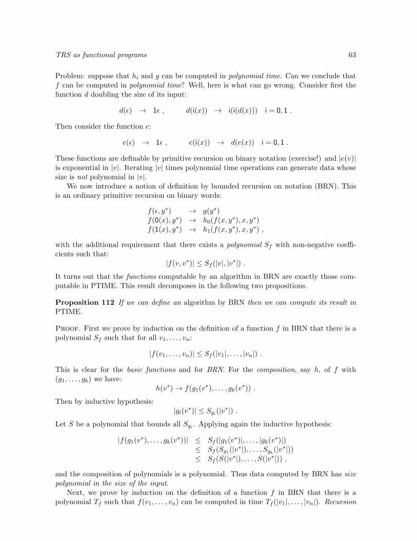
TRS as functional programs 63
Problem: suppose that hi and g can be computed in polynomial time. Can we conclude thatf can be computed in polynomial time? Well, here is what can go wrong. Consider first thefunction d doubling the size of its input:
d(ε) → 1ε , d(i(x)) → i(i(d(x))) i = 0, 1 .
Then consider the function e:
e(ε) → 1ε , e(i(x)) → d(e(x)) i = 0, 1 .
These functions are definable by primitive recursion on binary notation (exercise!) and |e(v)|is exponential in |v|. Iterating |v| times polynomial time operations can generate data whosesize is not polynomial in |v|.
We now introduce a notion of definition by bounded recursion on notation (BRN). Thisis an ordinary primitive recursion on binary words:
f(ε, y∗) → g(y∗)f(0(x), y∗) → h0(f(x, y∗), x, y∗)f(1(x), y∗) → h1(f(x, y∗), x, y∗) ,
with the additional requirement that there exists a polynomial Sf with non-negative coeffi-cients such that:
|f(v, v∗)| ≤ Sf (|v|, |v∗|) .
It turns out that the functions computable by an algorithm in BRN are exactly those com-putable in PTIME. This result decomposes in the following two propositions.
Proposition 112 If we can define an algorithm by BRN then we can compute its result inPTIME.
Proof. First we prove by induction on the definition of a function f in BRN that there is apolynomial Sf such that for all v1, . . . , vn:
|f(v1, . . . , vn)| ≤ Sf (|v1|, . . . , |vn|) .
This is clear for the basic functions and for BRN. For the composition, say h, of f with(g1, . . . , gk) we have:
h(v∗)→ f(g1(v∗), . . . , gk(v∗)) .
Then by inductive hypothesis:|gi(v∗)| ≤ Sgi(|v∗|) .
Let S be a polynomial that bounds all Sgi . Applying again the inductive hypothesis:
|f(g1(v∗), . . . , gk(v∗))| ≤ Sf (|g1(v∗)|, . . . , |gk(v∗)|)
≤ Sf (Sg1(|v∗|), . . . , Sgk(|v∗|))≤ Sf (S(|v∗|), . . . , S(|v∗|)) ,
and the composition of polynomials is a polynomial. Thus data computed by BRN has sizepolynomial in the size of the input.
Next, we prove by induction on the definition of a function f in BRN that there is apolynomial Tf such that f(v1, . . . , vn) can be computed in time Tf (|v1|, . . . , |vn|). Recursion

64 TRS as functional programs
is the interesting case. Consider again the loop computing primitive recursion, where vj =ij · · · i1ε, 1 ≤ j ≤ k:
r = g(v∗);for (j = 1; j ≤ k; j = j + 1)r = hij (r, vj , v
∗); return r .
For all steps j, we have that: |r| ≤ Sf (k, |v∗|). Let Th be a polynomial that bounds both Th0
and Th1 . Then the computation of the k steps is performed in at most:
k · Th(Sf (k, |v∗|), k, |v∗|) = |vk| · Th(Sf (|vk|, |v∗|), |vk|, |v∗|) ,
which is a polynomial in |vk|, |v∗|. 2
Proposition 113 If there is a PTIME algorithm in some Turing-equivalent formalism thenwe can compile it to an algorithm in BRN that computes the same function.
Proof. Let M = (Σ, Q, qo, F, δ) be a Turing machine (TM) with: (i) Σ alphabet, (ii) Qstates, qo ∈ Q initial state, (iii) F ⊆ Q final states, and (iv) δ : Σ × Q → Σ × Q × L,Rtransition function.
If x is a real number let dxe be the least integer n such that x ≤ n. Obviously, elementsin Σ and Q can be encoded as binary words of length dlog2(]Σ)e and dlog2(]Q)e, respectively.The configuration of a TM can be described by a tuple (q, h, l, r) where: (i) q is the currentstate, (ii) h is the character read, (iii) l are the characters on the left hand side of the head,and (iv) r are the characters on the right hand side of the head.
Next, we have to define a step function that simulates one step of a Turing machine whileworking on the encodings of states and characters. Informally, the function step is a caseanalysis corresponding to the finite table defining the transitions of the TM. E.g., the rule:
step(01ε, 1ε, 0l′, r)→ (11ε, 0ε, l′, 0r) ,
describes the situation where being in state 01 and reading 1, we go in state 11, write 0, andmove to the left. The only technical difficulty here is that tuples are not a primitive datastructures in our formalization. However, using the arithmetic functions, we can programpairing of natural numbers and the related projections. Alternatively (and more naturally),one could extend the framework with a pairing constructor.
We ignore these problems and assume a function step that takes a tuple (q, h, l, r) andreturns the tuple (q′, h′, l′, r′) describing the following state. Now comes a key idea which wepresent first using a simplified notation. We have an initial configuration v0 and a functionstep such that:
|step(v)| ≤ |v|+ 1 .
We want to iterate step on vo at least P (|vo|) times where P is a polynomial of degree k.W.l.o.g., we may assume the TM loops after reaching the final state so that running it longerdoes not hurt.
We assume an expansion function exp such that for all k there is an m such that:
|expm(v)| ≥ |v|k .

TRS as functional programs 65
To do this, it is enough to iterate a function that squares the size of its entry. Rememberthat k and therefore m are constants, i.e., they do not depend on the size of the input. Thenwe define a function it as:
it(ε, v) → v , it(i · u, v) → step(it(u, v)) i = 0, 1 . (6.1)
This is a definition by bounded recursion on notation since assuming Sit(n,m) = n + m (apolynomial!) we have:
|it(u, v)| ≤ Sit(|u|, |v|) .
Then to iterate the step function at least |v0|k times on the initial configuration we run:it(expm(v0), v0).
We can now go back to TM. All we have to do is to rewrite the it function above (6.1) asfollows:
it(ε, q, h, l, r) → (q, h, l, r) , it(iu, q, h, l, r) → step(it(u, q, h, l, r)) i = 0, 1 .
To summarize, given a TM running in P time (P fixed polynomial), for any input v0 we: (i)initialize a counter to a value u such that |u| ≥ P (|v0|) and (ii) perform a BRN on the counterthus iterating the step function |u| times. Notice that here the iteration works on the lengthof the counter and not on its binary representation. Otherwise, the definition would not beby BRN and termination could take exponential time! 2
Remark 114 (1) It is quite possible to program a function that takes exponential time andruns in polynomial space (never going twice through the same configuration!). For instance,take a function that counts from 0nε to 1nε. Implicitly, proposition 112 states that as longas we stick with BRN such function cannot be programmed. In the counting function, theproblem is not the size of the data (the identity function gives the bound!) but the fact thatthe recursion mechanism is not compatible with primitive recursion on notation.
(2) The proof of proposition 113 suggests that there is a trivial way of building PTIMEalgorithms. Take any program and instrument it so that it keeps a counter that stops aftera number of steps which is polynomial in the size of the input (for a fixed polynomial). Ofcourse, the problem with this ‘time-out’ approach is that we have no idea whether the programwill produce interesting answers before running it.
(3) The reader should keep in mind that while it is possible to build a programming language(a decidable syntax) that computes exactly the PTIME functions, it is not possible to buildone that contains exactly the PTIME programs, e.g., the set of Turing’s machines computingin PTIME is undecidable.
Proposition 112 restricts the programmer to primitive recursion and it provides no clueon how to find a polynomial bound on the size. Is it possible to find a syntactic criterion thatguarantees the existence of a polynomial bound? The high-complexity of programs defined byprimitive recursion on binary notation depends on the fact that we have nested recursions,i.e., the result of a primitive recursion can be used as the main argument of another primitiverecursion as in:
d(ε) → 1ε , d(i(x)) → i(i(d(x))) i = 0, 1 ,e(ε) → 1ε , e(i(x)) → d(e(x)) i = 0, 1 ⇐ (‘Bad’ recursion!)

66 TRS as functional programs
A key insight is that if we forbid this by a syntactic mechanism then data size stays polynomialand moreover it is still possible to define all functions computable in PTIME. To this end,functions’ arguments are partitioned into two zones (syntactically separated by a semi-colon):
f(x1, . . . , xn; y1, . . . , ym) n,m ≥ 0 .
The ones on the left are called normal and those on the right safe. Let us refer to the functionsin this new class as SRN functions. The invariant one maintains on SRN functions is thatthere is a polynomial Pf such that:
|f(v1, . . . , vn;u1, . . . , um)| ≤ Pf (|v1|, . . . , |vn|) + max(|u1|, . . . , |um|) .
In particular, if f has no normal arguments then the size of its result is bound by the size ofits arguments up to an additive constant.
Unlike in BRN, the existence of the polynomial is guaranteed by the way recursion andcomposition are restricted. Assuming g, h0, h1 are SRN functions, we can define a new SRNfunction f with the rules:
f(ε, x∗; y∗) → g(x∗; y∗)f(0x, x∗; y∗) → h0(x, x∗; y∗, f(x, x∗; y∗))f(1x, x∗; y∗) → h1(x, x∗; y∗, f(x, x∗; y∗)) .
The main argument lies in the normal zone (on the left) while the recursive calls take placein the safe zone (on the right). The way SRN functions are composed is also restrictedso that expressions plugged in the normal zone do not depend on arguments in the safezone. Specifically, assuming, f, g1, . . . , gk, h1, . . . , hl are SRN functions we define their safecomposition as:
f( g1(x∗; ), . . . , gk(x∗; ) ; h1(x∗; y∗), . . . , hl(x
∗; y∗) ) .
Example 115 Here is an example and a non-example of SRN functions.
d(ε; ) → 1(; ε) , d(i(;x); ) → i(; i(; d(x; ))) i = 0, 1 ,e(ε; ) → 1ε , e(i(;x); ) → d(e(x; )) i = 0, 1 ⇐ Not SRN!
e(x; ) should go to the safe zone, while d is waiting for an argument in the normal zone; nestedrecursions do not compose.
6.4 Summary and references
Functions defined by primitive recursion on unary or binary notation are guaranteed to ter-minate; the book [Ros84] is a compact reference on hierarchies of total recursive functions. Ifmoreover, we restrict the size of the computed values to be polynomial in the size of the inputthen we can program exactly the functions computable in polynomial time. This is an earlyresult in complexity theory [Cob64]. The fact that the size bounds can be obtained througha syntactic discipline has been observed more recently in [BC92]. The reader is warned thatthis syntactic discipline is quite restrictive and hardly practical.

Chapter 7
λ-calculus
The λ-calculus is a compact notation to represent (higher-order) functions. It turns outthat this notation embodies directly many concepts arising in programming languages suchas: (higher-order) functions, recursive definitions, scoping rules, and evaluation strategies.Moreover, it is sufficiently expressive to describe a number of programming features suchas: control flow operators, side-effects, records, and objects which will be discussed in thefollowing chapters. When enriched with types, the terms of the λ-calculus can be regardedas proofs in a (constructive) logic. This connection sheds light on the design of type systemsfor programming languages and explains the role of the λ-calculus in (higher-order) proofassistants.
In this chapter, we start the technical development by introducing an equational theory onλ-terms known as β-conversion and we prove the confluence of the related reduction rule. Wealso prove similar results for a stronger theory known as βη-conversion. Next, we show thatthe λ-calculus is sufficiently expressive to represent partial recursive functions (the λ-calculusis Turing equivalent). Finally we introduce a term rewriting system known as combinatorylogic which simulates, to some extent, the λ-calculus.
7.1 Syntax
The (type-free) λ-calculus is composed of the λ-terms defined by the following grammar:
M ::= id || (λid .M) || (MM) (λ-terms)
where id ::= x || y || . . . This is a minimal language where the only operations allowed areabstraction λx.M and application MN . In a language such as ML, one would write λx.M asfunction x -> M.
It is important to notice that the abstraction λx.M binds the variable x in the λ-term Mjust as the quantified first-order formula ∀x.A binds x in A. Consequently, in the λ-calculusa variable can occur free or bound. We denote with fv(M) the set of variables occurring freein the λ-term M .
When writing λ-terms we shall take some freedom. First, we may write λx1, . . . , xn.Mfor λx1 . . . λxn.M . Second, we assume application associates to the left, and therefore writeM1M2 . . .Mn for (· · · (M1M2) · · ·Mn). Third, we suppose application binds more than λ-abstraction and write λx.MN for λx.(MN).
67
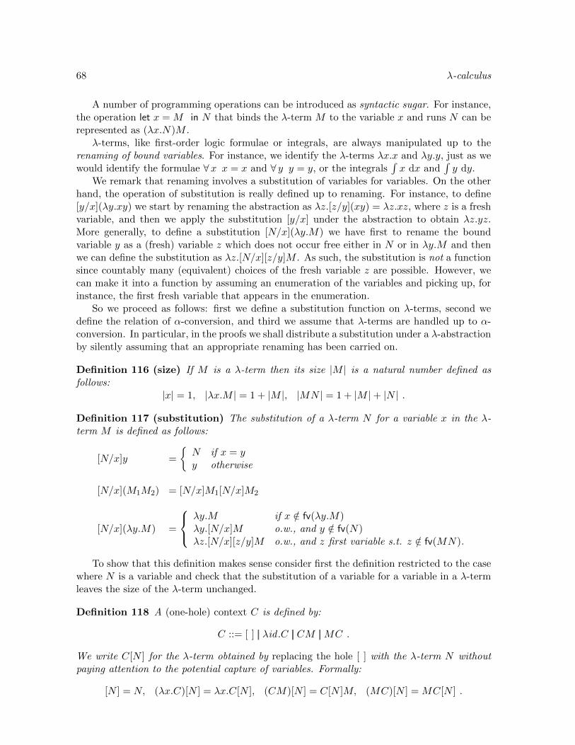
68 λ-calculus
A number of programming operations can be introduced as syntactic sugar. For instance,the operation let x = M in N that binds the λ-term M to the variable x and runs N can berepresented as (λx.N)M .
λ-terms, like first-order logic formulae or integrals, are always manipulated up to therenaming of bound variables. For instance, we identify the λ-terms λx.x and λy.y, just as wewould identify the formulae ∀x x = x and ∀ y y = y, or the integrals
∫x dx and
∫y dy.
We remark that renaming involves a substitution of variables for variables. On the otherhand, the operation of substitution is really defined up to renaming. For instance, to define[y/x](λy.xy) we start by renaming the abstraction as λz.[z/y](xy) = λz.xz, where z is a freshvariable, and then we apply the substitution [y/x] under the abstraction to obtain λz.yz.More generally, to define a substitution [N/x](λy.M) we have first to rename the boundvariable y as a (fresh) variable z which does not occur free either in N or in λy.M and thenwe can define the substitution as λz.[N/x][z/y]M . As such, the substitution is not a functionsince countably many (equivalent) choices of the fresh variable z are possible. However, wecan make it into a function by assuming an enumeration of the variables and picking up, forinstance, the first fresh variable that appears in the enumeration.
So we proceed as follows: first we define a substitution function on λ-terms, second wedefine the relation of α-conversion, and third we assume that λ-terms are handled up to α-conversion. In particular, in the proofs we shall distribute a substitution under a λ-abstractionby silently assuming that an appropriate renaming has been carried on.
Definition 116 (size) If M is a λ-term then its size |M | is a natural number defined asfollows:
|x| = 1, |λx.M | = 1 + |M |, |MN | = 1 + |M |+ |N | .
Definition 117 (substitution) The substitution of a λ-term N for a variable x in the λ-term M is defined as follows:
[N/x]y =
N if x = yy otherwise
[N/x](M1M2) = [N/x]M1[N/x]M2
[N/x](λy.M) =
λy.M if x /∈ fv(λy.M)λy.[N/x]M o.w., and y /∈ fv(N)λz.[N/x][z/y]M o.w., and z first variable s.t. z /∈ fv(MN).
To show that this definition makes sense consider first the definition restricted to the casewhere N is a variable and check that the substitution of a variable for a variable in a λ-termleaves the size of the λ-term unchanged.
Definition 118 A (one-hole) context C is defined by:
C ::= [ ] || λid .C || CM ||MC .
We write C[N ] for the λ-term obtained by replacing the hole [ ] with the λ-term N withoutpaying attention to the potential capture of variables. Formally:
[N ] = N, (λx.C)[N ] = λx.C[N ], (CM)[N ] = C[N ]M, (MC)[N ] = MC[N ] .

λ-calculus 69
We are now ready to define the relation of renaming which is called α-conversion in theλ-calculus. Henceforth λ-terms are considered up to α-conversion.
Definition 119 (α-conversion) α-conversion is the least equivalence relation ≡ on λ-termssuch that for any context C, λ-term M , and variables x, y such that y /∈ fv(M) we have:
C[λx.M ] ≡ C[λy.[y/x]M ] .
Remark 120 As already mentioned, the replacement operation does not pay attention to thebound variables. For instance, if C = λx.[ ] and N = x then C[N ] = λx.x. For this reason,contexts, unlike λ-terms, should not be considered up to renaming.
Definition 121 (β-reduction) The β-rule is the following reduction relation between λ-terms:
(β) C[(λx.M)N ]→ C[[N/x]M ] ,
where C is a context, M,N are λ-terms, and x is a variable.
The subterm (λx.M)N which is transformed by the β-rule is called the redex (or β-redex).We may also refer to the λ-term resulting from the application of the rule as the reduced λ-term. Notice that definition 121 is schematic but does not quite define a TRS since λ-termsare not quite first-order terms. The equivalence induced by β-reduction is called β-conversionand it is defined as follows.
Definition 122 (β-conversion) We denote with =β the equivalence relation∗↔β.
Example 123 Here are some λ-terms which are used often enough to deserve a specificname:
I ≡ λx.x, K ≡ λx, y.x, S ≡ λx, y, z.xz(yz), ∆ ≡ λx.xx, ∆f ≡ λx.f(xx) .
And here are some examples of β-reduction (up to α-conversion!):
II → I, KMN →M, SKK → I, ∆∆→ ∆∆, ∆f∆f → f(∆f∆f ) .
Exercise 124 (β-normal forms) Let NF be the smallest set of λ-terms such that:
Mi ∈ NF i = 1, . . . , k k ≥ 0
λx1 . . . xn.xM1 . . .Mk ∈ NF.
Show that NF is exactly the set of λ-terms in β-normal form.
Exercise 125 (Curry fixed point) Let Y ≡ λf.∆f∆f where ∆f ≡ λx.f(xx). Show that:
YM =β M(YM) .
This is known as Curry’s fixed point combinator.
Exercise 126 (Turing fixed point) Turing’s fixed point combinator is defined by:
YT ≡ (λx, y.y(xxy))(λx, y.y(xxy)) .
Show that YT f is not only convertible to, but reduces to: f(YT f).

70 λ-calculus
7.2 Confluence
Clearly, there are many possible ways of reducing a λ-term. Are they confluent? Let us firstexamine the case for local confluence.
Proposition 127 (local confluence) Let M be a λ-term. Then the following holds:
1. If M →M ′ then [M/x]N∗→ [M ′/x]N .
2. If N → N ′ then [M/x]N → [M/x]N ′.
3. β-reduction is locally confluent, that is:
∀M,N,P (M → N, M → P )
∃Q (N∗→ Q, P
∗→ Q).
Proof. (1) By induction on N .
(2) Suppose N = C[(λy.N1)N2]. We notice:
[M/x]((λy.N1)N2) ≡ (λy.[M/x]N1)[M/x]N2 → [[M/x]N2/y]([M/x]N1) ≡ [M/x]([N2/y]N1) .
(3) The interesting case arises if one redex is contained in the other. Suppose ∆ is a β-redex.If M ≡ C[(λx.M ′)C ′[∆]] apply (1), and if M ≡ C[(λx.C ′[∆])M ′] apply (2). 2
Let us notice that β reduction may both erase a redex as in (λx.I)(II)→ I and duplicateit as in ∆(II) → (II)(II). It turns out that it is possible to define a notion of parallelreduction ⇒ with the following properties.
• → ⊂ ⇒ ⊂ ∗→.
• A strong confluence property holds for⇒: if M ⇒ N and M ⇒ N ′ then there is P suchthat N ⇒ P and N ′ ⇒ P .
• The relation ⇒ is simple enough to be analyzed.
The idea is that in a parallel reduction we are allowed to reduce at once the redexes thatare in the λ-term but not those which are created by the reductions. For instance, we have:(II)(II)⇒ II but (II)(II) 6⇒ I.
Definition 128 (parallel β-reduction) Parallel β-reduction is defined as follows:
M ⇒M
M ⇒M ′ N ⇒ N ′
(λx.M)N ⇒ [N ′/x]M ′
M ⇒M ′ N ⇒ N ′
MN ⇒M ′N ′M ⇒M ′
λx.M ⇒ λx.M ′.
Exercise 129 Let M ≡ (λx.Ix)(II) where I ≡ λz.z. What is the minimum number ofparallel reductions needed to reduce M to I?

λ-calculus 71
First we notice the following structural and substitution properties of parallel reduction.
Proposition 130 Parallel reduction enjoys the following structural properties:
λx.M ⇒ N
N ≡ λx.M ′, M ⇒M ′
MN ⇒ L
(L ≡M ′N ′, M ⇒M ′, N ⇒ N ′) or(M ≡ λx.P, P ⇒ P ′, N ⇒ N ′, L ≡ [N ′/x]P ′)
Proof. By case analysis on the definition of parallel reduction. 2
Proposition 131 Parallel reduction enjoys the following substitution property:
M ⇒M ′ N ⇒ N ′
[N/x]M ⇒ [N ′/x]M ′.
Proof. By induction on the definition of M ⇒ M ′. For the base case we also need aninduction on the structure of M . 2
We are then ready to prove strong confluence of parallel reduction.
Proposition 132 Parallel reduction enjoys the following strong confluence property:
∀M,N1, N2 (N1 ⇐M ⇒ N2)
∃P (N1 ⇒ P ⇐ N2).
Proof. One can proceed by induction on M ⇒ N1 and case analysis on M ⇒ N2 to closethe diagram. 2
Corollary 133 (confluence, β) β-reduction is confluent.
Proof. We have:→β ⊂ ⇒ ⊂
∗→β .
If M →β · · · →β Ni, i = 1, 2 then M ⇒ · · · ⇒ Ni, i = 1, 2. Now apply strong conflu-ence to close the diagram and build P such that Ni ⇒ · · · ⇒ P , i = 1, 2. This impliesNi
∗→β · · ·∗→β P , i = 1, 2 and, by transitivity of
∗→β, we conclude that Ni∗→β P , i = 1, 2. 2
The β-rule is the basic rule of the λ-calculus. The second most popular rule is the η-rule.
Definition 134 (η-reduction) The η-rule is defined by:
(η) C[λx.Mx]→ C[M ] if x 6∈ fv(M) ,
for C context, M λ-term, and x variable.
The η-rule is a kind of extensionality rule. If we read it backwards, it asserts that ‘everyλ-term is a function’. This intuition can actually be made precise in the model theory ofλ-calculus.

72 λ-calculus
Proposition 135 (confluence βη) The following properties hold:
1. η reduction is strongly confluent in the following sense:
M →η Ni i = 1, 2 N1 6≡ N2
∃P (Ni →η P, i = 1, 2).
2. The β and η reductions commute in the following sense:
M →β N1 M →η N2 N1 6≡ N2
∃P (N1(→η)∗P, N2 →β P )
.
3. The (→β)∗ and (→η)∗ reductions commute in the following sense:
M(→β)∗N1 M(→η)∗N2
∃P (N1(→η)∗P, N2(→β)∗P )
.
4. βη reduction is confluent.
Proof. (1) Two redexes that superpose have the shape: λx.C[λy.My]x. Analyze what canhappen.
(2) If the β redex contains the η redex we can have the following situations:
• (λx.Mx)N : the reduced are identical.
• (λx.C[λy.My])N : close the diagram in one step.
• (λx.M)C[λy.Ny]: it may take 0, 1 or more η steps to close the diagram.
On the other hand, if the η redex contains the β redex we can have:
• λx.(λy.M)x: the reduced are identical.
• λx.C[(λy.M1)M2]x: close in one step.
(3) First show commutation of (→η)∗ with respect to →β ∪Id . Then proceed by induction
on the number of β reductions.
(4) Consider the number of alternations of (→β)∗ and (→η)∗. 2
Example 136 Here is an extension of the λ-calculus that does not preserve confluence (werefer to [Bar84] for a proof). We add to the language a constant D and the rule:
Dxx→ x .
This rule may seem artificial, but it is actually a simplification of a natural rule called sur-jective paring (an extensionality rule for pairs) which also leads to a non-confluent system:
D(Fx)(Sx)→ x .
Here D, F , S are constants where intuitively D is the pairing while F and S are the firstand second projection. We stress that here the property that fails is just confluence (not localconfluence). Indeed a surjective pairing rule is introduced in terminating typed λ-calculi. Byproposition 47, surjective pairing in these calculi is confluent.

λ-calculus 73
7.3 Programming
All partial recursive functions can be represented in the (type free) λ-calculus. Thus theλ-calculus, regarded as a computational model, is Turing equivalent. Proving this result is amatter of programming in the λ-calculus. The proof we outline below relies on the followingdefinition of the partial recursive functions.
Definition 137 (minimalisation) Given a total function f : Nk+1 → N a partial functionµ(f) : Nk N is defined by minimization as follows:
µ(f)(x1, . . . , xk) =
x0 if x0 = minx ∈ N | f(x, x1, . . . , xk) = 0↑ if ∀x f(x, x1, . . . , xk) > 0
where ↑ means that the function is undefined.
Definition 138 The set of partial recursive functions is the smallest set of functions on (vec-tors of) natural numbers which contains the basic functions (zero, successor, projections) andis closed under function composition, primitive recursion (see chapter 6.2), and minimization.
We discuss next the representation of partial recursive functions in the λ-calculus.
Definition 139 (Church numerals) A natural number n is represented by the followingλ-term n known as Church numeral:
n ≡ λf.λx.(f · · · (fx) · · ·) (Church numerals) (7.1)
where f is applied n times.
In a sense this is similar to the tally natural numbers considered in chapter 6.2. We shallsee in chapter 13 that the inductive definition of natural numbers actually suggests theirrepresentation in the λ-calculus as Church numerals.
We also have to fix a class of λ-terms that represent a diverging computation. A naturalchoice is to consider the λ-terms that do not have a head normal form.
Definition 140 (head normal form) A λ-term is (has) a head normal if it has the shape(it reduces to a λ-term of the shape):
λx1, . . . , xn.xM1 · · ·Mm n,m ≥ 0.
Definition 141 (function representation) A λ-term F represents a partial function f :Nk → N if for all n1, . . . , nk ∈ N:
f(n1, . . . , nk) = m iff Fn1 · · ·nk =β mf(n1, . . . , nk) ↑ iff Fn1 · · ·nk has no head normal form.
We can represent the arithmetic functions addition, successor, and multiplication with thefollowing λ-terms:
A ≡ λn.λm.λf.λx.(n f)(m f x) (addition)S ≡ λn.A n 1 (successor)M ≡ λn.λm.λf.n(m f) (multiplication).
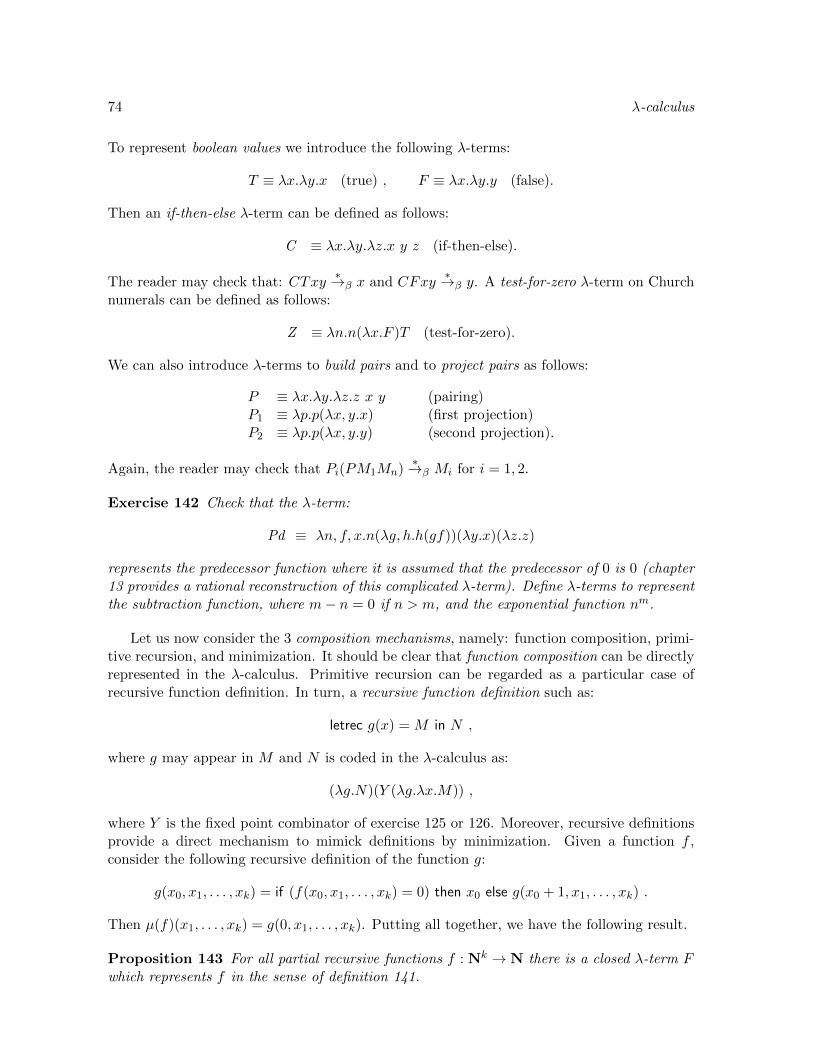
74 λ-calculus
To represent boolean values we introduce the following λ-terms:
T ≡ λx.λy.x (true) , F ≡ λx.λy.y (false).
Then an if-then-else λ-term can be defined as follows:
C ≡ λx.λy.λz.x y z (if-then-else).
The reader may check that: CTxy∗→β x and CFxy
∗→β y. A test-for-zero λ-term on Churchnumerals can be defined as follows:
Z ≡ λn.n(λx.F )T (test-for-zero).
We can also introduce λ-terms to build pairs and to project pairs as follows:
P ≡ λx.λy.λz.z x y (pairing)P1 ≡ λp.p(λx, y.x) (first projection)P2 ≡ λp.p(λx, y.y) (second projection).
Again, the reader may check that Pi(PM1Mn)∗→β Mi for i = 1, 2.
Exercise 142 Check that the λ-term:
Pd ≡ λn, f, x.n(λg, h.h(gf))(λy.x)(λz.z)
represents the predecessor function where it is assumed that the predecessor of 0 is 0 (chapter13 provides a rational reconstruction of this complicated λ-term). Define λ-terms to representthe subtraction function, where m− n = 0 if n > m, and the exponential function nm.
Let us now consider the 3 composition mechanisms, namely: function composition, primi-tive recursion, and minimization. It should be clear that function composition can be directlyrepresented in the λ-calculus. Primitive recursion can be regarded as a particular case ofrecursive function definition. In turn, a recursive function definition such as:
letrec g(x) = M in N ,
where g may appear in M and N is coded in the λ-calculus as:
(λg.N)(Y (λg.λx.M)) ,
where Y is the fixed point combinator of exercise 125 or 126. Moreover, recursive definitionsprovide a direct mechanism to mimick definitions by minimization. Given a function f ,consider the following recursive definition of the function g:
g(x0, x1, . . . , xk) = if (f(x0, x1, . . . , xk) = 0) then x0 else g(x0 + 1, x1, . . . , xk) .
Then µ(f)(x1, . . . , xk) = g(0, x1, . . . , xk). Putting all together, we have the following result.
Proposition 143 For all partial recursive functions f : Nk → N there is a closed λ-term Fwhich represents f in the sense of definition 141.

λ-calculus 75
7.4 Combinatory logic
Combinatory logic is a relative of the λ-calculus which can be presented as a term rewritingsystem.
Definition 144 We consider a binary application operation @ and two constants K and S.As in the λ-calculus, we write MN for @(M,N) and let application associate to the left. Thesystem comes with two term rewriting rules:
K x y → x , S x y z → x z(y z) .
It turns out that in combinatory logic there is a way to simulate λ-abstraction.
Definition 145 We define a function λ that takes a variable and a term of combinatory logicand produces a term of combinatory logic. We abbreviate SKK as I.
λ(x, x) = Iλ(x,M) = KM if x /∈ var(M)λ(x,MN) = S(λ(x,M))(λ(x,N)) .
The fact that we called the function above ‘λ′ is justified by the following proposition.
Proposition 146 If M,N are terms of combinatory logic and x is a variable then:
λ(x,M)N∗→ [N/x]M .
Proof. By induction on M following the definition of the translation. 2
Exercise 147 Using the fact that combinatory logic (CL) is a TRS prove local confluenceof CL. Then adapt the method of parallel reduction presented in section 7.2 to prove theconfluence of CL.
Combinatory logic seems mathematically simpler than the λ-calculus. Why is it not used?One reason is that terms written in combinatory logic tend to be unreadable. Another deeperreason is that the notion of conversion induced by the rules S and K is weaker than the oneinduced by the β rule. For instance, the reader may check that the translations in CL of theλ-terms λz.(λx.x)z and λz.z do not have a common reduct. An alternative approach goesthrough the notion of closure (see following chapter 8). This is quite appropriate for discussingimplementation techniques, but as in combinatory logic, the notation tends to become lessmanageable.
7.5 Summary and references
The λ-calculus is a minimal notation to represent higher-order functions. The λ-terms aretransformed according to one basic rewriting rule: the β-rule. The λ-calculus with the β-ruleis a confluent rewriting system and it is sufficiently expressive to represent all partial recursivefunctions. A second rule, the η-rule, can be added to the system while preserving confluence.The λ-calculus is not a term rewriting system but there are term rewriting systems such ascombinatory logic which can mimick to some extent the behavior of λ-terms.
76 λ-calculus
The λ-calculus was introduced by Church as part of an investigation in the formal foun-dations of mathematics and logic [Chu40]. At the time, the λ-calculus provided one of theconcurrent formalizations of partial recursive functions, i.e., computable functions, along with,e.g., Turing machines. The foundational character of the language is even stronger when it isenriched with types. We shall start addressing this point in chapter 10. The related system ofcombinatory logic is based on work by Schonfinkel and Curry. The book [Bar84] is the basicreference for the type-free λ-calculus. It is enough to skim the first introductory chapters tohave an idea of the great variety of results connected to the formalism.

Chapter 8
Weak reduction strategies, closures,and abstract machines
Full β(η)-reduction is the basis for the symbolic manipulation of λ-terms, e.g., in proof as-sistants, in program transformations, and in higher-order unification and pattern-matching.However, when the λ-calculus is regarded as the core of a programming language it is sensi-ble to consider weaker reduction strategies. This chapter focuses on these weaker reductionstrategies and their implementation.
8.1 Weak reduction strategies
A weak reduction strategy is a strategy to reduce λ-terms that does not reduce under func-tional abstractions. Thus in a weak reduction strategy all λ-terms of the form λx.M arenormal forms.
Definition 148 (weak reduction) We define the weak β-reduction relation→w as the leastbinary relation on λ-terms such that:
(λx.M)N →w [N/x]M
M →w M′
MN →w M′N
N →w N′
MN →w MN ′.
As such weak reduction is not confluent. For instance, we have:
K(II)→w KI , K(II)→w λx.II ,
and KI and λx.II have no common reduct. The problem here is that the redex II is undera λ and cannot be reduced. When considering the λ-calculus as the core of a programminglanguage, the usual approach is to fix a particular deterministic weak reduction strategy. Twopopular ones we discuss next are known as call-by-name and call-by-value. The definition ofthese strategies relies on a notion of value.
Definition 149 (value) A value V is a closed λ-term of the shape λx.M (a λ-abstraction).
In the following, the call-by-name and call-by-value reduction strategies are defined onclosed λ-terms. We actually define the reduction strategies in 3 different ways which turn outto be equivalent.
77
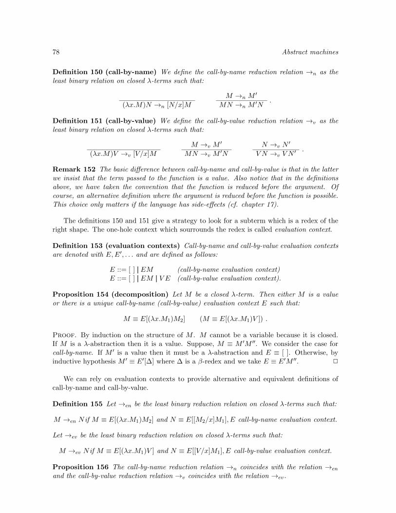
78 Abstract machines
Definition 150 (call-by-name) We define the call-by-name reduction relation →n as theleast binary relation on closed λ-terms such that:
(λx.M)N →n [N/x]M
M →n M′
MN →n M′N
.
Definition 151 (call-by-value) We define the call-by-value reduction relation →v as theleast binary relation on closed λ-terms such that:
(λx.M)V →v [V/x]M
M →v M′
MN →v M′N
N →v N′
V N →v V N′ .
Remark 152 The basic difference between call-by-name and call-by-value is that in the latterwe insist that the term passed to the function is a value. Also notice that in the definitionsabove, we have taken the convention that the function is reduced before the argument. Ofcourse, an alternative definition where the argument is reduced before the function is possible.This choice only matters if the language has side-effects (cf. chapter 17).
The definitions 150 and 151 give a strategy to look for a subterm which is a redex of theright shape. The one-hole context which sourrounds the redex is called evaluation context.
Definition 153 (evaluation contexts) Call-by-name and call-by-value evaluation contextsare denoted with E,E′, . . . and are defined as follows:
E ::= [ ] || EM (call-by-name evaluation context)E ::= [ ] || EM || V E (call-by-value evaluation context).
Proposition 154 (decomposition) Let M be a closed λ-term. Then either M is a valueor there is a unique call-by-name (call-by-value) evaluation context E such that:
M ≡ E[(λx.M1)M2] (M ≡ E[(λx.M1)V ]) .
Proof. By induction on the structure of M . M cannot be a variable because it is closed.If M is a λ-abstraction then it is a value. Suppose, M ≡ M ′M ′′. We consider the case forcall-by-name. If M ′ is a value then it must be a λ-abstraction and E ≡ [ ]. Otherwise, byinductive hypothesis M ′ ≡ E′[∆] where ∆ is a β-redex and we take E ≡ E′M ′′. 2
We can rely on evaluation contexts to provide alternative and equivalent definitions ofcall-by-name and call-by-value.
Definition 155 Let →en be the least binary reduction relation on closed λ-terms such that:
M →en N if M ≡ E[(λx.M1)M2] and N ≡ E[[M2/x]M1], E call-by-name evaluation context.
Let →ev be the least binary reduction relation on closed λ-terms such that:
M →ev N if M ≡ E[(λx.M1)V ] and N ≡ E[[V/x]M1], E call-by-value evaluation context.
Proposition 156 The call-by-name reduction relation →n coincides with the relation →en
and the call-by-value reduction relation →v coincides with the relation →ev.

Abstract machines 79
Proof. We consider the proof for call-by-name. To show that →n⊆→en, we proceed byinduction of the proof height of M →n N . For the base case take E = [ ]. For the inductivecase, suppose MN →n M
′N because M →n M′. Then by inductive hypothesis, there are E′
and ∆ ≡ (λx.M1)M2 such that M ≡ E′[∆] and M ′ ≡ E′[[M2/x]M1]. Then take E = E′N ,MN ≡ E[∆], M ′N ≡ E[∆′], and ∆′ ≡ [M2/x]M1.
In the other direction, suppose E[∆] →en E[∆′] where ∆ ≡ (λx.M1)M2 and ∆′ ≡[M2/x]M1. We proceed by induction on the structure of the evaluation context E. If E = [ ]then ∆ →n ∆′. If E = E′N then by induction hypothesis, E′[∆] →n E
′[∆′] and thereforeE[∆]→n E[∆′]. 2
Yet another presentation of call-by-name and call-by-value consists in defining a big-step(cf. section 1.1) evaluation relation ⇓.
Definition 157 (call-by-name evaluation) The call-by-name evaluation relation ⇓n is theleast binary relation on closed λ-terms such that:
V ⇓n VM ⇓n λx.M ′ [N/x]M ⇓n V
MN ⇓n V.
Definition 158 (call-by-value evaluation) The call-by-value evaluation relation ⇓v is theleast binary relation on closed λ-terms such that:
V ⇓v VM ⇓v λx.M ′ N ⇓v V ′ [V ′/x]M ⇓ V
MN ⇓v V.
Proposition 159 Let M be a closed λ-term. Then:
1. If M ⇓n V then M(→n)∗V .
2. If M →n M′ and M ′ ⇓n V then M ⇓n V .
3. If M(→n)∗M ′ 6→n then M ⇓n M ′.
The same properties hold if we replace ⇓n with ⇓v and →n with →v, respectively.
Proof. (1) By induction on the proof height of the judgment M ⇓n V . The base case followsby reflexivity of (→n)∗. For the inductive step, suppose MN ⇓n V because M ⇓n λx.M1 and[N/x]M1 ⇓n V . By inductive hypothesis, M(→n)∗λx.M1. Then:
MN(→n)∗(λx.M1)N →n [N/x]M1 ,
and by inductive hypothesis [N/x]M1(→n)∗V .
(2) If M →n M′ then M ≡ (λx.M1)M2N1 · · ·Nk and M ′ ≡ [M2/x]M1N1 · · ·Nk. If M ′ ⇓n V
we must have:
[M2/x]M1 ⇓n λx1.P1, [N1/x1]P1 ⇓n λx2.P2, · · · [Nk/xk]Pk ⇓n V .
Then to prove M ⇓ V it suffices to extend the proof for M ′ with an additional step λx.M1 ⇓nλx.M1.
(3) By proposition 154, if M ′ does not reduce then it is a value and we have M ′ ⇓n M ′. IfM reduces to M ′ in k steps then we apply property (2) k times starting from M ′. 2

80 Abstract machines
v[η] ⇓ v[η]η(x)[η] ⇓ v[η′]x[η] ⇓ v[η′]
e[η] ⇓ quote(e′)[η′] e′[η′] ⇓ v[η′′]unquote(e)[η] ⇓ v[η′′]
By-name:e[η[e′/x]] ⇓ v[η′],
(let x = e′ in e)[η]) ⇓ v[η′]
By-value:e′[η] ⇓ v′[η′] e[η[v′/x]] ⇓ v[η]
(let x = e′ in e)[η] ⇓ v[η]
Table 8.1: Dynamic binding with by-name and by-value evaluation
8.2 Static vs. dynamic binding
The implementation of the reduction of a β-redex such as (λx.M)N is usually decomposedin two steps.
• The formal parameter x is bound to the argument N . The collection of bindings iscalled an environment.
• When the formal parameter x is used in the body of the function M , the argumentbound to it is retrieved from the environment.
This high-level description leaves many design choices unspecified. One basic issue iswhat exactly constitutes an ‘argument’. Indeed, in the programming languages jargon, onespeaks of static vs. dynamic binding. This issue already arises in a very simple language ofexpressions whose syntax is as follows, where as usual id ::= x || y || · · ·:
e ::= ⊥ || n || id || let id = e in e || quote(e) || unquote(e) (expressions).
Here ⊥ represents a computation that diverges, n is an integer, quote allows to freeze theevaluation of an expression and unquote to unfreeze it. We denote with Exp the set ofexpressions in this language. The collection of values is defined by:
v ::= n || quote(e) (values).
It is possible to encode this simple language in the λ-calculus and reproduce the same phe-nomena we describe next.
Definition 160 (dynamic environment) A dynamic environment is partial function η :Id Exp with finite domain mapping identifiers to expressions.
Table 8.1 introduces two evaluation relations for this language of expressions with dynamicbinding following either a by-name or a by-value strategy. The basic assertion e[η] ⇓ v[η′] statesthat an expression e in an environment η evaluates to a value v in an environment η′. Thefirst four rules defining the assertion are shared while two distinct rules, one for by-name andthe other for by-value, cover expressions of the shape let x = e′ in e.
In dynamic binding, an environment binds an expression with an identifier. However, inturn the expression may contain identifiers and their binding with other expressions may belost. In static binding, we introduce a more complex object which is called a closure. Thisis an expression along with an environment that associates identifiers with closures. Thislooks like a circular definition of closure and environment but things can be well-defined inan inductive style as follows.
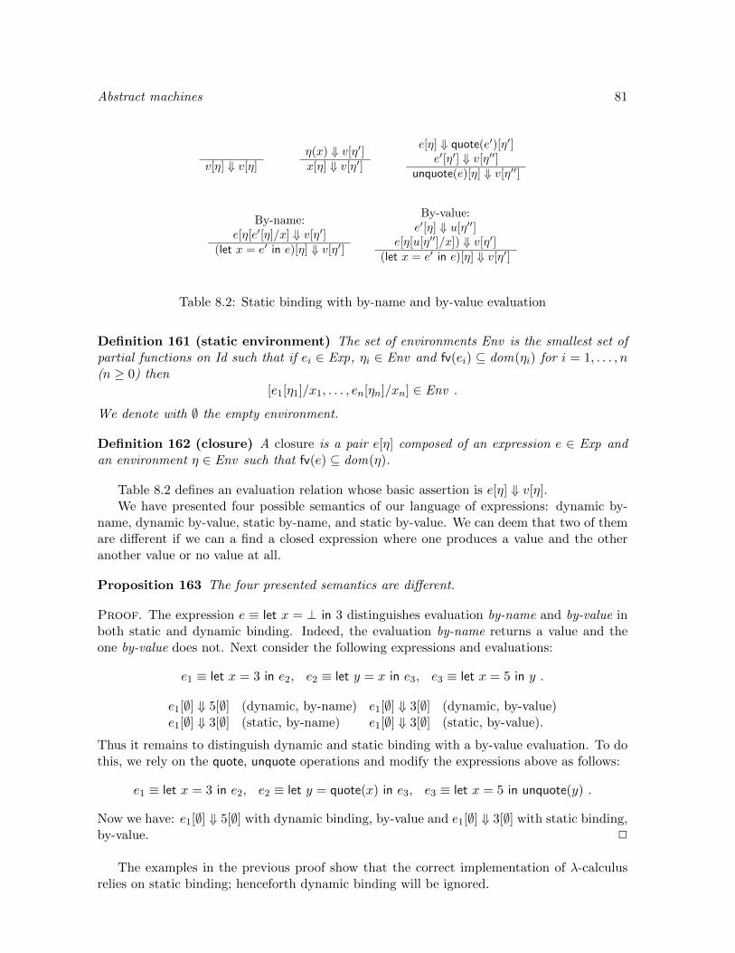
Abstract machines 81
v[η] ⇓ v[η]η(x) ⇓ v[η′]x[η] ⇓ v[η′]
e[η] ⇓ quote(e′)[η′]e′[η′] ⇓ v[η′′]
unquote(e)[η] ⇓ v[η′′]
By-name:e[η[e′[η]/x] ⇓ v[η′]
(let x = e′ in e)[η] ⇓ v[η′]
By-value:e′[η] ⇓ u[η′′]
e[η[u[η′′]/x]) ⇓ v[η′](let x = e′ in e)[η] ⇓ v[η′]
Table 8.2: Static binding with by-name and by-value evaluation
Definition 161 (static environment) The set of environments Env is the smallest set ofpartial functions on Id such that if ei ∈ Exp, ηi ∈ Env and fv(ei) ⊆ dom(ηi) for i = 1, . . . , n(n ≥ 0) then
[e1[η1]/x1, . . . , en[ηn]/xn] ∈ Env .
We denote with ∅ the empty environment.
Definition 162 (closure) A closure is a pair e[η] composed of an expression e ∈ Exp andan environment η ∈ Env such that fv(e) ⊆ dom(η).
Table 8.2 defines an evaluation relation whose basic assertion is e[η] ⇓ v[η].We have presented four possible semantics of our language of expressions: dynamic by-
name, dynamic by-value, static by-name, and static by-value. We can deem that two of themare different if we can a find a closed expression where one produces a value and the otheranother value or no value at all.
Proposition 163 The four presented semantics are different.
Proof. The expression e ≡ let x = ⊥ in 3 distinguishes evaluation by-name and by-value inboth static and dynamic binding. Indeed, the evaluation by-name returns a value and theone by-value does not. Next consider the following expressions and evaluations:
e1 ≡ let x = 3 in e2, e2 ≡ let y = x in e3, e3 ≡ let x = 5 in y .
e1[∅] ⇓ 5[∅] (dynamic, by-name) e1[∅] ⇓ 3[∅] (dynamic, by-value)e1[∅] ⇓ 3[∅] (static, by-name) e1[∅] ⇓ 3[∅] (static, by-value).
Thus it remains to distinguish dynamic and static binding with a by-value evaluation. To dothis, we rely on the quote, unquote operations and modify the expressions above as follows:
e1 ≡ let x = 3 in e2, e2 ≡ let y = quote(x) in e3, e3 ≡ let x = 5 in unquote(y) .
Now we have: e1[∅] ⇓ 5[∅] with dynamic binding, by-value and e1[∅] ⇓ 3[∅] with static binding,by-value. 2
The examples in the previous proof show that the correct implementation of λ-calculusrelies on static binding; henceforth dynamic binding will be ignored.
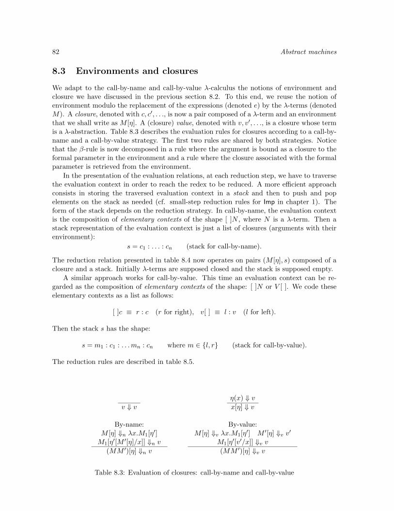
82 Abstract machines
8.3 Environments and closures
We adapt to the call-by-name and call-by-value λ-calculus the notions of environment andclosure we have discussed in the previous section 8.2. To this end, we reuse the notion ofenvironment modulo the replacement of the expressions (denoted e) by the λ-terms (denotedM). A closure, denoted with c, c′, . . ., is now a pair composed of a λ-term and an environmentthat we shall write as M [η]. A (closure) value, denoted with v, v′, . . ., is a closure whose termis a λ-abstraction. Table 8.3 describes the evaluation rules for closures according to a call-by-name and a call-by-value strategy. The first two rules are shared by both strategies. Noticethat the β-rule is now decomposed in a rule where the argument is bound as a closure to theformal parameter in the environment and a rule where the closure associated with the formalparameter is retrieved from the environment.
In the presentation of the evaluation relations, at each reduction step, we have to traversethe evaluation context in order to reach the redex to be reduced. A more efficient approachconsists in storing the traversed evaluation context in a stack and then to push and popelements on the stack as needed (cf. small-step reduction rules for Imp in chapter 1). Theform of the stack depends on the reduction strategy. In call-by-name, the evaluation contextis the composition of elementary contexts of the shape [ ]N , where N is a λ-term. Then astack representation of the evaluation context is just a list of closures (arguments with theirenvironment):
s = c1 : . . . : cn (stack for call-by-name).
The reduction relation presented in table 8.4 now operates on pairs (M [η], s) composed of aclosure and a stack. Initially λ-terms are supposed closed and the stack is supposed empty.
A similar approach works for call-by-value. This time an evaluation context can be re-garded as the composition of elementary contexts of the shape: [ ]N or V [ ]. We code theseelementary contexts as a list as follows:
[ ]c ≡ r : c (r for right), v[ ] ≡ l : v (l for left).
Then the stack s has the shape:
s = m1 : c1 : . . .mn : cn where m ∈ l, r (stack for call-by-value).
The reduction rules are described in table 8.5.
v ⇓ vη(x) ⇓ vx[η] ⇓ v
By-name:M [η] ⇓n λx.M1[η′]M1[η′[M ′[η]/x]] ⇓n v
(MM ′)[η] ⇓n v
By-value:M [η] ⇓v λx.M1[η′] M ′[η] ⇓v v′
M1[η′[v′/x]] ⇓v v(MM ′)[η] ⇓v v
Table 8.3: Evaluation of closures: call-by-name and call-by-value

Abstract machines 83
(x[η], s) → (η(x), s)((MM ′)[η], s) → (M [η],M ′[η] : s)((λx.M)[η], c : s) → (M [η[c/x]], s)
Table 8.4: Abstract machine for call-by-name
(x[η], s) → (η(x), s)((MM ′)[η], s) → (M [η], r : M ′[η] : s)(v, r : c : s) → (c, l : v : s)(v, l : (λx.M)[η] : s) → (M [η[v/x]], s)
Table 8.5: Abstract machine for call-by-value
Exercise 164 Suppose we add to the λ-calculus with call-by-value a certain number of oper-ators op1, . . . , opm with arity n1, . . . , nm, nj ≥ 0. (1) What are the new evaluation contexts?(2) How is the abstract machine to be modified?
The rules in the abstract machines described in tables 8.4 and 8.5 form the basis for animplementation. As usual in the implementation of term rewriting rules, one can avoid thecostly duplication of terms by using pointers. Specifically, in the rule for application onejust needs to duplicate the pointer to the environment rather than the whole environment.In a machine implementation, variables can be replaced by de Brujin indexes which expressthe number of λ’s that one has to traverse in the syntax tree to go from the variable to thebinder. For instance, the λ-term λx.x(λy.xy) is represented by λ.0(λ.10). We can rely on thisnotation for closures too. In this case, we regard the environment as a list and let a de Brujinindex express the number of λ’s and elements in the environment that one has to traverseto go from the variable to the term bound to the variable. For instance, in (λ.20)[c; c′] thevariable 2 refers to the closure c′ while the variable 0 refers to the λ. Using this notation,e.g., the last rule of Table 8.4 can be written as:
((λ.M)[η], c : s) → (M [c : η], s) .
It is interesting to notice that during the (abstract) machine computation (de Brujin) indexesare never modified. This simple remark makes manifest that the number of closures in anenvironment is bounded by the largest index (plus 1) of the initial λ-term to be reduced.In practice, the inputs of a functional program have indexes of bounded size and therefore,in this case, the selection of an element in an environment can be done in constant time.More generally, assuming that lists have bounded length and that duplicated environmentsare shared each step of computation described by the rules in Tables 8.4 and 8.5 can be imple-mented in costant time, thus justfying the ‘abstract machine’ terminology. Notice however,that this analysis ignores the hidden cost of garbage collection.
Exercise 165 Implement the abstract machines in Tables 8.4 and 8.5 using De Brujin no-tation.
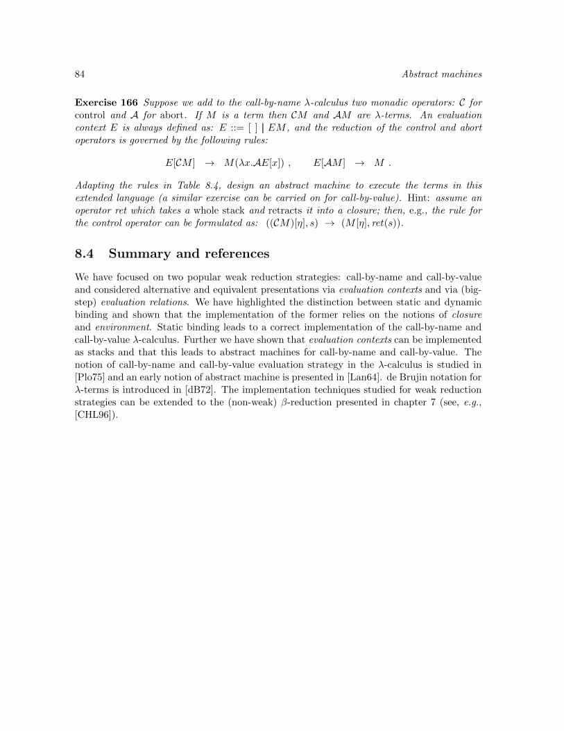
84 Abstract machines
Exercise 166 Suppose we add to the call-by-name λ-calculus two monadic operators: C forcontrol and A for abort. If M is a term then CM and AM are λ-terms. An evaluationcontext E is always defined as: E ::= [ ] || EM , and the reduction of the control and abortoperators is governed by the following rules:
E[CM ] → M(λx.AE[x]) , E[AM ] → M .
Adapting the rules in Table 8.4, design an abstract machine to execute the terms in thisextended language (a similar exercise can be carried on for call-by-value). Hint: assume anoperator ret which takes a whole stack and retracts it into a closure; then, e.g., the rule forthe control operator can be formulated as: ((CM)[η], s) → (M [η], ret(s)).
8.4 Summary and references
We have focused on two popular weak reduction strategies: call-by-name and call-by-valueand considered alternative and equivalent presentations via evaluation contexts and via (big-step) evaluation relations. We have highlighted the distinction between static and dynamicbinding and shown that the implementation of the former relies on the notions of closureand environment. Static binding leads to a correct implementation of the call-by-name andcall-by-value λ-calculus. Further we have shown that evaluation contexts can be implementedas stacks and that this leads to abstract machines for call-by-name and call-by-value. Thenotion of call-by-name and call-by-value evaluation strategy in the λ-calculus is studied in[Plo75] and an early notion of abstract machine is presented in [Lan64]. de Brujin notation forλ-terms is introduced in [dB72]. The implementation techniques studied for weak reductionstrategies can be extended to the (non-weak) β-reduction presented in chapter 7 (see, e.g.,[CHL96]).
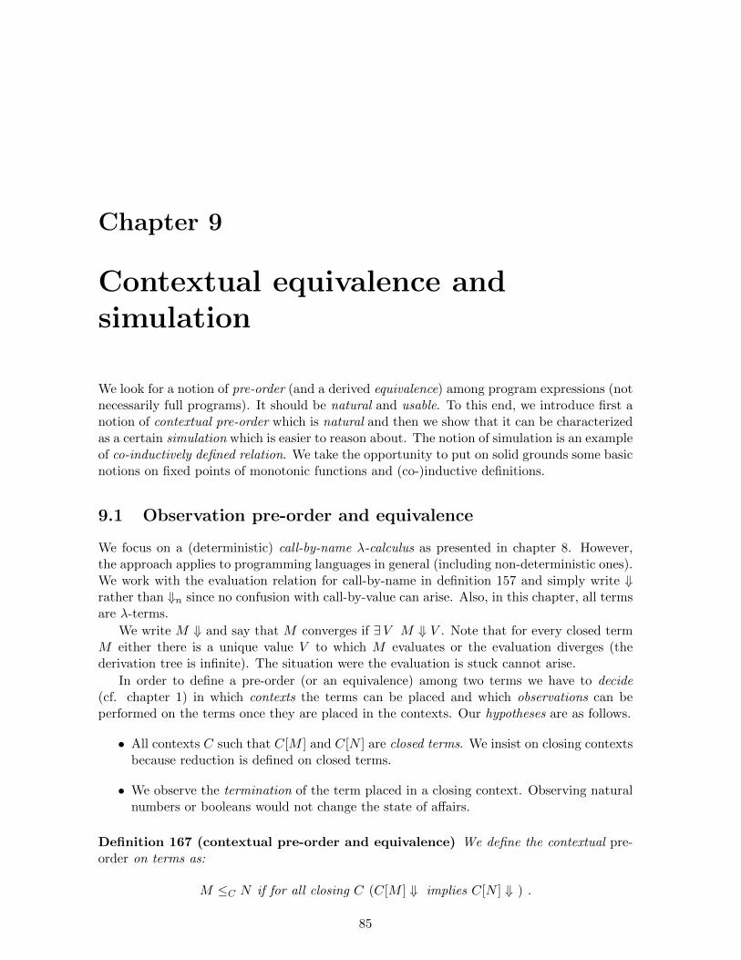
Chapter 9
Contextual equivalence andsimulation
We look for a notion of pre-order (and a derived equivalence) among program expressions (notnecessarily full programs). It should be natural and usable. To this end, we introduce first anotion of contextual pre-order which is natural and then we show that it can be characterizedas a certain simulation which is easier to reason about. The notion of simulation is an exampleof co-inductively defined relation. We take the opportunity to put on solid grounds some basicnotions on fixed points of monotonic functions and (co-)inductive definitions.
9.1 Observation pre-order and equivalence
We focus on a (deterministic) call-by-name λ-calculus as presented in chapter 8. However,the approach applies to programming languages in general (including non-deterministic ones).We work with the evaluation relation for call-by-name in definition 157 and simply write ⇓rather than ⇓n since no confusion with call-by-value can arise. Also, in this chapter, all termsare λ-terms.
We write M ⇓ and say that M converges if ∃V M ⇓ V . Note that for every closed termM either there is a unique value V to which M evaluates or the evaluation diverges (thederivation tree is infinite). The situation were the evaluation is stuck cannot arise.
In order to define a pre-order (or an equivalence) among two terms we have to decide(cf. chapter 1) in which contexts the terms can be placed and which observations can beperformed on the terms once they are placed in the contexts. Our hypotheses are as follows.
• All contexts C such that C[M ] and C[N ] are closed terms. We insist on closing contextsbecause reduction is defined on closed terms.
• We observe the termination of the term placed in a closing context. Observing naturalnumbers or booleans would not change the state of affairs.
Definition 167 (contextual pre-order and equivalence) We define the contextual pre-order on terms as:
M ≤C N if for all closing C (C[M ] ⇓ implies C[N ] ⇓ ) .
85

86 Equivalence
Contextual equivalence is derived by defining:
M ≈C N if M ≤C N and N ≤C M .
Thus two terms are deemed ‘equivalent’ if from the point of view of the admitted obser-vation they are indistinguishable in any closing context.
Exercise 168 Prove the following properties:
1. ≤C is a pre-order (reflexive and transitive).
2. If M ≤C N then for all contexts C (not necessarily closing) C[M ] ≤C C[N ].
3. λx.λy.x 6≤C λx.λy.y.
4. If n,m are Church numerals (cf. definition 139) with n 6= m then n 6≤C m.
5. Find a pair of terms M,N such that M 6=β N and you expect M ≈C N .
To prove that M 6≤C N it suffices to find a context such that C[M ] ⇓ and C[N ] 6⇓. Onthe other hand, to prove that M ≤C N we have to consider all closing contexts. For instance,proving (λx.M)N ≤C [N/x]M is not so easy! This motivates the quest for a more practicalproof method based on the notion of simulation which will be discussed in section 9.4.
Exercise 169 Let ≤IO be a relation on closed terms defined by:
M ≤IO N if ∀P closed MP ⇓ implies NP ⇓
Show that ≤IO is a pre-order and that it is not preserved by contexts.
9.2 Fixed points
In this and the following section, we make a pause to state and prove some general factson partial orders, monotonic/continuous functions, fixed points, and (co-)inductive defini-tions. These facts are used all the time when manipulating programming languages, formallanguages, logics,. . . The reader would be well-advised to become acquainted with these con-cepts. We start by recalling some standard definitions on partial orders (notice that, unlikein chapter 2, partial orders are supposed to be reflexive).
Definition 170 (partial order) A partial order (L,≤) is a set L equipped with a binaryrelation ≤ which is reflexive, anti-symmetric, and transitive.
Definition 171 (upper/lower bounds) Suppose (L,≤) is a partial order and let X ⊆ L(possibly empty). An element y ∈ L is an upper bound for X if ∀x ∈ X x ≤ y. An elementy ∈ L is the supremum (sup) of X if it is the least upper bound. The notions of lower boundand infimum (inf) are defined by duality.
Definition 172 (lattice) A lattice is a partial order (L,≤) such that every pair of elementsof L has a sup and an inf. A complete lattice is a partial order (L,≤) such that every subsetof L has a sup (the existence of the inf follows).

Equivalence 87
Exercise 173 Show that: (1) The subsets of a set with the inclusion relation as partial orderform a complete lattice. (2) Every subset of a complete lattice has an inf. (3) Every finitelattice is complete.
Next we introduce the notion of monotonic, i.e., order-preserving function and considerthe structure of its fixed points in a complete lattice.
Definition 174 (monotonic function) A monotonic function f on a partial order L is afunction respecting the order:
∀x, y ( x ≤ y implies f(x) ≤ f(y) ) .
We say that x is a fixed point of f if f(x) = x.
Proposition 175 (Tarski) Let f : L → L be a monotonic function on a complete lattice.Then f has a greatest and a least fixed point expressed by:
supx | x ≤ f(x) and inf x | f(x) ≤ x .
Proof. Set z = supx | x ≤ f(x). If f(y) = y then y ≤ z. Hence it remains to show that zis a fixed point. First, we show:
z ≤ supf(x) | x ≤ f(x) ≤ f(z) .
Then by monotonicity: f(z) ≤ f(f(z)). And by definition of z, we derive f(z) ≤ z. 2
Exercise 176 Let (N ∪ ∞,≤) be the set of natural numbers with an added maximumelement ∞, 0 < 1 < 2 < . . . <∞. Show that every monotonic function f on this order has afixed point.
The following exercises consider two situations which often arise in practice.
Exercise 177 (fixed points on finite lattices) Let (L,≤) be a finite lattice and f : L →L be a monotonic function. Let ⊥ (>) be the least (greatest) element of L. If x ∈ L then letfn(x) be the n-time iteration of f on x, where f0(x) = x.
1. Show that there is an n ≥ 0 such that the least fixed point of f equals fn(⊥).
2. State and prove a dual property for the greatest fixed point.
3. Show that these properties fail to hold if one removes the hypothesis that the lattice isfinite.
Exercise 178 (fixed points of continuous functions) A subset X of a partial order isdirected if
∀x, y ∈ X ∃ z ∈ (x ≤ z) and (y ≤ z) .
A function on a complete lattice is continuous if it preserves the sup of directed sets:
f(sup(X)) = sup(f(X)) (if X directed).

88 Equivalence
1. Show that a continuous function is monotonic.
2. Give an example of a function on a complete lattice which is continuous but does notpreserve the sup of a (non-directed) set.
3. Show that the least fixed point of a continuous function f is expressed by:
supfn(⊥) | n ≥ 0 .
We can summarize the exercises 177 and 178 as follows. If the the lattice is finite, tocompute the least (greatest) fixed point it suffices to iterate a finite number of times themonotonic function starting from the least (greatest) element. Otherwise, if the function iscontinuous (preserves directed sets), then the least fixed point is the sup of the (countable)iteration of the function starting from the least element. Similar remarks apply to the greatestfixed point modulo suitable definitions of the notions of co-directed set and co-continuousfunction.
In general, it is possible to build the least or greatest fixed point of a monotonic functionon a complete lattice as an iterative process provided one accepts a transfinite number ofiterations. To do this, we can rely on the notion of ordinal in set theory. Intuitively, ordinalsare obtained by iterating the operations of successor and supremum; the former are calledsuccessor ordinals and the latter limit ordinals:
0, 1, 2, . . . , ω, ω + 1, ω + 2, . . . , ω + ω, . . . (first few ordinals).
Formally, in set theory, the set X is an ordinal if:
• Z ∈ Y ∈ X implies Z ∈ X.
• All sequences such that X0 3 X1 3 X2 3 · · · are finite.
Notice that if we read X ∈ Y as X < Y the first property corresponds to transitivity andthe second to well-foundation. So an ordinal is a set which is transitive and well-foundedwith respect to the ∈-relation. In set theory, the role of 0 is played by the empty set, thesuccessor of an ordinal set κ is the set κ∪κ, and the limit of a sequence of ordinals is theirunion. Now given a complete lattice L and a monotonic function f : L → L, we can definethe (transfinite) sequence:
f0 = ⊥ , fκ+1 = f(fκ) , fκ =∨κ′<κ fκ′ κ limit ordinal.
This defines an increasing sequence which must reach the least fixed point when the cardinalityof the ordinal κ is greater than the cardinality of the complete lattice L; for otherwise, wewould have a subset of L whose cardinality is greater than L. A dual argument shows thatwe can approximate the greatest fixed point starting from the top element of the lattice.
9.3 (Co-)Inductive definitions
We discuss examples of inductive and co-inductive set definitions. Behind these definitionsthere is a complete lattice and a monotonic function, and the (co-)inductive set which isdefined is nothing but the least (the greatest) fixed point of the monotonic function.

Equivalence 89
Example 179 (an inductive definition) Let Z be the set of integer numbers and suc and+ the standard successor and addition operations, respectively. We could define:
The least subset of Z which contains 0, 2 and is closed under the addition oper-ation.
It is not so obvious that we are indeed defining a set. One has to make sure that the ‘leastset’ does exist. To do this, we explicit a function f : 2Z → 2Z,
f(X) = 0, 2 ∪ x+ y | x, y ∈ X ,
such that “X contains the set 0, 2 and X is closed under the addition operation” iff f(X) ⊆X. Then one remarks that 2Z is a complete lattice and f is monotonic (indeed continuous,see exercise 178). Hence the least fixed point exists and is expressed by:⋂
X | f(X) ⊆ X =⋃n≥0
fn(∅) .
Example 180 (another inductive definition) Let R be a binary relation on a set D. Thereflexive and transitive closure R∗ is the least relation that contains the identity relation, therelation R and such that if (x, y), (y, z) ∈ R∗ then (x, z) ∈ R∗. Let us show that we canregard R∗ as a least fixed point. As complete lattice, we take the binary relations on the setD ordered by inclusion. As monotonic function f , we define:
f(S) = IdD ∪R ∪ S S
where IdD is the identity relation on D and S S is the (relational) composition of S withitself.
Example 181 (buggy inductive definition) Monotonicity is a key property. As usual,let us write (x ≡ y) mod 2 if the integers x, y have the property that (x− y) is a multiple of2. Suppose we ‘define’ X as the least set of integers such that: (1) 0 ∈ X and (2) if x ∈ Xthen ∀ y ∈ X ( (x ≡ (y + 1)) mod 2 ). Unfortunately such a set does not exist. We shouldhave a set of integers X such that 0 ∈ X and (0 ≡ 1) mod 2.
The notion of co-inductive definition is obtained by dualization. Rather than looking forthe least set such that. . ., we now look for the greatest set such that. . .
Example 182 (co-inductive definition) A typical example of co-inductive definition arisesin the theory of finite automata. Let M = (Q,Σ, q0, F, δ) be a finite deterministic automa-ton with Q set of states, Σ input alphabet, q0 initial state, F set of accepting states, andδ : Σ × Q → Q transition function. Consider the function f : 2(Q×Q) → 2(Q×Q) defined by(q, q′) ∈ f(R) if
1. q ∈ F iff q′ ∈ F .
2. ∀ a ∈ Σ (δ(a, q), δ(a, q′)) ∈ R.

90 Equivalence
It is easy to check that the function f is monotonic on the set of binary relations on Qordered by inclusion. The least R such that R = f(R) is simply the empty relation whichis not very interesting. However, the greatest R such that f(R) = R is the relation thatcorresponds to state equivalence in finite automata. Indeed, since 2Q×Q is a finite lattice, thedefinition gives a way to compute the equivalence on states (see exercise 177). Start with thefull relation Q×Q and iterate the function f till you reach a fixed point.
Co-inductive definitions are quite useful in defining various notions of diverging compu-tation. We illustrate this point in the following example.
Example 183 (another example of co-inductive definition) Let (S,→) be a set of statesand →⊆ S × S a transition relation. Define D as the greatest subset of S such that if s ∈ Dthen: ∃ s′ s→ s′ and s′ ∈ D. We take as complete lattice the parts of S ordered by inclusion.The monotonic function f associated with the definition is for X ⊆ S:
f(X) = s ∈ X | ∃ s′ s→ s′ .
To see the definition at work, suppose S = 1, 2, 3, 4 with transitions: 1 → 2, 3, 4, 3 → 1,4→ 4. The greatest fixed point of f is 1, 3, 4 on the other hand the least fixed point is justthe empty set. Intuitively, the greatest fixed point of f is the collection of elements startingfrom which there is an infinite reduction sequence.
To summarize a (co-)inductive definition is well-defined if the associated function is mono-tonic. In this case, the defined set corresponds to a least (greatest) fixed point of the associatedfunction.
Exercise 184 Modify example 183 so as to define the collection of elements which are notnormalizing, i.e., there is no reduction sequence leading to an element in normal form (cf.definition 22).
9.4 Simulation
Simulation is a standard example of co-inductive definition of a binary relation which can beused to compare programs’ behaviors.
Definition 185 (simulation) We say that a binary relation on closed terms S is a sim-ulation if whenever (M,N) ∈ S we have: (1) if M ⇓ then N ⇓ and (2) for all P closed(MP,NP ) ∈ S. We shall also use the infix notation M S N for (M,N) ∈ S. We define ≤Sas the largest simulation.
Exercise 186 Show that ≤S is the largest fixed point of the following function on binaryrelations:
f(S) = (M,N) | M ⇓ implies N ⇓ , ∀P closed (MP,NP ) ∈ S .
Definition 187 We extend ≤S to open terms by defining:
M ≤S N if for all closing substitutions σ (σM ≤S σN) .
We also write M =S N if M ≤S N and N ≤S M .

Equivalence 91
To prove that M ≤S N (M,N closed) it suffices to find a relation S which is a simulationand such that M S N . The following proof contains several examples of this technique.
Proposition 188 The following properties of simulation hold:
1. ≤S is a pre-order (on open terms).
2. If M ≤S N then for any substitution σ (not necessarily closed) σM ≤S σN .
3. If M ⇓ V and N ⇓ V , M,N closed, then M =S N .
4. (λx.M)N =S [N/x]M (M,N can be open).
5. If M ≤C N then M ≤S N (M,N can be open).
Proof. (1) On closed terms ≤S is reflexive and transitive. If M is an open term thenM ≤S M because for every closing substitutions σM ≤S σM . Suppose M ≤S N andN ≤S P . Given a closing substitution σ for M,P we can always extend it to a closingsubstitution σ′ for N . Then we have:
σM ≡ σ′M ≤S σ′N ≤S σ′P ≡ σP .
(2) Suppose M ≤S N and σ is a substitution. To prove σM ≤S σN , we have to check thatfor all closing substitution σ′, σ′(σM) ≤S σ′(σN). And this holds because (σ′ σ) is a closingsubstitution for M,N .
(3) We check that the following relation on closed terms is a simulation:
S = (MP1 · · ·Pn, NP1 · · ·Pn) |M ⇓ V,N ⇓ V, n ≥ 0 .
If MP1 · · ·Pn ⇓ then we must have V P1 · · ·Pn ⇓ and therefore NP1 · · ·Pn ⇓.Also if (MP1 · · ·Pn, NP1 · · ·Pn) ∈ S then for all P closed, (MP1 · · ·PnP,NP1 · · ·PnP ) ∈ S.(4) Both the following relation and its inverse are simulations:
S = ((λx.M)NP1 · · ·Pn, [N/x]MP1 · · ·Pn) | n ≥ 0 .
Thus (λx.M)N =S [N/x]M holds if (λx.M)N is closed. If (λx.M)N is open and σ is aclosing substitution then we observe:
σ(λx.M)N ≡ (λx.σM)σN =S [σN/x]σM ≡ σ([N/x]M) .
(5) First check that ≤C on closed terms is a simulation. Thus ≤C⊆≤S on closed terms.For open terms, suppose M ≤C N , let x∗ be the list of variables free in M,N , and let σbe any closing substitution. Then take the closed terms: M ′ ≡ (λx∗.M)σ(x∗) and N ′ ≡(λx∗.N)σ(x∗). We have M ′ ≤C N ′ and therefore M ′ ≤S N ′. Moreover σM =S M ′ andσN =S N
′. Therefore: σM ≤S σN . 2
Exercise 189 Prove that:
1. If M 6⇓ and N 6⇓ then M =S N .
2. Let Ωn ≡ λx1. . . . .λxn.Ω. Then Ωn <S Ωn+1 (strictly) and, for all M , Ω0 ≤S M .

92 Equivalence
3. Let K∞ ≡ Y K. Then for all M , M ≤S K∞.
4. λx.x 6≤S λx, y.xy (thus η-conversion is unsound).
So it seems easier proving M ≤S N than proving M ≤C N . However, we still need toprove that ≤S is preserved by contexts. If this property holds, then it is easy to conclude thatthe largest simulation coincides with the contextual pre-order.
Proposition 190 Let x be a variable and M,N,P be terms. If M ≤S N then: (1) MP ≤SNP and (2) λx.M ≤S λx.N .
(1) Because ≤S is a simulation.
(2) Suppose M ≤S N and let σ be a closing substitution for λx.M, λx.N . As usual, supposeσ commutes with λ up to renaming. Now for all closed P , define σ′ as the substitution thatextends σ so that σ′(x) = P . Then, by hypothesis:
[P/x]σM = σ′M ≤S σ′N = [P/x]σN .
Then we have:(λx.σM)P =S [P/x]σM ≤S [P/x]σN = (λx.σN)P .
Clearly (λx.σM) ⇓ implies (λx.σN) ⇓. With reference to the function f defined in exercise186, we have shown (λx.σM) f(≤S) (λx.σN), and we know f(≤S) =≤S . 2
Exercise 191 Let us revise the pre-order considered in exercise 169 by defining a relation≤IO∗ on closed terms as:
M ≤IO∗ N if for all n ≥ 0, P1, . . . , Pn closed, MP1 · · ·Pn ⇓ implies NP1 · · ·Pn ⇓.
Prove that ≤IO∗ coincides with ≤S.
Unfortunately, it is not so easy to prove that M ≤S N implies PM ≤S PN . The proofplan is to introduce an auxiliary relation ≤A on open terms, which includes ≤S , is preservedby contexts, and, with some work, turns out to coincide with ≤S .
Definition 192 (auxiliary simulation relation) The auxiliary relation M ≤A N is de-fined inductively on M by the following rules:
x ≤S Nx ≤A N
M ≤A M ′ λx.M ′ ≤S Nλx.M ≤A N
M1 ≤A M ′1 M2 ≤A M ′2 M ′1M′2 ≤S N
M1M2 ≤A N.
The definition of the auxiliary relation seems rather mysterious. To have a clue, let uslook at its properties.
Proposition 193 The auxiliary relation ≤A enjoys the following properties:
1. ≤A is reflexive.
2. ≤A ≤S ⊆ ≤A.
3. ≤S ⊆ ≤A.

Equivalence 93
Proof. (1) By induction on the structure of the term.
(2) Suppose M ≤A N ≤S P and proceed by induction on the proof of M ≤A N .
(3) By the previous property (2), using the fact that ≤A is reflexive. 2
The next proposition introduces the key properties of the auxiliary relation.
Proposition 194 (key properties) Let M,M ′, N,N ′ be terms. Then:
1. If M ≤A M ′ and N ≤A N ′ then [N/x]M ≤A [N ′/x]M ′.
2. If M ≤A M ′ and N ≤A N ′ then MN ≤A M ′N ′.
3. If M ⇓ V and M ≤A N then V ≤A N .
Proof. (1) By induction on the proof of M ≤A M ′. For instance, suppose:
M ≤A M ′′ λy.M ′′ ≤S M ′λy.M ≤A M ′
.
We have to prove: λy.[N/x]M ≤A [N ′/x]M ′. By inductive hypothesis, we know: [N/x]M ≤A[N ′/x]M ′′. Also, by substitutivity of ≤S we have:
[N ′/x](λy.M ′′) ≡ λy.[N ′/x]M ′′ ≤S [N ′/x]M ′ .
Hence, by definition of ≤A, we conclude.
(2) Consider the terms Mx and M ′x, with x fresh. From M ≤A M ′ we can derive Mx ≤AM ′x. Then by property (1) above, we know that:
N ≤A N ′ implies [N/x](Mx) ≡MN ≤A [N ′/x](M ′x) ≡M ′N ′ .
(3) We proceed by induction on M ⇓ V . We detail the main case. Suppose:
M1 ⇓ λx.M ′′1 [M2/x]M ′′1 ⇓ VM1M2 ⇓ V
M1 ≤A M ′1 M2 ≤A M ′2 M ′1M′2 ≤S N
M1M2 ≤A N.
By induction hypothesis on M1 ⇓ λx.M ′′1 we derive:
λx.M ′′1 ≤A M ′1 . (9.1)
The proof of the property (9.1) above must have the following shape:
M ′′1 ≤A M ′′′1 λx.M ′′′1 ≤S M ′1λx.M ′′1 ≤A M ′1
. (9.2)
By the substitutivity property (proposition 194.1), we derive:
[M2/x]M ′′1 ≤A [M ′2/x]M ′′′1 . (9.3)
Also by proposition 190, we know that:
[M ′2/x]M ′′′1 =S (λx.M ′′′1 )M ′2 ≤S M ′1M ′2(≤S N) . (9.4)
So we have: [M2/x]M ′′1 ⇓ V , [M ′2/x]M ′′1 ≤A N , and by inductive hypothesis, we conclude:V ≤A N . 2
We can now prove the announced result: the largest simulation coincides with the con-textual pre-order.
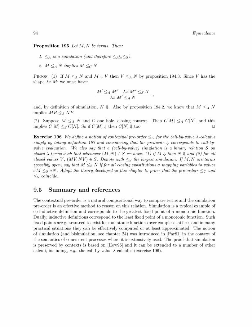
94 Equivalence
Proposition 195 Let M,N be terms. Then:
1. ≤A is a simulation (and therefore ≤A⊆≤S).
2. M ≤A N implies M ≤C N .
Proof. (1) If M ≤A N and M ⇓ V then V ≤A N by proposition 194.3. Since V has theshape λx.M ′ we must have:
M ′ ≤A M ′′ λx.M ′′ ≤S Nλx.M ′ ≤A N
,
and, by definition of simulation, N ⇓. Also by proposition 194.2, we know that M ≤A Nimplies MP ≤A NP .
(2) Suppose M ≤A N and C one hole, closing context. Then C[M ] ≤A C[N ], and thisimplies C[M ] ≤S C[N ]. So if C[M ] ⇓ then C[N ] ⇓ too. 2
Exercise 196 We define a notion of contextual pre-order ≤C for the call-by-value λ-calculussimply by taking definition 167 and considering that the predicate ⇓ corresponds to call-by-value evaluation. We also say that a (call-by-value) simulation is a binary relation S onclosed λ terms such that whenever (M,N) ∈ S we have: (1) if M ⇓ then N ⇓ and (2) for allclosed values V , (MV,NV ) ∈ S. Denote with ≤S the largest simulation. If M,N are terms(possibly open) say that M ≤S N if for all closing substitutions σ mapping variables to valuesσM ≤S σN . Adapt the theory developed in this chapter to prove that the pre-orders ≤C and≤S coincide.
9.5 Summary and references
The contextual pre-order is a natural compositional way to compare terms and the simulationpre-order is an effective method to reason on this relation. Simulation is a typical example ofco-inductive definition and corresponds to the greatest fixed point of a monotonic function.Dually, inductive definitions correspond to the least fixed point of a monotonic function. Suchfixed points are guaranteed to exist for monotonic functions over complete lattices and in manypractical situations they can be effectively computed or at least approximated. The notionof simulation (and bisimulation, see chapter 24) was introduced in [Par81] in the context ofthe semantics of concurrent processes where it is extensively used. The proof that simulationis preserved by contexts is based on [How96] and it can be extended to a number of othercalculi, including, e.g., the call-by-value λ-calculus (exercise 196).
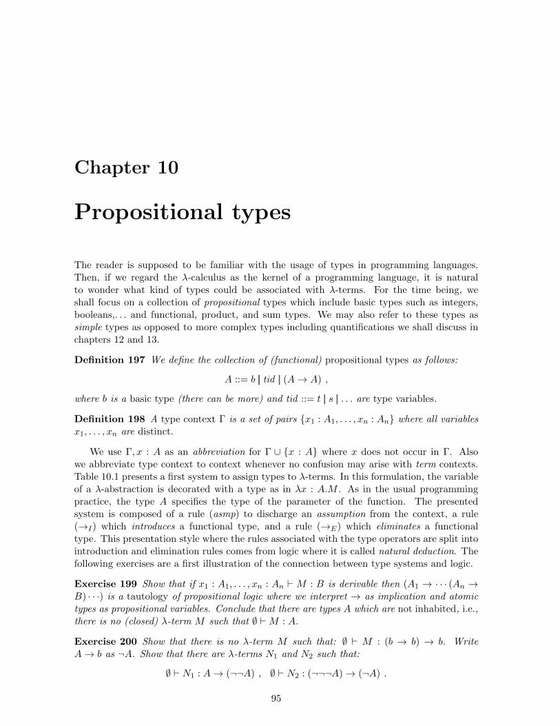
Chapter 10
Propositional types
The reader is supposed to be familiar with the usage of types in programming languages.Then, if we regard the λ-calculus as the kernel of a programming language, it is naturalto wonder what kind of types could be associated with λ-terms. For the time being, weshall focus on a collection of propositional types which include basic types such as integers,booleans,. . . and functional, product, and sum types. We may also refer to these types assimple types as opposed to more complex types including quantifications we shall discuss inchapters 12 and 13.
Definition 197 We define the collection of (functional) propositional types as follows:
A ::= b || tid || (A→ A) ,
where b is a basic type (there can be more) and tid ::= t || s || . . . are type variables.
Definition 198 A type context Γ is a set of pairs x1 : A1, . . . , xn : An where all variablesx1, . . . , xn are distinct.
We use Γ, x : A as an abbreviation for Γ ∪ x : A where x does not occur in Γ. Alsowe abbreviate type context to context whenever no confusion may arise with term contexts.Table 10.1 presents a first system to assign types to λ-terms. In this formulation, the variableof a λ-abstraction is decorated with a type as in λx : A.M . As in the usual programmingpractice, the type A specifies the type of the parameter of the function. The presentedsystem is composed of a rule (asmp) to discharge an assumption from the context, a rule(→I) which introduces a functional type, and a rule (→E) which eliminates a functionaltype. This presentation style where the rules associated with the type operators are split intointroduction and elimination rules comes from logic where it is called natural deduction. Thefollowing exercises are a first illustration of the connection between type systems and logic.
Exercise 199 Show that if x1 : A1, . . . , xn : An ` M : B is derivable then (A1 → · · · (An →B) · · ·) is a tautology of propositional logic where we interpret → as implication and atomictypes as propositional variables. Conclude that there are types A which are not inhabited, i.e.,there is no (closed) λ-term M such that ∅ `M : A.
Exercise 200 Show that there is no λ-term M such that: ∅ ` M : (b → b) → b. WriteA→ b as ¬A. Show that there are λ-terms N1 and N2 such that:
∅ ` N1 : A→ (¬¬A) , ∅ ` N2 : (¬¬¬A)→ (¬A) .
95

96 Propositional types
On the other hand, there are tautologies which are not inhabited! For instance, consider:A ≡ ((t→ s)→ t)→ t. Show that there is no λ-term M in normal form such that ∅ `M : Ais derivable. This is enough because later we shall show that all typable λ-terms normalize toa λ-term of the same type. For another example, show that there is no λ-term M in normalform such that ∅ ` M : ¬¬t → t is derivable (the intuitionistic/constructive negation is notinvolutive!).
Next we review a few alternative presentations of the type system. In Table 10.1, λ-abstractions are decorated with types. However, we can also consider a presentation wheretypes are assigned to pure, i.e., type-less, λ-terms. Then one speaks of a presentation inCurry-style, as opposed to the previous one which is in Church-style. In our case, the onlydifference between the two is that the rule (→I) in Curry-style becomes:
Γ, x : A `M : B
Γ ` λx.M : A→ B.
An important consequence of this change is that now a λ-term may have more than one type.This makes the type inference problem (see chapters 11 and 12) more interesting and so thisproblem is often studied for systems in Curry-style.
Yet another presentation of the type system is possible by labeling every variable with itstype and by dropping the context. This gives the system presented in Table 10.2. Finally, wemay decide to label every λ-term (not just the variables) with its type and in this case we candrop the type since the type of a λ-term is just the outermost label. The resulting system isgiven in Table 10.3.
The previous exercises 199 and 200 suggest that the functional type constructor can beregarded as a logical implication. It turns out that one may push this connection furtherby regarding the product (sum) type constructor as a logical conjunction (disjunction). Theresulting type system in natural deduction style is presented in Table 10.4. Later in chapters12 and 13, we shall see that this connection can be extended even further to types withuniversal and existential quantifications.
Not all term constructors found in a programming language have a logical interpretation.For instance, Table 10.5 introduces typing rules for a constant zero Z, a successor functionS, and a fixed point combinator Y. While the fixed point combinator allows to define generalrecursive functions (see chapter 7) its logical interpretation is problematic. Indeed, with therule (Y), every type A is inhabited by the closed λ-term Y (λx : A.x). Thus the typing rulefor Y is definitely incompatible with logic as it leads to inconsistency!
(asmp)x : A ∈ Γ
Γ ` x : A
(→I)Γ, x : A `M : B
Γ ` λx : A.M : A→ B(→E)
Γ `M : A→ B Γ ` N : A
Γ `MN : B
Table 10.1: Assignment of propositional types to λ-terms
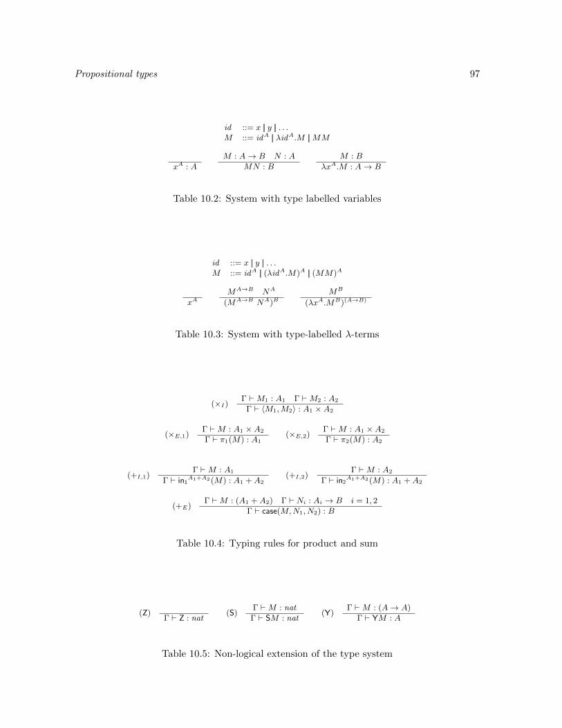
Propositional types 97
id ::= x || y || . . .M ::= idA || λidA.M ||MM
xA : A
M : A→ B N : A
MN : B
M : B
λxA.M : A→ B
Table 10.2: System with type labelled variables
id ::= x || y || . . .M ::= idA || (λidA.M)A || (MM)A
xAMA→B NA
(MA→B NA)BMB
(λxA.MB)(A→B)
Table 10.3: System with type-labelled λ-terms
(×I)Γ `M1 : A1 Γ `M2 : A2
Γ ` 〈M1,M2〉 : A1 ×A2
(×E,1)Γ `M : A1 ×A2
Γ ` π1(M) : A1(×E,2)
Γ `M : A1 ×A2
Γ ` π2(M) : A2
(+I,1)Γ `M : A1
Γ ` in1A1+A2(M) : A1 +A2
(+I,2)Γ `M : A2
Γ ` in2A1+A2(M) : A1 +A2
(+E)Γ `M : (A1 +A2) Γ ` Ni : Ai → B i = 1, 2
Γ ` case(M,N1, N2) : B
Table 10.4: Typing rules for product and sum
(Z)Γ ` Z : nat
(S)Γ `M : nat
Γ ` SM : nat(Y)
Γ `M : (A→ A)
Γ ` YM : A
Table 10.5: Non-logical extension of the type system

98 Propositional types
10.1 Subject reduction
If a λ-term is well-typed, then by inspection of the rules we see, e.g., that the λ-term cannotcontain the application of a natural number to a function. However, to get static guaranteeswe must make sure that typing is invariant under reduction, i.e., if a λ-term is well-typedand we reduce it then we still get a well-typed λ-term. To establish this property we note thefollowing property.
Proposition 201 (substitution) If Γ, x : A `M : B and Γ ` N : A then Γ ` [N/x]M : B.
Proof. By induction on the height of the proof of Γ, x : A ` M : B. For instance, supposethe root of the proof has the shape:
Γ, x : A, y : B′ `M : B′′
Γ, x : A ` λy.M : (B′ → B′′),
with x 6= y. Then by inductive hypothesis, Γ, y : B′ ` [N/x]M : B′′ and conclude by (→I). 2
We can now state the invariance of typing under reduction as follows. Historically, thisproperty is called subject reduction.
Proposition 202 (subject reduction) If Γ `M : A and M →β N then Γ ` N : A.
Proof. Recall, that M →β N means:
M ≡ C[(λx.M1)M2] N ≡ C[[M2/x]M1] .
To prove subject reduction we proceed by induction on the structure of C. The basic casefollows directly from the substitution lemma. For the inductive case consider in turn the caseswhere: (1) C = λy.C ′, (2) C = C ′P , and (3) C = PC ′. 2
In the ‘pure’ λ-calculus, we identify the normal forms with the results of the computation.In applications, however, one can distinguish two kinds of normal/irreducible forms: thosethat correspond to a value and those that correspond to an erroneous configuration like divid-ing by zero, or applying an integer to another integer. Thus a program, i.e., a closed λ-term,has three possible outcomes: (1) it returns a value, (2) it reaches an erroneous configuration,and (3) it diverges (cf. chapter 1). Besides being invariant by reduction, a desirable propertyfor a type system is that: well-typed programs cannot go wrong, or at least that they go wrongin some expected way (e.g., division by zero). This property is often called progress, becausein its simple form it requires that if a program is not a value then it can reduce (progress).The following exercise elaborates on this point.
Exercise 203 (on progress) Suppose we reconsider the non-logical extension of the simplytyped λ-calculus with a basic type nat, constants Z, S, Y, and with the following fixed-pointrule:
C[YM ]→ C[M(YM)] .
Let a program be a closed typable λ-term of type nat and let a value be a λ-term of the shape(S · · · (SZ) · · ·). Show that if P is a program in normal form (cannot reduce) then P is a value.

Propositional types 99
10.2 A normalizing strategy for the simply typed λ-calculus
We describe a normalizing strategy for the simply typed λ-calculus. To this end we introducesome measures of the complexity of a type and a λ-term.
Definition 204 (type degree) The degree of a type is defined as follows:
δ(t) = 1 , δ(A→ B) = 1 + max (δ(A), δ(B)) .
Definition 205 (redex degree) Let R ≡ (λx : A.M)N be a redex. The degree of the redex,written δr(R) is the degree of the type associated with the λ-term (λx : A.M).
Definition 206 (term degree) The degree of a λ-term, written δt(M), is 0 if M is innormal form and the maximum of the degrees of the redexes contained in M otherwise.
Remark 207 A redex R is also a λ-term and we have δr(R) ≤ δt(R).
Proposition 208 (degree and substitution) If x is of type A then
δt([N/x]M) ≤ max (δ(A), δt(M), δt(N)) .
Proof. The redexes in [N/x]M fall in the following categories. (1) The redexes already inM . (2) The redexes already in N . (3) New redexes arising by the substitution if N ≡ λy.N ′and M = C[xM ′]. These redexes have degree δ(A). 2
Proposition 209 (degrees and reduction) If M → N then δt(N) ≤ δt(M).
Proof. We apply the previous analysis. 2
We now define a reduction strategy that reduces first an innermost redex of maximaldegree.
Definition 210 (innermost maximal degree strategy) Let M be a λ-term which is notin normal form. The innermost maximal degree strategy selects a redex R of maximal degree(δr(R) = δt(M)) and such that all redexes contained in R have lower degree.
Proposition 211 The innermost maximal degree strategy is normalizing.
Proof. Notice that by reducing an innermost maximal degree redex we guarantee that thereduced λ-term contains strictly less redexes of maximal degree. Then we prove normalizationby taking as measure:
µ(M) = (n,m) ,
with the lexicographic order (from left to right), where n = δt(M) and m is the number ofredexes of maximal degree. If m = 0 then M is in normal form. If m = 1 then the reducedterm has lower degree (first component decreases). If m > 1 then the first component doesnot increase (proposition 209) and the second decreases. 2

100 Propositional types
10.3 Termination of the simply typed λ-calculus
A λ-term M is called strongly normalizable if all β-reductions starting from M terminate(thus strong-normalization is just a synonymous for termination!).
Definition 212 Let SN be the set of strongly normalizable λ-terms.
This set plays a role similar to the set WF for RPO termination (section 4.3). The notionof size of a λ-term follows definition 116.
Definition 213 (maximal length) If M ∈ SN then the maximal length of a derivationstarting from M is called the reduction depth of M , and is denoted depth(M).
Remark 214 The maximal length is well-defined because the reduction tree of a λ-term isfinitely branching (cf. proposition 42).
In order to show that all simply typed λ-terms are→β-strongly normalizable, the key ideais to interpret types as subsets of the set SN of strongly normalizing λ-terms.
Definition 215 (type interpretation) The interpretation of a propositional type A is de-fined as follows:
[[b]] = [[t]] = SN[[A→ B]] = M | ∀N ∈ [[A]] (MN ∈ [[B]]) .
Proposition 216 For any type A, the following properties hold:
1. [[A]] ⊆ SN .
2. If Ni ∈ SN for i = 1, . . . , k then xN1 · · ·Nk ∈ [[A]].
3. If [N/x]MM1 · · ·Mk ∈ [[A]] and N ∈ SN then (λx.M)NM1 · · ·Mk ∈ [[A]].
Proof. By induction on A.
Atomic types. (1) By definition. (2) The reductions of xN1 . . . Nk are just an interleaving ofthe reductions of N1, . . . Nk. (3) We have:
depth((λx.M)NM1 . . .Mk) ≤ depth(N) + depth([N/x]MM1 . . .Mk) + 1 .
Functional types A→ B. Suppose M ∈ [[A→ B]].
(1) By inductive hypothesis, x ∈ [[A]]. Hence Mx ∈ [[B]] ⊆ SN , by inductive hypothesis. Thisentails M ∈ SN .
(2) Take M = xN1 . . . Nk with Ni ∈ SN . Take Nk+1 ∈ [[A]] ⊆ SN . By inductive hypothesis,xN1 . . . NkNk+1 ∈ [[B]].
(3) If [N/x]MN1 . . . Nk ∈ [[A → B]] then by the interpretation of the functional types wehave:
∀Nk+1 ∈ [[A]] [N/x]MN1 . . . NkNk+1 ∈ [[B]] .
Then by inductive hypothesis on B:
∀Nk+1 ∈ [[A]] (λx.M)NN1 . . . NkNk+1 ∈ [[B]] ,
which is equivalent to (λx.M)NN1 . . . Nk ∈ [[A→ B]]. 2

Propositional types 101
Remark 217 These interpretations of types are called reducibility candidates. These aresets of of strongly normalizable λ-terms (property 1) which contain at least the variables (andmore) (property 2), and are closed under head expansions (property 3).
We can now state the soundness of the interpretation.
Proposition 218 (soundness) If x1 : A1, . . . , xk : Ak ` M : B (in Curry-style) and Ni ∈[[Ai]] for i = 1, . . . , k then [N1/x1, . . . , Nk/xk]M ∈ [[B]].
Proof. By induction on the typing proof.
(asmp) Immediate by definition.
(→E) By the interpretation of →.
(→I) Here is what goes on in a simplified case. By inductive hypothesis on x : A ` M : Bwe have:
∀N ∈ [[A]] [N/x]M ∈ [[B]].
Then, by the closure under head expansions of the interpretations we derive:
∀N ∈ [[A]] (λx.M)N ∈ [[B]] ,
which is equivalent to (λx : A.M) ∈ [[A→ B]]. 2
The strong normalization property follows as a simple corollary.
Corollary 219 (strong normalization) If a λ-term is typable then it is strongly normal-izing.
Proof. Suppose x1 : A1, . . . , xk : Ak ` M : B. We know xi ∈ [[Ai]]. By proposition 218(soundness), M ∈ [[B]] and we know [[B]] ⊆ SN . 2
A rational reconstruction of the proof could go as follows. (1) We decide to interprettypes as sets of strongly normalizing λ-terms and show that ` M : A implies M ∈ [[A]]. (2)Then the definition 215 of the type interpretation is natural and the properties 1 and 2 ofproposition 216 amount to check that indeed a type interpretation is composed of stronglynormalizing λ-terms and it is not empty. (3) Finally, the need for property 3 of proposition216 (closure under head expansion) appears in the proof of proposition 218 (soundness, case(→I)).
Exercise 220 (recursive types) Assume a recursively defined type t satisfying the equa-tion t = t→ b and suppose we add a rule for typing up to type equality:
Γ `M : A A = B
Γ `M : B.
Show that in this case the following λ-term (Curry’s fixed point combinator) is typable (e.g.,in Curry-style):
Y ≡ λf.(λx.f(xx))(λx.f(xx)) .
Are the λ-terms typable in this system terminating?

102 Propositional types
10.4 Summary and references
A minimal property required for a type system is that it is invariant under reduction. Some-times, it is possible to connect type systems to logic. This is the so called Curry-Howardcorrespondence which goes as follows:
λ-calculus proof system
type propositionλ-term proof
reduction proof normalization
In a natural deduction presentation, an opportunity for a proof normalization arises whenthe introduction of an operator is followed by an elimination. For instance, λ-abstraction isfollowed by an application, a pairing is followed by a projection, and an injection is followedby a case selection. The book [GLT89] is a good introduction to the connections betweenproof theory and type theory including alternative presentations of the logical systems.

Chapter 11
Type inference for propositionaltypes
Given a (pure) λ-term M and a context Γ, the type inference problem is the problem ofchecking whether there is a type A such that Γ `M : A. Given a (pure) λ-term M , a variantof the problem is to look for a type A and a context Γ such that Γ `M : A. Connected to thetype inference problem is the problem of actually producing an informative output. Typically,if a λ-term M is typable, we are interested in a synthetic representation of its types, and if itis not, we look for an informative error message.
11.1 Reduction of type-inference to unification
We present a polynomial time reduction of the type inference problem for the propositionaltype system in Curry style (chapter 10) to the syntactic unification problem (chapter 3). Theexistence of a most general unifier for the unification problem leads to the existence of a mostgeneral type for the type inference problem.
Definition 221 A goal is a finite set G of triples (Γ,M,A) where Γ is a context, M aλ-term, and A a propositional type.
We assume that all bound variables in M are distinct and different from the free ones,that all free variables occur in the context Γ, and that for every variable x we have a typevariable tx. We define a reduction relation on pairs (G,E). Assuming G = g ∪ G′ andg ≡ (Γ,M,A) /∈ G′, all the rules produce a pair (G′ ∪ Gg, E ∪ Eg) where Gg and Eg aredefined in Table 11.1.
Proposition 222 The reduction specified in Table 11.1 terminates.
g Gg Eg(Γ, x, A) ∅ tx = A
(Γ,M1M2, A) (Γ,M1, t1 → A), (Γ,M2, t1) ∅ (t1 fresh)(Γ, λx.M1, A) (Γ, x : tx,M1, t) A = tx → t (t fresh)
Table 11.1: Reduction of type inference to unification
103

104 Type inference
Proof. It is enough to notice that every reduction step replaces a triple (Γ,M,A) by a finitenumber of triples (Γ′,M ′, A′) where M ′ is structurally smaller than M . 2
We introduce some notation. In the following, we consider substitutions S that act on thefirst-order terms built over the signature Σ = b0,→2. We define:
S |= E if S unifies E ,S |= (Γ,M,A) if SΓ `M : S(A) is derivable,S |= G if ∀ g ∈ G S |= g ,S |= (G,E) if S |= G and S |= E .
Given a λ-term M0 with free variables x1, . . . , xn, we set the initial pair to (G0, ∅), withG0 = (Γ0,M0, t0), t0 fresh, and Γ0 = x1 : tx1 , . . . , xn : txn . Next, we state the mainproperties of the reduction.
Proposition 223 If (G0, ∅)∗→ (G,E) then:
1. If S |= (G,E) then SΓ0 `M0 : St0.
2. If Γ `M0 : A then ∃S(S |= (G,E), SΓ0 ⊆ Γ, and A = St0).
Proof. For both properties we proceed by induction on the length of the reduction.
(1) For instance, suppose (1) true for: (G ∪ (Γ,MN,A), E). The rule for applicationproduces the pair (G′, E) with G′ = G ∪ (Γ,M, t1 → A), (Γ, N, t1). Suppose S |= (G′, E).This means S |= (G,E), SΓ ` M : S(t1 → A), and SΓ ` N : St1. By (→E), we concludeSΓ `MN : SA. Thus S |= (G ∪ (Γ,MN,A), E), and by hypothesis SΓ0 `M0 : St0.
(2) For instance, suppose: Γ `M0 : A, S |= (G∪(Γ′, λx.M,A′), E), SΓ0 ⊆ Γ, and A = St0.This implies: SΓ′ ` λx.M : S(A′), which entails: SΓ′, x : A1 ` M : A2, SA′ = A1 → A2, forsome A1, A2. Suppose we reduce to the pair:
(G ∪ (Γ′, x : tx,M, t), E ∪ A′ = tx → t) .
Then take S′ = S[A1/tx, A2/t]. 2
Remark 224 Property (1) entails the soundness of the method. Indeed, suppose from theinitial goal we derive a set of equations E and a substitution S such that S |= E (a unifier).Then we derive a correct typing SΓ0 ` M0 : St0. On the other hand, property (2) entailsthe completeness of the method. Suppose Γ ` M0 : A is a valid typing. Then we can reduce(Γ0,M0, t0) to (∅, E) and find a unifier S for E such that SΓ0 is contained in Γ and St0 = A.In particular, if we take the most general unifier S of E and we apply it to t0 we obtain themost general type: every other type is an instance of St0.
Example 225 The most general type of the λ-term λf.λx.f(f(x)) is (t→ t)→ (t→ t). Notethat strictly speaking the most general type is not unique. For instance, (s → s) → (s → s)is also a most general type of the λ-term considered.
Remark 226 (graphical presentation) It is possible to give an equivalent ‘graphical’ pre-sentation of the unification method. (1) Rename bound variables so that they are all distinctand different from the free ones. (2) Draw the tree associated with the λ-term. (3) Associate

Type inference 105
a distinct type variable with every internal node of the tree. (4) Associate a type variable txwith a leaf node corresponding to the variable x. (5) For every abstraction node (λx.M t′)t
generate the equation t = tx → t′. (6) For every application node (M t′N t′′)t generate theequation t′ = t′′ → t.
Exercise 227 Compute, if they exist, the most general types of the following λ-terms:
λx.λy.λz.xz(yz), λx.λy.x(yx), λk.(k(λx.λh.hx)) .
11.2 Reduction of unification to type inference
We discuss a method to reduce any unification problem to a type-inference problem. We alsoshow that the principal types are exactly the types inhabited by a closed λ-term. We supposeas usual that K ≡ λx.λy.x.
Proposition 228 The principal type of the λ-term E below is t→ (t→ (s→ s)).
E ≡ λx.λy.λw.Kw(λf.λp.p(fx)(fy)) .
Proof. The fact that f is applied to both x and y forces the equality of the types of x andy. On the other hand, since the principal type of K is t → s → t, the type of w must beequal to the type of the result. 2
Proposition 229 Let M1 and M2 be λ-terms with principal types A1 and A2, respectively.Then the principal type of the λ-term λf.E (fM1)M2, for f /∈ fv(M1M2), is (A1 → A2) →(s→ s).
Proof. The function f must apply to the λ-term M1 and based on proposition 228, the typeof the result of f must be equal to the type of M2. 2
Proposition 230 For every type A with (type) variables contained in t1, . . . , tn there is aλ-term MA whose principal type is: t1 → · · · → tn → A→ (s→ s), where s /∈ t1, . . . , tn.
Proof. By induction on the structure of A. If A = ti we take:
λx1 . . . xn.λy.Exiy : t1 → · · · → tn → ti → s→ s .
If A = A1 → A2, by inductive hypothesis we have:
MAi : t1 → · · · → tn → Ai → (s→ s) i = 1, 2 .
We define:MA1→A2 ≡ λx1 . . . xn.λy.λz.KzP .
This λ-term has the expected type provided we can force in the λ-term P the type of y to be(A1 → A2). We observe that if we write:
Qi ≡MAix1 . . . xnyi .
we force the type of yi to be Ai. Then we can define P as follows:
P ≡ λy1, y2.λp.pQ1Q2(E (yy1)y2) ,
and as expected the type of y is A1 → A2. 2

106 Type inference
Exercise 231 (1) Apply the method to the types t1, t2 and (t1 → t2) relatively to the set of(type) variables t1, t2. (2) Write a program that builds the equivalent of the λ-term MA ina language of the ML-family and uses the type-inference system to compute its principal type.
Proposition 232 Given two types A and B there is a λ-term UA,B which is typable if andonly if A and B are unifiable.
Proof. We have:
MA : t1 → · · · → tn → A→ s→ s , MB : t1 → · · · → tn → B → s→ s .
We build:
UA,B ≡ λx1 . . . xn.λy1.λy2.λp.pPAPB(Ey1y2) ,PA ≡MAx1 . . . xny1 ,PB ≡MBx1 . . . xny2 .
2
Exercise 233 Apply proposition 232 if A = t1 and B = t2 and if A = t1 and B = t1 → t2.
Proposition 234 Every unification problem can be reduced to a type-inference problem.
Proof. We know from exercise 61 that every unification problem reduces to a unificationproblem composed of one equation with terms built over a signature with exactly one binarysymbol. We take ‘→’ as binary symbol and using the proposition 232 above we build twotypes A and B which are unifiable iff the λ-term UA,B is typable. 2
Proposition 235 For every type A, there is a λ-term F(A→A) whose principal type is (A→A).
Proof. Let A be a type whose type variables are contained in t1, . . . , tn. Let MA be aλ-term with principal type: t1 → · · · → tn → A → s → s (proposition 230). Then build theλ-term:
FA→A ≡ λy.Ky(λx1 . . . xn.(MAx1 . . . xny)) .
This λ-term has principal type (A→ A). 2
Proposition 236 Let M be a λ-term with type A (not necessarily its principal type). Thenone can build a closed λ-term N whose principal type is A. Thus the inhabited types areexactly the principal types.
Proof. By proposition 235, the principal type of FA→A is (A → A). Then the λ-termFA→AM has principal type A. 2

Type inference 107
11.3 Summary and references
A type inference problem can be (efficiently) reduced to a syntactic unification problem. Thenthe existence of a most general unifier is reflected back in the existence of a most general type.We have also shown that every unification problem reduces to a type inference problem andthat for every inhabited type A it is possible to build a λ-term whose principal type is A.Notice however that knowing if a type is inhabited is a Pspace-complete problem [Sta79].The connection between type inference and unification was already pointed out in [Hin69]. Bynow, the reduction of a program analysis problem to the solution of a set of constraints hasbecome a standard technique. For instance, the data flow analyses performed by optimizingcompilers are reduced to systems of monotonic boolean equations.

108 Type inference
Chapter 12
Predicative polymorphic types andtype inference
Consider any standard sorting algorithm sort on lists. Most likely, the sorting algorithm justdepends on a boolean predicate on the elements of the list while the type of the elements ofthe list does not really matter. One says that the sorting algorithm is polymorphic in that itcan be applied to data of different, but related, shape. We could type sort as follows:
sort : ∀ t list(t)→ (t→ t→ bool)→ list(t) ,
with the following intuitive meaning: for any type t, given a list of elements of type t, anda binary predicate on t, the function sort returns a list of elements of type t. Notice thatwe are assigning to sort a type which is not quite simple, i.e., propositional, as it containsa universal quantification over types. In this chapter, we introduce a particular class ofuniversally quantified types which can be used to type polymorphic functions. We then studythe type inference problem for the type system extended with such types.
12.1 Predicative universal types and polymorphism
The reader is supposed to be familiar with propositional and first-order logic. In the standardinterpretation of propositional logic predicates are boolean values while in first-order logicthey are regarded as relations over some universe. In second order logic, we can quantify overpredicates. For instance, here are some formulae in propositional, first-order, and second-order logic:
(P ⊃ P ) ⊃ (P ⊃ P ) (Propositional formula)∀x (P (x) ⊃ P (S(x))) ⊃ (P (Z) ⊃ ∀x P (x)) (First-order formula)∀P (P ⊃ P ) ⊃ (P ⊃ P ) (Second-order formula).
Following the types-as-formulae correspondence outlined in chapter 10, we may consider atype system where quantification over type variables is allowed. One fundamental question iswhether a type with quantified types should be regarded as an ordinary type, or if it shouldbe lifted to a superior status. In this chapter, we take the second option. In the logical jargon,this corresponds to a predicative approach to second-order quantification. We shall not dwell
109
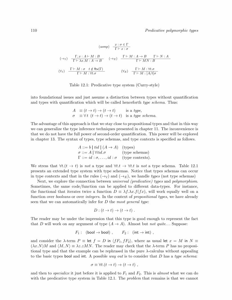
110 Predicative polymorphic types
(asmp)x : σ ∈ Γ
Γ ` x : σ
(→I)Γ, x : A `M : B
Γ ` λx.M : A→ B(→E)
Γ `M : A→ B Γ ` N : A
Γ `MN : B
(∀I)Γ `M : σ t /∈ ftv(Γ)
Γ `M : ∀t.σ (∀E)Γ `M : ∀t.σ
Γ `M : [A/t]σ
Table 12.1: Predicative type system (Curry-style)
into foundational issues and just assume a distinction between types without quantificationand types with quantification which will be called henceforth type schema. Thus:
A ≡ (t→ t)→ (t→ t) is a type,σ ≡ ∀ t (t→ t)→ (t→ t) is a type schema.
The advantage of this approach is that we stay close to propositional types and that in this waywe can generalize the type inference techniques presented in chapter 11. The inconvenience isthat we do not have the full power of second-order quantification. This power will be exploredin chapter 13. The syntax of types, type schemas, and type contexts is specified as follows.
A ::= b || tid || (A→ A) (types)σ ::= A || ∀tid .σ (type schemas)Γ ::= id : σ, . . . , id : σ (type contexts).
We stress that ∀t.(t → t) is not a type and ∀t.t → ∀t.t is not a type schema. Table 12.1presents an extended type system with type schemas. Notice that types schemas can occurin type contexts and that in the rules (→I) and (→E), we handle types (not type schemas)
Next, we explore the connection between universal (predicative) types and polymorphism.Sometimes, the same code/function can be applied to different data-types. For instance,the functional that iterates twice a function D ≡ λf.λx.f(fx), will work equally well on afunction over booleans or over integers. In the context of propositional types, we have alreadyseen that we can automatically infer for D the most general type:
D : (t→ t)→ (t→ t) .
The reader may be under the impression that this type is good enough to represent the factthat D will work on any argument of type (A→ A). Almost but not quite. . . Suppose:
F1 : (bool→ bool) , F2 : (int→ int) ,
and consider the λ-term P ≡ let f = D in 〈fF1, fF2〉, where as usual let x = M in N ≡(λx.N)M and 〈M,N〉 ≡ λz.zMN . The reader may check that the λ-term P has no proposi-tional type and that the example can be rephrased in the pure λ-calculus without appealingto the basic types bool and int. A possible way out is to consider that D has a type schema:
σ ≡ ∀t.(t→ t)→ (t→ t) ,
and then to specialize it just before it is applied to F1 and F2. This is almost what we can dowith the predicative type system in Table 12.1. The problem that remains is that we cannot
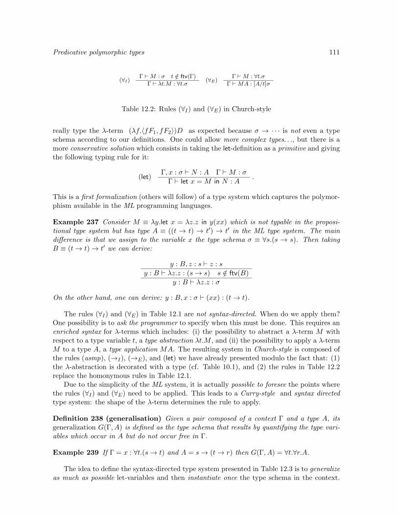
Predicative polymorphic types 111
(∀I)Γ `M : σ t /∈ ftv(Γ)
Γ ` λt.M : ∀t.σ (∀E)Γ `M : ∀t.σ
Γ `MA : [A/t]σ
Table 12.2: Rules (∀I) and (∀E) in Church-style
really type the λ-term (λf.〈fF1, fF2〉)D as expected because σ → · · · is not even a typeschema according to our definitions. One could allow more complex types. . ., but there is amore conservative solution which consists in taking the let-definition as a primitive and givingthe following typing rule for it:
(let)Γ, x : σ ` N : A Γ `M : σ
Γ ` let x = M in N : A.
This is a first formalization (others will follow) of a type system which captures the polymor-phism available in the ML programming languages.
Example 237 Consider M ≡ λy.let x = λz.z in y(xx) which is not typable in the proposi-tional type system but has type A ≡ ((t → t) → t′) → t′ in the ML type system. The maindifference is that we assign to the variable x the type schema σ ≡ ∀s.(s → s). Then takingB ≡ (t→ t)→ t′ we can derive:
y : B, z : s ` z : s
y : B ` λz.z : (s→ s) s /∈ ftv(B)
y : B ` λz.z : σ
On the other hand, one can derive: y : B, x : σ ` (xx) : (t→ t).
The rules (∀I) and (∀E) in Table 12.1 are not syntax-directed. When do we apply them?One possibility is to ask the programmer to specify when this must be done. This requires anenriched syntax for λ-terms which includes: (i) the possibility to abstract a λ-term M withrespect to a type variable t, a type abstraction λt.M , and (ii) the possibility to apply a λ-termM to a type A, a type application MA. The resulting system in Church-style is composed ofthe rules (asmp), (→I), (→E), and (let) we have already presented modulo the fact that: (1)the λ-abstraction is decorated with a type (cf. Table 10.1), and (2) the rules in Table 12.2replace the homonymous rules in Table 12.1.
Due to the simplicity of the ML system, it is actually possible to foresee the points wherethe rules (∀I) and (∀E) need to be applied. This leads to a Curry-style and syntax directedtype system: the shape of the λ-term determines the rule to apply.
Definition 238 (generalisation) Given a pair composed of a context Γ and a type A, itsgeneralization G(Γ, A) is defined as the type schema that results by quantifying the type vari-ables which occur in A but do not occur free in Γ.
Example 239 If Γ = x : ∀t.(s→ t) and A = s→ (t→ r) then G(Γ, A) = ∀t.∀r.A.
The idea to define the syntax-directed type system presented in Table 12.3 is to generalizeas much as possible let-variables and then instantiate once the type schema in the context.
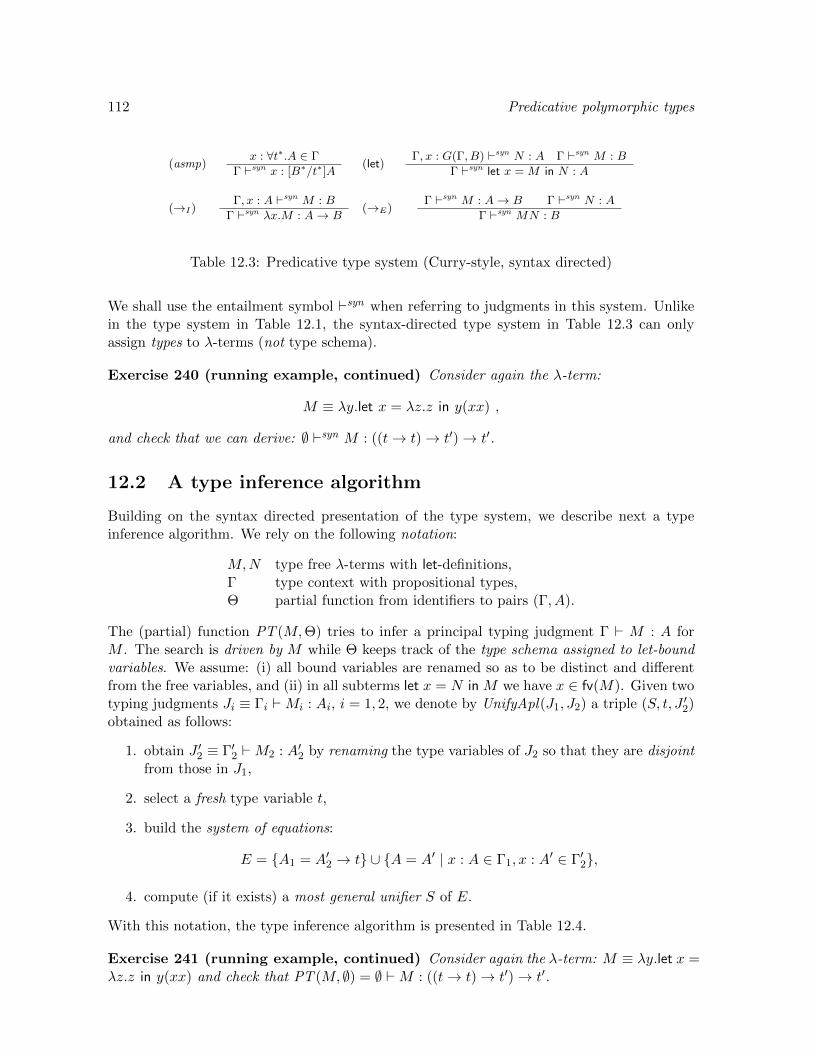
112 Predicative polymorphic types
(asmp)x : ∀t∗.A ∈ Γ
Γ `syn x : [B∗/t∗]A(let)
Γ, x : G(Γ, B) `syn N : A Γ `syn M : B
Γ `syn let x = M in N : A
(→I)Γ, x : A `syn M : B
Γ `syn λx.M : A→ B(→E)
Γ `syn M : A→ B Γ `syn N : A
Γ `syn MN : B
Table 12.3: Predicative type system (Curry-style, syntax directed)
We shall use the entailment symbol `syn when referring to judgments in this system. Unlikein the type system in Table 12.1, the syntax-directed type system in Table 12.3 can onlyassign types to λ-terms (not type schema).
Exercise 240 (running example, continued) Consider again the λ-term:
M ≡ λy.let x = λz.z in y(xx) ,
and check that we can derive: ∅ `syn M : ((t→ t)→ t′)→ t′.
12.2 A type inference algorithm
Building on the syntax directed presentation of the type system, we describe next a typeinference algorithm. We rely on the following notation:
M,N type free λ-terms with let-definitions,Γ type context with propositional types,Θ partial function from identifiers to pairs (Γ, A).
The (partial) function PT (M,Θ) tries to infer a principal typing judgment Γ ` M : A forM . The search is driven by M while Θ keeps track of the type schema assigned to let-boundvariables. We assume: (i) all bound variables are renamed so as to be distinct and differentfrom the free variables, and (ii) in all subterms let x = N in M we have x ∈ fv(M). Given twotyping judgments Ji ≡ Γi `Mi : Ai, i = 1, 2, we denote by UnifyApl(J1, J2) a triple (S, t, J ′2)obtained as follows:
1. obtain J ′2 ≡ Γ′2 `M2 : A′2 by renaming the type variables of J2 so that they are disjointfrom those in J1,
2. select a fresh type variable t,
3. build the system of equations:
E = A1 = A′2 → t ∪ A = A′ | x : A ∈ Γ1, x : A′ ∈ Γ′2,
4. compute (if it exists) a most general unifier S of E.
With this notation, the type inference algorithm is presented in Table 12.4.
Exercise 241 (running example, continued) Consider again the λ-term: M ≡ λy.let x =λz.z in y(xx) and check that PT (M, ∅) = ∅ `M : ((t→ t)→ t′)→ t′.

Predicative polymorphic types 113
PT (M,Θ) = case M
x : case Θ(x)(Γ, A) : Γ ` x : A
: x : tx ` x : tx
λx.M : let (Γ `M : A) = PT (M,Θ) incase x : A′ ∈ Γtrue : Γ\(x : A′) ` λx.M : A′ → A
: Γ ` λx.M : t→ A, t fresh
M1M2 : let Ji ≡ (Γi `Mi : Ai) = PT (Mi,Θ) i = 1, 2 inlet (S, t,Γ′
2 `M2 : A′2) = UnifyApl(J1, J2) in
S(Γ1 ∪ Γ′2 `M1M2 : t)
let x = M1 in M2 :let (Γ1 `M1 : A1) = PT (M1,Θ) inlet Θ′ = Θ[(Γ1, A1)/x] inlet (Γ2 `M2 : A2) = PT (M2,Θ
′) inΓ2 ` let x = M1 in M2 : A2
Table 12.4: Type-inference algorithm

114 Predicative polymorphic types
(asmp)x : A ∈ Γ
Γ `let x : A(let)
Γ `let [M/x]N : A Γ `let M : B
Γ `let let x = M in N : A
(→I)Γ, x : A `let M : B
Γ `let λx.M : A→ B(→E)
Γ `let M : A→ B Γ `let N : A
Γ `let MN : B
Table 12.5: Propositional typing with let-expansion
12.3 Reduction of stratified polymorphic typing to proposi-tional typing
We may consider a type system where to type let x = M in N we actually typeM and [N/x]M ,where by typing we mean propositional typing. This way of proceeding is not particularlyefficient because the let-expansion might take exponential time (see following exercise 243).However, the interesting point is that the λ-terms typable in this way are exactly those typablein the original ML system. Therefore we have the following intuitive characterization:
ML typing = Propositional typing + let-expansion.
The type inference algorithm presented in Table 12.4 is a way to keep implicit the let-expansion(but type renaming still forces a type expansion as we shall see shortly!). Table 12.5 describesa type system based on let-expansion. We use the entailment symbol `let to distinguish thissystem from the previous ones. In the (let) rule, we just check that the substituted term Mis typable with some type B; this check is necessary if x /∈ fv(M).
Exercise 242 (running example) Consider again the λ-term:
M ≡ λy.let x = λz.z in y(xx) ,
and check that we can derive: ∅ `let M : ((t→ t)→ t′)→ t′.
Exercise 243 (let-expansion) Consider a λ-calculus extended with let definitions of theshape let x = M in N . Let C denote a context with a hole (cf. definition 118) and define thereduction relation →let as follows:
→let= ( C[let x = N in M ] , C[[N/x]M ] ) | C context,M,N λ-terms , x variable .
We extend the definition of size of a λ-term |M | (cf. definition 116) with: |let x = M in N | =1 + |M |+ |N |. We also define the depth d(M) of a λ-term as follows:
d(x) = 1, d(MN) = max (d(M), d(N)),d(λx.M) = d(M), d(let x = M in N) = d(M) + d(N) .
1. Show that there is a strategy to reduce a λ-term M to a normal form N such that:
|N | ≤ |M |d(M) .
2. Show that the reduction relation →let is locally confluent.

Predicative polymorphic types 115
How hard is it to decide if a λ-term is typable in the ML system? Well, in theory itis hard but in practice it is easy! The characterization via propositional typing with letexpansion shows that the problem can be solved in exponential time: (1) let-expand the λ-term(exponential penalty), (2) reduce the propositional type-inference problem to a unificationproblem (efficient), and (3) solve the unification problem (efficient).
In fact one can show that any decision problem that runs in exponential time can becoded as an ML type inference problem. Hence any algorithm (including the symbolic one)that solves the problem will run in at least exponential time. The good news are that thecomplexity is exponential in the let-depth (example next) of the λ-term and that deeply nestedchains of let-definitions do not seem to appear in practice.
Example 244 Here is a way to blow up ML type inference.
P ≡ λx, y, z.zxy : t1 → t2 → (t1 → t2 → t3)→ t3M1 ≡ λy.Pyy : t1 → (t1 → t1 → t2)→ t2M2 ≡ λy.M1(M1y) : t1 → (((t1 → t1 → t2)→ t2)→
((t1 → t1 → t2)→ t2)→ t3)→ t3M3 ≡ λy.M2(M2y) : · · ·
The number of distinct type variables and the size of the principal type (roughly) doubles ateach step so that inferring the principal type of M6 is already problematic.
12.4 Summary and references
Universally quantified types are the types of polymorphic λ-terms. In particular we haveconsidered a predicative/stratified form of universal quantification (as used in ML). It turnsout that the type inference techniques developed in chapter 11 can be extended to predicativepolymorphism. The complexity of type inference is then exponential in the number of nestedlet-definitions. Still the approach works well because these complex definitions do not seem toarise in practice. The design of a polymorphic type system for ML language is due to [Mil78,LM82]. The complexity of the type inference problem is characterized in [KTU90, Mai90].The book [Mit96] contains a detailed analysis of the type inference algorithm described inTable 12.4.

116 Predicative polymorphic types

Chapter 13
Impredicative polymorphic types
In chapter 12, we have introduced universally quantified types and observed that these typescan be regarded as the types of polymorphic functions. In that context, a universally quanti-fied type lives in a higher universe of type schemas. In this chapter, we consider an alternativeapproach where a universally quantified type is still an ordinary type. Then one speaks ofimpredicative types as opposed to the predicative types introduced in chapter 12. In orderto formalize impredicative types we introduce an extension of the propositional type systempresented in chapter 10 known as system F.
A strong point of system F is its expressive power. In particular, we show that the additionof impredicative universal quantification suffices to represent product, sum, and existentialtypes. The reader is supposed to be familiar with the usage of product and sum types inprogramming. As for existential types, we shall see that they arise naturally when hiding therepresentation details of a data type.
We also provide an encoding of inductively defined data structures such as natural num-bers, lists, and trees, and of the iterative functions definable on them (iterative functions arerelated to the primitive recursive functions introduced in chapter 6).
While being quite expressive, system F can still be regarded as a logical system. Inparticular, λ-terms typable in system F are strongly normalizing. This is a difficult resultthat relies on a generalization of the reducibility candidates technique introduced in chapter10.
13.1 System F
System F is a logical system obtained from the propositional intuitionistic system (proposi-tional types as far as we are concerned) by introducing second order quantification. At thetype level, we can quantify over type variables:
A ≡ ∀ t (t→ t) .
At the term level, we can abstract with respect to a type and apply a λ-term to a type. Forinstance, we can define a a ‘polymorphic’ identity pid ≡ λt.λx : t.x with the type A above. Byapplying pid to the basic type nat , we obtain an identity pid nat of type nat → nat . However,we may also apply pid to the type A itself to obtain an identity pid A of type (A → A). InSystem F, the type quantification in the type A quantifies on all types including A itself. One
117

118 Impredicative types
says that the type system is impredicative, as opposed to the predicative/stratified system wehave considered in chapter 12.
Table 13.1 defines the syntax of types and λ-terms where we denote with ftv(Γ) thecollection of type variables that occur free in types occurring in the (type) context Γ.
Table 13.2 introduces the typing rules in Church-style and the reduction rules of system F.The novelties with respect to the system for propositional types (Table 10.1) are representedby the typing rules (∀I) and (∀E) and the (βt)-rule for reducing the application of a typeabstraction to a type. We stress that in this chapter the (β) and (βt) rules, as well as thefollowing (η) and (ηt) rules, can be applied in any context.
Exercise 245 Show that without the side condition ‘t /∈ ftv(Γ)’ in rule (∀I), one can build aclosed λ-term of type A, for any type A. In other terms, without the side condition the systemis logically inconsistent!
As usual, we can add extensional rules. The (η) and (ηt) reduction rules (applicable inany context) are the following:
(λx : A.Mx) →M if x /∈ fv(M) (η)(λt.Mt) →M if t /∈ ftv(M) (ηt) .
We leave it to the reader the check that in system F with the β and βt-rules (and possiblywith the η and ηt rules): (1) typing is preserved by reduction, and (2) reduction is locallyconfluent. In section 13.3, we shall prove that typable λ-terms are strongly normalizable; thusconfluence will follow from local confluence.
As a first example of the expressivity of second order quantification, we consider therepresentation of product, sum, and existential types in system F. The typing rules and thereduction rules are introduced in Table 13.3. The reader should be familiar with the rulesfor product and sum which have already been introduced in Table 10.4. On the other hand,the rules for existential types are new and deserve some comments. A λ-term of existentialtype ∃t.A is (up to conversion) a pair composed of a type B and a λ-term of type [B/t]A.Existential types can be used to hide the details of the implementation of a data type andas such they can be regarded as ‘abstract data types’. For instance, suppose we want torepresent sets of numbers with operations to create the empty set, test membership, insert anumber in the set, and remove a number from the set. Assuming, 1 is the unit type, N isthe type for natural numbers, and B the type for booleans, we could specify the signature ofa set data type as:
A ≡ ∃t.((1→ t)× (N→ t→ B)× (N→ t→ t)× (N→ t→ t)) . (13.1)
tid ::= t || s || . . . (type variables)A ::= tid || A→ A || ∀tid .A (types)id ::= x || y || . . . (variables)M ::= id || λid : A.M ||MM || λtid .M ||MA (λ-terms)Γ ::= id : A, . . . , id : A (contexts)
Table 13.1: Syntax of system F: types and λ-terms (Church style)

Impredicative types 119
Typing rules
(asmp)x : A ∈ Γ
Γ ` x : A
(→I)Γ, x : A `M : B
Γ ` λx : A.M : A→ B(→E)
Γ `M : A→ B Γ ` N : A
Γ `MN : B
(∀I)Γ `M : A t /∈ ftv(Γ)
Γ ` λt.M : ∀t.A (∀E)Γ `M : ∀t.A
Γ `MB : [B/t]A
Reduction rules (in any context)
(λx : A.M)N → [N/x]M (β)(λt.M)A → [A/t]M (βt)
Table 13.2: Typing (Church-style) and reduction rules in system F
We could then produce a concrete implementation of the data type by instantiating the typet, say, with the type of the lists of natural numbers along with the implementations of theoperations mentioned above. We stress that the type A above just describes the signature of aset data type but not its expected behavior. For instance, there is no guarantee that insertinga number in a set and then removing it produces a set which equals the original one.
Table 13.4 describes an encoding of product, sum, and existential types and λ-termsin system F. This encoding is quite good, as shown by the following proposition, and itcan be used, e.g., to reduce the strong normalization of the extended system to the strongnormalization of system F.
Proposition 246 Suppose Γ ` M : A in the system F extended with product, sum, andexistential types (table 13.3). Then, the encoding described in Table 13.4 preserves typing and
reduction. Namely, (1) Γ `M : A and (2) if M → N then M∗→ N .
Proof. (1) First check that the type encoding commutes with substitution. Then proceedby induction on the proof of Γ `M : A.
(2) First check that the term encoding commutes with substitution. Then proceed by caseanalysis on the redex. 2
Exercise 247 Show that for every type context Γ and λ-term M there is at most one type Asuch that Γ ` M : A is derivable according to the rules in Tables 13.2 and 13.3, and that inthis case the derivation is unique. What happens if we remove the type labels attached to theoperators in1, in2, and pack?
13.2 Inductive types and iterative functions
Iterative functions are defined on the ground (with no variables), first-order terms over asignature Σ. The basic idea is to define a function by induction on the structure of a groundterm, hence we have as many cases as function symbols in the signature Σ. Let us consider

120 Impredicative types
Typing rules
Γ `Mi : Ai i = 1, 2
Γ ` 〈M1,M2〉 : A1 ×A2
Γ `M : A1 ×A2
Γ ` π1(M) : A1
Γ `M : A1 ×A2
Γ ` π2(M) : A2
Γ `M : A1
Γ ` inA1+A21 (M) : A1 +A2
Γ `M : A2
Γ ` inA1+A22 (M) : A1 +A2
Γ `M : A1 +A2 Γ ` Ni : Ai → C i = 1, 2
Γ ` case(M,N1, N2) : C
Γ `M : [B/t]A
Γ ` pack∃t.A(B,M) : ∃t.AΓ `M : ∃t.A Γ ` N : ∀t.(A→ C) t /∈ ftv(C)
Γ ` unpack(M,N) : C
Reduction rules (in any context)
πi〈M1,M2〉 → Mi i = 1, 2
case(inA+Bi M)N1N2 → NiM i = 1, 2
unpack(pack∃t.A(B,M), N) → NBM
Table 13.3: Product, sum, and existential types
Type encoding
t = tA→ B = A→ B∀t.A = ∀t.AA1 ×A2 = ∀s.(A1 → A2 → s)→ sA1 +A2 = ∀s.(A1 → s)→ (A2 → s)→ s∃t.A = ∀s.(∀t.(A→ s))→ s
Term encoding
〈, 〉 = λx1 : A1, x2 : A2.λs.λp : A1 → (A2 → s).px1x2
πi = λp : A1 ×A2.pAi(λx1 : A1, x2 : A2.xi) (i = 1, 2)
inA1+A2i = λx : Ai.λs.λy1 : A1 → s.λy2 : A2 → s.yix (i = 1, 2)
case = λx : A1 +A2.λs.λy1 : A1 → s, y2 : A2 → s.xsy1y2
pack∃t.A = λt.λx : A.λs.λy : ∀t.A→ s.y t xunpack = λx : ∃t.A.λy : ∀t.A→ C.xCy
Table 13.4: Representation of product, sum, and existential types in system F

Impredicative types 121
the signature of tally natural numbers Σ = S1,Z0 and let T = TΣ(∅) be the set of groundterms. Given g : Tn → T and h : Tn+1 → T the function f : Tn+1 → T is defined by iterationby the following term rewriting rules:
f(Z, y∗) → g(y∗) , f(S(x), y∗) → h(f(x, y∗), y∗) .
At first sight this is less powerful than primitive recursive definitions because the function hdoes not depend directly on x.
However, one can first define pairing and projections and then show that a function fdefined by primitive recursion such as:
f(Z, y∗) → g(y∗) , f(S(x), y∗) → h(f(x, y∗), x, y∗) ,
can also be defined by iteration as follows:
f ′(Z, y∗) → 〈g(y∗),Z〉 ,f ′(S(x), y∗) → h′(f ′(x, y∗), y∗) ,h′(x, y∗) → 〈h(π1(x), π2(x), y∗),S(π2(x))〉 .
One checks by induction on x ∈ T that: f ′(x, y∗) = 〈f(x, y∗), x〉, and from f ′ one obtains fby projection.
Exercise 248 (predecessor, equality) Give a primitive recursive definition of the prede-cessor function p where p(0) = 0. Then transform the definition into an iterative definitionand derive a λ-term, typable in system F, to compute the predecessor function on Churchnumerals (cf. exercise 142). Further, derive a λ-term that checks the equality of two Churchnumerals.
Definition 249 (iterative functions) Let Σ be a signature with function symbols (con-structors) ci, where ar(ci) = ni, for i = 1, . . . , k. Let T = TΣ(∅) be the closed first-orderterms over the signature. The collection of iterative functions is the smallest set such that:
• The functions induced by the constructors and the projection functions are iterativefunctions.
• The set is closed under composition, namely if g : Tn → T and hi : Tm → T , fori = 1, . . . , n, are iterative functions then g(h1, . . . , hn) is an iterative function.
• The set is closed under iteration, namely if hi : Tni+m → T , for i = 1, . . . , k, areiterative functions then the function f : Tm+1 → T such that:
f(ci(x1, . . . , xni), y∗) = hi(f(x1, y
∗), . . . , f(xni , y∗), y∗) (for i = 1, . . . , k) ,
is an iterative function.
Table 13.5 explains how to associate: (1) with a signature Σ a type Σ of system F, (2)with a constructor of the signature Σ a closed λ-term of system F of the appropriate type,and (3) with a ground term a over the signature Σ a λ-term of system F a of type Σ.
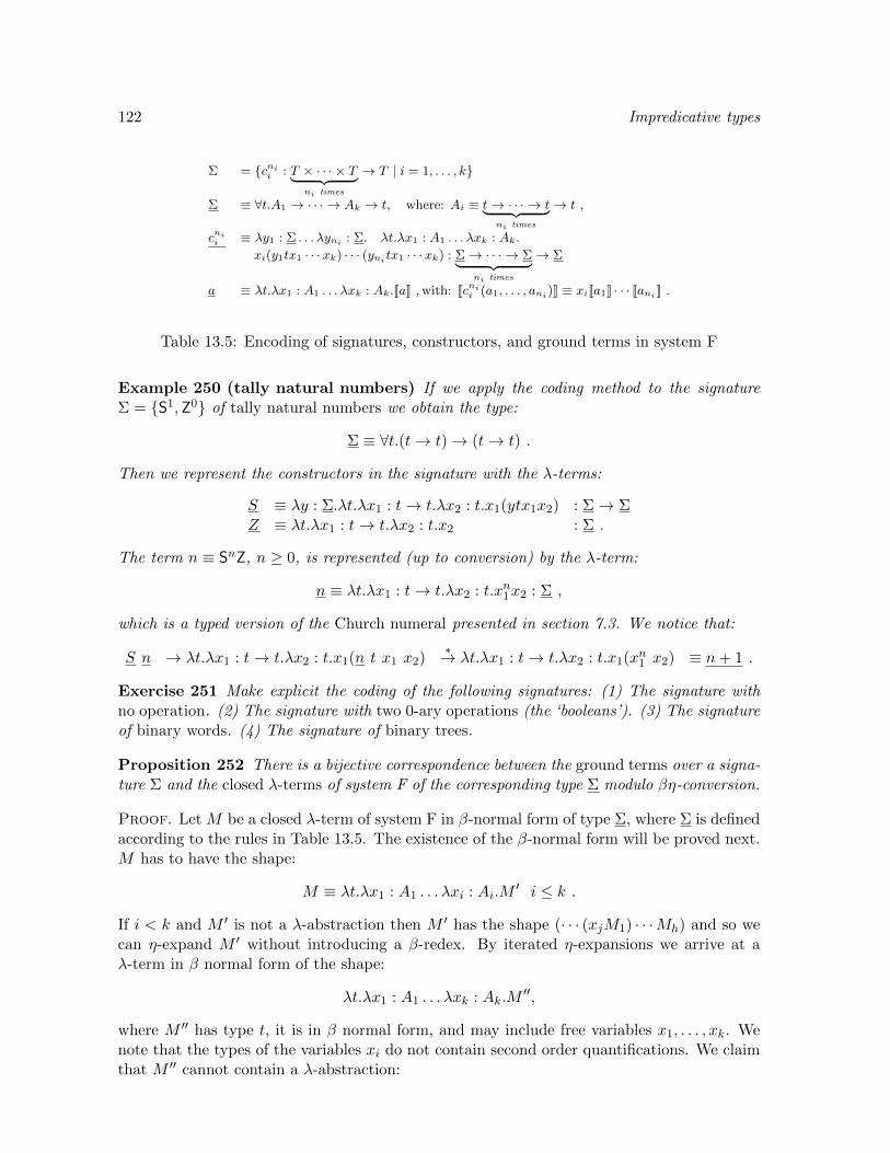
122 Impredicative types
Σ = cnii : T × · · · × T︸ ︷︷ ︸
ni times
→ T | i = 1, . . . , k
Σ ≡ ∀t.A1 → · · · → Ak → t, where: Ai ≡ t→ · · · → t︸ ︷︷ ︸ni times
→ t ,
cnii ≡ λy1 : Σ . . . λyni : Σ. λt.λx1 : A1 . . . λxk : Ak.
xi(y1tx1 · · ·xk) · · · (ynitx1 · · ·xk) : Σ→ · · · → Σ︸ ︷︷ ︸ni times
→ Σ
a ≡ λt.λx1 : A1 . . . λxk : Ak.[[a]] ,with: [[cnii (a1, . . . , ani)]] ≡ xi[[a1]] · · · [[ani ]] .
Table 13.5: Encoding of signatures, constructors, and ground terms in system F
Example 250 (tally natural numbers) If we apply the coding method to the signatureΣ = S1,Z0 of tally natural numbers we obtain the type:
Σ ≡ ∀t.(t→ t)→ (t→ t) .
Then we represent the constructors in the signature with the λ-terms:
S ≡ λy : Σ.λt.λx1 : t→ t.λx2 : t.x1(ytx1x2) : Σ→ ΣZ ≡ λt.λx1 : t→ t.λx2 : t.x2 : Σ .
The term n ≡ SnZ, n ≥ 0, is represented (up to conversion) by the λ-term:
n ≡ λt.λx1 : t→ t.λx2 : t.xn1x2 : Σ ,
which is a typed version of the Church numeral presented in section 7.3. We notice that:
S n → λt.λx1 : t→ t.λx2 : t.x1(n t x1 x2)∗→ λt.λx1 : t→ t.λx2 : t.x1(xn1 x2) ≡ n+ 1 .
Exercise 251 Make explicit the coding of the following signatures: (1) The signature withno operation. (2) The signature with two 0-ary operations (the ‘booleans’). (3) The signatureof binary words. (4) The signature of binary trees.
Proposition 252 There is a bijective correspondence between the ground terms over a signa-ture Σ and the closed λ-terms of system F of the corresponding type Σ modulo βη-conversion.
Proof. Let M be a closed λ-term of system F in β-normal form of type Σ, where Σ is definedaccording to the rules in Table 13.5. The existence of the β-normal form will be proved next.M has to have the shape:
M ≡ λt.λx1 : A1 . . . λxi : Ai.M′ i ≤ k .
If i < k and M ′ is not a λ-abstraction then M ′ has the shape (· · · (xjM1) · · ·Mh) and so wecan η-expand M ′ without introducing a β-redex. By iterated η-expansions we arrive at aλ-term in β normal form of the shape:
λt.λx1 : A1 . . . λxk : Ak.M′′,
where M ′′ has type t, it is in β normal form, and may include free variables x1, . . . , xk. Wenote that the types of the variables xi do not contain second order quantifications. We claimthat M ′′ cannot contain a λ-abstraction:

Impredicative types 123
• A λ-abstraction on the left of an application would contradict the hypothesis that M isin β normal form.
• A λ-abstraction on the right of an application is incompatible with the ‘first order’ typesof the variables Ai.
We have shown that a closed λ-term of type Σ is determined up to βη conversion by a λ-termM ′′ which is a well-typed combination of the variables xi, for i = 1, . . . , k. Since each variablecorresponds to a constructor of the signature we can conclude that there is a unique groundterm over the signature which corresponds to M ′′. 2
Remark 253 The rule (η) is needed to have a bijection between ground terms of the signatureΣ and closed λ-terms of type Σ. For instance, with reference to example 250 (tally naturalnumbers), there are two distinct λ-terms in β-normal form corresponding to the numeral 1,namely 1 and λt.λx1 : t→ t.x1.
Definition 254 A function f : Tn → T over a signature Σ is representable (with respect tothe proposed coding) if there is a closed λ-term M : Σn → Σ, such that for any vector ofground terms a∗:
Ma∗ =βη f(a∗) .
Proposition 255 All iterative functions over a signature Σ are representable.
Proof. We proceed by induction on the definition of iterative function. The interesting caseis iteration. Let hi : Tni+mS → TS be iterative functions for i = 1, . . . , k, and the functionf : Tm+1
S → TS be defined by:
f(x∗, ci(y∗)) = hi(x
∗, f(x∗, y1), . . . , f(x∗, yni)) i = 1, . . . , k , (13.2)
where x∗ ≡ x1, . . . , xm.1 We represent f with the function:
f ≡ λx1 : Σ. . . . λxm : Σ.λx : Σ.xΣ(h1x∗) · · · (hkx∗) ,
where we know inductively that hi represents hi. Note that iteration is already built into therepresentation of the data. We prove by induction on the structure of a ground term a thatfor any vector of ground terms b∗, f b∗ a =βη f(b∗, a).
• If a ≡ c0i then
f b∗ c0i →∗ c0
iΣ(h1b∗) · · · (hkb∗)→∗ hib∗ =βη hi(b
∗) ,
where the last step holds by induction hypothesis on hi.
• If a ≡ cni (a1, . . . , an) then:
f(b∗, ci(a1, . . . , an)) = hi(b∗, f(b∗, a1), . . . , f(b∗, an))
=βη hi b∗ f(b∗, a1) . . . f(b∗, an) (by induction hypothesis on hi).
1In this proof, it is convenient to write the additional parameters x∗ before the main argument of theiteration.

124 Impredicative types
On the other hand, we compute:
f b∗ cni (a1, . . . , an)
→ cni (a1, . . . , an)Σ(h1 b∗) · · · (hk b∗)
→ (hi b∗)(a1Σ(h1 b
∗) · · · (hk b∗)) · · · (anΣ(h1 b∗) · · · (hk b∗)) .
Also, by induction hypothesis on a, we have for i = 1, . . . , n:
f(b∗, ai) =βη fb∗ai
∗→ aiΣ(h1b∗) · · · (hkb∗)) .
Hence, by combining the computations above, we obtain:
f b∗ cni (a1, . . . , an) =βη hi b∗ f(b∗, a1) . . . f(b∗, an)
=βη f(b∗, ci(a1, . . . , an)) .
2
Example 256 Suppose T is the set of tally natural numbers and g : T → T and h : T 2 → T .The iteration it(h, g) of h and g must satisfy:
it(h, g)(Z, y) = g(y)it(h, g)(S(x), y) = h(it(h, g)(x, y), y)
In the pure λ-calculus, we would define:
it ≡ λh.λg.λx.λy. x (λz.h z y) (g y) .
For Σ ≡ ∀t.(t→ t)→ (t→ t), this is typable as follows:
it ≡ λh : Σ→ (Σ→ Σ).λg : Σ→ Σ.λx : Σ.λy : Σ.x Σ (λz : Σ.h z y) (g y)
: (Σ→ (Σ→ Σ))→ (Σ→ Σ)→ (Σ→ (Σ→ Σ)) .
Notice that this would not work with a propositional type of the shape (B → B)→ (B → B)!
Example 257 One can also handle the case of signatures which are defined parametricallywith respect to a collection of data. For instance List(D) is the signature of lists whoseelements belong to the set D. This signature is equipped with the constructors:
nil : List(D), cons : D × List(D)→ List(D) .
One can define iterative functions over List(D) and show that these functions can be rep-resented in system F for a suitable embedding of the closed λ-terms in system F. The sortList(D) is coded by the type:
∀t.t→ (r → t→ t)→ t ,
where r is a type variable, and generic elements in D are represented by (free) variables oftype r.

Impredicative types 125
13.3 Strong normalization
We now move towards a proof of the announced strong normalization result. The proofis based on a notion of reducibility candidate which is an abstraction of the notion alreadyconsidered for the strong normalization of the propositionally typed λ-calculus (chapter 10)and recursive path ordering (chapter 4). In order to make notation lighter we shall work withuntyped λ-terms obtained from the erasure of well-typed λ-terms.
Definition 258 (erasure) The (type) erasure function er takes a typed λ-term and returnsan untyped λ-term. It is defined by induction on the structure of the λ-term as follows:
er(x) = x, er(λx : A.M) = λx.er(M), er(MN) = er(M)er(N),er(λt.M) = er(M), er(MA) = er(M) .
In system F, we distinguish two flavors of β-reduction: the one involving a redex (λx :A.M)N which we call simply (β) and the one involving a redex (λt.M)A which we call (βt).Erasing type information we eliminate the reductions (βt). However this does not affect thestrong normalization property as shown in the following.
Proposition 259 (erasure vs. typed) Let M be a well-typed λ-term in system F. Then:
1. If M →β N then er(M)→β er(N).
2. If M →βt N then er(M) ≡ er(N).
3. If M may diverge then er(M) may diverge.
Proof. Properties (1) and (2) are left to the reader. For (3), we observe that sequences ofβt-reductions always terminate as the size of the λ-term shrinks. Hence we can extract aninfinite reduction of er(M) from an infinite reduction of M . 2
We can now address the key issue. Suppose we want to adapt the semantic method alreadyused in the propositional case. What is the interpretation of A ≡ ∀t.(t→ t)? We have to buildfirst a universe U of type interpretations where each type interpretation is a set of λ-terms.Then we could require:
[[A]] = M | ∀X ∈ U ∀N ∈ X (MN ∈ X) .
Technically, the type interpretations are the so-called reducibility candidates and are definedas follows. Let SN be the collection of untyped λ-terms which are strongly normalizable withrespect to the (β) rule. We shall use P,Q, . . . to denote the untyped λ-terms (as opposed tothe typed ones which are denoted with M,N, . . .).
Definition 260 (candidates) A set X of λ-terms is a reducibility candidate if:
1. X ⊆ SN .
2. Qi ∈ SN , i = 1, . . . , n, n ≥ 0 implies xQ1, . . . , Qn ∈ X.
3. [Q/x]PQ1, . . . , Qn ∈ X and Q ∈ SN implies (λx.P )QQ1, . . . , Qn ∈ X.

126 Impredicative types
We denote with RC the collection of reducibility candidates.
Remark 261 We have made into a definition the properties stated in proposition 216 of theinterpretation of propositional types.
Proposition 262 (properties reducibility candidates) The following properties hold.
1. The set SN is a reducibility candidate.
2. If X ∈ RC then X 6= ∅.
3. The collection RC is closed under arbitrary intersections.
4. If X,Y ∈ RC then the following set is a reducibility candidate:
X → Y = M | ∀N ∈ X (MN ∈ Y ) .
Proof. We abbreviate Q1, . . . , Qn with Q∗. We recall (definition 213) that if P ∈ SN thendepth(P ) is the length of its longest reduction.
(1) As in the propositional case, we observe that [Q/x]PQ∗ ∈ SN and Q ∈ SN implies(λx.P )QQ∗ ∈ SN . This is an induction on depth(P )+depth(Q)+depth(Q1)+· · ·+depth(Qn).
(2) By definition, x ∈ X.
(3) Immediate.
(4) Here we see the use of the ‘saturation’ condition (3) in definition 260. 2
Next we define a type interpretation.
Definition 263 (type interpretation) Let Tvar be the set of type variables. Given a typeenvironment η : Tvar → RC we interpret types as follows:
[[t]]η = η(t)[[A→ B]]η = [[A]]η → [[B]]η[[∀t.A]]η =
⋂X∈RC [[A]]η[X/t] .
We remark that the interpretations of a functional type and a universal type are well-defined because of propositions 262(4) and 262(3), respectively. Strong normalization followsfrom the soundness of the interpretation which is stated as follows.
Proposition 264 (soundness) Let η be a type environment and x1 : A1, . . . , xn : An `M :B a derivable judgment. If Pi ∈ [[Ai]]η, for i = 1, . . . , n then
[P1/x1, . . . , Pn/xn]er(M) ∈ [[B]]η .
Proof. We abbreviate [P1/x1, . . . , Pn/xn] with [P ∗/x∗]. We proceed by induction on thetyping proof.
(asmp) follows by definition.

Impredicative types 127
(→I) We have to show:
λx.[P ∗/x∗]er(M) ∈ [[A→ B]]η .
By inductive hypothesis, we know: [P ∗/x∗][P/x]er(M) ∈ [[B]]η, for all P ∈ [[A]]η. Weconclude by using the properties of reducibility candidates.
(→E) By the definition of →.
(∀I) We have to show:
[P ∗/x∗]er(M) ∈⋂
X∈RC
[[B]]η[X/t] .
By the side condition on the typing rule, we know: [[Ai]]η = [[Ai]]η[X/t], for an arbitraryX ∈ RC . By inductive hypothesis: [P ∗/x∗]er(M) ∈ [[B]]η[X/t], for an arbitrary X ∈RC .
(∀E) We have to show:
[P ∗/x∗]er(M) ∈ [[B]]η[[[A]]η/t] .
By inductive hypothesis: [P ∗/x∗]er(M) ∈⋂X∈RC [[B]]η[X/t]. Choose X = [[A]]η. 2
Corollary 265 (strong normalization) If Γ ` M : A in system F, then M is stronglynormalizing.
Proof. We note that ∀A, η, x (x ∈ [[A]]η). Then we apply proposition 264 with Pi ≡ xi,and derive that: er(M) ∈ [[A]]η ⊆ SN . By proposition 259, we conclude that M is stronglynormalizing. 2
Exercise 266 (neutral λ-term) Alternative definitions of reducibility candidates can befound in the literature; one follows. Say that a λ-term is neutral if it does not start witha λ-abstraction. Define Red(M) = M ′ |M →β M
′. The collection RC ′ is given by the setsX of strongly normalizing λ-terms satisfying the following conditions:
1. M ∈ X and M →β M′ implies M ′ ∈ X.
2. M neutral and Red(M) ⊆ X implies M ∈ X.
Carry on the strong normalization proof using the collection RC ′.
13.4 Summary and references
The introduction of second-order quantification preserves the standard properties of the propo-sitionally typed calculus: subject reduction, strong normalization, confluence . . . while in-creasing the expressivity in a very significant way as one can encode inductive data types anditerative functions. There is one catch however: type inference becomes undecidable whichis one reason why ML-like programming languages adopt a weaker/predicative form of poly-morphism. When extended with first-order quantification, system F is the backbone of ahigher-order constructive logic (the so called calculus of constructions on which the Coqproof assistant is built [CH88]).
128 Impredicative types
The system F has been introduced by Girard in [Gir71] as a tool for the study of thecut-elimination procedure in second order Peano arithmetic (PA2). More precisely the nor-malization of system F implies the termination of the cut-elimination procedure in PA2 (andthus the consistency of analysis!). By relying on this strong connection between system Fand PA2 it is proven that all functions that can be shown to be total in PA2 are representablein system F. This is a huge collection of total recursive functions that goes well beyond theprimitive recursive functions. The connections with the notion of type polymorphism (ortype parametricity) arising in programming are noticed in [Rey74] and the relationship be-tween existential types and abstract data types are pointed out in [MP88]. The results onthe representation of iterative functions are based on [BB85]. The type inference problem fora Curry-style system F (cf. chapter 12) turns out to be undecidable [Wel99].

Chapter 14
Program transformations
In this chapter, we introduce four program transformations. Each transformation has its owninterest. Moreover, when they are put in pipeline they provide a compilation chain from acall-by-value λ-calculus to a register transfer level (RTL) language. A RTL language can beregarded as a machine independent version of assembly code. Functions correspond to assem-bly level routines and the functions’ bodies correspond to sequences of vectors’ allocationsand vectors’ projections ended by a tail recursive call. The compilation chain is summarizedin the following diagram:
λCcps→ λcps
Cvn→ λcps,vnCcc→ λcc,vn
Ch→ λh,vn (14.1)
The source language is a call-by-value, λ-calculus (cf. chapter 8). The first transformation,called continuation-passing style (CPS), internalizes the notion of evaluation context, the sec-ond, called value naming, assigns a name to every value, the third, called closure conversion,internalizes the notion of closure and makes sure functions are closed, i.e., they do not containfree variables, and the last, called hoisting, transforms a collection of closed nested functiondefinitions into a collection of possibly open, flat, i.e., without nesting, function definitions.
Since we want to compose these transformations, we make sure the target language ofeach transformation coincides with the source of the following one. As a matter of fact, allthe languages are subsets of the initial source language though their evaluation mechanism isrefined along the way. In particular, one moves from an ordinary substitution to a specializedone where variables can only be replaced by other variables.
The approach to compiler correctness is similar to the one considered for the toy compilerof section 1.3. One proves that each transformation is correct in the sense that the objectcode simulates the source code. Then, by composition, one derives the correctness of thecompilation chain.
14.1 Continuation passing style form
The origin of the CPS transformation goes back to so called double-negation transformationsfrom classical to intuitionistic/constructive logic. In constructive logic, the formula ¬¬t→ tis not derivable but the formula ¬¬¬t → ¬t is (cf. exercise 200). Then the idea is totransform formulae in classical logic to negated formulae in constructive logic so that negationis involutive on the image of the transformation. For some fixed type variable s, let ¬A =
129

130 Program transformations
(A→ s), and define a transformation of propositional types and type contexts as follows:
t = t , A→ B = A→ ¬¬B , ∅ = ∅ , Γ, x : A = Γ, x : A .
What the transformation shows is that for for every formula A provable in classical logic,there is a classicaly equivalent formula ¬¬A which is provable in constructive logic. Nowsuppose we start with a λ-term of type A, say Γ ` M : A, i.e., with a constructive proof ofA. Can we build a λ-term M such that Γ `M : ¬¬A ? For variables and λ-abstractions, thetyping suggests directly:
x = λk.kx , λx.M = λk.k(λx.M) .
The case for application is a bit more complex, but the reader may easily check that thefollowing does the job:
MN = λk.M(λm.N(λn.mnk)) .
Moreover, the transformed λ-term simulates the original one as soon it is provided with anadditional argument which represents the initial evaluation context. For instance, the readermay check that:
((λx.x)y)(λz.z)∗→β y , (14.2)
where λz.z stands for the initial evaluation context. As a matter of fact, types are useless inproving the simulation property and they will be omitted in the following formal treatment.However, as we have seen, types shed light on the CPS transformation and we shall comeback to them in chapter 15. The reader may have noticed that the reduction (14.2) aboveperforms many ‘useless’ β-reductions. For this reason, as well as for simplifying the proofstrategy, we shall study an optimized version of the CPS transformation.
Table 14.1 introduces the source language: a type-free, left-to-right, call-by-value λ-calculus. Notice that for technical reasons we include the variables among the values. Alsonotice that the calculus is richer than the one studied in chapter 8 in that it includes let-definitions, polyadic abstraction, and tupling, with the related application and projectionoperators. Polyadic abstraction grants a function the right to take several arguments at oncewhile tupling allows to build vectors of terms. For the sake of readibility, we shall denoteexplicitly the polyadic application with the symbol @. We stress that polyadic abstractioncan be simulated by iterated λ-abstraction and tupling can be simulated by iterated pairing.Still, it is worth to take them as primitive in order to simplify the analysis of the followingprogram transformations.
Working with polyadic abstraction and tuples, we need a compact notation to representsequences of symbols. We shall write X+ (resp. X∗) for a non-empty (possibly empty) finitesequence X1, . . . , Xn of symbols. By extension, λx+.M stands for λx1 . . . xn.M , [V +/x+]Mstands for [V1/x1, . . . , Vn/xn]M , and let (x = V )+ in M stands for let x1 = V1 in · · · let xn =Vn in M . By default, a term is a λ-term in the enriched λ-calculus under consideration.
Table 14.2 introduces a fragment of the λ-calculus described in Table 14.1 and a relatedCPS transformation. An evaluation context E can be represented as a term λx.E[x]; in a CPStransformation each function takes its evaluation context, represented as a term, as a freshadditional parameter. The initial evaluation context is defined relatively to a fresh variablenamed ’halt ’.
The syntax of CPS terms is such that in an application all terms are values and thisproperty is preserved by reduction. A corollary of this syntactic restriction is that the redex

Program transformations 131
Syntax
V ::= id || λid+.M || (V ∗) (values)M ::= V || @(M,M+) || let id = M in M || (M∗) || πi(M) || (terms)E ::= [ ] || @(V ∗, E,M∗) || let id = E in M || (V ∗, E,M∗) || πi(E) (evaluation contexts)
Reduction Rules
E[@(λx1 . . . xn.M, V1, . . . , Vn)] → E[[V1/x1, . . . , Vn/xn]M ]E[let x = V in M ] → E[[V/x]M ]E[πi(V1, . . . , Vn)] → E[Vi] (1 ≤ i ≤ n)
Table 14.1: A polyadic, call-by-value, λ-calculus: λ
of a CPS term is always at top level, or in another terms, the evaluation context of a CPS termis always the trivial context ‘[ ]′. The reduction rules are essentially those of the λ-calculusmodulo the fact that we optimize the rule for the projection to guarantee that CPS termsare closed under reduction. For instance, the term let x = π1(V1, V2) in M reduces directly to[V1/x]M rather than going through the intermediate term let x = V1 in M which, accordingto Table 14.2, does not belong to the CPS terms. There is a potential ambiguity concerningthe CPS transformation of tuples of values. We remove it, by assuming that (V1, . . . , Vn) | Kis transformed according to the case for values. But note that if we follow the general casefor tuples we obtain the same result.
Next, we state the properties enjoyed by the presented CPS transformation, which is‘optimized’ so as to pre-compute many ‘administrative’ reductions. In particular, thanks tothis optimization, we can show that the CPS transformation of a term such as E[@(λx.M, V )]is a term of the shape @(ψ(λx.M), ψ(V ),KE) for a suitable continuation KE depending onthe evaluation context E.
Proposition 267 (CPS simulation) Let M be a term of the λ-calculus. If M → N then
Ccps(M)∗→ Ccps(N).
Proof. The proof takes the following steps.
1. We show that for all values V , terms M , and continuations K 6= x:
[V/x]M | [ψ(V )/x]K ≡ [ψ(V )/x](M | K) .
We proceed by induction on M .
variable By case analysis: M ≡ x or M ≡ y 6= x.
λz+.M By case analysis on K which is either a variable or a function. We develop thesecond case with K ≡ λy.N . We observe:
[V/x](λz+.M) | [ψ(V )/x]K≡ [λz+, k.([V/x]M | k)/y][ψ(V )/x]N≡ [λz+, k.[ψ(V )/x](M | k)/y][ψ(V )/x]N≡ [ψ(V )/x][λz+, k.(M | k)/y]N≡ [ψ(V )/x]((λz+.M) | K) .

132 Program transformations
@(M0, . . . ,Mn) We apply the inductive hypothesis on M0, . . . ,Mn as follows:
[ψ(V )/x](@(M0, . . . ,Mn) | K)≡ [ψ(V )/x](M0 | λx0 . . .Mn | λxn.@(x0, . . . , xn,K))· · ·≡ [V/x]M0 | λx0 . . . [ψ(V )/x](Mn | λxn.@(x0, . . . , xn,K))≡ [V/x]M0 | λx0 . . . [V/x]Mn | λxn.@(x0, . . . , xn, [ψ(V )/x]K)≡ [V/x]@(M0, . . . ,Mn) | [ψ(V )/x]K .
Note that in this case the substitution [ψ(V )/x] may operate on the continuation.The remaining cases (pairing, projection, let-definition) follow a similar patternand are omitted.
2. The evaluation contexts for the λ-calculus described in Table 14.1 can also be specified‘bottom up’ as follows:
E ::= [ ] || E[@(V ∗, [ ],M∗)] || E[let id = [ ] in M ] || E[(V ∗, [ ],M∗)] || E[πi([ ])] .
Following this specification, we associate with an evaluation context E a continuationKE as follows:
K[ ] = λx.@(halt , x)
KE[@(V ∗,[ ],M∗)] = λx.M∗ | λy∗.@(ψ(V )∗, x, y∗,KE)
KE[let x=[ ] in N ] = λx.N | KE
KE[(V ∗,[ ],M∗)] = (λx.M∗ | λy∗.(ψ(V )∗, x, y∗)) | KE
KE[πi([ ]) = λx.let y = πi(x) in y | KE ,
where M∗ | λx∗.N stands for M0 | λx0 . . .Mn | λxn.N with n ≥ 0.
3. For all terms M and evaluation contexts E,E′ we prove by induction on the evaluationcontext E that the following holds:
E[M ] | KE′ ≡M | KE′[E] .
For instance, we detail the case where the context has the shape E[@(V ∗, [ ],M∗)].
E[@(V ∗, [M ],M∗)] | KE′
≡ @(V ∗, [M ],M∗) | KE′[E] (by inductive hypothesis)
≡M | λx.M∗ | λx∗.@(ψ(V )∗, x, x∗,KE′[E])
≡M | KE′[E[@(V ∗,[ ],M∗)]] .
4. For all terms M , continuations K,K ′, and variable x /∈ fv(M) we prove by inductionon M and case analysis that the following holds:
[K/x](M | K ′)→M | K ′ if K abstraction,M value,K ′ = x≡ (M | [K/x]K ′) otherwise.

Program transformations 133
5. Finally, we prove the assertion by case analysis on the reduction rule. We consider thecase for application. Suppose E[@(λx+.M, V +)]→ E[[V +/x+]M ]. We have:
E[@(λx+.M, V +)] | K[ ]
≡ @(λx+.M, V +) | KE
≡ @(λx+, k.M | k, ψ(V )+,KE)→ [KE/k, ψ(V )+/x+](M | k)≡ [KE/k]([V +/x+]M | k)∗→ [V +/x+]M | KE
≡ E[[V +/x+]M ] | K[ ] .
2
We illustrate this result on the following example.
Example 268 (CPS) Let M ≡ @(λx.@(x,@(x, x)), I), where I ≡ λx.x. Then
Ccps(M) ≡ @(λx, k.@(x, x, λy.@(x, y, k)), I ′, H) ,
where: I ′ ≡ λx, k.@(k, x) and H ≡ λx.@(halt , x). The term M is simulated by Ccps(M) asfollows:
M → @(I,@(I, I)) → @(I, I) → ICcps(M) → @(I ′, I ′, λy.@(I ′, y,H)) →+ @(I ′, I ′, H) →+ @(halt , I ′) .
Exercise 269 Write down a simplified CPS transformation for a monadic call-by-value λ-calculus without let-definitions and tuples. Then apply the CPS transformation to show that itis possible to simulate the call-by-value λ-calculus in the call-by-name λ-calculus (cf. chapter8).
Exercise 270 So called control operators are programming instructions that alter the exe-cution flow. For instance, consider the continue and break commands of exercise 5 and thecontrol C and abort A operators of exercise 166. CPS transformations allow to simulate suchoperators in a purely functional setting.
1. In chapter 1, we have interpreted a statement of the Imp language as function of type(State → State). Define an alternative functional interpretation where a command isregarded as a function of type:
State → (State → State)→ State .
and show that such interpretation can be extended to interpret a command abort whichstops the computation and returns the current state.
2. Define a CPS transformation of the call-by-value λ-calculus extended with the controloperators C and A defined in exercise 166.
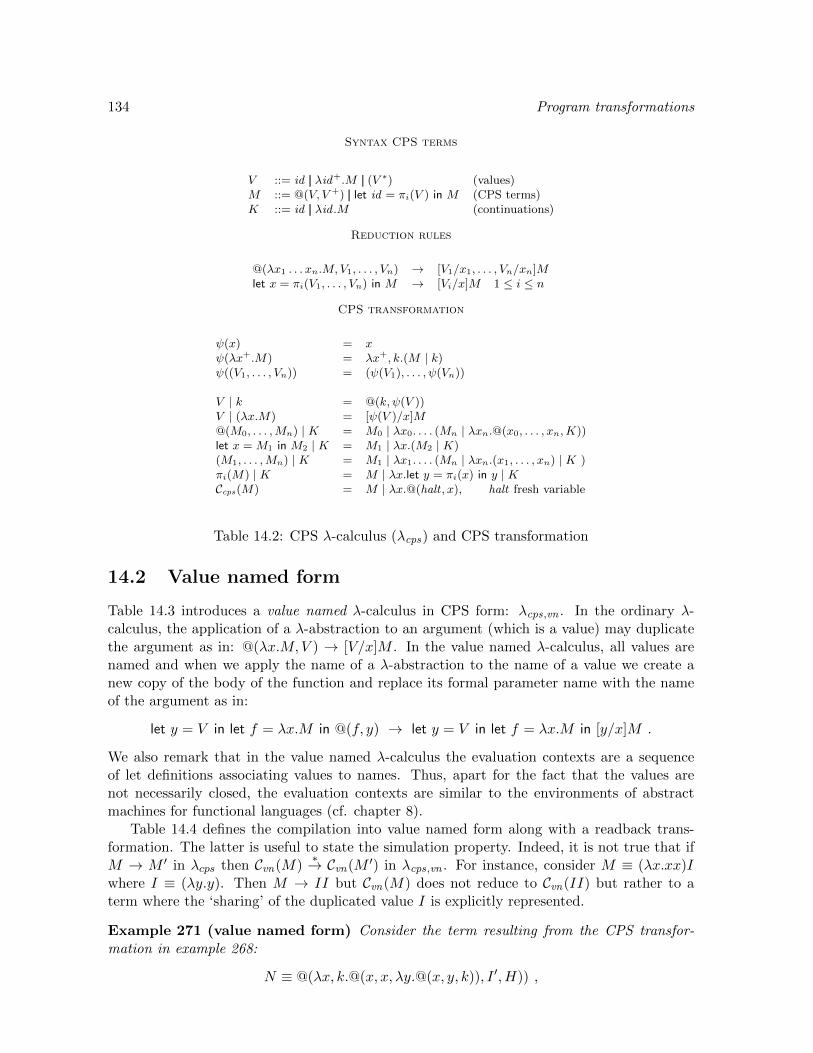
134 Program transformations
Syntax CPS terms
V ::= id || λid+.M || (V ∗) (values)M ::= @(V, V +) || let id = πi(V ) in M (CPS terms)K ::= id || λid .M (continuations)
Reduction rules
@(λx1 . . . xn.M, V1, . . . , Vn) → [V1/x1, . . . , Vn/xn]Mlet x = πi(V1, . . . , Vn) in M → [Vi/x]M 1 ≤ i ≤ n
CPS transformation
ψ(x) = xψ(λx+.M) = λx+, k.(M | k)ψ((V1, . . . , Vn)) = (ψ(V1), . . . , ψ(Vn))
V | k = @(k, ψ(V ))V | (λx.M) = [ψ(V )/x]M@(M0, . . . ,Mn) | K = M0 | λx0. . . . (Mn | λxn.@(x0, . . . , xn,K))let x = M1 in M2 | K = M1 | λx.(M2 | K)(M1, . . . ,Mn) | K = M1 | λx1. . . . (Mn | λxn.(x1, . . . , xn) | K )πi(M) | K = M | λx.let y = πi(x) in y | KCcps(M) = M | λx.@(halt , x), halt fresh variable
Table 14.2: CPS λ-calculus (λcps) and CPS transformation
14.2 Value named form
Table 14.3 introduces a value named λ-calculus in CPS form: λcps,vn . In the ordinary λ-calculus, the application of a λ-abstraction to an argument (which is a value) may duplicatethe argument as in: @(λx.M, V ) → [V/x]M . In the value named λ-calculus, all values arenamed and when we apply the name of a λ-abstraction to the name of a value we create anew copy of the body of the function and replace its formal parameter name with the nameof the argument as in:
let y = V in let f = λx.M in @(f, y) → let y = V in let f = λx.M in [y/x]M .
We also remark that in the value named λ-calculus the evaluation contexts are a sequenceof let definitions associating values to names. Thus, apart for the fact that the values arenot necessarily closed, the evaluation contexts are similar to the environments of abstractmachines for functional languages (cf. chapter 8).
Table 14.4 defines the compilation into value named form along with a readback trans-formation. The latter is useful to state the simulation property. Indeed, it is not true that ifM → M ′ in λcps then Cvn(M)
∗→ Cvn(M ′) in λcps,vn . For instance, consider M ≡ (λx.xx)Iwhere I ≡ (λy.y). Then M → II but Cvn(M) does not reduce to Cvn(II) but rather to aterm where the ‘sharing’ of the duplicated value I is explicitly represented.
Example 271 (value named form) Consider the term resulting from the CPS transfor-mation in example 268:
N ≡ @(λx, k.@(x, x, λy.@(x, y, k)), I ′, H)) ,

Program transformations 135
Syntax
V ::= λid+.M || (id∗) (values)C ::= V || πi(id) (let-bindable terms)M ::= @(id , id+) || let id = C in M (CPS terms)E ::= [ ] || let id = V in E (evaluation contexts)
Reduction Rules
E[@(x, z1, . . . , zn)] → E[[z1/y1, . . . , zn/yn]M ] if E(x) = λy1 . . . yn.ME[let z = πi(x) in M ] → E[[yi/z]M ]] if E(x) = (y1, . . . , yn), 1 ≤ i ≤ n
where: E(x) =
V if E = E′[let x = V in [ ]]E′(x) if E = E′[let y = V in [ ]], x 6= yundefined otherwise
Table 14.3: A value named CPS λ-calculus: λcps,vn
where: I ′ ≡ λx, k.@(k, x) and H ≡ λx.@(halt , x). The corresponding term in value namedform is:
let z1 = λx, k.(let z11 = λy.@(x, y, k) in @(x, x, z11)) inlet z2 = I ′ inlet z3 = H in@(z1, z2, z3) .
Proposition 272 (vn simulation) Let N be a term in CPS value named form. If R(N) ≡M and M
α→M ′ then there exists N ′ such that Nα→ N ′ and R(N ′) ≡M ′.
Proof. First we fix some notation. We associate a substitution σE with an evaluationcontext E of the λcps,vn -calculus as follows:
σ[ ] = Id σlet x=V in E = [R(V )/x] σE .
Then we prove the property by case analysis. We look at the case:
R(N) ≡ @(λy+.M, V +)→ [V +/y+]M .
Then N ≡ E[@(x, x+)], σE(x) ≡ λy+.M , and σE(x+) ≡ V +. Moreover, E ≡ E1[let x =λy+.M ′ in E2] and σE1(λy+.M ′) ≡ λy+.M . Therefore, N → E[[x+/y+]M ′] ≡ N ′ and wecheck that R(N ′) ≡ σE([x+/y+]M ′) ≡ [V +/y+]M . 2
14.3 Closure conversion
The next step is called closure conversion. It consists in providing each functional value withan additional parameter that accounts for the names free in the body of the function and inrepresenting functions using closures. Our closure conversion function implements a closureusing a pair whose first component is the code of the transformed function and whose secondcomponent is a tuple containing the values of the free variables.

136 Program transformations
Transformation in value named form (from λcps to λcps,vn)
Cvn(@(x0, . . . , xn)) = @(x0, . . . , xn)Cvn(@(x∗, V, V ∗)) = Evn(V, y)[Cvn(@(x∗, y, V ∗))] V 6= id , y freshCvn(let x = πi(y) in M) = let x = πi(y) in Cvn(M)Cvn(let x = πi(V ) in M) = Evn(V, y)[let x = πi(y) in Cvn(M)] V 6= id , y freshEvn(λx+.M, y) = let y = λx+.Cvn(M) in [ ]Evn((x∗), y) = let y = (x∗) in [ ]Evn((x∗, V, V ∗), y) = Evn(V, z)[Evn((x∗, z, V ∗), y)] V 6= id , z fresh
Readback transformation (from λcps,vn to λcps)
R(λx+.M) = λx+.R(M)R(x∗) = (x∗)R(@(x, x1, . . . , xn)) = @(x, x1, . . . , xn)R(let x = πi(y) in M) = let x = πi(y) in R(M)R(let x = V in M) = [R(V )/x]R(M)
Table 14.4: Transformations in value named CPS form and readback
It will be convenient to write “let (y1, . . . , yn) = x in M” for “let y1 = π1(x) in · · · let yn =πn(x) in M” and “let x1 = C1 . . . xn = Cn in M” for “let x1 = C1 in . . . let xn = Cn in M”.The transformation is described in Table 14.5. The output of the transformation is such thatall functional values are closed.
Example 273 (closure conversion) Let M ≡ Cvn(Ccps(λx.y)), namely:
M ≡ let z1 = λx, k.@(k, y) in @(halt , z1) .
Then Ccc(M) is the following term:
let c = λe, x, k.(let (y) = e, (c, e) = k in @(c, e, y)) inlet e = (y), z1 = (c, e), (c, e) = halt in@(c, e, z1) .
Proposition 274 (CC simulation) Let M be a CPS term in value named form. If M →M ′ then Ccc(M)
∗→ Ccc(M ′).
Proof. As a first step we check that the closure conversion function commutes with namesubstitution:
Ccc([x/y]M) ≡ [x/y]Ccc(M) .
This is a direct induction on the structure of the term M . Then we extend the closureconversion function to contexts as follows:
Ccc([ ]) = [ ]Ccc(let x = (y∗) in E) = let x = (y∗) in Ccc(E)Ccc(let x = λx+.M in E) = let c = λe, x+.let (z1, . . . , zk) = e in Ccc(M) in
let e = (z1, . . . , zk), x = (c, e) in Ccc(E)where: fv(λx+.M) = z1, . . . , zk .
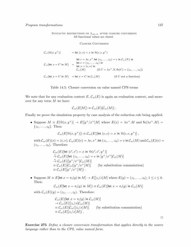
Program transformations 137
Syntactic restrictions on λcps,vn after closure conversionAll functional values are closed.
Closure Conversion
Ccc(@(x, y+)) = let (c, e) = x in @(c, e, y+)
Ccc(let x = C in M) =
let c = λe, x+.let (z1, . . . , zk) = e in Ccc(N) inlet e = (z1, . . . , zk) inlet x = (c, e) inCcc(M) (if C = λx+.N, fv(C) = z1, . . . , zk)
Ccc(let x = C in M) = let x = C in Ccc(M) (if C not a function)
Table 14.5: Closure conversion on value named CPS terms
We note that for any evaluation context E, Ccc(E) is again an evaluation context, and more-over for any term M we have:
Ccc(E[M ]) ≡ Ccc(E)[Ccc(M)] .
Finally we prove the simulation property by case analysis of the reduction rule being applied.
• Suppose M ≡ E[@(x, y+)] → E[[y+/x+]M ] where E(x) = λx+.M and fv(λx+.M) =z1, . . . , zk. Then:
Ccc(E[@(x, y+)]) ≡ Ccc(E)[let (c, e) = x in @(c, e, y+)] ,
with Ccc(E)(x) = (c, e), Ccc(E)(c) = λe, x+.let (z1, . . . , zk) = e in Ccc(M) and Ccc(E)(e) =(z1, . . . , zk). Therefore:
Ccc(E)[let (c′, e′) = x in @(c′, e′, y+)]∗→ Ccc(E)[let (z1, . . . , zk) = e in [y+/x+]Ccc(M)]∗→ Ccc(E)[[y+/x+]Ccc(M)]≡ Ccc(E)[Ccc([y+/x+]M)] (by substitution commutation)≡ Ccc(E[[y+/x+]M ]) .
• Suppose M ≡ E[let x = πi(y) in M ]→ E[[zi/x]M ] where E(y) = (z1, . . . , zk), 1 ≤ i ≤ k.Then:
Ccc(E[let x = πi(y) in M ]) ≡ Ccc(E)[let x = πi(y) in Ccc(M)]
with Ccc(E)(y) = (z1, . . . , zk). Therefore:
Ccc(E)[let x = πi(y) in Ccc(M)]→ Ccc(E)[[zi/x]Ccc(M)]≡ Ccc(E)[Ccc([zi/x]M)] (by substitution commutation)≡ Ccc(E[[zi/x]M ]) .
2
Exercise 275 Define a closure conversion transformation that applies directly to the sourcelanguage rather than to the CPS, value named form.
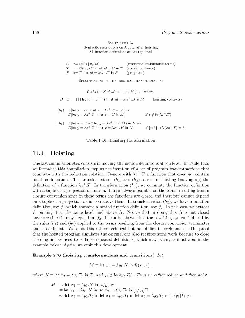
138 Program transformations
Syntax for λhSyntactic restrictions on λcps,vn after hoisting
All function definitions are at top level.
C ::= (id∗) || πi(id) (restricted let-bindable terms)T ::= @(id , id+) || let id = C in T (restricted terms)P ::= T || let id = λid+.T in P (programs)
Specification of the hoisting transformation
Ch(M) = N if M ; · · ·; N 6;, where:
D ::= [ ] || let id = C in D || let id = λid+.D in M (hoisting contexts)
(h1) D[let x = C in let y = λz+.T in M ] ;D[let y = λz+.T in let x = C in M ] if x /∈ fv(λz+.T )
(h2) D[let x = (λw+.let y = λz+.T in M) in N ] ;D[let y = λz+.T in let x = λw+.M in N ] if w+ ∩ fv(λz+.T ) = ∅
Table 14.6: Hoisting transformation
14.4 Hoisting
The last compilation step consists in moving all function definitions at top level. In Table 14.6,we formalize this compilation step as the iteration of a set of program transformations thatcommute with the reduction relation. Denote with λz+.T a function that does not containfunction definitions. The transformations (h1) and (h2) consist in hoisting (moving up) thedefinition of a function λz+.T . In transformation (h1), we commute the function definitionwith a tuple or a projection definition. This is always possible on the terms resulting from aclosure conversion since in these terms the functions are closed and therefore cannot dependon a tuple or a projection definition above them. In transformation (h2), we have a functiondefinition, say f1 which contains a nested function definition, say f2. In this case we extractf2 putting it at the same level, and above f1. Notice that in doing this f1 is not closedanymore since it may depend on f2. It can be shown that the rewriting system induced bythe rules (h1) and (h2) applied to the terms resulting from the closure conversion terminatesand is confluent. We omit this rather technical but not difficult development. The proofthat the hoisted program simulates the original one also requires some work because to closethe diagram we need to collapse repeated definitions, which may occur, as illustrated in theexample below. Again, we omit this development.
Example 276 (hoisting transformations and transitions) Let
M ≡ let x1 = λy1.N in @(x1, z) ,
where N ≡ let x2 = λy2.T2 in T1 and y1 /∈ fv(λy2.T2). Then we either reduce and then hoist:
M → let x1 = λy1.N in [z/y1]N≡ let x1 = λy1.N in let x2 = λy2.T2 in [z/y1]T1
; let x2 = λy2.T2 in let x1 = λy1.T1 in let x2 = λy2.T2 in [z/y1]T1 6;

Program transformations 139
or hoist and then reduce:
M ; let x2 = λy2.T2 in let x1 = λy1.T1 in @(x1, z)→ let x2 = λy2.T2 in let x1 = λy1.T1 in [z/y1]T1 6;
In the first case, we end up duplicating the definition of x2.
We conclude by sketching an alternative definition of the hoisting transformation. Let hbe a function that takes a term M in CPS, value named form where all functions are closedand produces a pair (T, F ), where T is a term without function definitions as specified inTable 14.6, and F is a one-hole context composed of a list of function definitions of the shape:
F ::= [ ] || let id = λid+.T in F .
The definition of the function h is given by induction on M as follows where C is a tuple ora projection as in Table 14.6:
h(@(x, y+)) = (@(x, y+), [ ])h(let x = C in M) = let (T, F ) = h(M) in (let x = C in T, F )h(let x = λy+.M in N) = let (T, F ) = h(M), (T ′, F ′) = h(N) in
(T ′, F [let x = λy+.T in F ′]) .
The hoisting transformation of the term M then amounts to compute (T, F ) = h(M) andthen build the term F [T ] which is a program according to the syntax defined in Table 14.6.
Exercise 277 Apply the hoisting transformation to the terms resulting from the closure con-version of exercise 275.
14.5 Summary and references
We have studied four program transformations: continuation passing style makes the evalu-ation context an additional parameter, value naming assigns a name to every value, closureconversion explicits the notion of closure, and hoisting removes nested function definitions.By putting these transformations in pipeline it is possible to transform a program written in ahigher-order language such as ML into a system of functions whose body includes operationsto build and project tuples of names and to perform tail-recursive routine calls. Thus wehave an implementation technique for higher-order languages which is alternative to the onebased on the abstract machines presented in chapter 8. A similar compilation chain has beenanalyzed in [Chl10] which provides machine certified simulation proofs. A simpler compila-tion chain arises if we bypass the CPS transformation. In this case, the function calls arenot necessarily tail-recursive and the target code can be described as C code with functionpointers (cf. exercises 275 and 277). An early analysis of the CPS transformation is in [Plo75].The idea of value-naming transformation is associated with various formalizations of sharing,see, e.g., [Lau93]. Closure conversion arises naturally when trying to define the interpreterof a higher-order language in the language itself, see, e.g., [Rey98]. Hoisting appears to befolklore.

140 Program transformations

Chapter 15
Typing the programtransformations
We describe a typing of the compilation chain described in chapter 14. Specifically, eachλ-calculus of the compilation chain is equipped with a type system which enjoys subjectreduction: if a term has a type then all terms to which it reduces have the same type. Thenthe compilation functions are extended to types and are shown to be type preserving: if aterm has a type then its compilation has the corresponding compiled type.
The two main steps in typing the compilation chain concern the CPS and the closureconversion transformations. The typing of the CPS transformation has already been sketchedin chapter 14 where it has served as a guideline. A basic idea is to type the continuation/theevaluation context of a term of type A with its negated type ¬A = (A → R), where Ris traditionally taken as the type of ‘results’. In typing closure conversion, one relies onexistential types (cf. chapter 13) to hide the details of the representation of the ‘environment’of a function, i.e., the tuple of variables occurring free in its body. Thus, to type the (abstract)assembly code coming from the compilation of propositionally typed programs, we need togo beyond propositional types.
To represent types we shall follow the notation introduced starting from chapter 10. Inparticular, we denote with tid the syntactic category of type variables with generic elementst, s, . . . and with A the syntactic category of types with generic elements A,B, . . . We writex∗ : A∗ for a possibly empty sequence x1 : A1, . . . , xn : An, and Γ, x∗ : A∗ for the contextresulting from Γ by adding the sequence x∗ : A∗. Hence the variables in x∗ must not be inthe domain of Γ. If A is a type, we write ftv(A) for the set of type variables occurring free init and, by extension, if Γ is a type context then ftv(Γ) is the union of the sets ftv(A) whereA is a type in the codomain of Γ. A typing judgment is typically written as Γ `M : A whereM is some term. We shall write Γ ` M∗ : A∗ for Γ ` M1 : A1, . . . ,Γ ` Mn : An. Similarconventions apply if we replace the symbol ‘∗′ with the symbol ‘+′ except that in this casethe sequence is assumed not-empty. A type transformation, say T , is lifted to type contextsby defining T (x1 : A1, . . . xn : An) = x1 : T (A1), . . . , xn : T (An). Whenever we write:
if Γ `S1 M : A then T (Γ) `S2 T (M) : T (A)
what we actually mean is that if the judgment in the hypothesis is derivable in a certain ‘typesystem S1’ then the transformed judgment in derivable in the ‘type system S2’. Proofs arestandard and are left as exercises.
141

142 Typing the transformations
Syntax types
A ::= tid || A+ → A || ×(A∗) (types)
Typing rules
x : A ∈ Γ
Γ ` x : A
Γ, x : A ` N : BΓ `M : A
Γ ` let x = M in N : B
Γ, x+ : A+ `M : B
Γ ` λx+.M : A+ → B
Γ `M : A+ → BΓ ` N+ : A+
Γ ` @(M,N+) : B
Γ `M∗ : A∗
Γ ` (M∗) : ×(A∗)
Γ `M : ×(A1, . . . , An) 1 ≤ i ≤ nΓ ` πi(M) : Ai
Restricted syntax CPS types, R type of results
A ::= tid || A+ → R || ×(A∗) (CPS types)
CPS type compilation
Ccps(t) = tCcps(×(A∗)) = ×(Ccps(A)∗)Ccps(A+ → B) = (Ccps(A))+,¬Ccps(B)→ R
where: ¬A ≡ (A→ R)
Table 15.1: Type system for λ and λcps
15.1 Typing the CPS form
Table 15.1 describes the typing rules for the polyadic, call-by-value, λ-calculus defined inTable 14.1. These rules are a slight generalization of those studied in chapter 10 and theyare preserved by reduction. The typing rules described in Table 15.1 apply to the CPS λ-calculus too. Table 15.1 describes the restricted syntax of the CPS types and the CPS typetransformation. Then the CPS term transformation defined in Table 14.2 preserves typing inthe following sense.
Proposition 278 (type CPS) If Γ `M : A then Ccps(Γ), halt : ¬Ccps(A) ` Ccps(M) : R.
15.2 Typing value-named closures
Table 15.2 describes the typing rules for the value named calculi with functional, product, andexistential types. Notice that for the sake of brevity, we shall omit the type of a term sincethis type is always the type of results R and write Γ `vn M rather than Γ `vn M : R. Thefirst five typing rules are just a specialization of the corresponding rules in Table 15.1, whilethe last two rules allow for the introduction and elimination of existential types. The need forexistential types will be motivated next. For the time being, let us notice that in the proposed

Typing the transformations 143
formalization we rely on the tuple constructor to introduce an existential type and the firstprojection to eliminate it. This has the advantage of leaving unchanged the syntax and thereduction rules of the value named λ-calculus. An alternative presentation (cf. chapter 13)consists in introducing specific operators to introduce and eliminate existential types denotedwith pack and unpack, respectively. Then one can read (x) as pack(x) and π1(x) as unpack(x)when x has an existential type. Notice that the rewriting rule which allows to unpack a packedvalue is just a special case of the rule for projection. As in the previous system, typing ispreserved by reduction.
Proposition 279 (subject reduction, value named) If M is a term of the λcps,vn-calculus,Γ `vn M and M → N then Γ `vn N .
Turning to the transformation from CPS to value named CPS form specified in Table 14.4we notice that it affects the terms but not the types. Therefore we have the following property.
Proposition 280 (type value named) If M is a term of the λcps-calculus and Γ `M : Rthen Γ `vn Cvn(M).
Next we discuss the typing of closure conversion via existential types (Table 15.2). Werecall that in closure conversion a function, say λx.M with free variables z1, . . . , zn, becomesa pair (here we ignore the details of the CPS, value named form):
(λe, x.let (z1, . . . , zn) = e in C(M), (z1, . . . , zn)) (15.1)
whose first component is the function itself, which is closed by taking the environment e asan additional argument, and the second component is a tuple containg the values of the freevariables. Now consider the functions identity and successor on the natural numbers codedas follows:
λx.x , let y = 1 in λx.x+ y , (15.2)
with a type, say, N → N. After closure conversion, we obtain the following pairs with therespective different types:
(λe, x.let () = e in x, ()) : ((1×N)→ N)× 1(λe, x.let (y) = e in x+ y, (y)) : ((N×N)→ N)×N .
Then take a function such as F : (N→ N)→ N which can operate both on the identity andthe successor function. This is no longer possible after closure conversion if we stick to thetyping outlined above. We can address this issue by abstracting the types of the identity andsuccessor functions after closure conversion into the following existential type:
∃t.((t×N)→ N)× t . (15.3)
To summarize, an environment is a tuple whose size depends on the number of variablesoccurring free in the function. This information should be abstracted in the type; otherwise,we cannot type functions operating on arguments with environments of different size.
In order to respect our conventions on the introduction and elimination of existential types,the closure conversion transformation is slightly modified in the way described in Table 15.3.This modified closure conversion still enjoys the simulation properties stated in proposition274 and moreover it preserves typing as follows.
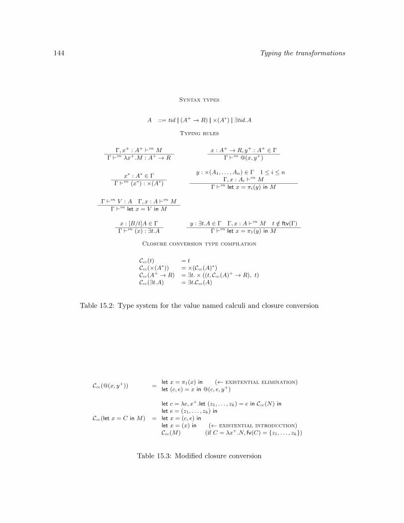
144 Typing the transformations
Syntax types
A ::= tid || (A+ → R) || ×(A∗) || ∃tid .A
Typing rules
Γ, x+ : A+ `vn MΓ `vn λx+.M : A+ → R
x : A+ → R, y+ : A+ ∈ Γ
Γ `vn @(x, y+)
x∗ : A∗ ∈ Γ
Γ `vn (x∗) : ×(A∗)
y : ×(A1, . . . , An) ∈ Γ 1 ≤ i ≤ nΓ, x : Ai `vn M
Γ `vn let x = πi(y) in M
Γ `vn V : A Γ, x : A `vn MΓ `vn let x = V in M
x : [B/t]A ∈ Γ
Γ `vn (x) : ∃t.Ay : ∃t.A ∈ Γ Γ, x : A `vn M t /∈ ftv(Γ)
Γ `vn let x = π1(y) in M
Closure conversion type compilation
Ccc(t) = tCcc(×(A∗)) = ×(Ccc(A)∗)Ccc(A+ → R) = ∃t.× ((t, Ccc(A)+ → R), t)Ccc(∃t.A) = ∃t.Ccc(A)
Table 15.2: Type system for the value named calculi and closure conversion
Ccc(@(x, y+)) =let x = π1(x) in (← existential elimination)let (c, e) = x in @(c, e, y+)
Ccc(let x = C in M) =
let c = λe, x+.let (z1, . . . , zk) = e in Ccc(N) inlet e = (z1, . . . , zk) inlet x = (c, e) inlet x = (x) in (← existential introduction)Ccc(M) (if C = λx+.N, fv(C) = z1, . . . , zk)
Table 15.3: Modified closure conversion
Typing the transformations 145
Proposition 281 (type closure conversion) If M is a term in λcps,vn and Γ `vn M thenCcc(Γ) `vn Ccc(M).
The last step in the compilation chain is the hoisting transformation. Similarly to thetransformation in value named form, the hoisting transformation affects the terms but notthe types.
Proposition 282 (type hoisting) If M is a term in λcps,vn , Γ `vn M , and M ; N thenΓ `vn N .
15.3 Typing the compiled code
We can now extend the compilation function to types by defining:
C(A) = Ccc(Ccps(A))
and by composing the previous results we derive the following type preservation property ofthe compilation function.
Proposition 283 (type preserving compilation) If M is a term of the λ-calculus andΓ `M : A then:
C(Γ), halt : ∃t.× (t, C(A)→ R, t) `vn C(M) .
Remark 284 The ‘halt’ variable introduced by the CPS transformation can occur only in asubterm of the shape @(halt , x) in the intermediate code prior to closure conversion. Thenin the closure conversion transformation, we can set Ccc(@(halt , x)) = @(halt , x), and give to‘halt ′ a functional rather than an existential type. With this proviso, theorem 283 above canbe restated as follows:
If M is a term of the λ-calculus and Γ `M : A then C(Γ), halt : ¬C(A) `vn C(M).
Example 285 (typing the compiled code) We consider again the compilation of the termλx.y (cf. example 273) which can be typed, e.g., as follows:
y : t1 ` λx.y : (t2 → t1) .
Its CPS transformation is then typed as:
y : t1, halt : ¬Ccps(t2 → t1) ` @(halt , λx, k.@(k, y)) : R .
The value named transformation does not affect the types:
y : t1, halt : ¬Ccps(t2 → t1) `vn let z1 = λx, k.@(k, y) in @(halt , z1) .
After closure conversion we obtain the following term M :
let c = λe, x, k.let y = π1(e), k = π1(k), c = π1(k), e = π2(k) in @(c, e, y) inlet e = (y), z1 = (c, e), z1 = (z1), halt = π1(halt), c = π1(halt), e = π2(halt) in@(c, e, z1) ,
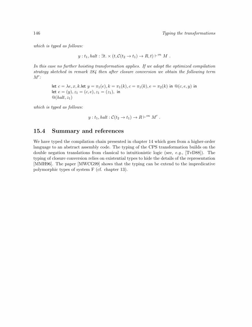
146 Typing the transformations
which is typed as follows:
y : t1, halt : ∃t.× (t, C(t2 → t1)→ R, t) `vn M .
In this case no further hoisting transformation applies. If we adopt the optimized compilationstrategy sketched in remark 284 then after closure conversion we obtain the following termM ′:
let c = λe, x, k.let y = π1(e), k = π1(k), c = π1(k), e = π2(k) in @(c, e, y) inlet e = (y), z1 = (c, e), z1 = (z1), in@(halt , z1)
which is typed as follows:
y : t1, halt : C(t2 → t1)→ R `vn M ′ .
15.4 Summary and references
We have typed the compilation chain presented in chapter 14 which goes from a higher-orderlanguage to an abstract assembly code. The typing of the CPS transformation builds on thedouble negation translations from classical to intuitionistic logic (see, e.g., [TvD88]). Thetyping of closure conversion relies on existential types to hide the details of the representation[MMH96]. The paper [MWCG99] shows that the typing can be extend to the impredicativepolymorphic types of system F (cf. chapter 13).

Chapter 16
Records, variants, and subtyping
Records and variants are common data types found in many programming languages whichallow to aggregate heterogeneous data. Record (variant) types provide a user-friendly alter-native to product (sum) types where components can be manipulated by labels rather thanby projections (injections).
In this chapter, we start by discussing an extension of the call-by-value, type-free, λ-calculus with records and a possible encoding of records. We then move on to consider atyped version of the language. In order to gain in flexibility, we introduce a subtyping rulefor records and study the properties of the derived type system. We conclude by brieflydiscussing how the approach with subtyping can be extended to variant types.
16.1 Records
A record is a notation to represent a function with a finite domain over a set of labels.Formally, we defined labels as follows.
Definition 286 (labels) We denote with L a countable and totally ordered set of labels withgeneric elements `, `′, . . .
We rely on the notation:
`1 = V1, . . . , `n = Vn , (16.1)
to denote the function that associates with the label `i the value Vi and which is undefinedotherwise. Whenever we write a record we assume that the labels are all distinct: `i 6= `j ifi 6= j. Given a record R, we write R.` for the selection of the value of R on the label `. If `is not in the domain of definition of the record then we are in an erroneous situation and thecomputation is stuck or alternatively an error message is produced.
Table 16.1 describes an extension of the type-free, call-by-value, λ-calculus with records.In order to have a deterministic evaluation strategy, we assume that records are always writtenwith labels in growing order and that the evaluation follows this order.
We pause to notice that in principle records could be represented in the pure λ-calculus.For instance, we could associate with each label a natural number and then associate withit a Church numeral. Suppose: (i) ` denotes the Church numeral that corresponds to thelabel `, (ii) E is a λ-term that decides the equality of two Church numerals (cf. exercise 248),(iii) C is the λ-term that represents the conditional, (iv) F is a special λ-term to represent
147

148 Subtyping
failure, and (v) we write let x1 = M1, . . . , xn = Mn in N for (λx1, . . . , xn.N)M1 · · ·Mn. Thenwe could compile the call-by-value λ-calculus with records into the call-by-value λ-calculus asfollows (simple cases omitted):
C(`1 = M1, . . . , `n = Mn) = let x1 = C(M1), . . . , xn = C(Mn) inλl.C(E l `1) x1(· · · (C(E l `n) xn F ) · · ·)
C(M.`) = let x = C(M) in (x `) .
Thus a record is compiled into a function taking a label as input and then performing asequence of conditionals. Selecting a record’s label just amounts to apply the compilation ofthe record to the encoding of the label.
16.2 Subtyping
Next we turn to the issue of typing the extension of the λ-calculus with records. We takeas starting point the type system in Table 10.1 that assigns simple types to λ-terms whoseλ-abstractions are decorated with types (Church style). We extend the syntax of types byintroducing a notion of record type which is a notation for representing a finite function fromlabels to types:
A ::= tid || (A→ A) || ` : A, . . . , ` : A (types).
And then we add two typing rules to introduce and eliminate record types.
Γ `Mi : Ai i = 1, . . . , n
Γ ` `1 = M1, . . . , `n = Mn : `1 : A1, . . . , `n : AnΓ `M : `1 : A1, . . . , `n : An
Γ `M.`i : Ai.
The extended type system still has the property that in a given type context each λ-term hasat most one type. However, consider the record types:
A = `1 : A1, `2 : A2 , B = `1 : A1 .
If we have a value of type A then we could use it in any context that waits for a value of typeB. This simple remark pleads for the introduction of a subtyping relation A ≤ B. Table 16.2describes a possible definition of the subtyping relation for records and functional types.
Syntax
M ::= id || λid .M ||MM || ` = M, . . . , ` = M ||M.` (λ-terms)V ::= λid .M || ` = V, . . . , ` = V (values)
Call-by-value evaluation contexts and reduction rules
E ::= [ ] || EM || V E || (` = V )∗, ` = E, (` = V )∗ || E.`
(λx.M)V → [V/x]M. . . , ` = V, . . ..` → V
Table 16.1: Type-free, call-by-value, λ-calculus with records

Subtyping 149
t ≤ tA′ ≤ A B ≤ B′A→ B ≤ A′ → B′
`′1, . . . , `′m ⊆ `1, . . . , `n A`′i ≤ B`′i i = 1, . . . ,m
`1 : A`1 , . . . , `n : A`n ≤ `′1 : B`′1 , . . . , `′m : B`′m
Table 16.2: Subtyping rules for records
We write ` A ≤ B if the assertion A ≤ B can be derived according to the rules in Table16.2. There are a couple of intriguing points in the definition of the rules. First, notice thatthe rule for functional types is anti-monotonic in the first argument. To get an intuition,suppose we can use natural numbers where integers are expected: N ≤ Z. Then a functionf of type Z → N can also be used whenever a function of type N → Z is expected. Indeed,f will be able to handle any natural number since it is built to work on integers and it willreturn an integer since it is expected to return a natural number. On the other hand, if g hastype N → N then it cannot be used where a function of type Z → Z is expected as g mayfail to handle a negative integer. Second, the rules are completely syntax directed: for eachpair of types there is at most one rule that applies and in this case there is only one way toapply it. We have the following properties.
Proposition 287 The subtyping relation defined in Table 16.2 enjoys the following proper-ties:
1. It is reflexive and transitive.
2. If ` A ≤ B then there is a coercion λ-term CA,B such that ` CA,B : A→ B.
Proof. (1) Reflexivity follows by induction on the structure of the type A. For transitivity,we build a proof of B ≤ C by induction on the height of the proofs of A ≤ B and B ≤ C andcase analysis on the last rules applied. For instance, suppose we have:
B′ ≤ A′ A′′ ≤ B′′A′ → A′′ ≤ B′ → B′′
C ′ ≤ B′ B′′ ≤ C ′′B′ → B′′ ≤ C ′ → C ′′
.
Then by inductive hypothesis we can prove C ′ ≤ A′ and A′′ ≤ C ′′ and we conclude as follows:
C ′ ≤ A′ A′′ ≤ C ′′A′ → A′′ ≤ C ′ → C ′′
.
(2) We proceed by induction on the proof of A ≤ B. For the basic case, take the identity.
For the functional case, take:
CA′→A′′,B′→B′′ = λf : A′ → A′′.λx : B′.cA′′,B′′(f(cB′,A′x)) .
For the record case, assume:
A = `1 : A`1 , . . . , `n : A`n , B = `′1 : B`′1 , . . . , `′m : B`′m ,
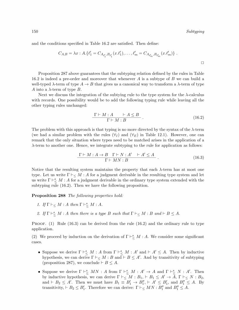
150 Subtyping
and the conditions specified in Table 16.2 are satisfied. Then define:
CA,B = λx : A.`′1 = CA`′1,B`′1
(x.`′1), . . . , `′m = CA`′m ,B`′m(x.`′m) .
2
Proposition 287 above guarantees that the subtyping relation defined by the rules in Table16.2 is indeed a pre-order and moreover that whenever A is a subtype of B we can build awell-typed λ-term of type A→ B that gives us a canonical way to transform a λ-term of typeA into a λ-term of type B.
Next we discuss the integration of the subtying rule to the type system for the λ-calculuswith records. One possibility would be to add the following typing rule while leaving all theother typing rules unchanged:
Γ `M : A ` A ≤ BΓ `M : B
. (16.2)
The problem with this approach is that typing is no more directed by the syntax of the λ-term(we had a similar problem with the rules (∀I) and (∀E) in Table 12.1). However, one canremark that the only situation where types need to be matched arises in the application of aλ-term to another one. Hence, we integrate subtyping to the rule for application as follows:
Γ `M : A→ B Γ ` N : A′ ` A′ ≤ AΓ `MN : B
. (16.3)
Notice that the resulting system maintains the property that each λ-term has at most onetype. Let us write Γ `≤ M : A for a judgment derivable in the resulting type system and letus write Γ `s≤ M : A for a judgment derivable in the ordinary type system extended with thesubtyping rule (16.2). Then we have the following proposition.
Proposition 288 The following properties hold:
1. If Γ `≤ M : A then Γ `s≤ M : A.
2. If Γ `s≤ M : A then there is a type B such that Γ `≤ M : B and ` B ≤ A.
Proof. (1) Rule (16.3) can be derived from the rule (16.2) and the ordinary rule to typeapplication.
(2) We proceed by induction on the derivation of Γ `s≤ M : A. We consider some significantcases.
• Suppose we derive Γ `s≤ M : A from Γ `s≤ M : A′ and ` A′ ≤ A. Then by inductivehypothesis, we can derive Γ `≤ M : B and ` B ≤ A′. And by transitivity of subtyping(proposition 287), we conclude ` B ≤ A.
• Suppose we derive Γ `s≤ MN : A from Γ `s≤ M : A′ → A and Γ `s≤ N : A′. Thenby inductive hypothesis, we can derive Γ `≤ M : B1, ` B1 ≤ A′ → A, Γ `≤ N : B2,and ` B2 ≤ A′. Then we must have B1 ≡ B′1 → B′′1 , ` A′ ≤ B′1, and B′′1 ≤ A. Bytransitivity, ` B2 ≤ B′1. Therefore we can derive: Γ `≤ MN : B′′1 and B′′1 ≤ A.
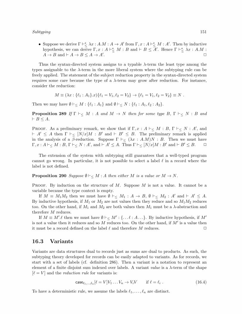
Subtyping 151
• Suppose we derive Γ `s≤ λx : A.M : A→ A′ from Γ, x : A `s≤ M : A′. Then by inductivehypothesis, we can derive Γ, x : A `s≤ M : B and ` B ≤ A′. Hence Γ `s≤ λx : A.M :A→ B and ` A→ B ≤ A→ A′. 2
Thus the syntax-directed system assigns to a typable λ-term the least type among thetypes assignable to the λ-term in the more liberal system where the subtyping rule can befreely applied. The statement of the subject reduction property in the syntax-directed systemrequires some care because the type of a λ-term may grow after reduction. For instance,consider the reduction:
M ≡ (λx : `1 : A1.x)`1 = V1, `2 = V2 → `1 = V1, `2 = V2 ≡ N .
Then we may have ∅ `≤ M : `1 : A1 and ∅ `≤ N : `1 : A1, `2 : A2.
Proposition 289 If Γ `≤ M : A and M → N then for some type B, Γ `≤ N : B and` B ≤ A.
Proof. As a preliminary remark, we show that if Γ, x : A `≤ M : B, Γ `≤ N : A′, and` A′ ≤ A then Γ `≤ [N/x]M : B′ and ` B′ ≤ B. The preliminary remark is appliedin the analysis of a β-reduction. Suppose Γ `≤ (λx : A.M)N : B. Then we must haveΓ, x : A `≤ M : B, Γ `≤ N : A′, and ` A′ ≤ A. Thus Γ `≤ [N/x]M : B′ and ` B′ ≤ B. 2
The extension of the system with subtyping still guarantees that a well-typed programcannot go wrong. In particular, it is not possible to select a label ` in a record where thelabel is not defined.
Proposition 290 Suppose ∅ `≤ M : A then either M is a value or M → N .
Proof. By induction on the structure of M . Suppose M is not a value. It cannot be avariable because the type context is empty.
If M ≡ M1M2 then we must have ∅ `≤ M1 : A → B, ∅ `≤ M2 : A′ and ` A′ ≤ A.By inductive hypothesis, if M1 or M2 are not values then they reduce and so M1M2 reducestoo. On the other hand, if M1 and M2 are both values then M1 must be a λ-abstraction andtherefore M reduces.
If M ≡ M ′.` then we must have ∅ `≤ M ′ : . . . ` : A . . .. By inductive hypothesis, if M ′
is not a value then it reduces and so M reduces too. On the other hand, if M ′ is a value thenit must be a record defined on the label ` and therefore M reduces. 2
16.3 Variants
Variants are data structures dual to records just as sums are dual to products. As such, thesubtyping theory developed for records can be easily adapted to variants. As for records, westart with a set of labels (cf. definition 286). Then a variant is a notation to represent anelement of a finite disjoint sum indexed over labels. A variant value is a λ-term of the shape[` = V ] and the reduction rule for variants is:
case`1,...,`n [` = V ]V1 . . . Vn → ViV if ` = `i . (16.4)
To have a deterministic rule, we assume the labels `1, . . . , `n are distinct.
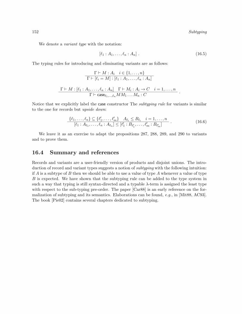
152 Subtyping
We denote a variant type with the notation:
[`1 : A1, . . . , `n : An] . (16.5)
The typing rules for introducing and eliminating variants are as follows:
Γ `M : Ai i ∈ 1, . . . , nΓ ` [`i = M ] : [`1 : A1, . . . , `n : An]
Γ `M : [`1 : A1, . . . , `n : An] Γ `Mi : Ai → C i = 1, . . . , n
Γ ` case`1,...,`nMM1 . . .Mn : C.
Notice that we explicitly label the case constructor The subtyping rule for variants is similarto the one for records but upside down:
`1, . . . , `n ⊆ `′1, . . . , `′m A`i ≤ B`i i = 1, . . . , n
[`1 : A`1 , . . . , `n : A`n ] ≤ [`′1 : B`′1 , . . . , `′m : B`′m ]
. (16.6)
We leave it as an exercise to adapt the propositions 287, 288, 289, and 290 to variantsand to prove them.
16.4 Summary and references
Records and variants are a user-friendly version of products and disjoint unions. The intro-duction of record and variant types suggests a notion of subtyping with the following intuition:if A is a subtype of B then we should be able to use a value of type A whenever a value of typeB is expected. We have shown that the subtyping rule can be added to the type system insuch a way that typing is still syntax-directed and a typable λ-term is assigned the least typewith respect to the sub-typing pre-order. The paper [Car88] is an early reference on the for-malization of subtyping and its semantics. Elaborations can be found, e.g., in [Mit88, AC93].The book [Pie02] contains several chapters dedicated to subtyping.

Chapter 17
References
In chapter 1, we have considered an elementary imperative programming language whoseprograms can be understood as sequences of commands acting on a global state. In thatcontext, the state was regarded as an abstraction of the notion of computer memory and wassimply modeled as a function from identifiers to (basic) values.
In this chapter, we reconsider the notion of imperative programming. We replace the statementioned above with a notion of heap. A heap can also be regarded as an abstraction ofthe notion of computer memory and it is modeled as a function from references to (possiblycomplex) values. In turn, references can be regarded as an abstraction of the notion of memoryaddress. References are first-class values. The value associated with a reference can be readand modified. Moreover, during the computation, it is possible to generate new referencesand associate values with them.
We formalize a higher-order functional language with references which is inspired by thelanguages of the ML-family. Technically, we introduce the reduction rules of a type-free, call-by-value, λ-calculus with references extended with operations to generate, read, and writereferences. We then discuss a possible compilation of the λ-calculus with ‘side effects’ onthe heap into an ordinary λ-calculus. The compilation turns each expression into a functionthat takes a heap as an argument and returns a pair composed of a new heap and a value.We conclude the chapter by introducing a propositional type system for the λ-calculus withreferences which enjoys a subject-reduction property and by discussing some typing anomalieswhich arise with references.
17.1 References and heaps
References can be regarded as an abstraction of memory addresses and a heap as an abstrac-tion of a computer memory.
Definition 291 (references) We denote with R a countable set of references with genericelements r, r′, . . . We assume R is equipped with a function N : Pfin(R) → R such that forall X, finite subset of R, we have N (X) /∈ X.
Definition 292 (heap) A heap h is a function over the set of references R whose domainof definition is finite.
153

154 References
Syntax
M ::= id || λid .M ||MM || r || ref M ||!M ||M := M || ∗ (λ-terms)V ::= λid .M || r || ∗ (values)
Call by value evaluation contexts and Reduction rules
E ::= [ ] || EM || V E || refE ||!E || E := M || V := E
(E[(λx.M)V ], h) → ([V/x]M,h)(E[ref V ], h) → (E[r], h[V/r]) if r = N (dom(h))(E[!r], h) → (E[h(r)], h) if r ∈ dom(h)(E[r := V ], h) → (E[∗], h[V/r]) if r ∈ dom(h)
Table 17.1: A call-by-value λ-calculus with references
We manipulate heaps using the standard notation for functions. Thus if h is a heap, thendom(h) is its domain of definition, h(r) its image at r, and h[v/r] is an ‘updated’ heap definedas follows:
h[v/r](r′) =
h(r) if r = r′
v otherwise.
Notice that we make no assumption on the nature of the values in a heap and that in particulara value can be a reference. In Table 17.1, we introduce an extension of the type-free call-by-value λ-calculus with a notation closely related to the one found in the programming languagesof the ML family: ref M allocates a new reference which is associated with the value of M , !Mreads the value associated with the reference resulting from the evaluation of M , and M := Nwrites in the reference resulting from the evaluation of M the value of N . We also introduce aconstant ∗ which is used as the value resulting from the evaluation of an assignment M := N .Ordinary programs are closed λ-terms where references do not occur. However this propertyis not preserved by reduction and for this reason we include references among the λ-termsand the values of the language. We rely on the following standard abbreviations:
let x = M in N = (λx.M)NM ;N = (λx.N)M x /∈ fv(N) .
References and heaps can be simulated in the pure λ-calculus. As for records’ labels (cf.chapter 16), we can use Church numerals to represent references. The operator N can beimplemented by computing the successor of the largest numeral in the set. A heap can thenbe represented as a list of pairs composed of a reference and a value. Computing the domainof a heap amounts to iterate the first projection on the list. Reading a reference r in the heapmeans scanning the list till a pair (r, V ) is found and updating a reference means building anew heap where the value corresponding to the reference is suitably modified. Let us assumeλ-terms New to create a new reference, Ext to extend a heap with a new pair, Read to read areference, and Write to write a value in the heap. In Table 17.2, we describe the compilationof the the λ-calculus with references into a λ-calculus with pairing. We also use the followingabbreviation for projections:
let (x, y) = M in N ≡ let z = M, x = π1z, y = π2 z in N .
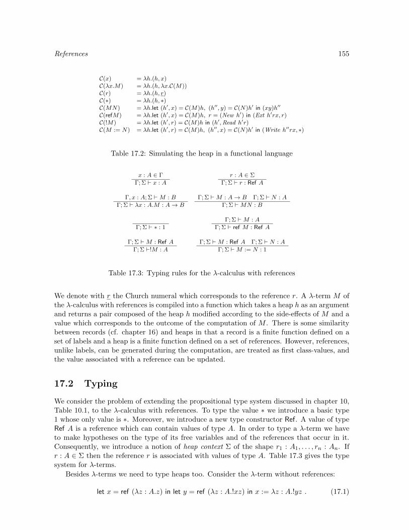
References 155
C(x) = λh.(h, x)C(λx.M) = λh.(h, λx.C(M))C(r) = λh.(h, r)C(∗) = λh.(h, ∗)C(MN) = λh.let (h′, x) = C(M)h, (h′′, y) = C(N)h′ in (xy)h′′
C(refM) = λh.let (h′, x) = C(M)h, r = (New h′) in (Ext h′rx, r)C(!M) = λh.let (h′, r) = C(M)h in (h′,Read h′r)C(M := N) = λh.let (h′, r) = C(M)h, (h′′, x) = C(N)h′ in (Write h′′rx, ∗)
Table 17.2: Simulating the heap in a functional language
x : A ∈ Γ
Γ; Σ ` x : A
r : A ∈ Σ
Γ; Σ ` r : Ref A
Γ, x : A; Σ `M : B
Γ; Σ ` λx : A.M : A→ B
Γ; Σ `M : A→ B Γ; Σ ` N : A
Γ; Σ `MN : B
Γ; Σ ` ∗ : 1
Γ; Σ `M : A
Γ; Σ ` ref M : Ref A
Γ; Σ `M : Ref A
Γ; Σ `!M : A
Γ; Σ `M : Ref A Γ; Σ ` N : A
Γ; Σ `M := N : 1
Table 17.3: Typing rules for the λ-calculus with references
We denote with r the Church numeral which corresponds to the reference r. A λ-term M ofthe λ-calculus with references is compiled into a function which takes a heap h as an argumentand returns a pair composed of the heap h modified according to the side-effects of M and avalue which corresponds to the outcome of the computation of M . There is some similaritybetween records (cf. chapter 16) and heaps in that a record is a finite function defined on aset of labels and a heap is a finite function defined on a set of references. However, references,unlike labels, can be generated during the computation, are treated as first class-values, andthe value associated with a reference can be updated.
17.2 Typing
We consider the problem of extending the propositional type system discussed in chapter 10,Table 10.1, to the λ-calculus with references. To type the value ∗ we introduce a basic type1 whose only value is ∗. Moreover, we introduce a new type constructor Ref. A value of typeRef A is a reference which can contain values of type A. In order to type a λ-term we haveto make hypotheses on the type of its free variables and of the references that occur in it.Consequently, we introduce a notion of heap context Σ of the shape r1 : A1, . . . , rn : An. Ifr : A ∈ Σ then the reference r is associated with values of type A. Table 17.3 gives the typesystem for λ-terms.
Besides λ-terms we need to type heaps too. Consider the λ-term without references:
let x = ref (λz : A.z) in let y = ref (λz : A.!xz) in x := λz : A.!yz . (17.1)

156 References
By reducing it, we can produce the following heap: h0 = [λx : A.(!r2)x/r1, λx : A.(!r1)x/r2].Notice that the values associated with r1 and r2 depend on r2 and r1 respectively. Thus totype a heap we have to find a heap context which assigns a type to all the references of theheap which is coherent with the type of the values associated with the references. Also werequire that all the references in the values of the heap belong to the domain of definition ofthe heap. This leads to the following rule for typing a heap with respect to a heap context:
dom(Σ) = dom(h) ∅; Σ ` h(r) : A for r ∈ dom(h)
Σ ` h . (17.2)
We write Γ; Σ ` (M,h) : A if Γ; Σ `M : A and Σ ` h.
Example 293 The heap h0 produced by the λ-term (17.1) above can be typed in the heapcontext: Σ = r1 : A→ A, r2 : A→ A.
Proposition 294 The typing system enjoys the following properties:
1. If Γ, x : A; Σ `M : B is derivable and x /∈ fv(M) then Γ; Σ `M : B is derivable.
2. If Γ, x : A; Σ ` M : B and Γ; Σ ` V : A are derivable then Γ; Σ ` [V/x]M : B isderivable.
Proof. By induction on the proof height. 2
We now discuss the way typing is preserved by reduction. Notice that during reductionthe domain of definition of the heap can grow since the operator ref may dynamically generatenew references. Hence we also need to extend the heap context. We write Σ′ ⊇ Σ if Σ′ is anextension of Σ. We notice the following weakening property of the heap context.
Proposition 295 If Γ; Σ `M : A is derivable and Σ′ ⊇ Σ then Γ; Σ′ `M : A is derivable.
Then we can state the following subject reduction property (proof left to the reader).
Proposition 296 If Γ; Σ ` (M,h) : A and (M,h)→ (M ′, h′) then there is Σ′ ⊇ Σ such thatΓ; Σ′ ` (M ′, h′) : A.
Exercise 297 Suppose we have ‘abstract types’ R and H and that we can assign the followingtypes to the heap-manipulating functions, where A can be any type:
New : H → R , Ext : H → R→ A→ H ,Read : H → R→ A , Write : H → R→ A→ H .
For every propositional type A and type context Γ define a type translation A and contexttranslation Γ, and show that the compilation function in Table 17.2 is type preserving in thesense that if Γ; ∅ `M : A according to the rules in Table 17.3 then Γ ` C(M) : H → H ×A.

References 157
17.3 Typing anomalies
As suggested by the λ-term (17.1) above, simply typed λ-terms with references can producecircular heaps. In fact it is possible to use references to define general recursive functions.First, let us consider a minimal example of typable and looping computation. Set:
M1 ≡ ref (λx : 1.x) , M2 ≡ let y = M1 in y := (λx : 1.(!y)x) ; (!y) .
Then ` M1 : Ref (1 → 1) and ` M2 : 1 → 1 and there is an infinite reduction starting withM2∗. We can generalize this idea to define a function f of type A → B which satisfies arecursive equation f = λx : A.M where M may depend on f . Let λx : A.N be any λ-term oftype A→ B. Then we set:
M1 ≡ ref (λx : A.N) , M2 ≡ let y = M1 in y := (λx : A.[!y/f ]M) ; (!y) .
Initially, y is a reference containing a fake function. Then we replace the fake function withthe real function where each call to f is replaced by !y. Then y is a reference which containsa value which refers to the reference y. This circularity allows to simulate recursion.
Another curious phenomenon arises when we try to mix references and subtyping. Namely,from A ≤ B we cannot infer Ref A ≤ Ref B (or Ref A ≤ Ref B). The Ref type constructor isneither monotonic nor anti-monotonic with respect to the subtyping pre-order. In practice,this means that no proper subtyping is possible on reference types. To see this, supposeA ≤ B where for instance:
A = `1 : C, `2 : C ≤ `1 : C = B .
Assume Ref is anti-monotonic and x : Ref B then we should also have x : Ref A and (!x.`2)will produce an error. On the other hand, if Ref is monotonic and x : Ref A then we shouldalso have x : Ref B and x := `1 = V ; !x.`2 will produce an error.
As a third and final typing anomaly, let us notice that the polymorphic generalization (cf.chapter 12) of a reference may also lead to errors. For instance, consider:
let x = ref (λx.x) in x := (λx.x+ 1); (!x) true . (17.3)
ML-like languages avoid these problems by allowing polymorphic generalization only on val-ues. For instance, the programming language ocaml accepts:
let x = (λx.x) in x∗;x true , (17.4)
but rejects the dangerous expression (17.3) above as well as the following innocuous one:
let x = (λy.(λx.x))2 in x∗;x true . (17.5)
In practice, most programs seem to meet this restriction.
17.4 Summary and references
Heaps can be regarded as an abstraction of computer memory. We have considered an exten-sion of the λ-calculus with operations to extend, read, and modify the heap. Expressions in
158 References
this extended λ-calculus may have side effects and can be understood as functions that takea heap and produce a new heap and a value.
References introduce the possibility to define recursive data structures and functions. Thispower comes at a price in that the ideas developed in the purely functional setting cannot bereadily lifted to the λ-calculus with side effects. For instance, termination of typable programsfails, no proper subtyping is possible on reference types, and polymorphic generalization isunsound (but in practice it can be fixed [Wri95]).
One may argue that these failures are due to the fact that the usual type systems neglectside effects completely. To address this issue, so called type and effect systems [LG88] havebeen proposed. In these type systems references are abstracted into a finite set of regionsand types become dependent on such regions. In particular, an expression is now expected toproduce both an effect and a value (this is an abstraction of the idea mentioned above wherean expression with side effects is expected to produce a heap and a value). Type and effectsystem have been applied to the design of static mechanisms for safe memory deallocation[TT97]. It has also been shown that a stratified version of the system can guarantee the strongnormalization of the typable λ-terms [Bou10, Ama09].
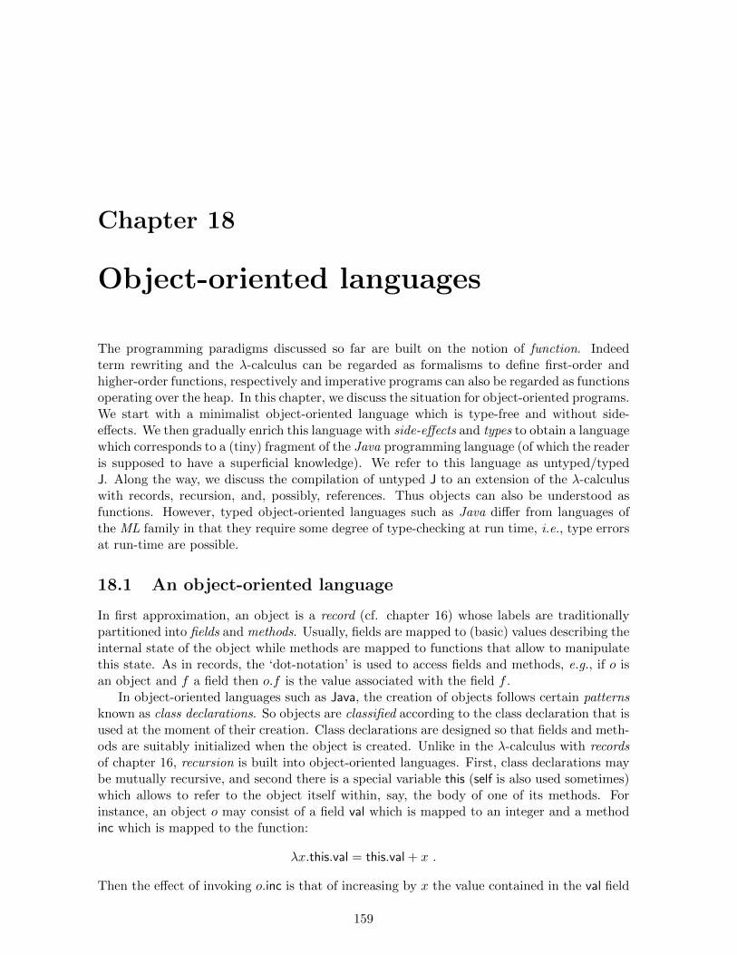
Chapter 18
Object-oriented languages
The programming paradigms discussed so far are built on the notion of function. Indeedterm rewriting and the λ-calculus can be regarded as formalisms to define first-order andhigher-order functions, respectively and imperative programs can also be regarded as functionsoperating over the heap. In this chapter, we discuss the situation for object-oriented programs.We start with a minimalist object-oriented language which is type-free and without side-effects. We then gradually enrich this language with side-effects and types to obtain a languagewhich corresponds to a (tiny) fragment of the Java programming language (of which the readeris supposed to have a superficial knowledge). We refer to this language as untyped/typedJ. Along the way, we discuss the compilation of untyped J to an extension of the λ-calculuswith records, recursion, and, possibly, references. Thus objects can also be understood asfunctions. However, typed object-oriented languages such as Java differ from languages ofthe ML family in that they require some degree of type-checking at run time, i.e., type errorsat run-time are possible.
18.1 An object-oriented language
In first approximation, an object is a record (cf. chapter 16) whose labels are traditionallypartitioned into fields and methods. Usually, fields are mapped to (basic) values describing theinternal state of the object while methods are mapped to functions that allow to manipulatethis state. As in records, the ‘dot-notation’ is used to access fields and methods, e.g., if o isan object and f a field then o.f is the value associated with the field f .
In object-oriented languages such as Java, the creation of objects follows certain patternsknown as class declarations. So objects are classified according to the class declaration that isused at the moment of their creation. Class declarations are designed so that fields and meth-ods are suitably initialized when the object is created. Unlike in the λ-calculus with recordsof chapter 16, recursion is built into object-oriented languages. First, class declarations maybe mutually recursive, and second there is a special variable this (self is also used sometimes)which allows to refer to the object itself within, say, the body of one of its methods. Forinstance, an object o may consist of a field val which is mapped to an integer and a methodinc which is mapped to the function:
λx.this.val = this.val + x .
Then the effect of invoking o.inc is that of increasing by x the value contained in the val field
159

160 Objects
of the object o.
Class declarations
We reserve C,C ′, D, . . . for class names. Each class name corresponds to a distinct classdeclaration. Usually, class declarations are built incrementally. At the very beginning, thereis a class Object without fields and methods. Then whenever we introduce a new classdeclaration we say that it extends another class declaration. For instance, one can declare aclass C which extends the class D and includes a field f and a method m as follows:
class C extends D = (class declaration)· · ·C′ f · · · (field declarations)· · ·D′ m (D1 x1, . . . ,Dn xn) e · · · (method declarations).
We are using here a notation based on Java where we specify the class C′ of the object in thefield f as well as the classes D1, . . . ,Dn of the objects x1, . . . , xn the (function associated withthe) method m is expecting as input and the class D′ of the object it returns as a result.
Expressions
The body of a method is an expression whose syntax is defined as follows:
e ::= id || (variable)v || (value)new C(e1, . . . , en) || (object generation)e.f || (field read)e.m(e1, . . . , en) || (method invocation)
e.f := e || (field write)e; e || (sequentialization)
(C)(e) || (casting)
We have split the expressions in 3 groups. The first group is composed of (object) variables,(object) values (to be defined next), an operator new to generate an object of the class C whileinitializing its fields with the values of the expressions e1, . . . , en, and the selection operatorfor fields and methods. As already mentioned, among the variables, we reserve the variablethis to refer to the object on which a method is invoked. The second group is optional andcorresponds to an imperative extension of the basic language where fields are modifiable, andtherefore the sequentialization of side effects is relevant. The third group is also optional andconsists of a casting operator. This operator is only relevant if we are interested in a typesystem for the language. We anticipate that the role of such a type system is not to avoiderrors (cf. exercise 203) but to localize them in certain points of the computation.
Values
The definition of a value expression depends on whether we are considering the imperativeextension or not. In the imperative extension, we assume all fields are modifiable. To modelfield assignment we proceed as in chapter 17. Namely, we assume an infinite set of references
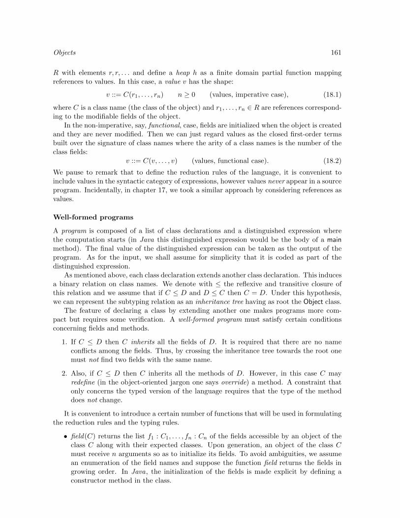
Objects 161
R with elements r, r, . . . and define a heap h as a finite domain partial function mappingreferences to values. In this case, a value v has the shape:
v ::= C(r1, . . . , rn) n ≥ 0 (values, imperative case), (18.1)
where C is a class name (the class of the object) and r1, . . . , rn ∈ R are references correspond-ing to the modifiable fields of the object.
In the non-imperative, say, functional, case, fields are initialized when the object is createdand they are never modified. Then we can just regard values as the closed first-order termsbuilt over the signature of class names where the arity of a class names is the number of theclass fields:
v ::= C(v, . . . , v) (values, functional case). (18.2)
We pause to remark that to define the reduction rules of the language, it is convenient toinclude values in the syntactic category of expressions, however values never appear in a sourceprogram. Incidentally, in chapter 17, we took a similar approach by considering references asvalues.
Well-formed programs
A program is composed of a list of class declarations and a distinguished expression wherethe computation starts (in Java this distinguished expression would be the body of a mainmethod). The final value of the distinguished expression can be taken as the output of theprogram. As for the input, we shall assume for simplicity that it is coded as part of thedistinguished expression.
As mentioned above, each class declaration extends another class declaration. This inducesa binary relation on class names. We denote with ≤ the reflexive and transitive closure ofthis relation and we assume that if C ≤ D and D ≤ C then C = D. Under this hypothesis,we can represent the subtyping relation as an inheritance tree having as root the Object class.
The feature of declaring a class by extending another one makes programs more com-pact but requires some verification. A well-formed program must satisfy certain conditionsconcerning fields and methods.
1. If C ≤ D then C inherits all the fields of D. It is required that there are no nameconflicts among the fields. Thus, by crossing the inheritance tree towards the root onemust not find two fields with the same name.
2. Also, if C ≤ D then C inherits all the methods of D. However, in this case C mayredefine (in the object-oriented jargon one says override) a method. A constraint thatonly concerns the typed version of the language requires that the type of the methoddoes not change.
It is convenient to introduce a certain number of functions that will be used in formulatingthe reduction rules and the typing rules.
• field(C) returns the list f1 : C1, . . . , fn : Cn of the fields accessible by an object of theclass C along with their expected classes. Upon generation, an object of the class Cmust receive n arguments so as to initialize its fields. To avoid ambiguities, we assumean enumeration of the field names and suppose the function field returns the fields ingrowing order. In Java, the initialization of the fields is made explicit by defining aconstructor method in the class.

162 Objects
public class Bool extends Object
public Object ite (Object x, Object y)return new Object();
public class True extends Bool
public Object ite (Object x, Object y)return x;
public class False extends Bool
public Object ite (Object x, Object y)return y;
public class Num extends Object
public Bool iszero ()return new Bool();
public Num pred()return new Num();
public Num succ()return new Num();
public class NotZero extends Num
public Num pd;
public NotZero(Num x)pd=x;
public Bool iszero()return new False();
public Num pred()return this.pd;
public Num succ()return new NotZero(this);
public class Zero extends Num
public Bool iszero()return new True();
public Num pred()return new Zero();
public Num succ()return new NotZero(this);
Table 18.1: Some class declarations in J (with Java syntax).
• mbody(m,C) returns the function that corresponds to the method m in the class C.For instance, if mbody(m,C) = λx1, . . . , xn.e then x1, . . . , xn are the formal parametersand e is the expression associated with the method, respectively.
• In the typed version of the language, it will also be useful to have a function mtypesuch that mtype(m,C) returns the type of the method m of the class C and a predicateoverride such that override(m,D,C∗ → C) holds if and only if mtype(m,D) is definedand it coincides with C∗ → C.
Example 298 In Table 18.1, we consider a list of class declarations which allows to representboolean values and natural numbers in unary notation. The examples are written in theslightly more verbose notation of the Java programming language. As already mentioned,Java requires a constructor method to build an object in a class with fields. Moreover, Javadistinguishes between private and public declarations while in J all declarations are public.These are really minor syntactic differences and therefore the typed version of the J languagecan be regarded as a subset of Java. Notice that the proposed representation of the conditionalvia the method ite is strict (both branches are evaluated); a more realistic fragment of Javawould include a non-strict conditional.
Exercise 299 (programming) With reference to the code in Table 18.1:
1. Enrich the classes for the booleans and natural numbers with a printing method whichprints (a representation of) the object on the standard output using Java’s printingfunctions.
2. Enrich the classes for natural numbers with an isequal method that takes a number objectand checks whether it is equal to the one on which the method is invoked.
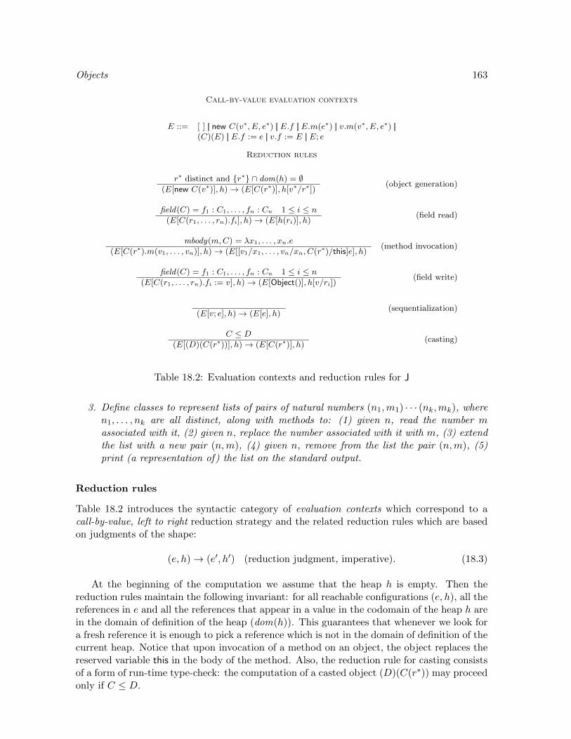
Objects 163
Call-by-value evaluation contexts
E ::= [ ] || new C(v∗, E, e∗) || E.f || E.m(e∗) || v.m(v∗, E, e∗) ||(C)(E) || E.f := e || v.f := E || E; e
Reduction rules
r∗ distinct and r∗ ∩ dom(h) = ∅(E[new C(v∗)], h)→ (E[C(r∗)], h[v∗/r∗])
(object generation)
field(C) = f1 : C1, . . . , fn : Cn 1 ≤ i ≤ n(E[C(r1, . . . , rn).fi], h)→ (E[h(ri)], h)
(field read)
mbody(m,C) = λx1, . . . , xn.e
(E[C(r∗).m(v1, . . . , vn)], h)→ (E[[v1/x1, . . . , vn/xn, C(r∗)/this]e], h)(method invocation)
field(C) = f1 : C1, . . . , fn : Cn 1 ≤ i ≤ n(E[C(r1, . . . , rn).fi := v], h)→ (E[Object()], h[v/ri])
(field write)
(E[v; e], h)→ (E[e], h)(sequentialization)
C ≤ D(E[(D)(C(r∗))], h)→ (E[C(r∗)], h)
(casting)
Table 18.2: Evaluation contexts and reduction rules for J
3. Define classes to represent lists of pairs of natural numbers (n1,m1) · · · (nk,mk), wheren1, . . . , nk are all distinct, along with methods to: (1) given n, read the number massociated with it, (2) given n, replace the number associated with it with m, (3) extendthe list with a new pair (n,m), (4) given n, remove from the list the pair (n,m), (5)print (a representation of) the list on the standard output.
Reduction rules
Table 18.2 introduces the syntactic category of evaluation contexts which correspond to acall-by-value, left to right reduction strategy and the related reduction rules which are basedon judgments of the shape:
(e, h)→ (e′, h′) (reduction judgment, imperative). (18.3)
At the beginning of the computation we assume that the heap h is empty. Then thereduction rules maintain the following invariant: for all reachable configurations (e, h), all thereferences in e and all the references that appear in a value in the codomain of the heap h arein the domain of definition of the heap (dom(h)). This guarantees that whenever we look fora fresh reference it is enough to pick a reference which is not in the domain of definition of thecurrent heap. Notice that upon invocation of a method on an object, the object replaces thereserved variable this in the body of the method. Also, the reduction rule for casting consistsof a form of run-time type-check: the computation of a casted object (D)(C(r∗)) may proceedonly if C ≤ D.

164 Objects
field(C) = f1 : C1, . . . , fn : CnE[new C(v1, . . . , vn)]→ E[C(v1, . . . , vn)]
(object generation)
field(C) = f1 : C1, . . . , fn : Cn 1 ≤ i ≤ nE[C(v1, . . . , vn).fi]→ E[vi]
(field read)
mbody(m,C) = λx1, . . . , xn.e
E[C(v∗).m(v1, . . . , vn)]→ E[[v1/x1, . . . , vn/xn, C(v∗)/this]e](method invocation)
C ≤ DE[(D)C(v∗)]→ E[C(v∗)]
(casting)
Table 18.3: Simplified reduction rules for the functional fragment of J
The specification of the functional fragment of J where fields are immutable can be sub-stantially simplified. Values are now the closed first-order terms built over the signature ofclass names (cf. grammar (18.2)). The evaluation contexts and the reduction rules for assign-ment and sequentialization can be dropped. The remaining rules are based on a judgment ofthe shape e→ e′ (we drop the heap) and are specified in Table 18.3.
18.2 Objects as records
We define an encoding of the functional, type free object-oriented language into a call-by-value λ-calculus extended with records and a fixed point combinator Y (in turn, records andthe fixed point combinator could be encoded in the λ-calculus). As a first step, we assumeeach class declaration is completely expanded so that we can associate with each class namethe list of its fields and its methods with the related bodies. So we have a system of classdeclarations of the shape (class names are omitted when irrelevant):
class C f1, . . . , fh,m1 = λx∗1.e1, . . . ,mk = λx∗k.ek . (18.4)
The methods’ bodies ei may generate objects of other classes and may refer to the objectitself via the variable this. This entails that class generators are mutually recursive and thevariable this is defined via a fixed point combinator.
Following this intuition, we define a compilation function C. We suppose the class namesare enumerated as C1, . . . , Cm and we reserve a fresh variable c and the labels 1, . . . ,m. Thevariable c will be defined recursively as a record with labels 1, . . . ,m such that the functionassociated with the label i is the generator for the objects of the class Ci. On expressions(which are not values or casted objects), the compilation function is simply defined as follows:
C(x) = xC(new Ci(e1, . . . , en)) = (c.i) C(e1) · · · C(en) (c fresh variable)C(e.f) = C(e).fC(e.m(e1, . . . , en)) = (C(e).m) C(e1) · · · C(en) .
For each declaration of a class C of the shape (18.4), we define the λ-term NC where y1, . . . , yh
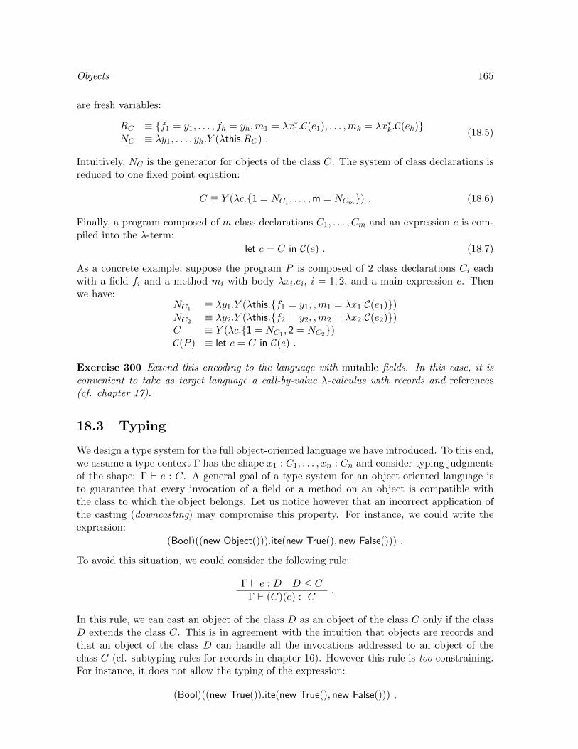
Objects 165
are fresh variables:
RC ≡ f1 = y1, . . . , fh = yh,m1 = λx∗1.C(e1), . . . ,mk = λx∗k.C(ek)NC ≡ λy1, . . . , yh.Y (λthis.RC) .
(18.5)
Intuitively, NC is the generator for objects of the class C. The system of class declarations isreduced to one fixed point equation:
C ≡ Y (λc.1 = NC1 , . . . ,m = NCm) . (18.6)
Finally, a program composed of m class declarations C1, . . . , Cm and an expression e is com-piled into the λ-term:
let c = C in C(e) . (18.7)
As a concrete example, suppose the program P is composed of 2 class declarations Ci eachwith a field fi and a method mi with body λxi.ei, i = 1, 2, and a main expression e. Thenwe have:
NC1 ≡ λy1.Y (λthis.f1 = y1, ,m1 = λx1.C(e1))NC2 ≡ λy2.Y (λthis.f2 = y2, ,m2 = λx2.C(e2))C ≡ Y (λc.1 = NC1 , 2 = NC2)C(P ) ≡ let c = C in C(e) .
Exercise 300 Extend this encoding to the language with mutable fields. In this case, it isconvenient to take as target language a call-by-value λ-calculus with records and references(cf. chapter 17).
18.3 Typing
We design a type system for the full object-oriented language we have introduced. To this end,we assume a type context Γ has the shape x1 : C1, . . . , xn : Cn and consider typing judgmentsof the shape: Γ ` e : C. A general goal of a type system for an object-oriented language isto guarantee that every invocation of a field or a method on an object is compatible withthe class to which the object belongs. Let us notice however that an incorrect application ofthe casting (downcasting) may compromise this property. For instance, we could write theexpression:
(Bool)((new Object())).ite(new True(), new False())) .
To avoid this situation, we could consider the following rule:
Γ ` e : D D ≤ CΓ ` (C)(e) : C
.
In this rule, we can cast an object of the class D as an object of the class C only if the classD extends the class C. This is in agreement with the intuition that objects are records andthat an object of the class D can handle all the invocations addressed to an object of theclass C (cf. subtyping rules for records in chapter 16). However this rule is too constraining.For instance, it does not allow the typing of the expression:
(Bool)((new True()).ite(new True(), new False())) ,

166 Objects
class C extends Object
public void m()return;
class D extends Object
public void m()return;
class Main
public static void main (String[] args)
D d = new D();
C c = new C();
((C)((Object)(d))).m(); //this types, but rises an exception at run time.
((C)(d)).m(); //this does not type, but it is a reduced of the above!
return;
Table 18.4: Typing anomaly in Java
as the result of the method ite belongs to the class Object and Object 6≤ Bool. Then, in Java,the rule for casting can be formulated as follows:
Γ ` e : D (C ≤ D or D ≤ C)
Γ ` (C)(e) : C.
In other terms, the casting is forbidden if C and D are incomparable. However, this prop-erty is not preserved by reduction! Let C,D be two incomparable classes and let e be anexpression of type C. Then the expression (D)((Object)(e)) is well typed, but it reduces tothe expression (D)(e) which is not. By climbing and descending the inheritance tree we canconnect incomparable classes. Table 18.4 gives a concrete example of this phenomenon inJava.
Because preservation of typing by reduction is a desirable property, we formulate thetyping rule for casting as follows:
Γ ` e : D
Γ ` (C)(e) : C.
At typing time, we do not try to verify that the value C ′(r∗) resulting form the evaluation ofthe expression e is such that C ′ ≤ C. Instead, we delay this verification at running time. Ifthe condition is not satisfied then reduction is stuck (alternatively, an error message could beproduced).
Table 18.5 specifies the rules to type expressions that do not contain values (as sourceprograms do). An important point to notice is that the typing rules allow to use an objectof the class C where an object of the class D is expected as long as C is a sub-class of D.This is a form of subtyping (cf. chapter 16). The rationale is that an object of the sub-classC will be able to handle all the field and method invocations which could be performed onan object of the super-class D. Indeed, objects of the class C have all fields of the class Dand may redefine methods of the class D provided their type is unchanged.
Beyond expressions, we also need to check the typing of the class declarations. Suppose amethod m of the class C has the shape:
C0 m(C1 x1, . . . , Cn xn)e ,
and that the class C extends the class D. Then the following must hold:

Objects 167
x : C ∈ Γ
Γ ` x : C
field(C) = f1 : D1, . . . , fn : DnΓ ` ei : Ci, Ci ≤ Di, 1 ≤ i ≤ n
Γ ` new C(e1, . . . , en) : C
Γ ` e : C field(C) = f1 : C1, . . . , fn : CnΓ ` e.fi : Ci
Γ ` e : C mtype(m,C) = (C1, . . . , Cn)→ DΓ ` ei : C′i C′i ≤ Ci 1 ≤ i ≤ n
Γ ` e.m(e1, . . . , en) : D
Γ ` e : D
Γ ` (C)(e) : C
Γ ` e : C field(C) = f1 : C1, . . . , fn : CnΓ ` e′ : Di Di ≤ CiΓ ` e.fi := e′ : Object
Γ ` e1 : C1 Γ ` e2 : C2
Γ ` e1; e2 : C2
Table 18.5: Typing rules for J program expressions
1. override(m,D, (C1, . . . , Cn)→ C0),
2. x1 : C1, . . . , xn : Cn, this : C ` e : C ′0 and C ′0 ≤ C0.
A class is well typed if all its methods are well typed in the sense above. Finally, a programis well typed if all its classes are well typed and the distinguished expression is well typedin the empty type context. For instance, the reader may check that we can type the classdeclarations in example 298.
Exercise 301 (more programming) Design a compiler from the Imp language (cf. chap-ter 1) to the typed J language. We outline a possible strategy.
1. Consider a restricted set of arithmetic expressions and boolean conditions that can beeasily coded in J. For instance, just work with natural numbers in unary notation anda boolean condition that checks if a number is zero (cf. Table 18.1).
2. Represent variables as unary numbers and implement a state as a finite list of pairscomposed of a variable and a number. A state is compiled into an object of a class Statewith methods to read, write, extend, and restrict (cf. exercise 298).
3. Define a class Code with subclasses Skip, Assignment, Conditional,. . . which correspondto the various ways of composing statements in Imp. It is assumed that each object ofthe class Code has a method execute that takes as argument an object of the class State.
4. For all programs P and states s of the Imp language define a compilation into a Jexpression e = C(P ).execute(C(s)) with the following properties: (1) if the expression eevaluates to a value v then v is the representation of a state s′ such that (P, s) ⇓ s′. (2)the evaluation of e never produces an exception or a type error,
As already mentioned, the task of the type system is to localize the type errors aroundthe application of the casting reduction rule. We formalize this property for the functional
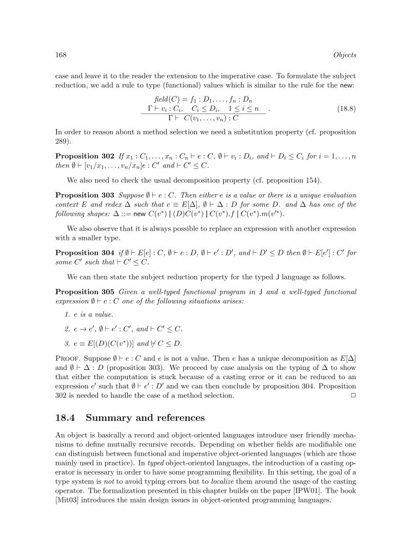
168 Objects
case and leave it to the reader the extension to the imperative case. To formulate the subjectreduction, we add a rule to type (functional) values which is similar to the rule for the new:
field(C) = f1 : D1, . . . , fn : Dn
Γ ` vi : Ci, Ci ≤ Di, 1 ≤ i ≤ nΓ ` C(v1, . . . , vn) : C
. (18.8)
In order to reason about a method selection we need a substitution property (cf. proposition289).
Proposition 302 If x1 : C1, . . . , xn : Cn ` e : C, ∅ ` vi : Di, and ` Di ≤ Ci for i = 1, . . . , nthen ∅ ` [v1/x1, . . . , vn/xn]e : C ′ and ` C ′ ≤ C.
We also need to check the usual decomposition property (cf. proposition 154).
Proposition 303 Suppose ∅ ` e : C. Then either e is a value or there is a unique evaluationcontext E and redex ∆ such that e ≡ E[∆], ∅ ` ∆ : D for some D. and ∆ has one of thefollowing shapes: ∆ ::= new C(v∗) || (D)C(v∗) || C(v∗).f || C(v∗).m(v′∗).
We also observe that it is always possible to replace an expression with another expressionwith a smaller type.
Proposition 304 if ∅ ` E[e] : C, ∅ ` e : D, ∅ ` e′ : D′, and ` D′ ≤ D then ∅ ` E[e′] : C ′ forsome C ′ such that ` C ′ ≤ C.
We can then state the subject reduction property for the typed J language as follows.
Proposition 305 Given a well-typed functional program in J and a well-typed functionalexpression ∅ ` e : C one of the following situations arises:
1. e is a value.
2. e→ e′, ∅ ` e′ : C ′, and ` C ′ ≤ C.
3. e ≡ E[(D)(C(v∗))] and 6` C ≤ D.
Proof. Suppose ∅ ` e : C and e is not a value. Then e has a unique decomposition as E[∆]and ∅ ` ∆ : D (proposition 303). We proceed by case analysis on the typing of ∆ to showthat either the computation is stuck because of a casting error or it can be reduced to anexpression e′ such that ∅ ` e′ : D′ and we can then conclude by proposition 304. Proposition302 is needed to handle the case of a method selection. 2
18.4 Summary and references
An object is basically a record and object-oriented languages introduce user friendly mecha-nisms to define mutually recursive records. Depending on whether fields are modifiable onecan distinguish between functional and imperative object-oriented languages (which are thosemainly used in practice). In typed object-oriented languages, the introduction of a casting op-erator is necessary in order to have some programming flexibility. In this setting, the goal of atype system is not to avoid typing errors but to localize them around the usage of the castingoperator. The formalization presented in this chapter builds on the paper [IPW01]. The book[Mit03] introduces the main design issues in object-oriented programming languages.

Chapter 19
Introduction to concurrency
In computer science, we are used to the idea of regarding a piece of software and/or hardwareas a system, i.e., a compound of interacting and interdependent components with varyingnames such as threads or processes that we use as synonymous.
Starting from this chapter, the general goal is to formalize and reason on systems whereseveral threads/processes compete for the same resources (e.g. write a variable or a channel).Most of the time, this results into non-deterministic behavior which means that with the sameinput the system can move to several (incomparable) states. For instance, the computationof a circuit may be non-deterministic due to the unpredictable delays in the propagation ofsignals. Similarly, the computation of an operating system may be non-deterministic due tounpredictable delays in managing the accesses to memory. We stress that non-determinismis both a way of representing our partial knowledge of the system and a method to keep itsspecification general. For instance, we may want to prove that a certain algorithm is correctindependently of the scheduling policy or the evaluation strategy chosen.
Some authors distinguish parallel from concurrent systems. The former are a subclassof the latter that typically exhibit a deterministic behavior. A standard problem in parallelprogramming is to decompose the task of computing a (deterministic) function into parallelsub-tasks that when executed on suitable hardware will hopefully provide a faster result interms of throughput and/or latency. We do not develop at all these algorithmic issues.
Besides being non-deterministic, certain concurrent systems may also exhibit a probabilis-tic behavior. In first approximation, this means that at certain points in the computation thenext state of the system is determined by tossing a coin. The basic idea we stress in chapter29 is that non-deterministic and probabilistic transitions should be kept separated and thata computation in a non-deterministic and probabilistic system is described by a transitionrelation that relates states to distributions over states.
The concurrent systems we consider can be classified according to two main criteria:
asynchronous vs. synchronous and shared memory vs. message passing.
The first criterion concerns the relative speed of the processes; we mainly focus on asyn-chronous systems where each process proceeds at its own speed, however we shall see inchapter 28 that the techniques can be adapted to synchronous/timed systems too, wherecomputation proceeds in phases or rounds. The second criterion concerns the interactionmechanism among the processes. In shared memory, processes interact by modifying a sharedarea of memory. Synchronization arises by waiting that a certain condition is satisfied (cf.
169
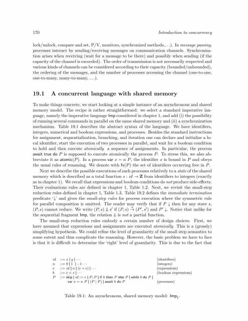
170 Introduction to concurrency
lock/unlock, compare and set, P/V, monitors, synchronized methods,. . .). In message passing,processes interact by sending/receiving messages on communication channels. Synchroniza-tion arises when receiving (wait for a message to be there) and possibly when sending (if thecapacity of the channel is exceeded). The order of transmission is not necessarily respected andvarious kinds of channels can be considered according to their capacity (bounded/unbounded),the ordering of the messages, and the number of processes accessing the channel (one-to-one,one-to-many, many-to-many, . . .).
19.1 A concurrent language with shared memory
To make things concrete, we start looking at a simple instance of an asynchronous and sharedmemory model. The recipe is rather straightforward: we select a standard imperative lan-guage, namely the imperative language Imp considered in chapter 1, and add (i) the possibilityof running several commands in parallel on the same shared memory and (ii) a synchronizationmechanism. Table 19.1 describes the abstract syntax of the language. We have identifiers,integers, numerical and boolean expressions, and processes. Besides the standard instructionsfor assignment, sequentialization, branching, and iteration one can declare and initialize a lo-cal identifier, start the execution of two processes in parallel, and wait for a boolean conditionto hold and then execute atomically a sequence of assignments. In particular, the processawait true do P is supposed to execute atomically the process P . To stress this, we also ab-breviate it as atomic(P ). In a process var x = n P , the identifier x is bound in P and obeysthe usual rules of renaming. We denote with fv(P ) the set of identifiers occurring free in P .
Next we describe the possible executions of such processes relatively to a state of the sharedmemory which is described as a total function s : id → Z from identifiers to integers (exactlyas in chapter 1). We recall that expressions and boolean conditions do not produce side-effects.Their evaluations rules are defined in chapter 1, Table 1.2. Next, we revisit the small-stepreduction rules defined in chapter 1, Table 1.3. Table 19.2 defines the immediate terminationpredicate ‘↓’ and gives the small-step rules for process execution where the symmetric rulefor parallel composition is omitted. The reader may verify that if P ↓ then for any state s,(P, s) cannot reduce. We write (P, s) ⇓ s′ if (P, s)
∗→ (P ′, s′) and P ′ ↓. Notice that unlike forthe sequential fragment Imp, the relation ⇓ is not a partial function.
The small-step reduction rules embody a certain number of design choices. First, wehave assumed that expressions and assignments are executed atomically. This is a (grossly)simplifying hypothesis. We could refine the level of granularity of the small step semantics tosome extent and thus complicate the reasoning. However, the basic problem we have to faceis that it is difficult to determine the ‘right’ level of granularity. This is due to the fact that
id ::= x || y || · · · (identifiers)n ::= 0 || 1 || −1 · · · (integers)e ::= id || n || (e+ e) || · · · (expressions)b ::= e < e || · · · (boolean expressions)P ::= skip || id := e || P ;P || if b then P else P || while b do P ||
var x = n P || (P | P ) || await b do P (processes)
Table 19.1: An asynchronous, shared memory model: Imp‖.

Introduction to concurrency 171
skip ↓P ↓
var x = n P ↓Pi ↓ i = 1, 2
(P1 | P2) ↓
(x := e, s) → (skip, s[v/x]) if (e, s) ⇓ v
(if b then P else P ′, s) → (P, s) if (b, s) ⇓ true(if b then P else P ′, s) → (P ′, s) if (b, s) ⇓ false
(while b do P, s) → (P ;while b do P, s) if (b, s) ⇓ true(while b do P, s) → (skip, s) if (b, s) ⇓ false
(P ;P ′, s) → (P ′, s) if P ↓(P ;P ′, s) → (P ′′;P ′, s′) if (P, s)→ (P ′′, s′)
(var x = n P, s) → (var x = n′ P ′, s′[s(x)/x]) if (P, s[n/x])→ (P ′, s′[n′/x])
(P | P ′, s) → (P ′′ | P ′, s′) if (P, s)→ (P ′′, s′)
(await b do P, s) → (await b do P, s) if (b, s) ⇓ false(await b do P, s) → (P ′, s′) if (b, s) ⇓ true,
(P, s)∗→ (P ′, s′), P ′ ↓
Table 19.2: Immediate termination and small-step reduction for Imp‖
there is no general agreement on the abstract memory model that should be presented to theprogrammer of a concurrent language with ‘shared memory’. Ideally, the model should be‘abstract’ while allowing for correct and efficient implementations on a variety of architectures.
Second, we assume that the body of an await always terminates. In practice, we can simplyenforce this condition by requiring that the body contains no while and no await instruction.
Third, a blocked await reduces (busy waiting) which may seem at odd with the usualidea that a process executing a synchronization condition which is not realized suspendsits execution. We could indeed formalize this idea at the price of distinguishing between(properly) terminated and deadlocked statements.
Let us consider a few examples that illustrate the expressivity of the language.
Example 306 (P and V ) Assuming assignment atomic (as we do), the operations P andV for manipulating a semaphore s of capacity k can be expressed as follows:
Initially: s := k ,P (s) = await s > 0 do s := s− 1 ,V (s) = s := s+ 1 .
In the special case where the initial capacity is 1, the operations P and V are also calledlock and unlock, respectively. By using them, processes can gain exclusive access to a sharedresource, e.g., a process can gain the right to execute without interruption, i.e., atomically, asequence of statements.
Example 307 (non-deterministic sum) We want to define a statement:
[b1 → P1 + · · ·+ bn → Pn]

172 Introduction to concurrency
which selects non-deterministically one of the branches (if any) for which the condition bi issatisfied and starts running Pi. This can be defined as follows assuming x, y /∈ fv(bi → Pi)for i = 1, . . . , n:
var x = 1 (Q1 | · · · | Qn), whereQi ≡ var y = 1
await bi do if x = 1 then x := 0 else y := 0 ;if y = 1 then Pi else skip
Exercise 308 (1) Modify the definition so that once the branch i is selected, the continuationPi is run atomically. (2) With the current definition, a statement such as [true→ skip+false→skip] does not terminate (which is not very satisfying). Adapt the definition to fix this problem.
Exercise 309 Suppose we enrich the Imp‖ language with a spawn operator. The processspawn P starts the execution of P in parallel and immediately terminates by reducing, say,to skip. (1) Propose a formal semantics of the Imp‖ language with spawn. (2) Explain whyin general the process (spawn P );Q is not equivalent to (P | Q). (3) Propose a compilationof the enriched language into the enriched language without parallel composition, i.e., find away to simulate parallel composition with spawn.
Example 310 (compare and set) The compare and set (cas) operation can be defined asfollows (this operation is also called compare and swap):
cas(x, e1, e2) = atomic(if (x = e1) then x := e2 else skip) .
We stress that it is essential that the boolean test x = e1 and the assignment x := e2 areexecuted atomically. The cas operation can be taken as basic building block to solve morecomplex problems in concurrency. For instance, it can be used to solve the so called consensusproblem which can be stated as follows. A collection of parallel processes P1, . . . , Pn eachholding a non-negative integer v1, . . . , vn have to agree on a value which is equal to one of thevalues held by the processes. A solution to this problem which treats all processes in the sameway and avoids centralization points goes as follows. Set a variable x with initial value −1and then let each process Pi run the following procedure:
decide(i) = cas(x, −1, vi); result i := x .
The first process that runs the decide procedure will set x to its value vi ≥ 0 (atomically,and thus deciding the outcome of the consensus protocol) while the following ones will keep xunchanged.
19.2 Equivalences: a taste of the design space
We consider the question of building an equivalence on processes on top of the reductionsystem. In the sequential framework (cf. chapters 1 and 9), we have already noticed thatan answer to this question depends on a certain number of factors such as the choice of theobservables, the compositionality properties, and the proof methods. With an enlarged rangeof choices, these factors play a role in the semantics of concurrent systems too. Moreover,new factors appear such as the hypotheses on the scheduling policy.
Introduction to concurrency 173
Observables The equivalence should be compatible with a notion of observation of theprocesses. If two processes P and P ′ are equivalent and P enjoys a certain observable propertythen P ′ should enjoy that property too. For instance, we may wait till the system comes to aproper termination and then observe its final result. As a second example, we may be informedthat the system has reached a deadlock, i.e., a situation where it has not properly terminatedand it cannot progress. As a third example, we may interact with the system during thecomputation and observe its capabilities. We refer to this observable as branching because,as explained in the following example 313, it amounts to observe the branching structure ofthe computation as opposed to its linearization.
Scheduling We may assume certain properties of the scheduler that controls the order inwhich parallel processes are executed. For instance, a preemptive scheduler will be allowedto interrupt the execution of a process at any point which is compatible with the atomicityassumptions while a cooperative scheduler will wait for the process to yield control or tosuspend on a synchronization condition. Further, schedulers can be classified according totheir ability to execute the various processes in a fair way.
Compositionality If a process P is equivalent to the process P ′ then we should be ableto replace P with P ′ in any (reasonable) process context. In other words, the notion ofequivalence should be preserved by some operators of the language, including at least parallelcomposition.
Proof method We should have a practical proof method to check the equivalence of twoprocesses. Depending on the class of processes we are considering, practical may mean thatthe equivalence can be efficiently automated or that the proof has a certain locality property.
We elaborate on the first two points (observables and scheduling hypotheses) in the followingexamples; we shall come back to compositionality and proof methods in the following sections.
Example 311 (termination) The following process diverges (or at least does not reachimmediate termination) while producing a sequence f(0), f(f(0)), . . . on the ‘output variable’y at a ‘rate’ determined by x.
y := 0;while true doawait x = 0 do (y := f(y);x := 1; )
Should it be considered equivalent to while true do skip (a diverging process)?
Example 312 (deadlock) Consider the following deadlocked process:
var x = 0 await x > 0 do x := x+ 1 .
Should it be considered equivalent to while true do skip (a diverging process, again) or to skip(an immediately terminated process)?
Example 313 (branching) Consider the following hypothetical controls of a vending ma-chine:
[b1 → P1; [b2 → P2 + b3 → P3]][b1 → P1; [b2 → P2] + b1 → P1; [b3 → P3]]

174 Introduction to concurrency
with the interpretation:
b1 = there is a coin P1 = accept the coinb2 = there is a second coin P2 = accept the coin and deliver coffeeb3 = water request P3 = deliver water.
Are the two controls equivalent? Well, one may remark that upon accepting the first coin, thesecond machine decides non-deterministically whether it is ready to wait for a second coin orto deliver water which is rather annoying for the user.
Example 314 (cooperative) In preemptive concurrency, a process can be interrupted afterany atomic step. In cooperative concurrency, a process is interrupted only when it has termi-nated or it is suspended on a waiting statement. For instance, the processes: x := 1;x := x+1and x := 1;x := 2 are equivalent in a cooperative (and a sequential) context but not in a pre-emptive one.
Example 315 (weak fairness) Consider the following process:
x := 0; y := 0; ((while x = 0 do y := y + 1) | x := 1) .
If the process terminates then y may contain an arbitrary natural number. This is calledunbounded non-determinism. Moreover, the process is actually guaranteed to terminate if weassume that every process that is ready to run will eventually get a chance of running. Thisassumption is called weak fairness.
Example 316 (strong fairness) A weak fairness hypothesis is not always enough to guar-antee progress. Consider:
x := 0; y := 0; ( while y = 0 do x := 1− x | await x = 1 do y := 1 ) .
In this example, the first process makes x oscillate between 0 and 1 while the second processcan really progress only when x = 1. A scheduler that gives control to the second process onlywhen x = 0 will not guarantee termination. Strong fairness is the assumption that in anyinfinite execution a process which is infinitely often ‘ready to run’ will indeed run infinitelyoften.
19.3 Summary and references
Early work on the semantics of concurrent processes started in the 60’s [Dij65] and wasmotivated by synchronization problems in operating systems. The first step in defining thesemantics of a concurrent language amounts to decide which actions can be regarded as atomic.This is an issue which can be hardly underestimated because there is a tension betweenatomicity and efficient implementations. At any rate, once atomicity is fixed a small-stepreduction semantics allows to define precisely the state transformations a concurrent processcan go through. The second step amounts to decide the observable properties of the systemand the execution hypotheses. This step gives rise to a variety of possible equivalences.Compositionality and the existence of practical proof methods are two basic criteria to assessthem. The article [KR90] surveys the parallelization of algorithms (which we do not cover).
Chapter 20
A compositional trace semantics
We consider the problem of defining and characterizing a compositional equivalence for theImp‖ model. For the sequential fragment of the Imp‖ model, the input-output interpretationprovides a satisfying answer (cf. chapter 1), but the extension to the full concurrent Imp‖language is not straightforward and rises some interesting issues which are discussed in thisand the following chapter.
20.1 Fixing the observables
Following the discussion in section 19.2, a first problem consists in fixing a notion of observable.Building on the semantics of the sequential Imp language (chapter 1) we shall take the input-output behavior or, equivalently, the partial correctness assertions (pca), as basic observable.We warn the reader that while being reasonable, this notion of observable is definitely notthe only possible one for concurrent processes; alternatives will be discussed in the followingchapters. Let P, P ′, . . . be the processes and s, s′, . . . be the memory states introduced insection 19.1. We adapt to processes the definitions presented in chapter 1.
The IO interpretation (cf. definition 1) of a process P is:
[[P ]]IO = (s, s′) | (P, s) ∗→ (P ′, s′) ↓ .
Also the notion of pca’s validity is extended to processes in the obvious way:
|= A P B if ∀ s (s |= A and (P, s)∗→ (P ′, s′) ↓ implies s′ |= B) .
Then the the pca interpretation of a process is:
[[P ]]pca = (A,B) | |= A P B .
Adapting proposition 11, we derive:
[[P1]]IO = [[P2]]IO iff [[P1]]pca = [[P2]]pca .
Let us take the input-out behavior (or equivalently the partial correctness assertions) asbasic observable. As usual, a context C is a process with a hole [ ]. E.g.
x := 3; [ ] | await x = 3 do x := x+ 1 .
175

176 Trace semantics
As already mentioned in chapters 1, 9, and 19 a desirable property of a semantics is that itis preserved by contexts, that is:
[[P1]] = [[P2]] implies [[C[P1]]] = [[C[P2]]] .
If two processes have the same ‘compositional semantics’ then we can replace one for the otherin any context. Unfortunately, the following example shows that, unlike in the sequential case(proposition 3), compositionality fails for the IO (and pca) interpretation.
Example 317 (non-compositionality of IO interpretation) The processes P1 ≡ x :=1;x := x+ 1 and P2 ≡ x := 2 are IO-equivalent. However when they are composed in parallelwith the process P2 we have: [[P1 | P2]]IO 6= [[P2 | P2]]IO.
20.2 Towards compositionality
As a first attempt at fixing the compositionality issue, we try to refine the semantics ofprocesses. In automata theory, we are used to associate to an automaton the collection of itsexecution traces. We follow a similar path by considering the traces of the states crossed bya terminating execution.
Definition 318 (trace interpretation) The trace interpretation of a process P is definedas follows:
[[P ]]T = s1 . . . , sn | (P, s1)∗→ (P2, s2) · · · ∗→ (Pn, sn) ↓ .
Remark 319 The IO semantics is exactly the subset of the trace semantics composed ofwords of length 2.
[[P ]]IO = (s, s′) | ss′ ∈ [[P ]]T .
With reference to the previous example 317, it is easy to check that [[P1]]T 6= [[P2]]T . However,for P3 ≡ x := 1;x := 2 we have:
[[P1]]T = [[P3]]T , [[P1 | P2]]T 6= [[P3 | P2]]T .
So this trace semantics is not compositional either!
While failing to characterize the ‘right equivalence/pre-order’ we can at least define it.
Definition 320 (pre-congruences) A pre-congruence is a pre-order on processes which ispreserved by contexts. We define two pre-congruences relatively to the IO and trace interpre-tations as follows:
P1 ≤IO P2 if ∀C [[C[P1]]]IO ⊆ [[C[P2]]]IO ,P1 ≤T P2 if ∀C [[C[P1]]]T ⊆ [[C[P2]]]T .
Exercise 321 Check that ≤IO (≤T ) is the largest pre-order (reflexive and transitive) whichrefines the IO containment (trace containment) and which is preserved by all contexts.
Somehow surprisingly, once we require preservation by contexts, it does not matter whetherwe look at the input-output or at the traces.

Trace semantics 177
Proposition 322 The pre-congruences ≤IO and ≤T coincide.
Proof. ≤T⊆≤IO . By remark 319, we know that [[P1]]T ⊆ [[P2]]T implies [[P1]]IO ⊆ [[P2]]IO.Then it follows by unfolding the definitions that:
P1 ≤T P2 implies P1 ≤IO P2 .
≤IO⊆≤T . For the other direction, assume by contradiction P1 6≤T P2. This means that forsome context C and trace s1 · · · sn:
s1 · · · sn ∈ [[C[P1]]]T and s1 · · · sn /∈ [[C[P2]]]T .
In particular, this entails, for Q1 ≡ C[P1]: (Q1, s1)∗→ (Q2
1, s2)∗→ · · · (Qn1 , sn) ↓. The key step
is the following: we build an observer O that may terminate iff it sees the state going throughs1 · · · sn; the observer reads the state without modifying it. Take X = fv(C[P1]) ∪ fv(C[P2])and recall the IS predicate from proposition 11:
IS (s,X) =∧x∈X
(x = s(x)) .
Then define:O ≡ await IS (s1, X) do skip;
· · ·await IS (sn, X) do skip .
We have: (s1, sn) ∈ [[C[P1] | O]]IO. On the other hand we claim that:
(s1, sn) /∈ [[C[P2] | O]]IO ,
because the only way O can terminate is that the state goes through the configurationss1, . . . , sn and since O does not modify the state this would mean s1 · · · sn ∈ [[C[P2]]]T . 2
Following these preliminary remarks, we can define our goal as follows:
find an interpretation [[ ]] such that: [[P1]] = [[P2]] iff ∀C [[C[P1]]]IO = [[C[P2]]]IO.
Such an interpretation (if it exists) will be compositional by definition. Sometimes one ishappy with the left to right implication. In this case, the interpretation is called adequatein that it provides a sufficient criterion to determine the equivalence of two processes. Ifmoreover the right to left implication holds, then one speaks of a fully adequate (or fullyabstract) interpretation. Notice that this last property can be reformulated as follows:
[[P1]] 6= [[P2]] implies ∃C [[C[P1]]]IO 6= [[C[P2]]]IO .
In words, whenever the interpretations differ we can find a context where the IO behaviors,i.e., observable behaviors of the processes differ.

178 Trace semantics
20.3 A trace-environment interpretation
To address the compositionality issue, we are guided by the following intuition:
to analyze a process in a concurrent system we have to account for the perturba-tions induced by the environment (the external world).
In particular, in the framework of a trace semantics, we allow the environment (the externalworld) to modify the state after any sequence of transitions.
Definition 323 (trace-environment interpretation) Let P be a process. Its trace-environment(TE) interpretation is defined as follows:
[[P ]]TE = (s1, s′1) · · · (sn, s′n) |
(P, s1)∗→ (P2, s
′1)
· · ·(Pn, sn)
∗→ (Pn+1, s′n) ↓ .
Exercise 324 In remark 319, we have observed the equivalence in the trace interpretation ofthe processes P1 ≡ x := 1;x := x+ 1 and P2 ≡ x := 1;x := 2. Check that: [[P1]]TE 6= [[P2]]TE.
Remark 325 An equivalent view of the TE-interpretation is to add a labelled rewriting rulethat explicitly accounts for the actions of the environment:
(P, s)e→ (P, s′)
(20.1)
Thus this labelled rule allows for an arbitrary modification of the state while leaving unchangedthe control of the observed process. Then we define:
[[P ]]TE = s1, s′1 · · · sn, s′n |
(P, s1)∗→ (P2, s
′1)
e→ (P2, s2)· · ·(Pn−1, sn−1)
∗→ (Pn, s′n−1)
e→ (Pn, sn)
(Pn, sn)∗→ (Pn+1, s
′n) ↓ .
The traces in the sense of definition 318 can be regarded as the trace-environment traces wheresi+1 = s′i, for i = 1, . . . , n− 1.
In chapter 21, we shall show that this interpretation is preserved by all the operators of thelanguage. For the time being we just consider the problematic case of parallel composition.
Proposition 326 The TE-inclusion is preserved by parallel composition.
Proof. First notice the following properties:
(P1 | P2) ↓ implies P1 ↓ and P2 ↓ ,(P1 | P2, s)→ (P, s′) implies (P1, s)→ (P ′1, s
′) and P ≡ (P ′1 | P2) or(P2, s)→ (P ′2, s
′) and P ≡ (P1 | P ′2) .
Trace semantics 179
Thus from a reduction such as:
(P | Q, s1)∗→ (P2 | Q2, s
′1)
· · ·(Pn | Qn, sn)
∗→ (Pn+1 | Qn+1, s′n) ↓
one can extract a reduction for P where all the reduction steps taken by the other processare simulated by the environment. As a concrete example, suppose [[P1]]TE ⊆ [[P ′1]]TE and
(P1 | Q1, s1)→ (P2 | Q1, s2)→ (P2 | Q2, s3)→ (P3 | Q2, s4) ↓ .
We can turn this into:
(P1, s1)→ (P2, s2)e→ (P2, s3)→ (P3, s4) ↓ .
Then (s1, s2)(s3, s4) ∈ [[P1]]TE ⊆ [[P ′1]]TE means:
(P ′1, s1)∗→ (P ′2, s2)
e→ (P ′2, s3)∗→ (P ′3, s4) ↓ .
Now put back the Q1 process and let him play the role of the environment:
(P ′1 | Q1, s1)∗→ (P ′2 | Q1, s2)→ (P ′2 | Q2, s3)
∗→ (P ′3 | Q2, s4) ↓ .
This argument can be generalized. Suppose α = (s1, s′1) · · · (sn, s′n), α ∈ [[P1 | Q]]TE , and
[[P1]]TE ⊆ [[P2]]TE . Derive a reduction for P1 which must also belong to P2. Then, by puttingback the thread Q, conclude that α ∈ [[P2 | Q]]TE . 2
Since the TE interpretation refines the IO interpretation, its adequacy will follow bythe announced compositionality property shown in chapter 21. We now address the fullabstraction problem.
Proposition 327 Let P1 and P2 be processes such that [[P1]]TE 6⊆ [[P2]]TE. Then there is acontext C such that [[C[P1]]]IO 6⊆ [[C[P2]]]IO.
Proof. Let α = (s1, s′1) · · · (sn, s′n) be a trace-environment sequence such that α ∈ [[P1]]TE
and α /∈ [[P2]]TE . We build an observer process O that in a sense plays the role of theenvironment and works as follows:
upon observing s′1 builds s2 and· · ·upon observing s′n−1 builds sn and terminates.
Notice that in this case the observer does modify the state. Formally, assume X = fv(P1) ∪fv(P2). The command that builds a new state is defined as follows:
MAKE s,x1,...,xn = x1 := s(x1); · · · ;xn := s(xn) ,
and the observer process O is defined by:
O ≡ O1
Oi ≡ await IS (s′i, X) do MAKE si+1,X ;· · ·await IS (s′n−1, X) do MAKE sn,X .
180 Trace semantics
Then take as process context C = [ ] | O and let Ci = [ ] | Oi. We have that (s1, s′n) ∈ [[C[P1]]]IO
because:(C[P1], s1)
∗→ (C[P2], s′1)∗→ (C2[P2], s2)
· · ·(Pn | skip, sn)
∗→ (P ′n | skip, s′n) ↓
On the other hand, (s1, s′n) /∈ [[C[P2]]]IO because O terminates only if it can observe the
states s′i and build atomically the states si+1 for i = 1, . . . , n − 1. And this contradicts thehypothesis that (s1, s
′1) · · · (sn, s′n) /∈ [[P2]]TE . 2
20.4 Summary and references
We have described a trace-environment interpretation for the Imp‖ language. The interpre-tation is compositional and abstract. The key point for compositionality is that we describethe way both the process and the environment may affect the store (which is what can beobserved). The key point for abstraction is that Imp‖ can simulate the environment’s actions;the await statement is crucial here. The presentation is based on [Bro96].
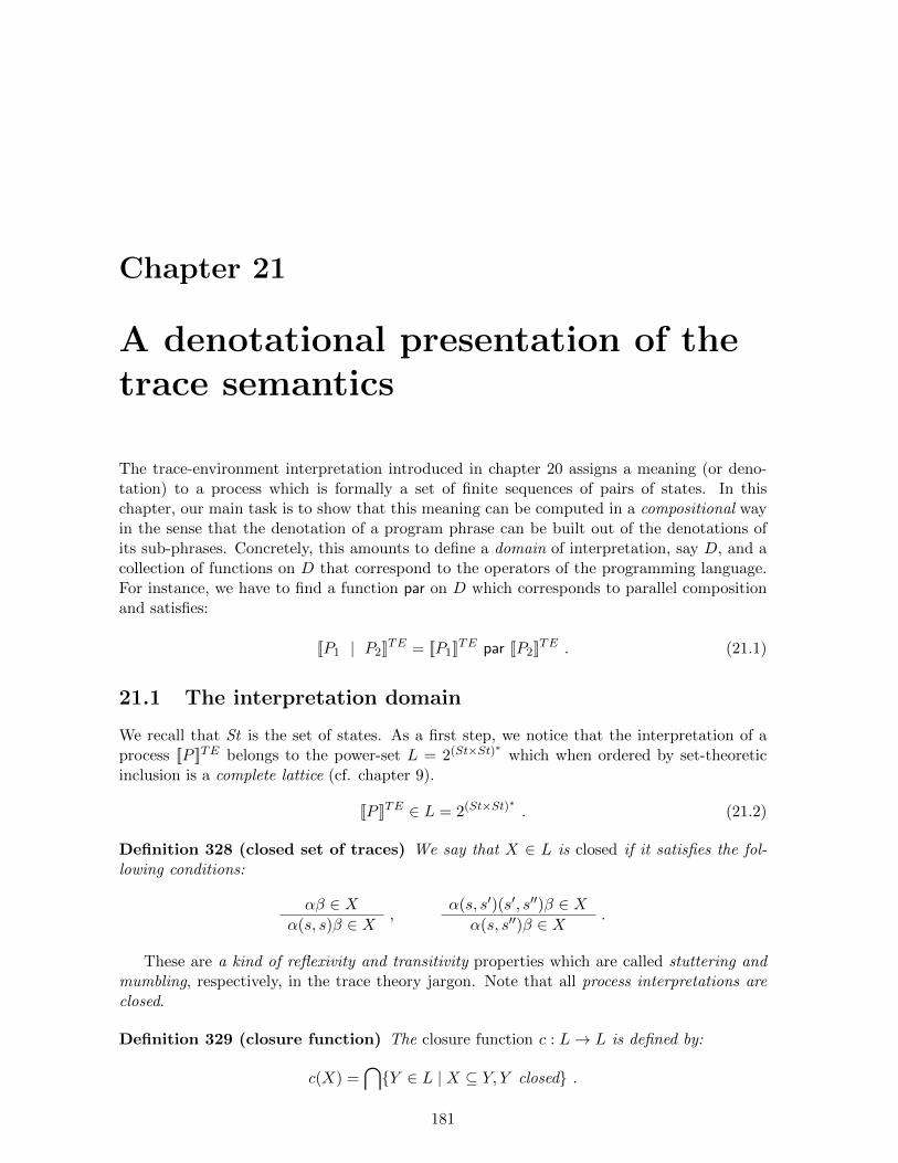
Chapter 21
A denotational presentation of thetrace semantics
The trace-environment interpretation introduced in chapter 20 assigns a meaning (or deno-tation) to a process which is formally a set of finite sequences of pairs of states. In thischapter, our main task is to show that this meaning can be computed in a compositional wayin the sense that the denotation of a program phrase can be built out of the denotations ofits sub-phrases. Concretely, this amounts to define a domain of interpretation, say D, and acollection of functions on D that correspond to the operators of the programming language.For instance, we have to find a function par on D which corresponds to parallel compositionand satisfies:
[[P1 | P2]]TE = [[P1]]TE par [[P2]]TE . (21.1)
21.1 The interpretation domain
We recall that St is the set of states. As a first step, we notice that the interpretation of aprocess [[P ]]TE belongs to the power-set L = 2(St×St)∗ which when ordered by set-theoreticinclusion is a complete lattice (cf. chapter 9).
[[P ]]TE ∈ L = 2(St×St)∗ . (21.2)
Definition 328 (closed set of traces) We say that X ∈ L is closed if it satisfies the fol-lowing conditions:
αβ ∈ Xα(s, s)β ∈ X ,
α(s, s′)(s′, s′′)β ∈ Xα(s, s′′)β ∈ X .
These are a kind of reflexivity and transitivity properties which are called stuttering andmumbling, respectively, in the trace theory jargon. Note that all process interpretations areclosed.
Definition 329 (closure function) The closure function c : L→ L is defined by:
c(X) =⋂Y ∈ L | X ⊆ Y, Y closed .
181

182 Denotational trace semantics
Thus the function c associates to a set X the least set of closed traces that contains it.We notice the following properties.
Proposition 330 Let X,Y,Xi vary over L and let c be the closure function. Then:
1. If X ⊆ Y then c(X) ⊆ c(Y ).
2. c(c(X)) = c(X) ⊇ X.
3. The union of closed sets is closed.
4. c(⋃i∈I Xi) =
⋃i∈I c(Xi).
Proof. We leave properties 1-3 as exercises and consider property 4, The inclusion fromleft to right follows by monotonicity (property 1). For the reverse inclusion, we know fromproperty 3 that
⋃i∈I c(Xi) is closed. Thus it suffices to check that:
⋃i∈I Xi ⊆
⋃i∈I c(Xi)
which holds since by property 2, Xi ⊆ c(Xi). 2
It follows that (c(L),⊆) is again a complete lattice where the sup are set-theoretic unions.We take D = c(L) as our domain of interpretation.
21.2 The interpretation
First, we define some standard operations on the domain D which are instrumental to theinterpretation of Imp‖ processes. The reader may recognize definition patterns found in formallanguages.
Skip We define: Skip = c((s, s) | s ∈ St) ∈ D. Notice that this is different from theclosure of the empty-set.
Concatenation For X,Y ∈ D let X;Y = c(αβ | α ∈ X,β ∈ Y ) ∈ D. Notice that we needto close the concatenation of X and Y in the ordinary language-theoretic sense.
Iteration For X ∈ D let:
X0 = Skip ∈ D , Xn+1 = X;Xn ∈ D , X∗ =⋃n≥0X
n ∈ D .
By proposition 330(3), there is no need to close the countable union.
Parallel A general shuffle operation | on words can be defined as follows:
ε | α = α | ε = α ,aα | bβ = aγ | γ ∈ (α | bβ) ∪ bγ′ | γ′ ∈ (aα | β) .
Notice that the shuffle of two words is a set of words which is not necessarily closed.Then define a parallel operator on X,Y ∈ D as:
X | Y =⋃
α∈X,β∈Yc(α | β) .
Exercise 331 (continuity) Show that the concatenation, iteration, and parallel operatorswe have defined on the complete lattice (D,⊆) are monotonic and preserve unions (continuity).

Denotational trace semantics 183
We associate a closed set with a boolean condition b (without side effects) as follows:
[[b]] = c((s, s) | (b, s) ⇓ true) .
Intuitively, this is the closed set induced by the set of states satisfying the boolean condition.Then associate a closed set to processes as follows:
[[skip]] = Skip[[x := e]] = c((s, s[n/x]) | (e, s) ⇓ n)[[P ;P ′]] = [[P ]]; [[P ′]][[if b then P else P ′]] = ([[b]]; [[P ]]) ∪ ([[¬b]]; [[P ′]])[[while b do P ]] = ([[b]]; [[P ]])∗; [[¬b]][[P | P ′]] = [[P ]] | [[P ′]][[await b do P ]] = c((s, s′) | (s, s) ∈ [[b]], (s, s′) ∈ [[P ]]) .
To force the atomic execution of the body of an await statement, we select the traces of length1 which correspond to the input-output behaviors (remark 325).
The extension to variable declarations requires some work. Given X ⊆ (St × St)∗, xvariable, n integer, define:
X[x = n] = (s1, s′1) · · · (sn, s′n) ∈ X |
s1(x) = n, si+1(x) = s′i(x), i = 1, . . . , n− 1
X\x = (s1[m1/x], s′1[m1/x]) · · · (sn[mn/x], s′n[mn/x]) |(s1, s
′1) · · · (sn, s′n) ∈ X, m1, . . . ,mn ∈ Z .
The operator ( )[x = n] fixes the initial value of x to n and makes sure the environmentcannot affect the value of x by forcing si+1(x) = s′i(x). The operator ( )\x makes sure thatthe internal modifications of x are not observable by the environment (the value of the stateat x is never modified by a process transition). Then define:
[[var x = n P ]] = c( ( [[P ]][x = n] )\x ) .
In words, first we select the traces where the initial value of the variable x is n and theenvironment cannot affect x’s value and second we hide to the environment the way x ismanipulated.
This concludes the compositional definition of the interpretation. The reader can checkthat this interpretation does indeed follow the pattern outlined in (21.1). Moreover, it turnsout to be equivalent to the operational interpretation.
Proposition 332 (denotational characterisation) For all processes P , [[P ]]TE = [[P ]] .
Proof. The proof proceeds by induction on the structure of P . As an example, we show:
[[P ;Q]] = [[P ;Q]]TE (21.3)
assuming [[P ]] = [[P ]]TE and [[Q]] = [[Q]]TE .
[[P ;Q]] ⊆ [[P ;Q]]TE . Suppose:
α = (s1, s′1) · · · (sn, s′n) ∈ [[P ]] = [[P ]]TE
β = (t1, t′1) · · · (tm, t′m) ∈ [[Q]] = [[Q]]TE .

184 Denotational trace semantics
We have already observed that the operational interpretation of a program is closed. Thenby the properties of the closure operator (proposition 330), it suffices to show that αβ ∈[[P ;Q]]TE . Indeed, we have:
(P ;Q, s1)∗→ (P1;Q, s′1)
· · · ∗→ · · ·(Pn−1;Q, sn)
∗→ (Pn;Q, s′n)→ (Q, s′n) (where: Pn ↓)(Q, t1)
∗→ (Q1, t′1)
· · · ∗→ · · ·(Qm−1, tm)
∗→ (Qm, t′m) ↓ .
[[P ;Q]] ⊇ [[P ;Q]]TE . Suppose γ ∈ [[P ;Q]]TE is generated as follows:
(P ;Q, s1)∗→ (P1;Q, s′1)
· · · ∗→ · · ·(Pn−1;Q, sn)
∗→ (Q1, s′n)
(Q1, sn+1)∗→ (Q2, s
′n+1)
· · · ∗→ · · ·(Qm, sn+m)
∗→ (Qm+1, s′n+m) ↓ .
By the semantics of concatenation, we must also have the following transitions:
(Pn−1, sn)∗→ (Pn, s
′′n) ↓
(Q, s′′n)∗→ (Q1, s
′n) .
It follows that:α = (s1, s
′1) · · · (sn, s′′n) ∈ [[P ]]TE = [[P ]] ,
β = (s′′n, s′n) · · · (sn+m, s
′n+m) ∈ [[Q]]TE = [[Q]] .
Then αβ ∈ [[P ]]; [[Q]] and by definition of closure (mumbling), γ ∈ [[P ;Q]]. 2
An immediate corollary is that the trace-environment interpretation is preserved by pro-cess contexts.
Corollary 333 If [[P ]]TE = [[P ′]]TE then [[C[P ]]]TE = [[C[P ′]]]TE.
Proof. For instance, if [[P ]]TE = [[P ′]]TE then by proposition 332, [[P ]] = [[P ′]]. Thus, for anyQ: [[P | Q]]TE = [[P | Q]] = [[P ′ | Q]] = [[P ′ | Q]]TE . 2
Another interesting application of the characterization is that it provides an angle toanalyze process equivalence.
Exercise 334 Show that the following processes (in-)equivalences hold in the TE semantics:
skip;P = P , P = P ; skip ,(P ;P ′);P ′′ = P ; (P ′;P ′′) , P | P ′ = P ′ | P ,
(P | P ′) | P ′′ = P | (P ′ | P ′′) , P | skip = P ,while true do skip ≤ P , while true do skip = await false do P .

Denotational trace semantics 185
Thus skip is the unit for both sequential and parallel composition. Further, sequentialcomposition is associative while parallel composition is both associative and commutative.Finally, the diverging computation is the least element of the interpretation.
Exercise 335 (invalid equivalences) Show that the following equivalences (which hold inthe sequential IO semantics) fail in the TE semantics:
x := y; y := x = x := y , x := y;x := z = x := z (x 6= z) ,x := y; z := x = x := y; z := y , x := y; z := y = z := y;x := y .
Exercise 336 (await from atomic) In section 19.1, we have regarded atomic(P ) as an ab-breviation for await true do P . Suppose we regard await′ b do P as an abbreviation for:
var x = 1 while x = 1 do (atomic(if b then (P ;x := 0)))
where x is a fresh variable. Show that the following equality holds in the considered semantics:
await b do P = await′ b do P .
Exercise 337 (shuffling of infinite words) Let Σ be an alphabet (a non-empty set) withgeneric elements a, b, c, . . . If X is a set let Xω be the set of infinite words on X (countableand not finite). If α is a word then αω is αα · · · We denote with R,S, . . . relations on D =Σω×Σω×Σω and write R(α, β, γ) as an abbreviation for (α, β, γ) ∈ R. We say that a relationR is admissible if:
R(α, β, aγ) implies ( α = aα′ and R(α′, β, γ) ) or( β = aβ′ and R(α, β′, γ) ) .
We define:S0 = D,Sn+1 = (α, β, aγ) | ( α = aα′ and Sn(α′, β, γ) ) or
( β = aβ′ and Sn(α, β′, γ) ) ,Sω = ∩n<ωSn .
Problems: (1) Show that there is a largest admissible relation that we denote with Shuffle.(2) Prove or disprove: Shuffle = Sω. (3) Prove or disprove: (i) Shuffle(aω, bω, (ab)ω). (ii)Shuffle((ab)ω, aω, (abb)ω). (iii) Shuffle(aω, bω, aω).
Exercise 338 (fair schedules and associativity) A k-schedule is a vector (f1, . . . , fk) ofk functions on the natural numbers N such that:
• for j = 1, . . . , k and n ∈ N: fj(n) < fj(n+ 1) (the functions are strictly growing).
• for i, j ∈ 1, . . . , k and i 6= j: im(fi) ∩ im(fj) = ∅ (the ranges of the functions aredisjoint).
• ∪j=1,...,kim(fj) = N (the union of the ranges covers the natural numbers).
Let Σ be a non-empty set with generic elements a, b, c, . . . and let Σω be the (countably)infinite words over Σ with generic elements α, β, . . .. If α ∈ Σω and i ∈ N then α[i] denotes

186 Denotational trace semantics
the character at position i of the word where we start counting from 0. For instance, ifα = ababab · · · then α[3] = b.
If (f1, . . . , fk) is a k-schedule and αi ∈ Σω for i = 1, . . . , k then M [f1, . . . , fk](α1, . . . , αk)is a word whose value at position i ∈ N is defined as follows:
M [f1, . . . , fk](α1, . . . , αk)[i] = αj [f−1j (i)] if i ∈ im(fj)
where f−1j (i) denotes the (unique!) number that the function fj maps to i.
1. Suppose α = aω and β = bω. (i) Assuming f1(i) = 2 · i and f2(i) = 2 · i + 1,compute M [f1, f2](α, β). (ii) Is there a 2-schedule (f, g) such that M [f, g](α, β) =(aab)ω = aabaabaab · · ·? (iii) Is there a 2-schedule (f, g) such that M [f, g](α, β) =abω = abbbbb · · ·?
2. Suppose (f1, f2) and (g1, g2) are two 2-schedules. Show that there is a 3-schedule(h1, h2, h3) such that for all words αi, i = 1, 2, 3 we have:
M [g1, g2](M [f1, f2](α1, α2), α3) = M [h1, h2, h3](α1, α2, α3).
3. Now suppose (h1, h2, h3) is a 3-schedule. Define two 2-schedules (f1, f2) and (g1, g2)such that for all words αi, i = 1, 2, 3 we have:
M [g1, g2](M [f1, f2](α1, α2), α3) = M [h1, h2, h3](α1, α2, α3) .
4. We define a binary merge operation M that associates a set of words to two words asfollows:
M(α, β) = M [f, g](α, β) | (f, g) is a 2-schedule .
We then extend the operation to sets of words by defining for X,Y ⊆ Σω:
M(X,Y ) =⋃
α∈X,β∈YM(α, β) .
Show that this merge operation is associative, i.e., for all sets of words Xi ⊆ Σω, i =1, 2, 3:
M(M(X1, X2), X3) = M(X1,M(X2, X3)) .
21.3 Summary and references
The trace-environment interpretation can be organized in a denotational style where themeaning of a program (process) is computed by composition of the meaning of its sub-programs. This makes manifest the compositionality of the interpretation. We refer thereader to [Bro96] for a variation over the presented semantics which takes into account fair-ness constraints. This requires working over infinite traces; exercises 337 and 338 go in thisdirection by defining shuffling operations on infinite words.
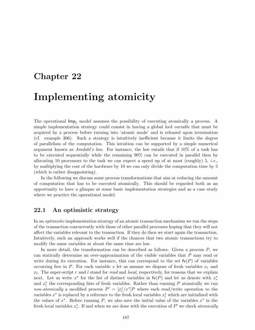
Chapter 22
Implementing atomicity
The operational Imp‖ model assumes the possibility of executing atomically a process. Asimple implementation strategy could consist in having a global lock variable that must beacquired by a process before turning into ‘atomic mode’ and is released upon termination(cf. example 306). Such a strategy is intuitively inefficient because it limits the degreeof parallelism of the computation. This intuition can be supported by a simple numericalargument known as Amdahl’s law. For instance, the law entails that if 10% of a task hasto be executed sequentially while the remaining 90% can be executed in parallel then byallocating 10 processors to the task we can expect a speed up of at most (roughly) 5, i.e.,by multiplying the cost of the hardware by 10 we can only divide the computation time by 5(which is rather disappointing).
In the following we discuss some process transformations that aim at reducing the amountof computation that has to be executed atomically. This should be regarded both as anopportunity to have a glimpse at some basic implementation strategies and as a case studywhere we practice the operational model.
22.1 An optimistic strategy
In an optimistic implementation strategy of an atomic transaction mechanism we run the stepsof the transaction concurrently with those of other parallel processes hoping that they will notaffect the variables relevant to the transaction. If they do then we start again the transaction.Intuitively, such an approach works well if the chances that two atomic transactions try tomodify the same variables at about the same time are low.
In more detail, the transformation can be described as follows. Given a process P , wecan statically determine an over-approximation of the visible variables that P may read orwrite during its execution. For instance, this can correspond to the set fv(P ) of variablesoccurring free in P . For each variable x let us assume we dispose of fresh variables xr andxl. The super-script r and l stand for read and local, respectively, for reasons that we explainnext. Let us write x∗ for the list of distinct variables in fv(P ) and let us denote with x∗rand x∗l the corresponding lists of fresh variables. Rather than running P atomically we runnon-atomically a modified process P ′ = [x∗l /x
∗]P where each read/write operation to thevariables x∗ is replaced by a reference to the fresh local variables x∗l which are initialized withthe values of x∗. Before running P , we also save the initial value of the variables x∗ in thefresh local variables x∗r . If and when we are done with the execution of P ′ we check atomically
187

188 Atomicity
that the current value of x∗ equals that of x∗r . If this is the case, in the same atomic step wewrite x∗l in x∗ and we conclude successfully the transaction, otherwise we try again. Noticethat it may happen that the variables x∗ are modified during the computation above. Allthat matters is that the value of x∗ is the same as the value of x∗r just before writing in x∗
the variables x∗l .
The transformation can be described formally by a function Co (o for optimistic) onImp‖ processes. The key case concerns the await and it is defined as follows assumingfv(await b do P ) = x1, . . . , xn, x∗ = x1, . . . , xn, and using vectorial notations such as x∗ :=v∗ and x∗r = x∗ as an abbreviation for x1 := v1; · · · ;xn := vn and xr,1 = x1 ∧ · · · ∧ xr,n = xn,respectively. We also assume that the variables c, x∗r , x
∗l do not appear free in await b do P
and that P does not contain await statements.
Co(await b do P ) = var c = 1, x∗r = 0∗, x∗l = 0∗
while c = 1 do( x∗r := x∗;x∗l := x∗r ;if [x∗l /x
∗]b then( [x∗l /x
∗]P ;atomic(if x∗r = x∗ then x∗ := x∗l ; c := 0; ) ) ) .
There are a number of possible variations on this schema. For instance, one can distinguishthe variables which are read from those that are written. In another direction, instead of com-puting an over-approximation of the collection of variables which are affected by the atomicstatement, we could determine this set at run time. Also, it should be noticed that in thetranslation above the computation of the process [x∗l /x
∗]Co(P ) may operate on unexpectedstates which in more complex programming settings may lead to exceptions or divergingcomputations. Certain implementations of atomic transactions ensure that the program al-ways operates over consistent states, i.e., states which could actually arise in the referencesemantics. The following exercise elaborates on this point.
Exercise 339 Suppose the Imp‖ language is extended with a command abort which stops thecomputation and returns the current state (such command was discussed in exercise 270).Extend the optimistic compilation function so that it handles abort commands.
22.2 A pessimistic strategy
A more pessimistic (or conservative) implementation strategy for atomic transactions consistsin gaining control of all the resources relevant to the atomic process before running it. Forinstance, suppose we associate a lock variable `x with every (shared) variable x. Recall thata lock variable is simply a variable that is supposed to be used as a semaphore of capacity 1(see example 306).
As in the optimistic strategy, given a process P we can statically determine an over-approximation of the variables the process P may read or write during its execution. Letus denote these variables with x1, . . . , xn. Then an implementation of atomic(P ) consistsin a process that acquires the locks for x1, . . . , xn, then runs P , and eventually releases thelocks for x1, . . . , xn. Such an implementation scheme is known as two phase locking: thefirst phase is the one where the process acquires the locks and the second the one where it

Atomicity 189
releases them. This locking scheme can be refined by distinguishing between reading andwriting accesses. Indeed a write access must be exclusive but a read access can be shared byan arbitrary number of processes. The function Cp formalizes this pessimistic transformationon Imp‖ processes. The key cases concern the variable declaration and the atomic statement:
Cp(var x = v in P ) = var x = v, `x = 1 in Cp(P )Cp(atomic(P )) = lock(`x1); · · · ; lock(`xn);P ; unlock(`x1); · · · ; unlock(`xn) .
It should be noticed that parallel processes running a two phase locking protocol may end upin a deadlock. For instance, suppose P1 tries to acquire the locks for x1 and x2 while P2 triesto acquire the locks for x2 and x1. We can arrive at a deadlocked configuration where P1
has acquired the lock for x1 and P2 the lock for x2. In general, one can represent a deadlockassociated with locks as a circular waiting situation where all parallel processes which are notproperly terminated are waiting to acquire a lock which is currently held by another process.
An approach to deadlock resolution consists in introducing a monitor process that at ap-propriate times detects circular waiting and breaks the circle by aborting one of the processes.This means that the selected process must release all the acquired locks and start again.
Rather than taking action after the deadlock has happened, another approach consists inpreventing it. One basic approach that works if the locks can be totally ordered consists inacquiring the locks in growing order. A more general approach not requiring a total orderconsists in introducing an information on the age of the atomic transactions. For instance,the so called wait-die scheme works as follows. If an older transaction tries to acquire a lockheld by a younger transaction then it waits the lock is released, while if a younger transactiontries to acquire a lock held by an older one then it must release all the acquired locks andstart again (while keeping its age).
Exercise 340 Suppose the age of a transaction is a positive natural number. Write pseudo-code for an acquire function that takes as input a list of locks and an age and tries to acquirethe locks following the wait-die strategy sketched above.
22.3 A formal analysis of the optimistic strategy
We conclude this section by sketching a formal analysis of the optimistic strategy. Withreference to the trace-environment interpretation defined in section 20.3, one would like toshow that for any Imp‖ process P , we have [[P ]]TE = [[Co(P )]]TE . We shall approach thisproblem through the notion of simulation which we have already met in chapter 9. Recallthat ↓ is a predicate on programs that defines immediate termination and → is a binaryrelation that defines the small-step reduction of Imp‖. As usual, we denote with
∗→ thereflexive and transitive closure of →.
Definition 341 A binary relation R on Imp‖ programs is a weak simulation if wheneverP R Q the following holds for any state s:
• if P ↓ then (Q, s)∗→ (Q′, s) and Q′ ↓.
• if (P, s)→ (P ′, s′) then ∃Q′ ( (Q, s)∗→ (Q′, s′) and P ′ R Q′ ).
We denote with ≤ the union of all weak simulations. The reader may check that this isagain a weak simulation. Also we notice the following properties.

190 Atomicity
Proposition 342 Let P,Q be Imp‖ processes. Then:
(1) If P ≤ Q then [[P ]]TE ⊆ [[Q]]TE.
(2) The reverse implication does not hold.
(3) If P ≤ Q then for any program R we have that (P | R) ≤ (Q | R).
(4) If P ≤ Q then for any variable x and integer value n we have that var x = n P ≤ var x =n Q.
Proof. (1) Suppose P ≤ Q and α ∈ [[P ]]TE . We proceed by induction on the length of thetrace α to show that α ∈ Q.
α = (s1, s′1) This means (P, s1)
∗→ (P2, s′1) and P2 ↓. Then by repeatedly applying the second
condition defining a simulation we have:
(Q, s)∗→ (Q2, s
′1) and P2 ≤ Q2 .
Also by the first condition (Q2, s′1)∗→ (Q′2, s
′1) and Q′2 ↓. Thus
(Q, s)∗→ (Q′2, s
′1) ↓
which means α ∈ [[Q]]TE .
α = (s1, s′1)α′, α′ 6= ε This means (P, s1)
∗→ (P2, s′1) and α′ ∈ [[P2]]TE . Then
(Q, s1)∗→ (Q2, s
′1) and P2 ≤ Q2 .
By inductive hypothesis, α′ ∈ [[Q2]]TE . It follows α ∈ [[Q]]TE .
(2) Recall that a non-deterministic sum can be defined in Imp‖. Then we consider:
P ≡ (a = 0)→ a := 1; [(b = 0)→ b := 1 + (c = 0)→ c := 1]Q ≡ [(a = 0)→ a := 1; [(b = 0)→ b := 1] + (a = 0)→ a := 1; [(c = 0)→ c := 1]] .
It is intended that only the first assignment after the test-for-zero is executed atomically.Thus for instance:
(P, [0/a]s)→→ ([(b = 0)→ b := 1 + (c = 0)→ c := 1], [1/a]s)
Moreover notice that:
([(b = 0)→ b := 1 + (c = 0)→ c := 1], [0/b, 0/c]s)→ (P ′, [1/b, 0/c]s), (P ′′, [0/b, 1/c]s) ,
where P ′, P ′′ ↓. On the other hand, Q cannot simulate the first step of P . If it takes the firstbranch it cannot modify c and if it takes the second it cannot modify b. Another possibility isto notice that in the trace-environment semantics all looping programs are interpreted as theempty set while the weak simulation semantics may distinguish two looping programs suchas P = while true do x := 1 and Q = while true do skip. Indeed, we have P 6≤ Q: the move(P, [0/x]s)→ (P, [1/x]s) cannot be matched by Q.
(3) We show that the following relation R is a weak simulation:
R =≤ ∪(P | R,Q | R) | P ≤ Q,R program .
Suppose P ≤ Q and (P | R, s)→ (P ′ | R′, s′). We analyze the two possible cases:
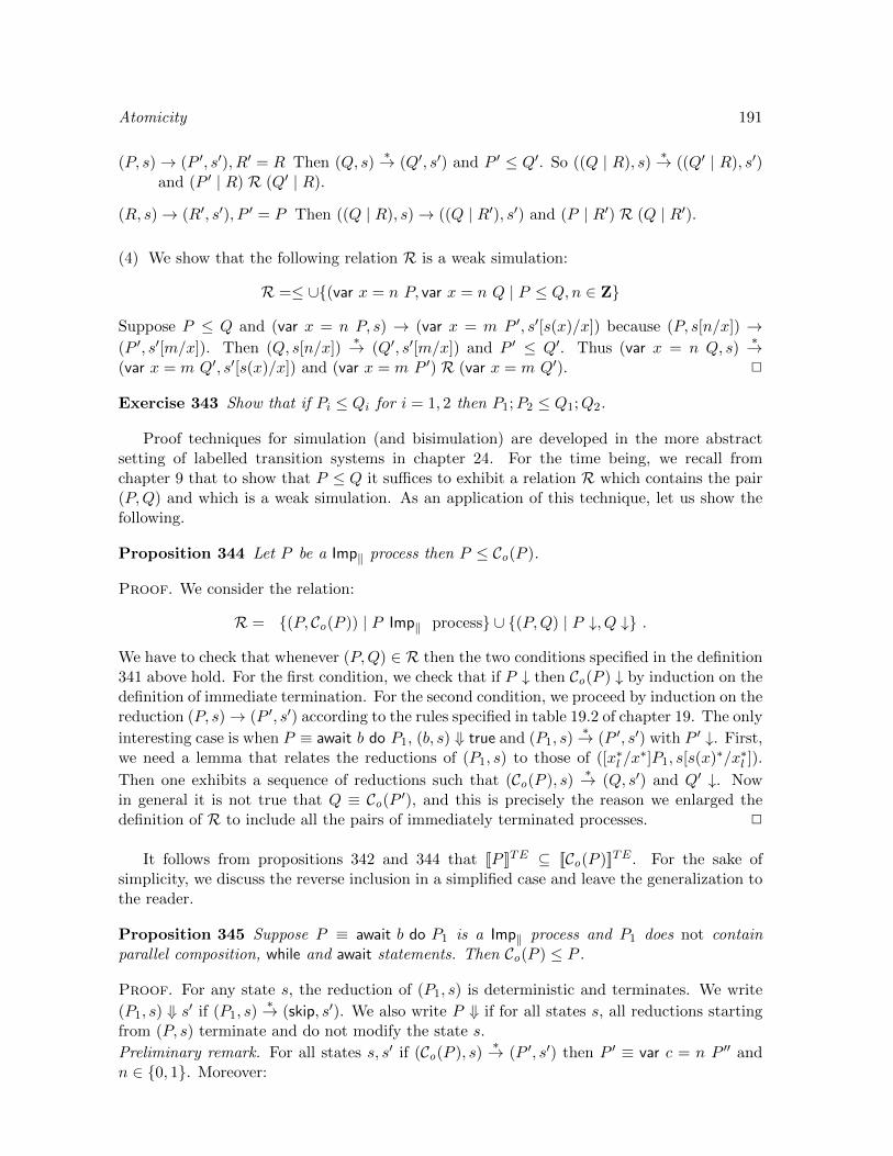
Atomicity 191
(P, s)→ (P ′, s′), R′ = R Then (Q, s)∗→ (Q′, s′) and P ′ ≤ Q′. So ((Q | R), s)
∗→ ((Q′ | R), s′)and (P ′ | R) R (Q′ | R).
(R, s)→ (R′, s′), P ′ = P Then ((Q | R), s)→ ((Q | R′), s′) and (P | R′) R (Q | R′).
(4) We show that the following relation R is a weak simulation:
R =≤ ∪(var x = n P, var x = n Q | P ≤ Q,n ∈ Z
Suppose P ≤ Q and (var x = n P, s) → (var x = m P ′, s′[s(x)/x]) because (P, s[n/x]) →(P ′, s′[m/x]). Then (Q, s[n/x])
∗→ (Q′, s′[m/x]) and P ′ ≤ Q′. Thus (var x = n Q, s)∗→
(var x = m Q′, s′[s(x)/x]) and (var x = m P ′) R (var x = m Q′). 2
Exercise 343 Show that if Pi ≤ Qi for i = 1, 2 then P1;P2 ≤ Q1;Q2.
Proof techniques for simulation (and bisimulation) are developed in the more abstractsetting of labelled transition systems in chapter 24. For the time being, we recall fromchapter 9 that to show that P ≤ Q it suffices to exhibit a relation R which contains the pair(P,Q) and which is a weak simulation. As an application of this technique, let us show thefollowing.
Proposition 344 Let P be a Imp‖ process then P ≤ Co(P ).
Proof. We consider the relation:
R = (P, Co(P )) | P Imp‖ process ∪ (P,Q) | P ↓, Q ↓ .
We have to check that whenever (P,Q) ∈ R then the two conditions specified in the definition341 above hold. For the first condition, we check that if P ↓ then Co(P ) ↓ by induction on thedefinition of immediate termination. For the second condition, we proceed by induction on thereduction (P, s)→ (P ′, s′) according to the rules specified in table 19.2 of chapter 19. The only
interesting case is when P ≡ await b do P1, (b, s) ⇓ true and (P1, s)∗→ (P ′, s′) with P ′ ↓. First,
we need a lemma that relates the reductions of (P1, s) to those of ([x∗l /x∗]P1, s[s(x)∗/x∗l ]).
Then one exhibits a sequence of reductions such that (Co(P ), s)∗→ (Q, s′) and Q′ ↓. Now
in general it is not true that Q ≡ Co(P ′), and this is precisely the reason we enlarged thedefinition of R to include all the pairs of immediately terminated processes. 2
It follows from propositions 342 and 344 that [[P ]]TE ⊆ [[Co(P )]]TE . For the sake ofsimplicity, we discuss the reverse inclusion in a simplified case and leave the generalization tothe reader.
Proposition 345 Suppose P ≡ await b do P1 is a Imp‖ process and P1 does not containparallel composition, while and await statements. Then Co(P ) ≤ P .
Proof. For any state s, the reduction of (P1, s) is deterministic and terminates. We write
(P1, s) ⇓ s′ if (P1, s)∗→ (skip, s′). We also write P ⇓ if for all states s, all reductions starting
from (P, s) terminate and do not modify the state s.
Preliminary remark. For all states s, s′ if (Co(P ), s)∗→ (P ′, s′) then P ′ ≡ var c = n P ′′ and
n ∈ 0, 1. Moreover:

192 Atomicity
• If n = 1 then s′ = s.
• If n = 0 then P ′ ⇓, (b, s) ⇓ true, and (P1, s) ⇓ s′.
To show this, we notice that a residual of (Co(P ), s) sets to 0 the variable c if and only if:
1. The boolean condition [x∗l /x∗]b evaluates to true. Notice that when this happens the
contents of x∗l and x∗r are identical.
2. The boolean condition x∗r = x∗ in the atomic statement evaluates to true.
This means that when c is set to 0, we know that the current state s is such that (b, s) ⇓ trueand (P1, s) ⇓ s′. As long as the two conditions above are not satisfied a residual of Co(P ) hasthe shape:
var c = 1 · · · ; while c = 1 · · ·
and cannot modify the visible state. Next, we define a relation R = R1 ∪R2 as follows:
R1 = (Q,P ) | ∃ s (Co(P ), s)∗→ (var c = 1 P ′, s)
R2 = (Q, skip) | ∃ s, s′ (Co(P ), s)∗→ (var c = 0 P ′, s′)
We conclude by checking that the relation R is a simulation. For R1 we use Property 1. Aslong as the reduction does not affect c, there is no modification of the visible state and noimmediate termination. So we can just simulate by doing nothing. As soon as the transitionset c to 0 we simulate by reducing atomically P . For R2, it suffices to check that:
(Q, skip) | Q ⇓
is a simulation. 2
22.4 Summary and references
Atomicity is a major issue in concurrency theory starting from early work on the implementa-tion of atomic transactions in databases [Pap79, BHG87, LMWF94]. Later, related conceptshave been developed in the framework of concurrent programming. In particular, let us men-tion the notion of concurrent object and linearizability [HW90] and the related results thatclassify the synchronization power of various concurrent objects [Her91] (see also chapter 32).Nowadays, the various strategies to implement atomicity we have discussed are applied tostandard programming languages (C++, Java, Haskell, ML,. . .). In particular, the work onso called hardware/software transactional memories [HM93, ST95] is mainly concerned withthe problem of finding an efficient implementation of the atomic operator. Amdahl’s law ispresented in [Amd67]. An early and quite readable description of the optimistic strategy inthe framework of database systems can be found in [KR81].

Chapter 23
Rely-guarantee reasoning
We have seen in chapter 20 that the semantics of concurrent processes calls for new techniques.Not surprisingly, a similar and related phenomenon arises in the specification of concurrentprocesses. In chapter 1, we have introduced the notion of partial correctness assertion (pca).Table 1.4 gives the rules to reason on a sequential fragment of the Imp‖ language. Theserules are sound (proposition 1.4) and can be inverted (proposition 9) thus providing a syntax-directed method to reduce a pca to an ordinary logical statement. Is it possible to extendthese results to the Imp‖ language?
23.1 Rely-guarantee assertions
We recall and extend some of the notation introduced in section 1.2 to reason on pca. Weassociate with a program P the input-output relation on states:
(s, s′) ∈ [[P ]]IO if (P, s) ⇓ s′ .
For example, in the case P is an assignment x := e, we have:
[[P ]]IO = (s, s[v/x]) | (e, s) ⇓ v ,
which turns out to be (the graph of) a total function.In the assertions, we identify a boolean predicate b with the set of states that satisfy it,
thus b stands for s | s |= b. We denote the set of states with St , unary relations on St withA,B, . . . and binary relations on St with R,G, . . .. To manipulate relations on states, we usethe following notation:
Id = (s, s) | s ∈ St (identity relation)Top = (s, s′) | s, s′ ∈ St (top relation)A;R = s′ | ∃ s s ∈ A and (s, s′) ∈ R (image)R;A = s | ∃ s′ s′ ∈ A and (s, s′) ∈ R (pre-image)R;R′ = (s, s′′) | ∃ s′ (s, s′) ∈ R and (s′, s′′) ∈ R′ (composition).
As usual, if R is a relation then R∗ is its reflexive and transitive closure.As mentioned above, the generation of the logical conditions follows the structure of the
program (proposition 9). One would like to follow this pattern for the concurrent programsof the Imp‖ language too. The following exercise suggests we can handle local variables.
193

194 Rely-guarantee assertions
Exercise 346 (rule for local variables) We write:
A[n/x] = s[n/x] | s ∈ A ,s =X s′ if ∀x ∈ X s(x) = s′(x) ,x /∈ fv(B) if ∀ s (s ∈ B, s =xc s
′ ⊃ s′ ∈ B) ,
∃x.B = s | ∃ s′ ∈ B s =xc s′ .
Then we formulate the rule for local variables as follows:
A[n/x] P ∃x.B x /∈ fv(B)
A var x = n P B .
Show that the rule is sound and that it can be inverted modulo α-renaming of the boundvariable provided y | y ∈ fv(B) is finite (which is always the case if the set B is defined bya formula).
Then let us turn to parallel composition, which is the core of the matter, and let us tryto formulate a rule of the shape:
Ai Pi Bi i = 1, 2
f(A1, A2) P1 | P2 g(B1, B2) ,
where f and g are two ways of combining predicates. Take: P1 ≡ x := 1;x := x + 1 andP2 ≡ x := 2. We already know from example 317 that:
[[P1]]pca = [[P2]]pca and [[P1 | P2]]pca 6= [[P2 | P2]]pca .
In particular, this means that any derivation that would end with a proof of the shape:
A1 P2 B1 A2 P2 B2true P2 | P2 x ≤ 2 ,
where |= g(B1, B2) ⊆ s | s(x) ≤ 2 could be turned into a derivation of the triple true P1 |P2 x ≤ 2 which is obviously not valid! An early approach to this problem goes back toOwicki and Gries. Their rule has the shape:
A1 P1 B1 A2 P2 B2A1 ∩A2 P1 | P2 B1 ∩B2
(23.1)
provided the proofs of the premises do not ‘interfere’. Having to look at the internal structureof processes is not very satisfying and it is clearly at odd with one basic principle of modulecomposition: to compose proofs (modules) one should just know what is proved (the interface)without depending on the details of the proof (the implementation). A way to tackle theselimitations is to consider a richer specification language whose judgments have the shape:
P : (A,R,G,B) (23.2)
where: (1) A and B are a pre-condition and a post-condition, respectively as in Floyd-Hoare rules, hence sets of states, (2) R is a relation on states that describes the environmenttransitions that are admitted (thus R is part of the pre-conditions), and (3) G is relationon states that describes the program transitions that are guaranteed (thus G is part of the

Rely-guarantee assertions 195
post-condition). We refer to assertions of the shape (23.2) as rely-guarantee assertions, or rgafor short. To define their validity, we recall from chapter20 that Imp‖ programs may performthe following labelled transitions:
(P, s)p→ (P ′, s′) (program transition, cf. Table 19.2)
(P, s)e→ (P, s′) (environment transition, cf. rule (20.1)).
Definition 347 (computation) A computation of a program P is a (finite or infinite)sequence:
(P, s0)λ0→ (P1, s1)
λ1→ (P2, s2)λ2→ · · · (23.3)
where si are states and λi ∈ p, e.
Definition 348 (validity rely-guarantee) The rely-guarantee assertion P : (A,R,G,B)is valid if for all computations of P of the shape (23.3) such that the following pre-conditionholds:
s0 ∈ A ∧ ∀ i (λi = e ⊃ (si, si+1) ∈ R) ,
it follows that the following post-condition holds:
∀ i (Pi ↓⊃ si ∈ B) ∧ (λi = p ⊃ (si, si+1) ∈ G) .
Thus the pre-condition concerns the initial configuration and all transitions performedby the environment (including those after termination) while the post-condition concerns thefinal configurations (if any) and all the transitions performed by the program.
Exercise 349 The validity of a given pca is equivalent to the validity of a derived rga. Specif-ically, show that the pca A P B is valid iff the rga P : (A, Id ,Top, B) is valid.
Remark 350 Rga’s can discriminate programs which are trace-environment equivalent. Forinstance, consider the programs loop ≡ while true do skip and P ≡ x := 0; loop. We knowthat [[loop]]TE = [[P ]]TE, since all the diverging computations receive the empty interpretation.On the other hand, the rga (true, Id , Id , false) is satisfied by loop but not by P because theassignment x := 0 does not respect the guarantee condition Id.
Definition 351 (stability) Let A be a unary relation and R a binary relation on some set.Then we write S(A,R) if s ∈ A and (s, s′) ∈ R implies s′ ∈ A and say that A is stable withrespect to R.
Proposition 352 Let A,B be unary relations and R be a binary relation. Then:
1. S(A,R) iff A;R∗ ⊆ A.
2. A;R∗ ⊆ B iff ∃A′ (A′ ⊇ A,S(A′, R), A′ ⊆ B).
Table 23.1 provides a collection of rules to derive valid rely-guarantee assertions, withthe proviso that the guarantee relation G in the conclusion of the rules contains the identityrelation Id . Without this hypothesis, the rules are unsound. For instance, one can deriveskip; skip : (true,Top, ∅, true) from skip : (true,Top, ∅, true).

196 Rely-guarantee assertions
A ⊆ A′ R ⊆ R′B′ ⊆ B G′ ⊆ GP : (A′, R′, G′, B′)
P : (A,R,G,B)
P : (A,R,G,C)Q : (C,R,G,B)
P ;Q : (A,R,G,B)
P : (A ∩ b,R,G,B)Q : (A ∩ ¬b,R,G,B)
if b then P else Q : (A,R,G,B)
A ⊆ B S(A,R)
skip : (A,R,G,B)
S(A,R) S(B,R)A; [[x := e]]IO ⊆ B
[[x := e]]IO ⊆ Gx := e : (A,R,G,B)
S(A,R) S(B,R)(A ∩ ¬b) ⊆ B
P : (A ∩ b,R,G,A)
while b do P : (A,R,G,B)
S(A,R) S(B,R)b; [[P ]]IO ⊆ G
P : (A ∩ b, Id ,Top, B)
await b do P : (A,R,G,B)
(R ∪G1) ⊆ R2 (R ∪G2) ⊆ R1
(G1 ∪G2) ⊆ G (B1 ∩B2) ⊆ BP : (A,R1, G1, B1)Q : (A,R2, G2, B2)
P | Q : (A,R,G,B)
.
Table 23.1: Rely-guarantee rules for Imp‖
Proposition 353 (soundness rga rules) The rely-guarantee assertions derivable in the sys-tem in Table 23.1 are valid.
Proof. We present the argument for the rule for parallel composition. A computation ofthe shape:
(P | Q, s0)λ0→ (P1 | Q1, s1)
λ1→ · · ·
can be turned into a computation of P where the moves played by Q are actually attributedto the environment:
(P, s0)λ′0→ (P1, s1)
λ′1→ · · · (23.4)
with λ′i = e if λi = e or λi = p and the ith move is due to Q, and λ′i = p otherwise. By asymmetric argument, we derive a computation for Q too:
(Q, s0)λ′′0→ (Q1, s1)
λ′′1→ · · · (23.5)
We claim that:λ′i = p implies (si, si+1) ∈ G1
λ′′i = p implies (si, si+1) ∈ G2 .
We reason by contradiction and take j to be least natural number where the property abovefails. For instance, suppose: λ′j = p and (sj , sj+1) /∈ G1. Now for a transition λ′i with i < jwe have 3 cases: either λ′i = p and (si, si+1) ∈ G1, or λi = e, λ′i = e and (si, si+1) ∈ R,or λi = p, λ′′i = p and (si, si+1) ∈ G2 because i < j. In particular, if λ′i = e we have that(si, si+1) ∈ R ∪G2 ⊆ R1. Then the following computation of P :
(P, s0)λ′0→ · · · (Pj , sj)
p→ (Pj+1, sj+1)

Rely-guarantee assertions 197
contradicts the hypothesis P : (A,R1, G1, B). It follows that if λi = p then (si, si+1) ∈G1∪G2 ⊆ G. Finally, we notice that (Pi | Qi) ↓ entails Pi ↓ and Qi ↓. Thus si ∈ B1∩B2 ⊆ B.2
Exercise 354 Prove the pca x = 0 x := 1;x := x + 1 | x := 2 x ∈ 2, 3 using therely-guarantee system.
Unfortunately, the move from pca’s to rga’s is not quite sufficient to reason about con-current programs. For instance, it is problematic to prove simple assertions such as:
x = 0 x := x+ 1 | x := x+ 1 x = 2 . (23.6)
The problem is that in the rule for parallel composition we need to abstract the possiblestate transformations of the parallel processes into a relation on states. In doing this, we loseinformation. For instance, we can record the fact that the variable x can be incremented byone, but we lose the information that this state transition can occur at most once. Further,in slightly more complicated programs such as x := x + 1;x := x + 2, one loses informationon the order of the state transformations too.
A ‘solution’ which goes back to the Owicki-Gries system is to allow for an instrumentationof the program. This means enriching the program with auxiliary variables and assignmentswhich allow to record (essential parts of) the history of the computation without affectingit. The ‘auxiliary variable’ rule states that if we can prove a rely-guarantee assertion of theinstrumented program then we can transfer this property to the original program where theinstrumentation is removed. For instance, with reference to the pca (23.6) above we canprove:
x = 0, p = 0, q = 0 atomic(x := x+ 1; p := 1) | atomic(x := x+ 1; q := 1) x = 2 (23.7)
and then derive the desired pca (23.6) by erasing the auxiliary variables p and q along withthe related assignments and atomic statements. In practice, one can insert program countersin all processes and describe exactly in the assertions the way the computation progresses.
It turns out that when adding an auxiliary variable rule, it is possible to invert the rulespresented in Table 23.1 along the spirit of proposition 9. However, as for the non-interferencerule (23.1), this is not very satisfying and really points to a weakness of the specificationlanguage. A more powerful and flexible approach consists in building a full fledged modallogic that allows to describe the transitions of the program and the environment. Examples ofsuch modal logics are discussed later in chapter 25 in the more abstract framework of labelledtransition systems.
23.2 A coarse grained concurrent garbage collector
We suppose the reader is familiar with the idea that a program may need to allocate memoryat run time and that such memory should be collected and reused whenever possible so thatthe program can carry on its execution within certain given memory bounds.
In general, it is hard to predict when a memory block becomes useless to the rest of thecomputation and can be collected. One approach to this issue consists in designing a specificprogram called garbage collector which periodically analyzes the state of the memory andcollects the blocks which are useless. Specifically, the memory is modelled as a directed graph

198 Rely-guarantee assertions
with a collection of root nodes which are the entry points of the program to the memory. Allnodes which are not accessible from the roots are considered as garbage and can be collected.Thus, at least from a logical point of view, the activity of the garbage collector can bedecomposed in two phases: a marking phase where the accessible nodes are determined anda collecting phase where the inaccessible nodes become again available for future usage. Inpractice, it is convenient to relax a bit this specification. Namely, one determines an over-approximation of the accessible nodes and consequently one collects a subset of the inaccessibleones.
Going towards a formalization, let us assume a fixed set of nodes N and a fixed subset ofroots Roots ⊆ N . We also use E ⊆ N × N to denote the collection of directed edges whichvaries over time. For any given collection of edges E, we have a collection of nodes which areaccessible from the roots: Acc(E) = Roots;E∗.
The activity of the program, henceforth called Mutator, on the memory graph can besummarized as follows: it selects two accessible nodes i, j and redirects an outgoing edge ofthe first node, say (i, k), towards j. In other terms, the edge (i, k) is replaced by the edge(i, j), where i, j, k are not necessarily distinct. The fundamental property which is guaranteedby the Mutator is that the collection of accessible nodes can only decrease. Thus if we denotewith E and E′ the collection of edges before and after a Mutator’s action we have that:
Acc(E′) ⊆ Acc(E) . (23.8)
This representation of the Mutator seems very simple but it is actually reasonable providedwe assume that among the root nodes there is: (i) a special node called nil without outgoingedges and (ii) a special node called fl (free list) that points to the list of free nodes that canbe used to allocate memory. With these hypotheses, expected operations of the Mutator suchas setting a pointer to nil or redirecting a pointer towards a newly allocated node, fall withinthe scope of the model.
The activity of the garbage collector is a bit more complex. The task of the marking phaseis to determine a set M ⊆ N which over-approximates the collection of reachable nodes. Anatural way to approach the task is to compute iteratively the least fixed point of the functionassociating to a set of nodes M the set of nodes Roots ∪M ;E. This can be expressed in animperative programming notation as follows:
Marker ≡ M := ∅; M1 := Roots;while M1 6⊆M do( M := (M ∪M1); M1 := (M ;E); )
The Marker program satisfies the pca:
true Marker (Roots ⊆M) ∧ (M ;E ⊆M) . (23.9)
It follows by induction that: Acc(E) ⊆ M . Once the marking phase is completed, thecollecting phase consists in inserting all the nodes which are not in the set M in the free listpointed by fl.
Our goal in the following is to reason on the properties of the Mutator and Marker whenthey are run in parallel. The property we want to check is that once the Marker terminates theset M is indeed an over-approximation of the set Acc(E). In order to express the specificationwe introduce an auxiliary variable done which is initially set to false and becomes true whenMarker terminates.
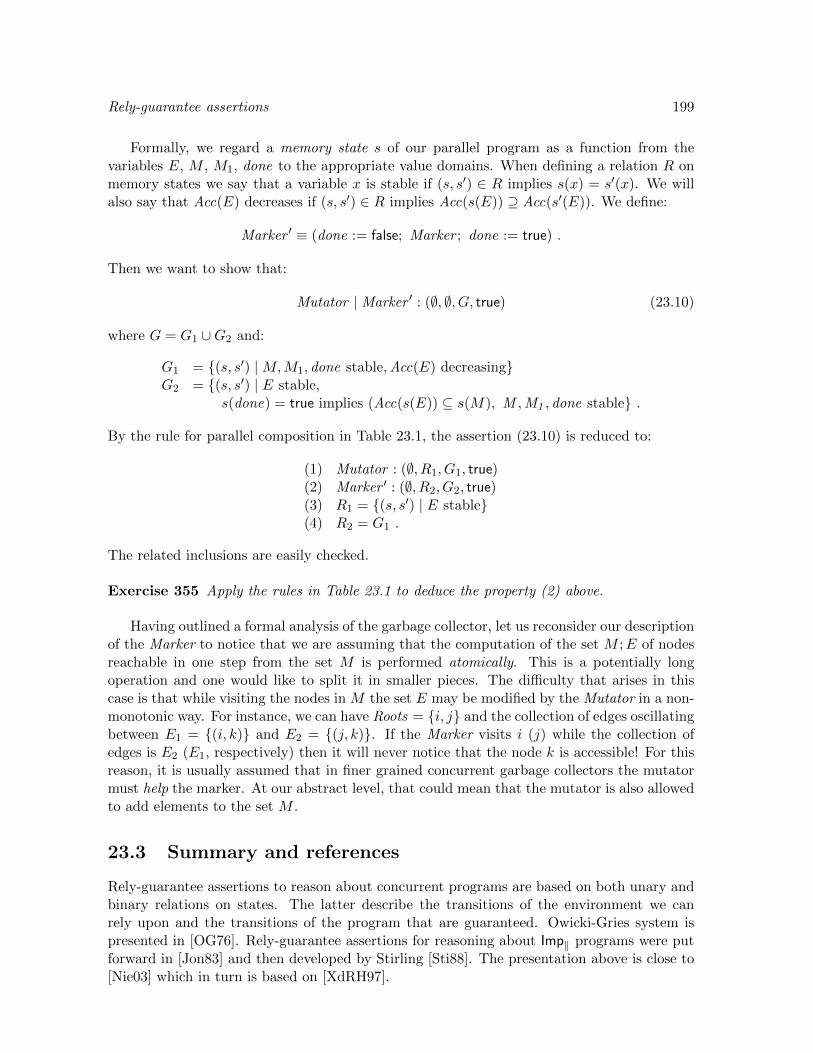
Rely-guarantee assertions 199
Formally, we regard a memory state s of our parallel program as a function from thevariables E, M , M1, done to the appropriate value domains. When defining a relation R onmemory states we say that a variable x is stable if (s, s′) ∈ R implies s(x) = s′(x). We willalso say that Acc(E) decreases if (s, s′) ∈ R implies Acc(s(E)) ⊇ Acc(s′(E)). We define:
Marker ′ ≡ (done := false; Marker ; done := true) .
Then we want to show that:
Mutator | Marker ′ : (∅, ∅, G, true) (23.10)
where G = G1 ∪G2 and:
G1 = (s, s′) |M,M1, done stable,Acc(E) decreasingG2 = (s, s′) | E stable,
s(done) = true implies (Acc(s(E)) ⊆ s(M), M ,M1 , done stable .
By the rule for parallel composition in Table 23.1, the assertion (23.10) is reduced to:
(1) Mutator : (∅, R1, G1, true)(2) Marker ′ : (∅, R2, G2, true)(3) R1 = (s, s′) | E stable(4) R2 = G1 .
The related inclusions are easily checked.
Exercise 355 Apply the rules in Table 23.1 to deduce the property (2) above.
Having outlined a formal analysis of the garbage collector, let us reconsider our descriptionof the Marker to notice that we are assuming that the computation of the set M ;E of nodesreachable in one step from the set M is performed atomically. This is a potentially longoperation and one would like to split it in smaller pieces. The difficulty that arises in thiscase is that while visiting the nodes in M the set E may be modified by the Mutator in a non-monotonic way. For instance, we can have Roots = i, j and the collection of edges oscillatingbetween E1 = (i, k) and E2 = (j, k). If the Marker visits i (j) while the collection ofedges is E2 (E1, respectively) then it will never notice that the node k is accessible! For thisreason, it is usually assumed that in finer grained concurrent garbage collectors the mutatormust help the marker. At our abstract level, that could mean that the mutator is also allowedto add elements to the set M .
23.3 Summary and references
Rely-guarantee assertions to reason about concurrent programs are based on both unary andbinary relations on states. The latter describe the transitions of the environment we canrely upon and the transitions of the program that are guaranteed. Owicki-Gries system ispresented in [OG76]. Rely-guarantee assertions for reasoning about Imp‖ programs were putforward in [Jon83] and then developed by Stirling [Sti88]. The presentation above is close to[Nie03] which in turn is based on [XdRH97].
200 Rely-guarantee assertions
The compact modeling of the garbage collector is introduced in [DLM+78]. More refinedsolutions to the concurrent garbage collection problem are described and analyzed, e.g., in[DLM+78, Gri77, BA84, vdS87]. The number of proof obligations to be checked for finegrained garbage collectors becomes quickly overwhelming and a machine-assisted proof isinstrumental to raise the confidence in the proposed solution. Examples of such developmentscan be found in [NE00, DG94]. Also it seems useful to cast the problem of concurrent garbagecollection in the more general framework of lock-free concurrent data structures [HM92] whichis discussed in chapter 32.
Chapter 24
Labelled transition systems andbisimulation
So far we have considered a rather concrete model of concurrent computation, namely parallelimperative programs with shared variables. To analyze the design spectrum which is availablein the semantics of concurrency, it is convenient to move to a more abstract framework wheresystems perform some set of actions. Such a system is called labelled transition system (lts).Concretely, an action could consist in changing the contents of a shared variable or sending amessage. In this chapter, we formalize the notion of (bi-)simulation over a lts, consider a wayto abstract away internal computation steps (weak (bi-)simulation), and present some prooftechniques for (bi-)simulation.
24.1 Labelled transition systems
A labelled transition system (lts) can be regarded as an automaton where we do not specifythe set of initial and final states.
Definition 356 (labelled transition system) A labelled transition system is a ternaryrelation → such that →⊆ S ×Act × S , S is a set of states, and Act is a set of actions. Wealso write s
α→ s′ for (s, α, s′) ∈→.
Remark 357 In section 19.1, we have presented a transition system for the Imp‖ language.It is possible to regard this system as a lts by taking the set of states S as the collection ofImp‖ processes and Act as the collection of pairs of memory states (not to be confused with thestates of the lts we are defining). Then we would write (P, (s, s′), Q) ∈→ if (P, s) → (Q, s′)according to the rules in Table 19.2.
Inspired by definition 318 of trace for Imp‖ processes, we introduce a notion of trace andtrace equivalence on lts.
Definition 358 (traces) We define the set of traces of a state s in a lts as:
tr(s) = α1 · · ·αn | sα1→ · · · αn→ .
We say that two states s and t are trace equivalent if tr(s) = tr(t).
201

202 LTS and bisimulation
There are a few points to be noticed concerning the definition 358 above. First, it neglectstermination since this notion is not even present in the definition 356 of lts (but a terminationpredicate on states could be added). And since termination is neglected, the set of traces isclosed under prefex. Second, there is no notion of closure of the traces under reflexivity andtransitivity. This point is treated later in section 24.3 once the notion of internal action isintroduced. Third, the environment seems to play no role in the behavior of the lts and therelated definition of trace equivalence. We shall see in chapter 26 that it is possible to enrichlts with a notion of synchronization and parallel composition and then prove that the notionof trace equivalence in definition 358 is indeed preserved by parallel composition.
24.2 Bisimulation
In chapter 19, we have motivated the interest of accounting for the branching behavior of asystem (example 313 of the vending machine). The notion of (bi-)simulation is a very popularapproach to this issue. We have already met this notion in chapter 9 in the framework ofthe λ-calculus and in chapter 22 in the framework of the Imp‖ concurrent language. Next, wereconsider this notion in the setting of labelled transition systems. The proposed definitionignores certain observables such as termination and deadlock. However, it is quite possible toenrich the notion of lts with predicates that represent termination and/or deadlock and thento formulate a notion of (bi-)simulation which depends on these predicates.
Definition 359 (bisimulation) Let →⊆ S × Act × S be a labelled transition system. Abinary relation R on S is a simulation if:
s R t, sα→ s′
∃ t′ t α→ t′, s′ R t′. (24.1)
Moreover we say that R is a bisimulation if:
s R t, tα→ t′
∃ s′ s α→ s′, s′ R t′. (24.2)
Remark 360 In definition 359 as well as in the following ones there is an implicit universalquantification on the states which are not existentially quantified.
Proposition 361 (on bisimulation) The following properties hold for the collection of bisim-ulations over a labelled transitions system:
1. The empty and identity relations are bisimulations.
2. The collection of bisimulations is closed under inverse, composition, and arbitrary unions.
3. There is a greatest bisimulation which is defined as the union of all bisimulations andthat we represent with ∼ (some authors call it bisimilarity).
4. Bisimulations are not closed under (finite) intersection.
Proof. Properties (1-3) follow by a simple unravelling of the definitions. For property (4),consider the lts 1
a→ 2, 1a→ 3, x
a→ y, xa→ z and the relations R1 = (1, x), (2, y), (3, z),
R2 = (1, x), (2, z), (3, y). 2

LTS and bisimulation 203
Exercise 362 (on simulation) Show that the properties above are true of simulations toobut for closure under inverse. Further, denote with ≤ the greatest simulation. Find a lts withstates s, t such that s ≤ t, t ≤ s, and s 6∼ t.
Exercise 363 (trace vs. simulation) For s, t states of a lts show that s ≤ t implies tr(s) ⊆tr(t), while the converse may fail.
Remark 364 (alternative definition of bisimulation) Sometimes a bisimulation is de-fined as a symmetric relation R such that:
s R t, sα→ s′
∃ t′ t α→ t′, s′ R t′.
The advantage of this definition is that one can omit the second condition (24.2). The in-convenience is that by forcing a bisimulation to be symmetric we make it larger than reallyneeded. However, notice that given a bisimulation R one can always derive a symmetricrelation which is a bisimulation by taking R∪R−1.
Let →⊆ S × Act × S be a labelled transition system. Notice that L = 2S×S is a completelattice with respect to inclusion (cf. definition 172). Bisimulation can be characterized as thegreatest fixed point of a certain monotonic function F on binary relations which we introducebelow.
Definition 365 (function F) We define F : L→ L as:
F(R) = (s, t) | sα→ s′ implies ∃ t′ t α→ t′ and s′ R t′ and
tα→ t′ implies ∃ s′ s α→ s′ and s′ R t′ .
The following properties of the function F are easily checked (cf. proposition 175).
Proposition 366 The following properties hold:
1. R is a bisimulation iff R ⊆ F(R).
2. F is monotonic on L.
3. The greatest bisimulation ∼ is the greatest fixed point of F .
Remark 367 (transfinite definition of bisimulation) The bisimulation ∼ being the great-est fixed point of the monotonic function F , it can be approximated from above as follows(cf. chapter 9):
∼κ+1 = F(∼κ) , ∼κ =⋂κ′<κ ∼κ′ (κ limit ordinal).
Thus to show s 6∼ t it suffices to find an ordinal κ such that s 6∼κ t.
Definition 368 (image finite lts) A lts →⊆ S ×Act × S is image finite if for all P, α theset s′ | s α→ s′ is finite.
For finite (image finite) lts the greatest fixed point is reached in a finite (countable) numberof iterations.

204 LTS and bisimulation
Proposition 369 (bisimulation for (image) finite lts) The following properties hold:
1. If the support S of the lts is finite then there is a natural number n such that the greatestbisimulation coincides with ∼n.
2. If the lts is image finite then the greatest bisimulation coincides with ∼ω, i.e., on imagefinite lts F is co-continuous (preserves intersections).
Proof. For the first property, see exercise 177. For the second property, suppose s ∼ω t andsα→ s′. Then:
∀n ∃ tn tα→ tn and s′ ∼n tn .
Since the set t′ | t α→ t′ is finite there must be a t′ in this set such that n | tn = t′ isinfinite.1 Thus there is an infinite sequence n1 < n2 < n3 < · · · such that s′ ∼nj tnj = t′.Then for any n we can find a nj ≥ n such that s′ ∼nj t′; and this entails s′ ∼n t′. Hences′ ∼ω t′. 2
We conclude this section by introducing a notation to denote lts which will be extendedin chapter 26 to a full language of processes known as CCS . The notation is generated bythe following grammar:
P ::= 0 || α.P || P + P α ∈ Act (24.3)
Here 0 denotes the empty lts, also called nil, α.P is the lts denoted by P prefixed by thetransition α, and P +Q is the non-deterministic sum of the lts denoted by P and Q. In thisnotation, the states’ identities are immaterial; what matters of a state is not its name butthe actions it can do. Using this notation, the lts version of the vending machines in example313 can be represented as follows:
a.(b.0 + c.0) vs. a.b.0 + a.c.0 ,
Notice that identifying the two machines amounts to distribute the prefix over the non-deterministic sum. We use the following abbreviations: b for b.0, bn for b. . . . .b.0 (b prefixedn times), and bω for the infinite lts b.b. · · ·. If I is a (possibly infinite) set then Σi∈IPi denotesthe non-deterministic sum of the lts denoted by Pi. We apply the notation in the followingexercise.
Exercise 370 (non-bisimilar lts) Consider the lts Pi, Qi defined as follows:
P0 = b.0 Q0 = c.0Pi+1 = a.(Pi +Qi) Qi+1 = a.Pi + a.Qi .
1. Show that for all i natural number: (i) Pi ∼i Pi +Qi ∼i Qi, (ii) Pi 6∼i+1 Pi +Qi 6∼i+1
Qi 6∼i+1 Pi.
2. Show that: (i) ∀ i ≤ n bn ∼i bω, (ii) Σi≥0bi + bω ∼ω Σi≥0b
i, (iii) ∀ i bi 6∼ω bω, (iv)Σi≥0b
i + bω 6∼ω+1 Σi≥0bi.
1This is a version of the so called pigeonhole principle which states that if infinitely many pigeons are putin finitely many boxes then at least one box must contain infinitely many pigeons.

LTS and bisimulation 205
24.3 Weak transitions
Certain computation steps should not be directly observable. For instance, in sequentialprograms usually one is just interested in the input-output behavior and not in the waythe output is computed. To model this situation in lts, we enrich the collection of actionswith a distinct internal action τ . For instance, τω is a diverging system which never inter-acts with the environment. As another example, we could regard a system such as a.τ.b.0equivalent to a.b.0. Though the internal action is not directly observable, it may make adifference. For instance, consider the lts a.0 + b.0 and τ.a.0 + τ.b.0 with the interpretation:a = ‘accepts to deliver coffee’ and b = ‘accepts to deliver tea’. The second system decides‘internally’ whether to deliver coffee or tea while the first will take a decision that may becontrolled by the environment.
Given a lts with τ transitions, we derive a related lts with the same states but wherean observable transition may be preceded and followed by an arbitrary number of internaltransitions (think of ε transitions in automata theory).
Definition 371 (derived weak lts) Let a lts→⊆ S×(Act∪τ)×S be given where τ /∈ Actis a distinct internal action. We derive from this lts another weak lts⇒ ⊆ S×(Act∪τ)×Swhere:
α⇒ =
(τ→)∗ if α = τ
(τ→)∗(
α→)(τ→)∗ otherwise.
Remark 372 When working with weak transitions, lts tend to be image infinite, and thereforeproposition 368 cannot be applied.
The notion of bisimulation for lts with internal actions is simply the standard notion ofbisimulation on the derived weak lts.
Definition 373 (weak bisimulation) Let →⊆ S × (Act ∪ τ)× S be a lts with a distinctinternal action τ . A binary relation R on S is a weak bisimulation if it is a bisimulation withrespect to the weak transition system ⇒. We denote with ≈ the largest weak bisimulation.
The following definition of weak bisimulation is the one which is used in practice.
Definition 374 (one step weak bisimulation) A relation R is a one step weak bisimu-lation if:
s R t sα→ s′
∃ t′ t α⇒ t′, s′ R t′,
s R t tα→ t′
∃ s′ s α⇒ s′, s′ R t′.
Proposition 375 A relation R on a lts is a weak bisimulation iff it is a one step weakbisimulation.
Proof. By diagram chasing. 2
Henceforth we just speak of weak bisimulation and use the more convenient definition.
Definition 376 (weak up to strong) We say that a relation R on a lts is a weak bisim-ulation up to strong bisimulation if:
s R t, sα→ s′
∃ t′ t α⇒ t′, s′ ∼ R ∼ t′,
s R t, tα→ t′
∃ s′ s α⇒ s′, s′ ∼ R ∼ t′.
Exercise 377 Show that if R is a weak bisimulation up to strong bisimulation then R ⊆≈.
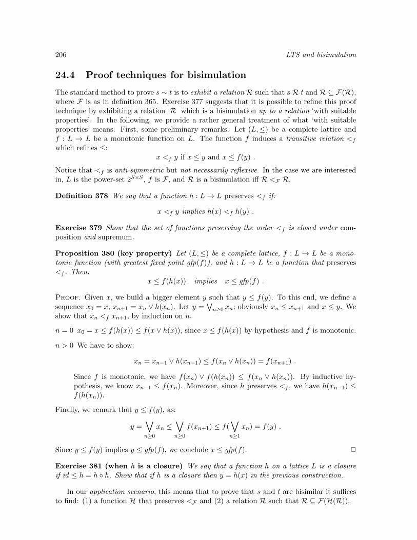
206 LTS and bisimulation
24.4 Proof techniques for bisimulation
The standard method to prove s ∼ t is to exhibit a relation R such that s R t and R ⊆ F(R),where F is as in definition 365. Exercise 377 suggests that it is possible to refine this prooftechnique by exhibiting a relation R which is a bisimulation up to a relation ‘with suitableproperties’. In the following, we provide a rather general treatment of what ‘with suitableproperties’ means. First, some preliminary remarks. Let (L,≤) be a complete lattice andf : L → L be a monotonic function on L. The function f induces a transitive relation <fwhich refines ≤:
x <f y if x ≤ y and x ≤ f(y) .
Notice that <f is anti-symmetric but not necessarily reflexive. In the case we are interestedin, L is the power-set 2S×S , f is F , and R is a bisimulation iff R <F R.
Definition 378 We say that a function h : L→ L preserves <f if:
x <f y implies h(x) <f h(y) .
Exercise 379 Show that the set of functions preserving the order <f is closed under com-position and supremum.
Proposition 380 (key property) Let (L,≤) be a complete lattice, f : L → L be a mono-tonic function (with greatest fixed point gfp(f)), and h : L → L be a function that preserves<f . Then:
x ≤ f(h(x)) implies x ≤ gfp(f) .
Proof. Given x, we build a bigger element y such that y ≤ f(y). To this end, we define asequence x0 = x, xn+1 = xn ∨ h(xn). Let y =
∨n≥0 xn; obviously xn ≤ xn+1 and x ≤ y. We
show that xn <f xn+1, by induction on n.
n = 0 x0 = x ≤ f(h(x)) ≤ f(x ∨ h(x)), since x ≤ f(h(x)) by hypothesis and f is monotonic.
n > 0 We have to show:
xn = xn−1 ∨ h(xn−1) ≤ f(xn ∨ h(xn)) = f(xn+1) .
Since f is monotonic, we have f(xn) ∨ f(h(xn)) ≤ f(xn ∨ h(xn)). By inductive hy-pothesis, we know xn−1 ≤ f(xn). Moreover, since h preserves <f , we have h(xn−1) ≤f(h(xn)).
Finally, we remark that y ≤ f(y), as:
y =∨n≥0
xn ≤∨n≥0
f(xn+1) ≤ f(∨n≥1
xn) = f(y) .
Since y ≤ f(y) implies y ≤ gfp(f), we conclude x ≤ gfp(f). 2
Exercise 381 (when h is a closure) We say that a function h on a lattice L is a closureif id ≤ h = h h. Show that if h is a closure then y = h(x) in the previous construction.
In our application scenario, this means that to prove that s and t are bisimilar it sufficesto find: (1) a function H that preserves <F and (2) a relation R such that R ⊆ F(H(R)).
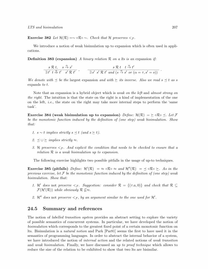
LTS and bisimulation 207
Exercise 382 Let H(R) =∼ R ∼. Check that H preserves <F .
We introduce a notion of weak bisimulation up to expansion which is often used in appli-cations.
Definition 383 (expansion) A binary relation R on a lts is an expansion if:
s R t, sα→ s′
∃ t′ t α⇒ t′ s′ R t′,
s R t tα→ t′
∃ s′ s′ R t′ and (sα→ s′ or (α = τ, s′ = s))
.
We denote with be the largest expansion and with its inverse. Also we read s t as sexpands to t.
Note that an expansion is a hybrid object which is weak on the left and almost strong onthe right. The intuition is that the state on the right is a kind of implementation of the oneon the left, i.e., the state on the right may take more internal steps to perform the ‘sametask’.
Exercise 384 (weak bisimulation up to expansion) Define: H(R) = R . Let Fbe the monotonic function induced by the definition of (one step) weak bisimulation. Showthat:
1. s ∼ t implies strictly s t (and s t).
2. ∪ implies strictly ≈.
3. H preserves <F . And explicit the condition that needs to be checked to ensure that arelation R is a weak bisimulation up to expansion.
The following exercise highlights two possible pitfalls in the usage of up-to techniques.
Exercise 385 (pitfalls) Define: H′(R) = ≈ R ≈ and H′′(R) = R . As in theprevious exercise, let F be the monotonic function induced by the definition of (one step) weakbisimulation. Show that:
1. H′ does not preserve <F . Suggestion: consider R = (τ.a, 0) and check that R ⊆F(H′(R)) while obviously R 6⊆≈.
2. H′′ does not preserve <F , by an argument similar to the one used for H′.
24.5 Summary and references
The notion of labelled transition system provides an abstract setting to explore the varietyof possible semantics of concurrent systems. In particular, we have developed the notion ofbisimulation which corresponds to the greatest fixed point of a certain monotonic function onlts. Bisimulation is a natural notion and Park [Par81] seems the first to have used it in thesemantics of programming languages. In order to abstract the internal behavior of a system,we have introduced the notion of internal action and the related notions of weak transitionand weak bisimulation. Finally, we have discussed an up to proof technique which allows toreduce the size of the relation to be exhibited to show that two lts are bisimilar.

208 LTS and bisimulation

Chapter 25
Modal logics
In chapter 23, we have considered partial correctness and rely-guarantee assertions as meansto specify the behaviour of concurrent processes and in doing this we have faced some problemsdue to the limited expressive power of the specification language. In this chapter, we take abold step in that for a given notion of equivalence on lts we aim at a specification languagewhich captures exactly the equivalence. The presented languages build on the notion of(propositional) modal logic which is an extension of usual logic with modalities that qualifythe validity of the assertions: possibly true, necessarily true,. . . In particular, we introduce adiamond modality indexed over the actions of the lts and stipulate:
s |= 〈α〉A if ∃ s′ s α→ s′ and s′ |= A ,
which is read as follows: a state s satisfies the formula 〈α〉A if there is a state s′ suchthat s
α→ s′ and s′ satisifies A. It turns out that the full infinitary specifications generatedby this extension characterize bisimulation, while restricted versions correspond to coarserequivalences such as simulation or trace equivalences.
In practice, one needs finite means to describe ‘infinitary’ specifications. An elegant wayto achieve this, is to define (monotonic) formulae by least and greatest fixed points (in thespirit of proposition 175). The resulting modal language is called the µ-calculus. For finitestate lts, we present a simple algorithm to decide whether a state satisfies a formula of theµ-calculus.
25.1 Modal logics vs. equivalences
We introduce a modal logic which consists of a classical propositional logic enriched with aso called diamond modality describing the ability to perform an action.
Definition 386 (formulae) The collection of formulae of a propositional modal logic is de-fined as:
A ::=∧i∈I
Ai || ¬A || 〈α〉A α ∈ Act (25.1)
where the set I can also be empty or infinite. By convention, we write true for∧∅ and [α]A
for ¬〈α〉¬A.
209

210 Modal logics
Definition 387 (formulae satisfaction) We define when a state in a lts satisfies a for-mula, written s |= A, as follows:
s |=∧i∈I Ai if ∀ i ∈ I s |= Ai
s |= ¬A if s 6|= A
s |= 〈α〉A if ∃ s′ s α→ s′ and s′ |= A .
We also write:[[A]] = s | s |= A (formula interpretation)[[s]] = A | s |= A (state interpretation)s ∼L s′ if [[s]] = [[s′]] (logical equivalence) .
Exercise 388 (on modal formulae) Spell out what it means to satisfy [α]A. Find a for-mula showing that a.(b.0 + c.0) 6∼L a.b.0 + a.c.0.
It is easily checked that two bisimilar states are logically equivalent.
Proposition 389 Let s, s′ be states in a lts. If s ∼ s′ then s ∼L s′.
To show the converse of proposition 389, we introduce the (possibly infinite) so calledcharacteristic formulae.
Definition 390 (characteristic formula) Given a state s in a lts and an ordinal κ thecharacteristic formula Cκ(s) is defined as follows:
Cκ+1(s) =∧sα→s′ 〈α〉C
κ(s′) ∧∧α∈Act [α](
∨sα→s′ C
κ(s′) )
Cκ(s) =∧κ′<κC
κ′(s) (κ limit ordinal).
(25.2)
Proposition 391 For any state s and ordinal κ:
1. |= s : Cκ(s).
2. |= s′ : Cκ(s) iff s ∼κ s′, where ∼κ is the approximation of bisimulation defined in remark367.
Proof. To prove a property for all ordinals one relies on the principle of transfinite induction.Namely one shows that if a property is true of all ordinals less than κ then it is true of κ. 2
Exercise 392 Suppose that the set of actions Act is finite. Then show for image finite ltsthe following property: if two processes are not bisimilar then there is a finite formula thatdistinguishes them.
Given that full modal logic characterizes bisimulation, one may look for fragments of thelogic that characterize coarser equivalences. We consider the cases of trace (definition 358)and simulation equivalence (definition 359).
Modal logics 211
Proposition 393 (trace equivalence) The modal formulae A of the following shape char-acterize trace equivalence:
A ::= B || C ||∧i∈I
Ai ,
where: B ::= true || 〈α〉B and C ::= false || [α]C .
Proof. One defines the characteristic formula as follows:
C(s) =∧
α1···αn∈tr(s)
〈α1〉 · · · 〈αn〉true ∧∧
α1···αn /∈tr(s)
[α1] · · · [αn]false .
2
Proposition 394 (simulation equivalence) The modal formulae A of the following shapecharacterize simulation equivalence:
A ::=∧i∈I
Ai || 〈α〉A .
Proof. We build the formula Cκ(s) taking the left hand side of the formula (25.2) thatworks for bisimulation. Then (1) |= s : Cκ(s) and (2) |= s′ : Cκ(s) iff s ≤κ s′, where ≤κ isthe approximation of simulation. One shows that s ≤ s′ and |= s : A implies |= s′ : A. Onthe other hand if s and s′ are logically equivalent then |= s′ : C(s) and |= s : C(s′). Therefores ≤ s′ and s′ ≤ s. 2
25.2 A modal logic with fixed points: the µ-calculus
In the presented modal language, to express, e.g., that a process can do infinitely many actionsα we need an infinite formula. It is possible to increase the expressive power of formulae whilekeeping the syntax finite. An elegant extension known as µ-calculus consists in adding to thelogical formulae least fixed points. Then the syntax of modal formulae given in definition 386is revisited as follows.
Definition 395 (formulae with fixed points) The modal formulae with fixed points havethe following syntax:
id ::= x || y || . . . (formula identifiers)A ::=
∧i∈I Ai || ¬A || 〈α〉A || id || µid .A (formulae).
In a formula µx.A the identifier x is bound in A by the least fixed point operator µ.Also we assume that each free occurrence of x in A is positive, i.e., under an even numberof negations. This positivity condition is essential to show that the function induced by theformula is monotonic and therefore has a least (and a greatest) fixed point (cf. exercise 396below).
Since a formula may contain free identifiers, its interpretation is given relatively to anassignment ρ : id → 2S as follows:
[[∧i∈I Ai]]ρ =
⋂i∈I [[Ai]]ρ
[[¬A]]ρ = ([[A]]ρ)c
[[〈α〉A]]ρ = s | s α→ s′ and s′ ∈ [[A]]ρ[[x]]ρ = ρ(x)[[µx.A]]ρ =
⋂X ⊆ S | [[A]]ρ[X/x] ⊆ X .
212 Modal logics
Of course, if A is a closed formula its interpretation does not depend on the assignment andwe can write s |= A if s ∈ [[A]]ρ, for some ρ.
Exercise 396 (positivity) Check that for all well-formed formulae A, identifier x, and as-signments ρ, the function X 7→ [[A]]ρ[X/x] is monotonic on 2S. Conclude that the semanticsof a formula µx.A does indeed correspond to a least fixed point.
An intuitive way to understand the meaning of a formula µx.A is to unfold it as aninfinite disjunction
∨κA
κ where: Aκ+1 = [Aκ/x]A and Aκ =∨κ′<κA
κ′ for κ limit ordinal.This viewpoint is based on the iterated definition of the least fixed point mentioned in chapter9.
Greatest fixed points are derived by duality from least fixed points by defining:
νx.A = ¬µx.¬([¬x/x]A) .
For instance: νx.〈α〉x = ¬µx.¬〈α〉¬x.
Exercise 397 (greatest fixed points) Check that the interpretation of ν does indeed cor-respond to a greatest fixed point, namely:
[[νx.A]]ρ =⋃X ⊆ S | X ⊆ [[A]]ρ[X/x] .
We have seen that disjunction and greatest fixed points can be derived from conjunction,least fixed points, and negation. An alternative approach consists in dropping negation andtaking conjunction, disjunction, µ and ν operators as primitive. This way we have to dealwith an additional operator but we can drop the positivity condition on the fixed points sinceconjunction and disjunction are guaranteed to induce monotonic functions.
Exercise 398 (deriving negation) Show that the negation operator can be defined (onclosed formulas). Hint: Consider the following equations:
¬〈α〉A = [α]¬A, ¬[α]A = 〈α〉¬A, ¬µx.A = νx.¬A, ¬νx.A = µx.¬A .
It turns out that for finite lts, the modal logic with fixed points can express the charac-teristic formula of a state by a finite formula.
Proposition 399 Let s be a state in a finite lts. Then there is a closed finite characteristicformula C(s) involving only greatest fixed points such that for any state s′, |= s′ : C(s) iffs ∼ s′.
Proof. For every state s introduce a propositional variable xs and an equation based on thecharacteristic formula in definition 390:
xs =∧sα→s′ 〈α〉xs′ ∧
∧α∈Act [α](
∨sα→s′ xs′ )
Then the general idea is to take the greatest fixed point of this system of equations and projecton the component which corresponds to the state s. 2
Another interesting property of the µ-calculus on finite lts is that the model-checkingproblem is decidable. We spend the rest of the section to present a proof of this fact thatrelies on the following elementary property of fixed points.

Modal logics 213
Proposition 400 (reduction) Let f be a monotonic function over 2S and s ∈ S be a state.Consider the following monotonic functions over 2S: (f ∪ s)(x) = f(x)∪ s and (f\s)(x) =f(x)\x. Also if g is a monotonic function denote by ν(g) and µ(g) its greatest and leastfixed point. Then:
1. s ∈ ν(f) iff s ∈ f(ν(f ∪ s)).
2. s ∈ µ(f) iff s ∈ f(µ(f\s)).
3. s ∈ ν(f ∪ s).
4. s /∈ ν(f\s).
Proof. (1) Suppose s ∈ ν(f). Then:
f(ν(f)) ∪ s = ν(f) ∪ s = ν(f) .
By definition of ν(f ∪ s) this implies ν(f) ⊆ ν(f ∪ s). By monotonicity, ν(f) = f(ν(f)) ⊆f(ν(f ∪ s)), and therefore s ∈ f(ν(f ∪ s)). On the other hand, suppose s ∈ f(ν(f ∪ s)). Itfollows:
ν(f ∪ s) = f(ν(f ∪ s)) ∪ s = f(ν(f ∪ s)) .
By definition of ν(f) this implies ν(f ∪ s) ≤ ν(f). By monotonicity, f(ν(f ∪ s)) ≤ f(ν(f)) =ν(f), and therefore s ∈ ν(f).
(2) Prove by a dual argument: s /∈ µ(f) iff s /∈ f(µ(f\s)).
(3− 4) Immediate by unfolding the fixed point. 2
This proposition suggests a strategy to unfold recursive formulae. The starting idea isto tag each fixed point with a set of states. Then properties (1-2) of proposition 400 whenread from left to right suggest to record in the tag the states that are crossed when unfoldinga fixed point while properties (3-4) of proposition 400 provide the halting conditions. Toformalize this idea, we begin by introducing the syntax of tagged formulae.
Definition 401 (formulae with tagged fixed points) The modal formulae with taggedfixed points have the following syntax:
id ::= x || y || . . . (formula identifiers)T ::= s1, . . . , sn (tags, finite sets of states)A ::=
∧i∈I Ai ||
∨i∈I Ai || 〈α〉A || [α]A || id || µid : T.A || νid : T.A (tagged formulae).
The interpretation of tagged fixed points is as follows while the interpretation of the logicaland modal operators is left unchanged:
[[µx : T.A]]ρ =⋂X ⊆ S | ([[A]]ρ[X/x])\T ⊆ X ,
[[νx : T.A]]ρ =⋃X ⊆ S | X ⊆ ([[A]]ρ[X/x]) ∪ T .
Based on this interpretation and proposition 400, we introduce in Table 25.1 the collection ofrules to model-check states against finite formulae of the µ-calculus.
Proposition 402 (soundness) Let A be a closed formula of the modal, tagged µ-calculus.If we can derive the assertion s : A according to the rules in Table 25.1 then s ∈ [[A]].

214 Modal logics
s : A s : B
s : A ∧B
s : A
s : A ∨Bs : B
s : A ∨B
s′ : A
s : 〈α〉A for some sα→ s′
s′ : A
s : [α]Awhenever s
α→ s′′
s /∈ T s : [µx : T ∪ s.A/x]A
s : µx : T.A
s /∈ T s : [νx : T ∪ s.A/x]A
s : νx : T.A
s ∈ Ts : νx : T.A
Table 25.1: A model checker for the µ-calculus
Proof. By induction on the height of the proof, relying on the reduction proposition 400 forthe rules that fold the fixed points. 2
Proving completeness of the method for finite state lts amounts to prove the terminationof the unfolding process. Suppose we look at the rules in Table 25.1 bottom up. All rulesbut those that unfold fixed points either entail termination or shrink the size of the formulato be proved. Hence any infinite backward development must include an infinite number ofapplications of the rules unfolding fixed points. Now we remark that these rules add newelements to the tags. Since T ⊆ S and S is finite, we might conjecture that this processeventually terminates. We prove this property in two steps. First, we present a simplerewriting system whose termination proof exposes the kernel of the combinatorial problem.Second, we show termination of the bottom up proof development by exhibiting a reductionpreserving translation from judgments to terms of the simple rewriting system.
Definition 403 We define a collection of σ-terms as follows where n is a natural number:
id ::= x || y || · · · (identifiers)θ ::= id || 1 || θ ∗ θ || •θ || σnid .θ (σ-terms)
Definition 404 A term θ can be reduced according to the following rules where the rules canbe applied at top level only:
σn+1x.θ → [σnx.θ/x]θ, •θ → θ, θ ∗ θ′ → θ, θ ∗ θ′ → θ′ .
Proposition 405 The rewriting system defined in 404 terminates.
Proof. Let WF be the collection of terminating σ-terms. If θ ∈WF let d(θ) be the lengthof the longest reduction sequence (this is well defined because the reduction tree is finitelybranching). We want to prove:
θ, θ′ ∈WF implies [θ′/x]θ ∈WF . (25.3)
Modal logics 215
We prove (25.3) by induction on d(θ). The only interesting case is when θ has the shapeσn+1y.θ. Then we observe:
[θ′/x](σn+1y.θ) ≡ σn+1y.[θ′/x]θ → [σny.[θ′/x]θ/y]([θ′/x]θ) ≡ [θ′/x][σny.θ/y]θ .
We note that (σn+1y.θ) → [σny.θ/y]θ ∈ WF . Hence, we can apply the inductive hypothesison d([σny.θ/y]θ), and we conclude that [θ′/x][σny.θ/y]θ ∈WF .
Next we prove that all σ-terms terminate. We proceed by induction on a relation whichis the least transitive relation such that:
σn+1x.θ σnx.θ , σn+1x.θ θ , •θ θ , θ ∗ θ′ θ , θ ∗ θ′ θ′ .
Clearly is a well founded relation. Again the only interesting case is when the termhas the shape σyn+1.θ. By the inductive hypothesis σyn.θ ∈ WF , θ ∈ WF , and by (25.3)[σyn.θ/y]θ ∈WF . 2
Definition 406 Given a finite lts with a set of states S, we associate a σ-term to a modalformula as follows, where n = ]S + 1:
〈x〉 = x , 〈A ∧B〉 = 〈A〉 ∗ 〈B〉 , 〈A ∨B〉 = 〈A〉 ∗ 〈B〉 ,〈〈α〉A〉 = •〈A〉 , 〈[α]A〉 = •〈A〉 , 〈µx : T.A〉 = σx(n−]T ).〈A〉 ,〈νx : T.A〉 = σx(n−]T ).〈A〉 .
Suppose s′ : A′ is a premise of s : A in the proof development. We show 〈A〉 → 〈A′〉 byinspection of the proof rules. The only interesting case is when we unfold a fixed point. Sincein the translation we have picked n = ]S+ 1 bigger than ]T we can compute, e.g., in the caseof the least fixed point:
〈µx : T.A〉 = σx(n−]T ).〈A〉 → [σx(n−]T−1).〈A〉/x]〈A〉 = 〈[µx : T ∪ s.A/X]A〉 .
Proposition 407 The model checker is complete on finite structures.
Proof. We show by induction on A that |= s : A iff a proof rule applies. We can bound thedepth of a path in a bottom up proof development. Hence, if |= s : A by developing the proofbottom up we eventually obtain a proof of s : A. 2
25.3 Summary and references
We have described a family of modal logical languages which can be used to characterizebisimulation as well as coarser equivalences. We have also presented a few basic results on afixed point extension of modal logic known as µ-calculus. The µ-calculus is a kind of basicmodal logical language to which more user-friendly logical languages can be compiled. Itwas introduced by Kozen [Koz83], following previous work by V. Pratt. The simple proofof decidability of the model checking problem for finite lts we have presented is based on[Win89]. The model-checking problem for the µ-calculus is known to be in NP∩co-NP (likethe graph isomorphism problem). Upper bounds on the time complexity are polynomial inthe size of the lts and exponential in the so called alternation depth of the formula. This isa measure that counts the number of alternations of nested greatest and least fixed points.It is also known [Bra96, Len96] that bounding the alternation depth limits the expressivityof the logic, i.e., the hierarchy of formulae obtained by measuring the alternation depth isstrict. The basic theory of the µ-calculus is developed systematically in [AN01].

216 Modal logics

Chapter 26
Labelled transition systems withsynchronization
One can make the basic model of labelled transition systems a bit more interesting by addingsome parallelism and synchronization mechanisms. One elegant way to provide a synchro-nization mechanism is to introduce a notion of co-action and suppose that synchronizationhappens when a process can perform an action and another parallel process can perform thecorresponding co-action. Thus, given a set A, take the set of actions to be:
Act = a, a | a ∈ A ∪ τ . (26.1)
It is convenient to extend the co-action definition to the whole set Act by assuming:
τ = τ , a = a .
CCS (Calculus of Communicating Systems) is a minimal set of operators to represent suchlabelled transition systems enriched with the co-action mechanism; we introduce this formal-ism and discuss two ways to define its bisimulation semantics which turn out to be equivalent.CCS is a simple model of concurrent systems and we shall build on it to discuss the notions ofdeterministic (chapter 27), timed (chapter 28), and probabilistic concurrent system (chapter29). We shall also consider an extension of CCS , known as π-calculus (chapter 30), thatallows for a rather direct embedding of higher-order functional programs.
26.1 CCS
Actions in CCS are defined according to the equation (26.1) above. Besides the nil, prefixand non-deterministic choice operators introduced in chapter 24, CCS includes operators todeclare a local action (cf. local variable in Imp‖), to put processes in parallel, and to definerecursive behaviors:
P ::= 0 || α.P || (P + P ) || (P | P ) || νa P || A(a∗)
where α ∈ Act and A,B, . . . are process identifiers. An action name is free if it is not in thescope of a local action declaration (a ν). We write a∗ for a possibly empty list of action namesa1, . . . , an. Similarly, νa∗ P stands for νa1 · · · νan P , and [b∗/a∗] for [b1/a1, . . . , bn/an]. Itis assumed that each process identifier A is defined by a unique equation A(b∗) = P where
217
218 CCS
the free names in P are contained in the set of parameters b∗. For instance, A could be aprocess identifier defined by the equation:
A(a, b) = a.νc (A(a, c) | b.A(c, b)) . (26.2)
Here the set of variables occurring free in a.νc (A(a, c) | b.A(c, b)) is a, b which happens tobe included (actually equal) to the set of parameters of the process identifier A. Also noticethat an action name, say b, may appear in a prefix as such or in its dual form b.
Moving towards semantics, the main design decision consists in regarding a, b, . . . as chan-nel names on which parallel processes synchronize. More precisely, a synchronization mayonly happen when a process is ready to perform an action and another parallel process isready to perform its dual action as, e.g., in the process (a.P | a.Q). Following the synchro-nization, the process moves to (P | Q). CCS is an asynchronous model of concurrency whereinteraction is possible through rendez-vous synchronization on pure channels. A rendez-vouschannel is a channel of null capacity where the sender must always wait for a receiver. Achannel is pure if no message value is exchanged; all that matters is the synchronization.
An important consequence of assuming a synchronization by rendez-vous is to offer a bettercontrol on the role of the environment. In the Imp‖ model, the environment can modify the(visible part of the) state and these modifications may affect the future computation of theprocess. In CCS , the only way the environment may affect the computation of the process isto perform an action which is dual to an action that the process is ready to perform.
Starting from this intuition, we follow two paths to define a compositional semantics ofCCS . The first path consists in associating a labelled transition system with each CCSprocess. Then the equivalences on lts defined in the previous chapter 24, apply to CCSprocesses too and lead to a compositional semantics. The second path consists in looking atCCS as a (rudimentary) programming language and define its possible reductions similarlyto what we have done for the Imp‖ language in chapter 19. Then what needs to be done is tofix a notion of observable and to derive a notion of compositional equivalence. We work withthe notion of (weak) bisimulation introduced in chapter 24 and in the end, we show that thetwo paths outlined above actually lead to the same compositional equivalence.
As a concrete example illustrating the difference between the two approaches, considerthe CCS process P ≡ (a.0 | a.0). In the first approach, we have to consider the labelledtransitions:
Pa→ (0 | a.0)
a→ (0 | 0) , Pa→ (a.0 | 0)
a→ (0 | 0) , Pτ→ (0 | 0) .
While in the second, we just have have the reduction:
P → (0 | 0) .
We shall see that the τ transitions correspond to the reductions while the other labelledtransitions correspond to interactions with the environment.
26.2 Labelled transition system for CCS
Table 26.1 describes a lts for CCS processes where the symmetric rules for | and + are omitted.
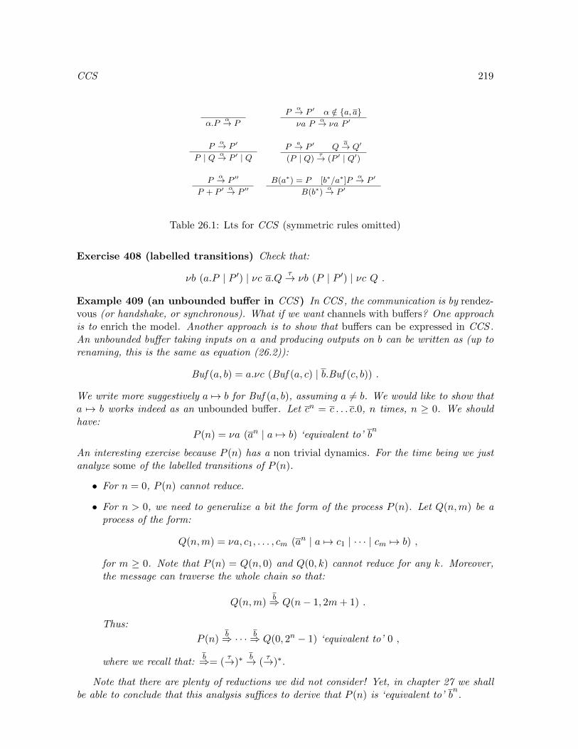
CCS 219
α.Pα→ P
Pα→ P ′ α /∈ a, aνa P
α→ νa P ′
Pα→ P ′
P | Q α→ P ′ | QP
a→ P ′ Qa→ Q′
(P | Q)τ→ (P ′ | Q′)
Pα→ P ′′
P + P ′α→ P ′′
B(a∗) = P [b∗/a∗]Pα→ P ′
B(b∗)α→ P ′
Table 26.1: Lts for CCS (symmetric rules omitted)
Exercise 408 (labelled transitions) Check that:
νb (a.P | P ′) | νc a.Q τ→ νb (P | P ′) | νc Q .
Example 409 (an unbounded buffer in CCS) In CCS, the communication is by rendez-vous (or handshake, or synchronous). What if we want channels with buffers? One approachis to enrich the model. Another approach is to show that buffers can be expressed in CCS.An unbounded buffer taking inputs on a and producing outputs on b can be written as (up torenaming, this is the same as equation (26.2)):
Buf (a, b) = a.νc (Buf (a, c) | b.Buf (c, b)) .
We write more suggestively a 7→ b for Buf (a, b), assuming a 6= b. We would like to show thata 7→ b works indeed as an unbounded buffer. Let cn = c . . . c.0, n times, n ≥ 0. We shouldhave:
P (n) = νa (an | a 7→ b) ‘equivalent to’ bn
An interesting exercise because P (n) has a non trivial dynamics. For the time being we justanalyze some of the labelled transitions of P (n).
• For n = 0, P (n) cannot reduce.
• For n > 0, we need to generalize a bit the form of the process P (n). Let Q(n,m) be aprocess of the form:
Q(n,m) = νa, c1, . . . , cm (an | a 7→ c1 | · · · | cm 7→ b) ,
for m ≥ 0. Note that P (n) = Q(n, 0) and Q(0, k) cannot reduce for any k. Moreover,the message can traverse the whole chain so that:
Q(n,m)b⇒ Q(n− 1, 2m+ 1) .
Thus:
P (n)b⇒ · · · b⇒ Q(0, 2n − 1) ‘equivalent to’ 0 ,
where we recall that:b⇒= (
τ→)∗b→ (
τ→)∗.
Note that there are plenty of reductions we did not consider! Yet, in chapter 27 we shallbe able to conclude that this analysis suffices to derive that P (n) is ‘equivalent to’ b
n.

220 CCS
We can regard CCS as a labelled transition system where states are processes. We saythat P and Q are strongly bisimilar (written P ∼ Q) if they are bisimilar with respect to thelts we have just defined. We say that they are weakly bisimilar (written P ≈ Q) if they arebisimilar with respect to the derived lts
α⇒ where internal actions are ‘abstracted’. ObviouslyP ∼ Q implies P ≈ Q. Next, we consider the issue of compositionality.
Definition 410 (CCS context) A context C is a process with a hole [ ] (here and in thefollowing we omit the symmetric cases when listing contexts):
C ::= [ ] || α.C || C + P || C | P || νa C .
Proposition 411 If P ∼ Q then C[P ] ∼ C[Q].
Proof. We apply the standard technique which amounts to define a relationR which includesthe processes of interest and show that it is a bisimulation.
Prefix R = (α.P1, α.P2) | P1 ∼ P2∪ ∼Sum R = (P1 +Q,P2 +Q) | P1 ∼ P2∪ ∼Parallel R = (P1 | Q,P2 | Q) | P1 ∼ P2∪ ∼Restriction R = (νa P1, νa P2) | P1 ∼ P2∪ ∼ .
2
Remark 412 In general, the non-deterministic sum does not preserve weak bisimulation as:
τ.a ≈ a but τ.a+ b 6≈ a+ b .
However a guarded version of the non-deterministic sum has this property. Denote withD the following contexts:
D ::= [ ] || α.D || α′.D + P || (D | P ) || νa D α′ 6= τ .
Proposition 413 If P ≈ Q then D[P ] ≈ D[Q].
Proof. Similar to the strong case. 2
Remark 414 (on unguarded sum) There are two viewpoints on the non-preservation ofweak-bisimulation by the sum:
1. One should take the largest congruence which refines ≈. Then, e.g., we should distin-guish τ.a from a.
2. In most applications one just needs a guarded sum and so it is enough to have a notionof equivalence which is preserved by guarded sums.
The second viewpoint tends to prevail at least in formalisms like Imp‖ (chapter 19) or the π-calculus (chapter 30) where a guarded form of sum is easily derived from parallel composition.

CCS 221
Exercise 415 (sequentialization in CCS) We consider a fragment of CCS (we drop sumand recursive definitions) extended with an operator ‘;’ for process sequentialization. Thusthe process syntax is as follows:
P ::= 0 || α.P || (P | P ) || P ;P || νa P α ∈ a, a | a ∈ A ∪ τ . (26.3)
The labelled transition system for CCS is extended with the following rules for process se-quentialization:
Pα→ P ′
P ;Qα→ P ′;Q
P ↓ Qα→ Q′
P ;Qα→ Q′
Here the predicate ↓ denotes proper termination and it is defined as the least set of processessuch that:1
0 ↓P ↓ Q ↓(P | Q) ↓
P ↓ Q ↓(P ;Q) ↓
P ↓νa P ↓ .
If P is a process in the extended language (26.3) and c is a name not occurring in P then[[P ]]c is a CCS process (without process sequentialization) defined as follows:
[[0]]c = c.0[[α.P ]]c = α.[[P ]]c[[P1 | P2]]c = νc1, c2 (([[P1]]c1 | [[P2]]c2) | c1.c2.c.0) (c1, c2 /∈ fv(P1) ∪ fv(P2) ∪ c)[[P1;P2]]c = νc′ ([[P1]]c′ | c′.[[P2]]c) (c′ /∈ fv(P1) ∪ fv(P2) ∪ c)[[νa P ]]c = νa [[P ]]c (c 6= a)
(1) Show that if P ↓ then [[P ]]cc⇒ Q and Q ∼ 0, where ∼ is the largest strong bisimulation.
(2) Define the notion of weak simulation up to strong bisimulation and show that this is asound technique to prove weak simulation. (3) Show that for all processes P , P is weaklysimulated by [[P ]]c up to strong bisimulation.
Exercise 416 (bisimulation up-to context) We introduce a notion of bisimulation up tothe contexts. For simplicity let us assume: D ::= [ ] || α.D || (D | P ) || νa D. Suppose:
H(R) = (P ′, Q′) | ∃D P ′ ≡ D[P ], P R Q,D[Q] ≡ Q′ .
Let F be the monotonic function associated with (one step) weak bisimulation.
1. Analyze the one-step transitions of a process D[P ] as a function of the transitions of Pand D[0].
2. Show that H preserves <F .
3. Explicit the associated notion of bisimulation up to context.
Exercise 417 (prime factorization) Let A be a set of actions with generic elements a, b, . . .and let P denote a process in the following fragment of CCS:
P ::= 0 || a.P || (P + P ) || (P | P ) a ∈ A .
1This is related to (but slightly different from) the immediate termination predicate introduced for thelanguage Imp‖ (chapter 19).

222 CCS
Notice that there is no notion of co-action and therefore no possibility of synchronizationamong parallel processes. In this exercise when we speak of a process, we refer to a process inthis fragment. We define the size of a process, say |P |, by induction on the structure of P asfollows:
|0| = 0 , |a.P | = 1 + |P | , |P +Q| = max (|P |, |Q|) , |P | Q| = |P |+ |Q| .
We say that a process P is irreducible if P ∼ P1 | P2 implies that P1 ∼ 0 or P2 ∼ 0 and wesay that P is prime if P is irreducible and moreover P 6∼ 0. Prove the following assertions.
1. If Pa→ Q then |P | > |Q|.
2. If P ∼ Q then |P | = |Q| (but the converse fails).
3. For all processes P,Q,R the following properties hold:
• If (P | R) ∼ (Q | R) then P ∼ Q (this is a kind of cancellation property).
• If (P | R) ∼ (Q | R′) and Ra→ R′ then there exists Q′ such that Q
a→ Q′ andP ∼ Q′.
4. Every process P such that P 6∼ 0 can be expressed up to strong bisimulation as theparallel composition of prime processes.
5. Every process P such that P 6∼ 0 has a unique decomposition as the parallel compositionof prime processes. Unicity here has to be understood in the same sense as the unicityof the prime factorization of a natural number.
26.3 A reduction semantics for CCS
We want to define a reduction semantics for CCS . A technical problem is that in the syntax,the synchronizing processes can be far away as in: νb (a.P | P ′) | νc a.Q. In the lts pre-sented in Table 26.1 we have tackled this problem by keeping track of the potential transitionsof every sub-process. An alternative approach consists in introducing a notion of structuralequivalence on processes which is strong enough to bring two synchronizing processes in con-tiguous positions and weak enough to identify only processes that are intuitively equivalent.In particular in the following, we assume a structural equivalence ≡ which is the least congru-ence which (i) includes renaming, (ii) such that | is associative and commutative, (iii) suchthat + is associative, commutative and idempotent, and (iv):
νa (P | Q) ≡ νa P | Q if a /∈ fv(Q)A(b∗) ≡ [b∗/a∗]P if A(a∗) = P .
An evaluation context E is defined by:
E ::= [ ] || νa E || E | P (evaluation contexts). (26.4)
Then the reduction relation is
P → Q if P ≡ E[a.P ′ +Q′ | a.P ′′ +Q′′] and Q ≡ E[P ′ | P ′′]P → Q if P ≡ E[τ.P +Q′] and Q ≡ E[P ] .
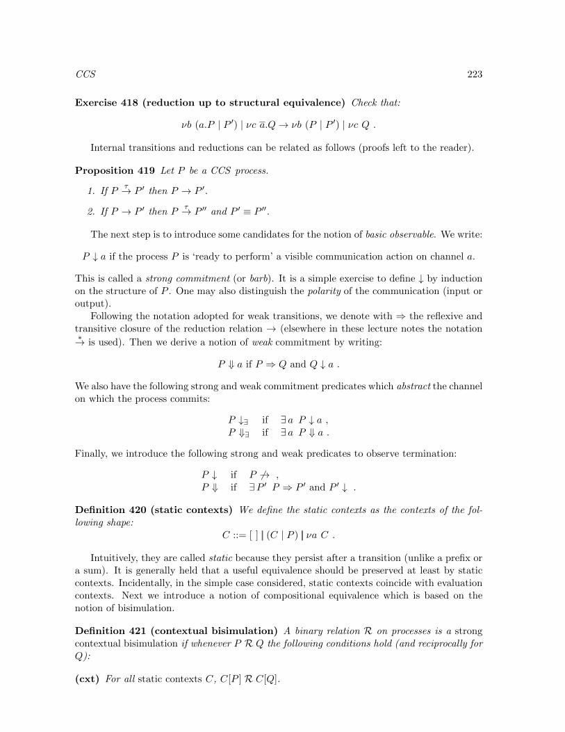
CCS 223
Exercise 418 (reduction up to structural equivalence) Check that:
νb (a.P | P ′) | νc a.Q→ νb (P | P ′) | νc Q .
Internal transitions and reductions can be related as follows (proofs left to the reader).
Proposition 419 Let P be a CCS process.
1. If Pτ→ P ′ then P → P ′.
2. If P → P ′ then Pτ→ P ′′ and P ′ ≡ P ′′.
The next step is to introduce some candidates for the notion of basic observable. We write:
P ↓ a if the process P is ‘ready to perform’ a visible communication action on channel a.
This is called a strong commitment (or barb). It is a simple exercise to define ↓ by inductionon the structure of P . One may also distinguish the polarity of the communication (input oroutput).
Following the notation adopted for weak transitions, we denote with ⇒ the reflexive andtransitive closure of the reduction relation → (elsewhere in these lecture notes the notation∗→ is used). Then we derive a notion of weak commitment by writing:
P ⇓ a if P ⇒ Q and Q ↓ a .
We also have the following strong and weak commitment predicates which abstract the channelon which the process commits:
P ↓∃ if ∃ a P ↓ a ,P ⇓∃ if ∃ a P ⇓ a .
Finally, we introduce the following strong and weak predicates to observe termination:
P ↓ if P 6→ ,P ⇓ if ∃P ′ P ⇒ P ′ and P ′ ↓ .
Definition 420 (static contexts) We define the static contexts as the contexts of the fol-lowing shape:
C ::= [ ] || (C | P ) || νa C .
Intuitively, they are called static because they persist after a transition (unlike a prefix ora sum). It is generally held that a useful equivalence should be preserved at least by staticcontexts. Incidentally, in the simple case considered, static contexts coincide with evaluationcontexts. Next we introduce a notion of compositional equivalence which is based on thenotion of bisimulation.
Definition 421 (contextual bisimulation) A binary relation R on processes is a strongcontextual bisimulation if whenever P R Q the following conditions hold (and reciprocally forQ):
(cxt) For all static contexts C, C[P ] R C[Q].

224 CCS
(red) If P → P ′ then for some Q′, Q→ Q′ and P ′ R Q′.
(cmt) If P ↓ a then Q ↓ a.
For the weak version replace → by ⇒ and ↓ by ⇓. For the one-step weak version the re-placement only takes place on the right of the implication. Denote with ∼C (≈C) the largestcontextual (weak) bisimulation.
Informally, we can say that a contextual bisimulation is a relation that is preserved bystatic contexts and by reduction, and that is compatible with commitments. If we drop thepreservation by static contexts we obtain the following notion.
Definition 422 (barbed bisimulation) A binary relation R on processes is a strong barbedbisimulation if whenever P R Q the following conditions hold (and reciprocally for Q):
(red) If P → P ′ then for some Q′, Q→ Q′ and P ′ R Q′.
(cmt) If P ↓ a then Q ↓ a.
We denote with ∼BB the largest such equivalence, and with ≈BB its weak variant.
Barbed bisimulation distinguishes less processes than contextual bisimulation and it is notpreserved by parallel composition.
Exercise 423 (on barbed bisimulation) In the framework of CCS, show that barbed bisim-ulation is not preserved by parallel composition.
Because preservation by the operators of the language is essential for compositional rea-soning, the notion of barbed bisimulation can be refined as follows.
Definition 424 (barbed equivalence) We say that two processes are barbed equivalent ifput in any static context they are barbed bisimilar. We denote such equivalence with ∼BE.The weak variant based on weak barbed bisimulation is denoted with ≈BE.
Then the comparison of contextual bisimulation and barbed equivalence arises as an ob-vious question.
Exercise 425 (on barbed equivalence) Show that if two processes are contextually bisim-ilar then they are barbed equivalent.
The converse can be quite tricky to prove. The characterization of labelled bisimulationwe are aiming at is more direct/natural when working with contextual bisimulation than withbarbed equivalence.
Exercise 426 (variations on commitment) Show that we get an equivalent notion of con-textual bisimulation if the condition [cmt] is replaced by: P ⇓∃ implies Q ⇓∃. On the otherhand, show that we get an incomparable notion of contextual bisimulation if the condition[cmt] is replaced by: P ⇓ implies Q ⇓.

CCS 225
The labelled bisimulation introduced in section 26.2 is an example of contextual bisimu-lation.
Proposition 427 The largest labelled bisimulation is a contextual bisimulation (both in thestrong and weak case).
Proof. Denote with ∼ (≈) the labelled (weak) bisimulation. It has been proved that ∼ and≈ are preserved by static contexts. Incidentally, note that an arbitrary labelled bisimulationdoes not need to be saturated by static contexts. Moreover the conditions [red] and [commit]of contextual bisimulation are particular cases of the bisimulation game in the labelled case. 2
The previous proposition shows that every labelled bisimulation is contained in contextualbisimulation. The converse is given by the following.
Proposition 428 The largest contextual bisimulation ∼C (or ≈C in the weak case) is alabelled (weak) bisimulation.
Proof. We consider directly the weak case. An internal choice2 in CCS can be defined asfollows:
P ⊕Q = νa (a.P | a.Q | a) = τ.P + τ.Q .
If P ≈C Q and Pτ⇒ P ′ then Q
τ⇒ Q′ and P ′ ≈C Q′, by condition [red] of contextualbisimulation.
So suppose Pa⇒ P ′. Let o1, o2 be two distinct fresh names (not in P and Q) and define
the static context:
C = [ ] | a.(o1 ⊕ (o2 ⊕ 0)) .
By hypothesis, C[P ] ≈C C[Q]. Clearly, C[P ]τ⇒ P ′ | (o2 ⊕ 0) and again by hypothesis
(condition [red]) C[Q]τ⇒ Q′′ and P ′′ ≡ P ′ | (o2 ⊕ 0) ≈C Q′′.
Now we argue that Q′′ must be of the shape Q′ | (o2 ⊕ 0) where Qa⇒ Q′. The case
Q′′ = C[Q′] and Qτ⇒ Q′ is impossible because P ′′ ⇓ o2 entails Q′ ⇓ o2, and the latter entails
Q′ ⇓ o1 which cannot be matched by P ′′. The cases Qa⇒ Q′ and Q′′ = Q′ | R′ where
R′ ∈ o1 ⊕ (o2 ⊕ 0), o1, o2, 0 are also impossible for similar reasons. Thus we must haveQ′′ = Q′ | (o2 ⊕ 0) and P ′ | (o2 ⊕ 0) ≈C Q′′.
It is easy to argue that since P ′ | (o2 ⊕ 0)τ⇒ P ′ | 0 we must have Q′ | (o2 ⊕ 0)
τ⇒ Q1 | 0and Q1 | 0 ≈C P ′ | 0. Thus Q
a⇒ Q1 and P ′ ≡ (P ′ | 0) ≈C (Q1 | 0) ≡ Q1. Strictly speaking,we use an up to technique. 2
Exercise 429 Do the previous proof in the strong case. Can you simplify the context C inthis case? Show that (weak) labelled bisimulation is a (weak) barbed bisimulation. Show that(weak) labelled bisimulation is a (weak) barbed equivalence.
2It is called internal because the environment has no way of controlling it; by opposition, a choice such asa.P + b.Q is called external.

226 CCS
26.4 Value-passing CCS
As already mentioned, in CCS communication is pure synchronization. We now consider anextension where values can be sent along channels. In the following, values are just basicatomic objects such as booleans or integers which can be tested for equality:
v ::= v0 || v1 || v2 . . . (values)
In chapter 30, we shall consider the more complex case where the values are actually channels.Let Val be the set of values. Then the collection of actions given by equation (26.1) is revisedas follows:
Act = av, av | a ∈ A, v ∈ Val ∪ τ (actions with value passing) (26.5)
Input and output actions are now pairs composed of a channel name and a value. To writevalue-passing CCS processes, we need a notion of variable ranging over values which standsfor the value read upon communication.
id ::= x || y || . . . (variables)
We also need a notion of term which is either a value or a variable (we call this term byanalogy with first-order logic):
t ::= v || id (term)
Then the syntax of CCS value-passing processes is as follows:
P ::= 0 || a(id).P || at.P || [t = t]P, P || (P + P ) || (P | P ) || νa P || A(a∗)
where a(x).P is the process that receives a value v on the channel a and becomes [v/x]P ,av.P is the process that sends v on a and becomes P , and [v = v′]P,Q is the process thatcompares the values v and v′ and runs P if they are equal and Q otherwise.
The reduction semantics for CCS is easily extended to value passing CCS . Omitting thedetails concerning the evaluation context and the structural equivalence, the synchronizationrule with exchange of values is:
av.P | a(x).Q→ P | [v/x]Q ,
and we add the usual rules for the conditional (cf. chapter 19):
[v = v]P,Q→ P [v = v′]P,Q→ Q (v 6= v′) .
Notice that the resulting reduction semantics is supposed to operate on terms without freevalue variables. As a matter of fact, reducing processes with free variables would be a formof symbolic execution and requires carrying along with the process a set of constraints whichdescribe the possible values of its free variables.
The labelled semantics of CCS with value passing rises some subtle issues concerning thetreatment of the input prefix. Consider a process a(x).P . The action structure we have givenabove in equation (26.5) suggests a rule of the shape:
a(x).Pav→ [v/x]P
(early binding) . (26.6)

CCS 227
However, by changing a little bit the action structure (26.5), we could also think of a rulethat maps a process to a function from values to processes:
a(x).Pa→ λx.P
(late binding) . (26.7)
This in turn requires defining an obvious notion of bisimulation on functions: two functionsλx.P and λx.Q from values to processes are bisimilar if for all values v ∈ Val , [v/x]P and[v/x]Q are bisimilar (cf. chapter 9). The first rule is called early binding and formalizes asituation where the communication channel and the value received are selected at the sametime. By opposition, the second rule is called late binding. It turns out that the late bindingapproach leads to a labelled bisimulations which is more discriminating than the one basedon early binding. For instance, consider the processes:
P ≡ a(x).([x = v0]b.0, 0 + [x = v1]c.0, 0) ,
Q ≡ a(x).[x = v0]b.0, 0 + a(x).[x = v1]c.0, 0 .
The processes P and Q are ‘early-binding bisimilar’ but not ‘late-binding bisimilar’. Specif-ically, by a late-binding input the process P goes to a function that cannot be matched byQ. In this case, the comparison with contextual bisimulation suggests that the early bindingsemantics is the ‘right’ one.
We conclude this quick review of value passing CCS by mentioning that at the price ofan infinitary syntax, it is quite simple to reduce it to ordinary CCS . This is similar in spiritto transformations from predicate logic to propositional logic where universal and existentialquantifications are replaced by infinitary conjunctions and disjunctions, respectively. In ourcase, the basic idea is to replace the input of a value by the non-deterministic sum of infinitelymany inputs:
[[a(x).P ]] = Σv∈Valav.[[[v/x]P ]] . (26.8)
Incidentally, for a finite and small set of values this gives an effective way of programmingvalue passing in basic CCS .
26.5 Summary and references
Labelled bisimulation requires: labels, labelled transitions, and labelled bisimulation. Thechoice of the labels and the rules of the bisimulation game may be hard to justify. On theother hand, contextual bisimulation requires reduction, static contexts, and commitments.This approach is more natural but it may be harder to prove that two processes are contextualbisimilar. For CCS , labelled bisimulation coincides with contextual bisimulation. In generalthis kind of result is a guideline when we are confronted to more complicated models (suchas the π-calculus in chapter 30).
CCS is a model of message passing based on redez-vous communication among two pro-cesses. Another popular interaction mechanism consists in allowing several parallel processesto synchronize on the same label. This mechanism does not scale so well when we want toadd more structure to the actions as, e.g., in value passing synchronization.
CCS has been introduced by Milner in [Mil80]; a revised presentation is in [Mil95]. Thereduction semantics of concurrent systems is put forward in [BB92]. The notion of contextualbisimulation is studied by [HY95]. The earlier definition of barbed equivalence can be foundin [MS92]. Exercise 417 is based on [MM93].

228 CCS
Chapter 27
Determinacy and confluence
In automata theory, one can consider various definitions of determinism. For instance, in theframework of finite automata, consider the following ones.
1. There is no word w that admits two computation paths in the graph such that one leadsto an accepting state and the other to a non-accepting state.
2. Each reachable configuration admits at most one successor.
3. For each state, either there is exactly one outgoing transition labelled with ε, or alloutgoing transitions are labelled with distinct symbols of the input alphabet.
Thus one can go from ‘extensional’ conditions (intuitive but hard to verify) to ‘syntac-tic’ conditions (verifiable but not as general). In the following, we propose a definition ofdeterministic lts and show that all the equivalences included between trace equivalence andbisimulation collapse on such systems. We also introduce a notion of confluence on labelledtransition systems. This is a stronger property than determinism which allows for a restrictedform of parallel composition and for the representation of deterministic models of parallel com-putation such as Kahn networks. Finally, we consider reactive systems, i.e., systems whichenjoy a kind of generalized termination property. It turns out that for such system, it isenough to check a local form of confluence.
27.1 Determinism in lts
In the first place, it is useful to recall why non-determinism is needed. First, it arises naturallyin race conditions where two ‘clients’ request the same service such as:
νa (a.P1 | a.P2 | a) .
Second, it is a tool for general specification and portability. It is often the case that we donot want to commit on a particular behavior. For instance, consider:
νa, b (τ.a.b.c | a.b.d | b) .
Depending on the compilation, the design of the virtual machine, the processors timing,. . .we might always run d rather than c (or the other way around).
229
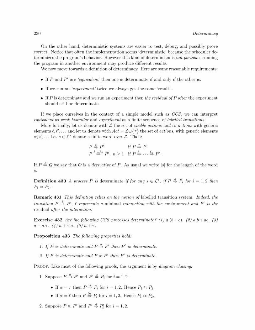
230 Determinacy
On the other hand, deterministic systems are easier to test, debug, and possibly provecorrect. Notice that often the implementation seems ‘deterministic’ because the scheduler de-terminizes the program’s behavior. However this kind of determinism is not portable: runningthe program in another environment may produce different results.
We now move towards a definition of determinacy. Here are some reasonable requirements:
• If P and P ′ are ‘equivalent’ then one is determinate if and only if the other is.
• If we run an ‘experiment’ twice we always get the same ‘result’.
• If P is determinate and we run an experiment then the residual of P after the experimentshould still be determinate.
If we place ourselves in the context of a simple model such as CCS , we can interpretequivalent as weak bisimilar and experiment as a finite sequence of labelled transitions.
More formally, let us denote with L the set of visible actions and co-actions with genericelements `, `′, . . . and let us denote with Act = L∪τ the set of actions, with generic elementsα, β, . . . Let s ∈ L∗ denote a finite word over L. Then:
Pε⇒ P ′ if P
τ⇒ P ′
P`1...`n⇒ P ′, n ≥ 1 if P
`1⇒ · · · `n⇒ P ′ .
If Ps⇒ Q we say that Q is a derivative of P . As usual we write |s| for the length of the word
s.
Definition 430 A process P is determinate if for any s ∈ L∗, if Ps⇒ Pi for i = 1, 2 then
P1 ≈ P2.
Remark 431 This definition relies on the notion of labelled transition system. Indeed, the
transition P`→ P ′, ` represents a minimal interaction with the environment and P ′ is the
residual after the interaction.
Exercise 432 Are the following CCS processes determinate? (1) a.(b+ c). (2) a.b+ ac. (3)a+ a.τ . (4) a+ τ.a. (5) a+ τ .
Proposition 433 The following properties hold:
1. If P is determinate and Pα→ P ′ then P ′ is determinate.
2. If P is determinate and P ≈ P ′ then P ′ is determinate.
Proof. Like most of the following proofs, the argument is by diagram chasing.
1. Suppose Pα→ P ′ and P ′
s⇒ Pi for i = 1, 2.
• If α = τ then Ps⇒ Pi for i = 1, 2. Hence P1 ≈ P2.
• If α = ` then P`·s⇒ Pi for i = 1, 2. Hence P1 ≈ P2.
2. Suppose P ≈ P ′ and P ′s⇒ P ′i for i = 1, 2.
Determinacy 231
• By definition of weak bisimulation: Ps⇒ Pi and Pi ≈ P ′i , for i = 1, 2.
• Since P is determinate, we have P1 ≈ P2.
• Therefore, we conclude by transitivity of ≈: P ′1 ≈ P1 ≈ P2 ≈ P ′2. 2
Definition 434 (τ-inertness) We say that a process P is τ -inert if for all its derivativesQ, if Q
τ⇒ Q′ then Q ≈ Q′.
Proposition 435 If a process is determinate then it is τ -inert.
Proof. Suppose Ps⇒ Q and Q
τ⇒ Q′. Then Ps⇒ Q and P
s⇒ Q′. Thus by determinacy,Q ≈ Q′. 2
Next we introduce a weak version of the notion of trace equivalence for lts presented indefinition 358.
Definition 436 (traces) We define the traces of a process P as:
tr(P ) = s ∈ L∗ | P s⇒ · ,
and say that two processes P,Q are trace equivalent if tr(P ) = tr(Q).
Notice that the traces of a process form a non-empty, prefix-closed set of finite words overL.
Exercise 437 Are the following equations valid for trace equivalence and/or weak bisimula-tion?
a+ τ = a, α.(P +Q) = α.P + α.Q, (P +Q) | R = P | R+Q | R, P = τ.P .
Exercise 438 (compositionality of trace semantics) Show that if P,Q,R are CCS pro-cesses and tr(P ) = tr(Q) then tr(P | R) = tr(Q | R).
The following result entails that on deterministic processes most equivalences (trace,simulation-induced equivalence, bisimulation,. . .) collapse.
Proposition 439 Let P,Q be processes.
1. If P ≈ Q then tr(P ) = tr(Q).
2. Moreover, if P,Q are determinate then tr(P ) = tr(Q) implies P ≈ Q.
Proof. (1) Suppose P ≈ Q and Ps⇒ ·. Then Q
s⇒ · by induction on |s| using the propertiesof weak bisimulation.
(2) Suppose P,Q determinate and tr(P ) = tr(Q). We show that:
(P,Q) | tr(P ) = tr(Q)
is a bisimulation.
232 Determinacy
• If Pτ→ P ′ then P ≈ P ′ by determinacy. Thus taking Q
τ⇒ Q we have:
P ′ ≈ P tr(P ) = tr(Q) .
By (1), we conclude: tr(P ′) = tr(P ) = tr(Q).
• If P`→ P ′ then we note that:
tr(P ) = ε ∪ ` · tr(P ′) ∪⋃
` 6=`′,P `′⇒P ′′
`′ · tr(P ′′) .
This is because all the processes P ′ such that P`⇒ P ′ are bisimilar, hence trace equiv-
alent. A similar reasoning applies to tr(Q). Thus there must be a Q′ such that Q`⇒ Q′
and tr(P ′) = tr(Q′). 2
Example 440 (the unbounded buffer reconsidered) Recall the unbounded buffer in ex-ample 409:
Buf (a, b) = a.νc (Buf (a, c) | b.Buf (c, b))P (n) = νa (an | Buf (a, b))
One can show that these processes are deterministic. In fact one can show that they actuallyenjoy a stronger property known as confluence which is introduced next in section 27.2.
27.2 Confluence in lts
We introduce a notion of confluence that strengthens determinacy and is preserved by someform of communication (parallel composition + restriction). For instance,
νa ((a+ b) | a)
will be rejected because a+ b is not confluent (while being deterministic).The notion of confluence we consider is reminiscent of confluence in rewriting systems
(cf. definition 23). By analogy, one calls confluence the related theory in process calculi butbear in mind that: (1) confluence is relative to a labelled transition system and (2) we closediagrams up to equivalence.
Before introducing formally the notion of confluence for lts we need to define a notion ofaction difference.
Definition 441 (action difference) Suppose α, β ∈ Act. Their action difference α\β isdefined as:
α\β =
α if α 6= βτ otherwise.
We can generalize the notion of action difference to sequences of visible actions r, s ∈ L∗.To compute the difference r\s of r by s we scan r from left to right deleting each label whichoccurs in s taking into account the multiplicities (cf. difference of multi-sets). We abusenotation by writing ` /∈ s to mean that ` does not occur in the word s.
(ε\s) = ε
(`r\s) =
` · (r\s) if ` /∈ sr\(s1 · s2) if s = s1`s2, ` /∈ s1 .
For instance: aba\ca = ba and ca\aba = c.

Determinacy 233
Exercise 442 Let r, s, t ∈ L∗. Show that:
1. (rs)\(rt) = s\t.
2. r\(st) = (r\s)\t.
3. (rs)\t = (r\t)(s\(t\r)).
We now introduce a notion of confluent process.
Definition 443 (confluence) A process P is confluent if for every derivative Q of P wehave:
Qα⇒ Q1 Q
β⇒ Q2
∃Q′1, Q′2 (Q1β\α⇒ Q′1, Q2
α\β⇒ Q′2, and Q′1 ≈ Q′2)[conf 0] (27.1)
The condition in definition 443 is labelled as [conf 0] to distinguish it from two moreequivalent conditions that we state below and that are labelled [conf 1] and [conf 2].
• A process P is confluent 1 if if for every derivative Q of P we have:
Qα→ Q1 Q
β⇒ Q2
∃Q′1, Q′2 ( Q1β\α⇒ Q′1, Q2
α\β⇒ Q′2, and Q′1 ≈ Q′2 )[conf 1] (27.2)
• A process P is confluent 2 if for all r, s ∈ L∗ we have:
Pr⇒ P1 P
s⇒ P2
∃P ′1, P ′2 ( P1s\r⇒ P ′1, P2
r\s⇒ P ′2, and P ′1 ≈ P ′2 )[conf 2] (27.3)
Remark 444 In conditions [conf 0] and [conf 1] if α = β then we close the diagram with τactions only.
A first sanity check is to verify that the confluent processes are invariant under transitionsand equivalence (cf. proposition 433).
Proposition 445 The following properties hold:
1. If P is confluent and Pα→ P ′ then P ′ is confluent.
2. If P is confluent and P ≈ P ′ then P ′ is confluent.
Proof. (1) If Q is a derivative of P ′ then it is also a derivative of P .
(2) It is enough to apply the fact that:
(P ≈ P ′ and Pα⇒ P1) implies ∃P ′1 (P ′
α⇒ P ′1 and P1 ≈ P ′1)
and the transitivity of ≈. 2
Confluence implies τ -inertness, and from this we can show that it implies determinacytoo.

234 Determinacy
Proposition 446 Suppose P is confluent. Then P is: (1) τ -inert and (2) determinate.
Proof. First a reminder. A relation R is a weak bisimulation up to ≈ if:
P R Q Pα⇒ P ′
∃Q′ Q α⇒ Q′ and P ′(≈ R ≈)Q′
(and symmetrically for Q). It is important that we work with the weak moves on both sides,otherwise the relation R is not guaranteed to be contained in ≈ (cf. exercise 384). Now wemove to the proof.
1. We want to show that Pτ⇒ Q implies P ≈ Q. We show that:
R = (P,Q) | P τ⇒ Q
is a weak bisimulation up to ≈. It is clear that whatever Q does, P can do too withsome extra moves. In the other direction, suppose, e.g., P
α⇒ P1 with α 6= τ (case α = τleft as exercise). By [conf 0], Q
α⇒ Q1, P1τ⇒ P2, and Q1 ≈ P2. That is: P1(R ≈)Q1.
2. We want to show that if P is confluent then it is determinate. Suppose Ps⇒ Pi for
i = 1, 2 and s ∈ L∗. We proceed by induction on |s|. If |s| = 0 and Pτ⇒ Pi for i = 1, 2
then by τ -inertness P1 ≈ P ≈ P2. For the inductive case, suppose P`⇒ P ′i
r⇒ Pi fori = 1, 2. By confluence and τ -inertness, we derive that P ′1 ≈ P ′2. By weak bisimulation,
P ′2r⇒ P ′′2 and P ′′2 ≈ P1. By inductive hypothesis, P2 ≈ P ′′2 . Thus P2 ≈ P ′′2 ≈ P1 as
required. 2
Exercise 447 We have seen that confluence implies determinacy which implies τ -inertness.Give examples that show that these implications cannot be reversed.
We now turn to the confluence 1 definition which is ‘asymmetric’ in that the move fromQ to Q1 just concerns a single action.
Proposition 448 (conf 1) A process P is confluent iff for every derivative Q of P , it sat-isfies condition [conf 1].
Proof. The diagrams of [conf 1] are a particular case of [conf 0]. Thus we just have to showthat the diagrams of [conf 1] suffice to complete the diagrams of [conf 0].
We may proceed by induction on the length of the transition Qα⇒ Q1. For instance,
suppose α 6= β, β 6= τ , and:
Qτ→ Q1
α⇒ Q2 , Qβ⇒ Q3 .
Then we derive:
Q1β⇒ Q4 Q3
τ⇒ Q5 Q4 ≈ Q5 (by [conf 1])
Q2β⇒ Q6 Q4
α⇒ Q7 Q4 ≈ Q7 (by inductive hypothesis)
Q5α⇒ Q8 Q7 ≈ Q8 (from Q4 ≈ Q5 and Q4
α⇒ Q7).
Therefore: Q2β⇒ Q6, Q3
α⇒ Q8, and Q6 ≈ Q8 as required. 2

Determinacy 235
Exercise 449 Consider another case of the proof. For instance, when Qα→ Q1
τ⇒ Q2.
We turn to condition [conf 2].
Proposition 450 (conf 2) A process P is confluent iff it satisfies [conf 2].
Proof. (⇐) It suffices to check that if P has property [conf 2] then its derivatives have ittoo.
• Suppose Pt⇒ Q for t ∈ L∗.
• Suppose further Qr⇒ Q1 and Q
s⇒ Q2.
• By composing diagrams and applying [conf 2] we get:
Q1(ts\tr)⇒ Q′1 Q2
(tr\ts)⇒ Q′2 Q′1 ≈ Q′2 .
• By exercise 442, ts\tr = s\r and tr\ts = r\s. Then we derive:
Q1(s\r)⇒ Q′1 Q2
(r\s)⇒ Q′2 Q′1 ≈ Q′2 .
(⇒) We proceed in three steps.
1. By induction on |s| we show that:
Pτ⇒ P1 P
s⇒ P2
∃P ′1, P ′2 P1s⇒ P ′1, P2
τ⇒ P ′2, and P ′1 ≈ P ′2.
2. Then, again by induction on |s|, we show that:
P`⇒ P1 P
s⇒ P2
∃P ′1, P ′2 P1s\`⇒ P ′1, P2
`\s⇒ P ′2, and P ′1 ≈ P ′2.
3. Finally we prove the commutation of diagram [conf 2] by induction on |r| when Pr⇒ P1.
2
Exercise 451 Complete the proof.
Next, we return to the issue of building confluent (and therefore determinate) processes.
Proposition 452 (building confluent processes) If P,Q are confluent processes then soare: (1) 0, α.P , (2) νa P , and (3) σP where σ is an injective substitution on the free namesof P .
Proof. Routine analysis of transitions (cf. similar statement for determinacy). 2
Remark 453 (on sum) In general, a+ b is determinate but it is not confluent for a 6= b.

236 Determinacy
Definition 454 (sorting) Let P be a process. We define its sorting L(P ) as the set:
` ∈ L | ∃ s ∈ L∗ P s⇒ Q`→ · .
Exercise 455 With reference to exercise 440, show that L(a 7→ b) = a, b.
Definition 456 (restricted composition) A restricted composition is a process of the shape:νa1, . . . , an (P | Q) where:
1. P and Q do not share visible actions: L(P ) ∩ L(Q) = ∅.
2. P and Q may interact only on the restricted names:
L(P ) ∩ L(Q) ⊆ a1, . . . , an ∪ a1, . . . , an .
Proposition 457 Confluence is preserved by restricted composition.
Proof. We abbreviate νa1, . . . , an (P | Q) as νa∗ (P | Q). First we observe that anyderivative of νa∗ (P | Q) will have the shape νa∗ (P ′ | Q′) where P ′ is a derivative of P andQ′ is a derivative of Q.
Since sorting is preserved by transitions, the two conditions on sorting in definition 454will be satisfied. Therefore, it is enough to show that the diagrams in [conf 1] commute forprocesses of the shape R = νa∗ (P | Q) under the given hypotheses.
We consider one case. Suppose: R`→ νa∗ (P1 | Q) because P
`→ P1. Also assume:
R`⇒ νa∗ (P2 | Q2) because P
s`r⇒ P2 and Qs·r⇒ Q2 with s · r ∈ a∗, a∗∗ and ` /∈ a∗, a∗.
Since P is confluent we have:
P`→ P1 P
s`r⇒ P2
∃P ′1, P ′2 P1sr⇒ P ′1, P2
τ⇒ P ′2, and P ′1 ≈ P ′2.
Then we have:νa∗ (P1 | Q)
τ⇒ νa∗ (P ′1 | Q2) ≈ νa∗ (P ′2 | Q2) ,
thus closing the diagram (note that we use the congruence properties of ≈). 2
Exercise 458 Consider other cases of the proof, for instance:
νa (P | Q)τ→ νa (P | Q) as P
a→ P1, Qa→ Q1 ,
νa (P | Q)τ⇒ νa (P2 | Q2) as P
s→ P2, Qs⇒ Q2 .
27.3 Kahn networks
Kahn networks are a deterministic model of parallel computation where communication ispoint-to-point, i.e., for every channel there is at most one sender and one receiver, andchannels are order preserving buffers of unbounded capacity, i.e., sending is non blocking andthe order of emission is preserved at the reception.
In this model, each (sequential) process may:
1. perform arbitrary sequential deterministic computation,
Determinacy 237
2. insert a message in a buffer,
3. receive a message from a buffer. If the buffer is empty then the process must suspend,
However, a process cannot try to receive a message from several channels at once. In anutshell Kahn’s approach to the semantics of such systems is as follows. First, we regard theunbounded buffers as finite or infinite words over some data domain and second, we modelthe nodes of the network as functions over words. Kahn observes that the associated systemof equations has a least fixed point which defines the semantics of the whole system.
Kahn networks are an important (practical) case where parallelism and determinism co-exist without producing race conditions. For instance, they are frequently used in the signalprocessing community. Our modest goal is to formalize Kahn networks as a fragment ofCCS and to apply the developed theory to show that the fragment is confluent and thereforedeterministic.
We will work with a ‘data domain’ that contains just one element. The generalizationto arbitrary data domains is not difficult, but we would need to formalize determinacy andconfluence in the framework of an extended CCS where messages carry values (as, e.g., inthe value passing CCS described in chapter 26). First, let us conclude the analysis of theunbounded buffers in CCS .
Exercise 459 With reference to exercises 409, 440, and 455:
1. Check that the process a 7→ b falls in the class of confluent processes defined in propo-sition 457. In particular:
L(a 7→ c) ∩ L(b.c 7→ b) = ∅ , L(a 7→ c) ∩ L(b.c 7→ b) ⊆ c, c .
2. Derive from proposition 439 that to prove P (n) = νa (an | a 7→ b) ≈ bn
it is enough tocheck:
tr(bn) = ε, b, bb, . . . , bn . (27.4)
3. Prove property (27.4).
We define a class of CCS processes sufficient to represent Kahn networks.
Definition 460 (restricted processes) Let KP be the least set of processes such that 0 ∈KP and if P,Q ∈ KP and α is an action then:
1. α.P ∈ KP,
2. A(b∗) ∈ KP provided the names b∗ are all distinct and A is defined by an equationA(a∗) = P and P ∈ KP.
3. νa∗ (P | Q) ∈ KP provided L(P ) ∩ L(Q) = ∅ and L(P ) ∩ L(Q) ⊆ a∗, a∗,
Exercise 461 Check that a 7→ b is a KP process and that Kahn processes are confluent.

238 Determinacy
Example 462 Suppose we have a Kahn network with three nodes, and the following portsand behaviors where we use ! for output and ? for input.
Node Ports Behaviors
1 ?a, ?b, ?c, !d, !e, !f A1 =?a.!d.!e.?b.?c.!f.A1
2 !b, ?d A2 =?d.!b.A2
3 !c, ?e A3 =?e.!c.A3 .
The corresponding CCS system relies on the equations for the buffer process plus:
A1(a, b, c, d, e, f) = a.d.e.b.c.f .A1(a, b, c, d, e, f)
A2(b, d) = d.b.A2(b, d)A3(c, e) = e.c.A3(c, e) .
The sorting is easily derived:
L(A1(a, b, c, d, e, f) = a, b, c, d, e, fL(A2(b, d)) = b, dL(A3(c, e)) = c, e .
To build the system, we have to introduce a buffer before every input channel. Thus theinitial configuration is:
νa′, b, b′, c, c′, d, d′, e, e′
(a 7→ a′ | b 7→ b′ | c 7→ c′ | d 7→ d′ | e 7→ e′ |A1(a′, b′, c′, d, e, f) | A2(b, d′) | A3(c, e′) )
It is easily checked that the resulting process belongs to the class KP.
To summarize, to build confluent processes we can use: (i) nil and input prefix, (ii)restricted composition, (iii) injective recursive calls, and (iv) recursive equations A(a∗) = P ,where P is built according to the rules above. This class of processes is enough to representKahn networks. Notice that, via recursion, we can also represent Kahn networks with adynamically changing number of nodes (see example 409).
27.4 Reactivity and local confluence in lts
We know that a terminating and locally confluent rewriting system is confluent (proposition47). We present a suitable generalization of this result to confluent lts. First we need togeneralize the notion of termination.
Definition 463 (reactivity) Let P be a process. We say that it is terminating (or stronglynormalizing) if there is no infinite sequence:
Pτ→ P1
τ→ · · ·
and that it is reactive (or fully terminating) if all its derivatives are terminating.
Definition 464 (local confluence) Let P be a process. We say that it is locally confluentif for all its derivatives Q:
Qα→ Q1 Q
β→ Q2
∃Q′1, Q′2 (Q1β\α⇒ Q′1, Q2
α\β⇒ Q′2, and Q′1 ≈ Q′2).
Determinacy 239
Exercise 465 Consider again the process:
A(a, b) = a.νc (A(a, c) | b.A(c, b)) .
Is the process A(a, b) reactive? Consider the cases a 6= b and a = b.
Exercise 466 Consider the process: A = a.b+τ.(a.c+τ.A). Check whether A is: (1) τ -inert,(2) locally confluent, (3) terminating, (4) reactive, (5) determinate, and (6) confluent.
Suppose P is a reactive process and let W be the set of its derivatives. For Q,Q′ ∈ Wwrite Q > Q′ if Q rewrites to Q′ by a positive number of τ -actions. Then (W,>) is a wellfounded set.
Proposition 467 If a process is reactive and locally confluent then it is confluent.
Proof. Let B be the relationτ→ ∪(
τ→)−1∪ ≈ (restricted to W ) and B∗ its reflexive andtransitive closure. Note that B∗ is symmetric too. We take the following steps.
1. For every derivative Q of P it holds:
Qτ⇒ Q1, Q
α⇒ Q2
∃Q3 ( Q1α⇒ Q3 and Q2B
∗Q3 ).
2. The relation B∗ is a weak-bisimulation.
3. The process P is τ -inert.
4. The process P is confluent.
Note that B∗ is a binary relation on W (the derivatives of P ).
Step 1 The argument is by induction (cf. proposition 30) on the well founded order (W,>).
• If Q = Q1 then the statement holds trivially.
• So assume Qτ→ Q3
τ⇒ Q1 and consider 2 cases.
1. If Qτ→ Q4
α⇒ Q2.
– By local confluence, Q3τ⇒ Q5, Q4
τ⇒ Q6, and Q5 ≈ Q6.
– By inductive hypothesis, Q6α⇒ Q7 and Q2B
∗Q7.
– By definition of bisimulation, Q5α⇒ Q8 and Q7 ≈ Q8.
– By inductive hypothesis, Q1α⇒ Q9 and Q8B
∗Q9.
So Q2B∗Q7 ≈ Q8B
∗Q9, and by definition of B, Q2B∗Q9.
2. If Qα→ Q4
τ⇒ Q2 with α 6= τ .
– By local confluence, Q3α⇒ Q5, Q4
τ⇒ Q6, Q5 ≈ Q6.
– By inductive hypothesis, Q1α⇒ Q7 and Q5B
∗Q7.
So Q2τ⇐ Q4
τ⇒ Q6 ≈ Q5B∗Q7. Hence Q2B
∗Q7.

240 Determinacy
Step 2 The relation B∗ is a weak-bisimulation.
Suppose Q0BQ1 · · ·BQnBQn+1 and Q0α⇒ Q′0. Proceed by induction on n and case
analysis on QnBQn+1. By inductive hypothesis, we know that Qnα⇒ Q′n and Q′0B
∗Q′n.
1. If Qn ≈ Qn+1 then Qn+1α⇒ Q′n+1 and Q′n ≈ Q′n+1. So Q′0B
∗Q′n ≈ Q′n+1 and we useB∗ ≈⊆ B∗.
2. If Qnτ← Qn+1 then Qn+1
α⇒ Q′n.
3. If Qnτ→ Qn+1 then by Step (1), Qn+1
α⇒ Q′n+1 and Q′nB∗Q′n+1.
So Q′0B∗Q′nB
∗Q′n+1 and we use B∗ B∗ ⊆ B∗.
Step 3 The process P is τ -inert.
By definition,τ→⊆ B∗ and by Step (2), B∗ ⊆≈.
Step 4 The process P is confluent.
By induction on the well-founded order W . We distinguish two cases.
1. Suppose Qα→ Q3
τ⇒ Q1 and Qβ→ Q4
τ⇒ Q2, with α, β 6= τ .
• By local confluence, Q3β\α⇒ Q5, Q4
α\β⇒ Q6, and Q5 ≈ Q6.
• By Step (3), Q4 ≈ Q2, and by weak bisimulation, Q2α\β⇒ Q8, Q6 ≈ Q8.
• By Step (3), Q3 ≈ Q1, and by weak bisimulation, Q1β\α⇒ Q7, Q5 ≈ Q7.
So we have Q8 ≈ Q6 ≈ Q5 ≈ Q7 as required.
2. Suppose Qτ→ Q3
α⇒ Q1 and Qβ⇒ Q2.
• By Step (3), Q ≈ Q3, and by weak bisimulation, Q3β⇒ Q5, Q2 ≈ Q5.
• By inductive hypothesis, Q1β\α⇒ Q6, Q5
α\β⇒ Q7, and Q6 ≈ Q7.
• By weak bisimulation, Q2α\β⇒ Q4 and Q4 ≈ Q7.
So Q4 ≈ Q7 ≈ Q6 as required. 2
Exercise 468 Suppose P is a CCS process that is reactive and such that for every derivativeQ of P we have:
Qτ→ Q1 Q
τ→ Q2
Q1 ≈ Q2.
Show that this implies that for every derivative Q of P we have:
Qτ⇒ Q1 Q
τ⇒ Q2
∃Q′1, Q′2 ( Q1τ⇒ Q′1, Q2
τ⇒ Q′2, and Q′1 ≈ Q′2 ).

Determinacy 241
27.5 Summary and references
A process is determinate if it always reacts in the same way to the stimuli coming from theenvironment. Confluence is a stronger property than determinacy that is preserved by arestricted form of parallel composition. Following [Mil95][chapter 11], we have presented 3alternative characterizations of confluence. We have seen that a restricted form of parallelcomposition preserves confluence and as a case study we have shown that this fragment ofCCS is enough to represent Kahn networks [Kah74]. Synchronous data flow languages suchas Lustre [CPHP87] can be regarded as a refinement of this model where buffers have size0. A rather complete study of the notion of confluence in the more general framework of theπ-calculus is in [PW97], which builds on previous work on confluence for CCS with valuepassing. Reactivity is a form of hereditary termination. A process is reactive if it terminatesafter any sequence of interactions with the environment. The presented generalization ofNewman’s proposition 47 is described in [GS96].

242 Determinacy
Chapter 28
Synchronous/Timed models
As mentioned in chapter 19, one important classification criterion in concurrent systems is therelative speed of the processes. In particular, in chapter 19 we have contrasted asynchronousand synchronous systems. So far we have considered models (Imp‖, CCS ) where processesare asynchronous, i.e., proceed at independent speeds. In particular, processes can onlysynchronize through an await statement or an input/output communication. In the followingwe are going to discuss an enrichment of the CCS model where processes are synchronous(or timed). In first approximation, in a synchronous concurrent system all processes proceedin lockstep (at the same speed). In other words, the computation is regulated by a notion ofinstant (or round, or phase, or pulse,. . .).
Though synchronous circuits are typical examples of synchronous systems, one should notconclude that synchronous systems are hardware. Notions of synchrony are quite useful in thedesign of software systems too. The programming of many problems in a distributed settingcan be ‘simplified’ or even ‘made possible’ by a synchronous assumption. Examples include:leader election, minimum spanning tree, and consensus in the presence of failures. In general,the notion of synchrony is a useful logical concept that can make programming easier.
The formalization of a synchronous model depends on the way the notion of instantis considered. One possibility is to assume that at each instant each (sequential) processperforms a locally defined amount of work. For instance, a popular definition found in bookson distributed algorithms requires that at each instant each process (1) writes in the outputcommunication channels, (2) reads the contents of the input communication channels, and(3) computes its next state. However, a less constrained viewpoint is possible which consistsin assuming that at each instant, each process performs an arbitrary (but hopefully finite)number of actions. The instant ends when each process has either terminated its task for thecurrent instant or it is suspended waiting for events that cannot arise. This is the viewpointtaken by synchronous languages such as Esterel and we shall describe next its formalizationin the framework of CCS . The reader should keep in mind that we select CCS because of itssimplicity but that the approach can be easily ported to other models of concurrent systems.
28.1 Timed CCS
We discuss the definition of a synchronous/timed model on top of CCS . Following the termi-nology in the literature, we call this model timed CCS (TCCS ). As usual, we write α, α′, . . .for the CCS actions and we reserve `, `′, . . . for the CCS actions but the τ action. We denote
243

244 Time
P 6 τ→ ·(P . Q)
tick→ Q 0tick→ 0
`.Ptick→ `.P
Pitick→ P ′i i = 1, 2 (P1 | P2) 6 τ→ ·
(P1 | P2)tick→ (P ′1 | P ′2)
Pitick→ P ′i i = 1, 2
(P1 + P2)tick→ (P ′1 + P ′2)
Ptick→ P ′
νa Ptick→ νa P ′
Table 28.1: Labelled transition system for the tick action
with µ, µ′, . . . the TCCS actions. They are obtained by extending the CCS actions (chapter26) with a new tick action which represents the move to the following instant:
µ ::= α || tick (TCCS actions).
We also extend the syntax of CCS processes with a new operator ‘else-next’ which allows toprogram processes which are time dependent and are able to react to the absence of an event.Intuitively, the process (P . Q) tries to run P in the current instant and if it cannot it runsQ in the following.
P ::= · · · || (P . P ) (TCCS processes).
The labelled transition system for TCCS includes the usual rules for the α actions (Table26.1) plus:
Pα→ P ′
(P . Q)α→ P ′
(a rule for else-next).
Moreover, we introduce in Table 28.1 special rules for the tick action describing the passageof time. The intuition is the following:
A process can tick if and only if it cannot perform τ actions.
Incidentally, this is in perfect agreement with the usual feeling that we do not see time passingwhen we have something to do!
Exercise 469 (on formalising tick actions) Check that Ptick→ · if and only if P 6 τ→ · The
lts in Table 28.1 uses the negative condition P 6 τ→ ·. Show that this condition can be formalizedin a positive way by defining a formal system to derive judgments of the shape P ↓ L where
L is a set of observable actions and P ↓ L if and only if P 6 τ→ · and L = ` | P `→ ·.
The following exercise identifies two important choices in the design of TCCS .
Exercise 470 (continuations of tick action) We say that P is a ‘CCS process’ if it doesnot contain the else next operator. Show that:
1. If Ptick→ Q1 and P
tick→ Q2 then Q1 = Q2. So the passage of time is deterministic.
2. If P is a CCS process and Ptick→ Q then P = Q. So CCS processes are insensitive to
the passage of time.
Time 245
Exercise 471 (programming a switch) Let tick .P = (0.P ) and tick n.P = tick · · · tick .P ,n times.
1. Program a light switch Switch(press, off , on, brighter) that behaves as follows:
• Initially the switch is off.
• If the switch is off and it is pressed then the light turns on.
• If the switch is pressed again in the following 2 instants then the light becomesbrighter while if it is pressed at a later instant it turns off again.
• If the light is brighter and the switch is pressed then it becomes off.
2. Program a fast user Fast(press) that presses the switch every 2 instants and a slow userSlow(press) that presses the switch every 4 instants.
3. Consider the systems:
νpress ( Switch(press, off , on, brighter) | Fast(press) )νpress ( Switch(press, off , on, brighter) | Slow(press) )
and determine when the light is going to be off, on, and bright.
Definition 472 The notion of weak transition is extended to the tick action by defining:
tick⇒ =τ⇒ tick→ τ⇒ (weak tick action) .
Then we denote with ≈tick the related largest weak bisimulation.
Exercise 473 (bisimulation for TCCS) Show that ≈tick is preserved by parallel composi-tion. Also show that ((P1 . P2) . P3) ≈tick (P1 . P3). Thus the nesting of else-next operatorson the left is useless!
Exercise 474 (more on congruence of ≈tick ) Suppose P1 ≈tick P1 and Q1 ≈tick Q2.Prove or give a counterexample to the following equivalences.
1. P1 +Q1 ≈tick P2 +Q2.
2. ((`.P1) . Q1) ≈tick ((`.P2) . Q2).
3. (P1 . Q1) ≈tick (P2 . Q2).
We have identified the CCS processes with the TCCS processes that do not contain anelse-next operator. A natural question is whether the equivalences we have on CCS are stillvalid when the CCS processes are placed in a timed environment. A basic observation isthat a diverging computation does not allow time to pass. Thus if we denote with Ω thediverging process τ.τ.τ · · · we have 0 6≈tick Ω while in the ordinary (termination insensitive)bisimulation for CCS we have 0 ≈ Ω. The situation is more pleasant for reactive processescf. chapter 27).
Proposition 475 (CCS vs. TCCS) Suppose P,Q are CCS processes.

246 Time
1. P ≈tick Q implies P ≈ Q.
2. If moreover, P,Q are reactive then P ≈ Q implies P ≈tick Q.
Proof. (1) TCCS bisimulation is stronger than CCS bisimulation and α-derivatives of CCSare again CCS processes.
(2) First notice that for a CCS process being reactive w.r.t. CCS actions is the same asbeing reactive w.r.t. TCCS actions. For α actions, the condition P ≈ Q suffices. Otherwise,
suppose Ptick⇒ P ′. By exercises 469 and 470(2), this means P
τ⇒ P ′tick→ P ′. By definition of
CCS bisimulation, Qτ⇒ Q1, P ′ ≈ Q1. By reactivity, Q1
τ⇒ Q′tick→ . Again by definition of
CCS bisimulation, P ′ ≈ Q′, Hence Qtick⇒ Q′ and P ′ ≈ Q′. 2
Exercise 476 (termination sensitive bisimulation) Rather than restricting the atten-tion to reactive processes, another possibility is to consider a bisimulation for CCS whichis sensitive to termination. We write P ↓ if P 6 τ→ · and P ⇓ if P
τ⇒ Q and Q ↓. Show that onCCS processes the bisimulation ≈tick can be characterized as the largest relation R which isa weak labelled bisimulation (in the usual CCS sense) and such that if P R Q and P ↓ thenQ ⇓.
28.2 A deterministic calculus based on signals
As a case study, we consider a variant of the TCCS model where processes interact throughsignals (rather than channels). A signal is either emitted or not. Once it is emitted it persistsduring the instant and it is reset at the end of it. Thus the collection of emitted signals growsmonotonically during each instant.
The presented calculus is named SL (synchronous language). We describe it as a fragmentof timed CCS where we write s, s′, . . . for signal names. The syntax of SL processes is asfollows:
P ::= 0 || s.P, P || (emit s) || (P | P ) || νs P || A(s∗) (SL processes).
The newly introduced operators can be understood in terms of those of TCCS as follows:
s.P,Q = (s.P . Q)(emit s) = (s.Emit(s) . 0)
where: Emit(s) = (s.Emit(s) . 0) .
Notice that in SL there is no sum and no prefix for emission (cf. asynchronous π-calculus,chapter 30). The input is a specialized form of the input prefix and the else-next operator.The derived synchronization rule is:
(emit s) | s.P,Q τ→ τ→ (emit s) | P .
The second τ transition is just recursion unfolding and we will ignore it in the following.Notice that:
(emit s) | s.P1, Q1 | s.P2, Q2τ⇒ (emit s) | P1 | P2 .
The tick action can be expressed as:
tick .P = νs s.0, P s /∈ fv(P ) .
Time 247
A persistent input (as in TCCS ) is expressed as:
await s.P = A(s∗), where: A(s∗) = s.P,A(s∗), fv(P ) ∪ s = s∗ .
Exercise 477 Re-program in SL the light switch seen in exercise 471. Compare the solutionwith the one based on TCCS.
The SL calculus enjoys a strong form of confluence where one can close the diagram in atmost one step and up to α-renaming.
Proposition 478 (strong confluence) For all SL programs P the following holds:
Pτ→ P1 P
τ→ P2
P1 ≡ P2 or ∃Q (P1τ→ Q,P2
τ→ Q)
Proof. Internal reductions are due either to unfolding or to synchronization. The onlypossibility for a superposition of the redexes is:
(emit s) | s.P1, Q1 | s.P2, Q2 .
And we exploit the fact that emission is persistent. 2
The bisimulation ≈tick developed for TCCS can be applied to SL too. However, becauseof the restricted form of SL processes, one can expect additional equations to hold. Forinstance:
s.(emit s), 0 should be ‘equivalent’ to 0 . (28.1)
A similar phenomenon arises with asynchronous communication in the π-calculus (cf. chapter30). More generally, because SL is deterministic (cf. proposition 478) one can expect a collapseof the bisimulation and trace semantics (cf. proposition 439).
Exercise 479 (on SL equivalence) Check that the equation (28.1) does not hold in theTCCS embedding. Also, prove or disprove the following equivalences:
1. s.(s.P,Q), Q ≈tick s.P,Q.
2. (emit s) | s.P,Q ≈tick (emit s) | P .
28.3 Summary and references
Time, in the sense we have described it here, is derived from the notion of computation andas such it is a logical notion rather than a concept we attach on top of the computationalmodel. Time passes when no computation is possible. Moving from an asynchronous to asynchronous model means enriching the language with the possibility to react to the absenceof computation, i.e., to the passage of time. The distinction between synchronous and asyn-chronous models is standard in the analysis of distributed algorithms (see, e.g., [Lyn96]). Inthe framework of process calculi, a notion of ‘timed’ CCS is introduced in [Yi91]. This calcu-lus has a tick(x) operator that describes the passage of x time units where x is a non-negativereal. A kind of else next operator is proposed in [NS94]. A so called testing semantics of a

248 Time
process calculus very close to the one presented here is given in [HR95]. However, it seemsfair to say that all these works generalize to CCS ideas that were presented for the Esterelprogramming language [BC84, BG92]. Two basic differences in the Esterel approach are thatprocesses interact through signals and that the resulting calculus is deterministic.
Another important difference is that in the Esterel model it is actually possible to reactimmediately (rather than at the end of the instant) to the absence of a signal. This requiressome semantic care, to avoid writing paradoxical programs such as s.0, (emit s) which aresupposed to emit s when s is not there (cf. stabilization problems in the design of synchronouscircuits). It also requires some clever compilation techniques to determine whether a signal isnot emitted. In fact these techniques (so far!) are specific to finite state models.
The SL model [BdS96] we have described is a relaxation of the Esterel model wherethe absence of a signal can only be detected at the end of the instant. If we forget aboutname generation, then the SL model essentially defines a kind of monotonic Mealy machine.Monotonic in the sense that output signals can only depend positively on input signals (withinthe same instant). The monotonicity restriction allows to avoid the paradoxical programs asmonotonic boolean equations do have a least fixed point! The SL model has a natural andefficient implementation model that works well for general programs (not just finite statemachines). The model has been adapted to several programming environments (C [Bou91],Scheme [SBS04], ML [MP05]) and it has been used to program significant applications.
The Esterel/TCCS/SL models described here actually follow an earlier attempt at de-scribing synchronous/timed systems in the framework of CCS known as SCCS/Meije model[Mil83, AB84]. The basic idea of these models is that the actions of the system live in anabelian (commutative) group freely generated from a collection of basic actions. At eachinstant, each (sequential) process must perform exactly one action and the observable re-sult of the computation is the group composition of the actions performed by each process.This gives rise to a model with pleasant algebraic properties but whose implementation andgeneralization to a full scale programming languages appear to be problematic.
Finally, let us mention timed automata as another popular formalism for describing ‘timed’systems [AD94]. This is an enrichment of finite state automata with timing constraints whichstill enjoys decidable model-checking properties. This is more a specification language forfinite control systems than a programming language.
Chapter 29
Probability and non-determinism
We discuss the modelling of systems which exhibit both non-deterministic and probabilisticbehaviors. We focus on three basic ideas. First, we should not confuse non-deterministic andprobabilistic choice. Second, because of probabilistic choice, we need to lift relations on states(such as bisimulations) to relations on distributions. Third, again because of probabilisticchoice, we need to revisit the notion of weak transition so as to formalize the notion that thesystem can evolve from one state to another with probability 1. In the following, these ideasare formalized in the framework of CCS , but the reader should keep in mind that the notion ofprobabilistic computation is an ‘orthogonal’ feature that can be added to a variety of modelsof concurrent systems (a similar consideration holds for the notion of synchronous/timedcomputation).
29.1 Preliminaries
Probabilities arise in several areas of system design and analysis. For instance, one maywant to analyze programs or protocols that toss coins at some point in the computation,e.g., the probability that a test for number primality returns the correct answer. In anotherdirection, one may want to evaluate the reliability of a system given some probability offailure of its components. And yet in another direction, one may be interested in evaluatingthe performance of a system in terms of, say, the average waiting time of its users.
As already mentioned, in concurrent systems, non-determinism arises to account for raceconditions and also as a specification device. It is then natural to lift methods for (determin-istic) probabilistic systems to non-deterministic ones.
To fix the ideas, we define some standard notions. Let S be a countable set of states. A(discrete) distribution on the states S is a function ∆ : S → [0, 1] such that Σs∈S∆(s) = 1.We denote with Dist(S) the collection of distributions on S. If S′ ⊆ S we denote with ∆[S′]the sum Σs′∈S′∆(s′). It is a well known fact that the value of the sum does not depend on theenumeration of the states. We may represent a distribution as a formal sum Σi∈I [pi]si whereΣi∈Ipi = 1. The binary version is also written as s1 +p s2 which stands for [p]s1 + [1− p]s2.The unary version is shortened to s which stands for [1]s.
The notion of discrete time Markov chain is standard in probability theory. It is basedon: (i) a discrete notion of time t = 0, 1, 2, . . . and (ii) a transition ‘matrix’:
P : S → Dist(S) (Markov chain), (29.1)
249

250 Probability
where p(s)(s′) is the probability that the system being at state s at time t moves into states′ at time t+ 1 (for any t). This is a beautiful theory connecting linear algebra to probabilitytheory.
The notion of Markov decision process is an elaboration on Markov chains popularized inthe 50’s. We add to a Markov chain a countable set of actions Act and redefine the transitionmatrix as a partial function:
P : (S ×Act) Dist(S) (Markov decision process), (29.2)
where P (s, a)(s′) is the probability of moving from s to s′ given that the decision to performaction a has been taken. Possibly, we may consider a reward functionR : (S×Act)→ (S → R)too, where R(s, a)(s′) is the reward the decision maker gets if being in s and taking the decisiona the system moves into s′. A typical problem in this area is to determine a policy for thedecision maker that maximizes some cumulative function of the rewards.
Following the introduction of labelled transition systems, it is natural to consider a relatednotion of probabilistic lts. The key point is that being in state s and taking the action a thesystem may end up in different distributions of states. We now have a transition relation:
→ ⊆ S ×Act ×Dist(S) (Probabilistic lts). (29.3)
If all the distributions are trivial (Dirac) then we are back to labelled transition systems (cf.definition 356). If for a given state and action there is at most one distribution then we areback to Markov Decision Processes.
29.2 Probabilistic CCS
We discuss how the process calculus framework CCS adapts to the move from lts to proba-bilistic lts. In particular we look at:
1. The definition of strong bisimulation on probabilistic lts.
2. How to associate a probabilistic lts with a Probabilistic CCS , namely a CCS enrichedwith a probabilistic choice operator.
Our first problem is to find a way of lifting a relation on states to a relation on distributions.Let R ⊆ S × S be an equivalence relation on states and let [s]R denote the equivalence classof s and S/R the set of equivalence classes.
Definition 480 (lumping equivalence) We lift R to an equivalence relation D(R) onDist(S) as follows:
∆ D(R) ∆′ if ∀ s ∈ S ∆[ [s]R ] = ∆′[ [s]R ] .
Thus two distributions are equivalent with respect to R if they are the same modulo theequivalence induced by R. This is also called lumping equivalence in Markov processes liter-ature (lumping=aggregate). We can then introduce a notion of bisimulation for probabilisticlts.
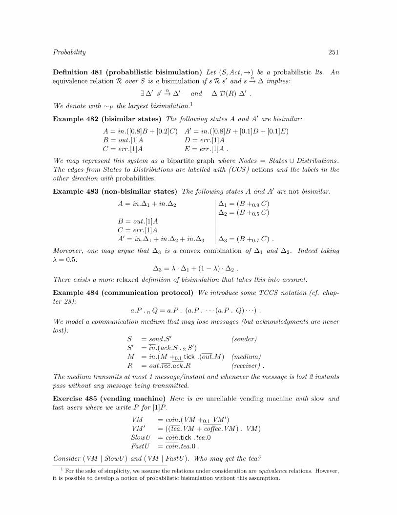
Probability 251
Definition 481 (probabilistic bisimulation) Let (S,Act ,→) be a probabilistic lts. Anequivalence relation R over S is a bisimulation if s R s′ and s
α→ ∆ implies:
∃∆′ s′α→ ∆′ and ∆ D(R) ∆′ .
We denote with ∼P the largest bisimulation.1
Example 482 (bisimilar states) The following states A and A′ are bisimilar:
A = in.([0.8]B + [0.2]C) A′ = in.([0.8]B + [0.1]D + [0.1]E)B = out .[1]A D = err .[1]AC = err .[1]A E = err .[1]A .
We may represent this system as a bipartite graph where Nodes = States ∪ Distributions.The edges from States to Distributions are labelled with (CCS) actions and the labels in theother direction with probabilities.
Example 483 (non-bisimilar states) The following states A and A′ are not bisimilar.
A = in.∆1 + in.∆2 ∆1 = (B +0.9 C)∆2 = (B +0.5 C)
B = out .[1]AC = err .[1]AA′ = in.∆1 + in.∆2 + in.∆3 ∆3 = (B +0.7 C) .
Moreover, one may argue that ∆3 is a convex combination of ∆1 and ∆2. Indeed takingλ = 0.5:
∆3 = λ ·∆1 + (1− λ) ·∆2 .
There exists a more relaxed definition of bisimulation that takes this into account.
Example 484 (communication protocol) We introduce some TCCS notation (cf. chap-ter 28):
a.P .n Q = a.P . (a.P . · · · (a.P . Q) · · ·) .We model a communication medium that may lose messages (but acknowledgments are neverlost):
S = send .S′ (sender)S′ = in.(ack .S .2 S
′)M = in.(M +0.1 tick .(out.M) (medium)
R = out .rec.ack .R (receiver) .
The medium transmits at most 1 message/instant and whenever the message is lost 2 instantspass without any message being transmitted.
Exercise 485 (vending machine) Here is an unreliable vending machine with slow andfast users where we write P for [1]P .
VM = coin.(VM +0.1 VM ′)
VM ′ = ((tea.VM + coffee.VM ) .VM )SlowU = coin.tick .tea.0FastU = coin.tea.0 .
Consider (VM | SlowU ) and (VM | FastU ). Who may get the tea?
1 For the sake of simplicity, we assume the relations under consideration are equivalence relations. However,it is possible to develop a notion of probabilistic bisimulation without this assumption.
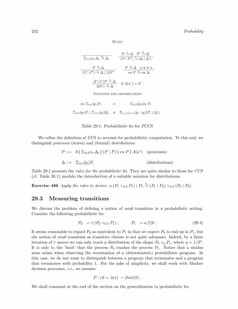
252 Probability
Rules
Σi∈Iαi.∆iαi→ ∆i
Pa→ ∆ P ′
a→ ∆′
(P | P ′) τ→ (∆ | ∆′)
Pα→ ∆
(P | P ′) α→ ∆ | [1]P ′P
α→ ∆ a, a 6= α
νa Pα→ νa ∆
[b∗/a∗]Pα→ ∆
A(b∗)α→ ∆
if A(a∗) = P .
Notation for distributions
νa Σi∈I [pi]Pi ≡ Σi∈I [pi]νa Pi
Σi∈I [pi]Pi | Σj∈J [qj ]Qj ≡ Σ(i,j)∈I×J [pi · qj ](Pi | Qj) .
Table 29.1: Probabilistic lts for PCCS
We refine the definition of CCS to account for probabilistic computation. To this end, wedistinguish processes (states) and (formal) distributions:
P ::= 0 || Σi∈Iαi.∆i || (P | P ) || νa P || A(a∗) (processes)
∆ ::= Σi∈I [pi]Pi (distributions)
Table 29.1 presents the rules for the probabilistic lts. They are quite similar to those for CCS(cf. Table 26.1) modulo the introduction of a suitable notation for distributions.
Exercise 486 Apply the rules to derive: a.(P1 +0.5 P1) | P3a→ (P1 | P3) +0.5 (P2 | P3).
29.3 Measuring transitions
We discuss the problem of defining a notion of weak transition in a probabilistic setting.Consider the following probabilistic lts:
P0 = τ.(P0 +0.5 P1) , P1 = a.[1]0 . (29.4)
It seems reasonable to regard P0 as equivalent to P1 in that we expect P0 to end up in P1, butthe notion of weak transition as transitive closure is not quite adequate. Indeed, by a finiteiteration of τ moves we can only reach a distribution of the shape P0 +p P1, where p = 1/2n.It is only to the ‘limit’ that the process P0 reaches the process P1. Notice that a similarissue arises when observing the termination of a (deterministic) probabilistic program. Inthis case, we do not want to distinguish between a program that terminates and a programthat terminates with probability 1. For the sake of simplicity, we shall work with Markovdecision processes, i.e., we assume:
P : (S ×Act) Dist(S) .
We shall comment at the end of the section on the generalization to probabilistic lts.
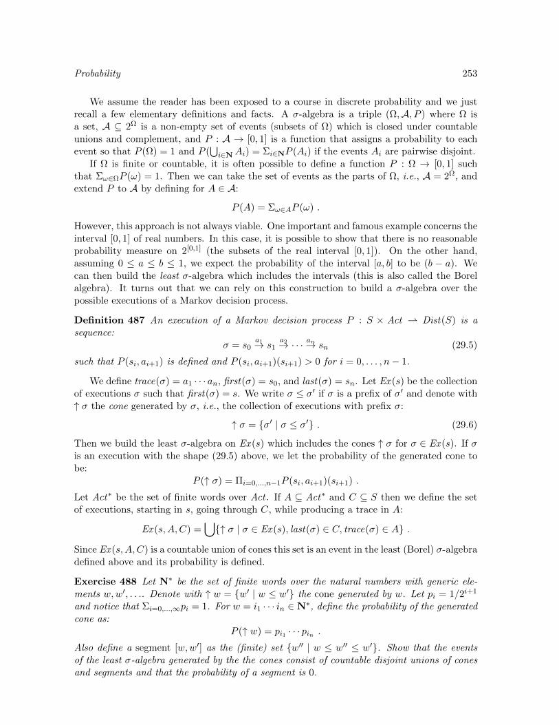
Probability 253
We assume the reader has been exposed to a course in discrete probability and we justrecall a few elementary definitions and facts. A σ-algebra is a triple (Ω,A, P ) where Ω isa set, A ⊆ 2Ω is a non-empty set of events (subsets of Ω) which is closed under countableunions and complement, and P : A → [0, 1] is a function that assigns a probability to eachevent so that P (Ω) = 1 and P (
⋃i∈NAi) = Σi∈NP (Ai) if the events Ai are pairwise disjoint.
If Ω is finite or countable, it is often possible to define a function P : Ω → [0, 1] suchthat Σω∈ΩP (ω) = 1. Then we can take the set of events as the parts of Ω, i.e., A = 2Ω, andextend P to A by defining for A ∈ A:
P (A) = Σω∈AP (ω) .
However, this approach is not always viable. One important and famous example concerns theinterval [0, 1] of real numbers. In this case, it is possible to show that there is no reasonableprobability measure on 2[0,1] (the subsets of the real interval [0, 1]). On the other hand,assuming 0 ≤ a ≤ b ≤ 1, we expect the probability of the interval [a, b] to be (b − a). Wecan then build the least σ-algebra which includes the intervals (this is also called the Borelalgebra). It turns out that we can rely on this construction to build a σ-algebra over thepossible executions of a Markov decision process.
Definition 487 An execution of a Markov decision process P : S × Act Dist(S) is asequence:
σ = s0a1→ s1
a2→ · · · an→ sn (29.5)
such that P (si, ai+1) is defined and P (si, ai+1)(si+1) > 0 for i = 0, . . . , n− 1.
We define trace(σ) = a1 · · · an, first(σ) = s0, and last(σ) = sn. Let Ex (s) be the collectionof executions σ such that first(σ) = s. We write σ ≤ σ′ if σ is a prefix of σ′ and denote with↑ σ the cone generated by σ, i.e., the collection of executions with prefix σ:
↑ σ = σ′ | σ ≤ σ′ . (29.6)
Then we build the least σ-algebra on Ex (s) which includes the cones ↑ σ for σ ∈ Ex (s). If σis an execution with the shape (29.5) above, we let the probability of the generated cone tobe:
P (↑ σ) = Πi=0,...,n−1P (si, ai+1)(si+1) .
Let Act∗ be the set of finite words over Act . If A ⊆ Act∗ and C ⊆ S then we define the setof executions, starting in s, going through C, while producing a trace in A:
Ex (s,A,C) =⋃↑ σ | σ ∈ Ex (s), last(σ) ∈ C, trace(σ) ∈ A .
Since Ex (s,A,C) is a countable union of cones this set is an event in the least (Borel) σ-algebradefined above and its probability is defined.
Exercise 488 Let N∗ be the set of finite words over the natural numbers with generic ele-ments w,w′, . . .. Denote with ↑ w = w′ | w ≤ w′ the cone generated by w. Let pi = 1/2i+1
and notice that Σi=0,...,∞pi = 1. For w = i1 · · · in ∈ N∗, define the probability of the generatedcone as:
P (↑ w) = pi1 · · · pin .Also define a segment [w,w′] as the (finite) set w′′ | w ≤ w′′ ≤ w′. Show that the eventsof the least σ-algebra generated by the the cones consist of countable disjoint unions of conesand segments and that the probability of a segment is 0.

254 Probability
Before defining a notion of weak bisimulation, it is convenient to characterize the notionof (strong) bisimulation introduced in definition 481.
Proposition 489 An equivalence relation R on the states S of a Markov decision processP : S × Act Dist(S) is a bisimulation if and only if the following holds: for all s, s′ ∈ S,α ∈ Act, and C ∈ S/R if (s, s′) ∈ R then
P (Ex (s, α, C)) = P (Ex (s′, α, C)) .
Proof. If P (s, α) is undefined then the set of executions is empty and the probability is 0.Otherwise, notice that P (Ex (s, α, [s′′]R)) = ∆([s′′]R) where ∆ = P (s, α). 2
The notion of weak bisimulation then amounts to replace the singleton set α with thesets corresponding to the regular expressions τ∗ and τ∗ατ∗, for α 6= τ ; in the definitionbelow, we shall actually abuse notation by denoting these sets by the corresponding regularexpressions.
Definition 490 An equivalence relation R on the states S of a Markov decision processP : S × Act Dist(S) is a bisimulation if for all states s, s′ ∈ S, word α ∈ Act ∪ ε, andequivalence class C ∈ S/R if (s, s′) ∈ R then
P (Ex (s, τ∗ατ∗, C)) = P (Ex (s′, τ∗ατ∗, C)) .
Example 491 The probabilistic lts (29.4) can be regarded as a Markov decision process withtransitions s0
τ→ s0 +1/2 s1 and s1a→ [1]s2. Let us check that the system goes from state s0 to
state s2 with probability 1 while producing a trace whose only observable action is a:
P (Ex (s0, τ∗aτ∗, s2)) = 1 .
To this end, consider the executions: σn = s0τ→ · · · τ→ s0
τ→ s1a→ s2, where the state s0 is
repeated n ≥ 1 times. Notice that ↑ σn∩ ↑ σm = ∅ if n 6= m. Thus:
P (⋃n≥1
↑ σn) = Σn≥1P (↑ σn) = Σn≥11
2n= 1 .
The definition of a σ-algebra on executions can be extended to probabilistic lts by intro-ducing a notion of scheduler (or adversary). A scheduler is a function that associates withevery execution the next non-deterministic move. The idea is then to measure executionsrelatively to a given scheduler.
29.4 Summary and references
Probabilistic lts are labelled relations from processes to distributions on processes. Takingthis approach one distinguishes between non-deterministic and probabilistic choice. A firstkey construction consists in lifting a relation on processes to a relation on distributions (thenotion of strong bisimulation is derived). A second key construction concerns the introductionof a σ-algebra on the collection of possible executions. This leads to a framework where wecan measure the probability of a weak transition and thus define a suitable notion of weakbisimulation.

Probability 255
Vitali [Vit05] shows that certain subsets of the real line are not measurable. Rabin [Rab63]introduces a notion of probabilistic automata as a generalization of finite deterministic au-tomata. The notion of Markov decision problem has been developed around 1950 (the book[Put94] is a standard reference). The notion of probabilistic lts has been put forward in[Var85] under the name of concurrent Markov chains in the framework of model-checking andit has been later revisited by [HJ90] in the framework of TCCS . The notion of bisimulationis introduced for Markov Decision Processes in [LS89] while the weaker notion of ‘convex’bisimulation for probabilistic lts is introduced in [SL95]. The book [Pan09] covers the situa-tion where distributions are on continuous state spaces and requires a non-trivial amount ofmeasure theory.

256 Probability
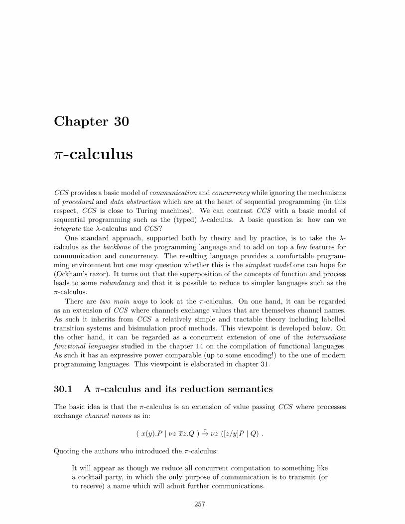
Chapter 30
π-calculus
CCS provides a basic model of communication and concurrency while ignoring the mechanismsof procedural and data abstraction which are at the heart of sequential programming (in thisrespect, CCS is close to Turing machines). We can contrast CCS with a basic model ofsequential programming such as the (typed) λ-calculus. A basic question is: how can weintegrate the λ-calculus and CCS?
One standard approach, supported both by theory and by practice, is to take the λ-calculus as the backbone of the programming language and to add on top a few features forcommunication and concurrency. The resulting language provides a comfortable program-ming environment but one may question whether this is the simplest model one can hope for(Ockham’s razor). It turns out that the superposition of the concepts of function and processleads to some redundancy and that it is possible to reduce to simpler languages such as theπ-calculus.
There are two main ways to look at the π-calculus. On one hand, it can be regardedas an extension of CCS where channels exchange values that are themselves channel names.As such it inherits from CCS a relatively simple and tractable theory including labelledtransition systems and bisimulation proof methods. This viewpoint is developed below. Onthe other hand, it can be regarded as a concurrent extension of one of the intermediatefunctional languages studied in the chapter 14 on the compilation of functional languages.As such it has an expressive power comparable (up to some encoding!) to the one of modernprogramming languages. This viewpoint is elaborated in chapter 31.
30.1 A π-calculus and its reduction semantics
The basic idea is that the π-calculus is an extension of value passing CCS where processesexchange channel names as in:
( x(y).P | νz xz.Q )τ→ νz ([z/y]P | Q) .
Quoting the authors who introduced the π-calculus:
It will appear as though we reduce all concurrent computation to something likea cocktail party, in which the only purpose of communication is to transmit (orto receive) a name which will admit further communications.
257
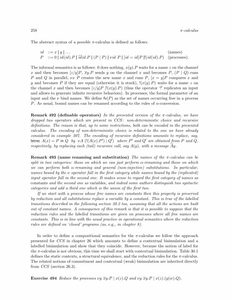
258 π-calculus
The abstract syntax of a possible π-calculus is defined as follows.
id ::= x || y || . . . (names)
P ::= 0 || id(id).P || idid .P || (P | P ) || νid P || [id = id ]P ||!(id(id).P ) (processes).
The informal semantics is as follows: 0 does nothing, x(y).P waits for a name z on the channelx and then becomes [z/y]P , xy.P sends y on the channel x and becomes P , (P | Q) runsP and Q in parallel, νx P creates the new name x and runs P , [x = y]P compares x andy and becomes P if they are equal (otherwise it is stuck), !(x(y).P ) waits for a name z onthe channel x and then becomes [z/y]P |!(x(y).P ) (thus the operator ‘!′ replicates an inputand allows to generate infinite recursive behaviors). In processes, the formal parameter of aninput and the ν bind names. We define fv(P ) as the set of names occurring free in a processP . As usual, bound names can be renamed according to the rules of α-conversion.
Remark 492 (definable operators) In the presented version of the π-calculus, we havedropped two operators which are present in CCS: non-deterministic choice and recursivedefinitions. The reason is that, up to some restrictions, both can be encoded in the presentedcalculus. The encoding of non-deterministic choice is related to the one we have alreadyconsidered in example 307. The encoding of recursive definitions amounts to replace, say,letrec A(x) = P in Q by νA (!(A(x).P ′) | Q′) where P ′ and Q′ are obtained from P and Q,respectively, by replacing each (tail) recursive call, say A(y), with a message Ay.
Remark 493 (name renaming and substitution) The names of the π-calculus can besplit in two categories: those on which we can just perform α-renaming and those on whichwe can perform both α-renaming and general (non-injective) substitutions. In particular,names bound by the ν operator fall in the first category while names bound by the (replicated)input operator fall in the second one. It makes sense to regard the first category of names asconstants and the second one as variables, and indeed some authors distinguish two syntacticcategories and add a third one which is the union of the first two.
If we start with a process whose free names are constants then this property is preservedby reduction and all substitutions replace a variable by a constant. This is true of the labelledtransitions described in the following section 30.2 too, assuming that all the actions are builtout of constant names. A consequence of this remark is that it is possible to suppose that thereduction rules and the labelled transitions are given on processes where all free names areconstants. This is in line with the usual practice in operational semantics where the reductionrules are defined on ‘closed’ programs (as, e.g., in chapter 8).
In order to define a compositional semantics for the π-calculus we follow the approachpresented for CCS in chapter 26 which amounts to define a contextual bisimulation and alabelled bisimulation and show that they coincide. However, because the notion of label forthe π-calculus is not obvious, this time we shall start with contextual bisimulation. Table 30.1defines the static contexts, a structural equivalence, and the reduction rules for the π-calculus.The related notions of commitment and contextual (weak) bisimulation are inherited directlyfrom CCS (section 26.3).
Exercise 494 Reduce the processes νy xy.P | x(z).Q and νy xy.P | x(z).(y(w).Q).

π-calculus 259
Syntax
C ::= [ ] || C | P || νx C (static contexts)
Structural equivalence
P1 | (P2 | P3) ≡ (P1 | P2) | P3 (associativity)P1 | P2 ≡ P2 | P1 (commutativity)
νx P1 | P2 ≡ νx (P1 | P2) x /∈ fv(P2) (extrusion)
Reduction
xy.P1 | x(z).P2 → P1 | [y/z]P2 xy.P1 |!(x(z).P2)→ (P1 | [y/z]P2) |!(x(z).P2)
[x = x]P → P
P ≡ C[P ′] P ′ → Q′ C[Q′] ≡ QP → Q
Table 30.1: Reductions for the π-calculus
30.2 A lts for the π-calculus
We now consider the problem of defining a labelled transition system for the π-calculus. Thisis a rather technical exercise. As a first step, we distinguish four types of actions:
Action α Example
τ xy.P | x(z).Qτ→ P | [y/z]Q
input xz x(y).Pxz→ [z/y]P
output xy xy.Pxy→ P
bound output x(y) νy xy.Px(y)→ P
We remark that the first three cases would arise naturally in an extension of CCS withground values too (section 26.4). The real novelty is the bound output case. Note that aneffect of the bound output action is to free the restricted name y. The bound output actioncarries a bound name and one has to be careful to avoid conflicts. Here are some typicalsituations.
νy x(y).P The name which is input must not conflict with the fresh one.νy xy.P The name which is output should become free.
νy xy.P | x(z).Q The scope of νy should extend to Q.νy xy.P | x(z).(y(w).Q) The fresh y and the one on the recipient side are distinct.
We fix some conventions concerning free and bound names in actions. (1) All occurrencesof a name in an action are free except y in a bound output action x(y). (2) Define fv(α) (bv(α))as the set of names occurring free (bound) in the action α. (3) Let n(α) = fv(α) ∪ bv(α).
Based on this, Table 30.2 defines a labelled transition system for the π-calculus. Rulesapply up to α-renaming and symmetric rules are omitted.
Exercise 495 (on the lts) Apply the definition to compute the labelled transitions of theprocesses discussed above.

260 π-calculus
x(y).Pxz→ [z/y]P xy.P
xy→ P
Pα→ P ′ x /∈ n(α)
νx Pα→ νx P ′
Pyx→ P ′ x 6= y
νx Py(x)→ P ′
Pxy→ P ′ Q
xy→ Q′
P | Q τ→ P ′ | Q′P
xy→ P ′ Qx(y)→ Q′ y /∈ fv(P )
P | Q τ→ νy (P ′ | Q′)
Pα→ P ′ bv(α) ∩ fv(Q) = ∅
P | Q α→ P ′ | Qx(y).P
α→ P ′
!(x(y).P )α→ P ′ |!(x(y).P )
[x = x]Pτ→ P
Table 30.2: A lts for the π-calculus
Exercise 496 (τ-transitions vs. reduction) In Table 30.1, we have defined a reductionrelation → on the π-calculus. Show that reduction and τ -transitions are the same up tostructural equivalence. Namely:
1. If P → Q then Pτ→ Q′ and Q ≡ Q′.
2. If Pτ→ Q then P → Q′ and Q ≡ Q′.
For instance, consider: (νy xy.P1 | P2) | x(z).P3.
The next step is to define a notion of bisimulation on the labelled transition system. Thisis not completely obvious. Suppose we want to show that P and Q are ‘labelled’ bisimilar.
Further, suppose Px(y)→ P ′ makes a bound output. What is the condition on Q? We note that
bisimilar processes may have different sets of free names. For instance, suppose P ≡ νy xy.P ′
and Q ≡ νy xy.Q′ | R, with y ∈ fv(R). Then the transition Px(y)→ · cannot be matched
(literally) by Q because y is free in Q. This leads to the following definition.
Definition 497 (labelled bisimulation) A binary relation R on processes is a strong la-belled bisimulation if:
P R Q, Pα→ Q, bv(α) ∩ fv(Q) = ∅
∃Q′ Q α→ Q′ P ′ R Q′.
and, as usual, a symmetric condition holds for Q. For the weak case, we replaceα→ by
α⇒.We denote with ∼L (≈L) the largest strong (weak) labelled bisimulation.
Proposition 498 Strong (weak) labelled bisimulation is preserved by static contexts.
Proof. We want to show that strong (weak) labelled bisimulation is preserved by staticcontexts. Let us abbreviate with νy∗ a possibly empty list νy1, . . . , νyn. We define a binaryrelation:
R = (νy∗ P | R, νy∗ Q | R) | P ∼L Q .
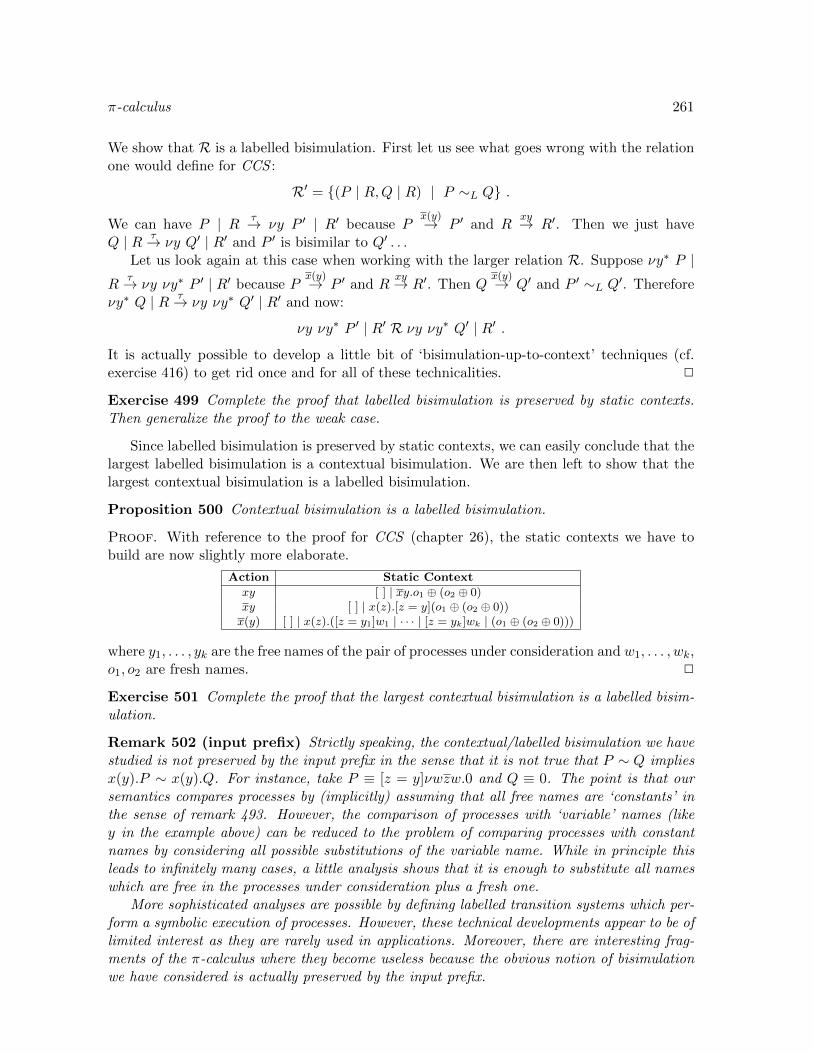
π-calculus 261
We show that R is a labelled bisimulation. First let us see what goes wrong with the relationone would define for CCS :
R′ = (P | R,Q | R) | P ∼L Q .
We can have P | R τ→ νy P ′ | R′ because Px(y)→ P ′ and R
xy→ R′. Then we just haveQ | R τ→ νy Q′ | R′ and P ′ is bisimilar to Q′ . . .
Let us look again at this case when working with the larger relation R. Suppose νy∗ P |R
τ→ νy νy∗ P ′ | R′ because Px(y)→ P ′ and R
xy→ R′. Then Qx(y)→ Q′ and P ′ ∼L Q′. Therefore
νy∗ Q | R τ→ νy νy∗ Q′ | R′ and now:
νy νy∗ P ′ | R′ R νy νy∗ Q′ | R′ .
It is actually possible to develop a little bit of ‘bisimulation-up-to-context’ techniques (cf.exercise 416) to get rid once and for all of these technicalities. 2
Exercise 499 Complete the proof that labelled bisimulation is preserved by static contexts.Then generalize the proof to the weak case.
Since labelled bisimulation is preserved by static contexts, we can easily conclude that thelargest labelled bisimulation is a contextual bisimulation. We are then left to show that thelargest contextual bisimulation is a labelled bisimulation.
Proposition 500 Contextual bisimulation is a labelled bisimulation.
Proof. With reference to the proof for CCS (chapter 26), the static contexts we have tobuild are now slightly more elaborate.
Action Static Context
xy [ ] | xy.o1 ⊕ (o2 ⊕ 0)xy [ ] | x(z).[z = y](o1 ⊕ (o2 ⊕ 0))x(y) [ ] | x(z).([z = y1]w1 | · · · | [z = yk]wk | (o1 ⊕ (o2 ⊕ 0)))
where y1, . . . , yk are the free names of the pair of processes under consideration and w1, . . . , wk,o1, o2 are fresh names. 2
Exercise 501 Complete the proof that the largest contextual bisimulation is a labelled bisim-ulation.
Remark 502 (input prefix) Strictly speaking, the contextual/labelled bisimulation we havestudied is not preserved by the input prefix in the sense that it is not true that P ∼ Q impliesx(y).P ∼ x(y).Q. For instance, take P ≡ [z = y]νwzw.0 and Q ≡ 0. The point is that oursemantics compares processes by (implicitly) assuming that all free names are ‘constants’ inthe sense of remark 493. However, the comparison of processes with ‘variable’ names (likey in the example above) can be reduced to the problem of comparing processes with constantnames by considering all possible substitutions of the variable name. While in principle thisleads to infinitely many cases, a little analysis shows that it is enough to substitute all nameswhich are free in the processes under consideration plus a fresh one.
More sophisticated analyses are possible by defining labelled transition systems which per-form a symbolic execution of processes. However, these technical developments appear to be oflimited interest as they are rarely used in applications. Moreover, there are interesting frag-ments of the π-calculus where they become useless because the obvious notion of bisimulationwe have considered is actually preserved by the input prefix.

262 π-calculus
30.3 Variations
We have considered a particular variety of the π-calculus with the aim of having a relativelysimple labelled transition system and labelled bisimulation. However, a number of variationsare possible. We mention a few and discuss their impact on the characterization of labelledbisimulation as contextual bisimulation.
Polyadic channels This is an extension where several names can be transmitted at once.We shall see in chapter 31 that this extension is quite natural when looking at the π-calculusas an intermediate language. The extension calls for some form of typing to guarantee that ina synchronization the sender and the receiver agree on the number of names to be exchanged(cf. Table 31.6). Moreover, in the formalization of the labelled transition system, the structureof the actions is a bit more complicated as several names can be extruded as the result of acommunication. The syntax of the actions becomes:
α ::= τ || x(y1, . . . , yn) || νz1, . . . , zm x(y1, . . . , yn)
with the requirement for the output that z1, . . . , zm is a (possibly empty) subsequence ofy1, . . . , yn composed of distinct names.
Asynchronous communication This is actually a restriction that requires that an outputaction cannot prefix another action. Again we shall see that this restriction is suggested bylooking at the π-calculus as an intermediate language. From a semantic viewpoint, thisrestriction entails that an input action is not directly observable and calls for a modificationof the bisimulation condition, or equivalently, for a modification of the labelled transitionsystem. In the adapted semantics, one can show, e.g., that the processes x(y).xy and 0 areweakly bisimilar.
Other restrictions We may consider restricted communication patterns. For instance, inthe context of asynchronous communication we may make the additional assumption thateach name has a unique receiver. Then in a process P ≡!(x(y).P ) | xz the output on the xchannel is not observable from the environment because the capability of receiving on x isattributed to the process P itself. In another direction, we may want to drop the operationfor name comparison. Then, modulo some additional hypotheses, it may be impossible todistinguish two names y and z. For instance, imagine y and z are two names for the sameservice and that the only way the observer can use y and z is to send a message on them. Inthis case, a theory of bisimulation will have to consider names modulo an equivalence relation.
30.4 Summary and references
The π-calculus is an extension of CCS where processes exchange channel names. As in CCS ,it is possible to define the notions of contextual and labelled bisimulation and show that theycoincide. In particular, this comes as a justification of the definition of the labelled bisim-ulation which is quite technical. The π-calculus is introduced by Milner et al. in [MPW92]following earlier work in [EN86]. The books [Hen07, SW01] explore its theory. The en-coding of non-deterministic choice is studied in [Nes00] while the notion of bisimulation forasynchronous communication is analyzed in [ACS98].

Chapter 31
Processes vs. functions
We develop the view that the π-calculus is a concurrent extension of an intermediate languageused in the compilation of languages of the ML family. In chapter 14, we have seen that astandard polyadic, call-by-value, λ-calculus can be put in CPS (continuation passing style),value named form. It turns out that, modulo a simple change of notation, this languagecorresponds to a deterministic and sequential fragment of the π-calculus. From chapter 15,we know that the CPS and value named transformations are type preserving. Thus modulothe change of notation, the π-calculus inherits the propositional typing discipline of the λ-calculus. As a second step, we consider an extension of the restricted π-calculus, called λj-calculus, which allows to express recursive, parallel, and concurrent behaviors and to whichthe ordinary π-calculus can be compiled. To summarize, we have the following diagram:
λCcps→ λcps
Cvn→ λcps,vn∼= πrestricted ⊂ λj
[[ ]]← π ,
which is read from left to right as follows. The call-by-value λ-calculus is put in CPS form(λcps) and then in CPS value named form (λcps,vn). This is equivalent to a restricted formof π-calculus (πrestricted ). When this restricted π-calculus is extended with recursive defini-tions, parallel composition, and a form of join definition, it becomes sufficiently expressive torepresent the ordinary π-calculus.
31.1 From λ to π notation
Table 31.1 recalls the value named λ-calculus in CPS form introduced in chapter 14. In thisλ-calculus, all values are named and when we apply the name of a λ-abstraction to the nameof a value we create a new copy of the body of the function and replace its formal parametername with the name of the argument as in:
let y = V in let f = λx.M in @(f, y) → let y = V in let f = λx.M in [y/x]M .
We also recall that in the value named λ-calculus the evaluation contexts are sequences of letdefinitions associating values to names. We can move from λ to π with a simple change ofnotation which is summarized in Table 31.2.
Example 503 (compilation and reduction simulation) The following example illustratesthe compilation of a λ-term and how the compiled term simulates the original one.
263

264 Processes vs. functions
I = λx.x, I ′ = λx, k.@(k, x), I(z) =!z(x, k).@(k, x),K = λx.@(halt , x), K(k) =!k(x).@(halt , x)
λ @(I, y) → y
λcps @(I ′, y,K) → @(K, y)→ @(halt , y)
λcps,vn let z = I ′ in let k = K in @(z, y, k) → let z = I ′ in let k = K in @(k, y)→ let z = I ′ in let k = K in @(halt , y)
π νz (I(z) | νk (K(k) | z(y, k))) → νz (I(z) | νk (K(k) | ky))
→ νz (I(z) | νk (K(k) | halt y))
We stress that the π-terms obtained from the compilation are highly constrained; thefollowing section 31.2 discusses the restrictions and some possible relaxations.
We can lift the correspondence between λ and π terms to types. In chapter 15, we haveshown that the CPS and value named transformations preserve (propositional) types. Modulothe change of notation presented above, this provides a propositional type system for the π-calculus. We recall that tid is the syntactic category of type variables with generic elementst, s, . . ., and A is the syntactic category of types with generic elements A,B, . . . A type contextis written x1 : A1, . . . , xn : An with the usual conventions. We also write x∗ : A∗ for a possiblyempty sequence x1 : A1, . . . , xn : An, and Γ, x∗ : A∗ for the context resulting from Γ by addingthe sequence x∗ : A∗. Table 31.3 recalls the typing rules for the CPS, value named calculusand presentes the very same rules formulated in the π-notation. For the sake of brevity, weshall omit the type of a term since this type is always the type of results R and write Γ `vn Mrather than Γ `vn M : R. A type of the form A+ → R corresponds to a channel type Ch(A+)in π-calculus notation. As expected, one can show that typing in this system is preserved byreduction.
31.2 Adding concurrency
The typed λcps,vn -calculus which is the target of the compilation chain is restricted in severalways. We show how these restrictions can be relaxed to obtain a calculus which can represent
Syntax
V ::= λid+.M (values)M ::= @(id , id+) || let id = V in M (CPS terms)E ::= [ ] || let id = V in E (evaluation contexts)
Reduction Rule
E[@(x, z1, . . . , zn)] → E[[z1/y1, . . . , zn/yn]M ] if E(x) = λy1, . . . , yn.M
where: E(x) =
V if E = E′[let x = V in [ ]]E′(x) if E = E′[let y = V in [ ]], x 6= yundefined otherwise.
Table 31.1: A value named, CPS λ-calculus: λcps,vn

Processes vs. functions 265
λ-interpretation λ-syntax π-syntax π-interpretation
function application @(x, y+) xy+ calling a servicefunction definition let x = λy+.M in N νx (!x(y+).M | N) service definition
Table 31.2: Changing notation from λ to π
Typing rules with λ notation
A ::= tid || (A+ → R) (types)
Γ, y : A+ → R `vn N Γ, x+ : A+ `vn MΓ `vn let y = λx+.M in N
x : A+ → R, y+ : A+ ∈ Γ
Γ `vn @(x, y+)
Typing rules with π notation
A ::= tid || Ch(A+) (types)
Γ, y : Ch(A+) `π N Γ, x+ : A+ `π MΓ `π νy (!y(x+).M | N)
x : Ch(A+), y+ : A+ ∈ Γ
Γ `π xy+
Table 31.3: Isomorphic type systems in λ and π notation
the computations of the π-calculus in a rather direct way. The restrictions and the relatedrelaxations concern the possibility of: (1) defining processes by general recursion, (2) runningprocesses in parallel, and (3) having a concurrent access to a resource. The first two relaxationsare rather standard while the third one lends itself to some discussion.
General recursion It is easily shown that in the typed λcps,vn -calculus all computationsterminate; this is a consequence of the termination of the corresponding typed λ-calculus. Toallow for infinite computations we introduce recursive definitions, that is in let x = M in Nwe allow M to depend recursively on x. For instance, we can write a non-terminating termlet x = λy.@(x, y) in @(x, z).
Parallelism The computations in the λcps,vn -calculus are essentially sequential since atany moment there is at most one function call which is active. To allow for some parallelismwe allow for function calls to be put in parallel as in @(x, y+) | @(z, w+). We notice thatwhile the resulting calculus allows for parallel computations it fails to represent concurrentcomputations (cf. discussion in chapter 19). The reason is that two parallel calls to the samefunction such as:
let x = λy.M in @(x, z) | @(x,w)
can be executed in an arbitrary order without affecting the overall behavior of the process.In other terms, the reductions of the calculus are (strongly) confluent (yet another exampleof parallel and deterministic system, cf. chapters 27 and 28).
Concurrency There are several possibilities to introduce concurrent behaviors in the cal-culus; we consider 3 of them. One possibility is to introduce a mechanism to define a function
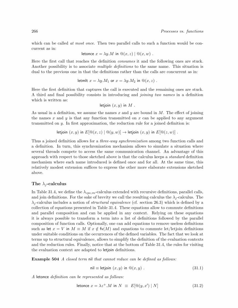
266 Processes vs. functions
which can be called at most once. Then two parallel calls to such a function would be con-current as in:
letonce x = λy.M in @(x, z) | @(x,w) .
Here the first call that reaches the definition consumes it and the following ones are stuck.Another possibility is to associate multiple definitions to the same name. This situation isdual to the previous one in that the definitions rather than the calls are concurrent as in:
letmlt x = λy.M1 or x = λy.M2 in @(x, z) .
Here the first definition that captures the call is executed and the remaining ones are stuck.A third and final possibility consists in introducing and joining two names in a definitionwhich is written as:
letjoin (x, y) in M .
As usual in a definition, we assume the names x and y are bound in M . The effect of joiningthe names x and y is that any function transmitted on x can be applied to any argumenttransmitted on y. In first approximation, the reduction rule for a joined definition is:
letjoin (x, y) in E[@(x, z) | @(y, w)]→ letjoin (x, y) in E[@(z, w)] .
Thus a joined definition allows for a three-way synchronization among two function calls anda definition. In turn, this synchronization mechanism allows to simulate a situation whereseveral threads compete to access the same communication channel. An advantage of thisapproach with respect to those sketched above is that the calculus keeps a standard definitionmechanism where each name introduced is defined once and for all. At the same time, thisrelatively modest extension suffices to express the other more elaborate extensions sketchedabove.
The λj-calculus
In Table 31.4, we define the λcps,vn -calculus extended with recursive definitions, parallel calls,and join definitions. For the sake of brevity we call the resulting calculus the λj-calculus. Theλj-calculus includes a notion of structural equivalence (cf. section 26.3) which is defined by acollection of equations presented in Table 31.4. These equations allow to commute definitionsand parallel composition and can be applied in any context. Relying on these equationsit is always possible to transform a term into a list of definitions followed by the parallelcomposition of function calls. Optionally, one can add equations to remove useless definitionssuch as let x = V in M ≡ M if x /∈ fv(M) and equations to commute let/letjoin definitionsunder suitable conditions on the occurrences of the defined variables. The fact that we look atterms up to structural equivalence, allows to simplify the definition of the evaluation contextsand the reduction rules. Finally, notice that at the bottom of Table 31.4, the rules for visitingthe evaluation context are adapted to letjoin definitions.
Example 504 A closed term nil that cannot reduce can be defined as follows:
nil ≡ letjoin (x, y) in @(x, y) . (31.1)
A letonce definition can be represented as follows:
letonce x = λz+.M in N ≡ E[@(y, x′) | N ] (31.2)

Processes vs. functions 267
Syntax
V ::= λid+.M (values)M ::= let id = V in M || letjoin (id , id) in M || (M |M) || @(id , id+) (terms)E ::= let id = V in E || letjoin (id , id) in E || (E |M) || [ ] (evaluation contexts)
Structural equivalence
Parallel composition is associative and commutative and assuming x, x′ /∈ fv(N) we have:
let x = V in M | N ≡ let x = V in (M | N) letjoin (x, x′) in M | N ≡ letjoin (x, x′) in (M | N)
Reduction Rules
E[@(x, z1, . . . , zn)] → E[[z1/y1, . . . , zn/yn]M ] if E(x) = λy1, . . . , yn.M
E[@(x, y) | @(x′, z+)] → E[@(y, z+)] if E(x, x′) = join
E(x) =
V if E = E′[let x = V in [ ]]E′(x) if E = E′[let y = V in [ ]] or E = E′[letjoin (y, y′) in [ ]] and x 6= y, y′
E′(x) if E = E′[[ ] |M ]undefined otherwise
E(x, x′) =
join if E = E′[letjoin (x, x′) in [ ]]E′(x, x′) if E = E′[let y = V in [ ]] or E = E′[letjoin (y, y′) in [ ]] and x, x′ ∩ y, y′ = ∅E′(x, x′) if E = E′[[ ] |M ]undefined otherwise.
Table 31.4: The value named CPS λ-calculus with join: λj

268 Processes vs. functions
[[0]] = nil[[xy.P ]] = letonce k = λ .[[P ]] in @(x↑, y↓, y↑, k)[[x(y).P ]] = letonce k = λy↓, y↑, k
′.([[P ]] | @(k′, )) in @(x↓, k)[[!x(y).P ]] = let k = λy↓, y↑, k
′.([[P ]] | @(k′, ) | @(x↓, k)) in @(x↓, k)[[P | Q]] = [[P ]] | [[Q]][[νx P ]] = letjoin (x↓, x↑) in [[P ]]
Table 31.5: Encoding of the π-calculus in λj
where: E = let x′ = λz+.M in letjoin (y, x) in [ ]. Assuming N ≡ @(x,w+), we have thefollowing reductions:
E[@(y, x′) | @(x,w+)] → E[@(x′, w+)] → E[[w+/z+]M ] .
Since the call @(y, x′) is not regenerated and the name y remains local, further invocations ofx will be stuck. Thus if we define: letzero x = λz+.M in N = E[N ], we have:
letonce x = λz+.M in @(x,w+)∗→ letzero x = λz+.M in [w+/z+]M .
A letmlt definition can be defined as follows:
letmlt x = λy+.M1 or x = λy+.M2 in N = E[@(x′, x1) | @(x′, x2) | N ] (31.3)
where E = letjoin (x′, x) in let x1 = λy+.(M1 | @(x′, x1)) in let x2 = λy+.(M2 | @(x′, x2)) in [ ].Assuming that N ≡ @(x,w+) and that the selected function definition is the first one, we havethe following reductions:
E[@(x′, x1) | @(x′, x2) | @(x,w+)] → E[@(x1, w+) | @(x′, x2)]
→ E[[w+/y+]M1 | @(x′, x1) | @(x′, x2)] .
Notice that each call to xi regenerates a call @(x′, xi) and that this requires a recursive defi-nition of xi where the body of the function associated to xi depends on xi itself.
Encoding of the (monadic) π-calculus in the λj-calculus
Table 31.5 presents an encoding of the monadic π-calculus described in chapter 30 (withoutname equality) into the λj-calculus. The encoding assumes that for each name x in the termof the π-calculus to be encoded we reserve a pair of names x↓, x↑ in the λj-calculus. Theintuition is that an input on x is transformed into a call to the name x↓ while an output on xbecomes a call to the name x↑. Then the names x↓, x↑ are joined so that a reduction in λj ispossible whenever there is at least one call to x↓ and one call to x↑. Not surprisingly, recursivedefinitions are needed in the encoding of the replicated input. In the translation of the outputwe use as a dummy variable, i.e., a variable which is not used in the body of the function.Correspondingly, in the translation of the input we use the notation @(k′, ) for a call to k′
with a dummy argument. By convention, we define @(k′, ) ≡ letjoin (x, x′) in @(k′, x′).
Example 505 The following reduction in the π-calculus:
R ≡ νx (x(y).P | xz.Q)→ νx ([z/y]P | Q) ,

Processes vs. functions 269
Syntax types and type contexts
A ::= tid || Ch(A+) (types)Γ ::= id : A, . . . , id : A (type contexts)
Typing rules for the polyadic π-calculus
Γ `π 0
x : Ch(A+), y+ : A+ ∈ Γ Γ `π PΓ `π xy+.P
x : Ch(A+) ∈ Γ Γ, y+ : A+ `π PΓ `π x(y+).P
x : Ch(A+) ∈ Γ Γ, y+ : A+ `π PΓ `π!(x(y+).P )
Γ `π P Γ `π QΓ `π P | Q
Γ, x : Ch(A+) `π PΓ `π νx P
Typing rules for the λj-calculus
Γ, x : Ch(A+) `j N Γ, x : Ch(A+), y+ : A+ `j MΓ `j let x = λy+.M in N
Γ, x : Ch(Ch(A+)), y : Ch(A+) `j MΓ `j letjoin (x, y) in M
x : Ch(A+), y+ : A+ ∈ Γ
Γ `j @(x, y+)
Γ `j M Γ `j NΓ `j M | N
Table 31.6: Typing rules for the (polyadic) π-calculus and the λj-calculus
is simulated as follows by the λj-term E[T ] ≡ [[R]] where:
E = letjoin (x↓, x↑) in letonce k = λy↓, y↑, k′.([[P ]] | @(k′, )) in letonce k′ = λ .[[Q]] in [ ]
E′ = letjoin (x↓, x↑) in letzero k = λy↓, y↑, k′.([[P ]] | @(k′, )) in letonce k′ = λ .[[Q]] in [ ]
E′′ = letjoin (x↓, x↑) in letzero k = λy↓, y↑, k′.([[P ]] | @(k′, )) in letzero k′ = λ .[[Q]] in [ ]
T = @(x↓, k) | @(x↑, z↓, z↑, k′)
E[T ]→ E[@(k, z↓, z↑, k′)]→ E′[[z↓/y↓, z↑/y↑][[P ]] | @(k′, )]→ E′′[[z↓/y↓, z↑/y↑][[P ]] | [[Q]]] .
Typing the encoding
The type system for the λcps,vn -calculus presented in Table 15.2 can be easily adapted tothe π-calculus and the λj-calculus. Following the notation in Table 31.3, we write the typeA+ → R as Ch(A+). Then Table 31.6 spells out the syntax and typing rules for the polyadicπ-calculus and the λj-calculus. To accommodate recursive definitions, we allow the nameintroduced by a let definition to occur in the body of the associated function. The rules forthe monadic π-calculus are just a special case where the channel type constructor is alwaysapplied to exactly one type.
Exercise 506 Determine the derived typing rules for the terms nil (31.1), letonce (31.2), andletmlt (31.3).
We can extend to types the translation from the monadic π-calculus to the λj-calculus. Weuse D = Ch(t) as the type of the dummy argument in @(k′, ). Then we define a translation
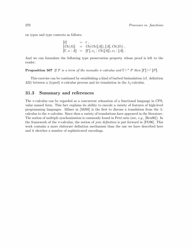
270 Processes vs. functions
on types and type contexts as follows:
[[t]] = t ,[[Ch(A)]] = Ch(Ch([[A]]), [[A]],Ch(D)) ,[[Γ, x : A]] = [[Γ]], x↓ : Ch([[A]]), x↑ : [[A]] .
And we can formulate the following type preservation property whose proof is left to thereader.
Proposition 507 If P is a term of the monadic π-calculus and Γ `π P then [[Γ]] `j [[P ]].
This exercise can be continued by establishing a kind of barbed bisimulation (cf. definition422) between a (typed) π-calculus process and its translation in the λj-calculus.
31.3 Summary and references
The π-calculus can be regarded as a concurrent relaxation of a functional language in CPS,value named form. This fact explains its ability to encode a variety of features of high-levelprogramming languages. Milner in [Mil92] is the first to discuss a translation from the λ-calculus to the π-calculus. Since then a variety of translations have appeared in the literature.The notion of multiple synchonization is commonly found in Petri nets (see, e.g., [Reu90]). Inthe framework of the π-calculus, the notion of join definition is put forward in [FG96]. Thiswork contains a more elaborate definition mechanism than the one we have described hereand it sketches a number of sophisticated encodings.

Chapter 32
Concurrent objects
In this chapter, we reconsider shared memory concurrency. The Imp‖ model introduced inchapter 19 has a pedagogical value in that it allows to illustrate many interesting problemsthat arise in concurrency in a relatively simple setting. On the negative side, it is clearthat its modelling power is rather limited. First, it does not support the introduction of datastructures such as lists, queues, trees, graphs, . . . and the related operations on them. Second,the memory model does not allow for the dynamic allocation, manipulation, and possiblydisposal of memory locations which is typical of imperative programming. (Incidentally,these considerations are similar to those motivating the move from CCS to the π-calculus.)
Research on concurrent programming in the shared memory model has focused on theissue of programming data structures that allow for concurrent access, i.e., for the concurrentexecution of several operations on the data structure, while providing an observable behaviorwhich is ‘equivalent’ to that of a data structure where the execution of the operations issequential, i.e., each operation is run from the beginning to the end without interference fromthe other operations. In a certain technical setting, this property is called linearizability andbecause the technical setting corresponds roughly to that of a Java-like concurrent object-oriented programming language one speaks of concurrent and sequential objects rather thanconcurrent and sequential data structures, respectively. Also, the operations of the datastructures correspond to the methods of the object.
An important result in this field is the existence of universal constructions that transformany ‘sequential’ object into a ‘concurrent’ one without introducing locks. Instead of locks,one relies on relatively simple atomic operations such as compare and set (cf. example 310).Such concurrent data structures are called lock-free. Because of the absence of locks suchdata structures guarantee a form of collective progress, i.e., there is a guarantee that someoperations will be completed while others may be delayed indefinitely. In fact one can goone step further and produce wait-free data structures where each operation is guaranteedto terminate in a bounded number of steps. Unfortunately, such universal transformationstend to be rather inefficient and research has focused on both ways to have more efficientconstructions in some special cases and on ways to relax the correctness conditions so as toallow for some efficient implementation techniques. Our goal in this chapter is to discussthese issues in a (fragment of a) state of the art programming language (Java) and to hint totheir formalization. We build on chapter 18 and the reader is supposed to have a superficialknowledge of the Java programming language.
271
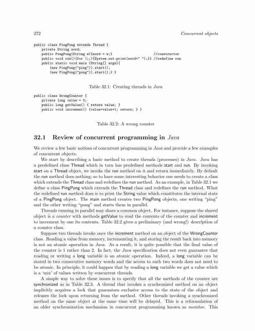
272 Concurrent objects
public class PingPong extends Thread
private String word;
public PingPong(String w)word = w; //constructor
public void run()for (;;)System.out.print(word+" "); //redefine run
public static void main (String[] args)
(new PingPong("ping")).start();
(new PingPong("pong")).start();
Table 32.1: Creating threads in Java
public class WrongCounter
private long value = 0;
public long getValue() return value;
public void increment() value=value+1; return;
Table 32.2: A wrong counter
32.1 Review of concurrent programming in Java
We review a few basic notions of concurrent programming in Java and provide a few examplesof concurrent objects.
We start by describing a basic method to create threads (processes) in Java. Java hasa predefined class Thread which in turn has predefined methods start and run. By invokingstart on a Thread object, we invoke the run method on it and return immediately. By defaultthe run method does nothing; so to have some interesting behavior one needs to create a classwhich extends the Thread class and redefines the run method. As an example, in Table 32.1 wedefine a class PingPong which extends the Thread class and redefines the run method. Whatthe redefined run method does is to print the String value which constitutes the internal stateof a PingPong object. The main method creates two PingPong objects, one writing “ping”and the other writing “pong” and starts them in parallel.
Threads running in parallel may share a common object. For instance, suppose the sharedobject is a counter with methods getValue to read the contents of the counter and incrementto increment by one its contents. Table 32.2 gives a preliminary (and wrong!) description ofa counter class.
Suppose two threads invoke once the increment method on an object of the WrongCounterclass. Reading a value from memory, incrementing it, and storing the result back into memoryis not an atomic operation in Java. As a result, it is quite possible that the final value ofthe counter is 1 rather than 2. In fact, the Java specification does not even guarantee thatreading or writing a long variable is an atomic operation. Indeed, a long variable can bestored in two consecutive memory words and the access to such two words does not need tobe atomic. In principle, it could happen that by reading a long variable we get a value whichis a ‘mix’ of values written by concurrent threads.
A simple way to solve these issues is to specify that all the methods of the counter aresynchronized as in Table 32.3. A thread that invokes a synchronized method on an objectimplicitly acquires a lock that guarantees exclusive access to the state of the object andreleases the lock upon returning from the method. Other threads invoking a synchronizedmethod on the same object at the same time will be delayed. This is a reformulation ofan older synchronization mechanism in concurrent programming known as monitor. This

Concurrent objects 273
public class SyncCounter
private long value = 0;
public synchronized long getValue() return value;
public synchronized void increment() value=value+1; return;
Table 32.3: A synchronized counter
public class CASCounter
private AtomicInteger value= new AtomicInteger(0);
public int getValue()return value.get();
public void increment()
int v;
do v = value.get();
while (!value.compareAndSet(v, v + 1));
return;
Table 32.4: A counter with compareAndSet
approach obviously guarantees linearizability but it can be inefficient.
An alternative approach consists in reducing the granularity of the operations to thatof compareAndSet operations. In Java, compareAndSet is actually a method which can beinvoked on an object of a special ‘Atomic’ class and which returns true if the comparison issuccessful and false otherwise. This implementation of the counter is described in Table 32.4which relies on a AtomicInteger class.
Notice that this time the implementation of the increment method is significantly different.First the value of the counter is read and incremented and then atomically the current value ofthe counter is compared to the value read and if they are equal then the counter is incremented.In case of contention, this solution relies on busy waiting while the previous one relies on acontext switch. 1
Table 32.5 presents an implementation of a concurrent stack object using compareAndSetwhich is known as Treiber’s algorithm. The implementation of the push and pop methodfollows the approach we have already presented for the increment method. First the methodsdo some speculative work on the side and then they make it visible with a compareAndSetmethod provided no interference has occurred so far. In this example, we work on objects ofthe AtomicReference class and the stack is implemented as a linked list of objects of the Nodeclass.
It should be noticed that compareAndSet can only manage a single pointer atomically.More complex operations such as inserting an element in a queue represented as a linked list,may require the (virtual) update of more pointers at once. In this case more sophisticatedprogramming techniques are needed.
1The general wisdom is that if the probability of contention is low then busy waiting may be more efficientthan context switch. In case of significant contention, exponential back-off is a general strategy to improve abusy waiting solution which is used, e.g., to handle collisions in the Ethernet protocol. In our case, it consistsin introducing a delay after each iteration of the while loop. The delay is chosen randomly from an intervalwhich increases exponentially with the number of iterations.

274 Concurrent objects
public class Node
int value;
Node next;
public Node(int v)value=v; next=this; // Node constructor
public class CASStack
AtomicReference<Node> head = new AtomicReference<Node>();
public void push(int v)
Node oldHead;
Node newHead = new Node(v);
do oldHead = head.get();
newHead.next = oldHead;
while (!head.compareAndSet(oldHead, newHead));
public int pop()
Node oldHead;
Node newHead;
do oldHead = head.get();
if (oldHead == null) return -1; // -1 default value for empty stack
newHead = oldHead.next;
while (!head.compareAndSet(oldHead,newHead));
return oldHead.value;
Table 32.5: A stack with compareAndSet
32.2 A specification of a fragment of concurrent Java
We introduce the syntax, reduction rules, and typing rules of a tiny imperative and concurrentobject-oriented language (called cJ) which is an extension of the (imperative) J languageformalized in chapter 18.
We recall that an object value is composed of the name of a class and a list of referenceswhich correspond to the object’s fields. A class is a declaration where we specify how to buildand manipulate the objects of the class. In particular, we specify the fields of each object andthe methods that allow their manipulation.
As usual, we assume a class Object without fields and methods. Every other class decla-ration extends a previously defined class and, in particular, we assume a class Thread whichextends the Object class with a method start with no arguments and returning an object ofthe Object class. The effect of invoking the start method on an object of the Thread class isto spawn in parallel the invocation of the run method on the object (if any). In this chapterwe assume all fields are modifiable (we stick to the imperative version of the language) anddenote with R an infinite set of references (cf. chapter 18) with elements r, r′, . . . A referenceis a pointer to an object. The value v of an object has the shape: C(r1, . . . , rn), for n ≥ 0,where C is the name of the class to which the object belongs and r1, . . . , rn are the referencesassociated with the modifiable fields of the object. A heap memory h is a partial functionwith finite domain from references to values.
Table 32.6 defines the syntactic category of expressions for cJ. As usual (cf. chapter 18),to define the reduction rules, it is convenient to include values in the syntactic category of ex-pressions. However, it is intended that expressions in a source program do not contain values.As in chapter 18, a program is composed of a list of class declarations and a distinguishedexpression where the computation starts. The final value of the distinguished expression canbe taken as the output of the program. Among the variables, we reserve this to refer to theobject on which a method is invoked. Also, we reserve the names start and run for methods of

Concurrent objects 275
e ::= id || (variable)v || (value)new C(e1, . . . , en) || (object generation)e.f || (field read)e.m(e1, . . . , en) || (method invocation)(C)(e) || (casting)e.f := e || (field write)e; e || (sequentialization)atomic(e) (atomicity)
Table 32.6: Expressions in cJ
objects of the Thread class. A well-formed program must satisfy certain conditions concerningfields and methods which are specified in chapter 18.
In order to define the reduction rules, it is convenient to introduce the syntactic categoryof sequential evaluation contexts which correspond to a call-by-value, left to right reductionstrategy and which are defined as follows:
E ::= [ ] || new C(v∗, E, e∗) || E.f || E.m(e∗) || v.m(v∗, E, e∗) ||(C)(E) || E.f := e || v.f := E || E; e (evaluation contexts)
(32.1)Along with the notion of evaluation context, we introduce a notion of redex, namely anexpression which (up to some type checks) is ready to reduce.
∆ ::= new C(v∗) || v.f || v.m(v∗) || (D)(v) || v.f := v || v; e || atomic(e) (redexes) (32.2)
The reduction of an expression involving the start method may produce the spawn of anexpression to be evaluated in parallel. Consequently, we consider a judgment of the shape:
(e, h)µ→ (e′, h′)
where µ is a (possibly empty) finite multi-set of expressions of the shape v.run(). Equivalently,µ can be regarded as a finite sequence of expressions where the order is irrelevant. As usual,
we denote with ∅ the empty multi-set and moreover we write → as an abbreviation for∅→.
Table 32.7 introduces the rules for reducing expressions and configurations (the last two rules).The first 8 rules are driven by the shape of the redexes specified in grammar (32.2). In therule for atomic, we write:
(e1, h1)µ
→∗ (en, hn) for (e1, h1)µ1→ · · · µn−1→ (en, hn) and µ = µ1 ∪ · · · ∪ µn−1 .
The rule for an atomic expression may spawn several threads, but their actual reduction mayonly start once the evaluation of the atomic expression is completed. Also note that in theproposed semantics atomic(v)→ v. The following rule allows to cross an evaluation context.The last two rules, explain how to reduce a configuration which is a triple (e, µ, h) composed ofa main expression, a multi-set of secondary expressions (initially empty), and a heap (initiallyempty too). This amounts to select non-deterministically one of the expressions and reduceit according to the rules above.
Recall that at the beginning of the computation we can assume that the multi-set ofexpressions µ contains no references and that the heap h is empty. Then the reduction rules

276 Concurrent objects
r∗ distinct and r∗ ∩ dom(h) = ∅(new C(v∗), h)→ (C(r∗), h[v∗/r∗])
(object generation)
field(C) = f1 : C1, . . . , fn : Cn 1 ≤ i ≤ n(C(r1, . . . , rn).fi, h)→ (h(ri), h)
(field read)
mbody(m,C) = λx1 · · ·xn.e(C(r∗).m(v1, . . . , vn), h)→ ([v1/x1, . . . , vn/xn, C(r∗)/this]e, h)
(method invocation)
C ≤ Thread
(C(r∗).start(), h)C(r∗).run()→ (Object(), h)
(start invocation)
C ≤ D((D)(C(r∗)), h)→ (C(r∗), h)
(casting)
field(C) = f1 : C1, . . . , fn : Cn 1 ≤ i ≤ n(C(r1, . . . , rn).fi := v, h)→ (Object(), h[v/ri])
(field write)
(v; e, h)→ (e, h)(sequentialization)
(e, h)µ
→∗ (v, h′)
(atomic(e), h)µ→ (v, h′)
(atomicity)
(e, h)µ→ (e′, h′)
(E[e], h)µ→ (E[e′], h′)
(evaluation context)
(e, h)µ′→ (e′, h′)
(e, µ, h)→ (e′, µ ∪ µ′, h′)(main expression)
(e′, h)µ′→ (e′′, h′)
(e, |e′| ∪ µ, h)→ (e, |e′′| ∪ µ ∪ µ′, h′)(secondary expression)
Table 32.7: Small step reduction rules for cJ
are supposed to maintain the following invariant: for all reachable configurations (e, µ, h), allthe references in e, µ and all the references that appear in a value in the codomain of theheap h are in the domain of definition of the heap (dom(h)). This guarantees that wheneverwe look for a fresh reference it is enough to pick a reference which is not in the domain ofdefinition of the current heap.
Following the discussion in chapter 18 (notably on the typing of casting), we present atype system for cJ. As usual, a type environment Γ has the shape x1 : C1, . . . , xn : Cn andwe consider typing judgments of the shape: Γ ` e : C. Table 32.8 specifies the rules totype expressions that do not contain values or references (as source programs do). The rulesgoverning the typing of class declarations and programs are those specified for the sequentialfragment J in chapter 18. The typed language, but for the atomic operator, can be regardedas a fragment of the Java programming language. General, but not very efficient, methodsto compile the atomic operator have been proposed. The basic idea is to follow an optimisticstrategy such as the one described in chapter 22. Unlike in the Imp‖ language however, in cJ,

Concurrent objects 277
x : C ∈ Γ
Γ ` x : C
field(C) = f1 : D1, . . . , fn : DnΓ ` ei : Ci, Ci ≤ Di, 1 ≤ i ≤ n
Γ ` new C(e1, . . . , en) : C
Γ ` e : C field(C) = f1 : C1, . . . , fn : CnΓ ` e.fi : Ci
Γ ` e : C mtype(m,C) = (C1, . . . , Cn)→ DΓ ` ei : C′i C′i ≤ Ci 1 ≤ i ≤ n
Γ ` e.m(e1, . . . , en) : D
Γ ` e : C C ≤ Thread
Γ ` e.start() : Object
Γ ` e : D
Γ ` (C)(e) : C
Γ ` e : C field(C) = f1 : C1, . . . , fn : CnΓ ` e′ : Di Di ≤ CiΓ ` e.fi := e′ : Object
Γ ` e1 : C1 Γ ` e2 : C2
Γ ` e1; e2 : C2
Γ ` e : C
Γ ` atomic(e) : C
Table 32.8: Typing rules for cJ program expressions
and more generally in Java, it is not possible to determine statically the collection of object’sfields which will be affected by the atomic transaction. In first approximation, the atomicexecution of an expression e is compiled into a speculative execution of the expression e whichmaintains a list of object’s fields which are read and/or written along with their updatedvalues. At the end of the speculative execution, if certain coherence conditions are met, thecomputation is committed, and otherwise the computation is re-started.
Exercise 508 Building on proposition 305, formulate and prove a subject reduction propertyfor the typed cJ language.
32.3 Summary and references
We have reviewed some basic notions of concurrent programming in Java and formalizedthe reduction and typing rules of a tiny fragment of it. Java’s synchronization builds onthe notion of monitor which was described in [Hoa74, Han75]. The notion of linearizability isintroduced in [HW90]. In a nutshell, linearizability means that the execution of the body of themethods of the concurrent object looks atomic. The introduction of a universal constructionto transform any ‘sequential’ object into a ‘concurrent’ one without introducing locks is dueto [Her91]. The book [HS08] is a good survey of the state of the art in this area.
Building a comprehensive model and proof methodology for concurrent object-orientedlanguages is the subject of ongoing research and seems to require the combination of insightscoming from different directions. We mention a few of them. The original work on lineariz-ability is described in a rather ad hoc model. Recent work, see, e.g., [FORY10] connects thisnotion with that of observational refinement. Also proofs of linearizability can be quite com-plex and research is active on developing proof methods and on mechanizing them. A problemrelated to linearizability is that of finding general and efficient ways of compiling the atomicexecution of a sequence of statements (see, e.g., [DSS06] for a proposal). The work on socalled separation logic [Rey02] has focused on developing scalable methods to reason in some
278 Concurrent objects
kind of Hoare logic on programs with pointers. However most of the work has been devotedto a simple model which roughly corresponds to the Imp model extended with operators toallocate, modify, and dispose memory locations (cf. chapter 23). Much remains to be doneto port the approach to object oriented and/or concurrent programs as it is witnessed bythe rather undisciplined proliferation of ‘separation logics’. The whole enterprise of (object-oriented) concurrent programming with shared memory is on shaky foundations because itmay rely on optimistic or plainly wrong hypotheses on the memory model. For instance, see[MPA05] for a tentative definition of a realistic Java memory model and [SVN+13] for theimplications on compilers’ correctness.

Bibliography
[AB84] Didier Austry and Gerard Boudol. Algebre de processus et synchronisation. Theor. Comput. Sci.,30:91–131, 1984.
[AC93] Roberto M. Amadio and Luca Cardelli. Subtyping recursive types. ACM Trans. Program. Lang.Syst., 15(4):575–631, 1993.
[AC98] Roberto M. Amadio and Pierre-Louis Curien. Domains and Lambda Calculi. Cambridge Tractsin Theoretical Computer Science. Cambridge University Press, 1998.
[ACS98] Roberto M. Amadio, Ilaria Castellani, and Davide Sangiorgi. On bisimulations for the asyn-chronous pi-calculus. Theor. Comput. Sci., 195(2):291–324, 1998.
[AD94] Rajeev Alur and David L. Dill. A theory of timed automata. Theor. Comput. Sci., 126(2):183–235,1994.
[Ama09] Roberto M. Amadio. On stratified regions. In APLAS, Springer LNCS 5904, pages 210–225,2009.
[Amd67] Gene M. Amdahl. Validity of the single processor approach to achieving large scale computingcapabilities. In American Federation of Information Processing Societies, Spring Joint ComputingConference, pages 483–485, 1967.
[AN01] Andre Arnold and Damian Niwinski. Rudiments of µ-calculus, volume 146 of Studies in logic andthe foundations of mathematics. North Holland, 2001.
[BA84] Mordechai Ben-Ari. Algorithms for on-the-fly garbage collection. ACM Trans. Program. Lang.Syst., 6(3):333–344, 1984.
[Bar84] Hendrik Pieter Barendregt. The lambda calculus; its syntax and semantics. North-Holland, 1984.
[BB85] Corrado Bohm and Alessandro Berarducci. Automatic synthesis of typed lambda-programs onterm algebras. Theor. Comput. Sci., 39:135–154, 1985.
[BB92] Gerard Berry and Gerard Boudol. The chemical abstract machine. Theor. Comput. Sci.,96(1):217–248, 1992.
[BC84] Gerard Berry and Laurent Cosserat. The ESTEREL synchronous programming language and itsmathematical semantics. In Seminar on Concurrency, Springer LNCS 197, pages 389–448, 1984.
[BC92] Stephen Bellantoni and Stephen A. Cook. A new recursion-theoretic characterization of thepolytime functions. Computational Complexity, 2:97–110, 1992.
[BdS96] Frederic Boussinot and Robert de Simone. The SL synchronous language. IEEE Trans. SoftwareEng., 22(4):256–266, 1996.
[BG92] Gerard Berry and Georges Gonthier. The Esterel synchronous programming language: design,semantics, implementation. Sci. Comput. Program., 19(2):87–152, 1992.
[BHG87] Philip A. Bernstein, Vassos Hadzilacos, , and Nathan Goodman. Concurrency Control and Re-covery in Database Systems. Addison-Wesley, 1987.
[BN99] Franz Baader and Tobias Nipkow. Term rewriting and all that. Cambridge University Press, 1999.
[Bou91] Frederic Boussinot. Reactive C: An extension of C to program reactive systems. Softw., Pract.Exper., 21(4):401–428, 1991.
[Bou10] Gerard Boudol. Typing termination in a higher-order concurrent imperative language. Inf. Com-put., 208(6):716–736, 2010.
279

280 Bibliography
[Bra96] Julian C. Bradfield. The modal mu-calculus alternation hierarchy is strict. In CONCUR, SpringerLNCS 1119, pages 233–246, 1996.
[Bro96] Stephen D. Brookes. Full abstraction for a shared-variable parallel language. Inf. Comput.,127(2):145–163, 1996.
[Car88] Luca Cardelli. A semantics of multiple inheritance. Inf. Comput., 76(2/3):138–164, 1988.
[CH88] Thierry Coquand and Gerard P. Huet. The calculus of constructions. Inf. Comput., 76(2/3):95–120, 1988.
[CHL96] Pierre-Louis Curien, Therese Hardin, and Jean-Jacques Levy. Confluence properties of weak andstrong calculi of explicit substitutions. J. ACM, 43(2):362–397, 1996.
[Chl10] Adam Chlipala. A verified compiler for an impure functional language. In ACM POPL, pages93–106, 2010.
[Chl13] Adam Chlipala. Certified Programming with Dependent Types - A Pragmatic Introduction to theCoq Proof Assistant. MIT Press, 2013.
[Chu40] Alonzo Church. A formulation of the simple theory of types. J. Symb. Log., 5(2):56–68, 1940.
[Cob64] Alan Cobham. The intrinsic computational difficulty of functions. In Proc. of the 1964 Interna-tional Congress for Logic, Methodology, and the Philosophy of Science, Y. Bar-Hillel ed., pages24–30. North Holland, 1964.
[CPHP87] Paul Caspi, Daniel Pilaud, Nicolas Halbwachs, and John Plaice. Lustre: A declarative languagefor programming synchronous systems. In ACM POPL, pages 178–188, 1987.
[dB72] Nicolaas G. de Brujin. Lambda calculus notation with nameless dummies, a tool for automaticformula manipulation, with application to Church-Rosser theorem. Indagationes Mathematicae,75(5):381–392, 1972.
[Der82] Nachum Dershowitz. Orderings for term-rewriting systems. Theor. Comput. Sci., 17:279–301,1982.
[DG94] Damien Doligez and Georges Gonthier. Portable, unobtrusive garbage collection for multiprocessorsystems. In ACM POPL, pages 70–83, 1994.
[Dij65] Edsger W. Dijkstra. Solution of a problem in concurrent programming control. Commun. ACM,8(9):569, 1965.
[DLM+78] Edsger W. Dijkstra, Leslie Lamport, Alain J. Martin, Carel S. Scholten, and Elisabeth F. M.Steffens. On-the-fly garbage collection: an exercise in cooperation. Commun. ACM, 21(11):966–975, 1978.
[DSS06] David Dice, Ori Shalev, and Nir Shavit. Transactional locking II. In DISC, Springer LNCS 4167,pages 194–208, 2006.
[EN86] Uffe Engberg and Mogens Nielsen. A calculus of communicating systems with label passing.Technical report, DAIMI PB 208, University Aarhus, 1986.
[FG96] Cedric Fournet and Georges Gonthier. The reflexive cham and the join-calculus. In ACM POPL,pages 372–385, 1996.
[Flo67] Robert W. Floyd. Assigning meaning to programs. In Proc. Symp. on Applied Maths, volume 19,pages 19–32. American Math. Soc., 1967.
[FORY10] Ivana Filipovic, Peter W. O’Hearn, Noam Rinetzky, and Hongseok Yang. Abstraction for concur-rent objects. Theor. Comput. Sci., 411(51-52):4379–4398, 2010.
[Gir71] Jean-Yves Girard. Une extension de l’interpretation de Godel a l’analyse et son application al’elimination des coupures dans l’analyse et la theorie des types. Proc. of the Second ScandinavianLogic Symposium, 63:63–92, 1971.
[GLT89] Jean-Yves Girard, Yves Lafont, and Paul Taylor. Proofs and types. Cambridge Tracts in Theo-retical Computer Science. Cambridge University Press, 1989.
[Gri77] David Gries. An exercise in proving parallel programs correct. Commun. ACM, 20(12):921–930,1977.
[GS96] Jan Friso Groote and M. P. A. Sellink. Confluence for process verification. Theor. Comput. Sci.,170(1-2):47–81, 1996.

Bibliography 281
[Gun92] Carl Gunter. Semantics of programming languages. MIT Press, 1992.
[Han75] Per Brinch Hansen. The programming language Concurrent Pascal. IEEE Trans. Software Eng.,1(2):199–207, 1975.
[Hen07] Matthew Hennessy. A distributed Pi-calculus. Cambridge University Press, 2007.
[Her91] Maurice Herlihy. Wait-free synchronization. ACM Trans. Program. Lang. Syst., 13(1):124–149,1991.
[Hig52] Graham Higman. Ordering by divisibility in abstract algebras. Proceedings of the London Math-ematical Society, 2(7):326336, 1952.
[Hin69] Roger Hindley. The principal type-scheme of an object in combinatory logic. Transactions of theAmerican Mathematical Society, 146:2960, 1969.
[HJ90] Hans Hansson and Bengt Jonsson. A calculus for communicating systems with time and proba-bilities. In IEEE Real-Time Systems Symposium, pages 278–287, 1990.
[HM92] Maurice Herlihy and J. Eliot B. Moss. Lock-free garbage collection for multiprocessors. IEEETrans. Parallel Distrib. Syst., 3(3):304–311, 1992.
[HM93] Maurice Herlihy and J. Eliot B. Moss. Transactional memory: architectural support for lock-freedata structures. In ACM-ISCA, pages 289–300, 1993.
[Hoa69] Charles A. R. Hoare. An axiomatic basis for computer programming. Commun. ACM, 12(10):576–580, 1969.
[Hoa74] C. A. R. Hoare. Monitors: An operating system structuring concept. Commun. ACM, 17(10):549–557, 1974.
[How96] Douglas J. Howe. Proving congruence of bisimulation in functional programming languages. Inf.Comput., 124(2):103–112, 1996.
[HR95] Matthew Hennessy and Tim Regan. A process algebra for timed systems. Inf. Comput.,117(2):221–239, 1995.
[HS08] Maurice Herlihy and Nir Shavit. The Art of Multiprocessor Programming. Morgan KaufmannPublishers Inc., San Francisco, CA, USA, 2008.
[HW90] Maurice Herlihy and Jeannette M. Wing. Linearizability: a correctness condition for concurrentobjects. ACM Trans. Program. Lang. Syst., 12(3):463–492, 1990.
[HY95] Kohei Honda and Nobuko Yoshida. On reduction-based process semantics. Theor. Comput. Sci.,151(2):437–486, 1995.
[IPW01] Atsushi Igarashi, Benjamin C. Pierce, and Philip Wadler. Featherweight Java: a minimal corecalculus for Java and GJ. ACM Trans. Program. Lang. Syst., 23(3):396–450, 2001.
[Jon83] Cliff B. Jones. Tentative steps toward a development method for interfering programs. ACMTrans. Program. Lang. Syst., 5(4):596–619, 1983.
[K26] Des Konig. Sur les correspondances multivoques des ensembles. Fundamenta Mathematicae,8:114–134, 1926.
[Kah74] Gilles Kahn. The semantics of simple language for parallel programming. In IFIP Congress, pages471–475, 1974.
[KB70] Donald Knuth and Peter Bendix. Simple word problems in universal algebra. In UniversalAlgerbras, J. Leech (ed.), pages 263–297. Pergamon Press, 1970.
[Koz83] Dexter Kozen. Results on the propositional mu-calculus. Theor. Comput. Sci., 27:333–354, 1983.
[KR81] Hsiang-Tsung Kung and John T. Robinson. On optimistic methods for concurrency control. ACMTrans. Database Syst., 6(2):213–226, 1981.
[KR90] Richard Karp and Vijaya Ramachandran. Parallel algorithms for shared-memory machines. InHandbook of theoretical computer science: algorithms and complexity, vol. A, J. van Leeuven (ed.).Elsevier, 1990.
[Kru60] Joseph Kruskal. Well-quasi-ordering, the tree theorem, and Vazsonyi’s conjecture. Transactionsof the American Mathematical Society, 95(2):210–225, 1960.
[KTU90] Assaf Kfoury, Jerzy Tiuryn, and Pawel Urzyczyn. ML typability is dexptime-complete. In CAAP,volume 431 of Springer LNCS, page 206220, 1990.

282 Bibliography
[Lan64] Peter Landin. The mechanical evaluation of expressions. The Computer Journal (British Com-puter Society), 6(4):308–320, 1964.
[Lau93] John Launchbury. A natural semantics for lazy evaluation. In ACM POPL, pages 144–154, 1993.
[Len96] Giacomo Lenzi. A hierarchy theorem for the µ-calculus. In ICALP, Springer LNCS 1099, pages87–97, 1996.
[Ler06] Xavier Leroy. Formal certification of a compiler back-end or: programming a compiler with aproof assistant. In ACM POPL, pages 42–54, 2006.
[Ler09] Xavier Leroy. Mechanized semantics, with applications to program proof and compiler verification.Technical report, Marktoberdorf Summer School, 2009.
[LG88] John M. Lucassen and David K. Gifford. Polymorphic effect systems. In ACM POPL, pages47–57, 1988.
[LM82] Damas Luis and Robin Milner. Principal type-schemes for functional programs. In ACM POPL,pages 207–212, 1982.
[LMWF94] Nancy Lynch, Michael Merritt, William Weil, and Alan Fekete. Atomic transactions. MorganKaufmann Publishers Inc., 1994.
[LS89] Kim Guldstrand Larsen and Arne Skou. Bisimulation through probabilistic testing. In ACMPOPL, pages 344–352, 1989.
[Lyn96] Nancy Lynch. Distributed algorithms. Morgan Kaufmann Publishers Inc., 1996.
[Mai90] Harry Mairson. Deciding ML typability is complete for deterministic exponential time. In ACMPOPL, pages 382–401, 1990.
[Mil78] Robin Milner. A theory of type polymorphism in programming. Journal of Computer and SystemScience, 17:348–374, 1978.
[Mil80] Robin Milner. A Calculus of Communicating Systems, volume 92 of Lecture Notes in ComputerScience. Springer, 1980.
[Mil83] Robin Milner. Calculi for synchrony and asynchrony. Theor. Comput. Sci., 25:267–310, 1983.
[Mil92] Robin Milner. Functions as processes. Mathematical Structures in Computer Science, 2(2):119–141, 1992.
[Mil95] Robin Milner. Communication and concurrency. Prentice Hall International, 1995.
[Mit88] John C. Mitchell. Polymorphic type inference and containment. Inf. Comput., 76(2/3):211–249,1988.
[Mit96] John C. Mitchell. Foundations for programming languages. MIT Press, 1996.
[Mit03] John C. Mitchell. Concepts in programming languages. Cambridge University Press, 2003.
[MM93] Robin Milner and Faron Moller. Unique decomposition of processes. Theor. Comput. Sci.,107(2):357–363, 1993.
[MMH96] Yasuhiko Minamide, J. Gregory Morrisett, and Robert Harper. Typed closure conversion. InACM POPL, pages 271–283, 1996.
[MP67] John McCarthy and James Painter. Correctness of a compiler for arithmetic expressions, vol-ume 19 of Mathematical aspects of computer science, Symposia in Applied Mathematics. NorthHolland, 1967.
[MP88] John C. Mitchell and Gordon D. Plotkin. Abstract types have existential type. ACM Trans.Program. Lang. Syst., 10(3):470–502, 1988.
[MP05] Louis Mandel and Marc Pouzet. ReactiveML: a reactive extension to ML. In ACM PPDP, pages82–93, 2005.
[MPA05] Jeremy Manson, William Pugh, and Sarita V. Adve. The Java memory model. In ACM POPL,pages 378–391, 2005.
[MPW92] Robin Milner, Joachim Parrow, and David Walker. A calculus of mobile processes, I. Inf. Comput.,100(1):1–40, 1992.
[MS92] Robin Milner and Davide Sangiorgi. Barbed bisimulation. In ICALP, pages 685–695, 1992.
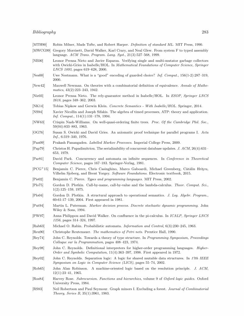
Bibliography 283
[MTH90] Robin Milner, Mads Tofte, and Robert Harper. Definition of standard ML. MIT Press, 1990.
[MWCG99] Gregory Morrisett, David Walker, Karl Crary, and Neal Glew. From system F to typed assemblylanguage. ACM Trans. Program. Lang. Syst., 21(3):527–568, 1999.
[NE00] Leonor Prensa Nieto and Javier Esparza. Verifying single and multi-mutator garbage collectorswith Owicki-Gries in Isabelle/HOL. In Mathematical Foundations of Computer Science, SpringerLNCS 1893, pages 619–628, 2000.
[Nes00] Uwe Nestmann. What is a “good” encoding of guarded choice? Inf. Comput., 156(1-2):287–319,2000.
[New42] Maxwell Newman. On theories with a combinatorial definition of equivalence. Annals of Mathe-matics, 43(2):223–243, 1942.
[Nie03] Leonor Prensa Nieto. The rely-guarantee method in Isabelle/HOL. In ESOP, Springer LNCS2618, pages 348–362, 2003.
[NK14] Tobias Nipkow and Gerwin Klein. Concrete Semantics - With Isabelle/HOL. Springer, 2014.
[NS94] Xavier Nicollin and Joseph Sifakis. The algebra of timed processes, ATP: theory and application.Inf. Comput., 114(1):131–178, 1994.
[NW63] Crispin Nash-Williams. On well-quasi-ordering finite trees. Proc. Of the Cambridge Phil. Soc.,59(04):833–883, 1963.
[OG76] Susan S. Owicki and David Gries. An axiomatic proof technique for parallel programs I. ActaInf., 6:319–340, 1976.
[Pan09] Prakash Panangaden. Labelled Markov Processes. Imperial College Press, 2009.
[Pap79] Christos H. Papadimitriou. The serializability of concurrent database updates. J. ACM, 26(4):631–653, 1979.
[Par81] David Park. Concurrency and automata on infinite sequences. In Conference in TheoreticalComputer Science, pages 167–183. Springer-Verlag, 1981.
[PCG+15] Benjamin C. Pierce, Chris Casinghino, Marco Gaboardi, Michael Greenberg, Catalin Hritcu,Vilhelm Sjoberg, and Brent Yorgey. Software Foundations. Electronic textbook, 2015.
[Pie02] Benjamin C. Pierce. Types and programming languages. MIT Press, 2002.
[Plo75] Gordon D. Plotkin. Call-by-name, call-by-value and the lambda-calculus. Theor. Comput. Sci.,1(2):125–159, 1975.
[Plo04] Gordon D. Plotkin. A structural approach to operational semantics. J. Log. Algebr. Program.,60-61:17–139, 2004. First appeared in 1981.
[Put94] Martin L. Puterman. Markov decision process. Discrete stochastic dynamic programming. JohnWiley & Sons, 1994.
[PW97] Anna Philippou and David Walker. On confluence in the pi-calculus. In ICALP, Springer LNCS1256, pages 314–324, 1997.
[Rab63] Michael O. Rabin. Probabilistic automata. Information and Control, 6(3):230–245, 1963.
[Reu90] Christophe Reutenauer. The mathematics of Petri nets. Prentice Hall, 1990.
[Rey74] John C. Reynolds. Towards a theory of type structure. In Programming Symposium, ProceedingsColloque sur la Programmation, pages 408–423, 1974.
[Rey98] John C. Reynolds. Definitional interpreters for higher-order programming languages. Higher-Order and Symbolic Computation, 11(4):363–397, 1998. First appeared in 1972.
[Rey02] John C. Reynolds. Separation logic: A logic for shared mutable data structures. In 17th IEEESymposium on Logic in Computer Science (LICS), pages 55–74, 2002.
[Rob65] John Alan Robinson. A machine-oriented logic based on the resolution principle. J. ACM,12(1):23–41, 1965.
[Ros84] Harvey Rose. Subrecursion. Functions and hierarchies, volume 9 of Oxford logic guides. OxfordUniversity Press, 1984.
[RS83] Neil Robertson and Paul Seymour. Graph minors I. Excluding a forest. Journal of CombinatorialTheory, Series B, 35(1):3961, 1983.

284 Bibliography
[SBS04] Manuel Serrano, Frederic Boussinot, and Bernard P. Serpette. Scheme fair threads. In ACMPPDP, pages 203–214, 2004.
[SL95] Roberto Segala and Nancy A. Lynch. Probabilistic simulations for probabilistic processes. Nord.J. Comput., 2(2):250–273, 1995.
[ST95] Nir Shavit and Dan Touitou. Software transactional memory. In ACM PODC, pages 204–213,1995.
[Sta79] Richard Statman. Intuitionistic propositional logic is polynomial-space complete. Theor. Comput.Sci., 9:67–72, 1979.
[Sti88] Colin Stirling. A generalization of Owicki-Gries’s Hoare logic for a concurrent while language.Theor. Comput. Sci., 58:347–359, 1988.
[SVN+13] Jaroslav Sevcık, Viktor Vafeiadis, Francesco Zappa Nardelli, Suresh Jagannathan, and PeterSewell. Compcerttso: A verified compiler for relaxed-memory concurrency. J. ACM, 60(3):22,2013.
[SW01] Davide Sangiorgi and David Walker. The pi-calculus: a theory of mobile processes. CambridgeUniversity Press, 2001.
[TT97] Mads Tofte and Jean-Pierre Talpin. Region-based memory management. Inf. Comput.,132(2):109–176, 1997.
[TvD88] Anne Sjerp Troelstra and Dirk van Dalen. Constructivism in mathematics. An introduction.Volume I. North-Holland, 1988.
[Var85] Moshe Y. Vardi. Automatic verification of probabilistic concurrent finite-state programs. In IEEEFOCS, pages 327–338, 1985.
[vdS87] Jan L. A. van de Snepscheut. Algorithms for on-the-fly garbage collection, revisited. Inf. Process.Lett., 24(4):211–216, 1987.
[Vit05] Giuseppe Vitali. Sul problema della misura dei gruppi di punti di una retta. Tipografia Gamberiniet Parmeggiani, 1905.
[vR01] Femke van Raamsdonk. On termination of higher-order rewriting. In Rewriting Techniques andApplications, Springer LNCS 2051, pages 261–275, 2001.
[Wel99] Joe B. Wells. Typability and type checking in system F are equivalent and undecidable. Ann.Pure Appl. Logic, 98(1-3):111–156, 1999.
[Win89] Glynn Winskel. A note on model checking the modal nu-calculus. In ICALP, Springer LNCS372, pages 761–772, 1989.
[Win93] Glynn Winskel. The formal semantics of programming languages. MIT Press, 1993.
[Wri95] Andrew K. Wright. Simple imperative polymorphism. Lisp and Symbolic Computation, 8(4):343–355, 1995.
[XdRH97] Qiwen Xu, Willem P. de Roever, and Jifeng He. The rely-guarantee method for verifying sharedvariable concurrent programs. Formal Asp. Comput., 9(2):149–174, 1997.
[Yi91] Wang Yi. CCS + time = an interleaving model for real time systems. In ICALP, Springer LNCS510, pages 217–228, 1991.
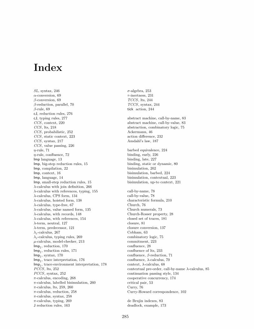
Index
SL, syntax, 246α-conversion, 69β-conversion, 69β-reduction, parallel, 70β-rule, 69cJ, reduction rules, 276cJ, typing rules, 277CCS , context, 220CCS , lts, 218CCS , probabilistic, 252CCS , static context, 223CCS , syntax, 217CCS , value passing, 226η-rule, 71η-rule, confluence, 72Imp language, 13Imp, big-step reduction rules, 15Imp, compilation, 22Imp, context, 16Imp, language, 14Imp, small-step reduction rules, 15λ-calculus with join definition, 266λ-calculus with references, typing, 155λ-calculus, CPS form, 134λ-calculus, hoisted form, 138λ-calculus, type-free, 67λ-calculus, value named form, 135λ-calculus, with records, 148λ-calculus, with references, 154λ-term, neutral, 127λ-term, predecessor, 121λj-calculus, 267λj-calculus, typing rules, 269µ-calculus, model-checker, 213Imp‖, reduction, 170Imp‖, reduction rules, 171Imp‖, syntax, 170Imp‖, trace interpretation, 176Imp‖, trace-environment interpretation, 178PCCS , lts, 252PCCS , syntax, 252π-calculus, encoding, 268π-calculus, labelled bisimulation, 260π-calculus, lts, 259, 260π-calculus, reduction, 258π-calculus, syntax, 258π-calculus, typing, 269J reduction rules, 163
σ-algebra, 253τ -inertness, 231TCCS , lts, 244TCCS , syntax, 244tick action, 244
abstract machine, call-by-name, 83abstract machine, call-by-value, 83abstraction, combinatory logic, 75Ackermann, 46action difference, 232Amdahl’s law, 187
barbed equivalence, 224binding, early, 226binding, late, 227binding, static or dynamic, 80bisimulation, 202bisimulation, barbed, 224bisimulation, contextual, 223bisimulation, up-to context, 221
call-by-name, 78call-by-value, 78characteristic formula, 210Church, 76Church numerals, 73Church-Rosser property, 28closed set of traces, 181closure, 81closure conversion, 137Cobham, 63combinatory logic, 75commitment, 223confluence, 28confluence of lts, 233confluence, β-reduction, 71confluence, λ-calculus, 70context, λ-calculus, 68contextual pre-order, call-by-name λ-calculus, 85continuation passing style, 134cooperative concurrency, 174critical pair, 53Curry, 76Curry-Howard correspondence, 102
de Brujin indexes, 83deadlock, example, 173
285
286 Index
degree, λ-term, 99degree, redex, 99degree, type, 99determinate process, 230Dickson, 49
environment, dynamic, 80environment, static, 81evaluation context, 78expansion, 207
fairness, strong, 174fairness, weak, 174fixed point, Curry, 69fixed point, Turing, 69fixed points monotonic functions, 87Floyd-Hoare rules, 18Floyd-Hoare rules, inversion, 19Floyd-Hoare rules, soundness, 18function F , 203function representation, λ-calculus, 73
Girard, 128
head normal form, 73heap, 153heap simulation, 155Higman, 51Hilbert, 43hoisting, 138homeomorphic embedding, 49Howe, 92
image finite lts, 203induction principle, 29infimum, 86IO interpretation, 16
Konig lemma, 31Kahn networks, 237Kozen, 215Kruskal, 50
label, records, 147labelled transition system, 201lattice, 86lattice, complete, 86local confluence, 32local confluence, in lts, 238lower bound, 86lumping equivalence, 250
Markov chain, 249Markov decision process, 250Matiyasevich, 43Milner, 227, 262minimization, 73modal logic with fixed points, 211
modal logic with tagged fixed points, 213modal logic, satisfaction, 210modal logic, syntax, 209monotonic function, 87multi-set, 31
Newman, 32non-deterministic sum, 171
order, lexicographic, 30order, multi-set, 31order, product, 30ordinals, 88
Park, 207partial correctness assertion, 18partial correctness assertion, interpretation, 20partial order, 29, 86partial recursive functions, 73Petri nets, 270predicative type system, Church-style, 111predicative type system, Curry style, 110primitive recursive function, 60probabilistic bisimulation, 251propositional types, interpretation, 100
reactive process, 238recursive path-order, 44reducibility candidate, 125reduction order, 41reduction, maximal degree, 99references, 153rely-guarantee assertion, 194, 195rely-guarantee rules, 195, 196restricted parallel composition, 236rewriting system, 27rewriting system, normalizing, 28rewriting system, terminating, 27Robinson, 39
Schonfinkel, 76simplification order, 45simulation, λ-calculus, 90size, λ-term, 68sorting in CCS , 236stability, 195strong normalization, 100strong normalization, propositional types, 100strong normalization, system F, 127substitution, λ-calculus, 68subtyping rules, 149supremum, 86
Tarski, 52, 87term rewriting system, 34term substitution, 33termination, interpretation method, 41trace equivalence on lts, 231
Index 287
traces in a lts, 201type assignment, Church-style, 96type assignment, non-logical rules, 97type assignment, product and sum, 97type assignment, with type labelled variables, 97type assignment, with type-labelled λ-terms, 97type context, 95type erasure, 125type inference, predicative polymorphic types, 113type inference, propositional types, 103type-assignment, Curry-style, 96types, propositional, 95
unification algorithm, 38upper bound, 86
value named form, 136value, λ-calculus, 77vending machine, 174virtual machine, reduction rules, 21
weak β-reduction, 77weak bisimulation, 205weak bisimulation, one step, 205weak lts, 205weak probabilistic bisimulation, 254weak up to strong bisimulation, 205well partial order, 49well-founded order, 29