Clément Roos - Archive ouverte HAL

HAL Id: tel-01801720https://hal.archives-ouvertes.fr/tel-01801720

Submitted on 28 May 2018

HAL is a multi-disciplinary open accessarchive for the deposit and dissemination of sci-entific research documents, whether they are pub-lished or not. The documents may come fromteaching and research institutions in France orabroad, or from public or private research centers.

L’archive ouverte pluridisciplinaire HAL, estdestinée au dépôt et à la diffusion de documentsscientifiques de niveau recherche, publiés ou non,émanant des établissements d’enseignement et derecherche français ou étrangers, des laboratoirespublics ou privés.

Advanced control laws design and validation - A set ofmethods and tools to bridge the gap between theory and

practiceClément Roos

To cite this version:Clément Roos. Advanced control laws design and validation - A set of methods and tools to bridgethe gap between theory and practice. Automatic Control Engineering. UNIVERSITE TOULOUSEIII - PAUL SABATIER, 2018. tel-01801720

https://hal.archives-ouvertes.fr/tel-01801720

https://hal.archives-ouvertes.fr

HABILITATION A DIRIGER DES RECHERCHES

UNIVERSITÉ TOULOUSE III - PAUL SABATIER

SPÉCIALITÉ AUTOMATIQUE

par

Clément Roos

Advanced control laws design and validation

A set of methods and tools to bridge the gap between theory and practice

Habilitation présentée le 16 avril 2018 devant le jury composé de :

Michel Basset Rapporteur Professeur Université de Haute Alsace

Jean-Marc Biannic Examinateur Directeur de recherche ONERA

Patrick Danès Examinateur Professeur Université de Toulouse

Andrés Marcos Examinateur Professeur Université de Bristol

Isabelle Queinnec Directrice de HDR Directrice de recherche LAAS-CNRS

Gérard Scorletti Rapporteur Professeur Ecole Centrale de Lyon

Peter Seiler Examinateur Professeur Université du Minnesota

Matthew Turner Rapporteur Professeur Université de Leicester

Contents 1

Contents

Acknowledgments 5

I Summary of research activities 7

Introduction 9

A µ-analysis based robustness tools 13

1 A brief introduction to µ-analysis . . . . . . . . . . . . . . . . . . . . . . . . . . . 142 µ lower bound computation . . . . . . . . . . . . . . . . . . . . . . . . . . . . . . 15

2.1 Survey of existing methods . . . . . . . . . . . . . . . . . . . . . . . . . . 152.2 Testing framework . . . . . . . . . . . . . . . . . . . . . . . . . . . . . . . 192.3 Numerical results . . . . . . . . . . . . . . . . . . . . . . . . . . . . . . . . 212.4 Results improvement . . . . . . . . . . . . . . . . . . . . . . . . . . . . . . 222.5 Conclusion . . . . . . . . . . . . . . . . . . . . . . . . . . . . . . . . . . . 24

3 µ upper bound computation . . . . . . . . . . . . . . . . . . . . . . . . . . . . . . 253.1 Classical (D,G)-scalings formulation . . . . . . . . . . . . . . . . . . . . . 253.2 Numerical results . . . . . . . . . . . . . . . . . . . . . . . . . . . . . . . . 273.3 Use of the µ-sensitivities . . . . . . . . . . . . . . . . . . . . . . . . . . . . 273.4 Partial LMI optimization of the scaling matrices . . . . . . . . . . . . . . 283.5 Multiplier-based µ upper bound . . . . . . . . . . . . . . . . . . . . . . . . 293.6 Conclusion . . . . . . . . . . . . . . . . . . . . . . . . . . . . . . . . . . . 33

4 Branch-and-bound to reduce conservatism . . . . . . . . . . . . . . . . . . . . . . 334.1 Standard algorithm . . . . . . . . . . . . . . . . . . . . . . . . . . . . . . . 334.2 Improved algorithm . . . . . . . . . . . . . . . . . . . . . . . . . . . . . . 344.3 Numerical results . . . . . . . . . . . . . . . . . . . . . . . . . . . . . . . . 35

5 What can be done with µ . . . . . . . . . . . . . . . . . . . . . . . . . . . . . . . 365.1 Modal performance . . . . . . . . . . . . . . . . . . . . . . . . . . . . . . . 365.2 Skewed robust stability margin . . . . . . . . . . . . . . . . . . . . . . . . 37

5.2.1 Problem statement . . . . . . . . . . . . . . . . . . . . . . . . . . 375.2.2 Skew-µ lower bound computation . . . . . . . . . . . . . . . . . 385.2.3 Skew-µ upper bound computation . . . . . . . . . . . . . . . . . 40

5.3 Worst case H∞ performance . . . . . . . . . . . . . . . . . . . . . . . . . . 405.4 Worst-case input-output margins . . . . . . . . . . . . . . . . . . . . . . . 42

6 An insight into the SMART library . . . . . . . . . . . . . . . . . . . . . . . . . . 437 Summary of the contributions . . . . . . . . . . . . . . . . . . . . . . . . . . . . . 43

Advanced control laws design and validation - A set of methods and tools to bridge the gap between theory and practice

2 Contents

B Extensions to time-varying uncertainties 45

1 A µ-analysis based approach . . . . . . . . . . . . . . . . . . . . . . . . . . . . . . 461.1 Problem statement . . . . . . . . . . . . . . . . . . . . . . . . . . . . . . . 461.2 Performance analysis . . . . . . . . . . . . . . . . . . . . . . . . . . . . . . 48

1.2.1 Computation of a worst-case performance level . . . . . . . . . . 481.2.2 Validation with a frequency elimination technique . . . . . . . . 491.2.3 Convergence of the algorithm . . . . . . . . . . . . . . . . . . . . 501.2.4 A suboptimal but faster algorithm . . . . . . . . . . . . . . . . . 50

1.3 Extension to robust feedforward design . . . . . . . . . . . . . . . . . . . . 511.3.1 Problem statement . . . . . . . . . . . . . . . . . . . . . . . . . . 511.3.2 Practical solution . . . . . . . . . . . . . . . . . . . . . . . . . . 52

1.4 Conclusion . . . . . . . . . . . . . . . . . . . . . . . . . . . . . . . . . . . 532 A Lyapunov based approach . . . . . . . . . . . . . . . . . . . . . . . . . . . . . . 53

2.1 Problem statement . . . . . . . . . . . . . . . . . . . . . . . . . . . . . . . 532.2 Stability analysis . . . . . . . . . . . . . . . . . . . . . . . . . . . . . . . . 54

2.2.1 LMI-based formulation of the stability analysis problem . . . . . 542.2.2 Grid-based resolution . . . . . . . . . . . . . . . . . . . . . . . . 552.2.3 Validity of the parameter-dependent Lyapunov function . . . . . 562.2.4 Determination of a worst-case conguration . . . . . . . . . . . . 572.2.5 Description of the algorithm . . . . . . . . . . . . . . . . . . . . 57

2.3 Extension to performance analysis . . . . . . . . . . . . . . . . . . . . . . 582.4 Conclusion . . . . . . . . . . . . . . . . . . . . . . . . . . . . . . . . . . . 58

3 Summary of the contributions . . . . . . . . . . . . . . . . . . . . . . . . . . . . . 59

C Generation of low-order LFR 61

1 From a set of scalar samples to a static LFR . . . . . . . . . . . . . . . . . . . . . 621.1 Problem statement . . . . . . . . . . . . . . . . . . . . . . . . . . . . . . . 621.2 Overview of existing methods . . . . . . . . . . . . . . . . . . . . . . . . . 62

1.2.1 Polynomial case . . . . . . . . . . . . . . . . . . . . . . . . . . . 631.2.2 Rational case . . . . . . . . . . . . . . . . . . . . . . . . . . . . . 64

1.3 Focus on sparse approximation techniques . . . . . . . . . . . . . . . . . . 651.3.1 Polynomial approximation using orthogonal least-squares . . . . 651.3.2 Rational approximation using genetic programming . . . . . . . 661.3.3 Rational approximation using surrogate modeling . . . . . . . . 68

1.4 Implementation issues . . . . . . . . . . . . . . . . . . . . . . . . . . . . . 701.4.1 Non singularity of the rational function . . . . . . . . . . . . . . 701.4.2 A Matlab library for polynomial and rational approximation . . 711.4.3 Towards low-order LFR . . . . . . . . . . . . . . . . . . . . . . . 71

1.5 Conclusion . . . . . . . . . . . . . . . . . . . . . . . . . . . . . . . . . . . 722 From a set of MIMO LTI models to a dynamic LFR . . . . . . . . . . . . . . . . 72

2.1 Motivations . . . . . . . . . . . . . . . . . . . . . . . . . . . . . . . . . . . 722.2 Generation of reduced and consistent models . . . . . . . . . . . . . . . . 732.3 Choice of a suitable state-space form . . . . . . . . . . . . . . . . . . . . . 752.4 Generation of a low-order LFR . . . . . . . . . . . . . . . . . . . . . . . . 752.5 Presentation of the LTI2LFR Library for Matlab . . . . . . . . . . . . . . 77

3 Summary of the contributions . . . . . . . . . . . . . . . . . . . . . . . . . . . . . 77


Contents 3

D Analysis and control of saturated systems 791 Full-order anti-windup design . . . . . . . . . . . . . . . . . . . . . . . . . . . . . 80

1.1 Problem statement . . . . . . . . . . . . . . . . . . . . . . . . . . . . . . . 801.2 Performance analysis of saturated systems . . . . . . . . . . . . . . . . . . 831.3 Convex characterization of full-order anti-windup design . . . . . . . . . . 84

2 Fixed-order anti-windup design . . . . . . . . . . . . . . . . . . . . . . . . . . . . 853 Dynamically-constrained anti-windup design . . . . . . . . . . . . . . . . . . . . . 864 From the AWAS Toolbox to the SAW Library . . . . . . . . . . . . . . . . . . . . 885 Summary of the contributions . . . . . . . . . . . . . . . . . . . . . . . . . . . . . 88

E Control laws design and implementation 891 Robust nonlinear compensation for the approach phase . . . . . . . . . . . . . . . 90

1.1 Description of the methodology . . . . . . . . . . . . . . . . . . . . . . . . 901.1.1 Robust nonlinear compensation based on dynamic inversion . . . 911.1.2 Preliminary LTI robustness analysis . . . . . . . . . . . . . . . . 931.1.3 Multi-model design . . . . . . . . . . . . . . . . . . . . . . . . . 951.1.4 Towards a global robustness analysis . . . . . . . . . . . . . . . . 96

1.2 Application to the approach phase . . . . . . . . . . . . . . . . . . . . . . 961.2.1 Nonlinear longitudinal aircraft model . . . . . . . . . . . . . . . 961.2.2 Nonlinear compensation technique . . . . . . . . . . . . . . . . . 971.2.3 Robustness analysis and multi-model design . . . . . . . . . . . . 981.2.4 Final approach simulations . . . . . . . . . . . . . . . . . . . . . 100

1.3 Conclusion . . . . . . . . . . . . . . . . . . . . . . . . . . . . . . . . . . . 1012 Robust multi-model H∞ design for the are phase . . . . . . . . . . . . . . . . . 101

2.1 Overall structure of the are control system . . . . . . . . . . . . . . . . . 1012.2 Vertical speed control via multi-channel structured H∞ optimization . . . 1022.3 Robustness against parametric uncertainties and modeling errors . . . . . 1032.4 Nonlinear implementation and simulation results . . . . . . . . . . . . . . 1042.5 Conclusion . . . . . . . . . . . . . . . . . . . . . . . . . . . . . . . . . . . 106

3 Adaptive anti-windup design for the ground phase . . . . . . . . . . . . . . . . . 1063.1 Design oriented modeling of an on-ground aircraft . . . . . . . . . . . . . 1063.2 Adaptive anti-windup for low speed maneuvers . . . . . . . . . . . . . . . 1083.3 Robust dynamic allocation for runway axis hold . . . . . . . . . . . . . . . 111

4 Control laws implementation . . . . . . . . . . . . . . . . . . . . . . . . . . . . . 1125 Summary of the contributions . . . . . . . . . . . . . . . . . . . . . . . . . . . . . 114

Research prospects 115Development of enhanced robustness analysis tools . . . . . . . . . . . . . . . . . . . . 115Computation of simple yet accurate linear fractional representations . . . . . . . . . . 117Design and implementation of advanced control architectures . . . . . . . . . . . . . . 118

References 119

II Detailed curriculum vitae 137


Acknowledgments

Je remercie en premier lieu Jean-Marc Biannic, que je côtoie depuis bientôt 14 ans à l'ONERA.Il a été mon professeur puis mon directeur de thèse avant de devenir mon plus proche collègue,précieux par ses conseils, toujours présent à mes côtés, et généreux dans son aide et son soutien.Si j'achève la rédaction de ce manuscrit aujourd'hui, c'est pour beaucoup grâce à lui.

Je remercie ensuite tous les autres chercheurs qui ont accepté de faire partie de mon jury :Michel Basset de l'Université de Haute-Alsace, Patrick Danès de l'Université de Toulouse, AndrésMarcos de l'Université de Bristol, Isabelle Queinnec du LAAS-CNRS, Gérard Scorletti de l'EcoleCentrale de Lyon, Peter Seiler de l'Université du Minnesota et Matthew Turner de l'Université deLeicester. Merci aux rapporteurs pour leur lecture attentive de ce manuscrit et leurs remarquesconstructives. Merci à ceux qui sont venus de loin. Et merci à tous d'avoir consacré du temps àmon habilitation, notamment Isabelle pour avoir accepté de jouer le rôle de directrice de HDRet pour m'avoir guidé dans ma préparation.

Je remercie également tous les chercheurs, ingénieurs, doctorants et stagiaires avec qui j'aipu mener à bien les travaux présentés dans ce manuscrit. Je m'abstiendrai de les nommer demanière exhaustive de peur d'en oublier, mais j'espère que je continuerai à collaborer avec euxet avec d'autres à l'avenir.

Je remercie enn Christelle Cumer, responsable de l'équipe de recherche Commande et Inté-gration, devenue récemment Automatique, Expérimentation, Intégration, qui n'a jamais ménagéses eorts pour me rendre la vie plus facile pendant toutes ces années.

Un clin d'÷il pour nir à Sophie qui m'a vivement encouragé (et c'est un euphémisme) à melancer dans la préparation de ce manuscrit, et à Victor qui du haut de ses 9 ans m'a proposé dem'aider à le rédiger.


Part I

Summary of research activities

Introduction

It all started 13 years ago. I was a young PhD student with no precise idea what directionI was heading to. I had few other options than carefully listening to my supervisor singingthe praises of robustness analysis in general, and of µ-analysis in particular. I also saw my closecolleagues working on the same topic. And I noticed the growing interest among control engineersfrom the aerospace industry. So I naturally took this path. At that time, it was already knownfor a long time that computing the exact value of the structured singular value µ is NP hard.So people were trying to develop polynomial-time algorithms to compute tight lower and upperbounds instead. And my colleagues were playing a key role with signicant contributions thatremain references even today [Ferreres and Biannic, 2001; Ferreres et al., 2003], as evidenced bythe Skew-Mu Toolbox for Matlab which was widely used during a whole decade [Ferreres et al.,2004]. It was in this environment that I took my rst steps.

Then I started thinking a little bit on my own. The rst major project I was involved indealt with the clearance of ight control laws. Before an aircraft can be tested in ight, ithas to be proven to the authorities that the ight control system is reliable, i.e. it has to gothrough a certication and qualication process. It must notably be shown that the control lawsprovide sucient stability margins to guarantee a safe operation of the aircraft over the entireight envelope and for all admissible parametric variations. In the aeronautical industry, this isusually achieved using intensive Monte-Carlo simulations. A major drawback of this strategy isthat clearance is restricted to a nite number of samples and nothing can in principle be assessedfor the rest of the parametric domain. Moreover, signicant time and money is frequentlyspent on this task. Fortunately, many stability, handling, loads and performance criteria canbe formulated as robustness analysis problems, which can then be solved using modern analysistechniques, such as µ-analysis, IQC-based analysis or Lyapunov-based analysis. At that point, Irealized that these techniques were not just research topics tailored to control theorists, but thatthey could be of signicant practical importance to improve the eciency and the reliability of thecertication process, and more generally to enhance the validation of any feedback system. Myconviction was reinforced when I noticed that the aerospace industry was following the subjectclosely: Airbus [Puyou et al., 2012], Boeing [Dailey, 1990], Astrium Satellites [Beugnon et al.,2003], Astrium Space Transportation [Ganet-Schoeller et al., 2009], Deimos & ESA [Pulecchi etal., 2012], Thales Alenia Space [Charbonnel, 2010] and others were all evaluating the potentialbenets of µ-analysis on real-world applications. But they were also very critical. As I hadalready invested quite a lot of time on this subject, I was cut to the quick, and I decided to trymaking my own contribution to address the issues raised by our industrial partners.

A rst recurrent criticism was that the gap between the bounds on µ was often too large. Theresulting robust stability margin was thus too pessimistic, and it was sometimes impossible toconclude about stability even though the considered system was indeed stable. In this context,my coworkers and I performed a thorough comparison of all pratical algorithms to computelower bounds on µ, and we proposed some strategies to take the most out of them (Section A.2).


10 Introduction

Noting that the µ upper bound was generally responsible for the conservatism, we tried toimprove the accuracy of existing algorithms, while maintaining a reasonable computational time(Section A.3). And as it was sometimes not sucient, we proposed some enhanced branch-and-bound algorithms to further tighten the gap up to a user-dened precision (Section A.4).Evaluation on a wide set of real-world benchmarks available in the literature shows that non-conservative robust stability margins can be obtained in almost all cases. So we believe now thatcomputing the exact value of µ is no longer an issue from a practical point of view.

Another criticism was that very few criteria could be evaluated with µ-analysis compared toother techniques such as Monte-Carlo simulations. It was true, and despite our eorts, it willremain partially. We proposed several algorithms to compute tight bounds on the skewed robuststability margin, the worst-caseH∞ performance level, the worst-case gain/phase/modulus/delaymargins (Section A.5). . . So µ-analysis clearly allows to go beyond stability and to address manyother practical issues. Nevertheless, it must be kept in mind that only parametric uncertaintiesand neglected dynamics can be considered (although a few applications to nonlinear systemshave been reported in the literature). Other techniques must be used to go further, such asIQC-based analysis or evolutionary algorithms, which allow uncertainties, varying parametersand various kinds of nonlinearities to be considered at the same time. But even so, the size ofthe considered models is limited to avoid high conservatism and prohibitive computational time.µ-analysis and similar methods thus prove useful in the early validation stages, but there comesa time when simulations are inevitable at the moment. It seems therefore obvious that there ismuch to be gained from combining both approaches. And this is the message we are trying toconvey to control engineers.

µ-analysis was nally criticized for being dicult to apply by non-expert users, which I canunderstand. I believe good theories only reveal their true potential when they become applicableto realistic problems. That is why I spend a lot of time developing tools to help both researchersand engineers get the most out of the methods I am working on. The SMART Library of theSystems Modeling Analysis and Control (SMAC) Toolbox for Matlab is one of them (Section A.6).It implements most of the µ-analysis based algorithms developed at ONERA during the last twodecades, and it symbolizes the way I position myself as a research engineer. I am not a purecontrol theorist, others do that much better than me. And I am not an engineer either. I amsomehere between the two, trying to bridge the gap between these two worlds. This is howmy contribution should be understood. I sometimes propose heuristics without any theoreticalproof. But I prefer a heuristic which works on most real-world applications, than a more rigorousapproach which can only be applied to simple examples.

As can be seen in the literature, much has been done in the eld of µ-analysis, and thistechnique is now quite mature. Unfortunately, the same observation cannot be made for allrobustness analysis techniques, and I could be criticized for having been primarily interestedin µ-analysis at the expense of other methods. But many projects during and after my PhDthesis dealt with this subject, so I naturally continued along this path. And anyway, I am stillyoung and I have quite a lot of time left to investigate other approaches! More seriously, Ibegan considering time-varying parameters and uncertainties as well a long time ago becausemost aerospace vehicles are characterized by parameters that vary more or less rapidly. We rstproposed generalizations of the aforementioned µ-analysis tools to evaluate the stability and theperformance properties of linear systems in the presence of both LTI and arbitrarily fast varyinguncertainties. Two complementary solutions were developed: the rst one (in the frequencydomain) is suitable for high-order models with few uncertainties (Section B.1), while the secondone (in the time domain using an extended version of the KYP lemma) is better for low-ordermodels with many uncertainties (not detailed in this manuscript due to space constraints). It


Introduction 11

should be noted that beyond analysis, these techniques also allow to design a robust feedforwardcontroller in order to improve performance. Nevertheless, in many practical applications, it isdesirable to consider the rate of variation of time-varying uncertainties and parameters to getmore accurate results. In this context, we proposed later a completely dierent strategy basedon parameter-dependent Lyapunov functions (Section B.2). Several kinds of dependence canbe considered, but the resulting optimization problem always boils down to solving an innitenumber of linear matrix inequalities. Rather than introducing some relaxation variables andworking on sucient conditions, we proposed to solve the problem on a nite parametric gridand to check the result on the whole parametric domain using a fast and reliable µ-analysis basedtest. This strategy is symbolic of our work. Most of the aforementioned methods were not new,but the previously existing algorithms often had two major drawbacks when high-order systemswere considered, namely a high computational time and a high conservatism. The central concernof our work and our main contribution have been to provide solutions to these problems.

Another issue that makes it dicult to convince control engineers to use modern robustnessanalysis techniques is that the considered systems must often be modeled using Linear FractionalRepresentations (LFR). Unfortunately in most industrial applications, physical systems are de-scribed using a mix of nonlinear analytical expressions and tabulated data, which are far frombeing in linear fractional form. . . But as no LFR means no µ-analysis, we had no other choicethan developing dedicated tools that can be used by non-expert users. In general, a two-stepprocedure has to be implemented to obtain a suitable LFR: a linear model with a polynomialor a rational dependence on the system parameters is rst generated, and then converted into alinear fractional form. Several techniques already existed to perform the latter transformationand to overcome complexity. Following the same motivations as for the SMART Library, weimplemented state-of-the-art algorithms in the GSS Library and proposed an intuitive yet verygeneral way to describe LFR, as well as a user-friendly Simulink interface (Section C.1.4). This isnot what we might call research, but sometimes you have to be pragmatic. We will have taken amajor step forward if engineers are no longer afraid to turn their models into LFRs. On the otherhand, the preliminary issue of converting the tabulated or irrational data into simple yet accuratepolynomial or rational expressions had been paid much less attention, although it is of signi-cant practical importance. Most of the methods that existed at that time have two drawbacks:they only produce polynomial approximations, and all admissible monomials are usually nonzeroregardless of their real ability to model the data. Yet, the additional degrees of freedom oeredby rational expressions can lead to simpler expressions, and thus to avoid unnecessarily complexLFRs, which are usually source of conservatism and can even lead to numerical intractability.Moreover, computing approximations with sparse structure is benecial, since it is a natural wayto prevent data overtting and to ensure a smooth behavior of the model between the points usedfor approximation. In this context, we developed several methods to ll this gap (Section C.1.3),and in the spirit of what we did before, we implemented the whole set of tools in the APRICOTLibrary, well organized for non-expert users (Section C.1.4). Finally, we proposed extensionsto generate a reduced-order LFR from a set of large-scale MIMO state-space representations,representing for example an aerospace vehicle at various operating conditions (Section C.2).

While we are at it, let us take a closer look at aerospace vehicles. They depend on manyparameters and are aected by plenty of uncertainties, varying or not, for which we now havea bunch of analysis tools at our disposal. But we are not out of the woods yet: they arealso full of nonlinearities, among which saturations gure prominently. And this is a majorissue. By limiting both the amplitude and the rate of the control signals, saturations induceparticularly disturbing nonlinear phenomena (such as limit cycles), that can impair the closedloop performance or even jeopardise its stability. We tried to model saturations with time-


12 Introduction

varying gains to apply the aforementioned tools, but the results obtained in practice are mostoften disappointing. Thus, we decided to focus on more appropriate analysis tools. Based onthe Lyapunov theory, they allow to compute a stability domain and to quantify performancedegradation. But beyond analysis, there is also the problem of taking saturations into accountduring the design step. Two strategies are possible. Either stay in the linear domain at the priceof a lower level of performance, by computing unsaturating control laws. Or be more adventurousby allowing saturations and adapting control signals as soon as one of them is active, so as toreturn as quickly as possible to the linear domain guaranteeing a well-controlled nominal behaviorof the system. The second approach, known as anti-windup, had already proved successful inthe past and we decided to go on in that direction. Indeed, aerospace applications cannottolerate an unnecessary loss of performance in the nominal case. Our contribution was againpragmatic and was mainly twofold. First, we developed a methodology to design a reduced-orderanti-windup controller of low complexity (Section D.2). Then we introduced modal constraintsduring the design to avoid too slow or too fast dynamics likely to lower performance or to causeimplementation issues (Section D.3). And unsurprisingly, the resulting algorithms were groupedtogether with a Simulink interface in the AWAS Toolbox for Matlab, which was later updatedand became the SAW Library of the SMAC Toolbox (Section D.4).

Plenty of ecient tools are now available to analyze robustness and to validate control laws,and those we have developed so far are just a drop in the ocean. But in most cases, they are mainlyapplied once the controllers have been computed. Yet it could be advisable to better integratethem into the design process, in the hope of reducing a little bit the number of iterations betweendesign and validation in an industrial context. And this is what we are trying to do now. We haveproposed several methodologies, among which one is inspired by dynamic inversion techniquesand looks promising (Chapter E). It combines partially linearizing inner-loops with structuredand robust outer-loops, which are designed using a non-smooth multi-model H∞ optimizationapproach. It also includes a robustness analysis scheme providing worst-case congurations,which are then used to enrich the bank of design models and thus to iteratively improve therobustness properties of the designed outer-loops. And it seems simple enough to be implementedin a ight computer. But for the moment, it is more a prospect than an achievement, and wewill talk about it again later.

This manuscript is deliberately concise and mainly contains personal contributions. It isnot exhaustive in the sense that I decided to highlight only certain methods, either becausethey are important to me or because they are little known although they may have a practicalinterest. Chapter A is signicantly longer than the others. Robustness analysis, and µ-analysisin particular, has indeed been central to my work since day one. I do not always spend a lotof time on it, but I come back to it regularly. Moreover, I decided to focus on methods andtools rather than on their application. My philosophy is to propose general methods that canbe applied to dierent kinds of systems. One could maybe do better by developing a specictechnique for each application. But my experience is that control engineers do not have muchtime, so it is better to have few well-used methods than many ignored ones.

Remark: Chapters 1 and 3 present the topics I spent most of my time on. I cannot go into toomuch detail because of space constraints, so I simply present a summary with the main results.Chapters 2 and 4, on the other hand, deal with issues that I addressed several years ago, and whichI have now put aside (but maybe not forever!). Finally, Chapter 5 illustrates my current desireto go further towards the development of advanced design methods and their implementation onxed wing UAVs.


Chapter A

µ-analysis based robustness tools

Despite evermore powerful design tools and increasing computer power, control laws arestill designed based on mathematical models, which signicantly simplify reality. A necessarybut costly task consists in thoroughly validating them before they can be implemented. Thisinvolves numerous simulations of generally nonlinear and nonstationary models, which are asrepresentative as possible of the real behavior of the considered physical system. However, it iscertainly possible to signicantly reduce the number of simulations by directing them towardsworst-case parametric congurations detected through a series of simplied robust stability andperformance tests.

Several approaches can be considered in this perspective: µ-analysis [Ferreres, 1999], integralquadratic constraints [Megretski and Rantzer, 1997], Lyapunov-based techniques [Garulli et al.,2012], sum of squares [Chesi, 2010], evolutionary methods [Menon et al., 2009], randomizedalgorithms [Tempo et al., 2013]. . . The objective of this chapter is not to perform an extensivecomparison of their advantages and drawbacks, but to focus on one of them, namely µ-analysis.This is the approach I have been working on most for a certain number of reasons alreadydiscussed in the introduction. And it is commonly accepted that this is the most suitable wayto compute stability margins and performance levels for LTI systems aected by structuredtime-invariant uncertainties. The exact computation of the structured singular value µ beingNP-hard [Braatz et al., 1994], only lower and upper bounds on these quantities can usually beobtained with a reasonnable computational eort. Until recently, it was quite common with theavailable software to obtain a non-zero gap between the bounds, which could even be large in somecases (typically exible systems aected by real parametric uncertainties). This is undesirable,as it may be impossible to conclude whether the required level of robustness is guaranteed ornot.

We have invested a great deal of eort in proposing solutions to this problem, as well asto the various recurrent criticisms mentioned in the introduction. This chapter summarizesour contributions. A complete strategy is rst described to compute accurate bounds on µin Sections A.2 and A.3, and to bring the resulting gap to (almost) zero with a reasonablecomputational cost in Section A.4. A brief overview of what can be done with µ is then presentedin Section A.5, where a series of pratical methods and computational tools are described tocompute the (almost) exact value of the (skewed) robust stability margin, the worst-case H∞performance level, as well as the worst-case gain, phase, modulus and time-delay margins. Finally,Section A.6 briey presents the SMART Library for Matlab, which implements most of the µ-analysis based tools we developed at ONERA during the last two decades.

13

14 µ-analysis based robustness tools

1 A brief introduction to µ-analysis

Let us consider the standard interconnection of Figure A.1. M(s) is a continuous-time stableand proper real-rational transfer function representing the nominal closed-loop system. ∆(s) isa continuous-time block-diagonal operator:

∆(s) = diag(∆1(s), . . . ,∆N (s)) (A.1)

which gathers all model uncertainties. Each ∆i(s) can be:

• either a time-invariant diagonal matrix ∆i(s) = δiIni , where δi is a real or a complexparametric uncertainty, and Ini is the ni × ni identity matrix,

• or a stable and proper real-rational unstructured transfer function of size ni × ni usuallyrepresenting neglected dynamics.

-

∆(s)

M(s)

Figure A.1: Standard interconnection for robustness analysis

Let n =∑N

i=1 ni. The set of all n× n matrices with the same block-diagonal structure and thesame nature (real or complex) as ∆(jω) is denoted by ∆. Let then kB∆ = ∆ ∈∆ : σ(∆) < k,where σ (∆) denotes the largest singular value of ∆. To simplify notation, ∆(s) ∈ ∆ is used tospecify that ∆(jω) ∈∆ for all ω ∈ Ω, where Ω denotes the frequency range of interest (equal toR+ in the sequel without loss of generality). ∆(s) ∈ kB∆ means in addition that ‖∆(s)‖∞ < k.In other words, ∆ is the set of all admissible uncertainties, whose size is measured in terms ofthe H∞ norm. In the sequel, the expression real problem is used when ∆(s) is only composedof real blocks corresponding to real parametric uncertainties. Conversely, the expression complexproblem is used when ∆(s) is only composed of unstructured transfer functions, which becomecomplex blocks when evaluated at a particular frequency.

The most ecient technique to analyze the stability of the interconnection of Figure A.1in the H∞ framework is certainly µ-analysis [Doyle, 1982], especially when high-dimensionalsystems are considered. The underlying theory [Ferreres, 1999; Zhou et al., 1996] is not broachedas such in this document due to space limitations, but a few useful denitions and results arerecalled below.

Denition A.1 (structured singular value) Let ω ∈ R+ be a given frequency. If no matrix∆ ∈ ∆ makes I −M(jω)∆ singular, then the structured singular value µ∆(M(jω)) is equal tozero. Otherwise:

µ∆(M(jω)) =[

min∆∈∆

σ(∆), det(I −M(jω)∆) = 0]−1

(A.2)


2 µ lower bound computation 15

Theorem A.1 (small gain theorem for structured uncertainties) The interconnection ofFigure A.1 is stable for all uncertainties ∆(s) ∈ kB∆ if and only if:

supω∈R+

µ∆(M(jω)) ≤ 1

k(A.3)

Denition A.2 (robust stability margin) The robust stability margin kr is dened as thelargest value of k for which equation (A.3) holds. In other words, kr is the inverse of the largestvalue of µ∆(M(jω)) over the whole frequency range:

kr =[

supω∈R+

µ∆(M(jω))]−1

(A.4)

The following conclusions can be drawn from the small gain theorem:

• the interconnection is stable for all admissible uncertainties ∆(s) of size less than kr,

• there exists at least one admissible uncertainty ∆(s) of size kr for which the interconnectionis unstable.

Problem A.1 (robust stability margin) With reference to Figure A.1, compute the robuststability margin kr dened in equation (A.4) for a given block structure ∆.

The exact computation of kr is known to be NP hard in the general case [Braatz et al., 1994],so both lower and upper bounds kr and kr are computed instead. But even computing thesebounds is a challenging problem with an innite number of frequency-domain constraints, sinceit requires to compute lower and upper bounds µ∆(M(jω)) and µ∆(M(jω)) on µ∆(M(jω)) foreach ω ∈ R+. On the one hand, a wide number of very dierent approaches exist to computeupper bounds on kr (i.e. µ lower bounds). They are summarized and compared in Section A.2on a wide set of real-world benchmarks. A strategy is also proposed to combine them, so as toimprove accuracy while keeping a reasonable computational time. On the other hand, most of thecomputationally tractable methods to compute lower bounds on kr (i.e. µ upper bounds) rely onthe so-called D and G scaling matrices. The problem is usually solved on a nite frequency gridwith the risk to miss a critical frequency and to over-evaluate kr. An algorithm is presented inSection A.3 to address this issue, and applied to the aforementioned benchmarks. Unfortunately,the gap between the bounds on kr is sometimes large and concluding about robust stability is notalways straightforward. Assume, for instance, that the uncertainties are normalized. Stabilityhas to be investigated ∀∆(s) ∈ B∆ and is guaranteed if and only if kr > 1. But if kr < 1

and kr > 1, no conclusion can be drawn. Strategies can then be implemented to tighten thegap between the bounds, among which branch-and-bound seems to be the most eective one, asshown in Section A.4.

2 µ lower bound computation

2.1 Survey of existing methods

This section is exhaustive in the sense that all methods that can reasonably be applied toreal-world benchmarks are mentioned. Only a few exponential-time algorithms are omitted, aswell as techniques with a very limited range of application. In all cases, both µ lower bounds andassociated destabilizing values of the uncertainties are obtained. For most methods, frequency



is xed during optimization. In this case, M(jω) and ∆(jω) are constant matrices, which aresimply denoted by M and ∆.

Exponential-time methods

The rst methods to compute µ lower bounds were proposed in the 1980's and most of themare exponential-time. One of the best known was introduced in [De Gaston and Safonov, 1988]for non-repeated (ni = 1) real uncertainties and later generalized in [Sideris and Sanchez Pena,1990]. It uses the mapping theorem of [Zadeh and Desoer, 1963]: the image of kB∆ by theoperator ∆→ det(I −∆M) is included into the convex hull of the images of the 2N vertices ofkB∆. A µ lower bound is obtained by considering the position of these images with respect to theorigin in the complex plane. Like the mapping theorem, the Kharitonov's theorem [Barmish andKang, 1993] and the edge theorem [Bartlett et al., 1988] can also be interpreted in a frequencydomain approach and used to derive µ lower bound algorithms. These are not detailed here, buta few interesting references can be found in [Sideris and Sanchez Pena, 1990].

Then, the algebraic method proposed in [Dailey, 1990] for non-repeated real uncertaintiessearches for a destabilizing uncertainty ∆ ∈ kB∆ such that all the δi except 2 attain the maximalmagnitude k, which can be achieved by simple matrix algebra operations. A one-dimensionalhalving search on k is performed to compute a µ lower bound. There are N(N − 1)/2 ways tochoose 2 uncertainties among N and 2N−2 ways to set each of the N − 2 others to −k or k, soN(N − 1)2N−3 searches are performed for each value of k. The method presented in [Elgersmaet al., 1996] is quite similar. It is based on the computation of the smallest common real root ofa system of linear polynomials using the Sylvester's theorem [van der Waerden, 1991]. The maindierence with [Dailey, 1990] is that both k and the two δi which do not attain the maximalmagnitude are computed in a single step. The optimal value of k is thus determined directly andno halving search is required.

More recently, a method was presented in [Matsuda et al., 2009] for (possibly repeated) realuncertainties. It consists of introducing b =

∏Ni=1(ni + 1) − 1 ctitious uncertainties δ1, . . . , δb

and rewriting the numerator of det(I −M(s)∆) as f(s) = p(s) +[δ1 . . . δb

][p1(s) . . . pb(s)]

T ,where p(s), p1(s), . . . , pb(s) are xed real polynomials. The stability of f(s) is then evaluatedusing the stability feeler introduced in [Matsuda and Mori, 2009], which leads to µ upper andlower bounds.

The algorithms mentioned in this section have dierent theoretical foundations. But they areall exponential-time, which means that they cannot be applied to most real-world benchmarkswith a reasonable computational time. Thus, only polynomial-time algorithms are considered inthe sequel.

Power algorithm

This technique can be used for all kinds of uncertainties. It is based on the following charac-terization [Young and Doyle, 1997]:

µ∆(M) = maxQ∈Q

ρR(QM) (A.5)

where ρR(QM) is the largest magnitude of the real eigenvalues of QM , while Q is the set of all∆ = diag(∆1, . . . ,∆N ) ∈ ∆ such that δi ∈ [−1, 1] if ∆i = δiIni is real and ∆∗i∆i = Ini if ∆i iscomplex. Equation (A.5) denes a non-concave optimization problem, which is solved in [Youngand Doyle, 1997] using a xed point iteration usually referred to as the power algorithm. Notheoretical convergence guarantee exists. But if the algorithm converges, a local maximum, i.e.a µ lower bound, is obtained. In practice, convergence is usually ensured for purely complex



and mixed real/complex uncertainties. But in the purely real case, limit cycles often appearand no µ lower bound can be obtained. Nevertheless, a technique is proposed in [Young etal., 1995] to get a nontrivial µ lower bound when the power algorithm does not converge butreturns nonzero values. Further improvements are also reported in [Tierno and Young, 1992;Cheng and De Moor, 1994; Newlin and Glavaski, 1995].

A dierent way to solve problem (A.5) is proposed in [Dehaene et al., 1997] in the particularcase of purely complex uncertainties (ρR is then replaced with the spectral radius ρ). The steepestascent and the conjugate gradient algorithms are used instead of a xed-point iteration. Unlikethe power algorithm, which only provides a µ lower bound in case of convergence, a nontrivialbound is obtained at each iteration at the price of a higher computational cost.

Gain-based algorithm

This method was introduced in [Seiler et al., 2010] to address the convergence issues ofthe power algorithm when purely real uncertainties are considered. The initial µ problem isreplaced with a series of worst-case H∞ performance problems, which are eciently solved usingthe approach of [Packard et al., 2000]. In the mixed real/complex case, the real blocks of thedestabilizing uncertainties are obtained using the aforementioned technique, while the complexblocks are computed using the power algorithm described above.

Poles migration techniques

These techniques are mainly dedicated to purely real problems, although they can in somecases be extended to handle mixed and complex uncertainties. The idea is to move an eigenvalueof the interconnection between M(s) and ∆ towards the imaginary axis, which requires to workin the time domain. The state matrix of the interconnection of Figure A.1 is A0 = A+B∆(I −D∆)−1C, where (A,B,C,D) is a state-space representation of M(s). An equivalent denitionof the robust stability margin (A.4) can thus be derived:

kr = min∆∈∆

σ(∆), λmax(A0) = 0 (A.6)

where λmax(A0) = maxi< (λi(A0)) and λi(A0) denotes the ith eigenvalue of A0.

A rst approach is to use a rst-order characterization of the variation dλi of λi(A0) caused bya small variation d∆ of ∆. This can be expressed as dλi = (uB+tD)d∆(Cv+Dw), where u/v arethe left/right eigenvectors associated to λi(A0), t = uB∆(I−D∆)−1 and w = ∆(I−D∆)−1Cv. Aseries of perturbations d∆ are computed, which progressively move the eigenvalues of A0 towardsthe imaginary axis. Two algorithms exist. On the one hand, a series of quadratic programmingproblems are solved in [Magni et al., 1999] for each λi(A0). The uncertainty with minimumFroebenius norm which brings λi(A0) on the imaginary axis is rst determined, and then the onewith minimum σ norm such that the interconnection remains at the limit of stability. On theother hand, [Ferreres and Biannic, 2001] notes that the power algorithm of [Young and Doyle,1997] is quite fast, but often suers from convergence problems when purely real uncertaintiesare considered. A three-step procedure is proposed in this case. The initial problem is rstregularized by adding a small amount ε 1 of complex uncertainty, i.e. ∆ is replaced with∆ + ε∆C , where ∆C has the same structure as ∆ but can take on complex values [Packard andPandey, 1993]. The power algorithm is then run at each point of a rough frequency grid, usuallywith good convergence properties. Using the resulting uncertainties as an initialization, a seriesor linear programming problems are nally solved, so as to nd the value ∆ of ∆ with minimumσ norm for which one of the eigenvalues of the initial interconnection becomes unstable. Theresulting µ lower bound is equal to σ(∆)−1.



More recently, a direct approach has been proposed by [Iordanov and Halton, 2015; Iordanovet al., 2003]. It considers the optimization problem:

min∆∈∆

σ(∆) such that λmax(A0) = 0 (A.7)

which can be recast as a sequential quadratic programming problem and solved for example usingthe Matlab Optimization Toolbox [The Mathworks, 2017a]. In practice, a relaxed condition isconsidered to avoid convergence issues: the equality constraint is replaced with |λmax(A0)| ≤ ε,where ε is a small user-dened threshold. Problem (A.7) is non-convex and the result thusstrongly depends on the initial value of ∆. Several strategies are combined in [Iordanov andHalton, 2015] to improve the resulting µ lower bounds.

Even more recently, problem (A.7) was considered again in [Apkarian et al., 2016] and solvedthis time with a nonsmooth bundle trust-region algorithm.

Direct optimization-based techniques

These algorithms are directly inspired by the denition of µ given in (A.2). A rst approachconsists of directly solving the following non-convex optimization problem using standard non-linear optimization tools such as the fmincon function of the Matlab Optimization Toolbox:

min∆∈∆

σ(∆) such that det(I −M∆) = 0 (A.8)

In practice, a relaxed condition is considered to avoid convergence issues: the equality constraintis replaced with σ(I −M∆) ≤ ε in [Hayes et al., 2001; Bates and Mannchen, 2004], and with|det(I−M∆)| ≤ ε in [Halton et al., 2008], where ε is a small user-dened threshold. Any kind ofuncertainties can be considered, but this approach is especially relevant for purely real problems,since the number of decision variables signicantly increases when complex uncertainties areconsidered.

A formulation similar to (A.8) is considered in [Yazc et al., 2011] in the case of (possiblyrepeated) real uncertainties:

min∆∈∆

λ1,λ2∈R

σ(∆) + (λq1 + λq2)λ such that<(det(I −M∆)) = λp1=(det(I −M∆)) = λp2

(A.9)

where p and q are odd and even positive integers respectively, and λ is a large penalty parameter.This optimization problem is solved using the modied subgradient algorithm based on feasiblevalues (F-MSG) introduced in [Kasimbeyli et al., 2009].

Another variation is proposed in [Brito and Kim, 2010]. The following optimization problemis rst solved for dierent values of k using the fmincon function of the Optimization Toolbox:

g(k) = min∆∈kB∆

< (det(I −M∆)) such that |= (det(I −M∆)) | ≤ ε (A.10)

where ε is a user-dened threshold. A function g is thus dened. A modication of the Newton-Raphson method called the secant method is then applied to determine the smallest value k ofk such that g(k) = 0. A µ lower bound is nally obtained as the inverse of k.

A common feature of the previous optimization-based algorithms is that they all use standardnonlinear optimization tools, although the objective to be minimized is a nonsmooth function.Breakdowns might thus be encountered at points that are not local optima, because the latter aretypically nonsmooth points in practice. In this context, [Lemos et al., 2014] proposes a nonsmoothoptimization technique to solve (A.8), whose convergence to a local minimum is ensured.



Geometrical approach

This method dedicated to (possibly repeated) real uncertainties combines randomization andnonlinear optimization [Kim et al., 2009]. The signs of the real and the imaginary parts ofdet(I −M∆) are computed for randomly selected points on the surface of a given hyperbox inthe uncertainty space RN . This hyperbox is enlarged until the four possible sign combinationsare found, which means that it might contain values of δ1, . . . , δN such that det(I −M∆) = 0.A series of contractions and expansions are then performed to approach the singular region untilthe size of the box becomes smaller than some tolerance value.

Remark A.1 Except for the poles migration techniques, a classical strategy is to compute µlower bounds on a predened frequency grid. An alternative is to compute bounds on a set offrequency intervals whose union covers the whole frequency range. This can be achieved byconsidering frequency as an additional uncertainty δω. An augmented interconnection M − ∆ isobtained, where ∆ = diag(δωIm,∆), m is the state dimension of M(s), and the frequency intervalof interest is covered when δω ∈ R varies between −1 and 1 (see e.g. [Halton et al., 2008; Lemoset al., 2014]). A skew-µ problem (see Section A.5.2) is then to be solved, since δω is bounded.

2.2 Testing framework

Considered algorithms

The most relevant µ lower bound algorithms are summarized in Table A.1 and comparedin Section A.2.3. The rst two are implemented in the function mussv of the Robust ControlToolbox for Matlab [The Mathworks, 2017b]. The fourth one is implemented in the SMACToolbox for Matlab (see [Roos, 2013] and Section A.6). For the other ve algorithms, Matlabfunctions provided by the respective authors are used. It is worth being emphasized that eachof the eight considered algorithms is called in a similar fashion for all considered benchmarks.

Algorithm Description Reference Admissible uncertainties

1 Power algorithm [Young and Doyle, 1997] all

2 Gain-based algorithm [Seiler et al., 2010] real & mixed real/complex

3 Poles migration technique [Magni et al., 1999] all

4 Poles migration technique [Ferreres and Biannic, 2001] real

5 Poles migration technique [Iordanov and Halton, 2015] all

6 Direct nonlinear optimization [Halton et al., 2008] all

7 Direct nonsmooth optimization [Lemos et al., 2014] all

8 Geometrical approach [Kim et al., 2009] real

Table A.1: Considered µ lower bound algorithms

To compute the best possible upper bounds on kr, grid-based methods (1-2-6-7-8) are appliedat each point of a 100-point frequency grid, composed of 50 logarithmically-spaced points withinthe system bandwidth and 50 additional points used to rene the grid in some frequency re-gions corresponding to weakly damped modes. Interval-based implementations are available formethods 6 and 7 (see Remark A.1). For these algorithms, the system bandwidth is divided into6 and 4 frequency intervals of equal size on a logarithmic scale respectively. A coarse 10-pointfrequency grid is used for method 4. Finally, methods 3 and 5 do not require any frequency grid.



List of benchmarks

As shown in Table A.2, 36 challenging benchmarks are considered here, corresponding tovarious elds of application, system dimensions and structures of the uncertainties. Some ofthem contain poorly damped modes, which often produce extremely sharp peaks on the µ plot,while others are characterized by large state vectors as well as numerous and/or highly repeateduncertainties. Purely real uncertainties are majority (benchmarks 1-29), since they are morecommon in engineering problems than complex or mixed ones (benchmarks 30-36). Moreover,the presence of complex uncertainties usually simplies the computation of µ upper and lowerbounds, making them of less interest in the present study. All these benchmarks are describedin the litterature and the associated references are provided in [Roos and Biannic, 2015]. Acomplete Matlab implementation is also available at http://w3.onera.fr/smac/smart_bench.

Benchmark Description Number of statesUncertainty block ∆

Size Structure

1 Academic example 5 1 1×12 Academic example 4 3 3×13 Academic example 4 4 2×24 Inverted pendulum 4 3 3×15 Anti-aliasing lter 2 5 3×1 + 1×26 DC motor 4 5 3×1 + 1×27 Bus steering system 9 5 1×2 + 1×38 Satellite 9 4 2×1 + 1×29 Bank-to-turn missile 6 4 4×110 Aeronautical vehicle 8 4 4×111 Four-tank system 10 4 4×112 Re-entry vehicle 6 8 1×2 + 2×313 Missile 14 4 4×114 Cassini spacecraft 17 4 4×115 Mass-spring-damper 7 6 6×116 Spark ignition engine 4 7 7×117 Hydraulic servo system 8 8 8×118 Academic example 41 5 3×1 + 1×219 Drive-by-wire vehicle 4 16 2×1 + 7×220 Re-entry vehicle 7 13 3×1 + 1×4 + 1×621 Space shuttle 34 9 9×122 Rigid aircraft 9 14 14×123 Fighter aircraft 10 27 7×1 + 1×2 + 1×3 + 1×1524 Flexible aircraft 46 20 20×125 Telescope mockup 70 20 20×126 Hard disk drive 29 27 19×1 + 4×227 Launcher 30 45 16×1 + 10×2 + 1×3 + 1×628 Helicopter 12 120 4×3029 Biochemical network 7 507 13×3930 Himat ghter aircraft 16 4 2×2(c)31 F14 ghter aircraft 52 8 1×2(c) + 1×6(c)32 DC motor 4 6 3×1 + 1×2 + 1×1(c)33 Four-tank system 12 6 4×1 + 1×2(c)34 Missile 19 6 4×1 + 2×1(c)35 Hydraulic servo system 9 9 8×1 + 1×1(c)36 Space shuttle 46 18 9×1 + 1×9(c)

The notation m×p in the last column means that ∆ contains m blocks of size p×p.All blocks are real unless (c) is specied. All real/complex blocks are diagonal/full.

Table A.2: List of benchmarks



2.3 Numerical results

Computations were performed in 2014 using Matlab R2010b on a Windows 7 Workstationwith a CPU Intel Xenon W3530 running at 2.8 GHz and 6 GB of RAM. Computational timewould certainly be lower with a state-of-the-art computer, but this is not an issue here. Indeed,the main objective is to compare the algorithms, and it should be emphasized that all tests havebeen performed with the same computer. More detailed numerical results can be found in [Roosand Biannic, 2015].

Purely real problems

All algorithms are applied to benchmarks 1-29 and results are summarized in Table A.3,where

˜µ∆ and µ∆ denote the highest µ lower bound (i.e. the lowest upper bound on kr)

for the considered algorithm and the highest µ lower bound out of all algorithms respectively.The notations (g) and (i) denote the grid-based and the interval-based implementations of thealgorithms (see Remark A.1). The mean computational time is computed for each algorithmover all benchmarks except the biochemical network (benchmark 29), which is signicantly morecomplicated than the others and requires a high computational eort.

AlgorithmNumber of benchs for which (µ∆−

˜µ∆)/µ∆ is Mean value of

Mean CPU time=0% ≤1% ≤5% ≤25% <100% (µ∆−

˜µ∆)/µ∆

1 6 6 9 13 25 44.10% 1.7 s

2 2 8 19 24 29 11.87% 27.1 s

3 5 6 16 22 27 18.81% 1.0 s

4 26 26 27 29 29 0.88% 0.9 s

5 22 25 26 26 29 8.95% 22.8 s

6 (g) 5 13 18 24 29 11.09% 448.8 s

6 (i) 9 18 20 23 29 15.72% 97.8 s

7 (g) 8 15 17 23 27 17.44% 1694.9 s

7 (i) 24 25 25 25 29 9.36% 124.3 s

8 0 4 8 17 28 24.38% 749.4 s

Table A.3: Synthetic results for purely real problems (benchmarks 1-29)

The poles migration technique of [Ferreres and Biannic, 2001] is the most ecientalgorithm, with the highest accuracy (less than 1% on average for all 29 benchmarks) andalso the lowest computational time (less than 1 second on average for benchmarks 1-28 and 47seconds for the biochemical network). The poles migration technique of [Iordanov and Halton,2015] gives very good results too for all except 3 benchmarks, and the computational timeremains reasonable (but still 20 times higher). This shows that poles migration is probably themost ecient way to compute accurate µ lower bounds for purely real problems. Moreover, anattractive feature of this approach is that frequency is not xed, which allows to detect criticalfrequencies corresponding to peak values of µ more easily. The gain-based algorithm of [Seileret al., 2010], the direct nonlinear optimization technique (grid-based version) of [Halton et al.,2008] and the direct nonsmooth optimization technique (interval-based version) of [Lemos etal., 2014] also give quite satisfactory results in most cases, since the accuracy is about 10%on average. Nevertheless, these algorithms are much slower (especially the last two). This ispartly explained by the fact that they compute a µ lower bound as a function of frequency,whereas the poles migration techniques focus on the peak values. Note also that the nonsmoothtechnique gives the best results in most cases but sometimes proves very conservative, whereas thenonlinear one usually produces bounds which are not the best ones but yet good ones. Moreover,



interval-based versions allow to drastically reduce the computational time, but do not bring anysignicant improvement in terms of accuracy. Then, the poles migration technique of [Magni etal., 1999] exhibits both a reasonable accuracy (less than 20% on average for all 29 benchmarks)and a very low computational time (about 1.0 seconds on average for benchmarks 1-28 and only63 seconds for the biochemical network). Finally, the power algorithm of [Young and Doyle,1997] often suers from convergence problems, especially for frequencies corresponding to peakvalues of µ∆(M(jω)). This is in stark contrast to the complex and mixed cases for which theconvergence properties are excellent (see below).

Purely complex and mixed real/complex problems

The poles migration technique of [Ferreres and Biannic, 2001] and the geometrical approachof [Kim et al., 2009] cannot be applied in the presence of complex uncertainties. Moreover, thegain-based algorithm of [Seiler et al., 2010] is not relevant when purely complex uncertaintiesare considered, since it reduces to the power algorithm of [Young and Doyle, 1997], and no im-provement over the power algorithm is observed for the considered mixed real/complex problems.Therefore, these methods are not considered in Table A.4.

AlgorithmNumber of benchs for which (µ∆−

˜µ∆)/µ∆ is Mean value of

Mean CPU time=0% ≤1% ≤5% ≤25% <100% (µ∆−

˜µ∆)/µ∆

1 4 7 7 7 7 0.10% 1.1 s

3 0 2 4 6 7 16.60% 0.9 s

5 2 2 2 3 4 57.12% 140.8 s

6 (g) 1 6 7 7 7 0.34% 2648.8 s

6 (i) 0 4 5 7 7 4.26% 874.2 s

7 (g) 4 4 4 6 7 10.63% 3972.6 s

7 (i) 2 4 5 6 7 7.91% 249.5 s

Table A.4: Synthetic results for purely complex & mixed real/complex problems (benchmarks 30-36)

The power algorithm of [Young and Doyle, 1997] is the most ecient algorithm,with the highest accuracy and almost the lowest computational time. This conrms its goodconvergence properties when mixed or complex uncertaintes are considered. The direct nonlinearoptimization technique (grid-based version) of [Halton et al., 2008] also gives very accurate re-sults, but the mean computational time is 2400 times higher. More generally, optimization-basedtechniques (algorithms 5-6-7) are not attractive in terms of computational time, since full com-plex blocks generate a large number of optimization variables (2n2

i variables for a ni × ni block).

2.4 Results improvement


The results presented in Section A.2.3 show that the best µ lower bounds are obtained for 26purely real benchmarks out of 29 with the poles migration technique of [Ferreres and Biannic,2001]. Moreover, the bounds computed for the other 3 benchmarks (20/26/29) are not veryfar from the highest values over all algorithms. Improving the poles migration technique toobtain the best results in all cases does not seem to be a trivial issue. A more promising ideais to combine dierent algorithms to get the most out of them. Apart from the poles migrationtechniques, the most ecient methods are the gain-based algorithm of [Seiler et al., 2010] andthe global optimization tools of [Halton et al., 2008] and [Lemos et al., 2014]. The followingthree-step strategy is thus proposed in [Roos and Biannic, 2015]:



1. The poles migration technique of [Ferreres and Biannic, 2001] (algorithm 4) is executedrst as explained in Section A.2.1.

2. The gain-based algorithm of [Seiler et al., 2010] (algorithm 2) is then executed for a fewselected frequencies only using the previous results as an initialization. These frequen-cies can be those for which the uncertain system becomes unstable after algorithm 4is applied or if a single uncertainty is considered. The frequency for which the lower boundon kr (i.e. the highest µ upper bound) is obtained is also a good candidate.

3. A global optimization tool is nally applied using the previous results as an initialization.Particle swarm optimization is implemented here, since it oers a bunch of tuning param-eters (numbers of swarms, of particles in each swarm, of topologies. . . ), which allows toeasily handle the trade-o between accuracy and computational time.

The improved µ lower bounds so obtained for benchmarks 20/26/29 are shown in Table A.5.They are compared with the bounds computed in Section A.2.3 by independently applying allalgorithms one at a time.

BenchmarkAlgorithm 4 only Other algorithms one at a time Proposed combination

value time best value time algorithm value time

20 0.9380 0.5 s 0.9947 41.6 s 7 0.9947 5.5 s

26 0.9881 2.2 s 1.2134 184.9 s 7 1.2144 18.0 s

29 724.15 46.9 s 733.86 2864.8 s 2 753.10 580.0 s

Table A.5: Improved µ lower bounds for purely real benchmarks

The best upper bound on kr is obtained in all cases with the proposed combination.The computational time is of course larger than if algorithm 4 is applied alone. Nevertheless, itremains much smaller than with algorithms 2 and 7, which produced the best results so far forbenchmarks 20/26/29. The bound is even improved for benchmarks 26 and 29, for which a singleapplication of any algorithm cannot bring the best value. The proposed strategy is implementedin the SMART Library of the SMAC Toolbox (see [Roos, 2013] and Section A.6).

Remark A.2 The method of [Apkarian et al., 2016] was published after our comparative studywas conducted. It is therefore not evaluated in this work. Nevertheless, it was applied by theauthors to benchmarks 1-29 and results are very consistent with the strategy proposed in [Roosand Biannic, 2015]. It conrms once again that solving problem (A.7) is probably the best wayto compute accurate upper bounds on kr, i.e. µ lower bounds.


The results presented in Section A.2.3 show that the power algorithm of [Young and Doyle,1997] is the most relevant technique for purely complex and mixed real/complex problems. Nev-ertheless, the resulting upper bounds on kr are conservative in some cases: the power algorithmis slightly outperformed by other techniques for benchmarks 33/34/35. A careful investigationof several benchmarks shows that the main reasons for this are threefold:

• The power algorithm is applied at each point of a xed frequency grid. Unless by somestroke of luck, the critical frequency corresponding to the exact value of kr is usually notpart of this grid, even if the latter is very tight.



• The power algorithm almost always converges in the presence of complex uncertainties,but it sometimes requires a quite large number of iterations.

• Optimization problem (A.5) is non-concave. Thus, the accuracy of the resulting µ lowerbound strongly depends on the way the power algorithm is initialized.

In this context, the following strategy introduced in [Roos and Biannic, 2015] can be imple-mented to improve the results of Section A.2.3. First, the power algorithm of [Young and Doyle,1997] is classically applied at each point of a xed frequency grid. In most cases, the µ plotdoes not exhibit very sharp peaks in the presence of complex uncertainties. Thus, a reasonablyrough grid (e.g. 20 frequency points) is usually enough to capture approximately the main peaks.Then, the grid is gradually tightened around the frequencies of these peaks until improvementin the µ lower bound becomes marginal. This strategy allows to address the rst two issueshighlighted before. Indeed, the grid becomes very tight in the most critical frequency regionsand the frequency corresponding to the exact value of kr can be detected with a very good ac-curacy. Moreover, repeatedly applying the power algorithm with a limited number of iterations(e.g. 100 iterations) at very close frequencies is roughly equivalent to applying it once with alarge number of iterations, provided that it is initialized every time with the result obtained atthe previous frequency. Finally, in order to address the third issue, the power algorithm is notonly applied with the latter initialization, but also with one or more random initializations. Theimproved µ lower bounds so obtained for benchmarks 33/34/35 are shown in Table A.6. Theyare compared with the ones computed in Section A.2.3 using the power algorithm of mussv on axed frequency grid, but also the other available algorithms.

BenchmarkStandard power algo Other algorithms one at a time Improved power algo

value time best value time algorithm value time

33 0.4346 0.7 s 0.4362 1380.1 7 (g) 0.4362 0.6 s

34 0.9587 1.1 s 0.9604 565.8 7 (g) 0.9606 1.3 s

35 0.9910 1.7 s 0.9927 12.3 5 0.9927 2.1 s

Table A.6: Improved µ lower bounds for purely complex & mixed real/complex benchmarks

The best upper bound on kr is obtained in all cases with the proposed strategy. Themean computational time over all purely complex & mixed real/complex benchmarks is 1.1 s.It is exactly the same as with the standard call to mussv (see Table A.4). Indeed, the initialfrequency grid is quite rough and it is only tightened in a few frequency intervals. Moreover, thenumber of power iterations performed at each frequency is quite low. The total computationaltime thus remains very reasonable. The enhanced call to the power algorithm is implemented inthe SMART Library of the SMAC Toolbox (see [Roos, 2013] and Section A.6).

Remark A.3 Several techniques have been proposed to improve the convergence properties of thepower algorithm in case of purely real problems [Tierno and Young, 1992; Cheng and De Moor,1994; Newlin and Glavaski, 1995]. But convergence is usually not an issue in the presence ofcomplex uncertainties. These techniques are thus of little help in the present context.

2.5 Conclusion

The main contribution of this section is to provide a thorough comparative analysis of allpractical methods to compute upper bounds on the robust stability margin kr, i.e. lower boundson the structured singular value µ. It appears that the tradeo between accuracy and computa-tional time is best handled by the poles migration technique of [Ferreres and Biannic, 2001] for


3 µ upper bound computation 25

purely real problems and by the power algorithm of [Young and Doyle, 1997] for purely complexand mixed real/complex problems. Based on these conclusions, simple improvements and combi-nations are proposed to further improve the bounds with a reasonable computational eort. Theresulting Matlab tools are evaluated on a wide set of 36 real-world benchmarks available in theliterature. Results are conclusive, since the best bounds are obtained in all cases. The next stepis to compute lower bounds on kr, i.e. guaranteed µ upper bounds on the whole frequency range.

3 µ upper bound computation

3.1 Classical (D,G)-scalings formulation

Most of the algorithms which can reasonably be applied to real-world benchmarks are basedon the following result [Young et al., 1995; Fan et al., 1991]:

Theorem A.2 Let M be a complex matrix and β > 0. If there exist matrices D ∈ D and G ∈ Gwhich satisfy one of the following relations:

M∗DM + j(GM −M∗G) ≤ β2D (A.11)

σ

((I +G2)−

14

(DMD−1

β− jG

)(I +G2)−

14

)≤ 1 (A.12)

where D = D = D∗ > 0 : ∀∆ ∈ ∆, D∆ = ∆D and G = G = G∗ : ∀∆ ∈ ∆, G∆ = ∆∗G,then µ∆(M) ≤ β. The problem of minimizing β can be solved either optimally using an LMIsolver or faster but suboptimally using a gradient descent algorithm.

Computing a lower bound on kr, i.e. an upper bound on µ∆(M(jω)) on the whole frequencyrange R+, is a challenging problem with an innite number of frequency-domain constraints andoptimization variables, since Theorem A.2 must be applied for each ω ∈ R+. In practice, itis usually solved on a nite frequency grid only. However, a crucial problem appears in thisprocedure: the grid must contain the frequency for which the maximal value of µ∆(M(jω)) isreached. If not, the resulting lower bound on kr can be over-evaluated, i.e. be larger than thereal value of kr. Unfortunately, the aforementioned critical frequency is usually unknown!

To overcome this issue, several approaches have been proposed to compute µ upper bounds,which are guaranteed on the whole frequency range. One of the rst solutions was introducedin [Sideris, 1992] and then further investigated in [Helmersson, 1995; Ferreres and M'Saad, 1994;Ferreres et al., 1996; Ferreres and Fromion, 1997; Young, 2001; Halton et al., 2008]. It consists ofconsidering the frequency as an additional parametric uncertainty δω. An augmented operator∆(s) = diag(δωIm, ∆(s)) is considered, where m is the order of M(s). A recursive applicationof Theorem A.2 then provides a guaranteed lower bound on kr. Alternatively, the problem canbe solved by computing a single skew-µ upper bound, which is computationally cheaper and canbe achieved using a rather straightforward generalization of Theorem A.2 (see Section A.5.2).Unfortunately, this approach is intractable for high-order systems. Indeed, the number of decisionvariables associated to δωIm in the D and G matrices increases quadratically with m, and it canbe quite large in real-world applications.

Another approach was proposed in [Ferreres et al., 2003] and improved in [Biannic andFerreres, 2005; Roos and Biannic, 2010]. A µ upper bound β and associated matrices D and Gare rst computed for a given frequency ω by setting M = M(jω) in Theorem A.2. It is thenslightly increased, i.e. β ← (1 + ε)β, so as to enforce a strict inequality:

σ

((I +G2)−

14

(DM(jω)D−1

β− jG

)(I +G2)−

14

)< 1 (A.13)



The objective is then to compute the largest frequency interval Iv containing ω, for which the in-creased upper bound β and the associated matricesD and G remain valid, i.e. such that ∀ω ∈ Iv:

σ

((I +G2)−

14

(DM(jω)D−1

β− jG

)(I +G2)−

14

)≤ 1 (A.14)

Proposition A.1 shows that the determination of Iv boils down to an eigenvalues computation.

Proposition A.1 Let (AM,BM,CM,DM ) be a state-space representation of M(s). Build theHamiltonian-like matrix:

H =

[AH 0

−CH∗CH −AH∗

]+

[BH

−CH∗DH

]X[DH

∗CH BH∗] (A.15)

where X = (I −DH∗DH)−1 and:

[AH BHCH DH

]=

I 0

0(I +G2)−1/4

√β

[AM − jωI BMD−1

DCM DDMD−1 − jβG

]I 0

0(I +G2)−1/4

√β

Dene δω− and δω+ as follows:

δω− = maxλ ∈ R− : det(λI + jH) = 0= −ω if jH has no positive real eigenvalue

δω+ = minλ ∈ R+ : det(λI + jH) = 0= ∞ if jH has no negative real eigenvalue

Then inequality (A.14) holds ∀ω ∈ Iv where:

Iv = [ω + δω− , ω + δω+ ] (A.16)

An iterative algorithm is nally implemented, which mainly consists of repeatedly applying theprevious strategy to a list of intervals. A guaranteed µ upper bound, i.e. a lower bound on kr,is obtained as soon as the union of all intervals covers the whole frequency range.

Algorithm A.1 (computation of a lower bound on kr)

1. Initialization:

(a) Compute a µ lower bound βmax (see Section A.2.4).

(b) Let I = R+ be the initial list of frequency intervals to be investigated.

2. While I 6= ∅, repeat:

(a) Choose an interval I ∈ I and a frequency ω ∈ I.(b) Compute the minimum value of β and the associated matrices D and G such that

inequality (A.12) holds with M = M(jω).

(c) Set β ← max((1 + ε)β, βmax). Apply Proposition A.1 to compute Iv.

(d) Set βmax ← β. Update the intervals in I by eliminating the frequencies contained in Iv.

3. A guaranteed lower bound on kr is given by 1/βmax.



The proposed algorithm is implemented in the SMART Library of SMAC Toolbox (see [Roos,2013] and Section A.6). It is not based on a frequency grid to be dened a priori, with therisk of missing a critical frequency. On the contrary, the list of frequency intervals is updatedautomatically during the iterations, and no tricky initialization is required.

Remark A.4 A fairly similar approach is proposed in [Lawrence et al., 2000] and implementedin the function munorm of the Subroutine Library in Systems and Control Theory (SLICOT) forMatlab.


A lower bound kr on kr is computed using Algorithm A.1 for each of the 36 benchmarks listedin Table A.2. The same computer is used as in Section A.2.3. For the moment, the objectiveis to get the most accurate results, i.e. to ensure that the gap with respect to the best upperbound kr on kr computed in Section A.2.3 is as low as possible. Computational time is not anissue here and an LMI solver is used in step 2(b) of Algorithm A.1 whenever possible, i.e. whenthe number of repetitions of the uncertanties is not too large.


For 19 benchmarks out of 29, the gap between kr and kr is less than 0.01%, which meansthat the exact value of kr is obtained. For the other 10 benchmarks, the gap is less than 10%in 4 cases, between 20% and 40% in 5 cases, and up to 215% for benchmark 27 (which has 28uncertainties, 12 of them being repeated). The mean value of the gap over all benchmarks is12.71%.


For 6 benchmarks out of 7, the gap between kr and kr is less than 0.01%, which means thatthe exact value of kr is obtained. For the last one, the gap is 2.68%. The mean value of the gapover all benchmarks is 0.39%.

3.3 Use of the µ-sensitivities

The gap between the bounds on kr can have several causes. The most obvious ones arementioned below:

1. The µ lower bound algorithms are conservative and they only provide an upper bound on kr,

2. A suboptimal result is obtained when the minimization of β in step 2(b) of Algorithm A.1is performed with a gradient descent algorithm instead of an LMI solver,

3. The sucient characterizations of Theorem A.2 are not necessary, and they only providea lower bound on kr.

In other words, is it the lower or the upper bound on kr which is responsible for this gap?Although there is no theoretical proof, it is observed in practice that the best kr upper boundobtained using the strategies proposed in Section A.2.4 almost always equals the exact value of kr.This will be highlighted in the next sections. So item 1 above is not really an issue. In contrast,two solutions are proposed in Sections A.3.4 and A.3.5 to address items 2 and 3 respectively, andto improve the accuracy of the µ upper bound. They both use the µ-sensitivities. The latterwere introduced in [Braatz and Morari, 1991], and they allow to quantify the extent to which aµ upper bound µ∆ changes when a single uncertainty slightly varies in ∆.



Denition A.3 Let M = M(jω) denote the frequency response of M(s) at a given frequency ω.Pre- and post-multiply ∆ by a diagonal matrix A(εj) = diag(In1 , . . . , (1 − εj)Inj , . . . , InN ), sothat the jth uncertainty is multiplied by (1 − εj)2 while the others stay at their nominal values.Let then Mεj = A(εj)MA(εj) (note that M0 = M). The jth µ-sensitivity is dened as:

Sµj =∂

∂εjµ∆(Mεj ) = lim

εj→0+

|µ∆(M)− µ∆(Mεj )|εj

Using the above formulation is numerically sensitive and the algorithm proposed in [Douglasand Athans, 1995] is preferred here. The µ-sensitivities can be very useful to identify whichuncertainties have the greatest inuence on stability. This can be interesting when the µ upperbound computation is based on solving large LMI problems. In such a case, only selected partsof the LMIs corresponding to the uncertainties with the largest µ-sensitivities are solved witha dedicated solver, while the others are solved using suboptimal and faster methods. This isillustrated for the (D,G)-scalings based formulation of Theorem A.2 in Section A.3.4, and forthe more general and less conservative multiplier based formulation of [Fu and Barabanov, 1997]in Section A.3.5. Branch-and-bound techniques can also benet from this approach by iterativelycutting the uncertainty domain along the edges with the largest µ-sensitivities only, as describedin Section A.4.

3.4 Partial LMI optimization of the scaling matrices

As already emphasized, the µ upper bound of [Young et al., 1995; Fan et al., 1991] can becomputed either with an LMI solver or with a gradient descent algorithm. The rst approachallows to compute the minimum value of β such that (A.12) is satised, at the price of a large (andsometimes dissuasive) computational eort in case of highly repeated uncertainties (ni 1). Incontrast, the second approach only gives a suboptimal result in most cases, but it is much faster.In order to master the numerical complexity while preserving the accuracy of the LMI-basedtechnique, step 2(b) of Algorithm A.1 is adapted as follows. Initial values of D and G are rstobtained using the gradient descent algorithm. Selected parts of these matrices are then re-optimized using an LMI solver, based on the µ-sensitivities computation and on a user-denedmaximum number of decision variables nopt, as described in [Lesprier et al., 2015c].

Remark A.5 The parameter nopt allows to handle the tradeo between accuracy and computa-tional time at step 2(b) of Algorithm A.1. A small value makes the algorithm faster but does notsignicantly increase the lower bound kr

GD on kr obtained with the gradient descent method. Onthe contrary, a large value increases the computational time but makes the lower bound on krtend to the optimal value kr

LMI obtained with the full LMI optimization approach.

This technique is especially useful when both the gap between krLMI and krGD and the compu-tational time required to compute krLMI are large. The results obtained on selected benchmarkssatisfying these conditions are summarized in Table A.7, where krpLMI denotes the lower bound onkr computed using the aforementioned procedure. The maximum number of decision variablesis set to nopt =80, so that the computation time to apply Algorithm A.1 is reasonable (ideallyaround 30 seconds). It can be observed that the gap between krLMI and krpLMI is usually quite low(third column) compared to the initial gap between krLMI and krGD (fth column), and that thecomputational time remains quite reasonable. Note that the last benchmark is not part of thelist of Table A.2. It corresponds to a exible satellite model with 95 states and a 34×34 ∆ opera-tor composed of 15 parametric uncertainties with the following structure: 3×1+8×2+1×3+3×4.For this benchmark, the gap is still high, but the improvement is nonetheless substantial since



the initial gap between krLMI and kr

GD is very large. These results prove the capability of themethod to compute an upper bound close to krLMI with a computation time close to the gradientdescent algorithm.

Benchmarkkr

LMI krpLMI kr

GD

time gap w.r.t krLMI time gap w.r.t kr

LMI time

19 26s 0.43% 17 s 12.56% 5 s

20 122 s 14.60% 30 s 66.52% 4 s

25 63 s 0.01% 20 s 20.41% 9 s

26 306 s 0.57% 30 s 20.47% 6 s

27 3546 s 26.58% 100 s 63.37% 36 s

- 2555 s 97.34% 49 s 230.48% 22 s

Table A.7: Results for partial LMI optimization

3.5 Multiplier-based µ upper bound

The previous section deals with the case where the gap between krLMI and krGD is large. Thecase where the gap between kr and kr

LMI is large is now considered. In this perspective, themultiplier based µ upper bound introduced in [Fu and Barabanov, 1997] is rst reviewed, whichis a generalization of the (D,G)-scalings based µ upper bound of [Young et al., 1995]. The mainresults are based on the following lemma.

Lemma A.1 A matrix family A is nonsingular if there exists another matrix C (called a mul-tiplier) such that He CA < 0 for all A ∈ A, where He X is the hermitian part of the matrix X.

In this section, it is assumed for simplicity reasons but without loss of generality that ∆ isonly composed of parametric uncertainties, i.e. ∆ = diag(δ1In1 , . . . , δNInN ). This assumption isrealistic anyway, since the gap between kr and krLMI is usually quite low as soon as there is at leastone complex block in ∆. The following theorem derives from Lemma A.1 and Denition A.1.

Theorem A.3 [Fu and Barabanov, 1997] Let M be a complex matrix and α > 0. If there existsa multiplier C ∈ Cn×n such that:

He C∗ (In −∆M) < 0 (A.17)

for all ∆ ∈ 1αB∆, then µ∆(M) ≤ α.

Equation (A.17) is linear in δi, so B∆ can be equivalently replaced with B∆ = ∆ ∈∆ : δi = ±1.The aim is thus to nd the minimum value of α > 0 such that (A.17) holds for each of the 2N ma-trices ∆ ∈ (1/α)B∆, which can be formulated as a GEVP (Generalized EigenValue minimizationProblem):

ν∆(M) = minα∈R+,C∈Cn×n

α

subject to He C∗ (αIn −∆M) < 0, ∀∆ ∈ B∆

(A.18)

where ν∆(M) is called the multiplier based µ upper bound. If M has the following structure:

M = AB∗ (A.19)

where A,B ∈ Cn×q and q = rank(M) ≤ n, then (A.17) can be equivalently replaced with:

He C∗(Iq −B∗∆A) < 0 (A.20)



where C ∈ Cq×q. Hence, if M does not have full rank, solving (A.20) is obviously advantageoussince the size of the multiplier is q× q, rather than n× n in (A.17). The following theorem thenshows that ν∆(M) is less conservative than the (D,G)-scalings based upper bound µLMI

∆ (M).

Theorem A.4 (adapted from [Fu and Barabanov, 1997]) For every structure ∆ and matrix M ,ν∆(M) ≤ µLMI

∆ (M).

The multiplier-based method is thus attractive, since it allows to get a more accurate µ upperbound. Nevertheless, it suers from two main drawbacks:

1. This is an exponential-time method. Indeed, the GEVP (A.18) involves 2N LMIs, whichcan be computationally very costly if the number of uncertainties is large.

2. It only provides a µ upper bound at a given frequency. Thus, a lower bound on the robuststability margin kr is usually computed on a frequency grid and can be over-evaluated, asalready emphasized in Section A.3.1.

A way to address the rst issue is to solve (A.18) only for a limited number of uncertaintiesr < N and to use the (D,G)-scalings based formulation for the N − r others. The obtainedupper bound ν r∆(M) lies between ν∆(M) and µLMI

∆ (M), yielding a slightly looser but morecomputationally-friendly bound than ν∆(M). Moreover, the µ-sensitivities can be used to selectthe r uncertainties of ∆ with the greatest inuence on stability, as explained in Section A.3.3.M and ∆ are thus reordered, so that ∆ = diag(∆1,∆2), where ∆1 ∈ ∆1 ⊂ Rp×p contains theselected r blocks (p =

∑ri=1 ni) and ∆2 the other N − r blocks. Let D ∈ D2 and G ∈ G2

be the scaling matrices associated to ∆2, as dened in Theorem A.2. A rank decomposition

M =

[A1

A2

] [B∗1 B∗2

]is also performed to reduce the number of decision variables, where A1, B1 ∈

Cp×q, A2, B2 ∈ C(n−p)×q and q = rank(M). The following problem must now be solved:

ν r∆(M) = minα∈R+,C∈Cq×q ,D∈D2,G∈G2

α

subject to

[L11 C∗B∗2 + jA∗2G

B2C − jGA2 −α2D

]< 0, ∀∆1 ∈

1

αB∆1

where L11 = 2He C∗(Iq −B∗1∆1A1) +A∗2DA2

(A.21)

With this new formulation there are only 2r LMIs to solve instead of 2N , and thanks to the µ-sensitivities, only the most relevant ones are considered. Note that the solution to problem (A.21)is also a solution to the initial problem (A.20), as shown below.

Theorem A.5 (adapted from [Fu and Barabanov, 1997]) Suppose that there exist α > 0 andC ∈ Cq×q such that (A.21) is satised. Then He C∗(Iq −B∗∆A) < 0 for all ∆ ∈ (1/α)B∆.

Let us now focus on the second issue. A method is proposed to determine on which frequencyintervals the multiplier C (or C) computed at one particular frequency remains valid. It is basedon the following theorem.

Theorem A.6 [Lesprier et al., 2015b] Let (AM , BM , CM , DM ) be a state-space representationof M(s). Let α > 0, ∆ ∈ 1

αB∆ and C ∈ Cn×n such that X = 2He C∗(In −∆DM ) is nonsingu-lar. Then He C∗(In − ∆M(jω)) is singular if and only if jω is an eigenvalue of the followingHamiltonian matrix:

H =

[AM 0

0 −A∗M

]+

[BM

C∗M∆C

]X−1

[C∗∆CM −B∗M

]Advanced control laws design and validation - A set of methods and tools to bridge the gap between theory and practice


Theorem A.6 can be used to compute the list of frequency intervals Iv on which:

He C∗(In −∆M(jω)) < 0 (A.22)

i.e. on which the multiplier C remains valid for a given uncertainty matrix ∆ ∈ 1αB∆. Let

jω1, . . . , jωk be the purely imaginary eigenvalues of H such that 0 < ω1 < . . . < ωk. It is obviousthat [0 ω1]∪ [ω1 ω2]∪ . . .∪ [ωk−1 ωk]∪ [ωk +∞[= R+. So it suces to pick a frequency ωt insideeach of these k + 1 intervals and to test whether He C∗ (In −∆M(jωt)) < 0. Iv is composed ofall the invervals for which this condition is satised.

Remark A.6 The nonsingularity condition on X in Theorem A.6 is not restrictive in practice.Indeed, the feedthrough matrix DM is generally a null matrix when real systems are considered.In this case, X is always nonsingular, since X = 2He C∗ < 0. Moreover, several benchmarkshave been studied, for which DM was not zero, and the condition on X was always satised.

Theorem A.6 is only valid for a multiplier C with full rank n. For the case where a multiplierC ∈ Cq×q, q < n, is computed (e.g. using (A.20) or (A.21)), the following theorem is appliedrst to derive a valid full-rank multiplier C ∈ Cn×n so that Theorem A.6 can then be used.

Theorem A.7 [Lesprier et al., 2015b] Let M = M(jω) denote the frequency response of M(s)at a given frequency ω. Consider the reduced-rank structure M = AB∗, where A,B ∈ Cn×q andq = rank(M). Assume that there exist C ∈ Cq×q and α > 0 such that:

He C∗(Iq −B∗∆A) < 0, ∀∆ ∈ 1

αB∆ (A.23)

Let C = BCB∗ − εEE∗ ∈ Cn×n, where ε > 0 is small enough and E ∈ Cn×(n−q) is such that[B E

]has full rank. Then:

He C∗(In −∆M) < 0, ∀∆ ∈ 1

αB∆ (A.24)

Remark A.7 Numerically speaking, a full-rank multiplier C is thus quickly computed from Cusing the above theorem. Indeed it suces to choose a small enough ε and a random complexmatrix E such that

[B E

]has full rank. Note that the latter assumption is not restrictive and

that a suitable E can be easily obtained.

The following algorithm is now proposed to compute a guaranteed multiplier based µ upperbound on the whole frequency range R+, i.e. a lower bound on kr.

Algorithm A.2 (computation of a lower bound on kr)

1. Initialization:

(a) Compute a µ lower bound αmax (see Section A.2.4).

(b) Let I = R+ be the initial list of frequency intervals to be investigated.

(c) Dene the number r of uncertainties with the highest µ-sensitivities to be put in ∆1.

2. While I 6= ∅, repeat:

(a) Choose an interval I ∈ I and a frequency ω ∈ I.(b) Compute the minimum value of α and the associated matrices C ∈ Cq×q, D and G

such that inequality (A.21) holds with M = M(jω).



(c) If q < n, apply Theorem A.7 to nd the corresponding full-rank multiplier C ∈ Cn×n.Otherwise, set C = C.

(d) Set α ← max(α, αmax). Apply Theorem A.6 for each uncertainty matrix ∆j ∈(1/α)B∆ to compute the list of frequency intervals Ivj on which (A.22) holds.

(e) Set αmax ← α. Update the intervals in I by eliminating the frequencies contained in⋂j Ivj .

3. A guaranteed lower bound on kr is given by 1/αmax.

The results obtained on several benchmarks are summarized in Table A.8. These benchmarksare interesting, since the (D,G)-scalings based approach of [Young et al., 1995] does not giveaccurate enough µ upper bounds. Algorithm A.2 is thus applied to reduce conservatism. krLMI

and krMULT denote the lower bounds on kr obtained with Algorithm A.1 (using an LMI solverto compute µ upper bounds at step 2(b)) and Algorithm A.2 respectively. kr is the best upperbound on kr computed in Section A.2.4 among all existing algorithms.

Benchmarkkr

LMI (Algorithm A.1) krMULT (Algorithm A.2)

gap w.r.t. kr time r gap w.r.t. kr time iterations

3 41.03% 1 s 2 1.23% 42 s 27

10 27.59% 6 s2 14.20% 120 s 50

4 0.09% 477 s 89

22 24.46% 11 s5 12.88% 133 s 4

9 5.34% 1190 s 6

Table A.8: Comparison between the (D,G)-scalings and the multiplier based approaches

Conservatism is drastically reduced with a reasonable computation time. Note that for bench-mark 22, the use of the reduced-rank structure ofM greatly decreases the computational burden.This property can be exploited for many realistic systems. It is also interesting to notice thatthe number of iterations to validate the multiplier based µ upper bound on the whole frequencyrange is reasonable, and even very small for benchmark 22. On the contrary, solving the problemon a frequency grid would require to consider a signicantly larger number of frequencies to getreasonably accurate results. This would imply a much larger computation time in addition toan impossibility to ensure that no critical frequency has been missed.

Finally, 50 runs of Algorithm A.2 are performed on benchmarks 10 and 22. At each iteration,the r uncertainty blocks handled by the multiplier-based µ upper bound are randomly chosenat step 2(b) instead of being selected using the µ-sensitivities. The corresponding results arepresented in Table A.9. The latter displays the minimum, the mean and the maximum valuesof the gap between kr

MULT and kr, and compares them with the gap previously obtained inTable A.8. This clearly shows the relevance of using the µ-sensitivities.

Benchmark rGap between kr

MULT and kr

using the µ-sensitivities min/mean/max values (50 runs)

10 2 14.20% 20.55% / 20.84% / 20.93%

225 12.88% 10.35% / 18.27% / 22.89%

9 5.34% 5.34% / 11.49% / 17.88%

Table A.9: Results showing the relevance of using the µ-sensitivities


4 Branch-and-bound to reduce conservatism 33

Remark A.8 The method of [Fu and Barabanov, 1997] was extended in [Chen and Sugie, 1997]

by considering a parameter dependent multiplier C(∆). The resulting µ upper bounds are nec-essarily less conservative than the ones computed using a constant multiplier C, but the LMIproblem to be solved becomes more demanding. This extension is thus restricted to small-sizeproblems and has not been considered in this work.

3.6 Conclusion

A practical method is rst proposed to compute lower bounds on the robust stability marginkr, i.e. upper bounds on the structured singular value µ. Unlike classical grid-based methods,the results are guaranteed on the whole frequency range, and there is no risk of missing a criticalfrequency. Moreover, the algorithm is computationally ecient and can be applied to high-ordermodels with highly repeated parametric uncertainties. The resulting Matlab tools are evaluatedon the same set of benchmarks as in Section A.2. The exact value of kr is obtained in 25 casesout of 36, and the mean gap over all benchmarks between the bounds on kr is only 10%. Somestrategies are then proposed to improve the accuracy of the lower bounds on kr, while keeping areasonable computational time. Firstly, the µ-sensitivities are used to identify the uncertainties,which have the greatest inuence on stability. When the classical (D,G)-scalings based µ upperbound is computed, the corresponding blocks of the matrices D and G are optimized with anLMI solver, while the other ones are determined using a suboptimal and faster method. Secondly,the multiplier-based µ upper bound of [Fu and Barabanov, 1997] is revisited. An algorithm isproposed to compute a guaranteed robust stability margin on the whole frequency range, andnot only on a nite frequency grid. To alleviate the computational cost, the µ-sensitivities arealso used to decide whether each uncertainty is treated with the more accurate multiplier basedcharacterization or the cheaper (D,G)-scalings based one. Signicantly less conservative µ upperbounds are obtained for many benchmarks, but computational time becomes prohibitive for themost complicated ones. The next step is to further tighten the gap between lower and upperbounds on kr using branch-and-bound techniques, so as to approach the exact value in all casesand with a moderate computational eort.

Remark A.9 Several other techniques exist to compute µ upper bounds (see e.g. [De Gastonand Safonov, 1988; Ly et al., 1998; Lee and Edgar, 2003; Scorletti et al., 2007]). It could beworthwhile to perform a detailed comparison of all existing algorithms and to propose ecientcombinations to get the most out of them. This would probably further improve the results reportedin Section A.3.

4 Branch-and-bound to reduce conservatism

4.1 Standard algorithm

Conservatism is dened here as the relative gap η between the lower and the upper boundson the robust stability margin:

η =kr − krkr

(A.25)

Despite the eorts reported in Sections A.2 and A.3 to improve the bounds on kr, η some-times reaches unacceptable values, notably in the presence of highly repeated real parametricuncertainties (see Section A.3.2). To overcome this issue, a branch-and-bound algorithm can beused to ensure that conservatism remains below a specied threshold ηtol [Balemi et al., 1991;Newlin and Young, 1997]. The idea is to partition the real parametric domain in more and more



subsets until the relative gap between the highest lower bound and the highest upper bound com-puted on all subsets becomes less than ηtol. This algorithm is known to converge for uncertainsystems with only real parametric uncertainties [Newlin and Young, 1997], i.e. η can be reducedto an arbitrarily small value. However, it suers from an exponential growth of computationalcomplexity as a function of the number of real uncertainties. The choice of ηtol thus allows tohandle the tradeo between accuracy and computational time.

A standard version of this branch-and-bound algorithm is rst applied to the benchmarkslisted in Table A.2. Upper bounds on kr are computed using the strategies described in Sec-tion A.2.4, and lower bounds on kr are obtained using Algorithm A.1. Algorithm A.2 could havebeen used for some benchmarks to compute better lower bounds, but it has not been consideredhere, since it cannot be applied to all benchmarks with a reasonable computational time.


For 19 benchmarks out of 29, the gap between kr and kr is already less than 0.01%, so nofurther improvement is needed (see Section A.3.2). For the other 10 benchmarks, branch-and-bound allows to increase kr, leading to a gap less than 0.01% in 7 cases, and of 0.12%, 1.99%and 10.00% in the last 3 cases. The mean value of the gap over all 29 benchmarks is reducedfrom 12.71% to only 0.42%. And the exact value of kr is (almost) obtained in all but one case.


For 6 benchmarks out of 7, the gap between kr and kr is already less than 0.01%, so nofurther improvement is needed (see Section A.3.2). For the last one, branch-and-bound allows toincrease kr, leading to a gap less than 0.01%. The mean value of the gap over all 29 benchmarksis reduced from 0.39% to less than 0.01%. And the exact value of kr is obtained in all cases.

Remark A.10 In all cases where branch-and-bound is applied, kr is improved while kr is not. Al-though there is no theoretical proof, this shows that the kr upper bounds obtained in Section A.2.4almost always equal the exact value of kr, i.e. that the best µ lower bound algorithms are almostalways non-conservative. This justies the claim of Section A.3.3.

However, despite these good results, computational complexity grows exponentially as afunction of the number N of uncertainties. Thus, computing tight lower bounds on kr can beextremely long (it can take hours and even days for some benchmarks).

4.2 Improved algorithm

Two solutions are proposed in this section to improve the computational time, while main-taining the same level of accuracy. A strategy based on the progressive validation of the frequencyrange is rst proposed in [Roos et al., 2011]. Assume for example that a subset S and a frequencydomain Ω are considered at step k of the branch-and-bound scheme. Algorithm A.1 is applied tocompute a validated frequency domain Ωv ⊂ Ω such that det (I −M(jω)∆) 6= 0 holds ∀∆ ∈ Sand ∀ω ∈ Ωv. During the next step, the analysis performed on each subset of S only considersthe frequencies Ωnv = Ω r Ωv which have not been validated at step k. Consequently, after afew steps, the analysis is restricted to very narrow frequency intervals corresponding to criticalfrequencies. This results in a drastic reduction of the computational load induced by a classicalbranch-and-bound procedure.

It is then proposed to use the µ-sensitivities to cut the uncertainty domain in a relevant way,so as to reduce the number of iterations and to decrease the computational time. The followingalgorithm is introduced in [Lesprier et al., 2015c]:


4 Branch-and-bound to reduce conservatism 35

Algorithm A.3 (branch-and-bound using the µ-sensitivities)

1. Initialization:

(a) Choose the maximum allowable gap η between the lower and the upper bounds on kr.

(b) Compute an upper bound kr on kr (see Section A.2.4). Let the candidate lower boundktestr on kr be dened as kr = (1 + η)ktest

r .

(c) Let E = (S0,Ω0) be the initial list of elements to be tested, where S0 = ktestr B∆ and

Ω0 = R+.

2. While E 6= ∅:

(a) Take an element (S,Ω) from E.(b) Compute M(s) such that the interconnections (M(s),∆ ∈ S) and (M(s), ∆ ∈ B∆)

are equivalent.

(c) Apply Algorithm A.1 to determine the frequencies Ωv ⊂ Ω such that the µ upperbound is less than 1 for the normalized interconnection (M(s),∆ ∈ B∆) computedat step 2(b).

(d) If Ωv 6= Ω, compute the µ-sensitivities for a frequency ω ∈ Ωnv = Ω r Ωv. PartitionS along the edge with the largest µ-sensitivity to get two subdomains S1 and S2. Add(S1,Ωnv) and (S2,Ωnv) to E.

Remark A.11 A new upper bound on kr, i.e. a µ lower bound, is also computed occasionally,for example every 10 or 20 iterations. This is enough, since upper bounds on kr are usually veryclose or even equal to kr, as highlighted in Section A.4.1. If the new upper bound is smaller,ktestr is updated as described in step 1(b) of Algorithm A.3 and the domain S associated to eachelement of E is adjusted accordingly.


Algorithm A.3 is applied to all benchmarks for which the gap between the lower and theupper bounds on kr is larger than 0.1%. The nal results obtained for all 36 benchmarks aresummarized below:

• For 26 benchmarks out of 36, the computational time is negligible: less than 5 s for a gapless than 0.1%.

• For 8 benchmarks, the computational time is low: between 8 s and 80 s for a gap less than1%, and between 10 s and 158 s for a gap less than 0.1%.

• Only 2 benchmarks (among the most complex ones with many uncertainties, some of thembeing highly repeated) require a larger but still reasonable computational eort:

benchmark 27 (launcher model with 30 states and a 45×45 ∆ matrix): 9min 30 s fora gap less than 1%, much longer for a gap less than 0.1%.

benchmark 29 (biochemical network with 7 states and a 507×507 ∆ matrix): 22min 30 sfor a gap less than 10%, 3 h 04min for a gap less than 5%, 14 h 54min for a gap lessthan 1%, much longer for a gap less than 0.1%.



Therefore, computing the exact value of the robust stability margin kr, i.e. the exactvalue of the structured singular value µ, is no longer an issue. Beyond this ratherprovocative claim stands a conclusion supported by 20 years of research, software developmentand practical validation. With very few exceptions, kr can be computed for all real-world ap-plications with both an excellent accuracy (less than 1%) and a low computational time (lessthan 5 minutes and usually just a few seconds) [Roos and Biannic, 2018]. This is illustrated inFigure A.2, which must be interpreted as follows. Let (x, y) be the coordinates of any star sign.Then x corresponds to the number of benchmarks for which the computational time is lowerthan y. Note that benchmarks 27 and 29 are not represented, since it is not possible with thecurrent tools to reduce the gap to 0.1% with a reasonable computational time.

Benchmarks0 5 10 15 20 25 30 35

Com

puta

tiona

l tim

e (s

)

0

20

40

60

80

100

120

140

160

gap=1%gap=0.1%

Figure A.2: Computational time to compute tight bounds on the robust stability margin

5 What can be done with µ

The most common use of µ-analysis is to compute the robust stability margin kr. But othercriteria of practical importance can be evaluated. Modal performance is rst considered in Sec-tion A.5.1. The skewed structured singular value is then introduced. It serves as a basis tocompute the skewed robust stability margin in Section A.5.2, the worst-case H∞ performancelevel in Section A.5.3, and the worst-case input-output margins in Section A.5.4. All the asso-ciated algorithms are implemented in the SMART Library of SMAC Toolbox for Matlab, whichis nally presented in Section A.6.

5.1 Modal performance

It is often desirable to quantify the performance degradations, which are induced by modeluncertainties and appear before instability. In this context, the objective is not only to checkthat the poles of the uncertain system are stable, but also that they are suciently fast andwell damped. In other words, the largest size of the uncertainties is to be computed, for whichit can be guaranteed that the poles of the interconnection between M(s) and ∆ are located tothe left of the truncated sector depicted in Figure A.3. The structured singular value µ is thus


5 What can be done with µ 37

computed along the boundary of this truncated sector instead of the imaginary axis, i.e. alongthe two following segments:

• segment 1: s = −α+ jω for ω ≤ ωc,

• segment 2: s = jωz for ω ≥ ωc,

where z = [1 + j tan(φ)] and ωc = α/ tan(φ). Let (AM , BM , CM , DM ) be a state-space repre-sentation of M(s). Then:

• M(−α + jω) = M1(jω) on segment 1, where (AM + αI, BM , CM , DM ) is a state-spacerepresentation of M1(s).

• M(jωz) = M2(jω) on segment 2, where (AM/z,BM/√z, CM/

√z,DM ) is a state-space

representation of M2(s).

Therefore, the adaptation of Algorithm A.1 to handle modal performance is rather straightfor-ward by considering M1(s) and M2(s) instead of M(s) [Roos et al., 2011]. The µ lower boundalgorithm proposed in Section A.2.4 is modied in the same way. A perturbation ∆ is computed,which brings an eigenvalue of the interconnection of Figure A.1 on the boundary of the truncatedsector of Figure A.3.

ωc

α

Φ

Figure A.3: Truncated sector used for modal performance assessment

5.2 Skewed robust stability margin

5.2.1 Problem statement

With the same notation as in Section A.1, assume now that ∆ is split into two distinct blockstructures, i.e. ∆ = diag(∆1,∆2). Let ∆s = diag(B∆1 ,∆2) and kB∆s = diag(B∆1 , kB∆2).The skewed structured singular value is dened as follows [Fan and Tits, 1992].

Denition A.4 (skewed structured singular value) Let ω ∈ R+ be a given frequency. If nomatrix ∆ = diag(∆1,∆2) ∈∆s makes I−M(jω)∆ singular, then the skewed structured singularvalue ν∆s(M(jω)) is equal to zero. Otherwise:

ν∆s(M(jω)) =[

min∆∈∆s

σ(∆2), det(I −M(jω)∆) = 0]−1

(A.26)



Lemma A.2 (skewed robust stability margin) The interconnection of Figure A.1 is stable∀∆(s) ∈ ksB∆s , where the skewed robust stability margin ks is dened as the inverse of the largestvalue of ν∆s(M(jω)) over the whole frequency range:

ks =[

supω∈R+

ν∆s(M(jω))]−1

(A.27)

In other words, ks is the H∞ norm of the smallest uncertainty ∆2(s) ∈∆2 such that there exists∆1(s) ∈ B∆1 for which the interconnection between M(s) and ∆(s) = diag(∆1(s),∆2(s)) ∈∆s is unstable. ∆1(s) and ∆2(s) thus correspond to xed range and unbounded uncertaintiesrespectively. ν-analysis is a more general framework than µ-analysis, since the classical structuredsingular value is recovered in Denition A.4 if ∆1 is empty. It also proves very useful in practice.For example, it allows to compute the maximal allowable amount of parametric uncertainties inthe presence of neglected dynamics [Ferreres and Fromion, 1996]. And it provides a solution toseveral analysis problems, such as computing the worst-case H∞ performance level (see [Roos,2010; Fan and Tits, 1992] and Section A.5.3) and the worst-case gain, phase, modulus and delaymargins (see [Lescher and Roos, 2011] and Section A.5.4). Similarly to kr, the exact computationof ks is NP hard in the general case, so both lower and upper bounds are computed instead.

Problem A.2 (skewed robust stability margin) With reference to Figure A.1, compute theskewed robust stability margin ks dened in equation (A.27) for a given block structure ∆s.

5.2.2 Skew-µ lower bound computation

Most of the µ lower bound algorithms surveyed in Section A.2.1 can be extended more orless easily to handle skew uncertainties. The objective here is not to study these generalizationsin details, but to show that the most relevant methods highlighted in Section A.2.4 still performvery well in the skew case.


The power algorithm of [Young and Doyle, 1997] is the most ecient way to compute µ lowerbounds. It can be easily extended as explained in [Ferreres and Fromion, 1996; Glavaski andTierno, 1998; Holland et al., 2005]. Combined with the strategy detailed in Section A.2.4, it usu-ally provides very good ν lower bounds. A signicant number of tests have indeed revealed thatthe exact value of ν can be obtained in many cases. This improved version of the power algorithmis implemented in the SMART Library of the SMAC Toolbox (see [Roos, 2013] and Section A.6).


The poles migration technique of [Ferreres and Biannic, 2001] is the most ecient µ lowerbound algorithm. It can be easily extended (see [Roos and Biannic, 2015]), and the main linesare summarized below. Similarly to the original algorithm briey described in Section A.2.1, theconsidered skew-µ problem is rst regularized by adding a small amount ε of complex uncertainty.In this perspective, a new block structure ∆sc ⊂ Cn×n is introduced, which satises ∆s =∆sc ∩ Rn×n [Packard and Pandey, 1993]. The power algorithm of [Ferreres and Fromion, 1996]is then applied at a given frequency ωi to the augmented interconnection between Ma(jωi) and

∆a ∈ diag(∆s,∆sc), where Ma(s) =

[M(s)

√εM(s)√

εM(s) εM(s)

]. Good convergence properties are

usually observed in practice. Nevertheless, the resulting ν lower bound is not a lower boundfor the original skew-µ problem. Indeed, an uncertainty ∆0

a = diag(∆0,∆0c) is obtained, which



renders the matrix I−Ma(jωi)∆0a singular, but it cannot be claimed that I−M(jωi)∆

0 is itselfsingular. Nevertheless, if ε is small enough, an eigenvalue λ0 of the interconnection of Figure A.1is usually located near the point jωi of the imaginary axis when ∆ = ∆0. Starting from thisgood initial guess ∆0 = diag(δ0

1In1 , . . . , δ0NInN ) ∈ ∆s, the idea is now to move λ0 through the

imaginary axis to obtain a destabilizing uncertainty for the initial skew-µ problem. A solution isto introduce a perturbation d∆ = diag(δ1In1 , . . . , δNInN ) ∈ ∆. The problem is then to nd theuncertainty ∆ = ∆0 + d∆ = diag(∆1, ∆2) ∈ ∆s with minimum σ(∆2), which brings λ0 on theimaginary axis. In this perspective, the rst-order relationship between the variation dλ of λ0

due to a variation d∆ of ∆0 (see the subsection on poles migration techniques in Section A.2.1)is reformulated as:

dλ =N∑i=1

αiδi (A.28)

where αi = (uB + tD)∂∆

∂δi(Cv + Dw) and

∂∆

∂δi= diag

(0n1+···+ni−1 , Ini , 0ni+1+···+nN

). A simple

linear programming problem is nally obtained:

minδi

η s.t.

−1 ≤ δ0i + δi ≤ 1 for xed-range uncertainties

−η ≤ δ0i + δi ≤ η for unbounded uncertainties

<

(λ0 +

N∑i=1

αiδi

)= 0

(A.29)

In the above formulation, the inequality constraints ensure that ∆ ∈ ∆s, while the equalityconstraint forces λ0 + dλ to lie on the imaginary axis once the perturbation d∆ is applied (orvery near since a rst-order approximation is used here). Problem (A.29) can be ecientlysolved using existing softwares [The Mathworks, 2017a]. The minimum value ηopt of η can thusbe computed with a very low computational cost, as well as the corresponding values dλoptand d∆opt of dλ and d∆. Moreover, det(I − M(jω)∆) ≈ 0, where ω = =

(λ0 + dλopt

)and

∆ = ∆0 + d∆opt. This quantity is not exactly equal to 0, since (A.29) is just a linearized versionof the problem to be solved. A solution to achieve equality is to replace ∆ with diag(∆1, α∆2)and to perform a dichotomy search on α until |det(I −M(jω)diag(∆1, α∆2))| becomes smallenough. An upper bound on ks is then given by αηopt, where α is usually very close to 1. Theresulting ν lower bound is equal to (αηopt)

−1.

Remark A.12 If λ0 is not suciently close to the imaginary axis, the rst order develop-ment (A.28) may not be accurate enough to directly move the eigenvalue onto the imaginaryaxis. A solution consists in partitioning the real segment which separates λ0 from the imaginaryaxis, and to iteratively perform the migration on each sub-segment.

Remark A.13 The frequency at which the interconnection of Figure A.1 becomes unstable isleft free during optimization and it can be very far from the initial one. Thus, applying theaforementioned algorithm at each point of a rough initial grid is usually sucient to capture themost critical frequencies.

The above method is implemented in the SMART Library of the SMAC Toolbox (see [Roos,2013] and Section A.6). It has been applied to the realistic examples proposed in [Lemos et al.,2014], and compared to the nonlinear and the nonsmooth optimization techniques of [Halton etal., 2008] and [Lemos et al., 2014]. Results are similar as in the classical µ case: the proposedalgorithm gives the best upper bounds on ks for both examples with a very low computationaltime (a few seconds on average).



5.2.3 Skew-µ upper bound computation

Theorem A.2 can be extended to handle skew uncertainties. The matrices D and G aresplit into two distinct blocks associated to the xed range and the unbounded uncertaintiesrespectively, i.e. D = diag(D1, D2) and G = diag(G1, G2). If the following inequality derivedfrom (A.11) holds:

M∗[D1 00 D2

]M + j

([G1 00 G2

]M −M∗

[G1 00 G2

])≤[D1 00 β2D2

](A.30)

then ν∆s(M) < β. A skew-µ upper bound can thus be computed by directly minimizing βin (A.30) using an LMI solver. To alleviate the computational cost, another solution rst consistsof reformulating inequality (A.12) in the same way as above. A dichotomic search on β isthen applied (or equivalently a xed-point algorithm), and at each iteration a gradient descentalgorithm is used to check quickly whether it can be satised or not. This is not detailed herefor the sake of brevity, but more details can be found in [Ferreres and Fromion, 1997]. Theresulting adapted version of Algorithm A.1 is implemented in the SMART Library of the SMACToolbox (see [Roos, 2013] and Section A.6). It has been applied to the examples of [Lemos etal., 2014]. In both cases, the lower bounds on ks are very good, and even equal to the upperbounds computed in Section A.5.2.2. The exact value of ks is thus obtained in both cases, whichconrms the good results already obtained in the classical µ case.

5.3 Worst case H∞ performance

Once robust stability is ensured, another question of interest is to determine whether theworst-case H∞ performance of the system is satisfactory. Assuming the uncertainties are nor-malized, i.e. ∆(s) ∈ B∆ , this can be formulated as follows:

Problem A.3 (worst-case H∞ performance level) With reference to Figure A.4 and as-suming that kr > 1, compute the highest value k∞ of the H∞ norm ‖Te→y(M(s),∆(s))‖∞ of themap from e to y when ∆(s) takes all possible values in B∆.

-

- -

∆(s)

M(s)ye

Figure A.4: Standard interconnection for worst-case H∞ performance analysis

The following proposition is a direct consequence of the main loop theorem [Packard andDoyle, 1993] and allows to reformulate Problem A.3 as a specic skew-µ problem. It is assumedwithout loss of generality that both e and y are p-dimensional signals.

Proposition A.2 The following statements are equivalent:

1. max∆(s)∈B∆

‖Te→y(M(s),∆(s))‖∞ ≤ γ



2. µ∆a

(diag(In, Ip/

√γ)M(jω)diag(In, Ip/

√γ))≤ 1 ∀ω ∈ R+, where ∆a = diag(∆,Cp×p)

Therefore, it appears that checking whether k∞ is less than a given value γ amounts to computingthe robust stability margin of the interconnection between diag(In, Ip/

√γ)M(s)diag(In, Ip/

√γ)

and an augmented uncertainty ∆a ∈ ∆a. The computation of k∞ can be performed using adichotomic search on γ. But a better solution is to note that a skew-µ problem can be solvedinstead. Indeed, statement 2. of Proposition A.2 is in turn equivalent to:

3. ν∆a(M(jω) ≤ γ ∀ω ∈ R+, where ∆a = diag(∆1,∆2) = diag(∆,Cp×p)

Thus, an upper bound on k∞ can be computed using a slightly modied version of Algorithm A.1.At step 2(b), γ is minimized under the following LMI constraint derived from (A.30):

M∗[D1 00 Ip

]M + j

([G1 00 0

]M −M∗

[G1 00 0

])≤[D1 00 γ2Ip

](A.31)

Two strategies can be used to compute a lower bound on k∞ depending on the nature of ∆(s):

• For purely real problems, a two-step procedure is implemented at each frequency ωi of arough grid, in the spirit of the skew-µ lower bound algorithm described in Section A.5.2.2:

1. The unit ball B∆ is investigated by iteratively:

computing the gradient of σ(Te→y(M(jωi),∆)), performing a line search to maximize this quantity (which boils down to comput-ing the eigenvalues of a Hamiltonian-like matrix),

until the problem is roughly solved at ωi.

2. Using the value of ∆ computed at step 1 as an initialization, a linear (if p = 1) or aquadratic (if p > 1) programming problem is repeatedly solved until convergence, soas to locally maximize σ(Te→y(M(jω),∆)) with respect to both ∆ and ω.

A lower bound on k∞ is nally obtained, as well as the associated value of ∆. The wholealgorithm is thoroughly described in [Roos, 2010] and implemented in the SMART Libraryof the SMAC Toolbox (see [Roos, 2013] and Section A.6). Numerical results obtained onseveral high-dimensional systems show that the proposed algorithm compares very favor-ably with previously existing ones, and almost non-conservative bounds are obtained witha low computational time. Note that another approach was published recently in [Apkarianand Noll, 2017] after our comparative study was conducted. It is therefore not evaluatedin this work, but very accurate results are reported.

• For purely complex and mixed real/complex problems, the skew version of the poweralgorithm presented in Section A.5.2.2 is applied.

Remark A.14 Problem A.3 assumes that there is a single performance channel between e and y.However, it is possible to consider several channels by splitting e = [e1 . . . eq]

T and y = [y1 . . . yq]T .

This leads to the following optimization problem:

k∞ = max∆(s)∈B∆

max1≤k≤q

‖Tek→yk(M(s),∆(s))‖∞ (A.32)

It suces to structure ∆2 and to solve a more general skew-µ problem using the algorithmspresented in Section A.5.2.2 and A.5.2.3.



5.4 Worst-case input-output margins

Structured robustness analysis considers that the systems uncertainties are perfectly identiedand localized, which can be unrealistic. So in addition to the robust stability margin, it is oftendesirable to compute some worst-case gain, modulus, phase and delay margins to evaluate theeective robustness. In this perspective, the uncertain closed-loop model is rst opened at thepoint where those margins are to be calculated. It is then rearranged to obtain the interconnectionof Figure A.4, in such a way that the uncertain closed-loop model can be recovered by directlyconnecting y to e. The following problem can then be stated.

Problem A.4 (worst-case input-output margins)With reference to Figure A.4 and assum-ing that kr > 1, compute the worst-case gain, modulus, phase and delay margins kg, km, kp andkd, i.e. the highest value of the real gain, the complex gain, the phase shift and the time delayrespectively that can be inserted between y and e without destabilizing the system when ∆(s) takesall possible values in B∆.

To address this issue, some additional uncertainties ∆m(s) = diag (δm,1, . . . , δm,p) are intro-duced between e and y, such that e = ∆m(s) y. The δm,i correspond to real gains, complex gains,phase shifts or time delays. Their expressions are given hereafter:

• real gain: δm,i = 1 + δi, δi ∈ R

• complex gain: δm,i = 1 + δi, δi ∈ C

• phase shift: δm,i = ejφi , φi ∈ [−π , π]

• time delay: δm,i = e−τis, τi ∈ R+

For the gain and the modulus margins, the expressions of δm,i are polynomial and can be writtendirectly in linear fractional form. For the phase and the delay margins, however, the non-rationalelements ejφi and e−τis must be transformed rst. A bilinear transform is applied to replace ejφi

with 1−jδi1+jδi

, where δi ∈ R. Similarly to ejφi , this new expression has a unitary modulus. Moreover,

its phase variation covers the whole interval [−π , π] when δi ∈ R. On the other hand, the caseof the delay e−τis is more complicated because of the Laplace variable s. A solution proposedin [Lescher and Roos, 2011] consists of replacing it with a static rational complex function f(δi),where the range of variation of δi ∈ R depends on ω.

The structured uncertainties ∆(s) and the additional real or complex parametric uncertain-ties δi are nally stacked into a single block-diagonal operator ∆(s) in feedback loop with anaugmented plant M(s), leading to an interconnection similar to that in Figure A.1. In thiscontext, Problem A.4 can be reformulated as a skew-µ problem: nd the highest amplitude ofthe δi for which the interconnection is stable for all ∆ ∈ B∆. On the one hand, upper boundson kg, km, kp or kd are obtained using the algorithms described previously:

• the poles migration technique of Section A.5.2.2 for purely real problems where the gain,phase or delay margin is to be computed,

• the two-step procedure of Section A.5.3 for purely real problems where the modulus marginis to be computed,

• the power algorithm of Section A.5.2.2 for purely complex or mixed real/complex problemswhatever the margin to be computed.


6 An insight into the SMART library 43

On the other hand, lower bounds on kg, km or kp can be computed using the adapted version ofAlgorithm A.1 presented in Section A.5.2.3. The case of the delay margin kd must be dealt withseparately, since the range of variation of δi ∈ R depends on ω. This dependence can be treatedusing some results from [Tits and Balakrishnan, 1998]. The whole process is quite tedious and isnot presented here for the sake of brevity. All details can be found in [Lescher and Roos, 2011],where an extension of Algorithm A.1 is proposed and validated on a realistic application.

6 An insight into the SMART library

Despite numerous contributions to µ-analysis from many researchers during the past threedecades, only few practical algorithms have been implemented. Some routines are available in theRobust Control Toolbox [The Mathworks, 2017b], but they cannot address all the aforementionedissues, although progress has been made recently with a new routine based on Algorithm A.1to compute a guaranteed µ upper bound on the whole frequency range. In this context, themain purpose of the Skew-Mu Analysis based Robustness Tools (SMART) Library of the Sys-tems Modeling, Analysis and Control (SMAC) Toolbox is to help bridging this gap betweentheory and practice. As already highlighted in the previous sections, it implements most ofthe µ-analysis based algorithms developed at ONERA during the last two decades [Roos, 2013;Roos et al., 2011]. It provides a complete suite of routines to compute the (skewed) structured sin-gular value, the (skewed) robust stability margin, the worst-caseH∞ performance level, as well asthe worst-case gain, modulus, phase and delay margins for linear time-invariant systems aectedby time-invariant uncertainties. A full version can be freely downloaded from the SMAC websitehttp://w3.onera.fr/smac/smart, which also provides a complete documentation as well as ap-plicative examples. It has been evaluated on a large set of challenging benchmarks, correspondingto various elds of application, system dimensions and structures of the uncertainties.

7 Summary of the contributions

The main contributions presented in this chapter are briey summarized below, and a selec-tion of related publications is given:

• Section A.2: detailed comparison of all existing methods to compute upper bounds onthe robust stability margin kr, i.e. lower bounds on the structured singular value µ ;improvements and combinations of existing algorithms to further rene the bounds with areasonable computational eort [Roos and Biannic, 2015; Fabrizi et al., 2014].

• Section A.3: computation of lower bounds on kr, i.e. µ upper bounds, which are guaran-teed on the whole frequency range ; use of the µ-sensitivities to better handle the tradeobetween computational time and accuracy ; improvement of the multiplier-based approachof Fu and Barabanov to make it reliable and computationally more attractive [Roos andBiannic, 2010; Lesprier et al., 2015b; 2015c].

• Section A.4: branch-and-bound algorithms to further reduce the gap between the boundsup to the desired accuracy [Lesprier et al., 2015c; Roos et al., 2011].

• Section A.5: extensions to modal performance, skewed robust stability, worst-case H∞performance and worst-case gain/phase/modulus/delay margins [Roos and Biannic, 2015;Roos, 2010; Lescher and Roos, 2011].



• Section A.6: implementation of all algorithms in the SMART Library of the SMACToolbox [Roos, 2013; Roos et al., 2011].

• all along Chapter A: validation of the proposed algorithms on a large set of realisticbenchmarks [Roos and Biannic, 2015].

A few other issues have also been addressed over the past decade, but they have not been discussedin this chapter due to space constraints: determination of a guaranteed stability domain for(possibly uncertain) parameter dependent plants [Roos and Biannic, 2010], evaluation of specicclearance criteria using µ tools [Biannic and Roos, 2012], use of a probabilistic framework (see thefuture prospects at the end of this manuscript), extension of the proposed tools to discrete-timesystems. . .


Chapter B

Extensions to time-varying uncertainties

µ-analysis is now well recognized as mature and ecient by the control community. Severalpractical issues can be adressed, as emphasized in Chapter A. Nevertheless, only time-invariantuncertainties can be considered, which may be restrictive in some applications, for example in theaerospace domain. It is thus desirable to develop some methods and tools to handle time-varyinguncertainties and parameters as well.

In this perspective, the µ-analysis framework was extended in [Meinsma et al., 2000; Paganini,1996; Shamma, 1994]. It is shown in these papers that the D and G scaling matrices classicallyused to compute a lower bound on the robust stability margin in the LTI case can still be usedin the presence of mixed time-invariant and arbitrarily fast time-varying uncertainties. Theidea is to consider either frequency dependent or constant blocks according to the nature of theuncertainties. The resulting optimization problem is convex, but it involves an innite numberof both decision variables and constraints. Moreover, it cannot be solved independently at eachfrequency because of the constant blocks, and this can be computationally demanding.

Another approach has aroused a growing interest in the last twenty years. It consists of char-acterizing the uncertainties using integral quadratic constraints (IQC) [Megretski and Rantzer,1997]. In addition to time-invariant and arbitrarily fast time-varying uncertainties, this techniqueallows to consider uncertainties with bounded rates of variation [Jonsson and Rantzer, 1996;Helmersson, 1999; Köro§lu and Scherer, 2007; Pfer and Seiler, 2016]. Computing a robuststability margin or a worst-case performance level is usually achieved by transforming an in-nite set of frequency-domain constraints into a single state-space based LMI using the Kalman-Yakubovich-Popov lemma. But a special attention must be paid to computational complexity.The resulting optimization problem may indeed become intractable when the size of the systemand the number of IQC used to characterize the uncertainties increase.

The main alternative to IQC analysis is to use parameter-dependent Lyapunov (PDL) func-tions [Gahinet et al., 1996; Haddad and Kapila, 1998; Amato et al., 1997; Montagner and Peres,2004; Chesi et al., 2007]. Indeed, this approach allows to introduce bounds on the rates ofvariation of the uncertain parameters in a relatively simple and natural fashion. Several kindsof dependence to the parameters can be considered: ane, multi-ane, quadratic, polynomial,rational. . . In practice, the ane case is often preferred to avoid an excessive increase in com-putational complexity. But whatever the form used, the resulting optimization problem almostalways boils down to solving an innite number of LMI. Various techniques can be implementedto address this issue, but the large number of decision variables usually makes it dicult toconsider high-order systems.

Most of the above techniques can be used to assess the robustness properties of a linearsystem in the presence of mixed time-invariant and time-varying uncertainties. Nevertheless,

45

46 Extensions to time-varying uncertainties

when the dimension of the system increases, they usually suer the same drawback: a dramaticincrease in the computational time. In this context, two methods are proposed in this chapter toalleviate the computational eort, while keeping the same level of accuracy. The rst one buildsupon the (D,G)-scalings based characterization of [Meinsma et al., 2000; Paganini, 1996]. A two-step procedure is described in Section B.1. Some scaling matrices are rst computed on a nitefrequency grid. A validation is then performed on the whole frequency range using a µ-analysisbased technique inspired from Algorithm A.1. This procedure is repeated until all frequenciesare validated. The second method, presented in Section B.2, is also a two-step procedure. APDL function is rst optimized on a nite parametric grid. Its validity is then checked on thewhole parametric domain using a fast and reliable µ-analysis based test. In case the validationfails, a worst-case conguration is added to the grid and the whole process is repeated.

The objective of this chapter is not to make an extensive comparison of all practical algorithmsto analyze LTI systems in the presence of mixed time-invariant and time-varying uncertainties.The primary concern is to show how µ-analysis can sometimes play a key role in making thecomputation of robust stability margins and worst-case performance levels more ecient.

1 A µ-analysis based approach

1.1 Problem statement

Let us consider the standard interconnections of Figure B.1. M(s) is a continuous-time stableand proper real-rational transfer function representing the nominal closed-loop system, exactlyas in Chapter A. For the sake of simplicity and because this is often sucient in practice, ∆ isrestricted to be a linear time-varying memoryless multiplication operator, i.e. w(t) = ∆(t)z(t)for all t ≥ 0. Moreover, it has a block-diagonal structure of the form:

∆(t) = diag(δ[1](t)In1 , . . . , δ[N ](t)InN ) (B.1)

where nv =∑N

i=1 ni and each δ[i] is a real-valued scalar function corresponding to a time-varyingparameter or uncertainty. The set of all such operators is denoted by ∆, and kB∆ = ∆ ∈ ∆ :‖∆‖i2 ≤ k, where ‖ ‖i2 denotes the induced L2 norm.

-

∆

M(s)

(a)

w z$y$

-

- -

∆

M(s)

(b)

w z

e y

Figure B.1: Interconnections for robust stability (a) and worst-case performance (b) analysis

Denition B.1 (stability) The interconnection of Figure B.1(a) is stable with respect to a setS of bounded operators ∆ if there exists α > 0 such that ‖(I −∆M)−1‖i2 < α for all ∆ ∈ S.

Two analysis problems are considered in this chapter. They are similar to Problems A.1 and A.3,except that ∆ contains time-varying parameters. Note that the induced L2 norm reduces to theH∞ norm when only time-invariant uncertainties are considered, and thus ki2 = k∞ in this case.


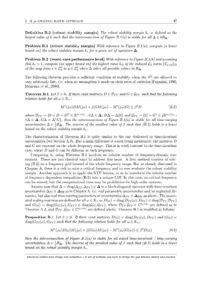
1 A µ-analysis based approach 47

Denition B.2 (robust stability margin) The robust stability margin kr is dened as thelargest value of k such that the interconnection of Figure B.1(a) is stable for all ∆ ∈ kB∆.

Problem B.1 (robust stability margin) With reference to Figure B.1(a), compute (a lowerbound on) the robust stability margin kr for a given set of operators ∆.

Problem B.2 (worst-case performance level)With reference to Figure B.1(b) and assumingthat kr > 1, compute (an upper bound on) the highest value ki2 of the induced L2 norm ‖Te→y‖i2of the map from e ∈ Lp2 to y ∈ Lp2 when ∆ takes all possible values in B∆.

The following theorem provides a sucient condition of stability when the δ[i] are allowed tovary arbitrarily fast, i.e. when no assumption is made on their rates of variation [Paganini, 1996;Meinsma et al., 2000].

Theorem B.1 Let β > 0. If there exist matrices D ∈ DTV and G ∈ GTV such that the followingrelation holds for all ω ∈ R+:

M∗(jω)DM(jω) + j(GM(jω)−M∗(jω)G) ≤ β2D (B.2)

where DTV = 0 < D = DT ∈ Rnv×nv : ∀∆ ∈ ∆, D∆ = ∆D and GTV = G = G∗ ∈ jRnv×nv :∀∆ ∈ ∆, G∆ = ∆∗G, then the interconnection of Figure B.1(a) is stable for all time-varyinguncertainties ∆ ∈ 1

βB∆. The inverse of the smallest value of β such that (B.2) holds is a lowerbound on the robust stability margin kr.

The characterization of Theorem B.1 is quite similar to the one dedicated to time-invariantuncertainties (see Section A.3). But a main dierence is worth being mentioned: the matrices Dand G are constant on the whole frequency range. This is in stark contrast to the time-invariantcase, where D and G can be dierent at each frequency.

Computing kr using Theorem B.1 involves an innite number of frequency-domain con-straints. There are two classical ways to address this issue. A rst method consists of solv-ing (B.2) on a frequency grid instead of the whole frequency range. But as already discussed inChapter A, there is a risk to miss a critical frequency and to over-evaluate the robust stabilitymargin. Another approach is to apply the KYP lemma, so as to transform the innite numberof frequency-dependent inequalities (B.2) into a unique LMI. In this case, no critical frequencycan be missed, but the computational time may be prohibitive for high-order systems.

Assume now that ∆ = diag(∆TI ,∆TV ) ∈∆ is a block-diagonal operator with time-invariantuncertainties ∆TI ∈∆TI as in Chapter A, i.e. real parametric uncertainties and/or neglected dy-namics, but also real time-varying parameters or uncertainties ∆TV ∈∆TV as above. The associ-ated scaling matrices are dened for all ω ∈ R+ asD(ω) = diag(DTI(ω), DTV ) ∈ diag(DTI ,DTV )and G(ω) = diag(GTI(ω), GTV ) ∈ diag(GTI ,GTV ), where DTI ,GTI ∈ Cni×ni are dened as inTheorem A.2, and DTV ,GTV ∈ Cnv×nv are dened above. Theorem B.1 is modied as follows:

Proposition B.1 Let β > 0. If there exist matrices D(ω) = diag(DTI(ω), DTV ) and G(ω) =diag(GTI(ω), GTV ) such that the following relation holds for all ω ∈ R+:

M∗(jω)D(ω)M(jω) + j(G(ω)M(jω)−M∗(jω)G(ω)) ≤ β2D(ω) (B.3)

then the interconnection of Figure B.1(a) is stable for all mixed time-invariant / time-varyinguncertainties ∆ ∈ 1

βB∆. The inverse of the smallest value of β such that (B.3) holds is a lowerbound on the robust stability margin kr.



The previous result can be extended to worst-case performance analysis.

Proposition B.2 Let γ > 0 and Mγ(s) = diag(Ini , Inv , γ−1Ip)M(s). If there exist matrices

D(ω) = diag(DTI(ω), DTV , Ip) and G(ω) = diag(GTI(ω), GTV , 0p) such that one of the followingrelation holds for all ω ∈ R+:

M∗γ (jω)D(ω)Mγ(jω) + j(G(ω)Mγ(jω)−M∗γ (jω)G(ω)) ≤ D(ω) (B.4)

σ((D(ω)Mγ(jω)D(ω)−1 − jG(ω)

) (I +G(ω)2

)− 12

)≤ 1 (B.5)

then ‖Te→y‖i2 ≤ γ for all mixed time-invariant / time-varying uncertainties ∆ ∈ B∆. The small-est value γ∗ of γ such that (B.4) holds is an upper bound on the worst-case performance level ki2.

A practical method is proposed in this section to solve the innite dimensional optimizationproblems of Proposition B.2, and to avoid the disadvantages of the classical grid-based and KYP-based techniques. Section B.1.2 is rst devoted to the computation of an upper bound on ki2(i.e. a guaranteed worst-case performance level). A nontrivial extension to the design of robustfeedforward controllers is then highlighted in Section B.1.3. Note that the extension to the com-putation of a lower bound on kr (i.e. a guaranteed robust stability margin) is straightworward,so it is not detailed here. Indeed, it suces to work with (B.3) instead of (B.4).

Remark B.1 (B.3) and (B.4) are only sucient conditions, that is why only a lower bound onkr and an upper bound on ki2 are obtained. We do not focus on computing upper bounds on krand lower bounds on ki2 (see e.g. [Köro§lu and Scherer, 2007; Peni and Seiler, 2016]).

Remark B.2 The uncertainties in ∆TV can vary arbitrarily fast, i.e. no bounds on their ratesof variation are taken into account. A Lyapunov-based approach which addresses this issue isproposed in Section B.2.

1.2 Performance analysis

1.2.1 Computation of a worst-case performance level

Proposition B.2 requires minimizing a linear objective γ under the LMI constraints (B.4).This problem has an innite number of optimization variables, namely the matrices DTI(ω) andGTI(ω). Let γ∗ be the global minimum solution. As already emphasized in Section B.1.1, thereare two classical ways to compute γ∗, which is the best upper bound on ki2 that can be computedusing Proposition B.2.

The rst one is a state-space solution. It consists of applying the KYP lemma to transform theconstraints (B.4) into a single LMI, so as to obtain an augmented nite dimensional optimizationproblem. This requires turning the frequency dependent scaling matrices DTI(ω) and GTI(ω)into LTI systems DTI(s) =

∑i αiDi(s) and GTI(s) =

∑i βiGi(s), where the lters Di(s) and

Gi(s) are xed while αi and βi are the optimization parameters. This approach has threedrawbacks. First, only an upper bound on γ∗ is computed, since nite dimensional bases ofDTI(s) and GTI(s) are used, which cannot cover the whole set of possible scaling matricesDTI(ω) and GTI(ω). Second, the choice of the bases is not obvious. Third, the order of theaugmented state-space representation resulting from the application of the KYP lemma can bevery high, since it containsM(s) as well as the Di(s) and the Gi(s). This can lead to an excessivecomputational burden for the LMI solver.

The second approach consists of solving (B.4) on a frequency grid instead of the wholefrequency range, which is a nite dimensional optimization problem. This was proposed in [Lind



et al., 1995; Sparks et al., 1996; Paganini, 1996], but the result can be unreliable for reasonsalready discussed in Chapter A and in Section B.1.1. Only a lower bound γ on γ∗ is obtained,since the optimization problem is less constrained than on the whole frequency range, and itcannot be guaranteed that γ > ki2. Moreover, the computational time can become prohibitiveif a ne grid is considered to reduce the risk of missing a critical frequency. The idea hereis to go one step further by rst solving the problem on a rough grid and then validating theresult on the whole frequency range using a fast and reliable Hamiltonian-based technique, in thespirit of Algorithm A.1. The computational time will be much lower, but still larger than in thetime-invariant case because of the constant matrices DTV and GTV , which make it impossible toindependently solve the problem at each frequency. The inequalities (B.4) to be considered onthe grid must indeed be stacked into a single one before an LMI solver can be used. The followingalgorithm is introduced in [Ferreres and Roos, 2007] to compute γ∗ with the desired accuracy.

Algorithm B.1 (optimal computation of an upper bound on ki2)

1. Dene an initial frequency grid (ωi)i composed of a few points (or even a single one).

2. Solve the optimization problem of Proposition B.2 on the grid with respect to the frequencydependent matrices DTI(ωi), GTI(ωi) and to the constant matrices DTV , GTV . Let γ bethe minimized value of γ. It is a lower bound on γ∗.

3. Let γ = (1 + ε)γ, where ε > 0 is a user-dened threshold. For the values of DTV and GTVcomputed at step 2, check whether there exist frequency dependent matrices DTI(ω) andGTI(ω) such that inequality (B.4) is satised ∀ω ∈ R+ (see Section B.1.2.2). If the answeris yes, stop the algorithm since γ = (1 + ε)γ is an upper bound on γ∗ and γ∗ has beencomputed with a precision ε. Otherwise, let ω be a frequency where (B.4) is not satised.Add ω to the grid and go back to step 2.

Algorithm B.1 eliminates most disadvantages of the classical grid-based techniques:

• the value of γ∗ is obtained, and not only a lower bound,

• the validation performed at step 3 guarantees that no worst-case frequency is missed,

• to some extent, the size of the frequency grid is minimized, as well as the computational time.

1.2.2 Validation with a frequency elimination technique

At the end of step 2 of Algorithm B.1, the constant matrices DTV and GTV are xed. Somematrices DTI(ωi) and GTI(ωi) are known, which satisfy inequality (B.4) at each point of thegrid (ωi)i for γ = γ. The objective is now to determine whether there exist matrices DTI(ω)and GTI(ω) such that inequality (B.4) holds on the whole frequency range for γ = (1 + ε)γ. Thefollowing proposition reformulates this problem as a µ test, which can then be solved ecientlywith Algorithm A.1.

Proposition B.3 [Ferreres and Roos, 2007] Let D2 = D1/22 and G2 = D

−1/22 G2D

−1/22 . Let:

F (jω) =

I 0 0

0 D2 00 0 I

M∗γ (jω)

I 0 0

0 D−12 0

0 0 I

−j

0 0 0

0 G2 00 0 0

I 0 0

0 (I + G22)−

12 0

0 0 I



The following two assertions are equivalent:

1. There exist matrices DTI(ω) and GTI(ω) satisfying inequality (B.4) for all ω ∈ R+, whereD(ω) = diag(DTI(ω), DTV , Ip), G(ω) = diag(GTI(ω), GTV , 0p) and γ = (1 + ε)γ.

2. There exist matrices DTI(ω) and GTI(ω) satisfying for all ω ∈ R+:

σ

((D(ω)F (jω)D−1(ω)− jG(ω)

)(I + G2(ω)

)− 12

)≤ 1 (B.6)

where D(ω) = diag(DTI(ω), Inv , Ip), G(ω) = diag(GTI(ω), 0nv , 0p) and γ = (1 + ε)γ.

The rst assertion is the one to be checked at step 3 of Algorithm B.1. The second one consistsof checking whether µ∆c(F (jω)) ≤ 1 for all ω ∈ R+, i.e. whether the robust stability margin ofF (s) is larger than 1. The corresponding block structure is ∆c = diag(∆TI,C(nv+p)×(nv+p)),where nv and p are the size of ∆TV and of the performance channel, i.e. the map between eand y, respectively. Algorithm A.1 can now be applied with βmax = 1 as an initialization. It isinterrupted if βmax becomes strictly larger than 1, which means that a worst-case frequency hasbeen found such that the test (B.6) cannot be satised. This frequency is added to the grid andanother iteration of Algorithm B.1 is performed.

1.2.3 Convergence of the algorithm

Algorithm B.1 converges in a nite number of iterations. The proof is quite technical and itis omitted here, but all details can be found in [Ferreres and Roos, 2007]. Moreover, it has beenobserved on several practical applications that the number of iterations is usually quite low.

1.2.4 A suboptimal but faster algorithm

The LMI optimization performed at step 2 of Algorithm B.1 can be very demanding. More-over, the number of decision variables and the computational time increase with the numberof frequencies, since DTI(ω) and GTI(ω) have to be determined at each point of the grid. Soinstead of performing a single LMI step, it can be worthwhile to compute DTI(ω) and GTI(ω)using a gradient descent algorithm as it is classically done when computing µ upper bounds (seeSection A.3.1). In this context, a suboptimal but faster algorithm is introduced, which consistsof iteratively optimizing with respect to the frequency dependent matrices DTI(ω) and GTI(ω)on the one hand, and to the constant matrices DTV and GTV on the other hand.

Algorithm B.2 (suboptimal computation of an upper bound on ki2)

1. Dene an initial frequency grid (ωi)i as for Algorithm B.1. Let DTV = Inv and GTV = 0nv .

2a. Let DTV and GTV be xed. At each frequency ωi, minimize γ with respect to DTI(ωi) andGTI(ωi) under the constraint (B.4). This can be achieved by performing a dichotomy searchon γ and iteratively applying the gradient descent algorithm of [Young et al., 1995].

2b. Let DTI(ωi) and GTI(ωi) be xed. Minimize γ with respect to DTV and GTV such that (B.4)is satised at all grid points. This can be achieved by stacking all constraints into a singleone and then using an LMI solver. If the decrease in γ after steps 2a and 2b have beenapplied is larger than a given threshold, return to step 2a to go on with the γ minimizationprocess. Otherwise, let γ be the minimized value of γ, and continue to step 3.

3. Same as step 3 of Algorithm B.1.



Unlike Algorithm B.1, the value of γ at the end of iteration 2b is not guaranteed to be a lowerbound of γ∗. Thus it is not possible to quantify the accuracy of the nal upper bound γ onγ∗. Nevertheless, Algorithms B.1 and B.2 can be combined to determine guaranteed lower andupper bounds of γ∗ with a given accuracy ε, while keeping a reasonable computational time.

Algorithm B.3 (combination of optimal and suboptimal algorithms)

1. Perform Algorithm B.2 to determine an upper bound γ of γ∗.

2. Perform Algorithm B.1 to compute a lower bound γ of γ∗ and stop as soon as γ > (1−ξ)γ,where ξ > 0 is the desired accuracy. Algorithm B.1 can be initialized with the frequency gridand the values of DTV and GTV obtained at the end of step 1. To reduce the computationaltime, this frequency grid can be reduced by keeping only critical frequencies correspondingto peak values of the µ upper bound.

These algorithms have been applied in [Ferreres and Roos, 2007] to a realistic missile examplewith 2 time-varying parameters and 8 time-invariant uncertainties, some of them being repeatedup to 6 times. All algorithms perform well, and the suboptimal one allows to decrease thecomputational time with no loss of accuracy.

1.3 Extension to robust feedforward design

In many industrial applications, badly damped exible modes and interactions among thevarious degrees of freedom of the system can result in large tracking errors. Although this canbe accounted for by an inverse-based feedforward controller, exible modes are often highlyuncertain, which may result in a large degradation of performance caused by the feedforwardcomponents [Devasia, 2002]. This is a strong motivation to design robust feedforward controllersfor systems that are aected by structured time-invariant and time-varying uncertainties. In thisperspective, Proposition B.2 is now adapted, so that the methodology developed in Section B.1.2can be further used.

1.3.1 Problem statement

Let us consider the interconnection of Figure B.2, where N(s) is a continuous-time stableand proper real-rational transfer function representing the nominal closed-loop system. Thefeedback controller is xed and included into N(s). The objective is to compute a feedforwardcontroller H(s) which minimizes the induced L2 norm ‖Te→y‖i2 of the map from e to y when∆ = diag(∆TI ,∆TV ) takes all possible values in B∆.

∆

N(s)

H(s)e

w z

y

Figure B.2: Interconnection for robust feedforward design



1.3.2 Practical solution

The design scheme of Figure B.2 is rst transformed into the interconnection of Figure B.1(b):

ifN(s) =

[N11(s) N12(s) N13(s)N21(s) N22(s) N23(s)

], thenM(s) =

[N11(s) N12(s) +N13(s)H(s)N21(s) N22(s) +N23(s)H(s)

]. Propo-

sition B.2 can now be applied to M(s). However, the considered feedforward design problem ismore complex than the worst-case performance problem solved in Section B.1.2, since inequal-ity (B.4) is no longer convex. The rst step to recover convexity in order to apply the algorithmsof Section B.1.2 is to set:

H(s) =

nH∑i=1

θiHi(s) (B.7)

where the lters Hi(s) are xed, while the real parameters θi are to be optimized. The orthonor-mal lters basis of [Akcay and Ninness, 1999] is chosen to reduce numerical issues:

Hi(s) =

√2<(ai)

s+ ai

i−1∏k=1

s− aks+ ak

(B.8)

where ak is the conjugate of ak. So both the order nH and the poles −ak of the feedforwardcontroller H(s) must be xed, but there is no constraint on the choice of nH . Proposition B.2can then be reformulated as follows.

Proposition B.4 [Ferreres and Roos, 2007] Let γ > 0. If there exist real parameters (θi)1≤i≤nH

and matrices D(ω) = diag(DTI(ω), DTV ) and G(ω) = diag(GTI(ω), GTV ) such that the followingrelation holds for all ω ∈ R+:D −N11DN

∗11 + j (N11G−GN∗11) −(N11D + jG)N∗21 N12 +N13

nH∑i=1

θiHi

? γI −N21DN∗21 N22 +N23

nH∑i=1

θiHi

? ? γI

≥ 0 (B.9)

where ? denotes the conjugate part of the hermitian matrix and where the dependence on ω isremoved to simplify notation, then ‖Te→y‖i2 ≤ γ for all mixed time-invariant and time-varyinguncertainties ∆ ∈ B∆.

The proof of Proposition B.4 is omitted here for the sake of brevity, but it shows that inequal-ities (B.4) and (B.9) are equivalent. The latter being convex in D(ω), G(ω) and θi, il can behandled by an LMI solver. All the algorithms detailed in Section B.1.2 can thus be applied.The only dierence concerns step 2, which now consists of solving the optimization problemof Proposition B.4 with respect to the frequency dependent matrices DTI(ω), GTI(ω) and theconstant matrices DTV , GTV as previously, but also to the real parameters θi of the feedforwardcontroller.

Remark B.3 Another method is proposed in [Giusto and Paganini, 1999], which does not requireto write H(s) as in (B.7)-(B.8). Frequency responses H(jωi) are rst computed independentlyat each point of a frequency grid (ωi)i. They are then approximated so as to obtain a transferfunction H(s). However, this last step is a delicate one, as a high-order feedforward controllermay be necessary to get a good approximation. Moreover, there is no guarantee that performanceis satisfactory on the whole frequency range.


2 A Lyapunov based approach 53

Remark B.4 Another design method allowing to consider both time-invariant and time-varyinguncertainties is proposed in [Köse and Scherer, 2009; Scorletti and Fromion, 2006]. The mainadvantage is that the poles of the feedforward controller do not have to be chosen a priori. Thecounterpart is that the scaling matrices are restricted to a set of real rational transfer functions,whose order and denominator are xed. Moreover, the design problem is convex only in case afull-order feedforward controller is computed. The order of H(s) is thus greater than or equal tothe order of the closed-loop system N(s), which can be quite large. A strategy could be to combinethis method and the one presented in this section, in the spirit of what is proposed in Section D.2to design anti-windup controllers. A full-order feedforward controller is rst designed. Its polesare analyzed and the ones which are too slow or too fast compared to the system dynamics areeliminated. The remaining ones are then used to dene the lters Hi(s) in equation (B.8).

1.4 Conclusion

A practical approach is proposed in this section to compute guaranteed stability marginsand performance levels in the presence of mixed time-invariant and arbitrarily fast time-varyinguncertainties. It is shown that µ-analysis can be used both to handle the time-invariant uncer-tainties with a low computational time, and to validate on the whole frequency range the resultsinitially obtained on a rough frequency grid. A convex extension to robust feedforward designis also highlighted. An application to realistic missile models is reported in [Ferreres and Roos,2007], which shows that computational time remains very reasonable despite the complexity ofthe problem.

Another method (not detailed in this manuscript due to space constraints) is proposedin [Roos and Biannic, 2006a] to address exactly the same issue. A state-space characteriza-tion of the robust stability margin kr is obtained thanks to an extended version of the KYPlemma. It involves the search for an extended Lyapunov matrix Z = R + jS where R = R∗

and S = S∗, and for scaling matrices D and G that are assumed to be constant but neverthelesscomplex in the case of time-invariant uncertainties. Applications to several benchmarks of Ta-ble A.2 show that almost non-conservative results are obtained in the purely time-invariant case.Moreover, numerical results and computational time are similar to the ones obtained with themethod of Section B.1 on the aforementioned missile example. Extensions to robust feedforwarddesign, as well as to combined robust feedback/feedforward design, are also described in [Roosand Biannic, 2006b].

Finally, it is worth being emphasized that both approaches are complementary. On the onehand, the frequency-domain technique described in Section B.1 is adapted to high-order systemswith a limited number of uncertainties. On the other hand, the time-domain method of [Roosand Biannic, 2006a] is better suited to low-order systems with a large number of uncertainties.

2 A Lyapunov based approach


The framework is roughly the same as in Section B.1.1. Let us consider the standard inter-connections of Figure B.1. M(s) is a continuous-time stable and proper real-rational transferfunction representing the nominal closed-loop system. ∆ is a linear time-varying memorylessmultiplication operator, i.e. w(t) = ∆(t)z(t) for all t ≥ 0. It has a block-diagonal structure ofthe form:

∆(t) = diag(δ[1](t)In1 , . . . , δ[N ](t)InN ) (B.10)



where nv =∑N

i=1 ni and each δ[i] is a real-valued scalar function corresponding to a time-varyingparameter or uncertainty. The set of all such operators is denoted by ∆. It is assumed in thesequel that ∆ is bounded:

‖∆‖i2 ≤ 1 (B.11)

which means that δ(t) = (δ[1](t), . . . , δ[N ](t)) belongs to the unit hypercube I for all t ≥ 0. Notethat any bounded operator (as dened above) can be normalized. Thus, imposing δ[k](t) ≤ 1 forall k is not restrictive. It is also assumed that the rate of variation of each δ[k] is bounded:

δ(t) ∈ J = [ν[1], ν[1]]× · · · × [ν[N ], ν[N ]] (B.12)

for all t ≥ 0. The set of all operators ∆ ∈ ∆ such that δ(t) ∈ I and δ(t) ∈ J for all t ≥ 0 isdenoted by B∆ (same denition as in Section B.1.1 plus the constraint on δ).

Remark B.5 The method proposed here can be applied to a wider class of operators (includingfor example time-invariant uncertainties as in Section B.1.1), but extensions are not presentedhere for the sake of simplicity.

Two analysis problems are considered: robust stability and worst-case performance. Thelatter exactly corresponds to Problem B.2. The former is a slight variation of Problem B.1:

Problem B.3 (robust stability check) Check whether the interconnection of Figure B.1(a)is stable for all operators ∆ ∈ B∆, i.e. whether the robust stability margin kr is larger than 1.

As already emphasized in the introduction, these problems can be addressed in dierent ways.The rst one consists of using IQC to characterize the uncertainties. The calculations can then becarried out in the time domain using the KYP lemma, or in the frequency domain by generalizingthe method of Section A.1: the time-invariant uncertainties are handled by µ-analysis basedtools, while the IQC characterization of [Helmersson, 1999] is used for time-varying ones. Thesecond way, proposed in [Roos et al., 2012] and summarized here, is to use PDL functions.Rather than introducing some relaxation variables or trying to deal with an innite dimensionalproblem, a two-step procedure is proposed in Section B.2.2 to solve Problem B.3 with a reasonablecomputational cost. The stability conditions are rst formulated in Section B.2.2.1 as an LMIfeasibility problem involving the search of a suitable parameter-dependent Lyapunov function.This problem is then solved in Section B.2.2.2 for a nite number of parametric congurations andthe validity of the resulting Lyapunov function is checked on the whole parametric domain usinga µ-analysis based test in Section B.2.2.3. In case the validation fails, a worst-case congurationis determined using particle swarm optimization in Section B.2.2.4 and the whole process isrepeated using an augmented set of parametric congurations. Extension of the method toperformance analysis is nally described in Section B.2.3.

2.2 Stability analysis

2.2.1 LMI-based formulation of the stability analysis problem

Let (A,B, C,D) denote a state-space representation of M . The dynamics of the interconnec-tion depicted in Figure B.1(a) are described for all t ≥ 0 by:

x = A(δ(t))x (B.13)

where:A(δ(t)) = A+ B∆(t)(I −D∆(t))−1C (B.14)

Assumption B.1 A(δ) is well-posed ∀δ ∈ I, i.e. µ∆(D)<1.



Lemma B.1 Stability of system (B.13) is guaranteed for all operators ∆ ∈ B∆ if there exists aparameter-dependent Lyapunov function P (δ) such that ∀δ ∈ I:

P (δ) = P (δ)T > 0 (B.15)

and ∀(δ, ν) ∈ I × J :

Φ(δ, ν) = A(δ)TP (δ) + P (δ)A(δ) +N∑k=1

ν[k]∂P (δ)

∂δ[k]< 0 (B.16)

Lemma B.1 is a direct consequence of the Lyapunov's stability theorem in which the Lyapunovfunction is dened as:

V (x, δ) = xTP (δ)x (B.17)

Indeed, inequality (B.16) clearly implies that V is negative along any trajectory of the plant(characterized by δ(t) ∈ I and δ(t) ∈ J for all t ≥ 0).

Unfortunately, this characterization of P (δ) is numerically intractable, since it involves aninnite number of both variables and constraints. The rst problem is easily solved by restrictingthe parameter dependence to a polynomial expression:

P (δ) =

x(d,N)∑i=1

fi(δ)Pi (B.18)

where x(d,N) denotes the dimension of the vector space of all N -variate polynomial functions ofdegree d and (fi)1≤i≤x(d,N) is any associated basis, while (Pi)1≤i≤x(d,N) are constant symmetricmatrices to be determined. Using this polynomial expression, nding a PDL function P (δ) whichsatises inequalities (B.15) and (B.16) boils down to a standard LMI feasibility problem, whichcan be stated as follows. Do there exist symmetric matrices (Pi)1≤i≤x(d,N) such that:

Ψ(δ) < 0 ∀δ ∈ I (B.19)

where:

Ψ(δ) = diag

− x(d,N)∑i=1

fi(δ)Pi,Φ(δ, ν1), . . . ,Φ(δ, ν2N )

(B.20)

and for all j ∈ [1 , 2N ]:

Φ(δ, νj) =

x(d,N)∑i=0

(fi(δ)(A(δ)TPi + PiA(δ)) +

N∑k=1

ν[k]j

∂fi(δ)

∂δ[k]Pi

)(B.21)

In equation (B.21), ν[k]j is equal to either ν[k] or ν[k] for each k ∈ [1 , N ], thus leading to 2N

combinations. Indeed, equation (B.16) is linear in the variables ν[k], which means that it issatised for all ν ∈ J if and only if it is satised on the 2N vertices of J .

2.2.2 Grid-based resolution

Let us now focus on the second problem related to the innite number of constraints. Twooptions are typically available here. The rst one consists of using the Kalman-Yakubovic-Popovlemma [Iwasaki and Hara, 2005]. By introducing some additional variables, this technique allows



to convert the innite set of parameterized inequalities (B.19) into a unique LMI. Unfortunately,as soon as either the order of the plant or the degree of the polynomial Lyapunov functionincreases, the latter becomes too large for existing softwares. The second option is denitelymore intuitive. It simply consists in gridding the hypercube I, so as to replace (B.19) with:

Ψ(δl) < 0 ∀ l ∈ [1 , M ] (B.22)

where δl denotes the value of δ at the lth grid point. Checking whether there exists a PDLfunction which satises (B.22) is numerically tractable. Moreover, no conservatism is introduced,since (B.19) clearly implies (B.22). Of course, the converse is not necessarily true. The validityof the PDL function must then be checked a posteriori between the grid points.

2.2.3 Validity of the parameter-dependent Lyapunov function

At this stage, a PDL function P (δ) has been computed such that Ψ(δl) < 0 for all l ∈ [1 , M ].The objective is now to check whether this function also satises Ψ(δ) < 0 for all δ ∈ I. Bycombining (B.14), (B.20) and (B.21), it can be easily checked that Ψ(δ) depends rationally onthe δ[k] and can thus be written in linear fractional form as follows (see Chapter C):

Ψ(δ) = L22 + L21∆(I − L11∆)−1L12 (B.23)

where ∆ = diag(δ[1]In1, . . . , δ[N ]InN

) is a structured matrix. Let us now assume that Ψ(0) < 0.Using a continuity argument, there exists ε > 0 such that for all δ ∈ RN which satisfy ‖δ‖∞ < ε,then Ψ(δ) < 0 and thus det(Ψ(δ)) 6= 0. The following lemma is introduced in this context.

Lemma B.2 Let Ψ(δ) be dened by equation (B.23). Assume that Ψ(0) = L22 < 0. LetX = L11 − L12L

−122 L21. The following two statements are equivalent:

1. det(Ψ(δ)) 6= 0

2. det(I −X∆) 6= 0

The largest value of ε for which det(I−X∆) 6= 0 for all δ ∈ RN such that ‖δ‖∞ < ε is by denitionequal to 1/µ

∆(X), where µ

∆(X) denotes the structured singular value of X. If µ

∆(X) < 1,

then (B.19) is satised and the interconnection of Figure B.1(a) is stable for all ∆ ∈ ∆, i.e.kr > 1. The validity of the PDL function can thus be checked using a single structured singularvalue computation. In practice, computing the exact value of µ

∆(X) is known to be NP-hard

in the general case (see Chapter A), but both upper [Young et al., 1995] and lower [Seiler etal., 2010] bounds µ

∆(X) and µ

∆(X) can be determined using polynomial-time algorithms. The

following strategy can thus be implemented:

1. If µ∆

(X) < 1, then µ∆

(X) < 1 and stability is proved by the current PDL function.

2. If µ∆

(X) > 1, then µ∆

(X) > 1 and stability cannot be proved by the current PDL function,since there exists at least one value δ0 ∈ I such that Ψ(δ0) is not negative denite.

3. If µ∆

(X) < 1 and µ∆

(X) > 1, no conclusion can be drawn. In such a case, a recursivealgorithm is implemented. It consists in splitting the unit hypercube I in more and moresubsets until either the µ lower bound computed on one of the subsets becomes largerthan 1 (stability cannot be proved) or the highest µ upper bound computed on all subsetsbecomes lower than 1 (stability is proved). Such an algorithm is described in [Roos andBiannic, 2010] and in Section A.4. It is guaranteed to converge if the size of the subsets isallowed to become arbitrarily small.



2.2.4 Determination of a worst-case conguration

In case the PDL function determined in Section B.2.2.2 does not satisfy Ψ(δ) < 0 for all δ ∈ I,a worst-case parametric conguration δ is determined, for which Ψ(δ) is not negative denite.Intuitively, a relevant choice is to compute the value of δ for which the constraint Ψ(δ) < 0 isthe most violated, which can be formulated as follows:

δ = arg maxδ∈I

λ(Ψ(δ)) (B.24)

where λ(Ψ(δ)) denotes the maximum eigenvalue of the real symmetric matrix Ψ(δ). Prob-lem (B.24) is nonconvex, which makes it dicult to compute the global maximum. Nevertheless,the objective here is not to capture exactly this maximum, but to quickly explore the parametricdomain I to nd a conguration δ for which λ(Ψ(δ)) is as positive as possible. Particle swarmoptimization [Clerc, 2006] is well adapted to address this issue. It is based on the swarm behaviorof birds or shes around food, and consists in moving a set of particles in the continuous para-metric domain I according to simple mathematical formulas. The movement of each particle isinuenced by its own best known position, and by the ones found by the neighboring particles.Such a strategy is expected to move the swarm towards the best solutions. It has been observedin practice that only a few iterations are necessary to nd a suitable worst-case conguration.Once the latter has been computed, it is added to the grid, and a new PDL function is computed.Note that the search for a conguration δ such that λ(Ψ(δ)) > 0 is necessarily successful. In-deed, the optimization is initialized with the conguration δ0 obtained during the µ lower boundcomputation, for which λ(Ψ(δ0)) ≥ 0 (see Section B.2.2.3).

2.2.5 Description of the algorithm

The results obtained in the previous sections are now combined. The following algorithm isintroduced, which provides a solution to Problem B.1.

Algorithm B.4 (robust stability check)

1. Select the initial degree d and the maximum degree dmax of the polynomial Lyapunov func-tion. Choose the maximum number of iterations imax.

2. Dene an initial grid G1 = (δl)1≤l≤M of the unit hypercube I. Set i = 1.

3. If i < imax, solve the LMI feasibility problem (B.22). If i = imax or (B.22) is infeasible,then stop the algorithm if d = dmax (stability not proved) or increase d and go back tostep 2 otherwise.

4. Compute X and µ∆

(X). If µ∆

(X)< 1, stop the algorithm (stability proved). Otherwise,compute µ

∆(X).

→ If µ∆

(X) > 1, solve problem (B.24). Set Gi+1 = Gi ∪ δ, increase i and go back tostep 3.

→ If µ∆

(X) < 1, apply the recursive algorithm described at the end of Section B.2.2.3. Ifthe highest µ upper bound computed on all subsets is lower than 1, stop the algorithm(stability proved). If the µ lower bound computed on one of the subsets is largerthan 1 or if the stopping criterion is reached and no conclusion can still be drawn,then stop the algorithm if d = dmax (stability not proved) or increase d and go backto step 2 otherwise.



Remark B.6 The numerically most demanding step in Algorithm B.4 is clearly the third one.An LMI feasibility problem has to be solved, whose complexity increases with the degree of the PDLfunction and the number of grid points. To reduce the computational cost, it is then recommendedto start with a low-order PDL function at step 1 (d = 1) and a rough grid at step 2 (M = 1).

2.3 Extension to performance analysis

The method described in Section B.2.2 can be easily adapted to solve Problem B.2. Let

(A, [B1 B2],

[C1

C2

],

[D11 D12

D21 D22

])denote a state-space representation of M . The dynamics of

the interconnection depicted in Figure B.1(b) are described for all t ≥ 0 by:

x = A(δ(t))x+B(δ(t))e (B.25)

y = C(δ(t))x+D(δ(t))e (B.26)where:

A(δ(t)) = A+ B1∆(t)(I −D11∆(t))−1C1

B(δ(t)) = B2 + B1∆(t)(I −D11∆(t))−1D12

C(δ(t)) = C2 +D21∆(t)(I −D11∆(t))−1C1

D(δ(t)) = D22 +D21∆(t)(I −D11∆(t))−1D12

Lemma B.3 Under the assumption that x(0) = 0, robust stability of system (B.25)-(B.26)is guaranteed and γ is an upper bound on ki2 if there exists a parameter-dependent Lyapunovfunction P (δ) such that ∀δ ∈ I:

P (δ) = P (δ)T > 0 (B.27)

and ∀(δ, ν) ∈ I × J :

Φ(δ, ν) =

A(δ)TP (δ) + P (δ)A(δ) +

N∑k=1

ν[k]∂P (δ)

∂δ[k]+ C(δ)TC(δ) P (δ)B(δ) + C(δ)TD(δ)

B(δ)TP (δ) +D(δ)TC(δ) −γ2I +D(δ)TD(δ)

< 0 (B.28)

Algorithm B.4 can be applied with minor modications. The optimization problem at step 3now consists of minimizing the linear objective γ under the LMI constraints (B.22), where Ψ(δ)is dened as in (B.20) and Φ(δ, νj) is obtained by combining (B.28) and (B.18). Moreover, aparameter α > 0 can be introduced to facilitate the validation of the PDL function and toimprove the convergence of the algorithm: the value of γ determined at step 3 is simply replacedwith (1 + α)γ at step 4. The increase in conservatism remains reasonable if α is small enough.

2.4 Conclusion

A practical method is proposed to assess the robustness properties of a system in the presenceof linear time-varying perturbations with bounded rates of variation. A parameter-dependentLyapunov function is rst optimized on a nite parametric grid. Its validity is then checked on thewhole parametric domain using a fast and reliable µ-analysis based test. In case the validationfails, a worst-case conguration is added to the grid and the whole process is repeated. Theproposed method is applied to a satellite in [Biannic et al., 2011] and to a ghter aircraft in [Rooset al., 2012]. Numerical results show that it compares favorably to IQC based analysis: for thesame computational time, the results are less conservative. This demonstrates the benet of using


3 Summary of the contributions 59

µ-analysis to speed up the analysis process. Nevertheless, it should be kept in mind that an LMIproblem must be solved at each iteration, which might lead to a prohibitive computational costif the order of the system or the number of uncertainties is too large.



• Section B.1: frequency-domain approach to compute guaranteed stability margins andworst-case performance levels in the presence of mixed time-invariant and arbitrarily fasttime-varying uncertainties ; extension to robust feedforward design [Ferreres and Roos,2007].

• Section B.1: time-domain approach to compute guaranteed stability margins and worst-case performance levels in the presence of mixed time-invariant and arbitrarily fast time-varying uncertainties ; extensions to robust feedforward design and combined robust feed-back/feedforward design [Roos and Biannic, 2006a; 2006b].

• Section B.2: Lyapunov-based technique to compute guaranteed stability margins andworst-case performance levels in the presence of time-varying uncertainties with boundedrates of variation [Roos et al., 2012; Biannic et al., 2011].

The guiding line between these dierent methods is to demonstrate that µ-analysis can play a keyrole in assessing the robustness properties of a system even if some uncertainties are time-varying,and to provide computational tools that can be applied to realistic applications.

Remark B.7 It would be interesting to compare all existing techniques to solve the aforemen-tioned issues, in terms of both accuracy and computational time. And also to evaluate theirconservatism on a large set of real-world benchmarks as in Chapter A, by computing worst-caseuncertainties (see e.g. [Köro§lu and Scherer, 2007; Peni and Seiler, 2016]).


Chapter C

Generation of low-order LFR

A Linear Fractional Representation (LFR) is a model in which all known and xed dynamicsof a given system are put together in a linear time-invariant plant M , while the uncertain andvarying parameters are stored in a block-diagonal operator ∆, as shown in Figure C.1. LFRmodeling is an essential step before the robustness properties of uncertain closed-loop systemscan be evaluated, e.g. using the µ-analysis based tools implemented in the SMART Library ofthe SMAC Toolbox (see Chapter A and [Roos, 2013]). It can also be useful to design robustcontrol laws (especially using H∞ approaches) or gain-scheduled controllers. But the eciencyof the aforementioned analysis and synthesis techniques strongly depends on the complexity ofthe considered LFR, which is measured in terms of both the size of the operator ∆ and the orderof the plant M . An increase in complexity is usually source of conservatism, and can even leadto numerical intractability.

-

- -

∆

M

Figure C.1: Linear Fractional Representation

In most industrial applications, physical systems are described using a mix of nonlinear ana-lytical expressions and tabulated data. Therefore, a two-step procedure has to be implementedto obtain a suitable LFR: a linear model with a polynomial or a rational dependence on thesystem parameters is rst generated, and then converted into a linear fractional form. Sev-eral techniques such as object-oriented realization exist to perform the latter transformation.Although the minimality of the resulting LFR cannot be guaranteed, symbolic preprocessingtechniques as well as numerical reduction usually permit to overcome complexity. Moreover,ecient software are available such as the LFR Toolbox for Matlab [Magni, 2006], which wasrecently replaced by the GSS Library of the SMAC Toolbox [Biannic and Roos, 2016]. On theother hand, the preliminary issue of converting the tabulated or irrational data into simple yetaccurate polynomial or rational expressions has been paid much less attention, although it is ofsignicant practical importance. In the aeronautic eld for example, most aircraft models include

61

62 Generation of low-order LFR

tabulated aerodynamic coecients determined by CFD (Computational Fluid Dynamics), windtunnel experiments or ight tests, and several controller gains depend on the ight parametersin a tabulated fashion.

The motivations for developing enhanced computational tools dedicated to tabulated dataapproximation are twofold. The rst one is of physical nature. Computing sparse expressions,for which the number of terms in the numerator and the denominator is as low as possible, is anatural way to prevent data overtting and to ensure a smooth behavior of the model betweenthe points used for approximation. On the other hand, building an LFR from a polynomial or arational expression f(x1, . . . , xn) results in a block diagonal matrix ∆ = diag(x1Ip1 , . . . , x

nIpn).The number pj of repetitions of each parameter xj in ∆ is strongly linked to the number ofoccurrences of xj in f . Indeed, although this is not an exact rule, the trend is as follows: thefewer the occurrences of xj in f(x1, . . . , xn), the smaller the size of ∆. In other words, no matterhow ecient the LFR generation tools can be, they are of little help if the expressions to beconverted are unnecessarily complex. Hence, the need to get tractable LFR for analysis anddesign purposes is another strong motivation for generating sparse expressions.

The issue of converting tabulated or irrational data into polynomial or rational expressionsis the core of this chapter. The case of scalar samples is considered in Section C.1. The problemis rst stated in Section C.1.1 and an overview of existing approximation methods is provided inSection C.1.2. Those allowing to get sparse expressions are then detailed in Section C.1.3 andimplementation issues to obtain a low-order static LFR are nally discussed in Section C.1.4.The case of a set of MIMO LTI models is considered next, and a whole methodology is describedin Section C.2 to obtain a low-order dynamic LFR.

1 From a set of scalar samples to a static LFR


Let yk, k ∈ [1, N ] be a set of samples (measurements, tabulated data. . . ) correspondingto dierent parametric congurations or operating points xk, k ∈ [1, N ] of a given system.More precisely, each xk =

[x1k, . . . , x

nk

]∈ Rn contains the values of the n explanatory variables

x1, . . . , xn for which the sample yk ∈ R was obtained. The main objective is to compute apolynomial or a rational function f : Rn → R of reasonable complexity which approximatesthese data, i.e. such that f(xk) is close to yk for all k ∈ [1, N ] in the sense of a certaincriterion (root-mean-square error, maximum local error. . . ). Another objective is to ensure thatthe denominator of f has no root in the considered parametric domain, which is assumed hereto be the smallest hyper-rectangle D ⊂ Rn containing every sampled data (xk)k∈[1,N ]. Thisrequirement guarantees that well-posed LFR are obtained.

Remark C.1 The case where an analytical expression fA : Rn → R is available instead of Nsamples is not considered here (see e.g. [Petrushev and Popov, 1987]). Moreover, this work onlydeals with approximation (or regression) and not with interpolation, which would aim at ndinga rational function f such that the equalities f(xk) = yk are strictly satised for a large numberN of samples (see [Floater and Hormann, 2007] and references therein).

1.2 Overview of existing methods

For a given precision, an intuitive idea is to determine a rational function for which thenumerator P and the denominator Q are two polynomials of the lowest possible degrees. Thisfairly simple strategy is followed by most existing methods. A classical linear least-squares


1 From a set of scalar samples to a static LFR 63

technique is usually applied in case the rational function is restricted to be polynomial [Magni,2006]. In the general case, a nonlinear least-squares technique can be implemented to minimizethe approximation error [The Mathworks, 2014], whereas a quadratic programming problem canbe solved to ensure that the resulting rational function intersects a set of intervals containing thedata [Celis et al., 2007]. But all those techniques suer from the same drawback: all admissiblemonomials of P and Q are usually nonzero, regardless of their real ability to model the data.More generally, the question of which terms should be included in the model is often addressed bytrial-and-error, or even ignored in practice. A way to deal with this question is to use orthogonalleast-squares. This allows to evaluate the ability of each monomial to eciently model thedata and therefore to select only the most relevant ones, leading to sparse expressions. Thisapproach is applied in [Poussot-Vassal and Roos, 2012; Roos, 2009; Döll et al., 2008; Morelliand DeLoach, 2003] to model aeronautical data with polynomials, but until recently, practicalmethods to compute rational functions were still missing. Yet, the additional degrees of freedomcan lead to simpler expressions and thus to smaller LFR. Consequently, two algorithms haverecently been developed to obtain rational expressions with sparse structure, i.e. with as fewmonomials in P and Q as possible. A direct approach computing a rational expression in asingle step thanks to a symbolic regression technique is proposed in [Hardier et al., 2013a],while an indirect approach creating a rational model by means of an intermediate surrogatemodeling is introduced in [Hardier et al., 2013b]. All these methods are now briey presented inSections C.1.2.1 and C.1.2.2.

1.2.1 Polynomial case

The most common approach consists in restricting f to be a polynomial function, that is:

f(x) = P (x) =

nP∑i=0

airi(x) (C.1)

where (ri)i∈[0,nP ] is a set of polynomial regressors and (ai)i∈[0,nP ] are coecients to be determined.

• A classical solution consists in solving a linear least-squares (LS) problem with respectto the coecients (ai)i∈[0,nP ], i.e. to minimize the following criterion [Magni, 2006]:

C =N∑k=1

[yk − P (xk)]2 (C.2)

• A well-known improvement to that approach relies on a preliminary orthogonalizationprocess to decouple the regressors. As a result, the ability of each new regressor to reducethe criterion C can be evaluated regardless of those already selected. Hence, only themost relevant ones are considered, which amounts to a certain extent to minimizing thecomplexity of the polynomial approximation while still guaranteeing a low approximationerror. This orthogonal least-squares (OLS) based variant was successfully appliedby [Morelli and DeLoach, 2003]. It was later improved, allowing to compute a sparsepolynomial expression satisfying the following global and local constraints: √

C/N ≤ ε1|yk − P (xk)| ≤ ε2 ∀k ∈ [1, N ]

(C.3)

where ε1 and ε2 are some user-dened tolerances [Poussot-Vassal and Roos, 2012; Roos,2009; Döll et al., 2008]. More details are given in Section C.1.3.1.



1.2.2 Rational case

The more general case where f is a rational function is now considered:

f(x) =P (x)

Q(x)=

nP∑i=0

airPi (x)

/ nQ∑i=0

birQi (x) (C.4)

where (rPi )i∈[0,nP ] and (rQi )i∈[0,nQ] are two sets of polynomial regressors, while (ai)i∈[0,nP ] and(bi)i∈[0,nQ] are coecients to be determined.

• A rst method consists of solving a nonlinear least-squares (NLS) problem with respectto the coecients (ai)i∈[0,nP ] and (bi)i∈[0,nQ], that is to minimize the following criterion:

C =

N∑k=1

[yk −

P (xk)

Q(xk)

]2

(C.5)

It is notably implemented in the Curve Fitting Toolbox of Matlab [The Mathworks, 2014],where several optimization tools can be used to compute a solution (Levenberg-Marquardtalgorithms, trust-region methods...). One of its major drawbacks is that several localminima may exist due to the non-convexity. Hence, the results strongly depend on theinitialization, which is not a trivial issue.

• A second method was introduced by [Markov et al., 1996] in the context of polynomial ap-proximation and then generalized by [Celis et al., 2007] to the rational case. An uncertaintyinterval

[yk, yk

]is rst dened around each yk. A rational function is then determined

which intersects all those intervals, i.e. yk≤ P (xk)/Q(xk) ≤ yk ∀k ∈ [1, N ]. This can

be achieved by solving a quadratic programming (QP) problem in the coecients(ai)i∈[0,nP ] and (bi)i∈[0,nQ] with a strictly convex objective function.

Those two algorithms suer from the same drawback: all admissible monomials of P andQ are usually nonzero, regardless of their real ability to model the data. In this context, twoadditional methods have recently been developed to generate sparse rational approximations,which avoid data overtting and lead to simple yet accurate LFR.

• A third method proposed in [Hardier et al., 2013a] and described in Section C.1.3.2 looksfor a rational approximation in a single step thanks to a symbolic regression technique.Genetic programming (GP) is implemented to select sparse monomials and coupledwith a nonlinear iterative procedure to estimate the coecients of the rational function.

• A fourth method proposed in [Hardier et al., 2013b] and described in Section C.1.3.3 createsa rational expression by means of an intermediate surrogate modeling (SM). It performsthe data approximation by building a sparse modeling based on neural networks, beforetranslating the result into a fractional form. A stepwise selection algorithm is used, combin-ing the benets of forward orthogonal least-squares to estimate the regression parameters,and of particle swarm optimization to determine the best location of the regressors.

Remark C.2 Rational approximation is also considered in linear systems theory, for example inthe elds of model reduction [Karlsson and Lindquist, 2008] and system identication [Deschrijveret al., 2007], where least-squares methods are usually implemented.



1.3 Focus on sparse approximation techniques

Our main contribution consists of developing some approximation methods which producesparse polynomial or rational expressions, with the ambition of limiting as much as possiblethe size of the resulting LFR. In this context, the emphasis is put in this section on the OLS, GPand SM methods presented in Section C.1.2. Note that the last two make use of techniques whichare a little outside the main topics of this manuscript, but they are the result of a successfulcollaboration with a colleague specialized in modeling and identication. So it seems relevant todescribe them briey.

1.3.1 Polynomial approximation using orthogonal least-squares

Let us assume for the moment that the polynomial regressors (ri)i∈[0,nP ] are xed. A classicway of doing this is to choose n positive integers d1, . . . , dn and to consider all monomials suchthat the degree of xi is less than or equal to di, in which case nP = (d1 + 1) . . . (dn + 1)− 1. Thequadratic criterion (C.2) then only depends on the coecients (ai)i∈[0,nP ] and the optimizationproblem to be solved can be reformulated as:

Aopt = arg minA∈RnP+1

C(A) (C.6)

where:C(A) = (Y −RA)T (Y −RA) (C.7)

R =

r0(x1) . . . rnP (x1)...

. . ....

r0(xN ) . . . rnP (xN )

=[R0 . . . RnP

](C.8)

AT =[a0 . . . anP

](C.9)

Y T =[y1 . . . yN

](C.10)

and (Ri)i∈[0,nP ] are called the modeling functions. This is a classical linear least-squares problem,whose solution is given by:

Aopt = (RTR)−1RTY (C.11)

Assume now that the modeling functions which compose the matrix R are made orthogonal,i.e. RTi Rj = 0 for all i 6= j, as proposed in [Morelli and DeLoach, 2003] and [Roos, 2009]. Thecomponents of Aopt are then expressed as:

ai,opt =RTi Y

RTi Ri, i ∈ [0 , nP ] (C.12)

and the corresponding value Copt of C(A) is given by:

Copt = Y TY −nP∑i=0

(RTi Y )2

RTi Ri(C.13)

Using orthogonal modeling functions is relevant for several reasons. First, RTR becomes diagonaland can be trivially inverted. Then, it can be observed in (C.13) that the reduction in the least-squares criterion C(A) resulting from the inclusion of Ri does not depend on Rj whatever j 6= i.This allows to evaluate each orthogonal modeling function (an thus each monomial) in terms of its



ability to reduce C(A), regardless of which other functions are selected. This property is exploitedin [Roos, 2009; Poussot-Vassal and Roos, 2012], where an iterative algorithm is introduced. Byprogressively releasing some tolerances, the most relevant set of monomials is determined, forwhich the approximation error remains lower than a given user-dened threshold. All the othermonomials are eliminated, thus leading to sparse polynomial expressions. This amounts toa certain extent to minimizing the complexity of the approximation formulas, and then thesize of the resulting LFR. Some recent applications can be found e.g. in [Iannelli et al., 2017;Biannic et al., 2016].

1.3.2 Rational approximation using genetic programming

In the rational case, when the model structure has to be determined as a whole (numeratorand denominator degrees, number and type of monomials), the approximation problem cannotgenerally be solved by means of classical techniques. Over a few variables, a sequential andsystematic exploration cannot be carried out either: for example, with 2 explanatory variablesand a maximum degree of 10, there are not less than 1015 rational candidates available. Moreover,the dual-purpose optimization (model structure and coecients) is complicated by the fact that arational model is no more Linear in its Parameters (LP). Fortunately, some promising techniqueshave recently appeared for global optimization, with the purpose of solving symbolic regressionproblems close to this one. This is especially the case of Genetic Programming (GP), and aftera short description of its main principles, the way it can be adapted to rational approximationwill be examined.

GP is part of the evolutionary family, as Genetic Algorithms (GA) are. It uses the principlesof natural evolution to evolve a population of individuals randomly created, until a satisfactorysolution is found. Opposite to GA, it is not based on a binary coding of information, butit uses a structured representation in the form of syntax trees. These trees are well adaptedto solve structural or symbolic optimization problems, since they can have dierent sizes andshapes. The associated alphabet is also exible enough to encode mathematical equations,behavior models or computer programs. The rst works date back to the early 60s, but GP wasreally implemented and brought up to date only in the early 90s, thanks also to an increase incomputing power [Koza and Poli, 2005]. An iterative process breeds a population and transformsthe individuals generation after generation by applying Darwinian mechanisms: reproduction,mutation, crossover, but also gene duplication or deletion. These are applied to the hierarchicallystructured trees of the individuals, comprising a set of nodes which fall into two categories: theset F of internal nodes called functions or operators, and the set T of tree leaves called terminals.

All types of functions are acceptable in F: mathematical (+,−,×, /,√ , exp . . . ), logical,conditional (tests) or user-dened. On the other hand, the terminals correspond to the functionarguments but can also include some internal parameters or predened constants. The contentof T is a central issue for the problem of a joint structural/parameter optimization. With LPmodels, a good choice is to take the regression coecients away and to include only the explana-tory variables xi and possibly some predened constants. Hence, the individuals just representthe functional relationships between the xi. At each GP iteration, the regressor functions rj (andtheir number m ≤ nP + nQ) are derived by analyzing the tree structure of any individual fromits root. The numerical values of the regression coecients (aj , bj) are then adapted afterwards,by applying any minimization technique to the squared error. Moreover, coupling GP with anOLS algorithm allows to solve the optimization of the (aj , bj) very eciently.

GP allows to produce polynomials by setting F = +,× and T = x0 = 1, x1, x2, . . . , xn,hence restricting the regressors to monomials. The modeling complexity can also be controlled



by penalizing some internal GP parameters like the tree depth, the number of branches/leaves,or by favoring the selection of the simplest operators. Practically, this can be achieved thanks tothe tness function which is used to handle the GP mechanisms of evolution. Similarly to whatis done in ridge regression, a penalty component can be added to the tness function to favorthe simplest models and to prevent overtting.

Let us now move on to the considered rational approximation problem. The following con-siderations come to mind:

• the rational case extends the polynomial one (structured modeling expressed as the quotientof two polynomials),

• GP is fully justied since there is no other classical option available for jointly optimizingthe structure of the numerator and the denominator (e.g. a brute-force search does notminimize the number of monomials),

• although a rational model is not LP, the numerator and the denominator remain LP whenconsidered separately, and it would be a pity not to take advantage of that.

Hence, GP appears as a promising alternative for rational modeling, but a prior adaptation ofthe method is required to use it with maximum eciency. A dedicated tool named TRACKER(Toolbox for Rational Approximation Computed by Knowing Evolutionary Research) was thusdeveloped, and it is briey described below (see also [Hardier et al., 2013a]).

Each component of the rational function (numerator or denominator) is represented by asingle separate chromosome, which comes in a syntax tree form as usual and a priori includesseveral genes. The sets T and F are chosen as for the polynomial case, and a specic syntaxrule is dened to ensure that all the non-terminal nodes located below a ×-type node are also×-type nodes. This trick avoids creating useless branching, which could result in splitting andmultiplying some monomials. Thanks to this architecture, a gene appears as a subtree linked tothe root node of its chromosome through one or several ×-type nodes. A parse analysis of thedierent genes composing a chromosome also permits to avoid the creation of spurious genes byidentifying and grouping them if any. Figure C.2 shows the architecture of a tree correspondingto a simple f(x) example. 5 genes related to the dierent monomials are highlighted by colors(except the constants a0 and b0 which are an integral part of the structure).

Figure C.2: Parse tree example for rational modeling



To solve the parametric optimization, i.e. to estimate the regression coecients (aj , bj) ofany created tree, a well-known technique used to identify transfer functions in the frequencydomain is implemented [Sanathanan and Koerner, 1963]. It consists of iteratively linearizingthe quadratic cost function C dened in equation (C.5) and computing estimates of (aj , bj)until convergence. At a given iteration, the coecients bi in the denominator are replaced bytheir most recent estimates bi, so they are xed during optimization. And the denominator isarbitrarily normalized by choosing b0 = 1 and rQ0 (xk) = 1. Therefore, the kth term of C becomeslinear in (aj , bj) and reads:

nP∑i=0

airPi (xk)−

nQ∑i=1

biykrQi (xk)− yk

1 +nQ∑i=1

birQi (xk)

(C.14)

Let D(xk) = 1 +nQ∑i=1

birQi (xk) be the estimate of the denominator. The vector of normalized out-

puts is written as y∗ =[y1/D(x1) . . . yN/D(xN )

]T, and the kth row Rk of the regression matrix

follows D(xk)Rk =[1 rP1 (xk) . . . r

PnP

(xk) − ykrQ1 (xk) · · · − ykrQnQ(xk)]. With these notations,

some estimates w of the coecients w =[a0 a1 . . . anP b1 . . . bnQ

]T are obtained by solving alinear LS problem, whose solution is w = (RTR)−1RT y∗. This method relies on the fact that theapproximation D(xk) ≈ D(xk) becomes fully justied when the iterative process has converged.In practice, the latter is initialized with D(xk) = 1, and 2 or 3 iterations are usually sucientto ensure convergence. In case of ill-conditioning, a few iterations of Levenberg-Marquardt op-timization are used to recover a satisfactory result. Introduced into the selection process, thistechnique enables to evaluate the performance of each individual very easily, by coming down toa short series of ordinary LS problems. The overcost remains limited because the major part ofthe computations required by matrix R can be stored and reused through the loop.

1.3.3 Rational approximation using surrogate modeling

The use of surrogate modeling is becoming widespread in many scientic domains to replacethe system or the reference model, when the latter is too restrictive to achieve some tasks likeoptimization, modeling, parameter identication. . . Hence, a wide range of techniques have beendeveloped to build surrogate models eciently, i.e. with both accuracy and parsimony. Forexample, Neural Networks (NN) are recognized nowadays as an ecient alternative to representcomplex nonlinear systems, and methods are available to model static nonlinearities such as thoseencountered when confronted with the considered approximation problem. The idea consists ofusing such methods to derive a rational model. In this perspective, an existing tool has beenadapted. It was initially developed for aircraft modeling and identication purposes and is namedKOALA (Kernel Optimization Algorithm for Local Approximation), see [Bucharles et al., 2012;Seren et al., 2011] for more details.

Let us rst briey describe the standard version of KOALA. Forward selection is used tochoose the regressors, starting with an empty set and adding them one at a time in orderto gradually improve the approximation. A preliminary orthogonalization technique is usedto speed up this constructive process, allowing to evaluate each regressor regardless of thosepreviously selected. Particle Swarm Optimization (PSO) is then used to optimize the regressorspositioning [Clerc, 2006]. The coupling of this PSO algorithm with the constructive technique



detailed in [Seren et al., 2011] allows to perform structural and parametric optimizations jointlyfor dierent types of regressors, typically Radial Basis Function (RBF) networks, but also moregeneral Local Linear Models (LLM) networks. The latter are obtained by replacing the RBFlinear weightings w by ane expressions depending on the model inputs. It is thus expectedthat fewer regressors are required to achieve the same accuracy in most applications. For LLM,the following generic formulation is used for the approximating function f :

f(x) =m∑j=1

(n∑i=0

wjixi

)rj(x) (C.15)

where rj(x) represents the kernel value of the jth regressor function, and where x0 = 1 toinclude the constant terms of the ane modeling into the second sum. By choosing Gaussianradial functions for rj , the jth term of f becomes:

fj(x) =

(n∑i=0

wjixi

)exp

(−

n∑i=1

(xi − cji)2

σ2ji

)(C.16)

With this choice, KOALA optimizes both the ellipsoid centers cji and radii σji associated to theradial functions (structure) and the weightings wji (parameters).

A rst idea to use KOALA in the context of rational modeling is to convert equation (C.16)a posteriori into a rational form, i.e. once cji, σji and wji have been computed. A Pade ap-proximation of the exponential function is used, so as to replace it with a rational function inreduced form. The latter is expressed as the quotient of two polynomials of degrees p and q, andthe corresponding approximation of fj(x) becomes a rational function of degrees 2p+ 1 and 2qfor each explanatory variable xi. However, getting high quality approximations requires largevalues for q. Hence, the degree of the resulting rational function is penalized, with no guaranteeabout the accuracy of the global regression f(x).

A more relevant approach proposed in [Hardier et al., 2013b] consists of replacing the ex-ponential function straight away with a Pade approximation, before optimizing cji, σji and wjiusing this new kind of regressors. The simplest transformation corresponds to the reduced formof degrees p = 0 and q = 1. Therefore, the resulting approximating function f is the sum of mcomponents given by:

fj(x) =

(n∑i=0

wjixi

)/(1 +

n∑i=1

(xi − cji)2

σ2ji

)(C.17)

This solution is preferred here, since it leads to simpler and more accurate rational functions.Hence, another class of models based on Pade approximation is included into KOALA, in additionto the aforementioned RBF and LLM kernels.

A post-processing of the resulting rational function f is nally performed before an LFR canbe computed, using for example the Matlab Symbolic Toolbox. Several options can be consid-ered for gathering the m components fj(x) into a single rational function: global expansionsof numerator and denominator, factorization of the denominator, sum of elementary rationalterms. . . The latter appears to be the most relevant one, since it allows some simplications, anda factor of two can usually be gained in the nal LFR size.



1.4 Implementation issues

1.4.1 Non singularity of the rational function

The coecients (bi)i∈[1,nQ] being determined, an important issue is now to check whether thedenominator Q of f has no roots in the considered parametric domain, i.e. Q(x) 6= 0 for allx ∈ D. Such a requirement is indeed a prerequisite to build a well-dened LFR. Unfortunately,checking whether a multivariate polynomial of degree 4 or higher with real coecients has a realzero is NP-hard in the general case [Blum et al., 1998]. A classical strategy is therefore to focuson sucient conditions, and some methods based on parameter-dependent slack variables [Sato,2009] or sum-of-squares [Shor, 1987] have been proposed. They give quite accurate results, butthey are likely to become computationally demanding if some multivariate polynomials of highdegrees are considered.

An ecient alternative based on µ-analysis is proposed here. In this perspective, Q(x)is rst converted into an LFR as depicted in Figure C.1, where M is a xed matrix and

∆ = diag(x1Ip1 , . . . , xnIpn) ∈ Rp×p. If M =

[M11 M12

M21 M22

]∈ R(p+1)×(p+1) is partitioned in

accordance with this interconnection, the following relation holds:

Q(x) = M22 +M21∆ (Ip −M11∆)−1M12 (C.18)

It is assumed here without loss of generality that D is the unit hypercube, i.e. xi ∈ [−1, 1] forall i ∈ [1, n], which can always be achieved using a suitable ane transformation. The followingtechnical lemma is then introduced, where M22 = Q(0) is assumed to be nonzero (otherwise, itcould directly be concluded that Q has a real zero in D).Lemma C.1 Let X = M11 −M12M

−122 M21. Then for all x ∈ D:

Q(x) 6= 0⇔ det(Ip −X∆) 6= 0 (C.19)

This result shows that the considered nonsingularity check is strongly linked to the notion ofstructured singular value (see Chapter A). Computing the exact value of µ∆(X) is NP-hard, butecient polynomial-time algorithms allow to compute both lower and upper bounds µ∆(X) andµ∆(X) [Seiler et al., 2010; Young et al., 1995]. The following algorithm can then be implemented:

• If µ∆(X) > 1, a value x ∈ D has been computed, for which Q(x) = 0.

• Else, if µ∆(X) < 1, it can be concluded that Q(x) 6= 0 for all x ∈ D.• Otherwise, nothing can be assessed. A strategy is then to divide D recursively and toapply the whole procedure again on each subdomain until one of the two aforementionedscenarios occurs.

Remark C.3 Such a procedure is heuristic. Nevertheless, its convergence properties appear quitegood in practice. Indeed, it can usually be observed that the smaller a subdomain, the smaller thegap between the bounds (see [Roos and Biannic, 2010] for a detailed study of such a behavior). Aconclusion is thus often obtained after only a few iterations, sometimes even after a single one.

Each time a worst-case value x ∈ D is identied for which Q(x) = 0, the rational approximationalgorithms presented in Section C.1.2.2 are applied again with the additional constraint Q(x) ≥ε > 0 (where ε is a user-dened tolerance), until a nonsingular rational function is computed (ora maximum number of iterations is reached).

Remark C.4 The non-singularity check presented here is useful only for the QP-based and theGP-based methods. Indeed, the SM-based approach described in Section C.1.3.3 cannot producea singular solution, since the denominator of fj(x) in (C.17) is always strictly positive.



1.4.2 A Matlab library for polynomial and rational approximation

Despite several theoretical contributions to polynomial and rational approximation, only fewpractical algorithms have been implemented. Those available are mainly based on linear least-squares in the polynomial case and nonlinear least-squares in the rational one [Magni, 2006;The Mathworks, 2014]. However, none of them is able to produce sparse expressions, where onlythe most relevant monomials are selected. In this context, the Approximation of Polynomial andRational-type for Indeterminate Coecients via Optimization Tools (APRICOT) Library of theSMAC Toolbox has been developed to help bridging this gap between theory and practice [Rooset al., 2014]. As shown in Table C.1, it is composed of ve main approximation routines, whichimplement most of the techniques surveyed in Sections C.1.2 and C.1.3. A full version canbe freely downloaded from the SMAC website http://w3.onera.fr/smac/apricot, which alsoprovides a complete documentation as well as applicative examples.

Matlab routine Description

lsapprox Polynomial approximation using linear least-squares

olsapprox Polynomial approximation using orthogonal least-squares

qpapprox Rational approximation using quadratic programming

tracker Rational approximation using genetic programming

koala Rational approximation using surrogate modeling

Table C.1: Main approximation routines of the APRICOT Library

The APRICOT library was evaluated on a number of challenging problems [Roos et al., 2014;Iannelli et al., 2017; Biannic et al., 2016; Döll et al., 2012], which allowed us to gain good ex-perience. Based on this, the main features of the dierent rational approximation methods aresummarized below. The QP-based method implemented in the routine olsapprox is quite fastand usually gives good results. But there are two main limitations. First, only full expres-sions with a large number of monomials are obtained, which can result in large-size LFR. Then,numerical problems are frequently encountered for degrees larger than 10. The GP-based algo-rithm implemented in the routine tracker gives very sparse expressions with only few nonzeromonomials, and it exhibits good numerical properties. The size of the resulting LFR can thusbe signicantly reduced. However, it is computationally demanding. Finally, the SM-basedapproach implemented in the routine koala also produces reduced-size LFR, but not for thesame reason as tracker. Indeed, the rational expressions are composed of a large number ofmonomials, but they directly come in factorized form. Computational cost is quite low, so veryaccurate approximations (with high degrees) can be obtained. Moreover, the non-singularity ofthe resulting rational functions is guaranteed implicitly, so the iterative procedure described inSection C.1.4.1 can be avoided. To conclude, GP and SM prove quite complementary: GP is moreaccurate for low degree approximations, while SM gives better results for degrees larger than 10.

1.4.3 Towards low-order LFR

Once a suitable rational function with no pole in the considered parametric domain is ob-tained, it is nally converted into an LFR. Several techniques such as object-oriented realizationexist to perform this transformation. Although the minimality of the resulting LFR cannot beguaranteed, symbolic preprocessing techniques as well as numerical reduction usually permit toovercome complexity. Moreover, ecient software are available such as the LFR Toolbox for Mat-lab (see [Magni, 2006] and references therein). This software oers many functionalities and hasbeen widely used, but it suers from two main drawbacks. First, it is not maintained anymore,



so compatibility with new versions of Matlab is increasingly dicult to ensure. Moreover, it isnot easily accessible to non-expert users, due to a rather complicated way of describing LFR.This motivated the development of the Generalized State-Space (GSS) Library of the SMACToolbox. It implements the new Matlab class gss, which allows to model uncertain and non-linear systems as Linear Fractional Representations [Biannic and Roos, 2016]. Several tools areproposed to manipulate gss objects (addition, multiplication, inversion, concatenation, feed-back. . . ), to obtain gss objects from symbolic models, to ensure compatibility with Matlab uss

objects, to manipulate the uncertainties and the nonlinearities (normalization, reordering, ran-dom sampling. . . ) and to perform order reduction or approximation. It is designed to be moreuser-friendly and it allows to handle a large class of continuous- and discrete-time systems withreal or complex uncertain or varying parameters, polytopic-type uncertain or varying elements,linear time-invariant uncertainties, sector nonlinearities, saturations and deadzones. . . It is stillunder development, and it will ultimately include the state-of-the-art realization and reductiontechniques. Finally, it is compatible with most libraries of the SMAC Toolbox: APRICOT (seeSection C.1.4.2), SMART (see Section A.6), IQC [Demourant, 2013], SAW (see Section D.4). . . Afull version can be freely downloaded from the SMAC website http://w3.onera.fr/smac/gss,which also provides a complete documentation as well as applicative examples.

1.5 Conclusion

In an industrial context, physical systems are usually represented by a mix of nonlinear ana-lytical expressions and tabulated data. A two-step procedure has to be implemented to obtain asuitable linear fractional representation: a linear model with a polynomial or a rational depen-dence on the system parameters is rst generated, and then converted into a linear fractionalform. In this work, three methods are proposed to generate sparse polynomial and rationalapproximations from a set of scalar or matrix samples, based on orthogonal least squares, ge-netic programming and surrogate modeling respectively. They usually compare very favorablyto classical ones. For a given precision, the symbolic expressions are indeed more compact, andhence the size of the resulting LFR is smaller. Good numerical properties are also observed.All existing algorithms have been implemented in the APRICOT Library of the SMAC Toolbox.The new Matlab class gss has also been dened and implemented in the GSS Library. It replacesand improves the LFR Toolbox, which is no longer maintained, and it can be used in conjunc-tion with the APRICOT Library to model uncertain and nonlinear systems as Linear FractionalRepresentations. Several improvements are possible, among which two are worth being men-tioned. The rst one is to improve the computational time of the tracker routine by using geneexpression programming instead of genetic programming. The second one deals with rationalapproximation of matrix samples. Currently, all coecients are approximated independently ofthe others. This results in completely dierent denominators, which strongly penalizes the sizeof the resulting LFR. A better trade-o between accuracy and complexity could probably beachieved by imposing (partly) identical denominators for all coecients.

2 From a set of MIMO LTI models to a dynamic LFR

2.1 Motivations

A prerequisite to apply certain modern control techniques is to build a representative LPVor LFT model of the system, see e.g. [Leith and Leithead, 2000]. This can be done in two dif-ferent ways. On the one hand, if a nonlinear analytical model derived from physical equationsis available, either symbolic [Marcos and Balas, 2004] or numerical [Pfer and Hecker, 2011]linearizations are usually performed around equilibrium points. In the rst case, an LPV model


2 From a set of MIMO LTI models to a dynamic LFR 73

is directly obtained, whereas in the second one, the resulting set of LTI models has to be approx-imated by an LPV model. On the other hand, the initial nonlinear model is sometimes overlycomplex or does not even exist, see e.g. [Ferreres, 2011]. Global or local identication techniquesare thus applied provided a (possibly reduced-scale) prototype of the considered system exists.Global techniques allow to obtain an LPV model in a single step, but they require the controlinputs and the scheduling parameters to be excited simultaneously and persistently during a sin-gle experiment, which is not always possible. In contrast, local techniques consist of performingseveral experiments during which the scheduling parameters remain constant, leading once againto a set of LTI models to be approximated. An alternative to local identication is to replace eachexperiment by a numerical analysis of the system using for example nite element techniques,which is commonly done in the aerospace industry. In this context, this section focuses on thegeneration of low-order LPV/LFT models from a set of large-scale LTI models. This can be seenas a generalization of what is done in Section C.1 for a set of scalar samples.

This question arises in particular when exible dynamics are to be taken into account. Forexample, the issue of representing the aeroelastic behavior of an aircraft in linear fractional formhas already been addressed in several papers, but most of them assume that a reasonable-sizeanalytical expression is available [Bennani et al., 2005; Baldelli et al., 2005]. Nevertheless, thisassumption does not always hold in practice. We have indeed been confronted a few years agowith purely numerical models of huge complexity, which describe both the rigid and the exibledynamics of an Airbus aircraft for dierent mass congurations. They were obtained in an indus-trial context, rst by combining a structural nite element model with a complete representationof the aerodynamic forces and moments acting on the aircraft, and then by removing the lessrelevant modes and making several adjustments to improve accuracy [Puyou and Losser, 2012].The resulting large-scale LTI models have about 300 states and no specic structure. Moreover,they cannot be directly approximated because of their size and of the non-consistency of theirstate vectors. And this example is not an isolated case, because we have also been confrontedwith large-scale aeroelastic bizjet aircraft models developped by Dassault Aviation, for whichthe problem is roughly the same [Poussot-Vassal et al., 2014]. First attempts to obtain accu-rate and tractable LFR from such sets of large-scale LTI models were made in [Ferreres, 2011;Roos, 2009]. Good results are reported in these papers, but the dynamics to be included inthe LFR are chosen empirically in both cases. The two aforementioned examples as well asthis limitation were our motivation to go one step further and to propose a systematic approachin [Poussot-Vassal and Roos, 2012], which can be applied to any set of purely numerical (and pos-sibly unstructured) models. The resulting two-step strategy is briey described in this section.All algorithms are omitted for the sake of simplicity, since reading them is a bit tedious.

2.2 Generation of reduced and consistent models

The rst step is to generate a set of N reduced-order models, which all have the samemodal content and are as representative as possible of the N initial large-scale models. In [Fer-reres, 2011] and [Roos, 2009], some empirical criteria combined with the physical knowledgeof the plant are used to generate reduced A matrices, and a biconvex optimization then pro-duces some suitable B, C and D matrices. These approaches assume that the most relevantmodes can be selected by hand, which is quite questionable in the general case. In contrast,a purely numerical method using a projection-based approach is proposed in [Poussot-Vassaland Roos, 2012]. An algorithm built on the work of [Gallivan et al., 2004; Gugercin, 2008;Van-Dooren et al., 2008] is implemented to obtain reduced-order models with consistent modalcontent and accurate frequency responses.



Let us rst assume that a single LTI model H = (A,B,C,D), where A ∈ Rn×n, has to bereduced. The objective is to compute state-space matrices H = (A, B, C, D), where A ∈ Rr×rand r n, such that H and H are close in the sense of a given norm (usually H2 or H∞).The projection-based approach consists of nding left and right projectors W and V such thatA = W TAV , B = W TB, C = CV and D = D. Several iterative procedures have been proposed,where the projectors are computed based on so-called interpolation points and directions (seee.g. [Vuillemin et al., 2013]). The latter are updated at each iteration, for example by taking theeigenvalues of the current reduced-order model and the associated right eigenvectors respectively.This kind of algorithm works well in practice when a single LTI model has to be reduced. But inthe multi-model case, scattered sets of eigenvalues are usually obtained if reduction is performedindependently for each model, as can be seen in Figure C.3 (left). This is a critical issue, whichcan lead to unrealistic modal trajectories after the state-space representations of the reduced-order LTI models are approximated with polynomial or rational function and converted into anLPV/LFT model in Section C.2.4.

−11 −10 −9 −8 −7 −6 −5 −4 −3 −2 −1 00

5

10

15

20

25

30

35

30

20

10

real part

imagin

ary

part

scattered eigenvalues

mixed real and complex eigenvalues

isolated eigenvalue

−11 −10 −9 −8 −7 −6 −5 −4 −3 −2 −1 00

5

10

15

20

25

30

35

30

20

10

0.75

0.48

0.32

real part

imagin

ary

part

rigid mode 2

aerodynamical delay

aerodynamical delay

rigid mode 1

Von Karman mode

flexible mode 1

flexible mode 2

flexible mode 3

flexible mode 4

high-frequency mode

Figure C.3: Eigenvalues with classical (left) and multi-model (right) reduction algorithms

In this context, a multi-model reduction algorithm is proposed in [Poussot-Vassal and Roos,2012], which forces the eigenvalues of the reduced-order models to remain within the same areasof the complex plane. A three-step procedure is applied. First, each full-order model is ap-proximated independently of the others using the algorithm of [Vuillemin et al., 2013]. Then,the modes of the resulting reduced-order models are sorted and new interpolation points anddirections are selected. More precisely, let (λik)k∈[1,N ] denote the eigenvalues corresponding tothe ith mode for all reduced-order models (represented by the same symbol and color in Fig-


2 From a set of MIMO LTI models to a dynamic LFR 75

ure C.3 (left)). If the variance of (λik)k∈[1,N ] is larger than a user-dened threshold, the meanvalue of (λik)k∈[1,N ] is used as the new interpolation point for all models. Otherwise, the inter-polation point for model number k is simply λik. The new interpolation directions are chosen ina similar way. Finally, a single iteration of the algorithm of [Vuillemin et al., 2013] is performedon each full-order model using these new interpolation points and directions as initialization.A set of N rth-order LTI models is thus generated, whose modal content is now much moreconsistent, as shown in Figure C.3 (right). The way of selecting the new interpolation pointsand directions has the advantage to keep the eigenvalues of all the reduced-order models in thesame areas of the complex plane if it was already the case after step 2, and to force them tobelong to the same areas if it was not initially the case. The counterpart is that the optimalityconditions may no longer be guaranteed, and the approximation error may be higher than if eachmodel was reduced independently of the others. Nevertheless, this leads to reduced-order models,whose modal content is more appropriate in the perspective of approximating their state-spacerepresentations by polynomial or rational expressions.

Remark C.5 This reduction step is omitted in most existing works, where small-scale modelsare often directly considered (see e.g. [de Caigny et al., 2011; Paijmans et al., 2006]). However, itis of signicant practical importance, as shown by the two examples mentioned in Section C.2.1.

2.3 Choice of a suitable state-space form

The second step is to approximate the reduced-order models, and a necessary conditionto obtain a suitable LPV/LFT model is to use the same state-space form for all of them. Severalsolutions have been proposed: the balanced state-space realization in [Lovera and Mercère, 2007],the series interconnection of rst- and second-order systems in [de Caigny et al., 2011], the scaledcompanion form in [Ferreres, 2011] and the modal form in [Roos, 2009]. An intuitive way tocompute a simple LPV/LFT model is to limit the number of varying elements in the state-spacematrices of the reduced-order models [Steinbuch et al., 2003], which speaks in favor of the lasttwo representations. In this work, the emphasis is put on the modal form, although it does notappear to be the easiest choice. Indeed, it requires to exactly pair the modes of the reduced-ordermodels. This is not an obvious task, but an algorithm is proposed in [Poussot-Vassal and Roos,2012], based on the natural pairing obtained with the companion form. The main reason for thischoice is that each element of the state-space matrices of the resulting models can be associatedto a single mode. This allows to use an approximation formula with a specic structure andcomplexity for each mode. A whole procedure that makes the best use of this property is thenintroduced in Section C.2.4 to select only the most relevant monomials during the approximationstep and thus to prevent data overtting. This signicantly reduces the LFR complexity, whilemaintaining a satisfactory accuracy.

2.4 Generation of a low-order LFR

Once all reduced-order models are written in modal form, an element-wise polynomial orrational approximation of their state-space matrices is performed to obtain an LPV model. Thiscan be achieved by applying any of the techniques described in Section C.1 and implemented inthe APRICOT Library of the SMAC Toolbox. The structured tree decomposition of [Cockburnand Morton, 1997] implemented in the GSS Library is nally applied to build an LFR. This fairlysimple strategy often works well in practice [Poussot-Vassal and Roos, 2012; Poussot-Vassal etal., 2014], but it sometimes results in overly complicated representations. A three-step procedureis described in [Poussot-Vassal and Roos, 2012] to address this issue and to master the complexityof the resulting LFR:



1. An iterative procedure is rst implemented. The state-space coecients with the lowestinuence on the frequency responses are determined (in the sense of a certain norm, usuallyH2 or H∞). They are progressively replaced by their mean value over the whole set of mod-els until the error with respect to the initial full-order models becomes larger than a giventhreshold ε1, which allows to limit the number of varying elements to be approximated.The B and C matrices of the resulting models are then optimized alternatively until con-vergence, so as to reduce the H2 error with respect to the initial full-order models. Thisis quite fast, since each of these problems is convex [Roos, 2009]. Note that the elementsof B and C which are constant over the whole set of models are not modied. The wholealgorithm is repeated until no more element can be replaced with its mean value.

2. The coecients which are not constant are now considered one after the other. An al-gorithm is rst applied to determine the smallest degrees d1, . . . , dn of the n explanatoryvariables, for which a maximum admissible error ε2 > ε1 is guaranteed. One of the sparseapproximation techniques of Section C.1.3 is then applied, which identies the most rele-vant monomials for which the approximation error remains lower than a given thresholdε3 > ε2. All the other monomials are eliminated, thus leading to sparse polynomial orrational expressions, which amounts to a certain extent to minimizing the complexityof the approximation formulas. The structured tree decomposition is nally applied toget an LFR.

3. The H2 error between the resulting LFR and the initial full-order models is minimized.More precisely, the matrices B and C of the LFR are optimized alternatively using themethod presented in [Torralba et al., 2009], which is a generalization to the LFR frameworkof the biconvex optimization applied at step 1.

Remark C.6 The acceptable error is gradually relaxed thanks to the increasing tolerances ε1, ε2and ε3. This allows to better handle the trade-o between the accuracy and the complexity of theresulting LFR.

Remark C.7 If the number N of available models is large enough, only some of them are usuallyconsidered for approximation, the other ones being used to evaluate the accuracy of the resultingLFR. Such an approach is relevant, since it provides quantitative information to validate thebehavior of the LFR between the parametric congurations used for approximation.

Remark C.8 This element-wise strategy is quite ecient in terms of computational time andusually leads to low-order LFR, which are tractable for control laws design and validation. But twoissues should be kept in mind. First, nothing can be assessed outside the parametric congurationsused for approximation, and a thorough validation is thus necessary. A common strategy toaddress this issue is to evaluate the stability and the performance properties of the LPV/LFTmodel at each point of a very ne grid of the operating domain, as suggested in [Steinbuch et al.,2003]. A more rigorous approach is to use the µ-analysis based tools described in Chapter A [Rooset al., 2011], which usually solve the problem very eciently. Then, no input/output criterionis considered during approximation. A solution to this problem is proposed in [Petersson andLofberg, 2009]. It consists of solving an SDP problem to minimize the H2 error between the desiredLPV model and the local LTI models. Nevertheless, such an approach can only be applied to low-order systems due to a prohibitive computational cost. Fortunately, recent work reported in [Vizerand Mercère, 2014] shows that non-smooth optimization techniques developed in [Apkarian et al.,2009] could help solving the problem in the H∞ framework at a reasonable cost.


3 Summary of the contributions 77

2.5 Presentation of the LTI2LFR Library for Matlab

All the tools and algorithms presented in Section C.2 have been implemented in the LTI2LFRLibrary for Matlab, which allows to convert a set of large-scale MIMO LTI models describingthe behavior of the considered system at various operating points into a single reduced-orderparameterized model (LPV model or LFR). Only a few high-level tuning parameters have to bedened, which makes it possible to use the toolbox without mastering all the underlying theory,and to eciently handle the trade-o between accuracy and complexity. A detailed documen-tation is available in [Roos, 2012; Poussot-Vassal et al., 2013], as well as several applications onchallenging Airbus and Dassault benchmarks already mentioned in Section C.2.1. The LTI2LFRLibrary will be integrated in the SMAC Toolbox in a near future.



• Section C.1.3.1: orthogonal least squares based method to compute sparse polynomialapproximations from a set of scalar or matrix samples [Poussot-Vassal and Roos, 2012;Roos, 2009].

• Section C.1.3.2: genetic programming based method to compute sparse rational approx-imations from a set of scalar or matrix samples [Hardier et al., 2013a].

• Section C.1.3.3: surrogate modeling based method to compute sparse rational approxi-mations from a set of scalar or matrix samples [Hardier et al., 2013b].

• Section C.1.4.1: µ-analysis based approach to check whether the denominator of a ra-tional function is non-singular, i.e. to ensure that the resulting LFR is well-posed [Hardieret al., 2013a].

• Section C.1.4.2: implementation of all polynomial and rational approximation algorithmsin the APRICOT Library of the SMAC Toolbox [Roos et al., 2014].

• Section C.1.4.3: implementation of a new Matlab class in the GSS Library of the SMACToolbox, which allows to model uncertain and nonlinear systems as Linear FractionalRepresentations [Biannic and Roos, 2016].

• Sections C.2.1 - C.2.4: whole methodology to generate low-order LPV/LFT modelsfrom a set of large-scale MIMO LTI models describing the behavior of a dynamical systemat various operating points [Poussot-Vassal and Roos, 2012; Poussot-Vassal et al., 2014;Roos, 2009].

• Section C.2.5: implementation of all related tools and algorithms in the LTI2LFR Li-brary [Roos, 2012; Poussot-Vassal et al., 2013].


Chapter D

Analysis & control of saturated systems

In the previous chapters, a linear framework was generally considered. But most physicalsystems, and especially aerospace ones, are also subject to nonlinearities, among which satura-tions gure prominently. And this is a major issue. By limiting both the amplitude and the rateof the control signals, saturations induce particularly disturbing nonlinear phenomena (such aslimit cycles), that can impair the closed loop performance or even jeopardise its stability. Sev-eral strategies are possible to cope with this issue. One of them consists of staying in the lineardomain by computing unsaturating control laws, at the price of a lower level of performance.Another one is to allow saturations and to adapt the control signals as soon as one of them isactive, so as to return as quickly as possible to the linear domain guaranteeing a well-controllednominal behavior of the system. The second approach is often preferred, since many applicationscannot tolerate an unnecessary loss of performance in the nominal operating domain. In thiscase, the controller can be designed in one or two steps. The latter solution is more intuitiveand exible. A nominal controller is rst designed using any linear technique to ensure thatthe nominal specications are met. An anti-windup controller is then computed, which becomesactive only when a saturation is reached and modies the closed-loop behavior such that it ismore resilient to saturations. Such a strategy is reassuring for control engineers, who can keeptheir usual control architectures and simply connect an additional block.

The origins of anti-windup are rather vague. Practioners were already aware of the prob-lems caused by saturations a long time ago, and they developed empirical solutions dedicatedin particular to PID controllers. Researchers began to consider saturations a few years af-ter. They managed to explain how saturations could create problems with integrators in PIcontrollers [Lozier, 1956], but it is only later that they proposed the rst well-documented anti-windup techniques, e.g. [Fertik and Ross, 1967; Åström and Rundqwist, 1989]. Among therst modern contributions, let us mention [Kothare et al., 1994], where a unifying frameworkinspired by the famous standard forms from robust control theory was developed. The studyof saturated systems then became very popular, as evidenced by the large number of papers inthis eld (see [Zaccarian and Teel, 2011; Tarbouriech and Turner, 2009; Galeani et al., 2009;Bernstein and Michel, 1995] and references therein).

Many LMI-based approaches exist to adjust the anti-windup gains in a systematic way.Most often, these are based on the optimization of either a stability domain [Cao et al., 2002;Tarbouriech et al., 2006c; Gomes da Silva Jr and Tarbouriech, 2005], or a nonlinear L2-inducedperformance level [Castelan et al., 2004; Lu et al., 2005; Hu et al., 2005]. Based on the LFT/LPVframework, extended anti-windup schemes were introduced in [Saeki and Wada, 2002; Turner andPostlethwaite, 2004; Wu and Soto, 2004; Lu et al., 2005]. In these contributions, the saturationsare viewed as sector nonlinearities and the anti-windup control design issue is recast into a convex

79

80 Analysis and control of saturated systems

optimization problem under LMI constraints. Following a similar path, alternative techniquesusing a less conservative representation of the saturation function based on a modied sectorcondition [Gomes da Silva Jr and Tarbouriech, 2005] were then proposed to compute eitherstatic [Biannic et al., 2006b; Gomes da Silva Jr and Tarbouriech, 2005] or dynamic [Tarbouriech etal., 2006a; Hu et al., 2005; Kiyama and Sawada, 2004] anti-windup controllers. These techniquesare further exploited in this chapter, and it is shown in Section D.1 that the design problem isconvex when the order of the anti-windup controller coincides with that of the nominal closed-loop model.

Unfortunately, this order can be quite large in some cases. Moreover, it is not easy to constrainthe dynamics of the anti-windup controller, which usually has some very slow or very fast poleslikely to lower performance or to cause implementation issues. Finally, it is generally observed inpractice that reduced-order controllers can be as ecient as full-order ones, provided their polesare chosen appropriately. In this context, a convex characterization is proposed in Section D.3to compute dynamically-constrained anti-windup controllers. More precisely, an upper bound isintroduced on the real part of their poles. An algorithm is also given in Section D.2 to computea reduced-order anti-windup controller based on the poles obtained in the full-order case. Theresulting tools are all implemented in the AWAS Toolbox, which has recently been updated andintegrated into the SMAC Toolbox, as explained in Section D.4.

1 Full-order anti-windup design


Consider the nonlinear interconnection of Figure D.1. The saturated plant G(s) to be con-trolled is written in a standard LFT form, for example using the GSS Library of the SMACToolbox (see [Biannic and Roos, 2016] and Chapter C):

G(s) :

xG = AG xG +BG

[Φ(z)u

][zy

]= CG xG +DG

[Φ(z)u

] (D.1)

where u and y denote the control inputs and the measured outputs respectively. The nonlinearoperator Φ : Rm → Rm is characterized as follows:

Φ(z) =[φ(z1) . . . φ(zm)

]T (D.2)

where φ(.) is a normalized deadzone nonlinearity dened as:

φ(zi) =

0 if |zi| ≤ 1

zi − sign(zi) if |zi| > 1(D.3)

This formulation is not restrictive, since any saturation satL(.) with lower and upper limits ±Lcan be converted into a normalized deadzone φ(.) as follows:

satL(zi) = zi − Lφ(ziL

)(D.4)

Remark D.1 Nested saturations are not considered here for the sake of simplicity. Therefore,

it is assumed that DG =

[0 0

DG21 DG22

], see e.g. [Tarbouriech et al., 2006b] for more details.


1 Full-order anti-windup design 81

+

+

+

−plant

linear feedback

anti−windup

nominal closed−loop plant

G(s)K(s)

J(s) Φ

R(s)

L(s)

z

v1 v2

u

y = [yTr . . .]T

r

yr zp

yrlin

M(s)

K(s)

Figure D.1: Standard interconnection with a general anti-windup architecture

Suppose that a nominal linear controller K(s) has been rst designed, so as to stabilize theplant G(s) and ensure good performance properties in the linear region. To mitigate the adverseeects of saturations, additional signals v1 and v2 are injected both at the input and outputof this controller [Grimm et al., 2003; Wu and Soto, 2004]. A state-space representation of theresulting controller K(s) is then given by:

K(s) :

xK = AK xK +BK

[ry

]+ v1

u = CK xK +DK

[ry

]+ v2

(D.5)

The signals v1 and v2 are obtained as the outputs v =

[v1

v2

]∈ Rnv of the dynamic anti-windup

controller J(s) to be determined:

J(s) :

xJ = AJ xJ + BJ Φ(z)

v = CJ xJ + DJ Φ(z)(D.6)

where the input signal Φ(z) can be interpreted as an indicator of the saturations activity.This nonlinear closed-loop plant can be aected by some exogenous input signals r such as

perturbations (wind, turbulences) or commanded inputs. In terms of performance analysis, aclassical problem is to ensure that for these inputs, some outputs yr of the saturated plant remainas close as possible to the outputs yrlin of the corresponding nominal unsaturated behavior L(s),which amounts to minimizing the energy of the error signal zp. On the one hand, step inputs areusually considered in practice to assess performance, and considering any kind of input signalscan lead to conservative results. On the other hand, it is convenient from a theoretical point ofview to work with nite-energy signals, for which LMI characterizations based on the induced L2

norm exist. Unfortunately, step inputs are not L2-bounded. . . The performance level introduced



in [Biannic et al., 2006b] allows to address this issue by restricting r to the set of slowly decreasingexponential signals Wε(ρ) dened as:

Wε(ρ) =r : R→ R , r(t) = r0e

−εt ∀t ≥ 0 , |r0| ≤ ρ

(D.7)

where ε is chosen small enough compared to the system dynamics. The elements of Wε(ρ) areboth L2-bounded and representative of step inputs, as can be seen in Figure D.2. A stableautonomous system R(s) with a non-zero initial state r0 is thus inserted into the interconnectionof Figure D.1 to generate r(t). For the sake of simplicity, it has been assumed that r is a scalarsignal, but the generalization to vector signals does not raise any technical diculties.

r(t)

r0

0 t

step input

slowly decreasing signal

Figure D.2: Approximation of a step input with a slowly decreasing L2-bounded signal

Let us now dene the augmented state vector ξ obtained by merging the states of the refer-ence model (r), the nominal (linear) closed-loop system (xL), the open-loop plant (xG) and thenominal controller (xK):

ξ =

rxLxGxK

∈ RnM (D.8)

The resulting systemM(s) connected with the anti-windup controller is illustrated in Figure D.3and can be dened as follows:

M(s) :

ξ = Aξ + Bφ Φ(z) + Bav

z = Cφ ξ

zp = Cp ξ + Dpφ Φ(z) + Dpa v = yr − yrlin ∈ Rp(D.9)

where yr corresponds to the rst elements of the output vector y = [yTr . . . ]T .

M(s)J(s)

Φ

z

v zp

Figure D.3: A synthetic view of Figure D.1


1 Full-order anti-windup design 83

Finally, by adding the state xJ ∈ RnJ of the anti-windup controller, the following augmentedstate vector is dened, where n = nM + nJ :

ν =

[ξxJ

]∈ Rn (D.10)

Therefore, the nonlinear closed-loop interconnection shown in Figure D.4 reads:

P (s) :

ν =

[A BaCJ0 AJ

]ν +

[Bφ +BaDJ

BJ

]w

z =[Cφ 0

]ν

zp =[Cp DpaCJ

]ν +

[Dpφ +DpaDJ

]w

w = Φ(z)

(D.11)

P (s)

Φ

zw

zp

Figure D.4: Nonlinear closed-loop interconnection including the anti-windup controller

Let the state vector ν be partitioned as ν = [r ζT ]T to distinguish more clearly the referencer from the internal states ζ = [xTL x

TG xTK xTJ ]T ∈ Rn−1. The anti-windup design problem to be

solved can then be summarized as follows:

Problem D.1 (anti-windup design) Compute a dynamic anti-windup controller J(s) (i.e.matrices AJ , BJ , CJ , DJ) and a domain E(ρ) as large as possible such that, for a given positivescalar ρ and any reference signal r ∈ Wε(ρ), the following properties hold:

• the nonlinear closed-loop plant (D.11) is stable for all initial condition ζ0 inside E(ρ),

• some outputs yr of the saturated plant remain as close as possible to the linear referenceoutputs yrlin (associated with the nominal unsaturated behavior), i.e. the energy of the errorsignal zp is minimized.

1.2 Performance analysis of saturated systems

Let us rst assume that an anti-windup controller J(s) is available. The following propositionintroduced in [Biannic et al., 2006b] allows to compute a performance level for the saturatedinterconnection of Figure D.4 when step-like input signals Wε(ρ) are considered. It makes useof the modied sector condition of [Gomes da Silva Jr and Tarbouriech, 2005] to describe thesaturations, which is less conservative than the classical one given in [Khalil, 1996].



Proposition D.1 (performance characterization) Let γ and ρ be some positive scalars, andu(ρ) = [ρ 0]T ∈ Rn. If there exist matrices Q = QT ∈ Rn×n, S = diag(s1, . . . , sm) > 0,Z ∈ Rm×n such that the following LMI conditions hold:[

Q ?

u(ρ)T 1

]> 0 (D.12)

[A BaCJ0 AJ

]Q+Q

[A BaCJ0 AJ

]T? ?

S

[Bφ +BaDJ

BJ

]T− Z −2S ?[

Cp DpaCJ]Q

[Dpφ +DpaDJ

]S −γIp

< 0 (D.13)

[Q ?

Zi +[Cφi 0

]Q 1

]> 0 , i = 1 . . .m (D.14)

where Zi and Cφi denote the ith rows of Z and Cφ respectively, and where the symmetric termsin the above matrices are replaced by ?, then for all ρ ≤ ρ, the interconnection of Figure D.1 isstable for all reference signals r ∈ Wε(ρ) and all initial condition ζ0 in the domain:

E(ρ) =

ζ ∈ Rn−1 :

[ρζ

]TP

[ρζ

]≤ 1

(D.15)

where P = Q−1. Moreover, the output energy satises:∫ ∞0

zp(t)T zp(t) dt ≤ γ (D.16)

Inequality (D.13) guarantees that the interconnection of Figure D.1 is stable if the internal statesζ are initialized inside the ellipsoid E(ρ), and that (D.16) is satised. Inequality (D.12) enforcesstability for all reference signals r ∈ Wε(ρ). Finally, inequality (D.13) is a technical condition,which ensures that the modied section condition of [Gomes da Silva Jr and Tarbouriech, 2005]is satised. Proposition D.1 is formulated as a feasibility problem, but there are several waysto turn it into an optimization problem. A classical one consists of minimizing the performanceindex γ for a given amplitude of the input signals r, i.e. for a xed ρ. On the contrary, it isalso possible to maximize ρ, or more generally the volume of the ellipsoid E(ρ), for a given γ, inwhich case inequality (D.12) has to be adapted.

1.3 Convex characterization of full-order anti-windup design

Let us now focus on the anti-windup design issue stated in Problem D.1. In this case,the matrix Q introduced in Proposition D.1 and the state-space matrices of J(s) have to becomputed simultaneously. As a result, inequality (D.13) becomes a BMI and is no longer convex.However, in the full-order case (i.e. nJ = nM ), convexity can be recovered thanks to the followingtheorem [Biannic et al., 2007].

Theorem D.1 (full-order anti-windup design) Let v(ρ) = [ρ 0]T ∈ RnM . Let Γ = diag(Na,Im, Npa), where Na and Npa denote any basis of the null-spaces of BT

a and DTpa respectively.


2 Fixed-order anti-windup design 85

There exists an anti-windup controller J(s) such that the conditions of Proposition D.1 are sat-ised i there exist matrices X = XT , Y = Y T ∈ RnM×nM , S = diag(s1, . . . , sm) > 0 andW =

[U V

]∈ Rm×(nM+nM ) such that the following LMI conditions hold:

v(ρ)TXv(ρ) < 1 (D.17)[ATX +XA ?

Cp −γIp

]< 0 (D.18)

ΓT

AY + Y AT ? ?SBT

φ − V −2S ?

CpY 0 −γIp

Γ < 0 (D.19)

X ? ?InM Y ?Ui Vi + CφiY 1

> 0 , i = 1 . . .m (D.20)

The most classical way to apply Theorem D.1 consists of xing ρ and minimizing γ with respectto the matrices X, Y , S, U and V under the linear constraits (D.17)-(D.20). This can be doneeasily using an LMI solver.

Remark D.2 The matrix Q of Theorem D.1 is obtained from X and Y as described in [Gahinetand Apkarian, 1994]:

Q =

[Y InM

N 0

] [InM X

0 M

]−1

where MTN = InM −XY (D.21)

Q being xed, inequality (D.13) becomes convex with respect to AJ , BJ = BJS, CJ , DJ = DJS,S and Z. These matrices can be computed with an LMI solver, and the anti-windup controllerAJ , BJ = BJS

−1, CJ , DJ = DJS−1 is nally obtained, since S is invertible.

2 Fixed-order anti-windup design

The order of the anti-windup controller J(s) computed in Section D.1.3 is equal to nM , andit may be quite large in some cases. Moreover, it is not easy to constrain the poles of J(s), sincethe state matrix AJ does not appear in equations (D.17)-(D.20), and unfortunately some of themare usually very slow or very fast. Finally, it is generally observed in practice that reduced-ordercontrollers can be as ecient as full-order ones, provided their poles are chosen appropriately.So the objective now is to develop an eective procedure to design an anti-windup controllerof order nJ < nM . Fixing AJ is a convenient way to control precisely the dynamics of J(s).Moreover, as stated in Proposition D.2 below, when CJ is also xed, the anti-windup problembecomes convex even if nJ < nM , and an algorithm can be implemented [Roos et al., 2010].

Proposition D.2 The BMI constraint (D.13) is convex if the matrices AJ and CJ are xed.

Algorithm D.1 (xed-dynamics anti-windup design)

1. Choose appropriate AJ and CJ matrices (see below).

2. Fix ρ and minimize γ under the LMI constraints (D.12)-(D.14) w.r.t. Q, S, Z, BJ , DJ .

3. Compute BJ = BJS−1 and DJ = DJS

−1.



The main diculty in the above algorithm consists of choosing the matrices AJ and CJ . Thismay appear more intuitive by considering the following decomposition:

J(s) = M0 +

n1∑i=1

Mi1

s+ λi+

n2∑i=1

Mi2

s2 + 2ηiωi + ω2i

(D.22)

where DJ = M0 and BJ contains the matrices Mi1 and Mi2. For this decomposition, the xedmatrices AJ and CJ can be chosen as:

AJ = diag (−λ1, . . . ,−λn1 , A1, . . . , An2) where Ai =

[0 1−ω2

i −2ηiωi

]CJk =

[1 . . . 1︸︷︷︸n1

[1 0] . . . [1 0]︸︷︷︸n2

], k = 1, . . . , nv

(D.23)

where CJk denotes the kth row of CJ . From this observation, the rst step of Algorithm D.1simply boils down to choosing a list of poles for the anti-windup controller, whose matrices AJand CJ are then immediately deduced from (D.23). This choice can be made by rst computinga full-order controller, as suggested by the following algorithm [Roos et al., 2010]:

Algorithm D.2 (xed-order anti-windup design)

1. Compute a full-order anti-windup controller using Theorem D.1.

2. Analyze the controller poles and keep only those that are neither too fast nor too slow.Compute AJ and CJ as explained above.

3. Run Algorithm D.1 to compute a reduced-order anti-windup controller.

Remark D.3 Alternatively, an iterative procedure can be implemented at step 3. Starting fromthe static case, the list of poles is progressively enriched until the gap between the full and thereduced-order cases becomes small enough.

This is a heuristic approach and there is no guarantee that the optimal anti-windup controlleris obtained, but satisfactory results have been reported in [Biannic et al., 2007].

3 Dynamically-constrained anti-windup design

The fast anti-windup poles can generally be eliminated without consequences in step 2 ofAlgorithm D.2. They are indeed not desirable from a practical point of view, since they make itdicult to implement the anti-windup controller, as is mentioned in [Turner and Postlethwaite,2004]. Moreover, their contribution to the enlargment of the stability domain or the improve-ment of the performance level is often negligible, which is notably conrmed by [Hencey andAlleyne, 2006]. The same cannot be said of slow anti-windup poles. Removing them can indeedsignicantly reduce the stability domain. But on the other hand, keeping them introduces slowdynamics, which may remain visible on certain plant outputs even when the saturations are nolonger active. This issue can be partly addressed by choosing a good tradeo between ρ and γwhen applying Theorem D.1, but this is not always obvious. Another option is to constrain thedynamics of the full-order anti-windup controller in step 1 of Algorithm D.2. In this context,Proposition D.1 and Theorem D.1 are modied in this section: an upper bound is introduced onthe real part of the controller poles, while maintaining convexity [Roos and Biannic, 2008]. Thereare no longer any slow poles to remove in step 2, and the aforementioned dilemma is avoided.


3 Dynamically-constrained anti-windup design 87

Proposition D.3 (modication of Proposition D.1) If (D.13) is replaced with:

[A BaCJ0 AJ

]Q+Q

[A BaCJ0 AJ

]T+

2λ

[0 00 InJ

]Q

[0 00 InJ

] ? ?

S

[Bφ +BaDJ

BJ

]T− Z −2S ?[

Cp DpaCJ]Q

[Dpφ +DpaDJ

]S −γIp

< 0 (D.24)

in Proposition D.1, then in addition to other conclusions, the poles λ1, λ2, . . . , λnJ of the anti-windup controller J(s) satisfy:

<(λj) < −λ for all j ∈ [1 , nJ ] (D.25)

Theorem D.2 (modication of Theorem D.1) If (D.18) and (D.20) are replaced with: AX +XAT − 2λX ? ?2λY −2λY ?Cp 0 −γIp

< 0 (D.26)

X ? ?X Y ?Ui Vi + CφiY 1

> 0 , i = 1 . . .m (D.27)

in Theorem D.1, then in addition to other conclusions, the poles λ1, λ2, . . . , λnJ of the anti-windupcontroller J(s) satisfy:

<(λj) < −λ for all j ∈ [1 , nJ ] (D.28)

The most classical way to apply Theorem D.2 consists of minimizing γ with respect to matricesX, Y , S, U and V under the linear constraits (D.17), (D.26), (D.19) and (D.27). This can bedone easily using an LMI solver.

Remark D.4 The matrix Q of Theorem D.2 is obtained from X and Y as follows:

Q =

[Y InM

N 0

] [InM X−1

0 M

]−1

where MTN = InM −X−1Y (D.29)

Q being xed, the anti-windup controller J(s) can be computed as in Remark D.4.

Remark D.5 Adding 2λ

[0 00 InJ

]Q

[0 00 InJ

]in Proposition D.3 allows to constrain only

the poles of the anti-windup controller and not the whole closed-loop plant dynamics as it is thecase in other contributions (see notably [Hencey and Alleyne, 2006]).

Proposition D.3 and Theorem D.2 can now be combined in the same way as in Section D.2 tocompute a reduced-order anti-windup controller with pole contraints. The only dierence is thatthere is no slow pole to remove in step 2 of Algorithm D.1. They are indeed avoided in step 1thanks to the introduction of λ in Theorem D.2. Moreover, it is often observed that only afew poles of J(s) lie within the bandwidth of the closed-loop plant M(s), the other ones beingsignicantly faster. Thus it is possible to design low-order anti-windup controllers, which arealmost as ecient as full-order ones. An application to a ghter aircraft model in [Roos andBiannic, 2008] conrms it. A second-order controller is obtained, which guarantees the samestability domain and performance level as the initial full-order controller with 6 states.



4 From the AWAS Toolbox to the SAW Library

Anti-windup controllers are widely used to mitigate the negative eects of actuators satura-tions on stability and performance. But despite recent theoretical advances in this eld, theircomputation remains a rather dicult and time-consuming task from a control engineer per-spective, which is often realized by a trial-and-error simulation-based approach. This can bepartly explained by the lack of user-friendly tools to help the designer dene and modify theanti-windup structure, perform the optimization of the gains by simply calling an appropriateroutine, and test the results with simulations. In this context and similarly to other librariesalready mentioned in this manuscript (SMART, GSS, APRICOT. . . ), the ambition of the Anti-Windup Analysis and Synthesis Toolbox for Matlab [Biannic and Roos, 2008] is to contributeto bridging the gap between theory and practice. It implements the Lyapunov-based approachdescribed in this chapter, which is rigorous since guaranteed stability domains or performancelevels can be computed, but remains limited to medium-order models (less than 20 states) due tothe high number of decision variables involved in the associated LMI problems. Based on this ob-servation, the AWAS Toolbox has recently been updated and integrated into the SMAC Toolboxunder the name of Saturated systems analysis & Anti-Windup design (SAW) Library [Biannicand Roos, 2017]. Now the H∞-based approach of [Biannic and Apkarian, 2011] is also available.Recently developed nonsmooth optimization techniques are used to compute xed-order feed-back and anti-windup controllers in a single step by minimizing the weighted transfer seen bythe deadzone nonlinearities. This approach is complementary to that described above. It doesnot allow directly to maximise a stability domain or a performance level, but it can be appliedto high-order systems.



• Section D.1 - D.2: convex characterization of full-order continuous-time anti-windupcontrollers ; practical algorithm to design reduced-order controllers, whose poles are asubset of those obtained in the full-order case [Roos et al., 2010; Biannic et al., 2007].

• Section D.3: introduction of an upper bound on the real part of the anti-windup con-troller poles to avoid slow dynamics ; convex characterization of full-order continuous-timecontrollers with pole constraints [Roos and Biannic, 2008].

• Section D.3: implementation in the AWAS Toolbox, which is now embedded in the SAWLibrary of the SMAC Toolbox [Biannic and Roos, 2008; 2017].

An extension of this methodology to parameter-varying saturated systems is proposed in [Rooset al., 2010; Roos, 2007], but it has not been discussed in this chapter due to space constraints.A non-standard anti-windup design strategy is also presented in [Biannic et al., 2006a; Rooset al., 2010] to improve the on-ground control system of a civilian aircraft. A linear fractionalrepresentation of the system (see Chapter C) is combined with an original approximation of thenonlinear ground forces by saturation-type nonlinearities. The resulting design method deliverslow-order and robust controllers, which are automatically adapted to the runway state and tothe aircraft longitudinal velocity (see Chapter E).


Chapter E

Control laws design and implementation

As illustrated in Figure E.1, automatic landing of a commercial aircraft can be divided intothree main phases in the vertical plane: the nal (or glide-slope) approach during which theaircraft must follow a predened descent path, the are segment which is activated when thelanding gear height H falls below a threshold value HFLA ≈ 15m (50 ft), and the decelerationon the runway where the aircraft velocity must be reduced up to taxi speed. Similarly, in thehorizontal plane, the aircraft trajectory must coincide with the runway axis (localizer phase) aslong as H ≥ HDEC ≈ 10m (30 ft). The alignment phase (or decrab mode) is then activated inorder to minimize the lateral eorts on the landing gears at touchdown. Finally, once on therunway, the lateral deviation with respect to the centerline must be maintained below a giventhreshold (usually 16 meters) despite crosswind, varying runway state, comfort constraints. . .

Figure E.1: Approach, landing and ground phases in the vertical plane

The steady growth of air trac in recent years has led to drastic safety standards with the goalof limiting the number of accidents. Since approach and landing remain the most critical phases(almost 50% of fatal accidents and 75% of non-fatal hull losses between 1997 and 2016 [Airbus,Technical Report 2017]), particular attention has recently focused on improving autoland systemsin adverse conditions. With the help of CAT III instrument landing systems (ILS), which are nowavailable in a rapidly growing list of airports, automatic landing control laws allow to better securethese phases, notably in degraded weather conditions such as fog and crosswind. However, despitenumerous methodological works over the past two decades (see e.g. [Kaminer and Khargonekar,1990; Biannic and Apkarian, 2001; Looye and Joos, 2006; Sadat-Hoseini et al., 2013]), the design,tuning and validation process of nal approach and are control systems remains a challengingand time-consuming task, which requires rather tricky multi-objective optimization.

89

90 Control laws design and implementation

Once on ground, the motion of the aircraft is usually controlled manually by the pilot usingthrottle levers, rudder pedals, handwheels and brake pedals. This is especially demanding incase of contaminated runway and severe crosswind. According to a study carried out by theInternational Civil Aviation Organization (ICAO), the number of runway excursions has notdecreased over the last 20 years [Eurocontrol, 2013]. So a rst benet of developing enhancedon-ground control functionalities would be to improve safety during airport operations. But itwould also allow for an increase in airport trac capacity. Most existing solutions focus onlow speed and taxiway maneuvers, where the nose-wheel steering system is sucient to controlthe aircraft (see e.g. [Duprez et al., 2004; Roos et al., 2010; Lemay et al., 2011; Bihua et al.,2013]). However, the main issue after landing is runway axis hold at high speed despite varyingconditions and external perturbations. This gives rise to a dicult control allocation problem,where dierential braking must be used in conjunction with classical control devices (nose wheelsteering system and rudder).

In the eld of ight control design, the most popular methods are still based today oneigenstructure assignment [Magni, 1999] or Linear Quadratic Regulator (LQR) control [Sadat-Hoseini et al., 2013]. Both approaches have been successfully used by Airbus and Boeing, andthey have contributed to signicant improvements in the ight control design process for nearly30 years. But they reach their limits when it comes to tackling the above issues. In the meantime,H∞ control techniques have been progressively developed and evaluated on various ight controlproblems, see for example [Kaminer and Khargonekar, 1990; Biannic and Apkarian, 2001] wherethe are phase receives a particular attention. But despite promising results even in ight tests[Dorobantu et al., 2012], this third approach has not become as popular as the other two inthe industry. Things are, however, likely to change in the near future with the emergence ofnew tools based on nonsmooth optimization techniques [Apkarian and Noll, 2006; Burke et al.,2006]. The latter allow to impose constraints on the structure and the order of the controller.Although convexity is unfortunately lost in that case, the aforementioned algorithms converge tolocal solutions, which are in a large majority of standard applications not so far from the global(non-structured) optimum. Another interesting feature of these new tools is their capacity tohandle multiple models and multiple separate channels [Apkarian et al., 2014].

In this context, the objective of this chapter is to show how such powerful control techniquescan be eciently combined with the analysis and design tools developed in Chapters A to D, inorder to solve challenging control problems such as automatic landing, for which classical meth-ods do not allow anymore to satisfy increasingly constrained specications. More precisely, threemethodology are proposed in Sections E.1, E.2 and E.3 to deal respectively with the approach,are and gound phases. The resulting control architectures comply with several stringent re-quirements. Moreover, their complexity is compatible with implementation in ight computers.This will be demonstrated in a near future by means of ight tests performed with xed-wingUAVs (see Section E.4).

1 Robust nonlinear compensation for the approach phase

1.1 Description of the methodology

Robust feedback linearization techniques [Isidori, 1995] have proved their eciency in manyaerospace applications, especially to control highly maneuverable aircraft or UAVs in largeoperating domains [Snell et al., 1992; Adams and Banda, 1993; Reiner et al., 1995; 1996;Kara Mohamed and Lanzon, 2012; Biannic et al., 2014]. Interestingly, such techniques do notonly permit to linearize and decouple a large class of nonlinear systems, but also to adapt the


1 Robust nonlinear compensation for the approach phase 91

control laws to the operating point. Therefore, they become a competitive alternative to stan-dard gain-scheduling techniques which often imply many adjustments, or to LPV control designstrategies which require high delity LPV models [Marcos and Balas, 2004].

However, standard dynamic inversion methods are often criticized for their lack of robustnessand the need of an accurate model. This drawback is generally bypassed via robust linearouter loops [Bing-Yu and Blaise, 1998], which still require dicult and possibly time-consumingrobustness evaluation a posteriori [Papageorgiou and Glover, 2004; 2005]. Severe problems arealso likely to occur when the actuators dynamics and limitations prevent an exact cancellation ofthe nonlinear terms. As emphasized in [Kara Mohamed and Lanzon, 2013], it is then essential totake these dynamics into account in the design process. As observed in [Franco et al., 2006], oneof the main reasons why standard dynamic inversion schemes exhibit poor robustness propertiesis due to the fact that the linearizing inner loops are designed to convert the nonlinear systeminto a generic Brunovsky's form. Following an intuitive path, it is then proposed in [Franco etal., 2006] to design the inner loops so that for given operating conditions, the nonlinear systemwill converge to its Jacobian linearization. Hence, the design of the linear robust outer loops isno longer based on a generic model but now explicitly depends on the linearized dynamics of theinitial plant.

A similar method is presented in this section, which consists of promoting interactions be-tween the inner and outer loops. More precisely, a feedback linearization is rst applied so thatin some enlarged neighborhood of given trim conditions, the nonlinear plant behaves like itslinearization. Then, a robust outer loop is designed. The originality of this approach lies in theparticular structure of the H∞-based outer controller, which uses a nonlinear signal as a keyinput to further enlarge the operating domain of the closed-loop system. Various uncertaintiesare also taken into account thanks to a µ-based robustness analysis step, during which worst-casecongurations are identied and then used in an iterative multi-objective and multi-model H∞design process.

1.1.1 Robust nonlinear compensation based on dynamic inversion

Consider a continuous-time parameter-dependent nonlinear input-ane system described as:ξ(t) = f(ξ(t), θp(t)) +G(ξ(t), θp(t))u(t)

u(t) = LA(uc(t))(E.1)

where ξ(t) ∈ Rn denotes the physical states evolving in the admissible operating domain X ⊂ Rn.The realized control inputs u(t) ∈ Rm are derived from the commanded inputs uc(t) ∈ Rm viaLTI actuator models LA with unitary static gains. The nonlinearities and parametric variationsof the system are captured by functions f and G, which both depend nonlinearly on the statevector and on a set of parameters θp(t) ∈ Θ ⊂ Rr.

Notation 1 Let (ξ, θp, u) ∈ Rn × Rr × Rm be an equilibrium point for system (E.1):

f(ξ, θp) +G(ξ, θp)u = f + Gu = 0 (E.2)

Then f(ξ(t), θp(t)) is rewritten as follows:

f(ξ(t), θp(t)) = f +Ax(t) + ∆f (t) (E.3)

where:

A =∂f

∂ξ

∣∣∣∣ξ,θp

and x(t) = ξ(t)− ξ (E.4)

and ∆f (t) denotes the deviation between the nonlinear function f and its linear approximation.



Assumption E.1 There exists a constant matrix B ∈ Rn×m such that ∀(ξ(t), θp(t)) ∈ X × Θ,a nonsingular matrix Λ ∈ Rm×m and a residual error matrix ∆G ∈ Rn×m can be found, whichsatisfy:

G(ξ(t), θp(t)) = BΛ + ∆G (E.5)

LA(Λ−1υ(t)) ≈ Λ−1LA(υ(t)) ∀υ(t) ∈ Rm (E.6)

The square matrix Λ typically represents the control inputs eciency. When considering aerospacesystems evolving in standard operating domains, the above non-singularity assumption con-nected to the notion of controllability is not restrictive. Moreover, the variations of thisdiagonal-dominant matrix are mainly induced by slowly-varying terms such as the dynamicpressure. This observation justies the commutative property (E.6) between Λ−1 and the fastdynamics LA of the actuators. Yet, a possible relaxation of (E.6) is proposed in Section E.1.1.2.

Given any two signals v(t) ∈ Rm and ζ(t) ∈ Rm, let us now dene the intermediate, inputlinearizing, control law:

uc(t) = Λ(ξ(t), θp(t))−1(v(t)− ζ(t)) + u (E.7)

With the above notation in mind, combining equations (E.7) and (E.1) leads to:

x = Ax+BLA(v) + wf + wu (E.8)

where parametric- and time-dependence have been omitted for clarity and:

wf = ∆f −BLA(ζ) (E.9)

wu = (G− G)u+ ∆GΛ−1LA(v − ζ) (E.10)

Equation (E.8) shows that the parameter-dependent nonlinear system (E.1) has been reduced toa linear model with a new control input v and two measured perturbations wf and wu. As usualin dynamic inversion schemes, wf can be partly canceled by an optimal choice of the auxiliaryinput signal ζ(t):

ζ(t) = arg minζ(t)∈Rm

‖∆f (t)−BLA(ζ(t))‖ (E.11)

Remark E.1 In the special case of square systems with ideal actuators, i.e. LA(u(t)) = u(t),wf = 0 is easily obtained with ζ(t) = B−1∆f (t).

Let w = wf + wu be the vector of remaining input perturbations which cannot be canceled,and assume that it is available for feedback, via estimation, at least on a limited bandwidth.The following structure for the linear outer loop can thus be considered:

v = K(s)

wwcy

(E.12)

where w, wc and y denote respectively the estimation of w, the reference inputs and the measuredoutputs. Without signicant loss of generality in most applications, both y(t) = Cx(t) ∈ Rpand z(t) = Lx(t) ∈ Rq are assumed to depend linearly on the state vector x, where z are thevariables to be tracked. The output feedback controller K(s) in (E.12) is to be designed so as tosatisfy the following requirements:

1. good tracking properties by minimizing the error between z and the reference outputszr = R(s)wc, where the LTI model R(s) describes the nominal closed-loop dynamics,



2. reasonable control activity, which is indirectly obtained by limiting v to avoid control inputssaturations,

3. good rejection of the perturbations w = wu + wf which could not be entirely removed bythe linearizing inner loop, so as to enlarge the operating domain.

Let ΣA(s) and Σ(s) =

[LC

](sI −A)−1 [ I B

]denote the transfer functions associated to the

linear operator LA and to the linearized model (E.8) respectively. The above outer loop designissue can be recast as a multi-objective H∞ minimization problem. More precisely, consideringthe linear interconnection of Figure E.2, it is proposed to compute K(s) by solving:

K(s) = arg minK(s)

‖Twc→zp(s)‖∞ (E.13)

under the constraints: ‖Twc→zu(s)‖∞ ≤ γu‖Tw→zp(s)‖∞ ≤ γr

(E.14)

Figure E.2: H∞ design-oriented scheme

The H∞-norm minimization of equation (E.13) corresponds to the nominal tracking require-ment. A weighting function Wp(s) typically a low-pass lter is used to specify the frequencydomain where this tracking should be the most ecient. Next, the second and third require-ments are respectively taken into account by the two additional constraints in (E.14). The rstone involves a high-pass weighting function Wu(s) to minimize the control activity in the high-frequency domain. Finally, a low-pass transfer function F (s) is introduced and can be viewed asan approximation of the estimation process, i.e. w ≈ F (s)w.

Problem (E.13)-(E.14) is a dicult nonconvex and nonsmooth optimization problem. How-ever, it can be eciently solved thanks to recent advances in nonsmooth optimization tech-niques [Apkarian and Noll, 2006; Burke et al., 2006]. Moreover the structure of the controlleras well as its order can be xed a priori, which makes the implementation easier. And lastbut not least, multiple models can be considered simultaneously during the design process. Thisexibility will be used below to improve the robustness properties of the proposed design scheme.

1.1.2 Preliminary LTI robustness analysis

Now that an initial controller has been designed, let us focus more closely on the validityof the approximations made in Section E.1.1.1 and on their potential impact on the closed-



loop behavior. More precisely, it is shown below how µ-analysis can be used to detect possibleproblems induced by the three main sources of uncertainties.

Plant uncertainties

When combining equations (E.1) and (E.7) to get (E.8), it is assumed that both f and G arewell-known. But in practice, uncertainties δ are always present so that equation (E.8) reads:

x = A(δ)x+B(δ)LA(v) + w (E.15)

where δ =[δ1 . . . δl

]T ∈ Rl. Assuming that both A and B depend rationally on δ, Σ(s) isreplaced with Σ(s, δ) and written as follows:

Σ(s, δ) = Fu(M(s),∆M ) (E.16)

where Fu denotes the upper Linear Fractional Transformation (LFT, see Chapter C), M(s) isan LTI system and:

∆M ∈∆M = diag(δ1In1 , . . . , δlInl), δi ∈ R (E.17)

Actuators uncertainties

In Assumption E.1, the commutative property (E.6) may not be valid in all cases. Follow-ing [Biannic et al., 2012], it is then proposed to relax it as follows.

Assumption E.2 There exist a nonlinear bounded operator Γ(.) and a positive bound kΓ ∈ R+

such that ∀υ(t) ∈ Rm:

LA(Λ−1υ(t)) = Λ−1LA(υ(t)) + Γ(υ(t)) (E.18)

‖Γ(υ(t))‖ ≤ kΓ‖υ(t)‖ (E.19)

It results from Assumption E.2 that the linear model ΣA(s) in Figure E.2 should now be replacedby ΣA(s) + Γ(.), as illustrated in Figure E.3.

Figure E.3: Closed-loop scheme for robustness analysis



Estimation uncertainties

Finally, it should be emphasized that only an estimate w of the nonlinear input perturba-tions w is available to the outer loop controller K(s). The estimation process has been taken intoaccount in the design phase through the approximation w ≈ F (s)w, but it might be too opti-mistic in practice. Therefore, a diagonal perturbation block ∆w corresponding to multiplicativeuncertainties is added to the robustness analysis diagram of Figure E.3, so that w is replacedwith (I + ∆w)w.

The three operators described above are then normalized, merged into a single block-diagonaloperator ∆ = diag (∆M ,Γ(.),∆w) and pulled out to generate an augmented linear model P (s),as depicted in Figure E.4. This can be achieved using the APRICOT and the GSS Libraries ofthe SMAC Toolbox (see [Roos et al., 2014; Biannic and Roos, 2016] and Chapter C).

Figure E.4: LFT-based representation for robustness analysis

Assuming for the moment that ∆ is a time-invariant operator, µ-analysis can be used to assessthe robustness properties of the uncertain closed-loop interconnection depicted in Figure E.4. TheSMART Library of the SMAC Toolbox (see [Roos, 2013] and Chapter A) can be used for thispurpose. Since ∆ is normalized, the system is robustly stable if the resulting µ upper boundis lower than 1. Otherwise, if the µ lower bound is larger than 1, there exists a destabilizingworst-case uncertainty matrix ∆∗ such that σ(∆∗) < 1.

1.1.3 Multi-model design

There exist two main ways to improve the initial controller K(s) using the above robustnessanalysis results. Since it was designed in the H∞ framework, it seems natural to use a µ-synthesisapproach. Existing software [The Mathworks, 2017b] is based on [Young, 1996] and referencestherein. It works well in the case of complex-valued uncertainties, but numerical diculties areoften reported with real-valued uncertain parameters. Moreover, results may be quite conser-vative in that case. A potentially more ecient technique is proposed in [Apkarian, 2011], butno practical implementation is currently available. For these reasons, an alternative is preferredhere, which consists of performing a multi-model design. First considered in [Ackermann, 1985],this intuitive approach leads to nonconvex optimization problems. However, as already pointedout in Section E.1.1.1, it has regained interest recently thanks to the exibility of nonsmooth H∞optimization algorithms. The latter indeed oer new perspectives, since multiple models can beconsidered simultaneously. From this observation, a simple iterative algorithm is proposed below.Starting from a single-model design, the idea is to alternate robustness analysis and multi-modeldesign. During the analysis step, worst-case congurations ∆∗ are isolated to enrich the bank ofmodels to be considered in the next design step.



Algorithm E.1 (robust multi-model design)

1. Choose a parametric conguration θp and apply the linearizing inner loop control law (E.7)to the nonlinear system (E.1), so as to get a linear nominal model Σ0(s) described by (E.8).

2. Set i = 0. Solve problem (E.13)-(E.14) to compute an initial controller K0(s).

3. Perform a µ-analysis based robustness test as described in Section E.1.1.2. If the µ upperbound is less than 1, stop since the controller stabilizes the system on the whole parametricdomain. If the µ lower bound in larger than one, extract the corresponding destabilizingmatrix ∆∗ and compute the associated model Σ(s, δ∗).

4. Set i ← i + 1. Add Σ(s, δ∗) to the bank of models. Compute Ki(s) via multi-model H∞design and go back to step 3.

1.1.4 Towards a global robustness analysis

In the simplied robustness analysis approach of Section E.1.1.2, the nonlinear input signalw is considered as an external perturbation. However, in view of (E.8) and (E.9), it is clear thatw may depend on x and θp in a quite complicated way. Robustness analysis thus becomes trickyin the most general case. Fortunately, with a good knowledge of the considered system, such asthe one discussed in Section 1.2, reasonably simpler approximations can be obtained in practice,for example:

w = H(θp)x+W (x) (E.20)

with the following assumptions:

• H(.) depends rationally on θp and can be written in LFT form,

• the nonlinear operator W (.) satises Lipschitz conditions.

Hence, the LFT model Fu(P (s),∆) of Figure E.4 is modied to include additional blocks in ∆,so that w no longer appears as an external perturbation:

∆ = diag (∆M ,Γ(.),∆w,W (.),Θp) (E.21)

The operator (E.21) now contains uncertainties ∆M and ∆w, time-varying parameters Θp, aswell as memoryless nonlinearities Γ(.) and W (.). Robustness analysis must then be performedwith more general tools based for example on the IQC framework [Megretski and Rantzer, 1997].

1.2 Application to the approach phase

The robust nonlinear compensation technique of Section E.1.1 is now applied to a commer-cial aircraft during the approach phase. A full description of the considered benchmark is outof the scope of this manuscript, but detailed equations are available in the appendix of [Biannicand Roos, 2018] and the whole Matlab package can be downloaded from the SMAC websitehttp://w3.onera.fr/smac/aircraftModel. This section only focuses on the longitudinal be-havior of the aircraft. The lateral behavior is described in [Biannic et al., 2017].

1.2.1 Nonlinear longitudinal aircraft model

Let us consider the following fourth-order longitudinal aircraft model:mV = −qSCD(α)−mg sin γ + F cosα

mV γ = qSCL(α, q, V, δe)−mg cos γ + F sinα

Jq = qSLCm(α, q, V, δe) + zeF

θ = q

(E.22)



with V the airspeed, γ the ight path angle, q the pitch rate, θ the pitch angle, q = 12ρV

2 thedynamic pressure, J the longitudinal inertia, m the mass, S the reference surface, L the referencelength, ρ the air density, α the angle of attack, F the engine thrust on the longitudinal axis andze the vertical shift between the position of the center of gravity and the thrust application point.The drag, lift and pitching moment coecients CD, CL and Cm can be expressed as follows:

CD(α) = CD0 + CDαα+ CDα2α2

CL(α, q, V, δe) = CL0 + CLαα+ CLqq

V︸︷︷︸CL

+CLδeδe

Cm(α, q, V, δe) = Cm0 + Cmαα+ CmqLq

V︸︷︷︸Cm

+Cmδeδe

(E.23)

where δe is the elevator deection angle and the Cxy are xed stability derivatives aected by±30% of multiplicative uncertainties. Here ξ = [V γ q θ]T , u = [F δe]

T and θp = [m xcg V0]T ,where xcg and V0 are the center of gravity position and the initial airspeed respectively. Theoperating domain for the considered approach phase is m ∈ [123 180] tons, xcg ∈ [15 41] % andV0 ∈ [60 80]m/s, dening the admissible set Θ. First-order linear actuators ΣA(s) are introduced.

Remark E.2 Using rst-order models for the actuators is common practice in the aeronauticalindustry, and it is suciently representative here. Rate limitations are neglected, but it would bepossible to add an anti-windup controller (see Chapter D) to take them into account.

Equation (E.22) is rewritten as in (E.1), (E.5) and (E.6), where:

f =

−qSm CD − g sin γqSmV CL −

gV cos γ

qSLJ Cmq

, B =

1 00 00 10 0

, Λ =

[ cosαm 0zeJ

qSLJ Cmδe

], ∆G =

0 0

sinαmV

qSmV CLδe

0 00 0

Remark E.3 Given the operating domain of the system, Λ is nonsingular. Moreover, Λ isslowly varying, since its dynamics mainly comes from the dynamic pressure q. Therefore, As-sumption E.1 is satised.

Remark E.4 The choice of B was made based on the maximum control eciency. Indeed, ascan be seen in (E.22), the thrust F mainly aects the airspeed V , while the elevator deection δehas a large impact on the pitch rate q.

1.2.2 Nonlinear compensation technique

The method described in Section E.1.1.1 can now be applied. The inner loop control law (E.7)is rst implemented, which leads to the linearized system (E.8). ζ is chosen to cancel thenonlinear dynamics on Va and q, so that only the nonlinear terms on γ are kept in wf . Thenominal conguration θp corresponds to a mass of 150 tons, a center of gravity position at 21%and an initial airspeed of 70m/s. This is a central conguration in terms of the location of thelinearized system poles. Choosing an extreme conguration may also be an option, but nominalperformance is severely degraded in this case and it is dicult to control the opposite extremecongurations. Finally, the frequency weighting functions Wp(s) and Wu(s) as well as the lterF (s) are dened as explaind in Section E.1.1.1 (see [Biannic et al., 2017] for numerical values).



The optimization problem (E.13)-(E.14) is solved. A third-order controller K0(s) proves to bea good compromise, since it oers a satisfactory performance level and it is suciently simple tobe implemented in a ight computer. Simulations are performed with this controller on the fullnonlinear benchmark, and a few results are displayed in Figure E.5. The upper plots show theaircraft response to a 3 deg step demand on the ight path angle γ for various parametric cong-urations: m ∈ 120, 150, 180 tons, xcg ∈ 15, 20, 40% and V0 ∈ 60, 70, 80m/s. Similarly, thelower plots show the response to a 3m/s step demand on the airspeed V . The red plots corre-spond to the reference signals zr to be tracked, i.e. to the outputs of the reference model R(s).

0 5 10 15 20 250

0.5

1

1.5

2

2.5

3

3.5

Time (s)

∆γ(deg)

0 5 10 15 20 25−0.2

−0.1

0

0.1

0.2

Time (s)

∆Va(m

/s)

0 5 10 15 20 25 30 35−1

−0.5

0

0.5

Time (s)

∆γ(deg)

0 5 10 15 20 25 30 350

0.5

1

1.5

2

2.5

3

Time (s)

∆Va(m

/s)

Figure E.5: Nonlinear simulations with the initial controller K0(s)

These simulations conrm the good stability and performance properties of the robust nonlin-ear compensation scheme, which maintains near-nominal performance in a large ight domain.Moreover, the controller follows the reference models quite well and a good decoupling betweenγ and V is also ensured.

1.2.3 Robustness analysis and multi-model design

The controller K0(s) has been designed to cope with a large operating domain in nominalconditions. Therefore, the uncertain operators represented by the gray boxes in Figure E.3 havenot yet been taken into account. The objective of this section is twofold. First, the eect of theseuncertainties is evaluated with µ-analysis tools. Next, the resulting worst-case congurations areused in the multi-model design strategy of Algorithm E.1 to compute a more robust controller.

Multiplicative uncertainties δCD, δCL

, δCm are introduced on the aerodynamic coecientsCD, CL, Cm, as well as additive uncertainties δV , δm, δxcg on the airspeed, the mass and thecenter of gravity location. Equations (E.22) are linearized and a set of LTI models is obtained.



An LFR is then generated as in equations (E.16)-(E.17) using the APRICOT and the LTI2LFRLibraries presented in Chapter C. Thanks to sparse approximation techniques, the size of ∆M

is reasonable, so that µ-analysis tools can be easily applied:

∆M = diag(δCD

I2, δCLI3, δCmI2, δV I6, δm, δxcg

)∈ R15×15 (E.24)

As a result, the size of the operator ∆ = diag (∆M ,Γ(.),∆w) ∈ ∆ in Figure E.4 is 20×20.A normalization step is performed, so that ±30% of uncertainties are introduced when ∆ isrestricted to the unit ball, i.e. σ(∆) < 1. Upper and lower bounds on the structured singularvalue µ are nally computed with the SMART Library of the SMAC Toolbox. With the nominalcontroller K0(s), a lower-bound µ∆ > 1 is obtained as well as a worst-case conguration ∆∗ suchthat σ(∆∗) = µ−1

∆ < 1. ∆∗ is used to initialize the multi-model design procedure of AlgorithmE.1. A new controller K(s) is obtained after 5 iterations. Robustness is signicantly improved,since µ∆ < 1 thanks to the branch-and-bound technique implemented in the SMART Library.

The same nonlinear simulations as in Section E.1.2.2, i.e. without uncertainties, are nowperformed with K(s) instead of K0(s). Results are displayed in Figure E.6. As expected,performance has slightly decreased, since K0(s) was optimized for the nominal case: responsesare a little bit slower and decoupling is not as good.

0 5 10 15 20 250

0.5

1

1.5

2

2.5

3

3.5

Time (s)

∆γ(deg)

0 5 10 15 20 25−0.2

−0.1

0

0.1

0.2

Time (s)

∆Va(m

/s)

0 5 10 15 20 25 30 35−2

−1.5

−1

−0.5

0

0.5

Time (s)

∆γ(deg)

0 5 10 15 20 25 30 350

0.5

1

1.5

2

2.5

3

Time (s)

∆Va(m

/s)

Figure E.6: Nonlinear simulations with the more robust controller K(s)

However, major improvements are obtained with K(s) in the presence of uncertainties. This canbe observed in Figure E.7, where ±25% uncertainties are allowed on the aerodynamic coecientsCD, CL and Cm. Results are not presented for ±30%. Parametric congurations can indeed befound, for which the nominal controller K0(s) is unstable (unlike K(s) which is always stable).This demonstrates the eciency of the proposed methodology.

Remark E.5 The lateral controller design is not presented here for the sake of brevity, but thewhole process is described in [Biannic et al., 2017].



0 5 10 15 20 250

1

2

3

4

Time (s)

∆γ(deg)

Figure E.7: Comparison between K0(s) (left) and K(s) (right)

1.2.4 Final approach simulations

PID-based guidance laws are designed in addition to the control laws described above, so asto bring to zero the lateral and the vertical deviations with respect to the glide and the localizerbeams respectively. Basic are and debrab laws are also implemented, whose robustness willbe improved in Section E.2. Several landing simulations are then run. Results are displayed inFigure E.8 for dierent initial values of mass, center of gravity position, uncertainties and ightpath angle. Two lateral wind gusts are generated at 35 sec and 55 sec.

(a) Lateral trajectory (b) Vertical trajectory

(c) φ vs time (d) ψ vs time (e) γ vs time

Figure E.8: Landing simulations in the presence of lateral wind for dierent initial conditions

In all cases, the reference glide path γgld = −3 deg is reached long enough before touchdown(Figure E.8(b)). The are controller then allows to land around 400m after runway threshold,while reducing γ (Figure E.8(e)) and consequently the vertical velocity. On the lateral axis,


2 Robust multi-model H∞ design for the flare phase 101

the decrab controller brings the azimuth angle Ψ back to 0 once arriving above the runway(Figure E.8(d)), while keeping the wings in a horizontal position (bank angle φ very close to 0in Figure E.8(c)). Finally, no lateral excursion can be observed at touchdown (Figure E.8(a)).

1.3 Conclusion

Inspired by dynamic inversion techniques, an original methodology is proposed to designnonlinear controllers over possibly large operating domains. A partial feedback linearization ofthe plant is combined with a xed-structure multi-model H∞ design technique. A preliminaryµ-based validation step is then performed, during which worst-case congurations are identiedand used to progressively enrich the set of design models. A global nonlinear validation strategyis nally sketched. The resulting algorithm is evaluated on a realistic aircraft landing problem.Future work will focus on its application to a small xed-wing UAV, including ight tests, asexplained in Section E.4.

2 Robust multi-model H∞ design for the are phase

2.1 Overall structure of the are control system

The nominal slope during approach is generally xed to γgld = −3 deg, and for the consideredaircaft the nominal approach airspeed is around V = 70m/s (see Section E.1.2). Therefore, thevertical speed Vz remains above 3.5m/s. The objective of the are phase is to provide enhancedvertical speed control capacities, so that the aircraft hits the runway about 400m after thresholdwith a much lower vertical speed of 0.76m/s (2.5 ft/s). During this short maneuver, rarelyexceeding 7 s, the engines are set to the idle position and the thrust δth is constant. Therefore,the only control input along the longitudinal axis is the elevator deection δe. Basic are controllaws were already used in Section E.1.2.4 to perform full landing simulations, but they are notrobust enough. A more ecient structure is shown in Figure E.9, which consists of two nestedloops. A reference vertical speed prole is generated by the outer loop, which sends a commandedvertical speed Vzc to the inner loop. This prole depends on both the initialization altitudeHFLA ≈ 15m (50 ft) and the airspeed. It must be tracked despite external perturbations andmodel uncertainties thanks to an appropriate tuning of the inner loop vertical speed controller,whose design is described in this section.

Vz , q , θ

Vzc

V

V

Vertical

Controller

Speed

AIRCRAFTidle

Vz,ref

flare control system

δth

δe

Figure E.9: Flare control system



2.2 Vertical speed control via multi-channel structured H∞ optimization

The central objectives and constraints of the are phase are fundamentally dierent fromthose encountered during the nal approach. From a control viewpoint, the design problemappears to be simpler since only one variable (the vertical speed) is being tracked and only onecontrol input (the elevator deection) is being managed. However, the uctuations of V (whichis no longer controlled) and the engines deceleration generate perturbations. In addition to theground and wind eects, this nally makes the control problem quite dicult. Fortunately, thelatter falls within the scope of H∞ techniques.

The key issue is to dene an appropriate design scheme, which begins with the choice of rel-evant linear approximations of the aircraft longitudinal dynamics near the ground. Such modelsare obtained using trimming and linearization tools for various points of the two-dimensionalare trajectory. A set of third-order models Σ(s,H) parameterized by the landing gear heightH is obtained, whose state-space representation is of the following form: Vz

q

θ

= A(H)

Vzqθ

+B1(H) δe +B2(H)

Vδthw

︸︷︷︸wpert

(E.25)

In these models, V and δth are no longer viewed as a state and a control input respectively,but as external perturbations. However, unlike wind inputs w, they are measured and can beused for feedback. This is illustrated in the design diagram of Figure E.10. The controller to beoptimized is a static gain K ∈ R7. The proposed vertical speed control law then reads:

δec = K

[Vzr Vzc

∫(Vzc − Vz) Vz q θ V

]T(E.26)

where δec is the commanded elevator deection and Vzr is the output of a linear reference modelR(s) to be tracked. The main interest of the proposed structure is to remain close to the one usedduring the approach phase, which not only simplies the switching strategy but also contributesto an improved safety level.

ff

Vzrw1=Vzc

K

Wu

Wpert

WЄ

z11

z2Vz WVz

ЄVz

z12

δe

w2 wpert

V V , δth , w

Vz

Vz , q , θ

X = [Vz q θ]T

R(s)

Figure E.10: H∞ design scheme



Let us now focus on the optimization criteria. Beyond the standard closed-loop stabilityrequirements, the objective is to determine the best controller K such that:

• the norm of the error εVz = Vzr − Vz is minimized,

• the control activity is such that magnitude and rate saturations are avoided,

• the perturbations wpert have a negligible eect on the vertical speed variations.

In the H∞ framework [Zhou et al., 1996] and using the notation of Figure E.10, the rst twoobjectives are realized through the H∞ norm minimization of the map from w1 to [z11 z12]T .The latter can be written as:

Tw1→[z11 z12]T (s) = Fl(P1(s,H),K) (E.27)

where Fl stands for the lower linear fractional transformation and P1(s,H) is a parameterized(height dependent) weighted LTI model. Following standard rules, the weighting functionsWε(s)and Wu(s) can be chosen as a high-gain low-pass lter and a static gain respectively. Thethird objective is achieved by the H∞ norm minimization of the map from w2 (where wpert =Wpert(s)w2) to z2 = WVz(s)Vz, which can be written as:

Tw2→z2(s) = Fl(P2(s,H),K) (E.28)

The three-dimensional lter Wpert(s) is used to shape the input perturbations. As (E.28) isconsidered independently of (E.27), it is not restrictive to choose a static function Wpert(s) =diag(WV ,Wδth,Ww), where the gains WV ,Wδth and Ww are used to adjust the relative weightsof each input perturbation. The three corresponding transfer functions are then weighted by asingle scalar dynamic lter WVz(s). In order to remove any static error on Vz (mostly inducedby the speed variations), which could be critical near ground, a high-gain low-pass lter mustbe used. To summarize the above discussion, the controller optimization can be stated as thefollowing multi-model and multi-channel structured H∞ control design problem:

K = arg minK

maxH≤HFLA

i=1,2

∥∥Fl(Pi(s,H),K)∥∥∞

(E.29)

2.3 Robustness against parametric uncertainties and modeling errors

By simultaneously considering several design models for dierent values of the landing gearheight H, robustness against ground eects modeling errors is enforced in the proposed designprocess. This is, however, not sucient in practice, where parametric robustness against massand center of gravity location is also required. To this end, the above multi-objective H∞ designframework is generalized to take these additional uncertainties into account. Therefore, thedesign problem (E.29) becomes:

K = arg minK

maxH≤HFLA

i=1,2

j=1...N

∥∥Fl(Pi,j(s,H),K)∥∥∞

(E.30)

In this formulation, N models are selected in the (mass × centering) domain, which typicallycorrespond to the vertices. Problem (E.30) is then solved using the same H∞ design tools as inSection E.1.1.1. A total of 2× 4× 2 = 16 design models are used, corresponding to:



• 2 values of the landing gear height (H = 5m and H = 15m),

• 4 models (indexed by j) corresponding to the minimum and maximum values of the massand the center of gravity location,

• 2 separate optimization channels (indexed by i).

Numerical values of the reference model and weighting functions can be found in [Biannic andRoos, 2018]. A static controller composed of 7 gains is computed, and the resulting minimizedH∞ norm is around 1, which means that the requirements are satised.

Such a design can be followed by an analysis step in order to detect any potential worst-case conguration that could appear inside the operating domain. An iterative design processsimilar to the one described in Section E.1.1.3 can therefore be considered by incorporating theworst-case scenarios into the initial selection of design models.

2.4 Nonlinear implementation and simulation results

The structured are control law resulting from the above optimization process is implementedin the nonlinear aircraft benchmark already used in Section E.1.2, as shown in Figure E.11. It ishighlighted in green and activated as soon as the landing gear height H is lower than a thresholdvalue HFLA ≈ 15m.

H

1X

Vc

y

HFLA

Vc,Vzc

LONGITUDINALOUTERLOOP

y

HDEC

nyc,phic

LATERALOUTERLOOP

LON

LAT

dth

da

de

dr

CONTROLALLOCATION

Vc,Vzc

ydth,de

GLIDECONTROL

Vzc

ydth,de

FLARECONTROL

SwitchGS->FL

Vc

ApproachSpeed

SwitchLOC->DC

nyc,phic

yda,dr

LOCCONTROL

nyc,phic

yda,dr

DECRABCONTROL

wind

HFLA

HDEC

U Y

U Y

H

2YM

eprc[1]

delta[2-4]

wind[5-7]

ILSnoise

x

ys

ym

FINALAPPROACH&LANDINGSIMULATIONMODEL

http://w3.onera.fr/smac/

States

NonMeasuredOutputs

MeasuredOutputs

δTH

δA,δE,δR

Wx,Wy,Wz

WLOC,WGLDnoise

3YS

Figure E.11: Nonlinear closed-loop simulation model

A rst simulation is displayed in Figure E.12 to evaluate the inuence of external perturbations.A deterministic wind step occurs at 30 s during the approach phase. Strong turbulence as wellas ILS noise are also introduced. The upper left plot shows the aircraft trajectory in the verticalplane during the whole maneuver, and it appears that the proposed guidance and control systembehaves well. The impact point is slightly after the 400m threshold and meets the requirements.A zoom on the are trajectory reveals that the vertical speed Vz remains close to the referenceone (upper right plot). Next, the robustness of the proposed controller is assessed for extremevalues of the mass (120 tons and 180 tons) and the center of gravity location (15% and 40%).



Results are presented in Figure E.13. A reasonable dispersion of the impact point is observed(between 400 and 600m), and the vertical speed is well tracked whatever the ight condition.More detailed simulation results can be found in [Biannic and Roos, 2018].

80 82 84 86 88 90Time (s)

64

66

68

70

72

V (m

/s)

80 82 84 86 88 90Time (s)

-6

-4

-2

0

V z (m

/s)

RefVz

80 82 84 86 88 90Time (s)

-15

-10

-5

0

5

e (d

eg)

-6000 -4000 -2000 0Distance to runway threshold (m)

0

100

200

300

H (m

)

0 200 4000

10

20

Figure E.12: Final approach and are trajectory (upper left plot) and zoom on the are phase(other plots) with deterministic wind step, strong turbulence and ILS noise

-400 -200 0 200 400 600 800

Distance to runway threshold (m)

-5

0

5

10

15

20

25

30

35

H (m

)

mass=120t, xcg=15%mass=120t, xcg=40%mass=180t, xcg=15%mass=180t, xcg=40%

78 80 82 84 86 88 90 92 94

Time (s)

-4.5

-4

-3.5

-3

-2.5

-2

-1.5

-1

-0.5

V z (m

/s)

mass=120t, xcg=15%mass=120t, xcg=40%mass=180t, xcg=15%mass=180t, xcg=40%

90 90.5 91 91.5 92 92.5-1

-0.8

-0.6

Figure E.13: Robustness to mass and center of gravity variations



2.5 Conclusion

A multi-model H∞-based design approach is proposed to improve and shorten the tuningprocess of are control systems. A fast and accurate tracking of the vertical speed is achieveddespite measured (longitudinal speed variations) and external (wind, gust, ILS noise) perturba-tions. Parametric uncertainties and modeling errors are also taken into account thanks to theexibility of the multi-model design tools, which are used here to improve robustness againstinaccurate modeling of the ground eects and signicant variations of the mass and the centerof gravity location. The resulting are control laws are combined with the glide and the outerloop controllers designed in Section E.1.2 to provide a complete control architecture that can beused during nal approach and until touchdown.

3 Adaptive anti-windup design for the ground phase

Safety and economy are the primary concerns during the ground phase for commercial aircraft,the ultimate goals being the automation and the optimization of taxi operations. But for now,most aircraft are still controlled manually by the pilot before landing and after touchdown. Oneof the main reasons for this is that the on-ground motion is quite complex due to the couplingof aerodynamic eects and tire-road interactions. The latter are indeed highly nonlinear anddepend on several parameters (runway characteristics and condition, tires characteristics, anti-skid braking system, longitudinal speed of the aircraft. . . ). Advanced control techniques thusprove necessary to reach satisfactory performance levels. In this context, an adaptive anti-windup approach is presented in Section E.3.2 to control the aircraft at low speed with thenose-wheel steering system. It is based on an original approximation of the nonlinear groundforces by saturation-type nonlinearities, which is described in Section E.3.1. But one of the mostchallenging on-ground control problems occurs at intermediate speed between 40 and 80 kts.The main objective is to follow the runway centreline in the worst possible conditions, i.e.on a contaminated runway and in the presence of crosswind. Achieving good robustness andperformance requires to combine all available actuators, and notably to use dierential brakingin conjunction with classical control devices, such as nose-wheel steering system and rudder. Ifdierential braking should be used sparingly in dry weather to avoid excessive tire and brake wear,it could signicantly reduce the lateral deviation on a wet or snowy runway. In this context,a dynamic control allocation scheme combined with a robust outer loop is briey outlined inSection E.3.3 to address this issue.

3.1 Design oriented modeling of an on-ground aircraft

High-delity models with 6 or more degrees of freedom, such as the ones presented in [Rankinet al., 2009; Jeanneau, 2007], are more convenient for analysis and validation than for control.Therefore, simplied design-oriented models have been developed. However, they generally focusonly on the lateral behavior of the aircraft [Lemay et al., 2011; Bihua et al., 2013; Looye, 2007].A few ones consider also the longitudinal behavior, but most of the time they do not discuss thecoupling eects or do not provide a complete modeling of the tire-road interactions [Biannic et al.,2006a; Turbuk and Paglione, 2010; Georgieva and Serbezov, 2017]. Moreover, the operationaldomain is often limited to low speed, and if higher speed is considered, only the rudder isusually taken into account in addition to the nose-wheel steering system [Bihua et al., 2013;Biannic et al., 2006a; Looye, 2007].

In order to bridge the gap between high-delity and oversimplied representations, a simple


3 Adaptive anti-windup design for the ground phase 107

but accurate design-oriented model with 3 degrees of freedom is proposed in [Sadien et al., 2018].It includes both the longitudinal and the lateral aerodynamic eects and tire-ground interactions,as well the dependence on runway conditions. The on-ground dynamics can be controlled byengines thrust, rudder deection, nose wheel steering and (dierential) braking, whose physicallimitations are taken into account. It can be used up to 100 kts, which makes it suitable to addressthe above control issue. All equations are not described here, but a particular emphasis is placedon the slip force model, which is the key point that will be used in Sections E.3.2 and E.3.3.

A rst simplied model was proposed in [Biannic et al., 2006a]. The slip force Fsy is repre-sented by a saturated linear function in the case of pure lateral slip:

Fsy = Nt sat[µFsymax ] (Gyβs) (E.31)

where the saturation level depends on the runway state µ and the maximum lateral force Fsymax

for a dry runway. Nt denotes the number of tires in the considered landing gear, βs is the sideslipangle, and the cornering gain Gy =

∂Fsy

∂βs

∣∣∣βs=0

is computed for a mean value of the normal

reaction Fz. No explicit dependence on Fz is considered, but an uncertainty is introduced on Gy,whose bounds are determined by extensive simulations of the high-delity model of [Jeanneau,2007]. This is illustrated in Figure E.14, where the nominal model (E.31) is shown in green,while the bounds on the uncertain cornering gain are displayed in brown.

Fsy

βs

Dry runway

Wet runway

Icy runway

Figure E.14: Lateral slip model proposed in [Biannic et al., 2006a]

Based on [Biannic et al., 2006a], an improved model is proposed in [Sadien et al., 2018], whichaccounts for combined slip, runway state and normal load variation. The combined longitudinaland lateral slip force Fs =

√F 2sx + F 2

sy generated by an isotropic tire, under non-zero sideslip andlongitudinal slip, cannot exceed µFz, where µ = µµmax denotes the tire-road friction coecientand µmax its maximum value corresponding to a dry runway [Brach and Brach, 2011]. Themaximum force boundary is illustrated by the pink circle in Figure E.15. The key idea to avoidthis coupling between Fsx and Fsy is to assume that the sideslip angle βs remains small during theroll-out phase, typically less than 5 deg in practice. Furthermore, the anti-skid system preventsthe longitudinal slip ratio of becoming too large. In this context, it is reasonable to assume thatthe resultant of the slip forces lies inside the pink area in Figure E.15 instead of the pink circle,where the longitudinal and lateral maximum forces are represented in green and blue respectively.



The following decoupled model is then assumed:

Fsx = Nt sat[µλsx

FzNt

] (KxTbrk) (E.32)

Fsy = Nt sat[µλsy

FzNt

](KyFzNtβs

)(E.33)

Tbrk is the braking torque. Kx and Ky correspond to the inverse of the eective rolling radiusand to the reduced lateral cornering gain respectively, while λsx and λsy denote the longitudinaland the lateral friction fractions, dened for a dry runway and satisfying λsx2 + λsy

2 = µmax2.

Ky does not depend on speed in the considered operational domain, but it is function of therunway state according to [Mitchell, 2006]:

Ky =Kymax

23 + 1

3µ

(E.34)

where Kymax is the maximum value of Ky, obtained for a dry runway.

βs

~x

~y

Contact patch

~V

Cornering forceboundaries

Braking forceboundaries

Maximum forceboundary

Figure E.15: Main landing gear wheel seen from above

The whole on-ground aircraft model is described in [Sadien et al., 2018] and compared to ahigh-delity Airbus simulator [Goupil et al., 2014]. One of the considered maneuvers is repre-sented in Figure E.16. It corresponds to a 3 deg deection of the brake pedal to the right andthen to the left on a wet runway at medium speed. The lateral behavior of the proposed modelis close to that of the simulator, and similar results are obtained for all maneuvers. Hence, it iswell-suited for the development of ground control laws.

3.2 Adaptive anti-windup for low speed maneuvers

The control objectives depend on the aircraft velocity. Let us rst focus on low speed (be-low 40 kts), where the main concern is maneuverability. The challenge is to design a controlarchitecture, which ensures a good tracking of the yaw rate r and the heading Ψ:

• with as fast a response as possible,

• without overshoot (especially in heading),

• whatever the runway state (dry, wet or icy),

• for any aircraft longitudinal speed.



0 5 10 15 20 25Time [s]

-0.1

-0.05

0

0.05

0.1V

y [m

/s]

SimulatorModel

(a) Lateral speed

0 5 10 15 20 25Time [s]

-0.2

-0.1

0

0.1

0.2

0.3

r [d

eg/s

]

SimulatorModel

(b) Yaw rate

0 5 10 15 20 25Time [s]

-0.1

-0.05

0

0.05

0.1

NW

[deg

]

SimulatorModel

(c) Nose-wheel sideslip angle

0 5 10 15 20 25Time [s]

0

0.5

1

1.5

2

YG

, [m

]SimulatorModel

(d) Lateral excursion

Figure E.16: Model validation - dierential braking order

The only control input is the nose-wheel deection θNW . Typical maneuvers are runway exit atthe right speed while minimizing the occupation time, or autonomous motion along the taxiwaystowards the selected gate. A methodology based on the on-ground aircraft model presented inSection E.3.1 is described in [Roos et al., 2010]. The main steps are briey outlined below.

The huge variation of the lateral slip forces with respect to the runway state (see Figure E.14)suggests that standard robust control methods would yield conservative results and reducedperformance. On the opposite, the proposed approach is to perform an on-line estimation ofthese forces. This information can then be used to maintain the sideslip angle βs just belowthe optimal value for which Fsy is the highest, so that the aircraft turns quickly without forall that slipping on the runway. In this perspective, it is necessary to capture the nonlinearbehavior of the slip forces. Very accurate models are for example used in [Falcone et al., 2007],but the resulting model predictive control approach is computationally demanding and cannotbe reasonably implemented in ight computers. Therefore, a simpler model seems preferable,such as the one proposed in Section E.3.1. And the associated saturations strongly suggest todesign an anti-windup controller using the techniques described in Chapter D, which becomesactive only when the sideslip angle reaches a certain limit. With this strategy, there is no needto modify the nominal control laws, which is a strong industrial requirement.

The proposed ground control architecture is represented in Figure E.17. A nominal controllerdepending on the aircraft longitudinal velocity Vx is rst designed, so as to ensure good stabilityand performance in the linear operating domain. It is composed of a rst-order inner loopcontroller Kr(s) for yaw rate tracking and a rst-order outer loop controller KΨ(s) for heading



tracking. The commanded yaw rate rc is followed without steady-state error, but an importantovershoot occurs when the saturations involved in the slip forces model are active, as shown bythe dotted line in Figure E.19(a). Therefore, a parameter-varying static anti-windup controllerJr function of Vx is designed to counter the adverse eects of these nonlinearities. The overshootbecomes negligible, which is conrmed by the solid line in Figure E.19(a).

+

+

+

−

on−ground

aircraft

outer loop controller inner loop controller

Kr(s)

Jr

KΨ(s)

rθNWc

Vx

Vx

Vx

Vx

1sΨ

Ψc

rc

ǫ

rpilot

rautopilot

Figure E.17: Ground control architecture

The input ε of the anti-windup controller Jr is computed as the dierence between theunsaturated and the saturated lateral slip forces. However, it is not available on a real aircraftand has to be estimated on-line. This is a dicult issue, since the saturation levels depend onthe runway state (see equation (E.31)), which is unknown and can change rapidly. An estimationprocedure is implemented, based on the dynamic inversion of the lateral aircraft model. EstimatesFsy of the lateral slip forces are obtained, and the signals:

εNW = sign (βsNW ) |FsyNW −GyNW βsNW |

εMG = sign (βsMG) |FsyMG −GyMGβsMG |(E.35)

can be used by the anti-windup device, where the subscripts NW and MG stand for the nose-wheel and the main landing gears respectively (see [Roos et al., 2010] for details).

The resulting adaptive controller is composed of the parameter-varying nominal and anti-windup compensators as well as the estimator. It is implemented on the nonlinear high-delitymodel of [Jeanneau, 2007] for validation, as shown in Figure E.18, where xNL = [rNL VyNL]T .Selected simulation results are presented in Figure E.19(a) for the inner loop and E.19(b) for theouter loop. It can be seen that the control objectives are satised. In particular, the heading iswell tracked whatever the runway state, which demonstrates the ability of the on-line estimatorto identity the slip forces.

Finally, an extensive validation is performed in [Roos and Biannic, 2007]. Stability andperformance are rst evaluated using the µ-analysis based tools presented in Chapter A. Theanalysis techniques of Chapter B are then applied to take into account time-invariant uncer-tainties (aerodynamic coecients) as well as time-varying uncertainties (cornering gains) andparameters (aircraft longitudinal velocity).



Controller

LFT model Estimator

LFT model

NL modelΨc / rc

VxVx

θNWcxNL

ǫ

rNL

ΨNL

Figure E.18: Controller implementation

0 1 2 3 4 5 6 7 8 9 10

0

2

4

6

8

10

12

14

time (s)

yaw

rate

(deg/s

)

(a) Yaw rate responses with no (dotted line), par-tial (dashed line) and full (solid line) anti-windup

0 2 4 6 8 10 12−5

0

5

10

15

20

25

30

35

time (s)

he

ad

ing

(d

eg

)

time (s)

headin

g(d

eg)

(b) Heading responses for dry (solid line), wet(dashed line) and icy (dotted line) runways

Figure E.19: Simulation results on the high-delity nonlinear model

3.3 Robust dynamic allocation for runway axis hold

The methodology presented in Section E.3.2 is limited to low speed maneuvers, where asingle actuator is sucient to control the lateral behavior of the aircraft. At higher speed, themain objective is to follow the runway centreline whatever the runway condition and despitestrong crosswind. All actuators must be combined to meet safety, performance and comfortrequirements, which raises a control allocation problem (see e.g. [Johansen and Fossen, 2013;Zaccarian, 2009; Härkegård, 2004] for a review of dynamic allocation techniques). However,dierential braking is systematically ignored in the on-ground control literature, and even therudder is rarely mentioned. One of the very few works facing the above control allocationproblem is [Looye, 2007], which presents a simple solution depending on the aircraft velocity Vx:only the nose wheel or the rudder is used if Vx < Vlow or Vx > Vhigh, and in between a linearblend is applied. This kind of approach is typically implemented by aircraft manufacturers dueto its simplicity, but it is clearly suboptimal. Work is underway to improve these results. Atwo-step strategy is proposed in [Cassaro et al., 2018], based on the on-ground aircraft modeldeveloped in [Sadien et al., 2018] and briey reviewed in Section E.3.1. A robust outer loopcontroller designed using structured H∞ tools allows to cope with severe crosswind and to limitthe aircraft lateral deviation, even on a contaminated runway. It produces a single output,which corresponds to a dierential braking command. Among the three available control actions,



dierential braking is indeed the only one to be eective across the entire speed range. A dynamiccontrol allocation scheme is then implemented based on the method of [Zaccarian, 2009], so asto account for abrupt changes in the actuators eectiveness due to the fast variations of velocityand loads during deceleration. Promising simulations are presented in [Cassaro et al., 2018],although further validation is required.

4 Control laws implementation

A wide variety of military and civilian tasks can be assigned to xed-wing UAV: search andrescue, exploration and detection, surveillance, imaging. . .Many of them take place in hazardousand remote environments, and their success often relies on ecient and robust control systems.However, the design of such systems is challenging because many specications have to be takeninto account with a limited computing power.

The objective in this context is twofold. First, apply advanced control techniques suchas those presented in the previous sections to improve performance and increase the operatingdomain of xed-wing UAV. Then, prove that the resulting control architectures are simple enoughto be implemented on low-performance avionics. Work is still in progress, but the ambition is tocarry out ight tests on some of the UAV operated by ONERA, which are shown in Figure E.20.Both of them are quite large (approximately 4m wingspan) and can carry a substantial payload(up to 20 kg for the K50). This makes it possible to integrate a whole set of sensors and allnecessary devices to monitor the ight.

(a) Avion Jaune (b) K50

Figure E.20: Fixed-wing UAV operated by ONERA

Fairly accurate models of these UAV have already been obtained, as reported in [Lesprier etal., 2015a]. A few key steps of the process are illustrated in Figure E.21:

(a)-(b) 3D modeling of the aircraft to compute the stability derivatives using software such asXFLR5, AVL or Tornado, but also the inertia matrix using CATIA.

(c) Identication of the dynamics as well as the rate and magnitude saturations of the actuatorsthanks to ground tests.

(d) Application of the APRICOT Library of the SMAC Toolbox to ight test data, so as toexpress the engine speed as a polynomial function of the thrust command and the airspeed.

(e)-(f) Development of a thrust model from propeller geometrical data and static thrust mea-surement on ground using dedicated software such as QPROP.

(g)-(h) First in-ight validation of the open-loop aircraft model by performing simple longitu-dinal and lateral maneuvers.


4 Control laws implementation 113

(a) 3D modeling for stability derivatives estimation (b) 3D modeling for inertia matrix computation

0 0.1 0.2 0.3 0.4 0.5

−20

−10

0

10

20

30

Time (s)

Elevo

ndeflection(deg) Ramp input

Experimental measure

Experimental measure (mean)

Model

(c) Actuators models identication

0 100 200 300 400 5004500

5000

5500

6000

6500

7000

7500

8000

Time (s)

Enginesp

eed(rpm)

Model

Experimental measure

(d) Engine model identication

(e) Propeller cutting to get precise geometrical data

5000

6000

7000

8000

10

20

30

−50

0

50

100

Engine speed (rpm)Airspeed (m/s)

Thrust

(N)

(f) Thrust modeling

0 2 4 6 8 1018

20

22

24

26

Time (s)

Va(m

/s)

Experimental

Simulation

(g) In-ight validation, longitudinal behavior

0 2 4 6 8 10−50

0

50

Time (s)

p(deg/s)

Experimental

Simulation

(h) In-ight validation, lateral behavior

Figure E.21: Dierent modeling steps of a xed-wing UAV



Triming and linearization routines have then been developed, and a whole control architecture hasnally been designed using the robust nonlinear compensation technique of Section E.1. The nextsteps are to improve the open-loop model thanks to enhanced identication techniques [Bucharleset al., 2012], to ne-tune the control laws, and to implement them in the avionics, before nalclosed-loop validation can be performed in ight.

Remark E.6 The microprocessor used on the Avion Jaune is an ARM Cortex-M41, which iscomposed of two cores with a frequency of 80MHz. There is a built-in Float Processing Unit, sothat oats operations do not need additional libraries. The tasks are currently run at a time periodof 20ms, within which at least 10ms are available for control (the other tasks being e.g. sensorsacquisition and data fusion). This is more than enough to perform the operations required by therobust nonlinear compensation technique of Section E.1: 2× 2 nonsingular matrix inversion forthe linearizing inner loop, third-order controller computation for the robust outer loop. Finally,the inevitable discretization process prior to the control laws implementation should not be aproblem. Simulations were successfully carried out with a time step of up to 50ms, which ismuch larger that the 20ms mentioned above.



• Section E.1: robust nonlinear compensation technique based on a partial feedback lin-earization of the plant combined with a xed-structure multi-model H∞ design tech-nique ; application to the approach phase of a commercial aircraft [Biannic et al., 2017;Lesprier et al., 2014].

• Section E.2: robust multi-model and multi-channelH∞ design for the are phase [Biannicand Roos, 2018; 2015].

• Section E.3: control oriented modeling of an aircraft during the ground phase, includingan original saturation-based representation of the slip forces ; adaptive anti-windup designtechnique for low speed maneuvers ; robust dynamic allocation method for runway axis holdat high speed despite contaminated runway and crosswind [Sadien et al., 2018; Biannic etal., 2006a; Roos et al., 2010; Roos and Biannic, 2007; Cassaro et al., 2018].

• Section E.4: practical approach to xed-wing UAV modeling and preliminary control lawsimplementation in a real avionics system developed by ONERA [Lesprier et al., 2015a].

1https://www.arm.com/products/processors/cortex-m4-processor.php


Research prospects

The nal chapter of this manuscript briey summarizes my research perspectives, which areorganized along three lines:

• Development of enhanced robustness analysis tools,

• Computation of simple yet accurate linear fractional representations,

• Design and implementation of advanced control architectures.

Each of these lines is described in more detail below.

Development of enhanced robustness analysis tools

As emphasized in this manuscript, a lot of work has already been done during the last threedecades in the eld of µ-analysis, and this technique is now well recognized as mature andecient by the control community. In most cases, stability margins and performance levels canbe computed with both a very good accuracy and a reasonably low computational time, as shownin Chapter A. But we can always go further! Here are a few ideas:

• In the same way as for the µ lower bound, perform an extensive comparison of all practicalµ upper bound algorithms, and propose some combinations to take the most out of them,

• Improve the branch-and-bound algorithms when they do not converge in a reasonablenumber of iterations, for example by better dividing the uncertainty domain (use othercriteria than the highest µ-sensitivity, create subdomains of dierent sizes. . . ),

• Focus on numerical issues (for example, when reducing ε in Algorithm A.1 to improveprecision, the size of the interval Iv sometimes becomes smaller and smaller around certainfrequencies, and many iterations are needed to validate the whole frequency range, whichsignicantly slows down the algorithm),

• Compare several optimization tools (notably LMI solvers). . .

The objective is to continually improve the SMART Library until all real-world applications canbe solved.

But despite the good results achieved on many benchmarks, µ-analysis based tools are onlymarginally used in industry. This is mostly because they are developed within a deterministicframework. In this context, the robustness margins can be too conservative, since the associatedworst-case congurations sometimes correspond to non-physical operating points or to situationsthat are unlikely to occur in practice. As an example, if some ight control laws fail to stabilizean aircraft for a parametric conguration whose probability of occurrence is below 10−9 peright hour, the proposed control system might be wrongly rejected. This is in stark contrastwith industrial practices, where Monte Carlo methods are commonly used by control engineers to


116 Research prospects

assess stability and performance of many kinds of aerospace systems in a probabilistic framework.These methods are easy to implement and do not pose any specic constraint on the representa-tion of the system to be analyzed. But on the other hand, their high computational complexitymakes them time-consuming and costly. In this context, there is a real need to bridge the gapbetween Monte Carlo simulations and deterministic optimisation-based methods, by developingnew validation tools which combine the advantages of both approaches. The main objective is toprovide fast and computationally ecient tools able to capture the probability of occurrence ofworst-case events, thus speeding up the control laws validation process. To do so, the idea is toconne the system uncertainties in a set as in the deterministic case, but also to consider themas random variables with given multivariate probability distributions. Probabilistic µ-analysiscould be investigated rst, since it is a fairly direct extension of classical µ-analysis, and thealgorithm introduced in Section IV of [Roos and Biannic, 2010] would be a good starting point.A more prospective study could then be conducted to evaluate the applicability of other proba-bilistic and randomized techniques (see e.g. [Calaore et al., 2011]) to high-order systems withmany uncertainties. Beyond control laws validation, these techniques could also be integrated inthe design process and used to optimize the controller gains, a context to which classical MonteCarlo methods cannot be directly applied. The ambition is to shorten the development timeby avoiding a tedious iterative process between design and validation, and to better handle thetrade-o between robustness margins and performance levels. We have proposed a PhD positionon this topic in collaboration with Politecnico di Milano.

We have spent a considerable amount of time working on µ-analysis, which is essentiallybased on the H∞ norm. This can be a little restrictive. Consider for example the clearance ofight control laws process mentionned in the introduction. Several criteria must be evaluated,among which some of them are formulated in terms of the H2 norm. This is typically the case ofcomfort and loads requirements [Papageorgiou et al., 2012]. An upper bound on the worst-caseH2 performance level was proposed in [Paganini and Feron, 2000] and could be useful in thiscontext. But its practical computation is a challenging issue with an innite number of frequency-domain constraints, each of them being an LMI involving scaling matrices with a large number ofdecision variables in case of highly repeated uncertainties. Fortunately, it should be possible toadapt some of the methods presented in Chapter A to cope with the H2 framework. For example,Algorithm A.1 was already adapted in [Garulli et al., 2013] to avoid solving the problem on anite frequency grid, and thus to get a guaranteed upper bound on the worst-case performancelevel. But it is still restricted to small and medium size problems due to the limited capabilitiesof LMI solvers. An idea to get a more tractable algorithm could be to use a gradient descenttechnique as in the H∞ case to obtain a solution that would probably be slightly suboptimal, butwith a much shorter computational time. Moreover, in the spirit of [Ferreres and Biannic, 2001;Roos, 2010], it should be investigated whether an accurate lower bound on the worst-case H2

performance level could be obtained.

Several methods have been proposed in Chapter B to deal with both LTI and time-varyinguncertainties. But when bounded rates of variation have to be considered (which is the mostcommon in practice), existing techniques are usually based on LMI characterizations involvingthe optimization of square matrices with n(n + 1)/2 decision variables, where n is the order ofthe considered system. This is typically the case when IQC-based analysis is coupled with theKYP lemma, or when parameter-dependent Lyapunov functions are used as in Section B.2. Incase of high-order systems, the computational time can be prohibitive and a frequency-domainapproach is a valuable alternative. In this context, generalizing the approach of [Ferreres andRoos, 2007] presented in Section B.2 could be relevant.


Research prospects 117

Finally, a more complicated problem is to consider both structured uncertainties and satu-rations when assessing the robustness properties of a feedback system. IQC-based analysis is anatural way to address this issue, see e.g. [Ge et al., 2012; Ferreres and Biannic, 2007]. But satu-rations are usually treated as classical sector-bounded nonlinearities, which can be conservative.And the computational time can become prohibitive in case of highly repreated parametric un-certainties. A better solution could be to characterize the saturations using the modied sectorcondition introduced in [Gomes da Silva Jr and Tarbouriech, 2005] instead of the classical one toreduce conservatism, and to handle the uncertainties in the µ framework to master computationaltime. But combining both approaches is not obvious. . .

Computation of simple yet accurate LFR

Before an LFR can be generated from tabulated data, it is important to ensure that thelatter are consistent and can be approximated. But experience shows that there is currently nomethod that works all the time, especially when a set of MIMO LTI systems must be turnedinto an LFR. A rst solution is to nd polynomial or rational approximations of the state-spacematrices, but it is dicult to guarantee that the state vector is consistent across all models. Sothe eigenvalues and the frequency responses of the resulting LFR may not evolve smoothly onthe whole parametric domain, leading to some unrealistic behavior. Strategies to constrain themin prescribed intervals could be investigated. Another solution is to generate an LFR, which onlypreserves the input-output behavior, without considering the eigenvalues. This can be achievedby minimizing an H∞ or an H2 criterion, see e.g. [Petersson and Lofberg, 2009] for the H2 case.But computational time often becomes an issue when the size of the problem increases. Keepingin mind that our objective is to provide robustness analysis tools, which are much faster thanclassical simulation-based techniques, more research has to be done to fasten the LFR generationstep. Indeed, it becomes useless to have analysis tools which run in a few seconds if it takes hoursor days to get the LFR! Recently, non-smooth optimization techniques have been developed andcould help minimizing the H∞ norm at a reasonable cost ([Apkarian et al., 2009]).

As already highlighted in Chapter B, a particular attention must also be paid to the size ofthe LFR when applying robustness analysis tools, so as to avoid conservatism, or even numericalintractability. A rst strategy is to create a high-delity LFR without trying to master com-plexity, so as to closely match the behavior of the considered system. But checking whether it isminimal of not (i.e. whether the size of ∆ is as small as possible) and computing the associatedminimal representation is a very dicult open problem. An alternative to reduce complexityis to apply reduction techniques such as the ones proposed in [D'Andrea and Khatri, 1997;Ferreres, 2004]. Recently, parametric model reduction has gained a lot of interest and severaltechniques dedicated to parameterized dynamical systems have been proposed [Benner et al.,2015]. It would be interesting to investigate the relevance of these algorithms when applied tothe LFR framework to see whether better results could be obtained.

A second strategy is to act upstream and to directly generate a simple yet accurate LFR.This question arises primarily when trying to obtain an LFR from tabulated data. Most of thetime, the user simply adjusts by trial and error the maximum degrees of the polynomial andrational approximations, which can lead to solutions that are far from being optimal. Attemptshave been made to automate this procedure (see e.g. [Roos et al., 2014; Pfer and Hecker, 2011])but much remains to be done. What are the best size and structure of ∆ (i.e. the number derepetitions of each parameter and uncertainty)? Is it relevant to add delays, nonlinearities. . . ?What is the best way to take into account the approximation errors? These are all questions that


118 Research prospects

remain largely unanswered for the moment. And what is the best way to choose the samples usedfor approximation, i.e. which parametric congurations of the system have to be considered? Asolution based on the ν-gap metric is proposed in [Vizer and Mercère, 2014], but it seems tediousto implement when several parameters are considered.

To sum up, plenty of interesting contributions exist in the eld of LFR generation, but thereis still much to be done to combine the most relevant ones, so as to obtain both reliable andgeneric methodologies.

Design and implementation of advanced control architectures

Many real-world applications can be cited, where strong cost constraints or weight limitationsdictate the use of potentially low performance hardware (such as actuators, sensors and onboardcomputers). For example, the access to space is becoming signicantly easier and cheaper withthe advent of nanosats. To promote this new economic model, low-cost launchers must bedeveloped. In the military domain, the need for guided projectiles has continuously increasedduring the last years with several such systems in development or in operational use. Oneof the most topical issues is to improve the precision and to enhance the range of traditionalartillery shells in the modern battleeld, while signicantly reducing costs. And UAV are nowwidely used to perform a large number of demanding missions. So there is a real need to controlvarious kinds of systems on extended operational domains in the presence of hardware limitations,uncertainties, varying parameters as well as actuator saturations.

Many ecient analysis tools are now available, but in most cases they are applied only oncethe control laws have been computed. However, it could be benecial to better integrate theminto the design step, so as to anticipate the tedious validation inherent to any industrial process.The methodology presented in Section E.1 is a rst step in that direction. It uses µ-analysisto compute worst-case congurations, which are used to enrich the bank of design models andto iteratively improve the robustness properties of the closed-loop system. When applied to theapproach phase of an aircraft, it could be extended by using evolutionary algorithms to optimizesome high-level parameters such as the altitudes at which the are and the decrab are initiated,in order to maximize the probability of safe landing. When applied to the aforementionedprojectiles, it could be coupled with an anti-windup device to cope with actuator saturations orwith aerodynamic nonlinearities at high angles, so as to increase the operational domain. Wehave proposed a PhD project in collaboration with the French German Institute of Saint Louis(ISL) to go one step further in the development of novel control architectures able to cope withdemanding specications such as those mentioned above, and to develop generic computationaltools that could be passed to control engineers.

But it must be paid attention not to make the laws too complicated. And for this, there isnothing like facing implementation constraints. Thanks to our growing involvement in ONERA'sUAV lab, the proposed control architectures will be implemented on a 4m wide aircraft andvalidated rst by hardware-in-the-loop simulations and then by ight tests. The feedback willallow us to take a fresh look at our design methodologies and to further improve them. We arecurrently setting up an ambitious research project on this topic.


References

[Ackermann, 1985] J. Ackermann. Multi-model approaches to robust control system design. InUncertainty and Control, volume 70 of Lecture Notes in Control and Information Sciences,pages 108130. Springer Berlin Heidelberg, 1985.

[Adams and Banda, 1993] R. Adams and S. Banda. Robust ight control design using dynamicinversion and structured singular value synthesis. IEEE Transactions on Control SystemsTechnology, 1(2):8092, 1993.

[Airbus, Technical Report 2017] Airbus. A statistical analysis of commercial aviation accidents1958-2016, Technical Report, 2017.

[Akcay and Ninness, 1999] H. Akcay and B. Ninness. Orthonormal basis functions forcontinuous-time systems and Lp convergence. Mathematics of Control, Signals and Systems,12(3):295305, 1999.

[Amato et al., 1997] F. Amato, M. Corless, M. Mattei, and R. Setola. A multivariable stabilitymargin in the presence of time-varying bounded rate gains. International Journal of Robustand Nonlinear Control, 7(2):127143, 1997.

[Apkarian and Noll, 2006] P. Apkarian and D. Noll. Nonsmooth H∞ synthesis. IEEE Transac-tions on Automatic Control, 51(1):7186, 2006.

[Apkarian and Noll, 2017] P. Apkarian and D. Noll. Worst-case stability and performance withmixed parametric and dynamic uncertainties. International Journal of Robust and NonlinearControl, 27:12841301, 2017.

[Apkarian et al., 2009] P. Apkarian, D. Noll, and O. Prot. A proximity control algorithm tominimize nonsmooth and nonconvex semi-innite maximum eigenvalue functions. Journal ofConvex Analysis, 16:641666, 2009.

[Apkarian et al., 2014] P. Apkarian, P. Gahinet, and P. Buhr. Multi-model, multi-objective tun-ing of xed-structure controllers. In Proceedings of the 13th European Control Conference,pages 856861, Strasbourg, France, 2014.

[Apkarian et al., 2016] P. Apkarian, D. Noll, and L. Ravanbod. Nonsmooth bundle trust-regionalgorithm with applications to robust stability. Set-Valued and Variational Analysis, 24(1):115148, 2016.

[Apkarian, 2011] P. Apkarian. Nonsmooth µ synthesis. International Journal of Robust andNonlinear Control, 21(8):14931508, 2011.


120 References

[Åström and Rundqwist, 1989] K. Åström and L. Rundqwist. Integrator windup and how toavoid it. In Proceedings of the American Control Conference, pages 16931698, Pittsburgh,Pennsylvania, 1989.

[Baldelli et al., 2005] D. Baldelli, R. Lind, and M. Brenner. Robust aeroelastic match-pointsolutions using describing function method. Journal of Aircraft, 42(6):15971605, 2005.

[Balemi et al., 1991] S. Balemi, S. Boyd, and V. Balakrishnan. Computation of the maximumH∞-norm of parameter-dependent linear systems by a branch and bound algorithm. In Pro-ceedings of the International Symposium on Mathematical Theory of Networks and Systems,pages 305310, Kobe, Japan, 1991.

[Barmish and Kang, 1993] B. Barmish and H. Kang. A survey of extreme point results forrobustness of control systems. Automatica, 29(1):1335, 1993.

[Bartlett et al., 1988] A. Bartlett, C. Hollot, and H. Lin. Root locations on an entire polytopeof polynomials: it suces to check the edges. Mathematics of Control, Signals and Systems,1(1):6171, 1988.

[Bates and Mannchen, 2004] D. Bates and T. Mannchen. Improved computation of mixed µbounds for ight control law robustness analysis. Proceedings of the Institution of MechanicalEngineers, Part I: Journal of Systems and Control Engineering, 218(8):609619, 2004.

[Bennani et al., 2005] S. Bennani, B. Beuker, J. van Staveren, and J. Meijer. Flutter analysisfor the F-16A/B in heavy store conguration. Journal of Aircraft, 42(6):15661575, 2005.

[Benner et al., 2015] P. Benner, S. Gugercin, and K. Willcox. A survey of projection-based modelreduction methods for parametric dynamical systems. SIAM Review, 57(4):483531, 2015.

[Bernstein and Michel, 1995] D. Bernstein and A. Michel. A chronological bibliography on satu-rating actuators. International Journal of Robust and Nonlinear Control, 5(5):375380, 1995.

[Beugnon et al., 2003] C. Beugnon, B. Girouart, B. Frapard, and K. Lagadec. Mixed µ-analysisapplied to the attitude control of the MetOp spacecraft. In Proceedings of the European ControlConference, pages 26432649, Cambridge, United Kingdom, 2003.

[Biannic and Apkarian, 2001] J-M. Biannic and P. Apkarian. A new approach to xed-order H∞synthesis : Application to autoland design. In Proceedings of the AIAA Guidance, Navigation,and Control Conference, Montreal, Canada, 2001.

[Biannic and Apkarian, 2011] J-M. Biannic and P. Apkarian. Anti-windup design via nonsmoothmulti-objective H∞ optimization. In Proceedings of the American Control Conference, pages44574462, San Francisco, California, 2011.

[Biannic and Ferreres, 2005] J-M. Biannic and G. Ferreres. Ecient computation of a guaranteedrobustness margin. In Proceedings of the 16th IFAC World Congress, Prague, Czech Republic,2005.

[Biannic and Roos, 2008] J-M. Biannic and C. Roos. Introduction to AWAST: the Anti-WindupAnalysis and Synthesis Toolbox. In Proceedings of the 9th IEEE International Symposium onComputer-Aided Control System Design, pages 589594, San Antonio, Texas, 2008.


References 121

[Biannic and Roos, 2012] J-M. Biannic and C. Roos. Chapter 7: Enhanced µ-analysis techniquesfor clearance. In Optimization based clearance of ight control laws, pages 131147. LectureNotes in Control and Information Sciences, vol. 416, Springer, 2012.

[Biannic and Roos, 2015] J-M. Biannic and C. Roos. Flare control law design via multi-channelH∞ synthesis: illustration on a freely available nonlinear aircraft benchmark. In Proceedingsof the American Control Conference, pages 13031308, Chicago, Illinois, 2015.

[Biannic and Roos, 2016] J-M. Biannic and C. Roos. Generalized State Space: a new Matlabclass to model uncertain and nonlinear systems as Linear Fractional Representations. Availablewith the SMAC toolbox at http://w3.onera.fr/smac/gss, 2016.

[Biannic and Roos, 2017] J-M. Biannic and C. Roos. Introduction to anti-windup design withthe SAW library. Available with the SMAC toolbox at http://w3.onera.fr/smac/saw, 2017.

[Biannic and Roos, 2018] J-M. Biannic and C. Roos. Robust autoland design by multi-modelH∞synthesis with a focus on the are phase. Aerospace, 5(1), 2018. doi:10.3390/aerospace5010018.

[Biannic et al., 2006a] J-M. Biannic, A. Marcos, M. Jeanneau, and C. Roos. Nonlinear simpliedLFT modelling of an aircraft on ground. In Proceedings of the IEEE Conference on ControlApplications, pages 22132218, Munich, Germany, 2006.

[Biannic et al., 2006b] J-M. Biannic, S. Tarbouriech, and D. Farret. A practical approach toperformance analysis of saturated systems with application to ghter aircraft ight controllers.In Proceedings of the 5th IFAC Symposium on Robust Control Design, Toulouse, France, 2006.

[Biannic et al., 2007] J-M. Biannic, C. Roos, and S. Tarbouriech. A practical method for xed-order anti-windup design. In Proceedings of the 7th IFAC Symposium on Nonlinear ControlSystems, pages 527532, Pretoria, South Africa, 2007.

[Biannic et al., 2011] J-M. Biannic, C. Roos, and C. Pittet. Linear parameter varying analysisof switched controllers for attitude control systems. AIAA Journal of Guidance, Control andDynamics, 34(5):15611566, 2011.

[Biannic et al., 2012] J-M. Biannic, L. Burlion, S. Tarbouriech, and G. Garcia. On dynamicinversion with rate limitations. In Proceedings of the American Control Conference, pages191196, Montreal, Canada, 2012.

[Biannic et al., 2014] J-M. Biannic, L. Burlion, and H. de Plinval. Robust control design overlarge ight envelopes: a promising approach for aerial robotics. Aerospace Lab Journal, 8,2014. Available at http://www.aerospacelab-journal.org/al8.

[Biannic et al., 2016] J-M. Biannic, G. Hardier, C. Roos, C. Seren, and L. Verdier. Surrogatemodels for aircraft ight control: some o-line and embedded applications. Aerospace LabJournal, 12, 2016. Available at http://www.aerospacelab-journal.org/al12.

[Biannic et al., 2017] J-M. Biannic, C. Roos, and J. Lesprier. Nonlinear structured H∞ con-trollers for parameter-dependent uncertain systems with application to aircraft landing.Aerospace Lab Journal, 13, 2017. Available at http://www.aerospacelab-journal.org/al13.

[Bihua et al., 2013] C. Bihua, J. Zongxia, and S. Ge. Aircraft-on-ground path following controlby dynamical adaptive backstepping. Chinese Journal of Aeronautics, 26(3):668675, 2013.


122 References

[Bing-Yu and Blaise, 1998] Z. Bing-Yu and M. Blaise. Robustness analysis of dynamic inver-sion control laws applied to nonlinear aircraft pitch-axis models. Nonlinear Analysis Theory,Methods and Applications, 32:501532, 1998.

[Blum et al., 1998] L. Blum, F. Cucker, M. Shub, and S. Smale. Complexity and real computa-tion. Springer Verlag, 1998.

[Braatz and Morari, 1991] R. Braatz and M. Morari. µ-sensitivities as an aid for robust iden-tication. In Proceedings of the American Control Conference, pages 231236, Boston, Mas-sachusetts, 1991.

[Braatz et al., 1994] R. Braatz, P. Young, J. Doyle, and M. Morari. Computational complexityof µ calculation. IEEE Transactions on Automatic Control, 39(5):10001002, 1994.

[Brach and Brach, 2011] R. Brach and M. Brach. The tire-force ellipse (friction ellipse) and tirecharacteristics. Technical Report 2011-01-0094, SAE International, 2011.

[Brito and Kim, 2010] A. Brito and J. Kim. Application of a two-step calculation of the realstructured singular value to the science mode of the LISA mission. In Proceedings of the AIAAGuidance, Navigation, and Control Conference, Toronto, Canada, 2010.

[Bucharles et al., 2012] A. Bucharles, C. Cumer, G. Hardier, B. Jacquier, A. Janot, T. Le Moing,C. Seren, C. Toussaint, and P. Vacher. An overview of relevant issues for aircraft model identi-cation. Aerospace Lab Journal, 4, 2012. Available at http://www.aerospacelab-journal.org/al4.

[Burke et al., 2006] J. Burke, D. Henrion, A. Lewis, and M. Overton. Stabilization via nons-mooth, nonconvex optimization. IEEE Transactions on Automatic Control, 51(11):17601769,2006.

[Calaore et al., 2011] G. Calaore, F. Dabbene, and R. Tempo. Research on probabilistic meth-ods for control system design. Automatica, 47:12791293, 2011.

[Cao et al., 2002] Y. Cao, Z. Lin, and D. Ward. An antiwindup approach to enlarging domain ofattraction for linear systems subject to actuator saturation. IEEE Transactions on AutomaticControl, 47(1):140145, 2002.

[Cassaro et al., 2018] M. Cassaro, C. Roos, and J-M. Biannic. Robust dynamic allocation foraircraft roll-out phase directional control. In Proceedings of the 17th European Control Con-ference, Limassol, Cyprus, 2018.

[Castelan et al., 2004] E. Castelan, I. Queinnec, S. Tarbouriech, and J. Gomes da Silva Jr. LMIapproach for L2-control of linear systems with saturating actuators. In Proceedings of theIFAC Symposium on Nonlinear Control Systems, pages 267272, Stuttgart, Germany, 2004.

[Celis et al., 2007] O.S. Celis, A. Cuyt, and B. Verdonk. Rational approximation of verticalsegments. Numerical Algorithms, 45(1-4):375388, 2007.

[Charbonnel, 2010] C. Charbonnel. H∞ controller design and µ-analysis: powerful tools forexible satellite attitude control. In Proceedings of the AIAA Guidance, Navigation, andControl Conference, Toronto, Canada, 2010.

[Chen and Sugie, 1997] G. Chen and T. Sugie. An upper bound of µ based on the parameterdependent multipliers. In Proceedings of the American Control Conference, pages 26042608,Albuquerque, New Mexico, 1997.


References 123

[Cheng and De Moor, 1994] Y. Cheng and B. De Moor. Continuous power iteration for comput-ing lower bound of µ. In Proceedings of the American Control Conference, pages 14161417,Baltimore, Maryland, 1994.

[Chesi et al., 2007] G. Chesi, A. Garulli, A. Tesi, and A. Vicino. Robust stability of time-varyingpolytopic systems via parameter-dependent homogeneous Lyapunov functions. Automatica,43(2):309316, 2007.

[Chesi, 2010] G. Chesi. LMI techniques for optimization over polynomials in control: a survey.IEEE Transactions on Automatic Control, 55(11):25002510, 2010.

[Clerc, 2006] M. Clerc. Particle swarm optimization. ISTE, London, 2006.

[Cockburn and Morton, 1997] J. Cockburn and B. Morton. Linear fractional representations ofuncertain systems. Automatica, 33(7):12631271, 1997.

[Dailey, 1990] R. Dailey. A new algorithm for the real structured singular value. In Proceedingsof the American Control Conference, pages 30363040, San Diego, California, 1990.

[de Caigny et al., 2011] J. de Caigny, J. Camino, and J. Swevers. Interpolation-based modelingof MIMO LPV systems. IEEE Transactions on Control Systems Technology, 19(1):4663,2011.

[De Gaston and Safonov, 1988] R. De Gaston and M. Safonov. Exact calculation of the multiloopstability margin. IEEE Transactions on Automatic Control, 33(2):156171, 1988.

[Dehaene et al., 1997] J. Dehaene, C. Yi, and B. De Moor. Calculation of the structured sin-gular value with gradient-based optimization algorithms on a Lie group of structured unitarymatrices. IEEE Transactions on Automatic Control, 42(11):15961600, 1997.

[Demourant, 2013] F. Demourant. New algorithmic approach based on integral quadratic con-straints for stability analysis of high order models. In Proceedings of the 12th European ControlConference, pages 359364, Zurich, Switzerland, 2013.

[Deschrijver et al., 2007] D. Deschrijver, B. Haegeman, and T. Dhaene. Orthonormal vectortting: a robust macromodeling tool for rational approximation of frequency domain responses.IEEE Transactions on Advanced Packaging, 30(2):216225, 2007.

[Devasia, 2002] S. Devasia. Should model-based inverse inputs be used as feedforward underplant uncertainty? IEEE Transactions on Automatic Control, 47(11):18651871, 2002.

[Döll et al., 2008] C. Döll, C. Bérard, A. Knauf, and J-M. Biannic. LFT modelling of the 2-DOF longitudinal nonlinear aircraft behaviour. In Proceedings of the 9th IEEE Symposium onComputer-Aided Control System Design, pages 864869, San Antonio, Texas, 2008.

[Döll et al., 2012] C. Döll, F. Lescher, and C. Roos. Chapter 5: Generation of LFRs for a nonlin-ear controller and closed-loop aircraft models. In Optimization based clearance of ight controllaws, pages 79109. Lecture Notes in Control and Information Sciences, vol. 416, Springer,2012.

[Dorobantu et al., 2012] A. Dorobantu, A. Murch, and G. Balas. Robust control design forthe NASA AirSTAR ight test vehicle. In Proceedings of the 50th AIAA Aerospace SciencesMeeting, Nashville, Tennessee, 2012.


124 References

[Douglas and Athans, 1995] J. Douglas and M. Athans. The calculation of µ-sensitivities. InProceedings of the American Control Conference, pages 437447, Seattle, Washington, 1995.

[Doyle, 1982] J. Doyle. Analysis of feedback systems with structured uncertainties. IEE Pro-ceedings, Part D, 129(6):242250, 1982.

[Duprez et al., 2004] J. Duprez, F. Mora-Camino, and F. Villaumé. Aircraft-on-ground lateralcontrol for low speed manoeuvers. In Proceedings of the 16th IFAC Symposium on AutomaticControl in Aerospace, pages 475478, St. Petersburg, Russia, 2004.

[D'Andrea and Khatri, 1997] R. D'Andrea and S. Khatri. Kalman decomposition of linear frac-tional transformation representations and minimality. In Proceedings of the American ControlConference, pages 35573561, Albuquerque, New Mexico, 1997.

[Elgersma et al., 1996] M. Elgersma, J. Freudenberg, and B. Morton. Polynomial methods forthe structured singular value with real parameters. International Journal of Robust and Non-linear Control, 6(2):147170, 1996.

[Eurocontrol, 2013] Eurocontrol. European action plan for the prevention of runway excursionsedition 1.0, Technical Report, 2013.

[Fabrizi et al., 2014] A. Fabrizi, C. Roos, and J-M. Biannic. A detailed comparative analysisof µ lower bound algorithms. In Proceedings of the 13th European Control Conference, pages220226, Strasbourg, France, 2014.

[Falcone et al., 2007] P. Falcone, F. Borrelli, J. Asgari, H. Tseng, and D. Hrovat. Predictiveactive steering control for autonomous vehicle systems. IEEE Transactions on Control SystemsTechnology, 15(3):566580, 2007.

[Fan and Tits, 1992] M. Fan and A. Tits. A measure of worst-case H∞ performance and oflargest acceptable uncertainty. Systems & Control Letters, 18(6):409421, 1992.

[Fan et al., 1991] M. Fan, A. Tits, and J. Doyle. Robustness in the presence of mixed parametricuncertainty and unmodeled dynamics. IEEE Transactions on Automatic Control, 36(1):2538,1991.

[Ferreres and Biannic, 2001] G. Ferreres and J-M. Biannic. Reliable computation of the robust-ness margin for a exible aircraft. Control Engineering Practice, 9(12):12671278, 2001.

[Ferreres and Biannic, 2007] G. Ferreres and J-M. Biannic. Convex design of a robust antiwindupcontroller for an LFT model. IEEE Transactions on Automatic Control, 52(11):21732177,2007.

[Ferreres and Fromion, 1996] G. Ferreres and V. Fromion. Robustness analysis using the ν tool.In Proceedings of the 35th IEEE Conference on Decision and Control, pages 45664571, Kobe,Japan, 1996.

[Ferreres and Fromion, 1997] G. Ferreres and V. Fromion. Computation of the robustness marginwith the skewed µ tool. Systems & Control Letters, 32(4):193202, 1997.

[Ferreres and M'Saad, 1994] G. Ferreres and M. M'Saad. Direct computation of the maximals.s.v. over the frequency range using the ν tool. In Proceedings of the 33rd IEEE Conferenceon Decision and Control, pages 21472148, Lake Buena Vista, Florida, 1994.


References 125

[Ferreres and Roos, 2007] G. Ferreres and C. Roos. Robust feedforward design in the presence ofLTI/LTV uncertainties. International Journal of Robust and Nonlinear Control, 17(14):12781293, 2007.

[Ferreres et al., 1996] G. Ferreres, G. Scorletti, and V. Fromion. Advanced computation of therobustness margin. In Proceedings of the 35th IEEE Conference on Decision and Control,pages 45804584, Kobe, Japan, 1996.

[Ferreres et al., 2003] G. Ferreres, J-F. Magni, and J-M. Biannic. Robustness analysis of exi-ble structures: practical algorithms. International Journal of Robust and Nonlinear Control,13:715734, 2003.

[Ferreres et al., 2004] G. Ferreres, J-M. Biannic, and J-F. Magni. A skew mu toolbox (SMT) forrobustness analysis. In Proceedings of the 13th IEEE International Symposium on ComputerAided Control Systems Design, pages 309314, Taipei, Taiwan, 2004.

[Ferreres, 1999] G. Ferreres. A practical approach to robustness analysis with aeronautical appli-cations. Kluwer Academic, 1999.

[Ferreres, 2004] G. Ferreres. Reduction of dynamic LFT systems with LTI model uncertainties.International Journal of Robust and Nonlinear Control, 14:307323, 2004.

[Ferreres, 2011] G. Ferreres. Computation of a exible aircraft LPV/LFT model using interpo-lation. IEEE Transactions on Control Systems Technology, 19(1):132139, 2011.

[Fertik and Ross, 1967] H. Fertik and C. Ross. Direct digital control algorithm with anti-windupfeature. ISA Transactions, 6:317328, 1967.

[Floater and Hormann, 2007] M. Floater and K. Hormann. Barycentric rational interpolationwith no poles and high rates of approximation. Numerische Mathematik, 107(2):315331,2007.

[Franco et al., 2006] A. Franco, H. Bourlès, E. De Pieri, and H. Guillard. Robust nonlinearcontrol associating robust feedback linearization and H∞ control. IEEE Transactions onAutomatic Control, 51:12001207, 2006.

[Fu and Barabanov, 1997] M. Fu and N. Barabanov. Improved upper bounds for the mixedstructured singular value. IEEE Transactions on Automatic Control, 42(10):14471452, 1997.

[Gahinet and Apkarian, 1994] P. Gahinet and P. Apkarian. A Linear Matrix Inequality approachto H∞ control. International Journal of Robust and Nonlinear Control, 4:421448, 1994.

[Gahinet et al., 1996] P. Gahinet, P. Apkarian, and M. Chilali. Ane parameter-dependent Lya-punov functions and real parametric uncertainty. IEEE Transactions on Automatic Control,41(3):436442, 1996.

[Galeani et al., 2009] S. Galeani, S. Tarbouriech, M. Turner, and L. Zaccarian. A tutorial onmodern anti-windup design. European Journal of Control, 3-4(15):418440, 2009.

[Gallivan et al., 2004] K. Gallivan, A. Vanderope, and P. Van-Dooren. Model reduction of MIMOsystems via tangential interpolation. SIAM Journal of Matrix Analysis and Application,26(2):328349, 2004.


126 References

[Ganet-Schoeller et al., 2009] M. Ganet-Schoeller, J. Bourdon, and G. Gelly. Non-linear androbust stability analysis for ATV rendezvous control. In Proceedings of the AIAA Guidance,Navigation, and Control Conference, Chicago, Illinois, 2009.

[Garulli et al., 2012] A. Garulli, A. Masi, S. Paoletti, and E. Turkoglu. Chapter 9: Lyapunov-based robustness analysis techniques for clearance. In Optimization based clearance of ightcontrol laws, pages 161178. Lecture Notes in Control and Information Sciences, vol. 416,Springer, 2012.

[Garulli et al., 2013] A. Garulli, A. Hansson, S. Khoshfetrat Pakazad, A. Masi, and R. Wallin.Robust nite-frequency H2 analysis of uncertain systems with application to ight comfortanalysis. Control Engineering Practice, 21(6):887897, 2013.

[Ge et al., 2012] D. Ge, G. Sun, and H. Karimi. Robust anti-windup control considering multipledesign objectives. Mathematical Problems in Engineering, 2012.

[Georgieva and Serbezov, 2017] H. Georgieva and V. Serbezov. Mathematical model of aircraftground dynamics. In Proceedings of the International Conference on Military Technologies,pages 514519, Brno, Czech Republic, 2017.

[Giusto and Paganini, 1999] A. Giusto and F. Paganini. Robust synthesis of feedforward com-pensators. IEEE Transactions on Automatic Control, 44(8):15781582, 1999.

[Glavaski and Tierno, 1998] S. Glavaski and J. Tierno. Advances in worst-case H∞ performancecomputation. In Proceedings of the IEEE Conference on Control Applications, pages 668673,Trieste, Italy, 1998.

[Gomes da Silva Jr and Tarbouriech, 2005] J. Gomes da Silva Jr and S. Tarbouriech. Anti-windup design with guaranteed regions of stability: an LMI-based approach. IEEE Trans-actions on Automatic Control, 50(1):106111, 2005.

[Goupil et al., 2014] P. Goupil, J. Boada-Bauxell, A. Marcos, E. Cortet, M. Kerr, and H. Costa.Airbus eorts towards advanced real-time fault diagnosis and fault tolerant control. In Pro-ceedings of the 19th IFAC World Congress, pages 34713476, Cape Town, South Africa, 2014.

[Grimm et al., 2003] G. Grimm, J. Hateld, I. Postlethwaite, A. Teel, M. Turner, and L. Zac-carian. Anti-windup for stable linear systems with input saturation: an LMI-based synthesis.IEEE Transactions on Automatic Control, 48(9):15091525, 2003.

[Gugercin, 2008] S. Gugercin. An iterative SVD-Krylov based method for model reduction oflarge-sale dynamical systems. Linear Algebra and its Applications, 428(8-9):19641986, 2008.

[Haddad and Kapila, 1998] W. Haddad and V. Kapila. Robust stabilization for continuous-timesystems with slowly time-varying uncertain real parameters. IEEE Transactions on AutomaticControl, 43(7):987992, 1998.

[Halton et al., 2008] M. Halton, M. Hayes, and P. Iordanov. State-space µ analysis for an ex-perimental drive-by-wire vehicle. International Journal of Robust and Nonlinear Control,18(9):975992, 2008.

[Hardier et al., 2013a] G. Hardier, C. Roos, and C. Seren. Creating sparse rational approxi-mations for Linear Fractional Representations using genetic programming. In Proceedings ofthe 3rd IFAC International Conference on Intelligent Control and Automation Science, pages232237, Chengdu, China, 2013.


References 127

[Hardier et al., 2013b] G. Hardier, C. Roos, and C. Seren. Creating sparse rational approxi-mations for Linear Fractional Representations using surrogate modeling. In Proceedings ofthe 3rd IFAC International Conference on Intelligent Control and Automation Science, pages238243, Chengdu, China, 2013.

[Härkegård, 2004] O. Härkegård. Dynamic control allocation using constrained quadratic pro-gramming. Journal of Guidance, Control, and Dynamics, 27(6):10281034, 2004.

[Hayes et al., 2001] M. Hayes, D. Bates, and I. Postlethwaite. New tools for computing tightbounds on the real structured singular value. AIAA Journal of Guidance, Control and Dy-namics, 24(6):12041213, 2001.

[Helmersson, 1995] A. Helmersson. A nite frequency method for µ-analysis. In Proceedings ofthe 3rd European Control Conference, pages 171176, Rome, Italy, 1995.

[Helmersson, 1999] A. Helmersson. An IQC-based stability criterion for systems with slowlyvarying parameters. In Proceedings of the 14th IFAC World Congress, pages 525530, Beijing,China, 1999.

[Hencey and Alleyne, 2006] B. Hencey and A. Alleyne. A static anti-windup compensator de-sign technique for robust regional pole placement. In Proceedings of the ASME InternationalMechanical Engineering Congress and Exposition, Chicago, Illinois, 2006.

[Holland et al., 2005] R. Holland, P. Young, and C. Zhu. Development of a skew µ lower bound.International Journal of Robust and Nonlinear Control, 15(11):495506, 2005.

[Hu et al., 2005] T. Hu, A. Teel, and L. Zaccarian. Regional anti-windup compensation forlinear systems with input saturation. In Proceedings of the American Control Conference,pages 33973402, Portland, Oregon, 2005.

[Iannelli et al., 2017] A. Iannelli, P. Simplicio, D. Navarro-Tapia, and A. Marcos. LFT modelingand µ analysis of the aircraft landing benchmark. In Proceedings of the 20th IFAC WorldCongress, pages 40264031, Toulouse, France, 2017.

[Iordanov and Halton, 2015] P. Iordanov and M. Halton. Computation of the real structuredsingular value via pole migration. International Journal of Robust and Nonlinear Control,,25:31633178, 2015.

[Iordanov et al., 2003] P. Iordanov, M. Hayes, and M. Halton. On µ-analysis and synthesis forsystems subject to real uncertainty. In Proceedings of the 7th European Control Conference,pages 420425, Cambridge, United Kingdom, 2003.

[Isidori, 1995] A. Isidori. Nonlinear Control Systems, volume 1 of Communications and ControlEngineering. Springer, 1995.

[Iwasaki and Hara, 2005] T. Iwasaki and S. Hara. Generalized KYP lemma: unied frequencydomain inequalities with design applications. IEEE Transactions on Automatic Control,50(1):4159, 2005.

[Jeanneau, 2007] M. Jeanneau. Chapter 1: The Airbus on-ground transport aircraft benchmark.In Nonlinear Analysis and Synthesis Techniques for Aircraft Control, pages 324. LectureNotes in Control and Information Sciences, vol. 365, Springer, 2007.


128 References

[Johansen and Fossen, 2013] T. Johansen and T. Fossen. Control allocation A survey. Auto-matica, 49(5):10871103, 2013.

[Jonsson and Rantzer, 1996] U. Jonsson and A. Rantzer. Systems with uncertain parameters -time-variations with bounded derivatives. International Journal of Robust and NonlinearControl, 6(9-10):969982, 1996.

[Kaminer and Khargonekar, 1990] I. Kaminer and P. Khargonekar. Design of the are controllaw for longitudinal autopilot using H∞ synthesis. In Proceedings of the 29th IEEE Conferenceon Decision and Control, pages 29812986, Honolulu, Hawaii, 1990.

[Kara Mohamed and Lanzon, 2012] M. Kara Mohamed and A. Lanzon. Design and control ofnovel tri-rotor UAV. In Proceedings of the 2012 UKACC International Conference on Control,pages 304309, Cardi, United Kingdom, 2012.

[Kara Mohamed and Lanzon, 2013] M. Kara Mohamed and A. Lanzon. Eect of unmodelled ac-tuator dynamics on feedback linearised systems and a two stage feedback linearisation method.In Proceedings of the 52nd IEEE Conference on Decision and Control, pages 841846, Florence,Italy, 2013.

[Karlsson and Lindquist, 2008] J. Karlsson and A. Lindquist. Stability-preserving rational ap-proximation subject to interpolation constraints. IEEE Transactions on Automatic Control,53(7):17241730, 2008.

[Kasimbeyli et al., 2009] R. Kasimbeyli, O. Ustun, and A. Rubinov. The modied subgradientalgorithm based on feasible values. Optimization, 58(5):535560, 2009.

[Khalil, 1996] H. Khalil. Nonlinear systems. Prentice Hall, 1996.

[Kim et al., 2009] J. Kim, D. Bates, and I. Postlethwaite. A geometrical formulation of theµ-lower bound problem. IET Control Theory & Applications, 3(4):465472, 2009.

[Kiyama and Sawada, 2004] T. Kiyama and K. Sawada. LMI-based L2 analysis / synthesis withsaturating control via generalized sector approach. In Proceedings of the IFAC Symposium onLarge Scale Systems, pages 504510, Osaka, Japan, 2004.

[Köro§lu and Scherer, 2007] H. Köro§lu and C. Scherer. Robust performance analysis for struc-tured linear time-varying perturbations with bounded rates-of-variation. IEEE Transactionson Automatic Control, 52(2):197211, 2007.

[Köse and Scherer, 2009] I. Köse and C. Scherer. Robust L2-gain feedforward control of uncer-tain systems using dynamic IQCs. International Journal of Robust and Nonlinear Control,19:12241247, 2009.

[Kothare et al., 1994] M. Kothare, P. Campo, M. Morari, and C. Nett. A unied framework forthe study of anti-windup designs. Automatica, 30(12):18691883, 1994.

[Koza and Poli, 2005] J. Koza and R. Poli. Genetic programming. In E. Burke and G. Kendall,editors, Search Methodologies. Introductory Tutorials in Optimization and Decision SupportTechniques, pages 127164. Springer, 2005.

[Lawrence et al., 2000] C. Lawrence, L. Tits, and P. Van Dooren. A fast algorithm for thecomputation of an upper bound on the µ-norm. Automatica, 36(3):449456, 2000.


References 129

[Lee and Edgar, 2003] J. Lee and T. Edgar. Upper bounds of structured singular values formixed uncertainties. In Proceedings of the 42nd IEEE Conference on Decision and Control,pages 798802, Maui, Hawaii, 2003.

[Leith and Leithead, 2000] D. Leith and W. Leithead. Survey of gain-scheduling analysis anddesign. International Journal of Control, 73:10011025, 2000.

[Lemay et al., 2011] D. Lemay, Y. Chamaillard, M. Basset, and J-P. Garcia. Gain-scheduled yawcontrol for aircraft ground taxiing. In Proceedings of the 18th IFAC World Congress, pages1297012975, Milano, Italy, 2011.

[Lemos et al., 2014] R. Lemos, A. Simões, and P. Apkarian. A non-smooth lower bound on ν.International Journal of Robust and Nonlinear Control, 24(3):477494, 2014.

[Lescher and Roos, 2011] F. Lescher and C. Roos. Robust stability of time-delay systems withstructured uncertainties: a µ-analysis based algorithm. In Proceedings of the 50th IEEE Con-ference on Decision and Control, pages 49554960, Orlando, Florida, 2011.

[Lesprier et al., 2014] J. Lesprier, J-M. Biannic, and C. Roos. Nonlinear structured H∞ con-trollers for parameter-dependent uncertain systems with application to aircraft landing. InProceedings of the IEEE Multiconference on Systems and Control, pages 433438, Antibes,France, 2014.

[Lesprier et al., 2015a] J. Lesprier, J-M. Biannic, and C. Roos. Modeling and robust nonlinearcontrol of a xed-wing UAV. In Proceedings of the IEEE Multiconference on Systems andControl, pages 13341339, Sydney, Australia, 2015.

[Lesprier et al., 2015b] J. Lesprier, C. Roos, and J-M. Biannic. Ecient computation of themultiplier based µ upper bound on large frequency intervals. In Proceedings of the 54th IEEEConference on Decision and Control, pages 46214626, Osaka, Japan, 2015.

[Lesprier et al., 2015c] J. Lesprier, C. Roos, and J-M. Biannic. Improved µ upper bound compu-tation using the µ-sensitivities. In Proceedings of the 8th IFAC Symposium on Robust ControlDesign, pages 214219, Bratislava, Slovak Republic, 2015.

[Lind et al., 1995] R. Lind, G. Balas, and A. Packard. Robustness analysis with linear time-invariant and time-varying real uncertainty. In Proceedings of the AIAA Guidance, Navigationand Control Conference, pages 132140, Baltimore, Maryland, 1995.

[Looye and Joos, 2006] G. Looye and H.D. Joos. Design of autoland controller functions withmultiobjective optimization. Journal of Guidance, Control and Dynamics, 29(2):475484,2006.

[Looye, 2007] G. Looye. Chapter 8: Rapid prototyping using inversion-based control and object-oriented modelling. In Nonlinear Analysis and Synthesis Techniques for Aircraft Control, pages147173. Lecture Notes in Control and Information Sciences, vol. 365, Springer, 2007.

[Lovera and Mercère, 2007] M. Lovera and G. Mercère. Identication for gain-scheduling: abalanced subspace approach. In Proceedings of the American Control Conference, pages 858863, New York City, New York, 2007.

[Lozier, 1956] J. Lozier. A steady-state approach to the theory of saturable servo systems. IRETransactions on Automatic Control, 1(1):1939, 1956.


130 References

[Lu et al., 2005] B. Lu, F. Wu, and S. Kim. Linear parameter varying anti-windup compensationfor enhanced ight control performance. AIAA Journal of Guidance, Control and Dynamics,28(3):494504, 2005.

[Ly et al., 1998] J. Ly, R. Chiang, K. Goh, and M. Safonov. LMI multiplier Km/µ analysis ofthe Cassini spacecraft. International Journal of Robust and Nonlinear Control, 8(2):155168,1998.

[Magni et al., 1999] J-F. Magni, C. Döll, C. Chiappa, B. Frappard, and B. Girouart. Mixed µ-analysis for exible systems. Part 1: theory. In Proceedings of the 14th IFAC World Congress,pages 325360, Beijing, China, 1999.

[Magni, 1999] J-F. Magni. Multimodel eigenstructure assignment in ight-control design.Aerospace Science and Technology, 3(3):141151, 1999.

[Magni, 2006] J-F. Magni. Linear Fractional Representation Toolbox for use with Matlab. Avail-able with the SMAC Toolbox at http://w3.onera.fr/smac/lfrt, 2006.

[Marcos and Balas, 2004] A. Marcos and G. Balas. Development of linear parameter varyingmodels for aircraft. AIAA Journal of Guidance, Control and Dynamics, 27(2):218228, 2004.

[Markov et al., 1996] S. Markov, E. Popova, U. Schneider, and J. Schulze. On linear interpolationunder interval data. Mathematics and Computers in Simulation, 42:3545, 1996.

[Matsuda and Mori, 2009] T. Matsuda and T. Mori. Stability feeler: a tool for parametric robuststability analysis and its applications. IET Control Theory & Applications, 3(12):16251633,2009.

[Matsuda et al., 2009] T. Matsuda, M. Kawanishi, and T. Narikiyo. Computation of real struc-tured singular value by stability feeler. In Proceedings of the Asian Control Conference, pages672677, Hong Kong, China, 2009.

[Megretski and Rantzer, 1997] A. Megretski and A. Rantzer. System analysis via IntegralQuadratic Constraints. IEEE Transactions on Automatic Control, 42(6):819830, 1997.

[Meinsma et al., 2000] G. Meinsma, T. Iwasaki, and M. Fu. When is (D,G)-scaling both neces-sary and sucient. IEEE Transactions on Automatic Control, 45(9):17551759, 2000.

[Menon et al., 2009] P. Menon, I. Postlethwaite, S. Bennani, A. Marcos, and D. Bates. Robust-ness analysis of a reusable launch vehicle ight control law. Control Engineering Practice,17:751765, 2009.

[Mitchell, 2006] D. Mitchell. Frictional and retarding forces on aircraft tyres part IV: Estimationof eects of yaw. Technical Report 86016a, ESDU, 2006.

[Montagner and Peres, 2004] V. Montagner and P. Peres. Robust stability and performanceof linear time-varying systems in polytopic domains. International Journal of Control,77(15):13431352, 2004.

[Morelli and DeLoach, 2003] E. Morelli and R. DeLoach. Wind tunnel database developmentusing modern experiment design and multivariate orthogonal functions. In Proceedings of the41st AIAA Aerospace Sciences Meeting and Exhibit, Reno, Nevada, 2003.


References 131

[Newlin and Glavaski, 1995] M. Newlin and S. Glavaski. Advances in the computation of theµ lower bound. In Proceedings of the American Control Conference, pages 442446, Seattle,Washington, 1995.

[Newlin and Young, 1997] M. Newlin and P. Young. Mixed µ problems and branch and boundtechniques. International Journal of Robust and Nonlinear Control, 7:145164, 1997.

[Packard and Doyle, 1993] A. Packard and J. Doyle. The complex structured singular value.Automatica, 29(1):71109, 1993.

[Packard and Pandey, 1993] A. Packard and P. Pandey. Continuity properties of thereal/complex structured singular value. IEEE Transactions on Automatic Control, 38(3):415428, 1993.

[Packard et al., 2000] A. Packard, G. Balas, R. Liu, and J. Shin. Results on worst-case per-formance assessment. In Proceedings of the American Control Conference, pages 24252427,Chicago, Illinois, 2000.

[Paganini and Feron, 2000] F. Paganini and E. Feron. Chapter 7: Linear matrix inequalitymethods for robust H2 analysis: a survey with comparisons. In Advances in linear matrixinequality methods in control, pages 129151. Society for Industrial and Applied Mathematics,2000.

[Paganini, 1996] F. Paganini. Robust stability under mixed time varying, time invariant andparametric uncertainty. Automatica, 32(10):13811392, 1996.

[Paijmans et al., 2006] B. Paijmans, W. Symens, H. van Brussel, and J. Swevers. A gain-scheduling-control technique for mechatronic systems with position-dependent dynamics. InProceedings of the American Control Conference, pages 29332938, Minneapolis, Minnesota,2006.

[Papageorgiou and Glover, 2004] C. Papageorgiou and K. Glover. Robustness analysis of non-linear dynamic inversion control laws with application to ight control. In Proceedings of the43rd IEEE Conference on Decision and Control, pages 34853490, Nassau, Bahamas, 2004.

[Papageorgiou and Glover, 2005] C. Papageorgiou and K. Glover. Robustness analysis of non-linear ight controllers. Journal of Guidance, Control and Dynamics, 28(4):639648, 2005.

[Papageorgiou et al., 2012] C. Papageorgiou, R. Falkeborn, and A. Hansson. Chapter 10: IQC-based analysis techniques for clearance. In Optimization based clearance of ight control laws,pages 179201. Lecture Notes in Control and Information Sciences, vol. 416, Springer, 2012.

[Peni and Seiler, 2016] T. Peni and P. Seiler. Computation of lower bounds for the induced L2

norm of LPV systems. International Journal of Robust and Nonlinear Control, 26:646661,2016.

[Petersson and Lofberg, 2009] D. Petersson and J. Lofberg. Optimization based LPV-approximation of multi-model systems. In Proceedings of the European Control Conference,pages 31723177, Budapest, Hungary, 2009.

[Petrushev and Popov, 1987] P. Petrushev and V. Popov. Rational approximation of real func-tions, volume 28 of Encyclopedia of Mathematics and its Applications. University Press, Cam-bridge, 1987.


132 References

[Pfer and Hecker, 2011] H. Pfer and S. Hecker. Generation of optimal linear parametric modelsfor LFT-based robust stability analysis and control design. IEEE Transactions on ControlSystems Technology, 19(1):118131, 2011.

[Pfer and Seiler, 2016] H. Pfer and P. Seiler. Less conservative robustness analysis of linear pa-rameter varying systems using integral quadratic constraints. International Journal of Robustand Nonlinear Control, 26(16):35803594, 2016.

[Poussot-Vassal and Roos, 2012] C. Poussot-Vassal and C. Roos. Generation of a reduced-orderLPV/LFT model from a set of large-scale MIMO LTI exible aircraft models. Control Engi-neering Practice, 20(9):919930, 2012.

[Poussot-Vassal et al., 2013] C. Poussot-Vassal, T. Loquen, and C. Roos. JTI Clean Sky SFWA-ITD / WP1.2.3 - Advanced load control techniques - Vibration control design for BizJetaircraft: a multi model approach. Technical Report 2/20894, ONERA/DCSD, 2013.

[Poussot-Vassal et al., 2014] C. Poussot-Vassal, C. Roos, P. Vuillemin, O. Cantinaud, and J-P. Lacoste. Chapter 11: Control-oriented aeroelastic BizJet low-order LFT modeling. InControl-oriented modelling and identication: Theory and practice, pages 241268. ControlEngineering Series, vol. 80, IET, 2014.

[Pulecchi et al., 2012] T. Pulecchi, A. Marcos, C. Roux, V. Mantini, and S. Bennani. Thrustvector control robustness of axial-symmetric launch vehicles with fuel slosh. In Proceedings ofthe AIAA Guidance, Navigation, and Control Conference, Minneapolis, Minnesota, 2012.

[Puyou and Losser, 2012] G. Puyou and Y. Losser. Chapter 2: Clearance benchmark for a civilaircraft. In Optimization based clearance of ight control laws, pages 1136. Lecture Notes inControl and Information Sciences, vol. 416, Springer, 2012.

[Puyou et al., 2012] G. Puyou, R. Fernandes de Oliveira, and A. Berard. Chapter 17: Evaluationof clearance techniques in an industrial context. InOptimization based clearance of ight controllaws, pages 319357. Lecture Notes in Control and Information Sciences, vol. 416, Springer,2012.

[Rankin et al., 2009] J. Rankin, E. Coetzee, B. Krauskopf, and M. Lowenberg. Bifurcation andstability analysis of aircraft turning on the ground. Journal of Guidance, Control and Dynam-ics, 32(2):499510, 2009.

[Reiner et al., 1995] J. Reiner, G. Balas, and W. Garrard. Robust dynamic inversion for controlof highly maneuverable aircraft. Journal of Guidance, Control and Dynamics, 18(1):1824,1995.

[Reiner et al., 1996] J. Reiner, G. Balas, and W. Garrard. Flight control design using robustdynamic inversion and time-scale separation. Automatica, 32:14931504, 1996.

[Roos and Biannic, 2006a] C. Roos and J-M. Biannic. On robustness analysis versus mixedLTI/LTV uncertainties. In Proceedings of the 5th IFAC Symposium on Robust Control Design,Toulouse, France, 2006.

[Roos and Biannic, 2006b] C. Roos and J-M. Biannic. A positivity approach to robust controllersanalysis and synthesis versus mixed LTI/LTV uncertainties. In Proceedings of the AmericanControl Conference, pages 36613666, Minneapolis, Minnesota, 2006.


References 133

[Roos and Biannic, 2007] C. Roos and J-M. Biannic. Chapter 9: Robustness analysis versusmixed LTI/LTV uncertainties for on-ground aircraft. In Nonlinear Analysis and SynthesisTechniques for Aircraft Control, pages 175194. Lecture Notes in Control and InformationSciences, vol. 365, Springer, 2007.

[Roos and Biannic, 2008] C. Roos and J-M. Biannic. A convex characterization of dynamically-constrained anti-windup controllers. Automatica, 44(9):24492452, 2008.

[Roos and Biannic, 2010] C. Roos and J-M. Biannic. Ecient computation of a guaranteedstability domain for a high-order parameter dependent plant. In Proceedings of the AmericanControl Conference, pages 38953900, Baltimore, Maryland, 2010.

[Roos and Biannic, 2015] C. Roos and J-M. Biannic. A detailed comparative analysis of all prac-tical algorithms to compute lower bounds on the structured singular value. Control EngineeringPractice, 44:219230, 2015.

[Roos and Biannic, 2018] C. Roos and J-M. Biannic. Computing the exact value of µ is no longeran issue. Submitted to the 9th IFAC Symposium on Robust Control Design, 2018.

[Roos et al., 2010] C. Roos, J-M. Biannic, S. Tarbouriech, C. Prieur, and M. Jeanneau. On-ground aircraft control design using a parameter-varying anti-windup approach. AerospaceScience and Technology, 14(7):459471, 2010.

[Roos et al., 2011] C. Roos, F. Lescher, J-M. Biannic, C. Döll, and G. Ferreres. A set of µ-analysis based tools to evaluate the robustness properties of high-dimensional uncertain sys-tems. In Proceedings of the IEEE Multiconference on Systems and Control, pages 644649,Denver, Colorado, 2011.

[Roos et al., 2012] C. Roos, L. Lafourcade, and J-M. Biannic. Stability and performance analysisin the presence of LTV perturbations with bounded rates of variation: a Lyapunov basedapproach. In Proceedings of the 51st IEEE Conference on Decision and Control, pages 66596664, Maui, Hawaii, 2012.

[Roos et al., 2014] C. Roos, G. Hardier, and J-M. Biannic. Polynomial and rational approx-imation with the APRICOT Library of the SMAC Toolbox. In Proceedings of the IEEEMulticonference on Systems and Control, pages 14731478, Antibes, France, 2014.

[Roos, 2007] C. Roos. Contribution à la commande des systèmes saturés en présenced'incertitudes et de variations paramétriques - Application au pilotage de l'avion au sol. PhDthesis, Institut Supérieur de l'Aéronautique et de l'Espace, Toulouse, France, 2007.

[Roos, 2009] C. Roos. Generation of exible aircraft LFT models for robustness analysis. InProceedings of the 6th IFAC Symposium on Robust Control Design, Haifa, Israel, 2009.

[Roos, 2010] C. Roos. A practical approach to worst-case H∞ performance computation. InProceedings of the IEEE Multiconference on Systems and Control, pages 380385, Yokohama,Japan, 2010.

[Roos, 2012] C. Roos. COCKPIT/OCKF/Co3.1 - Outils pour l'analyse de la robustesse desperformances. Génération d'un modèle LPV/LFT par interpolation d'un ensemble de modèlesLTI. Technical Report 1/17443, ONERA/DCSD, 2012.


134 References

[Roos, 2013] C. Roos. Systems Modeling, Analysis and Control (SMAC) Toolbox: an insightinto the robustness analysis library. In Proceedings of the IEEE Multiconference on Systemsand Control, pages 176181, Hyderabad, India, 2013.

[Sadat-Hoseini et al., 2013] H. Sadat-Hoseini, A. Fazelzadeh, A. Rasti, and P. Marzocca. Finalapproach and are control of a exible aircraft in crosswind landings. Journal of Guidance,Control and Dynamics, 36(4):946957, 2013.

[Sadien et al., 2018] E. Sadien, C. Roos, A. Birouche, C. Grimault, L-E. Romana, J. Boada-Bauxell, and M. Basset. Control design oriented modeling of an on-ground aircraft. In Pro-ceedings of the 17th European Control Conference, Limassol, Cyprus, 2018.

[Saeki and Wada, 2002] M. Saeki and N. Wada. Synthesis of a static anti-windup compen-sator via linear matrix inequalities. International Journal of Robust and Nonlinear Control,12(10):927953, 2002.

[Sanathanan and Koerner, 1963] C. Sanathanan and J. Koerner. Transfer function synthesis asa ratio of two complex polynomials. IEEE Transactions on Automatic Control, 8(1):5658,1963.

[Sato, 2009] M. Sato. Parameter-dependent slack variable approach for positivity check of poly-nomials over hyper-rectangle. In Proceedings of the American Control Conference, pages 53575362, St Louis, Missouri, 2009.

[Scorletti and Fromion, 2006] G. Scorletti and V. Fromion. Further results on the design ofrobust H∞ feedforward controllers and lters. In Proceedings of the 45th IEEE Conference onDecision and Control, pages 35603565, San Diego, California, 2006.

[Scorletti et al., 2007] G. Scorletti, X. Bombois, M. Barenthin, and V. Fromion. Improved e-cient analysis for systems with uncertain parameters. In Proceedings of the 46th IEEE Con-ference on Decision and Control, pages 50385043, New Orleans, Louisiana, 2007.

[Seiler et al., 2010] P. Seiler, A. Packard, and G. Balas. A gain-based lower bound algorithm forreal and mixed µ problems. Automatica, 46(3):493500, 2010.

[Seren et al., 2011] C. Seren, G. Hardier, and P. Ezerzere. On-line estimation of longitudinalight parameters. In Proceedings of the SAE AeroTech Congress and Exhibition, Toulouse,France, 2011.

[Shamma, 1994] J. Shamma. Robust stability with time-varying structured uncertainty. IEEETransactions on Automatic Control, 39(4):714724, 1994.

[Shor, 1987] N. Shor. Class of global minimum bounds of polynomial functions. Cybernetics,23(6):731734, 1987.

[Sideris and Sanchez Pena, 1990] A. Sideris and R. Sanchez Pena. Robustness margin calculationwith dynamic and real parametric uncertainty. IEEE Transactions on Automatic Control,35(8):970974, 1990.

[Sideris, 1992] A. Sideris. Elimination of frequency search from robustness tests. IEEE Trans-actions on Automatic Control, 37(10):16351640, 1992.


References 135

[Snell et al., 1992] A. Snell, D. Enns, and W. Garrard. Nonlinear inversion ight control fora supermaneuverable aircraft. Journal of Guidance, Control, and Dynamics, 15(4):976984,1992.

[Sparks et al., 1996] A. Sparks, P. Blue, and S. Banda. An LMI formulation of robustness analy-sis for systems with time-varying and LTI uncertainty. In Proceedings of the AIAA Guidance,Navigation and Control Conference, San Diego, California, 1996.

[Steinbuch et al., 2003] M. Steinbuch, R. van de Molengraft, and A. van der Voort. Experimentalmodelling and LPV control of a motion system. In Proceedings of the American ControlConference, pages 13741379, Denver, Colorado, 2003.

[Tarbouriech and Turner, 2009] S. Tarbouriech and M. Turner. Anti-windup design: an overviewof some recent advances and open problems. IET Control Theory and Applications, 3(1):119,2009.

[Tarbouriech et al., 2006a] S. Tarbouriech, J. Gomes da Silva Jr, and F. Bender. Dynamic anti-windup synthesis for discrete-time linear systems subject to input saturation and L2 distur-bances. In Proceedings of the 5th IFAC Symposium on Robust Control Design, Toulouse,France, 2006.

[Tarbouriech et al., 2006b] S. Tarbouriech, C. Prieur, and J. Gomes da Silva Jr. Stability analysisand stabilization of systems presenting nested saturations. IEEE Transactions on AutomaticControl, 51(8):13641371, 2006.

[Tarbouriech et al., 2006c] S. Tarbouriech, I. Queinnec, and G. Garcia. Stability region en-largement through anti-windup strategy for linear systems with dynamics restricted actuator.International Journal of Systems Science, 37(2):7990, 2006.

[Tempo et al., 2013] R. Tempo, G. Calaore, and F. Dabbene. Randomized algorithms for anal-ysis and control of uncertain systems. Communications and Control Engineering, Springer,2013.

[The Mathworks, 2014] The Mathworks. Curve Fitting Toolbox for Matlab. http://www. math-works.com/products/curvetting, 2014.

[The Mathworks, 2017a] The Mathworks. Optimization Toolbox for Matlab. https://www.mathworks.com/products/optimization/, 2017.

[The Mathworks, 2017b] The Mathworks. Robust Control Toolbox for Matlab. https://www.mathworks.com/products/robust/, 2017.

[Tierno and Young, 1992] J. Tierno and P. Young. An improved µ lower bound via adaptivepower iteration. In Proceedings of the 31st IEEE Conference on Decision and Control, pages31813186, Tucson, Arizona, 1992.

[Tits and Balakrishnan, 1998] A. Tits and V. Balakrishnan. Small-µ theorems with frequency-dependent uncertainty bounds. Mathematics of Control, Signals, and Systems, 11(3):220243,1998.

[Torralba et al., 2009] J. Torralba, F. Demourant, G. Puyou, and G. Ferreres. A method forexible aircraft LFT modelling. In Proceedings of the 10th European Control Conference,pages 39333938, Budapest, Hungary, 2009.


136 References

[Turbuk and Paglione, 2010] M. Turbuk and P. Paglione. Aircraft ground dynamics modeling. InProceedings of the VI National Congress of Mechanical Engineering, Campina Grande, Brazil,2010.

[Turner and Postlethwaite, 2004] M. Turner and I. Postlethwaite. A new perspective on staticand low order anti-windup synthesis. International Journal of Control, 77:2744, 2004.

[van der Waerden, 1991] B. van der Waerden. Algebra. Springer Verlag, New York, 1991.

[Van-Dooren et al., 2008] P. Van-Dooren, K. Gallivan, and P. Absil. H2-optimal model reductionof MIMO systems. Applied Mathematics Letters, 21(12):5362, 2008.

[Vizer and Mercère, 2014] D. Vizer and G. Mercère. H∞-based LPV model identication fromlocal experiments with a gap metric-based operating point selection. In Proceedings of theEuropean Control Conference, pages 388393, Strasbourg,France, 2014.

[Vuillemin et al., 2013] P. Vuillemin, C. Poussot-Vassal, and D. Alazard. H2 optimal and fre-quency limited approximation methods for large-scale LTI dynamical systems. In Proceedingsof the 6th IFAC Symposium on Systems Structure and Control, pages 719724, Grenoble,France, 2013.

[Wu and Soto, 2004] F. Wu and M. Soto. Extended anti-windup control schemes for LTI andLFT systems with actuator saturations. International Journal of Robust and Nonlinear Con-trol, 14(15):12551281, 2004.

[Yazc et al., 2011] A. Yazc, A. Karamanco§lu, and R. Kasimbeyli. A nonlinear programmingtechnique to compute a tight lower bound for the real structured singular value. Optimizationand Engineering, 12(3):445458, 2011.

[Young and Doyle, 1997] P. Young and J. Doyle. A lower bound for the mixed µ problem. IEEETransactions on Automatic Control, 42(1):123128, 1997.

[Young et al., 1995] P. Young, M. Newlin, and J. Doyle. Computing bounds for the mixed µproblem. International Journal of Robust and Nonlinear Control, 5(6):573590, 1995.

[Young, 1996] P. Young. Controller design with real parametric uncertainty. International Jour-nal of Control, 65:469509, 1996.

[Young, 2001] P. Young. Structured singular value approach for systems with parametric uncer-tainty. International Journal of Robust and Nonlinear Control, 11:653680, 2001.

[Zaccarian and Teel, 2011] L. Zaccarian and A. Teel. Modern anti-windup synthesis. Controlaugmentation for actuator saturation. Princeton University Press, 2011.

[Zaccarian, 2009] L. Zaccarian. Dynamic allocation for input redundant control systems. Auto-matica, 45(6):14311438, 2009.

[Zadeh and Desoer, 1963] L. Zadeh and C. Desoer. Linear system theory. New York: McGrawHill, 1963.

[Zhou et al., 1996] K. Zhou, J. Doyle, and K. Glover. Robust and optimal control. Prentice-Hall,New Jersey, 1996.


Part II

Detailed curriculum vitae

Advanced control laws design and validation - A set of methods and tools to bridge the gapbetween theory and practice

Many real-world applications suffer from strong cost constraints or weight limitations, which dictate the use of potentially low performance hardware (actuators, sensors, onboard computers). For example, the access to space is becoming significantly easier and cheaper with the advent of nanosats, and low-cost launchers must be developed to promote this new economic model. In the military domain, one of the most topical issues is to improve the precision and to enhance the range of traditional artillery shells in the modern battlefield, while significantly reducing costs. And UAV are now widely used to perform a large number of demanding missions. So there is a real need to control various kinds of systems on extended operational domains in the presence of hardware limitations, uncertainties, varying parameters as well as actuator saturations. In this context, our contribution lies at the frontier between research and engineering. Based on known theories and results in the fields of LFR modeling, µ/IQC/Lyapunov-based analysis, as well as analysis of saturated systems, we first try to develop validation methods that can be applied to real-world issues with a reasonable computational cost. Heuristics sometimes replace rigorous mathematical proofs, but we believe this is the price to pay for bridging the gap between theory and practice. Many efforts are also invested in the development of generic computational tools designed for control engineers. Then, we show how these methods and tools can be directly integrated into the control laws design process, so as to reduce a little bit the number of iterations between design and validation in an industrial context. The next step will be to face the implementation constraints. Thanks to our growing involvement in ONERA’s UAV lab, the proposed control architectures will be implemented and validated first by hardware-in-the-loop simulations and then by flight tests. The feedback will allow us to take a fresh look at our design and validation methodologies, and to further improve them.

Keywords : ROBUSTNESS ANALYSIS ; ROBUST CONTROL ; ANTI-WINDUP DESIGN ; LFT MODELING ; AEROSPACE APPLICATIONS

Synthèse et validation de lois de commande avancées - Un ensemble de méthodes et d'outilspour faire le lien entre théorie et pratique.

De nombreuses applications dans le monde réel souffrent de fortes contraintes de coût ou de poids, qui dictent l'utilisation de du matériel potentiellement peu performant (actionneurs, capteurs, ordinateurs de bord). Par exemple, l'accès à l'espace devient nettement plus facile et moins cher avec l'avènement des nanosats, et les lanceurs à bas prix doivent être de ce nouveau modèle économique. Dans le domaine militaire, l'une des questions les plus d'actualité est d'améliorer la précision et la portée des obus d'artillerie traditionnels sur le champ de bataille moderne, avec une réduction significative des coûts. Et les drones sont maintenant largement utilisés pour effectuer un grand nombre de missions exigeantes. Il y a donc un réel besoin de contrôler différents types de systèmes sur des domaines opérationnels étendus en présence de limitations matérielles, d'incertitudes, de paramètres variants ainsi que de saturations d'actionneurs. Dans ce contexte, notre travail se situe à la frontière entre la recherche et l'ingénierie. D'après des théories et des résultats connus dans les domaines de la modélisation LFR, de l'analyse µ/IQC/Lyapunov, ainsi que de l'analyse des systèmes saturés, nous essayons d'abord d'élaborer des méthodes de validation qui peuvent être appliquées à des problèmes du monde réel avec un temps de calcul raisonnable. L'heuristique remplace parfois des preuves mathématiques rigoureuses, mais nous pensons que c'est le prix à payer pour faire le lien entre la théorie et la pratique. De nombreux efforts sont également investis dans le développement d'outils de calcul génériques conçus pour les ingénieurs automaticiens. Ensuite, nous montrons comment ces méthodes et outils peuvent être directement intégrés dans le processus de conception des lois de commande, de manière à réduire le plus possible le nombre d'itérations entre la conception et la validation dans un contexte industriel. La prochaine étape consistera à faire face aux contraintes de mise en œuvre. Grâce à notre implication croissante dans le labo drones de l'ONERA, les architectures de contrôle proposées seront mises en œuvre et validées d'abord par des simulations Hardware-in-the-Loop, puis par des essais en vol. Le retour d'expérience nous permettra de jeter un regard neuf sur nos méthodologies de conception et de validation, et de les améliorer encore davantage.

Mots-clés : ANALYSE DE ROBUSTESSE ; COMMANDE ROBUSTE ; SYNTHESE ANTI-WINDUP ; MODELISATION LFT ; APPLICATIONS

AEROSPATIALES

Office National d'Études et de Recherches AérospatialesBP 72 - 29 avenue de la Division Leclerc

92322 CHATILLON CEDEXTél. : +33 1 46 73 40 40 - Fax : +33 1 46 73 41 41

http://www.onera.fr

Powered by TCPDF (www.tcpdf.org)

2 / 2

http://www.tcpdf.org

Clément Roos - Archive ouverte HAL

Documents

Transcript of Clément Roos - Archive ouverte HAL