Machine Learning in Computer Vision and String Processing

Machine Learning in Computer

Vision and String Processing

Supervisor:

Prof. PhD. Denis Enachescu

Radu Tudor Ionescu

Department of Computer Science

Faculty of Mathematics and Computer Science

University of Bucharest

Bucharest, December 2013

http://raduionescu.herokuapp.com

http://fmi.unibuc.ro



I would like to dedicate this thesis to my loving parents and to my

beautiful girlfriend, Andreea Lavinia.

Acknowledgements

Being a PhD student is an interesting and exciting journey. When you

are on the verge of a new discovery, you realize how important and

special this journey is. But, as every other journey in life, it has tough

moments, when things don’t always go as you expected. I only wonder

how is it possible for me to reach the end of this beautiful journey?

It is my belief that God was always there to guide me through my

research and through my entire life. Thus, I would first like to thank

God for helping me with my work. Of course, you always need some

people to be close to you and help you during the tough moments,

but also to share the joyful moments with you. Therefore, the time

has come to thank all the people who were close to me during these

years of my life and in many ways contributed directly or indirectly

to this thesis.

I would like to acknowledge my PhD Supervisor Denis Enachescu for

helping me with this thesis and for attracting me towards the path

of research in the field of machine learning. As a bachelor student, I

was really attracted by the beautiful and interesting stories he told

about artificial intelligence and neural networks during his lectures. I

was mostly intrigued by the idea of building a machine that reaches

human-level intelligence. This remains the ultimate goal of artificial

intelligence, and it is an honor for me to join the community that

tries to achieve this goal. Not only that professor Denis Enachescu

has introduced me to this field of study, but he has also continuously

guided me during both the Masters and the PhD programs.

This is a good moment to thank all the committee members for their

valuable comments regarding this thesis. I would also like to acknowl-

edge their interesting future work suggestions, that will enable me to

take my research into new directions. Thanks to all.

I must admit that I started my research before the PhD program.

My research started when Florentina Hristea decided that I am a

good candidate to work on word sense disambiguation, under her

guidance. She also introduced me to Marius Popescu, whom I consider

to be one of the best researchers in natural language processing and

machine learning. Thus, I must thank Florentina Hristea for giving

me her trust and for helping me with my first steps on the path of

research. I would also like to thank Marius Popescu for his guidance

and for his continuous help with my research. I learned most of the

important things I know today from many discussions with Marius

Popescu, who has also become my friend. But, he is not the only new

friend I made during my time as a PhD student. I would also like

to acknowledge Liviu Dinu, another good friend, who helped me with

my research from the early days. I must thank him for sharing his

strong theoretical knowledge with me.

I would like to thank my loving parents for all their continuous effort

in raising me as the person who I am today. I must thank them

for giving me the best possible education and always encouraging me

to follow my dreams. They were not too happy to hear that I was

going to leave them after high school to study in Bucharest, but they

understood this was the best choice for me. Thus, I would also like to

thank them for supporting me during all these years away from home.

I must confess that there is a special person who supported me the

most, while I was writing this thesis. She dedicated her time to take

care of me and help me in all the possible ways that she could. I can

only express my gratitude and deepest love for her, for my beautiful

girlfriend, Andreea Lavinia.

This is the right moment to thank my uncle Cristi who has inspired

me since I was a little boy. He was my role model as he inspired me

to overcome my limits and to achieve great things by following my

dreams.

It is my greatest pleasure to thank Adrian, my dear friend whom I

have met during my student years. We spent a lot of great moments

together and we learned a lot from each other. He is not only a true

friend, but also a young researcher as myself. I must thank him for

continuing my work on using word sense disambiguation to improve

information retrieval systems.

Last but not least, I would like to thank Silviu, Oana, Liviu, Dana,

Cristina, Cosmin, Aluna, Roxana, Alin, Tiberiu, Vinicius, and all my

other friends, colleagues, and family members.

List of Published Papers

1. Liviu P. Dinu and Radu Tudor Ionescu. A Genetic Approximation

for Closest String via Rank Distance. Proceedings of SYNASC, pages

207–215, 2011.

2. Adrian-Gabriel Chifu and Radu Tudor Ionescu. Word Sense Dis-

ambiguation to Improve Precision for Ambiguous Queries. Central

European Journal of Computer Science, 2(4):398–411, 2012.

3. Liviu P. Dinu and Radu Tudor Ionescu. An Efficient Rank Based

Approach for Closest String and Closest Substring. PLoS ONE, 7(6):

e37576, 06 2012.

4. Liviu P. Dinu and Radu Tudor Ionescu. A Rank-Based Approach

of Cosine Similarity with Applications in Automatic Classiffication.

Proceedings of SYNASC, pages 260–264, 2012.

5. Liviu P. Dinu and Radu Tudor Ionescu. Clustering Methods Based

on Closest String via Rank Distance. Proceedings of SYNASC, pages

207–214, 2012.

6. Liviu P. Dinu and Radu Tudor Ionescu. Clustering Based on

Rank Distance with Applications on DNA. Proceedings of ICONIP,

7667:722–729, 2012.

7. Liviu P. Dinu, Radu Tudor Ionescu, and Marius Popescu. Local

Patch Dissimilarity for Images. Proceedings of ICONIP, 7663:117–

126, 2012.

8. Liviu P. Dinu and Radu Tudor Ionescu. Clustering based on Me-

dian and Closest String via Rank Distance with Applications on DNA.

Neural Computing and Applications, 24(1): 77–84, 2013.

9. Radu Tudor Ionescu. Unisort: An algorithm to sort uniformly dis-

tributed numbers in O(n) time. International Journal on Information

Technology (IREIT), 1(3): 1–10, 2013.

10. Radu Tudor Ionescu and Marius Popescu. Speeding Up Local

Patch Dissimilarity. Proceedings of ICIAP, 8156:1–10, 2013.

11. Radu Tudor Ionescu and Marius Popescu. Kernels for Visual

Words Histograms. Proceedings of ICIAP, 8156:81–90, 2013 – received

Caianiello Best Young Paper Award.

12. Radu Tudor Ionescu, Marius Popescu, and Cristian Grozea. Local

Learning to Improve Bag of Visual Words Model for Facial Expression

Recognition. Workshop on Challenges in Representation Learning,

ICML, 2013.

13. Marius Popescu and Radu Tudor Ionescu. The Story of the

Characters, the DNA and the Native Language. Proceedings of the

Eighth Workshop on Innovative Use of NLP for Building Educational

Applications, pages 270–278, June 2013.

14. Radu Tudor Ionescu. Local Rank Distance. Proceedings of

SYNASC, pages 221–228, 2013.

15. Andreea Lavinia Popescu, Dan Popescu, Radu Tudor Ionescu,

Nicoleta Angelescu, and Romeo Cojocaru. Efficient Fractal Method

for Texture Classification. Proceedings of ICSCS, IEEE Computer

Society, August 2013.

16. Ian J. Goodfellow, Dumitru Erhan, Pierre Luc Carrier, Aaron

Courville, Mehdi Mirza, Ben Hamner, Will Cukierski, Yichuan Tang,

David Thaler, Dong-Hyun Lee, Yingbo Zhou, Chetan Ramaiah, Fangx-

iang Feng, Ruifan Li, Xiaojie Wang, Dimitris Athanasakis, John Shawe-

Taylor, Maxim Milakov, John Park, Radu Tudor Ionescu, Marius

Popescu, Cristian Grozea, James Bergstra, Jingjing Xie, Lukasz Ro-

maszko, Bing Xu, Zhang Chuang, and Yoshua Bengio. Challenges

in Representation Learning: A report on three machine learning con-

tests. Proceedings of ICONIP, 8228:117–124, 2013.

17. Liviu P. Dinu and Radu Tudor Ionescu. An Efficient Algorithm

for Rank Distance Consensus. Proceedings of AI*IA, 8249:505–516,

2013.

18. Andreea Lavinia Popescu, Radu Tudor Ionescu, and Dan Popescu.

A Spatial Pyramid Approach for Texture Classification. Proceedings

of ISEEE, IEEE Computer Society, October 2013.

19. Radu Tudor Ionescu, Andreea Lavinia Popescu, Dan Popescu,

and Marius Popescu. Local Texton Dissimilarity with Applications

on Biomass Classification. Proceedings of VISAPP, January 2014.

Abstract

Machine learning is currently a vast area of research with applications

in a broad range of fields, such as computer vision, bioinformatics,

information retrieval, natural language processing, audio processing,

data mining, and many others. Among the variety of state of the art

machine learning approaches for such applications, are the similarity-

based learning methods. Learning based on similarity refers to the

process of learning based on pairwise similarities between the train-

ing samples. The similarity-based learning process can be both super-

vised and unsupervised, and the pairwise relationship can be either a

similarity, a dissimilarity, or a distance function.

This thesis studies several similarity-based learning approaches, such

as Nearest Neighbor models, kernel methods and clustering algo-

rithms. A Nearest Neighbor model based on a novel dissimilarity

for images is presented in this thesis. It is used for handwritten digit

recognition and achieves impressive results. Kernel methods are used

in several tasks investigated in this thesis. First, a novel kernel for

visual word histograms is presented. It achieves state of the art per-

formance for object recognition in images. Several kernels based on

a pyramid representation are presented next. They are used for fa-

cial expression recognition. An approach based on string kernels for

native language identification is also presented in this work. The ap-

proach achieves state of the art performance levels, while being lan-

guage independent and theory neutral. Several clustering algorithms

are described in this thesis. The algorithms are evaluated on the

phylogenetic analysis of mammals. One can easily observe that the

machine learning tasks approached in this thesis can be divided into

two different areas: computer vision and string processing.

Despite the fact that computer vision and string processing seem to

be unrelated fields of study, image analysis and string processing are

in some ways similar. As will be shown in this thesis, the concept

of treating image and text in a similar fashion has proven to be very

fertile for specific applications in computer vision. In fact, one of

the state of the art methods for image categorization is inspired from

the bag of words representation, which is very popular in informa-

tion retrieval and natural language processing. Indeed, the bag of

visual words model, which builds a vocabulary of visual words by

clustering local image descriptors extracted from images, has demon-

strated impressive levels of performance for image categorization and

image retrieval. By adapting string processing techniques to image

analysis or the other way around, knowledge from one domain can

be transferred to the other. In fact, many breakthrough discoveries

have been made by transferring knowledge between different domains.

This thesis follows this line of research and presents novel approaches

or improved methods that exploit this concept. First, a dissimilarity

measure for images is presented. The dissimilarity measure is inspired

from the rank distance measure for strings. The main concern is to

extend rank distance from one-dimensional input (strings) to two-

dimensional input (digital images). While rank distance is a highly

accurate measure for strings, the empirical results presented in this

thesis suggest that the proposed extension of rank distance to images

is very accurate for handwritten digit recognition and texture analy-

sis. Second, some improvements to the popular bag of visual words

model are proposed in this thesis. As mentioned before, this model is

inspired by the bag of words model from natural language processing

and information retrieval. Third, a new distance measure for strings

is introduced in this work. It is inspired from the image dissimilarity

measure that is also described in this thesis. Designed to conform

to more general principles and adapted to DNA strings, it comes to

improve several state of the art methods for DNA sequence analysis.

Furthermore, another application of this novel distance measure for

strings is discussed. More precisely, a kernel based on this distance

measure is used for native language identification. To summarize, all

the contributions presented in this thesis come to support the concept

of treating image and text in a similar manner.

It is important to mention that the studied methods exhibit state

of the art performance levels in the approached tasks. A few argu-

ments come to support this claim. First of all, an improved bag of

visual words model described in this work obtained the fourth place

at the Facial Expression Recognition (FER) Challenge of the ICML

2013 Workshop in Challenges in Representation Learning (WREPL).

Second of all, the system based on string kernels presented in this

thesis ranked on third place in the closed Native Language Identifica-

tion Shared Task of the BEA-8 Workshop of NAACL 2013. Third of

all, the PQ kernel for visual word histograms described in this work

received the Caianiello Best Young Paper Award at ICIAP 2013.

Contents

Contents xi

List of Figures xvi

List of Tables xxi

1 Motivation and Overview 1

1.1 Introduction . . . . . . . . . . . . . . . . . . . . . . . . . . . . . . 1

1.2 Image and Text Processing: Common Concepts . . . . . . . . . . 3

1.3 Overview and Organization . . . . . . . . . . . . . . . . . . . . . 8

2 Learning Based on Similarity 13

2.1 Nearest Neighbor Model . . . . . . . . . . . . . . . . . . . . . . . 15

2.2 Local Learning . . . . . . . . . . . . . . . . . . . . . . . . . . . . 18

2.3 Kernel Methods . . . . . . . . . . . . . . . . . . . . . . . . . . . . 20

2.3.1 Mathematical Preliminaries and Properties of Kernels . . . 20

2.3.2 Overview of Kernel Classifiers . . . . . . . . . . . . . . . . 24

2.3.3 Kernel Normalization . . . . . . . . . . . . . . . . . . . . . 27

2.3.4 Combining Kernels . . . . . . . . . . . . . . . . . . . . . . 28

2.4 Clustering Analysis . . . . . . . . . . . . . . . . . . . . . . . . . . 29

2.4.1 State of the Art . . . . . . . . . . . . . . . . . . . . . . . . 31

I Machine Learning in Computer Vision 33

3 State of the Art 34

xi

CONTENTS

3.1 Image Distance Measures . . . . . . . . . . . . . . . . . . . . . . . 35

3.1.1 Color Image Distances . . . . . . . . . . . . . . . . . . . . 36

3.1.2 Gray-scale Image Distances . . . . . . . . . . . . . . . . . 37

3.1.3 Earth Mover’s Distance . . . . . . . . . . . . . . . . . . . . 38

3.1.4 Tangent Distance . . . . . . . . . . . . . . . . . . . . . . . 38

3.1.5 Shape Match Distance . . . . . . . . . . . . . . . . . . . . 39

3.2 Patch-based Techniques . . . . . . . . . . . . . . . . . . . . . . . 39

3.3 Image Descriptors . . . . . . . . . . . . . . . . . . . . . . . . . . . 40

3.4 Bag of Visual Words . . . . . . . . . . . . . . . . . . . . . . . . . 42

4 A New Dissimilarity for Images 44

4.1 Local Patch Dissimilarity . . . . . . . . . . . . . . . . . . . . . . . 46

4.1.1 Extending Rank Distance to Images . . . . . . . . . . . . . 46

4.1.2 Local Patch Dissimilarity Algorithm . . . . . . . . . . . . 48

4.1.3 LPD Algorithm Optimization . . . . . . . . . . . . . . . . 52

4.2 Properties of Local Patch Dissimilarity . . . . . . . . . . . . . . . 53

4.3 Experiments and Results . . . . . . . . . . . . . . . . . . . . . . . 54

4.3.1 Data Sets Description . . . . . . . . . . . . . . . . . . . . 54

4.3.2 Learning Methods . . . . . . . . . . . . . . . . . . . . . . . 56

4.3.3 Parameter Tuning . . . . . . . . . . . . . . . . . . . . . . . 58

4.3.4 Baseline Experiment . . . . . . . . . . . . . . . . . . . . . 66

4.3.5 Kernel Experiment . . . . . . . . . . . . . . . . . . . . . . 69

4.3.6 Difficult Experiment . . . . . . . . . . . . . . . . . . . . . 70

4.3.7 Filter-based Nearest Neighbor Experiment . . . . . . . . . 71

4.3.8 Local Learning Experiment . . . . . . . . . . . . . . . . . 76

4.3.9 Birds Experiment . . . . . . . . . . . . . . . . . . . . . . . 77

4.4 Local Texton Dissimilarity . . . . . . . . . . . . . . . . . . . . . . 79

4.4.1 Texton-based Methods . . . . . . . . . . . . . . . . . . . . 80

4.4.2 Texture Features . . . . . . . . . . . . . . . . . . . . . . . 80

4.4.3 Local Texton Dissimilarity Algorithm . . . . . . . . . . . . 82

4.5 Texture Experiments and Results . . . . . . . . . . . . . . . . . . 85


4.5.2 Learning Methods . . . . . . . . . . . . . . . . . . . . . . . 88

xii

CONTENTS

4.5.3 Brodatz Experiment . . . . . . . . . . . . . . . . . . . . . 89

4.5.4 UIUCTex Experiment . . . . . . . . . . . . . . . . . . . . 91

4.5.5 Biomass Experiment . . . . . . . . . . . . . . . . . . . . . 94

4.6 Discussion and Future Work . . . . . . . . . . . . . . . . . . . . . 96

5 Object Recognition with the Bag of Visual Words Model 98

5.1 Bag of Visual Words Model . . . . . . . . . . . . . . . . . . . . . 100

5.2 PQ Kernel for Visual Words Histograms . . . . . . . . . . . . . . 103

5.3 Object Recognition Experiments . . . . . . . . . . . . . . . . . . . 106


5.3.2 Implementation and Evaluation Procedure . . . . . . . . . 109

5.3.3 Pascal VOC Experiment . . . . . . . . . . . . . . . . . . . 110

5.3.4 Birds Experiment . . . . . . . . . . . . . . . . . . . . . . . 112

5.4 Bag of Visual Words for Facial Expression Recognition . . . . . . 114

5.5 Local Learning . . . . . . . . . . . . . . . . . . . . . . . . . . . . 118

5.6 Facial Expression Recognition Experiments . . . . . . . . . . . . . 118

5.6.1 Data Set Description . . . . . . . . . . . . . . . . . . . . . 118

5.6.2 Implementation . . . . . . . . . . . . . . . . . . . . . . . . 120

5.6.3 Parameter Tuning and Results . . . . . . . . . . . . . . . . 121

5.7 Discussion and Further Work . . . . . . . . . . . . . . . . . . . . 122

II Machine Learning in String Processing 125

6 State of the Art 126

6.1 Computational Biology . . . . . . . . . . . . . . . . . . . . . . . . 127

6.1.1 Sequencing and Comparing DNA . . . . . . . . . . . . . . 127

6.1.2 Phylogenetic Analysis . . . . . . . . . . . . . . . . . . . . 129

6.2 Natural Language Processing . . . . . . . . . . . . . . . . . . . . 130

6.2.1 String Kernels . . . . . . . . . . . . . . . . . . . . . . . . . 132

7 Clustering based on Rank Distance 135

7.1 Preliminaries . . . . . . . . . . . . . . . . . . . . . . . . . . . . . 137

7.2 Related Work . . . . . . . . . . . . . . . . . . . . . . . . . . . . . 140

xiii

CONTENTS

7.3 Consensus String under Rank Distance . . . . . . . . . . . . . . . 142

7.4 Genetic Algorithm for Rank Distance Consensus . . . . . . . . . . 143

7.5 Clustering Methods based on Rank Distance . . . . . . . . . . . . 146

7.5.1 K-means-type Algorithms based on Rank Distance . . . . 146

7.5.2 Hierarchical Clustering based on Rank Distance . . . . . . 148

7.6 Experiments . . . . . . . . . . . . . . . . . . . . . . . . . . . . . . 150


7.6.2 DNA Comparison . . . . . . . . . . . . . . . . . . . . . . . 150

7.6.3 K-means Experiment . . . . . . . . . . . . . . . . . . . . . 152

7.6.4 Hierarchical Clustering Experiment . . . . . . . . . . . . . 154


8 Local Rank Distance 159

8.1 Approach . . . . . . . . . . . . . . . . . . . . . . . . . . . . . . . 160

8.2 Local Rank Distance Definition . . . . . . . . . . . . . . . . . . . 163

8.3 Local Rank Distance Algorithm . . . . . . . . . . . . . . . . . . . 165

8.4 Properties of Local Rank Distance . . . . . . . . . . . . . . . . . . 167

8.5 Experiments and Results . . . . . . . . . . . . . . . . . . . . . . . 176


8.5.2 Phylogenetic Analysis . . . . . . . . . . . . . . . . . . . . 178

8.5.3 DNA Comparison . . . . . . . . . . . . . . . . . . . . . . . 182

8.6 Discussion and Future Work . . . . . . . . . . . . . . . . . . . . . 184

9 Native Language Identification with String Kernels 187

9.1 Motivation and Discussion . . . . . . . . . . . . . . . . . . . . . . 188

9.2 String Kernels . . . . . . . . . . . . . . . . . . . . . . . . . . . . . 190

9.3 Local Rank Distance . . . . . . . . . . . . . . . . . . . . . . . . . 191

9.4 Experiments . . . . . . . . . . . . . . . . . . . . . . . . . . . . . . 193


9.4.2 Choosing the Learning Method . . . . . . . . . . . . . . . 193

9.4.3 Parameter Tuning for String Kernel . . . . . . . . . . . . . 196

9.4.4 Parameter Tuning for LRD Kernel . . . . . . . . . . . . . 197

9.4.5 Combining Kernels . . . . . . . . . . . . . . . . . . . . . . 198

xiv

CONTENTS

9.4.6 Results and Discussion . . . . . . . . . . . . . . . . . . . . 199


10 Conclusions 204

Bibliography 207

xv

List of Figures

1.1 A picture of the sun in the left and a light bulb in the dark on

the right. The light bulb can easily be mistaken for the sun if

the rest of the image is disregarded. Copyrights of the two im-

ages are reserved to http://www.graphicshunt.com and http:

//hdwallpapers.lt, respectively. . . . . . . . . . . . . . . . . . . 5

1.2 An object that can be described by multiple categories such as

plastic toy, monkey, or both. Image copyrights are reserved to

http://www.allposters.com. . . . . . . . . . . . . . . . . . . . . 7

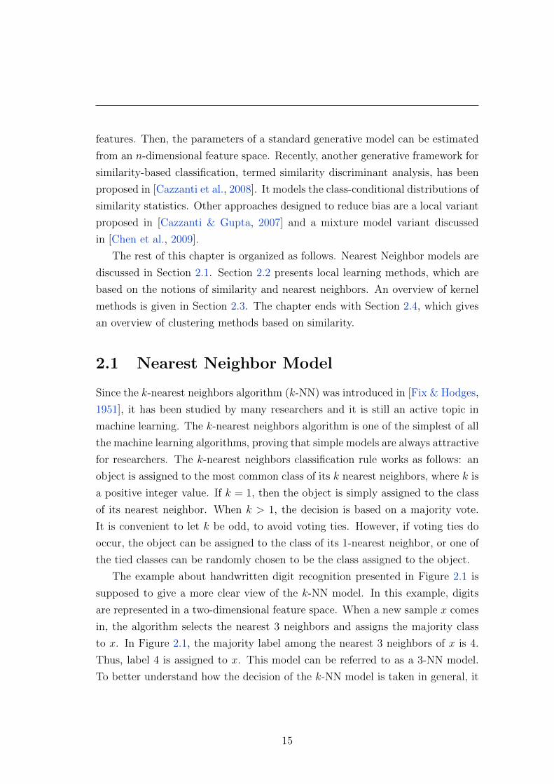
2.1 A 3-NN model for handwritten digit recognition. For visual in-

terpretation, digits are represented in a two-dimensional feature

space. The figure shows 30 digits sampled from the popular MNIST

data set. When the new digit x needs to be recognized, the 3-NN

model selects the nearest 3 neighbors and assigns label 4 based on

a majority vote. . . . . . . . . . . . . . . . . . . . . . . . . . . . . 16

2.2 A 1-NN model for handwritten digit recognition. The figure shows

30 digits sampled from the popular MNIST data set. The decision

boundary of the 1-NN model generates a Voronoi partition of the

digits. . . . . . . . . . . . . . . . . . . . . . . . . . . . . . . . . . 17

2.3 The function φ embeds the data into a feature space where the

nonlinear relations now appear linear. Machine learning methods

can easily detect such linear relations. . . . . . . . . . . . . . . . . 22

xvi

http://www.graphicshunt.com

http://hdwallpapers.lt


http://www.allposters.com

LIST OF FIGURES

4.1 Two images that are compared with LPD. At a certain step, the

patch at position (x1, y1) in the first image is matched with a patch

at offset 3 from position (x2, y2) in the second image. No patches

similar to the one at position (x1, y1) were found at offsets 0, 1 or 2. 49

4.2 A random sample of 15 handwritten digits from the MNIST data

set. . . . . . . . . . . . . . . . . . . . . . . . . . . . . . . . . . . . 55

4.3 A random sample of 12 images from the Birds data set. There are

two images per class. Images from the same class sit next to each

other in this figure. . . . . . . . . . . . . . . . . . . . . . . . . . . 56

4.4 Average accuracy rates of the 3-NN based on LPD model with

patches of 1× 1 pixels at the top and 2× 2 pixels at the bottom.

Experiment performed on the MNIST subset of 100 images. . . . 59











patches of 9×9 pixels at the top and 10×10 pixels at the bottom.



patches ranging from 2 × 2 pixels to 9 × 9 pixels. Experiment

performed on the MNIST subset of 300 images. . . . . . . . . . . 65

4.10 Similarity matrix based on LPD with patches of 4 × 4 pixels and

a similarity threshold of 0.12, obtained by computing pairwise dis-

similarities between the samples of the MNIST subset of 1000 images. 68

4.11 Euclidean distance matrix based on L2-norm, obtained by comput-

ing pairwise distances between the samples of the MNIST subset

of 1000 images. . . . . . . . . . . . . . . . . . . . . . . . . . . . . 69

xvii

LIST OF FIGURES

4.12 Error rate drops as K increases for 3-NN (◦) and 6-NN (�) classi-

fiers based on LPD with filtering. . . . . . . . . . . . . . . . . . . 74

4.13 Sample images from three classes of the Brodatz data set. . . . . 87

4.14 Sample images from four classes of the UIUCTex data set. Each

image is showing a textured surface viewed under different poses. 88

4.15 Sample images from the Biomass Texture data set. . . . . . . . . 89

4.16 Similarity matrix based on LTD with patches of 32 × 32 pixels

and a similarity threshold of 0.02, obtained by computing pairwise

dissimilarities between the texture samples of the Brodatz data set. 92

4.17 Similarity matrix based on LTD with patches of 64 × 64 pixels

and a similarity threshold of 0.02, obtained by computing pairwise

dissimilarities between the texture samples of the UIUCTex data

set. . . . . . . . . . . . . . . . . . . . . . . . . . . . . . . . . . . . 94

5.1 The BOW learning model for object class recognition. The feature

vector consists of SIFT features computed on a regular grid across

the image (dense SIFT) and vector quantized into visual words.

The frequency of each visual word is then recorded in a histogram.

The histograms enter the training stage. Learning is done by a

kernel method. . . . . . . . . . . . . . . . . . . . . . . . . . . . . 101

5.2 A random sample of 12 images from the Pascal VOC data set.

Some of the images contain objects of more than one class. For

example, the image at the top left shows a dog sitting on a couch,

and the image at the top right shows a person and a horse. Dog,

couch, person and horse are among the 20 classes of this data set. 107

5.3 A random sample of 12 images from the Birds data set. There are

two images per class. Images from the same class sit next to each

other in this figure. . . . . . . . . . . . . . . . . . . . . . . . . . . 108

xviii

LIST OF FIGURES

5.4 The BOW learning model for facial expression recognition. The

feature vector consists of SIFT features computed on a regular grid

across the image (dense SIFT) and vector quantized into visual

words. The presence of each visual word is then recorded in a

presence vector. Normalized presence vectors enter the training

stage. Learning is done by a local kernel method. . . . . . . . . . 116

5.5 An example of SIFT features extracted from two images represent-

ing distinct emotions: fear (left) and disgust (right). . . . . . . . . 117

5.6 The six nearest neighbors selected with the presence kernel from

the vicinity of the test image are visually more similar than the

other six images randomly selected from the training set. Despite

this fact, the nearest neighbors do not adequately indicate the test

label. Thus, a learning method needs to be trained on the selected

neighbors to accurately predict the label of the test image. . . . . 119

7.1 The graph of the density probability function. . . . . . . . . . . . 145

7.2 The distance evolution of the best chromosome at each generation

for the Rat-Mouse-Cow experiment. GREEN = rat-house mouse

distance, BLUE = rat-fat dormouse, RED = rat-cow distance. . . 153

7.3 Phylogenetic tree obtained for 22 mammalian mtDNA sequences

using median string via rank distance. . . . . . . . . . . . . . . . 155


using closest string via rank distance. . . . . . . . . . . . . . . . . 156


using consensus string via rank distance. . . . . . . . . . . . . . . 156

8.1 The intuition behind the proof of the triangle inequality for LRD.

For each occurrence xs, the three possible cases of sorting i, j and

k are shown in the upper side of the figure. The nearest match

position in C is denoted by k′. For each occurrence ys, the three

possible cases are shown in the lower side of the figure. The nearest

match position in A is denoted by i′. . . . . . . . . . . . . . . . . 171


using LRD based on 2-mers. . . . . . . . . . . . . . . . . . . . . . 179

xix

LIST OF FIGURES








using LRD based on 10-mers. . . . . . . . . . . . . . . . . . . . . 181


using LRD based on sum of k-mers. . . . . . . . . . . . . . . . . . 181


using LRD based on 18-mers . . . . . . . . . . . . . . . . . . . . . 183

8.9 The distance evolution of the best chromosome at each generation

for the Rat-Mouse-Cow experiment. GREEN = rat-house mouse

distance, BLUE = rat-fat dormouse, RED = rat-cow distance. . . 185

9.1 10-fold cross-validation accuracy on the train set for different n-

grams. . . . . . . . . . . . . . . . . . . . . . . . . . . . . . . . . . 196

xx

List of Tables

4.1 Results of the experiment performed on the MNIST subset of 300

images, using the 3-NN based on LPD model with patches ranging

from 2 × 2 pixels to 9 × 9 pixels. Reported accuracy rates are

averages of 10 runs. . . . . . . . . . . . . . . . . . . . . . . . . . . 64

4.2 Results of the experiment performed on the MNIST subset of 300

images, using various maximum offsets, patches of 4 × 4 pixels,

and a similarity threshold of 0.12. Reported accuracy rates are

averages of 10 runs. The time needed to compute the pairwise

dissimilarity is measured in seconds. . . . . . . . . . . . . . . . . . 65

4.3 Baseline 3-NN versus 3-NN based on LPD. Both the accuracy rate

and standard deviation is reported for MNIST subsets of 100, 300

and 1000 images. . . . . . . . . . . . . . . . . . . . . . . . . . . . 66

4.4 Accuracy rates of several classifiers based on LPD versus the ac-

curacy rates the standard SVM and KRR. Tests are performed

on 300 and 1000 images using cross-validation (CV), respectively.

Another test is performed using a 300/700 split. . . . . . . . . . . 70

4.5 Comparison of several classifiers (some based on LPD). Results for

the difficult experiment on 1866 test images. . . . . . . . . . . . . 71

4.6 Error and time of 3-NN classifier based on LPD with filtering. . . 73

4.7 Confusion matrix of the 3-NN based on LPD with filtering using

K = 50. . . . . . . . . . . . . . . . . . . . . . . . . . . . . . . . . 75

4.8 Error rates on the entire MNIST data set for baseline 3-NN, k-NN

based on tangent distance and k-NN based on LPD with filtering. 76

4.9 Error rates of different k-NN models on Birds data set. . . . . . . 78

xxi

LIST OF TABLES

4.10 Error on Birds data set for texton learning methods of [Lazebnik

et al., 2005a] and kernel methods based on LPD. . . . . . . . . . . 79

4.11 Accuracy rates on the entire Brodatz data set using 3 random

samples per class for training. Learning methods based on LTD

are compared with the state of the art method. . . . . . . . . . . 90

4.12 Accuracy rates on the UIUCTex data set using 20 random sam-

ples per class for training. Learning methods based on LTD are

compared with state of the art method. . . . . . . . . . . . . . . . 93

4.13 Accuracy rates on Biomass Texture data set using 20, 30 and 40

random samples per class for training and 70, 60 and 50 for testing,

respectively. . . . . . . . . . . . . . . . . . . . . . . . . . . . . . . 95

5.1 Mean AP on Pascal VOC 2007 data set for machine learning meth-

ods based on visual words histograms with different kernels. The

best AP on each class is highlighted with bold. . . . . . . . . . . . 111

5.2 The time for the second stage of the learning model and the number

of features for each kernel. The time is measured in seconds. . . . 112

5.3 Mean AP on Birds data set for machine learning methods based

on visual words histograms with different methods. The best AP

on each class is highlighted with bold. . . . . . . . . . . . . . . . . 113

5.4 Accuracy levels for several models obtained on the validation, test,

and private test sets. . . . . . . . . . . . . . . . . . . . . . . . . . 123

7.1 The 22 mammals from the EMBL database used in the phyloge-

netic experiments. The accession number is given on the last column.151

7.2 Consensus string results obtained with the genetic algorithm. . . . 152

7.3 Comparative results of the k-means based on median string (k-

median) versus the k-means based on closest string (k-closest).

Clustering results for 22 DNA sequences using rank distance. . . . 154

8.1 The 27 mammals from the EMBL database used in the phyloge-

netic experiments. The accession number is given on the last column.177

8.2 The number of misclustered mammals for different clustering tech-

niques on the 22 mammals data set. . . . . . . . . . . . . . . . . . 182

xxii

LIST OF TABLES

8.3 Closest string results for the genetic algorithm based on LRD with

3-mers. . . . . . . . . . . . . . . . . . . . . . . . . . . . . . . . . . 184

9.1 Accuracy rates using 10-fold cross-validation on the train set for

different kernel methods with k5 kernel. . . . . . . . . . . . . . . . 195

9.2 Accuracy rates, using 10-fold cross-validation on the training set,

of LRD with different n-grams, with and without normalization.

Normalized LRD is much better. . . . . . . . . . . . . . . . . . . 198

9.3 Accuracy rates of different kernel combinations using 10-fold cross-

validation on the training set. . . . . . . . . . . . . . . . . . . . . 198

9.4 Accuracy rates of submitted systems on different evaluation sets.

The Unibuc team ranked third in the closed NLI Shared Task

with the kernel combination improved by the heuristic to level the

predicted class distribution. . . . . . . . . . . . . . . . . . . . . . 200

9.5 Accuracy rates on different evaluation sets of systems based on the

KDA classifier. These systems were not submitted to the closed

NLI Shared Task. . . . . . . . . . . . . . . . . . . . . . . . . . . . 201

xxiii

Chapter 1

Motivation and Overview

1.1 Introduction

Machine learning is a branch of artificial intelligence that studies computer sys-

tems that can learn from data. In this context, learning is about recognizing

complex patterns and making intelligent decisions based on data. In the early

years of artificial intelligence, the idea that human thinking could be rendered

logically in a numerical computing machine emerged. But it was unclear if such

a machine could model the complex human brain, until Alan Turing proposed a

test to measure its performance in 1950. The Turing test states that a machine

exhibits human-level intelligence if a human judge engages in a natural language

conversation with the machine and cannot distinguish it from another human.

Despite the fact that intelligent machines that can pass the Turing test have not

been developed yet, many interesting systems that can learn from data have been

proposed since then.

One of the first breakthrough intelligent system was developed in 1952 by

Arthur Samuel from IBM. He developed a game-playing program, for checkers,

to achieve sufficient skill to challenge a world champion. Its program was based

on a search tree of the board positions reachable from the current state. Some of

the early intelligent systems were based on decision rules. Such systems are best

known as expert systems. The system that is often called the first expert system

is ELIZA, which was developed between 1964 and 1966 by Joseph Weizenbaum

1

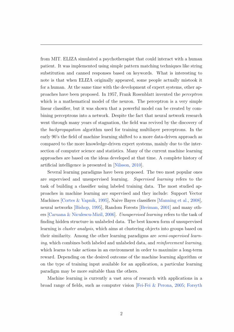
from MIT. ELIZA simulated a psychotherapist that could interact with a human

patient. It was implemented using simple pattern matching techniques like string

substitution and canned responses based on keywords. What is interesting to

note is that when ELIZA originally appeared, some people actually mistook it

for a human. At the same time with the development of expert systems, other ap-

proaches have been proposed. In 1957, Frank Rosenblatt invented the perceptron

which is a mathematical model of the neuron. The perceptron is a very simple

linear classifier, but it was shown that a powerful model can be created by com-

bining perceptrons into a network. Despite the fact that neural network research

went through many years of stagnation, the field was revived by the discovery of

the backpropagation algorithm used for training multilayer perceptrons. In the

early 90’s the field of machine learning shifted to a more data-driven approach as

compared to the more knowledge-driven expert systems, mainly due to the inter-

section of computer science and statistics. Many of the current machine learning

approaches are based on the ideas developed at that time. A complete history of

artificial intelligence is presented in [Nilsson, 2010].

Several learning paradigms have been proposed. The two most popular ones

are supervised and unsupervised learning. Supervised learning refers to the

task of building a classifier using labeled training data. The most studied ap-

proaches in machine learning are supervised and they include: Support Vector

Machines [Cortes & Vapnik, 1995], Naive Bayes classifiers [Manning et al., 2008],

neural networks [Bishop, 1995], Random Forests [Breiman, 2001] and many oth-

ers [Caruana & Niculescu-Mizil, 2006]. Unsupervised learning refers to the task of

finding hidden structure in unlabeled data. The best known form of unsupervised

learning is cluster analysis, which aims at clustering objects into groups based on

their similarity. Among the other learning paradigms are semi-supervised learn-

ing, which combines both labeled and unlabeled data, and reinforcement learning,

which learns to take actions in an environment in order to maximize a long-term

reward. Depending on the desired outcome of the machine learning algorithm or

on the type of training input available for an application, a particular learning

paradigm may be more suitable than the others.

Machine learning is currently a vast area of research with applications in a

broad range of fields, such as computer vision [Fei-Fei & Perona, 2005; Forsyth

2

& Ponce, 2002; Zhang et al., 2007], bioinformatics [Dinu & Ionescu, 2013a; Inza

et al., 2010; Leslie et al., 2002], information retrieval [Chifu & Ionescu, 2012;

Manning et al., 2008], natural language processing [Lodhi et al., 2002; Popescu

& Grozea, 2012], data mining [Enachescu, 2004], and many others. Among the

variety of state of the art machine learning approaches for such applications, are

the similarity-based learning methods [Chen et al., 2009].

This thesis studies similarity-based learning approaches such as Nearest Neigh-

bor models, kernel methods [Shawe-Taylor & Cristianini, 2004] and clustering

analysis [Enachescu, 2004]. The studied approaches exhibit state of the art per-

formance levels in two different areas: computer vision and string processing. It

is important to note that string processing refers to any task that needs to pro-

cess string data such as text documents, DNA sequences, and so on. This work

investigates string processing tasks ranging from phylogenetic analysis [Dinu &

Ionescu, 2012a,c, 2013a; Ionescu, 2013a] and DNA comparison [Dinu & Ionescu,

2012b, 2013b] to native language identification [Popescu & Ionescu, 2013], from a

machine learning perspective. On the other hand, a broad variety of computer vi-

sion tasks are also investigated in this thesis, such as object recognition [Ionescu

& Popescu, 2013b], optical character recognition [Dinu et al., 2012; Ionescu &

Popescu, 2013a], texture classification [Ionescu et al., 2014], and facial expression

recognition [Ionescu et al., 2013].

1.2 Image and Text Processing: Common Con-

cepts

In recent years, computer science specialists are faced with the challenge of pro-

cessing massive amounts of data. The largest part of this data is actually un-

structured and semi-structured data, available in the form of text documents,

images, audio, video and so on. Researchers have developed methods and tools

that extract relevant information and support efficient access to unstructured and

semi-structured content. Such methods that aim at providing access to informa-

tion are mainly studied by machine learning researchers. In fact, a tremendous

amount of effort has been dedicated to this line of research [Agarwal & Roth,

3

2002; Lazebnik et al., 2005b, 2006; Leung & Malik, 2001; Manning et al., 2008].

In the context of machine learning, the aim is to obtain a good representation of

the data that can later be used to build an efficient classifier. In computer vision,

image representations are obtained by feature detection and feature extraction.

Most of the feature extraction methods are handcrafted by researchers that have

a good understanding of the application and a vast experience. This is the case

of the bag of visual words model [Leung & Malik, 2001; Sivic et al., 2005] in

computer vision. A different approach is representation learning, which aims at

discovering a better representation of the data provided during training. This is

the case of deep learning algorithms [Bengio, 2009; Montavon et al., 2012] that

aim at discovering multiple levels of representation, or a hierarchy of features.

Deep algorithms learn to transform one representation into another, by better

disentangling the factors of variation that explain the observed data.

Whether the representation of the data is obtained through a handcrafted

method or learned by a fully automatic process, common concepts of treating

different kinds of unstructured and semi-structured data, such as image and text,

naturally arise. Despite the fact that computer vision and string processing seem

to be unrelated fields of study, the concept of treating image and text in a similar

fashion has proven to be very fertile for several applications. Furthermore, by

adapting string processing techniques to image analysis or the other way around,

knowledge from one domain can be transferred to the other.

An example of similarity between text and image is discussed next. It refers

to word sense disambiguation and object recognition in images. Word sense

disambiguation (WSD) is a core research problem in computational linguistics

and natural language processing, which was recognized since the beginning of the

scientific interest in machine translation, and in artificial intelligence, in general.

WSD is about determining the meaning of a word in a specific context. Actually

all the WSD methods use the context to determine the meaning of an ambiguous

word, because the entire information about the word sense is contained in the

context [Agirre & Edmonds, 2006]. The basic concept is to extract features from

the context that could help the WSD process. In a similar fashion, objects in

images can be recognized using the entire image as a context. For example, a

method that could detect the presence of the sun (as an object) in the image,

4

Figure 1.1: A picture of the sun in the left and a light bulb in the dark onthe right. The light bulb can easily be mistaken for the sun if the rest of theimage is disregarded. Copyrights of the two images are reserved to http://www.

graphicshunt.com and http://hdwallpapers.lt, respectively.

would have to look for distinctive features such as the round shape of the sun,

the color, and so on. However, there are other objects that have similar shape

or color, such as spot lights or lamps. Thus, a better approach could be to look

for other distinctive features in the image, such as the sky, the sun reflection in

water, and so on. This approach will help avoid confusions such as recognizing a

light bulb as the sun, which can be a quite common mistake as it can be observed

in Figure 1.1.

Another example of treating image and text in a similar manner is a state

of the art method for image categorization and image retrieval inspired from the

bag of words representation, which is very popular in information retrieval and

natural language processing. The bag of words model represents a text as an un-

ordered collection of words, completely disregarding grammar, word order, and

syntactic groups. The bag of words model has many applications from informa-

tion retrieval [Manning et al., 2008] to natural language processing [Manning &

Schutze, 1999] and word sense disambiguation [Agirre & Edmonds, 2006; Chifu

& Ionescu, 2012]. In the context of image analysis, the concept of word needs to

be defined somehow. Computer vision researchers have introduced the concept

of visual word. Local image descriptors, such as SIFT [Lowe, 1999], are vector

quantized to obtain a vocabulary of visual words. The vector quantization pro-

cess can be done, for example, by k-means clustering [Leung & Malik, 2001] or by

5




probabilistic Latent Semantic Analysis [Sivic et al., 2005]. The frequency of each

visual word is then recorded in a histogram which represents the final feature

vector for the image. This histogram is the equivalent of the bag of words rep-

resentation for text. The idea of representing images as bag of visual words has

demonstrated impressive levels of performance for image categorization [Zhang

et al., 2007] and image retrieval [Philbin et al., 2007].

One of the most important problems in computer vision is object recogni-

tion. Machine learning methods represent the state of the art approach for the

object recognition problem. A common approach is to make some assumptions

in order to treat object recognition as a classification problem. First, object cat-

egories are considered to be fixed and known. Second, each instance belongs to a

single category. However, some researchers argue that these assumptions are ob-

vious nonsense. The following example shows that these assumptions are indeed

wrong. The object presented in Figure 1.2 can be described either as a plastic

toy, a monkey, or both. It it clear that the object does not belong to a single cat-

egory. Furthermore, the category of the object might be irrelevant for particular

applications. Another drawback of this approach is that it misses out some of the

subtle aspects of object recognition. For example, an object classification system

does not understand the properties of an object and it cannot deal with unfamil-

iar objects. In other words, it fails to extract aspects of meaning. Thus, some

computer vision researchers have proposed different approaches for the object

recognition task. One alternative approach, proposed in [Duygulu et al., 2002],

is to model object recognition as machine translation. The model is based on the

observation that object recognition is a little like translation, in that a picture (or

text in a source language) goes in, and a description (or text in a target language)

comes out. In this model, object recognition becomes a process of annotating im-

age regions with words. First, images are segmented into regions, which are then

classified into region types. Next, a mapping between region types and keywords

provided with the images is learned. This process is similar to learning a lexi-

con from data, a standard problem in machine translation literature [Jurafsky

& Martin, 2000; Manning & Schutze, 1999]. This approach has proven fertile

for this interpretation of object recognition. Research in this area has led to the

development of other systems, such as the one described in [Farhadi et al., 2010]

6

Figure 1.2: An object that can be described by multiple categories such as plastictoy, monkey, or both. Image copyrights are reserved to http://www.allposters.

com.

which generates sentences from images. The system computes a score linking an

image to a sentence. This score can be used to attach a descriptive sentence to

a given image, or to obtain images that illustrate a given sentence. To take this

even further, the work of [Sadeghi & Farhadi, 2011] suggests that it is easier and

more effective to generate descriptions of images in terms of chunks of meaning,

such as “a person riding a horse”, rather than individual components, such as

“person” or “horse”. In this approach, categories are replaced with visual phrases

for recognition.

The examples described so far are successful cases of treating image as text.

However, research that studies how to improve text processing techniques with

knowledge from computer vision has also been conducted. A good example is

the method introduced in [Barnard & Johnson, 2005], which proposes the use

of images for WSD, either alone, or in conjunction with traditional text based

methods. To integrate image information with text data, the authors exploit

previous work on linking images and words [Barnard et al., 2003; Duygulu et al.,

2002]. The empirical results strongly suggest that images can help disambiguate

senses of words.

The concept of treating image and text in a similar manner is exploited in

some way or another in the previous examples. The knowledge transfer from one

domain to another has proven to be very fertile in the case of computer vision and

natural language processing. This thesis follows this line of research and presents

7



novel approaches or improved methods that exploit this concept. First, a dissim-

ilarity measure for images is presented in Chapter 4. The dissimilarity measure is

inspired from the rank distance measure [Dinu, 2003]. The main concern is to ex-

tend rank distance from one-dimensional input (strings) to two-dimensional input

(digital images). While rank distance is a highly accurate measure for strings, the

experiments presented in Chapter 4 suggest that the proposed extension of rank

distance to images is very accurate for handwritten digit recognition and texture

analysis. Second, some improvements to the popular bag of visual words model

are proposed in Chapter 5. As mentioned before, this model is inspired by the

bag of words model from natural language processing and information retrieval.

Third, a new distance measure for strings is introduced in Chapter 8. It is in-

spired from the image dissimilarity measure presented in Chapter 4. Designed

to conform to more general principles and adapted to DNA strings, it comes to

improve several state of the art methods for DNA sequence analysis. Further-

more, another application of this novel distance measure for strings is presented

in Chapter 9. More precisely, a kernel based on this distance measure is used for

native language identification. To summarize, all the contributions presented in

this thesis come to support the concept of treating image and text in a similar

manner.

1.3 Overview and Organization

The rest of this thesis is organized as follows. All the machine learning methods

that are employed to obtain results for different applications of computer vision

and string processing are described in Chapter 2. This chapter gives an overview

of the main concepts of learning based on similarity. Specific machine learning

methods that are based on these concepts are then presented. First, Nearest

Neighbor models are discussed. A non-standard learning formulation based on

the notions of similarity and nearest neighbors, known as local learning, is then

presented. An overview of kernel methods is also given, since the state of the art

methods consistently used in the supervised learning tasks presented throughout

this thesis are kernel methods. This chapter ends with a discussion about cluster

analysis. Several clustering techniques are proposed in this thesis and their utility

8

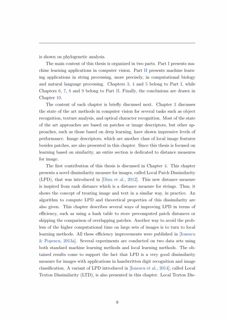
is shown on phylogenetic analysis.

The main content of this thesis is organized in two parts. Part I presents ma-

chine learning applications in computer vision. Part II presents machine learn-

ing applications in string processing, more precisely, in computational biology

and natural language processing. Chapters 3, 4 and 5 belong to Part I, while

Chapters 6, 7, 8 and 9 belong to Part II. Finally, the conclusions are drawn in

Chapter 10.

The content of each chapter is briefly discussed next. Chapter 3 discusses

the state of the art methods in computer vision for several tasks such as object

recognition, texture analysis, and optical character recognition. Most of the state

of the art approaches are based on patches or image descriptors, but other ap-

proaches, such as those based on deep learning, have shown impressive levels of

performance. Image descriptors, which are another class of local image features

besides patches, are also presented in this chapter. Since this thesis is focused on

learning based on similarity, an entire section is dedicated to distance measures

for image.

The first contribution of this thesis is discussed in Chapter 4. This chapter

presents a novel dissimilarity measure for images, called Local Patch Dissimilarity

(LPD), that was introduced in [Dinu et al., 2012]. This new distance measure

is inspired from rank distance which is a distance measure for strings. Thus, it

shows the concept of treating image and text in a similar way, in practice. An

algorithm to compute LPD and theoretical properties of this dissimilarity are

also given. This chapter describes several ways of improving LPD in terms of

efficiency, such as using a hash table to store precomputed patch distances or

skipping the comparison of overlapping patches. Another way to avoid the prob-

lem of the higher computational time on large sets of images is to turn to local

learning methods. All these efficiency improvements were published in [Ionescu

& Popescu, 2013a]. Several experiments are conducted on two data sets using

both standard machine learning methods and local learning methods. The ob-

tained results come to support the fact that LPD is a very good dissimilarity

measure for images with applications in handwritten digit recognition and image

classification. A variant of LPD introduced in [Ionescu et al., 2014], called Local

Texton Dissimilarity (LTD), is also presented in this chapter. Local Texton Dis-

9

similarity aims at classifying texture images. It is based on textons, which are

represented as a set of features extracted from image patches. One of the features

is based on the development of an efficient box counting method for estimating

fractal dimension, presented in [Popescu et al., 2013b]. Textons provide a lighter

representation of patches, allowing for a faster computational time and a better

accuracy when used for texture analysis. The performance level of the machine

learning methods based on LTD is comparable to the state of the art methods

for texture classification.

Chapter 5 presents some improvements of the bag of visual words model for

two applications, namely object recognition and facial expression recognition.

For the bag of visual words approach, images are represented as histograms of

visual words from a codebook that is usually obtained with a simple clustering

method. Next, kernel methods are used to compare such histograms. This chapter

introduces a novel kernel for histograms of visual words, namely the PQ kernel.

The PQ kernel was initially presented in [Ionescu & Popescu, 2013b]. It is worth

mentioning that the paper of [Ionescu & Popescu, 2013b] received the Caianiello

Best Young Paper Award. A proof that PQ is actually a kernel is also given in

this chapter. The proof is based on building its feature map. Object recognition

experiments are conducted to compare the PQ kernel with other state of the art

kernels on two benchmark data sets. The PQ kernel has the best performance

on both data sets. A novel formulation of the bag of visual words model is

also proposed for classifying human facial expression from low resolution images.

The modified bag of visual words model was presented in [Ionescu et al., 2013].

The proposed model participated at the Facial Expression Recognition (FER)

Challenge of the ICML 2013 Workshop in Challenges in Representation Learning

(WREPL), and ranked fourth with an accuracy of 67.484% on the final test.

More details about the FER Challenge are provided in [Goodfellow et al., 2013].

The model extracts dense SIFT descriptors either from the whole image or from a

spatial pyramid that divides the image into increasingly fine sub-regions. Then, it

represents images as normalized (spatial) presence vectors of visual words. Linear

kernels are built for several choices of spatial presence vectors, and combined into

weighted sums for multiple kernel learning (MKL). Instead of building a global

classifier for the machine learning task, local MKL was used to predict class labels

10

of test images. Empirical results indicate that the use of presence vectors, local

learning and spatial information improve recognition performance.

Chapter 6 presents the state of the art methods for several problems that

involve string processing. The problems studied by this work belong to two major

scientific fields, namely computational biology and text mining. Consequently,

this chapter is divided into two separate sections corresponding to the two fields of

study. First, clustering methods used for phylogenetic analysis and other methods

for sequencing and comparing DNA are discussed. An overview of state of the

art natural language processing techniques is given next. The state of the art

also includes recent advances in information retrieval showing that word sense

disambiguation can improve the precision for difficult queries [Chifu & Ionescu,

2012].

Chapter 7 presents several clustering methods based on rank distance. The

clustering algorithms were introduced in a series of recent papers [Dinu & Ionescu,

2012a,c, 2013a,b]. Two k-means algorithms are initially described. The k-means

algorithm usually represents each cluster by a mean vector with respect to a dis-

tance measure. However, for the proposed k-means approaches, each cluster is

represent either by the median string or by the closest string, which are computed

with the genetic algorithms of [Dinu & Ionescu, 2011, 2012b]. In the genetic ap-

proaches for median or closest string, a novel algorithm for sorting uniformly

distributed numbers in O(n) time is used in the selection process of the next

generation of chromosomes. The sorting algorithm was introduced in [Ionescu,

2013b]. This chapter also describes two hierarchical clustering techniques that use

rank distance. Hierarchical clustering builds models based on distance connectiv-

ity. The proposed hierarchical methods join clusters based on the rank distance

between their centroid strings. Again the cluster centroid is represented either by

the median string or the closest string. This chapter also discusses the consensus

string in the rank distance paradigm, which was initially investigated in [Dinu &

Ionescu, 2013b]. Among the conditions that a string should satisfy in order to be

accepted as consensus, are the median string and the closest string. Theoretical

results indicate that it is not possible to identify a consensus string via rank dis-

tance for three or more strings. Thus, an efficient genetic algorithm is proposed

to find the optimal consensus string, by adapting the approach proposed in [Dinu

11

& Ionescu, 2012b]. To show an application for the studied consensus problem,

this chapter also discusses a hierarchical clustering algorithm based on consensus

string. Experiments using mitochondrial DNA sequences extracted from several

mammals are performed to compare the results of all the proposed clustering

methods. Results demonstrate the clustering performance and the utility of the

algorithms presented in this chapter.

In Chapter 8, a new distance measure, called Local Rank Distance (LRD),

inspired from the image dissimilarity measure presented in Chapter 4, is intro-

duced. LRD was initially presented in [Ionescu, 2013a]. Designed to conform to

more general principles and adapted to DNA strings, LRD comes to improve sev-

eral state of the art methods for DNA sequence analysis. This chapter shows two

applications of LRD. The first application is the phylogenetic analysis of mam-

mals. Experiments show that phylogenetic trees produced by LRD are better or

at least similar to those reported in the literature. The second application is to

find the closest string for a set of DNA strings, using a genetic algorithm based on

LRD. The results obtained by LRD come to support the fact that concepts that

make a good dissimilarity measure for images can be transferred with success in

comparing and analyzing strings.

Chapter 9 presents an application of machine learning methods that work

at the character level. More precisely, several string kernels and a kernel based

on LRD are combined to obtain state of the art results for the native language

identification task. This chapter is based on the work of [Popescu & Ionescu,

2013], which describes the approach based on string kernels for the closed Native

Language Identification (NLI) Shared Task 2013. The method ranked on third

place in this competition with an accuracy of 82.7%. The results are even more

impressive, if one considers that the proposed approach is language independent

and linguistic theory neutral. While string kernels have been used before in text

analysis tasks, LRD is designed to work on DNA sequences. Thus, it is an inter-

esting fact that LRD can be successfully applied in native language identification.

The conclusions presented in Chapter 10 point to the fact that the concept of

treating image and text in a similar way is indeed fertile. Future work and new

directions of exploiting this concept are also discussed in the final chapter.

12

Chapter 2

Learning Based on Similarity

Learning based on similarity refers to the process of learning based on pairwise

similarities between the training samples. The similarity-based learning process

can be both supervised and unsupervised, and the pairwise relationship can be

either a similarity, a dissimilarity, or a distance function. Similarity functions may

be asymmetric and even fail to satisfy other mathematical properties required for

metrics or inner products, for example. When the learning process is supervised,

the similarity-based method aims at estimating the class label of a test sample

using both the pairwise similarities between the labeled training samples, and

the similarities between the test sample and the set of training samples. When

the learning process is unsupervised, the similarity-based method aims at finding

hidden structure in unlabeled training samples, using the pairwise similarities

between samples. An advantage of similarity-based learning is that it does not

require direct access to the features, as long as the similarity function is well

defined for any pair of samples. Thus, the feature space is not required to be an

euclidean space.

Similarity-based learning methods have been widely used in several domains

such as computer vision, natural language processing, computational biology,

and information retrieval. Computer vision researchers proposed several meth-

ods based on computing similarity between images for object recognition and

image retrieval. Such methods range from distance measures such as the Tangent

distance [Simard et al., 1996], the Earth Mover’s distance [Rubner et al., 2000],

or the shape matching distance [Belongie et al., 2002], to kernel methods such

13

as the pyramid match kernel [Lazebnik et al., 2006] or the PQ kernel [Ionescu

& Popescu, 2013b]. Most of the state of the art techniques in computational

biology, such as those that obtain phylogenetic trees or those that compare DNA

sequences, are based on distance measures for strings. Popular choices for recent

techniques are the Hamming distance [Chimani et al., 2011; Vezzi et al., 2012],

edit distance [Shapira & Storer, 2003], Kendall-tau distance [Popov, 2007] or rank

distance [Dinu & Ionescu, 2012a,b]. Other popular similarity-based tools from

computational biology are the FASTA algorithm [Lipman & Pearson, 1985] and

the BLAST algorithm [Altschul et al., 1990]. These tools compute the similar-

ity between different amino acid sequences for protein classification. The cosine

similarity between term frequency-inverse document frequency (TF-IDF) vectors

is widely used in information retrieval and text mining for document classifica-

tion [Manning et al., 2008]. More recently, the string kernel [Shawe-Taylor & Cris-

tianini, 2004], which computes the similarity between strings by counting common

character n-grams, has demonstrated impressive levels of performance for text

categorization (by topic) [Lodhi et al., 2002], authorship identification [Popescu

& Dinu, 2007; Popescu & Grozea, 2012; Sanderson & Guenter, 2006], and native

language identification [Popescu & Ionescu, 2013].

The similarity-based learning paradigm consists of a wide variety of algorithms

and approaches. Among the variety of similarity-based learning methods, only

four of them are extensively discussed in this thesis, namely the Nearest Neighbor

model, the local learning methods, the kernel methods and the cluster analysis

techniques. These four approaches are used in different applications presented in

this work. Other similarity-based learning methods, such as treating similarities

as features, or generative classifiers, are briefly discussed next. By treating the

similarities between a sample and training samples as features, similarity-based

classification problems can be regarded as standard classification problems [Chen

et al., 2009; Graepel et al., 1999, 1998; Liao & Noble, 2003; Pekalska & Duin,

2002]. In other words, each sample is represented by a feature vector obtained

by computing the similarity with a set of training samples. Generative classifiers

provide a structured probabilistic model of the data. Training data is used for

estimating the parameters of the generative model. Given the pairwise similarity

of n samples, one approach to generative classification is using the similarities as

14

features. Then, the parameters of a standard generative model can be estimated

from an n-dimensional feature space. Recently, another generative framework for

similarity-based classification, termed similarity discriminant analysis, has been

proposed in [Cazzanti et al., 2008]. It models the class-conditional distributions of

similarity statistics. Other approaches designed to reduce bias are a local variant

proposed in [Cazzanti & Gupta, 2007] and a mixture model variant discussed

in [Chen et al., 2009].

The rest of this chapter is organized as follows. Nearest Neighbor models are

discussed in Section 2.1. Section 2.2 presents local learning methods, which are

based on the notions of similarity and nearest neighbors. An overview of kernel

methods is given in Section 2.3. The chapter ends with Section 2.4, which gives

an overview of clustering methods based on similarity.

2.1 Nearest Neighbor Model

Since the k-nearest neighbors algorithm (k-NN) was introduced in [Fix & Hodges,

1951], it has been studied by many researchers and it is still an active topic in

machine learning. The k-nearest neighbors algorithm is one of the simplest of all

the machine learning algorithms, proving that simple models are always attractive

for researchers. The k-nearest neighbors classification rule works as follows: an

object is assigned to the most common class of its k nearest neighbors, where k is

a positive integer value. If k = 1, then the object is simply assigned to the class

of its nearest neighbor. When k > 1, the decision is based on a majority vote.

It is convenient to let k be odd, to avoid voting ties. However, if voting ties do

occur, the object can be assigned to the class of its 1-nearest neighbor, or one of

the tied classes can be randomly chosen to be the class assigned to the object.

The example about handwritten digit recognition presented in Figure 2.1 is

supposed to give a more clear view of the k-NN model. In this example, digits

are represented in a two-dimensional feature space. When a new sample x comes

in, the algorithm selects the nearest 3 neighbors and assigns the majority class

to x. In Figure 2.1, the majority label among the nearest 3 neighbors of x is 4.

Thus, label 4 is assigned to x. This model can be referred to as a 3-NN model.

To better understand how the decision of the k-NN model is taken in general, it

15

Figure 2.1: A 3-NN model for handwritten digit recognition. For visual inter-pretation, digits are represented in a two-dimensional feature space. The figureshows 30 digits sampled from the popular MNIST data set. When the new digitx needs to be recognized, the 3-NN model selects the nearest 3 neighbors andassigns label 4 based on a majority vote.

is worth considering a 1-NN model. For this model, the decision at every point

is to assign the label of the closest data point. This process generates a Voronoi

partition of the training samples, as seen in Figure 2.2. Each training data point

corresponds to a Voronoi cell. When a new data point comes in, it is assigned to

the class associated to the Voronoi cell that the respective data point falls in.

The k-NN algorithm is a non-parametric method for classification. Thus, no

parameters have to be learned. In fact, the k-NN model does not require training

at all. The decision of the classifier is only based on the nearest k neighbors of an

object with respect to a similarity or distance function. The euclidean distance

measure is a very common choice, but other similarity measures can also be used

16

Figure 2.2: A 1-NN model for handwritten digit recognition. The figure shows30 digits sampled from the popular MNIST data set. The decision boundary ofthe 1-NN model generates a Voronoi partition of the digits.

instead. Actually, the performance of the k-NN classifier depends on the strength

and the discriminatory power of the distance measure used. It is worth mentioning

that a good choice of the distance metric can help to achieve invariance with

respect to a certain family of transformations. For example, a distance metric

that is invariant to scale, rotation, luminosity and contrast changes is a suitable

choice for computer vision tasks. Researchers continue to study and develop new

similarity or dissimilarity measures for a broad variety of applications in different

domains. But, when it comes to testing the similarity measure in machine learning

tasks, the method of choice is the k-NN model, because it deeply reflects the

strength of the similarity measure. Good examples of this fact are the Tangent

distance [Simard et al., 1996] and the shape matching distance [Belongie et al.,

17

2002], which are both used for handwritten digit recognition. For the same reason,

the k-NN model is used to assess the performance of the new dissimilarity measure

for images presented in Chapter 4 of this work.

It is interesting to mention that the k-NN model is one of the first classifiers

for which an upper bound of its error rate has been demonstrated. More precisely,

a theoretical result demonstrated in [Cover & Hart, 1967] states that the nearest

neighbor rule is asymptotically at most twice as bad as the Bayes rule. Further-

more, if k is allowed to grow with n such that k/n→ 0, the nearest neighbor rule

is universally consistent. More consistency results and other theoretical aspects

of the k-NN model are discussed in [Devroye et al., 1996].

The k-NN model defers all the computations to the test phase. This rep-

resents a great disadvantage when the computational time is taken into consid-

eration. Searching for the k nearest neighbors among n training samples may

take time proportional to O(n · k · d) using a naive approach, where d represents

the computational cost of the distance function. Different approaches based on

multidimensional search trees that partition the space and guide the search have

been proposed to reduce the time complexity [Dasarathy, 1991]. Other fast k-NN

approaches are proposed in [Farago et al., 1993] and [Zhang & Srihari, 2004].

2.2 Local Learning

The development of unconventional (or nonstandard) learning formulations and

non-inductive types of inference was studied in [Vapnik, 2006]. The author ar-

gues in favor of introducing and developing unconventional learning methods, as

an alternative to algorithmic improvements of existing learning methods. This

view is consistent with the main principle of VC theory [Vapnik & Chervonenkis,

1971], suggesting that one should always use direct learning formulations for finite

sample estimation problems, rather than more general settings (such as density

estimation).

Local learning methods attempt to locally adjust the performance of the train-

ing system to the properties of the training set in each area of the input space.

A simple local learning algorithm works as follows: for each test sample, select a

few training samples located in the vicinity of the test sample, train a classifier

18

with only these few examples and apply the resulting classifier to predict the

class label of the testing example. For example, the k-NN model and the Radial

Basis Function (RBF) network are part of the family of local learning algorithms.

Actually, the k-NN model is the simplest form of local learning, since the dis-

criminant function is constant. But, almost any other classifier can be employed

in the local learning paradigm. However, it is important to mention that besides

the classifier, a similarity or distance measure is required to determine the neigh-

bors located in the vicinity of a test sample. Local learning has a few advantages

over standard learning methods. First, it divides a hard classification problem

into more simple sub-problems. Second, it reduces the variety of samples in the

training set, by selecting samples that are most similar to the test one. Third, it

improves accuracy for data sets affected by labeling noise. Considering these ad-

vantages, the local learning paradigm is suitable for classification problems with

large training data.

In [Bottou & Vapnik, 1992] the idea of local algorithms for pattern recognition

was used. The approach is based on local linear rules instead of local constant

rules, and VC bounds [Vapnik & Chervonenkis, 1971] instead of the distance to

the k-th nearest neighbor. The local linear rules demonstrated an improvement

in accuracy on the popular MNIST data set (from 4.1% to 3.2%).

For the regression estimation problem, a similar approach was used in the

Nadaraya-Watson estimator [Nadaraya, 1964] with a slightly different concept of

locality. Nadaraya and Watson suggested considering “soft locality” by using a

kernel as a weighting function for estimating a value of interest.

In Chapter 4, a k-NN with filtering approach that is also a pure local learning

algorithm is used. For the filter-based k-NN approach, the idea is to filter (or

select) the nearest K neighbors (where K is larger than k) using a distance

measure that is much faster and easy to compute. Instead of training a classifier,

the next step is to select the nearest k neighbors from those filtered K examples

using a distance measure that is able to capture much finer differences. This

latter distance measure is allowed to consume more time in order to determine

a better similarity (or dissimilarity) between training examples. This approach

is appropriate when it is unreasonable, from the perspective of time, to compute

the latter distance for all training examples. This two-step selection (or filtering)

19

process is much faster to compute than a standard k-NN based only on the

computationally heavy distance measure.

In Chapter 5, the learning phase of the framework used for facial expression

recognition is based on a local learning algorithm. The algorithm uses a kernel

based on visual word occurrences to select nearest neighbors in the vicinity of a

test image. Then, it trains a SVM classifier only on the selected neighbors to

predict the class label of the test image.

2.3 Kernel Methods

In the similarity-based learning paradigm, a popular approach is to treat the

pairwise similarities as inner products in some Hilbert space or to treat pairwise

dissimilarities as distances in some euclidean space. This can be achieved in

roughly two ways. One is to explicitly embed the samples in a euclidean space,

according to the pairwise similarities (or dissimilarities) using multidimensional

scaling [Borg & Groenen, 2005]. Another is to modify the similarities into kernels

and apply kernel methods. This section is focused on the latter approach and it

covers the following topics: an overview of kernel methods, methods of combining

kernels, such as kernel alignment, multiple kernel learning (MKL), and state of

the art kernel methods such as Support Vector Machines (SVM), Kernel Ridge

Regression (KRR), Kernel Linear Discriminant Analysis (KDA), or Kernel Partial

Least Squares Regression (KPLS). Special consideration is given to the topics

that discuss kernel approaches used throughout the experiments presented in

this thesis.

2.3.1 Mathematical Preliminaries and Properties of Ker-

nels

This section follows the theoretical presentation given in [Shawe-Taylor & Cris-

tianini, 2004]. Therefore, most of the definitions, propositions and theorems are

reproduced from [Shawe-Taylor & Cristianini, 2004] for the sake of completeness

of this chapter.

A definition of an inner product space is given next.

20

Definition 1 A vector space X over the set of real numbers R is an inner product

space, if there exists a real-valued symmetric bilinear (linear in each argument)

map 〈·, ·〉, that satisfies 〈x, x〉 ≥ 0, for all x ∈ X. The bilinear map is known as

the inner product, dot product or scalar product.

An inner product space is sometimes referred to as a Hilbert space, although

most researchers agree that additional properties of completeness and separability

are required. Formally, a Hilbert space can be defined as follows.

Definition 2 A Hilbert Space H is an inner product space with the additional

properties of completeness and separability. A space H is complete if every

Cauchy sequence {hn}n≥1 of elements of H converges to a element h ∈ H, where

a Cauchy sequence is one that satisfies the property that

supm>n‖hn − hm‖ → 0, as n→∞.

A space H is separable if for any ε > 0 there is a finite set of elements

{h1, ..., hN} of H such that for all h ∈ H

mini‖hi − h‖ < ε.

Note that Rn is a Hilbert space.

A kernel method performs a mapping into an embedding or feature space. An

embedding map (or feature map) is a function

φ : x ∈ Rn 7−→ φ(x) ∈ F ⊆ H.

A kernel function is defined as follows.

Definition 3 A kernel is a function k that for all x, z ∈ X satisfies

k(x, z) = 〈φ(x), φ(z)〉,

where φ is a mapping from X to an inner product feature space F

φ : x 7−→ φ(x) ∈ F.

21

Figure 2.3: The function φ embeds the data into a feature space where thenonlinear relations now appear linear. Machine learning methods can easily detectsuch linear relations.

The choice of the map φ aims to convert the nonlinear relations from X into

linear relations in the embedding space F . An example of feature embedding

were nonlinear patterns are converted into linear ones is given in Figure 2.3.

Given a set of vectors inX, the pairwise kernels between these vectors generate

a kernel matrix. The kernel matrix is defined next.

Definition 4 Given a set of vectors {x1, ..., xl} and a kernel function k employed

to evaluate the inner products in a feature space with feature map φ. The kernel

matrix is defined as the l × l matrix K with entries given by:

Kij = 〈φ(xi), φ(xj)〉 = k(xi, xj).

Given a square matrix A, the real number λ and the non-zero vector x are

an eigenvalue and corresponding eigenvector of A if Ax = λx. A square matrix

A is symmetric if A′ = A, where A′ represents the transpose of A. A symmetric

matrix is positive semi-definite, if its eigenvalues are all non-negative.

Proposition 1 Kernel matrices are positive semi-definite.

Finitely positive semi-definite functions are defined next.

22

Definition 5 A function k : X × X 7−→ R satisfies the finitely positive semi-

definite property if it is a symmetric function for which the matrices formed by

restriction to any finite subset of the space X are positive semi-definite.

The following theorem gives the characterization of kernels.

Theorem 1 A function k : X × X 7−→ R which is either continuous or has a

finite domain, can be decomposed into a feature map φ into a Hilbert space F

applied to both its arguments followed by the evaluation of the inner product in F

as follows:

k(x, z) = 〈φ(x), φ(z)〉,

if and only if it satisfies the finitely positive semi-definite property.

Given a function k that satisfies the finitely positive semi-definite property,

its corresponding space Fk can be referred to as its Reproducing Kernel Hilbert

Space (RKHS).

The following proposition shows the operations that can be used to build new

kernels from existing kernels.

Proposition 2 Let k1 and k2 be two kernels over X × X, X ⊆ H, a ∈ R+,

f(·) a real-valued function on X, and B a symmetric positive semi-definite n×nmatrix. Then the following functions are kernels:

(i) k(x, z) = k1(x, z) + k2(x, z)

(ii) k(x, z) = ak1(x, z)

(iii) k(x, z) = k1(x, y) · k2(x, z)

(iv) k(x, z) = f(x) · f(z)

(v) k(x, z) = x′Bz

Since the concept of kernel method appeared, researchers have proposed sev-

eral kernels. The most common kernel is the linear kernel that is obtained by

computing the inner product of two vectors. The map function in this case is

φ(x) = x. Let k1(x, z) be a kernel over X × X, where x, z ∈ X, and p(x) is

23

a polynomial with positive coefficients. Then the following functions are also

kernels. The polynomial kernel is defined by k(x, y) = p(k1(x, z)). Another two

kernels based on the exponential function are defined as k(x, z) = exp(k1(x, z))

and k(x, z) = exp(−‖x− z‖2/(2σ2)). The latter kernel is known as the Gaussian

kernel. Such functions form the hidden units of RBF networks, and the Gaussian

kernel is therefore also referred to as the RBF kernel. The intersection kernel is

given by k(x, z) =∑

i min {xi, zi}. The definition of the Hellinger’s kernel (also

known as the Bhattacharyya coefficient) is k(x, z) =∑

i

√xi · zi. Other examples

of kernels from a broad variety of such functions are the χ2 kernel, the Jensen-

Shanon kernel, or the Matern kernel. A new kernel, termed the PQ kernel, is

presented in Chapter 5 of this thesis.

2.3.2 Overview of Kernel Classifiers

Kernel-based learning algorithms work by embedding the data into a Hilbert

space, and searching for linear relations in that space using a learning algorithm.

The embedding is performed implicitly, that is by specifying the inner product

between each pair of points rather than by giving their coordinates explicitly. The

power of kernel methods lies in the implicit use of a RKHS induced by a positive

semi-definite kernel function. Despite the fact that the mathematical meaning of

a kernel is the inner product in a Hilbert space, another interpretation of a kernel

is the pairwise similarity between samples.

The kernel function offers to the kernel methods the power to naturally handle

input data that is not in the form of numerical vectors, such as strings, images,

or even video and audio files. The kernel function captures the intuitive notion of

similarity between objects in a specific domain and can be any function defined on

the respective domain that is symmetric and positive definite. For strings, many

such kernel functions exist with various applications in computational biology

and computational linguistics [Shawe-Taylor & Cristianini, 2004]. For images, a

state of the art approach is the pyramid match kernel [Lazebnik et al., 2006].

In the case of binary classification problems, kernel-based learning algorithms

look for a discriminant function, a function that assigns +1 to examples belonging

to one class and −1 to examples belonging to the other class. This function will

24

be a linear function in the space F, that means it will have the form:

f(x) = sign(< w, φ(x) > +b),

for some weight vector w. The kernel can be exploited whenever the weight

vector can be expressed as a linear combination of the training points,n∑i=1

αiφ(xi),

implying that f can be expressed as follows:

f(x) = sign

(n∑i=1

αik(xi, x) + b

).

Various kernel methods differ by the way in which they find the vector w (or

equivalently the vector α). Support Vector Machines [Cortes & Vapnik, 1995] try

to find the vector w that defines the hyperplane that maximally separates the im-

ages in F of the training examples belonging to the two classes. Mathematically,

the SVM classifier chooses the w and the b that satisfy the following optimization

criterion:

minw,b

1

n

n∑i=1

[1− yi(< w, φ(xi) > +b)]+ + ν||w||2

where yi is the label (+1/−1) of the training example xi, ν a regularization

parameter and [x]+ = max{x, 0}.Kernel Ridge Regression (KRR) selects the vector w that simultaneously has

small empirical error and small norm in the RKHS generated by the kernel k.

The resulting minimization problem is:

minw

1

n

n∑i=1

(yi− < w, φ(xi) >)2 + λ||w||2

where again yi is the label (+1/−1) of the training example xi, and λ a regular-

ization parameter.

The Linear Discriminant Analysis (LDA) method, also known as Fisher Dis-

criminant Analysis, maximizes the ratio of between-class variance to the within-

class variance in order to guarantee maximal separability for a particular set of

samples. The work of [Fisher, 1936] derived the LDA approach for a two class

25

problem, under the assumptions that the classes have normal distributions and

identical covariance matrices. The assumption of identical covariance matrices

implies that the Bayes classifier is linear. Therefore, LDA provides a projection

of the data points to a one-dimensional subspace where the Bayes classification

error is smallest. The KDA method [Shawe-Taylor & Cristianini, 2004] is the

kernel version of the LDA algorithm, which is somewhat similar to the KRR

algorithm.

It appears that sometimes the covariance of the input vectors with the targets

is more important than the variance of the vectors, for regression problems. The

partial least squares (PLS) approach is based on the covariance to guide feature

selection, before performing least-squares regression in the derived feature space.

More precisely, PLS is used to find the fundamental relations between the in-

put matrix X and response matrix Y . The kernel version of PLS is a powerful

algorithm that can also be used for classification problems.

For a particular classification problem, some kernel methods may be more

suitable than others. The accuracy level depends on many aspects such as class

distribution, the number of classes, data noise, size of the training data, and so on.

For example, the KRR classifier can be used with success for problems with well-

balanced classes, while the kernel partial least squares (KPLS) classifier is more

suitable for many class problems. In some particular cases, when the number of

classes is greater than two, there is a serious problem with the regression methods.

More precisely, some classes can be masked by others. The KDA classifier is able

to improve accuracy by avoiding the masking problem [Hastie & Tibshirani, 2003].

More details about SVM, KRR, KDA and KPLS can be found in [Shawe-Taylor

& Cristianini, 2004]. The important fact is that the optimization problems of

these classifiers are solved in such a way that the coordinates of the embedded

points are not needed, only their pairwise inner products which in turn are given

by the kernel function k.

The SVM and KRR classifiers are used in Chapter 4 for handwritten charac-

ter recognition and texture classification, and in Chapter 9 for native language

identification. The SVM classifier is also used in Chapter 5 for object recogni-

tion and facial expression recognition. The KDA and KPLS methods are used

in Chapter 4 for texture classification, along with the SVM and KRR methods.

26

The KDA classifier is also used in Chapter 9 for native language identification.

2.3.3 Kernel Normalization

An example of creating a new kernel from an existing one is provided by normal-

izing the existing kernel. Given a kernel k(x, y) that corresponds to the feature

mapping φ, the normalized kernel k(x, y) corresponds to the feature map given

by:

x 7−→ φ(x) 7−→ φ(x)

‖φ(x)‖.

Researchers have found that data normalization helps to improve machine

learning performance for various applications. Since the range of values of raw

data can have large variation, classifier objective functions will not work properly

without normalization. Features are usually normalized through a process called

standardization, which makes the values of each feature in the data have zero-

mean and unit-variance. By normalization, each feature has an approximately

equal contribution to the distance between two samples.

The kernel normalization can also be done directly on the kernel matrix. To

obtain a normalized kernel matrix, each component is divided by the square root

of the product of the two corresponding diagonal components:

Kij =Kij√Kii ·Kjj

. (2.1)

This is equivalent to normalizing the kernel function as follows:

k(xi, xj) =k(xi, xj)√

k(xi, xi) · k(xj, xj)(2.2)

An interesting study that gives a good insight into how different kernels

should be normalized is [Vedaldi & Zisserman, 2010]. The authors state that

γ-homogeneous kernels should be Lγ-normalized. For example, the linear ker-

nel or the Jensen-Shannon kernel should be L2-normalized, while the Hellinger’s

kernel should be L1-normalized.

27

2.3.4 Combining Kernels

Different kernel representations can be obtained from the same data. The idea of

combining all these kernels is natural when one wants to improve the performance

of a classifier. When multiple kernels are combined, the features are actually

embedded in a higher-dimensional space. As a consequence, the search space of

linear patterns grows, which helps the classifier to select a better a discriminant

function. The concept of learning using multiple kernels is known as multiple

kernel learning (MKL).

The most natural way of combining two kernels is to sum them up. Summing

up kernels or kernel matrices is equivalent to feature vector concatenation. But,

the feature vectors are usually high-dimensional vectors, and the concatenation of

such vectors is not a viable solution in terms of space and time. In this case, the

kernel trick can be employed to obtain the kernel matrices that must be summed

up. Another possibility to obtain a combination is to multiply the kernels. An

interesting remark is that multiplying sparse kernel matrices (component-wise)

will produce an even more sparse kernel matrix, which might not be desirable in

some cases, since patterns simply disappear. These two methods of combining

kernels are also given in Proposition 2.

Another option is to combine kernels by kernel alignment [Cristianini et al.,

2001]. Instead of simply summing kernels, kernel alignment assigns weights for

each of the two kernels based on how well they are aligned with the ideal kernel

Y Y ′ obtained from labels. The work of [Cortes et al., 2013] presents a new

algorithm for multi-class classification with multiple kernels, which is based on

a natural notion of the multi-class margin of a kernel. The algorithm shows

improvements over the performance of state of the art algorithms in binary and

multi-class classification with multiple kernels. A review of MKL algorithms is

presented in [Gonen & Alpaydin, 2011].

MKL based on kernel alignment and kernel sum is used in Chapter 5 to obtain

spatial pyramids for facial expression recognition, and in Chapter 9 to combine

string kernels for native language identification.

28

2.4 Clustering Analysis

A form of unsupervised learning used in data mining is clustering. Unlike super-

vised learning, it has the advantage that the training phase is not required and it

has more general applications. Clustering has long played an important role in a

wide variety of fields, such as biology, statistics, pattern recognition, information

retrieval, machine learning, data mining, psychology and other social sciences.

Clustering is the task of assigning a set of objects into groups (termed clusters)

so that the objects in the same cluster are more similar to each other than to

those in other clusters. Objects are clustered based only on the information

found in the data that describes the objects and their relationships. Pairwise

relationships are usually described through a similarity or dissimilarity function.

The goal of clustering is to maximize the similarity of objects within groups, and

in the same time, to minimize the similarity of objects from different groups.

The greater the similarity within a group and the greater the difference between

groups, the better or more distinct the clustering. The clusters should capture the

natural structure hidden in the data. An important remark is that the appropriate

clustering algorithm and parameter settings, such as the distance function to use,

the density threshold, or the number of expected clusters, all depend on individual

data sets.

There are various clustering algorithms that differ significantly in their notion

of what constitutes a cluster. Popular notions of clusters include groups with

low distances among the cluster members, dense areas of the data space, inter-

vals or particular statistical distributions. Clustering methods can be roughly

divided into several categories, such as hierarchical clustering methods, centroid

based methods, distribution based methods, grid based methods, and density

based methods. This section discusses only the first two categories of cluster-

ing methods, which are also used in some of the experiments presented in this

thesis. However, a complete reference of the major clustering methods is given

in [Enachescu, 2004]. It is important to mention that some of the recent ap-

proaches do not necessarily fall in one of these categories, such as the subspace

clustering method of [Kailing et al., 2004], and some of them use mixed mod-

els [McCallum et al., 2000].

29

The k-means clustering technique is a simple method of cluster analysis which

aims to partition a set of objects into K clusters in which each object belongs to

the cluster with the nearest mean. The algorithm begins with choosing K initial

centroids, where K is an a priori parameter, namely, the number of clusters

desired. Each object is then assigned to the nearest centroid, and each group

of objects assigned to a centroid is a cluster. The centroid of each cluster is

then updated based on the objects assigned to that cluster. The assignment and

update steps are repeated until no point changes clusters or until a maximum

number of iterations is reached. The k-means algorithm aims at minimizing an

objective function, given by

J =K∑j=1

n∑i=1

‖x(j)i − cj‖2

where x(j)i is a vector in cluster j and cj is the cluster centroid (or mean vector).

The alternating optimization procedure that minimizes this objective function is

given in [Enachescu, 2004; Hastie & Tibshirani, 2003].

It is interesting to mention that the k-means algorithm generates a Voronoi

partitioning of the data. Each cluster is a Voronoi cell determined by the cluster

centroid. In Chapter 5, the k-means algorithm is used to obtain visual words from

vector quantized image descriptors. Several k-means types for string objects are

presented in Chapter 7.

Hierarchical clustering creates a hierarchical decomposition of a given set of

data objects. Hierarchical methods can be divided into two main categories:

agglomerative methods and divisive methods. Agglomerative methods start at

the bottom and recursively join clusters two by two at each level, until a single

cluster is obtained. On the other hand, divisive methods start at the top and

recursively divide a cluster into two new clusters at each level, until objects are

completely divided into separate clusters. Divisive methods are not generally

available and have rarely been applied due to the difficulty of taking the right

decision of dividing clusters at a high level. Thus, many hierarchical clustering

techniques are variations of a single (agglomerative) algorithm: starting with in-

dividual objects as clusters, successively join the two nearest clusters until only

30

one cluster remains. These techniques connect objects to form clusters based on

their distance. An important remark is that hierarchical algorithms do not pro-

vide a single partitioning of the data set, but an extensive hierarchy of clusters

that merge with each other at certain distances. This structure can be repre-

sented using a dendrogram. Apart from the choice of a distance function, another

decision is needed for the linkage criterion to be used. The most popular choices

are the single-linkage, the complete-linkage, or the average-linkage. In the single-

linkage method, the similarity between two clusters is measured by the similarity

of the closest pair of data points from different clusters. The complete-linkage

takes the similarity of the furthest pair of data points from different clusters. The

average-linkage takes the average similarity between all the pairs of data points

from different clusters. Several hierarchical clustering techniques are presented in

Chapter 7, but instead of a linkage criterion they use a different approach, that

is to determine a centroid string for each cluster and join clusters based on the

rank distance between their centroid strings.

2.4.1 State of the Art

In recent years considerable effort has been made to improve the performance

of the existing clustering algorithms. The work of [Huang, 1998] proposes an

extension to the k-means algorithm for clustering large data sets with categorical

values. A clustering method that aims to identify spatial structures that may be

present in the data is proposed in [Ng & Han, 2002].

An unsupervised data mining algorithm used to perform hierarchical cluster-

ing over particularly large data-sets is presented in [Zhang et al., 1996]. The

advantage of this algorithm is its ability to incrementally and dynamically clus-

ter incoming, multi-dimensional metric data points in an attempt to produce the

best quality clustering with a given set of resources.

With the recent need to process larger and larger data sets (also known as big

data), the willingness to treat semantic meaning of the generated clusters for per-

formance has been increasing. This led to the development of pre-clustering meth-

ods such as canopy clustering [McCallum et al., 2000], which can process huge

data sets efficiently, but the resulting clusters are only a rough pre-partitioning

31

of the data set, to then analyze the partitions with existing slower methods such

as k-means clustering.

The development of new clustering methods has led to the improvement or

discovery of many classification methods. For example, in [Yin et al., 2013] a

fast classification algorithm to address the multi-class problems with cooperative

clustering is presented. The algorithm computes the cluster centers of all classes

simultaneously. In computer vision, image features are vector quantized into

visual words by k-means clustering [Leung & Malik, 2001], before training a

classifier on the bag of visual words representation.

For high-dimensional data, many of the existing methods fail due to the curse

of dimensionality, which renders particular distance functions problematic in high-

dimensional spaces. This led to new clustering algorithms for high-dimensional

data that focus on subspace clustering and correlation clustering [Kriegel et al.,

2009]. An example of subspace clustering algorithm is SUBCLU [Kailing et al.,

2004] which aims at automatically identifying subspaces of the feature space in

which clusters exist. This algorithm is able to detect arbitrarily shaped and po-

sitioned clusters in subspaces. Another similar algorithm is CLIQUE [Agrawal

et al., 1998] which identifies dense clusters in subspaces of maximum dimensional-

ity. Ideas from density-based clustering methods have been adopted to subspace

clustering [Achtert et al., 2006, 2007] and correlation clustering [Bohm et al.,

2004].

Several different clustering systems based on mutual information have also

been proposed. The author of [Meila, 2003] proposes an information theoretic

criterion (called variation of information) for comparing two clusterings of the

same data set. Also, message passing algorithms led to the creation of new types

of clustering algorithms [Frey & Dueck, 2007].

Clustering is also used in natural language processing. For example, several

unsupervised learning methods have been proposed for word sense disambigua-

tion [Agirre & Edmonds, 2006]. Unsupervised WSD has a wide variety of ap-

plications, since annotated training data is not required. Recently, unsupervised

WSD showed that it can improve the precision of an information retrieval (IR)

system for difficult queries [Chifu & Ionescu, 2012].

32

Part I

Machine Learning in Computer

Vision

33

Chapter 3

State of the Art

Computer vision is a field that studies methods for acquiring, processing, ana-

lyzing, and understanding images and video. Such methods attempt to solve dif-

ferent tasks including object recognition, scene reconstruction, event detection,

video tracking, image retrieval, image segmentation, motion estimation, image

restoration, and many others. One of the most important tasks in computer vi-

sion is object recognition. This task deals with building computer systems that

attempt to identify objects represented in digitized images or video, thus enabling

robots to see. Machine learning methods represent the state of the art approach

for the object recognition problem. The mainstream approach is to treat object

recognition as a classification task. Therefore, the problem is also referred to as

image classification or image categorization.

Computer vision researchers have developed several learning methods for im-

age categorization or related tasks. But, a preliminary task in order to obtain a

state of the art image categorization method is feature detection and extraction.

The goal is to obtain a better and more compact representation of the image. This

is usually done by detecting interest points in the image using edge detectors or

corner detectors, among others. The next step is to extract image descriptors

from the nearby regions of interest points. For example, the bag of visual words

model [Csurka et al., 2004; Fei-Fei & Perona, 2005; Leung & Malik, 2001; Sivic

et al., 2005; Zhang et al., 2007] is one of the state of the art methods that em-

ploys interest point detection and feature extraction in a preliminary phase. It

then builds a vocabulary of visual words by clustering local image descriptors

34

extracted from images. The bag of visual words model has demonstrated impres-

sive levels of performance for image categorization [Zhang et al., 2007] and image

retrieval [Philbin et al., 2007].

As discussed in Chapter 2, similarity-based learning methods are also used

as state of the art methods in computer vision. Researchers have proposed sev-

eral distance measures for images such as the Tangent distance [Simard et al.,

1996], the Earth Mover’s distance [Rubner et al., 2000], or the shape matching

distance [Belongie et al., 2002].

A broad variety of methods are based on deep learning [Bengio, 2009; Mon-

tavon et al., 2012]. Deep learning is a way to transform one representation into

another, by better disentangling the factors of variation that explain the observed

data. Such algorithms aim at discovering multiple levels of representation, or a

hierarchy of features. The main approach in this area is represented by the deep

belief neural networks. Deep networks minimize a non-convex loss function, thus

obtaining impressive levels of performance when very large training data is avail-

able. For example, the convolutional neural network of [Krizhevsky et al., 2012]

won the ImageNet Large Scale Visual Recognition Challenge 2012. But, usually

a lot of training data and time is needed to train such deep models. Indeed, the

network of [Krizhevsky et al., 2012], consisting of 650, 000 neurons, 832 million

synapses, and 60 million parameters, was trained with backpropagation on GPU

for almost one week. Another motivation that supports the good results of deep

networks is that handcrafted models are replaced by trainable models. Among

all the applications of deep learning, that go far beyond computer vision, deep

methods have also been used for 3D object classification in [Socher et al., 2012].

The chapter is organized as follows. State of the art image distance measures

are presented in Section 3.1. An overview of image descriptors and interest point

detectors is given in Section 3.3. Finally, Section 3.4 presents a state of the art

and some variations of the bag of visual word model.

3.1 Image Distance Measures

Similarity measures of images can be categorized as follows: pixel-wise compari-

son of intensities, morphological measures that define the distance between images

35

by the distance between their level sets, and measures based on the gray value

distributions of the image.

The similarity between vector representations of images is measured by usual

practical distances: Lp-metrics, weighted editing metrics, Tanimoto distance, co-

sine distance, Mahalanobis distance and its extension, the Earth Mover distance.

Among probability distances, the ones that are most used are Bhattacharyya 2,

Hellinger, Kullback-Leibler, Jeffrey and for histograms χ2, Kolmogorov-Smirnov,

Kuiper distances [Deza & Deza, 1998]. Many distance measures are specific for

a single type of images, such as color images, binary (black and white) images,

gray-scale images, and so on.

3.1.1 Color Image Distances

The basic assumption of colorimetry, supported experimentally by [Indow, 1991],

is that the perceptual color space admits a metric, the true color distance. This

metric is expected to be locally euclidean. Another assumption is that there is

a continuous mapping for the metric space of light stimuli to this metric space.

However, a uniform color space, where equal distances in the color space corre-

spond to equal differences in the color, was not obtained. Despite of this fact,

several color distances have been proposed in different color spaces such as RGB,

CIE L∗u∗v∗, CIE L∗a∗b∗, HSV or CMY. The main color image distances are

the average color distance, the histogram intersection quasi-distance and the his-

togram quadratic distance.

For a given 3D color space and a list of n colors, let (ci1, ci2, ci3) be a rep-

resentation of the i-th color of the list in this space. For a color histogram

x = (x1, ..., xn), its average color is the vector (x1, x2, x3), where xj =∑n

i=1 xicij

of the pixels in the image. For example, in the RGB color space, the average color

vector contains the average red, green and blue values. The average color dis-

tance between two color histograms [Hafner et al., 1995] is the euclidean distance

of their average colors.

Given two color histograms x = (x1, ..., xn) and y = (y1, ..., yn), where xi

and yi represent number of pixels in the bin i, the Swain-Ballard’s histogram

36

intersection quasi-distance between them is defined by

1−

n∑i=1

min{xi, yi}n∑i=1

xi

.

For L1-normalized histograms the above quasi-distance becomes the usual

L1-metric

n∑i=1

|xi − yi|.

Given two color histograms x = (x1, ..., xn) and y = (y1, ..., yn) (where n is

usually 256 or 64) representing the color percentages of two images, their his-

togram quadratic distance (used in IBM’s Query by Image Content system) is

the Mahalanobis distance, defined by

√(x− y)′A(x− y),

where A = (aij) is a symmetric positive-definite matrix, and weight aij is some

(perceptually justified) similarity between colors i and j. One of the similarities

used is given by

aij = 1− dijmax

16p,q6ndpq

,

where dij is the euclidean distance between vectors representing colors i and j in

some 3D color space.

3.1.2 Gray-scale Image Distances

Let f(x) and g(x) denote the brightness values of two digital gray-scale images

f and g at the pixel x ∈ X, where X is a raster of pixels. Any distance between

point-weighted sets (X, f) and (X, g) (for example, the Earth Mover distance) can

be applied for measuring distances between f and g. The most used distances,

37

which are sometimes called errors, between images f and g are the root mean-

square error, the signal-to-noise ratio, and the normalized Hamming distance.

The root mean-square error is defined by

(1

|X|∑x∈X

(f(x)− g(x))2

) 12

.

Another variant is to use the L1-norm |f(x)− g(x)| instead of the L2-norm.

The signal-to-noise ratio is defined by

( ∑x∈X g(x)2∑

x∈X(f(x)− g(x))2

) 12

.

The normalized Hamming distance, also known as the the pixel misclassifica-

tion error rate, is defined by

1

|X||{x ∈ X : f(x) 6= g(x)}|.

3.1.3 Earth Mover’s Distance

Given two distributions, the Earth Mover’s distance [Rubner et al., 2000] is the

least amount of work needed to transform earth or mass (which is properly spread

in space) from one distribution to the other (a collection of holes in the same

space). The Earth Mover’s distance is a discrete form of the Monge-Kantorovich

distance. Instead of histograms, the distance is based on signatures, which are

variable-size descriptions of distributions. A signature is a set of the main clusters

of a distribution. Each cluster is represented by its mean (or mode) and by the

fraction of pixels that belong to that cluster.

3.1.4 Tangent Distance

Tangent distance [Simard et al., 1996] is a distance measure that is invariant

with respect to specific transformation such as small distortions and translations

of the image. If an image is considered as a point in a high dimensional pixel

space, then an evolving distortion of the image traces out a curve in pixel space.

38

Taken together, all these distortions define a low-dimensional manifold in pixel

space. For small distortions, this manifold can be approximated by a tangent

plane. Tangent distance measures the closeness between the tangent planes of

two images.

3.1.5 Shape Match Distance

The shape matching distance [Belongie et al., 2002] is based on an algorithm

for finding correspondences between shapes. Shapes are represented by a set

of points sampled from the output of an edge detector. To describe the coarse

distribution of the entire of the shape with respect to a given point on the shape,

the method introduces the shape context descriptor, which describes a point by

its context. Finding correspondences between two shapes is then equivalent to

finding a bipartite graph match between sample points on the two shapes that

have the most similar shape context.

3.2 Patch-based Techniques

Image patches (or simply patches) denote squared subimages extracted from an

image. The parameters that determine a patch uniquely are the horizontal and

vertical location within the image, and its size. For a given location and size,

the patch can be extracted by simply determining which image pixels are located

within that particular square. Patches belong to the category of local features,

which means that they describe properties of a certain region of an image. In

contrast to that, global features provide information about an image as a whole.

For numerous computer vision applications, the image can be analyzed at

the patch level rather than at the individual pixel level or global level. Patches

contain contextual information and have advantages in terms of computation and

generalization. For example, patch-based methods produce better results and are

much faster than pixel-based methods for texture synthesis [Efros & Freeman,

2001]. However, patch-based techniques are still heavy to compute with current

machines [Barnes et al., 2011].

A paper that describes a patch-based approach for rapid image correlation or

39

template matching is [Guo & Dyer, 2007]. By representing a template image with

an ensemble of patches, the method is robust with respect to variations such as

local appearance variation, partial occlusion, and scale changes. Rectangle filters

are applied to each image patch for fast filtering based on the integral image

representation.

An approach to object recognition was proposed by [Deselaers et al., 2005],

where image patches are clustered using the EM algorithm for Gaussian mixture

densities and images are represented as histograms of the patches over the (dis-

crete) membership to the clusters. Patches are also regarded in [Paredes et al.,

2001], where they are classified by a nearest neighbor based voting scheme.

The work of [Agarwal & Roth, 2002] describes a method where images are

represented by binary feature vectors that encode which patches from a codebook

appear in the images and which spatial relationship they have. The codebook is

obtained by clustering patches from training images whose locations are deter-

mined by interest point detectors.

In [Passino & Izquierdo, 2007], an image classification system based on a Con-

ditional Random Field model is proposed. The model is trained on simple features

obtained from a small number of semantically representative image patches.

The patch transform, proposed in [Cho et al., 2010], represents an image as

bag of overlapping patches sampled on a regular grid. This representation allows

users to manipulate images in the patch domain, which then seeds the inverse

patch transform to synthesize a modified image.

In [Barnes et al., 2011], a new randomized algorithm for quickly finding ap-

proximate nearest neighbor matches between image patches is introduced. This

algorithm forms the basis for a variety of applications including image retarget-

ing, completion, reshuffling, object detection, digital forgery detection, and video

summarization.

3.3 Image Descriptors

Beside patches, another popular class of local image features are image descrip-

tors. They describe elementary visual features of the contents of images, such as

the shape, the color, the contrast and so on.

40

Image descriptors are usually extracted using interest point detectors. The

most widely used detector is the Harris detector [Harris & Stephens, 1988].

Based on the concept of automatic scale selection [Lindeberg, 1998], the au-

thors of [Mikolajczyk & Schmid, 2001] created robust and scale-invariant feature

detectors, called Harris-Laplace and Hessian-Laplace. In [Lowe, 1999], the au-

thor approximated the Laplacian of Gaussian (LoG) by a Difference of Gaussians

(DoG) filter. Among the other scale-invariant interest point detectors proposed

in literature are the salient region detector proposed in [Kadir & Brady, 2001],

and the edge-based region detector proposed in [Jurie & Schmid, 2004].

The most famous image descriptor is probably the Scale-invariant feature

transform (SIFT) [Lowe, 1999]. The SIFT descriptor converts each extracted

patch to a 128-dimensional vector containing a 3D histogram of gradient locations

and orientations . Each image is then represented as a set of vectors of same

dimension, where the order of different vectors is of no importance. The SIFT

descriptor is invariant to image scaling, translation, rotation, illumination changes

and affine or 3D projection. It has been used in a wide variety of applications,

even for object matching in videos [Sivic & Zisserman, 2003].

Researchers have developed improved variants of the SIFT descriptor. The

work of [Ke & Sukthankar, 2004] proposes the PCA-SIFT descriptor that uses the

image gradient patch and applies PCA to reduce the size of the SIFT descriptor.

In [Mikolajczyk & Schmid, 2005], another variant of the SIFT descriptor, termed

GLOH, is proposed. The GLOH descriptor proved to be even more distinctive

with the same number of dimensions. However, GLOH is computationally more

expensive. The SURF descriptor [Bay et al., 2008] approximates or even outper-

forms previously proposed schemes, yet can be computed and compared much

faster.

Shape context [Belongie et al., 2002] is similar to the SIFT descriptor, but

is based on edges. Shape context is a 3D histogram of edge point locations and

orientations. Edges are extracted by the Canny detector [Canny, 1986].

In [Dalal & Triggs, 2005], the use of grids of Histograms of Oriented Gradi-

ent (HOG) descriptors for human detection is proposed. The technique counts

occurrences of gradient orientation in localized portions of an image. Using the

appearance [Lowe, 1999] and shape [Dalal & Triggs, 2005] descriptors together

41

with the image spatial layout, the work of [Bosch et al., 2007] proposes two

representations: a pyramid histogram of visual words (PHOW) descriptor for

appearance and a pyramid HOG (PHOG) descriptor for shape. This method is

similar to that of edge orientation histograms, SIFT descriptors, and shape con-

texts, but differs in that it is computed on a dense grid of uniformly spaced cells

and uses overlapping local contrast normalization for improved accuracy.

Several other image descriptors have been proposed in literature. Examples,

that are also evaluated in [Mikolajczyk & Schmid, 2005], are spin images, steer-

able filters, differential invariants, complex filters, moment invariants, and cross-

correlation of sampled pixel values.

3.4 Bag of Visual Words

In computer vision, the bag of words (BOW) model can be applied to image

classification and related tasks, by treating image descriptors as words. A bag of

visual words is a sparse vector of occurrence counts of a vocabulary of local image

features. This representation can also be described as a histogram of visual words.

The vocabulary is usually obtained by vector quantizing image features into visual

words. One of the most popular methods is to apply a k-means clustering on the

image features [Leung & Malik, 2001]. Then, each cluster center becomes a

visual word in the vocabulary. Recent papers have demonstrated the advantage

of using a vocabulary tree [Nister & Stewenius, 2006] or a randomized forest of

k-d trees [Philbin et al., 2007] to reduce search cost in the quantization stage.

Note that the classical BOW model ignores any spatial relationships between

image features. Despite this fact, visual words showed a high discriminatory

power and have been used for region or image level classification [Csurka et al.,

2004; Fei-Fei & Perona, 2005; Zhang et al., 2007]. Although most approaches are

based on sparse descriptors, others have used dense descriptors [Fei-Fei & Perona,

2005; Winn et al., 2005].

One of the early approaches of building a vocabulary of features is [Leung

& Malik, 2001]. The main idea is to construct a vocabulary of prototype tiny

surface patches, called 3D textons. Textons obtained by k-means clustering are

used for texture classification. The work of [Sivic et al., 2005] also builds a

42

vocabulary of visual words using vector quantized SIFT descriptors. The vector

quantization is done via a probabilistic Latent Semantic Analysis (pLSA). Others

have used similar descriptors for object classification [Csurka et al., 2004], but

in a supervised setting. There are many other successful approaches to obtain

visual words from image data [Deselaers et al., 2005; Winn et al., 2005; Xie et al.,

2010].

The method proposed in [Winn et al., 2005] classifies regions according to the

proportions of different visual words. An optimally compact visual dictionary is

learned by pair-wise merging of visual words from an initially large dictionary.

The final visual words are described by Gaussian Mixture Models (GMM).

In [Xie et al., 2010], a novel texture classification method via patch-based

sparse texton learning is proposed. The dictionary of textons is learned by ap-

plying sparse representation to image patches in the training data set.

43

Chapter 4

A New Dissimilarity for Images

The chapter aims to present two novel distance measures for images and textures,

respectively. The first one is termed Local Patch Dissimilarity (LPD) and it was

published in [Dinu et al., 2012]. This new distance measure is inspired from rank

distance which is a distance measure for strings. Rank distance has been used

with very good results in biology, computational linguistics and computer science.

As many other computer vision techniques, LPD considers patches rather than

pixels, in order to capture distinctive features such as edges, corners, shapes, and

so on. Patches contain contextual information and have advantages in terms of

generalization.

An algorithm that computes the Local Patch Dissimilarity between two im-

ages is presented in this chapter. Because patch-based techniques are known

to be computational heavy, several ways of optimizing the LPD algorithm are

presented, such as using a hash table to store precomputed patch distances or

skipping the comparison of overlapping patches. Another way to avoid the prob-

lem of the higher computational time on large sets of images is to turn to local

learning methods. All these ways of optimizing the LPD algorithm were also

discussed in [Ionescu & Popescu, 2013a]. The theoretical properties of LPD are

also discussed. LPD fits best in the definition of a semi-metric with a relaxed co-

incidence axiom. Several experiments are conducted on two data sets using both

standard machine learning methods and local learning methods. All methods are

based on LPD. The obtained results come to support the fact that LPD is a very

good dissimilarity measure for images.

44

This chapter also presents a novel texture dissimilarity measure based on

textons, namely the Local Texton Dissimilarity (LTD), inspired from LPD. Local

Texton Dissimilarity was introduced in [Ionescu et al., 2014]. Instead of patches,

LTD works with textons, which are represented as a set of features extracted from

image patches. Similar textons are represented through similar features. Thus,

image patches are implicitly quantized into textons. Textons provide a lighter

representation of patches, allowing for a faster computational time and broader

application to practical problems. One of the texton features is based on the

development of an efficient box counting method for estimating fractal dimension,

presented in [Popescu et al., 2013b]. Several experiments are conducted on three

texture data sets. LTD shows its first application on biomass type identification, a

direct application of texture classification. The other experiments are conducted

on two popular texture classification data sets, namely Brodatz and UIUCTex.

The proposed method benefits from a faster computational time compared to

LPD and a better accuracy when used for texture classification. The performance

level of the machine learning methods based on LTD is comparable to the state

of the art methods.

The chapter is organized as follows. The concepts behind extending rank dis-

tance to images are presented in Section 4.1.1. An algorithm to compute LPD is

described in Section 4.1.2. Section 4.1.3 presents several means of optimizing the

LPD algorithm in terms of speed. Theoretical properties of LPD are discussed in

Section 4.2. Experiments with both standard and local learning methods based

on LPD are presented in Section 4.3. The Local Texton Dissimilarity is pre-

sented in Section 4.4. Related work about texton-based techniques is discussed

in Section 4.4.1. An algorithm to compute LTD is described in Section 4.4.3.

The algorithm is based on the texture features presented in Section 4.4.2. Exper-

iments with machine learning methods based on LTD are presented in Section 4.5.

Finally, a discussion about future work is given in Section 4.6.

45

4.1 Local Patch Dissimilarity

4.1.1 Extending Rank Distance to Images

Rank distance (RD) is a measure of similarity between strings proposed by [Dinu,

2003]. It has applications in many different fields such as computational biol-

ogy [Dinu & Ionescu, 2012b, 2013a; Dinu & Sgarro, 2006], computational linguis-

tics [Dinu & Dinu, 2005; Dinu & Popescu, 2009a] and computer science. In a

recent study on DNA comparison [Dinu & Ionescu, 2012b], rank distance seems

to achieve better results than other string distances such as Hamming distance or

edit (Levenshtein) distance [Levenshtein, 1966]. Rank distance can be computed

fast and benefits from some features of the edit distance.

The distance between two strings can be measured with rank distance by

scanning (from left to right) both strings. First, characters need to be annotated

with indexes in order to eliminate duplicates. For each annotated letter, rank

distance measures the offset between its position in the first string and its position

in the second string. Finally, all these offsets are summed up to obtain the rank

distance. In other words, the rank distance measures the “gap” between the

positions of a letter in the two given strings, and then sums up these values.

Intuitively, the rank distance computes the total non-alignment score between

two string.

There are a few aspects that need to be discussed and explained in order to

extends rank distance (that works very good on text) to images. The first concern

is that the rank distance, that works on one-dimensional input (strings), should

be extended to make it work on two-dimensional input (digital images). A way

of extending rank distance to images can be discovered by taking an example

in order to better understand how rank distance works on text. For two strings

s1 and s2, the characters must be annotated with indexes in order to eliminate

duplicate characters. Then, the rank distance between s1 and s2 can easily be

computed as in Example 1.

Example 1 If s1 = CCGAATTACG and s2 = AGACTCTGAC, the annotated

strings are s1 = C1C2G1A1A2T1T2A3C3G2 and s2 = A1G1A2C1T1C2T2G2A3C3.

46

The rank distance between s1 and s2 is

∆(s1, s2) = |1− 4|+ |2− 6|+ |3− 2|+ |4− 1|+ |5− 3|+ |6− 5|+ |7− 7|

+ |8− 9|+ |9− 10|+ |10− 8| = 18.

In order to compute rank distance on strings, a global order is introduced by

the annotation step. However, one may ask whether this global order is really

necessary or whether it can be defined in another way. For example, should

strings be annotated from right to left instead of left to right? Since text is

unidimensional data, this question is easy to answer because there are not so

many options. One can argue that strings can be annotated from left to right

and from right to left, and the two distances obtained after annotation can be

summed up. But, in order to define rank distance for images (two-dimensional

data), answering such questions becomes difficult. One would have to ask which

is the first pixel of the image, then which is the second one? There is a very large

number of possibilities to define a global order on the pixels of an image. And

one may ask if this global order is really necessary? All these questions have to

be answered before extending rank distance to images.

If longer DNA strings, that contain only characters in the alphabet Σ =

{A,C,G, T}, are considered, one can observe the local phenomenon without need-

ing to introduce a global order, because the characters in DNA strings are almost

randomly distributed and the frequency of the characters has a nearly uniform

distribution. By considering two very long DNA strings and looking at some

random aligned substrings (of the two strings):

...TTACGCTGAC...

...CATCTGACGA...

the local phenomenon, that appears disregarding the global order, is that a cer-

tain character (in the first string) should be paired with a similar character (in

the second string) such that their positions are very close with respect to the

size of the alphabet. In other words, rank distance can be computed (or rather

approximated), without annotating the characters, just by pairing each character

in one string with similar characters in the other string, that are nearby.

47

An interesting remark, that can be observed by looking at how rank distance

actually works, is that the global order introduced by the standard definition of

rank distance (for strings) is not really necessary. For images, introducing a global

order is a problem in the first place, because there are too many ways of defining

it. But this problem can be avoided by only replicating the local phenomenon

and how rank distance works on strings.

Another observation that follows the concept of treating text and image in

a similar fashion, is the difference between characters and pixels, which are the

building blocks of text and image, respectively. To extract meaning from text,

one should look at words, which are formed from a few characters. To extract

meaning from image, one should look at certain features such as contour, contrast,

shape, color, and so on. If rank distance measures the offset between characters

in two strings, the extension of rank distance for images should measure the off-

set between features such as contrast, contour, shape, etc. It is clear that these

features cannot be captured in single pixels, but rather in small, overlapping rect-

angles of fixed size (e.g., 4× 4 pixels), called patches. It is reasonable to consider

patches rather than pixels, since many researchers have developed state of the art

methods for analyzing and editing digital images, that are patch-based [Barnes

et al., 2011; Efros & Freeman, 2001; Guo & Dyer, 2007].

4.1.2 Local Patch Dissimilarity Algorithm

The algorithm to compute the extension of rank distance for gray-scale images,

termed Local Patch Dissimilarity, is described next. To compute the dissimilarity

between two images, the LPD algorithm sums up all the spatial offsets of similar

patches between the two images. The LPD algorithm works as follows. For every

patch in one image, the algorithm searches for a similar patch in the other image.

First, it looks for similar patches in the same position in both images. If those

patches are similar with respect to another distance that is computed between

the two patches, then the algorithm sums up 0 since there is no offset (or gap)

between the patches. If the patches are not similar, the algorithm starts looking

in concentric squares around the initial patch position in the second image until

it finds a patch similar to the one in the first image. In other words, this spatial

48

Figure 4.1: Two images that are compared with LPD. At a certain step, the patchat position (x1, y1) in the first image is matched with a patch at offset 3 fromposition (x2, y2) in the second image. No patches similar to the one at position(x1, y1) were found at offsets 0, 1 or 2.

search gradually explores the vicinity of the patch position from the first image

in the second image. The spatial offset from the initial position is increased as

the algorithm continues to search for a similar patch without success. If a similar

patch is found during this process, the algorithm sums up the current offset which

represents the minimum offset where a similar patch is found. The search goes

on until the algorithm finds a similar patch or until the offset reaches the borders

of the second image. In the latter case the algorithm sums up the latest offset,

which should not be greater than the diagonal of the image. Figure 4.1 gives a

visual hint of the steps involved in the computation of LPD.

Algorithm 1 computes the LPD between gray-scale images img1 and img2

using the underlying mean euclidean distance to compute the similarity between

patches.

Algorithm 1 Local Patch Dissimilarity

Input:

img1 – a gray-scale image of h1 × w1 pixels;

img2 – another gray-scale image of h2 × w2 pixels;

49

p – the square patch size (the patch has p× p pixels);

th – the patch similarity threshold.

Initialization:

dist = 0

h = min{h1, h2} − p+ 1

w = min{w1, w2} − p+ 1

Computation:

for x = 1 to h

for y = 1 to w

get patchleft at position (x, y) in img1

d = 0

while did not find patch at offset d similar to patchleft

get patchright at offset d from position (x, y) in img2

s1 =1

p2

p∑i=1

p∑j=1

(patchleftij − patch

rightij

)2

if s1 < th

dist = dist+ d

break

endif

if all patches at offset d were tested

d = d+ 1

endif

endwhile

get patchright at position (x, y) in img2

d = 0

while did not find patch at offset d similar to patchright

get patchleft at offset d from position (x, y) in img1

s2 =1

p2

p∑i=1

p∑j=1

(patchrightij − patchleftij

)2

if s2 < th

dist = dist+ d

break

endif

50

if all patches at offset d were tested

d = d+ 1

endif

endwhile

endfor

endfor

Output:

dist – the dissimilarity between img1 and img2.

In Algorithm 1, patchij represents the pixel on row i and column j of the patch.

The rank distance extension works with square patches of fixed size. The patches

must not be greater than the image. Actually, the image-patch ratio should be

somehow similar to the word-character ratio. In other words, the patch should

be several times smaller than the image itself.

The time complexity of the LPD algorithm is O(h2 × w2), where h and w

represent minimum height and width of the two compared images, respectively.

Algorithm 1 needs two input parameters besides the two images. The square

patch size parameter is the height and width measured in pixels for the patches

involved in the computation of LPD. The patch similarity threshold is a number in

the [0, 1] interval that determines when two patches are considered to be similar.

These parameters need to be adjusted with respect to image width and height,

type of information contained in the image, noise, etc.

It is important to mention that LPD is based on another distance between

patches. Any image distance can be used to compute the similarity between

patches, as long as a threshold, that determines what patches are similar and

what patches are not, can be provided. Algorithm 1 determines patch similarity

using the mean squared euclidean distance that corresponds to the L2-norm.

Another version of the LPD algorithm is also tested in the experiments, that

determines patch similarity using the mean euclidean distance that corresponds

to the L1-norm. Both algorithms show good results.

51

4.1.3 LPD Algorithm Optimization

As stated in [Barnes et al., 2011], patch-based algorithms are heavy to com-

pute with current computers because these algorithms must deal with millions

of patches. Some means of improving the LPD algorithm in terms of speed are

discussed here. It may not occur at first look, but LPD needs to compute the sim-

ilarity between many pairs of patches and for some of them, even several times.

Recomputation of patch similarities can be avoided by storing the precomputed

values in a hash table. Some of the tests presented in Section 4.3 are performed

using the hash table optimization which brings an 8− 10% speed improvement.

Another optimization is to stop the search for similar patches earlier. Recall

that the search goes on until a similar patch is found or until a maximum offset is

reached. It is very unlikely to find similar patches at high offset from each other.

Even if two similar patches are found at a great distance from each other, it does

not mean the images are similar. In fact, this phenomenon may bring noise into

the computation of LPD. To avoid this extensive search that can potentially harm

the dissimilarity measure, setting a maximum offset radius much lower than the

image diagonal size is a good choice. This search limitation was included in all

the experiments, which resulted in a great improvement in terms of speed and

accuracy. However, one must be careful not to reduce the maximum offset by too

much, which can badly alter the performance and strength of the dissimilarity

measure. To stop the spatial search too early would mean to disregard some sim-

ilar patches that bring important information in the dissimilarity computation.

In the experiments, an offset radius of 25− 50% of the image diagonal size works

very well. This also brings a speed improvement of 25− 30%.

The last proposed algorithm optimization comes from the fact that LPD com-

putes the similarity between many overlapping patches. A fast version of the LPD

algorithm is to skip the comparison of overlapping patches. Basically, this means

that LPD is computed on a dense grid over the image instead of the entire im-

age. This can be achieved by increasing the offset by more than one unit, each

time a similar patch is not found at the current offset. The results presented in

Section 4.3.9 are obtained by increasing the offset with two units at every step,

thus, skipping half of the comparisons between patches and speeding the LPD

52

algorithm by a factor of two. The proposed speed improvements do not affect

the time complexity.

4.2 Properties of Local Patch Dissimilarity

LPD replicates only the local phenomenon and how rank distance works on

strings. In order to do so, LPD is defined as a relaxed version of rank dis-

tance [Dinu, 2003]. Consequently, some of the distance properties are lost. The-

oretical properties of LPD are studied next, as the concern of this section is to

fit LPD into a standard definition. For this, the following definitions are needed.

Definition 6 A metric on a set X is a function (called the distance function or

simply distance) d : X ×X → R. For all x, y, z ∈ X, this function is required to

satisfy the following conditions:

(i) d(x, y) > 0 (non-negativity, or separation axiom);

(ii) d(x, y) = 0 if and only if x = y (coincidence axiom);

(iii) d(x, y) = d(y, x) (symmetry);

(iv) d(x, z) 6 d(x, y) + d(y, z) (triangle inequality).

Note that axioms (i) and (ii) from Definition 6 produce positive definiteness.

One can also observe that the first condition is implied by the others.

Definition 7 A pseudo-metric on X is a function d : X × X → R which sat-

isfies the axioms for a metric, except that instead of the coincidence axiom only

d(x, x) = 0 for all x is required.

Definition 8 A semi-metric on X is a function d : X × X → R that satisfies

the first three axioms, but not necessarily the triangle inequality.

In the LPD algorithm [Dinu et al., 2012], one can observe that the initial

value of the distance to be computed is 0. The computation can only increase

this distance by adding positive offsets of similar patches. This ensures the non-

negativity condition in Definition 6. Note that the algorithm computes the dis-

tance by taking all the patches from the first image and by searching for similar

53

patches in the second image. In the same manner, it takes all the patches from

the second image and searches for similar patches in the first one. Thus, the

same output is obtained when images are swapped. This ensures the symmetry

of LPD.

Because patches are allowed to be similar under a certain threshold, distinct

(non-identical) images may have a LPD equal to 0. This is a plus if images with

small differences in contrast or induced by noise must be considered similar. While

this helps detect similar images even with noise, it also drops the coincidence

axiom in the standard definition of a metric. However, the relaxed version in

Definition 7 is still verified. The dissimilarity of two identical images computed

with LPD is always 0, but allowing distinct images to also have a LPD equal to 0

drops the triangle inequality. Although the inequality is met in most cases (about

98.5%), LPD is not actually a distance. LPD fits best in the definition of a semi-

metric with a relaxed coincidence axiom as in Definition 7. Note that adjusting

the dissimilarity computation, so that conditions (ii) and (iv) in Definition 6 are

met, may be possible and could be the subject of further work.

LPD measures the dissimilarity between two images. Knowing the maximum

offset radius (used to stop similar patch searching), the maximum value of the

dissimilarity between two images can be computed as the product between the

maximum offset and the number of pairs of compared patches. Thus, LPD can

be normalized to a value in the [0, 1] interval. A value closer to 0 means that

images are similar, and a value closer to 1 means that images are dissimilar.

4.3 Experiments and Results

4.3.1 Data Sets Description

Isolated handwritten character recognition has been extensively studied in the

literature [Srihari, 1992; Suen et al., 1992], and was one of the early successful

applications of neural networks [LeCun et al., 1989]. Comparative experiments on

recognition of individual handwritten digits are reported in [LeCun et al., 1998].

While recognizing individual digits is one of many problems involved in designing

a practical recognition system, it is an excellent benchmark for comparing shape

54

Figure 4.2: A random sample of 15 handwritten digits from the MNIST data set.

recognition methods.

The data set used for testing the dissimilarity presented in this paper is the

MNIST set, which is described in detail in [LeCun et al., 1998]. The data set

was constructed by mixing the handwritten digits collected among Census Bureau

employees with the handwritten digits collected among high-school students. The

regular MNIST database contains 60, 000 train samples and 10, 000 test samples,

size-normalized to 20×20 pixels, and centered by center of mass in 28×28 fields.

A random sample of 15 images from this data set is presented in Figure 4.2. The

data set is available at http://yann.lecun.com/exdb/mnist/.

The second data set was collected from the Web by the authors of [Lazebnik

et al., 2005a] and consists of 100 images each of six different classes of birds:

egrets, mandarin ducks, snowy owls, puffins, toucans, and wood ducks. Because

LPD is designed for gray-scale images, the images from the Birds data set are

transformed to gray-scale. A random sample of 12 gray-scaled images from this

data set is presented in Figure 4.3. The Birds data set is available at http:

//www-cvr.ai.uiuc.edu/ponce_grp/data/. The Birds data set is used in the

last experiment presented in this section.

55

http://yann.lecun.com/exdb/mnist/

http://www-cvr.ai.uiuc.edu/ponce_grp/data/


Figure 4.3: A random sample of 12 images from the Birds data set. There aretwo images per class. Images from the same class sit next to each other in thisfigure.

4.3.2 Learning Methods

The LPD measure is put into a learning context in order to evaluate its perfor-

mance. Therefore, LPD is employed into several learning methods and used for

classification. The first classifier, that is intensively used through all the experi-

ments, is the k-nearest neighbors (k-NN). The k-NN classifier was chosen because

it reflects the characteristics of the dissimilarity measure.

Most patch-based algorithms are heavy to compute with current comput-

ers [Barnes et al., 2011]. This is also the downside of LPD, because the time to

compute k-NN based on LPD on the entire MNIST data set is too high to even

consider (on an Intel Core Duo 2.26 GHz processor and 4 GB of RAM memory

it would take almost one year). This time can be reduced by a factor of 15,

56

if the computation is done on GPU, but a faster learning algorithm is still of

great interest. One way to improve the time efficiency is to use a k-NN with

filtering algorithm, which is a pure local learning technique. For the k-NN with

filtering approach, the idea is to filter the nearest K neighbors using the stan-

dard euclidean distance measure (that is much faster to compute). Then select

the nearest k neighbors from those K images using LPD. The two-step selection

process is much faster to compute on a large data set (such as MNIST data set)

than a standard k-NN based only on LPD.

For the MNIST experiments, two state of the art kernel methods are used,

namely the SVM [Cortes & Vapnik, 1995] and the Kernel Ridge Regression

(KRR) [Shawe-Taylor & Cristianini, 2004]. In the Birds classification experi-

ment, the KDA classifier is also used. As discussed in Chapter 2, kernel methods

are based on similarity. LPD can be transformed into a similarity measure. The

classical way to transform a dissimilarity measure into a similarity measure is to

use the Gaussian-like kernel [Shawe-Taylor & Cristianini, 2004]:

k(img1, img2) = exp

(−LPD(img1, img2)

2σ2

),

where img1 and img2 are two gray-scale images. The parameter σ is usually

chosen to match the number of features so that values of k(img1, img2) are well

scaled. The number of features in an image are actually the number of pixels

contained in that image.

Several classification experiments are conducted using these machine learning

methods based on LPD. The experiments are organized as follows. First, the

LPD parameters are tuned using a 3-NN model in set of experiments described

in Section 4.3.3. LPD is compared to a baseline 3-NN model based on the eu-

clidean distance in Section 4.3.4. Kernel methods based on LPD are evaluated

in Section 4.3.5. Machine learning methods based on LPD are also compared to

the SVM+ model of [Vapnik & Vashist, 2009], in Section 4.3.6. The experiments

mentioned so far are conducted on different subsets of the MNIST data set. The

experiments described in Sections 4.3.7 and 4.3.8 are performed on the entire

MNIST data set. Finally, an experiment on the Birds data set is presented in

Section 4.3.9.

57

4.3.3 Parameter Tuning

A set of preliminary tests are performed to adjust the parameters of LPD, such

as the patch size, the patch similarity threshold, or the maximum offset radius.

Patch sizes ranging from 1× 1 to 10× 10 pixels were considered. The patch sim-

ilarity threshold was adjusted with respect to the patch size, but this parameter

was also tuned.

Experiments are conducted on the first 100 and 300 images extracted from the

MNIST training set. Since the number of images in each set is relatively small, the

tests were performed using the 10-fold cross-validation procedure. By repeating

the 10-fold cross-validation procedure, variations in accuracy larger than 1% were

observed. Thus, the reported accuracy rates represent an average of 10 runs of

the 10-fold cross-validation procedure, in order to obtain a better approximation

of the accuracy rate.

Figures 4.4, 4.5, 4.6, 4.7 and 4.8 show the results obtained by a 3-NN model

based on LPD with several patch sizes and similarity thresholds. These results

are obtained on the 100 images MNIST subset. For each patch size, a graph of the

accuracy rates obtained by varying the patch similarity threshold is presented.

The accuracy rates follow a Gaussian-like distribution, with the peak determined

by a certain similarity threshold. To obtain the best accuracy rates, the patch

similarity threshold must be increased as the patch size grows. It is interesting to

mention that the accuracy rates obtained with pixel-sized patches presented in

Figure 4.4(a) are relatively good. However, the empirical results obtained with

patches greater than 2 × 2 pixels confirm that it is better to compare patches

instead of pixels.

In the following experiment, conducted on the 300 images subset, patches of

1 × 1 pixels and 10 × 10 pixels are disregarded since they give lower accuracy

rates. For each remaining patch size, the patch similarity threshold that gives

the highest accuracy is selected. The accuracy rates averaged over 10 runs of the

10-fold cross-validation procedure using 300 images are presented in Table 4.1. A

graph with these accuracy rates obtained by varying the patch size is presented

in Figure 4.9. In this graph, a Gaussian-like distribution of the accuracy rates

can be observed again. The patch size with the highest accuracy rate is selected

58

0.01 0.02 0.03 0.04 0.05 0.06 0.07 0.0882

83

84

85

86

87

88

89

90

Patch Similarity Threshold

Accu

racy R

ate

(a) Accuracy rates with patches of 1× 1 pixels

0.04 0.045 0.05 0.055 0.06 0.065 0.07 0.075 0.0888.5

89

89.5

90

90.5

91

91.5


Accu

racy R

ate

(b) Accuracy rates with patches of 2× 2 pixels

Figure 4.4: Average accuracy rates of the 3-NN based on LPD model with patchesof 1× 1 pixels at the top and 2× 2 pixels at the bottom. Experiment performedon the MNIST subset of 100 images.

59

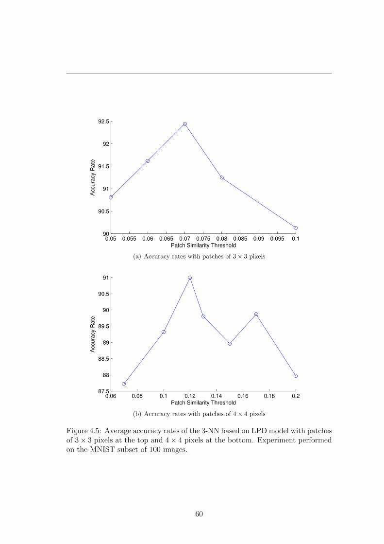
0.05 0.055 0.06 0.065 0.07 0.075 0.08 0.085 0.09 0.095 0.190

90.5

91

91.5

92

92.5


Accu

racy R

ate


0.06 0.08 0.1 0.12 0.14 0.16 0.18 0.287.5

88

88.5

89

89.5

90

90.5

91


Accura

cy R

ate



60

0.06 0.08 0.1 0.12 0.14 0.16 0.18 0.287.5

88

88.5

89

89.5

90

90.5

91


Accu

racy R

ate


0.08 0.1 0.12 0.14 0.16 0.18 0.287

88

89

90

91

92

93


Accu

racy R

ate



61

0.1 0.12 0.14 0.16 0.18 0.2 0.22 0.2485

86

87

88

89

90

91

92

93


Accu

racy R

ate


0.1 0.12 0.14 0.16 0.18 0.2 0.22 0.2485

86

87

88

89

90

91

92

93

94


Accura

cy R

ate



62

0.1 0.12 0.14 0.16 0.18 0.2 0.22 0.2485

86

87

88

89

90

91

92


Accu

racy R

ate


0.1 0.12 0.14 0.16 0.18 0.2 0.22 0.2485

85.5

86

86.5

87

87.5

88

88.5

89


Accu

racy R

ate


Figure 4.8: Average accuracy rates of the 3-NN based on LPD model with patchesof 9×9 pixels at the top and 10×10 pixels at the bottom. Experiment performedon the MNIST subset of 100 images.

63

Table 4.1: Results of the experiment performed on the MNIST subset of 300images, using the 3-NN based on LPD model with patches ranging from 2 × 2pixels to 9× 9 pixels. Reported accuracy rates are averages of 10 runs.

Patch size Patch similarity threshold Accuracy

2× 2 0.06 89.25%3× 3 0.07 90.68%4× 4 0.12 92.50%5× 5 0.17 91.53%6× 6 0.17 91.45%7× 7 0.15 91.44%8× 8 0.18 90.38%9× 9 0.18 89.89%

for the next experiments. Thus, LPD based on patches of 4 × 4 pixels will be

used.

It is interesting to mention that the computational time of LPD is proportional

to the patch similarity threshold. More precisely, a higher similarity threshold

will give a higher probability of finding similar patches sooner, thus reducing the

number of steps of the spatial search. However, the patch similarity threshold

should be adjusted with respect to the accuracy of the LPD. Consequently, the

rest of the experiments are conducted with a patch similarity threshold of 0.12

and 0.125, which are selected to obtain the highest accuracy with patches of 4×4

pixels. The similarity threshold of 0.125 is used for the heavy computational

experiments to slightly speed up the computation without affecting the accuracy

level.

Another parameter that needs to be tuned is the maximum offset radius.

Several experiments were performed with various maximum offsets values such as

5, 10, 15, and 20 pixels. These experiments were performed by keeping the rest

of the parameters unchanged. Patches of 4× 4 pixels and a similarity threshold

of 0.12 were used. The results with various maximum offsets are presented in

Table 4.2. The maximum offset can be adjusted to optimize the trade-off between

accuracy and time. Table 4.2 shows the average time needed to compute the

dissimilarity between two images. The reported average times were measured

on a computer with Intel Core i7 2.3 GHz processor and 8 GB of RAM memory

64

2 3 4 5 6 7 8 989

89.5

90

90.5

91

91.5

92

92.5

Accura

cy R

ate

Patch Size

Figure 4.9: Average accuracy rates of the 3-NN based on LPD model with patchesranging from 2× 2 pixels to 9× 9 pixels. Experiment performed on the MNISTsubset of 300 images.

using a single Core. The best time is obtained using a maximum offset of 5 pixels,

while the best accuracy (92.50%) is obtained using a maximum offset of 15 pixels.

Finally, the maximum offset chosen for the rest of the experiments is 15 pixels,

which is close to half the height or width of the MNIST images.

Table 4.2: Results of the experiment performed on the MNIST subset of 300images, using various maximum offsets, patches of 4 × 4 pixels, and a similaritythreshold of 0.12. Reported accuracy rates are averages of 10 runs. The timeneeded to compute the pairwise dissimilarity is measured in seconds.

Maximum offset Accuracy Average time per pair

5 90.21% 0.11 seconds10 92.11% 0.16 seconds15 92.50% 0.19 seconds20 91.98% 0.23 seconds

65

4.3.4 Baseline Experiment

The 3-NN classifier based on the LPD measure is compared with a baseline k-NN

classifier. The 3-NN based on the euclidean distance measure (L2-norm) between

input images is the chosen baseline classifier. In [LeCun et al., 1998] an error rate

of 5.00% on the regular test set with k = 3 for this classifier is reported. Other

studies [Wilder, 1998] report an error rate of 3.09% on the same experiment. The

experiment was recreated in this work, and an error rate of 3.09% was obtained.

The goal of this experiment is to prove that LPD can successfully be used as

a distance measure for images and that it has good results. The two classifiers,

that are distinct only by the metric used, are compared using the first 100, 300

and 1000 images extracted from the MNIST data set. These subsets contain

randomly distributed digits from 0 to 9 produced by different writers. Since the

number of samples in each subset is relatively small, the tests were performed

using the 10-fold cross-validation procedure which is repeated 10 times, in order

to obtain the final accuracy rates.

Table 4.3 compares the accuracy of the baseline 3-NN classifier with the accu-

racy of the 3-NN classifier based on LPD. Results are reported on all the MNIST

subsets of 100, 300 and 1000 samples, respectively. For all these subsets, the ac-

curacy of LPD was obtained with patches of 4×4 pixels and a similarity threshold

of 0.12.

Table 4.3: Baseline 3-NN versus 3-NN based on LPD. Both the accuracy rate andstandard deviation is reported for MNIST subsets of 100, 300 and 1000 images.

Number of samples Baseline 3-NN 3-NN + LPD

100 73.33%± 9.68% 87.53%± 7.38%300 83.19%± 5.47% 92.50%± 4.23%1000 87.12%± 2.59% 95.53%± 1.78%

The first test case requires only 100 images, but in order to obtain a more ac-

curate result, the first 200 examples from the MNIST training set were extracted

and divided into two subsets of 100 images each. The classification methods were

applied on both subsets, and the reported accuracy rates were averaged on the

two subsets of 100 samples. The baseline 3-NN classifier has an average accuracy

66

of 73.33%. The 3-NN classifier based on LPD has an average accuracy of 87.53%,

which represents an improvement of 14.20% over the baseline. The next test case

uses 300 images. This time, the baseline classifier has an accuracy of 83.19%. By

using LPD, an accuracy of 92.11% is obtained, which is 9.31% over the baseline.

The third test case uses 1000 images. The accuracy obtained with the baseline

classifier in the third test case is 87.12%. Again, the 3-NN classifier based on LPD

performs better than the baseline with an accuracy of 95.53%. This represents

an improvement of 8.41%.

One can observe that both classifiers have an increased accuracy when the

number of samples is larger. The baseline method has a 9.86% improvement from

100 images to 300 images, while the classifier based on LPD has an improvement

of 4.97%. A similar improvement in accuracy, from 300 to 1000 images, can be

observed. The baseline is 3.93% better and the classifier based on LPD is 3.03%

better.

In all test cases the 3-NN classifier based on LPD outperforms the baseline

3-NN classifier. It is worth pointing out that the accuracy of the classifier based

on LPD, that is trained and tested on 1000 images (95.53%), gets very close to

the accuracy of the baseline classifier (96.91%) trained on the full MNIST data

set with 60, 000 images and tested on other 10, 000 images.

Note that according to the standard deviations presented in Table 4.3, one

can state with confidence that the results of the 3-NN based on LPD are better

than the baseline classifier. A student test was performed on the results obtained

on 1000 images by the 3-NN based on LPD classifier on one hand, and by the

baseline classifier on the other hand. The null hypothesis, that obtained results

are independent random samples from normal distributions with equal means and

equal variances, was rejected with a 99% confidence interval.

The pairwise similarity matrix could reveal subtle characteristics of the sim-

ilarity or dissimilarity function. To analyze the LPD measure in more depth,

the pairwise similarity matrix produced by the LPD measure is compared with

the pairwise euclidean distance matrix. Figure 4.10 shows the similarity matrix

obtained with LPD, and Figure 4.11 shows the euclidean distance matrix. The

two matrices are obtained on the same MNIST subset of 1000 images. For the

visual analysis of the similarity matrices, the samples are sorted by class labels in

67

Figure 4.10: Similarity matrix based on LPD with patches of 4 × 4 pixels anda similarity threshold of 0.12, obtained by computing pairwise dissimilarities be-tween the samples of the MNIST subset of 1000 images.

ascending order, starting with digit 0 and finishing with digit 9. Darker regions

indicate higher similarity, and lighter regions indicate lower similarity. In both

matrices, darker squares that indicate higher within-class similarities on the prin-

cipal diagonal can be observed. The samples that represent the digit 1 are the

most distinct from the other samples, in both matrices. However, the similarity

matrix based on LPD has other distinctive classes such as digit 4, digit 6, digit

7 and digit 9. On the other hand, in the euclidean distance matrix the classes

represented by digits 4 and 6 are also distinctive, but there is a greater amount of

confusion between the digit 7 and digit 9 classes. The two measures also seem to

mix up the digit 3 and digit 5 classes. Overall, the similarity matrices are fairly

similar with each other, but the matrix produced by LPD seems to be slightly

better. This is confirmed by the experiments presented in Table 4.3.

68

Figure 4.11: Euclidean distance matrix based on L2-norm, obtained by computingpairwise distances between the samples of the MNIST subset of 1000 images.

4.3.5 Kernel Experiment

The goal of this experiment is to combine LPD with state of the art learning

techniques (such as kernel methods) instead of the simple k-NN model, in order

to improve the accuracy level. Therefore, the experiments on the MNIST subsets

of 300 and 1000 images are repeated using SVM and Kernel Ridge Regression.

In Table 4.4 the accuracy rates of the 3-NN, SVM and KRR classifiers based

on LPD are compared with the accuracy rates of the standard SVM and KRR

methods. The kernel parameter σ is chosen to be equal 1000, since the square

root of 1000 is close to the size of the images, which are 28 × 28 pixels. Results

are reported on 300 and 1000 examples from the MNIST data set using 10-fold

cross-validation. The last test case (identified as 300/700) divides the 1000 images

into two sets: 300 images for training and 700 images for testing. The reported

69

results on this last test case are on the 700 images used for testing.

Table 4.4: Accuracy rates of several classifiers based on LPD versus the accu-racy rates the standard SVM and KRR. Tests are performed on 300 and 1000images using cross-validation (CV), respectively. Another test is performed usinga 300/700 split.

Method 300 CV 1000 CV 300/700

SVM 86.33% 91.30% 81.71%KRR 86.19% 91.58% 79.86%3-NN+LPD 92.11% 95.53% 91.78%SVM+LPD 94.33% 96.90% 94.28%KRR+LPD 93.04% 96.16% 92.57%

As expected, the results slightly improve when a better learning method (such

as SVM or KRR) is used rather than a simple 3-NN model. But what shows that

LPD is very powerful, is that a simple 3-NN classifier based on LPD surpasses

the standard SVM and KRR classifiers. The best results is obtained using the

SVM combined with the LPD measure (96.90%).

The 300/700 test case shows that LPD is a robust dissimilarity measure be-

cause the results obtained on the test set of 700 images are very close to the

results reported using 10-fold cross-validation. For example, the results of the

SVM based on LPD drop from 94.33% on 300 images (using cross-validation) to

only 94.28% on the other 700 images. On the other hand, the performance of

the standard SVM and KRR classifiers reported on the 300/700 test case is much

worse than the performance reported using 10-fold cross-validation.

4.3.6 Difficult Experiment

In [Vapnik & Vashist, 2009] the learning using privileged information paradigm

is introduced. The problem of classifying images of digits 5 and 8 in the MNIST

database is considered as an application. To make it more difficult, the authors

have resized the digits from 28 × 28 pixel to 10 × 10 pixel images. The authors

have used 100 samples of 10 × 10 pixel images as the training set, 4002 samples

as the validation set (for tuning the parameters of SVM and SVM+) and the rest

70

of 1866 samples as the test set. The same split of the data set is used in this

experiment.

The results of the standard SVM (based on euclidean distance) and the

dSVM+ reported by [Vapnik & Vashist, 2009] are compared with three classi-

fiers based on LPD. In Table 4.5 the accuracy rates of the SVM and dSVM+

classifiers are compared with the accuracy rates of the k-NN, SVM and KRR

classifiers based on LPD. The number of neighbors of the k-NN model is 5, and

it was chosen for best performance on the validation set. The parameters of the

LPD are also tuned on the validation set. The best accuracy is obtained with

patches of 3 × 3 pixels and a similarity threshold of 0.11. Since the images are

smaller than in the previous experiments, it is natural to obtain better perfor-

mance with smaller patches of 3× 3 pixels instead of 4× 4 pixels. The values of

the kernel parameter σ is 100, because the images are 10× 10 pixels in this case.

Table 4.5: Comparison of several classifiers (some based on LPD). Results for thedifficult experiment on 1866 test images.

SVM dSVM+ 5-NN + LPD SVM + LPD KRR + LPD

92.50% 94.60% 91.32% 95.10% 95.00%

In this experiment one can observe that a simple 5-NN classifier based on

LPD is very close to the standard SVM (the difference is only 1.18%), showing

again that LPD is a very powerful dissimilarity.

The dSVM+ gains more than 2% in accuracy over the standard SVM by using

privileged information in the training process. The dSVM+ classifier is surpassed

by the SVM and KRR classifiers that are based on the LPD measure. Note that

these classifiers (SVM + LPD and KRR + LPD) use no privileged information.

This shows that using a better dissimilarity measure (such as LPD) is sometimes

more important than using privileged information to improve accuracy.

4.3.7 Filter-based Nearest Neighbor Experiment

The results presented in Section 4.3.4 look promising, but LPD should be tested

on the entire MNIST data set for a strong conclusion of its performance level.

71

The problem of the k-NN classifier based on LPD is that it is not feasible for

very large data sets, since it takes too much time to compute all the pairwise

dissimilarities. To avoid this problem, local learning methods that speed-up the

learning algorithm can be used. Therefore, LPD is plugged into different local

learning methods and used for image classification.

In this experiment, the local learning classifier employed for tests on the en-

tire MNIST data set is the filter-based k-NN model. This classifier was chosen

because it reflects the characteristics of the LPD measure. For the filter-based

k-NN approach, the idea is to filter the nearest K neighbors using the standard

euclidean distance measure (that is much faster to compute). Next, it selects

the nearest k neighbors from those K images using LPD. The two-step selection

process is much faster to compute on a large data set (such as the MNIST data

set) than a standard k-NN based entirely on LPD. Results show that this method

can improve accuracy and is among the top 4 k-NN models that reported results

on the MNIST data set.

The k-NN based on LPD with filtering is compared with two other k-NN

classifiers. One is the k-NN based on the euclidean distance measure (L2-norm)

between input images. This is the baseline classifier. In [LeCun et al., 1998],

an error rate of 5.00% was reported on the regular test set with k = 3 for this

classifier, while other studies [Wilder, 1998] report an error rate of 3.09% on the

same experiment. The results obtained in this work also show an error rate of

3.09% on this baseline experiment. The second classifier is the k-NN based on

Tangent Distance [Simard et al., 1996]. Tangent distance is insensitive to small

distortions and translations of the input image. The error rate of this classifier

reported in [LeCun et al., 1998] is 1.1%, but it was necessary to additionally

process the images by subsampling to 16×16 pixels in order to obtain the reported

error rate.

The accuracy of the k-NN based on LPD depends very much on the filtering.

Take into account that the nearest K images are selected using the euclidean

distance in the filtering phase. If K is close to k, a very fast classifier is obtained,

but its accuracy will be near the baseline k-NN. As K increases the accuracy

improves, but the method also becomes slower (since it has to compute LPD

between more images than it was before). If K is equal to the number of training

72

examples, there is no filtering at all and the highest accuracy is obtained. How-

ever, the time to compute k-NN based on LPD with no filtering is too high to

be considered. The idea is to choose an optimal K in order to obtain a trade-off

between accuracy and time. Table 4.6 shows the error rate and the execution

time of the 3-NN classifier based on LPD with filtering for several K values. The

time was measured on a computer with Intel Core Duo 2.26 GHz processor and 4

GB of RAM memory using a single Core. Empirical results show that an optimal

K would be somewhere between 100 and 500. When K is 100, approximately 8

seconds are needed to assign a label to a test image. This is reasonable for a real-

time application, since computing LPD on GPU and adding parallel processing

into assigning a label can improve the time even further.

Table 4.6: Error and time of 3-NN classifier based on LPD with filtering.

K Error Average time per test image Overall time

3 2.73% 2.2 seconds 6 hours10 1.78% 2.6 seconds 7 hours30 1.45% 3.7 seconds 10 hours50 1.38% 4.8 seconds 13 hours

100 1.26% 7.6 seconds 21 hours200 1.15% 13.2 seconds 36 hours500 1.09% 30.5 seconds 84 hours

1000 1.05% 58.8 seconds 162 hours

Looking at how the error gets lower as K increases, one can observe that the

error tends to stabilize at some point. In other words, the error rate will not

drop anymore after a certain K value. That error rate represents the actual error

rate of a 3-NN classifier based on LPD (without filtering). The limitation of

LPD induces this error, but what exactly is this error rate? Figure 4.12 gives an

overview of this phenomenon and a hint about the point where the error stabilizes

for both 3-NN and 6-NN classifiers. In order to make a prediction about the

stabilization point of the error, the stability of the k-NN with filtering needs to

be studied as K varies. It is clear from Figure 4.12 that the error drops with

no variation when K increases. But increasing K may induce a misclassification

on some test images (even if, overall, more images are classified correctly). For

73

0 100 200 300 400 500 600 700 800 900 10001

1.2

1.4

1.6

1.8

2

2.2

2.4

2.6

2.8

Err

or

rate

Number of nearest neighbours used for filtering

Figure 4.12: Error rate drops as K increases for 3-NN (◦) and 6-NN (�) classifiersbased on LPD with filtering.

K = 100, 200, ..., 1000, the set of misclassified images for a certain value of K

always includes the set of misclassified images for a greater value of K. Thus, the

method has very stable behavior as K varies. In these circumstances, the error

rates of the 3-NN and 6-NN classifiers based on LPD (without filtering) can be

obtained by testing the classifiers only on the previously misclassified images. By

doing so, an error rate of 1.03% is obtained for the 3-NN classifier and an error

rate of 0.98% is obtained for the 6-NN classifier. These error rates are based only

on a statistical proof. But as stated before, the real proof (that of testing the

3-NN and 6-NN classifiers with no filtering on all test images) is not practical

74

from the time perspective. The obtained error rates only give a good indication

of the actual ones, and they are not compared with the error rates of the other

k-NN classifiers based on euclidean and tangent distance, respectively.

The confusion matrix of the 3-NN based on LPD with filtering using K = 50

is presented in Table 4.7. The confusion matrix shows that most of the digits are

fairly well distinguished by LPD, but some confusions stand out from the rest.

The greatest confusions are between digits 4 and 9, between digits 3 and 5, and

between digits 2 and 7, respectively. From the total amount of 138 misclassified

images, there are 11 samples of digit 7 classified as digit 1, 10 samples of digit 2

classified as digit 7, and 10 samples of digit 4 classified as digit 9. The best per

class accuracy of the 3-NN model is on digit 1 (99.65%) and digit 0 (99.49%). On

the other hand, the worst accuracy is on digit 9 (97.82%) and digit 8 (97.95%).

Thus, LPD is better on recognizing digits 1 and 0 and slightly worse at recog-

nizing digits 9 and 8, despite the fact that there are not significant differences

between the per digit classification accuracy rates. Overall, the confusion matrix

shows that LPD is able to equally classify all the digits with only a few mistakes.

Actually, there are only 138 misclassified images from the total of 10, 000 samples.

Table 4.7: Confusion matrix of the 3-NN based on LPD with filtering usingK = 50.

Digits 0 1 2 3 4 5 6 7 8 9

0 975 1 1 0 0 1 1 1 0 0

1 0 1131 2 0 0 0 1 1 0 0

2 6 2 1013 0 0 0 1 10 0 0

3 0 0 1 994 1 6 0 5 1 2

4 0 4 0 0 963 0 4 0 1 10

5 1 0 0 4 1 883 1 0 1 1

6 2 3 0 0 2 1 950 0 0 0

7 0 11 3 1 0 0 0 1009 0 4

8 2 0 0 3 3 2 2 3 954 5

9 0 3 1 2 6 3 1 4 2 987

Table 4.8 compares error rates of the three k-NN classification methods (dis-

tinct only by the metric used) using the MNIST test set of 10, 000 samples. For

the k-NN classifier based on LPD with filtering, k = 3 and k = 6 are used.

75

The error rates of the k-NN models based on LPD are obtained using the nearest

K = 1000 images filtered by the euclidean distance. The LPD is based on patches

of 4 × 4 pixels and a similarity threshold of 0.125. The LPD parameter tuning

procedure is described in Section 4.3.3. The k-NN based on LPD with filtering

model has a better accuracy than the other k-NN models. In fact, it is among

the top 4 k-NN models that reported results on the MNIST data set. The 6-NN

classifier based on LPD with filtering has an error rate of only 1.01%. Note that

unlike the k-NN with filtering based on LPD, the other three methods from top

4 need additional preprocessing steps.

Table 4.8: Error rates on the entire MNIST data set for baseline 3-NN, k-NNbased on tangent distance and k-NN based on LPD with filtering.

Method Error

baseline 3-NN 3.09%k-NN + tangent distance 1.1%3-NN + LPD + filter 1.05%6-NN + LPD + filter 1.01%

4.3.8 Local Learning Experiment

Because LPD is computationally heavy, it is not feasible to compute a kernel

matrix with high dimensions. Even with a fast similarity measure, computing

and storing a large kernel matrix could pose a serious problem for the design and

implementation of a kernel classifier. Therefore, the use of kernel classifiers, such

as SVM and KRR based on LPD, on the entire MNIST data set should be avoided

as much as possible. Instead, kernel methods can be integrated into a local

learning algorithm. The proposed approach for this experiment is very similar

to the filter-based k-NN model. The filtering step remains unchanged. Thus,

the first step is to filter the nearest K neighbors using the standard euclidean

distance. The second step is to train a kernel classifier using only the filtered K

neighbors. A new classifier is trained for each test image. The classifier will be

used to predict only the label of the test image that was built for.

76

Before training the classifier, it is necessary to build a kernel matrix using

LPD. It is not feasible for a real-time application to build a K×K kernel matrix

for each test image, when K is larger than 100, especially if no GPU or parallel

processing is done. But, a large number of K neighbors is needed in order to

improve the accuracy of the kernel method. A feasible solution is to train a

kernel classifier only when a majority of images with the same label greater than

60% among the filtered K neighbors is not available, and use a k-NN model when

such a majority exists. There are two reasons for this approach. First, if such a

majority exists, the kernel method will be biased towards choosing the majority

class. Second, it is likely that a simple k-NN would also choose this majority

class that is probably the right one.

This local learning algorithm was tested on the MNIST data set. Using K =

200, it gives an error rate of 1.07%. From the 10, 000 test samples, 983 of them

had a majority class of less than 60% of the total 200 neighbors. For each of these

983 samples, a KRR classifier based on LPD was trained. The other test labels

were predicted using the 3-NN based on LPD. Note that the 3-NN with filtering

approach has an error rate of 1.15% for K = 200 and the local learning algorithm

is able to improve it to 1.07%. Another local learning algorithm, that uses SVM

instead of KRR, was tested without being able to improve the accuracy.

In conclusion, using kernel methods in a local learning context does not bring

a significant improvement in accuracy to the k-NN with filtering approach. How-

ever, the local learning algorithm proposed here can successfully be used for

handwritten digit recognition. It also benefits from a much faster computational

time compared to standard kernel methods based on LPD.

4.3.9 Birds Experiment

In this experiment, LPD is used to classify a more general type of images available

in the Birds data set. Several k-NN models based on different distance measures

are compared. The first k-NN model uses the Bhattacharyya coefficient to com-

pare spatiograms of HSV values extracted from images. This improved measure

of comparing spatiograms is proposed in [Conaire et al., 2007]. The second k-NN

model is based on the mean euclidean distance measure (L1-norm) between input

77

images. Another two k-NN classifiers based on LPD are tested. One of them uses

a slightly modified version of the LPD algorithm, in that it determines similar

patches using the mean euclidean distance corresponding to the L1-norm, which

seems to work better than the L2-norm on this experiment. The other one uses

a fast version of the LPD algorithm that skips half of the comparisons between

patches.

For both the euclidean distance measure and the LPD measure, images from

the Birds data set need to be brought to the same size in order to be compared.

Thus, images are resampled to 100 × 100 pixels. To observe the difference be-

tween original and resized images, the k-NN model based on the Bhattacharyya

coefficient is tested on both types of images. The other k-NN models are tested

only on the resampled images, that are also converted to gray-scale. While the

method proposed by [Conaire et al., 2007] works on color images, the euclidean

distance and LPD are naturally computed on gray-scale images. Table 4.9 com-

pares the error rates of all these k-NN models. The empirical results show that

skipping overlapping patches does not affect the accuracy of LPD.

Table 4.9: Error rates of different k-NN models on Birds data set.

Method Preprocessing Error

5-NN + Bhattacharyya none 57.33%5-NN + Bhattacharyya resize 54.67%3-NN + euclidean resize, gray-scale 51.00%3-NN + LPD resize, gray-scale 30.33%3-NN + LPD + skip resize, gray-scale 30.33%

Next, three kernel methods based on the fast version of LPD (that skips half

of the comparisons between patches) are compared with the state of the art tex-

ton learning methods from [Lazebnik et al., 2005a]. The proposed kernel methods

based on LPD are the SVM, the KRR and the KDA classifiers. Table 4.10 com-

pares error rates of kernel methods based on LPD and texton learning methods.

The kernel methods based on LPD have an accuracy similar to some of the state

of the art methods. However, the proposed kernel methods are more time effi-

cient. In [Lazebnik et al., 2005a], a time of about 7 days for a single experiment

is reported, while the kernel methods based on LPD need about 4 days for the

78

Table 4.10: Error on Birds data set for texton learning methods of [Lazebniket al., 2005a] and kernel methods based on LPD.

Method Error

Naive Bayes 21.33%Exp. parts 7.67%Exp. relations 24.67%Exp. parts + relations 8.33%SVM + LPD + skip 27.33%KRR + LPD + skip 26.00%KDA + LPD + skip 24.33%

same experiment on an Intel Core Duo 2.26 GHz processor and 4 GB of RAM

memory. Note that error rates of all models based on LPD, used in this exper-

iment, are obtained with patches of 4 × 4 pixels and a similarity threshold of

0.15. The parameters were obtained by cross-validation on the training set. In

conclusion, the fast version of LPD can successfully be used as a kernel for image

classification.

4.4 Local Texton Dissimilarity

This section presents a novel texture dissimilarity measure based on textons,

termed Local Texton Dissimilarity (LTD). It represents a development adapted

to textures of the more general LPD measure. Instead of patches, LTD works

with textons, which are represented as a set of features extracted from image

patches. It is reasonable to work with textons rather than patches, since many

state of the art texture classification methods are based on textons. Some of

these state of the art methods are presented in Section 4.4.1.

The algorithm proposed in [Dinu et al., 2012] and presented in Section 4.1.1

compares image patches by using the mean euclidean distance. LTD differs in the

way it compares these patches. First, texture specific features are extracted from

each patch. A patch can then be represented by a feature vector. Similar patches

are represented through similar features. Thus, image patches are implicitly

quantized into textons. Textons are compared using the Bhattacharyya coefficient

79

between their feature vectors. Section 4.4.2 describes the features extracted from

image patches, while the LTD algorithm [Ionescu et al., 2014] is presented in

Section 4.4.3.

4.4.1 Texton-based Methods

The work of [Lazebnik et al., 2005b] presents a texture representation that is

invariant to geometric transformations based on descriptors defined on affine in-

variant regions. A probabilistic part-based approach for texture and object recog-

nition is presented in [Lazebnik et al., 2005a]. Textures are represented using a

part dictionary obtained by quantizing the appearance of salient image regions.

In [Leung & Malik, 2001], texture images are classified by using 3D textons,

which are cluster centers of filter response vectors corresponding to different light-

ing and viewing directions of images. The work of [Varma & Zisserman, 2005]

models textures by the joint distribution of filter responses. This distribution is

represented by the frequency histogram of textons. For most texton based tech-

niques, the textons are usually learned by k-means clustering. In [Xie et al., 2010],

a novel texture classification method via patch-based sparse texton learning is

proposed. The dictionary of textons is learned by applying sparse representation

to image patches in the training data set.

4.4.2 Texture Features

Before computing LTD between texture images, a set of several image features

is extracted from each patch to obtain the texton representation. There are 9

features extracted from patches, that are described next. An interesting remark

is that the more features are added to the texton representation, the better the

accuracy of the LTD method gets. However, a lighter representation, such as the

one based on 9 features, results in a faster and more efficient algorithm. One

may choose to add or remove features in order to obtain the desired trade-off

between accuracy and speed. The texton representation based on the 9 features

that are about to be presented next gives state of the art accuracy levels in several

experiments presented in Section 4.5.

80

The first two statistical features extracted are the mean and the standard

deviation. These two basic features can be computed indirectly, in terms of

the image histogram. The shape of an image histogram provides many clues to

characterize the image, but the features obtained from an image histogram are

not always adequate to discriminate textures, since they are unable to indicate

local intensity differences.

One of the most powerful statistical methods for textured image analysis is

based on features extracted from the Gray-Level Co-Occurrence Matrix (GLCM),

proposed in [Haralick et al., 1973]. The GLCM is a second order statistical

measure of image variation and it gives the joint probability of occurrence of

gray levels of two pixels, separated spatially by a fixed vector distance. Smooth

texture gives a co-occurrence matrix with high values along diagonals for small

distances. The range of gray level values within a given image determines the

dimensions of a co-occurrence matrix. Thus, 4 bits gray level images give 16× 16

co-occurrence matrices. Relevant statistical features for texture classification can

be computed from a GLCM. The features proposed by [Haralick et al., 1973],

which show a good discriminatory power, are the contrast, the energy, the entropy,

the homogeneity, the variance and the correlation. Among these features that

show a good discriminatory power, LTD uses only four of them, namely the

contrast, the energy, the homogeneity, and the correlation.

Another feature that is relevant for texture analysis is the fractal dimension.

It provides a statistical index of complexity comparing how detail in a fractal

pattern changes with the scale at which it is measured. The fractal dimension

is usually approximated. The most popular method of approximation is box

counting [Falconer, 2003]. The idea behind the box counting dimension is to

consider grids at different scale factors over the fractal image, and count how

many boxes are filled over each grid. The box counting dimension is computed

by estimating how this number changes as the grid gets finer, by applying a box

counting algorithm. An efficient box counting algorithm for estimating the fractal

dimension was proposed in [Popescu et al., 2013b]. The idea of the algorithm is

to skip the computation for coarse grids, and count how many boxes are filled

only for finer grids. LTD includes this efficient variant of box counting in the

texton representation.

81

The work of [Daugman, 1985] found that cells in the visual cortex of mam-

malian brains can be modeled by Gabor functions. Thus, image analysis by the

Gabor functions is similar to perception in the human visual system. A set of Ga-

bor filters with different frequencies and orientations may be helpful for extracting

useful features from an image.

The local isotropic phase symmetry measure (LIPSyM) presented in [Kuse

et al., 2011] takes the discrete time Fourier transform of the input image, and

filters this frequency information through a bank of Gabor filters. The work

of [Kuse et al., 2011] also notes that local responses of each Gabor filter can be

represented in terms of energy and amplitude. Thus, Gabor features, such as

the mean-squared energy and the mean amplitude, can be computed through

the phase symmetry measure for a bank of Gabor filters with various scales and

rotations. These features are relevant because Gabor filters have been found to

be particularly appropriate for texture representation and discrimination.

Finally, textons are represented by the mean and the standard deviation of the

patch, the contrast, the energy, the homogeneity, and the correlation extracted

from the GLCM, the (efficient) box counting dimension, and the mean-squared

energy and the mean amplitude extracted by using Gabor filters. These texton

features can be extracted from all images before comparing them with LTD. Thus,

the LTD computation can be divided into two main steps, one for texton feature

extraction, and one for dissimilarity computation. After the feature extraction

step, features should be normalized. In practice, the described features work best

on squared image patches of a power of two size.

4.4.3 Local Texton Dissimilarity Algorithm

To compute LTD between two gray-scale texture images, the idea is to sum up

all the offsets of similar textons between the two images. The LTD algorithm is

briefly described next. For every texton in one image, the algorithm searches for

a similar texton in the other image. First, it looks for similar textons in the same

position in both textures. If those textons are similar, it sums up 0 since there

is no spatial offset between textons. If the textons are not similar, the algorithm

starts exploring the vicinity of the initial texton position in the second image to

82

find a texton similar to the one in the first image. If a similar texton is found

during this process, it sums up the offset between the two textons. The spatial

search goes on until a similar texton is found or until a maximum offset is reached.

The maximum texton offset must be set a priori. The computation of LTD is

similar the algorithm presented in Section 4.1.2. In practice, the computation

described above is too heavy for a large set of images. To speed up the algorithm,

textons are extracted and compared using a dense grid over the image. This is

similar to the idea of skipping overlapping patches to optimize LPD.

Algorithm 2 computes the LTD between gray-scale texture images img1 and

img2, using the underlying Bhattacharyya coefficient to compute the similarity

between texton feature vectors.

Algorithm 2 Local Texton Dissimilarity

Input:

img1 – a gray-scale texture image of h1 × w1 pixels;

img2 – another gray-scale texture image of h2 × w2 pixels;

n – the number of features that represent a texton;

gridStep – the skip step that generates a dense grid over the image;

offsetStep – the skip step used for comparing patches at different offsets;

w – a vector of feature weights (some features can be more important than

others);

th – the texton similarity threshold.

Initialization:

dist = 0

h = min{h1, h2} − p+ 1

w = min{w1, w2} − p+ 1

Computation:

for x = 1:gridStep:h

for y = 1:gridStep:w

get textonleft at position (x, y) in img1

d = 0

while did not find texton at offset d similar to textonleft

get textonright at offset d from position (x, y) in img2

83

s1 =1

n

n∑i=1

(wi ·

√textonlefti − wi ·

√textonrighti

)2

if s1 < th

dist = dist+ d

break

endif

if all textons at offset d were tested

d = d+ offsetStep

endif

endwhile

get textonright at position (x, y) in img2

d = 0

while did not find texton at offset d similar to textonright

get textonleft at offset d from position (x, y) in img1

s2 =1

n

n∑i=1

(wi ·

√textonrighti − wi ·

√textonlefti

)2

if s2 < th

dist = dist+ d

break

endif

if all textons at offset d were tested

d = d+ offsetStep

endif

endwhile

endfor

endfor

Output:

dist – the dissimilarity between textures img1 and img2.

Algorithm 2 needs a few input parameters besides the two images. The num-

ber of features gives the size of the feature vector. In this work, the 9 features

described in Section 4.4.2 were used. In the algorithm, textoni represents the i-th

84

feature of the texton representation, and wi represents the weight associated to

the i-th feature.

The results of the LTD algorithm can further be improved by adding more fea-

tures or probably by using completely different features. The parameter that gen-

erates a dense grid over the image, and the skip step used for comparing patches

at different offsets are used to speed up the LTD algorithm without losing too

much accuracy. These parameters induce a sparse representation of the images.

Using a sparse representation is indeed necessary, since patch-based algorithms

are heavy to compute with current computers because they usually manipulate

millions of patches [Barnes et al., 2011]. The texton similarity threshold is a

value in the [0, 1] interval, that determines when two textons are considered to

be similar. All these parameters need to be adjusted with regard to the data set

size and to the image dimensions, in order to obtain a good trade-off between

accuracy and speed.

4.5 Texture Experiments and Results

In the experiments, LTD is evaluated with different kernel methods to show that

good performance levels are due to the use of LTD. Two data sets of texture

images are used to assess the performance of several kernel methods based on

LTD, namely the Brodatz data set and the UIUCTex data set. All the experi-

ments presented in this work aim at showing that LTD has general applications

for texture classification, and that LTD is indeed a robust dissimilarity measure.

A potential application of LTD discussed in this work is biomass type identi-

fication. A method to determine the biomass type has practical motivations for

the biomass industry. Such methods are of great importance when one in the

biomass industry needs to produce another energy product, such as biofuel or

bioenergy, for example. Is the type of biomass appropriate to efficiently obtain

the bioproduct? Is the biomass conversion method the right one for this type

of biomass? Answering such questions can help reduce the operating costs of

biomass power plants. But, these questions can be answered with the help of a

biomass type identification method, such as the one presented in this chapter.

Indeed, LTD can be used in combination with several machine learning methods

85

for biomass texture classification. Therefore, another classification experiment is

conducted on a data set of biomass texture images.

It is important to mention that, in a general sense, biomass refers to the bio-

logical material from living, or recently living organisms. In this work, the term

biomass refers to a renewable energy source, that can be directly converted into

another type of energy product. The Biomass Texture data set used in this thesis

is a collection of close-up photos of different samples of three types of biomass:

municipal solid waste, corn, and wheat. The goal is to build a classifier that is

able to distinguish between these three types of biomass. This is a totally differ-

ent approach and understanding of the biomass classification problem, compared

to other researches. Usually, biomass classification refers to land cover type or

forest biomass classification. Land cover classification [Dash et al., 2007] and

forest biomass estimation [Wulder et al., 2008] are active research topics in the

area of remote sensing. The work of [Hoekman & Quinnones, 2000] shows that

remotely sensed image classification systems may be designed to accurately mon-

itor processes of deforestation, land and forest degradation and secondary forest

regrowth.


The first data set used for testing the dissimilarity presented in this paper is

the Brodatz data set [Brodatz, 1966]. This data set is probably the best known

benchmark used for texture classification, but also one of the most difficult, since

it contains 111 classes with only 9 samples per class. Samples of 213× 213 pixels

are cut using a 3 by 3 grid from larger images of 640 × 640 pixels. Figure 4.13

presents three sample images per class of three classes randomly selected from

the Brodatz data set.

The second experiment is conducted on the UIUCTex data set of [Lazebnik

et al., 2005b]. It contains 1000 texture images of 640 × 480 pixels representing

different types of textures such as bark, wood, floor, water, and more. There are

25 classes of 40 texture images per class. Textures are viewed under significant

scale, viewpoint and illumination changes. Images also include non-rigid defor-

mations. This data set is available for download at http://www-cvr.ai.uiuc.

86

http://www-cvr.ai.uiuc.edu/ponce_grp


Figure 4.13: Sample images from three classes of the Brodatz data set.

edu/ponce_grp. Figure 4.14 presents four sample images per class of four classes

representing bark, brick, pebbles, and plaid.

The third experiment is conducted on a data set of biomass texture images

available at http://biomass.herokuapp.com. It contains 270 images of 512×512

pixels representing close up photos of three types of biomass resulted after the

processing of wheat, municipal waste and corn, respectively. Photos where taken

at different zoom levels, under various lighting conditions. Figure 4.15 shows a

few random samples of biomass images from this data set. There are 90 images

per class. The goal is to build a classifier that is able to identify the three types

of biomass: wheat, waste, and corn, respectively.

87



http://biomass.herokuapp.com

Figure 4.14: Sample images from four classes of the UIUCTex data set. Eachimage is showing a textured surface viewed under different poses.

4.5.2 Learning Methods

To use LTD for texture classification, it should be plugged into a similarity-

based learning method. Several similarity-based classifiers are proposed. The

first classifier used in the experiments is the k-NN. It was chosen because it

directly reflects the discriminatory power of the dissimilarity measure. Several

state of the art kernel methods are also used, namely the KRR, the SVM, the

KDA, and the KPLS. LTD can be transformed into a similarity measure by using

88

Figure 4.15: Sample images from the Biomass Texture data set.

the Gaussian-like kernel, in a similar fashion to LPD:

k(img1, img2) = exp

(−LTD(img1, img2)

2σ2

),

where img1 and img2 are two gray-scale texture images. The parameter σ is

usually chosen to match the number of features so that values of k(img1, img2)

are well scaled.

4.5.3 Brodatz Experiment

The baseline method proposed for this experiment is a 1-NN model that is based

on the Bhattacharyya coefficient computed on the 9 texture features described

in Section 4.4.2. The features are extracted from entire images. The second

proposed model is a 1-NN classifier based on LTD. The baseline is useful to

assess the performance gained by the use of LTD. The other proposed classifiers

89

are the KRR, the KPLS, the SVM and the KDA, all based on LTD. The KDA

method is particularly suitable for problems with many classes, such as Brodatz.

In [Lazebnik et al., 2005b], the accuracy rate reported on the Brodatz data set

using 3 training samples per class is 88.15%. Table 4.11 compares accuracy rates

of the proposed classifiers with the accuracy rate of the state of the art method

described in [Lazebnik et al., 2005b], using the same setup with 3 random samples

per class for training. The accuracy rates presented in Table 4.11 are actually

averages of accuracy rates obtained over 20 runs for each method. The 1-NN

based on LTD model has a far better accuracy than the baseline, proving that

LTD helps the learning method to achieve better results. All the kernel methods

based on LTD are above the state of the art classifier. The best classifier among

them is KDA, which has an accuracy of 90.87%. It is 5.46% better than the 1-NN

based on LTD, and 2.72% better that the state of the art method. Therefore, it

seems that LTD is a good dissimilarity measure for texture classification. Com-

bined with suitable learning methods, LTD gives results comparable to state of

the art method. Despite better texture classification methods exist [Zhang et al.,

2007], the classifiers based on LTD can also be improved by adding more features

to the texton representation.

Table 4.11: Accuracy rates on the entire Brodatz data set using 3 random samplesper class for training. Learning methods based on LTD are compared with thestate of the art method.

Method Accuracy

baseline 1-NN 77.68%Best of [Lazebnik et al., 2005b] 88.15%1-NN + LTD 85.41%KRR + LTD 89.43%SVM + LTD 89.48%KPLS + LTD 89.57%KDA + LTD 90.87%

In this experiment, LTD was computed on patches of 32 × 32 pixels, using

a similarity threshold of 0.02 and a maximum offset of 80 pixels. Patches were

extracted on a dense grid with a gap of 32 pixels. Feature weighting can improve

90

accuracy by almost 1%. Thus, adjusting feature weights is not very important,

but it helps the classifier. However, the feature weights were manually adjusted

to increase the importance of Gabor features and fractal dimension by a factor of

two, and to decrease the importance of the mean and the standard deviation by

a factor of two. The weights were tuned on the baseline 1-NN model, which also

uses feature weighting in the reported results. The parameter σ of the LTD kernel

was chosen to be 10−3. All the parameters were chosen by cross-validation on a

subset of the Brodatz data set. An interesting remark is that these parameters

do not change by too much on the other data sets.

Using these parameters, it takes less than 1 second to compute LTD between

two images on a computer with Intel Core Duo 2.26 GHz processor and 4 GB of

RAM memory using a single Core. Reported accuracy rates can be improved by a

few percents using a more dense grid and a greater maximum offset, but the LTD

computation will also take more time. However, with the current parameters,

LTD is much faster than LPD, which takes about 5 minutes to compare two

images from the Brodatz data set with similar parameters, without skipping

overlapping patches.

The pairwise similarity matrix of LTD between Brodatz samples, shown in

Figure 4.16, is analyzed next. It reveals that the LTD measure is able to dis-

criminate most of the classes from the Brodatz data set. This fact is indicated in

Figure 4.16 by the tiny darker squares along the diagonal of the similarity matrix.

These squares represent a higher within class similarity. The fact that LTD dis-

criminates most of the classes by itself is also suggested by the good performance

of the 1-NN model based on LTD, compared to the 7.73% lower performance of

the baseline 1-NN.

4.5.4 UIUCTex Experiment

In this experiment, the same classifiers evaluated on the Brodatz data set are

also evaluated on the UIUCTex data set. More precisely, the evaluated classifiers

are the baseline 1-NN model based on the Bhattacharyya coefficient, the 1-NN

classifier based on LTD, and the kernel classifiers based on LTD, namely the

KRR, the KPLS, the SVM, and the KDA. These classifiers are compared with

91

Figure 4.16: Similarity matrix based on LTD with patches of 32 × 32 pixelsand a similarity threshold of 0.02, obtained by computing pairwise dissimilaritiesbetween the texture samples of the Brodatz data set.

the state of the art classifier of [Lazebnik et al., 2005b]. The best accuracy level

of the state of the art classifier on the UIUCTex data set, reported in [Lazebnik

et al., 2005b] using 20 training samples per class, is 97.41%.

Table 4.12 compares accuracy rates of the classifiers based on LTD with the

accuracy rate of the state of the art classifier of [Lazebnik et al., 2005b], using

the same setup with 20 random samples per class for training. The accuracy

rates are averaged over 20 runs for each method. The accuracy of the 1-NN

model based on LTD is 9.32% better than accuracy of the baseline 1-NN, proving

again that LTD is able to achieve much better results. However, the accuracy

of the 1-NN based on LTD is far behind the state of the art classifier. Even the

92

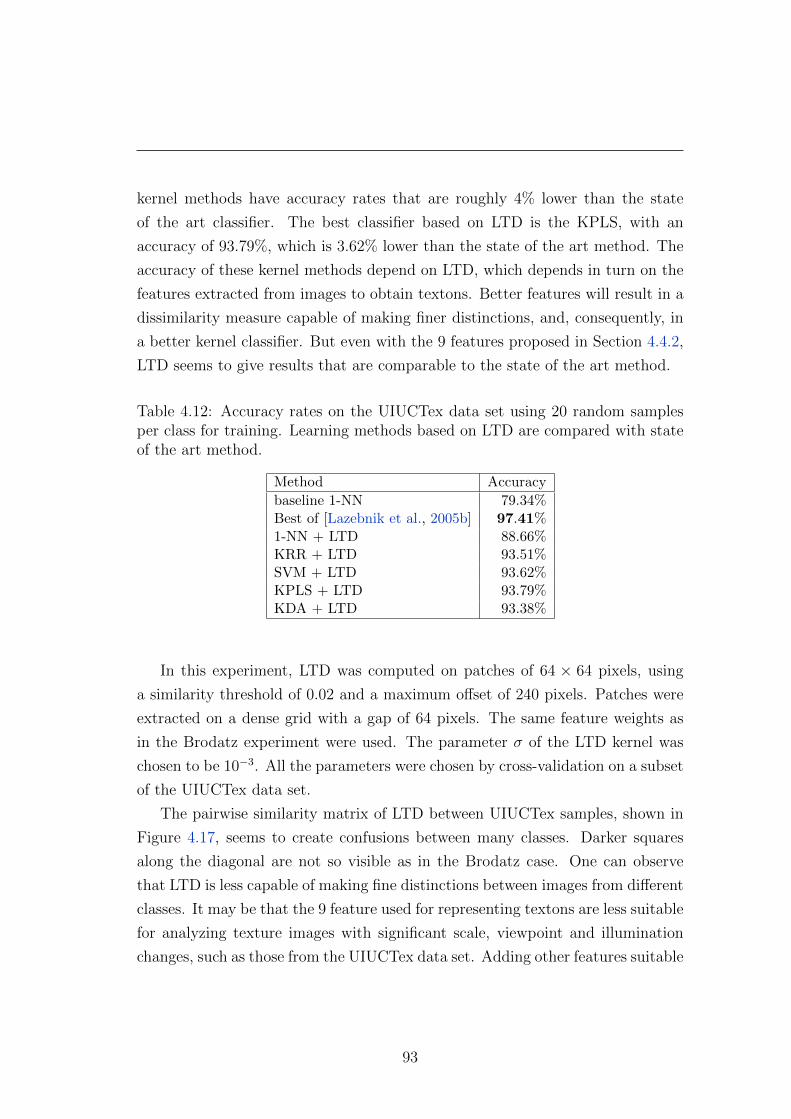
kernel methods have accuracy rates that are roughly 4% lower than the state

of the art classifier. The best classifier based on LTD is the KPLS, with an

accuracy of 93.79%, which is 3.62% lower than the state of the art method. The

accuracy of these kernel methods depend on LTD, which depends in turn on the

features extracted from images to obtain textons. Better features will result in a

dissimilarity measure capable of making finer distinctions, and, consequently, in

a better kernel classifier. But even with the 9 features proposed in Section 4.4.2,

LTD seems to give results that are comparable to the state of the art method.

Table 4.12: Accuracy rates on the UIUCTex data set using 20 random samplesper class for training. Learning methods based on LTD are compared with stateof the art method.

Method Accuracy

baseline 1-NN 79.34%Best of [Lazebnik et al., 2005b] 97.41%1-NN + LTD 88.66%KRR + LTD 93.51%SVM + LTD 93.62%KPLS + LTD 93.79%KDA + LTD 93.38%



extracted on a dense grid with a gap of 64 pixels. The same feature weights as

in the Brodatz experiment were used. The parameter σ of the LTD kernel was

chosen to be 10−3. All the parameters were chosen by cross-validation on a subset

of the UIUCTex data set.

The pairwise similarity matrix of LTD between UIUCTex samples, shown in

Figure 4.17, seems to create confusions between many classes. Darker squares

along the diagonal are not so visible as in the Brodatz case. One can observe

that LTD is less capable of making fine distinctions between images from different

classes. It may be that the 9 feature used for representing textons are less suitable

for analyzing texture images with significant scale, viewpoint and illumination

changes, such as those from the UIUCTex data set. Adding other features suitable

93

Figure 4.17: Similarity matrix based on LTD with patches of 64 × 64 pixelsand a similarity threshold of 0.02, obtained by computing pairwise dissimilaritiesbetween the texture samples of the UIUCTex data set.

for this type of images could improve the accuracy.

4.5.5 Biomass Experiment

The classifiers evaluated in this experiment are the baseline 1-NN model based on

the Bhattacharyya coefficient, the 1-NN classifier based on LTD, and the kernel

classifiers based on LTD, namely the KRR, the KPLS, the SVM, and the KDA.

These classifiers must identify the three classes of biomass from the Biomass

Texture data set.

Table 4.13 presents accuracy rates of the proposed classifiers using three dif-

ferent setup procedures. The first setup is to use 20 random samples per class

for training and the rest of 70 samples for testing. The second setup is to use 30

94

random samples per class for training and 60 samples for testing. The last setup

is to use 40 random samples per class for training and 50 samples for testing.

The accuracy rates are averaged over 50 runs for each method. As expected, the

accuracy of each method improves when more training samples are used. For

example, the accuracy of the baseline method grows by 6.83% from 20 training

samples to 40 training samples. However, the classifiers based on LTD are more

stable, since the accuracy of each classifier grows only by roughly 3 − 4% from

20 training samples to 40 samples. The learning methods based on LTD show a

significant improvement in accuracy over the baseline. The best classifier based

on LTD is KPLS. In all the test cases, the KPLS based on LTD has an accuracy

of at least 10% better than the accuracy of the baseline 1-NN. Overall, the ker-

nel classifiers achieve roughly similar accuracy levels. The empirical results show

again that LTD is a powerful dissimilarity measure for texture classification.

Table 4.13: Accuracy rates on Biomass Texture data set using 20, 30 and 40random samples per class for training and 70, 60 and 50 for testing, respectively.

Method 20/70 Accuracy 30/60 Accuracy 40/50 Accuracy

baseline 1-NN 80.35% 84.72% 87.18%1-NN + LTD 88.09% 90.20% 91.28%KRR + LTD 93.72% 96.40% 97.64%SVM + LTD 93.98% 96.58% 97.72%KPLS + LTD 94.48% 96.90% 97.97%KDA + LTD 94.08% 96.40% 97.67%



extracted on a dense grid with a gap of 64 pixels. Again, feature weights were

adjusted to increase the importance of Gabor features and fractal dimension by

a factor of two, and to decrease the importance of the mean and the standard

deviation by a factor of two. The parameter σ of the LTD kernel was chosen to

be 10−3. All the parameters were chosen by cross-validation on a subset of the

Biomass Texture data set.

95

4.6 Discussion and Future Work

In this chapter, a novel dissimilarity measure for images, which is based on patches

was presented. Several methods of speeding it up were also discussed, such as,

using a hash table to store already computed patch distances, and skipping the

comparison step of some overlapping patches.

Empirical results showed that LPD can be used for real-time image classifi-

cation, especially when local learning methods are preferred instead of standard

machine learning algorithms. Local learning methods based on LPD were pro-

posed and tested on the popular MNIST data set. The experiments show that

local learning algorithms perform very well in terms of accuracy and time. The

error rate achieved by the k-NN based on LPD with filtering approach is 1.01%

on the MNIST data set, which makes it one of the top 4 k-NN models that report

results on this data set.

There are other ways of avoiding the problem of high computational time that

are not studied in this thesis. For example, another local learning method to solve

this problem is to rescale images to a smaller size and compute LPD on those

images. For the k-NN with filtering approach, the nearest K neighbors can be

filtered using the smaller images, and then, the nearest k neighbors are selected

from those remaining K, using the original images.

In future work, an even faster version of LPD based on image descriptors

can be proposed. Instead of comparing the similarity between many patches,

LPD can compare the similarity of a few SIFT descriptors, for example. This

approach would bring a major improvement in terms of speed. Until further

investigation, it remains uncertain if such an approach can have similar or more

accurate results than the current formulation of LPD. A hint could be that LPD

somehow measures the difference of spatial information between images. Can this

difference still be measured using fewer image descriptors?

A step towards replacing raw patches with image descriptors or image fea-

tures was already taken through the development of LTD. Instead of comparing

patches, LTD compares textons, which are represented as a set of texture-specific

features extracted from images. Texture experiments presented in this chapter

showed that LTD is a robust dissimilarity measure, achieving state of the art

96

accuracy levels in several texture classification tasks. In future work, the LTD

measure can further be improved by adding more features to the texton feature

set, or by changing the features completely.

97

Chapter 5

Object Recognition with the Bag

of Visual Words Model

The classical problem in computer vision is that of determining whether or not the

image data contains some specific object, feature, or activity. Particular formula-

tions of this problem are image classification, object recognition, object detection.

Computer vision researchers have recently developed sophisticated methods for

such image related tasks. Among the state of the art models are discriminative

classifiers using the bag of words (BOW) representation [Sivic et al., 2005; Zhang

et al., 2007] and spatial pyramid matching [Lazebnik et al., 2006], generative

models [Fei-Fei et al., 2007] or part-based models [Lazebnik et al., 2005a]. The

BOW model, which represents an image as a histogram of local features, has

demonstrated impressive levels of performance for image categorization [Zhang

et al., 2007], image retrieval [Philbin et al., 2007], or related tasks.

This chapter is focused on improving the BOW model in several ways. Usually,

kernel methods are used to compare image histograms. Popular choices, besides

the linear kernel, are the intersection, Hellinger’s, χ2 and Jensen-Shannon (JS)

kernels. There is no reason to limit the choice of kernels to these options, when

other kernels are available. The final goal, that is to improve the results for image

related tasks, can be achieved by trying different kernels that could possibly work

better. In this chapter, a kernel for histograms of visual words that was introduced

in [Ionescu & Popescu, 2013b], namely the PQ kernel, is presented. The PQ

98

kernel is inspired from a class of similarity measures for ordinal variables, more

precisely Goodman and Kruskal’s gamma and Kendall’s tau. The idea is to treat

the visual words histograms as ordinal data, in which data is ordered but cannot

be assumed to have equal distance between values. In this case, a histogram will

be considered as a rank of visual words according to their frequencies in that

histogram. Usage of the ranking of visual words instead of the actual values of

the frequencies may seem as a loss of information, but the process of ranking

can actually make PQ more robust, acting as a filter and eliminating the noise

contained in the values of the frequencies. This work proves that PQ is a kernel

and it also shows how to build its feature map.

Image categorization experiments are conducted in order to assess the perfor-

mance of different kernels, including PQ, on two benchmark data sets of images,

more precisely, the Pascal VOC data set and the Birds data set. The idea behind

the evaluation is to use the same framework and variate only the feature maps

computed with different kernels. The experiments show that the PQ kernel has

the best mean average precision on both data sets.

In this chapter, an improved variant of the BOW model is also proposed for

classifying human facial expression from low resolution images. The proposed

model was also presented in [Ionescu et al., 2013] as an approach to the Facial

Expression Recognition (FER) Challenge of the ICML 2013 Workshop in Chal-

lenges in Representation Learning (WREPL). The BOW model is a rather general

approach for image categorization, because it does not use any particular char-

acteristics of the image. More precisely, this approach treats images representing

faces, objects, or textures in the same manner. The method developed for the

FER Challenge stems from this generic approach. The model had to be adapted

to the data set provided by the WREPL organizers. First, histograms of visual

words are replaced with normalized presence vectors, to eliminate noise intro-

duced by word frequencies. For facial expression recognition, the presence of a

visual word is more important than its frequency. Second, local multiple kernel

learning was used to predict class labels of test images, in order to reduce both

the image variation and the labeling noise in the resulting training sets.

Preliminary experiments were performed to validate the BOW approach. Em-

pirical results shown that presence vectors improve accuracy by roughly 1%, while

99

local learning improves performance by almost 2 − 3%. Several kernel methods

were also evaluated in the experiments. The SVM classifier performs better than

the KDA and the KRR. Experiments show that spatial information also helps

to improve recognition performance by almost 2 − 3%. Presence vectors that

record different spatial information are combined to improve accuracy even fur-

ther. The improved BOW method was fairly successful, it ranked fourth in the

FER Challenge, with an accuracy of 67.484% on the final (private) test, as the

work of [Goodfellow et al., 2013] also reports.

The chapter is organized as follows. Section 5.1 presents the classical BOW

framework used for image retrieval, image categorization and related tasks. The

PQ kernel for histograms of visual words is discussed in Section 5.2. Object

recognition experiments conducted on two benchmark data sets are presented

in Section 5.3. Section 5.4 presents the BOW learning model adapted to facial

expression recognition. The local learning approach is presented in Section 5.5.

Experiments conducted on the Facial Expression Recognition Challenge data set

are presented in section 5.6. Finally, a discussion about future developments is

given in Section 5.7.

5.1 Bag of Visual Words Model

In computer vision, the BOW model can be applied to image classification and

related tasks, by treating image descriptors as words. A bag of visual words

is a sparse vector of occurrence counts of a vocabulary of local image features.

This representation can also be described as a histogram of visual words. The

vocabulary is usually obtained by vector quantizing image features into visual

words.

The learning model (framework) has two different stages, one for training and

one for testing. Each stage is divided into two major steps. The first step in both

stages is for feature detection and representation. The second step is to train a

kernel method (in the training stage) in order to predict the class label of new

images (in the testing stage). The entire process, that involves both training and

testing stages, is summarized in Figure 5.1.

The feature detection and representation step in the training stage works as

100

Figure 5.1: The BOW learning model for object class recognition. The featurevector consists of SIFT features computed on a regular grid across the image(dense SIFT) and vector quantized into visual words. The frequency of eachvisual word is then recorded in a histogram. The histograms enter the trainingstage. Learning is done by a kernel method.

101

follows. Features are detected using a regular grid across the input image. At

each interest point, a SIFT feature [Lowe, 1999] is computed. This approach

is known as dense SIFT [Bosch et al., 2007; Dalal & Triggs, 2005]. Next, SIFT

descriptors are vector quantized into visual words and a vocabulary (or codebook)

of visual words is obtained. The vector quantization process is done by k-means

clustering [Leung & Malik, 2001], and visual words are stored in a randomized

forest of k-d trees [Philbin et al., 2007] to reduce search cost. The frequency

of each visual word is then recorded in a histogram which represents the final

feature vector for the image. The histograms of visual words enter the training

step. A kernel method is used for training. Several kernels can be used, such as

the linear kernel, the intersection kernel, the Hellinger’s kernel, the χ2 kernel or

the Jensen-Shannon kernel. In this chapter, a novel approach is proposed, that

of using the PQ kernel described in Section 5.2.

Feature detection and representation is similar during the testing stage. The

only difference is that of using the same vocabulary that was already obtained

in the training stage by vector quantization. The histogram of visual words that

represents the test image is compared with the histograms learned in the training

stage. The system can return either a label (or a score) for the test image or a

ranked list of images similar to the test image, depending on the application. For

image categorization a label (or a score) is enough, while for image retrieval a

ranked list of images is more appropriate.

As expected for an image retrieval system, the training stage can be done

offline. For this reason, the time that is necessary for vector quantization and

learning is not of great importance. What matters most is to return the result

for a new (test) image as quick as possible.

Performance level of the described model depends on the number of training

images, but also on the number of visual words. The number of visual words

must be set a priori. The accuracy gets better as the number of visual words is

greater.

An interesting remark is that the described model ignores spatial relationships

between image features. A good way to improve performance is to include spatial

information [Lazebnik et al., 2006]. This can be done by dividing the image into

spatial bins. The frequency of each visual word is then recorded in a histogram

102

for each bin. The final feature vector for the image is a concatenation of these

histograms. The first aim of this work is to improve the performance of the learn-

ing model by trying a different kernel method, namely the PQ kernel. Therefore,

other methods of improving the performance level are disregarded, since they are

beyond the purpose of this goal. However, one should be aware of all the possi-

bilities of improving the described model for a real application, where the level

of performance is of great importance. For example, spatial information is used

for the BOW model for facial expression recognition proposed in Section 5.4.

5.2 PQ Kernel for Visual Words Histograms

All common kernels used in computer vision treat histograms of visual words

either as finite probability distributions, for example, the Jensen-Shannon ker-

nel, either as random variables whose values are the frequencies of different vi-

sual words in the respective images, for example, the Hellinger’s kernel (Bhat-

tacharyya’s coefficient) and the χ2 kernel. Even the linear kernel can be seen as

the Pearson’s correlation coefficient if the two histograms are standardized.

But the histograms of visual words can also be treated as ordinal data, in

which data is ordered but cannot be assumed to have equal distance between

values. In this case, the values of histograms will be the ranks of visual words

according to their frequencies in the image, rather than of the actual values of

these frequencies.

An entire set of correlation statistics for ordinal data are based on the num-

ber of concordant and discordant pairs among two variables. The number of

concordant pairs among two variables (or histograms) X, Y ∈ Rn is:

P = |{(i, j) : 1 ≤ i < j ≤ n, (xi − xj)(yi − yj) > 0}|.

In the same manner, the number of discordant pairs is:

Q = |{(i, j) : 1 ≤ i < j ≤ n, (xi − xj)(yi − yj) < 0}|.

103

Goodman and Kruskal’s gamma [Upton & Cook, 2004] is defined as:

γ =P −QP +Q

.

Kendall developed several slightly different types of ordinal correlation as

alternatives to gamma. Kendall’s tau-a [Upton & Cook, 2004] is based on the

number of concordant versus discordant pairs, divided by a measure based on the

total number of pairs (n is the sample size):

τa =P −Qn(n−1)

2

.

Kendall’s tau-b [Upton & Cook, 2004] is a similar measure of association based

on concordant and discordant pairs, adjusted for the number of ties in ranks. It

is calculated as (P − Q) divided by the geometric mean of the number of pairs

not tied on X and the number of pairs not tied on Y , denoted by X0 and Y0,

respectively:

τb =P −Q√

(P +Q+X0)(P +Q+ Y0).

All the above three correlation statistics are very related. If n is fixed and X

and Y have no ties, then P , X0 and Y0 are completely determined by n and Q.

Actually, all are based on the difference between P and Q, normalized differently.

The PQ kernel between two histograms X and Y is defined as:

kPQ(X, Y ) = 2(P −Q).

Theorem 2 The function denoted by kPQ is a kernel function.

Proof: To prove that kPQ is indeed a kernel, the explicit feature map induced

by kPQ is provided next.

Let X, Y ∈ Rn be two histograms of visual words. Let Ψ be defined as follows:

Ψ : Rn →Mn,n Ψ(X) = (Ψ(X)i,j)1≤i≤n,1≤j≤n,

104

with

Ψ(X)i,j =

1 if xi > xj

−1 if xi < xj

0 if xi = xj

,∀1 ≤ i, j ≤ n.

Note that Ψ associates to each histogram a matrix that describes the order of its

elements.

If matrices are treated as vectors, then the following equality is true:

kPQ(X, Y ) = 2(P −Q) = 〈Ψ(X),Ψ(Y )〉 ,

where 〈·, ·〉 denotes the scalar product. This proves that kPQ is a kernel and

provides the explicit feature map induced by kPQ. utAnother approach inspired from rank correlation measures is the WTA hash

proposed in [Yagnik et al., 2011]. For K = 2, the WTA hash is closely related

to the PQ kernel. However, there are two important differences. The first one

is that WTA hash works with a random selection of pairs from the feature set.

The second one is that, unlike PQ kernel, the WTA hash ignores equal pairs.

In terms of feature representation, the PQ kernel represents a histogram with a

feature vector containing {−1, 0, 1} (0 for equal pairs), while the WTA hash with

K = 2 uses only {1, 0}. In the experiments, one can observe that these differences

have direct consequences to the performance level, creating an even greater gap

between the two methods.

According to the authors of [Vedaldi & Zisserman, 2010], the feature vec-

tors of γ-homogeneous kernels should be Lγ-normalized. Being linear in the

feature space, PQ is a 2-homogeneous kernel and the feature vectors should be

L2-normalized. Therefore, in the experiments, the PQ kernel is based on the

L2-norm. An important advantage of PQ being linear is that it can be used with

linear SVM classifiers, such as the PEGASOS algorithm [Shalev-Shwartz et al.,

2007], that are much faster to learn and evaluate than the original non-linear

SVM.

Treating visual words frequencies as ordinal variables means that in the calcu-

lation of the distance (or similarity) measure, the ranks of visual words according

105

to their frequencies in the image will be used, rather than the actual values of

these frequencies. Usage of the ranking of visual words in the calculation of the

distance (or similarity) measure, instead of the actual values of the frequencies,

may seem as a loss of information, but the process of ranking can actually make

the measure more robust, acting as a filter and eliminating the noise contained

in the values of the frequencies. For example, the fact that a specific visual word

has the rank 2 (is the second most frequent feature) in one image, and the rank 4

(is the fourth most frequent feature) in another image can be more relevant than

the fact that the respective feature appears 34 times in the first image, and only

29 times in the second.

It is important to note that for big vocabularies (with more than 1000 words),

the kernel trick should be employed to obtain the kernel representation of PQ in-

stead of computing its feature map, since there is a quadratic dependence between

the feature map and the number of visual words.

5.3 Object Recognition Experiments

Object recognition experiments presented in this section compare the PQ kernel

with state of the art kernels on two benchmark data sets. First, a brief description

of the data sets is given. Details about the implementation of the learning model

and the evaluation procedure are given next. Finally, the results for the two

experiments are separately discussed.


The Pascal Visual Object Classes (VOC) challenge [Everingham et al., 2010] is

a benchmark in visual object category recognition and detection, providing the

vision and machine learning communities with a standard data set of images

and annotation, and standard evaluation procedures. In the experiments of this

work, the Pascal VOC 2007 data set is used. The reason for this choice is that

this is the latest data set for which testing labels are available for download,

and the experiments can be done offline. There are roughly 10 thousand images

in this data set, that are divided into 20 classes. As Figure 5.2 shows, some

106

Figure 5.2: A random sample of 12 images from the Pascal VOC data set. Someof the images contain objects of more than one class. For example, the image atthe top left shows a dog sitting on a couch, and the image at the top right showsa person and a horse. Dog, couch, person and horse are among the 20 classes ofthis data set.

images may contain objects from several classes. Thus, the class labels are not

mutually exclusive. For each class the data set provides a training set, a validation

set and a test set. The training and validation sets have roughly 2500 images

each, while the test set has about 5000 images. This data set is available at

http://pascallin.ecs.soton.ac.uk/challenges/VOC/voc2007/.

107

http://pascallin.ecs.soton.ac.uk/challenges/VOC/voc2007/

Figure 5.3: A random sample of 12 images from the Birds data set. There aretwo images per class. Images from the same class sit next to each other in thisfigure.

The second data set was collected from the Web by the authors of [Lazebnik

et al., 2005a] and consists of 100 images each of 6 different classes of birds: egrets,

mandarin ducks, snowy owls, puffins, toucans, and wood ducks. The training set

consists of 300 images and the test set consists of another 300 images. For each

class, the data set contains 50 positive train images and 50 positive test images.

This data set of 600 images is used in order to assess kernels behavior when

less training data is available. Figure 5.3 shows two images from each class of

the Birds data set. The data set is available at http://www-cvr.ai.uiuc.edu/

ponce_grp/data/.

108



5.3.2 Implementation and Evaluation Procedure

The framework described in Section 5.1 is used for object class recognition. De-

tails about the implementation of the model are given next. In the feature de-

tection and representation step, a variant of dense SIFT descriptors extracted at

multiple scales is used [Bosch et al., 2007]. The number of visual words used in

the experiments is 500. For better accuracy, up to 10, 000 or more visual words

can be used.

Several state of the art kernel methods are compared with the PQ kernel

in both experiments. The baseline method is the linear kernel, for which the

histograms are L2-normalized. One of the state of the art methods is based on the

Hellinger’s kernel. Two variants with different norms of this kernel are used. The

first one is based on L1-normalized feature vectors, and the second one is based on

L2-normalized feature vectors. Another state of the art kernel is Jensen-Shannon,

which is L1-normalized. Finally, these kernels are to be compared with the PQ

kernel described in this chapter. The PQ kernel is L2-normalized. For all kernel

methods, feature maps are computed from the visual words histograms. The

training is always done using a linear SVM on the computed feature maps. The

linear SVM is based on an implementation of the PEGASOS algorithm described

in [Shalev-Shwartz et al., 2007]. The feature map of the JS kernel cannot be

computed directly. In order to use the same learning setting, its feature map

has to be approximated using the method proposed in [Vedaldi & Zisserman,

2010]. To approximate the JS kernel, 10, 500 features are used. The idea behind

the evaluation is to use the same framework and variate only the feature maps

computed with different kernels, since the final goal of the experiments is to

evaluate the difference between these kernels, in terms of performance. The

implementation of both the feature detection and representation step, and the

learning step, is mostly based on the VLFeat library [Vedaldi & Fulkerson, 2008].

The evaluation procedure for both experiments follows the Pascal VOC bench-

mark. The qualitative performance of the learning model is measured by using

the classifier score to rank all the test images. Next, the retrieval performance is

measured by computing a precision-recall curve. Note that the precision is given

by the proportion of returned images that are positive, while the recall is given

109

by the proportion of positive images that are returned. In order to represent the

retrieval performance by a single number (rather than a curve), the mean average

precision (mAP) is often computed. The average precision as defined by TREC

is used in the experiments. This is the average of the precision observed each

time a new positive sample is recalled.

5.3.3 Pascal VOC Experiment

The first experiment is on the Pascal VOC 2007 data set. The validation set was

used to validate the parameter C of the linear SVM algorithm. For the linear

kernel and Hellinger’s kernels, the values of parameter C range exponentially from

0.1 to 1000. For the JS and PQ kernels, the values of parameter C can be either

0.5 or 1.

Table 5.1 presents the mean AP of the linear kernel, the Hellinger’s kernel,

the JS kernel, the WTA hash (with K = 2 and 10, 000 random pairs) and the PQ

kernel, on the Pascal VOC data set. Looking at the results obtained by the JS

kernel on one hand, and the PQ kernel on the other, one can observe that these

methods are somehow complementary in terms of performance. This gives the

idea of combing the two kernels to possibly obtain better results. Indeed, in this

experiment another kernel based on the sum of JS and PQ kernels is presented.

In order to obtain the feature map of this kernel combination, the feature maps

of JS and PQ kernels are simply concatenated.

The accuracy of the state of the art kernels is well above the accuracy of the

baseline linear SVM. In terms of AP, the state of the art kernels are about 10%

better than the baseline method. The PQ kernel improves the accuracy of the

learning model, when compared to the state of the art methods. The mAP of the

PQ kernel is 3.3% above the mAP of the Hellinger’s kernels, 1.4% above the mAP

of the WTA hash, and 1.2% above the mAP of the JS kernel. The combination

of JS and PQ kernels improves the performance even further. The mAP of the

JS+PQ kernel is 3.6% above the mAP of the Hellinger’s kernels, 1.7% above the

mAP of the WTA hash, and 1.5% above the mean AP of the JS kernel. PQ

kernel improves results over WTA hash by 1.4%, showing that the two methods

are distinct.

110

Table 5.1: Mean AP on Pascal VOC 2007 data set for machine learning methodsbased on visual words histograms with different kernels. The best AP on eachclass is highlighted with bold.

Class Lin. L2 Hel. L1 Hel. L2 WTA L2 JS L1 PQ L2 JS+PQ

Airplane 0.395 0.555 0.558 0.534 0.564 0.526 0.574Bicycle 0.189 0.339 0.337 0.398 0.367 0.409 0.386Bird 0.178 0.248 0.247 0.274 0.284 0.281 0.305Boat 0.334 0.540 0.551 0.476 0.549 0.505 0.553Bottle 0.122 0.143 0.139 0.139 0.127 0.140 0.129Bus 0.239 0.334 0.336 0.404 0.379 0.419 0.406Car 0.518 0.599 0.602 0.659 0.644 0.670 0.659Cat 0.281 0.349 0.351 0.382 0.378 0.402 0.393Chair 0.308 0.399 0.399 0.398 0.414 0.405 0.414Cow 0.117 0.174 0.172 0.209 0.169 0.209 0.198Dining Table 0.205 0.238 0.227 0.237 0.242 0.253 0.255Dog 0.212 0.271 0.266 0.263 0.293 0.287 0.299Horse 0.484 0.518 0.530 0.601 0.595 0.609 0.614Motorbike 0.213 0.398 0.389 0.427 0.413 0.451 0.450Person 0.639 0.715 0.717 0.756 0.759 0.773 0.774Potted Plant 0.099 0.125 0.110 0.110 0.112 0.111 0.115Sheep 0.220 0.217 0.237 0.219 0.222 0.259 0.243Sofa 0.184 0.304 0.320 0.310 0.325 0.322 0.333Train 0.363 0.534 0.528 0.547 0.554 0.570 0.574TV Monitor 0.196 0.309 0.295 0.345 0.336 0.351 0.342

Overall 0.275 0.365 0.365 0.384 0.386 0.398 0.401

If the best AP per class is considered, the PQ kernel and the JS+PQ kernel

win most of the classes (18 out of 20). The results presented in Table 5.1 come

to support this statement. The Hellinger’s kernel based on the L1-norm wins 2

classes, more precisely the Bottle and the Potted Plant classes. The L1-normalized

Hellinger’s kernel seems to work best when classes are very difficult for all kernel

methods. The best AP on the Chair class is shared by the JS kernel and the

JS+PQ kernel, while the best AP on the Cow class is shared by the WTA hash

and the PQ kernel. This is also the only class that the WTA hash is able to

win. The PQ kernel has the best AP on 8 classes. The JS+PQ kernel wins 10

classes, also counting in the Chair class. Note that the linear kernel and the

L2-normalized Hellinger’s kernel are not able to take any class.

111

The feature detection and representation phase, that builds a vocabulary of

visual words and obtains histograms, takes a few hours on this data set. The

time for the second phase of the learning framework, that includes computing

feature maps, training and testing, depends on the number of features in the

feature space for each kernel. The time for the second phase and the number of

features for each kernel are reported in Table 5.2. The time was measured on a

computer with Intel Core i7 2.3 GHz processor and 8 GB of RAM memory using

a single Core. While the feature maps can be computed only once for the entire

experiment along with the feature detection and representation stage, training

and testing has to be repeated for each class. Despite the fact that the time

for the PQ kernel (14 − 15 minutes) is higher than the time for other kernels

(2− 15 seconds), it does not add an overhead to the overall time of the learning

framework, since the overall time is about 4− 6 hours.

Table 5.2: The time for the second stage of the learning model and the numberof features for each kernel. The time is measured in seconds.

Kernel Time Features

Linear L2 1− 2 500Hellinger’s L1 2− 3 500Hellinger’s L2 2− 3 500WTA L2 15− 16 10, 000JS L1 15− 16 10, 500PQ L2 830− 860 250, 000JS L1 + PQ L2 850− 880 260, 500

The PQ kernel and the JS+PQ kernel are constantly better than the other

methods. In conclusion, the PQ kernel, used either alone or in combination with

the JS kernel, has the best performance on this experiment.

5.3.4 Birds Experiment

The second experiment is on the Birds data set. Since there is no validation set

this time, the parameter C of the linear SVM algorithm is cross-validated on

the training set. Table 5.3 presents the mAP of the linear kernel, the Hellinger’s

kernel, the JS kernel, the WTA hash (with K = 2 and 10, 000 random pairs) and

112

the PQ kernel, on the Birds data set. A variant of the PQ kernel that ignores

equal pairs (PQ iq), which is more similar to the WTA hash, is also added to the

experiment to emphasize the difference between PQ kernel and WTA hash. This

variant of PQ is also based on the L2-norm.

Table 5.3: Mean AP on Birds data set for machine learning methods based onvisual words histograms with different methods. The best AP on each class ishighlighted with bold.

Class Lin. L2 Hel. L1 Hel. L2 JS L1 WTA L2 PQ iq PQ L2

Egret 0.552 0.760 0.747 0.416 0.735 0.738 0.753Mandarin Duck 0.446 0.585 0.607 0.375 0.784 0.791 0.835Owl 0.815 0.895 0.887 0.490 0.879 0.889 0.915Puffin 0.427 0.696 0.730 0.369 0.708 0.703 0.764Toucan 0.572 0.715 0.747 0.558 0.776 0.787 0.845Wood Duck 0.608 0.795 0.816 0.361 0.767 0.769 0.849

Overall 0.570 0.741 0.756 0.428 0.775 0.779 0.827

The performance of the Hellinger’s kernels is above the baseline linear SVM,

as in the previous experiment. Both Hellinger’s kernels are about 18% better

than the baseline method. Unlike the previous experiment, the JS kernel has the

worst accuracy on this data set, when compared to the rest of the methods. The

mAP of the JS kernel is 14.2% below the baseline AP. The bad performance of

the JS kernel on this data set can be explained by the fact that it is based on

an informational measure that uses an estimation of the distribution of the data.

The number of training samples may not be enough for a good estimation.

The results of the PQ kernel on this experiment are consistent with the previ-

ous experiment. The PQ kernel improves the performance of the learning model,

when compared to the state of the art kernels. The mean AP of the PQ kernel

is 8.6% above the mAP of the L1-normalized Hellinger’s kernel, 7.2% above the

mAP of the L2-normalized Hellinger’s kernel, and 5.2% above the mAP of the

WTA hash. Table 5.3 also shows that by ignoring equal pairs the mAP of the PQ

kernel drops by 4.8%. By taking into account equal pairs and by considering the

entire feature set, PQ has a significant improvement in terms of accuracy over

WTA hash. There is no question that the two methods are distinct.

113

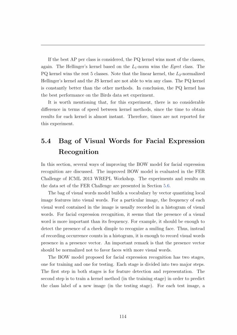
If the best AP per class is considered, the PQ kernel wins most of the classes,

again. The Hellinger’s kernel based on the L1-norm wins the Egret class. The

PQ kernel wins the rest 5 classes. Note that the linear kernel, the L2-normalized

Hellinger’s kernel and the JS kernel are not able to win any class. The PQ kernel

is constantly better than the other methods. In conclusion, the PQ kernel has

the best performance on the Birds data set experiment.

It is worth mentioning that, for this experiment, there is no considerable

difference in terms of speed between kernel methods, since the time to obtain

results for each kernel is almost instant. Therefore, times are not reported for

this experiment.

5.4 Bag of Visual Words for Facial Expression

Recognition

In this section, several ways of improving the BOW model for facial expression

recognition are discussed. The improved BOW model is evaluated in the FER

Challenge of ICML 2013 WREPL Workshop. The experiments and results on

the data set of the FER Challenge are presented in Section 5.6.

The bag of visual words model builds a vocabulary by vector quantizing local

image features into visual words. For a particular image, the frequency of each

visual word contained in the image is usually recorded in a histogram of visual

words. For facial expression recognition, it seems that the presence of a visual

word is more important than its frequency. For example, it should be enough to

detect the presence of a cheek dimple to recognize a smiling face. Thus, instead

of recording occurrence counts in a histogram, it is enough to record visual words

presence in a presence vector. An important remark is that the presence vector

should be normalized not to favor faces with more visual words.

The BOW model proposed for facial expression recognition has two stages,

one for training and one for testing. Each stage is divided into two major steps.

The first step in both stages is for feature detection and representation. The

second step is to train a kernel method (in the training stage) in order to predict

the class label of a new image (in the testing stage). For each test image, a

114

local classification problem is constructed by selecting only the nearest neighbors

from the kernel feature space. The local learning part of the framework is further

described in Section 5.5. The entire process, that involves both training and

testing stages, is summarized in Figure 5.4. It is interesting to notice the different

steps from the model presented in Figure 5.1.

The feature detection and representation step in the training stage is a slightly

modified version of the approach described in Section 5.1, which uses k-means

clustering [Leung & Malik, 2001] to quantize dense SIFT descriptors [Bosch et al.,

2007; Dalal & Triggs, 2005] into visual words that are stored in a randomized

forest of k-d trees [Philbin et al., 2007], to reduce search cost. The novelty

consists of a semi-supervised approach, in the sense that it can leverage the

SIFT descriptors from the unlabeled test set by including them in the k-means

clustering process as well, together with those from the training data set. For

increased test sets this has led to a better representation of the faces manifold

and to increased classification performance. The presence of each visual word

is recorded in a presence vector which represents the final feature vector for the

image. Normalized presence vectors of visual words can now enter the learning

step. Figure 5.5 presents a sample of 30 SIFT descriptors extracted from two

images of the FER data set.

Feature detection and representation is similar during the testing stage. The

presence vector of visual words that represents the test image is compared with

the training presence vectors, through the implicit distance defined by the kernel,

to select a number of nearest neighbors. For a certain test image, only its nearest

neighbors actually enter the learning step. In other words, a local recognition

problem is built for each test image. A kernel method is employed to learn the

local recognition problem and finally predict a class label for the test image.

Classifiers such as the SVM, the KDA or the KRR are good choices to perform

the local learning task.

The model described so far ignores spatial relationships between image fea-

tures. Despite ignoring spatial information, visual words showed a high discrimi-

natory power and have been used for region or image level classification [Csurka

et al., 2004; Fei-Fei & Perona, 2005; Zhang et al., 2007]. The performance im-

proves when spatial information is included. This can be achieved by dividing

115

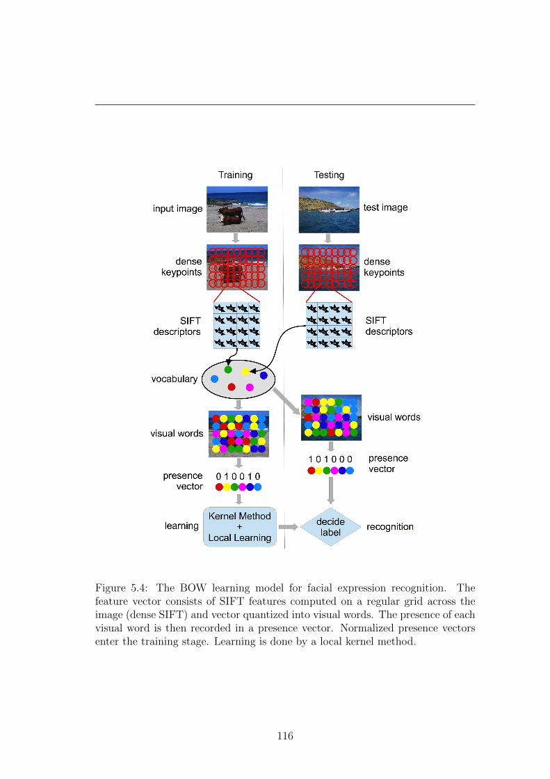
Figure 5.4: The BOW learning model for facial expression recognition. Thefeature vector consists of SIFT features computed on a regular grid across theimage (dense SIFT) and vector quantized into visual words. The presence of eachvisual word is then recorded in a presence vector. Normalized presence vectorsenter the training stage. Learning is done by a local kernel method.

116

Figure 5.5: An example of SIFT features extracted from two images representingdistinct emotions: fear (left) and disgust (right).

the image into spatial bins. The presence of each visual word is then recorded in

a presence vector for each bin. The final feature vector for the image is a con-

catenation of these presence vectors. A more robust approach is to use a spatial

pyramid, as the work of [Lazebnik et al., 2006] suggests. The spatial pyramid is

usually obtained by dividing the image into increasingly fine sub-regions (bins)

and computing histograms of visual words found inside each bin. It is worth

mentioning that a similar approach for texture classification was recently pro-

posed in [Popescu et al., 2013a]. The spatial pyramid representation presented

in [Popescu et al., 2013a] is designed to capture the fractal structure in texture

images. It can improve the accuracy by as much as 5% over the standard feature

representation, showing that the pyramid structure is indeed useful for texture

classification.

The framework proposed in this section makes use of the spatial information

by computing a spatial pyramid from presence vectors. It is reasonable to think

that dividing an image representing a face into bins is a good choice, since most

features, such as the contraction of the muscles at the corner of the eyes, are only

visible in a certain region of the face. In other words, one does not expect to find

raised eyebrows on the cheek, or cheek dimples on the forehead.

117

5.5 Local Learning

Local learning methods attempt to locally adjust the performance of the training

system to the properties of the training set in each area of the input space. A

simple local learning algorithm works as follows: for each testing example, select

a few training examples located in the vicinity of the testing example, train a

classifier with only these few examples and apply the resulting classifier to the

testing example.

The learning step of the BOW framework adapted to facial expression recog-

nition is based on a local learning algorithm that uses the presence kernel to

select nearest neighbors in the vicinity of a test image. Local learning has a few

advantages over standard learning methods. First, it divides a hard classification

problem into more simple sub-problems. Second, it reduces the variety of images

in the training set, by selecting images that are most similar to the test one.

Third, it improves accuracy for data sets affected by labeling noise. Considering

all these advantages, a local learning algorithm is indeed suitable for the FER

data set.

Figure 5.6 shows that the nearest neighbors selected from the vicinity of a

particular test image are visually more relevant than a random selection of train-

ing images. It also gives a hint that local learning should perform better than a

standard learning formulation.

5.6 Facial Expression Recognition Experiments

5.6.1 Data Set Description

The data set of the FER Challenge consists of 48× 48 pixel gray-scale images of

faces representing 7 categories of facial expressions: anger, disgust, fear, happi-

ness, sadness, surprise, and neutral. There are 28709 examples for training, 3589

examples for testing, and another 3589 examples for private testing. The task is

to categorize each face based on the emotion shown in the facial expression in to

one of 7 categories. Images were collected from the web using a semi-automatic

procedure. Therefore, the data set may contain images that do not represent

118

Figure 5.6: The six nearest neighbors selected with the presence kernel from thevicinity of the test image are visually more similar than the other six imagesrandomly selected from the training set. Despite this fact, the nearest neighborsdo not adequately indicate the test label. Thus, a learning method needs to betrained on the selected neighbors to accurately predict the label of the test image.

119

faces. Another issue is that the training data may also contain labeling noise,

meaning that the labels of some faces do not indicate the right facial expression.

5.6.2 Implementation

The framework described in Section 5.4 is used for facial expression recognition.

Details about the implementation of the model are given next. In the feature

detection and representation step, a variant of dense SIFT descriptors extracted

at multiple scales is used [Bosch et al., 2007]. The dense SIFT features were

extracted using a grid step of 1 pixel at scales ranging from 2 to 8 pixels. These

features are extracted from the entire FER data set. A random sample of 240, 000

features is selected to compute the vocabulary. The number of visual words

used in the experiments ranges from 5, 000 to 20, 000. A slight improvement in

accuracy can be observed when the vocabulary dimension grows. Both histograms

of visual words and presence vectors were tested. Empirical results show that

presence vectors are able to improve accuracy, by eliminating some of the noise

encoded by the histogram representation.

Different spatial presence vectors were combined to obtain several spatial pyra-

mid versions. Images were divided into 2× 2 bins, 3× 3 bins, and 4× 4 bins to

obtain spatial presence vectors. The basic presence vectors are also used in the

computation of spatial pyramids.

The kernel trick is implied to obtain spatial pyramids. Kernel matrices are

computed for each (spatial) presence vector representation. Then, kernel matrices

are summed up to obtain the kernel matrix of a certain spatial pyramid. Some of

the proposed models are based on a weighted sum of kernel matrices, with weights

adjusted to match the accuracy level of each (spatial) presence vector. Summing

up kernel matrices is equivalent to presence vector concatenation. But presence

vectors are actually high-dimensional sparse vectors, and the concatenation of

such vectors is not a viable solution in terms of space and time.

Several state of the art kernel methods are used to perform the local learning

tasks, namely the SVM, the KDA and the KRR. Empirical results showed that

the SVM performs slightly better than the KDA, and much better than the KRR.

The number of nearest neighbors selected to enter the local learning phase for each

120

test image is 1000. However, an experiment is conducted to show the accuracy

level as the number of nearest neighbors varies. The regularization parameter

C of the SVM was set to 1000. This choice is motivated by the fact that the

data set is separable since there is a small number of training examples (1000

neighbors), in a high-dimensional feature space. Thus, the best working SVM is

a hard margin SVM that can be obtained by setting the C parameter of the SVM

to a high value [Shawe-Taylor & Cristianini, 2004].

5.6.3 Parameter Tuning and Results

For parameter tuning and validation, the training set was randomly split in two

thirds kept for training and one third for validation. Preliminary experiments

using different models were performed on the validation set to assess the per-

formance levels of the kernel methods. Obtained results point that the SVM is

about 1−2% better than the KRR, and about 0.5% better than KDA. They also

indicate that presence vectors are 0.5 − 1% better than histograms. In the ex-

periments presented in Table 5.4 only results obtained with various SVM models

based on presence vectors are included.

Several kernels based on different vocabularies and various ways of encoding

spatial information were proposed. The model names of the form “8000 3 × 3”

specify the size of the vocabulary, followed by the size of the grid used to partition

the image into spatial bins. The kernel of “8000 SUM” is the mean of the kernels

based on 8000 visual words computed on spatial bins ranging from 1× 1 bins to

4 × 4 bins. In other words, the 8000 SUM model is based on spatial pyramids.

It has performed on the validation set better than each of its terms. The kernel

identified by “MIX3” is the mean of 17000 1×1, 14000 2×2, 11000 3×3, and 8000

4×4. Again, it has performed better than each of its terms. The kernel identified

by “20K” is a variant of “MIX3” built on even larger vocabularies, as is the mean

of 20000 1×1, 20000 2×2, 12000 3×3, and 8000 4×4. It did not perform better

than MIX3, neither on the validation data set nor on the actual test set. The

kernel identified as “MIX1” is the weighted mean of 7000 1× 1, 7000 2× 2, 7000

3 × 3, and 5000 4 × 4, with the weights 0.1, 0.2, 0.4, 0.3, respectively. Finally,

the last proposed model is the kernel identified as “MIX2”, which is the weighted

121

mean of 11000 1 × 1, 9000 2 × 2, 7000 3 × 3, and 5000 4 × 4, with the weights

0.2, 0.3, 0.3, 0.2, respectively. The vector quantization process of these models

initially included the descriptors extracted from the 28709 examples for training

and the 3589 examples for preliminary testing. Some of the models were re-built

to add the 3589 examples from the private testing set in the vector quantization

process.

In Table 5.4 one can observe that the performance of the global one-versus-

all SVM is at least 2% lower than that obtained with the local learning based

on one-versus-all SVM with the same parameters. Another interesting behavior

that can be observed in this table is the effect on accuracy of dividing the image

area into spatial bins: the accuracy increases as the image is divided into finer

sub-regions. This table also shows the effect of the number of neighbors, another

parameter that must be adjusted.

No model with more than 1500 neighbors was submitted to the FER Chal-

lenge, it may well be that using 3000 neighbors could have led to somewhat higher

scores. The parameter tuning was limited both by the amount of RAM available

in the machines (24 GB for the largest one) used to train the models, and by

the speed of the CPUs (4-core Xeon E5540 at 2.53 GHz in the fastest one). Test

cycles took therefore up to 9 hours. The best accuracy on the final test set is

67.484%. An interesting remark is that the proposed model has roughly achieved

human-level performance on this data set.

5.7 Discussion and Further Work

This chapter discussed several improvements of the BOW model either for object

recognition or for facial expression recognition. First, the work presented in this

chapter showed that the results for image classification, image retrieval or related

tasks, can be improved by using the PQ kernel. The PQ kernel comes from the

idea of treating feature vectors of visual words as ordinal variables.

Object recognition experiments compared the PQ kernel with other state of

the art kernels on two benchmark data sets. The PQ kernel, used either alone

or in combination with the JS kernel, has the best accuracy on the Pascal VOC

2007 experiment. On the Birds experiment, the PQ kernel improved the perfor-

122

Table 5.4: Accuracy levels for several models obtained on the validation, test,and private test sets.

Model Neighbors Validation Global SVM Test Private

8000 1× 1 1000 59.07%8000 2× 2 1000 62.22%8000 3× 3 1000 62.27%8000 4× 4 1000 62.93%8000 SUM 1000 63.27% 65.73% 66.73%17000 1× 1 1000 60.86%14000 2× 2 1000 62.69%11000 3× 3 1000 62.36%MIX1 1000 63.03% 65.89%MIX2 1000 63.74% 66.42%MIX3 1000 63.61% 66.65%

Re-built Models

MIX1 1000 62.91% 59.35% 66.59% 66.73%MIX2 1000 63.99% 60.95% 67.01% 67.31%MIX3 1000 64.30% 62.27% 67.32% 67.48%MIX3 3000 64.23% 62.27%20K 500 63.59% 61.82%20K 1000 63.90% 61.82%20K 1500 64.10% 61.82% 66.53% 66.98%20K 3000 64.45% 61.82%20K 5000 64.35% 61.82%

mance again. The PQ kernel is constantly better than the other methods. The

accuracy can be improved even further by increasing the number of visual words

used for building the vocabulary. Because the feature map of the PQ kernel

has a quadratic dependence of the size of the vocabulary, one should adjust the

vocabulary size by taking into consideration the trade-off between accuracy and

speed. Despite the fact that the kernel trick can be employed to use the PQ

kernel with larger vocabularies, a greater importance should be given to the idea

of selecting good visual words. A possible way of improving the results for the

PQ kernel may be that of using a TF-IDF measure for visual words as in [Philbin

et al., 2007]. Indeed, eliminating visual words that have a low TF-IDF score can

lead to an approximation of the PQ kernel that works faster and possibly better.

123

Another way is to extract descriptors only from the interesting image regions. In

the recent work of [Alexe et al., 2012], a measure that quantifies how likely it is

for an image window to contain an object of any class is proposed. This measure

is termed objectness. It is interesting to mention that objectness does not aim at

identifying the type of object contained in the image, but rather the image region

that potentially contains any kind of object. A vocabulary of visual words that

is built only from the image regions with a high objectness score should improve

the classification accuracy.

In future work, other methods inspired from ordinal measures can be inves-

tigated. For example, the most common correlation statistic for ordinal data,

namely the Spearman rank-order coefficient [Upton & Cook, 2004], or its L1 ver-

sion, namely the Spearman footrule, are successfully used in text processing [Dinu

& Popescu, 2009b]. It is perfectly reasonable to use them for image processing

in the BOW model context, since the BOW model is also inspired from text pro-

cessing. Methods to transform these measures into kernels would also have to be

developed.

Other improvements of the bag of visual words were proposed to adapted it

to the FER Challenge data set of faces. Histograms of visual words were replaced

with normalized presence vectors, then local learning was used to predict class

labels of test images. The proposed model also includes spatial information in

the form of spatial pyramids computed from presence vectors. Experiments were

performed to validate the proposed model. By reserving one third of the training

data set as validation set, the method’s parameters were tuned without over-

fitting, as can be seen in Table 5.4. Empirical results showed that the proposed

model has an almost 5% improvement in accuracy over a classical BOW model.

Also, using multiple kernel learning (with sum or weighted sum kernels) led to

accuracy levels higher than that of the individual kernels involved. Finally, the

proposed model ranked fourth in the FER Challenge, with an accuracy of 67.484%

on the final test. A different approach to local learning, that of clustering train

images to divide the learning task on each cluster separately, can be studied in

future work.

124

Part II

Machine Learning in String

Processing

125

Chapter 6

State of the Art

Researchers have developed a wide variety of methods for string data, that can

be applied with success in different fields such as computational biology, natural

language processing, information retrieval and so on. Such methods range from

clustering techniques used to analyze the phylogenetic trees of different organisms,

to kernel methods used to identify authorship or native language from text. This

chapter gives an overview of the state of the art methods used in two major fields

of study, namely computational biology and natural language processing.

Two intensively studied problems in computational biology are DNA sequenc-

ing and phylogenetic analysis. A state of the art of the methods used for sequenc-

ing and comparing DNA is given in Section 6.1.1. Phylogenetic analysis, one of

the first problems in computational biology, is discussed in Section 6.1.2. Sev-

eral methods that provide solutions to these computational biology problems are

presented in Chapters 7 and 8, respectively.

Natural language processing (NLP) is a vast domain that studies machine

translation, text summarization, document classification by topic, authorship

identification, sentiment analysis, among others. An overview of the state of

the art approaches in NLP is given in Section 6.2. Special consideration is given

to an approach based on string kernels, that works at character level. The string

kernel method has various applications that are discussed in Section 6.2.1. One of

the recently studied problems in NLP is native language identification [Brooke &

Hirst, 2012; Jarvis & Crossley, 2012; Tetreault et al., 2012]. A machine learning

solution for native language identification based on string kernels is presented in

126

Chapter 9.

6.1 Computational Biology

6.1.1 Sequencing and Comparing DNA

In many important problems in computational biology a common task is to com-

pare a new DNA sequence with sequences that are already well studied and an-

notated. DNA sequence comparison was ranked in the top of two lists with major

open problems in bioinformatics [Koonin, 1999; Wooley, 1999] over a decade ago,

but it is still receives the attention of researchers nowadays. Sequences that are

similar would probably have the same function, or, if two sequences from dif-

ferent organisms are similar, there may be a common ancestor sequence [Liew

et al., 2005]. Another important problem with practical motivations for biolo-

gists is related to the finding of motifs or common patterns in a set of given

DNA sequences. A typical case where the last mentioned problem occurs is, for

example, when one needs to design genetic drugs with structure similar to a set

of existing sequences of RNA [Lanctot et al., 2003]. Other applications in compu-

tational biology which involve this task are (from a rich literature): PCR primer

design [Gramm et al., 2002; Lanctot et al., 2003], genetic probe design [Lanctot

et al., 2003], antisense drug design [Deng et al., 2003], finding unbiased consensus

of a protein family [Ben-Dor et al., 1997], motif finding [Li et al., 2002; Wang &

Dong, 2005] and many others.

The standard method used in computational biology for sequence compari-

son is by sequence alignment. Sequence alignment is a procedure of comparing

DNA sequences, that aims at identifying regions of similarity that may be a

consequence of functional, structural, or evolutionary relationships between the

sequences. Algorithmically, the standard pairwise alignment method is based on

dynamic programming [Smith & Waterman, 1981]. The method compares every

pair of characters of the two sequences and generates an alignment and a score,

which is dependent on the scoring scheme used, for example, a scoring matrix for

the different base pair combinations, match and mismatch scores, or a scheme

for insertion or deletion (gap) penalties. Although dynamic programming for

127

sequence alignment is mathematically optimal, in practice, it is far too slow for

comparing a large number of bases, and too slow to be performed in a reasonable

time.

Recently, many tools designed to align short reads have been proposed [Li &

Homer, 2010]. The main efforts in the design of such tools are on improving speed

and correctness. Fast tools are needed to keep the pace with data production,

while the number of correctly placed reads is maximized. Usually, tools sacrifice

correctness over speed, allowing only few mismatches between the reads and the

reference genome. Tools that maximize such trade-off are BOWTIE [Langmead

et al., 2009] and BWA [Li & Durbin, 2009]. They make use of the seed-and-extend

heuristic: in order to align a read r, an almost exact match of the first l < |r|bases of the read is a necessary condition. The BFAST [Homer et al., 2009] tool

moves towards favoring correctness over speed, allowing alignments with a high

number of mismatches and indels.

Another highly accurate tool able to align reads in the presence of extensive

polymorphisms, high error rates and small indels, is rNA [Vezzi et al., 2012]. It

achieves an accuracy greater than other tools in a feasible amount of time.

Most of the techniques for comparing and aligning DNA need to compare

DNA strings based on a distance measure. Thus, several distance measures for

strings have been proposed and developed. Since most variations between organ-

isms of the same species consist of point mutations like single nucleotide poly-

morphisms, or small insertions or deletions, edit distance is the standard string

measure in many biomedical analyses, such as the detection of genomic variation,

genome assembly [Zerbino & Birney, 2008], identification and quantification of

RNA transcripts [Tomescu et al., 2013; Trapnell et al., 2009, 2010], identification

of transcription factor binding sites [Levy & Hannenhalli, 2002], or methylation

patterns [Prezza et al., 2012].

In the case of genomic sequences coming from different related species other

mutations are present, such as reversals [Bader et al., 2001], transpositions [Bafna

& Pevzner, 1998], translocations [Hannenhalli, 1996], fissions and fusions [Han-

nenhalli & Pevzner, 1995]. For this reasons, there have been a series of dif-

ferent proposals of similarity between entire genomes, including rearrangement

distance [Belda et al., 2005], k-break rearrangements [Alekseyev & Pevzner, 2008],

128

edit distance with block operations [Shapira & Storer, 2003]. The study of genome

rearrangement [Palmer & Herbon, 1988] was also investigated under Kendall tau

distance. Other choices of distance metrics in recent techniques are the Hamming

distance [Chimani et al., 2011; Vezzi et al., 2012], Kendall tau distance [Popov,

2007], and many others [Felsenstein, 2004].

Rank distance [Dinu, 2003] is another such measure of similarity, having low

computational complexity, but high significance in phylogenetic analysis [Dinu &

Ionescu, 2012a; Dinu & Sgarro, 2006].

6.1.2 Phylogenetic Analysis

Biologists have spent many years creating a taxonomy (hierarchical classification)

of all living things: kingdom, phylum, class, order, family, genus, and species.

Thus, it is perhaps not surprising that much of the early work in cluster analysis

sought to create a discipline of mathematical taxonomy that could automatically

find such classification structures. More recently, biologists have applied cluster-

ing to analyze the large amounts of genetic information that are now available.

For example, clustering has been used to find groups of genes that have similar

functions.

The phylogenetic analysis of organisms remains one of the most important

problems in biology. When a new organism is discovered, it needs to be placed

in a phylogenetic tree in order to determine its class, order, family and species.

But, the phylogenetic trees of already known organisms, obtained with different

methods, are still disputed by researchers. For example, there is no definitive

agreement on either the correct branching order or differential rates of evolution

among the higher primates, despite the research in this area. Joining human

with chimpanzee and the gorilla with the orangutan is currently favored, but the

alternatives that group humans with either gorillas or the orangutan rather than

with chimpanzees also have support [Holmquist et al., 1988]. Others have tried

to find the right place of an entire order of organisms in the evolutionary tree of

species. One such example is the work of [Reyes et al., 2000], which finds that

the position of Rodents in the mammalian tree remains an open question.

While distance methods are commonly utilized (for example, the neighbor-

129

joining method due to [Saitou & Nei, 1987] uses only distances), the standard

method of phylogenetic analysis is probably the maximum likelihood for the evolu-

tion of the strings under a biologically motivated model of evolution, for example

the Markov model (also known as General Time Reversible Model) [Saccone et al.,

1990] with various supplements such as some invariant states. Similarly, the now

commonly used Bayesian methods [Munch et al., 2008; Yang & Rannala, 1997]

are based on the aligned strings themselves, not on some distances between the

strings. Many trees are also found using parsimony methods. Some researchers

have also proposed to examine the phylogenetic evolution using only proteins

encoded by mitochondrial DNA [Cao et al., 1998], instead of entire mtDNA se-

quences.

There are many standard methods of phylogenetic inference from distances,

such as the Unweighted Pair Group Method with Arithmetic Mean (UPGMA)

of [Sneath & Sokal, 1973], least square methods [Bryant & Waddell, 1998; Fitch

& Margoliash, 1967], minimum evolution methods [Rzhetsky & Nei, 1992], or

neighbor-joining [Saitou & Nei, 1987]. These have been studied considerably

in the literature. Broad overviews may be found in [Nei & Kumar, 2000] and

in [Felsenstein, 2004]. The phylogenetic analysis methods proposed in Chapters 7

and 8 are also distance based. More precisely, Chapter 7 presents several clus-

tering methods based on rank distance [Dinu, 2003], while Chapter 8 discusses a

new distance measure for strings with applications in phylogeny [Ionescu, 2013a].

6.2 Natural Language Processing

There are two main directions in the study of NLP problems. One direction is

to develop methods based on linguistic knowledge, that comes from the study

of grammar, morphology, syntax, semantics, and so on. The other direction is

based on finding machine learning methods that can be used as good approximate

solutions for certain problems such as machine translation, text summarization,

or document classification, to name only a few of them. The two directions are a

result of the conjunction of researchers with different backgrounds. While some of

them dedicated their time to the study of language, the others developed machine

learning methods that can be applied with success in several domains, including

130

NLP. This thesis falls in the second category, as it studies a machine learning

approach for the task of native language identification. Therefore, this state of

the art section is only focused on the machine learning approach.

In the recent years, massive amounts of unstructured and semi-structured

data, including text documents, have become available with the help of the In-

ternet. Data mining and machine learning techniques can be employed to find

patterns in this data, but they rely on other methods for structuring text. Indeed,

machine learning methods usually work with features or pairwise similarities, that

must be obtained from the unstructured data. In order to treat text as a set of

features, researchers have proposed several representations that also keep the rel-

evant information from text. One of the most popular representations is the bag

of words model. In this model, text is represented as an unordered collection of

words, disregarding grammar and even word order. Other popular representa-

tions are based on word n-grams. An n-gram is defined as a contiguous sequence

of n items from a given sequence of text. An n-gram of size 1 is referred to

as unigram, one of size 2 is referred to as bigram, and one of size 3 is referred

to as trigram. While the use of word n-grams seems natural for text analysis,

another approach is to use character n-grams. String kernels based on character

n-grams have achieved state of the art performance in text categorization (by

topic), authorship identification, plagiarism detection. A recent application of

string kernels, that of identifying the native language from text, is presented in

Chapter 9.

Other tasks, such as machine translation, need to understand the syntactical

and semantic structure of text. Some researchers have developed part-of-speech

tagging techniques to identify the part of speech of words in a given text. Oth-

ers have studied word sens disambiguation (WSD) techniques that try to resolve

the ambiguity of words in a given context. All these techniques, that try to

automatically extract syntactic or semantic information from text, have appli-

cations beyond machine translation. For example, unsupervised WSD has been

used to improve the precision of an information retrieval (IR) system for difficult

queries [Chifu & Ionescu, 2012]. The approach is not concerned with performing

a straightforward WSD, but rather with discriminating among the meanings of

a polysemous word by identifying clusters of similar contexts, where each clus-

131

ter shows the polysemous word being used in a particular meaning. This type

of approach (sense discrimination) is quite distinct from the traditional task of

WSD, which classifies words relative to existing senses. The unsupervised WSD

method is employed to cluster the documents initially retrieved by the IR system.

Documents are assigned to the most probable group given the context as defined

by the Naıve Bayes model, where the parameter estimates are formulated via un-

supervised techniques. Feature selection based on the WordNet lexical database,

which has provided good disambiguation results for all parts of speech [Hristea

et al., 2008], was used.

Natural language processing is an active area of research with many appli-

cations. Researchers have developed a broad variety of techniques that aim at

solving different NLP tasks. Extensive overviews of such techniques may be found

in [Jurafsky & Martin, 2000; Manning & Schutze, 1999; Manning et al., 2008].

6.2.1 String Kernels

Using words is natural in text analysis tasks like text categorization (by topic),

authorship identification and plagiarism detection. Perhaps surprisingly, recent

results have proved that methods handling the text at character level can also

be very effective in text analysis tasks [Grozea et al., 2009; Lodhi et al., 2002;

Popescu, 2011; Popescu & Dinu, 2007; Popescu & Grozea, 2012; Sanderson &

Guenter, 2006].

In [Lodhi et al., 2002] string kernels were used for document categorization

with very good results. Trying to explain why treating documents as symbol

sequences and why using string kernels led to such good results, the authors

suppose that: “the [string] kernel is performing something similar to stemming,

hence providing semantic links between words that the word kernel must view as

distinct”.

String kernels were also successfully used in authorship identification [Popescu

& Dinu, 2007; Popescu & Grozea, 2012; Sanderson & Guenter, 2006]. For ex-

ample, the system described in [Popescu & Grozea, 2012] ranked first in most

problems and overall in the PAN 2012 Traditional Authorship Attribution tasks.

A possible reason for the success of string kernels in authorship identification is

132

given in [Popescu & Dinu, 2007]: “the similarity of two strings as it is measured

by string kernels reflects the similarity of the two texts as it is given by the short

words (2-5 characters) which usually are function words, but also takes into ac-

count other morphemes like suffixes (‘ing’ for example) which also can be good

indicators of the author’s style”.

Even more interesting is the fact that two methods, that are essentially the

same, obtained very good results for text categorization (by topic) [Lodhi et al.,

2002] and authorship identification [Popescu & Dinu, 2007]. Both are based on

SVM and a string kernel of length 5. Traditionally, the two tasks, text catego-

rization by topic and authorship identification are viewed as opposite. How is it

possible to obtain good results with the same technique? When words are con-

sidered as features, for text categorization the (stemmed) content words are used

(the stop words being eliminated), while for authorship identification the func-

tion words (stop words) are used as features, the other words (content words)

being eliminated. Then, why did the same string kernel (of length 5) work well in

both cases? It seems that the key factor is the kernel-based learning algorithm.

The string kernel implicitly embeds the texts in a high dimensional feature space,

in this case the space of all (sub)strings of length 5. The kernel-based learning

algorithm (SVM or any other kernel method), aided by regularization, implicitly

assigns a weight to each feature, thus selecting the features that are important for

the discrimination task. In this way, in the case of text categorization the learn-

ing algorithm enhances the features (substrings) representing stems of content

words, while in the case of authorship identification the same learning algorithm

enhances the features representing function words.

Using string kernels will make the corresponding learning method completely

language independent, because the texts will be treated as sequences of symbols

(strings). Methods working at the word level or above very often restrict their

feature space according to theoretical or empirical principles. For example, they

select only features that reflect various types of spelling errors or only some type

of words, such as function words, for example. These features prove to be very

effective for specific tasks, but other, possibly good features, depending on the

particular task, may exist. String kernels embed the texts in a very large feature

space, given by all the substrings of length k, and leave it to the learning algo-

133

rithm to select important features for the specific task, by highly weighting these

features. It is important to note that this approach is also language theory neu-

tral, since it disregards any features of natural language such as words, phrases,

or meaning.

134

Chapter 7

Clustering based on Rank

Distance

Clustering has long played an important role in a wide variety of fields: biology,

statistics, pattern recognition, information retrieval, machine learning, data min-

ing, psychology and other social sciences. There are various clustering algorithms

that differ significantly in their notion of what constitutes a cluster. The appro-

priate clustering algorithm and parameter settings depend on the individual data

set. But not all clustering algorithms can be applied on a particular data set. For

example, clustering methods that depend on a standard distance function (such

as k-means) cannot be applied on a data set of objects (such as strings) for which

a standard distance function cannot be computed.

The primary goal of this chapter is to exhibit several clustering algorithms

for strings, or more precisely, that are based on a distance measure for strings.

Many distance measures for strings can be considered, but this work is focused

on using a single distance that has very good results in terms of accuracy and

time for many important problems. The considered distance is termed rank dis-

tance [Dinu, 2003] and it has applications in biology [Dinu & Ionescu, 2012b; Dinu

& Sgarro, 2006], natural language processing [Dinu & Dinu, 2005], authorship at-

tribution [Dinu et al., 2008], and many other fields. The first type of clustering

algorithms presented in this chapter can be described as a centroid model that

represents each cluster either by a single median string or by a single closest

135

string. The second type can be described as a connectivity model that builds a

hierarchy of clusters based on distance connectivity. Clusters are connected by

considering either the median string, the closest string, or the consensus string of

each cluster. All the clustering methods described in this chapter were introduced

in previous work [Dinu & Ionescu, 2012a,c, 2013a,b].

The secondary goal of this chapter is to investigate the consensus string in

the rank distance paradigm, which is extremely interesting and has many appli-

cations. Indeed, in various research fields a common task is to summarize the

information shared by a collection of objects and to find a consensus of them. In

many scenarios, the object items for which a consensus needs to be determined

are rankings, and the process is called rank aggregation. Common applications of

rank aggregation schemes are electoral processes, meta-search engines, document

classification, selecting documents based on multiple criteria, and many others.

This chapter presents a particular application of such aggregation schemes, that

of finding motifs or common patterns in a set of given DNA sequences. Among

the conditions that a string should satisfy to be accepted as consensus, are the

median string and closest string. These approaches have been intensively studied

separately, but only recently, the work of [Amir et al., 2009] tries to combine both

problems: to solve the consensus string problem by minimizing both distance sum

and radius, in the Hamming distance paradigm.

Theoretical results show that it is not possible to identify a consensus string

via rank distance for three or more strings. Thus, an efficient genetic algorithm is

proposed to find the optimal consensus string, by adapting the approach proposed

in [Dinu & Ionescu, 2012b]. The genetic algorithm is used in the hierarchical

clustering algorithm based on consensus string.

Phylogenetic experiments using mitochondrial DNA sequences extracted from

several mammals demonstrate the clustering performance and the utility of the

two algorithms. The goal of these experiments is to compare the proposed meth-

ods by their ability to determine the evolutionary relationships among species.

Experiments on DNA comparison are also presented to show the efficiency of the

proposed genetic algorithm for consensus string.

The chapter is organized as follows. Section 7.1 introduces notation and math-

ematical preliminaries. Section 7.2 gives on overview of related work regarding

136

the closest string, the median string and the consensus string, studied under dif-

ferent distance metrics. Section 7.3 discusses the approach on consensus string

problem via rank distance. The genetic algorithm to find and optimal consensus

string is given in Section 7.4. The clustering algorithms are described in Sec-

tion 7.5. The experiments using mitochondrial DNA sequences from mammals

are presented in Section 7.6. Finally, a discussion is given in Section 7.7.

7.1 Preliminaries

A ranking is an ordered list that represents the result of applying an ordering

criterion to a set of objects. A formal definition is given next.

Definition 9 Let U = {1, 2, ...,#U} be a finite set of objects, named universe,

where #U denotes the cardinality of U. A ranking over U is an ordered list:

τ = (x1 > x2 > ... > xd), where xi ∈ U for all 1 ≤ i ≤ d, xi 6= xj for all

1 ≤ i 6= j ≤ d, and > is a strict ordering relation on the set {x1, x2, ..., xd}.

A ranking defines a partial function on U, where for each object i ∈ U, τ(i)

represents the position of the object i in the ranking τ .

The rankings that contain all the objects of an universe U are termed full

rankings, while the others are partial rankings. The order of an object x ∈ U in

a ranking σ of length d is defined by ord(σ, x) = |d + 1 − σ(x)|. By convention,

if x ∈ U \ σ, then ord(σ, x) = 0.

Definition 10 Given two partial rankings σ and τ over the same universe U,

the rank distance between them is defined as:

∆(σ, τ) =∑x∈σ∪τ

|ord(σ, x)− ord(τ, x)|.

Rank distance is an extension to partial rankings of the Spearman footrule

distance [Diaconis & Graham, 1977], defined below.

Definition 11 If σ and τ are two permutations of the same length, then ∆(σ, τ)

is named the Spearman footrule distance.

137

The rank distance is naturally extended to strings. The following observation

is immediate: if a string does not contain identical symbols, it can be transformed

directly into a ranking (the rank of each symbol is its position in the string).

Conversely, each ranking can be viewed as a string, over an alphabet equal to

the universe of the objects in the ranking. The next definition formalizes the

transformation of strings, that can have multiple occurrences of identical symbols,

into rankings.

Definition 12 Let n be an integer and let w = a1 . . . an be a finite word of

length n over an alphabet Σ. The extension to rankings of w, is defined as w =

a1,i(1) . . . an,i(n), where i(j) = |a1 . . . aj|aj for all j = 1, . . . , n (i.e. the number of

occurrences of aj in the string a1a2 . . . aj).

Observe that given w, the string w can be obtained by simply removing all

the index annotations. Rank distance can be extended to arbitrary strings as

follows.

Definition 13 Given w1, w2 ∈ Σ∗:

∆(w1, w2) = ∆(w1, w2).

Example 2 Given two strings x = abcaa and y = baacc, the annotated versions

of x and y are x = a1b1c1a2a3 and y = b1a1a2c1c2, respectively. Thus, the rank

distance between x and y is the sum of the absolute differences between the orders

of the characters in x and y (for missing characters, the maximum possible offset

is considered):

∆(x, y) = |1− 2|+ |4− 3|+ 5 + |2− 1|+ |3− 4|+ 5 = 14.

It is important to note that throughout this chapter, the notion of string and

the notion of ranking may be used interchangeably. The transformation of a

string into a ranking can be done in linear time, by memorizing for each symbol,

in an array, how many times it appears in the string. The computation of the rank

distance between two rankings can also be done in linear time in the cardinality

of the universe [Dinu & Sgarro, 2006].

138

Let χn be the space of all strings of size n over an alphabet Σ and let P =

{p1, p2, . . . , pk} be k strings from χn. The closest (or centre) string problem

(CSP) is to find the center of the sphere of minimum radius that includes all the

k strings. An alternative formulation of the problem is to find a string from χn

which minimizes the distance to all the input strings.

Problem 1 The closest string problem via rank distance (CSRD) is to find a

minimal integer d (and a corresponding string t of length n) such that the maxi-

mum rank distance from t to any string in P is at most d. Let t denote the closest

string to P , and d denote the radius. Formally, the goal is to compute:

minx∈χn

maxi=1..k

∆(x, pi). (7.1)

The median string problem (MSP) is similar to the closest string problem,

only that the goal is to minimize the average distance to all the input strings, or

equivalently, the sum of distances to all the input strings.

Problem 2 The median string problem via rank distance (MSRD) is to find a

minimal integer d (and a corresponding string t of length n) such that the average

rank distance from t to any string in P is at most d. Let t denote the median

string of P . Formally, the goal is to compute:

minx∈χn

avgi=1..k

∆(x, pi). (7.2)

Finally, the consensus string problem is to minimize both the maximum and

the average distance to all the input strings.

Problem 3 The consensus string problem via rank distance is to find a minimal

integer d (and a corresponding string t of length n) such that the sum of the

maximum and the average rank distance from t to any string in P is at most d.

Let t denote the consensus string of P . Formally, the goal is to compute:

minx∈χn

(maxi=1..k

∆(x, pi) + avgi=1..k

∆(x, pi)

). (7.3)

139

7.2 Related Work

The closest and the median string problems use a particular distance, and various

distance metrics usually conduct to different results. The most studied approach

was the one based on edit distance. In [Nicolas & Rivals, 2005], it is shown that

closest string and median string via edit distance are NP-hard for finite and even

binary alphabets. The existence of fast exact algorithms, when the number of

input strings is fixed, is investigated in [Nicolas & Rivals, 2003]. The first distance

measure used for the CSP was the Hamming distance and emerged from a coding

theory application [Frances & Litman, 1997]. The CSP via Hamming distance is

known to be NP-hard [Frances & Litman, 1997]. There are recent studies that

investigate CSP under Hamming distance with advanced programming techniques

such as integer linear programming (ILP) [Chimani et al., 2011]. In recent years,

alternative distance measures were also studied. The work of [Popov, 2007] shows

that the CSP via swap distance (or Kendall distance) and element duplication

distance are also NP-hard.

However, the consensus string problem was only studied recently. The work

of [Amir et al., 2009] presents a first algorithm which tries to combine both prob-

lems: to solve the consensus string problem by minimizing both distance sum

and radius in the same time. The problem was solved only for the set of three

strings in the case of the Hamming distance measure, and, as authors state, the

problem is still open for the edit distance or for more than three strings. The

consensus problem was also studied in the case of circular strings in [Lee et al.,

2013]. The work presents algorithms to find a consensus and an optimal align-

ment for circular strings by the Hamming distance. This chapter investigates

the consensus string problem under rank distance. Furthermore, several cluster-

ing methods that involve computing either the median string, the closest string,

or the consensus string from strings within clusters, using the underlying rank

distance, are proposed.

Rank distance (RD) was introduced in [Dinu, 2003] and has applications in

biology [Dinu & Ionescu, 2012b; Dinu & Sgarro, 2006], natural language process-

ing [Dinu & Dinu, 2005; Dinu et al., 2008], computer science and many other

fields. Rank distance can be computed fast and benefits from some features of

140

the edit distance.


scanning (from left to right) both strings. Letters need to be annotated in order

to eliminate duplicates. For each annotated letter, rank distance measures the

offset between its position in the first string and its position in the second string.

Finally, all these offsets are summed up to obtain the rank distance. Intuitively,

the rank distance gives us the total non-alignment score between two sequences.

Rank distance is formally defined in Section 7.1.

Clearly, rank distance gives a score zero only to letters which are in the same

position in both strings, as Hamming distance does. Note that Hamming distance

is given by the number of positions where two strings of the same length differ. On

the other hand, an important aspect is the reduced sensitivity of rank distance

with respect to deletions and insertions. Reduced sensitivity is of paramount

importance, since it allows the ad hoc extension to arbitrary strings, without

affecting the low computational complexity. In contrast, the extensions of Ham-

ming distance are mathematically optimal but computationally too heavy, and

lead to the edit distance [Levenshtein, 1966], which is the base of the standard

alignment principle.

Theoretically, rank distance works on strings from any alphabet, finite or infi-

nite. But, in many practical situations the alphabet is of fixed constant size. For

example, in computational biology, the DNA and protein alphabets are respec-

tively of size 4 and 20. For some applications, one needs to encode the DNA or

protein sequences on a binary alphabet that expresses only a binary property of

the molecule, for instance the hydrophoby, which is used in some protocols that

identify similar DNA sequences [States & Agarwal, 1996].

In [Dinu & Popa, 2012], it is shown that the CSRD is NP-hard. On the other

hand, the median string problem is tractable [Dinu & Manea, 2006] in the rank

distance case. In [Dinu & Ionescu, 2011], an approximation for CSRD based

on genetic algorithms was proposed, which was further developed in [Dinu &

Ionescu, 2012b]. In the clustering algorithms that are about to be presented in

this chapter, CSRD and MSRD are important because steps in the presented

algorithms involve finding the closest or median string for a cluster (subset) of

strings.

141

7.3 Consensus String under Rank Distance

There are a few things to consider for solving the consensus string problem in

the case of rank distance. Before going into details, it is important to note that

the CSRD and MSRD problems do not have unique solutions. In other words,

there are more strings that may satisfy one of the conditions imposed by the two

problems. There are three possible directions to follow that could lead to finding

the consensus string. The first direction is to obtain all the closest strings, and

then search for a median string among the closest strings. The second approach

is to obtain all the median strings at first, and then search for a closest string

among the median strings. The third and last approach is to directly minimize

equation (7.3). It has been shown that there is at least one string that satisfies

both conditions (7.1) and (7.2) in the same time, for a set of two strings [Dinu &

Sgarro, 2011]. However, the consensus problem was not discussed in the case of

three or more strings. Theorem 3 shows that it is not always possible to minimize

both the radius and the median distance, in the case of three or more strings.

Theorem 3 A string that minimizes both equations (7.1) and (7.2) does not

always exist, in the case of three or more strings.

Proof: Let x = 4321, y = 4312 and z = 2143 be three strings with letters from

Σ = {1, 2, 3, 4}. The closest strings of x, y and z are CS = {4213, 4123} at a

radius of 4. The median strings are MS = {4312, 4312} at a median distance of

10. Observe that CS ∩MS = ∅. Thus, there is no solution that minimizes both

the radius and the median distance. Despite this fact, a consensus string exists.

The consensus string that minimizes equation (7.3) is c = 4213. utThe proof of Theorem 3 points to the fact that a solution for Problem 3 can be

found, despite it is sometimes impossible to minimize conditions (7.1) and (7.2)

in the same time. This leads to the fact that trying to search either for a closest

string among median strings, or for a median string among closest strings, might

not lead to a solution of Problem 3. The only remaining approach is to find an

algorithm to directly minimize equation (7.3).

Theorem 4 The consensus problem via rank distance (defined in Problem 3) is

NP-hard.

142

Proof: Since the closest string problem via rank distance is NP-hard [Dinu &

Popa, 2012], it follows that Problem 3 is also NP-hard. utBecause Problem 3 is NP-hard, an efficient genetic algorithm is employed to

find a close-to-optimal solution for the consensus string problem via rank distance.

7.4 Genetic Algorithm for Rank Distance Con-

sensus

Genetic algorithms simulate the biological process of natural selection. The algo-

rithm proposed in this chapter applies this biological process to find a consensus

string. It applies a set of operations on a population of chromosomes over a num-

ber of generations. The population is a set of individual elements (also known

as chromosomes) represented as strings. The set of operations used are the ones

inspired from nature, namely the crossover, the mutation, and the selection.

Algorithm 3 Genetic algorithm for consensus string

Input: A set of strings from an alphabet Σ.

Initialization: Generate a random population that represents the first genera-

tion.

Loop: For a number of generations apply the next operations:

1. Apply the crossover according to the probability of having a crossover.

2. Apply mutations according to the probability of having a mutation.

3. Sort the chromosomes based on equation (7.3).

4. Select the best candidates for the next generation using a density of probability.

Output: Choose the best individual from the last generation as the optimal consensus

string.

All chromosomes are strings from an alphabet Σ. Each chromosome is a

possible candidate for the consensus string. At first, chromosomes are randomly

generated. In the case of DNA, chromosomes are actually DNA sequences, with

characters from the alphabet Σ = {A,C,G, T}.The crossover operation between two chromosomes is straightforward. First, a

random cutting point is generated. The prefixes of the two chromosomes remain

143

in place, while the suffixes of the two chromosomes are swapped. This is the

standard crossover operation inspired directly from nature.

To apply a mutation to a certain chromosome, one position is randomly cho-

sen. The character found at that position will be changed with another character

from the alphabet Σ. Multiple mutations may appear in the same chromosome,

although this is very unlikely. This is the classic mutation operation that can

also be found in nature.

To select the individuals for the next generation from the current one, a

density of probability function is used. The new generation is involved in the

next iteration of the algorithm. The first step is to sort the individuals using

equation (7.3) so that chromosomes at the top minimize the sum of the maximum

and the average rank distance. Then, indexes are generated according to the

density of probability function from the top to the bottom of the list of candidates.

The indexes close to the top have a greater probability of making it into the next

generation. Thus, good candidates for the consensus string will occur more often

in the next generation, while bad candidates will occur less often.

To speed up the selection process, an efficient sorting algorithm proposed

in [Ionescu, 2013b] was used. The Unisort algorithm has two main stages, one

for partitioning the numbers into bins, and another one to build sub-arrays and

combine them with merge sort. Given a uniformly distributed array of numbers,

the algorithm places the numbers in bins to obtain sorted sub-arrays in the first

stage. The second stage of the algorithm is straight forward. The sorted sub-

arrays are merged two by two, until a single array is obtained. A simple strategy

of merging is used to improve efficiency. At each step, the shortest two arrays

are merged. The Unisort algorithm obtains the final sorted array in O(n) time,

assuming that the numbers are uniformly distributed.

The density probability function used to select the candidates for the next

generation of the genetic algorithm is the normal distribution of mean 0 and

variance 0.081 on the interval [0, 1]:

f(x) =1√

2 · π · 0.0816e

−x2

2·0.0816 .

144

Figure 7.1: The graph of the density probability function.

The graph of the function used to select the candidates is represented in

Figure 7.1. In the implementation of the algorithm the fitness function was

statistically approximated.

The motivation for using this fitness function is based on test results. This

fitness function reduces the number of generations that are required to obtain

a close-to-optimal solution. Helped by the crossover and mutation operations,

the fitness function has a good generalization capacity: it does not favor certain

chromosomes which could narrow the solution space and lead to local minima

solutions.

An interesting remark is that the proposed genetic algorithm can also be used

to find a consensus substring. This is an important advantage of the algorithm if

one wants to a find consensus between strings of different lengths, such as DNA

sequences.

145

7.5 Clustering Methods based on Rank Distance

This section describes several clustering algorithms that are based on rank dis-

tance. These algorithms are to be applied on data sets that contain objects

represented as strings, such as text, DNA sequences, etc.

Despite using rank distance, the five proposed algorithms are different in other

aspects. Two of the algorithms are centroid based models similar to k-means, but

each of them minimizes a different objective function, with regard to the median

string and the closest string problems, respectively.

The other three algorithms build hierarchical trees without using a linkage

criterion as standard hierarchical clustering methods do. Instead, they compute

the centroid for each newly formed cluster and join clusters based on the rank

distance between their centroids. Centroids are obtained by minimizing the radius

(closest string), the average distance (median string), or both (consensus string).

The proposed algorithms are linked by the fact that they are designed to

work only for strings (with and without repetitions), since cluster centroids are

computed directly from strings, and the obtained centroids are also strings. This

is possible with the use of a distance metric, in this case rank distance, to solve the

median string, the closest string, or the consensus string problems, respectively.

7.5.1 K-means-type Algorithms based on Rank Distance

The k-means clustering technique is a simple method of cluster analysis which

aims to partition a set of objects into K clusters, in which each object belongs to

the cluster with the nearest mean. If string objects are considered for clustering,

then a way to determine the centroid string for a certain cluster of strings is

needed. The use of the median string computed with rank distance has been

proposed in [Dinu & Ionescu, 2012a], while the use of the closest string has

been proposed in [Dinu & Ionescu, 2012c]. Rank distance is also used to assign

strings to the nearest median or closest string. Thus, the described algorithms

are entirely based on rank distance.

Algorithm 4 partitions a set of strings into K clusters using rank distance and

146

median string. It aims at minimizing an objective function, given by

J =k∑j=1

n∑i=1

∆(x(j)i , cj),

where ∆(x(j)i , cj) is the rank distance between a string x

(j)i in cluster j and the

cluster centroid cj. The objective function is simply an indicator of the distance

of the input strings from their respective cluster centers.

Algorithm 4 K-means based on rank distance and median string

1. Initialization: Randomly select K strings as initial centroids.

2. Loop: Repeat until centroids do not change or until a maximum number of iterations

is reached

a. Form K clusters by assigning each string to its nearest median string.

b. Recompute the centroid (median string) of each cluster using rank distance.

Theorem 5 Algorithm 4 converges to a solution in a finite number of iterations

for any K strings as initial centroids.

Proof: The demonstration of the finite convergence of k-means algorithm for

any metric is given in [Selim & Ismail, 1984]. The rank distance is a metric

function [Dinu, 2003]. utAlgorithm 5 partitions a set of strings into K clusters using rank distance and

closest (centre) string. It aims at minimizing a different objective function, in

this case given by

J =k∑j=1

maxi=1..n

∆(x(j)i , cj).

Algorithm 5 K-means-type algorithm based on rank distance and centre string

1. Initialization: Randomly select K strings as initial centroids.

2. Loop: Repeat until centroids do not change or until a maximum number of iterations

is reached

a. Form K clusters by assigning each string to its nearest centre string.

147

b. Recompute the centroid (centre string) of each cluster using rank distance.

Notice that Algorithm 5 is only similar to a k-means clustering approach

since the choice of clusters centroids is fundamentally different from a standard

k-means. Thus, on should refer to Algorithm 5 as a k-means-type algorithm.

Although the two algorithms will always terminate, they do not necessar-

ily find the most optimal configuration, corresponding to the global objective

function minimum. The algorithms are also significantly sensitive to the initial

randomly selected centroids. However, they can be run multiple times to reduce

this effect. Despite Algorithm 4 uses the method described in [Dinu & Manea,

2006] to compute the median string, and Algorithm 5 uses the genetic algorithm

presented in [Dinu & Ionescu, 2012b], the computational complexity of both al-

gorithms is O(m×K×n3), where n is the string length, K is the desired number

of clusters, and m is the maximum number of iterations.

7.5.2 Hierarchical Clustering based on Rank Distance

Many hierarchical clustering techniques are variations on a single algorithm:

starting with individual objects as clusters, successively join the two nearest

clusters until only one cluster remains. These techniques connect objects to form

clusters based on their distance. Apart from the choice of a distance function,

another decision is needed for the linkage criterion to be used. Popular choices

are single-linkage, complete-linkage, or average-linkage.

A standard method of hierarchical clustering that uses rank distance is pre-

sented in [Dinu & Sgarro, 2006]. It presents a phylogenetic tree of several mam-

mals comparable to the structure of phylogenetic trees reported by other stud-

ies [Li et al., 2004; Reyes et al., 2000]. But, a hierarchical clustering method

designed to deeply integrate rank distance might perform better.

The three hierarchical clustering methods presented here work only on string

objects. Both use rank distance, but instead of a linkage criterion they use a

different approach, that is to determine a centroid string for each cluster and join

clusters based on the rank distance between their centroid strings. Algorithm 6

uses the median string as cluster centroid, while Algorithm 7 uses the closest

148

(or centre) string. Finally, Algorithm 8 employs the consensus string as cluster

centroid.

Algorithm 6 Hierarchical clustering based on rank distance and median string

1. Initialization: Compute rank distances between all initial strings.

2. Loop: Repeat until only one cluster remains

a. Join the nearest two clusters to form a new cluster.

b. Determine the median string of the newly formed cluster.

c. Compute rank distances from this new median string to existing median strings.

Algorithm 7 Hierarchical clustering based on rank distance and closest string

1. Initialization: Compute rank distances between all initial strings.

2. Loop: Repeat until only one cluster remains

a. Join the nearest two clusters to form a new cluster.

b. Determine the closest string of the newly formed cluster.

c. Compute rank distances from this new closest string to existing closest strings.

Algorithm 8 Hierarchical clustering based on consensus rank distance

Initialization: Compute rank distances between all initial strings.

Loop: Repeat until only one cluster remains

1. Join the nearest two clusters to form a new cluster.

2. Determine the consensus string of the newly formed cluster.

3. Compute rank distances from this new consensus string to existing consensus

strings.

The analysis of the computational complexity of the proposed hierarchical

algorithms is straightforward. Let m be the number of the input strings. The

time required to compute rank distances between the input strings is O(m2).

Each algorithm builds a binary tree structure where the leaves are the initial

m strings. Thus, each algorithm creates m − 1 intermediate clusters until only

one cluster remains. While the closest string in Algorithm 7 is computed with

the genetic algorithm presented in [Dinu & Ionescu, 2012b], the consesus string in

Algorithm 8 is computed with the genetic approach described in Section 7.4. The

149

most heavy computational step is to determine the centroid of a cluster using one

of the genetic algorithms, which takes O(n3) time, where n is the string length.

Usually n is much greater than m and the algorithm complexity in this case is

O(m× n3).

7.6 Experiments


The clustering methods are tested on a classical problem in bioinformatics: the

phylogenetic analysis of the mammals. In the phylogenetic experiments presented

in this chapter, mitochondrial DNA sequence genome of 22 mammals is used. The

genomes are available for download in the EMBL database (http://www.ebi.

ac.uk/ena/) using the accession numbers given in Table 7.1. The mammals se-

lected for the experiments belong to one of the following 7 orders: Carnivora,

Cetartiodactylae, Metatheria, Monotremata, Perissodactylae, Primates, and Ro-

dentia. Additionally, the fat dormouse (Myoxus glis, AJ001562) genome is only

considered in the DNA comparison experiment.

Mitochondrial DNA (mtDNA) is the DNA located in organelles called mito-

chondria. The DNA sequence of mtDNA has been determined from a large num-

ber of organisms and individuals, and the comparison of those DNA sequences

represents a mainstay of phylogenetics, in that it allows biologists to elucidate

the evolutionary relationships among species. In mammals, each double-stranded

circular mtDNA molecule consists of 15, 000− 17, 000 base pairs. DNA from two

individuals of the same species differs by only 0.1%. This means, for example,

that mtDNA from two different humans differs by less than 20 base pairs. Be-

cause this small difference cannot affect the study, the experiments are conducted

using a single mtDNA sequence for each mammal.

7.6.2 DNA Comparison

In this section an experiment is performed to show that finding the consensus

string for a set of DNA strings is relevant from a biological point of view, thus

150

http://www.ebi.ac.uk/ena/


Table 7.1: The 22 mammals from the EMBL database used in the phylogeneticexperiments. The accession number is given on the last column.

Mammal Latin Name Accession

human Homo sapiens V00662common chimpanzee Pan troglodytes D38116pigmy chimpanzee Pan paniscus D38113gorilla Gorilla gorilla D38114orangutan Pongo pygmaeus D38115Sumatran orangutan Pongo pygmaeus abelii X97707gibbon Hylobates lar X99256horse Equus caballus X79547donkey Equus asinus X97337Indian rhinoceros Rhinoceros unicornis X97336white rhinoceros Ceratotherium simum Y07726harbor seal Phoca vitulina X63726gray seal Halichoerus grypus X72004cat Felis catus U20753fin whale Balaenoptera physalus X61145blue whale Balaenoptera musculus X72204cow Bos taurus V00654sheep Ovis aries AF010406rat Rattus norvegicus X14848mouse Mus musculus V00711North American opossum Didelphis virginiana Z29573platypus Ornithorhynchus anatinus X83427

being an interesting problem for biologists. The genetic algorithm described in

Section 7.4 is employed to find the consensus string. Only the rat, the house

mouse, the fat dormouse, and the cow genomes are used in the experiment. The

task is to find the consensus string between the rat and house mouse DNAs,

between the rat and fat dormouse DNAs, and between the rat and cow DNAs.

The goal of this experiment is to compare the distances associated to the three

consensus strings. The cow belongs to the Cetartiodactylae order, while the rat,

the house mouse, and the fat dormouse belong to the Rodentia order. Expected

results should show that the rat-house mouse distance and the rat-fat dormouse

distance are smaller than the rat-cow distance. The same experiment was also

conducted in [Dinu & Ionescu, 2012b] by using three genetic algorithms based

151

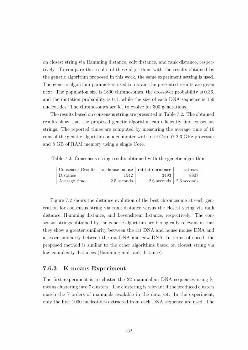
on closest string via Hamming distance, edit distance, and rank distance, respec-

tively. To compare the results of these algorithms with the results obtained by

the genetic algorithm proposed in this work, the same experiment setting is used.

The genetic algorithm parameters used to obtain the presented results are given

next. The population size is 1800 chromosomes, the crossover probability is 0.36,

and the mutation probability is 0.1, while the size of each DNA sequence is 150

nucleotides. The chromosomes are let to evolve for 300 generations.

The results based on consensus string are presented in Table 7.2. The obtained

results show that the proposed genetic algorithm can efficiently find consensus

strings. The reported times are computed by measuring the average time of 10

runs of the genetic algorithm on a computer with Intel Core i7 2.3 GHz processor

and 8 GB of RAM memory using a single Core.

Table 7.2: Consensus string results obtained with the genetic algorithm.

Consensus Results rat-house mouse rat-fat dormouse rat-cow

Distance 1542 3493 8807Average time 2.5 seconds 2.6 seconds 2.6 seconds

Figure 7.2 shows the distance evolution of the best chromosome at each gen-

eration for consensus string via rank distance versus the closest string via rank

distance, Hamming distance, and Levenshtein distance, respectively. The con-

sensus strings obtained by the genetic algorithm are biologically relevant in that

they show a greater similarity between the rat DNA and house mouse DNA and

a lesser similarity between the rat DNA and cow DNA. In terms of speed, the

proposed method is similar to the other algorithms based on closest string via

low-complexity distances (Hamming and rank distance).

7.6.3 K-means Experiment

The first experiment is to cluster the 22 mammalian DNA sequences using k-

means clustering into 7 clusters. The clustering is relevant if the produced clusters

match the 7 orders of mammals available in the data set. In the experiment,

only the first 1000 nucleotides extracted from each DNA sequence are used. The

152

Figure 7.2: The distance evolution of the best chromosome at each generation forthe Rat-Mouse-Cow experiment. GREEN = rat-house mouse distance, BLUE =rat-fat dormouse, RED = rat-cow distance.

clustering results of the two k-means methods are shown on columns in Table 7.3.

The number of correctly clustered mammals per class is represented in terms of

accuracy.

Both algorithms are able to separate the Metatheria, Monotremata, and Ro-

dentia orders. The k-means algorithm based on closest string is also able to clearly

distinguish the Perissodactylae order. On the other hand, the k-means algorithm

based on the median string is able to clearly distinguish the Carnivora and Pri-

mates orders. Both algorithms leave the sheep out of the Cetartiodactylae order.

Overall, the evaluated algorithms give comparable results. The algorithm based

153

Table 7.3: Comparative results of the k-means based on median string (k-median)versus the k-means based on closest string (k-closest). Clustering results for 22DNA sequences using rank distance.

Order k-median k-closest

Cetartiodactylae 75% 75%Carnivora 100% 0%Metatheria 100% 100%

Monotremata 100% 100%Rodentia 100% 100%Primates 100% 85%

Perissodactylae 50% 100%

Overall 86%(19/22) 77%(17/22)

on the median string seems to perform slightly better, but the two techniques

should be compared on more data sets in future work before a strong conclusion

can be drawn.

7.6.4 Hierarchical Clustering Experiment

The second experiment is to apply the three hierarchical clustering methods based

on rank distance on the 22 DNA sequences. The resulted phylogenetic trees are

compared with phylogenetic trees obtained with standard hierarchical clustering

methods, such as the one presented in [Dinu & Sgarro, 2006]. In this experiments,

the mammals are represented only by the first 3000 nucleotides of each mtDNA

sequence.

The phylogenetic tree obtained with Algorithm 6 is presented in Figure 7.3,

the tree obtained with Algorithm 7 is presented in Figure 7.4, and the tree ob-

tained with Algorithm 8 is given in Figure 7.5. Analyzing the phylogenetic trees,

one can observe that all the proposed clustering methods are able to separate

the Primates, Perissodactylae and Carnivora orders. The only confusion of the

phylogenetic tree obtained with median string is that the rat is clustered with the

sheep instead of the house mouse. The phylogenetic tree based on closest string

is slightly worse, since it is also unable to cluster the platypus, besides the rat

and the sheep. There are also two mistakes in the tree obtained with consensus

154

1234567

x 105

Pygmy ChimpanzeeChimpanzeeGorillaGibbonOrangutanSumatran OrangutanHumanCowBig WhaleFin WhaleSheepRatHorseDonkeyWhite RhinocerosIndian RhinocerosCatGray SealHarbour SealOpossumHouse MousePlatypus

Figure 7.3: Phylogenetic tree obtained for 22 mammalian mtDNA sequences usingmedian string via rank distance.

string. First, the rat is clustered with the sheep instead of the house mouse.

Second, the platypus should also be in the same cluster with the opossum and

the house mouse. Overall, the phylogenetic trees are relevant from a biological

point of view.

By comparing all the resulted trees, one can observe that the clusters near

the root are influenced by the use of the median, the closest, or the consensus

string, respectively. The clusters near the leaves are more similar for the three

methods, since the formation of these clusters is influenced by the distance itself

(in this case, rank distance). Thus, good results are in part an aftermath of rank

distance.

By considering the Primates cluster, one can observe a really interesting fact:

the human is very different from the other Primates, in all three methods. For ex-

ample, by choosing a cutting point that would separate the dendrogram obtained

with Algorithm 6 in 7 clusters, the human falls in a separate cluster. In other

words, there will be a cluster that contain a single representative DNA sequence,

that of the human’s.

155

0246810

x 105

Pygmy ChimpanzeeChimpanzeeGorillaGibbonOrangutanSumatran OrangutanHumanCatGray SealHarbour SealCowBig WhaleFin WhaleSheepRatHorseDonkeyWhite RhinocerosIndian RhinocerosPlatypusOpossumHouse Mouse

Figure 7.4: Phylogenetic tree obtained for 22 mammalian mtDNA sequences usingclosest string via rank distance.

02468

x 105

Pygmy ChimpanzeeChimpanzeeGorillaGibbonOrangutanSumatran OrangutanHumanCatGray SealHarbour SealCowBig WhaleFin WhaleSheepRatHorseDonkeyWhite RhinocerosIndian RhinocerosPlatypusOpossumHouse Mouse

Figure 7.5: Phylogenetic tree obtained for 22 mammalian mtDNA sequences usingconsensus string via rank distance.

156

By contrast to the results obtained here, in the phylogenetic tree presented

in [Dinu & Sgarro, 2006] the Perissodactylae and Carnivora orders are mixed

together. The standard hierarchical clustering method used in [Dinu & Sgarro,

2006] is also unable to join the rat with the house mouse. The phylogenetic trees

presented in this work are also comparable to those obtained in other studies [Li

et al., 2004; Reyes et al., 2000]. Therefore, the hierarchical clustering methods

presented in this chapter perform better or at least comparable to the state of

the art clustering methods.


The experiments demonstrate the utility of the algorithms described in this chap-

ter. Empirical results show that the proposed algorithms produce relevant clus-

ters, being good alternative approaches for the phylogenetic analysis of mammals.

Indeed, the results are similar or sometimes better to those reported in the lit-

erature [Dinu & Sgarro, 2006; Reyes et al., 2000]. Good results are in part an

aftermath of rank distance. The work of [Dinu & Ionescu, 2012b] shows that

rank distance can achieve better results than Hamming distance or edit distance,

when it comes to DNA sequence comparison. However, for other applications

and different kind of strings, the use of another distance metric may be more

appropriate.

One should also consider the computational time when there are many strings

to be clustered. Hamming distance should work faster than rank distance, and

it might be more suitable for use in a particular application. But, for the phy-

logenetic analysis problem, where there are usually not many individuals to be

clustered, rank distance works fine in terms of time efficiency and it also gives

more accurate clusters. For example, the results for the k-means experiment can

be obtained in less than half an hour on a machine with 2.3 GHz Intel Core i7

processor and 8GB of RAM. The most costly step in the algorithm is to solve

either the median string, the closest string, or the consensus string problems to

obtain cluster centroids. However, the parameters of the genetic algorithm pre-

sented in [Dinu & Ionescu, 2012b], that can be used to solve these three problems,

can easily be adjusted to speed up clustering. The trade-off between accuracy

157

and time must not be disregarded when setting up the parameters.

This chapter also investigated the consensus string problem under the rank

distance metric, and an efficient genetic algorithm was proposed. The genetic

approach has the advantage of finding the consensus for any number of strings,

being suitable for computational biology applications. The DNA comparison

experiment shows that the results of the genetic algorithm are indeed relevant

from a biological point of view. From the phylogenetic experiments, it seems that

the median string would be a better choice for the proposed clustering techniques.

Other applications of the proposed clustering methods, beyond computational

biology, might reveal that the median string is not always the best choice. In

future work, other distance measures, such as Hamming or edit distance, can also

be used for clustering instead of rank distance.

158

Chapter 8

Local Rank Distance

Computer science researchers have developed a wide variety of methods that can

be applied with success in computational biology. Such methods range from

clustering techniques used to analyze the phylogenetic trees of different organ-

isms, to genetic algorithms used to find motifs or common patterns in a set of

given DNA sequences. The results of many state of the art techniques for phy-

logenetic analysis or DNA sequence comparison are inaccurate from a biological

point of view, and can always be improved. Some of these methods are based on a

distance measure for strings. Popular choices for recent techniques are the Ham-

ming distance [Chimani et al., 2011; Vezzi et al., 2012], edit distance [Shapira &

Storer, 2003], Kendall-tau distance [Popov, 2007], rank distance [Dinu & Ionescu,

2012a,b], and many others [Felsenstein, 2004].

In this context, the chapter aims to introduce a new distance measure, termed

Local Rank Distance (LRD) [Ionescu, 2013a], inspired from the recently intro-

duced Local Patch Dissimilarity for images [Dinu et al., 2012]. Designed to

conform to more general principles and adapted to DNA strings, LRD is more

suitable to be used instead of other distances, from a biological point of view.

Phylogenetic analysis and DNA comparison experiments show that the use of

LRD enables significant improvements over several state of the art methods.

Theoretical properties of LRD are also investigated in this thesis. First, some

restrictions are imposed to LRD in order to prove that LRD can be a distance

function. A theoretical result about the expected distance between two random

strings is given next. Finally, the lower and the upper bounds of LRD with

159

respect to the Hamming distance are given.

The chapter is organized as follows. LRD and its principles are described in

Section 8.1. Section 8.2 presents the LRD definition. An algorithm to compute

LRD is presented in Section 8.3. Theoretical properties of LRD and a proof that

LRD can be a distance function are given in Section 8.4. Experiments conducted

on two important problems in computational biology are presented in Section 8.5.

The final remarks are given in Section 8.6.

8.1 Approach

The development of Local Rank Distance [Ionescu, 2013a] is based on Local Patch

Dissimilarity [Dinu et al., 2012], which is a generalization of rank distance for two-

dimensional input (digital images). Rank distance [Dinu, 2003] has applications

in biology [Dinu & Ionescu, 2012b; Dinu & Sgarro, 2006], natural language pro-

cessing [Dinu & Dinu, 2005; Dinu et al., 2008], computer science and many other

fields. Despite of having such broad applications, rank distance is not always

adequate for specific data types. Local Rank Distance comes from the idea of

adapting rank distance to string data, in order to capture a better similarity (or

dissimilarity) between string objects, such as DNA sequences or text.


scanning (from left to right) both strings. First, characters need to be annotated

with indexes in order to eliminate duplicates. For each annotated letter, rank

distance measures the offset between its position in the first string and its position

in the second string. Finally, all these offsets are summed up to obtain the rank

distance. In other words, the rank distance measures the offset between the

positions of a letter in the two given strings, and then sums up these values.

Intuitively, the rank distance computes the total non-alignment score between

two sequences.

Rank distance is based on mathematical principles that are not suited for

specific input data, such as images or DNA sequences. The reason is that rank

distance was designed to work with rankings (ordered sets of objects). It is useful

to consider the following example to understand how rank distance works on text

and how it can be adapted to specific input data. For two strings s1 and s2,

160

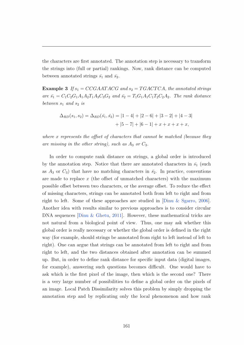
the characters are first annotated. The annotation step is necessary to transform

the strings into (full or partial) rankings. Now, rank distance can be computed

between annotated strings s1 and s2.

Example 3 If s1 = CCGAATACG and s2 = TGACTCA, the annotated strings

are s1 = C1C2G1A1A2T1A3C3G2 and s2 = T1G1A1C1T2C2A2. The rank distance

between s1 and s2 is

∆RD(s1, s2) = ∆RD(s1, s2) = |1− 4|+ |2− 6|+ |3− 2|+ |4− 3|

+ |5− 7|+ |6− 1|+ x+ x+ x+ x,

where x represents the offset of characters that cannot be matched (because they

are missing in the other string), such as A3 or C3.

In order to compute rank distance on strings, a global order is introduced

by the annotation step. Notice that there are annotated characters in s1 (such

as A3 or C3) that have no matching characters in s2. In practice, conventions

are made to replace x (the offset of unmatched characters) with the maximum

possible offset between two characters, or the average offset. To reduce the effect

of missing characters, strings can be annotated both from left to right and from

right to left. Some of these approaches are studied in [Dinu & Sgarro, 2006].

Another idea with results similar to previous approaches is to consider circular

DNA sequences [Dinu & Ghetu, 2011]. However, these mathematical tricks are

not natural from a biological point of view. Thus, one may ask whether this

global order is really necessary or whether the global order is defined in the right

way (for example, should strings be annotated from right to left instead of left to

right). One can argue that strings can be annotated from left to right and from

right to left, and the two distances obtained after annotation can be summed

up. But, in order to define rank distance for specific input data (digital images,

for example), answering such questions becomes difficult. One would have to

ask which is the first pixel of the image, then which is the second one? There

is a very large number of possibilities to define a global order on the pixels of

an image. Local Patch Dissimilarity solves this problem by simply dropping the

annotation step and by replicating only the local phenomenon and how rank

161

distance is computed on strings. Therefore, pixels or patches have no global

order to conform to. This will also be the case of Local Rank Distance, where

the annotation step is dropped, and characters in one string are simply matched

with the nearest similar characters in the other string. The advantage of using no

annotation immediately becomes clear. In Example 3, A3 remains unmatched in

the case of rank distance, while in the case of LRD, A3 from s1 will be matched

with A2 from s2, as in Example 4, since there are no annotations.

If long DNA strings (as found in nature) are considered, that contain only

characters in the alphabet Σ = {A,C,G, T}, one can observe that measuring

the non-alignment score between characters that might be randomly distributed

(with a uniformly distributed frequency) is not too relevant, because scores be-

tween different strings will almost be the same. Therefore, important information

encoded in the DNA strings might be lost or not completely captured by a dis-

tance measure that works at character level (this is the case of Hamming or rank

distance, for example). There is a similar situation in image processing. Instead

of analyzing images at the pixel level, computer vision researchers have developed

techniques that work with patches [Barnes et al., 2011; Cho et al., 2010]. To ex-

tract meaning from image, computer vision techniques, including Local Patch

Dissimilarity, look at certain features such as contour, contrast or shape. It is

clear that these features cannot be captured in single pixels, but rather in small,

overlapping rectangles of fixed size (e.g., 10 × 10 pixels), called patches. A sim-

ilar idea was introduced in the early years of bioinformatics, where k-mers (also

known as n-grams or substrings) are used instead of single characters. There are

recent studies that use k-mers for the phylogenetic analysis of organisms [Li et al.,

2004], or for sequence alignment [Melsted & Pritchard, 2011]. Analyzing DNA at

substring level is also more suited from a biological point of view, because DNA

substrings may contain meaningful information. For example, genes are encoded

by a number close to 100 base pairs, or codons that encode the twenty standard

amino acids are formed of 3-mers. LRD should also be designed to compare DNA

strings based on k-mers and not on single characters.

It is interesting to note that LRD does not require an alignment of the strings

by the addition of insertions and deletions, unlike other commonly used phylo-

genetic analysis methods. The most common methods in phylogeny deal with

162

aligned strings, and the alignment process is itself complicated. Removing this

step greatly speeds up the calculation of the distance between two strings.

Both rank distance [Dinu, 2003] and LRD [Ionescu, 2013a] are related to the

rearrangement distance [Amir et al., 2006]. The rearrangement distance works

with indexed k-mers and is based on a process of converting a string into another,

while LRD does not impose such global rules. LRD focuses only on the local

phenomenon present in DNA: strings may contain similar k-mers that are not

perfectly aligned.

8.2 Local Rank Distance Definition

To compute the LRD between two DNA strings, the idea is to sum up all the

offsets of similar k-mers between the two strings. For every k-mer in one string,

the LRD approach is to search for a similar k-mer in the other string. First, LRD

looks for similar k-mers in the same position in both DNA strings. If those k-mers

are similar, it sums up 0 since there is no offset between them. If the k-mers are

not similar, it starts looking around the initial k-mer position in the second string

to find a k-mer similar to the one in the first DNA string. If a similar k-mer is

found during this process, the offset between the two k-mers is summed up to

the total distance. The search goes on until a similar k-mer is found or until a

maximum offset is reached. Note that the maximum k-mer offset must be set a

priori and should be proportional to the size of the alphabet and to the lengths of

the DNA strings. Using the maximum offset parameter ensures that the search is

limited by a fixed window centered on the initial k-mer position. Finding similar

matches beyond this window is costly and it may also bring unwanted noise in the

process. A similar search limitation brought improvements in terms of accuracy

and speed for Local Patch Dissimilarity [Dinu et al., 2012; Ionescu & Popescu,

2013a]. LRD is formally defined next.

Definition 14 Let S1, S2 ∈ Σ∗ be two strings with symbols (k-mers) from the

163

alphabet Σ. Local Rank Distance between S1 and S2 is defined as:

∆LRD(S1, S2) = ∆left + ∆right

=∑xs∈S1

minxs∈S2

{|posS1(xs)− posS2(xs)|,m}

+∑ys∈S2

minys∈S1

{|posS1(ys)− posS2(ys)|,m},

(8.1)

where xs and ys are occurrences of symbol s ∈ Σ in strings S1 and S2, posS(xs)

represents the position (or the index) of the occurrence xs of symbol s ∈ Σ in

string S, and m ≥ 1 is the maximum offset.

A string may contain multiple occurrences of a symbol s ∈ Σ. LRD matches

each occurrence xs of symbol s ∈ Σ from a string, with the nearest occurrence

of symbol s in the other string. A symbol can be defined either as a single

character, or as a sequence of characters (k-mer). Overlapping k-mers are also

permitted in the computation of LRD, since there is no restriction that tells

where k-mers should start or end in a DNA string. Notice that in order to be

a symmetric distance measure, LRD must consider every k-mer in both strings.

Offsets between matched k-mers are computed with the euclidean distance based

on the L1-norm. Thus, offsets are always non-negative integer values.

To understand how LRD actually works, it is useful to consider Example 4

where LRD is computed between strings s1 and s2 from Example 3 using 1-mers

(single characters).

Example 4 Let s1 and s2 be defined as in Example 3, and m = 10 be the maxi-

mum offset. The LRD between s1 and s2 is given by:

∆LRD(s1, s2) = ∆left + ∆right,

where the two sums ∆left and ∆right are computed as follows:

∆left =∑xs∈s1

minxs∈s2{|poss1(xs)− poss2(xs)|, 10}

= |1− 4|+ |2− 4|+ |3− 2|+ |4− 3|+ |5− 3|

+ |6− 5|+ |7− 7|+ |8− 6|+ |9− 2| = 19,

164

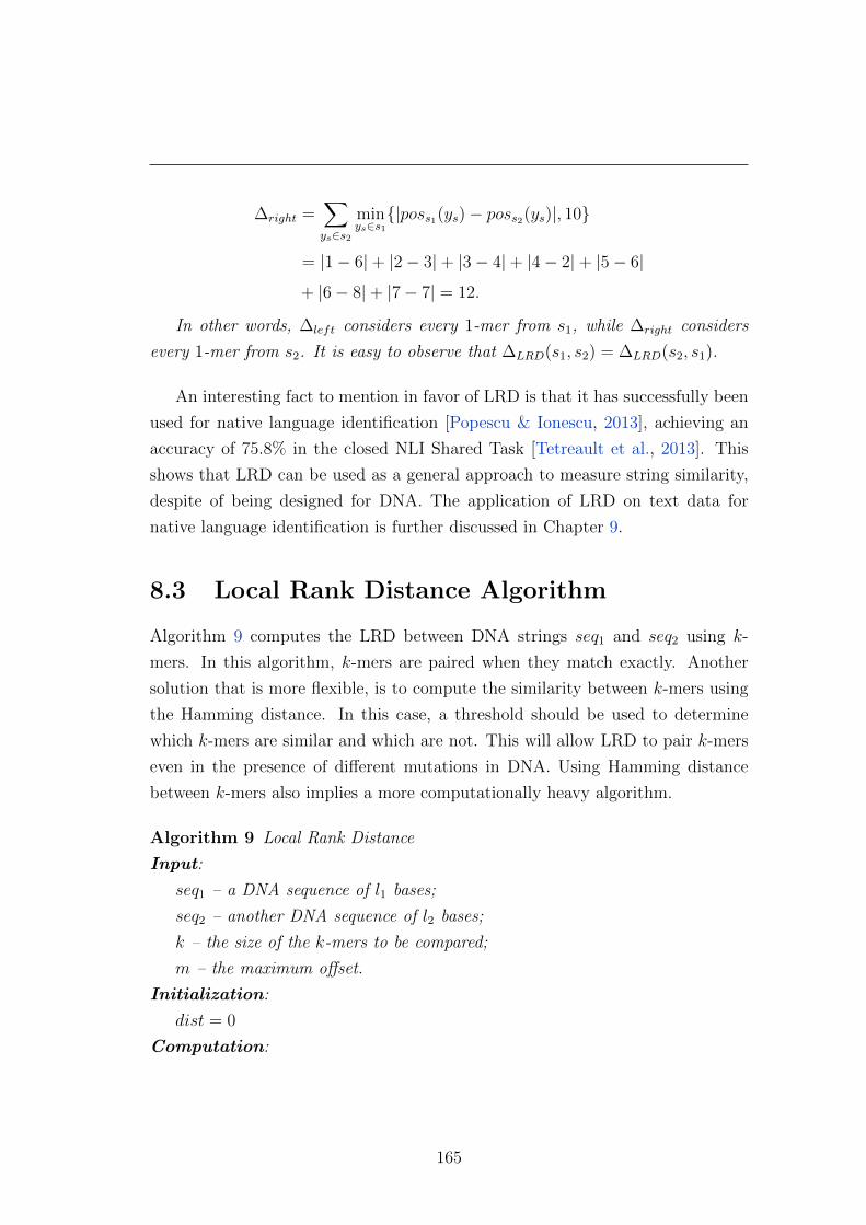
∆right =∑ys∈s2

minys∈s1{|poss1(ys)− poss2(ys)|, 10}

= |1− 6|+ |2− 3|+ |3− 4|+ |4− 2|+ |5− 6|

+ |6− 8|+ |7− 7| = 12.

In other words, ∆left considers every 1-mer from s1, while ∆right considers

every 1-mer from s2. It is easy to observe that ∆LRD(s1, s2) = ∆LRD(s2, s1).

An interesting fact to mention in favor of LRD is that it has successfully been

used for native language identification [Popescu & Ionescu, 2013], achieving an

accuracy of 75.8% in the closed NLI Shared Task [Tetreault et al., 2013]. This

shows that LRD can be used as a general approach to measure string similarity,

despite of being designed for DNA. The application of LRD on text data for

native language identification is further discussed in Chapter 9.

8.3 Local Rank Distance Algorithm

Algorithm 9 computes the LRD between DNA strings seq1 and seq2 using k-

mers. In this algorithm, k-mers are paired when they match exactly. Another

solution that is more flexible, is to compute the similarity between k-mers using

the Hamming distance. In this case, a threshold should be used to determine

which k-mers are similar and which are not. This will allow LRD to pair k-mers

even in the presence of different mutations in DNA. Using Hamming distance

between k-mers also implies a more computationally heavy algorithm.

Algorithm 9 Local Rank Distance

Input:

seq1 – a DNA sequence of l1 bases;

seq2 – another DNA sequence of l2 bases;

k – the size of the k-mers to be compared;

m – the maximum offset.

Initialization:

dist = 0

Computation:

165

for i = 1 to l1 − k + 1 // compute ∆left

get k-meri at position i in seq1

j = 0

found = false

while j < m and found == false

get k-merleft at position i− j in seq2

get k-merright at position i+ j in seq2

if k-meri == k-merleft or k-meri == k-merright

dist = dist+ j

found = true

endif

j = j + 1

endwhile

if found == false

dist = dist+m

endif

endfor

for i = 1 to l2 − k + 1 // compute ∆right

get k-meri at position i in seq2

j = 0

found = false

while j < m and found == false

get k-merleft at position i− j in seq1

get k-merright at position i+ j in seq1

if k-meri == k-merleft or k-meri == k-merright

dist = dist+ j

found = true

endif

j = j + 1

endwhile

if found == false

dist = dist+m

endif

166

endfor

Output:

dist – the Local Rank Distance between seq1 and seq2.

Algorithm 9 needs two input parameters besides the two DNA strings. The k-

mer size parameter represents the number of characters (bases) for the substrings

involved in the computation of LRD. The maximum offset parameter determines

the size of the search window. These parameters need to be adjusted with regard

to the length of the DNA strings. For example, using 10-mers for DNA strings of

100 or 200 bases is not reasonable, since finding similar 10-mers in such short DNA

strings is rare, if not almost impossible. But 10-mers are suited for mitochondrial

DNA strings of 15.000−17.000 bases. Notice that the maximum offset parameter

should be adjusted accordingly. Using 10-mers and a maximum offset that is too

small, such as 50, will result in finding almost no similar 10-mers in the search

window. This happens because there are |Σ|k possible k-mers, where |Σ| is the

size of the alphabet Σ = {A,C,G, T}. In the case of 10-mers, it means that there

are 410 = 1.048.576 combinations.

The analysis of the computational complexity of Algorithm 9 is straightfor-

ward. Let l = max{l1, l2} be the maximum length of the two strings. The

complexity of the Algorithm 9 is O(l ×m× k), when using brute (linear) search

to find similar k-mers. Using advanced string searching algorithms [Knuth et al.,

1977] the complexity can be reduced to O(l×m). If only 1-mers are considered,

the computational complexity of LRD becomes linear as Hamming distance or

rank distance. If approximate matches are allowed between k-mers, by using

Hamming distance to compare k-mers for example, the time complexity remains

O(l × m × k), since computing the Hamming distance between two strings (or

k-mers) cannot be done faster than linear time.

8.4 Properties of Local Rank Distance

LRD replicates how Local Patch Dissimilarity works on images. As Local Patch

Dissimilarity is adapted to images, LRD is based on principles that make it more

167

suited to DNA sequences. LRD essentially measures the non-alignment score

between k-mers. Both LRD and Local Patch Dissimilarity can be considered as

extended versions of rank distance [Dinu, 2003], which are adapted to specific

input data. Despite the fact that LRD is more adapted to DNA strings, LRD

remains a distance function. A proof that LRD is a distance function is first given.

More theoretical properties of LRD are studied next. The expected distance

between two random strings is also discussed in this section. Finally, the lower

and and the upper bounds of LRD with respect to the Hamming distance are

given.

The definition of a distance function is considered next, as the first concern

of this section is to prove that LRD is a distance measure.

Definition 15 A metric on a set X is a function (called the distance function

or simply distance) d : X ×X → R. For all x, y, z ∈ X, this function is required

to satisfy the following conditions:

(i) d(x, y) > 0 (non-negativity, or separation axiom);

(ii) d(x, y) = 0 if and only if x = y (coincidence axiom);

(iii) d(x, y) = d(y, x) (symmetry);

(iv) d(x, z) 6 d(x, y) + d(y, z) (triangle inequality).

One can observe that axioms (i) and (ii) from Definition 15 produce positive

definiteness. It can be easily observed that LRD is not a distance function if a

k-mer from one string is associated with two or more identical k-mers from the

other string. However, it can be demonstrated that LRD is a distance function

for a given k ≥ 1, such that all the k-mers occur only a single time in each of the

two strings.

Theorem 6 For all k ≥ 1, such that all the k-mers of length k occur only a

single time in each of the compared strings, Local Rank Distance is a distance

function.

Proof: The proof is based on showing that ∆LRD given by Definition 14 satisfies

the conditions in Definition 15.

168

Let S1, S2 ∈ Σ∗.

(i) Proof of non-negativity

∆LRD(S1, S2) is a sum of positive or 0 values that represent offsets between

symbols in S1 and S2. This sum can only be greater or equal to 0. This ensures

the non-negativity condition in Definition 15.

(ii) Proof of coincidence axiom

(⇒): Let ∆LRD(S1, S2) 6= 0. There is at least one occurrence xs ∈ S1 for which

minxs∈S2{|posS1(xs) − posS2(xs)|,m} > 0, or at least one occurrence ys ∈ S2 for

which minys∈S1{|posS1(ys)−posS2(ys)|,m} > 0, otherwise ∆LRD(S1, S2) would be

0.

Case 1: If minxs∈S2{|posS1(xs)− posS2(xs)|,m} > 0, then the symbol s corre-

sponding to xs ∈ S1 does not occur in the same position in S2 as in S1. It means

S2 contains a symbol different from s at the position given by posS1(xs). S1 and

S2 have at least one different symbol, therefore S1 6= S2.

Case 2: If minys∈S1{|posS1(ys)− posS2(ys)|,m} > 0, the proof is analogous to

Case 1. The implication is proven.

(⇐): Let S1 6= S2. There is at least one position i in S1, or j in S2 with

different symbols.

Case 1: The occurrence xs of symbol s at position i = posS1(xs) in S1 is consid-

ered. Since S2 does not contain the same symbol s at position i, minxs∈S2{|posS1(xs)−posS2(xs)|,m} > 0. In other words, there is at least one term in the sum ∆left

that is positive. Consequently, ∆LRD(S1, S2) 6= 0.

Case 2: The proof for occurrence ys of symbol s at position j = posS2(ys) in

S2 is analogous to Case 1. The coincidence axiom is proven.

(iii) Proof of symmetry

Using the commutative property of the + operation and that of the euclidean

169

distance, the proof of symmetry for ∆LRD is immediate:

∆LRD(S1, S2) =∑xs∈S1

minxs∈S2

{|posS1(xs)− posS2(xs)|,m}+

+∑ys∈S2

minys∈S1

{|posS1(ys)− posS2(ys)|,m}

=∑ys∈S2

minys∈S1

{|posS2(ys)− posS1(ys)|,m}+

+∑xs∈S1

minxs∈S2

{|posS2(xs)− posS1(xs)|,m} = ∆LRD(S2, S1).

(8.2)

(iv) Proof of triangle inequality

Let A,B,C ∈ Σ∗. To show that

∆LRD(A,B) + ∆LRD(B,C) ≥ ∆LRD(A,C), (8.3)

the ∆left and ∆right sums are treated as separate inequalities, as follows:

∆left(A,B) + ∆left(B,C) ≥ ∆left(A,C), (8.4)

∆right(A,B) + ∆right(B,C) ≥ ∆right(A,C). (8.5)

Obviously, summing inequalities given by equations 8.4 and 8.5, the triangle

inequality (equation 8.3) for LRD is obtained. Regarding equation 8.4, for each

occurrence xs in A, B and C, there are three possible cases for the positions of

xs in the respective strings. Let i = posA(xs) be a fixed position of xs in A. Let

j and k denote the nearest positions of xs in B and C, respectively. Positions j

and k are formally defined as:

j = argminp=posB(xs)

{|i− p|,m},

k = argminq=posC(xs)

{|i− q|,m}.(8.6)

There are six possible combinations of sorting positions i, j, k in ascending

170

Figure 8.1: The intuition behind the proof of the triangle inequality for LRD.For each occurrence xs, the three possible cases of sorting i, j and k are shownin the upper side of the figure. The nearest match position in C is denoted byk′. For each occurrence ys, the three possible cases are shown in the lower side ofthe figure. The nearest match position in A is denoted by i′.

order. This brings three distinct situations (or cases) that are discussed next.

Figure 8.1 shows the intuition behind the demonstration of the triangle inequality.

Cases 1, 2 and 3 for occurrences xs can be observed visually.

Case 1 (i < k < j or j < k < i):

Since LRD works with absolute positive values and i < k < j or j < k < i,

the following inequality is true:

|i− j| ≥ |i− k|. (8.7)

Note that the occurrence of xs in B may be matched with another closer oc-

currence of xs in C rather than the occurrence at position k. Let k′ denote the

position of this nearest occurrence. Position k′ is formally defined as:

k′ = argminq=posC(xs)

{|j − q|,m}. (8.8)

171

If position k′ exists, then:

|j − k| > |j − k′| ≥ 0. (8.9)

If a distinct k′ does not exist, then k′ = k. From equations 8.7 and 8.9, it results

that the triangle inequality is satisfied for each xs (even when k′ 6= k):

|i− j|+ |j − k′| ≥ |i− k|. (8.10)

Case 2 (k < i < j or j < i < k):

Note that the euclidean distance based on the L1-norm is used to compute

differences between positions i, j and k. Since the euclidean distance satisfies the

triangle inequality, the following equation is also satisfied:

|i− j|+ |j − k| ≥ |i− k|. (8.11)

As in Case 1, the occurrence of xs in B may be matched with another closer

occurrence of xs in C. Let k′ defined as in equation 8.8 denote the position of

this nearest occurrence. If k′ 6= k exists, then equation 8.9 also holds for Case

2. However, the equation 8.11 still holds if the condition in equation 8.7 is met.

In other words, the triangle inequality is still satisfied if the offset (euclidean

distance) between i and j is greater than the offset between i and k.

In the other case, when the condition in equation 8.7 is not met, the following

equations are possible:

|i− j|+ |j − k′| ≤ |i− k|, (8.12)

|i− j|+ |j − k′| ≥ |i− k′|. (8.13)

Equations 8.12 and 8.13 imply that:

|i− k| ≥ |i− k′|. (8.14)

From the definition of LRD and equation 8.14, it results that k′ = k. This

172

contradicts the assumption that k′ 6= k. Therefore, equation 8.12 can never be

true, and the triangle inequality holds for Case 2.

Case 3 (i < j < k or k < j < i):

Case 3 is similar to Case 2. Since the euclidean distance satisfies the triangle

inequality, equation 8.11 is also satisfied for this case. As in Case 1, the occurrence

of xs in B may be matched with another closer occurrence of xs in C. Let k′

defined as in equation 8.8 denote the position of this nearest occurrence. If k′ 6= k

exists, then equation 8.9 also holds for Case 3.

However, the condition in equation 8.7 cannot be met since i < j < k or

k < j < i, and equations 8.12 and 8.13 become possible. Again, equations 8.12

and 8.13 imply equation 8.14. From the definition of LRD and equation 8.14, it

results that k′ = k, contradicting the assumption that k′ 6= k.

For each occurrence xs in A, B and C, the triangle inequality is satisfied. This

implies that equation 8.4 is true, because ∆left involves only xs. The demonstra-

tion is similar for each occurrence ys in A, B and C. The difference is made by

the fact that the occurrence of ys in B may be matched with another closer oc-

currence of ys in A, also shown in Figure 8.1. Equation 8.5 is also true, because

∆right involves only ys. Finally, LRD satisfies the conditions in Definition 15.

This ends the proof of Theorem 6. utThe coincidence axiom is not longer verified if approximate matches are al-

lowed between k-mers. The use of Hamming distance to compare k-mers (and

match them under a similarity threshold) may seem appropriate from a biolog-

ical point of view, but from a mathematical point of view, LRD can no longer

be considered a distance function. In practice, better results may be obtained by

using approximate matches, but this subject is left for future study.

LRD measures the distance between two DNA strings. Knowing the maximum

offset (used to stop similar k-mer searching), the maximum LRD value between

two strings can be computed as the product between the maximum offset and the

number of pairs of compared k-mers. Thus, LRD can be normalized to a value in

the [0, 1] interval. By normalizing, LRD can also be transformed into a similarity

or dissimilarity measure.

The following theorem gives an approximation of LRD between two random

strings.

173

Theorem 7 Given S1, S2 ∈ Σ∗ and a maximum offset threshold m, where Σ is

an alphabet of symbols (or k-mers), the expected Local Rank Distance between S1

and S2 can be approximated by:

∆LRD(S1, S2) ≈

[(1−

(|Σ| − 1

|Σ|

)2m+1)m

2+

(|Σ| − 1

|Σ|

)2m+1

m

](|S1|+ |S2|),

(8.15)

where |Σ| gives the number of symbols in Σ, |S1| is the length of S1, and |S2| is

the length of S2, respectively.

Proof: For every symbol that occurs in S1, LRD adds the offset to the nearest

occurrence in S2. In the same manner, for every symbol that occurs in S2, LRD

adds the offset to the nearest occurrence in S1. If the expected offset is defined

by x ∈ [0,m], then the following equation approximates LRD:

∆LRD(S1, S2) ≈ x(|S1|+ |S2|). (8.16)

To determine the expected offset x of a certain symbol, the following discussion

is made. Let s be a symbol from Σ. LRD searches for symbol s in a window of

2m+ 1 symbols. But the symbol s may or may not occur in the search window.

Let A be the event defined by “there is at least one occurrence of symbol s in a

string of 2m+ 1 symbols”. Let AC denote the complementary event of A.

The probability of event AC is given by:

P (AC) =

(|Σ| − 1

|Σ|

)2m+1

. (8.17)

The probability of event A can be determined using equation 8.17 as follows:

P (A) = 1− P (AC) = 1−(|Σ| − 1

|Σ|

)2m+1

. (8.18)

When event A occurs, the average offset of symbol s is m/2, since each position

in the search window is equally likely to be the occurrence of s. When the

174

complementary event AC occurs, LRD adds the maximum offset, since symbol s

is not found in the search window. Thus, the expected offset is given by:

x =

(1−

(|Σ| − 1

|Σ|

)2m+1)m

2+

(|Σ| − 1

|Σ|

)2m+1

m (8.19)

By replacing x in equation 8.16 with the value determined in equation 8.19,

the equation 8.15 is obtained. This ends the proof. utTheorem 7 approximates the expected distance between two strings. This

approximation is useful in practice, especially when one wants to determine the

similarity of two strings. If the obtained distance is lower than the value given

in equation 8.15, then the strings can be considered as being similar. Otherwise,

the strings can be considered as being dissimilar.

The following theorem shows the relationship between LRD and Hamming

distance.

Theorem 8 Given S1, S2 ∈ Σ∗ and a maximum offset threshold m, the following

equation gives the lower and the upper bounds of the Local Rank Distance with

respect to the Hamming distance:

∆H(S1, S2) ≤ ∆LRD(S1, S2) ≤ m ·∆H(S1, S2). (8.20)

Proof: Let X be the set of positions with matching symbols in S1 and S2. The

Hamming distance is given by:

∆H(S1, S2) = |S1| − |X|+ |S2| − |X|, (8.21)

where |X| is the size of set X, |S1| is the length of S1, and |S2| is the length of

S2, respectively. Basically, the Hamming distance counts the number of symbols

that are not matched between S1 and S2. In the same manner, LRD adds an

offset of 0 for the symbols in X. For the other symbols, LRD adds an offset in

the interval [1,m]. The bounds are determined by considering the two extreme

cases.

Supposing that LRD always adds an offset of 1 for unmatched symbols, the

175

following equation is true:

∆LRD(S1, S2) = |S1| − |X|+ |S2| − |X|. (8.22)

Since 1 is the minimum offset that can be added, the lower bound is obtained

from equations 8.21 and 8.22:

∆H(S1, S2) ≤ ∆LRD(S1, S2). (8.23)

Supposing that LRD always adds an offset of m for unmatched symbols, the

following equation is true:

∆LRD(S1, S2) = m (|S1| − |X|) +m (|S2| − |X|) . (8.24)

Since m is the maximum offset that can be added, the upper bound is obtained

from equations 8.21 and 8.24:

∆LRD(S1, S2) ≤ m ·∆H(S1, S2). (8.25)

utTheorem 8 shows that LRD is a much more sensible distance than the Ham-

ming distance. LRD is being able to capture not only the unmatched symbols,

but also the offsets of such symbols. These offsets are recorded at a very fine

scale, giving LRD the power to find subtle differences between the two strings.

8.5 Experiments and Results


LRD is tested on two important problems in bioinformatics: the phylogenetic

analysis of mammals and the finding of common substrings in a set of given DNA

strings. In the experiments presented in this chapter, mitochondrial DNA se-

quence genome of the 27 mammals is used. The 27 mammals along with their

associated accession numbers are given in Table 8.1. The mtDNA sequences are

176

available for download in the EMBL database (http://www.ebi.ac.uk/ena/).

The mammals selected for the experiments belong to one of the following 8 or-

ders: Carnivora, Cetartiodactylae, Chiroptera, Metatheria, Monotremata, Peris-

sodactylae, Primates, and Rodentia.

Table 8.1: The 27 mammals from the EMBL database used in the phylogeneticexperiments. The accession number is given on the last column.

Mammal Latin Name Accession

human Homo sapiens V00662common chimpanzee Pan troglodytes D38116pigmy chimpanzee Pan paniscus D38113gorilla Gorilla gorilla D38114orangutan Pongo pygmaeus D38115Sumatran orangutan Pongo pygmaeus abelii X97707gibbon Hylobates lar X99256hamadryas baboon Papio hamadryas Y18001horse Equus caballus X79547donkey Equus asinus X97337Indian rhinoceros Rhinoceros unicornis X97336white rhinoceros Ceratotherium simum Y07726harbor seal Phoca vitulina X63726gray seal Halichoerus grypus X72004cat Felis catus U20753fin whale Balaenoptera physalus X61145blue whale Balaenoptera musculus X72204cow Bos taurus V00654sheep Ovis aries AF010406pig Sus scrofa AF034253rat Rattus norvegicus X14848mouse Mus musculus V00711fat dormouse Myoxus glis AJ001562Jamaican fruit-eating bat Artibeus jamaicensis AF061340North American opossum Didelphis virginiana Z29573wallaroo Macropus robustus Y10524platypus Ornithorhynchus anatinus X83427

Some general aspects on mtDNA sequences are discussed in Section 7.6. It is

worth mentioning that mtDNA from two individuals of the same species differs

by only 0.1%. This means, for example, that mtDNA from two different humans

177


differs by less than 20 base pairs. Because this small difference cannot affect the

study, the experiments are conducted using a single mtDNA sequence for each

mammal, as in Chapter 7.

8.5.2 Phylogenetic Analysis

Two experiments are performed on the phylogenetic analysis of mammals. The

first one includes mitochondrial DNA sequence genome of 22 mammals from the

EMBL database. Results on this data set of 22 mammals are also reported

by [Dinu & Ionescu, 2012a, 2013a; Dinu & Sgarro, 2006]. Similar studies were

also performed by [Cao et al., 1998; Li et al., 2004; Reyes et al., 2000].

In this work, a hierarchical clustering technique based on LRD, using the av-

erage linkage criterion, is tested on the 22 mammals data set. Single or complete

linkage criteria show similar results, but the average linkage seems to work best

in combination with LRD. Figures 8.2, 8.3, 8.4, 8.5, 8.6 show the results obtained

with the hierarchical clustering based on LRD using different k-mer sizes. As

the size of the k-mers grows, the dendrograms look better and better. For LRD

with 8-mers (Figure 8.5) and 10-mers (Figure 8.6), perfect phylogenetic trees are

obtained. In other words, mammals are clustered according to their biological

orders. The maximum offset of LRD ranges from 640 to 1000, and it is ad-

justed proportional to the size of k-mers used. Another dendrogram presented

in Figure 8.7 is obtained by summing up the Local Rank Distances with 6-mers,

7-mers, 8-mers, 9-mers and 10-mers, respectively. Again, mammals are perfectly

clustered according to their orders. The idea of summing up distances obtained

with different k-mers makes the hierarchical clustering method more robust.

Table 8.2 shows the number of misclustered mammals of previously proposed

techniques and that of the hierarchical clustering based on LRD with sum of

k-mers. The best result with 100% accuracy is obtained by the hierarchical

clustering based on LRD.

Since the hierarchical clustering based on LRD obtains perfect accuracy, an-

other clustering experiment with more DNA sequences is performed. This second

experiment includes mtDNA sequences from all the 27 mammals obtained from

the EMBL database. If 8-mers are enough to obtain a perfect phylogenetic tree

178

0.511.522.533.5

x 105

Pygmy ChimpanzeeChimpanzeeGibbonGorillaOrangutanSumatran Orangutan SheepHouse MouseRatCowBig WhaleFin WhaleHumanHorseDonkeyIndian RhinocerosWhite RhinocerosCatGray SealHarbour SealOpossumPlatypus

2−gram Local Rank Distance

Figure 8.2: Phylogenetic tree obtained for 22 mammalian mtDNA sequences usingLRD based on 2-mers.

1234

x 106

Pygmy ChimpanzeeChimpanzeeGorillaGibbonOrangutanSumatran Orangutan SheepHorseDonkeyIndian RhinocerosWhite RhinocerosHouse MouseRatOpossumPlatypusCowBig WhaleFin WhaleHumanCatGray SealHarbour Seal



179

0.511.52

x 107

Pygmy ChimpanzeeChimpanzeeGorillaOrangutanSumatran Orangutan GibbonSheepHorseDonkeyIndian RhinocerosWhite RhinocerosHouse MouseRatOpossumPlatypusCowBig WhaleFin WhaleHumanCatGray SealHarbour Seal



11.522.53

x 107

Gray SealHarbour SealCatCowSheepBig WhaleFin WhaleHorseDonkeyIndian RhinocerosWhite RhinocerosHouse MouseRatHumanGibbonGorillaPygmy ChimpanzeeChimpanzeeOrangutanSumatran Orangutan OpossumPlatypus



180

11.522.53

x 107




468101214

x 107


Sum of n−grams Local Rank Distance

Figure 8.7: Phylogenetic tree obtained for 22 mammalian mtDNA sequences usingLRD based on sum of k-mers.

181

Table 8.2: The number of misclustered mammals for different clustering tech-niques on the 22 mammals data set.

Method Misclustered Accuracy

Proposed by [Dinu & Sgarro, 2006] 3/22 86.36%Proposed by [Dinu & Ionescu, 2012a] 3/22 86.36%LRD + sum of k-mers 0/22 100.00%

in the first experiment, longer k-mers are considered for the second experiment.

Figure 8.8 shows the dendrogram obtained by the hierarchical clustering based

on LRD using 18-mers. Again the average linkage criterion gives the best results.

The only mistake of the proposed method is that it clusters the pig together with

members of the Carnivora order instead of the Cetartiodactylae order. Having 1

out of 27 misclustered mammals, the accuracy is 96.29% this time.

Overall, the accuracy level achieved by the clustering method based on LRD

is better or at least comparable with state of the art methods proposed in similar

studies [Cao et al., 1998; Dinu & Sgarro, 2006; Li et al., 2004; Reyes et al., 2000].

8.5.3 DNA Comparison

In this section an experiment is performed to show that LRD can also be used

to find the closest string (or closest substring) for set of DNA strings, using a

genetic algorithm based on LRD. Here, the genetic algorithm proposed in [Dinu

& Ionescu, 2012b] is combined with LRD.

Only the rat, house mouse, fat dormouse and cow genomes are used in the ex-

periment. The task is to find the closest string between the rat and house mouse

DNAs, between the rat and fat dormouse DNAs, and between the rat and cow

DNAs. The goal of this experiment is to compare the distances associated to the

three closest strings. The cow belongs to the Cetartiodactylae order, while the rat,

the house mouse, and the fat dormouse belong to the Rodentia order. Expected

results should show that the rat-house mouse distance and the rat-fat dormouse

distance are smaller than the rat-cow distance. The same experiment was also

conducted in [Dinu & Ionescu, 2012b] by using three genetic algorithms based

on Hamming distance, edit distance and rank distance, respectively. To compare

182

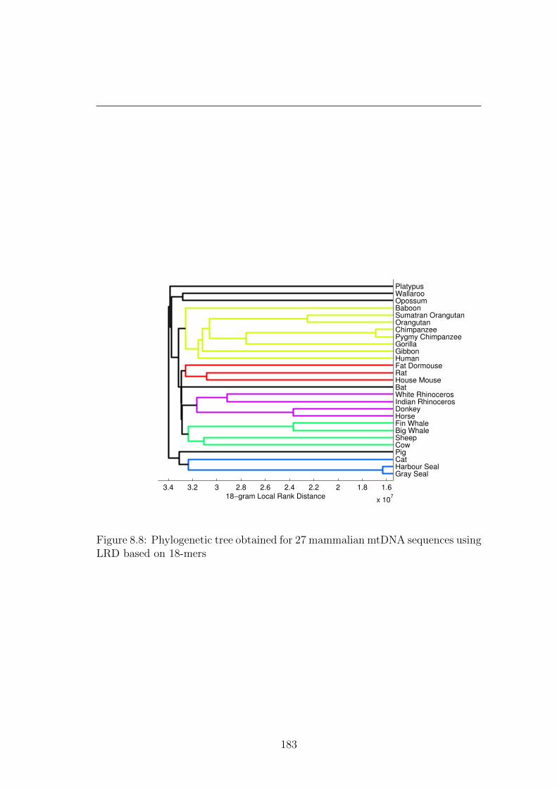
1.61.822.22.42.62.833.23.4

x 107

Gray SealHarbour SealCatPigCowSheepBig WhaleFin WhaleHorseDonkeyIndian RhinocerosWhite RhinocerosBatHouse MouseRatFat DormouseHumanGibbonGorillaPygmy ChimpanzeeChimpanzeeOrangutanSumatran Orangutan BaboonOpossumWallarooPlatypus


Figure 8.8: Phylogenetic tree obtained for 27 mammalian mtDNA sequences usingLRD based on 18-mers

183

the results of these algorithms with the results obtained by the genetic algorithm

based on LRD, the same experiment setting is used. The genetic algorithm pa-

rameters used to obtain the presented results are given next. The population size

is 600 chromosomes, the number of generations is 200, the crossover probability

is 0.36, the mutation probability is 0.005, and size of each DNA sequence is 150

bases. Details regarding experiment organization and parameters of the genetic

algorithm can also be found in [Dinu & Ionescu, 2012b]. The results presented

in Table 8.3 are obtained using LRD with 3-mers and a maximum offset of 48.

The reported time is computed by measuring the average time of 10 runs of the

genetic algorithm on a computer with Intel Core i7 2.3 GHz processor and 8 GB

of RAM memory using a single Core.

Table 8.3: Closest string results for the genetic algorithm based on LRD with3-mers.

LRD Results rat-house mouse rat-fat dormouse rat-cow

Distance 1524 2379 4169Average time 12 seconds 14 seconds 17 seconds

Figure 8.9 shows the distance evolution of the best chromosome at each gener-

ation for Local Rank Distance, rank distance, Hamming distance and edit (Leven-

shtein) distance. The use of LRD enables the genetic algorithm to achieve better

results than previously studied genetic algorithms [Dinu & Ionescu, 2012b], but

with a smaller population of chromosomes (600 instead of 1800) and a lower num-

ber of generations (200 instead of 300). In terms of speed, the proposed method

is similar to the other algorithms based on low-complexity distances (Hamming

and rank distance).

8.6 Discussion and Future Work

Designed to conform to more general principles and adapted to DNA strings, LRD

comes to improve several state of the art methods for DNA sequence analysis.

Phylogenetic experiments show that trees produced by LRD are better or at least

comparable with those reported in the literature [Dinu & Ionescu, 2012a; Dinu

184

Figure 8.9: The distance evolution of the best chromosome at each generation forthe Rat-Mouse-Cow experiment. GREEN = rat-house mouse distance, BLUE =rat-fat dormouse, RED = rat-cow distance.

185

& Sgarro, 2006; Li et al., 2004; Reyes et al., 2000]. The closest string experiment

shows that the use of LRD enables genetic algorithms to achieve similar or better

results than previously studied methods [Dinu & Ionescu, 2012b]. In conclusion,

LRD can be used to improve the results of several methods for DNA sequence

analysis or related tasks.

In future work, the Hamming distance could be used to compare k-mers in

the computation of LRD. This seems to be more appropriate from a biological

point of view, in that it allows the pairing of k-mers with mutations. A faster

version of LRD, that considers only the significant or the most frequent k-mers, is

also of great interest for sequence alignment or related tasks. Significant k-mers

could be those that encode genes, for example.

An interesting fact to mention in favor of LRD is that it has successfully been

used for native language identification [Popescu & Ionescu, 2013], achieving an

accuracy of 75.8% in the closed NLI Shared Task [Tetreault et al., 2013]. This

shows that LRD can be used as a general approach to measure string similarity,

despite being designed for DNA. The native language identification results are

discussed in Chapter 9.

186

Chapter 9

Native Language Identification

with String Kernels

Using words is natural in text analysis tasks like text categorization, authorship

identification and plagiarism detection, among others. Perhaps surprisingly, re-

cent results have proved that methods handling the text at character level can

also be very effective in text analysis tasks [Grozea et al., 2009; Lodhi et al.,

2002; Popescu, 2011; Popescu & Dinu, 2007; Popescu & Grozea, 2012; Sanderson

& Guenter, 2006]. This chapter follows this line of research and aims to investi-

gate if the native language can be identified with machine learning methods that

work at the character level. By disregarding features of natural language such as

words, phrases, or meaning, an approach that works at the character level has an

important advantage in that it is language independent.

This chapter describes an approach based on string kernels. In this approach,

texts are treated just as sequences of symbols (strings). Different string ker-

nels are combined with different kernel-based learning methods in a series of

experiments to assess the best performance level that can be achieved on native

language identification. It seems that the machine learning approach based on

string kernels achieves state of the art performance in native language identifica-

tion. Actually, the Unibuc team [Popescu & Ionescu, 2013] participated with the

described method in the Native Language Identification (NLI) Shared Task 2013

and obtained the third place [Tetreault et al., 2013].

187

The chapter is organized as follows. A motivation in favor of using charac-

ter level methods is given in Section 9.1. The string kernels are presented in

Section 9.2. Section 9.3 explains how the LRD measure can be used for text

analysis, and how to transform it into a kernel. Section 9.4 presents details about

the experiments. It gives details about choosing the learning method, parameter

tuning, combining kernels and results of submitted systems. Finally, the future

work is discussed in Section 9.5.

9.1 Motivation and Discussion

The string kernel implicitly embeds the texts in a high dimensional feature space.

Then, a kernel-based learning algorithm implicitly assigns a weight to each fea-

ture, thus selecting the features that are important for the discrimination task.

For example, in the case of text categorization the learning algorithm enhances

the features representing stems of content words [Lodhi et al., 2002], while in

the case of authorship identification the same learning algorithm enhances the

features representing function words [Popescu & Dinu, 2007].

Using string kernels will make the corresponding learning method completely

language independent, because the texts will be treated as sequences of symbols

(strings). Methods working at the word level or above very often restrict their

feature space according to theoretical or empirical principles. Thus, a method

that considers words as features can not be language independent. Even a method

that uses only function words as features is not completely language independent

because it needs a list of function words (specific to a language) and a way to

segment a text into words which is not an easy task for some languages, like

Chinese.

It is interesting to mention that character n-grams were already used in na-

tive language identification [Brooke & Hirst, 2012; Tetreault et al., 2012]. The

reported performance when only character n-grams were used as features was

modest compared with other type of features. But, in the above mentioned

works, the authors investigated only the bigrams and trigrams, as they probably

considered that longer n-grams would not improve the performance or that are

too expensive to compute. Particularly, in a set of preliminary experiments of

188

this work, similar results with [Tetreault et al., 2012] were obtained when using

character bigrams. However, the best performance has been achieved using a

range of 5 to 8 n-grams. A similar approach was used with success for the related

task of identifying translationese [Popescu, 2011]. Combining 5 to 8 n-grams

would generate millions of features, which are indeed expensive to compute and

represent. The key of avoiding to compute such a large number of features lies

in using the dual representation provided by the string kernel. String kernel sim-

ilarity matrices can be computed much faster and are extremely useful when the

number of samples is much lower than the number of features.

The first application of string kernel ideas came in the field of text catego-

rization, with the paper [Lodhi et al., 2002], followed by applications in bioinfor-

matics [Leslie et al., 2002]. Computer science researchers have developed a wide

variety of methods that can be applied with success in computational biology.

Such methods range from clustering techniques used to analyze the phylogenetic

trees of different organisms [Dinu & Ionescu, 2012a; Dinu & Sgarro, 2006], to

genetic algorithms used to find motifs or common patterns in a set of given DNA

sequences [Dinu & Ionescu, 2012b]. Some of these methods are based on distance

measure for strings that work at the character level. Among these measures are

the Hamming distance [Chimani et al., 2011; Vezzi et al., 2012], the edit dis-

tance [Shapira & Storer, 2003], the Kendall-tau distance [Popov, 2007], or the

rank distance [Dinu, 2003]. A similar idea to character n-grams was introduced

in the early years of bioinformatics, where k-mers are used instead of single char-

acters 1. There are recent studies that use k-mers for the phylogenetic analysis

of organisms [Li et al., 2004], or for sequence alignment [Melsted & Pritchard,

2011]. Analyzing DNA at substring level is also more suited from a biological

point of view, because DNA substrings may contain meaningful information. For

example, genes are encoded by a number close to 100 base pairs, or codons that

encode the twenty standard amino acids are formed of 3-mers.

The Local Rank Distance [Ionescu, 2013a] has been recently proposed as an

extension of rank distance. LRD drops the annotation step of rank distance, and

uses k-mers instead of single characters. Chapter 8 shows that LRD is a distance

1In biology, single DNA characters are also referred to as nucleotides or monomers. Polymersare also known as k-mers.

189

function and that it has very good results in phylogenetic analysis and DNA

sequence comparison. But, LRD can be applied to any kind of string sequences,

not only to DNA. Thus, LRD is transformed into a kernel and used for native

language identification. Despite the fact it has no linguistic motivation, LRD

gives surprisingly good results for this task. Its performance level is lower than

string kernel, but LRD can contribute to the improvement of string kernel when

the two methods are combined.

9.2 String Kernels

The kernel function offers to the kernel methods the power to naturally handle

input data that is not in the form of numerical vectors, such as strings. The

kernel function captures the intuitive notion of similarity between objects in a

specific domain and can be any function defined on the respective domain that

is symmetric and positive definite. For strings, many such kernel functions exist

with various applications in computational biology and computational linguis-

tics [Shawe-Taylor & Cristianini, 2004].

Perhaps one of the most natural ways to measure the similarity of two strings

is to count how many substrings of length p the two strings have in common. This

gives rise to the p-spectrum kernel. Formally, for two strings over an alphabet Σ,

s, t ∈ Σ∗, the p-spectrum kernel is defined as:

kp(s, t) =∑v∈Σp

numv(s) · numv(t),

where numv(s) is the number of occurrences of string v as a substring in s 1. The

feature map defined by this kernel associates to each string a vector of dimension

|Σ|p containing the histogram of frequencies of all its substrings of length p (p-

grams).

A variant of this kernel can be obtained if the embedding feature map is

modified to associate to each string a vector of dimension |Σ|p containing the

1Note that the notion of substring requires contiguity. In [Shawe-Taylor & Cristianini,2004], the authors discuss the ambiguity between the terms substring and subsequence acrossdifferent domains: biology, computer science.

190

presence bits (instead of frequencies) of all its substrings of length p. Thus, the

character p-grams presence bits kernel is obtained:

k0/1p (s, t) =

∑v∈Σp

inv(s) · inv(t),

where inv(s) is 1 if string v occurs as a substring in s, and 0 otherwise.

Normalized versions of these kernels ensure a fair comparison of strings of

different lengths:

kp(s, t) =kp(s, t)√

kp(s, s) · kp(t, t),

k0/1p (s, t) =

k0/1p (s, t)√

k0/1p (s, s) · k0/1

p (t, t)

.

Taking into account p-grams of different length and summing up the corre-

sponding kernels, new kernels, termed blended spectrum kernels, can be obtained.

9.3 Local Rank Distance

Local Rank Distance is an extension of rank distance that drops the annotation

step and uses n-grams instead of single characters. Thus, characters in one string

are simply matched with the nearest similar characters in the other string. To

compute the LRD between two strings, the idea is to sum up all the offsets

of similar n-grams between the two strings. For every n-gram in one string,

the algorithm searches for a similar n-gram in the other string. First, it looks

for similar n-grams in the same position in both strings. If those n-grams are

similar, it sums up 0 since there is no offset between them. If the n-grams are

not similar, the algorithm start looking around the initial n-gram position in the

second string to find an n-gram similar to the one in the first string. If a similar

n-gram is found during this process, it sums up the offset between the two n-

grams. The search goes on until a similar n-gram is found or until a maximum

offset is reached. LRD based on n-grams is formally defined next.

191

Definition 16 Let S1, S2 ∈ Σ∗ be two strings with symbols (n-grams) from the

alphabet Σ. Local Rank Distance between S1 and S2 is defined as:

∆LRD(S1, S2) = ∆left + ∆right

=∑xs∈S1

minxs∈S2

{|posS1(xs)− posS2(xs)|,m}+

+∑ys∈S2

minys∈S1

{|posS1(ys)− posS2(ys)|,m},

where xs and ys are occurrences of symbol s ∈ Σ in strings S1 and S2, posS(xs)

represents the position (or the index) of the occurrence xs of symbol s ∈ Σ in

string S, and m ≥ 1 is the maximum offset.

Notice that Definitions 14 and 16 are essentially the same. The only difference

is terminology adopted for the substrings. While in biology, LRD compares DNA

sequences using k-mers, in natural language processing, LRD compares texts

using n-grams. In both cases, a string may contain multiple occurrences of a

symbol s ∈ Σ. LRD matches each occurrence xs of symbol s ∈ Σ from a string,

with the nearest occurrence of symbol s in the other string. A symbol can be

defined either as a single character, or as a sequence of characters (n-grams).

Overlapping n-grams are also permitted in the computation of LRD. Notice that

in order to be a symmetric distance measure, LRD must consider every n-gram

in both strings.

LRD measures the distance between two strings. Knowing the maximum

offset (used to stop similar n-gram searching), the maximum LRD value between

two strings can be computed as the product between the maximum offset and the

number of pairs of compared n-grams. Thus, LRD can be normalized to a value

in the [0, 1] interval. By normalizing, LRD is transformed into a dissimilarity

measure. LRD can be also used as a kernel, since kernel methods are based on

similarity. The classical way to transform a distance or dissimilarity measure

into a similarity measure is by using the Gaussian RBF kernel [Shawe-Taylor &

Cristianini, 2004]:

k(s1, s2) = exp

(−∆LRD(s1, s2)

2σ2

),

192

where s1 and s2 are two strings. The parameter σ is usually chosen to match the

number of features (characters) so that values of k(s1, s2) are well scaled.

9.4 Experiments


The data set for the NLI shared task is the TOEFL11 corpus [Blanchard et al.,

2013]. This corpus contains 9900 examples for training, 1100 examples for de-

velopment (or validation) and another 1100 examples for testing. Each example

is an essay written in English by a person that is a non-native English speaker.

The people that produced the essays have one of the following native languages:

German, French, Spanish, Italian, Chinese, Korean, Japanese, Turkish, Arabic,

Telugu, Hindi. More details about the corpus are given in [Blanchard et al., 2013].

The approach described in this chapter participated only in the closed NLI

shared task, where the goal of the task is to predict the native language of testing

examples, only by using the training and the development data. In the string

kernels approach proposed in this work, documents or essays from this corpus

are treated as strings. Therefore, the notions of string or document is used

interchangeably throughout this chapter. Because the approach works at the

character level, there is no need to split the texts into words, or to do any NLP-

specific preprocessing. The only editing done to the texts was the replacing of

sequences of consecutive space characters (space, tab, new line, and so on) with

a single space character. This normalization was needed in order to prevent the

artificial increase or decrease of the similarity between texts, as a result of different

spacing. All uppercase letters were converted to the corresponding lowercase ones.

The additional information from prompts or the English language proficiency level

were not used in the proposed approach.

9.4.2 Choosing the Learning Method

Kernel-based learning algorithms work by embedding the data into a Hilbert

feature space, and searching for linear relations in that space. The embedding is

193

performed implicitly, that is by specifying the inner product between each pair

of points rather than by giving their coordinates explicitly.

Various kernel methods differ in the way they learn to separate the samples. In

the case of binary classification problems, kernel-based learning algorithms look

for a discriminant function, a function that assigns +1 to examples belonging

to one class and −1 to examples belonging to the other class. For the NLI

experiments, two binary kernel classifiers are used, namely the SVM [Cortes &

Vapnik, 1995], and the KRR. Support Vector Machines try to find the vector of

weights that defines the hyperplane that maximally separates the images in the

Hilbert space of the training examples belonging to the two classes. Kernel Ridge

Regression selects the vector of weights that simultaneously has small empirical

error and small norm in the Reproducing Kernel Hilbert Space generated by the

kernel k. More details about SVM and KRR can be found in [Shawe-Taylor &

Cristianini, 2004]. The important fact is that the above optimization problems

are solved in such a way that the coordinates of the embedded points are not

needed, only their pairwise inner products which in turn are given by the kernel

function k.

SVM and KRR produce binary classifiers and native language identification is

a multi-class classification problem. There are a lot of approaches for combining

binary classifiers to solve multi-class problems. Typically, the multi-class problem

is broken down into multiple binary classification problems using common decom-

posing schemes such as: one-versus-all (OVA) and one-versus-one (OVO). There

are also kernel methods that directly take into account the multi-class nature of

the problem, such as KPLS or KDA. Both the KPLS and the KDA classifiers are

used in the experiments presented in this chapter, despite the fact that KDA was

not initially considered for the NLI Shared Task. The KDA classifier is able to

improve accuracy by avoiding the masking problem [Hastie & Tibshirani, 2003].

In the case of multi-class native language identification, the masking problem

may appear when non-native English speakers have acquired, as the second lan-

guage, a different language rather than English. For example, an essay written in

English produced by a French native speaker that is also proficient in German,

can be identified either as French or German.

A series of preliminary experiments were conducted in order to select the learn-

194

ing method. In these experiments the string kernel was fixed to the p-spectrum

normalized kernel of length 5 (k5) and plugged it in the following learning meth-

ods: OVO SVM, OVA SVM, OVO KRR, OVA KRR and KPLS. At this stage,

the concern is to select the best learning method, and not to find the right kernel.

The preliminary tests were performed using k5 because it was reported to work

well in the case of the related task of identifying translationese [Popescu, 2011].

A 10-fold cross-validation procedure was carried out on the training set and

the obtained results (with the best parameters setting) are shown in Table 9.1.

Table 9.1: Accuracy rates using 10-fold cross-validation on the train set for dif-ferent kernel methods with k5 kernel.

Method Accuracy

OVO SVM 72.72%OVA SVM 74.94%OVO KRR 73.99%OVA KRR 77.74%KPLS 74.99%

The results show that for native language identification the one-vs-all scheme

performs better than the one-versus-one scheme. The same fact was reported

in [Brooke & Hirst, 2012]. Several arguments in favor of the one-vs-all scheme

are given in [Rifkin & Klautau, 2004]. The best result was obtained by one-vs-all

Kernel Ridge Regression and it was therefore selected as the learning method in

the following experiments.

It is important to mention that KDA was not compared in the preliminary

experiments with the other kernel methods. Actually, at the time of the compe-

tition, KDA was not considered at all. Consequently, no system based on KDA

was submitted to compete in the NLI Shared Task. However, KDA was later

found to work even better than KRR. Therefore, results of several systems based

on KDA are also presented in Section 9.4.6, despite the fact that they were not

submitted to the competition.

195

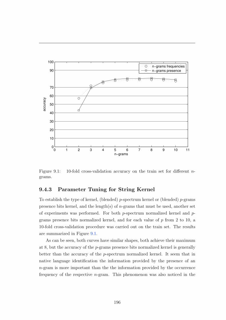
0 1 2 3 4 5 6 7 8 9 10 110

10

20

30

40

50

60

70

90

100

n−grams

accura

cy

n−grams frequencies

n−grams presence

Figure 9.1: 10-fold cross-validation accuracy on the train set for different n-grams.

9.4.3 Parameter Tuning for String Kernel

To establish the type of kernel, (blended) p-spectrum kernel or (blended) p-grams

presence bits kernel, and the length(s) of n-grams that must be used, another set

of experiments was performed. For both p-spectrum normalized kernel and p-

grams presence bits normalized kernel, and for each value of p from 2 to 10, a

10-fold cross-validation procedure was carried out on the train set. The results

are summarized in Figure 9.1.

As can be seen, both curves have similar shapes, both achieve their maximum

at 8, but the accuracy of the p-grams presence bits normalized kernel is generally

better than the accuracy of the p-spectrum normalized kernel. It seem that in

native language identification the information provided by the presence of an

n-gram is more important than the the information provided by the occurrence

frequency of the respective n-gram. This phenomenon was also noticed in the

196

context of sexual predator identification [Popescu & Grozea, 2012].

Experiments with different blended kernels were conducted to see whether

combining n-grams of different lengths can improve the accuracy. The best result

was obtained when all the n-grams with the length in the range 5-8 were used,

that is the 5-8-grams presence bits normalized kernel (k0/15−8). The 10-fold cross-

validation accuracy on the train set for this kernel was 80.94%. It was obtained

for the KRR parameter λ set to 10−5. The authors of [Bykh & Meurers, 2012]

also obtained better results using n-grams with the length in a range, rather than

using n-grams of a fixed length.

9.4.4 Parameter Tuning for LRD Kernel

Parameter tuning for LRD kernel (KLRD) was also done by using 10-fold cross-

validation on the training data. An interesting observation is that the KRR

based on LRD works much better with the normalized version of LRD (KnLRD).

Another concern was to choose the right length of n-grams. Several n-grams that

are around the mean English word length of 5-6 letters were evaluated. More

precisely, LRD kernels of 4-grams, 6-grams, and 8-grams, were used. The tests

show that the LRD kernels based on 6-grams (KnLRD6) and 8-grams (KnLRD8)

give the best results. In the end, the LRD kernels based on 6-grams and 8-

grams are combined to obtain even better results. The results of different kernel

combinations, including the LRD kernel based on 6-grams and 8-grams, are given

in Section 9.4.5.

Finally, the maximum offset parameter m involved in the computation of LRD

was chosen so that it generates a search window size close to the average number

of letters per document from the TOEFL 11 set. There are 1802 characters per

document on average, and m was chosen to be 700. This parameter was also

chosen with respect to the computational time of LRD, which is proportional to

the parameter value. Table 9.2 shows the results of the LRD kernel with different

parameters cross-validated on the training set. For KnLRD, the σ parameter of

the Gaussian-like kernel was set to 1. The reported accuracy rates were obtained

with the KRR parameter λ set to 10−5.

Regarding the length of strings, it seems that LRD is affected by the variation

197

Table 9.2: Accuracy rates, using 10-fold cross-validation on the training set, ofLRD with different n-grams, with and without normalization. Normalized LRDis much better.

Method Accuracy

KRR + KLRD6 42.1%KRR + KnLRD4 70.8%KRR + KnLRD6 74.4%KRR + KnLRD8 74.8%

of string lengths. When comparing two documents with LRD, the idea of cutting

the longer document to match the length of the shorter one was proposed and

evaluated. This made the accuracy even worse. It seems that the parts cut

out from longer documents contain valuable information for LRD. In the end, a

decision was made to use the entire strings, despite the fact that the variation of

string lengths brought a lot of noise. However, some of this noise is eliminated

by normalizing the LRD kernel.

9.4.5 Combining Kernels

A good way to improve results with almost no extra effort is to combine the

kernels in different ways. First, notice that the blended string kernels presented

in Section 9.4.3 are essentially a sum of the string kernels with different n-grams.

This combination improves the accuracy, being more stable and robust. In the

same manner, the LRD kernels based on 6-grams and 8-grams, respectively, were

summed up to obtain the kernel denoted by KnLRD6+8 . Indeed, the KnLRD6+8

kernel presented in Table 9.3 works better than each of its components presented

in Table 9.2.

There are other options to combine the string kernels with LRD kernels, be-

sides summing them up. One option is by kernel alignment [Cristianini et al.,

2001]. Instead of simply summing kernels, kernel alignment assigns weights for

each of the two kernels based on how well they are aligned with the ideal kernel

Y Y ′ obtained from labels. Thus, the 5-8-grams presence bits normalized kernel

(k0/15−8) was combined with the LRD kernel based on sum of 6,8-grams (KnLRD6+8),

198

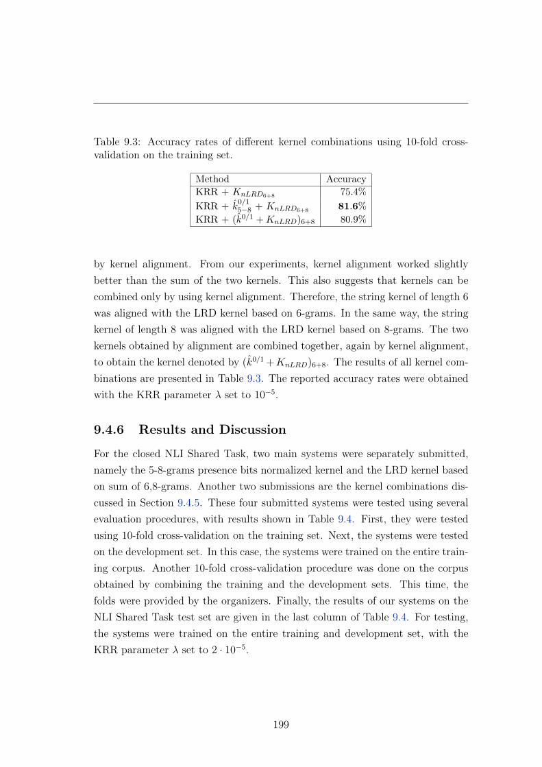
Table 9.3: Accuracy rates of different kernel combinations using 10-fold cross-validation on the training set.

Method Accuracy

KRR + KnLRD6+8 75.4%

KRR + k0/15−8 + KnLRD6+8 81.6%

KRR + (k0/1 + KnLRD)6+8 80.9%

by kernel alignment. From our experiments, kernel alignment worked slightly

better than the sum of the two kernels. This also suggests that kernels can be

combined only by using kernel alignment. Therefore, the string kernel of length 6

was aligned with the LRD kernel based on 6-grams. In the same way, the string

kernel of length 8 was aligned with the LRD kernel based on 8-grams. The two

kernels obtained by alignment are combined together, again by kernel alignment,

to obtain the kernel denoted by (k0/1 +KnLRD)6+8. The results of all kernel com-

binations are presented in Table 9.3. The reported accuracy rates were obtained

with the KRR parameter λ set to 10−5.

9.4.6 Results and Discussion

For the closed NLI Shared Task, two main systems were separately submitted,

namely the 5-8-grams presence bits normalized kernel and the LRD kernel based

on sum of 6,8-grams. Another two submissions are the kernel combinations dis-

cussed in Section 9.4.5. These four submitted systems were tested using several

evaluation procedures, with results shown in Table 9.4. First, they were tested

using 10-fold cross-validation on the training set. Next, the systems were tested

on the development set. In this case, the systems were trained on the entire train-

ing corpus. Another 10-fold cross-validation procedure was done on the corpus

obtained by combining the training and the development sets. This time, the

folds were provided by the organizers. Finally, the results of our systems on the

NLI Shared Task test set are given in the last column of Table 9.4. For testing,

the systems were trained on the entire training and development set, with the

KRR parameter λ set to 2 · 10−5.

199

Table 9.4: Accuracy rates of submitted systems on different evaluation sets. TheUnibuc team ranked third in the closed NLI Shared Task with the kernel combi-nation improved by the heuristic to level the predicted class distribution.

Method CV Tr. Dev. CV Tr.+Dev. Test

KRR + k0/15−8 80.9% 85.4% 82.5% 82.0%

KRR + KnLRD6+8 75.4% 76.3% 75.7% 75.8%

KRR + k0/15−8 + KnLRD6+8 81.6% 85.7% 82.6% 82.5%

KRR + (k0/1 + KnLRD)6+8 80.9% 85.6% 82.0% 81.4%

KRR + k0/15−8 + KnLRD6+8 + heuristic - - - 82.7%

The KnLRD6+8 kernel was not expected to perform better than the other sys-

tems on the test set. This system was submitted just to be compared with systems

submitted by other participants. Considering that LRD was originally designed

for biology applications, and that it has no ground in computational linguistics,

it performed very well, by standing in the top half of the ranking of all submitted

systems.

The kernel obtained by aligning the k0/15−8 and KnLRD6+8 kernels gives the best

results, no matter the evaluation procedure. It is followed closely by the other

two submitted systems.

A good idea to improve the accuracy on the test set was to exploit the distri-

bution of the test set in the last submitted system. This idea emerged by learning

that there should be exactly 100 examples per class for testing. The kernel ex-

pected to give the best accuracy among the submitted systems was chosen for an

adjustment of its output, in order to level the predicted class distribution. The

kernel obtained by combining the k0/15−8 and KnLRD6+8 kernels was considered for

this adjustment, since it obtains the best accuracy in all the other experiments.

The adjustment consists of taking all the classes with more than 100 examples,

and rank the examples by their confidence score (returned by regression) to be

part of the predicted class. The examples ranked below 100 were chosen to be

redistributed to the classes that had less than 100 examples per class. Examples

were redistributed only if their second most confident class had less than 100

examples. This heuristic improved the results on the test set by 0.2%, enough to

200

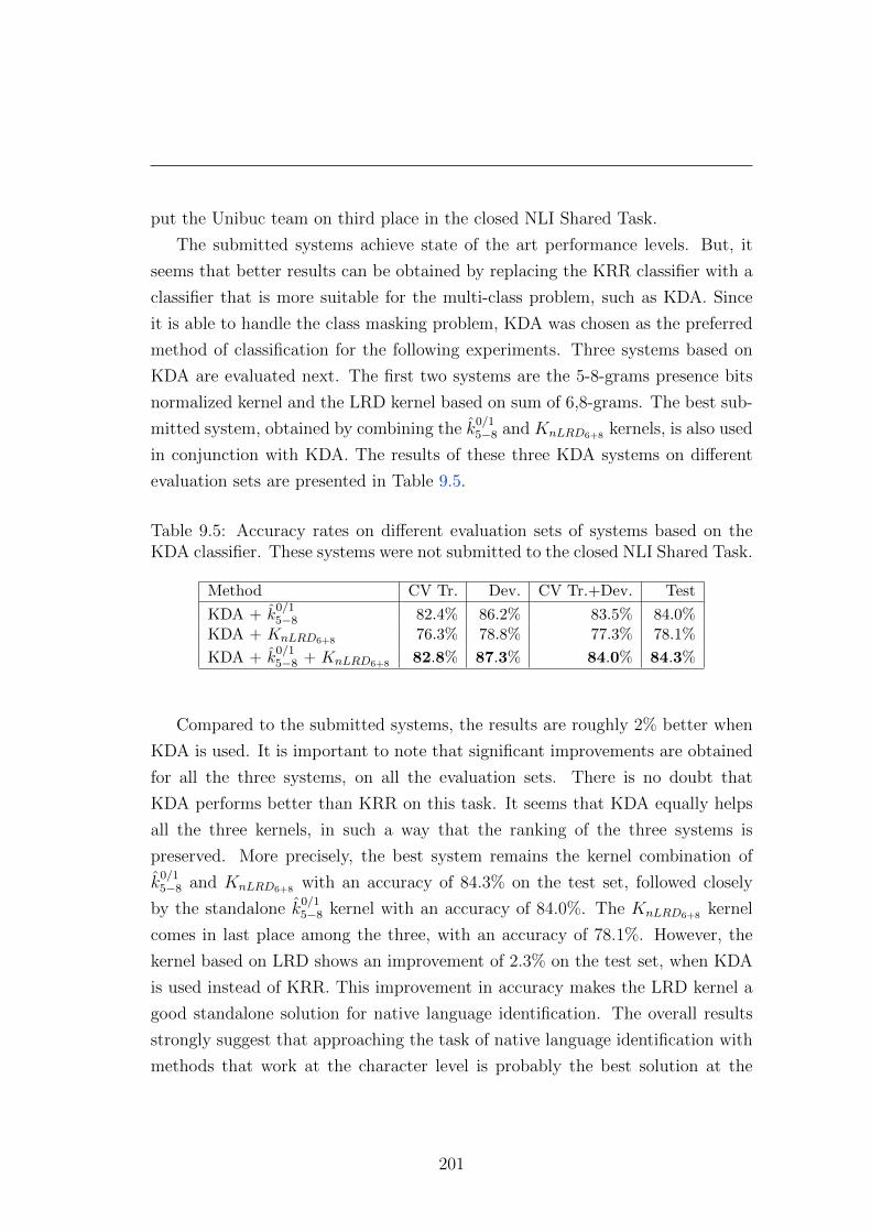
put the Unibuc team on third place in the closed NLI Shared Task.

The submitted systems achieve state of the art performance levels. But, it

seems that better results can be obtained by replacing the KRR classifier with a

classifier that is more suitable for the multi-class problem, such as KDA. Since

it is able to handle the class masking problem, KDA was chosen as the preferred

method of classification for the following experiments. Three systems based on

KDA are evaluated next. The first two systems are the 5-8-grams presence bits

normalized kernel and the LRD kernel based on sum of 6,8-grams. The best sub-

mitted system, obtained by combining the k0/15−8 and KnLRD6+8 kernels, is also used

in conjunction with KDA. The results of these three KDA systems on different

evaluation sets are presented in Table 9.5.

Table 9.5: Accuracy rates on different evaluation sets of systems based on theKDA classifier. These systems were not submitted to the closed NLI Shared Task.

Method CV Tr. Dev. CV Tr.+Dev. Test

KDA + k0/15−8 82.4% 86.2% 83.5% 84.0%

KDA + KnLRD6+8 76.3% 78.8% 77.3% 78.1%

KDA + k0/15−8 + KnLRD6+8 82.8% 87.3% 84.0% 84.3%

Compared to the submitted systems, the results are roughly 2% better when

KDA is used. It is important to note that significant improvements are obtained

for all the three systems, on all the evaluation sets. There is no doubt that

KDA performs better than KRR on this task. It seems that KDA equally helps

all the three kernels, in such a way that the ranking of the three systems is

preserved. More precisely, the best system remains the kernel combination of

k0/15−8 and KnLRD6+8 with an accuracy of 84.3% on the test set, followed closely

by the standalone k0/15−8 kernel with an accuracy of 84.0%. The KnLRD6+8 kernel

comes in last place among the three, with an accuracy of 78.1%. However, the

kernel based on LRD shows an improvement of 2.3% on the test set, when KDA

is used instead of KRR. This improvement in accuracy makes the LRD kernel a

good standalone solution for native language identification. The overall results

strongly suggest that approaching the task of native language identification with

methods that work at the character level is probably the best solution at the

201

moment.


An approach for the 2013 NLI Shared Task was presented in this chapter. What

makes this system stand out is that it works at the character level, making the

approach completely language independent and linguistic theory neutral. The

results obtained were very good. A standard approach based on string kernels,

that proved to work well in many text analysis tasks, obtained an accuracy of 82%

on test data with a difference of only 1.6% between it and the top performing

system. A second system based on a new kernel KLRD, inspired from biology

with no ground in computational linguistics, performed also unexpectedly well, by

standing in the top half of the ranking of all submitted systems. The combination

of the two kernels obtained an accuracy of 82.5% making it to the top five, while

an heuristic improvement of this combination ranked third with an accuracy of

82.7%. After the competition, the KDA classifier was also evaluated on this task,

only to improve the accuracy to 84.3%. This final system is 0.7% above to top

performing system of the NLI Shared Task.

Despite the fact that the approach based on string kernels performed so well,

there is little information known about why does the system works so well and

why is it better than the other systems that take into account words, lemmas,

syntactic information, or even semantics. It seems that enough mistakes that

are particular to certain non-native English speakers can be captured by n-grams

of different lengths. An interesting remark is that using a range of n-grams

generates a lot of features that include (but are not limited to) stop words, stems

of content words, word terminations, entire words, and even n-grams of short

words. Instead of doing feature selection before the training step, which is the

usual NLP approach, the kernel classifier is the one that selects the most relevant

features, during training. With enough training samples, the kernel classifier does

a better job in selecting the right features from a very high feature space. This

might give a good reason of why the string kernel approach works so well.

In future work, the proposed system can probably be improved by includ-

ing spatial information, in a similar fashion to the spatial pyramid representa-

202

tion [Lazebnik et al., 2006] that improves the recognition performance of the bag

of visual words model. The spatial pyramid approach divides the image into

increasingly fine sub-regions, and records the frequency of each visual word in

a histogram for each bin. In a similar way, the text document can be divided

into increasingly fine chunks of text. Then, n-grams can be extracted from each

chunk of text, and combined to obtain the final pyramid representation of the

document. The pyramid representation adds some information about the loca-

tion of the n-grams in the original text. It may be that this location information

might be useful to obtain a better classification performance.

203

Chapter 10

Conclusions

Machine learning is currently a vast area of research with applications in a variety

of fields, such as computer vision [Fei-Fei & Perona, 2005; Forsyth & Ponce, 2002;

Zhang et al., 2007], computational biology [Dinu & Ionescu, 2013a; Inza et al.,

2010; Leslie et al., 2002], information retrieval [Chifu & Ionescu, 2012; Manning

et al., 2008], natural language processing [Lodhi et al., 2002; Popescu & Grozea,

2012], data mining [Enachescu, 2004], and many others. This thesis has proposed

several machine learning methods that are designed for specific tasks, ranging

from handwritten digit recognition, texture classification, object recognition, or

facial expression recognition, to phylogenetic analysis, DNA comparison, or native

language identification. For this broad range of applications several similarity-

based learning methods [Chen et al., 2009] have been employed. This thesis

studied approaches such as Nearest Neighbor models, kernel methods [Shawe-

Taylor & Cristianini, 2004], and clustering methods [Enachescu, 2004]. The has

studied methods exhibit state of the art performance levels in the approached

tasks. To support this claim, it is important to mention the improved bag of

visual words model [Ionescu et al., 2013] that has obtained the fourth place at

the Facial Expression Recognition (FER) Challenge of the ICML 2013 Workshop

in Challenges in Representation Learning (WREPL), and the system based on

string kernels [Popescu & Ionescu, 2013] that has ranked on third place in the

closed Native Language Identification Shared Task of the BEA-8 Workshop of

NAACL 2013.

The applications approached in this thesis can be divided into two different ar-

204

eas: computer vision and string processing. Despite the fact that computer vision

and string processing seem to be unrelated fields of study, recent results as the

ones presented in this thesis suggest that image analysis and string processing are

actually similar in several ways. The concept of treating image and text in a sim-

ilar fashion has proven to be very fertile for particular applications in computer

vision [Duygulu et al., 2002; Farhadi et al., 2010; Leung & Malik, 2001; Sadeghi

& Farhadi, 2011; Sivic et al., 2005] and natural language processing [Barnard &

Johnson, 2005; Barnard et al., 2003; Ionescu, 2013a]. The concept of treating im-

age and text in a similar manner was also exploited in various ways in this thesis.

First, a dissimilarity measure for images was presented in Chapter 4. The dissim-

ilarity measure was inspired from the rank distance measure [Dinu, 2003]. The

main concern was to extend rank distance from one-dimensional input (strings)

to two-dimensional input (digital images). While rank distance is a highly accu-

rate measure for strings, the experiments presented in Chapter 4 suggest that the

proposed extension of rank distance to images is very accurate for handwritten

digit recognition and texture analysis. Second, some improvements to the popu-

lar bag of visual words model were proposed in Chapter 5. This model is inspired

by the bag of words model from natural language processing and information

retrieval. Third, a new distance measure was introduced in Chapter 8. It was

inspired from the image dissimilarity measure presented in Chapter 4. Designed

to conform to more general principles and adapted to DNA strings, Local Rank

Distance has shown that it can achieve better results than several state of the art

methods for DNA sequence analysis. Furthermore, another application of this

novel distance measure for strings was presented in Chapter 9. More precisely, a

kernel based on this distance measure was used for native language identification.

To summarize, all the contributions that were presented in this thesis come to

support the concept of treating image and text in a similar manner.

Although a significant amount of research has been conducted using the idea

of borrowing and adapting concepts from text processing to computer vision, or

from computer vision to text processing, the concept of treating image and text

in a similar fashion is far from saturated. The methods presented in this thesis

exploit this concept, only to lay the ground for future exploration. One interesting

approach that should be addressed in future work is mentioned here. Inspired

205

by the spatial pyramid representation [Lazebnik et al., 2006] that improves the

recognition performance of the bag of visual words model in computer vision,

an interesting future development would be to use a similar approach for text

categorization. Text documents can be divided into increasingly fine chunks of

text. Then, n-grams or any kind of features can be extracted from each chunk

of text in order to obtain pyramid representations of the documents. This is just

one of the directions that can be investigated in future work.

To conclude, this thesis represents a strong argument in favor of treating

image and text in a similar fashion, a concept that is very promising and truly

fertile for specific applications.

206

Bibliography

Achtert, Elke, Bohm, Christian, Kriegel, Hans P., Kroger, Peer, Muller-Gorman,

Ina, and Zimek, Arthur. Finding hierarchies of subspace clusters. Proceedings

of PKDD, pp. 446–453, 2006. 32

Achtert, Elke, Bohm, Christian, Kriegel, Hans P., Kroger, Peer, Muller-Gorman,

Ina, and Zimek, Arthur. Detection and visualization of subspace cluster hier-

archies. Proceedings of DASFAA, pp. 152–163, 2007. 32

Agarwal, Shivani and Roth, Dan. Learning a Sparse Representation for Object

Detection. Proceedings of ECCV, pp. 113–127, June 2002. 3, 40

Agirre, Eneko and Edmonds, Philip Glenny. Word Sense Disambiguation: Algo-

rithms and Applications. Springer, 2006. 4, 5, 32

Agrawal, Rakesh, Gehrke, Johannes, Gunopulos, Dimitrios, and Raghavan, Prab-

hakar. Automatic subspace clustering of high dimensional data for data mining

applications. SIGMOD Record, 27(2):94–105, 1998. 32

Alekseyev, Max A. and Pevzner, Pavel A. Multi-break rearrangements and chro-

mosomal evolution. Theoretical Computer Science, 395(2-3):193–202, 2008. 128

Alexe, Bogdan, Deselaers, Thomas, and Ferrari, Vittorio. Measuring the object-

ness of image windows. IEEE Transactions on Pattern Analysis and Machine

Intelligence, 34(11):2189–2202, 2012. 124

Altschul, S. F., Gish, W., Miller, W., Myers, E. W., and Lipman, D. J. Basic local

alignment search tool. Journal of Molecular Biology, 215(3):403–410, October

1990. ISSN 0022-2836. 14

207

BIBLIOGRAPHY

Amir, Amihood, Aumann, Yonatan, Benson, Gary, Levy, Avivit, Lipsky, Ohad,

Porat, Ely, Skiena, Steven, and Vishne, Uzi. Pattern matching with address

errors: rearrangement distances. Proceedings of SODA, pp. 1221–1229, 2006.

163

Amir, Amihood, Landau, Gad M., Na, Joong Chae, Park, Heejin, Park, Kunsoo,

and Sim, Jeong Seop. Consensus optimizing both distance sum and radius.

Proceedings of the 16th International Symposium on String Processing and In-

formation Retrieval, pp. 234–242, 2009. 136, 140

Bader, David A., Moret, Bernard M. E., and Yan, Mi. A Linear-Time Algorithm

for Computing Inversion Distance between Signed Permutations with an Exper-

imental Study. Proceedings of the 7th International Workshop on Algorithms

and Data Structures, pp. 365–376, 2001. 128

Bafna, Vineet and Pevzner, Pavel A. Sorting by transpositions. SIAM Journal

on Discrete Mathematics, 11(2):224–240, 1998. 128

Barnard, Kobus and Johnson, Matthew. Word sense disambiguation with pic-

tures. Artificial Intelligence, 167(1-2):13–30, September 2005. ISSN 0004-3702.

7, 205

Barnard, Kobus, Duygulu, Pinar, Forsyth, David, de Freitas, Nando, Blei,

David M., and Jordan, Michael I. Matching words and pictures. Journal

of Machine Learning Research, 3:1107–1135, March 2003. ISSN 1532-4435. 7,

205

Barnes, Connelly, Goldman, Dan B., Shechtman, Eli, and Finkelstein, Adam.

The PatchMatch Randomized Matching Algorithm for Image Manipulation.

Communications of the ACM, 54(11):103–110, November 2011. 39, 40, 48, 52,

56, 85, 162

Bay, Herbert, Ess, Andreas, Tuytelaars, Tinne, and Gool, Luc Van. Speeded-Up

Robust Features (SURF). Computer Vision and Image Understanding, 110(3):

346–359, June 2008. ISSN 1077-3142. 41

208

BIBLIOGRAPHY

Belda, E., Moya, A., and Silva, F.J. Genome rearrangement distances and gene

order phylogeny in gamma-proteobacteria. Molecular Biology and Evolution,

22(6):1456–1467, 2005. 128

Belongie, S., Malik, J., and Puzicha, J. Shape matching and object recognition

using shape contexts. IEEE Transactions on Pattern Analysis and Machine

Intelligence, 24(4):509–522, April 2002. 13, 17, 35, 39, 41

Ben-Dor, Amir, Lancia, Giuseppe, Perone, Jennifer, and Ravi, R. Banishing Bias

from Consensus Sequences. Proceedings of CPM, (1264):247–261, 1997. 127

Bengio, Yoshua. Learning deep architectures for AI. Foundations and Trends in

Machine Learning, 2(1):1–127, 2009. 4, 35

Bishop, Christopher M. Neural Networks for Pattern Recognition. Oxford Uni-

versity Press, Inc., New York, NY, USA, 1995. ISBN 0198538642. 2

Blanchard, Daniel, Tetreault, Joel, Higgins, Derrick, Cahill, Aoife, and

Chodorow, Martin. TOEFL11: A Corpus of Non-Native English. Technical

report, Educational Testing Service, 2013. 193

Bohm, Christian, Kailing, Karin, Kroger, Peer, and Zimek, Arthur. Comput-

ing clusters of correlation connected objects. Proceedings of the 2004 ACM

SIGMOD, pp. 455–466, 2004. 32

Borg, I. and Groenen, P. J. F. Modern multidimensional scaling: Theory and

applications. Springer Verlag, 2005. 20

Bosch, Anna, Zisserman, Andrew, and Munoz, Xavier. Image Classification using

Random Forests and Ferns. Proceedings of ICCV, pp. 1–8, 2007. 42, 102, 109,

115, 120

Bottou, Leon and Vapnik, Vladimir. Local Learning Algorithms. Neural Com-

putation, 4:888–900, 1992. 19

Breiman, Leo. Random forests. Machine Learning, 45(1):5–32, October 2001.

ISSN 0885-6125. 2

209

BIBLIOGRAPHY

Brodatz, Phil. Textures: a photographic album for artists and designers. Dover

pictorial archives. Dover Publications, New York, USA, 1966. 86

Brooke, Julian and Hirst, Graeme. Robust, Lexicalized Native Language Identi-

fication. Proceedings of COLING 2012, pp. 391–408, December 2012. 126, 188,

195

Bryant, David and Waddell, Peter. Rapid evaluation of least squares and mini-

mum evolution criteria on phylogenetic trees. Molecular Biology and Evolution,

15(10):1346–1359, 1998. 130

Bykh, Serhiy and Meurers, Detmar. Native Language Identification using Recur-

ring n-grams – Investigating Abstraction and Domain Dependence. Proceedings

of COLING 2012, pp. 425–440, December 2012. 197

Canny, John. A Computational Approach to Edge Detection. IEEE Transactions

on Pattern Analysis and Machine Intelligence, 8(6):679–698, June 1986. 41

Cao, Y., Janke, A., Waddell, P. J., Westerman, M., Takenaka, O., Murata, S.,

Okada, N., Paabo, S., and Hasegawa, M. Conflict among individual mito-

chondrial proteins in resolving the phylogeny of Eutherian orders. Journal of

Molecular Evolution, 47:307–322, 1998. 130, 178, 182

Caruana, Rich and Niculescu-Mizil, Alexandru. An empirical comparison of su-

pervised learning algorithms. Proceedings of ICML, pp. 161–168, 2006. 2

Cazzanti, Luca and Gupta, Maya R. Local similarity discriminant analysis. Pro-

ceedings of ICML, pp. 137–144, 2007. 15

Cazzanti, Luca, Gupta, Maya R., and Koppal, Anjali J. Generative models

for similarity-based classification. Pattern Recognition, 41(7):2289–2297, July

2008. ISSN 0031-3203. 15

Chen, Yihua, Garcia, Eric K., Gupta, Maya R., Rahimi, Ali, and Cazzanti, Luca.

Similarity-based Classification: Concepts and Algorithms. Journal of Machine

Learning Research, 10:747–776, June 2009. ISSN 1532-4435. 3, 14, 15, 204

210

BIBLIOGRAPHY

Chifu, Adrian-Gabriel and Ionescu, Radu Tudor. Word sense disambiguation to

improve precision for ambiguous queries. Central European Journal of Com-

puter Science, 2(4):398–411, 2012. 3, 5, 11, 32, 131, 204

Chimani, M., Woste, M., and Bocker, S. A closer look at the closest string and

closest substring problem. Proceedings of ALENEX, pp. 13–24, 2011. 14, 129,

140, 159, 189

Cho, Taeg Sang, Avidan, Shai, and Freeman, William T. The patch transform.

IEEE Transactions on Pattern Analysis and Machine Intelligence, 32(8):1489–

1501, 2010. 40, 162

Conaire, Ciarn O, O’Connor, Noel E., and Smeaton, Alan F. An Improved

Spatiogram Similarity Measure for Robust Object Localisation. Proceedings of

ICASSP, 1:1069–1072, 2007. 77, 78

Cortes, Corinna and Vapnik, Vladimir. Support-Vector Networks. Machine

Learning, 20(3):273–297, 1995. 2, 25, 57, 194

Cortes, Corinna, Mohri, Mehryar, and Rostamizadeh, Afshin. Multi-Class Classi-

fication with Maximum Margin Multiple Kernel. Journal of Machine Learning

Research, 28(3):46–54, June 2013. 28

Cover, T. and Hart, P. Nearest neighbor pattern classification. IEEE Transactions

on Information Theory, 13(1):21–27, 1967. ISSN 0018-9448. 18

Cristianini, Nello, Shawe-Taylor, John, Elisseeff, Andre, and Kandola, Jaz S. On

kernel-target alignment. Proceedings of NIPS, pp. 367–373, December 2001.

28, 199

Csurka, Gabriella, Dance, Christopher R., Fan, Lixin, Willamowski, Jutta, and

Bray, Cdric. Visual categorization with bags of keypoints. In Workshop on

Statistical Learning in Computer Vision, ECCV, pp. 1–22, 2004. 34, 42, 43,

115

Dalal, Navneet and Triggs, Bill. Histograms of Oriented Gradients for Human

Detection. Proceedings of CVPR, 1:886–893, 2005. 41, 102, 115

211

BIBLIOGRAPHY

Dasarathy, B. V. Nearest neighbor (NN) norms: Pattern Classification Tech-

niques. IEEE Computer Society Press, Los Alamitos, CA, 1991. 18

Dash, J., Mathur, A., Foody, G. M., Curran, P. J., Chipman, J. W., and Lillesand,

T. M. Land cover classification using multi-temporal MERIS vegetation indices.

International Journal of Remote Sensing, 28(6):1137–1159, January 2007. 86

Daugman, John G. Uncertainty relation for resolution in space, spatial frequency,

and orientation optimized by two-dimensional visual cortical filters. Journal of

the Optical Society of America A, 2(7):1160–1169, 1985. 82

Deng, Xiaotie, Li, Guojun, Li, Zimao, Ma, Bin, and Wang, Lusheng. Genetic

Design of Drugs Without Side-Effects. SIAM Journal on Computing, 32(4):

1073–1090, 2003. 127

Deselaers, Thomas, Keyser, Daniel, and Ney, Hermann. Discriminative Training

for Object Recognition using Image Patches. Proceedings of CVPR, pp. 157–

162, 2005. 40, 43

Devroye, L., Gyorfi, L., and Lugosi, G. A Probabilistic Theory of Pattern Recog-

nition. Springer, 1996. 18

Deza, Elena and Deza, Michel-Marie. Dictionary of Distances. Elsevier, The

Netherlands, 1998. 36

Diaconis, P. and Graham, R. L. Spearman footrule as a measure of disarray.

Journal of Royal Statistical Society. Series B (Methodological), 39(2):262–268,

1977. 137

Dinu, Anca and Dinu, Liviu P. On the syllabic similarities of romance languages.

Proceedings of CICLing, 3406:785–788, 2005. 46, 135, 140, 160

Dinu, Liviu P. On the classification and aggregation of hierarchies with different

constitutive elements. Fundamenta Informaticae, 55(1):39–50, 2003. 8, 46, 53,

129, 130, 135, 140, 147, 160, 163, 168, 189, 205

Dinu, Liviu P. and Ionescu, Radu Tudor. A genetic approximation for closest

string via rank distance. Proceedings of SYNASC, pp. 207–215, 2011. 11, 141

212

BIBLIOGRAPHY

Dinu, Liviu P. and Ionescu, Radu Tudor. Clustering Based on Rank Distance

with Applications on DNA. Proceedings of ICONIP, 7667, 2012a. 3, 11, 14,

129, 136, 146, 159, 178, 182, 184, 189

Dinu, Liviu P. and Ionescu, Radu Tudor. An efficient rank based approach for

closest string and closest substring. PLoS ONE, 7(6):e37576, 06 2012b. 3, 11,

14, 46, 135, 136, 140, 141, 148, 149, 151, 157, 159, 160, 182, 184, 186, 189

Dinu, Liviu P. and Ionescu, Radu Tudor. Clustering Methods Based on Closest

String via Rank Distance. Proceedings of SYNASC, pp. 207–214, 2012c. 3, 11,

136, 146

Dinu, Liviu P. and Ionescu, Radu Tudor. A Rank-Based Approach of Cosine Sim-

ilarity with Applications in Automatic Classification. Proceedings of SYNASC,

pp. 260–264, 2012d.

Dinu, Liviu P. and Ionescu, Radu Tudor. Clustering based on Median and Closest

String via Rank Distance with Applications on DNA. Neural Computing and

Applications, 24(1):77–84, 2013a. 3, 11, 46, 136, 178, 204

Dinu, Liviu P. and Ionescu, Radu Tudor. An Efficient Algorithm for Rank Dis-

tance Consensus. Proceedings of AI*IA, 8249:505–516, 2013b. 3, 11, 136

Dinu, Liviu P. and Manea, Florin. An efficient approach for the rank aggregation

problem. Theoretical Computer Science, 359(1–3):455–461, 2006. 141, 148

Dinu, Liviu P. and Popa, Alin. On the closest string via rank distance. Proceedings

of CPM, 7354:413–426, 2012. 141, 143

Dinu, Liviu P. and Popescu, Marius. Language independent kernel method for

classifying texts with disputed paternity. Proceedings of ASMDA, 2009a. 46

Dinu, Liviu P. and Popescu, Marius. Comparing Statistical Similarity Measures

for Stylistic Multivariate Analysis. Proceedings of RANLP, 2009b. 124

Dinu, Liviu P. and Sgarro, Andrea. A Low-complexity Distance for DNA Strings.

Fundamenta Informaticae, 73(3):361–372, 2006. 46, 129, 135, 138, 140, 148,

154, 157, 160, 161, 178, 182, 184, 189

213

BIBLIOGRAPHY

Dinu, Liviu P. and Sgarro, Andrea. Estimating Similarities in DNA Strings Using

the Efficacious Rank Distance Approach, Systems and Computational Biology

– Bioinformatics and Computational Modeling. InTech, 2011. ISBN 978-953-

307-875-5. 142

Dinu, Liviu P., Popescu, Marius, and Dinu, Anca. Authorship identification of

romanian texts with controversial paternity. Proceedings of LREC, 2008. 135,

140, 160

Dinu, Liviu P., Ionescu, Radu Tudor, and Popescu, Marius. Local Patch Dissim-

ilarity for Images. Proceedings of ICONIP, 7663:117–126, 2012. 3, 9, 44, 53,

79, 159, 160, 163

Dinu, Liviu Petrisor and Ghetu, Florin. Circular Rank Distance: A New Ap-

proach for Genomic Applications. DEXA Workshops, pp. 397–401, 2011. 161

Duygulu, P., Barnard, Kobus, Freitas, J. F. G. de, and Forsyth, David A. Object

Recognition as Machine Translation: Learning a Lexicon for a Fixed Image

Vocabulary. Proceedings of ECCV, pp. 97–112, 2002. 6, 7, 205

Efros, Alexei A. and Freeman, William T. Image quilting for texture synthesis

and transfer. Proceedings of SIGGRAPH ’01, pp. 341–346, 2001. 39, 48

Enachescu, Denis. Unsupervised Statistical Learning and Data Mining. Coopera-

tiva Libraria Editrice Universit di Padova, Padova, Italy, 2004. ISBN 88-7178-

948-2. 3, 29, 30, 204

Everingham, Mark, van Gool, Luc, Williams, Christopher K., Winn, John, and

Zisserman, Andrew. The Pascal Visual Object Classes (VOC) Challenge. In-

ternational Journal of Computer Vision, 88(2):303–338, June 2010. 106

Falconer, Kenneth. Fractal Geometry: Mathematical Foundations and Applica-

tions. Wiley, 2 edition, November 2003. ISBN 0470848626. 81

Farago, A., Linder, T., and Lugosi, G. Fast Nearest-Neighbor Search in Dissim-

ilarity Spaces. IEEE Transanctions on Pattern Analysis and Machine Intelli-

gence, 15(9):957–962, September 1993. ISSN 0162-8828. 18

214

BIBLIOGRAPHY

Farhadi, Ali, Hejrati, Mohsen, Sadeghi, Mohammad Amin, Young, Peter,

Rashtchian, Cyrus, Hockenmaier, Julia, and Forsyth, David. Every picture

tells a story: generating sentences from images. Proceedings of ECCV, pp.

15–29, 2010. 6, 205

Fei-Fei, Li and Perona, Pietro. A Bayesian Hierarchical Model for Learning Nat-

ural Scene Categories. Proceedings of CVPR, 2:524–531, 2005. 2, 34, 42, 115,

204

Fei-Fei, Li, Fergus, Rob, and Perona, Pietro. Learning generative visual models

from few training examples: An incremental Bayesian approach tested on 101

object categories. Computer Vision and Image Understanding, 106(1):59–70,

April 2007. 98

Felsenstein, Joseph. Inferring Phylogenies. Sinauer Associates, Sunderland, Mas-

sachusetts, 2004. 129, 130, 159

Fisher, R. A. The Use of Multiple Measurements in Taxonomic Problems. Annals

of Eugenics, 7(7):179–188, 1936. 25

Fitch, W. M. and Margoliash, E. Construction of phylogenetic trees. Science,

155(760):279–284, January 1967. ISSN 0036-8075. 130

Fix, E. and Hodges, J. Discriminatory analysis, non-parametric discrimina-

tion: consistency properties. Technical report, USAF School of Aviation and

Medicine, Randolph Field, TX, 1951. Technical Report 4. 15

Forsyth, David A. and Ponce, Jean. Computer Vision: A Modern Approach.

Prentice Hall Professional Technical Reference, 2002. ISBN 0130851981. 2, 204

Frances, M. and Litman, A. On covering problems of codes. Theory of Computing

Systems, 30(2):113–119, 1997. 140

Frey, Brendan J. and Dueck, Delbert. Clustering by passing messages between

data points. Science, 315:972–976, 2007. 32

215

BIBLIOGRAPHY

Gonen, Mehmet and Alpaydin, Ethem. Multiple Kernel Learning Algorithms.

Journal of Machine Learning Research, 12:2211–2268, July 2011. ISSN 1532-

4435. 28

Goodfellow, Ian J., Erhan, Dumitru, Carrier, Pierre Luc, Courville, Aaron, Mirza,

Mehdi, Hamner, Ben, Cukierski, Will, Tang, Yichuan, Thaler, David, Lee,

Dong-Hyun, Zhou, Yingbo, Ramaiah, Chetan, Feng, Fangxiang, Li, Ruifan,

Wang, Xiaojie, Athanasakis, Dimitris, Shawe-Taylor, John, Milakov, Maxim,

Park, John, Ionescu, Radu Tudor, Popescu, Marius, Grozea, Cristian, Bergstra,

James, Xie, Jingjing, Romaszko, Lukasz, Xu, Bing, Chuang, Zhang, and Ben-

gio, Yoshua. Challenges in Representation Learning: A report on three machine

learning contests. Proceedings of ICONIP, 8228:117–124, 2013. 10, 100

Graepel, T., Herbrich, R., Scholkopf, Bernhard, Smola, A., Bartlett, P., Muller,

K., Obermayer, K., and Williamson, R. Classification on proximity data with

LP-machines. Proceedings of ICANN, 1:304–309, 1999. ISSN 0537-9989. 14

Graepel, Thore, Herbrich, Ralf, Bollmann-Sdorra, Peter, and Obermayer, Klaus.

Classification on pairwise proximity data. Proceedings of NIPS, pp. 438–444,

1998. 14

Gramm, Jens, Huffner, Falk, and Niedermeier, Rolf. Closest Strings, Primer

Design, and Motif Search. Presented at RECOMB 2002 poster session, pp.

74–75, 2002. 127

Grozea, C., Gehl, C., and Popescu, M. ENCOPLOT: Pairwise Sequence Matching

in Linear Time Applied to Plagiarism Detection. In 3rd PAN WORKSHOP.

UNCOVERING PLAGIARISM, AUTHORSHIP AND SOCIAL SOFTWARE

MISUSE, pp. 10, 2009. 132, 187

Guo, Guodong and Dyer, Charles R. Patch-based Image Correlation with Rapid

Filtering. Proceedings of CVPR, 2007. 40, 48

Hafner, James L., Sawhney, Harpreet S., Equitz, William, Flickner, Myron, and

Niblack, Wayne. Efficient Color Histogram Indexing for Quadratic Form Dis-

tance Functions. IEEE Transactions on Pattern Analysis and Machine Intel-

ligence, 17(7):729–736, 1995. 36

216

BIBLIOGRAPHY

Hannenhalli, Sridhar. Polynomial-time algorithm for computing translocation

distance between genomes. Discrete Applied Mathematics, 71(1-3):137–151,

1996. 128

Hannenhalli, Sridhar and Pevzner, Pavel A. Transforming men into mice (poly-

nomial algorithm for genomic distance problem. Proceedings of 36th Annual

IEEE Symposium on Foundations of Computer Science, pp. 581–592, 1995. 128

Haralick, Robert M., Shanmugam, K., and Dinstein, Its’Hak. Textural Features

for Image Classification. IEEE Transactions on Systems, Man and Cybernetics,

3(6):610–621, November 1973. ISSN 0018-9472. 81

Harris, C. and Stephens, M. A combined corner and edge detector. Proceedings

of the 4th Alvey Vision Conference, pp. 147–151, 1988. 41

Hastie, Trevor and Tibshirani, Robert. The Elements of Statistical Learning.

Springer, corrected edition, July 2003. ISBN 0387952845. 26, 30, 194

Hoekman, Dirk H. and Quinnones, Marcela J. Land cover type and biomass

classification using AirSAR data fro evaluation of monitoring scenarios in the

Colombian Amazon. IEEE Transactions on Geoscience and Remote Sensing,

38:685–696, 2000. 86

Holmquist, Richard, Miyamoto, Michael M., and Goodman, Morris. Higher-

Primate Phylogeny - Why Can’t We Decide? Molecular Biology and Evolution,

3(5):201–216, 1988. 129

Homer, Nils, Merriman, Barry, and Nelson, Stanley F. BFAST: An Alignment

Tool for Large Scale Genome Resequencing. PLoS ONE, 4(11):e7767+, Novem-

ber 2009. 128

Hristea, Florentina, Popescu, Marius, and Dumitrescu, Monica. Performing word

sense disambiguation at the border between unsupervised and knowledge-based

techniques. Artificial Intelligence Review, 30(1-4):67–86, 2008. ISSN 0269-2821.

132

217

BIBLIOGRAPHY

Huang, Zhexue. Extensions to the k-means algorithm for clustering large data sets

with categorical values. Data Mining and Knowledge Discovery, 2(3):283–304,

1998. 31

Indow, Tarow. A Critical Review of Luneburg’s Model With Regard to Global

Structure of Visual Space. Psychological Review, 98(3):430–453, 1991. 36

Inza, Inaki, Calvo, Borja, Armananzas, Ruben, Bengoetxea, Endika, Larranaga,

Pedro, and Lozano, Jose A. Machine learning: an indispensable tool in bioin-

formatics. Methods in Molecular Biology (Clifton, N.J.), 593:25–48, 2010. ISSN

1940-6029. 3, 204

Ionescu, Radu Tudor. Local Rank Distance. Proceedings of SYNASC, pp. 221–

228, 2013a. 3, 12, 130, 159, 160, 163, 189, 205

Ionescu, Radu Tudor. Unisort: An algorithm to sort uniformly distributed num-

bers in O(n). International Journal on Information Technology (IREIT), 1(3):

171–188, May 2013b. 11, 144

Ionescu, Radu Tudor and Popescu, Marius. Speeding Up Local Patch Dissimi-

larity. Proceedings of ICIAP, 8156:1–10, 2013a. 3, 9, 44, 163

Ionescu, Radu Tudor and Popescu, Marius. Kernels for Visual Words Histograms.

Proceedings of ICIAP, 8156:81–90, 2013b. 3, 10, 14, 98

Ionescu, Radu Tudor, Popescu, Marius, and Grozea, Cristian. Local Learning

to Improve Bag of Visual Words Model for Facial Expression Recognition.

Workshop on Challenges in Representation Learning, ICML, 2013. 3, 10, 99,

204

Ionescu, Radu Tudor, Popescu, Andreea Lavinia, Popescu, Dan, and Popescu,

Marius. Local Texton Dissimilarity with Applications on Biomass Classifica-

tion. Proceedings of VISAPP, January 2014. 3, 9, 45, 80

Jarvis, Scott and Crossley, Scott (eds.). Approaching Language Transfer Through

Text Classification: Explorations in the Detection-based Approach, volume 64.

Multilingual Matters Limited, Bristol, UK, 2012. 126

218

BIBLIOGRAPHY

Jurafsky, Daniel and Martin, James H. Speech and Language Processing: An

Introduction to Natural Language Processing, Computational Linguistics, and

Speech Recognition. Prentice Hall PTR, Upper Saddle River, NJ, USA, 1st

edition, 2000. ISBN 0130950696. 6, 132

Jurie, Frederic and Schmid, Cordelia. Scale-invariant shape features for recogni-

tion of object categories. Proceedings of CVPR, 2:90–96, 2004. 41

Kadir, Timor and Brady, Michael. Saliency, Scale and Image Description. Inter-

national Journal of Computer Vision, 45(2):83–105, November 2001. 41

Kailing, Karin, Kriegel, Hans P., and Kroger, Peer. Density-connected subspace

clustering for high-dimensional data. Proceedings of the 4th SIAM International

Conference on Data Mining, 2004. 29, 32

Ke, Yan and Sukthankar, Rahul. PCA-SIFT: a more distinctive representation

for local image descriptors. Proceedings of CVPR, pp. 506–513, 2004. 41

Knuth, Donald E., Morris, J. H., and Pratt, Vaughan R. Fast pattern matching

in strings. SIAM Journal of Computing, 6(2):323–350, 1977. 167

Koonin, E. V. The emerging paradigm and open problems in comparative ge-

nomics. Bioinformatics, 15:265–266, 1999. 127

Kriegel, Hans P., Kroger, Peer, and Zimek, Arthur. Clustering high-dimensional

data: A survey on subspace clustering, pattern-based clustering, and correla-

tion clustering. ACM Transactions on Knowledge Discovery from Data, 3(1):

1:1–1:58, 2009. 32

Krizhevsky, Alex, Sutskever, Ilya, and Hinton, Geoffrey E. ImageNet Classifi-

cation with Deep Convolutional Neural Networks. Proceedings of NIPS, pp.

1106–1114, 2012. 35

Kuse, Manohar, Wang, Yi-Fang, Kalasannavar, Vinay, Khan, Michael, and Ra-

jpoot, Nasir. Local isotropic phase symmetry measure for detection of beta

cells and lymphocytes. Journal of Pathology Informatics, 2(2):2, 2011. 82

219

BIBLIOGRAPHY

Lanctot, Kevin J., Li, Ming, Ma, Bin, Wang, Shaojiu, and Zhang, Louxin. Dis-

tinguishing string selection problems. Information and Computation, 185(1):

41–55, August 2003. ISSN 0890-5401. 127

Langmead, Ben, Trapnell, Cole, Pop, Mihai, and Salzberg, Steven. Ultrafast and

memory-efficient alignment of short DNA sequences to the human genome.

Genome Biology, 10(3):R25–10, March 2009. ISSN 1465-6906. 128

Lazebnik, Svetlana, Schmid, Cordelia, and Ponce, Jean. A Maximum Entropy

Framework for Part-Based Texture and Object Recognition. Proceedings of

ICCV, 1:832–838, 2005a. xxii, 55, 78, 79, 80, 98, 108

Lazebnik, Svetlana, Schmid, Cordelia, and Ponce, Jean. A Sparse Texture Repre-

sentation Using Local Affine Regions. IEEE Transactions on Pattern Analysis

and Machine Intelligence, 27(8):1265–1278, August 2005b. 4, 80, 86, 90, 92, 93

Lazebnik, Svetlana, Schmid, Cordelia, and Ponce, Jean. Beyond Bags of Fea-

tures: Spatial Pyramid Matching for Recognizing Natural Scene Categories.

Proceedings of CVPR, 2:2169–2178, 2006. 4, 14, 24, 98, 102, 117, 202, 206

LeCun, Yann, Jackel, Lawrence D., Boser, Bernhard, Denker, John S., Graf,

Hans P., Guyon, Isabelle, Henderson, Donnie, Howard, R. E., and Hubbard,

Wayne. Handwritten digit recognition: Applications of neural net chips and

automatic learning. IEEE Communications, pp. 41–46, November 1989. 54

LeCun, Yann, Bottou, Leon, Bengio, Yoshua, and Haffner, Pattrick. Gradient-

based learning applied to document recognition. Proceedings of the IEEE, 86

(11):2278–2324, November 1998. 54, 55, 66, 72

Lee, Taehyung, Na, Joong Chae, Park, Heejin, Park, Kunsoo, and Sim,

Jeong Seop. Finding consensus and optimal alignment of circular strings. The-

oretical Computer Science, 468:92–101, 2013. 140

Leslie, Christina S., Eskin, Eleazar, and Noble, William Stafford. The spectrum

kernel: A string kernel for svm protein classification. Proceedings of Pacific

Symposium on Biocomputing, pp. 566–575, 2002. 3, 189, 204

220

BIBLIOGRAPHY

Leung, Thomas and Malik, Jitendra. Representing and Recognizing the Visual

Appearance of Materials using Three-dimensional Textons. International Jour-

nal of Computer Vision, 43(1):29–44, June 2001. ISSN 0920-5691. 4, 5, 32, 34,

42, 80, 102, 115, 205

Levenshtein, V. I. Binary codes capable of correcting deletions, insertions and

reverseals. Cybernetics and Control Theory, 10(8):707–710, 1966. 46, 141

Levy, Samuel and Hannenhalli, Sridhar. Identification of transcription factor

binding sites in the human genome sequence. Mammalian Genome, 13(9):

510–514, September 2002. ISSN 0938-8990. 128

Li, Heng and Durbin, Richard. Fast and accurate short read alignment with

Burrows-Wheeler transform. Bioinformatics, 25(14):1754–1760, July 2009.

ISSN 1367-4803. 128

Li, Heng and Homer, Nils. A survey of sequence alignment algorithms for next-

generation sequencing. Briefings in bioinformatics, 11(5):473–483, September

2010. ISSN 1477-4054. 128

Li, Ming, Ma, Bin, and Wang, Lusheng. Finding Similar Regions in Many Se-

quences. Journal of Computer and System Sciences, 65(1):73–96, August 2002.

127

Li, Ming, Chen, Xin, Li, Xin, Ma, Bin, and Vitanyi, Paul M. B. The similarity

metric. IEEE Transactions on Information Theory, 50(12):3250–3264, 2004.

148, 157, 162, 178, 182, 186, 189

Liao, Li and Noble, William S. Combining Pairwise Sequence Similarity and Sup-

port Vector Machines for Detecting Remote Protein Evolutionary and Struc-

tural Relationships. Journal of Computational Biology, 10(6):857–868, Decem-

ber 2003. ISSN 1066-5277. 14

Liew, Alan W., Yan, Hong, and Yang, Mengsu. Pattern recognition techniques

for the emerging field of bioinformatics: A review. Pattern Recognition, 38(11):

2055–2073, November 2005. 127

221

BIBLIOGRAPHY

Lindeberg, Tony. Feature detection with automatic scale selection. International

Journal of Computer Vision, 30:79–116, 1998. 41

Lipman, D. J. and Pearson, W. R. Rapid and sensitive protein similarity searches.

Science, 227:1435–1441, 1985. 14

Lodhi, Huma, Saunders, Craig, Shawe-Taylor, John, Cristianini, Nello, and

Watkins, Christopher J. C. H. Text classification using string kernels. Journal

of Machine Learning Research, 2:419–444, 2002. 3, 14, 132, 133, 187, 188, 189,

204

Lowe, David G. Object Recognition from Local Scale-Invariant Features. Pro-

ceedings of ICCV, 2:1150–1157, 1999. 5, 41, 102

Manning, Christopher D. and Schutze, Hinrich. Foundations of Statistical Natural

Language Processing. MIT Press, Cambridge, MA, USA, 1999. ISBN 0-262-

13360-1. 5, 6, 132

Manning, Christopher D., Raghavan, Prabhakar, and Schutze, Hinrich. Intro-

duction to Information Retrieval. Cambridge University Press, New York, NY,

USA, 2008. ISBN 0521865719, 9780521865715. 2, 3, 4, 5, 14, 132, 204

McCallum, Andrew, Nigam, Kamal, and Ungar, Lyle H. Efficient clustering of

high-dimensional data sets with application to reference matching. Proceedings

of ACM SIGKDD, pp. 169–178, 2000. 29, 31

Meila, Marina. Comparing clusterings by the variation of information. Proceed-

ings of COLT, 2777:173–187, 2003. 32

Melsted, Pall and Pritchard, Jonathan. Efficient counting of k-mers in DNA

sequences using a bloom filter. BMC Bioinformatics, 12(1):333, 2011. 162, 189

Mikolajczyk, Krystian and Schmid, Cordelia. Indexing Based on Scale Invariant

Interest Points. Proceedings of ICCV, 1:525–531, 2001. 41

Mikolajczyk, Krystian and Schmid, Cordelia. A Performance Evaluation of Local

Descriptors. IEEE Transactions on Pattern Analysis and Machine Intelligence,

27(10):1615–1630, October 2005. 41, 42

222

BIBLIOGRAPHY

Montavon, Gregoire, Orr, Genevieve B., and Muller, Klaus-Robert (eds.). Neural

Networks: Tricks of the Trade, volume 7700 of Lecture Notes in Computer

Science (LNCS). Springer, 2nd edition, 2012. 4, 35

Munch, Kasper, Boomsma, Wouter, Huelsenbeck, John P., Willerslev, Eske, and

Nielsen, Rasmus. Statistical Assignment of DNA Sequences Using Bayesian

Phylogenetics. Systematic Biology, 57(5):750–757, October 2008. ISSN 1076-

836X. 130

Nadaraya, E A. On estimating regression. Theory of Probability and its Applica-

tions, 9:141–142, 1964. 19

Nei, Masatoshi and Kumar, Sudhir. Molecular Evolution and Phylogenetics. Ox-

ford University Press, USA, 1 edition, August 2000. ISBN 0195135857. 130

Ng, Raymond T. and Han, Jiawei. Clarans: A method for clustering objects for

spatial data mining. IEEE Transactions on Knowledge and Data Engineering,

14(5):1003–1016, 2002. 31

Nicolas, F. and Rivals, E. Complexities of centre and median string. Proceedings

of CPM, 2676:315–327, 2003. 140

Nicolas, F. and Rivals, E. Hardness results for the center and median string prob-

lems under the weighted and unweighted edit distances. Journal of Discrete

Algorithms, 3:390–415, 2005. 140

Nilsson, Nils J. The quest for artificial intelligence: A history of ideas and achieve-

ments. 2010. 2

Nister, David and Stewenius, Henrik. Scalable Recognition with a Vocabulary

Tree. Proceedings of CVPR, 2:2161–2168, 2006. 42

Palmer, J. and Herbon, L. Plant mitochondrial DNA evolves rapidly in structure,

but slowly in sequence. Journal of Molecular Evolution, 28:87–89, 1988. 129

Paredes, Roberto, Prez-Cortes, Juan, Juan, Alfons, and Vidal, Enrique. Local

Representations and a Direct Voting Scheme for Face Recognition. Proceedings

223

BIBLIOGRAPHY

of Workshop on Pattern Recognition in Information Systems, pp. 71–79, July

2001. 40

Passino, Giuseppe and Izquierdo, Ebroul. Patch-based image classification

through conditional random field model. Proceedings of the International Con-

ference on Mobile Multimedia Communications, pp. 6:1–6:6, 2007. 40

Pekalska, Elzbieta and Duin, Robert P. W. Dissimilarity representations allow

for building good classifiers. Pattern Recognition Letters, 23(8):943–956, June

2002. ISSN 0167-8655. 14

Philbin, James, Chum, Ondrej, Isard, Michael, Sivic, Josef, and Zisserman, An-

drew. Object retrieval with large vocabularies and fast spatial matching. Pro-

ceedings of CVPR, pp. 1–8, 2007. 6, 35, 42, 98, 102, 115, 123

Popescu, Andreea Lavinia, Ionescu, Radu Tudor, and Popescu, Dan. A Spatial

Pyramid Approach for Texture Classification. Proceedings of ISEEE, October

2013a. 117

Popescu, Andreea Lavinia, Popescu, Dan, Ionescu, Radu Tudor, Angelescu, Nico-

leta, and Cojocaru, Romeo. Efficient Fractal Method for Texture Classification.

Proceedings of ICSCS, August 2013b. 10, 45, 81

Popescu, Marius. Studying translationese at the character level. Proceedings of

RANLP, pp. 634–639, September 2011. 132, 187, 189, 195

Popescu, Marius and Dinu, Liviu P. Kernel methods and string kernels for au-

thorship identification: The federalist papers case. Proceedings of RANLP,

September 2007. 14, 132, 133, 187, 188

Popescu, Marius and Grozea, Cristian. Kernel methods and string kernels for au-

thorship analysis. CLEF (Online Working Notes/Labs/Workshop), September

2012. 3, 14, 132, 187, 196, 204

Popescu, Marius and Ionescu, Radu Tudor. The Story of the Characters, the DNA

and the Native Language. Proceedings of the Eighth Workshop on Innovative

Use of NLP for Building Educational Applications, pp. 270–278, June 2013. 3,

12, 14, 165, 186, 187, 204

224

BIBLIOGRAPHY

Popov, Y. V. Multiple genome rearrangement by swaps and by element dupli-

cations. Theoretical Computer Science, 385(1-3):115–126, 2007. 14, 129, 140,

159, 189

Prezza, Nicola, Fabbro, Cristian Del, Vezzi, Francesco, Paoli, Emanuale De, and

Policriti, Alberto. ERNE-BS5: aligning BS-treated sequences by multiple hits

on a 5-letters alphabet. Proceedings of BCB, pp. 12–19, 2012. 128

Reyes, A., Gissi, C., Pesole, G., Catzeflis, F. M., and Saccone, C. Where Do

Rodents Fit? Evidence from the Complete Mitochondrial Genome of Sciurus

vulgaris. Molecular Biology and Evolution, 17(6):979–983, 2000. 129, 148, 157,

178, 182, 186

Rifkin, Ryan and Klautau, Aldebaro. In defense of one-vs-all classification. Jour-

nal of Machine Learning Research, 5(January):101–141, 2004. 195

Rubner, Yossi, Tomasi, Carlo, and Guibas, Leonidas J. The Earth Mover’s Dis-

tance as a Metric for Image Retrieval. International Journal of Computer

Vision, 40(2):99–121, 2000. 13, 35, 38

Rzhetsky, Andrey and Nei, Masatoshi. A Simple Method for Estimating and

Testing Minimum–Evolution Trees. Molecular Biology and Evolution, 9(5):

945–967, 1992. 130

Saccone, Cecilia, Lanave, Cecilia, Pesole, Graziano, and Preperata, Giuliano. In

Doolittle, Russsell F. (ed.), Molecular evolution: computer analysis of protein

and nucleic acid sequences, volume 183 of Methods In Enzymology, chapter 35,

pp. 570–583. Academic Press, New York, 1990. 130

Sadeghi, M. A. and Farhadi, A. Recognition using visual phrases. Proceedings of

CVPR, pp. 1745–1752, 2011. 7, 205

Saitou, N. and Nei, M. The neighbor-joining method: a new method for recon-

structing phylogenetic trees. Molecular Biology and Evolution, 4(4):406–425,

July 1987. ISSN 1537-1719. 130

225

BIBLIOGRAPHY

Sanderson, Conrad and Guenter, Simon. Short text authorship attribution via

sequence kernels, markov chains and author unmasking: An investigation. Pro-

ceedings of the 2006 Conference on Empirical Methods in Natural Language

Processing, pp. 482–491, July 2006. 14, 132, 187

Selim, Shokri Z. and Ismail, M. A. K-means-type algorithms: A generalized con-

vergence theorem and characterization of local optimality. IEEE Transactions

on Pattern Analysis and Machine Intelligence, PAMI-6(1):81–87, 1984. ISSN

0162-8828. 147

Shalev-Shwartz, Shai, Singer, Yoram, and Srebro, Nathan. Pegasos: Primal Es-

timated sub-GrAdient SOlver for SVM. Proceedings of ICML, pp. 807–814,

2007. 105, 109

Shapira, Dana and Storer, James A. Large Edit Distance with Multiple Block

Operations. Proceedings of SPIRE, 2857:369–377, 2003. 14, 129, 159, 189

Shawe-Taylor, John and Cristianini, Nello. Kernel Methods for Pattern Analysis.

Cambridge University Press, 2004. ISBN 978-0-521-81397-6. 3, 14, 20, 24, 26,

57, 121, 190, 192, 194, 204

Simard, Patrice, LeCun, Yann, Denker, John S., and Victorri, Bernard. Trans-

formation Invariance in Pattern Recognition, Tangent Distance and Tangent

Propagation. Neural Networks: Tricks of the Trade, 1996. 13, 17, 35, 38, 72

Sivic, Josef and Zisserman, Andrew. Video Google: A Text Retrieval Approach

to Object Matching in Videos. Proceedings of ICCV, 2:1470–1477, 2003. 41

Sivic, Josef, Russell, Bryan C., Efros, Alexei A., Zisserman, Andrew, and Free-

man, William T. Discovering Objects and their Localization in Images. Pro-

ceedings of ICCV, pp. 370–377, 2005. 4, 6, 34, 42, 98, 205

Smith, T. and Waterman, M. Comparison of biosequences. Advances in Applied

Mathematics, 2(4):482–489, December 1981. ISSN 01968858. 127

Sneath, P. and Sokal, R. Numerical taxonomy. 1973. 130

226

BIBLIOGRAPHY

Socher, Richard, Huval, Brody, Bath, Bharath, Manning, Christopher, and Ng,

Andrew. Convolutional-Recursive Deep Learning for 3D Object Classification.

Proceedings of NIPS, pp. 665–673, 2012. 35

Srihari, Sargur N. High-performance reading machines. Proceedings of the IEEE

(Special issue on Optical Character Recognition), 80(7):1120–1132, July 1992.

54

States, D. J. and Agarwal, P. Compact encoding strategies for dna sequence

similarity search. Proceedings of the 4th International Conference on Intelligent

Systems for Molecular Biology, pp. 211–217, 1996. 141

Suen, Ching Y., Nadal, Christine, Legault, Raymond, Mai, T. A., and Lam,

Louisa. Computer recognition of unconstrained handwritten numerals. Pro-

ceedings of the IEEE (Special issue on Optical Character Recognition), 80(7):

1162–1180, July 1992. 54

Tetreault, Joel, Blanchard, Daniel, Cahill, Aoife, and Chodorow, Martin. Native

Tongues, Lost and Found: Resources and Empirical Evaluations in Native Lan-

guage Identification. Proceedings of COLING 2012, pp. 2585–2602, December

2012. 126, 188, 189

Tetreault, Joel, Blanchard, Daniel, and Cahill, Aoife. A report on the first native

language identification shared task. Proceedings of the Eighth Workshop on

Innovative Use of NLP for Building Educational Applications, pp. 48–57, June

2013. 165, 186, 187

Tomescu, Alexandru I., Kuosmanen, Anna, Rizzi, Romeo, and Makinen, Veli.

A Novel Min-Cost Flow Method for Estimating Transcript Expression with

RNA-Seq. 14(Suppl 5):S15, 2013. presented at RECOMB-Seq 2013. 128

Trapnell, Cole, Pachter, Lior, and Salzberg, Steven L. TopHat: discovering splice

junctions with RNA-Seq. Bioinformatics, 25(9):1105–1111, 2009. 128

Trapnell, Cole, Williams, B.A., Pertea, G., Mortazavi, A., Kwan, G., van Baren,

M.J., Salzberg, S.L., Wold, B.J., and Pachter, Lior. Transcript assembly and

227

BIBLIOGRAPHY

quantification by RNA-Seq reveals unannotated transcripts and isoform switch-

ing during cell differentiation. Nature Biotechnology, 28:511–515, 2010. 128

Upton, Graham and Cook, Ian. A Dictionary of Statistics. Oxford University

Press, Oxford, 2004. 104, 124

Vapnik, Vladimir. Estimation of dependencies based on empirical data (Informa-

tion Science and Statistics). Springer-Verlag, 2nd edition, 2006. 18

Vapnik, Vladimir and Chervonenkis, Alexey. On the Uniform Convergence of

Relative Frequencies of Events to Their Probabilities. Theory of Probability

and its Applications, 16(2):264–280, 1971. 18, 19

Vapnik, Vladimir and Vashist, Akshay. A new learning paradigm: Learning using

privileged information. Neural Networks, 22(56):544 – 557, 2009. ISSN 0893-

6080. 57, 70, 71

Varma, Manik and Zisserman, Andrew. A Statistical Approach to Texture Clas-

sification from Single Images. International Journal of Computer Vision, 62

(1-2):61–81, April 2005. 80

Vedaldi, Andrea and Fulkerson, B. VLFeat: An Open and Portable Library of

Computer Vision Algorithms. http://www.vlfeat.org/, 2008. 109

Vedaldi, Andrea and Zisserman, Andrew. Efficient additive kernels via explicit

feature maps. Proceedings of CVPR, pp. 3539–3546, 2010. 27, 105, 109

Vezzi, Francesco, Fabbro, Cristian Del, Tomescu, Alexandru I., and Policriti, Al-

berto. rNA: a fast and accurate short reads numerical aligner. Bioinformatics,

28(1):123–124, 2012. 14, 128, 129, 159, 189

Wang, Lusheng and Dong, Liang. Randomized Algorithms for Motif Detection.

Journal of Bioinformatics and Computational Biology, 3(5):1039–1052, 2005.

127

Wilder, Kenneth J. Decision tree algorithms for handwritten digit recognition.

Electronic Doctoral Dissertations for UMass Amherst, January 1998. URL

http://scholarworks.umass.edu/dissertations/AAI9823791. 66, 72

228

http://www.vlfeat.org/

http://scholarworks.umass.edu/dissertations/AAI9823791

BIBLIOGRAPHY

Winn, J., Criminisi, A., and Minka, T. Object Categorization by Learned Uni-

versal Visual Dictionary. Proceedings of ICCV, 2:1800–1807, 2005. 42, 43

Wooley, J. C. Trends in computational biology: a summary based on a RECOMB

plenary lecture. Journal of Computational Biology, 6:459–474, 1999. 127

Wulder, Michael A., White, Joanne C., Fournier, Richard A., Luther, Joan E.,

and Magnussen, Steen. Spatially Explicit Large Area Biomass Estimation:

Three Approaches Using Forest Inventory and Remotely Sensed Imagery in a

GIS. Sensors, 8(1):529–560, 2008. 86

Xie, Jin, Zhang, Lei, You, Jane, and Zhang, David. Texture classification via

patch-based sparse texton learning. Proceedings of ICIP, pp. 2737–2740, 2010.

43, 80

Yagnik, Jay, Strelow, Dennis, Ross, David A., and Lin, Ruei-Sung. The power of

comparative reasoning. Proceedings of ICCV, pp. 2431–2438, 2011. 105

Yang, Z. and Rannala, B. Bayesian phylogenetic inference using DNA sequences:

a Markov Chain Monte Carlo Method. Molecular Biology and Evolution, 14

(7):717–724, July 1997. ISSN 1537-1719. 130

Yin, Chuanhuan, Zhao, Xiang, Mu, Shaomin, and Tian, Shengfeng. A fast multi-

class classification algorithm based on cooperative clustering. Neural Processing

Letters, pp. 1–14, 2013. 32

Zerbino, Daniel R. and Birney, Ewan. Velvet: Algorithms for de novo short read

assembly using de bruijn graphs. Genome Research, 18(5):821–829, 2008. 128

Zhang, Bin and Srihari, Sargur N. Fast k-nearest neighbor classification using

cluster-based trees. IEEE Transactions on Pattern Analysis and Machine In-

telligence, 26(4):525–528, 2004. ISSN 0162-8828. 18

Zhang, Jian, Marszalek, Marcin, Lazebnik, Svetlana, and Schmid, Cordelia. Local

Features and Kernels for Classification of Texture and Object Categories: A

Comprehensive Study. International Journal of Computer Vision, 73(2):213–

238, June 2007. 3, 6, 34, 35, 42, 90, 98, 115, 204

229

BIBLIOGRAPHY

Zhang, Tian, Ramakrishnan, Raghu, and Livny, Miron. Birch: an efficient data

clustering method for very large databases. SIGMOD Record, 25(2):103–114,

1996. ISSN 0163-5808. 31

230

Machine Learning in Computer Vision and String Processing

Documents

Transcript of Machine Learning in Computer Vision and String Processing