Sensors 2012, 12, 12489-12505; doi:10.3390/s120912489

sensors ISSN 1424-8220

www.mdpi.com/journal/sensors Article

Classification of Fruits Using Computer Vision and a Multiclass Support Vector Machine

Yudong Zhang and Lenan Wu *

School of Information Science and Engineering, Southeast University, Nanjing 210096, China; E-Mail: zhangyudongnuaa@gmail.com

* Author to whom correspondence should be addressed; E-Mail: wuln@seu.edu.cn.

Received: 16 July 2012; in revised form: 7 September 2012 / Accepted: 7 September 2012 / Published: 13 September 2012

Abstract: Automatic classification of fruits via computer vision is still a complicated task due to the various properties of numerous types of fruits. We propose a novel classification method based on a multi-class kernel support vector machine (kSVM) with the desirable goal of accurate and fast classification of fruits. First, fruit images were acquired by a digital camera, and then the background of each image was removed by a split-and-merge algorithm; Second, the color histogram, texture and shape features of each fruit image were extracted to compose a feature space; Third, principal component analysis (PCA) was used to reduce the dimensions of feature space; Finally, three kinds of multi-class SVMs were constructed, i.e., Winner-Takes-All SVM, Max-Wins-Voting SVM, and Directed Acyclic Graph SVM. Meanwhile, three kinds of kernels were chosen, i.e., linear kernel, Homogeneous Polynomial kernel, and Gaussian Radial Basis kernel; finally, the SVMs were trained using 5-fold stratified cross validation with the reduced feature vectors as input. The experimental results demonstrated that the Max-Wins-Voting SVM with Gaussian Radial Basis kernel achieves the best classification accuracy of 88.2%. For computation time, the Directed Acyclic Graph SVMs performs swiftest.

Keywords: fruit classification; principal component analysis; color histogram; Unser’s texture analysis; mathematical morphology; shape feature; multi-class SVM; kernel SVM; stratified cross validation

OPEN ACCESS

Sensors 2012, 12 12490 1. Introduction

Recognizing different kinds of vegetables and fruits is a difficult task in supermarkets, since the cashier must point out the categories of a particular fruit to determine its price. The use of barcodes has mostly ended this problem for packaged products but given that most consumers want to pick their products, they cannot be prepackaged, and thus must be weighed. A solution is issuing codes for every fruit, but the memorization is problematic leading to pricing errors. Another solution is to issue the cashier an inventory with pictures and codes, however, flipping over the booklet is time consuming [1].

Some alternatives were proposed to address the problem. VeggieVision was the first supermarket produce recognition system consisting of an integrated scale and image system with a user-friendly interface [2]. Hong et al. [3] employed morphological examination to separate walnuts and hazelnuts into three groups. Baltazar et al. [4] first applied data fusion to nondestructive image of fresh intact tomatoes, followed by a three-class Bayesian classifier. Pennington et al. [5] used a clustering algorithm for classification of fruits and vegetables. Pholpho et al. [6] used visible spectroscopy for classification of non-bruised and bruised longan fruits, and combined this with principal component analysis (PCA), Partial Least Square Discriminant Analysis (PLS-DA) and Soft Independent Modeling of Class Analogy (SIMCA) to develop classification models.

The aforementioned techniques may have one or several of the following shortcomings: (1) they need extra sensors such as a gas sensor, invisible light sensor, and weight sensor. (2) The classifier is not suitable to all fruits, viz., it can only recognize the varieties of the same category. (3) The recognition systems are not robust because different fruit images may have similar or identical color and shape features [7].

Support Vector Machines (SVMs) are state-of-the-art classification methods based on machine learning theory [8]. Compared with other methods such as artificial neural networks, decision trees, and Bayesian networks, SVMs have significant advantages because of their high accuracy, elegant mathematical tractability, and direct geometric interpretation. Besides, they do not need a large number of training samples to avoid overfitting [9].

In this paper, we chose an image recognition method which only needs a digital camera. To improve the recognition performance, we proposed a hybrid feature extraction technique which combines the color features, Unser’s texture, and shape features, followed by the principal component analysis (PCA) to reduce the number of features. Three different multi-class SVMs were used for multi-class classification. We expect this method will solve the fruit classification problem.

The rest of the paper is organized as follows: Section 2 discusses the methods used in this paper. Section 2.1 shows the split-and-merge algorithm for fruits extraction; Section 2.2 gives the descriptors of fruits with respect to the color component, shape component, and texture component. In addition, PCA was introduced as a methodology to reduce the number of features used by the classifiers; Section 2.3 introduced in the kernel SVM, and then gives three schemes for multi-class SVMs, including Winner-Take-All SVM (WTA-SVM), Max-Wins-Voting (MWV-SVM), and Directed Acyclic Graph SVM (DAG-SVM); Section 3 shows the use of 1,653 images of 18 different types of fruits to test our method; and lastly Section 4 is devoted to conclusions.

Sensors 2012, 12 12491 2. Methods

2.1. Image Segmentation with the Split-and-Merge Algorithm

First, we use image segmentation techniques to remove the background area since our research only focuses on the fruits. We choose a split-and-merge algorithm, which is based on a quadtree partition of an image. This method starts at the root of the tree that represents the whole image. If it is found inhomogeneous, then it is split into four son-squares (the splitting process), and so on so forth. Conversely, if four son-squares are homogeneous, they can be merged as several connected components (the merging process). The node in the tree is a segmented node. This process continues recursively until no further splits or merges are possible.

Figure 1 gives an example. Here the non-uniform light source causes color fluctuations on the surface of thes pear and background, therefore the gray value distributions of both pears and background mix together. Figure 1(b) shows the optimal threshold found by Otsu’s method [10]. Figure 1(c) shows the fruits extracted from the Otsu threshold. Apparently the Otsu segmentation only extracts half of the fruits area.

Figure 1(d–f) show our method. The splitting process splits the image to homogeneous small squares (Figure 1(d)) according to the splitting rules, and then combines the connected squares according to the merging rules (Figure 1(e)). The final extraction (Figure 1(f)) shows this split-and-merge process neatly extracts the whole area of fruits.

Figure 1. Comparison of Otsu’s Method with split-and-merge segmentation.

(a) Original Image (b) Otsu’s Threshold (c) Otsu’s Segmentation Results

(d) Splitting Results (e) Merging Results (f) Split-and-Merge Segmentation Results

2.2. Feature Extraction and Reduction

We propose a hybrid classification system based on color, texture, and appearance features of fruits. Here, we suppose the fruit images have been extracted by split-and-merge segmentation algorithm [11,12].

Sensors 2012, 12 12492 2.2.1. Color Histogram

At present, the color histogram is employed to represent the distribution of colors in an image [13]. The color histogram represents the number of pixels that have colors in a fixed list of color range that span the image’s color space [14].

For monochromatic images, the set of possible color values is sufficiently small that each of those colors may be placed on a single range; then the histogram is merely the count of pixels that have each possible color. For color images using RGB space, the space is divided into an appropriate number of ranges, often arranged as a regular grid, each containing many similar color values.

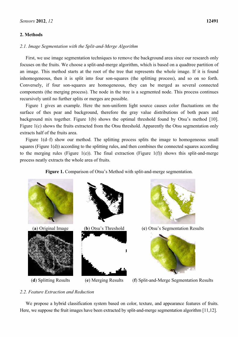
Figure 2(a) is an original rainbow image with RGB channels from 0 to 255, so there are totally 256 × 256 × 256 = 224 colors. Figure 2(b) uses four bins to represent each color component, Bins 0, 1, 2, 3 denote intensities 0-63, 64-127, 128-191, 192-255, respectively, so there are in total 4 × 4 × 4 = 64 colors. Figure 2(c) is the histogram of Figure 2(b), where the x-axis denotes the index of the 64 colors, and the y-axis denotes the number of pixels.

Figure 2. Rainbow image.

(a) Original Image (b) Reduced to 4 × 4 × 4 = 64 colors (c) Image Histogram

The histogram provides a compact summarization of the distribution of data in an image. The color histogram of an image is relatively invariant with translation and rotation about the viewing axis. By comparing histograms signatures of two images and matching the color content of one image with the other, the color histogram is well suited for the problem of recognizing an object of unknown position and rotation within a scene.

2.2.2. Unser’s Texture Features

Gray level co-occurrence matrix and local binary pattern are good texture descriptors, however, they are excessively time consuming. In this paper, we chose the Unser feature vector. Unser proved that the sum and difference of two random variables with same variances are de-correlated and the principal axes of their associated joint probability function are defined. Therefore, we use the sum s and difference d histograms for texture description [15].

The non-normalized sum and difference associated with a relative displacement (δ1, δ2) for an image I are defined as:

(1)

(2)

0

1000

2000

3000

4000

5000

0 20 40 60

1 2 1 2( , ; , ) ( , ) ( , )s k l I k l I k lδ δ δ δ= + + +

1 2 1 2( , ; , ) ( , ) ( , )d k l I k l I k lδ δ δ δ= − + +

Sensors 2012, 12 12493

The sum and difference histograms over the domain D are defined as:

(3)

(4)

Next, seven indexes can be defined on the basis of the sum and difference histogram. Those indexes and their corresponding formulas are listed in Table 1. In our method, we firstly abandoned the color information, followed by calculating the 64-bin histogram, and finally obtain the seven indexes.

Table 1. Sum and difference histogram based measures.

Measure FormulaMean (μ)

1 2(1 / 2) ( ; , )siih iμ δ δ= ×∑

Contrast (Cn) 21 2( ; , )n dj

C j h j δ δ=∑

Homogeneity (Hg) 21 2(1 / (1 )) ( ; , )g dj

H j h j δ δ= +∑

Energy (En) 2 21 2 1 2( ; , ) ( ; , )n s di j

E h i h jδ δ δ δ=∑ ∑ Variance (σ2) ( )2 2 2

1 2 1 2(1 / 2) ( 2 ) ( ; , ) ( ; , )s di ji h i j h jσ μ δ δ δ δ= × − +∑ ∑

Correlation (Cr) ( )2 21 2 1 2(1 / 2) ( 2 ) ( ; , ) ( ; , )r s di j

C i h i j h jμ δ δ δ δ= × − −∑ ∑

Entropy (Hn) 1 2 1 2 1 2 1 2( ; , ) log( ( ; , )) ( ; , ) log( ( ; , ))n s s d di jH h i h i h j h jδ δ δ δ δ δ δ δ= − −∑ ∑

2.2.3. Shape Features

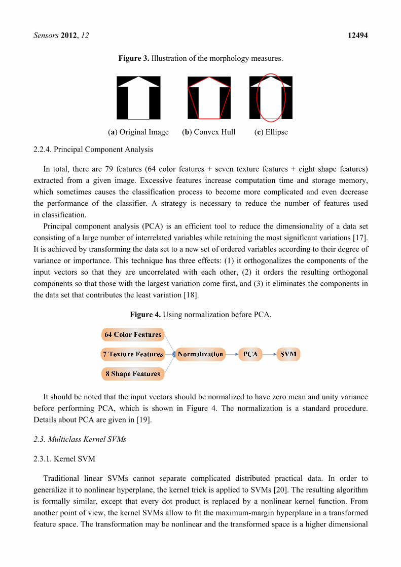
In this paper we propose eight measures based on mathematical morphology, which are listed in Table 2. The measures can be classified into four groups: (1) The “area”, “perimeter”, and the “Euler number” can be extracted directly from the object; (2) Create a convex hull using Graham Scan method [16] which is the smallest convex polygon that covers the object, then extract the “convex area” and “solidity” features; (3) Create an ellipse that has the same second-moments as the object, then extract the “minor length”, “major length”, and “eccentricity” features. Table 2 illustrates an example of generating the convex hull and the ellipse from original images.

Table 2. The Morphology based Measures.

Measure MeaningArea (Ar) The actual number of pixels inside the object

Perimeter (Pr) The distance around the boundary of the object Euler (El) The Euler number of the object

Convex (Cn) The number of pixels of the convex hull Solidity (Sl) The proportion of area to convex hull

MinorLength (Mn) The length of the minor axis of the ellipse MajorLength (Mj) The length of the major axis of the ellipse Eccentricity (Ec) The eccentricity of the ellipse

( )1 2 1 2( ; , ) card ( , ) , ( , ; , )sh i k l D s k l iδ δ δ δ= ∈ =

( )1 2 1 2( ; , ) card ( , ) , ( , ; , )dh j k l D d k l jδ δ δ δ= ∈ =

Sensors 2012, 12 12494

Figure 3. Illustration of the morphology measures.

(a) Original Image (b) Convex Hull (c) Ellipse

2.2.4. Principal Component Analysis

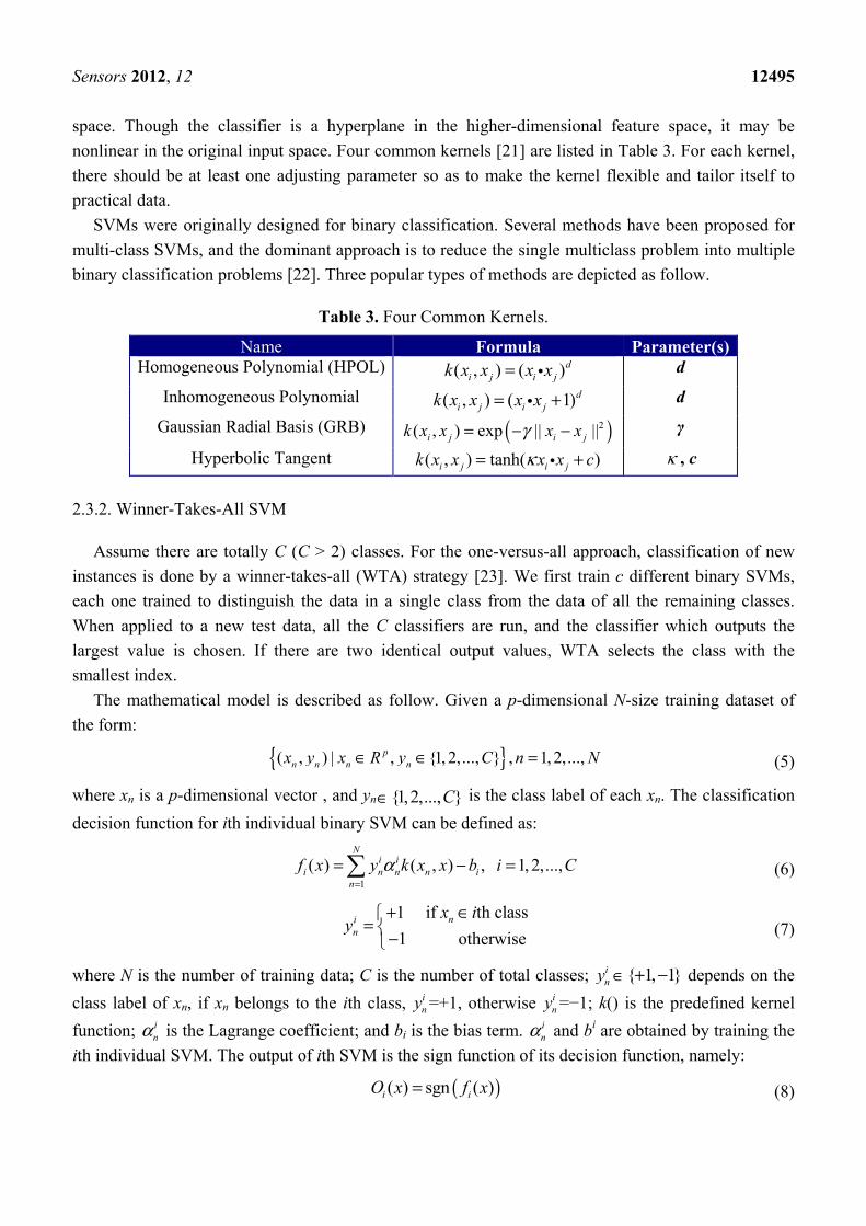
In total, there are 79 features (64 color features + seven texture features + eight shape features) extracted from a given image. Excessive features increase computation time and storage memory, which sometimes causes the classification process to become more complicated and even decrease the performance of the classifier. A strategy is necessary to reduce the number of features used in classification.

Principal component analysis (PCA) is an efficient tool to reduce the dimensionality of a data set consisting of a large number of interrelated variables while retaining the most significant variations [17]. It is achieved by transforming the data set to a new set of ordered variables according to their degree of variance or importance. This technique has three effects: (1) it orthogonalizes the components of the input vectors so that they are uncorrelated with each other, (2) it orders the resulting orthogonal components so that those with the largest variation come first, and (3) it eliminates the components in the data set that contributes the least variation [18].

Figure 4. Using normalization before PCA.

It should be noted that the input vectors should be normalized to have zero mean and unity variance before performing PCA, which is shown in Figure 4. The normalization is a standard procedure. Details about PCA are given in [19].

2.3. Multiclass Kernel SVMs

2.3.1. Kernel SVM

Traditional linear SVMs cannot separate complicated distributed practical data. In order to generalize it to nonlinear hyperplane, the kernel trick is applied to SVMs [20]. The resulting algorithm is formally similar, except that every dot product is replaced by a nonlinear kernel function. From another point of view, the kernel SVMs allow to fit the maximum-margin hyperplane in a transformed feature space. The transformation may be nonlinear and the transformed space is a higher dimensional

Sensors 2012, 12 12495 space. Though the classifier is a hyperplane in the higher-dimensional feature space, it may be nonlinear in the original input space. Four common kernels [21] are listed in Table 3. For each kernel, there should be at least one adjusting parameter so as to make the kernel flexible and tailor itself to practical data.

SVMs were originally designed for binary classification. Several methods have been proposed for multi-class SVMs, and the dominant approach is to reduce the single multiclass problem into multiple binary classification problems [22]. Three popular types of methods are depicted as follow.

Table 3. Four Common Kernels.

Name Formula Parameter(s)Homogeneous Polynomial (HPOL) ( , ) ( )d

i j i jk x x x x= i d

Inhomogeneous Polynomial ( , ) ( 1)di j i jk x x x x= +i d

Gaussian Radial Basis (GRB) ( )2( , ) exp || ||i j i jk x x x xγ= − − γ

Hyperbolic Tangent ( , ) tanh( )i j i jk x x x x cκ= +i κ , c

2.3.2. Winner-Takes-All SVM

Assume there are totally C (C > 2) classes. For the one-versus-all approach, classification of new instances is done by a winner-takes-all (WTA) strategy [23]. We first train c different binary SVMs, each one trained to distinguish the data in a single class from the data of all the remaining classes. When applied to a new test data, all the C classifiers are run, and the classifier which outputs the largest value is chosen. If there are two identical output values, WTA selects the class with the smallest index.

The mathematical model is described as follow. Given a p-dimensional N-size training dataset of the form:

(5)

where xn is a p-dimensional vector , and yn∈ {1,2,..., }C is the class label of each xn. The classification decision function for ith individual binary SVM can be defined as:

(6)

(7)

where N is the number of training data; C is the number of total classes; iny ∈ { 1, 1}+ − depends on the

class label of xn, if xn belongs to the ith class, iny =+1, otherwise i

ny =−1; k() is the predefined kernel function; i

nα is the Lagrange coefficient; and bi is the bias term. inα and bi are obtained by training the

ith individual SVM. The output of ith SVM is the sign function of its decision function, namely:

(8)

{ }( , ) | , {1, 2,..., } , 1, 2,...,pn n n nx y x R y C n N∈ ∈ =

1( ) ( , ) , 1, 2,...,

Ni i

i n n n in

f x y k x x b i Cα=

= − =∑

1 if th class1 otherwise

nin

x iy

+ ∈⎧= ⎨−⎩

( )( ) sgn ( )i iO x f x=

Sensors 2012, 12 12496

If ( )if x >0, then the output Oi(x) is +1, denoting x belongs to ith class; otherwise output is −1, denoting x belongs to other classes.

2.3.3. Max-Wins-Voting SVM

For the one-versus-one approach, classification is done by a max-wins voting (MWV) strategy [23]. First we construct a binary SVM for each pair of classes, so in total we will get C(C-1)/2 binary SVMs. When applied to a new test data, each SVM gives one vote to the winning class, and the test data is labeled with the class having most labels. If there are two identical votes, MWV selects the class with the smallest index.

The mathematical model is described as follow. The ijth (i = 1,2, …, C-1, j = i + 1, …, C) individual binary SVM is trained with all data in the ith class with +1 label and all data of the jth class with −1 label, so as to distinguish ith class from jth class. The decision function of ijth SVM is:

(9)

(10)

where Ni and Nj denotes the total number of ith class and jth class, respectively. ijny ∈ { 1, 1}+ − depends

on the class label of ijnx . If ij

nx belongs to ith class, ijny =+1; otherwise ij

nx belongs to jth class, ijny =−1.

ijnα is the Lagrange coefficient; and bij is the bias term. ij

nα and bij are obtained by training the ijth individual SVM. The output of ijth SVM is the sign function of its decision function, namely:

(11)

If ( )ijf x >0, then the output Oij(x) is +1, denoting x belongs to ith class; otherwise output is −1, denoting x belongs to jth class.

2.3.4. Directed Acyclic Graph SVM

A Directed Acyclic Graph (DAG) is a graph whose edges have an orientation and no cycles. The DAG-SVM constructs the individual SVM as the MWV-SVM, however, the output of each individual SVM is explained differently. When Oij(x) is +1, it denotes that x does not belong to jth class; when Oij(x) is −1, it denotes that x does not belong to ith class. Therefore, the final decision cannot be reached until the leaf node is reached [24].

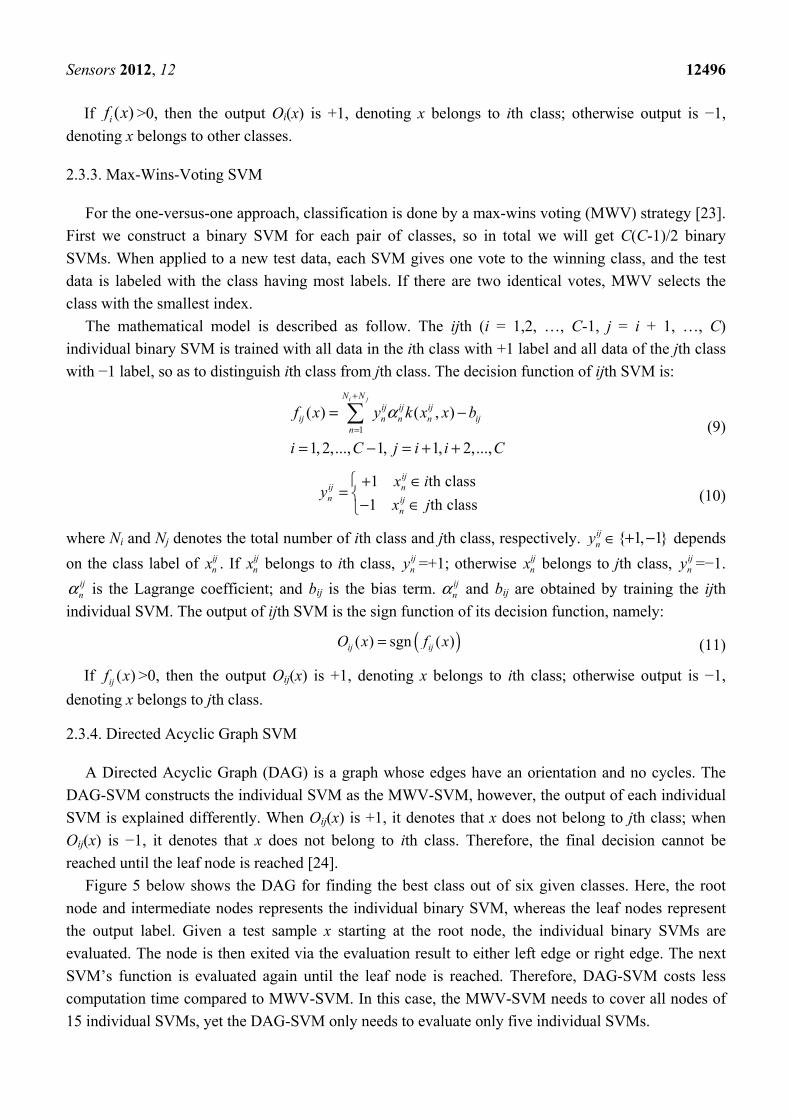
Figure 5 below shows the DAG for finding the best class out of six given classes. Here, the root node and intermediate nodes represents the individual binary SVM, whereas the leaf nodes represent the output label. Given a test sample x starting at the root node, the individual binary SVMs are evaluated. The node is then exited via the evaluation result to either left edge or right edge. The next SVM’s function is evaluated again until the leaf node is reached. Therefore, DAG-SVM costs less computation time compared to MWV-SVM. In this case, the MWV-SVM needs to cover all nodes of 15 individual SVMs, yet the DAG-SVM only needs to evaluate only five individual SVMs.

1

( ) ( , )

1, 2,..., 1, 1, 2,...,

i jN Nij ij ij

ij n n n ijn

f x y k x x b

i C j i i C

α+

=

= −

= − = + +

∑

1 th class1 th class

ijij nn ij

n

x iy

x j⎧+ ∈

= ⎨− ∈⎩

( )( ) sgn ( )ij ijO x f x=

Sensors 2012, 12 12497

Figure 5. The DAG for finding best class out of six classes.

3. Experiments & Discussions

The experiments were carried out on a P4 IBM platform with 3 GHz main frequency and 2 GB memory running under the Microsoft Windows XP operating system. The algorithm was developed in-house on the Matlab 2011b (The Mathworks©) platform. The programs can be run or tested on any computer platforms where Matlab is available.

3.1. Fruit Recognition System

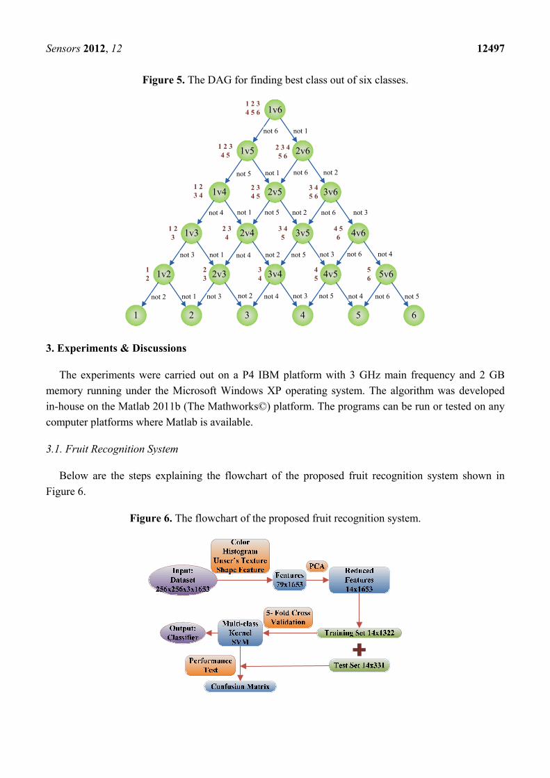
Below are the steps explaining the flowchart of the proposed fruit recognition system shown in Figure 6.

Figure 6. The flowchart of the proposed fruit recognition system.

1v6

1v5

1 2 3 4 5 6

2v6

1v4 2v5 3v6

1v3 2v4 3v5 4v6

1v2 2v3 3v4 4v5 5v6

not 6 not 1

not 5 not 1

not 4

not 3 not 1 not 4

not 5 not 2

not 6 not 2

not 6 not 3

not 5 not 3 not 6 not 4not 2

1 2 3 4 5

2 3 4 5 6

1 2 3 4

not 1

2 3 4 5

3 4 5 6

1 2 3

2 3 4

3 4 5

4 5 6

1 2

2 3

3 4

4 5

5 6

1

not 2

2 3 4 5 6

not 3not 1 not 2 not 4 not 3 not 5 not 4 not 6 not 5

Sensors 2012, 12 12498 Numbers in the figure are achieved by experiments below:

Step 1. The input is a database of 1,653 images consisting of 18 categories of fruits, and each image size is 256 × 256.

Step 2. The 79 features are extracted from each 256 × 256 image. These 79 features contain 64 color features, seven texture features, and eight shape features.

Step 3. The 79 features are reduced to only 14 features via PCA, and the selection standard is to preserve 95% energy.

Step 4. The 1,653 images are divided into training set (1,322) and test set (331) in the proportion of 4:1. Meanwhile, the training set is treated by 5-fold cross validation.

Step 5. The training set is used to train the multi-class SVM. The weights of the SVM are adjusted to make minimal the average error of 5-fold cross validation.

Step 6. The test dataset is constructed by randomly sampling in each group, and is used to analyze the performance of the classifier and to calculate the Confusion Matrix. If acceptable, then output the classifier, otherwise return to step 5 to re-train the weights of SVM.

3.2. Dataset

The fruit dataset was obtained after six months of on-site data collecting via digital camera and online collecting using images.google.com as the main search engine. The split-and-merge algorithm was used to remove the background areas; later images were cropped to leave the fruit in the center of the image, and finally downsampled to 256 × 256 in size.

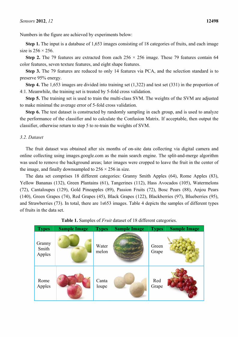
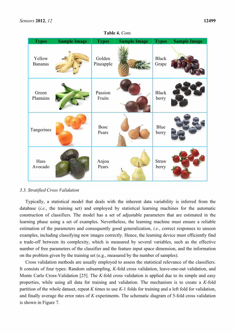
The data set comprises 18 different categories: Granny Smith Apples (64), Rome Apples (83), Yellow Bananas (132), Green Plantains (61), Tangerines (112), Hass Avocados (105), Watermelons (72), Cantaloupes (129), Gold Pineapples (89), Passion Fruits (72), Bosc Pears (88), Anjou Pears (140), Green Grapes (74), Red Grapes (45), Black Grapes (122), Blackberries (97), Blueberries (95), and Strawberries (73). In total, there are 1s653 images. Table 4 depicts the samples of different types of fruits in the data set.

Table 1. Samples of Fruit dataset of 18 different categories.

Types Sample Image Types Sample Image Types Sample Image

Granny Smith Apples

Water melon

Green Grape

Rome Apples

Canta loupe

Red Grape

Sensors 2012, 12 12499

Table 4. Cont.

Types Sample Image Types Sample Image Types Sample Image

Yellow Bananas

Golden Pineapple

Black Grape

Green Plantains

Passion Fruits

Black berry

Tangerines

Bosc Pears

Blue berry

Hass Avocado

Anjou Pears

Straw berry

3.3. Stratified Cross Validation

Typically, a statistical model that deals with the inherent data variability is inferred from the database (i.e., the training set) and employed by statistical learning machines for the automatic construction of classifiers. The model has a set of adjustable parameters that are estimated in the learning phase using a set of examples. Nevertheless, the learning machine must ensure a reliable estimation of the parameters and consequently good generalization, i.e., correct responses to unseen examples, including classifying new images correctly. Hence, the learning device must efficiently find a trade-off between its complexity, which is measured by several variables, such as the effective number of free parameters of the classifier and the feature input space dimension, and the information on the problem given by the training set (e.g., measured by the number of samples).

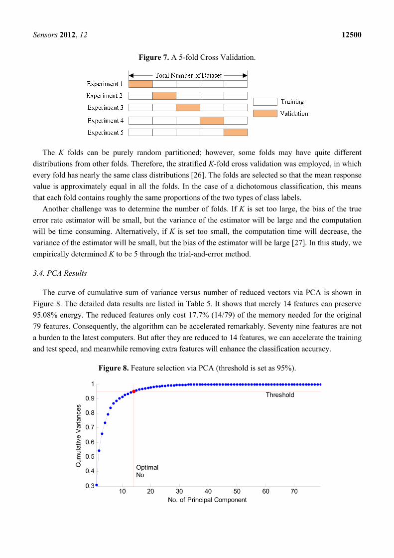
Cross validation methods are usually employed to assess the statistical relevance of the classifiers. It consists of four types: Random subsampling, K-fold cross validation, leave-one-out validation, and Monte Carlo Cross-Validation [25]. The K-fold cross validation is applied due to its simple and easy properties, while using all data for training and validation. The mechanism is to create a K-fold partition of the whole dataset, repeat K times to use K-1 folds for training and a left fold for validation, and finally average the error rates of K experiments. The schematic diagram of 5-fold cross validation is shown in Figure 7.

Sensors 2012, 12 12500

Figure 7. A 5-fold Cross Validation.

The K folds can be purely random partitioned; however, some folds may have quite different distributions from other folds. Therefore, the stratified K-fold cross validation was employed, in which every fold has nearly the same class distributions [26]. The folds are selected so that the mean response value is approximately equal in all the folds. In the case of a dichotomous classification, this means that each fold contains roughly the same proportions of the two types of class labels.

Another challenge was to determine the number of folds. If K is set too large, the bias of the true error rate estimator will be small, but the variance of the estimator will be large and the computation will be time consuming. Alternatively, if K is set too small, the computation time will decrease, the variance of the estimator will be small, but the bias of the estimator will be large [27]. In this study, we empirically determined K to be 5 through the trial-and-error method.

3.4. PCA Results

The curve of cumulative sum of variance versus number of reduced vectors via PCA is shown in Figure 8. The detailed data results are listed in Table 5. It shows that merely 14 features can preserve 95.08% energy. The reduced features only cost 17.7% (14/79) of the memory needed for the original 79 features. Consequently, the algorithm can be accelerated remarkably. Seventy nine features are not a burden to the latest computers. But after they are reduced to 14 features, we can accelerate the training and test speed, and meanwhile removing extra features will enhance the classification accuracy.

Figure 8. Feature selection via PCA (threshold is set as 95%).

10 20 30 40 50 60 700.3

0.4

0.5

0.6

0.7

0.8

0.9

1

No. of Principal Component

Cum

ulat

ive

Var

ianc

es

Threshold

OptimalNo

Sensors 2012, 12 12501

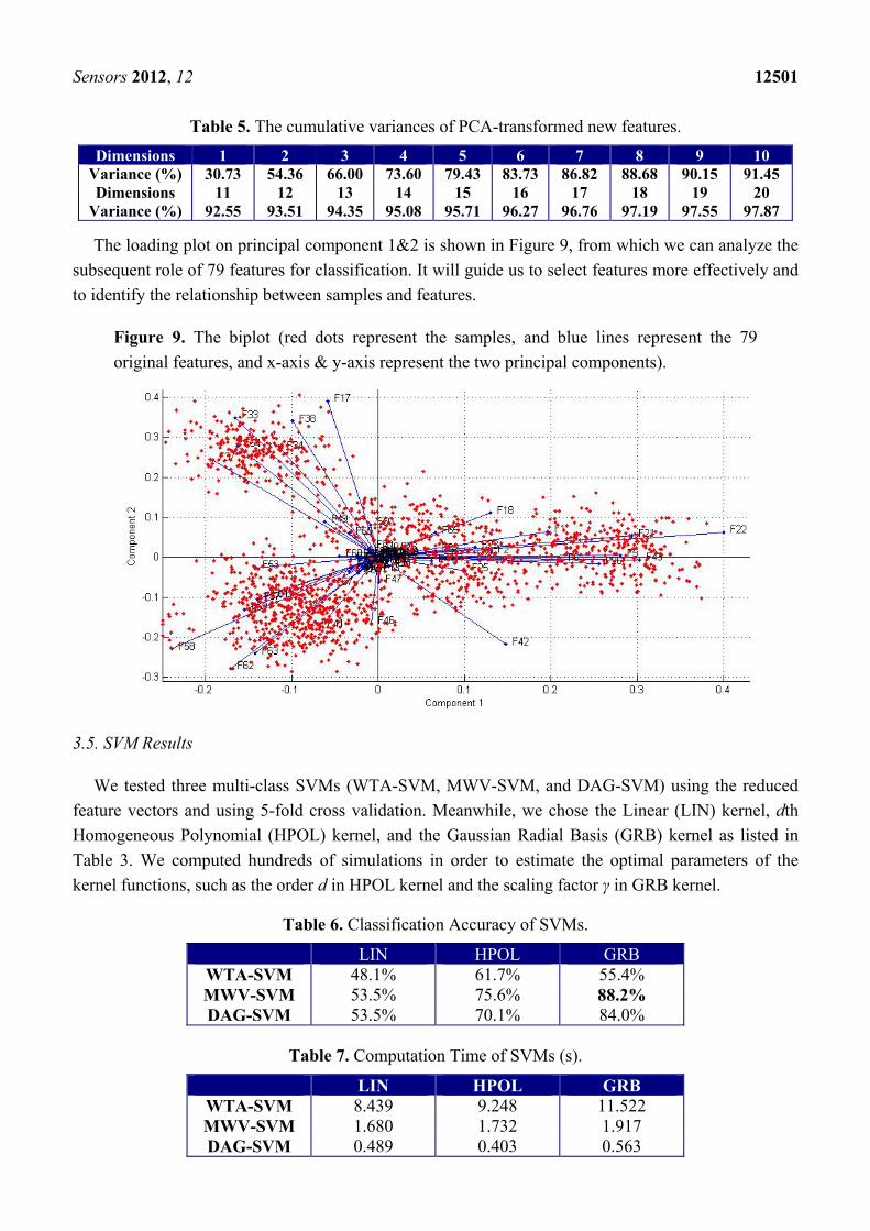
Table 5. The cumulative variances of PCA-transformed new features. Dimensions 1 2 3 4 5 6 7 8 9 10

Variance (%) 30.73 54.36 66.00 73.60 79.43 83.73 86.82 88.68 90.15 91.45 Dimensions 11 12 13 14 15 16 17 18 19 20

Variance (%) 92.55 93.51 94.35 95.08 95.71 96.27 96.76 97.19 97.55 97.87

The loading plot on principal component 1&2 is shown in Figure 9, from which we can analyze the subsequent role of 79 features for classification. It will guide us to select features more effectively and to identify the relationship between samples and features.

Figure 9. The biplot (red dots represent the samples, and blue lines represent the 79 original features, and x-axis & y-axis represent the two principal components).

3.5. SVM Results

We tested three multi-class SVMs (WTA-SVM, MWV-SVM, and DAG-SVM) using the reduced feature vectors and using 5-fold cross validation. Meanwhile, we chose the Linear (LIN) kernel, dth Homogeneous Polynomial (HPOL) kernel, and the Gaussian Radial Basis (GRB) kernel as listed in Table 3. We computed hundreds of simulations in order to estimate the optimal parameters of the kernel functions, such as the order d in HPOL kernel and the scaling factor γ in GRB kernel.

Table 6. Classification Accuracy of SVMs.

LIN HPOL GRB WTA-SVM 48.1% 61.7% 55.4% MWV-SVM 53.5% 75.6% 88.2% DAG-SVM 53.5% 70.1% 84.0%

Table 7. Computation Time of SVMs (s).

LIN HPOL GRB WTA-SVM 8.439 9.248 11.522 MWV-SVM 1.680 1.732 1.917 DAG-SVM 0.489 0.403 0.563

Sensors 2012, 12 12502

Tables 6 and 7 show the classification accuracy and calculation time in five-fold cross-validation for those SVMs with optimized parameters, respectively. For LIN kernel, the classification accuracies of MWV-SVM and DAG-SVM are the same of 53.5%, higher than the WTA-SVM of 48.1%; for the HPOL kernel, the classification accuracy of MWV-SVM is 75.6%, higher than WTA-SVM of 61.7% and DAG-SVM of 70.1%; for the GRB kernel, the classification accuracy of MWV-SVM is 88.2%, still higher than WTA-SVM of 55.4% and DAG-SVM of 84.0%. Therefore, the best results are achieved using the GRB kernel MWV-SVM with a classification accuracy of 88.2%.

As for the classification speed, the WTA-SVM is the slowest, for it uses one-versus-all strategy so the dataset needed for training is relatively large. The MWV-SVM is faster than WTA-SVM for it uses one-versus-one strategy so every individual binary SVM only takes about 2/18 portion of the data. The DAG-SVM is yet four times faster than MWV-SVM. The reason leans upon that the MWV-SVM needs all 153 individual SVMs to make the final decision, nevertheless the DAG-SVM needs only 17 binary SVMs to complete the equivalent task.

3.6. Confusion Matrix

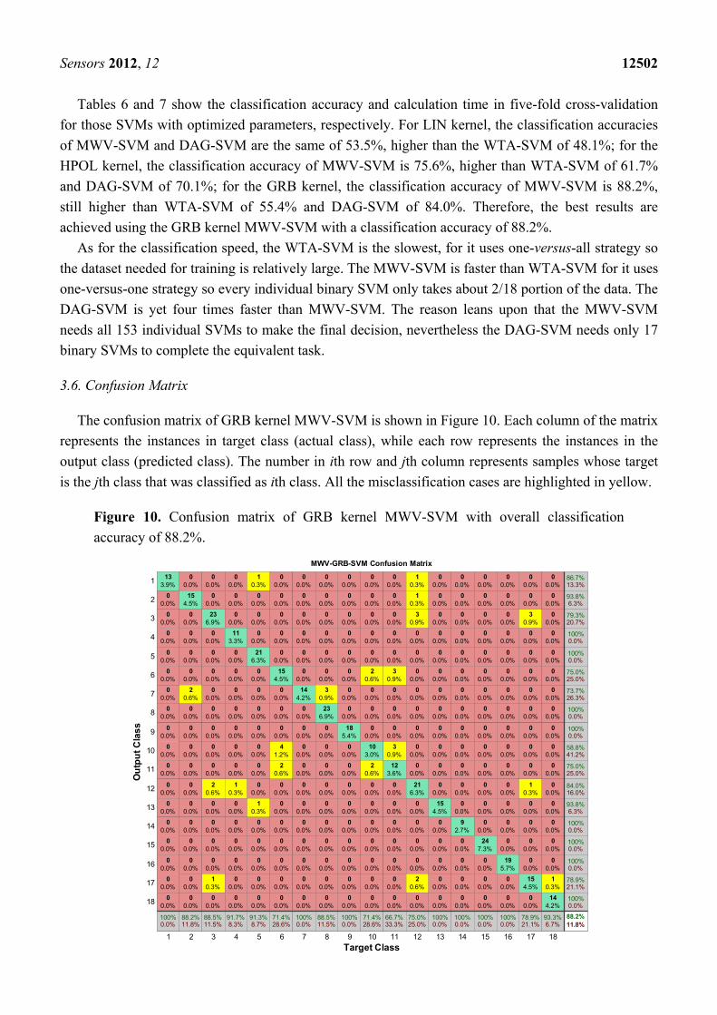
The confusion matrix of GRB kernel MWV-SVM is shown in Figure 10. Each column of the matrix represents the instances in target class (actual class), while each row represents the instances in the output class (predicted class). The number in ith row and jth column represents samples whose target is the jth class that was classified as ith class. All the misclassification cases are highlighted in yellow.

Figure 10. Confusion matrix of GRB kernel MWV-SVM with overall classification accuracy of 88.2%.

1 2 3 4 5 6 7 8 9 10 11 12 13 14 15 16 17 18

1

2

3

4

5

6

7

8

9

10

11

12

13

14

15

16

17

18

133.9%

00.0%

00.0%

00.0%

00.0%

00.0%

00.0%

00.0%

00.0%

00.0%

00.0%

00.0%

00.0%

00.0%

00.0%

00.0%

00.0%

00.0%

100%0.0%

00.0%

154.5%

00.0%

00.0%

00.0%

00.0%

20.6%

00.0%

00.0%

00.0%

00.0%

00.0%

00.0%

00.0%

00.0%

00.0%

00.0%

00.0%

88.2%11.8%

00.0%

00.0%

236.9%

00.0%

00.0%

00.0%

00.0%

00.0%

00.0%

00.0%

00.0%

20.6%

00.0%

00.0%

00.0%

00.0%

10.3%

00.0%

88.5%11.5%

00.0%

00.0%

00.0%

113.3%

00.0%

00.0%

00.0%

00.0%

00.0%

00.0%

00.0%

10.3%

00.0%

00.0%

00.0%

00.0%

00.0%

00.0%

91.7%8.3%

10.3%

00.0%

00.0%

00.0%

216.3%

00.0%

00.0%

00.0%

00.0%

00.0%

00.0%

00.0%

10.3%

00.0%

00.0%

00.0%

00.0%

00.0%

91.3%8.7%

00.0%

00.0%

00.0%

00.0%

00.0%

154.5%

00.0%

00.0%

00.0%

41.2%

20.6%

00.0%

00.0%

00.0%

00.0%

00.0%

00.0%

00.0%

71.4%28.6%

00.0%

00.0%

00.0%

00.0%

00.0%

00.0%

144.2%

00.0%

00.0%

00.0%

00.0%

00.0%

00.0%

00.0%

00.0%

00.0%

00.0%

00.0%

100%0.0%

00.0%

00.0%

00.0%

00.0%

00.0%

00.0%

30.9%

236.9%

00.0%

00.0%

00.0%

00.0%

00.0%

00.0%

00.0%

00.0%

00.0%

00.0%

88.5%11.5%

00.0%

00.0%

00.0%

00.0%

00.0%

00.0%

00.0%

00.0%

185.4%

00.0%

00.0%

00.0%

00.0%

00.0%

00.0%

00.0%

00.0%

00.0%

100%0.0%

00.0%

00.0%

00.0%

00.0%

00.0%

20.6%

00.0%

00.0%

00.0%

103.0%

20.6%

00.0%

00.0%

00.0%

00.0%

00.0%

00.0%

00.0%

71.4%28.6%

00.0%

00.0%

00.0%

00.0%

00.0%

30.9%

00.0%

00.0%

00.0%

30.9%

123.6%

00.0%

00.0%

00.0%

00.0%

00.0%

00.0%

00.0%

66.7%33.3%

10.3%

10.3%

30.9%

00.0%

00.0%

00.0%

00.0%

00.0%

00.0%

00.0%

00.0%

216.3%

00.0%

00.0%

00.0%

00.0%

20.6%

00.0%

75.0%25.0%

00.0%

00.0%

00.0%

00.0%

00.0%

00.0%

00.0%

00.0%

00.0%

00.0%

00.0%

00.0%

154.5%

00.0%

00.0%

00.0%

00.0%

00.0%

100%0.0%

00.0%

00.0%

00.0%

00.0%

00.0%

00.0%

00.0%

00.0%

00.0%

00.0%

00.0%

00.0%

00.0%

92.7%

00.0%

00.0%

00.0%

00.0%

100%0.0%

00.0%

00.0%

00.0%

00.0%

00.0%

00.0%

00.0%

00.0%

00.0%

00.0%

00.0%

00.0%

00.0%

00.0%

247.3%

00.0%

00.0%

00.0%

100%0.0%

00.0%

00.0%

00.0%

00.0%

00.0%

00.0%

00.0%

00.0%

00.0%

00.0%

00.0%

00.0%

00.0%

00.0%

00.0%

195.7%

00.0%

00.0%

100%0.0%

00.0%

00.0%

30.9%

00.0%

00.0%

00.0%

00.0%

00.0%

00.0%

00.0%

00.0%

10.3%

00.0%

00.0%

00.0%

00.0%

154.5%

00.0%

78.9%21.1%

00.0%

00.0%

00.0%

00.0%

00.0%

00.0%

00.0%

00.0%

00.0%

00.0%

00.0%

00.0%

00.0%

00.0%

00.0%

00.0%

10.3%

144.2%

93.3%6.7%

86.7%13.3%

93.8%6.3%

79.3%20.7%

100%0.0%

100%0.0%

75.0%25.0%

73.7%26.3%

100%0.0%

100%0.0%

58.8%41.2%

75.0%25.0%

84.0%16.0%

93.8%6.3%

100%0.0%

100%0.0%

100%0.0%

78.9%21.1%

100%0.0%

88.2%11.8%

Target Class

Out

put C

lass

MWV-GRB-SVM Confusion Matrix

Sensors 2012, 12 12503

By looking at the bottom line of Figure 10, we found that 1st class (Granny Smith Apples), 7th class (Water melon), 9th class (Golden Pineapple), 13th class (Green Grape), 14th class (Red Grape), 15th class (Black Grape), 16th class (Black berry) are all recognized successfully.

Notwithstanding, a few types of fruits were not recognized so successfully. The SVM for the 11th class (Bosc Pears) performs the worst. In the test dataset, there are 18 different pictures of Bosc Pears, however, three of them are misclassified as 6th class (Avocado), and another three of them are misclassified as 10th class (Passion Fruits), so the rest are recognized correctly leading to a 66.7% (12/18) success rate. For the 6th class (Avocado), it has twenty-one samples in the test dataset, but four are misclassified as 10th class (Passion Fruits) and two are misclassified as 11th class (Bosc Pears), so with the rest fifteen samples recognized, this give us a 71.43% (15/21) success rate. For the 10th class (Passion Fruits), it has fourteen samples in the test dataset, two are misclassified as 6th class (Avocado), and another two are misclassified as 11th class (Bosc Pears), so with the rest recognized, it give us a 71.43% (10/14) success rate. In other words, the 6th, 10th, and 11th classes are not distinct in the view of SVM, which is a motivation for our future work in order to solve this misclassification.

4. Conclusions

This work proposed a novel classification method based on multi-class kSVM. The experimental results demonstrated that the MWV-SVM with GRB kernel achieves the best classification accuracy of 88.2%. The combination of color histogram, Unser’s texture, and shape features are more effective than any single kind of feature in classification of fruits. Using PCA to reduce features, we tested three different multi-class SVMs (WTA-SVM, MWV-SVM, and DAG-SVM) with linear kernel, dth Homogeneous Polynomial kernel, and Gaussian Radial Basis kernel in the dataset of 1,653 fruit images. The best results were obtained for MWV-SVM with the GRB kernel with an overall classification accuracy of 88.2%. Future research will concentrate on: (1) extending our research to sliced, dried, canned, and tinned fruits; (2) include additional features to increase the classification accuracy; (3) accelerate the algorithm; and (4) find distinguishable features for Bosc Pears, Passion Fruits, and Avocado.

Acknowledgments

The authors give special thanks to Roberto Lam from The City College of New York-CUNY for the review of the whole paper.

References

1. Rocha, A.; Hauagge, D.C.; Wainer, J.; Goldenstein, S. Automatic fruit and vegetable classification from images. Comput. Electron. Agric. 2010, 70, 96–104.

2. Bolle, R.M.; Connell, J.H.; Haas, N.; Mohan, R.; Taubin, G. VeggieVision: A Produce Recognition System. In Proceedings 3rd IEEE Workshop on Applications of Computer Vision, WACV'96, Sarasota, FL, USA, 2–4 December 1996, pp. 244–251.

3. Hong, S.G.; Maccaroni, M.; Figuli, P.J.; Pryor, B.M.; Belisario, A. Polyphasic Classification of alternaria isolated from hazelnut and walnut fruit in Europe. Mycol. Res. 2006, 110, 1290–1300.

Sensors 2012, 12 12504 4. Baltazar, A.; Aranda, J.I.; González-Aguilar, G. Bayesian classification of ripening stages of

tomato fruit using acoustic impact and colorimeter sensor data. Comput. Electron. Agric. 2008, 60, 113–121.

5. Pennington, J.A.T.; Fisher, R.A. Classification of fruits and vegetables. J. Food Compos. Anal. 2009, 22, S23–S31.

6. Pholpho, T.; Pathaveerat, S.; Sirisomboon, P. Classification of longan fruit bruising using visible spectroscopy. J. Food Eng. 2011, 104, 169–172.

7. Seng, W.C.; Mirisaee, S.H. A New Method for Fruits Recognition System. In Proceedings of International Conference on Electrical Engineering and Informatics, ICEEI'09, Selangor, Malaysia, 5–7 August 2009; Volume 1, pp. 130–134.

8. Patil, N.S.; Shelokar, P.S.; Jayaraman, V.K.; Kulkarni, B.D. Regression models using pattern search assisted least square support vector machines. Chem. Eng. Res. Des. 2005, 83, 1030–1037.

9. Li, D.; Yang, W.; Wang, S. Classification of foreign fibers in cotton lint using machine vision and multi-class support vector machine. Comput. Electron. Agric. 2010, 74, 274–279.

10. Min, T.-H.; Park, R.-H. Eyelid and eyelash detection method in the normalized iris image using the parabolic Hough model and Otsu’s thresholding method. Pattern Recognit. Lett. 2009, 30, 1138–1143.

11. Xiao, Y.; Zou, J.; Yan, H. An adaptive split-and-merge method for binary image contour data compression. Pattern Recognit. Lett. 2001, 22, 299–307.

12. Damiand, G.; Resch, P. Split-and-merge algorithms defined on topological maps for 3D image segmentation. Graph. Models 2003, 65, 149–167.

13. Siang Tan, K.; Mat Isa, N.A. Color image segmentation using histogram thresholding—Fuzzy C-means hybrid approach. Pattern Recognit. Lett. 2011, 44, 1–15.

14. Maitra, M.; Chatterjee, A. A hybrid cooperative-comprehensive learning based PSO algorithm for image segmentation using multilevel thresholding. Expert Syst. Appl. 2008, 34, 1341–1350.

15. Unser, M. Texture classification and segmentation using wavelet frames. IEEE Trans. Image Process. 1995, 4, 1549–1560.

16. Lou, S.; Jiang, X.; Scott, P.J. Algorithms for morphological profile filters and their comparison. Precis. Eng. 2012, 36, 414–423.

17. Kwak, N. Principal Component Analysis Based on L1-Norm Maximization. IEEE Trans. Patt. Anal. Mach. Int. 2008, 30, 1672–1680.

18. Lipovetsky, S. PCA and SVD with nonnegative loadings. Pattern Recognit. Lett. 2009, 42, 68–76. 19. Jackson, J.E. A User’s Guide to Principal Components; John Wiley & Sons: Hoboken, NJ, USA

1991. 20. Acevedo-Rodríguez, J.; Maldonado-Bascón, S.; Lafuente-Arroyo, S.; Siegmann, P.;

López-Ferreras, F. Computational load reduction in decision functions using support vector machines. Signal Process. 2009, 89, 2066–2071.

21. Deris, A.M.; Zain, A.M.; Sallehuddin, R. Overview of Support Vector Machine in Modeling Machining Performances. Procedia Eng. 2011, 24, 308–312.

22. Maddipati, S.; Nandigam, R.; Kim, S.; Venkatasubramanian, V. Learning patterns in combinatorial protein libraries by Support Vector Machines. Comput. Chem. Eng. 2011, 35, 1143–1151.

Sensors 2012, 12 12505 23. Lingras, P.; Butz, C. Rough set based 1-v-1 and 1-v-r approaches to support vector machine

multi-classification. Inform. Sci. 2007, 177, 3782–3798. 24. Platt, J.C.; Cristianini, N.; Shawe-Taylor, J. Large margin DAGs for multiclass classification.

Adv. Neural. Inform. Process. Syst. 2000, 12, 547–553. 25. Pereira, A.C.; Reis, M.S.; Saraiva, P.M.; Marques, J.C. Madeira wine ageing prediction based on

different analytical techniques: UV–vis, GC-MS, HPLC-DAD. Chemometr. Intel. Lab. Syst. 2011, 105, 43–55.

26. May, R.J.; Maier, H.R.; Dandy, G.C. Data splitting for artificial neural networks using SOM-based stratified sampling. Neural Netw. 2010, 23, 283–294.

27. Armand, S.; Watelain, E.; Roux, E.; Mercier, M.; Lepoutre, F.-X. Linking clinical measurements and kinematic gait patterns of toe-walking using fuzzy decision trees. Gait Posture 2007, 25, 475–484.

© 2012 by the authors; licensee MDPI, Basel, Switzerland. This article is an open access article distributed under the terms and conditions of the Creative Commons Attribution license (http://creativecommons.org/licenses/by/3.0/).