Machine Dynamics Research - ICI Journals Master List
183
Machine Dynamics Research Warsaw University of Technology 2018, Vol. 42, No 1 ISSN 2080-9948
-
Upload
khangminh22 -
Category
Documents
-
view
0 -
download
0
Transcript of Machine Dynamics Research - ICI Journals Master List

Machine Dynamics Research
Warsaw Universityof Technology
2018, Vol. 42, No 1 ISSN 2080-9948

Machine Dynamics Research
Editor-in-Chief
JERZY BAJKOWSKI, Warsaw University of Technology
EditorsCZESŁAW BAJER, Institute of Fundamental Technological Research of the Pol-ish Academy of SciencesROMAN BOGACZ, Warsaw University of TechnologyZBIGNIEW DABROWSKI, Warsaw University of TechnologyDANUTA JASINSKA- CHOROMANSKA, Warsaw University of TechnologyROMAN KACZYNSKI, Białystok University of TechnologyKRZYSZTOF KALINSKI, Gdansk University of TechnologyJAN KICINSKI, Institute of Fluid-Flow Machinery of the Polish Academy of Sci-encesANDRZEJ KOCANDA, Warsaw University of TechnologyJAROSŁAW KOWALSKI, Air Force Institute of TechnologyWŁODZIMIERZ KURNIK, Warsaw University of TechnologyMARIUSZ GIERGIEL, AGH University of Science and TechnologyTADEUSZ NIEZGODA, Military University of TechnologyALEKSANDER OLEJNIK, Military University of TechnologyBOGDAN POSIADAŁA, Czestochowa University of TechnologyPIOTR PRZYBYŁOWICZ, Warsaw University of TechnologySTANISŁAW RADKOWSKI, Warsaw University of TechnologyBOGDAN SAPINSKI, AGH University of Science and TechnologyJERZY SWIDER, Silesian University of TechnologyWIESŁAW TRAMPCZYNSKI, Kielce University of TechnologyANDRZEJ TYLIKOWSKI, Warsaw University of TechnologyROBERT ZALEWSKI, Warsaw University of TechnologyTERESA ZIELINSKA, Warsaw University of TechnologyJÓZEF ZUREK, Air Force Institute of TechnologyANDRZEJ ZYLUK, Air Force Institute of Technology
Editorial secretary
PAWEŁ CHODKIEWICZ, Warsaw University of Technology
Edited and published byInstitute of Machine Design FundamentalsNarbutta 84, 02-524 Warszawa, Polandfax (+48 22) 234 86 22e-mail: [email protected]://www.mdr.simr.pw.edu.pl

Warsaw University of Technology
Machine Dynamics Research2018, Vol. 42, No 1
(Until Vol. 33/2009 Machine Dynamics Problems)
Published under the auspicesof the Committee on Machine Building
of the Polish Academy of Sciences

Scientific Committee
Abide Stéphane (FR), University of PerpignanAwrejcewicz Jan (PL), Lodz University of TechnologyBalthazar Jose Manoel (BR), University of Sao PauloBelingardi Giovanni (I), Polytechnic University of TorinoBarboteu Mikael (FR), University of PerpignanBinienda Wiesław (USA), University of AkronBogdevicius Marijonas (L), Vilnius Gediminas Technical UniversityCempel Czesław (PL), Poznan University of TechnologyDriss Zied (TN), University of SfaxDudziak Marian (PL), Poznan University of TechnologyDufrenoy Philippe (FR), Lille 1 University-Sciences and TechnologyFerreira Antoine (FR), INSA de BourgesFlorentin Eric (FR), INSA de BloisGaribaldi Luidi (I), Polytechnic University of TorinoGiergiel Józef (PL), Rzeszow University of TechnologyGlinka Grzegorz (CAN), University of WaterlooGolnariagi Farid (CAN), Franser University VancouverHaddar Mohamed (TN), ENIS de SfaxKanaev Andrei (FR), CNRS Universite de ParisKujawski Daniel (USA), Western Michigan UniversityKowal Janusz (PL), AGH University of Science and TechnologyLebon Frédéric (FR), AlX-Marseille UniversityLe Palec Georges (FR), UNIMECA MarseilleLobur Mykhaylo (UA), Lviv Polytechnic National UniversityMajewski Tadeusz (MEX), American University of PueblaMarchelek Krzysztof (PL), West Pomeranian University of TechnologyMazurkiewicz Adam (PL), Institute of Technology et Exploitation PIB in RadomMezyk Arkadiusz (PL), Silesian University of TechnologyMompeen Gilmar (FR), Lille 1 University-Sciences and TechnologyNardin Philippe (FR), University of Franche ComtéNizioł Józef (PL), Cracow University of TechnologyOstachowicz Wiesław (PL), Inst. of Fluid Flow Machinery Polish Acad. of SciencesOstermayer George Peter (D), Braunschweig University of TechnologyRade Alves Domingos (BR), Federal University of UberlandiaRusinski Eugeniusz (PL), Wroclaw University of TechnologySeweryn Andrzej (PL), Bialystok University of TechnologyShillor Meir (USA), Oakland University of RochesterSlomiana Maria (USA), Widener UniversitySofonea Mircea (FR), University of PerpignanStotsko Zinovij (UA), Lviv Polytechnic National UniversitySzczepaniak Ryszard (PL), Air Force Institute of TechnologySwitonski Eugeniusz (PL), Silesian of TechnologySun Fengchun (CH), Beijng Institute of TechnologyVerreman Yves (CAN), Ecole Polytechnique MontrealViano Juan (ESP), University Santiago de CompostellaWoznica Krzysztof (FR), INSA BourgesZeghmati Belkacem (FR), University of Perpignan

Machine Dynamics Research2018, Vol. 42, No 1
Contents
1. Roman Bogacz and Kurt FrischmuthFriction Induced Oscillations and Material Degradation in Rail-way Engineering
5
2. Anna Walicka, Edward Walicki, P. Jurczak, J. FalickiEffects of Hindrance Factors on a Squeeze Film of a PorousBearing LubricatedWith a Dehaven Fluid
15
3. Anna Jaskot, Bogdan PosiadałaModel of Motion of the Mobile Platform With Three WheelDrive
35
4. Józef Drewniak, Krzysztof ReszutaDynamic Model for Non-Symmetric Dual-Path Gearbox
45
5. Zdzisław Chłopek, Paulina Grzelak, Dagna ZakrzewskaEvaluation of the Influence of Car Engine Power SupplyWithRapeseed Oil Esters on Emission of Pollutants in DynamicConditions
55
6. Olimpia KunertHow Not to Lose the Valuable Know-How in Industry?
73
7. Andrzej Chudzikiewicz, Magdalena SowinskaThe Boltzmann-Hamel Formalism in Modelling of Rail VehicleMotion
87
8. Józef Pszczółkowski, Grzegorz DygaDetermination of the Electrical Structure Parameters of anAcid Battery
101
9. Arkadiusz Wzorek, Jacek Mateusz BajkowskiInfluence of Printer Head Velocity on FDM Deposited Path De-formations
117
10.Jan Misiak, Sławomir StachuraStatic Analysis and Stability of the Steel Framework
129
11.Robert Konowrocki, Andrzej ZbiecInfluence of Correctness of Running Gear Assembly onFreightWagon Wheels’Wear
139
12.Robert BrodzikThe Impact of Changes in the Designs of Concrete AirportPavement on Its Strength Properties
153
13.Zdzisław TrzaskaElectromechanical System for Charging Batteries of ElectricCars
165


Machine Dynamics Research2018, Vol. 42, No 1, 5-13
Friction Induced Oscillations and MaterialDegradation in Railway Engineering
Roman Bogacz1 and Kurt Frischmuth *2
1Warsaw University of Technology2Universität Rostock
AbstractMaintenance of tracks and vehicles is an important factor for security and passenger comfort.Late and insufficient repairs may have an accelerating effect on the degradation of a railwaysystem’s quality.
In the present paper, some phenomena related to the dynamics of running railway vehi-cles in the presence of geometric imperfections of rails are explored. In particular, the sensi-tivity of frictional forces to imperfections of contact surfaces is analyzed, and consequencesfor the propagation of defects are discussed.
Keywords: railway mechanics, maintenance, dynamics, degradation.
1 Introduction
The operation of railways requires permanent maintenance of track and vehicles.During exploitation, effects like aging, corrosion, wear and corrugation take place,affecting rolling stock and track as well. Important factors in this regard are runningspeeds and loads, but also geography related quantities like temperature, moisture,curviness of tracks. Also details of the used engines, e.g. torque control, may play arole.
Contact forces between rails and wheels play in this context an important role(Bogacz and Frischmuth, 2006, 2009). On the one hand, there are normal forces,which compensate first of all the weight of the vehicles. Typically, the normal forceamounts to about 50000[N] per wheel, distributed over a contact patch of an area ofthe order 10−4[m2], (Frischmuth, 1996, 2001). The normal stresses are hence quitehigh. Due to accelerations, caused e.g. by uneven surfaces, waviness, corrugationor polygonalization, this average level may be exceeded temporarily by a factor ofeven more than ten (Bogacz and Frischmuth, 2016). On the other hand, accelera-tion and deceleration, running up ascending or down descending tracks, is connected

6 Bogacz R., Frischmuth K.
Fig. 1. Speed limits in Poland.
to tangential forces, which are related via friction to the normal ones (Bogacz andFrischmuth, 2006). There is typically some creepage, i.e. a relative motion betweenthe contact partners rail and wheel, which brings about dissipation of energy. Thementioned factors contribute to the slow but inexorable degradation of the materialin the contact region. For abrasive wear, Archard’s law is assumed, i.e., under typ-ical running conditions, proportionality between dissipated energy and the mass ofremoved material holds (Frischmuth, 1996). Other forms of wear, related to percus-sive effects due to strong variations in the normal load, are much less understood.Scenarios involving lift-offs, impacts, local plastification, strain hardening and crackdevelopment are described (Bogacz and Kowalska, 2001). However, these phenom-ena are far less amiable to modeling and numerical simulation than those drivingabrasion (Bogacz and Frischmuth, 2016; Frischmuth, 2001). For obvious reasons,the considered effects take very long periods of time. Hundreds of miles are trav-elled before changes in geometry and material may be measured or detected. On theother hand, these changes are usually driven by highly dynamic oscillatory motionin the short run, e.g. the hunting motion of wheelsets, or the vertical dynamics of abouncing out-of-the round wheel. The phenomena connected with the stick-slip dis-tribution in the contact patches may considered high frequency effects. Also torquecontrol of the drive plays growing role in this regard.
Unfortunately, there are still considerable parts of the track length in most coun-tries, where such effects are unavoidable due to the very bad state of the rails. Obvi-ously, all relevant factors – but ageing and corrosion – are strongly increasing with therunning speed. Thus, an important indicator of the level and quality of maintenanceis the necessity of introducing speed limits.
Recent statistics show that e.g. in Poland, there is only 5% of the total rail netwithout any limitations due to poor track quality. On the other hand, there is onethird of the total track length, where it is considered not advisable to run faster than40 [km/h].
It is reasonable to suspect a correlation to the spending on track maintenance, seeTable 1. However, entries in Table 1 concerning spending on maintenance are also

Friction Induced Oscillations and Material Degradation ... 7
Table 1. Comparison of spending on track maintenance of selected European countries
Country Maintanance (C per km of track)Switzerland 349
Austria 258Sweden 151
Netherlands 129UK 110Italy 79
France 63Germany 51
Spain 38Poland 3.81
Fig. 2. Gap between rails (width 40 [mm]).
influenced by different costs of labor and geographic conditions – like mountains andtunnels in Switzerland and Austria.
The aim of this paper is to discuss some important aspects of mechanisms thateventually lead to serious degradation of material and threaten the safety of railwaytraffic, diminish passenger comfort and have a negative impact on the environment.
2 Spread of Damage
Gaps between rails may certainly be considered very severe faults, resulting in dam-age of wheels, even at small speeds. However, such defects are still quite commonon local subsidiary tracks, see Fig. 2.
Unfortunately, vehicles used on such tracks are not excluded from operating on

8 Bogacz R., Frischmuth K.
main lines, where a high level of surface quality is attempted to maintain. This leadsto a diffusion-type proliferation of damage. Any local singularity in a track leads toabnormal stresses and accelerations in wheels running over the spot. Any resultingdefects propagate by their impact along the trajectory of the vehicle. Hence, for anon-compartmentalized network, damage may spread like a virus. Sooner or later,bad maintenance of a small fraction of the track system will have a negative impactin a global scale. Further, geometric changes, concerning seemingly only the run-ning surfaces of rails and wheels, have the potential to propagate also deep into theconsidered construction. This will be discussed in the next section.
3 Excitation of Torsional Vibration by Gaps in Rails
In this section, we present some essential elements of modeling the dynamics of awheel’s motion over a gap between rail sections. In fact, a gap is just the ultimateform of an anomaly in the surface geometry. Analogous techniques are applied e.g.in the case of sine-type corrugation on a rail’s running surface or a wheel’s tread, cf.(Bogacz and Frischmuth, 2012, 2016; Bogacz and Kowalska, 2001). What is specialabout a gap is, first of all, that it is usually a singular defect, isolated from the nextcomparable one by a considerable distance. Furthermore, it can be modeled as anearly rectangular impulse, i.e., there are given neither smoothness nor continuity.
For a numerical calculation of forces and trajectories, a series of model assump-tions has to be made. Results will be, of course, always just approximations of thereal quantities. Random factors, higher order and coupling terms affect the qualityof simulations. Further, efforts to obtain very accurate results usually come at highcomputational cost, which is disadvantageous for the analysis of long-term evolution(Bogacz and Frischmuth, 2012, 2016; Frischmuth, 1996, 2001).
In this paper, we chose the framework of hybrid discrete-continuous mechanicalsystems. Indeed, the vehicle is, in this context, replaced by a finite system of lumpedmasses, coupled by massless springs and dampers (Bogacz et al., 1993). The trackand the wheel’s tread, however, constitute continuous components.
First, the geometry of gaps is approximated. From Fig. 2 it can be seen that gapsmay happen in both rails, but not necessarily exactly in the same position, and notalways of identical length. Since for a wheel, we usually chose the position of itscenter of mass as coordinates in a discrete-continuous model, the rectangular troughin the rail translates into a piecewise smooth constraint on the vertical center position,as shown in Fig. 3.
Now, considering the equations of motion for the vehicle’s degrees of freedom,the normal contact forces are evaluated as the reaction to the imposed constraints.Knowing, that the normal contact forces have to be distributed over a patch of pos-itive area, classical contact models are applied in order to approximate a contactpressure. Given the extraordinary numerical cost, such calculations are rarely done

Friction Induced Oscillations and Material Degradation ... 9
Fig. 3. Constraints resulting from gap in rails (width 40[mm]).
Fig. 4. Friction laws (dry contact).
by numerical methods like FEM or BEM, hence neither the true surface geometry nordynamical forces can be taken into account. Typically, the frictional effects resultingfrom the singularities of the pressure are studied in a separate step. This means thata feedback from the tangential stress components to the normal pressure is neglectedas well. These simplifications have been used for years, and the results have beenconfirmed by many researchers, so we adopt them here as well, cf. (Frischmuth,1996).
In order to understand the damaging effect of a rail gap on a vehicle, the under-standing of rolling friction is crucial. In sliding motion, a nearly jump in the forcevs speed characteristic was postulated by Coulomb, Fig. 4, left part. Near the origin,i.e. when a body is at rest, the tangential force is just compensating the total externaltangential force. It can be any value up to the limit, being the dry friction coefficientmultiplied by the normal force. After losing grip, first a drop of the tangential force,later an increase, with growing speed of relative motion is observed.
There are many variations of the classical form of Coulomb’s law. Originally,there was no dependence on the value of velocity. Measurements show, however, thatdepending on the material pair and the state of the surfaces, speed effects must not beneglected. In particular self-excited frictional vibration is closely related to the non-monotonicity of the characteristic. Moreover, the actual friction force may be evenrelated to the history of relative motion, including hysteresis effects and an influenceof acceleration. Some typical functional representations of dry friction relations areshown on the right part of Fig. 4.
When it comes to friction in rolling motion, there is generally no vertical branchof the relation like on the left plot in Fig. 4. However, anisotropy has to be consid-ered. The relative velocity vector between the surfaces in contact is normalized to the
10 Bogacz R., Frischmuth K.
speed of motion, and components influence each other. In the result, the directionsof tangential force and relative motion are not necessarily collinear. For the normalpressure, the theory of Hertz is still the approximation of choice, for the tangentialstresses, approaches due to Kalker and Kik are used for fast, yet acceptable withrespect to accurary, simulations.
It has to be admitted that a consequent dynamical approach on the scale of contactmodels is still not compatible with simulations e.g. of the lateral dynamics of awheelset, bogie or a vehicle. In recent papers, vertical dynamics of the Hertziancontact was included in the calculation of corrugation on a straight rail (Bogacz andFrischmuth, 2012). This, however, limits the complexity of possible vehicle models,and requires considerable computation times.
Obviously, any simulation concerning a temporal evolution of dynamical, ma-terial and geometrical states depends on initial conditions. When it comes to theinvestigation of damage due to geometric faults in the track – such as gaps – it ismost sensitive to assume an ideal state otherwise. By this we mean round wheels,homogeneous surfaces and material without imperfections. The dynamical quanti-ties, i.e. running speed, rotational velocity, normal force, friction force, cf. (Bogaczand Frischmuth, 2006, 2009, 2011a), are assigned stationary values. Next, the vehi-cle approaches the gap, which leads to a perturbation of the stationary situation. Atemporary drop of the normal force – and consequently the friction force as well – isfollowed by a sudden surge, related to the impact on the other side of the gap. This,in turn, acts as an impulse forcing on the multibody system representing the vehicle.In particular, in the axle torsional oscillations are initiated.
Depending on the gap width and the running speed, varying durations of saidforcing impulse may be observed. For instance, at 10 m/s and a 0.04 m gap, a timeinterval of 4 microseconds results, causing violent variation of contact forces for a tento twenty times longer time before damped out. This may trigger the torque control,which makes the simulation even more complex. For this reason, in the next section,we will focus on measurements, rather than on computer models.
4 Selected Results
For the considered problem of damage resulting from gaps in rails, the vertical androtational accelerations of a wheel can be identified as crucial factors. The verticalaccelerations translate into normal force, the time derivative of the spin measures thetorque.
Figs. 5 and 6 show typical results, obtained during recently performed measure-ments. Notice the asymmetry of the fluctuations on the left part of Fig. 5, which arecaused by loss of contact. In fact, we deal with a unilateral constraint (Frischmuth,1996, 2001). This fact is rarely acknowledged in simulations. Systematic studies ofthe loss of contact and its consequences were reported in (Frischmuth, 1996, 2001;

Friction Induced Oscillations and Material Degradation ... 11
Fig. 5. Accelerations.
Fig. 6. Torque.
Bogacz and Kowalska, 2001).The deviation of the torque, caused by the temporary losses of grip, see Fig. 6
and Fig. 7, leads to a much higher than expected number of load cycles of axle andwheel suspension.
Notice that, temporarily, the wheel’s rotational speed corresponds to a travelingvelocity by 60% larger than the actual one.
By restricting speed on particularly bad lines, the amplitude of the observed oscil-lations may by limited. Rescaling the time axis also changes the harmonic spectrumof the forcing, and thus the system’s response will alter (Bogacz and Frischmuth,2011b), the more so since the model is nonlinear. However, the increased number of
Fig. 7. Tangential speed in contact.

12 Bogacz R., Frischmuth K.
Fig. 8. Failure due to Fatigue.
loading-unloading cycles accelerates fatigue of the material. This may lead to severeconsequences – as is shown by the example of a damaged axle in Fig. 9.
5 Conclusions
All modes of motion in the train-track-system are coupled. This includes verticaland lateral medium time-scale components (like hunting) as well as high-frequencyoscillations of elastic parts, and stick-slip effects in the contact zone. In particular,drastic localized faults in the track geometry may result in fluctuations in verticalforces and accelerations, causing tangential force variations. This in turn may entraintorsional unloading and reloading of axles, driving fatigue of material and damage ofinitially flawless surfaces.
In the consequence, degradation of any part of the railway system propagates allover the connected system: from track to vehicles, from vehicles back to the track,and this way along the track, all the way into the subgrade and the environment. Inthe long run, imposing speed limits cannot replace proper maintenance.
References
Bogacz, R. and Frischmuth, K. (2006). Models of surface pattern development inrolling contact. In Proc. X Int. Conf. TRANSCOMP, volume 1, page 204.
Bogacz, R. and Frischmuth, K. (2009). Vibration in sets of beams and plates inducedby traveling loads. Archive of Applied Mechanics, 79(6-7):509–516.

Friction Induced Oscillations and Material Degradation ... 13
Bogacz, R. and Frischmuth, K. (2011a). Abrazion and percussion effects in rail-wheel contact. In VI German-Greek-Polish Symposium, pages 1–2.
Bogacz, R. and Frischmuth, K. (2011b). Resonance effects in bernoulli-euler beamsunder travelling load with variable speed. . Logistic Transactions, 6.
Bogacz, R. and Frischmuth, K. (2012). On some new aspects of contact dynam-ics with application in railway engineering. Journal of Theoretical and AppliedMechanics, 50(1):119–129.
Bogacz, R. and Frischmuth, K. (2016). On dynamic effects of wheel–rail interac-tion in the case of polygonalisation. Mechanical Systems and Signal Processing,79:166–173.
Bogacz, R. and Kowalska, Z. (2001). Computer simulation of the interaction be-tween a wheel and a corrugated rail. European Journal of Mechanics-A/Solids,20(4):673–684.
Bogacz, R., Krzyzynski, T., and Popp, K. (1993). On dynamics of systems modellingcontinuous and periodic guideways. Archives of Mechanics.
Frischmuth, K. (1996). On a numerical solution of rail-wheel contact problems.Journal of Theoretical and Applied Mechanics, 34(1):7–15.
Frischmuth, K. (2001). Contact, motion and wear in railway mechanics. Journal ofTheoretical and Applied Mechanics, 39(3):507–522.


Machine Dynamics Research2018, Vol. 42, No 1, 15-33
Effects of Hindrance Factors on a Squeeze Film ofa Porous Bearing Lubricated With a Dehaven
Fluid
Anna Walicka*, Edward Walicki, P. Jurczak, and J. FalickiUniversity of Zielona Góra
Faculty of Mechanical Engineering
AbstractIn the paper the influence of the hindrance factors on the pressure distribution and load-carrying capacity of a curvilinear thrust porous bearing is discussed. The equations of mo-tion of a pseudo-plastic fluid of DeHaven are used to derive the Reynolds equation. Thegeneral considerations on the flow in a bearing clearance were presented. The analytical con-siderations on the flow in a thin porous layer composed of capillaries were also presented.Two models of the porous region were used, e.g.: capillary tube with constant cross-sectionand capillary tube with variable cross-section with rectilinear generatrices. Next, using theMorgan-Cameron approximation the modified Reynolds equation was obtained. As a re-sult the formulae expressing pressure distribution and load-carrying capacity were obtained.Thrust radial bearing with a squeeze film of DeHaven fluid was considered as an example.
Keywords: DeHaven fluid, porous layer, capillary tube, curvilinear thrust bearing.
1 Introduction
Flows in porous media can be found in a number of technological, medical and indus-trial applications. Fundamental and applied research on flow, heat and mass transferin porous media has received increased attention during the past several decades dueto the importance of these research areas in many engineering and biological applica-tions. These flows can be modelled or approximated as transport phenomena throughporous media and can be used in drying technology, thermal insulation, tissue re-placement production, packed bed heat exchangers, geothermal systems, catalyticand biological reactors, gas and oil industries, etc.
There are many practical applications that can be modelled or approximated astransport through porous media. These applications have been discussed by Greenkorn

16 Walicka A., Walicki E., Jurczak P., Falicki J.
(1983); Bear and Bachmat (1990); Nield et al. (2006); Vafai (2000, 2005, 2015);Hadim and Vafai (2000a,b).
In the works cited above the porous medium is viewed as a continuum with solidand fluid phases in thermal equilibrium, isotropic, homogeneous and saturated withan incompressible Newtonian fluid. Vafai and Tien (1982) presented a comprehen-sive analysis of the generalized transport through porous media and developed a setof governing equations utilizing the local VAT (volume averaging theory/technique)or/and the REV (representative elementary volume) technique. The final forms ofthese equations can be found in the works by Amiri and Vafai (1998); Alazmi andVafai (2002); Peng and Wu (2005); Khanafer et al. (2007).
Another way to study the flows in porous media is to use conceptual models;a great example of such models are PNMs (pore network models). These modelshave gained a lot of popularity among researchers since they are much more sys-tematic than the real pore space of a soil and have been used in a variety of fieldssuch as petroleum engineering, hydrology and soil physics. In these models, the soilpore space is modelled by a discrete network of pores that are connected by throats(Jivkov et al., 2013). Throats in PNMs may be prismatic or non-prismatic, mainlyconverging-diverging types (Xiong et al., 2016). Studies of a Newtonian flow in cir-cular prismatic tubes (otherwise speaking: circular tubes of constant cross-sections)were performed by Mazaheri et al. (2005); Joekar Niasar et al. (2009); Nsir andSchäfer (2010). Studies of non-Newtonian flows in circular tubes of variable cross-sections, conical or similar geometry were made by Walicka and Walicki (2010b);Walicka (2018a,b); Walicka et al. (2018).
In recent years, tribologists have done a great deal of work on pseudo-plasticlubricants; the viscosity of these kinds of lubricants displays a non-linear relationshipbetween the shear stress and the shear strain rate. There are many known formulaeto model this relationship. One of the first was power-series development and inconsequence polynomials were suggested. The polynomial given by Kraemer andWilliamson (1929), which was later independently proposed by Rabinowitsch (1929)should be cited here. In the sixties of the past century Rotem and Shinnar (1961)returned to the polynomial representation proposing their own model similar to thatone of Rabinowitsch.
Theoretical considerations and some experiments carried out by Wada and Hayashi(1971) indicated the usefulness of the Rabinowitsch fluid to modelling various lubri-cation problems. These problems have been analyzed by many investigators, forinstance journal bearings were studied by Wada and Hayashi (1971); Rajalingamet al. (1978); Sharma et al. (2000); Swamy et al. (1975), hydrostatic thrust bearingswere investigated by a Singh et al. (2011), squeeze film bearings by Hashimoto andWada (1986); Lin (2012); Lin et al. (2013). More general lubrication problems in-clude hybrid bearings modelled by two generally non-coaxial surfaces of revolutionwhich can work simultaneously as journal and/or thrust bearings. Some theoreticalconsiderations about these bearings may be found in the works by Ratajczak et al.

Effects of Hindrance Factors on a Squeeze Film ... 17
(2006a,b); Walicka (2002, 2017); Walicka et al. (1999, 2017); Walicka and Walicki(2010a); these authors considered both externally pressurized bearings with and with-out rotational inertia and squeeze film bearings lubricated with a Rotem-Shinnar fluidor a DeHaven fluid. From the results of all the papers referred to above, it follows thatthe pseudo-plastic lubricants properties affect the bearing performance significantly.
This paper is concerned with the non-Newtonian effects in the squeeze film bear-ing lubricated with a DeHaven fluid whose one dimensional model is given as follows[41]:
µ0γ = τ (1+ k|τ|n) (1)
where k is an empirical constant determined from experiments.Let us consider - for example - two other models of pseudoplastic fluids, namely:Ree-Eyring fluid [42]:
τ = µ0γ[
sinh(kτ)kτ
]−1
(2)
Meter fluid [43]:
τ =
[µ∞ +
µ0−µ∞
1+(kτ)n
]γ (3)
In lubrication technology one uses only such fluids for which the material con-stants are small and which satisfy the relationship:
kτ < 1
it allows us to present the above model equations in series forms and taking intoaccount only the first of (kτ) we have, respectively:
µ0γ = τ(
1+ k2
6 τ2)
(4)
µ0γ = τ(
1+ µkn
µ0τn)
(5)
Let us consider other similar models of pseudoplastic fluids given in [22,37,39].Taking into account the forms of these models given there one can present them in asimple unified form:
µ0γ = τ (1+ ki|τ|ni) (6)
the material coefficient ki and power exponent ni are also given in [22,37,39].This paper is mainly concerned with the non-Newtonian effects in lubrication of
the squeeze film bearing with one porous wall lubricated with a DeHaven fluid. Themodified Reynolds equation is derived and its general solution for the curvilinearthrust bearing is presented. The analysis is based on the assumption that the porousmatrix of the porous wall consists of a system of capillary tubes of variable cross-section. To take into account the variable cross-sections of the system of capillary
18 Walicka A., Walicki E., Jurczak P., Falicki J.
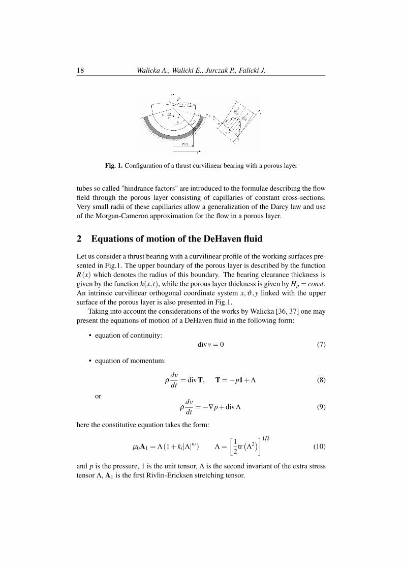
Fig. 1. Configuration of a thrust curvilinear bearing with a porous layer
tubes so called "hindrance factors" are introduced to the formulae describing the flowfield through the porous layer consisting of capillaries of constant cross-sections.Very small radii of these capillaries allow a generalization of the Darcy law and useof the Morgan-Cameron approximation for the flow in a porous layer.
2 Equations of motion of the DeHaven fluid
Let us consider a thrust bearing with a curvilinear profile of the working surfaces pre-sented in Fig.1. The upper boundary of the porous layer is described by the functionR(x) which denotes the radius of this boundary. The bearing clearance thickness isgiven by the function h(x, t), while the porous layer thickness is given by Hp = const.An intrinsic curvilinear orthogonal coordinate system x,ϑ ,y linked with the uppersurface of the porous layer is also presented in Fig.1.
Taking into account the considerations of the works by Walicka [36, 37] one maypresent the equations of motion of a DeHaven fluid in the following form:
• equation of continuity:divv = 0 (7)
• equation of momentum:
ρdvdt
= divT, T =−p1+Λ (8)
orρ
dvdt
=−∇p+divΛ (9)
here the constitutive equation takes the form:
µ0A1 = Λ(1+ ki|Λ|ni) Λ =
[12
tr(Λ2)]1/2
(10)
and p is the pressure, 1 is the unit tensor, Λ is the second invariant of the extra stresstensor Λ, A1 is the first Rivlin-Ericksen stretching tensor.

Effects of Hindrance Factors on a Squeeze Film ... 19
Let us consider a thrust curvilinear bearing with a porous layer connected with thelower bearing surface as it is shown in Fig.1. Taking into account the considerationsof the works (Walicka [37], Walicka et al. [39]), we may present Eqs (7)-(10) foraxial symmetry in the form:
1R
∂ (Rυx)
∂x+
∂υy
∂y= 0 (11)
∂ p∂x
=∂Λyx
∂y(12)
µ0∂υx
∂x= Λyx (1+ ki|Λyx|ni) (13)
The boundary conditions are as follows:
υx (x,0, t) = 0 υx (x,h, t) = 0 (14)
υy (x,0, t) =VH υy (x,h, t) =∂h∂ t
= h (15)
∂ p∂x
∣∣∣∣x=0
= 0, p(xo) = po (16)
After integration of Eqs (11) and (12) with respect to y, we will obtain the followingReynolds equation for the pressure distribution in a bearing clearance [37]:
1R
∂∂x
Rh3
[(−∂ p
∂x
)+
3kihni
2ni (ni +3)
(−∂ p
∂x
)ni+1]=−12µ0
(∂h∂ t−VH
)(17)
where VH denotes the velocity on the lower boundary between the fluid film and theporous layer.
3 Modified Reynolds equation for the flow in the porouspad
Frequently, to model the flow through the porous layer, rectilinear tubes of constantcross-sections are used (Fig.2). The flow velocity of the DeHaven fluid in a capillarytube is given as follows [37]:
υy =r2
c
8µ0
(−d p
dy
)+
kirni+2c
2ni µ0 (ni +4)
(−d p
dy
)ni+1
(18)
whereas the flow velocities through a thin layer - composed of system rectilinearcapillaries of constant cross-section - will be given by the following expressions:
υx =ϕpr2
c8µ0
(− ∂ p
∂x
)+
ϕpkirni+2c
2ni+1µ0(ni+4)
(− ∂ p
∂x
)ni+1
υy =ϕpr2
c8µ0
(− ∂ p
∂y
)+
ϕpkirni+2c
2ni+1µ0(ni+4)
(− ∂ p
∂y
)ni+1 (19)

20 Walicka A., Walicki E., Jurczak P., Falicki J.
Fig. 2. Geometry of a rectilinear capillary tube of a constant cross-section.
Fig. 3. The convergent-divergent and divergent-convergent capillaries with rectilinear gen-eratrices.

Effects of Hindrance Factors on a Squeeze Film ... 21
These results are similar to those obtained by utilizing the local VAT. Note that thereal porous media rarely consist of regular rectilinear pores; they consist of pores ofirregular forms which may be modelled as capillaries of variable cross-sections. Tomake the theoretical model more realistic Walicka et al. [22] proposed utilizing thecurvilinear (in general) capillary tubes of variable cross-sections, then the velocityfield for the flow through the porous layer is given by:
υx =ϕpr2
Mψn
8µ0
(−∂ p
∂x
)+
ϕpkirni+2M ψa
2ni+1µ0 (ni +4)
(−∂ p
∂x
)ni+1
(20)
υy =ϕpr2
Mψn
8µ0
(−∂ p
∂y
)+
ϕpkirni+2M ψa
2ni+1µ0 (ni +4)
(−∂ p
∂y
)ni+1
(21)
where ϕp is the porosity of the porous layer, ψn, ψa are respectively, the first, Newto-nian, and the second, additional, hindrance factor. Here index M indicates maximumvalues ri, ro which correspond to the capillary radius for the equivalent capillary ofconstant cross-section.
The forms and values of these factors may be found in [22] for different shapesof capillary tubes. For "conical" capillaries presented in Fig.3 these factors are asfollows:
ψn =[±3(ri−ro)]
r4M[±(r−3
o −r−3i )]
(22)
ψa =[±3(ri−ro)]
ni+1[±(r−3o −r−3
i )]
rni+4M
±(ni+1)[±(r−3
o −r−3i )]
1ni+1
(r− 3
ni+1o −r
− 3ni+1
i
)ni+1
Since the cross velocity component υy must be continuous at the porous wall-fluid film interface and must be equal to VH , we have then - by virtue of Eqs (20) and(21) - the following form of the modified Reynolds equation:
1R
∂∂x Rh3
[(− ∂ p
∂x
)+ 3kihni
2ni (ni+3)
(− ∂ p
∂x
)ni+1]= (23)
=−12µ0
∂h∂ t −
[ϕpr2
Mψn8µ0
(− ∂ p
∂y
)+
ϕpkirni+2M ψa
2ni+1µ0(ni+4)
(− ∂ p
∂y
)ni+1]∣∣∣∣
y=0
.
Using the Morgan-Cameron approximation, one obtains:(− ∂ p
∂y
)+
8kirniMψa
2ni+1(ni+4)ψn
(− ∂ p
∂y
)ni+1∣∣∣∣
y=0= (24)
=−HpR
∂∂x
R[(− ∂ p
∂x
)+
8kirniMψa
2ni+1(ni+4)ψn
(− ∂ p
∂x
)ni+1]
.

22 Walicka A., Walicki E., Jurczak P., Falicki J.
When formula (23) is inserted into Eq.27), the modified Reynolds equation takes theform:
1R
∂∂x R
[(h3 +12ψnΦnHp
)(− ∂ p
∂x
)+ 3ki
2ni (ni+3)× (25)
×(
hni+3 +16ψaΦnHprniM
(ni+3)(ni+4)
)(− ∂ p
∂x
)ni+1]=−12µ0
∂h∂ t
where
Φn =r2
Mϕp
8(26)
here Φn is the permeability of the porous layer.
4 Solution to the modified Reynolds equation
Consider the case of the DeHaven fluid of frequent occurrence for which the factorki|Λyx|ni < 1; the value of this factor indicates that the solutions to the Reynoldsequation (25) may be searched in the form of a sum:
p = p(0)+ p(1) (27)
Assuming thatp(1) p(0)
and substituting Eq.(27) into Eq.25) we arrive at two linearized equations, the firstone:
1R
∂∂x
R
[(h3 +12ψnΦnHp
)(−∂ p(0)
∂x
)]=−12µ0
∂h∂ t
(28)
and the other:
1R
∂∂x R
(h3 +12ψnΦnHp
)(− ∂ p(1)
∂x
)= (29)
=− 3ki2ni (ni+3)
1R
∂∂x
[R(
hni+3 +16ψaΦnHprniM
(ni+3)(ni+4)
)(− ∂ p(0)
∂x
)ni+1]
The boundary conditions for pressure are now:
∂ p(0)
∂x
∣∣∣∣∣x=0
= 0, p(0) (xo) = po,p(1)
∂x
∣∣∣∣∣x=0
= p(1) (xo) = 0 (30)
The solution of Eqs (28) and (29) is given as follows:
p(x, t) = po−12µ0
[F(ni)
o −F(ni) (x, t)]
(31)

Effects of Hindrance Factors on a Squeeze Film ... 23
Fig. 4. Squeeze film in a thrust radial bearing with a porous layer.
where
F(ni) (x, t) = I (x, t)+ 3ki6ni (µ0)ni
(ni+3) J (x, t) Fo = F (xo, t)
I (x, t) =∫ ∫
R ∂h∂ t dx
R(h3+12ψnΦnHp)dx (32)
J(n) (x, t) =∫[
hni+3+16ψaΦnHprniM(ni+3)(ni+4)
](−∫
R ∂h∂ t dx)
ni+1
Rni+1(h3+12ψnΦnHp)ni+2 dx
The load-carrying capacity is defined by
N = 2πxo∫
0
(p− po)Rcosϕdx (33)
the sense of angle ϕ arises from Fig.1.
5 Radial thrust bearing with a squeeze film
Let us consider a radial thrust bearing modelled by two parallel disks with a squeezefilm of the DeHaven lubricant. Introducing the following non-dimensional parame-ters:
x = xxo, R = R
Ro, h = h
ho= e(t) , e(t) = 1− ε (t) , ε = dε
dt
Kp =rMho, Hp =
ϕpHpho
, p = (p−po)µε
(hoxo
)2, N = Nh2
oµεx4
o,
λ (ni) = ki
(µεxo
ho
)ni
(34)
we will obtain the formulae for the dimensionless pressure distribution and load-carrying capacity for the porous bearing:
p =3
M(3)
[1− x2− 2 ·3ni+1λ (ni)
(ni +2)(ni +3)M(ni+3)
(M(3)
)ni+1
(1− xni+2)
](35)

24 Walicka A., Walicki E., Jurczak P., Falicki J.
N =3π
2M(3)
[1− 4 ·3ni+1λ (ni)
(ni +3)(ni +4)M(ni+3)
(M(3)
)ni+1
](36)
where
M(3) = h3 +32
ψnK2pHp, M(ni+3) = hni+3 +2
(ni +3ni +4
)ψaKni+2
p Hp (37)
note that the following relations hold for:
• ni = 1 (Peek-McLean fluid):
M(4) = h4 +85
ψaK3pHp
• ni = 2 (Rabinowitsch fluid):
M(5) = h5 +53
ψaK4pHp
• ni = 3 (DeHaven fluid):
M(6) = h6 +127
ψaK5pHp
To demonstrate clearly the effects of hindrance factors on a squeeze film of the porousbearing lubricated with the DeHaven fluid, let consider, for instance, the case of thediverging-converging capillary presented in Fig.2. We may assume that the inletradius of a capillary tube ri takes the maximum value (ri = rM) and ro is the mid-dle radius of a capillary tube. We calculated the values of the hindrance factors fordifferent values of ratio rM
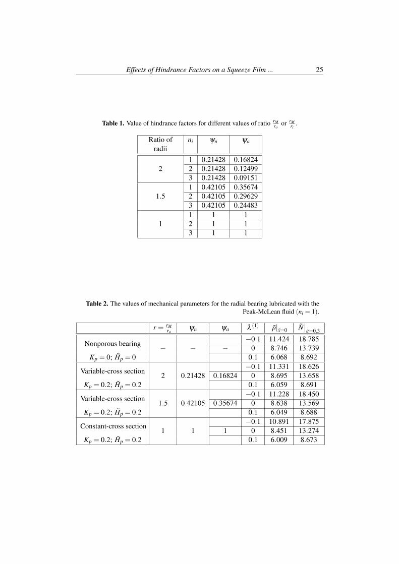
ro= 1, 1.5, 2 and for different values of the coefficient
ni = 1, 2, 3. For the values of the hindrance factors presented in Table 1 we willpresent the plots of the pressure distribution and load-carrying capacity for differentvalues of the coefficient λ (ni) (ni = 1, 2, 3).
Figures 5-7 present the dimensionless pressure distributions p and load-capacityfor a definite value of the squeezing ratio ε = 0.3.
The values of mechanical parameters for the radial porous squeeze film bearinglubricated with different fluids of DeHaven type were presented in Table 2-4. Thementioned values were obtained for the following values of the parameters: the pres-sure p for x = 0 and the load-carrying capacity N for ε = 0.3.
6 Conclusions
On the basis of the results obtained by Walicka [20] the modified Reynolds equationfor a curvilinear squeeze film porous bearing lubricated with a DeHaven fluid is de-rived. Using the Morgan-Cameron approximation to the Darcy flow of a viscoplastic
Effects of Hindrance Factors on a Squeeze Film ... 25
Table 1. Value of hindrance factors for different values of ratio rMro
or rMri
.
Ratio ofradii
ni ψn ψa
21 0.21428 0.168242 0.21428 0.124993 0.21428 0.09151
1.51 0.42105 0.356742 0.42105 0.296293 0.42105 0.24483
11 1 12 1 13 1 1
Table 2. The values of mechanical parameters for the radial bearing lubricated with thePeak-McLean fluid (ni = 1).
r = rMro
ψn ψa λ (1) p|x=0 N∣∣ε=0.3
Nonporous bearing − − −−0.1 11.424 18.785
0 8.746 13.739Kp = 0; Hp = 0 0.1 6.068 8.692
Variable-cross section2 0.21428 0.16824
−0.1 11.331 18.6260 8.695 13.658
Kp = 0.2; Hp = 0.2 0.1 6.059 8.691
Variable-cross section1.5 0.42105 0.35674
−0.1 11.228 18.4500 8.638 13.569
Kp = 0.2; Hp = 0.2 0.1 6.049 8.688
Constant-cross section1 1 1
−0.1 10.891 17.8750 8.451 13.274
Kp = 0.2; Hp = 0.2 0.1 6.009 8.673

26 Walicka A., Walicki E., Jurczak P., Falicki J.
Fig. 5. Dimensionless mechanical parameters for a radial bearing for different values ofλ (1) (Peak- McLean fluid):(a) pressure distribution; (b) load-carrying capacity.

Effects of Hindrance Factors on a Squeeze Film ... 27
Fig. 6. Dimensionless mechanical parameters for a radial bearing for different values ofλ (2) (Rabinowitsch fluid):(a) pressure distribution; (b) load-carrying capacity.

28 Walicka A., Walicki E., Jurczak P., Falicki J.
Table 3. The values of mechanical parameters for the radial bearing lubricated with theRabinowitsch fluid (ni = 2).
r = rMro
ψn ψa λ (2) p|x=0 N∣∣ε=0.3
Nonporous bearing − − −−0.01 9.730 15.798
0 8.746 13.738Kp = 0; Hp = 0 0.01 7.763 11.678
Variable-cross section2 0.21428 0.12499
−0.01 9.675 15.7040 8.708 13.678
Kp = 0.2; Hp = 0.2 0.01 7.741 11.653
Variable-cross section1.5 0.42105
0.29629 −0.01 9.601 15.5760 8.656 13.597
Kp = 0.2; Hp = 0.2 0.01 7.712 11.619
Constant-cross section1 1 1
−0.01 9.311 15.0750 8.451 13.274
Kp = 0.2; Hp = 0.2 0.01 7.591 11.473
Table 4. The values of mechanical parameters for the radial bearing lubricated with theDeHaven fluid (ni = 3).
r = rMro
ψn ψa λ (3) p|x=0 N∣∣ε=0.3
Nonporous bearing − − −−0.001 9.148 14.639
0 8.746 13.738Kp = 0; Hp = 0 0.001 8.345 12.837
Variable-cross section2 0.21428
0.09151 −0.001 9.113 14.5810 8.718 13.694
Kp = 0.2; Hp = 0.2 0.001 8.323 12.808
Variable-cross section1.5 0.42105 0.24483
−0.001 9.056 14.4850 8.672 13.622
Kp = 0.2; Hp = 0.2 0.001 8.287 12.758
Constant-cross section1 1 1
−0.001 8.789 14.0330 8.451 13.274
Kp = 0.2; Hp = 0.2 0.001 8.112 12.515

Effects of Hindrance Factors on a Squeeze Film ... 29
Fig. 7. Dimensionless mechanical parameters for a radial bearing for different values ofλ (3) (DeHaven fluid):(a) pressure distribution; (b) load-carrying capacity.
30 Walicka A., Walicki E., Jurczak P., Falicki J.
lubricant in a porous layer a new modification of the Reynolds equation is introduced.A detailed solution for squeeze film porous radial bearings is given. The formulaefor the dimensionless pressure distributions p and load-capacity were obtained; theirgraphic presentations are shown in Figs 5-7.
Plots are also drawn for different values of λ (ni) which indeed influence the pres-sure distribution and load-capacity. They are taken as successive terms of a powerseries: λ (1)
max = ±0.1, λ (2)max = ±0.01, λ (3)
max = ±0.001. These values ensure similarmaxima of the mechanical parameters of bearings for different fluids of DeHaventype (ni = 1 Peak-McLean fluid, ni = 2 Rabinowitsch fluid, ni = 3 DeHaven fluid)used for modelling of lubricant flows.
From the calculations, tables and plots we may conclude that a comparison withthe case of Newtonian lubricants
(λ (ni) = 0
)generally shows that the pseudo-plastic
effects(λ (ni) > 0
)decrease the values of mechanical parameters of bearings, but the
dilatant effects(λ (ni) < 0
)increase the values of mechanical parameters of bearings.
In this paper, two models of a porous layer were considered. The first one is asystem composed of capillary tubes of constant cross-section and the other is a sys-tem composed of capillary tubes of variable cross-section. Frequently, the real layeris replaced with matrix composed of rectilinear tubes of constant cross-section. Inpractice, the porous layers consist of capillaries of variable cross-section. Employingthe results of the papers [20-22] we replaced the real layer by the matrix composed ofrectilinear tubes of variable cross-section. The influence of the walls-porosity on themechanical parameters depends on the model of the porous layer. In this paper, twocases of the bearing wall porosity were considered, the matrix composed of: rectilin-ear tubes of constant cross-section (ψn = 1, ψa = 1) or rectilinear tubes of variablecross-section (ψn < 1, ψa < 1) .
Plots are drawn for different values of hindrance factors ψn and ψa which dependon the capillary shape and the value of the coefficient ni. The selected values of thehindrance factors are presented in Table 1. A comparison with the case of non-porouswall
(Hp = Kp = 0
)generally shows that the porosity effects
(Hp = Kp = 0.2
)de-
crease the values of mechanical parameters of bearings.From the results we may conclude that the pressure losses in the flow through the
thin porous layer composed of rectilinear tubes of variable cross-section(ψn < 1, ψa < 1) are smaller than in the flow through the thin porous layer com-posed of rectilinear tubes of constant cross-section (ψn = 1, ψa = 1).
The same conclusions are right for all models of lubricants under consideration.
References
Alazmi, B. and Vafai, K. (2002). Constant wall heat flux boundary conditions inporous media under local thermal non-equilibrium conditions. International Jour-nal of Heat and Mass Transfer, 45(15):3071–3087.

Effects of Hindrance Factors on a Squeeze Film ... 31
Amiri, A. and Vafai, K. (1998). Transient analysis of incompressible flow through apacked bed. International Journal of Heat and Mass Transfer, 41(24):4259–4279.
Bear, J. and Bachmat, Y. (1990). Introduction to modeling of transport phenomenain porous media. Springer Science & Business Media.
Greenkorn, R. A. (1983). Flow phenomena in porous media: fundamentals and ap-plications in petroleum, water and food production.
Hadim, H. and Vafai, K. (2000a). Overview of current computational studies of heattransfer in porous media and their applications—forced convection and multiphaseheat transfer. Advances in Numerical Heat Transfer, 2:291–329.
Hadim, H. and Vafai, K. (2000b). Overview of current computational studies of heattransfer in porous media and their applications—forced convection and multiphaseheat transfer. Advances in Numerical Heat Transfer, 2:291–329.
Hashimoto, H. and Wada, S. (1986). The effects of fluid inertia forces in parallelcircular squeeze film bearings lubricated with pseudo-plastic fluids. Journal oftribology, 108(2):282–287.
Jivkov, A. P., Hollis, C., Etiese, F., McDonald, S. A., and Withers, P. J. (2013). Anovel architecture for pore network modelling with applications to permeability ofporous media. Journal of Hydrology, 486:246–258.
Joekar Niasar, V., Hassanizadeh, S., Pyrak-Nolte, L., and Berentsen, C. (2009). Sim-ulating drainage and imbibition experiments in a high-porosity micromodel usingan unstructured pore network model. Water resources research, 45(2).
Khanafer, K., Bull, J. L., Pop, I., and Berguer, R. (2007). Influence of pulsatile bloodflow and heating scheme on the temperature distribution during hyperthermia treat-ment. International Journal of Heat and Mass Transfer, 50(23-24):4883–4890.
Kraemer, E. O. and Williamson, R. V. (1929). Internal friction and the structure of“solvated” colloids. Journal of Rheology (1929-1932), 1(1):76–92.
Lin, J.-R. (2012). Non-newtonian squeeze film characteristics between parallel an-nular disks: Rabinowitsch fluid model. Tribology international, 52:190–194.
Lin, J.-R., Chu, L.-M., Hung, C.-R., Lu, R., and Lin, M. (2013). Effects of non-newtonian rheology on curved circular squeeze film: Rabinowitsch fluid model. Z.Naturforsch, 68:291–299.
Mazaheri, A., Zerai, B., Ahmadi, G., Kadambi, J., Saylor, B., Oliver, M., Bromhal,G., and Smith, D. (2005). Computer simulation of flow through a lattice flow-cellmodel. Advances in water resources, 28(12):1267–1279.
32 Walicka A., Walicki E., Jurczak P., Falicki J.
Nield, D. A., Bejan, A., et al. (2006). Convection in porous media, volume 3.Springer.
Nsir, K. and Schäfer, G. (2010). A pore-throat model based on grain-size distributionto quantify gravity-dominated dnapl instabilities in a water-saturated homogeneousporous medium. Comptes Rendus Geoscience, 342(12):881–891.
Peng, X. and Wu, H. (2005). Pore-scale transport phenomena in porous media. InTransport Phenomena in Porous Media III, pages 366–398. Elsevier.
Rabinowitsch, B. (1929). Über die viskosität und elastizität von solen. Zeitschrift fürphysikalische Chemie, 145(1):1–26.
Rajalingam, C., Rao, B., and Prabhu, B. (1978). The effect of a non-newtonianlubricant on piston ring lubrication. Wear, 50(1):47–57.
Ratajczak, M., Walicka, A., Walicki, E., and Ratajczak, P. (2006a). Inertia effects inthe curvilinear thrust bearing lubricated by a pseudo-plastic fluid of rotem-shinnar.Zagadnienia Eksploatacji Maszyn, 41(2):159–170.
Ratajczak, M., Walicka, A., Walicki, E., and Ratajczak, P. (2006b). Reodynamics oflubricating curvilinear thrust bearings with ellis pseudo-plastic fluid. ZagadnieniaEksploatacji Maszyn, 41(2):147–158.
Rotem, Z. and Shinnar, R. (1961). Non-newtonian flow-between parallel boundariesin linear movement. Chemical Engineering Science, 15(1-2):130–143.
Sharma, S. C., Jain, S., and Sah, P. (2000). Effect of non-newtonian behaviour oflubricant and bearing flexibility on the performance of slot-entry journal bearing.Tribology International, 33(7):507–517.
Singh, U. P., Gupta, R. S., and Kapur, V. K. (2011). On the steady performanceof hydrostatic thrust bearing: Rabinowitsch fluid model. Tribology Transactions,54(5):723–729.
Swamy, S., Prabhu, B., and Rao, B. (1975). Stiffness and damping characteristicsof finite width journal bearings with a non-newtonian film and their application toinstability prediction. Wear, 32(3):379–390.
Vafai, K. (2000). Handbook of porous media 1-st ed. Crc Press.
Vafai, K. (2005). Handbook of porous media 2-st ed. Crc Press.
Vafai, K. (2015). Handbook of porous media 3-st ed. Crc Press.
Vafai, K. and Tien, C. (1982). Boundary and inertia effects on convective mass trans-fer in porous media. International Journal of Heat and Mass Transfer, 25(8):1183–1190.
Effects of Hindrance Factors on a Squeeze Film ... 33
Wada, S. and Hayashi, H. (1971). Hydrodynamic lubrication of journal bear-ings by pseudo-plastic lubricants: part 1, theoretical studies. Bulletin of JSME,14(69):268–278.
Walicka, A. (2002). Rotational flows of rheologically complex fluids in thin channels.Zielona Gora: University Press. Google Scholar.
Walicka, A. (2017). Rheology of fluids in Mechanical Engineering. OficynaWydawnicza Uniwersytetu Zielonogórskiego.
Walicka, A. (2018a). Flows of newtonian and power-law fluids in symmetrically cor-rugated cappilary fissures and tubes. International Journal of Applied Mechanicsand Engineering, 23(1):187–211.
Walicka, A. (2018b). Simulation of the flow through porous layers composed ofconverging-diverging capillary fissures or tubes. International Journal of AppliedMechanics and Engineering, 23(1):161–185.
Walicka, A., Falicki, J., and Jurczak, P. (2018). Flows of dehaven fluid in sym-metrically curved capillary fissures and tubes. International Journal of AppliedMechanics and Engineering, 23(2):521–550.
Walicka, A., Jurczak, P., and Falicki, J. (2017). Curvilinear squeeze film bearinglubricated with a dehaven fluid or with similar fluids. International Journal ofApplied Mechanics and Engineering, 22(3):697–715.
Walicka, A. and Walicki, E. (2010a). Performance of the curvilinear thrust bearinglubricated by a pseudo-plastic fluid of rotem-shinnar. International Journal ofApplied Mechanics and Engineering, 15(3):895–907.
Walicka, A. and Walicki, E. (2010b). Pressure drops in convergent flows of polymermelts. International Journal of Applied Mechanics and Engineering, 15(4):1273–1285.
Walicka, A., Walicki, E., and Ratajczak, M. (1999). Pressure distribution in a curvi-linear thrust bearing with pseudo-plastic lubricant. Applied Mechanics and Engi-neering, 4(spec.):81–88.
Xiong, Q., Baychev, T. G., and Jivkov, A. P. (2016). Review of pore network mod-elling of porous media: experimental characterisations, network constructions andapplications to reactive transport. Journal of contaminant hydrology, 192:101–117.


Machine Dynamics Research2018, Vol. 42, No 1, 35-43
Model of Motion of the Mobile Platform WithThree Wheel Drive
Anna Jaskot*and Bogdan Posiadała†
Czestochowa University of TechnologyInstitute of Mechanics and Machine Design Fundamentals
AbstractIn this paper the results of the analysis based on the kinematics and the dynamics modelsof the three-wheeled mobile robot, with two rear wheels and one front wheel have beenincluded. The prototype model has been developed by the author’s construction assumptionsto realize the motion of the platform in a various configurations of wheel drives. The platformdynamical model has been described considering the slippage conditions during the motionof the platform. The motion parameters of the mobile platform have been determined byadopting classical approach of mechanics. The formulated initial problem has been solvednumerically using the Runge-Kutta method of the fourth-order.
Keywords: mobile platform, kinematics, dynamics, friction, wheel motion.
1 Introduction
In scope of this work, the model of motion path of the three-wheeled mobile robotis analysed and presented. On the basis of the model contained in (Jaskot et al.,2017), the studies of motion have been performed. In the work (Lucet et al., 2015),the path tracking of the bicycle and the four-wheeled dynamical models have beenresearched and determined. The research on the four-wheeled mobile platform hasbeen performed by the authors and published among others in (Jaskot and Posiadała,2017). In this work the kinematics and dynamics of motion on the basis of the three-wheeled mobile platform have been formulated and the simulation results have beenincluded. Wheeled mobile platforms are being perceived as very extensively usedmachines, for a significant reason. Studies about trajectory tracking control motion,where forces and torques are the true inputs on the basis of the sliding mode controltechnique of a two driving wheels mounted on a bar have been described in (Ibrahim,

36 Jaskot A., Posiadała B.
Fig. 1. Model of the platform with three wheel drive.
2016). Motion trajectory tracking with models of kinematics and dynamics by adopt-ing the Langrange formulation has been included in (Ali et al., 2016). The dynamicand kinematic models of the three-wheeled differential drive mobile robots with twofixed and in-line with each other electric motors have been gathered in (Salem, 2013).
In this work the analysis of motion of a three wheeled mobile robot under un-steady conditions is presented. Relations between active and passive forces as wellas between the resultant forces and the motion parameters have been included andtheir impact on the motion trajectory has been graphically presented. The results ofthe analyses have been described and the conclusions have been formulated in thefourth chapter. The slippage during motion has been determined numerically andthe Runge-Kutta method of the fourth-order has been used for the solution to theproblem.
2 Model of the prototype
The research object presented in this work is the mobile platform with three wheeldrive. In this section the theoretical model of the prototype is presented. The schemeof the three-wheeled mobile platform, shown in Fig. 1, was the base in determiningthe dynamics description in global coordinate system OXY Z. The S point is the centerof mass of the platform. The local coordinate system Sxyz is denoted relative to the Spoint. The e1,e2,e3 are the unit vectors in the reference frame.
The description of both the kinematics and the dynamics of motion based ondesignations of forces in the system has been made. The details are gathered infurther sections of the work.
2.1 Kinematics model
In this section the kinematics of motion of the mobile platform with three wheel drivehas been described. The planar motion parameters have been determined with respectto the global reference frame with accordingly selected designations:
• a,b,c - distances between the wheels in longitudinal and the transverse sides

Model of Motion of the Mobile Platform ... 37
Fig. 2. Model of the platform in the reference frame.
of the platform (acc. to Fig. 2),
• β - inclination angle relative to the X axis of the reference frame,
• αi - inclination angles between the direction of motion and the x axes of thei-th wheel in local coordinate systems.
The following parameters have been determined. The angular velocity in generalform:
ωi =vi
ri(1)
where: vi - the linear velocity of the i-th wheel, ri - the radius of the i-th wheel. Thelinear velocity:
vi = ωE · γi (2)
where: ωE - the angular velocity of the instantaneous center of rotation, γi - thevector between point of the instantaneous center of rotation and the origins of thewheel coordinate systems.
Given the angular velocity of the platform, the angular velocities, the linear ve-locities, the angles of the remaining platform wheels can be determined.
2.2 Dynamics of motion
In order to obtain an accurate mathematical model of the mobile vehicles it is veryimportant to look into the dependencies between the road, wheels and the systemwith taking into account all forces applied upon the mobile platform system.

38 Jaskot A., Posiadała B.
Fig. 3. The i-th wheel forces in the local coordinate system.
Active and passive forces connected to wheels of the platform are presented inFig. 3.
The i, j,k are the unit vectors in local coordinate system. In the paper the descrip-tion of motion of the platform with two rear wheels and one front wheel has beenprovided.
Equation of active forces, which are consequent from the contact of the tire andthe ground, obtained from the drive torque, is given below.
Fci =Mni
ri· i (3)
where: ri - radius of the i-th drive wheel, Mni - the drive torque, which causes themotion.
The friction forces Twi and Tpi, which are the passive forces, need to be intro-duced in the model. Those passive forces during motion are taking the values fromzero to values obtained from the Eqs 4 and 5.
Twi =−µw ·Ni · sign(vwi) · i (4)
Tpi =−µp ·Ni · sign(vpi) · j (5)
where: µw,µp - the coefficients of friction in the longitudinal and transverse direction,vwi,vpi - the velocity components in the longitudinal and transverse direction. Ni - thereaction deriving from the wheel load on the ground.
Fci =
Mniri
f or Mniri
< Ti
Ti f or Mniri
> Ti(6)
In this paper the simulation results concern the motion case, when the value of thedeveloped friction forces has been exceeded by the value of active forces, and the
Model of Motion of the Mobile Platform ... 39
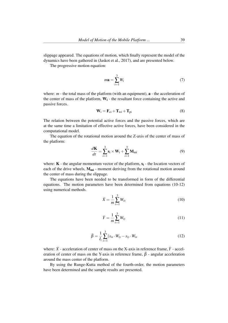
slippage appeared. The equations of motion, which finally represent the model of thedynamics have been gathered in (Jaskot et al., 2017), and are presented below.
The progressive motion equation:
ma =3
∑i=1
Wi (7)
where: m - the total mass of the platform (with an equipment), a - the acceleration ofthe center of mass of the platform, Wi - the resultant force containing the active andpassive forces.
Wi = Fci +Twi +Tpi (8)
The relation between the potential active forces and the passive forces, which areat the same time a limitation of effective active forces, have been considered in thecomputational model.
The equation of the rotational motion around the Z-axis of the center of mass ofthe platform:
dKdt
=3
∑i=1
si ×Wi +3
∑i=1
Mmi (9)
where: K - the angular momentum vector of the platform, si - the location vectors ofeach of the drive wheels, Mmi - moment deriving from the rotational motion aroundthe center of mass during the slippage.
The equations have been needed to be transformed in form of the differentialequations. The motion parameters have been determined from equations (10-12)using numerical methods.
X =1m
3
∑i=1
Wix (10)
Y =1m
3
∑i=1
Wiy (11)
β =1Iz
3
∑i=1
(six ·Wiy − siy ·Wix (12)
where: X - acceleration of center of mass on the X-axis in reference frame, Y - accel-eration of center of mass on the Y-axis in reference frame, β - angular accelerationaround the mass center of the platform.
By using the Runge-Kutta method of the fourth-order, the motion parametershave been determined and the sample results are presented.

40 Jaskot A., Posiadała B.
Fig. 4. Kinematic forcing of the i-th wheel of the platform.
Fig. 5. The sample trajectory of the mobile platform’s motion.
3 Sample simulation results
The results of the analyses have been considered in two cases. In this work the resultshave been obtained with respect to the following initial parameters (in both cases).Initial position of the center of the mass is denoted: x = 0,y = 0. Initial positionsof the wheels in coordinate space: O1: x1 = 0.45 m, y1 = 0 m; O2: x2 = −0.3 m,y2 = 0.3 m; O3: x3 = −0.3 m, y3 = −0.3 m. The angle β initially was equal 0.The gravitational acceleration g=9,81 m/s2. The total time of the analysis was equaltc = 20s. Mass of the platform: m = 100 kg. Radius of a drive wheel: r = 0.2m.
3.1 Kinematics of the mobile platform
To obtain the kinematics of motion, some initial inputs have been assumed. Thecalculations have been made as a response to the chosen kinematic forcings of thewheels’ motion and their positions. The chosen kinematic forcing is presented inFig. 4.
As a result, the path of the wheels’ motion has been obtained. In consequence theoutcomes are presented in Fig. 5.

Model of Motion of the Mobile Platform ... 41
Fig. 6. The drive torque representation.
Fig. 7. Dependence between moments from active and passive forces.
3.2 Dynamical motion of the mobile platform
The results have been obtained with the initial parameters: drive torque Mi = 17.5Nm for all drive units. Coefficients of friction in the longitudinal direction µw = 0.1and in the transverse direction µp = 0.05.
The drive torque course is presented in Fig. 6.In the Fig. 7, the representation of overcoming the value of developed friction is
presented.In this considered case of motion at its first four seconds every wheel of the
mobile platform drives on the same surface, represented in the same coefficients offriction.
After four seconds of motion, the left side wheels invaded the slippery surface,e.g. a frozen puddle, spilled oil or ride on a different pavement.
After four seconds of motion the coefficients of friction in the longitudinal di-rection µw = 0.02 for wheels no. 1 and 2, and µw = 0.1 - for no. 3; coefficients offriction in the transverse direction µp = 0.01 for wheels no. 1 and 2 and µw = 0.05 -

42 Jaskot A., Posiadała B.
Fig. 8. Motion parameters in the reference frame: a) X axis and b) Y axis coordinates.
for no. 3.The results of the analysis in form of the motion parameters are presented graph-
ically in Figures 8-9.Trajectory of motion of the center of mass of the platform, is presented in Fig.
10.The sample simulation results of motion under unsteady conditions have been
presented. The conclusions are gathered in the last section.
4 Conclusions
The proposed model is useful in investigations of different possible configurations ofwheels during the platform motion under the various possible initial motion condi-tions and drive torques.
Sample results of the performed analysis, in which the rates of the motion param-eters, among others: position, velocity and acceleration in planar translations, as wellas the angle, angular velocity and angular acceleration in rotations around the Z-axis,have been presented on the basis of the determined model.
The considered numerical example includes only the phenomenon of slippage of

Model of Motion of the Mobile Platform ... 43
Fig. 9. Angular parameters in motion around center of mass of the platform.
Fig. 10. Trajectory of motion of the center of mass of the platform.
the drive wheels. The case of slippage of the entire platform during its movementrequires the definition of the constraints in the calculation model, which will be thesubject of further work on the development of the computational model.
References
Ali, Z. A., Wang, D., Safwan, M., Jiang, W., and Shafiq, M. (2016). Trajectorytracking of a nonholonomic wheeleed mobile robot using hybrid controller. Inter-national Journal of Modeling and Optimization, 6(3):136.
Ibrahim, E. (2016). Wheeled mobile robot trajectory tracking using sliding modecontrol. J. Comput. Sci, 12(1):48–55.
Jaskot, A. and Posiadała, B. (2017). Dynamics model of the mobile platform forits various configurations. 4th International Conference Mechatronics: Ideas forIndustrial Applications, pages 13–15.
Jaskot, A., Posiadała, B., and Spiewak, S. (2017). Dynamics model of the mobileplatform for its various configurations. Procedia Engineering, 177:162–167.
Lucet, E., Lenain, R., and Grand, C. (2015). Dynamic path tracking control of avehicle on slippery terrain. Control Engineering Practice, 42:60–73.
Salem, F. A. (2013). Kinematics and dynamic models and control for differentialdrive mobile robots. Int. J. Current Eng. Technol, 3:253–263.


Machine Dynamics Research2018, Vol. 42, No 1, 45-53
Dynamic Model for Non-Symmetric Dual-PathGearbox
Józef Drewniak* and Krzysztof Reszuta†
University of Bielsko-BialaFaculty of Mechanical Engineering and Computer Science
AbstractThis paper presents a scheme of calculating the dynamic behavior of dual-path gearbox withnon-symmetric position of two pinions in regard to gear. The influence of mesh phase andtime-varying mesh stiffness of the two spur pinions and one gear was presented. Generalmodel with mathematical equations for dual-path gearbox were described. According to La-grange theorem, the dynamic differential equations were obtained. Based on these equationsresults of torsional oscillations, internal dynamic meshing forces were calculated as well asdynamic coefficient Kv. Conclusions were made.
Keywords: non-symmetric dual-path gearbox, gearbox dynamic, dynamic meshing forces.
1 Introduction
One of the most common mechanical devices used to transfer mechanical energy androtational movement are gearboxes. They are often used not only in industrial ma-chines and vehicles but also in aerospace and marine equipment, where transmittedenergy is very high and often exceeds several MW. Gears in such machines are heavyloaded components.
Although the simplest gear systems are those with just one gear engagement areabetween a pair of gears, alternatives are available for applications where it is nec-essary to transmit a very high torque in a very small space. One option to increasepower density is to use the split torque (multi path) systems that were mainly devel-oped for the aviation industry. These gear systems are based on a very simple idea:division of the transmission of force between several contact areas, thereby increas-ing the contact ratio εα . The greater the number of gears that engage the same pinion,the lower the torque exercised by each pinion.
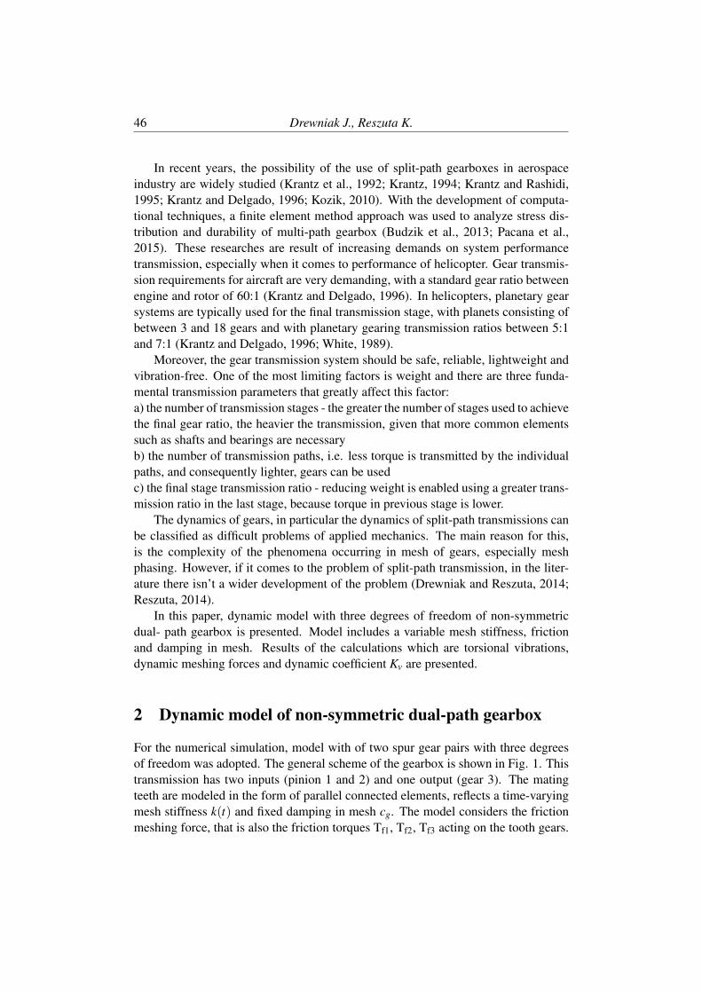
46 Drewniak J., Reszuta K.
In recent years, the possibility of the use of split-path gearboxes in aerospaceindustry are widely studied (Krantz et al., 1992; Krantz, 1994; Krantz and Rashidi,1995; Krantz and Delgado, 1996; Kozik, 2010). With the development of computa-tional techniques, a finite element method approach was used to analyze stress dis-tribution and durability of multi-path gearbox (Budzik et al., 2013; Pacana et al.,2015). These researches are result of increasing demands on system performancetransmission, especially when it comes to performance of helicopter. Gear transmis-sion requirements for aircraft are very demanding, with a standard gear ratio betweenengine and rotor of 60:1 (Krantz and Delgado, 1996). In helicopters, planetary gearsystems are typically used for the final transmission stage, with planets consisting ofbetween 3 and 18 gears and with planetary gearing transmission ratios between 5:1and 7:1 (Krantz and Delgado, 1996; White, 1989).
Moreover, the gear transmission system should be safe, reliable, lightweight andvibration-free. One of the most limiting factors is weight and there are three funda-mental transmission parameters that greatly affect this factor:a) the number of transmission stages - the greater the number of stages used to achievethe final gear ratio, the heavier the transmission, given that more common elementssuch as shafts and bearings are necessaryb) the number of transmission paths, i.e. less torque is transmitted by the individualpaths, and consequently lighter, gears can be usedc) the final stage transmission ratio - reducing weight is enabled using a greater trans-mission ratio in the last stage, because torque in previous stage is lower.
The dynamics of gears, in particular the dynamics of split-path transmissions canbe classified as difficult problems of applied mechanics. The main reason for this,is the complexity of the phenomena occurring in mesh of gears, especially meshphasing. However, if it comes to the problem of split-path transmission, in the liter-ature there isn’t a wider development of the problem (Drewniak and Reszuta, 2014;Reszuta, 2014).
In this paper, dynamic model with three degrees of freedom of non-symmetricdual- path gearbox is presented. Model includes a variable mesh stiffness, frictionand damping in mesh. Results of the calculations which are torsional vibrations,dynamic meshing forces and dynamic coefficient Kv are presented.
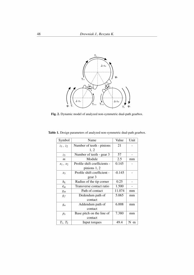
2 Dynamic model of non-symmetric dual-path gearbox
For the numerical simulation, model with of two spur gear pairs with three degreesof freedom was adopted. The general scheme of the gearbox is shown in Fig. 1. Thistransmission has two inputs (pinion 1 and 2) and one output (gear 3). The matingteeth are modeled in the form of parallel connected elements, reflects a time-varyingmesh stiffness k(t) and fixed damping in mesh cg. The model considers the frictionmeshing force, that is also the friction torques Tf1, Tf2, Tf3 acting on the tooth gears.

Dynamic Model for Non-Symmetric ... 47
Fig. 1. General scheme of analyzed non-symmetric dual-path gearbox.
in mesh torque. Gears are connected to rotating elements by weightless shafts withelastic-damping characteristic. In Figure 2 dynamic model of analyzed two-stagedual-path gearbox is presented. Parameters of analyzed non-symmetric dual-pathgearbox are summarized in Tables 1 and 2. Based on the finite element analysis forthe above model, maximum value of the stiffness was calculated. Cai equations (Caiand Hayashi, 1994; Cai, 1995) were used to determinate time varying stiffness forpair of gears. Figure 3 shows the positions of the pair of mating teeth of pinions 1, 2and gear 3:a) as they enter contact at point A’ (pinion 1 - gear 3),b) as they finish contact at point E ′′ at the same time (pinion 2 - gear 3).
This means that when one pair of teeth of gears 1-3 is just approaching contactat point A′, previous pair, already in single contact, is at the point D′. Similarlyin the case of gears 2-3, when a pair of teeth finish contact at point E ′′, followingpair of mating teeth is at point B′′. Exactly, the paths of contact A′E ′ and A′′E ′′
can be divided into segments A′B′,B′D′,D′E ′ and A′′B′′,B′′D′′,D′′E ′′, respectively,where: A′B′,D′E ′ and A′′B′′,D′′E ′′ are segments of double contact pairs, while B′D′
and B′′D′′ single contact pair. Figure 1 shows that between the pinions 1 and 2 thereis the mesh phase difference ∆ϕ1,2 = ϕ , where ϕ is the angle of pitch equal to theangle of meshing pitch ϕ = ϕe. This state of mesh phasing can be represented byan initial characteristic position as in Fig. 3. The resultant time-varying torsionalstiffness graph is shown in the Fig. 4.
48 Drewniak J., Reszuta K.
Fig. 2. Dynamic model of analyzed non-symmetric dual-path gearbox.
Table 1. Design parameters of analyzed non-symmetric dual-path gearbox.
Symbol Name Value Unitz1 , z2 Number of teeth - pinions
1, 221 -
z3 Number of teeth - gear 3 57 -m Module 2.5 mm
x1 , x2 Profile shift coefficients -pinions 1, 2
0.145 -
x3 Profile shift coefficient -gear 3
-0.145 -
hk Radius of the tip corner 0.25 -εα Transverse contact ratio 1.500 -gα Path of contact 11.074 mmg f Dedendum path of
contact5.065 mm
ga Addendum path ofcontact
6.008 mm
pe Base pitch on the line ofcontact
7.380 mm
T1, T2 Input torques 49.4 N ·m

Dynamic Model for Non-Symmetric ... 49
Table 2. Dynamic parameters of analyzed non-symmetric dual-path gearbox.
Symbol Name Value UnitSymbol Name Value UnitJ1 , J2 Moment of inertia -
pinions 1, 21.47·10−4 kg·m2
J3 Moment of inertia - gear3
7.81·10−3 kg·m2
rb1 , rb2 Base radius - pinions 1, 2 2.47·10−2 mrb3 Base radius - gear 3 6.70·10−2 m
r f1 , r f2 Radius of frictionalmoment - pinions 1, 2
7.47·10−3 m
r f3 Radius of frictionalmoment - gear 3
20.27·10−3 m
n1 , n2 Pinions rotational speed 1450 obr/mincg Damping in mesh 150 (N·s)/mµ Friction coefficient 0.1 -
Fig. 3. Characteristic positions of the mating teeth of the pinions 1, 2 and gear 3.
Fig. 4. Time varying torsional stiffness in the pinions 1, 2 with gear 3 meshes.

50 Drewniak J., Reszuta K.
Fig. 5. Torsional vibrations of pinions 1, 2 and gear 3.
3 Equation of dynamics for non-symmetric dual-path gear-box
Equations of motion of analyzed non-symmetric dual-path gearbox were derived us-ing Lagrange equations (Reszuta, 2014):
J1 · ϕ1 + kg1−3 (t) · (rb1 ·ϕ1− rb3 ·ϕ3) · rb1 + cg1−3 · (rb1 · ϕ1− rb3 · ϕ3) · rb1 == T1− r f1 ·
[kg1−3 (t) · (rb1 ·ϕ1− rb3 ·ϕ3)+ cg1−3 · (rb1 · ϕ1− rb3 · ϕ3)
]·µ1−3
(1)
J2 · ϕ2 + kg2−3 (t) · (rb2 ·ϕ2− rb3 ·ϕ3) · rb2 + cg2−3 · (rb2 · ϕ2− rb3 · ϕ3) · rb2 == T2− r f2 ·
[kg2−3 (t) · (rb2 ·ϕ2− rb3 ·ϕ3)+ cg2−3 · (rb2 · ϕ2− rb3 · ϕ3)
]·µ2−3
(2)
J3 · ϕ3 + kg1−3 (t) · (rb3 ·ϕ3− rb1 ·ϕ1) · rb3 + kg2−3 (t) · (rb3 ·ϕ3− rb2 ·ϕ2) · rb3++cg1−3 · (rb3 · ϕ3− rb1 · ϕ1) · rb3 + cg2−3 · (rb3 · ϕ3− rb2 · ϕ2) · rb3 =
=−T3− r f3 ·[kg1−3 (t) · (rb3 ·ϕ3− rb1 ·ϕ1)+ cg1−3 · (rb3 · ϕ3− rb1 · ϕ1)
]·µ1−3+
−r f3 ·[kg2−3 (t) · (rb3 ·ϕ3− rb2 ·ϕ2)+ cg2−3 · (rb3 · ϕ3− rb2 · ϕ2)
]·µ2−3
(3)
Above system of differential equations was solved using MATLAB software usingRunge-Kutta-Fehlberg method. The results of the torsional vibrations for analyzednon-symmetric dual-path gearbox are graphs of vibration, dynamic meshing forcesand dynamic factors Kv, which are presented in section 4.
4 Results of calculations
Figure 5 shows the chart of torsional vibrations of gears. Red color indicates vibrationof pinion 1, blue color indicates vibration of pinion 2, whereas green shows vibrationsof gear 3. A phase shifting of vibrations between pinions 1 and 2 can be seen. Thisshifting is due to the varying mesh stiffness shown in Fig. 4. For the data torsionaldisplacement φ (t) (graphs in Fig. 5) and torsional mesh stiffness kg1−3 (t) and kg2−3 (t)(graphs in Figure 4) dynamic forces in the meshing of the pinions 1, 2 and gear 3,Fc1−3 and Fc2−3 can be calculated from the formulas (4) and (5):
Fc1−3 = kg1−3 (t) · (rb1 ·ϕ1− rb3 ·ϕ3)+ cg1−3 · (rb1 · ϕ1− rb3 · ϕ3) (4)

Dynamic Model for Non-Symmetric ... 51
Fig. 6. Dynamic meshing force for pinions 1, 2 with gear 3 (full time).
Fig. 7. Dynamic meshing force for pinions 1, 2 with gear 3 (reduced period of time).
Fc2−3 = kg2−3 (t) · (rb2 ·ϕ2− rb3 ·ϕ3)+ cg2−3 · (rb2 · ϕ2− rb3 · ϕ3) (5)
Dynamic meshing force for mating pinions 1, 2 with gear 3 is shown in Figure 6.Figure 7 represents the same meshing force but for shorter period of time. Red colorindicates nominal meshing force (2131 N) resulting from static calculations of gears.Dynamic factor Kv are shown below in Fig. 8 and Fig. 9 (for reduced period of time).Red line indicates dynamic factor equal 1.0. Maximum dynamic force obtainedfor meshing of pinion 1 and gear 3 equals 2563 N during 1 pair gear meshing. Formeshing of pinion 2 and gear 3 maximum dynamic force occurs also in 1-pair gearmeshing and equals 2563 N.
Fig. 8. Dynamic factor Kv for pinions 1, 2 with gear 3 (full time).

52 Drewniak J., Reszuta K.
Fig. 9. Dynamic factor Kv for pinions 1, 2 with gear 3 (reduced period of time).
5 Conclusions
Paper shows the solutions for the dynamics of non-symmetric dual-path gearbox. Forthe given parameters of analyzed gears torsional vibrations, dynamic meshing forcesand the corresponding dynamic factors Kv are presented. The reason for generatingparametric vibrations of gears is periodically variable meshing stiffness. Torsionalvibrations obtained from system of Lagrange equations were basis for calculate dy-namic forces acting on the teeth between gears.
Model presented in this paper will allow for the optimal selection of spacingand angles between pinions and the related phase shift of gear teeth. This optimalconfiguration should take into account in addition to the dynamic factor which shouldbe as small as possible also almost equal force sharing between all pinions.
References
Budzik, G., Kozik, B., and Pacana, J. (2013). Defining influence of load conditionson distribution and value of stresses in dual-power-path gear wheels applying fem.Aircraft Engineering and Aerospace Technology, 85(6):453–459.
Cai, Y. (1995). Simulation on the rotational vibration of helical gears in considerationof the tooth separation phenomenon (a new stiffness function of helical involutetooth pair). Journal of Mechanical Design, 117(3):460–469.
Cai, Y. and Hayashi, T. (1994). The linear approximated equation of vibration ofa pair of spur gears (theory and experiment). Journal of Mechanical Design,116(2):558–564.
Drewniak, J. and Reszuta, K. (2014). Analiza wpływu wielodrogowosci na dynamikeprzekładni zebatej. Logistyka.
Kozik, B. (2010). An analysis of criterion for choosing constructional solutions foraeronautical multi-power path gear units. Journal of KONES, 18:169–175.

Dynamic Model for Non-Symmetric ... 53
Krantz, T. and Rashidi, M. (1995). Vibration analysis of a split path gearbox. InTechnical Memorandum 106875, NASA Lewis Research Center.
Krantz, T. L. (1994). Dynamics of a split torque helicopter transmission. Tech-nical report, NATIONAL AERONAUTICS AND SPACE ADMINISTRATIONCLEVELAND OH LEWIS RESEARCH . . . .
Krantz, T. L. and Delgado, I. R. (1996). Experimental study of split-path transmissionload sharing.
Krantz, T. L., Rashidi, M., and Kish, J. G. (1992). Split torque transmission loadsharing. Technical Memorandum 105884, NASA Lewis Research Center.
Pacana, J., Kozik, B., and Budzik, G. (2015). Strength analysis of gears in dual-pathgearing by means of fem. Diagnostyka, 16.
Reszuta, K. (2014). Analiza dynamiki przekładni zebatych dwudrogowych.Praca dyplomowa magisterska (w przygotowaniu). Akademia TechnicznoHumanistyczna-Bielsko–Biała, 20.
White, G. (1989). Split torque helicopter transmissions with widely separated en-gines. Proceedings of the Institution of Mechanical Engineers, Part G: Journal ofAerospace Engineering, 203(1):53–65.


Machine Dynamics Research2018, Vol. 42, No 1, 55-71
Evaluation of the Influence of Car Engine PowerSupply With Rapeseed Oil Esters on Emission
of Pollutants in Dynamic Conditions
Zdzisław Chłopek*1, Paulina Grzelak†2, and Dagna Zakrzewska‡3
1Warsaw University of Technology , Institute of Vehicles2Environment Protection Centre, Motor Transport Institute
3Automotive Industry Institute (PIMOT), Analytical Laboratory
AbstractThe paper presents the test results of pollutant emissions from the compression ignition en-gine in dynamic driving test conditions: the New European Driving Cycle type approval test(NEDC) and the Stop and Go special test for vehicle traffic congestion simulation and Auto-bahn test simulating traffic on motorways and expressways. The engine was fuelled with testfuels of different compositions of primary fuels: diesel fuel and RME fuel treated as dieselfuel. The dependence of the road emission of pollutants on the fuel content of RME in testfuels was presented. The sensitivity of the pollutant emissions to the RME fuel content in testfuels and the uniqueness of the sensitivity coefficient were investigated. It has been found thatthe RME fuel additive is conducive to the reduction of carbon monoxide, hydrocarbons and,especially, particulate matter road emissions and the increase of nitrogen oxides and carbondioxide road emissions. The strongest sensitivity of the pollutant emissions to the RME fuelcontent in the test fuel, as well as the uniqueness of the sensitivity coefficient, is in the trafficconditions of vehicles with high engine dynamics and low load, i.e. in the Stop and Go test.The most sensitive to RME fuel content in the test fuel is the particulate matter emission, theleast – carbon dioxide.
Keywords: pollutants emissions, combustion engines, rapeseed oil methyl esters, RME.
1 Introduction
This paper reviews the impact of engine power supply on RME (Rape Methyl Esters)for the emission of pollutants in dynamic conditions, with RME fuel being consideredas substitute fuel.

56 Chłopek Z., Grzelak P., Zakrzewska D.
Substitute fuels are unconventional fuels, which are the substitution of motorgasoline for spark-ignition engines or diesel fuel for compression-ignition engines(Chłopek and Zakrzewska, 2015; Szlachta, 2002).
The essence of substitute fuels in relation to classic petroleum fuels is that, it ispossible to use engines that are interchangeably fuelled with these fuels or conven-tional fuels, without additional engineered and regulated engine variations (Chłopekand Zakrzewska, 2015; Szlachta, 2002).
Fuel for piston internal combustion engines. As conventional fuels, fuels havebeen adopted, for which the internal combustion engines are standardized, i.e. for:
• spark-ignition engine – motor gasoline,
• combustion-ignition engine – diesel fuels.
In this article RME fuel is considered as a substitute for diesel fuel – this meansthat the test of the compression ignition engine was performed without its regulatorychanges.
Criteria for evaluating unconventional fuels considering the fulfillment of substi-tute fuels conditions are as follows (Chłopek and Zakrzewska, 2015):
• criteria based on the assessment of physicochemical properties due to the useof fuels to supply engines,
• criteria based on the assessment of phenomena occurring in internal combus-tion engines fuelled with rated fuels,
• criteria based on the assessment of the utility properties of internal combustionengines fuelled with considered fuels.
Criteria based on the assessment of physicochemical properties are characteristicsof fuels that determine the phenomena occurring in engines, e.g.:
• elementary composition, calorific value, stoichiometric constant,
• viscosity, density, surface tension,
• propensity to influence engine construction and operating materials,
• fuel stability due to its properties.
Criteria based on the evaluation of effect occurring in engines are properties ofeffect determining engine performance – above all:
• effect of fuel and air supply on engine,
• the effect of burning fuel in cylinders,
• tribological effect.

Evaluation of the Influence of Car Engine Power ... 57
Criteria based on the assessment of engine performance are:
• operational characteristics due to:
– energetic features,
– economic features,
– ecologic features.
• properties characterizing engine durability and reliability,
• engine maintenance requirements.
Energy features are characterized by the ability of the engine to perform usefulwork – these are primarily:
• effective power (engine torque and engine speed),
• the maximum speed of the car,
• acceleration time of the vehicle to the specified speed.
Economic features are characteristics of engine efficiency, primarily:
• general efficiency of the engine,
• fuel consumption by the car.
Ecological characteristics describe the characteristics of the impact on the environ-ment, primarily:
• emissions of substantial pollutants,
• noise emissions,
• biodegradability of the fuel.
It is of course a matter of discussion and – partly intuitively – treatment of un-conventional fuels as substitute fuels. From a formal point of view, the decision totreat unconventional fuel as a substitute requires the adoption of quantitative criteriain the form of zero-dimension characteristics and the ranges of their values. Thispaper is limited to the treatment of RME fuel as a substitute fuel for engine oil forthe practice of compression-ignition engines fuelled with various fuels and to knowl-edge derived from literature (Chłopek et al., 2005; Cháopek et al., 2006; Chłopek andZakrzewska, 2015; Chuepeng et al., 2007; Kowalewicz, 2006; Labeckas and Slavin-skas, 2006; Mancaruso and Vaglieco, 2012; Mayer et al., 2005; Namasivayam, 2011;Nwafor, 2004; Rounce, 2011; Ruan et al., 2009; Song et al., 2016; Stepien et al.,2011; Szlachta, 2002; Tuner, 2015; Yadav et al., 2013; Yoshida et al., 2008) as well

58 Chłopek Z., Grzelak P., Zakrzewska D.
Table 1. Basic physico-chemical properties of tested fuels.
FuelUnit ORLEN VERVA RME-S RME-W
Density kg/m3 832.5 880.0 880.0Calorific value MJ/kg 43 38 39Cetane number
Kinematicviscosity at
temperature 40 C
mm2/s 2.87 4.50 4.49
Elementarycomposition of
fuel:• carbon mass
content0.837 0.772 0.772
• hydrogen masscontent
0.149 0.120 0.120
• oxygen masscontent
0.014 0.108 0.108
• sulphur masscontent
ppm 7.5 3.0 3.0
Cold fuel filterlock temperature
C –28 –15 –20
Fuel ignitiontemperature
C 65 101 101
as the results of comparative studies of the combustion effect in compression-ignitiondiesel engine, fuelled with diesel oil and rapeseed oil esters with RME-W, and sum-mer package and RME-S winter additives package (Chłopek et al., 2016).
The table shows the basic physico-chemical properties of the fuels tested in thepublication (Chłopek et al., 2016).
RME fuel density is 6% higher than diesel density and calorific value is lessthan 10%, which means that the energy theoretically delivered to engine cylindersat volume dosing is less than 3.6% in the case of RME fuel. The RME fuels have agreater propensity for self-ignition – a cetane number greater by about 1.7. The muchhigher kinematic viscosity of RME fuels at 40C for diesel fuel – by almost 60% hasa significant effect on the engine start-up characteristics at low ambient temperatures.Significant differences are in temperature values of cold fuel filter blocking – biofuelproperties, especially the summer version of it, are much worse – RMR-S. RME fuelhas a significantly higher oxygen content – in this case, almost ten times larger thandiesel oil. The sulfur content of the tested fuels is trace. The ignition temperature

Evaluation of the Influence of Car Engine Power ... 59
of the RME fuel is over 30% higher than ignition temperature of diesel oil, which isprofitable, because of protection of engine fuel system.
The results of the study published in (Chłopek et al., 2016) show, that the differ-ences in assessed utility characteristics of diesel fuel and RME fuel are low, especiallyfor RME fuel with summer addition package. There were slight differences in usefulpower and torque in favor of diesel oil. For fuel oil and RME fuel with summer ad-dition package, the overall efficiency of the engine was similar. For RME fuels therewas a measurably lower unit emission of carbon monoxide and particulate matter –by about 30%. In the case of a unit emission of hydrocarbons and nitrogen oxides, therelative difference was about 10%, while for the RME summer fuel it was a reductionin unit emissions and for the winter fuel – an increase unit emissions.
The authors’ unpublished studies show, that also in the dynamics of heat emissionthere are no significant differences between diesel oil and RME fuel with summer ad-ditives, while the difference is in the case of winter version of RME. Comparison ofproperties of the engine fuelled with the tested fuels, like angle of self-ignition de-lay, maximal pressure and fluid temperature in the engine cylinder and the crankshaftangle of occurrence of these values, the share of heat generation in the kinetic com-bustion, diffusion combustion and afterburning phases, and the rate of heat emission(Merker et al., 2005; Rakowski et al., 2012).
The conclusion was that RME fuels, especially fuel with the summer additionpackage, could be considered as diesel fuel for research. The most significant differ-ences are in terms of operating properties due to differences in viscosity and temper-ature characteristics of RME fuels and diesel (Szlachta, 2002; Yadav et al., 2013),which may have significant effects on low temperature engine starting (Szlachta,2002).
This paper presents the study results on the ecological characteristics becauseof pollutants emission from compression ignition engine under dynamic driving testconditions. The vehicle was fed with test fuels of different compositions of primaryfuels: diesel fuel and RME fuel treated as diesel substitute fuel.
2 Comparative results of empirical research on pollutantemissions from vehicle engine fuelled with test fuels
As a research object for the test, a passenger car Citroën Berlingo was used, with aself-ignition PSA XUD9 diesel engine with a cubic capacity of 1868 cm3 and a ratedoutput of 51 kW, equipped with a power supply system with a manifold injectionpump.
The tests were repeated several times for start of cold and hot engine. The fol-lowing fuels and mixtures were used:
• ommercial diesel oil with a composition that complies with the PN EN 590standards,

60 Chłopek Z., Grzelak P., Zakrzewska D.
• rapeseed oil methyl esters – BIODIESEL F-FAME fuel, produced by RafineriaTrzebinia, complies with the PN-EN 14214 standards – symbol: RME fuel,
The tests were conducted for RME test fuels with volume combination with dieseloil: u = 0; 0.1; 0.2; 0.5 and 1.
The vehicle was tested on a chassis dynamometer at the Industrial AutomotiveInstitute in Warsaw. The test program included designation:
• the external speed characteristics of the engine under conditions of accelerationin the third gear,
• road emission of pollutants in tests1: NEDC, Stop and Go and Autobahn.
The selection of the test was dictated by the wish to test the emission of pollu-tants from the engine at significantly different working conditions determined by thevehicle’s motion conditions (Chłopek, 2010). The NEDC test is a homologation test,the Stop and Go test is used to simulate traffic in street congestion, and the Autobahntest – in traffic conditions on motorways and expressways.
The tests were performed under heated engine conditions to a stable tempera-ture. The research in each test was performed five times and the average value of themeasurement results was used for the analysis.
For the chassis dynamometer tests an equipment was used that meets the require-ments of the following documents: Directive 1999/96/EC of the European Parliamentand the Council of 13 December 1999, Regulation (EC) No 715/2007 of the Euro-pean Parliament and the Council of 20 June 2007, and Commission Regulation (EC)No 692/2008 of 18 July 2008. Pollutants emissions testing included the followingsubstances
• carbon monoxide – CO,
• hydrocarbons – HC,
• nitrogen oxides – NOx,
• particulate matter – PM,
• carbon dioxide – CO2.
Figure 1 shows the external torque speed characteristics of the engine fuelled withtest fuels in acceleration conditions on the third run (Chłopek et al., 2005; Cháopeket al., 2006). The effect of RME fuel additive on the reduction of engine torque isclearly visible.
Figures 2–6 present an example of the dependence of road pollutant emissionsin selected tests on RME fuel share in test fuel. The other test results confirm
1Worldwide emission standards, 2016/2017, Passenger cars and light duty vehicles, Innovation forthe real world, Delphi

Evaluation of the Influence of Car Engine Power ... 61
Fig. 1. The external torque speed characteristics of the engine fuelled with test fuels inacceleration conditions on the third run (Chłopek et al., 2005; Cháopek et al., 2006).
Fig. 2. The dependence of road emission of carbon monoxide in Stop and Go test on RMEfuel share in test fuel.
Fig. 3. The dependence of road emission of hydrocarbons in NEDC test on RME fuelshare in test fuel.

62 Chłopek Z., Grzelak P., Zakrzewska D.
Fig. 4. The dependence of road emission of nitrogen oxides in NEDC test on RME fuelshare in test fuel.
Fig. 5. The dependence of road emission of particulate matter in Autobahn test on RMEfuel share in test fuel.
Fig. 6. The dependence of road emission of carbon dioxide in NEDC test on RME fuelshare in test fuel.

Evaluation of the Influence of Car Engine Power ... 63
Fig. 7. Relation of relative carbon monoxide road emissions on volumetric RME contentin test fuel in the Stop and Go, NEDC and Autobahn tests.
the general conclusion, that the use of the RME fuel additive results in reductionof carbon monoxide, hydrocarbons and particulate matter road emissions and theincrease in road emissions of nitrogen oxides and carbon dioxide.
3 Analysis of effects of car engine supply by rapeseed oilesters on pollutant emissions
Analysis of effects of car engine supply with rapeseed oil esters on pollutant emis-sions concerned the sensitivity of the pollutant emissions to the RME fuel content inthe test fuel and the uniqueness of the sensitivity factor.
As a measure of the emission sensitivity of pollutants to the volume of RMEfuel in the test fuel, the value of the linear function coefficient approximating thedependence of the results of empirical studies on road emissions of the RME fuelcontent in fuel was accepted:
brx (u) = a+δ ·u (1)
with condition:brx (0) = 1 (2)
where: brx – relative road emission of pollution "x" in relation to the road emissionof pollution during diesel engine fuel supply, u – volumetric RME fuel content in testfuel, a – constant coefficient of linear function, δ – slope of the linear function.
Figures 7–11 illustrate the dependence of the relative road emissions of specificpollutants on the volumetric RME content in the test fuel in all road tests.
Figure 12 shows the road vehicle emission sensitivity factor of each pollutant onthe volumetric RME fuel content in the test fuel in all road tests.
Figures 13–15 show the dependence of the relative road emissions of all pollu-tants on the volumetric RME fuel content in the test fuel in the individual vehicle
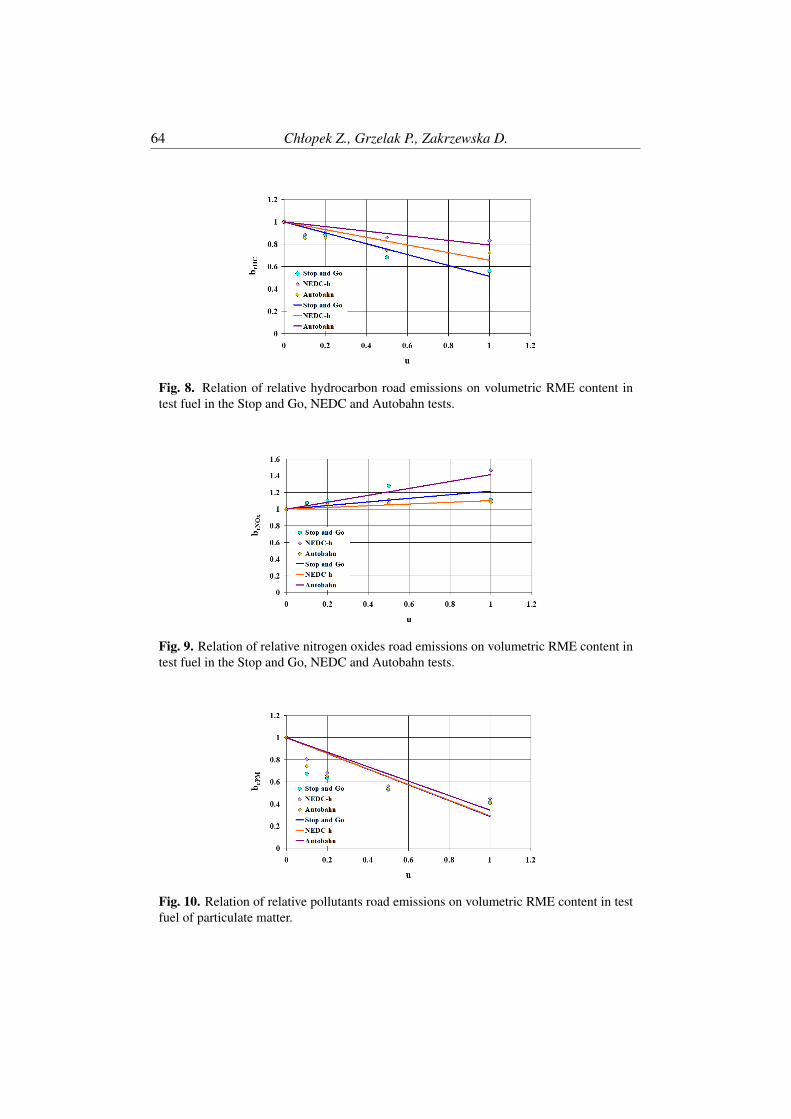
64 Chłopek Z., Grzelak P., Zakrzewska D.
Fig. 8. Relation of relative hydrocarbon road emissions on volumetric RME content intest fuel in the Stop and Go, NEDC and Autobahn tests.
Fig. 9. Relation of relative nitrogen oxides road emissions on volumetric RME content intest fuel in the Stop and Go, NEDC and Autobahn tests.
Fig. 10. Relation of relative pollutants road emissions on volumetric RME content in testfuel of particulate matter.

Evaluation of the Influence of Car Engine Power ... 65
Fig. 11. Relation of relative pollutants road emissions on volumetric RME content in testfuel of carbon dioxide.
Fig. 12. Road vehicle emission sensitivity factor of pollutants on the volumetric RME fuelcontent in the test fuel of carbon dioxide.

66 Chłopek Z., Grzelak P., Zakrzewska D.
Fig. 13. Dependence of the relative road emissions of pollutants on the volumetric RMEfuel content in the test fuel in the Stop and Go test.
Fig. 14. Dependence of the relative road emissions of pollutants on the volumetric RMEfuel content in the test fuel in NEDC test.
tests.Figure 16 shows the road vehicle emission sensitivity factor of each pollutant on
the volumetric RME fuel content in the test fuel in the individual vehicle tests.For carbon monoxide, hydrocarbons and particulate matter, the RME fuel addi-
tive results in road emissions reduction, with the strongest impact at the most unstabledriving speed, with the greatest share of engine dynamic states (Chłopek, 2010) – inthe Stop and Go test. The smallest absolute value of the pollutant emission sensi-tivity on the volumetric RME fuel content in the test fuel is in the Autobahn test,thus with the greatest stability of the driving speed and at the highest engine load.The sensitivity factor of the road emissions of nitrogen oxides and carbon dioxideis positive, which means that the RME fuel additive results in higher road emissionsof these substances, but the relative difference is considerably lower than for carbonmonoxide, hydrocarbons and particulate matter. The most sensitive to the RME fuelcontent in the test fuel is the particulate matter emission, the least – carbon dioxide.
The uniqueness factor of set y elements is defined as the ratio of the standard

Evaluation of the Influence of Car Engine Power ... 67
Fig. 15. Dependence of the relative road emissions of pollutants on the volumetric RMEfuel content in the test fuel in Autobahn test.
Fig. 16. Road vehicle emission sensitivity factor of pollutants on the volumetric RME fuelcontent in the test fuel in Autobahn test.

68 Chłopek Z., Grzelak P., Zakrzewska D.
Fig. 17. Coefficient of results uniqueness of sensitivity coefficient of the pollutants roademission on the volumetric RME fuel content in test fuel in each test: Stop and Go, NEDCand Autobahn.
deviation of the set y elements and the difference of mean values of the set y elementsand of the reference values for the set y elements4.
WNR [y] =D [y]
AV [y]−RV [y](3)
where: WNR[y] – uniqueness factor of set y elements, D[y] – standard deviation ofthe set y elements, AV [y] – mean value of the set y elements, RV [y] – reference valuefor the set y elements.
As a reference value for set y elements in tests, which is discussed in this publi-cation, is the minimum value of set y elements.
RV [y] = Min [y] (4)
where: Min[y] – minimum value operator of set y elements.Figure 17 shows the coefficient of results uniqueness of sensitivity coefficient of
the pollutant road emission on the volumetric RME fuel content in the test fuel in eachtest: Stop and Go, NEDC and Autobahn, and Fig. 18 – the coefficient of uniquenessof the sensitivity coefficient of pollutant road emission of specific pollutant on thevolumetric RME fuel content in test fuel in the Stop and Go, NEDC and Autobahntests.
The sensitivity coefficient of the pollutant road emissions on the RME fuel vol-umetric content in the test fuel is the most unique in the Stop and Go test, and theleast – in the Autobahn test. The strongest uniqueness is conducive to the operatingconditions of the internal combustion engine, characterized by a low load and a highshare of dynamic states, i.e. under conditions of high unsteady low speed driving(Chłopek, 2010).
Among the substances, the highest coefficient of uniqueness of the sensitivitycoefficient of road emission on the volumetric RME fuel content is for particulatematter, and the smallest – for carbon dioxide.

Evaluation of the Influence of Car Engine Power ... 69
Fig. 18. Uniqueness coefficient of sensitivity coefficient of the specific pollutants roademission on the volumetric RME fuel content in test fuel in each test: Stop and Go, NEDCand Autobahn.
4 Conclusion
As a result of the pollutant emission testing of a diesel engine fuelled with researchfuels with a different RME fuel contributions it is possible to formulate the followingconclusions:In all driving tests, the RME additive to the diesel fuel will reduce the emissions ofcarbon monoxide, hydrocarbons and – particularly – carbon monoxide.
Also, all the tests confirm the correctness of the increasing the road emissions ofnitrogen oxides and – to a lesser extent – carbon dioxide due to the increase in theshare of RME fuel in conventional fuels.
The smallest absolute value of the sensitivity factor of pollutant emission on thevolumetric RME fuel content in the test fuel is in the Autobahn test, the largest in theStop and Go test.
The most sensitive to the RME fuel content in the test fuel is the particulate matterroad emission, the least – carbon dioxide.
The highest uniqueness coefficient of the road vehicle emission sensitivity factoron the volumetric RME fuel content is in the Stop and Go test, the smallest – in theAutobahn test.
The strongest uniqueness of the road transport sensitivity coefficient to the volu-metric RME fuel content is for particulate matter, and the weakest for carbon dioxide.
Taking the RME fuel as a substitute fuel due to emission criteria brings somereflections on the biggest environmental problems of diesel engines such as the emis-sion of nitrogen oxides and particulate matter. The application of RME fuel for thesupply of compression-ignition engines reduces the emission of particulates, but alsoincreases the emission of nitrogen oxides. The strongest is the impact in conditionsof high unsteady speed of vehicles, so in the conditions of traffic in the cities.
70 Chłopek Z., Grzelak P., Zakrzewska D.
References
Cháopek, Z., Jarczewski, M., BardziEski, W., and Sar, H. (2006). Influence of fattyacid methyl esters’additive to diesel engine on ecology, fuel consumption and vehi-cle’s performance. Journal of KONES Powertrain and Transport, 13(1):261–268.
Chłopek, Z. (2010). Some remarks on engine testing in dynamic states. SilnikiSpalinowe, 49:60–71.
Chłopek, Z., Bardzinski, W., Jarczewski, M., and Sar, H. (2005). Emission of pollu-tion from engine powered by the fuel with additive of methyl ester of rape oil indynamic tests. Journal of KONES, 12(3-4):63–70.
Chłopek, Z., Jagiełło, S., Juwa, S., and Skrzek, T. (2016). Comparative examina-tion of performance characteristics of an ic engine fuelled with diesel oil and rapemethyl esters. Archiwum Motoryzacji, 74(4).
Chłopek, Z. and Zakrzewska, D. (2015). Kryteria oceny nosników energii jako paliwzastepczych do silników spalinowych. TTS Technika Transportu Szynowego, 22.
Chuepeng, S., Tsolakis, A., Theinnoi, K., Xu, H., Wyszynski, M., and Qiao, J.(2007). A study of quantitative impact on emissions of high proportion rme-basedbiodiesel blends. Technical report, SAE Technical Paper.
Kowalewicz, A. (2006). Eco-diesel engine fuelled with rapeseed oil methyl ester andethanol. part 3: combustion processes. Proceedings of the Institution of Mechani-cal Engineers, Part D: Journal of Automobile Engineering, 220(9):1283–1291.
Labeckas, G. and Slavinskas, S. (2006). The effect of rapeseed oil methyl ester on di-rect injection diesel engine performance and exhaust emissions. Energy conversionand Management, 47(13-14):1954–1967.
Mancaruso, E. and Vaglieco, B. M. (2012). Premixed combustion of gtl and rme fuelsin a single cylinder research engine. Applied Energy, 91(1):385–394.
Mayer, A., Czerwinski, J., Wyser, M., Mattrel, P., and Heitzer, A. (2005). Impactof rme/diesel blends on particle formation, particle filtration and pah emissions.Technical report, SAE Technical Paper.
Merker, G. P., Schwarz, C., Stiesch, G., and Otto, F. (2005). Simulating Combus-tion: Simulation of combustion and pollutant formation for engine-development.Springer Science & Business Media.
Namasivayam, A. M. (2011). Combustion, performance and emissions characteris-tics of compression-ignition engines fuelled by sustainable fuels. PhD thesis.

Evaluation of the Influence of Car Engine Power ... 71
Nwafor, O. (2004). Emission characteristics of diesel engine operating on rapeseedmethyl ester. Renewable Energy, 29(1):119–129.
Rakowski, S., Eckert, P., and Witt, A. (2012). Engine combustion. In CombustionEngines Development, pages 119–168. Springer.
Rounce, P. L. (2011). Engine performance and particulate matter speciation forcompression ignition engines powered by a range of fossil and biofuels. PhD thesis,University of Birmingham.
Ruan, D., Cheng, W., and Lee, C. (2009). Comparison of performance and com-bustion characteristics of diesel fuel and vegetable oils in di diesel engine. SAEInternational Journal of Fuels and Lubricants, 1(1):1049–1055.
Song, H., Quinton, K. S., Peng, Z., Zhao, H., and Ladommatos, N. (2016). Effects ofoxygen content of fuels on combustion and emissions of diesel engines. Energies,9(1):28.
Stepien, Z., Urzedowska, W., Oleksiak, S., and Czerwinski, J. (2011). Research onemissions and engine lube oil deterioration of diesel engines with biofuels (rme).SAE International Journal of Fuels and Lubricants, 4(1):125–138.
Szlachta, Z. (2002). Zasilanie silników wysokopreznych paliwami rzepakowymi.wkł. warszawa. Technical report, ISBN 83-206-1459-7.
Tuner, M. (2015). Combustion of alternative vehicle fuels in internal combustionengines. Report within Project.
Yadav, P. K., Singh, O., and Singh, R. (2013). Performance test of palm fatty acidbiodiesel on compression ignition engine. Journal of Petroleum Technology andAlternative Fuels, 1(1):1–9.
Yoshida, K., Taniguchi, S., Kitano, K., Tsukasaki, Y., Hasegawa, R., and Sakata, I.(2008). Effects of rme30 on exhaust emissions and combustion in a diesel engine.Technical report, SAE Technical Paper.


Machine Dynamics Research2018, Vol. 42, No 1, 73-85
How Not to Lose the Valuable Know-How inIndustry?
Olimpia Kunert*
Polish Air Force Academy
AbstractKnow-how belongs to the intangible assets of enterprises. They are defined as informationconsisting of verified in practice technical knowledge and skills in the goods trade (whichare not covered by patents) allowing the entrepreneur to achieve a competitive advantage.Intangible assets are currently the key resource of enterprises, within which innovative com-petences are included. They are not visible in the balance sheets of companies, they do notgrow in proportion to property investments and do not yield to ownership. They have a spa-tial dimension of a special character, they create the intellectual capital of the organization,which along with the acquired knowledge, using active growth factors, can gain the abilityto process innovations and act towards the development of the organization. However, thisis not always the case, hence the author’s attempt to answer the question of how not to losevaluable know-how in industry. The conducted surveys among enterprises providing servicesfor the industry have shown that they have innovative potential. This means that not onlyindustry and its development may affect the services sector and its performance, but also thereverse - the services sector may influence the demand of the industrial sector . The articlepresents the potential for innovation growth through the use of employees’ own knowledge.
Keywords: industrial enterprises, know-how, acquisition and loss of knowledge.
1 Introduction
Forecasts for the future indicate the decline of production in traditional form. Theincrease in the share of services provided to the industry is a determinant of changesin the industry. This process does not proceed in a uniform manner; some indus-trial functions, on the basis of outsourcing, are adopted from industrial enterprisesto the services sector or industrial related services remain in the industrial sector, asactivities provided by a service entity linked by capital or provided by employees.Such a limitation of strictly production activities and a statistically visible increasein services in the industrial sector, however, does not entail any increase in market

74 Kunert O.
competitiveness as if it were done in the case of services provided by external en-tities. There are benefits here, which lead to an improvement in the allocation ofresources and the possibility of achieving profit specialization and they result fromchanges in the value chains of industry and services (in industry reduction and in ser-vices growth of value chain), considered by industry, show economic benefits fromthe scale of outsourcing.
Globalization has created many conditions, including for industry products. Cur-rently, the industry requires much more services than several years ago and this trendis still growing. Global competition means, among other things, offering the bestproduct or service at the lowest price. As a result, what is constantly sought for waysto reduce costs that lead to business mergers or closures of companies, and merg-ers of companies result in the emergence of enterprises that seek to dominate on aglobal scale. All forms of mergers bring redundancies as well as changes in the labormarket.
A deeper analysis of the mutual relations between industry and services, whichgoes beyond the statistical data on employment and value added, makes it possibleto recognize whether from the point of view of industrial development, the industrysector is more important for the services sector or inversely. This type of extenededanalysis also shows the area of so-called "Related services", i.e. services for whichdemand increases appear as a result of increased demand from the side of the industry.There are intensified interactions in the area of "related services"; industry for thedevelopment of the services sector and the simultaneous impact of the services sectoron the productivity of the industrial sector. Moreover, we not only observe an increasein the demand for services related to the production industry, but mainly the growinginterdependence of industry with service companies. It means within the sectoralintegration of production and services, which in consequence results in the growth ofintersectoral links (industry and services) and the development of new organizationalforms in industry.
Linking services to the industry can be understood in two ways. The first methodcomes from the industry specified in the official statistics for which its services aredefined. In this case, the services also include related companies. However, the prob-lem is also the services provided to other service providers who are often industrialenterprises. It is difficult then to distinguish which services depend on the demandof manufacturing companies and which are not. The second problem is the criterionfor the division into services related to a specific industry and to industry sector, ingeneral. In this sense, an industrial enterprise that in part of its process is included inthe production process of another industrial enterprise provides a service around theindustry, but official statistics do not include this and both companies are included inthe industry.
The second way to understand industrial services is to perceive them as ser-vices provided by emerging industrial enterprises in connection with the supply ofindustrial products to other companies. This distinction concerns the development of

How Not to Lose the Valuable Know-How ... 75
cooperative services in industrial enterprises, which distinguish this difference as aproduct-service in their own reports as part of industrial added value.
The analysis of the process of building innovative competencies of enterpriseswith any types of market competences, which are often accompanied by the posses-sion of a specific innovation potential, was carried out using the MeRKI-U method(Ferenc and Kunert, 2013). The methodology refers to enterprises that can build theirinnovative competences from scratch, they can develop the already existing innova-tive potential, they can also assess the impact of innovation potential or competenceson the value of the company.
The method has been verified in the research project 4126 / B / H03 / 2011/40"Methodical basis for the dynamics of development of industrial services in Polandfor the purpose of merging the European Union market". The research subject wasbased on the analysis of technological connections between industry and service sec-tors in Poland, guaranteeing the development of industrial related services. For thepurposes of the integration of the industrial services market in the EU, it was nec-essary to recognize whether the innovative domestic industry provides the servicessector with new technologies and knowledge, mainly through the supply of interme-diate products and what kind of absorption capacity has the services sector in Poland.
The cooperators were identified in ten selected branches of industry in terms ofestablishing the dynamics of development of industrial services in Poland and thelinks between intermediate products and services and industry. The research con-cerned a representative sample of 100 classified enterprises into 10 selected indus-tries, i. e. mechanical, construction, textile, plastics, chemical, power energy andelectricity, cross-industry services, machinery, food, and paper and printing indus-tries. The survey was conducted in Poland, in the form of direct interviews usinga questionnaire. These were mainly individual interviews with the representants ofmanagement boards and extended interviews with the owners or co-owners of thesurveyed enterprises and were held at the headquarters of the surveyed companies.
The surveyed enterprises varied in size (small, medium, large), ownership re-lations (private, state treasury), capital origin (Polish, foreign and mixed capital),industry and voivodships. The sector of small and medium enterprises was the dom-inant environment among the surveyed enterprises. Large companies constituted aminority.
Small enterprises were dominated by services provided for one industry (53%).Medium and large companies usually provided services for two or three different in-dustries. Services related to the manufacturing process prevailed, product related ser-vices came second, the lowest percentage concerned service industry. The structureshown is a reflection of the current needs of Polish industry, which in the context ofownership changes resulting from privatization, are characteristic of countries aftersystemic transformation. The market of machine and equipment maintenance ser-vices has been limited due to the introduction of internal servicing within corporateorganizations. Other companies that have modernized the machine park also make

76 Kunert O.
Fig. 1. The impact of the services provided on the ordering process or productive effect.Source: own study.
Fig. 2. Has the modernized product been introduced to the market in the last three years?Source: own study.
use of maintenance service provided by suppliers, obligatory during the warranty pe-riod and for the most part also in the further period of operation. Enterprises largelylost their machines and devices of the older generation replacing them with mod-ern machines and thus the market of maintenance services changed. Meintenanceservices market is dynamic in relation to domestic suppliers; it mostly concerns ITservices, (electric motors, etc.). The majority of surveyed enterprises (over 90%) areengaged in pro-innovation activities, both products and processes.
This paper in its theoretical part is addressed to the circle of scholars studyingand describing the phenomena of knowledge management. In the practical (research)part, it is addressed to specialists and managers professionaly involved in the man-agement of corporations and enterprises, who often face the problem of assessing thevalue of innovative enterprises in the perspective of increasing the company’s value.

How Not to Lose the Valuable Know-How ... 77
2 Services development on a global scale
In the direct way, industrial related services are part of the industrial added valueand they can concern the production process or the product itself. Services are un-derstood as cooperation in the process of making subassemblies, parts, elements andcomponents or providing production services in the scope of processing or refiningof the products ordered by contracting entities as part of the logistics supply chain.These are often manufacturers executing orders from other manufacturers (as an in-termediate product) and contractual relationships between them. Indirect productionmay be associated with the product - e.g. packaging, conditioning, completing, etc.or with the production process - components included in another product ordered byits manufacturer, with specific technical and operating parameters, molds, specialisttools etc. made from own or entrusted materials or services on entrusted materials.
The needs of services on a global scale have meant that their character has changed.The need for global communication, transport, planning needs, market information,etc. is different today. This change made it almost impossible to sell industriallyproduced devices or products without additional services. Customers’ expectationsalso concern ’pre-sales’ and’ after-sales’ services.
The number of industrial products is increasing, in which services cease to per-form auxiliary functions and start to play a major role and thus contribute to thecompany’s profit. This is the case when the use of the product depends on the offerof services (service, software, facilities, etc.). In some cases, the share of industrialservices in the value added chain of producers exceeds even 50%. In many transac-tions of investment property, lessors, mainatenance service companies and companiesoffering software are taking part simultaneously. Without their participation, the saleof some products would be significantly hampered or even impossible. This stronghybrid combination of goods with the existence of services has created the conceptof a "bundled product" - prearranged combination of given product with other ser-vices and offered at an inclusive price. In such cases, the definitions of industrialproduction and services are blurred. An example could be the production of televi-sion sets, which would be impossible to sell without access to television programs ascomplementary services.
Industrial related services can be classified differently, but two groups are visi-ble from the point of view of a close relationship with an industrial product. The firstgroup of services is to launch the product and enable it to be used. These are typicallytechnical services related to documentation, assembly, installation, maintenance, re-pairs, training. The second group of industrial services includes the offer of servicesthat increase the value of an industrial product for the buyer, for example financing,insurance, service packages, etc. In this kind of service-related products, the inter-action between producers and customers is usually higher than in the first group ofproducts related to services. At the same time, the flow of information from buyersto suppliers of this type of services is particularly high, as financial service providers
78 Kunert O.
and insurers have access to the specific field of the client’s business. In this way, ifnecessary, you can get data for managing customer relationships and cross-selling ofother goods or services that are offered by industrial enterprises.
More sophisticated buyers can be attracted and maintained only by offering themnewer and more innovative products and services. It also requires focusing on the de-velopment of services that are tailored to individual customer segments. In this con-text, it is very important to exchange information with clients. This means that in thecase of new insights and changing customer needs, industrial enterprises with highproduction flexibility can react quickly to the product. Therefore, it is not surprisingthat the increasingly widespread use of information and communication technologiesin recent years has given a significant boost to the development of products related toservices.
Foreign direct investments on the internal market are dominated by services.Given the fact that services have also dominated the european economy, the potentialbenefits of merging the services market can be enormous. This explains the impor-tance of the Services Directive1, which shows the full potential of the EU servicessector. This potential, however, is not fully used. The problem is that despite the pos-sibility of increasing foreign investment in services by 20-35%, the services marketis not fully regulated by law. National law can work in favor of domestic companiesand at the same time discriminating foreign companies. The lack of competition inthe financial services sector leads to the conclusion of unfavorable contracts by cus-tomers: (high prices, less availability of credit). It is estimated that existing barriersto foreign companies in the financial sector caused an increase in prices by an av-erage of 5.3% by 2005. The elimination of such barriers would increase wages andsalaries throughout the EU by 0.4% on average and increase employment by 0.3%.In addition, with a merged market, there is the potential for an increase in Europeantrade by 15-30%.
Foreign investments within the EU-15 are focused on the services sector. In gen-eral, the share of foreign investment in services is three times higher than in produc-tion; (in 2002, the share of services was eight times greater). European companiesput services over production also in other regions of the world, but significantly lessthan in Europe.
German research on the determinants of the expansion of services related to theindustry has shown great determinants in the development of industry and indus-trial services2. Germany has a competitive advantage mainly in the production ofhigh-tech equipment, but the high export rate also applies to pharmaceutical firms,chemical companies, machinery industry and transport. In comparison with the restof the production, they show a high level of growth in demand for services. This sub-
1www.urtip.gov.pl/uke/index.jsp2Executive summary of the Project 22/02 Brema Dec. 2003, http://www.bmwi.de/B
MWi/Redaktion /PDF/C-D/die-bedeutung-einer-wettbewerbsfaehigen-industrie-fuer-die-entwicklung-des-dienstleistungssektors-engl,property=pdf,bereich=bmwi,sprache=de,rwb=true.pdf
How Not to Lose the Valuable Know-How ... 79
sector represents a demand factor of exceptional importance and shows the highestexpenditure on development and innovation.
3 Innovation of the industrial related services sector
The challenge for the scientific world in Poland is to develop a knowledge-basedeconomy faster than other countries do. The partners in this matter are enterprises thatneed to invest in innovation to participate more in international markets. According toIFW3, the decisive factors for successful management results are innovations and theprocess of disseminating it. Innovation is the ability to develop and implement newsolutions, both technological and organizational, which affects the competitivenessof enterprises and other organizations.
In an innovative process consisting of many stages, the most important issue isthe organization’s ability to transform innovation for its own use. This ability iscalled innovative competence. Intangible assets are currently the key resource of theorganization, within which innovative competences are included.
The most significant are changes in the way the information is used and howmuch the perception of its value evolved lately. Novadays, the information has be-come a source of wealth and career. These changes can be observed in the wholeeconomy. Even those entrepreneurs who operate on the market in a traditional wayare using the electronic devices and way of obtaining information and communi-cating with the environment and employees. This means that intangible resourcesbecome the source of economic value, and not material - as it used to be. Affluenceis determined by knowledge, inventions and intellectual property.
We have entered the era of information with all its consequences; in terms ofthe methods of obtaining information, its processing speed and its value for creatingprofit. If we are talking about an enterprise today, we are aware of its smooth organi-zational structure and multidimensional network of informal relationships based onintellectual values of employees. Qualifications, know-how and specialist knowledgeof co-workers have an increasing impact on the strategic success of the company. Atthe same time, faster technological development means that the distance to once ac-quired knowledge is still decreasing, hence investing in the most important factor ofsuccess: company’s know-how.
The organization of the virtual environment and tools is not hierarchical, it doesnot have structural characteristics in the traditional sense, but it ensures the relativestability of the organization of this virtual background. This is due to the "IT core",which is distributed horizontally in the form of a network (Fig.3.) and what can behope, is thus a strong structure that can carry significant loads.
The electronic economy based on IT features means that it is possible to achievehuge economic effects in the new conditions of communication and cooperation, but
3Institut für Wirtschaftsforschung – München

80 Kunert O.
Fig. 3. The external environment of the enterprise, taking into account the virtual environ-ment. Source: own study.
at the same time changes can be observed in the old ways of doing business. Themarket of an IT-based economy on is not divided, you can make transactions of ma-terial, financial and intellectual property. Today’s local entrepreneur who will existin virtual reality has access to the global market.
Tracking the achievements of Scania, which has increased the number of alliancesin five years with a virtual crew scattered around the world, it has been demonstratedthat human capital is decisive in the knowledge age and that intellectual capital iscrucial to the long-term success of the organization.
Intangible resources include assets and competencies(Penc, 2007):
• The assets are determined by such elements as: patents, trademarks, brandnames, copyrights, databases, contracts concluded, commercial contracts andcompany’s reputation,
• Competences are determined by: knowledge and skills of staff and employees,ability to learn and implement changes, and organizational culture.
Competence Management (Fig. 4) is an organized, methodical activity conducted bythe organization which is performing the following functions:
• determining the competencies necessary for individual positions;
• determining the employees’ individual competences;
• determining the possibilities, interests and preferences of managers and em-ployees in terms of development of their competences;
• determining missing competences in relation to job requirements;
• undertaking a set of activities in order to completing missing competences;

How Not to Lose the Valuable Know-How ... 81
Fig. 4. Place of the Competence Management System of an enterprise management sys-tem. Source: own study.
• substantive and psychological preparation of managers and employees to func-tion in the changing conditions in order to meet the company’s developmentneeds.
4 Silent knowledge of employees
Research has shown that apart from knowledge undergoing management processes,there is also a significant area of "hidden" knowledge, which remains largely un-used by the enterprise. This is the employees’ own knowledge (Fig.5.), which undercertain conditions can be obtained or lost by the company.
The management, manufacturing and information processing system were ana-lyzed. In the process of each of the mentioned above systems there were two types ofexisting knowledge i.e. employee’s own knowledge and documented knowledge aswell as knowledge kept by the employee who doesn’t share his knowledge or skillswith his employer. Extended studies of this last type of knowledge allowed to esti-mate the balance of loss and acquisition of employee’s own knowledge (Fig.5.).
This part of employees’ specific knowledge was analyzed in these three systemsmentioned above and in two other significant areas on which the company’s man-agement system has significant impact, namely during recruitment of employees andin the area of acquiring knowledge from the external environment. The results ofthis analysis are presented in Table 1, where the process of acquire employees’ ownknowledge is clearly visible through various management methods such as: compli-ance of competences with the position, employee activation strategy, designated fieldsof activity, management decentralization, motivation system, open innovation, com-
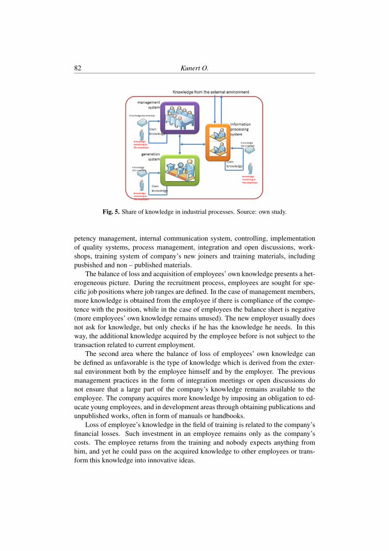
82 Kunert O.
Fig. 5. Share of knowledge in industrial processes. Source: own study.
petency management, internal communication system, controlling, implementationof quality systems, process management, integration and open discussions, work-shops, training system of company’s new joiners and training materials, includingpusbished and non – published materials.
The balance of loss and acquisition of employees’ own knowledge presents a het-erogeneous picture. During the recruitment process, employees are sought for spe-cific job positions where job ranges are defined. In the case of management members,more knowledge is obtained from the employee if there is compliance of the compe-tence with the position, while in the case of employees the balance sheet is negative(more employees’ own knowledge remains unused). The new employer usually doesnot ask for knowledge, but only checks if he has the knowledge he needs. In thisway, the additional knowledge acquired by the employee before is not subject to thetransaction related to current employment.
The second area where the balance of loss of employees’ own knowledge canbe defined as unfavorable is the type of knowledge which is derived from the exter-nal environment both by the employee himself and by the employer. The previousmanagement practices in the form of integration meetings or open discussions donot ensure that a large part of the company’s knowledge remains available to theemployee. The company acquires more knowledge by imposing an obligation to ed-ucate young employees, and in development areas through obtaining publications andunpublished works, often in form of manuals or handbooks.
Loss of employee’s knowledge in the field of training is related to the company’sfinancial losses. Such investment in an employee remains only as the company’scosts. The employee returns from the training and nobody expects anything fromhim, and yet he could pass on the acquired knowledge to other employees or trans-form this knowledge into innovative ideas.

How Not to Lose the Valuable Know-How ... 83
Table 1. Balance of loss and acquisition of the employee‘s knowledge.
The employee’s knowledge also results from his personal contacts, self-educationor information gathered directly from the environment. In this case, the loss and ac-quisition balance is also negative. Research has shown that only a few employees, ina well-managed company, could notice the use of the so-called "advance knowledge"for the needs of the enterprise.
5 Conclusion
The challenge of modern industrial management is to acquire intellectual resourcesand creative staff that increase the value of the company in a non-investment manner.As a result of the growing link between industry and services in many aspects, unilat-eral promotion of the services sector is not a suitable strategy to stimulate collectivegrowth and employment. The results of the research illustrate the fact that these ser-vices, which show an above-average growth (services connected with enterprises),directly depend on the production demand and the employees’ competencies. Tech-nological innovation consists of the introduction of new production methods, newways of implementing services and the adoption of new organizational order in thedomain of production processes or services.
The mutual relations of industrial enterprises and service providers also play asignificant role. Between them there is not only the exchange of goods and services,

84 Kunert O.
but also the transfer of knowledge. It can be assumed that in sectors of the economyin which there is intensive cooperation between producers and service providers, amuch greater amount of new knowledge is generated than in the other ones. However,everywhere we encounter a significant amount of unused employees’ own knowledgethat is not shared with co-workers or employer. The greatest loss of employees’ ownknowledge concerns knowledge gained from the environment in the form of training,self-education, acquiring information, gaining experience and obtained as a result ofprofessional contacts.
Technology transferred through training and transfer of know-how is measured bythe costs of resources used to carry them out. Payments for technology are providedin the form of royalties (eg. for copyrights) and license fees, they show a systematicincrease since the eighties and intra-firm trade between parent enterprises and theirforeign subsidiaries shows constant development.
Enterprises use many solutions that support knowledge management by partici-pating in management operational systems, such as: employee competence manage-ment, employee activation strategies, computerization, quality systems and motiva-tion systems. The innovation rate defines the share in the surveyed population ofindustrial enterprises that introduced technical innovations over a 3-year period.
However, research has shown that the balance of loss and acquisition of employ-ees’ own knowledge is still negative, which means that current management practicesare not sufficient, there is no focus on the so-called "advance knowledge", which islocated in the intellectual capital of employees. It is only the management of in-tellectual capital that creates the conditions for greater acquisition of this type ofknowledge.
References
Ferenc, R. and Kunert, O. (2011). Innovative strategy construction for a capital goodsproducer. Monographs of the Lodz University of Technology, Łódz.
Ferenc, R. and Kunert, O. (2013). Merki-u: a method for research and developmentin the industry. Foundation for Competence Promotion Lodz.
Grudzewski, W, M., Hejduk, I, K., and Sankowska, A.and Wantuchowicz, M. (2007).Managing trust in virtual organizations. Difin, Warszawa.
Kisielnicki, J. (2006). Virtual means intelligent. Management of the 21st Century,Infor special editions.
Kunert, O. (2011). Competencies of the polish manager. Competencies as a con-stituent of the success of a modern company, published by Foundation for Compe-tence Promoti.

How Not to Lose the Valuable Know-How ... 85
Kunert, O. (2016). The role of logistics in creating company value. ZeszytyNaukowe/Wyzsza Szkoła Oficerska Sił Powietrznych.
Penc, J. (2007). Innovative management controlling changes in the european integra-tion process. WSSM Łódz.
Serenko, A. and Bontis, N. (2004). Meta-review of knowledge management andintellectual capital literature: Citation impact and research productivity rankings.Knowledge and process management, 11(3):185–198.
Stachowicz, J. (2007). Social networks in the processes of social/entrepreneurialcapital building as the determinant of development of contemporary regions. Clus-ters & Regional Development Workshop, IDEGA-USC, Santiago de Compostella,Spain.


Machine Dynamics Research2018, Vol. 42, No 1, 87-99
The Boltzmann-Hamel Formalism in Modelling ofRail Vehicle Motion
Andrzej Chudzikiewicz*and Magdalena SowinskaWarsaw University of Technology
Faculty of Transport
1 Introduction
The most developed light rail transit networks are located primarily in Europe, butareas such as Africa or South America are also to consider Light Rail Vehicles asuitable solution, which is complementing the bus rapid transit lines. In Europe andAsia, in times of growing large agglomerations and long distances that their residentshave to travel in their day-to-day activities, the light rail vehicle network seems tobe the most convenient solution for increasing mobility. Separated from the trafficand simultaneously not insulated as a metro, it is easy to reach by a traveller. Itsconstruction is a much less complex project comparing to the metro. However, thekey to its success is ensuring the least invasiveness in the city’s structure, which atthe same time requires the design and development of modern rail vehicles.
Currently, the development of rail transport blurred the boundaries between thedifferent types of public transport and their classification is unclear. In urban ag-glomerations, the light rail vehicles partially cover the same functions with trams ormetro.
Sometimes light rail vehicles are getting similar to the rapid transit ("rapid tran-sit") and some of these systems are also called light metro.
Other light rail vehicles are similar to tram and operate on the streets of cities.The naming therefore depends to a large extent on the individual characteristics ofthe transport in the city.
This interpenetration of different types of rail transport is well visible in for ex-ample mean of transport called tram-train (double system trams), that can run throughurban tramway network to main-line railway lines. As another example we can men-tion the fast trams – the mean of transport which has a tunnel sections on its route,

88 Chudzikiewicz A., Sowinska M.
that are supposed to be included in future in the underground transit. The averagedistances between the stops are bigger than in the classical tramway, what is about600 (from ca 500 to 800 m) in comparison to the tramway – 400 – 500 meters.
While developing of urban rail transport we need to ensure the least invasivenessin the city’s structure, which also leads to finding new design of these vehicles’ con-struction. One of those is for example a Jazz Pesa tram with wheelsets with specialaxles (with independently rotating wheels - IRW), which allow to lower the floorlevel relatively to the road.
It is worth to mention that Siemens took some steps ahead in designing new LRV.It is modern tram with unconventional bogies, deviating strongly from the typicalbox construction. In this construction solution the wheels are not jointed by any axis– FIW. This solution allows to significantly reducing the level of the vehicle floorrelatively to the road. This type of construction is the subject of our consideration.
In general, the literature on bogies with fully independent wheels cannot befound. About the IRW - it can be divided into two groups – one about modelling(Eickhoff and Harvey, 1989; Frederich, 1989; Elkins, 1989; Satou and Miyamoto,1992; Sugiyama et al., 2011) and another about steering (Mei and Goodall, 2003;Perez et al., 2004; Obata et al., 2006; Wang et al., 2008).
Commonly used methods of modelling and analysis of conventional design solu-tions in light rail vehicles, which are generally basing on Lagrange or Newton-Eulerequations, do not provide comprehensive evaluation of dynamics of LRV in case ofusing unconventional solutions of IRW and FIW type. It is because they neglect thepresence of non-holonomic constraints in bogie – rail system. It is the reason for re-viewing the relevant literature in the paper on nonholonomic mechanics, inseparablyconnected with the modelling of drive systems with independently rotating wheels(Nemark and Fufaev, 2004; Maryniak and Molicki, 1985; Cameron and Book, 1997;Batista, 2006; Bloch et al., 2003).
The commercial software dedicated to the analysis of dynamics of railway ve-hicles are not equipped with tools of analysing such systems as FIW. Commercialsoftware realizes modelling by means of holonomic constraint and multibody dy-namics. It is the reason for creating a tool that will be made for examination of suchtype of topics.
It means that the different mathematical tool should be used for solving such classof vehicles, for example Boltzmann-Hamel equations, which can be used for derivingthe equations of motion.
2 Construction proposition of bogie equipped with fully in-dependent wheels
The use of the bogie running system with FIW type wheels requires a new conceptof its construction. Structural changes, if they were to be compared with the clas-

The Boltzmann-Hamel Formalism in Modelling ... 89
Fig. 1. Wheels with a clamp/axle box and elements of the first suspension stage with areference system.
sic solution found in conventional carriages, are necessary in the most of elementsand components of such a system. Independent pitching and yawing of each wheelrequires above all the change of the frame structure of the bogie and the methodof mounting the wheel in it, what is also associated with modifications of the firstsuspension stage.
The solid model shown in this chapter gives information about the mass-inertiaparameters of the main elements of the bogie and the possible prototype position ofthe elastic-damping elements of the first and second suspension stage.
Wheels in FIW type trucks, which do not have an axle connecting the wheels onboth sides of the track, require a different type of construction that sets the wheelin the trucks frame. In Fig. 1 the proposition of a structural solution for the wheelmounted in the axle box is shown.
In Fig. 2 are shown some details of design solution.The wheel is mounted on its own single axle which is supported by the hous-
ing. Housing is connected to the further –frame structure with elements of the firstsuspension. Because we can notice here some similarity to the caster swivel, onecan expect the phenomenon like yawing or shimmy vibration typical for such a sys-tems. Because of that the torsion damper was added to the wheel, what will dampthis yawing motion.
The shape of the bogie frame is based on the known type of the H frame (Fig. 3).There are no typical connections between right and left wheels in this construction,
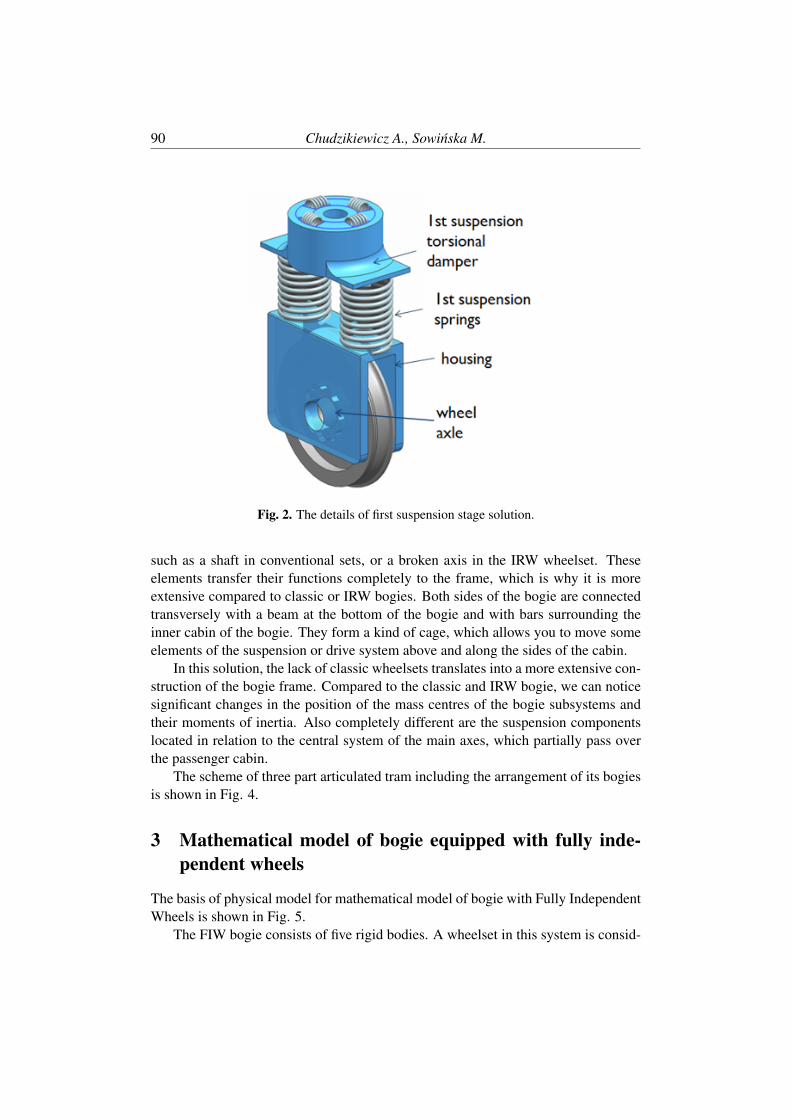
90 Chudzikiewicz A., Sowinska M.
Fig. 2. The details of first suspension stage solution.
such as a shaft in conventional sets, or a broken axis in the IRW wheelset. Theseelements transfer their functions completely to the frame, which is why it is moreextensive compared to classic or IRW bogies. Both sides of the bogie are connectedtransversely with a beam at the bottom of the bogie and with bars surrounding theinner cabin of the bogie. They form a kind of cage, which allows you to move someelements of the suspension or drive system above and along the sides of the cabin.
In this solution, the lack of classic wheelsets translates into a more extensive con-struction of the bogie frame. Compared to the classic and IRW bogie, we can noticesignificant changes in the position of the mass centres of the bogie subsystems andtheir moments of inertia. Also completely different are the suspension componentslocated in relation to the central system of the main axes, which partially pass overthe passenger cabin.
The scheme of three part articulated tram including the arrangement of its bogiesis shown in Fig. 4.
3 Mathematical model of bogie equipped with fully inde-pendent wheels
The basis of physical model for mathematical model of bogie with Fully IndependentWheels is shown in Fig. 5.
The FIW bogie consists of five rigid bodies. A wheelset in this system is consid-

The Boltzmann-Hamel Formalism in Modelling ... 91
Fig. 3. The bogie frame design proposition.
Fig. 4. The scheme of three part articulated tram.

92 Chudzikiewicz A., Sowinska M.
Fig. 5. Physical model of the FIW type bogie in a top view with characteristic dimensionsrelating to the suspension elements (a) and physical model of the FIW bogie in side view(b).

The Boltzmann-Hamel Formalism in Modelling ... 93
Fig. 6. Reference systems used for wheel analysis.
ered as one rigid body consisting of a single wheel and its housing with an axle boxon a short axis. It can therefore be assumed that the FIW wheelset has the followingdegrees of freedom:
1. lateral displacement y,
2. rotation angle ϕ around the longitudinal axis x,
3. rotation angle Ψ around the vertical axis z,
4. rotation angle of the left wheel θ about the lateral axis y.
Reference systems used for wheelset motion analysis is shown in Fig. 6. Used inmodelling coordinate systems are:
1. Inertial OXY Z coordinate system.
2. Non-inertial coordinate system O1XY Z related to the track centre line - a sys-tem used to describe the motion of the entire vehicle. This system moves alongthe centre line of the track at a constant speed v.
3. Non-inertial coordinate system Cxyz associated with the centre of the mass ofthe wheel. The centre of this system is in the centre of the mass C of the wheel.Its axes are directed parallel to the axis of the non-inertial system described inpoint 2.
4. Coordinate system Cξ ηζ rigidly connected to the wheel, and its axes are di-rected like the central main axes of inertia.
General assumptions connected to vehicle modelling are as follows:
a) one-point contact between wheel and rail,
94 Chudzikiewicz A., Sowinska M.
b) constant value of velocity component projected on plane OXY of center ofmass of the wheel,
c) nonholonomic constraints present in the system,
d) wheel is placed in the uniform gravitational field,
e) Rolling radius of the wheel is a function of (y,ψ,Ψ).
The equations of motion of the wheel rolling on the rail were derived with theuse of Boltzmann-Hamel formalism taking into account nonholonomic constaraints.
The degrees of freedom of bogie of type FIW are listed below:
~q= [y1l,φ1l,θ1l,ψ1l,y1r,φ1r,θ1r,ψ1r,y2l,φ2l,θ2l,ψ2l,y2r,φ2r,θ2r,ψ2r,yb,zb,φb,θb,ψb]T
(1)Basing on the mathematical models of trucks and the carbody, a simulation model
of the tram vehicle was built. This model contains all algorithms and numerical pro-cedures integrated in the form of a computer program. The most important numeri-cal procedures were used to perform such tasks as: determination of contact pointsbetween wheels and rails, determination of tangential contact forces (FASTSIM al-gorithm) and normal (algorithm based on Hertz theory), introduction and calculationof right sides of dynamic equations of motion of relevant vehicle components in ma-trix form and preparing them for further solution by numerical integration of motionequations.
The last task was performed according to method described in details in authors’papers (Chudzikiewicz et al., 2015; Chudzikiewicz and Sowinska, 2014; Sowinska,2015).
4 Simulations results
The simulation tests of the system were carried out on the track with Ri60 groovedrails, the wheel profile corresponds to the V15 profile according to the scenariospresented in Table 1.
4.1 Scenario 1 – regular curving
Two cases of vehicle motion along arc are considered. The radii of the arcs and thespeed of the vehicle model were subjects of variation.
The route on which the simulation was carried out consists of a straight sectionof length equal to 30 m, a regular left arc of length 0.5πR (quarter circle) and then astraight track. The whole route is 500 m long.
The lateral displacements of the centre of mass of wheels of the first wheelset areshown in Fig. 7.

The Boltzmann-Hamel Formalism in Modelling ... 95
Table 1. Simulation tests scenarios
Fig. 7. Lateral displacements of the centre masses of wheels.
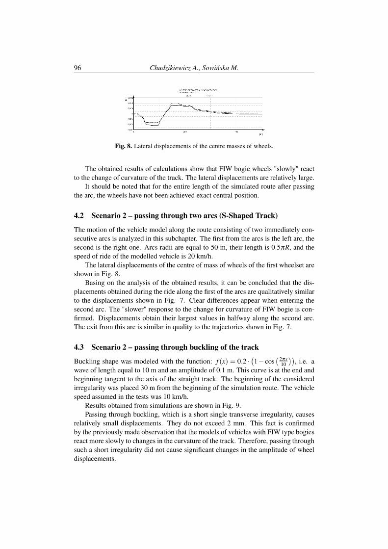
96 Chudzikiewicz A., Sowinska M.
Fig. 8. Lateral displacements of the centre masses of wheels.
The obtained results of calculations show that FIW bogie wheels "slowly" reactto the change of curvature of the track. The lateral displacements are relatively large.
It should be noted that for the entire length of the simulated route after passingthe arc, the wheels have not been achieved exact central position.
4.2 Scenario 2 – passing through two arcs (S-Shaped Track)
The motion of the vehicle model along the route consisting of two immediately con-secutive arcs is analyzed in this subchapter. The first from the arcs is the left arc, thesecond is the right one. Arcs radii are equal to 50 m, their length is 0.5πR, and thespeed of ride of the modelled vehicle is 20 km/h.
The lateral displacements of the centre of mass of wheels of the first wheelset areshown in Fig. 8.
Basing on the analysis of the obtained results, it can be concluded that the dis-placements obtained during the ride along the first of the arcs are qualitatively similarto the displacements shown in Fig. 7. Clear differences appear when entering thesecond arc. The "slower" response to the change for curvature of FIW bogie is con-firmed. Displacements obtain their largest values in halfway along the second arc.The exit from this arc is similar in quality to the trajectories shown in Fig. 7.
4.3 Scenario 2 – passing through buckling of the track
Buckling shape was modeled with the function: f (x) = 0.2 ·(1− cos
(2πx10
)), i.e. a
wave of length equal to 10 m and an amplitude of 0.1 m. This curve is at the end andbeginning tangent to the axis of the straight track. The beginning of the consideredirregularity was placed 30 m from the beginning of the simulation route. The vehiclespeed assumed in the tests was 10 km/h.
Results obtained from simulations are shown in Fig. 9.Passing through buckling, which is a short single transverse irregularity, causes
relatively small displacements. They do not exceed 2 mm. This fact is confirmedby the previously made observation that the models of vehicles with FIW type bogiesreact more slowly to changes in the curvature of the track. Therefore, passing throughsuch a short irregularity did not cause significant changes in the amplitude of wheeldisplacements.
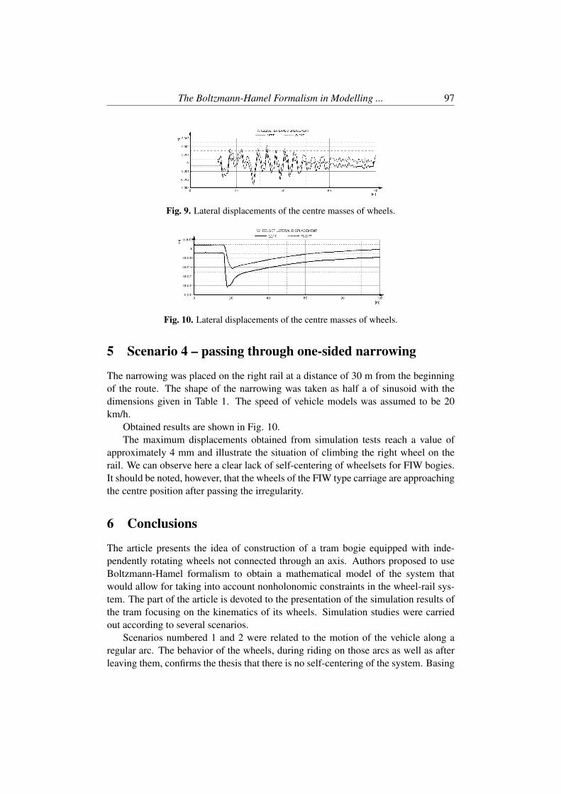
The Boltzmann-Hamel Formalism in Modelling ... 97
Fig. 9. Lateral displacements of the centre masses of wheels.
Fig. 10. Lateral displacements of the centre masses of wheels.
5 Scenario 4 – passing through one-sided narrowing
The narrowing was placed on the right rail at a distance of 30 m from the beginningof the route. The shape of the narrowing was taken as half a of sinusoid with thedimensions given in Table 1. The speed of vehicle models was assumed to be 20km/h.
Obtained results are shown in Fig. 10.The maximum displacements obtained from simulation tests reach a value of
approximately 4 mm and illustrate the situation of climbing the right wheel on therail. We can observe here a clear lack of self-centering of wheelsets for FIW bogies.It should be noted, however, that the wheels of the FIW type carriage are approachingthe centre position after passing the irregularity.
6 Conclusions
The article presents the idea of construction of a tram bogie equipped with inde-pendently rotating wheels not connected through an axis. Authors proposed to useBoltzmann-Hamel formalism to obtain a mathematical model of the system thatwould allow for taking into account nonholonomic constraints in the wheel-rail sys-tem. The part of the article is devoted to the presentation of the simulation results ofthe tram focusing on the kinematics of its wheels. Simulation studies were carriedout according to several scenarios.
Scenarios numbered 1 and 2 were related to the motion of the vehicle along aregular arc. The behavior of the wheels, during riding on those arcs as well as afterleaving them, confirms the thesis that there is no self-centering of the system. Basing

98 Chudzikiewicz A., Sowinska M.
on obtained results it may be concluded that the value of the radius of the arc onwhich the vehicle travels does not affect qualitatively the lateral displacements ofwheels of the tested vehicle models.
The non-rapid lateral displacement of the vehicles’ wheels when entering thetrack arc suggests a slower vehicle reaction on changes of the track curvature.
The simulation results obtained from the modeling of vehicle motion along thebuckling track confirm the thesis on “slow” reacting of the vehicle equipped withindependent wheels on changes of the curvature of the track.
Displacements obtained from simulation tests for scenario 4 illustrate the situ-ation of climbing the right wheel on the rail. We can observe here a clear lack ofself-centering of wheelsets for FIW bogies.
References
Batista, M. (2006). Steady motion of a rigid disk of finite thickness on a horizontalplane. International Journal of Non-Linear Mechanics, 41(4):605–621.
Bloch, A., Baillieul, J., Crouch, P., Marsden, J. E., Zenkov, D., Krishnaprasad, P. S.,and Murray, R. M. (2003). Nonholonomic mechanics and control, volume 24.Springer.
Cameron, J. M. and Book, W. J. (1997). Modeling mechanisms with nonholonomicjoints using the boltzmann-hamel equations. The International Journal of RoboticsResearch, 16(1):47–59.
Chudzikiewicz, A. and Sowinska, M. (2014). Low-flor trams running gear -comparative simulation studies. In Proceedings of the 14th Mini Conference onVehicle System Dynamics, Identification and Anomalies / Zobory Istvan (red. ),.
Chudzikiewicz, A., Sowinska, M., Krzyzynski, T., and Maciejewski, I. (2015).Modelowanie ruchu zestawu kołowego z niezaleznie obracajacymi sie kołami zuwzglednieniem układu sterowania kołami. Systemy Logistyczne, teoria i prak-tyka.
Eickhoff, B. and Harvey, R. (1989). Theoretical and experimental evaluation of in-dependently rotating wheels for railway vehicles. In IAVSD SYMPOSIUM (11TH:1989: KINGSTON, ONT) THE.
Elkins, J. A. (1989). The performance of three-piece trucks equipped with indepen-dently rotating wheels. In The dynamics of vehicles on roads and tracks.
Frederich, F. (1989). Dynamics of a bogie with independent wheels. Supplement toVehicle System Dynamics, 19:217–232.

The Boltzmann-Hamel Formalism in Modelling ... 99
Maryniak, J. and Molicki, W. (1985). Statecznosc spiralna samolotu w ruchuprzestrzennym z uwzglednieniem efektów elementów wirujacych zespołu nape-dowego. Journal of Theoretical and Applied Mechanics, 23(3-4):651–656.
Mei, T. and Goodall, R. (2003). Practical strategies for controlling railway wheelsetsindependently rotating wheels. Journal of dynamic systems, measurement, andcontrol, 125(3):354–360.
Nemark, Juru, I. and Fufaev, Nikola, A. (2004). Dynamics of nonholonomic systems.American Mathematical Soc., 33.
Obata, R., Tanifuji, K., Soma, H., and Masuda, T. (2006). Curving performanceof a rail vehicle with independently rotating wheels by torque difference control.Nippon Kikai Gakkai Ronbunshu C Hen(Transactions of the Japan Society of Me-chanical Engineers Part C)(Japan), 18(4):1064–1070.
Perez, J., Busturia, J. M., Mei, T., and Vinolas, J. (2004). Combined active steeringand traction for mechatronic bogie vehicles with independently rotating wheels.Annual Reviews in Control, 28(2):207–217.
Satou, E. and Miyamoto, M. (1992). Dynamics of a bogie with independently rotatingwheels. Vehicle System Dynamics, 20(sup1):519–534.
Sowinska, M. (2015). Modelling of the vehicle with trailer kinematics using boltz-mann – hamel formalism. Dynamical problems in rail vehicles, 367(3).
Sugiyama, H., Matsumura, R., Suda, Y., and Ezaki, H. (2011). Dynamics of in-dependently rotating wheel system in the analysis of multibody railroad vehicles.Journal of Computational and Nonlinear Dynamics, 6(1):011007.
Wang, W., Suda, Y., and Michitsuji, Y. (2008). Running performance of steeringtruck with independently rotating wheel considering traction and braking. VehicleSystem Dynamics, 46(S1):899–909.


Machine Dynamics Research2018, Vol. 42, No 1, 101-115
Determination of the Electrical StructureParameters of an Acid Battery
Józef Pszczółkowski * and Grzegorz Dyga†
Military Academy of TechnologyFaculty of Mechanical Engineering
AbstractThe article indicates the possibilities of using the crankshaft driving signals as diagnostic sig-nals of the battery, starter and internal combustion engine. The signals recorded during thecranking of the engine crankshaft by the starter are discussed. The test results of voltage mea-sured at the terminals of a loaded battery under constant load conditions have been presented.The principles of electric acid battery models building and various possibilities of its descrip-tion are presented. The principles of processing the results for the purpose of determiningand describing the battery model are characterized. The possibilities of description of thecharacteristics under stationary and non-stationary conditions by means of glued functions,linear combination of exponential functions and determination of electrical parameters of thebattery as components of the circuit, i.e. its electromotive force, resistance and capacity areindicated.
Keywords: combustion engine, diagnostic methods, lead-acid battery.
1 Introduction
Each technical device obtains a specific structure that provides it with the ability toperform the tasks for accomplishing which it has been designed. During operation,the elements and systems of the device are subject to various types of interactions,related both to its functioning and those coming from the environment. As a resultof these interactions, processes of wear of elements occur which generally cause anunfavorable change in its effective parameters. To maintain their value within certainlimits, it is necessary to restore the original state of the device’s elements. The scopeof operating activities related to maintaining or restoring the state is called servicing.Operational strategy is the relationship between how to use and operate machines.Existing operational strategies point to historically shaped changes in the approachto the maintenance of machines. You can distinguish here:

102 Pszczółkowski J., Grzegorz D.
1. reactive maintenance, in which the service and repair are carried out after theoccurrence of damage,
2. preventive maintenance, where service and repairs are ahead of the appearanceof damage - an example of this approach is the planned and preventive strategy,
3. prognostic maintenance consisting in monitoring the condition of machines,using diagnostic methods and reliability in predicting damage and implement-ing preventive actions.
The last decades have been characterized by a significant change in machine ex-ploitation principles, mainly regarding the method of implementing maintenance ac-tivities. The planned and preventive method of servicing and repairs is characterizedby the occurrence of fixed time intervals in which certain operations are carried outon the device provided by the manufacturer or the exploitation system. This methodundoubtedly has a number of advantages, but it is certainly not effective - the amountof expenditure incurred is not commensurate with the achieved or achievable effects.That is why more and more often the activities of implementing the dynamic ser-vice method according to the technical condition are being undertaken. In this case,the scope of service and repair activities is closely related to the actual condition ofthe device and the needs in this regard. The legitimacy of this type of activity de-pends on the precise recognition of the device status, and in particular the forecastof future state changes. That is why diagnostics is playing an increasingly importantrole in the systems of equipment operation, enabling a significant increase in theirreliability. The intensive development of technical diagnostics is connected with thedevelopment of means for measuring and registering parameters of machine workingprocesses and methods of data processing. For diagnostic purposes, more and moreparameters of the output processes of machines that can act as state symptoms areused.
The development and growth of the diagnostics importance results from the fol-lowing reasons:
• the need to rationalize the exploitation processes by limiting corrective actionsby performing preventive measures,
• changes in the features of exploitation objects consisting in the use of new con-struction materials, exploitation materials and technologies, as well as equip-ping them with a large number of measuring systems,
• technological progress in the field of diagnostics related to the emergence anddevelopment of existing means and methods of diagnosis. This increases thetechnical and methodological possibilities of diagnostics (the ability to mea-sure and interpret results),

Determination of the Electrical Structure ... 103
• the use of computer technology increases the speed of signal recording andprocessing and changes the rules and scope of object modeling.
For the purpose of internal combustion engine diagnostics, there are new possibili-ties to use the parameters of crankshaft driving by the electric starting system: thecurrent drawn by the starter, the voltage at the battery terminals, the crankshaft rota-tional speed (Pszczółkowski, 2002). For the diagnostic use of these parameters it isnecessary to build mathematical models of all objects.
The aim of the publication is to present the diagnostic method and principles forthe description of electrical characteristics of an acid battery and its electrical dia-grams - building its electric model. The construction of an electric battery model anddetermination of its parameters requires its operating characteristics testing in sta-tionary and dynamic conditions. These characteristics should show the dependenceof battery voltage on independent parameters affecting its value: nominal capacity,battery status, its charge status, current intensity, temperature, as well as manufactur-ing technology.
2 Diagnostic method principles
The existing cause-effect relationships of crankshaft driving parameters by the elec-tric starting system indicate the possibility of using these signals as diagnostic param-eters of the battery-electric starter-combustion engine set state. The analysis of theelectric starter characteristics allows to explain the essence of the diagnostic method,the existence of cause-effect relationships between quantities, and the conditions ofcooperation of the considered system (Enache et al., 2014) The set of starter charac-teristics (Fig. 1) contains dependencies on the current I [A] taken by the starter whenthe engine is cranked:
• the torque of the starter M [Nm],
• the speed of rotation of the starter shaft n [rpm],
• starter power P [kW],
• voltage U [V] at the terminals of a loaded battery.
The intensity of the current consumed by the starter, the voltage at the batteryterminals and the rotational speed of the crankshaft are the response of the engine-starter-the starting battery set to the forcing, which is the internal combustion enginecrankshaft driving by the starter. In the diagnostic test, the values of the system’sstate characteristics should be determined on the basis of the features of the outputsignals - system response to external excitation, which include:
• the intensity of the current consumed by the starter - it characterizes the bat-tery’s ability to return current under load conditions, it depends on the state
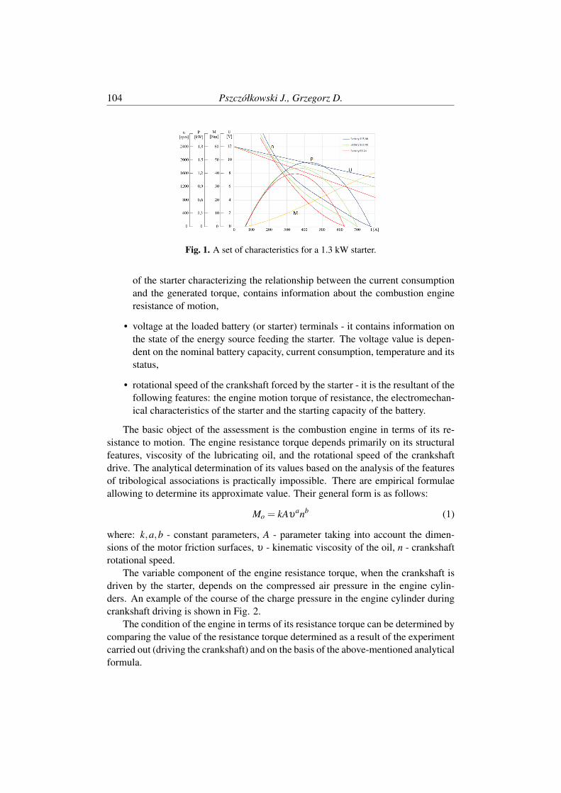
104 Pszczółkowski J., Grzegorz D.
Fig. 1. A set of characteristics for a 1.3 kW starter.
of the starter characterizing the relationship between the current consumptionand the generated torque, contains information about the combustion engineresistance of motion,
• voltage at the loaded battery (or starter) terminals - it contains information onthe state of the energy source feeding the starter. The voltage value is depen-dent on the nominal battery capacity, current consumption, temperature and itsstatus,
• rotational speed of the crankshaft forced by the starter - it is the resultant of thefollowing features: the engine motion torque of resistance, the electromechan-ical characteristics of the starter and the starting capacity of the battery.
The basic object of the assessment is the combustion engine in terms of its re-sistance to motion. The engine resistance torque depends primarily on its structuralfeatures, viscosity of the lubricating oil, and the rotational speed of the crankshaftdrive. The analytical determination of its values based on the analysis of the featuresof tribological associations is practically impossible. There are empirical formulaeallowing to determine its approximate value. Their general form is as follows:
Mo = kAυanb (1)
where: k,a,b - constant parameters, A - parameter taking into account the dimen-sions of the motor friction surfaces, υ - kinematic viscosity of the oil, n - crankshaftrotational speed.
The variable component of the engine resistance torque, when the crankshaft isdriven by the starter, depends on the compressed air pressure in the engine cylin-ders. An example of the course of the charge pressure in the engine cylinder duringcrankshaft driving is shown in Fig. 2.
The condition of the engine in terms of its resistance torque can be determined bycomparing the value of the resistance torque determined as a result of the experimentcarried out (driving the crankshaft) and on the basis of the above-mentioned analyticalformula.
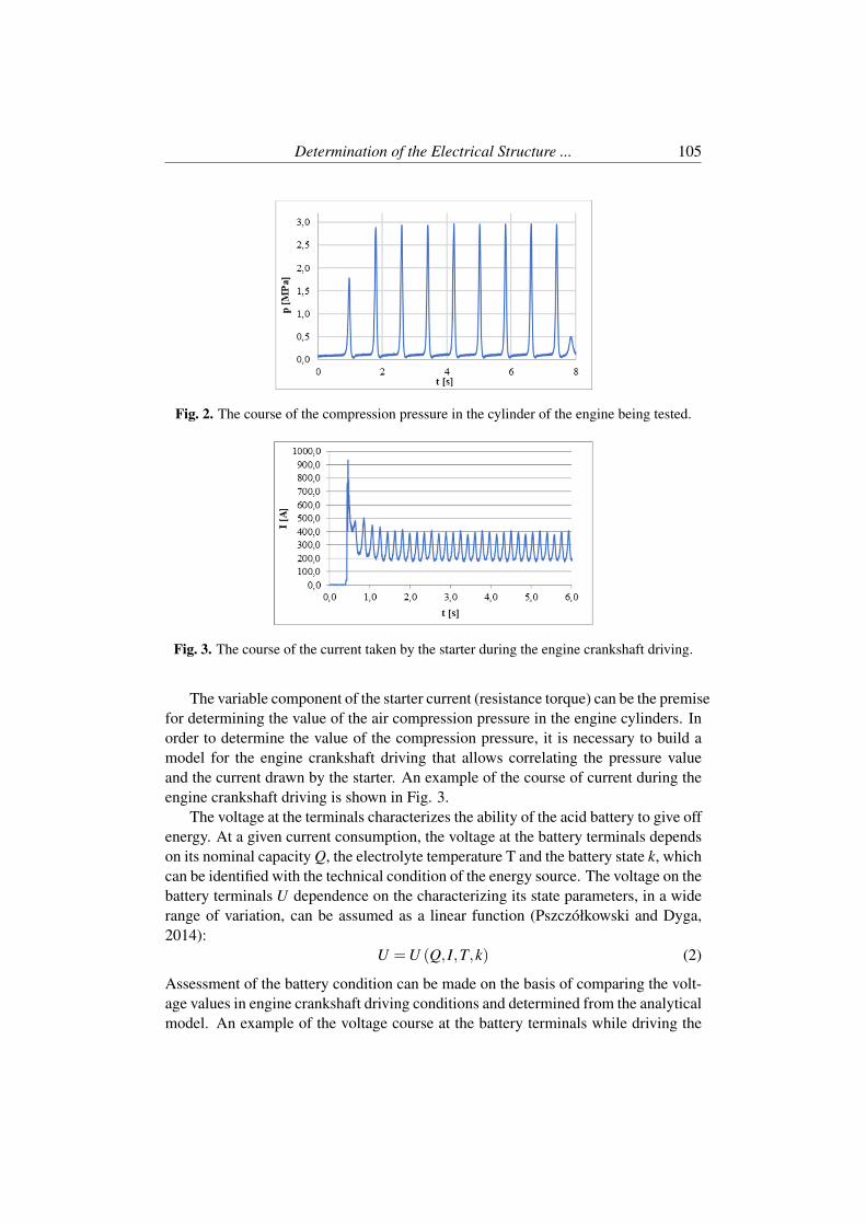
Determination of the Electrical Structure ... 105
Fig. 2. The course of the compression pressure in the cylinder of the engine being tested.
Fig. 3. The course of the current taken by the starter during the engine crankshaft driving.
The variable component of the starter current (resistance torque) can be the premisefor determining the value of the air compression pressure in the engine cylinders. Inorder to determine the value of the compression pressure, it is necessary to build amodel for the engine crankshaft driving that allows correlating the pressure valueand the current drawn by the starter. An example of the course of current during theengine crankshaft driving is shown in Fig. 3.
The voltage at the terminals characterizes the ability of the acid battery to give offenergy. At a given current consumption, the voltage at the battery terminals dependson its nominal capacity Q, the electrolyte temperature T and the battery state k, whichcan be identified with the technical condition of the energy source. The voltage on thebattery terminals U dependence on the characterizing its state parameters, in a widerange of variation, can be assumed as a linear function (Pszczółkowski and Dyga,2014):
U =U (Q, I,T,k) (2)
Assessment of the battery condition can be made on the basis of comparing the volt-age values in engine crankshaft driving conditions and determined from the analyticalmodel. An example of the voltage course at the battery terminals while driving the

106 Pszczółkowski J., Grzegorz D.
Fig. 4. The course of voltage measured at the terminals of a loaded battery.
Fig. 5. The course of the engine crankshaft rotational speed driven by the starting system.
engine crankshaft is shown in Fig. 4.To assess the state of the electric starter, it is necessary to know the engine resis-
tance torque. The basic weight in the proposed method of the starter state assessmentis to determine its actual power characteristic. The course of the power characteris-tics of the starter similar to the parabola indicates the possibility of their descriptionusing the second-degree polynomial in depending on the current.
The value of engine crankshaft rotational speed driven by the starting system canbe used to determine the actual starter power, if its torque value is determined on thebasis of the current. The power of the starter in given operating conditions is the basicparameter of the assessment of its technical condition (it must be related to its actualpower characteristic). An example of the course of rotational speed of the enginecrankshaft driven by starter is shown in Fig. 5
The signals of the engine crankshaft driving through the electric starting systemshow significant similarities and correspondence of their variability phases. This isdue to the existence of causal relationships between their values resulting from:
• characteristics of the battery, as a voltage source of electric current, which

Determination of the Electrical Structure ... 107
relate recorded courses of voltage and current to one another,
• a set of starter characteristics, as an electric motor, which uniquely bind thetorque of force with the current and rotation speed of the starter shaft with thevoltage of the power source.
3 Acid battery operating characteristics
The lead-acid battery is a chemical source of current in which electric current is gen-erated as a result of chemical processes taking place on its electrodes in the presenceof sulfuric acid. The factor that forces the course of the current generating processesis the electromotive force of the cell resulting from the difference in the electrodesconstituting the cell normal potentials. The basic parameters characterizing the elec-trical and energy properties of the battery are: voltage, twenty hours rated capacityand starting capacity. Existing chemical models of the battery explain the mecha-nism of generating electromotive force and the sum of its electrical and energeticcapacities, e.g. electric capacity. However, chemical models are not useful for an-alyzing electrical circuits where an acid battery is an element. When using them, itis not possible to determine the current electrical parameters of the circuit, currentand voltage. In such a circuit it is necessary to use electric battery models, composedof typical electrical circuit components: electromotive force, resistance, capacitance,inductance and others (Ceraolo, 2000). Modeling of batteries, including acid ones,has become necessary and is carried out particularly intensively due to the increaseddemand for electricity in vehicles with the arrival of electric and hybrid drives. Mod-eling and determination of battery model parameters is considered a difficult, unclear,laborious, expensive and ambiguous process (Jackey, 2007).
The battery performance tests were carried out on a station that was placed inthe low temperature chamber, which allowed for changing the ambient and the testedbattery temperature. The equipment of the measurement station enables the controlof the test implementation and the recording of the battery operation parameters. Thetested battery was loaded with a constant resistance value in about 10 seconds. Thecurrent and voltage values were recorded by means of a computer measuring system,also after switching off the load, to observe changes in the electromotive force of thebattery polarization during this period.
Examples of recorded current and voltage on the terminals’ dependencies duringthe battery of 54 Ah capacity load test are shown in Figs. 6 and 7.
At the moment of switching on the load, characteristic and correlated, propor-tional changes in the intensity of the absorbed current and voltage on the batteryterminals can be observed. In the initial discharge period, the voltage at the batteryterminals and the current decrease approximately exponentially, and then their val-ues stabilize. When the load is switched off, the voltage increases rapidly and thenincreases exponentially (Fig. 7). This is due to the increase of its electromotive force

108 Pszczółkowski J., Grzegorz D.
Fig. 6. The course of the current drawn from the battery.
Fig. 7. The course of the voltage at the loaded battery terminals.
caused by changes in the electrolyte concentration in the vicinity and in the innerlayers of the battery plates active mass.
The recorded characteristics have, apart from the visible and clear trend of changes,a significant irregularity. This can create difficulties in their further processing to de-termine and interpret electrical characteristics and the battery model. Therefore, thecourses were subjected to pre-processing, the aim of which was to smooth them. Thecauses of signal distortion were analyzed and methods of their removal were devel-oped. As sources of interference, were identified:
• measuring system own noise,
• interference from the external electricity network,
• quantization error.
Various forms and principles of averaging were adopted as methods of smoothing thereceived signals. They can be used in the case of a good recognition of the signal, of

Determination of the Electrical Structure ... 109
Fig. 8. The voltage at the loaded battery terminals.
Fig. 9. The classic electrical scheme of the battery.
the nature of its changes so as not to cause the loss of useful signal components. Thenatural noise of the measuring system, especially its high value, is usually a singleisolated deviation of its value from the set level. In principle, all distortions can bereduced using a method analogous to the moving average, with the difference thatthe moving average is a forecasting method in which the forecast value is assumed asthe moving average of the preceding values. In this case, the calculated value of themean, preferably from the odd number of data, was taken as the central data value.Depending on the degree of signal interference, the smoothing of the curve can beused several times.
As a characteristic of the battery load, the dependence of the voltage on its ter-minals at a constant value resistance load is considered. The analysis concerns thecharacteristics during the current load period, as shown in Fig. 8.
The lead-acid battery is most often treated as a voltage source of electric currentwith a defined electromotive force and variable internal resistance. In the electricalcircuit, certain voltage changes at its terminals (at a constant value resistance load)can be justified by changing its electromotive force or internal resistance. The occur-ring changes of electromotive force (or internal resistance) are caused by processesin the electrolyte around the electrodes or on their surface. When the constant valueof electromotive force is accepted under given discharge conditions, the classic elec-trical diagram of the battery can be presented as in Fig. 9.
In the electrical circuit in non-stationary operating conditions, the dynamic char-

110 Pszczółkowski J., Grzegorz D.
Fig. 10. The course of changes in the internal resistance of the loaded battery.
acteristics of the battery are revealed, which can be represented by the variability ofits internal resistance. When loaded with an external resistance R, the voltage at thebattery and receiver terminals is equal to:
U = RI = EA − IRw (3)
On the basis of equation (3), the internal resistance of the analyzed battery was deter-mined (Fig. 10), considering that the voltage at the terminals of the unloaded battery- its electromotive force - was equal to 12.97 V.
The analytical form of the obtained internal resistance courses (and analogouslyof the voltage and current consumption) is convenient for the engineering calculationsof predicting the features of an object. One of the significant problems in this caseis the choice of the form of a regression function that is an object or process model.In the analyzed case it is advisable to adopt the exponential function of the form (4)because of the nature of the variability of the observed dependency, as well as:
• it is a function commonly used in science and technology,
• it is easy to interpret,
• it gives the possibility, through interpretations, of building structural modelsof objects that perform an exponential response to step excitation and theiranalytical description.
Rw = Rs −Rz exp(−t/τ
)(4)
where: Rs - battery resistance in the steady state of work, Rz - amplitude of the vari-able resistance component of the battery, τ - time constant of the internal resistancechange process.
The obtained signal courses (Fig. 6, 7, 8) and (10) indicate the need to isolate afixed and variable part of dependences. There is a difficulty in clearly determining

Determination of the Electrical Structure ... 111
Fig. 11. The variable component of the internal resistance of the loaded battery togetherwith the approximating glued function lines.
the value of the determined course, because in exponential variability it is reachedin infinity. In addition, especially at high current values, low temperature and poorbattery condition, the changes in the value of the analyzed signals can also be a resultof the battery discharge, and thus a permanent change in its properties.
The variable part of the course in Fig. 10 can not be easily described using oneexponential function. In this case, one of the possibilities of description is the apply-ing of a glued function, i.e. a set of exponential functions defined in different timeintervals. The functions should meet the condition of continuity at the boundariesof the time intervals. The general form of the glued function F and the continuitycondition can be written (5):
F(t) = Fi(t) ti−1 6 t < tiFi(ti) = Fi+1(ti) i = 1, ...,n−1
(5)
In this case, another problem is the selection of the number and domain of the func-tion, which is related to the description complexity and accuracy. As a criterion forthe selection and assessment of these features, the R2 coefficient for individual func-tion can be used. For the analyzed dependency in Fig. 10, a fixed internal resistancevalue of 0.0133 Ω was determined. The range from 0 to 6 s of the battery’s resis-tance variable part, was divided into three intervals for which exponential regressionfunctions were determined. The final form of the analytical description of the courseis presented by the expression (6), and its illustration, together with the exponentialanalytic functions, is shown in Fig. 11.
Rz(t) =
0.006exp(−4.024t) 0 6 t < 0.10.0044exp(−0.948t) 0.1 6 t < 2.070.0011exp(−0.279t) 2.07 6 t < 6
(6)

112 Pszczółkowski J., Grzegorz D.
Fig. 12. Determined voltage components on the terminals of the charged battery in thetime range up to 2 s.
The second possible way of describing the presented dependencies with the ex-ponential function is using their linear combination, i.e. a mixture of functions. Themixture of Fi functions can be rendered:
F(t) =n
∑i=1
aiFi(t) (7)
where ai are the function weighting factors.For the analyzed battery the description was made using a mixture of the voltage
characteristic curve function - Fig. 8, in the time interval from 0 to 2 s. A stablecomponent of the value of Us = 11.37 was extracted. A very good correspondenceof the description with the real dependency was obtained here, by distinguishingthe range of fast polarization voltage variations in time up to 0.1 s. In this casea description according to (8) was obtained, and the separated intervals and theirapproximation functions are shown in Fig. 12.
U(t) = 0,225exp(−21,1t)+0,477exp(−0,98t) (8)
One should pay attention to the significant, more than twenty-fold differentiation ofboth functions time constants, which are respectively equal to about 0.05 s for thefast-changing component, i.e. in the time interval up to 0.1 s and 1 s for the slow-changing component (they are equal to the inverse of coefficients found in functionexponents).
4 Battery structural model
In the previous considerations, the change in its internal resistance was considered thereason for the voltage change at the terminals of a loaded battery, according to the

Determination of the Electrical Structure ... 113
Fig. 13. Electrical vicarious scheme for an acid battery.
electrical diagram given in Fig. 9. The reason for this are primarily the changes in theelectrolyte density around the electrodes and in the inner layers of the battery platesactive mass. The electrolyte density changing is also the reason for the electrodepotentials changing - the electromotive force of the battery. Therefore, the changein the voltage on the terminals can also be considered as the electromotive forcechange, its component called the electromotive force of polarization. The polarity ofeach electrode (anode and cathode) can be distinguished, depending on the locationof the polarization processes, and the voltage drop in the electrolyte. In general, thebattery’s electrical resistance is constituted by resistance, capacitance and inductancecomponents.
The electrical diagram of the acid battery shown in Fig. 9 can be used to describethe battery operation under constant current load or constant resistance. Variabilityin time of internal resistance under dynamic load conditions makes it practically im-possible to use this scheme to determine the battery response to variable - dynamicforce.
The description of the battery discharge characteristics (voltage at its terminals)using the exponential function makes it possible to introduce circuit elements to thecircuit equivalent scheme, whose electrical properties generate responses in the formof exponential function. An element consisting of a capacitor and a resistance throughwhich the capacitor is charged or discharged may be such an element of the batteryvicarious diagram. Therefore it is possible to connect to a stationary source of theelectromotive force of the battery Eo the RC circuit as in Fig. 13. In variable loadconditions, this circuit generates the electromotive force of the polarization. Descrip-tion of the battery discharge characteristics by means of a linear combination of twoor more exponential functions indicates the possibility and the need for applying ata battery vicarious circuit diagram also a larger number of RC circuits connected inseries.
Determining the parameters of the circuit elements is possible on the basis ofbattery discharge characteristics test results, as specified in (8). It is known that thecapacitor discharge characteristic is the exponential curve of the form (9):
U(t) =Uo exp(− tτ) =Uo exp(− t
RC) (9)

114 Pszczółkowski J., Grzegorz D.
Thus, the time constant of the discharge process is τ =RC. This creates the possibilityof assigning physical values to the indicated elements of the battery vicarious circuit.
5 Conclusions
A feature of modern machine operation is the constant, systematic increase of thetechnical diagnostics role and meaning. Wide possibilities of its application resultfrom the change of features of exploitation objects, including motor vehicles andthe development of methods and means of diagnosis using digital signal recordingand processing techniques. In diagnostics of internal combustion engines and itsstarting system it is possible to use as diagnostic parameters’ features of workingand accompanying processes of the crankshaft driving. As the diagnostic parameterscan be treated here: the current consumed by the starter, the voltage at the battery orstarter terminals and the speed of the crankshaft forced by the starter. On the basisof these parameter values, the battery, starter and, first of all, the engine state canbe assessed in the aspect of the factors influencing its resistance torque - viscosityof the lubricating oil, pressure of air charge compression and general wear of theassemblies.
The method of diagnosing can be developed on the basis of the model charac-terizing the features of the starting system components dependencies. In this modeldetermination of the engine cylinder air charge compression pressure and the startercharacteristics under real operating conditions are fundamental. The set of electricstarter characteristics depends on the properties of the energy source - the acid bat-tery.
An acid battery is a functionally and structurally complex non-linear power sourcewhose features are dependent on many parameters. To describe the characteristics ofits operation - the response to rapid jump, i.e. load with a constant current or re-sistance, it is convenient to use exponential functions in the form of glued functionsor a mixture of functions. Both methods of description correspond to two differentvicarious electric models of the acid battery in the form of electromotive force andvariable internal resistance and stationary electromotive force and RC systems withdifferent characteristics, performing changes in the electromotive force of the batterypolarization in the circuit. Consideration of many independent parameters in the bat-tery properties description and its structural parameters requires long-term extensiveexperimental research.
References
Ceraolo, M. (2000). New dynamical models of lead-acid batteries. IEEE transactionson Power Systems, 15(4):1184–1190.
Enache, B.-A., Constantinescu, L.-M., and Lefter, E. (2014). Modeling aspects of

Determination of the Electrical Structure ... 115
an electric starter system for an internal combustion engine. In Electronics, Com-puters and Artificial Intelligence (ECAI), 2014 6th International Conference on,pages 39–42. IEEE.
Jackey, R. A. (2007). A simple, effective lead-acid battery modeling process forelectrical system component selection. Technical report, SAE Technical Paper.
Pszczółkowski, J. (2002). Rozruch silnika tłokowego jako proces diagnostyczny.Diagnostyka, 27:48–53.
Pszczółkowski, J. and Dyga, G. (2014). Dwuwymiarowe liniowe zaleznoscifunkcyjne napiecia akumulatora kwasowego. Logistyka.

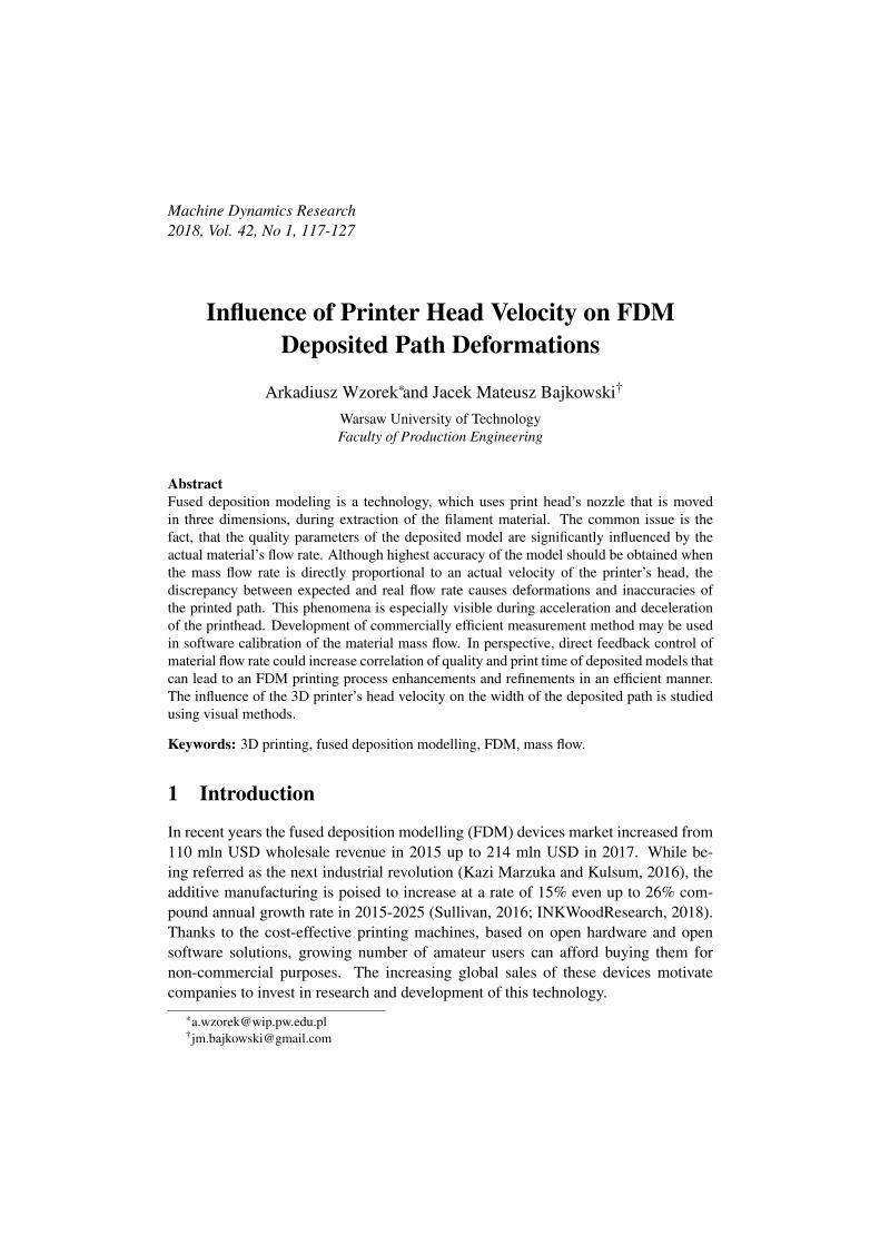
Machine Dynamics Research2018, Vol. 42, No 1, 117-127
Influence of Printer Head Velocity on FDMDeposited Path Deformations
Arkadiusz Wzorek*and Jacek Mateusz Bajkowski†
Warsaw University of TechnologyFaculty of Production Engineering
AbstractFused deposition modeling is a technology, which uses print head’s nozzle that is movedin three dimensions, during extraction of the filament material. The common issue is thefact, that the quality parameters of the deposited model are significantly influenced by theactual material’s flow rate. Although highest accuracy of the model should be obtained whenthe mass flow rate is directly proportional to an actual velocity of the printer’s head, thediscrepancy between expected and real flow rate causes deformations and inaccuracies ofthe printed path. This phenomena is especially visible during acceleration and decelerationof the printhead. Development of commercially efficient measurement method may be usedin software calibration of the material mass flow. In perspective, direct feedback control ofmaterial flow rate could increase correlation of quality and print time of deposited models thatcan lead to an FDM printing process enhancements and refinements in an efficient manner.The influence of the 3D printer’s head velocity on the width of the deposited path is studiedusing visual methods.
Keywords: 3D printing, fused deposition modelling, FDM, mass flow.
1 Introduction
In recent years the fused deposition modelling (FDM) devices market increased from110 mln USD wholesale revenue in 2015 up to 214 mln USD in 2017. While be-ing referred as the next industrial revolution (Kazi Marzuka and Kulsum, 2016), theadditive manufacturing is poised to increase at a rate of 15% even up to 26% com-pound annual growth rate in 2015-2025 (Sullivan, 2016; INKWoodResearch, 2018).Thanks to the cost-effective printing machines, based on open hardware and opensoftware solutions, growing number of amateur users can afford buying them fornon-commercial purposes. The increasing global sales of these devices motivatecompanies to invest in research and development of this technology.
118 Wzorek A., Bajkowski J.,M.
Although popular, the current additive manufacturing printers are characterizedby low productivity, insufficient repeatability, inconsistent roughness of the surface,low accuracy of printing and uncertainty of mechanical properties of the final model(Bikas et al., 2016; Taufik and Jain, 2016; Kim and Oh, 2008). This urges companiesto improve and develop the portfolio of the printers, which should be economic inexploitation, easy to operate, precise and fast, yet still being affordable for the finaluser.
In the fused deposition process, the plastic filament material is melted and pumpedthrough a nozzle and deposited as paths forming thin layers onto a fixtureless printbed. The print head moves along 3 axes, basically forming the model one layer at atime. Usually, once the build cycle begins, no operator attendance is required. Thedeposited material solidifies and forms a base for another layer. A key characteristicof a finished model is the surface finish which depends upon the filament viscos-ity, melting temperature, humidity, deposition speed, geometry of the part and otherparameters (Anitha et al., 2001; Chacón et al., 2017; Bähr and Westkämper, 2018).Also, the software control of the motion of the printer’s head and motion of the feedwheels supporting the filament is important.
In this paper, some work was undertaken to elaborate on measurement methodthat can help to measure actual material flow rate. The influence of the actual velocityof a 3D printer’s head on the geometry of the deposited path is studied using visualanalysis. The results can be useful for software calibration of the material mass flowrate inaccuracy, which influences the quality characteristics of the FDM prototype.The designed experiment allowed to determine the efficiency of the proposed method.
2 Inaccuracy of the mass flow rate
Conventional motion drives used in FDM technology allow performing complex 7-phase motion, taking advantage of a parameter called jerk, which is the first derivativeof an acceleration. The use of a complex motion profile allows reducing the head’svibration, increasing the head’s linear speed and smoothing the obtained path (Her-nandez, 2015).
Figure 1 shows a sample velocity of an FDM printing nozzle obtained through g-code analysis. The nozzle was following a labyrinth path which was generated usingFDM computer aided manufacturing program called Slic3r. It is an open sourcesoftware suitable for research purposes. The presented velocity map shows a single0.3 mm thick layer infill of a model with the side dimension of 150 mm. The presetlinear speed of the head was 120 mm/s and the acceleration reached 1000 mm/s2
while jerk was 10 mm/s3. Obviously, the desired velocity of 120 mm/s was achievedonly in some cycles of the motion. This is due to the characteristic of the motioncontrol. The synchronized electric motors need some time to achieve the desiredspeed, decelerate when change of direction is commanded, constantly maintain fair

Influence of Printer Head Velocity ... 119
Fig. 1. Sample velocity map of the print head for a single layer labyrinth path -a) andpre-processed image of the same path printed with constant material flow -b).
accuracy of the curve mapping, smoothen the curvature of the path as well as limitthe vibrations.
To better understand the problem of dynamic velocity control, it should be noticedthat for the analyzed path presented in Figure 1, the printing head was traveling atthe desired speed of 120 mm/s only during 41% of the total deposition time. Theremaining time was consumed for accelerating the printing head to the set value anddecelerating when change of direction of the travel was commanded. The averagevelocity was only 64.5 mm/s. During the layer deposition, a total of 48 positionchange commands were executed, but the desired preset velocity was achieved foronly 29 of them. As the velocity is constantly changing during the printing headmovement, the flow rate of the deposited material should be directly related to it.
Combined with the deposition speed, a steady-state pumping which the systemmust provide to ensure precise geometry and constant width of the deposited pathis pre-determined for selected type of the filament. One can notice, that at the startor stop of the path, the material flow should be inherently different than in the othersegments. Also, when the printing head is making turns, the flow rate should ac-commodate accordingly to avoid deformations. Before the head start to print a newroad, the feeder meters a small amount of filament in anticipation of the printing headto accelerate to the steady-state. During the carriage motion, the flow is controlledbased on the actual velocity, so near the points where the path changes its direction,the actual flow rate must be adapted. Close to the end of the path, the flow rate is de-celerated to create the finishing point precisely. This pattern is usually programmedin motion control algorithms used in FDM printers. Each material has its own visco-elastic characteristics, which should be taken into account when programming motionparameters like acceleration, deceleration and pre-start metering control.
Typically it is assumed in the algorithm control the printing head, that the flowrate should be proportional to the velocity of the carriage. Nevertheless, observationshows that when the preset velocity and thus, the material flow rate is increased toobtain faster printing, the flow accuracy deteriorates and the printed model becomesless accurate (?). This may be related to many effects, depending on type of the

120 Wzorek A., Bajkowski J.,M.
Fig. 2. Scheme of the custom 3D printer test stand using silicone as filament.
printer, type of material, geometry of the object, size of the nozzle, etc. A com-plex study on the influence of the geometry of the nozzle and the material flow onthe quality of the object was presented in (?). Although the best accuracy shouldbe obtained when the mass flow rate is proportional to the velocity of the printinghead, in reality the mass flow differs from the theoretical one, causing the object tobe less precise than expected. There are premises that inaccuracy of material massflow is proportional to the velocity due to microslipping of the feeding material. Thepresented research could lead to a development of a method for estimating an actualmaterial mass flow rate in relation to the theoretical one. Such a method could beuseful to perform additional software calibration, leading to better accuracy of theprinted models, without the necessity to upgrade the model of a printer. In the exper-imental test we use indirect measurement of the flow rate, based on visual analysis ofthe geometry of deposited path in correlation with the velocity of the print head.
3 Experimental test
3.1 Test stand configuration
A custom made laboratory test stand was built to perform the study. The three-axismanipulator presented schematically in Fig. 2 was made by assembling aluminumprofile frame, linear bearing rollers system and a set of additional structural parts.
The axial motion in XY plane was obtained with a belt gear system, while linearZ-axis motion was obtained with a trapezoidal screws. Rotational stepper motorswithout the encoder feedback were used to drive the gears and screws. The controlsystem was based on stepper motor controller AVR Trinamic TMC2100. Fig. 3presents the photo of the actual test stand.
Typically in FDM a solid, thermoplastic polymer is used as a filament. The feedwheels provide the torque to feed the filament which is then melted by a high tem-perature in a liquefier, and extruded through the nozzle. In our experiment, a single-

Influence of Printer Head Velocity ... 121
Fig. 3. Custom designed 3-axis cartesian manipulator used for the research.
component, liquid sanitary silicone manufactured by Soudal was used as a depositedmaterial. The viscosity of the silicone was 5000 cSt before the extrusion. The useof silicone eliminated the need to install the feed wheels supporting the filament andthus remove the risk of filament slipping between the rollers, or skip the issues withheating or dropping.
The silicone was placed in a dispenser with a 1.2 mm diameter nozzle, connectedto pressure pump through an electrovalve. As the pressure in applied, the siliconestarts to extrude from the dispenser, and deposits on the table. Pressure was setmanually using an air regulator before extruding the silicone. The pressure value waskept constant during the extrusion process. The accuracy of the pressure value insidethe silicone dispenser is related to the accuracy of the air regulator. It depends on theinlet pressure and is described by a hysteresis curve determined experimentally for agiven regulator. The characteristics of the used air regulator type AR30 produced bySMC pneumatics is presented in Fig. 4. Taking into account the small fluctuationsof the pressure value before the inlet of the air regulator, it was assumed that themaximum inaccuracy of the pressure value inside the container was 0.01 MPa.
To ensure the homogeneity of the material, the container with the silicone wasplaced in vacuum chamber for 24 hours before the extrusion to remove any air inclu-sions that could cause discontinuity of the material path during the extrusion. Thevulcanization of the silicone reacting with ambient humidity took place at a roomtemperature of 22.3C.
A polished granite plate with a class 0 surface roughness (according to DIN 876)

122 Wzorek A., Bajkowski J.,M.
Fig. 4. Hysteresis of the SMC AR30 air regulator.
was used as print bed platform to deposit the models. The flatness deviation of the250×250 mm surface of the plate was less than 0.005 mm. The displacement indica-tor and multipoint screw adjustment was performed to calibrate the drive system todeposit a single, horizontal, 0.3 mm high layer of silicone on the granite plate (Fig. 5).The achieved parallelism between XY plane and the granite platform was below 0.02mm for a 150×150 mm test area.
The 20 MPix photo camera was placed above the granite platform to acquire rawimages of the deposited path. The images were later filtered and processed to measurethe width of the deposited path.
Fig. 5. Parallelism calibration between XY plane and the granite platform.

Influence of Printer Head Velocity ... 123
Fig. 6. Preprocessed image of a single layer path deposited on a test platform.
Fig. 7. Comparison of measured path width due to the position for 10 samples.
3.2 Experimental results
In the experiment, the total number of 10 sample paths were printed. Each of the testroads was deposited by extruding semi-fluid acrylic silicone with a constant pressureof 0.25 MPa. Then, the specimen was left to solidify for 24 hours.
Single sample consisted of 7 collinear segments. Each segment was 5 mm longerfrom the previous one. The target printing velocity was set to 200 mm/s, target ac-celeration was 100 mm/s2 and the jerk was set to 20 mm/s3. The preset height ofthe path measured in Z-axis was 0.3 mm. An exemplary post-processed image of thedeposited path is presented in Fig. 6.
Matlab software with was Image Processing Toolbox was used to perform imageanalysis and determine the relation between the width of the deposition path and thedistance traveled by the print head. The image preprocessing consisted of contrastadjustment and converting image type from monochrome to binary. This type usesvalue of 1 to represent white pixel, while 0 is used for black. A 2 dimensional arrayof logical values determining color of each pixel in a segment is used for furtheranalysis.
To measure the width of the path, cells were added to each column of an ar-ray. Then measured path width was scaled from pixels to millimeters using standardsegment with known length Measuring error was influenced by the camera matrixresolution and parallax error. Assuming density of 5.8 pix/mm and geometricallydetermined parallax error of 1 pix, the total measurement error was 0.35 mm. The re-sults of the path width measurements for selected specimens are presented in Figure7.
The device driver handles commands using the g-code, which is a set of com-mands that appear consecutively. The current speed is enforced on the basis of theconditions in the form of maximum speed, acceleration and the set value of jerk.
Due to the fact that movement executed by open source algorithm was not similar

124 Wzorek A., Bajkowski J.,M.
Fig. 8. Comparison of average path width due to velocity of the printhead.
to the mathematical calculations. The driver calculates jerk value not as derivative ofthe acceleration, but uses some algorithm that gives an approximated results. Thisprohibits using g-code velocity data as a data representing the true velocity. To omitthis problem, a data acquisition card was connected to the output of the driver andrecord the true motion data, including the real velocity. The study was carried out us-ing National Instruments NI-6356 data acquisition device on the step signal betweenmotion driver and CNC controller. Obtained velocity in time function was calculatedto the position domain. The results are shown in Fig. 8, compared with the averagewidth of the path.
The data show the displacement of local minimum velocity in relation to the localmaxima of measured path width. This phenomena is caused by the material pulledbehind the needle. The proposed measurement method was validated by comparingincrement results of constant pressure deposited paths with the set velocity.
The correlation of the velocity to the width of the path, later approximated withfunction fit, is presented in Fig. 9.
The initials test showed that the preset velocity and the actual speed that the print-ing head is achieving differs greatly. The velocity of 200 mm/s was never achieved,since the lengths of the segments were too short for the motor to reach the presetvalue.
As one can notice, the resulting curve differs from the linear assumption which isoften programmed in the 3D printer software. The smallest error was obtained whenasymptotic fit was applied, despite whether the velocity was increasing or decreasing.This results shows than simple test runs performed prior to the first print out couldhelp to determine the true relation between the actual flow rate and velocity of theprinter head. Developing procedure to be implemented in printing software couldresult in limiting the exhibited inaccuracies of the final model.
4 Conclusions
The assumption used in FDM printers, that the deposited material flow ratio is pro-portional to the linear speed of the print head causes model inaccuracies. In thenormal operating cycle of the FDM device, the time of increasing and decreasing

Influence of Printer Head Velocity ... 125
Fig. 9. Correlation between velocity and path width for incrementing and decrementingvalue of velocity.

126 Wzorek A., Bajkowski J.,M.
velocity of the print head is significant. For this reason, it should be considered to ex-tend the conventionally used calibration of the extrusion system by introducing intothe control system a function approximating the actual measured output as a functionof speed. In the performed experiments it was shown that one can use simple testto acquire basic information on the relation between the width of the deposited pathand the desired velocity f the printing head. This information could be later helpfulin determining the true mass flow rate to be set in the software system. Incorpo-rating additional parameters of the particular extrusion system may improve qualityaspects, such as precision, accuracy and repeatability of the deposited model, as wellas shorten the production time. In perspective, direct feedback control of materialflow rate could take an influence on commercial devices development.
References
Anitha, R., Arunachalam, S., and Radhakrishnan, P. (2001). Critical parameters in-fluencing the quality of prototypes in fused deposition modelling. Journal of Ma-terials Processing Technology, 118(1-3):385–388.
Bähr, F. and Westkämper, E. (2018). Correlations between influencing parametersand quality properties of components produced by fused deposition modeling. Pro-cedia CIRP, 72(1):1214–1219.
Bikas, H., Stavropoulos, P., and Chryssolouris, G. (2016). Additive manufacturingmethods and modelling approaches: a critical review. The International Journal ofAdvanced Manufacturing Technology, 83(1-4):389–405.
Chacón, J., Caminero, M., García-Plaza, E., and Núñez, P. (2017). Additive man-ufacturing of pla structures using fused deposition modelling: Effect of processparameters on mechanical properties and their optimal selection. Materials & De-sign, 124:143–157.
Hernandez, D. D. (2015). Factors affecting dimensional precision of consumer 3dprinting. International Journal of Aviation, Aeronautics, and Aerospace, 2(4):2.
INKWoodResearch (2018). Global 3d printing market forecast 2017-2025. ReportSummary, access date: September 2018.
Kazi Marzuka, S. and Kulsum, J. U. (2016). 3d printing: a new avenue in pharma-ceuticals. WORLD JOURNAL OF PHARMACEUTICAL RESEARCH, 5(5).
Kim, G. and Oh, Y. (2008). A benchmark study on rapid prototyping processes andmachines: quantitative comparisons of mechanical properties, accuracy, rough-ness, speed, and material cost. Proceedings of the Institution of Mechanical Engi-neers, Part B: Journal of Engineering Manufacture, 222(2):201–215.

Influence of Printer Head Velocity ... 127
Sullivan, F. (2016). Global additive manufacturing market, forecast to 2025. Report,no. MB74-10, May 2016.
Taufik, M. and Jain, P. K. (2016). A study of build edge profile for prediction ofsurface roughness in fused deposition modeling. Journal of Manufacturing Scienceand Engineering, 138(6):061002.


Machine Dynamics Research2018, Vol. 42, No 1, 129-137
Static Analysis and Stability of the SteelFramework
Jan Misiak and Sławomir Stachura*
University of Ecology and Management in Warsaw
1 Introduction
The aim of the work is a qualitative and quantitative comparison of the results ofanalysis of stability of the steel section girder framework I-beam, aligning the frameelements and rod elements of the coating, using a finite element method.
The advantage of sheet metal cross-sections is the ability to freely select the thick-ness of the component sheets; the use of rigid belts and slender webs gives the mostefficient use of the cross-section load capacity. The plate girders show a large super-critical load capacity during bending, the breaking loads for this type of plate girderscan be significantly higher than the critical loads.
A stability analysis of a flat frame with supporting elements of the plate girderwith an I-section in the elastic range was made, taking into account the ribbing of thecolumn web, as a counteracting the phenomenon of local loss of stability of the web.The studies of the impact of concentrations on the loss of overall flexural, flexural-torsional and lateral-torsional buckling stability were investigated. In the analysis, thecomputational models were used and the coating rod, which allows for the analysisof the local loss of stability of each wall section girder (Misiak and Stachura, 2013).
2 Formulation of the problem
The calculations were made on the basis of the nave frame with a span of 32m, withdepressed roof bolt, pivotally supported, subjected to load combinationsFRd = (1+ 2)*1,15 + 3*1,5 , wherein: 1 - own weight, 2 - the weight of housingwall and roof and 3 - snow load (Fig.1).

130 Misiak J., Stachura S.
Fig. 1. The load applied to the frame from the combination FRd = (1+2)*1,15 + 3*1,5 .
The standard 1 requires the determination of the sensitivity coefficient for the lossof defined stability
αcr =Fcr
FRd(1)
where: FRd - comparative load equal to load combinations, Fcr - critical load.Numerical analysis equilibrium stable and stability was performed using the Au-
todesk Robot Structural Analysis program Finite Element Analysis (FEA) elementsof the bar type with a defined cross-sectional plate girder I-section and a shell usingthe linear and non-linear compounds geometry by solving the equations and staticstability
[K+Kσ (∆σ)+Ku(∆q)]∆q = ∆P[K+αcr Kσ (σ)+Ku(q)]q = 0
(2)
where K - linear stiffness matrix, Kσ - geometric stiffness matrix, Ku - displace-ment stiffness matrix. A detailed description of the equations can be found in lit.(Waszczyszyn et al., 1990), because the authors co-created the Robot program.
3 Bar calculation model of 2D and 3D frames
The flat bar frame has the cross-section of the plate girder with the following dimen-sions in [cm]: h = 53.6; b = 36; t f = 1.8; tw = 0.8.
After static calculations, results were obtainedRequired by standard 2 for normative models of dimensioning, is to determine
the critical length of individual bearing elements: columns for which there is a tiltloss of stability (Fig. 3a) αcr = 18,588 and a rafter αcr = 77,832with non-sustainedloss of stability (Fig.3b), in the geometric plane of the frame; results from stabilitycalculations for the 2D model
1Norma PN-EN 1993-1-1: Eurokod 3 – Projektowanie konstrukcji stalowych – Czesc 1-1: Regułyogólne i reguły dla budynków, PKN, Warszawa 2006
2See 1

Static Analysis and Stability of the Steel Framework 131
Fig. 2. The results of static calculations.
Fig. 3. Form of deformation-model 2D.
Then, the model 3D frame, after the concentrations of displacements receivedby the purlins buckling factors αcrfor heel and non-tilting loss of stability does notchange much with respect to the 2D model, but yet there is buckling of the minor axisz− z (Fig.4), deformation through the exit from the bending plane αcr = 24.041.
4 Shell frame calculation model
Plate girder was modeled by the surface coating finite elements, as analyzed the prob-lem of loss of stability, bending stresses under the action of the disc, the compressiveload at the median plane. From the static calculations (Fig.5), the obtained stressreduced from the Mises hypothesis is 382.54 MPa, and this value is too high for theS355 steel grade used. The corner mullion-transom introduced gain and decreasedvalue of the reduced stresses to the level of 291.65 MPa (Fig.6).
From the loss of frame stability calculations, the smallest value obtained relatesto the local loss of stability (Fig.7) of the buckling of the column web section in thereinforcement area between the two ribs.
For the prevention of buckling the ribs need to be implemented in this area (Fig.8)that reduce the stresses in the bottom portion of the connection post-boosting value185,01MPa value of 291,65 MPa.
Then, the results of calculations of frame stability losses are presented in Fig.9.For the first six buckling forms there is a local loss of stability of the walls in theorder with the highest slenderness.
Changing the placement of the rib direction (Figure 10) obviously causes changesin the stress values at the points where the rib is connected to the pole belts

132 Misiak J., Stachura S.
Fig. 4. Tilting deformation αcr,1 = 18.841, αcr,2 = 76.334, αcr,3 = 24.041- 3D model.
Fig. 5. Results of static frame calculations.
Fig. 6. Results of static frame calculations with corner reinforcement.
Static Analysis and Stability of the Steel Framework 133
Fig. 7. Local loss of stability of the column web.
Fig. 8. The results of static frame calculations with corner reinforcement and rib imple-mentation.

134 Misiak J., Stachura S.
Fig. 9. Local loss of stability of the plate girders.
Fig. 10. Results of static frame calculations after re-positioning of the rib.

Static Analysis and Stability of the Steel Framework 135
Fig. 11. Local loss of stability of the plate girders.
Fig. 12. Stress distributions after the implemented changes with the addition of ribs.
The change in the location of the rib does not have a qualitative effect on thelocation of the local loss of stability, but has an impact on the αcr value, reducing thelowest value.
We are practically interested in structural changes that will cause the global lossof stability, then the resistance of the structure to the loss of stability increases, themeasure of this resistance is the load value. Thus, the ribs on the reinforcement direc-tion of higher stresses Sxx (Fig.12) and on pillars were implemented. The changeshave not contributed significantly to increase the resistance of the frame on the lossof stability value of factor αcr = 7.597 before the change αcr = 5.555, it is analogousfor the second form αcr = 7.617and the next forms of buckling - this is a local loss ofstability, not global, for which the multiplier value would be much larger. The localloss of stability of the reinforcement associated with the reinforcement strip (Fig.14)is for the value αcr = 9.727and this is the 13th form of buckling the frame.
5 Conclusions
The presented results of calculations with two different ways of modeling frameworkas a model rod (in the description of one-dimensional FEM) with cross-sections of the
136 Misiak J., Stachura S.
Fig. 13. Local loss of stability of the plate girders.
Fig. 14. Local loss of stability of reinforcement walls.

Static Analysis and Stability of the Steel Framework 137
plate girder and the coating model (two-dimensional description of the MES) showno consensus results. Definitely, from the coating model, smaller αcrvalues of thecoefficient are obtained, corresponding to the local loss of stability, and not global asfrom the results of the rod model.
It is also necessary to carry out calculations related to determining the degree ofsection effort as per standard, as a bar and as a board, as well as to extend the range ofanalyzes to geometrically and physically nonlinear geometric imperfections. Dimen-sioning with a model for use with a model of the coating solution, to determine thecritical buckling length of the portion of the carrier for which there is local instability.
In general, the results from the coating model are very helpful for the properimplementation of stiffeners, e.g. in the form of ribs.
References
Ahnlen, M. and Westlund, J. (2013). Lateral torsional buckling of i-beams. Master’sthesis. Göteborg, Sweden: Chalmers University of Technology.
Gizejowski, M., Szczerba, R., Gajewski, M., and Stachura, Z. (2015). Analizanosnosci stalowej ramy płaskiej o blachownicowych elementach smukłosciennych.Czasopismo Inzynierii Ladowej, Srodowiska i Architektury", Politechnika Rzes-zowska (w druku).
Misiak, J. and Stachura, S. (2013). Wpływ zeber poprzecznych i podłuznych nastatecznosc blachownicy stalowej. Problemy Współczesnej Architektury i Budown-ictwa, ARCHBUD Zakopane.
Timoshenko, S. P. and Gere, J. M. (1963). Teoria statecznosci sprezystej. Arkady.
Waszczyszyn, Z., Cichon, C., and Radwanska, M. (1990). Metoda elementów skonc-zonych w statecznosci konstrukcji. Arkady.

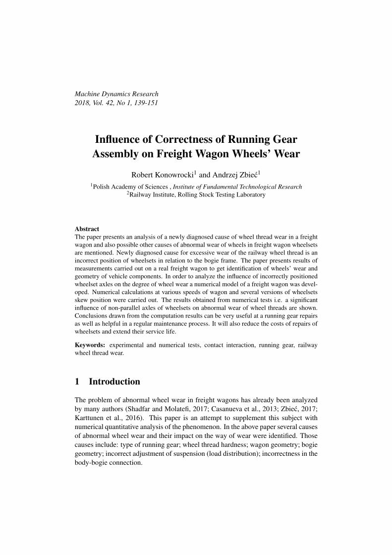
Machine Dynamics Research2018, Vol. 42, No 1, 139-151
Influence of Correctness of Running GearAssembly on Freight Wagon Wheels’ Wear
Robert Konowrocki1 and Andrzej Zbiec1
1Polish Academy of Sciences , Institute of Fundamental Technological Research2Railway Institute, Rolling Stock Testing Laboratory
AbstractThe paper presents an analysis of a newly diagnosed cause of wheel thread wear in a freightwagon and also possible other causes of abnormal wear of wheels in freight wagon wheelsetsare mentioned. Newly diagnosed cause for excessive wear of the railway wheel thread is anincorrect position of wheelsets in relation to the bogie frame. The paper presents results ofmeasurements carried out on a real freight wagon to get identification of wheels’ wear andgeometry of vehicle components. In order to analyze the influence of incorrectly positionedwheelset axles on the degree of wheel wear a numerical model of a freight wagon was devel-oped. Numerical calculations at various speeds of wagon and several versions of wheelsetsskew position were carried out. The results obtained from numerical tests i.e. a significantinfluence of non-parallel axles of wheelsets on abnormal wear of wheel threads are shown.Conclusions drawn from the computation results can be very useful at a running gear repairsas well as helpful in a regular maintenance process. It will also reduce the costs of repairs ofwheelsets and extend their service life.
Keywords: experimental and numerical tests, contact interaction, running gear, railwaywheel thread wear.
1 Introduction
The problem of abnormal wheel wear in freight wagons has already been analyzedby many authors (Shadfar and Molatefi, 2017; Casanueva et al., 2013; Zbiec, 2017;Karttunen et al., 2016). This paper is an attempt to supplement this subject withnumerical quantitative analysis of the phenomenon. In the above paper several causesof abnormal wheel wear and their impact on the way of wear were identified. Thosecauses include: type of running gear; wheel thread hardness; wagon geometry; bogiegeometry; incorrect adjustment of suspension (load distribution); incorrectness in thebody-bogie connection.

140 Konowrocki R., Zbiec A.
Fig. 1. 1XTa type bogie (Zbiec, 2017).
Fig. 2. Y25 type bogie (Zbiec, 2017).
2 Causes of abnormal wheel wear
Type of running gear of freight bogies is one of the most important factors that mayresult in abnormal wheel wear. The great majority of bogies used in railway freighttransport consist of 1XT (Fig. 1) a type bogies and all varieties of Y25 type bogies.The most important structural difference between those types of bogies is a clearancein the longitudinal guiding of the wheelsets. The 1XTa type bogies have such clear-ance between an axle box and bogie frame, while the Y25 series has not (Fig. 2).The clearance in wheelset guides provides for the possibility of parallel alignmentof the wheelsets on the straight track and radial alignment in curves. In case of theY25 type bogie that possibility does not exist since the axle box is pressed againstthe guiding plate with the plunger. Hardness of the wheel thread must be kept withindefined limits. Too hard wheels will result in excessive wear of rails, too soft in thesame of wheels.
The geometry of the wagon, or actually for the essence of the phenomenon dis-cussed here, the position of the bogie pivots may influence the higher loads of one ofthe bogies (longitudinal asymmetry) and/or the larger wheel loads on one side of thewagon (transverse asymmetry).
The geometry of the bogie - in this view, these are two elements. The first one isthe location of bogie pivot seats, which will have an analogous effect on each bogie,such as the position of the pivots in the wagon geometry - it can affect the higherloads of one of the wheelsets (longitudinal asymmetry) and/or higher wheel loads onone side of the wagon (transverse asymmetry). The second one is the geometry ofthe places responsible for guiding the wheelsets, and therefore their proper relativeposition. The wheelsets should be in one plane and parallel to each other. Their

Influence of Correctness of Running Gear Assembly ... 141
Fig. 3. Non-parallel position of wheelsets in B-bogie.
Fig. 4. New wheel thread and that with an excessively worn flange.
relative position cannot form a rhombus.Incorrect suspension adjustment changes the distribution of wheel loads within
the wagon (bogie), causing similar effects as in the wrong wagon geometry (geometryof the bogie pivots position), but with reference to a specific wheel. Incorrect torqueof the bogie relative to the body, and in the discussed issue - too high torque willcontribute to increasing the wear of the wheels when entering and exiting the curvesof the track.
Other reasons include those that result from incorrect maintenance of the wagon,such as badly repaired axle boxes (which can change the relative position of wheelsets),cracked or incorrectly mounted suspension springs (which can change the distribu-tion of wheel loads within the bogie) or incorrect buffer lengths, generating additionallateral forces.
Among the above mentioned factors, the relative parallel position of the wheelsetsin the bogie is of the greatest importance. In case the lack of it, despite riding on astraight track, the bogie behaves as if it were riding on a curve, which results ina continuous flange-rail contact of the leading wheelset of B-bogie (see Fig. 3),causing accelerated wear of the flange. An example of such wear observed duringmeasurements on a real object is shown in the picture (Fig. 4).
On the basis of measurements of the distance between the centers of the tread ofa given wheel and the center of the tread of wheel on the same side of the bogie, thevalues of distances a and b were determined (see Fig. 5). This allowed to estimate thevalue of parameter ∆ = a−b defining the skewed setting of wheelsets. From the ob-tained results, measured on several used Y25 type bogies, the value of parameter ∆ inthe range of 0-14 mm was determined. On that basis, the skew angle of the wheelsetϕskew in the range 0-0.53 was determined with the assumption of the measuring baselbase = 1500 mm.

142 Konowrocki R., Zbiec A.
Fig. 5. Position of measured distances defining relative non-parallelity of wheelsets.
Fig. 6. Excessively worn wheel flange of the tested vehicle.

Influence of Correctness of Running Gear Assembly ... 143
Because of observed excessive wear of flanges, measurements of thread profilewere also carried out during the investigation.
Taking into account the above observations on measurements, a theoretical analy-sis of the influence of skewed setting of the wheelsets of a freight wagon on excessivewear of the wheel flanges was carried out. Theoretical approach and obtained resultsare presented in the next chapter.
3 Numerical analysis of the considered phenomenon
3.1 Mathematical model of the vehicle-track system
In order to conduct numerical studies of wheel wear, a model of a freight wagonequipped with Y25 type bogies was created. The physical model of the vehicle as asystem of rigid bodies joined together by means of visco-elastic elements is consid-ered. This approach is called the MBS method (Fraczek and Wojtyra, 2008; De Jalonand Bayo, 1994) and is very often applied in commercial software, i.e. Simpack, Vi-Rail, Vampair. Numerous researchers (Konowrocki and Walczak, 2017; Szolc, 1998;Bogacz and Konowrocki, 2012; Piotrowski and Pazdzierniak, 2010; Konowrocki andWalczak, 2017; Szolc et al., 2002) have applied this method for an analysis of dy-namics of railway vehicle-track system. In this approach the structural elements ofthe vehicle and track are regarded as rigid bodies. The suspension is described byflexible elements with a given stiffness and damping. The trajectories of motion ofthose rigid bodies result from the imposed holonomic constraints. The freight wagonmodel consists of three basic elements: i.e. two bogie containing two wheelset eachand one carbody. The wheelset, the bogie frame and the carbody are described asrigid elements with three, five and five degrees of freedom, respectively. A motion ofsuch a structure of the wagon model can be mathematically described by means ofordinary second order differential equations derived using the Lagrange equations ofthe second kind. The general matrix form of the mathematical model is described byformula (1):
[Mp2 +Cp+K] ·q = F (1)
where: q - denotes the vector of system coordinates, M - is the symmetric inertiamatrix, C - denotes the damping matrix, K - is the stiffness matrix, F - denotes theforce vector and p = d/dt - is the differential operator.
Due to the fact that the analyzed case refers to wheel thread wear, the modelstructure of the freight wagon and its mathematical description are described briefly.More attention to the description of the wheel-rail contact and the methodology ofdetermination of the wheel wear is paid.

144 Konowrocki R., Zbiec A.
3.2 Prediction of wheel thread wear
Based on the model of the freight wagon described above, a wheel thread wear modelwas built. A wear model was created by integration of numerical procedures deter-mining a wheel-rail contact of the wagon model and particular wheel threads’ wear.An algorithm of the wheel wear model can be divided into five blocks. First one is thefreight wagon model, second one determines the contact conditions between wheelsand rails resulting from the interaction between the railway vehicle and track. In thethird block, a position, shape and size of a contact surface are calculated. Based onthose parameters local distribution of work of friction forces per unit of the contactsurface is determined in the fourth block. In the fifth block, by use of a wear modeldescribed below, the wheel profiles distorted by wear are created.
In the wheel wear prediction model, the numerical procedures to determine theforces and areas of their action in wheel-rail contact zones are used. The contact be-tween wheel and rail is modeled as a flexible contact element. Some authors (Bogaczand Frischmuth, 2016) study the rolling motion of a polygonalised railway wheel onthe rail. For uniform guiding motion, the trajectory of the contact point and verti-cal accelerations are evaluated first in the rigid case, then in the case of elastic andvisco-elastic contact. In our case, a rigid penetration of the undeformed wheel andrail profiles is adopted to calculate the normal pressure distribution, according to theprocedure shown in the paper by Piotrowski and Kik (2008). To determine tangentcontact forces the FASTSIM algorithm (?) is used. This algorithm divides the ellipse-shaped contact zone into smaller cells. In each of them, it determines shear stressesand micro-slips in the longitudinal and transverse direction in relation to the wheelmovement. Then in the wheel-rail contact zones the adhesion areas are determined.The contact geometry parameters as input values to the FASTSIM procedure are tabu-lated depending on the transverse displacement of the wheelset. This approach allowsreduction of the calculation time in relation to the calculation in each iteration at thenew contact parameters. Graphic visualizations of these contact geometry parametersare shown in the graphs (Fig. 7 and 8). In the next stage of procedure a determinationof the wheel wear is carried out by calculation of the right hand sides of the equationsof motion describing dynamics of the railway vehicle components. The results ob-tained from the calculations are used for determination of radial wheel profiles’ wearvalues. A description of the method used to determine the above mentioned wheelprofile wear is described in detail in the next chapter. For the analysis describedabove the UIC railway wheels (S1002) and UIC60 rail profiles were used. In numer-ical tests an inclination of the rails mounted in the railway track and the coefficientof friction between wheels and rails was assumed at 1:40 and 0.36, respectively. Thewheel wear simulation model was 59 degrees of freedom.

Influence of Correctness of Running Gear Assembly ... 145
Fig. 7. Contact points plot of the wheel profile UIC (S1002) and rail UIC60 at 1:40inclination.
Fig. 8. Wheel (S1002) - rail (UIC60) contact geometry as a function of wheelset lateraldisplacement.

146 Konowrocki R., Zbiec A.
3.3 Wear model
To determine quantitative wear of the wheel profile caused by rolling contact, it isnecessary to adopt a suitable wear model. Typically, input data to the wear modelshould include material properties and mechanical interactions in the contact zone,which allows to determine the distribution of the wear depth across the transverseprofile of the kinematic couple. The wear describes how much material per unit oftime or distance covered is removed. In this sense, we usually distinguish two typesof wear: normal, when the wear process takes place relatively slowly (e.g. intensityof wagon operation is rather low and mainly on the straight track), and accelerated(e.g. adhesive wear of flanges in tight curves of the track). The transition between theregime of normal and accelerated wear depends on the combination of contact condi-tions such as slip speed, contact pressure and temperature. In many publications wecan find models of wheel profile wear obtained both from theoretical considerations(Esveld et al., 2004; Jendel, 2002; Enblom, 2009), and from an experimental inves-tigation performed during the operation of railway vehicles (Lonsdale et al., 2011).However, they are to a great extent an approximation of selected phenomena thatcause the wheel wear. To assess the wear and tear resulting from the presence ofslippage and friction in rolling contact the Archard model (Archard, 1953) is mostwidely used. The wear model is based on the theory of asperity contact. Archard’sequation is often presented in the form of a formula:
mw =C ·wr (2)
where: mw [/mu g/m2] - denotes the mass of material removed on the contact surfacearea, C=1.24· 10 −9 [kg/Nm] - is the wear coefficient and wr [Nm/m2] - denotes thework of friction forces acting on the contact area.
In the wear simulation algorithm the Archard model is adapted to the case ofwheel-rail contact. According to that model, the wear of wheel thread occurs onlyin a slip area of the wheel-rail contact zone. Using the FASTSIM algorithm (Kalker,2007) the slip area is divided into small elements for which longitudinal and trans-verse slip velocities and the average density of tangential forces for each of them aredetermined. The average work density is proportional to the mass of the materialremoved in a certain proportion determined by the wear coefficient C, as describedin Chudzikiewicz (2001).
3.4 Numerical results
In preliminary numerical tests the above described freight wagon wheels’ wear modelwas used. Using that model the change in the skew angle ϕskew of wheelsets of thefirst bogie was analyzed. Such case can be caused for example by incorrect assemblyof wheelsets after repair. The values of the skew angle of wheelsets ϕskew = 0.25
and ϕskew = 0.5 were adopted. In the numerical studies, scenarios of freight wagon
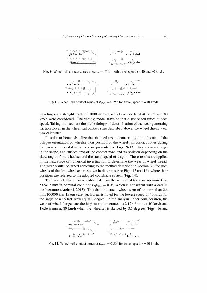
Influence of Correctness of Running Gear Assembly ... 147
Fig. 9. Wheel-rail contact zones at ϕskew = 0 for both travel speed v= 40 and 80 km/h.
Fig. 10. Wheel-rail contact zones at ϕskew = 0.25 for travel speed v = 40 km/h.
traveling on a straight track of 1000 m long with two speeds of 40 km/h and 80km/h were considered. The vehicle model traveled that distance ten times at eachspeed. Taking into account the methodology of determination of the wear generatingfriction forces in the wheel-rail contact zone described above, the wheel thread wearwas calculated.
In order to better visualize the obtained results concerning the influence of theoblique orientation of wheelsets on position of the wheel-rail contact zones duringthe passage, several illustrations are presented on Figs. 9-13. They show a changein the shape, and surface area of the contact zone and its position depending on theskew angle of the wheelset and the travel speed of wagon. These results are appliedin the next stage of numerical investigation to determine the wear of wheel thread.The wear results obtained according to the method described in Section 3.3 for bothwheels of the first wheelset are shown in diagrams (see Figs. 15 and 16), where theirpositions are referred to the adopted coordinate system (Fig. 14).
The wear of wheel threads obtained from the numerical tests are no more than5.09e-7 mm in nominal conditions ϕskew = 0.0, which is consistent with a data inthe literature (Archard, 2013). This data indicate a wheel wear of no more than 2.6mm/100000 km. In our case, such wear is noted for the lowest speed of 40 km/h forthe angle of wheelset skew equal 0 degree. In the analysis under consideration, thewear of wheel flanges are the highest and amounted to 2.12e-6 mm at 40 km/h and1.65e-6 mm at 80 km/h when the wheelset is skewed by 0.5 degrees (Figs. 16 and
Fig. 11. Wheel-rail contact zones at ϕskew = 0.50 for travel speed v = 40 km/h.

148 Konowrocki R., Zbiec A.
Fig. 12. Wheel-rail contact zones at ϕskew = 0.25 for travel speed v = 80 km/h.
Fig. 13. Wheel-rail contact zones at ϕskew = 0.50 for travel speed v = 80 km/h.
Fig. 14. Nominal wheel thread profiles (S1002) in the reference coordinate system usedfor the wear charts.
Fig. 15. Wheel thread profile wear for the two skew angles of wheelset axle at travel speedof 40 km/h.
Fig. 16. Wheel profile wear for the two skew angles of wheelset axle at travel speed of 80km/h.

Influence of Correctness of Running Gear Assembly ... 149
17). Such a value of wear is 4.24 times higher than without the wheelset skewed.
4 Conclusions
The experimental and numerical investigation are presented in the paper. The ob-tained results, the key influence of wheelset assembly incorrectness in the bogieframe for abnormal wear of wheel threads are shown. The effects, especially ex-cessive wear of their flanges are visible. The results of analysis show that the wearof wheel threads intensifies at a larger angle of wheelset skew, which agrees withthe intuition. On the other hand, the reduction of the intensity of undercutting of thewheel flange with an increasing speed is noticeable. The presented results indicatethe need for execution of further detailed experimental tests on other wagons in or-der to validate the observed phenomenon. As a first suggestion, the monitoring andimprovement of repair procedures of running gears are proposed. Within the frame-work of further investigations an attempt should also be made in order to determinethe limit non-parallelity of wheelsets in the bogie, which should become a param-eter being checked during repair or replacement of wheelsets. Such approach maylead to an improvement in the maintenance of railway rolling stock, namely an in-crease of service life between successive wheel reprofiling, and thus a reduction ofmaintenance costs.
References
Archard, J. (1953). Contact and rubbing of flat surfaces. Journal of applied physics,24(8):981–988.
Archard, J. (2013). Rail vehicles wheels wear and re-profiling. Scientific Journal ofSilesian University of Technology, Series Transport, (79):61–69.
Bogacz, R. and Frischmuth, K. (2016). On dynamic effects of wheel–rail interac-tion in the case of polygonalisation. Mechanical Systems and Signal Processing,79:166–173.
Bogacz, R. and Konowrocki, R. (2012). On new effects of wheel-rail interaction.Archive of Applied Mechanics, 82(10-11):1313–1323.
Casanueva, C., Jönsson, P.-A., and Stichel, S. (2013). Use of archard’s wear law forthe calculation of uniform wheel wear of high tonnage freight vehicles. In 2013Joint Rail Conference, pages V001T02A013–V001T02A013. American Societyof Mechanical Engineers.
Chudzikiewicz, A. (2001). Modelling of wheel and rail wear. , The Archives ofTransport, pages 1–4.

150 Konowrocki R., Zbiec A.
De Jalon, J. G. and Bayo, E. (1994). Kinematic and dynamic simulation of multibodysystems: the real-time challenge. Springer Science & Business Media.
Enblom, R. (2009). Deterioration mechanisms in the wheel–rail interface with focuson wear prediction: a literature review. Vehicle System Dynamics, 47(6):661–700.
Esveld, C., Markine, V., and Shevtsov, I. (2004). Shape optimization of a railwaywheel profile. XXI International Congress of Theoretical and Applied MechanicsWarsaw, Poland.
Fraczek, J. and Wojtyra, M. (2008). Kinematics of multibody. Calculation methods.WNT.
Jendel, T. (2002). Prediction of wheel profile wear—comparisons with field mea-surements. Wear, 253(1-2):89–99.
Kalker, J. (2007). A fast algorithm for the simplified theory of rolling contact. Vehiclesystem dynamics, 11(1):1–13.
Karttunen, K., Kabo, E., and Ekberg, A. (2016). Estimation of gauge corner andflange root degradation from rail, wheel and track geometries. Wear, 366:294–302.
Konowrocki, R. and Walczak, S. (2017). Influence of flexibility parameters of wheelsand wheelset on the railway bogie dynamics-experimental and theoretical investi-gations. Machine Dynamics Research, 41.
Lonsdale, C., Bogacz, R., and Norton, M. (2011). Application of pressure pouredcast wheel technology for european freight service. In Proc. of World CongressRailway Research. Lille, page 23.
Piotrowski, J. and Kik, W. (2008). A simplified model of wheel/rail contact mechan-ics for non-hertzian problems and its application in rail vehicle dynamic simula-tions. Vehicle System Dynamics, 46(1-2):27–48.
Piotrowski, J. and Pazdzierniak, P. (2010). Influence of dither generated byrolling contact on friction damping in freight wagons. Vehicle system dynamics,48(S1):195–209.
Shadfar, M. and Molatefi, H. (2017). A study on transient wear behavior of newfreight wheel profiles due to two points contact in curve negotiation. Journal ofTheoretical and Applied Mechanics, 55.
Szolc, T. (1998). Medium frequency dynamic investigation of the railway wheelset-track system using a discrete-continuous model. Archive of Applied Mechanics,68(1):30–45.

Influence of Correctness of Running Gear Assembly ... 151
Szolc, T., Nagórski, Z., and Piotrowski, J. (2002). Simulation of vehicle—track inter-action in the medium frequency range with application to analysis of mechanicaland thermal loading in contact. Vehicle System Dynamics, 37(sup1):641–652.
Zbiec, A. (2017). Causes of abnormal wear of wheelsets in freight wagons. Papersof the Railway Institute, 155:43–47.


Machine Dynamics Research2018, Vol. 42, No 1, 153-163
The Impact of Changes in the Designs of ConcreteAirport Pavement on Its Strength Properties
Robert Brodzik*
Polish Air Force UniversityDepartment of Logistics Management
AbstractThe article presents the analysis of dowelled slabs made of reinforced concrete which weresubjected to thermal and operational loads, in the aspect of varying diameter of the dowelsand their arrangement. The main object of the study was to present a stress-strength analysisof a fragment of a concrete airport pavement composed of a system of four identical slabswith dimensions of 5m x 5m and 0.3m thickness which were dowelled with one another.Using modifications of both the diameters of the dowels and their spacing, a detailed assess-ment of the state of stresses and displacements was made both in selected portions of airportconcrete slabs and in dowels themselves using the finite element method. Using certain vari-ants of dowel settings and diameters, an assessment was made as to the selection of optimumparameters for concrete airport pavement designs.
Keywords: concrete reinforcement, dowels, concrete airport pavement, numerical modeling,operational loads, thermal loads.
1 Introduction
The origins of concrete pavement date back to ancient times, when the Romansstarted using cement for bonding road surfacing. However, the first concrete pave-ment, as it is understood today, was created only in the early 20th century in theUnited States. It was a test section, whose length was 1 mile, made of slabs with thethickness of 0.175m, and the width of 4.5 m. The entire road surface was divided byexpansion gaps with wooden inserts situated every 7.5m. In Poland, the first experi-ments with the new road construction technology were conducted in Krakow in 1912.In comparison to the beginnings dating back to the twentieth century, a huge evolu-tion and technological revolution took place in concrete pavements, which includes:the introduction of concrete slabs, the obligation to use aerated concrete admixtures,the application of curing agents for fresh concrete, and the optimization of drivability

154 Brodzik R.
and strength parameters of the pavement by the application of reinforcement. Manycountries, mainly from Western Europe, have already learned about the advantagesof concrete pavements. It is Germany that has the longest and the most extensivetradition of their construction in Europe. In Germany, at present, there are more than12,000km of highways, and as much as 40 percent of such roads is made in concretetechnology.
Rigid pavements made of cement concrete are currently also the primary andcommonly used type of airport infrastructure. The main function of airport pave-ments is to transfer loads from aircraft wheels through concrete surface layers anddissipating those loads onto the lower base layers. In the concrete pavement itself,in addition to the stresses caused by the weight of the aircraft and transmitted by itsindividual wheels, there are also thermal stresses caused by weather conditions. Thedevelopment of concrete pavements depends largely on experimental tests performedon test and experimental pavement sections subjected to extreme operational condi-tions. Initially, concrete pavements were designed and constructed as a standard fora short period of use, in the range of 20÷25 years. At present, there is a good reasonto design and construct concrete pavements for up to 60 year-time periods. The ownweight of the airport pavement construction, as well as additional, variable, opera-tional loads caused by aircraft and thermal loads, causes fatigue weakening of theconcrete slab surfaces as a result of cyclic combination of operational and thermalloads. In the long run, this leads to damage to the surface in the form of scratches,followed by cracks and scaling. (Nita, 2005).
Doweling of the pavement is the joining of the slab edges with steel elements, toensure the cooperation of neighboring slabs in load transfer. A single dowel is a steelrod vertical in relation to the gap between the slabs. It provides partial transfer ofexternal loads to adjacent slabs and, at the same time, allows independent horizontalmovements of adjacent slabs. Observations and analyses of concrete pavements showthat doweling causes leveling of the slabs, reduces the maximum primary stresses,and contributes to the reduction of the maximum slab deflections. Moreover, it signif-icantly improves the cooperation between slabs in expansion gaps, thus contributingto eliminate the slab faulting phenomenon (Dacko and Brodzik, 2007).
2 Research problem formulation
It can be noticed on the basis of the analysis of domestic technical literature thatthe selection of parameters and dimensions of reinforcement elements is subject togreat flexibility1. One of the methods leading to understanding the nature of thedoweling influence on airport pavements under both operational and thermal loads isthe strength analysis of the surface using the finite element method (FEM).
1NO-17-A204:2015, Lotniskowe nawierzchnie betonowe. Wymagania i metody badan nawierzchniz betonu cementowego

The Impact of Changes in the Designs of Concrete Airport ... 155
Fig. 1. Continuous space divided into subspaces.
Dynamic development of approximate calculation methods is increasingly prompt-ing designers to use models based on the finite element method. The essence of FEMis that each parameter value (e.g. displacement) described by a continuous (basis)function in the area under consideration is approximated by a discrete model. Thismodel consists of a set of continuous functions defined in a finite number of sub-spaces (1), called elements, into which a given space has been divided (Fig.1):
Ω =n
∑i=1
Ω1 (1)
Continuous functions in subspaces are defined on the basis of the basis functionin a finite number of points located inside the space, called nodes(Rakowski andKasprzyk, 1993).
The analysis of the results comprises nine examples differing as to the dowelingmethod (change of the dowel diameter and spacing) of airport pavements in order toassess the state of stresses and displacements of airport concrete slabs and of dowelsthemselves. The numerical analysis takes into consideration operational and thermalloads as well as the weight of the slab itself. Having the results of numerical analyzes,a detailed analysis of pavement effort was made with regard to two major operationaland functional factors of airport pavements. The results obtained, in comparison withthe generalized and imprecise design requirements which are described in detail inthe standards, allow one to predict the pavement durability and to take the appropriateactions concerning the pavement design scheme.
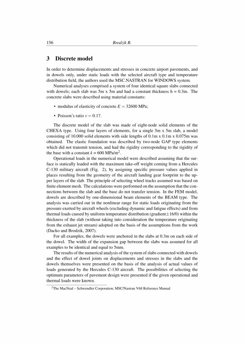
156 Brodzik R.
3 Discrete model
In order to determine displacements and stresses in concrete airport pavements, andin dowels only, under static loads with the selected aircraft type and temperaturedistribution field, the authors used the MSC.NASTRAN for WINDOWS system.
Numerical analyses comprised a system of four identical square slabs connectedwith dowels; each slab was 5m x 5m and had a constant thickness h = 0.3m. Theconcrete slabs were described using material constants:
• modulus of elasticity of concrete E = 32600 MPa;
• Poisson’s ratio v = 0.17.
The discrete model of the slab was made of eight-node solid elements of theCHEXA type. Using four layers of elements, for a single 5m x 5m slab, a modelconsisting of 10.000 solid elements with side lengths of 0.1m x 0.1m x 0.075m wasobtained. The elastic foundation was described by two-node GAP type elementswhich did not transmit tension, and had the rigidity corresponding to the rigidity ofthe base with a constant k = 600 MPa/m2.
Operational loads in the numerical model were described assuming that the sur-face is statically loaded with the maximum take-off weight coming from a HerculesC-130 military aircraft (Fig. 2), by assigning specific pressure values applied inplaces resulting from the geometry of the aircraft landing gear footprint to the up-per layers of the slab. The principle of selecting wheel tracks assumed was based onfinite element mesh. The calculations were performed on the assumption that the con-nections between the slab and the base do not transfer tension. In the FEM model,dowels are described by one-dimensional beam elements of the BEAM type. Theanalysis was carried out in the nonlinear range for static loads originating from thepressure exerted by aircraft wheels (excluding dynamic and fatigue effects) and fromthermal loads caused by uniform temperature distribution (gradient±16/0) within thethickness of the slab (without taking into consideration the temperature originatingfrom the exhaust jet stream) adopted on the basis of the assumptions from the work(Dacko and Brodzik, 2007).
For all examples, the dowels were anchored in the slabs at 0.3m on each side ofthe dowel. The width of the expansion gap between the slabs was assumed for allexamples to be identical and equal to 5mm.
The results of the numerical analysis of the system of slabs connected with dowelsand the effect of dowel joints on displacements and stresses in the slabs and thedowels themselves were presented on the basis of the analysis of actual values ofloads generated by the Hercules C-130 aircraft. The possibilities of selecting theoptimum parameters of pavement design were presented if the given operational andthermal loads were known.
2The MacNeal – Schwendler Corporation, MSC/Nastran V68 Reference Manual
The Impact of Changes in the Designs of Concrete Airport ... 157
Fig. 2. Hercules C-130 aircraft on the apron of the Powidz airport.
4 Analysis of results
Theoretical analysis of the process of joining slabs and the use of steel reinforcementelements in the form of dowels which is described, i.a. in Polish standards34 allowsfor a large freedom of selecting dowel diameters and spacing depending on the natureof the load.
On the basis of the above-mentioned assumptions, presented in the standards, thefollowing nine variants of a four-slab model were adopted for the analysis:
• circular cross-section dowels, from φ12mm to φ50mm (Examples 1÷5; φ12,φ20, φ30, φ40, φ50) uniform dowel spacing, one every 0.2m
• uniform dowel spacing along the slab edge, from 0.2m to 0.5m.(Examples6÷9; 0.2m; 0.3m; 0.4m; 0.5m spacing) for φ30mm dowels.
A detailed analysis comprised six characteristic examples out of nine, for whichthe results are presented in Table 1.
For the above calculations, two groups of results were obtained for each example:
• for concrete slabs: maximum principal stress σmax and maximum slab deflec-tion zmax/− zmin;
• for dowels normal stress σg and shear stress τmax calculated on the basis ofshearing forces distribution T .
On the basis of theoretical schemes of slab damage caused by thermal and operationalloads, as well as by the own weight of the slabs described in the work (Dacko andBrodzik, 2009), two variants in which the maximum principal stress in slabs reachesextreme values were selected for the analysis:
3PN-75/S-96015 Drogowe i lotniskowe nawierzchnie z betonu cementowego.4PN-EN 13877-3 Nawierzchnie betonowe – Part 3.

158 Brodzik R.
Table 1. Result summary for selected examples

The Impact of Changes in the Designs of Concrete Airport ... 159
Fig. 3. Example 3 - σmax at the top of the slab for the negative gradient and external loadat the corner of the slab [MPa].
• operational stress in the slab center and positive gradient +16/0;
• operational stress in the slab corner and negative gradient -16/0.
4.1 Result analysis for a slab
The analysis of the influence of dowel diameter and spacing changes at combinedloads shows only a slight effect on the values of the resulting maximum principalstresses as well as on the maximum slab deflections. The results obtained for slabsconfirm the principle that using a large freedom in the selection of doweling parame-ters, being within a wide range of recommended dowel diameters and spacings, theseparameter changes affect the values of maximum principal stresses and deflections ofthe slab only to a small extent.
However, on the basis of the analysis of selected examples, it can be observed thatwhen increasing the diameter of the dowels from φ12 to φ50 with an unchanged spac-ing, we initially observe a slight decrease in the value of σmax (1.57MPa->1.55MPa;2.75MPa ->2,74MPa), followed by another increase (1.55MPa -> 1.63MPa; 2.74MPa-> 2.76MPa). While the magnitude of changes in the σmax value shows a negligiblesignificance of modifying the diameter of the dowels, it can be concluded that foreach load one should look for the so-called optimum solution. A similar situationoccurs when analyzing the maximum slab deflections. For the described examples,in the aspect of the analysis conducted for the slab itself, Example 3 is an optimumsolution, where both the maximum principal stresses and the maximum deflectionsof the slab reach the minimum values (Fig.3÷4). On the basis of a detailed analysisof the results obtained for each pavement, it is possible to determine the state forwhich further increase of the diameter and reduction of the spacing between the dow-els becomes pointless. The optimum arrangement for the adopted assumptions andloads is the 0.2m spacing between individual dowels and their diameter being equalto φ30mm.

160 Brodzik R.
Fig. 4. Example 3 - plate deformation for the negative gradient and external load at thecorner of the board [mm].
5 Result analysis for dowels
As far as diameter changes and the spacing of the dowels are concerned, analyzeswere also performed of stress in the dowels themselves concerning total loads. Themaximum values of normal stresses in dowels for the analyzed examples fall in avery wide range: for the positive gradient from σg = 52MPa (Example 1) to σg =117MPa (Example 8), whereas for the negative gradient from σg = 100MPa (Exam-ple 3, Fig.5) to σg = 341MPa (Example 1, Fig.6). Extreme values of σg occur for thenegative gradient and the load exerted on the slab corner. In two cases out of nineexamples analyzed, it was observed that normal stresses σg exceeded the allowablevalues kg (Table 2 - red color). In accordance with the Polish standards 5 allow-able bending stress [kg] for dowels with the diameter in the range of 16÷40 mm is145MPa, whereas allowable tensile stress [kt] is 90MPa. It can be assumed for thenegative gradient that the dowel spacing and diameter applied in Examples 1-2 re-quires correction for loads exerted by the Hercules C-130 in the corner of the slab.Like in the case of normal stresses, the analysis of the transverse force distribution indowels, which was conducted in accordance with the formula:
τmax =43· Tmax
A(2)
where: Tmax - maximum value of shearing force [N], A - cross-sectional area of adowel [mm2]. proved that extreme values of τmax=469 MPa (Table 1) and τmax=164MPa, are also present for examples 1÷2, and the allowable stresses kt were observedto have been exceeded . Moreover, in the analysis of τmax the allowable values wereobserved to have been were exceeded in the case of increasing the spacing betweenthe dowels (Examples 7÷8). Detailed analysis of the results shows that for everypavement it is possible to determine the state for which further increase of the diame-ter and reduction of the spacing between the dowels becomes pointless. The optimum
5See 4

The Impact of Changes in the Designs of Concrete Airport ... 161
Fig. 5. Example 3 - distribution of normal stresses in dowels for the negative gradient andthe load at the slab corner [MPa].
Fig. 6. Example 1 - distribution of normal stresses in dowels for the negative gradient andthe load at the slab corner [MPa].
arrangement for the adopted assumptions and loads is the 0.2m spacing between in-dividual dowels and their diameter being equal to φ50mm.
The results obtained for selected examples point out that in most cases too smalldiameter or spacing of dowels, despite being compliant with the applicable standardsfor a given slab thickness, generates large values of normal and tensile stresses whichexceed the allowable values (Fig.6).
It should be stressed that the cases presented here are only an attempt at present-ing the FEM capabilities for conducting stress and displacement analyzes in slabsand dowels. In no way does the analysis adopted, covering nine examples, exhaustthe possibility of further analysis based on successive factors that can be influencedduring the development of the design project, e.g. change in the slab thickness orsize, or in the rigidity of the base.
6 Conclusions
• The analyzes presented in the work have shown the possibility of using profes-sional FEM programs to perform a full analysis of the state of displacementsand stresses within slabs and dowels.

162 Brodzik R.
Fig. 7. Example 1 - distribution of shearing forces in dowels for the negative gradient andexternal load at the corner of the slab [MPa].
Fig. 8. Example 4 - distribution of shearing forces in dowels for the negative gradient andexternal load at the corner of the slab [MPa].

The Impact of Changes in the Designs of Concrete Airport ... 163
• The analysis allows examples to be selected as being the most advantageousfor strength and safety reasons.
• The analyzes performed in the work show that the dowel scheme adopted rel-ative to the spacing and diameter of the dowels has an impact particularly onthe values of the maximum stress in the dowels.
• The complex nature of the pressure stresses occurring in the vicinity of doweljoints, requires additional analyzes involving the use of models of a differentscale.
• Apart from the analysis of the influence of dowel dimensions and spacing,the proposed numerical studies allow additional analyses to be performed inwhich the range of problems under consideration will contain many importantadditional factors, i.e. the impact of slab geometry, properties of materials usedor the properties of the base.
References
Dacko, M. and Brodzik, R. (2007). Numeryczna analiza betonowych dyblowanychpłyt lotniskowych. Drogownictwo, pages 196–202.
Dacko, M. and Brodzik, R. (2009). Analiza betonowych płyt lotniskowych przyobciazeniach uzytkowych i termicznych. Drogownictwo, pages 306–313.
Nita, P. (2005). Betonowe nawierzchnie lotniskowe: teoria i wymiarowanie konstruk-cyjne. Wydawnictwo Instytutu Technicznego Wojsk Lotniczych.
Rakowski, G. and Kasprzyk, Z. (1993). Metoda elementów skonczonych w mechan-ice konstrukcji. Oficyna Wydawnicza Politechniki Warszawskiej, wyd, 1.


Machine Dynamics Research2018, Vol. 42, No 1, 165-179
Electromechanical System for Charging Batteriesof Electric Cars
Zdzisław Trzaska*
University of Ecology and Management
AbstractAn electric vehicle battery charger based on the Faraday disk generator is developed in thispaper to reduce the amount of time it takes for the rotational energy to be converted intoelectrical energy. The kinetic energy of the generator during charging is transformed effec-tively into electric energy by rotating the compact formed from the disk permanent magnetand conducting shield by means of an electric motor supplied from the power grid using pos-sibly renewable energy sources. One of the advantages of the Faraday disk generator is itshigh power capability, which is applicable for high rate of charging and reducing the amountof time it takes for the rotational energy to be converted into electrical energy. Computersimulations have been performed for various sets of the charger element parameters and afterselecting the obtained results, the optimal set was established. Simulation results for chargingprocesses corresponding to the optimal element parameter tests are included.
Keywords: urban transport, electric car, Li-ion battery, Faraday disk generator, batterycharger, state-space model, computer simulation.
1 Introduction
Presently, the problem of energy becomes so important that all the attention of mod-ern societies and entire industries is turning towards clean, renewable energy (solarenergy, wind energy, etc.). In addition, many cars are designed to use only electricityas motive power, which reduces greenhouse gas emissions and noise level to zero. Itshould be emphasized that electric drive vehicles are among the most advanced ve-hicles at the moment, taking into account an important decrease of environment con-tamination. Therefore, the current priorities for the development of electric drivesin vehicles are primarily ecological. Electric vehicles (EVs) in the field of use donot emit any pollution (in fact, of course, they emit solid particles, derived from thepair of tribological parts in the vehicle, the cooperation of the wheels with the roadsurface and dust from the road). EVs are also characterized by much lower noise

166 Trzaska Z.
emissions than those with combustion engines. Moreover, an important advantage ofusing electric cars is the ability to protect raw materials for the production of liquidand gaseous fuels because there are many types of primary energy carriers that canbe used to power EVs such as, for instance, renewed energy sources (Eberhard andTarpenning, 2006).
In the case of vehicles with electric drives there is a possibility of "moving" placesof emission sources from the most dangerous areas - from the centres of large urbanagglomerations - to the location of power plants. However, the electric car has al-ready become a technology that in the world market has successfully busted throughthe bastions so far dominated by vehicles driven by conventional combustion engines(Bolonkin, 2007). From a technical point of view, it should be appreciated that intoday’s vehicles, the weakest elements are electric energy accumulators. This is byno means a surprise, as it is well-known that energy storage is a particularly difficultproblem - so far unsurpassed use is the use of liquid fuels (Struchtrup, 2014). It isworth to emphasize that in recent years great technical progress has been made in theareas of system structures and key component developments for EVs, but there is stilla performance gap between electric vehicles and conventional vehicles with respectto driving range, energy-saving and car power efficiency, as well as passenger safety.For these, among other reasons, today major research efforts in the wide world areinvested in the development of high energy density batteries with minimum electricservice requirements (ESR). Note also that modern EVs have full information systemthat is under constant modifications and does monitoring of inside and outside param-eters in order to achieve maximum energy savings. Development of new components,improved connections and electric engine control algorithms allow increase of effi-ciency of power appliances, therefore electric engine itself, to the possibly maximumtheoretical limits. This cautious approaching to EVs is not in any way contradictoryto the dynamic development of electric drives not only in small passenger cars butalso in buses, lorries and two-wheel vehicles (Trzaska, 2013). The condition for widedissemination of EVs is not only the availability of charging stations, but also theshort charging time of the car’s battery. It is essential that charging stations can beavailable at both the workplace and home, and at shopping centres, offices, parks,recreation centres and all other places that the driver uses. So far installed batterychargers are built on the basis of power converters, whose fundamental flaws includenegative impact on the supplying power network, strongly deformed charge current(Fig. 1) and this can be related to their complex structure and significant failure rate(Boldea, 2017).
Recent advances in electric-drive technologies enabled commercialization of plug-in electric vehicles (PEVs), which integrate a charging infrastructure or other powersource with batteries, regenerative braking, and an electric motor to boost fuel econ-omy.
It is worth mentioning that the complexity and cost of the charging system is pri-marily dependent on the type of battery and the recharge time. Hence, it is important

Electromechanical System for Charging Batteries ... 167
Fig. 1. Non-sinusoidal current absorbed from the supplying power network
to develop a cheaper and more accessible charger for electric vehicle applicationsusing renewable energy sources which addresses the problems of pollution and de-pleting non-renewable sources of energy.
Of the many types of batteries suitable for use in EVs, lithium-ion (Li-ion) bat-teries should be distinguished that have worked so far as a source of energy used incell phones and laptops (Zhang et al., 2017). These batteries last longest in opera-tion if they are frequently charged; fully discharging them will degrade their capacityrelatively quickly. A Li-ion battery is unique, as it is charged from a fixed voltagesource that is current limited. Such a case of battery charging is usually referred toas constant voltage charging (C-V charger). The essential properties of such systemsare shown in Section 2.
The Faraday disk generator can be considered as a candidate device for recharg-ing batteries, also called a homopolar machine or an acyclic machine that has pre-served a nimbus of mystery because it works based on the principle of the Lorentzforce which keeps a life of its own in engineering since this law is not directly con-tained in Maxwell’s equations, being the basis of electrodynamics (Chyba et al.,2015). The principle of its operation and properties are presented in the Subsection2.3. However, the Lorentz force is nothing else than the relativistic transformationlaw which Maxwell’s equations are based on, so nothing cryptic is contained in theprinciple of homopolar induction (Engel and Kontras, 2014). A precise explanationof the operation of such a device type is possible in the context of Einstein-Cartan-Evans (ECE) theory (Ivana et al., 2016). Section 3 presents considerations relatedto the mathematical model of the system under examination. Therefore, we give adeeper description of it in the next section and report on simulations which corrob-orate that a Faraday’s disk generator appears as an effective solution for the imple-mentation of a good and universal EVs battery charger. The results of simulationcalculations using the MATLAB program package are presented in Section 4. Con-clusions are included in Section 5.

168 Trzaska Z.
2 Principle of batteries charging with the Faraday disk gen-erator
2.1 Preliminaries
All-electric vehicles are powered only by one or more electric motors. They arepowered with electricity by plugging into the electrical power grid and store it in bat-teries. They consume no petroleum-based fuel while driving and produce no tailpipeemissions. The present day electrical power grids were not designed for this newtype of load, which corresponds to the battery charging systems of PEVs, thereforethe impact caused by the proliferation of EVs cannot be neglected. The challenge isto accommodate the electrical power grids, as early as possible, as “smart” as pos-sible, and the most environmentally friendly as it is possible. Smart grids appearto achieve these objectives, which are not characterized as a single technology ordevice, but rather as a near perspective of a distributed electrical system, supportedby such reference technologies as power electronics devices, integrated communi-cations, energy storage systems, and advanced controlling infrastructures (Gilbert,2003; Kirschner and Moon, 2010). PEVs are increasingly popular and the main en-ergy storage systems of these vehicles are the electrochemical batteries. The timerequired to recharge EVs batteries depends on the total amount of energy that can bestored in the battery pack, and the voltage and current (i.e., power) available fromthe battery charger. However, taking into account nowadays limits of those still mostused technologies of the energy storage, the EVs have limited travel range. This re-sults in the need to recharge the battery during the long travel route, which can beimplemented at the appropriate charging stations. Interactivity between the vehiclesand the electric power grid is expected to be one of the key technologies in the futureof the smart grids and battery charging systems in the context that the energy storedin EVs’ batteries may be suitable for providing regulation services, spinning reservesand peak power demand. This seemingly impossible task can only be accomplishedwith the help of engineering simulation. This is the common knowledge that the en-gineering simulation is a time-tested tool for accelerating technology development.Computer simulation is conducted in a virtual environment and is significantly fasterthan physical prototyping and testing, expediting a new product’s time-to-market.With computer simulation design parameters can be virtually tested with precision,speed and cost economy. Such an approach is far less expensive than physical proto-typing and testing, and can cut costs by an order of magnitude. Moreover, it providesdeep insights into the underlying physics involved in the construction and operationof a product, helping solve quality issues upfront (Perek and Kurnik, 2015).

Electromechanical System for Charging Batteries ... 169
2.2 Battery property and modelling
Nowadays, automotive industry considers Li-ion batteries to be the preferred choiceover the conventional batteries like Ni-MH, Mi-Cd and lead acid batteries due to itshigh single cell voltage, high energy density and long service life. One of the majorchallenges faced by the current EVs is the overall driving range, which is much lowercompared to the classic internal combustion engine vehicles. Adding to the problemis a frequent lack of a battery management system that can estimate and predict theactual remaining power of a battery i.e., to predict the residual driving range. There-fore, preventing EVs from running out of charge or leaving the passengers strandedappears presently as the main concern (Feng et al., 2015).
Studies about the impact of residential EVs batteries charging systems based onpower electronic transducers showed that, for the use of the EVs, the total harmonicdistortion (THD) of the grid current presents a variation from 3% (at the beginningof charging, with a unitary power factor) to 28.11% (at the end of the charging, witha power factor equal to 0.96). So, it is clear that the simultaneous use of a greatnumber of EVs batteries charging systems connected to the electrical distributiongrid can cause a significant degradation of the electrical power quality.
Taking into account the above unsatisfactory results and the previous experienceswith operations of the car battery charging pilot stations, it becomes essential to de-velop effective solutions in the concerned field. This requires the introduction of newtechnologies, mainly by putting into practice the charging systems based on applica-tion of homopolar induction phenomenon and developing effective circuit models ofLi-ion batteries (Feng et al., 2015).
In general, the car batteries charging systems can be of two types: public chargersand residential chargers. Public chargers are an optimal solution to charge the batter-ies of the vehicles using energy from several sources of energy (such as from windor sun) and can be deployed at strategic places around a town or city, like for exam-ple, at companies, public buildings and shopping centres parking lots. On the otherhand, residential chargers operate delivering low power, in an efficient way, since ingeneral they are used to make a complete charge of the batteries during long periodsof time (as. for example, slow charging during the night). It is worth noticing that atthe present time, the uncontrolled way is the most common charging procedure.
In order to safeguard the performance and to extend the battery’s useful life andat the same time to predict the residual range of the electric vehicle better controland management strategies are required for battery capacity. One of the parametersdirectly involved in its identification is state of charge (SoC) which describes the bat-tery’s remaining capacity status and is critically important for accurate measurementof safe operations of an EV battery.
The relationship between the battery factors and its running characteristics can besuitably described by an equivalent circuit model which captures the electrochemicalphysics and exhibits the advantage of simplicity and could be easily implemented

170 Trzaska Z.
Fig. 2. Equivalent circuit model for Li-ion battery.
using only electrical components. In a general case, the equivalent circuit model in-cludes an n-th order resistor-capacitor (RC) sub-circuit with a series connected opencircuit voltage (E), making it easy to incorporate into the system model of an electricvehicle with more precision and lower computational cost.
An equivalent circuit model for a Li-ion battery with the E source and a series-parallel RC network is shown in Fig.2. Essential properties of the battery are ex-pressed by parameters: R1 - the ohmic resistance of the battery which describes theelectrolyte resistance and connection resistance of the battery, R2 - the polarizationresistance, C – the polarization capacitance, and V denotes the terminal voltage ofthe battery.
The established model presents a good reflection of the dynamic and static char-acteristics of lithium-ion batteries, and on the other hand its complexity is also ap-propriate, easy to implement in engineering, and it is easy to implement parameteridentification with high precision. Having determined the model element parame-ters of the lithium-ion battery, we can connect it with the charger model and performsimulations in the Matlab/Simulink program of the whole system. Therefore, in thecase of testing the Li-ion battery charging process, the developed model could be thepreferred choice.
2.3 The Faraday disk generator
The Faraday disk generator is a DC electrical generator comprising an electricallyconductive disk rotating in a plane perpendicular to a uniform static magnetic field(Fig. 3a). A potential difference E is created between the centre of the disk and therim, the electrical polarity depending on the direction of rotation and the orientationof the field (Fig.3b). In contrast to classic DC generators, there is no effect of po-larity change because there is no effect of current rectifying. For this reason, theFaraday disk generators are placed among homopolar machines. They are unusualin that they can source tremendous electric current, because the homopolar gener-ator can be made to have very low internal resistance. This is not strange since inthe scientific community the homopolar electric generation is considered as naturally

Electromechanical System for Charging Batteries ... 171
Fig. 3. Principle of the Faraday disk generator: a) structure, b) generated voltage.
Table 1. Conditions for rotations of a magnetic disk and a conductive shield.
Magnet Shield Voltageω1 = 0 ω2 = 0 E = 0ω1 = 0 ω2 > 0 E > 0ω1 > 0 ω2 > 0 E > 0ω1 > 0 ω2 = 0 E = 0
extra-efficient. The voltage E generated in the rotating conducting shield is funda-mentally due to the Lorentz force on the electrons in the moving conductor placed inthe magnetic field. The electrons q move with the initial angular velocity ω of theconducting shield and in the presence of a magnetic field ~B (Nezhad, 2013).
The dynamics of the Faraday disk homopolar generator can be explained in astraightforward manner assuming that the established field near the permanent mag-net can be considered to be stationary relative to any motion of the magnetic disk thatcreates it. Thus the established field can be considered to be a static field and conse-quently no invocation of relativity physics is necessary to explain the actions of theFaraday disk generator. Only the relative motion between the conductive shield beingin rotation through a zero velocity magnetic field that is created by the disk made ofpermanent magnet is necessary. Possible cases are detailed in Tab. 1 and indicatethe generation of voltage between the center and the circumference of the conductiveshield only when it rotates relative to the magnetic field. The rotation of the magnetdoes not matter because the field it creates is stationary. Having the stationary fieldwith zero velocity relative to the motion of the magnetic disk that creates it explainswhy there is no voltage generated in a Faraday homopolar generator if the shield isheld motionless and the magnet disk is rotated (Moroz, 2001). The Lorentz force ~FL
acting on an electron q can be expressed as
~FL = q(~v×~B) (1)
where q,~v and ~B denote electron’s charge, linear velocity and magnetic field density,respectively.

172 Trzaska Z.
Now, applying usually the Faraday’s law of induction in terms of the Lorentzforce yields the voltage E generated between the centre and the rim of the conductingshield, namely
E =
r2∫
r1
~FL
qd~r =
r2∫
r1
(~v×~B) ·d~r = 12
ωB(r22 − r2
1) (2)
where B,ω,r1 and r2 denote the magnetic field density, angular velocity, internal andexternal radii of the conducting shield.
Therefore, it is clear that the voltage on the generator’s terminals is greater whengreater are: the rotation and the external radius of the shield, the magnetic inductionB produced in the shield and the radius of an annular permanent magnet. It is alsoseen that the output voltage E increases as the difference of the square of the innerand outer radius length increases, while only in a linear fashion as a direct functionof the angular velocity as well as of the magnetic field density.
Thus, it is possible to design a generator for commercial use of large diameteryielding relatively substantial voltage output at a fairly low rotation rate. This meansthat the use of the Faraday disk generator as a charger for EVs batteries would beideal since the size of the disk magnet would not be limited by gravitational forcestressing the magnets due to their sheer weight consideration.
In order to calculate the resistance for the conductive shield, we start with theassumption that the direction of the current I is radial. Then the resistance of ashield-shaped conductor can be calculated by considering an infinitesimal fractionof a circle (an arc) as a thin wire, of which the cross sectional area A is dependenton r. The material of the rotating shield is homogeneous, isotropic, and electricallylinear with the material constants ρ,ε0,µ0. The dimensions are appropriately chosenfor given applications. Therefore, the resistance Rs of a shield-shaped conductor canbe expressed as
Rs = ρr2∫
r1
dr2π∫0
hrdα=
ρ2πh
r2∫
r1
drr
=ρ
2hπln(
r2
r1) (3)
where ρ and h denote the material resistivity and thickness of the shield. Note thatthis model does not include electrical energy loss due to eddy currents because wetest only relatively low angular velocities of the conductive shield. It may be arguedthat increasing the radius of the conductive shield will increase the resistance pro-portionally, but this is not the case since the resistance is proportional to the productof resistivity and natural logarithm from the ratio of radii of the shield and this isthen divided by the thickness of the shield multiplied by 2π . As the resistance of thedisk varies both with the radius of the shield and the thickness according to equation(3), it is easily seen that the expected behaviour of the resistance is hard to predict.

Electromechanical System for Charging Batteries ... 173
Thus, it is worth mentioning that when the resistance will actually go down, then anincrease of the output current must take place. Convenient results in this directioncan be achieved by producing a shield of conductive material of low resistivity, suchas copper/graphene composite (Mazurkiewicz, 2007).
From the expression (2) it follows that the magnetic field induced in the gener-ator exerts a directly proportional effect on the voltage generated in the conductivedisk. Neodymium magnets can be chosen because they are strong and may be easilycoated by copper/graphene composites (Trzaska, 2015). The diameter of the magnetis chosen to be slightly larger than the diameter of the conductive shield. This allowsa large enough space for the brush to maintain contact with the circumference of theconductive shield while avoiding the larger moment of inertia caused from a largerdiameter magnet. Typically, the disk magnet and the conductor disk are stronglybonded to each other and are held on the same shaft that drives their rotation. Sucha compact can be located in a sealed and suitable plastic cylinder with a vacuum tominimize resistance during rotation. Using the above concept, a point will be reachedwhere only a small portion of drive energy will be required to balance bearing frictionand brushes (Hide et al., 1996).
3 Electro-magnetic-mechanical model of Faraday disk gen-erators
3.1 Structure of the charging system
Although there have been many experimental approaches up-to-date to find an ef-ficient homopolar generator, very few attempts have been conducted to develop anelectro-magnetic-mechanical model of a Faraday disk generator. In this section, wefocus on modelling the electro-magnetic behaviour of a Faraday disk generator de-pending on various system characteristics. We intend to investigate the conditionswhere the maximum efficiency can be obtained when based on simulation results.This research is significant in that it suggests a general strategy in building a Fara-day disk generator under the numerical and experimental constraints. To solve theseproblems a new and effective battery-charger system is developed in this section. Itsstructure is shown in Fig.4
In this design the single disk with a static magnetic field is replaced by a twindisk. A one conventional permanent magnet for one disk and an electromagnetic coilfor the other are used in this special design. The current produced by the machineflows through the electromagnet and provides a positive feed-back effect. If the cur-rent in the coil is higher, also higher is the magnetic field and higher the current again.A charged battery is connected between the shaft and the rim of the conducting shieldby means of brush contacts, and when the magnet and shield rotate a current is ob-served to flow. The conduction electrons in the shield take up its rotation, and they

174 Trzaska Z.
Fig. 4. Structure of a battery-charger system.
experience a radial magnetic force which drives them towards the brush and henceround the circuit. On the other hand the external circuit containing the battery is notin motion, and its electrons do not experience a magnetic force in the direction ofthe circuit. Thus the force driving the electrons round the circuit originates in therotating shield. The electromagnetic torque exerted on the conductive shield due tothe Lorentz force is
Ms =−12
IB(r22 − r2
1) (4)
The minus sign in formula (4) means that the Lorentz force acts on the shaft in thedirection opposite to the direction of its rotation. Hence, for the drive of the Faradaygenerator shaft, an electric motor is used that provides a torque equal to
3.2 State-space equations
The dynamics of a Faraday disk generator charger for EVs batteries can be explainedin a straightforward manner if the state-space equations governing the whole systemare considered taking into account simultaneously all processes running in the sys-tem. According to the Kirchhoff voltage law, the sum of voltages in the system ofFig. 3 gives
LdIdt
+R1I +U +E(I) =12
ω(B+Bs)(r22 − r2
1) (5)
where I,U,ωdenote state variables, and L is the coil inductance, R1 denotes the sumof the coil resistance, conducting shield resistance and series resistance of the battery.The feed-back magnetic induction Bs is determined by
Bs =µNI
l(6)
where N and l denote the turn number and length of the coil, respectively. The chargercurrent is related to the battery polarization voltage in accord to the Kirchhoff current

Electromechanical System for Charging Batteries ... 175
law as followsC
dUdt
+UR2
= I (7)
To the above two governing equations the description must be added of the physicalfriction and the armature reaction which represent factors decelerating the rotation ofthe disk. The frictional torque M f (t) acting on the conductive shield can be modelledthrough the following equation
M f (t) = α · sign(v(t))+βv(t) (8)
where v(t) denotes the car velocity and α and β are the coefficients of the dry kineticfriction and of the viscous friction, respectively. Taking into account the Newtondynamic equation for the rotational movement yields
Jdωdt
+M f (t)−Ms = M (9)
where J is the sum of inertia moments of the Faraday disk generator and the drivemotor with respect to the system shaft and M the driving torque.
Considering equations (5) - (9) together and subjecting them to appropriate trans-formations, we can present the system of equations described in the form of equationin the state space
ddt x = f (x,M)y = h(x,M)
(10)
wherex = [I,U,ω] means the state vector, f(x,M) is the state evolution function, y-the response variable and h(x,M) - read-out map.
The state evolution function takes the form
f (x,M) =
−R1L x1 − 1
L x2 +aL x3 +
bL x1x3 − 1
L E(x1)
− 1C x1 − 1
CR2x2
−αJ sign(r2x3)− β r2
J x3 +1J M
(11)
with a = 12 B(r2
2 − r21) and b = 1
2l µN(r22 − r2
1). As the system response we take y = Eand the read-out map is determined as
h(x,M) = E(x1) (12)
The state-space equations (10) accompanied by (11) and (12) contain quite a fewparameters and to make their set manageable, we may choose the simplest ones com-patible with the physical meaning of the distribution of the quantities entering intothe problem. A detailed analysis of the appearance of various regimes with a changein all parameters is beyond the scope of this study, because our goal is to demon-strate the compatibility of the simplest Faraday disk generator models with the needsof effective battery charging for electric cars. The determined mathematical modeldescribing the operation of the tested system appears as the basis for the implemen-tation of appropriate computer simulations, which allow to determine the optimumparameters of the components (Trzaska, 2010, 2015).

176 Trzaska Z.
4 Computer simulations
Computer modelling and simulation methods are important elements in the domain ofdesign and operation of battery charging systems. Several reasons justify simulationtests, namely: the cost of building a charger can be minimized based on the resultsof previous simulations, analysis of its operation can be performed with minimalrisk, dynamic analysis can be done without the need to build a prototype, simulationanalysis can be made in the system design phase for a fraction of the constructioncost. Because the main goal of the conducted research was not simulation taking intoaccount all the smallest details, but the global behaviour of the charging system of theelectric battery, its model was adopted with the form of state-space equations (10),which for this research are accurate enough. For simulating the time behaviour ofthe state variables we assume that WYKRESY the rigid shaft in the system is drivenby an external electric motor with a constant torque M. To solve the state-spaceequations (10) the numerical procedure ode23 from MATLAB program package hasbeen used for various sets of system element parameters. Computer simulations havebeen implemented for many sets of parameters of the elements forming the systemand after selecting the obtained results corresponding to the ones most needed in thepractice, the optimal set was established. In the completed computer simulations,the following parameters have been adopted: B = 1.5 T ,r2 = 55 cm, r1 = 2.50 cm,L= 0.2 H,C = 0.75 F,R1 = 2.3Ω R2= 109Ω, α = 0.5 Nm, β = 0.5 Ns, J = 0.5 Nms,µ = 4π10−5 H/m, l = 5 cm, N = 250, M = 4.8 Nm. The voltage at the terminals of thecharged battery was modeled by means of the relationship: E(x1) = a0+a1x1+a3x3
1with a0 = 8 V, a1 = 0.75 Ω, a3 = 0.5 Ω/A2. Corresponding results of performedsimulations are shown in Fig.5. The battery voltage and current waveforms in thesystem supplied by the Faraday disk generator exhibit the preferred shapes. Initial,very fast current change in the battery, with the forms quite similar to a short pulseand subsequent fast-damped sinusoidal oscillations with small amplitudes are veryeasy to see. Operation of the battery in these conditions can lead to its very rapidcharging without any damages. The results obtained from the performed simulationcan allow the potential user to observe the benefits of using a Faraday disk generatorfor effective charging of the electric vehicle battery, as well as evaluate benefits forthe battery itself, and thus the state of its charge, and even more so, its vitality andlimiting peak battery current values that can be accepted.
5 Conclusions
The time required to recharge electric vehicle batteries from the Faraday disk gen-erator depends on the total amount of energy that can be stored in the battery pack,and waveforms of the voltage and current (i.e., power) available from the batterycharger. It is possible to create a high-efficiency generator by reducing the amountof time it takes for the rotational energy to be converted into electrical energy. This
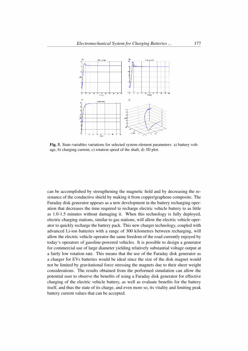
Electromechanical System for Charging Batteries ... 177
Fig. 5. State-variables variations for selected system element parameters: a) battery volt-age, b) charging current, c) rotation speed of the shaft, d) 3D plot.
can be accomplished by strengthening the magnetic field and by decreasing the re-sistance of the conductive shield by making it from copper/graphene composite. TheFaraday disk generator appears as a new development in the battery recharging oper-ation that decreases the time required to recharge electric vehicle battery to as littleas 1.0-1.5 minutes without damaging it. When this technology is fully deployed,electric charging stations, similar to gas stations, will allow the electric vehicle oper-ator to quickly recharge the battery pack. This new charger technology, coupled withadvanced Li-ion batteries with a range of 300 kilometres between recharging, willallow the electric vehicle operator the same freedom of the road currently enjoyed bytoday‘s operators of gasoline-powered vehicles. It is possible to design a generatorfor commercial use of large diameter yielding relatively substantial voltage output ata fairly low rotation rate. This means that the use of the Faraday disk generator asa charger for EVs batteries would be ideal since the size of the disk magnet wouldnot be limited by gravitational force stressing the magnets due to their sheer weightconsiderations. The results obtained from the performed simulation can allow thepotential user to observe the benefits of using a Faraday disk generator for effectivecharging of the electric vehicle battery, as well as evaluate benefits for the batteryitself, and thus the state of its charge, and even more so, its vitality and limiting peakbattery current values that can be accepted.

178 Trzaska Z.
References
Boldea, I. (2017). Electric generators and motors: An overview. CES Transactionson Electrical Machines and Systems, 1(1):3–14.
Bolonkin, A. (2007). New concepts, ideas and innovation in aerospace. AB Levitronsand their applications to Earth’s motionless satellites, pages 205–220.
Chyba, C. F., Hand, K. P., and Thomas, P. J. (2015). Energy conservation and poynt-ing’s theorem in the homopolar generator. American Journal of Physics, 83(1):72–75.
Eberhard, M. and Tarpenning, M. (2006). The 21 st century electric car tesla motors.Tesla Motors.
Engel, T. and Kontras, E. (2014). Analysis and design of homopolar motors and gen-erators. In Electromagnetic Launch Technology (EML), 2014 17th InternationalSymposium on, pages 1–6. IEEE.
Feng, F., Lu, R., Wei, G., and Zhu, C. (2015). Online estimation of model parametersand state of charge of lifepo4 batteries using a novel open-circuit voltage at variousambient temperatures. Energies, 8(4):2950–2976.
Gilbert, A. D. (2003). Dynamo theory. In Handbook of mathematical fluid dynamics,volume 2, pages 355–441. Elsevier.
Hide, R., Skeldon, A. C., and Acheson, D. J. (1996). A study of two novel self-exciting single-disk homopolar dynamos: theory. Proceedings of the Royal So-ciety of London. Series A: Mathematical, Physical and Engineering Sciences,452(1949):1369–1395.
Ivana, P., Vlcek, I., and Ivanova, M. (2016). The construction of the pure homopo-lar generator reveals physical problem of maxwell’s equations. arXiv preprintarXiv:1601.07750.
Kirschner, J. and Moon, S. (2010). An investigation of the homopolar generator.Electromagnetism: A Modelling and Simulation Approach. Project 2: Final Paper.
Mazurkiewicz, A. (2007). Nanosciences and nanotechnologies. present state anddevelopment perspectives. Institute of Exploitation Technology - State ResearchInstitute.
Moroz, I. M. (2001). Self-exciting faraday disk homopolar dynamos. InternationalJournal of Bifurcation and Chaos, 11(12):2961–2975.
Nezhad, M. B. (2013). Study of Homopolar DC Generator. PhD thesis, The Univer-sity of Manchester (United Kingdom).

Electromechanical System for Charging Batteries ... 179
Perek, A. and Kurnik, W. (2015). Kinematically excited vibration of an asymmetricrotor/bearing system with magnetic lubricant. Machine Dynamics Research, 39(4).
Struchtrup, H. (2014). Thermodynamics and energy conversion. Springer.
Trzaska, Z. (2010). Mixed mode and chaotic oscillations in a system with a self-excited disk generator. Proceedings of the Conference "Modeling and Simulation"MiS-6, Koscielisko.
Trzaska, Z. (2013). Dynamiczne procesy w napedzie samochodu elektrycznego wruchu miejskim. Transport Miejski i Regionalny, (11):26–31.
Trzaska, Z. (2015). Impact and chaotic phenomena in nonlinear nonsmooth electricaldynamical systems. Przeglad Elektrotechniczny, 91(4):77–85.
Zhang, L., Peng, H., Ning, Z., Mu, Z., and Sun, C. (2017). Comparative research onrc equivalent circuit models for lithium-ion batteries of electric vehicles. AppliedSciences, 7(10):1002.

Aims and scope of the journal
The aim of the journal is to provide a forum in which original research in thedeveloping field of machine dynamics can be communicated rapidly.
The scope of the journal encompasses dynamic problems of all kinds of ma-chinery (vehicles, flying objects, ships, engines, turbomachines, transportand building machines, cranes, machine tools, etc.), as listed below.
• Modelling of machines as dynamical systems
• Identification and modification of systems
• Basic material properties in machine building including rheology andinternal friction, crack propagation, fatigue, smart materials, etc.
• Machine elements mating problems like structural friction, wear, lubri-cation, hydro- and aerodynamic friction
• Vibrations and stability of machines and machine elements
• Vibroisolation and vibroacoustics of machines
• Dynamic machine diagnostics
• Synthesis of mechanisms and machines, optimisation, computer aideddesign
List of Reviewers
Professors: Awrejcewicz Jan (PL), Bajer Czesław (PL), Bajkowski Jerzy (PL), Balthazar JoseManoel (BR), Barboteu Mikaél (FR), Bogacz Roman (PL), Bogdevicius Marijonas (LT), CempelCzesław (PL), Czerwinski Jan (CH), Driss Zied (TN), Dudziak Marian (PL), Dufrenoy Philippe(FR), Dyniewicz Bartłomiej (PL), Ferrera Antoine (FR), Garibaldi Luigi (I), Giergiel Józef (PL),Glinka Grzegorz (CAN), Golnariagi Farid (CAN), Haddar Mohamed (TN), Hlavana Vladimir(SK), Kanaev Andrei (FR), Kocanda Andrzej (PL), Kowal Janusz (PL), Krawiec Piotr (PL), Ku-jawski Daniel (USA), Lebon Frédéric (FR), LePalec Georges (FR), Lobur Mykhaylo (UA), Ma-jewski Tadeusz (MEX), Marchelek Krzysztof (PL), Mazurkiewicz Adam (PL), Mezyk Arkadiusz(PL), Mompean Gilmar (FR), Nardin Philippe (FR), Nizioł Józef (PL), Rade Alves Domingos(BRA), Rusinski Eugeniusz (PL), Sado Danuta (PL), Seweryn Andrzej (PL), Shillor Meir (USA),Skup Zbigniew (PL), Slomiana Maria (USA), Sofonea Mircea (FR), Starczewski Zbigniew (PL),Stefanyk Vasyl (UA), Stotsko Zinovij (UA), Switonski Eugeniusz (PL), Tylikowski Andrzej (PL),Verreman Yves (CAN), Viano Juan (ESP), Woznica Krzysztof (FR), Zalewski Robert (PL),Zeghmati Belkacem (FR)

Machine Dynamics Research2018, Vol. 42, No 1
In this issue
1. Roman Bogacz and Kurt FrischmuthFriction Induced Oscillations and Material Degradation in RailwayEngineering
5
2. Anna Walicka, Edward Walicki, P. Jurczak, J. FalickiEffects of Hindrance Factors on a Squeeze Film of a Porous BearingLubricatedWith a Dehaven Fluid
15
3. Anna Jaskot, Bogdan PosiadałaModel of Motion of the Mobile Platform With Three Wheel Drive
35
4. Józef Drewniak, Krzysztof ReszutaDynamic Model for Non-Symmetric Dual-Path Gearbox
45
5. Zdzisław Chłopek, Paulina Grzelak, Dagna ZakrzewskaEvaluation of the Influence of Car Engine Power SupplyWith Rape-seed Oil Esters on Emission of Pollutants in Dynamic Conditions
55
6. Olimpia KunertHow Not to Lose the Valuable Know-How in Industry?
73
7. Andrzej Chudzikiewicz, Magdalena SowinskaThe Boltzmann-Hamel Formalism in Modelling of Rail Vehicle Mo-tion
87
8. Józef Pszczółkowski, Grzegorz DygaDetermination of the Electrical Structure Parameters of an Acid Bat-tery
101
9. Arkadiusz Wzorek, Jacek Mateusz BajkowskiInfluence of Printer Head Velocity on FDM Deposited Path Defor-mations
117
10. Jan Misiak, Sławomir StachuraStatic Analysis and Stability of the Steel Framework
129
11. Robert Konowrocki, Andrzej ZbiecInfluence of Correctness of Running Gear Assembly on Freight-Wagon Wheels’Wear
139
12. Robert BrodzikThe Impact of Changes in the Designs of Concrete Airport Pave-ment on Its Strength Properties
153
13. Zdzisław TrzaskaElectromechanical System for Charging Batteries of Electric Cars
165