1

Lung gas composition and transfer analysis: O2 and CO2 diffusion coefficients and metabolic rates D. N. Ghista1, K. M. Loh2 & D. Ng3 1School of Mechanical and Production Engineering, Nanyang Technological University, Singapore 639798; email:mdnghista@ntu,edu.sg 2School of Engineering (Electronics), Nanyang Polytechnic, Singapore 3Department of Nuclear Medicine and PET, Singapore General Hospital, Singapore Abstract The primary function of the lung is to (i) oxygenate the blood and thereby provide oxygen to the cells for metabolization purposes, and (ii) to remove the collected CO2 from the pulmonary blood. Herein, we will analyze the compositions of the inspired and expired air per breath, and from there compute the O2 consumption and CO2 production rates. Next, we derive expressions for diffusion coefficients

2OD and 2COD in terms of the evaluated cardiac output,

O2 and CO2 concentrations in arterial and venous blood, alveolar and blood O2 and CO2 partial pressures. We then take up a typical case study, and demonstrate the computation of

2OD and2COD , to represent the lung-performance capability

to oxygenate the blood.

2

1 Introduction The lung functional performance is characterized by (i) its ventilatory capacity, to bring air (and hence O2) into the alveoli, and (ii) its capacity to transfer O2 and CO2 into and from the pulmonary capillary bed. Hence, the O2 and CO2 diffusion coefficients as well as the O2 consumption rate and the CO2 production rate represent the lung-performance indices. 2. Lung air composition analysis (and 2O consumption and

2CO production rates) We carry out a mass balance analysis, involving:

(i) compositions of air breathed in and out (ii) consumption or losses of O2, CO2 and H2O.

The Table 1 below provides clinical data on partial pressures and volumes of

2N , 2O , 2CO and 2H O of atmospheric air breathed in and expired in one breath cycle. The monitored breathing rate (BR) = 12 breaths/min, and we assume PH2O at 37οC = 47 mmHg.

Table 1: Inspired air composition and partial pressures.

Atmospheric Air Expired Air Respiratory gases mmHg ml/% mmHg ml/%

N2 597 393.1 78.55%

566 393.1 74.5%

O2 159 104.2 20.84%

120 80.6 15.7%

CO2 0.3 0.2 0.04%

27 19.1 3.6%

H2O 3.7 2.5 0.49%

47 32.6 6.2%

Total 760 500 100%

760 525.3 100%

It can be noted that the expired air volume exceeds the inspired air volume for this particular breath cycle. The H2O loss of 30.1ml (=32.6 ml – 2.5 ml) contributes the major portion of this difference.

3

2.1 Calculation of 2O consumption-rate and CO2 production-rate We now determine the O2 consumption rate and CO2 production rates from the inspired and expired gases Assuming the patient breathes at 12 times per minute we have

2O Consumption Rate = (Inspired 2O – Expired 2O ) × 12 = (104.2–80.6) × 12

= 283.2 ml/min

2CO Production Rate = (Expired 2CO – Inspired 2CO ) × 12 = (19.1–0.2) × 12 = 226.8 ml/min

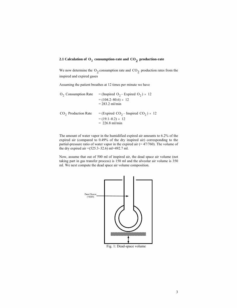
The amount of water vapor in the humidified expired air amounts to 6.2% of the expired air (compared to 0.49% of the dry inspired air) corresponding to the partial-pressure ratio of water vapor in the expired air (= 47/760). The volume of the dry expired air =(525.3–32.6) ml=492.7 ml. Now, assume that out of 500 ml of inspired air, the dead space air volume (not taking part in gas transfer process) is 150 ml and the alveolar air volume is 350 ml. We next compute the dead space air volume composition.

Fig. 1: Dead-space volume

4

2.2 Dead space air composition The clinical data of expired air composition is:

2

2

2

2

N = 393.1 ml

O = 83.36 ml

CO = 16.87 ml

H O = 34.15 ml

Total 527.49 ml

Now, the dead-space air will be made up of (i) a dry air portion from the inspired air (assumed to be =141 ml), plus (ii) the water vapor taken up by the dry air (estimated to be =9 ml) since the expired air portion of 141 ml will not have under gone O2 and CO2 transfer, it’s composition is the same as that of inspired air:

2N = 111 ml (78.55%), 2O = 29.40 ml (20.84%), 2CO = 0.06 ml (0.04%),

2H O = 0.69 ml (0.49%). When this inspired air (in the dead space) of 141 ml is fully humidified, it will take up a further X ml of 2H O vapor, in the ratio of the partial-pressures, as:

47

0.0659141 713

X= =

X = 0.0659×141 = 9.29 ml∴ of H O2 vapor (which is close to our estimate).

So, by adding 9.29 ml of H O2 vapor to 0.69 ml of water vapor in the inspired air volume of 141 ml, the total water vapor in the dead-space air is 9.98 ml. The humified dead-space air composition will be:

N = 111.00 ml (= 73.78%)2O = 29.40 ml (= 19.55%)2CO = 0.06 ml (= 0.04%)2H O = 9.98 ml (= 6.63%)2Total = 150.44 ml

5

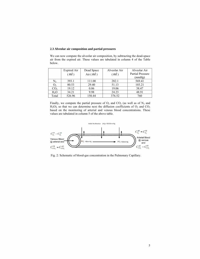
2.3 Alveolar air composition and partial pressures We can now compute the alveolar air composition, by subtracting the dead-space air from the expired air. These values are tabulated in column 4 of the Table below. Expired Air

( ml ) Dead Space Air ( ml )

Alveolar Air ( ml )

Alveolar Air Partial Pressure

(mmHg) N2 393.1 111.00 282.1 569.41 O2 80.53 29.40 51.13 103.21

CO2 19.12 0.06 19.06 38.47 H2O 34.21 9.98 24.23 48.91 Total 526.96 150.44 376.52 760

Finally, we compute the partial pressure of O2 and CO2 (as well as of N2 and H2O), so that we can determine next the diffusion coefficients of O2 and CO2 based on the monitoring of arterial and venous blood concentrations. These values are tabulated in column 5 of the above table.

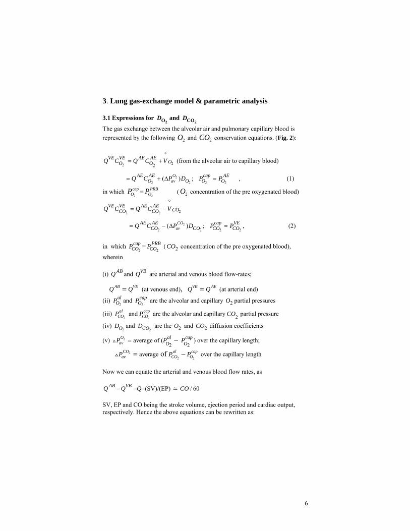
Fig. 2: Schematic of blood-gas concentration in the Pulmonary Capillary.

6

3. Lung gas-exchange model & parametric analysis 3.1 Expressions for

2OD and 2COD

The gas exchange between the alveolar air and pulmonary capillary blood is represented by the following 2O and 2CO conservation equations. (Fig. 2):

22 2VE VE AE AE

OO OQ C Q C V°

= + (from the alveolar air to capillary blood)

2

2 2 2 2( ) ;O

avcapAE AE AE

O O O OQ C P D P P= + ∆ = , (1)

in which 2

capOP =

2

PRBOP ( 2O concentration of the pre oxygenated blood)

22 2

VE VE AE AECOCO COQ C Q C V

°= −

2

2 2 2 2( ) ;CO

avcapAE AE VE

CO CO CO COQ C P D P P= − ∆ = , (2)

in which

2

capCOP =

2

PRBCOP ( 2CO concentration of the pre oxygenated blood),

wherein (i) ABQ and VBQ are arterial and venous blood flow-rates;

(at venous end) (at arterial end) ,AB VE VB AEQ Q Q Q= =

(ii) 2

alOP and

2

capOP are the alveolar and capillary 2O partial pressures

(iii) 2 2

2and are the alveolar and capillary partial pressure al capCO COP P CO

(iv) 2OD and

2COD are the 2O and 2CO diffusion coefficients

(v) 2

2 2 average of ( ) over the capillary length;O

avcapal

O OP P P= − 2

2 2average over the capillary length of CO al cap

av CO OP P P= − Now we can equate the arterial and venous blood flow rates, as

ABQ = VBQ =Q=(SV)/(EP) / 60CO SV, EP and CO being the stroke volume, ejection period and cardiac output, respectively. Hence the above equations can be rewritten as:

7

(vi) 2OV is the 2O transfer rate from alveolar air to capillary blood

(= 2O consumption rate), 2COV is the 2CO transfer rate from capillary blood to

alveolar air. From eqn. (1):

2

2

2 2 2 2 2 2

2 2 2

( ) ;

( )

O AEav

Oav

capVE VE AB ABO O O O O O

VB ABO O O

PQ C Q C P D P P

QC QC P D

== + =

= +

2 2

2 2 2 2( ) ( )

( ) ( )

AB VB

O Oav av

VE AEO O O OQ C C Q C C

P P=

− −=

2OD . (3)

From eqn. (2):

2

2 2( )

( )

VE

COav

ABCO COQ C C

P

−=

2COD , (4)

wherein (i) Q,

2

VEOC and

2

AEOC ,

2

VECOC and

2

AECOC can be monitored because

2 2 2 2 2 2 2 2 and = and and and = and AB AB VB VBVE VE AE AE

O CO O CO O CO O COC C C C C C C C

(ii) 2OD and

2COD (eqns. (3) & (4)) represent the lung gas-exchange

parameters. Now from eqns. (3) and (4), if we want to evaluate the diffusion coefficients

2OD and2COD , we need to also express

2

alOP ,

2

capOP and

2

alCOP ,

2

capCOP in terms of

monitorable quantities. In this regard,

2

2

2 2 2 2 2 2

2 2 2

( ) ;

( )

CO AEav

COav

capVE VE AE AE VBCO CO CO CO CO CO

VE AEO CO CO

Q C Q C P D P P P

QC QC P D

= − = =

= −

8

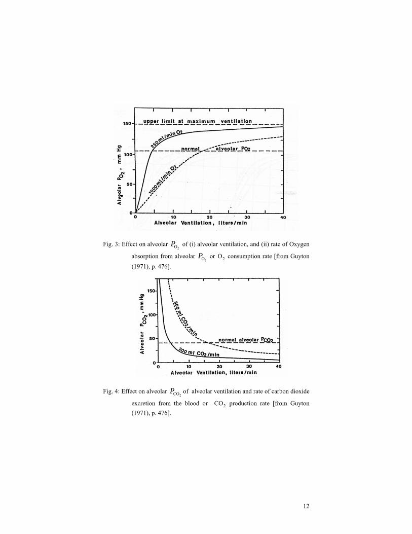
(i) Alveolar 2

alOP can be expressed in terms of V

°(the ventilation rate) and

2OV°

(the 2O consumption rate) as Fig. 3 :

O2

m

1V V V

e

⎡ ⎤⎛ ⎞⎢ ⎥⎜ ⎟⎜ ⎟⎢ ⎥⎝ ⎠⎣ ⎦

° ° °−

= −

⎡ ⎤⎢ ⎥⎢ ⎥⎢ ⎥⎣ ⎦

2

2alO 1

k

P k , (5)

where mV is the maximum ventilation rate and 2OV (the 2O consumption rate or

absorption rate from the alveoli)= 2 2O O )( AB VBQ C C− . Eqn. (5) implies that as

mV V⎛ ⎞⎜ ⎟⎝ ⎠

increases, (the exponential term decreases, and) 2O

alP increases (as in

Fig. 3), and as 2OV increases

2OalP decreases (as in Fig. 3).

(ii) Alveolar 2

alCOP can be expressed in terms of V

° and 2OV

° as in Fig. 4.

CO2

V

V mV

e

°

°

⎡ ⎤⎛ ⎞⎢ ⎥⎜ ⎟⎢ ⎥⎜ ⎟⎜ ⎟⎢ ⎥⎝ ⎠⎣ ⎦

°−

=4

alCO 32

k

P k , (6)

where2CO

°V (the 2CO production rate or excretion rate from the blood)

=2 2CO CO )( VB ABQ C C− . This equation implies that as mV V increases,

2COalP

decreases; also, as 2COV increases (the exponential term decreases, and hence)

2COalP increases.

(iii) Blood

2OP can be obtained in terms of blood 2CO , from the 2O

disassociation curve (providing concentrations in arterial and venous blood), is represented in Fig. 5, as:

O2

O22 2

5

O O(1 )

mP

kPmC C e

−

= − , or *

O22

*O 1

PC e

−= − 5k

, (7)

9

where

• 2O

mC and 2O

mP are the maximum values of blood 2O partial pressure

• *2 2 2CO CO COm=

• 2 2

*O O O2

mP P P=

(iv) Blood

2COP can be obtained in terms of 2COC , from the 2CO

disassociation curve or 2CO concentration in arterial and venous blood can be represented as per Fig. 6 as:

( )CO CO2 22 2

CO O(1 )

mP6k PmC C e−

= −

( )CO CO2 22

*2*or, 1 1

mCO

k Pk P P 66COC e e

−−== − − (8)

3.2 Alveolar 2 2O and CO partial pressure expressions

Now, let us refer eqn. (4) for the 2

alOP partial pressure curve (Fig. 3), represented

by the eqn.:

2

2O 12 O

m

Vk VVal

1P k e

°

°

⎡ ⎤⎛ ⎞⎢ ⎥⎜ ⎟⎢ ⎥⎜ ⎟⎜ ⎟⎢ ⎥⎝ ⎠⎣ ⎦

°−

= −

⎡ ⎤⎢ ⎥⎢ ⎥⎢ ⎥⎢ ⎥⎣ ⎦

*

21

2 Ok V V

1k e

° °⎡ ⎤⎢ ⎥⎢ ⎥⎣ ⎦

−

= −

⎡ ⎤⎢ ⎥⎢ ⎥⎢ ⎥⎣ ⎦

, where *

V°

= m

V

V

°

° (9)

wherein V is the alveolar ventilation rate (in liters/min), mV°

is the maximum

ventilation rate (= 50 liters/min) and 2O

V is the 2O consumption rate (in

liters/min). Herein, the coefficients 1k and 2k can be determined by having this

10

equation match the Fig. 3 data. Note, in this equation, when 0V°= ,

2O 0alP =

from the equation ,which satisfies the data.

Now for 2OV =0.25 liters/min, when *

V°

= m

V

V

°

° =0.5, 2O

alP =140 mmHg . Hence ,

0.520.25140 1 (1 )

22

k k1 1k e k e

⎡ ⎤⎢ ⎥⎣ ⎦

−−= − = −

⎡ ⎤⎢ ⎥⎢ ⎥⎣ ⎦

. (10)

Also, when 2OV =1 / minl , *

V°

=0.3 / minl , 2

100alOP = mmHg. Hence

0.30.31100 1 (1 )

22

k k1 1k e k e

⎡ ⎤⎢ ⎥⎣ ⎦

−−= − = −

⎡ ⎤⎢ ⎥⎢ ⎥⎣ ⎦

. (11)

From eqns. (10) and (11), we get:

2 2

0.3 0.3(1 )140 1

100 (1 ) 1

2 2

2 2

k k1

k k1

k e e

k e e

− −

− −− −

= =− −

0.3 2

2 0.3, 40 , so that

140 140 100 100

or 100 140 4.18

2 2

2 2

k k

k k2k

e e

e e min/l

− −

− −

∴ − = −

= + = (12)

Upon substituting 4.18 min/l2k = into eqn. (10) we obtain:

(2 4.18) that140 (1 ), so 140 mmHg1 1k e k− ×= − ≈ (13) Hence, the

2

alOP curve can be represented by:

*

2

2

4.18

O ,140 1OV V

alP e

° °⎡ ⎤⎢ ⎥⎢ ⎥⎣ ⎦

−

= −

⎡ ⎤⎢ ⎥⎢ ⎥⎢ ⎥⎣ ⎦

(14)

11

wherein 2OV =Q2 2

)( AB VBO OC C− and

*

50 / minV V l°

=

Now, let us look at the

2COalP expression:

2 2

2

*

CO

CO COVk V k V V4 4V mal

3 3P k e k e

⎡ ⎤⎛ ⎞⎡ ⎤⎢ ⎥⎜ ⎟⎢ ⎥⎢ ⎥⎜ ⎟⎢ ⎥⎢ ⎥⎜ ⎟

⎝ ⎠⎣ ⎦ ⎣ ⎦

° ° °− −°

= = ,

We note from Fig. 4 that for 2 0.2 / minCOV l°

= and 0.2mV°

= , 2CO

alP =12. Hence, from the above eqn., we get: 12 4-k

3k e= (15)

Also, for 2 0.8 /OV l min= and 0.2mV°

= , 2CO

alP = 62 mmHg. Hence

40.200.80

36244

kk

3k e k e⎡ ⎤⎢ ⎥⎣ ⎦

−−= = (16)

From eqn.s (15) and (16), we get:

4

23

, so that

12

62

12 2ln 2.46

62 3

44

4

k k

k

4

ee

e

k k4

−−= =−

= − =⎛ ⎞⎜ ⎟⎝ ⎠

(17)

Substituting 2.464k = into eqn. (16), we obtain :

2.464 ,62 114.683 3k e k

−

∴= = (18) Hence, the

2

alCOP curve can be represented as

22.46

CO2114.68

COV V

V malP e

°°

°

⎡ ⎤⎛ ⎞⎢ ⎥⎜ ⎟⎢ ⎥⎜ ⎟⎜ ⎟⎢ ⎥⎝ ⎠⎣ ⎦

−

= (19)

wherein *

50 l/minV V°

= and 2COV =Q2 2

)( VB ABCO COC C−

12

Fig. 3: Effect on alveolar 2OP of (i) alveolar ventilation, and (ii) rate of Oxygen

absorption from alveolar 2OP or 2O consumption rate [from Guyton

(1971), p. 476].

Fig. 4: Effect on alveolar 2COP of alveolar ventilation and rate of carbon dioxide

excretion from the blood or 2CO production rate [from Guyton (1971), p. 476].

13

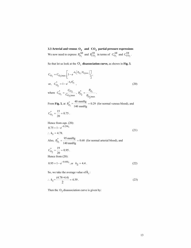
3.3 Arterial and venous 2 2O and CO partial pressure expressions

We now need to express 2O

ABP and 2CO

VBP in terms of 2O

ABC and 2CO

VBC .

So that let us look at the 2O disassociation curve, as shown in Fig. 5.

|max2 22 2O |max 1 5 O Ok P P

OC C e⎡ ⎤⎣ ⎦= −⎡ ⎤

⎢ ⎥⎣ ⎦-

,

*2*

2or, 1 5 Ok P

OC e−

= − , (20)

where 2

O* 2O O |max2

CC C= , 2*

2|max2

OO

O

PP

P= .

From Fig. 5, at 2

*OP =

40 mmHg0.29

140 mmHg= (for normal venous blood), and

2

*OC

150.75

20= = .

Hence from eqn. (20):

0.290.75 1

4.78.

5k

5

e

k

−= −

∴ = (21)

Also, 2

* 95 mmHg0.68

140 mmHgOP = = (for normal arterial blood), and

*2

190.95

20OC = = .

Hence from (20):

0.68 , or0.95 1 4.45ke k5−= − = . (22)

So, we take the average value of 5k :

(4.78+4.4)= 4.59

25k∴ = . (23)

Then the 2O disassociation curve is given by:

14

2

2 2

O4.59140

O O 0.2 1

P

BC C e

⎡ ⎤⎢ ⎥⎢ ⎥⎣ ⎦

−

= = −

⎡ ⎤⎢ ⎥⎢ ⎥⎢ ⎥⎣ ⎦

, (24)

and

22 2

OO O

140 0.2 0.2ln 30.5 ln

4.59 0.2 0.2B BPC C

= =− −

⎡ ⎤ ⎡ ⎤⎢ ⎥ ⎢ ⎥⎢ ⎥ ⎢ ⎥⎣ ⎦ ⎣ ⎦

. (25)

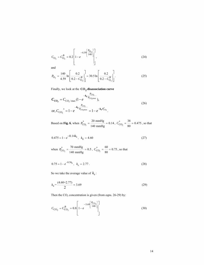
Finally, we look at the 2CO disassociation curve

2

|max22

2*

|max2 22

/ max

*

(1 ),

or, 1 1 .

CO

CO

CO

CO CO

PP

CO

PP P

CO

C e

C e e

−

−−

= −

= − = −

6

2

66

k

CO

kk

C (26)

Based on Fig. 6, when 2

* 20 mmHg0.14

140 mmHgCOP = = , 2

* 380.475

80COC = = , so that

,0.140.475 1 4.6066

ke k−= − = (27)

when 2

*CO

70 mmHg0.5

140 mmHgP = = ,

2

* 600.75

80COC = = , so that

0.5 ,0.75 1 2.7766

ke k−= − = . (28) So we take the average value of 6k :

(4.60+2.77)= 3.69

26k = (29)

Then the CO2 concentration is given (from eqns. 26-29) by:

CO2

2 2

3.69140

CO CO 0.8 1

P

BC C e

⎡ ⎤⎢ ⎥⎢ ⎥⎣ ⎦

−

= = −⎡ ⎤⎢ ⎥⎢ ⎥⎣ ⎦

(30)

15

and

22

COCO

0.837.94 ln

0.8 BPC

=−

⎡ ⎤⎢ ⎥⎢ ⎥⎣ ⎦

. (31)

16

Figure 5: O2 dissociation curves, showing the total oxygen in each 100 ml of normal blood, the portion dissolved in the water of the blood [from Guyton (1971), p. 485].

Figure 6: The carbon dioxide dissociation curve [from Guyton (1971), p. 491].

17

3.4 Sequential procedure to compute 2OD and

2COD

(1) We first monitor: ( ), ( )V t V t , SV(stroke volume), EP(cardiac ejection

period), 2O

VBC , 2O

ABC , 2CO

VBC and 2CO

ABC ( 2O and 2CO concentrations

in pre oxygenated and post oxygenated blood). (2) We substitute the values of

2OABC (=

2OVEC ) and

2OVBC (=

2OAEC ) into eqn.

(3), and the values of 2CO

ABC (=2CO

VEC ) and 2CO

VBC (=2CO

AEC ) into eqn. (4).

(3) We next determine:

Q= SV/ejection period, (33)

2O ( )V t =Q2 2O O( )VBABC C− , (34)

2CO ( )V t =Q2 2CO CO )( ABVBC C− . (35)

(4) We then substitute the expressions for 2O ( )V t and

2CO ( )V t into the

eqns. for 2O

alP (eqn. (14)) and 2CO

alP (eqn. (19)).

(5) We substitute the monitored values of

2OVBC (=

2OAEC ) and

2COVBC

(=2CO

AEC ) into eqns. (25) and (32), to obtain the values of 2O

AEP and

2COAEP .

(6) Now, in order to determine the values of the lung gas-exchange

parameters 2OD and

2COD , we substitute into eqns. (3) and (4) for Q

from eqn. (33), 2O

alP from (14), 2CO

alP from eqn. (19), 2O

VBP from eqn.

(26), and 2CO

VBP from eqn. (32) .

3.5 Determining 2OD and

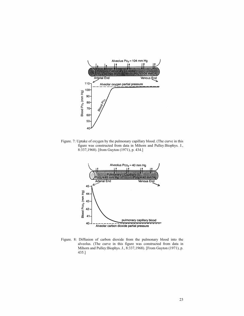
2COD Fig. 7 illustrates the variation of 2OP (=

2 2 2 2O O O Ocapal al ABP P P P− = − ) along the

length (l) of the capillary bed.

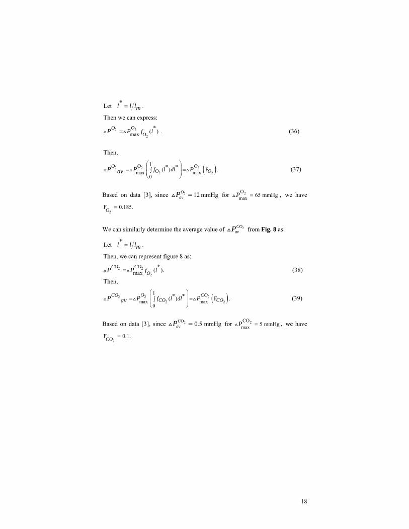
18

2 2

2

.

*( ) . max

*Let

Then we can express:

(36)OOOf l

l l lm

P P

=

=

( )2 2 22 2

1

max max0

* *( ) F .

Then,

(37)O OOO Of l dlP P Pav

⎛ ⎞⎜ ⎟ =∫⎜ ⎟⎝ ⎠

=

Based on data [3], since 2 12 mmHgOavP = for 2O

max 65 mmHgP = , we have

2F 0.185.O =

We can similarly determine the average value of 2CO

avP from Fig. 8 as:

2 2

2

.

*( ). max

*Let

Then, we can represent figure 8 as:

(38)COCOOf l

l l lm

P P

=

=

( )2 2 22 2

1

max max0

* *( ) F .

Then,

(39)O COCOCO COf l dlP P Pav

⎛ ⎞⎜ ⎟ =∫⎜ ⎟⎝ ⎠

=

Based on data [3], since 2CO 0.5 mmHgavP = for 2COmax 5 mmHgP = , we have

2F 0.1.CO =

19

From the 2OavP and 2CO

avP expressions, we can determine the O2 consumption and the CO2 production rates, as follows:

2 2222 2 2

Total consumed2AB VBO OO

OO O Oav avav

Q C C

P P

O VD

P

−⎛ ⎞⎜ ⎟⎝ ⎠= = = (40)

2 2222 2 2

Total C produced2VB ABCO COCO

COCO CO COav avav

Q C C

P P

O VD

P

−⎛ ⎞⎜ ⎟⎝ ⎠= = = . (41)

4. Case Studies (A) We monitor the partial pressures blood concentrations of O2 and CO2 as:

2 20.13AE VB

O OC C= = , 2 2

0.18VE ABO OC C= = ,

2 20.525,AE VB

CO COC C= =

2 20.485VE AB

CO COC C= =

From eqn. (26), we obtain:

22

0.2 0.230.5 ln 30.5 ln

0.2 0.2 0.13

32.02 mmHg (42)

VBO VB

OP

C= =

− −

=

⎡ ⎤ ⎡ ⎤⎢ ⎥ ⎢ ⎥⎣ ⎦⎢ ⎥⎣ ⎦

From eqn. (32), we obtain:

We now also monitor Q=5 l/min, *

0.1V°

= and 5 /minV l= : Then from eqn. (34):

2( )OV t =Q ( )2 2

AB VBO OC C− , so that from the above data,

2

0.8 0.837.94 ln 37.94 ln

0.8 0.8 0.5252

40.51 mmHg (43)

VBCO

VBPCO C= =

− −

=

⎡ ⎤ ⎡ ⎤⎢ ⎥ ⎢ ⎥⎣ ⎦⎢ ⎥⎣ ⎦

20

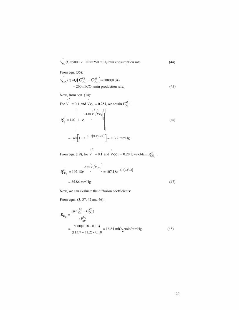
2( )OV t =5000 × 0.05=250 mlO2/min consumption rate (44)

From eqn. (35):

2( )COV t =Q ( )2 2

VB ABCO COC C− =5000(0.04)

= 200 mlCO2 /min production rate. (45)

Now, from eqn. (14):

For *°

= 0.1V and 2 2O O :0.25 , we obtain alV l P

°=

2

2

*4.18

4.18 0.1 0.25

(46)140 1

140 1 113.7 mmHg

V V Oal

OP e

e

⎡ ⎤⎢ ⎥⎢ ⎥⎢ ⎥⎣ ⎦

⎡ ⎤⎣ ⎦

° °−

−

= −

= − =

⎡ ⎤⎢ ⎥⎢ ⎥⎢ ⎥⎢ ⎥⎣ ⎦

⎡ ⎤⎣ ⎦

From eqn. (19), for *°

= 0.1V and 2 2CO CO :0.20 l, we obtain alV P

°=

[ ]

*

CO2

2

2.192.19 0.1 0.2

CO 107.18 107.18

35.86 mmHg (47)

V V

alP e e

° °⎡ ⎤⎢ ⎥−⎢ ⎥ −⎣ ⎦= =

=

Now, we can evaluate the diffusion coefficients: From eqns. (3, 37, 42 and 46):

2 2

2

( )

5000(0.18 0.13)16.84 mlO /min/mmHg. (48)2(113.7 31.2) 0.18

AB VBO O

Oav

Q C C

P

−=

−= =

− ×

2OD

21

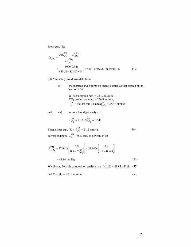
From eqn. (4):

2 22 2

CO COCO CO

( )

5000(0.04)430.11 m CO /min/mmHg. (49)2(40.51 35.86) 0.1

VB AB

av

Q C C

P

l

−=

= =− ×

D

(B) Alternately, we derive data from:

(i) the inspired and expired air analysis (such as that carried out in section 2.3):

O2 consumption rate = 283.2 ml/min, CO2 production rate = 226.8 ml/min,

2O 103.03 mmHgalP = and2CO 38.41 mmHgalP =

and (ii) venous blood gas analysis:

2O 0.13VBC = ,2CO 0.548VBC =

Then, as per eqn. (42),

2O 31.2 mmHgVBP = (50)

corresponding to 2

0.13VBOC = and, as per eqn. (43):

2

0.8 0.837.94 ln 37.94 ln

0.8 0.8 0.5482

43.84 mmHg (51)

VBCO

VBPCO C= =

− −

=

⎡ ⎤ ⎡ ⎤⎢ ⎥ ⎢ ⎥⎣ ⎦⎢ ⎥⎣ ⎦

We obtain, from air composition analysis, that 2

283.3 ml/min( )OV t = (52)

and 2CO 226.8 ml/min.( )V t = (53)

22

Hence,

2

2 2O

283.221.90 mlO /min/mmHg, (54)2(103.03 31.2) 0.18

OOav

V

P=

= =− ×

D

and

2

2 2

COCO CO

226.8417.68 mlCO /min/mmHg. (55)2(43.84 38.41) 0.1

av

V

P=

= =− ×

D

The advantage of this method (B) over (A) is that it does not require monitoring of the cardiac output, and is hence simpler to implement clinically.

23

Figure. 7: Uptake of oxygen by the pulmonary capillary blood. (The curve in this figure was constructed from data in Mihorn and Pulley:Biophys. J., 8:337,1968). [from Guyton (1971), p. 434.]

Figure. 8: Diffusion of carbon dioxide from the pulmonary blood into the alveolus. (The curve in this figure was constructed from data in Mihorn and Pulley:Biophys. J., 8:337,1968). [From Guyton (1971), p. 435.]

24

References [1] A. C. Guyton, M.D., Text Book of Medical Physiology, 8th edition, HBJ I.E.

Saunders, ISBN 0-7216-3994-1, pp.422-442, 1991. [2] J. H. Comroe, Physiology of Respiration, 2nd edition, Year Book Medical

Publishers Incorporated, ISBN 0-8251-1827-9, pp. 268-269, 1977. [3] D. O. Conney, Biomedical Engineering Principles, Marcel Dekker Inc.,

ISBN 0-8247-6347-5, pp. 248-251 342-397, 1976.