Loss performance model for wireless channelswith autocorrelated arrivals and losses

D. Moltchanov∗, Y. Koucheryavy, J. HarjuInstitute of Communications Engineering,

Tampere University of Technology,P.O.Box 553, Tampere, Finland

E-mail: {moltchan,yk,harju}@cs.tut.fi

Abstract

In this paper we firstly propose simple and computationally efficient

wireless channel modeling algorithm that explicitly takes into account first-

and second-order statistics of frame error observations. For this purpose we

use discrete-time Markov modulated processes with at most single event (er-

ror) at any time slot. We then adopt the special solution of the inverse eigen-

value problem initially proposed in [1] and show that its complexity sig-

nificantly decreases when the time series is covariance stationary binary in

nature. Then, we identify a class of priority queuing systems of G+G/GI/1/K

type capable to model the frame transmission process over wireless channels

with correlated arrival and loss processes. Using the proposed frame error

process, performance evaluation model of the wireless channel at the data-

link layer is then reduced to the spacial case of∑

iD-BMAPi/D/1/K queuing

system with non-preemptive priority discipline. The proposed queuing rep-

resentation allows to capture forward error correlation (FEC) and automatic

∗Dmitri Moltchanov, e-mail: moltchan@cs.tut.fi, tel.: +358 331154709, Fax: +358 331154988

1

repeat request (ARQ) functionality of the data-link layer as well as distri-

butional and autocorrelational properties of the frame arrival and frame loss

processes. This model is further analyzed for a number of performance pa-

rameters of interest including probability function of the number of frames

in the system and probability function of the number of lost frames. It is

shown that the channel response in terms of the mean number of frames in

the buffer and the mean number of lost frames varies substantially for dif-

ferent first- and second-order frame error and arrival statistics. This impact

of statistics is also different for normal (ρ < 1) and overloaded conditions

(ρ ≥ 1) of∑

iD-BMAPi/D/1/K queuing system.

Keywords: wireless channel model, non-preemptive∑

iD-BMAPi/D/1/K

queuing system, data-link layer performance evaluation model.

1 Introduction

Due to a fast growth in the number of users that wish to access Internet services

’anytime and anywhere’, wireless access became extremely popular. Vendors and

standardization bodies respond to such an increasingly growing interest develop-

ing new wireless access technologies. These technologies vary in many parame-

ters that are not necessary optimized for specific environments. This task is left

for further performance evaluation and optimization studies. Indeed, at the de-

velopment phase, a new technology is rarely supplemented with a performance

evaluation model. To compare efficacy of concurrent wireless access technolo-

gies and to facilitate their further optimization, versatile performance evaluation

frameworks are required.

Due to movement of a mobile user and different objects in a radio channel,

2

the propagation path between the transmitter and a receiver may vary from simple

line-of-sight (LOS) to very complex ones. An important consequence of propa-

gation characteristics is that bit and frame error observations are usually not inde-

pendent but correlated (see [2, 3, 4] among others). Techniques such as forward

error correction (FEC) and automatic repeat request (ARQ) may allow to recover

from these errors locally. To quantitatively study performance of these techniques

wireless channel models at the data-link layer are needed.

Recently, it was shown that the frame error process of a wireless channel can

be sufficiently well represented by the doubly-stochastic Markov modulated pro-

cess [5, 6, 7]. Such a model provides useful trade-off between complexity of the

model and accuracy of fitting to statistical data. However, modeling algorithms

developed for this model do not explicitly take into account second-order proper-

ties of statistical data that may lead to incorrect representation of the memory of

the frame error process (see [8, 9] among others). In this paper we develop simple

and computationally efficient wireless channel model at the data-link layer that is

capable to capture first- and second-order statistical characteristics of frame error

observations. For this purpose we use discrete-time Markov modulated process

with at most single event (error) at any time slot. We show that the solution of

the inverse eigenvalue problem returns unique transition probability matrix of the

modulating Markov chain that is capable to match statistical properties of empiri-

cal frame error processes. We also show that there is a unique Markov modulated

process approximating the histogram of relative frequencies of the frame error

trace and empirical normalized autocorrelation function (NACF). The associated

fitting algorithm is extremely simple, fast, and computationally efficient. The pro-

posed model is also not limited to the frame error process but can be used for any

3

covariance stationary binary observations.

Up to date performance of applications running over wireless channels have

been considered in a number of studies. Most of those rely on performance eval-

uation models specifically developed for wireless channels (see [10, 5] among

many others). As a result, they often need to be supplemented with new approx-

imations, algorithms, stable recursions etc. While such models may potentially

provide meaningful results, they require significant research ’investments’ in de-

velopment of associated algorithms.

Queuing theory is nowadays widely used in performance evaluation of fixed

networks. Modeling the information transmission process over wireless channels

is also related to its applications. However, early studies did not consider queuing

theory as an appropriate tool in wireless domain. The reason is that the service

process of the wireless channel is autocorrelated and queuing theory does not pro-

vide efficient solutions when both arrival and service processes are not renewal

ones. In this paper we fill this gap proposing a queuing-theoretic model for per-

formance evaluation of the frame transmission process over the wireless channel.

We identify a set of models that are well-suited for this purpose and outline their

properties. We consider a special type of∑

iD-BMAPi/D/1/K queuing system

with non-preemptive priority discipline as a candidate model and show how this

model can be used to derive performance parameters of the frame transmission

process. Numerical examples highlighting usefulness of the proposed approach

indicate that first- and second-order properties of the frame arrival and frame er-

ror processes significantly affect performance response of the wireless channel

in terms of the mean number of frames in the system and mean number of lost

frames.

4

The rest of the paper is organized as follows. In Section 2 we provide a re-

view of the related work in frame error modeling and performance evaluation of

the frame transmission process over wireless channels. We introduce our mod-

eling algorithm in Section 3. Models of the frame arrival and frame error pro-

cesses are then presented. The candidate performance evaluation model of∑

iD-

BMAPi/D/1/K type is proposed in Section 4. The system is studied for perfor-

mance parameters of interest in Section 5. Numerical examples are given in Sec-

tion 6. Conclusions are drawn in the last section.

2 Related work

2.1 Frame error modeling

There has been a lot of efforts aimed at developing a suitable model for frame error

observations. In [9], to capture statistical characteristics of error traces, authors

carried out statistical analysis of IEEE 802.11b frame error observations and used

a number of models, including hidden Markov models (HMM), and higher-order

Markov chains. They have shown that the first-order finite state Markov chain

(FSMC) may fail to model frame error traces accurately. Statistical analysis of

frame error traces was also carried out in [11] and that was the first paper where

dependence between successive frame error observations has been considered in

terms of NACF. It was suggested that with increasing of the number of states,

first-order FSMC is capable to capture autocorrelation properties of frame error

observations. Particularly, in [8] a 512-states first-order FSMC was introduced to

model IEEE 802.11b frame error observations. Due to a large number of states,

5

such model is only suitable for simulation studies of information transmission

over wireless channels. Contrarily, in a number of papers [5, 6, 7] Zorzi and Rao

have shown that two-states Markov modulated model is sufficient to capture frame

error statistics at the data-link layer.

2.2 Performance modeling

Up to date a number of performance evaluation models of the frame transmission

process over wireless channels have been proposed. We briefly review only those,

provided a breakthrough in novelty, accuracy or applicability.

Among others, one have to mention important studies of Zorzi and Rao [12,

13, 14, 5]. Throughput analysis of Go-Back-N ARQ with reliable and unreliable

feedback has been carried out in [12] and [13], respectively. In [14] authors ex-

tended previous results to the case of delay-constrained communication. Results

have been summarized in [5]. The presented approach is inherently theoretical

and based on two-states Markovian model of the wireless channel. Authors ar-

gue that their model is sufficient for accurate performance evaluation. However,

they employed rather simple traffic model that may not always provide adequate

representation of the frame arrival process from a traffic source.

An interesting approach was taken in [15]. Mukhtar et al. proposed an accu-

rate model for performance evaluation of ARQ/FEC error concealment procedures

at the data-link layer. The solution for steady-state parameters of the model in-

volves estimation of equilibrium probabilities of three-dimensional Markov chain.

Due to rather limited application field of such processes, there are no efficient al-

gorithms to compute these probabilities. However, relatively simple model was

6

used to represent the frame arrival process from a traffic source.

Those approaches cited above used simple traffic models, based on renewal

arrival processes. On the contrary, arrival processes from modern traffic sources

are characterized by complex distributional and autocorrelation properties. As a

result, those performance models may not always provide adequate representation

of the frame arrival process. Indeed, dealing with traffic modeling, processes

with versatile autocorrelation and distributional properties such as discrete-time

Markovian arrival process (D-MAP) or its batch extension (D-BMAP) should be

used instead [16, 17, 18, 19, 20]. However, usage of these processes may result in

significant increase of the complexity of those approaches cited above.

Queuing theory is nowadays widely used in performance evaluation of fixed

networks. However, there have been done only a little work related to its ap-

plicability in performance evaluation of information transmission over wireless

channels. Early studies did not consider queuing theory as an appropriate tool in

wireless domain. The reason is that the service process of wireless channels is

usually autocorrelated and classic queuing theory does not provide efficient solu-

tions when both arrival and service processes are not renewal. Moreover, usage of

ARQ at the data-link layer makes application and further interpretation of queu-

ing models even more complicated. On the other hand, queuing theory provides

a number of attractive features (priorities, batch arrivals, vacations, etc.) making

queuing models suitable even for such a complicated environment.

In [21], to study delay performance of applications at the data-link layer in

presence of selective-repeat ARQ (SR-ARQ), fluid-flow queuing-theoretic model

was adopted. In [10] this approach was extended to the case of hybrid FEC/ARQ.

In those studies both traffic and error processes were allowed to be autocorrelated.

7

The arrival process was modeled by ON-OFF Markovian process. It should be

however stressed that fluid-flow approximation usually provides good results for

very high-speed links for which influence of single events (e.g. frame arrivals,

errors) has only a negligible impact on the overall performance of the process.

However, wireless channels do not always provide high bandwidth for applica-

tion. In this case single arrivals are of higher importance and point processes

should be used instead. Additionally, in both studies the ’ideal’ SR-ARQ protocol

was considered, for which feedback delay was assumed to be constant and the

backward channel to be error-free. In this case the performance of stop-and-wait

ARQ (SW-ARQ) and SR-ARQ becomes identical [21] that may not always hold

in practice.

In [22], to model frame transmission process at the data-link layer, authors

used D-BMAP/PH/1 queuing system with first come first served (FCFS) service

discipline, where D-BMAP is used to represent frame arrivals. To capture ef-

fects of ARQ running over error-prone wireless channels, authors assumed that

the service time of any frame is distributed according to the discrete phase-type

(PH) distribution. Here, the service time refers to the time required to successfully

transmit a single frame over the wireless channel (including possible retransmis-

sions). Therefore, a frame is always transmitted irrespective of the time it takes.

However, ARQ schemes usually limit the transmission time allowing not more

than a certain number of retransmissions. Thus, D-BMAP/PH/1 queuing system

is only appropriate when the wireless channel conditions are relatively ’good’ or

data-link layer is completely reliable. Additionally, the service time of frames

were assumed to be independent and identically distributed (i.i.d.) random vari-

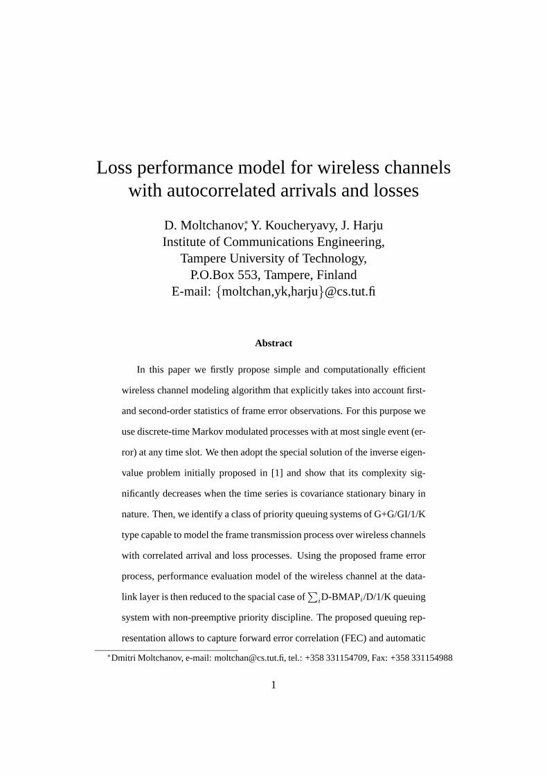
ables. This assumption does not hold in practise. As an example, NACF of two

8

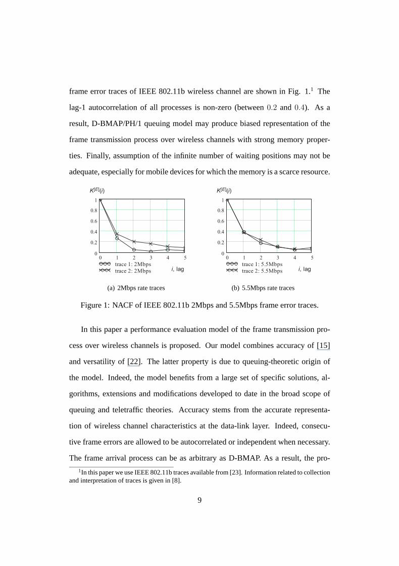
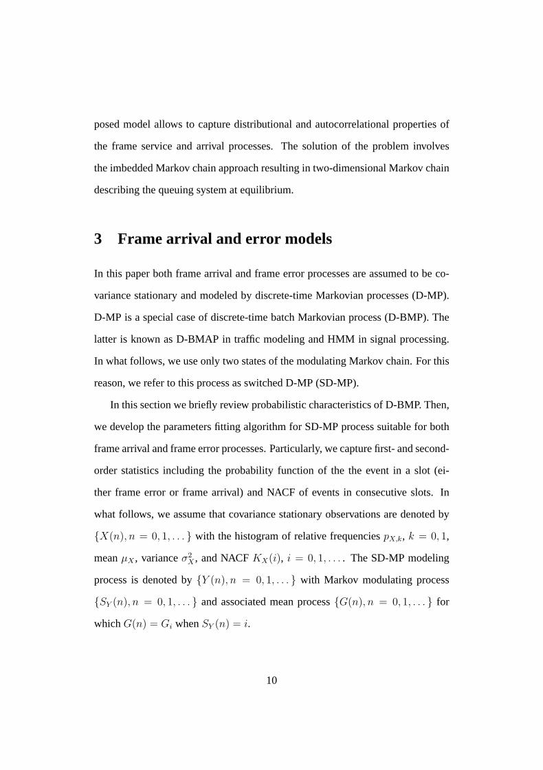
frame error traces of IEEE 802.11b wireless channel are shown in Fig. 1.1 The

lag-1 autocorrelation of all processes is non-zero (between 0.2 and 0.4). As a

result, D-BMAP/PH/1 queuing model may produce biased representation of the

frame transmission process over wireless channels with strong memory proper-

ties. Finally, assumption of the infinite number of waiting positions may not be

adequate, especially for mobile devices for which the memory is a scarce resource.

0 1 2 3 4 50

0.2

0.4

0.6

0.8

1

trace 1: 2Mbps

trace 2: 2Mbps

K[E](i)

i, lag

(a) 2Mbps rate traces

0 1 2 3 4 50

0.2

0.4

0.6

0.8

1

trace 1: 5.5Mbps

trace 2: 5.5Mbps

K[E](i)

i, lag

(b) 5.5Mbps rate traces

Figure 1: NACF of IEEE 802.11b 2Mbps and 5.5Mbps frame error traces.

In this paper a performance evaluation model of the frame transmission pro-

cess over wireless channels is proposed. Our model combines accuracy of [15]

and versatility of [22]. The latter property is due to queuing-theoretic origin of

the model. Indeed, the model benefits from a large set of specific solutions, al-

gorithms, extensions and modifications developed to date in the broad scope of

queuing and teletraffic theories. Accuracy stems from the accurate representa-

tion of wireless channel characteristics at the data-link layer. Indeed, consecu-

tive frame errors are allowed to be autocorrelated or independent when necessary.

The frame arrival process can be as arbitrary as D-BMAP. As a result, the pro-

1In this paper we use IEEE 802.11b traces available from [23]. Information related to collectionand interpretation of traces is given in [8].

9

posed model allows to capture distributional and autocorrelational properties of

the frame service and arrival processes. The solution of the problem involves

the imbedded Markov chain approach resulting in two-dimensional Markov chain

describing the queuing system at equilibrium.

3 Frame arrival and error models

In this paper both frame arrival and frame error processes are assumed to be co-

variance stationary and modeled by discrete-time Markovian processes (D-MP).

D-MP is a special case of discrete-time batch Markovian process (D-BMP). The

latter is known as D-BMAP in traffic modeling and HMM in signal processing.

In what follows, we use only two states of the modulating Markov chain. For this

reason, we refer to this process as switched D-MP (SD-MP).

In this section we briefly review probabilistic characteristics of D-BMP. Then,

we develop the parameters fitting algorithm for SD-MP process suitable for both

frame arrival and frame error processes. Particularly, we capture first- and second-

order statistics including the probability function of the the event in a slot (ei-

ther frame error or frame arrival) and NACF of events in consecutive slots. In

what follows, we assume that covariance stationary observations are denoted by

{X(n), n = 0, 1, . . . } with the histogram of relative frequencies pX,k, k = 0, 1,

mean µX , variance σ2X , and NACF KX(i), i = 0, 1, . . . . The SD-MP modeling

process is denoted by {Y (n), n = 0, 1, . . . } with Markov modulating process

{SY (n), n = 0, 1, . . . } and associated mean process {G(n), n = 0, 1, . . . } for

which G(n) = Gi when SY (n) = i.

10

3.1 Discrete-time batch Markovian process

Let us briefly review important characteristics of D-BMP. Assume a discrete-time

environment, i.e. time axis is slotted, the slot duration is constant and given

by ∆t = (ti+1 − ti), i = 0, 1, . . . . Consider a discrete-time homogenous er-

godic Markov chain {S(n), n = 0, 1, . . . } defined at the state space S(n) ∈{1, 2, . . . , M}. Let D be its transition probability matrix and �π = (π1, π2, .., πM)

be the row array of steady-state state distribution of the Markov chain. Let then

{Y (n), n = 0, 1, ..} be D-BMP whose underlying Markov chain is {S(n), n =

0, 1, . . . }. According to D-BMP, the value of the process is modulated by a

discrete-time Markov process {S(n), n = 0, 1, . . . }, S(n) ∈ {1, 2, . . . , M}. We

define D-BMP as a sequence of matrices D(k), k = 0, 1, . . . , each of which con-

tains probabilities of transition from state to state with k = 0, 1, . . . , arrivals,

respectively. For example, element dij(0) defines transition from state i to state j

without any arrivals while element dij(k) defines transition from state i to state

j with a batch arrival of size k. It is easy to see that for each pair of states

i, j ∈ {1, 2, . . . , M} the following

dij(k) = Pr{Y (n) = k, S(n) = j|S(n − 1) = i}, k = 0, 1, . . . , (1)

are conditional probability functions of D-BMP.

Let the vector �G = (G1, G2, . . . , GM) be the mean vector of D-BMP, where

Gi =∑M

j=0 kdij(1), i = 1, 2, . . . , M . The mean process of D-BMP is defined as

{G(n), n = 0, 1, . . . } with G(n) = Gi, when the Markov chain is in the state i at

11

the time slot n. The ACF of the mean process is given by

RG(i) =∑l,l �=1

φlλil, i = 1, 2, . . . , (2)

where φl = �π∑∞

k=0 kD(k)�gl�hl

∑∞k=0 kD(k)�e, λl is the ls eigenvalue of D, �gl

and �hl are ls left and right eigenvectors of D, respectively, and �e is the vector of

ones of size M . ACFs of D-BMP and the associated mean process of D-BMP are

generally different.

When only binary events are allowed in any state of the modulating Markov

chain (that is, when Y (n) ∈ {0, 1}), D-BMP decreases to D-MP. Particularly, for

D-MP the following holds

µG = µY , σ2G = σ2

Y , RG(i) = RY (i), i = 1, 2, . . . . (3)

When D-MP has only two states of the modulating Markov chain, it reduces

to SD-MP with the following expression for ACF

RY (i) = σ2Y λi

Y , i = 1, 2, . . . , (4)

where σ2Y is the variance of the process, λY is the non-unit eigenvalue. Note that

transition probability matrix of discrete-time irreducible and aperiodic Markov

chain always posses a unit eigenvalue that is referred to as simple eigenvalue.

NACF is then KY (i) = λiY , i = 1, 2, . . . . It is clear that the NACF of SD-MP

exhibits geometrical decay. Such a behavior may produce fair approximation of

empirical NACFs exhibiting nearly geometrical decay.

12

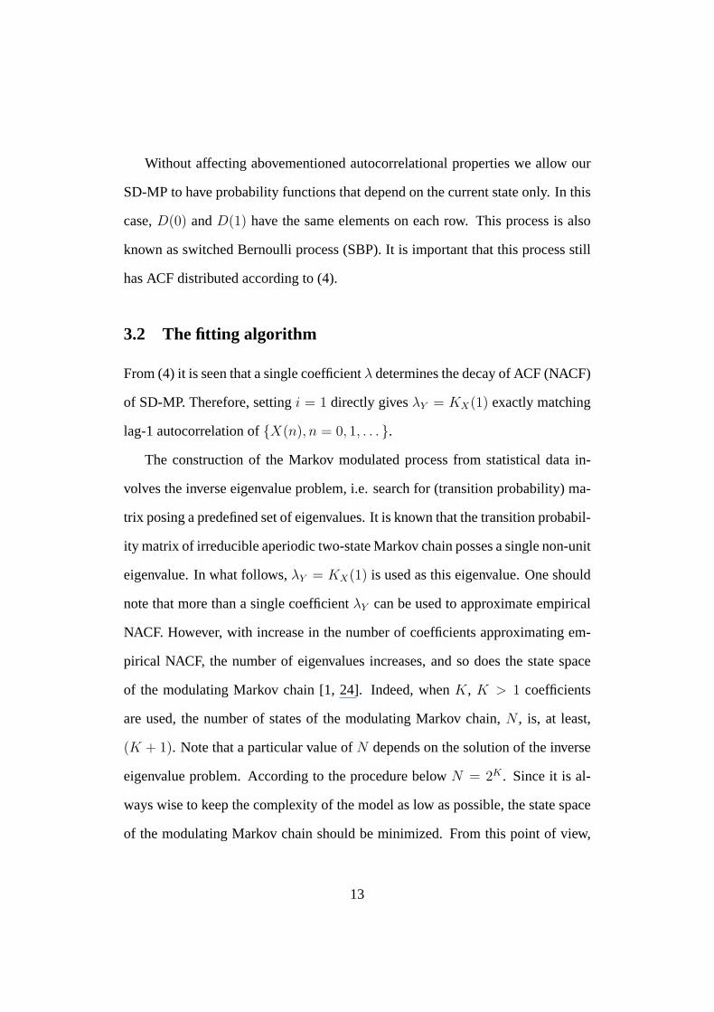
Without affecting abovementioned autocorrelational properties we allow our

SD-MP to have probability functions that depend on the current state only. In this

case, D(0) and D(1) have the same elements on each row. This process is also

known as switched Bernoulli process (SBP). It is important that this process still

has ACF distributed according to (4).

3.2 The fitting algorithm

From (4) it is seen that a single coefficient λ determines the decay of ACF (NACF)

of SD-MP. Therefore, setting i = 1 directly gives λY = KX(1) exactly matching

lag-1 autocorrelation of {X(n), n = 0, 1, . . . }.

The construction of the Markov modulated process from statistical data in-

volves the inverse eigenvalue problem, i.e. search for (transition probability) ma-

trix posing a predefined set of eigenvalues. It is known that the transition probabil-

ity matrix of irreducible aperiodic two-state Markov chain posses a single non-unit

eigenvalue. In what follows, λY = KX(1) is used as this eigenvalue. One should

note that more than a single coefficient λY can be used to approximate empirical

NACF. However, with increase in the number of coefficients approximating em-

pirical NACF, the number of eigenvalues increases, and so does the state space

of the modulating Markov chain [1, 24]. Indeed, when K, K > 1 coefficients

are used, the number of states of the modulating Markov chain, N , is, at least,

(K + 1). Note that a particular value of N depends on the solution of the inverse

eigenvalue problem. According to the procedure below N = 2K . Since it is al-

ways wise to keep the complexity of the model as low as possible, the state space

of the modulating Markov chain should be minimized. From this point of view,

13

usage of a single geometrical term as λY = KX(1) provides a trade-off between

the accuracy of the approximation and simplicity of the model.

It is known that the general solution of the inverse eigenvalue problem does not

exist. However, it is possible to solve it when some limitations on eigenvalues and

resulting process are set. Our limitation is that the non-unit eigenvalue should be

located in (0, 1] fraction of X axis. Since all eigenvalues of transition probability

matrix of irreducible aperiodic Markov chain are located in [−1, 1] fraction of 0X

axis, the requirement −1 ≤ λY ≤ 1 is already fulfilled. Finally, 0 ≤ λY ≤ 1 must

be fulfilled by the solution of the inverse eigenvalue problem.

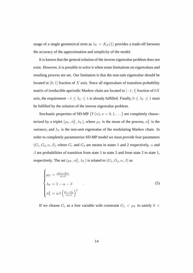
Stochastic properties of SD-MP {Y (n), n = 0, 1, . . . } are completely charac-

terized by a triplet (µY , σ2Y , λY ), where µY is the mean of the process, σ2

Y is the

variance, and λY is the non-unit eigenvalue of the modulating Markov chain. In

order to completely parameterize SD-MP model we must provide four parameters

(G1, G2, α, β), where G1 and G2 are means in states 1 and 2 respectively, α and

β are probabilities of transition from state 1 to state 2 and from state 2 to state 1,

respectively. The set (µY , σ2Y , λY ) is related to (G1, G2, α, β) as

⎧⎪⎪⎪⎪⎪⎪⎨⎪⎪⎪⎪⎪⎪⎩

µY = αG2+βG1

α+β

λY = 1 − α − β

σ2Y = αβ

(G1−G2

α+β

)2

. (5)

If we choose G1 as a free variable with constraint G1 < µY to satisfy 0 <

14

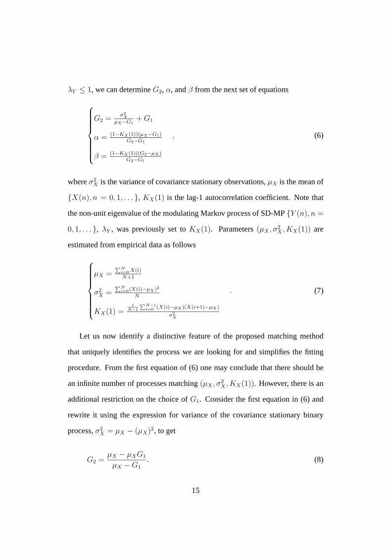
λY ≤ 1, we can determine G2, α, and β from the next set of equations

⎧⎪⎪⎪⎪⎪⎪⎨⎪⎪⎪⎪⎪⎪⎩

G2 =σ2

X

µX−G1+ G1

α = (1−KX(1))(µX−G1)G2−G1

β = (1−KX(1))(G2−µX)G2−G1

, (6)

where σ2X is the variance of covariance stationary observations, µX is the mean of

{X(n), n = 0, 1, . . . }, KX(1) is the lag-1 autocorrelation coefficient. Note that

the non-unit eigenvalue of the modulating Markov process of SD-MP {Y (n), n =

0, 1, . . . }, λY , was previously set to KX(1). Parameters (µX , σ2X , KX(1)) are

estimated from empirical data as follows

⎧⎪⎪⎪⎪⎪⎪⎨⎪⎪⎪⎪⎪⎪⎩

µX =∑N

i=0 X(i)

N+1

σ2X =

∑Ni=0(X(i)−µX)2

N

KX(1) =1

N−1

∑N−1i=0 (X(i)−µX)(X(i+1)−µX)

σ2X

. (7)

Let us now identify a distinctive feature of the proposed matching method

that uniquely identifies the process we are looking for and simplifies the fitting

procedure. From the first equation of (6) one may conclude that there should be

an infinite number of processes matching (µX , σ2X , KX(1)). However, there is an

additional restriction on the choice of G1. Consider the first equation in (6) and

rewrite it using the expression for variance of the covariance stationary binary

process, σ2X = µX − (µX)2, to get

G2 =µX − µXG1

µX − G1

. (8)

15

To represent the frame error trace, SD-MP {Y (n), n = 0, 1, . . . } must be

defined on the binary state space, e.g. Y (n) ∈ {0, 1}. Thus, the value of G2 must

be equal or less than 1 for any state of {SY (n), n = 0, 1, . . . }. To identify what

values of G1 must be chosen to satisfy 0 ≤ Gi ≤ 1, i = 1, 2, consider (8) with

extreme cases, G1 → E[X] and G1 → 0. We get

limG1→µX

µX − µXG1

µX − G1

= ∞, limG1→0

µX − µXG1

µX − G1

= 1. (9)

Observing (9) one may note that G1 = 0 and G2 = 1 gives us the only process

exactly matching (µX , σ2X , λX). Therefore, the only parameters we have to deter-

mine from empirical data to match the covariance stationary frame error trace are

α and β. Finally, the model is given by

⎧⎪⎪⎨⎪⎪⎩

α = (1 − KX(1))µX

β = (1 − KX(1))(1 − µX)

,

⎧⎪⎪⎨⎪⎪⎩

f1(1) = 0

f2(1) = 1

, (10)

where f1(1) and f2(1) are probabilities of 1 in states 1 and 2, respectively.

The proposed algorithm is not limited to the frame error process but can be

used for any covariance stationary binary observations. In what follows, we de-

note the model of covariance stationary frame error observations by {WF (n), n =

0, 1, . . . } and the model of covariance stationary frame arrival observations by

{WA, n = 0, 1, . . . }.

16

4 Performance model at the data-link layer

4.1 Service process of the wireless channel

The straightforward way to represent the frame transmission process over a ded-

icated constant bit rate (CBR) wireless channel is to use GA/GS/1/K queuing

system, where GA is the frame arrival process, GS is the service process of the

wireless channel, K is the capacity of the system. Here, the service process is

defined as times required to successfully transmit frames over a wireless channel.

Characteristics of this process are determined by the frame error process and error

concealment schemes of the data-link layer.

It is known that both interarrival times of frames and transmission times of

frames till successful reception are generally not independent but autocorrelated.

These properties make analysis of the GA/GS/1/K queuing system quite complex

task even when arrival and service processes can be accurately modeled by Marko-

vian processes. Indeed, theoretical background of queuing systems with autocor-

related arrival and service processes is not well-studied. Among few others, one

should mention BMAP/SM/1 queuing system and some modifications considered

in [25, 26, 27]. Analysis of such systems is more computationally intensive com-

pared to queuing systems with renewal service process. It usually involves imbed-

ded Markov chains of large orders (larger than two). From this point of view,

GA/GS/1/K performance model does not provide significant improvements over

other approaches.

17

4.1.1 Basic model for hybrid SW-ARQ/FEC and SR-ARQ/FEC

Consider the class of preemptive-repeat priority systems with two Markovian ar-

rival processes. We allow both processes to have arbitrary autocorrelation struc-

tures of homogenous Markovian type. Assume that the first arrival process rep-

resents the frame arrival process from a traffic source. To provide adequate rep-

resentation of unreliable transmission medium, we assume that the second arrival

process is one-to-one mapping of the frame error process. That is, every time an

error occurs, an arrival happens from this arrival process. In what follows, we

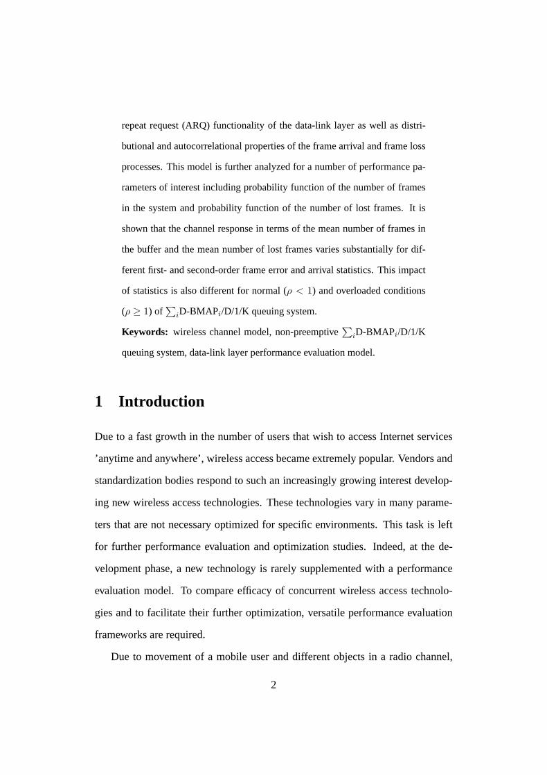
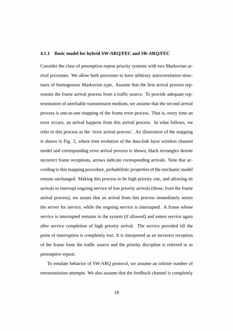
refer to this process as the ’error arrival process’. An illustration of the mapping

is shown in Fig. 2, where time evolution of the data-link layer wireless channel

model and corresponding error arrival process is shown, black rectangles denote

incorrect frame receptions, arrows indicate corresponding arrivals. Note that ac-

cording to this mapping procedure, probabilistic properties of the stochastic model

remain unchanged. Making this process to be high priority one, and allowing its

arrivals to interrupt ongoing service of low priority arrivals (those, from the frame

arrival process), we assure that an arrival from this process immediately seizes

the server for service, while the ongoing service is interrupted. A frame whose

service is interrupted remains in the system (if allowed) and enters service again

after service completion of high priority arrival. The service provided till the

point of interruption is completely lost. It is interpreted as an incorrect reception

of the frame from the traffic source and the priority discipline is referred to as

preemptive-repeat.

To emulate behavior of SW-ARQ protocol, we assume an infinite number of

retransmission attempts. We also assume that the feedback channel is completely

18

t

t

frame error model

frame arrival model

time slot

Figure 2: An illustration of error/arrival mapping.

reliable (perfect). Indeed, feedback acknowledgements are usually small in size

and well protected by FEC. We also assume that the feedback is instantaneous.

All these assumptions were tested and used in many studies and found to be ap-

propriate for wireless channels [5, 12, 13, 14]. Since the wireless channel model

is defined at the data-link layer, FEC capabilities are implicitly taken into account.

Note that the described model is also suitable to represent ’ideal’ SR-ARQ scheme

as in [10, 28]. In SR-ARQ frames are continuously transmitted and only incor-

rectly received frames are selectively requested for retransmission. According to

’ideal’ operation of SR-ARQ, round trip times (RTT) are assumed to be zero. In

this case operation of SR-ARQ and SW-ARQ schemes becomes identical and can

be represented using the proposed model.

Analysis of queuing systems with priority discipline is still a challenging task.

Among others, preemptive-repeat is probably most complicated priority disci-

pline. However, a number of assumptions can be further introduced to make

the queuing model less complicated. In what follows, we limit our model to the

discrete-time environment and require arrivals from any arrival process to have

a service time of one slot in duration. Indeed, frames at the data-link layer are

usually of equal length. According to such a system, arrivals occur just before the

end of slots. Since there can be at most one arrival from the arrival process repre-

senting the frame error process of the wireless channel, these arrivals do not wait

19

for service, enter the service in the beginning of nearest slots, and, if observed in

the system, are being served. To provide adequate representation of erroneous na-

ture of the wireless channel, we also have to ensure that all arrivals from the error

arrival process are accommodated by the system. Following these assumptions,

it is no longer needed to require preemptive-repeat priority discipline. Since all

arrivals occur simultaneously in batches, it is sufficient for such a system to have

non-preemptive priority discipline that is much easier to analyze.

4.1.2 Contention-free constant bit rate access

When a CBR channel is exclusively assigned to a mobile station during the whole

duration of a session, to estimate performance parameters of the frame transmis-

sion process we can directly apply non-preemptive GA+GF /D/1/K queuing sys-

tem, where GA is the frame arrival process, GF is the error arrival process. Such a

model provides adequate representation of time division multiple access (TDMA)

organization of the shared air interface. According to TDMA, each source has

an exclusive access to assigned circuit-switched channel over which frames trans-

mission is organized. There is no data-link layer concurrent traffic competing for

resources and the only performance degradation stems from unreliable nature of

the wireless channel.

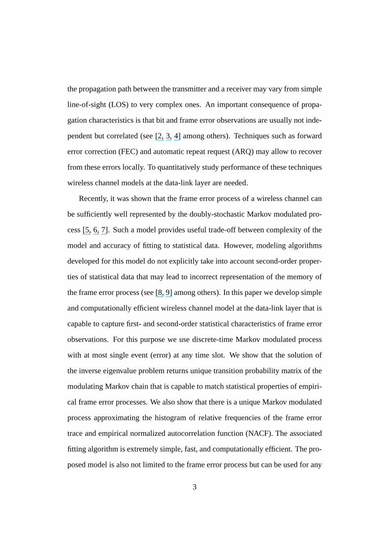
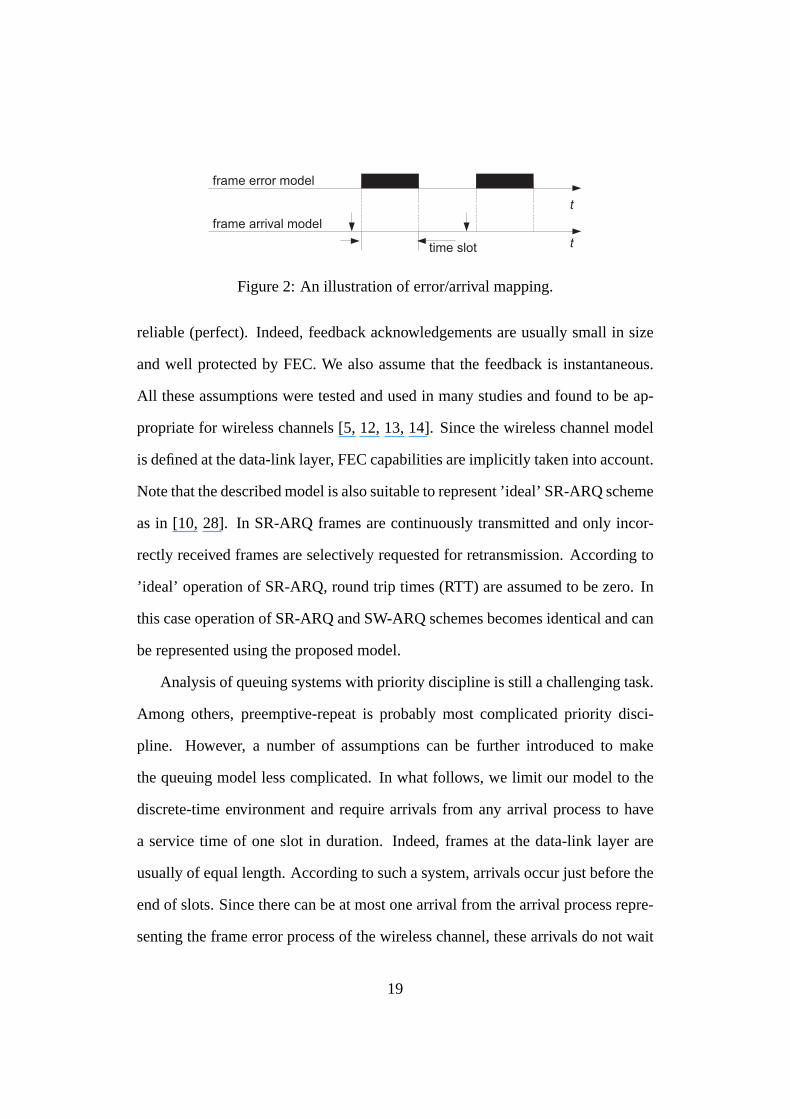
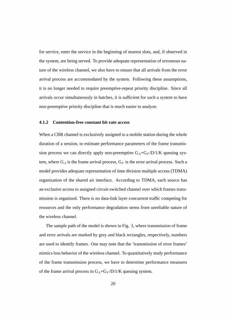
The sample path of the model is shown in Fig. 3, where transmission of frame

and error arrivals are marked by grey and black rectangles, respectively, numbers

are used to identify frames. One may note that the ’transmission of error frames’

mimics loss behavior of the wireless channel. To quantitatively study performance

of the frame transmission process, we have to determine performance measures

of the frame arrival process in GA+GF /D/1/K queuing system.

20

1

t

t

traffic

errors

t

transmission

2 3

time slot

1 2 ...

Figure 3: Sample path of the model for contention-free CBR access.

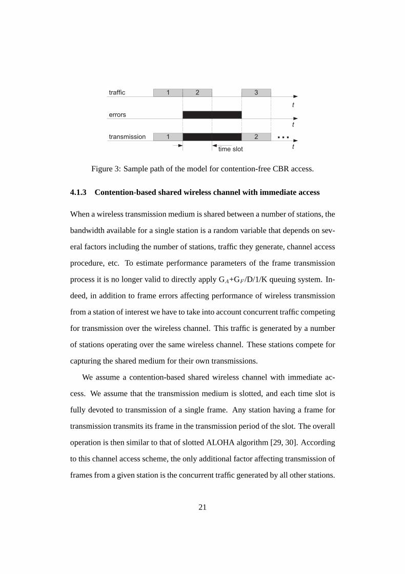
4.1.3 Contention-based shared wireless channel with immediate access

When a wireless transmission medium is shared between a number of stations, the

bandwidth available for a single station is a random variable that depends on sev-

eral factors including the number of stations, traffic they generate, channel access

procedure, etc. To estimate performance parameters of the frame transmission

process it is no longer valid to directly apply GA+GF /D/1/K queuing system. In-

deed, in addition to frame errors affecting performance of wireless transmission

from a station of interest we have to take into account concurrent traffic competing

for transmission over the wireless channel. This traffic is generated by a number

of stations operating over the same wireless channel. These stations compete for

capturing the shared medium for their own transmissions.

We assume a contention-based shared wireless channel with immediate ac-

cess. We assume that the transmission medium is slotted, and each time slot is

fully devoted to transmission of a single frame. Any station having a frame for

transmission transmits its frame in the transmission period of the slot. The overall

operation is then similar to that of slotted ALOHA algorithm [29, 30]. According

to this channel access scheme, the only additional factor affecting transmission of

frames from a given station is the concurrent traffic generated by all other stations.

21

We model such a type of traffic using the D-BMAP (or its special case). This pro-

cess may capture autocorrelation properties found in superposed traffic from a

number of sources. To estimate performance parameters of the frame service pro-

cess we can now apply GA+GF /D/1/K system, where the first arrival process is

the frame arrival process from a given source, the second one is the OR superpo-

sition of the frame error process and the frame arrival process from a number of

concurrent stations. The OR superposition gives 1 when at least one process has

a non-zero event in a slot. Otherwise, the value of the process is 0.

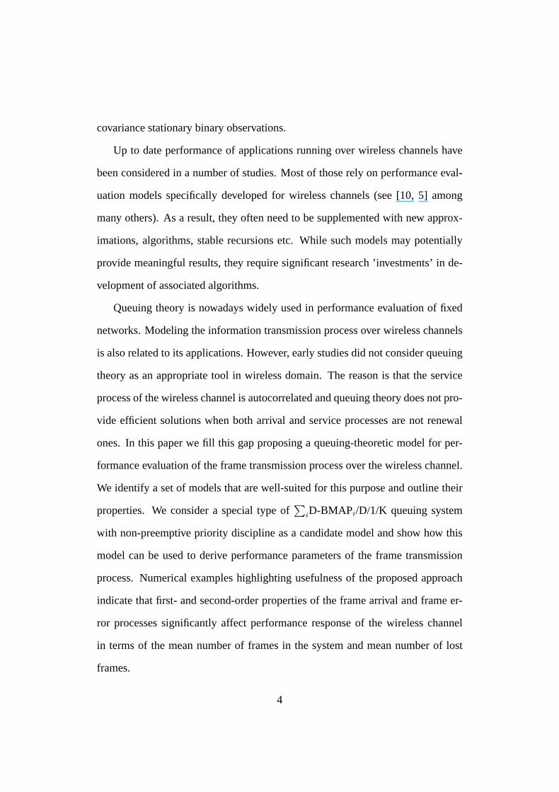
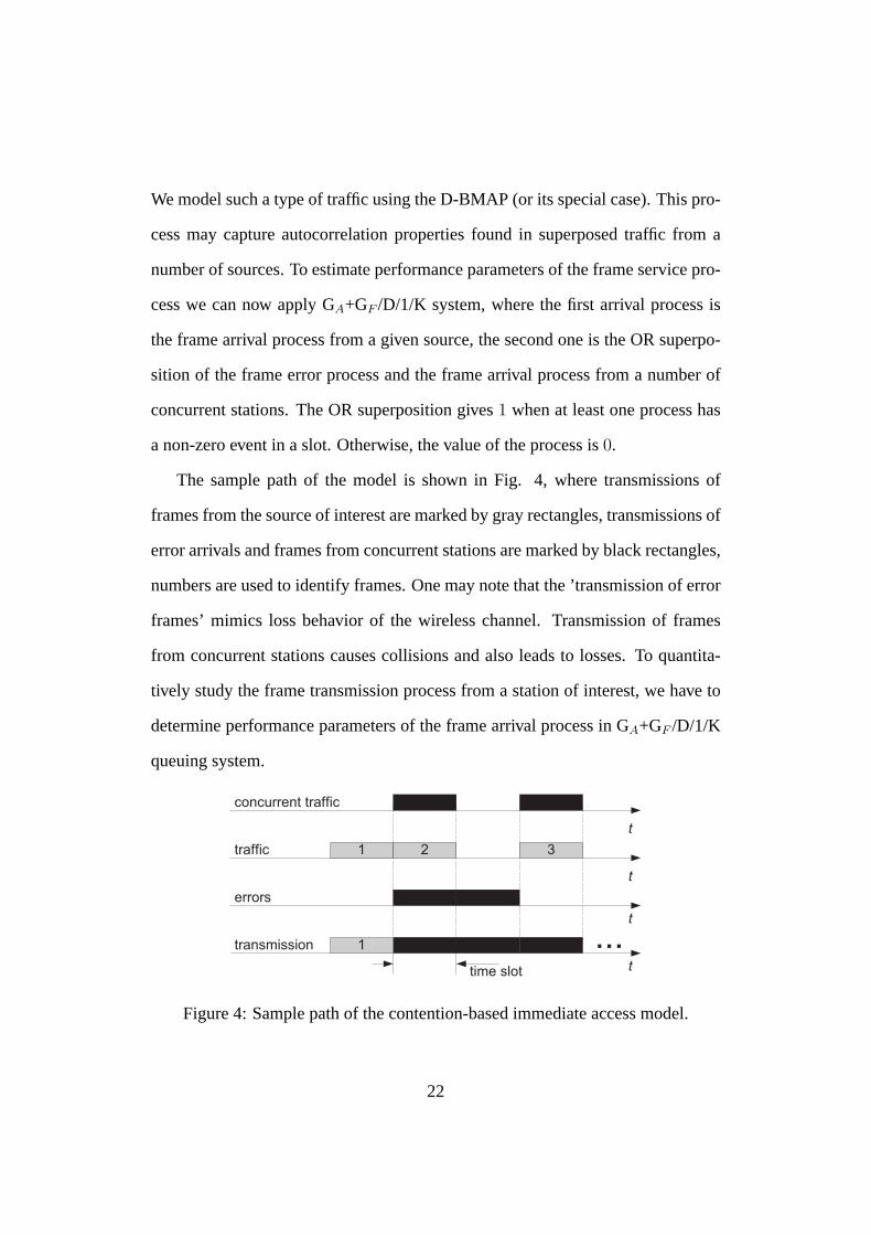
The sample path of the model is shown in Fig. 4, where transmissions of

frames from the source of interest are marked by gray rectangles, transmissions of

error arrivals and frames from concurrent stations are marked by black rectangles,

numbers are used to identify frames. One may note that the ’transmission of error

frames’ mimics loss behavior of the wireless channel. Transmission of frames

from concurrent stations causes collisions and also leads to losses. To quantita-

tively study the frame transmission process from a station of interest, we have to

determine performance parameters of the frame arrival process in GA+GF /D/1/K

queuing system.

1

t

t

traffic

errors

t

transmission

2 3

time slot

1 ...

t

concurrent traffic

Figure 4: Sample path of the contention-based immediate access model.

22

5 Performance evaluation

Previously, in Section 3, we modeled both frame arrival process and frame error

process using SBP. As a result, it is sufficient to consider performance parame-

ters of the frame arrival process in SBPA+SBPF /D/1/K queuing system. How-

ever, results for this system can be easily extended to the case of D-BMAPA+D-

MAPF /D/1/K queue. For this reason, in what follows, we proceed with perfor-

mance analysis of D-BMAPA+D-MAPF /D/1/K queuing system. Performance

parameters of interest are the probability function of the number of frames in the

system, probability function of lost frames, first and second moments of loss dis-

tribution and the probability of at least one frame loss. The number of states of the

modulating Markov chain of D-BMAPA and D-MAPF is allowed to be arbitrary

finite, MA and MF , respectively.

5.1 Description of the system

Consider D-BMAP/D/1/K queuing system, where the arrival process, denoted

by {W (n), n = 0, 1, . . . }, is the superposition of {WF (n), n = 0, 1, . . . } and

{WA(n), n = 0, 1, . . . }. Indeed, since both arrival processes are independent of

each other one can define their superposition that is D-BMAP [18]. The counting

variable n refers to the frame transmission time at the wireless channel. Steady-

state analysis of D-BMAP/D/1/K queuing system has been carried out in many

studies. Here, we take the method of imbedded Markov chain.

Time diagram of D-BMAP/D/1/K queuing system is shown in Fig. 5. Ac-

cording to such a system frames arrive in batches, batches of frames arrive just

before the end of slots. Arrivals are not allowed to seize the server immediately

23

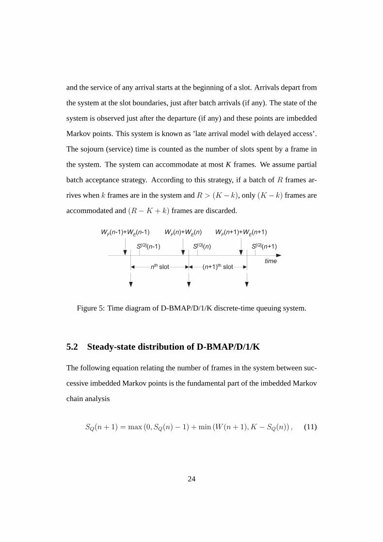
and the service of any arrival starts at the beginning of a slot. Arrivals depart from

the system at the slot boundaries, just after batch arrivals (if any). The state of the

system is observed just after the departure (if any) and these points are imbedded

Markov points. This system is known as ’late arrival model with delayed access’.

The sojourn (service) time is counted as the number of slots spent by a frame in

the system. The system can accommodate at most K frames. We assume partial

batch acceptance strategy. According to this strategy, if a batch of R frames ar-

rives when k frames are in the system and R > (K − k), only (K − k) frames are

accommodated and (R − K + k) frames are discarded.

nth slot (n+1)th slottime

WF(n-1)+W

E(n-1)

S[Q](n-1) S[Q](n) S[Q](n+1)

WF(n)+W

E(n) W

F(n+1)+W

E(n+1)

Figure 5: Time diagram of D-BMAP/D/1/K discrete-time queuing system.

5.2 Steady-state distribution of D-BMAP/D/1/K

The following equation relating the number of frames in the system between suc-

cessive imbedded Markov points is the fundamental part of the imbedded Markov

chain analysis

SQ(n + 1) = max (0, SQ(n) − 1) + min (W (n + 1), K − SQ(n)) , (11)

24

where SQ(n) denotes the number of customers (either frames or error frames) in

the system, W (n) denotes the number of arrivals in the slot n.

Observing (11) and Fig. 5, it can be deduced that the arrival from the frame

error process is not accepted by the system in the slot (n + 1) if and only if the

number of customers in the system in the slot (n− 1) is zero, there is an arrival of

K frames in the time slot n, and one frame arrives from the frame error process

in the slot (n + 1). Contrarily, if there is at least one frame in the system in the

slot (n − 1), one frame departs at the end of slot (n − 1), and there is always at

least one position in the system for the next arrival in the slot (n + 1). Thus, the

frame from the frame error process is not lost in the slot (n+1). To assure that the

frame from the frame error process is always accepted by the system we do not

allow the overall number of arrivals from both processes to be more than (K −1).

This implies that the maximum number of arrivals from the frame arrival process

is (K − 2). Note that it is usually sufficient for real applications.

Complete description of the queuing system requires two-dimensional Markov

chain {SQ(n), S(n), n = 0, 1, . . . } imbedded at the moments of frame depar-

tures, where S(n) = SF (n) ⊗ SA(n) is the state of the superposition of the

frame arrival and frame error processes, and SQ(n) ∈ {0, 1, . . . , K − 1} is the

number of frames in the system just after frame departures. Introducing matri-

ces D(≥ k), k = 0, 1, .., K − 1, containing transition probabilities with at least

k = 0, 1, .., K − 1 arrivals, respectively, one can define the transition probability

matrix, T , of the Markov chain {SQ(n), S(n), n = 0, 1, . . . } as usual (see [31]

among others). Let �x = (x0,1, .., xK−1,M ) be the row array containing steady-state

probabilities of {SQ(n), S(n), n = 0, 1, ..}, where M = MF MA. Solving matrix

equations �πT = �π, �π�eT = 1, where �e is the vector of ones of appropriate size, we

25

can compute steady-state probabilities xkj = limn→∞ Pr{SQ(n) = k, S(n) = j}.

There are a number of algorithms to compute these probabilities [32, 33, 34].

5.3 Loss performance

5.3.1 Probability function of lost frames

The probability function of lost frames completely determines loss performance

of applications. It can be used to determine user-oriented performance parameters

such as mean number of lost frames, variance of lost frames, quantiles, etc.

Since we guaranteed that the frame error process does not suffer losses, from

the loss performance point of view D-BMAPA+D-MAPF /D/1/K and D-BMAP/D/1/K

queuing systems, where D-BMAP is the superposition of D-BMAPA and D-MAPF ,

are equivalent. Consider the loss behavior of D-BMAP/D/1/K queuing system

between two arbitrary imbedded Markov points at equilibrium. Since at most

(K − 2) frames may arrive from the frame arrival process, there can be at most

(K − 2) lost frames in a slot. Let the RV L, L ∈ {0, 1, . . . , K − 2}, denote the

number of lost frames in a slot and let fL(l) = Pr{L = l}, l = 0, 1, . . . , K−2, be

its probability function. According to our assumptions the frame arrival process

does not suffer losses when there are no frames in the system. Consider the event

when l, l = 1, 2, . . . , K − 2, frames are lost in this time slot. This event occurs

when the following conditions are met

• there are k, k = 1, 2, . . . frames in the system in the slot (n − 1);

• there are exactly (K − k + l) arrivals to the system in the slot n.

To determine fL(l|WA ≥ 1) = Pr{L = l}, l = 1, 2, .., K − 2, we have to

26

take into account these conditions over all possible transitions of the underlying

Markov chain of the arrival process with exactly (K − k + l) arrivals. We get the

following

fL(l|WA(n) ≥ 1) =K−1∑k=2

M∑i=1

M∑j=1

xkidij(K − k + l), (12)

where dij(k), k > K − 1, are zeros. Since the system never reaches states (K, i),

i = 1, 2, . . . , M , the fist sum in (12) extends to (K − 1) only. Next sums in (12)

cover all possible states of underlying Markov chain of arrival process in previous

and next slots. Alternatively, in matrix notation we may write

fL(l|WA(n) ≥ 1) =K−1∑k=2

�xkD(K − k + l)�e, (13)

where �xk = (xk1, xk2, . . . , xk(MF MA)) is the vector containing steady-state prob-

abilities that there are k arrivals in the system and the state of the modulating

Markov chain of the arrival process is i = 1, 2, . . . , MF MA, �e is the vector of

ones of appropriate size.

In (12) and (13) we also have to ensure that arrivals from the frame arrival

process are indeed occurred. We find this condition of (12) and (13) as follows

Pr{WA ≥ 1} = �πA

(K−2∑i=1

DA(i)

)�eA, (14)

where �πA is the steady-state vector of {WA(n), n = 0, 1, . . . }, �eA is the vector of

27

ones of appropriate size. Finally, we have

fL(l) =

∑K−1k=2 �xkD(K − k + l)�e

�πA

(∑K−2i=1 DA(i)

)�eA

, l = 1, 2, . . . , K − 2,

fL(0) = 1 −K−2∑i=1

fL(i). (15)

If the maximum number of arrivals from the frame arrival process in any slot

is limited to 1 (the frame arrival process is modeled by D-MAP or its special

case), the computational complexity of (15) can be significantly reduced. Let

again RV L, L ∈ {0, 1}, denote the number of lost frames in an arbitrary slot

n given that a frame arrives. Let then fL(k) = Pr{L = k}, k = 0, 1, be its

probability function. The frame arrival process losses one arrival when the state

of the system is SQ(n) = (K−1) and arrivals from D-MAPA and D-MAPF occur

simultaneously. We get

fL(1) =�xK−1D(2)�e

�πADA(1)�eA

=�xK−1D(2)�e

E[WA],

fL(0) = 1 − fL(1). (16)

5.3.2 Moments of loss distributions

Mean and variance of the number of lost frames can be obtained from (15) as

E[L] =K−2∑l=1

lfL(l), σ2[L] = E[L2] − (E[L])2. (17)

28

If the maximum number of frame arrivals in any slot is limited to 1 we have

µL = fL(1), σ2L = fL(1) − [fL(1)]2. (18)

5.3.3 Probability of at least one frame loss

Probability of at least one frame loss can be obtained from (15). However, it is

convenient to determine it using matrices D(≥ k), k = 0, 1, . . . . The frame arrival

process losses at least one frame when the following conditions are met:

• there are k, k = 1, 2, . . . frames in the system in the slot (n − 1);

• there are at least (K − k + 1) arrivals to the system in the slot n.

Let fL(l ≥ 1) be the probability of at least one frame loss. Considering

these conditions over all possible transitions of the underlying Markov chain of

{W (n), n = 0, 1, . . . } with more than (K − k + 1) arrivals we get

fL(l ≥ 1|WA(n) ≥ 1) =K−1∑k=2

M∑i=1

M∑j=1

xkidij(≥ K − k + 1). (19)

Using matrix notation and removing conditioning we have

fL(l ≥ 1) =

∑K−1k=2 �xkD(≥ K − k + 1)�e

�πA

(∑K−2i=1 DA(i)

)�eA

. (20)

If the maximum number of frame arrivals in any slot is limited to 1 we have

fL(l ≥ 1) = fL(1) =�xK−1D(2)�e

E[WA]. (21)

29

6 Numerical examples

6.1 Frame error process

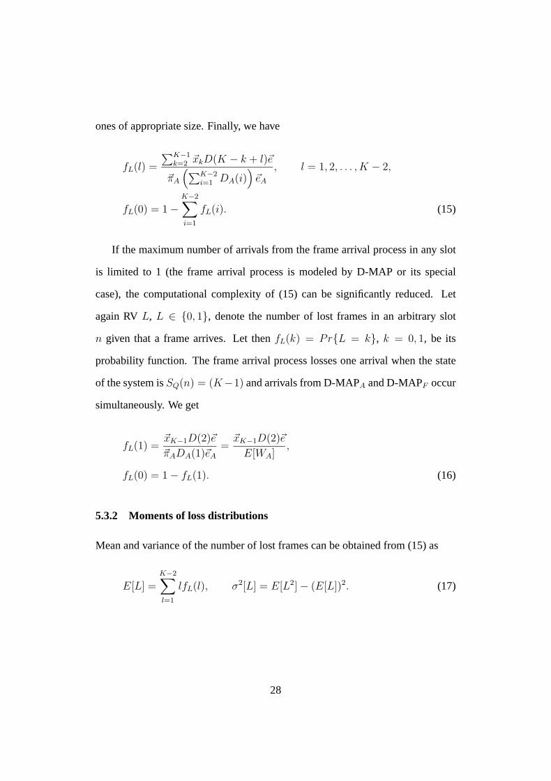
To explore the loss response of the wireless channel we use a number of SBP

wireless channel models with different means and lag-1 autocorrelations. We

constructed 64 models of the frame error process as follows: for each mean out of

�E[WF ] = (0.01, 0.02, . . . , 0.08) we generate models with the following lag-1 au-

tocorrelations �KF (1) = (0.1, 0.2, . . . , 0.8). Parameters of the frame error models,

α and β, as functions of E[WF ] and KF (1) are shown in Fig. 6.

E[W ]*100FKF(1)*10

�

KF(1)*10E[W ]*100F

�

Figure 6: α and β as functions of E[WF ] and KF (1).

6.2 Frame arrival process

In order to model the frame arrival process at the data-link layer we use SBP with

different means and lag-1 autocorrelations. We constructed 4 models of the frame

error traces as follows: for each mean out of �E[WA] = (0.6, 0.9) we generate

models with the following lag-1 autocorrelations �KA(1) = (0.3, 0.6).

30

6.3 Results

The resulting system is SBPA+SBPF /D/1/K. In what follows, we set capacity of

the system to K = 50. Since at most two arrivals are allowed in a slot we also

satisfied the requirement Pr{SQ(n) = K,S(n) = j|SQ(n) = 0, S(n) = i} = 0.

Due to the limited capacity, the system is always stable. For systems that are

always stable we distinguish between normal and overloaded conditions. The loss

response of the the proposed system to input first- and second-order statistics of

the frame arrival and frame error processes is different in these two conditions.

Due to this reason we consider these two cases separately.

6.3.1 Normal conditions

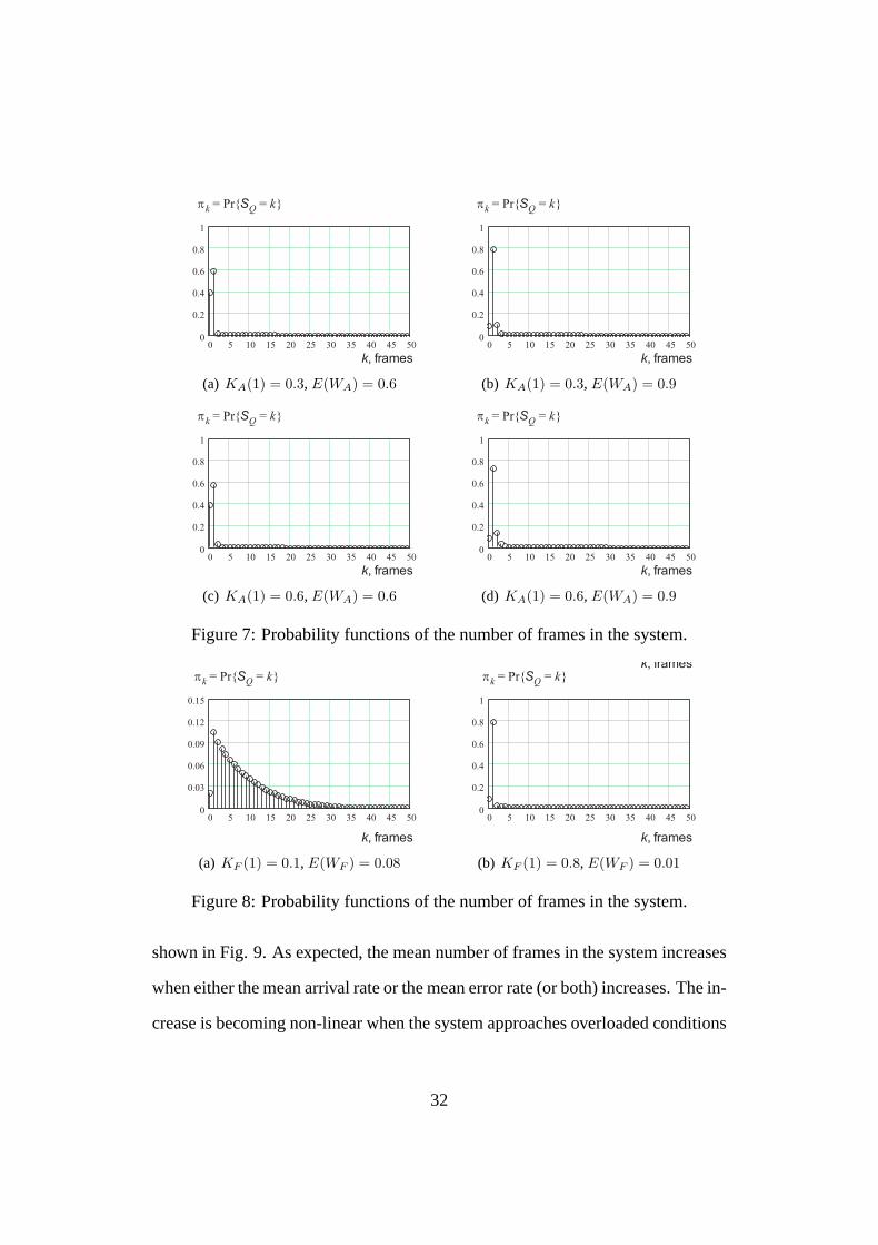
Probability functions of the number of frames in the system for frame error models

with KF (1) = 0.1, E[WF ] = 0.01 and frame arrival models with all possible val-

ues out of �KA(1) = (0.3, 0.6) and �A[WA] = (0.6, 0.9) are shown in Fig. 7. Even

from this illustrative example it is clear that first- and second-order frame arrival

statistics affect performance of the frame service process. Probability functions

of the number of frames in the system for frame error models with KF (1) = 0.8,

E[WF ] = 0.01 and KF (1) = 0.1, E[WF ] = 0.08 and the frame arrival model

with KA(1) = 0.6, E[WA] = 0.9 are shown in Fig. 8. Comparing these functions

to that shown in Fig. 7(d) one may note that first- and second-order frame error

statistics also affect performance of the frame service process.

The mean number of frames in the system, E[π], as a function of statistical

characteristics of the frame error process and for all defined frame arrival pro-

cesses with parameters out of �KA(1) = (0.3, 0.6) and �E[WA] = (0.6, 0.9) is

31

�k = Pr{SQ = k}

0 5 10 15 20 25 30 35 40 45 500

0.2

0.4

0.6

0.8

1

k, frames

(a) KA(1) = 0.3, E(WA) = 0.6

�k = Pr{SQ = k}

0 5 10 15 20 25 30 35 40 45 500

0.2

0.4

0.6

0.8

1

k, frames

(b) KA(1) = 0.3, E(WA) = 0.9

�k = Pr{SQ = k}

0 5 10 15 20 25 30 35 40 45 500

0.2

0.4

0.6

0.8

1

k, frames

(c) KA(1) = 0.6, E(WA) = 0.6

�k = Pr{SQ = k}

0 5 10 15 20 25 30 35 40 45 500

0.2

0.4

0.6

0.8

1

k, frames

(d) KA(1) = 0.6, E(WA) = 0.9

Figure 7: Probability functions of the number of frames in the system.

�k = Pr{SQ = k}

0 5 10 15 20 25 30 35 40 45 500

0.03

0.06

0.09

0.12

0.15

k, frames

(a) KF (1) = 0.1, E(WF ) = 0.08

k, frames�k = Pr{SQ = k}

0 5 10 15 20 25 30 35 40 45 500

0.2

0.4

0.6

0.8

1

k, frames

(b) KF (1) = 0.8, E(WF ) = 0.01

Figure 8: Probability functions of the number of frames in the system.

shown in Fig. 9. As expected, the mean number of frames in the system increases

when either the mean arrival rate or the mean error rate (or both) increases. The in-

crease is becoming non-linear when the system approaches overloaded conditions

32

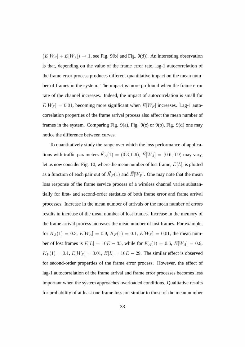
(E[WF ] + E[WA]) → 1, see Fig. 9(b) and Fig. 9(d)). An interesting observation

is that, depending on the value of the frame error rate, lag-1 autocorrelation of

the frame error process produces different quantitative impact on the mean num-

ber of frames in the system. The impact is more profound when the frame error

rate of the channel increases. Indeed, the impact of autocorrelation is small for

E[WF ] = 0.01, becoming more significant when E[WF ] increases. Lag-1 auto-

correlation properties of the frame arrival process also affect the mean number of

frames in the system. Comparing Fig. 9(a), Fig. 9(c) or 9(b), Fig. 9(d) one may

notice the difference between curves.

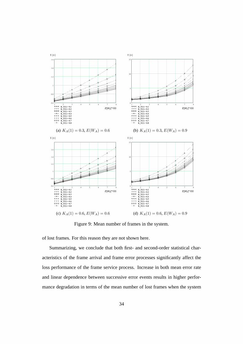
To quantitatively study the range over which the loss performance of applica-

tions with traffic parameters �KA(1) = (0.3, 0.6), �E[WA] = (0.6, 0.9) may vary,

let us now consider Fig. 10, where the mean number of lost frame, E[L], is plotted

as a function of each pair out of �KF (1) and �E[WF ]. One may note that the mean

loss response of the frame service process of a wireless channel varies substan-

tially for first- and second-order statistics of both frame error and frame arrival

processes. Increase in the mean number of arrivals or the mean number of errors

results in increase of the mean number of lost frames. Increase in the memory of

the frame arrival process increases the mean number of lost frames. For example,

for KA(1) = 0.3, E[WA] = 0.9, KF (1) = 0.1, E[WF ] = 0.01, the mean num-

ber of lost frames is E[L] = 10E − 35, while for KA(1) = 0.6, E[WA] = 0.9,

KF (1) = 0.1, E[WF ] = 0.01, E[L] = 10E − 29. The similar effect is observed

for second-order properties of the frame error process. However, the effect of

lag-1 autocorrelation of the frame arrival and frame error processes becomes less

important when the system approaches overloaded conditions. Qualitative results

for probability of at least one frame loss are similar to those of the mean number

33

� ��]

1 2 3 4 5 6 7 80.6

0.8

1

1.2

1.4

1.6

K_F(1) = 0.1

K_F(1) = 0.2

K_F(1) = 0.3

K_F(1) = 0.4

K_F(1) = 0.5

K_F(1) = 0.6

K_F(1) = 0.7

K_F(1) = 0.8

E[WF]*100

(a) KA(1) = 0.3, E(WA) = 0.6

� ��]

1 2 3 4 5 6 7 80

5

10

15

K_F(1) = 0.1

K_F(1) = 0.2

K_F(1) = 0.3

K_F(1) = 0.4

K_F(1) = 0.5

K_F(1) = 0.6

K_F(1) = 0.7

K_F(1) = 0.8

E[WF]*100

(b) KA(1) = 0.3, E(WA) = 0.9

� ��]

1 2 3 4 5 6 7 80.6

0.8

1

1.2

1.4

1.6

K_F(1) = 0.1

K_F(1) = 0.2

K_F(1) = 0.3

K_F(1) = 0.4

K_F(1) = 0.5

K_F(1) = 0.6

K_F(1) = 0.7

K_F(1) = 0.8

E[WF]*100

(c) KA(1) = 0.6, E(WA) = 0.6

� ��]

1 2 3 4 5 6 7 80

5

10

15

K_F(1) = 0.1

K_F(1) = 0.2

K_F(1) = 0.3

K_F(1) = 0.4

K_F(1) = 0.5

K_F(1) = 0.6

K_F(1) = 0.7

K_F(1) = 0.8

E[WF]*100

(d) KA(1) = 0.6, E(WA) = 0.9

Figure 9: Mean number of frames in the system.

of lost frames. For this reason they are not shown here.

Summarizing, we conclude that both first- and second-order statistical char-

acteristics of the frame arrival and frame error processes significantly affect the

loss performance of the frame service process. Increase in both mean error rate

and linear dependence between successive error events results in higher perfor-

mance degradation in terms of the mean number of lost frames when the system

34

E [L]

1 2 3 4 5 6 7 81 �10

511 �10501 �10491 �10481 �10471 �10461 �10451 �10441 �10431 �10421 �10411 �10401 �10391 �10381 �10371 �10361 �10351 �10341 �10331 �10321 �10311 �10301 �10291 �10281 �10271 �10261 �10251 �10241 �10231 �10221 �10211 �10201 �10191 �10181 �10171 �10161 �10151 �10141 �10131 �10121 �10111 �10101 �10

91 �1081 �1071 �106

K_F(1) = 0.1

K_F(1) = 0.2

K_F(1) = 0.3

K_F(1) = 0.4

K_F(1) = 0.5

K_F(1) = 0.6

K_F(1) = 0.7

K_F(1) = 0.8

E[WF]*100

(a) KA(1) = 0.3, E(WA) = 0.6

E [L]

1 2 3 4 5 6 7 81 �10

351 �10341 �10331 �10321 �10311 �10301 �10291 �10281 �10271 �10261 �10251 �10241 �10231 �10221 �10211 �10201 �10191 �10181 �10171 �10161 �10151 �10141 �10131 �10121 �10111 �10101 �10

91 �1081 �1071 �1061 �1051 �1041 �1030.01

K_F(1) = 0.1

K_F(1) = 0.2

K_F(1) = 0.3

K_F(1) = 0.4

K_F(1) = 0.5

K_F(1) = 0.6

K_F(1) = 0.7

K_F(1) = 0.8

E[WF]*100

(b) KA(1) = 0.3, E(WA) = 0.9

E [L]

1 2 3 4 5 6 7 81 �10

451 �10441 �10431 �10421 �10411 �10401 �10391 �10381 �10371 �10361 �10351 �10341 �10331 �10321 �10311 �10301 �10291 �10281 �10271 �10261 �10251 �10241 �10231 �10221 �10211 �10201 �10191 �10181 �10171 �10161 �10151 �10141 �10131 �10121 �10111 �10101 �10

91 �1081 �1071 �106

K_F(1) = 0.1

K_F(1) = 0.2

K_F(1) = 0.3

K_F(1) = 0.4

K_F(1) = 0.5

K_F(1) = 0.6

K_F(1) = 0.7

K_F(1) = 0.8

E[WF]*100

(c) KA(1) = 0.6, E(WA) = 0.6

E [L]

1 2 3 4 5 6 7 81 �10

291 �10281 �10271 �10261 �10251 �10241 �10231 �10221 �10211 �10201 �10191 �10181 �10171 �10161 �10151 �10141 �10131 �10121 �10111 �10101 �10

91 �1081 �1071 �1061 �1051 �1041 �1030.01

K_F(1) = 0.1

K_F(1) = 0.2

K_F(1) = 0.3

K_F(1) = 0.4

K_F(1) = 0.5

K_F(1) = 0.6

K_F(1) = 0.7

K_F(1) = 0.8

E[WF]*100

(d) KA(1) = 0.6, E(WA) = 0.9

Figure 10: Mean number of lost frames.

is not overloaded. While the effect of lag-1 autocorrelation is not so significant

as compared to the effect of the mean error rate, it is still important and should

be taken into account when predicting loss performance than a given application

experiences running over wireless channels. Note that these conclusions may not

however be true for higher layers (e.g. IP) if segmentation procedure between

data-link and IP layer is implemented. Indeed, in [35] it was shown that the lag-1

35

autocorrelation between successive events of errors may sometimes increase per-

formance as seen at the IP and higher layers. Discussion and numerical results

of this effect can be found in [35]. Those results do not, however, affect our con-

clusions proving that autocorrelation properties are of high importance for loss

performance of applications.

6.3.2 Overloaded conditions

When (E[WF + E[WA]) approaches unity, the system enters overloaded condi-

tion. Note that the system is still stable meaning that equilibrium probabilities

of system states exist. However, the response of the system to input statistics

changes substantially. To illustrate it, we use SBP arrival process with �KA(1) =

(0.3, 0.6) and mean E[WA] = 0.95 and 64 SBP frame error models with �E[WF ] =

(0.01, 0.02, . . . , 0.08) and lag-1 autocorrelations �KF (1) = (0.1, 0.2, . . . , 0.8). Note

that for all values of the frame error rate that are greater than E[WF ] = 0.05 the

system is overloaded (the offered load is more than unity).

The mean number of frames in the system for each value out of �KF (1) and

�E[WF ] is shown in Fig. 11. One may note that the frame error process with

KF (1) = 0.1 results in less mean number of frames in the system as compared to

higher values of KF (1) when the system is overloaded, i.e. (E[WF +E[WA]) > 1.

Recall that for (E[WF ] + E[WA]) < 1 higher lag-1 autocorrelation of the frame

error process leads to more mean number of frames in the system on average.

It is important that lag-1 autocorrelation of the frame arrival process also affects

performance parameters of the frame service process. Indeed, higher lag-1 auto-

correlation of the frame arrival process makes the effect of lag-1 autocorrelation

of the frame error process less significant. Results shown in Fig. 11 are explained

36

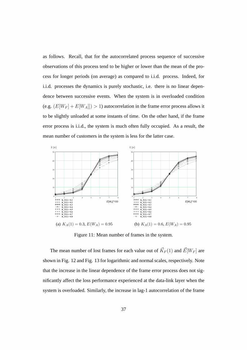
as follows. Recall, that for the autocorrelated process sequence of successive

observations of this process tend to be higher or lower than the mean of the pro-

cess for longer periods (on average) as compared to i.i.d. process. Indeed, for

i.i.d. processes the dynamics is purely stochastic, i.e. there is no linear depen-

dence between successive events. When the system is in overloaded condition

(e.g. (E[WF ] + E[WA]]) > 1) autocorrelation in the frame error process allows it

to be slightly unloaded at some instants of time. On the other hand, if the frame

error process is i.i.d., the system is much often fully occupied. As a result, the

mean number of customers in the system is less for the latter case.

� ��]

1 2 3 4 5 6 7 80

10

20

30

40

50

K_F(1) = 0.1

K_F(1) = 0.2

K_F(1) = 0.3

K_F(1) = 0.4

K_F(1) = 0.5

K_F(1) = 0.6

K_F(1) = 0.7

K_F(1) = 0.8

E[WF]*100

(a) KA(1) = 0.3, E(WA) = 0.95

� ��]

1 2 3 4 5 6 7 80

10

20

30

40

50

K_F(1) = 0.1

K_F(1) = 0.2

K_F(1) = 0.3

K_F(1) = 0.4

K_F(1) = 0.5

K_F(1) = 0.6

K_F(1) = 0.7

K_F(1) = 0.8

E[WF]*100

(b) KA(1) = 0.6, E(WA) = 0.95

Figure 11: Mean number of frames in the system.

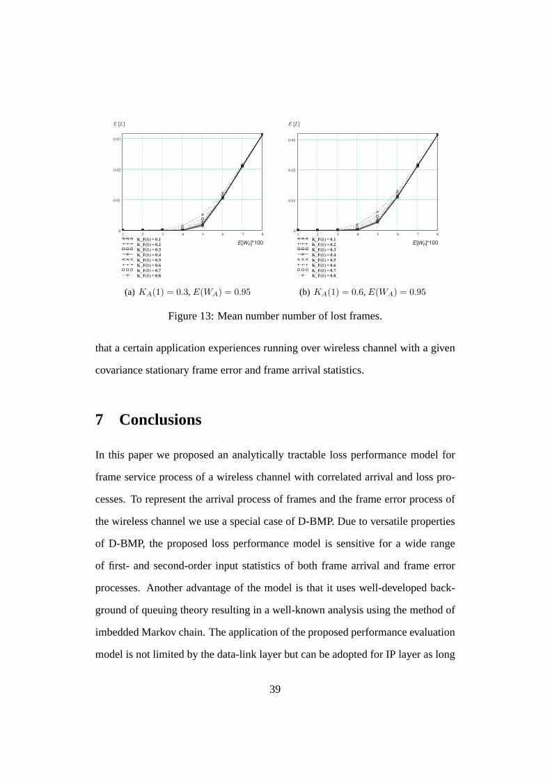
The mean number of lost frames for each value out of �KF (1) and �E[WF ] are

shown in Fig. 12 and Fig. 13 for logarithmic and normal scales, respectively. Note

that the increase in the linear dependence of the frame error process does not sig-

nificantly affect the loss performance experienced at the data-link layer when the

system is overloaded. Similarly, the increase in lag-1 autocorrelation of the frame

37

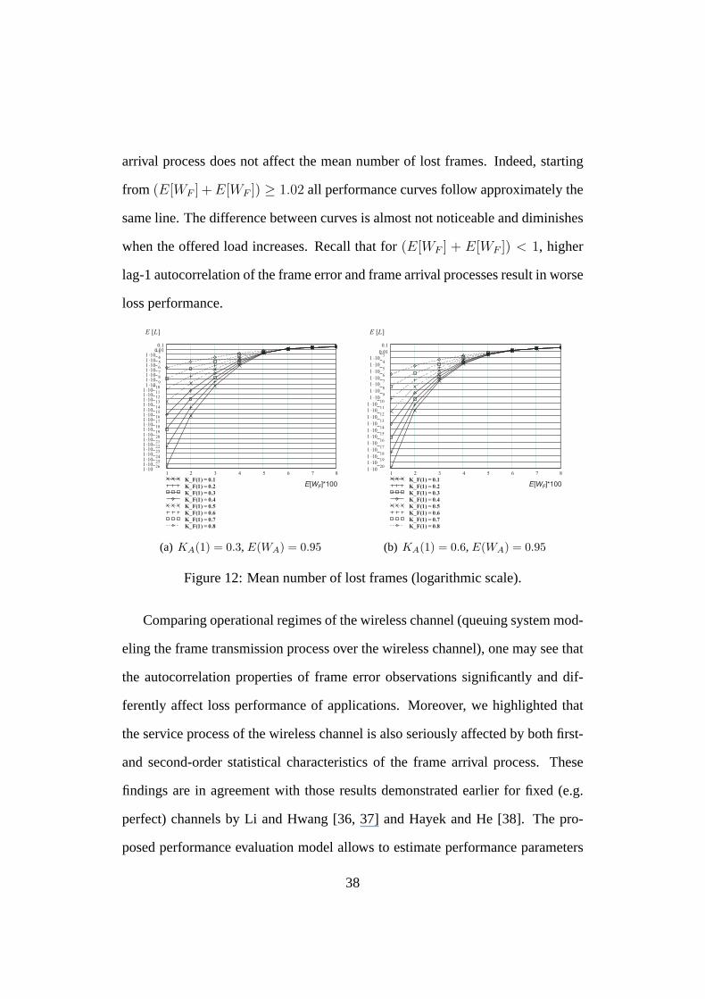
arrival process does not affect the mean number of lost frames. Indeed, starting

from (E[WF ] + E[WF ]) ≥ 1.02 all performance curves follow approximately the

same line. The difference between curves is almost not noticeable and diminishes

when the offered load increases. Recall that for (E[WF ] + E[WF ]) < 1, higher

lag-1 autocorrelation of the frame error and frame arrival processes result in worse

loss performance.

E [L]

1 2 3 4 5 6 7 81 �10

261 �10251 �1024

1 �10231 �10221 �10211 �10201 �1019

1 �10181 �10171 �10161 �10151 �1014

1 �10131 �10121 �10111 �10101 �10

91 �10

81 �1071 �1061 �1051 �104

1 �1030.010.1

K_F(1) = 0.1

K_F(1) = 0.2

K_F(1) = 0.3

K_F(1) = 0.4

K_F(1) = 0.5

K_F(1) = 0.6

K_F(1) = 0.7

K_F(1) = 0.8

E[WF]*100

(a) KA(1) = 0.3, E(WA) = 0.95

E [L]

1 2 3 4 5 6 7 81 �10

201 �10

191 �10

181 �10

171 �10

161 �10

151 �10

141 �10

131 �10

121 �10

111 �10

101 �10

91 �10

81 �10

71 �10

61 �10

51 �10

41 �10

30.01

0.1

K_F(1) = 0.1

K_F(1) = 0.2

K_F(1) = 0.3

K_F(1) = 0.4

K_F(1) = 0.5

K_F(1) = 0.6

K_F(1) = 0.7

K_F(1) = 0.8

E[WF]*100

(b) KA(1) = 0.6, E(WA) = 0.95

Figure 12: Mean number of lost frames (logarithmic scale).

Comparing operational regimes of the wireless channel (queuing system mod-

eling the frame transmission process over the wireless channel), one may see that

the autocorrelation properties of frame error observations significantly and dif-

ferently affect loss performance of applications. Moreover, we highlighted that

the service process of the wireless channel is also seriously affected by both first-

and second-order statistical characteristics of the frame arrival process. These

findings are in agreement with those results demonstrated earlier for fixed (e.g.

perfect) channels by Li and Hwang [36, 37] and Hayek and He [38]. The pro-

posed performance evaluation model allows to estimate performance parameters

38

E [L]

1 2 3 4 5 6 7 80

0.01

0.02

0.03

K_F(1) = 0.1

K_F(1) = 0.2

K_F(1) = 0.3

K_F(1) = 0.4

K_F(1) = 0.5

K_F(1) = 0.6

K_F(1) = 0.7

K_F(1) = 0.8

E[WF]*100

(a) KA(1) = 0.3, E(WA) = 0.95

E [L]

1 2 3 4 5 6 7 80

0.01

0.02

0.03

K_F(1) = 0.1

K_F(1) = 0.2

K_F(1) = 0.3

K_F(1) = 0.4

K_F(1) = 0.5

K_F(1) = 0.6

K_F(1) = 0.7

K_F(1) = 0.8

E[WF]*100

(b) KA(1) = 0.6, E(WA) = 0.95

Figure 13: Mean number number of lost frames.

that a certain application experiences running over wireless channel with a given

covariance stationary frame error and frame arrival statistics.

7 Conclusions

In this paper we proposed an analytically tractable loss performance model for

frame service process of a wireless channel with correlated arrival and loss pro-

cesses. To represent the arrival process of frames and the frame error process of

the wireless channel we use a special case of D-BMP. Due to versatile properties

of D-BMP, the proposed loss performance model is sensitive for a wide range

of first- and second-order input statistics of both frame arrival and frame error

processes. Another advantage of the model is that it uses well-developed back-

ground of queuing theory resulting in a well-known analysis using the method of

imbedded Markov chain. The application of the proposed performance evaluation

model is not limited by the data-link layer but can be adopted for IP layer as long

39

as appropriate statistics for arrival and loss models are available.

We studied two operational regimes of the wireless channel and showed that

performance parameters are significantly and differently affected by first- and

second-order statistical characteristics of frame error and frame arrival statistics.

For normal operation of the wireless channel higher lag-1 autocorrelation of the

frame error process results in worse performance in terms of the mean number of

lost frames. The effect is almost not noticeable for overloaded operation. For both

regimes higher lag-1 autocorrelation of the frame arrival process results in worse

loss performance of applications.

8 Acknowledgements

The financial support of Graduate School of Technology and Automation (GETA),

and Nokia Foundation is gratefully acknowledged.

References

[1] A. Lombardo, G. Morabito, and G. Schembra. An accurate and treatable

Markov model of MPEG video traffic. In Proc. of IEEE INFOCOM, pages

217–224, 1998.

[2] T. Rappaport. Wireless communications: principles and practice. Prentice

Hall, 2nd edition, 2002.

[3] B. Sklar. Rayleigh fading channels in mobile digital communication systems

Part I: characterization. IEEE Comm. Mag., pages 90–100, July 1997.

40

[4] H. Bai and M. Atiquzzaman. Error modeling schemes for fading channels

in wireless communications: a survey. Wireless Networks, 5(2):2–9, 4th

Quarter 2003.

[5] M. Zorzi, R. Rao, and L. Milstein. ARQ error control for fading mobile

radio channels. IEEE Trans. on Veh. Tech., 46(2):445–455, May 1997.

[6] M. Zorzi and R. Rao. The effect of correlated errors on the performance of

TCP. IEEE Comm. Let., 1(5):127–129, September 1997.

[7] M. Zorzi, A. Chockalingam, and R. Rao. Throughput analysis of TCP on

channels with memory. IEEE JSAC, 18(7):1289–1300, July 1999.

[8] S. Khayam and H. Radha. Markov-based modeling of wireless local area

networks. In ACM MSWiM, pages 100–107, San-Diego, US, September

2003.

[9] G. Nguyen, R. Katz, and B. Noble. A trace-based approach for modeling

wireless channel behavior. In Proc. Winter Simulation Conf., pages 597–

604, 1996.

[10] M. Krunz and J.-G. Kim. Fluid analysis of delay and packet discard perfor-

mance for QoS support in wireless networks. IEEE JSAC, 19(2):384–395,

February 2001.

[11] S. Karande, S. Khayam, M. Krappel, and H. Radha. Analysis and modeling

of errors at the 802.11b link layer. In Proc. IEEE ICME, July 2003.

41

[12] M. Zorzi, R. Rao, and L. Milstein. Performance analysis of ARQ Go-Back-N

protocol in fading mobile radio channels. In Proc. Milcom, pages 576–580,

November 1995.

[13] M. Zorzi and R. Rao. Throughput analysis of Go-Back-N ARQ in Markov

channels with unreliable feedback. In Proc. Globecom, pages 1232–1237,

June 1995.

[14] M. Zorzi and R. Rao. ARQ error control for delay-constrained communica-

tions on short-range burst-error channels. In Proc. VTC, pages 1528–1532,

May 1997.

[15] R. Mukhtar, S. Hanly, M. Zukerman, and F. Cameron. A model for the

performance evaluation of packet transmissions using type-ii hybrid ARQ

over a correlated error channel. Wireless Networks, 10(1):7–16, January

2004.

[16] A. Klemm, C. Lindemann, and M. Lohmann. Modeling IP traffic using the

batch Markovian arrival process. Perf. Eval., 54(2):149–173, 2003.

[17] J. Cosmas, G. Petit, R. Lehnert, C. Blondia, K. Kontovvassilis, O. Casals,

and T. Theimer. A review of voice, data and video traffic models for ATM.

European Transactions on Telecommunication and Related Technologies,

5(2):139–153, March–April 1994.

[18] C. Blondia. A discrete-time batch Markovian arrival process as B-ISDN

traffic model. Belgian Journal of Oper. Res., 32(3,4):3–23, 1993.

42

[19] A. Adas. Traffic models in broadband networks. IEEE Comm. Mag.,

35(7):82–89, July 1997.

[20] V. Frost and B. Melamed. Traffic modeling for telecommunications net-

works. IEEE Comm. Mag., 32(3):70–81, March 1994.

[21] M. Krunz and J.-G. Kim. Delay analysis of selective repeat ARQ for a

Markovian source over a wireless channel. IEEE Trans. on Veh. Tech.,

49(5):1968–1981, September 2000.

[22] J.-A. Zhao, B. Li, C.-W. Kok, and I. Ahmad. MPEG-4 video transmission

over wireless networks: a link level performance study. Wireless Networks,

10(2):133–146, March 2004.

[23] S. Khayam. IEEE 802.11b traces. Technical report, Available at:

http://www.egr.msu.edu/waves/people/Ali files/bit trace 802 11b.zip, Ac-

cessed: 11.11.2004, Michigan State University.

[24] D. Moltchanov, Y. Koucheryavy, and J. Harju. The model of single smoothed

MPEG traffic source based on the D-BMAP arrival process with limited state

space. In Proc. of ICACT, pages 55–60, Phoenix Park, R. Korea, January

2003.

[25] A. Dudin and A. Karolik. BMAP/SM/1 queue with markovian input of dis-

asters and non-instantaneous recovery. Perf. Eval., 45(1):19–32, May 2001.

[26] B. Choi, Y. Chung, and A. Dudin. The BMAP/SM/1 retrial queue with con-

trollable operation modes. Eur. J. of Oper. Res., 131(1):16–30, May 2001.

43

[27] A. Dudin and O. Semenova. A stable algorithm for stationary distribution

calculation for a BMAP/SM/1 queueing system with markovian arrival input

of disasters. J. Appl. Probab., 41(2):547–556, 2004.

[28] A. Fantacci. Queuing analysis of the selective repeat automatic repeat

request protocol for wireless packet networks. IEEE Trans. Veh. Tech.,

45:258–264, May 1996.

[29] N. Abramson. The ALOHA system-another alternative for computer com-

munications. In Proc. Joint Computer Conference, pages 281–285, Feb.

1970.

[30] M. M?edard, S. Meyn, J. Huang, and Goldsmith. Capacity of time-slotted

ALOHA systems. IEEE Trans. Wireless Comm., 3(2):486–499, March 2004.

[31] T. Takine, T. Suda, and T. Hasegawa. Cell loss and output process analyses

of a finite-buffer discrete-time ATM queuing system with correlated arrivals.

IEEE Trans. on Comm., 43(2/3/4):1022–1037, February/March/April 1995.

[32] L. Gemignani. Efficient and stable solutions of structured Hessenberg linear

systems arising from difference equations. Technical report, Departments of

Mathematics, University of Pisa, 1995.

[33] B. Meine. Fast algorithms for the numerical solutions of structured Markov

chains. Technical report, Departments of Mathematics, University of Pisa,

1997.

44

[34] N. Akar and K. Sohraby. Matrix-geometric solutions of M/G/1 type Markov

chains: a unifying generalized state-space approach. Technical report, Uni-

versity of Missouri, Kansas, 1998.

[35] D. Moltchanov, Y. Koucheryavy, and J. Harju. Cross-layer modeling of wire-

less channels for IP layer performance evaluation of delay-sensitive applica-

tions. Special Issue of Comp. Comm., In Press, 2005.

[36] S.-Q. Li and C.-L. Hwang. On the convergence of traffic measurement and

queuing analysis: a statistical-matching and queuing (SMAQ) tool. IEEE

Trans. Netw., 5:95–110, Dec. 1997.

[37] S.-Q. Li and C.-L. Hwang. Queue response to input correlation functions:

discrete spectral analysis. IEEE Trans. Netw., 1:522–533, Oct. 1997.

[38] B. Hajek and L. He. On variations of queue response for inputs with the

same mean and autocorrelation function. IEEE Trans. Netw., 6(5):588–598,

October 1998.

45