Beyond point forecasting: Evaluation of alternative prediction intervals for tourist arrivals

International Journal of Forecasting 27 (2011) 887–901www.elsevier.com/locate/ijforecast

Beyond point forecasting: Evaluation of alternative predictionintervals for tourist arrivals

Jae H. Kima,∗, Kevin Wongb, George Athanasopoulosc, Shen Liud

a School of Economics and Finance, La Trobe University, VIC 3086, Australiab School of Hotel and Tourism Management, The Hong Kong Polytechnic University, Hong Kong

c Department of Econometrics and Business Statistics and Tourism Research Unit, Monash University, Clayton, VIC 3800, Australiad Department of Econometrics and Business Statistics, Monash University, Caulfield East, VIC 3145, Australia

Available online 8 June 2010

Abstract

This paper evaluates the performances of prediction intervals generated from alternative time series models, in the contextof tourism forecasting. The forecasting methods considered include the autoregressive (AR) model, the AR model using thebias-corrected bootstrap, seasonal ARIMA models, innovations state space models for exponential smoothing, and Harvey’sstructural time series models. We use thirteen monthly time series for the number of tourist arrivals to Hong Kong and Australia.The mean coverage rates and widths of the alternative prediction intervals are evaluated in an empirical setting. It is found thatall models produce satisfactory prediction intervals, except for the autoregressive model. In particular, those based on the bias-corrected bootstrap perform best in general, providing tight intervals with accurate coverage rates, especially when the forecasthorizon is long.c⃝ 2010 International Institute of Forecasters. Published by Elsevier B.V. All rights reserved.

Keywords: Automatic forecasting; Bootstrapping; Interval forecasting

s

1. Introduction

Tourism forecasting is an area of enormous interestfor both academics and practitioners. A large numberof studies have compared the forecast accuracies of al-ternative econometric or time series models for fore-casting tourism demand. Li, Song, and Witt (2005),

∗ Corresponding author. Tel.: +61 3 94796616; fax: +61 394791654.

E-mail address: [email protected] (J.H. Kim).

0169-2070/$ - see front matter c⃝ 2010 International Institute of Forecadoi:10.1016/j.ijforecast.2010.02.014

Song and Li (2008) and Witt and Witt (1995) pro-vide comprehensive reviews of this issue. These re-views identify the application of time series methodsas a key innovation in this area. According to Song andLi (2008), the main question in past studies on tourismforecasting has been whether or not one could estab-lish a forecasting principle for academics and practi-tioners; that is, whether one can identify any models ormethods that consistently generate more accurate fore-casts than others in practice. However, the results frompast studies are rather mixed and often conflicting. Li

ters. Published by Elsevier B.V. All rights reserved.

http://dx.doi.org/10.1016/j.ijforecast.2010.02.014

http://www.elsevier.com/locate/ijforecast

mailto:[email protected]

http://dx.doi.org/10.1016/j.ijforecast.2010.02.014

888 J.H. Kim et al. / International Journal of Forecasting 27 (2011) 887–901

et al. (2005) state that no single forecasting methodoutperforms the alternatives in small samples, whileSong and Li (2008) conclude that there has not been apanacea for tourism demand forecasting.

An important point to note from past studies istheir preoccupation with point forecasting. To the bestof our knowledge, all of the studies discussed in theabove-mentioned reviews restrict their attention exclu-sively to point forecasting. A point forecast is a sin-gle number which is an estimate of the unknown truefuture value. Although it is the most likely realiza-tion of the possible future values implied by the es-timated model, it provides no information as to thedegree of uncertainty associated with the forecast. Forthis reason, one may justifiably argue that the com-parison of alternative point forecasts is of limited use,since it completely neglects the variability associatedwith forecasting. For an improved and more mean-ingful comparison of the performances of forecastingmodels, the degree of uncertainty associated with pro-ducing the forecasts should be taken into account ex-plicitly.

Our focus in this paper is on interval forecasting fortourism demand. An interval forecast (or predictioninterval) indicates a range of possible future outcomeswith a prescribed level of confidence.1 As Chatfield(1993) and Christoffersen (1998) point out, intervalforecasts are of greater value to decision-makers thanpoint forecasts, and should be used more widely inpractical applications, as they allow for a thoroughevaluation of the future uncertainty, and for contin-gency planning. We identify tourism forecasting as anarea where interval forecasting can add high marginalutility. This is because practitioners and governmentagencies in the tourism industry actively use the fore-casts from time series models as an input to theirdecision-making, in relation to planning, marketing,and the provision of infrastructure (see, for example,the web-based tourism demand forecasting system de-tailed by Song, Witt, & Zhang, 2008). The provisionof prediction intervals will benefit government bod-ies, destination marketing authorities and business in-vestors in tourism, who will be able to resort to moreflexible tourism infrastructure planning and improvedfine tuning of resources and tourism policies, given

1 In this paper, we use the terms “interval forecast” and“prediction interval” interchangeably.

that interval forecasts offer a “range of possible valuesthat one is quite certain will include the actual valueproduced by time” (Frechtling, 2001). This is rein-forced by the fact that “forecasts cannot be expected tobe perfect, and intervals emphasize this” (Makridakis,Wheelwright, & Hyndman, 1998). Interval forecastsalso allow tourism planners and managers to check forhypothetical inventory holdings under different proba-ble market and sales outcomes.

In this paper, we conduct an extensive comparisonof the accuracy of prediction intervals in the contextof tourism forecasting. Our aim is to provide thefirst empirical evidence within the tourism forecastingliterature as to whether popular time series methodsare useful for generating accurate prediction intervals,and which method should be preferred in practice. Weemploy a set of monthly time series for the numberof tourist arrivals to Hong Kong and Australia. For theformer, we consider the number of tourist arrivals fromfour individual source markets (Australia, China, theUK, and the US) and three aggregated markets (Asia,Europe, and the total) from 1985 to 2008. For thelatter, we consider those from four individual sourcemarkets (Germany, New Zealand, the UK, and the US)and two aggregated markets (Europe and the total)from 1980 to 2007.

We consider two types of prediction intervals basedon the autoregressive (AR) model: the conventionalinterval using a normal approximation, and a bias-corrected bootstrap version proposed by Kim (2004).In addition, we consider innovations state space mod-els for exponential smoothing, as presented by Hyn-dman, Koehler, Ord, and Snyder (2008); Harvey’s(1989) structural time series models; and the sea-sonal ARIMA (SARIMA) models of Box, Jenkins,and Reinsel (1994). These are popular univariate timeseries frameworks, with models capable of generat-ing prediction intervals. Their model specifications areflexible, and suitable for time series with trend andseasonality. We adopt fully automated and purely datadependent methods for model selection and estimationwithin each framework. All computational resourcesare readily available and fully accessible to both aca-demics and practitioners.

The main finding of the paper is that all of themodels considered provide prediction intervals withreasonably good properties in terms of coverage and

J.H. Kim et al. / International Journal of Forecasting 27 (2011) 887–901 889

width,2 except for the AR model, which provides pre-diction intervals that grossly underestimate the futureuncertainty. This finding is interesting, given that it iscontrary to the general belief that the prediction inter-vals generated from time series models are too nar-row. Overall, we have found that the bias-correctedbootstrap prediction intervals perform most desirably,especially when the forecast horizon is long.

The paper is organized as follows. In the next sec-tion, we provide a brief review of the literature onprediction intervals for time series models, and a dis-cussion of the models used in our analysis. Section 3gives details of the data and computations; and Sec-tion 4 provides the empirical results. Our conclusionsare drawn in Section 5.

2. Prediction intervals

2.1. A brief literature review

Since the work of Chatfield (1993), the provisionof prediction intervals has attracted particular atten-tion in time series forecasting. Traditionally, predic-tion intervals have been constructed based on theassumption that forecast errors follow a normal dis-tribution. However, as Chatfield (2001, p. 479) notes,the validity of this normal approximation is doubtful,since the assumption of normality of the forecast er-ror distribution is often not justified in practice. In ad-dition, it is well known that conventional predictionintervals totally ignore the sampling variability asso-ciated with parameter estimation, as De Gooijer andHyndman (2006, p. 460) point out. Largely for thesereasons, it is widely believed that prediction intervalsare too narrow, under-estimating the degree of futureuncertainty (see for example, Chatfield, 2001, p. 487;and Makridakis et al., 1998, p. 470).

Recently, the bootstrap method (Efron & Tibshi-rani, 1993) has been proposed as a means of produc-ing a prediction interval which is robust to possiblenon-normality, and which also takes into account thesampling variability associated with parameter esti-mation. Notable examples include Thombs and Schu-cany (1990) for the AR model, and Pascual, Romo,

2 In this paper, a prediction interval is said to have “reasonablygood” properties when it has an empirical coverage rate which isstatistically no different from the nominal coverage, without beingexcessively wide.

and Ruiz (2004) for the ARIMA model. However, theMonte Carlo results reported in these studies revealthat the bootstrap intervals are still too narrow. Chat-field (2001, p. 487) also states that “bootstrapping doesnot always work”, citing Meade and Islam (1995) as anexample. A possible reason for this is that bootstrap-ping is conducted using parameter estimators whichare biased in small samples. Following Clements andTaylor (2001), Kilian (1998) and Kim (2001, 2004)propose the use of the bias-corrected bootstrap forthe AR model, where bias-correction is conductedin two stages of the bootstrap. They find that thebias-corrected bootstrap prediction intervals are muchwider, with accurate coverage properties. In particu-lar, the bias-corrected bootstrap is found to be highlyeffective when the time series possess a near unitroot or the sample size is small, which are situationsfrequently encountered in practice. This demonstratesthe importance of bias-correction for improving theperformance of bootstrap prediction intervals for timeseries models.

Exponential smoothing is an area that has recentlywitnessed substantial improvements in interval fore-casting. Notable earlier work on prediction intervalsfor Holt-Winters’ method includes that of Chatfieldand Yar (1991) and Yar and Chatfield (1990), whileTaylor and Bunn (1999) propose an approach basedon the quantile regression method of Koenker andBassett (1978). Building on earlier work (see for ex-ample Hyndman, Koehler, Snyder, & Grose, 2002;Ord, Koehler, & Snyder, 1997; Taylor, 2003), Hynd-man and Khandakar (2008) present a comprehensivestatistical framework for building state space modelsfor exponential smoothing methods, in which predic-tion intervals can be constructed. They consider fifteenexponential smoothing methods, and for each methodthey derive two innovations state space models, onewith additive errors and one with multiplicative er-rors, resulting in a total of thirty different models. Themodels are estimated by maximum likelihood, and theassociated prediction intervals are obtained using an-alytical formulae or (parametric or non-parametric)bootstrapping.3

3 For forecasting high frequency data (e.g., minute-by-minute),Taylor (2008) proposes a Holt-Winters’ exponential smoothingmethod with a double seasonal component, where predictionintervals could be constructed in the framework of the innovationsstate space models of Hyndman and Khandakar (2008).


2.2. Models used in this study

In this section, we provide a brief review of the timeseries models we adopt in this paper. As we demon-strate in the next section, time series of tourist arrivalsexhibit a strong linear trend and seasonality. In par-ticular, they often possess strong seasonal variationswhich include both deterministic and stochastic com-ponents (see for example Kim & Moosa, 2001, 2005).Based on this observation, we use seasonal dummyvariables to capture the deterministic seasonality ineach series. We also take the natural logarithms of thedata before applying the time series models to each se-ries. The technical details of all models considered aregiven in the Appendix.

The AR model is widely used in practice, duemainly to its simplicity. In the tourism forecasting lit-erature, the model is referred to as the regression-based model (see for example Kim & Moosa, 2001,2005). A long order AR model is fitted in order tocapture cycles and stochastic seasonality, along witha linear trend term. The lag length of the AR modelis chosen by the AIC. Point forecasts are generatedrecursively from the estimated model, and predictionintervals are constructed based on a normal approx-imation. Given its simplicity and restrictiveness, thismodel may be considered as a “crude benchmark”.

A natural alternative to the AR model is theSARIMA model of Box et al. (1994). It allows forboth differencing and moving average components, atboth seasonal and non-seasonal frequencies. We im-plement the fully automated procedure of Hyndmanand Khandakar (2008) for selecting the models, andobtain prediction intervals based on a normal approxi-mation, similarly to the pure AR case.

We generate the bootstrap prediction intervals us-ing the bias-corrected bootstrap of Kim (2004), basedon the AR model. Similarly to the AR case, a longorder AR is fitted to capture cycles and stochasticseasonality, with a linear trend term included. As wehave mentioned previously, bootstrap prediction inter-vals with no bias-correction have been found to betoo narrow. For this reason, we do not consider boot-strap prediction intervals for the SARIMA model. Al-though in principle a bias-corrected bootstrap methodfor the SARIMA model could be developed, its prop-erties have not been thoroughly examined in the liter-ature to date. In addition, a bias-correction method for

the parameter estimators of the SARIMA model is yetto be developed.

The basic structural time series model of Harvey(1989) decomposes an observed time series into differ-ent unobserved components. These components can beforecast individually then combined to produce a fore-cast for the observed series. The point forecasts aregenerated by running the Kalman filter for the modelexpressed in state space form. Prediction intervals areobtained under the assumption of normality, using theprediction error variance given by Harvey (1989, p.222).4

For exponential smoothing, we use the statisticalframework for innovations state space models, as pre-sented by Hyndman and Khandakar (2008). A detailedclassification of the different exponential smoothingmethods and the corresponding innovations state spacemodels is given in their Chapter 2. We consider twosets of models within this fully automated framework.For the first set, the model with the lowest AIC of allmodels with either additive or multiplicative errors isselected; while for the second set the model with thelowest AIC from all models with additive errors onlyis chosen. This is because models with additive er-rors are more realistic when the time series are trans-formed to natural logarithms. Note that the innovationsstate space models with additive errors have the samegeneral form as Harvey’s models. However, Harvey’sformulations are more restrictive (see Hyndman &Khandakar, 2008, Chapter 13). We generate predictionintervals for all models using both the analytical for-mulae and the non-parametric bootstrap.

3. Data and computational details

We use the number of monthly tourist arrivals toHong Kong, from January 1985 to May 2008 (281observations), from four individual source markets(Australia, China, the UK, and the US) and threeaggregated markets (Asia, Europe, and the total).We also use the number of monthly tourist arrivals

4 Rodriguez and Ruiz (2009) and Stoffer and Wall (1991)proposed bootstrap prediction intervals for general state spacemodels, based on which bootstrap prediction intervals for Harvey’smodel can be generated. Since their applicability to Harvey’s modelwith a seasonal component is not fully known at this stage, we leavethis method as a subject for future research.


Fig. 1. Time plots of selected time series (in natural logarithms).

to Australia, from January 1980 to June 2007 (330observations), from four individual source markets(Germany, New Zealand, the UK, and the US) andtwo aggregated markets (Europe and the total). Theseseries represent different sections of the market whichare of interest to academics and practitioners. TheHong Kong tourist arrivals data are obtained from theHong Kong Tourism Board, while the Australian dataare provided by Tourism Research Australia.

All time series are transformed to natural loga-rithms for model estimation and forecasting. Fig. 1presents time plots for four selected time series: the to-tal number of arrivals and the number of arrivals fromEurope, to Hong Kong and Australia respectively. Allof the time series show a strong upward linear trendand seasonality with mild cycles, which are both typ-ical features of time series of tourist arrivals. Thenumber of tourist arrivals to Hong Kong was alsosignificantly affected by the SARS outbreak in 2003(from April to July). The effects of this unexpected

event were smoothed out using dummy variables. Thisis justifiable, since we are evaluating the performanceof prediction intervals under normal economic condi-tions.5 In Fig. 2 we report the sample autocorrelationfunctions of these time series in first differences, afterthe deterministic seasonality has been filtered out us-ing monthly dummy variables. It is evident that, for allfour cases, statistically significant stochastic seasonal-ity is still present. Based on this, as was stated in theprevious section, monthly seasonal dummy variablesare used to capture the deterministic seasonality for alltime series before model fitting is undertaken.

We evaluate the performance of alternative predic-tion intervals in a purely empirical setting. We usea rolling window of 120 observations (10 years) for

5 We conducted the forecasting exercise without smoothing outthe impact of this unexpected event, at an early stage of this study.As expected, the accuracy of the forecasts deteriorates. When themarket is subject to extreme panic and instability, judgementalforecasts may be preferable to time series forecasts.


Fig. 2. Sample autocorrelation functions of selected time series: the first differences of the time series, filtered with seasonal dummy variables.

estimation, and generate 1- to 12-step-ahead out-of-sample prediction intervals for each window. That is,we take the first 120 observations for estimation, andgenerate prediction intervals for each of the next 12months. We then take the next 120 observations (from2 to 121) and generate prediction intervals. For eachsub-sample, we update the model and parameter es-timates, going through the automatic model selectionand estimation procedures. This process continues un-til we reach the end of the data set. In total, we haveobtained 150 and 199 prediction intervals respectivelyfor Hong Kong and Australia, for each forecast hori-zon of 1 to 12. The use of 120 sample observationsis based on the consideration that the sample sizeis large enough to justify the asymptotic theories in-volved in the model selection and estimation. On theother hand, this is also a moderate sample length thathas commonly been adopted in empirical applicationsin tourism forecasting. We use a forecast horizon of12 months because the models adopted in this paper

are mainly for short-term forecasting. This exercisemay be likened to a situation where a forecaster isgenerating prediction intervals over a period of morethan twenty years, using time series data from thepast 10 years and adopting an automatic forecastingmethod, with a forecast horizon of 12 months. Allcomputations are conducted using the programminglanguage R (R Development Core Team, 2008), whichis a free and open-source language, and making useof the R packages BootPR (Kim, 2008) and forecast(Hyndman, 2008). The R code used in this study canbe provided on request.

We generate prediction intervals of the nominalcoverage rate of 95%. This means that in repeatedsampling, a prediction interval is expected to coverthe true future value with a probability of 0.95. Wecalculate the mean coverage rate for the forecasthorizon h as

C(h) =#{Lh ≤ Yh ≤ Uh}

N,


where Yh is the true future value, Lh and Uh arethe lower and upper bounds of a prediction intervalrespectively, N is the total number of predictionintervals for forecast horizon h, and # indicates thefrequency at which the condition inside the bracket issatisfied. If a prediction interval provides an accurateassessment of future uncertainty, the value of C(h)

should be close to 0.95. To test whether C(h) isstatistically different to the nominal coverage of 0.95,we use the 95% confidence interval based on a normalapproximation to a binomial distribution.6 That is,

p − 1.96

p(1 − p)

N, p + 1.96

p(1 − p)

N

,

where p = 0.95. If the calculated value of C(h)

belongs to this interval, we cannot reject the hypoth-esis that the true coverage is equal to the nominal cov-erage 0.95, at the 5% significance level. In addition toC(h), we also use the mean width for each horizon h,defined as the mean value of (Uh − Lh) over N predic-tion intervals. A higher value of the mean width indi-cates that there is more uncertainty associated with theforecasting, and thus the prediction intervals are lessinformative. We prefer a forecasting model that gen-erates prediction intervals whose C(h) belongs to theabove confidence interval. If two or more models gen-erate such prediction intervals, we prefer the one withthe smaller value of the mean width.

4. Empirical results

In this section, we compare the point and intervalforecasts generated from the alternative models. Theseinclude forecasts from: (i) the AR model (AR); (ii)the AR model using the bias-corrected bootstrap(BOOT)7; (iii) the SARIMA model; (iv) Harvey’sstructural model (ST); and the two sets of innovationsstate space models for exponential smoothing, (v)ETS1, where the model is selected from all models

6 The validity of this approximation depends on the independenceof successive trials. Although the details are not reported, we haveapplied Christoffersen’s (1998) independence test for the predictionintervals for h = 1, and find that the independence is satisfiedoverall for nearly all cases. However, we should note that theindependence assumption will not usually be satisfied for h > 1.

7 See Kim (2003) for details of bias-corrected point forecastingbased on the bootstrap.

with either multiplicative or additive errors, and (vi)ETS2, where the model is selected from those withadditive errors only.

4.1. Point forecasting

Although the focus of this paper is on interval fore-casting, it is also instructive to compare the accu-racy of point forecasts. We calculate the MSFE (meansquared forecast error) values of the point forecastsfrom each model in the same way as we did for in-terval forecasting. That is, we use the rolling windowof 120 observations and generate 12-step-ahead pointforecasts. For all models, the point forecasts are foundto be fairly accurate, with small MSFE values. To eval-uate the statistical significance of the differences inMSFE values, we have conducted the Diebold andMariano (1995) test, with the BOOT forecasts as thebenchmark. The null hypothesis is MSFE(BOOT) =

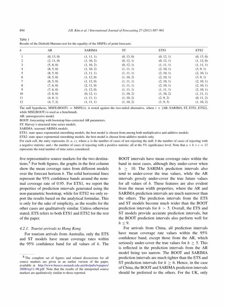
MSFE(i), tested against the two-tailed alternative,where i ∈ {AR, SARIMA, ST, ETS1, ETS2}. Notethat MSFE(BOOT) is used as the benchmark, anda negative Diebold-Mariano statistic indicates thatBOOT has a lower MSFE value than its competi-tor. Table 1 reports the outcomes of the test for eachforecast horizon. For each cell, the entry represents(b, a, c), where a is the number of cases of not reject-ing the null; b the number of cases of rejecting with anegative statistic; and c the number of cases of reject-ing with a positive statistic; all at the 5% significancelevel. As an example, for the AR model and for h = 2,the entry (2, 11, 0) indicates that the null hypothesisthat the MSFE of the BOOT forecasts is equal to thatof the AR forecasts is not rejected for eleven time se-ries; however, for two of the time series, the MSFEof BOOT is found to be statistically lower than thatof AR. For the other cases, it is evident that the nullhypothesis fails to be rejected for nearly all time se-ries and forecast horizons, except for the AR model.Hence, we conclude that, overall, all models exceptfor the AR provide point forecasts of an equal level ofaccuracy to the BOOT forecasts.

4.2. Interval forecasting

Figs. 3 and 4 plot the values of the mean coveragerates and widths of alternative prediction intervals fortourist arrivals to Hong Kong and Australia, respec-tively. For simplicity of exposition, we have chosen


Table 1Results of the Diebold-Mariano test for the equality of the MSFEs of point forecasts.

h AR SARIMA ST ETS1 ETS2

1 (0, 13, 0) (1, 11, 1) (0, 13, 0) (0, 12, 1) (0, 13, 0)2 (2, 11, 0) (1, 10, 2) (0, 12, 1) (0, 12, 1) (1, 12, 0)3 (5, 8, 0) (1, 10, 2) (0, 12, 1) (1, 11, 1) (1, 11, 1)4 (8, 5, 0) (1, 10, 2) (1, 11, 1) (2, 10, 1) (3, 9, 1)5 (8, 5, 0) (1, 11, 1) (1, 11, 1) (2, 10, 1) (2, 10, 1)6 (8, 5, 0) (1, 12, 0) (1, 10, 2) (2, 10, 1) (3, 9, 1)7 (8, 5, 0) (1, 12, 0) (1, 11, 1) (2, 10, 1) (2, 10, 1)8 (7, 6, 0) (2, 11, 0) (1, 11, 1) (2, 10, 1) (2, 10, 1)9 (7, 6, 0) (1, 12, 0) (1, 11, 1) (1, 11, 1) (2, 10, 1)

10 (5, 8, 0) (0, 12, 1) (1, 10, 2) (1, 10, 2) (1, 11, 1)11 (4, 8, 1) (1, 11, 1) (1, 10, 2) (2, 9, 2) (0, 11, 2)12 (4, 7, 2) (1, 11, 1) (1, 10, 2) (1, 9, 3) (1, 10, 2)

The null hypothesis, MSFE(BOOT) = MSFE(i), is tested against the two-tailed alternative, where i ∈ {AR, SARIMA, ST, ETS1, ETS2},while MSE(BOOT) is used as a benchmark.AR: autoregressive model.BOOT: forecasting with bootstrap bias-corrected AR parameters.ST: Harvey’s structural time series models.SARIMA: seasonal ARIMA models.ETS1: state space exponential smoothing models, the best model is chosen from among both multiplicative and additive models.ETS2: state space exponential smoothing models, the best model is chosen from additive models only.For each cell, the entry represents (b, a, c), where a is the number of cases of not rejecting the null; b the number of cases of rejecting witha negative statistic; and c the number of cases of rejecting with a positive statistic; all at the 5% significance level. Note that a + b + c = 13represents the total number of time series considered.

five representative source markets for the two destina-tions.8 For both figures, the graphs in the first columnshow the mean coverage rates from different modelsover the forecast horizon h. The solid horizontal linesrepresent the 95% confidence bands around the nom-inal coverage rate of 0.95. For ETS1, we report theproperties of prediction intervals generated using thenon-parametric bootstrap, while for ETS2 we only re-port the results based on the analytical formulae. Thisis only for the sake of simplicity, as the results for theother cases are qualitatively similar. Unless otherwisestated, ETS refers to both ETS1 and ETS2 for the restof the paper.

4.2.1. Tourist arrivals to Hong KongFor tourism arrivals from Australia, only the ETS

and ST models have mean coverage rates withinthe 95% confidence band for all values of h. The

8 The complete set of figures and related discussions for allsource markets are given in an earlier version of the paper,available at http://www.buseco.monash.edu.au/ebs/pubs/wpapers/2008/wp11-08.pdf. Note that the results of the unreported sourcemarkets are qualitatively similar to those reported.

BOOT intervals have mean coverage rates within theband in most cases, although they under-cover whenh ≥ 10. The SARIMA prediction intervals alsotend to under-cover the true values, while the ARintervals grossly under-cover the true future valuesfor all values of h. These features are also evidentfrom the mean width properties, where the AR andSARIMA prediction intervals are much narrower thanthe others. The prediction intervals from the ETSand ST models become much wider than the BOOTprediction intervals for h > 5. Overall, the ETS andST models provide accurate prediction intervals, butthe BOOT prediction intervals also perform well forh ≤ 9.

For arrivals from China, all prediction intervalshave mean coverage rate values within the 95%confidence band, except those from the AR, whichseriously under-cover the true values for h ≥ 5. Thisis reflected in the prediction intervals from the ARmodel being too narrow. The BOOT and SARIMAprediction intervals are much tighter than the ETS andST prediction intervals for h ≥ 6. Hence, in the caseof China, the BOOT and SARIMA prediction intervalsshould be preferred to the others. For the UK, only

http://www.buseco.monash.edu.au/ebs/pubs/wpapers/2008/wp11-08.pdf













Fig. 3. Mean coverage rates and widths of alternative prediction intervals: tourist arrivals to Hong Kong. The first column compares the meancoverage rates of prediction intervals, while the second compares the mean width of the prediction intervals, over forecast horizons 1–12. Thesolid horizontal lines in the coverage rate graphs indicate 95% confidence intervals around the nominal coverage rate of 0.95.


Fig. 4. Mean coverage rates and widths of alternative prediction intervals: tourist arrivals to Australia. The first column compares the meancoverage rates of prediction intervals, while the second compares the mean width of the prediction intervals, over forecast horizons 1–12. Thesolid horizontal lines in the coverage rate graphs indicate 95% confidence intervals around the nominal coverage rate of 0.95.


the BOOT and ST prediction intervals have all valuesof the mean coverage rate within the 95% confidenceband, while the others under-cover the true values.The AR and SARIMA prediction intervals grosslyunder-cover the true values, while the ETS predictionintervals, though still under-covering, perform muchbetter than these two. Looking at the widths of theintervals, the BOOT prediction intervals are muchtighter than the ETS and ST prediction intervals forh ≥ 6. Hence, the BOOT prediction intervals shouldbe preferred in the case of the UK.

In the case of the US, the BOOT prediction in-tervals have the best coverage properties: all cover-age rates are within the 95% confidence band and arevery close to the nominal coverage rate 0.95. However,the other prediction intervals also show good coverageproperties. The SARIMA prediction intervals have allmean coverage rates inside the 95% confidence bandfor all forecast horizons, while the ST and ETS in-tervals do for most of the forecast horizons. The onlyexception to this good performance is the AR model,which again provides prediction intervals that under-cover the true values in many cases. Looking at thewidth properties, the BOOT and SARIMA predictionintervals are again tighter than the ETS and ST inter-vals. Hence, similarly to the case of China, the BOOTand SARIMA prediction intervals should be preferred.For Asia, only the ETS and ST prediction intervalshave desirable coverage rates for all values of h, whilethe BOOT and SARIMA prediction intervals under-cover the true values for h ≥ 9. The AR predictionintervals substantially under-cover the true values fornearly all forecast horizons. All of the prediction in-tervals (except for AR) have similar mean width val-ues. Hence, in this case, the ETS and ST predictionintervals perform most desirably, but the BOOT andSARIMA prediction intervals also perform reasonablywell.

4.2.2. Tourist arrivals to AustraliaFig. 4 presents the mean coverage rates and widths

of alternative prediction intervals for tourist arrivals toAustralia. As in the case of Hong Kong, the AR mod-els provide prediction intervals which are much infe-rior to the others. Therefore, for the sake of simplicity,the AR prediction intervals will not be discussed anyfurther.

For Germany, only the BOOT prediction intervalshave all of their mean coverage values inside the

95% confidence intervals. The SARIMA intervals alsoperform well, with the value of the mean coveragebeing outside the 95% confidence band only when h =

2. The BOOT and SARIMA intervals are also verytight, with their mean width values being much smallerthan those of the ETS and ST intervals for nearly allvalues of h. The latter become increasingly wide asthe forecast horizon increases. For the UK, the BOOTand SARIMA intervals have all of their mean coveragevalues inside the 95% confidence band, while theETS and ST intervals either under- or over-cover thetrue values for a few forecast horizons. The formerare much tighter than the latter, again especially forlonger forecast horizons. For Europe, the ST is theonly model for which all of the prediction intervals areinside the 95% confidence band. The others tend tounder-cover the true future values, the ETS intervalsfor shorter forecast horizons and the BOOT andSARIMA intervals for longer horizons. Looking at thewidths of the prediction intervals, the ST intervals aremuch wider, suggesting that the other intervals under-estimate the future uncertainty in this case. For the US,the BOOT, SARIMA and ST prediction intervals havemean coverage values inside the 95% confidence bandfor all values of h. The BOOT prediction intervals arethe tightest for nearly all forecast horizons.

4.2.3. DiscussionAll of the models considered generate prediction

intervals with reasonable performances, except for theAR model, which often grossly underestimates thefuture uncertainty. This is particularly the case forshort forecast horizons (h ≤ 4), where, in mostcases, all models provide prediction intervals withcorrect coverage rates and similar width properties.Overall, we have found a strong tendency for theBOOT method to outperform its competitors. Ingeneral, the BOOT prediction intervals have themost desirable coverage properties, providing aninformative assessment of the future uncertainty. TheSARIMA, ETS and ST prediction intervals alsoperform reasonably well; however, the SARIMAintervals can sometimes be too narrow, and henceunderestimate the future uncertainty, while the ETSand ST intervals tend to become wider, relative tothe BOOT intervals, as the forecast horizon increases.In fact, for shorter forecast horizons (h ≤ 4), theETS and ST models often provide tighter prediction


intervals than the BOOT method. In general, theBOOT prediction intervals are slightly wider than theothers for shorter horizons, but become much tighteras the forecast horizon increases.

As was stated in Section 2, it is widely acceptedthat the prediction intervals generated from timeseries models are too narrow. This is because theconventional intervals (1) assume normality, whichmay not hold; (2) ignore the sampling variabilityassociated with parameter estimation; and (3) donot make adjustments for the small sample biasesof parameter estimators, where applicable. In thispaper, it is found that, consistent with the generalbelief, the conventional prediction intervals from theAR model are far too narrow. However, the otherprediction intervals (those from the bias-correctedbootstrap version of the AR, the SARIMA model,Harvey’s structural time series model, and the statespace models for exponential smoothing) are foundto be much wider, producing satisfactory coverageprobabilities.

From the methodological aspect, we have adoptedtwo innovative approaches. One is the use of a rollinghorizon methodology for evaluating the performancesof prediction intervals over a range of samples; whilethe other is the use of automatic model selection,which removes the subjectivity from the model selec-tion procedures. Although these represent sound ap-proaches, it should be noted that the findings of thispaper are limited to the current data set. We call formore extensive empirical research efforts of this kindin the future, in order to further explore the validity ofinterval forecasting for tourism forecasting.

5. Concluding remarks

Time series forecasting for tourist arrivals has beenan area of extensive empirical research. While a largenumber of studies published over the years havereported that the application of time series methodshas been a great success, their major concern hasbeen the issue of point forecasting. Although intervalforecasts can be invaluable for decision-makers in bothindustry and government, there have been no studiesthat have looked at the accuracy of prediction intervalsin the context of forecasting the number of touristarrivals.

The purpose of this paper is to evaluate the perfor-mance of the prediction intervals generated using al-ternative time series models. We consider univariatetime series models such as the AR model, the bias-corrected bootstrap for the AR model (Kim, 2004),the innovations state space models for exponentialsmoothing (as presented by Hyndman & Khandakar,2008), Harvey’s (1989) structural time series models,and the seasonal ARIMA model of Box et al. (1994).We employ an automatic forecasting approach, inwhich the prediction intervals are generated from fore-casting models whose specifications are determinedautomatically using a fully data-dependent procedure.The performances of the prediction intervals are evalu-ated in a purely empirical setting, calculating the cov-erage rate and width of the intervals using the rollingwindow method. For this purpose, we use thirteenmonthly time series for the number of tourist arrivalsto Hong Kong and Australia.

The main finding of the paper is that, in general, thebias-corrected bootstrap prediction intervals performmost desirably, providing tight intervals with accu-rate coverage values. The prediction intervals from theexponential smoothing and structural time series mod-els also show satisfactory probability coverage prop-erties, although they tend to become wider at longerforecast horizons relative to the bias-corrected boot-strap intervals. The seasonal ARIMA prediction inter-vals tend to under-estimate the future uncertainty. TheAR model also performs rather poorly, grossly under-estimating the future uncertainty. However, this paperdemonstrates that most of the popular time series mod-els adopted in this study generate prediction intervalswith desirable statistical properties, at least in the con-text of tourism forecasting.

Acknowledgements

We thank Andrew Maurer and Claude Calero atTourism Research Australia for providing the Aus-tralian data, explanations and comments. Athana-sopoulos and Song acknowledge financial supportfrom Tourism Research Australia, the SustainableTourism Cooperative Research Centre, Australian Re-search Council grant DR0984399; and the HongKong Polytechnic University (Grant No. G-YF35). Wewould like to thank Rob Hyndman (editor) and tworeferees for constructive comments.


Appendix

As was stated in Section 2.2, all time series arefiltered using seasonal dummy variables before thesemodels are applied. This is because the time series oftourist arrivals possess both stochastic and determinis-tic seasonality, as we have seen in Section 3.

A.1. Autoregressive model and bias-corrected boot-strap

We consider an AR(p) model of the form

Yt = α0 + α1Yt−1 + · · · + αpYt−p + βt + ut , (1)

where ut is i.i.d. with zero mean and fixed variance.The AR part of Eq. (1) is stationary, with all ofits characteristic roots outside the unit circle. Theunknown AR order is chosen by the AIC, with themaximum order being 18. Given the observed timeseries {Yt }

nt=1, the unknown parameters are estimated

using the least squares (LS) method. The LS estimatorfor α = (α0, . . . , αp) is denoted by α̂ = (α̂0, . . . , α̂p),and the associated residuals by {et }

nt=p+1. The point

forecasts for Yn+h made at n can be generated in theusual way, conditional on the last p observations of Y ,using α̂. The 100(1−θ)% prediction intervals for Yn+hcan be constructed based on a normal approximation.

Only a sketchy description of the bias-correctedbootstrap procedure of Kim (2004) is given here. Letthe bias of α̂ be denoted as Bias (α̂). This bias can beestimated using the analytical formula of Shaman andStine (1988), and the bias-corrected estimator can beobtained as

α̂c≡ (α̂c

0, α̂c1, . . . , α̂

cP ) = α̂ − Bias(α̂). (2)

The residuals associated with α̂c are denoted byec

t

nt=p+1. Generate an artificial data set recursively

using the backward AR form, as

Y ∗t = α̂c

0 + α̂c1Y ∗

t+1 + · · · + α̂cpY ∗

t+p + v∗t , (3)

where the p starting values are set equal to the last pvalues of the original series, and v∗

t is a random drawfrom

ec

t

nt=p+1 with replacement. Using the artificial

data setY ∗

t

nt=1, the parameters of the forward model

(1) are estimated, and the LS estimators are denotedby α̂∗. Obtain the bias-corrected estimator α̂∗c

= α̂∗−

Bias(α̂∗), again using the Shaman-Stine bias formula,

as in Eq. (2). The bootstrap replicates of the ARforecast for Yn+h made at time period n are generatedrecursively as

Y ∗n (h) = α̂∗c

0 + α̂∗c1 Y ∗

n (h − 1) + · · ·

+ α̂∗cp Y ∗

n (h − p) + u∗

n+h, (4)

where Y ∗n ( j) = Y ∗

n+ j = Yn+ j for j ≤ 0, and u∗

n+h

is a random draw fromec

t

nt=p+1 with replacement.

Repeat Eqs. (3) and (4) many times, say B, toyield the bootstrap distribution for the AR forecastY ∗

n (h; i)B

i=1. The 100(1 − θ)% prediction inter-vals for Yn+h , based on the percentile method(Efron & Tibshirani, 1993), are calculated as[Y ∗

n (h, τ ), Y ∗n (h, 1−τ)], where Y ∗

n (h, τ ) is the 100τ th

percentile of the bootstrap distributionY ∗

n (h; i)B

i=1,and τ = 0.5θ .

A.2. Seasonal ARIMA models

The general form of the seasonal ARIMA model(Box et al., 1994) with periodicity s (s = 12 formonthly data) can be written as

φp(B)ΦP (Bs)∆d∆Ds Yt = µ + θq(B)ΘQ(Bs)ut , (5)

where ut is a white noise process with fixed varianceand µ is a constant. B is the backward shift operator,and ∆d

≡ (1 − B)d and ∆Ds = (1 − Bs)D are the

operators for the dth order monthly difference andthe Dth order annual difference, respectively. φp(B),θq(B), ΦP (Bs) and ΘQ(Bs) are the polynomials in Band Bs , which can be written as

φp(B) = 1 − φ1 B − · · · − φp B p,

θq(B) = 1 − θ1 B − · · · − θq Bq ,

ΦP (Bs) = 1 − Φ1 Bs− · · · − ΦP B Ps, and

ΘQ(Bs) = 1 − Θ1 Bs− · · · − ΘQ B Qs,

where the φs, θs, Φs and Θs are parameters to beestimated. The model parameters are estimated usingthe maximum likelihood method. The point forecastYn(h) for Yn+h is generated recursively using the es-timated coefficients, conditional on the observed timeseries. The prediction intervals can be constructed inthe usual way under the assumption of normality. Formodel selection, we follow the automatic proceduredescribed by Hyndman and Khandakar (2008), wherethe numbers of differencing and seasonal differencing


d and D are determined using the Canova and Hansen(1995) seasonal unit root test, and the orders p, q,Ps , and Qs of model (5) are selected using the AIC,following the step-wise procedure for traversing themodel space.

A.3. Harvey’s basic structural model

The basic structural time series model of Harvey(1989) decomposes an observed time series intodifferent unobserved components. These componentscan be forecast individually and combined to producea forecast for the observed series. The model may bewritten as

Yt = µt + γt + εt ,

where Yt is the observed time series, µt is the trendcomponent, γt is the seasonal component and εtis the random component. The trend and seasonalcomponents are assumed to be uncorrelated, while εtis assumed to be white noise.

The trend, which represents the long-term move-ment in a series, can be represented by

µt = µt−1 + βt−1 + ηt ,

βt = βt−1 + ζt ,

where ηt ∼ N I D(0, σ 2η ) and ζt ∼ N I D(0, σ 2

ζ ). Theseasonal component is specified as

γt = −

s−1−j=1

γt− j + wt ,

where wt ∼ N I D(0, σ 2w). The seasonality is

deterministic when σ 2w = 0.

The point forecasts are generated by running theKalman filter for the above structural model expressedin state space form. The prediction intervals areobtained under the assumption of normality, using theprediction error variance given by Harvey (1989, p.222).

A.4. State space models for exponential smoothing

The general form of these models can be written as

Yt = w(X t−1) + r(X t−1)εt ;

X t = f (X t−1) + g(X t−1)εt ,

where εt is a Gaussian white noise with zero mean andfixed variance, and

X t = (lt , bt , st , st−1, . . . , st−m+1)′

is a state vector, while lt , bt , and st denote the level,slope, and seasonal components at time t , respectively,and m is the length of seasonality. Accordingto Hyndman and Khandakar (2008), the updatingformulae of all exponential smoothing methods arespecial cases of the above general model.

The innovations state space models are estimatedusing the maximum likelihood method, and the modelselection is done automatically using the AIC. Furtherdetails of the point forecasting, interval forecasting,and automatic model selection procedures are givenby Hyndman and Khandakar (2008).

References

Box, G. E. P., Jenkins, G. M., & Reinsel, C. (1994). Time seriesanalysis: forecasting and control. Englewood Cliffs: PrenticeHall.

Canova, F., & Hansen, B. (1995). Are seasonal patterns constantover time? A test for seasonal stability. Journal of Business andEconomic Statistics, 13, 237–252.

Chatfield, C. (1993). Calculating interval forecasts. Journal ofBusiness and Economic Statistics, 11(2), 121–135.

Chatfield, C. (2001). Prediction intervals for time-series forecasting.In J. S. Armstrong (Ed.), Principles of forecasting: a handbookfor researcher and practitioners (pp. 475–494). Boston: KrugerAcademic Publishers.

Chatfield, C., & Yar, M. (1991). Prediction intervals for multi-plicative Holt-Winters. International Journal of Forecasting, 7,31–37.

Christoffersen, P. F. (1998). Evaluating interval forecasts. Interna-tional Economic Review, 39, 841–862.

Clements, M. P., & Taylor, N. (2001). Bootstrapping predictionintervals for autoregressive models. International Journal ofForecasting, 17, 247–267.

De Gooijer, J., & Hyndman, R. J. (2006). 25 years of time seriesforecasting. International Journal of Forecasting, 22, 443–473.

Diebold, F. X., & Mariano, R. S. (1995). Comparing predictiveaccuracy. Journal of Business and Economic Statistics, 13,253–263.

Efron, B., & Tibshirani, R. J. (1993). An introduction to thebootstrap. New York: Chapman Hall.

Frechtling, D. C. (2001). Forecasting tourism demand: methods andstrategies. Oxford: Butterworth-Heinemann.

Harvey, A. C. (1989). Forecasting structural time series models andthe Kalman Filter. Cambridge: Cambridge University Press.

Hyndman, R. J. (2008). Forecast: forecasting func-tions for time series. R package version 1.14http://www.robjhyndman.com/software/forecast/.

Hyndman, R. J., & Khandakar, Y. (2008). Automatic time seriesforecasting: the forecast package for R. Journal of StatisticalSoftware, 26(3).

Hyndman, R. J., Koehler, A. B., Ord, J. K., & Snyder, R. D.(2008). Forecasting with exponential smoothing: the state spaceapproach. Berlin: Springer-Verlag.

http://www.robjhyndman.com/software/forecast/


Hyndman, R. J., Koehler, A. B., Snyder, R. D., & Grose, S.(2002). A state space framework for automatic forecastingusing exponential smoothing methods. International Journal ofForecasting, 18(3), 439–454.

Kilian, L. (1998). Small sample confidence intervals for impulseresponse functions. The Review of Economics and Statistics, 80,218–230.

Kim, J. H. (2001). Bootstrap-after-bootstrap prediction intervalsfor autoregressive models. Journal of Business and EconomicStatistics, 19, 117–128.

Kim, J. H. (2003). Forecasting autoregressive time series withbias-corrected parameter estimators. International Journal ofForecasting, 19, 493–502.

Kim, J. H. (2004). Bootstrap prediction intervals for autoregressionusing asymptotically mean-unbiased estimators. InternationalJournal of Forecasting, 20, 85–97.

Kim, J. H. (2008). BootPR: bootstrap prediction intervals and bias-corrected forecasting. R package version 0.56.

Kim, J. H., & Moosa, I. A. (2001). Seasonal behaviour of monthlyinternational tourist flows: specification and implications forforecasting models. Tourism Economics, 7, 381–396.

Kim, J. H., & Moosa, I. A. (2005). Forecasting international touristflows to Australia: a comparison between the direct and indirectmethods. Tourism Management, 26, 69–78.

Koenker, R. W., & Bassett, G. W. (1978). Regression quantiles.Econometrica, 46, 33–50.

Li, G., Song, H., & Witt, S. F. (2005). Recent developmentsin econometric modelling and forecasting. Journal of TravelResearch, 44, 82–99.

Makridakis, S., Wheelwright, S. C., & Hyndman, R. J. (1998).Forecasting: methods and applications. New York: John WileySons.

Meade, N., & Islam, T. (1995). Prediction intervals for growth curveforecasts. Journal of Forecasting, 14, 413–430.

Ord, J. K., Koehler, A. B., & Snyder, R. D. (1997). Estimation andprediction for a class of dynamic nonlinear statistical models.Journal of the American Statistical Association, 92, 1621–1629.

Pascual, L., Romo, J., & Ruiz, E. (2004). Bootstrap predictiveinference for ARMA process. Journal of Time Series Analysis,25, 449–465.

R Development Core Team. (2008). R: A language andenvironment for statistical computing. Vienna, Austria: RFoundation for Statistical Computing. ISBN 3-900051-07-0,URL: http://www.R-project.org.

Rodriguez, A., & Ruiz, E. (2009). Bootstrap prediction intervalsin state-space models. Journal of Time Series Analysis, 30,167–178.

Shaman, P., & Stine, R. A. (1988). The bias of autoregressivecoefficient estimators. Journal of the American StatisticalAssociation, 83, 842–848.

Song, H., & Li, G. (2008). Tourism demand modelling andforecasting—a review of recent research. Tourism Management,29, 203–220.

Song, H., Witt, S. F., & Zhang, X. (2008). Developing a web-basedtourism demand forecasting system. Tourism Economics, 14(3),445–468.

Stoffer, D. S., & Wall, K. D. (1991). Bootstrapping state-spacemodels: Gaussian maximum likelihood estimation and theKalman filter. Journal of the American Statistical Association,86, 1024–1033.

Taylor, J. W. (2003). Exponential smoothing with a dampedmultiplicative trend. International Journal of Forecasting, 19,273–289.

Taylor, J. W. (2008). An evaluation of methods for very short termelectricity demand forecasting using minute-by-minute Britishdata. International Journal of Forecasting, 24, 645–658.

Taylor, J. W., & Bunn, D. W. (1999). A quantile regression approachto generating prediction intervals. Management Science, 45(2),225–237.

Thombs, L. A., & Schucany, W. R. (1990). Bootstrap predictionintervals for autoregression. Journal of the American StatisticalAssociation, 85, 486–492.

Witt, S. F., & Witt, C. A. (1995). Forecasting tourism demand:A review of empirical research. International Journal ofForecasting, 11, 447–475.

Yar, M., & Chatfield, C. (1990). Prediction intervals for theHolt-Winters forecasting procedure. International Journal ofForecasting, 6, 127–137.

http://www.R-project.org

Beyond point forecasting: Evaluation of alternative prediction intervals for tourist arrivals

Documents

Transcript of Beyond point forecasting: Evaluation of alternative prediction intervals for tourist arrivals