Locus of control and Human Capital Investment Decisions
86
CERS-IE WORKING PAPERS | KRTK-KTI MŰHELYTANULMÁNYOK INSTITUTE OF ECONOMICS, CENTRE FOR ECONOMIC AND REGIONAL STUDIES, BUDAPEST, 2020 Locus of control and Human Capital Investment Decisions: The Role of Effort, Parental Preferences and Financial Constraints ÁGNES SZABÓ-MORVAI ® HUBERT JÁNOS KISS CERS-IE WP – 2020/55 December 2020 https://www.mtakti.hu/wp-content/uploads/2020/12/CERSIEWP202055.pdf CERS-IE Working Papers are circulated to promote discussion and provoque comments, they have not been peer-reviewed. Any references to discussion papers should clearly state that the paper is preliminary. Materials published in this series may be subject to further publication.
-
Upload
khangminh22 -
Category
Documents
-
view
2 -
download
0
Transcript of Locus of control and Human Capital Investment Decisions
CERS-IE WORKING PAPERS | KRTK-KTI MŰHELYTANULMÁNYOK
INSTITUTE OF ECONOMICS, CENTRE FOR ECONOMIC AND REGIONAL STUDIES,
BUDAPEST, 2020
Locus of control and Human Capital Investment Decisions:
The Role of Effort, Parental Preferences and Financial
Constraints
ÁGNES SZABÓ-MORVAI ® HUBERT JÁNOS KISS
CERS-IE WP – 2020/55
December 2020
https://www.mtakti.hu/wp-content/uploads/2020/12/CERSIEWP202055.pdf
CERS-IE Working Papers are circulated to promote discussion and provoque comments, they have not been peer-reviewed.
Any references to discussion papers should clearly state that the paper is preliminary. Materials published in this series may be subject to further publication.

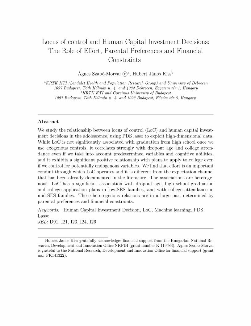
ABSTRACT
We study the relationship between locus of control (LoC) and human capital
investment decisions in the adolescence, using PDS lasso to exploit high-dimensional
data. While LoC is not significantly associated with graduation from high school once
we use exogenous controls, it correlates strongly with dropout age and college
attendance even if we take into account predetermined variables and cognitive
abilities, and it exhibits a significant positive relationship with plans to apply to college
even if we control for potentially endogenous variables.
We find that effort is an important conduit through which LoC operates and it is
different from the expectation channel that has been already documented in the
literature. The associations are heterogenous: LoC has a significant association with
dropout age, high school graduation and college application plans in low-SES families,
and with college attendance in mid-SES families. These heterogenous relations are in
a large part determined by parental preferences and financial constraints.
JEL codes: D91, I21, I23, I24, I26
Keywords: Human Capital Investment Decision, LoC, Machine learning, PDS Lasso
Szabó-Morvai Ágnes KRTK-KTI, 1097 Budapest, Tóth Kálmán u. 4. és Debreceni Egyetem, 4032 Debrecen, Böszörményi út 138. e-mail: szabomorvai.agnes at krtk.hu Hubert János Kiss KRTK KTI, 1097 Budapest, Tóth Kálmán u. 4, Magyarország. and Budapesti Corvinus Egyetem, 1093 Budapest, Fővám tér 8, Magyarország. e-mail: [email protected]
Agnes Szabo-Morvai is grateful to the National Research, Development and Innovation Office for
financial support (grant no.: FK141322). Hubert János Kiss acknowledges support from the Hungarian
National Research, Development and Innovation Office NKFIH (grant number K 119683).

A kontrollhely hatása a human tőke befektetési döntésre: az
erőfeszítés, a szülői preferenciák és a pénzügyi korlátok
szerepe
SZABÓ-MORVAI ÁGNES ® KISS HUBERT JÁNOS
ÖSSZEFOGLALÓ
A tanulmányban a kontrollhely és a human tőke befektetési döntések összefüggéseit
vizsgáljuk serdülőkorban, ehhez PDS lasso módszert használunk annak érdekében,
hogy az extém sok változós adatbázis kezdvező tulajdonságait kiaknázhassuk. A
független kontroll változók bevonása után a kontrollhely nem mutat erős összefüggést
a sikeres középiskolai érettségi valószínűségével. Ugyanakkor a középiskolai
lemorzsolódás életkora és az egyetemre való sikeres felvételi esetében erős összefügést
találunk a kontrollhellyel, még akkor is, ha kiszűrjük a független változók és a kognitív
képességek hatását. A kontrollhely erős összefüggést mutat az egyetemi jelentkezési
szándékkal még azt követően is, hogy a modellben kontrollálunk az egzogén változókra,
a kognitív képességekre, és potenciálisan endogen változókra is. Azt találjuk, hogy az
egyéni erőfeszítés igen fontos csatorna, amely a belső kontrollhely hatásait közvetíti a
humán tőke befektetések és teljesítmények felé. Megmutatjuk, hogy az erőfeszítés eltér
a szakirodalomban már dokumentált jövőbeli várakozások csatornájától.
A vizsgált összefüggések heterogének: a kotrollhely erős összefüggést mutat a
középiskolai lemorzsolódással, a sikeres érettségi valószínűségével és az egyetemi
jelentkezési szándékokkal az alacsony szocioökonómiai hátterű serdülők esetében,
valamint a sikeres egyetemi felvételivel a közepes szocioökonómiai hátterű
kamaszoknál. Ezen összefüggések heterogenitását a szülők preferenciái és a család
anyagi korlátai jelentős mérték,ben meghatározzák.
JEL: D91, I21, I23, I24, I26
Kulcsszavak: Humán tőke befektetési döntések, kontrollhely, gépi tanulás, PDS lasso
Locus of control and Human Capital Investment Decisions:
The Role of Effort, Parental Preferences and Financial
Constraints
Agnes Szabo-Morvai r○a, Hubert Janos Kissb
aKRTK KTI (Lendulet Health and Population Research Group) and University of Debrecen1097 Budapest, Toth Kalman u. 4. and 4032 Debrecen, Egyetem ter 1, Hungary
bKRTK KTI and Corvinus University of Budapest1097 Budapest, Toth Kalman u. 4. and 1093 Budapest, Fovam ter 8, Hungary.
Abstract
We study the relationship between locus of control (LoC) and human capital invest-ment decisions in the adolescence, using PDS lasso to exploit high-dimensional data.While LoC is not significantly associated with graduation from high school once weuse exogenous controls, it correlates strongly with dropout age and college atten-dance even if we take into account predetermined variables and cognitive abilities,and it exhibits a significant positive relationship with plans to apply to college evenif we control for potentially endogenous variables. We find that effort is an importantconduit through which LoC operates and it is different from the expectation channelthat has been already documented in the literature. The associations are heteroge-nous: LoC has a significant association with dropout age, high school graduationand college application plans in low-SES families, and with college attendance inmid-SES families. These heterogenous relations are in a large part determined byparental preferences and financial constraints.
Keywords: Human Capital Investment Decision, LoC, Machine learning, PDSLassoJEL: D91, I21, I23, I24, I26
Hubert Janos Kiss gratefully acknowledges financial support from the Hungarian National Re-search, Development and Innovation Office NKFIH (grant number K 119683). Agnes Szabo-Morvaiis grateful to the National Research, Development and Innovation Office for financial support (grantno.: FK141322).
1. Introduction
Those individuals who perceive to have control over their life and believe thatlife outcomes are due to their efforts are said to have an internal locus of control,while those who attribute those outcomes to external factors, like luck, have anexternal locus of control (Rotter, 1966). It is one of the most widely studied non-cognitive skills that is related to a vast array of life outcomes: individuals with moreinternal control tend to a) have higher and faster growing earnings (Andrisani, 1977;Goldsmith et al., 1997; Duncan and Dunifon, 1998; Groves, 2005; Semykina and Linz,2007; Heineck and Anger, 2010; Piatek and Pinger, 2016; Schnitzlein and Stephani,2016); b) have better job performance and greater job satisfaction (Judge and Bono,2001; Ng et al., 2006; Wang et al., 2010); c) lead a healthier life (Strudler Wallstonand Wallston, 1978; Wallston et al., 1978; Steptoe and Wardle, 2001; Chiteji, 2010;Cobb-Clark et al., 2014; Mendolia and Walker, 2014; Oi and Alwin, 2017); d) andaccumulate more savings (Cobb-Clark et al., 2016; Chatterjee et al., 2011).
When summarizing the main findings of the report on educational equality andopportunity in the US, James Coleman, the renowned sociologist, stated that LoC”was more highly related to achievement than any other factor in the student’sbackground or school.” (Coleman, 1966).1 Much evidence has been accumulating,showing that individuals with a more internal LoC tend to perform better academ-ically (Wang et al., 1999; Heckman and Kautz, 2012; Mendolia and Walker, 2014).However, it is not only school performance that matters for success in life, but alsohuman capital investment decisions, e.g., dropping out of school, graduating fromhigh school, attending university. A growing literature using large and representativesamples studies how LoC associates with these decisions.
We use data from the Life Course Survey (Hungary) comprising 10,000 adoles-cents attending the eighth grade in elementary school in May 2006 and who havecompleted the National Basic Capabilities Test (a nationwide test in reading andmaths, similar to the PISA test). Importantly, in 2006 and 2009, the survey con-tained a locus of control section, along with an outstandingly rich set of data. Dueto attrition the sample size is 7638. In this paper, we add to the literature on therelationship between LoC and human capital investment decisions in three ways.
First, we are the first to show that effort is an essential channel of LoC to humancapital investments. As Coleman and DeLeire (2003) already showed, when someonehas a more internal LoC, it increases her expectations regarding the returns of a
1Coleman did not call it LoC, but referred to it as ’an attitude which indicated the degree towhich the student felt in control of his fate.’
2
human capital investment. We show that students with a more internal LoC exertmore effort in studying, which leads to higher achievement and better human capitalinvestment decisions. Moreover, we show that the effort conduit is different from theexpectation channel.
Second, we explore the heterogeneity of LoC effect by gender and socioeconomicstatus (SES). Regarding gender, we find that in all outcomes except graduation fromhigh school LoC plays a more crucial role for females. Mendolia and Walker (2014)find that a more disadvantaged background is related to a stronger association be-tween LoC and educational outcomes. A possible explanation is that more internalcontrol might offset the adverse effects of a lack of positive stimuli and support fromhome. Our results confirm this finding. Moreover, we offer an alternative explana-tion. We utilize questions on parental preferences and financial constraints regard-ing the highest level of education of the child. We report that parental preferencesstrongly influence the magnitude of the association between LoC and educationaloutcomes. If parents prefer the child to attain an education lower than finishing highschool, LoC will have a very strong association with graduating from high school.That is most likely because that would be an excess accomplishment compared towhat is expected from the adolescent. In these families, LoC is not related to higherstake outcomes, like planning to apply to college or attending college, as these arefar from realistic options for most of these students. At the other extreme, whereparents expect that the child attains college education at the minimum, LoC is notassociated with low-stake achievements, like graduating from high school. Also, LoCis not associated with college application plans, as applying ti college is an implicitrequirement from their families that they have to meet. In the case of adolescentsin between, who seem to have more freedom to decide whether they would like toapply to college or not, it is apparent that LoC is strongly associated with collegeapplication plans and actual college attendance. These findings shed new light onthe channels of intergenerational transmission of socioeconomic status.
Third, we add to the literature by utilizing machine learning. Economists areconcerned about causal effects most of the time. For identification, one needs ex-ogenous variations in the primary variable of interest. However, if not impossible,it is hard to find such exogenous variations in personality traits. The second-bestsolution is to approach a model that includes all the relevant control variables, thusavoiding biased parameter estimates. However, with increasing the number of con-trol variables, the risk of overfitting the model rises. Post Double Selection lasso isa machine learning technique that uses out-of-sample testing for variable selection,preventing the model from overfitting. This technique assures that the most relevantcontrols are selected from a large set of potential variables. Our dictionary size, the
3
number of available control variables, is 119, counting only exogenous controls and221 if all the exogenous and the channel variables (that potentially mediate the ef-fect of LoC) are included. From the exogenous control variables, at most fifteen areselected in our various specifications, which results in R2 values of about about 40%in the models. This fit is much higher than those reported in the previous literature.Nevertheless, we still do not claim our results to be causal effects.
We also have two minor additions to the literature. First, besides human capitaldecisions already considered in the literature (dropout, graduation from high school,college attendance), we can see if LoC is associated with college application plans.It turns out to be an interesting variable because it is not as tightly related to schoolperformance as the other outcome variables, but it expresses aspiration for highereducation. Second, beyond exogenous (or pre-determined) variables that cannot beplausibly affected by the LoC, we investigate if the association between LoC and theoutcome variable persists even if we consider potential conduits and possibly endoge-nous variables. We document that the association between LoC and the outcomevariable of interest becomes insignificant once we control for exogenous variables andcognitive abilities for the low-end human capital investment decisions (that concerndropping out and graduation from high school). In contrast, for high-end decisionsrelated to tertiary studies (college application plans and attending college), the as-sociation remains significant even after controlling for conduits.
In section 2 we review briefly the literature. In section 3 the data are presented.The methodology used in this study is described in 4, and the results are shown in5.
2. Literature review
Once LoC became an accepted concept in psychology, scholars started to look athow it was associated with different outcomes in different domains, among them aca-demic performance. Most of this research found that students with an internal LoChave a better performance in school, spend more years in education, and are morelikely to go to college (Gurin et al., 1969; Bar-Tal and Bar-Zohar, 1977; Diesterhaftand Gerken, 1983; Findley and Cooper, 1983; Keith et al., 1986; Garner and Cole,1986; Mone et al., 1995; Nelson et al., 1995; Wang et al., 1999). Most of these studiesuse small samples that are not representative.
More recent research differs from the previous one in (at least) two dimensions.On the one hand, these studies use larger (and hence more representative) datasets. On the other hand, apart from academic performance, more attention has beengiven to human capital investment decisions that are tightly connected to academic
4
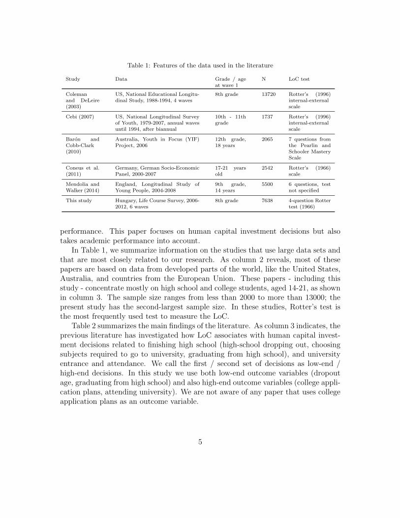
Table 1: Features of the data used in the literature
Study Data Grade / ageat wave 1
N LoC test
Colemanand DeLeire(2003)
US, National Educational Longitu-dinal Study, 1988-1994, 4 waves
8th grade 13720 Rotter’s (1996)internal-externalscale
Cebi (2007) US, National Longitudinal Surveyof Youth, 1979-2007, annual wavesuntil 1994, after biannual
10th - 11thgrade
1737 Rotter’s (1996)internal-externalscale
Baron andCobb-Clark(2010)
Australia, Youth in Focus (YIF)Project, 2006
12th grade,18 years
2065 7 questions fromthe Pearlin andSchooler MasteryScale
Coneus et al.(2011)
Germany, German Socio-EconomicPanel, 2000-2007
17-21 yearsold
2542 Rotter’s (1966)scale
Mendolia andWalker (2014)
England, Longitudinal Study ofYoung People, 2004-2008
9th grade,14 years
5500 6 questions, testnot specified
This study Hungary, Life Course Survey, 2006-2012, 6 waves
8th grade 7638 4-question Rottertest (1966)
performance. This paper focuses on human capital investment decisions but alsotakes academic performance into account.
In Table 1, we summarize information on the studies that use large data sets andthat are most closely related to our research. As column 2 reveals, most of thesepapers are based on data from developed parts of the world, like the United States,Australia, and countries from the European Union. These papers - including thisstudy - concentrate mostly on high school and college students, aged 14-21, as shownin column 3. The sample size ranges from less than 2000 to more than 13000; thepresent study has the second-largest sample size. In these studies, Rotter’s test isthe most frequently used test to measure the LoC.
Table 2 summarizes the main findings of the literature. As column 3 indicates, theprevious literature has investigated how LoC associates with human capital invest-ment decisions related to finishing high school (high-school dropping out, choosingsubjects required to go to university, graduating from high school), and universityentrance and attendance. We call the first / second set of decisions as low-end /high-end decisions. In this study we use both low-end outcome variables (dropoutage, graduating from high school) and also high-end outcome variables (college appli-cation plans, attending university). We are not aware of any paper that uses collegeapplication plans as an outcome variable.
5
Column 4 in Table 2 shows the controls used in the literature.2 Note that all thevariables used in the specifications are exogenous (or pre-determined), that is theymay affect LoC, but LoC cannot (or is very unlikely to) affect these variables. Thefirst specifications in these studies tend to contain the most basic exogenous variables(e.g. ethnicity / race, gender). Later specifications include variables related to familybackground and cognitive abilities (if available), though here the order and logic isless clear.3
In column 5 in Table 2 we summarize the main findings in a compact form.The different coefficients correspond to different specifications. For instance, in Cebi(2007), the first coefficient (5.4***) corresponds to specification 1, the next one(4.6***) to specification 2 and so on.
Considering low-end decisions, the only paper that studies dropout (Coneus et al.,2011) documents a significant association between LoC and the probability of drop-ping out at different ages. While for the ages of 18 and 19 years the GPA plays agreater role in explaining dropout, for the ages of 20 and 21 LoC is a more importantfactor to predict dropout than GPA, in the presence of other controls. Regardinggraduation from high school, all papers that investigate this decision report a sig-nificant association between LoC and graduation. However, while in Coleman andDeLeire (2003) and Baron and Cobb-Clark (2010) the significance remains after us-ing a large set of controls, in Cebi (2007) it vanishes when cognitive abilities arecontrolled for. The size of the effect varies from 1.4 pp to 4.5 pp increase in theprobability of graduation from high school upon a standard-deviation increase in theLoC. As of subject choice that may determine the possibilities to go to university,Mendolia and Walker (2014) report a significant correlation between LoC and theoutcome variable.
Turning to high-end decisions, Coleman and DeLeire (2003) and Cebi (2007) doc-ument a significant association between LoC and attending college in the specifica-tions with few controls. However, while it remains significant (albeit only marginally)in Cebi (2007) even after all controls are included, the significance disappears inColeman and DeLeire (2003), when including parenting controls (that are relatedto the home environment). Baron and Cobb-Clark (2010) find that LoC correlatessignificantly with performance at the university entrance exam.
2The numbers in parentheses indicate in which specification the variable was used. For instance,in Coleman and DeLeire (2003) the variables following (1) and before (2) are used in specification1. The variables following (2) (and before (3)) are the ones that the authors use in specification 2in addition to the previous variables, and so on.
3Some papers report only one specification for a given outcome variable.
6

Table 2: Summary of the main findings in the literature
Study Methods Outcome Controls Finding
Colemanand DeLeire(2003)
Probit Graduates from high school (1) Hispanic, Black, Female, Urban, Region,(2) Math, Reading, GPA, Parents’ education,(3) Parenting controls, (4) Family structure
A sd increase in LoC results in a 6.8 / 1.6**/ 1.4** / 1.4** pp higher probability of out-come variable.
Attends college Same as above A sd increase in LoC results in a 8.3** / 1**/ 0.6 / 0.5 pp higher probability of outcomevariable.
Cebi (2007) Probit Graduates from high school (1) Black, Hispanic, Female, Urban, Age,Residence, (2) Parental education, (3) Familystructure, (4) Home life, (5) AFQT (5)
A sd increase in LoC results in 5.4*** / 4.6***/ 4.1*** / 3.8*** / 1.5 pp higher probabilityof outcome variable.
Attends college Same as above A sd increase in LoC results in a 7.4*** /5.7*** / 6.2*** / 6*** / 2.3* pp higher prob-ability of outcome variable.
Baron andCobb-Clark(2010)
Probit Graduates from high school Social disadvantage, Family structure, Male,Indigenous, Home environment, Parental ed-ucation, Parent inmigrant, Early born
A sd increase in LoC results in a 4.5* pphigher probability of outcome variable.
Passes university entryexam
Same as above A sd increase in LoC results in a 2.9** pphigher probability of outcome variable.
University entrance rank Same as above A one standard deviation change in LoC isassociated with an increase of less than one(0.95*) percentiles in one’s university rank-ing.
Coneus etal. (2011)
Probit Drops out at age 18 /19 /20 GPA, Mother LoC, Female, Family struc-ture, Migration background, Mother educa-tion, Mother occupation, West
A sd increase in LoC results in a 1.9* / 2.8***/ 3.7*** pp higher probability of outcomevariable at age 18 / 19 / 20.
Mendoliaand Walker(2014)
OLS, Pro-bit withpropen-sity scorematching
GCSE performance (Has5+GCSE with A*-C, HasGCSEA*-C in English, HasGCSEA*-C in Maths)
(1) at-birth characteristics (birth weight, pre-mature, ethnicity, gender, family characteris-tics), (2) other family’s characteristics (child’sor parent’s disability, maternal educationand employment status, single parent family,grandparents’ education, family income andolder siblings)
Being external decreases GCSE performance.Very significant (***) effect in both specifica-tions for all the elements.
Has A levels (overall, inMaths, Science, English)
Same as above Being external decreases probability to haveA levels. Very significant (***) effect in bothspecifications overall, ** for Maths and Sci-ence, not consistent for English.
Points in A levels (overall,Maths, Science, English)
Same as above Being external decreases test scores in A lev-els. Very significant (***) effect in both spec-ifications overall, ** for Maths and English, *for Science.
No. facilitating subjects Same as above Being external decreases number of facilitat-ing subjects. Very significant (***) effect inboth specifications for all the elements.
Even though the idea of LoC seems intuitively important to explain human cap-ital investment decisions, it is vital to uncover how it exactly exerts its effect. Theexisting literature made essential attempts to unearth the conduits through whichLoC affects those decisions. Coleman and DeLeire (2003) show that LoC operatesthrough affecting the expectations of teenagers about future expected income andoccupation at the age of 30. More precisely, they find that more internal LoC cor-relates with more positive expectations about the future.4 In Coleman and DeLeire(2003)’s interpretation, more positive expectations reflect a higher subjective rateof return on human capital investment that is why more internal students are morelikely to graduate from high school and attend college.5 6
Effort may be a further conduit through which LoC operates. Psychologists of-ten link LoC to motivation. Atkinson (1964) claims that motivation has two keyelements, motive and expectancy. The latter refers to an individual’s judgement towhich extent her efforts and actions are causally related to desired results.7 Motiva-tion can be seen as a prerequisite of exerting effort. Borghans et al. (2008) use a labexperiment to show that internal LoC is associated with higher motivation that, inturn, translates into more effort. There are empirical papers showing the relation-ship between LoC and effort in job search (Caliendo et al., 2015; McGee, 2015) or inleading a healthy life (Cobb-Clark et al., 2014), but we are unaware of any studiesthat document such an association between effort put into academic activities andLoC.8 Our data permit us to check if such a relationship between LoC and effortexists and, in fact, we find that LoC is tightly related to effort.9
4There are also other studies documenting a link between LoC and future expectations (Marecekand Frasch, 1977; Bush et al., 1998; Mutlu et al., 2010).
5Cebi (2007) also investigates the role of expectations, but she fails to find a connection betweenLoC and future expectations.
6Similar arguments have been used to show that positive future expectations suggesting higherperceived health returns to investment in healthy life explains why individuals with internal LoCeat well and exercise regularly (Cobb-Clark et al., 2014).
7Bandura (1989) also links motivation to the effort individuals are willing to make.8Mendolia and Walker (2014) speculate on the relationship between LoC and academic effort-
making in the following way: ”One possible explanation for the negative effects of external LoC isthat external individuals tend to think that their choices have less impact on their future, whichthey believe are mostly driven by luck and external circumstances. As a consequence, these childrenare less likely to put a strong effort in their school work, as they do not believe this will impact theirfuture. This affects their performance and their chances to achieve high results in their education.”
9Delaney et al. (2013) document that conscientiousness (a Big Five trait that is positively corre-lated with LoC (Judge et al., 2002)) positively associates with lecture attendance and study hoursat university that can be seen as proxies for effort.
8
The existing literature also focused on the question whether LoC associates inthe same way with the outcome variable of interest in different subsamples, mainlyalong the socioeconomic status (SES).10 Baron and Cobb-Clark (2010) documentthat growing up in disadvantage (captured by family welfare receipt history) doesnot correlate with the adolescent’s LoC. However, Mendolia and Walker (2014) findthat the association of LoC with the outcome variables changes with socioeconomicstatus: more disadvantaged background is related to a stronger association. Theyspeculate that this result may be due to the fact that students from advantaged SESare more likely to receive positive stimuli and support at home and have parents whovalue more school performance and make efforts that their children succeed in school.Hence, students from high-SES families do not need to have a strong internal controlto make good human capital investment decisions, while for students from a low-SESbackground it is more likely that having an internal LoC makes a difference whenmaking such decisions. We confirm this finding as we find that for three (dropout age,graduating from high school and planning to apply to college) of the four outcomevariables LoC exhibits the strongest association for students whose mother has alow level of education. In the case of attending college the strongest correlationis observed when the mother has a mid-level education. In this study, we extendthe analysis to how different parental preferences for the level of education of theadolescent explain the differences of the LoC effect by the family SES.
Studies investigating the role of LoC in the labour market have revealed impor-tant gender differences (Goldsmith et al., 1996; Hansemark, 2003; Semykina andLinz, 2007; Cobb-Clark and Tan, 2011; Cobb-Clark, 2015) though with mixed re-sults as in some studies females, while in others males experience a stronger impactof LoC. With respect to human capital investment decisions, we are not aware of anypaper that studies the effect of LoC separately for females and males. However, inregressions (where females and males are pooled) reported in different studies gen-der is often significant (see Coleman and DeLeire (2003) and Baron and Cobb-Clark(2010)).
3. Data
We use an outstandingly detailed longitudinal database, Life Course Survey(Eletpalya) of the social research institute TARKI in Hungary. A sample of 10,000adolescents was selected from the students who completed the Hungarian NationalAssessment of Basic Competencies (a PISA-like national standardized test, see Sinka
10Coneus et al. (2011) report that the effect of LoC increases with age.
9
(2010) for details) in the 8th grade in May 2006. 9.8%, 64%, and 24% of the indi-viduals in the sample were born in 1990, 1991, and 1992 respectively. Participationin the survey required the written consent of parents. Due to sample attrition up tothe 6th wave in 2012, we are able to use the panel data from about 7600 students.11
Importantly, in 2006 and 2009, the survey (waves 1 and 4) contained a LoC section.At the time of the 2006 (2009) test, respondents were mostly 15 to 16 (18 to 19)years old.
Table 3 contains the LoC questions, the 4-question version of the Rotter-test thatwas administered to the respondents (in the brackets, we indicate the valuation ofthe answers). In each question (a to d) respondents had to choose a statement thatdescribes more their judgment about their own life. Note that for each item and inboth years, when LoC was measured, 60 to 80% of the respondents chose the answerindicating internal tendencies.
11Appendix A contains a table on the structure of data collection with information on in whichyear (wave) which question was asked that we use in our analysis.
10
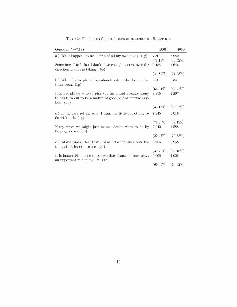
Table 3: The locus of control pairs of statements - Rotter-test
Question N=7,638 2006 2009
a.) What happens to me is first of all my own doing. (1p) 7,807 5,980(78.11%) (78.42%)
Sometimes I feel that I don’t have enough control over thedirection my life is taking. (0p)
2,188 1,646
(21.89%) (21.58%)
b.) When I make plans, I am almost certain that I can makethem work. (1p)
6,681 5,341
(66.84%) (69.93%)It is not always wise to plan too far ahead because manythings turn out to be a matter of good or bad fortune any-how. (0p)
3,315 2,297
(33.16%) (30.07%)
c.) In my case getting what I want has little or nothing todo with luck. (1p)
7,945 6,016
(79.57%) (79.12%)Many times we might just as well decide what to do byflipping a coin. (0p)
2,040 1,588
(20.43%) (20.88%)
d.) Many times I feel that I have little influence over thethings that happen to me. (0p)
3,956 2,968
(39.70%) (39.18%)It is impossible for me to believe that chance or luck playsan important role in my life. (1p)
6,008 4,608
(60.30%) (60.82%)
11

There are several ways to use the answers. The easiest is to add up the points,higher points indicating more internal LoC.12 There are other possible methods likeaveraging answers (Elkins et al., 2017) or using factor analysis (Mendolia and Walker,2014; Piatek and Pinger, 2016; Caliendo et al., 2020). We also use factor analysis,and we standardize the variable to come up with our LoC measure with zero meanand unit standard deviation.
As mentioned earlier, we study four outcome variables: dropout age, whether thestudent graduates from high school, whether the student plans to apply to college,and whether they attend college. We present the summary statistics in Table B.11in the Appendix.
To illustrate the dimensions and richness of the database, here we briefly reportsome statistics about it. The database contains answers to 4910 distinct questions,some of which were asked in each wave, and others not.13 Table B.12 in the Appendixcontains the dictionary of all the variables that we use in the analysis.
Related to family background, besides the usual questions on parental education,occupation, and household income, the Life Course Survey contains information evenon the level of education of the grandparents, the health, nationality, and languagesspoken by the parents. Importantly, it has detailed information on the home en-vironment.14 A widely used measure of that in empirical studies is the so-calledHOME (Home Observation for Measurement of the Environment) scale that is partof the database. This scale incorporates measures related to objects, activities, cir-cumstances, and events at home that may play an essential role in the developmentof the adolescent. In this survey, a young adolescent short version was administered,which followed the methodology of NSLY (for Human Resource Research, 2004). Theelements of the scale are described in Appendix C. The scale consists of 27 items, 9of which are rated by the interrogator, and the rest is based on the parents’ answers.The scale includes two part-scales, cognitive stimulation (13 items) and emotionalsupport (14 items).
Related to individual characteristics, the survey asks, for example, about thenumber of books and reading habits, it has many questions on the babyhood and
12Several other studies follow this strategy (Pearlin and Schooler, 1978; Semykina and Linz, 2007;Cobb-Clark and Schurer, 2013; Caliendo et al., 2015).
13The data is organized into four main (family background, individual characteristics, schoolenvironment, attrition), and many subblocks. Attrition refers to those respondents who did notrespond at a certain wave but then participated in later waves.
14According to the developmental psychology literature, psychological and physiological develop-ment of the children is strongly related to stimuli at the home environment (Strauss and Knight,1999; Davis-Kean, 2005; Sarsour et al., 2011).
12
childhood (e.g., birth weight; length of breastfeeding; if the parents read fairy tales;if they played board games), on health (asking about all major diseases), on self-evaluation, on employment, on future expectations, on friends, (un)healthy life (e.g.,exercising, smoking, alcohol or drug use), on prejudice, on political orientation.
Related to school environment, the database has detailed information on theschool the respondent attends, on the school performance, on schooling history (e.g.,the age of starting school, schools that the respondent went to earlier), on the class(e.g., composition of the class in terms of socioeconomic status), on extracurricularactivities, on parental involvement in schooling, on attachment to the school, onabsenteeism and dropping out.
As the database works with a tremendous number of variables, there is a highprobability that at least one variable is missing for an individual. To avoid sampleselection on missing variables, we impute missing values of control variables. Weuse the mean of the nonmissing observations in case of continuous variables and themode in categorical variables.
4. Empirical method
Economists are usually after the causal effects. However, it is challenging, ifnot impossible, to find any exogenous variability in the LoC, which would allow forcausal analysis. A second-best solution is to include the best possible explanatoryvariables to outrule confounders. In the previous literature, several variables areused as controls to measure the association of LoC with human capital investmentdecisions, see Table 2. Unless restricted by data availability, the specifications chosenreflect a professional judgment that might be correct or not. Nevertheless, variousstudies use different sets of control variables, which indicates that there is no scientificconsent in this question. Here, we circumvent this issue by making use of machinelearning.
We turn to the Post Double Selection (PDS) lasso method of Ahrens et al. (2019),based on Belloni et al. (2012, 2011, 2014b,a, 2016) which is designed to estimatecausal effects after a lasso selection procedure, using high-dimensional data.15 Al-though we do not claim our results to be causal, we would like to get as close to the
15The lasso technique uses shrinkage and thus offers a simple way to select a model with reasonablyfew variables, which performs best in predicting the value of the dependent variable out of sample(see https://web.stanford.edu/ hastie/StatLearnSparsity/). We are not the first to use machinelearning techniques to select control variables. Angrist and Frandsen (2019) claim that ”ML maybe useful for automated selection of ordinary least squares (OLS) control variables.” Other examplesinclude Boheim et al. (2020); Fluchtmann et al. (2020).
13
causal population parameter as possible.During the double selection part, PDS lasso selects control variables in two steps,
which make the best out-of sample prediction for the actual dependent variable(Yi,t+n) in the first step, and the LoC variable (LoCi,t) in the second step. As thelast step, a simple OLS regression is estimated using the union of the selected controlvariables.
Yi,t+n = γ × LoCi,t +X ′i,t−mβ + ξi,t (1)
where n and m may take different values for each variable, due to data availability,and n = {−3,−2,−1, 0, 2, 3} and m = {1, 2, 3}. This means that in the regression,the timing of the variables are selected such that the control variables refer to years2006 to 2008, the LoC values are from 2009, and the outcome variables refer tovarious years in the database. The robust standard errors are clustered at the schoollevel. We include four dependent variables in the regressions: dropout age, a dummyon graduating from high school, a dummy on planning to go to college, and a dummyon attending college.
Ideally, we would have a database that included all the factors that determineLoC, as well as all the factors that influence the outcome variables. Also, the idealtiming of these data would be such that the explanatory variables predate the out-come variables. In our regressions, we use LoC as measured in 2009, so that we caninclude a wide range of factors that determine LoC, which were measured before2009. If we were to use LoC measured in 2006, we would be able to include onlya very limited number of such factors, which were measured in May 2006 or deter-mined before 2006, like gender or parental education. This strategy, however, comesat a cost. The literature on non-cognitive skills has pointed out that the contem-poraneous measurement of the non-cognitive skill and the outcome variable may beproblematic because the direction of the effect is not clear (Almlund et al., 2011)and it may lead to overestimation of the impact of LoC (Piatek and Pinger, 2016).We have no contemporaneity issue in the case of two of the outcome variables.16
First, graduating from high school, LoC was measured in October 2009, and thenstudents graduated in May 2010. Second, attending college clearly postdates themeasurement of LoC in 2009. On the contrary, dropout age is measured throughoutthe six waves, some preceding the year 2009. Moreover, college application plans aremeasured in 2009 on the same day as LoC. In all four cases, we claim to be measuring
16Table A.10 in the Appendix contains information on when LoC and the outcome variables weremeasured.
14
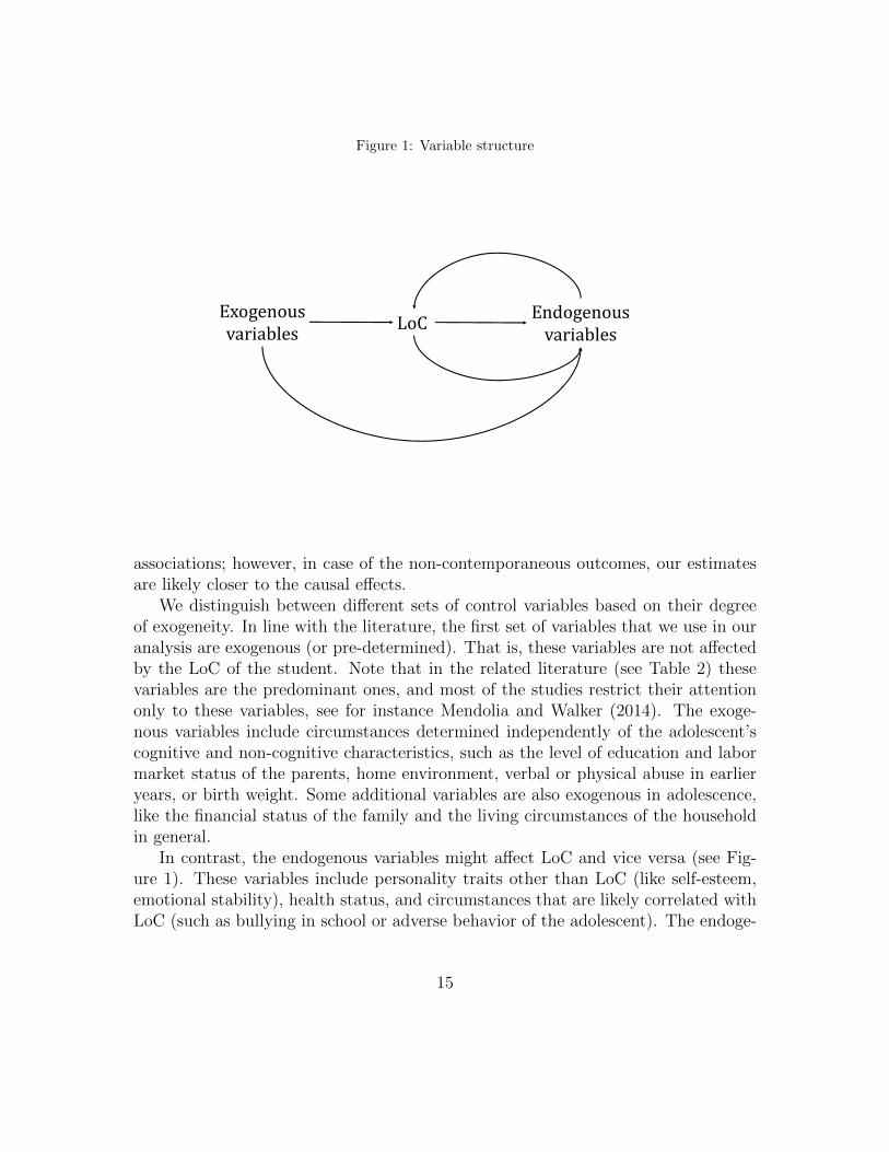
Figure 1: Variable structure
Exogenousvariables LoC Endogenous
variables
associations; however, in case of the non-contemporaneous outcomes, our estimatesare likely closer to the causal effects.
We distinguish between different sets of control variables based on their degreeof exogeneity. In line with the literature, the first set of variables that we use in ouranalysis are exogenous (or pre-determined). That is, these variables are not affectedby the LoC of the student. Note that in the related literature (see Table 2) thesevariables are the predominant ones, and most of the studies restrict their attentiononly to these variables, see for instance Mendolia and Walker (2014). The exoge-nous variables include circumstances determined independently of the adolescent’scognitive and non-cognitive characteristics, such as the level of education and labormarket status of the parents, home environment, verbal or physical abuse in earlieryears, or birth weight. Some additional variables are also exogenous in adolescence,like the financial status of the family and the living circumstances of the householdin general.
In contrast, the endogenous variables might affect LoC and vice versa (see Fig-ure 1). These variables include personality traits other than LoC (like self-esteem,emotional stability), health status, and circumstances that are likely correlated withLoC (such as bullying in school or adverse behavior of the adolescent). The endoge-
15
nous variables can be thought of as channels that mediate the effect of LoC to theoutcome variables of interest. These variables are included in the second to sixth setof controls, as shown in Cols 3 to 7 in Table 6. We refer to endogenous variables aschannels in our regressions, acknowledging the fact that these variables in themselvescould be regarded as outcomes.
By adding the sets of endogenous variables, instead of going for the exact pointestimate, we are after the channels likely to mediate the association between LoCand the human capital investment decisions.
5. Findings
5.1. Descriptive statistics
In Appendix D we provide a detailed analysis on our LoC measure, includingdescriptive statistics about the distribution and the determinants of the level and thechange of LoC. Here we briefly summarize the main findings. Our sample containsa high share of students with internal tendencies. The distribution of the changeis bell-shaped, peaking at zero, suggesting that LoC is a stable trait.17 The PDSlasso estimates with only exogenous variables indicate that many variables relatedto the family background (home environment, parental education, household’s fi-nancial position) predict LoC. All of these variables have the expected sign: more(less) favourable home environment, better (worse) schooling of the parents andgrandparents, better (worse) financial position of the household associates positively(negatively) with the level of internal tendencies in 2009. When we allow PDS lassoto select also from endogenous variables, many other variables also associate withthe level and change of LoC in the expected way, for instance, psychological traits(e.g., self-esteem), health-related variables, and environmental factors not relatedto home, but to school and friends. When considering endogenous variables, lassoselects considerably less exogenous variables, suggesting that those endogenous vari-ables mediate the effect of the exogenous variables that have been dropped. Overall,our findings related to the stability and determinants of LoC are in line with theliterature.
In Table 4 we present summary statistics for the variables of most interest tous. LoC is always higher in the groups with more favourable outcomes (e.g. above-median dropout age), suggesting that more internal tendencies associate with positive
17There is no change in LoC for 15% of the sample, and and 56% of the changes are at most 0.25of the standard deviation. We see only 0.78% (0.75%) of individuals experiencing the maximumdownward (upward) change.
16

outcomes. We observe the same pattern when considering our cognitive measureslike GPA, test scores in math, and reading. Better outcomes correlate with bettercognitive measures. Being female relates positively with better outcomes. Mother’seducation correlates expectedly with the outcome variables because the share oflow-educated (high-educated) mothers is higher when worse (better) outcomes areconsidered. Household income exhibits the expected relationship: higher incomesassociate with better outcomes. We see the same pattern with the components ofthe HOME scale. The difference in the scores of these scales between worse and bet-ter outcomes is clearly larger for the HOME cognitive scale, suggesting that it playsa more important role in human capital decisions than the HOME emotional scale.The last three variables (mother’s education, household income, HOME scale) cap-ture family background, and overall, better family background correlates with betteroutcomes, as expected. Conduits through which LoC may operate also associatewith the outcome variables as expected . Hence, more positive future expectations(either considered jointly as a factor variable, or the elements of it from which wereport two) are related with better outcomes. The same occurs with effort, eitherwhen considered as a factor composed of several elements or when those elementsare taken into account separately (see study time and effort grade). Better outcomesalso associate with the ability of the family to pay for the child’s studies (a con-straint), and also with the positive parental preferences regarding the minimum orideal educational attainment of the child.
17
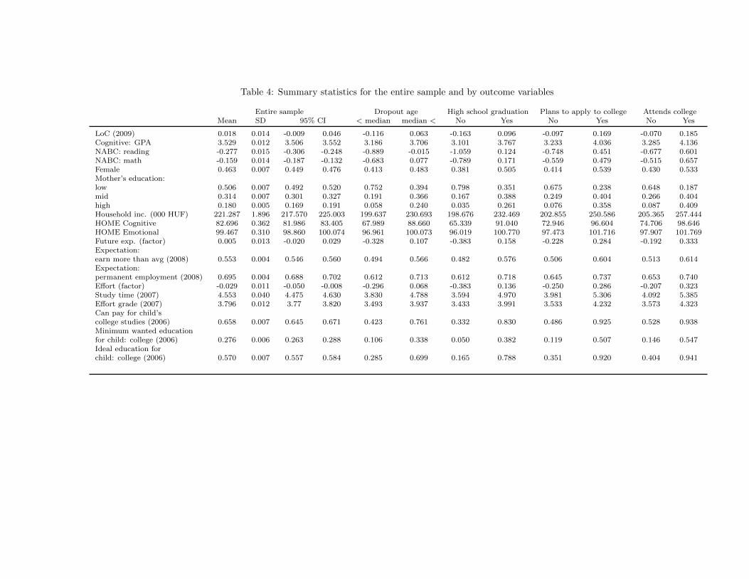
Table 4: Summary statistics for the entire sample and by outcome variables
Entire sample Dropout age High school graduation Plans to apply to college Attends collegeMean SD 95% CI < median median < No Yes No Yes No Yes
LoC (2009) 0.018 0.014 -0.009 0.046 -0.116 0.063 -0.163 0.096 -0.097 0.169 -0.070 0.185Cognitive: GPA 3.529 0.012 3.506 3.552 3.186 3.706 3.101 3.767 3.233 4.036 3.285 4.136NABC: reading -0.277 0.015 -0.306 -0.248 -0.889 -0.015 -1.059 0.124 -0.748 0.451 -0.677 0.601NABC: math -0.159 0.014 -0.187 -0.132 -0.683 0.077 -0.789 0.171 -0.559 0.479 -0.515 0.657Female 0.463 0.007 0.449 0.476 0.413 0.483 0.381 0.505 0.414 0.539 0.430 0.533Mother’s education:low 0.506 0.007 0.492 0.520 0.752 0.394 0.798 0.351 0.675 0.238 0.648 0.187mid 0.314 0.007 0.301 0.327 0.191 0.366 0.167 0.388 0.249 0.404 0.266 0.404high 0.180 0.005 0.169 0.191 0.058 0.240 0.035 0.261 0.076 0.358 0.087 0.409Household inc. (000 HUF) 221.287 1.896 217.570 225.003 199.637 230.693 198.676 232.469 202.855 250.586 205.365 257.444HOME Cognitive 82.696 0.362 81.986 83.405 67.989 88.660 65.339 91.040 72.946 96.604 74.706 98.646HOME Emotional 99.467 0.310 98.860 100.074 96.961 100.073 96.019 100.770 97.473 101.716 97.907 101.769Future exp. (factor) 0.005 0.013 -0.020 0.029 -0.328 0.107 -0.383 0.158 -0.228 0.284 -0.192 0.333Expectation:earn more than avg (2008) 0.553 0.004 0.546 0.560 0.494 0.566 0.482 0.576 0.506 0.604 0.513 0.614Expectation:permanent employment (2008) 0.695 0.004 0.688 0.702 0.612 0.713 0.612 0.718 0.645 0.737 0.653 0.740Effort (factor) -0.029 0.011 -0.050 -0.008 -0.296 0.068 -0.383 0.136 -0.250 0.286 -0.207 0.323Study time (2007) 4.553 0.040 4.475 4.630 3.830 4.788 3.594 4.970 3.981 5.306 4.092 5.385Effort grade (2007) 3.796 0.012 3.77 3.820 3.493 3.937 3.433 3.991 3.533 4.232 3.573 4.323Can pay for child’scollege studies (2006) 0.658 0.007 0.645 0.671 0.423 0.761 0.332 0.830 0.486 0.925 0.528 0.938Minimum wanted educationfor child: college (2006) 0.276 0.006 0.263 0.288 0.106 0.338 0.050 0.382 0.119 0.507 0.146 0.547Ideal education forchild: college (2006) 0.570 0.007 0.557 0.584 0.285 0.699 0.165 0.788 0.351 0.920 0.404 0.941
5.2. Conduits of LoC
Here we investigate if LoC associates with the two conduits that we consider:future expectations and effort. A strong association would suggest that LoC mayoperate through these conduits.
We measure expectations with five different questions from 2008. Respondentshave to rate the probability that at the age of 35, i) they will earn more money thanthe average, ii) they will be in the decile with the highest earnings, iii) will have apermanent job after finishing school, iv) will earn more than HUF 100,000 (appr.USD 350), and v) earn more than HUF 200,000 (appr. USD 700). We use factoranalysis to generate a factor that we use as a dependent variable. The level of theexpected salary and the probability of having a permanent job load onto factor 1,while factor 2 relies on relative salary.18 In this section we will use factor 1 as ourdependent variable to see if LoC is associated with it.
The effort is measured with teacher-given grades on diligence (in 2007, 2008 and2009), questions on studying time regarding hours spent studying in a week andwhether it occurred that the individual studied after 8PM on weekdays, or studiedon weekends (in 2007 and 2008).19 Similarly to expectations, we utilize factor analysisto come up with the dependent variables that we will use below. Grades on diligenceand study time load on factor 1, while the weekend study time and studying after8PM load onto factor 2. Table B.11 reports summary statistics for these factorvariables.
In Table 5 we show the results of PDS lasso regressions where the dependentvariable is future expectations or effort, and we deploy more and more control vari-ables in the different specifications. More specifically, in Column 1, we estimate aunivariate regression with LoC as the sole explanatory variable. In Column 2, weadd exogenous controls, in Column 3 we allow PDS lasso to include cognitive con-trols as well. In the next specification (Column 4), we add the conduit other thanthe dependent variable. So in the regression explaining expectations, we use effortas an independent variable and vice versa. We do so to see if the two conduits thatwe propose reflect the same mechanism or not. In the most thorough specification,in Column 5, besides the previous controls, PDS lasso also selects from the set ofendogenous variables. We observe a very strong association between LoC and future
18In Appendix E we show the graphical representation of the factor loadings, both for expecta-tions and effort.
19In Hungary, students get grades on two general issues: behavior (how they behave in school)and diligence (how much effort they make in the school). The second one is clearly related to theidea of effort.
19
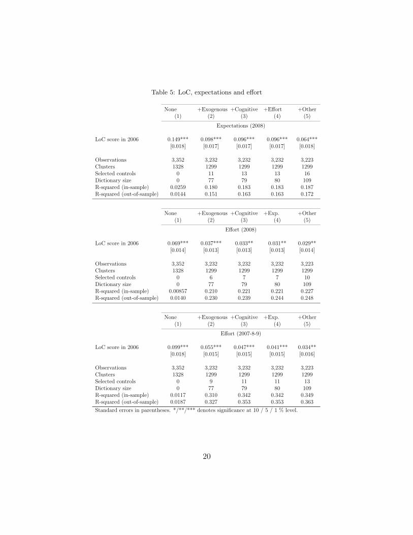
Table 5: LoC, expectations and effort
None +Exogenous +Cognitive +Effort +Other(1) (2) (3) (4) (5)
Expectations (2008)
LoC score in 2006 0.149*** 0.098*** 0.096*** 0.096*** 0.064***[0.018] [0.017] [0.017] [0.017] [0.018]
Observations 3,352 3,232 3,232 3,232 3,223Clusters 1328 1299 1299 1299 1299Selected controls 0 11 13 13 16Dictionary size 0 77 79 80 109R-squared (in-sample) 0.0259 0.180 0.183 0.183 0.187R-squared (out-of-sample) 0.0144 0.151 0.163 0.163 0.172
None +Exogenous +Cognitive +Exp. +Other(1) (2) (3) (4) (5)
Effort (2008)
LoC score in 2006 0.069*** 0.037*** 0.033** 0.031** 0.029**[0.014] [0.013] [0.013] [0.013] [0.014]
Observations 3,352 3,232 3,232 3,232 3,223Clusters 1328 1299 1299 1299 1299Selected controls 0 6 7 7 10Dictionary size 0 77 79 80 109R-squared (in-sample) 0.00857 0.210 0.221 0.221 0.227R-squared (out-of-sample) 0.0140 0.230 0.239 0.244 0.248
None +Exogenous +Cognitive +Exp. +Other(1) (2) (3) (4) (5)
Effort (2007-8-9)
LoC score in 2006 0.099*** 0.055*** 0.047*** 0.041*** 0.034**[0.018] [0.015] [0.015] [0.015] [0.016]
Observations 3,352 3,232 3,232 3,232 3,223Clusters 1328 1299 1299 1299 1299Selected controls 0 9 11 11 13Dictionary size 0 77 79 80 109R-squared (in-sample) 0.0117 0.310 0.342 0.342 0.349R-squared (out-of-sample) 0.0187 0.327 0.353 0.353 0.363
Standard errors in parentheses. */**/*** denotes significance at 10 / 5 / 1 % level.
20
expectations even after controlling for exogenous variables, cognitive abilities, effortand endogenous variables. This is in line with Coleman and DeLeire (2003) andCaliendo et al. (2020) who claim that an important channel through which LoC op-erates through future expectations. Turning to effort, we see a very similar picture.LoC correlates strongly with effort (considering effort data only from 2008 as wellas from 2007-2009) even when we take into account exogenous and cognitive vari-ables, expectations and the endogenous variables. Overall, there is strong evidencethat individuals with a more internal LoC are more likely to exert effort. The pointestimate on the effect of Loc on effort (2007-8-9) in Column 3 means that even aftercontrolling for exogenous variables and cognitive ability, a one standard deviationincrease in LoC would increase effort by 0.047 which is an increase of 5.3% of thestandard deviation of effort (calculating with a standard deviation of 0.871 as shownin Table B.11 in the Appendix).
Column 4 indicates that the two conduits represent different mechanisms throughwhich LoC operates, because neither the coefficient nor the significance of LoCchanges upon including the other conduit.
5.3. LoC and human capital investment decisions
In Figure 2 we show the raw associations between the outcome variables and LoC.In all cases, more internal LoC correlates with better outcomes. For graduating fromhigh school, college plans and college attendance, Figure 2 suggests some non-linearrelationship. However, given the wide confidence interval for low values of LoC, anincrease in LoC for those values does not correlate with the outcome variables. Incontrast, for larger values of LoC, more internal tendency goes hand in hand withbetter outcomes.20
Table 6 contains our main results. For each outcome variable, we have sevenspecifications. Column 1 indicates the raw association of LoC with the outcomevariable without any further controls. LoC associates at 1% significance level witheach of the outcome variables in the expected way, indicating that adolescents withmore internal tendencies drop out of school at an older age and are more likely tograduate from high school, to plan to go to college and to attend college. The effectsare substantial as a one-standard deviation increase in LoC is estimated to lead toa 0.134 year increase in dropout age, or a 5.4 / 6.3 / 5.6 percentage point increasein the likelihood of graduating from high school / college plans / college attendance.
20LoC of the students in our sample is skewed to the left, so students in our sample tend to haveinternal tendencies. Hence, at the lower end of the distribution, we have fewer observations andmore noise.
21

Figure 2: Raw associations between LoC and the outcome variables. Lowess curves.
20.8
2121
.221
.421
.6D
ropo
ut a
ge
-3 -2 -1 0 1LoC score in 2009
95% CI Fitted values
(a) Dropout age
.5.5
5.6
.65
.7.7
5G
radu
atin
g fro
m h
igh
scho
ol
-3 -2 -1 0 1LoC score in 2009
95% CI Fitted values
(b) Graduates from high school
.25
.3.3
5.4
.45
Plan
to a
pply
to u
nive
rsity
-3 -2 -1 0 1LoC score in 2009
95% CI Fitted values
(c) Plans to apply to college
.15
.2.2
5.3
.35
Atte
ndin
g co
llege
(201
1, 2
012)
-3 -2 -1 0 1LoC score in 2009
95% CI Fitted values
(d) Attends college
Note that the R-squared (in or out of sample) is a meager 1.2-1.9%.In Column 2 we add exogenous controls.21 Most of the exogenous variables that
PDS lasso selects to are related to family background. For instance, HOME cognitivescale appears in the regressions for each outcome variable and is significant at the1%. Similarly, the variable about parental preferences on the ideal education level isselected for each outcome variable and is significant at 1%. Other control variablesare selected only for some of the outcomes. For instance, financial distress of thefamily has a strong negative association with dropout age, but does not prove to bea relevant factor for the other outcomes.
As the selected controls row indicates in each panel, the PDS lasso techniqueselects 9 to 15 controls from the set of exogenous variables. The coefficient of LoCdrops markedly (by 57 to 78%) in all cases. It remains only marginally significant
21Appendix F contains the complete regressions for all the columns reported in Table 6.
22
when considering if the student graduates from high school, suggesting that for thisdecision factors related to the family background are very important and explainmost of the variation in the outcome variable. The coefficient reveals that a standarddeviation increase in LoC is associated with a 1.2 percentage point (corresponding toan 1.9% increase, calculated with averages shown in Table B.11) higher probabilityof graduating from high school. This is very similar to the 1.4 percentage pointfinding in the most related specification in Coleman and DeLeire (2003) and lowerthan the 3.8 and 4.5 percentage point increase documented by Cebi (2007) and Baronand Cobb-Clark (2010), respectively. Furthermore, a standard deviation increase inLoC correlates with a 2.3 percentage point (that is, a 6.6% increase, calculated withaverages shown in Table B.11) higher probability of planning to apply to college (forwhich there are no comparable findings in the literature). Last, a standard deviationincrease in LoC associates with a 2.4 percentage point (a 8.8% increase, calculatedwith averages shown in Table B.11) higher probability of college attendance, thatis higher than the non-significant 0.5 percentage point reported by Coleman andDeLeire (2003), but lower than the significant 6 percentage point documented byCebi (2007).
After controlling for exogenous variables, LoC is significant at the 5% for dropoutage, and maintains 1% significance for college plans and attending college. It isnoteworthy that the inclusion of variables that - to a large degree - predict LoC doesnot eliminate the association of LoC for three of our outcome variables. The presenceof the exogenous variables increases dramatically the predictive power of the modelas R-squared (in or out of sample) rises to 25-45%.
In Column 3 we allow PDS lasso to select also cognitive measures into the regres-sion as Cebi (2007) pointed out that controlling appropriately for cognitive abilitiesmay weaken or remove the significance of LoC. Our cognitive measures include thetest scores in reading and mathematics at the National Assessment of Basic Com-petencies. In fact, for all the outcome variables both reading and math scores areincluded in the regressions and in all cases they are significant at least at the 5%.Note that the number of selected controls drops in three cases even though we addedtwo new items to the set of variables from which PDS lasso can select control vari-ables. The coefficient of LoC decreases moderately in all cases. The significance levelchanges only in one case, as LoC ceases to be significant when predicting graduationfrom high school. Interestingly, in Cebi (2007) it is also at this stage when LoCbecomes insignificant, moreover the size of the coefficients is very similar (1 vs 1.5percentage point). After allowing for cognitive abilities, LoC still has a significantassociation with dropout age, planning to go to college and college attendance atleast at the 5% significance level. Again, our results are very similar to Cebi (2007)’s
23
findings if we consider college attendance, as she reports a significant coefficient of2.3 percentage points, very similar in magnitude to our 1.9 percentage points. Thepredictive power of the model increases further by 1-7 percentage points.
Next, in Column 4 we explore the role of expectations, allowing PDS lasso toselect from the expectation variables also besides the variables that we consideredin the previous regressions. From the expectations variables, PDS lasso selects threethat appear in the regressions of all outcome variables. Two refer to the probabilitythat the salary of the respondent at her / his first employment will be over 100,000/ 200,000 HUF, and the third is about the probability to earn a higher wage thanthe average at the age of 35. The literature proposes that such positive expectationsreflect that the respondents have more favourable expectations on the rate of returnin human capital investments. The coefficient of LoC remains the same or decreasesonly slightly in all cases except dropout age, where we observe a substantial drop.
In fact, as a consequence of this drop, LoC ceases to be significant in explainingdropout age. As dropout age and LoC are measured contemporaneously, there aretwo possible explanations for this. First, the different view on the rate of return playsa vital role in dropout, and LoC seems to operate through this conduit. Second, thecausality may go the other way around, that after a dropout, the expectations becomevery low and this happens more often if LoC is more external.
After allowing PDS lasso to choose from such a wide range of variables, LoCremains still significant at least at the 5% for the ‘high-end’ decisions (college plansand attending college). In this specification, the predictive power of the model in-creases very little for all outcome variables, except for the dropout age where we seea marked increase. This is in line with our interpretation that future expectationsplay a large role in understanding the dropout age.
In Column 5, we consider the role of effort as a potential conduit through whichLoC may operate. To be able to assess the relative role of effort to future expec-tations, in this column, we do not allow PDS lasso to select from the variablescorresponding to expectations. We capture effort through self-reported study timein 2007 and 2008 (hours per week), if the student studies after 8 PM, the hours thatthe student spends studying on weekends, and the grade on effort in 2007 and 2008which is given based on the diligence of the student in school. All of these variablesare selected in at least one specification, and they are often very significant. Forall outcome variables, the drop in the coefficient of LoC is more extensive when weconsider effort (Col 5) than in the case of future expectations (Col 4), suggesting thatLoC may be more related to the former. This is also corroborated by the fact thatthe increase in predictive power is higher when we add effort than after includingfuture expectations. Overall, effort seems to be at least as important a conduit as
24
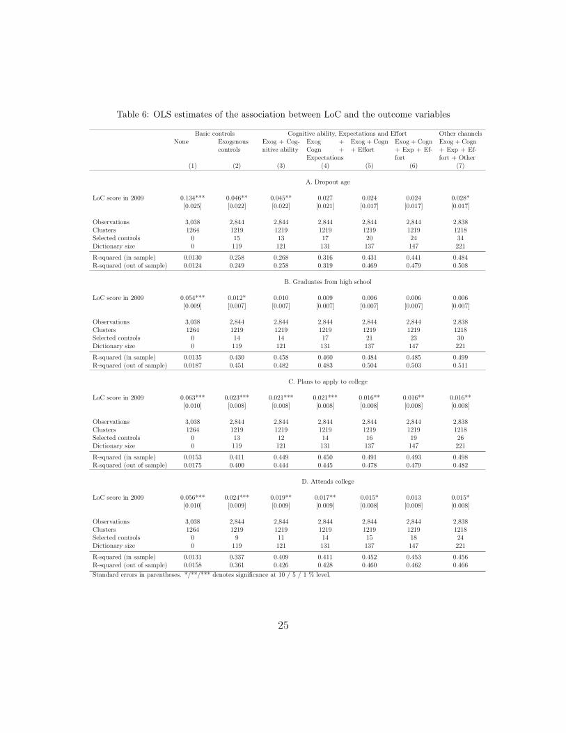
Table 6: OLS estimates of the association between LoC and the outcome variables
Basic controls Cognitive ability, Expectations and Effort Other channelsNone Exogenous
controlsExog + Cog-nitive ability
Exog +Cogn +Expectations
Exog + Cogn+ Effort
Exog + Cogn+ Exp + Ef-fort
Exog + Cogn+ Exp + Ef-fort + Other
(1) (2) (3) (4) (5) (6) (7)
A. Dropout age
LoC score in 2009 0.134*** 0.046** 0.045** 0.027 0.024 0.024 0.028*[0.025] [0.022] [0.022] [0.021] [0.017] [0.017] [0.017]
Observations 3,038 2,844 2,844 2,844 2,844 2,844 2,838Clusters 1264 1219 1219 1219 1219 1219 1218Selected controls 0 15 13 17 20 24 34Dictionary size 0 119 121 131 137 147 221
R-squared (in sample) 0.0130 0.258 0.268 0.316 0.431 0.441 0.484R-squared (out of sample) 0.0124 0.249 0.258 0.319 0.469 0.479 0.508
B. Graduates from high school
LoC score in 2009 0.054*** 0.012* 0.010 0.009 0.006 0.006 0.006[0.009] [0.007] [0.007] [0.007] [0.007] [0.007] [0.007]
Observations 3,038 2,844 2,844 2,844 2,844 2,844 2,838Clusters 1264 1219 1219 1219 1219 1219 1218Selected controls 0 14 14 17 21 23 30Dictionary size 0 119 121 131 137 147 221
R-squared (in sample) 0.0135 0.430 0.458 0.460 0.484 0.485 0.499R-squared (out of sample) 0.0187 0.451 0.482 0.483 0.504 0.503 0.511
C. Plans to apply to college
LoC score in 2009 0.063*** 0.023*** 0.021*** 0.021*** 0.016** 0.016** 0.016**[0.010] [0.008] [0.008] [0.008] [0.008] [0.008] [0.008]
Observations 3,038 2,844 2,844 2,844 2,844 2,844 2,838Clusters 1264 1219 1219 1219 1219 1219 1218Selected controls 0 13 12 14 16 19 26Dictionary size 0 119 121 131 137 147 221
R-squared (in sample) 0.0153 0.411 0.449 0.450 0.491 0.493 0.498R-squared (out of sample) 0.0175 0.400 0.444 0.445 0.478 0.479 0.482
D. Attends college
LoC score in 2009 0.056*** 0.024*** 0.019** 0.017** 0.015* 0.013 0.015*[0.010] [0.009] [0.009] [0.009] [0.008] [0.008] [0.008]
Observations 3,038 2,844 2,844 2,844 2,844 2,844 2,838Clusters 1264 1219 1219 1219 1219 1219 1218Selected controls 0 9 11 14 15 18 24Dictionary size 0 119 121 131 137 147 221
R-squared (in sample) 0.0131 0.337 0.409 0.411 0.452 0.453 0.456R-squared (out of sample) 0.0158 0.361 0.426 0.428 0.460 0.462 0.466
Standard errors in parentheses. */**/*** denotes significance at 10 / 5 / 1 % level.
25
future expectations. Regarding dropout age, the significance of LoC vanishes whenwe include effort, similarly to future expectations. Relative to future expectations,effort has a stronger effect in the ‘high-end’ decisions because there its inclusionlowers the significance of LoC a lot more. However, even after this lowering theassociation between LoC and college plans / attending college remains significant atthe 5% / 10% significance level.
When we consider both conduits at the same time (see Column 6), PDS lassoselects always the future expectations variables that were chosen also in Column 4and from the effort variables effort grades in years 2007 and 2008 and weekly studytime are chosen for each outcome variable. The effort variables tend to be significantmore often than the future expectations variables. Compared to the inclusion of ef-fort (Column 5), we see no change in the coefficient of LoC for three of our outcomevariables and in the fourth case the decrease is modest. The increase in R-squared isalso very small. The inclusion of both conduits eliminates the significance of LoC topredict college attendance (though when considering them separately, LoC remainedsignificant), indicating that LoC exerts its impact by affecting both future expecta-tions and effort. Interestingly, the significance of LoC survives the incorporation ofboth conduits when we predict college plans, showing that it is not through futureexpectations or effort that LoC impinges on this human capital investment decision.
Column 7 has the largest dictionary size, including variables which could beoutcomes themselves, like personality traits (emotional stability) and behaviouralvariables (related to health, sex, etc.). Even with this broadest set of variables, LoCremains significant at 5% for college plans. This result is intuitive, as all the otheroutcome variables are a sort of achievement, where internal LoC can have an affectonly if it facilitates a change in behaviour (e.g., putting more effort in studying). SoLoC exerts its effect through certain channels. Whereas, filling an application formis a mere expression of wants, where a more internal LoC can prove just enough.
Interestingly, in this last specification, the predictive power of the models doesnot increase much, neither does decrease the point estimate of LoC. Looking at thecomplete regressions we observe that often the new controls are significant whileprevious controls lose significance, suggesting that this additional set of controlsdo not really control for additional exogenous variations, rather these are channelsthrough which the controls included before exert their effects.22
22For instance, regarding dropout age the significance of father working and financial distressvanishes, while the number of positive events appears as a significant variable. Interestingly, theendogenous variable that is significant concerning all outcomes is the age at the first sex.
26
5.4. Heterogeneity
The association of LoC with the outcome variables may vary across subsamples.Studies about the relationship between LoC and labour market outcomes concen-trated on gender differences (see Cobb-Clark (2015)). We find that when we considergraduating from high school, LoC is slightly more relevant for males, however regard-ing the other outcome variables, LoC plays a more important role for females. WhileLoC ceases to be significant for males in all outcomes when we add the exogenousvariables, it remains significant for females for dropout age, planning to apply to col-lege and college attendance. The difference is starkest in the case of plans to applyto college as there LoC remains significant for females even when the endogenousvariables are added.23, while studies on human capital investment decisions focusedon the role of socioeconomic status. In this section, we concentrate on how the asso-ciation of LoC with the outcome variables varies according to socioeconomic status.We go a step further in this analysis by utilizing questions regarding parental pref-erences on the adolescent’s highest educational attainment and financial constraints.We offer an alternative explanation as to why LoC plays a different role in case oflow, middle and high SES students.
The role of socioeconomic status related to human capital investment decisionsreceived attention in the recent literature. Baron and Cobb-Clark (2010) investigateif growing up in disadvantage, captured by family welfare receipt history, affectshow LoC influences educational outcomes and report no significant association. Incontrast, Mendolia and Walker (2014) find that LoC has a larger impact for low-SESstudents.24 They conjecture that this result is because students with a high-SESbackground are more likely to live in a more stimulating home environment, withparents closely following and supporting their school work.
Given the divergent findings in the literature, we first investigate if LoC correlateswith the outcome variables differently according to socioeconomic status (see Table7). To capture SES, we use the mother’s education that we classify as low / mid /high (corresponding to less than high school / high school / college). The coefficientsin Table 7 indicate that indeed, the impact of LoC is dependent on the mother’seducation. When the mother’s education level is high, in three out of four casesLoC is not significant even in the univariate regressions (see Column 1). In case
23Our findings related to gender differences are summarized in Appendix G.24Related to other non-cognitive skills it has been also shown that non-cognitive skills have
a differential association with educational outcomes. For instance, Lundberg (2013) shows thatelements of the Big Five affect individuals’ schooling outcomes differently for men and women, andalso according to family background.
27
of mothers with lower education level (low and mid), LoC associates strongly withthe outcome variables if we do not use any further controls. However, when we addexogenous variables, in all but one case, the significance disappears in the case ofmid-education mothers. For dropout age, graduation from high school and collegeplans, clearly LoC has the most significant association for students whose motherended up with low education. For college attendance, we observe the largest effectin case of mothers with a middle level of education. Overall, these results are in linewith Mendolia and Walker (2014).
We make one step further to understand better how family background interactswith LoC. Based on the existing literature, it is not clear if the stronger associationthat we observe in students from a low-SES background is due to the poor stimulireceived at the home environment, the parental preferences (parents do not wanttheir child to invest in human capital) or financial constraints (parents cannot or arenot willing to financially support the human capital investment).
Our data set contains three relevant questions in this regard. The first / secondquestion asks the parents about the ideal / minimum level of education they wouldlike their child to obtain. The third question asks how long they can / plan tofinance the education of their child. The first two questions are more related toparental preferences about the child’s educational attainment, while the last one isinformative about the financial constraint.
By studying the role of parental preferences and / or financial constraints inthe association between LoC and the outcome variables, we complement Mendoliaand Walker (2014), because both of them are highly related to SES, see Table 8and Appendix H). We start with parental preferences and we define three groups.Parental preferences are low if both the minimum and ideal education level is less thangraduating from high school. In this group, parents do not expect much from theirchildren, and the lack of expectations may affect their motivations and educationalachievement. We call this group strict low. We expect that for (most of the) studentsin this group tertiary studies are not something that they strive to achieve so LoCmay be less critical for them when we consider the high-end decisions. For low-enddecision, LoC may make a difference. At the other end of the spectrum, we defineanother group (that we call the strict high group) where both the minimum andideal parental preferences are at least a college degree.25 In this group, students areexpected to end up in college, so graduating from high school is a must for them,so LoC may be less important for low-end decisions. However, in high-end decisions
25We discard from the analysis those observations where the minimum education level is higherthan the ideal. This involves 0.64% of the observations.
28
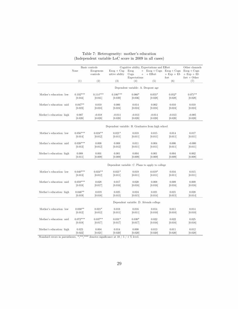
Table 7: Heterogeneity: mother’s education(Independent variable LoC score in 2009 in all cases)
Basic controls Cognitive ability, Expectations and Effort Other channelsNone Exogenous
controlsExog + Cog-nitive ability
Exog +Cogn +Expectations
Exog + Cogn+ Effort
Exog + Cogn+ Exp + Ef-fort
Exog + Cogn+ Exp + Ef-fort + Other
(1) (2) (3) (4) (5) (6) (7)
Dependent variable: A. Dropout age
Mother’s education: low 0.192*** 0.114*** 0.106*** 0.066* 0.055* 0.052* 0.071**[0.044] [0.041] [0.039] [0.036] [0.028] [0.028] [0.028]
Mother’s education: mid 0.047** 0.010 0.006 0.014 0.002 0.010 0.010[0.023] [0.024] [0.024] [0.024] [0.024] [0.024] [0.024]
Mother’s education: high 0.007 -0.018 -0.014 -0.013 -0.014 -0.013 -0.005[0.020] [0.020] [0.020] [0.020] [0.020] [0.020] [0.020]
Dependent variable: B. Graduates from high school
Mother’s education: low 0.056*** 0.024** 0.021* 0.018 0.015 0.014 0.017[0.014] [0.012] [0.011] [0.011] [0.011] [0.011] [0.011]
Mother’s education: mid 0.038*** 0.008 0.008 0.011 0.004 0.006 -0.000[0.013] [0.012] [0.012] [0.011] [0.011] [0.011] [0.011]
Mother’s education: high 0.008 0.001 0.001 0.004 0.001 0.004 0.002[0.011] [0.009] [0.009] [0.009] [0.009] [0.009] [0.008]
Dependent variable: C. Plans to apply to college
Mother’s education: low 0.040*** 0.024** 0.021* 0.019 0.019* 0.016 0.015[0.013] [0.012] [0.011] [0.011] [0.011] [0.011] [0.011]
Mother’s education: mid 0.059*** 0.028 0.017 0.020 0.008 0.009 0.009[0.018] [0.017] [0.016] [0.016] [0.016] [0.016] [0.016]
Mother’s education: high 0.046** 0.019 0.025 0.024 0.021 0.021 0.020[0.019] [0.016] [0.015] [0.015] [0.014] [0.015] [0.014]
Dependent variable: D. Attends college
Mother’s education: low 0.030** 0.021* 0.018 0.016 0.014 0.011 0.014[0.012] [0.012] [0.011] [0.011] [0.010] [0.010] [0.010]
Mother’s education: mid 0.072*** 0.037** 0.031* 0.030* 0.022 0.022 0.025[0.018] [0.017] [0.017] [0.017] [0.016] [0.016] [0.016]
Mother’s education: high 0.023 0.004 0.014 0.008 0.013 0.011 0.012[0.022] [0.021] [0.020] [0.020] [0.020] [0.020] [0.020]
Standard errors in parentheses. */**/*** denotes significance at 10 / 5 / 1 % level.
29
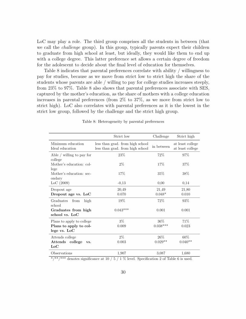
LoC may play a role. The third group comprises all the students in between (thatwe call the challenge group). In this group, typically parents expect their childrento graduate from high school at least, but ideally, they would like them to end upwith a college degree. This latter preference set allows a certain degree of freedomfor the adolescent to decide about the final level of education for themselves.
Table 8 indicates that parental preferences correlate with ability / willingness topay for studies, because as we move from strict low to strict high the share of thestudents whose parents are able / willing to pay for college studies increases steeply,from 23% to 97%. Table 8 also shows that parental preferences associate with SES,captured by the mother’s education, as the share of mothers with a college educationincreases in parental preferences (from 2% to 37%, as we move from strict low tostrict high). LoC also correlates with parental preferences as it is the lowest in thestrict low group, followed by the challenge and the strict high group.
Table 8: Heterogeneity by parental preferences
Strict low Challenge Strict high
Minimum education less than grad. from high schoolin between
at least collegeIdeal education less than grad. from high school at least college
Able / willing to pay forcollege
23% 72% 97%
Mother’s education: col-lege
2% 17% 37%
Mother’s education: sec-ondary
17% 35% 38%
LoC (2009) -0,13 0,00 0,14
Dropout age 20,49 21,49 21,80Dropout age vs. LoC 0.070 0.048* 0.010
Graduates from highschool
19% 72% 93%
Graduates from highschool vs. LoC
0.043*** 0.001 0.001
Plans to apply to college 3% 36% 71%Plans to apply to col-lege vs. LoC
0.009 0.038*** 0.023
Attends college 2% 26% 60%Attends college vs.LoC
0.003 0.029** 0.040**
Observations 1,907 3,087 1,680
*/**/*** denotes significance at 10 / 5 / 1 % level. Specification 2 of Table 6 is used.
30
Turning to the outcome variables, we observe that dropout age associates withparental preferences as expected, higher parental preferences correlating with higherdropout age. When we investigate how LoC associates with dropout age, we see thatthe coefficient decreases as we move from strict low to strict high, being marginallysignificant in the challenge group only, indicating that more internal students areslightly more likely to finish studying later.26
Graduation from high school also goes hand in hand with parental preferencesas the share of students that graduate from high school increases markedly withparental preferences (from 19% to 93%). Moreover, LoC has the largest coefficientin the strict low group that is significant at the 1% level. In contrast, in the othergroups the coefficient is not statistically different from zero. Hence, being internalhas a strong positive association with graduation from high school for students inthe strict low group.
Regarding college application plans, we observe an increasing pattern again asa function of parental preferences. Only 3% of the students in the strict low groupplans to apply to college, while this share is 36% in the challenge and 71% in thestrict high group. For this outcome, the only group in which the coefficient of LoCis statistically different from zero (and is significant at 1%) is the challenge group.Thus, in this group, those who have more internal LoC are more likely to plan toapply to college.
When looking at college attendance, we see that only 2% in the strict low groupdoes so, while the corresponding numbers in the challenge and strict high groupsare 26% and 60%. Coefficients of LoC are significantly different from zero in thechallenge and the strict high groups, showing the positive effect that having internalLoC tendencies has on attending college.
Overall, we see that LoC associates with the low-end decisions in a significantway in the groups with lower parental preferences, while in the high-end decisionsLoC plays a role in the groups with higher parental preferences. As a consequence,it is the challenge group in which LoC has an essential role in most decisions. Thesefindings suggest that it is not simply the SES that matters when investigating therole of LoC, but also the nature of the decision. The further away is the decision inquestion from the parental preferences, the less important is the role of LoC. Also,the wider liberty is allotted for the adolescent to decide on their further education,the larger role LoC plays in their human capital investment decisions.
26In Table 8 for simplicity, we use the coefficients of LoC corresponding to the specification thatincludes the exogenous variables besides LoC, specification 2 in Table 6. Table H.20 in AppendixH contains all the specifications.
31
Next, we focus on the effect of financial constraints. LoC probably helps adoles-cents to overcome difficulties related to financing a higher level of education. Table9 summarizes the main results of our findings. We divide the sample into low /mid / high level of ideal education (Less than high school graduation/ At least highschool graduation / At least college), and divide these further into groups wherethe financial constraints are non-binding (parents are able / willing to pay at leastthe ideal level of education) and binding (able to finance less than the ideal level).Most families can finance the ideal level of education, so there is only a low numberof adolescents who face financial constraints. The average level of education of themother is higher in groups where the ideal education is higher and where the finan-cial constraint is non-binding. Similar associations are detected with each outcomevariable, and there is a substantial increase from 2.7/2.7/0% to 88.9/58.6/46.5%in the probability of high school graduation, college plans and college attendance,respectively.
In the low-level subsample, the mother’s level of education is significantly higherin the non-binding group. Either as a consequence of this SES difference or thefinancial constraints, we see a considerable discrepancy between the averages of thelow-end outcome variables, dropout age and high school graduation. The high-endoutcomes, college plans and college attendance are similarly deficient in both groups.Although the sample size is as tiny as 37 observations in the binding subgroup, theestimated effect of LoC on dropout age is 0.89 and significant at the 1%. Thissuggests that for these adolescents, LoC makes a vast difference in dropout. On thecontrary, for these adolescents, LoC does not help to increase other outcomes. Inthe non-binding subsample, a one standard deviation increase in LoC elevates highschool graduation probability by 4.6%, and it is significant at the 1% level.
32
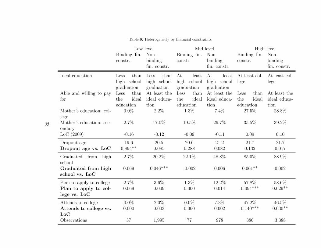
Table 9: Heterogeneity by financial constraints
Low level Mid level High levelBinding fin.constr.
Non-bindingfin. constr.
Binding fin.constr.
Non-bindingfin. constr.
Binding fin.constr.
Non-bindingfin. constr.
Ideal education Less thanhigh schoolgraduation
Less thanhigh schoolgraduation
At leasthigh schoolgraduation
At leasthigh schoolgraduation
At least col-lege
At least col-lege
Able and willing to payfor
Less thanthe idealeducation
At least theideal educa-tion
Less thanthe idealeducation
At least theideal educa-tion
Less thanthe idealeducation
At least theideal educa-tion
Mother’s education: col-lege
0.0% 2.2% 1.3% 7.4% 27.5% 28.8%
Mother’s education: sec-ondary
2.7% 17.0% 19.5% 26.7% 35.5% 39.2%
LoC (2009) -0.16 -0.12 -0.09 -0.11 0.09 0.10
Dropout age 19.6 20.5 20.6 21.2 21.7 21.7Dropout age vs. LoC 0.894** 0.085 0.288 0.082 0.132 0.017
Graduated from highschool
2.7% 20.2% 22.1% 48.8% 85.0% 88.9%
Graduated from highschool vs. LoC
0.069 0.046*** -0.002 0.006 0.061** 0.002
Plan to apply to college 2.7% 3.6% 1.3% 12.2% 57.8% 58.6%Plan to apply to col-lege vs. LoC
0.069 0.009 0.000 0.014 0.094*** 0.029**
Attends to college 0.0% 2.0% 0.0% 7.3% 47.2% 46.5%Attends to college vs.LoC
0.000 0.003 0.000 0.002 0.140*** 0.030**
Observations 37 1,995 77 978 386 3,388
33
In the mid-level groups, there are significant differences in the mother’s levelof education and all the outcome variables between subgroups. However, in thesegroups, we do not estimate any significant LoC effect whatsoever. The point esti-mates are very close to zero for most outcome variables except dropout age, but allare insignificant.
In the high-level groups, mother’s education is much more similar in the twosubgroups. There is only 1.3 (3.7) percentage point difference between college (highschool) education ratios. At the same time, the high school graduation rate is slightlylower in the binding group (85%) than in the non-binding group (88.9%). Never-theless, dropout age, college plans as well as the college attendance rates are verysimilar in the two groups.
The estimates of the LoC effects are significant for high school graduation aswell as the high-end decisions. Moreover, the point estimates in the group with abinding financial constraint are a lot higher and more significant compared to thegroup where the financial constraint is non-binding. It is three times higher forcollege plans (0.094 vs 0.029) and almost five times higher for college attendance(0.14 vs 0.030). The effects are significant at the 1 % in the binding and 5 % inthe non-binding group. In case of high school graduation, the impact of LoC is zeroand insignificant in the non-binding group, and 0.061 and significant at the 5% levelin the binding group. This suggests that in these groups, financial constraints canbe mastered if the adolescents have favourable personality traits, like more internalLoC.
Overall, where LoC is significant in the binding group, we see very little differencein the outcome variables between subgroups. Whereas, if LoC is significant in thenon-binding group, there is a huge difference in the outcome. This is an indicationof the power of LoC to combat the negative effects of financial constraints.
6. Conclusion
In this article, we analyze an outstandingly detailed database from Hungary andstudy how locus of control shapes human capital investment decisions. We are thefirst to show in human capital investment decisions that LoC may operate througheffort as students with more internal LoC tend to exert more effort in studying. Wealso find that after controlling for the exogenous factors and also cognitive ability, aone standard deviation increase in LoC increases dropout age significantly by 0.045years, the probability of college application by 2.1 percentage points (6%) and theprobability of college attendance by 1.9 percentage points (6.9%), while it does notaffect the probability of graduating from high school in a significant way. The point
34
estimates change to insignificant after including expectations and effort in case ofdropout age and college attendance. This suggests that these are important channelsbetween LoC and these outcomes. For college application plans, the impact of LoCstays significant and unchanged even after including a broad set of personality traitsand behavioural outcome variables as controls. A likely explanation is that for LoCto exert its effect on dropout, high school graduation and college attendance, LoCshould affect behaviour in a favourable way (e.g. increase study effort), which inturn, helps the person reach these outcomes. College application, on the contrary,is a decision variable, and not much behavioural change is needed to fill out anapplication form.
We also study the heterogeneity of the LoC effect on human capital outcomes. Weshow that LoC is more important for females as in all outcomes except graduationfrom high school. As to SES, our findings are very similar to those of Mendolia andWalker (2014) who document that LoC is significant in the low-SES families regardingdropout age, high school graduation and college application plans. However, when itcomes to college attendance, LoC is significant only in case of mid-SES adolescents.
We offer two explanations for this heterogeneity that are entirely new in thisliterature. First, we examine parental preferences regarding the minimum and theideal education level of the adolescent. These preferences are strongly correlatedwith family SES. We find that LoC only matters in those investment choices whichare allowed by parental preferences. That is, parental preferences do not seem tobe overridden by adolescents with the help of internal LoC. Also, LoC matters morewhen adolescents have more room to decide.
Second, constraints regarding the financing of education are also associated withSES. If parents prefer that the adolescent’s ideal education level is lower than highschool graduation, outcomes are very different for adolescents with binding or non-binding financial constraints. In these families, LoC does not seem to help in over-coming the financial obstacles. Whereas, if the ideal education is college, the mother’slevel of education and the adolescent’s outcomes are very similar in binding andnon-binding families. It seems that in these families LoC matters a lot more for thebinding group in high school graduation, college plans and college attendance.
The existing literature proved already that internal LoC played an essential rolein making human capital investment decisions and in reaching more favourable edu-cational outcomes. Nevertheless, there was no actual evidence on the process throughwhich the LoC exerted its effects. To summarize our findings, we can define LoC asa personality trait which can unfold its beneficial effects if the parents leave spacefor it. In that case, a more internal LoC may provide support for the adolescent toovercome certain impediments, just like financial difficulties related to keeping up
35

studying.
36
References
Abdallah, T.M., 1989. Self-esteem and locus of control of college men in saudi arabia.Psychological Reports 65, 1323–1326.
Ahrens, A., Hansen, C.B., Schaffer, M.E., 2019. LASSOPACK: Stata module forlasso, square-root lasso, elastic net, ridge, adaptive lasso estimation and cross-validation. URL: https://ideas.repec.org/c/boc/bocode/s458458.html. lan-guage: en Publication Title: Statistical Software Components.
Almlund, M., Duckworth, A.L., Heckman, J., Kautz, T., 2011. Personality psy-chology and economics, in: Handbook of the Economics of Education. Elsevier.volume 4, pp. 1–181.
Andrisani, P.J., 1977. Internal-external attitudes, personal initiative, and the labormarket experience of black and white men. Journal of Human Resources , 308–328.
Anger, S., Schnitzlein, D.D., 2017. Cognitive skills, non-cognitive skills, and familybackground: evidence from sibling correlations. Journal of Population Economics30, 591–620.
Angrist, J., Frandsen, B., 2019. Machine labor. Technical Report. National Bureauof Economic Research.
Arbuthnott, J., 1710. An Argument for Divine Providence, Taken from the Con-stant Regularity Observ’d in the Births of Both Sexes. By Dr. John Arbuthnott,Physitian in Ordinary to Her Majesty, and Fellow of the College of Physitiansand the Royal Society. Philosophical Transactions (1683-1775) 27, 186–190. URL:https://www.jstor.org/stable/103111. publisher: The Royal Society.
Archer, S.L., Waterman, A.S., 1988. Psychological individualism: Gender differencesor gender neutrality? Human Development 31, 65–81.
Atkinson, J.W., 1964. An introduction to motivation. van Nostrand.
Bandura, A., 1989. Human agency in social cognitive theory. American psychologist44, 1175 – 1184.
Bar-Tal, D., Bar-Zohar, Y., 1977. The relationship between perception of locus ofcontrol and academic achievement: Review and some educational implications.Contemporary educational psychology 2, 181–199.
37
Baron, J.D., Cobb-Clark, D.A., 2010. Are young people’s educational outcomeslinked to their sense of control? Available at SSRN 1594792 .
Battle, E.S., Rotter, J.B., 1963. Children’s feelings of personal control as related tosocial class and ethnic group. Journal of personality 31, 482–490.
Belloni, A., Chen, D., Chernozhukov, V., Hansen, C., 2012. SparseModels and Methods for Optimal Instruments With an Applica-tion to Eminent Domain. Econometrica 80, 2369–2429. URL:https://onlinelibrary.wiley.com/doi/abs/10.3982/ECTA9626,doi:10.3982/ECTA9626. eprint: https://onlinelibrary.wiley.com/doi/pdf/10.3982/ECTA9626.
Belloni, A., Chernozhukov, V., Hansen, C., 2011. Inference for High-Dimensional Sparse Econometric Models. arXiv:1201.0220 [econ, stat] URL:http://arxiv.org/abs/1201.0220. arXiv: 1201.0220.
Belloni, A., Chernozhukov, V., Hansen, C., 2014a. High-Dimensional Methods and Inference on Structural and Treat-ment Effects. Journal of Economic Perspectives 28, 29–50.URL: https://www.aeaweb.org/articles?id=10.1257/jep.28.2.29,doi:10.1257/jep.28.2.29.
Belloni, A., Chernozhukov, V., Hansen, C., 2014b. Inference onTreatment Effects after Selection among High-Dimensional Con-trols. The Review of Economic Studies 81, 608–650. URL:https://academic.oup.com/restud/article/81/2/608/1523757,doi:10.1093/restud/rdt044. publisher: Oxford Academic.
Belloni, A., Chernozhukov, V., Hansen, C., Kozbur, D., 2016. Inferencein High-Dimensional Panel Models With an Application to Gun Con-trol. Journal of Business & Economic Statistics 34, 590–605. URL:https://amstat.tandfonline.com/doi/full/10.1080/07350015.2015.1102733,doi:10.1080/07350015.2015.1102733. publisher: Taylor & Francis.
Boheim, R., Stollinger, P., et al., 2020. Decomposition of the Gender Wage Gapusing the LASSO Estimator. Technical Report.
Borghans, L., Golsteyn, B.H., Heckman, J.J., Humphries, J.E., 2016. What gradesand achievement tests measure. Proceedings of the National Academy of Sciences113, 13354–13359.
38
Borghans, L., Meijers, H., Ter Weel, B., 2008. The role of noncognitive skills inexplaining cognitive test scores. Economic inquiry 46, 2–12.
Bowles, S., Gintis, H., 1972. Iq in the us class structure. Social policy .
Browne, A., Evans, K., 2007. National evaluation of the prince’s trust xl programme–qualitative evaluation. QA Research .
Bush, S., Mandel, F.S., Giardina, P.J., 1998. Future orientation and life expectationsof adolescents and young adults with thalassemia major a. Annals of the New YorkAcademy of Sciences 850, 361–369.
Cairns, E., McWhirter, L., Duffy, U., Barry, R., 1990. The stability of self-conceptin late adolescence: Gender and situational effects. Personality and individualdifferences 11, 937–944.
Caliendo, M., Cobb-Clark, D.A., Obst, C., Seitz, H., Uhlendorff, A., 2020. Locus ofcontrol and investment in training. Journal of Human Resources , 0318–9377R2.
Caliendo, M., Cobb-Clark, D.A., Uhlendorff, A., 2015. Locus of control and jobsearch strategies. Review of Economics and Statistics 97, 88–103.
Cebi, M., 2007. Locus of control and human capital investment revisited. Journal ofHuman Resources 42, 919–932.
Chatterjee, S., Finke, M., Harness, N., 2011. The impact of self-efficacy on wealthaccumulation and portfolio choice. Applied Economics Letters 18, 627–631.
Chiteji, N., 2010. Time preference, noncognitive skills and well being across the lifecourse: do noncognitive skills encourage healthy behavior? American EconomicReview 100, 200–204.
Chubb, N.H., Fertman, C.I., Ross, J.L., 1997. Adolescent self-esteem and locus ofcontrol: A logitudinal study of gender and age differences. Adolescence 32, 113.
Cobb-Clark, D.A., 2015. Locus of control and the labor market. IZA Journal ofLabor Economics 4, 3.
Cobb-Clark, D.A., Kassenboehmer, S.C., Schurer, S., 2014. Healthy habits: The con-nection between diet, exercise, and locus of control. Journal of Economic Behavior& Organization 98, 1–28.
39
Cobb-Clark, D.A., Kassenboehmer, S.C., Sinning, M.G., 2016. Locus of control andsavings. Journal of Banking & Finance 73, 113–130.
Cobb-Clark, D.A., Schurer, S., 2013. Two economists’ musings on the stability oflocus of control. The Economic Journal 123, F358–F400.
Cobb-Clark, D.A., Tan, M., 2011. Noncognitive skills, occupational attainment, andrelative wages. Labour Economics 18, 1–13.
Coleman, J.S., 1966. Equal schools or equal students? The Public Interest 4, 70.
Coleman, J.S., Campbell, E., Hobson, C., McPartland, J., Mood, A., Weinfeld, F.,York, R., 1966. The coleman report: Equality of educational opportunity. USGovernment, Washington .
Coleman, M., DeLeire, T., 2003. An economic model of locus of control and thehuman capital investment decision. Journal of Human Resources 38, 701–721.
Coneus, K., Gernandt, J., Saam, M., 2011. Noncognitive Skills, School Achievementsand Educational Dropout. Schmollers Jahrbuch : Journal of Applied Social ScienceStudies / Zeitschrift fur Wirtschafts- und Sozialwissenschaften 131, 547–568.
Davis-Kean, P.E., 2005. The influence of parent education and family income on childachievement: the indirect role of parental expectations and the home environment.Journal of family psychology 19, 294.
Delaney, L., Harmon, C., Ryan, M., 2013. The role of noncognitive traits in under-graduate study behaviours. Economics of Education Review 32, 181–195.
Diesterhaft, K., Gerken, K., 1983. Self-concept and locus of control as related toachievement of junior high students. Journal of Psychoeducational Assessment 1,367–375.
Doepke, M., Sorrenti, G., Zilibotti, F., 2019. The economics of parenting. AnnualReview of Economics 11, 55–84.
Doherty, W.J., Baldwin, C., 1985. Shifts and stability in locus of control during the1970s: Divergence of the sexes. Journal of Personality and Social Psychology 48,1048.
Duncan, G.J., Dunifon, R., 1998. Soft-skills and long-run labor market success.Research in labor economics 17.
40
Elkins, R.K., Kassenboehmer, S.C., Schurer, S., 2017. The stability of personalitytraits in adolescence and young adulthood. Journal of Economic Psychology 60,37–52.
Ertac, S., 2020. The formation and malleability of preferences and noncognitiveskills. Handbook of Labor, Human Resources and Population Economics , 1–27.
Feather, N., 1967. Some personality correlates of external control. Australian Journalof Psychology 19, 253–260.
Findley, M.J., Cooper, H.M., 1983. Locus of control and academic achievement: aliterature review. Journal of personality and social psychology 44, 419.
Fluchtmann, J., Glenny, A.M., Harmon, N., Maibom, J., 2020. The Gender Applica-tion Gap: Do men and women apply for the same jobs? Technical Report. MimeoUniversity of Copenhagen.
Garner, C.W., Cole, E.G., 1986. The achievement of students in low-ses settings:An investigation of the relationship between locus of control and field dependence.Urban Education 21, 189–206.
Goldsmith, A.H., Veum, J.R., Darity Jr, W., 1996. The psychological impact ofunemployment and joblessness. The journal of socio-economics 25, 333–358.
Goldsmith, A.H., Veum, J.R., Darity Jr, W., 1997. The impact of psychological andhuman capital on wages. Economic inquiry 35, 815–829.
Gong, J., Lu, Y., Xie, H., 2015. Adolescent environment and noncognitive skills.Available at SSRN 2397046 .
Gore, P.M., Rotter, J.B., 1963. A personality correlate of social action. Journal ofpersonality 31, 58–64.
Groves, M.O., 2005. How important is your personality? labor market returns topersonality for women in the us and uk. Journal of Economic Psychology 26,827–841.
Gurin, P., Gurin, G., Lao, R.C., Beattie, M., 1969. Internal-external control in themotivational dynamics of negro youth. Journal of social issues 25, 29–53.
Hansemark, O.C., 2003. Need for achievement, locus of control and the predictionof business start-ups: A longitudinal study. Journal of economic Psychology 24,301–319.
41
Heckman, J.J., Kautz, T., 2012. Hard evidence on soft skills. Labour economics 19,451–464.
Heineck, G., Anger, S., 2010. The returns to cognitive abilities and personality traitsin germany. Labour economics 17, 535–546.
for Human Resource Research, C., 2004. Nlsy79 child and young adult data usersguide.
Judge, T.A., Bono, J.E., 2001. Relationship of core self-evaluations traits—self-esteem, generalized self-efficacy, locus of control, and emotional stability—with jobsatisfaction and job performance: A meta-analysis. Journal of applied Psychology86, 80.
Judge, T.A., Erez, A., Bono, J.E., Thoresen, C.J., 2002. Are measures of self-esteem,neuroticism, locus of control, and generalized self-efficacy indicators of a commoncore construct? Journal of personality and social psychology 83, 693.
Judge, T.A., Erez, A., Bono, J.E., Thoresen, C.J., 2003. The core self-evaluationsscale: Development of a measure. Personnel psychology 56, 303–331.
Katkovsky, W., Crandall, V.C., Good, S., 1967. Parental antecedents of children’sbeliefs in internal-external control of reinforcements in intellectual achievementsituations. Child Development , 765–776.
Keith, T.Z., Pottebaum, S.M., Eberhart, S., 1986. Effects of self-concept and locusof control on academic achievement: A large-sample path analysis. Journal ofPsychoeducational Assessment 4, 61–72.
Kohn, M.L., 1959. Social class and parental values. American Journal of sociology64, 337–351.
Kohn, M.L., Schooler, C., 1983. Work and personality: An inquiry into the impactof social stratification. Ablex Pub.
Krampen, G., 1989. Perceived childrearing practices and the development of locusof control in early adolescence. International Journal of Behavioral Development12, 177–193.
Krishnan, P., Krutikova, S., 2013. Non-cognitive skill formation in poor neighbour-hoods of urban india. Labour Economics 24, 68–85.
42

Lau, S., Leung, K., 1992. Self-concept, deliquency, relations with parents and schooland chinese adolescents’ perception of personal control. Personality and IndividualDifferences 13, 615–622.
Lefcourt, H.M., Ladwig, G.W., 1965. The american negro: A problem in expectan-cies. Journal of Personality and Social Psychology 1, 377–380.
Lekfuangfu, W.N., Powdthavee, N., Warrinnier, N., Cornaglia, F., 2018. Locus ofcontrol and its intergenerational implications for early childhood skill formation.The Economic Journal 128, 298–329.
Lewis, S.K., Ross, C.E., Mirowsky, J., 1999. Establishing a sense of personal controlin the transition to adulthood. Social forces 77, 1573–1599.
Lundberg, S., 2013. The college type: Personality and educational inequality. Journalof Labor Economics 31, 421–441.
Marecek, J., Frasch, C., 1977. Locus of control and college women’s role expectations.Journal of Counseling Psychology 24, 132.
McClun, L.A., Merrell, K.W., 1998. Relationship of perceived parenting styles, locusof control orientation, and self-concept among junior high age students. Psychologyin the Schools 35, 381–390.
McGee, A.D., 2015. How the perception of control influences unemployed job search.ILR Review 68, 184–211.
Mendolia, S., Walker, I., 2014. The effect of personality traits on subject choiceand performance in high school: Evidence from an english cohort. Economics ofEducation Review 43, 47–65.
Mone, M.A., Baker, D.D., Jeffries, F., 1995. Predictive validity and time dependencyof self-efficacy, self-esteem, personal goals, and academic performance. Educationaland Psychological Measurement 55, 716–727.
Mutlu, T., Balbag, Z., Cemrek, F., 2010. The role of self-esteem, locus of controland big five personality traits in predicting hopelessness. Procedia-Social andBehavioral Sciences 9, 1788–1792.
Nelson, E., Mathia, K.E., et al., 1995. The relationships among college students’locus of control, learning styles, and self prediction of grades. Education researchand perspectives 22, 110.
43

Ng, T.W., Sorensen, K.L., Eby, L.T., 2006. Locus of control at work: a meta-analysis.Journal of Organizational Behavior: The International Journal of Industrial, Oc-cupational and Organizational Psychology and Behavior 27, 1057–1087.
Oi, K., Alwin, D.F., 2017. Children’s sense of control as a determinant of adulthealth: Causation, mediation, and spuriousness. Journal of Health and SocialBehavior 58, 198–216.
Pearlin, L.I., Kohn, M.L., 1966. Social class, occupation, and parental values: Across-national study. American sociological review , 466–479.
Pearlin, L.I., Schooler, C., 1978. The structure of coping. Journal of health andsocial behavior , 2–21.
Piatek, R., Pinger, P., 2016. Maintaining (locus of) control? data combination forthe identification and inference of factor structure models. Journal of AppliedEconometrics 31, 734–755.
Piskin, M., 1996. Self-esteem and locus of control of secondary school children bothin England and Turkey. University of Leicester.
Rotter, J.B., 1966. Generalized expectancies for internal versus external control ofreinforcement. Psychological monographs: General and applied 80, 1.
Sarsour, K., Sheridan, M., Jutte, D., Nuru-Jeter, A., Hinshaw, S., Boyce, W.T.,2011. Family socioeconomic status and child executive functions: The roles oflanguage, home environment, and single parenthood. Journal of the InternationalNeuropsychological Society: JINS 17, 120.
Schnitzlein, D.D., Stephani, J., 2016. Locus of control and low-wage mobility. Journalof Economic Psychology 53, 164–177.
Semykina, A., Linz, S.J., 2007. Gender differences in personality and earnings:Evidence from russia. Journal of Economic Psychology 28, 387–410.
Sherman, A.C., Higgs, G.E., Williams, R.L., 1997. Gender differences in the locusof control construct. Psychology and Health 12, 239–248.
Sinka, E., 2010. Hungary - Country Background Report. Technical Report. OECD.
Skinner, E.A., Zimmer-Gembeck, M.J., Connell, J.P., Eccles, J.S., Wellborn, J.G.,1998. Individual differences and the development of perceived control. Monographsof the society for Research in Child Development , i–231.
44
Snedecor, G.W., Cochran, W.G., 1989. Statistical Methods. 8 edition ed., Iowa StateUniversity Press, Ames, Iowa.
Specht, J., Egloff, B., Schmukle, S.C., 2013. Everything under control? the effectsof age, gender, and education on trajectories of perceived control in a nationallyrepresentative german sample. Developmental psychology 49, 353.
Steptoe, A., Wardle, J., 2001. Locus of control and health behaviour revisited: a mul-tivariate analysis of young adults from 18 countries. British journal of Psychology92, 659–672.
Strauss, R.S., Knight, J., 1999. Influence of the home environment on the develop-ment of obesity in children. Pediatrics 103, e85–e85.
Strudler Wallston, B., Wallston, K.A., 1978. Locus of control and health: A reviewof the literature. Health education monographs 6, 107–117.
Tzuriel, D., Haywood, H.C., 1985. Locus of control and child-rearing practices inintrinsically motivated and extrinsically motivated children. Psychological reports57, 887–894.
Wallston, K.A., Strudler Wallston, B., DeVellis, R., 1978. Development of the mul-tidimensional health locus of control (mhlc) scales. Health education monographs6, 160–170.
Wang, L.Y., Kick, E., Fraser, J., Burns, T.J., 1999. Status attainment in amer-ica: The roles of locus of control and self-esteem in educational and occupationaloutcomes. Sociological Spectrum 19, 281–298.
Wang, Q., Bowling, N.A., Eschleman, K.J., 2010. A meta-analytic examination ofwork and general locus of control. Journal of Applied Psychology 95, 761.
Webster, R.A., Hunter, M., Keats, J.A., 1994. Personality and sociodemographicinfluences on adolescents’ substance use: A path analysis. International Journalof the Addictions 29, 941–956.
Wilcoxon, F., 1945. Individual Comparisons by Ranking Methods. Bio-metrics Bulletin 1, 80–83. URL: https://www.jstor.org/stable/3001968,doi:10.2307/3001968. publisher: [International Biometric Society, Wiley].
45

Table A.10: Structure of the data collection
Year of data col-lection
2006 2006 2007 2008 2009 2010 2011 2012
Month of data col-lection
May Oct Oct Oct Oct Oct Oct Oct
Name of survey NABC LCwave1
LCwave2
LCwave3
LCwave4
missing LCwave5
LCwave6
Class 8 9 10 11 12 13 14 15
School Elem. High High High High Univ. Univ. Univ.
Age (born in 1991) 14 15 16 17 18 19 20 21
LoC x x
Cognitive abilities x
Study time x x
Study at weekend x x
Study after 8PMon weekday
x x
Effort grade inschool
x x x
Expectationsabout the future
x
Plans to go to col-lege
x
Attends school x x x x x x
Attends college x x
Graduated fromhigh school
x x
Appendix A. Structure of data collection
In Table A.10 we show which year the main variables were collected. NABC refersto National Assessment of Basic Competencies, while LC stands for Life Course sur-vey. Cognitive abilities comprise standardized math and reading test scores. Studytime is the time the student spend studying on an average school day, and togetherwith Effort grade in school they are used to capture effort. Dropout age is calculatedbased on the question if the respondent attends school in a given year.
46

Appendix B. Variables
Appendix B.1. Dependent variables
Throughout the article, we use several dependent variables, here we present sum-mary statistics for each.
Table B.11: Summary statistics of the dependent variables in the regressions
Variable Obs Mean Std. Dev. Min Max
Dropout age 6,861 21.3 1.3 15 22High school graduation 6,861 0.618 0.486 0 1College plans 6,861 0.350 0.477 0 1College attendance 6,861 0.272 0.445 0 1
Expectations (2008) 6,861 -0.049 0.939 -2.403 2.544Effort (2008) 6,861 -0.071 0.716 -1.702 5.230Effort (2007-8-9) 6,861 -0.094 0.871 -2.436 3.798
47
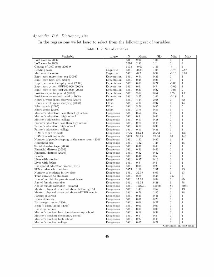
Appendix B.2. Dictionary size
In the regressions we let lasso to select from the following set of variables.
Table B.12: Set of variables
Variable Type N Mean SD Min MaxLoC score in 2006 6811 2.92 1.04 0 4LoC score in 2009 6216 2.92 1.1 0 4Change of LoC score 2006-9 6173 -0.01 1.36 -4 4Reading score Cognitive 6861 -0.33 1.05 -3.78 2.87Mathematics score Cognitive 6861 -0.2 0.99 -3.16 3.08Exp.: earn more than avg (2008) Expectation 6861 0.54 0.26 0 1Exp.: earn best 10% (2008) Expectation 6861 0.25 0.24 0 1Exp.: permanent employment (2008) Expectation 6861 0.68 0.27 -0.06 1Exp.: earn > net HUF100.000 (2008) Expectation 6861 0.6 0.3 -0.06 1Exp.: earn > net HUF200.000 (2008) Expectation 6861 0.33 0.27 -0.06 2Positive exp-s in general (2008) Expectation 6861 2.82 0.57 0.22 4.7Positive exp-s (school. work - 2008) Expectation 6861 3.55 1.42 -0.18 7Hours a week spent studying (2007) Effort 6861 4.44 2.68 0 52Hours a week spent studying (2008) Effort 6861 4.17 2.97 0 44Effort grade (2007) Effort 6861 3.78 0.85 1 5Effort grade (2008) Effort 6861 3.75 0.85 1 5Mother’s education: less than high school Exogenous 6861 0.52 0.5 0 1Mother’s education: high school Exogenous 6861 0.3 0.46 0 1Mother’s education: college Exogenous 6861 0.17 0.38 0 1Father’s education: less than high school Exogenous 6861 0.71 0.45 0 1Father’s education: high school Exogenous 6861 0.18 0.38 0 1Father’s education: college Exogenous 6861 0.11 0.31 0 1HOME cognitive scale Exogenous 6776 81.23 26.43 0 130HOME emotional scale Exogenous 6699 98.95 22.04 10 140Number of people sleeping in the same room (2006) Exogenous 6861 1.53 0.85 1 8Household size Exogenous 6861 4.32 1.36 2 15Social disadvantage (2006) Exogenous 6861 0.36 0.48 0 1Financial distress (2006) Exogenous 6861 0.31 0.46 0 1Financial distress (2009) Exogenous 6861 0.32 0.47 0 1Female Exogenous 6861 0.46 0.5 0 1Lives with mother Exogenous 6861 0.97 0.16 0 1Lives with father Exogenous 6861 0.8 0.4 0 1Has special education needs (SEN) Exogenous 6861 0.09 0.29 0 1SEN students in the class Exogenous 6853 1.16 2.57 0 23Number of students in the class Exogenous 6861 22.39 6.03 1 43Time enrolled to childcare Exogenous 6861 2.85 0.46 0.5 3How often did the parents read tales? Exogenous 6861 17.06 8.84 0 25Age of female caretaker Exogenous 6861 41.02 6.28 9 78Age of female caretaker - squared Exogenous 6861 1722.31 559.25 81 6084Mental. physical or sexual abuse before age 14 Exogenous 6861 1.48 2.52 0 19Mental. physical or sexual abuse AFTER age 14 Exogenous 6861 0.76 1.85 0 18Parents divorced Exogenous 6861 0.21 0.41 0 1Roma ethnicity Exogenous 6861 0.06 0.23 0 1Birthweight under 2500g Exogenous 6861 0.08 0.27 0 1Been in social home (2006) Exogenous 6861 0.01 0.09 0 1Has step parents Exogenous 6861 0.01 0.09 0 1Mother’s mother: less than elementary school Exogenous 6861 0.18 0.39 0 1Mother’s mother: elementary school Exogenous 6861 0.5 0.5 0 1Mother’s mother: high school Exogenous 6861 0.27 0.45 0 1Mother’s mother: college Exogenous 6861 0.05 0.21 0 1
Continued on next page
48

Table B.12 – continued from previous page
Variable Type N Mean SD Min MaxMother’s father: less than elementary school Exogenous 6861 0.13 0.34 0 1Mother’s father: elementary school Exogenous 6861 0.39 0.49 0 1Mother’s father: high school Exogenous 6861 0.4 0.49 0 1Mother’s father: college Exogenous 6861 0.07 0.26 0 1Father’s mother: less than elementary school Exogenous 6861 0.15 0.35 0 1Father’s mother: elementary school Exogenous 6861 0.64 0.48 0 1Father’s mother: high school Exogenous 6861 0.19 0.39 0 1Father’s mother: college Exogenous 6861 0.03 0.17 0 1Father’s father: less than elementary school Exogenous 6861 0.11 0.31 0 1Father’s father: elementary school Exogenous 6861 0.54 0.5 0 1Father’s father: high school Exogenous 6861 0.29 0.46 0 1Father’s father: college Exogenous 6861 0.06 0.23 0 1Max. wanted education for child: college (2006) Exogenous 6861 0.55 0.5 0 1Min. wanted education for child: college (2006) Exogenous 6861 0.25 0.44 0 1Can afford to pay college (2006) Exogenous 6861 0.64 0.48 0 1Death in the family (2008) Exogenous 6861 0.06 0.23 0 1Death in the family (2009) Exogenous 6861 0.05 0.22 0 1Accident in the family (2007) Exogenous 6861 0.05 0.21 0 1Accident in the family (2008) Exogenous 6861 0.04 0.19 0 1Accident in the family (2009) Exogenous 6861 1.96 0.19 1 2Illness in the family (2007) Exogenous 6861 0.07 0.26 0 1Illness in the family (2008) Exogenous 6861 0.07 0.26 0 1Illness in the family (2009) Exogenous 6861 1.91 0.29 1 2Household income (2006) Exogenous 6861 2.20E+05 1.30E+05 0 2.66E+06Household income (2007) Exogenous 6861 2.25E+05 3.19E+06 0 2.65E+08Household income (2008) Exogenous 6861 1.96E+05 2.39E+05 0 1.80E+07Household income (2009) Exogenous 6861 1.94E+05 82019.15 27000 8.50E+05Region Exogenous 6861 3.93 2.16 1 7Central Hungary (%) Exogenous 1502 21.89Central Transdanubia (%) Exogenous 817 11.91Western Transdanubia (%) Exogenous 696 10.14Southern Transdanubia (%) Exogenous 687 10.01Northern Hungary (%) Exogenous 936 13.64Northern Great Plain (%) Exogenous 1260 18.36Southern Great Plain (%) Exogenous 963 14.04Mother works (2006) Exogenous 6853 0.68 0.51 0 2No (%) Exogenous 2318 33.82Yes (%) Exogenous 4402 64.23We did not ask (%) Exogenous 133 1.94Mother works (2007) Exogenous 6861 0.76 0.54 0 2No (%) Exogenous 2032 29.62Yes (%) Exogenous 4474 65.21We did not ask (%) Exogenous 355 5.17Mother works (2008) Exogenous 6861 0.77 0.51 0 2No (%) Exogenous 1846 26.91Yes (%) Exogenous 4747 69.19We did not ask (%) Exogenous 268 3.91Mother works (2009) Exogenous 6861 0.77 0.52 0 2No (%) Exogenous 1877 27.36Yes (%) Exogenous 4651 67.79We did not ask (%) Exogenous 333 4.85Father works (2006) Exogenous 6830 1.01 0.61 0 2No (%) Exogenous 1254 18.36Yes (%) Exogenous 4286 62.75We did not ask (%) Exogenous 1290 18.89
Continued on next page
49
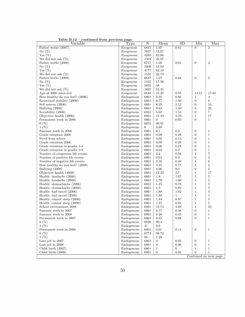
Table B.12 – continued from previous page
Variable Type N Mean SD Min MaxFather works (2007) Exogenous 6815 1.07 0.61 0 2No (%) Exogenous 1027 15.07Yes (%) Exogenous 4284 62.86We did not ask (%) Exogenous 1504 22.07Father works (2008) Exogenous 6717 1.08 0.61 0 2No (%) Exogenous 1009 15.02Yes (%) Exogenous 4177 62.19We did not ask (%) Exogenous 1531 22.79Father works (2009) Exogenous 6647 1.07 0.64 0 2No (%) Exogenous 1167 17.56Yes (%) Exogenous 3855 58We did not ask (%) Exogenous 1625 24.45Age at 2006 interview Exogenous 6840 15.25 0.55 13.51 17.84How healthy do you feel? (2006) Endogenous 6861 3.25 0.66 1 4Emotional stability (2006) Endogenous 6861 6.77 1.46 0 8Self esteem (2006) Endogenous 6861 8.19 2.12 0 10Bullying (2006) Endogenous 6861 9.93 1.39 9 25Sociability (2006) Endogenous 6861 5.65 1.54 0 7Objective health (2006) Endogenous 6861 14.43 2.59 1 17Permanent work in 2006 Endogenous 6861 0 0.03 0 10 (%) Endogenous 6855 99.911 (%) Endogenous 6 0.09Summer work in 2006 Endogenous 6861 0.1 0.3 0 1Grade retention 2006 Endogenous 6861 0.09 0.29 0 1Fired from school Endogenous 6861 0.02 0.13 0 1Grade retention 2006 Endogenous 6861 0.09 0.29 0 1Grade retention in grades 1-4 Endogenous 6861 0.06 0.24 0 1Grade retention in grades 5-8 Endogenous 6861 0.04 0.2 0 1Number of exogenous life events Endogenous 6861 2.2 0.56 1 7Number of positive life events Endogenous 6861 0.04 0.2 0 2Number of negative life events Endogenous 6861 2.16 0.49 1 6How healthy do you feel? (2008) Endogenous 6861 3.25 0.71 1 4Bullying (2008) Endogenous 6861 0.06 0.4 0 5Objective health (2008) Endogenous 6861 14.32 2.7 1 17Health: headache (2006) Endogenous 6861 1.8 1.07 1 5Health: headache (2008) Endogenous 6861 1.79 1.06 1 5Health: stomachache (2006) Endogenous 6861 1.45 0.78 1 5Health: stomachache (2008) Endogenous 6861 1.5 0.82 1 5Health: bad mood (2006) Endogenous 6861 1.88 1.02 1 5Health: bad mood (2008) Endogenous 6861 1.92 1 1 5Health: cannot sleep (2006) Endogenous 6861 1.44 0.87 1 5Health: cannot sleep (2008) Endogenous 6861 1.47 0.91 1 5School environment 2008 Endogenous 6861 15.74 3.69 1 23Summer work in 2007 Endogenous 6861 0.17 0.38 0 1Summer work in 2008 Endogenous 6861 0.28 0.45 0 1Permanent work in 2007 Endogenous 6861 0.01 0.08 0 10 (%) Endogenous 6820 99.41 (%) Endogenous 41 0.6Permanent work in 2008 Endogenous 6861 0.01 0.11 0 10 (%) Endogenous 6773 98.721 (%) Endogenous 88 1.28Lost job in 2007 Endogenous 6861 0 0.03 0 1Lost job in 2008 Endogenous 6861 0 0.06 0 1Child birth (2007) Endogenous 6861 1 0 1 1Child birth (2008) Endogenous 6861 0 0.02 0 1
Continued on next page
50
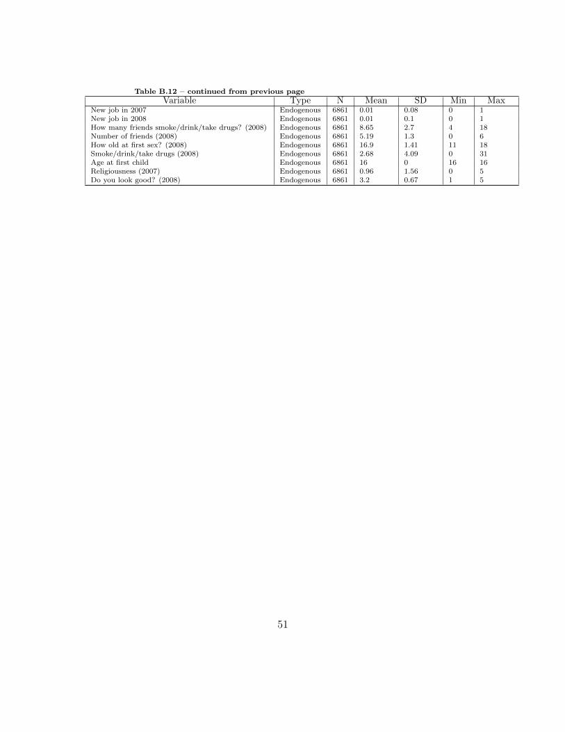
Table B.12 – continued from previous page
Variable Type N Mean SD Min MaxNew job in 2007 Endogenous 6861 0.01 0.08 0 1New job in 2008 Endogenous 6861 0.01 0.1 0 1How many friends smoke/drink/take drugs? (2008) Endogenous 6861 8.65 2.7 4 18Number of friends (2008) Endogenous 6861 5.19 1.3 0 6How old at first sex? (2008) Endogenous 6861 16.9 1.41 11 18Smoke/drink/take drugs (2008) Endogenous 6861 2.68 4.09 0 31Age at first child Endogenous 6861 16 0 16 16Religiousness (2007) Endogenous 6861 0.96 1.56 0 5Do you look good? (2008) Endogenous 6861 3.2 0.67 1 5
51
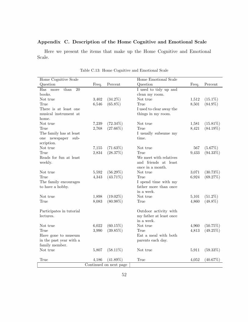
Appendix C. Description of the Home Cognitive and Emotional Scale
Here we present the items that make up the Home Cognitive and EmotionalScale.
Table C.13: Home Cognitive and Emotional Scale
Home Cognitive Scale Home Emotional ScaleQuestion Freq. Percent Question Freq. Percent
Has more than 20books.
I used to tidy up andclean my room.
Not true 3,402 (34.2%) Not true 1,512 (15.1%)True 6,546 (65.8%) True 8,501 (84.9%)There is at least onemusical instrument athome.
I used to clear away thethings in my room.
Not true 7,239 (72.34%) Not true 1,581 (15.81%)True 2,768 (27.66%) True 8,421 (84.19%)The family has at leastone newspaper sub-scription.
I usually subsume mytime.
Not true 7,155 (71.63%) Not true 567 (5.67%)True 2,834 (28.37%) True 9,433 (94.33%)Reads for fun at leastweekly.
We meet with relativesand friends at leastonce in a month.
Not true 5,592 (56.29%) Not true 3,071 (30.73%)True 4,343 (43.71%) True 6,924 (69.27%)The family encouragesto have a hobby.
I spend time with myfather more than oncein a week.
Not true 1,898 (19.02%) Not true 5,101 (51.2%)True 8,083 (80.98%) True 4,860 (48.8%)
Participates in tutoriallectures.
Outdoor activity withmy father at least oncein a week.
Not true 6,022 (60.15%) Not true 4,960 (50.75%)True 3,990 (39.85%) True 4,813 (49.25%)Have gone to museumin the past year with afamily member.
Eat a meal with bothparents each day.
Not true 5,807 (58.11%) Not true 5,911 (59.33%)
True 4,186 (41.89%) True 4,052 (40.67%)Continued on next page
52
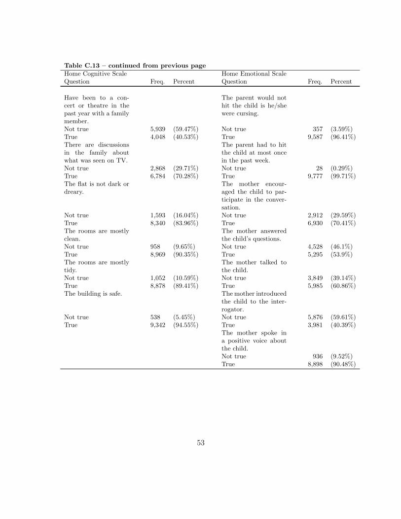
Table C.13 – continued from previous pageHome Cognitive Scale Home Emotional ScaleQuestion Freq. Percent Question Freq. Percent
Have been to a con-cert or theatre in thepast year with a familymember.
The parent would nothit the child is he/shewere cursing.
Not true 5,939 (59.47%) Not true 357 (3.59%)True 4,048 (40.53%) True 9,587 (96.41%)There are discussionsin the family aboutwhat was seen on TV.
The parent had to hitthe child at most oncein the past week.
Not true 2,868 (29.71%) Not true 28 (0.29%)True 6,784 (70.28%) True 9,777 (99.71%)The flat is not dark ordreary.
The mother encour-aged the child to par-ticipate in the conver-sation.
Not true 1,593 (16.04%) Not true 2,912 (29.59%)True 8,340 (83.96%) True 6,930 (70.41%)The rooms are mostlyclean.
The mother answeredthe child’s questions.
Not true 958 (9.65%) Not true 4,528 (46.1%)True 8,969 (90.35%) True 5,295 (53.9%)The rooms are mostlytidy.
The mother talked tothe child.
Not true 1,052 (10.59%) Not true 3,849 (39.14%)True 8,878 (89.41%) True 5,985 (60.86%)The building is safe. The mother introduced
the child to the inter-rogator.
Not true 538 (5.45%) Not true 5,876 (59.61%)True 9,342 (94.55%) True 3,981 (40.39%)
The mother spoke ina positive voice aboutthe child.Not true 936 (9.52%)True 8,898 (90.48%)
53
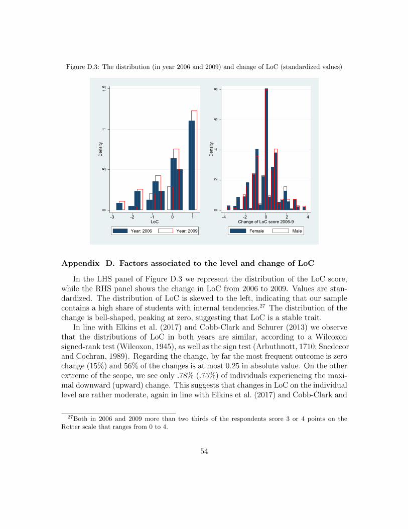
Figure D.3: The distribution (in year 2006 and 2009) and change of LoC (standardized values)
0.5
11.
5D
ensi
ty
-3 -2 -1 0 1LoC
Year: 2006 Year: 2009
0.2
.4.6
.8D
ensi
ty-4 -2 0 2 4
Change of LoC score 2006-9
Female Male
Appendix D. Factors associated to the level and change of LoC
In the LHS panel of Figure D.3 we represent the distribution of the LoC score,while the RHS panel shows the change in LoC from 2006 to 2009. Values are stan-dardized. The distribution of LoC is skewed to the left, indicating that our samplecontains a high share of students with internal tendencies.27 The distribution of thechange is bell-shaped, peaking at zero, suggesting that LoC is a stable trait.
In line with Elkins et al. (2017) and Cobb-Clark and Schurer (2013) we observethat the distributions of LoC in both years are similar, according to a Wilcoxonsigned-rank test (Wilcoxon, 1945), as well as the sign test (Arbuthnott, 1710; Snedecorand Cochran, 1989). Regarding the change, by far the most frequent outcome is zerochange (15%) and 56% of the changes is at most 0.25 in absolute value. On the otherextreme of the scope, we see only .78% (.75%) of individuals experiencing the maxi-mal downward (upward) change. This suggests that changes in LoC on the individuallevel are rather moderate, again in line with Elkins et al. (2017) and Cobb-Clark and
27Both in 2006 and 2009 more than two thirds of the respondents score 3 or 4 points on theRotter scale that ranges from 0 to 4.
54
Schurer (2013).Next, we briefly review the literature on what factors correlate with the level and
change of LoC.The role of age and gender is not unambiguous. Lewis et al. (1999) report that
age associates positively with higher levels of perceived control for both gendersin the adolescence (aged 14-22) using longitudinal data.28 However, Doherty andBaldwin (1985) document no change for men, but an increase in external tendenciesfor women for the same age group. Elkins et al. (2017) report only small mean-levelchanges in LoC with age in the adolescence. In a review of the literature Archerand Waterman (1988) find that in more than half of the studies there was no genderdifference in LoC, a finding echoed also by later studies (Sherman et al., 1997).29
Cognitive measures correlate positively with LoC (Lewis et al., 1999; Colemanand DeLeire, 2003). Generally cognitive skills are captured through achievement testscores, for instance Cebi (2007) uses the Armed Forces Qualifications Test (AFQT)as a proxy for cognitive abilities.30
There is plenty of research documenting that socioeconomic status affects the for-mation of non-cognitive skills. For instance, Kohn (1959); Kohn and Schooler (1983);Pearlin and Kohn (1966); Doepke et al. (2019) claim that parenting style that varywith SES affect skill acquisition.31 Katkovsky et al. (1967); Tzuriel and Haywood(1985); Krampen (1989); Lau and Leung (1992); Webster et al. (1994); McClun andMerrell (1998) show that parenting style may shape adolescents’ LoC.32 Therefore,it is not surprising that many studies report a positive relationship between SES andinternal LoC (Lefcourt and Ladwig, 1965; Battle and Rotter, 1963; Gore and Rotter,1963; Coleman et al., 1966). Often, SES is captured by parental education and / oroccupation (Lewis et al., 1999). However, other studies also consider other elements.For instance, Coleman et al. (1966) study structural integrity of the home, number of
28Cairns et al. (1990); Chubb et al. (1997); Specht et al. (2013) report similar findings.29When gender difference is found, then men tend to be more internal (Cairns et al., 1990; Lewis
et al., 1999), but in some samples women are found to be more internal (Feather, 1967).30Achievement test scores are often used as proxies for cognitive abilities, see for example
Borghans et al. (2016).31For example, low-SES parents place a high value on honesty, neatness and obedience, while
their high-SES counterparts value more self-control, curiosity and happiness (Wang et al., 1999;Bowles and Gintis, 1972).
32Lekfuangfu et al. (2018) document how LoC of the mother - in the form of a subjective beliefabout the effect of parental involvement on the child’s skill formation - predicts maternal attitudestowards parenting style and time investment. That is, parental LoC shapes parental attitudes thatin turn affect child’s LoC. The circle is closed.
55

brothers and sisters, reading material in home, parents’ interest in child’s schooling,while Skinner et al. (1998) point out the importance of the home environment. Usingsibling correlations, Anger and Schnitzlein (2017) show that 46.6% of the variance inLoC stems from shared sibling-related factors, indicating the importance of familybackground.
Judge et al. (2002) and Judge et al. (2003) propose that LoC along with self-efficacy, neuroticism and self-esteem underlie a higher order concept that they termas core self-evaluations (simply put, the fundamental assessment about individuals’own self-worth. Hence, LoC may be correlated with these traits as well. Judge et al.(2002) carries out a meta-analysis and reports a correlation of 0.52 between LoC andself-esteem, and a correlation of 0.4 between LoC and emotional stability.33
Several studies investigate the role of important life events in shaping LoC. Cobb-Clark and Schurer (2013) report that LoC is s quite stable trait. Furthermore,changes in LoC generally do not associate with demographic, labour market andhealth events that the respondents experience. Relevant life events that seem to beable this trait (e.g. serious illness, death of a family member) do not significantlycorrelate with changes in LoC at all. Neither do find the authors evidence thatintense or persistent negative life events affect in a meaningful manner individuals’LoC. However, some events (e.g. worsening of financial situation) do cause a changein the expected direction, moreover the young and the old exhibit less stability thanmiddle-aged individuals. While Cobb-Clark and Schurer (2013) analyze a repre-sentative sample of the whole Australian population, Elkins et al. (2017) focus onadolescents (aged 15-24). They find that in general one-off life events (e.g. beingfired or promoted, serious illness or injury, death of spouse / child) do not explainchanges in LoC in a consistent way. However, there are studies that show that strongand long-lasting life events may have a lasting effect (Gong et al., 2015).
It is an unresolved question to which extent non-cognitive skills are malleable(Ertac, 2020). Research on LoC presented in the previous paragraph shows that itis a quite stable trait, at least in the adulthood. However, there are also studies thatfind that intervention programs may have an important impact (Browne and Evans,2007; Krishnan and Krutikova, 2013).
In Table D.14 we show the results of the lasso regressions on the level and changeof LoC. Columns (1) and (3) contain the results from lasso regressions in which werestrict the set of controls to exogenous variables. In Columns (2) and (4) we showthe findings without the previous restriction. Note also that lasso selects variables
33Other studies also find a significant positive association between self-esteem and LoC, see forinstance Abdallah (1989); Piskin (1996).
56
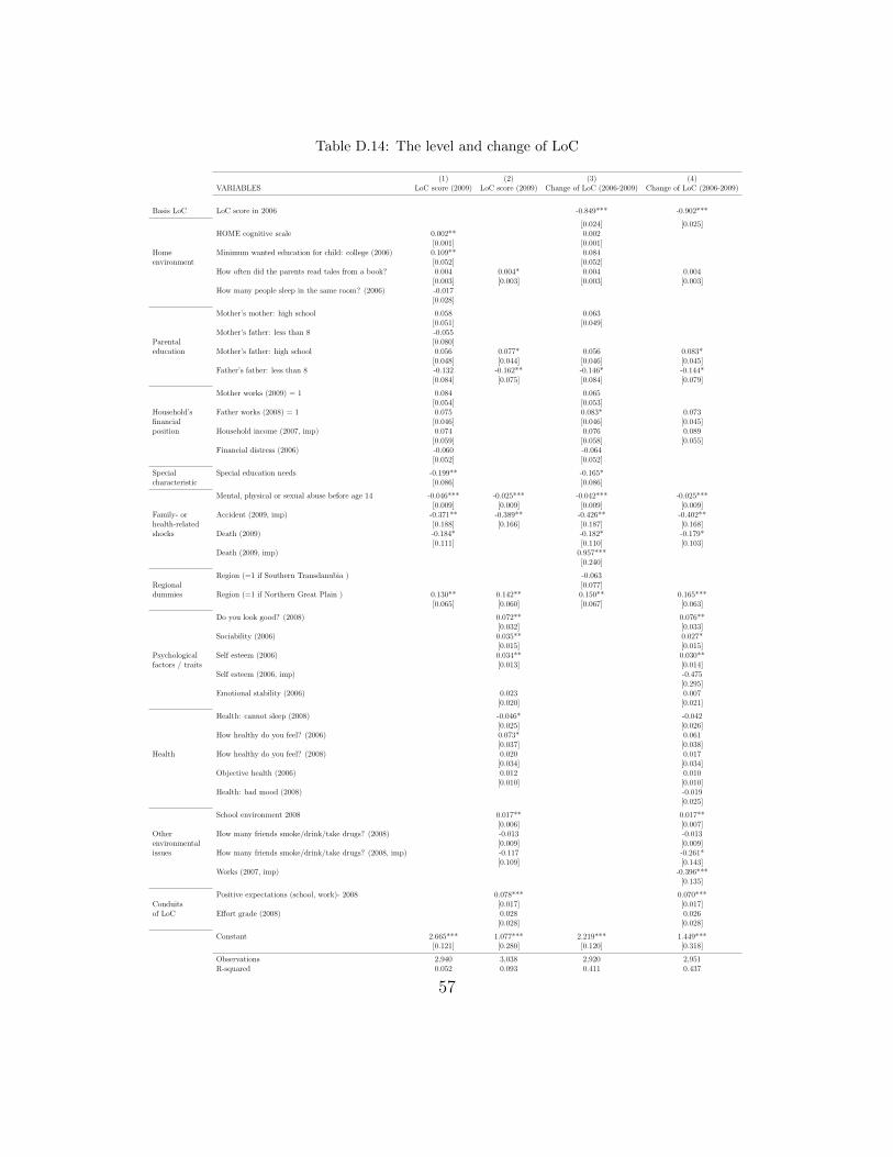
Table D.14: The level and change of LoC
(1) (2) (3) (4)VARIABLES LoC score (2009) LoC score (2009) Change of LoC (2006-2009) Change of LoC (2006-2009)
Basis LoC LoC score in 2006 -0.849*** -0.902***
[0.024] [0.025]HOME cognitive scale 0.002** 0.002
[0.001] [0.001]Home Minimum wanted education for child: college (2006) 0.109** 0.084environment [0.052] [0.052]
How often did the parents read tales from a book? 0.004 0.004* 0.004 0.004[0.003] [0.003] [0.003] [0.003]
How many people sleep in the same room? (2006) -0.017[0.028]
Mother’s mother: high school 0.058 0.063[0.051] [0.049]
Mother’s father: less than 8 -0.055Parental [0.080]education Mother’s father: high school 0.056 0.077* 0.056 0.083*
[0.048] [0.044] [0.046] [0.045]Father’s father: less than 8 -0.132 -0.162** -0.146* -0.144*
[0.084] [0.075] [0.084] [0.079]
Mother works (2009) = 1 0.084 0.065[0.054] [0.053]
Household’s Father works (2008) = 1 0.075 0.083* 0.073financial [0.046] [0.046] [0.045]position Household income (2007, imp) 0.074 0.076 0.089
[0.059] [0.058] [0.055]Financial distress (2006) -0.060 -0.064
[0.052] [0.052]
Special Special education needs -0.199** -0.165*characteristic [0.086] [0.086]
Mental, physical or sexual abuse before age 14 -0.046*** -0.025*** -0.042*** -0.025***[0.009] [0.009] [0.009] [0.009]
Family- or Accident (2009, imp) -0.371** -0.389** -0.426** -0.402**health-related [0.188] [0.166] [0.187] [0.168]shocks Death (2009) -0.184* -0.182* -0.179*
[0.111] [0.110] [0.103]Death (2009, imp) 0.957***
[0.240]
Region (=1 if Southern Transdanubia ) -0.063Regional [0.077]dummies Region (=1 if Northern Great Plain ) 0.130** 0.142** 0.150** 0.165***
[0.065] [0.060] [0.067] [0.063]
Do you look good? (2008) 0.072** 0.076**[0.032] [0.033]
Sociability (2006) 0.035** 0.027*[0.015] [0.015]
Psychological Self esteem (2006) 0.034** 0.030**factors / traits [0.013] [0.014]
Self esteem (2006, imp) -0.475[0.295]
Emotional stability (2006) 0.023 0.007[0.020] [0.021]
Health: cannot sleep (2008) -0.046* -0.042[0.025] [0.026]
How healthy do you feel? (2006) 0.073* 0.061[0.037] [0.038]
Health How healthy do you feel? (2008) 0.020 0.017[0.034] [0.034]
Objective health (2006) 0.012 0.010[0.010] [0.010]
Health: bad mood (2008) -0.019[0.025]
School environment 2008 0.017** 0.017**[0.006] [0.007]
Other How many friends smoke/drink/take drugs? (2008) -0.013 -0.013environmental [0.009] [0.009]issues How many friends smoke/drink/take drugs? (2008, imp) -0.117 -0.261*
[0.109] [0.143]Works (2007, imp) -0.396***
[0.135]
Positive expectations (school, work)- 2008 0.078*** 0.070***Conduits [0.017] [0.017]of LoC Effort grade (2008) 0.028 0.026
[0.028] [0.028]
Constant 2.665*** 1.077*** 2.219*** 1.449***[0.121] [0.280] [0.120] [0.318]
Observations 2,940 3,038 2,920 2,951R-squared 0.052 0.093 0.411 0.437
57

to optimize prediction and the final regression may have variables that fail to besignificant.34
When considering only exogenous variables, it is noteworthy how many factorsassociated with family background (home environment, parental education, house-hold’s financial position) predicts LoC, in line with studies cited in Appendix D.Lasso selects 12 variables to predict the level of LoC in 2009 and the HOME cognitivescale is itself a composite scale of 13 items. All of the items selected by lasso have theexpected sign: more (less) favourable home environment, better (worse) schooling ofthe ancestors, better (worse) financial position of the household associates positively(negatively) with the level of LoC in 2009. In line with the literature on the stabilityof LoC (Cobb-Clark and Schurer, 2013; Elkins et al., 2017) we find that negativeshocks have a detrimental effect on LoC. We document a strong negative effect ofmental, physical or sexual abuse before the age 14.35
When considering endogenous variables also, we observe that psychological traitsplay an important role. This is not surprising as Judge et al. (2002) and Judge et al.(2003) claim that LoC is related to other psychological traits, notably self esteem.
Health-related issues (both objective and subjective) are also related to the leveland change of LoC in the expected way: good / bad health improves / worsens LoC.
Some environmental issues not related to home, but to schools and friends alsoassociate with the level and change of LoC in the expected manner.
The conduits through which LoC may operate in education-related issues (see5.2) are also selected by lasso and the coefficients have the expected sign.
When we allow endogenous variables, then lasso selects considerably less exoge-nous variables, suggesting that those endogenous variables mediate the effect of theexogenous variables that have been dropped.
Overall, our findings related to the stability and determinants of LoC are in linewith the literature.
34If a variable name contains imp, then it refers to a dummy variable that has value =1 if for thegiven observation the variable has been imputed, and 0 otherwise.
35We have a similar variable related to abuse after the age 14, but lasso does not select it.
58
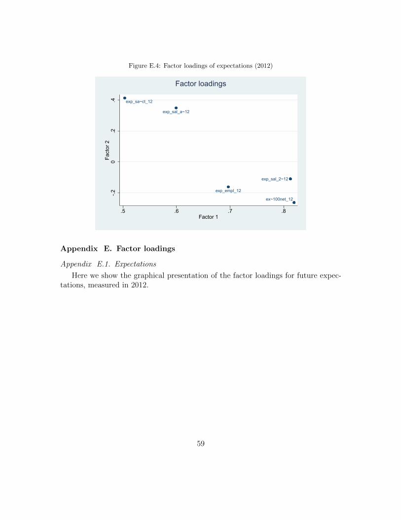
Figure E.4: Factor loadings of expectations (2012)
exp_sal_a~12
exp_sa~ct_12
exp_empl_12
ex~100net_12
exp_sal_2~12
-.20
.2.4
Fact
or 2
.5 .6 .7 .8Factor 1
Factor loadings
Appendix E. Factor loadings
Appendix E.1. Expectations
Here we show the graphical presentation of the factor loadings for future expec-tations, measured in 2012.
59
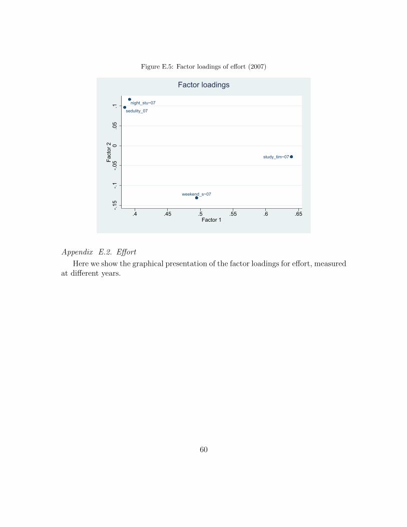
Figure E.5: Factor loadings of effort (2007)
study_tim~07
sedulity_07
night_stu~07
weekend_s~07
-.15
-.1-.0
50
.05
.1Fa
ctor
2
.4 .45 .5 .55 .6 .65Factor 1
Factor loadings
Appendix E.2. Effort
Here we show the graphical presentation of the factor loadings for effort, measuredat different years.
60

Figure E.6: Factor loadings of effort (2008)
study_tim~08
sedulity_08
night_stu~08
weekend_s~08
-.15
-.1-.0
50
.05
.1Fa
ctor
2
.4 .45 .5 .55 .6Factor 1
Factor loadings
Figure E.7: Factor loadings of effort (2007-2009)
study_tim~07
sedulity_07
night_stu~07
weekend_s~07 study_tim~08
sedulity_08
night_stu~08
weekend_s~08
sedulity_09
-.4-.2
0.2
.4Fa
ctor
2
.3 .4 .5 .6 .7Factor 1
Factor loadings
61
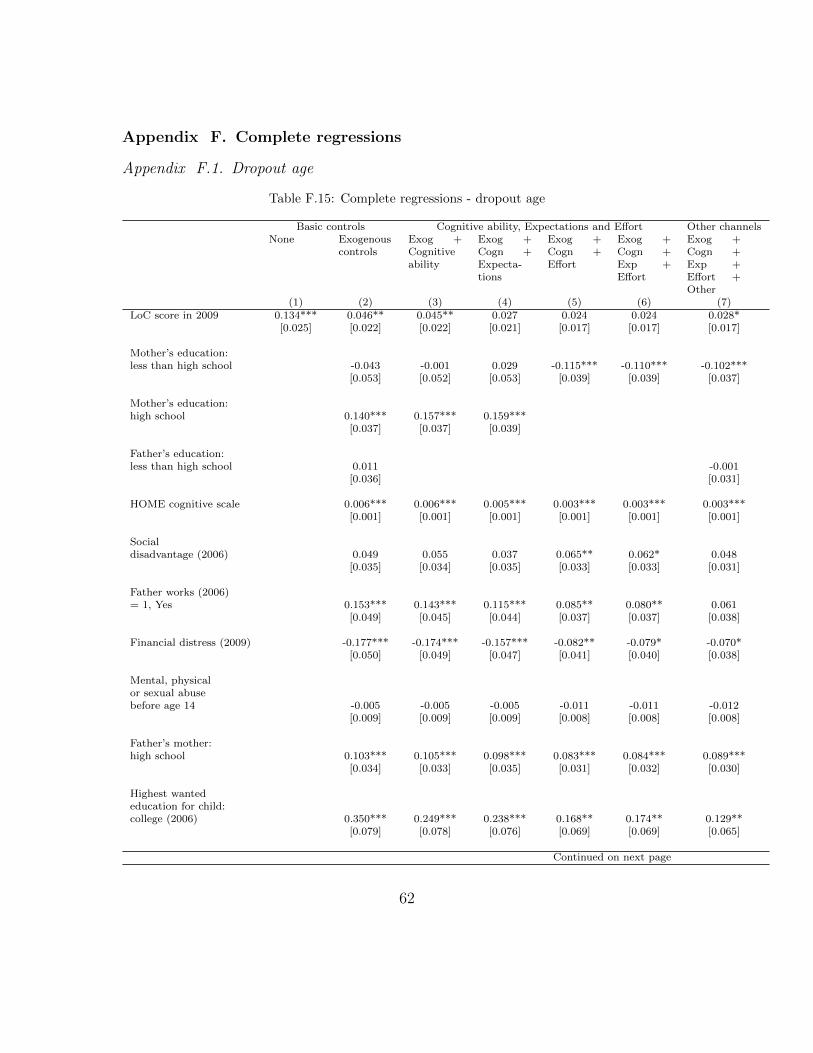
Appendix F. Complete regressions
Appendix F.1. Dropout age
Table F.15: Complete regressions - dropout age
Basic controls Cognitive ability, Expectations and Effort Other channelsNone Exogenous
controlsExog +Cognitiveability
Exog +Cogn +Expecta-tions
Exog +Cogn +Effort
Exog +Cogn +Exp +Effort
Exog +Cogn +Exp +Effort +Other
(1) (2) (3) (4) (5) (6) (7)LoC score in 2009 0.134*** 0.046** 0.045** 0.027 0.024 0.024 0.028*
[0.025] [0.022] [0.022] [0.021] [0.017] [0.017] [0.017]
Mother’s education:less than high school -0.043 -0.001 0.029 -0.115*** -0.110*** -0.102***
[0.053] [0.052] [0.053] [0.039] [0.039] [0.037]
Mother’s education:high school 0.140*** 0.157*** 0.159***
[0.037] [0.037] [0.039]
Father’s education:less than high school 0.011 -0.001
[0.036] [0.031]
HOME cognitive scale 0.006*** 0.006*** 0.005*** 0.003*** 0.003*** 0.003***[0.001] [0.001] [0.001] [0.001] [0.001] [0.001]
Socialdisadvantage (2006) 0.049 0.055 0.037 0.065** 0.062* 0.048
[0.035] [0.034] [0.035] [0.033] [0.033] [0.031]
Father works (2006)= 1, Yes 0.153*** 0.143*** 0.115*** 0.085** 0.080** 0.061
[0.049] [0.045] [0.044] [0.037] [0.037] [0.038]
Financial distress (2009) -0.177*** -0.174*** -0.157*** -0.082** -0.079* -0.070*[0.050] [0.049] [0.047] [0.041] [0.040] [0.038]
Mental, physicalor sexual abusebefore age 14 -0.005 -0.005 -0.005 -0.011 -0.011 -0.012
[0.009] [0.009] [0.009] [0.008] [0.008] [0.008]
Father’s mother:high school 0.103*** 0.105*** 0.098*** 0.083*** 0.084*** 0.089***
[0.034] [0.033] [0.035] [0.031] [0.032] [0.030]
Highest wantededucation for child:college (2006) 0.350*** 0.249*** 0.238*** 0.168** 0.174** 0.129**
[0.079] [0.078] [0.076] [0.069] [0.069] [0.065]
Continued on next page
62
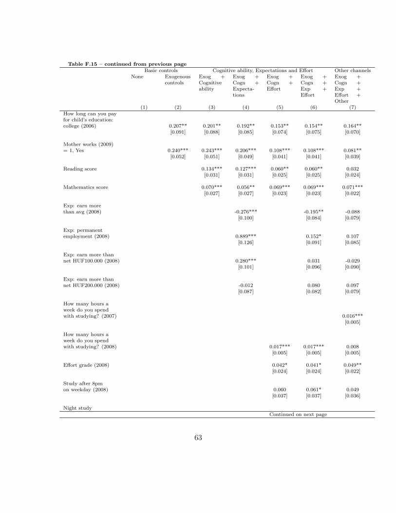
Table F.15 – continued from previous pageBasic controls Cognitive ability, Expectations and Effort Other channels
None Exogenouscontrols
Exog +Cognitiveability
Exog +Cogn +Expecta-tions
Exog +Cogn +Effort
Exog +Cogn +Exp +Effort
Exog +Cogn +Exp +Effort +Other
(1) (2) (3) (4) (5) (6) (7)How long can you payfor child’s education:college (2006) 0.207** 0.201** 0.192** 0.153** 0.154** 0.164**
[0.091] [0.088] [0.085] [0.074] [0.075] [0.070]
Mother works (2009)= 1, Yes 0.240*** 0.243*** 0.206*** 0.108*** 0.108*** 0.081**
[0.052] [0.051] [0.049] [0.041] [0.041] [0.039]
Reading score 0.134*** 0.127*** 0.060** 0.060** 0.032[0.031] [0.031] [0.025] [0.025] [0.024]
Mathematics score 0.070*** 0.056** 0.069*** 0.069*** 0.071***[0.027] [0.027] [0.023] [0.023] [0.022]
Exp: earn morethan avg (2008) -0.276*** -0.195** -0.088
[0.100] [0.084] [0.079]
Exp: permanentemployment (2008) 0.889*** 0.152* 0.107
[0.126] [0.091] [0.085]
Exp: earn more thannet HUF100.000 (2008) 0.280*** 0.031 -0.029
[0.101] [0.096] [0.090]
Exp: earn more thannet HUF200.000 (2008) -0.012 0.080 0.097
[0.087] [0.082] [0.079]
How many hours aweek do you spendwith studying? (2007) 0.016***
[0.005]
How many hours aweek do you spendwith studying? (2008) 0.017*** 0.017*** 0.008
[0.005] [0.005] [0.005]
Effort grade (2008) 0.042* 0.041* 0.049**[0.024] [0.024] [0.022]
Study after 8pmon weekday (2008) 0.060 0.061* 0.049
[0.037] [0.037] [0.036]
Night studyContinued on next page
63
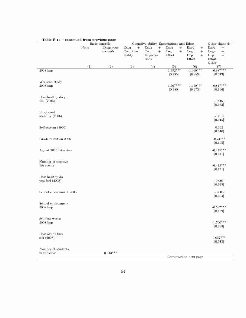
Table F.15 – continued from previous pageBasic controls Cognitive ability, Expectations and Effort Other channels
None Exogenouscontrols
Exog +Cognitiveability
Exog +Cogn +Expecta-tions
Exog +Cogn +Effort
Exog +Cogn +Exp +Effort
Exog +Cogn +Exp +Effort +Other
(1) (2) (3) (4) (5) (6) (7)2008 imp -1.492*** -1.460*** -0.887***
[0.295] [0.289] [0.213]
Weekend study2008 imp -1.507*** -1.450*** -0.817***
[0.280] [0.273] [0.196]
How healthy do youfeel (2006) -0.007
[0.032]
Emotionalstability (2006) -0.010
[0.015]
Self-esteem (2006) 0.002[0.010]
Grade retention 2006 -0.247**[0.105]
Age at 2006 interview -0.115***[0.041]
Number of positivelife events -0.415***
[0.141]
How healthy doyou feel (2008) -0.005
[0.025]
School environment 2008 -0.003[0.004]
School environment2008 imp -0.597***
[0.139]
Student works2008 imp -1.700***
[0.298]
How old at firstsex (2008) 0.057***
[0.013]
Number of studentsin the class 0.013***
Continued on next page
64

Table F.15 – continued from previous pageBasic controls Cognitive ability, Expectations and Effort Other channels
None Exogenouscontrols
Exog +Cognitiveability
Exog +Cogn +Expecta-tions
Exog +Cogn +Effort
Exog +Cogn +Exp +Effort
Exog +Cogn +Exp +Effort +Other
(1) (2) (3) (4) (5) (6) (7)[0.004]
How often didthe parents readtales from a book 0.006**
[0.003]
Minimum wantededucation for child:college (2006) 0.047
[0.034]
Effort grade (2007) 0.031 0.030[0.024] [0.024]
Effort 20008 imp -0.287*** -0.283***[0.106] [0.105]
Weekend study2007 imp -0.391*** -0.390***
[0.108] [0.108]
Constant 21.411*** 19.818*** 20.338*** 19.847*** 20.605*** 20.572*** 21.662***[0.025] [0.191] [0.140] [0.169] [0.128] [0.135] [0.709]
Observations 3,038 2,844 2,844 2,844 2,844 2,844 2,838Clusters 1264 1219 1219 1219 1219 1219 1218Selected controls 0 15 13 17 20 24 34Dictionary size 0 119 121 131 137 147 221R-squared (in-sample) 0.0130 0.258 0.268 0.316 0.431 0.441 0.484R-squared (out-sample) 0.0124 0.249 0.258 0.319 0.469 0.479 0.508
65
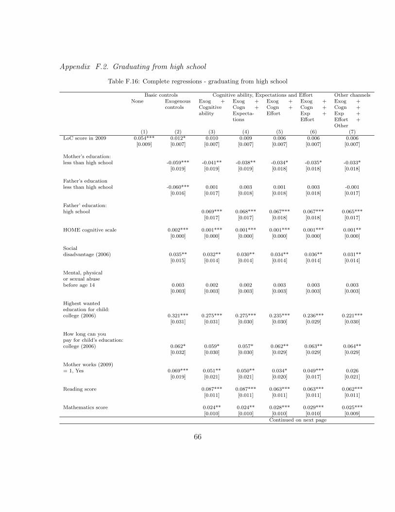
Appendix F.2. Graduating from high school
Table F.16: Complete regressions - graduating from high school
Basic controls Cognitive ability, Expectations and Effort Other channelsNone Exogenous
controlsExog +Cognitiveability
Exog +Cogn +Expecta-tions
Exog +Cogn +Effort
Exog +Cogn +Exp +Effort
Exog +Cogn +Exp +Effort +Other
(1) (2) (3) (4) (5) (6) (7)LoC score in 2009 0.054*** 0.012* 0.010 0.009 0.006 0.006 0.006
[0.009] [0.007] [0.007] [0.007] [0.007] [0.007] [0.007]
Mother’s education:less than high school -0.059*** -0.041** -0.038** -0.034* -0.035* -0.033*
[0.019] [0.019] [0.019] [0.018] [0.018] [0.018]
Father’s educationless than high school -0.060*** 0.001 0.003 0.001 0.003 -0.001
[0.016] [0.017] [0.018] [0.018] [0.018] [0.017]
Father’ education:high school 0.069*** 0.068*** 0.067*** 0.067*** 0.065***
[0.017] [0.017] [0.018] [0.018] [0.017]
HOME cognitive scale 0.002*** 0.001*** 0.001*** 0.001*** 0.001*** 0.001**[0.000] [0.000] [0.000] [0.000] [0.000] [0.000]
Socialdisadvantage (2006) 0.035** 0.032** 0.030** 0.034** 0.036** 0.031**
[0.015] [0.014] [0.014] [0.014] [0.014] [0.014]
Mental, physicalor sexual abusebefore age 14 0.003 0.002 0.002 0.003 0.003 0.003
[0.003] [0.003] [0.003] [0.003] [0.003] [0.003]
Highest wantededucation for child:college (2006) 0.321*** 0.275*** 0.275*** 0.235*** 0.236*** 0.221***
[0.031] [0.031] [0.030] [0.030] [0.029] [0.030]
How long can youpay for child’s education:college (2006) 0.062* 0.059* 0.057* 0.062** 0.063** 0.064**
[0.032] [0.030] [0.030] [0.029] [0.029] [0.029]
Mother works (2009)= 1, Yes 0.069*** 0.051** 0.050** 0.034* 0.049*** 0.026
[0.019] [0.021] [0.021] [0.020] [0.017] [0.021]
Reading score 0.087*** 0.087*** 0.063*** 0.063*** 0.062***[0.011] [0.011] [0.011] [0.011] [0.011]
Mathematics score 0.024** 0.024** 0.028*** 0.029*** 0.025***[0.010] [0.010] [0.010] [0.010] [0.009]
Continued on next page
66
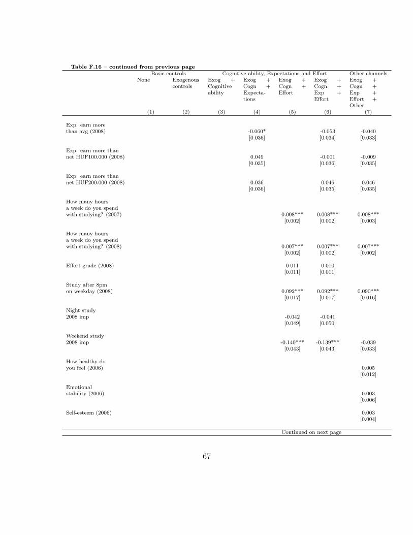
Table F.16 – continued from previous pageBasic controls Cognitive ability, Expectations and Effort Other channels
None Exogenouscontrols
Exog +Cognitiveability
Exog +Cogn +Expecta-tions
Exog +Cogn +Effort
Exog +Cogn +Exp +Effort
Exog +Cogn +Exp +Effort +Other
(1) (2) (3) (4) (5) (6) (7)
Exp: earn morethan avg (2008) -0.060* -0.053 -0.040
[0.036] [0.034] [0.033]
Exp: earn more thannet HUF100.000 (2008) 0.049 -0.001 -0.009
[0.035] [0.036] [0.035]
Exp: earn more thannet HUF200.000 (2008) 0.036 0.046 0.046
[0.036] [0.035] [0.035]
How many hoursa week do you spendwith studying? (2007) 0.008*** 0.008*** 0.008***
[0.002] [0.002] [0.003]
How many hoursa week do you spendwith studying? (2008) 0.007*** 0.007*** 0.007***
[0.002] [0.002] [0.002]
Effort grade (2008) 0.011 0.010[0.011] [0.011]
Study after 8pmon weekday (2008) 0.092*** 0.092*** 0.090***
[0.017] [0.017] [0.016]
Night study2008 imp -0.042 -0.041
[0.049] [0.050]
Weekend study2008 imp -0.140*** -0.139*** -0.039
[0.043] [0.043] [0.033]
How healthy doyou feel (2006) 0.005
[0.012]
Emotionalstability (2006) 0.003
[0.006]
Self-esteem (2006) 0.003[0.004]
Continued on next page
67
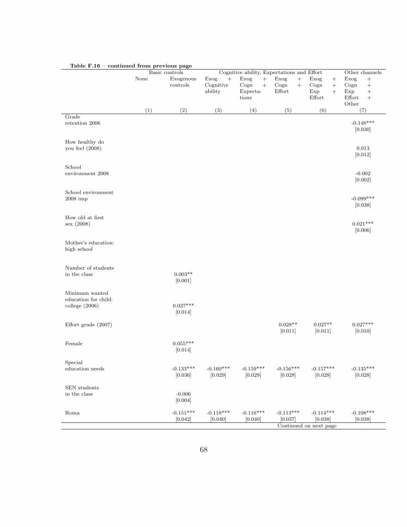
Table F.16 – continued from previous pageBasic controls Cognitive ability, Expectations and Effort Other channels
None Exogenouscontrols
Exog +Cognitiveability
Exog +Cogn +Expecta-tions
Exog +Cogn +Effort
Exog +Cogn +Exp +Effort
Exog +Cogn +Exp +Effort +Other
(1) (2) (3) (4) (5) (6) (7)Graderetention 2006 -0.148***
[0.030]
How healthy doyou feel (2008) 0.013
[0.012]
Schoolenvironment 2008 -0.002
[0.002]
School environment2008 imp -0.099***
[0.038]
How old at firstsex (2008) 0.021***
[0.006]
Mother’s education:high school
Number of studentsin the class 0.003**
[0.001]
Minimum wantededucation for child:college (2006) 0.037***
[0.014]
Effort grade (2007) 0.028** 0.027** 0.027***[0.011] [0.011] [0.010]
Female 0.055***[0.014]
Specialeducation needs -0.133*** -0.160*** -0.159*** -0.156*** -0.157*** -0.135***
[0.036] [0.029] [0.029] [0.028] [0.028] [0.028]
SEN studentsin the class -0.006
[0.004]
Roma -0.151*** -0.118*** -0.116*** -0.113*** -0.114*** -0.108***[0.042] [0.040] [0.040] [0.037] [0.038] [0.038]
Continued on next page
68
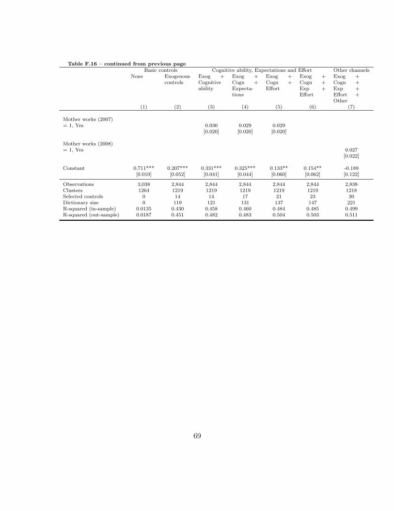
Table F.16 – continued from previous pageBasic controls Cognitive ability, Expectations and Effort Other channels
None Exogenouscontrols
Exog +Cognitiveability
Exog +Cogn +Expecta-tions
Exog +Cogn +Effort
Exog +Cogn +Exp +Effort
Exog +Cogn +Exp +Effort +Other
(1) (2) (3) (4) (5) (6) (7)
Mother works (2007)= 1, Yes 0.030 0.029 0.029
[0.020] [0.020] [0.020]
Mother works (2008)= 1, Yes 0.027
[0.022]
Constant 0.711*** 0.207*** 0.331*** 0.325*** 0.133** 0.154** -0.189[0.010] [0.052] [0.041] [0.044] [0.060] [0.062] [0.122]
Observations 3,038 2,844 2,844 2,844 2,844 2,844 2,838Clusters 1264 1219 1219 1219 1219 1219 1218Selected controls 0 14 14 17 21 23 30Dictionary size 0 119 121 131 137 147 221R-squared (in-sample) 0.0135 0.430 0.458 0.460 0.484 0.485 0.499R-squared (out-sample) 0.0187 0.451 0.482 0.483 0.504 0.503 0.511
69
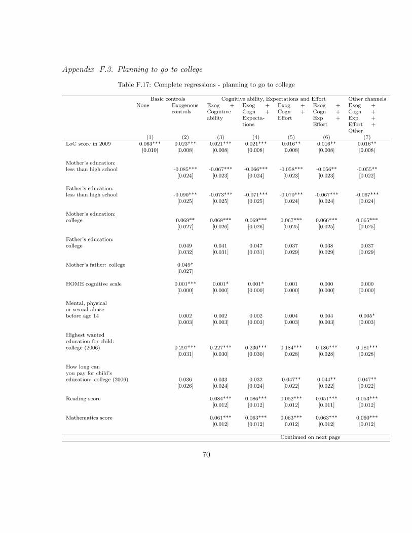
Appendix F.3. Planning to go to college
Table F.17: Complete regressions - planning to go to college
Basic controls Cognitive ability, Expectations and Effort Other channelsNone Exogenous
controlsExog +Cognitiveability
Exog +Cogn +Expecta-tions
Exog +Cogn +Effort
Exog +Cogn +Exp +Effort
Exog +Cogn +Exp +Effort +Other
(1) (2) (3) (4) (5) (6) (7)LoC score in 2009 0.063*** 0.023*** 0.021*** 0.021*** 0.016** 0.016** 0.016**
[0.010] [0.008] [0.008] [0.008] [0.008] [0.008] [0.008]
Mother’s education:less than high school -0.085*** -0.067*** -0.066*** -0.058*** -0.056** -0.055**
[0.024] [0.023] [0.024] [0.023] [0.023] [0.022]
Father’s education:less than high school -0.090*** -0.073*** -0.071*** -0.070*** -0.067*** -0.067***
[0.025] [0.025] [0.025] [0.024] [0.024] [0.024]
Mother’s education:college 0.069** 0.068*** 0.069*** 0.067*** 0.066*** 0.065***
[0.027] [0.026] [0.026] [0.025] [0.025] [0.025]
Father’s education:college 0.049 0.041 0.047 0.037 0.038 0.037
[0.032] [0.031] [0.031] [0.029] [0.029] [0.029]
Mother’s father: college 0.049*[0.027]
HOME cognitive scale 0.001*** 0.001* 0.001* 0.001 0.000 0.000[0.000] [0.000] [0.000] [0.000] [0.000] [0.000]
Mental, physicalor sexual abusebefore age 14 0.002 0.002 0.002 0.004 0.004 0.005*
[0.003] [0.003] [0.003] [0.003] [0.003] [0.003]
Highest wantededucation for child:college (2006) 0.297*** 0.227*** 0.230*** 0.184*** 0.186*** 0.181***
[0.031] [0.030] [0.030] [0.028] [0.028] [0.028]
How long canyou pay for child’seducation: college (2006) 0.036 0.033 0.032 0.047** 0.044** 0.047**
[0.026] [0.024] [0.024] [0.022] [0.022] [0.022]
Reading score 0.084*** 0.086*** 0.052*** 0.051*** 0.053***[0.012] [0.012] [0.012] [0.011] [0.012]
Mathematics score 0.061*** 0.063*** 0.063*** 0.063*** 0.060***[0.012] [0.012] [0.012] [0.012] [0.012]
Continued on next page
70

Table F.17 – continued from previous pageBasic controls Cognitive ability, Expectations and Effort Other channels
None Exogenouscontrols
Exog +Cognitiveability
Exog +Cogn +Expecta-tions
Exog +Cogn +Effort
Exog +Cogn +Exp +Effort
Exog +Cogn +Exp +Effort +Other
(1) (2) (3) (4) (5) (6) (7)Exp: earn morethan avg (2008) -0.068* -0.065* -0.062*
[0.037] [0.034] [0.034]
Exp: earn more thannet HUF100.000 (2008) 0.005 -0.002 -0.006
[0.040] [0.039] [0.040]
Exp: earn more thannet HUF200.000 (2008) 0.105** 0.093** 0.097**
[0.046] [0.043] [0.043]
How many hoursa week do you spendwith studying? (2008) 0.017*** 0.017*** 0.016***
[0.003] [0.003] [0.003]
Effort grade (2008) 0.059*** 0.058*** 0.057***[0.011] [0.011] [0.012]
How healthy doyou feel (2006) -0.020
[0.012]
Emotionalstability (2006) -0.003
[0.007]
Self-esteem (2006) 0.005[0.005]
How healthy doyou feel (2008) 0.025**
[0.012]
Schoolenvironment 2008 -0.001
[0.002]
How old atfirst sex (2008) 0.016***
[0.006]
Number of studentsin the class 0.007*** 0.004*** 0.004*** 0.004*** 0.004***
[0.002] [0.002] [0.001] [0.001] [0.001]
How often didthe parents read
Continued on next page
71
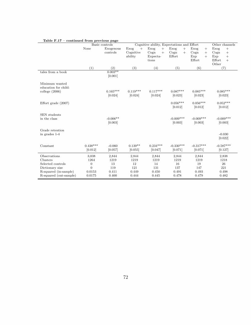
Table F.17 – continued from previous pageBasic controls Cognitive ability, Expectations and Effort Other channels
None Exogenouscontrols
Exog +Cognitiveability
Exog +Cogn +Expecta-tions
Exog +Cogn +Effort
Exog +Cogn +Exp +Effort
Exog +Cogn +Exp +Effort +Other
(1) (2) (3) (4) (5) (6) (7)tales from a book 0.003**
[0.001]
Minimum wantededucation for child:college (2006) 0.165*** 0.119*** 0.117*** 0.087*** 0.085*** 0.085***
[0.024] [0.024] [0.024] [0.023] [0.023] [0.023]
Effort grade (2007) 0.056*** 0.056*** 0.052***[0.012] [0.012] [0.012]
SEN studentsin the class -0.006** -0.009*** -0.009*** -0.009***
[0.003] [0.003] [0.003] [0.003]
Grade retentionin grades 1-4 -0.030
[0.022]
Constant 0.438*** -0.060 0.139** 0.234*** -0.330*** -0.317*** -0.587***[0.012] [0.057] [0.055] [0.047] [0.071] [0.071] [0.127]
Observations 3,038 2,844 2,844 2,844 2,844 2,844 2,838Clusters 1264 1219 1219 1219 1219 1219 1218Selected controls 0 13 12 14 16 19 26Dictionary size 0 119 121 131 137 147 221R-squared (in-sample) 0.0153 0.411 0.449 0.450 0.491 0.493 0.498R-squared (out-sample) 0.0175 0.400 0.444 0.445 0.478 0.479 0.482
72
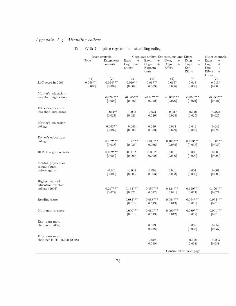
Appendix F.4. Attending college
Table F.18: Complete regressions - attending college
Basic controls Cognitive ability, Expectations and Effort Other channelsNone Exogenous
controlsExog +Cognitiveability
Exog +Cogn +Expecta-tions
Exog +Cogn +Effort
Exog +Cogn +Exp +Effort
Exog +Cogn +Exp +Effort +Other
(1) (2) (3) (4) (5) (6) (7)LoC score in 2009 0.056*** 0.024*** 0.019** 0.017** 0.015* 0.013 0.015*
[0.010] [0.009] [0.009] [0.009] [0.008] [0.008] [0.008]
Mother’s education:less than high school -0.099*** -0.065*** -0.062*** -0.059*** -0.056*** -0.053***
[0.023] [0.022] [0.022] [0.020] [0.021] [0.021]
Father’s education:less than high school -0.054** -0.033 -0.031 -0.029 -0.028 -0.028
[0.027] [0.026] [0.026] [0.025] [0.025] [0.025]
Mother’s education:college 0.063** 0.046 0.046 0.043 0.043 0.042
[0.032] [0.030] [0.030] [0.029] [0.029] [0.029]
Father’s education:college 0.132*** 0.108*** 0.108*** 0.103*** 0.103*** 0.100***
[0.038] [0.036] [0.036] [0.035] [0.035] [0.035]
HOME cognitive scale 0.002*** 0.001* 0.001* 0.001 0.000 0.000[0.000] [0.000] [0.000] [0.000] [0.000] [0.000]
Mental, physical orsexual abusebefore age 14 -0.001 -0.002 -0.002 0.001 0.001 0.001
[0.003] [0.003] [0.003] [0.003] [0.003] [0.003]
Highest wantededucation for child:college (2006) 0.247*** 0.153*** 0.150*** 0.124*** 0.120*** 0.120***
[0.022] [0.022] [0.022] [0.021] [0.021] [0.021]
Reading score 0.083*** 0.083*** 0.054*** 0.054*** 0.054***[0.013] [0.013] [0.013] [0.013] [0.013]
Mathematics score 0.090*** 0.089*** 0.090*** 0.089*** 0.091***[0.013] [0.013] [0.012] [0.012] [0.013]
Exp: earn morethan avg (2008) 0.033 0.039 0.052
[0.038] [0.038] [0.037]
Exp: earn morethan net HUF100.000 (2008) -0.008 -0.008 -0.005
[0.040] [0.038] [0.038]
Continued on next page
73
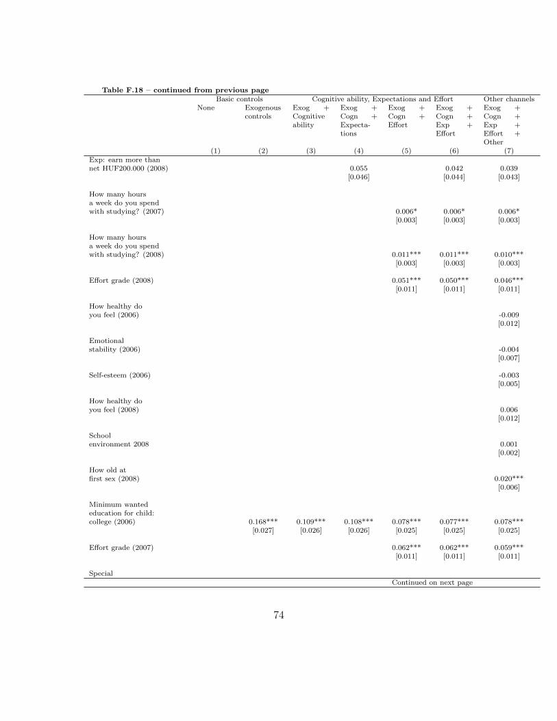
Table F.18 – continued from previous pageBasic controls Cognitive ability, Expectations and Effort Other channels
None Exogenouscontrols
Exog +Cognitiveability
Exog +Cogn +Expecta-tions
Exog +Cogn +Effort
Exog +Cogn +Exp +Effort
Exog +Cogn +Exp +Effort +Other
(1) (2) (3) (4) (5) (6) (7)Exp: earn more thannet HUF200.000 (2008) 0.055 0.042 0.039
[0.046] [0.044] [0.043]
How many hoursa week do you spendwith studying? (2007) 0.006* 0.006* 0.006*
[0.003] [0.003] [0.003]
How many hoursa week do you spendwith studying? (2008) 0.011*** 0.011*** 0.010***
[0.003] [0.003] [0.003]
Effort grade (2008) 0.051*** 0.050*** 0.046***[0.011] [0.011] [0.011]
How healthy doyou feel (2006) -0.009
[0.012]
Emotionalstability (2006) -0.004
[0.007]
Self-esteem (2006) -0.003[0.005]
How healthy doyou feel (2008) 0.006
[0.012]
Schoolenvironment 2008 0.001
[0.002]
How old atfirst sex (2008) 0.020***
[0.006]
Minimum wantededucation for child:college (2006) 0.168*** 0.109*** 0.108*** 0.078*** 0.077*** 0.078***
[0.027] [0.026] [0.026] [0.025] [0.025] [0.025]
Effort grade (2007) 0.062*** 0.062*** 0.059***[0.011] [0.011] [0.011]
SpecialContinued on next page
74
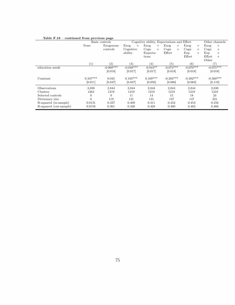
Table F.18 – continued from previous pageBasic controls Cognitive ability, Expectations and Effort Other channels
None Exogenouscontrols
Exog +Cognitiveability
Exog +Cogn +Expecta-tions
Exog +Cogn +Effort
Exog +Cogn +Exp +Effort
Exog +Cogn +Exp +Effort +Other
(1) (2) (3) (4) (5) (6) (7)education needs -0.068*** -0.048*** -0.044** -0.073*** -0.070*** -0.075***
[0.018] [0.017] [0.017] [0.018] [0.018] [0.018]
Constant 0.347*** 0.045 0.193*** 0.169*** -0.282*** -0.302*** -0.560***[0.011] [0.047] [0.047] [0.050] [0.060] [0.063] [0.119]
Observations 3,038 2,844 2,844 2,844 2,844 2,844 2,838Clusters 1264 1219 1219 1219 1219 1219 1218Selected controls 0 9 11 14 15 18 24Dictionary size 0 119 121 131 137 147 221R-squared (in-sample) 0.0131 0.337 0.409 0.411 0.452 0.453 0.456R-squared (out-sample) 0.0158 0.361 0.426 0.428 0.460 0.462 0.466
75

Appendix G. Gender differences
Studies on the labour market revealed that there are gender differences in howLoC associates with outcomes. Interestingly, in the case of some labour outcomesLoC matters more for women (e.g. in Semykina and Linz (2007) for wages) and forothers for men (e.g. in Cobb-Clark and Tan (2011) for occupational attainment).
Table G.19: Heterogeneity: gender differences(Independent variable LoC score in 2009 in all cases)
Basic controls Cognitive ability, Expectations and Effort Other channelsNone Exogenous
controlsExog + Cog-nitive ability
Exog +Cogn +Expectations
Exog + Cogn+ Effort
Exog + Cogn+ Exp + Ef-fort
Exog + Cogn+ Exp + Ef-fort + Other
(1) (2) (3) (4) (5) (6) (7)
Dependent variable: A. Dropout age
Female 0.191*** 0.066** 0.062** 0.047 0.040* 0.039* 0.027[0.037] [0.031] [0.030] [0.029] [0.023] [0.023] [0.023]
Male 0.085** 0.038 0.036 0.018 0.032 0.029 0.041*[0.036] [0.033] [0.032] [0.031] [0.025] [0.025] [0.024]
Dependent variable: B. Graduates from high school
Female 0.058*** 0.011 0.003 0.001 0.003 0.002 -0.001[0.012] [0.009] [0.009] [0.009] [0.009] [0.009] [0.009]
Male 0.050*** 0.019* 0.017* 0.017* 0.012 0.012 0.015[0.013] [0.010] [0.010] [0.010] [0.010] [0.010] [0.010]
Dependent variable: C. Plans to apply to college
Female 0.104*** 0.050*** 0.043*** 0.041*** 0.036*** 0.035*** 0.034***[0.015] [0.013] [0.012] [0.013] [0.012] [0.012] [0.013]
Male 0.027* 0.006 0.004 0.002 -0.001 -0.001 0.001[0.014] [0.011] [0.010] [0.010] [0.010] [0.010] [0.010]
Dependent variable: D. Attends college
Female 0.078*** 0.031** 0.025* 0.020 0.021 0.016 0.017[0.016] [0.014] [0.013] [0.014] [0.013] [0.013] [0.013]
Male 0.036*** 0.018 0.017 0.017 0.012 0.012 0.013[0.014] [0.011] [0.011] [0.011] [0.010] [0.010] [0.010]
Standard errors in parentheses. */**/*** denotes significance at 10 / 5 / 1 % level.
In Table G.19 we show if LoC associates with our outcome variables in a differentway for females and males. We carry out the same analysis as in Table 6, but wedo so separately for females and males. To economize on space, we only report thecoefficient of LoC for the different genders. We see a clear gender difference for three
76
outcome variables: dropout age, planning to apply to college, and attending college.For these outcome variables, in the case of females LoC is significantly associatedwith the given outcome at least marginally even if we control for cognitive abilities,while in the case of males LoC is significant only in the univariate regression. The sizeof the coefficients is generally markedly higher in the case of females (standard errorsbeing very similar), so overall for these outcomes LoC matters a lot more for females.More precisely, in the case of males once we take into account exogenous variables, thesignificance of LoC vanishes, suggesting that exogenous variables mediate the effectof LoC. For females LoC has an effect beyond exogenous variables. We observe thestrongest difference in planning to apply to college. Regarding graduation from highschool, males seem to be more affected by LoC, though in their case the significanceis only marginal.
77
Appendix H. Parental preferences and financial constraints
In Table H.20 we investigate the role of parental preferences and show all theseven specifications for all the outcome variables. The coefficients reported in Table8 correspond to the specification named Exogenous controls.
78
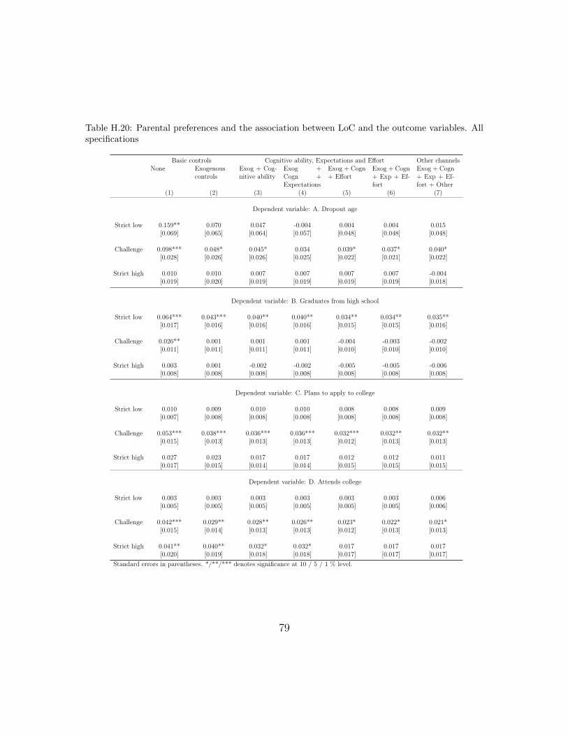
Table H.20: Parental preferences and the association between LoC and the outcome variables. Allspecifications
Basic controls Cognitive ability, Expectations and Effort Other channelsNone Exogenous
controlsExog + Cog-nitive ability
Exog +Cogn +Expectations
Exog + Cogn+ Effort
Exog + Cogn+ Exp + Ef-fort
Exog + Cogn+ Exp + Ef-fort + Other
(1) (2) (3) (4) (5) (6) (7)
Dependent variable: A. Dropout age
Strict low 0.159** 0.070 0.047 -0.004 0.004 0.004 0.015[0.069] [0.065] [0.064] [0.057] [0.048] [0.048] [0.048]
Challenge 0.098*** 0.048* 0.045* 0.034 0.039* 0.037* 0.040*[0.028] [0.026] [0.026] [0.025] [0.022] [0.021] [0.022]
Strict high 0.010 0.010 0.007 0.007 0.007 0.007 -0.004[0.019] [0.020] [0.019] [0.019] [0.019] [0.019] [0.018]
Dependent variable: B. Graduates from high school
Strict low 0.064*** 0.043*** 0.040** 0.040** 0.034** 0.034** 0.035**[0.017] [0.016] [0.016] [0.016] [0.015] [0.015] [0.016]
Challenge 0.026** 0.001 0.001 0.001 -0.004 -0.003 -0.002[0.011] [0.011] [0.011] [0.011] [0.010] [0.010] [0.010]
Strict high 0.003 0.001 -0.002 -0.002 -0.005 -0.005 -0.006[0.008] [0.008] [0.008] [0.008] [0.008] [0.008] [0.008]
Dependent variable: C. Plans to apply to college
Strict low 0.010 0.009 0.010 0.010 0.008 0.008 0.009[0.007] [0.008] [0.008] [0.008] [0.008] [0.008] [0.008]
Challenge 0.053*** 0.038*** 0.036*** 0.036*** 0.032*** 0.032** 0.032**[0.015] [0.013] [0.013] [0.013] [0.012] [0.013] [0.013]
Strict high 0.027 0.023 0.017 0.017 0.012 0.012 0.011[0.017] [0.015] [0.014] [0.014] [0.015] [0.015] [0.015]
Dependent variable: D. Attends college
Strict low 0.003 0.003 0.003 0.003 0.003 0.003 0.006[0.005] [0.005] [0.005] [0.005] [0.005] [0.005] [0.006]
Challenge 0.042*** 0.029** 0.028** 0.026** 0.023* 0.022* 0.021*[0.015] [0.014] [0.013] [0.013] [0.012] [0.013] [0.013]
Strict high 0.041** 0.040** 0.032* 0.032* 0.017 0.017 0.017[0.020] [0.019] [0.018] [0.018] [0.017] [0.017] [0.017]
Standard errors in parentheses. */**/*** denotes significance at 10 / 5 / 1 % level.
79
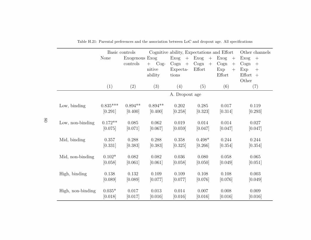
Table H.21: Parental preferences and the association between LoC and dropout age. All specifications
Basic controls Cognitive ability, Expectations and Effort Other channelsNone Exogenous
controlsExog+ Cog-nitiveability
Exog +Cogn +Expecta-tions
Exog +Cogn +Effort
Exog +Cogn +Exp +Effort
Exog +Cogn +Exp +Effort +Other
(1) (2) (3) (4) (5) (6) (7)
A. Dropout age
Low, binding 0.835*** 0.894** 0.894** 0.202 0.285 0.017 0.119[0.291] [0.400] [0.400] [0.258] [0.323] [0.314] [0.293]
Low, non-binding 0.172** 0.085 0.062 0.019 0.014 0.014 0.027[0.075] [0.071] [0.067] [0.059] [0.047] [0.047] [0.047]
Mid, binding 0.357 0.288 0.288 0.358 0.498* 0.244 0.244[0.331] [0.383] [0.383] [0.325] [0.266] [0.354] [0.354]
Mid, non-binding 0.102* 0.082 0.082 0.036 0.080 0.058 0.065[0.058] [0.061] [0.061] [0.058] [0.050] [0.049] [0.051]
High, binding 0.138 0.132 0.109 0.109 0.108 0.108 0.003[0.089] [0.089] [0.077] [0.077] [0.076] [0.076] [0.049]
High, non-binding 0.035* 0.017 0.013 0.014 0.007 0.008 0.009[0.018] [0.017] [0.016] [0.016] [0.016] [0.016] [0.016]
80

Table H.22: Parental preferences and the association between LoC and high school graduation. All specifications
Basic controls Cognitive ability, Expectations and Effort Other channelsNone Exogenous
controlsExog+ Cog-nitiveability
Exog +Cogn +Expecta-tions
Exog +Cogn +Effort
Exog +Cogn +Exp +Effort
Exog +Cogn +Exp +Effort +Other
(1) (2) (3) (4) (5) (6) (7)
B. Graduates from high school
Low, binding 0.059 0.069 -0.018 -0.018 -0.018 0.017 0.069[0.055] [0.066] [0.025] [0.025] [0.025] [0.018] [0.066]
Low, non-binding 0.069*** 0.046*** 0.041*** 0.041*** 0.036** 0.036** 0.040**[0.016] [0.016] [0.016] [0.016] [0.015] [0.015] [0.015]
Mid, binding 0.054 -0.002 -0.002 -0.002 0.016 0.016 0.016[0.100] [0.088] [0.088] [0.088] [0.050] [0.050] [0.046]
Mid, non-binding 0.009 0.006 0.015 0.015 0.006 0.006 0.007[0.026] [0.027] [0.025] [0.025] [0.022] [0.022] [0.023]
High, binding 0.069** 0.061** 0.045** 0.045** 0.045** 0.045** 0.040*[0.028] [0.028] [0.022] [0.022] [0.022] [0.022] [0.023]
High, non-binding 0.010 0.002 -0.001 -0.001 -0.008 -0.008 -0.010[0.008] [0.008] [0.008] [0.008] [0.007] [0.007] [0.007]
81
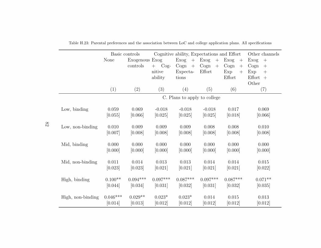
Table H.23: Parental preferences and the association between LoC and college application plans. All specifications
Basic controls Cognitive ability, Expectations and Effort Other channelsNone Exogenous
controlsExog+ Cog-nitiveability
Exog +Cogn +Expecta-tions
Exog +Cogn +Effort
Exog +Cogn +Exp +Effort
Exog +Cogn +Exp +Effort +Other
(1) (2) (3) (4) (5) (6) (7)
C. Plans to apply to college
Low, binding 0.059 0.069 -0.018 -0.018 -0.018 0.017 0.069[0.055] [0.066] [0.025] [0.025] [0.025] [0.018] [0.066]
Low, non-binding 0.010 0.009 0.009 0.009 0.008 0.008 0.010[0.007] [0.008] [0.008] [0.008] [0.008] [0.008] [0.008]
Mid, binding 0.000 0.000 0.000 0.000 0.000 0.000 0.000[0.000] [0.000] [0.000] [0.000] [0.000] [0.000] [0.000]
Mid, non-binding 0.011 0.014 0.013 0.013 0.014 0.014 0.015[0.023] [0.023] [0.021] [0.021] [0.021] [0.021] [0.022]
High, binding 0.100** 0.094*** 0.097*** 0.087*** 0.097*** 0.087*** 0.071**[0.044] [0.034] [0.031] [0.032] [0.031] [0.032] [0.035]
High, non-binding 0.046*** 0.029** 0.023* 0.023* 0.014 0.015 0.013[0.014] [0.013] [0.012] [0.012] [0.012] [0.012] [0.012]
82

Table H.24: Parental preferences and the association between LoC and college attendance. All specifications
Basic controls Cognitive ability, Expectations and Effort Other channelsNone Exogenous
controlsExog+ Cog-nitiveability
Exog +Cogn +Expecta-tions
Exog +Cogn +Effort
Exog +Cogn +Exp +Effort
Exog +Cogn +Exp +Effort +Other
(1) (2) (3) (4) (5) (6) (7)
D. Attends college
Low, binding 0.000 0.000 0.000 0.000 0.000 0.000 0.000[0.000] [0.000] [0.000] [0.000] [0.000] [0.000] [0.000]
Low, non-binding 0.004 0.003 0.003 0.003 0.003 0.003 0.007[0.005] [0.005] [0.005] [0.005] [0.005] [0.005] [0.006]
Mid, binding 0.000 0.000 0.000 0.000 0.000 0.000 0.000[0.000] [0.000] [0.000] [0.000] [0.000] [0.000] [0.000]
Mid, non-binding 0.005 0.002 0.003 0.003 0.003 0.003 0.002[0.021] [0.021] [0.021] [0.021] [0.021] [0.021] [0.021]
High, binding 0.131*** 0.140*** 0.113*** 0.113*** 0.103*** 0.103*** 0.087**[0.044] [0.044] [0.034] [0.034] [0.033] [0.033] [0.036]
High, non-binding 0.042*** 0.030** 0.022* 0.019 0.012 0.010 0.008[0.015] [0.014] [0.013] [0.013] [0.012] [0.012] [0.013]
83