DRAFT: Version 2.0 11/04/05

1

LINKING WATERSHED CONDITIONS TO EGG-TO-FRY SURVIVAL OF

SKAGIT CHINOOK SALMON

November 2005

Eric Beamer1 Bob Hayman2 Steve Hinton3

An appendix to the Skagit River System Cooperative Chinook Recovery Plan

1 Skagit River System Cooperative, Post Office Box 368, LaConner, Washington 98257 (360) 466-7228

DRAFT: Version 2.0 11/04/05

2

ACKNOWLEDGEMENTS We thank Karen Wolf for the maps shown in this report. Tim Beechie (NOAA Fisheries) contributed to the areas in this document related to sediment supply and streambed scour. George Pess (NOAA Fisheries) contributed significantly to the development of ideas related to changes in egg-to-fry survival by varying watershed conditions. Funding and efforts for work related to egg-to-fry survival of Chinook salmon in the Skagit River has come from numerous sources in the past decade. Our direct understanding of Chinook salmon egg-to-migrant-fry survival would not be possible without the Washington Department of Fish and Wildlife (WDFW) mainstem Skagit River trapping effort located near Burlington, Washington. Funding has been provided by WDFW and Seattle City Light. Analyses and inventories of watershed processes used in this document were made possible by funding through Skagit River System Cooperative and the Northwest Indian Fisheries Commission, through the funding initiatives linked to the Pacific Salmon Treaty and Pacific Coastal Salmon Recovery.

DRAFT: Version 2.0 11/04/05

3

TABLE OF CONTENTS 1. Introduction........................................................................................................................... 4 2. Observed Egg-to-Migrant-Fry Survival for Skagit River Chinook Salmon ................... 5 3. Spawning Range of Skagit Chinook Salmon Stocks.......................................................... 7 4. Watershed Processes Influencing Egg-to-Fry Survival..................................................... 8

4.1. Peak Flow Hydrology ..................................................................................................... 8 4.1.1 Methods................................................................................................................... 9 4.1.2 Limitations ............................................................................................................ 12

4.2. Sediment Supply ........................................................................................................... 12 4.2.1 Methods................................................................................................................. 13 4.2.2 Limitations ............................................................................................................ 14 4.2.3 Effect of Sediment Supply on Scour Depth.......................................................... 15 4.2.4 Sensitivity to Sediment Supply, Slope, and Discharge......................................... 16 4.2.5 Relationship Between Sediment Supply and Peak Flow ...................................... 18

4.3. Riparian and Floodplain Dynamics .............................................................................. 19 5. Skagit Chinook Salmon Response to Egg-to-Fry Survival Conditions.......................... 21

5.1. Spawner to Migrant Fry Productivity Under Current Habitat Conditions.................... 21 5.2. Spawner to Migrant Fry Productivity Under Fully Restored Habitat Conditions ........ 25

6. Impact of Climate Change on Egg-to-Migrant-Fry Survival ......................................... 26 7. References............................................................................................................................ 27

DRAFT: Version 2.0 11/04/05

4

1. INTRODUCTION Freshwater habitat conditions at the intragravel life stages of salmon (deposited egg to emerged fry) can be a constraint to salmon productivity and population levels (Thorne and Ames 1987, McNeil 1966, Seegrist and Gard 1972, Lisle and Lewis 1992). Survival of salmon eggs and embryos can be influenced by physical factors such as stream flooding, streambed scour and fill, and fine sediment deposition (Lisle and Lewis 1992, DeVries 1997). This report has been written to describe our basis for watershed restoration actions presented in the Skagit Chinook Recovery Plan that improve egg-to-fry survival for Chinook salmon. We present here the methods used to calculate the estimated change in egg-to-migrant-fry survival before and after watershed restoration. Biological factors such as spawner density also affect Chinook egg-to-fry survival through competition for limited spawning habitat (Vronskiy 1972, Davis and Unwin 1989). We do not consider the effect of these possible factors on Skagit Chinook salmon in this document.

DRAFT: Version 2.0 11/04/05

5

2. OBSERVED EGG-TO-MIGRANT-FRY SURVIVAL FOR SKAGIT RIVER CHINOOK SALMON

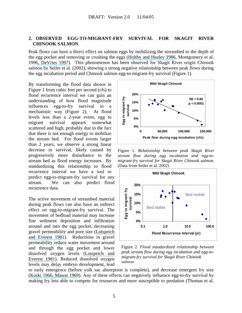
Peak flows can have a direct effect on salmon eggs by mobilizing the streambed to the depth of the egg pocket and removing or crushing the eggs (Holtby and Healey 1986, Montgomery et al. 1996, DeVries 1997). This phenomenon has been observed for Skagit River origin Chinook salmon by Seiler et al. (2002), showing a strong negative relationship between peak flows during the egg incubation period and Chinook salmon egg-to-migrant-fry survival (Figure 1). By transforming the flood data shown in Figure 1 from cubic feet per second (cfs) to flood recurrence interval we can gain an understanding of how flood magnitude influences egg-to-fry survival in a mechanistic way (Figure 2). At flood levels less than a 2-year event, egg to migrant survival appears somewhat scattered and high, probably due to the fact that there is not enough energy to mobilize the stream bed. For flood events larger than 2 years, we observe a strong linear decrease in survival, likely caused by progressively more disturbance to the stream bed as flood energy increases. By standardizing this relationship to flood recurrence interval we have a tool to predict egg-to-migrant-fry survival for any stream. We can also predict flood recurrence data. The active movement of streambed material during peak flows can also have an indirect effect on egg-to-migrant-fry survival. The movement of bedload material may increase fine sediment deposition and infiltration around and into the egg pocket, decreasing gravel permeability and pore size (Lotspeich and Everest 1981). Reductions in gravel permeability reduce water movement around and through the egg pocket and lower dissolved oxygen levels (Lotspeich and Everest 1981). Reduced dissolved oxygen levels may delay embryo development, lead to early emergence (before yolk sac absorption is complete), and decrease emergent fry size (Koski 1966, Mason 1969). Any of these effects can negatively influence egg-to-fry survival by making fry less able to compete for resources and more susceptible to predation (Thomas et al.

Figure 1. Relationship between peak Skagit River stream flow during egg incubation and egg-to-migrant-fry survival for Skagit River Chinook salmon.(Data from Seiler et al. 2002)

Wild Skagit Chinook

R2 = 0.82p < 0.0001

0%

5%

10%

15%

20%

0 50,000 100,000 150,000

Peak flow during egg incubation (cfs)

Egg

to m

igra

nt fr

y su

rviv

al

Wild Skagit Chinook

0%

5%

10%

15%

20%

0.1 1.0 10.0 100.0

Flood Recurrence Interval (yr)

Egg

to m

igra

nt fr

y su

rviv

al

Bed stable

Bed mobile

Wild Skagit Chinook

0%

5%

10%

15%

20%

0.1 1.0 10.0 100.0

Flood Recurrence Interval (yr)

Egg

to m

igra

nt fr

y su

rviv

al

Bed stable

Bed mobile

Figure 2. Flood standardized relationship between peak stream flow during egg incubation and egg-to-migrant-fry survival for Skagit River Chinook salmon.

DRAFT: Version 2.0 11/04/05

6

1969, Parker 1971). Fine sediment deposition that covers or plugs near-surface gravels may also prevent fry emergence (Koski 1966, Lisle and Lewis 1992). In addition, peak flows may displace age-0 salmonids downstream by reducing the availability of preferred or suitable slow water habitats and increasing competition for space (Seegrist and Gard 1972, Erman et al. 1988, Latterell et al. 1998). It is clear that the magnitude of flood events experienced by Chinook salmon eggs largely dictate their survival to the fry stage. However, flood events are natural processes that also form and maintain rearing habitats important to salmon capacity and productivity. Actions that seek to eliminate flood events only would likely also have adverse impacts to juvenile rearing life stages of salmon. We advocate that floods are not what need to be treated for salmon recovery. Rather, we should look at the natural processes that might be impaired such that flood magnitude or frequency are higher than normal. We should also look at sediment or floodplain processes and find areas where these processes are impaired to a degree where the stream channel is destabilized, causing increased mortality of salmon eggs during a particular flood. Actions that restore these processes to functioning levels should be pursued for Chinook salmon recovery.

DRAFT: Version 2.0 11/04/05

7

3. SPAWNING RANGE OF SKAGIT CHINOOK SALMON STOCKS Below we show the spatial distribution of the spawning ranges for the six different Skagit Chinook salmon stocks (Figure 3).

Figure 3. Map of Chinook salmon spawning ranges by stock for the Skagit River Basin.

DRAFT: Version 2.0 11/04/05

8

4. WATERSHED PROCESSES INFLUENCING EGG-TO-FRY SURVIVAL The following watershed or reach scale landscape processes influence spawning habitat capacity, egg incubation success, and fry emergence success. In this report we summarize their effects on the egg deposition stage to migrating fry stage for Skagit Chinook salmon. Disturbance to physical processes can affect egg-to-migrant-fry survival rates through alterations in the frequency and magnitude of key physical processes. Natural and human-caused disturbance to watershed processes will influence the mechanisms described above (e.g., stream bed scour and filling, fine sediment intrusion of egg pockets, flow displacement of fry) known to decrease egg-to-migrant-fry survival for salmon. Here we discuss some of the watershed processes that influence these mechanisms and egg-to-fry survival, and show their current condition within the Skagit River basin and by Chinook spawning stock range.

4.1. PEAK FLOW HYDROLOGY Increases in impervious surface area in low elevation watersheds resulting from urbanization may increase stream flooding frequency and magnitude (Hollis 1975, Booth and Jackson 1994). Generally, we have not considered this effect on Skagit Chinook salmon because few Chinook spawn in lower elevation watersheds where urbanization exists. Exceptions to this rule might be the Nookachamps, Hansen, and Carpenter Creek watersheds. Instead, we have examined peak flows in mountain basins. Our analysis has included results for the Nookachamps and Hansen Creek watersheds, but not Carpenter Creek. The peak flow map for mountain basins displays estimated alterations to peak flows in mountain basins due to changes in rain-on-snow runoff and extensions of drainage networks due to roads (Figure 4). All ratings are averaged by WAU, and based on existing GIS data for roads and land cover. Because data to identify the flood history for unregulated mountain sub-basins in the Skagit watershed is very limited, peak flow ratings were developed based on an empirical correlation between land use and elevated peak flows in the North Fork Stillaguamish River Basin, where a significant increase has been observed (see methods section below). Ratings are based on land cover and road density results from the North Fork Stillaguamish River Basin. Watershed Administrative Units with more than 50% area in hydrologically immature vegetation due to land-use and more than 2 km/km2 of roads were considered very likely impaired. The WAUs exceeding only one of the criteria were considered likely impaired. Remaining WAUs were considered functioning. Floodplain reaches were rated based on the weighted average of contributing WAUs (not including WAUs upstream of dams because of flood storage capability) (Figure 4). Chinook salmon egg-to-fry survival in areas in this map shown as impaired is expected to be significantly lower than normal. Chinook salmon egg-to-fry survival in areas in this map shown as functioning is expected to be normal.

DRAFT: Version 2.0 11/04/05

9

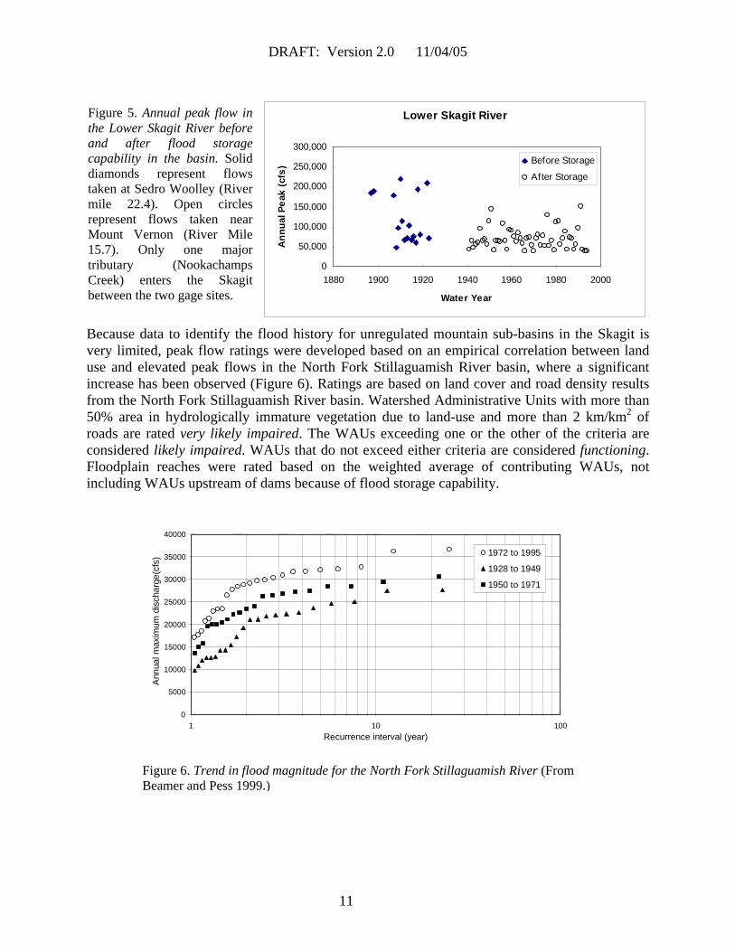
4.1.1 Methods Watersheds were considered “peak flow impaired” in forested mountain basins when the 2-year flood magnitude under disturbed watershed conditions equals or exceeds the 5-year flood magnitude under natural watershed conditions. Two commonly cited causes of increased peak flow are hydrologically immature vegetation and forest road drainage networks that compound and extend channels (e.g., Montgomery 1993, Washington Forest Practices Board 1995). We tried to apply this diagnostic with existing data and found that data to identify changes in peak flow are very limited (Table 1). Out of six gaged sites with long-term records, only three are unregulated basins (i.e., not influenced by flood storage capability). None of the unregulated basins showed a significant increasing trend in annual peak flow over their period of record using regression analysis (alpha level at 0.05). Additionally, annual peak flows in the Skagit River Basin have changed since flow regulation through the construction of reservoirs capable of flood storage. Before flood storage capability, floods in the lower Skagit River commonly approached or exceeded 200,000 cfs (Figure 5).

Figure 4. Map of watersheds and Chinook salmon spawning ranges indicating the state of peak flow hydrology.

DRAFT: Version 2.0 11/04/05

10

Floods in water years 1815 and 1856 were estimated at 400,000 and 300,000 cfs, respectively (not shown in Figures 2 through 5). Since the advent of flood storage capability, a flood approaching 200,000 cfs has not yet occurred. Log-Pearson III analysis shows that the number of floods between the 2-year and 100-year return period has been reduced by roughly 50% since dams were built on the Skagit and Baker Rivers (Table 2).

* gage sites influenced by flood storage capability. Table 2. Magnitude of peak flows by return period for the Skagit River. Estimates for the period prior to flood storage capability on the Skagit are from a gage near Sedro Woolley, reported in Williams et al. (1985). Estimates for the period after flood storage capability are from Sumioka et al. (1998) using data from the gage near Mount Vernon (years 1941 – 1996).

Flood Return Period (years)

Before Flood Storage (gage near Sedro Woolley)

After Flood Storage (gage near Mount Vernon)

2 111,145 64,640 5 167,218 87,560 10 207,020 103,600 25 259,954 125,000 50 301,145 141,800 100 343,743 159,200

Table 1. Currently operating gages with a long period of record in the Skagit River Basin. Flow data from other gages in the Skagit Basin were not examined because the period of record was too short. Data were retrieved from USGS web page. USGS Gage Period of Record (Water Year)

Skagit River near Mount Vernon* 1941-present

Skagit River near Concrete* 1925-present

Skagit River near Marblemount* 1947-1957, 1977-present

Sauk R. above Whitechuck (Upper Sauk) 1918-1922, 1929-present

Sauk River near Sauk (Lower Sauk) 1912, 1929-present

Newhalem Cr. (Upper Skagit Tributary) 1961-present

DRAFT: Version 2.0 11/04/05

11

0

5000

10000

15000

20000

25000

30000

35000

40000

1 10 100Recurrence interval (year)

Ann

ual m

axim

um d

isch

arge

(cfs

) 1972 to 1995

1928 to 1949

1950 to 1971

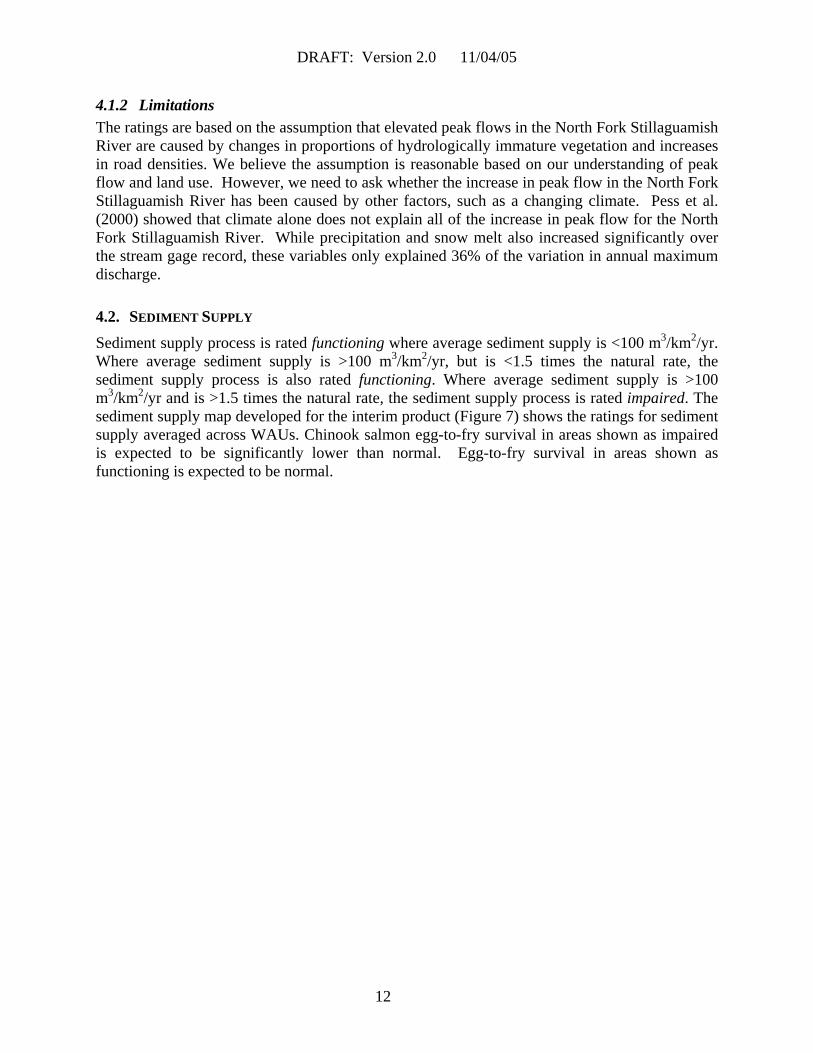
Figure 6. Trend in flood magnitude for the North Fork Stillaguamish River (From Beamer and Pess 1999.)

Because data to identify the flood history for unregulated mountain sub-basins in the Skagit is very limited, peak flow ratings were developed based on an empirical correlation between land use and elevated peak flows in the North Fork Stillaguamish River basin, where a significant increase has been observed (Figure 6). Ratings are based on land cover and road density results from the North Fork Stillaguamish River basin. Watershed Administrative Units with more than 50% area in hydrologically immature vegetation due to land-use and more than 2 km/km2 of roads are rated very likely impaired. The WAUs exceeding one or the other of the criteria are considered likely impaired. WAUs that do not exceed either criteria are considered functioning. Floodplain reaches were rated based on the weighted average of contributing WAUs, not including WAUs upstream of dams because of flood storage capability.

Lower Skagit River

0

50,000

100,000

150,000

200,000

250,000

300,000

1880 1900 1920 1940 1960 1980 2000

Water Year

Ann

ual P

eak

(cfs

) Before Storage

After Storage

Figure 5. Annual peak flow in the Lower Skagit River before and after flood storage capability in the basin. Solid diamonds represent flows taken at Sedro Woolley (River mile 22.4). Open circles represent flows taken near Mount Vernon (River Mile 15.7). Only one major tributary (Nookachamps Creek) enters the Skagit between the two gage sites.

DRAFT: Version 2.0 11/04/05

12

4.1.2 Limitations The ratings are based on the assumption that elevated peak flows in the North Fork Stillaguamish River are caused by changes in proportions of hydrologically immature vegetation and increases in road densities. We believe the assumption is reasonable based on our understanding of peak flow and land use. However, we need to ask whether the increase in peak flow in the North Fork Stillaguamish River has been caused by other factors, such as a changing climate. Pess et al. (2000) showed that climate alone does not explain all of the increase in peak flow for the North Fork Stillaguamish River. While precipitation and snow melt also increased significantly over the stream gage record, these variables only explained 36% of the variation in annual maximum discharge.

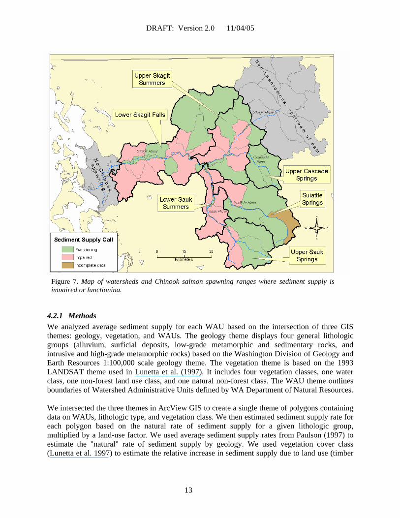
4.2. SEDIMENT SUPPLY Sediment supply process is rated functioning where average sediment supply is <100 m3/km2/yr. Where average sediment supply is >100 m3/km2/yr, but is <1.5 times the natural rate, the sediment supply process is also rated functioning. Where average sediment supply is >100 m3/km2/yr and is >1.5 times the natural rate, the sediment supply process is rated impaired. The sediment supply map developed for the interim product (Figure 7) shows the ratings for sediment supply averaged across WAUs. Chinook salmon egg-to-fry survival in areas shown as impaired is expected to be significantly lower than normal. Egg-to-fry survival in areas shown as functioning is expected to be normal.

DRAFT: Version 2.0 11/04/05

13

4.2.1 Methods We analyzed average sediment supply for each WAU based on the intersection of three GIS themes: geology, vegetation, and WAUs. The geology theme displays four general lithologic groups (alluvium, surficial deposits, low-grade metamorphic and sedimentary rocks, and intrusive and high-grade metamorphic rocks) based on the Washington Division of Geology and Earth Resources 1:100,000 scale geology theme. The vegetation theme is based on the 1993 LANDSAT theme used in Lunetta et al. (1997). It includes four vegetation classes, one water class, one non-forest land use class, and one natural non-forest class. The WAU theme outlines boundaries of Watershed Administrative Units defined by WA Department of Natural Resources. We intersected the three themes in ArcView GIS to create a single theme of polygons containing data on WAUs, lithologic type, and vegetation class. We then estimated sediment supply rate for each polygon based on the natural rate of sediment supply for a given lithologic group, multiplied by a land-use factor. We used average sediment supply rates from Paulson (1997) to estimate the "natural" rate of sediment supply by geology. We used vegetation cover class (Lunetta et al. 1997) to estimate the relative increase in sediment supply due to land use (timber

Figure 7. Map of watersheds and Chinook salmon spawning ranges where sediment supply is impaired or functioning.

DRAFT: Version 2.0 11/04/05

14

harvest and roads) based on Paulson (1997). Natural rates and land use factors are shown in Table 3. In equation form, each polygon has a sediment supply rate calculated as:

Total sediment supply rate = (natural sediment supply rate) x (land use factor) The estimated current sediment supply from each polygon is then (total sediment supply rate) x (area), and the estimated natural sediment supply is (natural sediment supply rate) x (area). From these estimates we calculated average current sediment supply from the WAU, and the average increase over the natural sediment supply for each WAU (current/natural). Table 3. Average sediment supply rates and vegetation factors used in estimating current sediment supply and changes from natural sediment supply for each WAU in the Skagit River basin.

Lithologic group

All rock types/alpine (applied only to

vegetation class 16)

Alluvium

Surficial deposits

Low-grade metamorphic

High-grade metamorphic

Natural sediment supply rate (m3/km2/yr) 409a 0b 33c 130d 53e

Land use factor for early-seral, mid-seral and late-seral

NA 1 1 1 1

Land use factor for other forest (clear-cut to hardwood)

NA 1 3f 4f 6f

Land use factor for vegetation, water and non-forest

NA 0 0 0 0

Land use factor for alpine areas, rock outcrops, and glaciers

1 NA NA NA NA

a. Average sediment supply rate from granitic rocks in alpine areas, New Zealand. Region has annual precipitation similar to that of the upper Skagit Basin, and granitic rocks are prevalent in the upper Skagit Basin.

b. Alluvial areas are predominantly floodplains. No mass wasting occurs. c. Sediment supply rate for forest >20 years old in a sub-basin dominated by glacial sediments (Paulson 1997). d. Sediment supply rate for forest >20 years old in 3 sub-basins dominated by phyllite and sandstone (Paulson

1997). e. Sediment supply rate for forest >20 years old in sub-basins dominated by granitic and high grade metamorphic

rocks (Paulson 1997). f. Relative increase in mass wasting rate where forests are less than 20 years old (Paulson 1997).

4.2.2 Limitations The method correctly estimated the sediment supply rating for seven of the ten sub-basins where sediment budget data were available (Table 4). It over-estimated average sediment supply for two of the ten test basins (i.e., rated them impaired when they are functioning), and under-estimated sediment supply for one sub-basin. Some of the error may be due to the fact that the model estimates sediment supply for the entire WAU, whereas six of the ten field-based sediment budgets covered only sub-watersheds within a WAU.

DRAFT: Version 2.0 11/04/05

15

Mass wasting rates are more strongly related to landform than to geology. However, our method does not incorporate landform in estimating sediment supply because but we had no automated procedure for identifying landforms on GIS. Nevertheless, geology and landform are correlated in the Skagit River Basin (e.g., there tends to be a small proportion of steep inner gorges in surficial deposits and a high proportion in high-grade metamorphic rocks), and the method remains reasonably accurate. Land-use intensity is based on LANDSAT data that poorly distinguish areas of low root strength (i.e., forests less than 20 years old) from mature hardwoods. Therefore, land-use categories do not accurately represent the proportion of forests less than 20 years old, and do not explicitly incorporate road areas. Table 4. Error matrix comparing sediment supply ratings from field-based sediment budgets to ratings based on GIS estimates.

Field-based sediment budget

GIS estimate Functioning Impaired % correct % commission

Functioning 4 1 80% 20%

Impaired 2 3 60% 40%

% omission 67% 75%

Overall percent correct = 70%

4.2.3 Effect of Sediment Supply on Scour Depth In this section we examine the possible effect of sediment supply on scour depth. We used only data from Tripp and Poulin (1986) for two reasons: (1) it was the only data set available with different levels of sediment supply, and (2) the basin/stream data are consistent throughout the data set. Sediment supply is indicated by descriptive categories in Tripp and Poulin (1986). They were grouped into three sediment supply categories based on the description in Table 4: Table 5. Features of sediment supply categories.

Sediment supply category Narrative descriptions (Tripp and Poulin 1986) Low (n = 4) • no recent disturbances Moderate (n = 5) • recent floods and debris jam failures

• mass wasting upstream, gravel aggrading downstream High (n = 3) • debris-torrented

DRAFT: Version 2.0 11/04/05

16

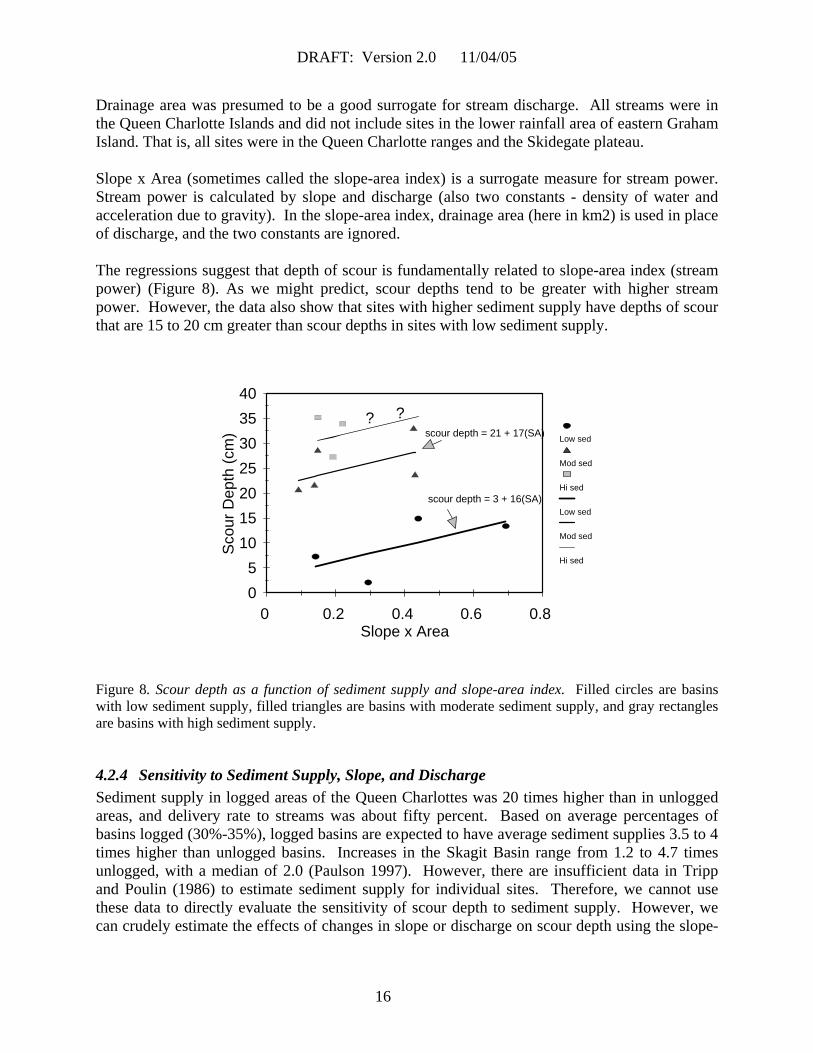
Drainage area was presumed to be a good surrogate for stream discharge. All streams were in the Queen Charlotte Islands and did not include sites in the lower rainfall area of eastern Graham Island. That is, all sites were in the Queen Charlotte ranges and the Skidegate plateau. Slope x Area (sometimes called the slope-area index) is a surrogate measure for stream power. Stream power is calculated by slope and discharge (also two constants - density of water and acceleration due to gravity). In the slope-area index, drainage area (here in km2) is used in place of discharge, and the two constants are ignored. The regressions suggest that depth of scour is fundamentally related to slope-area index (stream power) (Figure 8). As we might predict, scour depths tend to be greater with higher stream power. However, the data also show that sites with higher sediment supply have depths of scour that are 15 to 20 cm greater than scour depths in sites with low sediment supply.

0 5

10 15 20 25 30 35 40

Sco

ur D

epth

(cm

)

0 0.2 0.4 0.6 0.8 Slope x Area

Low sed

Mod sed

Hi sed

Low sed

Mod sed

Hi sed

??

scour depth = 3 + 16(SA)

scour depth = 21 + 17(SA)

Figure 8. Scour depth as a function of sediment supply and slope-area index. Filled circles are basins with low sediment supply, filled triangles are basins with moderate sediment supply, and gray rectangles are basins with high sediment supply.

4.2.4 Sensitivity to Sediment Supply, Slope, and Discharge Sediment supply in logged areas of the Queen Charlottes was 20 times higher than in unlogged areas, and delivery rate to streams was about fifty percent. Based on average percentages of basins logged (30%-35%), logged basins are expected to have average sediment supplies 3.5 to 4 times higher than unlogged basins. Increases in the Skagit Basin range from 1.2 to 4.7 times unlogged, with a median of 2.0 (Paulson 1997). However, there are insufficient data in Tripp and Poulin (1986) to estimate sediment supply for individual sites. Therefore, we cannot use these data to directly evaluate the sensitivity of scour depth to sediment supply. However, we can crudely estimate the effects of changes in slope or discharge on scour depth using the slope-

DRAFT: Version 2.0 11/04/05

17

area index or stream power. We can then compare these estimates to the changes caused by sediment supply changes. Figure 9 shows the estimated change in scour depth when slope or stream discharge is increased by approximately realistic amounts. Data from two altered channels in the Skagit Basin indicate that slope increases of about 0.5% have been measured (due to channel straightening). We altered slope by 1% for our assessment. Data from watershed analyses indicate that percentage increases in 2-year peak flows can be as high as 12% (Jordan-Boulder WAU) or 13% (Hansen WAU). Because these basins are not completely clearcut, we used a 20% increase in flow as a likely high-end increase in peak flow. It appears that neither effect (slope change or hydrologic change due to hydrologic immaturity alone) will approach the magnitudes of change expected to result from changes in sediment supply over the range of channel slopes (.007 to .04) and drainage areas (4 to 47 km2) included in the Queen Charlottes study. (Note that precipitation in the Queen Charlottes may be somewhat higher than in most of the Skagit - up 165 in/yr compared.) We should also note that these basins are at the small end of Skagit Chinook habitats. It seems reasonable to expect that the degree of increase in sediment supply (and hence, scour depth) may be proportionally smaller in larger channels. The Queen Charlotte sites are near the sediment source areas, some receiving debris torrents directly. As drainage areas increase, spawning sites will often be farther from sediment source areas, and increases in sediment supply may be moderated by bed load wave attenuation and particle attrition. Therefore, the effects of sediment supply may be smaller in larger streams.

0 5

10 15 20 25 30 35 40

Sco

ur D

epth

(cm

)

0 0.2 0.4 0.6 0.8 Slope x Area

Low sed

Mod sed

Hi sed

??

1% increase inenergy slope

20% increase inflood discharge

Figure 9. Relative increases in scour depth expected from changes in discharge or channel slope.

DRAFT: Version 2.0 11/04/05

18

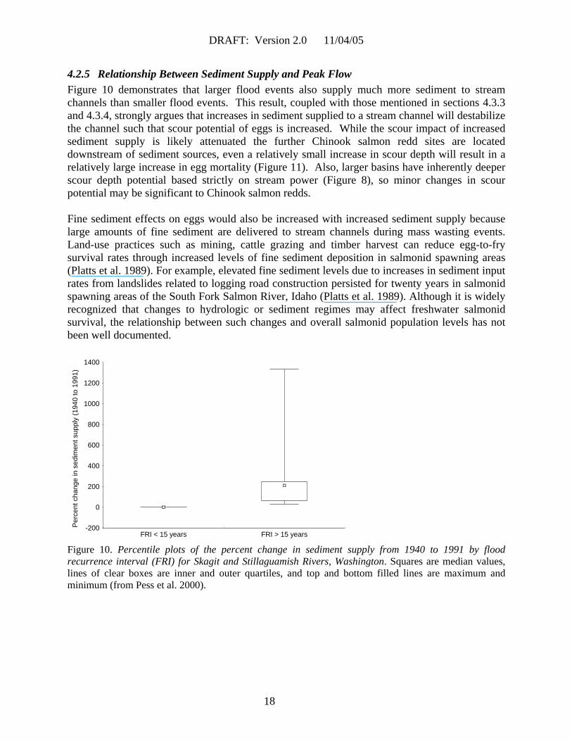
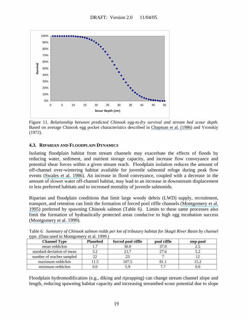
4.2.5 Relationship Between Sediment Supply and Peak Flow Figure 10 demonstrates that larger flood events also supply much more sediment to stream channels than smaller flood events. This result, coupled with those mentioned in sections 4.3.3 and 4.3.4, strongly argues that increases in sediment supplied to a stream channel will destabilize the channel such that scour potential of eggs is increased. While the scour impact of increased sediment supply is likely attenuated the further Chinook salmon redd sites are located downstream of sediment sources, even a relatively small increase in scour depth will result in a relatively large increase in egg mortality (Figure 11). Also, larger basins have inherently deeper scour depth potential based strictly on stream power (Figure 8), so minor changes in scour potential may be significant to Chinook salmon redds. Fine sediment effects on eggs would also be increased with increased sediment supply because large amounts of fine sediment are delivered to stream channels during mass wasting events. Land-use practices such as mining, cattle grazing and timber harvest can reduce egg-to-fry survival rates through increased levels of fine sediment deposition in salmonid spawning areas (Platts et al. 1989). For example, elevated fine sediment levels due to increases in sediment input rates from landslides related to logging road construction persisted for twenty years in salmonid spawning areas of the South Fork Salmon River, Idaho (Platts et al. 1989). Although it is widely recognized that changes to hydrologic or sediment regimes may affect freshwater salmonid survival, the relationship between such changes and overall salmonid population levels has not been well documented.

Per

cent

cha

nge

in s

edim

ent s

uppl

y (1

940

to 1

991)

-200

0

200

400

600

800

1000

1200

1400

FRI < 15 years FRI > 15 years Figure 10. Percentile plots of the percent change in sediment supply from 1940 to 1991 by flood recurrence interval (FRI) for Skagit and Stillaguamish Rivers, Washington. Squares are median values, lines of clear boxes are inner and outer quartiles, and top and bottom filled lines are maximum and minimum (from Pess et al. 2000).

DRAFT: Version 2.0 11/04/05

19

0%

10%

20%

30%

40%

50%

60%

70%

80%

90%

100%

0 5 10 15 20 25 30 35 40 45 50

Scour Depth (cm)

Surv

ival

Figure 11. Relationship between predicted Chinook egg-to-fry survival and stream bed scour depth. Based on average Chinook egg pocket characteristics described in Chapman et al. (1986) and Vronskiy (1972).

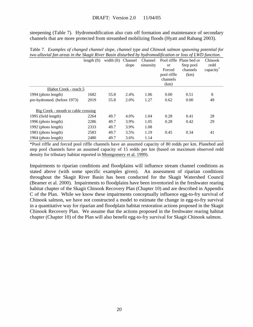
4.3. RIPARIAN AND FLOODPLAIN DYNAMICS Isolating floodplain habitat from stream channels may exacerbate the effects of floods by reducing water, sediment, and nutrient storage capacity, and increase flow conveyance and potential shear forces within a given stream reach. Floodplain isolation reduces the amount of off-channel over-wintering habitat available for juvenile salmonid refuge during peak flow events (Swales et al. 1986). An increase in flood conveyance, coupled with a decrease in the amount of slower water off-channel habitat, may lead to an increase in downstream displacement to less preferred habitats and to increased mortality of juvenile salmonids. Riparian and floodplain conditions that limit large woody debris (LWD) supply, recruitment, transport, and retention can limit the formation of forced pool riffle channels (Montgomery et al. 1995) preferred by spawning Chinook salmon (Table 6). Limits to these same processes also limit the formation of hydraulically protected areas conducive to high egg incubation success (Montgomery et al. 1999). Table 6. Summary of Chinook salmon redds per km of tributary habitat for Skagit River Basin by channel type. (Data used in Montgomery et al. 1999.)

Channel Type Planebed forced pool riffle pool riffle step-pool mean redds/km 1.7 30.0 37.0 2.5

standard deviation of mean 3.2 23.7 27.6 5.2 number of reaches sampled 22 23 7 12

maximum redds/km 11.5 107.5 81.1 15.2 minimum redds/km 0.0 5.9 7.7 0.0

Floodplain hydromodification (e.g., diking and riprapping) can change stream channel slope and length, reducing spawning habitat capacity and increasing streambed scour potential due to slope

DRAFT: Version 2.0 11/04/05

20

steepening (Table 7). Hydromodification also cuts off formation and maintenance of secondary channels that are more protected from streambed mobilizing floods (Hyatt and Rabang 2003). Table 7. Examples of changed channel slope, channel type and Chinook salmon spawning potential for two alluvial fan areas in the Skagit River Basin disturbed by hydromodification or loss of LWD function.

length (ft) width (ft) Channel slope

Channel sinuosity

Pool riffle or

Forced pool riffle channels

(km)

Plane bed or Step pool channels

(km)

Chinook redd

capacity*

Illabot Creek - reach 5 1994 (photo length) 1682 55.8 2.4% 1.06 0.00 0.51 8 pre-hydromod. (before 1973) 2019 55.8 2.0% 1.27 0.62 0.00 49

Big Creek - mouth to cable crossing

1995 (field length) 2264 49.7 4.0% 1.04 0.28 0.41 28 1996 (photo length) 2286 49.7 3.9% 1.05 0.28 0.42 29 1992 (photo length) 2333 49.7 3.9% 1.08 1983 (photo length) 2583 49.7 3.5% 1.19 0.45 0.34 41 1964 (photo length) 2480 49.7 3.6% 1.14 *Pool riffle and forced pool riffle channels have an assumed capacity of 80 redds per km. Planebed and step pool channels have an assumed capacity of 15 redds per km (based on maximum observed redd density for tributary habitat reported in Montgomery et al. 1999). Impairments to riparian conditions and floodplains will influence stream channel conditions as stated above (with some specific examples given). An assessment of riparian conditions throughout the Skagit River Basin has been conducted for the Skagit Watershed Council (Beamer et al. 2000). Impairments to floodplains have been inventoried in the freshwater rearing habitat chapter of the Skagit Chinook Recovery Plan (Chapter 10) and are described in Appendix C of the Plan. While we know these impairments conceptually influence egg-to-fry survival of Chinook salmon, we have not constructed a model to estimate the change in egg-to-fry survival in a quantitative way for riparian and floodplain habitat restoration actions proposed in the Skagit Chinook Recovery Plan. We assume that the actions proposed in the freshwater rearing habitat chapter (Chapter 10) of the Plan will also benefit egg-to-fry survival for Skagit Chinook salmon.

DRAFT: Version 2.0 11/04/05

21

5. SKAGIT CHINOOK SALMON RESPONSE TO EGG-TO-FRY SURVIVAL CONDITIONS

We have already shown that egg-to-migrant-fry survival for Skagit Chinook salmon is strongly negatively influenced by peak flow during the egg incubation period (Section 2; Figures 1 and 2) and that impairments to watershed processes will decrease egg-to-migrant-fry survival of Chinook salmon (Section 4). In this section we estimate productivity (migrant fry per spawner) of Skagit Chinook salmon under current watershed conditions. We also predict the change in productivity for the watershed restoration actions listed in the Skagit Chinook Recovery Plan.

5.1. SPAWNER TO MIGRANT FRY PRODUCTIVITY UNDER CURRENT HABITAT CONDITIONS Skagit Chinook spawn in both functioning (good) and impaired (bad) habitat, and this results in an overall freshwater survival rate that is intermediate between the survival rates that would be obtained either from spawning entirely in functioning habitat, or entirely in impaired habitat. This overall survival rate varies according to the percentage of Chinook salmon spawners that spawn in functioning habitat and the complementary percentage that spawn in impaired habitat: ST = SGood * %Good + SBad * %Bad (1) where ST is the total (overall) egg to smolt survival rate for migrating Chinook fry; SGood is the egg to smolt survival rate for migrating Chinook fry spawned in functioning habitat; %Good is the percentage of the total spawning that occurs in functioning habitat; SBad is the egg to smolt survival rate for migrating Chinook fry spawned in impaired habitat; and %Bad is the percentage of the total spawning that occurs in impaired habitat. Thus, if we have estimates of ST, %Good, SBad, and %Bad, we can calculate SGood. We estimated ST as the survival rate at the mean peak incubation flow experienced by all the brood years for which we have smolt outmigration estimates (brood years 1989-2002). The mean peak incubation flow for those broods is 67,936 cfs, which corresponds to a flood return interval (RI) of 3.03 years. Plotting brood year 1989-2002 survival rates as a function of RI (data shown in Figure 2), calculated the following exponential relation between survival rate and RI: ST = 0.180 * EXP(-0.035 * RI) (2) Thus, at a RI of 3.03 years, ST = 16.8%. We estimated SBad as the North Fork Stillaguamish during the stream flow period 1972 to 1995 survival rate calculated at a 3.03 year RI. At a 3.03 year RI, the North Fork Stillaguamish survival rate is 3.5% (Beamer and Pess 1999) (Figure 12).

DRAFT: Version 2.0 11/04/05

22

North Fork Stillaguamish River

0%

5%

10%

15%

0 10 20 30 40 50 60

Flood Recurrence (years)

Pre

dict

ed C

hino

ok s

alm

on e

gg

to m

igra

nt fr

y su

rviv

al

Survival for 1928 to 1949flow conditions

Survival for 1950 to 1971flow conditions

Survival for 1972 to 1995flow conditions

Figure 12. Estimated change in Chinook salmon egg-to-migrant-fry survival for the North Fork Stillaguamish River. To calculate the percentage of the total Chinook salmon spawning that occurs in functioning habitat, we estimated that the following percentages of each Skagit Chinook population’s spawning range lies in functioning or impaired habitat (Table 8): Table 8. Percentage of escapement that spawns in impaired or functioning habitat by population. Stock % escapement in impaired % escapement in functioning Lower Skagit Falls 100% 0% Upper Skagit Summers 7%* 93% Upper Cascade Springs 0% 100% Lower Sauk Summers 100% 0% Upper Sauk Springs 25% 75% Suiattle Springs 20% 80% * the average percentage of Upper Skagit Summers that spawn in the lower Cascade River (1974-1996) We then multiplied these percentages by each population’s spawning escapement, for the years 1989-2002, and, because we are measuring egg-to-migrant-fry survival rates only, we subtracted out the number of spawners attributed to yearling production, using the percentages of yearlings in the returning runs shown in Table 9.

DRAFT: Version 2.0 11/04/05

23

Table 9. Average percent of escapement that is yearling life history. (Using BY 1994 – 2000, because those were the only years for which we know that unmarked hatchery yearlings do not have the potential to bias the results). Stock % yearling life history represented in escapement Lower Skagit Falls 19.5% Upper Skagit Summers 2.6% Upper Cascade Springs 19.1% Lower Sauk Summers 9.1% Upper Sauk Springs 42.5% Suiattle Springs 43.9% After subtracting out the spawners attributed to yearling production, we estimated that an average of 74.1% of the Chinook spawning occurs in functioning habitat; hence, 25.9% of the spawning must occur in impaired habitat (Table 10). By substituting these percentages, the overall survival rate of 16.8%, and the survival rate in impaired habitat of 3.5%, into equation (1), we calculated that the egg to smolt survival rate of fingerling Chinook in functioning habitat is 21.4%. In order to convert this survival rate to a productivity value (in terms of smolts/spawner), we estimated the survival rate under average flow conditions and current habitat by standardizing the spawning escapements for flow, according to the following equation: Estd = E * ST/STmean (3) where Estd is the flow-standardized escapement; E is the observed escapement; ST is the survival rate calculated according to equation (2) for that year’s flow; and STmean is the survival rate calculated according to equation (2) for the mean peak flow. We then plotted the observed fingerling smolt outmigration each year from brood year 1989-2002 against these standardized escapements, and ran a regression line through the origin. The slope of this line is an estimate of migrant fry per spawner expected under average flow and current habitat. This slope, for brood years 1989-2002, is 341 smolts/spawner (Figure 13). The 95% confidence range is 306 to 376 smolts per spawner.

DRAFT: Version 2.0 11/04/05

24

Table 10. Calculation of the percentage of the Skagit Chinook migrant fry production spawned in habitat rated as functioning (“Good”) and impaired (“Bad”) based on watershed process screens for peak flow hydrology and sediment supply. Brood Yr

Lower Skagit Falls

Upper Skagit Summers

Lower Sauk Summers

Upper Sauk Springs

Suiattle Springs

Upper Cascade Springs

Total Good Habitat

Total Bad Habitat

Total % Good

1989 1454 4781 449 668 514 333 5119 2058 7177 71.3% 1990 3705 11793 1294 557 685 350 11513 5120 16633 69.2% 1991 1510 3656 658 747 354 311 4044 2210 6254 64.7% 1992 1331 5548 469 580 201 205 5532 1982 7514 73.6% 1993 942 4654 205 323 291 168 4621 1341 5963 77.5% 1994 884 4565 112 130 167 173 4406 1162 5568 79.1% 1995 666 5948 278 190 440 225 5849 1271 7120 82.1% 1996 1521 7989 1103 408 435 208 7776 2879 10655 73.0% 1997 409 4168 295 305 428 308 4348 973 5322 81.7% 1998 2388 11761 460 290 473 323 11252 3237 14489 77.7% 1999 1043 3586 295 180 208 83 3486 1401 4888 71.3% 2000 3262 13092 576 388 360 273 12409 4138 16547 75.0% 2001 2606 10084 1103 543 688 625 10183 3943 14126 72.1% 2002 4866 13815 910 460 265 340 13106 5782 18888 69.4% Unwtd Mean 74.1% Wtd Mean 7403 2679 10082 73.4%

Figure 13. Relationship between Skagit subyearling outmigration population size and spawning escapement. Spawning escapement is standardized for peak flow during the egg incubation period.

Skagit Wild Chinook

y = 341.2xR2 = 0.89

P<0.000001

0

2,000,000

4,000,000

6,000,000

8,000,000

0 5,000 10,000 15,000 20,000 25,000

Escapement (Standardized to BY89-02 Peak)

Age

0+ M

igra

nts

DRAFT: Version 2.0 11/04/05

25

5.2. SPAWNER TO MIGRANT FRY PRODUCTIVITY UNDER FULLY RESTORED HABITAT CONDITIONS

We believe regulatory actions already in place (Forest Practice regulations for industrial landowners relating to forest roads) and watershed restoration practices that treat forest road systems for sediment supply and hydrology impacts can reverse the screening calls for 100% of the WAUs in the Skagit River Basin. We believe this is a realistic Chinook salmon recovery objective because it does not involve an unsolvable issue over existing land use versus fish habitat. Forest road systems can either be decommissioned (a change in land use) or reconstructed and properly maintained (no change in land use), yet the sediment supply and hydrology functions can be restored through either strategy. This means we are predicting that the actions (if implemented) listed in the Skagit Chinook Recovery Plan for egg-to-fry survival (Chapter 9) will change all impaired watersheds shown in Figures 4 and 7 to functioning levels. We describe this fully restored condition as Properly Functioning Conditions (PFC). To estimate spawner to migrant fry productivity at PFC, we then multiplied the flood standardized estimate of productivity observed in current habitat conditions (341 migrant fry per spawner) by the ratio of survival under PFC to mean overall survival: PPFC = PCurrent * (SGood/ST) (4) where PPFC is productivity, in terms of smolts/spawner, at PFC; and PCurrent is smolts/spawner under current habitat conditions (i.e., 341 smolts/spawner). By substituting in the values for SGood (21.4%) and ST (16.8%), we estimated that under PFC freshwater conditions, productivity at mean flow would be 435 fingerling smolts/spawner (95% confidence range is 390 to 480 smolts/spawner).

DRAFT: Version 2.0 11/04/05

26

6. IMPACT OF CLIMATE CHANGE ON EGG-TO-MIGRANT-FRY SURVIVAL We have not completed an analysis regarding the effects of climate change on egg-to-migrant-fry survival for Skagit Chinook salmon. However, increased flooding during the egg incubation period has been observed in the North Fork Stillaguamish River (Figure 6) and 36% of the increase is thought to be climate change related (Pess et al. 2000). This trend of increased flooding during the egg incubation has been predicted by climate experts so we anticipate egg-to-fry survival to generally be lower in the future if watershed conditions remain the same. This makes restoration of impaired watersheds a high implementation priority in the Chinook Recovery Plan.

DRAFT: Version 2.0 11/04/05

27

7. REFERENCES Beamer, E.M., and G.R. Pess. 1999. Effects of peak flows on Chinook Oncorhynchus

tshawytscha spawning success in two Puget Sound river basins in R. Sakrison and P. Sturtevant, editors. Watershed Management to Protect Declining Species. American Water Resources Association, Middleburg, Virginia.

Beamer, E.M., J.C. Sartori, and K.A. Larsen. 2000. Skagit Chinook life history study Progress Report Number 3. Prepared for Non-flow Coordination Committee under the Chinook Research Program in the Non-flow Mitigation part of the Skagit Fisheries Settlement Agreement. Federal Energy Regulatory Commission Project Number 553.

Booth, D. B., and C. R. Jackson. 1994. Urbanization of aquatic systems – degradation thresholds and the limits of mitigation. Pages 425-433 in R. A. Marston and V. R. Hasfurther, editors. Proceedings from the effects of human-induced changes on hydrologic systems. American Water Resources Association, Jackson Hole, Wyoming.

Chapman, D.W., D.E. Weitkamp, T.L. Welsh, M.B. Dell, and T.H. Schadt. 1986. Effects of River Flow on the Distribution of Chinook Salmon Redds. Transactions of the American Fisheries Society 115:537-547.

Davis, S. F., and M. J. Unwin. 1989. Freshwater life history of Chinook salmon Oncorhynchus tshawytscha in the Rangitata River catchment, New Zealand. New Zealand Journal of Marine and Freshwater Research 23:311-319.

DeVries, P. 1997. Riverine salmon egg burial depths: review of published data and implications for scour studies. Canadian Journal of Fisheries and Aquatic Sciences 54:1685-1698.

Erman, D. C., E. D. Andrews, and M. Yoder-Williams. 1988. Effects of winter floods on fishes in the Sierra Nevada. Canadian Journal of Fisheries and Aquatic Sciences 45:2195-2200.

Hollis, G. E. 1975. The effects of urbanization on floods of different recurrence intervals. Water Resources Research 11:431-435.

Holtby, L. B., and M. C. Healey. 1986. Selection for adult size in female coho salmon Oncorhynchus kisutch. Canadian Journal of Fisheries and Aquatic Sciences 43:1946-1959.

Hyatt, T. L., and A. D. Rabang. 2003. Nooksack River Chinook Salmon spawning and incubation assessment. Nooksack Natural Resources Department, Deming, Washington.

Koski, K. V. 1966. The survival of coho salmon Oncorhynchus kisutch from egg deposition to emergence in three Oregon coastal streams. Master’s thesis. Oregon State University, Corvallis.

Latterell, J. L., K. D. Fausch, C. Gowan, and S. C. Riley. 1998. Relationship of trout recruitment to snowmelt runoff flows and adult trout abundance in six Colorado mountain streams. Rivers 6:240-250.

Lisle, T. E., and J. Lewis. 1992. Effects of sediment transport on survival of salmonid embryos in a natural stream: a simulation approach. Canadian Journal of Fisheries and Aquatic Sciences 49:2337-2344.

Lotspeich, F. B., and F. H. Everest. 1981. A new method for reporting and interpreting textural composition of spawning gravel. U.S. Forest Service Research Note PNW-139.

Lunetta, R. S., B. Cosentino, D. R. Montgomery, E. M. Beamer, and T. J. Beechie. 1997. GIS-based evaluation of salmon habitat in the Pacific Northwest. Photogrammetric Engineering and Remote Sensing 63(10):1219-1229.

DRAFT: Version 2.0 11/04/05

28

Mason, J. C. 1969. Hypoxial stress prior to emergence and competition among coho salmon fry. Journal of the Fisheries Research Board of Canada 26:63-91.

McNeil, W. J. 1966. Effect of spawning bed environment on reproduction of chum salmon. Fishery Bulletin 65:495-523.

Montgomery, D. R. 1993. Road surface drainage, channel extension, and slope stability. Geomorphological Watershed Analysis Project. Final report #TFW-SH01-93-001, for the period from 10/01/1991 to 06/03/1993. Washington Department of Natural Resources, Olympia.

Montgomery, D. R., E. M. Beamer, G. R. Pess, and T. P. Quinn. 1999. Channel type and salmonid spawning distribution and abundance. Canadian Journal of Fisheries and Aquatic Sciences 56:377-387.

Montgomery, D. R., J. M. Buffington, N. P. Peterson, D. Schuett-Hames, and T. P. Quinn. 1996. Streambed scour, egg burial depths and the influence of salmonid spawning on bed surface mobility and embryo survival. Canadian Journal of Fisheries and Aquatic Sciences 53:1061-1070.

Montgomery, D. R., J. M. Buffington, R.D. Smith, K.M. Schmidt, and G. R. Pess. 1995. Pool spacing in forest channels. American Geophysical Union, paper # 94WR03285.

Parker, R. R. 1971. Size selective predation among juvenile salmonid fishes in a British Columbia inlet. Journal of the Fisheries Research Board of Canada 28:1503-1510.

Paulson, K. M. 1997. Estimating changes in sediment supply due to forest practices: A sediment budget approach to the Skagit River Basin in Northwestern Washington. Master’s Thesis. University of Washington, Seattle.

Pess, G. R., E. M. Beamer, and A. E. Steel. 2000. Effects of peak flows and spawning density on Chinook Oncorhynchus tshawytscha spawning success in two Puget Sound River Basins. NOAA Fisheries, Northwest Fisheries Science Center Watershed Program Open House Presentation.

Platts, W. S., R. J. Torquemada, M. L. McHenry, and C. K. Graham. 1989. Changes in salmon spawning habitat from increased delivery of fine sediment to the South Fork Salmon River, Idaho. Transactions of the American Fisheries Society 118:274-283.

Seegrist, D. W., and R. Gard. 1972. Effects of floods on trout in Sagehen Creek, California. Transactions of the American Fisheries Society 101:478-482.

Seiler, D., S. Neuhauser, and L. Kishimoto. 2002. 2001 Skagit River wild 0+ Chinook production evaluation. Annual Project Report funded by Seattle City Light. Washington Department of Fish and Wildlife, Olympia.

Sumioka, S.S., D.L. Kresch, and K.D. Kasnick. 1998. Magnitude and Frequency of Floods in Washington. USGS Water Resources Investigations Report 97-4277. Tacoma, WA.

Swales, S., R. B. Lauzier, and C. D. Levings. 1986. Winter habitat preferences of juvenile salmonids in two interior rivers in British Columbia. Canadian Journal of Zoology 64:1506-1514.

Thomas, A. E., J. L. Banks, and D. C. Greenland. 1969. Effect of yolk sac absorption on the swimming ability of fall Chinook salmon. Transactions of the American Fisheries Society 98:406-410.

Thorne, R. E., and J. J. Ames. 1987. A note on variability of marine survival of sockeye salmon Oncorhynchus nerka and effect of flooding on spawning success. Canadian Journal of Fisheries and Aquatic Sciences 44:1791-1795.

DRAFT: Version 2.0 11/04/05

29

Tripp, D. B., and V. A. Poulin. 1986. The effects of logging and mass wasting on salmonid spawning habitat in streams on the Queen Charlotte Islands. British Columbia Ministry of Forests and Lands.

USGS 1997 Vronskiy, B. B. 1972. Reproductive biology of the Kamchatka River Chinook salmon

Oncorhynchus tshawytscha. Journal of Ichthyology 12:259-273. Washington Forest Practices Board. 1995. Standard methodology for conducting watershed

analysis under Chapter 222-22 WAC. Version 3.0 Module to evaluate hydrologic change. Williams, J.R., H.E. Pearson, and J.D. Wilson. 1985. Streamflow Statistics and Drainage-Basin

Characteristics for the Puget Sound Region, Washington. USGS open file report 84-144-B. Tacoma, WA.