Effects of Hydroelectric Dam Operations on the Restoration Potential of Snake River Fall Chinook Salmon (Oncorhynchus tshawytscha) Spawning Habitat

Final Report

October 2005–September 2007

Prepared by

Timothy P. Hanrahan, Marshall C. Richmond, Evan V. Arntzen, Andre M. Coleman,

Kyle B. Larson, William A. Perkins, Jerry D. Tagestad

Pacific Northwest National Laboratory Richland, WA 99352

Prepared for

U.S. Department of Energy

Bonneville Power Administration Division of Fish and Wildlife

P.O. Box 3621 Portland, OR 97208-3621

Project No. 2003-038-00 Contract No. 00000652-00031

September 2007

Summary

This report describes research conducted by the Pacific Northwest National Laboratory for the Bonneville Power Administration (BPA) as part of the Fish and Wildlife Program directed by the Northwest Power and Conservation Council. The study evaluated the restoration potential of Snake River fall Chinook salmon spawning habitat within the impounded lower Snake River. The objective of the research was to determine if hydroelectric dam operations could be modified, within existing system constraints (e.g., minimum to normal pool levels; without partial removal of a dam structure), to increase the amount of available fall Chinook salmon spawning habitat in the lower Snake River.

Empirical and modeled physical habitat data were used to compare potential fall Chinook salmon spawning habitat in the Snake River, under current and modified dam operations, with the analogous physical characteristics of an existing fall Chinook salmon spawning area in the Columbia River. The two Snake River study areas included the Ice Harbor Dam tailrace downstream to the Highway 12 bridge and the Lower Granite Dam tailrace downstream approximately 12 river kilometers. These areas represent tailwater habitat (i.e., riverine segments extending from a dam downstream to the backwater influence from the next dam downstream). We used a reference site, indicative of current fall Chinook salmon spawning areas in tailwater habitat, against which to compare the physical characteristics of each study site. The reference site for tailwater habitats was the section extending downstream from the Wanapum Dam tailrace on the Columbia River. Fall Chinook salmon spawning habitat use data, including water depth, velocity, substrate size and channelbed slope, from the Wanapum reference area were used to define spawning habitat suitability based on these variables. Fall Chinook salmon spawning habitat suitability of the Snake River study areas was estimated by applying the Wanapum reference reach habitat suitability criteria to measured and modeled habitat data from the Snake River study areas. Channel morphology data from the Wanapum reference reach and the Snake River study areas were evaluated to identify geomorphically suitable fall Chinook salmon spawning habitat.

The results of this study indicate that a majority of the Ice Harbor and Lower Granite study areas contain suitable fall Chinook salmon spawning habitat under existing hydrosystem operations. However, a large majority of the currently available fall Chinook salmon spawning habitat in the Ice Harbor and Lower Granite study areas is of low quality. The potential for increasing, through modifications to hydrosystem operations (i.e., minimum pool elevation of the next downstream dam), the quantity or quality of fall Chinook salmon spawning habitat appears to be limited. Estimates of the amount of potential fall Chinook salmon spawning habitat in the Ice Harbor study area decreased as the McNary Dam forebay elevation was lowered from normal to minimum pool elevation. Estimates of the amount of potential fall Chinook salmon spawning habitat in the Lower Granite study area increased as the Little Goose Dam forebay elevation was lowered from normal to minimum pool elevation; however, 97% of the available habitat was categorized within the range of lowest quality. In both the Ice Harbor and Lower Granite study areas, water velocity appears to be more of a limiting factor than water depth for fall Chinook salmon spawning habitat, with both study areas dominated by low-magnitude water velocity. The geomorphic suitability of both study areas appears to be compromised for fall Chinook salmon spawning habitat, with the Ice Harbor study area lacking significant bedforms along the longitudinal thalweg profile and the Lower Granite study area lacking cross-sectional topographic diversity.

iii

iv

To increase the quantity of available fall Chinook salmon spawning habitat in the Ice Harbor and Lower Granite study area, modifications to hydroelectric dam operations beyond those evaluated in this study likely would be necessary. Modifications may include operational and structural changes, such as lowering downstream dam forebay elevations to less than minimum pool. There is a large amount of uncertainty as to whether or not such modifications could increase the quantity of available fall Chinook salmon spawning habitat in the Ice Harbor and Lower Granite study area. The results from this study provide some certainty that the quantity and quality of fall Chinook salmon spawning habitat within the lower Snake River are not likely to be increased within the existing hydroelectric dam operations.

Acknowledgments

We thank Jonathan McCloud (BPA) as the contracting officer’s technical representative providing oversight of this project. Special gratitude is given to Grant County PUD and the U.S. Army Corps of Engineers Walla Walla District for providing data from the Wanapum and Snake River study areas, respectively. We thank PNNL staff Corey Duberstein, Fenton Khan, Bob Mueller, Katie Murray, Jennifer Panther, Cynthia Rakowski, Scott Titzler, Cherylyn Tunnicliffe, Jessica Vucelick, and Abby Welch for their work on this project.

v

Contents

Summary ............................................................................................................................................ iii

Acknowledgments.............................................................................................................................. v

1.0 Introduction................................................................................................................................ 1.1

2.0 Methods...................................................................................................................................... 2.1

2.1 Wanapum Reference Area.................................................................................................. 2.1

2.1.1 Bathymetry............................................................................................................... 2.1

2.1.2 Hydrodynamic Model .............................................................................................. 2.3

2.1.3 Substrate................................................................................................................... 2.4

2.1.4 Channel Morphology ............................................................................................... 2.6

2.1.5 Fall Chinook Salmon Spawning Habitat.................................................................. 2.7

2.2 Ice Harbor and Lower Granite Study Areas ....................................................................... 2.10

2.2.1 Bathymetry............................................................................................................... 2.10

2.2.2 Hydrodynamic Model .............................................................................................. 2.13

2.2.3 Substrate................................................................................................................... 2.15

2.2.4 Channel Morphology ............................................................................................... 2.15

2.2.5 Fall Chinook Salmon Spawning Habitat.................................................................. 2.15

3.0 Results ........................................................................................................................................ 3.1

3.1 Fall Chinook Salmon Spawning Habitat Availability ........................................................ 3.1

3.1.1 Ice Harbor ................................................................................................................ 3.1

3.1.2 Lower Granite .......................................................................................................... 3.5

3.2 Channel Morphology.......................................................................................................... 3.25

3.2.1 Reference Locations ................................................................................................ 3.25

3.2.2 Ice Harbor and Lower Granite ................................................................................. 3.27

4.0 Discussion .................................................................................................................................. 4.1

5.0 Conclusions................................................................................................................................ 5.1

6.0 References .................................................................................................................................. 6.1

Appendix A – Maps of Fall Chinook Salmon Spawning Habitat Suitability .................................... A.1

Appendix B – Model Results of Depth, Velocity, and Suitability Index Values within Suitable Spawning Habitat ........................................................................................ B.1

Appendix C – Maps of Depth and Velocity within Suitable Fall Chinook Salmon ......................... C.1 Spawning Habitat

vii

Figures

2.1 The Wanapum Reference Area Extended from Wanapum Dam Downstream to Crab Creek............................................................................................................................... 2.2 2.2 The Continuum of Cross-Sectional Channel Form Based on the Combination of Width to Mean Depth Ratio F and Maximum Depth to Mean Depth Ratio d* ...................... 2.6 2.3 Velocity and Depth at Fall Chinook Salmon Redds in the Wanapum Reference Area........... 2.9 2.4 Study Areas were Located in the Lower Snake River, Washington........................................ 2.11 3.1 Fall Chinook Salmon Spawning Habitat Suitability Downstream from Ice Harbor Dam, Based on a 50% Exceedance Discharge During a Normal Water Year, with the McNary Dam Forebay at Normal Pool Elevation ............................................................. 3.2 3.2 Fall Chinook Salmon Spawning Habitat Suitability Downstream from Ice Harbor Dam, Based on a 10% Exceedance Discharge During a Wet Water Year, with the McNary Dam Forebay at Normal Pool Elevation ............................................................. 3.3 3.3 Depth Within Suitable Fall Chinook Salmon Spawning Habitat Downstream from Ice Harbor Dam, During a Normal Water Year, with the McNary Dam Forebay at Normal Pool Elevation ............................................................................................................ 3.4 3.4 Velocity Within Suitable Fall Chinook Salmon Spawning Habitat Downstream from Ice Harbor Dam, During a Normal Water Year, with the McNary Dam Forebay at Normal Pool Elevation .......................................................................................... 3.5 3.5 Depth Within Suitable Fall Chinook Salmon Spawning Habitat Downstream from Ice Harbor Dam, Based on a 50% Exceedance Discharge During a Normal Water Year, with the McNary Dam Forebay at Normal Pool Elevation............................................ 3.6 3.6 Velocity Within Suitable Fall Chinook Salmon Spawning Habitat Downstream from Ice Harbor Dam, Based on a 50% Exceedance Discharge During a Normal Water Year, with the McNary Dam Forebay at Normal Pool Elevation................................. 3.7 3.7 Fall Chinook Salmon Spawning Habitat Suitability Downstream from Ice Harbor Dam, Based on a 50% Exceedance Discharge During a Normal Water Year, with the McNary Dam Forebay at Minimum Pool Elevation.......................................................... 3.8 3.8 Depth Within Suitable Fall Chinook Salmon Spawning Habitat Downstream from Ice Harbor Dam, During a Normal Water Year, with the McNary Dam Forebay at Minimum Pool Elevation..................................................................................................... 3.10 3.9 Velocity Within Suitable Fall Chinook Salmon Spawning Habitat Downstream from Ice Harbor Dam, During a Normal Water Year, with the McNary Dam Forebay at Minimum Pool Elevation....................................................................................... 3.11 3.10 Velocity Within Suitable Fall Chinook Salmon Spawning Habitat Downstream from Ice Harbor Dam, Based on a 50% Exceedance Discharge During a Normal Water Year, with the McNary Dam Forebay at Minimum Pool Elevation ............................. 3.12 3.11 Depth Within Suitable Fall Chinook Salmon Spawning Habitat Downstream from Ice Harbor Dam, Based on a 50% Exceedance Discharge During a Normal Water Year, With the McNary Dam forebay at Minimum Pool Elevation........................................ 3.13 3.12 Fall Chinook Salmon Spawning Habitat Suitability Downstream from Lower Granite Dam, Based on a 50% Exceedance Discharge During a Normal Water Year, with the Little Goose Dam Forebay at Normal Pool Elevation ..................................... 3.14

viii

3.13 Fall Chinook Salmon Spawning Habitat Suitability Downstream from Lower Granite Dam, Based on a 10% Exceedance Discharge During a Wet Water Year, with the Little Goose Dam Forebay at Normal Pool Elevation ..................................... 3.15 3.14 Depth Within Suitable Fall Chinook Salmon Spawning Habitat Downstream from Lower Granite Dam, During a Normal Water Year, with the Little Goose Dam Forebay at Normal Pool Elevation .......................................................................................... 3.16 3.15 Velocity Within Suitable Fall Chinook Salmon Spawning Habitat Downstream from Lower Granite Dam, During a Normal Water Year, with the Little Goose Dam Forebay at Normal Pool Elevation.................................................................................. 3.17 3.16 Depth Within Suitable Fall Chinook Salmon Spawning Habitat Downstream from Lower Granite Dam, Based on a 50% Exceedance Discharge During a Normal Water Year, with the Little Goose Dam Forebay at Normal Pool Elevation .......................... 3.18 3.17 Velocity Within Suitable Fall Chinook Salmon Spawning Habitat Downstream from Lower Granite Dam, Based on a 50% Exceedance Discharge During a Normal Water Year, with the Little Goose Dam Forebay at Normal Pool Elevation ............. 3.19 3.18 Fall Chinook Salmon Spawning Habitat Suitability Downstream from Lower Granite Dam, Based on a 50% Exceedance Discharge During a Normal Water Year, with the Little Goose Dam Forebay at Minimum Pool Elevation ................................. 3.20 3.19 Depth Within Suitable Fall Chinook Salmon Spawning Habitat Downstream from Lower Granite Dam, During a Normal Water Year, with the Little Goose Dam Forebay at Minimum Pool Elevation....................................................................................... 3.21 3.20 Velocity Within Suitable Fall Chinook Salmon Spawning Habitat Downstream from Lower Granite Dam, During a Normal Water Year, with the Little Goose Dam Forebay at Minimum Pool Elevation.............................................................................. 3.22 3.21 Depth Within Suitable Fall Chinook Salmon Spawning Habitat Downstream from Lower Granite Dam, Based on a 50% Exceedance Discharge During a Normal Water Year, with the Little Goose Dam Forebay at Minimum Pool Elevation....................... 3.23 3.22 Velocity Within Suitable Fall Chinook Salmon Spawning Habitat Downstream from Lower Granite Dam, Based on a 50% Exceedance Discharge During a Normal Water Year, with the Little Goose Dam Forebay at Minimum Pool Elevation....................... 3.24 3.23 Riffle Proximity Index for Fall Chinook Salmon Spawning and Non-Spawning Locations ................................................................................................................................. 3.26 3.24 Riffle Proximity Index for Fall Chinook Salmon Spawning Locations and Non- Spawning Locations ................................................................................................................ 3.27 3.25 Estimates of the Mean Riffle Proximity Index were Significantly Larger in Fall Chinook Salmon Spawning Locations on the Barge Dock Bar that in Non- Spawning Locations. ............................................................................................................... 3.28 3.26 Pool and Riffle Bedforms Along the Longitudinal Riverbed Profile Within the Wanapum Study Area Located in the Columbia River ........................................................... 3.29 3.27 Pool and Riffle Bedforms Along the Longitudinal Riverbed Profile Within the Ice Harbor Study Area Located in the Snake River ...................................................................... 3.30 3.28 Pool and Riffle Bedforms Along the Longitudinal Riverbed Profile Within the Lower Granite Study Area Located in the Snake River .......................................................... 3.31

ix

x

Tables

2.1 Columbia River Fall Chinook Salmon Spawning Season Scenarios Used for Upstream and Downstream Boundary Conditions for the MASS2 Model of the Wanapum Reference Area................................................................................................. 2.4 2.2 Criteria for Categorizing Cross Sections Based on F and d* .................................................. 2.7 2.3 Criteria Defining Suitable Fall Chinook Salmon Spawning Habitat....................................... 2.8 2.4 Bathymetry Data Downstream from Ice Harbor Dam............................................................. 2.12 2.5 Bathymetry Data Downstream from Lower Granite Dam ...................................................... 2.12 2.6 Snake River Fall Chinook Salmon Spawning Season Discharges Used As Upstream Inflow Conditions to the MASS2 Models of the Lower Granite and Ice Harbor Tailraces ................................................................................................................ 2.14 2.7 Forebay Elevations Used in the MASS1 Simulations to Determine the Downstream Water Surface Elevation To Be Used in the MASS2 Simulations .......................................... 2.14 3.1 Quantity and Relative Percentage of Potential Spawning Habitat for Each Discharge Scenario at the Ice Harbor Dam Study Area ........................................................................... 3.1 3.2 Suitability Index Summary of the Quantity and Relative Percentage of Potential Spawning Habitat at the Ice Harbor Dam Study Area Based on a Normal Operating Pool Level at McNary Dam..................................................................................................... 3.2 3.3 Suitability Index Summary of the Quantity and Relative Percentage of Potential Spawning Habitat at the Ice Harbor Dam Study Area Based on a Minimum Operating Pool Level at McNary Dam.................................................................................... 3.8 3.4 Quantity and Relative Percentage of Potential Spawning Habitat for Each Discharge Scenario at the Lower Granite Dam Study Area ..................................................................... 3.13 3.5 Suitability Index Summary of the Quantity and Relative Percentage of Potential Spawning Habitat at the Lower Granite Dam Study Area Based on a Normal Operating Pool Level at Little Goose Dam ............................................................................. 3.14 3.6 Suitability Index Summary of the Quantity and Relative Percentage of Potential Spawning Habitat at the Lower Granite Dam Study Area Based on a Minimum Operating Pool Level at Little Goose Dam ............................................................................. 3.19 3.7 Summary Frequency Table of Four Bedform Types in Fall Chinook Salmon Spawning and Non-Spawning Areas........................................................................................................ 3.25 3.8 Riverbed Morphology Characteristics of Reference Fall Chinook Salmon Spawning Areas in the Columbia River and Snake River........................................................................ 3.29 3.9 Classification Summary of Sampled Cross Sections in the Wanapum Study Area ................ 3.30 3.10 Riverbed Morphology Characteristics of the Ice Harbor and Lower Granite Study Areas ............................................................................................................................. 3.31 3.11 Geomorphic Classification Summary of Sampled Cross Sections in the Ice Harbor and Lower Granite Study Areas .............................................................................................. 3.32

1.0 Introduction

Development of hydroelectric dams in the Columbia River basin has contributed to the declining abundance of fall Chinook salmon (Oncorhynchus tshawytscha) through conversion of rivers to reservoirs and blocked access to historic spawning areas (Dauble et al. 2003). Populations of Snake River fall Chinook salmon have declined to the point that they now are protected under the Endangered Species Act (57 FR 14653). The decline of fall Chinook salmon has prompted management and regulatory agencies to consider actions directed at recovering lost salmon spawning areas, including dam removal, reservoir drawdown, and reintroduction into blocked historic habitat (Dauble et al. 2003; Hanrahan et al. 2004, 2005; Groves and Chandler 2005), as well as expanding existing salmon spawning areas. Because hydroelectric dams impound the majority of the Snake River, the potential exists for increasing mainstem natural production of fall Chinook salmon by increasing the amount of riverine habitat available for spawning and rearing through operational or structural changes of selected hydroelectric dams.

Fall Chinook salmon historically spawned in the mainstem of the Snake River as far upstream as Salmon Falls at river kilometer (rkm) 925 (Dauble et al. 2003). Access to the upper river was blocked in the late 19th and early 20th century by the construction of a series of hydroelectric dams. Swan Falls Dam (rkm 737) was constructed in 1901 and was the upstream terminus for Chinook salmon until the construction of Brownlee Dam (rkm 459) in 1958. Shortly after Brownlee Dam was built, construction was completed on Oxbow Dam (rkm 439) in 1961 and Hells Canyon Dam (rkm 399) in 1967. Brownlee, Oxbow, and Hells Canyon dams form what is now referred to as the Hells Canyon Complex, operated by the Idaho Power Company (IPC). Subsequent to the completion of the Hells Canyon Complex of dams, available Snake River fall Chinook salmon spawning habitat was reduced further by the construction of four hydroelectric dams on the lower Snake River. Ice Harbor Dam (rkm 16) was constructed in 1962, followed by Lower Monumental Dam (rkm 67) in 1969, Little Goose Dam (rkm 113) in 1970, and Lower Granite Dam (rkm 173) in 1975. Completion of the four lower Snake River dams converted 240 rkm of riverine environment into a series of low-velocity impoundments.

Remaining spawning areas for Snake River fall Chinook salmon are largely limited to the Hells Canyon Reach of the Snake River (rkm 240–399). A few fall Chinook salmon (<10 redds per year) also spawn downstream of Lower Granite and Little Goose dams (Dauble et al. 1999; Mueller 2007), where the tailrace environment provides some resemblance of riverine habitat. The presence of these tailrace satellite populations suggests that there is the potential for increasing the spawning habitat use of these locations, if the amount of available spawning habitat can be increased.

This research evaluated the restoration potential of Snake River fall Chinook salmon spawning habitat. The studies addressed two research questions: “Are there sections not currently used by spawning fall Chinook salmon within the impounded lower Snake River that possess the physical characteristics for potentially suitable fall Chinook spawning habitat?” and “Can hydrosystem operations affecting these sections be adjusted such that the sections closely resemble the physical characteristics of current fall Chinook salmon spawning areas in similar physical settings?” The objective of this research was to determine if hydroelectric dam operations could be modified, within existing system constraints (e.g., minimum to normal pool levels; without partial removal of a dam structure), to increase the amount of available fall Chinook salmon spawning habitat in the lower Snake River.

1.1

2.0 Methods

Research efforts were focused at two study sites in the lower Snake River: 1) the Ice Harbor Dam tailrace downstream to the Highway 12 bridge and 2) the Lower Granite Dam tailrace downstream approximately 12 rkm. Previous studies indicated that these two areas have the highest potential for restoring Snake River fall Chinook salmon spawning habitat (Dauble et al. 2003). These areas represent tailwater habitat (i.e., riverine segments extending from a dam downstream to the backwater influence from the next dam downstream). We used a reference site, indicative of current fall Chinook salmon spawning areas in tailwater habitat, against which to compare the physical characteristics of each study site. The reference site for tailwater habitats was the section extending downstream from the Wanapum Dam tailrace on the Columbia River. Escapement estimates for recent years indicate more than 9,000 adult fall Chinook salmon return to this area, accounting for more than 2,100 redds within a 5-km section of river (Grant PUD, personal communication).

2.1 Wanapum Reference Area

Fall Chinook salmon spawning habitat was evaluated from Wanapum Dam downstream to Crab Creek, which is the downstream extent of fall Chinook salmon spawning (Figure 2.1) on the Columbia River. The study area shoreline is characterized by arid shrub-steppe ecotypes with low vegetative cover. Near-shore habitat throughout the study area consists of basalt bedrock formations, unconsolidated basalt, and unconsolidated cobble/gravel.

Spawning habitat suitability was quantified within the reference area using suitability indices. Characterization of channel morphology and hydraulic modeling required creation of a three-dimensional surface of channel bed elevations (bathymetry). Suitability criteria were based on empirical and modeled measurements of depth, substrate, velocity, and channel bed slope of fall Chinook salmon redds from the Wanapum tailrace. A hydraulic model was used to predict how habitat suitability changed with discharge. For the modeling, the suitability indices of individual characteristics were combined into one composite index to assess relative habitat quality for the entire project area.

2.1.1 Bathymetry

The development of a bathymetry dataset for the Wanapum tailrace (Priest Rapids pool) involved the compilation of new and existing data. The following datasets were acquired and processed into the final bathymetric dataset.

Data were acquired from a light detection and ranging (LiDAR) data collection effort performed in 2002 and encompassed the full pool length of Priest Rapids, extending from rkm 635 to rkm 666. Data were provided by the LiDAR contractor (3Di, Inc.) in an ASCII text file format and were extracted and processed into a vector GIS format using a specially developed UNIX Bourne shell script. The data have a ground spacing (resolution) of approximately 4 meters. LiDAR data were used to build out-shore terrestrial areas (including in-stream islands) in the bathymetric dataset.

2.1

Figure 2.1. Wanapum Reference Area Extending from Wanapum Dam Downstream to Crab Creek

2.2

Bathymetry data originally collected by Sverdrup for other forebay/tailrace studies were acquired and incorporated into the data processing. The data were provided in the form of spot elevations and contour data. The data were concentrated primarily at the Priest Rapids Dam tailrace and the Wanapum Dam forebay and tailrace. Approximate resolution of the dataset is 1-2 meters.

PNNL collected bathymetry data in the form of vector spot elevations to fill in areas with little or no existing data in the Priest Rapids pool. Data were collected using an Innerspace 455 single-beam, survey-grade, echo sounder with an 8-degree transducer, operating at 208 kHz, and a manufacturer’s stated vertical accuracy of 3.05 cm. The echo sounder was coupled and synchronized with a real-time differentially corrected submeter Global Positioning System receiver (Trimble ProXR) providing horizontal positioning and depth values. Vertical positioning was established using piezometers positioned throughout the Priest Rapids pool. The piezometers were surveyed in to allow for the measurement of an accurate water surface elevation, and logger results were extrapolated by time and space to establish a true pool bottom elevation.

Data were processed primarily using a geographic information system (GIS) software package, Arc/INFO v. 8.1.2, from Environmental Systems Research Institute, Inc. (ESRI). As indicated previously, LiDAR data were preprocessed using a customized data extraction script and then incorporated into the GIS. The various data sources were brought into a common projection and horizontal/vertical datum before surface generation was performed. Prior to surface processing, raw dataset elevations were compared for a measure of quality control. Vector elevation data were then compiled into a three-dimensional surface using a triangulated irregular network (TIN) methodology. Several iterations of this processing were performed to eliminate data anomalies. The final TIN was converted into a regularly spaced raster using a nearest-neighbor type of interpolation. The output resolution of the dataset is approximately 3 x 3 meters. This surface was used to create the computational mesh for the two-dimensional hydrodynamic model.

2.1.2 Hydrodynamic Model

Depth-averaged water velocities downstream of Wanapum Dam were simulated using the hydro-dynamic and water quality model MASS2 (Modular Aquatic Simulation System 2-D). MASS2 is an unsteady, two-dimensional model that simulates hydrodynamics and water quality in rivers and estuaries for subcritical and supercritical flow regimes (Perkins and Richmond 2004a, 2004b). The model uses a structured multi-block, boundary-fitted, curvilinear computational mesh to represent the river geometry. The blocks may be of varying resolution that allows the simulation of complex river or estuary systems. Finite-volume methods (Patankar 1980) are used to discretize and solve the conservation equations for mass, momentum, and water quality constituents. The model is computationally efficient; it has been used to simulate flow conditions over long reaches (10 to 120 rkm) at high spatial resolution (cells sizes are typically 3 to 50 m) and high temporal resolution (on the order of 30 seconds).

Gridgen (Pointwise, Inc., Fort Worth, Texas) was used to develop the computational mesh for each study reach. Bottom elevations for each mesh cell were determined from continuous, three-dimensional, raster-based bathymetric surfaces for each reach. The computational mesh extends from Wanapum Dam, the upstream inflow boundary, to Priest Rapids Dam, where the downstream stage boundary is specified. The mesh contains 18 blocks with a total of 96,512 cells. The lateral resolution ranged from 3 to 218 m and averaged 12 m. The longitudinal resolution ranged from 4 to 172 m and averaged 17 m, with smaller

2.3

mesh cells representing regions of particular interest. The variable mesh size increases computational efficiency by using increased resolution only in areas of interest.

The input boundary conditions required for MASS2 are river discharge at the upstream boundary and water surface elevation (stage) at the downstream boundary. Hourly discharges from Wanapum Dam and hourly forebay elevations from Priest Rapids Dam were obtained for the fall Chinook salmon spawning period of October 2000. These data were used to calculate the 10, 50, and 90% percent exceedence values for discharge (Q10, Q50, Q90, respectively) and forebay elevation during October 2000 (Table 2.1). These values were used to specify the upstream inflow and downstream water elevation for the MASS2 model of the Wanapum reference area.

Table 2.1. Columbia River Fall Chinook Salmon Spawning Season Scenarios Used for Upstream (inflow) and Downstream (stage) Boundary Conditions for the MASS2 Model of the Wanapum Reference Area. The exceedence discharge is the volumetric flow rate (cfs) that was equaled or exceeded 10, 50, and 90% of the time (Q10, Q50, Q90, respectively). The exceedence forebay elevation (ft) is that which was equaled or exceeded 10, 50, and 90% of the time (Q10, Q50, Q90, respectively).

Exceedance Boundary Condition Q10 Q50 Q90

Wanapum inflow (cfs) 120,600 75,000 38,500 Priest Rapids forebay elevation (ft) 487 486 484.4 Note: the volumetric discharge unit ft3 s-1 (cfs) is the standard unit of discharge used by regional water management agencies, and is used throughout this report; similarly, forebay elevations are given in units of feet.

The Wanapum tailrace was a new application of MASS2, and model results were validated by comparing simulated depth-averaged velocity, both magnitude and direction, with observations from acoustic Doppler current profiling. The simulated depth-averaged velocity magnitude and directions were in reasonable agreement with the measurements. The mean absolute velocity error was 0.62 ft s-1. After the model was validated, steady-state simulations were run for the specified boundary conditions. Simulations provided water velocities and depths at a resolution corresponding to the computational mesh. MASS2 simulation results were exported to the GIS database as Arc/Info grids.

2.1.3 Substrate

Grain-size distribution was determined using Wolman pebble counts in areas sufficiently shallow to wade; in areas too deep to wade, we used an underwater video camera to determine grain size. Pebble counts were distributed evenly, and points selected at random from within the selected polygon. A distance of approximately 30 meters between points was used. Points were collected below the high-water mark and marked with a Trimble ProXR GPS. Pebble count sample locations were determined randomly using a consistent selection method. The exact location of each grain was always the same relative to the observer—for example, the first grain encountered in front of the observer’s left boot. If the observer reached down to that point and contacted two grains, the grain on the left would be used each time, and so forth. After a grain was selected, the size class was determined using a metal template with holes representing ½ phi size classes. We recorded the largest size class for which the grain would not pass through the template.

2.4

The underwater video system consisted of a high-sensitivity remote camera (Sony Model HVM-352) attached to a weighted platform. Recordings were made using a digital 8-mm recorder (Sony Model GV-D800) located on the survey vessel. Two high-resolution monitors were used during the surveys for better viewing of the video obtained by the remote camera. An integrated video/tow cable attached to a manual winch with slip ring mechanism was used to raise and lower the camera sled to the desired depth. The camera was mounted on a diving sled platform containing two downward-pointing lasers, providing reference scale within each video image. Positional data were recorded using a Trimble ProXRS DGPS (real-time differentially corrected) receiver controlled with Trimble Aspen or TerraSync. From each location where video images were recorded to determine the riverbed grain size, underwater video tapes were reviewed and one grain randomly selected for analysis. The random selection process followed arbitrary rules similar to the process of selecting a grain for a pebble count (i.e., if the reference laser falls between two grains, always select the one from the same side, etc.). The intermediate (B) axis of each grain was measured using Optimus software to determine its length.

Ten equal-area polygons were established to define the reference study site in the Wanapum Dam tailrace area. Within the polygon coverage, an evenly distributed 10-m spacing point coverage was created to assist with data collection. The point coverage was loaded into Aspen and used as a navigational reference to collect each data point.

Several indices of substrate composition provide means of evaluating the quality of spawning gravels. The geometric mean (dg) provides a measure of central tendency, while emphasizing the extremes of the distribution rather than the median (Kondolf 2000). The geometric mean (dg) is determined by

dg = (d84 x d16)0.5 (2.1)

The symbols d84 and d16 represent the grain size (in millimeters) at which 84% and 16% of the sampled grains were finer than. The geometric sorting coefficient (sg) is an indication of the sorting (or grouping) of similarly sized particles (Kondolf 2000). When particles of all sizes are well mixed together (also known as dispersion), sg values increase. Conversely, when particles of the same size are grouped together (i.e., a deposit is well sorted by particle size classes), sg values decrease. The geometric sorting coefficient is determined by

sg = (d84 / d16)0.5 (2.2)

The Fredle index (Fi) combines central tendency (dg ) with a different sorting coefficient (st). The Fredle sorting coefficient (st) is similar to sg, except uses d25 and d75 instead of d16 and d84. The Fredle index is a concise measure of dg and sg, is common in the literature (Kondolf 2000), and is thus a useful tool for comparing results to the literature. The Fredle index is determined by

Fi = dg/ st = [(d84 x d16)0.5]/[(d75/d25)0.5] (2.3)

A total of 4,974 underwater video substrate images were processed for the Wanapum Dam tailrace reference area. For each point where an image was processed, a grain size was determined and entered into a GIS. Grain-size sorting indices (e.g., dg, Sg, and Fi) were computed for each polygon.

2.5

2.1.4 Channel Morphology

The MASS2 model output was imported into a GIS database for analysis of hydraulic geometry at closely spaced cross sections. Model results were extracted from 85 cross-sections spaced 50–100 m apart throughout the study area. The hydraulic geometry at these cross sections was estimated with a steady discharge of 120,600 cfs and a Priest Rapids Dam forebay elevation of 487 ft. At each cross section, the model results were used to calculate the top width, mean depth, and depth at individual stations spaced 3 m apart along a cross section. These data were used to calculate the ratio of width to mean depth (F, an index of channel shape) and the ratio of maximum depth to mean depth (d*, an index of cross-section asymmetry) for each cross section. When considered simultaneously, these two indices summarize a continuum of cross-sectional channel form that ranges from narrow and deep triangular channels to wide and shallow rectangular channels (Figure 2.2). To categorize each cross section within this continuum, we assigned each cross section into one of four categories based on the combined F and d* values (Table 2.2).

Quantifying the channel morphology of existing spawning areas involved identifying the longitudinal bedforms where fall Chinook salmon spawning occurs. The analysis of the longitudinal bedform profile

Figure 2.2. The Continuum of Cross-Sectional Channel Form Based on the Combination of Width to Mean Depth Ratio F and Maximum Depth to Mean Depth Ratio d*. These cross-section plots of bed elevation (solid line) and water surface elevation (dashed line) at a total dis-charge of 120,600 cfs, represent the extremes of the F and d* values for the sampled cross sections. All cross sections are plotted at the same scale. The vertical exaggeration is 40x.

2.6

Table 2.2. Criteria for Categorizing Cross Sections Based on F and d*

Fd* Category Definition Description 1 trical, wide,

with part shallow bar deepening into a V-shaped deep t

F >= 100 and d* >= 2.0 Cross section is typically asymme

halweg 2 F >= 100 and d* < 2.0 Cross section is symmetrical, wide, and with

relatively uniform shallow depths Cross section is asymmetrical, narrow, 3 F < 100 and d* >= 2.0 with part shallow bar deepening into a V-shaped thalweg

4 F < 100 and d* < 2.0 Cross section is symmetrical, narrow, and relatively uniformly deep

was comple ntia the d bathymetry surface. Thalweg points from each of the 85 cro a bedform differencing technique to identify pools and riffles (O’Neill and Abrahams 1984). Application of the

lassify

e

ted using seque l bed elevation data from thalweg of the river based on the createss sections were used in

technique resulted in identification of the thalweg points that were either riffle crests or pool bottoms. After riffle crests and pool bottoms were identified, two additional analyses were completed to cwhere the remaining thalweg points were located relative to the riffle crests and pool bottoms. First, ththalweg points were determined to be in riffles or pools based on their riffle proximity index (RPI):

1 rcelev - tpelevRPI - rcelev - pbelev

(2.4)

here rcelev = nearest riffle crest elevation, tpelev = thalweg point elevation, and pbelev = nearest pool elevation (Hanrahan 2006). The RPI ranges from 0.0 to 1.

greater than 0.50 were categorized as being in riffles, while the remaining points were categorized as

iques were used to code all cross sections and thalweg points as spawning or non-spawning, depending on their proximity to the observed spawning

mported into the GIS database, providing hydraulic ea. A continuous surface for each hydraulic

variable was created using an inverse distance weighting interpolation between nodes. The interpolated

wbottom 0, where thalweg points with an RPI

being in pools. Second, all thalweg points were categorized as being located in one of four areas along the longitudinal profile: 1) upstream side of riffle crests, 2) downstream side of riffle crests, 3) upstreamside of pool bottoms, and 4) downstream side of pool bottoms.

Fall Chinook salmon spawning locations were incorporated into the GIS database for an analysis of their spatial relationship with bedform types. GIS overlay techn

locations. Cross-tabulation tables and Pearson’s chi-square (F2) test statistic were used to test the null hypothesis that spawning habitat use was independent of bedform category (D = 0.05). Wald-Wolfowitz runs test was used to test the null hypothesis that thalweg points in spawning and non-spawning areas had the same mean RPI (D = 0.05). Similar channel morphology data from other fall Chinook salmon spawning habitat reference locations in the Columbia and Snake rivers were used for comparative purposes (Geist et al. 2006; Hanrahan 2007a).

2.1.5 Fall Chinook Salmon Spawning Habitat

The results from each MASS2 model run were idata (e.g., depth and velocity) for each node in the study ar

value of individual “habitat cells” (Payne and Lapointe 1997) was determined by a linearly weighted average of the three nearest nodes of each cell. The weight was a function of inverse distance, such that

2.7

nearby sampling points had more influence on the interpolated value. The resulting surfaces for depth and velocity had cell sizes of 9 m2 (3 m x 3 m) and were used to estimate potential spawning habitat. habitat cell size of 3 m was chosen to estimate hydraulic conditions at a fine scale relative to channel size(mean widths ~300 to 800 m), particularly near the shorelines. Each habitat cell (i.e., 9 m2) was assumeto represent depth and velocity conditions of a hydraulically uniform area of river.

Once the physical channel characteristics were assessed and the hydraulic modeling was completed, spawning habitat suitability was assessed by comparing suitability criteria develope

A

d

d from characteristics of habitat cells in spawning areas to the entire population of habitat cells that were available for spawning.

orphic

e

ondolf 2000).

s ation). To be

suitable, all of the characteristics of habitat cells had to fall within the criteria range (Table 2.3).

d

habitat cells that contained at least one fall Chinook redd.

Habitat suitability criteria were formulated using a combination of empirical measurements of habitat usebased on substrate, slope, depth and velocity at the location of individual redds and modeled data (Table 2.3). As previously described, depth and velocity values were modeled for each habitat cell for all nine model scenarios and pooled for analyses. Channel bed slopes were calculated for all habitat cells as described above. Available substrate was determined using empirical measurements made at geomunits within the entire study area. Substrate summary statistics based on the distribution within each geomorphic unit were used to categorize individual geomorphic units as “suitable” or “not suitable.” A unit (and consequently a habitat cell within that unit) was categorized as suitable for substrate if

1. The dg, d84, and d75 values (i.e., grain size in millimeters) were within the criteria defining the sizrange of suitable fall Chinook spawning substrate (Table 2.5).

2. The unit lacked an appreciable amount of fine sediment as indicated by strongly negatively skewed grain-size distributions (Kondolf and Wolman 1993; K

Once depth, velocity, substrate, and slope were assigned to each habitat cell, the cell was classified aeither suitable or not suitable for fall Chinook spawning habitat (i.e., a binary classific

Table 2.3. Criteria Defining Suitable Fall Chinook Salmon Spawning Habitat. Criteria were baseon empirical data measured at individual redds, as well as modeled hydraulic data within

Variable Values Depth 0.30–11.50 m Velocity 0.10–2.25 m�s Substrate 20

l bed slope

-1

–270 mmChanne 0.0–7.0 %

Suitable habitat was classified further for quality by as suitability index (SI) values (weights) to each cell of suitable spawning habitat, thereby partitioning the suitable habitat into categories ranging from low to high quality. Habitat modeling with suitability curves typically requires the use of

vee

a

s tigning habita

suitability criteria originating within the river of interest (Bovee 1995). We developed our depth, velocity, and channel bed slope SI curves based on data from the Wanapum tailrace using the modeled data and measured data from redds. We completed a frequency analysis with the depth, velocity, and slope data, resulting in probability-of-use values (SI curves) for a range of hydraulic conditions (Boand Cochnauer 1977; Bovee 1995). The SI curves represented weighted criteria, where a value of 1.0 indicated the optimum condition for a given hydraulic variable (Figure 2.3). Because the measured datfrom redds were biased toward the extremes of the depth and velocity distributions, the SI curves were

2.8

Figure 2.3. Velocity (top panel) and Depth (bottom panel) at Fall Chinook Salmon Redds in the Wanapum Reference Area. The resulting suitability curves were based on modeled (n = 47,227 cells) and empirical observations (n = 62 redds).

2.9

adjusted at the lower and upper ends to eliminate any artificial bimodal distributions. The SI curves were adjusted through range and optimum analysis (Bovee and Cochnauer 1977); however, the depth and velocity values were always assigned an SI value less than or equal to the nearest value from the original SI curve.

2.2 Ice Harbor and Lower Granite Study Areas

Fall Chinook salmon spawning habitat was evaluated at two study areas of the lower Snake River: 1) the Ice Harbor Dam tailrace downstream to the Highway 12 bridge and 2) the Lower Granite Dam tailrace downstream approximately 12 rkm (Figure 2.4). The study area shoreline is characterized by arid shrub-steppe ecotypes with low vegetative cover. Near-shore habitat throughout the study area consists of basalt bedrock formations, unconsolidated basalt, and unconsolidated cobble/gravel.

Spawning habitat suitability was quantified within the study areas using suitability indices derived from the Wanapum reference area. Predictions of spawning habitat suitability for both study areas were made by comparing characteristics of channel morphology and hydraulics to suitability criteria from redds in the Wanapum tailrace. Characterization of channel morphology and hydraulic modeling required the creation of a three-dimensional surface of channel bed elevations (bathymetry). A hydraulic model was used to predict how habitat suitability changed with discharge. For the modeling, the suitability indices of individual characteristics were combined into one composite index to assess relative habitat quality for the entire project area.

2.2.1 Bathymetry

A continuous three-dimensional, raster-based bathymetric dataset was required to develop the computational mesh used by the MASS2 hydrodynamic model and to describe the physical habitat characteristics for each reach in the study. New hydrographic surveys were conducted at the tailraces of Ice Harbor and Lower Granite dams to supplement existing bathymetric data used in previous hydro-dynamic models of these reaches.

Bathymetric data were collected using an Innerspace 455 single-beam, survey-grade, echo sounder with an 8-degree transducer, operating at 208 kHz, and a manufacturer’s stated vertical accuracy of 3.05 cm. Positioning and depth data were collected and saved on a rate of one measurement per second. Horizontal and vertical position of the echo sounder was derived using a Trimble 5800 Real-Time Kinematic Global Positioning System (RTK-GPS) receiver providing the most efficient and accurate data possible for the survey. The horizontal and vertical accuracy of the RTK-GPS was calculated to be less than 4 cm and was verified using other known and published benchmarks from the Washington State Department of Transportation, U.S. Army Corps of Engineers, and the National Geodetic Survey. The RTK-GPS antenna and integrated receiver was mounted on a fixed-length survey pole above the echo sounder transducer. To calculate a true bottom elevation, the echo-sounder reported depth and survey pole length were subtracted on-the-fly from the synced RTK-GPS elevations.

4, te nite

Dam tailrace w

The hydrographic survey was conducted in the tailrace areas of Ice Harbor Dam on February 2–2005, and ex nded from rkm 3.8 (Highway 12 bridge) to rkm 13.8. The surveys for the Lower Gra

ere conducted on February 7–9, 2005, and extended from rkm 160 to rkm 170.

2.10

Figure 2.4. Study Areas in the Lower Snake River, Washington. The Ice Harbor study area (top panel) extended from Ice Harbor Dam downstream to near the Highway 12 Bridge (approximately

ed river kilometer (rkm) 2 to rkm 16). The Lower Granite study area (bottom panel) extendfrom Lower Granite Dam downstream 12 rkm (approximately rkm 161 to rkm 173).

2.11

For the Ice Harbor Dam tailrace, the RTK-GPS base station was set at the National Geodetic Survey (NGS) benchmark “SA2465” on the deck of the dam. This is a horizontal order “A” and vertical order “3” benchmark with a relative horizontal accuracy of 5 mm and a relative vertical accuracy of 3 mm. The RTK-GPS base station was verified with Washington State Department of Transportation benchmark “Sacajawea 2/Monument ID 30” at the northeast side of the Snake River Highway 12 bridge.

For the Lower Granite Dam survey, NGS benchmark “RZ1892” on the deck of the dam was used as a base station for the tailrace hydrographic survey. This benchmark is a part of the High Accuracy Reference Network and is published as a horizontal order “B” and vertical order “3” benchmark with a relative horizontal accuracy of 8 mm and a relative vertical accuracy of 3 mm. The base station was verified with the U.S. Army Corps of Engineers reference mark “39+52.98” also located on the dam platform. A new benchmark was established upstream of the Almota port and was verified back to the original reference benchmarks.

As a verification of the elevation data collected with the RTK-GPS/echo-sounder system, three pressure sensors were deployed and surveyed-in at the upstream, middle, and downstream location of each survey area to track possible water level changes. These data were then used independently witho the RTK-GPS vertical data to determine a bottom elevation. The bathymetric data were collected in a pattern of lateral transects (perpendicular to flow direction) that were preplanned using ArcGIS software with digital orthophotography and existing bathymetry data. In the field, the preplanned transects were loaded and viewed in real time using Trimble’s HydroPro navigation and data collection software. The distance between transects was 51.8 m and 305 m in alternating orders at the Ice Harbor Dam tailrace, and 51.8 m at the Lower Granite Dam tailrace. The varying transect widths were determined by using existing bathymetric data, allowing for the collection of data where none currently existed. To test for the data quality of our hydrographic survey, all existing bathymetric data were overlapped with the current survey and later tested for mean differences (determined to be no greater than 20 cm in both tailraces). Data from a total 187 transects were collected at Lower Granite Dam tailrace and 149 transects at Ice Harbor Dam. Tables 2.4 and 2.5 reference source data and dates of collection for both Ice Harbor and Lower Granite tailraces.

Table 2.4. Bathymetry Data Downstream from Ice Harbor Dam

Name Data Source Year

ut

Ice Harbor Tailrace Survey USACE Walla Walla 1993 Port Survey USACE Walla Walla 1995

Sediment Range Survey USACE Walla Walla 1997 Navigation Channel Survey USACE Walla Walla 2002

PNNL Survey PNNL 2005

Table 2.5. Bathymetry Data Downstream from Lower Granite Dam

Name Data Source Year Sediment Range Survey USACE Walla Walla 1987

Navigation Channel Survey USACE Walla Walla 1992 Lower Granite Tailrace Survey USACE Walla Walla 2003

PNNL Survey PNNL 2005

2.12

The bathymetric data for the 2005 fieldwork was processed using Golden Software’s Surfer and ESRI’s ArcGIS 9.x software. The 2005 dataset was divided into sections with similar flow orientations and processed using an anisotropic kriging technique, which generates a stream-wise surface grid from an irregular set of point data. This procedure ultimately provided a set of contour lines that would then beused generate a raster-based bathymetric surface. The use of anisotropic kriging has been foun

d to

minimize typical sinkhole and hillock effects that are commonly found when processing transect data,

was

nd a )

S. Geological Survey 10-m digital elevation models (DEM) to represent the surrounding terrestrial topography of the two tailrace areas. IDW is an interpolation

om

sed

mined from continuous, three-dimensional, raster-based bathymetric surfaces for each reach. The Ice Harbor tailrace model extended from Ice Harbor Dam downstream to just upstream of the con h t e lateral resolu-tion ranged from 1 to 16 m and averaged 9 m. The longitudinal resolution ranged from 3 to 15 m and averaged 7.5 m. The Low nite tailrace model covered the area from Lower Granite Dam down-stream to rkm 1 55 cells. d fro 24 m and averaged 8 m. The lon olution ranged f eraged 10

The input b d for MA rge at the u m boundary and water surface elevation (stage) at the downstream boundar w discharges for the Snake River MASS2 simulations of the Ice Harbor and Lower Granite tailraces were determined using 1975 to 2004 operations record bo vision, Northwestern Division, U.S. Army Corps of Engineers, see www.nwd-wc.usace.army.mil). Review of the data revealed that the L ranite annual average discharge was higher than that at Ice Harbor during several year ce Harbor used in the subsequent analysis.

Inflow disc eloped year types, including wet, normal, and dry. A we ear does not necessar n a corresponding wet or dry fall Chinook salmon spawning season occurred in that year. To better represent the range of flow conditions,

often leaving regions between data points with a higher elevations than actually observed (e.g., bullseye effect) or other miscellaneous data interpolation anomalies. Each stream section that was processedverified for conformity with adjacent sections and if necessary, suspect data points were eliminated and data were reprocessed. The individual stream sections were assembled into the two tailrace reaches, afinal surface with a resolution of 1.52 x 1.52 m was created using an inverse distance weighting (IDWtechnique that combined the anisotropic kriging-generated contour lines, survey point data, other available sources of bathymetry, and U.

technique that estimates cell values in the raster that have been weighted so that the farther a point is frthe cell being evaluated, the less important it is in calculating the value of a cell. The final bathymetric surface grids were used for the hydrodynamic model MASS2.

2.2.2 Hydrodynamic Model

Depth-averaged water velocities downstream of Ice Harbor and Lower Granite Dams were simulatedusing the hydrodynamic and water quality model MASS2 described above. The Ice Harbor and Lower Granite Dam tailrace reaches were subsections of existing MASS2 models that originally encompaslarger river reaches that were configured and validated for the U.S. Army Corps of Engineers dissolved gas abatement study (Richmond et al. 1999). These existing model configurations were used as the starting point for this work.

Gridgen was used to develop the computational mesh for each study reach. Bottom elevations for each mesh cell were deter

fluence wit he Columbia River and consisted of 104,837 cells. Th

er Gra60 using a mesh with 74,9 The lateral resolution range m 3 to

gitudinal res rom 5 to 20 m and av m.

oundary conditions require SS2 are river discha pstreay. Inflo

s at Ice Har r and Lower Granite (North Pacific Water Management Di

ower Gs. Therefore, only the I discharge data were

harges to be modeled were dev for a range of water t or dry water y ily mea

2.13

the annual records were ranked based on the average discharge during the fall Chinook salmon spawnseason. Ranking the data in this manner yielded the following classification: 2002 (dry), 1990 (normal),and 1984 (wet). For each of these types of fall Chinook salmon spawning seasons, a discharge that was exceeded 10, 50, and 90% of the time (Q10, Q50, Q90, respectively) was computed (Table 2.6), representina range of discharges from high flow (Q10) to low flow (Q90). These discharges were used as inflowconditions to both tailraces.

Table 2.6. Snake River Fall Chinook Salmon Spawning Season Discharges (cfs) Used As Upstream Inflow Conditions to the MASS2 Models of the Lower Granite and Ice Harbor Tailraces. The exceedence discharge is the volumetric flow rate (cfs) that was equaled or exceeded 10, 50, and 90% of the time (Q10, Q50, Q90, respectively).

Discharge (cfs) for Each Exceedance (%)

ing

g

Type of Spawning Season Q10 Q50 Q90 Wet 52,000 44,000 34,500 Normal 34,500 21,700 19,100 Dry 18,200 15,300 12,600

The MASS2 models of the Lower Granite and Ice Harbor tailraces covered a reach that did not extend downstream to the forebay of the next downstream dam. The required downstream stage was supplied by

tions Used in the MASS1 Simulations to Determine the Downstream Water Surface Elevation To Be Used in the MASS2 Simulations

the one-dimensional MASS1 model previously applied to these sections of the river (Richmond et al. 2000). MASS1 simulations used the upstream discharges specified in Table 2.6 and the forebay eleva-tions shown in Table 2.7. The computed stage at the appropriate locations were extracted and used as downstream boundary conditions for the MASS2 simulations.

Table 2.7. Forebay Eleva

Dam Normal Forebay Elevation (ft) Minimum Operating Elevation (ft) Little Goose 638.0 633.0 McNary 340.0 335.0

In the Ice Harbor and Lower Granite tailraces, previous MASS2 validation simulations documentein Richmond et al. (1999) show that the model accurately represents the spatial and temporal distributof the simulated hydrodynamics. Water surface elevations and velocities compared fav

d ions

orably with measured tailwater elevations at both dams and velocities measured using an acoustic Doppler current

al S

profiler.

After the model was validated, steady-state simulations were run for the conditions specified. Simulations provided water velocities and depths at a resolution corresponding to the computationmesh. MASS2 simulation results for the Lower Granite and Ice Harbor reaches were exported to the GIdatabase as Arc/Info grids.

2.14

In summary, hydraulic conditions at the Ice Harbor and Lower Granite study areas were estimated for the fall Chinook salmon spawning period by modeling three discharges (low, median, high) during three different water year types (dry, normal, wet) under both current operating conditions (normal forebay elevation of the next downstream dam) and modified operating conditions (minimum forebay elevation of the next downstream dam).

2.2.3 Substrate

Substrate methods descr were used to s ntially suitable habitat based on depth or velocity. Riverbed bathymetry was then used to create polygons that represented distinct

eomorphic features within the channel (i.e., a la d using a 35-m sugg

tal of 2,178 underwater video im processed to p rain-size data c from ower Granite and Ice Harbor tailrace dition, 193 grain ed using p ounts in

the Ice Harbor tailrace to augment underwater video data in shallow locations. The geometric mean (dg),

e for analysis of hydraulic geometry at closely spaced cross sections. Model results were extracted from 133 cross sections spaced 50–100 m

the Lower Gra ctions was estimated with a steady discharge of 21,700 cfs and normal forebay elevations of the next downstream dam. The same meth scribed fo ere used at the

tailrace sites.

2.2.5 Fall Chinook Salmon Spawning Habitat

a, a a-

een nodes. The resulting surfaces for depth and velocity had cell sizes of 9 m (3 m x 3 m) and were used to estimate potential fall Chinook salmon spawning habitat.

substrate values were assigned SI values of either 1.0 or 0.0, based on the values in Table 2.3, and included in the calculation of the composite SI (CI) for the study areas. The CI was calculated as the geometric mean of the input variables:

CI = (SI1 x SI2 x … SIn) 1/n (2.5)

sampling in the Ice Harbor and Lower Granite dam tailraces was completed using the same ibed above. In the Lower Granite and Ice Harbor tailrace areas, previous modeling resultselect sampling locations that could not be ruled out as pote

g teral bar). Nine polygons were establisheested point spacing.

A to ages were roduce g ollectedthe L s. In ad s were measur ebble c

geometric sorting coefficient (Sg), and the Fredle index (Fi) were determined for the Lower Granite and Ice Harbor study areas.

2.2.4 Channel Morphology

The MASS2 model output was imported into a GIS databas

apart throughout the Ice Harbor Dam tailrace and 161 cross sections spaced 50–100 m apart throughout nite Dam tailrace. The hydraulic geometry at these cross se

ods de r the Wanapum reference area w to quantify the channel morphologySnake River

The results from each MASS2 model run were imported into the GIS database, providing hydraulic data (e.g., depth and velocity) for each node in the study areas. As with the Wanapum reference arecontinuous surface for each hydraulic variable was created using an inverse distance weighting interpoltion betw 2

The habitat suitability modeling proceeded by assigning SI values derived from the Wanapum reference area (described above) to the habitat cells based on depth, velocity, and channel bed slope for each discharge scenario; the

2.15

2.16

ric

ensate for it. The resulting CI for each discharge scenario represents the weighted suitability of the study area, where a value of 1.0 indicates optimum potential fall Chinook

where SIn is the suitability index value for variable n, and n is the number of input variables. Calculating the CI based on geometric mean allows for compensatory relationships among variables but not as much as the arithmetic mean (USFWS 1981). For example, if the SI value of one variable is 0.0, the geometmean will calculate the CI as 0, meaning that if one variable is outside the range of suitable criteria, the other variables cannot comp

spawning habitat.

3.0 Results

3.1 Fall Chinook Salmon Spawning Habitat Availability

3.1.1 Ice Harbor

Under the current hydrosystem operations (i.e., normal pool elevation of McNary Dam forebay), the stimate of total potential fall Chinook salmon spawning habitat in the study area ranged from 316 to

489 ha, depending on the discharge regime from Ice Harbor Dam. The discharge representing the median hourly flow during the fall Chinook salmon spawning period (i.e., the Q50 flow) of a normal water year resulted in a potential spawning habitat estimate of 415 ha, or 67% of the total study area (Table 3.1). The quantity of potential spawning habitat increased as the discharge regime increased from low flow (Q90) to high flow (Q10), and as water availability increased from dry to wet water years (Table 3.1). The greatest amount of potential spawning habitat is available under the high discharge (Q10) during a wet water year, when 489 ha (78%) is potentially suitable (Table 3.1).

Table 3.1. Quantity and Relative Percentage of Potential Spawning Habitat for Each Discharge Scenario at the Ice Harbor Dam Study Area

Q10 Q50 Q90

e

Pool Level Water Year ha % ha % ha % Dry 281.7 60.1 264.4 57.6 242.0 53.5

Normal 346.3 68.5 298.8 62.5 284.7 60.4 Minimum Pool

Wet 404.8 73.5 388.5 72.1 347.5 68.6

Dry 393.1 64.0 351.8 57.4 315.9 51.8 Normal 463.6 74.6 414.6 67.3 396.5 64.5 Normal

Pool Wet 489.0 78.2 481.3 77.1 464.1 74.7

Under the current hydrosystem operations, the estimates of composite suitability index (SI) indicated that the majority of potential spawning habitat is of low quality. For the Q50 discharge during a normal water year, 79% of the potential spawning habitat had an SI value d 0.50, or less than half the optimal index (1.0) of other fall Chinook salmon spawning areas in the Columbia Basin (Table 3.2, Figure 3.1). For this same flow regime, high quality habitat (SI ! 0.75) accounted for 0.2% (1 ha) of the total potential spawning habitat within the study area. Most of the higher-quality (SI ! 0.5) potential spawning habitat is located on lateral bars away from the navigation channel (Figure 3.1). The amount of high-quality potential spawning habitat increased as the discharge regime increased from low flow (Q90) to high flow (Q10) and as water availability increased from dry to wet water years (Table 3.2). The greatest amount of high-quality potential habitat is available under the high discharge (Q10) during a wet water year, when 14% (70 ha) of the potential habitat has an SI value ! 0.75 (Table 3.2, Figure 3.2).

Under the current hydrosystem operations, and within the potential spawning habitat, water depths toward the shallow end of the suitable range and water velocities toward the slower end of the suitable range comprise a significant portion of the available habitat. For example, during the Q50 discharge of a normal water year 36% of the potential spawning habitat is in water depths less than 2 m, while 89% of those areas contain water velocities less than 0.5 m s-1 (Figures 3.3 and 3.4). Water velocity appears to be

3.1

Table 3.2. Suitability Index ( nd Relative Percentage of Potential Spawning Habitat at the Ice Harbor Dam al Operating Pool

Suitability Index

SI) Summary of the Quantity a Study Area Based on a Norm

Level at McNary Dam

0.01-0.25 0.26-0.50 0.51-0.75 0.76-1.0 Discharge Water Regime Year

Total Suitable

Area (ha) ha % ha % ha % ha % Q10 Dry 283.1 72.0 41.8 10.6 67.7 17.2 0.5 0.1 393.1

Normal 252.1 54.4 86.0 18.6 98.3 21.2 27.2 5.9 463.6 Wet 218.0 44.6 108.9 22.3 92.5 18.9 69.7 14.2 489.0

Q50 Dry 287.5 81.7 37.8 10.7 26.3 7.5 0.2 0.0 351.8 Normal 271.1 65.4 56.9 13.7 85.6 20.7 1.0 0.2 414.6 Wet 236.5 49.1 96.3 20.0 100.1 20.8 48.3 10.0 481.3

Q Dry 273.0 86.4 35.2 11.1 7.3 90 2.3 0.5 0.2 315.9 N 96.5

98.0 21.1 28.2 6.1 464.1 ormal 281.6 71.0 43.8 11.0 70.5 17.8 0.6 0.2 3

Wet 251.8 54.3 86.1 18.5

Figure 3.1. Fall Chinook Salmon Spawning Habitat Suitability Downstream from Ice Harbor Dam, Based on a 50% Exceedance Discharge (21.7 kcfs) During a Normal Water Year, with thMcNary Dam Forebay at Normal Pool Elevation. Suitability index values indicate a rangeof potential habitat from unsuitable (0.0) to high quality (1.0). The navigation channel begins just downstream from Ice Harbor Dam along the north side of the river.

e

3.2

Figure 3.2. Fall Chinook Salmon Spawning Habitat Suitability Downstream from Ice Harbor Dam, Based on a 10% Exceedance Discharge (52.0 kcfs) During a Wet Water Year, with the McNary Dam Forebay at Normal Pool Elevation. Suitability index values indicate a range of potential habitat from unsuitable (0.0) to high quality (1.0).

more of a limiting factor than water depth, as 26% of the potential spawning habitat is within the optimal water depth range of 2.0–4.0 m (Figure 3.3). However, another 26% of the potential spawning habitat is in the very low suitability water depth range of 6.0–11.5 m, much of which is located in the navigation channel (Figures 3.3 and 3.5). Nearly all of the potential spawning habitat with water velocities within the optimal range (0.7–1.5 m s-1) is also located within the navigation channel (Figure 3.6), and not within areas of optimal water depths.

Under modified hydrosystem operations (i.e., minimum pool elevation of McNary Dam forebay), the estimate of total potential fall Chinook salmon spawning habitat in the study area ranged from 242 to 405 ha, depending on the discharge regime from Ice Harbor Dam. The Q50 discharge during a normal water year resulted in a potential spawning habitat estimate of 299 ha, or 63% of the total study area (Table 3.1). This estimate of potential spawning habitat under modified hydrosystem operations represents a 28% (116 ha) decrease from the potential spawning habitat (415 ha) available for the same Q50 discharge under current hydrosystem operations (Table 3.1). A similar reduction (17–28%) in thequantity of potential spawning habitat was observed for all discharges and water years as the pool

elevation of McNary Dam forebay was lowered from normal to minimum pool elevation.

3.3

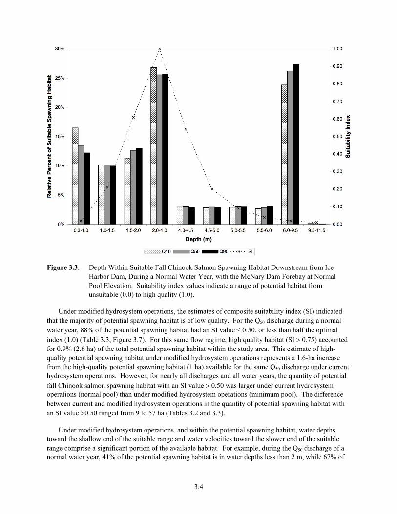
Figure 3.3. am Forebay at Normal

.7). For this same flow regime, high quality habitat (SI ! 0.75) accounted

nt al

ter depths toward the shallow end of the suitable range and water velocities toward the slower end of the suitable range comprise a significant portion of the available habitat. For example, during the Q50 discharge of a normal water year, 41% of the potential spawning habitat is in water depths less than 2 m, while 67% of

Depth Within Suitable Fall Chinook Salmon Spawning Habitat Downstream from Ice Harbor Dam, During a Normal Water Year, with the McNary DPool Elevation. Suitability index values indicate a range of potential habitat from unsuitable (0.0) to high quality (1.0).

Under modified hydrosystem operations, the estimates of composite suitability index (SI) indicated that the majority of potential spawning habitat is of low quality. For the Q50 discharge during a normal water year, 88% of the potential spawning habitat had an SI value d 0.50, or less than half the optimal index (1.0) (Table 3.3, Figure 3for 0.9% (2.6 ha) of the total potential spawning habitat within the study area. This estimate of high-quality potential spawning habitat under modified hydrosystem operations represents a 1.6-ha increase from the high-quality potential spawning habitat (1 ha) available for the same Q50 discharge under currehydrosystem operations. However, for nearly all discharges and all water years, the quantity of potentifall Chinook salmon spawning habitat with an SI value ! 0.50 was larger under current hydrosystem operations (normal pool) than under modified hydrosystem operations (minimum pool). The difference between current and modified hydrosystem operations in the quantity of potential spawning habitat withan SI value !0.50 ranged from 9 to 57 ha (Tables 3.2 and 3.3).

Under modified hydrosystem operations, and within the potential spawning habitat, wa

3.4

Figure 3.4. al

es indicate a range of potential habitat from unsuitable (0.0) to high quality (1.0).

elevation of Little Goose Dam forebay), o

r .

Velocity Within Suitable Fall Chinook Salmon Spawning Habitat Downstream from IceHarbor Dam, During a Normal Water Year, with the McNary Dam Forebay at NormPool Elevation. Suitability index valu

those areas contain water velocities less than 0.5 m s-1 (Figures 3.8 and 3.9). The change in hydrosystemoperations from normal to minimum pool elevation of McNary Dam forebay resulted in an increase in shallow water spawning habitat, and an increase in water velocities within the optimal range of 0.7–1.5 m s-1. Nevertheless, water velocity appears to be more of a limiting factor than water depth, as only 0.2% of the potential spawning habitat contains water velocities greater than 1.5 m s-1 (Figure 3.9). Nearly all of the potential spawning habitat with water velocities within the optimal range of 0.7–1.5 m s-1 is located within the navigation channel (Figure 3.10), which is largely comprised of low suitability water depths exceeding 5.0 m (Figures 3.8 and 3.11).

3.1.2 Lower Granite

Under the current hydrosystem operations (i.e., normal poolthe estimate of total potential fall Chinook salmon spawning habitat in the study area ranged from 86 t313 ha, depending on the discharge regime from Lower Granite Dam. The discharge representing the median hourly flow during the fall Chinook salmon spawning period (i.e., the Q50 flow) of a normal wateyear resulted in a potential spawning habitat estimate of 272 ha, or 50% of the total study area (Table 3.4)The quantity of potential spawning habitat increased as the discharge regime increased from low flow

3.5

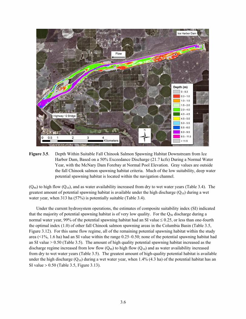
Figure 3.5. Depth Within Suitable Fall Chinook Salmon Spawning Habitat Downstream from Ice Harbor Dam, Based on a 50% Exceedance Discharge (21.7 kcfs) During a Normal Water Year, with the McNary Dam Forebay at Normal Pool Elevation. Gray values are outside

r

(Q90) to high f reased from dry to wet water years (Table 3.4). The greatest amount of potential spawning habitat is available under the high discharge (Q10) during a wet

rth

e 0.25–0.50; none of the potential spawning habitat had an SI value > 0.50 (Table 3.5). The amount of high quality potential spawning habitat increased as the

om low flow (Q90) to high flow (Q10) and as water availability increased from dry to wet water years (Table 3.5). The greatest amount of high-quality potential habitat is available

the fall Chinook salmon spawning habitat criteria. Much of the low suitability, deep watepotential spawning habitat is located within the navigation channel.

low (Q10), and as water availability inc

water year, when 313 ha (57%) is potentially suitable (Table 3.4).

Under the current hydrosystem operations, the estimates of composite suitability index (SI) indicated that the majority of potential spawning habitat is of very low quality. For the Q50 discharge during a normal water year, 99% of the potential spawning habitat had an SI value d 0.25, or less than one-fouthe optimal index (1.0) of other fall Chinook salmon spawning areas in the Columbia Basin (Table 3.5, Figure 3.12). For this same flow regime, all of the remaining potential spawning habitat within the study area (<1%, 1.6 ha) had an SI value within the rang

discharge regime increased fr

under the high discharge (Q10) during a wet water year, when 1.4% (4.3 ha) of the potential habitat has an SI value ! 0.50 (Table 3.5, Figure 3.13).

3.6

Figure 3.6. Velocity Within Suitable Fall Chinook Salmon Spawning Habitat Downstream from IcHarbor Dam, Based on a 50% Exceedance Discharge (21.7 kcfs) During a Normal Water Year, with the McNary Dam Forebay at Normal Pool Elevation. Gray values are outside the fall Chinook salmon spawning habitat criteria. Much of the potential spawning habitat with water velocities within the optimal range (0.7–1.5 m s-1) is locat

e

ed within the navigation channel.

ard the slower end of the suitable

range comprise a significant portion of the available habitat. For example, during the Q discharge of a

g

e

on spawning habitat in the study area ranged from 181 to 356 ha, depending on the discharge regime from Lower Granite Dam. The Q50 discharge during a normal water year resulted in a potential spawning habitat estimate of 327 ha, or 61% of the total study area (Table 3.4). This estimate of potential spawning habitat under modified hydrosystem operations repre-sents a 20% (55 ha) increase from the potential spawning habitat (272 ha) available for the same Q50

Under the current hydrosystem operations, and within the potential spawning habitat, water depthstoward the deeper end of the suitable range and water velocities tow

50

normal water year, 88% of the potential spawning habitat is in water depths greater than 6.0 m, while 64% of those areas contain water velocities less than 0.2 m s-1 (Figures 3.14 and 3.15). Water velocityappears to be more of a limiting factor than water depth, as less than 0.1% of the potential spawning habitat contains water velocities greater than 0.7 m s-1 (Figure 3.15). Nearly all of the potential spawninhabitat with the greatest water velocities available (>0.2 m s-1) is located where low-suitability water depths exceed 6.0 m (Figures 3.16 and 3.17). In much of the shallower lateral and mid-channel bar areas with more suitable water depths (2.0–4.0 m), water velocities are on the lower end of the suitability rang(0.1–0.2 m s-1) (Figures 3.16 and 3.17).

Under modified hydrosystem operations (i.e., minimum pool elevation of Little Goose Dam forebay), the estimate of total potential fall Chinook salm

3.7

Table 3.3. Suitability Index (SI) Summary of the Quantity and Relative Percentage of Potential Spawning Habitat at the Ice Harbor Dam Study Area Based on a Minimum Operating Pool Level at McNary Dam

Suitability Index 0.01-0.25 0.26-0.50 0.51-0.75 0.76-1.0

Discharge Regime

Water Year ha % ha % ha % ha %

Total Suitable

Area (ha) Q10 Dry 175.7 62.4 80.1 28.4 24.8 8.8 1.1 0.4 281.7

Normal 167.5 48.4 110.6 31.9 55.7 16.1 12.6 3.6 346.3 Wet 162.2 40.1 100.7 24.9 76.0 18.8 65.9 16.3 404.8

Q50 Dry 176.4 66.7 70.6 26.7 17.0 6.4 0.5 0.2 264.4 Normal 175.3 58.7 87.2 29.2 33.6 11.3 2.6 0.9 298.8 Wet 169.7 43.7 109.9 28.3 68.8 17.7 40.1 10.3 388.5

Q90 Dry 174.6 72.2 56.3 23.3 10.5 4.3 0.6 0.2 242.0 Normal 175.2 61.5 82.1 28.8 26.0 9.1 1.4 0.5 284.7 Wet 167.4 48.2 111.0 31.9 56.0 16.1 13.1 3.8 347.5

Figure 3.7. Fall Chinook Salmon Spawning Habitat Suitability Downstream from Ice Harbor Dam, Based on a 50% Exceedance Discharge (21.7 kcfs) During a Normal Water Year, with the McNary Dam Forebay at Minimum Pool Elevation. Suitability index values indicate a range of potential habitat from unsuitable (0.0) to high quality (1.0).

3.8

discharge u er current hydrosystem operations (Table 3.4). An increase in the quantity of potentialtat was observed for all discharges and water years as the pool elevation of Little Goose as lowered from norma

nd spawning habiDam forebay w l to minimum pool elevation. The corresponding estimates from the Q50 discharge resulted in the potential spawning habitat area increasing for all water years, with the percentage increase ranging 14%–73% (Table 3.4 low (Q90) during a dry water year, the potential spawning habit n d uble ttle oos eba n

vation (Table 3.4).

er modified hy te r io e e te f dex indicthat the majo o sp g ow qu F Q norm l water 96. in ita h SI d .2 les one-fourth the optimal in .0 gure 3.18). F re , 3 1% ha) e reing ntial g t w t s are a SI w th ra .25 0; 0.(1.1 ha) of th t S e 0 able 3.6). Th ma potespawning habitat within the SI range 0.25–0. esents a 9.5-ha increase under modified hydrosys m operations fro po sp ng a va f th e Q isc ar der ent hydrosystem n le n 3.6). For c rg d all water yea he q ity opotential fall Chinook s in h i S a 0.5 l g er m fied hydrosystem operations (minimum pool) than under current hydrosystem operations (normal pool). The difference between current and modified hydrosystem operations in the quantity of potential spawning habitat with an SI value ! 0.50 ranged from 0.2 to 15.5 ha (Tables 3.5 and 3.6).

Under modified hydrosystem operations, and within the potential spawning habitat, water depths toward the deeper end of the suitable range and water velocities toward the slower end of the suitable range continue to comprise a significant portion of the available habitat. For example, during the Q50 discharge of a normal water year, 70% of the potential spawning habitat is in water depths greater than 6.0 m, while 53% of those areas contain water velocities less than 0.2 m s-1 (Figures 3.19 and 3.20). The change in hydrosystem operations from normal to minimum pool elevation of Little Goose Dam forebay resulted in an increase in shallower water spawning habitat and an increase in water velocities within the range of 0.2–0.5 m s-1. Nevertheless, water velocity continues to be more of a limiting factor than water depth, as less than 0.1% of the potential spawning habitat contains water velocities greater than 0.7 m s-1 (Figure 3.20). Nearly all of the potential spawning habitat with the greatest water velocities available (>0.2 m s-1) is located where low-suitability water depths exceed 6.0 m (Figures 3.22 and 3.23). In much of the shallower lateral and mid-channel bar areas with more suitable water depths (2.0–4.0 m), water velocities are on the lower end of the suitability range (0.1–0.2 m s-1) (Figures 3.22 and 3.23).

). Under the low fat more tha o d when Li G e Dam for y was lowered from ormal

to minimum pool ele

Und drosys m ope at ns, th stima s o composite suitability in (SI) ated rity of p tential awnin habitat remains l ality. or the 50 discharge during a

a year, 6% of the potential spawn g hab t ad an value 0 5, or s thandex (1 ) (Table 3.6, Fi or this same flow gime . (10 of th main-

p teo spawnine potential spawning habit

habita ithin he tudy a had n value ithin e nge 0 –0.5 3% a had an I valu > .50 (T is esti te of ntial

75 repr tem the tential awni h bitat a ilable or e sam 50 d h ge un curr

operatio s (Tab s 3.5 a d all dis ha es an rs, t uant f salmon pawn g abitat w th an I v lue ! 0 was ar er und odi

3.9

Figure 3.8. Depth Within Suitable Fall Chinook Salmon Spawning Habitat Downstream from Ice Harbor Dam, During a Normal Water Year, with the McNary Dam Forebay at Minimum Pool Elevation. Suitability index values indicate a range of potential habitat from unsuitable (0.0) to high quality (1.0).

3.10

Figure 3.9. Velocity Within Suitable Fall Chinook Salmon Spawning Habitat Downstream from IcHarbor Dam, During a Normal Water Year, with the McNary Dam Forebay at Minimum Pool Elevation. Suitability index values indicate a range of potential habitat from unsuitable (0.0) to high quality (1.0).

e

3.11

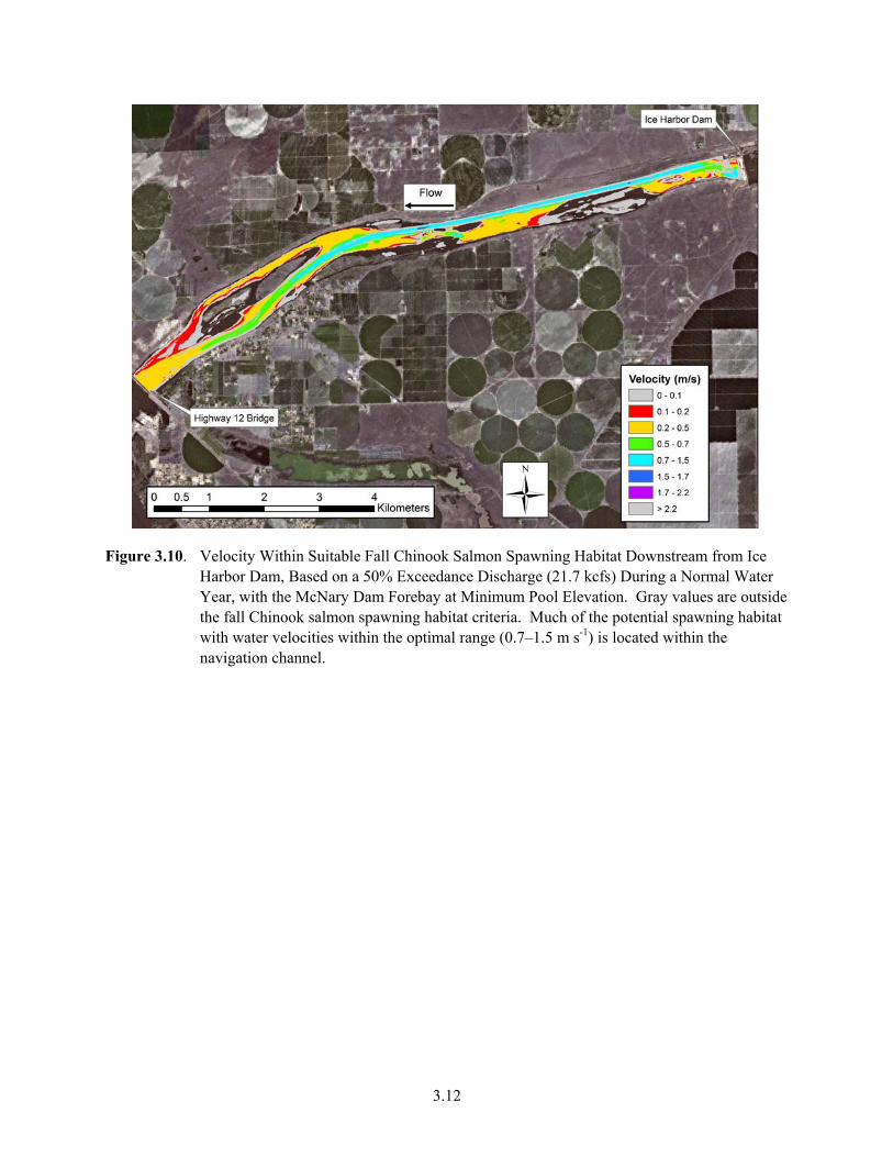
Figure 3.10. Velocity Within Suitable Fall Chinook Salmon Spawning Habitat Downstream from Ice Harbor Dam, Based on a 50% Exceedance Discharge (21.7 kcfs) During a Normal Water

e t

Year, with the McNary Dam Forebay at Minimum Pool Elevation. Gray values are outsidthe fall Chinook salmon spawning habitat criteria. Much of the potential spawning habitawith water velocities within the optimal range (0.7–1.5 m s-1) is located within the navigation channel.

3.12

Figure 3.11. Depth Within Suitable Fall Chinook Salmon Spawning Habitat Downstream from Ice Harbor Dam, Based on a 50% Exceedance Discharge (21.7 kcfs) During a Normal Water Year, With the McNary Dam Forebay at Minimum Pool Elevation. Gray values are outside the fall Chinook salmon spawning habitat criteria. Much of the low suitability, deep water potential spawning habitat is located within the navigation channel.

Table 3.4. Quantity and Relative Percentage of Potential Spawning Habitat for Each Discharge Scenario at the Lower Granite Dam Study Area

Q10 Q50 Q90 Pool Level Water Year ha % ha % ha %

Dry 289.7 54.0 239.0 44.6 180.7 33.7 Normal 346.7 64.6 327.1 61.0 307.8 57.4 Minimum

Pool Wet 355.9 66.2 354.4 66.0 347.7 64.8

Dry 201.0 36.9 138.2 25.3 86.1 15.8

Normal 303.1 55.6 271.6 49.8 204.4 37.5 Normal Pool

Wet 312.7 57.3 311.3 57.1 301.5 55.3

3.13

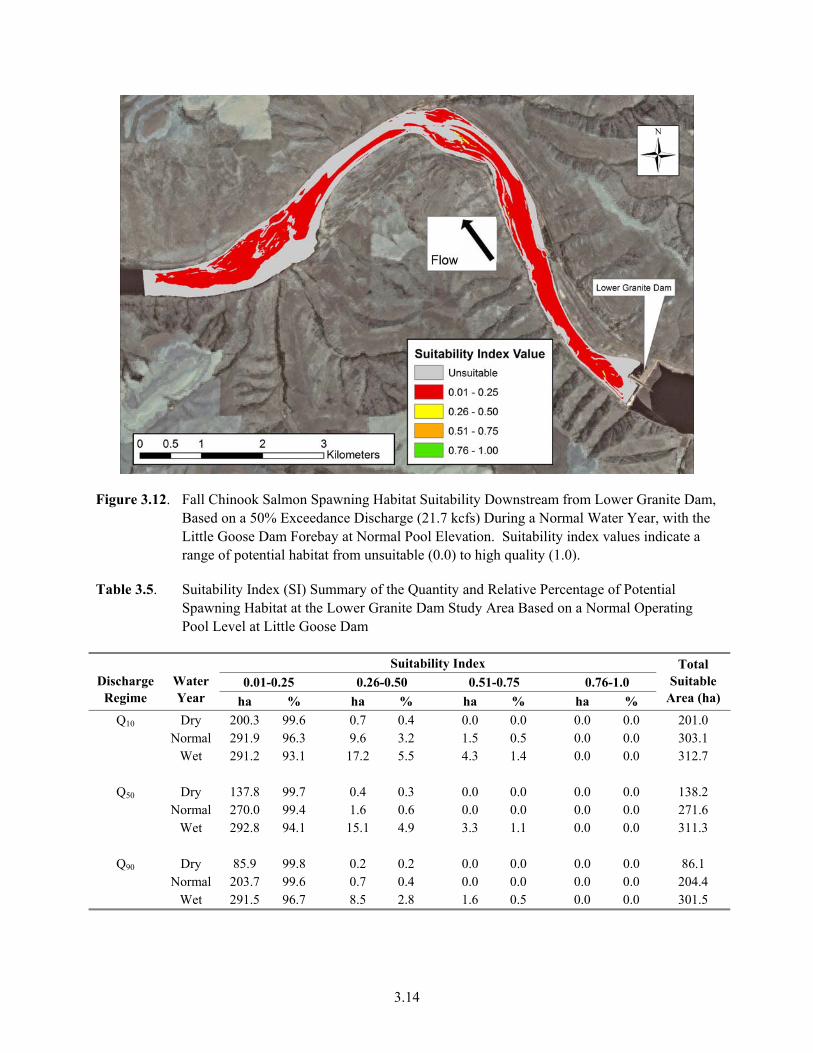
Figure 3.12. Fall Chinook Salmon Spawning Habitat Suitability Downstream from Lower Granite DBased on a 50% Exceedance Discharge (21.7 kcfs) During a Normal Water Year, with the Little Goose Dam Forebay at Normal Pool Elevation. Suitability index values indicatrange of potential habitat from unsuitable (0.0) to high quality (1.0).

Suitability Index (SI) Summary of the Quantity and Relative Percentage of Pote

am,

e a

Table 3.5. ntial g

Suitability Index

Spawning Habitat at the Lower Granite Dam Study Area Based on a Normal OperatinPool Level at Little Goose Dam

0.01-0.25 0.2 50 -0.75 0.76-16-0. 0.51 .0 D Wa

Year % ha % ha % a

Total Suitable

Area (ha) ischarge Regime

ter ha h %

Q10 Dry 3 99 7 0.4 0.0 0 2 200. .6 0. 0.0 0. 0.0 01.0 Normal 1.9 96 6 3.2 0. 0 3 Wet 1.2 93.1 17.2 5.5 4 1.4 0 0 31 7

Dry 8 99 4 0.3 0.0 0 1Normal 0.0 99 6 0.6 0. 0 2

Wet 292.8 94.1 15.1 4.9 3.3 1.1 0.0 0.0 311.3

Q90 Dry 85.9 99.8 0.2 0.2 0.0 0.0 0.0 0.0 86.1 Normal 203.7 99.6 0.7 0.4 0.0 0.0 0.0 0.0 204.4 Wet 291.5 96.7 8.5 2.8 1.6 0.5 0.0 0.0 301.5

29 .3 9. 1.5 5 0. 0.0 03.1 29 .3 0. 0. 2.

Q50

137. .7 0. 0.0 0. 0.0 38.2

27 .4 1. 0.0 0 0. 0.0 71.6

3.14

Figure 3.13. Fall Chinook Salmon Spawning Habitat Suitability Downstream from Lower Granite Dam, Based on a 10% Exceedance Discharge (52.0 kcfs) During a Wet Water Year, with the Little Goose Dam Forebay at Normal Pool Elevation. Suitability index values indicate a range of potential habitat from unsuitable (0.0) to high quality (1.0).

3.15

Figure 3.14. Forebay at Normal

Pool Elevation. Suitability index values indicate a range of potential habitat from unsuitable (0.0) to high quality (1.0).

Depth Within Suitable Fall Chinook Salmon Spawning Habitat Downstream from Lower Granite Dam, During a Normal Water Year, with the Little Goose Dam

3.16

Figure 3.15. Velocity Within Suitable Fall Chinook Salmon Spawning Habitat Downstream from Lower Granite Dam, During a Normal Water Year, with the Little Goose Dam Forebay at Normal Pool Elevation. Suitability index values indicate a range of potential habitaunsuitable (0.0) to high quality (1.0).

t from

3.17

Figure 3.16. Depth Within Suitable Fall Chinook Salmon Spawning Habitat Downstream from Lower Granite Dam, Based on a 50% Exceedance Discharge (21.7 kcfs) During a Normal Water Year, with the Little Goose Dam Forebay at Normal Pool Elevation. Gray values are outside the fall Chinook salmon spawning habitat criteria.

3.18

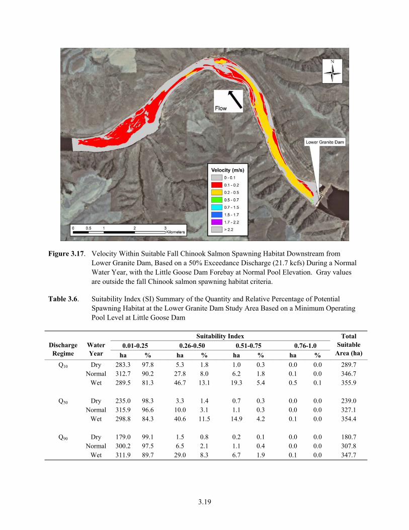
Figure 3.17. Velocity Within Suitable Fall Chinook Salmon Spawning Habitat Downstream from Lower Granite Dam, Based on a 50% Exceedance Discharge (21.7 kcfs) During a Normal Water Year, with the Little Goose Dam Forebay at Normal Pool Elevation. Gray valuare outside the fall Chinook salmon spawning habitat criter

es ia.

Table 3.6. Suitability Index (SI) Summary of the Quantity and Relative Percentage of Potential Spawning Habitat at the Lower Granite Dam Study Area Based on a Minimum Operating Pool Level at Little Goose Dam

Suitability Index 0.01-0.25 0.26-0.50 0.51-0.75 0.76-1.0 Discharge

Regime Water Year ha % ha % ha % ha %

Total Suitable

Area (ha)

Q10 Dry 283.3 97.8 5.3 1.8 1.0 0.3 0.0 0.0 289.7 Normal 312.7 90.2 27.8 8.0 6.2 1.8 0.1 0.0 346.7 Wet 289.5 81.3 46.7 13.1 19.3 5.4 0.5 0.1 355.9

Q50 Dry 235.0 98.3 3.3 1.4 0.7 0.3 0.0 0.0 239.0 Normal 315.9 96.6 10.0 3.1 1.1 0.3 0.0 0.0 327.1 Wet 298.8 84.3 40.6 11.5 14.9 4.2 0.1 0.0 354.4

Q90 Dry 179.0 99.1 1.5 0.8 0.2 0.1 0.0 0.0 180.7 Normal 300.2 97.5 6.5 2.1 1.1 0.4 0.0 0.0 307.8 Wet 311.9 89.7 29.0 8.3 6.7 1.9 0.1 0.0 347.7

3.19

Figure 3.18. Fall Chinook Salmon Spawning Habitat Suitability Downstream from Lower Granite Based on a 50% Exceedance Discharge (21.7 kcfs) During a Normal Water Year, with the Little Goose Dam Forebay at Minimum Pool Elevation. Suitability index values indicate range of potential habitat from unsuitable (0.0) to high quality

Dam,

a (1.0).

3.20

Figure 3.19. m Forebay at

Minimum Pool Elevation. Suitability index values indicate a range of potential habitat from unsuitable (0.0) to high quality (1.0).

Depth Within Suitable Fall Chinook Salmon Spawning Habitat Downstream from Lower Granite Dam, During a Normal Water Year, with the Little Goose Da

3.21

Figure 3.20. Velocity Within Suitable Fall Chinook Salmon Spawning Habitat Downstream from Lower Granite Dam, During a Normal Water Year, with the Little Goose Dam ForeMinimum Pool Elevation. Suitability index values indicate a range of potential habitat from unsuitable (0.0) to high quality (1.0).

bay at

3.22

Figure 3.21. Depth Within Suitable Fall Chinook Salmon Spawning Habitat Downstream from Lower Granite Dam, Based on a 50% Exceedance Discharge (21.7 kcfs) During a Normal Water

re Year, with the Little Goose Dam Forebay at Minimum Pool Elevation. Gray values aoutside the fall Chinook salmon spawning habitat criteria.

3.23

Figure 3.22. Velocity Within Suitable Fall Chinook Salmon Spawning Habitat Downstream from Lower Granite Dam, Based on a 50% Exceedance Discharge (21.7 kcfs) During a Normal Water Year, with the Little Goose Dam Forebay at Minimum Pool Elevation. Gray valueare outside the fall Chinook salmon spawning habitat criter

s ia.

3.24

3.2 Channel Morphology

3.2.1 Reference Locations

Results from the analyses of thalweg points in the Wanapum study area indicated that spawning locations were more likely to occur near riffle crests than elsewhere along the longitudinal profile. The cross-tabulation analysis indicated that spawning habitat use was dependent on bed form type (F2 = 10.1, df = 3, P = 0.02). The upstream and downstream sides of riffle crests contained 26% and 42% of the spawning habitat use, respectively (Table 3.7). The remaining spawning habitat use occurred on the upstream (32%) ends of pools, while no spawning occurred on the downstream ends of pools.

Table 3.7. Summary Frequency Table of Four Bedform Types in Fall Chinook Salmon Spawning and Non-Spawning Areas. Points along the longitudinal profile were categorized as being on the upstream (proximal) or downstream (distal) side of a riffle crest or pool bottom. The data included all thalweg points in spawning areas (N = 19), and a random sample of thalweg points in non-spawning areas (N = 20). The cross tabulation analysis indicated that spawning habitat use was dependent on bedform type (F2 = 10.1, df = 3, P = 0.02).

Riffle Proximal Riffle Distal Pool Proximal Pool Distal Spawning Count 5 8 6 0

Count Frequency

Frequency 26% 42% 32% 0% Non-spawning

6 5 3 6 30% 25% 15% 30%

The majority of spawning areas occurred at elevations in the transition zone between riffle and pool bedforms. The median riffle proximity index (RPI) for all spawning areas was 0.51, which is 51% of the elevation difference between the nearest riffle crest and pool bottom (Figure 3.23). The Barge Dock Bar spawning locations (typically containing over 90% of the fall Chinook salmon redds in the area) are situated exclusively on a riffle bedform, with a median RPI = 0.54 (Figure 3.24). Results from the Wald-Wolfowitz runs test indicated that the mean RPI in the Barge Dock Bar spawning area was significantly larger than the mean RPI in non-spawning areas (z = -2.08, P = 0.04) (Figure 3.25).

Within the Wanapum study area, three riffle bedforms were identified (Figure 3.26). All of the bedforms are large, with 15 m of riverbed elevation change along the thalweg over the length of the study area. The slopes of individual bedforms ranged from 0.004 to 0.01 (Table 3.8). The bedform slopes on the upstream and downstream side of the Barge Dock Bar (rkm 666.5–667.5) are 0.01 and 0.008, respectively. The dimensions of these bedforms are similar to those of the other fall Chinook salmon spawning habitat reference locations in the Columbia and Snake rivers. The tolerance value T (used in the bedform differencing technique to distinguish bedforms from local undulations of smaller magnitude in the riverbed profile) at the reference locations ranges from 2.5 m to 3.9 m (Table 3.8). The bedform slopes in the Hanford Reach of the Columbia River range from 0.002 to 0.009, while those in the Hells Canyon Reach of the Snake River are much larger, ranging from 0.001 to 0.156 (Table 3.8).

3.25

Figure 3.23. Riffle Proximity Index (RPI) for Fall Chinook Salmon Spawning and Non-Spawning Locations. The boxplots indicate the median (small box), surrounded by the 25th and 75th percentiles (large box), and extend to the 10th and 90th percentiles (whiskers) of observed values.

f the e

h

Within the Wanapum study area, 93% of the fall Chinook salmon spawning areas were located at cross sections with large width-to-depth ratios (Fd*1 and Fd*2, Table 16). The majority (75%) of the cross sections containing spawning areas were asymmetrical from bank to bank (Fd*1), with part otransect containing a shallow bar that deepened into a V-shaped deep thalweg. A remaining 18% of thcross sections containing spawning areas were symmetrical from bank to bank, with large width-to-deptratios (Fd*2) (Table 3.9).

3.26

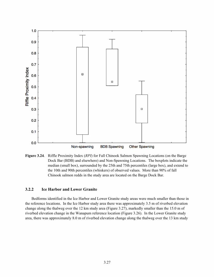
Figure 3.24. Riffle Proximity Index (RPI) for Fall Chinook Salmon Spawning Locations (on the BaDock Bar (BDB) and elsewhere) and Non-Spawning Locations. The boxplots indicate the median (small box), surrounded by the 25th and 75th percentiles (large box), and extend to the 10th

rge

and 90th percentiles (whiskers) of observed values. More than 90% of fall Chinook salmon redds in the study area are located on the Barge Dock Bar.

.2.2 Ice Harbor and Lower Granite

e in

3

Bedforms identified in the Ice Harbor and Lower Granite study areas were much smaller than thosthe reference locations. In the Ice Harbor study area there was approximately 3.5 m of riverbed elevationchange along the thalweg over the 12 km study area (Figure 3.27), markedly smaller than the 15.0 m of riverbed elevation change in the Wanapum reference location (Figure 3.26). In the Lower Granite study area, there was approximately 8.0 m of riverbed elevation change along the thalweg over the 13 km study

3.27

Figure 3.25. Estimates of the Mean Riffle Proximity Index (RPI) were Significantly Larger in Fall

d on

area (Figure 3.28). There was so little topographic relief along the thalweg of the Ice Harbor study area pecific to the study area was too small (1.1 m) to identify

any bedforms. With T values applied from the Lower Granite study area (2.1 m) and Hanford Reach

and Hanford Reach reference locations (Tables 3.8 nd Table 3.10).

The cross-section channel morphology at the Ice Harbor study area was very different from that at the Lower Granite study area. Within the Ice Harbor study area, 86% of the sampled cross sections contained large width-to-depth ratios (Fd*1 and Fd*2, Table 3.11). The majority (73%) of the Ice Harbor sampled

Chinook Salmon Spawning Locations on the Barge Dock Bar (BDB) that in Non-Spawning Locations (P = 0.04). The boxplots indicate the mean (small box), surrounded by the standard error of the mean (large box), and extend to the 95% confidence interval (whiskers). More than 90% of fall Chinook salmon redds in the study area are locatethe Barge Dock Bar.

that the calculated bedform tolerance value (T) s

reference location (2.5 m), there were 2 and 1 riffle crests, respectively, identified in the Ice Harbor study area (Figure 3.27). The local bedform slope of these riffles was much smaller than those in the reference locations, with the maximum bedform slope in the Ice Harbor study area being less than the minimum bedform slope in the reference locations (Tables 3.8 and 3.10). Local bedform slopes in the Lower Granite study area were similar to those of the reference locations, with mean and maximum slopes larger in the Lower Granite study area than in the Wanapuma

3.28

Figure 3.26. Pool and Riffle Bedforms (�) Along the Longitudinal Riverbed Profile Within the Wanapum Study Area Located in the Columbia River. Most (68%) fall Chinook salmon

Table 3.8.

tween adjacent riffle crests and pool bottoms is

spawning ({) occurred on riffle bedforms.

Riverbed Morphology Characteristics of Reference Fall Chinook Salmon Spawning Areasin the Columbia River (Wanapum and Hanford Reach) and Snake River (Hells Canyon). The tolerance value (T, m) is used in the bedform differencing technique to distinguish bedforms (riffle crests and pool bottoms) from local undulations of small magnitude in the riverbed profile. The change in elevation beidentified as bedform slope (unitless). Reach slope (unitless) indicates the change in riverbed elevation throughout the identified river reach.

Bedform Slope Location T (m) Min Mean Max Reach Slope Wanapum 2.8 0.004 0.007 0.010 0.0002 Hanford Reach 2.5 0.002 0.004 0.009 0.0004 Hells Canyon 3.9 0.001 0.040 0.156 0.0020(a)

0.0010(b) 0.0007(c)

b(a, ,c) Upper, middle, and lower reach, respectively. See Hanrahan (2007b) for details.

3.29

Table 3.9. Classification Summary of Sampled Cross Sections in the Wanapum Study Area

Fd* Category Count Relative Frequency (%) % Spawning 1 44 52 75 2 22 26 18 3 8 9 <4 4 11 13 <4

Figure 3.27.

(2.1 m, �) and the Hanford Reach reference location (2.5 m, z).

mmetrical from bank to bank (Fd*1), with part of the transect containing a shallow deep thalweg. The next mo frequent cross ction type in the Ice

y area was symmetrical from b , with idth-to-d tios (Fd*2thin the Lo ranite stud , only 18% sampled cross sections contained large

ratios (Fd*1 Fd*2, Table 3.8). The maj 2%) of th r Granite cross sections were symmetrical, narrow, and relatively unifor ly deep (Fd*4) (Table 3.8). The cross section channel mo hology at the Ice Harbor study area was very similar to tha of the Wan

Pool and Riffle Bedforms Along the Longitudinal Riverbed Profile Within the Ice Harbor Study Area Located in the Snake River. Bedforms were identified based on tolerancevalues (T) calculated from the Lower Granite study area

cross sections were asybar that deepened into a V-shaped st seHarbor stud ank to bank large w epth ra ) (Table 3.8). Wi wer G y area of thewidth-to-depth and ority (8 e Lowe sampled

mrp t apum

reference location (Table 3.9).

3.30

Figure 3.28. Pool and Riffle Bedforms Along the Longitudinal Riverbed Profile Within the Lower Granite Study Area Located in the Snake River. Bedforms were identified based on tolerance values (T) calculated from the Lower Granite study area (2.1 m, �) and the Hanford Reach reference location (2.5 m, z).

Table 3.10. Riverbed Morphology Characteristics of the Ice Harbor and Lower Granite Study Areas. The tolerance value (T, m) is used in the bedform differencing technique to distinguish

s is

he identified river reach.

bedforms (riffle crests and pool bottoms) from local undulations of small magnitude in the riverbed profile. The change in elevation between adjacent riffle crests and pool bottomidentified as bedform slope (unitless). Reach slope (unitless) indicates the change in riverbed elevation throughout t

Bedform Slope Location T (m) Min Mean Max Reach Slope Ice Harbor 1.1(a) 0.0002 2.1(b) 0.0005 0.001 0.002 2.5(c) 0.001 0.001 0.001 Lower Granite 2.1(b) 0.002 0.009 0.024 0.0003 2.5(c) 0.002 0.007 0.018 (a) The calculated bedform tolera

bedforms. nce value (T) for the Ice Harbor study area was too small to identify any

(b) Bedform slopes calculated from bedforms identified with the Lower Granite T value of 2.1 m. (c) Bedform slopes calculated from bedforms identified with the Hanford Reach T value of 2.5 m.

3.31

3.32

Table 3.11. Geomorphic Classification Summary of Sampled Cross Sections in the Ice Harbor and Lower Granite Study Areas

Study Area Fd* Category Count Relative Frequency (%) Ice Harbor 1 88 73

2 15 13 3 3 <3 4 14 <12

Lower Granite 1 1 <1 2 21 18 3 0 0 4 98 82

4.0 Discussion

The results of this study indicate that a majority of the or an reas contai ll Chinook salmon spawning habitat under existing hydrosystema large majority of the currently available fall Chinook salmon spawning habitat in the Ice Harbor and Lower Granite study areas is of low qu y. The potential fo creasing, through ifications to hydrosystem operations (i.e., minimum ol elevation of the t downstream dam e quantity or quality of fall Chinook salmon spawning habitat appears to be limited. Estimates of the amount of poten k salmon spawning habitat in the Ice Harbor study area decreased as the McNary Dam forebay elevation was lowered fr normal to minimum ol elevation. Esti s of the amount of potential fall Chinook salmon spawning habitat in the Lower Granite study area increased as the Little Goose Dam elevation was lowered from normal to m um pool elevation; however, 97% of the vailable habitat was categorized within the range of lowest quality. In both the Ice Harbor and Lower

Granite study areas, water velocity appears to be more of a limiting factor for fall Chinook salmon pawning habitat than water depth, with both study areas dominated by low-magnitude water velocity.

The geomorphic suitability of both study areas appears to be compromised for fall Chinook salmon spawning habitat, with the Ice Harbor study area lacking significant bedforms along the longitudinal thalweg profile and the Lower Granite study area lacking cross-sectional topographic diversity.

The results from the modeling of potential fall Chinook spawning habitat availability suggest that the primary limiting physical factors in the Ice Harbor and Lower Granite study areas are the hydraulic characteristics of water depth and velocity. The large amount of shallow water fall Chinook salmon spawning habitat in the Ice Harbor study area is considered low quality, and becomes dewatered or outside the fall Chinook salmon spawning suitability range when the McNary Dam forebay elevation is lowered to minimum pool. On the contrary, much of the Lower Granite study area contains deep water near the upper end of the fall Chinook salmon spawning habitat suitability range, and this habitat remains relatively deep even when the Little Goose forebay elevation is lowered to minimum pool.

Some researchers have suggested that water depth alone does not limit spawning habitat use by Chinook salmon (Chapman et al. 1986). While this may be true, studies of deep water fall Chinook spawning in the Columbia River have not documented redds deeper than approximately 11 m (Chapman et al. 1986; Swan 1989), and researchers in the Snake River noted that no fall Chinook redds were deeper than 6.5 m, even though searches for redds in suitable habitat frequently occurred in deeper water (Groves and Chandler 1999). One reason may be that visual cues related to mate recognition and substrate differentiation would be reduced at depths greater than light penetration levels (Geist and Dauble 1998). Whether the lack of documented redds in water depths greater than 11 m is a function of habitat selection or sampling methodology is unknown. Indeed, Swan (1989) concluded that up to 80% of fall Chinook spawning in the Hanford Reach may occur in water too deep to sample by aerial observation.

Regardless of water depths beyond those within the suitability criteria, areas estimated as potential spawning habitat are dominated by water depths on the deeper end of the suitable range and water velocities toward the slower end of the suitable range. In contrast, within one spawning area of the Hanford Reach, 80% of the habitat within fall Chinook redd clusters contained water velocities of 1.4–2.0 m s-1 and water depths of 2.0–4.0 m (Geist et al. 2000). Additional data from Hanford Reach redds (N = 230, PNNL, unpublished data) indicate that only 10.5% of the redds were constructed in water depths > 4.0 m, while 29% of those redds were located in water velocities d0.75 m s-1. Conversely, 43%

Ice Harb d Lower Granite study an suitable fa operations. However,

alit r in mod po nex ), th

tial fall Chinooom po mate

forebay inima

s

4.1

of the redds were in water depths redds were in areas of the water velocities from of 0.75–1.25 m ke River were observed in average

-1

large .

ook ea

.

longitudinal riverbed profile. The results from the Wanapum reference reach indicate that most fall

re s in

the

rate these

re ed in riffles

c

between 2–3 m, and 58% of the s-1. Fall Chinook redds in the Sna

water depth of 2.8 m and average water velocity of 1.1 m s . In deep water fall Chinook spawning habitat in the Columbia River, near bottom water velocities at redds averaged 1.75 m s-1 (Swan 1989), and0.93–1.13 m s-1 over a range of discharges (Chapman et al. 1986).

Results from the hydrodynamic modeling indicate that the lack of water velocity of sufficiently magnitude is more of a limiting factor in the Lower Granite study area than the Ice Harbor study areaFor all the modeled scenarios in the Lower Granite study area, less than 1% of the suitable fall Chinsalmon spawning habitat contained water velocity greater than 0.7 m s-1. While the Ice Harbor study arcontains more potential fall Chinook salmon spawning habitat with water velocity within the optimal range of 0.7–1.5 m s-1, nearly this entire higher velocity habitat is located within the navigation channelThe fall Chinook salmon spawning habitat suitability of these higher-velocity areas is compromised, as the navigation channel contains deep-water habitat beyond the optimal water depths and lacks the longitudinal bedforms along the thalweg typically associated with fall Chinook salmon spawning (Hanrahan 2007a).

Research from the Wanapum reference reach, and elsewhere within the Columbia River basin, indicates that fall Chinook salmon spawning is associated with significant bedforms along the

Chinook salmon spawning occurs in riffles and at a vertical location near the riffle crest elevation. This location corresponds to the transitional area between pools and riffles, an important habitat area whemany salmon species tend to prefer to spawn (Bjornn and Reiser 1991). Owing to localized variationsediment transport rates, these transitional areas are depositional zones that are often associated withformation of bars (lateral, midchannel, point) and islands. Previous researchers have observed salmon spawning locations to be associated with depositional ‘response’ reaches (Montgomery et al. 1999; Moiret al. 2004), especially near the upstream end of bars and islands (Dauble and Watson 1997; Geist and Dauble 1998; Coulombre-Pontbriand and Lapointe 2004). The results reported here corroboearlier findings and quantify the location along the longitudinal profile where Chinook salmon spawning occurs. By quantifying the two-dimensional location (vertical and longitudinal) of salmon spawningareas, these findings complement previous planform mapping of fall Chinook salmon spawning areas. Dauble and Geist (2000) reported that Chinook salmon spawning in the Hanford Reach of the Columbia River and the Hells Canyon Reach of the Snake River was associated with the presence of bars that were mapped along 1.6-km river segments. Based on planform mapping of morphological channel types (bar, fan, glide, pool, rapid, riffle), Groves and Chandler (2002) observed that most fall Chinook salmon spawning in the Snake River occurred in riffles. Hanrahan (2007) quantified the relationship between Snake River fall Chinook salmon spawning and channel morphology, reporting that 84% of the spawning occurred in riffles and at a vertical location within 80% of the riffle crest elevation. Similar findings wereported for Hanford Reach fall Chinook salmon spawning areas, where most spawning occurrand at a vertical location within 80% of the riffle crest elevation (Geist et al. 2006).

Although channelbed substrate is not a primary limiting factor of fall Chinook spawning habitatwithin the study areas, it is likely a contributing factor due largely to hydraulic conditions rather than grain-size composition. The hydraulic conditions within the potential spawning areas, especially in the Lower Granite study area, are likely not sufficient to initiate channelbed movement, or to sustain periodisediment transport and deposition necessary to maintain a substrate matrix dominated by coarse gravel and cobble with a relative small percentage of sand and finer material (i.e., typical salmonid spawning

4.2

4.3

h unit. lity

ant components in determining habitat quality of spawning sites.

d

reas 7;

d Dauble 1998; Groves and Chandler 1999; Geist et al. 2000). Collectively, these data best represent the entire range of conditions within which fall Chinook salmon spawn within the

less,

ns

substrate). Our substrate surveys adequately characterized the overall grain-size distribution of eacgeomorphic unit, but we did not map small-scale changes in substrate composition within a samplingIn general, site-scale evaluations of geomorphic competency (e.g., sediment transport), substrate qua(e.g., permeability, %fines), and surface water–groundwater interactions (e.g., riverbed pore water velocity) were not completed for this study, all of which are import

Uncertainties in our estimates of potential habitat arise from the suitability index (SI) curves we usefor calculating suitability of a spawning area. The suitability criteria for depth, velocity, substrate, and channelbed slope were compiled for the fall Chinook salmon spawning areas of the Wanapum reference reach, which represents a tailwater habitat physical setting similar to that of the Ice Harbor and Lower Granite study areas. To create the depth and velocity SI curves, we used data from more than 62 redds and 47,000 spawning habitat cells in the Wanapum reference reach. These data were evaluated for consistency with depth and velocity data from studies of all major fall Chinook salmon spawning awithin the mainstem Columbia and Snake rivers (Chapman et al. 1986; Swan 1989; Geist et al. 199reviewed in Geist an

mainstem Columbia and Snake rivers. While the SI curves represent the best available to date, the proportion of fall Chinook selected spawning areas with these microhabitat characteristics (i.e.,depth/velocity combinations) relative to the total availability of microhabitat is not known. Neverthewe believe the suitability index modeling produced estimates of potential spawning habitat within acceptable ranges.

While approximately 65% and 50% of the Ice Harbor and Lower Granite study areas, respectively, contain suitable fall Chinook salmon spawning habitat, it is very unlikely that most of this habitat wouldbe used, even if adult escapement were increased considerably. Estimating the redd capacity of a river reach based on potentially suitable habitat leads to a high degree of uncertainty. Much of the variabilityin habitat and capacity estimates may result from a general lack of understanding of the habitat conditioinfluencing fall Chinook spawning. Observations from studies in the Columbia and Snake rivers indicate that spawning fall Chinook salmon utilize a relatively small proportion of seemingly suitable habitat within a contiguous area (Swan 1989; Dauble and Watson 1990, 1997; Geist and Dauble 1998; Geist et al. 2000; Visser 2002). Research from the Hanford Reach of the Columbia River indicates that fall Chinook salmon spawn in distinct clusters within areas predicted by habitat models, or other methods, to be suitable (Dauble and Watson 1997; Geist et al. 2000; Visser 2002). Indeed, fall Chinook redds have been observed aggregated in clusters, even though apparently suitable spawning habitat was widely distributed (Dauble and Watson 1990). To account for proportional use of suitable habitat, previous estimates of redd capacity considered that only 5–30% of suitable fall Chinook salmon habitat would actually be used (Hanrahan et al. 2004; Geist et al. 2006).

5.0 Conclusions

The modifications to hydroelectric dam operations that were evaluated in this study are unlikely to increase the quantity of available fall Chinook salmon spawning habitat in the Ice Harbor and Lower Granite study areas. Lowering the McNary Dam forebay elevation from normal pool to minimum pool will result in a net loss of available fall Chinook salmon spawning habitat in the Ice Harbor study area, as

e

thin

he

d

not such modifications could increase the quantity of available fall Chinook

formerly suitable habitat becomes dewatered. Lowering the Little Goose Dam forebay elevation from normal pool to minimum pool will result in a small net increase in available fall Chinook salmon spawning habitat in the Lower Granite study area. However, the modest increase in available habitat in the Lower Granite study area should be tempered by the finding that 81–99% of this habitat (dependingon discharge regime and water year type) is characterized as being of the lowest quality available. Whilthe change in hydroelectric dam operations may elicit some improvement in hydraulic conditions withe study areas, the geomorphic suitability of both study areas appears to be compromised for fall Chinook salmon spawning habitat, with the Ice Harbor study area lacking significant bedforms along tlongitudinal thalweg profile and the Lower Granite study area lacking cross-sectional topographic diversity.

To increase the quantity of available fall Chinook salmon spawning habitat in the Ice Harbor anLower Granite study area, modifications to hydroelectric dam operations beyond those evaluated in this study likely would be necessary. Modifications may include operational and structural changes, such as lowering downstream dam forebay elevations to less than minimum pool. There is a large amount of uncertainty as to whether orsalmon spawning habitat in the Ice Harbor and Lower Granite study area. The results from this study provide some certainty that the quantity and quality of fall Chinook salmon spawning habitat within the lower Snake River are not likely to be increased within the existing hydroelectric dam operations.

5.1

6.0 References

57 FR 14653). April 22, 1992. “Endangered and Threatened Species; Threatened Status for Snake RiveSpring/Summer Chinook Salmon, Threatened Status for Snake River Fall Chinook Salmon.” FederalRegister, National Marine Fisheries Service, pp. 14653-14663.

Bjornn TC and DW Reiser. 1991. “Habitat Requirements of Salmonids in Streams.” In Influences of Forest and Rangeland Management on Salmonid Fishes and Their Habitats, WR Meehan (ed). ASpecial Publication 19, American Fisheries Society, Bethesda, Maryland.

Bovee KD. 1995. A Comprehensive Overview of the Instream Flow Incremental Methodology. IF 250, National Biological Service, Fort Collins, Colorado.

Bovee KD and T Cochnauer. 1977. Development and Evaluation of Weighted-Criteria, Probability-of-Use Curves for Instream Flow Assessments. Instream Flow Information Paper No. 3, FWS/OBS-77/63, U.S. Fish and Wildlife Service, Fort Collins, Colorado.

r

FS

the

ville ower Administration, Portland, Oregon.

Dauble DD and DG Watson. 1997. “Status of Fall Chinook Salmon Populations in the Mid-Columbia River, 1948-1992.” North American Journal of Fisheries Management 17:283-300.

Dauble DD, TP Hanrahan, DR Geist, and MJ Parsley. 2003. “Impacts of the Columbia River Hydroelectric System on Main-Stem Habitats of Fall Chinook Salmon.” North American Journal of Fisheries Management 23:641-659.

Geist DR and DD Dauble. 1998. “Redd Site Selection and Spawning Habitat Use by Fall Chinook Salmon: The Importance of Geomorphic Features in Large Rivers.” Environmental Management 22:655-669.

Geist DR, DD Dauble, and Visser. 1997. The Development of a Spawning Habitat Model to Aid in Recovery Plans for Snake River Fall Chinook Salmon. Fiscal Year 1995 and 1996 Progress Report. Bonneville Power Administration, Portland, Oregon.

Chapman DW, DE Weitkamp, TL Welsh, MB Dell, and TH Schadt. 1986. “Effects of River Flow onDistribution of Chinook Salmon Redds.” Transactions of the American Fisheries Society 115:537-547.

Dauble DD and DR Geist. 2000. “Comparison of Mainstem Spawning Habitats for Two Populations of Fall Chinook Salmon in the Columbia River Basin.” Regulated Rivers: Research and Management 16:345-361.

Dauble DD and DG Watson. 1990. Spawning and Abundance of Fall Chinook Salmon (Oncorhynchus tshawytscha) in the Hanford Reach of the Columbia River, 1948-1988. DOE/BP-62611-16, BonneP

6.1

Geist D, J Jones, CJ Murray, a Criteria Analyzed at the Spatial Scale of Redd Clusters Improved Estim ) Spawning

Perkins, MC Richmond, and Y Xie. .

ook Salmon in the Snake

Availability of Fall Chinook Salmon Spawning and

Historic Snake River Fall Chinook Salmon

2007b. “Effects of river discharge on hyporheic exchange flows in salmon spawning areas

Capacity Upstream of a Migration Barrier in the Upper

River Fall Chinook y.” River

onid Spawning Gravel Quality.” Transactions of the American

ces 275-2285.

al ogy

Montgomery DR, EM Beamer, GR Pess, and TP Quinn. 1999. “Channel Type and Salmonid Spawning Distribution and Abundance.” Canadian Journal of Fisheries and Aquatic Sciences 56:377-387.

nd DD Dauble. 2000. “Suitability ates of Fall Chinook Salmon (Oncorhynchus tshawytscha

Habitat Use in the Hanford Reach, Columbia River.” Canadian Journal of Fisheries and Aquatic Sciences 57:1636-1646.

Geist DR, EV Arntzen, YJ Chien, TP Hanrahan, CJ Murray, WA2006. Spawning Habitat Studies of Hanford Reach Fall Chinook Salmon (Oncorhynchus tshawytscha)Bonneville Power Administration, Portland, Oregon.

Groves PA and JA Chandler. 1999. “Spawning Habitat Used by Fall ChinRiver.” North American Journal of Fisheries Management 19:912-922.

Groves PA and JA Chandler. 2002. The Quality andIncubation Habitat Downstream of the Hells Canyon Complex. Technical Report Appendix E.3.1.3 to FERC Relicensing Application, Idaho Power Company, Boise, Idaho.

Groves PA and JA Chandler. 2005. “Habitat Quality ofSpawning Locations and Implications for Incubation Survival: Part 2, Intra-Gravel Water Quality.” River Research and Applications 21:469-483.

Hanrahan TP. 2007a. “Bedform Morphology of Salmon Spawning Areas in a Large Gravel-Bed River. Geomorphology 86:529-536.

Hanrahan TP.of a large gravel-bed river. Hydrological Processes DOI: 10.1002/hyp.6605.

Hanrahan TP, DD Dauble, and DR Geist. 2004. “An Estimate of Chinook Salmon (Oncorhynchus tshawytscha) Spawning Habitat and Redd Columbia River.” Canadian Journal of Fisheries and Aquatic Sciences 61:23-33.

Hanrahan TP, DR Geist, and EV Arntzen. 2005. “Habitat Quality of Historic Snake Salmon Spawning Locations and Implications for Incubation Survival: Part 1, Substrate QualitResearch and Applications 25:455-467.

Kondolf GM. 2000. “Assessing SalmFisheries Society 129:262-281.

Kondolf GM and MG Wolman. 1993. “The Sizes of Salmonid Spawning Gravels.” Water ResourResearch 29:2

Moir HJ, CN Gibbins, C Soulsby, and J Webb. 2004. “Linking Geomorphic Characteristics to SpatiPatterns of Spawning Activity and Discharge Use by Atlantic Salmon (Salmo salar L.).” Geomorphol60:21-35.

6.2

6.3

rical Heat Transfer and Fluid Flow. Hemisphere, New York.

n

36.

orthwest National Laboratory, Richland, Washington.

hwest National Laboratory, Richland, Washington.

ed ttelle–Pacific Northwest Division, Richland, Washington.

f the Columbia and Snake Rivers. Part 1: Summary and Model Formulation. U.S. Army Corps of Engineers, Walla Walla District, Walla Walla, Washington.

arge, Regulated River.” Regulated Rivers: Research and Management 4:355-370.

ility ervice, Washington,

D.C.

.” Transactions of the American Fisheries Society 131:1173-1179.

O'Neill MP and AD Abrahams. 1984. “Objective Identification of Pools and Riffles.” Water Resources Research 20:921-926.

Patankar S. 1980. Nume

Payne BA and MF Lapointe. 1997. “Channel Morphology and Lateral Stability: Effects on Distributioof Spawning and Rearing Habitat for Atlantic Salmon in a Wandering Cobble-Bed River.” Canadian Journal of Fisheries and Aquatic Sciences 54:2627-26

Perkins WA and MC Richmond. 2004a. MASS2, Modular Aquatic Simulation System in Two Dimensions: Theory and Numerical Methods. PNNL-14820-1, Pacific N

Perkins WA and MC Richmond. 2004b. MASS2, Modular Aquatic Simulation System in Two Dimensions: User Guide and Reference. PNNL-14820-2, Pacific Nort

Richmond MC, WA Perkins, and Y Chien. 2000. Numerical Model Analysis of System-Wide DissolvGas Abatement Alternatives. PNWD-3245, Ba

Richmond MC, WA Perkins, and TD Scheibe. 1999. Two-Dimensional Hydrodynamic, Water Quality, and Fish Exposure Modeling o

Swan GA. 1989. “Chinook Salmon Spawning Surveys in Deep Waters of a L

USFWS (U.S. Fish and Wildlife Service). 1981. Standards for the Development of Habitat SuitabIndex Models. 103 ESM, Division of Ecological Services, U.S. Fish and Wildlife S

Visser RH, DD Dauble, and DR Geist. 2002. “Use of Aerial Photography to Monitor Fall Chinook Salmon Spawning in the Columbia River

Appendix A

Maps of Fall Chinook Salmon Spawning Habitat Suitability

Appendix A

Maps of Fall Chinook Salmon Spawning Habitat Suitability

Figure A.1. Fall Chinook Salmon Spawning Habitat Suitability Downstream from Ice Harbor Dam,

Based on a 90% Exceedence Discharge (12.6 kcfs) During a Dry Water Year, with the McNary Dam Forebay at Normal Pool Elevation. Suitability index values indicate a range of potential habitat from unsuitable (0.0) to high quality (1.0).

A.1

Figure A.2. Fall Chinook Salmon Spawning Habitat Suitability Downstream from Ice Harbor Dam,

Based on a 50% Exceedence Discharge (15.3 kcfs) During a Dry Water Year, with the McNary Dam Forebay at Normal Pool Elevation. Suitability index values indicate a range of potential habitat from unsuitable (0.0) to high quality (1.0).

A.2

Figure A.3. Fall Chinook Salmon Spawning Habitat Suitability Downstream from Ice Harbor Dam,

Based on a 10% Exceedence Discharge (18.2 kcfs) During a Dry Water Year, with the McNary Dam Forebay at Normal Pool Elevation. Suitability index values indicate a range of potential habitat from unsuitable (0.0) to high quality (1.0).

A.3

Figure A.4. Fall Chinook Salmon Spawning Habitat Suitability Downstream from Ice Harbor Dam,

Based on a 90% Exceedence Discharge (19.1 kcfs) During a Normal Water Year, with the McNary Dam Forebay at Normal Pool Elevation. Suitability index values indicate a range of potential habitat from unsuitable (0.0) to high quality (1.0).

A.4

Figure A.5. Fall Chinook Salmon Spawning Habitat Suitability Downstream from Ice Harbor Dam,

Based on a 50% Exceedence Discharge (21.7 kcfs) During a Normal Water Year, with the McNary Dam Forebay at Normal Pool Elevation. Suitability index values indicate a range of potential habitat from unsuitable (0.0) to high quality (1.0).

A.5

Figure A.6. Fall Chinook Salmon Spawning Habitat Suitability Downstream from Ice Harbor Dam,

Based on a 10% Exceedence Discharge (34.5 kcfs) During a Normal Water Year, with the McNary Dam Forebay at Normal Pool Elevation. Suitability index values indicate a range of potential habitat from unsuitable (0.0) to high quality (1.0).

A.6

Figure A.7. Fall Chinook Salmon Spawning Habitat Suitability Downstream from Ice Harbor Dam,

Based on a 90% Exceedence Discharge (34.5 kcfs) During a Wet Water Year, with the McNary Dam Forebay at Normal Pool Elevation. Suitability index values indicate a range of potential habitat from unsuitable (0.0) to high quality (1.0).

A.7

Figure A.8. Fall Chinook Salmon Spawning Habitat Suitability Downstream from Ice Harbor Dam,

Based on a 50% Exceedence Discharge (44.0 kcfs) During a Wet Water Year, with the McNary Dam Forebay at Normal Pool Elevation. Suitability index values indicate a range of potential habitat from unsuitable (0.0) to high quality (1.0).

A.8

Figure A.9. Fall Chinook Salmon Spawning Habitat Suitability Downstream from Ice Harbor Dam,

Based on a 10% Exceedence Discharge (52.0 kcfs) During a Wet Water Year, with the McNary Dam Forebay at Normal Pool Elevation. Suitability index values indicate a range of potential habitat from unsuitable (0.0) to high quality (1.0).

A.9

Figure A.10. Fall Chinook Salmon Spawning Habitat Suitability Downstream from Ice Harbor Dam,

Based on a 90% Exceedence Discharge (12.6 kcfs) During a Dry Water Year, with the McNary Dam Forebay at Minimum Pool Elevation. Suitability index values indicate a range of potential habitat from unsuitable (0.0) to high quality (1.0).

A.10

Figure A.11. Fall Chinook Salmon Spawning Habitat Suitability Downstream from Ice Harbor Dam,

Based on a 50% Exceedence Discharge (15.3 kcfs) During a Dry Water Year, with the McNary Dam Forebay at Minimum Pool Elevation. Suitability index values indicate a range of potential habitat from unsuitable (0.0) to high quality (1.0).

A.11

Figure A.12. Fall Chinook Salmon Spawning Habitat Suitability Downstream from Ice Harbor Dam,

Based on a 10% Exceedence Discharge (18.2 kcfs) During a Dry Water Year, with the McNary Dam Forebay at Minimum Pool Elevation. Suitability index values indicate a range of potential habitat from unsuitable (0.0) to high quality (1.0).

A.12

Figure A.13. Fall Chinook Salmon Spawning Habitat Suitability Downstream from Ice Harbor Dam,

Based on a 90% Exceedence Discharge (19.1 kcfs) During a Normal Water Year, with the McNary Dam Forebay at Minimum Pool Elevation. Suitability index values indicate a range of potential habitat from unsuitable (0.0) to high quality (1.0).

A.13

Figure A.14. Fall Chinook Salmon Spawning Habitat Suitability Downstream from Ice Harbor Dam,

Based on a 50% Exceedence Discharge (21.7 kcfs) During a Normal Water Year, with the McNary Dam Forebay at Minimum Pool Elevation. Suitability index values indicate a range of potential habitat from unsuitable (0.0) to high quality (1.0).

A.14

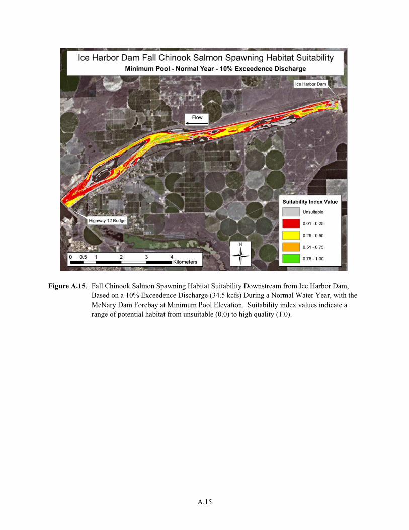
Figure A.15. Fall Chinook Salmon Spawning Habitat Suitability Downstream from Ice Harbor Dam,

Based on a 10% Exceedence Discharge (34.5 kcfs) During a Normal Water Year, with the McNary Dam Forebay at Minimum Pool Elevation. Suitability index values indicate a range of potential habitat from unsuitable (0.0) to high quality (1.0).

A.15

Figure A.16. Fall Chinook Salmon Spawning Habitat Suitability Downstream from Ice Harbor Dam,

Based on a 90% Exceedence Discharge (34.5 kcfs) During a Wet Water Year, with the McNary Dam Forebay at Minimum Pool Elevation. Suitability index values indicate a range of potential habitat from unsuitable (0.0) to high quality (1.0).

A.16

Figure A.17. Fall Chinook Salmon Spawning Habitat Suitability Downstream from Ice Harbor Dam,

Based on a 50% Exceedence Discharge (44.0 kcfs) During a Wet Water Year, with the McNary Dam Forebay at Minimum Pool Elevation. Suitability index values indicate a range of potential habitat from unsuitable (0.0) to high quality (1.0).

A.17

Figure A.18. Fall Chinook Salmon Spawning Habitat Suitability Downstream from Ice Harbor Dam,

Based on a 10% Exceedence Discharge (52.0 kcfs) During a Wet Water Year, with the McNary Dam Forebay at Minimum Pool Elevation. Suitability index values indicate a range of potential habitat from unsuitable (0.0) to high quality (1.0).

A.18

Figure A.19. Fall Chinook Salmon Spawning Habitat Suitability Downstream from Lower Granite Dam,

Based on a 90% Exceedence Discharge (12.6 kcfs) During a Dry Water Year, with the Little Goose Dam Forebay at Normal Pool Elevation. Suitability index values indicate a range of potential habitat from unsuitable (0.0) to high quality (1.0).

A.19

Figure A.20. Fall Chinook Salmon Spawning Habitat Suitability Downstream from Lower Granite Dam,

Based on a 50% Exceedence Discharge (15.3 kcfs) During a Dry Water Year, with the Little Goose Dam Forebay at Normal Pool Elevation. Suitability index values indicate a range of potential habitat from unsuitable (0.0) to high quality (1.0).

A.20

Figure A.21. Fall Chinook Salmon Spawning Habitat Suitability Downstream from Lower Granite Dam,

Based on a 10% Exceedence Discharge (18.2 kcfs) During a Dry Water Year, with the Little Goose Dam Forebay at Normal Pool elevation. Suitability index values indicate a range of potential habitat from unsuitable (0.0) to high quality (1.0).

A.21

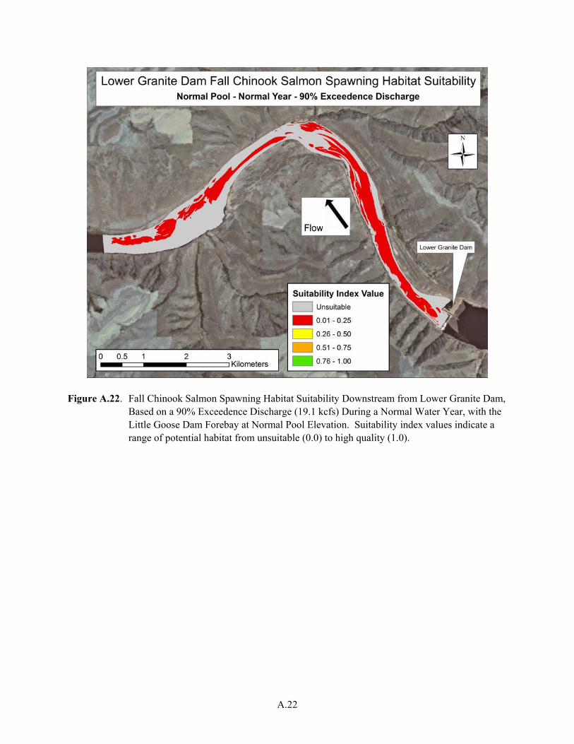
Figure A.22. Fall Chinook Salmon Spawning Habitat Suitability Downstream from Lower Granite Dam,

Based on a 90% Exceedence Discharge (19.1 kcfs) During a Normal Water Year, with the Little Goose Dam Forebay at Normal Pool Elevation. Suitability index values indicate a range of potential habitat from unsuitable (0.0) to high quality (1.0).

A.22

Figure A.23. Fall Chinook Salmon Spawning Habitat Suitability Downstream from Lower Granite Dam,

Based on a 50% Exceedence Discharge (21.7 kcfs) During a Normal Water Year, with the Little Goose Dam Forebay at Normal Pool Elevation. Suitability index values indicate a range of potential habitat from unsuitable (0.0) to high quality (1.0).

A.23

Figure A24. Fall Chinook Salmon Spawning Habitat Suitability Downstream from Lower Granite Dam,

Based on a 10% Exceedence Discharge (34.5 kcfs) During a Normal Water Year, with the Little Goose Dam Forebay at Normal Pool Elevation. Suitability index values indicate a range of potential habitat from unsuitable (0.0) to high quality (1.0).

A.24

Figure A.25. Fall Chinook Salmon Spawning Habitat Suitability Downstream from Lower Granite Dam,

Based on a 90% Exceedence Discharge (34.5 kcfs) During a Wet Water Year, with the Little Goose Dam Forebay at Normal Pool Elevation. Suitability index values indicate a range of potential habitat from unsuitable (0.0) to high quality (1.0).

A.25

Figure A.26. Fall Chinook Salmon Spawning Habitat Suitability Downstream from Lower Granite Dam,

Based on a 50% Exceedence Discharge (44.0 kcfs) During a Wet Water Year, with the Little Goose Dam Forebay at Normal Pool Elevation. Suitability index values indicate a range of potential habitat from unsuitable (0.0) to high quality (1.0).

A.26

Figure A.27. Fall Chinook Salmon Spawning Habitat Suitability Downstream from Lower Granite Dam,

Based on a 10% Exceedence Discharge (52.0 kcfs) During a Wet Water Year, with the Little Goose Dam Forebay at Normal Pool Elevation. Suitability index values indicate a range of potential habitat from unsuitable (0.0) to high quality (1.0).

A.27

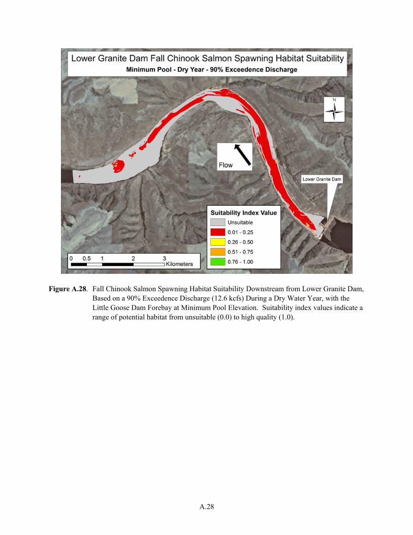
Figure A.28. Fall Chinook Salmon Spawning Habitat Suitability Downstream from Lower Granite Dam,

Based on a 90% Exceedence Discharge (12.6 kcfs) During a Dry Water Year, with the Little Goose Dam Forebay at Minimum Pool Elevation. Suitability index values indicate a range of potential habitat from unsuitable (0.0) to high quality (1.0).

A.28

Figure A.29. Fall Chinook Salmon Spawning Habitat Suitability Downstream from Lower Granite Dam,

Based on a 50% Exceedence Discharge (15.3 kcfs) During a Dry Water Year, with the Little Goose Dam Forebay at Minimum Pool Elevation. Suitability index values indicate a range of potential habitat from unsuitable (0.0) to high quality (1.0).

A.29

Figure A.30. Fall Chinook Salmon Spawning Habitat Suitability Downstream from Lower Granite Dam,

Based on a 10% Exceedence Discharge (18.2 kcfs) During a Dry Water Year, with the Little Goose Dam Forebay at Minimum Pool Elevation. Suitability index values indicate a range of potential habitat from unsuitable (0.0) to high quality (1.0).

A.30

Figure A.31. Fall Chinook Salmon Spawning Habitat Suitability Downstream from Lower Granite Dam,

Based on a 90% Exceedence Discharge (19.1 kcfs) During a Normal Water Year, with the Little Goose Dam Forebay at Minimum Pool Elevation. Suitability index values indicate a range of potential habitat from unsuitable (0.0) to high quality (1.0).

A.31

Figure A.32. Fall Chinook Salmon Spawning Habitat Suitability Downstream from Lower Granite Dam,

Based on a 50% Exceedence Discharge (21.7 kcfs) During a Normal Water Year, with the Little Goose Dam Forebay at Minimum Pool Elevation. Suitability index values indicate a range of potential habitat from unsuitable (0.0) to high quality (1.0).

A.32

Figure A.33. Fall Chinook Salmon Spawning Habitat Suitability Downstream from Lower Granite Dam,

Based on a 10% Exceedence Discharge (34.5 kcfs) During a Normal Water Year, with the Little Goose Dam Forebay at Minimum Pool Elevation. Suitability index values indicate a range of potential habitat from unsuitable (0.0) to high quality (1.0).

A.33

Figure A.34. Fall Chinook Salmon Spawning Habitat Suitability Downstream from Lower Granite Dam,

Based on a 90% Exceedence Discharge (34.5 kcfs) During a Wet Water Year, with the Little Goose Dam Forebay at Minimum Pool Elevation. Suitability index values indicate a range of potential habitat from unsuitable (0.0) to high quality (1.0).

A.34

Figure A.35. Fall Chinook Salmon Spawning Habitat Suitability Downstream from Lower Granite Dam,

Based on a 50% Exceedence Discharge (44.0 kcfs) During a Wet Water Year, with the Little Goose Dam Forebay at Minimum Pool Elevation. Suitability index values indicate a range of potential habitat from unsuitable (0.0) to high quality (1.0).

A.35

Figure A.36. Fall Chinook Salmon Spawning Habitat Suitability Downstream from Lower Granite Dam,

Based on a 10% Exceedence Discharge (52.0 kcfs) During a Wet Water Year, with the Little Goose Dam Forebay at Minimum Pool Elevation. Suitability index values indicate a range of potential habitat from unsuitable (0.0) to high quality (1.0).

A.36

Appendix B

Model Results of Depth, Velocity, and Suitability Index Values within Suitable Spawning Habitat

Appendix B

Model Results of Depth, Velocity, and Suitability Index Values within Suitable Spawning Habitat

Figure B.1. Depth within Suitable Fall Chinook Salmon Spawning Habitat Downstream from Ice

Harbor Dam, with the McNary Dam Forebay at Normal Pool Elevation, During a Dry Water Year. Suitability index values indicate a range of potential habitat from unsuitable (0.0) to high quality (1.0).

B.1

Figure B.2. Velocity within Suitable Fall Chinook Salmon Spawning Habitat Downstream from Ice Harbor Dam, with the McNary Dam Forebay at Normal Pool Elevation, During a Dry Water Year. Suitability index values indicate a range of potential habitat from unsuitable (0.0) to high quality (1.0).

B.2

Figure B.3. Depth within Suitable Fall Chinook Salmon Spawning Habitat Downstream from Ice Harbor Dam, with the McNary Dam Forebay at Normal Pool Elevation, During a Normal Water Year. Suitability index values indicate a range of potential habitat from unsuitable (0.0) to high quality (1.0).

B.3

Figure B.4. Velocity within Suitable Fall Chinook Salmon Spawning Habitat Downstream from Ice Harbor Dam, with the McNary Dam Forebay at Normal Pool Elevation, During a Normal Water Year. Suitability index values indicate a range of potential habitat from unsuitable (0.0) to high quality (1.0).

B.4

Figure B.5. Depth within Suitable Fall Chinook Salmon Spawning Habitat Downstream from Ice Harbor Dam, with the McNary Dam Forebay at Normal Pool Elevation, During a Wet Water Year. Suitability index values indicate a range of potential habitat from unsuitable (0.0) to high quality (1.0).

B.5

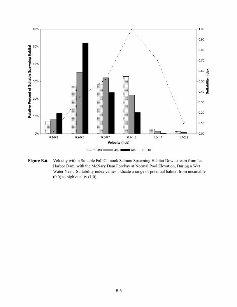
Figure B.6. Velocity within Suitable Fall Chinook Salmon Spawning Habitat Downstream from Ice Harbor Dam, with the McNary Dam Forebay at Normal Pool Elevation, During a Wet Water Year. Suitability index values indicate a range of potential habitat from unsuitable (0.0) to high quality (1.0).

B.6

Figure B.7. Depth within Suitable Fall Chinook Salmon Spawning Habitat Downstream from Ice Harbor Dam, with the McNary Dam Forebay at Minimum Pool Elevation, During a dry Water Year. Suitability index values indicate a range of potential habitat from unsuitable (0.0) to high quality (1.0).

B.7

Figure B.8. Velocity within Suitable Fall Chinook Salmon Spawning Habitat Downstream from Ice Harbor Dam, with the McNary Dam Forebay at Minimum Pool Elevation, During a Dry Water Year. Suitability index values indicate a range of potential habitat from unsuitable (0.0) to high quality (1.0).

B.8

Figure B.9. Depth within Suitable Fall Chinook Salmon Spawning Habitat Downstream from Ice Harbor Dam, with the McNary Dam Forebay at Minimum Pool Elevation, During a Normal Water Year. Suitability index values indicate a range of potential habitat from unsuitable (0.0) to high quality (1.0).

B.9

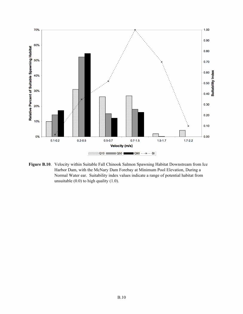
Figure B.10. Velocity within Suitable Fall Chinook Salmon Spawning Habitat Downstream from Ice Harbor Dam, with the McNary Dam Forebay at Minimum Pool Elevation, During a Normal Water ear. Suitability index values indicate a range of potential habitat from unsuitable (0.0) to high quality (1.0).

B.10

Figure B.11. Depth within Suitable Fall Chinook Salmon Spawning Habitat Downstream from Ice Harbor Dam, with the McNary Dam Forebay at Minimum Pool Elevation, during a Wet Water Year. Suitability index values indicate a range of potential habitat from unsuitable (0.0) to high quality (1.0).

B.11

Figure B.12. Velocity within Suitable Fall Chinook Salmon Spawning Habitat Downstream from Ice Harbor Dam, with the McNary Dam Forebay at Minimum Pool Elevation, During a Wet Water Year. Suitability index values indicate a range of potential habitat from unsuitable (0.0) to high quality (1.0).

B.12

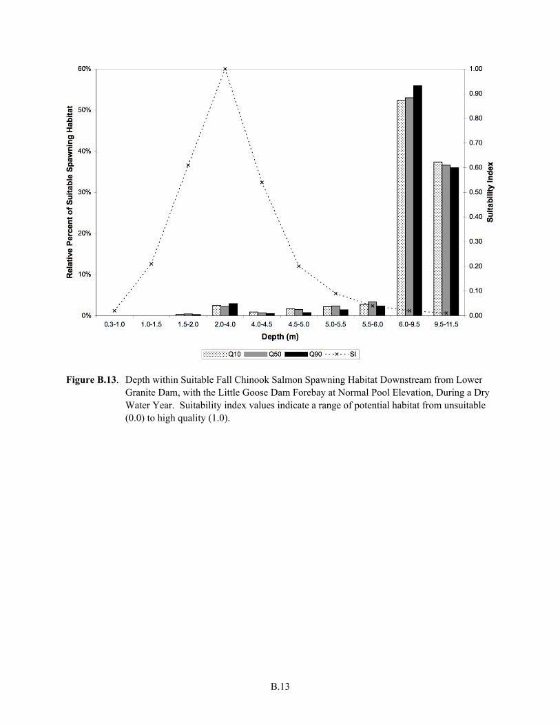
Figure B.13. Depth within Suitable Fall Chinook Salmon Spawning Habitat Downstream from Lower Granite Dam, with the Little Goose Dam Forebay at Normal Pool Elevation, During a Dry Water Year. Suitability index values indicate a range of potential habitat from unsuitable (0.0) to high quality (1.0).

B.13

Figure B.14. Velocity within Suitable Fall Chinook Salmon Spawning Habitat Downstream from Lower Granite Dam, with the Little Goose Dam Forebay at Normal Pool Elevation, During a Dry Water Year. Suitability index values indicate a range of potential habitat from unsuitable (0.0) to high quality (1.0).

B.14

Figure B.15. Depth within Suitable Fall Chinook Salmon Spawning Habitat Downstream from Lower

Granite Dam, with the Little Goose Dam Forebay at Normal Pool Elevation, During a Normal Water Year. Suitability index values indicate a range of potential habitat from unsuitable (0.0) to high quality (1.0).

B.15

Figure B.16. Velocity within Suitable Fall Chinook Salmon Spawning Habitat Downstream from Lower Granite Dam, with the Little Goose Dam Forebay at Normal Pool Elevation, During a Normal Water Year. Suitability index values indicate a range of potential habitat from unsuitable (0.0) to high quality (1.0).

B.16

Figure B.17. Depth within Suitable Fall Chinook Salmon Spawning Habitat Downstream from Lower

Granite Dam, with the Little Goose Dam Forebay at Normal Pool Elevation, During a Wet Water Year. Suitability index values indicate a range of potential habitat from unsuitable (0.0) to high quality (1.0).

B.17

Figure B.18. Velocity within Suitable Fall Chinook Salmon Spawning Habitat Downstream from Lower

Granite Dam, with the Little Goose Dam Forebay at Normal Pool Elevation, During a Wet Water Year. Suitability index values indicate a range of potential habitat from unsuitable (0.0) to high quality (1.0).

B.18

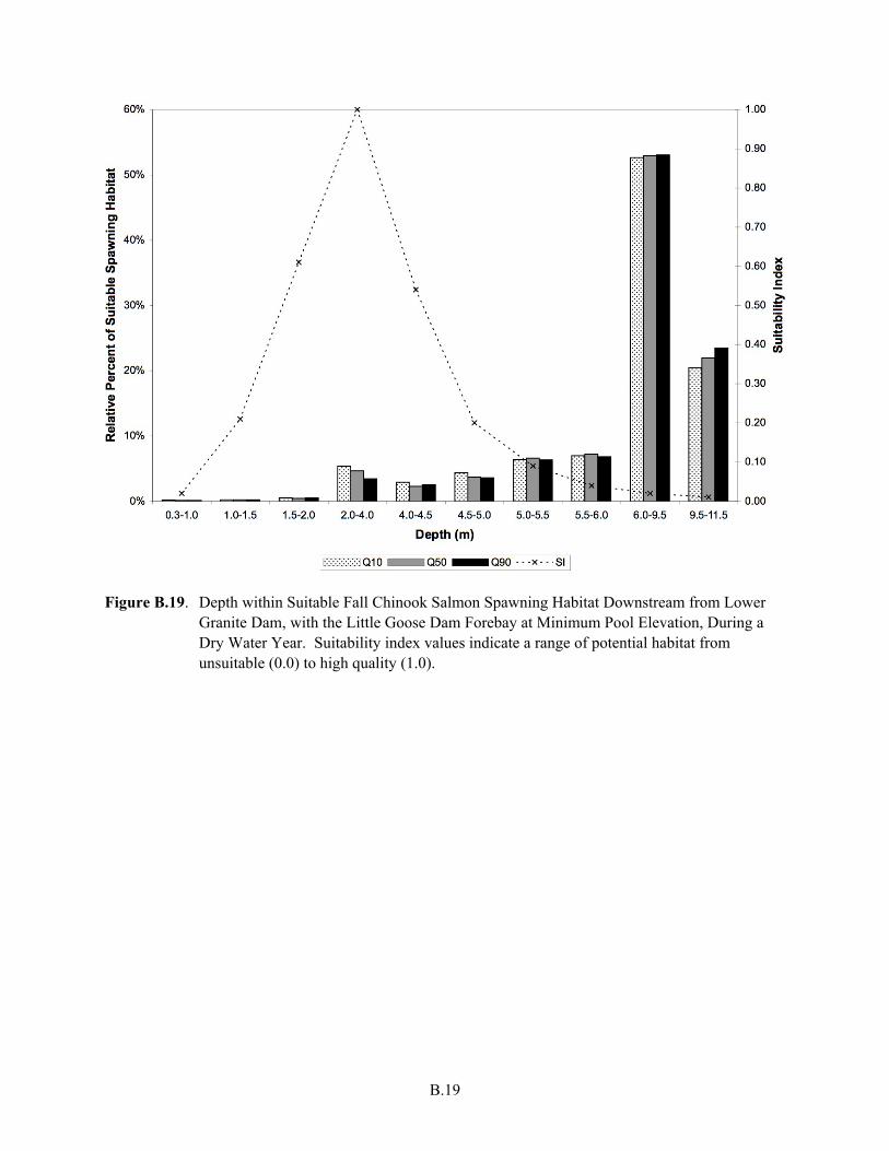
Figure B.19. Depth within Suitable Fall Chinook Salmon Spawning Habitat Downstream from Lower Granite Dam, with the Little Goose Dam Forebay at Minimum Pool Elevation, During a Dry Water Year. Suitability index values indicate a range of potential habitat from unsuitable (0.0) to high quality (1.0).

B.19

Figure B.20. Velocity within Suitable Fall Chinook Salmon Spawning Habitat Downstream from Lower Granite Dam, with the Little Goose Dam Forebay at Minimum Pool Elevation, During a Dry Water Year. Suitability index values indicate a range of potential habitat from unsuitable (0.0) to high quality (1.0).

B.20

Figure B.21. Depth within Suitable Fall Chinook Salmon Spawning Habitat Downstream from Lower Granite Dam, with the Little Goose Dam Forebay at Minimum Pool Elevation, During a Normal Water Year. Suitability index values indicate a range of potential habitat from unsuitable (0.0) to high quality (1.0).

B.21

Figure B.22. Velocity within Suitable Fall Chinook Salmon Spawning Habitat Downstream from Lower Granite Dam, with the Little Goose Dam Forebay at Minimum Pool Elevation, During a Normal Water Year. Suitability index values indicate a range of potential habitat from unsuitable (0.0) to high quality (1.0).

B.22

Figure B.23. Depth within Suitable Fall Chinook Salmon Spawning Habitat Downstream from Lower Granite Dam, with the Little Goose Dam Forebay at Minimum Pool Elevation, During a Wet Water Year. Suitability index values indicate a range of potential habitat from unsuitable (0.0) to high quality (1.0).

B.23

Figure B.24. Velocity within Suitable Fall Chinook Salmon Spawning Habitat Downstream from Lower

Granite Dam, with the Little Goose Dam Forebay at Minimum Pool Elevation, During a Wet Water Year. Suitability index values indicate a range of potential habitat from unsuitable (0.0) to high quality (1.0).

B.24

Appendix C

Maps of Depth and Velocity within Suitable Fall Chinook Salmon Spawning Habitat

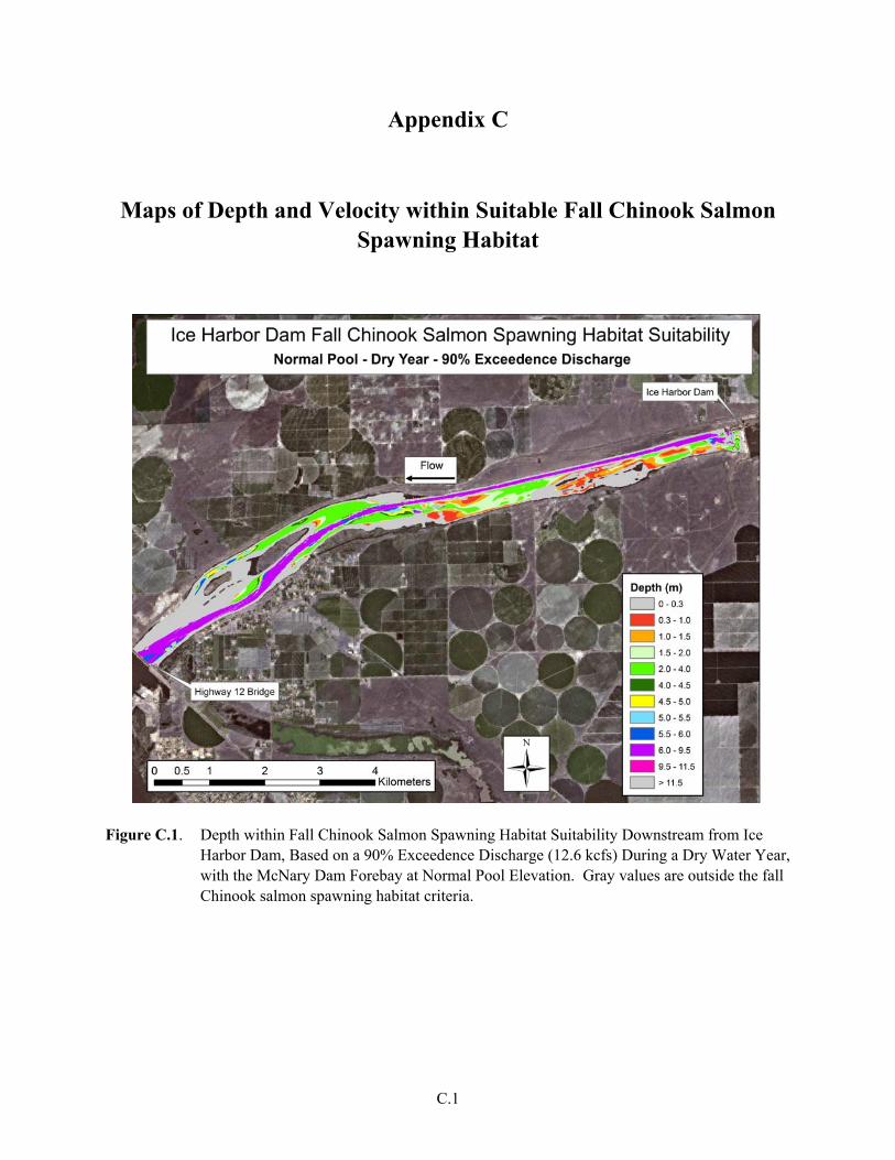
Appendix C

Maps of Depth and Velocity within Suitable Fall Chinook Salmon Spawning Habitat

Figure C.1. Depth within Fall Chinook Salmon Spawning Habitat Suitability Downstream from Ice

Harbor Dam, Based on a 90% Exceedence Discharge (12.6 kcfs) During a Dry Water Year, with the McNary Dam Forebay at Normal Pool Elevation. Gray values are outside the fall Chinook salmon spawning habitat criteria.

C.1

Figure C.2. Velocity within Fall Chinook Salmon Spawning Habitat Suitability Downstream from Ice

Harbor Dam, Based on a 90% Exceedence Discharge (12.6 kcfs) During a Dry Water Year, with the McNary Dam Forebay at Normal Pool Elevation. Gray values are outside the fall Chinook salmon spawning habitat criteria.

C.2

Figure C.3. Depth within Fall Chinook Salmon Spawning Habitat Suitability Downstream from Ice

Harbor Dam, Based on a 50% Exceedence Discharge (15.3 kcfs) During a Dry Water Year, with the McNary Dam Forebay at Normal Pool Elevation. Gray values are outside the fall Chinook salmon spawning habitat criteria.

C.3

Figure C.4. Velocity within Fall Chinook Salmon Spawning Habitat Suitability Downstream from Ice

Harbor Dam, Based on a 50% Exceedence Discharge (15.3 kcfs) During a Dry Water Year, with the McNary Dam Forebay at Normal Pool Elevation. Gray values are outside the fall Chinook salmon spawning habitat criteria.

C.4

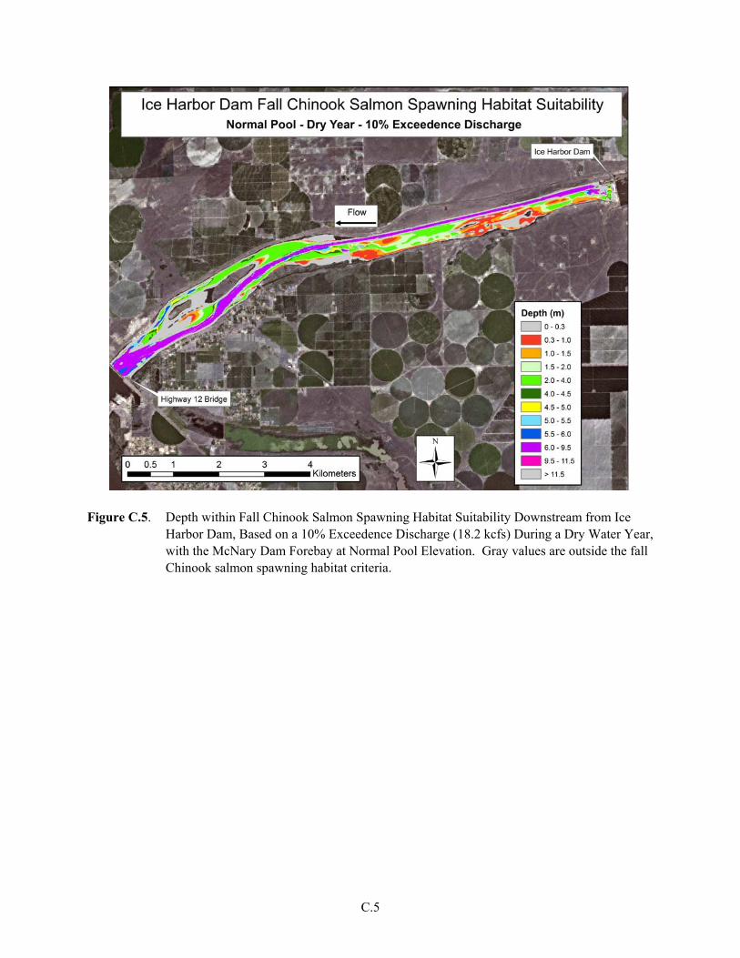
Figure C.5. Depth within Fall Chinook Salmon Spawning Habitat Suitability Downstream from Ice

Harbor Dam, Based on a 10% Exceedence Discharge (18.2 kcfs) During a Dry Water Year, with the McNary Dam Forebay at Normal Pool Elevation. Gray values are outside the fall Chinook salmon spawning habitat criteria.

C.5

Figure C.6. Velocity within Fall Chinook Salmon Spawning Habitat Suitability Downstream from Ice

Harbor Dam, Based on a 10% Exceedence Discharge (18.2 kcfs) During a Dry Water Year, with the McNary Dam Forebay at Normal Pool Elevation. Gray values are outside the fall Chinook salmon spawning habitat criteria.

C.6

Figure C.7. Depth within Fall Chinook Salmon Spawning Habitat Suitability Downstream from Ice

Harbor Dam, Based on a 90% Exceedence Discharge (19.1 kcfs) During a Normal Water Year, with the McNary Dam Forebay at Normal Pool Elevation. Gray values are outside the fall Chinook salmon spawning habitat criteria.

C.7

Figure C.8. Velocity within Fall Chinook Salmon Spawning Habitat Suitability Downstream from Ice

Harbor Dam, Based on a 90% Exceedence Discharge (19.1 kcfs) During a Normal Water Year, with the McNary Dam Forebay at Normal Pool Elevation. Gray values are outside the fall Chinook salmon spawning habitat criteria.

C.8

Figure C.9. Depth within Fall Chinook Salmon Spawning Habitat Suitability Downstream from Ice

Harbor Dam, Based on a 50% Exceedence Discharge (21.7 kcfs) During a Normal Water Year, with the McNary Dam Forebay at Normal Pool Elevation. Gray values are outside the fall Chinook salmon spawning habitat criteria.

C.9

Figure C.10. Velocity within Fall Chinook Salmon Spawning Habitat Suitability Downstream from Ice

Harbor Dam, Based on a 50% Exceedence Discharge (21.7 kcfs) During a Normal Water Year, with the McNary Dam Forebay at Normal Pool Elevation. Gray values are outside the fall Chinook salmon spawning habitat criteria.

C.10

Figure C.11. Depth within Fall Chinook Salmon Spawning Habitat Suitability Downstream from Ice

Harbor Dam, Based on a 10% Exceedence Discharge (34.5 kcfs) During a Normal Water Year, with the McNary Dam Forebay at Normal Pool Elevation. Gray values are outside the fall Chinook salmon spawning habitat criteria.

C.11

Figure C.12. Velocity within Fall Chinook Salmon Spawning Habitat Suitability Downstream from Ice

Harbor Dam, Based on a 10% Exceedence Discharge (34.5 kcfs) During a Normal Water Year, with the McNary Dam Forebay at Normal Pool Elevation. Gray values are outside the fall Chinook salmon spawning habitat criteria.

C.12

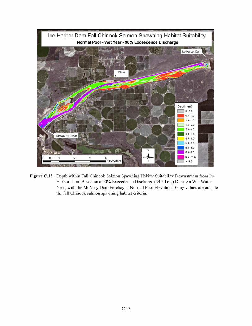
Figure C.13. Depth within Fall Chinook Salmon Spawning Habitat Suitability Downstream from Ice

Harbor Dam, Based on a 90% Exceedence Discharge (34.5 kcfs) During a Wet Water Year, with the McNary Dam Forebay at Normal Pool Elevation. Gray values are outside the fall Chinook salmon spawning habitat criteria.

C.13

Figure C.14. Velocity within Fall Chinook Salmon Spawning Habitat Suitability Downstream from Ice

Harbor Dam, Based on a 90% Exceedence Discharge (34.5 kcfs) During a Wet Water Year, with the McNary Dam Forebay at Normal Pool Elevation. Gray values are outside the fall Chinook salmon spawning habitat criteria.

C.14

Figure C.15. Depth within Fall Chinook Salmon Spawning Habitat Suitability Downstream from Ice

Harbor Dam, Based on a 50% Exceedence Discharge (44.0 kcfs) During a Wet Water Year, with the McNary Dam Forebay at Normal Pool Elevation. Gray values are outside the fall Chinook salmon spawning habitat criteria.

C.15

Figure C.16. Velocity within Fall Chinook Salmon Spawning Habitat Suitability Downstream from Ice

Harbor Dam, Based on a 50% Exceedence Discharge (44.0 kcfs) During a Wet Water Year, with the McNary Dam Forebay at Normal Pool Elevation. Gray values are outside the fall Chinook salmon spawning habitat criteria.

C.16

Figure C.17. Depth within Fall Chinook Salmon Spawning Habitat Suitability Downstream from Ice

Harbor Dam, Based on a 10% Exceedence Discharge (52.0 kcfs) During a Wet Water Year, with the McNary Dam Forebay at Normal Pool Elevation. Gray values are outside the fall Chinook salmon spawning habitat criteria.

C.17

Figure C.18. Velocity within Fall Chinook Salmon Spawning Habitat Suitability Downstream from Ice

Harbor Dam, Based on a 10% Exceedence Discharge (52.0 kcfs) During a Wet Water Year, with the McNary Dam Forebay at Normal Pool Elevation. Gray values are outside the fall Chinook salmon spawning habitat criteria.

C.18

Figure C.19. Depth within Fall Chinook Salmon Spawning Habitat Suitability Downstream from Ice

Harbor Dam, Based on a 90% Exceedence Discharge (12.6 kcfs) During a Dry Water Year, with the McNary Dam Forebay at Minimum Pool Elevation. Gray values are outside the fall Chinook salmon spawning habitat criteria.

C.19

Figure C.20. Velocity within Fall Chinook Salmon Spawning Habitat Suitability Downstream from Ice

Harbor Dam, Based on a 90% Exceedence Discharge (12.6 kcfs) During a Dry Water Year, with the McNary Dam Forebay at Minimum Pool Elevation. Gray values are outside the fall Chinook salmon spawning habitat criteria.

C.20

Figure C.21. Depth within Fall Chinook Salmon Spawning Habitat Suitability Downstream from Ice

Harbor Dam, Based on a 50% Exceedence Discharge (15.3 kcfs) During a Dry Water Year, with the McNary Dam Forebay at Minimum Pool Elevation. Gray values are outside the fall Chinook salmon spawning habitat criteria.

C.21

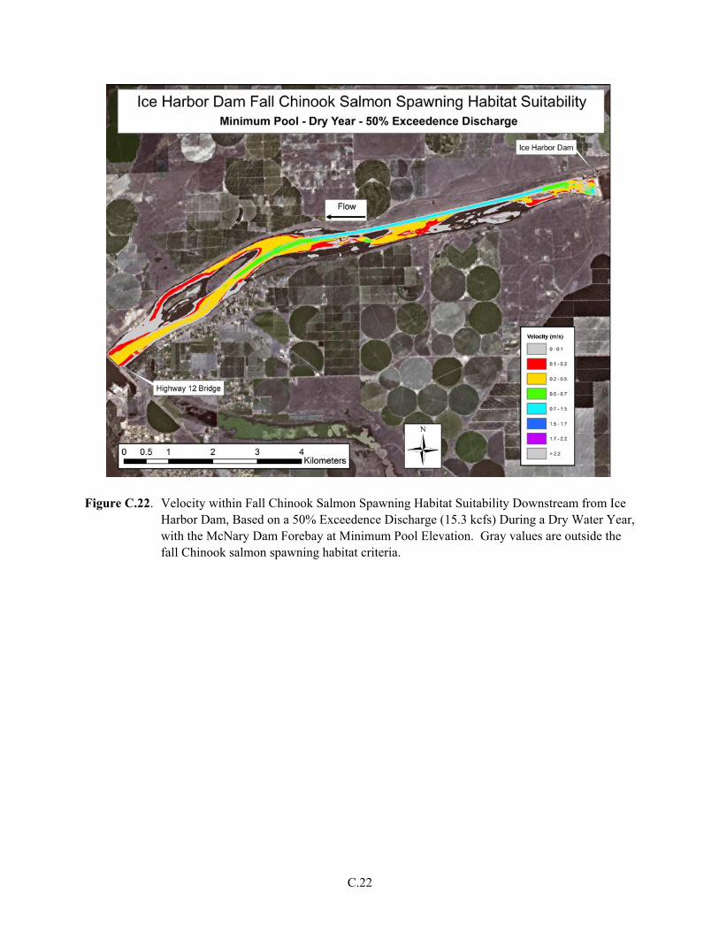
Figure C.22. Velocity within Fall Chinook Salmon Spawning Habitat Suitability Downstream from Ice

Harbor Dam, Based on a 50% Exceedence Discharge (15.3 kcfs) During a Dry Water Year, with the McNary Dam Forebay at Minimum Pool Elevation. Gray values are outside the fall Chinook salmon spawning habitat criteria.

C.22

Figure C.23. Depth within fall Chinook Salmon Spawning Habitat Suitability Downstream from Ice

Harbor Dam, Based on a 10% Exceedence Discharge (18.2 kcfs) During a Dry Water Year, with the McNary Dam Forebay at Minimum Pool Elevation. Gray values are outside the fall Chinook salmon spawning habitat criteria.

C.23

Figure C.24. Velocity within Fall Chinook Salmon Spawning Habitat Suitability Downstream from Ice

Harbor Dam, Based on a 10% Exceedence Discharge (18.2 kcfs) During a Dry Water Year, with the McNary Dam Forebay at Minimum Pool Elevation. Gray values are outside the fall Chinook salmon spawning habitat criteria.

C.24

Figure C.25. Depth within fall Chinook Salmon Spawning Habitat Suitability Downstream from Ice

Harbor Dam, Based on a 90% Exceedence Discharge (19.1 kcfs) During a Normal Water Year, with the McNary Dam Forebay at Minimum Pool Elevation. Gray values are outside the fall Chinook salmon spawning habitat criteria.

C.25

Figure C.26. Velocity within Fall Chinook Salmon Spawning Habitat Suitability Downstream from Ice

Harbor Dam, Based on a 90% Exceedence Discharge (19.1 kcfs) During a Normal Water Year, with the McNary Dam Forebay at Minimum Pool Elevation. Gray values are outside the fall Chinook salmon spawning habitat criteria.

C.26

Figure C.27. Depth within Fall Chinook Salmon Spawning Habitat Suitability Downstream from Ice

Harbor Dam, Based on a 50% Exceedence Discharge (21.7 kcfs) During a Normal Water Year, with the McNary Dam Forebay at Minimum Pool Elevation. Gray values are outside the fall Chinook salmon spawning habitat criteria.

C.27

Figure C.28. Velocity within Fall Chinook Salmon Spawning Habitat Suitability Downstream from Ice

Harbor Dam, Based on a 50% Exceedence Discharge (21.7 kcfs) During a Normal Water Year, with the McNary Dam Forebay at Minimum Pool Elevation. Gray values are outside the fall Chinook salmon spawning habitat criteria.

C.28

Figure C.29. Depth within Fall Chinook Salmon Spawning Habitat Suitability Downstream from Ice

Harbor Dam, Based on a 10% Exceedence Discharge (34.5 kcfs) During a Normal Water Year, with the McNary Dam Forebay at Minimum Pool Elevation. Gray values are outside the fall Chinook salmon spawning habitat criteria.

C.29

Figure C.30. Velocity within Fall Chinook Salmon Spawning Habitat Suitability Downstream from Ice

Harbor Dam, Based on a 10% Exceedence Discharge (34.5 kcfs) During a Normal Water Year, with the McNary Dam Forebay at Minimum Pool Elevation. Gray values are outside the fall Chinook salmon spawning habitat criteria.

C.30

Figure C.31. Depth within Fall Chinook Salmon Spawning Habitat Suitability Downstream from Ice

Harbor Dam, Based on a 90% Exceedence Discharge (34.5 kcfs) During a Wet Water Year, with the McNary Dam Forebay at Minimum Pool Elevation. Gray values are outside the fall Chinook salmon spawning habitat criteria.

C.31

Figure C.32. Velocity within Fall Chinook Salmon Spawning Habitat Suitability Downstream from Ice

Harbor Dam, Based on a 90% Exceedence Discharge (34.5 kcfs) During a Wet Water Year, with the McNary Dam Forebay at Minimum Pool Elevation. Gray values are outside the fall Chinook salmon spawning habitat criteria.

C.32

Figure C.33. Depth within Fall Chinook Salmon Spawning Habitat Suitability Downstream from Ice

Harbor Dam, Based on a 50% Exceedence Discharge (44.0 kcfs) During a Wet Water Year, with the McNary Dam Forebay at Minimum Pool Elevation. Gray values are outside the fall Chinook salmon spawning habitat criteria.

C.33

Figure C.34. Velocity within Fall Chinook Salmon Spawning Habitat Suitability Downstream from Ice

Harbor Dam, Based on a 50% Exceedence Discharge (44.0 kcfs) During a Wet Water Year, with the McNary Dam Forebay at Minimum Pool Elevation. Gray values are outside the fall Chinook salmon spawning habitat criteria.

C.34

Figure C.35. Depth within Fall Chinook Salmon Spawning Habitat Suitability Downstream from Ice

Harbor Dam, Based on a 10% Exceedence Discharge (52.0 kcfs) During a Wet Water Year, with the McNary Dam Forebay at Minimum Pool Elevation. Gray values are outside the fall Chinook salmon spawning habitat criteria.

C.35

Figure C.36. Velocity within Fall Chinook Salmon Spawning Habitat Suitability Downstream from Ice

Harbor Dam, Based on a 10% Exceedence Discharge (52.0 kcfs) During a Wet Water Year, with the McNary Dam Forebay at Minimum Pool Elevation. Gray values are outside the fall Chinook salmon spawning habitat criteria.

C.36

Figure C.37. Depth within Fall Chinook Salmon Spawning Habitat Suitability Downstream from Lower

Granite Dam, Based on a 90% Exceedence Discharge (12.6 kcfs) During a Dry Water Year, with the Little Goose Dam Forebay at Normal Pool Elevation. Gray values are outside the fall Chinook salmon spawning habitat criteria.

C.37

Figure C.38. Velocity within Fall Chinook Salmon Spawning Habitat Suitability Downstream from

Lower Granite Dam, Based on a 90% Exceedence Discharge (12.6 kcfs) During a Dry Water Year, with the Little Goose Dam Forebay at Normal Pool Elevation. Gray values are outside the fall Chinook salmon spawning habitat criteria.

C.38

Figure C.39. Depth within Fall Chinook Salmon Spawning Habitat Suitability Downstream from Lower

Granite Dam, Based on a 50% Exceedence Discharge (15.3 kcfs) During a Dry Water Year, with the Little Goose Dam Forebay at Normal Pool Elevation. Gray values are outside the fall Chinook salmon spawning habitat criteria.

C.39

Figure C.40. Velocity within Fall Chinook Salmon Spawning Habitat Suitability Downstream from

Lower Granite Dam, Based on a 50% Exceedence Discharge (15.3 kcfs) During a Dry Water Year, with the Little Goose Dam Forebay at Normal Pool Elevation. Gray values are outside the fall Chinook salmon spawning habitat criteria.

C.40

Figure C.41. Depth within Fall Chinook Salmon Spawning Habitat Suitability Downstream from Lower

Granite Dam, Based on a 10% Exceedence Discharge (18.2 kcfs) During a Dry Water Year, with the Little Goose Dam Forebay at Normal Pool Elevation. Gray values are outside the fall Chinook salmon spawning habitat criteria.

C.41

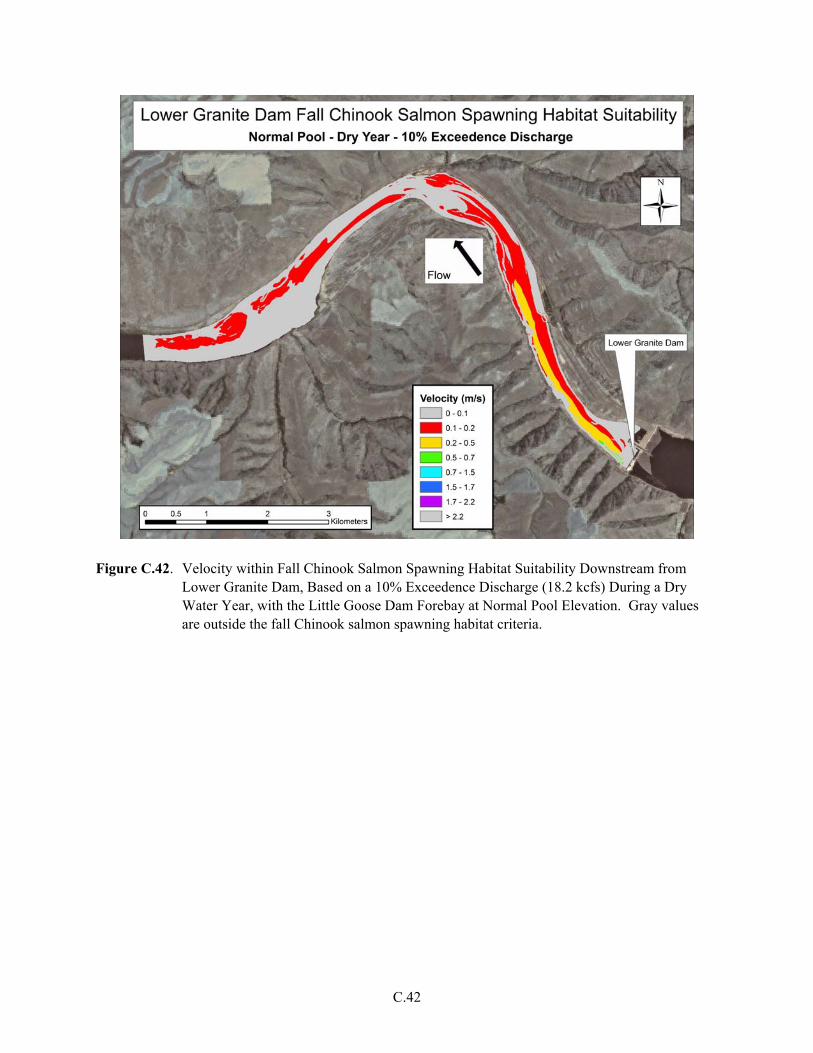
Figure C.42. Velocity within Fall Chinook Salmon Spawning Habitat Suitability Downstream from

Lower Granite Dam, Based on a 10% Exceedence Discharge (18.2 kcfs) During a Dry Water Year, with the Little Goose Dam Forebay at Normal Pool Elevation. Gray values are outside the fall Chinook salmon spawning habitat criteria.

C.42

Figure C.43. Depth within Fall Chinook Salmon Spawning Habitat Suitability Downstream from Lower

Granite Dam, Based on a 90% Exceedence Discharge (19.1 kcfs) During a Normal Water Year, with the Little Goose Dam Forebay at Normal Pool Elevation. Gray values are outside the fall Chinook salmon spawning habitat criteria.

C.43

Figure C.44. Velocity within Fall Chinook Salmon Spawning Habitat Suitability Downstream from

Lower Granite Dam, Based on a 90% Exceedence Discharge (19.1 kcfs) During a Normal Water Year, with the Little Goose Dam Forebay at Normal Pool Elevation. Gray values are outside the fall Chinook salmon spawning habitat criteria.

C.44

Figure C.45. Depth within Fall Chinook Salmon Spawning Habitat Suitability Downstream from Lower

Granite Dam, Based on a 50% Exceedence Discharge (21.7 kcfs) During a Normal Water Year, with the Little Goose Dam Forebay at Normal Pool Elevation. Gray values are outside the fall Chinook salmon spawning habitat criteria.

C.45

Figure C.46. Velocity within Fall Chinook Salmon Spawning Habitat Suitability Downstream from

Lower Granite Dam, Based on a 50% Exceedence Discharge (21.7 kcfs) During a Normal Water Year, with the Little Goose Dam Forebay at Normal Pool Elevation. Gray values are outside the fall Chinook salmon spawning habitat criteria.

C.46

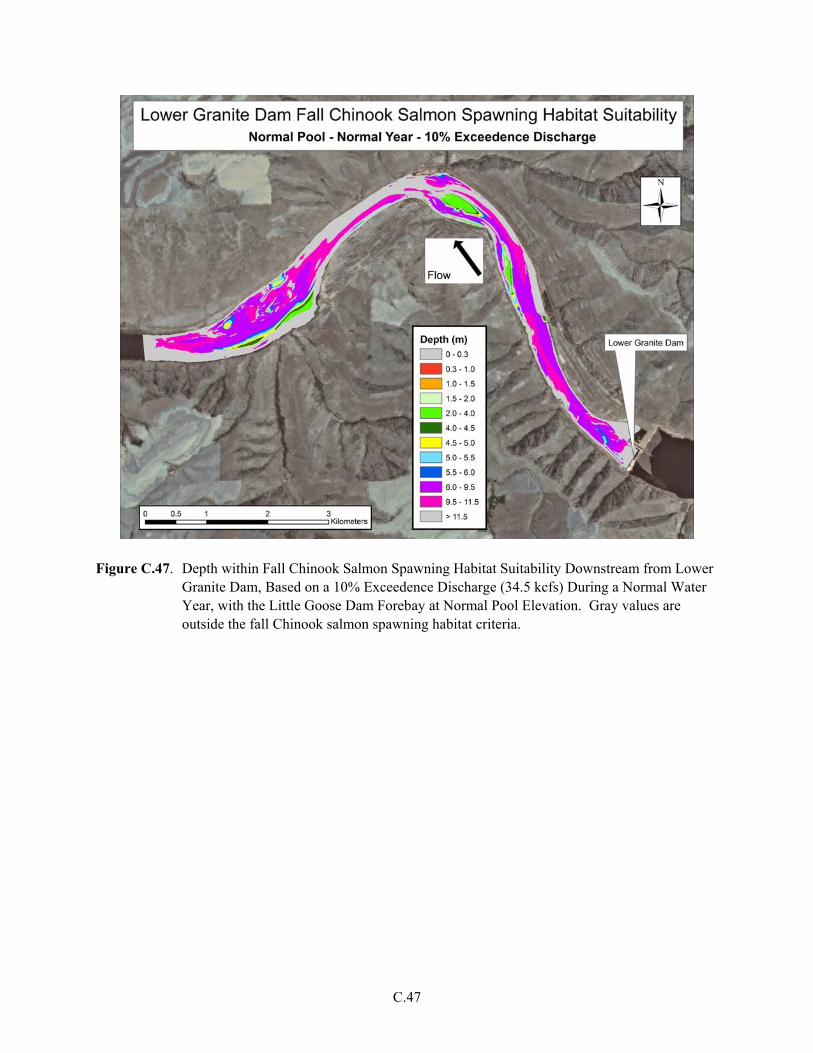
Figure C.47. Depth within Fall Chinook Salmon Spawning Habitat Suitability Downstream from Lower

Granite Dam, Based on a 10% Exceedence Discharge (34.5 kcfs) During a Normal Water Year, with the Little Goose Dam Forebay at Normal Pool Elevation. Gray values are outside the fall Chinook salmon spawning habitat criteria.

C.47

Figure C.48. Velocity within Fall Chinook Salmon Spawning Habitat Suitability Downstream from

Lower Granite Dam, Based on a 10% Exceedence Discharge (34.5 kcfs) During a Normal Water Year, with the Little Goose Dam Forebay at Normal Pool Elevation. Gray values are outside the fall Chinook salmon spawning habitat criteria.

C.48

Figure C.49. Depth within Fall Chinook Salmon Spawning Habitat Suitability Downstream from Lower

Granite Dam, Based on a 90% Exceedence Discharge (34.5 kcfs) During a Wet Water Year, with the Little Goose Dam Forebay at Normal Pool Elevation. Gray values are outside the fall Chinook salmon spawning habitat criteria.

C.49

Figure C.50. Velocity within Fall Chinook Salmon Spawning Habitat Suitability Downstream from

Lower Granite Dam, Based on a 90% Exceedence Discharge (34.5 kcfs) During a Wet Water Year, with the Little Goose Dam Forebay at Normal Pool Elevation. Gray values are outside the fall Chinook salmon spawning habitat criteria.

C.50

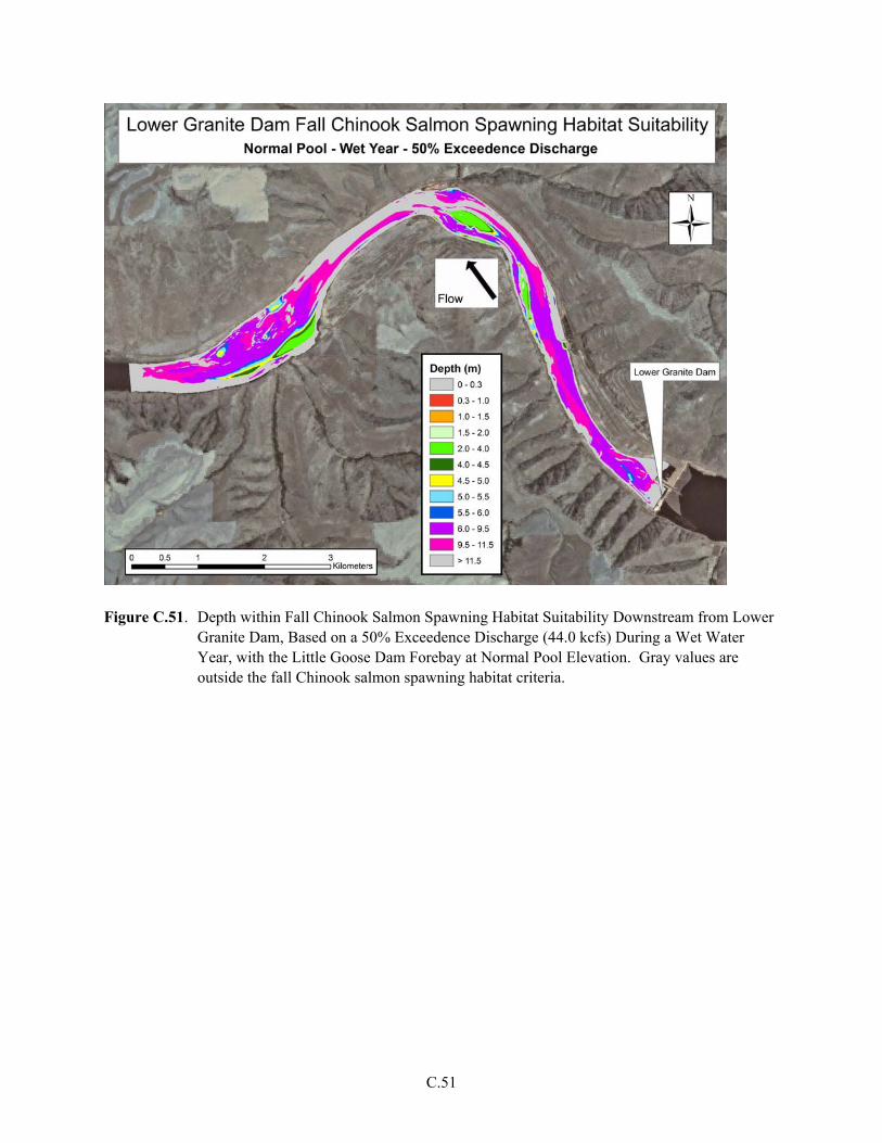
Figure C.51. Depth within Fall Chinook Salmon Spawning Habitat Suitability Downstream from Lower

Granite Dam, Based on a 50% Exceedence Discharge (44.0 kcfs) During a Wet Water Year, with the Little Goose Dam Forebay at Normal Pool Elevation. Gray values are outside the fall Chinook salmon spawning habitat criteria.

C.51

Figure C.52. Velocity within Fall Chinook Salmon Spawning Habitat Suitability Downstream from

Lower Granite Dam, Based on a 50% Exceedence Discharge (44.0 kcfs) During a Wet Water Year, with the Little Goose Dam Forebay at Normal Pool Elevation. Gray values are outside the fall Chinook salmon spawning habitat criteria.

C.52

Figure C.53. Depth within Fall Chinook Salmon Spawning Habitat Suitability Downstream from Lower

Granite Dam, Based on a 10% Exceedence Discharge (52.0 kcfs) During a Wet Water Year, with the Little Goose Dam Forebay at Normal Pool Elevation. Gray values are outside the fall Chinook salmon spawning habitat criteria.

C.53

Figure C.54. Velocity within Fall Chinook Salmon Spawning Habitat Suitability Downstream from

Lower Granite Dam, Based on a 10% Exceedence Discharge (52.0 kcfs) During a Wet Water Year, with the Little Goose Dam Forebay at Normal Pool Elevation. Gray values are outside the fall Chinook salmon spawning habitat criteria.

C.54

Figure C.55. Depth within Fall Chinook Salmon Spawning Habitat Suitability Downstream from Lower

Granite Dam, Based on a 90% Exceedence Discharge (12.6 kcfs) During a Dry Water Year, with the Little Goose Dam Forebay at Minimum Pool Elevation. Gray values are outside the fall Chinook salmon spawning habitat criteria.

C.55

Figure C.56. Velocity within Fall Chinook Salmon Spawning Habitat Suitability Downstream from

Lower Granite Dam, Based on a 90% Exceedence Discharge (12.6 kcfs) During a Dry Water Year, with the Little Goose Dam Forebay at Minimum Pool Elevation. Gray values are outside the fall Chinook salmon spawning habitat criteria.

C.56

Figure C.57. Depth within Fall Chinook Salmon Spawning Habitat Suitability Downstream from Lower

Granite Dam, Based on a 50% Exceedence Discharge (15.3 kcfs) During a Dry Water Year, with the Little Goose Dam Forebay at Minimum Pool Elevation. Gray values are outside the fall Chinook salmon spawning habitat criteria.

C.57

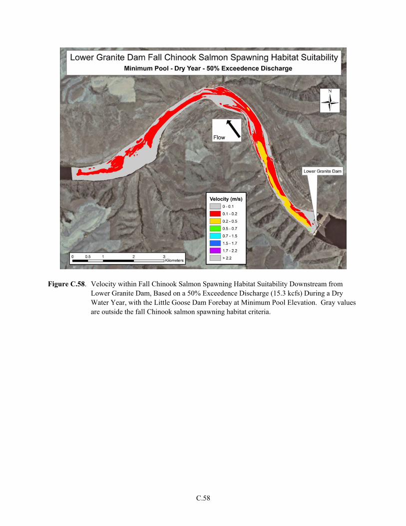
Figure C.58. Velocity within Fall Chinook Salmon Spawning Habitat Suitability Downstream from

Lower Granite Dam, Based on a 50% Exceedence Discharge (15.3 kcfs) During a Dry Water Year, with the Little Goose Dam Forebay at Minimum Pool Elevation. Gray values are outside the fall Chinook salmon spawning habitat criteria.

C.58

Figure C.59. Depth within Fall Chinook Salmon Spawning Habitat Suitability Downstream from Lower

Granite Dam, Based on a 10% Exceedence Discharge (18.2 kcfs) During a Dry Water Year, with the Little Goose Dam Forebay at Minimum Pool Elevation. Gray values are outside the fall Chinook salmon spawning habitat criteria.

C.59

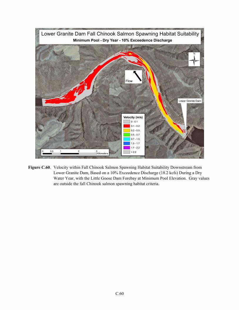
Figure C.60. Velocity within Fall Chinook Salmon Spawning Habitat Suitability Downstream from

Lower Granite Dam, Based on a 10% Exceedence Discharge (18.2 kcfs) During a Dry Water Year, with the Little Goose Dam Forebay at Minimum Pool Elevation. Gray values are outside the fall Chinook salmon spawning habitat criteria.

C.60

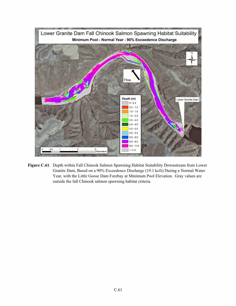
Figure C.61. Depth within Fall Chinook Salmon Spawning Habitat Suitability Downstream from Lower

Granite Dam, Based on a 90% Exceedence Discharge (19.1 kcfs) During a Normal Water Year, with the Little Goose Dam Forebay at Minimum Pool Elevation. Gray values are outside the fall Chinook salmon spawning habitat criteria.

C.61

Figure C.62. Velocity within Fall Chinook Salmon Spawning Habitat Suitability Downstream from

Lower Granite Dam, Based on a 90% Exceedence Discharge (19.1 kcfs) During a Normal Water Year, with the Little Goose Dam Forebay at Minimum Pool Elevation. Gray values are outside the fall Chinook salmon spawning habitat criteria.

C.62

Figure C.63. Depth within Fall Chinook Salmon Spawning Habitat Suitability Downstream from Lower

Granite Dam, Based on a 50% Exceedence Discharge (21.7 kcfs) During a Normal Water Year, with the Little Goose Dam Forebay at Minimum Pool Elevation. Gray values are outside the fall Chinook salmon spawning habitat criteria.

C.63

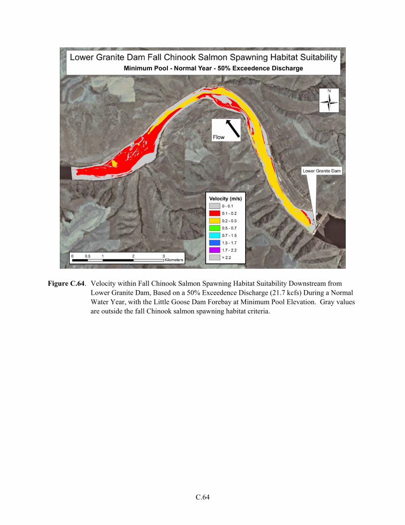
Figure C.64. Velocity within Fall Chinook Salmon Spawning Habitat Suitability Downstream from

Lower Granite Dam, Based on a 50% Exceedence Discharge (21.7 kcfs) During a Normal Water Year, with the Little Goose Dam Forebay at Minimum Pool Elevation. Gray values are outside the fall Chinook salmon spawning habitat criteria.

C.64

Figure C.65. Depth within Fall Chinook Salmon Spawning Habitat Suitability Downstream from Lower

Granite Dam, Based on a 10% Exceedence Discharge (34.5 kcfs) During a Normal Water Year, with the Little Goose Dam Forebay at Minimum Pool Elevation. Gray values are outside the fall Chinook salmon spawning habitat criteria.

C.65

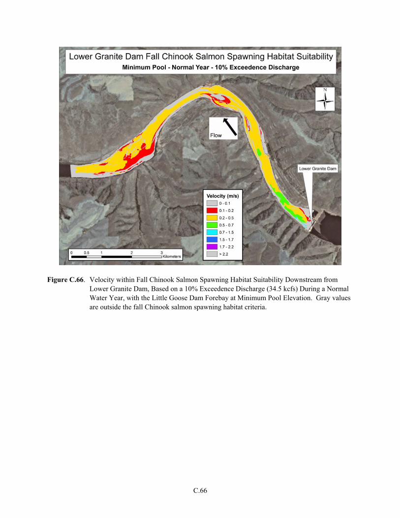
Figure C.66. Velocity within Fall Chinook Salmon Spawning Habitat Suitability Downstream from

Lower Granite Dam, Based on a 10% Exceedence Discharge (34.5 kcfs) During a Normal Water Year, with the Little Goose Dam Forebay at Minimum Pool Elevation. Gray values are outside the fall Chinook salmon spawning habitat criteria.

C.66

Figure C.67. Depth within Fall Chinook Salmon Spawning Habitat Suitability Downstream from Lower

Granite Dam, Based on a 90% Exceedence Discharge (34.5 kcfs) During a Wet Water Year, with the Little Goose Dam Forebay at Minimum Pool Elevation. Gray values are outside the fall Chinook salmon spawning habitat criteria.

C.67

Figure C.68. Velocity within Fall Chinook Salmon Spawning Habitat Suitability Downstream from

Lower Granite Dam, Based on a 90% Exceedence Discharge (34.5 kcfs) During a Wet Water Year, with the Little Goose Dam Forebay at Minimum Pool Elevation. Gray values are outside the fall Chinook salmon spawning habitat criteria.

C.68

Figure C.69. Depth within Fall Chinook Salmon Spawning Habitat Suitability Downstream from Lower

Granite Dam, Based on a 50% Exceedence Discharge (44.0 kcfs) During a Wet Water Year, with the Little Goose Dam Forebay at Minimum Pool Elevation. Gray values are outside the fall Chinook salmon spawning habitat criteria.

C.69

Figure C.70. Velocity within Fall Chinook Salmon Spawning Habitat Suitability Downstream from

Lower Granite Dam, Based on a 50% Exceedence Discharge (44.0 kcfs) During a Wet Water Year, with the Little Goose Dam Forebay at Minimum Pool Elevation. Gray values are outside the fall Chinook salmon spawning habitat criteria.

C.70

Figure C.71. Depth within Fall Chinook Salmon Spawning Habitat Suitability Downstream from Lower

Granite Dam, Based on a 10% Exceedence Discharge (52.0 kcfs) During a Wet Water Year, with the Little Goose Dam Forebay at Minimum Pool Elevation. Gray values are outside the fall Chinook salmon spawning habitat criteria.

C.71

Figure C.72. Velocity within Fall Chinook Salmon Spawning Habitat Suitability Downstream from

Lower Granite Dam, Based on a 10% Exceedence Discharge (52.0 kcfs) During a Wet Water Year, with the Little Goose Dam Forebay at Minimum Pool Elevation. Gray values are outside the fall Chinook salmon spawning habitat criteria.

C.72