This article was downloaded by: [US Fish & Wildlife Service]On: 20 March 2012, At: 10:02Publisher: Taylor & FrancisInforma Ltd Registered in England and Wales Registered Number: 1072954 Registered office: Mortimer House,37-41 Mortimer Street, London W1T 3JH, UK

Transactions of the American Fisheries SocietyPublication details, including instructions for authors and subscription information:http://www.tandfonline.com/loi/utaf20

Assessing Freshwater and Marine EnvironmentalInfluences on Life-Stage-Specific Survival Rates ofSnake River Spring–Summer Chinook Salmon andSteelheadSteven L. Haeseker a , Jerry A. McCann b , Jack Tuomikoski b & Brandon Chockley ba U.S. Fish and Wildlife Service, Columbia River Fishery Program Office, 1211 SoutheastCardinal Court, Suite 100, Vancouver, Washington, 98683, USAb Fish Passage Center, 1827 Northeast 44th Avenue, Suite 240, Portland, Oregon, 97213, USA

Available online: 30 Jan 2012

To cite this article: Steven L. Haeseker, Jerry A. McCann, Jack Tuomikoski & Brandon Chockley (2012): Assessing Freshwaterand Marine Environmental Influences on Life-Stage-Specific Survival Rates of Snake River Spring–Summer Chinook Salmon andSteelhead, Transactions of the American Fisheries Society, 141:1, 121-138

To link to this article: http://dx.doi.org/10.1080/00028487.2011.652009

PLEASE SCROLL DOWN FOR ARTICLE

Full terms and conditions of use: http://www.tandfonline.com/page/terms-and-conditions

This article may be used for research, teaching, and private study purposes. Any substantial or systematicreproduction, redistribution, reselling, loan, sub-licensing, systematic supply, or distribution in any form toanyone is expressly forbidden.

The publisher does not give any warranty express or implied or make any representation that the contentswill be complete or accurate or up to date. The accuracy of any instructions, formulae, and drug doses shouldbe independently verified with primary sources. The publisher shall not be liable for any loss, actions, claims,proceedings, demand, or costs or damages whatsoever or howsoever caused arising directly or indirectly inconnection with or arising out of the use of this material.

Transactions of the American Fisheries Society 141:121–138, 2012C© American Fisheries Society 2012ISSN: 0002-8487 print / 1548-8659 onlineDOI: 10.1080/00028487.2011.652009

ARTICLE

Assessing Freshwater and Marine Environmental Influenceson Life-Stage-Specific Survival Rates of Snake RiverSpring–Summer Chinook Salmon and Steelhead

Steven L. Haeseker*U.S. Fish and Wildlife Service, Columbia River Fishery Program Office, 1211 Southeast Cardinal Court,Suite 100, Vancouver, Washington 98683, USA

Jerry A. McCann, Jack Tuomikoski, and Brandon ChockleyFish Passage Center, 1827 Northeast 44th Avenue, Suite 240, Portland, Oregon 97213, USA

AbstractPacific salmon Oncorhynchus spp. from the Snake River basin experience a wide range of environmental conditions

during their freshwater, estuarine, and marine residence, which in turn influence their survival rates at each life stage.In addition, researchers have found that juvenile out-migration conditions can influence subsequent survival duringestuarine and marine residence, a concept known as the hydrosystem-related, delayed-mortality hypothesis. In thisanalysis, we calculated seasonal, life-stage-specific survival rate estimates for Snake River spring–summer Chinooksalmon Oncorhynchus tshawytscha and steelhead O. mykiss and conducted multiple-regression analyses to identify thefreshwater and marine environmental factors associated with survival at each life stage. We also conducted correlationanalyses to test the hydrosystem-related, delayed-mortality hypothesis. We found that the freshwater variables weexamined (the percentage of river flow spilled over out-migration dams and water transit time) were important forcharacterizing the variation in survival rates not only during freshwater out-migration but also during estuarine andmarine residence. Of the marine factors examined, we found that the Pacific Decadal Oscillation index was the mostimportant variable for characterizing the variation in the marine and cumulative smolt-to-adult survival rates of bothspecies. In support of the hydrosystem-related, delayed-mortality hypothesis, we found that freshwater and marinesurvival rates were correlated, indicating that a portion of the mortality expressed after leaving the hydrosystem isrelated to processes affected by downstream migration conditions. Our results indicate that improvements in life-stage-specific and smolt-to-adult survival may be achievable across a range of marine conditions through increasingspill percentages and reducing water transit times during juvenile salmon out-migration.

The adult abundance of Pacific salmon Oncorhynchusspp. is determined by survival across multiple life stages anda high degree of variation exists at each life stage (Bradford1995), across-years (Peterman 1987; Pearcy 1992) and within-years (Scheuerell et al. 2009). Pacific salmon experience awide range of environmental conditions during periods offreshwater, estuarine, and marine residence, which in turninfluence survival rates at each life stage. However, quantifyingthe relative importance of freshwater and marine factors onsurvival is often complicated by the lack of life-stage-specific

*Corresponding author: steve haeseker@fws.govReceived June 23, 2010; accepted July 1, 2011Published online January 30, 2012

survival data for many salmon populations (Greene et al. 2005).Improving the understanding of the environmental factors thataffect salmon survival is especially important for prioritizingand implementing conservation and recovery actions for stockslisted as threatened or endangered under the U.S. EndangeredSpecies Act (Good et al. 2005).

Within the Columbia River basin, Snake River spring–summer Chinook salmon O. tshawytscha and steelhead O.mykiss declined dramatically in the 1970s, which coincidedwith development and operation of the Federal Columbia River

121

Dow

nloa

ded

by [

US

Fish

& W

ildlif

e Se

rvic

e] a

t 10:

02 2

0 M

arch

201

2

122 HAESEKER ET AL.

Power System (FCRPS) (Raymond 1988; Marmorek et al. 1998;Schaller et al. 1999). The development and operation of theFCRPS dams and reservoirs has drastically altered freshwa-ter migration habitat conditions, which has resulted in reducedfreshwater survival and delayed migration timing of juvenileChinook salmon and steelhead (Raymond 1988; Williams et al.2001; Budy et al. 2002; Muir et al. 2006; Williams 2008). Forboth species, measures of smolt-to-adult survival rates (SARs)also decreased coincident with development and operation ofthe FCRPS (Raymond 1988; Schaller et al. 1999; Schaller andPetrosky 2007; Petrosky and Schaller 2010).

Beginning in 2003, after these declines in abundance andsmolt-to-adult survival became evident, the Northwest Powerand Conservation Council (NPCC) adopted a goal of achievingSARs averaging 4% and a minimum of 2% for listed Snake Riverand upper Columbia River salmon and steelhead (NPCC 2003,2009). The NPCC (2009) highlighted the need for identifyingthe effects of ocean conditions on anadromous fish survival sothat this information can be used to evaluate and adjust inlandactions. The NPCC recognized that a better understanding ofthe conditions that salmon face in the ocean can suggest whichfactors will be most critical to survival. New data could be usedto determine which actions taken inland will provide the great-est benefit in terms of improving the likelihood that ColumbiaRiver basin salmon can survive varying ocean conditions (NPCC2009).

In addition to the environmental factors that influence sur-vival at each life stage, Budy et al. (2002) presented and dis-cussed evidence that some of the mortality that occurs duringthe period of estuary and early ocean residence is related toearlier hydrosystem experience during downstream migration,a concept known as the hydrosystem-related, delayed-mortalityhypothesis (Schaller and Petrosky 2007). This delayed mortalityis thought to be due to the cumulative effects of stress and itseffects on energetic condition, predation vulnerability, disease,and physiology of migrating smolts, which eventually influencelevels of delayed mortality. Because the same hydrosystem fac-tors that cause direct mortality during downstream migrationalso impose stress on those fish that do survive, under the Budyet al. (2002) hypothesis mortality rates during downstream mi-gration are expected to be positively correlated with mortalityrates at later life stages.

The overall goals of this analysis were to evaluate the Budyet al. (2002) hydrosystem-related, delayed-mortality hypothesisand to quantify the influences of freshwater and marine envi-ronmental factors on life-stage-specific survival rate estimatesof Snake River spring–summer Chinook salmon and steelhead.To accomplish these goals, we used fish tagged with passiveintegrated transponder (PIT) tags (Prentice et al. 1990a, 1990b,1990c) along with the detection system infrastructure located atColumbia and Snake river dams. The PIT-tag detection systemsfor smolts and adults, when combined with mark–recapture sur-vival estimation models (Burnham et al. 1987; Skalski et al.1998; Muir et al. 2001a), allow for estimates of survival over

several key life stages: (1) during smolt out-migration througha series of hydropower dams and reservoirs; (2) during the pe-riod of estuarine and marine residence through adult return; and(3) cumulative smolt-to-adult survival, from the period of smoltout-migration through adult return (Figure 1).

To accomplish these goals, this research effort had four pri-mary objectives. Our first objective was to measure cumulativesmolt-to-adult survival to determine whether the NPCC SARgoal (SARs averaging 4% with a minimum of 2%) was beingmet. Our second objective was to estimate and test the degreeof correlation between freshwater survival during juvenile out-migration and subsequent marine survival for each species inorder to evaluate the hydrosystem-related, delayed-mortalityhypothesis of Budy et al. (2002). Our third objective was toevaluate which environmental factors were most important forcharacterizing variation in survival rates at each life stage and interms of cumulative smolt-to-adult survival. Finally, our fourthobjective was to identify which actions taken inland would bemost critical for improving cumulative smolt-to-adult survivalrates (NPCC 2009) and to identify the corresponding freshwatersurvival rates that may be necessary to achieve the NPCC SARgoal. To accomplish these objectives, we used mark–recapturemodels (Burnham et al. 1987) with PIT-tagged Snake Riverspring–summer Chinook salmon and steelhead in combinationwith information-theoretic and multimodel inference methods(Burnham and Anderson 2002).

METHODS

Study AreaOur study focused on spring and summer Chinook salmon

(hereafter Chinook salmon) and steelhead populations originat-ing from the Snake River basin within the Columbia River basin(Figure 1). The Chinook salmon populations are stream-type(Healey 1991) composed of yearling smolts of wild and hatch-ery origin. The steelhead populations examined in this studyproduce multiple smolt ages and also were of wild and hatcheryorigin. Smolts of both species out-migrate through a series ofeight hydropower dams and reservoirs (Lower Granite Dam[LGR], Little Goose Dam [LGS], Lower Monumental Dam[LMN], Ice Harbor Dam [IHR], McNary Dam [MCN], JohnDay Dam [JDA], The Dalles Dam [TDA], and Bonneville Dam[BON]) during the spring, primarily in April and May. A pro-portion of the out-migrating smolts were collected at the damsand placed onto transportation barges for release downstream ofBonneville Dam, the lowermost dam in the system. The remain-ing smolts, which migrate in-river through the FCRPS, were thefocus of this study.

Tagging with Passive Integrated TranspondersJuvenile Snake River Chinook salmon and steelhead were

tagged with PIT tags during the fall in the year before theirout-migration and during the spring in the year of out-migrationas smolts at traps, at hatcheries, and at Lower Granite Dam

Dow

nloa

ded

by [

US

Fish

& W

ildlif

e Se

rvic

e] a

t 10:

02 2

0 M

arch

201

2

ENVIRONMENTAL INFLUENCES ON CHINOOK SALMON AND STEELHEAD 123

FIGURE 1. The Columbia and Snake rivers showing the spawning and rearing area currently accessible to Snake River spring–summer Chinook salmon andsteelhead (shaded). The locations of eight hydropower dams on the lower Snake River and Columbia River are also shown: Lower Granite Dam (LGR), Little GooseDam (LGS), Lower Monumental Dam (LMN), Ice Harbor Dam (IHR), McNary Dam (MCN), John Day Dam (JDA), The Dalles Dam (TDA), and BonnevilleDam (BON). The life stages that were assessed included freshwater survival (SH, defined as survival from the tailrace of LGR to the tailrace of BON), ocean-adultsurvival (SOA, defined as survival from the tailrace of BON as a smolt to adult detection at LGR), and life cycle survival (smolt-to-adult survival or SAR, definedas survival from the tailrace of LGR as a smolt to detection as an adult at LGR).

(Figure 1) as part of ongoing monitoring and evaluation pro-grams, including the Smolt Monitoring Program (DeHart 2009),the Comparative Survival Study (Schaller et al. 2007), andsmolt survival and transportation evaluations (Muir et al. 2001a,2006; Marsh et al. 2004). Smolts with PIT tags can be detectedat Lower Granite, Little Goose, Lower Monumental, McNary,John Day, and Bonneville dams, as well as downstream fromBonneville Dam by using specialized trawl equipment (Ledger-wood et al. 2004) for PIT-tag detection (Figures 1, 2). Adult fishwith PIT tags migrating upriver can be detected at Bonneville,McNary, and Lower Granite dams.

Juvenile Fish Survival in ReachesWe applied the Cormack–Jolly–Seber (CJS) multiple

mark–recapture model (Cormack 1964; Jolly 1965; Seber 1965)to estimate survival rates, detection probabilities, and their asso-ciated variances during smolt out-migration through the FCRPSover migration years 1998–2006. Details of the CJS model are

fully described in Burnham et al. (1987), Skalski et al. (1998),and Muir et al. (2001a). The CJS model has been routinelyand extensively applied to mark–recapture data for PIT-taggedfish throughout the Columbia River basin (Skalski et al. 1998;Muir et al. 2001a; Smith et al. 2002) and can produce accu-rate and valid survival estimates as well as reliable estimates ofuncertainty in the survival estimates (Skalski et al. 1998; Muiret al. 2001a). The Cormack–Jolly–Seber model has four mainassumptions: (1) all fish in a cohort have the same probabilityof recapture; (2) fish in a cohort have the same probability ofsurvival from each sample site to the next; (3) marks are notlost or missed; (4) all samples are instantaneous and releaseis immediately after the sample. Goodness-of-fit tests showedthat for most cohorts analyzed the data were mildly overdis-persed, which suggests that assumptions 1 and 2 may have beenviolated. To account for issues with overdispersion, we usedc-adjustments (described below) to account for this potentialviolation (White et al. 2001).

Dow

nloa

ded

by [

US

Fish

& W

ildlif

e Se

rvic

e] a

t 10:

02 2

0 M

arch

201

2

124 HAESEKER ET AL.

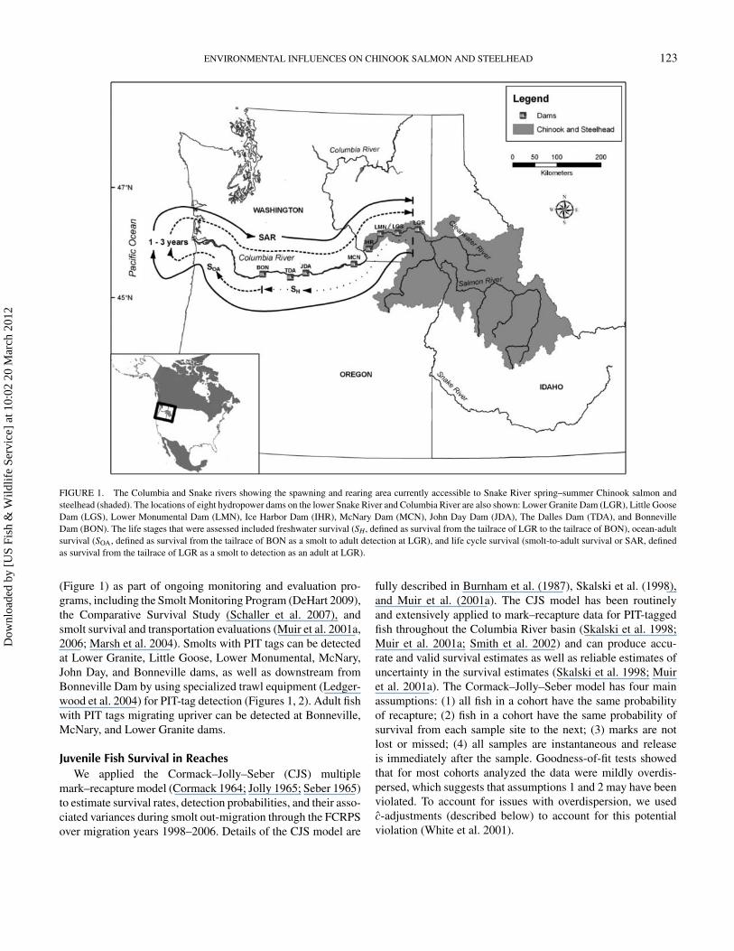
FIGURE 2. Graphical representation of the 11 Cormack–Jolly–Sebermark–recapture model parameters estimated in this analysis. Survival proba-bilities (Si) are defined from release in the tailrace until the tailrace of the nextsubsequent dam with PIT-tag detection capability. Detection probabilities (pi)are estimated for each of the dams with PIT-tag detection capability. Down-river from Bonneville Dam (BON), a PIT-tag detection trawl (TWX) operatesas a terminal detection site, with the joint probability of survival and detectionestimated by λ. See Figure 1 for the abbreviations for the dams.

Release groups.—We used a cohort-based approach for estimat-ing life-stage-specific and cumulative smolt-to-adult survivalrates (Figure 2). Cohort-based approaches allow for increasedsample sizes (i.e., more than one survival rate per year) andallow for finer-scale attribution of environmental conditions ex-perienced during out-migration (Muir et al. 2001a; Smith et al.2002). Cohorts consisted of PIT-tagged smolts that were de-tected and released into the tailrace at LGR using a PIT-tagdiversion system (Marsh et al. 1999) as well as smolts that werePIT-tagged at LGR (Muir et al. 2001a; Marsh et al. 2004) andsubsequently released into the tailrace over four 2-week periodsin each year: April 8–21, April 22–May 5, May 6–19, and May20–June 2. Hatchery-reared and wild smolts of each specieswere combined in the analyses, but we recorded the percentageof hatchery-origin smolts for each release cohort in order toexamine the effects of hatchery proportion on survival at eachlife stage (described below). To increase sample sizes of thePIT-tagged smolts that were released at LGR we augmented thedetection histories for each cohort with smolts that were PIT-tagged and released upriver from LGR but were first detected atLGS. Assignment of smolts that were first detected at LGS to arelease cohort at LGR was based on the median travel time be-tween LGR and LGS for each cohort in each year. For example,if the median travel time between LGR and LGS for the firststeelhead release cohort in 1998 was 4 d, the detection historydata set for that cohort was augmented with steelhead that werefirst detected at LGS during April 12–25. Following passage atLGS, we assumed that the LGR-releases and the first-time de-tected smolts at LGS were effectively mixed and shared identicalsurvival rates and detection probabilities downriver from LGS.Because the CJS model survival (S) and detection probabilities(p) are conditioned upon first release, only the LGR releases areused to estimate S1 and p1 (Figure 2), while both releases (i.e.,LGR releases and first-time detected smolts at LGS) are used toestimate the remaining survival and detection probabilities.

Theoretically, the LGR releases could be augmented withfirst-time detections at all of the downriver dams. However,owing to the variation in travel times of individual smolts andincreasing variability with migration distance (Zabel 2002), itbecomes more and more difficult to assign first-time detections

to the appropriate release cohort timing at LGR as migration dis-tance increases. In our judgment, we determined that first-timedetections at LGS could be reliably assigned to the appropriaterelease cohort timing at LGR owing to the relatively narrowvariation between individuals, but that first-time detections atLMN or below could not.

Survival estimates.—After their release, PIT-tagged smoltscould be detected at five downriver dams or the PIT-detectiontrawl operating downriver from Bonneville Dam (Figures 1,2). At each site, smolts could be detected and returned to theriver (Marsh et al. 1999), detected and removed from the taggedpopulation (e.g., for smolt transportation or for biological sam-pling), or undetected at that site. The series of event histories ateach site (i.e., detection, nondetection, or removal) constituteda detection history record for each tagged smolt suitable forsurvival estimation in the multiple-recapture CJS model. In ourapplication, the CJS model is applied to these detection historydata to estimate five reach survival parameters (S1, S2, . . . , S5),five detection probability parameters (p1, p2, . . . , p5) and oneparameter (λ) representing the joint probability of survival anddetection at the PIT-detection trawl (Figure 2).

Cumulative smolt survival estimates through the hydropowerdams and reservoirs (SH) and associated error estimates wereproduced for PIT-tagged Chinook salmon and steelhead thatout-migrated during the years from 1998 to 2006 in the riverreach between LGR and BON dams (Figures 1 and 2) by usingthe CJS methodology as described by Burnham et al. (1987) andimplemented within the MARK program (White and Burnham1999). Cumulative smolt survival was estimated as the productof the five, reach-specific survival rates:

SH = S1S2S3S4S5. (1)

To account for potential overdispersion in the mark–recapturedata (i.e., extrabinomial variation), we used the program RE-LEASE implemented within MARK to estimate c, the vari-ance adjustment factor. The variance–covariance matrix forS1, S2, . . . , S5 was multiplied by c (Burnham and Ander-son 2002), and we used the delta method (Burnham et al.1987) to calculate the variance of SH from the c-adjustedvariance–covariance matrix. This process was repeated for eachof the four release cohorts per year and for each species over 9years for a total of 36 possible cohort-year cases for each species.

Smolt-to-Adult SurvivalAs a measure of overall survival, smolt-to-adult-return sur-

vival estimates (SARs; Figure 1) were produced for PIT-taggedChinook salmon and steelhead release cohorts that out-migratedduring the years 1998 to 2006. The SARs are defined as thenumber of adults that return to LGR divided by the number ofsmolts that were released at LGR. However, as mentioned previ-ously, a portion of the PIT-tagged smolts after release are subse-quently removed from the tagged population owing to biological

Dow

nloa

ded

by [

US

Fish

& W

ildlif

e Se

rvic

e] a

t 10:

02 2

0 M

arch

201

2

ENVIRONMENTAL INFLUENCES ON CHINOOK SALMON AND STEELHEAD 125

sampling at the dams or to placement on transportation bargesat Lower Granite, Little Goose, Lower Monumental, or McNarydams. Those fish that are removed, along with the mortality thatoccurs before removal, must be accounted for when the num-ber of smolts that are actually migrating in-river are calculated,otherwise a bias could occur.

In this study we adopted a similar approach to that describedin Schaller et al. (2007) for estimating the number of PIT-taggedsmolts at Lower Granite Dam that are expected to migrate in-river without being removed, termed “Lower Granite equiva-lents.” The number of Lower Granite equivalent smolts wascalculated as

NLGR = RLGR + n01

S1−

5∑i=1

di∏i1 Si

, (2)

where RLGR is the number of PIT-tagged smolts released at LGR,n01 is the number of PIT-tagged smolts released upriver of LGRthat were first-detected at LGS (i.e., having a “01” detectionhistory at LGR and LGS), S1, S2, . . . , S5 are the five, reach-specific CJS survival estimates (Figure 2), and d1, d2, . . . , d5

are the numbers of PIT-tagged smolts that are removed at LGS,LMN, MCN, JDA, and BON, respectively. The method accountsfor the cumulative survival that occurs before the arrival andremoval of smolts at downriver dams and augments the numberof original releases (RLGR) with the effective number of smoltspassing LGR but were first detected at LGS.

By following the calculation of NLGR, smolt-to-adult survival(SAR) estimates were calculated as

SAR = Nadult

NLGR, (3)

where Nadult is the number of PIT-tagged fish that were detectedas adults at LGR and were not removed during juvenile out-migration. Precocial male Chinook salmon may return as “mini-jacks” after 0 years in the ocean (Larsen et al. 2004) or asjacks after 1 year in the ocean. Full-term adults return after 2or 3 years in the ocean. For Chinook salmon, mini-jacks andjacks (0-ocean and 1-ocean, respectively) were not includedin the adult return numbers, while for steelhead 1-ocean andolder returns were considered adults. We used a bootstrappingprocedure (Efron and Tibshirani 1993) to estimate the varianceof SAR. The procedure consisted of randomly sampling (withreplacement) the detection history records from N′ individualsmolts, where N′ is the number of detection history records inthe original data set, creating a bootstrap sample data set. Usingthis bootstrap sample data set, we calculated S1, S2, . . . , S5

by using the closed-form CJS equations (Burnham et al. 1987),NLGR by using equation (2), and SAR by using equation (3). Thisprocess was repeated 1,000 times to produce 1,000 bootstrapestimates of SAR. Our estimate of the variance of SAR was thevariance of these 1,000 bootstrap estimates of SAR. As with

SH , the SAR estimation and variance calculation process wasrepeated for each of the four release cohorts per year and foreach species over 9 years for a total of 36 possible cohort-yearcases for each species.

Ocean-Adult SurvivalGiven estimates of smolt survival from Lower Granite Dam

to Bonneville Dam (SH ) and survival from Lower Granite Damas smolts back to Lower Granite Dam as adults (SAR), weestimated ocean-adult survival (SOA, Figure 1) as

SOASAR

SH

. (4)

Survival estimates from this life stage encompass all survivalprocesses during the period following passage at BonnevilleDam as a smolt through the time when adults migrate pastLower Granite Dam. As such, SOA includes survival down theremaining portion of the Columbia River from Bonneville Dam,survival through the estuary and nearshore ocean, survival dur-ing the 1–3 years spent in the ocean, and survival during theupriver migration from the ocean and through the FCRPS toLower Granite Dam. For simplicity, we refer to this as ocean-adult survival. Because SOA is calculated as the quotient of tworandom variables (SAR and SH ), we used the approximation forthe variance of the quotient of two random variables providedby Mood et al. (1974) to estimate the variance of SOA:

var(SOA) = var

(SAR

SH

)∼=

(SAR

SH

)2

×⎛⎝ σ2

SAR

SAR2+ σ2

SH

S2H

−2r(SAR, SH ) ·

√σ2

SARσ2SH

SAR · SH

⎞⎠ , (5)

where r(SAR, SH ) is the estimated correlation between SARand SH across cohorts, and σ2

SAR and σ2SH

are the cohort-specificvariance estimates for SAR and SH, respectively. We estimatedSOA and its variance for all Chinook salmon and steelhead co-horts that we had estimates of both freshwater survival (SH ) andsmolt-to-adult survival (SAR) during 1998–2006.

Correlation AnalysesWe used correlation analyses to examine patterns of covaria-

tion in the life-stage-specific survival rate estimates for Chinooksalmon and steelhead. Budy et al. (2002) provided a review ofthe evidence supporting the hypothesis that a portion of the mor-tality expressed after passage at Bonneville Dam is related toearlier hydrosystem experience during downstream migration.Their paper synthesized the evidence documenting that the hy-drosystem causes direct mortality during juvenile out-migrationand imposes cumulative stress on those fish that survive, whichcan lead to delayed mortality. By using survival rates as a mea-sure of the degree of cumulative stress (or alternatively, the lack

Dow

nloa

ded

by [

US

Fish

& W

ildlif

e Se

rvic

e] a

t 10:

02 2

0 M

arch

201

2

126 HAESEKER ET AL.

thereof), under the Budy et al. (2002) hypothesis we would ex-pect a positive correlation between measures of hydrosystem(SH) and post–Bonneville Dam (SOA) survival. In addition, wewere interested in assessing the degree to which shared envi-ronmental processes may be influencing survival rates betweenthese two species, as indicated by patterns of positive correla-tion between the two species in their life-stage-specific survivalrates (Pyper et al. 2005). A priori, we hypothesized that correla-tions in survival rates between the two species would be highestduring juvenile out-migration (SH), when the two species sharedthe same migration pathway through the FCRPS and would belowest during the period of ocean residence through adult return(SOA) because of potential differences in ocean distributions andocean ecology. We hypothesized that correlations between thetwo species for SAR would be intermediate between the SH

correlation (hypothesized to be high) and the SOA correlation(hypothesized to be low) because the SAR is the product of SH

and SOA.To evaluate these hypotheses, we conducted a series of

comparisons between life-stage-specific survival rates by us-ing Pearson’s product-moment correlation coefficient. Pearson’sproduct-moment correlation coefficient is a measure of the de-gree of linear relationship between two variables. In preliminarybivariate plots of the life-stage-specific survival rates we noticedheteroscedasticity in some of the plots, which could reduce thepower to detect positive correlations. Therefore, we used a logittransformation on the stage-specific survival rates to reduce het-eroscedasticity and improve measurement of the degree of linearrelationship between the stage-specific survival rates:

logit(Si) = loge

(Si

1 − Si

), (6)

where Si is the life-stage-specific survival rate (SH, SOA, or SAR)for release cohort i. We calculated Pearson’s product-momentcorrelation coefficient for five pairs of logit-transformed sur-vival rates: (SH,CHN, SOA,CHN) and (SH,STH, SOA,STH) for evaluat-ing the hydrosystem-related, delayed-mortality hypothesis, and(SH,CHN, SH,STH), (SOA,CHN, SOA,STH) and (SARCHN, SARSTH)for evaluating patterns of covariation shared across species.

To account for positive autocorrelation evident in the survivalrate time series, we conducted significance tests for all correla-tions by using the method recommended by Pyper and Peterman(1998). Their recommended method consists of approximatingthe “effective” degrees of freedom (N∗) in correlation tests byusing

1

N∗ ≈ 1

N+ 2

N

∞∑j=1

ρXX(j )ρYY (j ), (7)

where N is the sample size, and ρXX(j) and ρYY(j) are the autocor-relation parameters of X and Y at lag j. Sample autocorrelation

coefficients were calculated with the estimator

rXX(j ) = N

N − j

∑N−j

t=1 (Xt − X)(Xt+j − X)∑Nt=1 (Xt − X)2

. (8)

Sample correlations between series X and Y (rXY ) were com-pared to a critical value (rcrit), based on the standard normaldistribution (Z)

rcrit = Za

√1/(N∗−2), (9)

to determine the statistical significance of the tests (one-tailedtests; H0: rXY = 0, HA: rXY > 0, α = 0.05).

Freshwater Environmental IndicesWithin the freshwater environment of the Columbia River

basin hydropower system, freshwater survival and mortalityrates of salmon have been associated with water transit timeand the percentage of water spilled at dams (spill), along withseasonal effects indexed by release day of the year (Muir et al.2001a; Schaller et al. 2007). Water transit time is a measure ofthe number of days it takes an average water particle to transitthe length of a reservoir and is calculated by dividing a reser-voir volume by the outflow rate (Petrosky and Schaller 2010).When water transit times are high (i.e., low water velocity),freshwater mortality rates of salmon and measures of their mi-gration delay tend to increase (Raymond 1988; Berggren andFilardo 1993; Schaller et al. 2007). The provision of spill in-creases the proportion of smolts passing the dams by nonturbineroutes and reduces migratory delays through dam forebays andtailraces. Estimates of smolt survival are often highest throughspillways compared with estimates of smolt survival throughjuvenile bypass systems or turbines (Muir et al. 2001b). Giventhese findings, we developed two indices to characterize con-ditions within the freshwater environment during the period ofjuvenile out-migration of each cohort during each year. Averagespill percentage and total water transit time (WTT) indices werecalculated for each cohort based on timing and fish travel timethrough the hydrosystem. The median fish travel time betweendams was estimated for each cohort and used to determine theperiod over which to calculate the average spill percentagesand WTT indices. Conditions at downstream dams were av-eraged over a 2-week period by using the travel time to thenext dam to adjust the start date of the calculations. The overallreach (LGR–BON) index for average spill percentage was theaverage of the dam-specific spill percentage values across theseven intermediary dams, while for water transit time the indiceswere the summation of the water transit times across the sevenintermediary reservoirs. In addition to these two indices charac-terizing the out-migration conditions through the hydrosystem,we also used release day of the year for each cohort to exam-ine changes in survival rates that may occur over the migrationseason. The day of the year for each release cohort was set atthe midpoint (day 7) of each 2-week cohort. To account for

Dow

nloa

ded

by [

US

Fish

& W

ildlif

e Se

rvic

e] a

t 10:

02 2

0 M

arch

201

2

ENVIRONMENTAL INFLUENCES ON CHINOOK SALMON AND STEELHEAD 127

90

100

50

60

70

80

Percenthatchery

10

20

30

40

01997 1998 1999 2000 2001 2002 2003 2004 2005 2006 2007

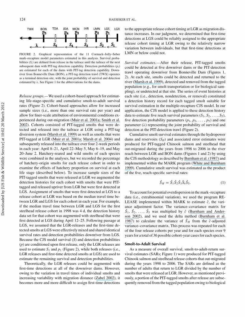
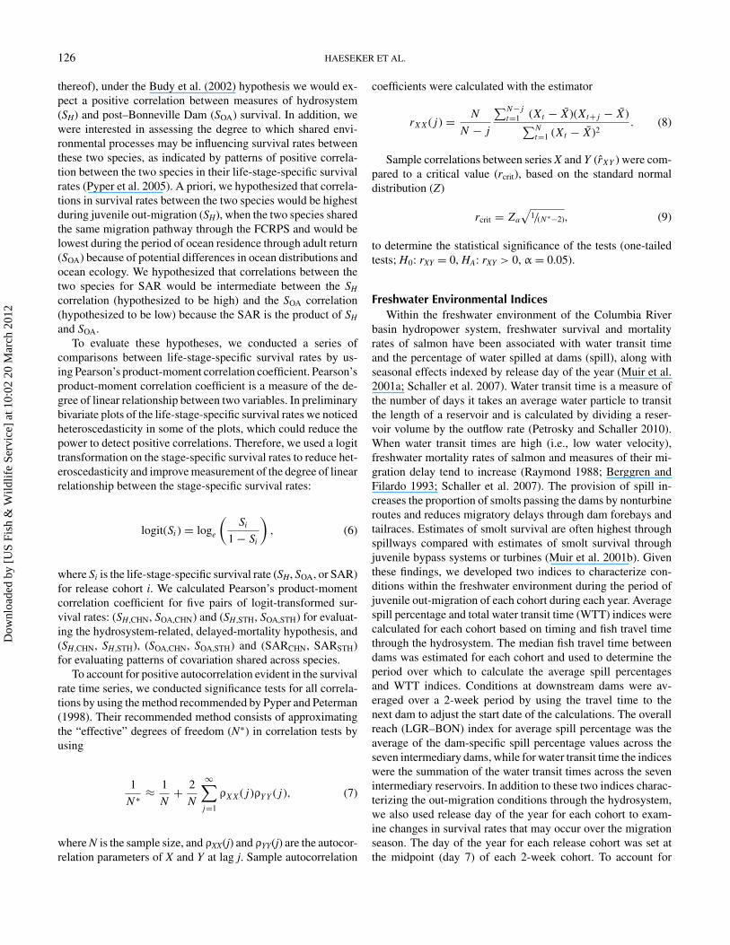
FIGURE 3. Percent of the release cohorts that were of hatchery origin forspring–summer Chinook salmon (filled diamonds) and steelhead (open squares).

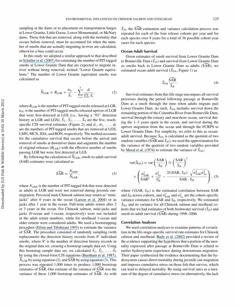
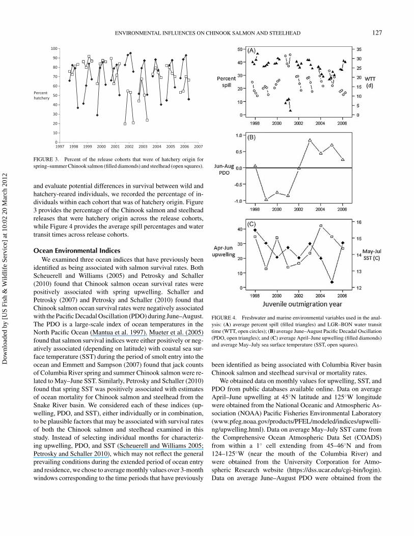
and evaluate potential differences in survival between wild andhatchery-reared individuals, we recorded the percentage of in-dividuals within each cohort that was of hatchery origin. Figure3 provides the percentage of the Chinook salmon and steelheadreleases that were hatchery origin across the release cohorts,while Figure 4 provides the average spill percentages and watertransit times across release cohorts.

Ocean Environmental IndicesWe examined three ocean indices that have previously been

identified as being associated with salmon survival rates. BothScheuerell and Williams (2005) and Petrosky and Schaller(2010) found that Chinook salmon ocean survival rates werepositively associated with spring upwelling. Schaller andPetrosky (2007) and Petrosky and Schaller (2010) found thatChinook salmon ocean survival rates were negatively associatedwith the Pacific Decadal Oscillation (PDO) during June–August.The PDO is a large-scale index of ocean temperatures in theNorth Pacific Ocean (Mantua et al. 1997). Mueter et al. (2005)found that salmon survival indices were either positively or neg-atively associated (depending on latitude) with coastal sea sur-face temperature (SST) during the period of smolt entry into theocean and Emmett and Sampson (2007) found that jack countsof Columbia River spring and summer Chinook salmon were re-lated to May–June SST. Similarly, Petrosky and Schaller (2010)found that spring SST was positively associated with estimatesof ocean mortality for Chinook salmon and steelhead from theSnake River basin. We considered each of these indices (up-welling, PDO, and SST), either individually or in combination,to be plausible factors that may be associated with survival ratesof both the Chinook salmon and steelhead examined in thisstudy. Instead of selecting individual months for characteriz-ing upwelling, PDO, and SST (Scheuerell and Williams 2005;Petrosky and Schaller 2010), which may not reflect the generalprevailing conditions during the extended period of ocean entryand residence, we chose to average monthly values over 3-monthwindows corresponding to the time periods that have previously

FIGURE 4. Freshwater and marine environmental variables used in the anal-ysis: (A) average percent spill (filled triangles) and LGR–BON water transittime (WTT, open circles); (B) average June–August Pacific Decadal Oscillation(PDO, open triangles); and (C) average April–June upwelling (filled diamonds)and average May–July sea surface temperature (SST, open squares).

been identified as being associated with Columbia River basinChinook salmon and steelhead survival or mortality rates.

We obtained data on monthly values for upwelling, SST, andPDO from public databases available online. Data on averageApril–June upwelling at 45◦N latitude and 125◦W longitudewere obtained from the National Oceanic and Atmospheric As-sociation (NOAA) Pacific Fisheries Environmental Laboratory(www.pfeg.noaa.gov/products/PFEL/modeled/indices/upwelli-ng/upwelling.html). Data on average May–July SST came fromthe Comprehensive Ocean Atmospheric Data Set (COADS)from within a 1◦ cell extending from 45–46◦N and from124–125◦W (near the mouth of the Columbia River) andwere obtained from the University Corporation for Atmo-spheric Research website (https://dss.ucar.edu/cgi-bin/login).Data on average June–August PDO were obtained from the

Dow

nloa

ded

by [

US

Fish

& W

ildlif

e Se

rvic

e] a

t 10:

02 2

0 M

arch

201

2

128 HAESEKER ET AL.

Joint Institute for the Study of the Atmosphere and Ocean(http://jisao.washington.edu/pdo/). Figure 4 summarizes thefreshwater and marine environmental variables used in theanalysis.

Multivariate Regression and Multimodel InferenceSimilar to the approach of Greene et al. (2005), we used mul-

tivariate regression and multimodel inference techniques basedon information theory (Burnham and Anderson 2002) to char-acterize associations between the freshwater and ocean indicesand the life-stage-specific survival rates of Chinook salmon andsteelhead. In all analyses we used a logit transformation (equa-tion 3) of the life-stage-specific survival rates as dependent vari-ables. All environmental indices were standardized to have amean value of zero and a SD of one by subtracting the meanand dividing by the SD. The full model for examining survivalduring juvenile out-migration through the hydrosystem was

logit(SH ) = β0 + β1 · Day + β2 · WTT + β3 · Spill

+ β4 · Hat.% + ε, (10)

where β0, β1, . . . , β4 are estimated regression coefficients andε ≈ N(0, σ2

SH). In this model we assume that only the freshwater(WTT and spill), seasonal (Day) and rearing-type composition(hatchery percentage) indices may contribute to variation infreshwater survival rates. The full model for examining ocean-adult survival rates was

logit(SOA) = β0 + β1 · Day + β2 · WTT + β3 · Spill

+β4 · Hat.% + β5 · PDO + β6 · Up.

+ β7 · SST + ε, (11)

where β0, β1, . . . , β7 are estimated regression coefficients andε ≈ N(0, σ2

SOA). In this model we assume that the freshwa-ter, seasonal, rearing-type composition, and ocean indices maycontribute to variation in ocean-adult survival. By allowing forpotential freshwater influences on ocean-adult mortality, thismodel represents another means of evaluating the Budy et al.(2002) hypothesis that freshwater migration experiences influ-ence subsequent survival after passage at Bonneville Dam. Thefull model for examining cumulative smolt-to-adult survivalrates was:

logit(SAR) = β0 + β1 · Day + β2 · WTT + β3 · Spill

+β4 · Hat.% + β5 · PDO + β6 · Up

+ β7 · SST + ε, (12)

where β0, β1, . . . , β7 are estimated regression coefficients andε ≈ N(0, σ2

SAR). In this model we assumed that the freshwa-ter, seasonal, rearing-type composition, and ocean indices maycontribute to variation in the cumulative smolt-to-adult survivalrates.

We calculated Akaike’s information criterion (AIC) for smallsample sizes (AICc) for all possible model combinations of thepredictor variables (all subsets regression). For the SH regres-sions, there were 16 possible combinations of the four predictorvariables and for the SOA and SAR regressions, there were128 possible combinations of the seven predictor variables. Toaccount for differences in the relative precision of the individualsurvival rate estimates, each model was estimated with aninverse-coefficient of variation weighting of the observations.The models were ranked according to AICc, the model with theminimum AICc was identified, and Akaike weights (wi) werecalculated for each model (Burnham and Anderson 2002). Toassess our assumption that residuals were normally distributed,we conducted Shapiro–Wilk tests on the residuals for thebest-fitting models (best-fitting as determined by minimumAICc) for each life stage and species. Similarly, to assess ourassumption that residuals were uncorrelated (i.e., independent),we used the Durbin–Watson test statistic (Draper and Smith1998). Durbin–Watson test statistics less than 1.0 are indicativeof strong, positive autocorrelation of regression residuals.

By using the AICc-ranked set, we calculated model-averagedpredictions for the life-stage-specific survival rates of eachspecies. Model-averaged predictions were calculated with theequation

θ =R∑

i=1

wi θ, (13)

where θ denotes the model-averaged prediction of θ (i.e., SH,SOA, or SAR) across the R models and wi denotes the Akaikeweight for model i = 1, 2, . . . , R (Burnham and Anderson2002). In addition to model-average predictions of the life-stage-specific survival rates of each species, we also used equation (13)to calculate model-averaged parameter coefficients for each ofthe environmental indices (substituting β for θ in equation 13).

We calculated the unconditional variance estimates for β withthe equation

var(βi

)=

[R∑

i=1

wi

√var

(βi |gi

) +(βi − β

)2]2

, (14)

where β is the model-averaged estimate of β determined fromequation (13) and var(βi |gi) is the variance of βi conditionalon model gi (Burnham and Anderson 2002). To help understandthe directionality and strength of the associations (effect sizes)between the environmental variables and survival rates, we con-structed and plotted 95% confidence intervals (CIs) for the β byusing the unconditional variance estimates. We interpreted anenvironmental variable as having a strong effect if its 95% CIdid not contain zero. We interpreted an environmental variableas having a moderate effect if the value of zero was within, but

Dow

nloa

ded

by [

US

Fish

& W

ildlif

e Se

rvic

e] a

t 10:

02 2

0 M

arch

201

2

ENVIRONMENTAL INFLUENCES ON CHINOOK SALMON AND STEELHEAD 129

near the tail of the 95% CI. We interpreted an environmental

variable as having a weak effect if the β was near zero.The sets of best-fitting models were also used to evaluate

the relative importance of each predictor variable used in theregressions (Burnham and Anderson 2002). The relative vari-able importance is a quantitative measure of the degree to whichvariables are consistently included among the best-fitting mod-els based on AICc relative to the other variables that were con-sidered. The relative variable importance for variable j among aset of R models is calculated as

R∑i=1

wiIj (gi), (15)

where wi is the Akaike weight for model i and Ij(gi) is anindicator variable equal to one if variable j is in model i (gi)and equal to zero otherwise. Variables with relative variableimportance values near one are consistently in the top-fittingmodels while variables with relative variable importance valuesnear zero are rarely, if ever, included in the top-fitting models.

Assessing Inland Actions under Variable OceanConditions

As mentioned previously, our objectives included identify-ing which actions taken inland would be most critical for im-proving cumulative smolt-to-adult survival rates across variableocean conditions (NPCC 2009) and identifying the correspond-ing freshwater survival rates that may be necessary to achieve theNPCC SAR goal of SARs averaging 4% and having a minimumof 2% (NPCC 2003, 2009). To accomplish these objectives,the effects of variable ocean conditions and their influenceson smolt-to-adult survival rates must be accounted for. We ac-counted for variable ocean conditions by first determining whichocean environmental index (upwelling, SST, or PDO) had thehighest relative variable importance in the SAR regressions foreach species. We then classified each year as having favorable,neutral, or unfavorable ocean environmental conditions basedon the sign of the model-averaged parameter coefficient for theselected ocean index variable and the ocean index value in eachyear. To determine which actions inland would be most criti-cal for improving SAR, we graphically examined associationsbetween WTT, spill, and SAR and identified which SAR obser-vations occurred under favorable, neutral, or unfavorable oceanenvironmental conditions. Similarly, to identify freshwater sur-vival rates that may be necessary to achieve the NPCC SAR goal,we graphically examined associations between SH and SAR andidentified which SAR observations occurred under favorable,neutral, or unfavorable ocean environmental conditions.

RESULTSWe were able to estimate SARs for all 36 release cohorts

of each species (Figure 5). However, owing to a combinationof low sample sizes and low detection probabilities, we were

able to estimate SH for only 33 of the Chinook salmon and 22of the steelhead release cohorts. Likewise, because calculationof SOA required an estimate of SAR and SH, we were able toestimate SOA for only 33 of the Chinook salmon and 22 of thesteelhead release cohorts. Low sample sizes or low detectionprobabilities, or both, also influenced the precision of the SH,with the highest precision for both species occurring in 2001when detection probabilities were high owing to the eliminationof spill for fish passage in that year (Figure 4). Several of the SH

estimates had SE values exceeding 0.3.Across release cohorts and years, survival rates during juve-

nile out-migration tended to be higher for Chinook salmon thanfor steelhead, with an average SH of 0.53 for Chinook salmonand 0.39 for steelhead (Figure 5). The lowest estimates of SH

for Chinook salmon occurred in 2001, 2004, and 2005, aver-aging 0.28, 0.43, and 0.48, respectively, across cohorts withinthose years. Similarly, the lowest estimates of SH for steelheadoccurred in 2001, 2004, and 2005 and averaged 0.03, 0.12, and0.33, respectively, across cohorts in those years. These years oflow SH corresponded with the 3 years with the longest watertransit times and the lowest average percent spill levels (Figure4). Within-year changes in SH were variable and had increasing,decreasing, or relatively stable seasonal patterns in SH, depend-ing on the year for both species.

Across release cohorts and years, the average SOA was 1.01%for Chinook salmon and 1.64% for steelhead (Figure 5). ForChinook salmon, the lowest estimates of SOA occurred in 2001and 2003–2005, while the lowest estimates for steelhead SOA

occurred in 2001 and 2004–2005. These years of low SOA cor-responded with the 3 years with the longest water transit timesand the lowest average percent spill levels (Figure 4). The high-est estimates of SOA occurred in 1999 and 2000 for Chinooksalmon and 2000 for steelhead. Within-year changes in SOA

were variable for Chinook salmon and had increasing, decreas-ing, or relatively stable seasonal patterns, depending on the year.In contrast, steelhead generally exhibited a decreasing seasonaltrend in SOA within years.

The SAR estimates for both species were well below theNPCC (2009) goal of SARs averaging 4% and a minimum of2%. The average SAR for Chinook salmon was 0.59% and theaverage SAR for steelhead was 0.61%. Only 1 of the 36 SARestimates for Chinook salmon was above the 2% minimum andonly 1 of the 36 SAR estimates for steelhead was above the 2%minimum. Within-year changes in SAR were variable for Chi-nook salmon and had increasing, decreasing, or relatively stableseasonal patterns, depending on the year. Steelhead SARs con-sistently declined over the migration season, with the exceptionof 2001 when low SARs (average = 0.02%) were exhibitedthroughout the migration season.

When we accounted for autocorrelation in the logit-transformed time series’ of SH, SOA and SAR the original samplesizes were reduced from 22–36 observations to 15–21 effectivesamples (Table 1). After we accounted for this autocorrelation,we identified significant positive correlations between the SH

Dow

nloa

ded

by [

US

Fish

& W

ildlif

e Se

rvic

e] a

t 10:

02 2

0 M

arch

201

2

130 HAESEKER ET AL.

steelheadChinook salmon

0.8

1.0

1.2

0.8

1.0

1.2

SH

0.0

0.2

0.4

0.6

1997 1998 1999 2000 2001 2002 2003 2004 2005 2006 20070.0

0.2

0.4

0.6

1997 1998 1999 2000 2001 2002 2003 2004 2005 2006 20071997 1998 1999 2000 2001 2002 2003 2004 2005 2006 2007

4%

5%

6%

1997 1998 1999 2000 2001 2002 2003 2004 2005 2006 2007

4%

5%

6%

SOA

0%

1%

2%

3%

1997 1998 1999 2000 2001 2002 2003 2004 2005 2006 20070%

1%

2%

3%

1997 1998 1999 2000 2001 2002 2003 2004 2005 2006 2007

3%

4%

5%

3%

4%

5%

0%

1%

2%

1997 1998 1999 2000 2001 2002 2003 2004 2005 2006 20070%

1%

2%

1997 1998 1999 2000 2001 2002 2003 2004 2005 2006 2007

SAR

Juvenile outmigra�on year

FIGURE 5. Estimates of SH, SOA, and SAR (filled triangles, ±1 SE) and model-averaged predictions of SH, SOA, and SAR (open circles) for Chinook salmon(left column) and steelhead (right column). A horizontal dashed line at 4% on the SAR graphs denotes the Northwest Power and Conservation Council SAR goal.

and SOA life-stage survival rates for both species (Table 1). ForChinook salmon, the estimated correlation between SH and SOA

was r = 0.49(P = 0.0085). For steelhead, the estimated corre-lation between SH and SOA was r = 0.55(P = 0.0215). Theseresults demonstrated that there are significant positive correla-tions between survival during juvenile out-migration through thehydrosystem and subsequent survival during the ocean-adult lifestage. Also, these sample correlation coefficients are probablyunderestimates of their true values. Because of the measurementerror in each of the life-stage-specific survival rates (especiallyfor SH), the estimated correlation coefficient is biased to somedegree towards zero (Buonaccorsi 2010).

In addition to positive correlations between life stages, wealso found significant positive correlations in the life-stage-

specific survival rate estimates between species (Table 1). Thehighest correlations between the two species occurred during ju-venile out-migration through the hydrosystem (SH) (r = 0.75,P = 0.0015) and during the ocean-adult life stage (SOA)(r = 0.75, P = 0.0020). The correlation between the twospecies for smolt-to-adult survival was lower, but was statis-tically significant (r = 0.61, P = 0.0040). While the highcorrelation between species during juvenile out-migration wasconsistent with our expectation, we were surprised by the equiv-alently high correlation between species during the ocean-adultlife stage (SOA). We hypothesized that the correlation betweenSARs of the two species would be intermediate between the SH

and SOA correlations, but instead it was the lowest among thethree.

Dow

nloa

ded

by [

US

Fish

& W

ildlif

e Se

rvic

e] a

t 10:

02 2

0 M

arch

201

2

ENVIRONMENTAL INFLUENCES ON CHINOOK SALMON AND STEELHEAD 131

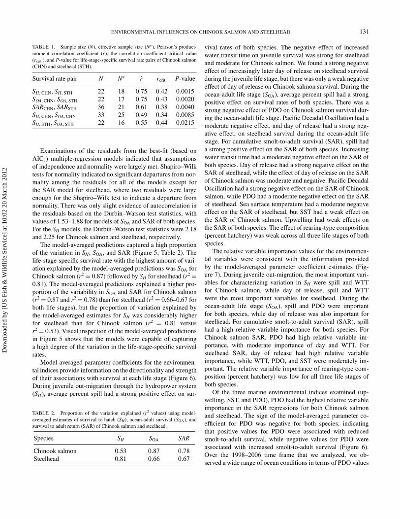
TABLE 1. Sample size (N), effective sample size (N∗), Pearson’s product-moment correlation coefficient (r), the correlation coefficient critical value(rcrit.), and P-value for life-stage-specific survival rate pairs of Chinook salmon(CHN) and steelhead (STH).

Survival rate pair N N∗ r rcrit. P-value

SH, CHN, SH, STH 22 18 0.75 0.42 0.0015SOA, CHN, SOA, STH 22 17 0.75 0.43 0.0020SARCHN, SARSTH 36 21 0.61 0.38 0.0040SH, CHN, SOA, CHN 33 25 0.49 0.34 0.0085SH, STH, SOA, STH 22 16 0.55 0.44 0.0215

Examinations of the residuals from the best-fit (based onAICc) multiple-regression models indicated that assumptionsof independence and normality were largely met. Shapiro–Wilktests for normality indicated no significant departures from nor-mality among the residuals for all of the models except forthe SAR model for steelhead, where two residuals were largeenough for the Shapiro–Wilk test to indicate a departure fromnormality. There was only slight evidence of autocorrelation inthe residuals based on the Durbin–Watson test statistics, withvalues of 1.53–1.88 for models of SOA and SAR of both species.For the SH models, the Durbin–Watson test statistics were 2.18and 2.25 for Chinook salmon and steelhead, respectively.

The model-averaged predictions captured a high proportionof the variation in SH, SOA, and SAR (Figure 5; Table 2). Thelife-stage-specific survival rate with the highest amount of vari-ation explained by the model-averaged predictions was SOA forChinook salmon (r2 = 0.87) followed by SH for steelhead (r2 =0.81). The model-averaged predictions explained a higher pro-portion of the variability in SOA and SAR for Chinook salmon(r2 = 0.87 and r2 = 0.78) than for steelhead (r2 = 0.66–0.67 forboth life stages), but the proportion of variation explained bythe model-averaged estimates for SH was considerably higherfor steelhead than for Chinook salmon (r2 = 0.81 versusr2 = 0.53). Visual inspection of the model-averaged predictionsin Figure 5 shows that the models were capable of capturinga high degree of the variation in the life-stage-specific survivalrates.

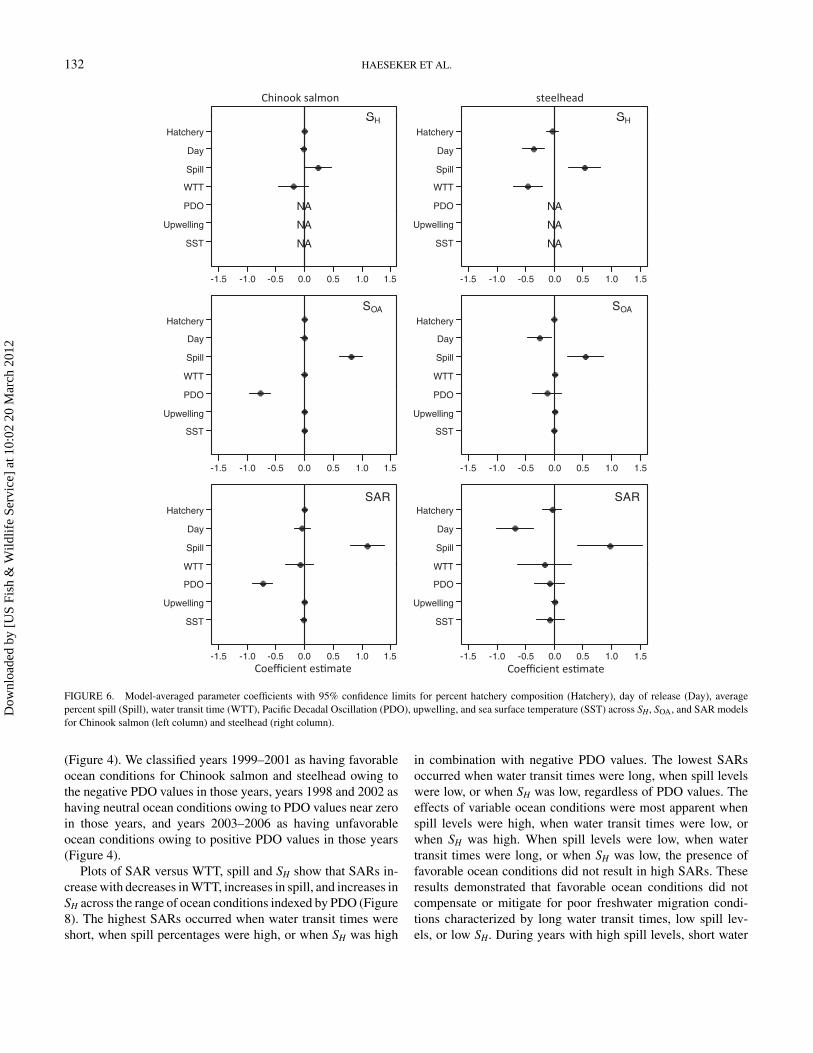
Model-averaged parameter coefficients for the environmen-tal indices provide information on the directionality and strengthof their associations with survival at each life stage (Figure 6).During juvenile out-migration through the hydropower system(SH), average percent spill had a strong positive effect on sur-

TABLE 2. Proportion of the variation explained (r2 values) using model-averaged estimates of survival to hatch (SH), ocean-adult survival (SOA), andsurvival to adult return (SAR) of Chinook salmon and steelhead.

Species SH SOA SAR

Chinook salmon 0.53 0.87 0.78Steelhead 0.81 0.66 0.67

vival rates of both species. The negative effect of increasedwater transit time on juvenile survival was strong for steelheadand moderate for Chinook salmon. We found a strong negativeeffect of increasingly later day of release on steelhead survivalduring the juvenile life stage, but there was only a weak negativeeffect of day of release on Chinook salmon survival. During theocean-adult life stage (SOA), average percent spill had a strongpositive effect on survival rates of both species. There was astrong negative effect of PDO on Chinook salmon survival dur-ing the ocean-adult life stage. Pacific Decadal Oscillation had amoderate negative effect, and day of release had a strong neg-ative effect, on steelhead survival during the ocean-adult lifestage. For cumulative smolt-to-adult survival (SAR), spill hada strong positive effect on the SAR of both species. Increasingwater transit time had a moderate negative effect on the SAR ofboth species. Day of release had a strong negative effect on theSAR of steelhead, while the effect of day of release on the SARof Chinook salmon was moderate and negative. Pacific DecadalOscillation had a strong negative effect on the SAR of Chinooksalmon, while PDO had a moderate negative effect on the SARof steelhead. Sea surface temperature had a moderate negativeeffect on the SAR of steelhead, but SST had a weak effect onthe SAR of Chinook salmon. Upwelling had weak effects onthe SAR of both species. The effect of rearing-type composition(percent hatchery) was weak across all three life stages of bothspecies.

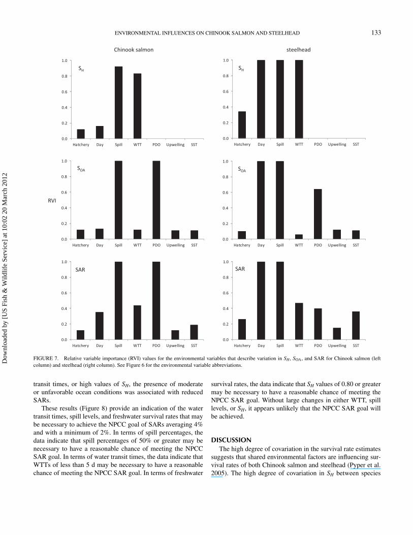
The relative variable importance values for the environmen-tal variables were consistent with the information providedby the model-averaged parameter coefficient estimates (Fig-ure 7). During juvenile out-migration, the most important vari-ables for characterizing variation in SH were spill and WTTfor Chinook salmon, while day of release, spill and WTTwere the most important variables for steelhead. During theocean-adult life stage (SOA), spill and PDO were importantfor both species, while day of release was also important forsteelhead. For cumulative smolt-to-adult survival (SAR), spillhad a high relative variable importance for both species. ForChinook salmon SAR, PDO had high relative variable im-portance, with moderate importance of day and WTT. Forsteelhead SAR, day of release had high relative variableimportance, while WTT, PDO, and SST were moderately im-portant. The relative variable importance of rearing-type com-position (percent hatchery) was low for all three life stages ofboth species.

Of the three marine environmental indices examined (up-welling, SST, and PDO), PDO had the highest relative variableimportance in the SAR regressions for both Chinook salmonand steelhead. The sign of the model-averaged parameter co-efficient for PDO was negative for both species, indicatingthat positive values for PDO were associated with reducedsmolt-to-adult survival, while negative values for PDO wereassociated with increased smolt-to-adult survival (Figure 6).Over the 1998–2006 time frame that we analyzed, we ob-served a wide range of ocean conditions in terms of PDO values

Dow

nloa

ded

by [

US

Fish

& W

ildlif

e Se

rvic

e] a

t 10:

02 2

0 M

arch

201

2

132 HAESEKER ET AL.

steelheadChinook salmon

S S

PDO

WTT

Spill

Day

Hatchery

NA

SH

PDO

WTT

Spill

Day

Hatchery

NA

SH

-1.5 -1.0 -0.5 0.0 0.5 1.0 1.5

SST

Upwelling

NA

NA

-1.5 -1.0 -0.5 0.0 0.5 1.0 1.5

SST

Upwelling

NA

NA

WTT

Spill

Day

Hatchery

SOA

WTT

Spill

Day

Hatchery

SOA

-1.5 -1.0 -0.5 0.0 0.5 1.0 1.5

SST

Upwelling

PDO

-1.5 -1.0 -0.5 0.0 0.5 1.0 1.5

SST

Upwelling

PDO

WTT

Spill

Day

HatcherySAR

WTT

Spill

Day

HatcherySAR

SST

Upwelling

PDO

WTT

SST

Upwelling

PDO

WTT

Coefficient es�mateCoefficient es�mate-1.5 -1.0 -0.5 0.0 0.5 1.0 1.5 -1.5 -1.0 -0.5 0.0 0.5 1.0 1.5

FIGURE 6. Model-averaged parameter coefficients with 95% confidence limits for percent hatchery composition (Hatchery), day of release (Day), averagepercent spill (Spill), water transit time (WTT), Pacific Decadal Oscillation (PDO), upwelling, and sea surface temperature (SST) across SH, SOA, and SAR modelsfor Chinook salmon (left column) and steelhead (right column).

(Figure 4). We classified years 1999–2001 as having favorableocean conditions for Chinook salmon and steelhead owing tothe negative PDO values in those years, years 1998 and 2002 ashaving neutral ocean conditions owing to PDO values near zeroin those years, and years 2003–2006 as having unfavorableocean conditions owing to positive PDO values in those years(Figure 4).

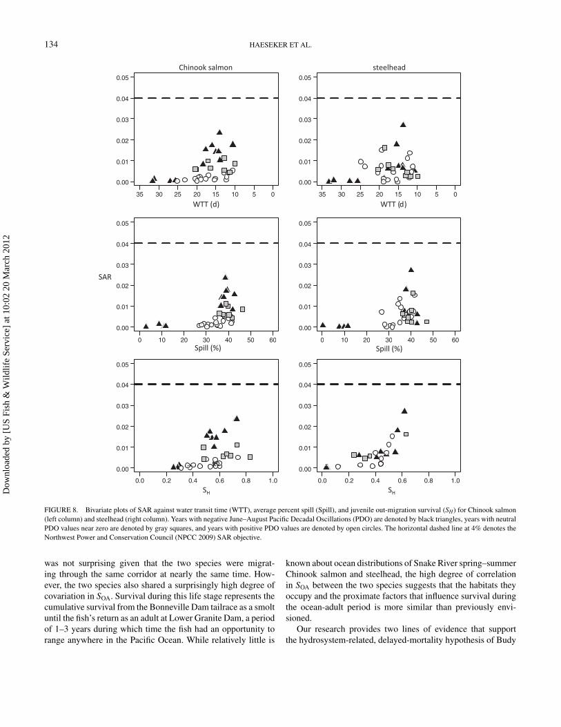
Plots of SAR versus WTT, spill and SH show that SARs in-crease with decreases in WTT, increases in spill, and increases inSH across the range of ocean conditions indexed by PDO (Figure8). The highest SARs occurred when water transit times wereshort, when spill percentages were high, or when SH was high

in combination with negative PDO values. The lowest SARsoccurred when water transit times were long, when spill levelswere low, or when SH was low, regardless of PDO values. Theeffects of variable ocean conditions were most apparent whenspill levels were high, when water transit times were low, orwhen SH was high. When spill levels were low, when watertransit times were long, or when SH was low, the presence offavorable ocean conditions did not result in high SARs. Theseresults demonstrated that favorable ocean conditions did notcompensate or mitigate for poor freshwater migration condi-tions characterized by long water transit times, low spill lev-els, or low SH. During years with high spill levels, short water

Dow

nloa

ded

by [

US

Fish

& W

ildlif

e Se

rvic

e] a

t 10:

02 2

0 M

arch

201

2

ENVIRONMENTAL INFLUENCES ON CHINOOK SALMON AND STEELHEAD 133

1 0 1 0

steelheadChinook salmon

0.4

0.6

0.8

1.0

0.4

0.6

0.8

1.0

SH SH

0.0

0.2

Hatchery Day Spill WTT PDO Upwelling SST

0.8

1.0

0.0

0.2

Hatchery Day Spill WTT PDO Upwelling SST

0.8

1.0

SOA SOA

0.0

0.2

0.4

0.6

0.0

0.2

0.4

0.6

RVI

Hatchery Day Spill WTT PDO Upwelling SST

0.6

0.8

1.0

Hatchery Day Spill WTT PDO Upwelling SST

0.6

0.8

1.0

SAR SAR

0.0

0.2

0.4

Hatchery Day Spill WTT PDO Upwelling SST0.0

0.2

0.4

Hatchery Day Spill WTT PDO Upwelling SST

FIGURE 7. Relative variable importance (RVI) values for the environmental variables that describe variation in SH, SOA, and SAR for Chinook salmon (leftcolumn) and steelhead (right column). See Figure 6 for the environmental variable abbreviations.

transit times, or high values of SH, the presence of moderateor unfavorable ocean conditions was associated with reducedSARs.

These results (Figure 8) provide an indication of the watertransit times, spill levels, and freshwater survival rates that maybe necessary to achieve the NPCC goal of SARs averaging 4%and with a minimum of 2%. In terms of spill percentages, thedata indicate that spill percentages of 50% or greater may benecessary to have a reasonable chance of meeting the NPCCSAR goal. In terms of water transit times, the data indicate thatWTTs of less than 5 d may be necessary to have a reasonablechance of meeting the NPCC SAR goal. In terms of freshwater

survival rates, the data indicate that SH values of 0.80 or greatermay be necessary to have a reasonable chance of meeting theNPCC SAR goal. Without large changes in either WTT, spilllevels, or SH, it appears unlikely that the NPCC SAR goal willbe achieved.

DISCUSSIONThe high degree of covariation in the survival rate estimates

suggests that shared environmental factors are influencing sur-vival rates of both Chinook salmon and steelhead (Pyper et al.2005). The high degree of covariation in SH between species

Dow

nloa

ded

by [

US

Fish

& W

ildlif

e Se

rvic

e] a

t 10:

02 2

0 M

arch

201

2

134 HAESEKER ET AL.

steelheadChinook salmon

0.02

0.03

0.04

0.05

0.02

0.03

0.04

0.05

35 30 25 20 15 10 5 0

0.00

0.01

35 30 25 20 15 10 5 0

0.00

0.01

WTT d( )WTT (d)

0.03

0.04

0.05

0.03

0.04

0.05

0 10 20 30 40 50 60

0.00

0.01

0.02

0 10 20 30 40 50 60

0.00

0.01

0.02SAR

0 10 20 30 40 50 60

0.04

0.05

0 10 20 30 40 50 60

0.04

0.05

Spill (%) Spill (%)

0.01

0.02

0.03

0.01

0.02

0.03

0.0 0.2 0.4 0.6 0.8 1.0

0.00

0.0 0.2 0.4 0.6 0.8 1.0

0.00

SH SH

FIGURE 8. Bivariate plots of SAR against water transit time (WTT), average percent spill (Spill), and juvenile out-migration survival (SH) for Chinook salmon(left column) and steelhead (right column). Years with negative June–August Pacific Decadal Oscillations (PDO) are denoted by black triangles, years with neutralPDO values near zero are denoted by gray squares, and years with positive PDO values are denoted by open circles. The horizontal dashed line at 4% denotes theNorthwest Power and Conservation Council (NPCC 2009) SAR objective.

was not surprising given that the two species were migrat-ing through the same corridor at nearly the same time. How-ever, the two species also shared a surprisingly high degree ofcovariation in SOA. Survival during this life stage represents thecumulative survival from the Bonneville Dam tailrace as a smoltuntil the fish’s return as an adult at Lower Granite Dam, a periodof 1–3 years during which time the fish had an opportunity torange anywhere in the Pacific Ocean. While relatively little is

known about ocean distributions of Snake River spring–summerChinook salmon and steelhead, the high degree of correlationin SOA between the two species suggests that the habitats theyoccupy and the proximate factors that influence survival duringthe ocean-adult period is more similar than previously envi-sioned.

Our research provides two lines of evidence that supportthe hydrosystem-related, delayed-mortality hypothesis of Budy

Dow

nloa

ded

by [

US

Fish

& W

ildlif

e Se

rvic

e] a

t 10:

02 2

0 M

arch

201

2

ENVIRONMENTAL INFLUENCES ON CHINOOK SALMON AND STEELHEAD 135

et al. (2002). First, we found significant, positive correlationsbetween SH and SOA for both species. Under the hydrosystem-related, delayed-mortality hypothesis, mortality rates at laterlife stages are expected to be positively associated with mor-tality rates at previous life stages, and our results support thisexpectation. Second, we identified spill as having measureableeffects not only on survival during juvenile out-migration, butalso on survival during the ocean-adult period for both species.The identification of spill as a factor that accounts for variabilityacross multiple life stages is consistent with the hydrosystem-related, delayed-mortality hypothesis because this factor, whichexplains variability in mortality in the later life stage (SOA), alsoexplains variability in the previous life stage (SH). Therefore,our research provides two lines of direct evidence that a portionof the mortality expressed after Chinook salmon and steelheadleave the hydrosystem is related to processes that reflect down-stream migration conditions.

Research continues to indicate that both freshwater and ma-rine factors are important drivers of the observed variabilityin Chinook salmon and steelhead survival rates, particularly inriver systems where freshwater habitat is highly influenced byanthropogenic factors (Lawson et al. 2004; Greene et al. 2005;Schaller and Petrosky 2007; Petrosky and Schaller 2010). Ourstudy provides additional information on the influences of fresh-water and marine factors, but we share the view, expressed byBisbal and McConnaha (1998), that it is the cumulative effectsof factors across the freshwater, estuarine, and marine environ-ments that determine salmon survival and abundance. In addi-tion to the factors that influence survival within each life stage,the positive correlations between freshwater and ocean-adultsurvival rates have important implications for improving the un-derstanding of interactions between the freshwater and marineenvironments for Snake River Chinook salmon and steelhead.The potential for covariation between freshwater and marinesurvival rates was recognized by Bradford (1995), but to ourknowledge our study is the first to quantify the degree of covari-ation. The significant, positive correlations between SH and SOA

for both species demonstrates that survival within the ocean en-vironment is not independent of survival within the freshwaterenvironment. The evidence presented in this study indicates thata portion of the mortality expressed during the ocean-adult lifestage is due to delayed mortality effects related to factors thatoccur during the freshwater life stage. Some of this covariationappears to be related to levels of spill, with spill affecting SH andSOA of both species. Thus, the effects of freshwater conditionsare manifested across several life stages and are not limited toonly affecting variation during the freshwater life stage.

From a modeling standpoint, these results also have impor-tant implications. Several researchers have conducted popula-tion projection analyses that examine how changes in survivalduring various life stages (e.g., egg to smolt, freshwater migra-tion survival, early ocean survival, adult survival and harvest)would affect population growth rates (Kareiva et al. 2000; Mc-Clure et al. 2003; Wilson 2003). These are useful areas of re-

search for prioritizing conservation actions at these life stages.However, the analyses that have been conducted to date have im-plicitly assumed that freshwater and ocean-adult survival ratesare independent of each other. For example, Kareiva et al. (2000)conducted population projections under a hypothetical scenariowhere freshwater survival rates were increased to 100%, butwithout any function for characterizing how ocean-adult sur-vival would be expected to change along with those assumedchanges in freshwater survival. The identification of significant,positive correlation between SH and SOA for both species indi-cates that the independence assumption of Kareiva et al. (2000)is not consistent with the new available data. The correlationbetween freshwater and ocean-adult survival rates is a criticalissue for properly characterizing and modeling the expected ef-fects of changes in survival across various life stages, and thepresence of correlation between life stages can have large ef-fects on population growth models (Doak et al. 1994). From theperspective of prioritizing conservations actions, Kareiva et al.(2000) and Wilson (2003) both concluded that improving earlyocean survival rates was critical for achieving Chinook salmonrecovery objectives. Given the strong positive associations be-tween spill and SOA, our results indicate that increasing spillpercentages may be a way to increase SOA.

Although our results indicate that freshwater factors are im-portant influences on freshwater, ocean-adult, and cumulativesmolt-to-adult survival, our results clearly show that marinefactors are also important. Of the three marine variables exam-ined, PDO appeared to be the most important factor regulatingocean-adult and smolt-to-adult survival rates of Snake RiverChinook salmon and steelhead. Consistent with Schaller andPetrosky (2007) and Petrosky and Schaller (2010), we found thatwarm-phase PDO values were negatively associated with ocean-adult and smolt-to-adult survival rates of Chinook salmon andsteelhead. Warm SSTs were negatively associated with smolt-to-adult survival rates of steelhead, but had little measurableeffect on ocean-adult or smolt-to-adult survival rates of Chi-nook salmon. In contrast to Scheuerell and Williams (2005) andSchaller and Petrosky (2007), we found that April–June up-welling generally had weak or inconsistent effects, or both, onocean-adult and smolt-to-adult survival rates of Chinook salmonand steelhead. These differences may be due to the multivariatenature of the regressions, with spill and PDO explaining most ofthe variation in ocean-adult and smolt-to-adult survival, leavinglittle remaining variation to be explained by upwelling.

Large-scale climatic variables such as measures of oceantemperature anomalies (PDO and SST) and upwelling are linkedto some degree with climatic conditions inland, and these inlandconditions could affect the freshwater variables we evaluated,such as water transit time. Several researchers have found cor-relations between ocean indices, such as upwelling, SST, andPDO, and freshwater climate indices, such as flow and wintersnowpack (Beamish 1993; Miller et al. 1994; Cayan 1996; Man-tua et al. 1997). Mueter et al. (2005) speculated that correlationsbetween wintertime ocean temperatures and sockeye salmon O.

Dow

nloa

ded

by [

US

Fish

& W

ildlif

e Se

rvic

e] a

t 10:

02 2

0 M

arch

201

2

136 HAESEKER ET AL.

nerka survival rates in British Columbia and Washington mayhave been due to the correlation between ocean climate condi-tions and inland climate conditions affecting freshwater habitat.However, the marine variables used in this analysis accountedfor less than 7% of the variation in WTT and spill. Therefore, theobserved correlations between freshwater and ocean survival donot appear to simply be the result of large-scale climatic factorsthat simultaneously influence survival within the freshwater andmarine environments.

Some caution is warranted when comparing the SARs ob-served in this study to the NPCC SAR goals. First, the SARsreported in this study were derived from Chinook salmon andsteelhead smolts that were detected at either Lower Granite Damor Little Goose Dam. Several studies have found that fish that ex-perience the bypass–detection systems at dams show negativelybiased SARs compared with fish that migrate through unde-tected routes (Budy et al. 2002; Williams et al. 2005; Tuomikoskiet al. 2009). Tuomikoski et al. (2009) found that the magnitudeof the bias varies across years, but on average, SARs of un-detected fish were estimated to be 23% greater than SARs offish that experience the bypass–detection systems. Whether thisbias remains constant or changes over the migration season isunknown. However, assuming the 23% bias is reasonable, multi-plying the SARs in this study by 123% does not result in achiev-ing the NPCC SAR goals. Second, a recent study by Knudsen etal. (2009) found that hatchery Chinook salmon from the YakimaRiver, Washington, that were only coded-wire-tagged had 33%higher SARs than those for fish that were tagged with both a PITtag and a coded wire tag. Knudsen et al. (2009) were not able toidentify when the bias occurred, though they suggested that itoccurred within the first 6 months after release from the hatch-ery. In our study, some of the fish were tagged in the fall beforethe year of out-migration and migrated some distance withinthe Snake River basin before being detected at Lower Graniteor Little Goose dams. These smolts may or may not have ex-pressed a tagging bias by the time they arrived at Lower Graniteand Little Goose dams. There are also questions as to whetherthe tagging bias is applicable to the wild and hatchery Chinooksalmon and steelhead in the Snake River, or whether it is uniqueto the Yakima River hatchery Chinook salmon. Resolving thesequestions will require additional research. Assuming that boththe detection and tagging biases are fully present and applicablein our study, we estimate that the SARs may be up to 64% higherthan what we have reported (123% × 133% = 164%). Even as-suming both biases are present, the Chinook salmon and steel-head SARs would remain substantially below the NPCC goals.

In conclusion, the models that were developed for character-izing variation in overall life cycle mortality rates indicate thatincreases in spill levels and reductions in water transit times areexpected to increase stage-specific survival rates (SH and SOA) aswell as cumulative smolt-to-adult survival rates. Across a rangeof ocean conditions, higher spill levels and reductions in watertransit time are expected to result in higher SARs than wouldoccur with lower spill levels and higher water transit times. At

a minimum, the models developed here can predict the SH, SOA,and SAR that may result under various flow and spill alter-natives. These predictions would provide quantitative, testablehypotheses on the predicted survival responses that could occurunder a true adaptive management experiment (Walters 1986)conducted within the FCRPS, where spill and water transit timesare extended beyond the range of available data and the resultingsurvival rates are monitored to determine whether the expectedincreases are realized.

ACKNOWLEDGMENTSThe opinions expressed in this paper are those of the authors

and do not necessarily reflect those of the U.S. Fish and WildlifeService. We thank three anonymous reviewers and the journaleditor Richard Beamish for providing helpful review comments.We thank David Hines for creating the map.

REFERENCESBeamish, R. J. 1993. Climate and exceptional fish production off the west

coast of North America. Canadian Journal of Fisheries and Aquatic Sciences50:2270–2291.

Berggren, T. J., and M. J. Filardo. 1993. An analysis of variables influencing themigration of juvenile salmonids in the Columbia River basin. North AmericanJournal of Fisheries Management 13:48–63.

Bisbal, G. A., and W. E. McConnaha. 1998. Consideration of ocean conditionsin the management of salmon. Canadian Journal of Fisheries and AquaticSciences 55:2178–2186.

Bradford, M. J. 1995. Comparative review of Pacific salmon survival rates.Canadian Journal of Fisheries and Aquatic Sciences 52:1327–1338.

Budy, P., G. P. Thiede, N. Bouwes, C. E. Petrosky, and H. Schaller. 2002.Evidence linking delayed mortality of Snake River salmon to their earlierhydrosystem experience. North American Journal of Fisheries Management22:35–51.

Buonaccorsi, J. P. 2010. Measurement error: models, methods, and applications.Chapman and Hall, Boca Raton, Florida.

Burnham, K. P., and D. R. Anderson. 2002. Model selection and multimodelinference: a practical information-theoretic approach, 2nd edition. Springer-Verlag, New York.

Burnham, K. P., D. R. Anderson, G. C. White, C. Brownie, and K. H. Pol-lock. 1987. Design and analysis methods for fish survival experiments basedon release-recapture. American Fisheries Society, Monograph 5, Bethesda,Maryland.

Cayan, D. R. 1996. Interannual climate variability and snowpack in the westernUnited States. Journal of Climate 9:928–948.

Cormack, R. M. 1964. Estimates of survival from the sighting of marked animals.Biometrika 51:429–438.

DeHart, M. 2009. Fish passage center 2008. Annual Report to the BonnevillePower Administration, Project 1994–033-00, Portland, Oregon.

Doak, P., P. Kareiva, and B. Klepetka. 1994. Modeling population viability forthe desert tortoise in the western Mojave Desert. Ecological Applications4:446–460.

Draper, N. R., and H. Smith. 1998. Applied regression analysis, 3rd edition.Wiley, New York.

Efron, B., and R. J. Tibshirani. 1993. An introduction to the bootstrap. Chapmanand Hall, New York.

Emmett, R. L., and D. B. Sampson. 2007. The relationships between predatoryfish, forage fishes, and juvenile salmonid marine survival off the ColumbiaRiver: a simple trophic model analysis. California Cooperative Oceanic Fish-eries Investigations Reports 48:92–105.

Dow

nloa

ded

by [

US

Fish

& W

ildlif

e Se

rvic

e] a

t 10:

02 2

0 M

arch

201

2

ENVIRONMENTAL INFLUENCES ON CHINOOK SALMON AND STEELHEAD 137

Good, T. P., R. S. Waples, and P. Adam, editors. 2005. Updated status offederally listed ESUs of West Coast salmon and steelhead. NOAA TechnicalMemorandum NMFS-NWFSC-66.

Greene, C., D. W. Jensen, G. R. Pess, E. A. Steel, and E. Beamer. 2005. Effectsof environmental conditions during stream, estuary, and ocean residency onChinook salmon return rates in the Skagit River, Washington. Transactionsof the American Fisheries Society 134:1562–1581.

Healey, M. C. 1991. Life history of Chinook salmon (Oncorhynchustshawytscha). Pages 311–394 in C. Groot and L. Margolis, editors. Pacificsalmon life histories. University of British Columbia Press, Vancouver.

Jolly, G. M. 1965. Explicit estimates from capture-recapture data with bothdeath and immigration-stochastic model. Biometrika 52:225–247.

Kareiva, P., M. Marvier, and M. McClure. 2000. Recovery and managementoptions for spring/summer Chinook salmon in the Columbia River basin.Science 290:977–979.

Knudsen, C. M., M. V. Johnston, S. L. Schroder, W. J. Bosch, D. E. Fast, andC. R. Strom. 2009. Effects of passive integrated transponder tags on smolt-to-adult recruit survival, growth, and behavior of hatchery spring Chinooksalmon. North American Journal of Fisheries Management 29:658–669.

Larsen, D. A., B. R. Beckman, K. A. Cooper, D. Barrett, M. Johnston, P. Swan-son, and W. W. Dickhoff. 2004. Assessment of high rates of precocious malematuration in a spring Chinook salmon supplementation hatchery program.Transactions of the American Fisheries Society 133:98–120.

Lawson, P. W., E. A. Logerwell, N. J. Mantua, R. C. Francis, and V. N. Agostini.2004. Environmental factors influencing freshwater survival and smolt pro-duction in Pacific Northwest coho salmon (Oncorhynchus kisutch). CanadianJournal of Fisheries and Aquatic Sciences 61:360–373.

Ledgerwood, R. D., B. A. Ryan, E. M. Dawley, E. P. Nunnallee, and J. W.Ferguson. 2004. A surface trawl to detect migrating juvenile salmonids taggedwith passive integrated transponder tags. North American Journal of FisheriesManagement 24:440–451.

Mantua, N. J., S. R. Hare, Y. Zhang, J. M. Wallace, and R. C. Francis.1997. A Pacific interdecadal climate oscillation with impacts on salmonproduction. Bulletin of the American Meteorological Society 78:1069–1079.

Marmorek, D. R., C. N. Peters, and I. Parnell, editors. 1998. Plan for analyz-ing and testing hypotheses (PATH) final report for fiscal year 1998. ESSATechnologies, Vancouver.

Marsh, D. M., J. R. Harmon, N. N. Paasch, K. L. Thomas, K. W. McIntyre, B.P. Sandford, and G. M. Matthews. 2004. Research related to transportationof juvenile salmonids on the Columbia and Snake rivers, 2002. U.S. ArmyCorps of Engineers, Report of Research, Delivery Order E86960099, WallaWalla, Washington.

Marsh, D. M., G. M. Matthews, S. Achord, T. E. Ruehle, and B. P. Sandford.1999. Diversion of salmonid smolts tagged with passive integrated transpon-ders from an untagged population passing through a juvenile collection facil-ity. North American Journal of Fisheries Management 19:1142–1146.

McClure, M. M., E. E. Holmes, B. L. Sanderson, and C. E. Jordan. 2003.A large-scale, multispecies status assessment: anadromous salmonids in theColumbia River basin. Ecological Applications 13:964–989.

Miller, A. J., D. R. Cayan, T. P. Barnett, N. E. Graham, and J. M. Oberhuber.1994. The 1976–77 climate shift of the Pacific Ocean. Oceanography 7:21–26.

Mood, A. M., F. A. Graybill, and D. C. Boes. 1974. Introduction to the theoryof statistics, 3rd edition. McGraw-Hill, New York.

Mueter, F. J., B. J. Pyper, and R. M. Peterman. 2005. Relationships betweencoastal ocean conditions and survival rates of northeast Pacific salmon atmultiple lags. Transactions of the American Fisheries Society 134:105–119.

Muir, W. D., D. M. Marsh, B. P. Sandford, S. G. Smith, and J. G. Williams.2006. Post-hydropower system delayed mortality of transported Snake Riverstream-type Chinook salmon: unraveling the mystery. Transactions of theAmerican Fisheries Society 135:1523–1534.

Muir, W. D., S. G. Smith, J. G. Williams, E. E. Hockersmith, and J. R. Skalski.2001a. Survival estimates for migrant yearling Chinook salmon and steel-head tagged with passive integrated transponders in the lower Snake and

lower Columbia rivers, 1993–1998. North American Journal of FisheriesManagement 21:269–282.

Muir, W. D., S. G. Smith, J. G. Williams, and B. P. Sandford. 2001b. Survival ofjuvenile salmonids passing through bypass systems, turbines, and spillwayswith and without flow deflectors at Snake River dams. North American Journalof Fisheries Management 21:135–146.

NPCC (Northwest Power and Conservation Council). 2003. Main-stem amendments to the Columbia River basin fish and wildlifeprogram. NPCC, Document 2003–11, Portland, Oregon. Available:www.nwcouncil.org/library/2003/2003–11.htm. (June 2010).

NPCC (Northwest Power and Conservation Council). 2009. Columbia Riverbasin fish and wildlife program. NPCC, Document 2009–09, Portland, Ore-gon. Available: www.nwcouncil.org/library/2009/2009–09.pdf. (June 2010).

Pearcy, W. G. 1992. Ocean ecology of North Pacific salmonids. University ofWashington Press, Seattle.

Peterman, R. M. 1987. Review of the components of recruitment of Pacificsalmon. Pages 417–429 in M. J. Dadswell, R. J. Klauda, C. M. Moffitt, R.L. Saunders, R. A. Rulifson, and J. E. Cooper, editors. Common strategiesof anadromous and catadromous fishes. American Fisheries Society, Sympo-sium 1, Bethesda, Maryland.

Petrosky, C. E., and H. A. Schaller. 2010. Influence of river conditions duringseaward migration and ocean conditions on survival rates of Snake RiverChinook salmon and steelhead. Ecology of Freshwater Fish 19:520–536.

Prentice, E. F., T. A. Flagg, and C. S. McCutcheon. 1990a. Feasibility of usingimplantable passive integrated transponder (PIT) tags in salmonids. Pages317–322 in N. C. Parker, A. E. Giorgi, R. C. Heidinger, D. B. Jester Jr., E.D. Prince, and G. A. Winans, editors. Fish-marking techniques. AmericanFisheries Society, Symposium 7, Bethesda, Maryland.

Prentice, E. F., T. A. Flagg, C. S. McCutcheon, and D. F. Brastow. 1990b.PIT-tag monitoring systems for hydroelectric dams and fish hatcheries. Pages323–334 in N. C. Parker, A. E. Giorgi, R. C. Heidinger, D. B. Jester Jr., E.D. Prince, and G. A. Winans, editors. Fish-marking techniques. AmericanFisheries Society, Symposium 7, Bethesda, Maryland.

Prentice, E. F., T. A. Flagg, C. S. McCutcheon, D. F. Brastow, and D. C. Cross.1990c. Equipment, methods, and an automated data-entry station for PITtagging. Pages 335–340 in N. C. Parker, A. E. Giorgi, R. C. Heidinger, D. B.Jester Jr., E. D. Prince, and G. A. Winans, editors. Fish-marking techniques.American Fisheries Society, Symposium 7, Bethesda, Maryland.

Pyper, B. J., F. J. Mueter, and R. M. Peterman. 2005. Across-species compar-isons of spatial scales of environmental effects on survival rates of northeastPacific salmon. Transactions of the American Fisheries Society 134:86–104.

Pyper, B. J., and R. M. Peterman. 1998. Comparison of methods to accountfor autocorrelation in correlation analyses of fish data. Canadian Journal ofFisheries and Aquatic Sciences 55:2127–2140.

Raymond, H. L. 1988. Effects of hydroelectric development and fisheries en-hancement on spring and summer Chinook salmon and steelhead in theColumbia River basin. North American Journal of Fisheries Management8:1–24.

Schaller, H. A., and C. E. Petrosky. 2007. Assessing hydrosystem influenceon delayed mortality of Snake River stream-type Chinook salmon. NorthAmerican Journal of Fisheries Management 27:810–824.

Schaller, H. A., C. E. Petrosky, and O. P. Langness. 1999. Contrasting pat-terns of productivity and survival rates for stream-type Chinook salmon(Oncorhynchus tshawytscha) populations of the Snake and Columbia rivers.Canadian Journal of Fisheries and Aquatic Sciences 56:1031–1045.

Schaller, H. A., P. Wilson, S. Haeseker, C. Petrosky, E. Tinus, T. Dal-ton, R. Woodin, E. Weber, N. Bouwes, T. Berggren, J. McCann, S.Rassk, H. Franzoni, P. McHugh, and M. DeHart. 2007. Compara-tive survival study (CSS) of PIT-tagged spring/summer Chinook andsteelhead in the Columbia River basin: ten-year retrospective sum-mary report. CSS Oversight Committee and Fish Passage Center, BPAProject 1996–020-00 and 1994–033-00, Portland, Oregon. Available:www.fws.gov/columbiariver/publications/FINAL10YEARCSSREPORT-8–31-07.pdf. (June 2010).

Dow

nloa

ded

by [

US

Fish

& W

ildlif

e Se

rvic

e] a

t 10:

02 2

0 M

arch

201

2

138 HAESEKER ET AL.

Scheuerell, M. D., and J. G. Williams. 2005. Forecasting climate-inducedchanges in the survival of Snake River spring/summer Chinook salmon. Fish-eries Oceanography 14:1–10.

Scheuerell, M. D., R. W. Zabel, and B. P. Sandford. 2009. Relating juvenilemigration timing and survival to adulthood in two species of threatened Pacificsalmon (Oncorhynchus spp.). Journal of Applied Ecology 46:983–990.

Seber, G. A. F. 1965. A note on the multiple recapture census. Biometrika52:249–259.

Skalski, J. R., S. G. Smith, R. N. Iwamoto, J. G. Williams, and A. Hoffmann.1998. Use of passive integrated transponder tags to estimate survival of mi-grant juvenile salmonids in the Snake and Columbia rivers. Canadian Journalof Fisheries and Aquatic Sciences 55:1484–1493.

Smith, S. G., W. D. Muir, J. G. Williams, and J. R. Skalski. 2002. Factorsassociated with travel time and survival of migrant yearling Chinook salmonand steelhead in the lower Snake River. North American Journal of FisheriesManagement 22:385–405.

Tuomikoski, J., J. McCann, T. Berggren, H. Schaller, P. Wilson, S. Haeseker, C.Petrosky, E. Tinus, T. Dalton, R. Ehlke, and M. DeHart. 2009. Comparativesurvival study (CSS) of PIT-tagged spring/summer Chinook and summersteelhead, 2009 annual report. CSS Oversight Committee and Fish PassageCenter, BPA Contract 19960200, Portland, Oregon. Available: www.fws.gov/columbiariver/publications/2009CSSAnnualReport-Final.pdf. (June 2010).

Walters, C. J. 1986. Adaptive management of renewable resources. Macmillan,New York.

White, G. C., and K. P. Burnham. 1999. Program MARK: survival estima-tion from populations of marked animals. Bird Study 46(Supplement):120–138.

White, G. C., K. P. Burnham, and D. R. Anderson. 2001. Advanced features ofprogram MARK. Pages 368–377 in R. Field, R. J. Warren, H. Okarma, and P.R. Sievert, editors. Wildlife, land, and people: priorities for the 21st century.Proceedings of the Second International Wildlife Management Congress, TheWildlife Society, Bethesda, Maryland.

Williams, J. G. 2008. Mitigating the effects of high-head dams on theColumbia River, USA: experience from the trenches. Hydrobiologia 609:241–251.

Williams, J. G., S. G. Smith, and W. D. Muir. 2001. Survival estimates for down-stream migrant yearling juvenile salmonids through the Snake and Columbiarivers hydropower system, 1966–1980 and 1993–1999. North American Jour-nal of Fisheries Management 21:310–317.

Williams, J. G., S. G. Smith, R. W. Zabel, W. D. Muir, M. D. Scheuerell, B.P. Sandford, D. M. Marsh, R. A. McNatt, and S. Achord. 2005. Effects ofthe federal Columbia River power system on salmonid populations. NOAATechnical Memorandum NMFS-NWFSC-63.

Wilson, P. H. 2003. Using population projection matrices to evaluate recoverystrategies for Snake River spring and summer Chinook salmon. ConservationBiology 17:782–794.

Zabel, R. W. 2002. Using “travel time” data to characterize the behavior ofmigrating animals. American Naturalist 159:372–387.

Dow

nloa

ded

by [

US

Fish

& W

ildlif

e Se

rvic

e] a

t 10:

02 2

0 M

arch

201

2