Application of an entropy maximizing and dynamics model forunderstanding settlement structure: the Khabur Triangle in theMiddle Bronze and Iron Agesq

Toby Davies a, Hannah Fry a, Alan Wilson a, Alessio Palmisano b, Mark Altaweel b,*,Karen Radner c

aCentre for Advanced Spatial Analysis, University College London, 1st Floor e 90 Tottenham Court Road, London W1T 4TJ, UKb Institute of Archaeology, University College London, 31-34 Gordon Square, London WC1H 0PY, UKcDepartment of History, University College London, Gower Street, London WC1E 6BT, UK

a r t i c l e i n f o

Article history:Received 29 May 2013Received in revised form11 December 2013Accepted 25 December 2013

Keywords:UrbanizationSpatial modelingMiddle Bronze AgeIron AgeKhabur TriangleMesopotamiaSimulation

a b s t r a c t

We present a spatial interaction entropy maximizing and structural dynamics model of settlements fromthe Middle Bronze Age (MBA) and Iron Ages (IA) in the Khabur Triangle (KT) region within Syria. Themodel addresses factors that make locations attractive for trade and settlement, affecting settlementgrowth and change. We explore why some sites become relatively major settlements, while othersdiminish in the periods discussed. We assess how political and geographic constraints affect regionalsettlement transformations, while also accounting for uncertainty in the archaeological data. Modeloutputs indicate how the MBA settlement pattern contrasts from the IA for the same region whendifferent factors affecting settlement size importance, facility of movement, and exogenous site in-teractions are studied. The results suggest the importance of political and historical factors in theseperiods and also demonstrate the value of a quantitative model in explaining emergent settlement sizedistributions across landscapes affected by different socio-environmental causal elements.

� 2013 The Authors. Published by Elsevier Ltd. All rights reserved.

1. Introduction

In the Middle Bronze Age (2000e1600 BC; MBA), large settle-ments arose in northeast Syria in the region of the Khabur Triangle(KT). The distribution of settlement sizes in this region was rela-tively broad; numerous small and medium sized sites arose, whilefew sites became very large. These structures reflect the rise ofkingdoms that briefly integrated this region within larger states,while at other times the regionwas politically fragmented. Roughlyone millennium later in the KT, the political and settlement picturein the Iron Age (1200e600 BC; IA) were very different when thelarge territorial Neo-Assyrian state dominated the landscape.Although during this long period there are likely key settlement

size variations, very few settlements reached sizes evident in theMBA and many sites were small.

It is not well understood how such settlement size structuresdeveloped based on inter- and intra-regional interactions andsocio-environmental factors. While there are historical sources thatexplain the political situation for the region, we are missing vitalinformation. Based on this, a methodology is needed that canexplain such urban distribution structures, notwithstandingimperfect knowledge. Data on geography, transport, the local andregional political situation, and relative attractiveness of sites canbe determined from archaeological survey and historical research,indicating where settlement would have been generally favoredand where other regions were likely to be less populated. However,explanations are also needed that demonstrate how settlementtransformations, specifically in population, arise, based on uncer-tainty, while not being overly simplified.

Spatial interaction and structural dynamic models that applyentropy-based (Boltzmann) and dynamic LotkaeVolterramethods (Wilson, 1970; Harris and Wilson, 1978; Wilson, 2012)have the potential to provide explanations that address

q This is an open-access article distributed under the terms of the CreativeCommons Attribution-NonCommercial-No Derivative Works License, which per-mits non-commercial use, distribution, and reproduction in any medium, providedthe original author and source are credited.* Corresponding author. Tel.: þ44 (0) 20 7679 4607; fax: þ44 (0) 20 7383 2572.

E-mail address: m.altaweel@ucl.ac.uk (M. Altaweel).

Contents lists available at ScienceDirect

Journal of Archaeological Science

journal homepage: http : / /www.elsevier .com/locate/ jas

0305-4403/$ e see front matter � 2013 The Authors. Published by Elsevier Ltd. All rights reserved.http://dx.doi.org/10.1016/j.jas.2013.12.014

Journal of Archaeological Science 43 (2014) 141e154

settlement expansion or contraction within these geographicsettings. This paper explores the utility of such modeling andpotential insights that might be gained even when information islimited. The goal is to present a generalized simulation that ex-plores how the spatial setting and factors that affect the flow ofgoods and people can influence urban size transformations andsettlement interactions. The paper uses sites surveyed in the KT

region in northern Mesopotamia, including those that date toboth the MBA and the IA.

We first introduce background information on the data. Wediscuss both the background of entropy maximizing and structuraldynamics modeling approaches. Outputs from the two periods’modeling are then presented. These results explore and demon-strate relevant causal factors that lead to settlement structure

Fig. 1. Maps (a & b) showing sites in the KT region during the MBA and IA periods respectively.

T. Davies et al. / Journal of Archaeological Science 43 (2014) 141e154142

differences between the periods discussed. The model and the re-sults’ importance to understanding the development of urbanismin the periods are then explored, including broader benefits derivedfrom the approach.

2. Background

2.1. Landscape

The KT is located within the Syrian Jezira, an area measuring anextent of 37,480 KM2 and confined between the Tigris andEuphrates rivers. The investigated area is largely flat and boundedby the Syrian/Iraqi border to the east, by the Syrian/Turkish borderto the north, by the Jebel Sinjar and by the Jebel ‘Abd-al-Aziz’ to thesouth, and by the Khabur river to the west (Fig. 1). Scholars haveproposed that a major drying trend led to site abandonment by thelate third millennium BC (Weiss, 2000), but by the early secondmillennium BC conditions likely allowed for major settlements toreemerge (Issar and Zohar, 2004).

2.2. Middle Bronze Age and Iron Age settlement patterns

Archaeological excavations and surveys carried out in the KTprovided the body of data on spatial extent at both regional andlocal scales as well as occupation histories. While at times such datacan be problematic, as sites are obscured from the archaeologicalrecord or are simply undetected, considering the scale of the areastudied, many sites have been detected because they are moundsthat protrude. In the KT, relevant survey data include: Eidem andWarburton (1996), Gavagin (2012), Lyonnet (2000), Meijer (1986),Ristvet (2005), Wright et al. (2007), Ur and Wilkinson (2008), andUr (2010). Other nearby surveys (Algaze, 1989; Wilkinson andTucker, 1995; Ball, 2003) have been left out of the analysis, asthese are not as continuous with the others.

Within the KT, there are 260 sites that are occupied in the MBA(Fig. 1a). In the western KT (i.e., west of the JaghJagh River), set-tlements are nucleated and populations were likely concentrated intowns such as Chagar Bazar (ca. 9 ha), Tell Mozan (ca. 35 ha), andTell Arbid (ca. 7 ha), with the surrounding territory largely devoid ofsmaller settlements. In the eastern KT, the Tell Leilan (Ristvet, 2005)area alone has 148 sites during the MBA. Here, the dominant role ofTell Leilan is clear, which had an area of ca. 90 ha with many sur-rounding small villages. Other centers were Tell Farfara (ca. 80 ha)and Tell Muhammed Diyab (ca. 35 ha). Along the Jaghjagh, themainsettlements were Tell Brak (ca. 25 ha) and Tell Barri (ca. 9 ha).Overall, far more settlements and greater diversity of site sizes arefound in the east; this could be because the area hadmore favorableclimatic conditions (Evans and Smith, 2006). Fig. 1a and Table 1show and summarize the sites.

In the IA (Fig. 1b), there are 276 settlements in the KT. The westhas 194 sites, but only 82 sites are in the east and they were larger(Table 1). In general, settlements during the IA were mostly smalland somewhat evenly dispersed in the region (Wilkinson et al.,2005). At the beginning of the IA, few settlements have beenlocated, while in the late IA, during the time of the Assyrian

conquest, many small settlements (i.e., less than 5 ha) becameestablished. In the late IA, the aggregate settled area more thandoubles from the late second millennium BC (Wilkinson andBarbanes, 2000). During the IA, known larger sites are Tell Halaf(14 ha; Novák, 2009), Tell Hamidya (24 ha; Wäfler, 2003), Tell al ’Id(19 ha), Tell Badan (17.5 ha), Tell Effendi (17 ha), and Tell Beydar(12 ha). The modern city of Nusaybin in Turkey likely overlies arelatively large center, but this site is largely unexplored.

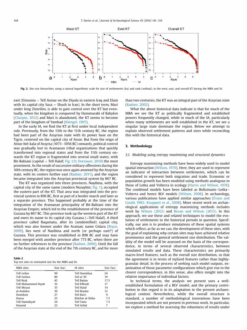
A natural log scale showing settlement size and hierarchies,ranking from largest to smallest, are displayed in Fig. 2. For thewestern KT (2a), the MBA and IA sites show a significant difference(p-value < 0.5) in site size and hierarchy, using a KolmogoroveSmirnov test, while the eastern KT (2b) there does not seem to beany statistically significant difference (p-value < 0.05) for the twoperiods’ sites. However, this is close to significant (p-value ¼ 0.06).Overall, comparing all of theMBA and IA sites (2c), the distributionsare not statistically significant, but looking at each region andperiod we see that site size and hierarchy are significantly different(p-value < 0.05). Table 1 shows average and standard deviation insite sizes between the regions and periods. From this, it is clear thattheMBA sites are larger in the eastern KTand have greater variationin site size, while in all the KT sites are generally larger in the MBAthan in the IA. Table 2 summarizes the top ten largest sties and theirsize estimates for the periods.

2.3. Historical background on the Middle Bronze and Iron Ages

For reasons that are unknown, sometime after 2000 BC, the localkingdoms of Nagar (capital ¼ Tell Brak; Fig. 1.4; Oates et al., 2001)and Urke�s (capital ¼ Tell Mozan; Fig. 1.3; Buccellati and Kelly-Buccellati, 2009) come to an end. Subsequently, the KT finds itselfunder outside control for much of the time. The political situation iscomplex and in part documented by textual materials, such as fromthe archives of Tell Leilan, (Fig. 1.7; ancient �Sehna; Eidem, 2012),Chagar Bazar (Fig. 1.1; ancient A�snakkum; Tunca and Baghdo, 2008)and Mari (Tell Hariri).

During the MBA, the KT is split into various local principalities,not all of which can be localized with confidence. The kingdom ofApûm (Eidem, 2008) seems to control most of the eastern part ofthe KT, while the rest is divided into several small states includingA�snakkum, Urke�s, and �Suduhum (Guichard, 2009) that can bespecified with the group designation Ida-maraṣ (Fleming, 2004;Bryce, 2009). For most of that time, these small states accept thesovereignty of the kingdom of Mari (Margueron, 2004), first underthe so-called �sakkanakku dynasty and then under several rulersthat owe their regional importance and their position to theirconnection with the kingdom of Yamhad (Klengel, 1997), whosecentre is Aleppo (Halab) which is outside of the investigated region.

The local states in the KT profit from the important eastewestoverland route that leads from Upper Mesopotamia through the KTto the Mediterranean and Anatolia. It is used most prominently bythe donkey caravans linking Assur (modern Qala’at Sherqat) on theTigris in northern Iraq with the region of the Great Salt Lake inCentral Anatolia (Barjamovic, 2012). While there is a well estab-lished tradition of trade links with the Tigris region, there is aperiod of about two decades, around 1800 BC, when the KT alsocomes under the direct political influence of its eastern neighbors.At that time, the Tigris region between Assur and Nineveh (modernMosul) forms the powerbase of king Samsi-Addu (1833e1776 BC;Charpin and Ziegler, 2003). Tell Leilan comes to serve as Samsi-Addu’s local centre, who has the city renamed �Subat-Enlil. Thedominion of the Tigris region over the KT does not last long afterSamsi-Addu’s death. For the next decades (Eidem, 2012), the tex-tual sources attest to the military and political maneuvers ofregional powers and outside powers frommuch further away in the

Table 1Average site size (ha) and standard deviation for the western and eastern KT duringthe two periods.

Region Period Numberof sites

Averagesize (ha)

Standarddeviation (ha)

West KT MBA 55 3.15 5.89West KT IA 194 2.2 2.91East KT MBA 205 4.7 9.89East KT IA 82 3.3 2.58

T. Davies et al. / Journal of Archaeological Science 43 (2014) 141e154 143

east (E�snunna ¼ Tell Asmar on the Diyala in eastern Iraq and Elamwith its capital city Susa ¼ Shush in Iran). In the short term, Mariunder king Zimrilim, is able to gain control over the KT but even-tually, when his kingdom is conquered by Hammurabi of Babylon(Charpin, 2012) and Mari is abandoned, the KT seems to becomepart of the kingdom of Yamhad (Klengel, 1997).

In the early IA, we find the KT at first under local independentrule. Previously, from the 13th to the 11th century BC, the regionhad been part of the Assyrian state with its power base on theTigris, centered on the capital city of Assur. But from the reign ofA�s�sur-bel-kala of Assyria (1073e1056 BC) onwards, political controlwas gradually lost to Aramaean tribal organizations that quicklytransformed into regional states and from the 11th century on-wards the KT region is fragmented into several small states, withBit-Bahiani (capital ¼ Tell Halaf; Fig. 1.9; Dornauer, 2010) the mostprominent. As the result of successivemilitary offensives during the10th century BC, the regionwas once again annexed by the Assyrianstate, with its centers further east (Radner, 2011), and the regionbecame integrated into the Assyrian provincial system by 867 BC.

The KT was organized into three provinces. Naṣibina, with thecapital city of the same name (modern Nusaybin; Fig. 1), occupiedthe eastern part of the KT. That area was integrated into the pro-vincial system in 896 BC, first as part of a border march and later asa separate province. This happened probably at the time of theintegration of the Aramaean principality of Bit-Bahiani into theAssyrian Empire, which led to the establishment of the province ofGuzana by 867 BC. This province took up the western part of the KTand owes its name to its capital city Guzana (¼Tell Halaf). A thirdprovince called Raqamatu, after its (unidentified) capital city,which was also known under the Aramaic name Gidara (Bryce,2009), lies west of Nasibina and north (or perhaps east?) ofGuzana. This province was established in 898 BC and may havebeen merged with another province after 773 BC, when there areno further references to the province (Radner, 2006). Until the fallof the Assyrian state at the end of the 7th century BC, and for more

than two centuries, the KT was an integral part of the Assyrian state(Radner, 2002).

What the above historical data indicate is that for much of theMBA we see the KT as politically fragmented and establishedpowers frequently changed, while in much of the IA, particularlywhen many settlements are well established in the KT, we see asingular large state dominate the region. Below we attempt toexplain observed settlement patterns and sizes while reconcilingthis with the historical data.

3. Methodology

3.1. Modeling using entropy maximizing and structural dynamics

Entropy maximizing methods have been widely used to modelspatial interaction (Wilson, 1970). Here, they are used to representan indicator of interaction between settlements, which can beconsidered to represent both migration and trade. Economic orpopulation growth has been modeled using methods analogous tothose of Lotka and Volterra in ecology (Harris and Wilson, 1978).The combined models have been labeled as BoltzmanneLotkaeVolterra and hence BLV models (Wilson, 2008). In archaeology,various publications have applied similar approaches (Evans andGould, 1982; Knappett et al., 2008). More recent work on archae-ological applications of entropy maximizing methods includeswork by Wilson (2012) and Bevan and Wilson (2013). In thisapproach, we use these and related techniques to model the evo-lution of settlements in the historical periods in question. Specif-ically, our aim is to produce simulations of these spatial systemswhich reflect, as far as we can, the development of these sites, withthe goal of explaining why certain sites may have achieved relativeprominence and the general settlement size distribution. The val-idity of the model will be assessed on the basis of the correspon-dence, in terms of several observed characteristics, betweensimulated results and data. These characteristics are primarilymacro-level features, such as the overall size distribution, so thatthe agreement is in terms of stylized features rather than highly-granular detail. In the process of seeking such model outputs, ex-amination of those parameter configurations which give rise to theclosest correspondence, in this sense, also offers insight into therelative importance of individual factors.

In technical terms, the analysis we present uses a well-established formulation of a BLV model, and the primary contri-bution in this regard is in its adaptation to the present archaeo-logical context. Nevertheless, while the overall structure isstandard, a number of methodological innovations have beenincorporated which are not present in previous work. In particular,we explore a method for assessing the robustness of results under

Fig. 2. Site size hierarchies, using a natural logarithmic scale for size of settlements (ha) and rank (ordinal), in the west, east, and overall KT during the MBA and IA.

Table 2Top ten sites in estimated size for the MBA and IA.

MBA sites Size (ha) IA sites Size (ha)

Tell Leilan 90 Tell Hamidiya 24Tell Farfara 80 Tell al ’ID 19Tell Brak 45 Tell Badan 17.5Tell Muhammed Diyab 35 Tell Effendi 17Tell Mozan 35 Tell Halaf 14al-Andalus 30 Tell Beydar 12Dumdum 27 Tell Barri 9Hansa 25 Khirbat al-Shiha 7.5Tell Hamidiyah 24 Tell Tamr 7.3Hameid 23 Tell Arbid 7

T. Davies et al. / Journal of Archaeological Science 43 (2014) 141e154144

uncertainty in data, which is motivated explicitly by the nature ofthe archaeological data available.

The spatial data required for our model is provided in the formof two site datasets; one for each of the periods. For each set e

containing 260 and 276 sites respectively e these contain the lo-cations of sites and cost matrices for travel between each pair ofsites, calculated via cost surface analysis, using methods applied byFontenari et al. (2005), in order to account for the effect of varyingterrain. We also have rough estimates for the size of each site inhectares, based on surveys referenced, which provide a relativeproxy as to which sites likely had larger populations.

3.2. Model formulation

The model takes the form of a standard spatial interactionmodel (SIM) of the type which has been used previously in othercontexts (e.g., Harris and Wilson, 1978; Bevan and Wilson, 2013),with some modifications for the present setting. We define thefollowing variables for each of the sites:

Xi¼ volume of flow (i.e., people and goods) originating at a givensite iZj¼ ‘attractiveness’ or size of site j; a variable that represents anyfactor that makes a site attractive to settledij ¼ distance (i.e., cost of travel) between any two sites i and j,normalized by the mean of all such distancesrij ¼ number of rivers crossed by a direct path from i to j

In the case of cost values dij for which i ¼ j (representing,notionally, the distance from a site i to itself), these are set to f, aparameter which represents impedance to internal trade at a givensite, before the normalization step. In addition, for every riverwhich is crossed by a direct path between two sites i and j, anadditional impedance r is added to the corresponding cost value, sothat the total is (dij þ rrij).

One further factor worthy of note here is that of externalinteraction; that is, each site’s interaction with sites outside thearea of study. This would be manifested as an additional in-flow foreach site and therefore contribute to site growth. A simple repre-sentation of this in the model would be the inclusion of a constantterm for ’rate of growth due to external interaction’, encapsulatingall such effects. Simulations were carried out with such a termincluded, but it was found that its effect could also be achieved, ingeneral, through variation of f. This can be rationalized byconsidering the function of f as a barrier to internal interaction:such interaction is a feedback effect, providing in-flow to a site inproportion to its current size, and so increasing this flow mimicsthe consequence of external influence.

The model itself can, broadly, be divided into two parts: theestimation of interaction flows and the use of these flows todetermine site size evolution. The first of these relies upon estab-lishing, for any pair of sites i and j, the utility of interactionwith j asperceived by i. This takes the form of a cost/benefit calculation, withthe benefit being a function of the size of j and the cost representingthe physical impedance (i.e., distance between). Two parameters, aand b, are introduced at this stage: a specifies the scaling of utilityas size varies, and b determines the strength of the negative effectof cost. Using entropy-maximizing methods, the most likely set offlows, given that the total flow originating at each site is known, isthen found. The allocation given by this method is relatively sim-ple: for any given site i, the total out-flow Xi is shared between eachother site j in proportion to the utility of j. In this way, we find theflow Sij between any such pair of sites.

In the second part of the model, these flows are used to updatethe site sizes; that is, to determine the growth/decline of each site

under the calculated set of flows. For each site j, the total inwardflow is found by summing Sij over all i, and this value is comparedwith the site’s current size Zj. If the total flow is less than Zj, thecurrent size is unsustainable and the site shrinks, whereas a surplusof inward flow leads to the growth of j. The model, in essence, isappropriate for measuring generic factors (e.g., environmentalconstraints, political conditions, economic conditions) that couldlead to some sites becoming larger than others.

Having made these calculations and adjusted Xi and Zj accord-ingly, the model proceeds to the next time-step and the process isrepeated. For any individual simulation, we run the model for a setnumber of discrete time-steps dt:

The flow Sij between each pair of nodes i and j is calculated usingthe following formula, which utilizes a and b:

Sij ¼ Xi

Zaj e�bðdijþrrijÞ

PkZak e

�bðdikþrrikÞ (1)

These flows are summed to give the total incoming flow Dj toeach site j:

Dj ¼Xi

Sij (2)

This incoming flow is used to calculate Zj at the next time step,Zj

(t þ dt), via the formula:

Ztþdtj ¼ Ztj þ dt

�Dj � Ztj

�Ztj (3)

We now find Xi(t þ dt) for the next time step by taking it to be the

corresponding Zi(t þ dt) value, normalized according to the total of allZi(t þ dt) and rescaled so that the Xi

(t þ dt) continue to have mean 1:

Xtþdti ¼ n

ZtþdtiP

kZtþdtk

(4)

Then return to (1).

3.3. Model outputs

Having completed any given numerical simulation of the model,a natural question arises of which quantities should be regarded asthe fundamental outputs of the model; these are precisely thosequantities which will be used to evaluate settlement sizes anddistributions for the periods discussed. For each simulation, wehave several observable features upon which to base assessments:

� the final site size Zi for each site j, and the distribution of thesevalues across all sites. Since we have numerical estimates forthese values within our datasets (the distributions of which areshown in Fig. 3) we canmakemeaningful numerical comparisonbetween these distributions using statistical tests;

� the structure and properties of a NystueneDacey (NeD) graph(Nystuen and Dacey, 1961; construction described in AppendixA) derived from the simulated flow matrix Sij. Such a graphdefines a hierarchy of sorts for sites, with links representingsubordinate relationships. This facilitates the analysis of bothgraph-theoretical properties and the average geographicallength of the estimated links, i.e. the typical length traveled to alocally-dominant site. Although true flow data is not availablefor comparison, we can compare the link length with that ofanother graph derived from the real data, for example by linkingeach site to its closest ‘large’ site;

T. Davies et al. / Journal of Archaeological Science 43 (2014) 141e154 145

Fig. 3. Simulation outputs for the MBA as a and b are varied, with r ¼ f ¼ 2500, : a) a ¼ 0.8 and b ¼ 45, b) a ¼ 1.2 and b ¼ 45, c) a ¼ 0.8 and b ¼ 15, d) a ¼ 1.2 and b ¼ 15. The sites are colored according to size, ranging from yellow to redas size increases, and the links are those of the induced NeD graph. It is notable that the links are significantly longer in the low-b simulations where there is a lower associated cost to travel, and that the changing value of a has theeffect of picking out different dominant sites. (For interpretation of the references to color in this figure legend, the reader is referred to the web version of this article.).

T.Davies

etal./

Journalof

Archaeological

Science43

(2014)141

e154

146

� the extent to which the largest sites in the real data are found tobe large during simulated runs. ‘Large’ is taken here to refer tosites whose size is an order of magnitude higher (i.e., 10 times)than other sites: for each dataset, we identify a set of L such sites(L is 19 and 6 for MBA and IA respectively) and, for each simu-lation, record the number of these which appear in the top Lsimulated sites, when ranked;

� visual inspection of outputs and evaluation of their historicalvalidity.

It is in these terms, therefore, that we characterize individualsimulations; however, we stop short of identifying specific criteriafor what constitutes a ‘match’ with real data. Firstly, each of theabove points represents a well-justified objective for a model and itis far from clear how they should be combined. More importantly,though, to be prescriptive in this way implies a level of confidencein the accuracy and completeness of the data, which is not present,and therefore to fit in this way may be counter-productive.

4. Results

There is clearly a wide degree of variation possible within themodel, in terms of parameter choices, manipulation of the under-lying datasets, and synthesis of results. In the following sections weexplore several of these, incrementally building the complexity ofthe approach. All simulations are run for 3000 ticks, with step sizedt as 0.01; in all cases this was sufficient for the site sizes to reach asteady state. Initially, all variables were the same for sites, whileonly distances (i.e., cost surface) between sites were different. Data,code, and instructions for the model are made publically available(http://discovery.ucl.ac.uk/1414597/).

4.1. Parameter variations

The model features four parameters e a, b, r and f ewhich canbe varied to give different outputs, for a given set of initial condi-tions. Each has a real-world interpretation: a represents returns toscale of attractiveness as a function of settlement size, with a valueof 1 indicating a linear relationship; b determines the impedance ofdistance (i.e., how easily goods and people can move across givendistances); r governs the extent to which rivers inhibit interaction;f controls the relative attractiveness of internal and exogenousactivity for a site, which accounts for edge effects as this addressesoutside interactions and sites not addressed in the model.

The effect of such parameter variation can be seen visually inFig. 3, which shows outputs for the MBA as a and b are varied. Inthese simulations, the system is initialized in a homogeneous state;specifically, Xi

(0) is set to 1 for all sites i. These particular simulationsare intended not as an attempt to produce realistic results, butinstead to give a visual impression of the effect of parameter vari-ation: it is clear to see that b is a significant determinant of thelength-scale of interactions, while a influences which sites becomedominant.

A different perspective can be seen in Fig. 4, which shows theaverage length of connections in the induced NeD graph for the IA,across a range of b and r. While this offers limited insight into theunderlying system, these results exemplify the significant andhighly non-linear manner in which the model parameters interact.As would be expected, smaller b values e representing lowerimpedance to travel e lead to longer interaction links. The behaviorwith r, however, is more interesting, particularly at low values of b:as impedance increases, link length decreases, before unexpectedlyincreasing towards higher values. An explanation might be foundby considering the relative positions of rivers and sites: in thesouthern area, many sites are clustered around rivers, and the

impedance of the river increasing above a certain valuemight causetheir dominant interactions to switch from those involving rivercrossings to favor sites on the same side of the river, which may befurther away.

4.2. Fitting to empirical data

The ultimate objective of analyzing parameter space in this wayis to identify a set of values that correspond most closely to the realdata. Although this correspondence could be defined inmany ways,we take as our first objective the distribution of site sizes. Thisrequires a measure of the similarity of distributions, and for this weuse KolmogoroveSmirnov (KeS) distance. For any set of data, it ispossible to calculate an empirical cumulative distribution function(ECDF): a step-functionwhich, for any value x, gives the probabilityof finding a value less than or equal to x when randomly samplingfrom the data. The KeS distance between any two distributions issimply the maximum difference between their ECDFs, over allpossible x; it therefore ranges between 0, in case of a perfect fit, and1 in the worst case. For each output, we compare the distribution ofthe modeled site sizes with that of empirical site size estimates,having first normalized each set by dividing by its mean.

In order to investigate the goodness of fit for various configu-rations, a grid search of parameter spacewas carried out and the KeS distance found in each case. One feature which becomes imme-diately apparent is the disparity between the two periods in termsof the parameter configurations which give rise to the closest cor-respondence. Fig. 5 shows the results of simulations for a samplingof the parameter space of a, b, r and f, shown as an interpolated‘heat map.’ Presented in this way, the difference in character be-tween the two periods is immediately apparent, since the areas ofparameter space indicating good agreement differ markedly be-tween the two plots. For the MBA, better fit is found for highervalues of a, for example, implying that returns to scale were largerfor this system. In addition, higher values of f also lead to closer fitsin MBA than in IA, suggesting that the MBA sites were less relianton internal interactions. Above all, the dissimilarity between theplots suggests a significant difference in character between the twoperiods.

Using the results of this parameter search, configurations werefound for MBA and IA sites, which give the minimal KeS distance.

Fig. 4. The average length of NeD links for the IA, as a function of b and r. The colorsrange from blue to red. (For interpretation of the references to color in this figurelegend, the reader is referred to the web version of this article.).

T. Davies et al. / Journal of Archaeological Science 43 (2014) 141e154 147

The relevant parameters are given in Table 3, and the results areshown in Figs. 6 and 7, which show site size distributions andmapped results respectively. The relatively good fit e seen bothvisually and in the low KeS values e indicates that, on this gauge,the model has successfully reproduced the empirical distribution.

Although these results show good agreement in terms of sitesizes, the sites which have large estimated size in the observed datatend not to be those which the model forecasts to be large. Thefailure to identify precise sites does not necessarily imply that themodel has not identified more general geographical areas, whichwould be expected to feature large sites. Of course, in reality, thereare various factors that lead to the dominance of certain sites (e.g.,earlier settlements could initially be larger, socio-environmentfactors may favor one site vs. others), whereas only geographiclocation is included here. Considering the case of Tell Leilan, forexample, it is clear from inspection that there is no a priori reasonwhy it, rather than its nearest neighbor Rehaya, should becomedominant in the model. If the analysis is widened, though, toconsider situations where the dominant simulated site is not one ofthe true largest sites, but is in close proximity to one, it is possible tofind the extent to which the localities of large sites are identified.

To do this for any given simulation output, we take each of the10 largest simulated sites and calculate the distance to the nearestof the ‘true’ 10 largest sites (that is, the minimum distance one

would have to travel to reach one of the true top 10). The average ofthese values is an estimate of the extent to which the true largesites have been ‘missed’, in geographical terms. In the MBA case,this value, for the parameters given in Table 3, is 7564m. To put thisvalue in perspective, we can compare it with the value it would takeif, instead of using the top 10 simulated sites, a random set of 10sites were chosen and the distances from these to the true top 10calculated. Doing this 100 times, we find a mean value of 15,597 mwith standard deviation of 4648; that is, the sites which are fore-casted as large by ourmodel are significantly closer to the true largesites thanwould be expected by chance. Although comparisonwithrandom points is relatively unambitious, this value, along with vi-sual comparison, suggests that the model is indeed finding sitesthat are geographically close to known large sites, suggesting themodel is far better at forecasting the largest sites than randomselection. The equivalent value for the IA is 4272 m, with a corre-sponding null value of 12,062 m (s.d. 2602).

Fig. 5. KeS distances for simulations of a) MBA and b) IA data across a range of parameter values. The ‘outer’ grid axes represent changing a and b; for any pair of these values, theimage within the grid is a plot of f against r for the fixed a and b, as shown in the expanded panels. The color represents KeS distance, with red representing the best fit and bluethe worst. Uniform initial conditions were used in these simulations. (For interpretation of the references to color in this figure legend, the reader is referred to the web version ofthis article.).

Table 3Parameter values giving minimal KeS distance for site sizes when compared withobserved data.

a b r f KeS

MBA 0.7 35 1500 1000 0.077IA 0.5 15 0 1000 0.101

T. Davies et al. / Journal of Archaeological Science 43 (2014) 141e154148

4.3. Initial conditions

The results of the previous section suggest that, whenwe seek toproduce a distribution of site sizes similar to the real data, knownlarge sites do not, in general, emerge in the model. In order todistinguish such sites, therefore, some modification to the model isrequired. A natural approach to this, within the current framework,is to manipulate the initial conditions for site size; rather thantaking these to be uniform, we adjust these according to what isknown about the sites in question. Such an adjustment perturbs themodel in favor of certain sites; inmore concrete terms, this could beregarded as accounting for any effects not explicitly included in themodel which currently only considers the spatial configuration ofthe system.

Our approach to this is to divide the sites into three categories,according to the order of magnitude of their given size in the data(essentially a classification as ’small’, ’medium’ or ’large’ on thebasis of their hectare sizes lying in the ranges [0,1), [1,10) or [10,N),respectively). The initial condition for each site is then set to be themean of the known size of all sites in its category. In the MBA, forexample, the mean size of ‘large’ sites is 28.73, and so all large sitesare initialized with this value. Although guiding the system, thisstill represents a relatively coarse-grained classification of sites.Fig. 8 shows the result of simulations under this modification, withparameters identical to those shown in Table 3. In terms of top sites,a modest improvement is apparent: for the MBA, the sites at Hansa,al-Andalus and Khirbet el-‘Abd are now significant, and in the IAthere is now a larger site at Tell Halaf.

If we allow ourselves to make changes to the parameters,however, the results can be improved still further in these terms.For the MBA, using the values a¼ 0.7, b¼ 45, r ¼ 1000 and f ¼ 500leads to the output shown in Fig. 9a. Several empirically large sites,such as Tell Brak, Tell Hamidiyah and Tell Leilan, are now amongstthe largest forecasted, and several of the other sites found to belarge (e.g., Duger, Lazzaga and Khirbet el-‘Abd) are known to besignificant. For the IA, on the other hand, the values used area ¼ 0.4, b ¼ 45, r ¼ 5000 and f ¼ 500, with the output shown inFig. 9b. We can, of course, also consider the distributions of sitesizes in these cases: we have KeS values of 0.21 and 0.19 respec-tively. Although these do not represent such a close fit as the pre-vious section, the difference is not so large as to nullify the results.

The ability of the model to identify these sites is encouraging: itoffers further confirmation that the model is capable of producing

sensible outcomes and demonstrates that only a small amount ofadditional information is required to improve the accuracy of thesimulation. It is, however, instructive to consider the nature of thechanges to themodel that were required to give rise to such results.The need to change initial conditions suggests the existence ofcertain site-specific factors, which have a material effect on thereal-world outcome but are not included in the basic model (whichincorporates geographical location only). Without accounting forthese factors in a more elaborate model, the results of this section,achieved by imposing the three-tiered initial classification, shouldbe viewed as illustrative only.

In terms of parameters, we may draw some insight from aninspection of results e suggesting that the most crucial change interms of the identification of major sites is the lowering of f. Thiscan be rationalized by considering the spatial layout of sites in bothperiods, which includes significant clustering in both cases. Sinceevery site represents a source of flow, a site which is situated in anarea of high site density has a large potential in-flow within rela-tively short distance. If such a site is able to dominate locally, astends to be the case within the model, it is therefore likely to reachlarger size than a similarly dominant site in a sparse region, simplybecause of the greater resource onwhich it may draw. Lower valuesof f represent greater emphasis on internal development at a site;as noted previously, this might also be thought of as giving greaterweight to extra-regional trade and, therefore, mediate against theabove effect. A good example of this is the southern region aroundUwayja in the IA period, which has a high density of sites: in Fig. 8b,this density is clearly associated with large site sizes, whereas theeffect is much less pronounced in Fig. 9b.

4.4. Partial dataset sampling

The clustering of sites mentioned above may be the result ofunevenness in the surveying of sites, but also relates to a moregeneral problemwith the data: that of the contemporaneousness ofsites. The possible lifetimes of the locations we are modeling liewithin a wide range; at any given time, it may be the case that onlya subset would be in existence (and these subsets may not beknown). To ameliorate this, we use a new simulation protocol,which involves repeated sampling of the sites.

To do this, instead of performing one simulation run for a givenparameter configuration,weperform a series ofM such simulations.For each simulation, we randomly sample a subset of R of the sites,

Fig. 6. Comparison of site size distributions between empirical data and the optimal simulations, in terms of KeS distance, for a) MBA, and b) IA. The distributions are plotted ascomplementary ECDFs on doubly logarithmic axes.

T. Davies et al. / Journal of Archaeological Science 43 (2014) 141e154 149

Fig. 7. Mapped outputs from basic simulations for a) MB and b) IA periods, with parameter settings as indicated in Table 3. Darker red indicates larger relative site size under the model. (For interpretation of the references to color inthis figure legend, the reader is referred to the web version of this article.).

Fig. 8. Mapping of simulation outputs for a) MBA, and b) IA, using the parameters of Table 3, but with initial conditions modified according to the known size of sites, as described in the text.

T.Davies

etal./

Journalof

Archaeological

Science43

(2014)141

e154

150

and carry out the simulation using only these sites. When all sim-ulations are complete, we take the mean modeled size of each siteacross all the simulations inwhich it featured, and take this to be ourestimates of that site’s size. The underlying principle of this methodis that each sampling represents a possible ‘state of the world’, andthat averaging in this way accounts for our uncertainty about thecomposition of the dataset: when a site is consistently modeled tobe large, for example, we can be confident that it is likely to be largewhatever the true composition of the system should be.

We carry out this process for each of the MBA and IA datasets,taking M ¼ 500 and R ¼ 100 and with the other parameters asspecified in Table 3. Encouragingly, there is good consistency be-tween the results of these simulations and those of the originalsimulations, which used the whole dataset. We can use Spearman’srank correlation coefficient (which gives a value of 1 in the case ofperfect correlation and 0 in case of total absence) to examine howclosely the rankings of the sites under each protocol match; thisquantity is 0.556 for theMBA and 0.976 for the IA. This is significantin both cases, and indeed remarkably high in the IA case, suggestingconsistency of results. In other words, sites which are found to belarge under the original algorithm remain large under this aver-aging and random sampling system, and vice versa.

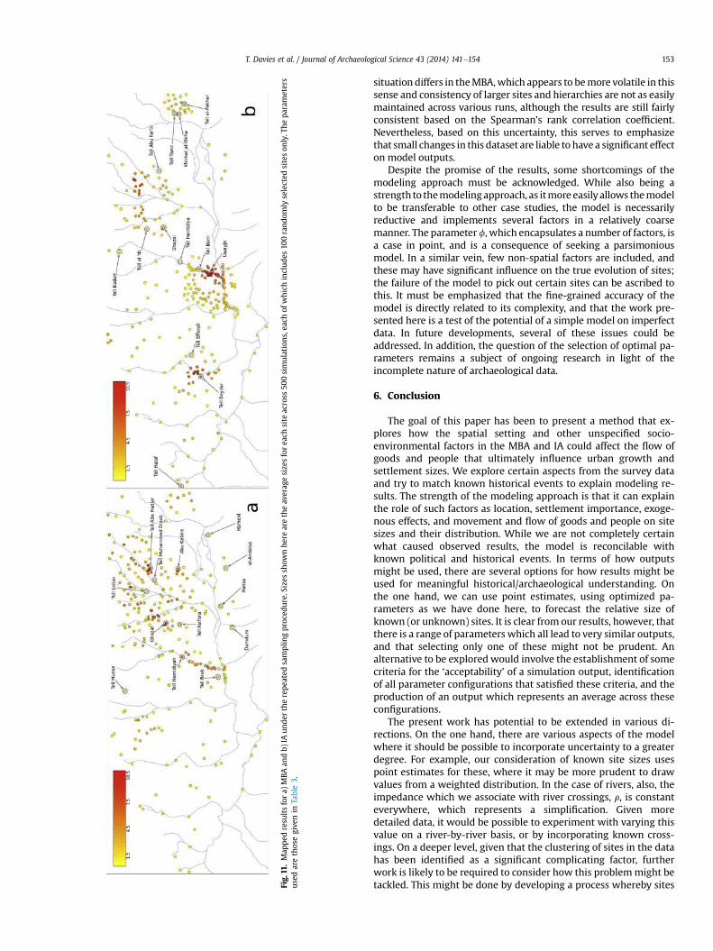
If we consider the variation of individual sites across such a run ofsimulations, we observe a further difference between MBA and IAperiods. Fig.10 shows the sizes of individual sites across various runs;it is noticeable that the distributions are normal-like in the IA case,whereas theMBA case has a muchmore flat distribution, with manylow values. This can again be understood in terms of the clustering ofsites: many IA sites are well-clustered and are therefore somewhatinterchangeable from thepoint of themodel, whereas greater spatialdiversity of theMBA sitesmeans that system ismuch less resilient tochanges. The results are also shown in map form in Fig. 11.

In terms of size distribution, however, those simulations show asignificant disparity with the reference distribution (in terms of KeS distance); in particular the distribution has much lower variance.This can be understood in terms of the averaging procedure; anygiven site will be modeled as large in some of the simulations andsmaller in others (as shown in Fig. 10). Averaging over runs gives animpression of which of these regimes it tends to be in, but does notnecessarily reflect its true size. Under this principle, the true size isthe outcome of the model under one particular (but unknown)sampling; the averaging simply offers insight into its tendencyacross all possibilities.

5. Discussion

The results demonstrate the utility of the model as a methodthat explores spatial systems in historical contexts such as thoseconsidered here, while also forecasting, at least far better thanrandom sampling, lager sites nearer to their true location usinginput survey data. The model produces important insights anddemonstrates broader utility in describing settlement hierarchiesand detecting a variety of factors that may have caused some sitesto become relatively larger than others. Results show potentialpolitical and historical differences affecting settlement in the MBAand IA that can be explained by the advanced model.

Several aspects are particularly notable, both from the point ofview of modeling and of providing insight into the underlyingsystem. Firstly, themodel is able to produce close matches with realdata in terms of the distribution of site sizes, even in the most basicimplementation that focuses on spatial location. As well asproviding partial validation of the model, this stage of the work isnotable for the varying parameter configurations that are requiredto produce the closest matches in each time period. The fact thatthe best fits are found in markedly different areas of parameterFi

g.9.

Map

pedsimulationou

tputsus

ing‘small/med

ium/large

’initialc

ondition

sas

describe

din

thetext,w

ithpa

rametersch

osen

soas

toiden

tify

keysites:

a)MBA

withpa

rametersa¼

0.7,

b¼

45,r

¼10

00an

d4¼

500,

b)IA

with

parametersa¼

0.4,

b¼

45,r

¼50

00an

df¼

500.

T. Davies et al. / Journal of Archaeological Science 43 (2014) 141e154 151

space e particularly in terms of a and b e implies that there is aninherent difference between the periods. The results indicate thatreturns to scale in site size were greater in the MBA (due to highera) and that interactions typically had a shorter length-scale (higherb). In the IA, lower a indicates less importance on site size, whilelower b indicates greater movement or facility of movement acrossthe landscape. Translated to the discussed historical data, a politi-cally fragmented landscape, such as in the MBA, could restrictmovement, thereby leading to larger local sites that also absorbmore flow from nearby sites. There may have been more emphasison establishing large sites, perhaps for protection (i.e., which re-flects higher a) during periods of political competition, furtherencouraging larger sites to become even larger.

We can interpret the results by the fact that in the MBA the KT ischaracterized by the presence of several peer polities aiming toexert their influence over their surrounding hinterland, while in theIA settlements are well integrated into the Assyrian imperialstructure. During the MBA, we see the Jaghjagh River playing animportant physical/political boundary, and modeling resultsdemonstrate how river impedance can differentially affect site sizedistributions depending onwhich side of the river bank a sitemightbe located.While in the IA, the landscapewould have been easier tonavigate due to the Neo-Assyrian empire’s control of the region,with movement likely to be less restricted, particularly for a longperiod of time (i.e., more than 200 years). Easier movement enablesthe dispersion of flow to many sites, leading to greater similarity insite sizes. Diminished a indicates less of a need or ability to havelarger sites in the IA, which could be caused deliberately by theNeo-Assyrians or other environmental factors.

Overall, andanother important result demonstrated in themodel,is that it was far better at forecasting larger sites near their true lo-cations than by selecting sites randomly. In order to locate such sites,it was necessary to manipulate both the initial conditions of themodel and some of the parameter choices. The first of these impliesthat it was necessary to include a certain amount of known infor-mation about the sites in question; in otherwords, that location dataalone were not sufficient to explain their dominance. Nevertheless,the manipulation of initial conditions here was done in a coarse-grained way, suggesting perhaps that any extra information need

not be particularly detailed. In the case of parameter variation, it wasfound that closer matches tended to be associatedwith lower valuesoff, a parameter controlling local andexogenous interactions,whichcan be related specifically to the nature of the data. The fact that thedata contained several areas of high site density presents somethingof a modeling challenge. A large number of sites translates to a highactivity potential in the model, which may not represent reality: thehigh density of sites may simply be an artifact of the area beingrelatively well-surveyed or other distortion in identification of sites.The parameter f has the potential to reduce this effect, by placinggreater interpretation on internal site features or interaction withexogenous, non-KTsites outside of the simulated area, depending oninterpretation. In a sense, then, it is able to ‘tune’ the relative influ-ence of local interaction effects and address edge effects.

The results generally show that other non-geographic factors domake specific known sites larger, as sites become relatively largethrough modifications to initial size and f. This can, for instance,reflect external political conditions or initial site advantages. Inparticular, it seems that Tell Brak, Tell Leilan and Tell Mozan in theMBA would need greater exogenous effects or initial advantages toenable them to consistently reach a relatively greater size. Thiscould come in the form of Samsi-Addu making Tell Leilan (theancient �Subat-Enlil) an important political capital, Tell Brak beingthe seat of the “Lady of Nagar”(Oates et al., 1997, 141), and local orexternal benefits that Tell Mozanmay have relative to other sites. Inthe IA, the Neo-Assyrians choosing Tell Halaf as a provincial capitalcould enable that site to be relatively large.

The issue of clustering of sites is once again apparent when weconsider another method of simulation: that of running repeatedsimulations on only partial datasets (i.e., see section 4.4). The moti-vation for this is to combat the effect of temporal uncertainty in thedata, since possibly only some of the sites are likely to be contem-porary. The IA case, remarkably, shows little difference when usingthis method, primarily because of the spatial structure: high clus-tering means that the role of deleted sites is essentially assumed byclose neighbors and in simulation runs site size hierarchies are verycomparable. This indicates that even if some sites were occupied atdifferent times or missed in survey, the hierarchy of site sizes wouldnot be significantly different than that achieved in the results. The

Fig. 10. Distribution of site sizes across 500 repeated simulations, where each simulation involves only a randomly-selected 100 sites (and each individual site therefore features inonly approximately 200 of the simulations, on average). Results are shown for a) MBA, and b) IA; in each case the upper panel shows the site with largest mean size and the lowershows the 20th ranked.

T. Davies et al. / Journal of Archaeological Science 43 (2014) 141e154152

situation differs in theMBA,which appears to bemore volatile in thissense and consistency of larger sites and hierarchies are not as easilymaintained across various runs, although the results are still fairlyconsistent based on the Spearman’s rank correlation coefficient.Nevertheless, based on this uncertainty, this serves to emphasizethat small changes in this dataset are liable to have a significant effecton model outputs.

Despite the promise of the results, some shortcomings of themodeling approach must be acknowledged. While also being astrength to themodelingapproach, as itmore easilyallows themodelto be transferable to other case studies, the model is necessarilyreductive and implements several factors in a relatively coarsemanner. The parameter f, which encapsulates a number of factors, isa case in point, and is a consequence of seeking a parsimoniousmodel. In a similar vein, few non-spatial factors are included, andthese may have significant influence on the true evolution of sites;the failure of the model to pick out certain sites can be ascribed tothis. It must be emphasized that the fine-grained accuracy of themodel is directly related to its complexity, and that the work pre-sented here is a test of the potential of a simple model on imperfectdata. In future developments, several of these issues could beaddressed. In addition, the question of the selection of optimal pa-rameters remains a subject of ongoing research in light of theincomplete nature of archaeological data.

6. Conclusion

The goal of this paper has been to present a method that ex-plores how the spatial setting and other unspecified socio-environmental factors in the MBA and IA could affect the flow ofgoods and people that ultimately influence urban growth andsettlement sizes. We explore certain aspects from the survey dataand try to match known historical events to explain modeling re-sults. The strength of the modeling approach is that it can explainthe role of such factors as location, settlement importance, exoge-nous effects, and movement and flow of goods and people on sitesizes and their distribution. While we are not completely certainwhat caused observed results, the model is reconcilable withknown political and historical events. In terms of how outputsmight be used, there are several options for how results might beused for meaningful historical/archaeological understanding. Onthe one hand, we can use point estimates, using optimized pa-rameters as we have done here, to forecast the relative size ofknown (or unknown) sites. It is clear from our results, however, thatthere is a range of parameters which all lead to very similar outputs,and that selecting only one of these might not be prudent. Analternative to be explored would involve the establishment of somecriteria for the ‘acceptability’ of a simulation output, identificationof all parameter configurations that satisfied these criteria, and theproduction of an output which represents an average across theseconfigurations.

The present work has potential to be extended in various di-rections. On the one hand, there are various aspects of the modelwhere it should be possible to incorporate uncertainty to a greaterdegree. For example, our consideration of known site sizes usespoint estimates for these, where it may be more prudent to drawvalues from a weighted distribution. In the case of rivers, also, theimpedance which we associate with river crossings, r, is constanteverywhere, which represents a simplification. Given moredetailed data, it would be possible to experiment with varying thisvalue on a river-by-river basis, or by incorporating known cross-ings. On a deeper level, given that the clustering of sites in the datahas been identified as a significant complicating factor, furtherwork is likely to be required to consider how this problemmight betackled. This might be done by developing a process whereby sitesFi

g.11.Map

pedresu

ltsfora)

MBA

andb)

IAun

dertherepe

ated

samplingproc

edure.Size

ssh

ownhe

rearetheav

erag

esize

sforea

chsite

across

500simulations

,eachof

which

includ

es10

0rand

omly

selected

siteson

ly.T

hepa

rameters

used

arethosegive

nin

Table3.

T. Davies et al. / Journal of Archaeological Science 43 (2014) 141e154 153

which are consistently insignificant can be deleted, or merged withother sites, in order to reduce imbalances of density.

As for larger benefits to archaeology, the model demonstratesthat it can begin to reconcile socio-political or even environmentalconstraints to an abstract level, whereby such circumstances can betranslated to parameters such as a, b, and f that affect the impor-tance of site size, cost of movement, and internal-exogenous siteinteractions respectively. While such variables can be affected by ahost of circumstances, the benefit is the method can be transferredto other and very different case studies more easily. The model isapplicable to describing observed settlement structures byproviding parameter estimates that enable nearly matching simu-lated settlement data. The model is also useful for forecastinggeneral areas where larger or smaller sites are to be expected,demonstrating its potential for helping archaeologists to locatesuch sites. Overall, such modeling allows archaeologists to differ-entiate how significantly different periods are in site distributionand size structures and begin to understand this with causalfactors.

Acknowledgments

This research was supported financially by a grant from Uni-versity College London’s Strategic Development Fund in theHumanities.

Appendix A. Supplementary data

Supplementary data related to this article can be found at http://dx.doi.org/10.1016/j.jas.2013.12.014.

Supplementary Data: http://discovery.ucl.ac.uk/1414597/.

References

Algaze, G., 1989. A new frontier: first results of the Tigris-Euphrates archaeologicalreconnaissance project, 1988. J. Near East. Stud. 48 (4), 241e281.

Ball, W., 2003. Ancient Settlement in the Zammar Region: Excavations by the BritishArchaeological Expedition to Iraq in the Saddam Dam Salvage Project, 1985-86.In: BAR International Series, vol. 1096. Archaeopress, Oxford.

Barjamovic, G., 2012. A Historical Geography of Anatolia in the Old Assyrian ColonyPeriod. Museum Tusculanum Press, Copenhagen.

Bevan, A., Wilson, A., 2013. Models of spatial hierarchy based on partial evidence.J. Archaeol. Sci. 40, 2415e2427.

Bryce, T., 2009. The Routledge Handbook of the Peoples and Places of AncientWestern Asia from the Early Bronze Age to the Fall of the Persian Empire.Routledge, London.

Buccellati, G., Kelly-Buccellati, M., 2009. The great temple terrace at Urkesh and thelions of Tish-atal. In: Wilhelm, G. (Ed.), General Studies and Excavations at Nuzi11/2 in Honor of David I. Owen on the Occasion of His 65th Birthday, Studies onthe Civilization and Culture of Nuzi and the Hurrians, vol. 18. CDL Press,Bethesda, MA, pp. 33e70.

Charpin, D., Ziegler, N., 2003. Mari et le Proche-Orient à l’époque amorrite: essaid’histoire politique, Florilegium marianum, vol. 5. Société pour l’étude duProche-Orient ancien, Paris.

Charpin, D., 2012. Hammurabi of Babylon. I.B. Tauris, London.Dornauer, A.A., 2010. Die Geschichte von Guzana im Lichte der schriftlichen

Zeugnisse. In: Cholidis, N., Martin, L. (Eds.), Tell Halaf: Im Krieg zerstörteDenkmäler und ihre Restaurierung. De Gruyter, Berlin, pp. 47e67.

Eidem, J., Warburton, D., 1996. In the land of Nagar: a survey around Tell Brak. Iraq58, 51e64.

Eidem, J., 2008. Apum: a kingdom on the Old Assyrian route. In: Veenhof, K.R.,Eidem, J. (Eds.), Mesopotamia: The Old Assyrian Period, Orbis biblicus et ori-entalis, vol. 160/5. Academic Press, Vandenhoeck & Ruprecht, Fribourg & Göt-tingen, pp. 265e352.

Eidem, J., 2012. The Royal Archives from Tell Leilan: Old Babylonian Letters andTreaties from the Eastern Lower Town Palace. Nederlands Instituut voor hetNabije Oosten, Leiden.

Evans, J.P., Smith, R.B., 2006. Water vapor transport and the production of precip-itation in the Eastern Fertile Crescent. J. Hydrometeorol. 7, 1295e1307.

Evans, S., Gould, P., 1982. Settlement models in archaeology. J. Anthropol. Archaeol.1, 275e304.

Fleming, D.E., 2004. Democracy’s Ancient Ancestors: Mari and Early CollectiveGovernance. Cambridge University Press, Cambridge.

Fontenari, S., Franceschetti, S., Sorrentino, D., Mussi, F., Pasolli, M., Napolitano, M.,Flor, R., 2005. r.walk. GRASS GIS.

Gavagnin, K., 2012. The Neo-Assyrian and Post-Assyrian Settlement in the Leilanregion, Northeastern Syria: some preliminary results. In: Matthews, R., Curtis, J.,Seymour, M., Fletcher, A., Gascoigne, A., Glatz, C., Simpson, S.J., Taylor, H.,Tubb, J., Chapman, R. (Eds.), Proceedings of the 7th International Congress ofthe Archaeology of the Ancient Near East (7th ICAANE), 12 Aprile16 April 2010,British Museum and UCL, London. Harasowitz, Wiesbaden.

Guichard, M., 2009. �Suduhum, un royaume d’Ida-Maraṣ et ses rois Yatar-malik,Hammi-kun et Amud-pa-El. In: Cancik-Kirschbaum, E., Ziegler, N. (Eds.), Entreles fleuves 1: Untersuchungen zur historischen Geographie Obermesopota-miens im 2. Jahrtausend v. Chr, Berliner Beiträge zum Vorderen Orient, vol. 20.PeWe-Verlag, Gladbeck, pp. 75e120.

Harris, B.,Wilson, A.G.,1978. Equilibriumvalues anddynamics of attractiveness termsinproduction-constrained spatial interactionmodels. Environ. Plan.10, 371e388.

Issar, A., Zohar, M., 2004. Climate Change: Environment and Civilization in theMiddle East. Springer, Berlin.

Klengel, H., 1997. Die historische Rolle der Stadt Aleppo im vorantiken Syrien. In:Wilhelm, G. (Ed.), Die orientalische Stadt: Kontinuität, Wandel, Bruch. SDV,Saarbrücken, pp. 359e374.

Knappett, C., Evans, T., Rivers, R., 2008. Modelling maritime interaction in theAegean Bronze Age. Antiquity 82, 1009e1024.

Lyonnet, B., 2000. Haut-Khabur Occidental. Institut Francais du Proche Orient,Beyrouth.

Margueron, J.-C., 2004. Mari, métropole de l’Euphrate au IIIe et au début du IIemillénaire avant J.-C. Picard, Paris.

Meijer, D.J.W., 1986. A Survey in Northeastern Syria. Nederlands Historisch-Archaeologisch Institute Istanbul, Leiden.

Novák, M., 2009. Zur Geschichte der aramäisch-assyrischen Stadt Guzana. In:Baghdo, A.-M. (Ed.), Vorbericht über die erste und zweite syrisch-deutscheGrabungskam- pagne auf dem Tell Halaf, Vorderasiatische Forschungen derMax Freiherr von Oppenheim-Stiftung 3, vol. 1. Ludwig Reichert Verlag, Wies-baden, pp. 93e98.

Nystuen, J.D., Dacey, M.F., 1961. A graph theory interpretation of nodal regions. Pap.Proc. Reg. Sci. Assoc. 7, 29e42.

Oates, D., Oates, J., McDonald, H., 1997. Excavations at Tell Brak 1: The Mitanni andOld Babylonian Periods. British School of Archaeology in Iraq, London.

Oates, D., Oates, J., McDonald, H., 2001. Excavations at Tell Brak 2: Nagar in the ThirdMillennium BC. British School of Archaeology in Iraq, London.

Radner, K., 2002. Die neuassyrischen Texte aus Tall �S�eḫ Ḥamad. In: Beiträge zu denAusgrabungen von Tall �S�eḫ Ḥamad, vol. 6. Reimer, Berlin.

Radner, K., 2006. Provinz. C. Assyrien. In: Reallexikon der Assyriologie und Vor-derasiatischen Archäologie, pp. 42e68, 11/1e2.

Radner, K., 2011. The Assur-Nineveh-Arbela Triangle: central Assyria in the Neo-Assyrian period. In: Miglus, P., Mühl, S. (Eds.), Between the Cultures: TheCentral Tigris Region in Mesopotamia from the 3rd to the 1st Millennium BC.Heidelberger Studien zum Alten Orient 14. Heidelberger Orient-Verlag, Hei-delberg, pp. 321e329.

Ristvet, L., 2005. Settlement, Economy, and Society in the Tell Leilan Region, Syria,3000e1000 BC. Ph.D. dissertation. Cambridge University.

Tunca, Ö., Baghdo, A. (Eds.), 2008. Les trouvailles épigraphiques et sigillographiques duchantier I (2000e2002). Chagar Bazar (Syrie) III. Peeters, Louvain.

Ur, J., Wilkinson, T.J., 2008. Settlement and economic landscapes of Tell Beydar andits hinterland. In: Lebeau, M., Suleiman, A. (Eds.), Beydar Studies 1. Brepols,Turnhout, pp. 305e327.

Ur, J., 2010. Urbanism and Cultural Landscapes in Northeastern Syria. The TellHamoukar Survey, 1999e2001. Oriental Institute Publication 137. University ofChicago, Chicago.

Wäfler, M., 2003. Tall al-Ḥam�ıd�ıya 4. Academic Press Fribourg/Paulusverlag FreiburgSchweiz Vandernhoeck & Ruprecht Göttingen, Fribourg.

Weiss, H., 2000. Beyond the Younger Dryas: collapse as adaption to abrupt climatechange in ancient West Asia and the Eastern Mediterranean. In: Bawden, G.,Reycraft, R.M., Albunquerque, N.M. (Eds.), Environmental Disaster and theArchaeology of Human Response. Maxwell Museum of Anthropology, Albu-querque, pp. 75e98.

Wilkinson, T.J., Tucker, D.J., 1995. Settlement Development in the North Jazira, Iraq.Aris & Phillips, Warminster.

Wilkinson,T.,Barbanes, E., 2000. Settlementpatterns in theSyrian Jazirahduring the IA.In: Bunnens, G. (Ed.), Essays on Syria in the Iron Age. Peters, Louvain, pp. 397e422.

Wilkinson, T.J., Wilkinson, E.B., Ur, J., Altaweel, M., 2005. Landscape and settlementin the Neo-Assyrian empire. Bull. Am. Sch. Orient. Res. 340, 23e56.

Wilson, A.G., 1970. Entropy in Urban and Regional Modelling. Pion, London.Wilson, A.G., 2008. Boltzmann, Lotka and Volterra and spatial structural evolution:

an integrated methodology for some dynamical systems. J. R. Soc. Interface 8,865e871.

Wilson, A.G., 2012. Geographic modeling for archaeology and history: two casestudies. Adv. Complex Syst. 15 (1e2). http://dx.doi.org/10.1142/S0219525911003384.

Wright, H.T., Rupley, E.S.A., Ur, J., Oates, J., Ganem, E., 2007. Preliminary report onthe 2002 and 2003 seasons of the Tell Brak sustaining area survey. Les Ann.Archéol. Arabes Syriennes 49e50, 7e21.

T. Davies et al. / Journal of Archaeological Science 43 (2014) 141e154154