Movement and locality in Sundanese wh-questions (Davies & Kurniawan)
Upload
khangminh22Category
view
0download
0
Mantle ConvectionAuthor(s): Geoffrey F. Davies and Mark A. RichardsSource: The Journal of Geology, Vol. 100, No. 2 (Mar., 1992), pp. 151-206Published by: The University of Chicago PressStable URL: http://www.jstor.org/stable/30081131 .Accessed: 23/01/2011 20:55
Your use of the JSTOR archive indicates your acceptance of JSTOR's Terms and Conditions of Use, available at .http://www.jstor.org/page/info/about/policies/terms.jsp. JSTOR's Terms and Conditions of Use provides, in part, that unlessyou have obtained prior permission, you may not download an entire issue of a journal or multiple copies of articles, and youmay use content in the JSTOR archive only for your personal, non-commercial use.
Please contact the publisher regarding any further use of this work. Publisher contact information may be obtained at .http://www.jstor.org/action/showPublisher?publisherCode=ucpress. .
Each copy of any part of a JSTOR transmission must contain the same copyright notice that appears on the screen or printedpage of such transmission.
JSTOR is a not-for-profit service that helps scholars, researchers, and students discover, use, and build upon a wide range ofcontent in a trusted digital archive. We use information technology and tools to increase productivity and facilitate new formsof scholarship. For more information about JSTOR, please contact [email protected].
The University of Chicago Press is collaborating with JSTOR to digitize, preserve and extend access to TheJournal of Geology.
http://www.jstor.org

ARTICLES
Mantle Convection'
Geoffrey F. Davies and Mark A. Richards2 Research School of Earth Sciences, Australian National University,
GPO Box 4, Canberra, ACT 2601, Australia
ABSTRACT
A wide range of geophysical and geochemical observations pertaining to convection in the earth's mantle and the dynamics of the tectonic plates is discussed. It is inferred that the dominant mode of mantle convection is a plate-scale flow and that the plates are an integral part of this flow. Upwelling buoyant plumes, that cause volcanic hotspots, are inferred to comprise a secondary model of convection arising from a relatively weak thermal boundary layer at the base of the mantle. The balance of a large range of evidence weighs against the transition zone being a barrier to flow, the strongest evidence coming from seafloor topography and the gravity field. We infer a significant viscosity increase, by perhaps two to three orders of magnitude, through the depth of the mantle, with a large part of this increase occurring through the transition zone. This viscosity increase can account for the low velocities of hotspots relative to plates and the apparent lag between surface plate configuration and deep mantle structure, as probed by seismology and the gravity field. The viscosity increase also enhances the survival of chemical heterogeneities in the mantle and produces an increase in heterogeneity and mean residence time with depth. There may also be inefficient gravitational settling of old subducted oceanic crust near the bottom of the mantle, which might account for seismological complications in the D" layer at the bottom of the mantle and for trace elements exceeding bulk- earth concentrations in hotspot sources. With ridges sampling the top of the mantle and plumes sampling the bottom, these features offer explanations for the main geochemical characteristics of, and differences between, mid-ocean ridge basalts and oceanic island (hotspot) basalts.
Contents
Introduction Thermal Convection
Boundary Layer Theory Plates, Hotspots, and the Near-Surface Flow
The Lithospheric Boundary Layer Plate Geometry and Kinematics The Organizing Role of the Lithosphere Ocean Bathymetry and Heat Flow The Cooling Oceanic Lithosphere Heat Transported by the Plate-Scale Flow Hotspots and Plumes Hotspot Swells and the Plume Flux A Lower Thermal Boundary Layer Other Small-Scale Modes of Convection Other Topographic and Gravity Signals Passive Upwelling Under Mid-Ocean
Ridges
152 152 153 154 154 155 155 156 156 158 158 159 159 160 162
163
Manuscript received December 17, 1990; accepted Octo- ber 15, 1991.
Department of Geology and Geophysics, University of Cal- ifornia, Berkeley, CA 94720.
Chaos? Summary
The Role of the Transition Zone The Seismological Transition Zone The Seismicity Cutoff in Descending
Lithosphere The Shapes of Wadati-Benioff Zones Stress Orientations in Wadati-Benioff
Zones Reflectivity in the 670 km Discontinuity Topography on the 670 km Discontinuity Aseismic Extensions of Wadati-Benioff
Zones Geoid Anomalies over Subduction Zones The Robustness of the Geoid Constraint Heat Sources in the Mantle and Core Surface Effects of a 670 km Thermal
Boundary Layer Can the Effects of a 670 km Thermal
Boundary Layer be Hidden? Location and Persistence of a Density
Interface
163 163 164 164
164 165
166 166 166
167 167 168 169
170
172
175
(Journal of Geology, 1992, volume 100, p. 151-206] © 1992 by The University of Chicago. All rights reserved. 0022-1376/92/10002-001$1.00
151

GEOFFREY F. DAVIES AND MARK A. RICHARDS
Mass Fluxes across a 670 km Interface Separation by Phase Transformation
Buoyancy Laboratory Constraints on Mantle
Composition Temperature of the Outer Core
Flow Structure and Viscosity in the Deep Mantle
Seismic Velocity Structure in the Lower Mantle
Other Observations Correlating with Deep Velocity Structure
Origin of Temperature Variations: Old Subducted Lithosphere?
Viscosities in the Lower Mantle Hotspot Velocities
The Bottom of the Mantle The Seismic D" Layer at the Base of the
Mantle Dynamics of the Thermal Boundary
Layer at the Base of the Mantle "Dregs" at the Bottom of the Mantle?
175 Plume Dynamics Chemical Heterogeneity of the Mantle
175 Refractory Incompatible Elements Noble Gases
176 Direct Inferences from Chemical 177 Observations
The Physical Process of Stirring by 177 Convection
Stirring and Mixing 177 Shear Strain and Normal Strain
Extreme Heterogeneity of Strain 178 Alternative Characterizations of Stirring
Unsteadiness of Flow 178 Effects of Viscosity Stratification 179 Multiple Scales of Flow and 180 Three-Dimensional Flow 180 Heterogeneities on all Scales
Interpretation of Geochemical Observations 181 Discussion of Alternative Models
A Scorecard 181 Summary and Conclusion 182 References Cited
182 184 184 187
188
189 189 190 190 191 191 192
193 193 193 195 197 198 199
Introduction
With the establishment of the theory of plate tec- tonics over two decades ago (Dietz 1961; Hess 1962; Vine and Matthews 1963; Wilson 1965; Sykes 1967; Morgan 1968; Maxwell et al. 1970; Morley 1973), it became clear that the earth's sili- cate mantle niust be in internal motion. Determin- ing the form of that motion and its relationship with the surface plates has involved a long process of learning about the behavior of an unfamiliar type of fluid, as well as a search for observational constraints. A number of important quantitative constraints have emerged recently that make use of both old and new observations. There are as well a great many observations that have been used one way or another in the discussion that must be re- evaluated as new arguments are brought to bear. We attempt here a comprehensive survey of the relevant evidence, both geophysical and geo- chemical.
We examine the physical evidence from the sur- face down, which turns out, not too surprisingly, to take us from the better-established to the more conjectural. We then return, via plumes, to the sur- face and to chemical observations of mantle heter- ogeneity, which require both physics and chemis- try to interpret. We conclude with a discussion of some alternative models.
We think that some important features of man- tle convection can be inferred fairly directly and quantitatively from observations, and our inten-
tion is to present this view here. Thus the paper is not a review in the sense that the term is often understood: it is more a review of the observations than of the literature. Although much of the litera- ture is inevitably encountered in such a broad dis- cussion, we have not attempted to survey it ex- haustively.
Thermal Convection
Plate tectonics is a kinematic theory only, in which horizontal motions of the earth's surface are described in terms of the relative motion of about 10 large, rigid plates (Wilson 1965). The fundamen- tal source of these motions has not been controver- sial: the earth's internal heat, maintained in part by radioactivity, was presumed to drive a form of thermal convection which in some way moved the plates. Fisher (1881) gave perhaps the first account of convection in the earth's interior as a tectonic agent, arguing for upwelling under oceans and downwelling under continents, though he also in- ferred an interior that was a liquid, rather than a deforming solid. More precipiently, Fisher pointed out that it would extend the cooling time of the earth, a role that was not finally accepted and quantified for another century. Mantle convection was developed by Holmes (1929) as an explanation for continental drift, ironically just when that the- ory was being consigned to decades of neglect for
152

MANTLE CONVECTION
apparent lack of a viable mechanism (Hallam 1973). Indeed, Holmes' suggestion was a key idea underlying Hess's (1962) proposal of seafloor spreading; the latter term was actually coined by Dietz (1961), whose proposal was perhaps even closer to Holmes' concept, though less so to Wil- son's sharply defined plates.
With the revival of the theory of continental drift in the 1950s, following paleomagnetic mea- surements of polar wander (Runcorn 1956; Irving 1959), and with the advent of plate tectonics, in- terest in mantle convection was revived. An im- portant obstacle was removed by Goldreich and Toomre (1969), who showed that the slight excess bulge of the earth at the equator was consistent with the lower mantle having a moderate viscosity (less than about 1022 Pa.s). This bulge had previ- ously been attributed to the earth's delayed adjust- ment of its shape as its rotation slowed due to tidal interactions with the moon, which implied much higher viscosities (greater than about 1027 Pa.s). Their argument was that a viscous earth would in any case tend to align its axis of greatest moment of inertia with its spin axis, and they noted as well that undulations around the equator were about as large as the excess bulge of the equator relative to the poles, and these obviously could not be related to a change in rotation rate. Haskell (1937) had ear- lier used the post-glacial rebound of Fennoscandia to show that the upper mantle has a viscosity of about 1021 Pa.s., a clear result that was strangely neglected during the subsequent debate about con- tinental drift and mantle convection.
A robust argument for mantle convection was presented by Tozer (1965, 1972), who noted that silicates have a strongly temperature-dependent rheology, becoming more ductile near their melt- ing points. If the earth had been hot at the time of its formation, as was commonly believed, this rheology would regulate the temperature of the mantle, maintaining it in a state of slow sub- solidus convection driven by radiogenic heating. Thus, if the mantle were hotter, its viscosity would be greatly reduced and it would convect and cool rapidly. Conversely, if it were cooler, the vis- cosity would be much higher, convection would be very slow, and radiogenic heat would accumulate until the viscosity declined and convection was en- abled. Tozer's argument was also rather neglected at a time when it was still commonly assumed that the lower mantle was very viscous and static (McKenzie 1967a; Isacks et al. 1968; McKenzie et al. 1974).
Turcotte and Oxburgh (1967) quantitatively demonstrated the feasibility of thermal convection
D
Figure 1. The relationship between the main thermal boundary layer (the lithosphere) and the dominant mode of mantle flow.
as a mechanism for plate tectonics using a boundary-layer model of high Rayleigh number, low Reynolds number convection. Their model yielded surface velocities of the order of 100 mm/ yr, assuming a mantle viscosity of 1021 Pa.s deter- mined from post-glacial rebound. Their treatment of the upper boundary layer, in particular, marked the introduction of important concepts into the geophysical discussion, although they were not then identified as explicitly as will be done here.
The approach of Turcotte and Oxburgh can be described fairly simply with the aid of figure 1. Fig- ure 1 actually depicts a variant of their model, since it includes only a cold upper boundary layer, and not a hot lower boundary layer as well. The principles are the same, however, and we argue later that this variant is more appropriate for the mantle. The essence of the approach is to balance the driving force generated by the excess weight (or negative buoyancy) of cold material sinking from the surface and the resisting force due to the viscosity of the hot, fluid interior. A minimally mathematical version of this theory is given as follows.
Boundary Layer Theory. Referring to figure 1, the thickness, d, of the top thermal boundary layer (the plate) is proportional to the square root of the time the plate spends adjacent to the cold surface. This time is D/v, where D is the length of the plate (assumed to be the same as the depth of the fluid, for simplicity) and v is the plate velocity. Then
d = KD/ (1)
where K is the thermal diffusivity. The plate thus formed then subducts, and its
excess mass anomaly per unit length of the plate, due to thermal contraction, just after it has turned downward will be the same as it was just before. If it descends with uniform velocity, as we will assume, then its mass anomaly per unit depth will
153 Journal of Geology

GEOFFREY F. DAVIES AND MARK A. RICHARDS
Table 1. Values Used to Calculate Plate Velocities
g 10 m/s2 p 4000 kg/m3 a 2 x 10-so/K T 1400°K K 10-6 m2/s D 3 x 10⁶ m n 1022 Pa.s
remain constant: the effect of thermal diffusion is to spread the thermal anomaly out, but not to change the total heat deficit per unit depth. The temperature in the plate just before it subducts var- ies from zero to T, the temperature below the plate, and its average is thus approximately T/2. The av- erage excess density in the subducted plate is then paT/2, where p is density and a is the thermal expansion coefficient. The total excess mass in the subducted plate, which extends from top to bottom with width d, is the excess density times the vol- ume: DdpaT/2. (All quantities here will be per unit length in the third dimension, out of the dia- gram in figure 1, so there is an implicit length of 1 multiplying this expression.) This column of heavy material exerts a force, F, on the adjacent fluid:
F = gDdpaoT/2 (2)
where g is the acceleration due to gravity. This driving force is opposed by a viscous resis-
tance from the adjacent fluid. Viscous stress is pro- portional to strain rate, which is the same thing as velocity gradient. In this case, the vertical velocity rises from zero in the middle of the cell to v near the edge, so the velocity gradient is approximately v/(D/2) and the viscous stress is 2iqv/D, where q is the viscosity. Stress is the force exerted per unit area, on the side of the subducting plate in this case, so the total resisting force, R, is
R = D.2qv/D = 2qv (3)
Since R is proportional to v, the velocity will adjust until the resistance balances the driving force. We can find this velocity by equating R with F:
v = gDdpaT/(4) (4)
Finally, d can be eliminated from (4) using (1). Then
v = D(gpaTV4Tq)2/3 (5)
Temperature (C)
Figure 2. Representative geotherms, illustrating the cool thermal boundary layer at the earth's surface. Three oceanic geotherms are included, corresponding to sea- floor ages of 5, 25, and 100 Ma. The "craton" geotherm represents relatively thick continental lithosphere. A dry mantle solidus (McKenzie and Bickle 1988) is included, along with the extrapolation of the adiabat (gradient 0.3°K/km) to the surface.
Using the values given in table 1, this yields v = 80 mm/yr, a good approximation to the speed of the faster plates.
Plates, Hotspots, and the Near-Surface Flow
The Lithospheric Boundary Layer. Near the earth's surface, temperature increases with depth typically at about 15-20°C/km. At about 100-200 km depth, the temperature levels off at about 1400°C (otherwise most of the mantle would be molten), as illustrated in figure 2. The (adiabatic) gradient below that depth is estimated to be only a fraction of a degree per kilometer (Stacey 1977). We now recognize the near-surface region of steep thermal gradients as a thermal boundary layer.
The rheology of silicates, like most solids, is strongly dependent upon temperature. Experimen- tal data are broadly consistent with viscosities of about 1021 Pa.s at temperatures of about 1400°C (Paterson 1987). As temperature is decreased, the viscosity rises by nearly an order of magnitude for each 100°C drop in temperature (Weertman 1968), then the rheology becomes more nearly plastic,
154

MANTLE CONVECTION
and finally brittle-elastic. As a result, although the cooler thermal boundary layer is stronger than the underlying hot mantle, it can yield and break at stresses of a few hundred megapascals. This rheo- logical stratification was recognized in the context of the theory of isostatic balance of mountain ranges, and the terms "lithosphere" and "astheno- sphere" were coined to describe the upper, stronger layer and the underlying weaker layer, respectively (Barrell 1914). We now recognize that the litho- sphere is broken into pieces, and that the pieces comprise the "plates" of plate tectonics.
Plate Geometry and Kinematics. Plates range in size from the large Pacific plate, 14,000 km at its widest, to small ones like Cocos and Juan de Fuca, about 2000 km or less across. They also have some rather irregular shapes. It is inferred from the rec- ord of marine magnetic anomalies and other evi- dence that sea-floor spreading is approximately symmetric most of the time, while subduction is completely asymmetric: only one plate goes down. It is inferred further that spreading centers and sub- duction zones move relative to each other, usually while still following the above empirical rules, so that plates may grow or shrink. The magnetic anomaly record on the Pacific plate records its growth from a small plate to being currently the largest, while also documenting the disappearance or dramatic shrinking of its neighboring Izanagi, Kula, Farallon, and Phoenix plates.
These features of the surface of the convecting mantle do not resemble familiar convection in a fluid. Rather, the plate boundaries are correctly recognized as corresponding to the fault types found in the brittle crust: normal (at spreading cen- ters), reverse (at subduction zones) and strike-slip (at transform faults). In other words, much of the surface manifestation of the moving plate-mantle system, the convective "planform," seems to be controlled by the properties of a brittle solid (the lithosphere) rather than of a fluid (the sublitho- spheric mantle).
The Organizing Role of the Lithosphere. The litho- spheric plates were soon recognized as the key to understanding the remarkable regularity of the depth of the sea floor and the heat flux conducted through the sea floor, as will be explained below. Here, however, we emphasize another implication of the existence of strong plates.
If a layer of fluid is cooled from above, heat is lost from a layer near the surface by conduction, forming a cool boundary layer. It is the negative buoyancy of this boundary layer that causes it to sink into the warmer interior, in the process driv- ing the fluid motion in the interior that we call
convection. In fluids of common experience, like water, blobs of cool fluid may fall away from the boundary layer anywhere, because the water in the boundary layer flows as readily as the water in the interior. However, in the earth, this boundary layer (the lithosphere) is strong, but fractured (at the plate boundaries). Where it is fractured, one side of the fracture may slide under the other and sink into the mantle: in other words, one plate may sub- duct. Away from the plate boundaries, the bound- ary layer, quite evidently, is too strong to founder en masse.
An important inference follows immediately. The upper boundary layer, to first order, drives de- scending flow in the mantle only under subduction zones and not under plate interiors. This means that the mantle circulation driven by the upper boundary layer will have a structure that closely reflects the pattern of plates on the earth's surface, descending under subduction zones, and with a complementary ascending flow in the intervening regions (figure 1). We will call this flow the "plate- scale" flow and later see good observational evi- dence for the plate-scale flow being the dominant mode of mantle convection, as would be expected from the argument just given.
If this description of the role of the lithosphere is correct, it leads to the answers to a number of questions that have dogged discussion of mantle convection since the formulation of plate tecton- ics. Do the plates drive the mantle or does the mantle drive the plates? Is the mantle convection pattern similar to the pattern of plates or different? What is the nature of the coupling between the plates and the mantle? Is there circulation on scales less than the plate scale?
The answers, in simplest terms and to first or- der, are that the plates drive the mantle, the man- tle flow is on the same scale as the plates with a pattern closely related to plate geometry, and the plates are an integral part of the convection sys- tem: they comprise the dominant driving thermal boundary layer. Another way to say this is that the plates organize the flow, because of their higher strength; we first heard this concise description from Brad Hager.
Despite the seemingly direct logic of this argu- ment that the plates must play a crucial role in mantle convection, most studies of mantle convec- tion have been based on models with constant vis- cosity and no semblance of plates, even though they very often are purported to model aspects of the mantle that depend directly on the structure of mantle flow, such as gravity perturbations or the stirring of chemical heterogeneities.
Journal of Geology 155

GEOFFREY F. DAVIES AND MARK A. RICHARDS
(a)
VEL xE 4
STR
0 1 2 3 4 5 6 7 8
X
(b)
STR
VIS
0 1 2 3 4 X
Figure 3. Comparison of convection in constant viscos- ity and temperature- dependent viscosity fluids. (a) Con- vection in an internally heated, constant viscosity fluid illustrating the approximately equidimensional convec- tion cells typical of such convection. The panels show, from the top, surface heat flux (Q), isotherms (T), surface horizontal velocity (VEL), and streamlines (STR). X is dimensionless distance, in units of box depth (from Da- vies 1988a). (b) Convection in an internally heated fluid with a strongly temperature-dependent viscosity (vary- ing by a factor of 1000), illustrating the stabilizing influence of the higher viscosities in the top thermal boundary layer and the consequent control of this "lithosphere" on the flow structure. The "lithosphere" is broken by two low-viscosity "faults" at X = 0 and X = 3 (see lower panel) that permit the left "plate" to move (from Davies 1989a).
Figure 3 contrasts two numerical models of con- vection from Davies (1988a, 1989). One model has constant viscosity throughout (figure 3a), while the other has a stiffer "lithosphere" (due to the viscosity being temperature-dependent) that is nevertheless moving (figure 3b). The mobility in the later case is enabled by imposing low-viscosity "faults" through the boundary layer. The flow structure in the former case is typical of familiar Rayleigh-Benard convection, in which circulation cells are approximately equidimensional. In con-
trast, the flow in the latter case is constrained by the higher viscosity of the upper boundary layer to rise and descend at the plate boundaries. Thus the organizing role of the lithosphere is illustrated by its first-order control on the structure of the flow, such that upwellings and downwellings correspond with plate boundaries.
Ocean Bathymetry and Heat Flow. Sea-floor depth increases away from oceanic spreading cen- ters in proportion to the square root of the age of the sea floor, while the heat flux varies inversely with square root of the age (figure 4). Although there are significant deviations these square-root- of-age trends are clearly the first-order features of the data.
There has been a lot of discussion of apparently systematic departures from the main trends at greater ages (Sclater and Francheteau 1970; Parsons and Sclater 1977; Parsons and McKenzie 1978), but when the data are selected to represent normal cooling lithosphere there is no clear evidence for such departures. The apparent flattening of the heat flux trend at ages greater than about 80 Ma (Sclater and Francheteau 1970) has been shown to have been due to unrecognized complications in younger sea floor. Hydrothermal circulation in younger oceanic crust reduces the near-surface geo- thermal gradient, thus causing the conductive heat flux there to be underestimated (Sclater et al. 1976). A careful selection of sites free of hydrother- mal circulation yielded higher values from younger sea floor, so that a single root-age trend (figure 4) describes the entire 160 Myr range of the oceanic crust reasonably well. (Recent results do indicate some excess heat flow at the greatest ages; Lister et al. 1990.) Ocean depth shows clear departures from the main trend, but more recent analyses have shown that the departures have identifiable geographical extents, with hotspot tracks one obvi- ous source of anomalies (Heestand and Crough 1981; Schroeder 1984; Marty and Cazenave 1989). With these areas excluded, the remaining data are much more consistent with a single root-age trend (compare figure 4a and b). Perhaps more important, there is little basis in the regional plots of Marty and Cazenave (1989) for characterizing the depar- tures as an asymptotic approach to a constant depth at old ages, as had been done earlier (Parsons and McKenzie 1977).
The Cooling Oceanic Lithosphere. A very simple model can account for the main trends in figure 4: as sea floor drifts away from a spreading center, heat is lost to the surface by vertical conduction. The model was presented in its most elegant form by Davis and Lister (1974) after evolving through a
156

MANTLE CONVECTION
(a)
T = To + (Tm - To)erf(z/2V-t)
2-
3
4
5
6-
7--
(c)
0 2 3 4 5 6 7 8 9 I0 II 12 13
Figure 4. Oceanic heat flow and depth versus age. (a) Mean heat flow (Sclater et al. 1980). (b) Pacific ba- thymetry (Schroeder 1984). (c) The data set from (b), but excluding data within 600 km of a hotspot track. Verti- cal axes show depth in kilometers; horizontal axes how square-root of age in Ma.
where To is the surface temperature, Tm is the ini- tial temperature in the mantle, erf(x) is the error function, and K is the thermal diffusivity, equal to K/pCp, where K is the thermal conductivity, p is density, and Cp is the specific heat. The surface heat flux, q, as a function of time is then
q = KAT/VTKt (7)
where AT = (Tm - To). Surface subsidence due to thermal contraction as this heat is lost is given by
d = do + (2paAT/Ap)VKt/ (8)
where p is the mantle density, Ap is the density contrast between the mantle and the exterior (wa- ter or air), and a is the volume coefficient of ther- mal expansion. The root-age dependence of d re- flects the fact that the depth to a given temperature contour increases in proportion to the square root of time according to equation (6). Thus the sim- plest way to think of the process is that the litho- sphere thickens in proportion to V\, with a tem- perature profile that keeps the same relative shape but stretches vertically in proportion to the thick- ening. This theory can account for the main trends in figure 4 with reasonable values of the parame- ters, as the straight-line segments in those figures attest.
Two things are remarkable about this result. One is that the theory is so simple. The other, less remarked upon, is that it involves only a shallow, non-dynamic process, confined to about the upper 100 km of the mantle. If the deeper mantle is dy- namically active, why does it not have a more ob- vious influence on the topography of the sea floor? We shall see that this relative absence of "dy- namic" topography provides a strong constraint on the dynamics of the underlying mantle.
series of papers by Langseth et al. (1966), McKenzie (1967b), and Parker and Oldenburg (1973). The heat conduction is predominantly in the vertical direc- tion because temperature variations that occur over thousands of kilometers horizontally occur over only tens of kilometers vertically. If one imag- ines riding with the moving plate as it leaves a spreading center, then the plate motion can be ig- nored. One can then treat the plate as an initially hot halfspace with a cold surface. This is a long known problem in heat conduction (Carslaw and Jaeger 1959). The temperature, T, as a function of depth, z, and time, t, is
300 200
100
50
1 2 5 10 20 AGE IN MA
50 100 200
(b)
ALL DATA DEPTH -2776 + 3074t
R - .924
(6)
157 Journal of Geology

GEOFFREY F. DAVIES AND MARK A. RICHARDS
Table 2. Contributions to Global and Mantle Heat Flow
Mean Total Area heat flux heat flow % of % of
(10'4 m2) (mW/m2) (10'a W) global mantle
1. Sea floor 3.1 100 3.1 76 86 2. Continental crust 2.0 50 1.0 24
a. Crustal radiogenic 25 .5 12 b. Sub-continental 25 .5 12
mantle 3. Total mantle (1 + 2b) 5.1 70 3.6 88 100 4. Total global 5.1 80 4.1 100
(1 + 2a + 2b)
The cooling oceanic lithosphere constitutes the thermal boundary layer discussed earlier, a concept introduced explicitly by Turcotte and Oxburgh (1967). Their treatment of it was equivalent to that of equation (1), and in fact the approximation is more accurate for the real mantle boundary layer than for the deformable constant-viscosity fluid as- sumed in their model.
Heat Transported by the Plate-Scale Flow. The heat flux given by equation (7) comprises heat lost from the mantle because of the plate-scale flow: heat is transported to the near-surface by passive upwelling under spreading centers and is then lost through the surface by conduction. The cooled boundary layer then returns to the deeper mantle, to be recharged with heat so that the cycle may repeat itself.
The average heat flux through the sea floor is about 100 mW/m2 (Sclater et al. 1980), and the sea floor covers about 60% of the earth's surface (see table 2). Given that the global average heat flux is about 80 mW/m2, it is readily seen that about 75% of the global heat flow is lost through the sea floor (table 2). The rest is lost through continental crust, but we must account for the fact that a significant fraction of the continental heat flux is generated by radioactivity in the continental crust: a model- dependent estimate by Sclater et al. (1980) yields about 50%, but it could be more. With a mean continental heat flux of about 50 mW/m2 (Sclater et al. 1980), this means at least 12% of the global heat loss is generated outside the mantle in the continental crust. Thus the heat flow from the mantle (sea floor plus sub-continental mantle) is about 88% of the global heat flow, while the heat flow through the sea floor comprises at least 85% of the heat lost from the mantle (summarized in table 2). (Note that heat transported by plumes has not been included here, since little of it seems to reach the surface-see below.)
Since the pattern of heat flux out of the sea floor is consistent with it being due to the cooling of the plate-scale boundary layer (see earlier), this implies that the plate-scale flow is responsible for trans- porting at least 85% of the heat out of the mantle. In other words, in terms of heat transport, the plate-scale mode is the dominant form of mantle convection.
In view of the directness of this argument, and even of the qualitative impression that the domi- nant topography of the sea floor is associated with plate-scale flow, it is curious that so much of the discussion and modeling of mantle convection has been concerned with other putative modes, partic- ularly the so-called small-scale modes, for which the evidence is so slight that their existence is still in doubt (see later).
Hotspots and Plumes. Volcanic centers like Hawaii and Iceland were recognized by Wilson (1963) as belonging to a class dubbed "hotspots." These are characterized as isolated volcanic cen- ters, sometimes on or near plate boundaries but often not. In fact they are distributed fairly (but not completely) randomly over the earth's surface (Jurdy and Stefanick 1990). At least 40 such hot- spots have been generally agreed upon (see Sleep 1990). Those in oceanic areas usually have a chain of extinct and progressively older volcanic centers stretching away from them, often for thousands of kilometers (Morgan 1981).
Wilson (1963) proposed that hotspots are due to relatively stationary mantle sources that generate chains or tracks of volcanos as plates pass over them. Morgan (1970, 1972) proposed that hotspots are underlain by buoyant upwelling columns called mantle plumes. The narrow confines of the volca- nic activity imply that the plumes are also narrow, of the order of 100 km across. Morgan (1981) and Duncan (1981) showed that hotspots exhibit little motion relative to each other. More precisely, they
158

MANTLE CONVECTION
tested the hypothesis that the hotspots are in fact fixed relative to each other. More recently, relative hotspot velocities have been constrained to less than 10 mm/yr, or less than 5 mm/yr if the Pacific hotspots are excluded on the basis that the motion of the Pacific plate relative to the other plates is less rigorously constrained (Duncan and Richards 1991). Relative hotspot motions are thus an order of magnitude slower than plate velocities. The im- plication is that plume sources also have small horizontal velocities (see later section).
Several alternatives to the plume hypothesis were explored, an example being that hotspots are caused by rifts that propagate across plates (Tur- cotte and Oxburgh 1973). This idea seems to have fallen by the wayside, but some workers still seem to envisage that upwellings under hotspots are simply part of a more pervasive system of upper mantle convection whose scale is smaller than the plates (e.g., McKenzie et al. 1980; White and McKenzie 1989): they use the term "jets" rather than plumes, presumably to make this distinction. Since such convection under fast plates would tend to organize itself into rolls aligned with the direc- tion of flow (Richter 1973), and indeed such rolls are invoked (McKenzie et al. 1980) to explain hot- spot swells (see discussion below), it is not clear why in this model volcanism should occur as hot- spots rather than hotlines at locations like Ha- waii. We will see later that in any case other evi- dence for such "small-scale" convection seems to be lacking.
Hotspot Swells and the Plume Flux. Hotspots are often associated with a broad region of elevated topography. One of the clearest examples is around Hawaii, where the seafloor is about 1 km shallower for about 500 km on either side of the hotspot track (figure 5). These features were termed "hotspot swells" by Crough (1983), who compiled informa- tion on them and discussed their origin. Data on crustal thickness and gravity are not consistent with their origin being within the lithosphere; they must be supported by buoyant mantle under the lithosphere. (Crough [1983] and some others in fact envisaged the lithosphere as being thinned and replaced by hotter athenosphere, but this amounts to the same thing in this context.) This suggests that the swell is supported by hotter plume mate- rial that has spread out under the lithosphere, and some laboratory experiments have supported this idea (Olson and Nam 1986; Griffiths et al. 1988).
Davies (1988b) and Richards et al. (1988) pointed out that the size of a hotspot swell could be com- bined with the velocity of the plate over the hot- spot to get a measure of the buoyancy flux and heat
flux carried by the plume (figure 6). The swell and the buoyant material supporting it must be in iso- static balance. This means that the positive mass anomaly represented by the swell is balanced by a negative mass anomaly of equal magnitude com- prising the plume material, the density of which is anomalously low compared with normal mantle at that depth. Thus an estimate of the excess mass of the swell is an estimate of the mass deficiency or buoyancy of the plume material, and an estimate of the rate at which new swell topography is form- ing is an estimate of the buoyancy flux in newly arriving plume material. Thus, for example, the Hawaiian swell is about 1000 km wide and 1 km high, and it propagates across the Pacific plate at about 100 mm/yr. This means that each year new topography with a mass of about 2.3 x 10¹¹ kg is created, so the flow of anomalous mass in the plume is about 2.3 x 10¹¹ kg/yr. This can be ex- pressed as a buoyancy flow, B, equal to the anoma- lous mass flow times g, the acceleration due to gravity: B = 2.3 x 10¹² N/yr = 7.1 x 10⁴ N/s. If the buoyancy of the plume is thermal, it can be converted to a heat flow, Q, using the relation
Q = CpB/ag (4)
which gives about 3 x 10¹¹ W for the case of Hawaii.
The rough estimates made by Davies (1988b) have been supported by a more detailed study by Sleep (1990), who obtained a total heat flow for all plumes of 2.3 x 10¹² W. Note that this is an esti- mate of the heat that plumes carry through the mantle to the base of the lithosphere, and that only a fraction of this may reach the surface (Davies 1988b; Sleep 1990). Subsequently, it has been esti- mated that about the same amount of heat may be transported by the large "heads" of new plumes inferred to produce flood basalts (Richards et al. 1989; Griffiths and Campbell 1990; see later). Thus the main conclusion is that all of the plumes be- tween them at present carry only 10-15% of the heat that flows out of the earth's surface, so that plumes are a clearly resolved but secondary mode of mantle convection. This heat flow is compara- ble to that expected to be emerging from the core (see later).
A Lower Thermal Boundary Layer. If plumes are hotter than normal mantle, as indicated by the vol- canism and uplift associated with them, then they must arise in a hotter region of the mantle. A plau- sible hypothesis is that they originate at a hot lower thermal boundary layer. Davies (1984a) sug- gested that they might arise from regions of the
Journal of Geology 159

GEOFFREY F. DAVIES AND MARK A. RICHARDS
300-
180 1700 160° Figure 5. The Hawaiian swell. The swell (medium gray) extends WNW from Hawaii with a width of about 1000 km. The contours are at 4400 m and 5400 m depth, the latter outlining most of the swell. The 4400 m contour clips the top of the swell north of Hawaii, reflecting the approximately 1 km amplitude of the swell and also outlines the narrow volcanic seamount chain along the axis of the swell. The structure branching to the SW is the Necker Ridge connecting to the mid-Pacific Mountains. The latter, and the Hess Rise, are unrelated oceanic plateaus.
mantle with higher concentrations of radioactive heating, but this has been shown to be implausible (Griffiths 1986c). A hot lower boundary layer would be formed if heat were being conducted across the lower boundary of the convecting re- gion. This boundary layer would be the comple- ment of the lithospheric boundary layer: it would be hot, buoyant, and have a lower viscosity. In the long term, the heat flow through the lower bound- ary would equal the heat carried away by buoyant upwellings. Thus we see that the plume flux ob-
tained above gives us an estimate of the heat flux into the base of the convecting layer. If no other buoyant upwellings are identified, this would be about 12% of the global heat flow, much less than the 85% or more associated with the upper, litho- spheric boundary layer. Presumably the origin of the bulk of the heat emerging from the top of the mantle is due to a combination of radioactive heat- ing and slow cooling of the mantle; this will be discussed later.
Other Small-Scale Modes of Convection. Richter
160

MANTLE CONVECTION
I AB
(a) Longitudinal section
100 mm/yr
IA
(b) Map view
<---- 1000 km --- A B 1 km
(c) Transverse section
Figure 6. Sketch of a plume (shaded) rising under a moving plate and producing a hotspot swell. The uplift can be used to calculate the buoyancy flux in the plume (see text).
(1973), assuming that convection was confined to the upper mantle, suggested that under large plates there would be a system of "small-scale" convec- tion cells with dimensions comparable to the depth of the upper mantle (670 km). The sugges- tion was repeated by McKenzie and Weiss (1975). Parsons and McKenzie (1978) suggested another small-scale mode: they noted that the lower, softer part of the lithosphere might eventually become unstable and "drip" off. They presented models that illustrated the phenomenon, but these were not sufficiently realistic to test their viability in the mantle. Yuen et al. (1981) showed that with a realistic temperature-dependence of viscosity, this instability is only marginally viable. The observa- tional evidence for these modes has been discussed by Davies (1988c), whose arguments are summa- rized here.
A major motivation for proposing these modes was to explain the apparent "flattening" of sea- floor depth and heat flux for ages greater than about 70 Ma. The idea was that these modes would
0 1 2 3 4 5 6 7 8
Figure 7. Convection model with an instability in the lower "lithosphere," from Davies (1988c). The temper- ature-dependent viscosity varies by only a factor of 10, which allows the instability to develop.
transport extra heat to the base of the lithosphere, thereby preventing its further thickening and sub- sidence and also maintaining a steady surface heat flux. We have seen in an earlier section that devia- tions of the heat flux from the square-root of age trend is much less than earlier thought. We have also seen that whatever the cause of deviations of seafloor depth from the square-root of age trend, they are not well-described as an asymptotic ap- proach to a constant depth. It is clear that some of the deviations are due to hotspot swells. Further- more, as O'Connell and Hager (1980) pointed out and Davies (1988c) demonstrated with numerical models, the effect on the average sea-floor depth is small and of the opposite sign. By enhancing the heat transport out of the upper mantle, such modes would cause greater thermal contraction and subsi- dence in the long term. In the short term, the cooler material of the lower lithosphere is merely changing places with the warmer, deeper material, and the effect on topography, averaged over many cells, is zero, to first order. The earlier arguments had neglected the effect of the subsided cool mate- rial, instead making the unphysical assumption of a constant-temperature boundary condition at depth.
A more direct problem with these modes is the topography and gravity anomalies they would pro- duce. Figure 7 shows a numerical model with an instability of the lithosphere like that proposed by Parsons and McKenzie (1978). The topography, gravity, and geoid perturbations calculated from this model are shown in figure 8. Depressions of at least 1 km depth are caused by the descending drips of lithosphere. One can debate whether a low viscosity zone under the lithosphere might attenu- ate these effects and what the rheology of the lower lithosphere is, but one effect would be robust: be-
Journal of Geology 161

GEOFFREY F. DAVIES AND MARK A. RICHARDS
500.
0. 0.
10. 0.
0 100 200 AGE (Myr)
300
Figure 8. Surface observables calculated from the model of figure 7 (solid curves), showing the large anom- alies caused by the instability in the lower lithosphere. Note also that subsidence continues even in the pres- ence of the instability. The origins of the depth, geoid, and gravity scales are arbitrary. Predictions from the simple conduction model (equations 6-8) are shown medium-dashed. Also included on the depth plot are a square-root of age curve that is the best fit to the smooth part of the subsidence (long-dashed) and the part of the topography caused by the actual thermal boundary layer in the model (short-dashed).
cause the drips would be cooler, they would be strongly coupled to the lithosphere and hence likely to produce topographic and gravity anoma- lies. Davies (1988c) concluded that any small-scale mode that was transporting anything close to the 40 mW/m2 heat flux of the old sea floor would produce obvious and pervasive anomalies in ocean depth, gravity, and geoid.
McKenzie et al. (1980) and Watts et al. (1985) have in fact claimed to have resolved such bathy- metric and geoid anomalies, with wavelengths near 3000 km, but there are several problems with that work. First, they did not attempt to remove the effects of hotspot swells, apparently in the be-
lief, discussed in an earlier section, that these small-scale modes can explain hotspots. Second, the claimed correlations between bathymetry and geoid that are an important part of their interpreta- tion are hardly evident in the data, and are non- existent if obvious hotspot effects are discounted. Third, the main signal in the geoid anomalies is an artifact of the sharp truncation of the geoid spec- trum used to eliminate longer-wavelength geoid components. Sandwell and Renkin (1988) have shown that a smoother filter yields a different pat- tern of geoid anomalies that correlates well with many bathymetric features of the Pacific, mostly hotspots and oceanic plateaus.
Some much smaller-scale geoid and bathymetric features, with wavelengths of about 200 km, have been resolved by Haxby and Weissel (1986), Par- sons et al. (1986), and Cazenave et al. (1987). These occur in some regions of young oceanic crust and are elongated in the direction of "absolute" plate motion (i.e., relative to the approximately station- ary hotspots). These are possibly a form of the boundary layer instability proposed by Parsons and McKenzie (1978) (Buck and Parmentier 1986), but their interpretation is not clear, and it has been suggested that they might be a form of boudinage of the lithosphere under tensional stress (Sandwell and Dunbar 1988). In any case, they are very low- amplitude (200 m in depth, 10-20 mgal in gravity and <1 m in the geoid) and have not been resolved over older lithosphere. They cannot be important in terms of mantle heat or mass transport.
Other Topographic and Gravity Signals. Not all of the observed sea-floor topography and gravity and geoid anomalies are explained by what has been discussed so far. For example, the depths of mid- ocean ridges vary by more than a kilometer, and although some of the variations are obviously re- lated to hotspots, others may not be. The most clear example is at the Australian-Antarctic dis- cordance (Weissel and Hayes 1971), where the ridge is about a kilometer deeper than normal. Da- vies and Pribac (1991) have identified a huge region of the western Pacific that is anomalously shallow relative to the square-root of age subsidence de- scribed by equation (8). They propose that it is the Darwin Rise, a large, anomalously shallow region identified from atoll subsidence by Hess (1962) and Menard (1964) as having existed in the Cretaceous. This implies that it has continued to exist for at least 100 Myr. The region of slow subsidence in the French Polynesian area, identified by McNutt and Fischer (1987) as the South Pacific Superswell, is only a part of the larger Darwin Rise.
Evidence for the existence of other large-scale
162

MANTLE CONVECTION
anomalies also comes from Marty and Cazenave (1989), who have documented substantial regional variation not only in ridge crest depth but in rates of subsidence, including asymmetric subsidence. These variations involve both variations in the proportionality between depth and square-root of age and departures from that form. Cazenave et al. (1989) have shown that their estimate of the earth's low-degree "dynamic" topography is con- sistent with that expected from models for the ge- oid, seismic tomography, and hotspot distribution (Hager et al. 1985; Richards et al. 1988). Such broad, non-hotspot anomalies as these and the Dar- win Rise probably have their origin deep in the mantle, so discussion of them will be deferred to a later section.
Passive Upwelling under Mid-Ocean Ridges. It was noted earlier that for the cooling lithosphere model to work so well, the underlying mantle must exert little influence on sea-floor topography. Implicit from the beginning of this model is that there is no abnormally hot mantle welling up un- der spreading centers. Mid-ocean ridges are super- ficial structures that stand high because the older lithosphere has thermally contracted and subsided. If the mantle under the ridge crests were exces- sively hot, their flanks would be steeper than the square-root-of-age curve of figure 4, and their crests would be nearer sea level. Iceland attests to this, since it is not a normal ridge crest, having the hot material of the Iceland plume ascending under it (Schilling 1973; Schilling et al. 1975). This behav- ior was also exhibited by a numerical model pre- sented by Davies (1988b).
As well as having important implications for how petrologists should think about melting pro- cesses under ridges, this means that the existence of mid-ocean ridges does not provide us with any evidence for buoyant mantle ascending from a lower boundary layer, and so does not cause us to increase our estimate of the heat flux through the lower boundary of the convecting layer.
The absence of abnormally hot upwelling un- der ridges also avoids any problem with the way the convective upwelling stays coupled with the ridges. If the material under ridges is normal man- tle ascending passively under the influence of forces elsewhere in the system, the ridge can draw up whatever mantle happens to be there. We will see (below) numerical models that illustrate what would happen if there were buoyant, active up- wellings that became decoupled from the ridge location.
Chaos? There have been some claims recently that mantle convection is likely to be chaotic (e.g.,
Christensen 1987; Machatel and Yuen 1987; Stew- art and Turcotte 1989; Kellogg and Turcotte 1990). Several aspects of these claims need to be carefully distinguished. First, a demonstration of chaos in numerical models (Vincent and Yuen 1988) is obvi- ously not the same as a demonstration of chaos in the mantle. In particular, none of these models to date has a mobile lithosphere: since chaos in this context is generated by the instability of boundary layers, the stabilizing effect of the lithosphere is obviously crucial. One might more reasonably sup- pose that instabilities in a hot lower boundary layer would generate chaotic flow, but this will require three-dimensional models to test and must take account of the above arguments that this boundary layer involves a relatively minor compo- nent of the earth's heat flux.
Second, although chaotic flow may not be very important in view of the arguments just noted, chaotic fluid particle paths can be generated with rather simple unsteady flows (Ottino et al. 1988). This is important for considering how chemical tracers are stirred in the mantle and will be dis- cussed in a later section.
Third, the term "chaos," which has a strict tech- nical meaning, might be used loosely by some to mean "irregular" or "unsteady." One source of un- steadiness, implicit in the earlier discussion of plate kinematics, is the migration of spreading cen- ters and subduction zones. Certainly this has been irregular, particularly when new plate boundaries were formed, but this process is strongly influ- enced or dominated by the mechanical behavior of the lithosphere, which is a completely different physical regime from the fluid instabilities driving chaos in convection models, and probably difficult to analyze for the existence of chaos. Furthermore, the timescale of this unsteadiness is 100 Myr or more, and with the age of the earth only a few tens of times this timescale, it will hardly matter whether the mantle flow is chaotic or not.
We can certainly say that mantle flow is un- steady, and this is a crucial property when consid- ering the stirring of chemical heterogeneities (see later). The identifiable sources of unsteadiness are plates and plumes. The initiation of new plumes may be irregular, even chaotic, plates less so. That is as much as we can say at this time, and perhaps it is as much as we need to say.
Summary. We have established that the plates are the thermal boundary layer of a plate-scale flow whose upwellings and downwellings must be closely related to plate boundaries. The plate-scale flow accounts for about 85% of the heat loss from the earth's interior, and so it is the dominant near-
Journal of Geology 163

GEOFFREY F. DAVIES AND MARK A. RICHARDS
surface flow. The only clearly resolved evidence for complementary buoyant upwellings from a lower, hot boundary layer is the hotspot swells. Hot columnar mantle plumes seem to be the most straightforward explanation for the hotspots and their associated swells, and we have deduced from the swells that the plumes transport only about 12% of the earth's heat budget through the mantle. Regional occurrences of low amplitude, very small-scale (200 km) topographic and gravity anomalies near some spreading centers may be due to a boundary layer instability of the lower litho- sphere, but this is not yet clear, and such a mode must be relatively minor. Although there are clearly other long-wavelength, low-amplitude con- tributions to sea-floor topography and to the grav- ity field, there is at this point no clear evidence for a pervasive small-scale mode of convection, and the absence of obvious topographic and gravity ex- pression implies that if such modes exist, they must be minor in terms of heat transport.
The Role of the Transition Zone
We now come to the most controversial aspect of mantle convection, the question of whether con- vection penetrates through the transition zone of the mantle or is separated there into two (or more) layers.
The Seismological Transition Zone. The transi- tion zone is a region where the density and seismic velocities of the mantle increase relatively rapidly. As illustrated in figure 9, it extends from about 400 km to 670 km depth. Birch (1952) demonstrated that the increases were best accounted for by pressure-induced phase transformations of upper mantle minerals to denser crystal structures, rather than by a change of chemical composition, such as an increase of iron content, which would increase the density but decrease the seismic ve- locities. Since then the zone has been resolved in more detail (figure 9) and the likely sequence of phase transformations identified with some con- fidence (Ringwood 1982). It is now widely agreed that the seismic 400 km discontinuity represents the phase change from olivine to 3-spinel, and that much or all of the 670 km discontinuity is due to the *y-spinel to perovskite phase change.
There has persisted, however, a suggestion that as well as the phase transformations there is a small change in chemical composition, usually taken to be at the 670 km discontinuity and in- volving an increase in iron or silica content, or both (e.g., Liu 1979; Anderson and Bass 1986). If such a chemical boundary could be demonstrated,
200
400
600
800
1000
Figure 9. Vertical variation of P-wave (a, right) and S- wave (p, left) seismic velocities through the upper man- tle (above 400 km) and transition zone (400-670 km) from three reference models (Kennett and Engdahl 1991). The models give a not unreasonable representation of the consistency between models and of the combined effects of lateral variations and uncertainty of current models. Model iasp91, the most recent, is designed to represent average first-arrival travel times in continental regions.
it would imply that the upper mantle and lower mantle had not been thoroughly mixed, and would thus preclude substantial penetration of convec- tion through the transition zone. If the chemical change were such as to make the lower mantle material a few percent denser than upper mantle material under the same conditions, then the chemical density increase might provide the mech- anism for separating the upper and lower mantle convection layers (Richter and Johnson 1974; Olson 1984; Christensen and Yuen 1984).
Ringwood and Irifune (1988) have shown that the dependence of phase transformation pressures on temperature and chemical composition is likely to give rise to anomalous buoyancies (positive and negative) of subducted lithosphere within re- stricted depth ranges and have suggested that such buoyancy might prevent the penetration of de- scending lithosphere into the lower mantle, even in a chemically uniform mantle.
The Seismicity Cutoff in Descending Lithosphere. Earthquake hypocenters trace the loci of litho- sphere descending under subduction zones to depths of hundreds of kilometers. Sections through some examples of so-called Wadati-Benioff (W-B) zones with the greatest penetration depths are il- lustrated in figure 10. The fact that Wadati-Benioff zones never extend into the lower mantle, below the transition zone, was taken initially to indicate
164

MANTLE CONVECTION
670 km PHILIPPINES MARIANAS JAVA KURILES
670 km TONGA 23S JAPAN
Figure 10. Seismicity of the deepest Wadati-Benioff zones. Except for Tonga, the shapes are rather smooth, with little indication that the subducted lithosphere does not continue into the lower mantle. Data digitized from figures, not all hypocenters shown. Data from Veith (1974), Cardwell and Isacks (1978), Cardwell et al. (1980), Yoshii (1983), Giardini and Woodhouse (1984), Creager and Jordan (1984, 1986).
that the descending lithosphere does not penetrate into the lower mantle (Isacks et al. 1968). We need to examine the validity of this inference.
If deep earthquakes occur because there are large stresses in the descending lithosphere, which is cool and therefore in some sense brittle, then the earthquakes might cease if the lithosphere warms up, or if the stress is reduced. If we suppose, as well, that the lithosphere does penetrate into the lower mantle, then the earthquakes might cease either while or after it undergoes the 670 km phase transformation. The cessation might be associated either with mechanical weakening and resultant stress release during the phase change (noted also by Loper 1985) or with the cessation of stress gen- eration associated with volume reductions during the phase change (Kirby et al. 1991).
The depths of Wadati-Benioff zones have been examined for correlations with subduction rate, age of lithosphere at subduction, and combinations of such variables (Molnar et al. 1979; Davies 1980; Jarrard 1986). There is a reasonable correlation of the time it takes for lithosphere to descend to the cutoff with the time the lithosphere spent cooling at the surface, as would be expected if the cutoff were thermally controlled (Jarrard 1986). There is, however, some scatter, some of which may be due to variations in state of stress, although this is dif- ficult to estimate.
Another striking relationship is the fact that in several widely spaced locations the Wadati-Benioff
-3 -1 +1 +3 (%)
Figure 11. Interpretation of the Marianans subduction zone, showing the possibility of a slab that has buckled on entering the higher-viscosity lower mantle. Shading shows variations in seismic velocity, circles show earth- quake hypocenters. Modified from Kamiya et al. (1988).
zone reaches to a depth of 660-680 km (figure 10) (Stark and Frohlich 1985). In other words, the max- imum depth correlates extremely well with the known location of a phase transformation.
If the lower mantle is intrinsically denser than the upper mantle, which prevents the penetration of descending lithosphere, then the compositional interface must be deflected downward by hundreds of kilometers by the weight of the cold (and there- fore temporarily dense) lithosphere (Christensen and Yuen 1984; Hager and Richards 1989); the ef- fective buoyancy force of the downwarped chemi- cal boundary would stop the slab. Similarly, the phase-change buoyancy invoked by Ringwood and Irifune (1988) is positive in a narrow region below the 670 km phase transition. Thus in either case the lithosphere must penetrate below 670 kmin, so it would seem that the seismicity cutoff can only be due to the lithosphere undergoing the phase transformation there. In other words, the seis- micity cutoff cannot distinguish between separate mantle convection layers and an isochemical man- tle convecting as a single layer.
The Shapes of Wadati-Benioff Zones. The major- ity of deeply penetrating W-B zones describe smooth, nearly straight curves in their deeper re- gions (figure 10). The exceptions are the Tonga zone (figure 10) and a section of the Marianas zone (figure 11). The contortions of the Tonga zone may
Journal of Geology 165

GEOFFREY F. DAVIES AND MARK A. RICHARDS
reflect the complicated kinematics of the surface trench system in this region during the past few million years (Hamburger and Isacks 1987; Fischer et al. 1990). It is also possible that the slab has buckled under the action of compressional stresses oriented in the down-dip direction (Giardini and Woodhouse 1984). It should be noted that the Tonga slab is exceptional in three respects: it is the only one in compression throughout most of its depth range (Isacks and Molnar 1971; Giardini and Woodhouse 1986); subduction started there relatively recently (Jarrard 1986); and it is part of the large Pacific plate, which is subject to other driving forces. Thus it is possible that the Tonga slab is being forced down at a velocity greater than the local balance of forces would otherwise re- quire.
The evidence for contortion in part of the Mari- anas slab comprises one or two earthquake hypo- centers away from the main plane of seismicity (Kamiya et al. 1988), some anomalous travel times indicating a nearly horizontal slab segment (Okino et al. 1988) and some poorly resolved velocity anomalies in a tomographic inversion (Kamiya et al. 1988). There is a suggestion in these data that the slab has buckled into tight folds at and just below 670 km depth (figure 11), in the manner ob- served by Griffiths and Turner (1988) in laboratory experiments.
Apart from these two cases, there is no evidence for major contortions in deep subducted litho- sphere near 670 km depth. This is despite the fact that higher seismicity would be expected where contortions were greatest, as seems to be borne out by the Tonga W-B zone, the most contorted and by far the most seismically active. If the lithosphere turns horizontally because it cannot penetrate be- low this depth, why is there so little suggestion in the observations?
Stress Orientations in Wadati-Benioff Zones. The prevalence of down-dip compression in the deep portions of W-B zones was noted early (Isacks and Molnar 1971) and was taken as evidence for slabs not penetrating into the lower mantle. However, it was also noted early that down-dip compression merely indicates that the slab is encountering increased resistance, without necessarily being stopped (O'Connell 1977). It has been demon- strated quantitatively that an increase in viscosity by a factor between 10 and 100 would be sufficient to account for these observations, without pre- venting further descent of the slab (Vassiliou et al. 1984; Gurnis and Hager 1988). Such a viscosity in- crease would plausibly be associated with the phase change at 670 km depth. It is also possible
that olivine, tectonically driven past its stability field (below 400 km depth), results in this down- dip compression, as well as deep earthquakes themselves (Kirby 1991).
Reflectivity of the 670 km Discontinuity. Reflec- tions of P-waves near 1 sec period from a depth of 670 km have been observed at near-normal inci- dence ahead of the P'P' seismic phase (Anderson and Whitcomb 1970; Nakanishi 1988). It has been pointed out that this required the 670 km disconti- nuity to be confined to a narrow depth range (20 km or less) to account for the strength of the re- flections (P. G. Richards 1972). Such a narrow dis- continuity was unlikely to be due to a phase trans- formation, and a compositional boundary therefore seemed to be required (Lees et al. 1983; Ringwood and Irifune 1988). Recently, however, Ito and Taka- hashi (1989) have found experimentally that the -olivine to perovskite plus magnesiowustite trans- formation takes place over only 0.15 GPa, equiva- lent to a depth range of 4 km. This is adequate to account for the observed reflections.
Topography on the "670 kmin" Discontinuity. Two recent studies offer direct seismic constraints on the topography of the 670 km discontinuity. Fol- lowing on observations of shear wave to compres- sional wave (S-P) conversions from the 670 km dis- continuity beneath western Pacific subduction zones (Barley et al. 1982; Bock and Ha 1984), Rich- ards and Wicks (1990) have shown that S-P conver- sions occur at a depth no greater than about 690 km beneath the Tonga subduction zone. Because these conversions occur immediately adjacent to or within the slab itself, this provides a very strong constraint on possible deformation of the 670: That is, there is none resolvable at the very place where the most is expected; thus we conclude that the S-P conversions must be arising from a phase boundary not greatly perturbed in depth by the cold temperature of the slab. Furthermore, since these observations were made at short-period (~-1 sec), it is clear that this phase transition is sharp (in accord with the experimental work of Ito and Takahashi 1989), and there is no need to appeal to a chemical boundary to explain the sharpness of the 670 km discontinuity observed away from sub- duction zones, as was proposed by Lees et al. (1983) and Ringwood and Irifune (1988).
In another study, Revenaugh and Jordan (1989) have used long-period S-wave reverberations be- tween the surface and the core to probe the depths of the 400 km and 670 km discontinuities, finding only about 12 km of topography on each in the regional wavelength band 500-5000 km. Thus we conclude that neither dynamically nor thermally
166

MANTLE CONVECTION
induced deformation of the 670 km discontinuity exceeds -20 km, consistent with a phase transi- tion at 670 km. This implies that any chemical component of this discontinuity must be minor.
Aseismic Extensions of Wadati-Benioff Zones. Sev- eral studies have reported evidence for high seis- mic velocity extensions below deep W-B zones to depths as great as 1700 km, based on residual sphere anomalies (Creager and Jordan 1984, 1986; Fischer et al. 1988, 1990), seismic tomography (Grand 1987; Kamiya et al. 1988), and azimuthal dependence of waveforms from deep earthquakes (Silver and Chan 1986; Vidale and Garcia-Gonzales 1988). The resolution of the residual sphere anom- alies, which record travel time anomalies as a func- tion of take-off angle and azimuth, have been ques- tioned by Zhou et al. (1990), who argue that the effects of more distant large-scale structure has not been adequately accounted for. In defense, Creager and Jordan (1986) and Fischer et al. (1990) argue that the strikes of their aseismic anomalies consis- tently follow the strikes of shallower seismic W-B zones and trenches, a result unlikely to be due to spurious signals. One can also argue on the one hand that the tomographic results of Kamiya et al. (1988) are in good agreement with the residual sphere results of Creager and Jordan (1986), and on the other hand that this coincidence might have been conditioned by similar data sets. At present, the seismic evidence for deep slab penetration re- mains inconclusive and controversial.
One further and unexpected feature of the re- sults of some of the analyses is a kink to greater dip in the vicinity of 670 km depth (Creager and Jordan 1986; Kamiya et al. 1988). While this was an ad hoc feature required to fit the seismic data, it has subsequently been reproduced in numerical models of subduction through a viscosity jump (Gurnis and Hager 1988), the observed increase in dip being consistent with a viscosity jump by a factor of about 30. This kink is a general feature of streamlines passing through a viscosity interface (e.g., Davies 1977), which results from the continu- ity of shear stress through the interface: a vicosity increase requires a compensating decrease in the vertical gradient of the horizontal velocity. While one might suspect (though without firm basis) that seismologists might get the strike they knew was required, one cannot in this case suspect the dips of their anomalies of being conditioned by fore- knowledge.
A final point here is that even in two-layer con- vection, cold, descending flow in the lower layer might be located under a W-B zone, due to the cool- ing influence of the subducted lithosphere. There
Observed Geoid: degree 2-20
Observed Geoid: degree 4-20
(b) contour interval: 10 m
Figure 12. Observed long-wavelength geoid (Lerch et al. 1983) referred to the hydrostatic figure of the earth (Na- kiboglu 1982). (a) Spherical harmonic degree and order 2-20 representation. (b) Degrees 4-20 only. Continents are outlined for reference and plate boundaries are also shown in (a). Geoid lows are shaded; cylindrical equidis- tant projection. From Richards and Hager (1988).
is also the influence of the shear stresses from the upper layer of the lower layer, which would tend to locate upwellings under W-B zones. Some nu- merical modeling has attempted to choose be- tween these two possibilities, with inconclusive results (Ellsworth and Schubert 1988). We also note that the non-vertical dips of W-B zones seem to result from the asymmetry of plate subduction (Gurnis and Hager 1988). The thermal coupling mechanism does not seem to be a very likely expla- nation of the non-vertical aseismic extensions of W-B zones in the lower mantle, if they indeed ex- ist, since it would seem to require the presence of brittle internal "plates" at the top of the lower mantle.
Geoid Anomalies over Subduction Zones. Al- though the geoid does not correlate very obviously with surface tectonic features (figure 12a), one cor- relation emerges clearly when the lowest-degree (2 and 3) spherical harmonic components are fil-
Journal of Geology 167

GEOFFREY F. DAVIES AND MARK A. RICHARDS
tered out (figure 12b): subduction zones are associ- ated with positive geoid anomalies in degree range 4-9 (approximately wavelengths 4000-10,000 km) (Kaula 1972; Hager 1984). Since subducted litho- sphere creates positive density anomalies in the mantle that will result in stronger gravity, this as- sociation may at first seem straightforward. How- ever, subducted lithosphere also causes depres- sions in the earth's surface (most obvious in the deep ocean trenches), which amount to negative mass anomalies, and simple models of a slab in a mantle of uniform viscosity predict a net negative geoid anomaly.
Richards and Hager (1984) and Hager (1984) quantitatively modeled mantles with chemical or viscous layering. They concluded, first, that in or- der to get a positive geoid anomaly the slab had to encounter increased resistance at depth. They concluded further that any model for the geoid with a chemical boundary at 670 km depth re- quired a slab density anomaly that was a factor of 5 too large for plausible slab models. They found, finally, that viscous layering gave the right sign and amplitude if a viscosity increase by a factor between 10 and 100 occurs in the transition zone.
The Robustness of the Geoid Constraint. Since the robustness of the arguments of Hager and Richards may not be immediately apparent, it is worth ex- amining carefully the nature of the constraints imposed by the geoid. Although intepretation of geoid anomalies includes some subtleties, the main points can be understood in relatively simple terms.
The geoid is the gravitational equipotential sur- face that coincides in oceanic areas with sea level. Since gravitational potential decreases inversely with distance from the source mass, whereas gravi- tational acceleration decreases inversely as the square of distance, the geoid provides a longer range probe into the earth: in other words, it is sensitive to greater depths in the earth than are gravity anomalies. An uncompensated positive mass anomaly causes a locally greater attraction and results in the geoid surface locally bowing up- ward (think of it as attracting more sea water). The earth's geoid deviates by up to about 100 m from that for an ideal rotating earth, so geoid variations can be represented by contours of anomalous geoid topography (figure 12).
If the mantle were rigid, then a positive mass anomaly in the mantle would yield a positive geoid anomaly, as illustrated in figure 13a. However, the mantle is not rigid, it is ductile, so the positive mass anomaly causes a downward flow locally in the mantle, and this downward flow causes a de-
(a) Figid mantle
(b) Viscous mantle
(c) Top and bottom deflection
(d) Bottom deflection
(e) Layered density (p)
(f) Layered viscosity (TI)
Figure 13. How the geoid is affected by the interaction of a positive mass anomaly ("m," dark shading) with various types of mantle interface. (a) If the mantle is rigid, with no deflection of any surface, the geoid pertur- bation is due to the mass alone. Since the geoid is an equipotential surface, it is perturbed upward over the mass. (b) Viscous mantle: if mass deflects mainly top surface ("t"), net geoid (heavy curve) is negative and small. (c) Viscous mantle, both top and bottom ("b") surfaces deflected: net geoid again small and negative. (d) Viscous mantle, mainly bottom surface deflected: ge- oid small and negative. (e) Two-layered mantle, different densities: mass is compensated mainly by deflection of the internal ("i") interface, and net geoid is very small (with sign depending on the viscosity in the lower layer). ( f) Layered viscosity, uniform density: internal interface makes no contribution, net geoid positive and larger than in case (e). See text for more detailed discussion.
pression in the top surface (figure 13b). Since the depression results in air (or sea water) replacing rock, the depression amounts to a mass deficiency relative to a laterally uniform earth, and this re- sults in a negative contribution to the geoid. If the original mass anomaly is near the surface, then to a good approximation the mass deficiency of the surface depression is equal and opposite to the mass excess of the mantle anomaly. (In other
168

MANTLE CONVECTION
words, they are in isostatic balance; although the mantle flows in response to the applied stresses, in this kind of "creeping" flow the forces are always very closely balanced, since nothing is accelerat- ing.) Their contributions to the geoid will be of opposite sign, but that of the surface depression will be larger in magnitude because it is closer to the point of measurement (at the surface). Thus the net geoid anomaly will be negative, and much smaller in amplitude than either of its contribu- tions (a small difference of large numbers).
The mantle mass anomaly will also cause a de- flection on the bottom of the mantle layer (which might be the 670 km discontinuity or the core- mantle boundary), and this will also make a small negative contribution to the geoid. In general, both the top and bottom surfaces will be deflected (fig- ure 13c), their combined mass deficiencies will bal- ance the mantle mass excess and, for a uniform layer, the net geoid will be negative (Richards and Hager 1984). If the mantle mass anomaly is near the bottom surface, then the bottom surface will be deflected the most and will provide most of the compensation (figure 13d).
Now consider two fluid layers of different den- sity (figure 13e). If the mantle mass anomaly is just above the internal interface, the internal interface will provide much of the isostatic compensation. If both layers have the same viscosity, the net geoid anomaly remains a negative, but the sign can re- verse, as in the whole mantle case, for other viscos- ity structures. More important, the magnitude of geoid anomaly, in general, decreases markedly for chemically layered models, because the compen- sating boundary deformations (for upper mantle loads) are separated from each other and the load by a smaller distance (or "moment arm").
Finally, consider two layers of different viscos- ity, with higher viscosity in the lower layer (figure 13 f; note that if the viscosity contrast is due to a phase transformation, fluid will still be able to flow through the interface). As the mass anomaly descends into the lower layer, it will be resisted more strongly and, correspondingly, the stresses it generates will be transmitted more efficiently through the lower layer. The result is that the de- flection of the bottom surface will increase and the deflection of the top surface will decrease, so that the mass will be compensated mainly by a depres- sion at the bottom. Since the main compensation is at much greater depth, its geoid contribution will be attenuated much more, and the net geoid anomaly will be positive and relatively large.
Another way to think of these cases is in terms of mass dipoles, since each internal mass anomaly
is compensated by one or more surface deflections whose total mass anomaly nearly balances the in- ternal anomaly. The net geoid contribution de- pends not only on the magnitude of the masses, but on their separation. Thus in figure 13e the main mass dipole is composed of the internal anomaly and the deflection of the internal inter- face: since their separation is small, their net geoid contribution is small. On the other hand, in figure 13/f, the main dipole is formed by the internal anomaly and the deflection of the core-mantle boundary, which are separated by about 2000 km vertically: although the masses are similar to those in figure 13e, their large separation results in a large net geoid anomaly.
The robustness of the arguments of Richards and Hager can now be appreciated more clearly. If subducted lithosphere is confined to the upper mantle by opposing buoyancy near 670 km depth (whether by a change in chemical composition or by distortion of phase change boundaries), the de- flected lithosphere will always be close to its com- pensating mass anomaly, and their geoid contribu- tions will nearly cancel.
One way to accommodate this constraint might be to postulate large accumulations of subducted lithosphere near 670 km depth (e.g., Ringwood and Irifune 1988). We estimate, for example, that a pile 400 km thick and 800 km wide could be adequate to account for the magnitude of the geoid anoma- lies. However, this represents about 50 Myr of sub- duction at 64 mm/yr, and such an accumulation seems implausible because the plate-scale flow would tend to sweep the material away as fast as it arrived. Alternatively, Anderson (1987) has sug- gested that a super-dense ilmenite-structure phase might exist in the colder parts of slabs, but this phase would have to occupy a large volume and so persist nearly up to normal mantle temperatures in order to amount to enough mass to approach the discrepancy in geoid signal, and this possibility is only conjectural.
There is also the possibility, discussed earlier, that a slab impinging on the interface triggers the descent of a cool boundary layer at the top of the lower mantle. However, this would still involve a depression of the density interface that would can- cel a lot of the geoid contributions from the upper and lower descending columns, leaving only a small net geoid. Although this type of model can- not be ruled out, only the whole-mantle model, with a significant viscosity increase in the transi- tion zone, is consistent with the observed geoid anomalies over subduction zones.
Heat Sources in the Mantle and Core. The argu-
Journal of Geology 169

GEOFFREY F. DAVIES AND MARK A. RICHARDS
ment of the following subsection requires us to re- view the sources of heat emerging at the earth's surface. There is believed to be enough radioactiv- ity in the mantle to account, within a factor of two or so, for the heat flux emerging from the earth's surface (Urey 1956; Jackson and Pollack 1984). However, the shallow mantle, as inferred from mid-ocean ridge basalts (MORBs), has a radioactive heat production of only about 0.6 pW/kg, with an upper limit of 1.5 pW/kg (Jochum et al. 1983). Inte- grated through the upper mantle (to a depth of 670 kmin), this would contribute only 1.6 (3.9) mW/m2 to the surface heat flux, compared with a mean global heat flux of 80 mW/m2, about 70 mW/m2 of which comes from the mantle, as discussed earlier.
Some of the surface heat flux is due to the slowly declining temperatures in the earth's inte- rior. Present cooling rates are estimated from pa- rameterized convection models to be about 50°C/ Gyr, with 80°C/Gyr as a reasonable upper limit (Jackson and Pollack 1984; Stacey and Loper 1984). Assuming a specific heat of about 1000 J/kgK, the rate of heat release per unit mass of the earth is then about 1.7 pW/kg. Integrated over the upper mantle, this would account for another 4.3 mW/ m2 of surface heat flux. Integrated over the core, the cooling would account for about 7 mW/m2 of surface heat flux.
Since the average heat flux out of the mantle is about 70 mW/m2, these figures imply that about 90% of the heat emerging from the top of the man- tle must be coming from deeper than 670 km depth, while only about 10% is coming from the core (assuming the core has no significant radioac- tive heat sources). Three important conclusions follow. First, the upper mantle is heated mainly from below, rather than from within, with a flux through its lower boundary of at least 62 mW/m2, or about 90% of the heat emerging from the top of the mantle. Second, the whole mantle (or lower mantle) is heated mainly from within, with 10% or less coming from the core. Third, the estimate of the heat emerging from the core is consistent with the estimate of the heat flux transported by plumes, discussed earlier, suggesting that the source of plumes is a thermal boundary layer at the base of the mantle caused by the heat emerging from the core.
Surface Effects of a 670 km Thermal Boundary Layer. If the upper mantle, above 670 km depth, convects as a separate layer, then most of the heat driving its convection must be conducted across the 670 km interface, according to the above argu- ments. This will generate a substantial thermal boundary layer just above the interface, compara-
ble to the lithospheric boundary layer at the earth's surface. This boundary layer will generate (posi- tive) buoyancy comparable to the (negative) buoy- ancy in the lithospheric boundary layer. This buoy- ant material will of course rise to the surface, driving upper mantle circulation in the process, and as it arrives at the base of the lithosphere it will raise the lithosphere, thus generating surface topography. We might anticipate that the topogra- phy generated by this buoyant 670 km material should be in some way comparable to that gener- ated by the lithospheric boundary layer, since they involve comparable heat fluxes.
We have already seen that most of the topogra- phy on the earth's surface (excluding the conti- nents) is due to the cooling lithospheric boundary layer: the mid-ocean rises stand high because of the negative buoyancy that the lithospheric bound- ary layer accumulates as it ages, causing it to sub- side, and the deep ocean trenches are clearly due to the negative buoyancy of subducted lithosphere. The only other topography with a clearly identi- fied mantle origin is the hotspot swells, which imply the presence under them of buoyant mantle plumes. We have seen, however, that plumes trans- port only a small fraction of the global heat flow, whereas the putative 670 km boundary layer mate- rial should be transporting about 90% of the global heat flow. Thus, again, we are led to the expecta- tion of large positive topography arising from the putative 670 km boundary layer, distinct in form from the mid-ocean rises and much larger than the hotspot swells.
This question has been examined quantitatively by Davies (1988b, 1989b) using numerical models of a fluid layer heated from below. A sequence of frames from a model by Davies (1989b) is shown in figure 14. The model has two simulated plates at the surface separated by a spreading center. The spreading center migrates to the right because the plate speeds are unequal. Hot material from the lower boundary initially ascends under the spread- ing center (the starting model was steady state), but as the spreading center migrates, the hot up- welling is left behind. Later in the sequence, sev- eral hot upwellings have been formed, and they all ascend under the left-hand plate. The topography and other surface observables calculated from the last frame of this sequence are shown in figure 15. The model topography (solid line) bears no resem- blance to observed seafloor topography (approxi- mated by the dashed curve): the spreading center is not at the topographic high, and the topography is quite asymmetric about the spreading center. This is because of the upwelling hot material,
170

MANTLE CONVECTION
0.035 0.055 Dimensionless Temperature
-2.10
500.
0. 0.
5. 0.
100. 200.
1.30 log(viscosity)
Figure 14. Convection under a migrating spreading cen- ter, with heating from below, for a convection layer con- fined to the upper mantle. Upper five panels show tem- perature (grey tones) with streamlines superimposed. Spreading center location is marked by a tick on the top surface, with plate velocities shown by the arrows. The model in the top panel is steady. In subsequent panels the spreading center migrates to the right because the left plate has been slowed to half the speed of the right plate. There is a cold, stiff boundary layer at the top ("lithosphere") and a hot, low-viscosity boundary layer at the bottom. The latter generates hot ascending sheets (uniform in the third dimension), whose location is not strongly tied to the location of the spreading center. (These sheets are not plumes: they necessarily disrupt the large-scale flow.) This hot material accumulates un- der the lithosphere and causes the anomalous uplift shown in figure 15. Bottom panel: viscosity structure (grey tones) resulting from a superposition of tempera- ture dependence (total variation a factor of 1000) and depth dependence (reduced by a factor of 100 in a low- viscosity layer under the "lithosphere"). From Davies (1989b), where more details are given.
some of which has accumulated under the litho- sphere in the center and left parts of the box. There are also large positive anomalies in the surface ge- oid and gravity due to this hot material.
For comparison, figure 16 shows a convection model from Davies (1988b) in which heating is
80 60 40 20 AGE (Myr)
0 20
Figure 15. Surface observables calculated from figure 14 model; same format as figure 8. Large positive anoma- lies are caused by the accumulation under the litho- sphere of hot material from the lower thermal boundary layer. The dashed curves show the predictions of the simple conductive cooling lithosphere model (equations 6-8).
entirely internal, simulating radioactive heating, with no heat entering through the base. This model thus approximates whole-mantle convec- tion. The topographic high from this model (figure 17) coincides with the spreading center, and the topography is roughly symmetrical about the high. This model reproduces the key features of seafloor topography at least semi-quantitatively, whereas the bottom-heated model of figure 14 clearly does not.
Actually, in the model of figure 16, the ampli- tude of the ridge topography is too small and the deviations from the square-root-of-age form are rather large. This is plausibly due to some inade- quacies of the model: the viscosity contrast in the "lithosphere" is still not sufficiently high and there is no low viscosity layer under the litho- sphere, as is discussed in more detail by Davies
171 Toumal of Geology

GEOFFREY F. DAVIES AND MARK A. RICHARDS
T VEL xE 4
STR
VIS
0 1 2 3 4 5 6 7 8
X Figure 16. Convection under a stationary spreading center, with internal heating, as appropriate for convec- tion penetrating through the whole mantle. Format as in figure 7, with plate margins marked by triangles. In this model there is no hot boundary layer at the bottom, and so no hot ascending sheets, because no heat is enter- ing through the bottom boundary. In the mantle, a small amount of heat enters from the core and generates plumes, but these cannot be properly represented in a two-dimensional model, and in any case they will pene- trate the plate-scale flow without dramatically changing it, as do the two-dimensional sheets of figure 14 (from Davies 1988b).
(1988b). More realistic models are expected to im- prove the agreement with observations.
These models confirm that buoyant material as- cending from a hot lower boundary layer would be expected to produce topography comparable in amplitude and extent to that produced by the cool upper boundary layer, if the boundary layers have similar heat fluxes through them. The apparent absence of such topography, apart from hotspot swells, as discussed in earlier sections, thus weighs against the presence of a barrier to flow at 670 km depth.
Can the Effects of a 670km Thermal Boundary Layer be Hidden? The importance of this question and the dramatic inconsistency of the results in figure 15 with observations prompts a search for ways in which the effects of a 670 km thermal boundary layer might be reduced to the point where they might not be detectable.
One possibility might be to bring the buoyant material up in many small, closely spaced blobs or columns. If the spacing were less than a few times the flexural length scale of the elastic lithosphere (no more than about 100 km in oceanic areas; Watts et al. 1980b; Davies 1983), then the flexural stiffness of the lithosphere might prevent the closely spaced uplifts from being observed. How- ever, there is a very strong tendency in convection
150 100 50 0 o50 100oo 150 AGE (Myr)
Figure 17. Surface observables from figure 16 model. Note the first-order agreement with observed forms. For- mat and conventions as in figure 15.
(evident in figure 14) for such upwellings to be spaced 1-2 times the layer depth apart, and with spacings of 600 km or more their topographic ef- fects would be clearly separated.
Another possibility suggested to us is that cold lithosphere may descend and move along the 670 km interface, where it is reheated to about the am- bient upper mantle temperature by the heat enter- ing through the 670 km interface before leaving the interface. In this way heat might be conducted across the interface without giving rise to abnor- mally hot material, and anomalous uplifts might be avoided. There is no reason to confine this sug- gestion to the mantle context: it raises the quite general question of why, in bottom-heated convec- tion, there always seems to be a boundary layer of material hotter than the internal fluid or, put another way, why is the interior temperature in- termediate between the boundary temperatures rather than being equal to the temperature of one boundary?
The reason can be understood in qualitative terms as follows. Figure 18a shows the hypotheti- cal case where the interior temperature is the same
172

MANTLE CONVECTION
(a) T=0
Tb
Tb
B
(b)
B Tb
T
(c)
A
T
Figure 18. Sketch illustrating why the internal temper- ature of a convecting fluid is intermediate between the temperatures of the top and bottom boundaries in steady state, so that there is always a buoyant boundary layer at the base if heat is entering through the base. If the interior temperature is initially the same as the base temperature (Tb), the heat lost to the top at A is not completely regained from the bottom at B, so the interior cools below the base temperature. See text for more de- tails.
as the temperature of the bottom boundary. Con- sider the packet of fluid that moves along the top boundary losing heat to the surface, then descends and moves along the bottom boundary gaining heat from below. Temperature profiles through the top and bottom boundary layers at positions A and B, near the ends of each traverse, are sketched in fig- ures 18c and 18b, respectively. At A, the profile is the standard error function type. At B, the profile will not have returned to its original state (a uni- form temperature equal to the interior tempera- ture): it only approaches the uniform profile as- ymptotically. This means that the fluid packet has not regained all of the heat it lost at the top, and there is a net heat loss. As this heat loss continues, the average temperature and the interior tempera- ture will decline. This decline will reduce the heat loss to the top and increase the heat gain through the bottom. The decline will continue until the heat loss and gain are equal, at which stage the system will be in steady state, and the interior temperature will be intermediate between the boundary temperatures. It is thus evident that the state shown in figure 18a is not a steady state, and it will naturally evolve to a state where the lower boundary temperature is hotter than the interior
temperature, where a lower thermal boundary layer is hot and buoyant relative to the interior. We can conclude that this is not a viable way to avoid the buoyancy effects of a boundary layer at 670 km.
A third possibility might be to invoke a higher conductivity at 670 km. This would allow the same heat flux to pass with a smaller temperature excess. It is the heat flux, however, not just the temperature, that governs the rate at which buoy- ancy is generated in the boundary layer, buoyancy being the mass anomaly times the gravitational acceleration. The lower-amplitude temperature anomaly would be spread through a larger volume, and thus the anomalous mass-and hence the po- tential to uplift the surface-would be unchanged. The same argument applies to invoking lower vis- cosity in the lower boundary layer: the fluid might flow faster and its temperature rise less, but there will be a greater volume flux. Similarly one might invoke a more contorted interface: by increasing the surface area of the lower boundary, one can reduce the temperature difference across it, but the buoyancy flux would be unchanged. The fun- damental point is that the heat flux through the lower boundary controls the buoyancy flux through the fluid layer, and the buoyancy flux con- trols the topography, so neither the boundary layer viscosity nor the conductivity will significantly af- fect the topography.
A subtler possibility is raised by the model pro- posed by Silver et al. (1988), illustrated in figure 19. Their proposal is a hybrid of the two-layer and one-layer mantle models. The lower mantle is slightly denser than the upper mantle (perhaps 2-3%), and this maintains a partial separation of the two layers; however cold subducting litho- sphere is presumed to be denser than the lower mantle and therefore to sink through it. At some later time, the cold lithosphere will have warmed to the point where it is neutrally buoyant in the lower mantle. It will then begin to rise, eventually re-emerging into the upper mantle. From the point of view of heat transport, this is a variation on the contorted interface case mentioned above: the in- terface deforms around the descending slabs and may become non-simply connected or discon- nected.
The essence of the Silver et al. model is sketched in figure 20a: the upper mantle extends down into the lower mantle where it functions as a heat ex- changer; its topology is immaterial. Figure 20b shows the density-depth profile of the model and a schematic density-depth path of subducted litho- sphere. The corresponding temperature-depth pro-
Journal of Geology 173

GEOFFREY F. DAVIES AND MARK A. RICHARDS
Figure 19. "Leaky" two-layer man- tle model of Silver et al. (1988). The lower mantle is presumed to be denser than the upper, but not so dense that cold, dense slabs can- not sink into it. After slabs have warmed, they are assumed to be- come buoyant and return to the up- per mantle.
(a)
UPPER MANTLE
LOWER MANTLE
(b) p (C) T
Figure 20. Sketch of the essence, from the point of view of heat transport, of the Silver et al. (1988) model illus- trated in figure 19. (a) Subducted lithosphere is effec- tively a transient extension of the upper mantle into the lower, where it functions as a heat exchanger. In (b) and (c), the density and temperature trajectories of this mate- rial (heavy curves) are compared with the profiles of the surrounding material. If upper and lower mantle temper- atures are initially the same, the subducted material will not regain from the lower mantle all of the heat it lost to the top surface, so there will be a net cooling of the upper mantle, thus establishing a buoyant thermal boundary layer at the base of the upper mantle. See text for further discussion.
Chile Trench
Soudi Amenca
Mid-Adlantic Ridgc
files are shown in figure 20c. In figure 20c we have assumed that the lower mantle temperature is the same as the upper mantle temperature to avoid generating a buoyant thermal boundary layer in the upper mantle. The subducted lithosphere is ini- tially denser than both layers and descends into the lower mantle. Eventually it warms to the point of neutral buoyancy in the lower layer, but its tem- perature will still be below the mantle temperature (figure 20b, c). Thereafter it warms further, be- comes buoyant, and returns to the upper mantle. At this point it will still be below the ambient mantle temperature, and the argument given above comes into play: it will not have regained as much heat as it originally lost at the surface, and so there will be a net cooling of the upper mantle, with the eventual establishment of the buoyant upper mantle boundary layer we were trying to avoid.
The density path shown in figure 20b is based on the assumption that the intrinsic density of the slab is the same as that of the upper mantle (i.e., when they are at the same temperature and pres- sure). The slab is possibly less dense than the upper mantle, but then it would rise to the top and cause uplift. On the other hand, if it were denser it would tend, in the long term, either to raise the mean density of the upper mantle, thus reducing its den- sity contrast with the lower mantle, or to accumu- late above the interface, where it would interfere with both the passage of slabs and the transport of heat. It is also possible to consider cases where the lower mantle is only a little hotter than the upper
174

MANTLE CONVECTION
mantle, but the lesson from conventional convec- tion seems to be that the system will find a steady state that involves substantial temperature differ- ences.
Perhaps it can be concluded at this stage that it may not be impossible, in models of the type advocated by Silver et al. (1988), to extend the timescale over which the temperature difference across the bottom boundary layer builds up, but this is not obvious and it would need to be estab- lished quantitatively. The timescale would need to be comparable to the roughly 2 Ga timescale of the decay of internal radioactive heat sources for such a model to be viable. Another problem with this model is the mass flux that might accompany the heat flux through the transition zone, as discussed above, but we have already noted that a mecha- nism to replenish the layers might overcome this problem if one could be demonstrated.
Location and Persistence of a Density Interface. Models invoking mantle layering require the sepa- ration of material in the layers to be imperfect, since the geochemical purpose of the deeper layers is to store material for a long time, that neverthe- less is observed at the surface. This opens some seldom-addressed questions about models invok- ing a density increase as the separation mecha- nism. If there is mass flow across the interface, is that flow bidirectional and does it sum to zero? Is there any mechanism operating to ensure that the net flow is zero? If the net flow is not zero, the location of the interface must be changing. In that case, why is the interface coincident with the 670 km phase transformation? Is it just coincidence that the interface happens to be at that depth at this stage of the earth's development?
Several mechanisms of mass transfer across at 670 km interface have been envisaged or implied. Silver et al. (1988) explicitly allow subducted litho- sphere to penetrate into the lower mantle. Since plume material is postulated to include material from the lower mantle in some models (Schilling 1973; Schilling et al. 1975; Jacobsen and Wasser- burg 1979; Allegr6 and Turcotte 1985), plumes would presumably also play some role in transfer- ring material, though the mechanism has often been left unspecified. One mechanism is for lower mantle material to be entrained by a plume (by being pinched off from a cusp on the interface un- der the base of the plume), assuming plumes origi- nate at 670 km (Olson 1984; Sleep 1987). Another might be for plumes to originate in the lower man- tle, but to penetrate through the interface. Since the mechanisms for upward and downward trans- fer noted here are not directly related, there is no
Table 3. Mass Flux of Subducted Lithosphere and Upper Mantle Replacement Time
Quantity Symbol Value
Rate of subduction A 3 km2/yr Thickness t 100 km Density p 3500 kg/m3 Mass flux m = pAtlOs kg/yr Upper mantle mass M 1.3 x 1024 kg Replacement time T = M/m1.3 Gyr
obvious reason that the net mass flux should be zero.
Mass Fluxes across a 670 km Interface. For some models the mass flux across 670 km is assumed to be small, but for the model of Silver et al. (1988), which involves the temporary penetration of sub- ducted lithosphere into the lower mantle, the mass flux is an important question. This has been exam- ined by Griffiths and Turner (1988). They demon- strated, with laboratory experiments and support- ing theory, that penetrating slabs would drag with them a boundary layer of upper mantle material that would have a thickness of the order of 100 km for likely values of the viscosity and the density increments through the interface. Thus the flux of upper mantle material would be comparable to the flux of slabs and could remove the mass of the up- per mantle within a few billion years. A reference calculation is given in table 3, assuming a rate of subduction (and penetration into the lower mantle) of 3 km2/yr (Chase 1972) and a boundary layer thickness of 100 km. Griffiths and Turner (1988) found further that the slab may buckle and fold as it enters the lower mantle, and in that case a substantially greater flux of upper mantle material would become entrapped in the folds and carried down. In fact this entrapped material could make the mean density of the descending material inter- mediate between that of the upper and lower mantles.
The model of Silver et al. (1988) is intended to reconcile the observations of slab penetration into the lower mantle with the existence of mantle lay- ering due to density stratification. None of the evi- dence for stratification is compelling, as is dis- cussed below. Also, since this requires the density contrast across the interface to be small in order to permit substantial slab penetration, the flux of entrained upper mantle material will also be sub- stantial. Thus the maintenance of the integrity of the mantle layers is a significant problem for this model.
Separation by Phase Transformation Buoyancy.
Journal of Geology 175

GEOFFREY F. DAVIES AND MARK A. RICHARDS
The dependence of the pressure at which phase transformations occur on temperature and compo- sition means that a phase transformation boundary in the mantle may be deflected up or down, partic- ularly in subduction zones. These deflections would give rise to substantial local buoyancy (posi- tive or negative). This has led to a lot of discussion of whether or not a subducted slab would penetrate through the phase transformation boundary. The temperature dependence of the transformation was considered by Richter (1973) and Schubert et al. (1975), with inconclusive results. Chris- tensen and Yuen (1984, 1985) were able to address the problem with more realistic numerical models and found that a large negative Clapeyron slope (dP/dT of the transformation boundary = -4 to -8 Mpa/K) would be required to stop a slab from penetrating, whereas Ito and Takahashi (1989) have measured -2.8 Mpa/K.
More recently, Ringwood (1982) and Ringwood and Irifune (1988) have pointed out, on the basis of experimental data, that the chemical stratification of the subducted lithosphere would also cause the phase transformation boundary to be deflected, causing the slab to be buoyant for several tens of kilometers below 670 km. They propose that this buoyancy is often sufficient to prevent deeper slab penetration. The feasibility of this mechanism has been quantitatively examined by Richards and Da- vies (1989), who found that the phase transforma- tion buoyancy would have to be 5-10 times greater than the experimental data indicate to stop the slab. In fact, their models show that the phase transformation buoyancy would have to approxi- mately balance the negative thermal buoyancy of the whole descending slab. The numerical resolu- tion of the Richards and Davies models limited the viscosity contrast of the slab and thereby precluded the occurrence of buckling, but the magnitude of the discrepancy is sufficient to make the feasibility of the phase transformation buoyancy mechanism doubtful.
Christensen (1989a) quantitatively examined this mechanism from a different approach, suppos- ing the pre-existence of a layer of subducted mate- rial trapped near 670 km depth by this mechanism and examining its survival in a convecting re- gime. Initially the convection was separated into two layers, as proposed by Ringwood and Irifune, but the convective upwellings and downwellings steadily eroded the trapped layer, eventually pene- trating and disrupting it. Christensen estimated the survival time of the layer to be around 1 Gyr, making its continued existence in the present mantle only marginally feasible.
Laboratory Constraints on Mantle Composition. As we have already noted, a change of chemical composition through the transition zone would imply that the upper and lower mantles do not mix efficiently. The composition of the upper mantle can be inferred with reasonable confidence from the composition of the oceanic crust, which is de- rived from the upper mantle by melting under oce- anic spreading centers (Ringwood 1975). The com- position of the lower mantle, on the other hand, can be inferred only indirectly from comparisons of its observed physical properties (density, elastic wave velocities) with measured properties of candi- date minerals extrapolated to appropriate tempera- tures and pressures. This is difficult not only be- cause of the difficulty of creating these conditions in the laboratory, but also because of the difficulty of recovering and measuring lower mantle phases outside their high-pressure stability field.
A key step was the identification by Liu (1974) of (Mg, Fe)SiO3 in the perovskite structure as the likely dominant lower mantle phase, with acces- sory magnesiowustite, (Mg, Fe)O. Since then, Liu (1979) has suggested that the lower mantle is en- riched in silica relative to the upper mantle, while Lees et al. (1983), Anderson and Bass (1986), and Knittle et al. (1986) have argued for an enrichment in iron. Jackson (1983) reviewed the constraints available at that time and concluded that such in- terpretations were possible, but not required by the data: a uniform mantle composition was also within the uncertainties.
Recently Bina and Silver (1990) have again care- fully evaluated the uncertainties in the constraints on lower mantle composition, concentrating on the seismologically derived profiles of density and bulk sound velocity, the latter being independent of the less well-constrained shear properties. They found that enrichments of both iron and silica con- tents are favored by the available data taken at face value, with a uniform mantle composition requir- ing an implausibly low temperature in the lower mantle or improbably large systematic errors in models of lower mantle density and seismic wave velocities. They show, however, that if the thermal expansion coefficient of the perovskite phase is only 2.5 x 10-s K-1, rather than 4.0 x 10-s K-1 as measured by Knittle et al. (1986), then no iron or silica enrichment is required. In fact, Hill and Jackson (1990) argue that the thermal expansion measured by Knittle et al. (1986) is unlikely to rep- resent the pure perovskite phase, since the data do not fit plausible Gruneisen-Debye models of ther- mal expansion. It has since been demonstrated that part of the measured thermal expansion is attribut-
176

MANTLE CONVECTION
able to a temperature-induced phase transforma- tion (Wang et al. 1991). Although uncertainties re- main in the extrapolation of the measured expansion to mantle conditions, there is no com- pelling evidence that the average expansivity ex- ceeds 2.5 x 10-s K-1.
The single-crystal elastic moduli of MgSiO3 have recently been reported by Yeganeh-Haeri et al. (1989), from which they calculated a shear modulus of 184 GPa, which is rather high com- pared with the bulk modulus (246 GPa). They con- cluded that the new data on shear modulus could not resolve whether the lower mantle has a silica enrichment, but they did find that a rather high- temperature dependence of the shear modulus was required in any case to fit the observations. They argued that this might plausibly be associated with a ferroelastic transformation of the perovskite phase.
Some attempts have been made to resolve the mantle composition through the transition zone (400-670 km). It must first be noted that seismo- logical models do not have good resolution through the complexities of this region. Conflicting conclu- sions have been reached. For example, Bass and An- derson (1984) concluded that the interval 400-670 km was better fit with a pyroxene-rich composi- tion (eclogite or "piclogite"), whereas Weidner (1986) concluded that a pyrolite composition was marginally better, but that the uncertainties in ma- terial properties did not permit a clear discrimina- tion between these alternatives. We must conclude that this long-running controversy is still unre- solved.
Temperature of the Outer Core. The temperature of the outer core determines the temperature at the core-mantle boundary (CMB). A recent estimate, based on static and shock compression measure- ments, is 3800°K (Williams et al. 1987). On the other hand, upper mantle temperatures extrapo- lated adiabatically downward yield less than about 3000°K near the base of the mantle (Jeanloz and Morris 1986). The difference between these esti- mates must be made up by one or more thermal boundary layers. It has been argued that this tem- perature difference is too large to be attributed to one thermal boundary layer at the base of the man- tle, and that another at 670 km depth must also be invoked, implying a barrier to convection at this depth (Jeanloz and Richter 1979; Williams and Jeanloz 1990).
There are substantial uncertainties attached to the 3800°K outer core temperature estimate, and these come from two sources. One source is in the experimental determination of the melting point
of pure iron and at the CMB, given as 4800 + 200°K by Williams et al. (1987). There has been no inde- pendent confirmation of this as yet. The other un- certainty is the amount the melting temperature is lowered by the presence of a light alloying ele- ment (or elements), the identity of which is not even agreed upon (sulfur or oxygen being leading contenders). Williams et al. (1987) take 1000°K as a "plausible" estimate, which it is, but the uncer- tainty is substantial.
It may also be that a single boundary layer can accommodate a quite large temperature difference. It is found that the application of Stacey and Loper's (1973) theory of the CMB thermal bound- ary layer using surface constraints on the plume buoyancy flux (Davies 1990a, and below) can readily yield estimates of the temperature differ- ence across the boundary layer of over 600°K, though with substantial uncertainty. If, in addi- tion, there is a layer or a concentration of heavy "dregs" near the CMB (see later), even higher tem- perature differences can be accommodated. Grif- fiths and Campbell (1991) have considered thermal entrainment in plume tails and suggest that their temperature anomaly needs to be at least 600°C at the base of the mantle. Thus, it seems quite plausi- ble at this time that heat is transferred rather inef- ficiently into the lower mantle from the core, so that a large temperature difference and a relatively small heat flux (see later) need not be incom- patible.
Flow Structure and Viscosity in the Deep Mantle
Despite its greater inaccessibility, the lower man- tle seems to lack the structural complications of the upper mantle and transition zone, which are due mostly to phase changes. In recent years a vari- ety of observational constraints have been shown to be consistent with a rather simple picture of the flow structure in the lower mantle. Although constraints on lower mantle viscosity remain rather weak, they too are consistent with this sim- ple picture.
Seismic Velocity Structure in the Lower Mantle. The verticle variations of seismic velocities and density obtained from seismological studies con- tain little indication of any departure from the properties of a layer of uniform composition through most of its depth (Kennett and Engdahl 1991). There has been a suggestion of a discontinu- ity or steeper gradient near 800 km depth, but if there is one it seems to be minor. Near the bottom of the mantle there is clear evidence for complica-
Journal of Geology 177
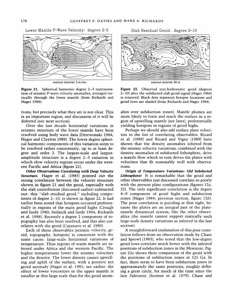
GEOFFREY F. DAVIES AND MARK A. RICHARDS
Lower Mantle P-Wave Velocity: degree 2-3 Slab Residual Geoid: degree 2-10
contour interval: 3 m/sec contour interval: 20 m
Figure 21. Spherical harmonic degree 2-3 representa- tion of seismic P-wave velocity anomalies, averaged ver- tically through the lower mantle (from Richards and Hager 1988).
tions, but precisely what they are is not clear. This is an important region, and discussion of it will be deferred (see next section).
Over the last decade horizontal variations in seismic structure of the lower mantle have been resolved using body wave data (Dziewonski 1984; Hager and Clayton 1989). The lower degree spheri- cal harmonic components of this variation seem to be resolved rather consistently, up to at least de- gree and order 3. The largest-scale and largest- amplitude structure is a degree 2-3 variation in which slow velocity regions occur under the west- ern Pacific and Africa (figure 21).
Other Observations Correlating with Deep Velocity Structure. Hager et al. (1985) pointed out the strong correlation between the velocity structure shown in figure 21 and the geoid, especially with the slab contribution (discussed earlier) subtracted out: this "slab residual geoid," including compo- nents of degree 2-10, is shown in figure 22. It had earlier been noted that hotspots occurred preferen- tially in regions of the main geoid highs (Crough and Jurdy 1980; Stefanik and Jurdy 1984; Richards et al. 1988). Recently a degree 2 component of to- pography has also been resolved, and this also cor- relates with the geoid (Cazenave et al. 1989).
Each of these observables (seismic velocity, ge- oid, topography, hotspots) is consistent with the same cause: large-scale horizontal variations of temperature. Thus regions of warm mantle are in- ferred under Africa and the western Pacific. The higher temperatures lower the seismic velocities and the density. The lower density causes upwell- ing and uplift of the surface, with a positive net geoid anomaly (Hager et al. 1985; see earlier: the effect of lower viscosities in the upper mantle is smaller at this large scale than for the geoid anom-
Figure 22. Observed non-hydrostatic geoid (degrees 2-10) after the subducted slab geoid signal (Hager 1984) is removed. Black dots represent hotspot locations and geoid lows are shaded (from Richards and Hager 1988).
alies over subduction zones). Mantle plumes are more likely to form and reach the surface in a re- gion of upwelling mantle (see later), preferentially yielding hotspots in regions of geoid highs.
Perhaps we should also add surface plate veloci- ties to the list of correlating observables: Ricard et al. (1989) and Ricard and Vigny (1989) have shown that the density anomalies inferred from the seismic velocity variations, combined with the density anomalies of subducted lithosphere, drive a mantle flow which in turn drives the plates with velocities that fit reasonably well with observa- tions.
SOrigin of Temperature Variations: Old Subducted Lithosphere? It is remarkable that the geoid and other observables just discussed correlate so poorly with the present plate configurations (figures 12a, 22). The only significant correlation is the degree 4-9 component of geoid highs and subduction zones (Hager 1984; previous section, figure 12b). The poor correlation is puzzling at first sight, be- cause the plates are an integral part of the plate- mantle dynamical system, like the other observ- ables (the mantle cannot support statically such large-scale density variations as inferred in the last section).
A straightforward explanation of this poor corre- lation follows from an observation made by Chase and Sprowl (1983), who noted that the low-degree geoid lows correlate much better with the inferred positions of subduction zones in the Mesozoic. Fig- ure 23a shows their comparison of the geoid with the positions of subduction zones at 125 Ga. In fact, there seem to have been subduction zones in approximately the same positions, roughly defin- ing a great circle, for much of the time since the late Paleozoic (Scotese et al. 1979). Chase and
178

MANTLE CONVECTION
Figure 23. Comparison of the non-hydrostatic geoid (cf. figure 12a) with the reconstructed positions of continents and subduction zones from 125 Ma, showing the correlation between former subduction zones and the main band of geoid lows (from Chase and Sprowl 1983).
Sprowl suggested that the thermal structure in the deep mantle still carries the memory of these past episodes of subduction, and that there might be only weak coupling between the upper mantle and lower mantle flows.
Davies (1984b) argued that in fact this memory was to be expected in a single-layered convection system, since convection patterns typically lag be- hind changes in boundary conditions (as we have already seen in the case of hot upwellings, figure 14). Thus the geoid lows might be directly re- flecting the presence in the deep mantle of much of the lithosphere subducted over the past 200 Ma or so. Richards et al. (1988) have estimated that this amount of old lithosphere can account for the magnitudes of the geoid and seismic heterogene- ities at low degrees.
More recently, Richards and Engebretson (1991) have demonstrated correspondence between old subduction zones, geoid lows, and high-seismic ve- locity lower mantle in a more quantitative way. By calculating the amount, time, and location (in the hotspot reference frame) of subducted slabs, they found high correlations of subduction histories in- tegrated back into the Mesozoic with both the ge- oid and seismic velocities.
Viscosities in the Lower Mantle. After Goldreich and Toomre (1969) (see p. 153) re-examination of post-glacial rebound data led to estimates that the mantle viscosity was fairly uniform, and about 1021
Pa.s (1022 Poise; Cathles 1975; Peltier and Andrews 1976). More recent studies seem to have resolved some vertical structure, with the upper mantle having a viscosity in the range 1-5 x 10²⁰ Pa.s and the lower mantle 2-10 x 1021 Pa.s (Nakada and Lambeck 1987, 1989; Lambeck et al. 1990). Small wobbles about the rotation axis and small varia- tions in the rotation rate are also consistent with such a viscosity structure (Yuen et al. 1982, 1986).
Unfortunately, the interpretation of postglacial rebound observations is beset with a number of difficulties that make it hard to get stronger con- straints on mantle viscosity. Calculated rebound histories are sensitive to details in the spatial and temporal variations of the glacial ice loads (Nakada and Lambeck 1987, 1988a). Many of the observa- tions are of changes in relative sea level, and are of necessity from coastal locations, but the rebound can also be very sensitive to local variations in the sea-water load, which depends in turn on details of the local bathymetry and topography (Nakada and Lambeck 1989). Also, coastal locations are close to the transition between continental and oceanic lithosphere, where there may be substantial lateral variations in viscosity structure (Nakada and Lam- beck 1988b). Finally, it has been suggested that the timescale of postglacial rebound (a few thousand years) is not long enough for the mantle material to have emerged from an initial stage of transient creep, during which apparent viscosities can vary
Journal of Geology 179

GEOFFREY F. DAVIES AND MARK A. RICHARDS
substantially (Weertman 1978; Yuen et al. 1986). Thus the viscosities deduced from postglacial re- bound may not be directly relevant to mantle con- vection, which operates on much longer time- scales.
Perhaps the probe that currently provides the most robust measure of a difference in viscosity between the upper and lower mantles is subducted lithosphere. We have already seen how the geoid highs over subduction zones are best accounted for if slabs encounter an increase in viscosity of 1-2 orders of magnitude, and that this will also ex- plain the steepening dip of slabs as they enter the lower mantle. Another argument was provided by O'Connell and Hager (1984; also Hager and Clay- ton 1988), who showed that the flow driven in the lower mantle by density variations inferred from seismic velocity variations would transport too much heat unless the viscosity of the lower mantle is at least 1022 Pa.s.
Laboratory data on rheologies of mantle rocks provide some further guidance, but not strong con- straints. Besides the fairly well characterized strong dependence of rheology on temperature (Paterson 1987), pressure is likely to have a sub- stantial effect (Weertman 1978). O'Connell (1977) and Davies (1984a) noted that viscosities in the deep mantle were extremely sensitive to the acti- vation volume of the material, and that it is diffi- cult to avoid increases of viscosity by many orders of magnitude unless that activation volume is sub- stantially less (at least at high pressures) than indi- cated by laboratory data (Carter 1976; Paterson 1987). Davies (1984a) and Christensen (1984a) noted that the problem was ameliorated somewhat if the rheology is non-linear, since then the depen- dence of effective viscosity on pressure is reduced by the exponent in the stress-strain relation. At this stage it is not clear how to reconcile laboratory data with apparent viscosities obtained from post- glacial and other observations. We can only con- clude that increases of viscosity with depth are cer- tainly plausible in the light of laboratory data.
Besides the direct effect of pressure on rheology, there is the indirect effect of pressure-induced phase transformations. Lower mantle material would only coincidentally have the same rheology as upper mantle material, and the closer-packed lower mantle phases would possibly have stiffer rheologies. Sammis et al. (1977) examined avail- able data for evidence of systematic effects of rele- vant phase transformations in analogue com- pounds. They concluded that a viscosity increase through the transition zone by 1 or 2 orders of mag- nitude is plausible, but that the constraints are not
log(VISCOSITY) Pa.s
Figure 24. A plausible viscosity profile through the mantle, showing the direct, pressure-induced increase with depth below the lithosphere, an increase through the transition zone due to pressure-induced phase trans- formations, and a variable and uncertain low viscosity zone in the upper mantle.
strong. A plausible (but not definitive) viscosity structure that takes account of the factors dis- cussed here is shown in figure 24.
Hotspot Velocities. It was noted in earlier that hotspot velocities are about an order of magnitude lower than plate velocities. The most straightfor- ward way of accounting for this is to suppose that plumes come from a region of the mantle where convection velocities are about a factor of 10 less than they are at the surface. Gurnis and Davies (1986b) have shown that in a convecting layer where the viscosity increases exponentially with depth, the velocities are reduced by about a factor of 10 if the viscosity at the bottom is 2-3 orders of magnitude higher than at the top. For simple layered viscosity models of plate-driven flow, Richards (1991) showed that core-mantle boundary velocities are reduced approximately in proportion to the logarithm of the ratio of upper and lower mantle viscosities. Also remembering arguments that plumes come from the bottom of the mantle, the implication is that the viscosity at the base of the mantle is a factor of 100-1000 higher than at the top.
The Bottom of the Mantle
The lowest few hundred kilometers of the mantle have more seismic complexity, probably include a
180

MANTLE CONVECTION
thermal boundary layer that is the source of plumes, and may be a repository for dense material that has settled out of the mantle.
The Seismic D" Layer at the Base of the Mantle. The seismic D" layer was so named by Bullen (1965), a region within a few hundred kilometers of the core where seismic velocity gradients are anomalously low. It has always been difficult to resolve because of the need to separate the ef- fects of diffraction around the core, and it has be- come increasingly clear that its seismic structure is complex. The complexities may be due to a sharp compositional interface 100-300 km above the core-mantle boundary (CMB) (Lay 1986) or to small-scale scatterers near the CMB (Haddon and Buchbinder 1986), or both. Recent estimates of the thickness of D" range from about 100 km (Doornbos 1983) to about 600 km (Lay and Helm- berger 1983). There is also evidence for major large-scale lateral variations in the expression of D" (Garnero et al. 1988).
Dynamics of the Thermal Boundary Layer at the Base of the Mantle. It was inferred earlier that about 12% of the earth's heat flux passes through the boundary layer from which plumes originate, comparable to the heat estimated to be emerging from the core if the core is cooling at a rate of 50-80°K/Gyr (Davies 1988b), further supporting the inference that plumes come from the core- mantle boundary (CMB). Jackson and Pollack (1984) and Stacey and Loper (1984) obtain a similar heat flux with a much smaller cooling rate, due to the inclusion of latent heat and gravitational en- ergy. We can now consider in more detail what this implies for this boundary layer, and how plumes are fed from it.
Because of the strong temperature dependence of silicate rheology, the mantle viscosity will be lowered in this boundary layer, reaching a mini- mum at the CMB. This will enhance the flow of boundary layer material into the base of a plume. Stacey and Loper (1983; also Loper and Eltayeb 1986) developed a theory that lateral flow would be concentrated in the lowermost part of the thermal boundary layer, comprising a velocity boundary layer. This lateral flow into the base of the plumes would be balanced by a slow subsidence of the overlying mantle. Although the quantitative re- sults obtained by Stacey, Loper, and Eltayeb are plausible, they are based on very poorly con- strained estimates of the thermal boundary layer thickness and temperature jump.
Davies (1990a) combined the plume heat flux estimate with this theory to estimate the thick- nesses of the thermal and velocity boundary layers.
A potentially important factor is that plumes may entrain surrounding mantle material as they as- cend, thus increasing their mass flow but reducing their temperature (Richards and Griffiths 1989; Griffiths and Campbell 1991; Loper and Stacey 1983 estimated that entrainment amounts to only 3%, but this is for an exactly vertical plume with no lateral background flow). Denoting the plume mass flux at the top of the mantle as ft, it is related to the buoyancy flux, B (discussed earlier), as
ft = B/gaA Tt (10)
where A T is the temperature excess of the plume at the top of the mantle. Then an entrainment fac- tor, E, can be defined as
E = ft//fb (11)
where fb is the mass flux at the bottom of the man- tle. The subsidence velocity, v, of overlying mantle into the boundary layer is
v = fb/(AcPb) (12)
where Ac is the surface area of the core (1.53 x 10⁸ km2) and Pb is the density of the bottom of the mantle. Then the thickness, dT, of the thermal boundary layer is
dT = K/V (13)
and the thickness, d,, of the velocity boundary layer is
dv = ed OO1dT/(EATt) (14)
These quantities are evaluated in table 4. Both E and the thermal diffusivity at the base of the man- tle are rather uncertain, but the results indicate that dT will be a few hundred kilometers and dv will be <100 km. In other words, the lateral flow
Table 4. Estimated Properties of the Thermal Boundary Layer at the Base of the Mantle
Quantity Symbol Value
Conductivity K 4-10 W/mK Plume entrainment factor E 1-3 Plume mass flux from CMB fb 2.5-8 x 10⁶ kg/s Mantle subsidence velocity v 0.1-0.3 mm/yr Temperature jump A Tb 200-700°K Temperature gradient at CMB Tb 1.3-3.0°K/km Thermal boundary layer thickness dT 150-500 km Velocity boundary layer thickness dv 30-75 km
Journal of Geology 181

GEOFFREY F. DAVIES AND MARK A. RICHARDS
0
Figure 25. Streamlines of the flow feeding into a plume near the base of the mantle, showing how the horizontal flow occurs predominantly in the lower part of the ther- mal boundary layer, implying that the plume samples a thin tabular region at the bottom of the mantle. Num- bers show radius and height, in kilometers. The central plume is included schematically. The dotted line shows the scale height, dT = 500 km, of the thermal boundary layer, and the dashed line hows the scale height, dy = 75 km of the velocity boundary layer, based on values in table 3.
into the base of plumes is strongly concentrated within the lowest 100 km or so of the CMB. Figure 25 shows an example of flow into the base of a plume calculated from Loper and Eltayeb's (1986) theory with E = 3.3 and K = 10 W/km. A smaller value of E would yield thinner boundary layers and a smaller temperature drop.
The implication of these results, important for the discussion of chemical heterogeneities in the mantle (later section), is that plumes are fed from the lowermost mantle, in contrast to mid-ocean rises, which are fed (obviously) from the uppermost mantle. The subsidence velocity of the mantle into the boundary layers is surprisingly small (about 0.33/E mm/yr). Combining this with an estimate of the feeding area of a plume (core area divided by number of plumes, which is between 40 and 100: Burke and Wilson 1976; Crough and Jurdy 1980), we find that a plume could be fed for 100 m.yr. from a volume a few tens of kilometers thick and 500-1000 km in diameter.
Another significant result is the small tempera- ture gradient at the CMB required to conduct the core heat flux into the mantle: only 1-3°K/km. This is much less than the gradient of about 30°K/ km required to yield zero gradient in the compres- sional wave velocity (Stacey and Loper 1983). This
2000
500
75 0
suggests that the thermal boundary layer makes little contribution to the seismic velocity anoma- lies of D".
"Dregs" at the Bottom of the Mantle? The proper- ties of the seismic D" layer would be consistent with the presence of slightly denser compositional "dregs" at the bottom of the mantle. Gurnis (1986) investigated the possibility that compositionally denser components, such as subducted oceanic crust (e.g., Ringwood and Irifune 1988) might settle to the base of the convecting mantle. He found that former oceanic crust would settle rather ineffi- ciently, but this left the implication that a small fraction might indeed accumulate at the CMB. The interaction of such a layer of "dregs" with convec- tion in the overlying mantle has been studied by Christensen (1984b) and Davies and Gurnis (1986), who found that the dregs would be piled up in re- gions of mantle upwelling and thinned in regions of downwelling, with the clear possibility that parts of the CMB would be swept clean of dregs under downwellings. Sleep (1987) has investigated how such a layer would be entrained in mantle flow and has found that entrainment would prob- ably be sufficient to remove such a layer within the age of the earth. This means that if such a layer exists, it must have been continually replen- ished, which would be consistent with inefficient settling. Lateral variations in thickness would account for the large-scale variations in seismic expression, while small-scale compositional het- erogeneity or convection within the dregs layer could account for smaller-scale variations and for scattering of seismic waves.
Plume Dynamics
Recently a series of elegant experiments and theo- retical works has clarified the dynamics of plumes in terms of a few relatively simply quantified con- cepts. This has provided further evidence on the source of plumes, as well as stimulating consider- ation of a broad array of near-surface effects that may have important implications for many geolog- ical processes. A number of aspects of plumes have been reviewed by Loper (1991).
Whitehead and Luther (1975) demonstrated that a steady stream of buoyant lower-viscosity mate- rial ascending through a higher-viscosity fluid is preceded by a spherical "head" of buoyant mate- rial whose diameter is much larger than the follow- ing column or "tail" (figure 26). This occurs be- cause the ascent velocity of a new column is limited by the higher viscosity of the surrounding material, and the head grows until its Stokes rise
182

MANTLE CONVECTION
Figure 26. Photograph of a starting plume in a labora- tory experiment, showing the large head and the nar- rower tail or conduit feeding the head. The plume was formed by continuously injecting hotter, lower- viscosity, dyed fluid into the base of a cool, higher- viscosity layer of the same fluid. Viscosity contrasts are about an order of magnitude. Light regions in the head are from surrounding fluid heated by the head and en- trained into it; the thermal head is actually spherical. Such plumes are discussed in detail by Griffiths and Campbell (1990). Photograph courtesy of Ross Griffiths.
velocity matches the flux of material into the base of the plume. Once a path is made by the head, the low-viscosity material ascends through a relatively narrow conduit, since its ascent velocity depends mainly on its viscosity and the diameter of the conduit, and not on the higher viscosity of the sur- rounding material.
Griffiths (1986a, 1986b) and Griffiths and Campbell (1990) showed that if the buoyancy is thermal, rather than compositional, then the head
entrains surrounding material and grows as it as- cends. This is because thermal diffusion heats a thin boundary layer of surrounding material which thereby becomes buoyant and rises with the plume head. They calculated that a plume head starting at the core-mantle boundary would reach a diame- ter of about 1000 km at the top of the mantle. En- trainment will also occur into the conduit if it becomes inclined to the vertical (Richards and Griffiths 1989; Griffiths and Campbell 1990).
Olson and Singer (1985) showed that a station- ary plume source will give rise to a stationary sur- face trace despite any intervening horizontal flow in the mantle, so long as the flow is steady. Rich- ards and Griffiths (1988) showed that the shape of a conduit inclined by a horizontal shear flow can be well approximated by assuming that each seg- ment of the conduit rises like an individual Stokes droplet. Griffiths and Richards (1989) pointed out that a hotspot track will undergo a delayed adjust- ment to a change of plate motion and noted that the sharpness of the bend in the Hawaiian-Emperor seamount chain implies that the Hawaiian plume is quite close to vertical. This constrains the buoy- ancy per unit height of the plume: if the density deficit of the plume is 50 kg/m3, then the Hawai- ian plume would have a diameter of about 70 km (Duncan and Richards 1991), which accords rea- sonably with the extent of active volcanism. Rich- ards (1991) also pointed out that it is unlikely that any of the major hotspot plumes suffers significant horizontal deflection, because there has been so lit- tle relative motion among major hotspot groups (e.g., Atlantic and Indian Ocean) despite major changes in plate motion during the past -100 m.y. (Duncan and Richards 1991).
A plume inclined >60° from the vertical tends to break up into droplets (Whitehead 1982; Olson and Singer 1985), although entrainment will sup- press this (Richards and Griffiths 1989). An exactly vertical plume would have a structure analogous to the boundary layer structure discussed in the last section: upward flow through the conduit would be concentrated in an inner core where the temperature is highest and the viscosity is lowest (Lopper and Stacey 1983). However, transverse cir- culation in an inclined plume would tend to ho- mogenize the temperature and internal flow (Grif- fiths and Campbell 1990).
Petrological observations (Schilling 1973; White and McKenzie 1989; Campbell and Griffiths 1990) and some simplified models of plume dynamics (Sleep 1990) constrain the maximum temperature of plume material in the upper mantle to be no more than about 250°C greater than normal upper
Journal of Geology 183

GEOFFREY F. DAVIES AND MARK A. RICHARDS
mantle. The temperature excess at the base of the mantle might be several times larger, due to the effects of entrainment (Griffiths and Campbell 1990).
As a plume head approaches the lithosphere it will flatten, and as the hot plume head crosses the solidus near the surface, it would be expected to produce a voluminous basaltic melt. Morgan (1981) suggested that continental flood basalts may repre- sent such plume initiation events, but also pointed out that they may result from continental rifting over long-lived plumes, a hypothesis developed by White and McKenzie (1989). Richards et al. (1989) showed that a number of large continental flood basalts occurred as the initial activity of mantle plumes and pointed out that the minimum possi- ble size of initial diapirs (>250 km in diameter), estimated from simple considerations of the amount of melt produced were unlikely to arise from a boundary layer within the upper mantle. Richards et al. (1989) also suggested that several large oceanic plateaus were initial outbursts of mantle plumes, a prediction that has received con- firmation from subsequent geochronological and geochemical studies (Richards et al. 1991). Rifting is not required for flood volcanism, and it has been argued that many continental flood basalt events were not preceded by significant extension (Rich- ards et al. 1989; Hooper 1990). Thus it is argued that neither continental flood basalts nor oceanic plateaus were produced by passive rifting, and that they represent a much more profound expression of plume activity.
Campbell and Griffiths (1990) and Griffiths and Campbell (1990) explored the dynamics of thermal plume heads in laboratory experiments, showing that starting plumes of order - 1000 km in diame- ter provided a plausible model for flood basalts. They pointed out specifically that such plume heads would spread rapidly beneath the litho- sphere to about twice their diameter, or about 2000 km. Continental flood basalt provinces are ob- served to be 2000-2500 km in diameter (e.g., White and McKenzie 1989), and the size, timing, and many compositional characteristics of flood basalts accord well with the predictions of the plume head model. On the other hand, a plume head originating at a depth of only 670 km would be much smaller and cannot explain both the size and brief duration of flood basalt episodes (Camp- bell and Griffiths 1990). Flood basalts thus provide further evidence for the plume source being at the core-mantle boundary.
There are many important geological implica- tions of this plume model. One, mentioned before,
is that Davies (1988) and Sleep (1990) may have underestimated plume-related heat flux. For exam- ple, the volume of the Deccan basalts that erupted at the initiation (67 Ma) of the currently active Re- union plume is roughly equal to the entire volume of basalts that makes up the Reunion hotspot track (Richards et al. 1989). Thus it is likely that if plume heads are included in the inventory, the es- timated plume heat flux may increase to the range of 10-15% of the total mantle heat flux. Plume heads may also have been associated with the for- mation of Archean greenstone belts (Campbell and Hill 1988; Campbell et al. 1989) and with the open- ing of the Atlantic (Hill 1991). The possible roles of plume heads and tails in some episodes of crustal anatexis, regional metamorphism, basin forma- tion, and mineralization are also under investiga- tion. Implications for the role of plumes in sam- pling the mantle are discussed in the next section.
Chemical Heterogeneity of the Mantle
Isotopic analyses of rocks from the sea floor have provided clear evidence for ancient chemical heter- ogeneities in the mantle (e.g., Hofmann 1984). Het- erogeneities exist on many scales, from within sin- gle seamounts to between ocean basins (Zindler and Hart 1986). The greatest isotopic diversity is observed in oceanic island basalts (OIBs) from volcanic hotspots, the mid-ocean ridge basalts (MORBs) being more uniform (e.g., White 1985). The range of apparent ages, inferred principally from lead isotopes, is about 1-3 Ga (Chase 1981), with MORBs having a range of 1.6-1.8 Ga (Tatsu- moto 1978). At least five source types are required to span the range of isotopic variation (White 1985; Allegre et al. 1987b), and at least three main differ- entiation processes must have produced the varia- tions (Hofmann 1988; Allegre et al. 1987a).
The compatibility of any physical model of the mantle with these constraints must be evaluated. A selection of the data will be presented here to illustrate some key constraints. More comprehen- sive discussions of this large subject can be found in Zindler and Hart (1986), Hofmann (1984, 1988), Hofmann et al. (1986), Hart et al. (1985), Allegre et al. (1987a), and Sun and McDonough (1988).
Refractory Incompatible Elements. A selection of isotopic data from the Pb, Sr, and Nd systems is reproduced in figure 27. The data can be viewed as radiating from the most depleted MORB end- member (e.g., with the least radiogenic Sr and Pb and the most radiogenic Nd). Then the principal distinction between MORB and OIBs is that MORB spans a smaller range of variation: all of the
184

MANTLE CONVECTION Journal of Geology
a
17.0 17.5 18.0 18.5 19.0 19.5 20.0 20.5 21.0 21.5 5
206pb/204pb
b
17.0 17.5 18.0 18.5 19.0 19.5 20.0 20.5 21.0 21.5 5
206pb/204pb
C
702 702 704 705 706 707 708
87Sr/86Sr
Figure 27. Summary of lead, strontium, and neodym- ium isotopic data from oceanic basalts. The labeled groups, with corresponding symbol types, identify five possible mantle source types required to span these data. Regression lines are drawn through MORB in (a) and (b). "Geochron" is the isochron defined by meteorites. Cross-labeled P.M. is a possible primitive mantle compo- sition (from White 1985).
Cs Ba U Ta La Sr Sm Hf Tb Yb AI Si Ni Rb Th K Nb Ce Nd Zr Ti Y Ca Sc Mg
Figure 28. Abundances of major and trace elements in average (depleted) MORB, a Hawaiian tholeiite (Kilauea), and a Hawaiian nephelinite from Oahu. Abundances are normalized to estimated abundances for the primitive mantle (from Hofmann 1984).
trends in OIBs can be seen to a lesser degree in MORB. The need for at least three source types can be seen particularly in the Sr-Pb plot (figure 27b), although five are identified there on the basis of additional criteria. The correlation of MORB data in figure 27a, and of all oceanic data more loosely, defines the mean apparent age of about 1.8 Ga.
OIBs show enrichments of light rare earth and other incompatible elements relative to MORB, as is illustrated in figure 28. This is unlikely to be due to fractional crystallization effects, and so is interpreted as reflecting enrichment of the OIB source relative to the MORB source (Hofmann and White 1982). This and the long-term enrichments of Rb/Sr, Nd/Sm, and U/Pb in OIB relative to MORB implied by the isotope data of figure 27 led Hofmann and White (1982) to propose that the OIB source is dominated by recycled oceanic crust, probably with some key modifications due to sea- floor alteration and subduction.
Some trace element ratios reveal a key relation- ship between OIB and MORB sources. Figure 29 shows Nb/U versus Nb concentrations from Hof- mann et al. (1986). On this plot, MORBs and OIBs show remarkable similarity of Nb/U, but both are quite distinct from continental crust. Wasserburg and DePaolo (1979) proposed a model based on early Nd isotope data in which OIBs represent a mixture of depleted (upper mantle) material and primitive (lower mantle) material, with the MORB source and continental crust being complementary differentiates from the primitive reservoir. This model is not compatible with the data in figure 29,
185

GEOFFREY F. DAVIES AND MARK A. RICHARDS
50 100
Figure 29. Nb/U ratios versus Nb concentrations in fresh glasses of mid-ocean ridge basalts (MORB) and oceanic island (hotspot) basalts (OIB). The Nb/U ratio of 47 is significantly higher than the ratios found in some carbonaceous chondrites (solid stars) and estimates for average continental crust (open stars) (from Hofmann et al. 1986).
since OIBs are clearly not intermediate between MORB and primitive chondrites. Rather, these data indicate that MORB plus OIB are complemen- tary to continental crust, with primitive mantle being represented by intermediate chondrite-like material. The uniformity of oceanic Nb/U limits contributions from either continental crust or primitive material to less than a few percent (Hof- mann et al. 1986). It is clear from figures 27a, b and 29, as well as from hafnium isotopes (Patchett et al. 1984; Galer et al. 1989) that most OIB comes from non-primitive sources. In fact, there is no clear evidence at all for a source with primitive refractory incompatible element ratios. Although there are some clear indications of the involve- ment of subducted continental sediment in some OIB sources (e.g., Woodhead and McCulloch 1989), trace element abundances seem to preclude the involvement of more than a few percent of conti- nental material in OIB sources (Hofmann et al. 1986; Sun and McDonough 1988).
Allegrd and Turcotte (1985) have proposed that some apparent lead ages (figure 27a) are in fact inherited ages from subducted continental mate- rial. However, oceanic 207Pb/204Pb is systematically lower than in continental crustal rocks and pelagic sediments, forming a subparallel array in the lead- lead diagram (figure 30). The more radiogenic oce- anic lead data could only be reconciled with the continental recycling hypothesis if some highly radiogenic continental sediments were recycled.
They propose that old continental lithosphere might be relatively primitive, but available data indicate that it is isotopically diverse and cannot be considered primitive (Sun and McDonough 1988). Neither lead isotopes nor the Nb/U ratios discussed above support Allegre and Turcotte's in- terpretation.
Other origins for some OIB source types have been proposed, such as remobilized continental lithosphere (Richardson et al. 1982; Allegr6 and Turcotte 1985) or metasomatism within the man-
18 19
°Pb/ Pb
20 21 22
Figure 30. Summary of lead isotope data from various oceanic and continental sources. MORB and OIB data courtesy of W. McDonough. Continental and pelagic sediment fields after Doe and Zartman (1979).
10
5
MORB * Atlantic £ Pacific * Indian Ocean
OIB x Azores a Galapagos o St. Helena v Samoa o Hawaii + Tristan da Cunha o Gough o Societies * Comoros o0 Reunion I Macquarie Isl.
0.1 0.5 1 5 Nb [ppm ]
10
186

MANTLE CONVECTIO N
tle (Menzies 1983), but the identification of the ultimate origins of the various OIB source types is not proving to be straightforward (Sun and McDonough 1988).
Using Nd isotopes, many authors have esti- mated that the depleted MORB source comprises 30-50% of the mass of the mantle, assuming the balance of the mantle has primitive concentrations of refractory incompatible elements, but the lack of evidence for this assumption means that the mass of the depleted mantle is poorly constrained by this method. Hofmann et al. (1986) avoided this assumption by using the Nb/U ratios of figure 28 (and analogous Ce/Pb data) to estimate that about 50% of the mantle had been differentiated to pro- duce the continental crust (and complementary MORB plus OIB) but could not rule out differentia- tion of most of the mantle.
The current Th/U of the MORB source (about 2.5) is less than the time-integrated ratio (about 3.75) revealed by lead isotopes (Galer and O'Nions 1985). Galer et al. (1989) have quantitatively mod- eled the evolution of Sr, Nd, Pb, and Hf isotopes using this and other constraints and found that an influx of less-depleted material into the MORB source is required, either by exchange with one or more other sources or by growth of the MORB source at the expense of deeper mantle. The in- fluxing material may be less depleted mantle or bulk continental crust, but not pelagic sediments. The residence time of very incompatible elements in the MORB source is short relative to the mean age of the continents. In particular, they demon- strated that these constraints do not distinguish between models with distinct mantle layers and models with only trace element stratification, nor between models in which the volume of the MORB reservoir is either fixed or growing in time.
It has been recently established that there are large isotopic variations within individual oceanic islands and between islands of the same group (e.g., Woodhead and McCulloch 1989). This implies that OIB sources are not large, homogeneous volumes, and advances the possibility that different hotspots have different chemistries simply because they are feeding from different parts of a large heteroge- neous region of the mantle.
Noble Gases. Helium and argon isotopic data from MORBs and OIBs are shown in figure 31. In this plot there seems to be a clear separation be- tween MORBs and OIBs. MORBs have radiogenic argon components (40Ar/39Ar) much greater than the atmosphere or sea water, indicating that the MORB source was strongly degassed early in earth history, and that radiogenic 40Ar has been accumu- lating since then (e.g., Hart et al. 1985). On the
24
- MORB o Plume o Sea water
20-
16
12-
8 16 24 32 40 3He/4He (x10-6)
48 56
Figure 31. Argon and helium isotopic data for oceanic basalts (after Hart et al. 1985).
other hand, both MORBs and OIBs have less radio- genic 4He compared with non-radiogenic 3He than does the atmosphere (3He/4He = 1.4 x 10⁻⁶), which is taken to indicate that "primitive" helium is still leaking out of the earth in significant quan- tities. The standard interpretation of the difference between MORB and OIB in figure 31 is that some OIB sources have been less strongly degassed than the MORB source, so that the accumulated radio- genic components are relatively less important in the OIB source (Hart et al. 1985; Allegre et al. 1987a), but this interpretation requires further dis- cussion (see below).
In fact, OIB samples have yielded atmosphere- like isotopes in all the noble gases except helium and argon, with argon in OIBs being relatively close to atmospheric (figure 31). Since the helium difference is explicable in terms of the loss of at- mospheric helium to space, the OIB source and the atmosphere (excluding helium) are hypothesized as representative of the original noble gas content of the silicate earth (e.g., Allegr6 et al. 1987a). The implication would then be that the atmosphere was formed by strong degassing of a primitive source, leaving the MORB source as a residue, with the current OIB source being some remaining "un- degassed" mantle (where "undegassed" means not degassed to the point where accumulating radio- genic isotopes are significant). However, the neon isotope data from MORBs and other sources (figure 32) are not compatible with this interpretation: these data imply a mantle component neither at- mospheric nor nucleogenic (spallation), and is plausibly a solar componant (Ozima and Zashu
Journal of Geology 187

GEOFFREY F. DAVIES AND MARK A. RICHARDS
0.02 0.04 0.06 0.08
Figure 32. Three-isotope plot for neon. Air, solar (solar wind, SW), and planetary (P1) sources are included. Arrows point to spallation (Spall) end-member, due to secondary nuclear reactions in the mantle. Steep line is the mass fractionation line (mfl) for neon isotopes. The dashed line is the correlation for MORB given by Sarda et al. (1988). Other date are from CO2 well gas (wg), MORB (solid circles; Marty 1989), diamond inclusions (diamonds; Ozima and Zashu 1988) (modified from Marty 1989).
1988; Sarda et al. 1988; Marty 1989). Thus the at- mosphere cannot be representative of the bulk or primitive earth.
The argon data have been used to estimate the degassed proportion of the mantle or rather the pro- portion of mantle argon removed from the mantle. Allegro et al. (1987a) estimate 46%, while Hart et al. (1985) estimate 50-90%, depending on the estimated potassium content of the earth. In both studies the OIB source is assumed to have a near- atmospheric isotopic composition, which may not be justified, as we have seen. It would seem to be within the range of uncertainties of such estimates that the OIB source has been moderately degassed, say by 90%, while the MORB source, comprising (say) 80% of the volume of the mantle, has been nearly completely degassed (>99%). The helium data would be quite consistent with this picture, since the original amount of He in the earth is un- known.
'29Xe/'3°Xe ratios from some MORB and CO2 well gas samples are higher than atmospheric, showing that these sources have been distinct from the atmosphere since before the parent of '29Xe (129I, half life 17 Myr) became extinct (e.g., Allegr6 et al. 1987a). The latter argues directly for degas- sing of the atmosphere from the mantle within tens of millions of years of the formation of the earth. Furthermore, Ozima et al. (1985) and Marty (1989) argue that radiogenic and fissiogenic Xe iso- topes require the atmosphere, or its mantle source, to have closed some tens of millions of years after
the isotopically distinct mantle sources currently observed. This argument further supports the con- clusion that the atmosphere noble gas isotopic composition (excepting He) cannot be representa- tive of the bulk earth or primitive composition.
The close resemblance of the heavier noble gases in OIB to atmospheric compositions prompts the question of possible contamination: it is only helium, whose atmospheric abundance is very low because of loss to space, whose OIB isotopes are markedly different from atmospheric. This ques- tion has been re-examined by Patterson et al. (1990), who conclude that plausible contamination mechanisms may account for the observed abun- dances, such as hydrothermal interaction or assim- ilation of seawater-altered oceanic crust, although they could not establish conclusively that contam- ination had occurred. Of course, it is necessary to establish that contamination has not occurred be- fore the data can be treated with confidence. It fol- lows that until the question of atmospheric con- tamination of OIB samples has been settled, the only clearly established difference between OIB and MORB noble gas isotopes is for helium. Some, but not all, hotspots have a greater component of "primitive" helium than does MORB.
Direct Inferences from Chemical Observations. Topologically, there is a minimum of five source types required to span the six-space array defined by the radiogenic isotopes of Pb, Sr, Nd, and He (Allegrd et al. 1987b). In addition to the depleted MORB source, some of the OIB sources can be rea- sonably identified with subducted oceanic crust and subducted sediment derived from continental crust (Hofmann and White 1982; Sun and McDon- ough 1988). A tentative identification of some with metasomatized continental or oceanic lithosphere is also suggested (Sun and McDonough 1988).
There is no clear evidence for a primitive reser- voir in the mantle. High 3He/4He ratios in some OIBs show only that not all of the helium origi- nally incorporated into the earth has escaped, hardly a surprising conclusion. A reservoir with at- mospheric noble gas isotopic compositions must be doubted until the question of near-surface con- tamination of OIB samples is settled. In any case, the neon and xenon isotopes in MORB establish that such a reservoir would not be representative of the whole earth, and therefore could not be primitive.
Chemical heterogeneities in the mantle have survived for about 2 Ga. Strictly speaking this has not been rigorously established, since there is clear evidence for mixing having occurred in some of the samples represented in figure 27a (e.g., Sun and McDonough 1988), but few doubt that the overall
188

MANTLE CONVECTION
linear trend in figure 27a implies a mean age of heterogeneities of about 1.8 Ga. The directly mea- sured parent/daughter ratios of several systems im- ply ages of this order to accumulate the observed isotopic variations.
On the other hand, it is not clear that heteroge- neities in xenon isotopes have survived from the earliest earth, since this was suggested on the basis of differences between MORB and OIB 129Xe/13°Xe (Allegr6 et al. 1987), which are in doubt because of the possible near-surface contamination of OIB samples. Heterogeneities in helium isotopes are well-established, but they may be continuously in- troduced, for example by helium leaking out of the core (Sun and McDonough 1988; Davies 1990).
Three main aggregate differentiation processes are identifiable. The earliest was degassing of noble gases (Allegr6 et al. 1987a), presumably along with much of the rest of the atmosphere and hydro- sphere. The next, in terms of mean age, was extrac- tion of the continental crust, and the youngest in mean age is from the formation of the heterogene- ities evident from oceanic rocks and represented principally by the MORB-OIB dichotomy (Hof- mann 1988).
The uppermost mantle, almost by definition, is occupied by MORB source. What is often meant by "MORB source" is that the uppermost mantle is occupied by relatively homogeneous material that plots near the depleted ("MORB") end-member of the isotopic mantle arrays. This may be the volu- metrically dominant material, and it may exclude obvious hotspots, like Iceland, but how much else is meant to be excluded is not clear. Locally, it is quite possible to identify mixing between a nearby plume and local MORB source (Schilling 1973; Schilling et al. 1975), and more generally major hotspots can be clearly distinguished from the more depleted MORBs. However, globally the two populations overlap and merge, so that there is no clear demarcation between the depleted and less- depleted compositions, by either geochemical or geophysical criteria (Davies 1984). For example, how does one usefully categorize MORB less de- pleted than average, from perhaps slightly elevated ridge crest, but which cannot be associated with any obvious hotspot? Calling it E-type (enriched) MORB is little help, since the only good definition of its complement, N-type (normal) MORB seems to be MORB that is not abnormal.
An inference that seems to be both correct and useful is that MORB source comprises a range of depleted and less-depleted compositions and does not include material that obviously arrived only recently in the upper mantle, such as Iceland plume source, but the demarcation between these
source types is not very clear. Even this inference is not strictly required, but only Anderson (1982) in recent times has been willing to postulate that MORB source material ascends to ridges from a deeper layer, rather in the way plumes ascend from deeper regions. Since ridges migrate about the earth's surface mostly in accord with simple em- pirical rules that seem to reflect mechanical prop- erties of the lithosphere (Davies 1988a), this im- plies either that material from the deeper layer somehow knows where to come up or (Anderson, pers. comm.) it ascends in broad regions under oceans, in which case the semantics of layering become confused.
The Physical Process of Stirring by Convection
The chemical and isotopic heterogeneities in mantle-derived rocks are the product of both chemical and physical processes. Although the chemical data provide important constraints, they cannot by themselves tell us about the geometry and topology of their sources in the mantle, nor about the physical context of the chemical process.
Some quite divergent conclusions have been reached from studies of stirring by convective and other flows: at one extreme have been claims that passive chemical heterogeneities in the mantle would be homogenized within a few hundred mil- lion years (e.g., Kellogg and Turcott 1986), while at the other extreme, Gurnis and Davies (1986c) have suggested that some heterogeneities might have survived for the age of the earth. The claims may not, in fact, be incompatible: the answer one gets depends strongly on the question one asks. Several distinctions must be carefully drawn to understand the different aspects of this process: between stir- ring and mixing, between stirring by normal strains and shear strains, between the most and the least stirred components, amongst the various ways in which the distribution of stirred material can be characterized, between steady and unsteady flows, and amongst the various kinds of unsteady flow in experiments or in the mantle.
Stirring and Mixing. Stirring is the intermin- gling of fluids that remain distinct, while mixing is the merging of distinct fluid types into an inter- mediate type. Mixing usually requires stirring so that the fluids are intermingled on a small length scale, as well as diffusion to homogenize the fluids. Solid-state diffusion is extremely slow in the man- tle, spanning less than meters in billions of years (Hofmann and Hart 1978).
On the other hand, one must also consider the way the mantle is sampled-usually by melting.
Journal of Geology 189

GEOFFREY F. DAVIES AND MARK A. RICHARDS
Figure 33. Stretching of a passive heterogeneity at a stagnation point. A block of 2500 passive tracers (top square) is advected by the steady flow represented by the streamlines, and shown at several successive times. At the last time, the tracers are shown displaced below the box so they can be distinguished from the box outline. The original block then comprises two relatively thick sections joined by a tendril so thin that no tracers have plotted within it.
Because of much higher diffusion rates in liq- uids and possibly also substantial stirring during magma ascent, heterogeneities over length scales of kilometers or larger may be effectively homoge- nized from the perspective of mantle-derived mag- mas. Then again, even well-stirred components may still be sampled differently if they have sig- nificantly different solidus temperatures. This is a potentially complex process, since melt initially derived from the lowest-solidus component may subsequently interact with higher-solidus compo- nents. Also, as pointed out by Sleep (1984), the preferential melting of the low-solidus compo- nent may be substantially amplified in a well- stirred mixture by the conduction of heat from adjacent material to replace latent heat absorbed by melting.
Shear Strain and Normal Strain. There are two kinds of volume-conserving strain, and they result in very different rates of stirring. In simple shear- ing, the length or perimeter of a heterogeneity in- creases approximately linearly with time, while in normal straining, the length increases exponen- tially with time. A simple example shown in figure 33 illustrates both kinds. A large blob is carried into a stagnation point of a steady flow (i.e., a point where the flow diverges in opposite directions). The strain at the stagnation point is normal strain (steady shortening vertically and stretching hori- zontally), and the result is that the parts of the
190
heterogeneity near the stagnation point are de- formed into an ever thinner, ever longer tendril. On the other hand, the parts further from the stag- nation point are carried around the streamlines of one or the other cells, undergoing simply shear par- allel to the streamlines. The original blob is split into two main blobs connected by a thin tendril. The thickness of the blobs will decrease inversely with time, while the thickness of the thinnest part of the tendril will decrease exponentially with time. After a few overturns, the tendril will be or- ders of magnitude thinner than the thickest parts of the blob.
This distinction between normal and shear straining was drawn by Olson et al. (1984a), who went on to show that shear straining dominates in a single steady circulation cell. Kellog and Tur- cotte (1986), on the other hand, assumed that nor- mal straining predominated without offering any justification. Hoffman and McKenzie (1985) con- cluded on the basis of relatively short runs of an unsteady numerical convection model that the pe- rimeter of a heterogeneity increased exponentially with time and implied that normal strains predom- inated. Gurnis and Davies (1986b) found in long runs of unsteady numerical convection and kine- matic flows that some heterogeneities persisted for much longer than was predicted by either normal straining or shear straining.
Extreme Heterogeneity of Strain. This confusing situation was clarified substantially by Gurnis (1986b), who followed the perimeter of a single blob for many overturns in a simple unsteady kine- matic flow, as reproduced in figure 34. The flow comprises two cells whose boundary oscillates hor- izontally and sinusoidally in time, so that the cells alternately grow and shrink. Time is depicted in terms of transit times: the time taken to traverse the layer depth at a typical fluid velocity. An ini- tially circular blob undergoes mainly simple shear for about 10 transit times, its perimeter not in- creasing dramatically. In fact the sense of shearing is occasionally reversed, as the blob is transferred from one cell to the other: this tends to partially "unstir" the blob, so that the perimeter increases, on average, less rapidly than in the case of the steady simple shearing studied by Olson et al. (1984a). Eventually, part of the blob passes through a stagnation point, creating a long thin tendril. Thereafter the tendril has a high probability of passing again through a stagnation point and being further stretched and convoluted, as can be seen in the last two frames of figure 34. In this phase the perimeter of the blob increases rapidly and expo- nentially, and so the average thickness decreases exponentially. However, a considerable fraction of

MANTLE CONVECTION
Figure 34. Stirring of a passive heterogeneity by time- dependent flow. A sequence of frames is labeled by time (in transit times, upper right); the box outline is shown only in the first two frames so as not to obscure the stirred blob. The flow comprises two cells (first frame) whose boundary oscillates horizontally. A small circular blob was introduced at time zero, and its perimeter was traced through subsequent frames. The blob is eventu- ally stretched into extremely thin tendrils (much thinner than the lines shown), but the thickest part still contains a significant fraction of the original volume, as shown in the magnified section from the last frame (from Gurnis 1986b).
the blob remains in compact form, with a maxi- mum thickness only about a factor of 10 less than at the start, even after more than 20 transits.
We can now account for some of the differences of interpretation noted above. Olson et al. (1984a) considered only a single steady convection cell in which stagnation point stretching could not occur. Hoffman and McKenzie (1985) noted the rapid in- crease of the perimeter of their heterogeneity and so their characterization of the results applied to the average thickness. Since the convection model was run for only a few transit times, they could not observe the much slower decrease of the maxi- mum thickness. Because they assumed that nor- mal straining was dominant, Kellogg and Tur- cotte's (1986) analysis implicitly applied only to tendrils, and their results characterize the average thickness and say nothing about the maximum thickness. Gurnis and Davies' (1986b) use of vol- ume tracers (rather than perimeter tracers) was suitable for revealing the presence of compact blobs, but not for revealing the convolutions of tendrils, so their results characterize the rate of decrease of the maximum thickness and say noth- ing about the average thickness.
It is thus crucial to distinguish between the av-
erage straining or thinning of a heterogeneity and the minimum straining or thinning, since these may differ by many orders of magnitude within different parts of the same heterogeneity. To am- plify this a little, objects that are much smaller than the smallest scale of circulation will have only a small chance of being torn apart by a stagna- tion point in one overturn time, so they will be stretched by shear straining which increases their perimeter approximately linearly with time. On the other hand, objects larger than the smallest scale of circulation (such as tendrils already cre- ated) will undergo stagnation point stretching vir- tually every overturn, with the consequence that their perimeter will approximately double every overturn and will therefore increase rapidly and ex- ponentially.
Alternative Characterizations of Stirring. These two characterizations (i.e., average thickness and maximum thickness) are appropriate for different contexts. Thus if one wants to know how much a given piece of mantle is likely to be permeated with bands of old subducted crust, then Kellogg and Turcotte's (1986) results show that after a few hundred million years, old crust is likely to perva- sively permeate the mantle down to meter scales or less. On the other hand, if one wants to know if there are regions of the mantle with substantially higher concentrations of old crust, then Gurnis and Davies' (1986b) results show that such regions may persist for 1 or 2 Gyr. These results are not so much contradictory as complementary.
There are other examples of the way the infor- mation conveyed can depend very strongly on the way the results are characterized and presented. Figure 35 simply shows the spatial locations of tracers at a particular time, and it is immediately evident that there are heterogeneities in the distri- bution ranging over a variety of length scales. On the other hand, Olson et al. (1984b) used autocor- relation functions to characterize their results. These are useful for characterizing the length scale and anisotropy of small-scale, strain-induced band- ing, for example, but tend to obscure information about the kind of multiscale heterogeneity evident in figure 35. Kellogg and Turcotte (1990) displayed individual particle paths and distributions of cu- mulative stain, but neither of these is very directly related to the existence of spatial heterogeneity. (These authors did include plots of spatial distribu- tion early and late in the stirring process, but this choice conveyed only a weak upper bound on the survival times of heterogeneities.)
Unsteadiness of Flow. One more important rea- son for the divergence of stated conclusions noted earlier was only revealed by some careful numeri-
Tournal of Geology 191

GEOFFREY F. DAVIES AND MARK A. RICHARDS
0.0 tronsits 0.0 Gvr
7.5 transits 0.4 Gyr
30.0 transits 1.2 Gyr
60.0 transits 1. 9 Gyr
Figure 35. Stirring of passive tracers in a time- dependent, plate-scale flow. Three plates are separated by a spreading center (left) and a subduction zone (right), both of which migrate in a cyclic pattern (plate evolution model 1 of Gurnis and Davies 1986b). Note that, apart from the second panel, the panels correspond to the same part of this cycle. The viscosity increases with depth (see figure 24). The large tracers mark fluid "subducted" during the first 10 transit times. The small tracers mark "primitive" fluid initially in the lower, high-viscosity region. Panels are labeled with time, measured in both transit times and billions of years, based on the scaling of Gumrnis and Davies (1986c), which takes account of the considerably faster convection likely early in earth history. Heterogeneities in the distributions of both kinds of tracers persist at all length scales for billions of years (after a model by Gurnis 1986c).
cal experiments by Christensen (1989b). We have noted that stagnation point stretching cannot oc- cur in steady flow (except for heterogeneities that initially straddle the boundaries of circulation cells, as in figure 33), so unsteadiness clearly has an important bearing on stirring. Christensen (1989b) has found that different kinds of unsteadiness can yield very different rates of stirring. Using two- dimensional kinematic flows with various kinds of unsteadiness, he identified two main regimes of stirring that removed heterogeneities at very differ- ent rates: fast stirring (his regime A) and slow stir- ring (regime B). A third, hybrid regime (C), had per- sistent islands of slow stirring with fast stirring in the surrounding fluid.
The slow stirring occurred in two-cell flows in which the boundary between the cells migrated steadily across the box or oscillated sinusoidally in position. Fast stirring occurred when the position of the boundary moved more irregularly (with higher harmonics) and rapidly. Fast stirring also oc- curred in another kind of flow, in which a single cell is first bisected, with the emergence of a third, counter-rotating cell with the flow returning later to the single cell form. This flow is also character- ized by relatively rapid and irregular passage of cell boundaries through the fluid. Christensen (1989b) also found fast stirring in numerical convection models featuring unstable boundary layers from which blobs of buoyant material detached irregu- larly, causing the kind of cell breakup and merging just described.
The relevance of these results to the mantle has been debated by Davies (1990b) and Christensen (1990). It is clear in retrospect that the flows con- sidered by Gurnis and Davies (1986b) yielded slow stirring. These included not only kinematic flows with oscillating cell boundaries, but also flows in- tended to mimic the unsteadiness induced by the migration of the spreading centers and subduction zones separating the earth's plates, including occa- sional breakup of plates and their underlying cells. On the other hand, boundary layer instabilities, ei- ther of the lower lithosphere or the lower thermal boundary layer, might yield enough unsteadiness to move the mantle into the fast stirring regime (Christensen 1990). Also, the kinematic flows as- sumed by Kellogg and Turcotte (1990) were of the cell breakup and re-merging kind that yield fast stirring. The relevant arguments concerning appli- cation to the mantle are essentially those given earlier: there is little observational evidence for instability of the lower lithosphere, and while plumes probably arise from instabilities of the lower thermal boundary layer, their axial geometry does not greatly disrupt the plate-scale flow, so that they are less likely to induce fast stirring. These possibilities require further investigation.
Effects of Viscosity Stratification. In earlier sec- tions we have seen observational evidence for an increase of viscosity with depth in the mantle, the viscosity at the bottom being perhaps 2-3 orders of magnitude higher than that just below the litho- sphere. The effect of this on stirring has been in- vestigated by Gurnis (1986c) and Gurnis and Da- vies (1986c) and further discussed and illustrated by Davies (1990a and in figure 35, this paper). The survival time of heterogeneities is considerably en- hanced because of the slower flow at depth (figure 35). Tracers in the shallower fluid are removed (or
192

MANTLE CONVECTION
reset) by a spreading center more often than tracers at depth, so a continuous stratification of residence time accumulates, such that the average time since the introduction of the tracers increases with depth; also, the deep fluid is more heterogeneous than the shallow fluid, where stirring is faster (Gurnis and Davies 1986c). (We will use the term "continuous stratification" here to mean a contin- uous variation of [horizontally averaged] properties with depth. This terminology is often used in fluid dynamics, though many geologists may take strati- fication to mean layering, and prefer the term "zoned," for example. The important distinction here is that we mean to include continuous grada- tion, and not [necessarily] to imply uniform layers with sharp boundaries.)
From these results it is concluded that in the mantle we would expect the shallow mantle to be better stirred, more often sampled at spreading centers (and thus perhaps more depleted of incom- patible trace elements due to extraction of conti- nental material), and to show evidence for shorter residence times of material recycled from subduc- tion zones. Conversely, the deep mantle would be more heterogeneous, less depleted, with residence times of up to 2 Gyr. The possibility was raised by Gurnis and Davies (1986c) that a small fraction of the mantle initially at the bottom may have under- gone little or no stirring or melting.
Multiple Scales of Flow and Three-Dimensional Flow. Stirring might be much more efficient in the presence of flow at more than one scale, since the smaller scale will move material across the streamlines of the larger-scale flow, and it might also introduce more stagnation points. It is thus very important in this context to determine the existence and nature of any possible modes of man- tle convection whose scale is smaller than that of the plates.
The effect of mantle plumes on stirring needs to be investigated, but it may be noted here that they involve a substantially smaller mass flux than the plate-scale flow, and that they are narrow colum- nar structures than do not disrupt a large fraction of the plate-scale flow they penetrate. Thus it is not obvious that they will have a major effect on mantle stirring, although they might.
As discussed earlier, the existence of other small-scale flows is not clearly established. The best case is for 200 km wavelength rolls near the East Pacific Rise, but these would occupy only a small volume of the mantle and are probably of low amplitude (implying small flow velocities), so their effect is unlikely to be substantial. The exis- tence of other modes is not precluded, but the argu-
ments given earlier indicate that if they exist, they must be low in amplitude. Thus, at this stage, there is no strong indication that small-scale flows will substantially enhance stirring rates.
Plumes introduce three-dimensionality into mantle flow, but of course the plate-scale flow is already three-dimensional and globally connected, so that it is not really accurate to think in terms of cells or rolls (e.g., Hager and O'Connell 1979). The study of stirring in three-dimensional flows is only beginning. While it is easy to imagine three- dimensional flows that might stir very efficiently, the experience of two-dimensional stirring has made it clear that the stirring efficiency can de- pend on subtleties of the flow. Thus one can point to the organizing role of the plates, to higher vis- cosities at depth and to the proximate core-mantle boundary in the lower reaches of the mantle as factors that may limit the stirring rate. We regard this question as quite open at present: no strong statements can be made either way until three- dimensional stirring has been carefully and quanti- tatively studied.
Heterogeneities on All Scales. A crucial feature of figure 35 is that at dimensional times of about 1-2 Gyr the model can represent heterogeneities on all scales (i.e., on scales from the numerical grid size to the box size). The model does not predict ran- dom, small-scale heterogeneities, except at much later times. This point seems to have been com- monly misunderstood (e.g., Allegr6 and Turcotte 1985; Silver et al. 1988). The distinction is impor- tant, because the differences between average com- positions in different ocean basins imply large- scale heterogeneities in the mantle, along with heterogeneities at all smaller scales (Zindler and Hart 1986). There is no inconsistency between these observations and figure 35.
Interpretation of Geochemical Observations
The geophysical evidence discussed earlier is inter- preted to favor penetration of the plate-scale flow through the full depth of the mantle, but with higher viscosities in the deep mantle causing slower flow there. We have just seen in the pre- vious section that this should yield continuous stratification in trace element concentrations, heterogeneity, and residence times. Melting un- der spreading centers samples the shallowest man- tle, while the earlier discussion of plumes and the lower thermal boundary layer favors the interpre- tation that plumes sample the lowermost mantle. The resulting composite picture is sketched in figure 36.
Tournal of Geology 193

GEOFFREY F. DAVIES AND MARK A. RICHARDS
Figure 36. The main features of the mantle. Lithosphere is formed at a spreading center on the (right) and subducted at a subduction zone (left) at the edge of a continental plate (far left). The subducted slab kinks at the 650 km transition zone (long-dashed) due to the increase in viscosity there (Gurnis and Hager 1988). It may buckle at greater depth due to steadily increasing viscosity in the lower mantle. The plate-scale flow is indicated by the arrows; it is slower by about a factor of 10 at the bottom of the mantle because of higher viscosity. An established plume rises from the core-mantle boundary near the center of the sketch. It feeds from a thin velocity boundary layer (dashed line) within the lower part of the thermal boundary layer (dotted line), but above a discontinuous layer of heavier mantle dregs (black) at the bottom of the mantle. The established plume has left a track of volcanoes on the surface plate, beginning with an oceanic volcanic plateau due to the starting head of the plume. A second, new plume is rising on the right, with a large head that has entrained surrounding material during its ascent. Both plumes are deflected from the vertical by relatively small amounts by the plate-scale flow through which they penetrate. Chemi- cal heterogeneities (background squiggles) are more pronounced in the high viscosity region at the bottom of the mantle where material is more heterogeneous, older, and less depleted than in the shallower mantle (see text). Whereas the mid-ocean ridge (spreading center) samples the uppermost mantle, the plumes sample the lowermost mantle (except possibly the dregs).
Some features of this model have been discussed by Davies (1990a). It can accommodate all of the suggested chemical source types (recycled oceanic crust, continental crust, continental lithosphere, primitive mantle). The close relationship between MORB and OIB sources revealed in such things as the Nb/U ratio reflects the fact that they differ only in degree of stirring and sampling, and possi- bly in proportion of recycled oceanic crust. The Pb-Pb ages (figure 27a) are real ages of recycled oce- anic crust to first order (though local mixing will have averaged and/or contaminated them). The heterogeneity between and within OIB sources simply reflects the heterogeneity of the deepest mantle, with some modifications due to entrain- ment into plumes during their ascent (Griffiths and Campbell 1990). The greater homogeneity of MORB sources reflects the faster stirring in the shallow mantle. An implication of this is that the MORB source contains all of the source types evi- dent in OIB sources, but with a muted expression due to dilution with more strongly depleted shal-
low mantle, and this seems to accord with observa- tions. Galer et al. (1989) have shown that U, Th, and Pb have short residence times (<1 Gyr) in the MORB source. This constraint is accommodated by the flux of deep mantle into the shallow mantle via plumes, whose mass flux amounts to roughly 10% of the upper mantle per billion years (Davies 1990a). The faster stirring and more frequent sam- pling of the shallow mantle seems to be reflected in the U, Th, and Pb residence times, but not in the Pb-Pb ages. This is explained by the fact that the shallow mantle is strongly depleted in lead and thus is very susceptible to lead contamination (Galer et al. 1989): the influx of lead from plumes dominates the MORB lead signature. To explain the difference in helium isotopes between MORB and some OIBs it is necessary to invoke either some remaining less degassed mantle that has avoided homogenization for 4.5 Gyr or a flux of helium from the core, a possibility that is difficult to evaluate at this time (Davies 1990a). As noted earlier, no other noble gas difference between the
194

MANTLE CONVECTION
OIB and MORB sources has been convincingly demonstrated at this time.
The enrichments in incompatible trace ele- ments in OIBs relative to MORBs (figure 28) imply a greater proportion of old oceanic crust has con- tributed to the OIB than is the case for MORB. Three factors could be responsible for this. First, if the shallow MORB source overturns and is de- pleted at subduction zones more often, then the MORB source would become more depleted. How- ever this does not explain why the OIBs are also enriched relative to chondrites. Second, gravita- tional settling, although unlikely to be as efficient as supposed by Hofmann and White (1982), could lead to a greater concentration of old oceanic crust at the bottom of the mantle (Gurnis 1986b), since it is likely to be denser than a peridotite composi- tion in the lower mantle (Ringwood 1982).
A third factor, not discussed by Davies (1990a), is that relatively small inclusions of material with a lower solidus can melt to a much greater degree (by a factor of 2 or more) if heat can conduct in from surrounding material (Sleep 1984). For exam- ple, heat can conduct into old oceanic crust of 3 km thickness on a time scale of about 0.1 Myr. In a plume rising at 100 mm/yr (100 km/Myr) that intersects the solidus at (say) 100 km depth, there is ample time for heat to conduct into the crustal inclusions, replacing latent heat of fusion, and the melts formed will be predominantly from the old crustal component. If this melt were to migrate to the surface without reacting significantly with the surrounding mantle, it would seem to have come from a source dominated by old oceanic crust. Of course, this effect will be reduced by the extent to which the melts react with surrounding material during ascent, and this has not been estimated.
Gravitational settling is the most quantified of these processes at the moment (Gurnis 1986b), so the least conjectural assumption is that there is a concentration of old oceanic crust in the deepest mantle; this is consistent with seismological evi- dence. The resulting picture (figure 36) has the es- sence of the Hofmann and White (1982) model, but without the assumption of a discrete layer of old crust at the base of the mantle.
We can, with this model, better understand the difficulty of separating the global MORB and OIB populations. We have seen from stirring experi- ments that part of a new heterogeneity may remain compact for a long time, but part of it may become extremely convoluted and stretched through the mantle. Conversely, any volume of mantle is likely to contain streaks of old heterogeneities through it. When such a volume is melted under a
spreading center, the resulting MORB composition will be some average of the depleted matrix and whatever heterogeneities are streaked through it. Occasionally a volume may contain a more sub- stantial heterogeneity of a particular kind, and the resulting melt might be termed "enriched" MORB. When a strong plume brings material up from the more heterogeneous deep mantle, its chemical sig- nature should be obvious, but the presence of a weak plume may not be recognized, though its chemical effect may be resolvable. The effects of a strong plume may be evident at some distance from its hotspot because of lateral spreading of the buoyant plume material under the lithosphere: this is clear near the Iceland hotspot (Schilling 1973) and plausible for near-ridge hotspots (Schil- ling et al. 1975). Thus there are several ways heter- ogeneities can contribute to MORB, and we would expect MORB to exhibit all of the chemical diver- sity evident in OIBs, though in diluted form. This expectation seems to accord well with observa- tions.
Discussion of Alternative Models
Wasserburg and DePaolo (1979) proposed, on the basis of early neodymium isotope data, a two-layer mantle in which the depleted upper mantle is the complement of the continental crust and the lower mantle is primitive. Plumes ascending from the in- terface and comprising a mixture of upper mantle and lower mantle material were presumed to ac- count for OIB data. We have seen, however, that there is no evidence requiring a primitive source type in the mantle and that OIBs have non- primitive lead isotopes and Nb/U ratios. Allegrd et al. (1980) modified this model by proposing a continuing segregation of metal phase from the lower mantle into the core to account for the higher U/Pb ratios implied by OIB lead isotopes. It was necessary also to assume that stirring in the lower mantle was inefficient to explain the hetero- geneities of lead isotopes. Newsom et al. (1986) showed that abundances of siderophile (metal af- finity) and chalcophile (sulphide affinity) elements in OIBs are incompatible with this idea.
Hofmann and White (1982) proposed that the OIB source is primarily recycled oceanic crust, modified by hydrothermal alteration on the seafloor and by extraction of some components during subduction. They proposed also that the subducted crust accumulates in a layer, perhaps at the core-mantle boundary, and is stored there for 1-2 Gyr before gaining thermal buoyancy and ris- ing as plumes to the top of the mantle. The main
Journal of Geology 195

GEOFFREY F. DAVIES AND MARK A. RICHARDS
chemical part of their model (recycling oceanic crust) has gained widespread acceptance. The dy- namical part has had less acceptance, but a modi- fied version, in which segregation of the denser oceanic crust is less efficient than they envisaged, seems to be capable of explaining many of the ob- servations reviewed here.
Davies (1981), after noting the uncertainties in estimates of the volume of the depleted (MORB) source, the evidence for some OIB sources and kimberlite inclusions being more enriched than chondritic, and the fact that subduction of litho- sphere is a continuously operating source of heter- ogeneities in the mantle, proposed that the mantle contains heterogeneities of many sizes and degrees of enrichment or depletion. Subsequently, Davies (1984), noting evidence for increasing mantle vis- cosity with depth and the possibility of gravita- tional settling, allowed for the possibility of an overall stratification of trace elements and isotopes with depth and suggested that higher viscosities and gravitational settling might account for the long survival and residence times of heterogene- ities.
Allegr6 and Turcotte (1985) proposed another elaboration of the two-layer mantle by invoking a "mesosphere boundary layer," just above the lower mantle, in which various source types might accu- mulate: recycled continental crust and continental and oceanic lithosphere. Although capable of ac- commodating many of the geochemical observa- tions, the residence time of material in this bound- ary layer would be only a few hundred million years, so it is necessary to interpret the apparent lead ages (about 1.8 Ga) as relict ages from sub- ducted material. The only evident sources of such material are the continental crust and lithosphere. We have seen, however, that neither of these sources can contribute substantially to OIB sources without violating trace element or isotopic con- straints.
Yet another elaboration of the two-layer model was proposed by Allegre et al. (1987a), to accom- modate noble gas isotope data that they interpreted to mean that half of the mantle had been strongly degassed. The lower layer was assumed to be prim- itive and to have atmospheric compositions of no- ble gas isotopes. They proposed that early in earth history the upper layer comprised about half of the mantle, so it would have extended into the lower mantle, and this layer was strongly degassed. Later the compositional boundary was assumed to have migrated upward to the 650 km seismic disconti- nuity, and the continental crust was extracted from this smaller upper layer. This of course is dy-
namically quite ad hoc, and it was noted earlier that the estimates of the volume of degassed man- tle are quite uncertain and that the atmosphere cannot be representative of the primitive noble gas isotopic composition.
Ringwood (1982; Ringwood and Irifune 1988) suggested that subducted oceanic lithosphere might become gravitationally trapped in the man- tle transition zone near 650 km depth because it is positively buoyant for a few tens of kilometers be- low this depth. The OIB source in this model is derived partly from the (primitive) lower mantle and partly from a trapped layer of former basaltic crust and strongly depleted harzburgite derived from subducted lithosphere. The former oceanic crust ultimately sinks into the lower mantle, but not before it has melted slightly and transferred its incompatible element complement to the adjacent, more buoyant harzburgite, which may then rise as a plume to yield OIBs. This model has elements in common with that of Hofmann and White (1982), Anderson (below), and Davies (1984), but it re- quires dynamical separation of components of dif- ferent density on timescales of a few million years, which is unlikely, especially as the subducted ma- terial will be cool and have a high viscosity (Grif- fiths and Turner 1988; Richards and Davies 1989).
Anderson (1982; Anderson and Bass 1986) has advocated a model in which former oceanic crust has accumulated in the depth range 220-650 km, with the depleted mantle component of the oce- anic lithosphere accumulating above 220 km. This model also features a transfer of incompatible ele- ments from the former crust to the depleted mate- rial, which lies above it. It suffers, like Ringwood's model, from the problem that separation of sub- ducted lithosphere components is required to hap- pen on a very short timescale, and the additional problem that the MORB source is the intermediate layer, and so this material has to know where to come up, and then must melt almost totally. The ascent problem was discussed earlier. This model is both geochemically and geodynamically ad hoc.
Loper (1985) reviewed a wide range of data and reached general conclusions very compatible with those reached here. However, his conclusions were based on a model of plate-scale flow that is not viable. He argued at some length that the vertical temperature gradient in the mantle will be steeper than adiabatic if the viscosity tends to increase with depth, which is true. He went on to argue that the temperature gradient will increase until the viscosity is independent of depth, but this is not true: an isoviscous and superadiabatic mantle would be highly unstable and would convect rap-
196

MANTLE CONVECTION
idly until it achieved a profile intermediate be- tween isoviscous and adiabatic. This has been con- firmed with numerical models (e.g., Davies and Pribac 1991). Despite this problem, many other points made by Loper are valid and valuable, partic- ularly on the role of plumes in transferring heat from the core without inducing circulation compa- rable to that driven by the plates.
Silver et al. (1988) have modified the two-layer model to allow transient penetration of subducted lithosphere into the lower mantle, where it resides for 1-2 Gyr, warming up, before returning to the upper mantle. This model may be able to accom- modate many of the geophysical and geochemical constraints, but it is poorly quantified dynami- cally, and likely cannot accomplish the required transfer of heat from the lower to the upper mantle without incurring a large mass transfer that would destroy the layering on a timescale of 1 Gyr or so (Griffiths and Turner 1988; see earlier discussion). On the other hand, such a model might be viable if there were a mechanism to replenish the layers, although Silver et al. did not discuss this possi- bility.
Of course, all of the models that involve a chem- ical and/or dynamical boundary in the transition zone (650 km depth), that is, all except those of Hofmann and White (1982) and Davies (1984), seem to be in conflict with the evidence from sub- duction zone geoids, seafloor topography, and the many other lines of evidence against the existence of a chemical interface in the transition zone, as discussed earlier.
A Scorecard. A fundamental point of this paper is that a large amount of observational evidence can be used to constrain models of mantle dynam- ics. Most discussions of mantle models consider or emphasize only a subset of these observations, and many of the models are poorly quantified. Of course, no model will ever be tested with complete rigor against all of the available observations. It is useful in this context to rank the tests by quantita- tive rigor, say on a scale of 1 to 5, and separately to measure the success or failure of the model in a test by counting success with a positive score and failure with a negative score.
Table 5 lists most of the relevant observations identified in this review. The reader is invited to assign scores by the above system for each model of the mantle and to calculate an average score, based on all 42 of the entries in table 5. Of course there is a substantial subjective element in as- signing scores for individual tests, so we will not present our own assignments here. The point is simply to ensure that any model is tested against
Table 5. Observational Tests Considered in this Paper
Test Page
Plate speeds Oceanic heat flow Dominance of square-root-of-age seafloor
topography Long wavelength (>2000 km) deviations
from root-age topography Hotspots (not hotlines) Hotspot swells and plume buoyancy flux Short wavelength (<2000 km) seafloor
topography, gravity, geoid Very long-wavelength seafloor topography Deep seismicity cutoff Wadati-Benioff zone shapes Down-dip orientation of W-B zone stresses 670 km reflectivity Absence of topography on 670 km disconti-
nuity Aseismic W-B zone extensions Subduction zone geoids Lack of evidence for separate density and
phase-trans-formation interfaces Mass flux across 670 km Chemical/phase buoyancy separation
mechanism Seismic velocities and densities of mantle
materials Mantle and core melting temperatures Correlation of lower mantle seismic veloci-
ties, geoid, hotspots, topography, old trench locations
Lower mantle viscosity Hotspot velocities D" discontinuity (?) D" seismic scattering D" lateral variation Hawaii-Emperor kink Flood basalts 5 or more mantle source types OIB heterogeneity greater than MORB het-
erogeneity Apparent lead ages of about 1.8 Ga <1 Ga U, Th, Pb residence times in MORB
source OIB light rare-earth enrichments Nb/U: similarity of OIB and MORB, differ-
ent from chondrites < few percent sediment in OIB (from
Nb/U, Ce/Pb, Pb isotopes) Mass of depleted mantle Intra-hotspot heterogeneity Degassed MORB source (Ar, Xe) 3He/4He: some OIB > MORB Ne isotopes: non-atmospheric primitive
mantle component Fissiogenic Xe: atmosphere not the same
as mantle Lack of evidence for primitive mantle
source
153 156 156, 170
156, 170
158 159 160-
162 164 165 166 166 166
167 167 175
175 176
176
177 177-
161
178
179 180 181 181 181 183 184 184 184
184 187
185 185
185-186
187 187 187 187 187
188
186, 188
Journal of Geology 197

GEOFFREY F. DAVIES AND MARK A. RICHARDS
all of the available constraints, and that account is taken of the rigor of the tests.
Summary and Conclusion
A wide range of geophysical and geochemical ob- servations pertaining to convection in the earth's mantle and the dynamics of the tectonic plates has been reviewed. It is readily demonstrated that ther- mal convection in the mantle can yield velocities comparable to those observed for the plates. The plates play a crucial role in organizing the struc- ture of mantle flow and determining the main loca- tions of upwelling and downwelling. The plates thicken with age by conduction of heat to the sur- face, and this shallow process accounts, to first or- der, for at least 85% of the heat lost from the man- tle, as well as for the variation of heat flux through and topography of the seafloor. This implies that the underlying dynamic mantle accounts for only secondary features of seafloor topography and this is a strong constraint on the convection process. It also implies that plates are an integral part of man- tle convection, comprising the main driving ther- mal boundary layer of the system.
Hotspots, being isolated volcanic centers sur- rounded by broad swells in the seafloor, are in- ferred to be underlain by narrow, columnar plumes of buoyant mantle. The hotspot swells constrain the buoyancy flux and heat flux transported by plumes, the heat flux comprising about 12% of the total heat flux out of the earth. This heat flux is comparable to estimates of the heat emerging from the core, and is thus consistent with plumes origi- nating in a thermal boundary layer at the base of the mantle. Apart from possible 200 km wave- length, low-amplitude rolls near some spreading centers, there is no evidence for pervasive small- scale convection under the oceanic plates.
A variety of evidence favors or is consistent with the mantle transition zone being an isochemical phase change. Strong evidence comes from the pos- itive geoid anomalies over subduction zones and the lack of seafloor topography due to upwellings from a 670 km thermal boundary layer. Other supporting evidence comes from the shapes of Wadati-Benioff (W-B) deep earthquake zones, from aseismic extensions of these zones into the lower mantle, and from the lack of topography on the 670 km seismic discontinuity. Remaining evidence is inconclusive: the sharp seismicity cutoff near 670 kmin, stress orientations in W-B zones, the reflec- tivity of the 670 km discontinuity and laboratory constraints on mantle composition. Some labora-
tory evidence on the thermal expansion of the sili- cate perovskite phase inferred to be present in the lower mantle would require a chemical difference between the upper and lower mantles, and imply separate, two-layer convection; the accuracy of these data has been questioned.
Several observables correlate at low harmonic degree: lateral variations in lower mantle seismic velocities, the geoid, topography and hotspot densi- ties. These are all consistent with the existence of low-amplitude temperature variations in the lower mantle. The inferred cool regions correlate with past locations of subduction zones, suggesting a causal relationship. Several lines of evidence sug- gest that viscosity increases by 2-3 orders of mag- nitude from top to bottom of the mantle, with about a factor of 30 concentrated in the transition zone. Low relative velocities among hotspots are consistent with their origin in the high viscosity deep mantle.
Seismological evidence suggests that the lowest few hundred kilometers of the mantle (the D" layer) have small- and large-scale variations and possibly a discontinuity. These would be consis- tent with the presence of denser material in an ir- regular, possibly ill-defined layer. Though a ther- mal boundary layer is likely to be present, its seismological expression may be small. The re- gions at the bottom of the mantle that feed plumes are likely to be broad and thin because of the lower viscosity in this thermal boundary layer. A quanti- tative understanding of plumes has been provided by recent experiments and theories, and plumes may be responsible for flood basalts and other crustal reworking events.
Isotopic data from mid-ocean ridge basalts (MORB) and oceanic island or hotspot basalts (OIB) require the existence of at least five distinct source types in the mantle. Isotopic heterogeneity occurs on all length scales, with apparent ages averaging about 1.8 Gyr. Atmospheric noble gas isotopic compositions from some OIBs may be due to near- surface contamination: the only unequivocal dif- ference in noble gas isotopes between OIB and MORB is in helium. Neon isotopes show that the atmosphere (except helium) cannot be representa- tive of the bulk or primitive earth. There is no clear evidence, from either noble gases or refractory in- compatible elements, for a primitive mantle reser- voir, although a flux of primitive helium could be coming either from the core or from a small amount of less-degassed mantle. Some trace ele- ment ratios demonstrate a close relationship be- tween MORBs and OIBs, and trace element enrich-
198

MANTLE CONVECTION
ments in OIBs are consistent with their source containing a substantial proportion of old sub- ducted MORB.
Numerical models of stirring of tracers in time- dependent flow have shown that in some flows likely to be appropriate to the mantle heterogene- ities survive for the equivalent of about 2 Gyr if the viscosity increases with depth by 2-3 orders of magnitude. Such models generate heterogeneities on all length scales, and stratifications in degree and age of heterogeneity that explain many of the differences between MORBs (produced by sam- pling the top of the mantle) and OIBs (from plumes sampling the bottom of the mantle). Important to these conclusions is the modest level of heat and mass transport by plumes and the meagre evidence for other small-scale modes of convection. The ef- fect of three-dimensionality of mantle flow is quite uncertain.
The model preferred here, sketched in figure 36, is a convergence and development of those advo- cated by Hofmann and White (1982) and Davies (1984). It features plate-scale flow that penetrates throughout the mantle, plumes coming from a rel- atively weak thermal boundary layer at the base of the mantle, a viscosity that increases by 2-3 orders of magnitude through the depth of the mantle, with a substantial part of that increase being con- centrated in the mantle transition zone, a concen-
tration of old subducted oceanic crust near the bottom of the mantle (but probably not in a well- defined layer, and with much old crust distributed through the rest of the mantle), and a flux of he- lium either from the core or from a small amount of remaining less degassed mantle. Each of these features follows fairly directly from observational evidence. There are no hidden reservoirs or bound- aries or modes of convection. The many other properties listed in table 5 can be deduced from this specification of the model with varying but reasonable confidence.
ACKNOWLEDGMENTS
We thank Robert Hill, Stewart Turner, Ross Grif- fiths, lan Campbell, and Norman Sleep for many stimulating discussions, Ross Griffiths for figure 26, and Jean Braun for the use of his 2DMap soft- ware in preparing figure 5. GFD would like espe- cially to thank Mike Grunis, Mark Richards, and Robert Hill for their enthusiasm, stimulating com- pany and encouragement over a long period, and lan Jackson and Stewart Turner for support through some difficult times. MAR is grateful to Brad Hager for suggesting and collaborating on as- pects of this work, to Robert Duncan for sharing his knowledge, ideas and enthusiasm, and to NSF for continued sponsorship (grant EAR89-177730).
REFERENCES CITED
Allegrd, C. J.; Brevart, O.; Dupre, B.; and Minster, J.-F., 1980, Isotopic and chemical effects produced in a con- tinuously differentiating convecting Earth mantle: Royal Soc. (London) Philos. Trans., Ser. A, v. 297, p. 447-477.
, Hamelin, B.; Provost, A.; and Dupre, B., 1987b, Topology in isotopic multispace and origin of mantle chemical heterogeneities: Earth Planet. Sci. Lett., v. 81, p. 319-337.
, Staudacher, T.; and Sarda, P., 1987a, Rare gas systematics: formation of the atmosphere, evolution, and structure of the earth's mantle: Earth. Planet. Sci. Lett., v. 81, p. 127-150.
, and Turcotte, D. L., 1985, Geodynamic mixing in the mesosphere boundary layer and the origin of oceanic islands: Geophys. Res. Lett., v. 12, p. 207-210.
Anderson, D. L., 1982, Isotopic evolution of the mantle: a model: Earth Planet. Sci. Lett., v. 57, p. 13-24.
, 1987, Thermally induced phase changes, lateral heterogeneity of the mantle, continental roots, and deep slab anomalies: Jour. Geophys. Res., v. 92, p. 13,968-13,980.
, and Bass, J. D., 1986, The transition region of the earth's upper mantle: Nature, v. 320, p. 321-328.
Barley, B. J., 1977, The origin of complexity in some P seismograms from deep earthquakes: Geophys. Jour. Roy. Astr. Soc., v. 49, p. 773-777.
Barrell, J., 1914, The strength of the earth's crust: Jour. Geology, v. 22, p. 655-683.
Bass, J. D., and Anderson, D. L., 1984, Composition of the upper mantle: Geophysical tests of two petrologi- cal models: Geophys. Res. Lett., v. 11, p. 229-232.
Bina, C. R., and Silver, P. G., 1990, Constraints on lower mantle composition and temperature from density and bulk sound velocity profiles: Geophys. Res. Lett., v. 17, p. 1153-1156.
Birch, F., 1952, Elasticity and constitution of the earth's interior: Jour. Geophys. Res., v. 57, p. 227-286.
Bock, G., and Ha, J., 1984, Short-period S-P conversion in the mantle at a depth near 700 km: Geophys. Jour. Roy. Astr. Soc., v. 77, p. 593-615.
Buck, W. R., and Parmentier, E. M., 1986, Convection beneath young oceanic lithosphere: implications for thermal structure and gravity: Jour. Geophys. Res., v. 91, p. 1961-1974.
Journal of Geology 199

GEOFFREY F. DAVIES AND MARK A. RICHARDS
Bullen, K. E., 1965, An Introduction to the Theory of Seismology (3rd ed.): Cambridge, Cambridge Univer- sity Press, 381 p.
Burke, K. C., and Wilson, J. T., 1976, Hot spots on the earth's surface: Sci. Am., v. 235, p. 46-57.
Campbell, I. H., and Griffiths, R. W., 1990, Implications of mantle plume structure for the evolution of flood basalts: Earth Planet. Sci. Lett., v. 99, p. 79-83.
, and Hill, R. I., 1988, A two-stage model for the formation of the granite-greenstone terrains of the Kalgoorlie-Norseman area, Western Australia: Earth Planet, Sci. Lett., v. 90, p. 11-25.
Cardwell, R. K., and Isacks, B. L., 1978, Geometry of subducted lithosphere beneath the Banda Sea in east- ern Indonesia from seismicity and fault plane solu- tions: Jour. Geophys. Res., v. 83, p. 2825-2838.
, Isacks, B. L.; and Karig, D. E., 1980, The spatial distribution of earthquakes, focal mechanism solu- tions and subducted lithosphere in the Philippine and northeastern Indonesian Islands, in Hayes, D. E., ed., Tectonic and Geologic Evolution of Southeast Asian Seas and Islands: AGU Geophys. Mon. Ser., 23, p. 1-35.
Carslaw, H. S., and Jaeger, J. C., 1959, Conduction of Heat in Solids: Oxford, Oxford University Press, 510 p.
Carter, N. L., 1976, Steady state flow of rocks: Rev. Geo- phys., v. 14, p. 301-360.
Cathles, L. M., III, 1975, The Viscosity of the Earth's Mantle: Princeton, Princeton University Press, 390 p.
Cazenave, A.; Monnereau, M.; and Gibert, D., 1987, Sea- sat gravity undulations in the central Indian Ocean: Phys. Earth Planet, Interiors, v. 48, p. 130-141.
, Souriau, A.; and Dominh, K, 1989, Global cou- pling of earth surface topography with hotspots, ge- oid, and mantle heterogeneities: Nature, v. 340, p. 54-57.
Chase, C. G., 1972, The n-plate problem of plate tecton- ics: Geophys. Jour. Roy. Astr. Soc., v. 29, p. 117-122. ---- , 1981, Oceanic island Pb: two-stage histories and mantle evolution: Earth Planet. Sci. Lett., v. 52, p. 277-284.
, and Sprowl, D. R., 1983, The modern geoid and ancient plate boundaries: Earth Planet. Sci. Lett., v. 62, p. 314-320.
Christensen, U. R., 1984a, Convection with pressure- and temperature-dependent non-Newtonian rheol- ogy: Geophys. Jour. Roy. Astr. Soc., v. 77, p. 343-384.
- , 1984b, Instability of a hot thermal boundary layer and initiation of thermo-chemical plumes: Anal. Geophys., v. 2, p. 311-314.
, 1987, Time-dependent convection in elongated Rayleigh-Benard cells: Geophys. Res. Lett., v. 14, p. 220-223.
- , 1989a, Is subducted lithosphere trapped at the 670-km discontinuity?: Nature, v. 336, p. 462-463.
- , 1989b, Mixing by time-dependent convection: Earth Planet. Sci. Lett., v. 95, p. 382-394.
, 1990, Reply to comment on 'Mixing by time-
dependent convection': Earth Planet Sci. Lett., v. 98, p. 408-410.
, and Yuen, D. A., 1984, The interaction of a sub- ducting lithospheric slab with a chemical or phase boundary: Jour. Geophys. Res., v. 89, p. 4389-4402.
, and - , 1985, Layered convection induced by phase transitions: Jour. Geophys. Res., v. 90, p. 10,291-10,300.
Creager, K. C., and Jordan, T. H., 1984, Slab penetration into the lower mantle: Jour. Geophys. Res., v. 89, p. 3031-3049.
, and , 1986, Slab penetration into the lower mantle beneath the Mariana and other island arcs of the northwest Pacific: Jour. Geophys. Res., v. 91, p. 3573-3589.
Crough, T. S., 1983, Hotspot swells: Ann. Rev. Earth Planet. Sci., v. 11, p. 165-193.
, and Jurdy, D. M., 1980, Subducted lithosphere, hotspots, and the geoid: Earth Planet. Sci. Lett., v. 48, p. 15-22.
Davies, G. F., 1977, Whole mantle convection and plate tectonics: Geophys. Jour. Roy. Astr. Soc., v. 49, p. 459-486.
, 1980, Mechanics of subducted lithosphere: Jour. Geophys. Res., v. 85, p. 6304-6318.
, 1981, Earth's neodymium budget and structure and evolution of the mantle: Nature, v. 290, p. 208-213. - , 1983, Subduction zone stresses: constraints from mechanics and from topographic and geoid anoma- lies: Tectonophysics, v. 99, p. 85-98.
, 1984a, Geophysical and isotopic constraints on mantle convection: an interim synthesis: Jour. Geo- phys. Res., v. 89, p. 6017-6040. - , 1984b, Lagging mantle convection, the geoid and mantle structure: Earth Planet. Sci. Lett., v. 69, p. 187-194.
, 1988a, Role of the lithosphere in mantle convec- tion: Jour. Geophys. Res., v. 93, p. 10,451-10,466.
, 1988b, Ocean bathymetry and mantle convec- tion, 1. Large-scale flow and hotspots: Jour. Geophys. Res., v. 93, p. 10,467-10,480.
, 1988c, Ocean bathymetry and mantle convec- tion, 2. Small-scale flow: Jour. Geophys. Res., v. 93, p. 10,481-10,488. - , 1989a, Mantle convection with a dynamic plate: topography, heat flow and gravity anomalies: Geo- phys. Jour., v. 98, p. 461-464.
, 1989b, Effect of a low viscosity layer on long- wavelength topography, upper mantle case: Geophys. Res. Lett., v. 16, p. 625-628. - , 1989c, The structure of mantle flow and the stir- ring and persistence of chemical heterogeneities, in Hart, S. R., and Gulen, L., eds., Crust/Mantle Recy- cling at Convergence Zones: Dordrecht, Kluwer Acad. Publishers, p. 215-225.
, 1990a, Mantle plumes, mantle stirring, and hot- spot chemistry: Earth Planet. Sci. Lett., v. 99, p. 94-109.
200

MANTLE CONVECTION
- , 1990b, Comment on 'Mixing by time-dependent convection' by U. Christensen: Earth Planet. Sci. Lett., v. 98, p. 405-407. -, and Gumrnis, M., 1986, Interaction of mantle dregs with convection: lateral heterogeneity at the core- mantle boundary: Geophys. Res. Lett., v. 13, p. 1517-1520. - , and Pribac, F., 1991, The Darwin Rise: persis- tence to the present and mantle origin, unpub. data.
Davis, E. E., and Lister, C. R. B., 1974, Fundamentals of ridge crest topography: Earth Planet. Sci. Lett., v. 21, p. 405-413.
Dietz, R. S., 1961, Continent and ocean evolution by spreading of the sea floor: Nature, v. 190, p. 854-857.
Doe, B. R., and Zartman, R. E., 1979, Plumbotectonics, the Phanerozoic, in Barnes, H. L., ed., Geochemistry of Hydrothermal Ore Deposits: New York, Wiley In- terscience, p. 22-70.
Doornbos, D. J., 1983, Present seismic evidence for a boundary layer at the base of the mantle: Jour. Geo- phys. Res., v. 88, p. 3498-3505.
Duncan, R. A., and Richards, M. A., 1991, Hotspots, mantle plumes, flood basalts, and true polar wander: Rev. Geophys., v. 29, p. 31-50.
Dziewonski, A. M., 1984, Mapping the lower mantle: determination of lateral heterogeneity in P velocity up to degree and order 6: Jour. Geophys. Res., v. 89, p. 5929-5952.
Ellsworth, K., and Schubert, G., 1988, Numerical models of thermally and mechanically coupled two-layer con- vection of highly viscous fluids: Geophys. Jour. Int., v. 93, p. 347-363.
Fischer, K. M.; Jordan, T. H.; and Creager, K. C., 1988, Seismic constraints on the morphology of deep slabs: Jour. Geophys. Res., v. 93, p. 4773-4783.
Fisher, O., 1881, Physics of the Earth's Crust: Murray, London.
, Creager, K. C.; and Jordan, T. H., 1990, Mapping the Tonga slab: Jour. Geophys. Res., in press.
Galer, S. J. G.; Goldstein, S. L.; and O'Nions, R. K., 1989, Limits on chemical and convective isolation in the earth's interior: Chem. Geol., v. 75, p. 257-290.
, and O'Nions, R. K., 1985, Residence time of tho- rium, uranium and lead in the mantle with implica- tions for mantle convection: Nature, v. 316, p. 778-782.
Garnero, E.; Helmberger, D.; and Engen, G., 1988, Lat- eral variations near the core-mantle boundary: Geo- phys. Res. Lett., v. 15, p. 609-612.
Giardini, D., and Woodhouse, J. H., 1984, Deep seis- micity and modes of deformation in Tonga subduc- tion zone: Nature, v. 307, p. 505-509.
, and Woodhouse, J. H., 1986, Horizontal shear flow in the mantle beneath the Tonga arc: Nature, v. 319, p. 551-555.
Goldreich, P., and Toomre, A., 1969, Some remarks on polar wandering: Jour. Geophys. Res., v. 74, p. 2555-2567.
Grand, S. P., 1987, Tomographic inversion for shear ve-
locity beneath the North American plate: Jour. Geo- phys. Res., v. 92, p. 14,065-14,090.
Griffiths, R. W., 1986a, Thermals in extremely viscous fluids, including the effects of temperature-dependent viscosity: Jour. Fluid Mech., v. 166, p. 115-138. - , 1986b, The differing effects of compositional and thermal buoyancies on the evolution of mantle dia- pirs: Phys. Earth Planet, Interiors, v. 43, p. 261-273.
, 1986c, Dynamics of mantle thermals with con- stant buoyancy or anomalous internal heating: Earth Planet. Sci. Lett., v. 78, p. 435-446.
, and Campbell, I. H., 1990, Stirring and structure in mantle plumes: Earth Planet. Sci. Lett., v. 99, p. 66-78.
, and , 1991, On the dynamics of long-lived plume conduits in the convecting mantle: Earth Planet. Sci. Lett., v. 103, p. 214-227.
; Gumis, M.; and Eitelberg G., 1989, Holographic measurements of surface topography in laboratory models of mantle hotspots: Geophys. Jour., v. 96, p. 477-495.
, and Turner, J. S., 1988, Viscous entrainment by sinking plumes: Earth Planet. Sci. Lett., v. 90, p. 467-477.
, and Richards, M. A., 1989, The adjustment of mantle plumes to changes in plate motion: Geophys. Res. Lett., v. 16, p. 437-440.
Gurnis, M., 1986a, The effect of chemical density differ- ences on convective mixing in the earth's mantle: Jour. Geophys. Res., v. 91, p. 11,407-11,419.
, 1986b, Stirring and mixing in the mantle by plate-scale flow: large persistent blobs and long ten- drils coexist: Geophys. Res. Lett., v. 13, p. 1474-1477.
, 1986c, Convective mixing in the earth's mantle: Unpub. Ph.D. Thesis, Australian National Univer- sity, Canberra.
, and Davies, G. F., 1986a, Numerical models of high Rayleigh number convection in a medium with depth-dependent viscosity: Geophys. Jour. Roy. Astr. Soc., v. 85, p. 523-541.
, and - , 1986b, Mixing in numerical models of mantle convection incorporating plate kinematics: Jour. Geophys. Res., v. 91, p. 6375-6395.
, and , 1986c, The effect of depth-dependent viscosity on convective mixing in the mantle and the possible survival of primitive mantle: Geophys. Res. Lett., v. 13, p. 541-544.
, and Hager, B., 1988, Controls on the structure of subducted slabs: Nature, v. 335, p. 317-321.
Haddon, R. A. W., and Buchbinder, G. G. R., 1986, Wave propagation effects and the earth's structure in the lower mantle: Geophys. Res. Lett., v. 13, p. 1489- 1492.
Hallam, A., 1973, A Revolution in the Earth Sciences: Oxford, Clarendon Press, 127 p.
Hamburger, M. W., and Isacks, B. L., 1987, Deep earth- quakes in the southwest Pacific: a tectonic interpreta- tion: Jour. Geophys. Res., v. 92, p. 13,841-13,854.
Hager, B. H., 1984, Subducted slabs and the geoid: con-
Journal of Geology 201

GEOFFREY F. DAVIES AND MARK A. RICHARDS
straints on mantle rheology and flow: Jour. Geophys. Res., v. 89, p. 6003-6015.
, and O'Connell, R. J., 1979, Kinematic models of large-scale flow in the earth's mantle: Jour. Geophys. Res., v. 84, p. 1031-1048.
, and Clayton, R. W., 1989, Constraints on the structure of mantle convection using seismic observa- tions, flow models, and the geoid, in Peltier, W. R., ed., Mantle Convection, New York, Gordon and Breach, p. 657-763.
, Richards, M. A.; Comer, R. P.; and Dzie- wonski, A. M., 1985, Lower mantle heterogeneity, dy- namic topography, and the geoid: Nature, v. 313, p. 541-545.
Hart, R.; Hogan, L.; and Dymond, G., 1985, The closed- system approximation for evolution of argon and he- lium in the mantle, crust, and atmosphere: Chem. Geology (Isotope Geosci. Sec.), v. 52, p. 45-73.
Haskell, N. A., 1937, The viscosity of the asthenosphere: Am. Jour. Sci., ser. 5, v. 33, p. 22-28.
Haxby, W. F., and Weissel, J. K., 1986, Evidence for small-scale mantle convection from seasat altimeter data: Jour. Geophys. Res., v. 91, p. 3507-3520.
Heestand, R. L., and Crough, S. T., 1981, The effect of hotspots on the oceanic age-depth relation: Jour. Geo- phys. Res., v. 86, p. 6107-6114.
Hess, H. H., 1962, History of ocean basins, in Engel, A. E. J.; James, H. L.; and Leonard, B. F., eds., Petrologic Studies: a Volume in Honor of A. F. Buddington: Geol. Soc. America, p. 599-620.
Hill, R. I., 1991, Starting plumes and continental breakup, Earth Planet. Sci. Lett., in press.
Hill, R. J., and Jackson, I., 1990, The thermal expansion of ScAlO3-a close perovskite analogue: Phys. Chem. Minerals, v. 17, p. 89-96.
Hoffman, N. R. A., and McKenzie, D. P., 1985, The de- struction of chemical heterogeneities by differential fluid motions during mantle convection: Geophys. Jour. Roy. Astr. Soc., v. 82, p. 163-206.
Hofmann, A. W., 1984, Geochemical mantle models: Terra Cognita, v. 4, p. 157-165.
- , 1988, Chemical differentiation of the earth: the relationship between mantle, continental crust, and oceanic crust: Earth Planet. Sci. Lett., v. 90, p. 297-314.
, and Hart, S. R., 1978, An assessment of local and regional isotopic equilibrium in the mantle: Earth Planet. Sci. Lett., v. 38, p. 4-62.
, and White, W. M., 1982, Mantle plumes from ancient oceanic crust: Earth Planet. Sci. Lett., v. 57, p. 421-436.
; Jochum, K. P.; Seufert, M.; and White, W. M., 1986, Nb and Pb in oceanic basalts: new constraints on mantle evolution: Earth Planet. Sci. Lett., v. 79, p. 33-45.
Holmes, A., 1931, Radioactivity and earth movements: Geol. Soc. Glasgow Trans., v. 18, p. 559-606.
Hooper, P. R., 1990, The timing of crustal extension and the eruption of continental flood basalts: Nature, v. 345, p. 246-249.
Isacks. B., and Molnar, P., 1971, Distribution of stresses in the descending lithosphere from a global survey of focal-mechanism solutions of mantle earthquakes: Rev. Geophys. Space Phys., v. 9, p. 103-174.
; Oliver, J.; and Sykes, L. R., 1968, Seismology and the new global tectonics: Jour. Geophys. Res., v. 73, p. 5855-5899.
Ito, E., and Takahashi, T., 1989, Postspinel transforma- tions in the system Mg2SiO4-Fe2SiO4 and some geo- physical implications: Jour. Geophys. Res., v. 94, p. 10,637-10,646.
Jackson, I., 1983, Some geophysical constraints on the chemical composition of the earth's lower mantle: Earth Planet. Sci. Lett., v. 62, p. 91-103.
Jackson, M. J., and Pollack, H. N., 1984, On the sensitiv- ity of parameterized convection to the rate of decay of internal heat: Jour. Geophys. Res., v. 89, p. 10,103-10,108.
Jacobsen, S. B., and Wasserburg, G. J., 1979, The mean age of mantle and crustal reservoirs: Jour. Geophys. Res., v. 84, p. 7411-7427.
Jarrard, R. D., 1986, Relations among subduction param- eters: Rev. Geophys., v. 24, p. 217-284.
Jeanloz, R., and Morris, S., 1986, Temperature distribu- tion in the crust and mantle: Ann. Rev. Earth Planet. Sci., v. 14, p. 377.
, and Richter, F. M., 1979, Convection, composi- tion, and the thermal state of the lower mantle: Jour. Geophys. Res., v. 84, p. 5497-5504.
Jochum, K. P.; Hofmann, A. W.; Ito, E.; Seufert, H. M.; and White, W. M., 1983, K, U, and Th in mid-ocean ridge basalt glasses and heat production: Nature, v. 306, p. 431-436.
Kamiya, S.; Miyatake, T.; and Hirahara, K., 1988, How deep can we see the high velocity anomalies beneath the Japan islands?: Geophys. Res. Lett., v. 15, p. 828-831.
Kaula, W. M., 1972, Global gravity and mantle convec- tion: Tectonophysics, v. 13, p. 341-359.
Kellogg, L. H., and Turcotte, D. L., 1986, Homogeniza- tion of the mantle by convective mixing and diffu- sion: Earth Planet. Sci. Lett., v. 81, p. 371-378.
, and , 1990, Mixing and the distribution of heterogeneities in a chaotically convecting mantle: Jour. Geophys. Res., v. 95, p. 421-432.
Kennett, B. L. N., and Engdahl, E. R., 1991, Travel times for global earthquake location and phase identifica- tion, Geophys. Jour. Int., v. 105, p. 429-465.
Kirby, S. H.; Durham, W. B.; and Stern, L. A., 1987, Man- tle phase changes and deep-earthquake faulting in subducting lithosphere: Science, v. 252, p. 216-225.
Knittle, E.; Jeanloz, R.; and Smith, G., 1986, The thermal expansion of silicate perovskite and stratification of the earth's mantle: Nature, v. 319, p. 214-216.
Lambeck, K.; Johnston, P.; and Nakada, M., 1990, Holo- cene glacial rebound and sea-level change in north- western Europe: Geophys. Jour. Int., v. 103, p. 451- 468.
Langseth, M. G.; LePichon, X.; and Ewing, M., 1966, Crustal structure of midocean ridges, 5, Heat flow
202

MANTLE CONVECTION
through the Atlantic Ocean floor and convection cur- rents: Jour. Geophys. Res., v. 71, p. 5321-5355.
Lay, T., 1986, Evidence of a lower mantle shear velocity discontinuity in S and sS phases: Geophys. Res. Lett., v. 13, p. 1493-1496.
, and Helmberger, D. V., 1983, A lower mantle S-wave triplication and the shear velocity structure of D": Geophys. Jour. Roy. Astr. Soc., v. 75, p. 799- 838.
Lees, A.; Bukowinski, M.; and Jeanloz, R., 1983, Reflec- tion properties of phase transition and compositional change models of the 670 km discontinuity: Jour. Geophys. Res., v. 88, p. 8145-8159.
Liu, L.-G., 1974, Silicate perovskite from phase transfor- mations of pyrope garnet at high pressure and temper- ature: Geophys. Res. Lett., v. 1, p. 277-280.
, 1979, On the 650 km seismic discontinuity: Earth Planet. Sci. Lett., v. 42, p. 202-208.
Loper, D. E., 1985, A simple model of whole-mantle con- vection: Jour. Geophys. Res., v. 90, p. 1809-1836.
, 1991, Mantle plumes: Tectonophysics, v. 187, p. 373-384.
, and Stacey, F. D., 1983, The dynamical and ther- mal structure of deep mantle plumes: Phys. Earth Planet. Interiors, v. 33, p. 304-317.
- , and Eltayeb, I. A., 1986, On the stability of the D" layer: Geophys. Astrophys. Fluid Dynamics, v. 36, p. 229-255.
Machatel, P., and Yuen, D. A., 1987, Chaotic axisym- metric convection and large-scale mantle circulation: Earth Planet. Sci. Lett., v. 86, p. 93-104.
Marty, B., 1989, Neon and xenon isotopes in MORB: implications for the earth-atmosphere evolution: Earth Planet. Sci. Lett., v. 94, p. 45-56.
Marty, J. C., and Cazenave, A., 1989, Regional variations in subsidence rate of oceanic plates: a global analysis: Earth Planet. Sci. Lett., v. 94, p. 301-315.
Maxwell, A. E.; Von Herzen, R. P.; Hsu, K. J.; Andrews, J. E.; Saito, T.; Percival, S. F.; Milow, E. D.; and Boyce, R. E., 1970, Deep sea drilling in the South Atlantic: Science, v. 168, p. 1047-1059.
McKenzie, D. P., 1967a, The viscosity of the mantle: Geophys. Jour. Royal Astr. Soc., v. 14, p. 297-305.
, 1967b, Some remarks on heat flow and gravity anomalies: Jour. Geophys. Res., v. 72, p. 61-71.
, and Bickle, M. J., 1988, The volume and composi- tion of melt generated by extension of the litho- sphere: Jour. Petrol., v. 29, p. 625-679.
, Roberts, J. M.; and Weiss, N. O., 1974, Convec- tion in the earth's mantle: towards a numerical solu- tion: Jour. Fluid Mech., v. 62, p. 465-538.
, Watts, A. B.; Parsons, B.; and Roufosse, M., 1980, Planform of mantle convection beneath the Pacific Ocean: Nature, v. 288, p. 442-446.
, and Weiss, N., 1975, Speculations on the thermal and tectonic history of the earth: Geophys. Jour. Roy. Astr. Soc., v. 42, p. 131-174.
McNutt, M. K., and Fischer, K. M., 1987, The south Pacific superswell; in Keating, B. H.; Fryer, P.; Ba- tiza, R.; and Boehlert, G. W., eds., Seamounts, Islands
and Atolls: Am. Geophys. Union Geophys. Mon. 43, p. 25-34.
Menzies, M., 1983, Mantle ultramafic xenoliths in alka- line magmas: evidence for mantle heterogeneity mod- ified by magmatic activity, in Hawkesworth, C. J., and Norry, M. J., eds., Continental Basalts and Mantle Xenoliths: Shiva, Cheshire, p. 92-110.
Molnar, P.; Friedman, D.; and Shih, J.S.F., 1979, Lengths of intermediate and deep seismic zones and tempera- tures in downgoing slabs of lithosphere: Geophys. Jour. Roy. Astr. Soc., v. 56, p. 41-54.
Morgan, W. J., 1968, Rises, trenches, great faults, and crustal blocks: Jour. Geophys. Res., v. 73, p. 1959- 1982.
- , 1971, Convection plumes in the lower mantle: Nature, v. 230, p. 42-43.
- , 1972, Plate motions and deep mantle convection: Geol. Soc. America Mem., v. 132, p. 7-22.
- , 1981, Hotspot tracks and the opening of the At- lantic and Indian Oceans, in Emilianin, C., ed., The Sea, Vol. 7: New York, Wiley, p. 443-487.
Morley, L. W., 1973, in Cox, A., Plate Tectonics and Geomagnetic Reversals: Freeman, San Francisco, p. 224-225.
Nakada, M., and Lambeck, K., 1987, Glacial rebound and relative sea-level variations: a new appraisal: Geo- phys. Jour. Roy. Astr. Soc., v. 90, p. 171-224.
, and , 1988a, The melting history of the late Pleistocene Antarctic ice sheet: Nature, v. 333, p. 36-40.
, and , 1988b, Non-uniqueness of litho-
spheric thickness estimates based on glacial rebound data along the east coast of North America, in Vlaar, N. J.; Nolet, G.; Woertel, M. J. R.; and Cloetingh, S. A. P. L., eds., Mathematical Geophysics: Dor- drecht, Reidel, p. 347-361.
, and - , 1989, Late Pleistocene and Holocene sea-level change in the Australian region and mantle rheology: Geophys. Jour., v. 96, p. 497-517.
Nakanishi, I., 1988, Reflections of P'P' from upper man- tle discontinuities beneath the Mid-Atlantic Ridge: Geophys. Jour., v. 93, p. 335-346.
Newsom, H. E.; White, W. M.; Jochum, K. P.; and Hof- mann, A. W., 1986, Siderophile and chalcophile ele- ment abundances in oceanic basalts, Pb isotope evolu- tion and growth of the earth's core: Earth Planet. Sci. Lett., v. 80, p. 299-313.
O'Connell, R. J., 1977, On the scale of mantle convec- tion: Tectonophysics, v. 38, p. 119-136.
, and Hager, B. H., 1980, On the thermal state of the earth, in Dziewonski, A., and Boschi, E., eds., Physics of the earth's interior: Proc. Enrico Fermi Int. Sch. Phys. 78, p. 270-317.
, and - , 1984, Velocity anomalies, convec- tion, heat transport, and viscosity of the lower mantle (abs.): Eos, Trans. Am. Geophys. Union, v. 65, p. 1093.
Okino, K.; Ando, M.; Kaneshima, S.; and Hirahara, K., 1988, The horizontally lying slab (abs.): Eos, Trans. Am. Geophys. Union, v. 69, p. 1325.
Olson, P., 1984, An experimental approach to thermal
Journal of Geology 203

GEOFFREY F. DAVIES AND MARK A. RICHARDS
convection in a two-layered mantle: Jour. Geophys. Res., v. 89, p. 11,293-11,301.
, and Singer, 1985, Creeping plumes: Jour. Fluid Mech., v. 158, p. 511-531.
- , and Nam, I. S., 1986, Formation of seafloor swells by mantle plumes: Jour. Geophys. Res., v. 91, p. 7181-7191.
, Yuen, D. A.; and Balsiger, D., 1984a, Mixing of passive heterogeneities by mantle convection: Jour. Geophys. Res., v. 89, p. 425-436.
, and , 1984b, Convective mixing and the fine structure of mantle heterogeneity: Phys. Earth Planet. Interiors, v. 36, p. 291-304.
Ottino, J. M.; Leong, C. W.; Rising, H.; and Swanson, P. D., 1988, Morphological structures produced by mixing in chaotic flows: Nature, v. 333, p. 419-425.
Ozima, M., and Zashu, S., 1988, Solar-type Ne in Zaire cubic diamonds: Geochim. Cosmochim. Acta, v. 52, p. 19-25.
Parker, R. L., and Oldenburg, D. W., 1973, Thermal model of ocean ridges: Nature Phys. Sci., v. 242, p. 137-139.
Parsons, B., and Sclater, J. G., 1977, An analysis of the variation of ocean floor bathymetry and heat flow with age: Jour. Geophys. Res., v. 82, p. 803-827.
, and McKenzie, D. P., 1978, Mantle convection and the thermal structure of the plates: Jour. Geo- phys. Res., v. 83, p. 4485-4496.
; Weissel, J.; Daly, S.; Buck, R.; and Haxby, W., 1986, The development of lineated gravity anomalies over young ocean floor in the central Pacific Ocean (abs.): Eos, Trans. Am. Geophys. Union, v. 67, p. 356.
Patchett, P. J.; White, W. M.; Feldmann, H.; Kielinc- zuk, S.; and Hofmann, A. W., 1984, Hafnium/rare- earth fractionation in the sedimentary system and crustal recycling into the earth's mantle: Earth Planet. Sci. Lett., v. 69, p. 365-378.
Paterson, M. S., 1987, Problems in the extrapolation of laboratory rheological data: Tectonophysics, v. 133, p. 33-43.
Patterson, D. B.; Honda, M.; and McDougall, I., 1990, Atmospheric contamination: a possible source for heavy noble gases in basalts from Loihi Seamount, Hawaii: Geophys. Res. Lett., v. 17, p. 705-708.
Peltier, W. R., and Andrews, J. T., 1976, Glacial isostatic adjustment-I: the forward problem: Geophys. Jour. Roy. Astr. Soc., v. 46, p. 605-646.
Revenaugh, J., and Jordan, T. H., 1989, A study of mantle layering beneath the western Pacific: Jour. Geophys. Res., v. 94. p. 5787-5813.
Ricard, Y., and Vigny, C., 1989, Mantle dynamics with induced plate tectonics: Jour. Geophys. Res., v. 94, p. 17,543-17,559.
, , and Froidevaux, C., 1989, Mantle hetero- geneities, geoid, and plate motion: a Monte-Carlo inversion: Jour. Geophys. Res., v. 94, p. 13,739- 13,754.
Richards, M. A., 1991, Hotspots and the case for a high- viscosity lower mantle, in Sabadini, R., et al., eds., Glacial Isostasy, Sea Level, and Mantle Rheology: Dordrecht, Netherlands, Kluwer, p. 571-587.
, and Davies, G. F., 1989, On the separation of relatively buoyant components from subducted litho- sphere: Geophys. Res. Lett., v. 16, p. 831-834.
, Duncan, R. A.; and Courtillot, V. E., 1989, Flood basalts and hot-spot tracks: plume heads and tails: Science, v. 246, p. 103-107.
- , and Engebretson, D. C., 1991, Large-scale mantle convection and the history of subduction: Nature, in press.
, and Griffiths, R. W., 1988, Deflection of plumes by mantle shear flow: experimental results and a sim- ple theory: Geophys. Jour., v. 94, p. 367-376.
- , and , 1989, Thermal entrainment by de- flected mantle plumes: Nature, v. 342, p. 900-902.
- , and Hager, B. H., 1984, Geoid anomalies in a dynamic earth: Jour. Geophys. Res., v. 89, p. 5487-6002.
, and - , 1988, The earth's geoid and the large-scale structure of mantle convection, in Run- corn, S. K., ed., Physics of the Planets: New York, Wiley, p. 247-272.
, Hager, B. H.; and Sleep, N. H., 1988, Dynami- cally supported geoid highs over hotspots: observa- tion and theory: Jour. Geophys. Res., v. 93, p. 7690-7708.
, Jones, D. L.; Duncan, R. A.; and DePaolo, D. J., 1991, A mantle plume initiation model for the Wrangellia flood basalt and other oceanic plateaus: Science, in press.
, and Wicks, C. W., 1990, S-P conversion from the transition zone beneath Tonga and the nature of the 670 km discontinuity: Geophys. Jour. Int., v. 101, p. 1-35.
Richards, P. G., 1972, Seismic waves reflected from ve- locity gradient anomalies within the earth's upper mantle: Z. Geophys., v. 38, p. 517-527.
Richardson, S. H.; Erlank, A. J.; Duncan, A. R.; and Reid, D. L., 1982, Correlated Nd, Sr, and Pb isotopes varia- tion in Walvis Ridge basalts and implications for the evolution of their mantle source: Earth Planet. Sci. Lett., v. 59, p. 327-342.
Richter, F. M., 1973a, Convection and the large-scale circulation of the mantle: Jour. Geophys. Res., v. 78, p. 8735-8745.
, 1973b, Finite amplitude convection through a phase boundary: Geophys. Jour. Roy. Astr. Soc., v. 35, p. 265-276.
, and Johnson, C. E., 1974, Stability of a chemi- cally layered mantle: Jour. Geophys. Res., v. 79, p. 1635-1639.
Ringwood, A. E., 1975, Composition and Petrology of the Earth's Mantle: New York, McGraw-Hill, 618 p.
, 1982, Phase transformations and differentiation in subducted lithosphere: implications for mantle dy- namics, basalt petrogenesis, and crustal evolution: Jour. Geology, v. 90, p. 611-643.
- , and Irifune, T., 1988, Nature of the 650 km dis-
continuity: implications for mantle dynamics and dif- ferentiation: Nature, v. 331, p. 131-136.
Runcorn, S. K., 1956, Paleomagnetic comparisons be-
204

MANTLE CONVECTION
tween Europe and North America: Geol. Assoc. Can- ada Proc., v. 8, p. 77-85.
Sammis, C. G.; Smith, J. C.; Schubert, G.; and Yuen, D. A., 1977, Viscosity-depth profile of the earth's mantle: effects of polymorphic phase transitions: Jour. Geophys. Res., v. 82, p. 3747-3761.
Sandwell, D. T., and Renkin, M. L., 1988, Compensation of swells and plateaus in the north Pacific: no direct evidence for mantle convection: Jour. Geophys. Res., v. 93, p. 2775-2783.
, and Dunbar, J. A., 1988, Stretching of the central Pacific lithosphere: super swell, crossgrain lineations and en-echelon lineations (abs.): Eos, Trans. Am. Geo- phys. Union, v. 69, p. 1429.
Sarda, P.; Staudacher, T.; and Allegr6, C. J., 1988, Neon isotopes in submarine basalts: Earth Planet. Sci. Lett., v. 91, p. 73-88.
Schilling, J. G., 1973, Iceland mantle plume: geochemi- cal evidence along Reykjanes Ridge: Nature, v. 242, p. 565-571.
, Thompson, G.; Kingsley, R.; and Humphries, S., 1975, Hotspot-migrating ridge interaction in the South Atlantic: Nature, v. 313, p. 187-191.
Schroeder, W., 1984, The empirical age-depth relation and depth anomalies in the Pacific Ocean basin: Jour. Geophys. Res., v. 89, p. 9873-9884.
Schubert, G.; Yuen, D. A.; and Turcotte, D. L., 1975, Role of phase transitions in a dynamic mantle: Geo- phys. Jour. Roy. Astr. Soc., v. 42, p. 705-735.
Sclater, J. G., and Francheteau, J., 1970, The implications of terrestrial heat flow observations on current tec- tonic and geochemical models of the crust and upper mantle of the Earth: Geophys. Jour. Roy. Astr. Soc., v. 20, p. 509-542.
, Crowe, J.; and Anderson, R. N., 1976, On the reliability of oceanic heat flow averages: Jour. Geo- phys. Res., v. 81, p. 2997-3006.
, Jaupart, C.; and Galson, D., 1980, The heat flow through the oceanic and continental crust and the heat loss of the earth: Rev. Geophys., v. 18, p. 269-312.
Scotese, C. R.; Bambach, R. K.; Barton, C.; Van der Voo, R.; and Ziegler, A. M., 1979, Paleozoic base maps: Jour. Geology, v. 87, p. 217-277.
Silver, P. G.; Carlson, R. W.; and Olson, P., 1988, Deep slabs, geochemical heterogeneity, and the large-scale structure of mantle convection: investigation of an enduring paradox: Ann. Rev. Earth Planet. Sci., v. 16, p. 477-541.
, and Chan, W. W., 1986, Observations of body wave multipathing from broadband seismograms: evidence for lower mantle slab penetration beneath the sea of Okhotsk: Jour. Geophys. Res., v. 91, p. 13,787-13,802.
Sleep, N. H., 1984, Tapping of magmas from ubiqui- tous mantle heterogeneities: an alternative to man- tle plumes?: Jour. Geophys. Res., v. 89, p. 10,029- 10,041.
, 1987, An analytic model for a mantle plume fed by a boundary layer: Geophys. Jour. Roy. Astr. Soc., v. 90, p. 119-128.
, 1990, Hotspots and mantle plumes: some phe- nomenology: Jour. Geophys. Res., v. 95, p. 6715- 6736.
Stacey, F. W., 1977, Physics of the Earth (2d. ed.): Wiley, New York, 414 p.
, 1980, The cooling earth: a reappraisal: Phys. Earth Planet. Interiors, v. 22, p. 89-96.
, and Loper, D. E., 1983, The thermal boundary layer interpretation of D" and its role as a plume source: Phys. Earth Planet. Interiors, v. 33, p. 45-55.
, and - , 1984, Thermal histories of the core and mantle: Phys. Earth Planet. Interiors, v. 36, p. 99-115.
Stark, P. B., and Frohlich, C., 1985, The depths of the deepest deep earthquakes: Jour. Geophys. Res., v. 90, p. 1859-1869.
Stefanick, M., and Jurdy, D. M., 1984, The distribu- tion of hot spots: Jour. Geophys. Res., v. 89, p. 9919- 9925.
Stewart, C. A., and Turcotte, D. K., 1989, The route to chaos in thermal convection at infinite Prandtl num- ber, 1, some trajectories and bifurcations: Jour. Geo- phys. Res., v. 94, p. 13,707-13,718.
Sun, S.-s., and McDonough, W. F., 1988, Chemical and isotopic characteristics of oceanic basalts: implica- tions for mantle composition and processes, in Saun- des, A. D., and Norry, M. J., eds., Magmatism in ocean basins: Geol. Soc. Am. Spec. Pub. 42, p. 313-345.
Sykes, L. R., 1967, Mechanism of earthquakes and nature of faulting on the mid-ocean ridges; Jour. Geophys. Res., v. 72, p. 2131-2153.
Tozer, D. C., 1965, Heat transfer and convection cur- rents: Royal Soc. (London) Philos. Trans., Ser. A, v. 258, p. 252-271.
, 1972, The present thermal state of the terrestrial planets: Phys. Earth Planetary Interiors, v. 6, p. 182-197.
Turcotte, D. L., and Oxburgh, E. R., 1967, Finite ampli- tude convection cells and continental drift: Jour. Fluid Mech., v. 28, p. 29-42.
, and - , 1973, Mid-plate tectonics: Nature, v. 244, p. 337-339.
Urey, H. C., 1956, The cosmic abundance of potassium, uranium, and thorium and the heat balances of the Earth, Moon, and Mars: Proc. Natl. Acad. Sci. U.S.A., v. 42, p. 889-891.
Vassiliou, M. S.; Hager, B. H.; and Raefsky, A., 1984, The distribution of earthquakes with depth and stress in subducting slabs: Jour. Geodyn., v. 1, p. 11-28.
Veith, K. F., 1974, The relationship of island arc seis- micity to plate tectonics: Unpub. Ph.D. dissertation, Southern Methodist Univ., Dallas, Texas.
Vidale, J. E., and Garcia-Gonzales, D., 1988, Seismic ob- servation of a high-velocity slab 1200-1600 km in depth: Geophys. Res. Lett., v. 15, p. 369-372.
Vincent, A., and Yuen, D. A., 1988, Thermal attractor in chaotic convection with high-Prandtl-number fluids: Phys, Rev. A, v. 38, p. 328-334.
Vine, F. J., and Matthews, D. H., 1963, Magnetic anoma- lies over oceanic ridges: Nature, v. 199, p. 947-949.
Wang, Y.; Weidner, D. J.; Liebermann, R. C.; Liu, X.;
~ournal of Geology 205

GEOFFREY F. DAVIES AND MARK A. RICHARDS
Ko, J.; Vaughan, M. T.; Zhao, Y.; Yeganeh-Haeri, A.; and Pacalo, R. E. G., 1990, Phase transition and ther- mal expansion of MgSiO3 perovskite: Science, v. 251, p. 410-413.
Wasserburg, G. J., and DePaolo, D. J., 1979, Models of earth structure inferred from neodymium and stron- tium isotopic abundances: Proc. Natl. Acad. Sci. USA, v. 76, p. 3594-3598.
Watts, A. B.; Bodine J. H.; and Ribe, N. M., 1980, Obser- vations of flexure and the geological evolution of the Pacific ocean basin: Nature, v. 283, p. 532-537.
, McKenzie, D. P.; Parsons, B. E.; and Roufosse, M., 1985, The relationship between gravity and ba- thymetry in the Pacific Ocean: Geophys. Jour. Roy. Astr. Soc., v. 83, p. 263-298.
Weertman, J., 1978, Creep laws for the mantle of the earth: Royal Soc. (London) Philos. Trans., Ser. A, v. 288, p. 9-26.
Weidner, D. J., 1986, Mantle model based on measured physical properties of minerals, in Saxena, S. K., ed., Chemistry and Physics of Terrestrial Planets: New York, Springer-Verlag, p. 251-274.
Weissel, J. K., and Hayes, D. E., 1971, Asymmetric spreading south of Australia: Nature, v. 231, p. 518-521.
Whitcomb, J. H., and Anderson, D. L., 19790, Reflections of P'P'seismic waves from discontinuities in the man- tle: Jour. Geophys. Res., v. 75, p. 5713-5728.
White, R., and McKenzie, D., 1989, Magmatism at rift zones: the generation of volcanic continental margins and flood basalts: Jour. Geophys. Res., v. 94, p. 7685-7730.
White, W. M., 1985, Sources of oceanic basalts: radio- genic isotopes evidence: Geology, v. 13, p. 115-118.
Whitehead, J. A., 1982, Instabilities of fluid conduits in a flowing earth-are plates lubricated by the as- thenosphere?: Geophys. Jour. Roy. Astr. Soc., v. 70, p. 415-433.
, and Luther, D. S., 1975, Dynamics of laboratory diapir and plume models: Jour. Geophys. Res., v. 80, p. 705-717.
Williams, Q., and Jeanloz, R., 1990, Melting relations in the iron-sulfur system at ultra-high pressures: impli- cations for the thermal state of the earth: Jour. Geo- phys. Res., v. 95, p. 19,299-19,310.
- ; - ; Bass, J.; Svendsen, B.; and Ahrens, T. J., 1987, The melting curve of iron to 250 gigapascals: a constraint on the temperature at the earth's center: Science, v. 236, p. 181-183.
Wilson, J. T., 1963, Evidence from islands on the spread- ing of the ocean floor: Nature, v. 197, p. 536-538.
- , 1965, A new class of faults and their bearing on continental drift: Nature, v. 207, p. 343-347.
Woodhead, J. D., and McCulloch, M. T., 1989, Ancient seafloor signals in Pitcairn Island lavas and evidence for large amplitude, small length-scale mantle hetero- geneities: Earth Planet. Sci. Lett., v. 94, p. 257-273.
Yeganeh-Haeri, A.; Weidner, D. J.; and Ito, E., 1989, Elas- ticity of MgSiO3 in the perovskite structure: Science, v. 243, p. 787-789.
Yoshii, T., 1983, Cross-sections of some geophysical data around the Japanese Islands, in Hilde, T. W. C., and Uyeda, S., eds., Geodynamics of the Western Pacific- Indonesian Region, AGU Geodyn. Ser., v. 11, p. 343-354.
Yuen, D. A.; Peltier, W. R.; and Schubert, G., 1981, On the existence of a second scale of convection in the upper mantle: Geophys. Jour. Roy. Astr. Soc., v. 65, p. 171-190.
, Sabadini, R.; and Boschi, E. V., 1982, Viscosity of the lower mantle from rotational data: Jour. Geophys. Res., v. 87, p. 10,745-10,762.
, , Gasperini, P.; and Boschi, E., 1986, On transient rheology and glacial isostasy: Jour. Geophys. Res., v. 91, p. 11,420-11,438.
Zhou, H.; Anderson, D. L.; and Clayton, R. W., 1990, Modeling of residual spheres for subduction zone earthquakes, 1. Apparent slab penetration signatures in the NW Pacific caused by deep diffuse mantle anomalies: Jour. Geophys. Res., v. 95, p. 6799-6828.
Zindler, A., and Hart, S., 1986, Chemical geodynamics: Ann. Rev. Earth Planet. Sci., v. 14, p. 493-570.
206
Copyright © 2022 FDOKUMEN