PAGEOPH, Vol. 136, No. 2/3 (1991) 0033-4553/91/030245-2051.50 + 0.20/0 �9 1991 Birkh/iuser Verlag, Basel

Crustal and Upper Mantle Structures of the Brazilian Coast

JORGE LUIS DE SOUZA'

Abstract The Rayleigh wave phase and group velocities in the period range of 24-39 sec, obtained from two earthquakes which occurred in northeastern Brazil and which were recorded by the Brazilian seismological station RDJ (Rio de Janeiro), have been used to study crustal and upper mantle structures of the Brazilian coastal region. Three crustal and upper mantle models have been tried out to explain crustal and upper mantle structures of the region. The upper crust has not been resolved, due basically to the narrow period range of the phase and group velocities data. The phase velocity inversions have exhibited good resolutions for both lower crust and upper mantle, with shear wave velocities characteristic of these regions. The group velocity data inversions for these models have showed good results only for the lower crust. The shear wave velocities of the lower crust (3.86 and 3.89 km/sec), obtained with phase velocity inversions, are similar to that (/~ = 3.89 km/sec) found by HWANG (1985) to the eastern South American region, while group velocity inversions have presented shear velocity (p = 3.75 km/sec) similar to that (/~ = 3.78 km/sec) found by LAZCANO (1972) to the Brazilian shield. It was not possible to define sharply the crust-mantle transition, but an analysis of the phase and group velocity inversions results has indicated that the total thickness of the crust should be between 30 and 39 km. The crustal and upper mantle model, obtained with phase velocity inversion, can be used as a preliminary model for the Brazilian coast.

Key words: Rayleigh waves, phase and group velocities, differential inversion, shear-wave velocities, crust and upper mantle, Brazilian Atlantic shield.

In troduct ion

T h e f o r m e r s tudy p e r t a i n i n g to c rus ta l and u p p e r m a n t l e s t ruc tu res o f the

Braz i l i an t e r r i t o ry was d e v e l o p e d by LAZCANO (1972). H e used sur face w a v e s

g e n e r a t e d by e a r t h q u a k e s wh ich o c c u r r e d a l o n g the A t l a n t i c O c e a n a n d which were

r e c o r d e d by six S o u t h A m e r i c a n W W S S N s ta t ions . T h e mul t ip le - f i l t e r m e t h o d

(DzIEWONSKI et aI., 1969) was used fo r c o m p u t a t i o n o f the o b s e r v e d d i spe r s ion

curves in the p e r i o d r ange o f 1 5 - 7 5 sec. T h e m i x e d pa th s were spl i t in to ocean i c

a n d c o n t i n e n t a l pa ths , respec t ive ly , so tha t c o n t i n e n t a l R a y l e i g h and L o v e w a v e

g r o u p ve loc i t ies were used to d e t e r m i n e c rus ta l a n d u p p e r m a n t l e s t ruc tu res o f the

Braz i l i an te r r i to ry . In this work , he def ined a m o d e l w i th c rus ta l th ickness o f 39 km,

d iv ided in to three layers o f 7, 12 and 20 k m th ickness , respec t ive ly , o v e r a sub-

M o h o layer o f 160 k m th ickness , and a l ow ve loc i ty layer v a r y i n g f r o m a b o u t

8 0 - 1 0 0 k m in th ickness .

~ Observatdrio Nacional, Departamento de Geofisica, R: Gal. Jos6 Cristino, 77 Silo Cristovgo, Rio de Janeiro, 20921, Brasil.

246 Jorge Luis de Souza PAGEOPH,

Another surface wave study in the Brazilian land was recently developed by SOUZA (1988). He studied the crustal structure of the Brazilian Atlantic shield, using records of surface waves obtained at two Brazilian seismological stations ( R D J - - R i o de Janeiro and BDF--Brasilia). Interstations phase (SATt, 1955) and group velocities (DZIEWONSKI et al., 1969) in the period range of 10-40 sec were calculated. The observed group velocities were compared with a set of theoretical group velocities. These standard curves provide a quick means for investigating the average properties of the earth's crust, either as part of a reconnaissance study or to complement the evidence gathered with other geophysical methods (CLOETINGH et al., 1980). This analysis has demonstrated that the best crustal structure for the region was a two-layer model of 20 km thickness, with physical parameters slightly similar to those found by LAZCANO (1972).

Recently, HWANG and MITCHELL (1987) have used Rayleigh waves within the South American continent and Indian subcontinent in order to study velocity structure and Q~ structure in those regions. They have split the South American continent into western and eastern regions. In the eastern region, they have sampled the central part of Brazil, because they used records obtained at two Brazilian seismological stations (BDF and NAT), and the Brazilian coast (see Figure 1 of HWANG and MITCHELL'S paper). They have pointed out that the eastern region presents three major discontinuities at depths of 10, 20 and 40 kin, respectively, separated by gentle velocity gradients.

The purpose of this work is to present a crustal and upper mantle model for the Brazilian coast region, using Rayleigh wave phase and group velocities obtained at the RDJ (Rio de Janeiro) seismological station.

General Geological Features o f the Brazilian Coast

The surface waves, generated by both earthquakes, have crossed three geological provinces: Borborema, Silo Francisco and Mantiqueira, respectively (Figure 1). A detailed description of these regions' geological features has been presented by ALMEIDA et al. (1981).

These provinces have been classified by ALMEIDA et al. (1981) as the Atlantic shield. The Atlantic shield area is basically composed of the older basement of the Precambrian.

The Borborema province is a complex geological area which is characterized by an older basement, reworked during the Upper-Precambrian, and Brasiliano fold belts.

The Silo Francisco province is a cratonic area with its basement covered by rocks of different ages.

The Mantiqueira province is also an older basement, however it is a mountain- ous region.

Vol. 136, 1991 Crustal and Upper Mantle Structures 247

~ O 4 5 ~ + 5~

15

�9 . " : . . : : . - . . . . . . : ' 2 . . . .

- - . ~ U o ' , ~

25

+ ' ' I - + 3 5 ~

Figure 1 Some of the Brazilian structural provinces classified by ALMEIDA et al. (1981). The numbers are associated with the following provinces: 1--Mantiqueira; 2--S~o Francisco; 3--Borborema; 4 - -

Coastal Province and Continental Margin; 5--Tocantins; 6--Parnaiba; 7--Par_an~.

248 Jorge Luis de Souza PAGEOPH,

Determination of Phase and Group Velocities

The phase velocity of surface waves with a single-station method has been successfully used to study crustal and upper mantle structures (WEIDNER, 1974; FORSYTH, 1975; CHEW and Yv, 1982; SINGH, 1988). The Rayleigh wave phase velocity for period, T, has been estimated from the observed phase, ~obs, using the relation

2rcA c(T) - (1)

T(~obs -- (])ins -- ~r q- N + 2~zt

where A is the epicentral distance, qbin s is the phase delay of the instrument, Of is the initial phase of the source, t is the time delay between earthquake origin time and the first digitized sample and N is an arbitrary integer. Rayleigh wave initial phase depends on the focal depth, source orientation of the assumed double-couple, medium structure in the source area, fault length, rupture velocity of the fault and rise time of the source. The fault-plane solutions, listed in Table 1, and the shield structure proposed by HARKRIDER (1970), have been employed to calculate the initial phase, using the method given by BEN-MENAHEM and HARKRIDER (1964).

The Rayleigh wave group velocities obtained by the multiple-filter technique (DzIEWONSKI et al., 1969) have been used to determine crustal and upper mantle structures in different global places (BHATTACHARYA, 1981; DORBATH and MON- TAGNER, 1983; ELLIS and DENHAM, 1985). By this method, the seismic signal is Fourier transformed and narrow bandpass-filtered with a series of center frequen- cies. For each center frequency or period (T), the group arrival time is approxi- mated by measuring the arrival time of the maximum amplitude of the envelope of the filtered signal. Using the epicentral distance (A) and the arrival time (t), the Rayleigh wave group velocity is obtained by

A U(T) = --. (2)

t

This process is repeated for all period components.

Data Processing and Error Analysis

The hypocentral parameters of the earthquakes used in this study are shown in Table 1. These parameters have been taken from the Bulletin of the Earthquake Data Report (EDR), published monthly by the United States Geological Survey. The epicenters of the earthquakes, the seismological station RDJ (Rio de Janeiro) as well as the appropriate paths of the Rayleigh waves are shown in Figure 2. The RDJ station is composed of three long-period seismometers with photographic records and instrumental characteristics slightly similar to WWSSN stations. The

Vol. 136, I991 Crustal and Upper Mantle Structures

b-,

~ +

~...:

r

~, f i ~ +

" 0 I

.= ~ g ~ - g

�9 ~ +~ +1

249

250 Jorge Luis de Souza PAGEOPH,

Figure 2 Contour of the Brazilian territory with the seismological station RDJ (Rio de Janeiro), epicenters of the

earthquakes used in the present study, and paths of the Rayleigh waves.

seismograms produced by the vertical and radial components of the motion were digitized at variable intervals. A linear interpolation was used to yield new data points at 1 sec digitization intervals. The instrumental correction was performed through the expressions described by HAGIWARA (1958).

The dispersion curves, obtained using vertical and radial components and the methods described in the previous section, were smoothed through the technique described by DEAN (1986). This technique is based on the nonlinear least-squares technique with Chebyshev polynomials as the expansion functions. The principal advantage of this method is that it reduces phase and group velocity errors, normally obtained by a simple arithmetic average between two or more velocities at each period components.

Some sources of errors can affect the determination of group velocities. Epicen- ter mislocation is probably the largest source of systematic error. For these earthquakes the path length is approximately 2080 kin, and therefore a radial 10 km error would produce a group velocity error of 0.017 km/sec. The uncertainties in origin time (Table 1) will produce an error in the group velocities of 0.003 km/sec.

Source finiteness errors arise because no real earthquake is a point source in either time or space. According to KANAMORI (1970) the source finiteness error is of the order of L/V, where L is the fault length and V is the rupture velocity. For earthquakes with magnitudes between 5.0 and 6.0 rn b, L is approximately 10 km (HANKS and THATCHER, 1972) and V is in the range of 2 - 4 km/sec. It will produce an uncertainty of about 3 sec, and therefore an error of 0.015 km/sec in the group velocity.

Vol. 136, 1991 251 Crustal and Upper Mantle Structures

Table 2

The observed Rayleigh wave phase and group velocities with their corresponding uncertainties

Period Phase Velocity Group Velocity (sec) (km/sec) (km/sec)

24.3 3.801 4- 0.014 3.292 ___ 0.026 25.6 3.818 4- 0.014 3.317 _ 0.023 26.9 3.836 + 0.014 3.341 _+ 0.021 28.4 3.855 + 0.014 3.369 4- 0.019 30.1 3.878 + 0.014 3.401 + 0.018 32.0 3.903 _ 0.014 3.427 + 0.018 34.1 3.931 +_ 0.014 3.476 + 0.020 36.5 3.962 _+ 0.014 3.521 + 0.024 39.3 3.999 _+ 0.014 3.574 • 0.030

Several factors can give rise to uncertainties in phase velocity estimation. These

include mislocation of earthquake epicenters, errors in origin time, effect of source finiteness and uncertainties in the source phase due to the use of an inaccurate earth or source model. YOSHIDA (1982) has discussed the accuracy of the initial phase in the phase velocity determinations with a single-station method. He has pointed out that for an error in the initial phase of 0.6 radian at the periods 40 and 100 sec, for

the path length of about 9000 km, the phase velocity error of Rayleigh waves is

estimated to be 0.007 km/sec and 0.018 km/sec, respectively. By virtue of lack of dis- cussion regarding source phase error at short periods (T < 40 sec), I have considered

a constant source phase error of 0.02 km/sec for the period range used in this work.

The uncertainties displayed in Table 2 are the root mean square sum of the

standard errors from the phase and group velocity measurements, epicenter misloca-

tion error, origin time error, source finiteness error, and source phase error (only for phase velocity).

Inversion o f Phase and Group Velocities Data

The small number of seismological stations in Brazilian territory is the main

factor for the limited knowledge of crustal and upper mantle structures. Conse- quently, I have used other surface waves studies, developed in similar places

(LEVANDER and KOVACH, 1990), in order to make a parameterization of the models. According to MEISSNER (1986), the coastal region is generally characterized by

a crust of 30 km thickness, shared into three layers. The first layer is normally a thin layer ( 1 -2 km thickness) composed of sediments. The second one is a granitic-gneis- sic layer of 18-20 km thickness and P-wave velocities varying from about 5.7 to 6.3 km/sec. The last one, of approximately 10 km thickness, is an amphibolitic and granulitic layer with a P-wave velocity range between 6.5 and 6.8 km/sec. The upper

252 Jorge Luis de Souza PAGEOPH,

mantle is a pyroxenitic peridotitic layer with P-wave velocities usually larger than 7.8 km/sec and S-wave velocities larger than 4.4 km/sec.

In this study, a differential inversion method (RUSSELL, 1987) will be used to invert the models corresponding to the Brazilian coast. This method minimizes both the magnitude of the error vector between observed and computed velocities and differences between adjacent layers, thereby minimizing large velocity changes between adjacent layers.

An interactive computer program (RUSSELL et al., 1984) will be used for the inversion process. That program inverts observed phase and/or group velocities for plane-layered shear velocity structures, and uses singular value decomposition in stochastic or differential form.

The inversion procedure will be carried out in two steps. In the first step, the shear velocities of the Brazilian shield model (LAZCANO, 1972) will be used as the initial model. The last one will be a slight modification of the initial model, based mainly on the results obtained in the first step. The shear velocities of the Brazilian shield model are shown in Table 3.

All crustal models used in this work are composed of flat layers overlying an infinite half-space. The thickness of the layers is fixed. A Poisson ratio of 0.25 has been used in the crust, and 0.27 for the upper mantle. Using the shear velocity (/~) and Poisson ratio (cr), the compressional wave velocity (e) is calculated. The densities for the crust have been calculated using the Nafe-Drake relation (TAL- WANI et al., 1959). The density for the upper mantle has been calculated through the relation given by BIRCH (1964). The inversion results are restricted to p because

Table 3

Initial shear-wave velocity models used in the inver- sion procedures. The model 1 & the Brazilian shield

model proposed by LAZCANO (1972)

(km) (km/sec)

M O D E L 1 7 3.40

12 3.55 20 3.78

4.60

M O D E L 2 30 5.00

5.00

M O D E L 3 40 5.00 oe 5.00

Vol. 136, 1991 Crustal and Upper Mantle Structures 253

Rayleigh waves are more sensitive to shear velocity than compressional wave velocity and density. No sphericity correction has been applied because this correction is negligible for the period range considered (BHATTACHARYA, 1976).

Discussion and Interpretation

In order to each model, two kinds of data will be used for inversion, e.g., phase and group velocities. This procedure will furnish consistent shear-wave velocity structures, and therefore more elements to the definition of the best model.

The shear-wave velocities of the LAZCANO'S model (Table 3) was used for the first inversion process, and the results of this procedure are shown in Figures 3a and 3b. The physical parameters (compressional and shear velocities, and density) of the model obtained with phase velocity inversion are shown in Table 4. Figure 3a exhibits the final shear velocity structure, as well as the resolving kernels corre- sponding to the layers of the model. Figure 3b presents the fit between observed and theoretical phase velocities. The first and most important aspect observed in Figure 3a is the lack of resolution in the upper two layers of the model. It has occurred due to the lack of period components smaller than 24 sec. In spite of the lack of resolution in the upper crust, the lower crust and upper mantle layers have presented an excellent resolution (Figure 3a), with shear velocities of 3.89 and 4.52 km/sec, respectively. It is important to emphasize that the shear velocity of the lower crust (Table 4) is the same of that (fl = 3.89 km/sec) found by HWANG (1985) in the eastern South American region. Another important feature is the gentle velocity gradient between the second and third layers (Table 4). The similarity between the shear velocities of these layers suggests, initially, a reduction in the number of layers, e.g., these layers should be replaced by only one, because it is clear that at this point a sharp interface does not exist. Additionally, the crust- mantle transition was sharply defined, e.g., the upper mantle has a shear velocity of 4.52 km/sec, which is characteristic of this zone.

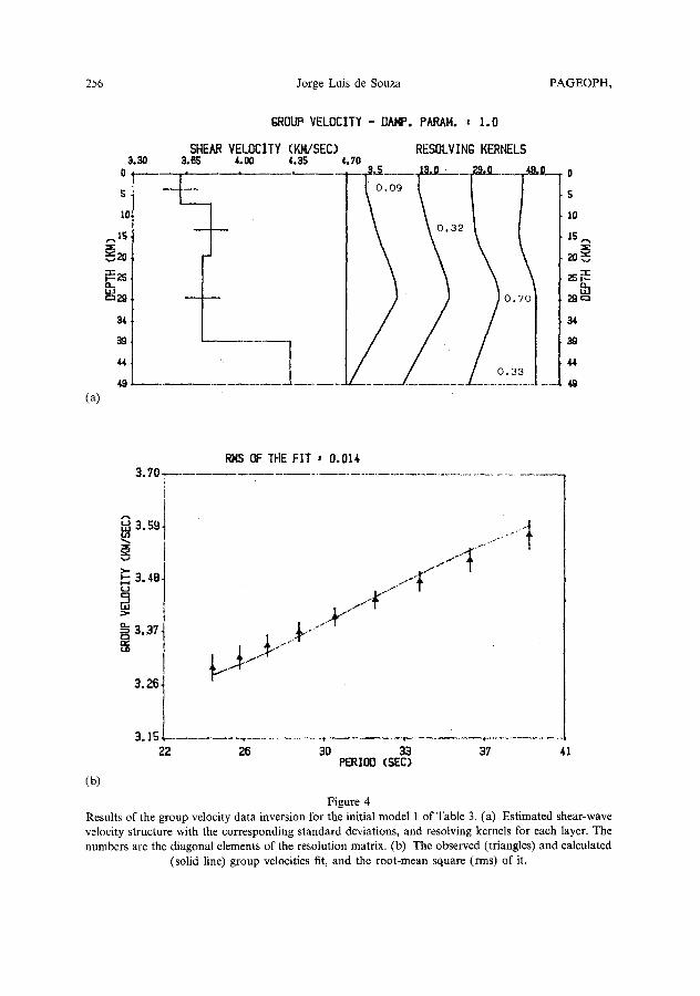
After finishing the inversion procedure with phase velocity, the LAZCANO'S model (Table 3) was again used to invert group velocity data. The shear wave velocities and resolving kernels for this inversion can be seen in Figure 4a. Figure 4b exhibits the observed and calculated dispersion curves. The final model obtained in this inversion procedure is displayed in Table 4. In general, the results obtained in this procedure are slightly similar to those obtained with phase velocity inversion. The upper crust has not been well resolved, because of the narrow period range of the dispersion curves. A good resolution was also obtained for the lower crust (Figure 4a), with a shear velocity of 3.75 km/sec, which is very similar to that obtained by LAZCANO (1972) for the lower crust (Table 3). Meanwhile, the upper mantle layer has not exhibited comparable resolution to the case of the phase velocity inversion. This layer also showed a shear velocity (fl = 4.33 km/sec) slightly

254 Jorge Luis de Souza PAGEOPH,

3.30 0

5

lO

,..,15

~ , ~ . r"~ 2 9 '

3 4 .

39,

4 4 ,

(a)

PHASE VELOCITY- DAMP. PARAM. i 0.1

SHEAR VELOCITY (KM/SEC) 3.65 ,I. 00 4:35 ,1.70

RE~LVINg KERNELS

- . - - ~ .......... ~ , L . _ _

2

~,~ . . . . . . . ~ , o - - - T 0 5

10

t . . ~N 34

44

�9 O . 49

4 . 1 0 - -

RHS OF THE FIT ~ GOlD

(b)

4.00 t , o

3.90

,~ 3.SO

3.70

3 . 6 0 , .. -,, 22 26 30 33 37 41

PERIQD (SEC)

Figure 3 Results of the phase velocity data inversion for the initial model 1 of Table 3. (a) Estimated shear-wave velocity structure with the corresponding standard deviations, and resolving kernels for each layer. The number are the diagonal elements of the resolution matrix�9 (b) The observed (triangles) and calculated

(solid line) phase velocities fit, and the root-mean square (rms) of it.

Vol. 136, 1991 Crustal and Upper Mantle Structures 255

Table 4

Physical parameters of the models obtained with phase and group velocity inversions and corresponding standard deviations (S.D.) of the estimated shear-wave velocities

H a fl p S.D. H c~ fl p S.D. (kin) (km/sec) (km/sec) (g/crn 3) (km/sec) (km) (km/sec) (km/sec) (g/cm 3) (km/sec)

Phase Velocity Group velocity 7 6.28 3.63 2.78 0.15 7 6.25 3.61 2.77 0,11

12 6.63 3.82 2,88 0.15 12 6.60 3.81 2.87 0.I1 20 6.74 3.89 2.91 0.13 20 6.50 3.75 2.85 0.11 co 8.06 4,52 3.33 0.13 co 7.72 4.33 3.21 0.12

30 6.22 3,59 2.76 0.10 30 6.24 3.60 2.77 0.10 co 8.03 4.50 3.32 0.11 oo 7.29 4.09 3.07 0.12

40 6.68 3.86 2.89 0,10 40 6.50 3.75 2.85 0.10 oo 8.03 4.51 3.32 0.11 co 7.59 4.26 3.17 0.12

smaller than that found in the phase velocity inversion (fl = 4.52 km/sec). It is possible that the damping parameter (1.0) of this inversion should have con-

tributed to the degeneration of the resolving kernel of the last layer of the model, due to the rapid decrease of the eigenvalues of the system. The gentle shear velocity gradient between the second and third layers was also observed in this inversion (Table 4).

In both phase and group velocity inversions for the LAZCANO's model, it was possible to verify that the observed dispersion curves have not sampled the upper two layers of the model. These results suggest that the number of layers of the model should be decreased to one. Therefore, I will use a crustal and upper mantle model composed of only two layers, so that the first layer is the crust and the last one the upper mantle.

Two models will be tried out in this step. The first model is composed of one layer of 30 km thickness. The shear wave velocities of the initial model can be seen in Table 3. The Rayleigh wave phase velocities are used in the inversion procedure, and the results are presented in Figures 5a and 5b. The physical parameters corresponding to this inversion are displayed in Table 4. The resolution is good for both crust and upper mantle layers (Figures 5a). However, the shear wave velocity (fl = 3.59 km/sec) has a value characteristic of the intermediate crustal layer. As shear velocity in this case will represent essentially the lower crust, this value does not seem appropriate for this layer, in spite of good resolution obtained in it. The crust-mantle interface was sharply defined by a strong velocity gradient (Figure 5a). The upper mantle has a value of shear velocity (fl = 4.50 km/sec), which is charac- teristic of this region. The fit between both observed and calculated dispersion

256 Jorge Luis de Souza PAGEOPH,

3.30 0

GROUP VELOCITY - DAMP. PAR, AM. = 1.0

lO

,,z.

34

39

44

(a)

SHEAR VELOCITY (KM/SEC) 3.6S 4.00 4.35 4.70

RESOLVING KERNELS

o

S

1o

15 ..., . m -

20 N

~ N

34

44

PJ4S OF THE FIT = 0.014 3 . 7 0 . . . . . . . . . . . . . . . . . . . . . . . . . . . . . . . . . . . . . . . . . . . . . .

(b)

3 . ~

X

3.48 r

3.37 LID

3:26

3 . 1 5 ~ - - - . . . . . . . . . . . . , 1 - . , - . . . . . . . . . . . . . . . . .

22 26 30 33 37 41 PERIOD (SEC)

Figure 4 Results of the group velocity data inversion for the initial model 1 of Table 3. (a) Estimated shear-wave velocity structure with the corresponding standard deviations, and resolving kernels for each layer. The numbers are the diagonal elements of the resolution matrix. (b) The observed (triangles) and calculated

(solid line) group velocities fit, and the root-mean square (rms) of it.

Vol. 136, 1991 Crustal and Upper Mantle Structures 257

(a)

3.30 01 . . . . . . sl

't e,,14

+it -

PHASE VELOCITY - DAMP. PAP, AM. : 1.0

SHEAR VELOCITY (KM/SEC) 3.65 4.00 /,.3S 4.?0

_ + . . . . . . . . . . . . _ . . . . !

RESOLVING KERNELS

o.(~4 I 14 ~. / \ " ~

/ ~ ,,~

/ : . . . . . . . . JL . . . . . . . . . . . . . . . . . . . . . . . . . . . . . . . _ . . . . . . "t_ 4 5

/ o.+ \ .

RI4S 0F THE FIT s 0.013 4. I0 . . . . . . . . . . . . . . . . . . . . . . . . . . . . . . . . . . . . . . . . . . . . . . . . . . . . . . . . . . . . . . . . . . . . . . . . . . . . . . . . . . . . . . .

(b)

4.00 L O

X

I J

~ 3.eO

+

~ l y . f z ( "g "

3.70,

3.60 22 26 30 33 37 41

PERIOD (SEC)

Figure 5 Results of the phase velocity data inversion for the initial model 2 of Table 3. (a) Esimated shear-wave velocity structure with the corresponding standard deviations, and resolving kernels for each layer. The numbers are the diagonal elements of the resolution matrix. (b) The observed (triangles) and calculated

(solid line) phase velocities fit, and the root-mean square (rms) of it.

258 Jorge Luis de Souza PAGEOPH,

curves is similar to the last inversions (Figure 5b). It also shows that the reduction of the number of layers did not alter the general results, and therefore this kind of model is more suitable than the first one with three layers in the crust.

The initial model 2 (Table 3) was again used to invert group velocity data. The results of this inversion are shown in Figures 6a and 6b. The final model is presented in Table 4. The first aspect observed is the great similarity between crustal shear velocity of the last inversion and crustal shear velocity of this inversion (Table 4). In the present inversion, the resolving kernels for the first layer have presented a better value than the last one (Figure 6a). Despite this, the upper mantle has shown a resolution slightly smaller than the last one (Figure 6a), with a shear velocity of 4.09 km/sec, which can be considered as an anomalous value to the upper mantle. Two hypotheses have been considered to explain the reduction in shear-wave velocity in the upper mantle. First, the crustal thickness considered is thinner than the true one, and therefore the crust-mantle interface was not found. The second possibility is that the Poisson ratio adopted for the upper mantle should be smaller than that of the value considered in the inversion process. A thicker model will be tested and the results will be compared to attempt an explanation for the anomalous value of the shear velocity in the upper mantle. The fit of the group velocities was similar to that obtained in the last inversion (Figure 6b).

In this step, a one layer model of 40 km thickness will be used to invert the observed Rayleigh wave phase and group velocities. The initial model is shown in Table 3. The results of the phase velocity inversion are exhibited in Figures 7a and 7b. The final model is exhibited in Table 4. This model has shown good resolution in both crust and upper mantle layers (Figure 7a). Now, the crustal shear velocity (/3 = 3.86 km/sec) seems to be more adequate for the lower crust. It is also compatible with the shear velocity of the lower crust (/~ = 3.89 km/sec) found by HWANG (1985). A better fit between observed and theoretical phase velocities was obtained (Figure 7b). A shear velocity of 4.51 km/sec was obtained for the upper mantle, so that the crust-mantle transition was perfectly defined. In spite of the difference between the thickness of the last two models, the shear velocity for the upper mantle is similar to that obtained in the phase velocity inversion of the second model (Table 4). The good resolving kernels, obtained with phase velocity inversions, for both model 2 and model 3 (Table 4), indicate that the crust-mantle transition has not been well determined.

Finally, the last model of Table 3 will be used to invert the group velocity data. The results of the inversion procedure are contained in Figures 8a and 8b. The final model is shown in Table 4. This model has exhibited the best crustal resolution of all models, as well as a very poor resolution in the upper mantle (Figure 8a). It was possible to verify a considerable increase in the shear velocity of the upper mantle layer (/? = 4.26 km/sec). As the Poisson ratio of the models was not modified, and shear velocity has yielded a higher value than that obtained in the group velocity inversion of model 2 (Table 4), it is possible that the thickness of the crust can

Vol. I36, 1991 Crustal and Upper Mantle Structures 259

GROUP VELOCITY - DAMP. PAP, AM. : l .O

SHEAR VELOCITY (KM/SEC) RESOLVING KERNELS 3,3o 3.8s 4.00 4.3s 4.7o

o . . . . . . . . l_~,_O . . . . . . . . . . . ~ , Q

g

,,'5 "'2}'

"! t 0 56 ~z.- ................... a- Z .................... "" ................

(a)

o

s

g

1 ,1 .

32

41

4S

(b)

3.70.

~.s~

3 . 4 B (-3

.:3.37

3.26

3.1! 22

RMS OF THE FIT s 0.013

.)

.

26 30 33 37 41 PERIOD (SEC)

Figure 6 Results of the group velocity data inversion for the initial model 2 of Table 3. (a) Esimated shear-wave velocity structure with the corresponding standard deviations, and resolving kernels for each layer. The numbers are the diagonal elements of the resolution matrix. (b) The observed (triangles) and calculated

(solid line) group velocities fit, and the root-mean square (rms) of it.

260 Jorge Luis de Souza PAGEOPH,

(a)

3.30 0

O.

1 2

~ 4 N~.

48.

54.

6O

PHASE VELOCITY - DAMP. PARAM. , 1.0

SHEAR VELOCITY (IO, VSEC) 3.05 4.00 4.35

RESOLVING KERNELS 4.70 ~O,g [.. ........ ~.___.,

........... J .......

0

B

12

18 X

24N.

t l l

42

48

54

60

4.10

RMS OF THE FIT a 0 .009

(b)

~ 4.00

3.90 0

3.BO

3.70

3.60 - -

22

4:

- - v 1 . . . . . . . . . . . . . . ! " . . . . . . . . . . . . . qr . . . . . . . . . . . . . . . . . .

2 B 30 33 37 41 PERIOD (SEC)

Figure 7 Results of the phase velocity data inversion for the initial model 3 of Table 3. (a) Estimated shear-wave velocity structure with the corresponding standard deviations, and resolving kernels for each layer. The numbers are the diagonal elements of the resolution matrix. (b) The observed (triangles) and calculated

(solid line) phase velocities fit, and the root-mean square (rms) of it.

Vol. 136, 1991 Crustal and Upper Mantle Structures 261

3.30 o

6

12

~.,18 X 324

54

6O

(a)

GROUP VELOCITY - DAMP. PARAM. = 1.0

SHEAR VELOCITY (KNVSEC) 3.B~ 4.0Q 4.~

i

RESOLVING KERNELS 4.70

. . . . . 20.0_. i " - - - ~ ~ . . . .

/ ......

o

6

12

30 N

42

54

6o

3.70. RI4S OF THE FIT = 0.002

C3 3 .$9 u,1

~ 3.4e.

~ �9

3.37.

3.26.

�9 . . - ' " ' I

V§ .... + . . . . . .

22 26 30 33 37 41 PERIOD (SEC)

(b)

Figure 8 Results of the group velocity data inversion for the initial model 3 of Table 3. (a) Estimated shear-wave velocity structure with the corresponding standard deviations, and resolving kernels for each layer. The numbers are the diagonal elements of the resolution matrix. (b) The observed (triangles) and calculated

(solid line) group velocities fit, and the root-mean square (rms) of it.

262 Jorge Luis de Souza PAGEOPH,

exceed 40 km. It should also be noted that crustal shear velocity (/~ = 3.75 km/sec) is the same as that obtained in the third layer of model 1, using group velocity data (Table 4). Besides, this value is also slightly similar to that (/~ = 3.78 km/sec) obtained by LAZCANO (1972) for the lower crust of the Brazilian shield (Table 3). It means that the value of 3.75 km/sec is really representative of the lower crust, where the dispersion curves have presented a better sample of the medium. Another important aspect was an excellent result for the fit between observed and calculated dispersion curves (Figure 8b).

In general, the crustal shear velocity structures obtained with phase and group velocities for each model are consistent (Table 4). However, phase velocity inver- sions have displayed the best resolved kernels for the crust and upper mantle structures. These inversions have also shown the crust-mantle transition clearer than group velocity inversions (Table 4), but it was not possible to define precisely the thickness of the crust in the Brazilian coast. The group velocity inversions have yielded in all cases, good results only for the lower crust. In the upper mantle, low shear velocity values have been found for these kinds of inversion.

The lower crustal shear velocities of models 1 and 3 (Table 4), for both phase and group velocities, are very similar to those obtained by both HWANG (1985) and LAZCANO (1972), respectively.

An important feature was also observed in the results of the group velocity inversions (Table 4). It is known that shear-wave velocity of the upper mantle is normally larger than 4.4 km/sec (MHSSNER, 1986). Meanwhile, if the shear velocity values of the upper mantle were organized according to the thickness of the crust, it would be possible to verify the following values: 4.09 km/sec (30 km thickness), 4.33 km/sec (39 km thickness) and 4.26 km/sec (40 km thickness). This sequence indicates that the shear-wave velocity is increasing when the thickness of the crust is decreasing. This fact is strengthened by the behaviour of the resolving kernels. Utilizing the same previous thickness order, the resolving kernels yield the following values: 0.56, 0.33 and 0.29. Similar behaviour was ascertained for the phase velocity inversions, with the following sequence: 0.80, 0.95 and 0.72. These facts indicate that the crust-mantle interface should be between 30 and 39 km.

It is known that group velocities can be derived from phase velocities, and that they have more non-uniqueness than phase velocities. For these reasons, I will consider the last model of Table 4, obtained with phase velocity inversion, as a preliminary model for the Brazilian coast region, in spite of the fact that the model obtained with group velocity inversion shows shear-wave velocity similar to LAZ- CANO'S result for the Brazilian shield.

Conclusions

The main features observed in the present study can be summarized in the following conclusions:

Vol. 136, 1991 Crustal and Upper Mantle Structures 263

1. Three models have been used to study crustal and upper mantle structures of

the Brazilian coast. The upper crust has not been well resolved due to the narrow

period range (24 sec < T -< 39 sec) of the dispersion curves. The lower crust and

upper mantle have been well resolved with Rayleigh wave phase velocity inversions

for two models (models 1 and 3). The Rayleigh wave group velocity inversions of

these models have exhibited good results only for the lower crust.

2. The shear wave velocities of the lower crust (3.86 and 3.89 km/sec) obtained

with phase velocity inversions are similar to those (/? = 3.89 km/sec) found by

HWANG (1985) in the eastern South American region, while group velocity inver-

sion has yielded shear velocity ( /?=3.75km/sec) slightly similar to that

(/? = 3.78 km/sec) found by LAZCANO (1972) for the Brazilian shield.

3. It was impossible to define with good precision the crust-mantle transition,

but an analysis of the phase and group velocity inversion results have indicated that

the total thickness of the crust be between 30 and 39 km.

4. It was impossible, in this stage, to find the best crustal model for the region

studied. However, the last crustal and upper mantle model of Table 4, obtained

with phase velocity inversion, can be used as a preliminary model for the Brazilian

coast region.

A c k n o w l e d g m e n t s

The author would like to thank Dr. Robert H. Herrmann for the use of his

computer programs. The author wishes to thank his colleagues Ester Ferreira

Baptista, Maria das Graqas Brito de Vargas, Rosane Marques Sampaio Santos and

Jo~o Francisco de Oliveira Dias, for their collaboration on the tables and drawings.

REFERENCES

ALMEIDA, F. F. M. DE, HASUI, Y., BRITO NEVES, B. B. DE, and FUCK, R. A. (1981), Brazilian Structural Provinces: An Introduction, Earth Sci. Rev. 17, 1-29.

BEN-MENAHEM, A., and HARKRIDER, D. G. (1964), Radiation Patterns of Seismic Surface Waves from Buried Dipolar Point Sources in a Flat Stratified Earth, J. Geophys. Res. 69, 2605-2620.

BHATTACHARYA, S. N. (1976), The Extension of Thomson-Haskell Method to Non-homogeneous Spherical Layers, Geophys. J. R. Astr. Soc. 47, 411-444.

BHATTACHARYA, S. N. (1981), Observation and Inversion of Surface Wave Group Velocities Across Central India, Bull. Seismol. Soc. Am. 71, 1489 1501.

BIRCH, F. (1964), Density and Composition of Mantle and Core, J. Geophys. Res. 69, 4377-4388. CHEW, M.-Y, and Yu, G.-K. (1982), Surface Wave Study of the Ryukyus-Japan Island Arc Area, Bull.

Geophys. Natl. Central Univ. 23, 39-56. CLOETINGH, S. A. P. L., NOLET, G., and WORTEL, M. J. R. (1980), Standard Graphs and Tables for the

Interpretation of Rayleigh Wave Group Velocities in the Crustal Studies, Proc. K. Ned. Akad. Wet. B83, 101-118.

COSTA, J. M., FERREIRA, J. M., OLIVEIRA, R. T., ASSUMP~,~O, M., ANJOS, C. A., MENEZES, E. A. E., and AIRES, A. (1989), O sismo de Jo8o C6mara de 10 de marfo de 1989 (mb = 4.9), 1st Congress of the Brazilian Geophysical Society, Rio de Janeiro, Brazil.

264 Jorge Luis de Souza PAGEOPH,

DEAN, E. A. (1986), The Simultaneous Smoothing of Phase and Group and Velocities from Multi-event Surface Wave Data, Bull. Seismol. Soc. Am. 76, 1367-1383.

DORBATH, L., and MONTAGNER, J. P. (1983), Upper Mantle Heterogeneities in Africa Deduced from Rayleigh Wave Dispersion, Phys. Earth Planet. Int. 32, 218-225.

DZlEWONSK1, A., BLOCH, S., and LANDISMAN, M. (1969), A Technique for the Analysis of Transient Seismic Signals, Bull. Seismol. Soc. Am. 59, 427-444.

DZIEWONSKI, A. M., EKSTR(SM, G., WOODHOUSE, J. H., and ZWART, G. (1987), Centroid-moment Tensor Solutions for October-December 1986, Phys. Earth Planet. Int. 48, 5-17.

ELLIS, R. M., and DENHAM, D. (1985), Structure of the Crust and Upper Mantle Beneath Australia from Rayleigh and Love-wave Observations, Phys. Earth Planet. Int. 38, 224-234.

FORSYTH, D. W. (1975), The Early Structural Evolution and Anisotropy of the Oceanic Upper Mantle, Geophys. J. R. Astr. Soc. 43, 103-162.

HAGIWARA, T. (1958), A Note on the Theory of the Electromagnetic Seismograph, Bull. Earth. Res. Inst. 36, 139-161.

HANKS, T. C., and THATCHER, W. (1972), A Graphical Representation of Seismic Source Parameters, J. Geophys. Res. 77, 4393-4405.

HARKRIDER, D. G. (1970), Surface Waves in Multilayered Elastic Media, 2. Higher Mode Spectra and Spectral Ratios from Point Sources in Plane Layered Earth Models, Bull. Seismol. Soc. Am. 60, 1937-1967.

HWANG, H.-J. (1985), Lateral Variation and Frequency Dependence of Crustal Q,, Ph.D. Dissertation, Saint Louis University, 214 pp.

HWANG, H.-J., and MITCHELL, B. J. (1987), Shear Velocities, Q~, and the Frequency Dependence of Qt~ in Stable and Tectonically Active Regions from Surface Wave Observations, Geophys. J. R. Astr. Soc. 90, 575 613.

KANAMOR1, H. (1970), The Alaska Earthquakes of 1964: Radiation of Long-period Surface Waves and Source Mechanism, J. Geophys. Res. 75, 5029-5040.

LAZCANO, J. O. (1972), Estructura del escudo brasiler~o a partir de la dispersion de ondas superficiales, Faculdad de Ciencias Fisicas y Matematicas, Departamento de Geofisica, Sismologia y Geodesia, Publicacion No. 153, Universidad de Chile, 66 pp.

LEVANDER, A. R., and KOVACH, R. L. (1990), Shear Velocity Structure of the Northern California Lithosphere, J. Geophys. Res. 95, 19,773-19,784.

MEISSNER, R., Introduction: Crust, mantle, lithosphere, and asthenosphere, In The Continental Crust: A Geophysical Approach (ed. Rolf Meissner) (Academic Press, Inc. 1986) pp. 1 7.

RUSSELL, D. R., HERRMANN, R. B., and HWANG, H.-J. (1984), SURF: An Interactive Set of Surface Wave Dispersion Programs for Analyzing Crustal Structures, Earth. Notes 55, i3.

RUSSELL, D. R. (1987), Multi-channel Processing of Dispersed Surface Waves, Ph.D. Dissertation, St. Louis University, St. Louis, MO.

SAT(5, Y. (1955), Analysis of Dispersed Surface Waves by Means of Fourier Transform I, Bull. Earth. Res. Inst. 33, 33-48.

SINGH, D. D. (1988), Crustal and Upper Mantle Velocity Structure Beneath the Northern and Central Indian Ocean from the Phase and Group Velocity of Rayleigh and Love Waves, Phys. Earth Planet. Int. 50, 230-239.

SOUZA, J. L. DE (1988), Estrutura da crosta terrestre na regi~o do escudo Atlgmtico Brasileiro, M.Sc. Dissertation, Departamento de Geofisica, Observat6rio Nacional, 195 pp.

TALWAN1, M., SUTTON, G. H., and WORZEL, J. L. (1959), A Crustal Section across the Puerto Rico Trench, J. Geophys. Res. 64, 1545 1555.

WEIDNER, D. J. (1974), Rayleigh Wave Phase Velocities in the Atlantic Ocean, Geophys. J. R. Astr. Soc. 36, 105-139.

YOSHIDA, M. (1982), Accuracy of the Initial Phase and the Phase Velocity of Surface Waves with Special Reference to the Single-station Method, Bull. Earth. Res. Inst. 57, 627-652.

(Received October 24, 1990, revised July 14, 1991, accepted July 19, 1991)