Linear Modeling of Genetic Networks from Experimental Data

E.P. van Someren a, L.F.A. Wessels ~,b and M.J.T. Reindersa

"Information and Communication Theory Group, bControl LaboratoryFaculty of Information Technology and Systems,

Delft University of Technology,P.O. Box 5031, 2600 GA Delft, The Netherlands

E-mail: E.P.van~omeren@its.tudelft.nlTel: +31-152786424 Fax: +31-152781843

Keywords: Genetic Networks, Quasi-Linear Model, Clustering

Abstract Currently, several different types of models are stud-

In this paper, the regulatory interactions between genesare modeled by a linear genetic network that is esti-mated from gene expression data. The inference ofsuch a genetic network is hampered by the dimension-ality problem. This problem is inherent in all gene ex-pression data since the number of genes by far exceedsthe number of measured time points. Consequently,there are infinitely many solutions that fit the data setperfectly. In this paper, this problem is tackled by com-bining genes with similar expression profiles in a sin-gle prototypical ’gene’. Instead of modeling the genesindividually, the relations between prototypical genesare modeled. In this way, genes that cannot be distin-guished based on their expression profiles are groupedtogether and their common control action is modeledinstead. This process reduces the number of signals andimposes a structure on the model that is supported bythe fact that biological genetic networks are thought tobe redundant and sparsely connected. In essence, theambiguity in model solutions is represented explicitlyby providing a generalized model that expresses the ba-sic regulatory interactions between groups of similarlyexpressed genes. The modeling approach is illustratedon artificial as well as real data.

IntroductionThe introduction of the micro-array technology hasmade it possible to measure the simultaneous expres-sion of thousands of genes with a single experiment.Since then, much research has been done on how thisamount of data can be employed to infer the func-tionality of genes. Such inference is currently mainlyperformed by means of clustering (Eisen et al. 1998;Wessels et al. 1999) and pattern recognition techniques(Brown et al. 1999). The type of information that isnot considered in these approaches is how genes regu-late each other. If such relationships are known, morelight can be shed on the functionality of genes. Thismight indicate which genes are responsible for a cer-tain disease or process and can (ultimately) aid in thedesign of drugs that can cure a disease with minimalside-effects.

Copyright O 2000, American Association for Artificial In-telligence (www.aaai.org). All rights reserved.

ied, like Boolean networks (Liang, Fuhrman, & Somo-gyi 1998), Bayesian networks (Friedman, Goldszmidt,& Wyner 1999; Friedman et al. 1999), (Quasi)-Linear networks (D’Haeseleer et al. 1999), Neural net-works (Weaver, Workman, & Stormo 1999) and Differ-ential Equations (Chen, He, & Church 1999). Booleanand Bayesian networks need some way to discretize thecontinuous measurement values, a process that is sensi-tive to the quantization scheme and might introduceartifacts which will make these models less realistic.More biologically inspired models, like the MjolsnessModel (E. Mjolsness & Reinitz 1991), contain so manyparameters that there are serious limitations on learn-ing these parameters from current real data-sets. Themajor problem concerning currently available data-setsis that they generally consist of hundreds to thousandsof genes whose activation levels are measured at nomore than twenty time points. From an information-theoretic point of view this dlmensionality problem willrender any network model inferred from this data virtu-ally meaningless. We therefore choose an approach thatemploys a network model containing as few parametersas necessary and aim additionally to extract as muchinformation as possible from ambiguous data. Usefulinformation can be extracted from the data by incor-porating sensible constraints on the modeling processbased on available biological information.In this paper, a linear network is used as a basis tomodel the regulating interactions between genes andthe model is learned from measurements of gene ac-tivity over consecutive time points. The basic linearmodel follows the assumption that the activity levelI ofa gene at a certain point in time can be determined bythe weighted sum of the activity levels of all genes atthe previous time-point2.

Nxj (t) = ~ r~,j- xi(t -- xj, ri,j e Kl (1

i----1

1Throughout the paper we define the activity level ofa gene as the logarithm of the ratio between normal andsample mRNA level.

2In other words, relationships between genes are assumedto be stationary.

ISMB 2000 355

From: ISMB-00 Proceedings. Copyright © 2000, AAAI (www.aaai.org). All rights reserved.

, where xj (t) represents the activity level of gene j time t, r~,j represents how strongly gene i controls genej and N is the total number of genes under consider-ation. Note that the linear model captures negativeand positive regulatory interactions between genes, butprocesses such as mRNA degradation are not explicitlymodeled. A more complete modeling approach is cov-ered in the next section, were the linear model is aug-mented with appropriate pre~and post-processing steps.Our main contribution lies in the way the dimension-ality problem is tackled by employing hierarchical clus-tering to combine genes with similar expression profiles.Genes with similar profiles introduce ambiguity whenthe linear model is learned, because they cannot be dis-tinguished in terms of the way they control (are beingcontrolled by) other genes. This approach is also bio-logically plausible because redundancy in genes impliesinput and output sharing among genes involved withina gene family or pathway (D’Haeseleer, Liang, & Som-ogyi 2000). This constraint is implemented by forcinggenes in the same cluster to share one set of weights.Furthermore, the fact that genes are estimated on aver-age to interact with four to eight other genes (Arnone& Davidson 1997) warrants the restriction of possibleinputs that is caused by the clustering process.

The Modeling ApproachOur modeling approach is illustrated in Fig. 1 and con-sist of three major processes, i.e. a combination of pre-and post-processing, clustering and the linear model.Pre-processing is used to convert the raw measurementsX into a set of useful signals X’ that reflect the im-portant properties of the original data. Signals thatare not significantly up- or down-regulated are removedand the remaining signals are normalized. The normal-ization step actually reflects which signals are thoughtto be similar and what control actions should be lin-early modeled. To tackle the dimensionality problem,the number of signals must be reduced in a way thatdoes not degrade the validity of the resulting model.The clustering is employed to determine groups of sim-ilar signals and to compute a prototype signal for eachof the clusters (using Q). These prototypes Y’ forma representation of the basic signal shapes among allgene-profiles. These prototypes are used to learn thereduced linear model R between the prototypes. Sucha constrained model removes any ambiguity introducedby the data and represents the basic interactions of theunderlying genetic network. After the linear model islearned it can predict the signals of the prototypes ~tgiven the value of the prototypes at the first time-point.From the estimated prototype signals an estimation ofthe normalized signals X~ can be determined by meansof an ’inverse’ clustering step W. Similarly, an esti-mate of the original signals ~[ can be determined byemploying an inverse normalization step. A more de-tailed description of each part of the approach is givenin the subsections below.

356 VAN SOMEREN

Thresholding

Experimental observations (D’Haeseleer, Liang, & So-mogyi 2000) have shown that the ratio of gene-expression of the same genes taken from different cul-tures under similar conditions can vary up to an abso-lute ratio of two, however when one culture is differ-entiated by a change in condition the gene-expressionratios of a substantial part of the genes exceed a two-fold and (some) even a five-fold ratio. Such observationsindicate that genes with profiles that remain below anabsolute value of two are not significantly expressed orrepressed and therefore do not participate in the reg-ulation. The removal of such insignificant signals willnot only help to reduce the dimensionality problem, butalso avoid erroneous relationships when learning the lin-ear model. A signal with a small amplitude contains alarge portion of measurement error that introduces lo-cal distortions, such as additional peaks. Nevertheless,the erroneous shape of that signal might be such thatwhen multiplied by a large weight, it closely predictsone of the other significant signals. In such cases thelinear model will erroneously infer a strong relation be-tween a largely random signal and one of the significantsignals. Therefore, in our approach all genes whose ac-tivity level over all time instances is below a value oftwo will be removed.

Normalization

In our approach, normalization is an important step asit actually determines which characteristics of the origi-nal signals are thought to express dissimilarity as well asthe regulatory action between genes. When two signalsshare a characteristic considered to be important, thesetwo signals should be very similar after normalization.For example, if the shape of the signals are thought tobe important this can be emphasized by normalizing thesignals with respect to their mean and variance. Aftersuch normalization the Euclidean distance measure willexpress the same similarity as the Pearson CorrelationMeasure expresses when applied to the original signals.Similarly, a linear model relating normalized signals isequivalent to a quasi-linear model on the original sig-nals. To simplify these model’choices we only alter thetype of normalization and keep the Euclidean distancemeasure and the basic linear model fixed. A visualiza-tion of the normalized signals indicates what the userexactly determines as being similar c.q. dissimilar, andalso depicts the actual control action of each gene thatis linearly modeled. The types of normalization can bewritten as a combination of an additive term cl and amultiplicative term c2. The relation between originalsignal x and normalized signal x’ is represented by thefollowing equation:

x’ - x - cl (2)C2

The original signals can be reconstructed from the nor-realized signals by means of a post-processing step that

PRE-PROCESSING

Normalization

Thresholding

CLUSTERING LINEAR MODEL

Eucl.D~

D ClusL

IQ

X’

W

y,~’ Model ~,

POST-PROnG

De-normalization

q,q

Figure 1: The modeling approach.

Type C1 C2 X!

None 0 1 X t ~X

Mean ! ET-- x(t)T 1 X! ~--- X -- el

Variance 0 T 2C2

Mean and Variance X! -- xX! : X--elCa

Table 1: Types of normalization

performs the inverse operation of Eq. (2). We distin-guish between the types of normalization as depicted intable 1.

The Linear ModelThe linear model as defined in Eq. (1) serves as a repre-sentation of the regulatory interaction between genes. Ifthe weights, being the parameters of the linear model,and the activity levels of all genes at a certain time-point are known, the activity levels of all genes at latertime points can be predicted. However, the weights arenot known and must be inferred from a set of mea-surements of gene-activities at consecutive time points.Such measurements can be represented in a so calledgene expression matrix,

X=[x~,~ liel,--.,N tel,...,T] (3)

, where each row, denoted by xi, represents the gene-profile of gene i taken over T time points. The t-thcolumn of X is denoted by x(t) = xl (t), .. ., xN (t) ]Tand determines the state of the system at time t. Forease of notation we represent the linear model usingmatrix and vector notation rather than by means ofEq. (1).

x(t + 1)T = x(t) T-R Vt = 1, ..., T- 1 (4)

The first goal is to find all weight-matrices R that areconsistent with our data and thus with Eq. (4), i.e.using R and a given state will exactly determine thenext state. In general, the weight-matrix will be under-constrained which means that there exist multiple so-

lutions which can be written as a combination of a par-ticular solution P, a basis of homogeneous solutions Hand a set of free variables F, i.e.

R=P+H-F (5)

The particular solution P reflects the information fromthe data, i.e. it is one solution that satisfies Eq. (4)(Note, many other solutions exist).

x(t + 1)T : x($) T- P Vt = 1, ..., T - 1 (6)

The homogeneous solution H ̄ F reflects the resultingambiguity in the data, i.e. it is that part of the weight-matrix that reflects the possible changes that do notinfluence the estimation of the signals in the data, i.e.

x(t) T- H- F = 0 Vt = 1, ..., T - 1 (7)

Each column of the basis of homogeneous solutions Hdetermines how a particular change in one weight mustbe compensated by the other weights in the same col-umn3. The more columns H contains the more inde-pendent directions of change are allowed. The set offree variables F reflects the degrees of freedom as eachelement can be substituted with any particular valuewithout changing the estimation of the given data. Fora given data-set the particular and homogeneous solu-tion can be found by Gaussian Elimination.For actual biologically measured gene-expression ma-trices, the amount of ambiguity, i.e. the number of

3If a weight from gene A to gene B is altered, the relationsof the other genes to gene B must compensate for the changein order keep the prediction of gene B the same.

ISMB 2000 357

columns in H is large as the number of measurementsis significantly less than the number of genes. Althoughthe ambiguity is exactly known it seems almost impos-sible to represent it in a interpretable way. However,when two genes react similarly one can group thesegenes together and in this way decrease the ambigu-ity in the system. When two signals, xi and xj, arevery similar and both signals can predict one of theother signals xk accurately then removing one of thesimilar signals still gives a good prediction4. In fact,a good prediction is influenced only by the sum of theweights that correspond to the input of both signals,i.e. ri,k + rj,k. This introduces an ambiguity in theset of possible weight-matrices that can be made ex-plicit by replacing each group of similar signals with aprototype signal and learning the weights between theprototypes instead of between the original signals. Aweight that is assigned to a prototype means that oneof the signals corresponding to that prototype should beassigned that weight, but given the data no choice canbe made. This gives a motivation to perform clusteringin order to tackle the dimensionality problem withoutdegrading the interpretation of the resulting simplifiedrule-base and with minimal loss of the estimation per-formance.

Clustering

The two main functions of clustering are to find groups(clusters) of signals based on similarity and to conceptu-alize the data by representing each cluster with a properprototype. The most important aspect of clustering isthe choice of distance measure. It basically expressesthe way similarity between signals depends on the val-ues of the signals. Because the similarity of the signalsis part of the normalization step it is not longer nec-essary to consider multiple distance measures and werestrict ourselves to the Euclidean distance measure.An important step which follows clustering is to repre-sent each cluster with a proper prototype. In our view,the choice of distance measure completely determineshow a proper prototype must be computed. A proto-type is a signal that is the most similar to all signals itrepresents. In terms of the distance measure, the rep-resentative will be that signal y which has the minimalroot mean square (RMS) distance to all signals in thecluster. For the Euclidean distance, this corresponds totaking the mean of all signals in a cluster. The vari-ance of all signals in a cluster represents the error thatis made by replacing the signals with their prototype,also denoted by the within scatter of the clustering.Note that the clustering process reduces the noise inthe signals due to the averaging of signals within thesame cluster.Complete linkage hierarchical clustering based on theEuclidean distance is performed. The number ofclusters is decreased until the system becomes over-

4The remaining signal can compensate for the removed

signal, because of its similar shape

358 VAN SOMEREN

constrained (i.e. the homogeneous solution becomesempty). This clustering can be represented by meansof matrix multiplication. Transforming signals to pro-totypes is performed by multiplying the normalized sig-nals with matrix Q.

V’ ~ XtT " Q (8)

, where Q is a (N x P) matrix where each row corre-sponds to each signal and each column corresponds toeach prototype. Each element q,,p of the matrix rep-resents the contribution of the n-th signal to the p-thprototype, with a mean prototype this becomes:

qn,p = 0 otherwise (9)

Cp is the set of all signals in cluster p. The inverse op-eration of transforming prototypes into signals is per-formed by multiplying the estimated prototype signalswith matrix W.

X,r = q,. W (10)

, where W is a (P x N) matrix where the rows corre-spond to the prototypes and the columns correspond tothe signals. Each element wp,n of the matrix representshow the n-th signal can be reconstructed from the p-thprototype. With a mean prototype the prototype itselfcan directly represent the signal:

1 xn e Cp(11)wp,n --- 0 otherwise

To validate the modeling approach two experimentswere performed. First, an artificial problem with aknown and structured weight-matrix is used to test thecapability of our method to uncover the right structureand relations from generated signals. The second ex-periment was done on a real yeast data-set on whichseveral analysis were performed.

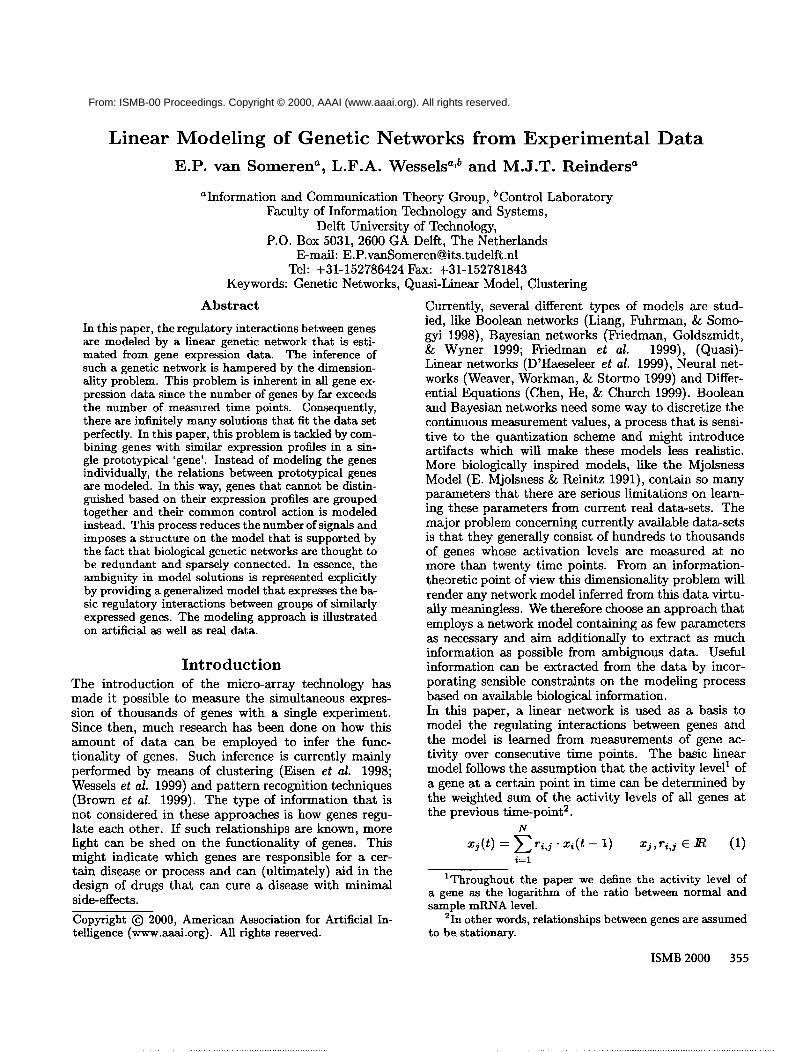
Example: Artificial ProblemIn this section, we discuss the experimental results thatwere obtained on a simple artificial example, whichserves to illustrate the principles on which the modelingapproach is based. This example mimics the structurepresent in large scale genetic networks: groups of genesbeing co-regulated and thus exhibiting similar time re-sponses.As a first step, a linear system consisting of five genesis constructed by choosing a particular (5 × 5) matrixR5 { 5= ri,j}. The superscript indicates the size. Inanalogy with Eq. (4), the behavior of this system described by the following equation:

x(t + 1)r ---- x(t) T- R5 (12)

Starting from any initial state this system will settleinto a stable steady state after a finite time interval.The specifically chosen weight-matrix is graphically de-picted in Figure 2. From this small network, a network

I iii!i~iiiii!i~i~iii~ii~iiiii~i~i~iiii!~i~i~iii~iii~i~i~i~i!i~iiiiiii~i~ii~ i~iiiii!~ii~i~iiiiiii~i~i~i!~i~i~i~iiiii!i!~i~iiiii~i~ii~i~iiii~!?

::::i:i~::~::::~:i:i:i~:i:i:~ i~i~iiii.~.~iii!~iiiiiiiiiii~i~iiil ~!~iiiiiiiiii~i~iiiii!ii!~iiiiiiiiiiiiiiii~!~:~!i!iii!i!~!~!!!!~ii~i!iiiiiii!iii!~i~!i~iiiiiiii!i!!~!~!!~!~!!!~!~!!!!iii!i!i!!i~

ili!iiii! i~iiii iiiiiiiii~i~i~i~i~i~i~li~i~i~I i~i~il

Figure 2: Graphical representation of R5 used for theartificial example. A black square at position (i, j) rep-resents a positive control action of gene i on gene j, i.e.ri,j > 0, while a negative control action is representedby a white square. The size of a square is proportionalto the absolute size of the weight value.

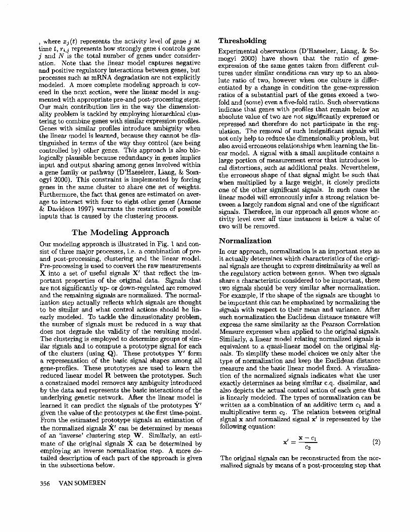
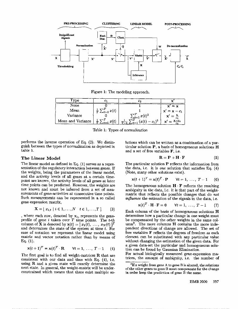
of twenty-five genes was constructed by replicating thesimple system five times. This was achieved by con-structing tt 2s in the following fashion: the (i, j)-th 5 x sub-matrix in R2s was constructed by placing ri~,j onthe diagonal with all other positions in the sub-matrixoccupied by zeros. Figure 3 contains a graphical rep-resentation of tt ~. The initial state of the genes isdetermined such that each signal has an initial statethat is more similar to the initial states of the genes inits group than to the initial states of the genes in theother groups. Figure 4 depicts the first 20 time points ofthe gene activity levels after such an initialization andcalculating subsequent time points using weight-matrixtt ~s. We will denote this gene-expression matrix byX. The ’grouping’ of the signals within a subsystemis quite apparent, and simulates groups of co-regulatedgenes in a biological genetic network. If purely judgedon the number of signals (N = 25) and the number time points in the gene-expression matrix (T = 20) theproblem of estimating the values of tt ~5 based on X isunder-constrained, i.e. infinitely many solutions exist.We estimated the model based on the methodology de-scribed in the previous sections, but without pre- andpost-processing. More specifically, we employed com-plete linkage hierarchical clustering and the Euclideandistance measure to build a complete dendogram of thesignals. For each possible clustering, C~, ranging froma single cluster (k = 1, all signals in one cluster) to dusters (k = 25, a single signal per cluster) the follow-ing steps were performed:

1. The set of prototypes, Y~ associated with the clustersin Ck was determined by averaging the signals in eachcluster.

2. The weight matrix, 15~~, corresponding to each clus-

:::::::::::::::::::::::::::::::::::::::::

Figure 3: Graphical representation of R.2~: Expandedfrom tt ~ for the artificial example.

Figure 4: Time response for the 25 x 25 system of theartificial problem.

ISMB 2000 359

tering was determined from yk. In the under-constrained case, the particular solution was used;

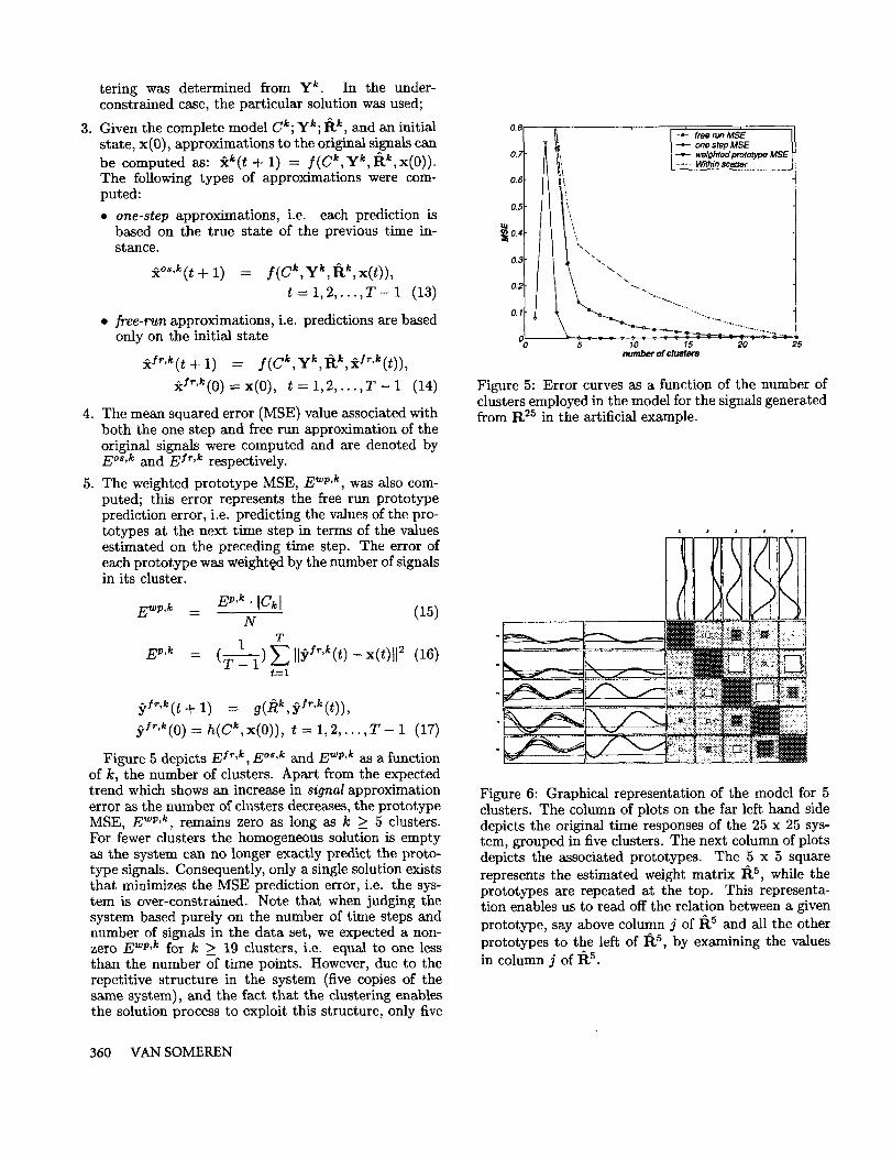
3. Given the complete model Ck; yk; l~k, and an initialstate, x(0), approximations to the original signals canbe computed as: ~(t + 1) f( Ck,Yk,l:[k,x(O)).The following types of approximations were com-puted:

¯ one-step approximations, i.e. each prediction isbased on the true state of the previous time in-stance.

~o8,k(t + l) = f(C~,Y~,R~, x( t))t=l,2,...,T-1 (13)

¯ free-run approximations, i.e. predictions are basedonly on the initial state

#r’k(t + 1) = I(CLYk,P~L#r’k(t)),

~l~’k(0)=x(0), t=l,2,...,T-1

4. The mean squared error (MSE) value associated withboth the one step and free run approximation of theoriginal signals were computed and are denoted byE°8’k and E:r’k respectively.

5. The weighted prototype MSE, Ewp’k, was also com-puted; this error represents the free run prototypeprediction error, i.e. predicting the values of the pro-totypes at the next time step in terms of the valuesestimated on the preceding time step. The error ofeach prototype was weighted by the number of signalsin its cluster.

E~’p’k - EP’k’lOk] (15)N

T

Ep’k = (~_1)~[[Srf~’k(t)-x(t)H 2 (16)t=l

:~f"k(0)=h(Ck,x(0)), t=l,2,...,T-1

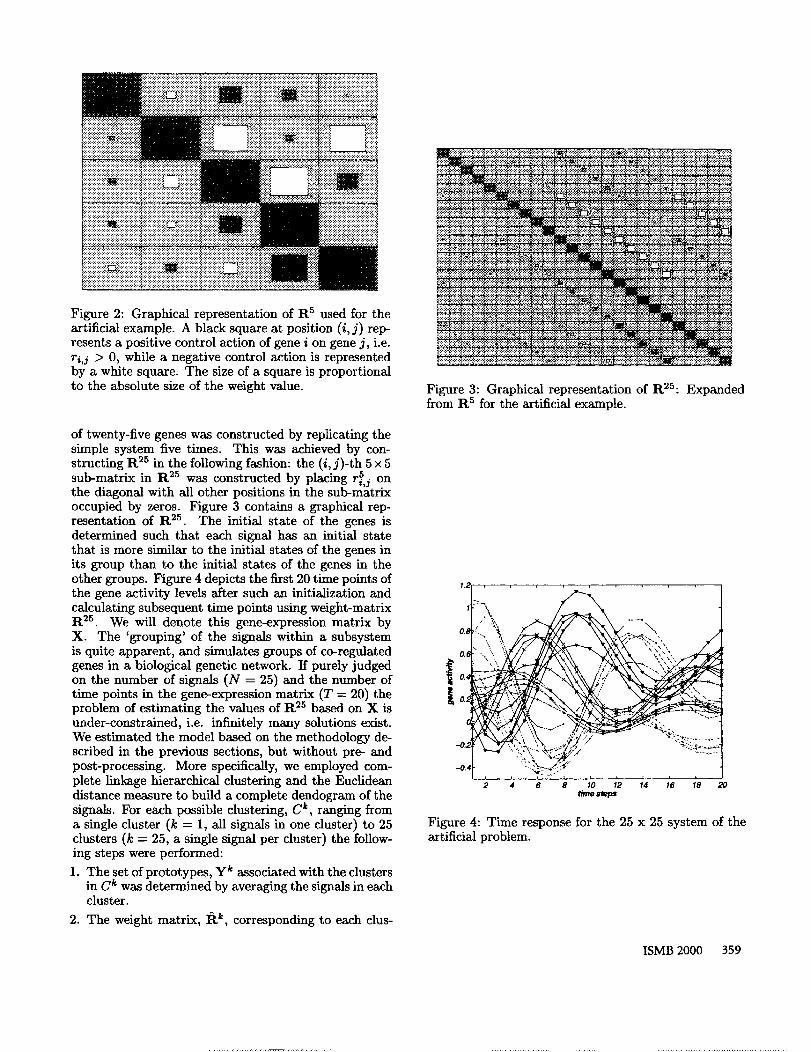
Figure 5 depicts Ef~,k, E°s,k and Ewp’k as a functionof k, the number of clusters. Apart from the expectedtrend which shows an increase in signal approximationerror as the number of clusters decreases, the prototypeMSE, Ew~,k, remains zero as long as k > 5 clusters.For fewer clusters the homogeneous solution is emptyas the system can no longer exactly predict the proto-type signals. Consequently, only a single solution existsthat minimizes the MSE prediction error, i.e. the sys-tem is over-constrained. Note that when jud~g thesystem based purely on the number of time steps andnumber of signals in the data set, we expected a non-zero Ewp’k for k => 19 clusters, i.e. equal to one lessthan the number of time points. However, due to therepetitive structure in the system (five copies of thesame system), and the fact that the clustering enablesthe solution process to exploit this structure, only five

O.B

0.?

0.~

0.~

0,4

0.1

!~ -.:. ~ ~ M~one step MSE

-e- weighted prototype MSEI .... W4hin sce{ter

5 10 15 20 25numberofclusters

Figure 5: Error curves as a function of the number ofclusters employed in the model for the signals generatedfrom R25 in the artificial example.

/ .:,:~:~.. :.: - ,~

::::::: :::::::::::::::::: i:-:i:i:i:~::::~

Figure 6: Graphical representation of the model for 5clusters. The column of plots on the far left hand sidedepicts the original time responses of the 25 x 25 sys-tem, grouped in five clusters. The next column of plotsdepicts the associated prototypes. The 5 x 5 squarerepresents the estimated weight matrix 1~5, while theprototypes are repeated at the top. This representa-tion enables us to read off the relation between a givenprototype, say above column j of 1~5 and all the otherprototypes to the left of 1~~, by examining the valuesin column j of 1~s.

360 VAN SOMEREN

prototypes are required to exactly predict the signals.The resulting model is depicted in Figure 6. It is quiteclear from this figure that the resulting estimate 1{5 isa good approximation of R~. However, at the sametime we should point out that interpretation of the Rmatrix can, in some cases, be fairly difficult. For exam-ple, consider prototype 5 directly above column 5 of the1~5 matrix in Figure 6. The large value of r5,5 impliesthat it has a large positive relation with itself, which isunderstandable, However, large values for r2,~ and r3,5imply that these prototypes are also involved in pro-ducing the time response of prototype 5. Such subtleinteractions are fairly difficult to comprehend by look-ing at the signals. In any event, this artificial exampleillustrates that the approach holds promise, since it en-abled us to extract the essential (original) structure a system consisting of co-regulated genes.

Experiment: Yeast data-setThe analyzes described in this section were carried outon the gene expression profiles extracted from the 2467genes in the budding yeast S. cerevisiae (Eisen et aL1998). The dataset consists of several sub-sets collectedunder different conditions: mitotic cell division cy-cle, sporulation and temperature and reducing shocks.Since the approach described in this paper models thetime behavior of the genes, appropriate external inputsshould be included to model changing external condi-tions, if the concatenation of the sub-sets were to beemployed as input data. Since such inputs are not in-cluded in our model yet, we can only apply the approachon a single sub-set at a time.

Thresholding:In a previous section it was motivated why genes withexpression profiles which never exceed +2 should beconsidered as ’insignificant’ and why such genes shouldbe removed from the data set. Removal of all suchexpression profiles reduces the sizes of all the data setsdramatically and consequently alleviates the dimension-ality problem. For the ALPHA subset which consists of18 time points, 45 genes remain as significant signals,for the CDC15 subset consisting of 14 time points 113genes remain as significant signals.

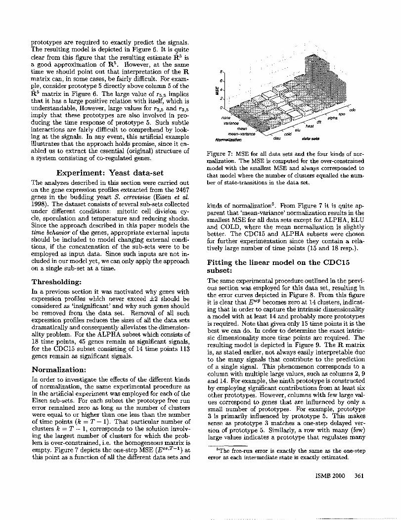
Normalization:In order to investigate the effects of the different kindsof normalization, the same experimental procedure asin the artificial experiment was employed for each of theEisen sub-sets. For each subset the prototype free runerror remained zero as long as the number of clusterswere equal to or higher than one less than the numberof time points (k = T - 1). That particular number clusters k - T - 1, corresponds to the solution involv-ing the largest number of clusters for which the prob-lem is over-constrained, i.e. the homogeneous matrix isempty. Figure 7 depicts the one-step MSE (E°8,T-t) atthis point as a function of all the different data sets and

Figure 7: MSE for all data sets and the four kinds of nor-realization. The MSE is computed for the over-constrainedmodel with the smallest MSE and always corresponded tothat model where the number of clusters equalled the num-ber of state-transitions in the data set.

kinds of normalization5. From Figure 7 it is quite ap-parent that ’mean-variance’ normalization results in thesmallest MSE for all data sets except for ALPHA, ELUand COLD, where the mean normalization is slightlybetter. The CDC15 and ALPHA subsets were chosenfor further experimentation since they contain a rela-tively large number of time points (15 and 18 resp.).

Fitting the linear model on the CDC15subset:

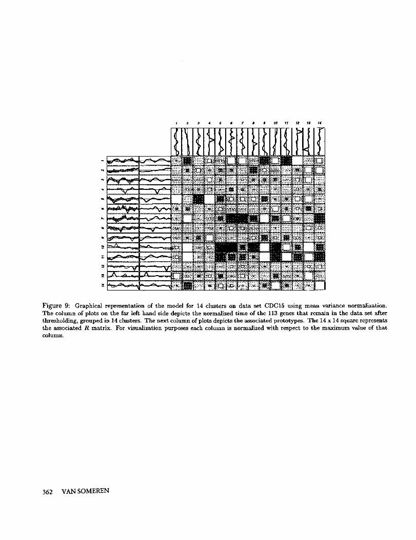
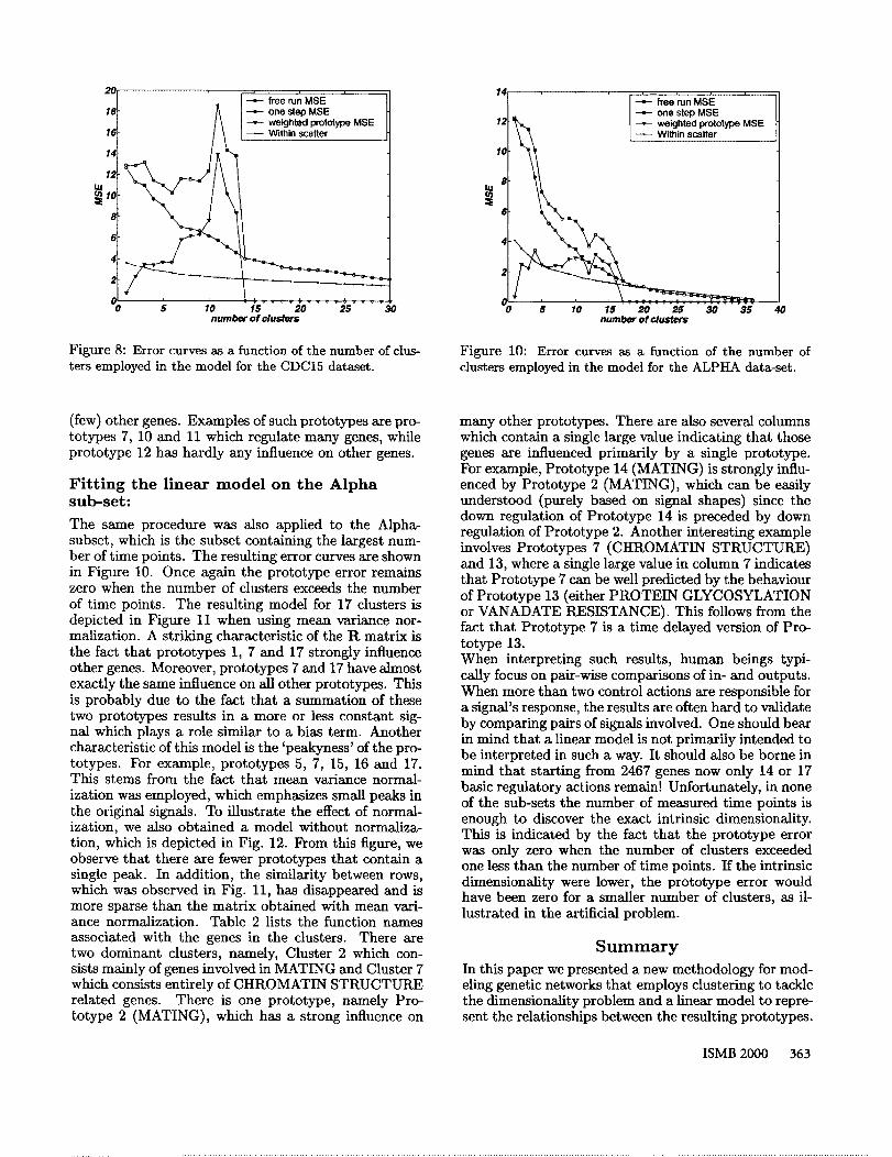
The same experimental procedure outlined in the previ-ous section was employed for this data set, resulting inthe error curves depicted in Figure 8. From this figureit is clear that E~p becomes zero at 14 clusters, indicat-ing that in order to capture the intrinsic dimensionalitya model with at least 14 and probably more prototypesis required. Note that given only 15 time points it is thebest we can do. In order to determine the exact intrin-sic dimensionality more time points are required. Theresulting model is depicted in Figure 9. The R matrixis, as stated earlier, not always easily interpretable dueto the many signals that contribute to the predictionof a single signal. This phenomenon corresponds to acolumn with multiple large values, such as columns 2, 9and 14. For example, the ninth prototype is constructedby employing significant contributions from at least sixother prototypes. However, columns with few large val-ues correspond to genes that are influenced by only asmall number of prototypes. For example, prototype3 is primarily influenced by prototype 5. This makessense as prototype 3 matches a one-step delayed ver-sion of prototype 5. Similarly, a row with many (few)large values indicates a prototype that regulates many

5The free-run error is exactly the same as the one-steperror as each intermediate state is exactly estimated.

ISMB 2000 361

I 2 3 4 5 6 7 ¯ J 10 11 12

b<

:i’:’: :::~N ....... ’:’:’-’:’.’:’:

::::::::::::5 --

....... :i:i:!:i:?:i:~: :’:’:,:,:,:,:" ’:::’i":"i!.................... ::::::::::::::~ :?:’:’:’:?~I :;: : : :: ,J," ....

:::::::::::5:

~.,...-.. : :.:.:.:+:

~ ::’:555:::: ~-,-,~-~

13 14

Figure 9: Graphical representation of the model for 14 clusters on data set CDCI5 using mean variance normalization.The column of plots on the far left hand side depicts the normalized time of the 113 genes that remain in the data set afterthresholding, grouped in 14 clusters. The next column of plots depicts the associated prototypes. The 14 x 14 square representsthe associated R matrix. For visualization purposes each col, mn is normalized with respect to the maximum value of thatcolumn.

362 VAN SOMEREN

20. ~ free run MSE

18 ~ I -.e- one step MSE/\ ] + weighted prototype MSE

14

12ui

Is 20 2s 3onumber of clusters

Figure 8: Error curves as a function of the number of clus-ters employed in the model for the CDC15 dataset.

’ 4- f,.,~ ~n aS~: ’-,,.- one step MSE

"-. 1 -’- weighted prototype MSE

5 10 15 20 25 30 35 40number of dusters

Figure 10: Error curves as a function of the number ofclusters employed in the model for the ALPHA data-set.

(few) other genes. Examples of such prototypes are pro-totypes 7, 10 and 11 which regulate many genes, whileprototype 12 has hardly any influence on other genes.

Fitting the linear model on the Alphasub-set:

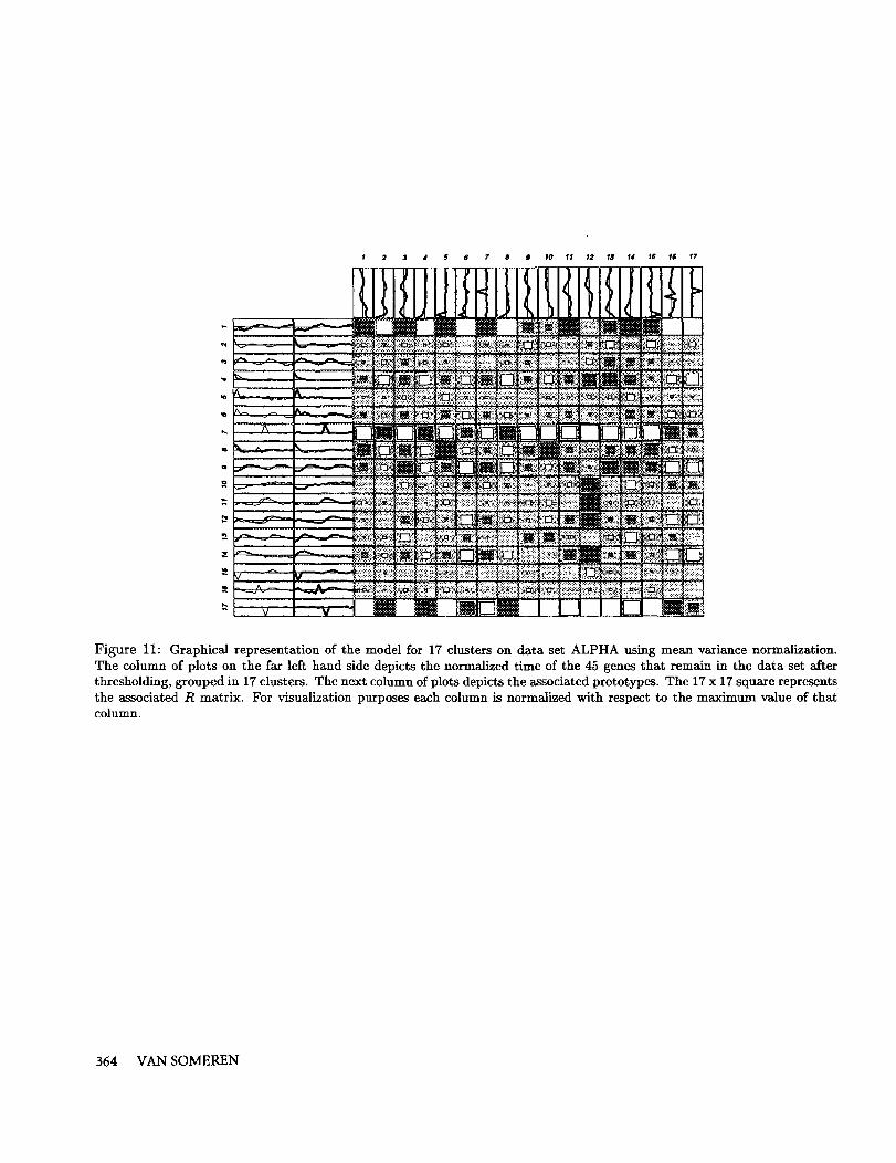
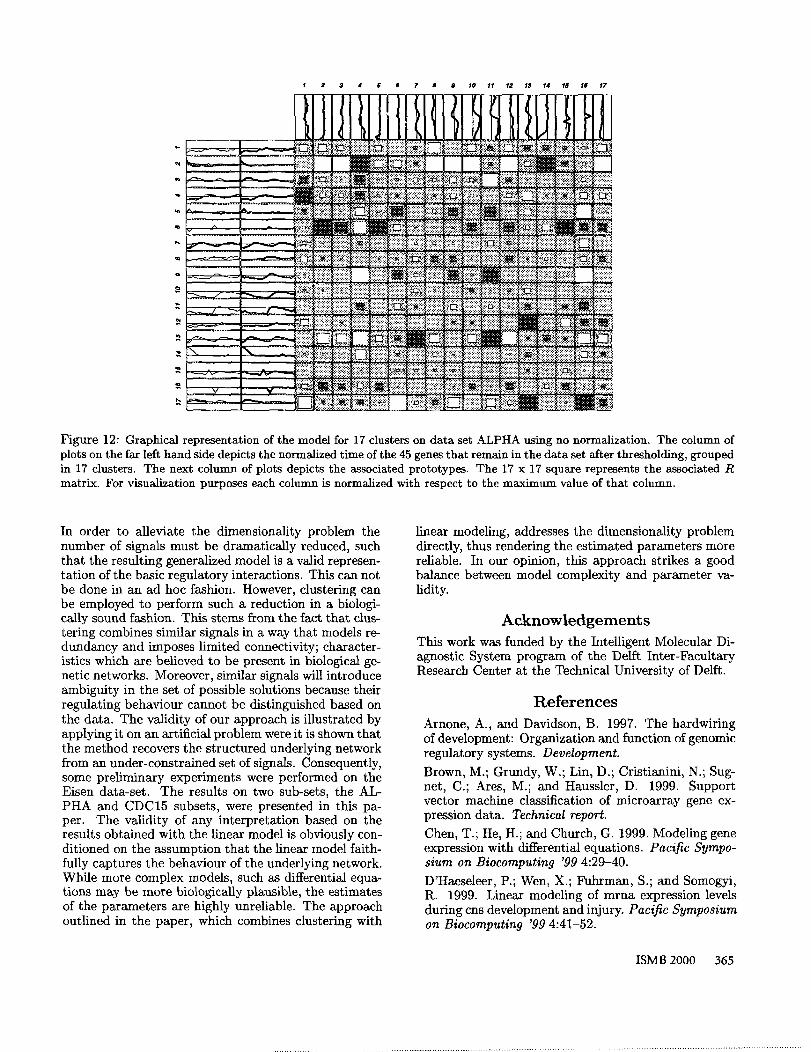
The same procedure was also applied to the Alpha-subset, which is the subset containing the largest num-ber of time points. The resulting error curves are shownin Figure 10. Once again the prototype error remainszero when the number of clusters exceeds the numberof time points. The resulting model for 17 clusters isdepicted in Figure 11 when using mean variance nor-malization. A striking characteristic of the R matrix isthe fact that prototypes 1, 7 and 17 strongly influenceother genes. Moreover, prototypes 7 and 17 have almostexactly the same influence on all other prototypes. Thisis probably due to the fact that a summation of thesetwo prototypes results in a more or less constant sig-nal which plays a role similar to a bias term. Anothercharacteristic of this model is the ’peakyness’ of the pro-totypes. For example, prototypes 5, 7, 15, 16 and 17.This stems from the fact that mean variance normal-ization was employed, which emphasizes small peaks inthe original signals. To illustrate the effect of normal-ization, we also obtained a model without normaliza-tion, which is depicted in Fig. 12. From this figure, weobserve that there are fewer prototypes that contain asingle peak. In addition, the similarity between rows,which was observed in Fig. 11, has disappeared and ismore sparse than the matrix obtained with mean vari-ance normalization. Table 2 lists the function namesassociated with the genes in the clusters. There aretwo dominant clusters, namely, Cluster 2 which con-sists mainly of genes involved in MATING and Cluster 7which consists entirely of CHROMATIN STRUCTURErelated genes. There is one prototype, namely Pro-totype 2 (MATING), which has a strong influence

many other prototypes. There are also several columnswhich contain a single large value indicating that thosegenes are influenced primarily by a single prototype.For example, Prototype 14 (MATING) is strongly influ-enced by Prototype 2 (MATING), which can be easilyunderstood (purely based on signal shapes) since thedown regulation of Prototype 14 is preceded by downregulation of Prototype 2. Another interesting exampleinvolves Prototypes 7 (CHROMATIN STRUCTURE)and 13, where a single large value in column 7 indicatesthat Prototype 7 can be well predicted by the behaviourof Prototype 13 (either PROTEIN GLYCOSYLATIONor VANADATE RESISTANCE). This follows from thefact that Prototype 7 is a time delayed version of Pro-totype 13.When interpreting such results, human beings typi-cally focus on pair-wise comparisons of in- and outputs.When more than two control actions are responsible fora signal’s response, the results are often hard to validateby comparing pairs of signals involved. One should bearin mind that a linear model is not primarily intended tobe interpreted in such a way. It should also be borne inmind that starting from 2467 genes now only 14 or 17basic regulatory actions remain! Unfortunately, in noneof the sub-sets the number of measured time points isenough to discover the exact intrinsic dimensionality.This is indicated by the fact that the prototype errorwas only zero when the number of clusters exceededone less than the number of time points. If the intrinsicdimensionality were lower, the prototype error wouldhave been zero for a smaller number of clusters, as il-lustrated in the artificial problem.

Summary

In this paper we presented a new methodology for mod-eling genetic networks that employs clustering to tacklethe dlmensionality problem and a linear model to repre-sent the relationships between the resulting prototypes.

ISMB 2000 363

U

[]

Figure 11: Graphical representation of the model for 17 clusters on data set ALPHA using mean variance normalization.The column of plots on the far left hand side depicts the normalized time of the 45 genes that remain in the data set afterthresholding, grouped in 17 clusters. The next column of plots depicts the associated prototypes. The 17 x 17 square representsthe associated R matrix. For visualization purposes each column is normalized with respect to the maximum value of thatcolumn.

364 VAN SOMEREN

$4

|

U~:~:::~::::: :.:.:.:.:.:.

:.:.:.:.:.:.

V,’.U;: ....

$ 8

.̄.........

J.:........,

iiiii~ii~i~~

10 11 12

w~I’%.,~

N~

............. iii............iiiii~iiii!i i i

i~iiiiiiiiiiii~

~.~>i.i.151.!5

.......... i.,.......-...:i:::: :::::::::::::;.:+:-:+:.........

,:.:.:+;.:,.:.: ....

....... :.:+..

13 14

:i:i:~i:i:i:.. -.......

:i:2:~?:i:i-...........

,...........

:.m x..,...........ij:;:::f~iiii

[]

Figure 12: Graphical representation of the model for 17 clusters on data set ALPHA using no normalization. The column ofplots on the far left hand side depicts the normalized time of the 45 genes that remain in the data set after thresholding, groupedin 17 clusters. The next column of plots depicts the associated prototypes. The 17 x 17 square represents the associated Rmatrix. For visualization purposes each column is normalized with respect to the maximum value of that column.

In order to alleviate the dimensionality problem thenumber of signals must be dramatically reduced, suchthat the resulting generalized model is a valid represen-tation of the basic regulatory interactions. This can notbe done in an ad hoc fashion. However, clustering canbe employed to perform such a reduction in a biologi-cally sound fashion. This stems from the fact that clus-tering combines similar signals in a way that models re-dundancy and imposes limited connectivity; character-istics which are believed to be present in biological ge-netic networks. Moreover, similar signals will introduceambiguity in the set of possible solutions because theirregulating behaviour cannot be distinguished based onthe data. The va~idity of our approach is illustrated byapplying it on aa artificial problem were it is shown thatthe method recovers the structured underlying networkfrom an under-constrained set of signals. Consequently,some preliminary experiments were performed on theEisen data-set. The results on two sub-sets, the AL-PHA and CDC15 subsets, were presented in this pa-per. The validity of any interpretation based on theresults obtained with the linear model is obviously con-ditioned on the assumption that the linear model faith-fully captures the behaviour of the underlying network.While more complex models, such as differential equa-tions may be more biologically plausible, the estimatesof the parameters are highly unreliable. The approachoutlined in the paper, which combines clustering with

linear modeling, addresses the dimensionality problemdirectly, thus rendering the estimated parameters morereliable. In our opinion, this approach strikes a goodbalance between model complexity and parameter va-lidity.

AcknowledgementsThis work was funded by the Intelligent Molecular Di-agnostic System program of the Delft Inter-FacultaryResearch Center at the Technical University of Delft.

References

Arnone, A., and Davidson, B. 1997. The hardwiringof development: Organization and function of genomicregulatory systems. Development.Brown, M.; Grundy, W.; Lin, D.; Cristianini, N.; Sug-net, C.; Ares, M.; and Haussler, D. 1999. Supportvector machine classification of microarray gene ex-pression data. Technical report.Chen, T.; He, H.; and Church, G. 1999. Modeling geneexpression with differential equations. Pacific Sympo-sium on Biocomputing ’99 4:29-40.D’Haeseleer, P.; Wen, X.; Fuhrman, S.; and Somogyi,R. 1999. Linear modeling of mrna expression levelsduring cns development and injury. Pacific Symposiumon Biocomputing ’99 4:41-52.

ISMB 2000 365

Cluster

6

7

8

9101112

13

14151617

Function NameSECRETION, NON-CLASSICAL

CYTOSKELETONMATING; CELL FUSION

MATINGKARYOGAMY

MATINGMATINGMATING

MATING; CELL FUSIONCELL CYCLETCA CYCLECELL CYCLE

CELL WALL BIOGENESISCELL CYCLE

CU2+ ION HOMEOSTASISDNA REPLICATION

CELL WALL BIOGENESISRRNA PROCESSING

CELL CYCLEMRNA SPLICING

CELL CYCLESECRETION

CHROMATIN STRUCTURECHROMATIN STRUCTURECHROMATIN STRUCTURECHROMATIN STRUCTURECHROMATIN STRUCTURECHROMATIN STRUCTURECHROMATIN STRUCTURECHROMATIN STRUCTURE

TRANSPORTPHOSPHATE METABOLISMMATING TYPE SWITCHING

CELL WALL BIOGENESISCELL CYCLE

AGINGBUD SITE SELECTION, BIPOPROTEIN GLYCOSYLATION

VANADATE RESISTANCEMATINGMEIOSIS

PROTEIN SYNTHESISTRANSPORT

SECRETION, NON-CLASSICALCELL CYCLE

Table 2: F~nction names of signals in clusters

D’Haeseleer, P.; Liang, S.; and Somogyi, R. 2000. Ge-netic network inference: From co-expression clusteringto reverse engineering. Submitted to Bioinformatics.E. Mjolsness, D. S., and Reinitz, J. 1991. A connec-tionist model of development. Journal of TheoreticalBiology 152.Eisen, M.; Spellman, P.; Brown, P.; and Bottstein,D. 1998. Cluster analysis and display of genome-wide expression patterns. Proceedings of the NationalAcadamy of Sciences of the USA 95(25):14863-14868.

Friedman, N.; Linial, M.; Nachman, I.; and Pe’er, D.1999. Using bayesian networks to analyze expressiondata. Submitted.Friedman, N.; Goldszmidt, M.; and Wyner, A. 1999.Data analysis with baysian networks: A bootstrap ap-proach. Proc. Fifteenth Conf. on Uncertainty in Arti-ficial Intelligence (UAI).Liang, S.; Fuhrman, S.; and Somogyi, R. 1998. Reveal,a general reverse engineering algorithm for inference ofgenetic network architectures. Pacific Symposium onBiocomputing ’98 3:18-29.

Weaver, D.; Workman, C.; and Stormo, G. 1999. Mod-eling regulatory networks with weight matrices. Pa-cific Symposium on Biocomputing ’99 4:112-123.Wessels, L.; Reinders, M.; Baldochi, R., and Gray, J.1999. Statistical analysis of gene expression data. Pro-ceedings of the Ninth Belgium-Dutch Conference onMachine Learning (BENELEARN’99).

366 VAN SOMEREN