A hybrid genetic-linear algorithm for 2D inversion of sets of vertical electrical sounding

A HYBRID GENETIC-LINEAR ALGORITHM FOR 2D INVERSIONOF SETS OF VERTICAL ELECTRICAL SOUNDING

Niraldo R. Ferreira,1 Milton José Porsani,2 Saulo Pomponet de Oliveira3

Recebido em 23 out. 2003 / Aceito em 6 may, 2004Received oct. 23, 2003 / Accepted may 6, 2004

ABSTRACT

The inversion of vertical electrical sounding (VES) is normally performed considering a stratified medium formed by homogeneous, isotropic and horizontal layers.The simplicity of this geophysical model makes the inversion simple and computationally fast, and together with the main characteristics of the electroresistivitymethod, it was greatly responsible to make VES one of the most popular geophysical method for groundwater exploration and engineering geophysics. However,even in a sedimentary basin where the geology is more conform, the assumption of horizontal and homogeneous layers is not necessarily valid, limiting thereliability of the inversion results.

In this paper we present a fast and robust 2D resistivity modeling and inversion algorithm for the interpretation of sets of VES. We consider three inversionalgorithms: the Gauss-Newton method of linearized inversion (LI), the genetic algorithm (GA), and a hybrid approach (GA-LI) that uses LI to improve the best modelat the end of each step of the GA. The medium parametrization consists of the partition of the domain into fixed homogeneous rectangular blocks such that theirresistivities are the only free parameters. The apparent resistivity is evaluated by an iterative scheme that is derived from a finite-difference discretization of thepotential differential equation. We enhance the convergence rate of the scheme by adopting an incomplete Cholesky preconditioner.

Numerical results using synthetic and real 2D apparent resistivity data formed by sets of VES for the Schlumberger configuration illustrate the performance of thehybrid GA-LI algorithm. The VES field data were acquired near Conceição do Coité, state of Bahia, Brazil. We compare the performance of the LI, GA and GA-LIalgorithms.

Keywords: Incomplete Cholesky, 2D resistivity modeling, geophysical inversion, genetic algorithms, linearized inversion, hybrid optimization.

RESUMO

A inversão de uma sondagem elétrica vertical (SEV) normalmente assume que o meio é estratifcado e formado por camadas horizontais homogêneas e isotrópicas.A simplicidade deste modelo geofísico torna a inversão simples e com reduzido custo computacional. Esta simplicidade, junto às principais qualidades do métodode eletroresistividade, foi responsável por tornar a SEV um dos métodos geofísicos mais populares nos trabalhos de exploração de águas subterrâneas e geofísicaaplicada à engenharia. Porém, mesmo em bacias sedimentares, onde a geologia é mais conforme, a hipótese de camadas planas e homogêneas não é válida, oque limita a confiabilidade dos resultados da inversão.

Apresentamos neste artigo um algoritmo rápido e robusto de modelagem e inversão eletroresistiva para a interpretação de conjuntos de SEVs. Consideramos trêsalgoritmos de inversão: o método de inversão linearizada de Gauss-Newton (LI), o algorítmo genético (GA), e uma abordagem híbrida (GA-LI) que usa a inversãolinearizada para aprimorar o melhor modelo obtido ao final de cada geração do algoritmo genético. A parametrização do meio consiste na partição do dommínioem blocos retangulares e homogêneos, de modo que a resistividade de cada bloco é um parâmetro do modelo. A resistividade aparente é calculada com um métodoiterativo baseado numa aproximação por diferenças finitas da equação do potencial elétrico. Um precondicionamento do tipo Cholesky incompleto é utilizado paraacelerar a convergência do método.

Avaliamos a performance do método híbrido por meio de experimentos numéricos com perfis de eletroresistividades reais e sintéticos, formados por conjuntos deSEVs obtidas com o arranjo Schlumberger. Os dados de campo foram coletados nas proximidades de Conceição do Coité, estado da Bahia, Brasil.

Palavras-chave: fatoração incompleta de Cholesky, modelagem bidimensional de resistividade, inversão geofísica, algoritmos genéticos, inversão linearizada,otimização híbrida.

1 Escola Politécnica - Universidade Federal da Bahia -Rua Prof. Aristides Novis, 02 - Federação - CEP: 40210-730 Salvador- BA - E-mail: [email protected]

2 Centro de Pesquisa em Geofísica e Geologia - Instituto de Geociências - Universidade Federal da Bahia - Rua Caetano Moura, 123 sala 312- C - Campus Universitário de Ondina - Salvador - BA- CEP: 40170-115 - Telefax: (71) 203-8551 - E-mail: [email protected]

3 Centro de Pesquisa em Geofísica e Geologia - Instituto de Geociências - Universidade Federal da Bahia - Rua Caetano Moura, 123 sala 312- C - Campus Universitário de Ondina - Salvador - BA- CEP: 40170-115 - Telefax: (71) 203-8551 - E-mail: [email protected]

Revista Brasileira de Geofísica, Vol. 21 (3), 2003

236 A HYBRID GENETIC-LINEAR ALGORITHM FOR 2D INVERSION OF SETS OF VERTICAL ELECTRICAL SOUNDING

INTRODUCTION

Inversion of resistivity sounding is a non-linear problem thatestimates the spatial distribution of resistivities of the subsoil materialsfrom apparent resistivity data measurements. Local and global optimi-zation algorithms have been reported in geophysical data inversion bymany authors (TARANTOLA; VALETTE, 1982; ROTHMAN, 1985; SEN;BHATTACHARYA; STOFFA, 1993; CHUNDURU et al., 1997). In case webegin the inversion using a starting model located near to a local or aglobal minimum, gradient methods can be very useful to find an opti-mal solution. Otherwise, global optimization algorithms such as simu-lated annealing or genetic algorithms can be used. The major draw-backs associated with local and global algorithms are the requirementfor a priori information and the computational cost, respectively. Severaldifferent hybrid optimization approaches can be proposed to overcomethese drawbacks (CHUNDURU et al., 1997; PORSANI et al., 2000).

To develop an efficient hybrid optimization scheme, it is impor-tant to choose efficient global and local algorithms. For geophysical in-version, successful attempts were made by several authors (CARY;CHAPMAN, 1988; PORSANI et al., 1993; LIU; HARTZELL; STEPHENSON,1995). A very good explanation about the advantages and drawbacks oflocal, global and hybrid algorithms was presented by Chunduru andothers (1997). Also to develop an efficient hybrid inversion algorithmfor 2D resistivity inversion, a fast forward modeling algorithm is re-quired. For the 2D inversion of field resistivity sounding data we haveimplemented a 2D finite-difference algorithm for computation of theforward modeling that uses an incomplete Cholesky factorization scheme(MEIJERINK; VAN DER VORST, 1977) coupled with the preconditionedconjugate gradient method (GREENBAUM, 1997).

Electrical resistivity inversion methods aim to determine the dis-tribution of subsurface resistivity by measuring the distribution of electri-cal potential from a set of current electrodes at the earth surface. For aSchlumberger configuration of electrodes, the apparent resistivity satis-fies the equation

ρ πφ

a

AB

MN

MN

I= −

2

4 4

∆, (1)

where ∆φ is the electrical potential difference between two electrodeslocated at M and N, and I is the current generated by two electrodeslocated at A and B. The axis x is set along the electrodes.

The one-dimensional method of Vertical Electrical Sounding (VES)for horizontally layered media is well known4. The free parameters of

this model are the resistivity ρi (1 ≤ ι ≤ n) and the thickness

hi (1 ≤ i ≤ n) of each layer, and are represented by the vector m.

The center of electrode configuration is fixed, and the spacings = AB/2 is the only independent variable. One can evaluate theapparent resistivity ρ

a(m, s)in closed form (KOEFOED, 1979).

The two-dimensional model accounts for both lateral and verti-cal variations of resistivity. In this case, the apparent resistivity r

a also

depends on the position x where the VES is performed. We partition thedomain into N rectangular blocks. The components of the free param-eter vector m are the resistivity of each block. Unlike the 1D model, theapparent resistivities ρ

a(m, x, s

i) are approximated by a numerical

method. We employ a finite-difference method to evaluate the scalarelectrical potential φ, as described in the following section.

FINITE-DIFFERENCE MODELING

Assuming that the electric conductivity σ of the medium variesonly along the axis x and the depth z, the electrical potential generatedby a pointwise source at (x

f, 0, 0) is a solution of the Poisson equation

−∇ ( )∇ ( ) = −( ) ( ) ( ). , , , ,σ φ δ δ δx z x y z I x x y zf (2)

where δ(•) is the Dirac delta and ∇ is the gradient vector operator. AFourier transform in the y direction yields

−∇⋅ ( )∇ ( )

+ ( )

( )= −( ) ( )

σ φ σ

φ δ δ

x z x z k x z

x zI

x x z

k

k f

, , ,

, ,

2

2

(3)

φ φk x z x y z ky dy, , , cos ,( )= ( ) ( )∞

∫0(4)

φπ

φx y z x z kyk, , , cos( )= ( ) ( )∞

∫2

0

dk . (5)

Equation (3) is discretized using an NxM non-uniform rectangu-lar grid. We evaluate the finite-difference solution φ φi j k i jx z, ,≈ ( )in its interior domain of validity according to Dey and Morrison (1979):

C C C

C C

li j

i j ri j

i j ui j

i j

di j

i j ci j

,,

,,

,,

,,

,

φ φ φ

φ− + −

+

+ + +

+ +

1 1 1

1φi j ijb, ,=

, (6)

bij

I if

=

=2

1

0 , i

, i,j ,

,,j ,

( )≠( )

i f ,1

(7)

4 Cf. Porsani and others (2001) and the references therein

Brazilian Journal of Geophysics, Vol. 21 (3), 2003

Niraldo R. Ferreira, Milton José Porsani, Saulo Pomponet de Oliveira 237

Cx x

z z z zli j

i ii j j j i j j j

,, ,=

−−( )

−( )+ −( )

−− − − − +

1

2 11 1 1 1 1σ σ ,,

Cx x

z z z zri j

i ii j j j i j j j

,, , ,=

−−( )

−( )+ −( )

+− − − +

1

2 11 1 1 1σ σ

Cz z

x x x xui j

j j

i j i i i j i i,

, ,=−−( )

−( )+ −( )

−− − − − +

1

2 1

1 1 1 1 1σ σ ,, (8)

Cz z

x x x xdi j

j j

i j i i i j i i,

, , ,=−−( )

−( )+ −( )

+− − +

1

2 1

1 1 1σ σ

C C C C C k Aci j

li j

ri j

ui j

di j

i j, , , , ,

,=− + + + −

2 ,

A x x z z x x z zi j i j i i j j i j i i j j, , ,= −( ) −( )+ −( ) −( )− − − − − + −

1

4 1 1 1 1 1 1 1σ σ

+ −( ) −( )+ −( )+ + − − +i,jσ σx x z z x x zi i j j i j i i j1 1 1 1 1, −−( )z j .

The boundary condition at the top layer is

σφ

ii j

n,, .1 0

∂

∂=

(9)

We stretch the grid in geometric progression near the lateral andlower boundaries, imposing the following condition (DEY; MORRISON,1979):

∂ ( )∂

+( )( )

( )= = +

φφ

x k z

nk

K kr

K krx k z

, ,, , ,1

0

0 r x z ,2 22 (10)

where K0,1

are the modified Bessel functions (ABRAMOWITZ; STEGUN,1970). We employed growth factors of 2.529 and 2.215 in the horizon-tal and vertical directions, respectively (MEDEIROS, 1987).

Let x=( ) φ φ φ φ11 1 21,..., , ,...,N MN

T and b=( )b bMN

T

11 , ... .Equations (6)-(10) yield a linear system of the form Cx = b. Thecapacitance matrix C is symmetric, positive definite, and satisfiesC

i,j = 0 if |i - j| ≠ 0,1, M.

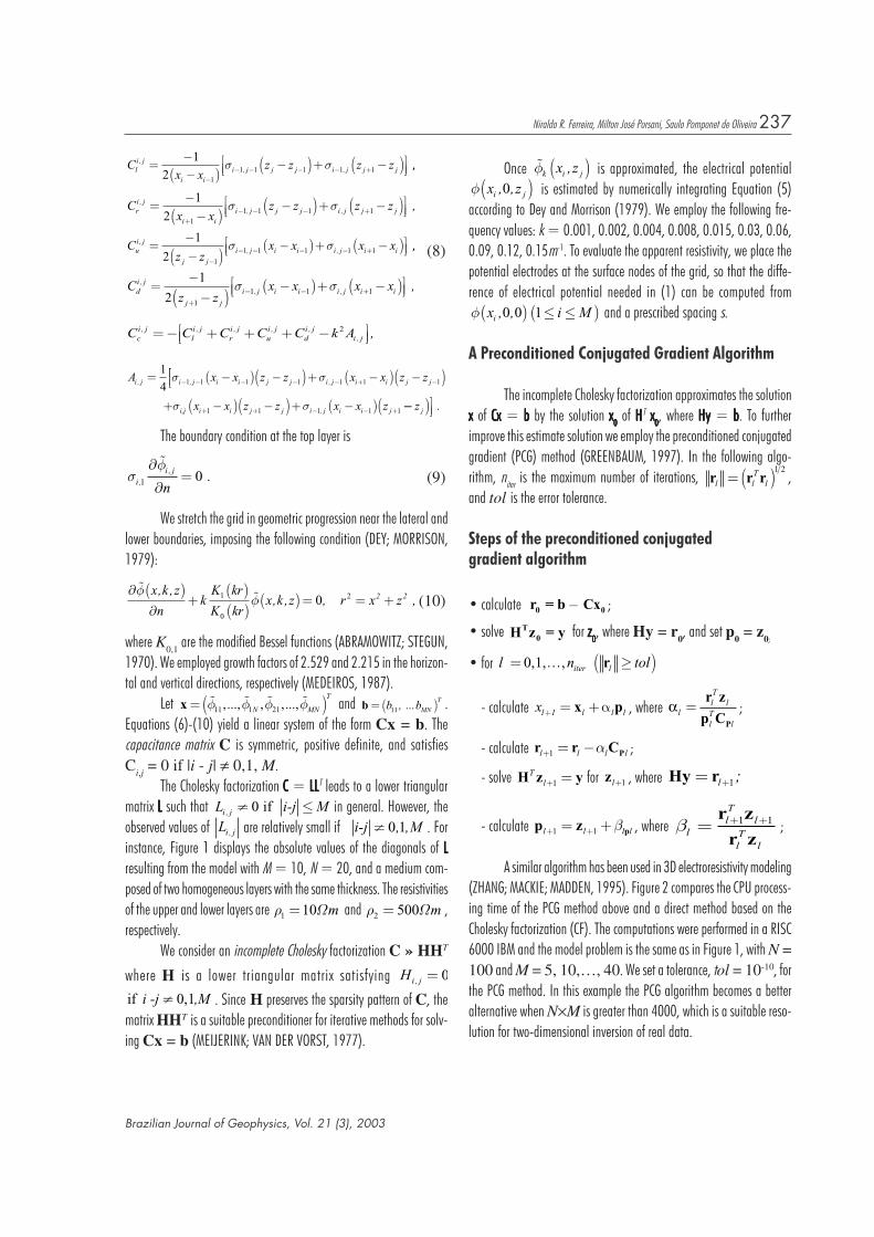
The Cholesky factorization CCCCC = LLLLLLLLLLT leads to a lower triangularmatrix LLLLL such that L Mi j, ≠ ≤0 i-jif in general. However, theobserved values of Li j, are relatively small if i-j ≠ 0 1, ,M . Forinstance, Figure 1 displays the absolute values of the diagonals of LLLLLresulting from the model with M = 10, N = 20, and a medium com-posed of two homogeneous layers with the same thickness. The resistivitiesof the upper and lower layers are ρ1 10= Ωm and ρ2 500= Ωm ,respectively.

We consider an incomplete Cholesky factorization C » HHT

where H is a lower triangular matrix satisfying Hi j, = 0

≠ i -j ,if 0,1 M . Since H preserves the sparsity pattern of C, thematrix HHT is a suitable preconditioner for iterative methods for solv-ing Cx = b (MEIJERINK; VAN DER VORST, 1977).

Once φk i jx z,( ) is approximated, the electrical potentialφ x zi j, ,0( ) is estimated by numerically integrating Equation (5)according to Dey and Morrison (1979). We employ the following fre-quency values: k = 0.001, 0.002, 0.004, 0.008, 0.015, 0.03, 0.06,0.09, 0.12, 0.15m-1. To evaluate the apparent resistivity, we place thepotential electrodes at the surface nodes of the grid, so that the diffe-rence of electrical potential needed in (1) can be computed fromφ x i Mi , ,0 0 1( ) ≤ ≤( ) and a prescribed spacing s.

A Preconditioned Conjugated Gradient Algorithm

The incomplete Cholesky factorization approximates the solutionxxxxx of CxCxCxCxCx = bbbbb by the solution xxxxx00000 of HHHHHT xxxxx00000, where HyHyHyHyHy = bbbbb. To furtherimprove this estimate solution we employ the preconditioned conjugatedgradient (PCG) method (GREENBAUM, 1997). In the following algo-rithm, niter is the maximum number of iterations, r r rl l

Tl=( )1 2

,and tol is the error tolerance.

Steps of the preconditioned conjugatedgradient algorithm

• calculate r = b 0 – Cx0 ;

• solve H z = yT0 for zzzzz00000, where Hy = r

0, and set p

0= z

0;

• for l n iter l= … ≥( ) 0,1, , r tol

- calculate x l l ll 1+ = +x pα , where αllT

l

lT

=r z

p CPl

;

- calculate r r CPl l l l+ = −1 α ;

- solve H z yTl+ =1 for zl+1 , where Hy r= +l 1;

- calculate p z pl l l l+ += +1 1 β , where βllT

l

lT

l

= + +r z

r z1 1 ;

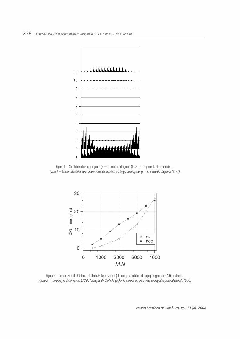
A similar algorithm has been used in 3D electroresistivity modeling(ZHANG; MACKIE; MADDEN, 1995). Figure 2 compares the CPU process-ing time of the PCG method above and a direct method based on theCholesky factorization (CF). The computations were performed in a RISC6000 IBM and the model problem is the same as in Figure 1, with N =100 and M = 5, 10,…, 40. We set a tolerance, tol = 10-10, forthe PCG method. In this example the PCG algorithm becomes a betteralternative when N×M is greater than 4000, which is a suitable reso-lution for two-dimensional inversion of real data.



Figure 1 – Absolute values of diagonal (k = 1) and off-diagonal (k > 1) components of the matrix L.Figura 1 – Valores absolutos dos componentes da matriz L, ao longo da diagonal (k=1) e fora da diagonal (k>1).

Figure 2 – Comparison of CPU times of Cholesky factorization (CF) and preconditioned conjugate gradient (PCG) methods.Figura 2 – Comparação do tempo de CPU da fatoração de Cholesky (FC) e do método de gradientes conjugados precondicionado (GCP).



LINEARIZED INVERSION

Let 1 2≤ ≤p . The Lp norm of an M-dimensional vector

vvvvv = (v1,…vM)T is given by vp i

p

i

M p

v=

=∑

1

1

.

Let us introduce an iterative scheme to minimize theobjective function proposed by Scales and Gersztenkorn(1986):

E x s x sa i i a i ii

M p

m m( )= ( )− ( )=∑ ρ ρ, , ,

1, (11)

where ρa i ix s,( ) and ρa i ix sm, ,( ) are the observed and theoreti-

cal apparent resistivities, respectively. Note that E(m) is the Lp norm

of the error of the theoretical apparent resistivities to the power p. Welinearize ρ

a(m, x

i, s

i) by Taylor’s series about an estimate free pa-

rameter vector mk:ρ ρ

ρ ρ

a i i a i i

a i ia i i

k

x s x s

x sx s

m m

mm

mm m

, , , ,

, ,, ,

( )≈ ( )=

= ( )+∂ ( )

∂−

kk (( ) .

(12)

Let dk,i k= ( )− ( ) =ρ ρa i i a i i k ix s x s r, , , , ,m

= ( )− ( )−

ρ ρa i i a i i

px s x s, , ,m

221≤ ≤( )i M , and

∆d Rk

k

k M

k

kd

d

r

=

=,

,

,

,1 1

0

00 rk M

k

a k x s

,

, ,

,

=

∂ ( )∂

G

mρ 1 1

m1

…

∂ ( )∂

ρa k x s

N

m , ,1 1

m

∂ ( )∂

∂ ( )∂

ρ ρa k a k

N

m m, ,xM,sM

m

xM,sM

m1

.

Substituting (12) into (11), we find a quadratic function of m,whose minimum satisfies

G R G m G R dkT

k k kT

k k( ) =∆ ∆ . (13)

Where ∆m = (mk+1

– mk). By using a regularization factor

λ (MENKE, 1989) we compute the new solution mk+1

as

m m G R G I G R dk 1 k kT

k k kT

k k+ = + +( )» .-1

∆ (14)

In particular, the method with p = 2 and λ = 0 corresponds tothe plain least squares method. The row i of the sensitivity matrix G

k is

weighted by the i-th diagonal component of the matrix Rk, which is a

function of the deviation between the observed resistivity values, and

the ones computed from current model mk

(PORSANI; NIWAS;FERREIRA, 2001).

To increase the robustness of the algorithm, we apply a logarith-mic scaling to the free parameters and to the field data (RIJO et al.,

1977). Moreover, given a tolerance parameter ε, we set rk ip

, =−ε 2

if ρ ρ εa i i a i ix s x s, , ,( )− ( ) ≤ m .

We employ a harmonic measure of fitness (PORSANI et al., 2000)

Φρ ρ

ρ ρm

m

mk

a i i a k i ii

M

a k i i a i i

x s x s

x s x s( )=

( ) ( )

( ) +−∑2

1

2

, , ,

, , ,(( )

−∑ 2

1i

M .

(15)

The ratio Φ varies within [-1,1], and approaches 1 as

ρa k i ix sm , ,( ) approaches ρa i ix s i M,( ) ≤ ≤( )1 . The compo-

nents of the sensitivity matrix are approximated by forward differences(MCGILLIVRAY; OLDENBURG, 1990). We employ a conjugated gradient

method to evaluate mk+1 from (14). Let A G R G I= +kT

k k λ .We have that:

p Ap p G R G p p p

q R p p p q G qlT

l lT

kT

k k l lT

l

lT

k l lT

l l k l

= + =

= + =

λ

λ , , (16)

which motivates modifying the conjugated gradient algorithm to avoidthe computation of G R Gk

Tk k :

Steps of the conjugated gradientalgorithm for Lp inversion

• s d G x0 0= −∆ k k ;

• r G R0 »= −kT

k s x0 0 ;

• p r0 0= and q G0 k p0 ;

• for l n r toliter l= ≥( )0 1, ,. . ., .

- x xl l l l+ = +1 α p , where r r

llT

l

lT

k l lT

l

=+

αq R q p pλ

;

- s s ql l l l+ = −1 α ;

- r G R s xl kT

k l+ + +−1 1 λ l 1 ;

- p = r pl l l+ + +1 1 βl , where βll

l

r r

r rlT

l 1T+ +

+

1 1 ;

- q G pk k k= ;



When λ = 0, the algorithm designed by Gersztenkorn, Bednarde Lines (1986) for 1D inversion of the acoustic wave equation is recovered.

NUMERICAL EXAMPLES

Inversion of synthetic data

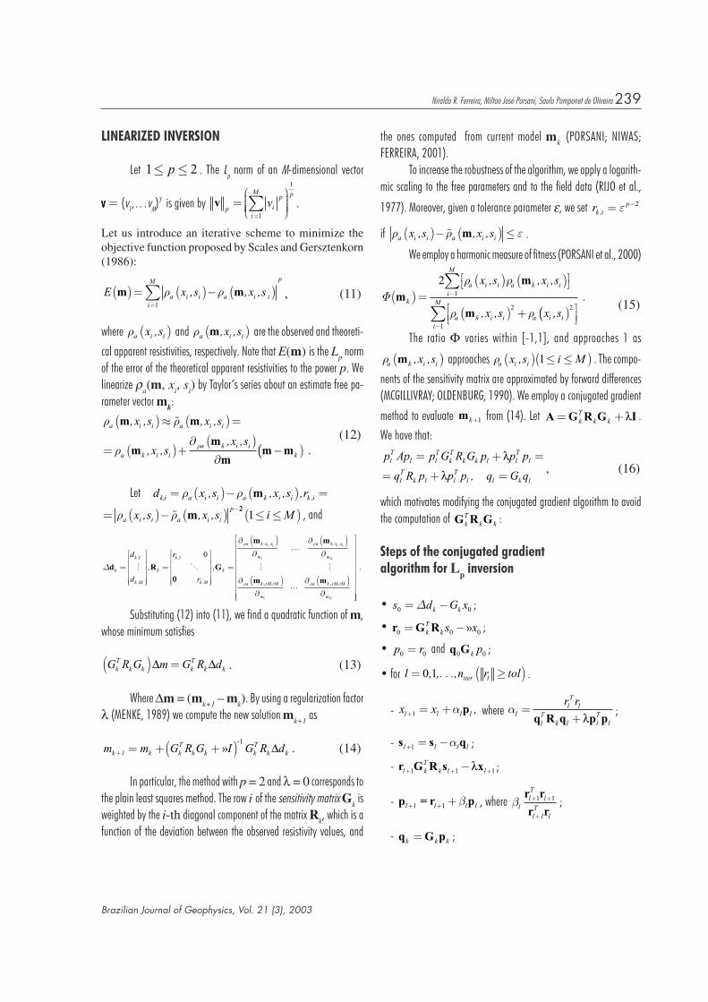
We consider the model of a buried dike outlined in Figure 3. Thevertical electrical soundings are performed throughout 21 stations witha set of 19 s-values. Noise is introduced when AB/2 = 17.5m,47.5m, 87.5m and 107.5m.

The horizontal grid employs 252 nodes. Five nodes are distrib-uted in geometric progression on both ends, while the increment be-tween interior nodes is 5m. The vertical grid employs 26 nodes withnon-uniform spacing.

In the experiment it is assumed that the location and size of theblocks are known. The initial solution is m

0=ρ(1,1,1,1)T,

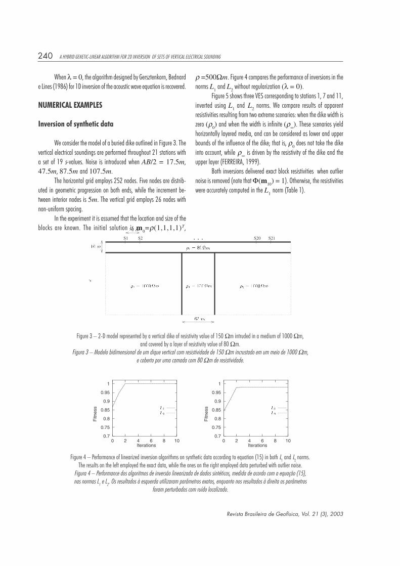
ρ =500Ωm. Figure 4 compares the performance of inversions in thenorms L

1 and L

2 without regularization (λ = 0).

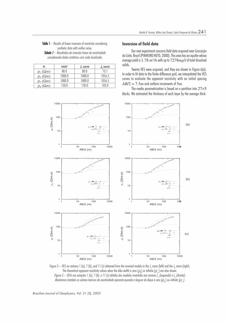
Figure 5 shows three VES corresponding to stations 1, 7 and 11,inverted using L

1 and L

2 norms. We compare results of apparent

resistivities resulting from two extreme scenarios: when the dike width iszero (ρ

0) and when the width is infinite (ρ∞). These scenarios yield

horizontally layered media, and can be considered as lower and upperbounds of the influence of the dike; that is, ρ

0 does not take the dike

into account, while ρ∞ is driven by the resistivity of the dike and theupper layer (FERREIRA, 1999).

Both inversions delivered exact block resistivities when outliernoise is removed (note that Φ(m

10) = 1). Otherwise, the resistivities

were accurately computed in the L1

norm (Table 1).

Figure 3 – 2-D model represented by a vertical dike of resistivity value of 150 Ωm intruded in a medium of 1000 Ωm,and covered by a layer of resistivity value of 80 Ωm.

Figura 3 – Modelo bidimensional de um dique vertical com resistividade de 150 Ωm incrustado em um meio de 1000 Ωm,e coberto por uma camada com 80 Ωm de resistividade.

Figure 4 – Performance of linearized inversion algorithms on synthetic data according to equation (15) in both L1 and L2 norms.The results on the left employed the exact data, while the ones on the right employed data perturbed with outlier noise.

Figura 4 – Performance dos algoritmos de inversão linearizada de dados sintéticos, medida de acordo com a equação (15),nas normas L1 e L2. Os resultados à esquerda utilizaram parâmetros exatos, enquanto nos resultados à direita os parâmetros

foram perturbados com ruído localizado.



TTTTTable 1able 1able 1able 1able 1 – Results of linear inversion of resistivity consideringsynthetic data with outlier noise.

TTTTTabela 1abela 1abela 1abela 1abela 1 – Resultados da inversão linear de resistividadeconsiderando dados sintéticos com ruído localizado.

Inversion of field data

Our next experiment concerns field data acquired near Conceiçãodo Coité, Brazil (PINHEIRO NETO, 2000). This area has an aquifer whoseaverage yield is 1.78 m3/h with up to 7278mg/l of total dissolvedsolids.

Twenty VES were acquired, and they are shown in Figure 6(a).In order to fit data to the finite-difference grid, we interpolated the VEScurves to evaluate the apparent resistivity with an initial spacingAB/2 = 7.5m and uniform increments of 5m.

The media parametrization is based on a partition into 27×5blocks. We estimated the thickness of each layer by the average thick-

Figure 5 – VES on stations 1 (a), 7 (b), and 11 (c) obtained from the inverted models in the L1 norm (left) and the L2 norm (right).The theoretical apparent resistivity values when the dike width is zero (ρ0) or infinite (ρ∞) are also shown.

Figura 5 – SEVs nas estações 1 (a), 7 (b), e 11 (c) obtidas dos modelos invertidos nas normas L1 (esquerda) e L2 (direita).Mostramos também os valores teóricos da resistividade aparente quando a largura do dique é zero (ρ0 ) ou infinita (ρ∞).



ness calculated at each station by using 1D VES inversion. The initialmodel had ρ = 40Ωm in the first four layers and ρ = 300Ωm inthe bottom layer. The horizontal grid was similar to the horizontal gridused in the synthetic model. We employed 302×9 nodes.

We performed 10 iterations of linearized inversion in the normsL

1and L

2 with the same regularization factors λ = 0.001 and

λ = 0.1 in the L1 and L

2 norms, respectively. The percent relative

errors with respect to the interpolated data were similar and under 45%as illustrated in Figure 7.

The region of low resistivity near station S5 of the computedmodels (Figure 6) is consistent with the presence of a water well nearthis station. The low resistivity between stations S14 and S16 is consist-ent with the evidence of salinization between stations S12 and S17.

Figure 6 – Pseudo-section of apparent resistivity values generated by 20 unevenly spaced VES (a). The symbols (+) below eachVES indicate the AB/2 position where the measurements were performed. Contours of the apparent resistivity values generated

from linearized inversion in the L1 norm (b) and L2 norm (c).Figura 6 – Pseudo-seção de valores de resistividade aparente gerados por 20 SEVs com espaçamento não-uniforme (a).

Os símbolos (+) abaixo de cada SEV indicam a abertura AB/2 com que as medidas foram feitas. Pseudo-seção de valoresde resistividade aparente gerados por inversão linearizada nas normas L1 (b) e L2 (c).



Figure 7 – Pseudo-section of percent relative error of the theoretical apparent resistivity values with respect to the observed apparent resistivity values for the linearized inversion algorithm in the L1 norm (a) and the L2 norm (b).Figura 7 – Pseudo-seção do erro relativo dos valores teóricos de resistividade aparente gerados por inversão linearizada

nas normas L1 (a) e L2 (b) com respeito aos valores de resistividade aparente observados.

GENETIC AND HYBRID ALGORITHMS

Genetic algorithms (GA) employ the concepts of survival of thefittest, crossover, and mutation to generate a set of free parameter vec-tors that progressively approach field data. These methods fit into theclass of global, probabilistic optimization methods. Genetic algorithmsare based on the principle of natural selection and genetics. Detaileddescriptions of GA are given by Holland (1975) and Goldberg (1989),and theory and examples of geophysical applications can be found inSen and Stoffa (1995). Basically, in the GA the model free parametersare coded in binary form. The algorithm starts with an ensemble of ran-dom models, and a new ensemble is generated similarly to the biologi-cal mechanism of reproduction that exists in nature. The models are

chosen for reproduction with a probability proportional to their fitnessvalue, and pairs of models are selected at random and exchange part oftheir binary chain. The crossover points are selected at random and allthe bits to the right side are interchanged with a crossover probability,generating new models. To assure genetic variability in the population,a mutation process is adopted by changing at random a bit inside thebinary chain based on a fixed probability. The new set of models areaccepted with an update probability by comparing them with the modelsin the previous generation. The process of selection, crossover and muta-tion is applied until the fitness values converge, i.e., until the meanfitness approaches the highest fitness value in the population.

We start by randomly selecting a set (or population) of free pa-rameter vectors m

g,j, 1 ≤ j ≤ P, and g = 0. We refer to each m

g,j



as a model. In the second step, we evaluate the fitness Φ(mg,j

) ofeach model according to equation (15). Then, we perform the followinggenetic operations.• Selection:Selection:Selection:Selection:Selection: we select a limited number of models in pairs for

reproduction. They are selected by a non-uniform probability functiongiven by

PT

Ts g j

g j

g j

mm

m,

,

,

exp /

/( )=

( )

( )

=∑

Φ

Φexp1j

n, (17)

where T = T0γg is associated with the temperature in the simulated

annealing method. The temperature is used to de-emphasize the differ-ences in the fitness values of the models in the initial generations and toexaggerate their differences at later generations (STOFFA; SEN, 1991).• Crossover:Crossover:Crossover:Crossover:Crossover: each pair exchanges free parameter data with a fixed

probability Px; two new models are generated. Each componentm i Mgj

y 1≤ ≤( ) of a model mmmmmg,,j is restricted to a prescribedresolution; that is,

m m m mgji

i i m ii∈ +,min ,min ,max, ,...,∆ (18)

• Mutation:Mutation:Mutation:Mutation:Mutation: a random change with fixed probability Pm

may take placein each member of all pairs. Mutation helps to preserve the populationdiversity and leads to new search regions.

• Update:Update:Update:Update:Update: each new model mg∗ is compared with a randomly chosen

current model mg j, . If Φ Φm mg g j∗( )> ( ), , then m

g,jis

replaced by mg∗ according to a fixed probability P

u.

These steps create a new generation m1 1, j j P≤ ≤( ) . Wecan go back to the second step, and repeat the process until the g-thgeneration has a model m

g,j such that Φ mg J,( ) is sufficiently close

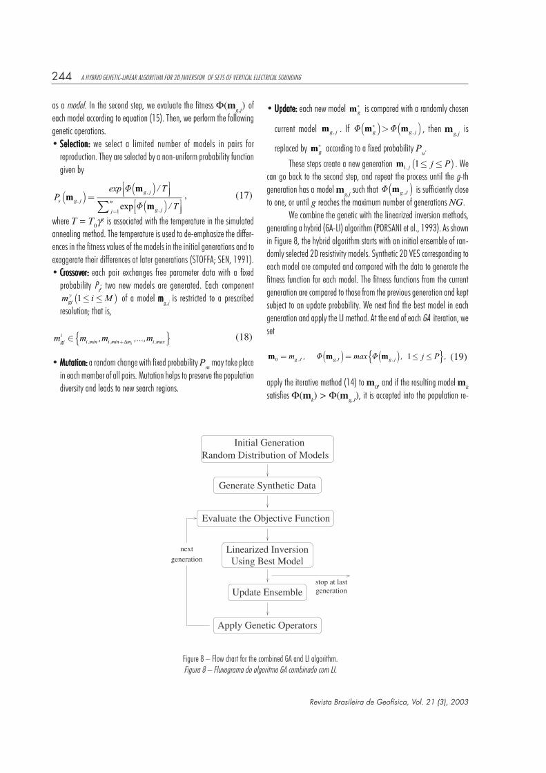
to one, or until g reaches the maximum number of generations NG.We combine the genetic with the linearized inversion methods,

generating a hybrid (GA-LI) algorithm (PORSANI et al., 1993). As shownin Figure 8, the hybrid algorithm starts with an initial ensemble of ran-domly selected 2D resistivity models. Synthetic 2D VES corresponding toeach model are computed and compared with the data to generate thefitness function for each model. The fitness functions from the currentgeneration are compared to those from the previous generation and keptsubject to an update probability. We next find the best model in eachgeneration and apply the LI method. At the end of each GA iteration, weset

m m m0 1= ( )= ( ) ≤ ≤ m j Pg J g j, ,, max , , g,JΦ Φ (19)

apply the iterative method (14) to m0, and if the resulting model m

k

satisfies Φ(mk) > Φ(m

g,J), it is accepted into the population re-

Figure 8 – Flow chart for the combined GA and LI algorithm.Figura 8 – Fluxograma do algoritmo GA combinado com LI.



placing m0. The algorithm then proceeds as in AG. The genetic opera-

tors of selection, crossover and mutation are applied to the models toprovide the next generation of 2D resistivity models for evaluation.

INVERSION OF FIELD DATA

This section illustrates the improvement of the hybrid approachover genetic algorithms. We consider the same settings as in the experi-ment with linearized algorithms.

The probabilities associated with the genetic algorithm are setsimilarly to earlier cases (CHUNDURU et al., 1995; SEN; STOFFA, 1995):P

c = 0.6, P

m = 0.01 and P

u = 0.95. The resolution of the free

parameters is shown in Table 2. Moreover, T0 = 5 and γ = 0.98.

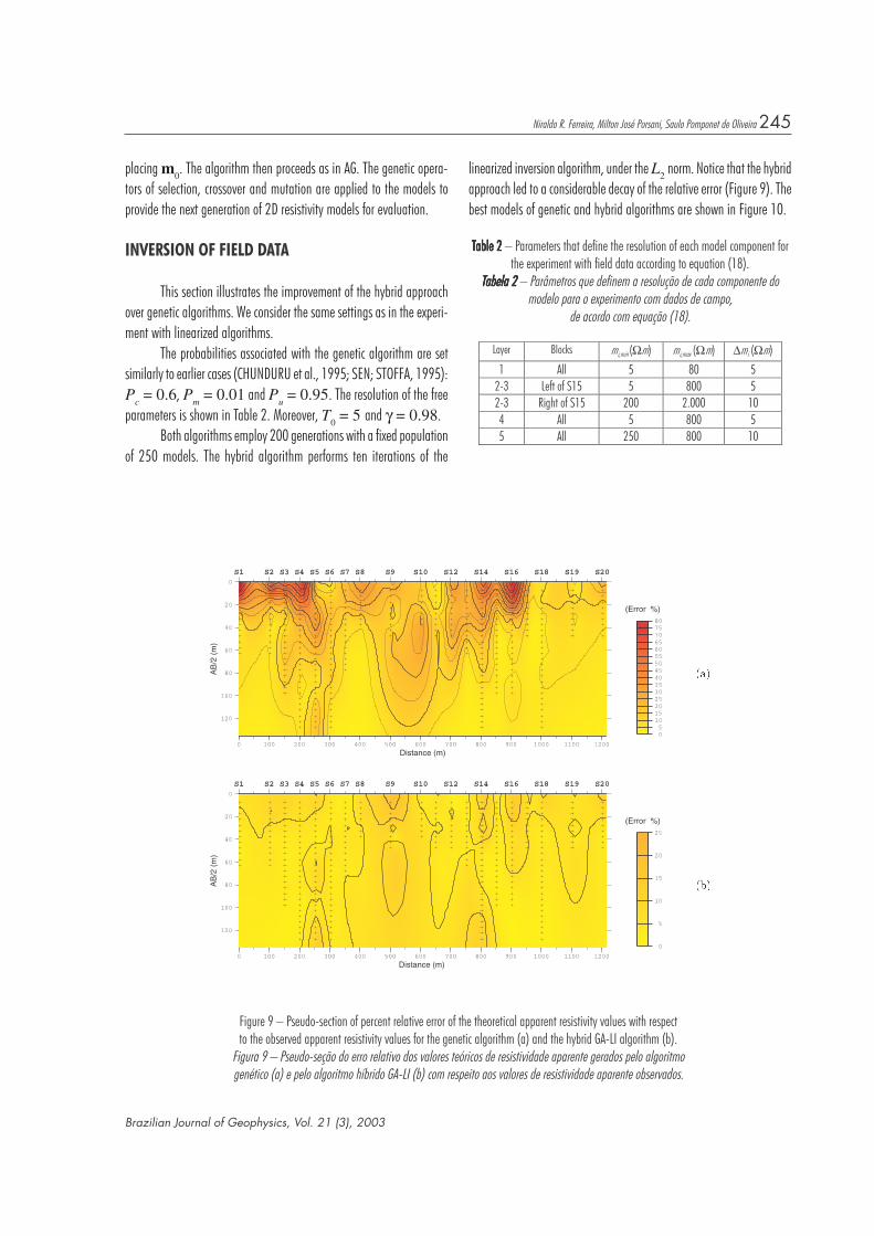
Both algorithms employ 200 generations with a fixed populationof 250 models. The hybrid algorithm performs ten iterations of the

linearized inversion algorithm, under the L2

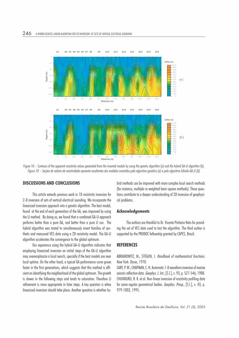
norm. Notice that the hybridapproach led to a considerable decay of the relative error (Figure 9). Thebest models of genetic and hybrid algorithms are shown in Figure 10.

TTTTTable 2able 2able 2able 2able 2 – Parameters that define the resolution of each model component forthe experiment with field data according to equation (18).

TTTTTabela 2abela 2abela 2abela 2abela 2 – Parâmetros que definem a resolução de cada componente domodelo para o experimento com dados de campo,

de acordo com equação (18).

Figure 9 – Pseudo-section of percent relative error of the theoretical apparent resistivity values with respectto the observed apparent resistivity values for the genetic algorithm (a) and the hybrid GA-LI algorithm (b).

Figura 9 – Pseudo-seção do erro relativo dos valores teóricos de resistividade aparente gerados pelo algoritmogenético (a) e pelo algoritmo híbrido GA-LI (b) com respeito aos valores de resistividade aparente observados.



DISCUSSIONS AND CONCLUSIONS

This article extends previous work in 1D resistivity inversion for2-D inversion of sets of vertical electrical sounding. We incorporate thelinearized inversion approach into a genetic algorithm. The best model,found at the end of each generation of the GA, was improved by usingthe LI method. By doing so, we found that a combined GA-LI approachperforms better than a pure GA, and better than a pure LI run. Thehybrid algorithm was tested to simultaneously invert families of syn-thetic and measured VES data using a 2D resistivity model. The GA-LIalgorithm accelerates the convergence to the global optimum.

Our experience using the hybrid GA-LI algorithm indicates thatemploying linearized inversion on initial steps of the GA-LI algorithmmay overemphasize a local search, specially if the best models are nearlocal optima. On the other hand, a typical GA performance curve growsfaster in the first generations, which suggests that this method is effi-cient on identifying the neighborhood of the global optimum. The growthis slower in the following steps and tends to saturation. Therefore LIrefinement is more appropriate in later steps. A key question is whenlinearized inversion should take place. Another question is whether hy-

brid methods can be improved with more complex local search methods(for instance, multiple re-weighted least-square methods). These ques-tions contribute to a deeper understanding of 2D inversion of geophysi-cal problems.

Acknowledgements

The authors are thankful to Dr. Vicente Pinheiro Neto for provid-ing the set of VES data used to test the algorithm. The third author issupported by the PRODOC fellowship granted by CAPES, Brazil.

REFERENCES

ABRAMOWITZ, M.; STEGUN, I. Handbook of mathematical functions.New York: Dover, 1970.CARY, P. W.; CHAPMAN, C. H. Automatic 1-D waveform inversion of marineseismic reflection data. Geophys. J. Int., [S.l.], v. 93, p. 527-546, 1988.CHUNDURU, R. K. et al. Non-linear inversion of resistivity profiling datafor some regular geometrical bodies. Geophys. Prosp., [S.l.], v. 43, p.979-1003, 1995.

Figure 10 – Contours of the apparent resistivity values generated from the inverted models by using the genetic algorithm (a) and the hybrid GA-LI algorithm (b).Figura 10 – Seções de valores de resistividade aparente resultantes dos modelos invertidos pelo algoritmo genético (a) e pelo algoritmo híbrido GA-LI (b).



GERSZTENKORN, A.; BEDNARD, J. B.; LINES, L. R., 1986. Robust itera-tive inversion for the one-dimensional acoustic wave equation. Geophysics,[S.l.], v. 51, p. 357-368, 1986.GOLBERG D. E. Genetic algorithms in search, optimization and machinelearning. New York: Addison-Wesley, 1989.HOLLAND, J. H. Adaptation in natural and artificial systems. Ann Arbor:University of Michigan Press, 1975.GREENBAUM, A. Iterative methods for solving linear systems. Philadel-phia: SIAM, 1997.KOEFOED, O. Geosounding principles 1: resistivity sounding measure-ments. Amsterdam: Elsevier, 1979.LIU, P.; HARTZELL, S. A; STEPHENSON, W. Nonlinear multiparameterinversion using a hybrid global search algorithm: applications in reflec-tion seismology. Geophys. J. Int., [S.l.], v. 122, p. 991-1000, 1995.MCGILLIVRAY, P. R.; OLDENBURG, D. W. Methods forcalculating Fréchetderivatives and sensitivities for non-linear inverse problem: a compara-tive study. Geophys. Prosp., [S.l.], v. 38, p. 499-524, 1990.MEDEIROS, W. E. Eletro-resistividade aplicada à hidrogeologia docristalino: um problema de modelamento bidimensional. 1987.Dissertação (Mestrado)-Universidade Federal da Bahia, Salvador, 1987.MEIJERINK, J. A.; VAN DER VORST, H. A. An iterative solution methodfor linear systems of which the coefficient matrix is a symmetric M-ma-trix. Mathematics of Computation, [S.l.], v. 31, p. 148-162, 1977.MENKE, W. Geophysical data analysis: discrete inverse theory. New York:Academic Press, 1989.PINHEIRO NETO, V. Modelagem estrutural-geoelétrica de rochascristalinas fraturadas. 2000. Tese (Doutorado)-Universidade Federal daBahia, Salvador, 2000.PORSANI, M. J. et al. A combined genetic and linear inversion algorithmfor waveform inversion. In: ANN. INTERNAT. MTG., 63., 1993, Wash-

ington, DC. Expanded Abstracts…Washington, DC: [s.n.], 1993. p. 692-695.______ et al. Fitness functions, genetic algorithms and hybrid opti-mization in seismic waveform inversion. J. Seism. Explor., [S.l.], v. 9, p.143-164, 2000.______, NIWAS, S.; FERREIRA, N. F. Robust inversion of vertical elec-trical sounding data using a multiple re-weighted least square method.Geophys. Prosp., [S.l.], v. 49, p. 255-264, 2001.RIJO, L. et al. Interpretation of apparent resistivity data from Apodi Val-ley, Rio Grande do Norte, Brazil. Geophysics, [S.l.], v. 42, p. 811-822,1977.ROTHMAN, D. H. Nonlinear inversion, statistical mechanics and residualstatics estimation. Geophysics, [S.l.], v. 50, p. 2784-2796, 1985.SCALES, J. A.; GERSZTENKORN A. Robust methods in inverse theory.Inverse Problems, [S.l.], v. 4, p. 1071-1091, 1988.SEN, M. K.; BHATTACHARYA, B. B.; STOFFA, P. L. Nonlinear inversion ofresistivity sounding data. Geophysics, [S.l.], v. 58, p. 496-507, 1993.______; STOFFA, P. L. Global optimization methods in geophysicalinversion. Amsterdam: Elsevier, 1995.STOFFA, P. L.; SEN, M. K. Nonlinear multiparameter optimization usinggenetic algorithms: inversion of plane-wave seismograms. Geophysics,[S.l.], v. 56, p. 1794-1810, 1991.TARANTOLA, A.; VALETTE, B. Inverse problems-quest for information. J.Geophys., [S.l.], v. 50, p. 159-170, 1982.ZHANG, J.; MACKIE, R. L.; MADDEN, T. R. 3-D resistivity forward modelingand inversion using conjugate gradients. Geophysics, [S.l.], v. 60, p.1313-1325, 1995.



NOTAS SOBRE OS AUTORES

Niraldo Roberto Ferreira é graduado em Engenharia Elétrica na Universidade Federal de Pernambuco em 1977. Mestrado em Geofísicapela Universidade Federal da Bahia, 1994. Doutorado em Geofísica pela Universidade Federal da Bahia, 1999. Atualmente professor daEscola Politécnica da UFBA.

Milton José Porsani é B. C. em Geologia pela USP, 1976. Licenciado em Geologia pela Faculdade de Educação da USP, 1977. Mestreem Geofísica pela UFPA, 1981. Doutor em Geofísica pela UFBA, 1986. Pós-doutorado em Geofísica, Institute for Geophysics at Universityof Texas at Austin, EUA, setembro/92 a outubro/93. De 1986 até o presente é Pesquisador do CPGG/UFBA onde coordena o Programa deExploração de Petróleo. Em 1990 foi contratado pela UFBA mediante concurso público para professor do Departamento de Geologia eGeofísica Aplicada do IGEO. Desde 2000 é professor Titular na matéria Exploração de Petróleo. Pesquisador do CNPq, nível I-B. Tematuado no desenvolvimento de métodos e algoritmos de filtragem e processamento de dados sísmicos e na inversão de dados sísmicos eelétricos.

Saulo Pomponet de Oliveira é graduado em Matemática Aplicada e Computacional pela Universidade Estadual de Campinas, Campi-nas, SP, em 1997. Mestrado em Matemática Aplicada, Universidade Estatual de Campinas, Campinas, SP, em 1998. Doutorado emMatemática Aplicada, University of Colorado, Denver, Estados Unidos, em 2003. Atualmente bolsista recém-doutor (PRODOC-CAPES) doprograma de pós-graduação em geofísica da Universidade Federal da Bahia.

A hybrid genetic-linear algorithm for 2D inversion of sets of vertical electrical sounding

Documents

Transcript of A hybrid genetic-linear algorithm for 2D inversion of sets of vertical electrical sounding