Soft Computing manuscript No.(will be inserted by the editor)

Learning behavior in abstract memory schemes fordynamic optimization problems

Hendrik Richter · Shengxiang Yang

Received: 13 August, 2008 / Accepted: 13 March 2009

Abstract Integrating memory into evolutionary algo-rithms is one major approach to enhance their perfor-

mance in dynamic environments. An abstract memory

scheme has been recently developed for evolutionary al-

gorithms in dynamic environments, where the abstrac-tion of good solutions is stored in the memory instead

of good solutions themselves to improve future problem

solving. This paper further investigates this abstract

memory with a focus on understanding the relationship

between learning and memory, which is an importantbut poorly studied issue for evolutionary algorithms in

dynamic environments. The experimental study shows

that the abstract memory scheme enables learning pro-

cesses and hence efficiently improves the performanceof evolutionary algorithms in dynamic environments.

Keywords Evolutionary Algorithm · Dynamic

Optimization Problem · Learning · Memory Dynamics

1 Introduction

A main concern of evolutionary algorithms (EAs) for

solving dynamic optimization problems (DOPs) is to

maintain the genetic diversity of the population [6,10,

16] in order to guarantee continuing and sustainable

H. RichterHTWK Leipzig, Fachbereich Elektrotechnikund InformationstechnikInstitut Mess–, Steuerungs– und RegelungstechnikPostfach 30 11 66, D–04125 Leipzig, GermanyE-mail: richter@fbeit.htwk-leipzig.de

S. YangDepartment of Computer ScienceUniversity of LeicesterUniversity Road, Leicester LE1 7RH, United KingdomE-mail: s.yang@mcs.le.ac.uk

evolutionary search for optima that change with time.Next to standard adaptive schemes that are also used

in solving static optimization problems, such as self–

adaption of mutation [1,3], for achieving the mainte-

nance of diversity, two main lines have been followedin solving DOPs. One line is to preserve diversity by

mainly random means, which is realized by designs such

as hyper–mutation [15] and random immigrants [20].

Another line is to promote diversity by basically deter-

ministic methods through saving individuals or groupsof individuals for future re–insertion or mergence. Such

ideas are implemented in memory [4,11,21] and multi–

population approaches [5].

Although both of the above concepts have shown to

be successful for certain dynamic environments, thereare some points of criticism. One is that they do not or

do not explicitly incorporate information about the dy-

namics and hence do not discriminate between different

kinds of dynamic fitness landscapes. Another concern is

the usage of past and present solutions for improvingthe quality of future solution finding. This aspect is

not addressed by random diversity enhancement at all.

In contrast, memory techniques do use previous good

solutions for later reuse [4,19,22,23]. Here, it is natu-ral to ask how and why this brings improvements in

performance and an obvious answer is that by storing

and reusing information some kinds of learning pro-

cesses take place. However, the detailed relationships

between memory and learning in dynamic optimizationare poorly studied. A related example is an analysis of

how self–adaptive mutation steps reflect the movement

of the optima [3], which can be regarded as an implicit

learning process. However, we intend to study learn-ing in a more literal sense as for instance considered

in machine learning [13,14]. Therefore, we introduce a

method for evaluating the memory dynamics and the

2

learning process based on an information–theoretical

quantity, the Kullback–Leibler divergence.

This paper analyzes an abstraction based memory

scheme for EAs for multimodal DOPs, which was re-cently proposed in [18]. In this abstract memory scheme,

the abstraction of good solutions (i.e., to use their ap-

proximate location in the search space to deduce a prob-

abilistic model for the spatial distribution of good so-lutions) is stored in the memory instead of good solu-

tions themselves. We show that such a memory scheme

enables learning processes conceptionally and function-

ally similar to those considered in machine learning.

It explicitly uses the past and present solutions in anabstraction process that is employed to improve fu-

ture problem solving and differentiates between differ-

ent kinds of dynamics of the fitness landscape. In par-

ticular, we intend to study how learning takes place inthe abstract memory scheme.

The rest of this paper is outlined as below. The next

section reviews the relationship between memory and

learning and links it to solving DOPs with a memoryenhanced EA. The abstract memory scheme is given

in Section 3, where we also show how it can be de-

scribed by the memory dynamics. Experiments are re-

ported and discussed in Section 4. Section 5 concludesthe paper with discussions on future work.

2 Memory and Learning

When tackling similar problems repeatedly, it is nat-

ural to credit the long–term success in problem solv-

ing to learning in both its conceptual and metaphori-

cal meaning. By long–term success we mean that theobtained results become increasingly better over time

with respect to some performance criteria. Evolutionary

optimization in dynamic fitness landscapes implies the

repeated solution of a multi–modal optimization prob-

lem and hence meets this description. As we are using amemory scheme in the EA to improve its performance,

it makes sense to ask about the relationships between

memory and learning for DOPs.

In cognitive science, learning is understood as a chan-

ge of behavior as a result of experience, while memory is

a record of events leading to experience [12]. So, learn-

ing emphasizes acquiring experience with the aim of ex-

tracting information from past and current events likelyto be useful in the future behavior, while memory em-

phasizes retaining experience with the function to carry

it forward in time. A computer science example that is

related to this study and applies these principles is thememory design of autonomous agents in artificial life

for dynamic environments [9]. In machine learning, this

matter can be formalized further by defining the learn-

ing problem as finding a mapping between inputs and

outputs [14]. This mapping is constructed from a train-

ing set of past and current inputs and outputs and can

be used to predict future outputs using future inputs

alone. The quality of the mapping is evaluated by per-formance measures; the quality becoming better over

training time is the learning process. In this way, the

experiences in the cognitive science view roughly relate

to the training set of inputs and outputs and the per-formance evaluation of the mapping between them in

machine learning. Moreover, the memory in the former

functionally corresponds to the mapping in the latter,

which applies almost literally in machine learning using

artificial neural networks. Our aim is to employ theseconcepts in the design of and the numerical experiments

with the abstract memory scheme.

Memory schemes that only store good solutions as

themselves, known as direct memory [4,19,21], for laterreuse carry out learning processes implicitly at best.

Learning is something different than memorizing all

previous solutions. In cases, this might be helpful. In

general, every realizable memory will soon prove insuf-

ficient in a more complex context; if not by the stor-ing capacity itself, then by a timely retrieval of the

stored content for further usage. In the wider sense dis-

cussed above, learning refers to detecting the essence

and meaning of a solution.The abstract memory scheme proposed in [18] in-

tends to address and employ these relations. Abstrac-

tion means to select, evaluate and code information be-

fore storing. A good solution is evaluated with respect

to physically meaningful criteria and in the result of thisevaluation, storage is undertaken but no longer as the

solution itself but as the information coded with respect

to the criteria. So, abstraction means a threshold for

and compression of information, e.g., see [8] which pro-poses similar ideas for reinforcement learning. The fill-

ing of the abstract memory takes place during the run–

time of the EA in the dynamic fitness function. It grad-

ually builds a mapping between the search space ele-

ments and good solutions. This mapping is constructedvia the abstract memory. So, the scheme we present is

not merely concerned with anticipating the dynamics

of the fitness function alone, as considered in [2], but to

predict where good solutions of the DOP are likely tooccur. Hence, we bring together learning and memory

for evolutionary optimization in dynamic environments.

3 The Abstract Memory Scheme

The main idea of the abstract memory scheme is that it

does not store good solutions directly but as their ab-

straction. The abstraction of a good solution is based on

3

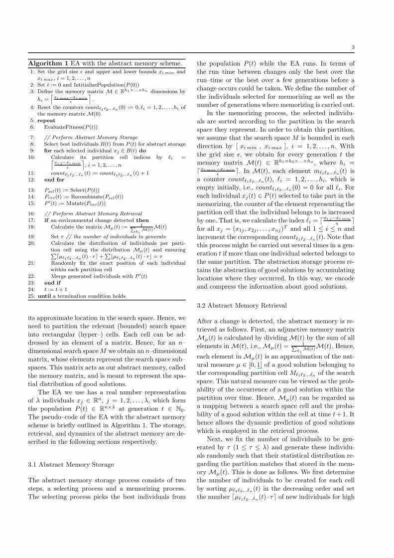
Algorithm 1 EA with the abstract memory scheme.1: Set the grid size ǫ and upper and lower bounds xi min and

xi max, i = 1, 2, . . . , n2: Set t := 0 and IntitializePopulation(P (0))3: Define the memory matrix M ∈ R

h1×...×hn dimensions by

hi =l

xi max−xi minǫ

m

.

4: Reset the counters countℓ1ℓ2...ℓn(0) := 0, ℓi = 1, 2, . . . , hi of

the memory matrix M(0)5: repeat

6: EvaluateFitness(P (t))

7: // Perform Abstract Memory Storage8: Select best individuals B(t) from P (t) for abstract storage9: for each selected individual xj ∈ B(t) do

10: Calculate its partition cell indices by ℓi =l

xi j−xi min

ǫ

m

, i = 1, 2, . . . , n

11: countℓ1ℓ2...ℓn(t) := countℓ1ℓ2...ℓn

(t) + 112: end for

13: Psel(t) := Select(P (t))14: Prec(t) := Recombinate(Psel(t))15: P ′(t) := Mutate(Prec(t))

16: // Perform Abstract Memory Retrieval17: if an environmental change detected then

18: Calculate the matrix Mµ(t) := 1P

hiM(t)

M(t)

19: Set τ // the number of individuals to generate20: Calculate the distribution of individuals per parti-

tion cell using the distribution Mµ(t) and ensuringP

⌈µℓ1ℓ2...ℓn(t) · τ⌉ +

P

⌊µℓ1ℓ2...ℓn(t) · τ⌋ = τ

21: Randomly fix the exact position of each individualwithin each partition cell

22: Merge generated individuals with P ′(t)23: end if

24: t := t + 125: until a termination condition holds

its approximate location in the search space. Hence, weneed to partition the relevant (bounded) search space

into rectangular (hyper–) cells. Each cell can be ad-

dressed by an element of a matrix. Hence, for an n–

dimensional search space M we obtain an n–dimensional

matrix, whose elements represent the search space sub–spaces. This matrix acts as our abstract memory, called

the memory matrix, and is meant to represent the spa-

tial distribution of good solutions.

The EA we use has a real number representationof λ individuals xj ∈ R

n, j = 1, 2, . . . , λ, which form

the population P (t) ∈ Rn×λ at generation t ∈ N0.

The pseudo–code of the EA with the abstract memory

scheme is briefly outlined in Algorithm 1. The storage,

retrieval, and dynamics of the abstract memory are de-scribed in the following sections respectively.

3.1 Abstract Memory Storage

The abstract memory storage process consists of two

steps, a selecting process and a memorizing process.

The selecting process picks the best individuals from

the population P (t) while the EA runs. In terms of

the run–time between changes only the best over the

run–time or the best over a few generations before a

change occurs could be taken. We define the number of

the individuals selected for memorizing as well as thenumber of generations where memorizing is carried out.

In the memorizing process, the selected individu-

als are sorted according to the partition in the search

space they represent. In order to obtain this partition,we assume that the search space M is bounded in each

direction by [ xi min , xi max ], i = 1, 2, . . . , n. With

the grid size ǫ, we obtain for every generation t the

memory matrix M(t) ∈ Rh1×h2×...×hn , where hi =

⌈xi max−xi min

ǫ⌉. In M(t), each element mℓ1ℓ2...ℓn

(t) isa counter countℓ1ℓ2...ℓn

(t), ℓi = 1, 2, . . . , hi, which is

empty initially, i.e., countℓ1ℓ2...ℓn(0) = 0 for all ℓi. For

each individual xj(t) ∈ P (t) selected to take part in the

memorizing, the counter of the element representing thepartition cell that the individual belongs to is increased

by one. That is, we calculate the index ℓi = ⌈xi j−xi min

ǫ⌉

for all xj = (x1j , x2j , . . . , xnj)T and all 1 ≤ i ≤ n and

increment the corresponding countℓ1ℓ2...ℓn(t). Note that

this process might be carried out several times in a gen-eration t if more than one individual selected belongs to

the same partition. The abstraction storage process re-

tains the abstraction of good solutions by accumulating

locations where they occurred. In this way, we encodeand compress the information about good solutions.

3.2 Abstract Memory Retrieval

After a change is detected, the abstract memory is re-

trieved as follows. First, an adjunctive memory matrix

Mµ(t) is calculated by dividing M(t) by the sum of all

elements in M(t), i.e., Mµ(t) = 1P

hiM(t)M(t). Hence,

each element in Mµ(t) is an approximation of the nat-

ural measure µ ∈ [0, 1] of a good solution belonging tothe corresponding partition cell Mℓ1ℓ2...ℓn

of the search

space. This natural measure can be viewed as the prob-

ability of the occurrence of a good solution within the

partition over time. Hence, Mµ(t) can be regarded asa mapping between a search space cell and the proba-

bility of a good solution within the cell at time t+1. It

hence allows the dynamic prediction of good solutions

which is employed in the retrieval process.

Next, we fix the number of individuals to be gen-erated by τ (1 ≤ τ ≤ λ) and generate these individu-

als randomly such that their statistical distribution re-

garding the partition matches that stored in the mem-

ory Mµ(t). This is done as follows. We first determinethe number of individuals to be created for each cell

by sorting µℓ1ℓ2...ℓn(t) in the decreasing order and set

the number ⌈µℓ1ℓ2...ℓn(t) · τ⌉ of new individuals for high

4

values of µ and the number ⌊µℓ1ℓ2...ℓn(t) · τ⌋ for low

values respectively. The rounding needs to ensure that∑

⌈µℓ1ℓ2...ℓn(t)·τ⌉+

∑

⌊µℓ1ℓ2...ℓn(t)·τ⌋ = τ . Then, we fix

the positions of the new individuals uniformly randomly

within each partition cell Mℓ1ℓ2...ℓn. This means the τ

individuals are distributed such that the number within

each cell approximates the probability of the occurrence

of good solutions. These individuals are inserted in the

population P (t) after mutation has been carried out.

This abstract retrieval process can create an arbi-

trary number of individuals from the abstract mem-

ory. In the implementation considered here we upper

bound this creation by the number of individuals in thepopulation. As the abstract storage can be regarded as

encoding and compression of information about good

solutions in the search space, the abstract retrieval be-

comes decoding and expansion.

3.3 Abstract Memory Dynamics

Using the scheme described above leads to a consid-

erable reduction of the information content to be pro-

cessed by the memory, which is typical for abstraction.

The storing capacity needed depends on the coarsenessof the partitioning, but not on the number of individ-

uals taken to the memory. This also means that the

number of individuals that take part in the memorizing

and the number of individuals that are retrieved fromthe memory and inserted in the population are com-

pletely independent of each other. Also, in the mem-

ory matrix not the good solutions are stored but the

events of occurrence of the solution at a specific loca-tion in the search space. This means a change of rep-

resentation (EA uses real, memory uses integer), which

is another feature of abstraction. Such a change of rep-

resentation requires less storage capacity and is partic-

ularly interesting for higher–dimensional search spaces.As the memory matrix Mµ(t) is filled over the run–time

t, learning as discussed in Section 2 takes place and can

be quantified by studying the relationship between the

performance and the matrix filling.

To compare the memory dynamics to a reference, we

introduce a master memory (or demon) Dµ(t), which

has the elements δℓ1ℓ2...ℓn(t). It is a matrix of the same

dimension and size as Mµ(t) and is built exactly the

same way with the difference being that the solutiontrajectory is stored in Dµ(t). Hence, it is a probabilis-

tic mapping between search space cells and the solution

of the DOP. With Mµ(t) and Dµ(t), we have two spa-

tial probability distributions which represent the onlinecalculated memory and the solution. By measuring the

degree of the difference between these quantities, we

have a way to establish how good the memory is and to

evaluate the memory dynamics. Such a difference mea-

sure is the Kullback–Leibler divergence (KLD), e.g.,

see [7], p. 19:

KLD(t) =∑

iℓi

δℓi(t) log2

(

δℓi(t)

µℓi(t)

)

, (1)

where the measures δℓi(t) and µℓi

(t) are the elementsof Dµ(t) and Mµ(t), respectively. In the following, we

report numerical experiments with the abstract mem-

ory scheme and study its learning behavior. Therefore,

we will particularly look at the memory dynamics.

4 Experimental study

4.1 Experimental setup and performance measurement

The experimental results given here are obtained with

an EA that uses the tournament selection of tourna-

ment size 2, the fitness–related intermediate sexual re-

combination (which is operated λ times and for each

recombination two individuals are chosen randomly toproduce an offspring that is the fitness–weighted arith-

metic mean of both parents), a standard mutation with

the mutation rate 0.1, and the proposed abstract mem-

ory (AM) scheme. The dynamic fitness landscape is ann–dimensional “field of cones on a zero plane”, where N

cones with coordinates ci(k), i = 1, · · · , N , are moving

with discrete time k ∈ N0. These cones are distributed

across the landscape and have randomly chosen initial

coordinates ci(0), heights hi, and slopes si. So, the dy-namic fitness function is given as:

f(x, k) = max{

0 , max1≤i≤N

[hi − si‖x − ci(k)‖]}

. (2)

We study four types of dynamics regarding the coordi-

nates ci(k) of the cones: (i.) chaotic dynamics generated

by the Henon map, see [17] for details of the genera-

tion process, (ii.) random dynamics with each ci(k) for

each k being an independent realization of a normallydistributed random variable, (iii.) random dynamics as

in (ii.) but with a uniformly distributed random vari-

able, and (iv.) cyclic dynamics where each ci(k) is con-

sequently forming a circle.

We consider the dynamic fitness function (2) with

dimension n = 2 and the number of cones N = 7. Theupper and lower bounds of the search space are set to

x1 min = x2 min = −3 and x1 max = x2 max = 3. The

best three individuals of the population take part in

the memorizing process for all three generations beforea change in the environment occurs. Further, dynamic

severity is normalized for all considered dynamics and

hence has no differentiating influence. The scales t and

5

020

4060

80100

20

40

60

80

100

1200.5

1

1.5

2

2.5

3

τ/λ [in %]λ

MFE

020

4060

80100

20

40

60

80

100

1200.5

1

1.5

2

2.5

3

τ/λ [in %]λ

MFE

(a) chaotic (b) normal

020

4060

80100

20

40

60

80

100

1200.5

1

1.5

2

2.5

3

τ/λ [in %]λ

MFE

020

4060

80100

20

40

60

80

100

1200.5

1

1.5

2

2.5

3

τ/λ [in %]λ

MFE

(c) uniform (d) cyclic

Fig. 1 The MFE against the population size λ and the number of individuals retrieved from the memory τ , given as percentage τ/λin %.

k are related by the change frequency γ ∈ N as t = γk.The performance of the algorithms is measured by the

Mean Fitness Error (MFE), defined as below:

MFE =1

R

R∑

r=1

[

1

T

T∑

t=1

(

f(xs(k), k)

− maxxj(t)∈P (t)

f(xj(t), k)

)]

k=⌊γ−1t⌋

, (3)

where maxxj(t)∈P (t)

f(

xj(t), ⌊γ−1t⌋)

is the fitness value of

the best–in–generation individual xj(t) ∈ P (t) at gen-

eration t, f(

xs(⌊γ−1t⌋), ⌊γ−1t⌋

)

is the maximum fitnessvalue at generation t, T is the number of generations

used in the run, and R is the number of consecutive

runs. We set R = 50 and T = 2000 in all experiments.

4.2 Properties of the abstract memory

The first set of experiments examines the relationshipsbetween the population size λ, the number of individu-

als τ retrieved from the memory, and the performance

measure MFE. Fig. 1 shows the results for the fixed

change frequency γ = 15 and the grid size ǫ = 0.1. FromFig. 1, it can be observed that an exponential relation-

ship exists between MFE and λ, which is typical for

EAs. Along this general trend, the number of retrieved

individuals, here given in percent of the total popula-

tion, has only a small influence on the MFE, wherein general a medium and large number gives slightly

better results than a very small percentage.

Next, we look at the influence of the grid size ǫ

on performance of the AM scheme, see Fig. 2. Here,

the MFE is given over ǫ and different γ on a semi–

logarithmic scale while we set here and subsequentlyλ = 50 and τ = 20. For all types of dynamics and all

change frequencies we obtain a kind of bath-tub curves,

which indicates that an optimal grid size depends on the

type of dynamics and the size of the bounded region in

the search space where the memory is considered. Thisgives raise to the question of whether an adaptive grid

size would increase the performance of the abstraction

memory scheme. Also, it can be seen that a drop in

performance is more significant if the grid is too large.For smaller grid the performance is not decreasing very

dramatically, but the numerical effort for calculation

with small grids becomes considerable. This result al-

6

10−3

10−2

10−1

100

101

102

1.2

1.4

1.6

1.8

2

2.2

2.4

2.6

log(ε)

MFE

γ = 25

γ = 15

γ = 5

10−3

10−2

10−1

100

101

102

1.2

1.4

1.6

1.8

2

2.2

2.4

2.6

log(ε)

MFE

γ = 25

γ = 15

γ = 5

(a) chaotic (b) normal

10−3

10−2

10−1

100

101

102

1.2

1.4

1.6

1.8

2

2.2

2.4

2.6

log(ε)

MFE

γ = 25

γ = 15

γ = 5

10−3

10−2

10−1

100

101

102

1.2

1.4

1.6

1.8

2

2.2

2.4

2.6

log(ε)

MFE

γ = 25

γ = 15

γ = 5

(c) uniform (d) cyclic

Fig. 2 Comparison of performance of abstraction memory scheme (AM) measured by the MFE for different grid size ǫ and differenttypes of dynamics and γ = 5, γ = 15 and γ = 25.

lows us to choose an ǫ that compromises between the

performance and the numerical effort. In the following

experiments, we set ǫ = 0.1.

In the second set of experiments, the abstract mem-

ory scheme (AM) is tested and compared with a direct

memory scheme (DM) that stores good solutions andinserts them again in a retrieval process, an EA with no

memory (NM) that uses hypermutation [15] with base

mutation ∼ 0.1N (0, 1) and hypermutation ∼ 3N (0, 1),

and an evolutionary strategy with self–adaptive muta-tion (SA) with 12 parents and 48 offspring candidates.

Note that by these parameters, we have a comparable

number of fitness function evaluations. In Fig. 3, the

MFE over the change frequency γ for all four types of

dynamics considered is given and the 95% confidenceintervals are also given.

From Fig. 3, it can be seen that the memory schemesoutperform the no memory scheme for all dynamics.

This is particularly noticeable for small change frequen-

cies γ and means that by memory the limit of γ for

which the algorithm still performs reasonably can beconsiderably lowered. It can also be seen that the ab-

stract memory gives better results than the direct mem-

ory for irregular dynamics, i.e., chaotic and random.

For chaotic dynamics, this is even significant within

the given bounds. For regular, cyclic dynamics, we find

the contrary, with direct memory being better than ab-

stract. A comparison to the self–adaptive scheme yieldsthat memory schemes are better than self–adaption for

chaotic and uniform random dynamics. For normal ran-

dom dynamics, memory outperforms self–adaption for

small change frequencies, while for large γ, for instance

γ = 25 and γ = 30, it is the other way around. Finally,for circle dynamics, self–adaption is the best option

yielding results far better than all other tested schemes.

However, in our experiments with the self–adaptivescheme we observed that for a small but existing per-

centage of runs the EA diverged and produced invalid

results. These runs were not taken into account in the

performance evaluation. A possible explanation for this

behavior is that a self-adaptive mutation rate evolvestowards optimal values in between changes, but may

become ill–posed after the change. This leads in some

cases to diverging population dynamics because there

is no direct feedback between the population dynam-ics and mutation rate. Note that such a behavior was

not observed with the other three schemes. The aim

here, however, is not to argue that one scheme is supe-

7

0 5 10 15 20 25 30 351

1.5

2

2.5

3

3.5

4

NM

DM

AM

SA

γ

MFE

0 5 10 15 20 25 30 351

1.5

2

2.5

3

3.5

4

NM

DM

AM

SA

γ

MFE

(a) chaotic (b) normal

0 5 10 15 20 25 30 351

1.5

2

2.5

3

3.5

4

NM

DM

AM

SA

γ

MFE

0 5 10 15 20 25 30 350.5

1

1.5

2

2.5

3

3.5

4

NMDMAMSA

γ

MFE

(c) uniform (d) cyclic

Fig. 3 Performance of the EA measured by the MFE over change frequency γ for different types of dynamics and no memory buthypermutation (NM), direct memory (DM), abstract memory (AM) and self–adaption (SA).

rior over another but to study the underlying workingmechanisms and particularly the effect of learning. For

self–adaption this has been done by analyzing the evo-

lution of self–adaptive mutation steps depending on the

dynamics of the fitness landscape [3], which can be re-garded as an implicit learning process. Our approach to

study learning is different, inspired by machine learn-

ing [14,13] and will be introduced and discussed next.

4.3 Learning behavior

To quantify learning depends on metrics for perfor-

mance, which ideally shows improvement over time. For

evaluating the effect of learning and obtaining the learn-

ing curve, the experiment has to enable learning for a

certain time, then turn learning off and measure theperformance using the learned ability [14]. Regarding

the abstract memory scheme, learning takes place as

long as the memory matrix Mµ(t) is filled. This gives

raise to the following measure for learning success. Wedefine tL to be the learning time. For 0 < t ≤ tL the

matrix Mµ(t) is filled as described in Section 3. For

tL < t ≤ tL + T the storage process is discarded and

only retrieval using the now fixed memory is carriedout. We calculate the MFE in Eq. (3) for t > tL only

and denote it MFEL. It is a performance measure for

the learning success, where MFEL over tL shows the

learning curve.

Fig. 4 depicts the results for fixed λ = 50, τ = 20

and several change frequencies γ on the semi–logarithmicscale. These learning curves are an experimental evalu-

ation of the learning behavior. We see that the MFEL

gets gradually smaller with the learning time tL becom-

ing larger, which confirms the learning success. We finda negative linear relation between MFE and log(tL),

which indicates an exponential dependency between tLand MFE. Also, it can be seen that the learning curves

are slightly steeper for larger change frequencies. An ex-

ception to this general trend is cyclic dynamics, wherethe learning curves are almost parallel for all γ and a

large proportion of the tested tL. A comparison of the

learning success between the different kinds of land-

scape dynamics suggests that the uniform random move-ment is the most difficult to learn. The results in Fig. 4

clearly indicate the positive effect of learning on the

performance of the EA.

8

101

102

103

1.5

2

2.5

3

3.5

4

4.5

5

log(tL)

MFE

L

γ = 5

γ = 15

γ = 25

101

102

103

1.5

2

2.5

3

3.5

4

4.5

5

log(tL)

MFE

L

γ = 5

γ = 15

γ = 25

(a) chaotic (b) normal

101

102

103

1.5

2

2.5

3

3.5

4

4.5

5

log(tL)

MFE

L

γ = 5

γ = 15

γ = 25

101

102

103

1.5

2

2.5

3

3.5

4

4.5

5

log(tL)

MFE

L

γ = 5

γ = 15

γ = 25

(c) uniform (d) cyclic

Fig. 4 Learning curves for the abstract memory scheme showing the learning success measured by MFEL over the learning time tL.

Next, we are interested in how the memory reflects

the learning process. We consider the memory dynam-

ics which can be quantified by the KLD in Eq. (1).

The KLD for the learning time tL, that is, KLD =KLD(tL), over tL on the semi–logarithmic scale is plot-

ted in Fig. 5. As the KLD may differ in every run, we

record the mean over R = 50 runs and the 95% confi-

dence intervals. The KLD measures the difference be-tween the spatial probability distribution stored in the

memory Mµ(tL) compared to the reference of the mas-

ter memory (or demon) Dµ(tL) that stores the solution

of the DOP for the learning time tL. The KLD is a

measure of the degree of similarity between the “true”distribution in Dµ(tL) and the “estimated” distribution

in Mµ(tL); KLD = 0 defines that both distributions

are equal. The results in Fig. 5 show that the memory

gets gradually better with the learning time becominglarger, following similar characteristics as the learning

curves. For a small γ, the KLD goes near zero, indicat-

ing that the distribution in the memory almost fits the

distribution obtained for the solution of the DOP. The

reason for this result lies most likely in that for a smallerγ, a larger variety of the landscape’s dynamics is feeded

to the memory for a constant learning time compared

to a larger γ, which causes it to become better.

We finally relate the memory dynamics to the learn-

ing success. In Fig. 6, the relationship between the learn-

ing success MFEL and the memory dynamics KLD is

shown. Note that as both quantities are the result of nu-merical experiments, the means over R = 50 runs are

recorded and we get vertical as well as horizontal con-

fidence intervals. The general trend is that both quan-

tities are directly proportional for a constant γ, whichimplies that a good memory results in a good perfor-

mance of the EA. The most striking detail is that KLD

is the smallest for the smallest change frequency, while

this is not accompanied by the MFEL being the small-

est, too. One explanation is that the change frequencyaffects the performance much stronger than the qual-

ity of memory. In other words, a good memory does not

guarantee for high performance if the EA does not have

a certain run time between changes in the landscape.

5 Conclusions

This paper investigates an abstract memory scheme forEAs in dynamic environments, where memory is used to

store the abstraction of good solutions (i.e., to use their

approximate location in the search space to deduce a

9

101

102

103

0

1

2

3

4

5

6

7

log(tL)

KLD

γ = 5

γ = 15

γ = 25

101

102

103

0

1

2

3

4

5

6

7

log(tL)

KLD

γ = 5

γ = 15

γ = 25

(a) chaotic (b) normal

101

102

103

0

1

2

3

4

5

6

7

log(tL)

KLD

γ = 5

γ = 15

γ = 25

101

102

103

0

1

2

3

4

5

6

7

log(tL)

KLD

γ = 5

γ = 15

γ = 25

(c) uniform (d) cyclic

Fig. 5 Memory dynamics measured by the KLD over the learning time tL.

probabilistic model for the spatial distribution of good

solutions) instead of good solutions themselves. Thisabstraction is employed to generate solutions to im-

prove future problem solving. In order to understand

the relationship between memory and learning in dy-

namic environments, experiments were carried out to

study how learning takes place in the abstract memoryand how the performance changes over time for different

kinds of dynamics in the fitness landscape. The exper-

imental study revealed several results on the dynamic

test environments. First, the abstraction based mem-ory scheme enables learning processes, which efficiently

improves the performance of EAs in dynamic environ-

ments. Second, the effect of the abstract memory on the

performance of the EA depends on the learning time

and the frequency of environmental changes.

We studied the relationship between learning andthe abstract memory in dynamic environments. For the

future work, it is valuable to compare and combine the

abstract memory scheme with other approaches devel-

oped for EAs in dynamic environments. Also, if thedynamics is non–stationary in a strict statistical sense,

that is, the statistical properties change fast over the

algorithm’s run–time, as for instance in the translatory

movements, then forecasting the movements requires

other schemes, for instance prediction by a linear es-timator. However, if the changes of statistical proper-

ties are rather slow, it might be helpful if the memory

matrix has some evaporation to prevent unlimited ac-

cumulation of its elements. This would mean that in

the storage process a third step is needed to add: anamnesia (or forgetting) process.

Acknowledgments

The work by S. Yang was supported by the Engineering

and Physical Sciences Research Council (EPSRC) of

UK under Grant EP/E060722/1.

References

1. D. V. Arnold and H. G. Beyer. Optimum tracking with evo-lution strategies. Evol. Comput., 14(3): 291–308, 2006.

2. P. A. N. Bosman. Learning and anticipation in online dynamicoptimization. In: S. Yang, Y. S. Ong, and Y. Jin (eds.), Evo-lutionary Computation in Dynamic and Uncertain Environ-ments, Chapter 6, pp. 129–152, Springer-Verlag Berlin Heidel-berg, 2007.

10

0 1 2 3 4 5 6 71.5

2

2.5

3

3.5

4

4.5

5

γ = 5

γ = 15

γ = 25

MFE

L

KLD0 1 2 3 4 5 6 7

1.5

2

2.5

3

3.5

4

4.5

5

γ = 5

γ = 15

γ = 25

MFE

L

KLD

(a) chaotic (b) normal

0 1 2 3 4 5 6 72

2.5

3

3.5

4

4.5

5

5.5

γ = 5

γ = 15

γ = 25

MFE

L

KLD0 1 2 3 4 5 6 7

1.5

2

2.5

3

3.5

4

4.5

5

γ = 5

γ = 15

γ = 25

MFE

L

KLD

(c) uniform (d) cyclic

Fig. 6 Relationship between learning success MFEL and memory dynamics KLD.

3. A. M. Boumaza: Learning environment dynamics from self-adaptation. GECCO Workshops 2005: pp. 48–54, 2005.

4. J. Branke. Memory enhanced evolutionary algorithms forchanging optimization problems. In: Proc. of the 1999 IEEECongress on Evolutionary Computation, pp. 1875–1882, 1999.

5. J. Branke, T. Kaußler, C. Schmidt and H. Schmeck. A multi-population approach to dynamic optimization problems. Proc.of the 4th Int. Conf. on Adaptive Computing in Design andManufacturing, pp. 299–308, 2000.

6. J. Branke. Evolutionary Optimization in Dynamic Environ-ments, Kluwer Academic Publishers, 2002.

7. T. M. Cover and J. A. Thomas. Elements of Information The-ory, Wiley, Hoboken, NJ, 2006.

8. R. Fitch, B. Hengst, D. Suc, G. Calbert, and J. Scholz. Struc-tural abstraction experiments in reinforcement learning. In: AI2005: Advances in Artificial Intelligence, pp. 164–175, 2005.

9. W. C. Ho, C. Nehaniv, and K. Dautenhahn. Autobiographicagents in dynamic virtual environments - performance com-parison for different memory control architectures. In: Proc.of the 2005 IEEE Congress on Evol. Comput., pp. 573–580,2005.

10. Y. Jin and J. Branke. Evolutionary optimization in uncertainenvironments - a survey. IEEE Trans. on Evol. Comput., 9(3):303–317, 2005.

11. E. H. J. Lewis and G. Ritchie. A comparison of dominancemechanisms and simple mutation on non-stationary problems.In: Parallel Problem Solving from Nature–PPSN V, pp. 139–148, 1998.

12. D. A. Lieberman. Learning and Memory: An Integrative Ap-proach, Wadsworth, Belmont, CA, 2004.

13. R. S. Michalski. Learnable evolution model: Evolutionaryprocesses guided by machine learning. Machine Learning,38(1): 9–40, 2000.

14. T. M. Mitchell. Machine Learning, McGraw–Hill, New York,1997.

15. R. W. Morrison and K. A. De Jong. Triggered hypermutationrevisited. In: Proc. of the 2000 IEEE Congress on Evol. Com-put., pp. 1025–1032, 2000.

16. R. W. Morrison. Designing Evolutionary Algorithms for Dy-namic Environments, Springer, Berlin, 2004.

17. H. Richter. A study of dynamic severity in chaotic fit-ness landscapes. In: Proc. of the 2005 IEEE Congress onEvol. Comput., pp. 2824–2831, 2005.

18. H. Richter and S. Yang. Memory based on abstraction fordynamic fitness functions. In: EvoWorkshops 2008: Applica-tions of Evolutionary Computing, LNCS 4974, pp. 597–606,2008.

19. A. Simoes and E. Costa. Variable-size memory evolutionaryalgorithm to deal with dynamic environments. In: EvoWork-shops 2007: Applications of Evolutionary Computing, LNCS4448, pp. 617–626, 2007.

20. R. Tinos and S. Yang. A self-organizing random immigrantsgenetic algorithm for dynamic optimization problems. GeneticProgramming and Evolvable Machines, 8(3): 255–286, 2007.

21. S. Yang. Population-based incremental learning with mem-ory scheme for changing environments. Proc. of the 2005 Ge-netic and Evol. Comput. Conf., vol. 1, pp. 711–718, 2005.

22. S. Yang. Associative memory scheme for genetic algorithmsin dynamic environments. In: EvoWorkshops 2006: Applica-tions of Evolutionary Computing, LNCS 3907, pp. 788–799,2006.

11

23. S. Yang and X. Yao. Population-based incremental learn-ing with associative memory for dynamic environments. IEEETrans. on Evol. Comput., 12(5): 542–561, October 2008.