Generalized OCI Schemes for Boundary Layer Problems
37
MATHEMATICS OF COMPUTATION, VOLUME 35, NUMBER 151 JULY 1980, PAGES 695-731 Generalized OCI Schemes for Boundary Layer Problems* By Alan E. Berger, Jay M. Solomon, Melvyn Ciment, Stephen H. Leventhal and Bernard C. Weinberg Abstract. A family of tridiagonal formally fourth-order difference schemes is devel- oped for a class of singular perturbation problems. These schemes have no cell Reynolds number limitation and satisfy a discrete maximum principle. Error esti- mates and numerical results for this family of methods are given, and are compared with those for several other schemes. I. Introduction. Mathematical models of diffusion-convection phenomena gen- erally involve one or more spatial operators of the form (1.1) Lu = euxx + bux - du. In many applications, the diffusion coefficient e is much smaller than the convection coefficient b; for example, steady and unsteady viscous flow problems with large Reynolds numbers, and convective heat transport problems with large Peclet numbers. In this paper we consider difference approximations for Lu that are suitable when e is a parameter in (0, 1], and b and d are smooth functions of x with b positive and d nonnegative in [0, 1]. Some of the difficulties encountered in these applications are typified by the singular perturbation problem (1.2) Lu = f(x) for x G (0, 1), u(0) = a0, u(l) = a,, where /is smooth and a0 and al are given constants. With the assumptions made on b and d, it is well known that as e —► 0 (1.2) has no turning points, and the solution of (1.2) exhibits a boundary layer adjacent to x = 0, e.g. [26]. Furthermore (1.2) possesses a maximum principle [23, p. 6]. Although we will concentrate on the treat- ment of (1.2), we are interested in schemes that can be applied as well to initial bound- ary value problems for aut = Lu + f, and to nonlinear problems. It has long been recognized that difficulties can arise when certain "centered" finite-difference and finite-element methods are applied to (1.2) when e is small. In particular, as pointed out in, e.g. [5], [6], [12], [13], [19], [25], such schemes when applied to (1.2) on a uniform grid have an inherent formal cell Reynolds number limitation. Namely, with a uniform mesh length h, d = / = 0, and b constant, one Received May 25, 1979. 1980 Mathematics Subject Classification. Primary 65L10, 65M05, 65M10; Secondary 34E15. * This work was supported jointly by the NSWC Independent Research Fund and NAVSEA and ONR and NBS. © 1980 American Mathematical Society 0025-5718/80/0000-O102/$10.25 695 License or copyright restrictions may apply to redistribution; see http://www.ams.org/journal-terms-of-use
-
Upload
independent -
Category
Documents
-
view
1 -
download
0
Transcript of Generalized OCI Schemes for Boundary Layer Problems
MATHEMATICS OF COMPUTATION, VOLUME 35, NUMBER 151
JULY 1980, PAGES 695-731
Generalized OCI Schemes
for Boundary Layer Problems*
By Alan E. Berger, Jay M. Solomon, Melvyn Ciment,
Stephen H. Leventhal and Bernard C. Weinberg
Abstract. A family of tridiagonal formally fourth-order difference schemes is devel-
oped for a class of singular perturbation problems. These schemes have no cell
Reynolds number limitation and satisfy a discrete maximum principle. Error esti-
mates and numerical results for this family of methods are given, and are compared
with those for several other schemes.
I. Introduction. Mathematical models of diffusion-convection phenomena gen-
erally involve one or more spatial operators of the form
(1.1) Lu = euxx + bux - du.
In many applications, the diffusion coefficient e is much smaller than the convection
coefficient b; for example, steady and unsteady viscous flow problems with large
Reynolds numbers, and convective heat transport problems with large Peclet numbers.
In this paper we consider difference approximations for Lu that are suitable when e is
a parameter in (0, 1], and b and d are smooth functions of x with b positive and d
nonnegative in [0, 1 ]. Some of the difficulties encountered in these applications are
typified by the singular perturbation problem
(1.2) Lu = f(x) for x G (0, 1), u(0) = a0, u(l) = a,,
where /is smooth and a0 and al are given constants. With the assumptions made on
b and d, it is well known that as e —► 0 (1.2) has no turning points, and the solution
of (1.2) exhibits a boundary layer adjacent to x = 0, e.g. [26]. Furthermore (1.2)
possesses a maximum principle [23, p. 6]. Although we will concentrate on the treat-
ment of (1.2), we are interested in schemes that can be applied as well to initial bound-
ary value problems for aut = Lu + f, and to nonlinear problems.
It has long been recognized that difficulties can arise when certain "centered"
finite-difference and finite-element methods are applied to (1.2) when e is small. In
particular, as pointed out in, e.g. [5], [6], [12], [13], [19], [25], such schemes when
applied to (1.2) on a uniform grid have an inherent formal cell Reynolds number
limitation. Namely, with a uniform mesh length h, d = / = 0, and b constant, one
Received May 25, 1979.
1980 Mathematics Subject Classification. Primary 65L10, 65M05, 65M10; Secondary 34E15.
* This work was supported jointly by the NSWC Independent Research Fund and NAVSEA
and ONR and NBS.
© 1980 American Mathematical Society
0025-5718/80/0000-O102/$10.25695
License or copyright restrictions may apply to redistribution; see http://www.ams.org/journal-terms-of-use
696 ALAN E. BERGER ET AL.
finds that the cell Reynolds number bh/e must be bounded by some constant depend-
ing on the scheme in order to avoid spurious oscillations or gross inaccuracies. For
small e this requires a prohibitive number of grid points, and so alternative approaches
have been developed. One approach is to use a nonuniform mesh (which must be ap-
propriately chosen) which is very fine "in the boundary layer" and coarser elsewhere,
e.g. [4], [7], [18], [22]. Another approach has been to devise schemes which have no
formal cell Reynolds number limitation. Schemes of this type have been constructed
by using noncentered ("upwind") differencing for the first derivative term, or, more
generally, by adding an "artificial viscosity" to the diffusion coefficient e, e.g., [1],
[5], [7], [10], [11], [13], [28], [29].In this paper we confine our attention to the case of a uniform mesh, and de-
velop and analyze a family of formally fourth-order accurate finite-difference represen-
tations for Lu having no formal cell Reynolds number limitation. We consider approx-
imations to (1.1) on a uniform mesh x¡ = jh (h = 1//, / a positive integer, / = 0,
1, . . . , J) having the tridiagonal form
(1.3) ^ (rjuj^ + ffUj + rfuj+ x) = qJ(Lu)hl + qjiLu} + q¡{Lu)j+ ̂ ,
where u¡ and (Lu)j are approximations to u(xj) and Lu(xf), respectively, (e.g., in the
corresponding difference equation for (1.2), Lu¡ is fj). This representation for Lu is
said to be explicit when qj= qt=> 0, and implicit otherwise. Following the terminol-
ogy of [6], a scheme of the form (1.3) will be referred to as an operator compact
implicit (OCI) scheme if it is a formally fourth-order accurate representation of Lu
(i.e., if its appropriately scaled truncation error is 0(h4) for fixed e). Note that formal
fourth-order accuracy is the highest that can be obtained by a scheme of the form
(1.3) (cf. Remark 2.1 below). Such an OCI scheme, which we will refer to as the stan-
dard OCI scheme, was originally developed in the context (1.3) by Swartz [27]; this
scheme is given in (2.6) below. For a recent review of some of the literature on higher-
order (i.e., fourth-order) three-point finite-difference methods, we refer to [6]. There,
it is shown that this standard OCI scheme, and various other higher-order schemes all
have formal cell Reynolds number limitations.
Here, a new family of OCI schemes which generalizes the standard OCI scheme is
obtained using the Taylor development of the truncation error for (1.3). These schemes
are polynomial schemes, meaning that rj'c'+ (i.e., rj, r°¡, rt) and qj'c'+ in (1.3) are
polynomials in z = h/e, the coefficients of the powers of z depending only on b¡_ x,
bj, bj+i, dj^y, dj, dJ+l, and h (e.g., the well-known centered and upwind schemes for
(1.2) are all polynomial schemes). The form of polynomial schemes is such that they
can be conveniently implemented with standard iterative procedures when, for example,
b, d, and / depend on u (e.g., [6]). Our family of OCI schemes is chosen so that when
applied to (1.2), they have no formal cell Reynolds number limitation; in particular,
the resulting tridiagonal system of difference equations is diagonally dominant and
satisfies a maximum principle corresponding to that satisfied by (1.2). In addition,
these schemes are selected so that, when applied to initial-boundary value problems for
aut = Lu + /(by setting Lu = aut- /in (1.3)) using, e.g., Crank-Nicolson time
License or copyright restrictions may apply to redistribution; see http://www.ams.org/journal-terms-of-use
GENERALIZED OCI SCHEMES FOR BOUNDARY LAYER PROBLEMS 697
discretization, the resulting method is unconditionally stable in the sense of von
Neumann [24] for all e in (0, 1]. These schemes also admit an ADI factorization under
appropriate conditions; see [6] and Section II below. This family is defined in Theorem
3.7 (the reader may well wish to read Theorem 3.7 and the paragraph following it be-
fore going through the preceding lengthy algebraic arguments and motivation).
These OCI schemes, while formally fourth order, approach a formally second-
order accurate "upwind" scheme for the reduced operator Lu = bux - du as e —► 0
with h fixed (i.e., as z = h/e becomes large). This phenomenon of reduction of formal
order of accuracy in the limit e —► 0 has been observed in [16], where it is demon-
strated that explicit tridiagonal schemes satisfying certain (desirable) properties have at
most formal first-oidei accuracy as e goes to 0. In Theorem 4.11 we show that any
scheme of the form (1.3) satisfying certain properties has at most formal second-order
accuracy as e goes to 0, and so the above-mentioned behavior of these OCI schemes is
not unexpected. At the other limit, as z = h/e —► 0, these schemes approach the
formally fourth-order accurate St0rmer-Numerov scheme for euxx = /(i.e., rj - ifss
1, rc. = -2, qj = qt = 1/12, qc= = 10/12), and so these schemes may indeed be viewed
as automatically shifting their form from the higher-order accurate SWrmer-Numerov
scheme to a formally second-order accurate upwind scheme as z becomes large.
A complete error analysis for the full range of values of e will be given for our
family of OCI schemes applied to (1.2); see Section IV. These error estimates are
obtained using the comparison function approach of Kellogg and Tsan [16]. The error
analysis demonstrates a fourth-order rate of convergence when e is fixed (i.e., the error
in the approximate solution of (1.2) at all the grid points is bounded by 0(e)/i4 for
some constant 0(e) depending on e but not on h). Furthermore, "away from the
boundary layer," these schemes achieve 0{h2) convergence (uniformly for all e in
(0, 1]), and 0(n4/e2) convergence when h < e. These schemes are 0(n2) at all the
grid points when e is sufficiently small relative to h (i.e. e = 0(h2) for all these OCI
schemes, and e = 0(/z3'2) for one particular OCI scheme). However, when e and h
are of the same order of magnitude (i.e., when z =» 1), the error in the approximate
solution of (1.2) "near the edge of the boundary layer" is 0(1).
The latter 0(1) behavior is the case for all the standard polynomial schemes (e.g.,
the centered and upwind schemes, and the usual finite-element methods). This can be
seen by directly comparing the exact solution with the finite-difference solution for
the special case of (1.2) with «(0) = 1, «(1) = 0, /= d = 0, and b constant; cf. (2.12).
The rough idea is that when h¡e is a constant, this 0(1) behavior will occur unless
rjlrt becomes exp(-ft/i/e) as h —► 0. Indeed, Miller [20] has shown that uniform
convergence for any positive order (i.e., for some S > 0 the error at all the mesh points
is bounded by chs with c and Ô independent of h and e) can be obtained only by
schemes that incorporate an appropriate exponential character into their coefficients
An explicit scheme of this type was given some time ago in [2]. The proof of
uniform first-order convergence for this scheme applied to (1.2) is of more recent
vintage [14], [16], [21]. An implicit scheme of this type has been obtained in [9]
License or copyright restrictions may apply to redistribution; see http://www.ams.org/journal-terms-of-use
698 ALAN E. BERGER ET AL.
using a modification of the approach of [2], cf. also the references in [9]. Recently,
this implicit scheme has been shown to be uniformly second-order convergent when
applied to (1.2) when d = 0 [3] (a statement of this result is given here in Theorem
4.10). As pointed out earlier, second order is the highest uniform order of convergence
that one would expect to be able to obtain with a scheme of the form (1.3) satisfying
certain properties (see Theorem 4.11), and thus the scheme [9] is optimal in this
sense. It remains an open question if a (formally fourth-order) OCI scheme exists
which is uniformly second-order convergent for (1.2). In some circumstances it may
thus be advantageous to use a formally fourth-order scheme such as those developed
here, while under other conditions it may be preferable to use a uniformly convergent
scheme such as given in [9]; cf. the numerical results in Section V.
In the next section, basic notation is given and criteria for choosing desirable
difference approximations to L having the form (1.3) are discussed. In Section III,
polynomial OCI schemes are examined, and then a specific family of such schemes is
given, and is shown to satisfy the criteria of Section II; see Theorem 3.7 and the para-
graph following it. Using the approach of Kellogg and Tsan [16], a complete error
analysis is given in Section IV for these schemes when applied to (1.2). The error be-
havior for the generalized OCI schemes is also compared with that of other schemes
for (1.2). In the final section, numerical results for the OCI and several other schemes
are given.
II. Implicit Tridiagonal Finite-Difference Methods.
2.1. Notation and Preliminaries. Consider a uniform mesh X: = jh (f = 0, 1,
2, ...,/;/ a positive integer) where h = 1// is the mesh length. By definition, a
tridiagonal finite-difference scheme for Lu given in (1.1) has the general form
(2.1) -^ R(Uf) = Q(LUj) (j = 1, 2, . . . , J - 1),
where R and Q are tridiagonal operators defined by
(2.2a) R(Uj) = rJUHl + rfU, + rf Uj+,,
(2.2b) Q{U¡) 3 qJUhl + qfU,. + qf Uj+,.
Here and throughout the paper, U¡ and LUj are approximations of u(xj) and Lu(xj),
respectively. The coefficients rj'c'+, qj'c'+ are to be functions of ¿>_j, b¡, b¡+ x,
dj_x, dj, dj+ j, h, and e (b¡ - bÇxj), etc.). Note that of the six coefficients in (2.2)
one must be regarded as a multiplicative normalizing factor which has no effect on
(2.1). Without loss of generality, throughout this paper (2.1) is assumed normalized so
that for all/= 1,2, ...,/- 1,
(2.3) 9/ ~*" a positive constant as h —*■ 0 (e fixed).
This normalization corresponds to that of standard explicit schemes for Lu; e.g., the
representation of Lu obtained using central difference approximations to uxx and ux
which is given by (2.1) with rf « 1 + zbf/2, rf = -(2 + hd¡z), rj - 1 - zfy/2, qj =
qf = 0, <7? = 1 where z = h/e. Throughout the paper, R will denote the (/ - 1) by
(7-1) tridiagonal matrix Rq = o)+lrJ+, + 8jrf + 6^_,/jL, («{ - 1; S' = 0, * */) and
License or copyright restrictions may apply to redistribution; see http://www.ams.org/journal-terms-of-use
GENERALIZED OCI SCHEMES FOR BOUNDARY LAYER PROBLEMS 699
Q is similarly defined in terms of Q. For simplicity of notation, the / index depen-
dence of the coefficients rj, qj', etc. will be omitted when convenient.
The local truncation error t¡ of (2.1) is defined in the usual way; i.e.,
(2.4) ry = ^ R(u(Xj)) - QiLu{xj)), /= 1,...,/- 1.
For u(x) sufficiently smooth, the standard Taylor development of r, for e fixed is
given by
(2.5a) Tf = Tfu(x¡) + T¡éx\x¡) + •■■ + TfuS6\x¡) + 0(hs),
where
(2.5b) Tf=f2[rf+rJ + rf + hz(qfdj+, + qfd, + qjdj_x)],
(2.5c) Tj =€-{rf-rj- z[qfbj+, + qfbf + qjbhl - h(qfdj+, - qjd,^)]},
fj=\ {{rf + rj) - 2(qf + qf + qj)(2.5d) ' L
- z[2(qfbj+ ! - qjbhl)-h(qfdj+, + qjdhl)]},
Ti - ^ í'* + (-^ñ - K" - mf + (-i)Vi
(2.5e) - Mafbj+ ! + (-if-**7Vi)
- «(9/d/+ ! + (-l)"^/-i)]} (" = 3, 4, 5, 6).
The truncation error of (2.1) is said to be formally of order p if t;- = 0{hp) as h —► 0
(e fixed) for / = 1, 2./- 1. The normalization (2.3) makes the formal order of
Tj well defined and directly comparable with that of well-known explicit methods; for
example, the explicit centered difference method given earlier has, for fixed e, t.- =
OQi2) as can be seen by direct substitution into (2.5). The following result will be
needed in the next section.
Remark 2.1. Let (2.1) be normalized according to (2.3). Then r;-has formal
order no larger than four. Furthermore, for e fixed, a necessary and sufficient condi-
tion for Tj = 0(«4) is that TJ = 0(h4) for v = 0, 1, 2, 3, 4.
Proof. The result follows directly from (2.5) with e fixed. For the first part,
note that if Tj = 0(«4) and Tf = 0(/i4) it follows from (2.5d) and (2.5e) that Tf =
ehAqfl2G0 + 0(hs). Because of the normalization (2.3), Tf and hence r;- cannot be
of order greater than 4. Turning to the second part of the remark, necessity is obvious.
To prove sufficiency one need only show that Tf = 0(h4). Note that Tj = 0(«4)
and Tf = 0(/i4) imply that rf -rj = 0(h) and qf - qj = 0(h) which implies that
Tf = 0(«4).The standard OCI scheme [27] is defined by choosing R and Q such that Tf = 0,
v = 0, 1, 2, 3, 4. These five equations uniquely define this scheme (modulo a multi-
plicative factor that has no effect) which is given by
License or copyright restrictions may apply to redistribution; see http://www.ams.org/journal-terms-of-use
700 ALAN E. BERGER ET AL.
qj » 6 + (2b¡+ , - Sb,y¡ - bfbj+ xz2,
(2.6a) qf = 60 + 16(Z>/+, - bH1)z - 4bhlbj+ ,z2,
qf = 6 + (5fy - 2bhl)z - bj^bjZ2;
rf = ~rj- rf - hz(qfdj+, + qfd¡ + qjdhl),
(2.6b) 2rr - qj(2 - 3zè/_1) + qf(2 - zbj) + qf(2 + zbj+,) - 2fcty «^,,
2rf = ?7(2 - zbhi) + qf(2 + zbj) + qf(2 + 3zbj+,) - 2hzqfdj+,.
Note that (2.6b), which defines Ä in terms of Q, follows solely from Tf = Tf =
Tf = 0. The above OCI scheme was derived from approximation theory considera-
tions by Swartz [27]. Later the corresponding formally third-order scheme for nonuni-
form meshes was obtained in [6] using a straightforward Taylor series development. In
Section III, we will show that a multi-parameter family of OCI schemes can be pro-
duced by allowing Tf and Tf to be 0(h4) rather than zero. First we develop a set of
criteria for selecting appropriate R and Q.
2.2. Criteria for R and Q. We consider two typical applications for schemes of
the type (2.1). Our objective will be to formulate conditions on the operators R and
Q which will insure that the resulting numerical methods for these applications will be
well behaved.
The first application is the two-point boundary value problem
(2.7) Lu=f(x), xE(0, 1); u(0) = a0, u(l) = a,,
where (as in Section I) a0 and at are given constants, b(x), d(x), and f(x) are smooth
on [0, 1], e is in (0, 1], and d > 0 and b > 0 on [0, 1]. The application of (2.1) to
the problem (2.7) results in
(2.8) -1-R(Uj) = Of/}), /=1,...,/-1; U0 = <%, Uj = ol1.h
Obviously one requirement is that the tridiagonal matrix R associated with R must be
invertible. Also, since a fundamental property of (2.7) is its maximum principle, it is
natural and desirable to require that (2.8) possesses an analogous discrete maximum
principle (i.e., if a0 < 0, a, < 0, and each f¡ > 0 then each U¡ < 0). The following
conditions are sufficient to insure that these requirements are met:
(2.9) rj>0, rf>0, -rf > rj + rf (j = 1, ...,/- 1);
(2.10) qj>0, qf>0, qf > 0 (f = 1, ...,/- 1).
Note that (2.9) implies that R can be inverted by simple tridiagonal Gaussian decom-
position; cf. [15, p.56]. Furthermore, the discrete maximum principle follows from
(2.10) and
Remark 2.2. If (2.9) holds, U0 < 0, Uj < 0, and R(Uj) > 0 for / = 1, 2, . . . ,
/ - 1 then each U¡ < 0.
License or copyright restrictions may apply to redistribution; see http://www.ams.org/journal-terms-of-use
GENERALIZED OCI SCHEMES FOR BOUNDARY LAYER PROBLEMS 701
Proof. If not, then there must be a k such that Uk = ttax^Uj) > 0. It then
follows from (2.9) that Uk = Uk+, = • • • = Uj < 0, a contradiction.
As suggested in [6], some indication of the correctness of the solution to (2.8)
when e is small can be obtained by considering the special case when b(x) = b, d(x) =
d (b and d constants), and f(x) = 0. For this case, the solution of (2.7) at x = x, =
jh is
(2.11) u(Xj) = Clexia- + c2e*t*+ = c^j + c2i/a+/',
where c1 and c2 are constants and
Since b and d are constants, rj, rf, and rf are independent of/. Hence, the solution
of (2.8) with /= 0 is easily obtained as
(2.12) Uf = c3(id + c4(m+/; u± = ̂ [l t (l ~)^
where c3 and c4 are constants. Note that since a+ > 0 and a_ < 0, t/;- properly ap-
proximates the analytic solution (2.11) if and only if
(2.13) 0<u_<l and p+ > 1.
These conditions, if not always satisfied by a given scheme, are the source of the so-
called formal cell Reynolds number limitation on h. For example, in [6] it was shown
that for d = 0 the standard OCI scheme satisfies (2.13) only when bh¡e < 2yj3. Al-
though this severely limits h when e is small, it is an improvement over that of the
explicit centered scheme which satisfies (2.13) only when bh/e < 2. Note that for
(2.13) to hold, it is sufficient to require (2.9) and (since ß_n+ = r~lr+)
(2.14) r+ > r.
In the following, (2.14) will be invoked locally at each mesh point /= 1, ...,/- 1,
when b and d are not constants.
We turn now to the application of schemes (2.1) to parabolic equations of the
form
(2.15) a(x,t)ut-Lu=f(x, f).
Here a(x, t)>A0>0 and the coefficients b and d in Lu are functions of (jc, t) which
for fixed t satisfy the conditions imposed earlier in this section. For equations of this
type, Ciment, Leventhal, and Weinberg [6] developed techniques which use the stan-
dard OCI scheme, to approximate the spatial operator, with a Crank-Nicolson or a
three-level Lees type time integration method. Although we consider here only one
space dimension, certain equations with two space dimensions can be considered using
a splitting method which results in an ADI (alternating direction implicit) factorization;
see [6] for details.
Following [6], LUj in (2.1) is formally replaced by (aut - f)¡ and an appropriate
License or copyright restrictions may apply to redistribution; see http://www.ams.org/journal-terms-of-use
702 ALAN E. BERGER ET AL.
approximation for ut is employed. We illustrate by applying a Crank-Nicolson ap-
proximation; i.e., for each /
— Rn+v*(U?+1 + Uf) = ß" + ,/2 + 1 ~Uf)-ff+*
where the n index indicates the t dependence (t"+l = At + t", t"+,/2 = t" + At/2,
fn = f(x¡, t"), etc. (Ä"+v4 can be taken to be (Rn + Rn + 1)/2, etc.) The above can
be rearranged into the following algorithmic form
[(QA)n+V2 - X#"+y2](t/?+/ - O?)
(2.16) ' '= 2XR"+,/2(0?) + AtQn+Vl(f» + '/2), / = 1, ...,/- 1,
where X = eAt/(2h2) and (QA) is the tridiagonal operator defined by (QA)Uj =
qjahlUhl + qfajUg + qfa¡+ iUi+v The method (2.16) is for fixed e formally
second-order accurate in Ai and fourth-order in h when (2.1) is an OCI scheme. Algo-
rithms with the same general structure as (2.16) will result when either a Lees type or
a fully implicit (Euler) time integration method is employed [6]. Moreover, in certain
two-dimensional problems the individual ADI sweeps also have the above form [6].
Observe that the invertibility of Q is not required in (2.16), however, it is used, at
least formally, in many applications; for example, in formulating ADI methods for two-
dimensional problems [6]. It therefore seems prudent to require that Q~l exists.
Obviously, for (2.16) to be well defined, the tridiagonal matrix QA - \R (Ä is the
diagonal matrix A^ = Sja-) must be invertible; further, it is desirable that it be diag-
onally dominant.
To examine the stability of (2.16), we consider (2.15) with constant coefficients
a, b, and d and /= 0 and perform the standard Fourier stability analysis [24]. For
constant coefficients (QA) and R are independent of n; thus, for /= 0 (2.16) can be
written as
(2.17) (aQ-\R)Uf+i = (aQ + >Ji)Uf, /= 1, ...,/-1.
Since for constant coefficients f~'c,+ and q~'c~ are independent of/, the substitution
of Vf = ^(¿oy into (2.17) yields
, , a + X/(6) . „^ re''6 + r+e>'e + r°(2.18) X =-r^T" where 1(d) = - .1 > a-\l(B) q-e-iB +q+ei6 +qc
For stability it is sufficient that Ixl < 1. It follows from (2.18) that if a > 0 and
X > 0, a necessary and sufficient condition for Ixl < 1 is Re 1(8) < 0. Direct compu-
tation of Re 1(9) yields
Re 1(6) = [r° + (r+ + r~)cos 6][qc + (q+ + q~)cos 6] + (r+ - r\q+ - q-)sin26
= ~{(r+ + r)(qc -q+ - <n(l - cos 0)
- (rc + r+ + r)[qc + cos d(q+ + q~)] + 2 sin2d(rq+ + r+q~)}.
Observe that if (2.9) and (2.10) hold and in addition
(2-19) qc>q++q-
License or copyright restrictions may apply to redistribution; see http://www.ams.org/journal-terms-of-use
GENERALIZED OCI SCHEMES FOR BOUNDARY LAYER PROBLEMS 703
holds, then Re 1(6) < 0 and (2.17) is unconditionally stable. It can also be shown
that (2.9), (2.10), (2.19) insure unconditional stability for the methods using fully
implicit or Lees type time discretization (Lees type is stable whenever Ixl < 1 for
Crank-Nicolson; cf. [6]). Note also that if (2.9), (2.10) and (2.19) hold and, say, q+ >
0, it follows that for constant coefficients the tridiagonal matrices Q and (aQ - XR)
are diagonally dominant and invertible by simple tridiagonal Gaussian decomposition
[15]. We note that when a fully explicit (Euler) time integration method is used, a
similar analysis suggests that stability could be a problem for all values of Ar if qc =
q+ + q~.
Observe that the condition (2.19) arises from consideration of the constant co-
efficient case. It will be seen that for the schemes presented in the next section the
condition (2.19) cannot, in general, be satisfied when b(x) is not constant (cf. Remark
3.5). In the next section, we will replace (2.19) by the heuristic condition
(2-2°) bjqf>bj+lqf+b,._1qj.
Recall that b(x) is assumed to be positive and bounded away from zero; hence, for
constant coefficients (2.19) and (2.20) are equivalent. Also, when b(x) is not con-
stant, (2.20) along with (2.10) and, say, q+ > 0 insures that Q is invertible. Indeed,
these conditions are sufficient to insure that QB is invertible where B is the diagonal
matrix Bt]- = öjfy. Diagonal dominance of the matrix QA - \R will be examined at the
end of Section III.
III. Generalized OCI Schemes. In this section, we present a broad family of
formally fourth-order OCI approximations for Lu which generalize the standard OCI
scheme given in (2.6). Our primary interest will be to exhibit a subfamily of schemes
that satisfy the conditions formulated in Section II (see Theorem 3.7 and the paragraph
following it) and, thus, are well behaved for 0 < e < 1 without requiring that h/e is
bounded (i.e., there is no formal cell Reynolds number limitation). As will be seen
later in this section, certain restrictions will be placed on h. These restrictions, how-
ever, are independent of e and involve only the coefficients b(x), d(x), and a(x) (when
(2.15) is considered). Throughout this section, the / index notation on rj, qj, etc.
will be dropped in order to simplify the notation.
3.1. A Family of OCI Schemes. As we have seen in the previous section, the
standard OCI scheme is uniquely defined (within an unessential multiplicative con-
stant) by the conditions Tf = 0, v = 0, 1, 2, 3, 4; cf. (2.5). These conditions repre-
sent the maximum number of lower-order terms in the Taylor development of the
truncation error which can be "zeroed" by a scheme of the form (2.1). For the family
of OCI schemes to be considered here, these conditions on (2.5) are weakened to
(3.1a) Tf = Tf = Tf = 0;
(3.1b) Tf = 0(h4), Tf = 0(h*) (e fixed),/=1.J-\.
As indicated earlier, the conditions (3.1a) imply that R is uniquely defined in terms of
0 by (2.6b). The conditions (3.1b), therefore, serve as constraints on Q to insure
formal fourth-order accuracy; cf. Remark 2.1. Note that it follows from (2.6b) and
License or copyright restrictions may apply to redistribution; see http://www.ams.org/journal-terms-of-use
704 ALAN E. BERGER ET AL.
(2.5e) that Tf and Tf can be written in terms of Q as
(3.2a) Tf = e*[flT " q+ " ^(<?+*/+ » + *~Vi " 2«"*/)]'
(3.2b) Tf ~|£ [q< - 5(q+ + q~) - z(q+ bj+, - 0/-i)]. * = */e.
The conditions (3.1a) are motivated by the desire to find OCI schemes (2.1) that
"zero" the maximum number of lower-order derivative terms in the Taylor development
(2.5) and still allow the possibility of satisfying the conditions of Section 2.2 for z G
(0, °°). In this regard, we have the following
Remark 3.1. Consider a nontrivial scheme of the form (2.2) (i.e., f~'c'+ and
q~'c<+ do not vanish simultaneously) and assume that Tf = Tf = Tf = Tf = 0.
Then q + > 0, q ~ > 0, qc > 0, and r~ > 0 cannot all hold for z G (0, °°).
Proof. To show this, use the expression for f given in (2.6b) and (3.2) (with
Tf = 0) to write
2r~ = -q+ - QAzbf - 2)qc - [2z(2bhl + hdhi) -5]q~.
For bj, bj_l positive, dj_1 nonnegative, and q+ > 0, q ~ > 0, qc > 0 (and not simul-
taneously zero), it follows that f < 0 for z greater than some finite value.
We will consider the family of OCI schemes (2.1) which satisfy (3.1) and have
q~, q+t qc'. defined as polynomials in z of order M at each mesh point / = 1, . . . ,
/- 1, i.e.,
M(3-3) q-,c<+= X q^'V,
where the coefficients q 1'c'+ are independent of e. It is understood that M is well
defined in the sense that (Qc,+ are not all identically zero as functions of h. Note
that the standard OCI scheme (2.6) belongs to this family. The implication of (3.1a)
is that f~'c'+ defined by (2.6b) are also polynomials in z but of order M + 1; viz.,
(3.4a) r,c,+ =M-¿\:,c+zV>
v=0
where, for example, the coefficients for f are given by
« . *v = (ïv + ti+ ll-^bj-iCL'v-i +*/í5-i -bj+iqLi)-nqZ-idj-i>(3.4c)
for v = 1, . . . , M;
(3-4d) Hm+1 = -W3bMqM + b¡qcM - bj+,qM) - hqMdhl.
The coefficients for rc and r+ are of a similar form. To examine the implications of
(3.1b), substitute (3.3) into (3.2) and impose (3.1b). The result is the following as-
ymptotic relations as h —► 0 (e fixed):
License or copyright restrictions may apply to redistribution; see http://www.ams.org/journal-terms-of-use
GENERALIZED OCI SCHEMES FOR BOUNDARY LAYER PROBLEMS 705
/4 _ eh2
where
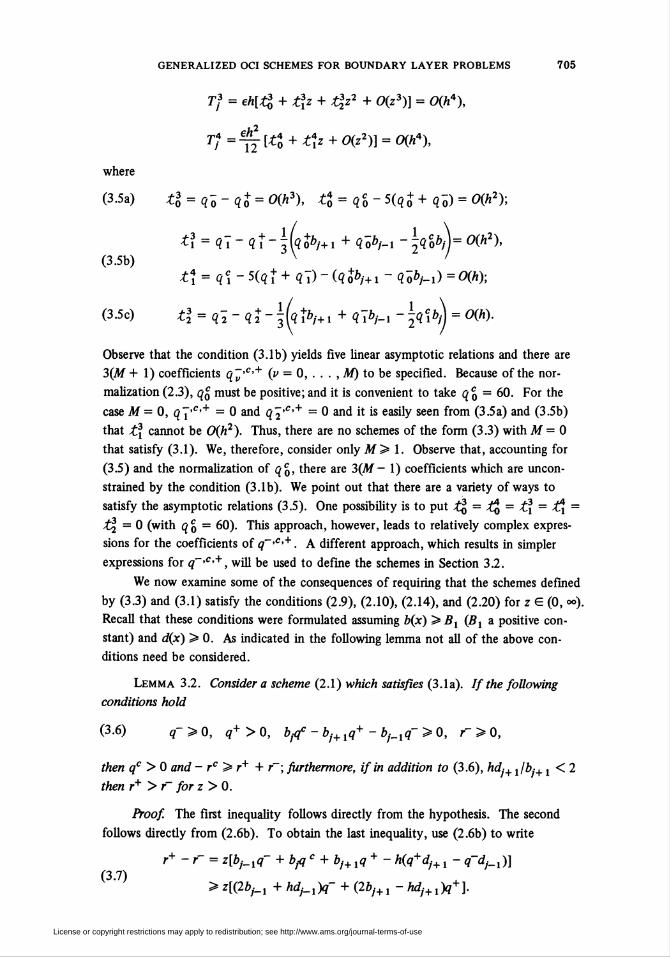
Tf = eh[4 + t\z + t¡z2 + 0(z3)] = 0(Ä4),
ah1
Tf=fj-[tt + tîz + 0(z2)] = 0(h*),
(3.5b)
(3.5a) t30 = q-0-qt = O(h3), t% = qc0 - 5(q+ + q~0) = 0(h2);
t\ = qT-qî-|kî*/+i + ubhi-\qcobj=0(h2),
ti = q\ - S(qî+ ql) - (qr>/+, - ?öVi) = °W;
(3.5c) t23 = qj - q + -^ft.+ 1 + q\bhl -\q\b\ = O(Ä).
Observe that the condition (3.1b) yields five linear asymptotic relations and there are
3(M + 1) coefficients q~'c'+ (v = 0, . . . , M) to be specified. Because of the nor-
malization (2.3), q£ must be positive; and it is convenient to take q q = 60. For the
case M = 0, q~['c'+ = 0 and q2'c'+ = 0 and it is easily seen from (3.5a) and (3.5b)
that t\ cannot be 0(h2). Thus, there are no schemes of the form (3.3) with M = 0
that satisfy (3.1). We, therefore, consider only M > 1. Observe that, accounting for
(3.5) and the normalization of qc0, there are 3(Af- 1) coefficients which are uncon-
strained by the condition (3.1b). We point out that there are a variety of ways to
satisfy the asymptotic relations (3.5). One possibility is to put t% = £q = ¿I = t\~
t3, = 0 (with q g = 60). This approach, however, leads to relatively complex expres-
sions for the coefficients of q~'c,+. A different approach, which results in simpler
expressions for q~'c'+, will be used to define the schemes in Section 3.2.
We now examine some of the consequences of requiring that the schemes defined
by (3.3) and (3.1) satisfy the conditions (2.9), (2.10), (2.14), and (2.20) for z G (0, «>).
Recall that these conditions were formulated assuming b(x) > Bx (Bt a positive con-
stant) and d(x) >0. As indicated in the following lemma not all of the above con-
ditions need be considered.
Lemma 3.2. Consider a scheme (2.1) which satisfies (3.1a). If the following
conditions hold
(3.6) q->Q, q+>0, b¡qc - bj+lq+ - bhlq~ > 0, r > 0,
then qc > 0 and - rc > r+ + r~; furthermore, if in addition to (3.6), hdj+ijbf+1 < 2
then r+ > f for z > 0.
Proof. The first inequality follows directly from the hypothesis. The second
follows directly from (2.6b). To obtain the last inequality, use (2.6b) to write
r+ - r = z[b¡_iq- + bjqc + b,+ ,q+- h(q+dj+, - q'd^)]
> z[(2bhl + hdhl)q- + (2bf+1 - hdi+i)q+].
License or copyright restrictions may apply to redistribution; see http://www.ams.org/journal-terms-of-use
706 ALAN E. BERGER ET AL.
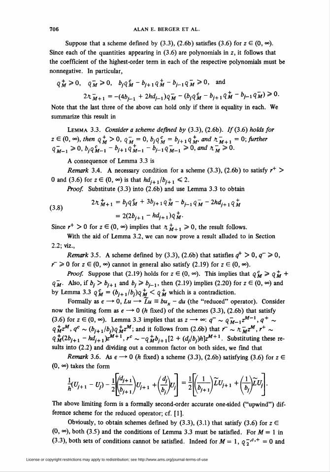
Suppose that a scheme defined by (3.3), (2.6b) satisfies (3.6) for z G (0, °°).
Since each of the quantities appearing in (3.6) are polynomials in z, it follows that
the coefficient of the highest-order term in each of the respective polynomials must be
nonnegative. In particular,
qM>0, qM>0, bjqcM-bj+1qM-bj_lqM>0, and
24-M+1 = -(4&,-i + IMi-Mni - (brfM -bj+tltt- bM4m) > °-
Note that the last three of the above can hold only if there is equality in each. We
summarize this result in
Lemma 3.3. Consider a scheme defined by (3.3), (2.6b). V/(3.6) holds for
z G (0, °°), then qM>0,qM = 0, bfqcM = bf+ j q + , and Kja+ x = 0; further
q~M-i >Q'bfqcM^-bj+lq+M_l-bhiqM_l>0,andfiM>0.
A consequence of Lemma 3.3 is
Remark 3.4. A necessary condition for a scheme (3.3), (2.6b) to satisfy r+ >
0 and (3.6) for z G (0, °°) is that hdj+Jbf+ x < 2.
Proof. Substitute (3.3) into (2.6b) and use Lemma 3.3 to obtain
,, „ 2*m+ i = b,qm + 3*/+ iqM~bhlqM- 2hdj+ ,q+M
= 2(2Z>/+1 -hdj+i)qM.
Since r+ > 0 for z G (0, °°) implies that fiM+i >0, the result follows.
With the aid of Lemma 3.2, we can now prove a result alluded to in Section
2.2; viz.,
Remark 3.5. A scheme defined by (3.3), (2.6b) that satisfies q+ > 0, q~ > 0,
f > 0 for z G (0, °°) cannot in general also satisfy (2.19) for z G (0, °°).
Proof. Suppose that (2.19) holds for z G (0, °°). This implies that qM > qM +
qM. Also, if bj > bj+1 and b¡ > b¡_l, then (2.19) implies (2.20) for z G (0, °°) and
by Lemma 3.3 qM = (b¡Jrilbj)qM < qM which is a contradiction.
Formally as e —*■ 0, Lu —* Lu = bux - du (the "reduced" operator). Consider
now the limiting form as e —► 0 (h fixed) of the schemes (3.3), (2.6b) that satisfy
(3.6) for z G (0, °o). Lemma 3.3 implies that as z —► °°: q~ ~ qM^lzM~1, q+ ~
qliZ1*, qc ~ (bj+llbj)qMz?4; and it follows from (2.6b) that r ~ HMz^, r+ ~
qi(2*/+ i-hd/+l)z*t+l,re~-q + b/+,[2 + (djlbj)h\zM+ ». Substituting these re-
sults into (2.2) and dividing out a common factor on both sides, we find that
Remark 3.6. As e —► 0 (h fixed) a scheme (3.3), (2.6b) satisfying (3.6) for z G
(0, °°) takes the form
K.-^-feM^;W4J., +Í-T-W;W"*' 6<r'J
The above limiting form is a formally second-order accurate one-sided ("upwind") dif-
ference scheme for the reduced operator; cf. [1].
Obviously, to obtain schemes defined by (3.3), (3.1) that satisfy (3.6) for z G
(0, °°), both (3.5) and the conditions of Lemma 3.3 must be satisfied. For M = 1 in
(3.3), both sets of conditions cannot be satisfied. Indeed for Ai = 1, q2'c'+ = 0 and
License or copyright restrictions may apply to redistribution; see http://www.ams.org/journal-terms-of-use
GENERALIZED OCI SCHEMES FOR BOUNDARY LAYER PROBLEMS 707
Lemma 3.3 implies q~[ = 0 and b¡q\ = bJ+lq'f. It follows from (3.5c) that q f =
0(h) and the condition t\ = 0(h2) in (3.5b) cannot be satisfied. For M = 2 in (3.3)
the situation is more complex, but for the case of b(x) = b (a constant) and d(x) = 0
it can be shown that the conditions of Lemma 3.3 and (3.5) are incompatible. We
sketch here this demonstration leaving the details to the reader. Put qc0 = 60 and use
(3.5a) and (3.5b) to obtain asymptotic relations for q\ and q\ in terms of q\. Note
that lOqY = q\ - 30ft + 0(h). By Lemma 3.3, q2 = 0 and q J = q2. Now use
(3.4c) and (3.5c) to obtain 5^l2 = -@qï ~ 30Z>) + 0(h). But Lemma 3.3 also re-
quires that q~[ > 0 and fi2 > 0. Hence, for sufficiently small h there is a contradic-
tion. These observations have led us to the consideration of M = 3 in (3.3) which will
occupy the remainder of this section.
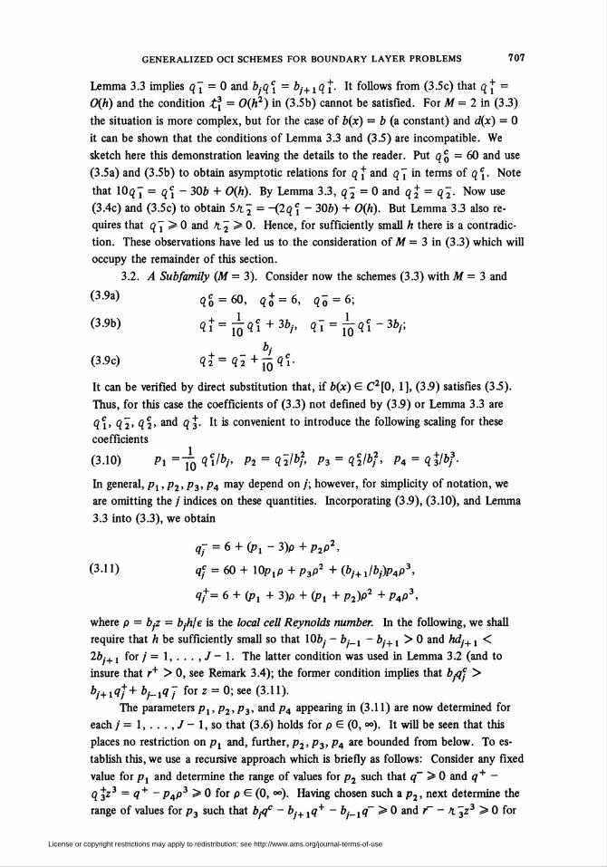
3.2. A Subfamily (M = 3). Consider now the schemes (3.3) with M = 3 and
(3-9a) qc0 = 60, q+ = 6, q~0 = 6;
(3-9b) qí=¿qí+3i/, q7 = ^qî-3i/;
bj(3.9c) qt=ql+^qci-
It can be verified by direct substitution that, if b(x) G C2[0, 1], (3.9) satisfies (3.5).
Thus, for this case the coefficients of (3.3) not defined by (3.9) or Lemma 3.3 are
qci> Í2> q2> and q3. It is convenient to introduce the following scaling for these
coefficients
(3.10) Pi =Y0 qVbp P2 = qVbf, P3 = qc2lbf, P4 = qtlbf.
In general, pi, p2, p3, p4 may depend on /; however, for simplicity of notation, we
are omitting the / indices on these quantities, incorporating (3.9), (3.10), and Lemma
3.3 into (3.3), we obtain
qj = 6 + (/>! -3)p +p2p2,
(3-10 qf = 60 + 10plP + p3p2 + (bj+ Jb^p3,
qf= 6 + (p1 + 3)p + (p! + p2)p2 + p4p3,
where p = bjz — bjh/e is the local cell Reynolds number. In the following, we shall
require that h be sufficiently small so that 10i- - è_1 - b.-+ ! > 0 and hd.+1 <
2bj+ ( for /= 1,...,/- 1. The latter condition was used in Lemma 3.2 (and to
insure that r+ > 0, see Remark 3.4); the former condition implies that b.-qf >
b/+iqf+ bj^^qj for z = 0; see (3.11).
The parameters px, p2,p3, and p4 appearing in (3.11) are now determined for
each / = 1,...,/- 1, so that (3.6) holds for p G (0, °°). It will be seen that this
places no restriction on pl and, further, p2, p3, p4 are bounded from below. To es-
tablish this, we use a recursive approach which is briefly as follows: Consider any fixed
value for pl and determine the range of values for p2 such that q~ >0 and q+ -
q \z3 = q + - pAp3 > 0 for p G (0, °°). Having chosen such a p2, next determine the
range of values for p3 such that bflc - b+ tq+ - b_iq~ > 0 and r~ - >t\z3 > 0 for
License or copyright restrictions may apply to redistribution; see http://www.ams.org/journal-terms-of-use
708 ALAN E. BERGER ET AL.
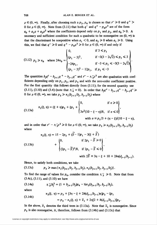
p G (0, °°). Finally, after choosing such a p3, p4 is chosen so that f > 0 and q+ >
0 for p G (0, °°). Note from (3.11) that both q~ and q+ - p4p3 are of the form
a0 + a,p + a2p2 where the coefficients depend only onp1 and p2, and a0 > 0. A
necessary and sufficient condition for such a quadratic to be nonnegative on (0, °°) is
that the discriminant be nonpositive when a, < 0, and a2 > 0 when ax > 0. Using
this, we find that q~ > 0 and q+ - p4p3 > 0 for p G (0, °°) if and only if
0, if3<p,
(Pj-3)2, if-3(3-2v/2)<p,<3
-24Pl, if-3<Pl <-3(3-2V2)
.0»! -3)2 - 12P!, ifp,<-3
(3.12) p2 > 7r0 where 247:0 = <
The quantities bflc - b¡+ xq + - bj_xq~ and r- - /r. 3z3 are also quadratics with coef-
ficients depending only on pt, p2, and p3 and with the zero-order coefficient positive.
For the first quantity this follows directly from (3.11); for the second quantity use
(3.11), (3.10) and (3.4) (note that fi~ = 0). In order that b¡qc - bj+1q+ - bhlq~ >
0 for p G (0, °°), we take p3 > n1(b¡+l/bj, bj_í/bj) where
0, if o>0
(3.13a)ffitt» V) - (% + V)P2 + £Pi +
3o2(10 - £ - Tj)/8, ifo<0)
with a = p,/3 + (n - 0/(10 - ç - r¡),
and in order that r - n. 3z3 > 0 for p G (0, °°), we take p3 > 7r2(Z>/+ \lb¡, bJ_l/bj)
where
ff2ft, tí) = 15 - 2p2 +(S- l)Pl -3(| + 5)
10, if 2p, - S > 0
(3.13b)
(2pl-S)2/8, if2p1-5'<0
with 25 = 3r? - | + 10 + 2hr(dj_llbj_i).
Hence, to satisfy both conditions, we take
(3.13c) p3 > max{jr,(o/+ ,/iy, fy-,/0/)- jt2(ä/+ t/iy, bhxlbj)}.
To find the range of values for p4, consider the condition /i 3 > 0. Note that from
(3.4c), (3.11), and (3.10) we have
(3.14a) kybf = (1 + bj+llbj)pA - Kir3(bj+1lbf, b^Jbj),
where
ff3(S, t?) = p3 + [3tj - ? + 2h(dhllbf_lyn]p2 - %px
= P3 - »ift. »I) + *i + 2t?[2 + h(dhllbhl)]P2-
In the above, n-j denotes the third term in (3.13a). Note that Wj is nonnegative. Since
p2 is also nonnegative, it, therefore, follows from (3.14b) and (3.13c) that
(3.14b)
License or copyright restrictions may apply to redistribution; see http://www.ams.org/journal-terms-of-use
GENERALIZED OCI SCHEMES FOR BOUNDARY LAYER PROBLEMS 709
7T3(Z)/+ Jbj, bj_l/bf) is nonnegative. Hence, in order to satisfy K.3 > 0 and p4 > 0,
we take
(3.15) p4 >m + bi+ 1/6/r1T3(iy+1/*/. W/)-
It is obvious from the above that r~ > 0 and q + > 0 for p G (0, °°) if (3.12), (3.13c),
(3.15) hold. We now show that under these conditions, q+ > 0 for p G (0, °°). Note
that o+ = 0 is possible only if p4 = 0 which in turn is possible only when equality is
taken in (3.15) and it3 = 0; further, by (3.14b), ti3 = 0 only if p2 =0 which by
(3.12) is possible only if pj > 3. But for pl > 3, p2 = 0, p4 = 0 it follows from
(3.11) that q+ > 0 for p G (0, °°). We summarize the above results in
Theorem 3.7. Assume that h is sufficiently small so that lOfy - bj+, - b}_x >
0 and hdf+, /bj+1 <2 for j = I, . . . ,J - 1. Then, the OCI schemes defined by
(2.1), (3.11), and (2.6b) with px arbitrary and p2,p3, and p4 satisfying (3.12), (3.13c),
and (3.15), respectively, will satisfy the following for each /,/= 1, ...,/- 1, and
0 < hie < °°:
q->0, qc>0, q+>0, btf > bj+lq+ + bhiq~, and
r+ >r~> 0, -rc>r+ + r.
Note that the parameters px and p2 do not necessarily depend on / and, thus, in
practical calculations can be chosen, subject to (3.12), once and for all. The lower
bounds for p3,p4, however, indicate that these parameters will need to be determined
for each /,'/ = 1, . . . , / - 1. Concerning the choice of the parameters, the error
analysis in Section IV indicates that better convergence behavior is achieved when
r~/r+ is small, particularly, in the limit as z —► °°. This suggests choosing p1,p2,p3,
p4 so that the coefficient of the highest degree term in f is made as small as possible.
In this regard, if p4 is defined by taking equality in (3.15), then h. 3 = 0, cf. (3.14a).
It one also takes pl > 3, p2 = 0, and p3 defined by equality in (3.13c), it follows
(as we shall see below) that H.2 = 0(h). Furthermore, /i~ = 0(h) when p, = 3. For
definiteness, and motivated by the above observations, for the error analysis in Section
IV and the numerical experiments in Section V, we will consider the following sub-
family of the OCI schemes defined in Theorem 3.7:
(3.16a) schemes defined by (2.1), (3.11), (2.6b) with
Pi ^y fkœd constant (i.e., the same for; = 1, ...,/- 1), and(3.16b)
p2 = 7T0 (see (3.12)), and
C\ 16 1 ^or eac^ ' = 1 > • • • > "^ - 1 > P3 an<* P4 are defined by equality in
(3.13c) and (3.15), respectively,
under the assumption that h is restricted so that
lObf ~bhl- bi+ 1>B0>0, 2 - hdi+1lbj+ ! > B0 > 0(3.16d)
0"=i,...,/-i),where B0 is any positive constant smaller that 8 • min{b(x)} and 2. The error anal-
ysis, and the numerical results in Section V tend to suggest the choice pt = 3 in (3.16)
License or copyright restrictions may apply to redistribution; see http://www.ams.org/journal-terms-of-use
710 ALAN E. BERGER ET AL.
when solving (2.7). For the case d = 0 and b a constant, and with p = bh/e, this
scheme is given by
(3.17a) q~ = 6, qc = 60 + 30p + 9p2 + 1.5p3, q+ = 6 + 6p + 3p2 + 1.5p3 ,
(3.17b) r = 72, r+ = 72 + 72p + 36p2 + 12p3 + 3p4, r° = -f - r+.
One can observe that r~/r+ from (3.17) is the (4,0) Padéapproximation to e~p (e.g.,
[8], [30, p. 269]).We remark that even if the schemes given in (3.16) appear somewhat complicated,
it is actually quite simple to program the evaluation of rj'c,+ , qj'c'+ (using (3.11)
and (2.6b)). The relative efficiency of (3.16) will depend on (among other things) the
balance between its possibly better accuracy (in principle requiring fewer mesh points
to obtain a satisfactory solution) and the somewhat larger number of operations re-
quired to evaluate each coefficient of R and Q. The use of fewer mesh points is par-
ticularly significant in applications where many operations are required to evaluate b
and d at each grid point.
3.3. Some Properties of R for Schemes (3.16). The following technical results
concerning (3.16) will be used in the error analysis in Section IV. Let / be given and
suppose b]+1 = bj_x = b¡ and d = 0. Then for a scheme (3.16) the resulting R co-
efficients (denoted by Tj'c'+) are given by
(3.18a) rj = 72 + (12Pl - 36)p + (6 - 5Pl + 2p2 + p3)p2,
Tf = 72 + (12p. + 36)p + (6 + 7p. + 2p, + p3)p2(3.18b) '
+ (lip, + p2 + .5p3 + 2p4)p3 + 2p4p4,
(3.18c) rf =-7j -7f where p = bfi/e.
Observe that, in the above, p3 and p4 are constants defined by equality in (3.13c)
and (3.15) with bj+l = bJ_1 = b¡ and d/_1 = 0. The quantities Tf will be used to ap-
proximate rf. In what follows, it will be convenient to consider rf as functions of
p = bjh/e; viz.,
(3.19) rf= ¿ Ky, rj= ¿ n.~p\i»=0 v=0
where it is understood that h. * in general depend on /. (Note the change in notation
from (3.4)). The corresponding coefficients in (3.18) will be denoted by >if,. From
the definitions (3.16), (3.18), (3.19), it can be seen that
Remark 3.8. Given a scheme (3.16), for each / (j = 1, . . . , / - 1) it is true
that
(3.20a) 1*7 -^7| + \K2 -7Li\<Oi and fi~0 = 12,
(3.20b) 1^+ _£+| + . . . + LI + -4+KC& and ^.¿" = 72,
where Cis a constant depending only on 5t = {p,, B0, min b, max(Z>, d, \b'(x)[f).
With this result one can show that
License or copyright restrictions may apply to redistribution; see http://www.ams.org/journal-terms-of-use
GENERALIZED OCI SCHEMES FOR BOUNDARY LAYER PROBLEMS 711
Lemma 3.9. Consider an OCI scheme (3.16). Then there exists a constant c >
0 such that for h <c and for each /=1,...,/-1,
(3.21) fit -H\>B2 >0, M + >0, H + >B3>Q,
where the positive constants c, B2, and B3 depend only on Sv Also, rj'c'+ and
qj'c'+ considered as polynomials in z (or p) have coefficients that are bounded in
magnitude by some constant B4 depending only on 5,.
Proof. The second part of the lemma is obvious from (3.16). For the first
part, Remark 3.8 indicates that we need only consider Tj'+ given by (3.18) (i.e., the
case bj+1 = b¡_1 = b¡,d = 0). Now from the way in which the schemes (3.16) are
chosen, the coefficients of p2 in q~,q+, and qc - q~ - q+ are nonnegative; and
hence, p2,pl + p2, and p3 - Pi - 2p2 are nonnegative. Further, from (3.12), p2 > 0
when p, < 3. From (3.15), 2p4 = p3/2 + p2 - p,/2 and so %3=p1 + 2p2 +p3>
2(Pi + P2) + 2p2 > 0. Now ̂ 7 - Tj" = 72, so it remains to deal with \\ = 2p4.
But 2p4 > (pj/2 + p2) + p2 - Pi/2 = 2p2 which is positive when p, < 3. Suppose
pt > 3. Then itl = pl while tt2 = 5pt - 6 so p3 = 5p, - 6 and 2p4 = 2p1 - 3 and
the result follows.
3.4. Diagonal Dominance for Parabolic Problems. We now consider the tri-
diagonal matrix QA - (At/2zh)R that arises in applications of (2.2) to parabolic equa-
tions; cf. Section 2.2. We confine our attention to the class of schemes defined in
Theorem 3.7 and determine sufficient conditions for the diagonal dominance of this
matrix for z G (0, °°). Observe that if the matrix QA is itself diagonally dominant for
z G (0, oo) then the diagonal dominance of QA - (At/2zh)R would follow immediately
from (2.9). However, QA cannot in general be diagonally dominant for z G (0, °°)
becuase of the particular form of the highest-order terms in q+ and qc required by
Lemma 3.3. As a preliminary result consider the condition
(3.22) afcf - q\z3) - aj+l(q+ - q +z3) - ahlq~ > 0.
Note that (3.22) is the condition for diagonal dominance of the product of A with the
matrix Q in which the highest-order terms in qc, q+ are removed. As can be readily
seen from (3.11) and (3.10), this condition is analogous to the condition (2.20) with
the function b(x) replaced by a(x, f) (t fixed). Recall that it is assumed that a(x, t) >
A0 > 0. Hence, (3.22) is satisfied for z G (0, °°) if 10ay - a/+ j - a,_i > 0 and p3 >
1li(aj+ilaj> ai-Ja¡)- This result is now used to prove the following
Theorem 3.10. Assume that h is sufficiently small so that hdj+1/b)+, < 2,
10ft;- - bj+, - bf_i > 0, and 10a,- - a]+, - ahl > 0, / = 1, . . . , / - 1. Consider an
OCI scheme defined in Theorem 3.7 and such that for j = 1, . . . , J - 1,
p3 > max{ir1(i/+1/ô/, b^Jbf), if2(bf+llbf, bhJbj), íTi(«/+,/^,«M/«/)}•
Then for k a positive constant satisfying
!a,+ íbj-ab+1)■■ 4; \*"ml.■"'■
the tridiagonal matrix QA - (k/z)R is strictly diagonally dominant for z G (0, °°).
License or copyright restrictions may apply to redistribution; see http://www.ams.org/journal-terms-of-use
712 ALAN E. BERGER ET AL.
Note that for the applications in Section 2.2, k = At/2h. Hence, the above con-
dition on k is satisfied if Ch2 < Ai where C is independent of e and h.
Proof. The hypothesis implies that the results of Theorem 3.7 and (3.22) hold
for z G (0, °°). Note that 4>c = qcaj - (k/z)rc > 0. Let 0* = q±aj±i - (fr/zy*. We
will establish that $ = <¡>c - |0+1 - |#~| > 0. First assume that <j>+ > 0, then
$ = (fa, - q+aj+l + q~aj_x + (k/z)(-rc + r+ ± r)
> qcaf - q+aj+l - q~ahl + (k¡z){-rc + r+ - r).
It follows from (2.6b) that
- rc + r+ - r > z[q+(3bj+, - hdj+,) + qcb} - q-bM ] > 2zq+b¡+,
>2z\tbi+l.
The last inequality in the above is obtained using the fact that q+ - z3q+ > rj. It
then follows using (3.22) that
$ > z3[a,q% -aj+lqt + 2kbj+ iq%] = z3[ajbj+ Jb, - aj+, + 2kb,-+ t]q%.
Since q 3 = p¡jbf > 0, we conclude that for k restricted as indicated, 4> > 0 if ct>+ >
0. Assume now that <j>+ < 0, then
$ = acay + q +a/+, T q~ahi + (klz\-rc - r+ ± O > qcaf + q+a,+, - q~ahl.
Since q+ > 0, q+ - q +z3 > 0, q% > 0, it follows using (3.22) that $ > 0 for 0+ <
0 which completes the proof.
rV. Error Estimates.
4.1. Statement of Results. In this section we will establish an error estimate for
the family of OCI schemes (3.16) applied to the problem (2.7). Also for comparison,
the convergence behavior for several other schemes applied to (2.7) will be given. In
this section (unless otherwise stated) it will be assumed that
(4.1) 0 < Bt < b(x) for some constant B1,
(4.2) b(x) and d(x) ¡Lie in Cm[0, 1],
with Bs = Hell and B6 = \\d\\ in Cm[0, 1] (i.e., Bs bounds the magnitude of the fth
derivative of b for / = 0, 1, . . . , m, etc.). The function /in (2.7) may depend on e
such that f(x, e) has m continuous x-derivatives satisfying
(43) \fii\x, e)| < Bn + ^r'expi-Sjx/e)
for i = 0, 1, . . . , m, x in [0, 1], and e in (0, 1], where B1 and S, are positive con-
stants (independent of x and e). The choice m = 5 is used in the analysis of (3.16),
and is indeed sufficient for the other schemes to be considered here. Let 2?8 denote
la0l + lot! |.To state (and prove) the error estimate, we need to describe a particular function
associated with each scheme (3.16). Let a specific value for pl be given and consider
for the moment the situation where b(x) is some positive constant ß and d = 0. Then
p2 and p3 defined by (3.16) are constants depending only on pt. Define p3 by
License or copyright restrictions may apply to redistribution; see http://www.ams.org/journal-terms-of-use
GENERALIZED OCI SCHEMES FOR BOUNDARY LAYER PROBLEMS 713
(4-4) ,-,= " + 1 "><\{P3+h if Pl > 3)
and p4 by equality in (3.15) with p3 = p3, i.e., pA = (p3 + 2p2 - Pi)/4. Now de-
fine pT = p~(ß) and p+ = u+(ß) by (cf. (3.18))
(4.5a) pT = 72 + (12pt - 36)p + (6 - 5pt + 2p2 + p3)p2,
"+ = 72 + (12pi + 36>° + (6 + 7Pi + 2P2 + P3)P2(4.5b)
+ (1.5p! + p2 + .5p3 + 2p4)p3 + 2p4p4,
where p = ßz = ßh/e, and define
(4.5c) p. = p(ß) = pr(ß)lp+(ß).
Throughout the rest of this paper c, C, c¡, C¡ (i = 1, 2, . . .) will be used to denote
generic positive constants which may depend on elements of the set S = 52 U
{B0, pj} where 52 = {B1, B5, B6, B7, 5 ¡, Bs}, but which are independent of h and
e. Also, {Uj} (J = 0, 1, . . . , /) will be used to denote the approximation to the
solution of (2.7), {u(xj)}, obtained by (2.8) and whichever scheme is being discussed.
Our error estimate is given by
Theorem 4.1. Let {Uj\ be obtained by an OCI scheme (3.16). Then there are
constants o and C depending only on S such that for j — \, . . . ,J - \,
(4.6a) \U¡ - u(xj)\ < Ch*e-2 + Ch*e-*u(o)i when h < e,
(4.6b) \U¡ - u(xj)\ <Ch2 + Cp(oy when e < h,
with p(a) defined by (4.5).
For e fixed, (4.6a) clearly implies 0(h4) convergence. Also, when e is sufficiently
small relative to h, (4.6b) shows that the error is 0(h2) at every mesh point. In par-
ticular, this is true when p, < 3 and e < Ch2; when pl > 3 and e < Chs^3; and when
Pj = 3 and e < Ch3l2. To verify this, one need only check that p(a) has the required
behavior as ah/e —► °°. The numerical results given in the next section indicate that
the estimates (4.6) are "sharp." Later in this section we will also prove
Corollary 4.2. Let {Uj\ be obtained by an OCI scheme (3.16), and let x be
a given number in (0, 1). Then there is a constant Cx depending only on x and S
such that
(4.7a) \Uj - u(xf)\ < Cxh4e~2 for h<e, x¡ in [x, 1],
(4.7b) \Uf - u(x,)\ < Cxh2 for e < h, x¡ in [x, 1 ].
In particular, Corollary 4.2 shows that the error is always 0(h2) "away from the
boundary layer." The above results make rigorous the comments in the introduction
concerning the error behavior of the OCI schemes. The proof of Theorem 4.1 utilizes
the comparison function techniques employed by Kellogg and Tsan in [16]. The anal-
ysis of the OCI schemes, however, is more complicated because of the more complex
License or copyright restrictions may apply to redistribution; see http://www.ams.org/journal-terms-of-use
714 ALAN E. BERGER ET AL.
nature of the schemes, and in particular (as will be seen) because q~ is not zero. Be-
fore giving the proof, we present, for comparison, convergence results for several other
schemes for (2.7).
4.2. Convergence Results for Other Schemes for (2.7). Using the same procedures
as in the proof of Theorem 4.1, one can prove the following result for the standard
OCI scheme:
Theorem 4.3. Let {Uj) be obtained by the standard OCI scheme (2.6). There
are constants a, c, and C depending only on S2 such that if h/e < c, then one has
(4.8) \Uj - u(Xj)\ < ChAe~2 + Cli4e-4(1 + ah/ep for / = 1, ...,/- 1.
We have briefly considered the scheme resulting from the use of interpolating
cubic finite elements to solve (2.7) with b constant and d = 0. Using nodal condensa-
tion (see for example [5], [29]) followed by a local quadratic approximation of / to
obtain a~'c,+ (i.e., / at x¡ ± A/3 and x¡ ± 2h/3 is evaluated using the quadratic passing
through f(Xj_ l ), f(xj), f(x¡+ j )), we obtain the following formally fourth-order scheme
for (2.7) (b constant, d = 0),
q- = 6 - 3p + .2p2 where p = bh/e,(4.9a)
ac = 60 + .8p2, q+ = 6 + 3p + .2p2.
r = 12- 36p + 7.2p2 - .6p3,(4.9b)
r+ = 72 + 36p + 7.2p2 + .6p3, rc = - r - r+.
Note that (2.6b) is valid for (4.9), and r~/r+ is the (3,3) Pade approximation to e~p.
By the same type of analysis as used for Theorems 4.1 and 4.3 one has
Remark 4.4. Assume b is constant and d = 0. Let {Uj) be obtained by (4.9).
There are constants a, c, and C depending only on S2 such that if h/e < c, then
(4.10) \Ut - u(xf)\ < Oi4e-2 + C7z4e-4(1 + oh/ep for / = 1,_/- 1.
Since (4.9) suffers a formal cell Reynolds number limitation, we have not pursued
the derivation and analysis of the corresponding difference scheme for variable b and d.
We now present results for the classical centered and upwind schemes. The
centered scheme for (2.7) is given by
rj - 1 - bh/(2e), rf - - 2 - h2d,/e,(4.11) ' ;
rf m 1 + bjhlQë), qf=\, qj = qf =0.
Abrahamsson, Keller, and Kreiss [1] have obtained an error estimate for (4.11) applied
to (2.7) by expanding the true and approximate solutions in powers of e, h, and hie.
This approach permits treatment of certain systems generalizing (2.7). For the scalar
equation (2.7), the following result is also obtainable by comparison function
techniques.
Theorem 4.5 (Abrahamsson, Keller and Krebs [1]). Let {Uj\ be obtain-
ed by the centered scheme (4.11). There are constants a, c, and C depending only on
License or copyright restrictions may apply to redistribution; see http://www.ams.org/journal-terms-of-use
GENERALIZED OCI schemes for boundary layer PROBLEMS 715
S2 such that if h/e < c, then
(4.12) \Uj - u(xj)\ <Ch2 + Ch2e~2(l + ah/ep for j - 1,...,/- 1.
The classical first-order upwind scheme for (2.7) is given by
77 = 1, rc = -2-bjhle-h2djle,(4.13) iiii
rf = \+b¡hle, qf=\, qj = qf = 0.
For this scheme one has
Theorem 4.6 (Kellogg and Tsan [16]> Let {Uj} be obtained by the up-
wind scheme (4.13). Then there are constants a and C depending only on S2 such
that for /= 1, ...,/- 1,
(4.14a) \Uf - u(x¡)\ <Ch + Í7ze_1(l + ah/ep when h<e,
(4.14b) \Uf - u(Xj)\ < Ch + 0(1 + ah/ep when e < h.
Note that (4.14b) implies that the error at all the grid points is 0(h) when e <
Ch2.
An upwind scheme which is second order for "small" e was presented and anal-
yzed in [1] (see (1.12) therein). A slight variant of this scheme is
»7=1, rf = - 2 - .5(0, + b,+ !)A/e - d,h2/(2e),(4.15)
rf = 1 + .5(Z>,. + bj+ !)h/e - dj+lh2l(2e), qf = qf =%, qj = 0.
The scheme (4.15) satisfies Tf = Tf = 0. The following error estimate of [1] can be
obtained by the comparison function approach as well.
Theorem 4.7 (Abrahamsson, Keller and Kreiss [1]). Let {Uj\ be
obtained by the upwind scheme (4.15). There are constants a, c, and C depending
only on S2 such that if h < c then for j = 1, . . . ,J' - 1, one has
(4.16a) \Uj - u(xj)\ <Ch2 + Che + Che~l(l + ah/ep when h < e,
(4.16b) \Uj - u(xj)\ < Ch2 + 0(1 + ah/ep when e<h.
This scheme is 0(h) for fixed e, while achieving 0(h2) at all the grid points
when e < C7j3. We note that (4.15) can also be obtained using "upwind" linear finite
elements [13] with a certain treatment of the integral containing d(x).
It can be observed that of the schemes presented thus far, (3.16) displays the
best theoretical convergence behavior. We now turn our attention to uniformly ac-
curate schemes. The first such scheme, originally given by Allen and Southwell in [2], is
rj = p • exp(-p)/[l - exp(-p)], rf = rje",
(4.17) 'rf = -rj - rf - djh2\e, qf = 1, qj = qf = 0, where p = bjh\e.
The scheme (4.17) has been shown in [14], [16], [21] to be uniformly 0(h) for (2.7).
The sharpest estimate is obtained in [16]; viz.,
License or copyright restrictions may apply to redistribution; see http://www.ams.org/journal-terms-of-use
716 ALAN E. BERGER ET AL.
Theorem 4.8 (Kellogg and Tsan [16]> Let {Uj) be obtained by the scheme
(4.17). Then there are constants a and C depending only on S2 such that for j =
(4.18) Wj - u(Xj)\ < Ch2/(h + e).
Note that the estimate (4.18) implies uniform 0(h) convergence, as well as 0(h2)
behavior for fixed e. The following scheme was formulated by El-Mistikawy and
Werle in [9]; cf. also the references in [9]. When d = 0, it has the form given below
(note (4.19) can also be obtained by using "upwind" linear finite elements with
"optimal" one-point quadrature; see [13]).
rj = p- exp(-p~)/[l - exp(-p-)], rf = p+/[l - exp(-p+)],
(4.19) rj=-rj-rj, qj = (I - rj)/(2p-), qf = (rf - l)/(2p+), qf = qj + qf,
where p~ = (bj_, + bj)h/(2é), p+ = (b¡ + bj+ l)h/(2e).
Using comparison function techniques, the following preliminary error estimate can be
obtained:
Theorem 4.9 (Berger, Solomon and Ciment [3]> Assume d = 0, and let
{Uj} be obtained by (4.19). Then there are constants a and C depending only on S2
such that for / = 1,...,/- 1,
(4.20a) \Uj - u(Xj)\ <Ch2 + Ch2e~1 exp(-o^./e) when h<e,
(4.20b) \Uj - u(Xj)\ <Ch2 + Ce ■ expí-ox^./e) when e<h.
Using this result in a manner to be indicated in Section 4.3, one can obtain the
following estimate:
Theorem 4.10 (Berger, Solomon and Ciment [3]> Assume (4.1), d = 0,
and b(x) and f(x) are in C*[0, 1] (here f does not depend on e). Let {Uj} denote
the approximate solution of (2.1) obtained by (4.19). Then there is a constant C de-
pending only on b, f, a0, o^ such that
(4.21) \U¡ - u(xj)\ <Ch2 forj=\,. . . ,J-l,ein (0, 1].
The scheme given in [9], in the case d J= 0, can be written in the following form.
Let ïïj denote the negative root of ew2 + (bj_t + bj)w/2 - (df_1 + dj)/2 = 0, and
let kl denote the nonnegative root. Define nl = hnl and kl = hk1. Similarly define
n2 and k2 using the quadratic ew2 + (b¡ + bj+ i)w/2 - (d¡ + d¡+1)/2. Define the
functions e(w) = exp(w), g(w) = (e(w) - l)/w with g(0) s 1 ; and let 2vx =
[1 - e(nl - fc,)]-1 and 2u2 = [1 - e(n2 - k2)]~l■ The scheme [9] then has the form
rj = e("i)/s("i - kx), rf = e(-k2)/g(n2 - k2),
(4.22) ri = _Ml ~ ^"i ~ fci) + *2 " ll&ni - *a)>
<lj = «(« i >i - e(n, )g(-kl )v1,
qf = g(-k2)v2 - e(-k2)g(n2)v2, qf = qj + qf.
License or copyright restrictions may apply to redistribution; see http://www.ams.org/journal-terms-of-use
GENERALIZED OCI SCHEMES FOR BOUNDARY LAYER PROBLEMS 717
One can verify that when d = 0, (4.22) becomes (4.19). The results of a numerical
experiment (to be reported in [3]) are consistent with the assertion that (4.22) is
uniformly 0(h2) for (2.7) when b, d, and /are "smooth." It appears to us that the
extension of Theorems 4.9 and 4.10 to the case d =£ 0 by comparison function tech-
niques would involve a formidable amount of algebra, if not more serious difficulties.
The following result suggests that 0(h2) is the best uniform order of accuracy
obtainable by the schemes we are considering:
Theorem 4.11. Consider an arbitrary scheme of the form (2.1) (here rj, . . . ,
qf can be arbitrary functions of bj_l, b¡, b¡+,, dj_1, d¡, d¡+1, h, and e), and let Tj
be defined by (2.4)-(2.5). Assume rj > 0, (2.10) is true, and (for proper scaling)
assume qf = 1. Then it cannot be true that \Tf\ < Ch2+S for e in (0, 1] and k' = 1,
2, 3 (here C and S denote positive constants independent of h and e).
The proof (given later) is similar to that of Theorem 4.5 of [16] which states
that if also q~ = q+ = 0, then \Tf\ + \Tf\ cannot be uniformly 0(h1+s). It is an
open question whether there is a scheme of the form (2.1) which has an error behavior
combining the best aspects of the generalized OCI schemes and the uniformly 0(h2)
scheme, perhaps behaving like 0(h4/(h2 + e2)).
4.2. Outline of the Proof of Theorem 4.1. We now outline the proof of Theorem
4.1 in a sequence of lemmas (lengthy proofs are deferred to the end of the section).
The first two lemmas bound the behavior of the solution u of (2.7), and are used in
estimating the truncation error t¡.
Lemma 4.12 (Kellogg and Tsan [16]). Equation (2.7) has a unique solution,
and there are positive constants S and C depending only on S2 such that
(4 23) |m(°(JC)I < CT1 + e_'exP(~2S^/e)] for i = 0, 1, . . . ,m + I
( ' ' (mis that of(4.2)).
Lemma 4.13 (slight extension of Lemma 2.4 of [16]). The solution of (2.1) can
be written in the form
(4.24a) u(x) = (-eux(0)/b(0))exp(-b(0)xle) + w(x),
where, for some positive constants 5 and C depending only on S2
(4.24b) \wV\x)\ < C[l + e_/+ lexp(-2ox/e)] for i = 0,1.m + 1.
Note that by Lemma 4.12, \eux(0)/b(0)\ < Ct.
The next two remarks, along with Remark 2.2, give the basis of the comparison
function approach used here. As in [16], two comparison functions, ty = -2 + Xj and
i¡/j = \/jj(ß) = -[u(ß)]J (for some ß > 0 to be chosen), will be utilized. The function
<t>j is used to estimate the error where u is "well behaved," while ip- estimates the error
"near" the boundary layer at x = 0. The error estimate is obtained using 0.-, \\/j, and
bounds on the truncation error, as indicated in the next two results.
Remark 4.14. Let e;- = u(xj) - U¡, then the truncation error defined in (2.4) is
Tj = eh~2Rej for / = 1,...,/- 1.
License or copyright restrictions may apply to redistribution; see http://www.ams.org/journal-terms-of-use
718 ALAN E. BERGER ET AL.
Remark 4.15. Let k^(h, e) > 0 and k2(h, e)>0 such that
eh~2R(±ej + kt(h, e)^ + k2(h, e)fy) > 0 for / = 1,...,/- 1.
Then (by Remark 2.2) \e¡\ < £,(/!, e)|fy| + *2(A, e>l^/l-
It, thus, remains to find lower bounds for eh~2R<¡>j and eh~2R\jij, and to bound
|r«|, thus determining k^(h, e) and £2(A, e) and, hence, giving the estimate for ley|. For
the rest of the proof, it is convenient to take h bounded above by some "small" con-
stant (independent of e). The following observation shows that this is permissible.
Remark 4.16. Consider any scheme of the form (2.1) with Tf = Tf = 0. As-
sume that for some given h and e (2.9) and (2.10) are valid. Then each component of
the solution {Uj} of (2.8) (for the given h and e) is bounded by some constant C,
which depends only on min b, max|/|, and |a0| + \at\.
This follows from Remark 2.2 and the fact that if C is a constant, then
eh~^R(C<l>j ± Uj) = Q(CL<t>j ± fj) which is nonnegative for C sufficiently large. The
lower bound for eh~2R<t>j is given in
Lemma 4.17. There are positive constants c and c1 depending only on S such
that when h<c¡ then for /= 1,...,/- 1,
(4.25a) e/T2Ä<fy > c when h<e,
(4.25b) eh-2R(e3h-3d>j) > c when e<h.
Proof. By Lemma 3.9, for h sufficiently small, p4 > c2 (c2 a positive constant).
Since Tf = Tf= 0, e/T2/^- = QL4>¡ > (qj + qf + ifWi- By Theorem 3.7, (2.10)is valid. Hence, since qf as a polynomial in p (see (3.11)) is positive for p > 0,
(4.25a) holds. Now by the definition of p2,qf ~P4p3 >0 and (4.25b) follows.
We now turn our attention to \¡/.-. The following technical result is used to bound
exp(-6ft/e) (with 6 as in Lemmas 4.12 and 4.13) by u.
Lemma 4.18. Let 8 be a given positive number. Then there is a constant c de-
pending on 6 andpx such that if0<ß<c, then
(4.26) exp(-Sz) <p(j3) /or0<z<°°.
Proof. For z <c1 (c1 some positive constant), exp(-6z) < 1 - 5z/2 while u(ß) >
1 - 2ßz which resolves the case of z near zero. Now p~(ß) > 0 for all p = ßz, so
u~~(ß) > c2 > 0 where c2 depends only on p1. Thus, p > c2/u+(ß); and hence, it
suffices to find ß such that c2 > p+(j3)/exp(Sz). But for any ß < 1 this will be true for
z larger than some constant C3. Now for cx <z <C3, u(ß) —> 1 as ß —* 0, and so the
result follows.
The desired lower bound for eh~2Ripj is given by
Lemma 4.19. Let 5 be as in Lemmas 4.12 and 4.13. There exist constants cx
and c2 depending only on S such that when h<ct and ß < c2 then for / = 1, . . . ,
/- 1,
(4.27a) eh-2R(eijjj(ß)) > cßp(ß)/ > cß exp(-öx;./e) for h < e,
(4.27b) eh-2R(e3h~2 i//ß)) > cßu(ß)> > cßexp(-6Xjle) for e < h,
License or copyright restrictions may apply to redistribution; see http://www.ams.org/journal-terms-of-use
GENERALIZED OCI schemes for boundary layer problems 719
(4.27c) eh-2R(e3hr2tj(ß)/p(ß)) > cßp(py^ > cpexp(-6xM/e) for e < h,
where the constant cß depends only on S and on ß.
The proof is rather involved and so will be given later.
It remains to estimate t¡. As in [16], essential use will be made of the integral
form of the remainder in Taylor's theorem (which can be derived by repeated integra-
tion by parts). For a sufficiently smooth function g(x), and numbers a and p
(4.28) •"• l! (n + 1
= -. f(p-s)V + 1)(s)*.n\ J a
Here % is a point between the points a and p. The derivative form of Rn will be used
when h < e. However, when e < h, the integral form will be used, since when p =
a ± h and g = exp(-ßx/e), this "gains" an e while only "giving up" an h (in com-
parison to the derivative form of Rn). The proof of Theorem 4.1 is completed by
estimating |*ry| and, thus, finding the k1 and k2 of Remark 4.15.
4.3. Proofs and Additional Remarks. We first treat Theorem 4.1 in the case
h < e. Recalling that Tf = Tf = Tf = 0 for the OCI schemes (3.16),
7) = TfufV + TfufV + [eh3(rf - rp/120 + eh3(qj - a+)/6]U(5>
- bj_lR3(Xj, xhl, «(1)>?7 - bj+ iR^Xj, Xj+ ,, u^)qf
(4.29) + dj^R^Xj, Xj^, u)qj + dy+ 1R4(x¡, xj+ x, iity*
+ ehr2Rs(Xj, Xj^, u)rj + eh~2Rs(Xj, xj+ !, u)rf
- eR3(Xj, Xj_x, uW)qj - eR3(xf, x¡+1, u™)qf.
The expansion out to terms involving u^ when h < e is necessary in order to dem-
onstrate the formal fourth-order accuracy of the OCI schemes. Analyzing a formally
second-order scheme generally only requires Taylor expansion out to u^ terms. To
bound the terms in (4.29), we recall the fact that the schemes (3.16) satisfy the con-
ditions (3.5), and so \Tf\ < Cehz3 and IT,41 < Ceh2z2 for h < e. Using Lemma 4.12
to bound the derivatives in (4.29) and choosing a ß sufficiently small so that Lemmas
4.18 and 4.19 are valid, we obtain, for h < e,
\Tj\ < C{ehz3(\ + e_V) + eÄ2z2(l + e-V) + e/i3z(l + e_V)
+ h4(l + e-V-1) + eh~2h6(l + r6//"1) + e/i4(l + ^V-1)}-
Since h < e, there is a constant c(ß) independent of h and e such that 0 < c(ß) <
u(ß); and so, each pf'1 in (4.30) may be replaced by pf. Then Remarks 4.14. and 4.15
and Lemmas 4.17 and 4.19 yield (4.6a).
We now obtain the estimate (4.6b) for the case z > 1. When / > 2 we write the
truncation error in the form
License or copyright restrictions may apply to redistribution; see http://www.ams.org/journal-terms-of-use
720 ALAN E. BERGER ET AL.
— ^1,-2 p r*. v t/W- j. ,1,-2r; = eh~2R2(Xj, Xj_i,u)rj + eh~2R2(Xj, xj+l,u)rf
(4.31) + {-eR0(Xj, *,-_,, u(2)) - Vi*i(*/> */-i- "(1)) + ¿j-M*,; *m, ")}<?7
+ {-eÄofy, x/+ !, m<2)) - ô/+ i/ijCxy, Xy+ !, u(1)) + df+ ̂ (Xj, xj+,, u)}a/-,
while when / = 1, we replace the term W1 = -bj^iRl(Xj, x¡_x, u^)qj by
(4.32) W, = ~bhlR0(x,, Xj_y, u<l% - bj_xhuf\j.
We now appeal to (4.24) and observe by linearity, the error in approximating u is the
sum of the errors in separately using the difference scheme for w(x) and for the first
term in (4.24a). To treat w(x), we utilize the integral form of Rn given in (4.28) with
Lemma 4.13, and also the fact thatXj
(4.33) f exp(-25s/e)da<eô_1exp(-25x_i/e).
We, thus, find that the truncation error t.- in (4.31) for the function w(x) is bounded
\Tj(w)\ < C\[erj + eqj + hqj + h2qj] j ' (1 + e-2e-26s'e)ds
(4.34)
+ [erf + eqf + hqf]Ç'+ï (1 + e-2e-26s'e)ds\ .
Then using (4.33) and Lemma 4.18, we obtain
\Tj(w)\ < C{ehrj + ehqj + h2qj + ehrf + ehqf + h2qf)
(4.35) + C{rj +qj + zqj + hzqj}e~Sx'-1'ep(ßy-i
+ C{rf + qf + zqf}e~Sx>',ep(ß)>.
The term which produced the factor zqj (i.e., W1 with u replaced by w) will be
handled separately when / = 1. Except for this, by noting that zkexp(-T6z) is bounded
(k any given positive integer, z > 0) and by using Lemmas 4.17 and 4.19, we would
have the following estimate for the error e/vv) when e < h;
(4.36) \e¡(w)\ < cíh2 + e3/T2max(/7 + qj)pJ~l + pl\.
We also have
Remark 4.20. The second summand on the right side of (4.36) is bounded by
Cut + Ch2 when e < h.
Proof. This follows by recalling (3.11), (3.18a), (3.20a), and then verifying that
for e < h; e3h~2(rj + qj)p+ < Cp~ when h2 < e, and e3h~2(rj + qj) < CTi2 when
e < h2. The cases p1 <3,p1 = 3, and px > 3 are done individually.
To complete the treatment of w, at / = 1 we use the expression (4.32) for Wt
(with u replaced by w). Now
(4.37a) \Wt | < Cqj(h + fjh1) + Chqj(\ + e^e'™*^)
and so at / = 1 it is true that
License or copyright restrictions may apply to redistribution; see http://www.ams.org/journal-terms-of-use
GENERALIZED OCI SCHEMES FOR BOUNDARY LAYER PROBLEMS 721
(4.37b) \W1\<Cqjp'-\
which completes the proof of (4.36).
To complete the proof of (4.6b) it remains to bound the error resulting from
approximating v(x) = exp(-¿>(0)x/e) (cf. (4.24a)) by the difference scheme. Let V¡ be
the approximate solution; cf. (4.38b) below. Then e/v) = \V¡- vj < \V}\ + \vj <
\Vj\ + p' (the latter step by Lemma 4.18), so it remains only to bound \V¡\. The dif-
ferential equation satisfied by v(x) is evxx + bvx - dv = g where
(4.38a) g(x) = [(b(0) - b(x))b(0)/e - d(x)]u(x);
and so
(4.38b) eh'2R Vj = G, = qjg¡_, + qfg¡ + qfg,+,.
But
(4.39) 10,-1 < C{qj(xhl/e + lty., + qf(xf/e + l)vf + qf(xf+l/e + 1)»/+1}.
Since Xj_1 = 0 at / = 1, and ykexp(-b(0)yl2) is bounded for y > 0 (k any fixed posi-
tive integer), and recalling Lemma 4.18, we have
(4.40) \Gj\ < Cqjp'-1 + Cpi.
At / = 0 and /, 7- = v.- < pt, so the discrete maximum principle (Remark 2.2) implies
that
(4.41) |71 < Ce3h~2p!'x max(ap + Ce3h~2p' + p' for e < h.i
This result, together with Remark 4.20 completes the proof of Theorem 4.1.
Proof of Corollary 4.2. Let x be given in (0, 1). We demonstrate that
Ä4e_4p(ay < C(x)h4e-2 for h < e and xf in (x, 1), and that p(o)> < C(x)h2 for e <
h and x¡ in (x, 1). First, we verify that
Remark 4.21. Given a > 0, there is a ß > 0 such that p(o) < (1 + ßh/ef1.
Proof. Recalling (4.5) and Lemma 3.9, this is easy to obtain for h/e near 0, and
for h/e large. For h/e in between; p(a) < c < 1 for some constant c, and so choosing
ß small enough so that (1 + ßh/ef1 > c gives the result.
Now if x, G (5c, 1), then / > x/h, so for the result when h < e, it suffices to find
C(3c) such that
(4.42) (1 + ßh/e)-*lh < Cfx)e2 for A < e,
which is true if and only if
(4.43) -xh-^l + ßh/e) < In C(x) + 2 ln(e) for h < e.
Observe that ln(l + ßh/e) > ßhe~l - .5ß2h2e~2. Thus, the term on the left side
of (4.43) is bounded above by -(33ce_1 + 5xß2he~2 which, since h < e, is bounded
above by (-/33c + 5xß2)e~l. Since we may assume that ß < 1, the left side of (4.43) is
bounded above by ~.5ßx/e. Hence, (4.43) is valid if C(3c) can be found such that
-.5ßx/e < In C(x) + 2 ln(e), or if e_2exp(-.5/35c/e) < C(x). Such a C(3c) indeed exists.
For the case e < h, it suffices to find a C(x) for which
(4.44) (1 + ßh/e)-*lh < C(x)h2 for e < h.
License or copyright restrictions may apply to redistribution; see http://www.ams.org/journal-terms-of-use
722 ALAN E. BERGER ET AL.
But since e < h, (1 + ßh/e) > (1 + ß); and so, the left side of (4.44) is bounded above
by (1 + ß)~xlh = exp(-3cA-1ln(l + ß)); and the result follows. We observe that
Remark 4.22. By using (4.42) and (4.44), "interior estimates" can be obtained
as well for the other polynomial schemes described in this section.
We next comment briefly on the proofs of Theorems 4.9 and 4.10 which will be
given elsewhere [3]. The demonstration of Theorem 4.9 follows the general pattern of
the proof of Theorem 4.8 done by Kellogg and Tsan [16]. The analysis of the first
term on the right of (4.24a), however, involves algebra even more involved than that
encountered in [16]. With Theorem 4.9 in hand, Theorem 4.10 is obtained by a
"bootstrapping" technique, using the decomposition of the solution u suggested by its
uniformly valid asymptotic expansion as e —► 0 (e.g., see Smith [26, p. 257]); viz.,
(4.45) u(x) = A0(x) + ^r exp T-e"1 _[* b(i-)d^ + eR0(x, e),
where c is a constant, A0 is smooth, and R0(x, e) satisfies an equation of the same
general form as (2.7). Since A0 is smooth and (4.19) is formally 0(h2) for all e in
(0, 1], it follows that the contribution to the error from approximating A0 using (4.19)
is 0(h2). The error from approximating R0 is demonstrated to be given by (4.20), so
the error from eR0 is given by e times (4.20) which is 0(h2). The final step in obtain-
ing (4.21) is to directly show that (4.19) is uniformly 0(h2) for the middle term on
the right side of (4.45). This involves lengthy but rather methodical Taylor series ex-
pansions along with the comparison function methods.
Proof of Theorem 4.11. Suppose the contrary, and consider the situation with b
constant and d = 0, and set p = bh/e. Use the expressions in (2.5) for T1 and T2 to
find that
(4.46a) 2r~ = (2 - 3p)q~ + (2 - p)qc + 2q+ + pq+ - he'1 T1 + 2e_1 T2,
(4.46b) r+ - r = pq~ + pqc + pq+ +he~iT1,
and from the expression for T3,
(4.46c) (r+ - r~) + (6 - 3p>T + (-6 - 3p>7+ = óe^h^T3.
Using the expression for r+ - f~ in (4.46b) in (4.46c) yields
(4.47) (6 - 2p)a~ + pq° - 6q+ + he~l Tl - 6e"1 h~lT3 = 2pq +.
Using the expression for pq + given in (4.47) in (4.46a) produces
(4.48) 2T = (5 - 4p)q- + (2 - .5p)qc - q+ - .5he'lTl + 2e_17'2 - 3e-1h~1T3.
Now since it is assumed that qc - l,q~ >0,q+ >0, it follows that
(4.49) 2T < (5 - 4p)q~ + 2 - .5p - .She'1 T1 + 2e~lT2 - 3e-1h'1 T3.
Multiplying (4.49) through by eh~l, letting e = ch for some constant c, and supposing
Tl,T2,T3 are 0(A2+S) for some Ô > 0 then implies that for h and c sufficiently
small f < 0, a contradiction. Note also that Theorem 4.5 of [16] can be demonstrated
in a similar fashion using (4.46a).
The last result which needs to be proven is Lemma 4.19.
License or copyright restrictions may apply to redistribution; see http://www.ams.org/journal-terms-of-use
GENERALIZED OCI SCHEMES FOR BOUNDARY LAYER PROBLEMS 723
Proof of Lemma 4.19. Since -rf > rj + rf, we have for any given ß > 0,
(4.50a) eh~2Rip0) > eh^^rjp'-1 + (rj + rf)p> - rfp>+l)
(4.50b) = eh'2pi-lrf(\ - p)(p - rj/rf).
Recall (4.5), set p = ßh/e, and write p in the form
(4.51) U(ß) = uT/p+ = (72 + pjp + p2p2)/(12 + pfp + • • ■ + p+p4).
We estimate the last three factors in (4.50b) in order to obtain (4.27). Now for h < c
and z < £*! it is true that rf > c0 (since rf at z = 0 is 72 and Lemma 3.9 obtains).
Also for h < c and z > c3, we have rf > c2z*\ cf. (3.21). For cl<z<¡ c3,Tf
(given by (3.18)) is >c5 (by Theorem 3.7). Then Remark 3.8 implies that for h < c
and cx < z < c3, rf > c6. Combining these results we have
(4.52) r/>c7 forA<c,z<l; and rf > csz* for h <c,z> 1.
We next examine (1 - p). We may suppose throughout that ß < 1. Now since
(1 + .y)-1 = 1 - y + y2 - • • • for [y| < 1, we have for p near 0
(4.53a) p = 1 - (p+ - p7)p/72 + 0(p2).
Recalling (4.5), we then have
(4.53b) p=i-ß + o(p2),
(4.53c) 2p > 1 - p > p/2 for p < c.
In particular, the latter holds for ß < c and z < 1. Now consider any given ß < 1. For
z>cl(ß) (i.e., ct can depend on 0 as well as the set S) and h < c one has p < 1/2
and so 1 - p > 1/2. For 1 < z < cx(ß) and A < c, one finds by Theorem 3.7 that
p+ > p~ and, hence, 1 - p > c2(ß) > 0, and so,
(4.54) l-p>c3(ß)>0 for h <c,z> 1.
We now have remaining the task of finding an adequate lower bound for the last
factor in (4.50b). We first consider the situation for z < 1. Following the same type
of reasoning used in obtaining (4.53) (recall Remark 3.8 and (3.18)), there results
(4.55) rj/rf = Tjfrf + Cz2 < 1 - min(b)z + Cz2 for z < c;
and so, using (4.53b), there are positive constants cl and c such that
(4.56) p - rj/rf > min(b)z - 1 + 1 - 2ßz + 0(z2) > c(ß)z ioxz<cx,ß<c.
Now for h < c and Cj < z < 1, we have rj/rf < c2 < 1 while for ß sufficiently small
and z < 1 we have p(ß) > (1 + c2)/2. Hence, we conclude that
(4.57) p - rj/rf >cx(ß)z for h < c, z < 1, ß < c.
Combining (4.50), (4.52), (4.53c), (4.57), and Lemma 4.18 yields (4.27a).
We now show that p - rj/rf > c(ß)p when z> \,h<cl,ß<c2 which with
(4.50), (4.52), (4.54), and Lemma 4.18 proves (4.27b, c). For any given ß, there are
positive constants c and c1 such that
(4.58a) p>cl when 0 < ßz < 1 and h < c.
License or copyright restrictions may apply to redistribution; see http://www.ams.org/journal-terms-of-use
724 ALAN E. BERGER ET AL.
Also, there is an 17 > 1 and a c > 0 such that
(4.58b) rj/rf < cl/2 for z > v, h < c,
and so, since p < 1,
(4.58c) p - rj/rf >ci/2> clp/2 when 0 < ßz < 1, z > 77, and h < c.
Since 0 < i?! < A(x) < Bs, there is a constant M < 1 and a constant c > 0 such that
(4.58d) rj/rf < M < 1 when 1 < z < tj and h < c.
Since p(ß) —► 1 as ]3 —► 0, there are positive constants cx,c2, c3 such that
(4.58e) p - /Ç/r+ >p-M>c3>c3p when 0 < c2, 1 < z < t?, and h < c,.
By reviewing (4.58) we find that it only remains to deal with the situation where z >
r¡ and ßz > 1. Henceforth, the latter conditions are assumed to obtain. Note that for
any given ß, p~ < Cß2z2 while, analogously to (4.52), p+ > cs^zA when h < c, and
so,
(4.59a) p < cß~2z~2 when A < c,.
Also, there are constants c and C such that p+ < C/34z4 for A < c. Consider the case
p, < 3. Then from the définition (4.4) of p3, p~ > ß2z2 ; and so, p > ß2z2/(Cß*z*) >
(cn/ß2)z-2. However, recalling (4.52), rj/rf < Cz2/(csz4) = c9z~2. Hence, if ß is
chosen small enough so that (c7/ß2) > 2c9, then
(4.59b) p - rj/rf > cgz~2 for ß < c2, A < Cl ;
and so, (4.59) gives p - fT/fy" > ^(j3)p. Taking into account the definition of p3, the
analysis of the cases px = 3 and p¡ > 3 is similar.
V. Numerical Experiments. In this section we present some numerical results
for the schemes that have been previously discussed. These results indicate that the
convergence rates described in Section IV are "sharp," and give, for one particular prob-
lem, a comparison of the accuracy of the various schemes. The problem on which the
numerical experiments were conducted was
(5.1) euxx + b(x)ux = f(x, e), x in (0, 1); «(0) = a0, u(l) = a,(e),
where b(x) = (x + l)3 and the solution u(x) is given by
(5.2) u(x) = ¡j- exp [-e"1 J* bQé)d¿\ + exp(-x/2).
The function u(x) determines f(x, e), a0, and a,(e). Note that the resulting f(x, e)
satisfies (4.3) and further |ai(e)| is bounded for e in (0, 1]. The motivation for this
choice of the form of the exact solution u comes from the expression (4.45). The first
term on the right side of (5.2) has the form of the "most singular part" of a solution
of (5.1), while the second term is smooth. Note that as e becomes much smaller than
the mesh size A, the first term becomes virtually zero at all grid points except x = 0.
Thus for e « A, u(x) and, in general, its numerical approximation are dominated by
the second term on the right side of (5.2).
License or copyright restrictions may apply to redistribution; see http://www.ams.org/journal-terms-of-use
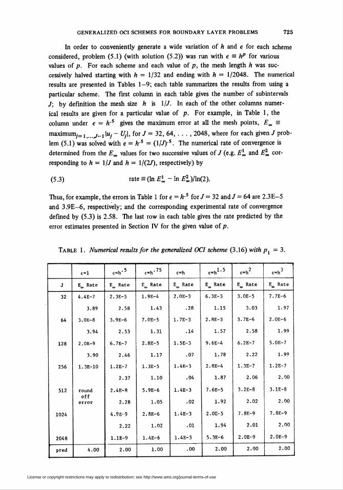
GENERALIZED OCI SCHEMES FOR BOUNDARY LAYER PROBLEMS 725
In order to conveniently generate a wide variation of A and e for each scheme
considered, problem (5.1) (with solution (5.2)) was run with e = hp for various
values of p. For each scheme and each value of p, the mesh length A was suc-
cessively halved starting with A = 1/32 and ending with A = 1/2048. The numerical
results are presented in Tables 1—9; each table summarizes the results from using a
particular scheme. The first column in each table gives the number of subintervals
/; by definition the mesh size A is 1//. In each of the other columns numer-
ical results are given for a particular value of p. For example, in Table 1, the
column under e = A-5 gives the maximum error at all the mesh points, E„ =
maximum/= j >.„>/_1 \u¡ - Uj, for / = 32, 64, . . . , 2048, where for each given / prob-
lem (5.1) was solved with e = As = (l//)'s. The numerical rate of convergence is
determined from the E„ values for two successive values of J (e.g. El, and El, cor-
responding to A = \/J and A = 1/(27), respectively) by
(5.3) rates(ln£'i0-ln£^)/ln(2).
Thus, for example, the errors in Table 1 for e = A-5 for / = 32 and/ = 64 are 2.3E-5
and 3.9E—6, respectively; and the corresponding experimental rate of convergence
defined by (5.3) is 2.58. The last row in each table gives the rate predicted by the
error estimates presented in Section IV for the given value of p.
Table 1. Numerical results for the generalized OCI scheme (3.16) with p. = 3.
e=l e=h.5
c=h75
e=h e=h1.5
e=h e=hJ
E Rate E Rate E Rate E Rate E Rate E Rate E Rate
32
64
128
256
512
1024
2048
pred
4.4E-7
3.89
3.0E-8
3.94
2.0E-9
3.90
1.3E-10
round
offerror
4.00
2.3E-5
2.58
3.9E-6
2.53
6.7E-7
2.46
1.2E-7
2.37
2.4E-8
2.28
4.9E-9
2.22
1.1E-9
2.00
1.9E-4
1.43
7.0E-5
1.31
2.8E-5
1.17
1.3E-5
1.10
5.9E-6
1.05
2.8E-6
1.02
1.4E-6
1.00
2.0E-3
.28
1.7E-3
.14
1.5E-3
.07
1.4E-3
.04
1.4E-3
.02
1.4E-3
.01
1.4E-3
.00
6.3E-3
1.15
2.8E-3
1.57
9.6E-4
1.78
2.8E-4
1.87
7.6E-5
1.92
2.0E-5
1.94
5.3E-6
2.00
3.0E-5
3.03
3.7E-6
2.58
6.2E-7
2.22
1.3E-7
2.06
3.2E-8
2.02
7.8E-9
2.01
2.0E-9
2.00
7.7E-6
1.97
2.0E-6
1.99
5.0E-7
1.99
1.2E-7
2.00
3.1E-8
2.00
7.8E-9
2.00
2.0E-9
2.00
License or copyright restrictions may apply to redistribution; see http://www.ams.org/journal-terms-of-use
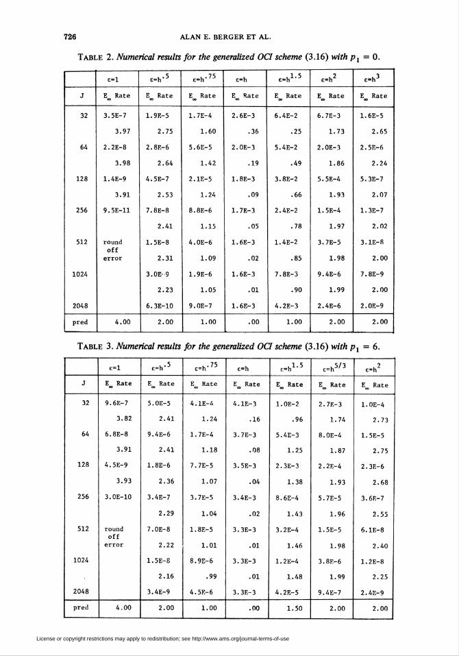
726 ALAN E. BERGER ET AL.
Table 2. Numerical results for the generalized OCI scheme (3.16) with p1 = 0.
e=l e=h.5
E=h75
E=h e=h1.5
e=h' E=h"
E Rate E Rate E Rate E Rate E Rate E Rate E Rate
32
64
128
256
512
1024
2048
3.5E-7
3.97
2.2E-8
3.98
1.4E-9
3.91
9.5E-11
round
off
error
1.9E-5
2.75
2.8E-6
2.64
4.5E-7
2.53
7.8E-8
2.41
1.5E-8
2.31
3.0E-S
2.23
6.3E-10
1.7E-4
1.60
5.6E-5
1.42
2.1E-5
1.24
8.8E-6
1.15
4.0E-6
1.09
1.9E-6
1.05
9.0E-7
2.6E-3
.36
2.0E-3
.19
1.8E-3
.09
1.7E-3
.05
1.6E-3
.02
1.6E-3
.01
1.6E-3
6.4E-2
.25
5.4E-2
.49
3.8E-2
.66
2.4E-2
.78
1.4E-2
.85
7.8E-3
.90
4.2E-3
6.7E-3
1.73
2.0E-3
1.86
5.5E-4
1.93
1.5E-4
1.97
3.7E-5
1.98
9.4E-6
1.99
2.4E-6
1.6E-5
2.65
2.5E-6
2.24
5.3E-7
2.07
1.3E-7
2.02
3.1E-8
2.00
7.8E-9
2.00
2.0E-9
pred 4.00 2.00 1.00 .00 1.00 2.00 2.00
Table 3. Numerical results for the generalized OCI scheme (3.16) with px = 6.
E=l E=h" E=h75
E=h E=h1.5
£=h5/3E=h"
E Rate E Rate E Rate E Rate E Rate E Rate E Rate
32
64
128
256
512
1024
2048
pred
9.6E-7
3.82
6.8E-8
3.91
4.5E-9
3.93
3.0E-10
round
off
error
4.00
5.0E-5
2.41
9.4E-6
2.41
1.8E-6
2.36
3.4E-7
2.29
7.0E-8
2.22
1.5E-8
2.16
3.4E-9
2.00
4.1E-4
1.24
1.7E-4
1.18
7.7E-5
1.07
3.7E-5
1.04
1.8E-5
1.01
8.9E-6
.99
4.5E-6
1.00
4.1E-3
.16
3.7E-3
.08
3.5E-3
.04
3.4E-3
.02
3.3E-3
.01
3.3E-3
.01
3.3E-3
.00
1.0E-2
.96
5.4E-3
1.25
2.3E-3
1.38
8.6E-4
1.43
3.2E-4
1.46
1.2E-4
1.48
4.2E-5
1.50
2.7E-3
1.74
8.0E-4
1.87
2.2E-4
1.93
5.7E-5
1.96
1.5E-5
1.98
3.8E-6
1.99
9.4E-7
2.00
1.0E-4
2.73
1.5E-5
2.75
2.3E-6
2.68
3.6E-7
2.55
6.1E-8
2.40
1.2E-8
2.25
2.4E-9
2.00
License or copyright restrictions may apply to redistribution; see http://www.ams.org/journal-terms-of-use
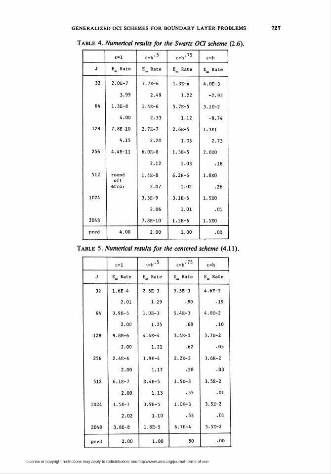
GENERALIZED OCI SCHEMES FOR BOUNDARY LAYER PROBLEMS
Table 4. Numerical results for the Swartz OCI scheme (2.6).
727
32
64
128
256
512
1024
2048
£=1
E Rate
pred
2.0E-7
3.99
1.3E-8
4.00
7.8E-10
4.15
4.4E-11
round
off
error
£=h
E Rate
4.00
7.7E-6
2.49
1.4E-6
2.33
2.7E-7
2.20
6.0E-8
2.12
1.4E-8
2.07
3.3E-9
2.06
7.8E-10
2.00
£=h75
E Rate
1.3E-4
1.22
5.7E-5
1.12
2.6E-5
1.05
1.3E-5
1.03
6.2E-6
1.02
3.1E-6
1.01
1.5E-6
1.00
e=h
E Rate
4.0E-3
-2.95
3.1E-2
-8.74
1.3E1
2.73
2.0E0
.18
1.8E0
.26
1. 5E0
.01
1.5E0
.00
Table 5. Numerical results for the centered scheme (4.11).
32
64
128
256
512
1024
2048
pred
£ = 1
E Rate
1.6E-4
2.01
3.9E-5
2.00
9.8E-6
2.00
2.4E-6
2.00
6.1E-7
2.00
1.5E-7
2.02
3.8E-8
2.00
£=h"
E Rate
2.5E-3
1.29
1.0E-3
1.25
4.4E-4
1.21
1.9E-4
1.17
8.4E-5
1.13
3.9E-5
1.10
1.8E-5
1.00
E=h.75
E Rate
9.5E-3
.80
5.4E-3
.68
3.4E-3
.62
2.2E-3
.58
1.5E-3
.55
1.0E-3
.53
6.7E-4
.50
E=h
E Rate
4.6E-2
.19
4.0E-2
.10
3.7E-2
.05
3.6E-2
.03
3.5E-2
.01
3.5E-2
.01
3.5E-2
.00
License or copyright restrictions may apply to redistribution; see http://www.ams.org/journal-terms-of-use
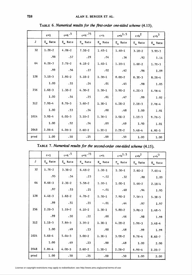
728 ALAN E. BERGER ET AL.
Table 6. Numerical results for the first-order one-sided scheme (4.13).
E=l E=h.5
E=h.75
£=h £=h1.5
£=h' £ = (1
E Rate E Rate E Rate E Rate E Rate E Rate E Rate
32
64
128
256
512
1024
2048
pred
1.2E-2
.98
6.2E-3
.99
3.1E-3
1.00
1.6E-3
1.00
7.9E-4
1.00
3.9E-4
1.00
2.0E-4
4.0E-2
.57
2.7E-2
.56
1.9E-2
.55
1.3E-2
.54
8.7E-3
.53
6.0E-3
.52
4.2E-3
1.00 .50
7.5E-2
.29
6.1E-2
.27
5.1E-2
.24
4.3E-2
.25
3.6E-2
.24
3.1E-2
.24
2.6E-2
.25
1.4E-1
.04
1.4E-1
.02
1.3E-1
.01
-1
01
-1
.00
1.3E-1
.00
1.3E-1
1.3E-
1.3E-
1.4E-1
.36
1.1E-1
.42
8.0E-2
.45
5.9E-2
.47
4.2E-2
.48
3.0E-2
.49
2.2E-2
3.1E-2
.92
1.6E-2
.96
8.3E-3
.98
4.2E-3
.99
2.1E-3
1.00
1.1E-3
1.00
5.4E-4
3.9E-3
1.14
1.7E-3
1.09
8.2E-4
1.05
4.0E-4
1.02
2.0E-4
1.01
9.7E-5
1.01
4.8E-5
.00 .50 1.00 1.00
Table 7. Numerical results for the second-order one-sided scheme (4.15).
E=l £=h £=h.75
E=h E=h1.5
E=h E = hJ
E Rate E Rate E Rate E Rate E Rate E Rate E Rate
32
64
128
256
512
1024
2048
pred
1.7E-2
.95
8.6E-3
.97
4.4E-3
.99
2.2E-3
.99
1.1E-3
1.00
5.6E-4
1.00
2.8E-4
1.00
3.3E-2
.54
2.3E-2
.53
1.6E-2
.51
1.1E-2
.50
7.8E-3
.49
5.6E-3
.49
4.0E-3
.50
6.4E-2
.23
5.5E-2
.21
4.7E-2
.21
4.1E-2
.22
3.5E-2
.23
3.0E-2
.23
2.6E-2
.25
1.3E-1
-.02
1.3E-1
-.01
1.3E-1
-.01
1.3E-1
.00
1.3E-1
.00
1.3E-1
.00
1.3E-1
.00
1.3E-1
.32
1.0E-1
.40
7.9E-2
.44
5.8E-2
.46
4.2E-2
.48
3.0E-2
.48
2.2E-2
.50
2.6E-2
.88
1.4E-2
.94
7.5E-3
.97
3.8E-3
.98
1.9E-3
.99
9.7E-4
1.00
4.9E-4
1.00
7.6E-4
1.89
2.1E-4
1.95
5.3E-5
1.97
1.4E-5
1.99
3.4E-6
1.99
8.6E-7
2.00
2.2E-7
2.00
License or copyright restrictions may apply to redistribution; see http://www.ams.org/journal-terms-of-use
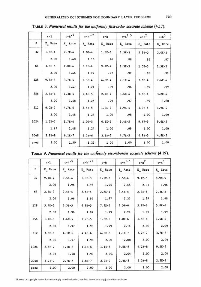
GENERALIZED OCI SCHEMES for boundary LAYER PROBLEMS 729
Table 8. Numerical results for the uniformly first-order accurate scheme (4.17).
E = l E=h E=h75
E=h £=h1.5
E = tl E=h"
E Rate E Rate E Rate E Rate
32
64
128
256
512
1024
2048
1.5E-4
2.00
3.8E-5
2.00
9.6E-6
2.00
2.4E-6
2.00
6.0E-7
2.00
1.5E-7
1.97
3.9E-8
2.7E-4
1.40
1.0E-4
1.46
3.7E-5
1.47
1.3E-5
1.48
4.7E-6
1.48
1.7E-6
1.48
6.1E-7
7.0E-4
1.18
3.1E-4
1.27
1.3E-4
1.21
5.6E-5
1.25
2.4E-5
1.24
1.0E-5
1.24
4.2E-6
1.8E-3
.96
9.4E-4
.97
4.8E-4
.99
2.4E-4
.99
1.2E-4
1.00
6.1E-5
1.00
3.1E-5
E Rate E Rate E Rate
2.5E-3
.88
1.3E-3
.92
7.1E-4
.96
3.6E-4
.97
1.9E-4
.98
9.4E-5
.99
4.7E-5
2.9E-3
.95
1.5E-3
.98
7.6E-4
.99
3.8E-4
.99
1.9E-4
1.00
9.6E-5
1.00
4.8E-5
1.
7.
0E-3
.97
5E-3
.99
6E-4
.99
8E-4
1.00
9E-4
1.00
6E-5
1.00
8E-5
pred 2.00 1.50 1.25 1.00 1.00 1.00 1.00
Table 9. Numerical results for the uniformly second-order accurate scheme (4.19).
r.=l E=h.5
£=h75
E=h E-h1.5
£=h E = ll
E Rate E Rate E_ Rate E Rate E Rate E Rate E Rate
32
64
128
256
512
1024
2048
pred
9.1E-4
2.00
2.3E-4
2.00
5.7E-5
2.00
1.4E-5
2.00
3.6E-6
2.00
8.8E-7
2.01
2.2E-7
2.00
9.5E-4
1.96
2.4E-4
1.96
6.3E-5
1.96
1.6E-5
1.97
4.1E-6
1.97
1.1E-6
1.98
2.7E-7
2.00
1.0E-3
1.97
2.6E-4
1.94
6.8E-5
1.97
1.7E-5
1.98
4.4E-6
1.98
1.1F-6
1.99
2.8E-7
2.00
1.1E-3
1.95
2.8E-4
1.97
7.2E-5
1.99
1.8E-5
1.99
4.6E-6
2.00
1.1E-6
2.00-
2.9E-7
2.00
2.5E-4
2.48
4.4E-5
2.37
8.5E-6
2.24
1.8E-6
2.14
4.1E-7
2.08
9.8E-8
2.04
2.4E-8
2.00
9.4E-5
2.01
2.3E-5
1.99
5.9E-6
1.99
1.5E-6
2.00
3.7E-7
2.00
9.2E-8
2.00
2.3E-8
2.00
8.9E-5
1.96
2.3E-.5
1.98
5.8E-6
1.99
1.5E-6
2.00
3.7E-7
2.00
9.2E-8
2.00
2.3E-8
2.00
License or copyright restrictions may apply to redistribution; see http://www.ams.org/journal-terms-of-use
730 ALAN E. BERGER ET AL.
It seems fair to state that the agreement between the predicted and experimental
rates is rather good for all the schemes. The tables also give (even if for only one par-
ticular problem) a comparison of the numerical behavior of the various methods. Of
the generalized OCI schemes (3.16) run, the one with Pj = 3 seems overall the best
for this problem. The generalized OCI schemes are the most accurate schemes of those
tested when e is not "near" A, while the uniformly second-order accurate scheme
(4.19) gives the best results for e "near" A.
Acknowledgment. The authors thank Professor Bruce Kellogg for many very
helpful discussions and comments and for kindly providing us with an early draft of
[16].
Code R44
Naval Surface Weapons Center
Silver Spring, Maryland 20910
Code R44
Naval Surface Weapons Center
Silver Spring, Maryland 20910
Mathematical Analysis Division
National Bureau of Standards
Washington, D. C. 20234
Gulf Science and Technology Company
Simulation Research Section
P. O. Drawer 20 38
Pittsburgh, Pennsylvania 15230
Scientific Research Associates
P. O. Box 498
Glastenbury, Connecticut 06033
1. L. R. ABRAHAMSSON, H. B. KELLER & H.-O. KREISS, "Difference approximations
for singular perturbations of systems of ordinary differential equations," Numer. A.ath., v. 22,
1974, pp. 367-391.
2. D. N. DE G. ALLEN & R. V. SOUTHWELL, "Relaxation methods applied to determine
the motion, in two dimensions, of a viscous fluid past a fixed cylinder," Quart. J. Mech. AppL
Math., v. 8, 19SS, pp. 129-145.
3. A. E. BERGER, J. M. SOLOMON & M. CIMENT, "On a uniformly accurate difference
method for a singular perturbation problem." (In preparation.)
4. T. H. CHONG, "A variable mesh finite difference method for solving a class of parabolic
differential equations in one space variable," SIAM J. Numer. Anal., v. 15, 1978, pp. 835—857.
5. I. CHRISTIE & A. R. MITCHELL, "Upwinding of high order Galerkin methods in con-
duction-convection problems," Internat. J. Numer. Methods Engrg., v. 12, 1978, pp. 1764—1771.
6. M. CIMENT, S. H. LEVENTHAL & B. C. WEINBERG, "The operator compact implicit
method for parabolic equations," /. Computational Phys., v. 28, 1978, pp. 135-166.
7. F. W. DORR, "The numerical solution of singular perturbations of boundary value
problems," Siam J. Numer. Anal, v. 7, 1970, pp. 281-313.
8. B. L. EHLE, "A -stable methods and Fade approximations to the exponential," SIAM J.
Math. Anal, v. 4, 1973, pp. 671-680.
9. T. M. EL-MISTIKAWY & M. J. WERLE, "Numerical method for boundary layers with
blowing—the exponential box scheme," AIAA J„ v. 16, 1978, pp. 749—751.
10. J. C. HEINRICH, P. S. HUYAKORN, O. C. ZIENKIEWICZ & A. R. MITCHELL, "An
upwind finite element scheme for two-dimensional convective transport equation," Internat. J.
Numer. Methods Engrg., v. 11, 1977. pp. 131-143.
11. J. C. HEINRICH & O. C. ZIENKIEWICZ, "Quadratic finite element schemes for two-
dimensional convective-transport problems," Internat. J. Numer. Methods Engrg., v. 11, 1977,
pp. 1831-1844.
License or copyright restrictions may apply to redistribution; see http://www.ams.org/journal-terms-of-use
GENERALIZED OCI SCHEMES FOR BOUNDARY LAYER PROBLEMS 731
12. R. S. HIRSH & D. H. RUDY, "The role of diagonal dominance and cell Reynolds num-
ber in implicit difference methods for fluid mechanics problems," J. Computational Phys., v. 25,
1974, pp. 304-310.
13. T. J. R. HUGHES, W. K. LIU & A. BROOKS, "Finite element analysis of incompressible
viscous flows by the penalty function formulation," J. Computational Phys., v. 30, 1979, pp. 1—60.
14. A. M. IL IN, "Differencing scheme for a differential equation with a small parameter
affecting the highest derivative," Mat. Zametki, v. 6, 1969, pp. 237—24&=Math. Notes, v. 6, 1969,
pp. 596-602.15. E. ISAACSON & H. B. KELLER, Analysis of Numerical Methods, Wiley, New York,
1966.
16. R. B. KELLOGG & A. TSAN, "Analysis of some difference approximations for a singu-
lar perturbation problem without turning points," Math. Comp., v. 32, 1978, pp. 1025-1039.
17. H.-O. KREISS, "Difference approximations for singular perturbation problems,"
Numerical Solutions of Boundary Value Problems for Ordinary Differential Equations (A. K. Aziz,
Ed.), Academic Press, New York, 1975, pp. 199-211.
18. H.-O. KREISS & N. NICHOLS, Numerical Methods for Singular Perturbation Problems,
Lecture Notes in Phys., Vol. 58 (R. Glowinski and J. L. Lions, Eds.), Springer-Verlag, Berlin, 1976,
pp. 544-558.19. D. C. L. LAM & R. B. SIMPSON, "Centered differencing and the box scheme for dif-
fusion convection problems," J. Computational Phys., v. 22, 1976, pp. 486—500.
20. J. J. H. MILLER, "Some finite difference schemes for a singular perturbation problem,"
in Constructive Function Theory, Proc. Internat. Conf. on Constr. Fen. Theory, Blagoevgrad,
30 May-4 June 1977. (To appear.)
21. J. J. H. MILLER, "Sufficient conditions for the convergence, uniformly in epsilon, of
a three point difference scheme for a singular perturbation problem," in Praktische Behandlung
von Differentialgleichungen in Anwendungsgebieten (Proc. Conf., Oberwolfach, 1977), Lecture
Notes in Math., Springer, Berlin. (To appear.)
22. C. E. PEARSON, "On a differential equation of boundary layer type," J. Math, and
Phys., v. 49, 1968, pp. 134-154.
23. M. H. PROTTER & H. F. WEINBERGER, Maximum Principles in Differential Equa-
tions, Prentice-Hall, Englewood Cliffs, N. J., 1967.
24. R. D. RICHTMYER & K. W. MORTON, Difference Methods for Initial-Value Problems,
2nd ed., Interscience, New York, 1967.
25. P. J. ROACHE, Computational Fluid Dynamics, Hermosa, Albuquerque, N. M., 1972.
26. D. R. SMITH, "The multivariable method in singular perturbation analysis," SIAM Rev.,
v. 17, 1975, pp. 221-273.
27. B. K. SWARTZ, "The construction of finite difference analogs of some finite element
schemes," in Mathematical Aspects of Finite Elements in Partial Differential Equations
(C. de Boor, Ed.), Academic Press, New York, 1974, pp. 279-312.
28. M. VAN VELDHUIZEN, "Higher order methods for a singularly perturbed problem,"
Numer. Math., v. 30, 1978, pp. 267-279.
29. M. VAN VELDHUIZEN, "Higher order schemes of positive type for singular perturba-
tion problems," Numerical Analysis of Singular Perturbation Problems (P. W. Hemker and J. J. H.
Miller, Eds.), Academic Press, New York, 1979, pp. 361-383.
30. R. S. VARGA, Matrix Iterative Analysis, Prentice-Hall, Englewood Cliffs, N. J., 1962.
License or copyright restrictions may apply to redistribution; see http://www.ams.org/journal-terms-of-use