arX

iv:h

ep-p

h/97

0226

2v3

27

Sep

1997

Large angle QED processes at e+e− colliders

at energies below 3 GeV

A.B. Arbuzov1, G.V. Fedotovich2, E.A. Kuraev1, N.P. Merenkov3,V.D. Rushai4 and L. Trentadue5

1 Bogoliubov Laboratory of Theoretical Physics, JINR,

Dubna, 141980, Russia

2 Budker Institute for Nuclear Physics,

Prospect Nauki, 11, Novosibirsk, 630090, Russia

3 Kharkov Institute of Physics and Technology,

Kharkov, 310108, Ukraine

4 Laboratory of Computing Techniques and Automation,

JINR, Dubna, 141980, Russia

5 Dipartimento di Fisica, Universita di Parma and INFN,

Gruppo Collegato di Parma, 43100 Parma, Italy

Abstract

QED processes at electron–positron colliders are considerd. We present differential

cross–sections for large–angle Bhabha scattering, annihilation into muons and photons.

Radiative corrections in the first order are taken into account exactly. Leading loga-

rithmic contributions are calculated in all orders by means of the structure–function

method. An accuracy of the calculation can be estimated about 0.2%.

PACS 12.20.–m Quantum electrodynamics, 12.20.Ds Specific calculations

1 Introduction

At the existing VEPP–2M e+e− collider and planned meson factories QED processes of thelowest order of the perturbation theory (PT) play an important role. These processes areto be considered as an essential background when extracting subtle mesons properties fromexperimental data. QED processes are used also for calibration and monitoring purposes.For instance, large–angle Bhabha scattering is used for a precise determination of luminosityat e+e− colliders. That is the reason, why radiative corrections (RC) to QED processes areto be considered in detail.

A lot of attention was paid to the problem of radiative correction calculations to variousQED processes, starting more than 50 years ago [1], concerning mainly the lowest order of

1

PT calculations. The accuracy requirements of modern experiments, however, exceed theones provided by the first order RC. Unfortunately, calculations of radiative corrections inhigher orders encounter tremendous technical difficulties. Nevertheless, powerful methodsdeveloped in quantum chromodynamics (see paper [2] and references therein) provide apossibility to improve essentially the results obtained earlier. At first we mean the methodsbased on the renormalization group ideas and on the factorization theorem. Thay allow usto get a differential cross–section of a certain process similar to the Drell–Yan process cross–section, and to consider leading logarithmic RC of higher orders. Meanwhile, nonleadingcontributions are to be taken from the lowest order PT calculations.

The aim of our paper is to provide relevant theoretical formulae for QED processes, whichare required for experiments with CMD–2 and SND detectors at VEPP–2M (Novosibirsk) [3]collider, at DAΦNE (Frascati) [4] and BEPC/BES (Beijing) [5] machines. Formulae citedbelow may be applied also for higher energies (see the Conclusions), if one will take intoaccount weak interaction and higher hadronic resonance contributions.

A cross–section calculated with an account of radiative corrections (RC) in the n-th orderof perturbation theory (PT) contains enhanced contributions of the form (α/π)nLn, whereL = ln(s/m2

e) is the large logarithm (for s ∼ 1 GeV2, L ≈ 15). We call these contributionsthe leading ones. Nonleading contributions have the order (α/π)nLm, m < n. The terms,proportional to (α/π)nLn, can be calculated by means of the structure function method [6].The structure function formalism, based on the renormalization group approach, permitsone to keep all leading terms of order (αL/π)n, n = 0, 1, 2 . . . explicitly.

In the first order of PT the nonleading terms, proportional to (α/π), can be accountedby means of so–called K–factor, K = 1 + (α/π)K. As for nonleading terms of the order(α/π)2L, they can be correctly calculated in the two–loop approximation. We will considerthem in further publications [7]. Fortunately, this second order nonleading RC are small:(α/π)2L ∼ 10−4. So, the presented formulae guarantee theoretical precision of the order0.2%. Considering hard photon emission in the first order of PT we distinguish the cont-ributions due to the initial state radiation, the final state radiation, and their interference.The first one always contains large logarithms. The ones due to the final state radiation aswell as the initial–final state interference do not enhance the corrections considerably, exceptthe case of Bhabha scattering. In the case of hard photon radiation large logarithms comefrom kinematical regions, where the photona are emitted along electron and positron beams.We will call this kinematics as the collinear one.

Our work consist in explicit calculations of the Born and the first order RC contributi-ons to differential cross–sections. We apply the structure function method to increase theaccuracy.

The paper is organized as follows. In Section 2 we consider µ+µ− production. Bothcharge–even and charge–odd contributions to the differential cross–section are evaluated. InSect. 3 we consider the electron–positron scattering process at large angles. In Sect. 4 weinvestigate electron–positron annihilation into photons. In the Conclusions we discuss theresults obtained and estimate the provided precision. Numerical illustrations are given for arealistic experimental set up.

2

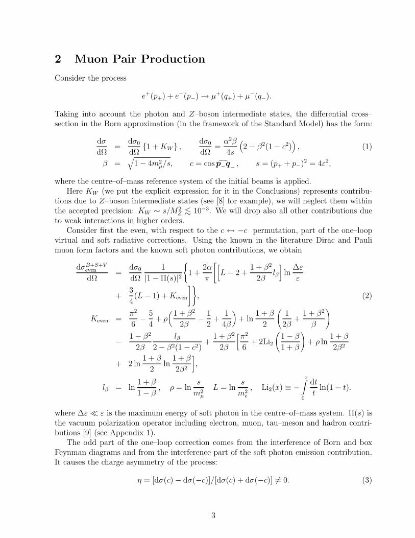
2 Muon Pair Production

Consider the process

e+(p+) + e−(p−) → µ+(q+) + µ−(q−).

Taking into account the photon and Z–boson intermediate states, the differential cross–section in the Born approximation (in the framework of the Standard Model) has the form:

dσ

dΩ=

dσ0

dΩ1 + KW ,

dσ0

dΩ=

α2β

4s

(2 − β2(1 − c2)

), (1)

β =√

1 − 4m2µ/s, c = cos p−q− , s = (p+ + p−)2 = 4ε2,

where the centre–of–mass reference system of the initial beams is applied.Here KW (we put the explicit expression for it in the Conclusions) represents contribu-

tions due to Z–boson intermediate states (see [8] for example), we will neglect them withinthe accepted precision: KW ∼ s/M2

Z<∼ 10−3. We will drop also all other contributions due

to weak interactions in higher orders.Consider first the even, with respect to the c ↔ −c permutation, part of the one–loop

virtual and soft radiative corrections. Using the known in the literature Dirac and Paulimuon form factors and the known soft photon contributions, we obtain

dσB+S+Veven

dΩ=

dσ0

dΩ

1

|1 − Π(s)|2

1 +2α

π

[[L − 2 +

1 + β2

2βlβ

]ln

∆ε

ε

+3

4(L − 1) + Keven

], (2)

Keven =π2

6− 5

4+ ρ

(1 + β2

2β− 1

2+

1

4β

)+ ln

1 + β

2

(1

2β+

1 + β2

β

)

− 1 − β2

2β

lβ2 − β2(1 − c2)

+1 + β2

2β

[π2

6+ 2Li2

(1 − β

1 + β

)+ ρ ln

1 + β

2β2

+ 2 ln1 + β

2ln

1 + β

2β2

],

lβ = ln1 + β

1 − β, ρ = ln

s

m2µ

L = lns

m2e

, Li2(x) ≡ −x∫

0

dt

tln(1 − t).

where ∆ε ≪ ε is the maximum energy of soft photon in the centre–of–mass system. Π(s) isthe vacuum polarization operator including electron, muon, tau–meson and hadron contri-butions [9] (see Appendix 1).

The odd part of the one–loop correction comes from the interference of Born and boxFeynman diagrams and from the interference part of the soft photon emission contribution.It causes the charge asymmetry of the process:

η = [dσ(c) − dσ(−c)]/[dσ(c) + dσ(−c)] 6= 0. (3)

3

The odd part of the differential cross–section has the following form:

dσS+Vodd

dΩ=

dσ0

dΩ

2α

π

[2 ln

∆ε

εln

1 − βc

1 + βc+ Kodd

], (4)

Kodd =1

2l2− − L−(ρ + l−) + Li2

(1 − β2

2(1 − βc)

)+ Li2

(β2(1 − c2)

1 + β2 − 2βc

)

−1−β2∫

0

dx

xf(x)

(1 − x(1 + β2 − 2βc)

(1 − βc)2

)− 12

+1

2 − β2(1 − c2)

×−1 − 2β2 + β2c2

1 + β2 − 2βc(ρ + l−) − 1

4(1 − β2)

[l2− − 2L−(l− + ρ)

+ 2Li2

(1 − β2

2(1 − βc)

)]+ βc

[− ρ

2β2+(

π2

12+

1

4ρ2)(

1 − 1

β− β

2+

1

2β3

)

+1

β(−1 − β2

2+

1

2β2)(ρ ln

1 + β

2− 2Li2

(1 − β

2

)− Li2

(−1 − β

1 + β

))

− 1

2l2− + L−(ρ + l−) − Li2

(1 − β2

2(1 − βc)

)]− (c → −c),

f(x) =(

1√1 − x

− 1)

ln

√x

2− 1√

1 − xln

1 +√

1 − x

2,

l− = ln1 − βc

2, L− = ln

(1 − 1 − β2

2(1 − βc)

).

In the ultra–relativistic limit (β → 1) for the even part we obtain:(

dσB+S+Veven

dΩ

)

β→1

=dσ0

dΩ

1

|1 − Π(s)|2

1 +2α

π

[(−2 + L + ρ) ln

∆ε

ε

− 2 +3

4L +

3

4ρ +

π2

3

]. (5)

For the odd part in this limit we obtained the same as Khriplovich [10]:(

dσS+Vodd

dΩ

)

β→1

=α3

sπ

2(1 + c2)

[ln(ctg

θ

2) ln

ε

∆ε+

1

2ln2(sin

θ

2) − 1

2ln2(cos

θ

2)

− 1

4Li2(sin

2 θ

2) +

1

4Li2(cos2 θ

2)]

+ cos2 θ

2ln(sin

θ

2) − sin2 θ

2ln(cos

θ

2)

− cos θ[ln2(cos

θ

2) + ln2(sin

θ

2)]

. (6)

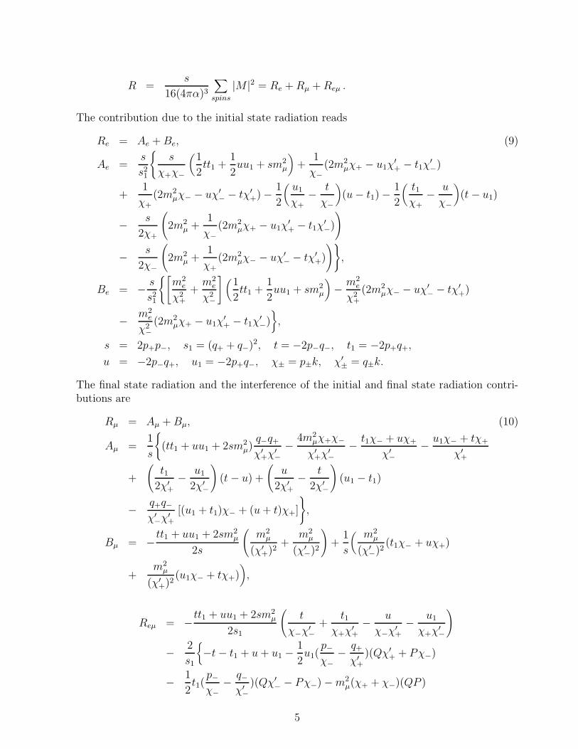
Consider now the process of hard photon emission

e+(p+) + e−(p−) → µ+(q+) + µ−(q−) + γ(k). (7)

It was studied in detail [13]. The photon energy is assumed to be larger than ∆ε. Thedifferential cross–section has the form

dσ =α3

2π2s2RdΓ, dΓ =

d3q−d3q+d3k

q0−q0

+k0δ(4)(p+ + p− − q− − q+ − k), (8)

4

R =s

16(4πα)3

∑

spins

|M |2 = Re + Rµ + Reµ .

The contribution due to the initial state radiation reads

Re = Ae + Be, (9)

Ae =s

s21

s

χ+χ−

(1

2tt1 +

1

2uu1 + sm2

µ

)+

1

χ−(2m2

µχ+ − u1χ′+ − t1χ

′−)

+1

χ+(2m2

µχ− − uχ′− − tχ′

+) − 1

2

(u1

χ+− t

χ−

)(u − t1) −

1

2

(t1χ+

− u

χ−

)(t − u1)

− s

2χ+

(2m2

µ +1

χ−(2m2

µχ+ − u1χ′+ − t1χ

′−)

)

− s

2χ−

(2m2

µ +1

χ+(2m2

µχ− − uχ′− − tχ′

+)

),

Be = − s

s21

[m2

e

χ2+

+m2

e

χ2−

] (1

2tt1 +

1

2uu1 + sm2

µ

)− m2

e

χ2+

(2m2µχ− − uχ′

− − tχ′+)

− m2e

χ2−

(2m2µχ+ − u1χ

′+ − t1χ

′−),

s = 2p+p−, s1 = (q+ + q−)2, t = −2p−q−, t1 = −2p+q+,

u = −2p−q+, u1 = −2p+q−, χ± = p±k, χ′± = q±k.

The final state radiation and the interference of the initial and final state radiation contri-butions are

Rµ = Aµ + Bµ, (10)

Aµ =1

s

(tt1 + uu1 + 2sm2

µ)q−q+

χ′+χ′

−− 4m2

µχ+χ−

χ′+χ′

−− t1χ− + uχ+

χ′−

− u1χ− + tχ+

χ′+

+

(t1

2χ′+

− u1

2χ′−

)(t − u) +

(u

2χ′+

− t

2χ′−

)(u1 − t1)

− q+q−χ′−χ′

+

[(u1 + t1)χ− + (u + t)χ+]

,

Bµ = −tt1 + uu1 + 2sm2µ

2s

(m2

µ

(χ′+)2

+m2

µ

(χ′−)2

)+

1

s

( m2µ

(χ′−)2

(t1χ− + uχ+)

+m2

µ

(χ′+)2

(u1χ− + tχ+)),

Reµ = −tt1 + uu1 + 2sm2µ

2s1

(t

χ−χ′−

+t1

χ+χ′+

− u

χ−χ′+

− u1

χ+χ′−

)

− 2

s1

−t − t1 + u + u1 −

1

2u1(

p−χ−

− q+

χ′+

)(Qχ′+ + Pχ−)

− 1

2t1(

p−χ−

− q−χ′−

)(Qχ′− − Pχ−) − m2

µ(χ+ + χ−)(QP )

5

+

(m2

µ

χ′+

− m2µ

χ′−

)(χ− − χ+) − 1

2t(

q+

χ′+

− p+

χ+)(Qχ′

+ − Pχ+)

− 1

2u(

q−χ′−− p+

χ+

)(Qχ′− + Pχ+)

, (11)

P =p+

χ+

− p−χ−

, Q =q−χ′−− q+

χ′+

.

Quantity Re contains collinear and infrared singularities. Aµ and Aeµ have only infraredsingularities. Bµ and Beµ are free from singularities. Quantity R in the ultra–relativisticcase is given in Appendix 3.

After algebraic transformations we get

Re =s

χ−χ+B − m2

e

2χ2−

(t21 + u21 + 2m2

µs1)

s21

− m2e

2χ2+

(t2 + u2 + 2m2µs1)

s21

+m2

µ

s21

∆s1s1,

Reµ = B(

u

χ−χ′+

+u1

χ+χ′−− t

χ−χ′−− t1

χ+χ′+

)+

m2µ

ss1∆ss1

, (12)

Rµ =s1

χ′−χ′

+

B +m2

µ

s2∆ss , B =

u2 + u21 + t2 + t214ss1

,

∆s1s1= −(t + u)2 + (t1 + u1)

2

2χ−χ+

,

∆ss = −u2 + t21 + 2sm2µ

2(χ′−)2

− u21 + t2 + 2sm2

µ

2(χ′+)2

+1

χ′−χ′

+

(ss1 − s2 + tu + t1u1 − 2sm2µ),

∆ss1=

s + s1

2

(u

χ−χ′+

+u1

χ+χ′−− t

χ−χ′−− t1

χ+χ′+

)+

2(u − t1)

χ′−

+2(u1 − t)

χ′+

.

Note that from these expressions one may in a moment obtain the corresponding matrixelement of the cross symmetrical process e−µ+ → e−µ+γ. To be rigorous, we have notethat in the cross symmetrical channel one has to take into account some additional termsproportional to m2

e. In our channel they can be shown as follows:

Rµ → Rµ +m2

e

s2∆′

ss,

∆′ss =

2m2µs1

χ′−χ′

+

+t + u1

χ′−

+t1 + u

χ′+

+4m2

µ

χ′−

+4m2

µ

χ′+

. (13)

We checked the matrix element by a comparison with the one used in FORTRAN program [14],describing electron–muon scattering.

The sum of the hard photon contribution, integrated over the photon phase volume withthe condition k0 > ∆ε, and the contribution due to the soft and virtual photon emission doesnot depend on the auxiliary parameter ∆ = ∆ε/ε ≪ 1. The main contribution, proportionalto the large logarithm, comes from the integration of Re in the case of collinear kinematicsof photon emission. For definiteness let us consider the case when the photon moves closeto the initial electron direction:

p−k = θ ≤ θ0 ≪ 1, θ0 ≫me

ε. (14)

6

Here we can use

Re

∣∣∣∣k‖p−

=s2

s21

1 + (1 − x)2

xχ−− m2

e

χ2−

(1 − x)

tt1 + uu1 + 2sm2

µ

2, (15)

where x is the energy fraction carried away by the emitted photon, x = k0/ε = 1 − s1/s.Performing the integration over the photon emission angles, we can present the correspondingpart of the cross–section (a similar contribution of the hard photon emission along thepositron is included below also) in the form

(dσ

dΩ−

)

coll

= C + D, (16)

C =α

2π

(ln

s

m2e

− 1) 1∫

∆

dx1 + (1 − x)2

x

[dσ0(1 − x, 1)

dΩ−+

dσ0(1, 1 − x)

dΩ−

],

D =α

2π

1∫

∆

dxx +

1 + (1 − x)2

xln

θ20

4

[dσ0(1 − x, 1)

dΩ−+

dσ0(1, 1 − x)

dΩ−

],

where dσ0(1 − x1, 1 − x2)/dΩ− is the so–called shifted Born differential cross–section. Itdescribes the process e+(p+(1 − x2)) + e−(p−(1 − x1)) → µ+(q+) + µ−(q−),

dσ0(z1, z2)

dΩ−=

α2

4s

y1[z21(Y1 − y1c)

2 + z22(Y1 + y1c)

2 + 8z1z2m2µ/s]

z31z

32 [z1 + z2 − (z1 − z2)cY1/y1]

, (17)

y21,2 = Y 2

1,2 −4m2

µ

s, Y1,2 =

q0−,+

ε, z1,2 = 1 − x1,2 .

Using the conservation laws

z1 + z2 = Y1 + Y2, z1 − z2 = y1c− + y2c+, (18)

y1

√1 − c2

− = y2

√1 − c2

+, c− ≡ c, c+ = cos p−q+

,

we obtain the energy fraction of the created muon

Y1 =4m2

µ

s

(z2 − z1)c

2z1z2 + [4z21z

22 − 4(m2

µ/s)((z1 + z2)2 − (z1 − z2)2c2)]1/2

+2z1z2

z1 + z2 − c(z1 − z2). (19)

Quantity C, after adding the corrections due to soft and virtual photons, turns out to bethe lowest order perturbative expansion of the convolution of the structure function D withthe shifted Born differential cross–section. Quantity D plays role of a compensating term.Namely, in the sum with the contribution of the cross–section due to hard (k0 > ∆ε) photonemission at angles (with respect to the electron and positron) larger than θ0 the dependenceon the auxiliary parameters will cancel.

Here we remind about experimental conditions of the final particles detection mentionedabove. They are to be imposed explicitly by introducing the restriction of the following kind:

Θ(z1, z2) = Θ(Y1 − yth)Θ(Y2 − yth)Θ(cos2 Ψ0 − c2+)Θ(cos2 Ψ0 − c2

−), c+ = p+q+

, (20)

7

where ythε = εth is the threshold of the detectors, angle Ψ0 determines the dead cones,surrounding beam axes, unattainable for detection. More detailed cuts can be implementedin a Monte Carlo program, using the formulae given above.

The leading contributions to the cross–section, containing large logarithm L, as may berecognized, combine to the kernel of Altarelli–Parisi–Lipatov evolution equation:

dσ =∫

dz1dz2D(z1)D(z2)dσ0(z1, z2)

|1 − Π(sz1z2)|2, (21)

D(z) = δ(1 − z) +α

2π(L − 1)P (1)(z) +

(α

2π

)2 (L − 1)2

2!P (2)(z) + . . . ,

P (1)(z) = lim∆→0

δ(1 − z)(2 ln ∆ +

3

2) + Θ(1 − z − ∆)

1 + z2

1 − z

,

P (2)(z) =

1∫

z

dt

tP (1)(t)P (1)

(z

t

),

1∫

0

dzP (1,2)(z) = 0.

This formula is valid in the leading logarithmical approximation. We will modify it by in-cluding nonleading contributions and using the smoothed representation for structure func-tions [6]:

D(z, s) = Dγ(z, s) + De+e−(z, s), (22)

Dγ(z, s) =1

2b(1 − z

) b

2−1[

1 +3

8b +

b2

16

(9

8− π2

3

)]

− 1

4b(1 + z) +

1

32b2(4(1 + z) ln

1

1 − z+

1 + 3z2

1 − zln

1

z− 5 − z

),

De+e−(z, s) =1

2b(1 − z

) b

2−1[

− b2

288(2L − 15)

]

+(

α

π

)2 [ 1

12(1 − z)

(1 − z − 2me

ε

) b

2(ln

s(1 − z)2

m2e

− 5

3

)2

×(1 + z2 +

b

6

(ln

s(1 − z)2

m2e

− 5

3

))+

1

4L2(

2

3

1 − z3

z+

1

2(1 − z)

+ (1 + z) ln z)]

Θ(1 − z − 2me

ε), b =

2α

π(L − 1).

In comparison with the corresponding formula in ref. [6] we shifted the terms, arising due tovirtual e+e− pair production corrections, from Dγ into De+e−.

Finally, the differential cross–section can be presented in the form

dσe+e−→µ+µ−(γ)

dΩ−=

1∫

zmin

1∫

zmin

dz1dz2D(z1, s)D(z2, s)

|1 − Π(sz1z2)|2dσ0(z1, z2)

dΩ−

(1 +

α

πK)

+

α3

2π2s2

∫

k0>∆ε

kp±>θ0

Re|me=0

|1 − Π(s1)|2dΓ

dΩ−+

D

|1 − Π(s1)|2

8

+

α3

2π2s2

∫

k0>∆ε

(Re

Reµ

(1 − Π(s1))(1 − Π(s))∗+

Rµ

|1 − Π(s)|2)

dΓ

dΩ−

+ReCeµ

(1 − Π(s1))(1 − Π(s))∗+

Cµ

|1 − Π(s)|2

, (23)

Cµ =2α

π

dσ0

dΩ−ln

∆ε

ε

(1 + β2

2βln

1 + β

1 − β− 1

), zmin =

2mµ

2ε − mµ,

Ceµ =4α

π

dσ0

dΩ−ln

∆ε

εln

1 − βc

1 + βc, K = Kodd + Keven,

where D, Ceµ and Cµ are compensating terms, which provide cancellation of auxiliary pa-rameters ∆ and θ0 inside figure brackets. In the first term, containing D functions, wegather all leading terms. A part of nonleading terms proportional to the Born cross–sectionis written as the K–factor. The rest nonleading terms are written as two additional terms.The compensating term D (see Eq. (16)) comes from the integration in the collinear regionof hard photon emission. Quantities Cµ and Ceµ come from the even and odd parts of thedifferential cross–section (arising due to soft and virtual corrections), respectively. Here weconsider the phase volumes of two (dΩ−) and three (dΓ) final particles as the ones, whichalready include all required experimental cuts. Using the conservation laws Eq. (18) andconcrete experimental conditions one can define the lower limits of the integration over z1

and z2.There is a peculiar feature in the spectrum of hard photons. Namely, in the end of the

spectrum the differential cross–section is proportional to the factor

I(s1) =2m2

µ + s1

s21

√

1 − 4m2µ

s1

, (24)

which defines a peak at s1 ≈ 5.6m2µ. It comes from the Feynman diagrams describing the

emission by the initial particles [15].

3 Large–Angle Bhabha Scattering

The cross–section of Bhabha scattering (corrected by the vacuum polarization factor), whichenter into the Drell–Yan form of corrected cross–section, has a bit more complicated form, asfar as the scattering and annihilation amplitudes and their interference are to be taken intoaccount. We remind here the form of the Lorentz–invariant matrix element module squaredin the Born approximation:

R0(s, t, u) =1

16(4πα)4

∑

spins

∣∣∣M(e−(p−) + e+(p+) → e−(p′−) + e+(p′+))∣∣∣2

=s2 + u2

2t2+

u2 + t2

2s2+

u2

st, (25)

s = (p− + p+)2, t = (p− − p′−)2, u = (p− − p′+)2, s + t + u = O(m2e).

The first term in the right hand side describes the scattering–type Feynman diagram square.The second one corresponds to the square of the annihilation–type diagram. And the third

9

one deals with the interference of the two diagrams. A more compact representation of R0 isalso useful, R0 = (1 + s/t + t/s)2. The differential cross–section in the Born approximationhas the form

dσBorn0

dΩ−=

α2

4s

(3 + c2

1 − c

)2

. (26)

We will need also quantity R for arbitrary energies of initial particles. Suppose that theinitial electron and positron lost a certain energy fraction. The corresponding kinematics isdefined as follows:

e−(z1p−) + e+(z2p+) −→ e−(p−) + e+(p+),

s = sz1z2, t = −1

2sz1Y1(1 − c), u = −1

2sz2Y1(1 + c),

Y1 =p0−ε

=2z1z2

a, a = z1 + z2 − (z1 − z2)c.

Here the shifted Born cross–section corrected by vacuum polarization insertions into virtualphoton propagators reads

dσ0(z1, z2) =4α2

sa2

1

|1 − Π(t)|2a2 + z2

2(1 + c)2

2z21(1 − c)2

+1

|1 − Π(s)|2z21(1 − c)2 + z2

2(1 + c)2

2a2

− Re1

(1 − Π(t))(1 − Π(s))∗z22(1 + c)2

az1(1 − c)

dΩ− . (27)

Rewriting the known results [11, 12] for the cross–section in the Born approximationwith one–loop virtual corrections to it and with the other ones arising due to soft photonemission, we obtain

dσB+S+V

dΩ−=

dσ0(1, 1)

dΩ−

1 +

2α

π(L − 1)

[2 ln

∆ε

ε+

3

2

]

− 8α

πln(ctg

θ

2) ln

∆ε

ε+

α

πKSV

, (28)

where

KSV = −1 − 2Li2(sin2 θ

2) + 2Li2(cos2 θ

2) +

1

(3 + c2)2

[π2

3(2c4 − 3c3 − 15c)

+ 2(2c4 − 3c3 + 9c2 + 3c + 21) ln2(sinθ

2) − 4(c4 + c2 − 2c) ln2(cos

θ

2)

− 4(c3 + 4c2 + 5c + 6) ln2(tgθ

2) + 2(c3 − 3c2 + 7c − 5) ln(cos

θ

2)

+ (10

3c3 + 10c2 + 2c + 38) ln(sin

θ

2)]

(29)

is the part of the K–factor coming from soft and virtual photon corrections,

dσ0(1, 1)

dΩ−=

α2

s

5 + 2c + c2

2(1 − c)2|1 − Π(t)|2 +1 + c2

4|1 − Π(s)|2

10

− Re(1 + c)2

2(1 − c)(1 − Π(t))(1 − Π(s))∗

, (30)

s = 4ε2, t = −s1 − c

2, u = −s

1 + c

2, c = cos θ, θ = p−p′

− .

Quantity ∆ε in Eq. (28) is the maximum energy of emitted soft photons. Π(s) and Π(t)are the vacuum polarization operators in the s and t channels. In the Conclusions we willestimate the contribution of weak interactions.

Consider now the process of hard photon (with the energy ω = k0 > ∆ε) emission

e+(p+) + e−(p−) → e+(p′+) + e−(p′−) + γ(k).

We start with the differential cross–section in the form suggested by F.A. Berends et al. [11](which is valid for scattering angles being large compared with me/ε):

dσhard =α3

2π2sReeγ dΓ, dΓ =

d3p′+d3p′−d3k

ε′+ε′−k0δ(4)(p+ + p− − p′+ − p′− − k), (31)

Reeγ =WT

4− m2

e

(χ′+)2

(s

t+

t

s+ 1

)2

− m2e

(χ′−)2

(s

t1+

t1s

+ 1)2

− m2e

χ2+

(s1

t+

t

s1

+ 1)2

− m2e

χ2−

(s1

t1+

t1s1

+ 1)2

,

where

W =s

χ+χ−+

s1

χ′+χ′

−− t1

χ′+χ+

− t

χ′−χ−

+u

χ′+χ−

+u1

χ′−χ+

,

T =ss1(s

2 + s21) + tt1(t

2 + t21) + uu1(u2 + u2

1)

ss1tt1,

and the invariants are defined as

s = 2p−p+, s1 = 2p′−p′+, t = −2p−p′−, t1 = −2p+p′+,

u = −2p−p′+, u1 = −2p+p′−, χ± = kp±, χ′± = kp′±.

It is convenient to extract the contribution of the collinear kinematics. We do that forthe following reasons. First, it is natural to separate the region with very a sharp behaviourof the cross–section and to consider it carefully. Second, we keep in mind the idea of theleading logarithm factorization, which is valid in all orders of the perturbation theory. Wewill evaluate the collinear kinematical regions in two different ways. The first one (thequasireal electron approximation) is suitable for a generalization in order to account higherorder leading corrections by means of the structure function method. In this way we willobtain below the leading logarithmic contributions and the compensating terms, which willprovide the cancellation of auxiliary parameters. The second one (the direct calculation) ismore rigorous, it can be used as a check of the first one. We discuss it in detail in Appendix 2.

To obtain explicit formulae for compensators it is needed to consider four kinematicalregions corresponding to hard photon emission inside narrow cones, surrounding the initial

11

and final charged particle momenta. The vertices of the cones are taken in the interactionpoint. We introduce a small auxiliary parameter θ0, it should obey the restriction

me/√

s ≪ θ0 ≪ 1. (32)

So, we define a collinear kinematical region, as the part of the whole phase space, in whichthe hard photon is emitted within the cone of θ0 polar angle with respect to the direction ofmotion of one of the charged particles.

Using the method of quasireal electrons [16], the matrix element M (squared and summedup over polarization states) of the process of hard photon emission can be expressed througha shifted matrix element of the process without photon emission (see Eq. (4) in [16]):

∑|M(p1, k, p′1,X )|2 = 4πα

[1 + (1 − x)2

x(1 − x)

1

kp1− m2

(kp1)2

]∑|M0(p1 − k, p′1,X )|2,

∑|M(p1, p

′1, k,X )|2 = 4πα

[y2 + Y 2

ωY

ε

kp′1− m2

(kp′1)2

]∑|M0(p1, p

′1 + k,X )|2, (33)

x =ω

ε, p0

1 = ε, y =p′1

0

ε, Y = x + y,

where X denotes the momenta of non–radiating incoming and outgoing particles in a concreteprocess. The integration over the phase volume of the emitted photon inside the narrow cone,surrounding its parent charged particle momentum, gives the following factors:

4α

16π2

∫d3k

ω

[1 + (1 − x)2

x(1 − x)

1

kp1− m2

(kp1)2

]=

α

2π

dz1

z1

[P

(1)Θ (z1)

(L − 1 + ln

θ20

4

)

+1 − z1

], z1 = 1 − x, (34)

4α

16π2

∫d3k

ω

[y2 + Y 2

xY

1

kp′1− m2

(kp′1)2

]=

α

2π

dz3

z3

[P

(1)Θ (z3)

(L − 1 + ln

θ20

4

+2 ln z3

)+ 1 − z3

], z3 = 1 − ω

p′10 + ω

= 1 − x

Y.

Note that the terms proportional to (L−1) contain the kernel P (1) (see Eq. (21)) of Altarelli–Parisi–Lipatov evolution equations (more precisely, they contain Θ–part of the nonsingletkernel):

P(1)Θ (z) =

1 + z2

1 − zΘ(1 − z − ∆).

Collecting the contributions of the four collinear regions, we obtain

dσcoll

dΩ−=

α

π

1∫

∆

dx

x

[(1 − x +

x2

2

)(L − 1 + ln

θ20

4+ 2 ln(1 − x)

)+

x2

2

]

× 2dσ0(1, 1)

dΩ−+[(

1 − x +x2

2

)(L − 1 + ln

θ20

4

)+

x2

2

]

×[dσ0(1 − x, 1)

dΩ−+

dσ0(1, 1 − x)

dΩ−

], (35)

12

where the shifted Born cross–section is defined in Eq. (27).Adding the contributions of virtual and soft photon emission, we restore the complete

kernel. Generalizing the procedure for the case of photon emission by all charged particles,we come to the representation of the cross–section in the leading logarithmic approximation.The final expression for the cross–section therefore has the form

dσe+e−→e+e−(γ)

dΩ−=

1∫

z1

dz1

1∫

z2

dz2 D(z1)D(z2)dσ0(z1, z2)

dΩ−

(1 +

α

πKSV

)Θ

×Y1∫

yth

dy1

Y1

Y2∫

yth

dy2

Y2D(

y1

Y1)D(

y2

Y2)

+α

π

1∫

∆

dx

x

[(1 − x +

x2

2

)ln

θ20(1 − x)2

4+

x2

2

]2

dσBorn0

dΩ−

+[(

1 − x +x2

2

)ln

θ20

4+

x2

2

][4α2

s(1 − x)2[2 − x(1 − c)]4

×(

3 − 3x + x2 + 2x(2 − x)c + c2(1 − x + x2)

1 − c

)2

+4α2

s[2 − x(1 + c)]4

(3 − 3x + x2 − 2x(2 − x)c + c2(1 − x + x2)

1 − c

)2]Θ

− α2

4s

(3 + c2

1 − c

)28α

πln(ctg

θ

2) ln

∆ε

ε+

α3

2π2s

∫

k0>∆ε

π−θ0>θ>θ0

WT

4Θ

dΓ

dΩ−, (36)

Y1 =2z1z2

z1 + z2 − c(z1 − z2), Y2 =

z21 + z2

2 − (z21 − z2

2)c

z1 + z2 − c(z1 − z2),

z1 =yth(1 + c)

2 − yth(1 − c), z2 =

z1yth(1 − c)

2z1 − yth(1 + c).

The last term describes hard photon emission process, provided that the photon energyfraction x is larger than ∆ = ∆ε/ε, and its emission angle with respect to any chargedparticle direction is larger than some small quantity θ0. The sum of the last 3 terms inEq. (36) does not depend on the auxiliary parameters ∆ and θ0, if they are sufficiently small.We omitted the effects due to vacuum polarization in the last three terms which describe realhard photon emission. Because the theoretical uncertainty, coming from this approximation,has the order δ(dσ)/dσ ∼ (α/π)2L <∼ 10−4. Nevertheless if the centre–off–mass energy isclose to some resonance mass (say to mφ) the effect due to vacuum polarization may becomevisible. The differential cross–section of non–collinear hard photon emission, that takes intoaccount vacuum polarization explicitly, is presented in Appendix 3.

13

4 Annihilation of e+e− into photons

Considering the RC due to emission of virtual and soft real photons to the cross–section oftwo quantum annihilation process

e+(p+) + e−(p−) → γ(q1) + γ(q2), (37)

we will use the results obtained in papers [17]:

dσB+S+V = dσ0(1, 1)

1 +

α

π

[(L − 1)

(2 ln

∆ε

ε+

3

2

)+ KSV

], (38)

KSV =π2

3+

1 − c2

2(1 + c2)

[(1 +

3

2

1 + c

1 − c

)ln

1 − c

2

+(1 +

1 − c

1 + c+

1

2

1 + c

1 − c

)ln2 1 − c

2+ (c → −c)

],

dσ0(1, 1) =α2(1 + c2)

s(1 − c2)dΩ1 , s = (p+ + p−)2, c = cos θ1, θ1 = q1p− .

We suppose that the two final photons are registered in an experiment and their polar angleswith respect to the initial beam directions are not small (θ1,2 ≫ me/ε).

Consider the three–quantum annihilation process

e+(p+) + e−(p−) → γ(q1) + γ(q2) + γ(q3)

with the cross–section (see the paper by M.V. Terentjev [17])

dσe+e−→3γ =α3

8π2sR3γ dΓ , (39)

R3γ = sχ2

3 + (χ′3)

2

χ1χ2χ′1χ

′2

− 2m2e

[χ2

1 + χ22

χ1χ2(χ′3)

2+

(χ′1)

2 + (χ′2)

2

χ′1χ

′2χ

23

]

+ two cyclic permutations,

dΓ =d3q1d

3q2d3q3

q01q

02q

03

δ(4)(p+ + p− − q1 − q2 − q3),

where

χi = qip−, χ′i = qip+, i = 1, 2, 3 .

The process can be treated as a radiative correction to the two–quantum annihilation.In the same way as we have done before we will distinguish the contributions of the

collinear kinematical region, when extra photons are emitted within narrow cones of theopening angle 2θ0 ≪ 1 to one of the charged particles and the semi–collinear ones, whenextra photons are emitted outside these cones. This contribution can be obtained using thequasireal electron method [16]. It reads:

dσcoll =α

π

1∫

∆

dx

x

[(1 − x +

x2

2)(L − 1 + ln

θ20

4

)+

x2

2

](40)

× [dσ0(1 − x, 1) + dσ0(1, 1 − x)] ,

14

where the shifted cross–section has the form

dσ0(z1, z2) =2α2

s

z21(1 − c)2 + z2

2(1 + c)2

(1 − c2)(z1 + z2 + (z2 − z1)c)2dΩ1 . (41)

Again rearranging the separate contributions and applying the structure functions method,we obtain the improved cross–section

dσe+e−→γγ(γ) =

1∫

z1

dz1 D(z1)

1∫

z2

dz2 D(z2)dσ0(z1, z2)(1 +

α

πKSV

)

+α

π

1∫

∆

dx

x

[(1 − x +

x2

2

)ln

θ20

4+

x2

2

] [dσ0(1 − x, 1) + dσ0(1, 1 − x)

]

+1

3

∫

zi≥∆

π−θ0≥θi≥θ0

4α3

π2s2

[z23(1 + c2

3)

z21z

22(1 − c2

1)(1 − c22)

+ two cyclic permutations]dΓ, (42)

zi =q0i

ε, ci = cos θi, θi = p−q

i,

where lower limits z1,2 are defined in Eq. (36). The multiplier 13

in the last term takes intoaccount the identity of the final photons. The sum of the last two terms does not dependon ∆ and θ0. Note that the annihilation process is a pure QED one, hadronic contributionsas well as weak interaction effects are far beyond the required accuracy.

5 Conclusions

Thus we had considered the series of processes at electron–positron colliders of moderatelyhigh energies. We presented differential cross–sections to be integrated over concrete expe-rimental conditions. The formulae are good as for semi–analytical integration, as well asfor the creation of a Monte Carlo event generator [20]. In a separate publication we aregoing to present analysis of the effects of radiative corrections for the conditions of VEPP–2M (Novosibirsk), DAΦNE (Frascati) and BEPC/BES (Beijing). The idea of our approachwas to separate the contributions due to 2 → 2 like processes and 2 → 3 like ones. Thecompensating terms allow us to eliminate the dependence on auxiliary parameters in bothcontributions separately.

Note that all presented formulae are valid only for large–angle processes. Indeed, in theregion of very small angles θ ∼ me/ε of final particles with respect to the beam directionsthere are contributions of double logarithmic approximation [9]. These small angle regionsgive the main part of the total cross–section. We suppose that this kinematics is rejected byexperimental cuts.

In the Table and Figures we present some results of numerical calculations according toour formulae. We suppose that a process–event implies detecting of two final particles withthe polar angles with respect to the beam axes more than some value Ψ0. The energies ofthe particles have to exeed some experimental threshold εth. A cut–off on the acollinearityof the final particle momenta is possible. But we switched off it in the computations.

15

Table 1: The values of Bhabha cross–section and radiative corrections to it.θ± σBorn

0 (mb) δVP (%) δiniSF (%) δfin

SF (%) δK (%) δγ (%) σtot (mb)9 < θ± < 171 3.77 · 10−2 1.53 0.11 - 0.30 -1.82 1.50 3.81 · 10−2

1 < θ± < 179 3.08 0.80 0.70 -0.17 - 3.5 4.74 3.16

In the Table we give the values of different RC contributions to large–angle Bhabhascattering cross–section. Here we switched off also the cut–off on the final particle energies(we used only kinematical restrictions). The contributions (see Eq.(36)) are defined asfollows:

σtot ≡∫

dσe+e−→e+e−(γ)

dΩ−dΩ− =

∫dσBorn

0

dΩ−dΩ−

[1 +

1

100%

(δVP + δini

SF + δfinSF + δK + δγ

)], (43)

where δVP is due to the vacuum polarization being included into the Born level diagrams;δini(fin)SF is due to the initial (final) state leading logarithmic corrections; δK shows the impact

of the K–factor; δγ describes the contribution of one hard photon emission at large angles.The effect due to the width of φ meson is included as a part of vacuum polarization. Itis small for the given integrated cross–sections. But for the description of a differentialcross–section it is important, especially for large scattering angles (see [23, 24]).

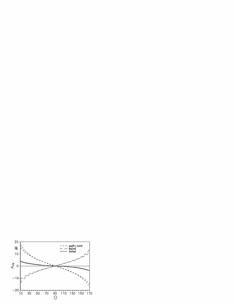
In Figures 1 and 2 we illustrate the charge–odd part of the differential cross–section forthe e+e− → µ+µ− process (see Eq.(23)). The quantity

AFB =dσ

e+e−→µ+µ−(γ)odd /dc

dσe+e−→µ+µ−(γ)0 /dc

100% (44)

is shown there as a function of c. The short–dashed line represents the contribution due tosoft photon emission and virtual corrections. The long–dashed line represents the corres-ponding odd contribution due to hard photon emission. It comes from the intereference ofthe amplitudes due to initial and final radiation (Reµ). In the sum of the two contributionsthe dependence on the auxiliary parameter ∆ disappears (it was chosen ∆ = 0.01). And weobtain an experimentally measurable asymmetry AFB (the solid line). There is also a con-tribution to the asymmetry due to electroweak interactions. Namely, due to the interferenceof the Born level amplitudes with γ and Z boson in the s–channel. It can be found fromthe weak K–factor (46). It is included in the total sums (solid lines). But for the chosenenergies it is really small (it gives a maximal shift of about 0.01% for Ebeam = 0.51 GeV andabout 0.1% for Ebeam = 1.55 GeV.

Let us discuss the accuracy, provided by our formulae. The contribution of weak interac-tion to the cross–section of muon pair production and Bhabha scattering was parameterizedbe so–called weak K–factors:

KW =(dσ)EW − (dσ)QED

(dσ)QED

, (45)

where quantities (dσ)EW and (dσ)QED are the cross–sections calculated in the Born appro-ximation in the frames of the Standard Model and QED, respectively. The weak K–factors

16

(we used the results of papers [8, 18]) are

Kee→µµW =

s2(2 − β2(1 − c2))−1

(s − M2Z)2 + M2

ZΓ2Z

(2 − β2(1 − c2))

(c2v

(3 − 2

M2Z

s

)+ c2

a

)

− 1 − β2

2(c2

a + c2v) + cβ

[4(1 − M2

Z

s

)c2a + 8c2

ac2v

], (46)

ca = − 1

2 sin 2θW

, cv = ca(1 − 4 sin2 θW ),

Kee→eeW =

(1 − c)2

2(3 + c2)2

[4B1 + (1 − c)2B2 + (1 + c)2B3

]− 1, (47)

B1 = (s

t)2∣∣∣1 + (g2

v − g2a)ξ∣∣∣2, B2 =

∣∣∣1 + (g2v − g2

a)χ∣∣∣2,

B3 =1

2

∣∣∣∣1 +s

t+ (gv + ga)

2(s

tξ + χ)

∣∣∣∣2

+1

2

∣∣∣∣1 +s

t+ (gv − ga)

2(s

tξ + χ)

∣∣∣∣2

,

χ =Λs

s − m2z + iMZΓZ

, ξ =Λt

t − M2Z

,

Λ =GF M2

Z

2√

2πα= (sin 2θW )−2, ga = −1

2, gv = −1

2(1 − 4 sin2 θW ),

here θW is the weak mixing angle.These quantities are of order 0.1% up to

√s < 3 GeV. Contribution of weak interactions

to the cross–section of the annihilation into photons (which is absent at the Born level) canbe estimated as

(KW )ee→γγ <∼αs

πM2W

. (48)

It comes from one–loop electroweak radiative corrections. Another source of uncertaintiescomes from the approximation of collinear kinematics (or the approximation of quasirealelectrons [16]) It can be estimated by the largest omitted terms

α

πθ20 and

α

π

(me

εθ0

)2

. (49)

Really in the calculations we used the value of the parameter θ0 of the order 10−2 becauseof the restrictions θ0 ≪ 1 and εθ0/me ≫ 1. Note that the coefficient before terms of thatsort (calculable in principle) is the function of energy fractions and angles, they are of orderof 1. For typical values of energy ε = 0.5 GeV this uncertainty is of order 2 · 10−4 or less.

The third source of uncertainties is the error in the definition of the hadronic vacuumpolarization. It has been estimated [9] to be of order 0.04%. For φ–meson factories asystematic error in the definition of the φ–meson contribution into vacuum polarization isto be added.

Next point concerns nonleading terms of order (α/π)2L. There are several sources ofthem. One is the emission of two extra hard particles (for the case of Bhabha scattering itwas considered in the series of papers [11]). Other are related to virtual and soft–photon

17

radiative corrections to single hard photon emission and Born processes. The most partof these contributions was not considered up to now. Nevertheless, we can estimate thecoefficient before the quantity (α/π)2L ≈ 1 ·10−4 to be of order of unity. That was indirectlyconfirmed by our complete calculations of these terms for the case of small–angle Bhabhascattering [21].

Considering all mentioned above sources of uncertainties as independent, we concludethat the systematic error of our formulae does not exceed 0.2%. The main error is due tounknown second–order next–to–leading radiative corrections.

For precise luminosity measurements we suggest to use the large–angle Bhabha scatteringprocess. It has a very large cross–section, a good signature in detectors, and the lowesttheoretical uncertainty.

Acknowledgement

The authors are grateful to A. Sher, S. Panov and V. Astakhov for their close interest inthe initial stage [19], to V. Fadin and L. Lipatov for critical comments, and to D. Bardinfor cross checks. This work was partially supported by INTAS grant 1867–93 and by RFBRgrant N 96–02–17512. One of us (A.B.A.) is thankful to the INTAS foundation for thefinancial support via the International Centre for Fundamental Physics in Moscow.

Appendix 1

We present here leptonic and hadronic contributions into the vacuum polarization operator:

Π = Πl + Πh, (50)

Πl(s) =α

πΠ1(s) +

(α

π

)2

Π2(s) +(

α

π

)3

Π3(s) + . . .

Πh(s) =s

4πα

[PV

∞∫

4m2π

σe+e−→hadrons(s′)

s′ − sds′ − iπσe+e−→hadrons(s)

].

The first order leptonic contribution is well known [1]:

Π1(s) =1

3L − 5

9+ f(xµ) + f(xτ ) − iπ

[1

3+ φ(xµ)Θ(1 − xµ) + φ(xτ )Θ(1 − xτ )

], (51)

where

f(x) =

−59− x

3+ 1

6(2 + x)

√1 − x ln

∣∣∣1+√

1−x1−

√1−x

∣∣∣ for x ≤ 1,

−59− x

3+ 1

6(2 + x)

√1 − x arctg

(1√x−1

)for x > 1,

φ(x) =1

6(2 + x)

√1 − x, xµ,τ =

4m2µ,τ

s.

In the second order it is enough to take only the logarithmic term from the electron contri-bution

Π2(s) =1

4(L − iπ) + ζ(3) − 5

24. (52)

18

A discussion of the φ–meson contribution to the vacuum polarization operator, which isimportant for

√s ≈ mφ, can be found in [23, 24].

Appendix 2

Here we present the direct evaluation of the collinear region contribution to the Bhabhascattering cross–section. Let us write the contribution of the collinear kinematics in theform:

(dσ)coll = dσk‖p−+ dσk‖p

+

+ dσk‖p′−

+ dσk‖p′+

≡ dσa + dσb + dσc + dσd . (53)

For the case of photon emission along the initial electron we have

Wa =2

ω2

1

1 − βc2

, Ta =1 + (1 − x)2

1 − xR(s1, t

a, ua), dΓa =d3k

ω

ya1

aa

dΩ−, (54)

c2 = cos(kp−), β =

√

1 − m2e

ε2, ω = k0 = xε, s1 = s(1 − x), ta1 = ta(1 − x),

ua1 = ua(1 − x), ta = −s

(1 − x)2(1 − c)

aa, ua = −s

(1 − x)(1 + c)

aa, s = 4ε2,

aa = 2 − x(1 − c), ya1 =

2(1 − x)

aa, c = cos(p−p

′−).

Performing the angular integration over photon angles inside the narrow cone, surroundingthe direction of the initial electron beam, we get

∫WadΓa = 4π

dω

ωdΩ−

1∫

1−θ20/2

dc1

1 − βc1

= 4πdx

xdΩ−

ya1

a2a

(L + ln

θ20

4

)+ O(θ2

0). (55)

We neglect the terms proportional to θ20. Collecting all the factors and reminding the con-

tribution of the terms proportional to m2e (see Eq. (31)), we obtain the contribution of the

first collinear region:

dσa

dΩ−=

4α2

s

α

π

1∫

∆

dx

x

[(1 − x +

x2

2

)(L − 1 + ln

θ2

4

)+

x2

2

]1

a2a

× [a2a + (1 − c)2(1 − x)2 − aa(1 − c)(1 − x)]2

a2a(1 − x)2(1 − c)2

. (56)

For the case of photon emission inside the narrow cone, surrounding p+, in a similar wayone gets

dσb

dΩ−=

4α2

s

α

π

1∫

∆

dx

x

[(1 − x +

x2

2

)(L − 1 + ln

θ2

4

)+

x2

2

]1

a2b

× [a2b + (1 − c)2(1 − x)2 − ab(1 − c)(1 − x)]2

a2b(1 − c)2

, ab = 2 − x(1 + c). (57)

19

Here we used the following formulae:

Wb =2

ω2

1

1 − βc+, Tb =

1 + (1 − x)2

1 − xR(s1, t

b, ub), dΓb =d3k

ω

yb1

abdΩ−,

yb1 =

p0−ε

=1 − x

ab, tb = −s1

1 − c

ab, ub = −s1

(1 + c)(1 − x)

ab, tb + ub + s1 = 0.

For the cases k ‖ p′− and k ‖ p′

+ quantity R (if suppose Π=0) is simple:

Rc = Rd =1

4

(3 + c2

1 − c

)2

, Tc = Td =1 + (1 − x)2

1 − xRc,

dΓc,d = ε2dx dΩ− dφ1 dc1xyc,d

2 − x + xc1, c1 = cos kp′

−,

yc =p′0−ε

∣∣∣∣∣k‖p′

−

≈ 2(1 − x)

2 − x + xc1

∣∣∣∣∣c1→1

= 1 − x,

yd =p′0−ε

∣∣∣∣∣k‖p′

+

≈ 2(1 − x)

2 − x + xc1+ c1

m2e

4ε2

x

1 − x,

Wc · (kp′−) = Wd · (kp′+) =2(1 − x)

x.

Note that kp′+ = 2ε2(1− y). In the evaluation of the rest multipliers for these cases one hasto be careful:

∫WcdΓc

∣∣∣∣1−θ2

0/2≤c1≤1

=∫

WddΓd

∣∣∣∣−1+θ2

0(1−x)2/2≥c1≥−1

= 2πdx

xdΩ−

1 − x

2

[L + ln

θ20

4+ 2 ln(1 − x)

].

Note that the collinear region d is defined by the condition 1 − θ20/2 ≤ cos kp′

+ ≤ 1, whichleads to the bounds on c1 shown above. So, the contributions of these two collinear regionsare

dσc + dσd

dΩ−= 2

α2

4s

(3 + c2

1 − c

)2α

π

1∫

∆

dx

x

[(1 − x +

x2

2

)

×(L − 1 + ln

θ20

4+ 2 ln(1 − x)

)+

x2

2

]. (58)

Note that there is an asymmetry between the contributions due to the emission along thedirections of the (initial or final) electron and the ones due to production of collinear photonsalong the positron momenta. The symmetry was broken when we decided to write a differ-ential cross–section with respect to the electron scattering angles (dΩ− = d cos(p−p

′−) dφ).

After an integration over a symmetrical angular acceptance the contributions would becomeequal. Compensating terms are to be extracted from the Eqs.(56,57,58) by omitting theterms proportional to (L − 1).

20

Appendix 3

The following expression could be used instead of WT in Eq. (36) for more precise defini-tion of the contribution due to non–collinear hard photon emission in large-angle Bhabhascattering:

(WT )Π =(SS)

|1 − Π(s)|2sχ′−χ′

+

+(S1S1)

|1 − Π(s1)|2s1χ−χ+

− (TT )

|1 − Π(t)|2tχ+χ′+

(59)

− (T1T1)

|1 − Π(t1)|2t1χ−χ′−

+ Re

(TT1)

(1 − Π(t))(1 − Π(t1))∗tt1χ−χ′−χ+χ′

+

− (SS1)

(1 − Π(s))(1 − Π(s1))∗ss1χ−χ′−χ+χ′

+

+(TS)

(1 − Π(t))(1 − Π(s))∗tsχ′−χ+χ′

+

+(T1S1)

(1 − Π(t1))(1 − Π(s1))∗t1s1χ−χ′−χ+

− (T1S)

(1 − Π(t1))(1 − Π(s))∗t1sχ−χ′−χ′

+

− (TS1)

(1 − Π(t))(1 − Π(s1))∗ts1χ−χ+χ′+

,

where

(SS) = (S1S1) = t2 + t21 + u2 + u21, (TT ) = (T1T1) = s2 + s2

1 + u2 + u21,

(SS1) = (t2 + t21 + u2 + u21)(tχ+χ′

+ + t1χ−χ′− − uχ+χ′

− − u1χ−χ′+),

(TT1) = (s2 + s21 + u2 + u2

1)(uχ+χ′− + u1χ−χ′

+ + sχ′−χ′

+ + s1χ−χ+),

(TS) = −1

2(u2 + u2

1) [s(t + s1) + t(s + t1) − uu1] ,

(TS1) = −1

2(u2 + u2

1) [t(s1 + t1) + s1(s + t) − uu1] ,

(T1S) =1

2(u2 + u2

1) [t1(s + t) + s(s1 + t1) − uu1] ,

(T1S1) =1

2(u2 + u2

1) [s1(s + t1) + t1(s1 + t) − uu1] .

We checked analytically that for the switched off vacuum polarization the above formula isequivalent to the multiplication WT in Eq. (31):

(WT )Π|Π=0 = WT. (60)

In the compensating terms, entering into Eq. (36) the vacuum polarization corrections,have to be inserted also. That can be easily done starting with Eq. (35). We get

dσe+e−→e+e−(γ)comp

dΩ−=

α

π

1∫

∆

dx

x

[(1 − x +

x2

2

)ln

θ20(1 − x)2

4+

x2

2

]

× dσ0(1, 1)

dΩ−

(1 +

1

(1 − x)2

)+[(

1 − x +x2

2

)ln

θ20

4+

x2

2

]

×[dσ0(1 − x, 1)

dΩ−+

dσ0(1, 1 − x)

dΩ−

]

− dσ0(1, 1)

dΩ−

8α

πln(ctg

θ

2) ln

∆ε

εdΩ− . (61)

21

We note that quantity R (see Eq.(9)) in the ultra–relativistic limit s ≫ m2µ can be derived

from Eq.(59). One has to omit there all terms except the ones proportional to (SS), (SS1),(S1S1) and divide by 4.

References

[1] A.I. Akhieser and V.B. Berestetskij, Quantum Electrodynamics , Nauka, Moscow, 1981.

[2] G. Sterman et al., Rev. Modern Phys. 67 (1995) 157.

[3] S.I. Dolinsky et al., Phys. Rep. 202 (1991) 99–170;R.R. Akhmetshin et al., Phys. Lett. B 364 (1995) 199.

[4] A. Aloisio et al., preprint LNF-92/019 (IR); also in The DAΦNE Physics Handbook

Vol.2, 1993;P. Franzini, in The Second DAΦNE Physics Handbook, L. Maiani, G. Pancheri, N. Paver(eds.), Vol.2, p.471, 1995.

[5] Hui–Ling Ni et al., Nucl. Instr. and Meth. A 336 (1993) 542.

[6] E.A. Kuraev and V.S. Fadin, Sov. J. Nucl. Phys. 41 (1985) 466.

[7] A.B. Arbuzov, E.A. Kuraev, N.P. Merenkov, L. Trentadue, Nucl. Phys. B 474 (1996)271;A.B. Arbuzov et al., Preprint JINR E2–95–460, hep–ph/9610228, Nucl. Phys. B 483

(1997) 83.A.B. Arbuzov et al., JINR preprint E2–95–421, Dubna, 1995, Yad. Fiz. in press.

[8] F.A. Berends et al., Nucl. Phys. B 202 (1981) 63;A.B. Arbuzov et al., Mod. Phys. Lett. A 7 (1992) 2029.

[9] S. Eidelman, F. Jegerlehner, Z. Phys. C 67 (1995) 585.

[10] I.B. Khriplovich, Yad. Fiz. 17 (1973) 576.

[11] F.A. Berends et al., Nucl. Phys. B 57 (1973) 381;E.A. Kuraev and G.V. Meledin, Nucl. Phys. B 122 (1977) 485.

[12] W. Beenakker, E.A. Berends and S.C. van der Mark, Nucl. Phys. B 349 (1991) 323.

[13] S.I. Eidelman, E.A. Kuraev, V.S. Panin, Nucl. Phys. B 148 (1979) 245.

[14] D. Bardin, L. Kalinovskaya, FORTRAN code µela, http://www.ifh.de/∼bardin.

[15] V.N. Baier, V.M. Katkov, V.S. Fadin, Emission of the relativistic electrons, Moscow,Atomizdat, 1973.

[16] V.N. Baier, V.S. Fadin, V.A. Khoze, Nucl. Phys. B 65 (1973) 381.

22

[17] F.A. Berends and R. Gastmans, Nucl. Phys. B 61 (1973) 414;S.I. Eidelman and E.A. Kuraev, Nucl. Phys. B 143 (1978) 353;M.V. Terentjev, Yad. Fiz. 9 (1969) 1212;F.A. Berends at al., Nucl. Phys. B 206 (1982) 61.

[18] R. Budny, Phys. Lett. B 55 (1975) 227;D. Bardin, W. Hollik and T. Riemann, Z. Phys. C 49 (1991) 485;M. Boehm, A. Denner and W. Hollik, Nucl. Phys. B 304 (1988) 687.

[19] E.A. Kuraev, S.N. Panov, Preprint Budker INP 91–26, 1991.

[20] V.A. Astakhov, G.V. Fedotovich et al., Monte Carlo generator for VEPP–2M, inprogress.

[21] A.B. Arbuzov, E.A. Kuraev, N.P. Merenkov, L. Trentadue, JETP 81 (1995) 638;A.B. Arbuzov, V.S. Fadin, E.A. Kuraev, L.N. Lipatov, N.P. Merenkov, L. Trentadue,prerint CERN–TH/95–313, hep–ph/9512344, Nucl. Phys. B 485 (1997) 457.

[22] E.A. Kuraev, preprint INP 80-155, Novosibirsk.

[23] A. Bramon, M. Greco, in The Second DAΦNE Physics Handbook, L. Maiani,G. Pancheri, N. Paver (eds.), Vol.2, p.451, 1995;E. Drago, G. Venanzoni, KLOE MEMO N59/96.

[24] A.B. Arbuzov et al., hep–ph/9703456.

23

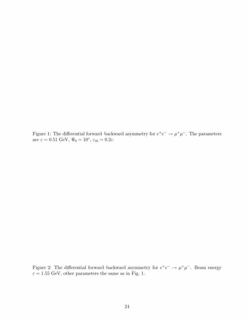
Figure 1: The differential forward–backward asymmetry for e+e− → µ+µ−. The parametersare ε = 0.51 GeV, Ψ0 = 10, εth = 0.2ε.

Figure 2: The differential forward–backward asymmetry for e+e− → µ+µ−. Beam energyε = 1.55 GeV, other parameters the same as in Fig. 1.

24