Les Houches 2013: Physics at TeV CollidersStandard Model Working Group Report

ConvenersHiggs physics: SM issuesD. De Florian (Theory), M. Kado (ATLAS), A. Korytov (CMS),S. Dittmaier (Electroweak Contact)

SM: Loops and MultilegsN. Glover (Theory), J. Huston (ATLAS), G. Dissertori (CMS),S. Dittmaier (Electroweak Contact)

Tools and Monte CarlosF. Krauss (Theory), J. Butterworth (ATLAS), K. Hamilton (MC-NLO Contact),G. Soyez (Jets Contact)

Abstract

This Report summarizes the proceedings of the 2013 Les Houches workshop on Physics atTeV Colliders. Session 1 dealt primarily with (1) the techniques for calculating standard modelmulti-leg NLO and NNLO QCD and NLO EW cross sections and (2) the comparison of thosecross sections with LHC data from Run 1, and projections for future measurements in Run 2.

Acknowledgements

We would like to thank the organizers (G. Belanger, F. Boudjema, P. Gras, D. Guadagnoli,S. Gascon, J.P. Guillet, B. Herrmann, S. Kraml, G.H. de Monchenault, G. Moreau, E. Pilon,P. Slavich and D. Zerwas) and the Les Houches staff for the stimulating environment alwayspresent at Les Houches.

i

arX

iv:1

405.

1067

v1 [

hep-

ph]

5 M

ay 2

014

Authors

J. R. Andersen1, S. Badger2, L. Barzè3, J. Bellm4, F. U. Bernlochner5, A. Buckley6,J. Butterworth7, N. Chanon8, M. Chiesa9, A. Cooper-Sarkar10, L. Cieri11, G. Cullen12, H. vanDeurzen13, G. Dissertori8, S. Dittmaier14, D. de Florian15, S. Forte16, R. Frederix3,B. Fuks3,17, J. Gao18, M.V. Garzelli19, T. Gehrmann20, E. Gerwick21, S. Gieseke22,D. Gillberg23, E. W. N. Glover1, N. Greiner13, K. Hamilton7, T. Hapola1, H.B. Hartanto24,G. Heinrich13, A. Huss14, J. Huston25, B. Jäger26, M. Kado27, A. Kardos28, U. Klein29,F. Krauss1, A. Kruse30, L. Lönnblad31, G. Luisoni13, Daniel Maître1, P. Mastrolia13,32,O. Mattelaer33, J. Mazzitelli15, E. Mirabella13, P. Monni34, G. Montagna9, M. Moretti35,P. Nadolsky18, P. Nason3, O. Nicrosini36, C. Oleari28, G. Ossola37,38, S. Padhi39, T. Peraro13,F. Piccinini36, S. Plätzer40, S. Prestel40, J. Pumplin25, K. Rabbertz22, Voica Radescu40,L. Reina41, C. Reuschle42, J. Rojo3, M. Schönherr1, J. M. Smillie43,J.F. von Soden-Fraunhofen13, G. Soyez44, R. Thorne7, F. Tramontano45, Z. Trocsanyi19,D. Wackeroth46, J. Winter13, C-P. Yuan25, V. Yundin 13, K. Zapp3

1 Institute for Particle Physics Phenomenology, Department of Physics, University of Durham,Durham DH1 3LE, UK

2 Niels Bohr Institute (NBI), University of Copenhagen, Blegdamsvej 17 DK-2100 Copen-hagen, Denmark

3 PH Department, TH Unit, CERN, CH-1211, Geneva 23, Switzerland4 Institute for Theoretical Physics, Karlsruhe Institute of Technology, D - 76128 Karlsruhe,Germany

5 University of Victoria, Victoria, British Columbia, Canada V8W 3P6 School of Physics & Astronomy, University of Glasgow, Glasgow, UK7 Department of Physics and Astronomy, University College London, Gower Street, LondonWC1E 6BT, UK

8 Institute for Particle Physics, ETH Zurich, 8093 Zurich, Switzerland9 Dipartimento di Fisica, Università di Pavia and INFN, Sezione di Pavia, Via A. Bassi, 6,27100 Pavia, Italy

10 Department of Physics, University of Oxford, Denys Wilkinson Building, Keble Road,Oxford OX1 3RH, UK

11 Dipartimento di Fisica, Università di Roma La Sapienza and INFN, Sezione di Roma,I-00185 Rome, Italy

12 DESY, Zeuthen, Platanenallee 6, D-15738 Zeuthen, Germany13 Max-Planck-Institut für Physik, Werner-Heisenberg-Institut, Föhringer Ring 6, D-80805

München, Germany14 Physikalisches Institut, Albert-Ludwigs-Universitat Freiburg, D-79104 Freiburg, Germany15 Departamento de Física, Facultad de Ciencias Exactas y Naturales, Universidad de Buenos

Aires, Pabellon I, Ciudad Universitaria (1428), Capital Federal, Argentina16 Dipartimento di Fisica, Università degli Studi di Milano and INFN, Sezione di Milano,

Via Celoria 16, I-20133 Milan, Italy17 Institut Pluridisciplinaire Hubert Curien, Department Recherches Subatomiques, Univer-

site de Strasbourg, CNRS-IN2P3, 23 rue du Loess, F-67037 Strasbourg, France18 Southern Methodist University, Dept. of Physics, Dallas, TX 75275, USA19 MTA-DE Particle Physics Research Group, University of Debrecen, H-4010 Debrecen

P.O.Box 105, Hungary

ii

20 Institute for Theoretical Physics, University of Zurich, Winterthurerstrasse 190, CH-8057Zurich, Switzerland

21 II. Physikalisches Institut, UniversirR Gottingen, Germany22 Institut für Experimentelle Kernphysik, Karlsruher Institut für Technologie, D-76131 Karl-

sruhe, Germany23 CERN, CH-1211 Geneva 23, Switzerland24 Institut für Theoretische Teilchenphysik und Kosmologie, RWTH Aachen University, D-

52056 Aachen, Germany25 Department of Physics and Astronomy, Michigan State University, East Lansing, MI

48824, USA26 PRISMA Cluster of Excellence and Institute of Physics, Johannes Gutenberg University,

D-55099 Mainz, Germany27 Laboratoire de l’Accélérateur Linéaire, CNRS/IN2P3, F-91898 Orsay CEDEX, France28 Università di Milano-Bicocca and INFN, Sezione di Milano-Bicocca, Piazza della Scienza

3, 20126 Milan, Italy29 University of Liverpool, Dept. of Physics Oliver Lodge Lab, Oxford St. Liverpool L69

3BX, UK30 Univ. of Wisconsin, Dept. of Physics, High Energy Physics,2506 Sterling Hall 1150 Uni-

versity Ave, Madison, WI 53706, USA31 Theoretical High Energy Physics, Department of Theoretical Physics, Lund University,

Sölvegatan 14A, SE-223 62 Lund, Sweden32 Dipartimento di Fisica e Astronomia, Università di Padova, and INFN Sezione di Padova,

Via Marzolo 8, I-35131 Padova, Italy33 Centre for Cosmology, Particle Physics and Phenomenology (CP3), Université Catholique

de Louvain, B-1348 Louvain-la-Neuve, Belgium34 Rudolf Peierls Centre for Theoretical Physics, University of Oxford, 1 Keble Road, Oxford

OX1 2NP, UK35 Dipartimento di Fisica e Science della Terra, Universita di Ferrara, and INFN Sezione di

Ferrara, Via Saragat 1, 44100 Ferrara, Italy36 INFN, Sezione di Pavia, Via A. Bassi 6, 27100 Pavia, Italy37 Physics Department, New York City College of Technology, The City University of New

York, 300 Jay Street Brooklyn, NY 11201, USA38 The Graduate School and University Center, The City University of New York, 365 Fifth

Avenue, New York, NY 10016, USA39 Department of Physics, University of California at San Diego, La Jolla, CA 92093, USA40 DESY, Notkestrasse 85, D-22607 Hamburg, Germany41 Physics Department, Florida State University, Tallahassee, FL 32306-4350, USA42 Institute for Theoretical Physics, Karlsruhe Institute of Technology, D - 76128 Karlsruhe,

Germany43 The Higgs Centre for Theoretical Physics, University of Edinburgh, Mayfield Road, Edin-

burgh, EH9 3JZ44 IPhT, CEA Saclay, Orme des Merisiers, Bat 774, F-91191 Gif-sur-Yvette, cedex, France45 Dipartimento di Fisica, Università di Napoli Federico II, and INFN, Sezione di Napoli,

Complesso di Monte Sant’Angelo, via Cintia I-80126 Napoli, Italy46 Department of Physics, SUNY at Buffalo, Buffalo, NY 14260-1500, USA

iii

Contents

1 Introduction1 . . . . . . . . . . . . . . . . . . . . . . . . . . . . . . . . . . . . . . . 12 Dictionary for electroweak corrections2 . . . . . . . . . . . . . . . . . . . . . . . . . 11

I NLO automation and (N)NLO techniques 261 The first use case for BLHA2 extensions: NJet plus Herwig++/Matchbox3 . . . . 262 GoSam plus Herwig++/Matchbox4 . . . . . . . . . . . . . . . . . . . . . . . . . . . 31

II Parton distribution functions 371 PDF dependence of the Higgs production cross section in gluon fusion from HERA

data5 . . . . . . . . . . . . . . . . . . . . . . . . . . . . . . . . . . . . . . . . . . 372 Dataset sensitivity of the gg → H cross-section in the NNPDF analysis6 . . . . . . 563 New access to PDF data via LHAPDF67 . . . . . . . . . . . . . . . . . . . . . . . . 64

III Phenomenological studies 701 Inclusive jet cross section at the LHC and the impact of weak radiative corrections8 702 NNLO QCD and NLO EW Drell Yan background predictions for new gauge boson

searches9 . . . . . . . . . . . . . . . . . . . . . . . . . . . . . . . . . . . . . . . . 803 Electroweak Sudakov corrections to Z/γ+ jets at the LHC10 . . . . . . . . . . . . . 914 Jet rates from recursion relations11 . . . . . . . . . . . . . . . . . . . . . . . . . . . 965 Study of the average number of hard jets12 . . . . . . . . . . . . . . . . . . . . . . . 1006 Uncertainties in pp→ h+ 2 jets production through gluon fusion13 . . . . . . . . . 1057 Higgs boson plus di- and tri-jet production at NLO in QCD14 . . . . . . . . . . . . 1178 Jet-bin uncertainties estimate through jet efficiencies15 . . . . . . . . . . . . . . . . 1269 Higgs production in association with top quarks at the LHC: comparison of different

approaches for NLO QCD simulations matched with parton shower16 . . . . . . 13210 Next-to-next-to-leading order corrections to Higgs boson pair production at the LHC1714211 Photon isolation studies18 . . . . . . . . . . . . . . . . . . . . . . . . . . . . . . . . 145

1G. Dissertori, S. Dittmaier, N. Glover, J. Huston, A. Korytov, F. Krauss2S. Dittmaier3S. Badger, S. Plätzer, V. Yundin4J. Bellm, S. Gieseke, N. Greiner, G. Heinrich, S. Plätzer, C. Reuschle and J.F. von Soden-Fraunhofen5A. Cooper-Sarkar, S. Forte, J. Gao, J. Huston, P. Nadolsky, J. Pumplin, V. Radescu, J. Rojo, R. Thorne and

C.-P. Yuan6S. Forte and J. Rojo7A. Buckley8S. Dittmaier, A. Huss and K. Rabbertz9U. Klein

10M. Chiesa, L. Barzè, G. Montagna, M. Moretti, O. Nicrosini, F. Piccinini, F. Tramontano11E. Gerwick, S. Plätzer12J.R. Andersen, D. Maître13J.R. Andersen, F.U. Bernlochner, D. Gillberg, K. Hamilton, T. Hapola, J. Huston, A. Kruse, L. Lönnblad,

P. Nason, S. Prestel, M. Schönherr, J.M. Smillie, K. Zapp14G. Cullen, H. van Deurzen, N. Greiner, J. Huston, G. Luisoni, P. Mastrolia, E. Mirabella, G. Ossola, T. Peraro,

F. Tramontano, J. Winter and V. Yundin15P. F. Monni (Work in collaboration wit A. Banfi, G.P. Salam, and G. Zanderighi)16M.V. Garzelli, H.B. Hartanto, B. Jäger, A. Kardos, L. Reina, Z. Trócsányi, D. Wackeroth17D. de Florian and J. Mazzitelli18L. Cieri and D. de Florian

iv

12 Diphotons and jets at NLO19 . . . . . . . . . . . . . . . . . . . . . . . . . . . . . . 152

IV MC tuning and output formats 1581 Extensions to the Les Houches Event Format20 . . . . . . . . . . . . . . . . . . . . 1582 Proposed updates for HepMC event record21 . . . . . . . . . . . . . . . . . . . . . . 1623 Improvements in the Rivet MC analysis toolkit22 . . . . . . . . . . . . . . . . . . . 164

19N. Chanon, T. Gehrmann, N. Greiner, G. Heinrich20A. Buckley, J. Butterworth, R. Frederix, B. Fuks, F. Krauss, L. Lonnblad, O. Mattelaer, P. Nason, C. Oleari,

S. Padhi, S. Plätzer, S. Prestel21A. Buckley, J. Butterworth, F. Krauss, L. Lonnblad, S. Plätzer, S. Prestel22A. Buckley

v

1 Introduction1

The Les Houches Workshop in 2011 was the first for which data from the LHC was available.In 2013, we had high statistics data for the first time, at both 7 TeV and 8 TeV, and, mostimportantly, the discovery of the Higgs boson to contemplate. The LHC data for StandardModel (SM) processes encompassed a very wide kinematic range, accessing transverse momentaand masses on the order of a TeV or greater. For precision understanding at such scales, higher-order electroweak (EW) corrections need to be taken into account in addition to higher-orderQCD corrections. There was perhaps more emphasis on EW physics and corrections in the 2013Les Houches than in previous workshops. As for the 2011 workshop, there was no evidenceof beyond-SM (BSM) processes; if such events are present in the data, they are hiding well,indicating even more the need for precision SM calculations to indicate the presence of anydeviations.

The SM data taken at 7 TeV and 8 TeV, with its small statistical errors and decreasing(with time) systematic errors, is useful not only to test the theoretical predictions, but to serveas input for the global parton distribution function (PDF) fits. Currently, the PDF fits aredominated by data taken at HERA and at fixed target deep-inelastic experiments, especially inthe parton x range from around 0.01 to 0.1. This kinematic range is especially important forHiggs production, and in particular for the process gg → Higgs. The PDF(+αs) uncertainty isthe largest theoretical uncertainty for this important process. As more (and better) data is takenat the LHC, there is the possibility for PDF uncertainties to be reduced, especially in the TeVmass range. Until now, EW and QED corrections to PDFs have been mostly ignored, but again,given the mass scales being considered (and the importance of processes such as γγ →WW atthose mass scales), such considerations will become increasingly important.

The rapid rate of progress beyond leading-order (LO) calculations has continued on thetheoretical side, in terms of semi-automated calculations of multi-leg next-to-leading order(NLO) QCD processes, advances in next-to-next-to-leading order (NNLO) QCD calculations,and advances in NLO EW, and mixed EW+QCD, calculations. In the last two years, we haveseen the NLO calculation of complex multi-leg processes such as for the production of 5 jets [1],W + 5 jets [2], and Higgs + 3 jets [3] as well as the further development of general purposeNLO codes such as GoSaM [4], HELAC-NLO [5], MadLoop [6], OpenLoops [7], and Recola [8].At NNLO, there have been new results for diphoton [9] and Zγ production [10]. The completeNNLO tt cross section calculation is available [11–14], along with the partial (gluons only) cal-culation for dijet production [15, 16] and for Higgs + 1 jet production [17], with the likelihoodof further progress within the near future. The sticking point for processes with coloured final-state particles has been the infrared subtraction. Now several subtraction schemes have beendeveloped [18–20] and the techniques have been applied to the processes listed above. Based onthese experiences, further progress should come more quickly. In some sense, part of the frontieris now NNNLO, where some approximate gg → Higgs calculations have been performed [21,22],and a full calculation might be possible within the next few years [23–25].

Naively, NLO EW corrections are roughly as important as NNLO QCD corrections. How-ever, NLO O(α) EW corrections can be magnified by the presence of large logarithms and/orkinematical effects, such as when the hard scale(s) in the process are large compared to the W-boson mass. When all invariants for the 4-vectors of pairs of particles become large comparedto the W mass, this is referred to as the Sudakov regime, or ‘Sudakov zone’. There is a needin principle for mixed QCD+EW calculations of order αsα. Sadly, however, in most cases, themulti-scale NNLO calculations required at this order are currently out of reach, and we haveto rely on approximations as to whether for example QCD and EW corrections are additive ormultiplicative.

1G. Dissertori, S. Dittmaier, N. Glover, J. Huston, A. Korytov, F. Krauss

1

The Les Houches NLO Wish List, constructed in 2005, and added to in 2007 and 2009, wasformally dis-continued in 2011, due to the progress in NLO automation evident at that time.Instead in 2011, an NNLO Wish List was started, with a few essential processes given highpriority. These included the processes listed above, in addition to vector-boson + jet productionand double-vector-boson production. In 2013, we have gone beyond the 2011 list, and haveconstructed a High Precision Wish List that has to be considered as extremely ambitious, andthat will no doubt still exist several Les Houches Workshops from now. The calculation of theprocesses on this list will allow us to fully exploit the data to come at the LHC at 14 TeV, andhopefully to understand the SM to such an extent that any evidence of new physics encounteredwill be unambiguous.

As stressed in earlier Les Houches Workshops, it is important not only for advancedQCD+EW calculations to be completed, but for the calculations and their results to be availableto experimenters. This has been made easier in recent years with the use of the ROOT outputformat and with Rivet routines. It is now standard technology as well to allow for ‘on-the-fly’re-weighting of matrix element results for new PDFs, new scales and even new jet algorithms,and this should be incorporated, where possible, in public programs.

In addition to progress on fixed-order calculations, there has also been progress on resum-mation calculations, in particular for cross sections with jet vetoes, or jet binning, such as usedfor Higgs+jets production through gg fusion, that has lead to the restoration of the accuracypresent in the related inclusive cross section predictions.

Another area of rapid theoretical progress has been in the combination of the fixed-orderresults with a parton shower, leading to particle-level predictions with improved perturbativeaccuracy. The principles of matching a parton shower with NLO calculations for a particularfinal state are well established and have been partially or fully automated [6, 26–29] to exploitthe automated NLO codes. Alternatively, the description of multi-jet final states with partonshowers can be improved by merging matrix element calculations of varying multiplicity with aparton shower. This approach has recently been refined and extended, leading to algorithms [30,31] which can combine multiple NLO calculations of varying multiplicity into a single, inclusivesimulation. The MINLO method [32] for choosing the factorisation and remormalisation scalesaccounts for Sudakov suppression effects and enables NLO calculations to extrapolate to zerojet transverse momentum, thus offering the opportunity to match to NNLO calculations for alimited class of processes and observables [33, 34]. Other ideas have been floated for matchingNNLO parton-level calculations with a parton shower [35] and one hopes that in the next fewyears the precision of event generators for collider physics can be improved to NNLO accuracy.

For the first time, the Les Houches Workshop coincided with a Snowmass Workshop in theUS. There was a great deal of synergy between the two workshops with regards to QCD and EWcalculations and measurements. This was especially true as the focus of the two workshops weredifferent, with Les Houches being concerned with physics of the present-day, or near-future, andSnowmass being concerned with the physics possible in the future with higher-energy machines.It was very informative, for example to extrapolate theoretical predictions and corrections from8−14 TeV to the higher energies being considered at Snowmass.

The structure of the proceedings is as follows. Later in the introduction, we discussthe new Les Houches Wish List. Then follows in Section 2 a ‘dictionary’ for EW corrections.Chapter I has contributions related to NLO automation and NNLO techniques. In Chapter IIare contributions related to PDF studies, including the gg → Higgs study mentioned above, andin Chapter III are contributions related to phenomenological studies. Finally, in Chapter IV arecontributions related to Monte Carlo tuning and output formats.

2

1.1 The Les Houches High Precision Wish ListBelow we discuss the revised High Precision Wish List. As mentioned above, the list is ambitious,but not out of the question for the advances that might be expected in the next 5 years, or overthe span of Run 2 at the LHC. Historically, reducing the theoretical uncertainty by a factor oftwo typically takes O(10−15) years and one might expect that over the remaining lifetime ofthe LHC, a further factor of two improvement is feasible.

For convenience, we have divided the wish list into three parts;

1. Final states involving the Higgs Boson,2. Final states involving Jets or Heavy Quarks,3. Final states involving Electroweak Gauge Bosons.

In each case, Tables 1.1, 1.1.2, and 1.1.3 show the final state, what is currently known, andthe desired accuracy. Throughout, V = Z or W±. We systematically use the shorthand dσ toindicate the fully differential cross section while the accuracy is specified after the ampersandaccording to the following notation;

– LO ≡ O(1),– NLO QCD ≡ O(αs),– NNLO QCD ≡ O(α2

s ),– NLO EW ≡ O(α),– NNNLO QCD ≡ O(α3

s ),– NNLO QCD+EW ≡ O(αsα).

This counting of orders O is done relative to LO QCD, which is O(1) by definition, independentof the absolute power of αs in its cross section. Note that it is simplified in two respects: Firstly,it suppresses the possibility (as in tt or dijet production) that there is no uniform scaling in αsand α at tree or at the lowest loop level. In this case EW corrections involve orders O(α/αs)relative to LO as well. Secondly, the counting can depend on the observable, as e.g. in inclusiveHiggs-boson production, where the NLO correction to the total cross section comprises only aLO prediction for the transverse-momentum distribution for the Higgs boson.

Parametrically, α ∼ α2s so that NNLO QCD and NLO EW effects are naively of a similar

size (although there may well be regions of phase space where one dominates over the other). Inthis notation, dσ @ NNLO QCD + NLO EW would indicate a single code computing the fullydifferential cross section including both O(α2

s ) and O(α) effects.The following lists of LHC processes are very comprehensive, rendering it impossible to

quote all relevant higher-order calculations to each process here. We, therefore, mostly restrictthe explicitly given theoretical references to the relevant publications of the last 2–3 years, whilereferences to previous work can be found in the recent papers. Whenever possible, we point tospecific reviews as well. We did also not spell out the obvious desire to have all NLO predictionsmatched to QCD parton showers, as obtained for instance in the MC@NLO [36] or Powheg [37]approaches. Similarly, the experimental references are not intended to be exhaustive either, butare cited to support the current or expected experimental precisions.

Note also that we did not compile a separate wish list for decay sub-processes, but indicatethe inclusion of particle decays whenever relevant in the context of production processes. Thedescription of Higgs-boson decays and their accuracy have been discussed in Refs. [38–40] ingreat detail. At the level of some percent the approach of describing full processes in thefactorized approach (production cross section) × (decay branching ratio) is limited. Instead thefull resonance process, with prossible interference effects with background, should be considered.

3

Process State of the Art DesiredH dσ @ NNLO QCD (expansion in 1/mt) dσ @ NNNLO QCD (infinite-mt limit)

full mt/mb dependence @ NLO QCD full mt/mb dependence @ NNLO QCDand @ NLO EW and @ NNLO QCD+EWNNLO+PS, in the mt →∞ limit NNLO+PS with finite top quark mass effects

H + j dσ @ NNLO QCD (g only) dσ @ NNLO QCD (infinite-mt limit)and finite-quark-mass effects and finite-quark-mass effects@ LO QCD and LO EW @ NLO QCD and NLO EW

H + 2j σtot(VBF) @ NNLO(DIS) QCD dσ(VBF) @ NNLO QCD + NLO EWdσ(VBF) @ NLO EWdσ(gg) @ NLO QCD (infinite-mt limit) dσ(gg) @ NNLO QCD (infinite-mt limit)and finite-quark-mass effects @ LO QCD and finite-quark-mass effects

@ NLO QCD and NLO EWH + V dσ @ NNLO QCD with H→ bb @ same accuracy

dσ @ NLO EW dσ(gg) @ NLO QCDσtot(gg) @ NLO QCD (infinite-mt limit) with full mt/mb dependence

tH and dσ(stable top) @ LO QCD dσ(top decays)tH @ NLO QCD and NLO EWttH dσ(stable tops) @ NLO QCD dσ(top decays)

@ NLO QCD and NLO EWgg → HH dσ @ NLO QCD (leading mt dependence) dσ @ NLO QCD

dσ @ NNLO QCD (infinite-mt limit) with full mt/mb dependence

Table 1: Wishlist part 1 – Higgs (V = W,Z)

In the context of Higgs-boson observables, this issue is discussed in some detail in Refs. [39,40] (see also references therein); general considerations about this issue can also be found inSection 2.8.

1.1.1 Final states involving the Higgs BosonNow that the Higgs boson has been discovered, the next key step is the detailed measurement ofits properties and couplings. Already much has been accomplished during the 2011–2012 runningat the LHC, but differential measurements, for example, are still in their infancy, due to the lackof statistics. Given its importance, a great deal of theoretical attention has already been given tocalculations of the Higgs-boson production sub-processes for each of the production modes [38–40] including a concise summary of the predictions available for each channel.2 Nevertheless, asindicated in Table 1.1, more precise calculations are needed.

H: The current situation is well summarized in Refs. [38–40]: we know the production crosssection for the gg fusion subprocess to NNLO QCD in the infinite-mt limit and includingfinite-quark-mass effects at NLO QCD and NLO EW. The current experimental uncer-tainties associated with probing the gg → H process cross section are of the order of20–40%, depending on the amount of model-dependent assumptions. Theoretically, theuncertainty is of the order of 15%, with the uncertainties due to PDF+αs and higher-ordercorrections, as estimated through scale variations, both being on the order of 7–8%. Theaccuracy of the experimental cross section is statistically limited, with the total error ex-pected to decrease to the order of 10% with 300 fb−1 in Run 2, running at an energy close

2For more references, see also Ref. [41].

4

to 14 TeV [42]. Thus, the desire is to improve upon our knowledge of the higher-order cor-rections to gg fusion, in parallel with improvements to the PDF+αs uncertainty. NNNLOQCD corrections to gg fusion in the infinite-mt limit are already underway [23–25] andcould reduce the residual scale dependence to below 5%. Ultimately, one may need toknow the NNLO QCD and mixed NNLO QCD+EW contributions retaining finite top-quark mass effects. Currently, experimental physicists are using parton-shower programswhich include the cross sections for Higgs production to NLO. An NNLO+PS simulationfor Higgs boson production, in the infinite top mass limit, has already been presented in[33,34] (which could be extended to include finite top mass effects).

H + j: The first attempts at differential Higgs+jets measurements were made in the diphotonchannel with the 8 TeV data in ATLAS [43]. At 14 TeV, with 300 fb−1, there will be avery rich program of differential jet measurements, with on the order of 3000 events per ex-periment (in the diphoton channel) with jets above the top mass scale, thus probing insidethe top-quark loop in the gg production process. Currently, the NNLO QCD Higgs+jetcross section for the gluons-only process in the infinite-mt limit is known [17], and the fullcross section is expected later this year. The (LO) one-loop QCD and EW contributionsretaining the dependence on the masses of the particles circulating in the loop are alsoknown, but as for the inclusive case, the finite-mass contributions to the Higgs+jet crosssection at NLO QCD and NLO EW may also be needed.

H + 2j: The Higgs+2jet channel is crucial in order to understand Higgs couplings, and in partic-ular to understand the coupling to vector bosons through the vector-boson fusion (VBF)channel. VBF production itself is known to NNLO QCD in the double-DIS approximationtogether with QCD and EW effects at NLO, while the gg fusion channel is available atNLO QCD in the infinite-mt limit [44, 45] and to LO QCD retaining finite-mass effects.With 300 fb−1, there is the possibility of measuring the HWW coupling strength to theorder of 5% which could require both the VBF and gluon fusion Higgs+2jet cross sectionsto NNLO QCD and finite-mass effects to NLO QCD and NLO EW accuracy [42].

H + V: Two important, but poorly known, couplings of the Higgs boson are to the top and bottomquarks. Currently the couplings are known to the order of 50% or more for the bottomquark and 100% for the top quark. Higgs→ bb is primarily measured through the Higgs+ vector-boson final state. Currently, the production cross section is known at NNLOQCD and at NLO EW, recently generalized to differential cross section including leptonicZ-boson and W/Z-boson decays at NNLO QCD [46] and NLO EW order [47], respectively.The gg → HZ channel, which is known [48] at NLO QCD in the infinite-mt limit for thetotal cross section, contributes about 14% to the cross section at the LHC for 14 TeVand significantly increases the scale uncertainty. The scale uncertainty is about 1%(4%)for HW(HZ) production, the PDF uncertainty is about 3.5%. The bb decay is currentlylinked to the HV production process to NLO QCD in the narrow-width approximation(NWA) [49], but it is desirable to combine Higgs production and decay processes to thesame order, i.e., NNLO in QCD and NLO in EW for the Higgs-strahlung process. TheNNLO QCD corrections to the H → bb decay, in fact, are known fully differentially [50].With 300 fb−1 at a 14 TeV LHC, the signal strength for the Higgs→ bb final state shouldbe measured to the 10–15% level, shrinking to 5% for 3000 fb−1 [42].

tH, tH, ttH: In the presence of CP violation, the Higgs–top coupling may have both scalar and pseu-doscalar components, κt and κt, which are weakly bounded by the present experimentalconstraints. These couplings can be probed using measurements of H production in as-sociation with tt, single t, or single t [51]. With 300(3000) fb−1, the top-quark Yukawacoupling should be measured to approximately 15% (5–10%) [42]. The t(t)[tt]Higgs crosssection is currently known at LO (LO) [NLO] QCD, respectively, and with stable top

5

Process State of the Art Desiredtt σtot(stable tops) @ NNLO QCD dσ(top decays)

dσ(top decays) @ NLO QCD @ NNLO QCD + NLO EWdσ(stable tops) @ NLO EW

tt + j(j) dσ(NWA top decays) @ NLO QCD dσ(NWA top decays)@ NNLO QCD + NLO EW

tt + Z dσ(stable tops) @ NLO QCD dσ(top decays) @ NLO QCD+ NLO EW

single-top dσ(NWA top decays) @ NLO QCD dσ(NWA top decays)@ NNLO QCD + NLO EW

dijet dσ @ NNLO QCD (g only) dσ @ NNLO QCD + NLO EWdσ @ NLO EW (weak)

3j dσ @ NLO QCD dσ @ NNLO QCD + NLO EWγ + j dσ @ NLO QCD dσ @ NNLO QCD + NLO EW

dσ @ NLO EW

Table 2: Wishlist part 2 – Jets and Heavy Quarks

quarks. In all three cases, it is necessary to know the cross section (with top decays) atNLO QCD, possibly including NLO EW effects.

HH: The self-coupling of the Higgs boson arises from the EW symmetry breaking of the Higgspotential and measuring the triple-Higgs-boson coupling then directly probes the EWpotential. Double-Higgs production via gluon fusion, used to measure the triple-Higgscoupling, is known at LO QCD with full top mass dependence, including the leadingfinite-mass effects at NLO QCD [52,53] and at NNLO QCD in the infinite-mt limit [54]. Itmay be necessary to compute the full top mass dependence at NLO QCD. The productioncross section for double-Higgs production is small, and the backgrounds non-negligible.Nonetheless, it is hoped that a 50% precision on the self-coupling parameter may bepossible with 3000 fb−1 at 14 TeV [42]. Other double-Higgs production processes, such asvia gluon fusion or associated production with W/Z bosons, are mostly known to NLOQCD (excluding final states with top quarks) and were recently discussed in Refs. [55,56].Owing to the strong suppression of their cross sections, their observability at the LHC isextremely challenging.

1.1.2 Final states involving Jets or Heavy Quarkstt: Precision top physics is important for a number of reasons. It is by far the most massive

quark, and it is possible that new physics might have a strong coupling to top quarks;hence the need for precision predictions. For example, a forward–backward asymmetryhas been observed at the Tevatron larger than predicted by NLO QCD+EW predictions.The larger than expected asymmetry may be the result of new physics, due to missinghigher-order corrections, or caused by unknown problems in the experimental analysis.At the LHC, the dominant production mechanism for top pair production is through ggfusion, for basically all kinematic regions. Thus, a comparison of precise top-quark mea-surements with similar predictions can greatly help the determination of the gluon PDF,especially at high x where the current uncertainty is large. The present experimentaluncertainty on the total top-quark pair cross section is on the order of 5% for the dilep-ton final state, and should improve for the lepton + jets final state to be of the sameorder [57, 58]. Note that a sizeable portion of that uncertainty is due to the luminosity

6

uncertainty, emphasizing the utility of using the top pair cross section as a handle on pre-cision normalizations. Currently, the total cross section is known in NNLO QCD [11–14]and to NLO EW for stable tops (see, e.g., Ref. [59] and older references therein), but onlyto NLO QCD with decays of on-shell [60] or off-shell [61–64] top quarks. The theoreticaluncertainty for predictions for the total cross section is 4%, while differential predictionshave a larger uncertainty (currently at the NLO level). It is expected that fully differentialNNLO QCD predictions will be known in the near future, perhaps even this year. Thisis very important, especially for a better understanding of tt asymmetry measurementsat the Tevatron and LHC. Note that a non-negligible contribution to the experimentaluncertainty for the top-quark cross section is the extrapolation from the fiducial phasespace to the full phase space. To fully exploit the physics potential, we need to be able tocompare experimental fiducial cross sections to theoretical fiducial cross sections, requiringa knowledge of top-quark pair production (with decays) including NNLO QCD and NLOEW effects.

tt + j(j): Due to the dominant gg sub-process production mechanism, and the large phase space forgluon emission at the LHC, most tt final states also contain one or more jets. Extendingprevious work on stable top quarks [65–67], the NLO QCD corrections to tt+jet production(supplemented by parton-shower effects in Ref. [68]) were calculated with on-shell topdecays including spin correlation effects in Ref. [69]. In the future, a knowledge of tt+jetproduction (with decays) including NNLO QCD and NLO EW effects may be necessary.For tt + 2jet production NLO QCD corrections were first worked out for on-shell topquarks [70, 71] and were recently generalized to include spin-correlated top-quark decaysin LO as well as a consistent merge with a QCD parton shower [72]. At least the inclusionof QCD corrections to the top-quark decays is desirable also in this case.

tt + W/Z: Top pair production in association with a vector boson is an important process for com-paring with ttHiggs production, but also for measuring the coupling of the top quark withthe W or Z. The NLO QCD corrections in the NWA with on-shell top decays includingspin correlation effects are known [73–76] (generalizing earlier work on ttZ with stable topquarks [77]). It may be necessary to study the effect of hard radiation in the top decay.Evidence for the production of a tt + Z final can be found in Ref. [78].

single-top: Measurements of single-top production are important for precision top physics, and specif-ically the measurement of Vtb. The current experimental cross section precision is on theorder of 10%, and a precision of >5% during Run 2 is likely [79]. The single-top processestW and tZ are more problematic. Both ATLAS [80] and CMS [81] have results (but lessthan 5σ significance) from Run 1 (7 TeV) for the first channel, while the measurement ofthe second channel may be possible with the 8 TeV data, but with some difficulty. The tWcross section has been measured with an approximately 40% uncertainty, dominated bystatistical errors, and by the incomplete knowledge of the backgrounds. These uncertain-ties should decrease significantly with the 8 TeV data, and certainly will with the 14 TeVdata.Currently the single-top cross section in the various channels (including decay) is knownto NLO in QCD [82–84] and including dominant soft-gluon and threshold effects at NNLOQCD [85, 86], with a theoretical uncertainty of the order of less than 10% (tW) and lessthan 5% (tZ). A theoretical uncertainty much less than the experimental precision isdesired, leading to the need for a calculation of the single-top cross section to NNLO inQCD and including NLO EW effects.

dijet: Dijet production at the LHC probes the smallest distance scales measurable, and thusis an obvious place to search for the impact of new physics. The cross section has beenknown to NLO QCD for over 20 years, and considerable effort to extend the calculation to

7

NNLO QCD has been made and the partial (gluons only) calculation is available [15, 16]with the expectation of further progress in the near future. The cross section is also knownat NLO EW (weak, non-photonic corrections only) [87], with the weak corrections beingpotentially very important at high transverse momentum. The current state of the artfor global PDF fitting is NNLO QCD, with the processes currently included in the fits allknown at NNLO QCD, except for inclusive jet production. Thus, a complete calculationincorporating both NNLO QCD and NLO EW effects is vital. Currently, the experimentaluncertainty for the inclusive jet cross section is between 5% and 10% (in the jet transversemomentum range roughly from 200 GeV to 1 TeV), necessitating a theoretical uncertaintybelow that [88–90].

3j: The 3-jet to 2-jet ratio is a useful process to measure the running of the strong couplingconstant over a wide dynamic range, in a way that removes much of the sensitivity to thegluon distribution. Because this measurement is the ratio of two related cross sections,many of the experimental systematic errors cancel. For example, the jet energy scaleuncertainty for the ratio can be reduced to less than or equal to 1% [91]. The measurementsare currently statistically limited for jet transverse momenta below the TeV range, but thiswill not be the case for the high luminosity running at 14 TeV. The largest uncertaintiesare those from the residual scale dependence at NLO QCD [92, 93], typically of the order5% at high pT. For this reason, it is desirable to know the cross section for 3-jet productionto NNLO QCD and NLO EW, as for dijet production.

γ + j: Photon + jet production is another process that will be extremely useful for the determi-nation of the gluon distribution, especially at high parton momentum fraction x. Due tothe relatively clean measurement of the photon 4-vector, an experimental precision betterthan with dijet production is possible. To put the two processes on an equal theoreticalbasis, the calculation of photon + jet to NNLO QCD + NLO EW is desirable.

1.1.3 Final states involving EW Gauge BosonsV: Vector-boson production is one of the key benchmark processes at hadron colliders. Exper-

imentally, the cross sections can be measured with great precision (on the order of 1–2%,excluding luminosity uncertainties [94,95]), while the current best theoretical calculationsat NNLO QCD and NLO EW have small uncertainties (see, e.g., Ref. [96] and referencestherein). The resulting comparisons of data to theory thus serve both as precision testsof QCD and sensitive probes of PDFs. For example, measurements of W and Z bosonrapidity distributions have indicated that the strange quark distribution may be largerthan presented in current PDFs [97]. To take full advantage of the experimental precision,it is necessary to know the cross section to NNNLO QCD and NNLO QCD+EW, and toimplement such a cross section in a NNLO+PS format.

V + j(j): Vector boson + 1,2 jets are useful both for PDF determination (for example, the Z+jetcross section for the gluon distribution and the W+charm cross section for the strangequark PDF) as well as a well-known system in which to study the systematics of multiplejet production, with an accessible wide kinematic range (useful for example to understandthe parallel dynamics of Higgs+jet(s) systems). Currently, the V+jet and V+2jet crosssections are known to NLO QCD. The NLO EW corrections are known for V+jet, includingV decays and off-shell effects [98–100]. For Z+2jet production, the NLO EW correctionsare known for on-shell Z bosons [8] and are in progress for the off-shell case [101]. Theresulting differential uncertainties can reach 10–20% for high jet momenta, exceeding theexperimental uncertainties [102]. It is desirable to know both types of cross sections atNNLO QCD + NLO EW.

8

Process State of the Art DesiredV dσ(lept. V decay) @ NNLO QCD dσ(lept. V decay) @ NNNLO QCD

dσ(lept. V decay) @ NLO EW and @ NNLO QCD+EWNNLO+PS

V + j(j) dσ(lept. V decay) @ NLO QCD dσ(lept. V decay)dσ(lept. V decay) @ NLO EW @ NNLO QCD + NLO EW

VV′ dσ(V decays) @ NLO QCD dσ(decaying off-shell V)dσ(on-shell V decays) @ NLO EW @ NNLO QCD + NLO EW

gg → VV dσ(V decays) @ LO QCD dσ(V decays) @ NLO QCDVγ dσ(V decay) @ NLO QCD dσ(V decay)

dσ(PA, V decay) @ NLO EW @ NNLO QCD + NLO EWVbb dσ(lept. V decay) @ NLO QCD dσ(lept. V decay) @ NNLO QCD

massive b + NLO EW, massless bVV′γ dσ(V decays) @ NLO QCD dσ(V decays)

@ NLO QCD + NLO EWVV′V′′ dσ(V decays) @ NLO QCD dσ(V decays)

@ NLO QCD + NLO EWVV′ + j dσ(V decays) @ NLO QCD dσ(V decays)

@ NLO QCD + NLO EWVV′ + jj dσ(V decays) @ NLO QCD dσ(V decays)

@ NLO QCD + NLO EWγγ dσ @ NNLO QCD + NLO EW qT resummation at NNLL matched to NNLO

Table 3: Wishlist part 3 – Electroweak Gauge Bosons (V = W,Z)

VV′: With precision measurements of double-vector-boson production (VV′), one has a han-dle on the determination of triple gauge couplings, and a possible window onto newphysics. Currently, the cross sections are known to NLO QCD (with V decays) andto NLO EW (with on-shell or at least resonant V’s). WZ cross sections currently havea (non-luminosity) experimental uncertainty on the order of 10% or less, dominated bythe statistical error [103, 104]. The current theoretical uncertainty is on the order of 6%.Both the experimental statistical and systematic errors will improve with more data, ne-cessitating the need for a calculation of VV′ to NNLO QCD + NLO EW (with V decays).Recently the well-known NLO QCD corrections have been complemented by the NLOEW corrections, first for stable W and Z bosons [105–107], and in the WW case also in-cluding corrections to leptonic W-boson decays [108]. Moreover, the EW corrections toon-shell VV′ production have been implemented in the Herwig Monte Carlo generator inan approximative way [109].A thorough knowledge of the VV production cross section is needed, because of mea-surements of triple gauge couplings and since that final state forms a background forHiggs measurements in those channels. The non-luminosity errors for the VV final stateare of the order of 10% or less, with the theoretical uncertainties approximately halfthat [103,104,110–113].

gg → VV: An important piece of the VV cross section is that resulting from a gg initial state. For-mally, the gg production sub-process is suppressed by a factor of α2

s with respect to thedominant qq sub-process, but still contributes 5–10% to the cross section for typical event-selection cuts due to the large gluon flux at the LHC. As background to Higgs-boson stud-ies, it can even be enhanced to the level of some 10% (see, e.g., discussions in Refs. [38–40]

9

and references therein). Currently, this subprocess is known (with lepton decays) at LOQCD. It is desirable to know the cross section to NLO. An approximative approach hasbeen suggested recently in Ref. [114].

Vγ: Vγ measurements serve for precision tests of the EW sector and also as a probe of newphysics appearing for example in anomalous triple-gauge-boson couplings or in productionof new vector-meson resonances decaying into Vγ. Experimental uncertainties are cur-rently of the order of 10% and the theoretical errors are on the order of 5–10% [115,116].Currently, Wγ production is known (with decays) at NLO QCD, Zγ production even atNNLO QCD [10]. The NLO EW corrections are known in the pole approximation (reso-nant V bosons with decays) in either case. It is desirable to fully know the cross sectionsto NNLO QCD + NLO EW.

Vbb: Associated Higgs-boson production (VH) with the Higgs boson decaying into a bb finalstate is a key process to measure the coupling of the Higgs boson into b-quarks. Thereis a significant background to this final state from Vbb production. The state of theart for calculating Vbb production is at NLO QCD (including b-quark mass effects).Currently, both the experimental and theoretical systematic errors are at the order of 20%.The experimental errors will improve with more data. Thus, it is crucial to improve thetheoretical accuracy by extending the QCD calculation to NNLO (for massless b quarks).This includes a proper understanding of uncertainties in the approaches based on four orfive active quark flavours.

VV′V′′: Cross sections for triple-gauge-boson production are currently known to NLO QCD, butonly the NLO EW corrections to WWZ are known in the approximation of stable Wand Z bosons [117]. Triple-gauge-boson production processes serve as channels for thedetermination of quartic gauge boson couplings and will allow for a better understandingof EW symmetry breaking. Currently, all of these final states are very statistically limited(no measurements have been published by ATLAS or CMS for example although analysesare currently underway for the 8 TeV data), but precision measurements will be possiblein Run 2. Thus, it is desired for the calculation of these final states to NLO QCD + NLOEW.

VV′ + j(j): The reasoning above applies as well to the VV′+j(j) final states, whose production crosssections are currently known to NLO QCD. VV′+j production is useful as a backgroundto Higgs-boson production and for BSM searches, while VV′+jj production contains theEW vector-boson scattering sub-process that is particularly sensitive to EW quartic gauge-boson couplings and to details of EW symmetry breaking. EW corrections to these processclasses are yet unknown, although they are certainly as important as QCD corrections inthe vector-boson scattering channels.

γγ Diphoton production is a very clean channel in which to carry out precision tests of pertur-bative QCD, as well as one of the primary decay modes used first for the discovery of theHiggs bosons and now for detailed measurements of the same. Although sideband subtrac-tion is a very powerful tool in which to separate resonant Higgs boson production from thenon-resonant diphoton background, it is still important to gain as much understanding ofthe QCD mechanisms for diphoton production as possible. The diphoton cross section hasbeen recently calculated at NNLO [9] and the NLO EW corrections are also known [106].Detailed measurements of the diphoton final state system have been carried out [118,119],with a considerable improvement in agreement between data and theory resulting from thecalculation at NNLO. The next theoretical improvement needed is a qT resummation atNNLL matched to the NNLO calculation. If Drell-Yan and Higgs production are known infully differential form at NNNLO, then it should be possible to extend those calculationsto include all colorless final states (including γγ) at NNNLO.

10

2 Dictionary for electroweak corrections3

In the coming years, the LHC explores particle phenomena at the TeV scale at its full centre-of-mass energy

√s = 13−14TeV with an increasingly higher luminosity, so that plenty of particle

processes can be investigated at the accuracy level of several percent. This perspective, and al-ready several measurements at lower energies in the previous LHC run, are calling for theoreticalpredictions at the level of few percent, i.e. electroweak (EW) radiative corrections have to betaken into account in predictions beyond the level of crude approximations. Since QCD radia-tive corrections are substantial in predictions for hadronic collisions, their structure and generalfeatures are much better known in the experimental community than their EW counterparts,which are smaller in general.

The following survey of EW higher-order issues is meant as orientation guide for non-experts in view of EW radiative corrections. Particular attention is paid to those EW effectsthat can enhance NLO EW corrections (expected to be of the small size α/π) to a size that cancompete with or even exceed the size of QCD corrections in specific situations (e.g. final-stateradiation, EW corrections at high energies). Moreover, some subtle aspects in the calculationof EW corrections are discussed that are crucial for consistent predictions (e.g. photon–jet sep-aration, treatment of unstable particles).

2.1 Input-parameter scheme – choice of αA convenient choice for the input parameters of the SM is: the electromagnetic coupling α =e2/(4π), the strong coupling constant αs = g2

s /(4π), the weak gauge-boson masses MW and MZ,the Higgs-boson mass MH, the fermion masses mf , and the CKM matrix V .

The masses can all be defined as pole masses, defined by the locations of the particle polesin the respective propagators, but for the quarks it is often useful to switch to a running mass atsome appropriate scale. Properly defined observables and their predictions should be insensitiveto the perturbatively problematic light-quark masses, as discussed below in more detail. Recallthat the Yukawa couplings do not represent free parameters, but are fixed by the fermion massesand the other EW input parameters. Disturbing the relation between Yukawa couplings andfermion masses, in general, violates EW gauge invariance and can lead to inconsistent and wrongpredictions, especially in the calculation of EW corrections.

The definition of the CKM matrix in the presence of EW corrections, in general, is a non-trivial task. However, apart from applications in flavour physics, for high-energy scattering theapproximations of taking all quarks other than bottom and top massless and ignoring mixingwith the third generation are appropriate. In this approximation, the CKM matrix can onlybecome relevant in charged-current quark–antiquark annihilation channels, such as Drell–Yan-like W-boson production, and leads to global factors |Vij |2 to partonic channels with qiqj orqj qi annihilation. Note that this statement holds at the level of NLO EW corrections as well,because of the mass degeneracy in the first two quark generations where the mixing takes place.

For the boson massesMW,MZ, andMH, real on-shell masses are usually employed. Detailsabout different schemes are discussed in Sect. 2.8 in the context of the description of instabilityeffects. Here, we only emphasize that the weak mixing angle θW is not an independent inputparameter. The most common choice in EW physics follows the on-shell prescription whichdefines cw ≡ cos θW ≡ MW/MZ and sw =

√1− c2

w via the on-shell W/Z-boson masses. Takingsw as independent parameter in addition toMW andMZ, e.g. by setting it to some ad hoc valueor to the sine of the effective weak mixing angle measured at the Z pole, in general breaks gaugeinvariance, destroys gauge cancellations, and can lead to totally wrong results.

For the electromagnetic coupling α basically the choice is between three different values:3S. Dittmaier

11

the fine-structure constant α(0) ≈ 1/137 (“α(0)-scheme”), the effective value α(MZ) ≈ 1/129(“α(MZ)-scheme”), where α(0) is evolved via renormalization-group equations from zero-momen-tum transfer to the Z pole, and an effective value derived from the Fermi constant GF leadingto αGF =

√2GFM2

W(1−M2W/M

2Z)/π ≈ 1/132, defining the so-called “GF -scheme”. The various

choices for α differ by 2−6% and represent an important part of the so-called input-parameterscheme. Which scheme is the most appropriate in practice, depends on the nature of the processunder consideration. Whatever scheme will be used, it is crucial that a common coupling factorαn is used in complete gauge-invariant subsets of diagrams, otherwise important consistencyrelations (compensation of divergences, unitarity cancellations, etc.) will be destroyed. Notethat this does not necessarily mean that there is only one value of α, but that all α-factors areglobal factors to gauge-invariant pieces of amplitudes.

In the following we describe which input-parameter scheme is appropriate for a contribu-tion to a cross section (or squared matrix element) whose LO contribution is proportional toa fixed order αms αn, i.e. NLO EW contributions scale like αms αn+1. Corrections to LO contri-butions scaling with different powers m or n belong to disjoint gauge-invariant contributions,which can, thus, be treated independently. The standard QED definition of α employs anon-shell renormalization condition in the Thomson limit (photon momentum transfer Q = 0),leading to the renormalized value α = α(0) of the α(0)-scheme. Our notation and conventionsused below for field-theoretical quantities and renormalization constants follow Ref. [120]. The“best” scheme is the one that absorbs most of the universal corrections resulting from EW renor-malization into the corresponding lowest-order prediction, thereby leading to smaller corrections.The most prominent EW renormalization effect is the the running of α, i.e. the question whetheran EW coupling naturally takes place at low (Q2 = 0) or high (|Q2| >∼M2

W) momentum transferQ2. Let us first consider a process without external photons in the initial or final state. In theα(0)-scheme with the on-shell charge renormalization, each of the n EW couplings leads to arelative correction 2δZe. The charge renormalization constant δZe contains mass-singular termslike α lnmf from each light fermion f which remain uncancelled in the EW corrections. Theseterms are contained in the quantity

∆α(MZ) = Πγγf 6=t(0)− Re{Πγγ

f 6=t(M2Z)} ≈ α(0)

3π∑f 6=t

N cfQ

2f

[ln(M2

Zm2f

)− 5

3

], (1)

with Πγγf 6=t denoting the photonic vacuum polarization induced by all fermions f (with charge

Qf ) other than the top quark (see also Ref. [120]), and N cl = 1 and N c

q = 3 are the colour factorsfor leptons and quarks, respectively. The correction ∆α(MZ) ≈ 6% quantifies the running ofα from Q2 = 0 to the high scale Q2 = M2

Z induced by vacuum polarization effects of the lightfermions,

α(MZ) = α(0)/[1−∆α(MZ)], (2)

a quantity that is non-perturbative, signalled by its sensitivity to the light-quark masses. Thenumerical value for α(MZ) is obtained from an experimental analysis of e+e− annihilation intohadrons at low energies below the Z-boson resonance, combined with theoretical arguments usingdispersion relations [121]. Eliminating α(0) in favour of α(MZ) in the LO prediction, i.e. goingover to the α(MZ)-scheme, effectively subtracts the ∆α(MZ) terms from the EW correctionsand, thus, cancels all light-fermion logarithms resulting from charge renormalization in theEW correction. This cancellation happens at any loop order in α, i.e. employing the α(MZ)-scheme resums the dominant effects from the running of α and, at the same time, removesthe (perturbatively unpleasant) light-quark masses, which should have been taken from a fit toΠγγf 6=t(Q2) otherwise. For high-energy processes without external photons the α(MZ)-scheme is

appropriate from this point of view.

12

For processes with l external photons (l ≤ n), however, the relative EW correction com-prises l times the photonic wave-function renormalization constant δZAA, which exactly cancelsthe light-fermion mass logarithms appearing in 2δZe. This statement expresses the fact thatexternal, i.e. real photons effectively couple with the scale Q2 = 0. Consequently, the couplingfactor αn in the LO cross section should be parametrized as α(0)lα(MZ)n−l, and the corre-sponding ∆α(MZ) terms should be subtracted only (n − l) times from the EW correction, inorder to absorb the large effects from ∆α(MZ) into the LO prediction. For l = n, this scalingcorresponds to the pure α(0)-scheme, but for l < n to a mixed scheme.

The GF -scheme, finally, offers the possibility to absorb some significant universal correc-tions connected with the renormalization of the weak mixing angle into LO contributions. AtNLO, the GF - and α(0)-schemes are related according to

αGF ≡√

2GFM2W(M2

Z −M2W)

πM2Z

= α(0)(1 + ∆r(1)

)+O(α3), (3)

where ∆r(1) is the NLO EW correction to muon decay [120, 122]. The quantity ∆r(1) can bedecomposed according to ∆r(1) = ∆α(MZ) − ∆ρ(1)c2

w/s2w + ∆rrem with ∆α(MZ) from above,

the universal (top-mass-enhanced) correction ∆ρ(1) = 3Gµm2t/(8√

2π2) to the ρ-parameter, anda very small remainder ∆rrem. In view of the running of α, the GF -scheme corresponds toan α at the EW scale similar to the α(MZ)-scheme, since ∆r(1) contains exactly one unit of∆α(MZ). The GF -scheme is, thus, similar to the α(MZ)-scheme as far as the running of α isconcerned, i.e. it is better than the α(0)-scheme except for the case of external photons. Thechoice between the GF - or α(MZ)-scheme is driven by the appearance of sw in the EW couplings.Whenever sw (or cw) is involved in an EW coupling, the corresponding EW correction receivesa contribution from ∆ρ(1) according to s2

w → s2w + ∆ρ(1)c2

w. Using (3), it is easy to see thatthe combination α/s2

w, which corresponds to the SU(2) gauge coupling, does not receive thisuniversal correction, since the ∆ρ(1) terms from ∆r(1) and the correction associated with s2

wcancel. In other words, employing the GF -scheme for SU(2) gauge couplings absorbs the leadingcorrection to the ρ-parameter into the LO coupling. This statement also holds at the two-looplevel [123]. The GF -scheme is, thus, most appropriate for describing couplings of W bosons.For Z bosons this scheme absorbs at least part of the ∆ρ(1) corrections because of additionalcw factors in the coupling from the weak mixing, while the scheme is actually not appropriatefor photonic couplings. However, also here it should be kept in mind that a fixed scheme witha global definition of couplings has to be employed within gauge-invariant subsets of diagrams.In most cases, it is advisable to use the GF -scheme for couplings that involve weak bosons,although the gauge-invariant subsets of diagrams, in general, also contain internal photons.

The application of the various input-parameter schemes to the neutral- and charged-current Drell–Yan processes, including also leading EW effects beyond NLO, is discussed inRefs. [124–126].

2.2 Electroweak corrections at high energiesAt high energies, where scattering processes involve large scales Q2 � M2

W, EW correctionsdevelop large logarithmic contributions such as (α/s2

w) ln2(Q2/M2W) and (α/s2

w) ln(Q2/M2W) at

NLO, and powers of those beyond NLO. These mass-singular corrections originate from softand/or collinear exchange of EW gauge bosons in loop diagrams. The corresponding logarithmsgrow to tens of percent in the TeV range, i.e. EW corrections become very significant at highenergies.

The kinematic regime in which such EW corrections are most pronounced is character-ized by the situation that all invariants sij = 2ki · kj for pairs of particles’ four-momenta ki,j

13

become large (sij � M2W) and is known as Sudakov regime. The structure of EW corrections

in this domain has been investigated in detail at O(α) and beyond by several groups (see e.g.Refs. [127–137] and references therein). As described for example in Refs. [131,134,137], theleading EW logarithmic corrections, which are enhanced by large factors L = ln(sij/M2

W), canbe divided into an SU(2)×U(1)-symmetric part, an electromagnetic part, and a subleading partinduced by the mass difference between W and Z bosons. The last part does not contribute tocorrections ∝ (αL2)n. The leading (Sudakov) logarithms ∝ (αL2)n of electromagnetic origincancel between virtual and real (soft) bremsstrahlung corrections, so that the only source ofleading logarithms is, thus, the symmetric EW part, which can be characterized by comprisingW bosons, Z bosons, and photons of a common mass MW. These leading EW Sudakov correc-tions can be obtained to all orders from the respective NLO result via exponentiation. For thesubleading EW high-energy logarithms corresponding resummations are not fully proven, butthe corrections are expected to obey so-called infrared evolution equations, a statement that isbacked by explicit two-loop calculations.

The detailed knowledge of the tower of EW high-energy logarithms is important for adeeper understanding of EW dynamics, but making use of it in predictions is a subject thatdeserves care:

– It is certainly advisable to make use of full NLO EW corrections, i.e. without applyingexpansions for high energies, whenever possible for a given process. Non-logarithmic cor-rections typically amount to some percent, depending on the process under consideration.A safe assessment of the quality of logarithmic approximations usually requires the com-parison to full NLO results.

– Beyond NLO, the knowledge of higher-order EW logarithms can be very useful and ex-ploited to improve pure NLO predictions. However, particular care has to be taken if theEW logarithms show large cancellations between leading and subleading terms, as for in-stance observed in the case of neutral-current fermion–antifermion scattering [135]. If thefull tower of logarithms of a fixed perturbative order is not known, it is not clear to whichaccuracy truncated towers approximate the full correction. However, the known part ofthe tower can at least deliver estimates for the size of missing corrections and be used inthe assessment of theoretical uncertainties.

– While the analytical structure of EW corrections was studied in the literature at verydetail for the Sudakov regime, there is only little knowledge on EW corrections beyondNLO in more general kinematical situations where not all invariants sij are large. Notethat there are many cross sections that are in fact not dominated by the Sudakov regime inthe high-energy limit, including all processes that are dominated by t-channel diagrams.For example, unless specifically designed cuts are applied, reactions like W-boson pairproduction via e+e−, pp, or γγ collisions are dominated by the Regge limit, where theMandelstam variable t remains small while s gets large. Moreover, it often depends on thespecific observable which regime is probed in high-energy tails of kinematical distributions.Taking Drell–Yan processes (see, e.g., Refs. [124–126]) and dijet production [87] at the LHCas examples, differential distributions in the transverse momenta of the produced leptonsor jets probe the Sudakov regime in the high-momentum tails. On the other hand, theinvariant-lepton- or jet-mass distributions of these processes are not dominated by thisregime at high scales, so that the EW high-energy logarithms derived in the Sudakovregime do not approximate the EW corrections well in those observables.

– Since the EW high-energy logarithmic corrections are associated with virtual soft and/orcollinear weak-boson or photon exchange, they all have counterparts in real weak-boson orphoton-emission processes which can partially cancel the large negative virtual corrections(but not completely, see Ref. [129]). This cancellation will not be complete, since SU(2)

14

doublets are in general not treated inclusively in EW corrections—a fact that is by someabuse of language called Bloch–Nordsieck violation.4 To which extent the cancellationoccurs depends on the experimental capabilities to separate final states with or withoutweak bosons or photons. Logarithmic approximations, as recently implemented in thePythia shower [138] can deliver first estimates, but solid predictions have to be based oncomplete matrix elements. The general issue and specific examples have been discussedfor example in Refs. [139–142]. For instance, the numerical analysis [140] of neutral-current Drell–Yan production demonstrates the effect of real weak-boson emission in thedistributions in the transverse lepton momentum pT,l and in the invariant mass Mll ofthe lepton pair. At the LHC, at Mll = 2TeV the EW corrections are reduced from about−11% to −8% by weak-boson emission. At pT,l = 1TeV the corresponding reduction fromabout −10% to −3% is somewhat larger.

2.3 Photonic final-state radiation off leptonsThe emission of photons collinear to incoming or outgoing charged leptons l leads to correctionsthat are enhanced by large logarithms of the form αn lnn(m2

l /Q2) with Q denoting a character-

istic scale of the process. For lepton colliders, such as a high-energy e+e− collider, this collinearinitial-state radiation (ISR) leads to pronounced photonic corrections, which are particularlylarge whenever the underlying total or differential cross section shows strong variations (e.g.near resonances or thresholds). In the following we focus on final-state radiation (FSR) offleptons, the situation that is also relevant at hadron colliders. Both for ISR and FSR, the loga-rithmically enhanced corrections are universal in the sense that they do not change the natureof the cross section of the underlying hard scattering process, but depend only on the type andkinematics of the incoming or outgoing charged particles. More precisely, ISR distorts crosssections in terms of some convolution over the radiative energy loss in the initial state of thehard scattering, while FSR only influences the kinematics and acceptance of the outgoing parti-cles. The first-order logarithm α ln(m2

l /Q2) is, of course, contained in a full (process-dependent)

NLO EW O(α) correction, and likewise for higher orders, so that Q is unambiguously fixed inany completely calculated order. In a fixed perturbative order that is not completely taken intoaccount, but where ISR or FSR is included in logarithmic accuracy, the ambiguity in the scaleQ is part of the remaining theoretical uncertainty.

The universal logarithmic corrections can be evaluated in the so-called structure-functionapproach (see Ref. [143,144] and references therein), where these logarithms are derived fromthe universal factorization of the related mass singularity, or by dedicated photonic partonshowers (see e.g. Refs. [145–147]). For FSR in a process in which a lepton l with momentum klis produced, the incorporation of the mass-singular logarithms takes the form of a convolutionintegral over the LO cross section σLO,

σLLFSR =∫

dσLO(kl)∫ 1

0dz ΓLL

ll (z,Q2) Θcut(zkl), (4)

where ΓLLll is the structure function describing the radiation in logarithmic accuracy. The variable

(1 − z) is the momentum fraction of the respective lepton lost by collinear (single or multiple)photon emission, and the step function Θcut is equal to 1 if the event passes the cuts on therescaled lepton momentum zkl and 0 otherwise. The structure function is known to O(α5) in theliterature, including the resummation of soft-photon effects. At NLO, i.e. in O(α), the structurefunction has the well-known form

ΓLL,1ll (z,Q2) =

βl4

(1 + z2

1− z

)+

(5)

4The Bloch–Nordsieck theorem simply does not apply to non-Abelian gauge theories.

15

with the variableβl = 2α(0)Q2

l

π

[ln(Q2

m2l

)− 1

], (6)

quantifying the large logarithm, with Ql denoting the electric charge of the lepton l. Herewe also indicated that α(0) is the appropriate electromagnetic coupling constant to describethese photon radiation effects. Note that in contrast to the parton-shower approaches to photonradiation, the structure-function approach neglects the photon momenta transverse to the leptonmomentum.

For FSR the Kinoshita–Lee–Nauenberg (KLN) theorem [148, 149] guarantees that theselogarithms cancel if collinear lepton–photon systems are treated fully inclusively, like in a totalcross section, defined without any phase-space cuts. Such observables are called collinear safe.In the presence of phase-space cuts and in differential cross sections, in general, mass-singularcontributions survive, leading to enhanced radiation effects, since the necessary inclusivenessfor their compensation is disturbed. At NLO, these features can be easily understood from theexplicit analytic form shown in Eq. (5), where the integral over the plus distribution vanisheswhen taken over the full z range (i.e. Θcut(zkl) = 1 for all z). For differential observables thelevel of inclusiveness necessary for collinear safety can be restored by a procedure known asphoton recombination, which treats collinear lepton–photon systems as one quasi-particle. Thisprocedure is similar to the application of a jet algorithm in QCD. For final-state electrons,photon recombination automatically is involved in their reconstruction from electromagneticshowers detected in calorimeters. Muons, on the other hand, can be observed as bare leptonsfrom their tracks in the muon chambers, but in order to reduce large FSR corrections, observedmuons are sometimes also reconstructed as dressed leptons via photon recombination, as e.g.described in Ref. [150] for an ATLAS analysis. Working with dressed leptons, where mass-singular FSR effects cancel, has the advantage that the resulting cross section does not dependon the mass (and thus on the flavour) of the charged lepton, i.e. the reconstructed lepton looksuniversal (at least electrons and muons).

We conclude this part by an appeal to experimentalists. Obviously data should be storedfor future use in such a way that measured total and differential cross sections can be unam-biguously confronted with new calculations in the future. This requires that there should be atleast one set of results without any unfolding or presubtraction of FSR effects, because unfoldedresults depend on details (including version dependences) and intrinsic uncertainties of the toolused in the unfolding. Data should be free of such conventions (which most often are not suf-ficiently well documented) and limitations. Making use of some standard definition of dressedleptons (cf. Ref. [150]), could be a step towards the right direction, since photon recombinationreduces unpleasantly large FSR corrections.

2.4 QED-corrected parton distribution functionsThe inclusion of NLO EW O(α) corrections to hadronic cross sections conceptually proceedsalong the same lines as the incorporation of NLO QCD corrections, with the slight generalizationthat the photon appears as parton in the hadron as well. The O(α)-corrected parton crosssections contain mass singularities which are due to collinear photon radiation off the initial-state quarks or due to a collinear splitting γ → qq for initial-state photons. If small quark massesare used as regulators for collinear divergences, these singularities appear as terms of the formα ln(mq), in dimensional regularization with strictly massless quarks they appear as poles ∝ α/εin D = 4−2ε dimensions. In complete analogy to factorization in NLO QCD calculations, thesecollinear singularities are absorbed into the quark and photon distributions. The explicit form ofthe redefinition of PDFs can, e.g., be found in Ref. [126]. The factorization scheme for the QEDpart of the redefinition is determined by the O(α) part of the so-called coefficient functions,

16

and the MS and DIS-like schemes are defined in complete analogy to QCD. The MS scheme ismotivated by formal simplicity, because it merely rearranges the infrared-divergent terms (plussome trivial constants) as defined in dimensional regularization. The DIS-like scheme is definedin such a way that the DIS structure function F2 does not receive any corrections; in otherwords, the radiative corrections to electron–proton DIS are implicitly contained in the PDFsin this case. Whatever scheme has been adopted in the extraction of PDFs from experimentaldata, the same scheme has to be used when predictions for other experiments are made usingthese PDFs.

In complete analogy to the pure QCD case, a factorization scale µfact,QED rules up towhich scale collinear QED splitting processes in the initial state are considered to be part of thecolliding hadron. The absorption of the collinear singularities of O(α) into PDFs requires theinclusion of the corresponding O(α) corrections into the Dokshitzer–Gribov–Lipatov–Altarelli–Parisi (DGLAP) evolution of these distributions, which describe the dependence of the PDFs onthe factorization scales. Note, however, that the two factorization scales µfact,QCD and µfact,QEDhave to be identified, µfact = µfact,QCD = µfact,QED, if the DGLAP equations are to keep theirusual form as integro-differential equation in one scale, which is the common practice.

The first set of parton distributions including QED corrections was MRST2004QED [151],which takes into account O(α) corrections to the DGLAP evolution, but uses a theoretical modelas ansatz for the photon PDF at some starting scale. In 2013 the new set NNPDF2.3QED [152]of QED-corrected PDFs became available, which also provides error estimates for the PDFsand, for the first time, employed data to fit the photon distribution function. For typicalscales relevant for LHC processes, the NNPDF photon density confirms the older MRST resultfor x-values >∼ 0.03, but is somewhat smaller for lower values of x. Generically the impactof QED corrections on quark PDFs is below the percent level for x <∼ 0.4. There are someslight shortcomings in those sets of QED-corrected PDF sets concerning the issue of the QEDfactorization scheme. The QED evolution is treated in LO only, and EW corrections are ignoredin the fit of the PDFs to data. This means that there is some mismatch in the use of thePDFs at the level of non-enhanced O(α) terms, which should be quite small, and that a veryconservative error estimate should treat the difference between results obtained with variousQED factorization schemes as theoretical uncertainty. However, as discussed in Refs. [152,153]the neglect of EW corrections in the PDF fit to data favours the central value of the DISscheme for EW corrections. Thus, the recommendation for the NNPDF2.3QED PDF set is touse a mixed scheme which follows the MS scheme for QCD and the DIS scheme for EW NLOcorrections.

2.5 Photon-induced processesThe inclusion of the photon in the set of partons inside hadrons leads to so-called photon-induced processes, i.e. partonic channels with photons in the initial state, in addition to thepartonic channels of QCD. At NLO EW level, contributions from photon-induced processesalways result as crossed counterparts of photonic bremsstrahlung corrections. For instance,quark-initiated qq, qq, qq channels always receive (real) O(α) corrections from qγ and/or qγscattering, where the additional q or q in the final state leads to an additional jet with respectto the LO signature, similar to real NLO QCD corrections. For specific final states with chargedparticles, but without net electric charge, there is also a contribution from γγ scattering withLO kinematics and without additional partons in the final state. This is, for instance, the casefor µ+µ− or W+W− production.

For processes, where the diagrams of the qγ-induced corrections have direct counterpartsin the qg channels of the NLO QCD corrections, the qγ channels typically contribute at thepercent level to the hadronic cross section. This suppression originates from the relative coupling

17

factor α/αs and from the fact that the photon and gluon PDFs are similar in shape, but thegluon PDF is larger by about two orders of magnitude for scales and x values of typical LHCprocesses. A similar statement holds for γγ channels whenever similar gγ or gg channels exist.More significant contributions from photon-induced processes can only arise if the photonicchannels involve diagrams without QCD counterparts, i.e. diagrams where the photon couplesto colour-neutral charged particles like muons or W bosons. Recently discussed examples forenhanced photon-induced contributions are the channels γγ → l+l− [96, 126, 154] and γγ →W+W− [105–108], where the γγ channels comprise more than 10% in certain regions of phasespace.

2.6 Photon–jet separationIncluding QCD and EW corrections in predictions for the production of a specific final state Fin association with a hard jet or a hard photon necessarily raises the issue of a proper separationof jets and photons, since the real corrections to F + jet and F +γ production both involve finalstates with F +jet+γ final states. The process of F +jet+γ production contributes to the NLOEW corrections to F + jet production and to the NLO QCD corrections to F + γ production atthe same time. A consistent isolation of F + jet from F + γ signatures at full (QCD+EW) NLOaccuracy requires a photon–jet separation that guarantees a proper cancellation of all infrared(soft and collinear) singularities on the theory side and is experimentally feasible at the particlelevel.

Since calorimetric information is decisive for the reconstruction of jets and photons, it isnatural to take the electromagnetic energy fraction inside some hadronic/electromagnetic showeras criterion to decide whether it is called a jet or a photon. Note that this criterion, however,necessarily leads to an incomplete cancellation of collinear singularities for photon emissionoff (anti)quarks. This can be explicitly seen by inspecting the integral (4) with the structurefunction (5) interpreting l as the radiating (anti)quark. The selection criterion cuts into thez-integration and destroys the cancellation of the collinear singularity, which would require theintegration to be taken over the full z-range. Two different methods have been suggested inthe literature to cope with this situation: one method introduces a phenomenological quark-to-photon fragmentation function that absorbs the collinear singularity in the same way as thePDFs absorb collinear singularities from the initial state. Another method, known as Frixioneisolation, shifts the complete collinear singularity to the jet side upon designing a speciallyadapted definition of the allowed hadronic energy fraction in a photonic shower:

– Quark-to-photon fragmentation functionThe quark-to-photon fragmentation functionDq→γ(zγ) describes the probability of a quarkfragmenting into a jet containing a photon carrying the fraction zγ of the total jet en-ergy. Since fragmentation is a long-distance process, it cannot be calculated entirely inperturbation theory, but receives two types of contributions: (a) the perturbatively cal-culable radiation of a photon off a quark, which contains a collinear divergence; (b) thenon-perturbative production of a photon during the hadronization of the quark, whichis described by a bare non-perturbative fragmentation function Dbare

q→γ(zγ). The lattercontributes to the photon-emission cross section as

dσfrag(zcut) = dσLO∫ 1

zcutdzγDbare

q→γ(zγ), (7)

where zcut is the smallest photon energy fraction required in the collinear photon–quarksystem to be identified as a photon. The perturbative and non-perturbative (bare) con-tributions to the fragmentation function are sensitive to the infrared dynamics inside thequark jet and can a priori not be separated from each other in a unique way. Since

18

the infrared singularity present in the perturbative contribution must be balanced by adivergent piece in the bare fragmentation function, Dbare

q→γ(zγ) can be decomposed at a fac-torization scale µF into a universal divergent piece and a phenomenological contributionDq→γ(zγ , µF), which has to be taken from experiment,

Dbare,DRq→γ (zγ) =

αQ2q

2π1ε

(4πµ2

µ2F

)ε 1Γ(1− ε)Pff (1− zγ) +Dq→γ(zγ , µF), (8)

where Qq is the electric charge of the massless quark q and Pff (z) = (1+z2)/(1−z) is theq → q + γ splitting function. Here, the collinear singularity is regularized in D = 4 − 2εdimensions (with the arbitrary reference mass µ) and isolated by an MS-type factorizationscheme; the respective result for mass regularization with a small quark mass can be foundin Ref. [155].In Ref. [156] a method was proposed how to measure Dq→γ(zγ , µF) upon analyzing theprocess e+e− → n jet+photon. The key feature of the proposed method is the democraticclustering of both hadrons and photons into jets, while keeping track of the photonic energyfraction in the jet, i.e. technically one has to deal with identified particles in the final statethat lead to infrared-non-safe observables (with respect to collinear singularities). Thetreatment of this situation with one-cutoff phase-space slicing and dipole subtraction isdescribed in Refs. [156] and [155], respectively. The first determination of Dq→γ(z, µ0) wasperformed by the ALEPH collaboration [157] using the ansatz

DALEPHq→γ (zγ , µF) =

αQ2q

2π

[Pff (1− zγ) ln

(µ2

Fµ2

0

1(1− zγ)2

)+ C

], (9)

with two fitting parameters, C = −12.1 and µ0 = 0.22GeV.– Frixione isolation [158]This procedure defines isolated hard photons by the requirement that only soft partonscan become collinear to the photon. In detail, the total transverse energy

∑iET,i of

all partons i with small distances Riγ =√

(ηi − ηγ)2 + (φi − φγ)2 to the photon in thepseudo-rapidity–azimuthal-angle plane is required to go to zero with the maximally alloweddistance Riγ , i.e. ∑

i

ET,iθ(δ −Riγ) ≤ X (δ) for all δ ≤ δ0, (10)

where δ0 is a measure for the size of the cone around the photon, in which the criterion isused, and X (δ) is an appropriate function with X (δ)→ 0 for δ → 0. Specifically, the form

X (δ) = ET,γεγ

( 1− cos δ1− cos δ0

)n(11)

is suggested in Ref. [158] for a photon of transverse energy ET,γ , where the two parametersεγ and n can just be taken to be 1. This condition excludes any hard jet activity collinearto the photon, but still takes into account soft jet activity at a sufficiently inclusive levelto guarantee the proper cancellation of infrared singularities when calculating NLO QCDcorrections to F + γ production with γ being the isolated photon. Taking the inverseprocedure to define F +jet production, i.e. interpreting F +jet+γ production as photonicEW correction to F + jet if condition (10) is not fulfilled, formally shifts the completecontribution of the quark-to-photon fragmentation function to F+jet production. Whetherthis means that F + γ production is really insensitive to non-perturbative corrections isnot proven and sometimes under debate. Moreover, the implementation of condition (10)at the experimental level raises issues, in particular concerning shower effects on the hardphoton kinematics and the realizability at the apex of the cone.

19

At the LHC, a prominent example for photon–jet separation is given by W/Z production in asso-ciation with a jet or a photon, where the NLO EW corrections to W/Z+jet production [98–100]and the NLO QCD corrections to W/Z +γ production (e.g. implemented in MCFM [159]) over-lap. Comparing, for instance, results on W + γ production obtained with the two separationprocedures as implemented in MCFM reveals differences at the level of ∼ 2% only. Note, how-ever, that it is not possible to make generic, process-independent statements on such differences.

2.7 Combination of QCD and electroweak correctionsNaively a comparison of coupling strengths suggests that along with NLO O(αs) and NNLOO(α2

s ) QCD corrections simply taking into account NLO EW corrections of O(α) ∼ O(α2s )

would be adequate in predictions. However, as explained in the previous sections, EW O(α)corrections can be significantly enhanced compared to the small value of α/π by large logarithmsand/or kinematical effects, raising the question about mixed QCD–EW corrections of O(αsα).In spite of the great progress of recent years in NNLO QCD calculations, the required multi-scaleNNLO calculations needed at O(αsα) are still out of reach at present. As long as this is thecase, we have to rely on approximations—an issue that already comes up in the combination ofNLO QCD and EW corrections (δNLO

QCD and δNLOW ) in cross-section predictions. Schematically, the

choice is between the two extreme variants of adding, 1+δNLO = 1+δNLOQCD+δNLO

W , or multiplyingrelative corrections, 1 + δNLO = (1 + δNLO

QCD) × (1 + δNLOW ), and variants in between these two

extreme cases. The differences between different variants are of O(αsα), and the optimal choiceshould minimize the remaining corrections of this order for the most important observables.

Since long-distance effects such as soft or collinear parton emission off quarks or gluonsand collinear final-state photon radiation off leptons are known to factorize from the actual hardscattering, the variant of factorizing QCD and EW corrections seems to be preferable in manycases. For the prediction of a cross section which is differential in some observable x at theparton level, this idea of factorization can be translated into the recipe

dσdx = dσQCD

dx ×[1 + δNLO

W (x)]

+ dσγdx , (12)

where σQCD stands for the best available QCD prediction for the cross section, δNLOW (x) is the

relative EW correction differential in x, and σγ denotes the contribution from photon-inducedprocesses. This approach is, e.g., useful if the various contributions are calculated indepen-dently, possibly even by independent programs. For instance, the state-of-the-art predictionsfor Higgs production via vector-boson fusion and Higgs-strahlung provided by the LHC HiggsCross Section Working Group [38–40] are calculated in this way.

Similar factorization approaches can also be directly included in the event generationwithin QCD-based event generators upon applying differential reweighting factors for the EWcorrections. In simple cases where the relative EW correction δNLO

W depends mainly on a singlekinematical variable x, while δNLO

W is flat in the other relevant kinematical variables, generatedevents can simply be reweighted by the factor 1 + δNLO

W (x). As discussed in Ref. [160] (Sec-tion 19), this method is quite successful for Higgs production via vector-boson fusion, where xcan be identified with the transverse momentum of the Higgs boson. Specifically, in Ref. [160]the QCD-based prediction of Herwig [161] was dressed with the relative EW correction fromHAWK [162, 163]. A similar approach has been advocated recently in Ref. [109] where theEW corrections [105,106] to on-shell diboson production (neglecting corrections to W/Z decays)were included in Herwig++ [164, 165] by reweighting factors that are double-differential inthe partonic scattering energy and the angle of the LO kinematics. It should be kept in mind

20

that generally such reweighting procedures represent some approximative compromise with ad-vantages and weaknesses. As in the two examples mentioned above, usually no hard photon isgenerated along with the EW reweighting, but photon emission is integrated over, i.e. in thereal-photonic bremsstrahlung corrections the kinematic effects from hard photon emission areneglected. While observables that are not sensitive to photonic recoil effects can be describedwell via the reweighting approach (see, e.g., Ref. [109] for examples in diboson production), themethod is expected to fail whenever photonic recoil is important (see, e.g., the transverse mo-mentum of the dilepton system in W-pair production as discussed in Ref. [108]). Before appliedin practice, the applicability and reliability of the reweighting approach should be checked by acomparison to fully differential results.

This discussion reveals one of the crucial problems in the combination of NLO QCD andNLO EW corrections when following the factorization idea: The QCD and EW correctionsof the two different factors are in general defined on different phase spaces. Only a completecalculation of O(αsα) corrections can fully solve this problem. Since matrix elements and phasespaces for jet and/or photon emission factorize in the soft and/or collinear limits of the radiatedparticle, there is at least the possibility to correctly describe the leading soft and/or collinearO(αsα) effects at the fully differential level. Based on this idea, Monte Carlo generators such asHerwig++ [164,165] and Sherpa [166] already dress QCD-based predictions with soft and/orcollinear photon radiation (at least off final-state leptons), in order to catch some leading O(αsα)effects and even higher-order effects in α. Likewise dedicated Monte Carlo programs for Drell–Yan processes such as Resbos-A [167], Horace [168], and Winhac [169] proceed similarly.

Finally, we comment on the issue of matching fixed-order NLO calculations of O(αs)and O(α) with parton showers that take into account multiple jet and/or photon emission insome leading logarithmic approximation. Here the central issue is to avoid double-countingeffects at the level of one-parton and one-photon emission and to keep full NLO accuracy afterthe matching. In pure QCD, two matching prescriptions are widely in use: MC@NLO [36]and Powheg [37, 170]. When matching NLO QCD+EW calculations to a pure QCD partonshower (as e.g. done in Ref. [171] for Drell–Yan processes in the Powheg framework), thus,improves the NLO prediction not only in the pure QCD sector, but also in O(αsα) by dressingO(α) effects with soft/collinear QCD radiation. If the matched shower even includes photonradiation, where the Powheg matching has to be generalized as described in Refs. [172,173]for Drell–Yan processes, then the effectively included O(αsα) effects account for O(αs) effectsdressed with soft/collinear photon radiation.

As long as complete corrections of O(αsα) are missing, they are one particular sourcefor theoretical uncertainties. Their size can be conservatively estimated upon comparing theresults obtained from the additive and multiplicative approaches to combine NLO QCD and EWcorrections. If leading effects of O(αsα), which show factorization properties (such as photonicFSR or EW Sudakov logarithms), are properly included, those effects should be excluded fromthe assessment of uncertainties at O(αsα).

2.8 Instability effects and the treatment of W/Z resonancesAlthough external W and Z bosons always appear as resonances in experiments which haveto be reconstructed from their decay products, LO predictions for W/Z production processesoften start from the approximation of stable W/Z bosons on their mass shell. The more re-alistic treatment as resonance processes changes cross-section predictions typically at the levelof O(ΓV /MV ) ∼ 3% (MV = mass, ΓV decay width of V = W,Z) when the resonances areintegrated over. For such observables off-shell effects of the weak gauge bosons, derived fromLO calculations for the resonant and non-resonant production of the decay products, can becounted as O(α) corrections. The remaining O(α) corrections can be calculated from virtual

21

one-loop and real emission corrections to on-shell W/Z production if the decays of the weakgauge bosons are treated inclusively.

For an inclusion of the W/Z decays in predictions, the simplest (but somewhat crude) wayis to employ the narrow-width approximation (NWA), which treats the W/Z bosons as “stableintermediate states”, i.e. the full process is decomposed into on-shell W/Z production and on-shell W/Z decays. This decomposition results from the limit ΓV → 0 in the squared matrixelement of the full resonance process, where the squared propagator factor (momentum transferk) behaves like

1|k2 −M2

V + iMV ΓV |2� ΓV → 0 π

MV ΓVδ(k2 −M2

V ). (13)

The 1/ΓV factor on the r.h.s. is part of the well-known branching ratio which emerges after theinclusive integration over the V decay phase space. If cuts are imposed on the decay products,or if distributions in kinematical variables of those are considered, in general effects of spincorrelations between W/Z production and decay (or between various decaying gauge bosons)appear. The naive NWA, which employs unpolarized production cross sections and decay widths,can be easily improved to include these correlations by properly combining production and decayparts for definit polarization states. Note that O(α) corrections to a cross section in NWA donot only consist of corrections to the V -production cross section and to the relevant branchingratio, but also comprise the off-shell effects of O(ΓV /MV ) mentioned above. Furthermore, it hasbeen shown [174] that naive estimates often underestimate the theoretical uncertainties of theNWA; in scenarios with cascade decays, which are quite common in non-standard models, theNWA can even fail completely, as demonstrated in Ref. [175].

A detailed description of a resonance process, keeping the full differential informationof the kinematics of the decay products, has to be based on complete matrix elements forthe full process, including both resonant and non-resonant diagrams. Note that in standardperturbation theory, particle propagators do not include decay widths. The decay widths ratherappear in the propagator denominators only after a Dyson summation of self-energy diagrams(or at least the imaginary parts thereof near resonances). Depending on the details of thefield-theoretical definition of the unstable particle’s mass, different results are obtained for theresonant propagator. Writing generically

PV (k) = 1k2 −M2

V + iMV ΓV (k2)(14)

for the V -propagator factor, two frequently used versions are:

– Fixed width (FW): ΓV (k2) = ΓV = const.In this parametrization, the complex squared mass M2

V − iMV ΓV plays the role of thecomplex location of the pole in the propagator, i.e. it is a field-theoretically sound, gauge-invariant quantity resulting from an all-order definition (see Ref. [176,177] and older ref-erences therein). The real and imaginary parts of this complex quantity define the polemass and its associated pole width.

– Running width (RW): ΓV (k2) = ΓV × k2/M2V × θ(k2).

This behaviour results from the so-called on-shell definition (OS) of the gauge-bosonmasses (see, e.g., Ref. [120]), MOS

V , which are tied to the zeroes of the real parts of therespective self-energies. This definition has the drawback that it is gauge dependent atthe two-loop level and beyond. The values for the Z- and W-boson masses have, however,been determined within this scheme at LEP and the Tevatron.

For reasons of theoretical consistency, the pole definition of mass and width are clearly preferable.

22

Fortunately, there is a simple translation from one scheme to the other [178,179]:

MV = MV√1 + Γ2

V /M2V

∣∣∣∣∣OS

, ΓV = ΓV√1 + Γ2

V /M2V

∣∣∣∣∣OS

, (15)

so that MZ,OS − MZ ≈ 34MeV and MW,OS − MW ≈ 27MeV. For precision EW physics, inparticular for a precision MW measurement, it is important to be consistent in the use of ascheme and the respective input.

The FW and the RW prescriptions represent different parametrizations of resonances,but none of them represents a consistent scheme to calculate full cross sections for resonanceprocesses, since both in general lead to gauge-dependent results. This is due to the fact thatusing Eq. (14) for propagator factors necessarily mixes different orders in perturbation theory inpractice, since the width term in the propagator results from partial all-order resummations, butthe cross-section calculation stops at some finite loop level. While the FW usually at least leadsto acceptable LO results, the k2-dependence of the width term in the RW propagator can enhancegauge-breaking terms already in LO predictions to a level that completely destroys predictions.Various examples are, e.g., discussed in Refs. [179–181]. Proper cross-section predictions shouldbe based on consistent, gauge-invariant schemes, or at least be validated by comparing to suchresults.

In a nutshell, we briefly describe the schemes that are most frequently used in LHC physicsto deliver gauge-invariant predictions at LO and NLO:

– Factorization schemesDifferent variants of factorizing resonant structures from amplitudes have been suggestedand used in the literature, but they all share the idea to separate a simple resonance factorfrom complete (gauge-invariant) amplitudes or from gauge-invariant subsets of diagrams.In Ref. [124], for instance, the virtual electroweak correction to Drell–Yan-like W produc-tion was factorized from the resonant LO amplitude, so that the relative correction factordid not involve resonance factors anymore. At first sight, such schemes seem to be verysimple, but for more complicated processes it is highly non-trivial to guarantee the aimedprecision (e.g. NLO) everywhere in phase space and to match virtual and real correc-tions. Simply modifying LO cross sections with fudge factors containing decay widths forresonances in general introduces spurios O(α) terms destroying NLO EW accuracy. A con-sistent implementation of weak NLO corrections to Z-boson production in a factorizationscheme is, e.g., described in Ref. [126].

– Pole schemeThe pole scheme exploits the fact that both the location of the V propagator pole andits residue in amplitudes are gauge-independent quantities. The idea [182,183] is, thus, tofirst isolate the residue for the considered resonance and subsequently to introduce a finitedecay width only in the gauge-independent resonant part. If done carefully this procedurerespects gauge invariance and can be used to make uniform predictions in resonant andnon-resonant phase-space regions. There is some freedom in the actual implementationof the scheme, because the resonant part of an amplitude is not uniquely determined bythe propagator structure alone, but depends on a specific phase-space parameterizationand in most cases also on the separation of polarization-dependent parts (spinors, polar-ization vectors). Taking the pole prescription literally, the scattering amplitude on theresonance pole (i.e. with k2 being complex) involves matrix elements with complex kine-matical variables, which is a subtle issue [184]. This complex pole scheme was applied toHiggs production via gluon fusion at the LHC in Ref. [185], with particular emphasis on aheavy, i.e. very broad, Higgs boson. For narrow resonances such as the weak gauge bosons

23

V = W,Z, the complex kinematics can be avoided by suitable expansions in ΓV /MV , ase.g. done in Ref. [126] for single-Z production.The pole scheme offers a well-defined separation between resonant and non-resonant partsof a cross section, i.e. in some sense a definition of signal and background for the productionof a resonance. This scheme is, thus, ideal for a parametrization of a resonance by so-called pseudo-observables, such as total and partial decay widths, peak cross sections,effective couplings, etc. Moreover, the consistent separation of signal and backgroundcontributions is an ideal starting point to further improve the description of the signalby higher-order corrections, a point that is particularly important if the signal dominatesover the background and, thus, deserves higher precision.

– Pole approximationA pole approximation—in contrast to a full pole-scheme calculation—results from a res-onant amplitude defined in the pole scheme upon neglecting non-resonant parts. Conse-quently, NLO calculations in pole approximation deliver NLO accuracy only in the neigh-borhood of resonances, but not in off-shell tails. Note that NLO corrections in pole approx-imations do not only involve independent corrections to the production and to the decayof resonances (called factorizable corrections), but also comprise soft-photon or soft-gluonexchange between production and decay subprocesses (called non-factorizable corrections).Different variants of double-pole approximations have, for instance, been employed to de-scribe W-pair production with decays in e+e− annihilation at LEP2 (reviewed, e.g., inRef. [186]). Recently, this concept has been applied to W-pair production at the LHC inRef. [108].

– Effective field theoriesApproaches [187–189] via effective field theories (EFT) deliver a field-theoretically elegantway to carry out pole expansions owing to their formulation via Lagrangians and effectiveactions. Like pole approximations, their validity is restricted to the resonance region, butthey offer the combination with further expansions, e.g. around thresholds, and suggestbetter possibilities to carry out dedicated resummations. The EFT shows limitations orcomplications if detailed information on differential properties of observables is needed,since different degrees of freedom are integrated out. For e+e− collisions the EFT ap-proach was, for instance, used to evaluate NLO EW corrections to the W-pair productioncross section near the WW threshold [190], including leading EW higher-order effectsbeyond NLO. Currently, the formalism is applied to the NLO QCD corrections to top-quark pair production at the LHC, with first results on the quark–antiquark annihilationchannel [191].

– Complex-mass schemeThis scheme was introduced in Ref. [180] for LO calculations and generalized to NLO inRef. [192]. In this approach the squared W- and Z-boson masses are consistently identifiedwith the complex values M2

V − iMV ΓV (V = W,Z), not only in the V -propagators, butalso in the couplings, which therefore become complex and involve a complex weak mixingangle via c2

w = 1 − s2w = (M2

W − iMWΓW)/(M2Z − iMZΓZ). Otherwise the usual pertur-

bative calculus with Feynman rules and counterterms works without modification. Allrelations following from gauge invariance are respected, because the gauge-boson massesare modified only by an analytic continuation. NLO calculations deliver uniform predic-tions with NLO accuracy everywhere in phase space, i.e. both in resonant and non-resonantregions. Spurious terms spoiling unitarity are unproblematic, since they are of (N)NLO inan (N)LO calculation (i.e. of higher order) without any unnatural amplification, becauseunitarity cancellations, which are ruled by gauge invariance, are respected.The complex-mass scheme, first used for four-fermion production in e+e− physics [192],

24

is frequently used in NLO calculations for weak gauge-boson or Higgs-boson processes atthe LHC, for example for the off-shell Higgs-boson decays H →WW/ZZ → 4 fermions atNLO accuracy in the Monte Carlo program Prophecy4f [193,194] and in the previouslymentioned NLO EW calculations for single-Z [126] and W/Z + jet [98–100] at the LHC.As discussed in the context of the (two-loop) calculation of NLO EW corrections to Higgsproduction via gluon fusion [195, 196], the complex-mass scheme delivers also a sounddescription of particle thresholds in loop amplitudes (which can be viewed as resonancesinside loops).

Finally, we want to reemphasize that this survey is just meant to assist non-experts in thefield in finding their bearings upon putting some keywords into context. It is by no meanscomprehensive or complete, i.e. several issues concerning unstable particles are left untouchedhere, such as signal–background interferences or many technical details and subtleties. There isstill much work to be done until all relevant resonance processes at the LHC are theoreticallydescribed in a satisfactory way—a statement that is also backed by the recent report of theHiggs CAT [197].

AcknowledgmentsThe author (S.D.) is grateful to A. Denner and A. Mück for valuable discussions and commentson this contribution.

25

Chapter I

NLO automation and (N)NLO techniques

1 The first use case for BLHA2 extensions: NJet plus Herwig++/Matchbox1

We present first results from interfacing NJet to Herwig++/Matchbox. This combination hasprovided the first working example for extensions of the BLHA interface regarding tree-level, aswell as colour and spin correlated matrix elements on top of virtual corrections.

1.1 IntroductionWe explore the possibility of a more general interface between next-to-leading order (NLO)Monte-Carlo event generators and automated matrix element generators. Apart from specializedimplementations, currently the BLHA [198] has been used to provide loop level matrix elements.The purpose of this study is to use the updated BLHA2 accord [199] to provide more generalmatrix elements to the Monte-Carlo program for use in the real radiation contributions as NLO.

Our starting point is the differential cross section to NLO accuracy in QCD in hadron-hadron collisions written using the Catani-Seymour subtraction scheme [200]:

dσn(µR, µF ;H1(p1) +H2(p2)→ X) =K∑k=0

dσNkLOn (µR, µF ;H1(p1) +H2(p2)→ X) +O(αn−1+K

s ) (I.1)

dσLOn (µR, µF ;H1(p1) +H2(p2)→ X) =∑

i,j

fi/H1(x1, µF )fj/H2(x2, µF )dσBn (µR, µF ; i(x1p1) + j(x2p2)→ X)dx1dx2 (I.2)

dσNLOn (µR, µF ;H1(p1) +H2(p2)→ X) =∑

i,j

fi/H1(x1, µF )fj/H2(x2, µF )dσVn (µR, µF ; i(x1p1) + j(x2p2)→ X)dx1dx2

+∑i,j

fi/H1(x1/z, µF )fj/H2(x2, µF )dσIn(µR, µF , z; i(x1p1) + j(x2p2)→ X)dx1dx2dz

+∑i,j

fi/H1(x1, µF )fj/H2(x2/z, µF )dσIn(µR, µF , z; i(x1p1) + j(x2p2)→ X)dx1dx2dz

+∑i,j

fi/H1(x1, µF )fj/H2(x2, µF )dσRSn (µR, µF ; i(x1p1) + j(x2p2)→ X)dx1dx2 (I.3)

where fi/H(x, µF ) is the parton distribution function giving the probability of finding a parton iwith momentum fraction x inside the hadron H. The partonic cross sections can then be writtenin terms of matrix elements and dipole subtraction terms as follows:

dσBn = c(αs, µR) dPSn∑λh=±

Bn({λh}) (I.4)

dσVn = c(αs, µR)αs(µR) dPSn∑λh=±

Vn(µR, {λh}) (I.5)

dσIn = c(αs, µR)αs(µR) dPSn∑k,l

∑λh=±

Bkln ({λh})Dkl(z) (I.6)

1S. Badger, S. Plätzer, V. Yundin

26

dσRSn = c(αs, µR)αs(µR) dPSn+1

∑λh=±

Bn+1({λh})−∑k,l

Skln+1({λh})

(I.7)

where

Bn({λh}) =∑i,j

(A

(0)i (pλ1

1 , . . . , pλnn ))†C

(0)ij A

(0)j (pλ1

1 , . . . , pλnn ) (I.8)

Vn(µR, {λh}) =∑i,j

(A

(0)i (pλ1

1 , . . . , pλnn ))†C

(1)ij A

(1)j (µR, pλ1

1 , . . . , pλnn ) (I.9)

Bkln ({λh}) =

∑i,j

(A

(0)i (pλ1

1 , . . . , pλnn ))†C

(0),klij A

(0)j (pλ1

1 , . . . , pλnn ) (I.10)

Sn+1({λh}) =∣∣∣ ∑λP=±

An(pλ11 , . . . , p

λk−1k−1 , p

λPk+l, p

λk+1k+1 , . . . , p

λl−1l−1 , p

λl+1l+1 , . . . , p

λn+1n+1 )Skl→P (−p−λPk+l ; pλkk , p

λll )∣∣∣2

(I.11)

Dkl are the integrated dipoles and S represents a polarized splitting function. The coloursums over the indices i and j run over the independent set of primitive amplitudes definedtogether with the colour matrices C(L)

ij and colour correlated matrices C(L),lmij whose entries are

polynomials in Nc.The subtraction terms must be expanded before they can be written in terms of helicity

and colour correlated tree-level matrix elements. There are clearly four terms in the expansionthough only two are independent due to parity symmetry. These are labelled using λP = ± inthe amplitude and λ†P = ± in the conjugate amplitude. The first of these, (λP , λ†P ) = (+,−), is the same colour correlated born amplitudes appearing in the integrated subtraction termswhile the second involves the off-diagonal elements (λP , λ†P ) = (+,+). This term is the spin-correlated born amplitude can be written as a usual colour correlated born together with flippingthe helicity of the P th particle in the conjugate amplitude:

Bflip(P ),kln (λ1, . . . , λn) =∑i,j

(A

(0)i (pλ1

1 , . . . , p−λPP , . . . , pλnn ))†C

(0),klij A

(0)j (pλ1

1 , . . . , pλPP , . . . , pλnn ) (I.12)

Once collected in terms of helicity summed objects, the real-subtraction terms are,∑λh=±

Skln+1({λh}) = Dkl→p(pk, pl)∑λ′h

=±Bkln ({λ′h})

+

Dflip(P ),kl→P (pk, pl)∑λ′h

=±Bflip(P ),kln ({λ′h}) + (c.c)

, (I.13)

where {λ′h} is are the n-point helicity configurations. Note that we have used parity symmetryto write, ∑

λh=±Bkln ({λh=1,n}) = 2

∑λh=±

Bkln ({+, λh=2,n}). (I.14)

While the first term proportional to the dipole Dkl→P is phase independent, the spin correlatedterm depends on a complex phase which cancels with the phase in Dflip(P ),kl→P . When passingspin correlated amplitudes via the BLHA interface the necessary phase information is extractedusing the polarization vector εµ+(p, q) provided via the function,

27

PolVec(double* p, double* q, double* eps)

For the current set-up we pass the helicity summed objects between NJet [201] and the Her-wig++/Matchbox [164]. The BLHA2 keyword AmplitudeType takes options defined as follows

AmplitudeType functionloop

∑c(1, µR)VµR,n(h)

tree∑c(1, µR)Bn(h)

cctree∑c(1, µR)Bkl

n (h)

sctree∑c(1, µR)Bflip(P ),kl

n (h,m)

The colour correlated tree amplitudes form a real symmetric n×n matrix which is accessed usingthe OLP_EvalSubProcess2 function to return a n(n−1)/2 array of type double where Bkl is thek+ l(l− 1)/2-th element. The spin correlated amplitudes form a complex n×n matrix which isaccessed using the OLP_EvalSubProcess2 function to return a 2n2 array of type double whereRe(Bflip(P ),kl) is the (2k + 2nl)-th element and Im(Bflip(P ),kl) is the (2k + 2nl + 1)-th element.

1.2 Proof of Concept and Validation: Multi-jet ProductionIn this section we describe the application of the BLHA2 interface to calculate jet production atNLO QCD. We have compared all tree-level and one-loop amplitudes required for two and threejet production, as well as selected colour and spin correlated matrix elements to NLOJet++ [93](via a dedicated interface [202]) and found full agreement. Let us stress that the comparisonof the one loop contributions, i.e. one loop matrix elements and integrated subtraction dipoles,also provided another non-trivial check of the framework, since the conventions of the finiteone loop pieces differ between NLOJet++ and the BLHA2 interface. On top of this, there aredifferent regularization schemes used, however both of these complications did not complicatethe implementation as Matchbox provides a transparent way of communicating conventionson the one loop contributions to the integrated dipoles. To present few more details on howthe interface is working, we show an example BLHA2 order file produced by Herwig++ forthe dd → gg channel, and the contract file produced by njet.py in figure I.1. These files areautomatically processed; Herwig++ is run as with any other builtin process by a simple additionto the Matchbox input file,

library HwMatchboxNJet.socd /Herwig/MatrixElements/Matchbox/Amplitudescreate Herwig::NJetAmplitude NJetinsert /Herwig/MatrixElements/Matchbox/PPFactory:Amplitudes 0 NJet

and the process of interest, say three-jet production, is enabled by

set /Herwig/MatrixElements/Matchbox/PPFactory:OrderInAlphaS 3do /Herwig/MatrixElements/Matchbox/PPFactory:Process p p j j j

Note that the coupling power is always taken with respect to the leading order process.Besides the low-level check of matrix elements on a point-by-point basis, Matchbox offers

a variety of checks to enable a full NLO cross section calculation, including the cancellation ofε-poles between integrated subtraction terms and one-loop amplitudes, as well as tests of thesingularity cancellation in the unresolved limit of the real emission matrix element. In figures I.2and I.3 we present few examples of this kind, showing full functionality of the setup.

1.3 Outlook & ConclusionsWe have implemented a tested the BLHA2 interface as a method to pass all loop-level andtree-level-type matrix elements relevant for all components of the NLO calculation. The new

28

# OLP order file created by Herwig++/MatchboxInterfaceVersion BLHA2Model SMCorrectionType QCDIRregularisation CDRExtra HelAvgInitial noExtra ColAvgInitial noExtra MCSymmetrizeFinal noNJetReturnAccuracy yesNJetRenormalize yesNJetNf 2AlphasPower 2AlphaPower 0AmplitudeType loop1 -1 − > 21 21AmplitudeType cctree1 -1 − > 21 21AmplitudeType sctree1 -1 − > 21 21AlphasPower 3AmplitudeType tree1 -1 − > 21 21 21

# OLP order file created by Herwig++/Matchbox# Generated by njet.py, do not edit by hand.# Signed by NJet 364882640.# 1021 1 1e-05 0.01 2 3 1 1 3 2InterfaceVersion BLHA2 | OKModel SM | OKCorrectionType QCD | OKIRregularisation CDR | OKExtra HelAvgInitial no | OKExtra ColAvgInitial no | OKExtra MCSymmetrizeFinal no | OKNJetReturnAccuracy yes | OKNJetRenormalize yes | OKNJetNf 2 | OKAlphasPower 2 | OKAlphaPower 0 | OKAmplitudeType loop | OK1 -1 − > 21 21 | 1 1 # 2 1 0 1 (-1 -2 3 4)AmplitudeType cctree | OK 1 -1 − > 21 21 | 1 2 # 2 10 3 (-1 -2 3 4)AmplitudeType sctree | OK1 -1 − > 21 21 | 1 3 # 2 1 0 5 (-1 -2 3 4)AlphasPower 3 | OKAmplitudeType tree | OK1 -1 − > 21 21 21 | 1 4 # 6 1 0 2 (-1 -2 3 4 5)

Fig. I.1: Example order and contract files of the BLHA2 interface.

10−6

10−5

10−4

10−3

10−2

10−1

100

101

10−3 10−2 10−1 100 101 102

max{|D−M|/|M|}

√s03/GeV

dg → dgg

10−6

10−5

10−4

10−3

10−2

10−1

100

101

10−3 10−2 10−1 100 101

max{|D−M|/|M|}

E2/GeV

gg → gggg

Fig. I.2: Validation of the subtraction for a collinear (left) and a soft limit (right). We show themaximum relative deviation of the subtraction terms to the real emission matrix element, as a functionof s03 = 2p0 · p3 for configurations which are collinear but not soft, and as a function of the gluonenergy E2 for purely soft configurations. The incoming partons are labelled 0, 1 and outgoing partonsare numbered from 2 onwards.

29

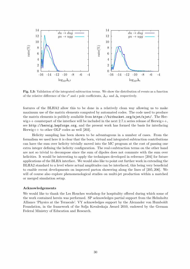
02468

101214

-16 -14 -12 -10 -8 -6 -4

rate

(%)

log10∆ε2

du→ duggu→ ugg

02468101214

-16 -14 -12 -10 -8 -6 -4

rate

(%)

log10∆ε

du→ duggu→ ugg

Fig. I.3: Validation of the integrated subtraction terms. We show the distribution of events as a functionof the relative difference of the ε2 and ε pole coefficients, ∆ε2 and ∆ε respectively.

features of the BLHA2 allow this to be done in a relatively clean way allowing us to makemaximum use of the matrix elements computed by automated codes. The code used to producethe matrix elements is publicly available from https://bitbucket.org/njet/njet/. The Her-wig++ counterpart of the interface will be included in the next 2.7.x series release of Herwig++,see http://herwig.hepforge.org, and the present work has formed the basis for interfacingHerwig++ to other OLP codes as well [203].

Helicity sampling has been shown to be advantageous in a number of cases. From theformalism we used here it is clear that the born, virtual and integrated subtraction contributionscan have the sum over helicity trivially moved into the MC program at the cost of passing oneextra integer defining the helicity configuration. The real+subtraction terms on the other handare not so trivial to decompose since the sum of dipoles does not commute with the sum overhelicities. It would be interesting to apply the techniques developed in reference [204] for futureapplications of the BLHA interface. We would also like to point out further work in extending theBLHA2 standard to a level where actual amplitudes can be interfaced, this being very beneficialto enable recent developments on improved parton showering along the lines of [205, 206]. Wewill of course also explore phenomenological studies on multi-jet production within a matchedor merged simulation setup.

AcknowledgementsWe would like to thank the Les Houches workshop for hospitality offered during which some ofthe work contained herein was performed. SP acknowledges partial support from the HelmholtzAlliance ‘Physics at the Terascale’. VY acknowledges support by the Alexander von HumboldtFoundation, in the framework of the Sofja Kovaleskaja Award 2010, endowed by the GermanFederal Ministry of Education and Research.

30

2 GoSam plus Herwig++/Matchbox2

We describe how GoSam and Herwig++ are linked via the new version of the Binoth-LesHouches-interface (BLHA2), emphasizing new features of the interface. We also give a phe-nomenological example and comment on prospects to match NLO calculations with a partonshower and hadronisation in a fully automated way.

2.1 IntroductionNext-to-leading order (NLO) calculations matched to a Monte Carlo program which can providenot only the phase space integration, but also a parton shower and subsequent hadronisation,should be the new standard for LHC data analysis.

To this aim, automated tools providing the various ingredients of an NLO calculationat parton level are indispensable. These tools comprise a part providing the one-loop virtualcorrections, and parts providing the ingredients which do not involve loops, i.e. the real radiationmatrix element, the subtraction terms for the infrared singularities, and the Born matrix element.The full NLO code therefore can be divided into the categories “one-loop provider" (OLP) and“Monte Carlo program" (MC).

The past years have seen enormous progress in the development of programs for automatedone-loop calculations for multi-particle final states [4–8,201,207–210]. On the Monte Carlo side,a lot of progress has been achieved in matching NLO real radiation matrix elements with aparton shower, see e.g. [26, 28–30,37,211].

The various one-loop matrix element generators and Monte Carlo programs each havedifferent focuses and strengths. Therefore, in order to achieve maximal flexibility in connectingvarious OLP’s with different MC’s, it is desirable to have a standard interface allowing tolink these two parts smoothly. Such an interface has been initiated at the Les Houches 2009workshop [198], known as the “Binoth-Les Houches-Accord" (BLHA) and has been updated in2013 [199]. The latter update will be called BLHA2 in the following.

Here we present the combination of the one-loop program GoSam [4] with the MonteCarlo program Herwig++ [164, 212] based on the BLHA2 interface, with particular emphasison the new features of the interface.

2.2 Linking GoSam and Herwig++/Matchbox via the BLHA2 interfaceVarious function calls, as defined according to BLHA2, have been implemented on both sides inorder to enable the communication between OLP and MC.

2.2.1 Herwig++/MatchboxOn the side of Herwig++ the interface has been realized within the Matchbox module [28],providing functionality to perform hard process generation at the level of NLO QCD accur-cay and easing the setup of run time interfaces to external codes for hard process generation.Herwig++/Matchbox provides thereby the phase space generation and integration, as wellas the organization of the matrix elements and of the appropriate real radiation subtractionterms for the infrared singular regions. The class GoSamAmplitude has been implemented in theMatchbox module, to be included through the shared object file HwMatchboxGoSam.so, whichitself is globally operated through the class MatchboxOLPME.

To configure Herwig++ accordingly a prefix with the installation path (DIR) to Go-Sam has to be specified prior to the installation: ./configure –with-gosam=DIR.

2J. Bellm, S. Gieseke, N. Greiner, G. Heinrich, S. Plätzer, C. Reuschle and J.F. von Soden-Fraunhofen

31

The user only needs to enable the interface from the Herwig++/Matchbox processinput files, using for example the following syntax:

library HwMatchboxGoSam.socd /Herwig/MatrixElements/Matchbox/Amplitudescreate Herwig::GoSamAmplitude Gosamset Gosam:GoSamSetup /desiredpath/gosam_setup.ininsert /Herwig/MatrixElements/Matchbox/PPFactory:Amplitudes 0 Gosam

where a GoSamAmplitude object Gosam will be created. This amplitude can be used tocalculate a specific process, which can be enabled from the Herwig++/Matchbox processinput files, as is usual for a Herwig++/Matchbox calculation, using for example the followingsyntax:

do PPFactory:Process p p e+ e- j

upon which the calculation will be performed fully automatically. This includes Catani-Seymour dipole subtraction for NLO calculations as well as matching procedures if requiredfrom the input file, etc. From a user point of view this means that, except for creating andinserting the GoSamAmplitude object, nothing changes.

Internally, according to BLHA, the process setup is communicated between OLP and MCby exchanging an order file and a contract file. On the side of Herwig++/Matchbox this is at-tended to by the functions GoSamAmplitude::fillOrderFile() and GoSamAmplitude::checkOLPContract(),where an intermediate process-ID map is used to translate the numbering of the process ID’s be-tween GoSam and Herwig++/Matchbox. The contract is “signed" by calling the appropriateGoSam-OLP python script within the function GoSamAmplitude::signOLP(), whereupon the Go-Sam-OLP python script reads the GoSam configuration input file /desiredpath/gosam_setup.in3.Subsequently the process setup is started and the corresponding Fortran90 matrix elementsare created by GoSam, organized into the various subprocesses and helicity configurationsthereof. The function GoSamAmplitude::buildGoSam() then calls the appropriate make routine,provided by GoSam, whereupon the compilation of the various Fortran90 matrix elements isperformed.

Since Herwig++/Matchbox does momentarily not possess the means to create its owntree-level matrix elements, GoSam is also used to provide the various tree-level matrix elements(usual Born matrix elements as well as spin- and colour-correlated Born matrix elements). Thevarious subprocesses, specified in the order/contract file, are therefore grouped into variousamplitude types (Tree, ccTree, scTree and Loop) as well as the different powers of αs, as specifiedaccording to BLHA2.

The function GoSamAmplitude::startOLP() loads the object file libgolem_olp.so from theFortran90 matrix element compilation. It also calls the GoSam Fortran90 function OLP_Start(),as well as the GoSam Fortran90 function OLP_SetParameter() to set the initial parameters ofthe calculation. If required, it also calls for the GoSam Fortran90 function OLP_PrintParameter(),which prints the parameters of the calculation into an output file. From the Herwig++/Matchbox pro-cess input files this feature can be enabled as follows (see example above):

set Gosam:PrintParameter On

The runtime evaluation for each phase-space point is performed by the functions

GoSamAmplitude::evalSubProcess(),GoSamAmplitude::evalColourCorrelator(),GoSamAmplitude::evalSpinColourCorrelator(),

3Various GoSam specific options can be set within the GoSam configuration input file.

32

depending on the various amplitude types. Within those functions the GoSam For-tran90 function OLP_Eval SubProcess2() is called, where the type of ouput depends on theamplitude type in question.

To acquire the spin-correlated Born matrix elements the exchange of the polarizationvectors of the associated gluons is required. For a specific spin-correlation the correspondingpolarization vector is communicated through the function GoSamAmplitude::plusPolarization()and the GoSam Fortran90 function OLP_Polvec(), as specified according to BLHA2. Thespin-colour-correlated Born matrix element can be written as

〈Mµ|CijCµν |Mν〉 = 1

Q2

[〈M|Cij |M〉

(−CQ2 + |ε+ · q|2

)+ 2Re

((ε+ · q)2

{〈M−|Cij |M+〉 outgoing g〈M+|Cij |M−〉 incoming g

)](I.15)

whereM± refers to the amplitude with positive/negative gluon helicity and a sum over helicitiesis understood ifM carries no subscript. The polarization vector which is communicated throughthe function OLP_Polvec() is hereby ε+ [199] and the standard is that of outgoing gluons, i.e.〈M−|Cij |M+〉 for the spin-correlated result. In the case of incoming gluons the polarization vec-tors are simply complex conjugated within the function GoSamAmplitude::plusPolarization(),which yields the correct result since only the real part is of interest here.

The calls to the Fortran90 functions of GoSam are realized by external function callsin the class GoSamAmplitude:

extern "C" void OLP_Start(const char*, int*);extern "C" void OLP_Polvec(double*,double*,double*);extern "C" void OLP_SetParameter(char*,double*,double*,int*);extern "C" void OLP_PrintParameter(char*);extern "C" void OLP_EvalSubProcess2(int*,double*,double*,double*,double*);

The class GoSamAmplitude also provides an automated way to hand over the correct elec-troweak parameters according to the chosen electroweak scheme in the Herwig++ processinput files, via the function OLP_SetParameter(). GoSam automatically chooses the appropriatescheme upon recognizing the corresponding electroweak parameters. Note also that, regard-ing regularization schemes, conventional dimensional regularization (cdr) as well as dimensionalreduction (dred) are supported and yield the same results.

2.2.2 GoSamOn the GoSam side, dedicated OLP modules are provided which host the interface. It shouldbe emphasized again that the user does not need to have a detailed knowledge of these modules,but only interacts via the user interface of the Monte Carlo program, in the present case theHerwig++ process input files.

The function OLP_Start(char* fname, int* ierr), which was already in place with thefirst version of the BLHA interface, takes the name of the contract file as first argument and ini-tializes the OLP setup. The function OLP_Info(char olp_name,char olp_version,char message)prints the GoSam version, svn revision number and references which should be cited when usingthe program.

An important new feature of BLHA2 is the function OLP_SetParameter(), which allows toset parameters like αs, α, masses, widths etc. These parameters are set in the Herwig++ pro-cess input files. Note that this function can also be used to exchange dynamic parameters likeαs(µ2) at runtime.

33

# OLP order file created by# Herwig++/Matchbox for GoSam

InterfaceVersion BLHA2MatrixElementSquareType CHsummedCorrectionType QCDIRregularisation CDR

AlphasPower 1AmplitudeType ccTree1 -1 − > -11 11 21...21 3 − > -11 3 11

AmplitudeType scTree1 -1 − > -11 11 21...21 3 − > -11 3 11

AmplitudeType Loop1 -1 − > -11 11 21...21 3 − > -11 3 11

AlphasPower 2AmplitudeType Tree1 1 − > -11 1 1 11...21 21 − > -11 -3 3 11

# vim: syntax=olp#@OLP GOSAM 2.0.beta#@IgnoreUnknown False#@IgnoreCase False#@SyntaxExtensionsInterfaceVersion BLHA2 | OKMatrixElementSquareType CHsummed | OKCorrectionType QCD | OKIRregularisation CDR | OKAlphasPower 1 | OKAmplitudeType ccTree | OK1 -1 − > -11 11 21 | 1 131...21 3 − > -11 3 11 | 1 70AmplitudeType scTree | OK1 -1 − > -11 11 21 | 1 145...21 3 − > -11 3 11 | 1 71AmplitudeType Loop | OK1 -1 − > -11 11 21 | 1 137...21 3 − > -11 3 11 | 1 63AlphasPower 2 | OKAmplitudeType Tree | OK1 1 − > -11 1 1 11 | 1 42...21 21 − > -11 -3 3 11 | 1 106

Fig. I.4: Automatically created order and contract file for Z+jet. The various subprocesses are given aprocess ID by the OLP.

At runtime, the OLP returns the values for the virtual amplitude to the MC via thefunction OLP_EvalSub Process2(). As compared to the original function OLP_EvalSubProcess(),the new function OLP_Eval SubProcess2() does not contain the passing of coupling constantsanymore, as their values are now passed separately by using OLP_SetParameter()4. It also has anew argument appended which serves to assess the accuracy of the result returned by the OLP.The arguments of OLP_EvalSubProcess2() are described in detail in ref. [199]. Here we pointout that the amplitude types scTree and ccTree, denoting spin- and colour-correlated Bornmatrix elements, can also be provided by GoSam, as described already in section 2.2.1. Thisallows Herwig++/Matchbox to construct the real radiation subtraction terms for the infraredsingular regions. To this end GoSam also provides the function OLP_Polvec() as described insection 2.2.1.

At this point we would like to stress another useful feature of GoSam, which is theability to read in model files in the UFO (Universal Feynrules Output) [213] format and which isparticularly useful for calculations beyond the Standard Model. The UFO format also provideshuman readable name attributes for the model parameters, as well as the SLHA identifiers [214],which are processed by the subroutine read_slha_file.

2.3 Example Z+jet at NLOAs an example we use the built-in process pp→ Z/γ∗+ jet→ e+e−+ jet of Herwig++/Matchbox andcompare it against the same automatically generated GoSam process. The corresponding, yet

4The function OLP_EvalSubProcess(), using BLHA1 conventions, is also still in operation in GoSam.

34

b

b

b

b

b

b

bb

bb

b bb

b b bb b

b b bHerwig++/MatchboxGoSamb

1 2 3 4 5 6 710−1

1

10 1

10 2

Separation between Z boson and leading jet

∆R(Z,j1)

dσ

/d

∆R(Z

,j 1)[p

b]

0.5

1

1.5

2

10−3 10−2 10−1 100 101

|∑ σdip|/σR

√s14/GeV

uu→ e+e−gg

Fig. I.5: Left: The fixed order parton level R-separation between the Z boson and the leading jet inZ+jet production at NLO. Right: Testing the numerical stability in the collinear and soft region showsthe expected behaviour. As an example we show the sum over all Catani-Seymour-dipoles [200] dividedby the real contribution, at phase-space points were the ug1 invariant mass is smaller than 10 GeV. Heres14 denotes the invariant mass between the u and the first gluon in the list.

b

b

b

b

b

b

bb

bb

b bb

b b bb b

b b bHerwig++/MatchboxGoSamb

GoSam + PSHerwig++/Matchbox + PS

1 2 3 4 5 6 710−1

1

10 1

10 2

Separation between Z boson and leading jet

∆R(Z,j1)

dσ

/d

∆R(Z

,j 1)[p

b]

b

bbbb b b b b b b b b b b b b b b

bb b b b b

b b b b b b b bb b b b b b b b b b b b b b b b b b b

b b b b b b b b b b b b b bb b b b

b bb bb bb b b b b

b bbb bb bb

Herwig++/MatchboxGoSamb

GoSam + PSHerwig++/Matchbox + PS

10 2 10 310−5

10−4

10−3

10−2

10−1

1

10 1

Transverse momentum of leading jet

p⊥(j1) [GeV]

dσ

/d

p ⊥(j

1)[p

b/G

eV]

Fig. I.6: Left: The R-separation between the Z-boson and the leading jet in Z+jet production. Right:The transverse momentum of the leading jet. Both with and without parton shower matching. The –for this process – inclusive observable p⊥ of the first jet is hardly affected by the parton shower. The redand pink lines show the results with the Herwig++/Matchbox built-in matrix elements, the blue dotsand green lines show the results of Herwig++/Matchbox with the GoSam matrix elements.

shortened, order and contract files are shown in fig. I.4. Here we want to stress again that thewhole compuation proceeds fully automatically only upon a few commands in the Herwig++ in-put files, which includes the automatic generation of the order and the contract file. To getagreement between the Herwig++/Matchbox built-in and the GoSam matrix elements, weneed to make the same assumptions on both sides: While in the Herwig++/Matchbox built-in matrix elements the diagrams with photon- and Z-radiation from bottom- and top-trianglesare not implemented, because they are numerically negligible, GoSam produces these by de-fault. For the comparison, these contributions were eliminated by using the appropriate filteroptions in the GoSam configuration input file.

To calculate the cross sections and distributions shown in fig. I.5 and fig. I.6 we use theminimal set of cuts

66GeV < me+e− < 116GeV, pT,j > 20GeV , |ηj| < 5 ,

and the dynamical scaleµr = µF = me+e− .

The scale choice may not be ideal from a phenomenological point of view, but it showsthat dynamical scales work fine within the interface. The shower matched distributions are

35

obtained using the dipole shower outlined in [215] and a modified version of the MC@NLO-typematching described in [28], which accounts for subleading colour contributions. The matchingcan be enabled, as is usual for Matchbox processes, with a single command line:

set PPFactory:ShowerApproximation DipoleMatching

2.4 Conclusions & OutlookThe combination of one-loop providers (OLP) and Monte Carlo programs (MC) using a stan-dardized interface has been proven to be a successful strategy for automated NLO calculations.We have presented phenomenological results obtained through the automatized combination ofthe Monte Carlo program Herwig++/Matchbox with the one-loop program GoSam. Thelink between the two codes is based on the new version of the Binoth-Les-Houches interface(BLHA2), which has been worked out at the Les Houches 2013 workshop, including proof-of-concept interfaces to other OLPs, [216]. In particular, the new feature to pass spin- andcolour-correlated tree level matrix elements from the one-loop provider to the Monte Carlo pro-gram allows the Herwig++/Matchbox module to provide the full NLO real radiation part.As a first application we calculated the NLO QCD corrections to Z+jet production at the LHC.We validated the results with the GoSam matrix elements against a corresponding built-inimplementation in Herwig++/Matchbox.

In combination with the Herwig++ shower, the full chain from process definition to theproduction of showered event samples at NLO accuracy is thus provided in a fully automatedway. This opens the door for a multitude of phenomenological applications. As both GoSamand Herwig++ are also able to import model files in UFO format, and offer various featureswhich are important for calculations involving unstable particles, the applications are not limitedto QCD, but also well suited for electroweak corrections and BSM calculations.

AcknowledgementsThis work was supported in part by the Marie Curie Initial Training Network MCnetITN, theGerman Federal Ministry of Education and Research (BMBF), the Helmholtz Alliance “Physicsat the Terascale” and the Karlsruhe School of Elementary Particle and Astroparticle Physics(KSETA).

36

Chapter II

Parton distribution functions

1 PDF dependence of the Higgs production cross section in gluon fusion fromHERA data1

We document a detailed comparison of theoretical settings and fitting methodologies employedin the determination of parton distribution functions (PDFs) of the proton, focusing on thefactors driving the PDF uncertainty in Higgs boson production in the gluon fusion channel.In order to understand the moderate discrepancies among predictions obtained using CT10,HERAPDF1.5, MSTW08 and NNPDF2.3 PDF ensembles, we first complete a benchmarkingcomparison of computations of NNLO neutral current DIS cross sections used in the fitting codesof these groups. Then, we compare results of the fits performed by following the methodologiesof the four groups to a reduced common set of DIS data from HERA experiments. We concludethat the predictions for gg → H observables, obtained when the PDFs are constrained usingonly the HERA DIS data, are in fairly good agreement, within the PDF uncertainty.

1.1 IntroductionFollowing the discovery of the Higgs boson at the LHC, it is crucial to measure all of its propertiesprecisely in order to identify the underlying mechanism of electroweak symmetry breaking.PDF uncertainty is one of the limiting factors in the accuracy with which one can extractthe Higgs boson couplings from experimental data. Its control is needed for precise Higgscharacterization [40].

It has been shown that recent NNLO PDFs from various PDF analysis groups are ingenerally good agreement. However, moderate differences due to the gluon PDFs are observedaround the Higgs mass region, at ≈ 125 GeV. This leads to discrepancies at the level of 1 to2 standard deviations [217] in the predictions for the Higgs production cross sections throughgluon fusion, which is the dominant production channel at the LHC. In part because the originof this spread in the results is not understood, the PDF4LHC convention [218], adopted by theHiggs working group [38, 40], recommends a conservative estimate for the combined PDF+αsuncertainty based on the envelope of results obtained using different PDF sets. If this sizableuncertainty is of theoretical origin, it would remain irreducible unless its source is identified.Whereas the problem may be resolved after including more experimental data, this is by nomeans guaranteed, and thus it is important to investigate the origin of the differences amongthe various PDF sets and, if possible, reduce or even eliminate it.

There have been in the past several related PDF benchmarking studies, some in thecontext of other Les Houches workshops. The evolution of PDFs was benchmarked in ref. [219],where the HOPPET [220] and PEGASUS [221] codes were compared, including the effect ofscale variations. This exercise was extended within the context of the HERA-LHC workshopto NNLO evolution and polarized PDF evolution [222]. Differences in general-mass heavy-quark schemes for DIS charm structure functions, F2,c, were studied in detail in ref. [160],where good agreement between the ACOT, FONLL and TR schemes was found up to differenttreatments of powerlike corrections. Finally, other recent benchmarking exercises have focusedon the comparison of PDFs and their predictions for LHC cross sections [217,223–227], and the

1A. Cooper-Sarkar, S. Forte, J. Gao, J. Huston, P. Nadolsky, J. Pumplin, V. Radescu, J. Rojo, R. Thorne andC.-P. Yuan

37

aforementioned differences in the gluon PDFs were already noted.The main goal of this contribution is to begin a benchmarking exercise aimed at advancing

the control of PDF dependence of the gg → H cross section. We will restrict ourselves tothe comparison of the PDFs based on the general-mass schemes for heavy-quark scatteringcontributions, as it has been noted in a number of studies [228–231] that the PDFs (and αs) candiffer rather significantly if a fixed-flavor number (FFN) scheme is used.2 The recent NNLO setsutilizing the general-mass schemes include CT10 [233], HERAPDF1.5 [234], MSTW2008 [235]and NNPDF2.3 [236]. Except for HERAPDF1.5, which is based on inclusive HERA data only,three other PDF sets include information from a variety of data sets from fixed-target andcollider DIS, as well as from hadron-hadron scattering processes, including, in some cases, theLHC data. Detailed comparisons of these NNLO PDFs and the respective LHC predictionscan be found in a recent benchmarking study [217]. In all these fits, the backbone of the fitis provided by the combined HERA-1 inclusive DIS data [237], which also plays an importantrole in constraining the gluon PDFs in the Higgs mass region [238]. Recently combined charmquark production measurements at HERA have also been published [239], which introduce anadditional constraint on the gluon PDF.

Given the relevance of the HERA data for pinning down the gluon PDF, and the factthat this data set underwent careful examination of all the experimental uncertainties, we havechosen to initiate this benchmarking exercise by first studying the fits that include exclusivelythe HERA-1 data. In this highly controlled environment, we can compare the output from thedifferent fitting codes and try to isolate possible sources of discrepancy related to, for example,implementation of reduced cross section calculations, alternative parametrizations, kinematicalcuts used in the fits, and the different definitions of χ2 used in determining the fit quality. Wecan then study how these differences translate into the predictions for Higgs cross sections inthe gluon fusion channel.

As a prerequisite for this benchmarking exercise, we compared the NNLO QCD predictionsfor the neutral-current DIS cross sections from four different codes, but always using the samePDF set. This is an important starting point: we show that, when all groups use commonPDFs and settings, they find good agreement among their NC DIS cross sections, with (small)remaining differences arising from known sources such as the selection of the heavy-quark scheme.

This contribution is organized as follows. In Section 2 we briefly recall the status of thePDF dependence of the NNLO Higgs cross section in gluon fusion. In Section 3 we present theresults of the benchmarking of the NNLO neutral current DIS structure functions from differ-ent groups using a common PDF set. Section 4 contains the main results of this study, wherefits to HERA only data are performed, and the impact of various theoretical and methodolog-ical settings is assessed. Finally in Section 5 we summarize our main results and outline thecontinuation of this benchmarking exercise beyond the HERA-only fits.

1.2 The Higgs cross section via gluon fusion obtained with recent NNLO PDF setsWe first review the settings of the four recent NNLO PDF determinations that will be studiedin this paper. Table II.1 summarizes the heavy-quark scheme, the scale at which the PDFsare parametrized, the charm-quark mass, and the kinematic cuts on DIS data. Note that, inaddition to these differences in settings, the four PDF analyses also differ in the data sets thatthey include. We compare the corresponding predictions for the Higgs cross section in the gluonfusion channel in Table II.2 and Fig. II.1. These predictions use versions of the PDF sets witha common αs(MZ) value of 0.118 and are calculated with iHixs1.3 [240] at NNLO in QCD,

2Studies of the gluon PDF and predictions for the Higgs and other benchmark LHC cross sections in the FFNscheme are available in [226,227,232].

38

with both Higgs boson mass and QCD scales set to 125 GeV in the heavy top-quark limit. Weshow the PDF uncertainties at the 68% confidence level (c.l.). For the LHC at 8 TeV, the twoextreme results, CT10 and NNPDF2.3, differ by about 4%, or 2σ if their uncertainties are addedin quadrature. This spread is the origin of the significant PDF+αs uncertainty in the gg → Hchannel [40]. A similar results holds for the LHC at 14 TeV.

PDFs set Ref. Initial Heavy-quark mc Q2 cut W 2 cutscale [GeV] scheme mass [GeV] ≥ GeV2 ≥ GeV2

CT10 [233] 1.3 S-ACOT-χ [241] 1.3 4 12.25HERAPDF1.5 [234] 1.378 default TR’ 1.4 3.5 N.A.∗MSTW’08 [235] 1.0 default TR’ [242] 1.4 2.0 15.0

NNPDF2.3 (Nf = 5) [236] 1.414 FONLL-C [243] 1.414 3.0 12.5

∗All HERA data have W 2 > 350 GeV2.

Table II.1: Basic inputs of the recently published NNLO PDFs based on a GM-VFN scheme.

σH [pb] CT10 MSTW’08 NNPDF2.3 HERAPDF 1.5LHC 8 TeV 18.36±0.35 18.78±0.31 19.23±0.21 18.63±0.23LHC 14 TeV 47.60±1.02 48.71±0.77 49.76±0.47 48.18±0.47

Table II.2: Predictions for inclusive cross sections of SM Higgs boson production through gluon fusionutilizing recently published NNLO PDFs.

íí

óó

õõ

çç

LHC 8 TeV, with iHixs 1.3 at NNLO

MSTW2008 NNPDF2.3 CT10 HERAPDF1.5

17.5

18.0

18.5

19.0

19.5

20.0

ΣH@p

bD

íí

óó

õõ

çç

LHC 14 TeV, with iHixs 1.3 at NNLO

MSTW2008 NNPDF2.3 CT10 HERAPDF1.5

46.0

48.0

50.0

52.0

ΣH@p

bD

Fig. II.1: Predictions for inclusive cross sections of the SM Higgs boson production through gluonfusion based on recently published NNLO PDFs.

These discrepancies of the Higgs cross sections can be traced back to the differences in thenormalization and shape of the corresponding gluon PDFs, as shown in Fig. II.2. In this plotall gluon PDFs are normalized to the gluon PDF of the first, or central, set of the NNPDF2.3

39

ensemble, and only the PDF uncertainty of the NNPDF2.3 ensemble is shown in the figurefor simplicity. The three vertical lines indicate the x values of 0.005, 0.01, and 0.02, coveringtypical x values for Higgs production in the central rapidity region, x = mH/

√s ∼ 0.016 (0.009)

for LHC 8 (14) TeV. We can see that at Q = 85 GeV, and for x from 0.005 to 0.1, the gluonPDF from CT10 lies below that of NNPDF2.3. MSTW lie in between, while HERAPDF isclose to CT10 at x < 0.02 and larger than CT10 at x > 0.02. Fig. II.3 shows a comparison ofthe gluon-gluon parton luminosity as a function of the invariant mass of the final state. Thefactorization scale is set to the invariant mass. The vertical line indicates the mass of the SMHiggs boson at 125 GeV. For higher invariant masses (> 400 GeV), all predictions are within68% c.l. uncertainties of NNPDF2.3 until very high masses, (> 1000 GeV).

Normalized to NNPDF2.3 NNLO

at Q=85 GeV, default sets

MSTWCTEQ

HERAPDF± 68% C.L.

10-4 10-3 10-2 10-1 10.90

0.95

1.00

1.05

1.10

x

Norm

aliz

ed

gHxL

Fig. II.2: Comparison of central gluon PDFs from recently published NNLO PDF sets at a commonscale Q = 85 GeV, normalized to the NNPDF2.3 gluon PDF and superimposed on the NNPDF2.3 68%c.l. PDF uncertainty.

Normalized to NNPDF2.3 NNLO

default sets

MSTWCTEQ

HERAPDF± 68% C.L.

10 100 10000.8

0.9

1.0

1.1

1.2

M@GeVD

No

rma

lize

dLHg

g,8

Te

VL

Normalized to NNPDF2.3 NNLO

default sets

MSTWCTEQ

HERAPDF± 68% C.L.

10 100 10000.8

0.9

1.0

1.1

1.2

M@GeVD

No

rma

lize

dLHg

g,1

3T

eVL

Fig. II.3: Comparison of the gluon-gluon parton luminosity as a function of invariant mass at the LHC8 and 13 TeV from recently published NNLO PDFs, normalized to the NNPDF 2.3 central prediction.The factorization scale is set to the invariant mass. The vertical line corresponds to the mass of the SMHiggs boson.

To illustrate the sensitivity of the Higgs cross section to the gluon PDF, we also plot therapidity distribution of the Higgs boson from gluon fusion in Fig. II.4. The predictions arecalculated at NLO using MCFM 6.0 [209], with both the Higgs mass and QCD scales set at 125

40

GeV, and knowing that the NNLO/NLO K-factors cancel well in these ratios. We see that inthe central production region (|y| < 1), which contributes the bulk of the total cross section,the difference between CT10 and NNPDF2.3 can reach 6%, i.e., it is larger than in the inclusiverate. At higher rapidities the predictions of all groups overshoot that of NNPDF2.3, reflectingthe behavior of their large-x gluon PDFs in Fig. II.2.

Normalized to

NNPDF2.3 NNLO

LHC 8 TeV

MCFM 6.0 at NLO

MSTW

CTEQ

HERAPDF

± 68% C.L.

0.0 0.5 1.0 1.5 2.0 2.5 3.00.8

0.9

1.0

1.1

1.2

y

Ra

tio

so

fdΣ

H�d

y

Normalized to

NNPDF2.3 NNLO

LHC 14 TeV

MCFM 6.0 at NLO

MSTW

CTEQ

HERAPDF

± 68% C.L.

0.0 0.5 1.0 1.5 2.0 2.5 3.00.8

0.9

1.0

1.1

1.2

yR

atio

so

fdΣ

H�d

y

Fig. II.4: Comparison of the rapidity distribution of the SM Higgs boson in production through gluonfusion from recently published NNLO PDFs, normalized to the NNPDF 2.3 central prediction. Thematrix elements of hard scattering are calculated at NLO.

In Section 4 we will investigate the origin of these differences in the gluon PDFs in a simplerscenario than that of the global fit, namely, by comparing the PDF fits of the HERA-1 DIS dataset alone. However, before doing that, we want to make sure that the differences among thetheoretical predictions for NNLO DIS neutral current cross sections in different fitting codes areunder control, and with this aim we discuss now a new benchmarking of DIS structure functions.

1.3 Benchmark comparisons of NNLO neutral current DIS cross sectionsAs in the previous benchmarking studies, in this section we adopt the Les Houches toy PDFs andsettings [160]. The corresponding LHAPDF grid file was generated with the APFEL program [244]by evolving the Les Houches toy PDFs from the starting scale Q2

0 = 2 GeV2. We set the bottomand top masses to infinity, and use as a boundary condition αs(µ) = 0.35 at a scale µ approachingQ0 from below. Theoretical predictions are made at the (x,Q2) values of the neutral currentpositron HERA-1 combined data set [237] for Q2 ≥ 3.5 GeV2.

Modern GM-VFN schemes, like FONLL-C [243] used by NNPDF, TR [229] used by MSTWand HERAPDF, and S-ACOT-χ [241] used by CTEQ, are expected to be very similar at NNLO,and we will demonstrate the convergence here.

For the comparisons of this section, the MSTW and HERAPDF results will both usethe optimal TR heavy-quark scheme [229], instead of the standard scheme that is used in thepublished NNLO PDF sets. As noted in [229], the change in the TR scheme leads to only anextremely small change in the MSTW fit quality and the resulting PDFs at NNLO, i.e. smallfractions of a percent in the Higgs cross section at the LHC. The NNPDF2.3 results for structurefunctions will be obtained using the APFEL code, instead of using the FastKernel NNPDF fittingcode, because of its ease of use (the predictions of the two codes agree at the per mille levelanyway.). The HERAPDF results on structure functions are obtained with the HERAFittercode [237,245–247].

In the following, we will compare the total (with subscript “tot”) and charm-quark con-tributions (“c”) to inclusive F2, F3, and FL structure functions, which are defined as in [237]

41

Q2 [GeV2] x y F2,lt F2,c FL,lt FL,c σ+r,NC

2.7 0.0000309 0.86398 0.7768 0.1411 0.1267 0.00844 0.81892.7 0.00013 0.20523 0.6275 0.09204 0.1173 0.00592 0.71632.7 0.02 0.00133 0.3871 0.00723 0.0849 0.00074 0.39434.5 0.0000618 0.71999 0.964 0.193 0.1866 0.01879 1.05834.5 0.00032 0.13896 0.7187 0.1136 0.1547 0.01191 0.83054.5 0.013 0.00342 0.4317 0.02011 0.0898 0.00259 0.451810. 0.00013 0.85281 1.192 0.31011 0.2535 0.04618 1.288610. 0.0008 0.12352 0.8064 0.16391 0.1758 0.0263 0.968510. 0.02 0.00494 0.4614 0.03152 0.0766 0.00564 0.4929120. 0.0016 0.74111 1.1038 0.41841 0.179 0.08637 1.3852120. 0.008 0.14822 0.6915 0.18639 0.0905 0.03846 0.8761120. 0.18 0.00659 0.3312 0.00591 0.0128 0.00095 0.3371650. 0.0085 0.84779 0.768 0.24564 0.0791 0.04104 0.9216650. 0.032 0.20072 0.5249 0.09203 0.0364 0.01444 0.6122650. 0.25 0.02569 0.252 0.00306 0.0059 0.00032 0.25452000. 0.032 0.6929 0.5502 0.10329 0.0328 0.01347 0.59732000. 0.13 0.15202 0.3634 0.0164 0.011 0.00172 0.36982000. 0.25 0.07905 0.244 0.00327 0.0049 0.00027 0.24338000. 0.13 0.68224 0.3948 0.01837 0.01 0.00149 0.2848000. 0.18 0.43917 0.3307 0.00903 0.0069 0.00066 0.26498000. 0.25 0.31621 0.254 0.00356 0.0043 0.00022 0.2148

Table II.3: Predictions for NC DIS structure functions and reduced cross sections from HERA-1 [237]at NNLO, obtained with the CT10 code [233] and Les Houches toy PDFs [160].

and include all scattering contributions coupled to the photon and Z boson currents. The lightquark contributions (“lt”) are defined by subtracting the charm-quark contributions from thetotal structure functions. This means that Fc is defined as the structure function that one wouldget if only the electromagnetic charge of the charm quark was nonzero [241, 243], and then Fltis implicitly defined by

Ftot ≡ Flt + Fc =Nl∑l=1

Fl + Fc, (II.1)

where Fl is the structure function obtained when only the charge of the l-th quark is nonzero.With this definition, at NNLO Fl receives a contribution from the process with charm in thefinal state, such as γ∗u → ucc, as well as from diagrams containing the charm quark in virtualloops. Note that there is a cancellation of terms with large logs of Q2/m2

c between these twocontributions.

The NNLO results for F2,lt(c), FL,lt(c), and the reduced cross sections obtained for a rep-resentative subset of the HERA-1 data points, using the four different codes, are collected inTables II.3-II.6. These tables should be useful for future comparisons, for instance for validationof structure function codes. In the following we compare and discuss these results, both at NLOand at NNLO. Comparisons at LO are not meaningful because of the different perturbativeordering between different codes.

In Fig. II.5 we plot the light structure function F2,lt at NLO and NNLO, normalized to theHERAPDF results. The data point indexing is ordered in increasing Q2 (starting from Q2 =2.7GeV2), then increasing x. We find excellent agreement at NLO among all groups, with smallfluctuations at the per mille level at low Q due to numerical precision, and moderate oscillations

42

Q2 [GeV2] x y F2,lt F2,c FL,lt FL,c σ+r,NC

2.7 0.0000309 0.86398 0.7821 0.17992 0.261 0.01067 0.76282.7 0.00013 0.20523 0.6318 0.10519 0.1711 0.00669 0.73242.7 0.02 0.00133 0.3893 0.01013 0.0829 0.00073 0.39954.5 0.0000618 0.71999 0.972 0.2175 0.2507 0.01961 1.05964.5 0.00032 0.13896 0.7249 0.11996 0.1685 0.01122 0.84294.5 0.013 0.00342 0.435 0.02257 0.0885 0.00244 0.457510. 0.00013 0.85281 1.2026 0.32346 0.2759 0.04743 1.295810. 0.0008 0.12352 0.8135 0.16653 0.1771 0.02543 0.978310. 0.02 0.00494 0.465 0.03274 0.0797 0.00588 0.4978120. 0.0016 0.74111 1.107 0.40842 0.1824 0.08717 1.3761120. 0.008 0.14822 0.693 0.18279 0.0935 0.03914 0.8739120. 0.18 0.00659 0.3317 0.00594 0.0149 0.00113 0.3376650. 0.0085 0.84779 0.7681 0.2396 0.0817 0.04192 0.9133650. 0.032 0.20072 0.5249 0.09021 0.0385 0.01505 0.6103650. 0.25 0.02569 0.252 0.00305 0.0068 0.00022 0.25462000. 0.032 0.6929 0.5489 0.10207 0.0345 0.01416 0.59392000. 0.13 0.15202 0.3632 0.0163 0.0121 0.00189 0.36952000. 0.25 0.07905 0.2439 0.00326 0.0055 0.00019 0.24328000. 0.13 0.68224 0.3937 0.01893 0.011 0.0017 0.28378000. 0.18 0.43917 0.3301 0.00928 0.0077 0.00076 0.26498000. 0.25 0.31621 0.2537 0.00365 0.0048 0.00017 0.2148Table II.4: Same as Table II.3, using the HERAFitter code [237,245–247].

Q2 [GeV2] x y F2,lt F2,c FL,lt FL,c σ+r,NC

2.7 0.0000309 0.86398 0.7809 0.17478 0.2611 0.01104 0.76042.7 0.00013 0.20523 0.6316 0.10218 0.1713 0.00678 0.72922.7 0.02 0.00133 0.3895 0.01016 0.0835 0.00074 0.39974.5 0.0000618 0.71999 0.9713 0.2174 0.2488 0.02008 1.06234.5 0.00032 0.13896 0.7249 0.12013 0.1678 0.0113 0.84314.5 0.013 0.00342 0.4351 0.02258 0.0888 0.00246 0.457710. 0.00013 0.85281 1.2024 0.32374 0.2735 0.04786 1.299110. 0.0008 0.12352 0.8134 0.16673 0.1762 0.02555 0.978410. 0.02 0.00494 0.465 0.03268 0.0797 0.00592 0.4977120. 0.0016 0.74111 1.1067 0.40833 0.181 0.08729 1.3784120. 0.008 0.14822 0.6929 0.18255 0.0929 0.03919 0.8736120. 0.18 0.00659 0.3317 0.0059 0.0147 0.00113 0.3376650. 0.0085 0.84779 0.7669 0.23899 0.0811 0.04189 0.9126650. 0.032 0.20072 0.5243 0.08985 0.0382 0.01503 0.6093650. 0.25 0.02569 0.2519 0.00302 0.0067 0.00037 0.25452000. 0.032 0.6929 0.5462 0.1013 0.0341 0.01409 0.58962000. 0.13 0.15202 0.3624 0.01615 0.0119 0.00188 0.36822000. 0.25 0.07905 0.2437 0.00322 0.0054 0.00031 0.24298000. 0.13 0.68224 0.3893 0.0186 0.0107 0.00167 0.27568000. 0.18 0.43917 0.3277 0.00914 0.0075 0.00075 0.26078000. 0.25 0.31621 0.2525 0.0036 0.0047 0.00026 0.2129

Table II.5: Same as Table II.3, using the MSTW08 code [235].

43

Q2 [GeV2] x y F2,lt F2,c FL,lt FL,c σ+r,NC

2.7 0.0000309 0.86398 0.7809 0.13392 0.1035 0.0089 0.83242.7 0.00013 0.20523 0.6309 0.08936 0.0981 0.00628 0.71762.7 0.02 0.00133 0.3884 0.0069 0.0736 0.00073 0.39534.5 0.0000618 0.71999 0.9629 0.19426 0.1706 0.01982 1.06564.5 0.00032 0.13896 0.7181 0.1138 0.1425 0.01266 0.83024.5 0.013 0.00342 0.431 0.01932 0.0828 0.00293 0.450310. 0.00013 0.85281 1.1897 0.31837 0.247 0.05032 1.296210. 0.0008 0.12352 0.8046 0.16446 0.1714 0.02859 0.967310. 0.02 0.00494 0.4601 0.03125 0.0742 0.00642 0.4913120. 0.0016 0.74111 1.1083 0.40632 0.1794 0.08744 1.3769120. 0.008 0.14822 0.6939 0.18171 0.0907 0.03899 0.8738120. 0.18 0.00659 0.3319 0.00614 0.013 0.00098 0.338650. 0.0085 0.84779 0.771 0.23832 0.0795 0.0412 0.9169650. 0.032 0.20072 0.5268 0.08994 0.0367 0.01452 0.612650. 0.25 0.02569 0.2524 0.00307 0.006 0.00032 0.2552000. 0.032 0.6929 0.5519 0.10081 0.0332 0.01354 0.59652000. 0.13 0.15202 0.3643 0.01615 0.0112 0.00174 0.37042000. 0.25 0.07905 0.2443 0.00324 0.005 0.00027 0.24368000. 0.13 0.68224 0.3953 0.01807 0.0104 0.00152 0.28478000. 0.18 0.43917 0.3311 0.0089 0.0072 0.00067 0.26558000. 0.25 0.31621 0.2541 0.00352 0.0044 0.00023 0.2151

Table II.6: Same as Table II.3, using the APFEL code [244] with the FONLL-C scheme. These resultsagree at the per mille level with those of the N -space FastKernel code adopted in the NNPDF fits.

of at most 1.5% at high Q from different treatment of electroweak corrections and Z or γ/Zinterference terms. Note that at large Q2 experimental uncertainties are typically > 10%, sothese differences have no impact on the fit results.

At NNLO we observe some systematic shifts of 1% between MSTW/HERAPDF andCTEQ/NNPDF especially around the data point 50, which corresponds to Q2 ∼ 6 GeV2. How-ever, we have checked that if we use a 3-flavor scheme we find very good agreement, within 0.2%,for F2,lt at NNLO in that Q region. Therefore, we attribute these shifts to the aforementionedcontribution from the processes with γ∗q → qcc contributions, or charm quark loops, which firstappear at NNLO and are known to be implemented differently in the codes that were compared.As with other flavor scheme differences, there should be convergence at higher orders.

Turning now to the heavy-quark structure function, Fig. II.6 shows the results for F2,c.MSTW and HERAPDF agree as they should, since they both use the optimal TR’ scheme. Wealso observe close similarity between CTEQ and NNPDF, which are based on the numericallyclose schemes S-ACOT-χ, FONLL-A (at NLO) and FONLL-C (at NNLO). In the low-Q region,CTEQ and NNPDF are in very good agreement, and both are smaller than MSTW/HERAPDF.In the intermediate-Q region, all groups agree within a couple of percent. It has been furtherverified that, if one uses the NNPDF or CTEQ scheme definition in the MSTW code at NNLO,even better agreement is found between the groups. The “spike” structure for NNPDF is due tothe use of a different kinematical variable in the GM-VFN scheme definition, i.e. x is used in theFONLL scheme [243], while χ = x(1 + 4m2

c/Q2) is used in the TR’ [242] and S-ACOT-χ [241]

schemes. This effect is mainly seen at the highest x point in each Q2 bin, where F c2 is a smallcontribution to the total.

The overall trends in F2,c are consistent with the results obtained in the context of the 2010

44

Les Houches heavy-quark benchmarks [160] (see also the follow-up comparisons with S-ACOT-χat NNLO in [241]). The differences are reduced when going from NLO and NNLO, in agreementwith the general expectation that, at each order in αs, the GM-VFN heavy-quark schemesare equivalent up to contributions proportional to m2

c/Q2 at one higher order. Apart from

the residual differences in their heavy-quark schemes, the CTEQ and NNPDF codes evaluateO(α2

s) heavy-quark scattering contributions by interpolation of integral tables [248] and directintegration [243], respectively. This contributes to some of the minor differences seen betweenthe CTEQ and NNPDF F2,c values at NNLO.

Fig. II.7 presents comparisons of F2,tot, which is impacted by all effects seen in Figs. II.5and II.6. Again the differences decrease as we go from NLO to NNLO.

We now turn to the other structure functions. Figs. II.8-II.10 show results for FL. Heredifferent counting of perturbative orders adopted by the groups results in large discrepanciesbetween the MSTW/HERAPDF and CTEQ/NNPDF FL values of nominally the same orders,e.g., at LO FL vanishes for CTEQ/NNPDF, while it is of O(αs) for MSTW/HERAPDF. Wehave checked explicitly that, once we use the O(αs) (O(α2

s)) Wilson coefficients for FL with LO(NLO) toy PDFs both in CTEQ and MSTW codes, the respective CTEQ and MSTW valuesagree at the 1-2% level. We also find very good agreement on F3 among all groups.

Finally, in Fig. II.11 we show a comparison of the HERA reduced cross sections con-structed from F2, FL, and F3 [237], which can be directly compared to the data. Again we seeexcellent agreement between all groups, and significant convergence from NLO to NNLO. Exceptfor the extremely high Q region, where there exist some differences in the implementations ofelectroweak corrections (and where data points have very large errors), all curves agree within1% in the moderate-Q region, and 2% in the low-Q region. The MSTW and HERAPDF predic-tions are essentially identical, as they should be (other than the differences due to electroweakcorrections or numerical precision). CTEQ and NNPDF are quite close, too, even at low Q, dueto the similarities of the S-ACOT-χ and FONLL-A (FONLL-C) heavy-quark schemes at NLO(NNLO).

We conclude from this benchmark exercise that the differences in theoretical predictionsof neutral current DIS cross sections between CT, HERAPDF, MSTW and NNPDF are well un-derstood as mostly arising from the choice of the respective heavy-quark schemes, non-identicalcounting of perturbative orders, electroweak contributions, and that these theoretical differencesare small at NNLO compared to the experimental margin of error. Therefore, we expect thatthe differences in heavy-quark schemes should not have a large impact on the fits using onlyHERA-1 data or on the Higgs cross sections predicted from them at the NNLO. This will beinvestigated in the next section.

Before closing this section, we note that in the following fits, NNPDF uses the trun-cated solution for the DGLAP evolution equations and the αs renormalization-group evolution.Modifications resulting from this choice (essentially from a different treatment of higher-orderperturbative corrections as compared to the exact solutions used in the CT, MSTW and HER-APDF codes) should be quite small at NNLO. We have verified that it is certainly negligible forthe running of αs. Second, larger differences (of order 10%) are observed between the group’spredictions for charged-current DIS cross sections, which are still evaluated at NLO. As theexperimental uncertainties on the charged-current DIS cross sections are still rather significant,the current differences between the codes in the charged-current sector are not anticipated to beof the same consequence for the gluon PDF as those in the neutral-current DIS cross sections.

45

1.4 Benchmark PDF fits to HERA-1 data1.4.1 SetupWe will first describe the setup used for the fits to the reduced data set based on the combinedHERA-1 DIS data only. At this stage we performed the baseline fit based on the default settings,as well as a series of alternative fits designed to assess dependence on the input assumptions.The kinematical ranges of the data sets included in the fits, and the number of points in eachmeasurement, are summarized in Table II.7. The baseline fit includes only the combined inclusivedata with Q2 > 5GeV2 to minimize the differences due to the heavy-quark schemes. Somealternative fits also include the combined charm quark production data and vary the lower Q2

cut or other input parameters. We assume the strong coupling constant to be αs(MZ) = 0.118and set the pole mass of the charm quark to a common value of 1.4 GeV in the baseline fit andto the default values of each group in the variant fits. NNLO QCD theory is used throughout.

In the HERA-1-only fits, the data do not constrain PDFs in the extremely large x regionor some of the flavor combinations, e.g., u− d, (s+ s)/(u+ d), s− s. The remaining degrees offreedom are associated mostly with g, uv, dv, and u+d PDFs. Therefore, CTEQ fits use a smallernumber of free PDF parameters than in their global fits, as well as updated parametrizationforms for some flavors based on Chebyshev polynomials [249,250]. The MSTWHERA1-only fit isdone using an updated parametrization based on Chebyshev polynomials for some flavors, whichhas been shown [250] to lead to a change in the Higgs cross section at the LHC of only a smallfraction of a percent compared to the published MSTW’08 parametrizations. The HERAPDFbaseline fit uses the same number of free parameters as in HERAPDF1.5, which is smaller thanin CTEQ and MSTW global fits. Similarly, the baseline neural-network parametrizations ofNNPDF are the same as in their global fits and produce very large uncertainty bands for theirunconstrained PDF combinations. The dependence on the PDF parametrization form is furtherdiscussed in Sec. 1.4.3.

All PDF analyses utilize the figure-of-merit χ2 to find the best fit and estimate the PDFuncertainties. In the presence of correlated systematics, χ2 can be written as a function of thePDF parameters a and nuisance parameters λ,

χ2(a, λ) =Npt∑k=1

1s2k + σ2

k

Dk − Tk −Nλ∑α=1

βk,αλα

2

+Nλ∑α=1

λ2α, (II.2)

where Npt and Nλ are the total numbers of data points and correlated systematic errors, respec-tively [251,252]. Tk are the theoretical predictions, and Dk are the central values of experimentalmeasurement. sk, σk, and βk,α are the statistical, uncorrelated systematic, and correlated sys-

F2lt at NLO

MSTWNNPDFCTEQ

HERAPDF

0 100 200 300 4000.985

0.990

0.995

1.000

1.005

Data Point ID

F2

lta

tN

LOHn

orm

alize

dto

HE

RA

PD

FL F2lt at NNLO

MSTWNNPDFCTEQ

HERAPDF

0 100 200 300 4000.985

0.990

0.995

1.000

1.005

Data Point ID

F2

lta

tN

NL

OHn

orm

alize

dto

HE

RA

PD

FL

Fig. II.5: Structure function F2,lt(x,Q) at NLO and NNLO from all groups, normalized to the resultsfrom the HERAPDF1.5 code.

46

NC (e+p) NC (e−p) CC (e+p) CC (e−p) CharmQ2 range [GeV2] 0.045-30000 90-30000 300-15000 300-30000 2.5-1000

x range 0.621×10−6-0.65 0.0013-0.65 0.008-0.4 0.013-0.4 3×10−5-0.05Npt, Q2 ≥ 2 GeV2 408 145 34 34 52Npt, Q2 ≥ 3.5 GeV2 379 145 34 34 47Npt, Q2 ≥ 5 GeV2 353 145 34 34 47

Table II.7: Kinematic ranges and number of points in the HERA-1-only fits.

sk (sta.) σk (unc. sys.) βk,NL (cor., not lum.) βk,L (lum.)d1(exp.) Dk Dk Dk Dk

d2(HERAPDF)√Dk · Tk Tk Tk Tk

d3(NNPDF/MSTW) Dk Dk Dk Tkd4(CTEQ) Dk Dk Tk Tk

Table II.8: Normalization factors in the definitions of experimental errors adopted by the PDF analysisgroups.

tematic errors, including luminosity error. The available experimental errors are published inthe form of fractional errors. Depending on how they are normalized, there exist several defi-nitions of the χ2 function [217, 233, 237], some of which are reviewed in Table II.8. The tableentries list the variables that multiply the corresponding fractional errors.

The usage of χ2 with the d1 definition in the fit would lead to the D’Agostini bias fromthe luminosity error [253]. The published HERAPDF set adopts the d2 definition. MSTWand NNPDF use the d3 definition for their published sets3. The CT10 PDF sets use the d4definition by default. The justification for d2,3,4 requires one to draw a clear distinction betweenthe additive and multiplicative experimental errors, which has not been done in the combinedHERA-1 publications. Instead, in the published combined HERA-1 data set, the uncertaintyassociated with the χ2 definition in the combination procedure has been counted as one of thecorrelated systematics. In the HERA1-only baseline fits, all four groups used the d4 definition.The effects of using the alternative χ2 definitions is discussed in Sec. 1.4.3.

1.4.2 Baseline fitsIn their baseline fits, each group provides a best-fit candidate set, which yields the lowest χ2 forthe HERA-1 inclusive DIS data. The NNPDF group additionally provides an estimate of thePDF uncertainty, serving as a measure of the agreement between the best fits of the differentgroups. CTEQ and MSTW have both examined the Higgs cross section variation using theLagrange Multiplier method [255], each obtaining a 68% c.l. uncertainty of about 0.4 pb on σHat 8 TeV (corresponding to ∆χ2 = 1), which is a bit bigger than the standard HERAPDF1.5uncertainty of ≈0.25 pb.

In Table II.9 the first three rows show the quality of the best fits from the four groups,including total χ2, luminosity shift and maximum systematic shift required. We see that allthese best fits describe the HERA-1 inclusive data pretty well, with χ2/d.o.f. being less thanunity. The systematic shifts are less than 2σ and show similarities among the different groups.The Higgs production cross sections through gluon fusion at the LHC for 8 and 14 TeV are alsoincluded in Table II.9 and illustrated in Fig. II.12. Comparing with Table II.2 we find that, for

3NNPDF actually use the T (0) method [254], in which the theoretical values multiplying the correlated sys-tematic errors are held constant in a series of iterations. MSTW2008 apply a quartic penalty to the normalizationuncertainty.

47

566 data points CTEQ MSTW NNPDF HERAPDFχ2 521.8 514.8 548.5 535.0

lum. shift -0.19 0.27 0.16 0.18max. shift 1.64 1.51 1.82 1.81

σH [pb], 8 TeV 17.86 18.25 18.60±1.10 18.82σH [pb], 14 TeV 46.37 47.38 48.76±2.26 48.78

Table II.9: Outputs of the best baseline fits, including values of χ2 as defined in Eq. (II.2), luminosityand maximal systematic shifts, and Higgs cross sections.

all groups except HERAPDF, the cross sections are lowered by a similar amount compared tothe public sets: by 0.6 pb at 8 TeV and 1.2 pb at 14 TeV. The cross sections from HERAPDFare increased a little compared to HERAPDF1.5 due to the removal of the preliminary HERA-2data included in HERAPDF1.5. The trends of relative differences between the groups are verysimilar to those for the public sets. The spread of the Higgs cross sections is still at the levelof 4 − 5 %. The PDF uncertainties in the NNPDF column are larger than those predicted byNNPDF2.3, which has many additional data sets included. All predictions are now within the1σ error bands of NNPDF.

Fig. II.13 shows a plot for the gluon PDFs that is analogous to Fig. II.2. The hierarchy ofCT, MSTW, and NNPDF predictions at the values of x relevant for Higgs production remainssimilar to that of Fig. II.2. The HERAPDF curve moved above both CT and MSTW curvesat these x, in contrast to Fig. II.2, where it is below CT. At large x the relative gluon shapesare very similar to those in the global fits, with the central gluon PDF from NNPDF beinglower than those of the other three groups in the x ∼> 0.2 region, but still within the large gluonuncertainty from all of them. (The HERA DIS data set does not impose a strong constraint ong(x,Q) at high x.) However, for x ∼< 10−3 the shapes and ordering of gluon PDFs change, withthe MSTW and CTEQ gluons staying below the NNPDF one in the central Higgs productionregion. Fig. II.14 presents plots for the gluon-gluon parton luminosity similar to Fig. II.3.All predictions are located inside, or close to the PDF uncertainties predicted by NNPDF forinvariant masses above 100 GeV.

Fig. II.15 is a counterpart of Fig. II.4 and shows Higgs rapidity distributions obtainedwith the HERA-1 baseline PDFs. The spread of the distribution in the central region is a littlelarger than the spread of the inclusive cross sections. It generally amounts to ∼ 1.5σ of theuncertainties predicted by NNPDF. While all curves moved somewhat in Fig. 15 as comparedto Fig. 4, the HERAPDF curve underwent the most pronounced change between the two setsof figures, mostly as a consequence of the removal of the HERA-2 data set from their fit. Theratio to NNPDF is flatter in the rapidity distribution for the HERA-1-only fit.

1.4.3 Dependence of the fits on input assumptionsIn addition to the fits with the baseline settings, we carried out various exploratory fits tounderstand sensitivity to the input parameters.

Choice of the Q2 cut. The internal consistency of the HERA-1 inclusive DIS data setwas examined by varying the low Q2 cut for data selection. Fig. II.16 shows the best fits ofMSTW and HERAPDF with Q2 cuts of 2, 3.5, 5, 7.5, and 10 GeV2. Fig. II.17 gives similar plotsfor CT10 and NNPDF fits with Q2 cuts of 2, 3.5, and 5 GeV. The gluon PDFs can vary by upto 2% around the central region of Higgs production depending on the chosen Q2 cut. However,the inclusive gg → H cross sections are less sensitive to the Q2 cut due to compensation fromthe gluon PDFs across the whole range of x which is accessed. For example, Table II.10 shows

48

the relative variations of the inclusive cross sections. Cross sections from MSTW, CTEQ, andHERAPDF fits are rather stable, with variations of about 1%. The NNPDF cross sections showa larger variation of about 2%.

Inclusion of charm production. Another group of fits included the combined HERA-1charm quark production data in addition to the inclusive data. Fig. II.18 shows the ratios of thegluon PDFs from fits with and without the charm data for different groups. In the comparisonwe choose a Q2 cut of 3.5 GeV2 and the charm quark mass of the default value of each groupas in Table II.1. The charm quark production data generally prefer slightly smaller gluon PDFsaround the Higgs mass region, especially in the NNPDF PDFs, which show a reduction of about1.5%. The relative changes of the predictions for Higgs cross sections when including the charmdata are shown in Table II.11. There is little variation, the largest change being a reduction ofabout 2% for the NNPDF fits.

Parametrization dependence was studied by repeating the fits using alternative PDFparametrization forms and input scales Q0.

The requirement of the positivity imposed on the gluon PDF or gluon-mediated crosssections alters the span of allowed gluon PDF shapes at x < 10−3 and also may affect verylarge x via the momentum sum rule. All published PDF sets except for CTEQ allow a negativegluon PDF at very small x and Q. In the alternative series, HERAPDF replaced the secondgluon term, introduced to allow small x negativity, by a positive definite form with an additionalpolynomial. In this case the input scale was set to 1.9 GeV2. Similarly MSTW have removedthe second term in the original parametrization and included one more Chebyshev polynomialwhile simultaneously changing the initial scale to 1.3 GeV, the same as for CTEQ, but lowerthan for HERAPDF. They checked that changing the input scale while maintaining the sameparametrization form resulted in a fit quality and PDFs essentially identical to those using thedefault input scale of 1 GeV.

The NNPDF fits use the same very general parametrization for the HERA-only fit as intheir global fit, hence little parametrization dependence is expected. In the public global fit,NNPDF does not require a positive definite gluon (though positivity of observables such as FLis imposed). NNPDF also examined how their PDFs would change if positivity on their gluonPDFs is imposed.

Fig. II.19a shows the ratios of gluon PDFs with positive-definite and default parametriza-tions, from HERAPDF, MSTW, and NNPDF. In the case of the HERAPDF or NNPDF fits,the gluon PDFs are only affected by the positivity requirement at small x ∼ 10−4 and largex ∼ 0.2, and the Higgs cross sections are reduced or increased by about half percent. The gluonPDF in the MSTW fit could change by 10% at x ∼ 0.1 and induce a reduction of the Higgscross sections by 4%. However, the MSTW fit with positive gluon has a χ2 larger by 15 unitsand thus is not favored by the HERA-1 data.

The baseline parametrization of HERA-only fits by CTEQ uses a positive-definite gluonand Chebyshev polynomials for some flavors. In addition, we explored three alternative parametriza-tions: CTEQ-1, a more flexible parametrization with Chebyshev polynomials; CTEQ-2, equiv-alent to the CT10 NNLO parametrization with fewer free parameters; and CTEQ-3, which isthe baseline parametrization in which one Chebyshev polynomial is replaced by a term pro-portional to xp (1 − x)64 to allow a negative gluon. The best-fit χ2 values are about 521 forthe parametrizations with Chebyshev polynomials (baseline, CTEQ-1, and CTEQ3) and 539(somewhat worse) for CTEQ-2. The shapes of the gluon PDF for the alternative parametriza-tions, compared to the alternative parametrization, are illustrated in Fig. II.19b. We see somevariation in the shape of g(x,Q), especially for x ∼ 0.1, but the total Higgs production crosssections remain rather stable. The χ2 vs. σH dependence (for the LHC 8 TeV) in a Lagrangemultiplier (LM) scan for the baseline, CTEQ-1, and CTEQ-2 parametrizations is illustrated in

49

F2c at NLO

MSTWNNPDFCTEQ

HERAPDF

0 100 200 300 4000.7

0.8

0.9

1.0

1.1

1.2

1.3

Data Point ID

F2

ca

tN

LOHn

orm

alize

dto

HE

RA

PD

FL F2c at NNLO

MSTWNNPDFCTEQ

HERAPDF

0 100 200 300 4000.7

0.8

0.9

1.0

1.1

1.2

1.3

Data Point ID

F2

ca

tN

NL

OHn

orm

alize

dto

HE

RA

PD

FL

Fig. II.6: Same as Fig. II.5, for the structure function F2,c.

F2tot at NLO

MSTWNNPDFCTEQ

HERAPDF

0 100 200 300 4000.95

0.96

0.97

0.98

0.99

1.00

1.01

1.02

Data Point ID

F2

tota

tN

LOHn

orm

alize

dto

HE

RA

PD

FL F2tot at NNLO

MSTWNNPDFCTEQ

HERAPDF

0 100 200 300 4000.95

0.96

0.97

0.98

0.99

1.00

1.01

1.02

Data Point ID

F2

tota

tN

NL

OHn

orm

alize

dto

HE

RA

PD

FL

Fig. II.7: Same as Fig. II.5, for the structure function F2,tot.

FLlt at NLO

MSTWNNPDFCTEQ

HERAPDF

0 100 200 300 4000.6

0.7

0.8

0.9

1.0

1.1

1.2

1.3

1.4

Data Point ID

FL

lta

tN

LOHn

orm

alize

dto

HE

RA

PD

FL FLlt at NNLO

MSTWNNPDFCTEQ

HERAPDF

0 100 200 300 4000.6

0.7

0.8

0.9

1.0

1.1

1.2

1.3

1.4

Data Point ID

FL

lta

tN

NL

OHn

orm

alize

dto

HE

RA

PD

FL

Fig. II.8: Structure function FL,lt(x,Q) at nominal NLO and NNLO from all groups, normalized tothe results from the HERAPDF1.5 code. The counting of perturbative orders for FL(x,Q) differs in theCTEQ/NNPDF and HERAPDF/MSTW conventions, as discussed in the main text.

CTEQ MSTW NNPDF HERAPDFRange of low Q2 cuts [GeV2] 2.0-5.0 2.0-10.0 2.0-5.0 2.0-10.0δσH/σH [%], LHC 8 TeV 1.3 0.9 2.6 1.1δσH/σH [%], LHC 14 TeV 1.2 0.8 2.2 1.4

Table II.10: Relative variations in predicted Higgs cross sections when changing the Q2 cut in selectionof the HERA-1 inclusive DIS data.

50

FLc at NLO

MSTWNNPDFCTEQ

HERAPDF

0 100 200 300 400

0.4

0.6

0.8

1.0

1.2

1.4

1.6

Data Point ID

FL

ca

tN

LOHn

orm

alize

dto

HE

RA

PD

FL FLc at NNLO

MSTWNNPDFCTEQ

HERAPDF

0 100 200 300 400

0.4

0.6

0.8

1.0

1.2

1.4

1.6

Data Point ID

FL

ca

tN

NL

OHn

orm

alize

dto

HE

RA

PD

FL

Fig. II.9: Same as Fig. II.8, for the structure function FL,c.

FLtot at NLO

MSTWNNPDFCTEQ

HERAPDF

0 100 200 300 400

0.6

0.8

1.0

1.2

1.4

Data Point ID

FL

tota

tN

LOHn

orm

alize

dto

HE

RA

PD

FL FLtot at NNLO

MSTWNNPDFCTEQ

HERAPDF

0 100 200 300 400

0.6

0.8

1.0

1.2

1.4

Data Point ID

FL

tota

tN

NL

OHn

orm

alize

dto

HE

RA

PD

FL

Fig. II.10: Same as Fig. II.8, for the structure function FL,tot.

Σr ,NC+

at NLO

MSTWNNPDFCTEQ

HERAPDF

0 100 200 300 4000.90

0.95

1.00

1.05

Data Point ID

Σr,N

C+

atN

LOHn

orm

alize

dto

HE

RA

PD

FL Σ

r ,NC+

at NNLO

MSTWNNPDFCTEQ

HERAPDF

0 100 200 300 4000.90

0.95

1.00

1.05

Data Point ID

Σr,N

C+

atN

NL

OHn

orm

aliz

ed

toH

ER

AP

DFL

Fig. II.11: Same as Fig. II.5, for the HERA reduced cross section, σ+r,NC .

CTEQ MSTW NNPDF HERAPDFδσH/σH [%], LHC 8 TeV -0.7 -0.4 -2.0 -0.2δσH/σH [%], LHC 14 TeV -0.5 -0.4 -1.9 0.2

Table II.11: Relative changes in the predicted Higgs cross sections upon including the HERA-1 charmproduction data in addition to the inclusive DIS data.

51

íí

óó

õõ

çç

LHC 8 TeV, with iHixs 1.3 at NNLO

MSTW NNPDF CTEQ HERAPDF

17.0

17.5

18.0

18.5

19.0

19.5

20.0

ΣH@p

bD

íí

óó

õõ

çç

LHC 14 TeV, with iHixs 1.3 at NNLO

MSTW NNPDF CTEQ HERAPDF

46.0

48.0

50.0

52.0

ΣH@p

bD

Fig. II.12: Predictions for inclusive cross sections of the SM Higgs boson production through gluonfusion based on the HERA-1-only NNLO PDFs. The settings are the same as in Fig. II.1. The dashedlines are the edges of the 1σ uncertainty band determined using the NNPDF set (and including PDFuncertainties only).

Normalized to NNPDF

at Q=85 GeV, baseline fit

MSTWCTEQ

HERAPDF± 68% C.L.

10-4 10-3 10-2 10-1 10.90

0.95

1.00

1.05

1.10

x

Norm

aliz

ed

gHxL

Fig. II.13: Comparison of the gluon PDFs from the baseline HERA-1 NNLO fits at a common scaleQ = 85 GeV, normalized to the NNPDF central prediction.

Normalized to NNPDF

baseline fits

MSTWCTEQ

HERAPDF± 68% C.L.

10 100 10000.6

0.8

1.0

1.2

1.4

M@GeVD

No

rma

lize

dLHg

g,8

Te

VL

Normalized to NNPDF

baseline fits

MSTWCTEQ

HERAPDF± 68% C.L.

10 100 10000.6

0.8

1.0

1.2

1.4

M@GeVD

No

rma

lize

dLHg

g,1

3T

eVL

Fig. II.14: Comparison of the gluon-gluon parton luminosity as a function of invariant mass at theLHC 8 and 13 TeV from the HERA-1-only NNLO fits, normalized to the NNPDF central prediction. Thefactorization scale is set to the invariant mass. The vertical line indicates mass of the SM Higgs boson.

52

Normalized to

NNPDF baseline fit

LHC 8 TeV

MCFM 6.0 at NLO

MSTW

CTEQ

HERAPDF

± 68% C.L.

0.0 0.5 1.0 1.5 2.0 2.5 3.00.7

0.8

0.9

1.0

1.1

1.2

1.3

y

Ra

tio

so

fdΣ

H�d

y

Normalized to

NNPDF baseline fit

LHC 14 TeV

MCFM 6.0 at NLO

MSTW

CTEQ

HERAPDF

± 68% C.L.

0.0 0.5 1.0 1.5 2.0 2.5 3.00.7

0.8

0.9

1.0

1.1

1.2

1.3

y

Ra

tio

so

fdΣ

H�d

y

Fig. II.15: Comparison of the rapidity distribution of the SM Higgs boson in production throughgluon fusion for baseline HERA-1-only NNLO PDFs, normalized to the NNPDF central prediction. Thesettings are the same as in Fig. II.3.

MSTW NNPDF HERAPDFδσH/σH [%], LHC 8 TeV -0.4 -1.3 1.2δσH/σH [%], LHC 14 TeV 0.4 -0.6 0.2

Table II.12: Relative changes in the predicted Higgs cross sections when the default χ2 definition ofeach group is replaced by d4 definition.

Fig. II.20. All three scans show consistent results for the values of the best-fit cross sectionsand overall dependence of χ2 on σH . For the CTEQ-3 form (allowing for a negative gluon), theconvergence of the fit is worse for some values of σH in the LM scan. Nevertheless, the best-fitvalue of σH for CTEQ-3 is 17.9 pb, which is close to the baseline result.

Definition of χ2. As mentioned in Sec. 1.4.1, several definitions of χ2 can be implementedin the fits with only HERA-1 data. The dependence on the χ2 definition may be viewed as anadditional systematic uncertainty. In Fig. II.21 we plot ratios of the gluon PDFs from the fitwith the d4 definition of the χ2 to the gluon PDFs from the fit with the default χ2 definitionof HERA, MSTW, and NNPDF groups. CTEQ fits always use the d4 definition and are notincluded in the figure. Other settings, besides the χ2 definition, are the same in this comparison.We can see that the χ2 definition can have some impact on the shape of the gluon PDF, andthus on the rapidity distribution of the Higgs boson. For example, when we change from thed3 definition to the d4 definition the gluon PDF is enhanced in the small x region (< 0.01) andreduced for x > 0.1. An opposite trend is observed when changing from the d2 definition to d4.However, the inclusive cross sections are still stable, with changes less than 1%. This is shownin Table II.12.

Treatment of heavy quarks and other theoretical choices, such as the values of factor-ization and renormalization scales, may affect the gluon PDFs. Dependence on parameters of theheavy-quark schemes and mass of the charm quark has been studied before [160, 239, 256, 257],and relatively small impact on the gluon PDF at a fixed αs has been observed. In the context ofthe current study, we varied some settings of the heavy-quark schemes and observed the changesin the gluon PDFs. In CTEQ fits, the pole charm mass and the λ parameter introduced bythe slow rescaling convention in the S-ACOT-χ scheme [241, 258] has been varied to gauge theassociated theoretical uncertainty due to the heavy-quark contributions. [The baseline CTEQfit assumes λ = 0 and mc = 1.4 GeV.] The dependence on mc and λ in the CTEQ HERA-1 only

53

Ratio of MSTW-like fits to

MSTW2008 NNLO at Q=85 GeV

Q2³ 2.0 GeV2

Q2³ 3.5 GeV2

Q2³ 5.0 GeV2

Q2³ 7.0 GeV2

Q2³ 10.0 GeV2

10-4 10-3 10-2 10-1 10.90

0.95

1.00

1.05

1.10

x

No

rma

lize

dgHxL

Ratio of HERAPDF-like fits to

HERAPDF1.5 NNLO at Q=85 GeV

Q2³ 2.0 GeV2

Q2³ 3.5 GeV2

Q2³ 5.0 GeV2

Q2³ 7.0 GeV2

Q2³ 10.0 GeV2

10-4 10-3 10-2 10-1 10.90

0.95

1.00

1.05

1.10

x

No

rma

lize

dgHxL

Fig. II.16: Dependence of the gluon PDF on the Q2 cut in HERA-1 inclusive data selection, fromMSTW and HERAPDF fits.

Ratio of CTEQ-like fits to

CT10 NNLO at Q=85 GeV

Q2³ 2.0 GeV2

Q2³ 3.5 GeV2

Q2³ 5.0 GeV2

10-4 10-3 10-2 10-1 10.90

0.95

1.00

1.05

1.10

x

No

rma

lize

dgHxL

Ratio of NNPDF-like fits to

NNPDF2.3 NNLO at Q=85 GeV

Q2³ 2.0 GeV2

Q2³ 3.5 GeV2

Q2³ 5.0 GeV2

10-4 10-3 10-2 10-1 10.90

0.95

1.00

1.05

1.10

x

No

rma

lize

dgHxL

Fig. II.17: Dependence of the gluon PDF on the Q2 cut in HERA-1 inclusive data selection, for CTEQand NNPDF fits.

Ratios of fit with charm data to

without, at Q=85 GeV, with cut 3.5 GeV2

NNPDFMSTWCTEQ

HERAPDF

10-4 10-3 10-2 10-1 10.90

0.95

1.00

1.05

1.10

x

Norm

aliz

ed

gHxL

Fig. II.18: Changes of the gluon PDF when including the HERA-1 charm quark production data inaddition to the inclusive DIS data.

54

fit is compatible with the behavior seen in the global fits [257], with the Higgs cross sectionschanging within 2-3% under variation of mc and λ before appreciable increase in χ2 is reached.In the MSTW study the gluon and Higgs cross sections have been obtained from fits which usethe FONLL-C scheme used by NNPDF at NNLO, and HERAPDF have performed fits using thefull ACOT scheme. In all cases, variations were small, though not totally negligible. Overall,this suggests that higher-order effects beyond NNLO in HERA DIS cross sections compare to afraction of the current experimental uncertainty.

1.5 Summary and outlookThis work is motivated by the need to understand, and possibly reduce, the discrepancies be-tween different PDF sets related to the predictions for the cross sections for inclusive Higgsboson production via gluon fusion at the LHC, in order to improve the prospects of Higgs bosoncharacterization. In this contribution we have performed a first step in this direction, by com-paring in detail the outcomes of the PDF fits by CT, HERAPDF, MSTW and NNPDF groups tothe well-understood combined HERA-1 data set. As an important spin-off, we have carried outa benchmark comparison of NNLO neutral-current DIS structure functions, which have shownreasonable agreement between the four fitting codes when using the same toy PDF set. Wehave acquired good understanding of the remaining differences arising from the use of diverseGM-VFN schemes and counting of perturbative orders, and observed a distinctly improvingagreement when going from NLO to NNLO.

We have then completed a series of benchmark fits at NNLO using only HERA-1 dataand studied the predictions of the resulting PDFs for the gluon fusion Higgs cross sections. Ingeneral the HERA-1 only fits prefer slightly smaller Higgs cross sections than in the global fits,though they are fully consistent within the larger uncertainties of the former. Predictions fromdifferent groups for the Higgs cross sections show a spread at a similar level as in the publishedNNLO PDF sets, and with mostly similar hierarchy. However, since in the HERA-1 only fits thePDF uncertainties are substantially larger than in the global fits, we find that the predictionsfrom all groups agree well within the PDF uncertainty in this case. Various systematic effectson the Higgs cross section predictions have also been studied, leading to effects at the level of apercent or two, well within the PDF uncertainties.

Therefore, the main conclusion of this work is that, in the HERA-1-only fits, the predic-tions of all four fitting groups are consistent within the PDF uncertainties. There are howeversome interesting trends, for instance the hierarchy between NNPDF, MSTW and CT seemsto be maintained both in the global and HERA1-only fits. This could be related to differentmethodological choices associated with the selection of the gluon parametrization or alike issues,some of which were investigated in Sec. 1.4.3.

The next natural step will be to continue this exercise by adding additional experimentaldata sets into the PDF fits sequentially. This will require both benchmarking the theoreticalpredictions used by each group for the different observables and ensuring that all groups useexactly the same data points, uncertainties and definition of the systematic uncertainties andcovariance matrix. The data that could be added to the HERA-1 data include fixed-targetneutral current DIS data, charged current neutrino DIS data, vector boson and inclusive jetproduction data, and future HERA-2 combined data, until a data set similar to that used in thethree global fits is reproduced.4 Another possible way forward would be to compare the impactof new LHC data that is sensitive to the gluon PDF in the region relevant for Higgs production,like direct photon production [259, 260], vector boson production in association with jets [261],top quark pair production [262] and inclusive jet production [263]. We hope that, by building

4 A first exercise in this direction by the NNPDF Collaboration is presented as a separate contribution to theseproceedings.

55

on the results and strategy presented in this contribution, this future work will contribute toreduction of PDF uncertainties at the NNLO level of accuracy that is called for by the LHCphysics program.

AcknowledgmentsThis work at MSU and SMU was supported by the U.S. DOE Early Career Research AwardDE-SC0003870, U.S. National Science Foundation under Grant No. PHY-0855561, and byLightner-Sams Foundation. The work of RST is supported partly by the London Centre forTerauniverse Studies (LCTS), using funding from the European Research Council via the Ad-vanced Investigator Grant 267352 and is also funded by the Science and Technology ResearchCouncil (STFC). The work of S.F. is supported by an Italian PRIN 2010 grant and by a Euro-pean EIBURS grant. This research was supported in part by the European Commission throughthe “HiggsTools” Initial Training Network PITN-GA-2012-316704.

2 Dataset sensitivity of the gg → H cross-section in the NNPDF analysis5

2.1 IntroductionParton distributions provide a dominant source of uncertainty on all Higgs production modesat the LHC: combined PDF+αs uncertainties are around ∼ 8% for gluon fusion, the productionmode with largest cross section. In a particularly unfortunate situation, for this process, andfor the Higgs mass of mH = 125 GeV, differences between the three PDF sets that enter thePDF4LHC recommendation [218] adopted by the Higgs Cross Section Working Group predic-tions [38], namely CT10 [233], MSTW [235] and NNPDF2.3 [236], are such that their gluon-gluonluminosities differ more than for any other mass value [217]. The reason for this discrepancycould be methodological: this is investigated in a companion contribution to these proceedings,where methodological differences between CTEQ, HERAPDF, NNPDF and MSTW are studiedin the controlled setting of fitting to a common and consistent dataset, the combined HERA-Idata.

However, the reason could also be that there are tensions, i.e. minor inconsistencies,between data included in a global fit. Results could then differ either because of small differencesin the dataset adopted, or because different fits respond differently to data inconsistencies. Ifthis is the case, the discrepancies would eventually be resolved as more and more data becomeavailable, specifically from the LHC, but in practice this might take a very long time. It istherefore important to understand whether this might be the case.

With this motivation, in this contribution we explore, in the framework of the NNPDF2.3global analysis, how the Higgs cross section in the gluon fusion channel is affected by the choiceof fitted dataset. First of all we present a correlation study to quantify which of the experimentsin the global fit affect more the gluon PDF in the region of x relevant for Higgs production.Then we present the results of a wide variety of NNPDF2.3-like fits with different datasets, andstudy how the Higgs production cross-section changes as these different choices of fitted datasetare adopted.

As mentioned above, the present study is based on the NNPDF2.3 framework [236], butnow varying the fitted dataset. In all the fits that are presented in this contribution, the value ofαs(MZ) = 0.119 is adopted. This value is consistent with the current PDG average [264] and alsowith a direct determination from the NNPDF2.1NNLO fit [265–267]. Theoretical predictions forthe inclusive gg → H cross-section at NNLO were computed with the iHixs code, v1.3.3 [268].A similar, more detailed study was presented in the framework of the CT10 global fits in [238],and an earlier related study in the MSTW08 framework can be found in [269].

5S. Forte and J. Rojo

56

2.2 Gluon sensitivity to individual datasetsWe first study the sensitivity of the gluon PDF to the different data included in the global fit, withthe motivation of quantifying which datasets mostly constrain g(x,mH) in the region relevantto the gg → H cross-section, namely x ∈ [0.005, 0.05]. Note that the total Higgs productioncross-section in the gluon fusion channel is dominated by the threshold region, which means thateven beyond leading order the result is mostly controlled by the gluon luminosity at τ = m2

Hs ,

i.e. the gluon PDF at x =√

m2Hs ≈ 0.01.

This sensitivity of the gluon on each individual dataset can be quantified by computingthe correlation [223,225] between the gluon PDF g(x,mH) and the contribution to the χ2 fromthe given experiment. This is given by

ρ(x) =

⟨g(k)(x,mH)χ2(k)

⟩rep−⟨g(k)(x,mH)

⟩rep

⟨χ2(k)

⟩rep

σg(x,mH)σχ2(II.3)

where averages are computed over the sample of k = 1, . . . , Nrep replicas. We normalize thecorrelation to the number of datapoints, i.e. such that ρ = Ndat means complete correlation,thereby accounting for the fact that datasets with a larger number of points will carry moreweight in the global fit. In practice this is done by multiplying by Ndat the correlation coefficientdefined according to Eq. II.3.

In Fig. II.22 we show the correlation between the gluon PDF g(x,Q = mH) and the χ2

for different datasets in the NNPDF2.3 fit. From these correlation profiles, we see that in theregion relevant for the Higgs cross-section in the gluon fusion channel, the experiments whichcarry highest weight in the global fit are some of the DIS fixed target data, in particular BCDMSand CHORUS, as well as the inclusive HERA-I data. Other experiments have a smaller weightin the global fit χ2 because of the smaller number of points, like ATLAS jets or HERA charmdata, but they could still have a non-negligible impact as they may affect PDFs in regions forwhich experimental information is scarce.

Having established which data have a potential impact on the results of the fit, we nowstudy in detail how the NNPDF2.3 predictions for the Higgs cross section are affected whensome of these datasets are added to or removed from the global fit. These results however areindirect, since they do not allow us to quantify how the Higgs gg → H cross-section (with theassociated PDF uncertainties) vary when only a subset of the data is included, as compared tothe reference value from the NNPDF2.3 global fit. To address this issue, in the next section westudy the dataset dependence of σ(gg → H) in the NNPDF2.3 fit

2.3 Dataset dependence of σ(gg → H) in the NNPDF2.3 fitWe have performed a large number of variants of the NNPDF2.3NNLO fit keeping all thesettings unchanged and varying only the fitted dataset. For each of these fits, we have thencomputed the gg → H cross-section with iHixs, and compared the results with the referenceNNPDF2.3 values, as well as with those of CT10 and MSTW08 NNLO fits. In all cases we useαs(MZ) = 0.119

In our first two exercises, we start with a fit to HERA data only, and then we build upthe dataset of the global fit by adding experiments or groups of experiments one after the other.In the first case, shown in Fig. II.23, we start with experiments which should be subject torelatively smaller systematics, namely deep-inelastic scattering (DIS), starting with the veryclean combined HERA-I data (which have minimal systematics), then adding combined HERAF c2 data, then HERA-2 ZEUS data, and then fixed target DIS data, first with charged leptonbeams and then with neutrino beams. We then add first, jet data (Tevatron and LHC) which

57

are the hadron collider data which should mostly impact the gluon (though at rather largerx), and finally other (Drell-Yan, W and Z production) hadron collider data, which we do notexpect to have a big impact, first Tevatron and then LHC. The reader is referred to Ref. [236]and references therein for a detailed list and discussion of the various datasets (including numberof datapoints, kinematic cuts, and references). For reference, we also show the correspondingvalues from CT10 and MSTW, with the same value of αs(MZ) = 0.119.

When only HERA data is used the PDF uncertainties are large, around 7%, because onlyindirect constraints on the gluon PDF for x ∼ 0.01 are provided. Still, it is remarkable thateven with a single dataset, PDF uncertainties are already below the 10% range. Furthermore, nomanifest inconsistencies appear: each time a dataset is added, the cross-section always moveswithin the 1-sigma band of the previous result, and PDF uncertainties are reduced. Despitetheir overall consistency, it is clear that different data pull in different directions. In particular,HERA-II and HERA F c2 data seem to pull the cross section towards smaller values; charged-lepton fixed-target DIS data then have little impact; however, neutrino DIS data increase thecross-section and reduce the PDF uncertainties substantially. Hadron collider data finally havea minor effect.

This exercise raises several questions: are the charm data also pulling the cross-sectiondown, or only the HERA-2 data? Are neutrino data pulling the cross section up because of thelack of hadron collider data, or would they even if the hadron collider data were not included?Are hadron collider data having little effect only because they were added in the very end?

In order to try to answer some of these questions, we repeat the exercise but now changingthe order in which datasets are added. To answer the first question, we add the charm datadirectly to the HERA-I data. To answer the third question, we then add the LHC data immedi-ately after the HERA-I and charm data. To answer the second question, we only add neutrinodata after all hadron collider data have been also added. Results are shown in Fig. II.24.

A tentative conclusion would be that first, the charm data do pull the cross section down,without affecting much the uncertainty. Second, LHC data reduce the PDF errors substantiallyand also lead to smaller cross-sections (always within 1-sigma). And third, neutrino DIS dataincrease the cross-section by a factor around 2-sigma (this time without affecting much PDFuncertainties). Again, all other data have a minor effect. This exercise shows that a “collideronly” fit leads to a smaller Higgs cross section, something that was already noticed in Ref. [236].Such a collider-only fit is not subject to uncertainties related to the treatment of lower-scaledata, nuclear targets, and neutrino beams, and thus in principle more reliable. It is importantto understand, however, that PDF uncertainties for the collider-only fit are significantly larger,and results are consistent at a 90% confidence level with those of the global fit. Therefore, wecannot conclude that there is any clear evidence of inconsistency in the global fit, which remainsthus the most reliable result, even though there is some indication that LHC data and neutrinoDIS data do pull the fit in opposite directions.

In order to try to elucidate this, we have performed an exercise in which, with the goal ofunderstanding the impact of each individual data set, we remove from the global fit only a singledataset at a time. Results are shown in Fig. II.25. Again, the overall consistency of the globalfit is quite remarkable, since no experiment leads to a pull larger that one–sigma, and typicallyrather less. Results seem consistent with those of the previous exercise: removing neutrino datathe cross-section goes down, which confirms that neutrino data tend to increase the cross-section.Removing jet data, the cross-section goes up, which confirms that hadron collider data seem topull the cross section in the opposite direction as neutrino data, and suggests that it is jet datawhich have this effect. The remaining datasets seem to have a more moderate impact either interms of absolute shift of the cross section (such as LHC data) or in terms of their pull, i.e. theamount the cross-section moves in units of the standard deviation (such as HERA data).

58

Whereas these studies start providing some indications, more detailed investigations wouldbe needed in order to reach a clear-cut conclusion. These include studying multiple correlations:for example, it was shown in Ref. [266] that the impact of a particular set of DIS data on αsdepends on whether jet data are or are not included in the fit: namely, it may turn out thateffects (including possible inconsistencies) are only revealed when a pair of data (or more) aresimultaneously considered (and included or removed). Also, it might be worth studying moredetailed statistical indicators, such as those which can be defined when including new datathrough Bayesian reweighting [270,271].

ConclusionIn summary, we have seen that there is no clear sign of inconsistency for any of the data includedin the NNPDF2.3 global fit. However, there does seem to be some indication of possible tensionbetween data, with neutrino DIS data pulling the Higgs cross section up, and the predictionfrom a collider-only fit leading to a rather lower cross-section than that of the global fit, witha rather larger uncertainty and compatible with it at a 90% confidence level. More detailedstudies within the NNPDF framework, including investigations of multiple correlations, couldshed further light on these issues, but it would be especially interesting if it were possible tocompare the behavior of different global fits upon the inclusion of individual datasets.

Of course, future measurements of LHC processes are going to provide significant furtherconstraints, and are likely to eventually resolve all discrepancies. These include isolated photonproduction [259], the total cross-sections and differential distributions in top quark pair produc-tion [262], the transverse momentum distribution of electroweak vector bosons [261], inclusivejet and dijet producton data [90] as well as ratios of the above cross-sections between 13 and 8TeV [272].

AcknowledgmentsWe would like to acknowledge useful discussions with R. D. Ball, J. Huston, P. Nadolsky,J. Pumplin, and R. Thorne. We thank the organizers of the Les Houches "Physics at TeVcolliders 2013" workshop were part of this work was performed. The work of S. F. is supportedby an Italian PRIN 2010 and by a European EIBURS grant

59

Ratios of fits with positive defined gluon

to default, at Q=85 GeV, with cut 3.5 GeV2

NNPDFMSTW

HERAPDF

10-4 10-3 10-2 10-1 10.90

0.95

1.00

1.05

1.10

x

No

rma

lize

dgHxL

Ratios of fits with alternative

para. to default, at Q=85 GeV, with cut 5 GeV2

CTEQ-1CTEQ-2CTEQ-3

10-4 10-3 10-2 10-1 10.90

0.95

1.00

1.05

1.10

x

No

rma

lize

dgHxL

(a) (b)Fig. II.19: Dependence of the gluon PDF on the choice of parametrization forms of the PDFs for (a)MSTW, NNPDF, and HERAPDF fits with HERA-1 inclusive and charm quark production data, and (b)CTEQ fits with only HERA-1 inclusive data.

LM scan on ΣH, 8 TeV for fits with only HERA1

inclusive data and cut of 5 GeV2

Χ2HCTEQ2L-15

Χ2HCTEQ1L

Χ2HdefaultL

17.2 17.4 17.6 17.8 18.0 18.2 18.4

522

524

526

528

530

ΣH@pbD

Χ2

Fig. II.20: LM scan of the Higgs cross section at the LHC 8 TeV for CTEQ fits with differentparametrization forms and only HERA-1 inclusive data.

60

Ratios of fits with d4 Χ2 definition

to default, at Q=85 GeV, with cut 5.0 GeV2

NNPDFMSTW

HERAPDF

10-4 10-3 10-2 10-1 10.90

0.95

1.00

1.05

1.10

x

Norm

aliz

ed

gHxL

Fig. II.21: Dependence of the gluon PDF on χ2 definition used, for MSTW, NNPDF, and HERAPDFfits with only HERA-1 inclusive data.

­510 ­410

­310 ­210 ­110 1

* (

Co

rre

latio

n c

oe

ffic

ien

t )

data

N

­400

­300

­200

­100

0

100

200

300

400

)H

and g( x,Q = m2χNNPDF2.3, Correlation

NMCPD

NMC

SLAC

BCDMS

)H

and g( x,Q = m2χNNPDF2.3, Correlation

­510 ­410

­310 ­210 ­110 1

* (

Co

rre

latio

n c

oe

ffic

ien

t )

data

N

­400

­300

­200

­100

0

100

200

300

400

)H

and g( x,Q = m2χNNPDF2.3, Correlation

HERA1AV

CHORUS

FLH108

NTVDMN

)H

and g( x,Q = m2χNNPDF2.3, Correlation

­510 ­410

­310 ­210 ­110 1

* (

Co

rre

latio

n c

oe

ffic

ien

t )

data

N

­400

­300

­200

­100

0

100

200

300

400

)H

and g( x,Q = m2χNNPDF2.3, Correlation

ZEUSH2

ZEUSF2C

H1F2C

DYE886

)H

and g( x,Q = m2χNNPDF2.3, Correlation

­510 ­410

­310 ­210 ­110 1

* (

Co

rre

latio

n c

oe

ffic

ien

t )

data

N

­400

­300

­200

­100

0

100

200

300

400

)H

and g( x,Q = m2χNNPDF2.3, Correlation

CDFR2KT

ATLASR04JETS

ATLASWZRAP

CMSWEASY

LHCBWZ

)H

and g( x,Q = m2χNNPDF2.3, Correlation

Fig. II.22: The correlation coefficient (normalized to Ndat) between the gluon PDF at Q = mH and theχ2 for a representative subset of the experiments included in the NNPDF2.3 NNLO fit, as a function ofx.

61

0 2 4 6 8 10 12 14

( gg >

H )

[pb]

σ

17.5

18

18.5

19

19.5

20

20.5

21

21.5

22

=0.119S

αNNPDF2.3 settings, NNLO Higgs xsec, iHixs1.3.3,

GLOBAL

HERAI

+HERA2

+F2C

+BCDMS

+SLAC,NMC

+CHORUS

+NUTEV

+Jets

+DY,TeV

+LHCWZ

CT10

MSTW

=0.119S

αNNPDF2.3 settings, NNLO Higgs xsec, iHixs1.3.3,

Fig. II.23: NNLO predictions for the Higgs production cross-section in the gluon fusion channel forNNPDF2.3-like fits with different datasets. Starting from the HERA-I dataset (second point from theright), we sequentially add all datasets until the global fit result (first point) is reproduced. For reference,we also show the corresponding values from CT10 and MSTW, with the same value of αs(MZ) = 0.119.

2 4 6 8 10

( gg >

H )

[pb]

σ

17.5

18

18.5

19

19.5

20

20.5

21

21.5

22

=0.119S

αNNPDF2.3 settings, NNLO Higgs xsec, iHixs1.3.3,

HERA­I

+F2C

+LHC

+TeVjets

+TeV_WZ+DY

+nuDIS

+NCDIS

GLOBAL

CT10 MSTW

=0.119S

αNNPDF2.3 settings, NNLO Higgs xsec, iHixs1.3.3,

Fig. II.24: Same as Fig. II.23, but changing the order in which datasets are added.

62

0 2 4 6 8 10 12

( gg >

H )

[pb]

σ

18.5

19

19.5

20

20.5

21

=0.119S

αNNPDF2.3 settings, NNLO Higgs xsec, iHixs1.3.3,

CT10

MSTW

GLOBAL

­CHORUS

­NUTEV

­HERA­I

­JETS

­HERAall

­NCDIS

­DY,W,Z

­LHC

Leave­one­out

=0.119S

αNNPDF2.3 settings, NNLO Higgs xsec, iHixs1.3.3,

Fig. II.25: Same as Fig. II.23, but with one dataset at a time removed from the global fit.

63

3 New access to PDF data via LHAPDF66

I present an overview of problematic technical issues in the LHAPDF system, and of a completerewrite of LHAPDF which addresses them, plus prospects for future development of systems forPDF data access in HEP.

3.1 History and evolution of LHAPDFLHAPDF v5 and earlier themselves arose out of a Les Houches meeting [273], as the need for ascalable system to replace PDFLIB became pressing. The problem with PDFLIB was that thedata for interpolating each PDF was stored in the library, and as PDF fitting became somethingof an industry (particularly with the CTEQ and MRST collaborations producing many sets),this model was no longer viable due to the explosion in the size of the compiled library.

LHAPDF was originally intended to address this problem by instead storing only theparameters of each parton density fit at a fixed low scale and then using standard DGLAPevolution in Q via QCDNUM [246] to evolve this, build a dynamic interpolation grid, andthereafter work as before.

However, by the mid-2000s and version 4 of LHAPDF, this model had also broken down.Each PDF parameterisation required custom code to be included in the LHAPDF library, and thebundled QCDNUM within LHAPDF had itself become significantly outdated: upgrading it wasnot an option due to the need for consistent behaviour between LHAPDF versions. AdditionallyPDF fitting groups, concerned that the built-in QCDNUM evolution would not precisely matchthat used by their own fitting code, had universally chosen to supply full interpolation grid filesrather than evolution starting conditions, and LHAPDF had acquired a large collection of set-specific interpolation routines to read and use these files. At the time of writing, of the manyactively used PDFs in use for LHC simulation and phenomenology only the CTEQ6L1 [251]PDF uses QCDNUM evolution; all others are interpolation-based.

At the same time as these trends back to interpolation-based PDF provision, user demandresulted in new features for simultaneous use of several PDFs – a so-called “multiset” mode.The implementation of this simply involves multiplying the amount of allocated interpolationspace by a factor of NMXSET, which defaults to a value of 3. Hence in a default LHAPDF5 build,it is possible to switch rapidly between up to three PDF sets (although only one of these “slots”can be active at any time).

3.2 Memory/speed and correctness problems with LHAPDF5Aside from the maintenance issue of requiring new interpolation code in LHAPDF in order touse a new PDF set (an issue ameliorated some time ago by addition of special PDF names forvarious orders of generic spline interpolation), the major problems with LHAPDF v5 relate tothe technical implementation of the various interpolation routines and the multiset mode.

Both these issues are rooted in Fortran’s static memory allocation. As usual, the inter-polation routines for various PDFs operate on large arrays of floating point data declared ascommon blocks. However, in practice they are not used commonly, but rather each PDF “wrap-per” code operates on its own array. As the collection of supported PDF sets has become larger,the memory requirements of LHAPDF have continually grown, and with version 5.9.1 (the finalversion in the v5 series) more than 2GB is declared as necessary to use it at all. In practicethis is not a “real” issue – operating systems are not so foolish as to allocate memory to storeuninitialized data for PDFs which are not being used – but on memory managed systems suchas the LHC Grid where 2GB is the maximum level permitted per core/process, it is enough to

6A. Buckley

64

block any LHAPDF5 jobs from running.A workaround solution was provided some time ago for this problem: a so-called “low

memory mode” in which LHAPDF5 could be built, reducing the static memory footprint withinacceptable limits. This has the effect of only providing interpolation array space for one memberin each PDF set, which is usually sufficient for event generation but unworkable for uncertaintystudies in which each event must be re-evaluated or reweighted to each member in the PDFerror set: unless the user structures their code runs in a rather unnatural way, constant re-initialisation of the single PDF slots from the data file slows operations to a crawl. For thisreason, PDF reweighting studies for the LHC have had to be done using special, often private,user builds of LHAPDF rather than the standard versions distributed by the LHC experiments.There is danger here for error and inconsistency.

Notably, low-memory mode is incompatible with the recent trend to compute (in particularNLO) PDF reweightings within an MC generator run rather than post hoc, since every eventinvolves upwards of 40 slow PDF re-initializations which dominate the generation time: largescale experiment MC production with this feature enabled in aMC@NLO [6], Sherpa [166], orPOWHEG [26] requires an improved LHAPDF.

Further options exist for selective disabling of LHAPDF support for particular PDF fam-ilies, as an alternative way to reduce the memory footprint. However, since this highly restrictsthe parton density fits which can be used, it has not found much favour.

The last set of problems with LHAPDF5 relate, concerningly, to the correctness of theoutput. For example different generations of PDF fit families share the same interpolation code,although they may have different ranges of validity in x–Q phase space, and wrong ranges aresometimes reported. The reporting of ΛQCD metadata has notoriously been dysfunctional fora long time and cannot be fixed, with the result that shower MC generators which attempt toacquire an appropriate αsdefinition from the PDF will fail – indeed PYTHIA6’s many tunesdepend on this behaviour! And since the multiset mode is only implemented as a multiplyingfactor on the size and indexing offsets, reported values of metadata such as αsand x,Q boundariesdoes not match the currently active PDF slot, but rather the last set to be initialized.

All of these problems stem from the combination of the static nature of Fortran memoryhandling and from the way that evolving user demands on LHAPDF forced retro-fitting offeatures such as grid interpolation and multiset mode on to a system not designed to incorporatethem. These combine with other “emergent” features such as the lack of any versioned connectionbetween the PDF data files and the library, the menagerie of interpolation grid data formats(each group has its own, and sometimes several), and the need for code additions to use newsets, to make LHAPDF5 difficult both to use and to maintain.

3.3 LHAPDF6: a new library design and programmatic interfaceLHAPDF v6 is a completely new PDF library system, written specifically to address all of theabove problems, both technical and maintenance/manpower related. As so many of the problemsfundamentally stem from Fortran’s memory handling (at least prior to Fortran 90) and the bulkof new experimental and event generator code is written in C++, we have also chosen to writethe new LHAPDF6 in object oriented C++.

The central code/design object in LHAPDF6 is the PDF, an interface class representingparton density functions for a variety of parton flavours.7 An extra object, PDFSet is providedpurely for (significant) convenience in accessing PDF set metadata and all the members in the

7The nomenclature around “PDFs”, “PDF sets” etc. is historically rather sloppy: we use the LHAPDFtradition of referring to a single multi-flavour fit as a “PDF” or ”member”, and several such PDFs as a “set”;single-flavour parton densities do not exist as named entities in the code.

65

set, e.g. for making systematic variations within a set.As LHAPDF5 included special case treatments for PDFs including a photon or gluino

constituent, which were rather “hacky”, LHAPDF6 allows completely general flavours, identifiedusing the standard PDG Monte Carlo ID code [264] scheme. An alias of 0 for 21 = gluon isalso supported, for backward compatibility and the convenience of being able to access all QCDpartons with a for-loop from -6 to 6. A hypothetical PDF might hence declare,for example, thatit only contains explicit up, down and gluino flavours, and all other parton flavours would returnxf(x,Q2) = 0 everywhere (this PDF would not be expected to describe data particularly well,but there is no technical obstacle to its construction!) xf(x,Q2) values may be retrieved fromthe library either for a single flavour at a time, for all flavours simultaneously as a int→ doublestd::map, or for the standard QCD partons as a std::vector of double s. The latter methodcan also be used to fill a pre-existing vector for improved speed.

A key feature in the LHAPDF6 design is a powerful “cascading metadata” system,whereby any information (integer, floating point, string, or lists of them) can be attached to aPDF, a PDF set, or the global configuration of the LHAPDF system via a string-valued lookupkey. If, for example, αs(MZ) is not defined on a PDF, the system will automatically fall back tolooking in its containing set and then the LHAPDF configuration for a value before throwingan error. This information is set by default in the PDF/set/configuration data files using thestandard YAML [274] syntax. The access to this information is via the general Info class, fromwhich PDFSet and PDFInfo are specialised. The info system is used to compactly implement amultitude of metadata properties, from quark and Z masses to the PDG ID of the parent particle(to allow for identifiable nuclear PDFs), and the error treatment, confidence level, etc. to allowautomated error computation. All metadata set from file may also be explicitly overridden inthe user code. PDF sets can contain metadata keys expressing the version of LHAPDF requiredto correctly process it, and an integer data version key to allow for tracking of bugfixes to thedata file: these provide a robust way to track PDF data versions, and also to declare that aPDF is unvalidated (with no DataVersion key, or a declared negative version).

Following the strong trend towards interpolated PDFs, whereby PDF groups can obtainarbitrarily faithful representations of their fits by increasing the sampling density, and awayfrom internally QCD-evolved PDFs, the only internally provided PDF type in LHAPDF6 isan interpolation on a rectangular grid in x–Q2 space. The PDF class, however, is abstract inthe sense that any means of PDF evolution may be implemented according to the interfacethat it defines. The built-in grid interpolation is provided in the internal GridPDF class andassociated helper structures for handling the grid and flavour decomposition. In fact, each PDFmay contain many distinct grids in Q2, in order to allow for parton density discontinuities (ordiscontinuous gradients) across quark mass thresholds: however these subgrids, and the x, Q2

sampling points (interpolation “knots”) within them must be the same for all flavours in thePDF. The interpolation is currently performed using cubic splines in logQ–log x space, but asthe interpolator algorithm is configurable via a metadata key there is the possibility of evolvingbetter interpolators in a controlled way without changing previous PDF behaviours. Internally,PDF querying is natively done via Q2 rather than Q, since event generator shower evolutionnaturally occurs in a squared energy (or p⊥) variable and it is advisable to minimise expensivecalls of sqrt. For this log-based interpolation measure, however, the logarithms of (squared)knot positions are also pre-computed in the interpolator construction to avoid excessive logcalls. Custom extrapolators are also possible, but at present only “freeze” and “throw error”extrapolation handlers are provided for handling PDFs outside their fitted range.

The interpolation PDF data files use a single uniform plain text format. This starts witha YAML-format header section (to provide member-specific metadata overrides), then blocksof numbers for each x–Q2 subgrid, each started by a header declaring the knot positions and

66

encoded parton flavours. As opposed to LHAPDF5, where each PDF set was encoded in asingle text data file, the LHAPDF6 format is that each set is a directory, which contains one“.info” file of set-wide metadata, plus one “.dat” file for each PDF member in the set. Thispermits much faster lookup of set-level metadata, and random access to single members in theset. If desired, the member content of a set could be stripped down to save space in specialapplications. It is possible, using the zlibc library [275], to zip the data files in the directoryfor space-saving and faster data reading. The data parser has internally been optimised for fastreading of ASCII numerical data. As there is no set-specific or family-specific handling codein the library, new PDFs may be made and privately tested (or even released separately fromLHAPDF) without needing a new version of the LHAPDF library. The only update required fora new official set is an updated version of the pdfsets.index file, which provides a lookup toPDF names and member numbers from the global LHAPDF ID code. The latest version of thisfile, along with the PDF data itself compressed as one tarball per set, is available for downloadfrom the LHAPDF website [276].

Since αsevolution is key to correct PDF evolution and usage, LHAPDF6 contains imple-mentations of αsrunning via three methods: an analytic approximation, a cubic spline interpo-lation in logQ, and numerical solution of the ODE – the latter used to dynamically populate aninterpolation grid which is used thereafter for performance reasons. These evolvers are specified(cf. grid interpolators and extrapolators) via metadata keys on the PDF member or set, whichcan be programmatically overridden. Flavour thresholds/masses, orders of QCD running, andfixed points/ΛQCD are all correctly handled in the analytic and ODE solvers, and subgrids areavailable in the interpolation.

The most distinctive change in LHAPDF6 is how the user manages the memory associatedwith PDF objects, namely they are now fully responsible for it. A user may create as many oras few PDF s at runtime as they wish – there is neither a necessity to create a whole set at atime, nor any need to re-initialise objects, nor a limitation to NMXSETS concurrent PDF sets.The flip-side to this flexibility is that the user is also responsible for cleaning up the memoryuse afterwards, either with manual calls to delete or by use of e.g. smart pointers. PDFs orinfo objects (or interpolators, extrapolators, αsobjects. . . ) are created by the new operator inhelper functions, via string-valued identifiers or the global LHAPDF ID code, which is still in useand will continue to be allocated for submitted PDFs. Unlike in LHAPDF5, the different PDFobjects exist independently of each other and can be used concurrently, e.g. in multi-threadedprogramming, although as always with concurrent programming care must be taken to avoidaccidentally sharing memory between the threads.

Finally, since uptake of LHAPDF6 is realistically contingent on the mass of pre-existingcode continuing to work (while providing a more friendly and powerful alternative interface)legacy interfaces have been provided to the Fortran LHAPDF and PDFLIB interfaces, and tothe LHAPDF5 C++ interface. C++ preprocessor hooks have been provided to allow smoothmigration to v6 based on the version of LHAPDF found on the system at compile time. Theselegacy interfaces have been successfully tested with a variety of MC generator codes.

3.4 Migration and validation programmeA major task, at least as substantial as writing the new library, has been the migration of PDFsfrom the multitude of version 5 formats to the new format and interpolator, and then validatingtheir faithfulness to the originals. This has been done in several steps, starting with a Pythonscript which used the LHAPDF5 interface (with some extensions) to extract the grid knots anddump the PDF data at the original knot points into the new format. This script has undergoneextensive iteration, as support was added for subgrids, member-specific metadata, etc. etc., andto allow more automation of the conversion process for hundreds of PDFs. The choice was made

67

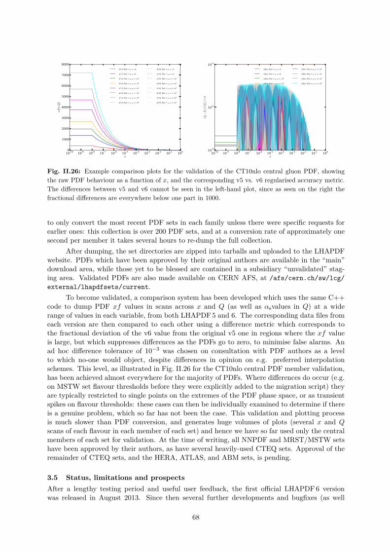
10-10 10-9 10-8 10-7 10-6 10-5 10-4 10-3 10-2 10-1 100

x

0

1000

2000

3000

4000

5000

6000

7000

8000

xf(x,Q

)

xf v5, flav = g, q=10

xf v5, flav = g, q=50

xf v5, flav = g, q=1×102

xf v5, flav = g, q=2×102

xf v5, flav = g, q=5×102

xf v5, flav = g, q=1×103

xf v5, flav = g, q=2×103

xf v5, flav = g, q=5×103

xf v6, flav = g, q=10

xf v6, flav = g, q=50

xf v6, flav = g, q=1×102

xf v6, flav = g, q=2×102

xf v6, flav = g, q=5×102

xf v6, flav = g, q=1×103

xf v6, flav = g, q=2×103

xf v6, flav = g, q=5×103

10-10 10-9 10-8 10-7 10-6 10-5 10-4 10-3 10-2 10-1 100

x

10-5

10-4

10-3

|f6−f 5|/

(|f5|+ε)

xfacc, flav = g, q=10

xfacc, flav = g, q=50

xfacc, flav = g, q=1×102

xfacc, flav = g, q=2×102

xfacc, flav = g, q=5×102

xfacc, flav = g, q=1×103

xfacc, flav = g, q=2×103

xfacc, flav = g, q=5×103

Fig. II.26: Example comparison plots for the validation of the CT10nlo central gluon PDF, showingthe raw PDF behaviour as a function of x, and the corresponding v5 vs. v6 regularised accuracy metric.The differences between v5 and v6 cannot be seen in the left-hand plot, since as seen on the right thefractional differences are everywhere below one part in 1000.

to only convert the most recent PDF sets in each family unless there were specific requests forearlier ones: this collection is over 200 PDF sets, and at a conversion rate of approximately onesecond per member it takes several hours to re-dump the full collection.

After dumping, the set directories are zipped into tarballs and uploaded to the LHAPDFwebsite. PDFs which have been approved by their original authors are available in the “main”download area, while those yet to be blessed are contained in a subsidiary “unvalidated” stag-ing area. Validated PDFs are also made available on CERN AFS, at /afs/cern.ch/sw/lcg/external/lhapdfsets/current.

To become validated, a comparison system has been developed which uses the same C++code to dump PDF xf values in scans across x and Q (as well as αsvalues in Q) at a widerange of values in each variable, from both LHAPDF5 and 6. The corresponding data files fromeach version are then compared to each other using a difference metric which corresponds tothe fractional deviation of the v6 value from the original v5 one in regions where the xf valueis large, but which suppresses differences as the PDFs go to zero, to minimise false alarms. Anad hoc difference tolerance of 10−3 was chosen on consultation with PDF authors as a levelto which no-one would object, despite differences in opinion on e.g. preferred interpolationschemes. This level, as illustrated in Fig. II.26 for the CT10nlo central PDF member validation,has been achieved almost everywhere for the majority of PDFs. Where differences do occur (e.g.on MSTW set flavour thresholds before they were explicitly added to the migration script) theyare typically restricted to single points on the extremes of the PDF phase space, or as transientspikes on flavour thresholds: these cases can then be individually examined to determine if thereis a genuine problem, which so far has not been the case. This validation and plotting processis much slower than PDF conversion, and generates huge volumes of plots (several x and Qscans of each flavour in each member of each set) and hence we have so far used only the centralmembers of each set for validation. At the time of writing, all NNPDF and MRST/MSTW setshave been approved by their authors, as have several heavily-used CTEQ sets. Approval of theremainder of CTEQ sets, and the HERA, ATLAS, and ABM sets, is pending.

3.5 Status, limitations and prospectsAfter a lengthy testing period and useful user feedback, the first official LHAPDF6 versionwas released in August 2013. Since then several further developments and bugfixes (as well

68

as increased PDF set support) has occurred and at the time of writing version 6.0.5 may bedownloaded, along with data files, from http://lhapdf.hepforge.org. An automatic datadownloader/manager script is provided with the library to help with PDF data management.Author approval of the remaining unvalidated sets is hoped to happen soon.

At present the scope of LHAPDF6 is intentionally more LHC-focused than LHAPDF5:we are mindful of the small amount of development manpower and the interests of those involved.Accordingly, no QCD evolution is planned for the library although we will consider proposals andcode patches, and the class interface is available for anyone to plug their own implementationsinto, should they so wish. Similarly, there is at present no plan to include automatic nuclearcorrections or PDFs of the resolved virtual photon: we believe that the former is better doneexplicitly using one of several nuclear corrections tools, and the latter is not presently of interestat the LHC (although EW constituents of nucleons are fully supported) and can be implementedfor fixed values of virtuality and impact parameter using the current interface. Double-partonPDFs and generalised PDFs for CCFM QCD evolution are also considered as special cases andare not directly supported by the LHAPDF6 interface (after consultation with PDF authors.)

The library is currently considered in a production-ready state, and several generators andLHC experiments have updated their code interfaces to make use of it. The performance hasbeen found to be (of course) vastly better than LHAPDF5 in terms of memory usage, by explicitdesign. It has also been pleasing to find that design decisions such as the split member data fileslead to a measurably faster start-up time, and that the possibility of evolving single flavoursat a time (as opposed to LHAPDF5, which always evolved all flavours) can produce significantspeed-ups (of order a factor of 3) in MC event generation and event reweighting. We havescheduled several developments to get even better performance, such as caching interpolationweights between calls to a PDF interpolator, and optimising the interpolation code to make useof vectorized instructions on modern CPUs. Use of GPGPUs has been suggested, but we advisethat anyone wanting that functionality contact the LHAPDF developers with a plan for theirimplementing at least a proof of concept version. Zipped access to PDF data files is alreadypossible by slightly tricky use of zlibc, but this could also become a built-in library feature ifit can be implemented without incurring unacceptable dependency and build difficulties.

Some physics improvements have also been suggested, such as use of a log(1 − x) mea-sure for high-x interpolation, a low-Q extrapolation scheme based on computed anomalousscaling dimensions, and (optional) distinction between quark masses and flavour thresholds inαsevolution.

We are pleased that a year after the project started, LHAPDF6 is a mature, performantand powerful library for future PDF access at Run 2 of the LHC and beyond, with an active andincreasing user base. Our thanks to all who helped us to get here!

AcknowledgementsAB thanks the Les Houches workshop once again for the hospitality and enjoyable/productiveworking environment in the Chamonix valley, and acknowledges support from a Royal SocietyUniversity Research Fellowship, a CERN Scientific Associateship, an IPPP Associateship, andthe University of Glasgow’s Leadership Fellow programme.

69

Chapter III

Phenomenological studies

1 Inclusive jet cross section at the LHC and the impact of weak radiativecorrections1

1.1 IntroductionQuantum chromodynamics (QCD) describes the strong interaction between quarks and gluons,which are confined within bound states and cannot be observed as free particles. Instead, inhigh-energetic hadron collisions, collimated streams of particles, known as “jets”, are producedthat convey essential information about the hard scattering process between the hadrons’ con-stituents. The investigation of these jets, technically defined through jet algorithms, allows tocompare predictions from perturbation theory with measurements and to look for new phenom-ena at the highest accessible transverse momenta. In particular, the energy scale dependence ofthe strong coupling can be determined, and the parton distribution functions (PDFs), notablythe gluon PDF, can be constrained.

The high quality and precision of the measurements performed by the experiments at theLarge Hadron Collider (LHC) at CERN demand a similar level of accuracy in the theoretical pre-dictions. The QCD corrections to jet production are known up to next-to-leading order (NLO)in perturbation theory [277–279], and a substantial effort is currently put into the computationof the corrections at next-to-next-to-leading order (NNLO), where the purely gluonic channel,retaining the full dependence on the number of colours, was completed recently [15,16].

Probing the high-energy regime beyond 1 TeV of jet transverse momentum, electroweak(EW) corrections might become large because of the appearance of Sudakov-type and otherhigh-energy logarithmic terms in the calculations. In particular, the leading term is given byαw ln2(Q2/MW2), where Q denotes the typical scale of the hard-scattering reaction, MW isthe W-boson mass, and αw = α/s2

w = e2/(4πs2w) is derived from the SU(2) gauge coupling

e/sw with sw being the sine of the weak mixing angle θw. The potential impact of these EWcorrections has to be evaluated in order to accompany the NNLO QCD prediction.

This article is organized as follows: In Section 1.2, the purely weak radiative correctionsof O(α2

sα) to the inclusive jet production are presented, where the restriction to the weakcorrections, denoted by α2

sαw, is motivated by the aforementioned logarithmic enhancements.In the following section 1.3 the measurement is introduced, to which the theory predictions arecompared in Section 1.4. Section 1.5 summarizes the results and gives a short outlook.

1.2 Weak radiative corrections and tree-level electroweak contributionsThe weak corrections form a well-defined gauge-invariant subset of the full EW ones and canbe supplemented by the photonic contributions at a later time. In case of the photonic cor-rections to jet production the high-energy logarithmic terms correspond to the well-known in-frared singularities, which cancel against bremsstrahlung corrections and therefore do not leadto logarithmically enhanced contributions. The results shown in the following are based on thecalculation of the respective corrections to dijet production presented in Ref. [87], which includesa detailed discussion of the numerical results presented in the form of distributions in the dijetinvariant mass and the transverse momenta of the leading and sub-leading jets. Corrections at

1S. Dittmaier, A. Huss and K. Rabbertz

70

this order have been previously calculated for the single-jet inclusive cross section in Ref. [280],and preliminary results to dijet production were shown in Ref. [281].

The EW interaction does not only affect jet cross sections through radiative corrections,but in case of the four-quark subprocesses the production of jets can also occur via the exchangeof EW gauge bosons already at leading order (LO). As a consequence, the Born cross sectionreceives, in addition to the pure QCD contribution of O(α2

s ), further contributions of O(αsα)and O(α2) from the interference between QCD and EW diagrams and the squares of the EWamplitudes. The different contributions that need to be considered at tree level are illustratedexemplarily for the case of the partonic subprocess u + d→ u + d in Fig. III.1. The interferenceterm of O(αsα) only contributes to the product between t- and u-channel diagrams due to thecolour structure. Note that all EW gauge bosons are accounted for in the LO prediction, i.e.the photonic contributions are included.

As motivated in the introduction, the NLO calculation is restricted to the purely weakcorrections defined by the order α2

sαw. A selection of interference contributions that enter thecalculation of the virtual corrections is shown in Fig. III.2. The purely gluonic channel does notreceive corrections through this order, and the corrections to the subprocesses with two gluonsand two quarks correspond to the weak O(αw) corrections to the LO O(α2

s ) cross section whichare shown in Fig. III.2(a). The fact that diagrams of both, O(αs) and O(αw), occur at LOin case of the four-quark process leads to two different ways to obtain corrections of the orderα2

sαw. Firstly, the one-loop diagrams of O(αsαw) interfered with the LO QCD diagram, similarlyto the corrections to the two-gluon–two-quark subprocess, which is illustrated in Fig. III.2(b).Secondly, the one-loop NLO QCD diagrams of O(α2

s ) interfered with the LO weak diagrams asshown in Fig. III.2(c). Note, however, that a strict separation of the weak and QCD correctionsis not possible, which is reflected by the appearance of diagrams such as the third loop diagram inFig. III.2(b). This box diagram can be obtained in two ways: by considering the weak correctionsto the tree-level diagram shown on the right of Fig. III.2(b), and by attaching a virtual gluonto the tree-level diagram in Fig. III.2(c). This signals that all contributions of the definingorder α2

sαw have to be taken consistently into account and, furthermore, the corresponding real-emission corrections need to be included in the case of the four-quark processes to ensure theproper cancellation of infrared divergences. Further details on the calculation of the correctionscan be found in Ref. [87].

1.3 Measurement of the inclusive jet cross section with the CMS detectorThe inclusive jet cross section that is compared to theory predictions has been measured withthe CMS detector [282] in 2011 from proton–proton collision data at

√s = 7 TeV. The recorded

(a)

∣∣∣∣∣∣∣∣∣u

d

u

d

g

∣∣∣∣∣∣∣∣∣2

(b)

∣∣∣∣∣∣∣∣∣u

d

u

d

γ,Z +u

d

u

dW

∣∣∣∣∣∣∣∣∣2

(c) 2 Re

u

d

u

d

g ×

u

d

u

dW

∗

Fig. III.1: The tree-level contributions to the process u + d → u + d of the orders (a) α2s , (b) α2, and

(c) αsα.

71

(a)

Z,W Z,W Z,W . . .

× . . .

∗

(b)

Z,WZ,W

Z,W

. . .

× . . .

∗

(c)

. . .

× Z,W

. . .

∗

Fig. III.2: The virtual corrections of O(α2sαw) illustrated in terms of typical interferences for the (a)

two-gluon–two-quark and (b), (c) four-quark subprocess.

data correspond to 5.0 fb−1 of integrated luminosity and reach up to 2 TeV in jet transversemomentum pT and 2.5 in absolute jet rapidity |y|. The measurement is performed double-differentially with five equally sized bins of ∆|y| = 0.5 up to |y| = 2.5 and a binning in jet pTthat follows the jet pT resolution of the central detector. The minimal pT imposed on any jet is114 GeV while the upper reach in pT is limited by the available amount of data and decreaseswith |y|.

Employing the FastJet package [283] jets are reconstructed using the collinear- andinfrared-safe anti-kT clustering algorithm [284] with a jet size parameter of R = 0.7. Themeasured cross sections, corrected for detector effects, are published in Ref. [90] and are availablevia the HepData project [285, 286] including correlations between systematic and statisticalexperimental uncertainties. Non-perturbative QCD corrections, see Sect. 1.4, that were used inthe CMS reference are provided in the HepData files as well.

The measurement is subject to four categories of experimental uncertainties: the jet en-ergy scale, the luminosity, the unfolding, and a residual uncertainty. The jet energy scale asthe dominant source of systematic uncertainty affects the jet cross section to about 5–25% ofuncertainty. The luminosity, which is known to a precision of 2.2%, corresponds to a globalnormalization uncertainty. The unfolding corrects for detector effects and is related to the jetenergy resolution and the modelling of the detector response in detailed Monte Carlo simula-tions. It leads to an uncertainty on the cross section of the order of 3–4%. Diverse residualeffects are summarized into an uncorrelated uncertainty of 1%.

1.4 Comparison between theory and measurementThe EW corrections studied here consist of the two contributions introduced in Sect. 1.2. Theyhave been evaluated with the renormalization and factorization scales, µR and µF, set to themaximum jet pT, pT,max. The results are presented in Fig. III.3 as a function of the transversemomentum pT for the five rapidity bins in terms of correction factors K:The weak radiative corrections of O(α2

sαw) denoted by K1-loopweak are negligible for small

transverse momenta and become increasingly negative towards higher scales. This cor-

72

Inclusive Jets Anti-kT R = 0.7 CT10-NLO√s = 7 TeV

0.9

1

1.1

1.2

2 · 102 5 · 102 1 · 103 2 · 103

K

pT [GeV]

|y| < 0.5

0.9

1

1.1

1.2

2 · 102 5 · 102 1 · 103

K

pT [GeV]

0.5 ≤ |y| < 1.0

0.9

1

1.1

1.2

2 · 102 5 · 102 1 · 103

K

pT [GeV]

1.0 ≤ |y| < 1.5

0.9

1

1.1

1.2

2 · 102 5 · 102 1 · 103

K

pT [GeV]

1.5 ≤ |y| < 2.0

0.9

1

1.1

1.2

2 · 102 5 · 102

K

pT [GeV]

2.0 ≤ |y| < 2.5

KEW = KtreeEW ·K1-loop

weak

KtreeEW

K1-loopweak

KEW = KtreeEW ·K1-loop

weak

KtreeEW

K1-loopweak

KEW = KtreeEW ·K1-loop

weak

KtreeEW

K1-loopweak

KEW = KtreeEW ·K1-loop

weak

KtreeEW

K1-loopweak

KEW = KtreeEW ·K1-loop

weak

KtreeEW

K1-loopweak

Fig. III.3: The EW correction factors to the transverse-momentum distribution for inclusive jet pro-duction for each rapidity bin, divided into the weak radiative corrections of O(α2

sαw) (dotted blue), thetree-level contributions of O(αsα, α

2) (dashed green), and the combination of both contributions (solidred).

responds to the typical behaviour known from the weak high-energy logarithms, whichbecome large in the so-called “Sudakov regime”, where all scalar invariants of differentmomenta in the hard scattering are required to be simultaneously much larger than theweak gauge-boson masses. For instance, as discussed in more detail in Ref. [87], the tailsof the dijet invariant-mass distributions do not probe this Sudakov regime, but are domi-nated by the Regge (forward) region. As a consequence, the weak corrections to the dijetinvariant-mass distribution turn out to be much smaller than in the case of the inclusivejet pT considered here, where the Sudakov regime is probed at high pT.

The tree-level contributions of O(αsα, α2) with the associated correction factor Ktree

EWsolely appear in the four-quark subprocesses and are negligible at small transverse mo-menta, where the cross section is dominated by gluon-induced channels. Towards highertransverse momenta, the PDFs are probed at larger values of the momentum fraction x,so that the relative size of the quark–quark luminosity becomes more and more relevant

73

|y| < 0.5 0.5 ≤ |y| < 1.0 1.0 ≤ |y| < 1.5 1.5 ≤ |y| < 2.0 2.0 ≤ |y| < 2.5

pT [GeV] KtreeEW

K1-loopweak

}KEW pT [GeV] Ktree

EWK1-loop

weak

}KEW pT [GeV] Ktree

EWK1-loop

weak

}KEW pT [GeV] Ktree

EWK1-loop

weak

}KEW pT [GeV] Ktree

EWK1-loop

weak

}KEW

114− 133 1.0020.997} 0.999 114− 133 1.002

0.997} 0.999 114− 133 1.0030.997} 0.999 114− 133 1.003

0.996} 0.999 114− 133 1.0030.996} 0.999

133− 153 1.0030.996} 0.999 133− 153 1.003

0.996} 0.999 133− 153 1.0030.996} 0.999 133− 153 1.003

0.995} 0.999 133− 153 1.0040.995} 0.998

153− 174 1.0040.995} 0.999 153− 174 1.004

0.995} 0.999 153− 174 1.0040.995} 0.999 153− 174 1.004

0.994} 0.999 153− 174 1.0040.993} 0.998

174− 196 1.0050.994} 0.999 174− 196 1.005

0.994} 0.999 174− 196 1.0050.993} 0.999 174− 196 1.005

0.993} 0.998 174− 196 1.0050.993} 0.998

196− 220 1.0060.993} 0.999 196− 220 1.006

0.993} 0.999 196− 220 1.0060.992} 0.998 196− 220 1.006

0.991} 0.998 196− 220 1.0060.991} 0.997

220− 245 1.0070.991} 0.999 220− 245 1.008

0.991} 0.999 220− 245 1.0080.991} 0.998 220− 245 1.008

0.990} 0.997 220− 245 1.0070.989} 0.996

245− 272 1.0090.990} 0.999 245− 272 1.009

0.990} 0.999 245− 272 1.0090.989} 0.998 245− 272 1.009

0.988} 0.997 245− 272 1.0080.987} 0.995

272− 300 1.0110.988} 0.999 272− 300 1.011

0.988} 0.999 272− 300 1.0110.987} 0.998 272− 300 1.010

0.986} 0.996 272− 300 1.0090.986} 0.994

300− 330 1.0130.987} 1.000 300− 330 1.013

0.986} 0.999 300− 330 1.0130.985} 0.998 300− 330 1.012

0.984} 0.996 300− 330 1.0100.984} 0.994

330− 362 1.0160.985} 1.000 330− 362 1.015

0.984} 1.000 330− 362 1.0150.983} 0.998 330− 362 1.013

0.982} 0.995 330− 362 1.0110.982} 0.993

362− 395 1.0190.983} 1.001 362− 395 1.018

0.982} 1.000 362− 395 1.0170.981} 0.998 362− 395 1.015

0.980} 0.995 362− 395 1.0130.979} 0.992

395− 430 1.0220.981} 1.002 395− 430 1.021

0.980} 1.001 395− 430 1.0190.979} 0.998 395− 430 1.016

0.978} 0.994 395− 430 1.0140.977} 0.991

430− 468 1.0260.979} 1.004 430− 468 1.025

0.978} 1.002 430− 468 1.0220.977} 0.998 430− 468 1.018

0.976} 0.994 430− 468 1.0160.974} 0.990

468− 507 1.0300.976} 1.006 468− 507 1.028

0.976} 1.003 468− 507 1.0250.974} 0.998 468− 507 1.020

0.973} 0.993 468− 507 1.0170.972} 0.989

507− 548 1.0350.974} 1.008 507− 548 1.032

0.973} 1.005 507− 548 1.0280.972} 0.999 507− 548 1.023

0.971} 0.993 507− 548 1.0190.969} 0.988

548− 592 1.0400.972} 1.011 548− 592 1.037

0.971} 1.007 548− 592 1.0310.969} 0.999 548− 592 1.025

0.968} 0.992 548− 592 1.0210.966} 0.987

592− 638 1.0460.969} 1.014 592− 638 1.042

0.968} 1.009 592− 638 1.0340.967} 1.000 592− 638 1.027

0.965} 0.991 592− 638 1.0230.963} 0.985

638− 686 1.0530.966} 1.018 638− 686 1.047

0.965} 1.011 638− 686 1.0380.964} 1.001 638− 686 1.030

0.962} 0.991 638− 686 1.0260.959} 0.984

686− 737 1.0600.964} 1.022 686− 737 1.053

0.963} 1.013 686− 737 1.0420.961} 1.001 686− 737 1.033

0.959} 0.990 686− 905 1.0290.955} 0.983

737− 790 1.0680.961} 1.026 737− 790 1.059

0.960} 1.017 737− 790 1.0460.958} 1.002 737− 790 1.036

0.956} 0.990790− 846 1.076

0.959} 1.032 790− 846 1.0650.957} 1.020 790− 846 1.050

0.955} 1.003 790− 846 1.0390.952} 0.989

846− 905 1.0850.956} 1.037 846− 905 1.072

0.954} 1.023 846− 905 1.0550.952} 1.004 846− 905 1.042

0.949} 0.989905− 967 1.094

0.954} 1.044 905− 967 1.0790.952} 1.026 905− 967 1.059

0.949} 1.005 905− 967 1.0450.945} 0.988

967− 1032 1.1040.951} 1.050 967− 1032 1.086

0.949} 1.030 967− 1032 1.0640.946} 1.006 967− 1248 1.049

0.941} 0.9871032− 1101 1.115

0.949} 1.058 1032− 1101 1.0930.946} 1.034 1032− 1101 1.068

0.942} 1.0071101− 1172 1.126

0.946} 1.065 1101− 1172 1.1010.943} 1.038 1101− 1172 1.074

0.939} 1.0081172− 1248 1.137

0.944} 1.073 1172− 1248 1.1090.941} 1.043 1172− 1684 1.081

0.934} 1.0101248− 1327 1.148

0.942} 1.081 1248− 1327 1.1170.938} 1.047

1327− 1410 1.1600.940} 1.090 1327− 1410 1.125

0.935} 1.0521410− 1497 1.171

0.938} 1.098 1410− 1784 1.1390.931} 1.060

1497− 1588 1.1850.936} 1.109

1588− 1784 1.2020.934} 1.122

1784− 2116 1.2290.931} 1.144

Table III.1: The numerical values of the correction factors for each transverse-momentum pT andrapidity |y| bin, c.f. Fig. III.3.

compared to the gluon-induced channels. Hence, the tree-level contributions become largeat high pT and are positive at the LHC.It is observed that these two contributions are of the same generic size, however, with

opposite sign, leading to significant cancellations in the combined correction factor Eq. (III.2).2In the central region (|y| < 1.0) the tree-level contributions exceed the weak radiative ones,leading to a net correction that is positive and increases towards higher jet pT up to 15% forpT = 2 TeV and |y| < 0.5. In the more forward region with 2.0 ≤ |y| < 2.5, on the other hand,the weak corrections slightly surpass the tree-level contributions leading to negative correctionsthat amount to −2% for transverse momenta of pT ≈ 800 GeV. The numerical values of therespective correction factors are given in Table III.1 separately for each bin in pT and |y|.

The different corrections that enter the comparison between theory and measurementare shown in Fig. III.4 and comprise the pure QCD corrections at NLO, the EW correctionsdiscussed above, and non-perturbative corrections.

The NLO QCD predictions are obtained using NLOJet++ [92,93] within the frameworkof fastNLO [287] and represent the dominant corrections, which are typically of the order of20%. They have been derived for renormalization and factorization scales of µR = µF = pT,jet foreach jet, which differs from the scale choice µR = µF = pT,max in the EW corrections. However,differences in the QCD corrections induced by the two scale settings are negligible at high pTand amount to at most +4% at lowest jet pT.

2At the Tevatron proton–anti-proton collider, the tree-level contribution is dominated by the quark–anti-quark induced channels. They turn out to be negative at high pT, so that they further enhance the negative weakcorrections.

74

Inclusive Jets anti-kTR = 0.7 CT10-NLO√s = 7 TeV

1

1.2

1.4

103

pT (GeV)

K

|y| < 0.5

CT10-NLO

NLO QCD correctionEW correctionNP correction

2·10 5·102 2

1

1.2

1.4

103

pT (GeV)

K

0.5 ≤ |y| < 1.0

CT10-NLO

NLO QCD correctionEW correctionNP correction

2·10 5·102 2

1

1.2

1.4

103

pT (GeV)

K

1.0 ≤ |y| < 1.5

CT10-NLO

NLO QCD correctionEW correctionNP correction

2·10 5·102 2

1

1.2

1.4

103

pT (GeV)

K

1.5 ≤ |y| < 2.0

CT10-NLO

NLO QCD correctionEW correctionNP correction

2·10 5·102 2

1

1.2

1.4

pT (GeV)

K

2.0 ≤ |y| < 2.5

CT10-NLO

NLO QCD correctionEW correctionNP correction

2·10 5·102 2

Fig. III.4: The three correction factors that enter the theory–data comparison as given by the NLOQCD corrections (“NLO QCD” dash-dotted black), the EW corrections (“EW” solid red), and the non-perturbative effects (“NP” dashed blue).

75

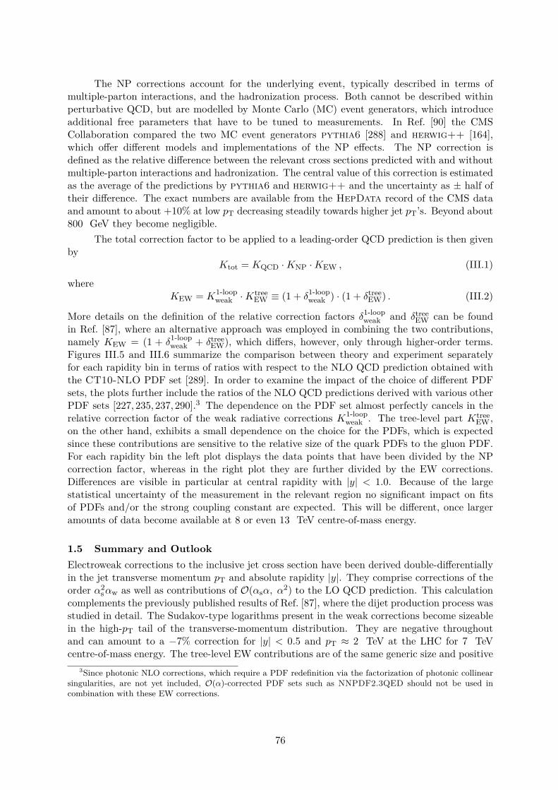
The NP corrections account for the underlying event, typically described in terms ofmultiple-parton interactions, and the hadronization process. Both cannot be described withinperturbative QCD, but are modelled by Monte Carlo (MC) event generators, which introduceadditional free parameters that have to be tuned to measurements. In Ref. [90] the CMSCollaboration compared the two MC event generators pythia6 [288] and herwig++ [164],which offer different models and implementations of the NP effects. The NP correction isdefined as the relative difference between the relevant cross sections predicted with and withoutmultiple-parton interactions and hadronization. The central value of this correction is estimatedas the average of the predictions by pythia6 and herwig++ and the uncertainty as ± half oftheir difference. The exact numbers are available from the HepData record of the CMS dataand amount to about +10% at low pT decreasing steadily towards higher jet pT’s. Beyond about800 GeV they become negligible.

The total correction factor to be applied to a leading-order QCD prediction is then givenby

Ktot = KQCD ·KNP ·KEW , (III.1)

whereKEW = K1-loop

weak ·KtreeEW ≡ (1 + δ1-loopweak ) · (1 + δtreeEW) . (III.2)

More details on the definition of the relative correction factors δ1-loopweak and δtreeEW can be foundin Ref. [87], where an alternative approach was employed in combining the two contributions,namely KEW = (1 + δ1-loopweak + δtreeEW), which differs, however, only through higher-order terms.Figures III.5 and III.6 summarize the comparison between theory and experiment separatelyfor each rapidity bin in terms of ratios with respect to the NLO QCD prediction obtained withthe CT10-NLO PDF set [289]. In order to examine the impact of the choice of different PDFsets, the plots further include the ratios of the NLO QCD predictions derived with various otherPDF sets [227, 235, 237, 290].3 The dependence on the PDF set almost perfectly cancels in therelative correction factor of the weak radiative corrections K1-loop

weak . The tree-level part KtreeEW ,

on the other hand, exhibits a small dependence on the choice for the PDFs, which is expectedsince these contributions are sensitive to the relative size of the quark PDFs to the gluon PDF.For each rapidity bin the left plot displays the data points that have been divided by the NPcorrection factor, whereas in the right plot they are further divided by the EW corrections.Differences are visible in particular at central rapidity with |y| < 1.0. Because of the largestatistical uncertainty of the measurement in the relevant region no significant impact on fitsof PDFs and/or the strong coupling constant are expected. This will be different, once largeramounts of data become available at 8 or even 13 TeV centre-of-mass energy.

1.5 Summary and OutlookElectroweak corrections to the inclusive jet cross section have been derived double-differentiallyin the jet transverse momentum pT and absolute rapidity |y|. They comprise corrections of theorder α2

sαw as well as contributions of O(αsα, α2) to the LO QCD prediction. This calculation

complements the previously published results of Ref. [87], where the dijet production process wasstudied in detail. The Sudakov-type logarithms present in the weak corrections become sizeablein the high-pT tail of the transverse-momentum distribution. They are negative throughoutand can amount to a −7% correction for |y| < 0.5 and pT ≈ 2 TeV at the LHC for 7 TeVcentre-of-mass energy. The tree-level EW contributions are of the same generic size and positive

3Since photonic NLO corrections, which require a PDF redefinition via the factorization of photonic collinearsingularities, are not yet included, O(α)-corrected PDF sets such as NNPDF2.3QED should not be used incombination with these EW corrections.

76

0

0.5

1

1.5

2

103

pT (GeV)

Rati

o t

o N

LO

(C

T10-N

LO

)

L = 5.0 fb-1

√s = 7 TeVInclusive Jets Anti-kT R=0.7|y| < 0.5

CMS Data 2011 / NPCT10-NLO, ∆PDF CL68MSTW2008-NLONNPDF21-NLOHERAPDF15-NLOABM11-NLO

2·10 5·102 2

0

0.5

1

1.5

2

103

pT (GeV)R

ati

o t

o N

LO

(C

T10-N

LO

)

L = 5.0 fb-1

√s = 7 TeVInclusive Jets Anti-kT R=0.7|y| < 0.5

CMS Data 2011 / NP / EWCT10-NLO, ∆PDF CL68MSTW2008-NLONNPDF21-NLOHERAPDF15-NLOABM11-NLO

2·10 5·102 2

0

0.5

1

1.5

2

103

pT (GeV)

Rati

o t

o N

LO

(C

T10-N

LO

)

L = 5.0 fb-1

√s = 7 TeVInclusive Jets Anti-kT R=0.70.5 ≤ |y| < 1.0

CMS Data 2011 / NPCT10-NLO, ∆PDF CL68MSTW2008-NLONNPDF21-NLOHERAPDF15-NLOABM11-NLO

2·10 5·102 2

0

0.5

1

1.5

2

103

pT (GeV)

Rati

o t

o N

LO

(C

T10-N

LO

)

L = 5.0 fb-1

√s = 7 TeVInclusive Jets Anti-kT R=0.70.5 ≤ |y| < 1.0

CMS Data 2011 / NP / EWCT10-NLO, ∆PDF CL68MSTW2008-NLONNPDF21-NLOHERAPDF15-NLOABM11-NLO

2·10 5·102 2

0

0.5

1

1.5

2

103

pT (GeV)

Rati

o t

o N

LO

(C

T10-N

LO

)

L = 5.0 fb-1

√s = 7 TeVInclusive Jets Anti-kT R=0.71.0 ≤ |y| < 1.5

CMS Data 2011 / NPCT10-NLO, ∆PDF CL68MSTW2008-NLONNPDF21-NLOHERAPDF15-NLOABM11-NLO

2·10 5·102 2

0

0.5

1

1.5

2

103

pT (GeV)

Rati

o t

o N

LO

(C

T10-N

LO

)

L = 5.0 fb-1

√s = 7 TeVInclusive Jets Anti-kT R=0.71.0 ≤ |y| < 1.5

CMS Data 2011 / NP / EWCT10-NLO, ∆PDF CL68MSTW2008-NLONNPDF21-NLOHERAPDF15-NLOABM11-NLO

2·10 5·102 2

Fig. III.5: The theory–data comparison for the rapidity bins |y| < 0.5, 0.5 ≤ |y| < 1.0, and 1.0 ≤ |y| <1.5, illustrated in terms of ratios with respect to the NLO QCD prediction obtained with the CT10-NLOPDF set. On the left, only NP correction factors are taken into account in this ratio, and on the rightalso the EW corrections.

77

0

0.5

1

1.5

2

103

pT (GeV)

Rati

o t

o N

LO

(C

T10-N

LO

)

L = 5.0 fb-1

√s = 7 TeVInclusive Jets Anti-kT R=0.71.5 ≤ |y| < 2.0

CMS Data 2011 / NPCT10-NLO, ∆PDF CL68MSTW2008-NLONNPDF21-NLOHERAPDF15-NLOABM11-NLO

2·10 5·102 2

0

0.5

1

1.5

2

103

pT (GeV)

Rati

o t

o N

LO

(C

T10-N

LO

)

L = 5.0 fb-1

√s = 7 TeVInclusive Jets Anti-kT R=0.71.5 ≤ |y| < 2.0

CMS Data 2011 / NP / EWCT10-NLO, ∆PDF CL68MSTW2008-NLONNPDF21-NLOHERAPDF15-NLOABM11-NLO

2·10 5·102 2

0

0.5

1

1.5

2

pT (GeV)

Rati

o t

o N

LO

(C

T10-N

LO

)

L = 5.0 fb-1

√s = 7 TeVInclusive Jets Anti-kT R=0.72.0 ≤ |y| < 2.5

CMS Data 2011 / NPCT10-NLO, ∆PDF CL68MSTW2008-NLONNPDF21-NLOHERAPDF15-NLOABM11-NLO

2·10 5·102 2

0

0.5

1

1.5

2

pT (GeV)

Rati

o t

o N

LO

(C

T10-N

LO

)

L = 5.0 fb-1

√s = 7 TeVInclusive Jets Anti-kT R=0.72.0 ≤ |y| < 2.5

CMS Data 2011 / NP / EWCT10-NLO, ∆PDF CL68MSTW2008-NLONNPDF21-NLOHERAPDF15-NLOABM11-NLO

2·10 5·102 2

Fig. III.6: The theory–data comparison for the rapidity bins 1.5 ≤ |y| < 2.0, and 2.0 ≤ |y| < 2.5,illustrated in terms of ratios with respect to the NLO QCD prediction obtained with the CT10-NLOPDF set. On the left, only NP correction factors are taken into account in this ratio, and on the rightalso the EW corrections.

at the LHC, which induces large cancellations between the two, so that the impact of the EWcorrections to the inclusive jet cross section turns out to be of moderate size.

Accounting for the sizeable QCD corrections at NLO and estimating non-perturbativeeffects, which are small at high pT, the presented theory predictions have been compared todata published by the CMS experiment at the LHC for a centre-of-mass energy of 7 TeV [90].For the given amount of 5 fb−1 of integrated luminosity the statistical uncertainties of themeasurement are too large at jet transverse momenta beyond 1 TeV to detect a significantimpact of the EW corrections. However, it will be most interesting to repeat this comparisonwith data collected at higher centre-of-mass energies and with more data. At 8 TeV for example,the LHC delivered roughly four times the luminosity of the 7 TeV running period.

Furthermore, the two contributions that enter the EW corrections behave differently withrespect to an increase of the collider energy [87], which can strongly affect the accidental cancel-lations observed here. For a fixed value of the jet transverse momentum, the scales appearing inthe large logarithms that are responsible for the bulk of the weak corrections will remain mostlyunchanged. This in turn means that for a given value of the transverse momentum, the weak

78

radiative corrections will not be affected much by the collider energy. The tree-level contribu-tions, on the other hand, are strongly dependent on the parton luminosities, in particular, theq and q PDFs. For fixed values of the transverse momentum, an increase in the collider energycorresponds to probing smaller values of the momentum fractions x in the PDFs. Therefore,the tree-level contributions will decrease for higher collision energies and the impact of the weakone-loop corrections are expected to become more strongly pronounced.

79

2 NNLO QCD and NLO EWDrell Yan background predictions for new gaugeboson searches4

2.1 IntroductionNew gauge boson searches belong to the flagship measurements at the high energy frontier. Inparticular, searches for Z’ and W’ bosons are ’golden channels’ due to their clean final statesignatures and rather high rates. However, they require a precise modelling of the large neutralcurrent (NC) and charged current (CC) Drell Yan backgrounds, which have the same final statesignatures. For this kind of searches, very high invariant masses could and will be exploredwith the available LHC c.m.s. energies of 8 TeV in Run I and of anticipated 14 TeV in Run II,respectively. High invariant masses challenge the understanding of a kinematic region whereNNLO QCD corrections O(α2

s) and NLO electroweak corrections O(α) become of similar size(c.f. discussion at this workshop). In the following a few observations and practical, novelmethods related to the modelling of NNLO QCD and NLO EW high mass Drell Yan crosssections are summarised. Part of the methodologies have been developed in the context of arecent Z’ search analysis [291].

2.2 Framework and toolsDrell Yan production in proton-proton collisions can be calculated with high precision andover a wide kinematic range up to next-to-next-to-leading-order (NNLO) in the strong couplingconstant using recent versions of the programs FEWZ [292–294] and DYNNLO [295,296]. Bothprograms calculate vector boson production and decays with full spin correlations and finitewidth effects. They are used widely by LHC experimentalist since they allow the applicationof important kinematic phase space requirements. In addition, powerful and fast programs likeZWPROD [297] and VRAP [298] are used for total cross section calculations and estimates of e.g.factorisation and renormalisation scale uncertainties as well as to cross check the predictions ofthe various programs for high invariant masses. Such a cross check revealed that the total NNLO

0.8

0.9

1

1.1

1.2

1.3

1.4

1.5

10 102

103

FEWZ

DYNNLO

VRAP

Mll (GeV)MS

TW

NN

LO

/CT

10 N

LO

NLO

NNLO

Mll (GeV)

DY

NN

LO

/FE

WZ

-1 (

%)

-10

-5

0

5

10

15

20

25

30

102

103

Fig. III.7: NNLO-to-NLO QCD k-factors for total NC Drell Yan cross sections at√s = 8 TeV using

VRAP 0.9, FEWZ 3.1.b2 and DYNNLO 1.3. See text and Ref. [276] for the details of the PDFs.

QCD cross section predictions by FEWZ 3.1.b2 and VRAP 0.9 are in excellent agreement forinvariant dilepton masses from 10 to 5000 GeV, whereas the DYNNLO 1.3 version appears not tobe suitable for off-resonant cross section calculations. This observation is illustrated in Fig. III.7for NC DY channel using an LHC c.m.s. energy of

√s = 8 TeV. The calculation of the QCD

4U. Klein

80

NNLO-to-NLO k-factors shown uses the proton parton distribution functions MSTW2008nnlo atNNLO QCD and CT10 at NLO QCD (a similar observation was obtained for CC DY but is notshown here) [299]. An updated version of DYNNLO 1.4 is now available which shows for totalLO QCD NC DY cross sections in the mass range 60 to 5000 GeV an excellent agreement [299],however, more detailed cross checks are worthwhile also for CC DY production and specificphase space cuts also for the resonant region where the experimental precision is very high (lessthan a few percent). For example, the fiducial resonant W cross section predictions varied within1% between FEWZ and DYNNLO (using the same SM and electroweak parameters for bothprograms) as reported by ATLAS [94] already in 2012.

The QCD NNLO-to-NLO k-factor for LHC Run II at√s = 14 TeV are illustrated for NC

Drell Yan production in Fig. III.8 (right). The QCD k-factors show a wide spread for invariantmasses larger than about 4 TeV reflecting the lack of knowledge in the proton parton distributionfunctions at high Bjorken-x values. The corresponding spread in the predictions at NNLO QCDusing modern PDFs with respect to the CT10nnlo PDF is shown in Fig. III.8 (left).

0.50.60.70.80.9

11.11.21.31.41.5

10 102

103

104

CT10nnlo

HERAPDF15nnlo

JR09nnloABM11nnlo

MSTW08nnlo

NNPDF2.3nnlo (0.118)

Mll (GeV)

NN

LO

PD

F/C

T10

NN

LO

CT10nnlo

HERAPDF15nnlo

JR09nnloABM11nnloMSTW08nnlo

NNPDF2.3nnlo (0.118)

Mll (GeV)

NN

LO

PD

F/C

T10

NN

LO

0

0.5

1

1.5

2

2.5

3

10 102

103

104

0.50.60.70.80.9

11.11.21.31.41.5

1000 2000 3000 4000 5000 6000 7000 8000 9000 10000

CT10nnlo

HERAPDF15nnloMSTW08deutCP

JR09nnloABM11nnlo

MSTW08nnlo

NNPDF2.3nnlo (0.118)

Mll (GeV)

NN

LO

PD

F/C

T10

CT10nnlo

HERAPDF15nnlo

MSTW08deutCP

JR09nnloABM11nnloMSTW08nnlo

NNPDF2.3nnlo (0.118)

Mll (GeV)

NN

LO

PD

F/C

T10

0

0.5

1

1.5

2

2.5

3

1000 2000 3000 4000 5000 6000 7000 8000 9000 10000

Fig. III.8: Invariant mass dependence of the total NC Drell Yan production cross section predictionsfor modern NNLO PDFs w.r.t. the CT10nnlo PDF (left plots) and the QCD NNLO-to-NLO QCD k-factors w.r.t. to CT10 NLO QCD (right plots). The lower and upper panels show the same quantitiesbut with different y-axis ranges from 0 to 3 and 0.5 to 1.5), respectively. The LHC energy is

√s = 14

TeV. Calculations are based on VRAP 0.9 and the NNLO (NLO) PDFs [276] as indicated in the legend.

While the QCD k-factors are rather insensitive to the choice of the SM model inputs andthe electroweak parameter scheme, care has to be taken for the absolute cross section predictionsincluding those NLO electroweak corrections which are not addressed already in the unfolding ofthe experimental data. It is well know from the literature, see e.g. [126] for a brief introductioninto the most commonly used electroweak schemes, that the Gµ electroweak scheme is well suitedfor Drell Yan production.

In the calculations presented here, the electroweak scheme is set to the Gµ scheme accord-ing to the details outlined in [126] and calculated by SANC [300]. A summary of the values isgiven in Tab. III.2.

The CKM values are taken from electroweak fits based on all precision observables asreported in [301]. Here the values of the CKM fit [301] are used. The pseudo-rapidity η`distribution of resonant single W± production is sensitive to the choice of the value of Vcs.Fig.III.9 illustrates the effect of changing the fitted Vcs to the currently best experimentally

81

MZ 91.1876 GeV Vud 0.97427ΓZ 2.4949 GeV Vus 0.22534Γ(Z → ll) 0.084 GeV Vub 0.00351MW 80.385 GeV Vcd 0.22520ΓW 2.0906 GeV Vcs 0.97344Γ(W → lν) 0.22727 GeV Vcb 0.0412MH 125 GeV Vtd 0.00867mt 173.5 GeV Vts 0.0404GF 1.1663787× 10−5 GeV−2 Vtb 0.999146sin2 θW 0.22289722252391828αG 7.56239563669733848× 10−3

vecup 0.40560740660288463vecdn -0.70280370330144226vecle -0.10841110990432690

Table III.2: Electroweak input parameters in the Gµ scheme for the NC and CC Drell Yan cross sectioncalculations.

known value of Vcs = 1.006 ± 0.023 [301] on the fiducial pseudo-rapidity η` distributions ofresonant single W+ and W− production. Since all other CKM matrix elements relevant forCC Drell Yan production are determined with high precision, the use of either the fitted or themeasured values (except the above described Vcs features) give the same results otherwise.

-0.5-0.25

00.25

0.50.75

11.25

1.51.75

2

0 0.25 0.5 0.75 1 1.25 1.5 1.75 2 2.25 2.5

W- Vcs from expW+ Vcs from expW- full CKM fit

W+ full CKM fit

W ηl1-σ(

Vcs

-exp

)/σ(

Vcs

-fit

) (%

)

W- ηl

NL

O d

σ/d

η l (p

b/b

in)

Vcs=0.97344 from fit

Vcs=1.006 from exp.

170

180

190

200

210

220

230

240

0 0.25 0.5 0.75 1 1.25 1.5 1.75 2 2.25 2.5

Fig. III.9: Effect of the choice of Vcs on the fiducial pseudo-rapidity η` distributions of resonant Wcross sections at

√s = 7 TeV. Calculations are performed with DYNNLO 1.3 NLO QCD and the CT10

NLO PDF.

The free Standard Model input parameters are chosen from the 2012 PDG [301], except thepartial leptonic decay width, Γ(W → lν). The PDG value of Γ(W → lν) = 226.36 MeV includesalready higher order QCD and more importantly higher order electroweak effects and the use ofthis value would be then inconsistent with the set-up of higher order electroweak programs likee.g. SANC [300,302]. To get a consistent evaluation of higher order electroweak effects (exceptQED FSR) also on the W decay kinematics, thus the LO partial width Γ(W → lν) = 227.27 MeVhas to be used in the QCD and EW calculations.

82

2.3 Combining NNLO QCD with NLO EW correctionsIn Drell Yan production, the by far dominant part of the higher order electroweak correctionsis the final state QED radiation (QED FSR) from the final state leptons. The LHC Drell YanMonte Carlo simulations often use PHOTOS [303] as an "afterburner" for the modelling of QEDFSR, and the experimental data are usually unfolded for QED FSR effects. PHOTOS andSANC QED FSR agree quantitatively very well [304]. The SANC program can be thus usedto calculate the electroweak corrections excluding QED FSR for both NC and CC Drell Yan.Those missing HO EW terms include contributions from initial state photon radiation (ISRQED), electroweak loop corrections and initial and final state photon interferences. The recentFEWZ 3.1 versions allow for the NC Drell Yan channel to select the Gµ electroweak schemeand and the simultaneous calculation of NLO electroweak corrections [294] . To enable thecalculation of NLO EW effects except QED FSR and to match thus QCD and EW predictionsto experimental data the following EW control flags had been introduced into FEWZ 3.1.a3(and maintained in the updated versions), where FEWZ reads the control flag (EWflag) anduses it as a binary number [305]:

– EWflag = 0 = (0000)_2 means nothing off (Weak, ISR∗FSR, ISR, FSR all on)– EWflag = 1 = (0001)_2 means FSR off– EWflag = 2 = (0010)_2 means ISR off– EWflag = 4 = (0100)_2 means ISR∗FSR off– EWflag = 8 = (1000)_2 means Weak off– EWflag = 7 = (0111)_2 means ISR∗FSR, ISR and FSR all off (only Weak is on)

Various NLO QCD and NLO EW calculations have been performed for NC Drell Yan over awide invariant mass range, where each mass bin has been calculated separately to avoid biasesin the calculations, using the CT10 NLO PDF and the EWflag options as described above inFEWZ 3.1.b2. The HO EW corrections show a strong invariant mass dependence as illustratedin Fig. III.10 for the NC Drell Yan production at

√s = 8 TeV and the expected large QED FSR

contributions. The significant reduction of the QED FSR contributions using a recombinationof the FSR photon and lepton with in a cone of 0.1 (w R(γ, l) < 0.1), usually called "dressedleptons" by experimenters, is shown in Fig. III.10 as well. The ATLAS strategy of dressingleptons has been widely discussed within the LPCC EW working group initiated by Ref. [306].It is important to note that any lepton dressing can be performed on Monte Carlo generator levelonly, i.e. experimental measurements can be unfolded to various levels of QED FSR correctionsbased on the QED FSR code and EW parameter settings as implemented in the used MonteCarlos.

FEWZ LOQCD based HO EW correction calculations, except QED FSR (FEWZ EWflag=1),and corresponding SANC calculations, performed in the Gµ scheme, agree very well for NC DrellYan process. Hence in the following the FEWZ results are used to demonstrate an improvedunderstanding of the application of HO EW corrections to (N)NLO QCD predictions relevant foran estimate of an EW (except QED FSR) systematic uncertainty for very high invariant masses.The method developed here has been transferred successfully to CC Drell Yan production whereno combined NNLO QCD and NLO EW code is available yet, and the results of various externalprograms need to be combined in a consistent way.

Various methodologies of combining HO QCD and HO EW effects for DY productionhave been discussed over the past decade, see e.g. also this and other Les Houches workshopcontributions and references therein. From the viewpoint of an experimenter performing newgauge boson searches and SM DY measurements, the practical question needed an answer howmass dependent EW systematic uncertainties could be estimated when further mixed O(ααs)contributions are not calculated yet.

83

Full HO EW muonsFull HO EW electrons

HO EW muons w R(γ,l) < 0.1HO EW electrons w R(γ,l) < 0.1QED FSR electrons w R(γ,l) < 0.1

HO EW except QED FSR

NLO QCD CT10, 8 TeV, no cuts Minv (GeV)

δ (%

)

-40

-35

-30

-25

-20

-15

-10

-5

0

500 1000 1500 2000 2500 3000 3500 4000 4500 5000

Fig. III.10: Invariant mass dependence of various higher order EW contributions (δ in %) for NC DrellYan production at

√s = 8 TeV. Shown are the full NLO EW corrections for electrons (full circles) and

muons (open circles), the full NLO EW corrections using a recombination of the FSR photon and leptonwith in a cone of 0.1 (w R(γ, l) < 0.1) for electrons (full triangles top down) and muons (full trianglestop up), the NLO EW corrections except QED FSR (open squares), the QED FSR corrections using arecombination of the FSR photon and electron (open crosses) with in a cone of 0.1 (w R(γ, l) < 0.1).Calculations are based on FEWZ 3.1.b2 NLO QCD and NLO EW using the CT10 NLO PDF.

Using fixed order LO QCD calculations for a given EW parameter scheme as the base-line, σLO_QCD, there are mainly two methodologies which are called here in short "factorisedapproach", Eq. III.3, and "additive approach", Eq. III.6 to construct a combined NNLO QCDand NLO EW DY cross section, σNNLO_QCD+NLO_EW . In the context of the here discussednew gauge boson searches, "EW" refers here always to the HO EW corrections except QED FSR(also sometimes called "missing HO EW corrections", δmiss, since those corrections are missingin the experimental Monte Carlos while QED FSR is included already).Factorised approach:

σNNLO_QCD+NLO_EW = kQCD × kEW × σLO_QCD (III.3)

kQCD = σNNLO_QCDσLO_QCD

(III.4)

kEW = σNLO_EW,LO_QCDσLO_QCD

. (III.5)

Additive approach:

σNNLO_QCD+NLO_EW = σNNLO_QCD + ∆σLO_QCD+NLO_EW (III.6)

= σNNLO_QCD(1 + ∆σLO_QCD+NLO_EW

σNNLO_QCD

). (III.7)

84

The factorised approach, Eq. III.3, assumes that the HO EW corrections are the same for allorders of QCD, and thus can be determined based on LO QCD and then transferred to anyhigher order in QCD. The additive approach, Eq. III.6, is e.g. followed in the NC DY FEWZcode [294] for the combination of HO QCD and EW corrections. This approach assumes thatthe EW except QED FSR corrections are mainly additive in their nature and the same termneeds to be added for all orders of QCD, thus the relative fraction of HO EW corrections foreach order of QCD is changing. Here a careful analysis has been performed to understand the

Fig. III.11: HO EW except QED FSR (δmiss in %) corrections for NC Drell Yan production. Theresults of the factorised approach based on LO QCD and the MST2008lo LO PDF (open diamonds)and MSTW2008nnlo NNLO PDF (full triangles on top) are shown. Using the MSTW2008nnlo PNNLOPDF, the results of a full, one-step NNLO QCD and NLO EW (open circles) and the additive approachaccording to Eq. III.6 (full circles) are shown. Calculations are based on FEWZ 3.1.b2 and

√s = 8 TeV.

transfer of the additive EW term to all orders of QCD. It has been found that consistent resultscan only be achieved if the term

∆σLO_QCD+NLO_EW = σLO_QCD+NLO_EW − σLO_QCD (III.8)

is calculated at LO QCD with exactly the same PDF as the wanted highest order QCD result.For example, if a NNLO QCD prediction using the MSTW2008nnlo PDF is aimed for, thenthe additive EW corrections term can be calculated with high precision based on LO QCDbut using the MSTW2008nnlo PDF. Similarly e.g. for a NLO QCD prediction using the CT10PDF, this would require the HO EW calculation done based on LO QCD using CT10. Theresults of this study are shown in Fig. III.11 where the mass dependence of the HO EW exceptQED FSR corrections are shown for the factorised and the additive approach, and the excellentagreement of the resulting NNLO QCD and NLO EW except QED FSR predictions using eitherdirectly FEWZ 3.1.b2 or the strategy according to Eq. III.6. The formalism described aboveis robust and gives a prescription also applicable for CC DY processes where the NNLO QCDand NLO EW calculation rely on different external programs for the QCD and the EW part.Also indicated in Fig. III.11 is the expected weak PDF dependence of the HO EW corrections.For higher invariant masses the discrepancies between the additive and factorised approachesare significant, and the results of the two approaches are used to get an estimate of the massdependent systematic uncertainty for the HO EW except QED FSR corrections for NC and CCDrell Yan processes. Since roughly speaking, the factorised approach maximises potential mixedO(ααs) contributions but with its sign is unknown, the following strategy has been suggested for

85

each invariant mass bin: The central value of the combined NNLO QCD and NLO EW exceptQED FSR prediction is taken from the additive approach while the difference to the factorisedapproach results is taken as a double sided systematic uncertainty estimate. The resulting meanHO EW except QED FSR corrections with those symmetric uncertainties are shown in Fig.III.12(lower plot) for the expected LHC Run II at

√s = 14 TeV. Also illustrated in Fig. III.12 (upper

plot) is the rather weak energy dependence for the HO EW except QED FSR corrections.

-30

-25

-20

-15

-10

-5

0

0 2000 4000 6000 8000 10000

7 TeV NLO CT1014 TeV NLO CT107 TeV LO MSTWnnlo14 TeV LO MSTWnnlo

Mll (GeV)

δ mis

s (%

)

14 TeV EW systematic

Mll (GeV)

δ mis

s (%

)

-30

-25

-20

-15

-10

-5

0

0 2000 4000 6000 8000 10000

Fig. III.12: HO EW except QED FSR (δmiss in %) corrections for NC Drell Yan production. Theresults of the factorised (additive) approach based on LO QCD (NLO QCD) for

√s = 7 TeV are shown

in the upper plot with empty squares (empty circles) and for 14 TeV with full squares (full circles). Anestimate of the EW except QED FSR systematic uncertainty, see text, is shown in the lower plots for√s = 14 TeV. All calculations are based on FEWZ 3.1.b2 and the PDFs as indicated in the legend.

2.4 Matching Monte Carlo programs and external calculationsThe methodologies discussed in the previous chapter work reliably for total cross sections andwell defined variables like the invariant mass or the pseudo-rapidity of the final state leptons,but fail e.g for variables like the pT (`) or pT (Z,W ) which rely on a modelling of soft gluonresummation and parton shower effects usually taken care of in Monte Carlo programs. Whilethe LHC Monte Carlo programs are powerful tools for the description of complex QCD processes,they are not very well defined w.r.t. the electroweak part and the EW parameter schemeused. Here, a study has been performed to understand the matching of a well-defined externalQCD calculation using the Gµ scheme with parameters according to Tab. III.2 and currentlyPDG guided EW parameter settings as used in LHC Monte Carlo generations. Fig. III.13shows the deviations between external NLO (LO) QCD predictions using FEWZ 3.1.b2 with

86

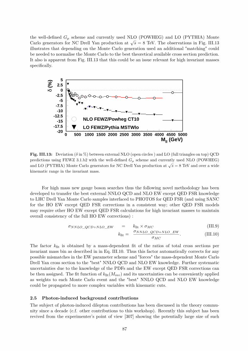
the well-defined Gµ scheme and currently used NLO (POWHEG) and LO (PYTHIA) MonteCarlo generators for NC Drell Yan production at

√s = 8 TeV. The observations in Fig. III.13

illustrates that depending on the Monte Carlo generation used an additional "matching" couldbe needed to normalise the Monte Carlo to the best theoretical available cross section prediction.It also is apparent from Fig. III.13 that this could be an issue relevant for high invariant massesspecifically.

NLO FEWZ/Powheg CT10

LO FEWZ/Pythia MSTWlo

Mll (GeV)

δ (%

)

-20-17.5

-15-12.5

-10-7.5

-5-2.5

02.5

5

0 500 1000 1500 2000 2500 3000 3500 4000 4500 5000

Fig. III.13: Deviation (δ in %) between external NLO (open circles ) and LO (full triangles on top) QCDpredictions using FEWZ 3.1.b2 with the well-defined Gµ scheme and currently used NLO (POWHEG)and LO (PYTHIA) Monte Carlo generators for NC Drell Yan production at

√s = 8 TeV and over a wide

kinematic range in the invariant mass.

For high mass new gauge boson searches thus the following novel methodology has beendeveloped to transfer the best external NNLO QCD and NLO EW except QED FSR knowledgeto LHC Drell Yan Monte Carlo samples interfaced to PHOTOS for QED FSR (and using SANCfor the HO EW except QED FSR corrections in a consistent way; other QED FSR modelsmay require other HO EW except QED FSR calculations for high invariant masses to maintainoverall consistency of the full HO EW corrections) :

σNNLO_QCD+NLO_EW = kfit × σMC (III.9)

kfit = σNNLO_QCD+NLO_EWσMC

. (III.10)

The factor kfit is obtained by a mass-dependent fit of the ratios of total cross sections perinvariant mass bin as described in in Eq. III.10. Thus this factor automatically corrects for anypossible mismatches in the EW parameter scheme and "forces" the mass-dependent Monte CarloDrell Yan cross section to the "best" NNLO QCD and NLO EW knowledge. Further systematicuncertainties due to the knowledge of the PDFs and the EW except QED FSR corrections canbe then assigned. The fit function of kfit(Minv) and its uncertainties can be conveniently appliedas weights to each Monte Carlo event and the "best" NNLO QCD and NLO EW knowledgecould be propagated to more complex variables with kinematic cuts.

2.5 Photon-induced background contributionsThe subject of photon-induced dilepton contributions has been discussed in the theory commu-nity since a decade (c.f. other contributions to this workshop). Recently this subject has beenrevived from the experimenter’s point of view [307] showing the potentially large size of such

87

contributions for off-peak (low and high mass) NC Drell Yan production at the LHC. Further-more, indications are found in a recent Standard Model high mass Drell Yan analysis performedby ATLAS that LHC data may include such backgrounds [308]. In Ref. [308] also the radiationof real (on-shell) W and Z bosons has been quantified for the experimental conditions followingthe procedure outlined in Ref. [140]. Using the same technique, the contributions due to real Wand Z boson radiation have been also calculated for the 2012 Z’ analysis [291], but those back-ground contributions are much smaller than the photon-induced background contributions andhence not discussed here further. Since our knowledge of photon-induced processes is very poor,

photon induced normalized to CT10 PowhegEW normalized to CT10 FEWZ

Mll (GeV)

δ (%

)

-20

0

20

40

60

80

100

500 1000 1500 2000 2500 3000 3500 4000 4500 5000

δNLO current quark masses

Mll (GeV)

(σN

LO-σ

LO)/

σ LO (

%)

-40

-30

-20

-10

0

10

20

30

40

0 500 1000 1500 2000 2500 3000 3500 4000 4500 5000

Fig. III.14: Photon induced background contributions calculated with pT,` > 25 GeV and η` < 2.5MRST2004QED photon PDF and

√s = 8 TeV over a wide invariant mass range. Shown are the leading

order photon induced dilepton contribution using the mean of the two available MRST2004qed predictionsas the central values and the deviations between the two predictions and the central value as an uncertaintyestimate (upper plot). The LO photon induced contribution is displayed as a fraction of a NLO POWHEGNC DY prediction. Overlaid is also the HO EW except QED FSR correction including its systematicuncertainty estimate as described in the text. Next-to-leading order photon induced dilepton productioncontribution w.r.t. to the dominant LO photon-induced cross sections over a wide invariant mass range(lower plot). Calculations are performed with MCSANC [302]. using the nominal MRST2004qed PDF.

only rough estimates are possible using the MRST2004QED PDF [151]. Here a modified versionof the MRST2004qed PDF is used which offers two parameterisations [309], i.e. reflecting thesensitivity to the choice of the quark mass, either current quark masses as used for the nominalparameterisation or constituent quark masses as used for an alternative parameterisation.

First estimates of the size of photon-induced contributions have been performed at partonlevel only due to the lack of full Monte Carlo simulations at that time. Since dilepton productionγγ → `` is an additional background which can be significant at high invariant masses, it is

88

important that the fiducial phase space requirements are applied. The general strategy is thenthat this background contribution is quantified separately and added to the theory predictionincluding its model uncertainty in data-theory comparisons, see e.g. Ref. [308]. This strategyallows for a re-analysis of the data in the future if the knowledge about this background mayhave been improved.

The photon induced background contributions for kinematic requirements of pT,` > 25 GeVand η` < 2.5 are shown in Fig. III.14 (upper plot) for a LHC c.m.s. energy of

√s = 8 TeV over

a wide invariant mass range. The potential contributions could sizeable and may reach upto 50% - 100 % of the fiducial NC DY cross section at invariant masses of 4 to 5 TeV. Suchbackground contributions may then also significantly reduced expected HO EW effects (alsoshown in Fig. III.14 upper plot). NLO, quark-photon initiated dilepton production contributionsare expected to be negative at lower invariant masses but may add even more backgrounds athigher masses, see Fig. III.14 (lower plot). The current procedure to estimate an uncertainty duethis background relies on a simple mean between the two available MRST2004qed predictions atLO to avoid single-sided systematic uncertainties. It was also lively discussed at this workshopthat LHC experiments should aim for a measurement of this background employing specificphase space regions.

2.6 NNLO QCD scale uncertainties

-4

-3

-2

-1

0

1

2

3

4

102

103

MSTW2008

HERAPDF1.5CT10nnloABM11JR09 5VF

NNPDF2.3 (0.118)

Mll (GeV)

δ scal

es (

%)

HERAPDF1.5

CT10nnlo

ABM11

JR09 5VF

NNPDF2.3 (0.118)

Mll (GeV)

Pd

f/M

ST

W20

08

0.8

0.85

0.9

0.95

1

1.05

1.1

1.15

1.2

102

103

Fig. III.15: Effect on the total NC Drell Yan NNLO QCD cross section predictions due to the changeof the renormalisation and factorisation scales simultaneously by a factor 2 or 1/2 for an invariant massrange of 10 to 2000 GeV. See Ref. [276] for the details of the NNLO QCD PDFs; the NNPDF calculationsis obtained for αs = 0.118. Calculations are based on VRAP 0.9 and

√s = 7 TeV.

The nominal renormalisation and factorisation scales for the calculation of DY cross sec-tions are set to either directly to the invariant mass in VRAP or to the mean of an invariantmass bin in FEWZ (DYNNLO). The variation of the renormalisation and factorisation scalessimultaneously by a factor of 2 or 1/2 can be conveniently calculated in NNLO QCD for thetotal Drell Yan production cross section using the program VRAP. Fig.III.15 and Fig.III.16show the resulting effects for NC and CC Drell Yan, respectively, for all modern NNLO partondistribution functions. The mass-dependencies of the scale variations are observed to very simi-lar for NC and CC Drell Yan, and also to show very similar and significant dependencies on thePDF choice. For low and high invariant masses the scale uncertainties are rising, even at NNLO

89

QCD, and deserve further detailed studies.

-6

-4

-2

0

2

4

6

10 102

103

CT10nnlo

HERAPDF15nnlo

JR09nnloABM11nnloMSTW08nnlo

NNPDF2.3nnlo (0.118)

W+ Mνl (GeV)

δ scal

e (%

)

CT10nnlo

HERAPDF15nnlo

JR09nnloABM11nnloMSTW08nnlo

NNPDF2.3nnlo (0.118)

W- Mνl (GeV)

δ scal

e (%

)

-6

-4

-2

0

2

4

6

10 102

103

Fig. III.16: Effect on the total CC Drell Yan NNLO QCD cross section predictions due to the changeof the renormalisation and factorisation scales simultaneously by a factor 2 or 1/2 for an invariant massrange of 10 to 5000 GeV. See Ref. [276] for the details of the NNLO QCD PDFs; the NNPDF calculationsis obtained for αs = 0.118. Calculations are based on VRAP 0.9 and

√s = 8 TeV.

AcknowledgementsThe electroweak and photon-induced background studies of this work have been done togetherwith Dimitry Bardin, Serge Bondarenko, and Lidia Kalinovskaya with the support of the grantCERN-RFBR-Scientific-Cooperation 12-02-91526-CERN_a, and I am very thankful for thisexceptional and fruitful collaboration. I also like to thank Lance Dixon, Frank Petriello, Ye Li,Seth Quackenbush and Massimiliano Grazzini for many useful discussions over the past years.Part of this work were supported by my PPSC20 grant "Precision modelling of hadron structureat highest energies". Thanks to my ATLAS and LPCC WG colleagues for the co-operation. Lastbut not least it is my pleasure to thank warmly the Les Houches workshop for the hospitalityand perfect organisation.

90

3 Electroweak Sudakov corrections to Z/γ+ jets at the LHC5

3.1 IntroductionImportant searches for new phenomena beyond the Standard Model (SM) at the proton-proton(pp) collider LHC are based on the analysis of events with jets and missing transverse momentum(/pT ). Typical examples of such studies are searches for squarks and gluinos in all-hadronicreactions containing high-pT jets, missing transverse momentum and no electrons or muons,as predicted in many supersymmetric extensions of the SM. These final states can appear ina number of R-parity conserving models where squarks and gluinos can be produced in pairsand subsequently decay to standard strongly interacting particles plus neutralinos that escapedetection, thus giving rise to a large amount of /pT . Typically, the event selections adopted atrun I of the LHC, at center of mass energies of 7 and 8 TeV, require the leading jet pT largerthan 130 GeV or the single jets pT ’s larger than 50 GeV. Moreover, the signal region is definedby meff > 1000 GeV, where meff =

∑i pT i + /ET , or HT > 500 GeV and | /~HT | > 200 GeV, where

HT =∑i pT i and /~HT = −

∑i ~pti [310–312].

The main SM backgrounds to the above mentioned signal(s) are given by the production ofweak bosons accompanied by jets (W/Z+n jets), pure QCDmultiple jet events and tt production.Among these processes only Z + n jets (in particular with Z → νν) constitutes an irreduciblebackground, particularly relevant for final states with 2 and 3 jets. Because new physics signalscould manifest themselves as a mild deviation with respect to the large SM background, precisetheoretical predictions for the processes under consideration are needed. In order to reduce thetheoretical systematic uncertainties, the experimental procedure for the irreducible backgrounddetermination relies on data driven methods. For instance, a measurement of the cross section forZ(→ νν)+n jets could be done through the measured cross section for Z(→ l+l−)+n jets timesthe ratio B(Z→νν)

B(Z→l+l−) , which is known with high precision from LEP1 data. With the exception ofthe ratio of branching ratios, the method is free of theoretical systematics. However, due to thelow production rate of Z(→ l+l−)+n jets, in particular in the signal regions, this method resultsto be affected by large statistical uncertainty. Other possible choices of reference processes areW + n jets and γ + n jets. In both cases the statistics is not a limitation and the requiredtheoretical input is the ratio

RnV =[dσ(Z(→ νν) + n jets)

dX

]/

[dσ(V + n jets)

dX

], (III.11)

where X is the observable under consideration and V = W , γ. Additional sources of uncertain-ties, specific for each channel, are the contamination of other processes, such as tt events (forthe case of W+ jets) and photon isolation (for the case of γ+ jets). Recent theoretical work hasbeen devoted to the study of the theoretical uncertainties related to the ratio of Eq. (III.11).In particular, in Ref. [261] a study of the cancellation in RnW of systematic theoretical uncer-tainties originating from higher-order QCD corrections, including scale variations and choice ofPDF’s, has been presented. A first detailed analysis of the impact of higher-order QCD correc-tions, PDF’s and scale choice to R1,2,3

γ has been shown in Ref. [313]. More recently, the levelof theoretical uncertainty induced by QCD higher-order corrections in the knowledge of R2

γ andR3γ , relying on the comparison of full NLO QCD calculations with parton shower simulations

matched to LO matrix elements, has been discussed in Refs. [314] and [315], respectively. Allthese studies point out that many theoretical systematics related to pQCD and PDF’s largelycancel in the ratio and the corresponding theoretical uncertainty in the ratio Riγ can be safelyestimated to be within 10%.

What is not expected to cancel in the ratio is the contribution of higher-order electroweak(EW) corrections, which are different for the processes Z(→ νν)+n jets and γ+n jets. Moreover

5M. Chiesa, L. Barzè, G. Montagna, M. Moretti, O. Nicrosini, F. Piccinini, F. Tramontano

91

these effects can be enhanced by Sudakov logarithms. For R1γ the higher-order EW corrections

have been calculated in Refs. [316–318], where it is shown that for a vector boson transversemomentum of 2 TeV they are of the order of 20%. In view of the forthcoming run II of theLHC, it is therefore necessary to quantitatively estimate the effects of EW corrections to Rnγ , inparticular for n ≥ 2.

In this contribution we present first numerical results on the impact of EW Sudakovcorrections to R2

γ and R3γ , for two realistic event selections at the LHC, at a center of mass

energy of 14 TeV. These results have been obtained by means of the algorithmic implementationof EW Sudakov corrections discussed in Ref. [142], which we describe below.

3.2 Implementation of EW Sudakov corrections in ALPGENFor energy scales well above the EW scale, EW radiative corrections are dominated by doubleand single logarithmic contributions (DL and SL, respectively) whose argument involves the ratioof the energy scale to the mass of the weak bosons. These logs are generated by diagrams inwhich virtual and real gauge bosons are radiated by external leg particles, and correspond to thesoft and collinear singularities appearing in QED and QCD, i.e. when massless gauge bosons areinvolved. At variance with this latter case, the weak bosons masses put a physical cutoff on these“singularities", so that virtual and real weak bosons corrections can be considered separately.Moreover, as the radiation of real weak bosons is in principle detectable, for those event selectionswhere one does not include real weak bosons radiation, the physical effect of (negative) virtualcorrections is singled out, and can amount to tens of per cent. Since these corrections originatefrom the infrared structure of the EW theory, they are “process independent" in the sense thatthey depend only on the external on-shell legs [127, 129, 131, 133, 134, 316, 319–327]. As shownby Denner and Pozzorini in Refs. [131,322], DL corrections can be accounted for by factorizinga proper correction which depends on flavour and kinematics of all possible pairs of electroweakcharged external legs. SL corrections can be accounted for by factorizing an appropriate radiatorfunction associated with each individual external leg. Notice that our implementation includescorrectly all single logarithmic terms of O(α2αns ) of both UV and infrared origin, as detailedin Ref. [328]. The above algorithm has been implemented in ALPGEN v2.14 [329], where allthe contributing tree-level amplitudes are automatically provided. Since the matrix elementsin ALPGEN are calculated within the unitary gauge, for the time being we do not implementthe corrections for the amplitudes involving longitudinal vector bosons, which, according toRefs. [131,322], are calculated by means of the Goldstone Boson Equivalence Theorem. For theprocesses Z + 2 jets and Z + 3 jets, this approximation affects part of the O(α3) and O(α3αs)contributions, respectively, and we checked that in view of our target precision of few percent itcan be accepted 6.

3.3 Numerical resultsOur numerical results have been obtained by using the code ALPGEN v2.14 with default inputparameters/PDF set. The algorithm has been validated with results available in the literature.In Fig. III.17 we show our predictions for the jet pt distribution for γ + 1 jet, Z(→ νν) + 1 jetand for the ratio R1

γ at√s = 14 TeV in the region

pjt > 100 GeV, |y(j)| < 2.5, |y(V )| < 2.5 (V = γ, Z) (III.12)6The logarithms of photonic origin have not been considered in this realization since they can be treated

separately together with their real counterpart for the processes under investigation. At any rate, these gaugeinvariant contributions (at the leading order αnjetss α) for sufficiently inclusive experimental setup give rise torather moderate corrections.

92

and we compare our results with the ones obtained from Refs. [316, 324, 325] by including alsothe terms proportional to log(MW

MZ): the level of agreement we find is well within the percent

level. Moreover, we estimated the corrections to pZT and to the leading jet pT distributions

10−710−610−510−410−310−210−1100101

dσ

dpj t

[pb

GeV

] γ + 1j

-0.20

-0.15

-0.10

-0.05

δ EW

0.990

0.995

1.000

1.005

100 400 800 1200 1600 2000

Ratio

pjt [GeV]

LONLO Virt.

NLO Virt., hep-ph/0508253

δ Virt.δ Virt., hep-ph/0508253

NLO/(hep-ph/0508253)

10−710−610−510−410−310−210−1100101

dσ

dpj t

[pb

GeV

] Z + 1j

-0.40

-0.30

-0.20

-0.10

δ EW

0.990

0.995

1.000

1.005

100 400 800 1200 1600 2000

Ratio

pjt [GeV]

LONLO Virt.

NLO Virt., hep-ph/0507178

δ Virt.δ Virt., hep-ph/0507178

NLO/(hep-ph/0507178)

0.16

0.18

0.20

0.22

0.24

0.26

0.28

0.30

100 400 800 1200 1600 2000

R1 γ

pjt [GeV]

LONLO

Fig. III.17: pjt distribution at√s = 14 TeV for γ+ 1 jet and Z(→ νν) + 1 jet and their ratio R1

γ at theLO (solid blue lines) and at approximated NLO (dashed red lines). Green dotted lines are the results ofRefs. [316, 324, 325] when the difference between the W and the Z masses is not neglected. The ratio ofour predictions with the ones of Refs. [316,324,325] is shown in the lower panels of the first two plots forγ + 1 jet and Z(→ νν) + 1 jet, respectively.

in the large tails for the process Z + 2 jets with only one fermionic current, as discussed inRef. [8], finding good agreement. Finally, for Z + 2 jets we cross-checked our results withthe automatic package GOSAM v1.0 [4], with the event selection adopted in the present study.Since the electroweak renormalization is not yet available in the present version of GOSAM, wesubtracted the logarithmic terms due to the renormalization counterterms from the formulaeof Refs. [131, 322] and tested the asymptotic behaviour of all relevant distributions. Since therelative weight of two-quark and four-quark subprocesses is about 75% and 25% for total crosssections, while for the observables under consideration and in the high tails is about 50% eachat the LO, respectively, we performed this analysis for different subprocesses involving both oneand two fermionic currents such as qq → Zgg, qq → Zq′′q′′, qq → Zqq and qq′ → Zqq′ (with qand q′ belonging to the same isodoublet). For all the above cases we found that the shape ofthe distributions predicted by the two calculations is in good agreement.

We present our results on R2,3γ for two sets of cuts that mimic the real experimental event

selections used by ATLAS and CMS in run I analysis. For the Z(→ νν) + 2 jets and γ + 2 jetsfinal states we consider the observable/cuts adopted by ATLAS, namely

meff > 1 TeV /ET /meff > 0.3pj1T > 130 GeV pj2T > 40 GeV |ηj | < 2.8∆φ(~pjT , /~pT ) > 0.4 ∆R(j1,j2) > 0.4 (III.13)

where j1 (j2) are the leading (next-to-leading) pT jets, the missing momentum /~pT is definedas minus the sum of the jet transverse momenta and /ET is the magnitude of /~pT . For theZ(→ νν) + 3 jets and γ + 3 jets final states we consider the observables/cuts used by CMS,namely

HT > 500 GeV | /~HT | > 200 GeVpjT > 50 GeV |ηj | < 2.5 ∆R(ji,jk) > 0.5

93

∆φ(~pj1,j2T , /~HT ) > 0.5 ∆φ(~pj3T , /~HT ) > 0.3 (III.14)

Fig. III.18 shows the meff distribution for γ + 2 jets and Z(→ νν) + 2 jets, with the ATLAScuts of Eq. (III.13). In the tails of the distributions the effect of EW Sudakov corrections is ofthe order of −20% and −40% for the processes γ + 2 jets and Z(→ νν) + 2 jets, respectively.As a result, the ratio R2

γ of the two distributions, which is almost flat at the LO, decreasesat the NLO of about 8% for meff ' 1 TeV up to 20% for meff ' 4.5 TeV. Fig. III.19 is the

10−7

10−6

10−5

10−4

10−3

10−2

dσ

dm

eff

[pb

GeV

] γ + 2j

-0.25

-0.20

-0.15

-0.10

-0.05

1000 1500 2000 2500 3000 3500 4000 4500

δ EW

meff [GeV]

LONLO Virt.

δ Virt.

10−7

10−6

10−5

10−4

10−3

10−2

dσ

dm

eff

[pb

GeV

] Z + 2j

-0.40

-0.30

-0.20

-0.10

1000 1500 2000 2500 3000 3500 4000 4500

δ EW

meff [GeV]

LONLO Virt.

δ Virt.

0.20

0.22

0.24

0.26

0.28

0.30

1000 1500 2000 2500 3000 3500 4000 4500

R2 γ

meff [GeV]

LONLO

Fig. III.18: meff distribution at√s = 14 TeV for γ + 2 jets and Z(→ νν) + 2 jets and their ratio R2

γ

under the ATLAS event selection (same notation of Fig. III.17).

analogous of Fig. III.18 for the observable | /~HT | under CMS conditions of Eq. (III.14) for theprocesses Z(→ νν) + 3 jets and γ + 3 jets at

√s = 14 TeV. As in the two jets case, EW

Sudakov corrections are larger for Z(→ νν) + 3 jets (where they are of the order of −45% for| /~HT | ' 2 TeV), while for γ+ 3 jets the size of the corrections is of the order of −20% in the high| /~HT | tail. Due to the different impact of EW corrections to γ+ 3j and Z(→ νν) + 3j, the shapeof their ratio R3

γ changes at the NLO w.r.t. LO and decreases of about 20% for | /~HT | ' 2 TeV.

10−7

10−6

10−5

10−4

10−3

10−2

10−1

dσ

d|~ /H

T|

[pb

GeV

] γ + 3j

-0.25

-0.20

-0.15

-0.10

-0.05

200 500 1000 1500 2000

δ EW

| ~/HT | [GeV]

LONLO Virt.

δ Virt.

10−7

10−6

10−5

10−4

10−3

10−2

dσ

d|~ /H

T|

[pb

GeV

] Z + 3j

-0.45

-0.35

-0.25

-0.15

-0.05

200 500 1000 1500 2000

δ EW

| ~/HT | [GeV]

LONLO Virt.

δ Virt.

0.20

0.22

0.24

0.26

0.28

0.30

200 500 1000 1500 2000

R3 γ

| ~/HT | [GeV]

LONLO

Fig. III.19: | /~HT | distribution at√s = 14 TeV for γ + 3 jets and Z(→ νν) + 3 jets and their ratio R3

γ

under the CMS event selection (same notation of Fig. III.17).

To summarize, the theoretical accuracy on the quantity Rnγ is relevant in the calibrationof the process Z(→ νν) + n jets, an important irreducible background to New Physics searchesat the LHC. Contrary to higher-order QCD corrections, which largely cancel in the ratio, asshown in the literature, EW NLO corrections are sizeable, in particular in the phase spaceregions interesting for New Physics searches. We computed the NLO EW Sudakov correctionsto Z(→ νν) + n jets, γ + n jets and to the ratio Rnγ = dσ(Z(→νν)+n jets)

dσ(γ+n jets) (where n = 1, 2, 3) andwe showed our results for the LHC at

√s = 14 TeV. In the typical event selections used for

New Physics searches based on the signature /ET + n jets, electroweak Sudakov corrections to

94

Z(→ νν)+n jets and γ+n jets in the tails of the distributions considered are of the order of −40%and −20%, respectively. Since the impact of EW corrections to γ+n jets and Z(→ νν) +n jetsis different, the shape of the ratio Rnγ changes at NLO accuracy w.r.t. LO, decreasing of about20% (slightly depending on the observable considered) in the regions where the corrections arelarger. Thus EW Sudakov corections are important in view of a target uncertainty on the ratioRnγ of the order of 10%. In this contribution we do not address the issue of real weak corrections,which is left to a future study. While the results presented in Ref. [142] suggest a non-negligiblecontribution to the signatures Z(→ νν)+2 jets and Z(→ νν)+3 jets, preliminary investigationsof Ref. [315] on R3

γ show modest effects, at the % level at most.AcknowledgmentsThis work was supported in part by the Research Executive Agency (REA) of the EuropeanUnion under the Grant Agreement number PITN-GA-2010-264564 (LHCPhenoNet), and by theItalian Ministry of University and Research under the PRIN project 2010YJ2NYW. The work ofL.B. is supported by the ERC grant 291377, “LHCtheory - Theoretical predictions and analysesof LHC physics: advancing the precision frontier". F.P. and M.M. would like to thank the CERNPH-TH Department for partial support and hospitality during several stages of the work. F.P.and G.M. thank the organizers of the LH13 Workshop for their kind invitation.

95

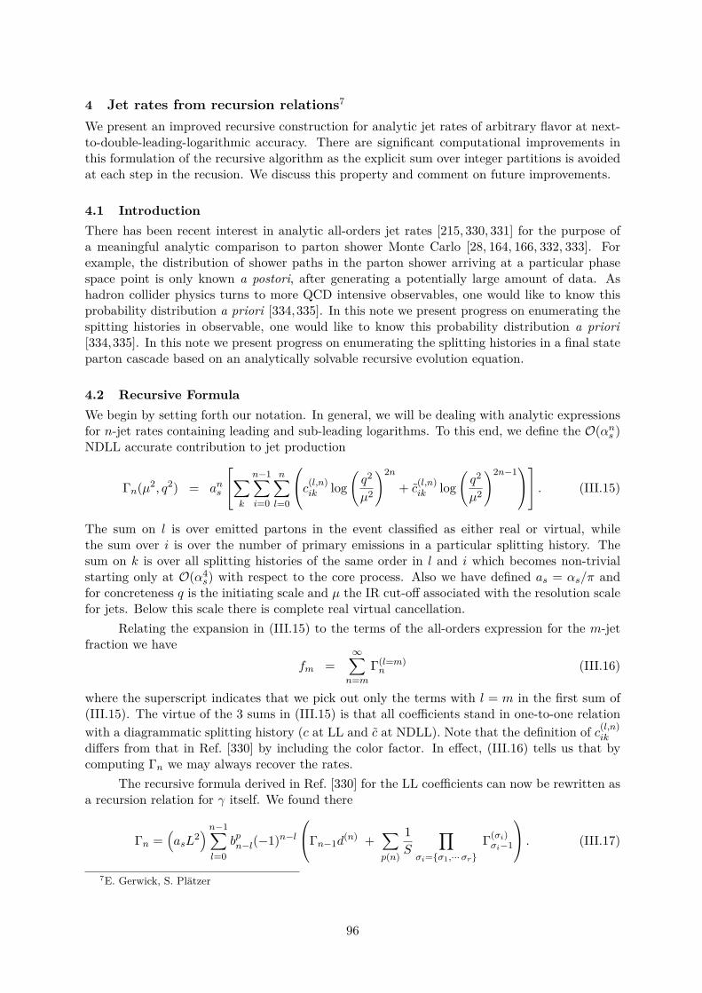
4 Jet rates from recursion relations7

We present an improved recursive construction for analytic jet rates of arbitrary flavor at next-to-double-leading-logarithmic accuracy. There are significant computational improvements inthis formulation of the recursive algorithm as the explicit sum over integer partitions is avoidedat each step in the recusion. We discuss this property and comment on future improvements.

4.1 IntroductionThere has been recent interest in analytic all-orders jet rates [215, 330, 331] for the purpose ofa meaningful analytic comparison to parton shower Monte Carlo [28, 164, 166, 332, 333]. Forexample, the distribution of shower paths in the parton shower arriving at a particular phasespace point is only known a postori, after generating a potentially large amount of data. Ashadron collider physics turns to more QCD intensive observables, one would like to know thisprobability distribution a priori [334,335]. In this note we present progress on enumerating thespitting histories in observable, one would like to know this probability distribution a priori[334,335]. In this note we present progress on enumerating the splitting histories in a final stateparton cascade based on an analytically solvable recursive evolution equation.

4.2 Recursive FormulaWe begin by setting forth our notation. In general, we will be dealing with analytic expressionsfor n-jet rates containing leading and sub-leading logarithms. To this end, we define the O(αns )NDLL accurate contribution to jet production

Γn(µ2, q2) = ans

∑k

n−1∑i=0

n∑l=0

c(l,n)ik log

(q2

µ2

)2n

+ c(l,n)ik log

(q2

µ2

)2n−1 . (III.15)

The sum on l is over emitted partons in the event classified as either real or virtual, whilethe sum over i is over the number of primary emissions in a particular splitting history. Thesum on k is over all splitting histories of the same order in l and i which becomes non-trivialstarting only at O(α4

s) with respect to the core process. Also we have defined as = αs/π andfor concreteness q is the initiating scale and µ the IR cut-off associated with the resolution scalefor jets. Below this scale there is complete real virtual cancellation.

Relating the expansion in (III.15) to the terms of the all-orders expression for the m-jetfraction we have

fm =∞∑n=m

Γ(l=m)n (III.16)

where the superscript indicates that we pick out only the terms with l = m in the first sum of(III.15). The virtue of the 3 sums in (III.15) is that all coefficients stand in one-to-one relationwith a diagrammatic splitting history (c at LL and c at NDLL). Note that the definition of c(l,n)

ik

differs from that in Ref. [330] by including the color factor. In effect, (III.16) tells us that bycomputing Γn we may always recover the rates.

The recursive formula derived in Ref. [330] for the LL coefficients can now be rewritten asa recursion relation for γ itself. We found there

Γn =(asL

2) n−1∑l=0

bpn−l(−1)n−lΓn−1d

(n) +∑p(n)

1S

∏σi={σ1,···σr}

Γ(σi)σi−1

. (III.17)

7E. Gerwick, S. Plätzer

96

Here we define p as as the degree of the stripped splitting history expressed in terms of primordialcoefficients (discussed in more detail in [330]). Also we define the binomial coefficient bij ≡i!/(j!(i− j)!). The factor S is the over-all permutation symmetry factor of a particular splittinghistory. The proof of (III.17) was sketched in Ref. [330] from the generating functional in thecoherent branching formalism. A few additional comments are in order regarding the terms of(III.17).

– The first sum on l counts the number of real gluons at a given order in n. Thus the l = nterm corresponds to the coefficient where all emissions are resolved.

– The sum inside brackets is over the integer partitions p(n) of n, while the product is over thecorresponding coefficient of each element of the partition. In practice, as p(n) ∼ exp(

√n)

this becomes the most computationally intensive step at high parton multiplicity.– The number of previous components i needed for the Γn recursion, and thus necessarilystored in memory, also grows with n, as the degree of the splitting history must be tracked.

– We find an expression for the exclusive rate σn inserting all Γi with i ≤ n in (III.16).

We now provide a different recursive formulation for the real emission components ofΓn which provides significant improvements, both by including sub-leading logarithmic piecesand boosting numerical properties at large n. This constitutes a crucial step towards realisticanalytic constructions of shower histories.

For the resolved components it is sufficient to sum over the c and c coefficients in (III.15),as these are treated on equal footing. We now define

Γn(µ2, q2) = ans

CLLnk log

(q2

µ2

)2n

+ CNLLnk log

(q2

µ2

)2n−1 , (III.18)

for the emission of n− 1 partons from an initial configuration k. The k index is neglected in thedefinition of (III.15) for simplicity, but is easily restored. Here, we keep it explicit. Accordingto (III.18), we claim accuracy on the integrated multi-parton splitting function to the level ofαnL2n−1, which amounts to next-to-double-leading-logarithmic (NDLA) accuracy.

Each coefficient CLLn and CNLL

n is degenerate on a potentially large number of splitting his-tories. Using the modified coherent branching formalism, the sub-leading logarithms in (III.18)are propagated through to the n-jet rates. A simple evolution equation reads

Γnk(µ2, Q2) =

αs2π

n−1∑m=0

∑i,j

∫ Q2

4µ2

dq2

q2

∫ 1−µ/q

µ/qdz Pk→ij(z)Γ

(m)i (µ2, z2q2)Γ(n−m−1)

j (µ2, (1− z)2q2) , (III.19)

with Γ(0)k = 1, effectively enforcing the 0-th order expanded Sudakov boundary condition. The

sum on n is now over partitions of partons of length 2 while the sum over i, j is over flavors(q/g) and is a purely NDLA effect. The diagrammatic form of (III.19) is

=k,Q2 k,Q2

i, z2q2

j, (1 − z)2q2

n

m

n−m− 1

Σi, j

Σm = 0

n− 1

(III.20)

97

Now we insert the general expression (III.18) into the previous evolution equation (III.19) andexpand the respective coefficients. We find

Γnk(µ2, Q2) =(αs2π

)n n−1∑m=0

∑i,j

∫ Q2

4µ2

dq2

q2 ×CLLi,mC

LLi,n−m−1

2m∑α=0

2(n−m)−2∑β=0

b2mα b2(n−m)−2β L2n−2−α−β γα,βk→ij +

CNLLi,m CLL

i,n−m−1

2m−1∑α=0

2(n−m)−2∑β=0

b2m−1α b

2(n−m)−2β L2n−3−α−β γα,βk→ij+

CLLi,mC

NLLi,n−m−1

2m∑α=0

2(n−m)−3∑β=0

b2mα b2(n−m)−3β L2n−3−α−β γα,βk→ij+

CNLLi,m CNLL

i,n−m−1

2m−1∑α=0

2(n−m)−3∑β=0

b2m−1α b

2(n−m)−3β L2n−4−α−β γα,βk→ij

, (III.21)

whereγα,βk→ij ≡

∫ 1−µ/q

µ/qdzPk→ij(z) lnα z2 lnβ(1− z)2. (III.22)

As is already evident from (III.18), the splitting function P (z), with singular pieces in bothz → 0 and (1− z)→ 0, picks out the logarithmically enhanced coefficients of the correspondingΓ. To this end, we decompose the splitting function as

Pk→ij(z) =P

(−)k→ij

1− z +P

(+)k→ijz

+ P(0)k→ij(z) , (III.23)

where P (0)k→ij(z) is regular at both z → 0, z → 1 and we let 〈P (0)

k→ij〉 denote its average over z ∈(0, 1). This allows us to extract the logarithmic pieces from (III.22). The relevant contributionsare

γα,βk→ij = P(−)k→ij

(−1)β

2(β + 1)Lβ+1δα,0 + P

(+)k→ij

(−1)α

2(α+ 1)Lα+1δβ,0 + 〈P (0)

k→ij〉δα,0δβ,0 +O(µ) .

(III.24)

The leading and next-to-leading logarithmic coefficients, defined in (III.18), are given by sumsof coefficients from lower n, with pre-factors assigned by the integrated splitting functions. Wefind

CLLk,n = 1

4n

n−1∑m=0

∑i,j

CLLi,mC

LLj,n−m−1

(P

(−)k→ijξ2n−2m−2 + P

(+)k→ijξ2m

)

CNLLk,n = 1

2(2n− 1) ×n−1∑m=0

∑i,j

[P

(−)k→ij

(CNLLi,m CLL

j,n−m−1ξ2n−2m−2 + CLLi,mC

NLLj,n−m−1ξ2n−2m−3

)+

P(+)k→ij

(CNLLi,m CLL

j,n−m−1ξ2m−1 + CLLi,mC

NLLj,n−m−1ξ2m

)+ 2〈P (0)

k→ij〉CLLi,mC

LLj,n−m−1

]. (III.25)

with initial condition CLLk,0 = 1, CNLL

k,0 = 0. We define here

ξn =n∑k=0

(−1)k

k + 1 bnk =

{ 1n+1 n ≥ 00 else

. (III.26)

98

4.3 DiscussionPartitions of integers:

We clarify here the relation between the two recursive constructions, (III.17) and (III.25).In (III.25) there is no sum over integer partitions of the number of partons n. This dramaticallyreduces the (potentially prohibitive at high multiplicity) computational expense. It is useful toinductively analyze precisely how the second construction (III.25) aviods this complication.

The coefficients CLLk,n contain information on all splitting histories up to n, including the

partitions (and sub-partitions) of n. Now consider the partition {σ1, σ2, · · · σq} of length q ofn so that σ1 + σ2 + · · · σq = n. We take the term included in Γn which is proportional tocσ1cσ2 · · · cσq . Now we will display how all partitions of length q of n+ 1 are generated.

Consider the partition {σ2, · · · σq} of length q − 1 in Γn−σ1 which we label Γq−1n−σ1 . The

z → 0 region of the integral

P (z) Γσ1(µ2, z2q2) Γqn−σ1(µ2, (1− z)2q2) (III.27)

gives the contribution corresponding to the partition {σ1 + 1, σ2, · · · σq}. Similarly, the termΓσ2Γn−σ2 generates {σ1, σ2 + 1, · · · σq}. It is clear that this procedure exhausts all partitions ofn + 1 of length q, which are now contained in Γn+1. The only partition not includes here is oflength n+ 1, which clearly originates from the non-singular regions of P (z)Γ0Γn.Systematic improvements:

As presented the recursive contruction only includes the resolved coefficienst which areleading order in αs. Including the virtual coefficients along with the NDLL terms, one shouldhave enough information to include the leading effects of the running coupling which formallystart at one power higher in the coupling together with sub-leading logarithms. At this stage adirect comparison with parton shower Monte Carlo is possible.Validation:

We have compared results from the recursion relation presented here (at LL), with the re-cursion relation discussed previously. The NDLC calculation has been verified for the coefficientsquoted in [336]Outlook:

Both the original recursion proposed in [330], and the new approach with the inclusionof NDLC terms are available as symbolic Mathematica code, while we have also developed ahighly efficient numerical implementation in C++. Work is ongoing on including the unresolvedcomponents in the new approach, as well. We foresee providing the results in both in the analyticand numeric tools which will in turn enable us to perform more realistic cross checks of the jetrate coefficients against parton shower implementations.

ConclusionsOur prescription for computing analytic jet rate coefficients is relevant a more complete un-derstanding of the probability distributions of exclusive final states. These are typically onlyaccessed via parton shower Monte Carlo, although there are recent attempts to put these onmore solid analytic footing [215,334,335].

AcknowledgementsWe would like to thank the Les Houches workshop for hospitality offered during which some of thework contained herein was performed, and the stimulating environment to foster collaborationon comparing and developing two different approaches to the same problem. SP acknowledgespartial support from the Helmholtz Alliance ‘Physics at the Terascale’.

99

0 1 2 3 4 5 6∆y

0

20

40

60

80

100

120

140nb

/[rap

idity

uni

t]

jets massHT /2

Fig. III.20: Distribution of inclusive 2-jet events with no jets in the ragion of rapidity between the twojets of highest transverse momentum, for two choices of factorisation and renormalisation scale.

=======

5 Study of the average number of hard jets8

5.1 IntroductionJet vetos are an important ingredient in many analysis, in particular for analysis involving aHiggs boson produced through vector boson fusion. It is necessary to understand the impact ofthe jet vetos on theoretical predictions and their uncertainties. For this purpose it is useful totest the description offered by different tools in a process offering more available and precise data.In this contribution we investigate the extent to which pure perturbative tools (no underlyingevent, no hadronisation) can describe dijet events when vetos on further jets are imposed.

We compare theoretical predictions obtained using HEJ [337–339] and NLO predictionsobtained by BlackHat+Sherpa [340–345]. We base the analysis on the observables measured bythe Atlas collaboration described in [346].

For the NLO predictions we used the invariant mass of all jets as the scale and notthe usual HT /2 variable since in configurations with two widely separated jets with moderatetransverse momenta (the type of configuration dominant for most observables in this study) HT

is not a good scale to represent the scale of the process, as it is much lower than the partoniccenter of mass energy. The fact that this scale is too low in these configurations is evidencedby the fact that distributions turn negative for the corresponding observables, as can be seen inFigure III.20, illustrating the cross section for dijet production with no further jets in the regionof rapidity between the two hardest jets, as obtained with two different choices for the scale inthe calculation of dijets@NLO.

There are different ways of defining the gap fraction at NLO given the ambiguity in theinclusion of higher order terms. In this contribution we will follow two approaches, equivalentup to higher order terms, trying to identify whether one agrees with the data better than thether.

8J.R. Andersen, D. Maître

100

5.2 Gap fractions for a fixed pt-thresholdIn this section we use Q0 to denote the minimum transverse momentum for the jets. The gapfraction is given by:

g =σY/pt(Q0)

σtot, (III.28)

where σY/pt(Q0) is the cross section with the constraint that there are no additional jets with pTabove Q0 between (in rapidity) the two leading pT jets (pt) or the forward/backward jets (Y ).We use the notation g = i to specify how many jets are in the region of rapidity between thetagging dijets (the condition for this to happen depend on the context, e.g. whether the taggingdijet system is defined by the most energetic jets or the most forward and backward). j = i isused to specify the number of jets. In both cases the equal sign correspond to an exclusive finalstate, for example j = 2 means exactly two jets, while inequalities mean inclusive final stateg ≥ 1 means one or more jets in the gap.

We investigate two different approximations for the gap fraction, which are both equivalentup to α3

s. These are

g = σg=0σtot

= 1− σg>=1σtot

= 1−σNLO,j≥3g≥1σNLO,j≤2 = 1−

σNLO,j>=3 − σNLO,j=3g=0 − σLO,j=4

g=0σNLO,j≤2 (III.29)

and

g = σg=0σtot

=σNLO,j=2g=0 + σNLO,j=3

g=0 + σNLO,j≥4g=0

σNLO,j=2 + σNLO,j=3 + σNLO,j≥4 (III.30)

In the case where the jets defining the dijet system are the forward/backward ones, the formulaesimplify to

gY = σg=0σtot

= σNLO,j=2

σNLO,j≥2 (III.31)

and

gY = σg=0σtot

= σNLO,j=2

σNLO,j=2 + σNLO,j=3 + σNLO,j≤4 . (III.32)

Figure III.21 shows the gap fraction as a function of the the rapidity difference between thetwo highest transverse momentum jet. The curves corresponds to different slices of the averagetransverse momentum of the jets

pT = 12(pj1T + pj2

T

).

From the top to the bottom the slices are:

240 GeV < pT < 270 GeV210 GeV < pT < 240 GeV180 GeV < pT < 210 GeV150 GeV < pT < 180 GeV120 GeV < pT < 150 GeV90 GeV < pT < 120 GeV70 GeV < pT < 90 GeV (III.33)

101

0 1 2 3 4 5 6∆y

0.0

0.5

1.0

1.5

2.0

2.5

3.0

3.5

4.0

4.5

Gap

fract

ion

0 1 2 3 4 5 6∆y

0.20.40.60.81.01.21.41.60.51.01.5

0.51.01.52.02.50.51.01.52.02.50.51.01.52.02.50.51.01.52.02.50.51.01.52.02.5

Theo

ry/D

ata

Fig. III.21: Gap fraction as a function of ∆y for various slices of pT . The jets defining pT and ∆y arethe two jets with the largest pT .

The green curve corresponds to the HEJ prediction, while the blue and red curves correspondto the NLO predictions of formulae (III.29) and (III.30), respectively. The band representthe statistical Monte Carlo intgration only. For this observable, the NLO-based predictionfares marginally better compared to ATLAS data [346] when using Eq. (III.30) rather thanEq. (III.29).

In Figure III.22 we present the gap fraction as a function of the average transverse momen-tum of the highest transverse momentum jets for different slices of rapidity difference betweenthem. The slices are give, from top to bottom by

5 < ∆y < 64 < ∆y < 53 < ∆y < 42 < ∆y < 31 < ∆y < 2 . (III.34)

The green curve corresponds to the HEJ prediction, while the blue and red curves correspondto the NLO predictions of formulae (III.29) and (III.30), respectively. The band represent thestatistical Monte Carlo intgration only. For this observable the NLO-based predictions are againbetter using the gap formula (III.30) rather than that of (III.29); the former overshooting thedata less than the latter. The difference between the two formulae becomes larger as the rapidityseparation between the jets increases, which is fully understood from the increased of yet higherorder terms for increasing rapidity spans.

102

50 100 150 200 250 300 350 400 450 500pT

0

1

2

3

4

5

6

7

8

Gap

fract

ion

50 100 150 200 250 300 350 400 450 500pT

0.80.91.01.11.21.31.4

0.51.01.52.0

0.51.01.52.02.5

0.51.01.52.02.5

0.51.01.52.02.5

Theo

ry/D

ata

Fig. III.22: Gap fraction as a function of pT for various slices of ∆y. The jets defining pT and ∆y arethe two jets with the largest pT .

5.3 Mean number of jetsThe mean number of jets in the relevant region of rapidity is obviously defined as

< Ngap >= σg=1 + 2σg=2 + 3σg=3 + . . .

σtot. (III.35)

Based on NLO-calculations, we can construct equivalent predictions for the average number ofjets as

< Ngap >=1(σj=3

g=1 + σj>=4g=1 ) + 2σj>=4

g=2 + 3σj=5g=3

σNLO,j=2 + σNLO,j=3 + σNLO,j≤4 (III.36)

and

< Ngap >=1(σj=3

g=1 + σj=4,LOg=1 ) + 2

(σj=4,LOg=2

)σj≤2,NLO (III.37)

In the case where the jets defining the dijet system are the forward/backward ones, the formulaesimplify to

< Ngap >=1σj=3

g=1 + 2σj=4g=2 + 3σj=5

g=3σNLO,j=2 + σNLO,j=3 + σNLO,j=4 (III.38)

and

< Ngap >=1(σj=3

g=1) + 2(σj=4,LOg=2

)σNLO,j≤2 (III.39)

In Figure III.23 we show the average number of jets in the gap as a function of the average trans-verse momentum for the last four ∆y slices in Eq. III.34. Both the HEJ and the NLO predictionundershoot the data with an increasing difference at large average transverse momentum. Theratio looks similar for the all slices for the HEJ prediction while the disagreement gets worse forincreasing rapidity difference for the NLO predictions.

103

50 100 150 200 250 300 350 400 450 500pT

4

2

0

2

4

6

8

Mea

n nu

mbe

r of j

ets

in th

e ga

p

50 100 150 200 250 300 350 400 450 500pT

0.50.60.70.80.91.01.11.20.20.40.60.81.01.21.40.20.40.60.81.01.21.41.6

0.51.01.52.02.5

Theo

ry/D

ata

Fig. III.23: Mean number of jets in the gap as a function of pT for various slices of ∆y. The jets definingpT and ∆y are the two jets with the largest pT .

5.4 ConclusionsIn this contribution we have compared predictions for gap probabilities and related observ-ables from HEJ and BlackHat+Sherpa with experimental data from the ATLAS collaboration.Our analysis shows that both HEJ and NLO can provide a very good (and fully perturbative)description of e.g. the gap fraction in the full range of rapidities and all slices of pT (Fig. III.21).

However, neither HEJ nor the NLO combination provide a perfect description of the datawhen it comes to e.g. the average number of soft (20GeV) jets in events with two much harderjets (Figure III.23. This is perhaps not surprising, since this is the region where the systematicresummation provided by a parton shower is necessary.

Furthermore, there is no clear preference for one or the other NLO ’stategies’ to definethe gap fraction. In future work we hope to understand to which extent perturbative methodscan describe the gap fraction and extend the study to all distributions in [346]. The statisticalsamples used for this analysis leaves us with quite large uncertainties, for further studies morestatistics will be needed.

104

6 Uncertainties in pp → h + 2 jets production through gluon fusion9

6.1 INTRODUCTIONThe process of Higgs boson production in association with dijets is of interest for several rea-sons. The interference between the two production channels of Weak-boson fusion (WBF) andgluon fusion (GF) is insignificant [347–349], so it is justified to discuss the processes separately.This study is concerned with the description of the gluon fusion contribution to Higgs bosonproduction in association with dijets.

The gluon fusion channel is of interest not just as a background to the direct studythrough WBF of the couplings between the weak bosons and the Higgs boson, but also becausethe structure of the heavy-quark-mediated coupling of the Higgs boson to gluons can be studiedbeyond the question of normalisation. The structure of the higgs-couplings means that for aCP -specific coupling the cross section displays a striking dependence on the azimuthal anglebetween rapidity-separated jets. In contrast, the weak-boson-fusion component is relativelyflat [350,351].

In this region of phase space of large rapidity spans of the jets, the component of gluonfusion and weak-boson fusion exhibit very different patterns of radiative corrections. This iscaused by a dominant colour octet exchange between the dijets in the case of gluon-fusion,whereas the weak-boson fusion component has no colour exchange between the jets [352, 353].For the gluon fusion sample, this enhances the contribution from jet multiplicities beyond thetwo required, and necessitates a generalisation of the Born-level jet analysis to stabilise theextraction of the azimuthal dependence [354]. Furthermore, the enhanced contribution fromfurther hard radiation severely tests the current limits of the perturbative description.

With a satisfactory description of each component, the very different radiation patternsin WBF and GF can be utilised to study each contribution separately (for extraction andverification of the CP -structure of the couplings).

The purpose of the current study is to investigate the variation in the current description ofthe gluon-fusion contribution, in particular in the testing region of the cuts employed to enhancethe weak-boson fusion contribution to Higgs boson production in association with dijets.

6.2 GENERATORSIn this section all generators employed in this study, including their settings and methods ofdetermining the uncertainties, are briefly reviewed.

6.2.1 aMC@NLOEvents were generated using MadGraph5_aMC@NLO 2.0 [355] for exclusive jet multiplicities(pp → h + 0j, pp → h + 1j, pp → h + 2j), each at NLO accuracy. The virtual correctionswere taken from Mcfm [44, 356]. Jet multiplicities are then merged using the FxFx mergingprescription [357]. Events are then showered with Herwig++ [164], where events are matchedto the hard process. To avoid double counting, the jet multiplicity after showering must matchthe jet multiplicity of the hard process for which NLO accuracy is desired. This means that onlyevents with 0 jets after showering are kept if they were generated with 0 partons in the matrixelement. Because NLO is only desired for Higgs in association with up to two jets, events whichhave more than two jets after showering are kept if the hard process was generated with twojets. In addition, jets after showering must be matched with the hard partons of the generatedevent by imposing a ∆R = 1 requirement between jets before and after showering. All matched

9J.R. Andersen, F.U. Bernlochner, D. Gillberg, K. Hamilton, T. Hapola, J. Huston, A. Kruse, L. Lönnblad,P. Nason, S. Prestel, M. Schönherr, J.M. Smillie, K. Zapp

105

(µR/mh, µF /mh) (0.5,0.5) (0.5,1) (1,0.5) (1,1) (1,2) (2,1) (2,2)Powheg ggF 15.83 15.90 13.20 13.29 13.34 11.27 11.31MiNLO-HJ 16.58 16.68 12.32 12.58 12.74 10.76 10.90MiNLO-HJJ 22.36 23.58 16.89 17.74 18.19 13.14 13.35

Table III.3: Inclusive pp → h cross sections in pb for Powheg ggF, MiNLO-HJ and MiNLO-HJJ forvarious scale choices.

jets after showering must have p⊥ larger than the merging scale.Events were produced using the CT10 parton distribution function [289] throughout. The

renormalisation and factorisation scales, µR and µF , are set following the MiNLO procedure [32].The merging scale was chosen to be 30 GeV for the nominal sample. Scale variations were foundby varying µR and µF up and down by factors of two.

6.2.2 HejHigh Energy Jets (Hej) describes hard, wide angle (high energy-) emissions to all orders andto all multiplicities. The predictions are based on events generated according to an all-orderresummation, merged with high-multiplicity full tree-level matrix-elements. The explicit resum-mation is built on an approximation to the n-parton hard scattering matrix element [337–339]which becomes exact in the limit of wide-angle emissions, ensuring leading logarithmic accuracyfor both real and virtual corrections. These logarithmic terms are important when the partonicinvariant mass is large compared to the typical transverse momentum in the event. This isprecisely the situation which arises in typical “VBF” cuts, including those used in this study.Matching to the full tree level accuracy for up to three jets is obtained by supplementing theresummation with a merging procedure [358,359].

The implementation of this framework in a fully-flexible Monte Carlo event generatoris available at http://hej.web.cern.ch, and produces exclusive samples for events with atleast two jets. The predictions include resummation also for events with up to two un-orderedemissions, i.e. contributions from the first sub-leading configurations [360].

The factorisation and renormalisation scales can be chosen arbitrarily, just as in a standardfixed-order calculation. Here, we have chosen to evaluate two powers of the strong coupling at ascale given by the Higgs mass, and for the central predictions the remaining scales are evaluatedat µR = HT /2. Thus, for the n-jet tree-level evaluation,

αn+2s = α2

s(mh) · αns (µR). (III.40)

The scale variation bands shown in the plots here correspond to varying µF and µR independentlyby a factor of two in either direction, but discarding evaluations where any ratio is bigger thantwo. The CT10nlo [233,289] parton distribution functions were used in the predictions.

6.2.3 PowhegBoxSamples were generated using the latest version of PowhegBox (SVN revision 2550). Theproduced Les Houches files were passed through Pythia 8 [333] (v8.1.6) for parton showering(ISR+FSR). This was done for default Powheg ggF, MiNLO-HJ and MiNLO-HJJ for each of thescale variation settings. CT10 [289] was used both for the matrix element and hardest emissioncalculation in PowhegBox and parton showering in Pythia 8 [361,362]. The total cross sectionof these samples are summarised in Tab. 6.2.3.

106

The Pythia 8 default parton showering interface to the PowhegBox was used that picksup the SCALUP parameter from the LesHouches file and restricts parton shower emissions to thisscale (aka “wimpy showers”). Parton showering/resummation uncertainties were evaluated byproducing separate samples with the SCALUP parameter varied by factors of 0.75 and 1.5. Across check was performed replacing the SCALUP restriction by the “power shower”+“pT veto”approach10. The difference between the two approaches is (well) within the SCALUP variation.

Additional results switching off ISR and/or FSR and including hadronisation and/or MPIare provided at https://dgillber.web.cern.ch/dgillber/Rivet/Powheg_ggF.html.

For the study presented in Sec. 6.3 the MiNLO-HJJ setup was used throughout as it givesthe highest formal accuracy for most observables under scrutiny. Please note: for the sake ofconsistency in describing correllations inbetween the different observable classes the MiNLO-HJJsetup was also used for zero- and one-jet inclusive observables where its formal accuracy fallsbelow the MiNLO-HJ setup.

6.2.4 Pythia 8The unlops method [35] allows to incorporate multiple next-to-leading order calculations intoa parton shower event generator. The implementation of this NLO merging scheme in Pythia 8[333] uses external next-to-leading order matrix element generators to produce events distributedaccording to inclusive NLO cross sections. Higher-order terms (of the umeps merging scheme[31]) are supplied by reweighting additional tree-level input samples. In the unlops approach,the merged prediction for an observable is

〈O〉 =M−1∑m=0

∫dφ0

∫· · ·∫O(S+mj)

{Bm +

[Bm]−m,m+1

−M∑

i=m+1

∫sBi→m −

M∑i=m+1

[ ∫sBi→m

]−i,i+1

−N∑

i=M+1

∫sBi→m

}

+∫dφ0

∫· · ·∫O(S+Mj)

{BM +

[BM

]−M,M+1

−N∑

i=M+1

∫sBi→M

}

+N∑

n=M+1

∫dφ0

∫· · ·∫O(S+nj)

Bn −N∑

i=n+1

∫sBi→n

. (III.41)

The notation is defined in [35]. For this study, M = 2 and N = 3. The PowhegBox generator[26] is used to produce the inclusive NLO samples B0 [363], B1 and B2 [364], while additionaltree-level inputs are taken from MadGraph/MadEvent [355,365]. The merging scale criterion(see Appendix A.1 of [35]) is used to remove infrared divergences due to additional jets at Bornlevel. This cut is applied internally in Pythia 8, so that no user interference with e.g. thePowhegBox source code becomes necessary. All input samples are computed with fixed scalesµF and µR. Terms of O

(αn+2s

)and higher due to running scales are included, in a controlled

way, by reweighting tree-level samples with factors to produce the CKKW-L [366–368] scalesetting prescription.

This NLO merging scheme replaces the approximate αn+1s -terms of the umeps tree-level

merging method with the desired full fixed-order expressions, but otherwise leaves higher-ordercorrections untouched. Particularly, no higher-order terms are introduced by reweighting virtualcorrections. Note further that the method keeps the inclusive cross section fixed to the zero-jet

10 See Pythia8/examples/main31.

107

NLO cross section, without producing spurious logarithmic artifacts of the merging procedure,and without introducing additional finite terms.

To produce results, we generate fixed-order input events with PowhegBox and MadE-vent at ECM = 8 TeV, using CT10nlo [233, 289] parton distributions, massless b-quarks, van-ishing coupling between b-quarks and Higgs-boson and a stable Higgs-boson of mass mh = 125GeV. We define the merging scale as the minimal relative shower p⊥evol and use a merging scalevalue of ρms = 15 GeV. The samples are merged within Pythia 8.180. Pythia 8 is run withTune AU2-CTEQ6L1 [362], which uses CTEQ6L1 [251] parton distributions. Masses and widthsare, naturally, set equal in PowhegBox, MadEvent and Pythia 8. We assess uncertaintiesby producing two sets of variations:

– Parton shower variation: Use PowhegBox and MadEvent inputs generated with µF =µR = mh, and choose the Pythia 8 starting scale µQ for adding emissions to zero-partonevents as µQ,low = 1

2 mh, µQ,central = mh or µQ,high = 2mh. Construct an envelope fromthe results of these variations. Only the starting scale for adding emissions to zero-partonevents can be varied, as the starting scale for showering n≥ 1-parton events is locked bythe CKKW-L prescription.

– Matrix element variation: Vary the renormalisation and factorisation scales in Powheg-Box and MadEvent as µF,low = µR,low = 1

2 mh, µF,central = µR,central = mh or µF,high =µR,high = 2mh, keep the Pythia 8 starting scale µQ for adding emissions to zero-partonevents fixed at µQ = mh. Construct an envelope from the results of the variations.

We do not attempt a more complete uncertainty study including variation of renormalisation andfactorisation scales in the parton shower, mainly because we have not decided on a strategy ofhow to deal with such uncertainties, and other fixed-order uncertainties, in the context of partonshower resummation and tuning. However, the envelope of the uncertainty bands presented hereshould, for most cases, yield a reasonably conservative estimate. Also, for this perturbative-physics driven study, we do not address the (potentially important) uncertainties due to non-perturbative modelling in the event generator.

6.2.5 SherpaThe Sherpa event generator implements the meps@nlo [30, 369] technique to merge multiplenlops matched [29] samples of successive jet multiplicities into an inclusive calculation thatretains both the NLO accuracy for every individual jet multiplicity and the parton shower’sresummation properties in resumming emission scale hierarchies wrt. inclusive process. Thisimplementation has already been successfully applied to various background processes to Higgsproduction channels [370,371]. Also Higgs production through gluon fusion has been studied indetail with this approach recently [372].

For the contribution to this comparative study the subprocesses pp→ h+0 jets, pp→ h+1jet and pp → h + 2 jets are calculated at next-to-leading order and pp → h + 3 jets at leadingorder accuracy. The one-loop matrix elements are taken from [373,374], [375,376] and [44,356],respectively. The LO pp→ h+ 3 jets process, as it is merged on top of the NLO pp→ h+ 2 jetsprocess by the menlops mehtod [369], receives a local K-factor in dependence of the pp→ h+2jets composition in terms of S- and H-events. For the central prediction, the individual jetmultiplicities were separated by Qcut = 20 GeV. The renormalisation and factorisation scaleswere set according to the CKKW prescription, i.e. α2+n

s (µR) = αs(m2h)αs(t1) · · ·αs(tn) and

µF = mh for the core process. The parton shower starting scale µQ was set to mh. Throughout,the CT10nlo [233,289] PDF set was used.

The uncertainties on the central prediction were estimated by varying µR and µF inde-pendently by the customary factor of two and the parton shower starting scale by a factor

√2.

108

Inclusive event selection

aMC@NLOPowhegBoxPythia 8Sherpa

10−3

10−2

10−1

1Transverse momentum of the Higgs boson

dσ

/dp ⊥

[pb/

GeV

]

0 50 100 150 200

0.5

1

1.5

2

2.5

p⊥(h) [GeV]

Rat

iow

.r.t.

Pow

heg

Box

Inclusive event selection

HejaMC@NLOPowhegBoxPythia 8Sherpa

10−2

10−1

1

10 1

Inclusive jet multiplicity

σ(N

jet)

[pb]

0 1 2 3 4

0.5

1

1.5

2

2.5

Njet

Rat

iow

.r.t.

Pow

heg

Box

Fig. III.24: Transverse momentum of the Higgs boson (left) and inclusive jet multiplicity (right)as predicted by the different generators. The individual sources of uncertainties used to generate therespective bands are described in Sec. 6.2. Note that for PowhegBox the MiNLO-HJJ prediction hasbeen used throughout, despite its lowered accuracy for inclusive and one-jet observables, for consistenciessake.

The merging scale was varied in the range {15, 20, 30} GeV. Further, the intrisic parton showeruncertainties were estimated by varying the evolution variable and the recoil scheme accordingto [372]. Non-perturbative uncertainties which may very well play a role in analyses lookinginto hadronic activity within jets widely separated in rapidity [377,378] are not assessed in thisstudy.

6.3 RESULTSThis study aims at quantifying the gluon fusion contribution and its perturbative uncertaintyto typical VBF Higgs plus two jets event selections at the LHC at a centre-of-mass energy of 8TeV. To summarise Sec. 6.2, the following parameters were then varied to estimate the respectivegenerator’s uncertainty:

Hej: µR, µF ∈ [12 , 2] separately

aMc@Nlo: µR, µF ∈ [12 , 2]

PowhegBox: µR, µF ∈ [12 , 2] separately, SCALEUP ∈ [0.75, 1.5]

Pythia 8: µR, µF ∈ [12 , 2], µQ ∈ [ 1√

2 ,√

2]Sherpa: µR, µF ∈ [1

2 , 2] separately, µQ ∈ [ 1√2 ,√

2], Qcut ∈ [15, 20, 30]

A common Rivet [379, 380] analysis implementing the observables for the event selections de-scribed below has been used. This analysis is inclusive with respect to the Higgs, i.e. there areno phase space cuts on the Higgs and all decay channels are included. Concerning the presenceof additional jets the analysis defines several stages of cuts.

First we study the transverse momentum of the Higgs boson for inclusive Higgs productionas obtained in the shower based approaches to study the overall consistency of their fixed-order and resummation properties. The results are shown in Fig. III.24 on the left hand side.PowhegBox, Pythia 8 and Sherpa are compatible within uncertainties, where PowhegBox

109

Leading jet selectionDijet cuts

HejaMC@NLOPowhegBoxPythia 8Sherpa

0

0.2

0.4

0.6

0.8

1Rapidity separation of the two leading jets

dσ

/d∆

y[p

b]

0 1 2 3 4 5 6 7 8

0.5

1

1.5

2

2.5

∆y(j1, j2)

Rat

iow

.r.t.

Pow

heg

Box

Forward-backward selectionDijet cuts

HejaMC@NLOPowhegBoxPythia 8Sherpa

0

0.2

0.4

0.6

0.8

1Rapidity separation of the two leading jets

dσ

/d∆

y[p

b]

0 1 2 3 4 5 6 7 8

0.5

1

1.5

2

2.5

∆y(j1, j2)

Rat

iow

.r.t.

Pow

heg

Box

Fig. III.25: Rapidity difference of both tagging jets in the leading jet selection (left) and the forward-backward selection (right) as predicted by the different generators. The individual sources of uncertaintiesused to generate the respective bands are described in Sec. 6.2. The location of the VBF cut is indicated.

reports somewhat larger central values and uncertainties due to the usage of the MiNLO-HJJ11,cf. Tab. III.3. aMC@NLO has a similar description of the Sudakov region but its predictionsfall below those of the other generators for larger transverse momenta. Hej generates at leasttwo jets and thus is not included in the comparison for this observable.

The following observables all depend on the presence of at least one jet. Jets are recon-structed using the anti-kt algorithm provided by FastJet [283] with radius parameter R = 0.4within the pseudo-rapidity range |η| < 5 and are required to have a minimal transverse momen-tum of p⊥ > 30 GeV. The predictions for the number of jets, shown in Fig. III.24 on the righthand side, are largely consistent, only aMC@NLO has somewhat less cross section in the zero-and one-jet inclusive bins. The inclusive dijet cross section is consistent within uncertaintiesfor all generators. From here on, as a minimum of two jets accompanying the Higgs are alwaysrequired, the Hej prediction is included and it is found to be in good agreement with the showerbased approaches. For the higher inclusive jet multiplicities the spread and also the uncertain-ties are significantly larger. This is expected, as the theoretical accuracy decreases there for allgenerators. This is especially true for the inclusive four jet rate since – with the exception ofHej – the fourth jet comes from the parton shower only.

For the Higgs+dijet selection two alternatives are considered: In the leading jet selectionthe two hardest jets in the event constitute the tagging jets, while in the forward-backwardselection the most forward and the most backward (in rapidity) jet are defined as tagging jets.For events with exactly two jets the two selections are obviously identical, for events with morethan two jets they can differ. This general dijet selection defines the second level of cuts. Thethird level is a VBF-like selection in which the two tagging jets are required to have a rapidityseparation ∆y(j1, j2) > 2.8 and a large invariant mass mjj > 400 GeV. The invariant massand rapidity separation of the tagging jets are shown in Figs. III.25 and III.26, respectively, for

11 As this study focusses on pp → h + 2 jets topologies MiNLO-HJJ is used throughout despite its reduceduncertainty for more inclusive observables for consistencies sake.

110

Leading jet selectionDijet cuts

HejaMC@NLOPowhegBoxPythia 8Sherpa

10−4

10−3

10−2

Invariant mass of the two tagging jets

dσ

/dm

jj[p

b/G

eV]

0 200 400 600 800 1000

0.5

1

1.5

2

2.5

mjj [GeV]

Rat

iow

.r.t.

Pow

heg

Box

Forward-backward selectionDijet cuts

HejaMC@NLOPowhegBoxPythia 8Sherpa

10−4

10−3

10−2

Invariant mass of the two tagging jets

dσ

/dm

jj[p

b/G

eV]

0 200 400 600 800 1000

0.5

1

1.5

2

2.5

mjj [GeV]

Rat

iow

.r.t.

Pow

heg

Box

Fig. III.26: Invariant mass of both tagging jets in the leading jet selection (left) and the forward-backward selection (right) as predicted by the different generators. The individual sources of uncertaintiesused to generate the respective bands are described in Sec. 6.2. The location of the VBF cut is indicated.

both dijet selections before the VBF cuts. As expected, the rapidity separation between thetwo tagging jets, Fig. III.25, is larger in the forward-backward than in the leading jet selection.In this observable differences between the generators become visible: While PowhegBox andPythia 8 are consistent in shape but differ slightly in normalisation, Sherpa and aMC@NLOpredict significantly more cross section at large ∆y but also differ in normalisation. A possibleorigin of such differences within the parton shower based event generators is the behaviour oftheir respective parton shower, which affects distributions both explicitly by radiating additionalpartons and (for some approaches) through the computation of Sudakov form factors. Theslightly higher cross section in the Pythia 8 prediction can, for example, be traced to the highvalue of αs in Tune AU2-CTEQ6L1. Hej, on the contrary, falls off faster at large ∆y. Thiscan be understood from the systematic resummation of virtual correction in log s

t which becomeimportant at large ∆y. In the leading jet selection there is the additional effect that whenjets are produced at large rapidity differences the void in between them tends to be filled withadditional hard jets unordered in p⊥. These differences are, however, partially covered by theuncertainties.

The invariant mass distribution is almost identical in the two dijet selections. The pre-dictions are all consistent in shape but differ somewhat in normalisation with Pythia 8 atthe upper and Hej on the lower end of the normalisation spectrum. Noteworthy is thatSherpa, and to some extent also Pythia 8, predicts more cross section at larger mjj thanthe other generators, while Hej predicts slightly less. Here a discussion of how the aMC@NLO,PowhegBox, Pythia 8 and Sherpa treat configurations with at least three jets which makeup a large fraction of the events in the high invariant mass as well as the large ∆y regions,seems expedient. Treating three jet configurations as a separate contribution, as is the casein Pythia 8 and Sherpa, leads to assigning them a renormalisation scale defined throughα2+3s (µR) = α2

s(mh)αs(t1)αs(t2)αs(t3) for ordered jet emissions in the CKKW approach (tibeing the reconstructed emission/clustering scales of the respective approach) whereas treat-ing three jet configurations as real emission corrections to the underlying two jet configuration

111

Leading jet selectionDijet cuts

HejaMC@NLOPowhegBoxPythia 8Sherpa

10−4

10−3

10−2

Transverse momentum of the Higgs boson

dσ

/dp ⊥

[pb/

GeV

]

0 50 100 150 200 250 300

0.5

1

1.5

2

2.5

p⊥(h) [GeV]

Rat

iow

.r.t.

Pow

heg

Box

Leading jet selectionVBF cuts

HejaMC@NLOPowhegBoxPythia 8Sherpa

10−5

10−4

10−3

Transverse momentum of the Higgs boson

dσ

/dp ⊥

[pb/

GeV

]

0 50 100 150 200 250 300

0.5

1

1.5

2

2.5

p⊥(h) [GeV]

Rat

iow

.r.t.

Pow

heg

Box

Fig. III.27: Transverse momentum of the Higgs boson produced in association with two jets before(left) and after (right) the application of the VBF selection cuts in the leading jet selection as predictedby the different generators. The individual sources of uncertainties used to generate the respective bandsare described in Sec. 6.2.

would result in assigning them a coupling α2+3s (µR) where the renormalisation scale is defined

through that underlying two jet configuration as α2+2s (µR) = α2

s(mh)αs(t1)αs(t2). Though thedifference is of higher order, the latter definition clearly leads to higher values of µR in mostcases, and therefore lower cross sections. However, note that this simple picture is significantlymuddied and partly remedied by the treatment of the real emission configuration in Powheg-like approaches and the interplay of S- and H-events in MC@NLO-like calculations. In case ofHej, the slight depletion of the cross section at large mjj is also closely related to that at large∆y: instigated by the filling of large rapidity intervals through emissions unordered in transversemomentum leads to a potentially different selection of tagging jets. In conclusion, however, de-spite all differences in the respective calculations, the resulting predictions are largely coveredby the uncertainties. Still, the differences seen for ∆y and mjj have a non-negligible effect onthe efficiency of the VBF cuts, as seen in the following.

The Higgs transverse momentum in the leading jet selection before and after VBF cuts isdisplayed in Fig. III.27. It comes out to be very similar in between the different generators, againexcept for small differences in the normalisation. Only the predictions of PowhegBox seem tohave a slight tilt as compared to the other generators before and after VBF cuts. Noteworthy isalso that while the cross sections after VBF cuts are largely in agreement among aMC@NLO,PowhegBox, Pythia 8 and Sherpa the cross section predicted by Hej now drops outside theuncertainties of the parton shower based approaches. This is a result of a trend already seen onFig. III.25.

Fig. III.28 shows the transverse momentum distribution of the system consisting of theHiggs boson and the two tagging jets in the leading jet selection, again before and after VBFcuts. The results are largely compatible within the uncertainties, with Pythia 8 and Sherpapredicting a harder spectrum than aMC@NLO, PowhegBox or Hej. Again, as this distributionis dominated by three jet topologies, this can be understood by the same reasoning as for Fig.III.26. Hej does not exhibit the typical Sudakov shape with a maximum around 25 GeV as it

112

Leading jet selectionDijet cuts

HejaMC@NLOPowhegBoxPythia 8Sherpa

10−6

10−5

10−4

10−3

10−2

10−1Transverse momentum of Higgs plus leading jet system

dσ

/dp ⊥

[pb/

GeV

]

0 50 100 150 200 250 300

0.5

1

1.5

2

2.5

p⊥(hj1 j2) [GeV]

Rat

iow

.r.t.

Pow

heg

Box

Leading jet selectionVBF cuts

HejaMC@NLOPowhegBoxPythia 8Sherpa

10−7

10−6

10−5

10−4

10−3

10−2Transverse momentum of Higgs plus leading jet system

dσ

/dp ⊥

[pb/

GeV

]

0 50 100 150 200 250 300

0.5

1

1.5

2

2.5

p⊥(hj1 j2) [GeV]

Rat

iow

.r.t.

Pow

heg

Box

Fig. III.28: Transverse momentum of the Higgs boson plus tagging jets system before (left) and after(right) the application of the VBF selection cuts in the leading jet selection as predicted by the differentgenerators. The individual sources of uncertainties used to generate the respective bands are describedin Sec. 6.2.

Leading jet selectionDijet cuts

HejaMC@NLOPowhegBoxPythia 8Sherpa

0

0.2

0.4

0.6

0.8

1

1.2

1.4Azumuthal separation of the two leading jets

dσ

/d∆

φ[p

b]

0 14 π 1

2 π 34 π π

0.5

1

1.5

2

2.5

∆φ(j1, j2)

Rat

iow

.r.t.

Pow

heg

Box

Leading jet selectionVBF cuts

HejaMC@NLOPowhegBoxPythia 8Sherpa

0

0.05

0.1

0.15

0.2

0.25Azumuthal separation of the two leading jets

dσ

/d∆

φ[p

b]

0 14 π 1

2 π 34 π π

0.5

1

1.5

2

2.5

∆φ(j1, j2)

Rat

iow

.r.t.

Pow

heg

Box

Fig. III.29: Azimuthal separation of the tagging jets before (left) and after (right) the application ofthe VBF selection cuts in the leading jet selection as predicted by the different generators. The individualsources of uncertainties used to generate the respective bands are described in Sec. 6.2.

is not matched to a parton shower and, therefore, does not contain DGLAP resummation.In the case of the azimuthal separation between the tagging jets, shown again for the

leading jet selection before and after VBF cuts in Fig. III.29, the shapes are very similar beforethe VBF cuts. But after VBF cuts Sherpa, and to a lesser extent aMC@NLO, predict slightlymore cross section in the region ∆φ(j1, j2) ∼ π/2, whereas Pythia 8 predicts slightly more

113

Leading jet selectionVBF cuts

HejaMC@NLOPowhegBoxPythia 8Sherpa

10−7

10−6

10−5

10−4

10−3

10−2

Transverse momentum of hardest non-tagging jet

dσ

/dp ⊥

[pb/

GeV

]

0 50 100 150 200 250 300

0.5

1

1.5

2

2.5

p⊥(j3) [GeV]

Rat

iow

.r.t.

Pow

heg

Box

Forward-backward selectionVBF cuts

HejaMC@NLOPowhegBoxPythia 8Sherpa

10−7

10−6

10−5

10−4

10−3

10−2

Transverse momentum of hardest non-tagging jet

dσ

/dp ⊥

[pb/

GeV

]

0 50 100 150 200 250 300

0.5

1

1.5

2

2.5

p⊥(j3) [GeV]

Rat

iow

.r.t.

Pow

heg

Box

Fig. III.30: Transverse momentum of the hardest non-tagging jet in the leading jet selection (left)and the forward-backward selection (right) after VBF cuts as predicted by the different generators. Theindividual sources of uncertainties used to generate the respective bands are described in Sec. 6.2.

events in the back-to-back region than the other generators. The Pythia 8 result can to someextend again be attributed to the usage of CTEQ6L1 PDFs and its rather high αs-value in TuneAU2-CTEQ6L1 used for its parton showering.

Fig. III.30 displays the transverse momentum of the hardest non-tagging jets after VBFcuts for both the leading jet and the forward-backward selection. Naturally, in the forward-backward selection, not necessarily taking the two hardest jets as tagging jets, the p⊥ of thisthird jet is much higher than in the leading jet selection. All generators predict roughly similarshapes for both distributions, but at very different rates. Sherpa predicts the largest cross-section for such events containing at least three jets, followed by aMC@NLO and PowhegBox,while Pythia 8 and Hej predict the lowest rates.

Finally, the cross sections at the different selection levels are summarised in Tabs. III.4and III.5. While good agreement is found for inclusive pp → h + 2 jets production, as alreadyseen in the distributions, the cross sections in Hej are generally smaller than those predicted bythe other generators once VBF cuts are applied. This can be understood by the difference in thedescription of additional hard radiation from an underlying configuration. While all generatorslargely agree for the observables before VBF cuts within their respective uncertainties, bothPowhegBox and Pythia 8 are significantly higher than either aMC@NLO, Sherpa or Hej.The differences to Hej are larger for the additional requirement of having the Higgs bosonproduced within the tagging jets (in rapidity).

After VBF cuts the picture is slightly changed, emphasising their different efficienciesacross the generators. The effect of the cuts on predictions of Hej is larger by a factor of 1.5-2as compared to the parton shower based generators. This is again understood from the effectsseen in Fig. III.25. The cross sections predicted by the parton shower based approaches arein somewhat better agreement than before this set of additional cuts, though their respectiveuncertainties have increased in some cases, especially in the forward-backward selection. Theprobability to also find the Higgs boson in between both tagging jets now is substantially in-creased. This nicely illustrates the effect of the VBF cuts shaping the pp → h + 2 jets events

114

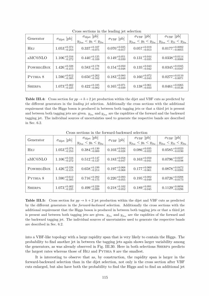
Cross sections in the leading jet selection

Generator σdijet [pb]σdijet [pb] σVBF [pb] σVBF [pb] σVBF [pb]

yjbw < yh < yjfw yjbw < yh < yjfw yjbw < yj3 < yjfw

Hej 1.053+0.374−0.253 0.337+0.107

−0.075 0.070+0.025−0.017 0.057+0.019

−0.013 0.0177+0.0092−0.0055

aMC@NLO 1.106+0.316−0.272 0.440+0.125

−0.109 0.149+0.051−0.039 0.131+0.044

−0.035 0.0338+0.0114−0.0088

PowhegBox 1.426+0.328−0.415 0.583+0.178

−0.181 0.154+0.050−0.048 0.135+0.043

−0.042 0.0345+0.0165−0.0167

Pythia 8 1.590+0.612−0.385 0.650+0.262

−0.162 0.183+0.083−0.049 0.160+0.072

−0.043 0.0277+0.0110−0.0071

Sherpa 1.073+0.462−0.225 0.422+0.185

−0.082 0.165+0.071−0.039 0.138+0.061

−0.033 0.0461+0.0265−0.0126

Table III.4: Cross section for pp→ h+ 2 jet production within the dijet and VBF cuts as predicted bythe different generators in the leading jet selection. Additionally the cross sections with the additionalrequirement that the Higgs boson is produced in between both tagging jets or that a third jet is presentand between both tagging jets are given. yjfw and yjbw are the rapidities of the forward and the backwardtagging jet. The individual sources of uncertainties used to generate the respective bands are describedin Sec. 6.2.

Cross sections in the forward-backward selection

Generator σdijet [pb]σdijet [pb] σVBF [pb] σVBF [pb] σVBF [pb]

yjbw < yh < yjfw yjbw < yh < yjfw yjbw < yj3 < yjfw

Hej 1.053+0.374−0.253 0.384+0.130

−0.089 0.103+0.044−0.028 0.086+0.035

−0.022 0.0585+0.0323−0.0190

aMC@NLO 1.106+0.316−0.272 0.512+0.147

−0.127 0.183+0.058−0.047 0.163+0.050

−0.041 0.0796+0.0237−0.0198

PowhegBox 1.426+0.328−0.415 0.658+0.199

−0.214 0.197+0.068−0.068 0.177+0.060

−0.061 0.0878+0.0472−0.0394

Pythia 8 1.590+0.612−0.385 0.716+0.282

−0.175 0.220+0.093−0.055 0.195+0.082

−0.049 0.0726+0.0288−0.0173

Sherpa 1.073+0.462−0.225 0.499+0.229

−0.099 0.218+0.102−0.052 0.189+0.091

−0.045 0.1129+0.0656−0.0296

Table III.5: Cross section for pp → h + 2 jet production within the dijet and VBF cuts as predictedby the different generators in the forward-backward selection. Additionally the cross sections with theadditional requirement that the Higgs boson is produced in between both tagging jets or that a third jetis present and between both tagging jets are given. yjfw and yjbw are the rapidities of the forward andthe backward tagging jet. The individual sources of uncertainties used to generate the respective bandsare described in Sec. 6.2.

into a VBF-like topology with a large rapidity span that is very likely to contain the Higgs. Theprobability to find another jet in between the tagging jets again shows larger variability amongthe generators, as was already observed in Fig. III.30. Here in both selections Sherpa predictsthe largest rates whereas those of Hej and Pythia 8 are the smallest.

It is interesting to observe that as, by construction, the rapidity span is larger in theforward-backward selection than in the dijet selection, not only is the cross section after VBFcuts enlarged, but also have both the probability to find the Higgs and to find an additional jet

115

in between the two tagging jets increased. In particular the latter is interesting in the context ofusing jet vetoes to suppress the gluon fusion contribution to VBF-like signatures. This possibilityis not studied here, as it also requires careful treatment of the underlying event, which can alsoproduce additional jets.

The full set of observables studied can be found athttp://phystev.in2p3.fr/wiki/2013:groups:sm:higgs:hdijetsresults.

6.4 CONCLUSIONSThe aim of this study was to quantify the gluon fusion contribution to h+2 jets with a VBF-likesignature and its uncertainties. The strategy was to obtain state-of-the-art NLO or multi-jetmerged NLO predictions from the event generators Hej, aMC@NLO, PowhegBox, Pythia 8and Sherpa including perturbative uncertainties and do a detailed comparison of both rates anddistributions. The events were analysed with a common, generic Higgs analysis. Distributionsare plotted at different levels of cuts going from inclusive Higgs via Higgs+dijet to a VBF-likeselection.

The gluon fusion contribution to Higgs events with a VBF-like signature turns out to be ofthe order of 0.1-0.2 pb and is thus non-negligible. This is especially relevant as observables suchas ∆φ(j1, j2) exhibit different shapes in Higgs production through gluon fusion as opposed toproduction through weak-boson fusion, diluting characteristic patterns used to measure Higgsproperties. The predictions by the NLO event generators are in good agreement with one-another within their respective uncertainty estimates. In all cases (except for aMC@NLO) allsources of perturbative uncertainties, stemming from the fixed-order cross-section input, thematched parton shower resummation (in the form of its starting scale), and, where applicable,also the unphysical multijet merging parameter, were accounted for. Additional uncertaintiesoriginating in the parton shower splitting functions (evolution variables, choice of the scales ofthe strong coupling, recoil schemes) are current topics of investigation.

The differences in cross section are reflected in the normalisation of the distributions. Theshapes are largely consistent. Pythia 8 and Sherpa have been observed to have a tendency topredict slightly harder transverse momentum spectra, but these differences are mostly coveredby the reported uncertainties.

Although it is reassuring that the predictions by different generators are generally consis-tent, the uncertainties remain rather large. Taking the perturbative uncertainties reported bythe generators and the spread of the predictions seriously, one arrives at an uncertainty estimateon the cross section that is roughly a factor 2. One possible avenue for the reduction of theseuncertainties is the experimental study of the VBF phase space on various signal processes,e.g. [381], to constrain the models. It is further important to note that this study only investi-gated perturbative uncertainties. Noneperturbative uncertainties stemming from the modellingof the parton-to-hadron fragmentation and especially multiple parton interaction, however, mayalso play an important role in analyses with gap fractions [377].

AcknowledgementsWe would like to thank the organisers of Les Houches 2013 for repeatedly hosting such a fantasticand fruitful workshop. We would also like to thank all participants for a lively and stimulatingatmosphere and lots of inspiring discussions.

KH gratefully acknowledges support from Durham University IPPP through their associ-ateship program. TH’s and MS’s work was supported by the Research Executive Agency (REA)of the European Union under the Grant Agreement number PITN-GA-2010-264564 (LHCPhe-noNet). MS further acknowledges support by PITN-GA-2012-315877 (MCnet). JMS is funded

116

by a Royal Society University Research Fellowship.

7 Higgs boson plus di- and tri-jet production at NLO in QCD12

7.1 IntroductionAmong the different production mechanisms of a Higgs boson (H) within the Standard Model,Gluon-Gluon Fusion (GGF) via a virtual top-quark loop is the one with the largest cross sectionat the Large Hadron Collider (LHC). Although direct measurements of the Higgs boson proper-ties in this channel, without applying any vetoes on additional jets, are difficult due to the largeQCD background, precise theoretical predictions for the associate production of a Higgs bosonand jets in GGF are important for several aspects. On the one hand the possibility to reliablyestimate the theoretical uncertainty when a jet veto is applied heavily relies on the knowledgeof inclusive and exclusive cross sections for Higgs boson production and additional jets, on theother hand the production of a Higgs boson together two jets in GGF is one of the main irre-ducible backgrounds to the production of a Higgs boson in Vector Boson Fusion (VBF), whichallows to directly probe the coupling of the Higgs boson to other electroweak bosons.

The leading order (LO) contribution to the production of a Higgs boson in association withtwo jets (H+2-jets) and three jets (H+3-jets), retaining the full top-mass (mt) dependence, havebeen computed respectively in Refs. [382, 383], and Ref. [384]. These calculations showed thatlarge top-mass approximation (mt → ∞) is valid whenever the mass of the Higgs particle andthe pT of the jets are not much larger than the mass of the top quark. In the results presentedhere we adopt this approximation and introduce a set of effective vertices, which directly couplethe Higgs particle to two, three and four gluons [373,374]. Feynman rules for these vertices canbe found e.g. in Ref. [385]. The next-to-leading order (NLO) corrections for H+2-jets in GGFat LHC were first computed in Ref. [44,356] using amplitudes computed in Refs. [349,386–396].These amplitudes have been also used to obtain matched NLO plus shower predictions [364,372].More recently they have been recomputed using for the first time an automated tool for theevaluation of both tree-level and loop amplitudes in Ref. [385]. A similar setup was also used tocompute the first NLO results for H+3-jets in GGF [3].

In these proceedings we present some new results forH+3-jets at NLO to which we applieda set of ATLAS-like cuts, and compare it with predictions for H+2-jets at NLO. In Section 7.2the computational setup used to obtain the various predictions is presented. Compared to theoriginal setup used in Ref. [3], here the newest developments regarding the evaluation of loopamplitudes with integrand reduction techniques based on Laurent expansion were used [397]. InSection 7.3 we present our results and discuss them. They include predictions for the total crosssections and for several relevant distributions, together with scale uncertainty bands.

7.2 Calculational detailsAll parton-level predictions, which we present in these proceedings, have been produced bycombined generator packages. The H+2-jets samples were obtained with the GoSam+Sherpapackage while those describing H+3-jets production required the combination of contribu-tions from GoSam+Sherpa and the MadGraph/Dipole/Event framework. More specif-ically, the H+3-jets samples were built from the Born plus virtual (BV) terms as provided byGoSam+Sherpa and the dipole-subtracted real emission (RS) contribution as well as the in-tegrated subtraction terms (I) as produced by MadGraph/Dipole/Event. We checked theconsistency of our hybrid MC integration for H+3-jets on H+2-jets, verifying that the full crosssection at NLO agrees with the corresponding result for the integration of all contributions

12G. Cullen, H. van Deurzen, N. Greiner, J. Huston, G. Luisoni, P. Mastrolia, E. Mirabella, G. Ossola, T. Peraro,F. Tramontano, J. Winter and V. Yundin

117

(BVIRS) obtained with GoSam+Sherpa alone. Moreover, for H+3-jets we found excellentagreement between MadGraph and Sherpa for the LO cross section.

7.2.1 Virtual amplitudesThe virtual 1-loop amplitudes are generated and computed using the GoSam framework [4],which combines the algebraic generation of d-dimensional integrands via Feynman diagrams [398–401], with the numerical evaluation based upon integrand-reduction [397, 402–407], as imple-mented in Samurai [397, 408–410] and Ninja [397, 411–413] and tensor integral calculus, asimplemented in Golem95 [414,415].

The virtual amplitudes for the production of Higgs plus two- and three-jets presented inRef. [385] and Ref. [3] respectively, were obtained by using the Samurai reduction library. Forthe results presented here, instead, GoSam was used to generate the input for the new libraryNinja [411], which computes the loop amplitude using a novel technique based on the interplayof the reduction at the integrand level and the Laurent expansion of the numerator [397], andproved to be in general faster and more stable compared to the standard integrand reductionmethod [412]. In fact, by employing Ninja, the evaluation time per phase-space point reducedby a factor of 50%, and the fraction of unstable point dropped below the permille level. Thescalar loop integrals are computed using OneLOop [416].

In order to deal with the complexity of the amplitudes of the processes computed here,several improvements were introduced into GoSam. They will become public with the releaseof the new version of the program, whose final development is currently in progress. Amongthe improvements, there is the possibility to exploit the optimized manipulation of polynomialexpressions available in FORM 4.0 [417].

The one-loop amplitudes for Higgs production in GGF containing the effective ggH cou-pling lead to integrands that may exhibit numerators with rank larger than the number of thedenominators. More details about the treatment of these so-called higher-rank integrals can befound in Refs. [3, 385,410,415].

7.2.2 GoSam+Sherpa specificsWithin Sherpa [166] the tree amplitudes for the Born contributions and real corrections wereobtained using the automatic amplitude generator Amegic [418], which also automatically gen-erates the subtraction terms and their integrated counterpart using an implementation [419] ofthe Catani-Seymour dipoles subtraction [200]. The integration of the virtual amplitudes was alsoperformed using Sherpa. The amplitudes generated with GoSam were interfaced to Sherpavia the Binoth-Les-Houches Accord (BLHA) [198,199], which sets the standards for the commu-nication between a Monte Carlo program and a One Loop Program, and allows to generate andlink the two codes fully automatically. The integration of the H+3-jets amplitudes is carriedout by generating O(106) events, sampled on a MC grid trained on the Born matrix element,and weighted with the sum of the Born and the virtual amplitudes.

7.2.3 MadGraph/Dipole/Event specificsIn the MadGraph setup the tree-level amplitudes are obtained using MadGraph 4 [420,421]and the subtraction terms are provided by MadDipole [422,423], which also implements Catani-Seymour dipole subtraction. The numerical integration is done using MadEvent [365]. Weverified the independence of our result under the variation of the so called α-parameter thatfixes the amount of subtractions around the divergences of the real corrections.

118

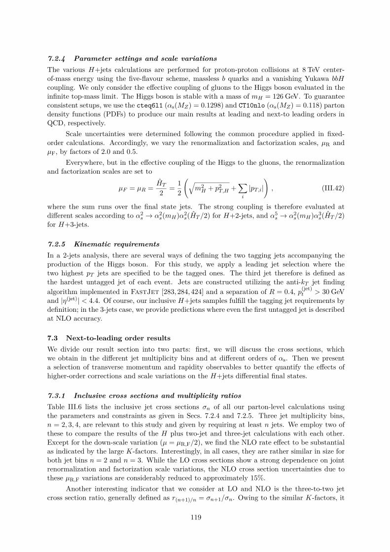
7.2.4 Parameter settings and scale variationsThe various H+jets calculations are performed for proton-proton collisions at 8 TeV center-of-mass energy using the five-flavour scheme, massless b quarks and a vanishing Yukawa bbHcoupling. We only consider the effective coupling of gluons to the Higgs boson evaluated in theinfinite top-mass limit. The Higgs boson is stable with a mass of mH = 126 GeV. To guaranteeconsistent setups, we use the cteq6l1 (αs(MZ) = 0.1298) and CT10nlo (αs(MZ) = 0.118) partondensity functions (PDFs) to produce our main results at leading and next-to leading orders inQCD, respectively.

Scale uncertainties were determined following the common procedure applied in fixed-order calculations. Accordingly, we vary the renormalization and factorization scales, µR andµF, by factors of 2.0 and 0.5.

Everywhere, but in the effective coupling of the Higgs to the gluons, the renormalizationand factorization scales are set to

µF = µR = HT

2 = 12

(√m2H + p2

T,H +∑i

|pT,i|), (III.42)

where the sum runs over the final state jets. The strong coupling is therefore evaluated atdifferent scales according to α2

s → α2s(mH)α2

s(HT /2) for H+2-jets, and α5s → α2

s(mH)α3s(HT /2)

for H+3-jets.

7.2.5 Kinematic requirementsIn a 2-jets analysis, there are several ways of defining the two tagging jets accompanying theproduction of the Higgs boson. For this study, we apply a leading jet selection where thetwo highest pT jets are specified to be the tagged ones. The third jet therefore is defined asthe hardest untagged jet of each event. Jets are constructed utilizing the anti-kT jet findingalgorithm implemented in FastJet [283, 284, 424] and a separation of R = 0.4, p(jet)

t > 30 GeVand |η(jet)| < 4.4. Of course, our inclusive H+jets samples fulfill the tagging jet requirements bydefinition; in the 3-jets case, we provide predictions where even the first untagged jet is describedat NLO accuracy.

7.3 Next-to-leading order resultsWe divide our result section into two parts: first, we will discuss the cross sections, whichwe obtain in the different jet multiplicity bins and at different orders of αs. Then we presenta selection of transverse momentum and rapidity observables to better quantify the effects ofhigher-order corrections and scale variations on the H+jets differential final states.

7.3.1 Inclusive cross sections and multiplicity ratiosTable III.6 lists the inclusive jet cross sections σn of all our parton-level calculations usingthe parameters and constraints as given in Secs. 7.2.4 and 7.2.5. Three jet multiplicity bins,n = 2, 3, 4, are relevant to this study and given by requiring at least n jets. We employ two ofthese to compare the results of the H plus two-jet and three-jet calculations with each other.Except for the down-scale variation (µ = µR,F/2), we find the NLO rate effect to be substantialas indicated by the large K-factors. Interestingly, in all cases, they are rather similar in size forboth jet bins n = 2 and n = 3. While the LO cross sections show a strong dependence on jointrenormalization and factorization scale variations, the NLO cross section uncertainties due tothese µR,F variations are considerably reduced to approximately 15%.

Another interesting indicator that we consider at LO and NLO is the three-to-two jetcross section ratio, generally defined as r(n+1)/n = σn+1/σn. Owing to the similar K-factors, it

119

Sample Cross sections for Higgs boson plusK-factor ≥ 2 jets f3 ≥ 3 jets r3/2

LO

H+2-jet2 (LO PDFs) 1.23 +37%−24%

H+3-jets (LO PDFs) (0.381) 1.0 0.381 +53%−32% 0.310 0.347

0.278

H+2-jets (NLO PDFs) 0.970 +33%−23%

H+3-jets (NLO PDFs) (0.286) 1.0 0.286 +50%−31% 0.295 0.332

0.265

NLO

H+2-jets 1.590 −4%−7% 0.182 0.289 +49%

−31%

H+3-jets (0.485) 1.0 0.485 −3%−13% 0.305 0.307

0.284

K2, K3 (LO PDFs for LO) 1.29 0.9111.59 1.27 0.806

1.63

K2, K3 (NLO PDFs for LO) 1.64 1.191.98 1.70 1.10

2.13

Table III.6: Cross sections in pb for the various parton-level Higgs boson plus jet samples used in thisstudy. The upper and lower parts of the table show the LO and NLO results, respectively, together withtheir uncertainties (in percent) from varying scales by factors of two, up (subscript position) and down(superscript position). NLO-to-LO K-factors, Kn, for both the inclusive 2-jets (n = 2) and 3-jets (n = 3)bin, the cross section ratio r3/2 and m-jet fractions, fm, are given in addition.

remains fairly stable at ∼ 30%, roughly a factor 3 times higher than a sole αs effect. Just forcompleteness, we have also listed the inclusive three-jet fraction, f3, belonging to each sample.

7.3.2 Differential observablesThe set of observables we want to present here includes Higgs boson and single-jet transversemomenta, pT,x, as well as their respective rapidities, yx (x ∈ {H, j1,2,3}). As an example of amulti-object observable, we also discuss the pT distribution of the Hj1j2 system.

We start our discussion by presenting several predictions for the Higgs boson rapidity dis-tribution in Fig. III.31. In all three panels of this figure, we show the same NLO prediction forH+3-jets production (red lines), and compare it, in the left two panels, with two different H+3-jets predictions of LO accuracy (blue lines). We observe large, O(50%), positive correctionsthat are spread almost uniformly over the entire H rapidity range; they increase in the for-ward/backward region. In the leftmost panel, both the LO and NLO predictions were obtainedfrom the same NLO PDF set, that is CT10nlo. As seen in the middle panel, the correctionsdecrease by ∼ 20% if one uses an order αs treatment that is consistent between the PDFs and theparton-level calculations. Half of the effect can then simply be attributed to the larger αs(MZ)value of the cteq6l1 parametrization that we used to compute the middle panel’s LO result.The scale uncertainties of the central predictions are shown by the respective envelopes of samecolour. Enhancing the description to NLO accuracy, we find a reduction of these errors from±50% to less than modulus 30%, which also means that the scale variation bands turn frombeing fairly symmetric to rather one-sided. This is a consequence of fixing the central/default

120

LHC 8 TeV

anti-kt: R=0.4, pT > 30 GeV, |η| < 4.4

LO

NLO

10−5

10−4

10−3

10−2

10−1

H + 3 jets: Higgs rapidity

dσ/dy H

[pb]

-4 -2 0 2 40.5

1

1.5

2

2.5

yH

NLO/LO

LHC 8 TeV

anti-kt: R=0.4, pT > 30 GeV, |η| < 4.4

LO (cteq6l1 PDFs)

NLO (CT10nlo PDFs)

10−5

10−4

10−3

10−2

10−1

H + 3 jets: Higgs rapidity

dσ/dy H

[pb]

-4 -2 0 2 40.5

1

1.5

2

2.5

yH

NLO/LO

LHC 8 TeV

CT10nlo pdf

anti-kt: R=0.4, pT > 30 GeV, |η| < 4.4

PRELIM

INARY

H+2 jets NLO

H+3 jets NLO

10−5

10−4

10−3

10−2

10−1

H + 3 jets: Higgs rapidity

dσ/dy H

[pb]

-4 -2 0 2 40

0.2

0.4

0.6

0.8

1

1.2

yH

Ratio

Fig. III.31: Higgs boson rapidity distributions and their µR,F scale uncertainties (depicted by pastel-coloured bands) in H+3-jets production at the Ecm = 8 TeV LHC. The two plots to the left show acomparison of the NLO (red) to LO (blue) predictions where the left panel’s LO result has been obtainedusing the same PDF as for the NLO computation. The ratio plots at the bottom visualize the K-factorvariation over the Higgs boson’s rapidity range. In the rightmost panel, the yH distributions of the 3-jets(red) and 2-jets (blue) NLO samples (requiring two tagging jets only) are compared to each other, andtheir differential cross section ratio is shown in the lower part.

scales right where the NLO cross section plateaus.The plot to the right of Fig. III.31 is a direct comparison of the yH distributions given by

the 2-jets (blue) and 3-jets (red) NLO samples. Scale variations lead to O(20%) uncertaintiesover a fairly broad yH range. Although the two NLO samples differ by one order of αs, theassociated scale uncertainties are comparable in size, and only somewhat smaller for the H+2-jets case. Since we do not require more than the two tagging jets, the H+3-jets line in thelower plot actually visualizes the r3/2 quantity differentially in dependence on yH . It varies onlymildly around the inclusive, ∼ 0.3 value given in the table above. The differential ratio alsoshows that the production of Higgs bosons in the 3-jets sample is slightly more central than inthe 2-jets sample.

We now turn to discuss our results, which we obtained for the single jet observables andthe H-system pt spectra. Figs. III.32, III.34 and Figs. III.33, III.35 follow the same plottingstyles/layouts and colour code as chosen for the center and rightmost subfigures of Fig. III.31,respectively. The former set of figures is therefore used to give a broader comparison betweenNLO and LO predictions as generated by the Higgs boson plus 3-jets final state. In the latterset, we then display how the H+3-jets and H+2-jets NLO results compare to each other forexactly the same selection of observables.

Focusing on the jet transverse momenta and rapidities, pt,ji (left columns) and yji (rightcolumns), as depicted for the three hardest jets in Figs. III.32 and III.33, we notice that theyshow very similar scale variation characteristics and reduction of errors as discussed for the yHspectra presented in Fig. III.31. Similarly for the NLO corrections on the jet rapidities, we againfind these to be rather well described by constant positive shifts, which here are of the orderof 20%, see Fig. III.32. In contrast to this, all differential K-factors associated with the jet ptdistributions in this figure show a decline towards larger pt values. In other words, even thatthe rate of Higgs associated jet production gets enhanced at NLO, the pt tails loose hardnesswhen taking relative measures. This is due to the extra radiation carried away from the systemby the fourth jet, which shifts the spectra of all the other jets to lower values. Note that thesoft jet K-factors can take values as large as 1.4.

Turning to Fig. III.33, the very same set of H+3-jets NLO predictions is plotted againstthe corresponding H+2-jets predictions such that the differential r3/2 ratios can be read off

121

LHC 8 TeV

anti-kt: R=0.4, pT > 30 GeV, |η| < 4.4

PRELIM

INARY

LO (cteq6l1 PDFs)

NLO (CT10nlo PDFs)

10−4

10−3

H + 3 jets: leading jet transverse momentumdσ/dpt,j1[pb/GeV

]

0 50 100 150 200 250 300

0.70.80.91.01.11.21.31.41.5

pt,j1[GeV]

NLO/LO

LHC 8 TeV

anti-kt: R=0.4, pT > 30 GeV, |η| < 4.4

PRELIM

INARY

LO (cteq6l1 PDFs)

NLO (CT10nlo PDFs)

10−3

10−2

10−1

H + 3 jets: leading jet rapidity

dσ/dy j

1[pb]

-4 -2 0 2 4

0.8

1

1.2

1.4

1.6

1.8

2

yj1

NLO/LO

LHC 8 TeV

anti-kt: R=0.4, pT > 30 GeV, |η| < 4.4

PRELIM

INARY

LO (cteq6l1 PDFs)

NLO (CT10nlo PDFs)

10−5

10−4

10−3

10−2

H + 3 jets: second jet transverse momentum

dσ/dpt,j2[pb/GeV

]

0 50 100 150 200 250 300

0.70.80.91.01.11.21.31.41.5

pt,j2[GeV]

NLO/LO

LHC 8 TeV

anti-kt: R=0.4, pT > 30 GeV, |η| < 4.4

PRELIM

INARY

LO (cteq6l1 PDFs)

NLO (CT10nlo PDFs)

10−3

10−2

10−1

H + 3 jets: second leading jet rapidity

dσ/dy j

2[pb]

-4 -2 0 2 4

0.8

1

1.2

1.4

1.6

1.8

2

yj2

NLO/LO

LHC 8 TeV

anti-kt: R=0.4, pT > 30 GeV, |η| < 4.4

PRELIM

INARY

LO (cteq6l1 PDFs)

NLO (CT10nlo PDFs)

10−6

10−5

10−4

10−3

10−2

H + 3 jets: third jet transverse momentum

dσ/dpt,j3[pb/GeV

]

0 50 100 150 200 250 300

0.70.80.91.01.11.21.31.41.5

pt,j3[GeV]

NLO/LO

LHC 8 TeV

anti-kt: R=0.4, pT > 30 GeV, |η| < 4.4

PRELIM

INARY

LO (cteq6l1 PDFs)

NLO (CT10nlo PDFs)10−2

10−1

H + 3 jets: third leading jet rapidity

dσ/dy j

3[pb]

-4 -2 0 2 4

0.8

1

1.2

1.4

1.6

1.8

2

yj3

NLO/LO

Fig. III.32: Higgs boson plus three-jet production at leading (blue) and next-to leading (blue) orderfor proton–proton collisions at Ecm = 8 TeV. The transverse momenta and rapidities of the three hardestjets are shown in the left and right column, respectively. The size of the scale uncertainties has beenindicated by the lightly coloured bands occurring around each central prediction. The lower plots showthe K-factor variations for each of these single jet observables.

122

LHC 8 TeV

CT10nlo pdf

anti-kt: R=0.4, pT > 30 GeV, |η| < 4.4

PRELIM

INARY

H+2 jets NLO

H+3 jets NLO

10−3

10−2

H + 3 jets: leading jet transverse momentum

dσ/dpt,j1[pb/GeV

]

0 50 100 150 200 250 3000

0.2

0.4

0.6

0.8

1

1.2

pt,j1[GeV]

Ratio

LHC 8 TeV

CT10nlo pdf

anti-kt: R=0.4, pT > 30 GeV, |η| < 4.4

PRELIMINARY

H+2 jets NLO

H+3 jets NLO

10−4

10−3

10−2

10−1

H + 3 jets: leading jet rapidity

dσ/dy j

1[pb]

-4 -2 0 2 40

0.2

0.4

0.6

0.8

1

1.2

yj1

Ratio

LHC 8 TeV

CT10nlo pdf

anti-kt: R=0.4, pT > 30 GeV, |η| < 4.4

PRELIM

INARY

H+2 jets NLO

H+3 jets NLO

10−4

10−3

10−2

10−1

H + 3 jets: second jet transverse momentum

dσ/dpt,j2[pb/GeV

]

0 50 100 150 200 250 3000

0.2

0.4

0.6

0.8

1

1.2

pt,j2[GeV]

Ratio

LHC 8 TeV

CT10nlo pdf

anti-kt: R=0.4, pT > 30 GeV, |η| < 4.4

PRELIMINARY

H+2 jets NLO

H+3 jets NLO

10−4

10−3

10−2

10−1

H + 3 jets: second leading jet rapidity

dσ/dy j

2[pb]

-4 -2 0 2 40

0.2

0.4

0.6

0.8

1

1.2

yj2

Ratio

LHC 8 TeV

CT10nlo pdf

anti-kt: R=0.4, pT > 30 GeV, |η| < 4.4

PRELIM

INARY

H+2 jets NLO

H+3 jets NLO

10−6

10−5

10−4

10−3

10−2

H + 3 jets: third jet transverse momentum

dσ/dpt,j3[pb/GeV

]

0 50 100 150 200 250 300

0.8

1

1.2

1.4

1.6

1.8

2

pt,j3[GeV]

Ratio

LHC 8 TeV

CT10nlo pdf

anti-kt: R=0.4, pT > 30 GeV, |η| < 4.4

PRELIMINARY

H+2 jets NLO

H+3 jets NLO

10−3

10−2

10−1

H + 3 jets: third leading jet rapidity

dσ/dy j

3[pb]

-4 -2 0 2 4

0.8

1

1.2

1.4

1.6

1.8

2

yj3

Ratio

Fig. III.33: Comparison of QCD NLO predictions for inclusive 2-jets (blue) and 3-jets (red) final statesin Higgs boson plus jets production at the Ecm = 8 TeV LHC. The transverse momenta and rapidities ofthe three hardest jets are shown in the left and right column, respectively. The colourful envelops aroundthe central predictions depict the size of their scale uncertainties. Each lower plot is used to indicatethe cross section ratio between the three-jet and two-jet samples in dependence on the respective singlejet observable. Note that in the H+2-jet calculation, the third-jet spectra are only described with LOaccuracy.

123

LHC 8 TeV

anti-kt: R=0.4, pT > 30GeV, |η| < 4.4

PRELIMINARY

LO (cteq6l1 PDFs)

NLO (CT10nlo PDFs)

10−4

10−3

H + 3 jets: Higgs transverse momentumdσ/dpt,H[pb/GeV

]

0 50 100 150 200 250 3000.5

1

1.5

2

2.5

3

pt,H [GeV]

NLO/LO

LHC 8 TeV

anti-kt: R=0.4, pT > 30GeV, |η| < 4.4

PRELIM

INARY

LO (cteq6l1 PDFs)

NLO (CT10nlo PDFs)

10−6

10−5

10−4

10−3

10−2

H + 3 jets: Higgs-jet1-jet2 transverse momentum

dσ/dpt,Hj 1

j 2[pb/GeV

]

0 50 100 150 200 250 3000.51

1.52

2.53

3.54

pt,Hj1j2 [GeV]

NLO/LO

Fig. III.34: Higgs boson plus three-jet production at leading (blue) and next-to leading (blue) order forproton–proton collisions at Ecm = 8 TeV. Transverse momentum distributions of the Higgs boson (left)and the H plus tagging jet system (right) are shown together with their scale uncertainties indicatedby the lightly coloured bands surrounding each central prediction. The lower plots show the K-factorvariations as functions of pT,H and pT,Hjj .

easily. As before, they are rather flat for the yji predictions, and do not exceed values largerthan 35% owing to the two-tagging-jet requirement. Only if a third jet has to be resolved (cf. thelast row of Fig. III.33), we find this ratio to be as large as 1.6, which is no surprise, since itnow denotes a K-factor based on a LO third-jet description obtained with NLO PDFs. For thetransverse momenta of the first two jets, the r3/2 variables show a strong dependence on thehardness of the jets. They rise quickly from very low values of O(0.1) at the jet threshold to over50% for pt ∼ 100 GeV. This emphasizes the importance of higher jet multiplicity contributionsif one targets a complete description of H+jets final states.

Lastly we discuss, in the same manner as before, our findings regarding the pt distributionsof the Higgs bosons and the Hj1j2 three-body objects. The NLO corrections to the Higgsboson pt in three-jet final states (Fig. III.34 to the left) are of the order of +30% and decreasevery slowly over the pt range plotted here. The behaviour under scale variations is as before.Comparing to the pt,H spectrum extracted from the corresponding 2-jets sample, we observe anr3/2 ratio that is rising as those for the tagging jet pt, but on a slower rate; see the left panelin Fig. III.35. In particular, for pt,H values below 100 GeV, it remains locked around 0.2. Fortransverse momenta above 2MH , the 3-jet contributions are again as large as 50%, with similarimplications regarding an inclusive multi-jet description of H+jets final states as pointed out inthe case of the single jet pt.

We round off by discussing our three different predictions for the transverse momentumdistribution of the Hj1j2 systems. Each of the right panels in Figs. III.34 and III.35 shows thept spectrum computed from the H+3-jets NLO samples. First we compare it to correspondingLO predictions (Fig. III.34), then to the ones of the H+2-jets NLO samples (Fig. III.35). Thept,Hj1j2 is an interesting variable for our study since it is sensitive to the description of anyadditional parton radiation beyond the two tagging jets. It is out of question that a fixed-orderdescription of the low pt region cannot be achieved reliably without supplementing the neces-sary resummation contributions. Nevertheless we can use this variable to point out importantfeatures of the three different calculations as well as discuss the formal accuracy of the tails ofthese pt,Hj1j2 spectra. The prediction taken from the H+3-jets LO sample is just given by the

124

third-jet pt distribution of lowest order, with a clear indication of the jet pt threshold at 30 GeV,cf. Fig. III.34. The hardness of the third jet simply determines the recoil of the Hj1j2 system.Above threshold, we therefore have a LO accurate description of the pt,Hj1j2 spectrum. The sit-uation cannot be improved by an H+2-jets NLO computation (Fig. III.35): the difference in thetails is caused by the replacement of LO with NLO PDFs, again pointing to a 20% effect as dis-cussed earlier. The region below the jet threshold gets filled by real emission contributions thatare too soft to be resolved as a jet. However, the resulting low-pt spectrum is highly unphysicaldue to the missing contributions from multiparton emissions.13 Turning to the NLO accurateevaluation of H+3 jets, we finally improve the precision to which we describe the pt,Hj1j2 tail.For transverse momenta larger than 60 GeV, we have achieved NLO precision. Besides neglectingSudakov corrections, below this value we are missing contributions only a full NNLO H+2-jetcalculation can provide (contributions such as double unresolved and virtual plus unresolvedemissions). However, contributions with two more jets beyond the tagged ones or three jets andunresolved extra emission already lead to pt balancing as well as pt enhancing effects such thatwe find large, O(3), fairly constant corrections for higher pt,Hj1j2 and a depletion towards zeropt,Hj1j2 . A last few comments are in order concerning the scale variation characteristics of thept,Hj1j2 predictions: firstly, a reduction from ±50% to ±30% is only found for the predictionfrom the H+3-jets NLO calculation (red envelopes). As discussed the other evaluations onlygive LO accurate results. Secondly, in contrast to other H+3-jets NLO predictions, the muchmore symmetric band found here is a consequence of the dominance of the four-jet contributionsthat feature a LO scale variation behaviour.14

ConclusionsTaking advantage of the recent developments in the automated computation of NLO predictionswe reported on NLO QCD results in an ATLAS-like analysis of inclusive Higgs boson plus 2-jetsand 3-jets final states.

The loop amplitudes were generated with GoSam and computed using a new develop-ment in integrand reduction techniques, based on a Laurent expansion, and implemented in thecode Ninja. For tree-level amplitudes and phase space integration we used Sherpa and theMadGraph/Dipole/Event framework.

We find that NLO corrections are important and result in a substantial change of rate andjet hardness. At the level of the total inclusive cross section we find an increase of almost 30%for both H+2-jets and H+3-jets, whereas the scale variation reduces to approximately 15%.Considering differential distributions, we observe that rapidity distributions for the Higgs bosonand the first three hardest jets obtain a positive shift of about 20%, which is rather constant overthe full kinematical range. For the transverse momentum distributions of the jets instead, weobserve a decrease in the K-factor towards larger pt values, whereas in the transverse momentumdistribution of the Higgs boson, this decrease is only very slow. The differential r3/2 ratios for therapidities are rather flat and never exceed 35%, however in the case of the transverse momentumdistributions they reach up to 50% for the leading jet and the Higgs boson. This shows thatH+3-jets contributions cannot be neglected in an inclusive two-jet sensitive analysis. Anotherobservable, where NLO corrections to H+3-jets play an important role is the pt distribution of

13Known as the Sudakov effect, the very same discussion occurs, for example, for the pt,H distribution in Higgsboson production at NLO. The reduction seen here for the very first pt,Hj1j2 bin of theH+2-jets NLO computationis caused by those events satisfying pt,Hj1j2 ≡ 0, i.e. Born, virtual and integrated subtraction contributions as wellas those from counter events fall into the first bin diminishing the large effect from (unresolved) real emissions.

14On a more quantitative level, we note that the ‘BVI’ contributions of the pt,Hj1j2 and pt,j3 distributions areexactly the same while the ‘RS’ ones of the former are considerably harder than those of the latter. This leads toa different cancellation pattern when combining the scale varied ‘BVI’ and ‘RS’ predictions (they work in oppositedirections). For the pt,Hj1j2 , we then find the ‘RS’ uncertainties to be the dominating ones for pt,Hj1j2 & 60 GeV.

125

LHC 8 TeV

CT10nlo pdf

anti-kt: R=0.4, pT > 30GeV, |η| < 4.4

PRELIM

INARYH+2 jets NLO

H+3 jets NLO

10−4

10−3

10−2

H + 3 jets: Higgs transverse momentumdσ/dpt,H[pb/GeV

]

0 50 100 150 200 250 3000

0.2

0.4

0.6

0.8

1

1.2

pt,H [GeV]

Ratio

LHC 8 TeVCT10nlo pdf

anti-kt: R=0.4, pT > 30GeV, |η| < 4.4

PRELIM

INARY

H+2 jets NLO

H+3 jets NLO

10−6

10−5

10−4

10−3

10−2

10−1

H + 3 jets: Higgs-jet1-jet2 transverse momentum

dσ/dpt,Hj 1

j 2[pb/GeV

]

0 50 100 150 200 250 3000.51

1.52

2.53

3.54

4.5

pt,Hj1j2 [GeV]

Ratio

Fig. III.35: Comparison of QCD NLO predictions for inclusive 2-jets (blue) and 3-jets (red) final statesin Higgs boson plus jets production at the Ecm = 8 TeV LHC. The transverse momenta of the Higgs bosonand Higgs boson plus j1j2 system are shown in the left and right panel, respectively. Colourful envelopsare used to depict the size of scale uncertainties. The lower plots indicate the cross section ratios betweenthe three-jet and two-jet samples in dependence on the pT value. Note that in the H+2-jets case, thepT,Hjj distribution has LO accuracy only.

the Hj1j2 system. In fact, for the first time, the distribution is described at NLO accuracy forpt > 2p(jet)

t,min = 60 GeV.It would be interesting to study the impact of the NLO corrections presented here when

typical VBF cuts are applied. Modern Monte Carlo tools allow furthermore to study thesecorrection in a matched NLO plus parton shower framework merged with lower multiplicitypredictions. We postpone these studies to future publication.

AcknowledgementsWe would like to thank the organizers of the Les Houches "Physics at TeV colliders 2013"workshop for the stimulating environment.

The work of G.C. was supported by DFG SFB-TR-9 and the EU TMR Network LHCPHE-NOnet. The work of H.v.D., G.L., P.M., T.P., and V.Y. was supported by the Alexander vonHumboldt Foundation, in the framework of the Sofja Kovaleskaja Award 2010, endowed by theGerman Federal Ministry of Education and Research. G.O. was supported in part by the Na-tional Science Foundation under Grant PHY-1068550. F.T. acknowledges partial support byMIUR under project 2010YJ2NYW. This research used computing resources from the Rechen-zentrum Garching.

8 Jet-bin uncertainties estimate through jet efficiencies15

8.1 IntroductionIn order to fully establish whether the new particle recently discovered at the LHC [425, 426]is the SM Higgs boson, precise measurements of its properties, in particular its couplings, areessential. Establishing a significant departure from the simple SM-like pattern could be a firstmanifestation of New Physics. In fact, the new particle lies in a region of parameter space where

15P. F. Monni (Work in collaboration wit A. Banfi, G.P. Salam, and G. Zanderighi)

126

many decay modes have an appreciable branching fraction, leading to a very rich phenomenology.On the other hand, many decay channels (e.g. H → bb, H → W+W−) are very difficult tomeasure because of the large QCD background. Most Higgs-boson events involve either none orone jet, since higher multiplicity events are suppressed by powers of the strong coupling constant,and hence more rare. It is natural then to impose a veto on additional jets so as to significantlyreduce the dominant background, while reducing only modestly the signal. Therefore, it isessential to know how much these tight kinematical cuts reduce the signal cross section, andwhat the uncertainties in the resulting signal are. However, a precise assessment of the theoryerror in the presence of a jet veto is a challenging task.

Tight kinematical cuts applied to QCD radiation give rise to large Sudakov logarithms ofthe form αns ln2n(mH/pt,veto) in the perturbative series. When scale variation is used to estimatethe theory uncertainty, the K-factor effects nearly cancel against the large logarithms leading toan underestimate of the actual perturbative error. Such logarithmic terms spoil the convergenceof the perturbative series in the region where the logarithms are very large, and they must beresummed to all orders in the strong coupling. Not only does resummation allow for a moreprecise theory prediction, but it also gives a direct handle to estimate the size of higher-orderSudakov logarithms, which is necessary for a reliable assessment of uncertainties.

Resummed predictions for the Higgs+0 jet cross section and efficiencies have been obtainedboth in the context of the CAESAR method [427,428], and in an effective theory framework [429]up to next-to-next-to-leading logarithmic level. Some terms beyond this accuracy have beenrecently obtained in [430,431]. The impact of heavy quark masses on the resummed predictionshas been also studied for both the pt,veto [432] and pt,H [432,433] cross sections. When more thana tagged jet is present in the process, the infrared structure of the perturbative series becomesmore complex and new logarithms of the non-global type [434, 435] appear. For the H+1 jetcross section, NLL resummation for the global class in the regime pt,vetol+l−pt,jet ∼ mH wasobtained in [436].

In order to optimize the sensitivity, some experimental analyses (e.g. gg → H →W+W−,VBF) combine data with different jet multiplicities. Since resummed predictions are currentlyonly available for 0- and 1-jet bins, it is of primary importance to have a robust prescription toestimate reliably the uncertainties associated with a fixed-order calculation. Moreover, a goodmethod should allow one to incorporate any resummed predictions whenever available.

A first approach based on the combination of inclusive jet bin uncertainties was proposedby Stewart and Tackmann in [437]. Uncertainties in the exclusive jet-bin cross sections are ob-tained by treating the errors in the inclusive jet-bins as uncorrelated. An alternative prescriptionwas presented in [427, 428], and it is referred to as the jet-veto efficiency (JVE) method. It isbased on the assumption that the uncertainties in the jet-fractions (efficiencies) with differentmultiplicities are uncorrelated with each other and with the uncertainty in the total cross sec-tion. This is physically motivated by the fact that uncertainties in jet fractions are dominated bySudakov suppression effects, whilst K-factor effects (which rule the uncertainty in the total crosssection) largely cancel in the definition of the jet fractions themselves. The latter method allowsone to treat resummed predictions for different jet bins on the same footing as fixed-order ones.For the resummed 0-jet cross section, the error obtained with the JVE method is consistent withthe direct estimate obtained from scale variations in the resummed calculation. More recently,a recipe to combine uncertainties for different resummed jet-bin cross sections in the contextof SCET resummation was presented in [438]. When resummed predictions are not available,the latter method reduces to the standard scale variation which underestimates the theoreticalerror. In the following sections, we briefly recall the JVE method, and present a generalisationto any jet multiplicity.

127

8.2 The JVE methodThe uncertainties in jet-bin cross sections are due to a combination of K-factor effects which rulethe uncertainty in the total cross section, and Sudakov suppression effects due to the presenceof severe cuts on the real QCD radiation. The idea behind the JVE approach is to disentanglethese two effects and treat them separately. Therefore, we define n-jet efficiencies εn as

εn = σn−jetσ≥n−jet

, (III.43)

where σn−jet is the exclusive n−jet cross section.To a large extent, K-factor effects cancel in the ratio (III.43), since the uncertainty in

the n−jet efficiency is largely ruled by Sudakov suppression. Therefore, one can treat theuncertainties in the n−jet efficiency and in the inclusive n−jet cross section as uncorrelated.The uncertainties in the two quantities are computed separately and then combined accordingto the latter assumption.

The theory error in the inclusive n−jet cross section is obtained by standard scale variation,which is not affected by cancellations in the inclusive case. Threshold resummation effects canbe also included [40]. To obtain the uncertainty in the n−jet efficiency, we start by noticing thatm+1 different schemes for the jet fractions can be defined at NmLO. As an example we considerthe 0−jet efficiency ε0. Using the current state-of-the-art calculations at NNLO for both the0−jet and the total cross sections, the following three equivalent schemes can be defined to thisperturbative accuracy

ε(a)0 (pt,veto) = Σ0(pt,veto) + Σ1(pt,veto) + Σ2(pt,veto)

σ0 + σ1 + σ2, (III.44)

ε(b)0 (pt,veto) = Σ0(pt,veto) + Σ1(pt,veto) + Σ2(pt,veto)

σ0 + σ1, (III.45)

ε(c)0 (pt,veto) = 1 + Σ1(pt,veto)

σ0+(

Σ2(pt,veto)σ0

− σ1σ2

0Σ1(pt,veto)

), (III.46)

where

Σ0−jet(pt,veto) = Σ0(pt,veto) + Σ1(pt,veto) + Σ2(pt,veto) + . . . (III.47)σ≥0−jet = σtot = σ0 + σ1 + σ2 + . . . , (III.48)

andΣi(pt,veto) = Σi(pt,veto) + σi, Σi(pt,veto) = −

∫ ∞pt,veto

dptdΣi(pt)dpt

. (III.49)

Schemes (III.45) and (III.46) differ from Eq. (III.44) only by terms O(α3s

), which are not un-

der control. The uncertainty in the 0−jet efficiency is obtained as the envelope of all scalevariations for the central scheme (III.44) and the central values relative to the remaining twoschemes (III.45) and (III.46). The spread between different schemes is associated with the Su-dakov suppression effects and it increases for lower efficiencies, i.e. when more radiation issuppressed. When resummation of large Sudakov logarithms is available, it can be included asshown in [427,428], and the variation of the corresponding resummation scale is included in theenvelope. Resummed and fixed-order calculations for different jet bins are treated in the sameway, and can be straightforwardly combined. Below we discuss the JVE method for an arbitrarynumber of exclusive jet bins, and we explicitly work out the case of only two jet bins.

128

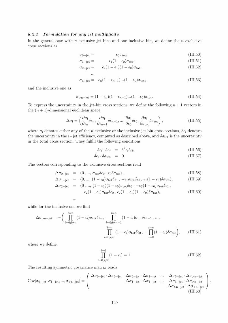
8.2.1 Formulation for any jet multiplicityIn the general case with n exclusive jet bins and one inclusive bin, we define the n exclusivecross sections as

σ0−jet = ε0σtot, (III.50)σ1−jet = ε1(1− ε0)σtot, (III.51)σ2−jet = ε2(1− ε1)(1− ε0)σtot, (III.52)

...

σn−jet = εn(1− εn−1)...(1− ε0)σtot, (III.53)

and the inclusive one as

σ>n−jet = (1− εn)(1− εn−1)...(1− ε0)σtot. (III.54)

To express the uncertainty in the jet-bin cross sections, we define the following n+ 1 vectors inthe (n+ 1)-dimensional euclidean space

∆σi =(∂σi∂εn

δεn,∂σi∂εn−1

δεn−1, ...,∂σi∂ε0

δε0,∂σi∂σtot

δσtot

), (III.55)

where σi denotes either any of the n exclusive or the inclusive jet-bin cross sections, δεi denotesthe uncertainty in the i−jet efficiency, computed as described above, and δσtot is the uncertaintyin the total cross section. They fulfill the following conditions

δεi · δεj = δ2εiδij , (III.56)δεi · δσtot = 0. (III.57)

The vectors corresponding to the exclusive cross sections read

∆σ0−jet = (0 , ..., σtotδε0 , ε0δσtot) , (III.58)∆σ1−jet = (0, ..., (1− ε0)σtotδε1 , −ε1σtotδε0 , ε1(1− ε0)δσtot) , (III.59)∆σ2−jet = (0 , ..., (1− ε1)(1− ε0)σtotδε2 , −ε2(1− ε0)σtotδε1 ,

−ε2(1− ε1)σtotδε0 , ε2(1− ε1)(1− ε0)δσtot), (III.60)...

while for the inclusive one we find

∆σ>n−jet = −( i=n∏i=0;i 6=n

(1− εi)σtotδεn ,i=n∏

i=0;i 6=n−1(1− εi)σtotδεn−1 , ...,

i=n∏i=0;i 6=0

(1− εi)σtotδε0 , −i=n∏i=0

(1− εi)δσtot

), (III.61)

where we definei=0∏

i=0;i 6=0(1− εi) = 1. (III.62)

The resulting symmetric covariance matrix reads

Cov[σ0−jet, σ1−jet, ..., σ>n−jet] =

∆σ0−jet ·∆σ0−jet ∆σ0−jet ·∆σ1−jet ... ∆σ0−jet ·∆σ>n−jet∆σ1−jet ·∆σ1−jet ... ∆σ1−jet ·∆σ>n−jet

∆σ>n−jet ·∆σ>n−jet

.(III.63)

129

8.2.2 Case with two jet binsAs a case of study we analyse the case of a 0−jet bin and an inclusive 1−jet bin. Resummedpredictions for the 0−jet efficiency ε0 were obtained in [427, 428] up to NNLO+NNLL. Theinclusive 1−jet cross section can be written in terms of ε0 as

σ≥1−jet(pt,veto) = (1− ε0)σtot, (III.64)

where σtot is the total cross section for Higgs boson production in gluon fusion, currently knownto NNLO. Since we only have two jet bins, we can define the following two 2-dimensionalvectors (III.55)

∆σ0−jet = (σtotδε0 , ε0δσtot) , (III.65)∆σ≥1−jet = (−σtotδε0 , (1− ε0)δσtot) . (III.66)

The covariance matrix between the exclusive 0−jet and the inclusive 1−jet cross sections canbe easily obtained as shown in Eq. (III.63) and it can be written as a sum of a totally correlatedand a totally anti-correlated terms

Cov[σ0−jet, σ≥1−jet] =(ε20δ

2σtot ε0(1− ε0)δ2σtotε0(1− ε0)δ2σtot (1− ε0)2δ2σtot

)+(σ2

totδ2ε0 −σ2

totδ2ε0

−σ2totδ

2ε0 σ2totδ

2ε0

).(III.67)

The two matrices in the right hand side of Eq. (III.67) are uncorrelated. The first term corre-sponds to the K-factor contribution and it is proportional to the uncertainty in the total crosssection. This gives rise to a totally correlated uncertainty between the two jet bins. The secondterm in Eq. (III.67) encodes Sudakov effects, and thus it is proportional to the uncertainty inthe 0−jet efficiency, yielding a totally anti-correlated uncertainty between the two jet bins.

8.2.2.1 Numerical results for LHCBelow we provide tables with numerical results for cross sections and efficiencies for the valuesof veto scales and jet radii, as used in current LHC analyses. The predictions for the 0−jetefficiency are computed to NNLO+NNLL and top- and bottom-quark mass effects are includedas described in [432]. All uncertainties have been made symmetric with respect to the centralvalue.

Exact mt and mb corrections

R pt,veto [GeV] σ8TeVtot [pb] ε

(8TeV)0 σ

(8TeV)0−jet [pb] σ

(8TeV)≥1−jet [pb]

0.4 25 19.24 ± 1.78 0.602 ± 0.070 11.59 ± 1.72 7.66 ± 1.520.5 30 19.24 ± 1.78 0.657 ± 0.070 12.64 ± 1.79 6.60 ± 1.48

Table III.7: Total inclusive cross section, jet-veto efficiency and zero-jet cross section for Higgs produc-tion at the 8 TeV LHC for two different values of the jet radius R and pt,veto. Results include exact topand bottom mass dependence. The quoted total cross section and the corresponding errors have beencomputed with the hnnlo 2.0 code [433].

In the first two tables the total cross section is computed at NNLO QCD. Quark-masseffects lead to a modest decrease of about half a percent in the zero-jet cross section with respectto the large-mt result. The uncertainties in the cross section increase by about 2% (and amountto about 14%) when top and bottom masses are taken into account. In tab. III.9 we report

130

Large-mt approximation

R pt,veto [GeV] σ8TeVtot [pb] ε

(8TeV)0 σ

(8TeV)0−jet [pb] σ

(8TeV)≥1−jet [pb]

0.4 25 19.03 ± 1.76 0.613 ± 0.064 11.66 ± 1.62 7.36 ± 1.390.5 30 19.03 ± 1.76 0.667 ± 0.058 12.70 ± 1.61 6.34 ± 1.25

Table III.8: As table III.7 but in the large mt approximation.

Large-mt approximation (σ8TeVtot from HXSWG)

R pt,veto [GeV] σ8TeVtot [pb] ε

(8TeV)0 σ

(8TeV)0−jet [pb] σ

(8TeV)≥1−jet [pb]

0.4 25 19.27 ± 1.45 0.613 ± 0.064 11.81 ± 1.51 7.46 ± 1.350.5 30 19.27 ± 1.45 0.667 ± 0.058 12.86 ± 1.47 6.42 ± 1.22

Table III.9: As table III.7 but in the largemt approximation. Unlike in table III.8 the total cross sectionis taken from the HXSWG [40] and includes finite-width, electro-weak and threshold resummation effects.

the jet-veto efficiency and cross section using the improved total cross section recommendedby the Higgs Cross Section Working Group (HXSWG) [40] instead of the pure NNLO value.Improvements include the treatment of the Higgs width, NNLL threshold effects and NLOelectro-weak corrections. To figure out only the size of mass effects one has to compare resultsincluding mass corrections to tab. III.8, rather than tab. III.9, since the improved predictionsfor the total cross section included in tab. III.9 are not available when finite-mass effects areincluded.

8.2.3 Case with three jet binsCurrent LHC analyses for H → W+W− use exclusive 0− and 1− jet bins, and an inclusive2−jet bin. In addition to the 0−jet efficiency ε0 defined in Eqs. (III.44), (III.45), (III.46), weintroduce the three schemes for the 1−jet efficiency ε1 available at NNLO

ε(a)1 = 1−

σNLO≥2−jetσNNLO≥1−jet

, (III.68)

ε(b)1 = 1−

σNLO≥2−jetσNLO≥1−jet

, (III.69)

ε(c)1 = 1−

σNLO≥2−jetσLO≥1−jet

+(σNLO≥1−jetσLO≥1−jet

− 1)σLO≥2−jetσLO≥1−jet

. (III.70)

These three schemes differ by NNNLO terms. Notice that scheme (III.68) is currently notavailable yet, but the NNLO QCD corrections to H + 1−jet production is being computed. Thethree 3−dimensional vectors (III.55) are

∆σ0−jet = (0 , σtotδε0 , ε0δσtot) , (III.71)∆σ1−jet = ((1− ε0)σtotδε1 , −ε1σtotδε0 , ε1(1− ε0)δσtot) , (III.72)

∆σ≥2−jet = (−(1− ε0)σtotδε1 , −(1− ε1)σtotδε0 , (1− ε1)(1− ε0)δσtot). (III.73)

The covariance matrix reads

Cov[σ0−jet, σ1−jet, σ≥2−jet] =

∆σ0−jet ·∆σ0−jet ∆σ0−jet ·∆σ1−jet ∆σ0−jet ·∆σ≥2−jet∆σ1−jet ·∆σ1−jet ∆σ1−jet ·∆σ≥2−jet

∆σ≥2−jet ·∆σ≥2−jet

,(III.74)

131

with the following scalar products

∆σ0−jet ·∆σ0−jet = σ2totδ

2ε0 + ε20δ2σtot,

∆σ0−jet ·∆σ1−jet = −ε1σ2totδ

2ε0 + ε0ε1(1− ε0)δ2σtot,

∆σ0−jet ·∆σ≥2−jet = −(1− ε1)σ2totδ

2ε0 + ε0(1− ε1)(1− ε0)δ2σtot,

∆σ1−jet ·∆σ1−jet = (1− ε0)2σ2totδ

2ε1 + ε21σ2totδ

2ε0 + ε21(1− ε0)2δ2σtot,

∆σ1−jet ·∆σ≥2−jet = −(1− ε0)2σ2totδ

2ε1 + ε1(1− ε1)σ2totδ

2ε0 + ε1(1− ε1)(1− ε0)2δ2σtot,

∆σ≥2−jet ·∆σ≥2−jet = (1− ε0)2σ2totδ

2ε1 + (1− ε1)2σ2totδ

2ε0 + (1− ε1)2(1− ε0)2δ2σtot.(III.75)

ConclusionsThe jet-veto-efficiency (JVE) method is generalised to an arbitrary jet multiplicity, and a generalparametrization for the covariance matrix is provided. The method presented here can be appliedto any exclusive production of a color singlet accompanied by jets.

9 Higgs production in association with top quarks at the LHC: comparisonof different approaches for NLO QCD simulations matched with partonshower16

Research focusWe present a comparison of the predictions for t t H production at the Large Hadron Collider(LHC) including NLO QCD corrections matched to parton shower as obtained by different ap-proaches: i) PowHel, that uses HELAC-NLO to compute NLO matrix-elements and the POWHEG-Boxfor the matching, ii) the POWHEG-Box combined with a routine that provides the analytic virtualmatrix elements as calculated in [439–442], iii) SHERPA combined with the same aforementionedroutine. Predictions from these different approaches at NLO QCD / LHE level show very goodagreement among each other, with an uncertainty on the inclusive cross section of less than 1%,whereas the differential distributions at the hadron level computed by i) and ii) agree withina few percents, i.e. within the uncertainty due to the renormalization- and factorization-scalevariation.

9.1 IntroductionAmong the main single-Higgs-boson production mechanisms at the LHC, the associated pro-duction of a Higgs boson with a pair of top quarks, i.e. pp→ ttH, has the smallest cross sectionat both

√s = 8 and 14 TeV. However, the experimental discovery of a Higgs boson with a mass

around 125−126 GeV has cast new light on the role played by t t H production. Detailed studiesof the properties of the discovered particle will be used to confirm or exclude the Higgs mecha-nism of electroweak symmetry breaking as minimally implemented in the Standard Model. Inthis context, the measurement of the t t H production rate can provide a clean direct access tothe top-Higgs Yukawa coupling, probably the most crucial coupling to fermions, on which thepresent SM uncertainties are still very large. Thus, both the ATLAS and CMS experimentalcollaborations at LHC have provided analyses trying to isolate t t H events, exploiting the fullamount of data available at both

√s = 7 and 8 TeV [443–446], and even more dedicated studies

are part of the Higgs precision program for Run II of the LHC.First analyses of t t H events mainly considered the H → bb decay channel [443,444], since

it offers the highest branching ratio for a Higgs boson with a mass around 125 GeV. However,due to the high uncertainties on the background for this channel, also related to the difficulties

16M.V. Garzelli, H.B. Hartanto, B. Jäger, A. Kardos, L. Reina, Z. Trócsányi, D. Wackeroth

132

in reconstructing heavy-flavor jets and distinguishing them from light jets, more recent analyseshave tried to exploit different decay channels, like H → τ+τ− and H → γγ [445,446].

For most of the analyses published so far, the shapes of the expected differential distribu-tions used during the experimental studies are still produced on the basis of LO results, providedby PYTHIA, although fully differential theoretical predictions and events including QCD NLOcorrections matched with parton shower are already publicly available since 2011. In particular,NLO QCD corrections to t t H have first been computed in Refs. [439–442,447,448] and specifiedto the case of both the Tevatron and the LHC with

√s = 14 TeV. These predictions have further

been extended to the case of the LHC with√s = 7 TeV and 8 TeV in Ref. [38] and Ref. [40],

respectively, whereas matchings with parton shower have been presented both in Ref. [449] bymeans of the aMC@NLO approach and in Ref. [450] by means of the PowHel approach. Further-more, a comparison between the last two approaches, specified to the case of the LHC with

√s

= 7 TeV, appeared in Ref. [39] and showed very good agreement at least at the level of theresidual uncertainties due to variations of the renormalization and factorization scales, of theparton distribution function (PDF), and of the shower Monte Carlo (SMC) (PYTHIA [288, 333]vs. Herwig++ [161]) used.

In this contribution we present a study of theoretical predictions for t t H at√s = 8

TeV by comparing three different methods: the already existing PowHel approach and two newimplementations, both relying on virtual matrix elements analytically computed on the basis ofRefs. [439–442], interfaced with the POWHEG-Box [26] and SHERPA [166,451], respectively.

9.2 Short review of the implementations9.2.1 PowHelThe PowHel implementation of t t H relies on the interface between the publicly available eventgenerators HELAC-NLO [5] and the POWHEG-Box [26]. In particular, the HELAC-NLO components(HELAC- Phegas [452], HELAC-1LOOP [453], HELAC-Dipole [204]) are used to compute all matrixelements required as input by the POWHEG-Box, that performs the matching to parton showeraccording to the POWHEG [37, 170] formalism. Working in a general multiparticle framework,1-loop matrix elements are computed automatically, by using the OPP method [402] comple-mented by analytical formulas for calculating the contributions of the R2 rational terms [454],all implemented in HELAC-1LOOP [455]. On the other hand, the subtraction terms necessaryto factor out the infrared NLO singularities in dimensional regularization are computed au-tomatically by the POWHEG-Box, on the basis of the FKS subtraction formalism [456]. ThePowHel implementation of t t H was described in detail and extensively tested in the originalpaper [450] and cross-checked with respect to the aMC@NLO one at both partonic and hadroniclevel in Refs. [39, 450]. The output of PowHel are events stored in files in Les Houches format(LHE) [457], including up to first radiation emission, publicly available on the web [458] at theaddress: http://grid.kfki.hu/twiki/bin/view/DbTheory/TthProd . These events can befurther showered by means of standard SMC event generators (so far, both the interfaces withthe fortran version of PYTHIA and Herwig++ have been tested and used to produce theoreticalpredictions). Several millions of t t H events provided by PowHel at different energies (

√s = 7,

8 and 14 TeV) and in different configurations, have already been made available and used bythe experimental collaborations at LHC for their preliminary studies aiming at optimizing theirt t H analysis setup.

9.2.2 One-loop matrix elements matched with the POWHEG-Box and SHERPA

In this study we have implemented the one-loop QCD matrix elements for qq → ttH andgg → ttH calculated in Refs. [439–442] in both the POWHEG-Box and SHERPA. Both implemen-

133

tations have been tested at the NLO QCD parton level comparing total and differential crosssections against the original calculation, where the O(αs) real-radiation emission is calculatedusing phase-space-slicing techniques. They are in the form of a library of routines that con-tains all the analytical building blocks needed to calculate the O(αs) one-loop QCD correctionsto the partonic channels mentioned above and have been thoroughly tested against the anal-ogous calculation presented in Refs. [447, 448]. These routines are already publicly availablein SHERPA and will soon be made available as part of the POWHEG-Box repository. The toolsand algorithms that have been used in the calculation are thoroughly explained in the originalpublications to which we refer for all details.

9.3 Checks and predictionsThe NLO predictions discussed in this section were obtained by considering proton-proton col-lisions at

√s = 8 TeV, using the CT10 NLO set of parton distribution functions with five active

flavours [289] as provided by the LHAPDF interface [273] and a running strong coupling computedaccordingly. We fixed masses and couplings using mt = 172.5 GeV, mH = 125 GeV, mW =80.385 GeV, mZ = 91.1876 GeV, and the Fermi constant GF = 1.16639 10−5 GeV−2. The elec-tromagnetic coupling was derived from GF, mZ and mW in the Gµ scheme. Factorization andrenormalization scales were varied around the central value µ0 = µR = µF = mt + mH/2 by afactor of two, in order to compute scale-uncertainty. Top quarks, as well as the Higgs boson, wereproduced on shell, whereas their subsequent decays were handled by the SMC code used, accord-ing to its default implementation. In this study recent fortran versions of PYTHIA (PYTHIA 6.4.25- 6.4.28) were interfaced to both the PowHel and the POWHEG-Box implementations, whereasSHERPA includes its own parton-shower implementation.

For each of the implementations described in the previous section, we generated severalmillions of events and stored them in the Les Houches Event (LHE) file format, including up tofirst radiation emission (LHE level). This first emission is computed internally according to thematching scheme of the respective program, i.e. the POWHEG scheme in the POWHEG-Box andthe MC@NLO scheme in SHERPA. Subsequent emissions are always computed by the SMC.

We first compare inclusive results, without applying any selection cuts. The total NLOQCD cross sections from the three implementations at the central-scale value turned out to berespectively σPowHel = 126.8 ± 0.1 fb, σPOWHEG-Box = 126.7 ± 0.1 and σSHERPA = 126.8 ± 0.1 fb,showing agreement within the statistical uncertainty. Uncertainties related to scale variation inthe interval [µ0/2, 2µ0], as computed by PowHel amount to + 5.2 - 11.8 fb, corresponding to +4.1% - 9.3% with respect to the central value quoted above.

Differential distributions of the transverse momentum of the top quark, the antitop quarkand the Higgs boson, as well as their rapidities, are shown in Fig. III.36. The ratio of thepredictions of the POWHEG-Box and PYTHIA with respect to those by PowHel is also shown ineach panel. The slightly larger fluctuations shown by SHERPA predictions with respect to thosefrom PowHel and POWHEG-Box have a statistical origin (the number of events we generated sofar using SHERPA is slightly lower than those using the other two implementations). Agreementwithin 10% is found for the three different implementations considered in this paper, in the p⊥region below 450 GeV.

In the pre-showered events, a resolved first radiation emission may emerge, leading to alight jet. The predictions for the transverse momentum and rapidity of this emission, shownin Fig. III.37, are very sensitive to the matching. A further zoom in the Sudakov region ispresented in Fig. III.38. From these plots we can conclude that the matching implementationsin PowHel and the POWHEG-Box are fully consistent among each other. On the other hand, aconsistent comparison with the first radiation emission from SHERPA is more delicate due to thedifferences in the matching algorithm, which accounts for the respective different way to solve

134

10−32

5

10−22

5

10−12

5

1dσ

dp ⊥

,t[fb]

PowHel

POWHEG-Box

SHERPA

0.91.01.1

ratioto

PowHel

0 50 100 150 200 250 300 350 400 450 500

p⊥,t [GeV]

10−3

10−2

10−1

1

10

102

dσ

dy t[fb]

PowHel

POWHEG-Box

SHERPA

0.91.01.1

ratioto

PowHel

-4 -3 -2 -1 0 1 2 3 4yt

10−3

2

5

10−2

2

5

10−1

2

5

1

dσ

dp ⊥

,t[fb]

PowHel

POWHEG-Box

SHERPA

0.91.01.1

rati

oto

PowHel

0 50 100 150 200 250 300 350 400 450 500

p⊥,t [GeV]

10−3

10−2

10−1

1

10

102

dσ

dy t[fb]

PowHel

POWHEG-Box

SHERPA

0.91.01.1

rati

oto

PowHel

-4 -3 -2 -1 0 1 2 3 4yt

10−32

5

10−22

5

10−12

5

1

dσ

dp ⊥

,H[fb]

PowHel

POWHEG-Box

SHERPA

0.91.01.1

ratioto

PowHel

0 50 100 150 200 250 300 350 400 450 500

p⊥,H [GeV]

10−3

10−2

10−1

1

10

102

dσ

dy H

[fb]

PowHel

POWHEG-Box

SHERPA

0.91.01.1

ratioto

PowHel

-4 -3 -2 -1 0 1 2 3 4yH

Fig. III.36: Transverse momentum and rapidity of the top (upper panel), the anti-top (intermediatepanel), and the Higgs boson (lower panel), as obtained at LHE level by the three NLO QCD + PSimplementations [PowHel (red solid line), the POWHEG-Box (blue dotted line), and SHERPA (green dashedline)]. The ratio of the POWHEG-Box and SHERPA predictions with respect to those from PowHel is shownin the lower inset of each panel.

the double-counting problem.In order to further explore the kinematic properties of the produced particles the sepa-

rations in the rapidity − azimuthal-angle plane between different pairs of heavy particles areshown in Fig. III.39. Predictions from PowHel and the POWHEG-Box agree within 3% in the [0,∼ 3.5] ∆R interval for all considered pairs, whereas, for larger ∆R, PowHel produces a small

135

10−3

10−2

10−1

1

dσ

dp ⊥

,j1[fb]

PowHel

POWHEG-Box

0.91.01.1

ratioto

PowHel

0 100 200 300 400 500 600 700

p⊥,j1 [GeV]

5

10

2

dσ

dy j1[fb]

PowHel

POWHEG-Box

0.91.01.1

ratioto

PowHel

-4 -3 -2 -1 0 1 2 3 4yj1

Fig. III.37: Transverse momentum and rapidity of the hardest resolved jet, as obtained at LHE levelby the two POWHEG-based NLO QCD + PS implementations [PowHel (red solid line), and the POWHEG-Box(blue dotted line)]. The ratio of the POWHEG-Box and SHERPA predictions with respect to those fromPowHel is shown in the lower inset of each panel.

5

1

2

dσ

dp ⊥

,j1[fb]

PowHel

POWHEG-Box

0.91.01.1

ratioto

PowHel

0 5 10 15 20 25 30 35 40 45 50

p⊥,j1 [GeV]

Fig. III.38: Zoom of the transverse momentum of the hardest resolved jet in the low p⊥ region, asobtained at LHE level by the two POWHEG-based NLO QCD + PS implementations [PowHel (red solidline), and the POWHEG-Box (blue dotted line) ]. The ratio of the POWHEG-Box predictions with respect tothose from PowHel is shown in the lower inset.

excess of events with respect to the POWHEG-Box. SHERPA predictions for ∆R(t, t), ∆R(t, H) and∆R(t, H), agree within 10% with those from the other two implementations up to ∆R ∼ 3.5,although the distributions show some shape distortion with a steeper slope with respect to thosefrom the other two implementations, which are characterized by a similar stable shape.

After checking the predictions at the NLO accuracy and from pre-showered events, as anext step we compare predictions after full SMC simulation, i.e. after parton shower, hadroniza-tion, and hadron decay. We showered the events produced by PowHel and the POWHEG-Box bymeans of PYTHIA, by using the Perugia-0 tune [459], providing a p⊥-ordered shower. Shower

136

10−1

1

10

102

dσ

d∆R

tt[f

b]

PowHel

POWHEG-Box

SHERPA

0.91.01.1

rati

oto

PowHel

0 1 2 3 4 5

∆Rtt

10−2

10−1

1

10

102

dσ

d∆R

tH[f

b]

PowHel

POWHEG-Box

SHERPA

0.91.01.1

rati

oto

PowHel

0 1 2 3 4 5

∆RtH

10−2

10−1

1

10

102

dσ

d∆R

tH[f

b]

PowHel

POWHEG-Box

SHERPA

0.91.01.1

rati

oto

PowHel

0 1 2 3 4 5

∆RtH

Fig. III.39: Separation in the rapidity − azimuthal-angle plane of different pairs of heavy particles[(t,t), (t,H), (t,H), (tt,H)], as obtained at LHE level by the three NLO QCD + PS implementations[PowHel (red solid line), the POWHEG-Box (blue dotted line), and SHERPA (green dashed line)]. The ratioof the POWHEG-Box and SHERPA predictions with respect to those from PowHel is shown in the lower insetof each panel.

emissions beyond the leading one were forced to occur with a p⊥ smaller than the first one,already computed by the POWHEG matching. In order to limit jet activity, we forced the Higgsto decay in the H → γγ channel. All other particles and hadrons were treated according to thePYTHIA default implementation.

In order to investigate the effect of the parton shower on experimentally accessible distri-butions, we consider differential cross-sections involving hard jets and leptons at the SMC level.We reconstruct jets out of all hadronic tracks with rapidity |y| < 5 by the anti-kT algorithm [284]as implemented in the Fastjet package [283], with a resolution parameter of R = 0.4. Jets thatdo not exhibit a transverse momentum pjet

⊥ > 20 GeV and a rapidity |yjet| < 4.5 are discarded.Similarly, we consider only leptons with a transverse momentum p`⊥ > 20 GeV and rapidity|y`| < 2.5 that are well-separated from all hard jets in the rapidity − azimuthal-angle plane, i.e.such that ∆R`,jet > 0.4.

Distributions concerning the total number of jets per event and the number of jets perevent with a p⊥ > 50 GeV are shown in Fig. III.40, and are peaked around 4 and 2 jets,respectively, for both implementations. These peaks correspond to the semileptonic decay ofthe top quarks, taking into account that in these simulations the Higgs boson was not allowedto decay hadronically. The agreement between PowHel and the POWHEG-Box is within a very few

137

10−1

2

5

1

2

5

10

2

5dσ

dN[fb]

PowHel

POWHEG-Box

0.91.01.1

POWHEG−Box

PowHel

0 2 4 6 8 10

N (# of jets) )

10−12

5

1

2

5

10

2

5

dσ

dN[fb]

PowHel

POWHEG-Box

0.91.01.1

POWHEG−Box

PowHel

0 2 4 6 8 10

N (# of jets with p⊥,j > 50GeV

Fig. III.40: Number of jets per event and number of jets per event with p⊥,j > 50 GeV, as obtained atthe hadron level by the two NLO QCD+ PS implementations [PowHel (red solid line), and the POWHEG-Box(blue dotted line)] interfaced to PYTHIA. The ratio of the POWHEG-Box predictions with respect to thosefrom PowHel is shown in the lower inset of each panel.

10−3

10−2

10−1

1

dσ

dp ⊥

,j1[fb]

PowHel

POWHEG-Box

0.91.01.1

POWHEG−Box

PowHel

0 50 100 150 200 250 300 350 400

p⊥,j1 [GeV]

10−3

10−2

10−1

1

10

dσ

dp ⊥

,j2[fb]

PowHel

POWHEG-Box

0.91.01.1

POWHEG−Box

PowHel

0 50 100 150 200 250 300 350 400

p⊥,j2 [GeV]

Fig. III.41: Transverse momenta of the hardest and next-to-hardest jets, as obtained at the hadronlevel by the two NLO QCD + PS implementations [PowHel (red solid line), and the POWHEG-Box (bluedotted line)] interfaced to PYTHIA. The ratio of the POWHEG-Box predictions with respect to those fromPowHel is shown in the lower inset of each panel.

percents from 0 up to 6 jets, whereas, for higher jet multiplicities, PowHel leads to slightly moreevents with a larger number of (slightly softer) jets than the POWHEG-Box.

The distributions of the transverse momentum of the hardest and next-to-hardest jets areshown in Fig. III.41, from where it is clear that PowHel and the POWHEG-Box predictions agreeup to about 200 GeV. The small differences at higher transverse momentum reflect the slightdeviation found in the distributions of p⊥,t and p⊥,t in the pre-showered events.

The rapidities of these same jets are presented in Fig. III.42 showing very good agreementbetween the two implementations in the whole phase-space region plotted.

Predictions concerning the ∆R separation between these two jets, presented in Fig. III.43,show again an almost perfect agreement between PowHel and the POWHEG-Box, whereas thoseconcerning their invariant mass show agreement within 10%, with the POWHEG-Box distributionslightly harder than the PowHel one.

138

10−1

2

5

1

2

5

10

2

5

102dσ

dy j1[fb]

PowHel

POWHEG-Box

0.91.01.1

POWHEG−Box

PowHel

-4 -3 -2 -1 0 1 2 3 4yj1

10−1

2

5

1

2

5

10

2

5

102

dσ

dy j2[fb]

PowHel

POWHEG-Box

0.91.01.1

POWHEG−Box

PowHel

-4 -3 -2 -1 0 1 2 3 4yj2

Fig. III.42: Rapidities of the hardest and next-to-hardest jets, as obtained at the hadron level bythe two NLO QCD + PS implementations [PowHel (red solid line), and the POWHEG-Box (blue dottedline)] interfaced to PYTHIA. The ratio of the POWHEG-Box predictions with respect to those from PowHelis shown in the lower inset of each panel.

1

2

5

10

2

5

102

dσ

d∆Rj 1j 2

[fb

]

PowHel

POWHEG-Box

0.91.01.1

POWHEG−Box

PowHel

0 1 2 3 4 5

∆Rj1j2

10−3

2

5

10−2

2

5

10−1

2

5

1

dσ

dmj 1j 2[fb]

PowHel

POWHEG-Box

0.91.01.1

POWHEG−Box

PowHel

0 100 200 300 400 500 600 700 800

mj1j2 [GeV]

Fig. III.43: Separation between the two hardest jets in the rapidity − azimuthal-angle plane and theirinvariant mass, as obtained at the hadron level by the two NLO QCD + PS implementations [PowHel(red solid line),and the POWHEG-Box (blue dotted line)] interfaced to PYTHIA. The ratio of the POWHEG-Boxpredictions with respect to those from PowHel is shown in the lower inset of each panel.

Finally, distributions related to the hardest isolated lepton and antilepton of each event areshown in Fig. III.44 and III.45. As for transverse momentum distributions, shown in Fig. III.44,the agreement between PowHel and the POWHEG-Box predictions decreases with increasing p⊥,staying within 10% up to ∼ 200 GeV, with the POWHEG-Box predictions increasingly harder thanthose from PowHel in the tails. As for rapidities, shown in Fig. III.45, the agreement betweenPowHel and the POWHEG-Box predictions is within 5% over the whole range under study and noshape distortion occurs.

The comparison of the predictions by PowHel + PYTHIA and the POWHEG-Box + PYTHIAshown in Figs. III.40 - III.45 with those from SHERPA after its whole internal SMC evolution isstill under way.

139

10−32

5

10−22

5

10−12

5

1

dσ

dp ⊥

,`− 1[fb]

PowHel

POWHEG-Box

0.91.01.1

POWHEG−Box

PowHel

0 50 100 150 200 250 300

p⊥,`−1 [GeV]

10−32

5

10−22

5

10−12

5

1

dσ

dp ⊥

,`+ 1

[fb]

PowHel

POWHEG-Box

0.91.01.1

POWHEG−Box

PowHel

0 50 100 150 200 250 300

p⊥,`+1 [GeV]

Fig. III.44: Transverse momenta of the hardest isolated lepton and the hardest isolated antilepton, asobtained at the hadron level by the two NLO QCD + PS implementations [PowHel (red solid line), andthe POWHEG-Box (blue dotted line)] interfaced to PYTHIA. The ratio of the POWHEG-Box predictions withrespect to those from PowHel is shown in the lower inset of each panel.

2

5

1

2

5

10

2

dσ

dy `− 1

[fb]

PowHel

POWHEG-Box

0.91.01.1

POWHEG−Box

PowHel

-2.5 -2.0 -1.5 -1.0 -0.5 0.0 0.5 1.0 1.5 2.0 2.5y`−1

2

5

1

2

5

10

2

dσ

dy `+ 1

[fb]

PowHel

POWHEG-Box

0.91.01.1

POWHEG−Box

PowHel

-2.5 -2.0 -1.5 -1.0 -0.5 0.0 0.5 1.0 1.5 2.0 2.5y`+1

Fig. III.45: Rapidities of the hardest isolated lepton and the hardest isolated antilepton, as obtained atthe hadron level by the two NLO QCD+ PS implementations [PowHel (red solid line), and the POWHEG-Box(blue dotted line)] interfaced to PYTHIA. The ratio of the POWHEG-Box predictions with respect to thosefrom PowHel is shown in the lower inset of each panel.

9.4 ConclusionsWe have compared three different implementations of t t H production at the LHC, includingNLO QCD corrections matched to parton showers. One of these implementations (PowHel) canbe considered mature, and was already extensively checked in the past, whereas the other two(POWHEG-Box and SHERPA) are new and introduced in this paper for the first time. Distributionsat the inclusive level are in agreement within a few percent, i.e. within renormalization andfactorization scale uncertainties, over a large fraction of the phase-space. The regions wheredistributions from different implementations show the largest disagreement turned out to be thehigh transverse momentum tails. Thus, in view of experimental studies in boosted regions, thecomparison of different implementations is particularly important. The PowHel and POWHEG-Boxmatching implementations turned out to be fully consistent among each other, as shown by thevery good agreement on the properties of first radiation emission in the Sudakov region. A more

140

detailed comparison will be presented elsewhere.

AcknowledgementsM. V. G., B. J., A. K., L. R., and D. W. would like to thank the Aspen Center for Physicswhere preliminary work on the comparison presented in this study was initiated, after initialdiscussions in Les Houches. Their work in Aspen was supported in part by the National ScienceFoundation under Grant No. PHYS-1066293. B. J. would like to thank the AHRP alliance forsupport. A. K. and Z. T. would like to thank the LHCPhenoNet network PITN-GA-2010-264564for support, the Hungarian Scientific Research Fund grant K-101482, and the Supercomputer,the national virtual lab TAMOP-4.2.2.C-11/1/KONV-2012-0010 project. The work of L.R. ispartially supported by the U.S. Department of Energy under grant DE-FG02-13ER41942, andby the European Research Council under the European Union’s Seventh Framework Programme(FP/2007-2013) ERC Grant Agreement n. 279972 "NPFlavour". The work of D.W. is supportedin part by the U.S. National Science Foundation under grant no. PHY-1118138.

141

10 Next-to-next-to-leading order corrections to Higgs boson pair productionat the LHC17

10.1 IntroductionRecently, both ATLAS [425] and CMS [426] collaborations discovered a new boson at the LargeHadron Collider (LHC), whose properties are so far compatible with the long sought standardmodel (SM) Higgs boson [460–462]. In order to decide whether this particle is indeed responsiblefor the electroweak symmetry breaking, a precise measurement of its couplings to fermions, gaugebosons and its self-interactions is needed. In particular, the knowledge of the Higgs self-couplingsis the only way to reconstruct the scalar potential.

The possibility of observing Higgs pair production at the LHC have been discussed inRefs. [55, 463–470]. In general, it has been shown that despite the smallness of the signal andthe large background its measurement can be achieved at a luminosity-upgraded LHC.

The dominant mechanism for SM Higgs pair production at hadron colliders is gluon fusion,mediated by a heavy-quark loop. The leading-order (LO) cross section has been calculated inRefs. [471–473]. The next-to-leading order (NLO) QCD corrections have been evaluated inRef. [52] within the large top-mass approximation and found to be large, with an inclusive Kfactor close to 2. The finite top-mass effects were analysed at this order in Ref. [53], finding thata precision of O(10%) can be achieved if the exact top-mass leading-order cross section is usedto normalize the corrections.

Given the size of the NLO corrections, it is necessary to reach higher orders to provideaccurate theoretical predictions. In this proceeding we present the next-to-next-to-leading order(NNLO) corrections for the inclusive Higgs boson pair production cross section [54].

10.2 Description of the calculationThe effective single and double-Higgs coupling to gluons is given, within the large top-massapproximation, by the following Lagrangian

Leff = −14GµνG

µν

(CH

H

v− CHH

H2

v2

). (III.76)

Here Gµν stands for the gluonic field strength tensor and v ' 246GeV is the Higgs vacuum ex-pectation value. While the O(α3

S) of the CH expansion is known [474,475], the QCD correctionsof CHH are only known up to O(α2

S) [374]. Up to that order, both expansions yield the sameresult.

The NNLO contributions to the SM Higgs boson pair production squared matrix elementcan be separated into two different classes: (a) those containing two gluon-gluon-Higgs vertices(either ggH or ggHH) and (b) those containing three or four effective vertices. Given thesimilarity between ggH and ggHH vertices, the contributions to the class (a) are equal to thoseof single Higgs production, except for an overall LO normalization (assuming that CH = CHHup to O

(α3

S)). These results can be obtained from Refs. [476–478].

Contributions to the class (b) first appear at NLO as a tree-level contribution to thesubprocess gg → HH, given that each ggH and ggHH vertex is proportional to αS. Then,at NNLO we have one-loop corrections and single real emission corrections. The former havebeen calculated in Ref. [479]. The remaining contributions involve the partonic subprocessesgg → HH + g and qg → HH + q (with the corresponding crossings). Examples of the Feynmandiagrams involved in the calculation are shown in Figure III.46.

17D. de Florian and J. Mazzitelli

142

Fig. III.46: Example of Feynman diagrams needed for the NNLO calculation for gg → HHg (top) andqg → HHq (bottom) subprocesses. Other parton subprocesses can be obtained from crossings.

To compute this contribution we used the Mathematica packages FeynArts [480] andFeynCalc [481] in order to generate the Feynman diagrams and evaluate the correspondingamplitudes. The calculation was performed using nonphysical polarizations, which we cancelby including ghosts in the initial and final states. In order to subtract the soft and collineardivergencies, we used the Frixione, Kunszt, and Signer subtraction method [456]. Further detailsof the calculation, together with the explicit expressions for the NNLO results, can be found inRef. [54].

10.3 PhenomenologyHere we present the numerical results for the LHC. At each order, we use the correspondingMSTW2008 [235] set of parton distributions and QCD coupling. We recall that we alwaysnormalize our results using the exact top- and bottom-mass dependence at LO. For this analysiswe use MH = 126GeV, Mt = 173.18GeV and Mb = 4.75GeV. The bands of all the plots areobtained by varying independently the factorization and renormalization scales in the range0.5Q ≤ µF , µR ≤ 2Q, with the constraint 0.5 ≤ µF /µR ≤ 2, being Q the invariant mass of theHiggs pair system.

We assume for the phenomenological results that the two-loop corrections to the effectivevertex ggHH are the same than those of ggH (that is C(2)

HH = C(2)H , following the notation of

Ref. [479]), as it happens at one-loop order. We change its value in the range 0 ≤ C(2)HH ≤ 2C(2)

H

in order to evaluate the impact of this unknown coefficient and find a variation in the total crosssection of less than 2.5%.

In Figure III.47 we present the LO, NLO and NNLO predictions for the hadronic crosssection at the LHC as a function of the Higgs pair invariant mass, for a c.m. energy Ecm =14TeV. As can be noticed from the plot, only at this order the first sign of convergence ofthe perturbative series appears, finding a nonzero overlap between the NLO and NNLO bands.Second order corrections are sizeable, this is noticeable already at the level of the total inclusivecross sections, where the increase with respect to the NLO result is of O(20%), and the Kfactor with respect to the LO prediction is about KNNLO = 2.3. The scale dependence is clearlyreduced at this order, resulting in a variation of about ±8% around the central value, comparedto a total variation of O(±20%) at NLO.

In Figure III.48 we show the total cross section as a function of the c.m. energy Ecm, in therange from 8TeV to 100TeV. We can observe that the size of the NLO and NNLO corrections

143

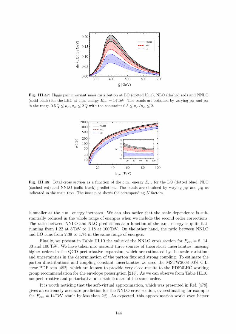
300 400 500 600 7000.00

0.05

0.10

0.15

0.20

Q HGeVL

d�dQHfb�GeVL

LO

NLO

NNLO

Fig. III.47: Higgs pair invariant mass distribution at LO (dotted blue), NLO (dashed red) and NNLO(solid black) for the LHC at c.m. energy Ecm = 14TeV. The bands are obtained by varying µF and µRin the range 0.5Q ≤ µF , µR ≤ 2Q with the constraint 0.5 ≤ µF /µR ≤ 2.

20 40 60 80 100

10

20

50

100

200

500

1000

2000

E cm H TeVL

ΣHfbL

20 40 60 80 100

0.5

1.0

1.5

2.0

2.5

3.0

K

LO

NLO

NNLO

Fig. III.48: Total cross section as a function of the c.m. energy Ecm for the LO (dotted blue), NLO(dashed red) and NNLO (solid black) prediction. The bands are obtained by varying µF and µR asindicated in the main text. The inset plot shows the corresponding K factors.

is smaller as the c.m. energy increases. We can also notice that the scale dependence is sub-stantially reduced in the whole range of energies when we include the second order corrections.The ratio between NNLO and NLO predictions as a function of the c.m. energy is quite flat,running from 1.22 at 8TeV to 1.18 at 100TeV. On the other hand, the ratio between NNLOand LO runs from 2.39 to 1.74 in the same range of energies.

Finally, we present in Table III.10 the value of the NNLO cross section for Ecm = 8, 14,33 and 100TeV. We have taken into account three sources of theoretical uncertainties: missinghigher orders in the QCD perturbative expansion, which are estimated by the scale variation,and uncertainties in the determination of the parton flux and strong coupling. To estimate theparton dinstributions and coupling constant uncertainties we used the MSTW2008 90% C.L.error PDF sets [482], which are known to provide very close results to the PDF4LHC workinggroup recommendation for the envelope prescription [218]. As we can observe from Table III.10,nonperturbative and perturbative uncertainties are of the same order.

It is worth noticing that the soft-virtual approximation, which was presented in Ref. [479],gives an extremely accurate prediction for the NNLO cross section, overestimating for examplethe Ecm = 14TeV result by less than 2%. As expected, this approximation works even better

144

Ecm 8 TeV 14 TeV 33 TeV 100 TeVσNNLO 9.76 fb 40.2 fb 243 fb 1638 fbScale [%] +9.0− 9.8 +8.0− 8.7 +7.0− 7.4 +5.9− 5.8PDF [%] +6.0− 6.1 +4.0− 4.0 +2.5− 2.6 +2.3− 2.6PDF+αS [%] +9.3− 8.8 +7.2− 7.1 +6.0− 6.0 +5.8− 6.0

Table III.10: Total cross section as a function of the c.m. energy at NNLO accuracy. We use the exactLO prediction to normalize our results. The different sources of theoretical uncertainties are discussed inthe main text.

than for single Higgs production, due to the larger invariant mass of the final state.

AcknowledgementsThis work was supported in part by UBACYT, CONICET, ANPCyT and the Research Exec-utive Agency (REA) of the European Union under the Grant Agreement number PITN-GA-2010-264564 (LHCPhenoNet).

11 Photon isolation studies18

11.1 IntroductionMany interesting physics signatures at the LHC involve the presence of single or multiple photonsin the final state. These photons may either be produced directly, through the fragmentation ofa quark or gluon, or else through the decay of a resonance – such as e.g. the Higgs boson.

The production of prompt photons is the subject of this analysis. The expression ‘promptphotons’ refers to photons produced at large transverse momenta which do not arise from thedecay of hadrons, such as π0, η, etc. Prompt photons can be produced according to two possiblemechanisms, one of them being fragmentation.

To be precise, the collider experiments at the Tevatron and the LHC do not perform in-clusive photon measurements. The background of secondary photons coming from the decaysof π0, η, etc., overwhelms the signal by several orders of magnitude. To reject this background,the experimental selection of prompt diphotons requires isolation cuts. In addition to the re-jection of the background of secondary photons, the isolation cuts (or criteria) also affect theprompt-diphoton cross section itself, in particular by reducing the effect of fragmentation.

The standard cone isolation and the “smooth” cone isolation proposed by Frixione [158]are two of these criteria. The standard cone isolation is easily implemented in experiments,but it only suppresses a fraction of the fragmentation contribution. The smooth cone isolation(formally) eliminates the entire fragmentation contribution, but its experimental implementation(at least in its original form) is complicated19 by the finite granularity of the LHC and Tevatrondetectors.

On the theoretical side, including fragmentation contributions to photon production cangreatly increase the complexity of the calculations, while the application of appropriate isolationcuts can effectively remove those fragmentation contributions. How to apply these isolationcriteria to the theoretical tools and how to deal with the fragmentation contributions consistentlyby the theory side is one of the subjects of this note.

18L. Cieri and D. de Florian19There is activity in the experimental implementation [160, 483, 484] of the discretized version of the smooth

isolation criterion. An experimental implementation of the smooth isolation criterion was done by the OPALcollaboration [485].

145

Besides the differences between these two isolation criteria, it is possible (i.e. it hasphysical meaning) to compare theoretical descriptions obtained using the smooth cone isolationcriterion and data taken with the standard criterion, because a cross section obtained using thesmooth cone isolation criterion provides always a lower bound for a cross section in which thestandard criterion was implemented, if one uses the same isolation parameters for both criteria.Furthermore, as we show in this note, this bound turns out to be an excellent approximation tothe standard criterion result with an accuracy of the order of the 1% if tight cuts are imposed.

Given these results, and the fact that in general it is not possible to exactly match theexperimental isolation conditions to the theoretical implementation and viceversa, we proposea pragmatic accord to perform a more precise comparison between the data and the fixed ordercalculations, that allows to extend the TH computation up to NNLO in some cases. That is themajor motivation for this note.

The following studies concern Monte Carlo integrators (as DIPHOX [486], JetFOX [487] or2γNNLO [488], etc) for which the fragmentation component is a purely collinear phenomenon. ForMonte Carlo generators (parton–shower Monte Carlo), in which the fragmentation photons areemited off quarks at non–zero angle during the showering process, we recomend reference [378].

11.2 Isolation criteriaIn this section we sumarize the standard and “smooth” isolation criteria, including their advan-tages and problems concerning the theoretical and experimental implementations.

11.2.1 The standard cone isolation criterionThe isolation criterion used by collider experiments is schematically as follows. A photon issaid to be isolated if, in a cone of radius R in rapidity and azimuthal angle around the photondirection, the amount of deposited hadronic transverse energy

∑EhadT is smaller than some value

ET max chosen by the experiment:∑EhadT ≤ ET max inside (y − yγ)2 + (φ− φγ)2 ≤ R2 , (III.77)

where ET max can be either, a fixed value20 or a fraction of the transverse momentum of thephoton (pγT ε, where typically 0 < ε ≤ 1). This is the so-called standard cone isolation criterion.In addition to the rejection of the background of secondary photons, these isolation cuts alsoaffect the prompt-diphoton cross section itself, in particular by reducing the effect of fragmen-tation, but should be structured so as to have a high efficiency for the retention of real, isolatedphotons.

A theoretical description of isolated photons is complicated because of the occurence ofcollinear singularities between photons and final-state quarks. A finite cross section is onlyobtained when these singularities are absorbed into the fragmentation functions. As a result theonly theoretically well-defined quantity (if we don’t use the smooth cone criterion) is the sum ofthe direct and fragmentation contributions. Once these two contributions are included one canisolate the photon using the cuts of Eq. (III.77) in an infrared safe way [489].

In addition, a tight isolation cut also has the undesirable effect of making the theoreticalprediction unstable [489], due to the restriction of the available phase-space for parton emission.When the size of the cone used is in the limit of the narrow cone (Rl+l−1, R ∼ 0.1) earlierstudies reveal potential problems. This leads to a collinear sensitivity in the form of a fairly large

20This requirement was typically used at the Tevatron and was motivated by the fact that most of the energy inthe isolation cone results from the underlying event (and pile-up), and so is independent of the photon energy [160].

146

dependence on ln(1/R), which could make the prediction unreliable21. In a recent calculation[490] these large logarithmic terms were ressumed restoring the reliability of the calculation.

11.2.2 The “smooth” isolation criterionThere exist an alternative to the standard criterion: the criterion proposed by Frixione inRef. [158] (see also Ref. [491,492]). This criterion modifies Eq. (III.77) in the following way∑

EhadT ≤ ET max χ(r) , inside any r2 = (y − yγ)2 + (φ− φγ)2 ≤ R2 . (III.78)

with a suitable choice for the function χ(r). This function has to vanish smoothly when itsargument goes to zero (χ(r) → 0 , if r → 0 ), and has to verify 0 < χ(r) < 1, if 0 < r < R .One possible election is,

χ(r) =(1− cos(r)

1− cosR

)n, (III.79)

where n is typically chosen as n = 1 (unless otherwise stated we rely on this value for thephenomenlogical results presented in this note). This means that, closer to the photon, lesshadronic activity is permitted inside the cone. At r = 0, when the parton and the photon areexactly collinear, the energy deposited inside the cone is required to be exactly equal to zero, andthe fragmentation component (which is a purely collinear phenomenon in perturbative QCD)vanishes completely. Since no region of the phase space is forbidden, the cancellation of softgluon effects takes place as in ordinary infrared-safe cross sections. This is the advantage of thiscriterion: it eliminates all the fragmentation component in an infrared-safe way.

We can also notice, comparing Eqs. (III.77) and (III.78), that both criteria coincide atthe outer cone (r = R, χ(R) = 1), and due to the presence of the χ(r) function which verifies0 ≤ χ(r) ≤ 1, the smooth cone isolation criterion is more restrictive than the standard one. Forthis reason, we expect smaller cross sections when one uses the smooth cone criterion comparedto the case when one implements the standard one if the same parameters are imposed,

σsmooth{R,ET max} ≤ σStand{R,ET max} . (III.80)

The smooth behaviour of the χ(r) function is the main obstacle to implement the new isolationcriterion into the experimental situation. First, because of the finite size of the calorimetercells used to measure the electromagnetic shower, the smooth cone criterion must be appliedonly beyond a minimum distance of approximately 0.1 (in {∆η,∆φ} plane). This allows acontribution from fragmentation in the innermost cone and one has to check to which extentthe fragmentation component is still suppressed. In addition, the transverse energy in theexperimental isolation cone is deposited in discrete cells of finite size. Thus concerning itsexperimental implementation, the continuity criterion, initially proposed by Frixione has to bereplaced by a discretized version consisting of a finite number of nested cones, together withthe collection of corresponding maximal values for the transverse energy allowed inside each ofthese cones.

As was previously noted, another interesting (theoretical) feature of the smooth coneisolation criterion is that it is free of the large logarithmic contributions of the type of ln(1/R)associated with the narrow cone.

11.2.3 Theoretical issuesAs it was previously stated, the inclusion of the fragmentation contributions complicates thecalculation. And in some cases, such as when one wants to reach NNLO accuracy in pQCD

21This could even lead to an unphysical result such as an isolated cross section larger than the inclusive one,thereby violating unitarity.

147

(like in diphoton production) it would make the calculation very unlikely for at least quite a fewyears since the machinary for such a computation is not available yet.

For those cases, one can find in the literature theoretical calculations in which the frag-mentation component is considered at one pertubative level less than the direct component(e.g. the γγ and W/Zγ production at NLO in pQCD in MCFM [159] or γγ+ Jet at NLO inpQCD [493], etc.). This procedure, which is a way to approximate the full calculation where thefragmentation component is included at the same perturbative level that the direct component,could introduce unexpected (inconsistent) results in the presence of the standard cone isolationcriterion. The following exercise shows how these problems can easely appear.

Let’s consider diphoton production at the LHC (√s = 8 TeV) computed at NLO, the

highest perturbative order at which both direct and fragmentation calculations are available.The acceptance criteria in this case requires: pharder

T ≥ 40 GeV and psofterT ≥ 30 GeV. The

rapidity of both photons is restricted to |yγ | ≤ 2.5 and 100 GeV< Mγγ < 160 GeV. The isolationparameters are set to the values n = 1 (in the case of the smooth cone) and R = 0.4, andthe minimum angular separation between the two photons is Rγγ = 0.5. The remain isolationparameter ET max (or ε) is varied in order to understand the cross section dependence on it.All the cross sections are obtained using the CTEQ6M set of parton distributions functions. Weused for this analysis the DIPHOX code that includes the full NLO pQCD description.

First, we compare the calculation using the fragmentation at NLO with the case in whichthe fragmentation is considered only at LO (one pertubative order less than the direct NLOcomponent). The results in Fig. III.49 (right) show that for the LO fragmentation one can obtainlarger cross sections for more severe isolation cuts (smaller ε), which is clearly inconsistent. Thesame behaviour was reported in Ref. [493] for γγ+ Jet at NLO, and we obtained similar featuresfor γγ, W/Zγ production at NLO in pQCD with MCFM. On the other hand, the left panel in Fig.III.49 shows that the correct behaviour is found when one considers the full result in which thefragmentation contribution is computed at same perturbative level than the direct component(i.e., NLO in this case).

The precedent comparison suggests that one has to be aware that approximating thefragmentation component at one order lower than the direct one can result in unphysical results.The situation can be even more serious when one looks at some extreme kinematical region wherethe cross section is dominated by higher order contributions.

In Table III.11 we present the results for the corresponding cross section with differentisolation prescriptions and parameters. The values presented there help to understand the un-expected behaviour in Fig. III.49 (right). In this case, the results are obtained imposing thecuts used by CMS in a recent measurement of the production cross section for pairs of isolatedphotons in pp collisions at

√s = 7 TeV [119]. Therefore, we require the harder photon to have

a transverse momentum phardT ≥ 40 GeV while for the softer we choose psoftT ≥ 30 GeV. Therapidity of both photons is restricted to |yγ | ≤ 2.5. Finally, we constrain the invariant mass ofthe diphotons to lie in the range 100 GeV ≤ Mγγ ≤ 160 GeV. And to simulate the CMS crack,we reject photons with 1.442 ≤ yγ ≤ 1.556. In the cases in which the standard criterion wasapplied (a− f in Table III.11) we observe that as the isolation criterion turns out to be “loose”the NLO direct component becomes smaller and the NLO fragmentation (single and double)component larger. The sum of them behaves as expected with respect to the isolation param-eters, since the increase in the fragmentation component overcompensates the decrease of thedirect one. We remind the reader that in the standard isolation the theoretical separation be-tween direct and fragmentation components is not physical and the results presented in this notecorrespond to the conventional MS subtraction. On the other hand, if only the LO calculationis used for the fragmentation contributions, for which the QCD corrections are quite large (withK−factors exceding 2), the mismatch in the perturbative order spoils the compensation between

148

dσ/dMνν [dir=NLO,frag=NLO]dσ/dM

νν [fb/G

eV]

50

100

150

200

50

100

150

200

Mνν [GeV]

100 110 120 130 140 150 160

100 110 120 130 140 150 160

ε=1

ε=0.5

ε=0.05

dσ/dMνν [dir=NLO,frag=LO]

dσ/dM

νν [fb/G

eV]

20

40

60

80

100

120

140

20

40

60

80

100

120

140

Mνν [GeV]

100 110 120 130 140 150 160

100 110 120 130 140 150 160

ε=1

ε=0.5

ε=0.05

Fig. III.49: Diphoton cross section as a function of the invariant mass Mγγ . (Left) With NLO fragmen-tation component. (Right) With LO fragmentation component.

the behaviour of the NLO direct and the LO fragmentation terms resulting in the unphysicalbehaviour observed in Fig. III.49 (right) as one considers less restringent isolation parameters.

Furthermore, from the cases in which the smooth cone criterion was applied (h−m in TableIII.11) we observed that, as expected, the result in the smooth cone case always provides a lowerbound for the one obtained with the standard criterion when the same isolation parameters(energy in this case) are used. In the case of smooth cone isolation the (single and double)fragmentation components are identically null. Even more interestingly, and with one singleexception, the results for the NLO cross sections computed using different isolation precriptionsdiffer by less than 1%. This result indicates that using the smooth cone prescription for atheoretical calculation (even when the data is analyzed using the standard one) provides anapproximation that it is is far much better than the one consisting in the standard prescriptionwith a lowest order calculation for the fragmentation component. The only case where one canobserve larger differences (of the order of 10%) corresponds to the use a very loose isolation, asfor

∑EhadT ≤ 0.5 pγT , where the fragmentation component in the standard case amounts more

than half of the total cross section.In all cases we have studied, the smooth cone provides an excellent approximation to the

standard result as long as the isolation parameters are tight enough, i.e.∑EhadT ≤ 0.1 pγT or∑

EhadT ≤ 5 GeV for the LHC at 7 TeV. Equivalently, one could define the isolation to be tightenough when the contribution from the fragmentation component does not exceeds ∼ 15− 20%of the total cross section.

While the previous analysis refers only to the fiducial crosss section, it is known that thefragmentation contributions could be larger in kinematical regions far away from the back-to-back configuration22, and the approximation could in principle become less accurate for thosedistributions. In order to check that feature, in Fig. III.51 we compare the distributions forthe full NLO calculation with the standard prescription, the one obtained using only the LOfragmentation component and the result for the smooth cone with

∑EhadT ≤ 0.05 pγT for cos θ∗

(left) and ∆φγγ (right). In both cases we observe that for all the bins the smooth cone provides22The low mass region in the invariant mass distribution, the low ∆φγγ distribution and the kinematical regions

near to cos θ∗ = ±1 belong to this case.

149

Code∑EhadT ≤ σNLOtotal (fb) σNLOdir (fb) σNLOonef (fb) σNLOtwof (fb) Isolation

a DIPHOX 2 GeV 3756 3514 239 2.6 Standardb DIPHOX 3 GeV 3776 3396 374 6 Standardc DIPHOX 4 GeV 3796 3296 488 12 Standardd DIPHOX 5 GeV 3825 3201 607 17 Standarde DIPHOX 0.05 pγT 3770 3446 320 4 Standardf DIPHOX 0.5 pγT 4474 2144 2104 226 Standardg DIPHOX incl 6584 1186 3930 1468 noneh 2γNNLO 0.05 pγT χ(r) 3768 3768 0 0 Smoothi 2γNNLO 0.5 pγT χ(r) 4074 4074 0 0 Smoothj 2γNNLO 2 GeV χ(r) 3754 3754 0 0 Smoothk 2γNNLO 3 GeV χ(r) 3776 3776 0 0 Smoothl 2γNNLO 4 GeV χ(r) 3795 3795 0 0 Smoothm 2γNNLO 5 GeV χ(r) 3814 3814 0 0 Smooth

Table III.11: Cross sections for the pp → γγ + X process at the LHC at NLO. All these values are at1% of statistical accuracy level.

ε=0.05

dσ/dCosθ* [fb]

0

1000

2000

3000

4000

5000

6000

7000

0

1000

2000

3000

4000

5000

6000

7000

Cosθ*

-1 -0.5 0 0.5 1

-1 -0.5 0 0.5 1

Dir(NLO)+Frag(LO)Dir(NLO)+Frag(NLO)Dir(NLO)+"smooth"

ε=0.05

dσ/dφ

νν [fb/rad]

10

100

1000

1e+04

10

100

1000

1e+04

φνν [rad]

0 0.5 1 1.5 2 2.5 3

0 0.5 1 1.5 2 2.5 3

Dir(NLO)+Frag(LO)Dir(NLO)+Frag(NLO)Dir(NLO)+"smooth"

Fig. III.50: Diphoton cross section as a function of the cos θ∗ (Left), and the angular separation betweenthe photons ∆φγγ (Right). A comparison between the different isolation criteria is showed. The appliedcuts are the same as in Fig. III.49, and are described in the text.

the best approximation to the full result, always within a 2.5% accuracy. A more detailedanalysis in presented in Fig. III.51 for the diphoton invariant mass distributions with twodifferent isolation parameters,

∑EhadT ≤ 0.05 pγT (left) and

∑EhadT ≤ 4 GeV (right). Again,

while using the LO fragmentation component fails to reproduce the full NLO result by up to6%, the smooth cone approximation is always better than 1.5% in the same kinematical region.

The discrepancies between the full result and the smooth approach with the LO frag-mentation approximation that evidently manifest in the invariant mass distribution (see Fig.III.51) or in kinematical regions far away from cos θ∗ = ±1 (see Fig. III.50 (left)) are “hidden”in the ∆φγγ distribution, in the bin corresponding to ∆φγγ = π (the bin containing the back-to-back configurations). Moreover in the low ∆φγγ region we are dealing with events far awayfrom the back-to-back configuration, and the only configuration that survives at NLO (in these

150

Fig. III.51: Diphoton cross section as a function of the invariant mass Mγγ . Cross sections obtainedwith the standard cone isolation criterion (with LO and NLO fragmentation contributions) are comparedwith the cross section obtained with the smooth cone criterion using the same isolation parameters.

ε=1

dσ/dφ

νν [fb/rad]

10

100

1000

1e+04

10

100

1000

1e+04

φνν [rad]

0 0.5 1 1.5 2 2.5 3

0 0.5 1 1.5 2 2.5 3

Dir(NLO)+Frag(NLO)Dir(NLO)+Frag(LO)Dir(NLO)+"smooth"

ε=1

dσ/dM

νν [fb/GeV]

40

60

80

100

120

140

160

180

200

40

60

80

100

120

140

160

180

200

Mνν [GeV]

100 110 120 130 140 150 160

100 110 120 130 140 150 160

Dir(NLO)+Frag(NLO)Dir(NLO)+Frag(LO)Dir(NLO)+"smooth"

Fig. III.52: Diphoton cross section as a function of the angular separation between the photons ∆φγγ(Left), and the invariant mass of the diphoton system Mγγ (Right).

kinematical regions) is the real emission at LO which is for the three cases effectively the samecontribution under these conditions.

If one relaxes the isolation and considers ε = 1 (which is equivalent to EmaxT > 40 GeV,allowing for a huge amount of fragmentation contribution), the effects of fragmentation nowstrongly manifests at low ∆φγγ values, and the full result considerably differs from both the LOfragmentation approximation and the smooth cone criterion as we can observe in Fig. III.52(azimuthal distribution in the upper plot and invariant mass in the lower one). Also we cansee from Fig. III.52, in the bin corresponding to ∆φγγ = π (the bin containing the back-to-back configurations) the cross section obtained with the smooth cone criterion provides a betterapproximation than the LO fragmentation one.

151

11.3 Tight isolation accordFinally, considering the results presented in the preceeding sections we conclude this note byproposing a pragmatic accord in order to compare experimental data and theoretical calculationsobtained at the highest possible perturbative order. Given the fact that matching experimentalconditions to theoretical calculations always implies certain degree of approximation, we believethat considering the large QCD corrections to processes involving photons (with NNLO essentialto understand diphoton data [488]) and the agreement (tipically at the % level for the diphotoncase studied here) between the standard and smooth cone TH calculations, the use of the laterfor TH purposes is well justified.

We call this approach "pragmatic", in the sense that we do not recommend the experimentsto implement the smooth cone isolation, but to proceed to the analysis of the data with the usualstandard isolation with cuts tight enough if the interesting observable needs to be an isolatedcross section or distribution. While the definition of "tight enough" might slightly depend on theparticular observable (that can always be checked by a lowest order calculation), our analysisshows that at the LHC isolation parameters as EmaxT ≤ 5 GeV (or ε < 0.1), R ∼ 0.4 andRγγ ∼ 0.4 are safe enough to proceeed.

This procedure would allow to extend available NLO calculations to one order higher(NNLO) for a number of observables, since the direct component is always much simpler toevaluate than the fragmentation part, which identically vanishes under the smooth cone isolation.

We also refer to this approach as pragmatic in a numerical sense: we are certain that thesmooth cone isolation applied for the TH calculation is NOT the one used in the experimentaldata, but considering that NNLO corrections are of the order of 50% for diphoton cross sec-tions [488] and a few 100% for some distributions in extreme kinematical configurations, it isfar better accepting a few % error arising from the isolation (less than the size of the expectedNNNLO corrections and within any estimate of TH uncertainties!) than neglecting those hugeQCD effects towards some "more pure implementation" of the isolation prescription.

We believe that a more detailed analysis of the profile function in the smooth cone isolationcan be performed on a case by case basis in order to select, also in a pragmatic way, the mostconvenient for each observable, even though again, differences are expected to be very small asdiscussed before.

AcknowledgementsThis work was supported in part by UBACYT, CONICET, ANPCyT, INFN and the ResearchExecutive Agency (REA) of the European Union under the Grant Agree- ment number PITN-GA-2010-264564 (LHCPhenoNet, Initial Training Network).

12 Diphotons and jets at NLO23

We study diphoton production in association with up to three jets at the LHC. In particular,we compare NLO predictions for up to two jets with leading order predictions matched to aparton shower. For the one-jet bin, we also include fragmentation contributions in the partoniccalculation, which enables us to study the impact of different isolation criteria.

12.1 IntroductionStudies of the Higgs boson decay channel into two photons are of major importance in orderto scrutinize the Higgs couplings and to be able to judge whether small deviations from theStandard Model predictions are hints of new physics.

23N. Chanon, T. Gehrmann, N. Greiner, G. Heinrich

152

Measurements of the inclusive diphoton cross section by both ATLAS [118] and CMS [119]based on the

√s = 7 TeV data set have been published recently. The production of photon pairs

in association with jets are also very interesting processes, despite their smaller cross sections,as they constitute the main background to Higgs production in association with jets, where thehiggs boson decays into two photons. In particular, the knowledge of diphoton production inassociation with two jets at next-to-leading order (NLO) accuracy allows to study the impact ofvector boson fusion (VBF) cuts and thus helps to disentangle Higgs production in gluon fusionfrom the electroweak production meachnism.

Large-pT photons in the final state can originate either from the hard interaction processitself or from the fragmentation of a large-pT hadron. To single out the photons originating fromthe hard interaction from the secondary photons, photon isolation criteria need to be applied,which are typically formulated in the form of a maximum amount of hadronic energy allowedin the vicinity of the photon. The photons originating from fragmentation are, in a partoniccalculation, described by fragmentation functions, which – in analogy to PDFs in the initialstate – are non-perturbative objects that have to be determined from experimental data. Tosuppress the dependence of isolated photon cross sections on the fragmentation functions, asmooth cone isolation criterion has been proposed [494], where the allowed hadronic energyinside the isolation cone decreases with decreasing radial distance from the photon.

While diphoton production without extra jets has been calculated at NLO already sometime ago, including also the fragmentation contribution at NLO in the public code Diphox [495],and even the NNLO corrections (without fragmentation contributions) have been calculatedmeanwhile [9], diphotons in association with jets at NLO have become available only recently.Photon pair plus one jet production at NLO has first been calculated in [496], using an isolationcriterion [494] where the fragmentation component is eliminated. In Ref. [493], the fragmentationcomponent has been included, allowing to study the impact of different isolation criteria atNLO, and the corresponding code is publicly available [497]. The virtual corrections are basedon the automated one-loop program GoSam [4], while the real corrections are built on theMadGraph/MadDipole/MadEvent [420–423] framework.

Photon pair plus two jet production at NLO has first been calculated in [498], also basedon GoSam+MadGraph/MadDipole/MadEvent, using a smooth isolation criterion. NLOresults for γγ+2 jet production also have been presented in [499–501], and Ref. [500] in additionpresents results for γγ + 3 jet production at NLO.

12.2 Diphoton plus one jet productionIn this section we consider diphoton production in association with one tagged jet. We comparethe following samples:

1. NLO and LO samples produced by GoSam+MadGraph/MadDipole/MadEvent (par-ton level). Renormalisation and factorisation scales µ and µF have been chosen as dynam-ical scales, with the default choice being µ0 = 1

2 (mγγ +∑j p

jetT ), µ = µF . The PDF set

used is CT10. For the NLO sample based on GoSam+MG we also compare cone isolationwith Frixione [494] type isolation.

2. NLO samples produced by aMC@NLO [6] interfaced with a Herwig6 shower [502], wherethe scale choice is µ0 = 1

2 (mγγ +∑ppartonsT ), µ = µF . The PDF set used here is CTEQ6M.

3. MadGraph LO samples with up to two jets at matrix element level, interfaced with aPythia6 shower [288]. The scales are set to µ0 = pγ1

T + pγ2T +

∑ppartonsT . The PDF set

used is CTEQ6L1.

The LO computations based on MadGraph do not need any isolation criterion applied atparton level, as we require Rγ,j > 0.5. At NLO, however, collinear quark-photon configurations

153

due to extra radiation need to be taken care of. The singularities related to these configurationsare cancelled by absorbing them into the “bare" fragmentation functions, analogous to the caseof PDFs in the initial state. Therefore, the fragmentation part needs to be taken into accountin an NLO calculation, unless it is completely suppressed by an isolation criterion like the onesuggested by Frixione [494]. With this criterion, one considers smaller cones of radius rγ insidethe R-cone and calls the photon isolated if the energy in any sub-cone does not exceed

Ehad,max(rγ) = ε pγT

(1− cos rγ1− cosR

)n.

When applying this criterion in our calculations, we use the isolation parameters R = 0.4, n = 1and ε = 0.05.However, the latter criterion is difficult to implement in a realistic experimental environment,where the photon will always be accompanied by some amount of hadronic energy. Therefore,whenever we produce showered events, an isolation is applied at shower level which is a classi-cal cone-type isolation: GenIso < 0.05 × pγT , where GenIso is computed from the transversemomentum sum of all particles falling in a cone ∆R < 0.4 around the photon. In the partonicNLO calculation labelled “GoSam+MG NLO cone", where the fragmentation component is in-cluded, we apply the same cone isolation parameters. Further we apply the following kinematicrequirements on the two photons:

pjetT > 30 GeV, pγ1

T > 40 GeV, pγ2T > 25 GeV,

mγγ > 100 GeV, |ηγ | ≤ 2.5, Rγ,γ > 0.45.

With GoSam+MG, the jets are clustered with the anti-kT algorithm using a cone of 0.5, appliedto the QCD partons only. For the showered samples, the two hardest pT photons in the eventare selected as diphoton candidates, and they are removed from the list of particle candidatesbefore the jet clustering algorithm is run. We then select the hardest jet in the event and require:

pjetT > 30 GeV, |ηj | ≤ 4.7, Rγ,j > 0.5 .

Differential distributions for the samples produced with different generators after kinematic andisolation requirements, for

√s = 8TeV, are shown in Fig. III.53 for the leading photon and

leading jet transverse momentum distributions. In particular, we compare, at NLO partonlevel, Frixione and cone-type isolation. We observe that for the rather tight isolation criteriaconsidered here, the differences are quite small. In addition, we compare to showered sampleswith the same cone-type isolation. As expected, we observe that the effect of the isolation afterthe shower is considerably larger than at parton level. This can be seen particularly clearlyin Fig. III.54, in distribution of the relative azimuthal angle ∆φγ1γ2 between the two photons.Note that the difference between GoSam NLO with Frixione isolation and aMC@NLO withFrixione isolation at the LHE level can be attributed to the different scale choice (running overthe partons for aMC@NLO and over the jets for GoSam). The difference due to the differentPDF set is negligible. Once the shower with Herwig6 is applied, the kinematic acceptance isreduced, giving a lower cross section.

12.3 Diphoton plus two jet productionFor the production of two photons and two jets, we consider similar samples as for the one jetcase, also adding Sherpa [166] LO samples with up to three jets at matrix element level. As theNLO calculation also contains up to three partons accompanying the photons in the final state, itmakes sense to consider up to three jets at matrix element level in a LO sample. In the Sherpasample, the box diagram gg → γγ, where the two additional jets are produced by the shower,

154

(GeV) leadγT,P0 50 100 150200 250 300 350 400 450 500

lead

γT,

/dP

σd

-510

-410

-310

-210

-110

1+1j LOγγGoSam+MG

+1j NLO coneγγGoSam+MG

+1j NLO frixγγGoSam+MG

+up to 2j LO shower+GenIsoγγMG

+1j NLO LHE frixγγaMC@NLO

+1j NLO frix shower+GenIsoγγaMC@NLO

(GeV)T,jet leadP0 50 100 150200 250 300 350 400 450 500

T,je

t lea

d/d

Pσd

-510

-410

-310

-210

-110

1+1j LOγγGoSam+MG

+1j NLO coneγγGoSam+MG

+1j NLO frixγγGoSam+MG

+up to 2j LO shower+GenIsoγγMG

+1j NLO LHE frixγγaMC@NLO

+1j NLO frix shower+GenIsoγγaMC@NLO

Fig. III.53: Transverse momentum distribution of the leading-pT photon for the γγ+1 jet process.

2γ1,γφ∆

0 0.5 1 1.5 2 2.5 3

2γ1,γφ∆

/dσd

0

0.5

1

1.5

2

2.5

3

3.5

4

4.5

5+1j LOγγGoSam+MG

+1j NLO coneγγGoSam+MG

+1j NLO frixγγGoSam+MG

+up to 2j LO shower+GenIsoγγMG

+1j NLO LHE frixγγaMC@NLO

+1j NLO frix shower+GenIsoγγaMC@NLO

(GeV)γγM0 100 200 300400 500 600 700 800 9001000

γγ/d

Mσd

-510

-410

-310

-210

-110

1+1j LOγγGoSam+MG

+1j NLO coneγγGoSam+MG

+1j NLO frixγγGoSam+MG

+up to 2j LO shower+GenIsoγγMG

+1j NLO LHE frixγγaMC@NLO

+1j NLO frix shower+GenIsoγγaMC@NLO

Fig. III.54: ∆φγ1γ2 and diphoton invariant mass distributions for the γγ+1 jet process.

is also included, but its numerical impact is negligible. Factorisation and renormalisation scalesare set by the METS scale, which uses a modified CKKW matching algorithm. The PDF setused is CT10. Differential distributions produced by the various generators after kinematic andisolation requirements are shown in Fig. III.55 for the leading photon and leading jet transversemomentum and in Fig. III.56 for the difference in azimuthal angle between the two photons andthe diphoton invariant mass. One can see that the effect of the parton shower on the LO samplesis different in the two-jet case: the kinematical and isolation cuts reduce the cross-section morestrongly than in the one-jet case. This is easily understood by the fact that after the shower,the probability to identify two hard jets in addition to two isolated photons is much lower thanthe probability to identify just one hard jet.

12.4 ConclusionsWe have studied the processes of diphoton production in association with one and two jets atthe LHC. For the process γγ+ 1 jet, we have compared partonic LO results, LO results matched

155

(GeV) leadγT,P0 50 100 150200 250 300 350 400 450 500

lead

γT,

/dP

σd

-510

-410

-310

-210

-110 +2j LOγγGoSam+MG

+2j NLO frixγγGoSam+MG

+up to 2j LO shower+GenIsoγγMG

+up to 3j LO shower+GenIsoγγSherpa

(GeV)T,jet leadP0 50 100 150200 250 300 350 400 450 500

T,je

t lea

d/d

Pσd

-510

-410

-310

-210

-110+2j LOγγGoSam+MG

+2j NLO frixγγGoSam+MG

+up to 2j LO shower+GenIsoγγMG

+up to 3j LO shower+GenIsoγγSherpa

Fig. III.55: Transverse momentum distribution of the leading-pT photon and jet for the γγ+2 jetsprocess.

2γ1,γφ∆

0 0.5 1 1.5 2 2.5 3

2γ1,γφ∆

/dσd

0

0.2

0.4

0.6

0.8

1

1.2

1.4+2j LOγγGoSam+MG

+2j NLO frixγγGoSam+MG

+up to 2j LO shower+GenIsoγγMG

+up to 3j LO shower+GenIsoγγSherpa

(GeV)γγM0 100 200 300400 500 600 700 800 9001000

γγ/d

Mσd

-510

-410

-310

-210

-110+2j LOγγGoSam+MG

+2j NLO frixγγGoSam+MG

+up to 2j LO shower+GenIsoγγMG

+up to 3j LO shower+GenIsoγγSherpa

Fig. III.56: ∆φγ1γ2 and diphoton invariant mass distribution for the γγ+2 jets process.

to a parton shower, NLO results at parton level with two different isolation criteria, and NLOresults combined with a parton shower. As to be expected, we find that the NLO showeredresults lie between the LO results and the NLO partonic results. Comparing standard coneisolation with Frixione-type isolation at NLO at parton level, we observe that the difference isvery small for the tight isolation criteria used in this study.For the process γγ+2 jets, we have compared LO and NLO samples at parton level produced withGoSam+MadGraph/MadDipole/MadEvent to two different showered LO samples, producedwith MadGraph or Sherpa. Comparing to the behaviour in the γγ + 1 jet case, we observethat in the presence of the additional tagged jet, switching on the parton shower leads to aconsiderably stronger reduction of the (LO) cross section, as the probability to identify twohard jets is reduced more strongly after the parton shower than in the one-jet case.

156

AcknowledgementsWe would like to thank the organisers of “Les Houches 2013" for the stimulating workshop.We are also grateful to all members of the GoSam project for their contributions to codedevelopment. This work is supported by the Sinergia program of the Swiss National ScienceFoundation (SNF) under grant number CRSII2-141847.

157

Chapter IV

MC tuning and output formats

1 Extensions to the Les Houches Event Format1

1.1 BackgroundThe LHE file format has been around since 2006 and has been very successful. At the LesHouches workshop in 2009 an update was suggested, mainly to improve the handling of NLO andmatching/merging. The proposal was published in the proceedings (arXiv:1003.1643), but havenever really been properly used. Nevertheless, some shortcomings have been noticed and somesuperfluous features identified, both of which issues we attempt to address in this contribution.

In the discussions at this years workshop some ideas on how to better specify weights weresuggested, and also some other new features were suggested and old features were suggestedto be dropped. Here we summarise the discussion as a set of agreed-upon proposals to defineversion 3.0 of the LHE format.

1.2 Changes in the format of 2009Some XML tags that were introduced in 2009 were not adopted by the community, possiblybecause their usefulness was very limited. In order not to clutter the new proposal with unnec-essary features, we recommend that the following XML tags be removed.

In the <init> block, we recommend that<mergeinfo> Should be removed due to very limited usability.In the <event> block, we recommend that<weight> Should be removed and replaced by <weights> (see below), to avoid clashes with

the new weight tag defined below.<clustering> Should be removed due to very limited usability.<pdfinfo> Should be removed due to unclear purpose.None of these XML tags seem to have been used. Thus, we do not expect backward-compatibilityproblems if they were to be removed, and hence propose that they be simply ignored by futureparsers, as per the normally defined LHE parsing behaviour for unknown XML tags. Any newLHE-parsing/writing code should be based on this definition rather than the previous one.

In discussions before and during the Les Houches workshop, it became obvious that theLHEF standard should be updated. This mainly concerns the handling of multiple event weightsper phase space point. Allowing for multiple weights can significantly speed up the assessment ofuncertainties as well as performing finely-grained parameter scans. For a well-defined handlingof multiple weights, two proposals for extending the LHEF format were made, and were latercombined into a single definition agreed on by the authors of the MC generator codes (bothmatrix element and parton shower) actively using the format.

1A. Buckley, J. Butterworth, R. Frederix, B. Fuks, F. Krauss, L. Lonnblad, O. Mattelaer, P. Nason, C. Oleari,S. Padhi, S. Plätzer, S. Prestel

158

1.3 Additions to the LHEF format for dealing with multiple weightsThe main improvement to the LHEF format is the need to deal with multiple event weights.We therefore describe the additional XML tags dealing with them first.

1.3.1 Multiple weight definition in the event file headerIn the case where additional event weights are computed by the code that generates the eventfile, the header of that file should contain a new block, <initrwgt>, which syntax should followthis example:

<initrwgt><weight id=’1’> This is the original event weight </weight><weightgroup name=’scale variation’ combine=’envelope’>

<weight id=’2’> muR = 2.0 </weight><weight id=’3’> muR = 0.5 </weight>

</weightgroup><weightgroup name="MRST2008 PDF uncertainty" combine="hessian"><weight id=’4’> set 01 </weight><weight id=’5’> set 02 </weight>...

</weightgroup><weightgroup name=’Qmatch variation’ combine=’envelope’>

<weight id=’44’> Qmatch=20 </weight><weight id=’my_own_id’> Qmatch=40 </weight>

</weightgroup><weight id=’46’> BSM benchmark point number 42B </weight>

</initrwgt>

The information in the <weight> tags should be human-readable and explain what the weightsmean. It can simply contain all the parameters that were used in to generate this weight; oronly the ones that were changed compared to the original run; or simply a sentence explainingwhat this number means. It is up to the user that is doing the analysis to make sure that thisinformation is correctly used (and up to the authors of the codes to make sure that the user hasenough information to understand what the weights correspond to). The <weight> tag has theweight name id as mandatory argument. Suggested optional arguments aremuf The factor multiplying the nominal factorization scale for the event for the given weightmur The factor multiplying the nominal renormalization scale for the event for the given weightpdf The LHAPDF code corresponding to the given weightpdf2 The LHAPDF code corresponding to the given weight for the second beam if different

from pdf

These arguments can be useful to concatenate a helpful string identifier when parsing the in-formation through events in HepMC format. In this context, it is also helpful to choose adescriptive value for id.

The <weightgroup> tag allows to group several weights together and to have the infor-mation about how to combine weights to obtain, e.g., scale variation or pdf uncertainties. Theattribute name is mandatory and should define the name of the group. The attribute combine isoptional and it indicates how the weights should be combined to define the associated uncertain-ties. Possible arguments are none, hessian, envelope or gaussian. If not specified, the defaultchoice is combine=’none’, all the curves associated with each weights being kept independent.For combine=’hessian’, the first weight is the central value and the next weights correspondrespectively to the positive and negative variations along a specific direction of the parameterspace.

159

1.3.2 Multiple weights in the <event> blockAs already hinted above, there are two formats for the inclusions of the weights in each of theevents in the <event> block: a compressed format and a detailed format. The compressed formatis designed to be memory-efficient, by avoiding repetition of identical strings for each event asmuch as possible. It amounts to adding a single <weights> tag to each event. The<weights>tag contains a space-separated list of weights for the events given in the order they are definedby the <weight> tags in the <initrwgt> block. If for some obscure reason a weight source isabsent, its position in the list should be filled with a zero weight entry. In this case, a typicalevent will look like:

<event>7 100 0.100E+01 0.200E+00 0.000E+00 0.000E+00-2 -1 0 0 0 0 0.126E+01 0.554E+01 0.576E+02 0.579E+02 0.000E+00 0. 0.2 -1 0 0 0 0 -.913E+00 0.131E+01 -.349E+02 0.350E+02 0.000E+00 0. 0.

23 2 1 1 0 0 0.356E+00 0.685E+01 0.226E+02 0.929E+02 0.898E+02 0. 0.-13 2 3 3 0 0 0.516E+01 0.211E+02 0.539E+02 0.581E+02 0.105E+00 0. 0.13 2 3 3 0 0 -.480E+01 -.142E+02 -.312E+02 0.347E+02 0.105E+00 0. 0.-13 1 0 0 0 0 0.516E+01 0.211E+02 0.539E+02 0.581E+02 0.105E+00 0. 0.13 1 0 0 0 0 -.480E+01 -.142E+02 -.312E+02 0.347E+02 0.105E+00 0. 0.<weights> 1.000e+00 0.204e+00 ... 1.564e+00 </weights></event>

In http://home.thep.lu.se/~leif/LHEF there is a small example class which is able to readand write this representation of the suggested new format. Future development and documen-tation of the format will take place at http://lhef.hepforge.org.

For the detailed format the weights are put in <wgt> tags and are identified by theiridentifier id; their order is not of relevance. The list of weights should be put in the <rwgt>block, and each weight should be on a separate line. In this case a typical example event lookslike:

<event>7 100 0.100E+01 0.200E+00 0.000E+00 0.000E+00-2 -1 0 0 0 0 0.126E+01 0.554E+01 0.576E+02 0.579E+02 0.000E+00 0. 0.2 -1 0 0 0 0 -.913E+00 0.131E+01 -.349E+02 0.350E+02 0.000E+00 0. 0.

23 2 1 1 0 0 0.356E+00 0.685E+01 0.226E+02 0.929E+02 0.898E+02 0. 0.-13 2 3 3 0 0 0.516E+01 0.211E+02 0.539E+02 0.581E+02 0.105E+00 0. 0.13 2 3 3 0 0 -.480E+01 -.142E+02 -.312E+02 0.347E+02 0.105E+00 0. 0.-13 1 0 0 0 0 0.516E+01 0.211E+02 0.539E+02 0.581E+02 0.105E+00 0. 0.13 1 0 0 0 0 -.480E+01 -.142E+02 -.312E+02 0.347E+02 0.105E+00 0. 0.<rwgt><wgt id=’1’> 1.000e+00 </wgt><wgt id=’2’> 0.204e+00 </wgt><wgt id=’3’> 1.564e+00 </wgt><wgt id=’4’> 2.248e+00 </wgt><wgt id=’5’> 1.486e+00 </wgt>...<wgt id=’my_own_id’> -0.839e+00 </wgt><wgt id=’46’> -0.899e+00 </wgt>

</rwgt></event>

This representation of the proposed format has been implemented in the MadGraph5_aMC@NLO,MadAnalysis5 and POWHEG BOX V2 packages.

Note that for both formats the weight for the nominal event is still also given by XWGTUPentry.

160

1.4 Additional new tags not related to multiple event weightsWe agreed upon two more tags to become part of the LHEFv3.0 accord. The first one shouldbe put in the <init> block and helps to transfer the program version with which the LHEF hasbeen generated:<generator> There should be at least one such tag (potentially more) with a name and a

version attribute in the <init> section.A typical example is

<generator name=’SomeGen’ version=’1.2.3’> some additional comments </generator>

The additional comments can either identify sub-modules or libraries, or other information, likean arXiv number.

The second tag, <scales>, is optional and should be put within the <event> block. It is definedas:<scales> contains information about different scales used by the matrix element generator in

the given event. The scales are given as attributes, and any attribute name is allowed.However, only the following attributes have a pre-defined meaning:muf The factorization scale (in GeV)mur The renormalization scale (in GeV)mups Suggested shower starting scale (in GeV)If any of these attributes are missing, then the value in SCALUP is to be assumed for themissing attribute.

AcknowledgementsThe authors thank the Les Houches workshop once again for the hospitality and enjoyable/productiveworking environment in the Chamonix valley. AB acknowledges support from a Royal SocietyUniversity Research Fellowship, a CERN Scientific Associateship, an IPPP Associateship, andthe University of Glasgow’s Leadership Fellow programme.

161

2 Proposed updates for HepMC event record2

2.1 GenRunThere is a need to store the names and version numbers of all generators used in producing anevent. We propose to define a GenRun object to contain cross-section (GenCrossSection) andother run-level quantities discussed below. Each GenEvent should link to the GenRun.

2.2 Generator names and versionsAdd string array to GenRun with pairs of strings specifying (generator name, generator version).All generators used in the production should be listed, in order of processing, with full versionnumbers.

2.3 Vertex IDThe GenVertex.id() is not currently used/specified. We propose to define six codes:0 undefined (no information)1 matrix element vertex (i.e. the hard process which defines the PDF arguments). (Must

be the same as the GenEvent::signal_vertex());2 secondary partonic scatters (useful for studies of MPI jet production, e.g. for suppressing

jets from MPI while retaining the low p⊥ tail of the underlying event;3 hard decay (prehadronisation) e.g. of W , H, Z, t. Useful e.g. for optimisation studies of

mass resolution;4 parton shower (including QED radiation) useful for e.g. identifying g → bb splitting

probability; ME/PS matching studies; identifying photons for dressing leptons. Note: anyparton shower after a hadronisation is ignored, and the hadrons from it are flagged asbeing produced in a hadron decay;

5 primary hadron formation. Useful for e.g re-doing hadronisation, applying BEC correc-tions, studying/tracking decay chains;

6 hadron, tau and muon decaysWe propose that 10–99 be reserved for generator-specific types. Use of this information mustbe made carefully, to avoid generator-specific physics conclusions.

2.4 Weight namesSome standardisation of weight names is desirable. We propose several standard weight namecomponents, to be separated from each other by single underscore characters:MUF0.5, MUF2 factorization scale multiplication. Any float may occur between MUF and the

underscore divider / end of string;MUR0.5, MUR1.414 renormalization scale multiplication. Any float may occur between MUR

and the underscore divider / end of string;PDF10801, PDF20123 PDF variations, with the number following PDF up to the under-

score/end being the LHAPDF/PDFLIB unique PDF member ID.The potentially composite names for each weight are proposed to be stored in the GenRun, linkedto the WeightContainer to avoid replication in the ASCII event format.

2A. Buckley, J. Butterworth, F. Krauss, L. Lonnblad, S. Plätzer, S. Prestel

162

AcknowledgementsAll authors thank the Les Houches workshop once again for the hospitality and enjoyable/productiveworking environment in the Chamonix valley. AB acknowledges support from a Royal SocietyUniversity Research Fellowship, a CERN Scientific Associateship, an IPPP Associateship, andthe University of Glasgow’s Leadership Fellow programme.

163

3 Improvements in the Rivet MC analysis toolkit3

Rivet [379] is the de facto analysis toolkit used for phenomenology and experimental MC analysisat the LHC. It comprises a steering system for efficiently processing events (as HepMC [503]code objects) through a user-specified set of analysis routines, each of which outputs a set ofhistograms for comparison to data or to other MC predictions. User-written analyses can beeasily run without rebuilding Rivet, or any of the currently 250 built-in analyses may be used.

Rivet makes a major point of portability between any parton shower MC generators byreconstructing all quantities from physically reliable final-state (or decayed hadron) quantities,i.e. those which are at least in principle measurable and are not subject to the computationalambiguities of perhaps interfering quantum amplitudes. This has had the side-effect of mak-ing Rivet a useful “straw man” system for development of more robust definitions of physicalquantities at “MC truth” level.

In this contribution I describe several major updates made to data processing and physicsobservable features in the Rivet MC analysis toolkit, which defined the step from the long-established Rivet version 1 to version 2, and the planned / in-development features for the nextmajor release.

3.1 Histogramming and run mergingPartially as an historical accident of its genesis, Rivet has never been able to fully merge generatorruns. Primarily this is because it converts all histograms (i.e. objects which preserve the historyof their fills somehow) into simple “scatter” plots of x and y points with associated error bars.Histograms typically compute the visual heights of their bins from stored weighted moments like∑wi,

∑w2i ,∑wixi, etc. (where wi is the weight of the ith histogram fill and xi the value in

that fill), by standard statistical rules (and of course the width of each bin to preserve the shapeinvariance of the observable under rebinning). It is therefore possible to merge runs by simplyadding the summed moments, either directly if the process type in the different runs is thesame, or with a cross-section scaling if they are different or contain the same process but withcomplementary kinematic generation cuts, cf. the classic “jet slices” beloved of experiment MCproductions. It is not possible to get the same exact merging behaviour from “scatter” graphs,and hence Rivet’s run merging has always relied on asymptotic scaling which break down onunpopulated distribution tails.

In Rivet version 2, a major redevelopment of the histogramming system was made, re-placing the formerly used AIDA system (in a much-hacked implementation called LWH) with anew histogramming system, YODA [504]. This was written specifically to support MC analysisidioms and issues but intentionally does not contain any specific binding to particle physicsconcepts or usage. Usage of the ubiquitous ROOT [505] system was also extensively considered,but ROOT’s pervasive global state / threading unfriendliness and issues with object ownershipand histogram behaviour convinced us that it was better to start from scratch and attempt to“do it right”. YODA precisely stores the sorts of weighted moments discussed above, for 1Dand 2D histograms and profile histograms, as well as 1D, 2D, and 3D scatters and functions forconversion between these objects and to their ROOT equivalents.

The YODA statistics implementations are based on those from our LWH code, and areextremely careful in their treatments of low statistics errors, unfilled bins, overflow/underflowbins and whole distribution properties, as well as permitting gaps in binning as required by manyhistorical public datasets in the HepData system. Extensions to the YODA binning systemare intended to allow any type of object to be stored and looked up in an efficient binningrepresentation. YODA histogram objects can be arbitrarily “annotated” with key–value pairs,

3A. Buckley

164

which proves extremely useful for e.g. storing information about scaling operations applied tohistograms, as well as style information to be used by the Rivet plotting system. Unlike inROOT and AIDA, YODA histograms do not need to be immediately registered with a uniquepath or name string: it is perfectly allowed to handle YODA histograms which are unknown tothe system, and paths are purely used for identification of analysis objects when writing to orreading from a data file. The main YODA data format is a plain text one closely related to thesimple format previously used by Rivet’s plotting system, and is far simpler and more compactto handle than the verbose AIDA XML format. Several scripts are provided for merging YODAdata files, or for converting them to or from other formats, including ROOT to the extent thatROOT can encode all the information stored by YODA’s data objects.

Converting Rivet’s 200+ built-in analyses to use YODA was an extremely lengthy anddifficult process. The actual conversion of the code was mostly straightforward, as the majorityof analyses do not do anything more complex than filling and normalisation of histogramsand the necessary class renamings were trivial. Subtractions and additions of histograms werealso easily converted. Some, however, performed quite complex operations and these requiredextensive work. This conversion process, and the motivation to keep simple things simple whilemaking complex ones not unpleasant, was of great help in designing and iterating the YODAinterface. We are confident that the new YODA mechanisms in every non-trivial case madehistogramming in Rivet more intuitive and expressive than previously.

Simply converting the code was not the whole story, of course: the Herwig++ [164] Rivet-based internal validation system was used to run sets of pre-generated events through both theAIDA- and YODA-based Rivet versions, and numerical agreement of better than one part in105 was required. Such a stringent test unavoidably threw up many false positives and a greatdeal of time was spent individually going through the discrepant cases and understanding thesource of the disagreement. Again this helped to improve the YODA design and behaviour, andin several cases bugs were found (and fixed) in the original Rivet analyses.

3.2 Lepton dressingDuring the Rivet 2 development process, discussions arose relating to the definition of howcharged leptons are to be “dressed” with photons in Rivet. The discussion of lepton dressing,with the primary intention of capturing the physical effects of QED final state radiation (FSR)in W and Z decays, without introducing generator-dependent analysis code, was previouslydiscussed in the 2009 Les Houches proceedings [506].

The definition of dressing used in that note noted that “near-Born” performance couldbe achieved by clustering photons in a narrow cone around the lepton – the radius of the conebeing of order R = 0.1 to reflect the typical granularity of a collider experiment EM calorimeter.This neglects the effect of wide-angle FSR, which cannot be distinguished from other photonsunrelated to the EW hard process.

The refinement made in Rivet 2 (and backported to 1.9.0, the final release in the 1.xseries) is to by default restrict the clustered photons to those which do not have a hadron or tauparent. This classification is made by recursively walking the HepMC decay chain from finalstate photons: if any hadrons or tau leptons with status = 2 are found in a photon’s historythen it is considered of hadronic origin and hence emitted on a timescale entirely factorized fromthat of the hard-process. This change to the clustering achieves an accuracy for EW precisionobservables (e.g. Z p⊥) of order a few per-mille as opposed to 1%.

Alternative refinements have also been proposed, particularly those involving a use of a jetclustering algorithm for photon gathering. Studies so far indicate no significant advantage to begained from such an approach. Other suggestions have included process dependent distinguishing

165

of QED ISR from FSR which, even if considered desirable, is not sufficiently generic for use ina system like Rivet.

This change to clustering once again shows the value of Rivet as a concrete exampleof a generator-agnostic standard analysis system for driving physically motivated observabledefinitions. Isolation of hard leptons is still important, of course: if two leptons are closeenough for their clustering cones to overlap, then duplicate clusterings and double countings areavoided, but most likely the photon-to-lepton identifications are not reliable. (This is similar tothe treatment of b-tagging with boosted jets, another area where we hope that Rivet will provea useful testing ground.)

The charged leptons considered so far just include stable electrons and muons. Taus aremuch more troublesome, since they decay (both hadronically and leptonically) and the decayitself is a source of photon emission, albeit one unrelated to the hard process of the EW bosondecay. Rivet’s treatment of taus will be improved in future, in connection with the evolvingexperimental treatment of tau issues.

3.3 Status, plans and prospectsRivet 2.0.0 was finally released in November 2013, using YODA for all histogramming. Itwas followed by a catch-up release 1.9.0 to include analyses provided during the final stagesof the v2 development, and shortly thereafter by an equivalent 2.1.0. No further releases willbe made in the Rivet v1 series. All versions of Rivet can be downloaded from the website athttp://rivet.hepforge.org, along with (updated) bootstrap scripts to help with installationon systems both with and without CERN AFS available.

Version 2.2 of Rivet is envisaged to contain the following important new features, all ofwhich have already been significantly developed:

– FastJet integration: Since Rivet development began concurrently with the developmentof FastJet [283], the original jet clustering tools were not based on FastJet but rather onindependent implementations. In the intervening years FastJet has become the de factopackage for jet studies (and other IRC-safe clustering applications), and in particularcontains many powerful features for jet grooming, pile-up/underlying event subtraction,jet substructure, etc. While these can be accessed from within Rivet, it does not currentlyintegrate well with the Rivet Jet objects. This will be improved by basing the Rivet Jeton FastJet’s PseudoJet and providing conversion operators between them. FastJet v3is now required by Rivet, meaning that Rivet’s jet objects will also now automaticallyhold connections to the clustering sequence for jet deconstruction studies. The deeperintegration with FastJet will also permit more physical b, c and tau tagging, using newprojections developed for finding heavy hadrons immediately before their weak decays.

– Kinematic cuts: The interfaces of many Rivet tools involve calling constructors or classmethods with arguments expressing the values of kinematic cuts, such as p⊥ or pseudo-rapidity thresholds. All these are currently expressed as floating point numbers, meaningthat a) it is easy to forget the correct orderings and the compiler cannot distinguishbetween the intended meanings of several double s, and b) it is not possible to havemethods which take arguments of e.g. (ηmin, ηmax, p

min⊥ ) and (ymin, ymax, E

min⊥ ) because

again all the compiler sees is three double s. Expressing complex cuts such as severaldisjoint ranges of rapidity is also awkward. This has been addressed by creation of anobject-based “cuts” system, where only one argument needs to be passed to represent acollection of kinematic selections. Rather than use a pre-approved set of combined cuts,users can build them “inline” as desired, using logical operators, e.g. ptMin(10*GeV) &(etaIn(-2,-1) | etaIn(-0.5,0.5) | etaIn(1,2)). This will make analysis code both

166

more powerful/expressive, and easier to read.– “Re-entrant” analysis and general run merging: While the developments of YODA

and Rivet 2 have made “normal” merging of MC runs possible, they cannot handle allobservables. While YODA has the advantage that normalized and scaled plots can becombined (which is not normally the case, but YODA stores the scaling factor so it canbe temporarily undone during the combination), it still cannot combine more complexobservables such as histogram divisions A/B or asymmetries (A−B)/(A+B) constructedin the finalize step of the analysis. These objects cease to be histograms in the divisionstep – i.e. it would not make sense to continue calling fill on them, and their weightedmoments are lost – hence they cannot be combined to get the equivalent result to onelarge run.The solution to this is to write out both the finalized histogram objects and any tempo-rary objects used to construct them: this latter group includes the A and B intermediatehistograms above and any weight counters, in their state at the start of finalize, afterthe event loop has run. Some machinery is needed to make sure that the necessary in-formation is all stored in the YODA data files, and that declarations are passed throughthe processing chain to avoid unwanted plotting of temporary histograms. It is envisagedthat extra bookkeeping information such as the estimated cross-section, number of events,and perhaps a process ID code will also be automatically stored to aid automatic runcombination.The resulting data files, containing a mix of temporary and final analysis data objects,will then be combinable using the usual YODA merging mechanisms – although of courseonly the intermediate object will be correctly combinable. The final step in the processwill then be to re-run Rivet with the merged histogram file as a starting point for thestatistical aggregation, and usually to jump immediately to the finalize method(s) tocreate the fully merged complex observables. The ability to re-start the Rivet event loopbased on a previous run obviously has other benefits, such as the ability to trivially extendrun statistics should they be found to be insufficient, and to periodically write out finalizedhistograms during a run: it is for this reason that we call the system “re-entrant” analysis.

– NLO and multi-weighted event handling: The re-entrant system described abovealso provides a clean route for handling awkward event streams in which NLO generatorsplace several counter-events in order, requiring that each counter-event group be treatedas a single statistical unit, or the increasing phenomenon of events with very many weightsrepresenting systematic variations of scales, PDFs, etc. calculated during the generatorrun. Rivet (nor any other analysis system) cannot currently handle such situations auto-matically, and we strongly wish to avoid burdening all authors of analysis codes with theneed to understand and implement a complex data processing procedure which most likelydoes not apply to their personal usage of the system.The planned development is that the histogram objects used in the analysis routine arein fact proxies for the permanent histograms (both intermediate and final) which will bewritten out at the end of the run. The user should be mainly oblivious to this distinction,but behind the scenes the analysis histograms are used automatically for filling an ensembleof histograms for each event weight, automatically combined according to the counter-event grouping. This places a requirement on the user to register temporary histogramswith the Rivet histogram booking system, but this requirement already exists for there-entrant histogramming. Conveniently, this development will also remove the need forusers to explicitly make use of event weights when filling histograms, as this will be doneautomatically by the Rivet system.A final development for NLO counter-events is the optional use of “fuzzy” histogramming.It is well known that NLO predictions only remain finite when a resolution parameter of

167

some form is used, since perfect resolution of soft or collinear emissions breaks the necessarycancellation of divergences between real and virtual terms in the calculation [148, 149].While histogram bins themselves implement this finite resolution, the boundaries betweenthem are in a sense perfectly sharp and so can re-introduce problems. The classic case ofthis is when two counter-events fall just on opposite sides of a bin boundary, producinga large positive contribution in one bin and a large negative entry in its neighbour: therequired cancellation fails to occur. To handle this situation, we have developed a “fuzzybinning” procedure, whereby a single fill operation will actually fill two bins, identified byand in proportion to the position of the fill within a bin: a fill in the middle of a bin willonly fill that bin, but one close to a bin edge will proportionally contribute both to thatbin and to its neighbour on the other side of the bin edge. It has not yet been decidedwhether this feature should be implemented in YODA itself, or be performed by Rivetusing YODA objects.

– Decay chain tools: Finally, we mention that Rivet will acquire tools to assist withanalysis of (mainly hadron) decay chains – a topic of interest for flavour physics analysesin particular but for which Rivet provides little assistance, requiring the user to dropinto the raw HepMC event record. This, as with the need for better tau lepton decayhandling mentioned above, reflects the increasing trend toward dealing with details ofevent properties and modelling in LHC Run 2.

Rivet continues to be heavily used in the LHC experimental and phenomenological com-munities for a variety of analysis types. Limitations of our histogramming capabilities have longbeen lamented, and we are pleased to have substantially improved this area. Work remainsto be done, of course, in particular to support the rise in fully exclusive event simulation withNLO-subtracted matrix elements and use of internal event reweighting for modelling system-atics. Developments such as incremental improvements in lepton dressing and flavour taggingalgorithms in Rivet are well connected to LHC experiment discussions on the same topics oftruth object definition, which are of key importance as the LHC enters its precision physics era.

AcknowledgementsAB thanks the Les Houches workshop once again for the hospitality and enjoyable/productiveworking environment in the Chamonix valley, and acknowledges support from a Royal SocietyUniversity Research Fellowship, a CERN Scientific Associateship, an IPPP Associateship, andthe University of Glasgow’s Leadership Fellow programme. Much of the key final developmentand testing of Rivet 2, as well as the now-traditional Rivet tutorials, was performed duringLes Houches 2013.

168

References[1] S. Badger, B. Biedermann, P. Uwer, and V. Yundin, Next-to-leading order QCD

corrections to five jet production at the LHC , Phys.Rev. D89 (2014) 034019,arXiv:1309.6585 [hep-ph].

[2] Z. Bern, L. Dixon, F. Febres Cordero, S. Hoeche, H. Ita, et al., Next-to-Leading OrderW + 5-Jet Production at the LHC , Phys.Rev. D88 (2013) 014025, arXiv:1304.1253[hep-ph].

[3] G. Cullen, H. van Deurzen, N. Greiner, G. Luisoni, P. Mastrolia, et al., NLO QCDcorrections to Higgs boson production plus three jets in gluon fusion, Phys.Rev.Lett. 111(2013) 131801, arXiv:1307.4737 [hep-ph].

[4] G. Cullen, N. Greiner, G. Heinrich, G. Luisoni, P. Mastrolia, et al., Automated One-LoopCalculations with GoSam, Eur.Phys.J. C72 (2012) 1889, arXiv:1111.2034 [hep-ph].

[5] G. Bevilacqua, M. Czakon, M. Garzelli, A. van Hameren, A. Kardos, et al.,HELAC-NLO, Comput.Phys.Commun. 184 (2013) 986–997, arXiv:1110.1499[hep-ph].

[6] V. Hirschi, R. Frederix, S. Frixione, M. V. Garzelli, F. Maltoni, et al., Automation ofone-loop QCD corrections, JHEP 1105 (2011) 044, arXiv:1103.0621 [hep-ph].

[7] F. Cascioli, P. Maierhofer, and S. Pozzorini, Scattering Amplitudes with Open Loops,Phys.Rev.Lett. 108 (2012) 111601, arXiv:1111.5206 [hep-ph].

[8] S. Actis, A. Denner, L. Hofer, A. Scharf, and S. Uccirati, Recursive generation of one-loopamplitudes in the Standard Model, JHEP 1304 (2013) 037, arXiv:1211.6316 [hep-ph].

[9] S. Catani, L. Cieri, D. de Florian, G. Ferrera, and M. Grazzini, Diphoton production athadron colliders: a fully-differential QCD calculation at NNLO, Phys.Rev.Lett. 108(2012) 072001, arXiv:1110.2375 [hep-ph].

[10] M. Grazzini, S. Kallweit, D. Rathlev, and A. Torre, Zγ production at hadron colliders inNNLO QCD, arXiv:1309.7000 [hep-ph].

[11] P. Baernreuther, M. Czakon, and A. Mitov, Percent Level Precision Physics at theTevatron: First Genuine NNLO QCD Corrections to qq → tt+X, Phys.Rev.Lett. 109(2012) 132001, arXiv:1204.5201 [hep-ph].

[12] M. Czakon and A. Mitov, NNLO corrections to top-pair production at hadron colliders:the all-fermionic scattering channels, JHEP 1212 (2012) 054, arXiv:1207.0236[hep-ph].

[13] M. Czakon and A. Mitov, NNLO corrections to top pair production at hadron colliders:the quark-gluon reaction, JHEP 1301 (2013) 080, arXiv:1210.6832 [hep-ph].

[14] M. Czakon, P. Fiedler, and A. Mitov, The total top quark pair production cross-section athadron colliders through O(α4

s), arXiv:1303.6254 [hep-ph].[15] A. Gehrmann-De Ridder, T. Gehrmann, E. Glover, and J. Pires, Second order QCD

corrections to jet production at hadron colliders: the all-gluon contribution, Phys. Rev.Lett. 110 (2013) no. 16, 162003, arXiv:1301.7310 [hep-ph].

[16] J. Currie, A. Gehrmann-De Ridder, E. Glover, and J. Pires, NNLO QCD corrections tojet production at hadron colliders from gluon scattering, JHEP 1401 (2014) 110,arXiv:1310.3993 [hep-ph].

[17] R. Boughezal, F. Caola, K. Melnikov, F. Petriello, and M. Schulze, Higgs bosonproduction in association with a jet at next-to-next-to-leading order in perturbative QCD,JHEP 1306 (2013) 072, arXiv:1302.6216 [hep-ph].

[18] M. Czakon, A novel subtraction scheme for double-real radiation at NNLO, Phys.Lett.B693 (2010) 259–268, arXiv:1005.0274 [hep-ph].

169

[19] A. Gehrmann-De Ridder, T. Gehrmann, and E. N. Glover, Antenna subtraction atNNLO, JHEP 0509 (2005) 056, arXiv:hep-ph/0505111 [hep-ph].

[20] R. Boughezal, K. Melnikov, and F. Petriello, A subtraction scheme for NNLOcomputations, Phys.Rev. D85 (2012) 034025, arXiv:1111.7041 [hep-ph].

[21] R. D. Ball, M. Bonvini, S. Forte, S. Marzani, and G. Ridolfi, Higgs production in gluonfusion beyond NNLO, Nucl.Phys. B874 (2013) 746–772, arXiv:1303.3590 [hep-ph].

[22] S. Buehler and A. Lazopoulos, Scale dependence and collinear subtraction terms forHiggs production in gluon fusion at N3LO, JHEP 1310 (2013) 096, arXiv:1306.2223[hep-ph].

[23] C. Anastasiou, C. Duhr, F. Dulat, and B. Mistlberger, Soft triple-real radiation for Higgsproduction at N3LO, JHEP 1307 (2013) 003, arXiv:1302.4379 [hep-ph].

[24] C. Anastasiou, C. Duhr, F. Dulat, F. Herzog, and B. Mistlberger, Real-virtualcontributions to the inclusive Higgs cross-section at N3LO, JHEP 1312 (2013) 088,arXiv:1311.1425 [hep-ph].

[25] C. Anastasiou, C. Duhr, F. Dulat, E. Furlan, T. Gehrmann, et al., Higgs bosongluon-fusion production at threshold in N3LO QCD, arXiv:1403.4616 [hep-ph].

[26] S. Alioli, P. Nason, C. Oleari, and E. Re, A general framework for implementing NLOcalculations in shower Monte Carlo programs: the POWHEG BOX , JHEP 1006 (2010)043, arXiv:1002.2581 [hep-ph].

[27] S. Hoche, F. Krauss, M. Schonherr, and F. Siegert, Automating the POWHEG method inSherpa, JHEP 1104 (2011) 024, arXiv:1008.5399 [hep-ph].

[28] S. Plätzer and S. Gieseke, Dipole Showers and Automated NLO Matching in Herwig++,Eur.Phys.J. C72 (2012) 2187, arXiv:1109.6256 [hep-ph].

[29] S. Höche, F. Krauss, M. Schönherr, and F. Siegert, A critical appraisal of NLO+PSmatching methods, JHEP 1209 (2012) 049, arXiv:1111.1220 [hep-ph].

[30] S. Höche, F. Krauss, M. Schönherr, and F. Siegert, QCD matrix elements + partonshowers: The NLO case, JHEP 1304 (2013) 027, arXiv:1207.5030 [hep-ph].

[31] L. Lönnblad and S. Prestel, Unitarising Matrix Element + Parton Shower merging,JHEP 1302 (2013) 094, arXiv:1211.4827 [hep-ph].

[32] K. Hamilton, P. Nason, and G. Zanderighi, MINLO: Multi-Scale Improved NLO, JHEP1210 (2012) 155, arXiv:1206.3572 [hep-ph].

[33] K. Hamilton, P. Nason, C. Oleari, and G. Zanderighi, Merging H/W/Z + 0 and 1 jet atNLO with no merging scale: a path to parton shower + NNLO matching, JHEP 1305(2013) 082, arXiv:1212.4504.

[34] K. Hamilton, P. Nason, E. Re, and G. Zanderighi, NNLOPS simulation of Higgs bosonproduction, JHEP 1310 (2013) 222, arXiv:1309.0017 [hep-ph].

[35] L. Lönnblad and S. Prestel, Merging Multi-leg NLO Matrix Elements with PartonShowers, JHEP 1303 (2013) 166, arXiv:1211.7278 [hep-ph].

[36] S. Frixione and B. R. Webber, Matching NLO QCD computations and parton showersimulations, JHEP 0206 (2002) 029, arXiv:hep-ph/0204244 [hep-ph].

[37] S. Frixione, P. Nason, and C. Oleari, Matching NLO QCD computations with PartonShower simulations: the POWHEG method, JHEP 0711 (2007) 070, arXiv:0709.2092[hep-ph].

[38] LHC Higgs Cross Section Working Group Collaboration, S. Dittmaier et al., Handbook ofLHC Higgs Cross Sections: 1. Inclusive Observables, arXiv:1101.0593 [hep-ph].

[39] S. Dittmaier, C. Mariotti, G. Passarino, R. Tanaka, et al., Handbook of LHC Higgs CrossSections: 2. Differential Distributions, arXiv:1201.3084 [hep-ph].

170

[40] LHC Higgs Cross Section Working Group Collaboration, S. Heinemeyer, C. Mariotti,G. Passarino, R. Tanaka, et al., Handbook of LHC Higgs Cross Sections: 3. HiggsProperties, arXiv:1307.1347 [hep-ph].

[41] S. Dittmaier and M. Schumacher, The Higgs Boson in the Standard Model - From LEPto LHC: Expectations, Searches, and Discovery of a Candidate, Prog.Part.Nucl.Phys. 70(2013) 1–54, arXiv:1211.4828 [hep-ph].

[42] S. Dawson, A. Gritsan, H. Logan, J. Qian, C. Tully, et al., Higgs Working Group Reportof the Snowmass 2013 Community Planning Study, arXiv:1310.8361 [hep-ex].

[43] T. A. collaboration, Differential cross sections of the Higgs boson measured in thediphoton decay channel using 8 TeV pp collisions, .

[44] J. M. Campbell, R. K. Ellis, and C. Williams, Hadronic production of a Higgs boson andtwo jets at next-to-leading order , Phys.Rev. D81 (2010) 074023, arXiv:1001.4495[hep-ph].

[45] H. van Deurzen, N. Greiner, G. Luisoni, P. Mastrolia, E. Mirabella, et al., NLO QCDcorrections to the production of Higgs plus two jets at the LHC , Phys.Lett. B721 (2013)74–81, arXiv:1301.0493 [hep-ph].

[46] G. Ferrera, M. Grazzini, and F. Tramontano, Associated WH production at hadroncolliders: a fully exclusive QCD calculation at NNLO, Phys.Rev.Lett. 107 (2011)152003, arXiv:1107.1164 [hep-ph].

[47] A. Denner, S. Dittmaier, S. Kallweit, and A. Muck, Electroweak corrections toHiggs-strahlung off W/Z bosons at the Tevatron and the LHC with HAWK , JHEP 1203(2012) 075, arXiv:1112.5142 [hep-ph].

[48] L. Altenkamp, S. Dittmaier, R. V. Harlander, H. Rzehak, and T. J. Zirke, Gluon-inducedHiggs-strahlung at next-to-leading order QCD, JHEP 1302 (2013) 078,arXiv:1211.5015 [hep-ph].

[49] G. Ferrera, M. Grazzini, and F. Tramontano, Higher-order QCD effects for associatedWH production and decay at the LHC , arXiv:1312.1669 [hep-ph].

[50] C. Anastasiou, F. Herzog, and A. Lazopoulos, The fully differential decay rate of a Higgsboson to bottom-quarks at NNLO in QCD, JHEP 1203 (2012) 035, arXiv:1110.2368[hep-ph].

[51] J. Ellis, D. S. Hwang, K. Sakurai, and M. Takeuchi, Disentangling Higgs-Top Couplingsin Associated Production, arXiv:1312.5736 [hep-ph].

[52] S. Dawson, S. Dittmaier, and M. Spira, Neutral Higgs boson pair production at hadroncolliders: QCD corrections, Phys.Rev. D58 (1998) 115012, arXiv:hep-ph/9805244[hep-ph].

[53] J. Grigo, J. Hoff, K. Melnikov, and M. Steinhauser, On the Higgs boson pair productionat the LHC , Nucl.Phys. B875 (2013) 1–17, arXiv:1305.7340 [hep-ph].

[54] D. de Florian and J. Mazzitelli, Higgs Boson Pair Production at Next-to-Next-to-LeadingOrder in QCD, Phys. Rev. Lett. 111, 201801 (2013) 201801, arXiv:1309.6594[hep-ph].

[55] J. Baglio, A. Djouadi, R. GrÃűber, M. MÃijhlleitner, J. Quevillon, et al., Themeasurement of the Higgs self-coupling at the LHC: theoretical status, JHEP 1304(2013) 151, arXiv:1212.5581 [hep-ph].

[56] R. Frederix, S. Frixione, V. Hirschi, F. Maltoni, O. Mattelaer, et al., Higgs pairproduction at the LHC with NLO and parton-shower effects, arXiv:1401.7340[hep-ph].

[57] ATLAS Collaboration Collaboration, G. Aad et al., Measurement of the cross section for

171

top-quark pair production in pp collisions at√s = 7 TeV with the ATLAS detector using

final states with two high-pt leptons, JHEP 1205 (2012) 059, arXiv:1202.4892[hep-ex].

[58] CMS Collaboration, S. Chatrchyan et al., Measurement of the tt production cross sectionin the dilepton channel in pp collisions at

√s = 7 TeV , JHEP 1211 (2012) 067,

arXiv:1208.2671 [hep-ex].[59] J. KÃijhn, A. Scharf, and P. Uwer, Weak Interactions in Top-Quark Pair Production at

Hadron Colliders: An Update, arXiv:1305.5773 [hep-ph].[60] K. Melnikov and M. Schulze, NLO QCD corrections to top quark pair production and

decay at hadron colliders, JHEP 0908 (2009) 049, arXiv:0907.3090 [hep-ph].[61] A. Denner, S. Dittmaier, S. Kallweit, and S. Pozzorini, NLO QCD corrections to WWbb

production at hadron colliders, Phys.Rev.Lett. 106 (2011) 052001, arXiv:1012.3975[hep-ph].

[62] G. Bevilacqua, M. Czakon, A. van Hameren, C. G. Papadopoulos, and M. Worek,Complete off-shell effects in top quark pair hadroproduction with leptonic decay atnext-to-leading order , JHEP 1102 (2011) 083, arXiv:1012.4230 [hep-ph].

[63] A. Denner, S. Dittmaier, S. Kallweit, and S. Pozzorini, NLO QCD corrections to off-shelltop-antitop production with leptonic decays at hadron colliders, JHEP 1210 (2012) 110,arXiv:1207.5018 [hep-ph].

[64] F. Cascioli, S. Kallweit, P. MaierhÃűfer, and S. Pozzorini, A unified NLO description oftop-pair and associated Wt production, arXiv:1312.0546 [hep-ph].

[65] S. Dittmaier, P. Uwer, and S. Weinzierl, NLO QCD corrections to t anti-t + jetproduction at hadron colliders, Phys.Rev.Lett. 98 (2007) 262002,arXiv:hep-ph/0703120 [HEP-PH].

[66] S. Dittmaier, P. Uwer, and S. Weinzierl, Hadronic top-quark pair production inassociation with a hard jet at next-to-leading order QCD: Phenomenological studies forthe Tevatron and the LHC , Eur.Phys.J. C59 (2009) 625–646, arXiv:0810.0452[hep-ph].

[67] K. Melnikov and M. Schulze, NLO QCD corrections to top quark pair production inassociation with one hard jet at hadron colliders, Nucl.Phys. B840 (2010) 129–159,arXiv:1004.3284 [hep-ph].

[68] A. Kardos, C. Papadopoulos, and Z. Trocsanyi, Top quark pair production in associationwith a jet with NLO parton showering, Phys.Lett. B705 (2011) 76–81, arXiv:1101.2672[hep-ph].

[69] K. Melnikov, A. Scharf, and M. Schulze, Top quark pair production in association with ajet: QCD corrections and jet radiation in top quark decays, Phys.Rev. D85 (2012)054002, arXiv:1111.4991 [hep-ph].

[70] G. Bevilacqua, M. Czakon, C. Papadopoulos, and M. Worek, Dominant QCDBackgrounds in Higgs Boson Analyses at the LHC: A Study of pp→ tt + 2jets atNext-To-Leading Order , Phys.Rev.Lett. 104 (2010) 162002, arXiv:1002.4009[hep-ph].

[71] G. Bevilacqua, M. Czakon, C. Papadopoulos, and M. Worek, Hadronic top-quark pairproduction in association with two jets at Next-to-Leading Order QCD, Phys.Rev. D84(2011) 114017, arXiv:1108.2851 [hep-ph].

[72] S. Hoeche, F. Krauss, P. Maierhoefer, S. Pozzorini, M. Schonherr, et al., Next-to-leadingorder QCD predictions for top-quark pair production with up to two jets merged with aparton shower , arXiv:1402.6293 [hep-ph].

[73] A. Kardos, Z. Trocsanyi, and C. Papadopoulos, Top quark pair production in association

172

with a Z-boson at NLO accuracy, Phys.Rev. D85 (2012) 054015, arXiv:1111.0610[hep-ph].

[74] M. Garzelli, A. Kardos, C. Papadopoulos, and Z. Trocsanyi, Z0 - boson production inassociation with a top anti-top pair at NLO accuracy with parton shower effects,Phys.Rev. D85 (2012) 074022, arXiv:1111.1444 [hep-ph].

[75] J. M. Campbell and R. K. Ellis, ttW+− production and decay at NLO, JHEP 1207(2012) 052, arXiv:1204.5678 [hep-ph].

[76] M. Garzelli, A. Kardos, C. Papadopoulos, and Z. Trocsanyi, t t W+− and t t ZHadroproduction at NLO accuracy in QCD with Parton Shower and Hadronizationeffects, JHEP 1211 (2012) 056, arXiv:1208.2665 [hep-ph].

[77] A. Lazopoulos, T. McElmurry, K. Melnikov, and F. Petriello, Next-to-leading order QCDcorrections to ttZ production at the LHC , Phys.Lett. B666 (2008) 62–65,arXiv:0804.2220 [hep-ph].

[78] CMS Collaboration Collaboration, S. Chatrchyan et al., Measurement of associatedproduction of vector bosons and top quark-antiquark pairs at sqrt(s) = 7 TeV ,Phys.Rev.Lett. 110 (2013) 172002, arXiv:1303.3239 [hep-ex].

[79] Top Quark Working Group Collaboration, K. Agashe et al., Snowmass 2013 Top quarkworking group report, arXiv:1311.2028 [hep-ph].

[80] ATLAS Collaboration Collaboration, G. Aad et al., Evidence for the associatedproduction of a W boson and a top quark in ATLAS at

√s = 7 TeV , Phys.Lett. B716

(2012) 142–159, arXiv:1205.5764 [hep-ex].[81] CMS Collaboration Collaboration, S. Chatrchyan et al., Evidence for associated

production of a single top quark and W boson in pp collisions at√s = 7 TeV ,

Phys.Rev.Lett. 110 (2013) 022003, arXiv:1209.3489 [hep-ex].[82] B. Harris, E. Laenen, L. Phaf, Z. Sullivan, and S. Weinzierl, The Fully differential single

top quark cross-section in next to leading order QCD, Phys.Rev. D66 (2002) 054024,arXiv:hep-ph/0207055 [hep-ph].

[83] J. M. Campbell, R. K. Ellis, and F. Tramontano, Single top production and decay atnext-to-leading order , Phys.Rev. D70 (2004) 094012, arXiv:hep-ph/0408158 [hep-ph].

[84] J. Campbell, R. K. Ellis, and R. Rontsch, Single top production in association with a Zboson at the LHC , Phys.Rev. D87 (2013) 114006, arXiv:1302.3856 [hep-ph].

[85] N. Kidonakis, Single top production at the Tevatron: Threshold resummation andfinite-order soft gluon corrections, Phys.Rev. D74 (2006) 114012,arXiv:hep-ph/0609287 [hep-ph].

[86] N. Kidonakis, Next-to-next-to-leading-order collinear and soft gluon corrections fort-channel single top quark production, Phys.Rev. D83 (2011) 091503, arXiv:1103.2792[hep-ph].

[87] S. Dittmaier, A. Huss, and C. Speckner, Weak radiative corrections to dijet production athadron colliders, JHEP 1211 (2012) 095, arXiv:1210.0438 [hep-ph].

[88] ATLAS Collaboration, G. Aad et al., Measurement of inclusive jet and dijet productionin pp collisions at

√s = 7 TeV using the ATLAS detector , Phys.Rev. D86 (2012)

014022, arXiv:1112.6297 [hep-ex].[89] ATLAS Collaboration Collaboration, G. Aad et al., Measurement of dijet cross sections

in pp collisions at 7 TeV centre-of-mass energy using the ATLAS detector ,arXiv:1312.3524 [hep-ex].

[90] CMS Collaboration Collaboration, S. Chatrchyan et al., Measurements of differential jetcross sections in proton-proton collisions at

√s = 7 TeV with the CMS detector ,

173

Phys.Rev. D87 (2013) 112002, arXiv:1212.6660 [hep-ex].[91] CMS Collaboration Collaboration, S. Chatrchyan et al., Measurement of the ratio of the

inclusive 3-jet cross section to the inclusive 2-jet cross section in pp collisions at√s = 7

TeV and first determination of the strong coupling constant in the TeV range,Eur.Phys.J. C73 (2013) 2604, arXiv:1304.7498 [hep-ex].

[92] Z. Nagy, Three jet cross-sections in hadron hadron collisions at next-to-leading order ,Phys. Rev. Lett. 88 (2002) 122003, arXiv:hep-ph/0110315.

[93] Z. Nagy, Next-to-leading order calculation of three jet observables in hadron hadroncollision, Phys. Rev. D 68 (2003) 094002, arXiv:hep-ph/0307268.

[94] ATLAS Collaboration, G. Aad et al., Measurement of the inclusive W± and Z/gammacross sections in the electron and muon decay channels in pp collisions at

√s = 7 TeV

with the ATLAS detector , Phys.Rev. D85 (2012) 072004, arXiv:1109.5141 [hep-ex].[95] CMS Collaboration Collaboration, S. Chatrchyan et al., Measurement of inclusive W and

Z boson production cross sections in pp collisions at sqrt(s) = 8 TeV , arXiv:1402.0923[hep-ex].

[96] R. Boughezal, Y. Li, and F. Petriello, Disentangling radiative corrections using high-massDrell-Yan at the LHC , Phys.Rev. D89 (2014) 034030, arXiv:1312.3972 [hep-ph].

[97] ATLAS Collaboration Collaboration, G. Aad et al., Determination of the strange quarkdensity of the proton from ATLAS measurements of the W → `ν and Z → `` crosssections, Phys.Rev.Lett. 109 (2012) 012001, arXiv:1203.4051 [hep-ex].

[98] A. Denner, S. Dittmaier, T. Kasprzik, and A. Mück, Electroweak corrections to W + jethadroproduction including leptonic W-boson decays, JHEP 0908 (2009) 075,arXiv:0906.1656 [hep-ph].

[99] A. Denner, S. Dittmaier, T. Kasprzik, and A. Mück, Electroweak corrections to dilepton+ jet production at hadron colliders, JHEP 1106 (2011) 069, arXiv:1103.0914[hep-ph].

[100] A. Denner, S. Dittmaier, T. Kasprzik, and A. Mück, Electroweak corrections to monojetproduction at the LHC , Eur.Phys.J. C73 (2013) 2297, arXiv:1211.5078 [hep-ph].

[101] A. Denner, L. Hofer, A. Scharf, and S. Uccirati, Electroweak corrections to Z + 2 jetsproduction at the LHC , arXiv:1311.5336 [hep-ph].

[102] ATLAS Collaboration Collaboration, G. Aad et al., Measurement of the production crosssection of jets in association with a Z boson in pp collisions at

√s = 7 TeV with the

ATLAS detector , JHEP 1307 (2013) 032, arXiv:1304.7098 [hep-ex].[103] ATLAS Collaboration Collaboration, G. Aad et al., Measurement of WZ production in

proton-proton collisions at√s = 7 TeV with the ATLAS detector , Eur.Phys.J. C72

(2012) 2173, arXiv:1208.1390 [hep-ex].[104] CMS Collaboration Collaboration, S. Chatrchyan et al., Measurement of the W+W−

Cross section in pp Collisions at√s = 7 TeV and Limits on Anomalous WWγ and

WWZ couplings, Eur.Phys.J. C73 (2013) 2610, arXiv:1306.1126 [hep-ex].[105] A. Bierweiler, T. Kasprzik, J. H. Kühn, and S. Uccirati, Electroweak corrections to

W-boson pair production at the LHC , JHEP 1211 (2012) 093, arXiv:1208.3147[hep-ph].

[106] A. Bierweiler, T. Kasprzik, and J. H. Kühn, Vector-boson pair production at the LHC toO(α3) accuracy, JHEP 1312 (2013) 071, arXiv:1305.5402 [hep-ph].

[107] J. Baglio, L. D. Ninh, and M. M. Weber, Massive gauge boson pair production at theLHC: a next-to-leading order story, Phys.Rev. D88 (2013) 113005, arXiv:1307.4331.

[108] M. Billoni, S. Dittmaier, B. Jäger, and C. Speckner, Next-to-leading order electroweak

174

corrections to pp→W+W− → 4 leptons at the LHC in double-pole approximation,JHEP 1312 (2013) 043, arXiv:1310.1564 [hep-ph].

[109] S. Gieseke, T. Kasprzik, and J. H. Kühn, Vector-boson pair production and electroweakcorrections in HERWIG++, arXiv:1401.3964 [hep-ph].

[110] ATLAS Collaboration Collaboration, G. Aad et al., Measurement of W+W− productionin pp collisions at

√s = 7 TeV with the ATLAS detector and limits on anomalous WWZ

and WWγ couplings, Phys.Rev. D87 (2013) 112001, arXiv:1210.2979 [hep-ex].[111] ATLAS Collaboration Collaboration, G. Aad et al., Measurement of ZZ production in pp

collisions at√s = 7 TeV and limits on anomalous ZZZ and ZZγ couplings with the

ATLAS detector , JHEP 1303 (2013) 128, arXiv:1211.6096 [hep-ex].[112] CMS Collaboration Collaboration, S. Chatrchyan et al., Measurement of the ZZ

production cross section and search for anomalous couplings in 2 l2l ’ final states in ppcollisions at

√s = 7 TeV , JHEP 1301 (2013) 063, arXiv:1211.4890 [hep-ex].

[113] CMS Collaboration Collaboration, S. Chatrchyan et al., Measurement of W+W- and ZZproduction cross sections in pp collisions at sqrt(s) = 8 TeV , Phys.Lett. B721 (2013)190–211, arXiv:1301.4698 [hep-ex].

[114] M. Bonvini, F. Caola, S. Forte, K. Melnikov, and G. Ridolfi, Signal-backgroundinterference effects for gg → H →W+W− beyond leading order , Phys.Rev. D88 (2013)034032, arXiv:1304.3053 [hep-ph].

[115] ATLAS Collaboration Collaboration, G. Aad et al., Measurements of Wγ and Zγproduction in pp collisions at

√s= 7 TeV with the ATLAS detector at the LHC ,

Phys.Rev. D87 (2013) 112003, arXiv:1302.1283 [hep-ex].[116] CMS Collaboration Collaboration, S. Chatrchyan et al., Measurement of the production

cross section for Zγ → ννγ in pp collisions at√s = 7 TeV and limits on ZZγ and Zγγ

triple gauge boson couplings, JHEP 1310 (2013) 164, arXiv:1309.1117 [hep-ex].[117] D. T. Nhung, L. D. Ninh, and M. M. Weber, NLO corrections to WWZ production at the

LHC , JHEP 1312 (2013) 096, arXiv:1307.7403 [hep-ph].[118] ATLAS Collaboration, G. Aad et al., Measurement of isolated-photon pair production in

pp collisions at√s = 7 TeV with the ATLAS detector , JHEP 1301 (2013) 086,

arXiv:1211.1913 [hep-ex].[119] CMS Collaboration, S. Chatrchyan et al., Measurement of the Production Cross Section

for Pairs of Isolated Photons in pp collisions at√s = 7 TeV , JHEP 1201 (2012) 133,

arXiv:1110.6461 [hep-ex].[120] A. Denner, Techniques for calculation of electroweak radiative corrections at the one loop

level and results for W physics at LEP-200 , Fortsch.Phys. 41 (1993) 307–420,arXiv:0709.1075 [hep-ph].

[121] S. Eidelman and F. Jegerlehner, Hadronic contributions to g-2 of the leptons and to theeffective fine structure constant α(M2

Z), Z.Phys. C67 (1995) 585–602,arXiv:hep-ph/9502298 [hep-ph].

[122] A. Sirlin, Radiative Corrections in the SU(2)L×U(1) Theory: A Simple RenormalizationFramework, Phys.Rev. D22 (1980) 971–981.

[123] M. Consoli, W. Hollik, and F. Jegerlehner, The Effect of the Top Quark on theMW −MZ Interdependence and Possible Decoupling of Heavy Fermions fromLow-Energy Physics, Phys.Lett. B227 (1989) 167.

[124] S. Dittmaier and M. Krämer, Electroweak radiative corrections to W boson production athadron colliders, Phys.Rev. D65 (2002) 073007, arXiv:hep-ph/0109062 [hep-ph].

[125] S. Brensing, S. Dittmaier, M. Krämer, and A. Mück, Radiative corrections to W− boson

175

hadroproduction: Higher-order electroweak and supersymmetric effects, Phys.Rev. D77(2008) 073006, arXiv:0710.3309 [hep-ph].

[126] S. Dittmaier and M. Huber, Radiative corrections to the neutral-current Drell-Yanprocess in the Standard Model and its minimal supersymmetric extension, JHEP 1001(2010) 060, arXiv:0911.2329 [hep-ph].

[127] V. S. Fadin, L. Lipatov, A. D. Martin, and M. Melles, Resummation of double logarithmsin electroweak high-energy processes, Phys.Rev. D61 (2000) 094002,arXiv:hep-ph/9910338 [hep-ph].

[128] J. H. Kühn, A. Penin, and V. A. Smirnov, Summing up subleading Sudakov logarithms,Eur.Phys.J. C17 (2000) 97–105, arXiv:hep-ph/9912503 [hep-ph].

[129] M. Ciafaloni, P. Ciafaloni, and D. Comelli, Bloch-Nordsieck violating electroweakcorrections to inclusive TeV scale hard processes, Phys.Rev.Lett. 84 (2000) 4810–4813,arXiv:hep-ph/0001142 [hep-ph].

[130] M. Hori, H. Kawamura, and J. Kodaira, Electroweak Sudakov at two loop level,Phys.Lett. B491 (2000) 275–279, arXiv:hep-ph/0007329 [hep-ph].

[131] A. Denner and S. Pozzorini, One loop leading logarithms in electroweak radiativecorrections. 2. Factorization of collinear singularities, Eur.Phys.J. C21 (2001) 63–79,arXiv:hep-ph/0104127 [hep-ph].

[132] M. Melles, Resummation of angular dependent corrections in spontaneously broken gaugetheories, Eur.Phys.J. C24 (2002) 193–204, arXiv:hep-ph/0108221 [hep-ph].

[133] W. Beenakker and A. Werthenbach, Electroweak two loop Sudakov logarithms for on-shellfermions and bosons, Nucl.Phys. B630 (2002) 3–54, arXiv:hep-ph/0112030 [hep-ph].

[134] A. Denner, M. Melles, and S. Pozzorini, Two loop electroweak angular dependentlogarithms at high-energies, Nucl.Phys. B662 (2003) 299–333, arXiv:hep-ph/0301241[hep-ph].

[135] B. Jantzen, J. H. Kühn, A. A. Penin, and V. A. Smirnov, Two-loop electroweaklogarithms, Phys.Rev. D72 (2005) 051301, arXiv:hep-ph/0504111 [hep-ph].

[136] B. Jantzen, J. H. Kühn, A. A. Penin, and V. A. Smirnov, Two-loop electroweaklogarithms in four-fermion processes at high energy, Nucl.Phys. B731 (2005) 188–212,arXiv:hep-ph/0509157 [hep-ph].

[137] A. Denner, B. Jantzen, and S. Pozzorini, Two-loop electroweak next-to-leadinglogarithmic corrections to massless fermionic processes, Nucl.Phys. B761 (2007) 1–62,arXiv:hep-ph/0608326 [hep-ph].

[138] J. R. Christiansen and Sjöstrand, Torbjörn, Weak Gauge Boson Radiation in PartonShowers, arXiv:1401.5238 [hep-ph].

[139] P. Ciafaloni and D. Comelli, The Importance of weak bosons emission at LHC , JHEP0609 (2006) 055, arXiv:hep-ph/0604070 [hep-ph].

[140] U. Baur, Weak Boson Emission in Hadron Collider Processes, Phys.Rev. D75 (2007)013005, arXiv:hep-ph/0611241 [hep-ph].

[141] G. Bell, J. Kühn, and J. Rittinger, Electroweak Sudakov Logarithms and RealGauge-Boson Radiation in the TeV Region, Eur.Phys.J. C70 (2010) 659–671,arXiv:1004.4117 [hep-ph].

[142] M. Chiesa, G. Montagna, L. BarzÃĺ, M. Moretti, O. Nicrosini, et al., ElectroweakSudakov Corrections to New Physics Searches at the LHC , Phys.Rev.Lett. 111 (2013)121801, arXiv:1305.6837 [hep-ph].

[143] W. Beenakker et al., WW cross-sections and distributions, arXiv:hep-ph/9602351[hep-ph].

176

[144] A. Arbuzov, Nonsinglet splitting functions in QED, Phys.Lett. B470 (1999) 252–258,arXiv:hep-ph/9908361 [hep-ph].

[145] W. Placzek and S. Jadach, Multiphoton radiation in leptonic W boson decays,Eur.Phys.J. C29 (2003) 325–339, arXiv:hep-ph/0302065 [hep-ph].

[146] C. Carloni Calame, G. Montagna, O. Nicrosini, and M. Treccani, Higher order QEDcorrections to W boson mass determination at hadron colliders, Phys.Rev. D69 (2004)037301, arXiv:hep-ph/0303102 [hep-ph].

[147] P. Golonka and Z. Was, Next to Leading Logarithms and the PHOTOS Monte Carlo,Eur.Phys.J. C50 (2007) 53–62, arXiv:hep-ph/0604232 [hep-ph].

[148] T. Kinoshita, Mass singularities of Feynman amplitudes, J.Math.Phys. 3 (1962) 650–677.[149] T. Lee and M. Nauenberg, Degenerate Systems and Mass Singularities, Phys.Rev. 133

(1964) B1549–B1562.[150] ATLAS Collaboration Collaboration, G. Aad et al., Measurement of the transverse

momentum distribution of Z/γ∗ bosons in proton-proton collisions at√s = 7 TeV with

the ATLAS detector , Phys.Lett. B705 (2011) 415–434, arXiv:1107.2381 [hep-ex].[151] A. Martin, R. Roberts, W. Stirling, and R. Thorne, Parton distributions incorporating

QED contributions, Eur.Phys.J. C39 (2005) 155–161, arXiv:hep-ph/0411040[hep-ph].

[152] NNPDF Collaboration, R. D. Ball et al., Parton distributions with QED corrections,Nucl.Phys. B877 (2013) no. 2, 290–320, arXiv:1308.0598 [hep-ph].

[153] K.-P. Diener, S. Dittmaier, and W. Hollik, Electroweak higher-order effects andtheoretical uncertainties in deep-inelastic neutrino scattering, Phys.Rev. D72 (2005)093002, arXiv:hep-ph/0509084 [hep-ph].

[154] C. Carloni Calame, G. Montagna, O. Nicrosini, and A. Vicini, Precision electroweakcalculation of the production of a high transverse-momentum lepton pair at hadroncolliders, JHEP 0710 (2007) 109, arXiv:0710.1722 [hep-ph].

[155] A. Denner, S. Dittmaier, T. Gehrmann, and C. Kurz, Electroweak corrections to hadronicevent shapes and jet production in e+e− annihilation, Nucl.Phys. B836 (2010) 37–90,arXiv:1003.0986 [hep-ph].

[156] E. N. Glover and A. Morgan, Measuring the photon fragmentation function at LEP,Z.Phys. C62 (1994) 311–322.

[157] ALEPH Collaboration Collaboration, D. Buskulic et al., First measurement of the quarkto photon fragmentation function, Z.Phys. C69 (1996) 365–378.

[158] S. Frixione, Isolated photons in perturbative QCD, Phys.Lett. B429 (1998) 369–374,arXiv:hep-ph/9801442 [hep-ph].

[159] J. M. Campbell, R. K. Ellis, and C. Williams, Vector boson pair production at the LHC ,JHEP 1107 (2011) 018, arXiv:1105.0020 [hep-ph].

[160] SM and NLO Multileg Working Group Collaboration, J. Andersen et al., The SM andNLO Multileg Working Group: Summary report, arXiv:1003.1241 [hep-ph].

[161] G. Corcella et al., HERWIG 6.5 release note, arXiv:hep-ph/0210213 [hep-ph].[162] M. Ciccolini, A. Denner, and S. Dittmaier, Strong and electroweak corrections to the

production of Higgs + 2jets via weak interactions at the LHC , Phys.Rev.Lett. 99 (2007)161803, arXiv:0707.0381 [hep-ph].

[163] M. Ciccolini, A. Denner, and S. Dittmaier, Electroweak and QCD corrections to Higgsproduction via vector-boson fusion at the LHC , Phys.Rev. D77 (2008) 013002,arXiv:0710.4749 [hep-ph].

[164] M. Bahr, S. Gieseke, M. Gigg, D. Grellscheid, K. Hamilton, et al., Herwig++ Physics

177

and Manual, Eur.Phys.J. C58 (2008) 639–707, arXiv:0803.0883 [hep-ph].[165] K. Arnold et al., Herwig++ 2.6 Release Note, arXiv:1205.4902 [hep-ph].[166] T. Gleisberg, S. Höche, F. Krauss, M. Schönherr, S. Schumann, et al., Event generation

with SHERPA 1.1 , JHEP 0902 (2009) 007, arXiv:0811.4622 [hep-ph].[167] Q.-H. Cao and C. Yuan, Combined effect of QCD resummation and QED radiative

correction to W boson observables at the Tevatron, Phys.Rev.Lett. 93 (2004) 042001,arXiv:hep-ph/0401026 [hep-ph].

[168] G. Balossini et al., Combination of electroweak and QCD corrections to single Wproduction at the Fermilab Tevatron and the CERN LHC , JHEP 1001 (2010) 013,arXiv:0907.0276 [hep-ph].

[169] W. PÅĆaczek, S. Jadach, and M. Krasny, Drell-Yan processes with WINHAC , ActaPhys.Polon. B44 (2013) no. 11, 2171–2178, arXiv:1310.5994 [hep-ph].

[170] P. Nason, A New method for combining NLO QCD with shower Monte Carlo algorithms,JHEP 0411 (2004) 040, arXiv:hep-ph/0409146 [hep-ph].

[171] C. Bernaciak and D. Wackeroth, Combining NLO QCD and Electroweak RadiativeCorrections to W boson Production at Hadron Colliders in the POWHEG Framework,Phys.Rev. D85 (2012) 093003, arXiv:1201.4804 [hep-ph].

[172] L. Barze, G. Montagna, P. Nason, O. Nicrosini, and F. Piccinini, Implementation ofelectroweak corrections in the POWHEG BOX: single W production, JHEP 1204 (2012)037, arXiv:1202.0465 [hep-ph].

[173] L. Barze, G. Montagna, P. Nason, O. Nicrosini, F. Piccinini, et al., Neutral currentDrell-Yan with combined QCD and electroweak corrections in the POWHEG BOX ,Eur.Phys.J. C73 (2013) 2474, arXiv:1302.4606 [hep-ph].

[174] N. Kauer, Narrow-width approximation limitations, Phys.Lett. B649 (2007) 413–416,arXiv:hep-ph/0703077 [hep-ph].

[175] D. Berdine, N. Kauer, and D. Rainwater, Breakdown of the Narrow Width Approximationfor New Physics, Phys.Rev.Lett. 99 (2007) 111601, arXiv:hep-ph/0703058 [hep-ph].

[176] P. Gambino and P. A. Grassi, The Nielsen identities of the SM and the definition ofmass, Phys.Rev. D62 (2000) 076002, arXiv:hep-ph/9907254 [hep-ph].

[177] P. A. Grassi, B. A. Kniehl, and A. Sirlin, Width and partial widths of unstable particlesin the light of the Nielsen identities, Phys.Rev. D65 (2002) 085001,arXiv:hep-ph/0109228 [hep-ph].

[178] D. Y. Bardin, A. Leike, T. Riemann, and M. Sachwitz, Energy Dependent Width Effectsin e+ e- Annihilation Near the Z Boson Pole, Phys.Lett. B206 (1988) 539–542.

[179] W. Beenakker et al., The Fermion loop scheme for finite width effects in e+e−annihilation into four fermions, Nucl.Phys. B500 (1997) 255–298,arXiv:hep-ph/9612260 [hep-ph].

[180] A. Denner, S. Dittmaier, M. Roth, and D. Wackeroth, Predictions for all processese+e− → 4 fermions + γ, Nucl.Phys. B560 (1999) 33–65, arXiv:hep-ph/9904472[hep-ph].

[181] S. Dittmaier and M. Roth, LUSIFER: A LUcid approach to six FERmion production,Nucl.Phys. B642 (2002) 307–343, arXiv:hep-ph/0206070 [hep-ph].

[182] R. G. Stuart, Gauge invariance, analyticity and physical observables at the Z0 resonance,Phys.Lett. B262 (1991) 113–119.

[183] A. Aeppli, G. J. van Oldenborgh, and D. Wyler, Unstable particles in one loopcalculations, Nucl.Phys. B428 (1994) 126–146, arXiv:hep-ph/9312212 [hep-ph].

[184] G. Passarino, C. Sturm, and S. Uccirati, Higgs Pseudo-Observables, Second Riemann

178

Sheet and All That, Nucl.Phys. B834 (2010) 77–115, arXiv:1001.3360 [hep-ph].[185] S. Goria, G. Passarino, and D. Rosco, The Higgs Boson Lineshape, Nucl.Phys. B864

(2012) 530–579, arXiv:1112.5517 [hep-ph].[186] G. M. W. et al., Reports of the Working Groups on Precision Calculations for LEP2

Physics: Proceedings. Four fermion production in electron positron collisions,arXiv:hep-ph/0005309 [hep-ph].

[187] M. Beneke, A. Chapovsky, A. Signer, and G. Zanderighi, Effective theory approach tounstable particle production, Phys.Rev.Lett. 93 (2004) 011602, arXiv:hep-ph/0312331[hep-ph].

[188] M. Beneke, A. Chapovsky, A. Signer, and G. Zanderighi, Effective theory calculation ofresonant high-energy scattering, Nucl.Phys. B686 (2004) 205–247,arXiv:hep-ph/0401002 [hep-ph].

[189] A. H. Hoang and C. J. Reisser, Electroweak absorptive parts in NRQCD matchingconditions, Phys.Rev. D71 (2005) 074022, arXiv:hep-ph/0412258 [hep-ph].

[190] M. Beneke, P. Falgari, C. Schwinn, A. Signer, and G. Zanderighi, Four-fermionproduction near the W pair production threshold, Nucl.Phys. B792 (2008) 89–135,arXiv:0707.0773 [hep-ph].

[191] P. Falgari, A. Papanastasiou, and A. Signer, Finite-width effects in unstable-particleproduction at hadron colliders, JHEP 1305 (2013) 156, arXiv:1303.5299 [hep-ph].

[192] A. Denner, S. Dittmaier, M. Roth, and L. Wieders, Electroweak corrections tocharged-current e+e− → 4 fermion processes: Technical details and further results,Nucl.Phys. B724 (2005) 247–294, arXiv:hep-ph/0505042 [hep-ph].

[193] A. Bredenstein, A. Denner, S. Dittmaier, and M. Weber, Precise predictions for theHiggs-boson decay H→WW/ZZ→ 4 leptons, Phys.Rev. D74 (2006) 013004,arXiv:hep-ph/0604011 [hep-ph].

[194] A. Bredenstein, A. Denner, S. Dittmaier, and M. Weber, Radiative corrections to thesemileptonic and hadronic Higgs-boson decays H→WW/ZZ→ 4 fermions, JHEP 0702(2007) 080, arXiv:hep-ph/0611234 [hep-ph].

[195] S. Actis, G. Passarino, C. Sturm, and S. Uccirati, NLO Electroweak Corrections to HiggsBoson Production at Hadron Colliders, Phys.Lett. B670 (2008) 12–17,arXiv:0809.1301 [hep-ph].

[196] S. Actis, G. Passarino, C. Sturm, and S. Uccirati, Two-Loop Threshold Singularities,Unstable Particles and Complex Masses, Phys.Lett. B669 (2008) 62–68,arXiv:0809.1302 [hep-ph].

[197] G. Passarino, Higgs CAT , arXiv:1312.2397 [hep-ph].[198] T. Binoth, F. Boudjema, G. Dissertori, A. Lazopoulos, A. Denner, et al., A Proposal for

a standard interface between Monte Carlo tools and one-loop programs,Comput.Phys.Commun. 181 (2010) 1612–1622, arXiv:1001.1307 [hep-ph].

[199] S. Alioli, S. Badger, J. Bellm, B. Biedermann, F. Boudjema, et al., Update of the BinothLes Houches Accord for a standard interface between Monte Carlo tools and one-loopprograms, Comput.Phys.Commun. 185 (2014) 560–571, arXiv:1308.3462 [hep-ph].

[200] S. Catani and M. Seymour, A General algorithm for calculating jet cross-sections inNLO QCD, Nucl.Phys. B485 (1997) 291–419, arXiv:hep-ph/9605323 [hep-ph].

[201] S. Badger, B. Biedermann, P. Uwer, and V. Yundin, Numerical evaluation of virtualcorrections to multi-jet production in massless QCD, arXiv:1209.0100 [hep-ph].

[202] J. Kotanski, J. Katzy, S. Plätzer, and Z. Nagy, Interfacing nlojet++ andHerwig++/Matchbox, unpublished, .

179

[203] J. Bellm, S. Gieseke, N. Greiner, G. Heinrich, S. Plätzer, C. Reuschle, and J. vonSoden-Fraunhofen, GoSam plus Herwig++/Matchbox, these proceedings, .

[204] M. Czakon, C. Papadopoulos, and M. Worek, Polarizing the Dipoles, JHEP 0908 (2009)085, arXiv:0905.0883 [hep-ph].

[205] S. Plätzer and M. Sjödahl, Subleading Nc improved Parton Showers, JHEP 1207 (2012)042, arXiv:1201.0260 [hep-ph].

[206] S. Plätzer, Summing Large-N Towers in Colour Flow Evolution, arXiv:1312.2448[hep-ph].

[207] C. Berger, Z. Bern, L. Dixon, F. Febres Cordero, D. Forde, et al., An AutomatedImplementation of On-Shell Methods for One-Loop Amplitudes, Phys.Rev. D78 (2008)036003, arXiv:0803.4180 [hep-ph].

[208] T. Hahn, Feynman Diagram Calculations with FeynArts, FormCalc, and LoopTools, PoSACAT2010 (2010) 078, arXiv:1006.2231 [hep-ph].

[209] J. M. Campbell and R. Ellis, MCFM for the Tevatron and the LHC ,Nucl.Phys.Proc.Suppl. 205-206 (2010) 10–15, arXiv:1007.3492 [hep-ph].

[210] K. Arnold, J. Bellm, G. Bozzi, M. Brieg, F. Campanario, et al., VBFNLO: A PartonLevel Monte Carlo for Processes with Electroweak Bosons – Manual for Version 2.5.0 ,arXiv:1107.4038 [hep-ph].

[211] S. Plätzer, Controlling inclusive cross sections in parton shower + matrix elementmerging, JHEP 1308 (2013) 114, arXiv:1211.5467 [hep-ph].

[212] J. Bellm, S. Gieseke, D. Grellscheid, A. Papaefstathiou, S. Plätzer, et al., Herwig++ 2.7Release Note, arXiv:1310.6877 [hep-ph].

[213] C. Degrande, C. Duhr, B. Fuks, D. Grellscheid, O. Mattelaer, et al., UFO - TheUniversal FeynRules Output, Comput.Phys.Commun. 183 (2012) 1201–1214,arXiv:1108.2040 [hep-ph].

[214] P. Z. Skands, B. Allanach, H. Baer, C. Balazs, G. Belanger, et al., SUSY Les Houchesaccord: Interfacing SUSY spectrum calculators, decay packages, and event generators,JHEP 0407 (2004) 036, arXiv:hep-ph/0311123 [hep-ph].

[215] S. Plätzer and S. Gieseke, Coherent Parton Showers with Local Recoils, JHEP 01 (2011)024, arXiv:0909.5593 [hep-ph].

[216] S. Badger, S. Plätzer, and V. Yundin, The first use case for BLHA2 extensions: NJetplus Herwig++/Matchbox, these proceedings, .

[217] R. D. Ball, S. Carrazza, L. Del Debbio, S. Forte, J. Gao, et al., Parton DistributionBenchmarking with LHC Data, JHEP 1304 (2013) 125, arXiv:1211.5142 [hep-ph].

[218] M. Botje et al., The PDF4LHC Working Group Interim Recommendations,arXiv:1101.0538 [hep-ph].

[219] W. Giele, E. N. Glover, I. Hinchliffe, J. Huston, E. Laenen, et al., The QCD / SMworking group: Summary report, arXiv:hep-ph/0204316 [hep-ph].

[220] G. P. Salam and J. Rojo, A Higher Order Perturbative Parton Evolution Toolkit(HOPPET), Comput.Phys.Commun. 180 (2009) 120–156, arXiv:0804.3755 [hep-ph].

[221] A. Vogt, Efficient evolution of unpolarized and polarized parton distributions withQCD-PEGASUS , Comput.Phys.Commun. 170 (2005) 65–92, arXiv:hep-ph/0408244[hep-ph].

[222] M. Dittmar, S. Forte, A. Glazov, S. Moch, S. Alekhin, et al., Working Group I: Partondistributions: Summary report for the HERA LHC Workshop Proceedings,arXiv:hep-ph/0511119 [hep-ph].

[223] F. Demartin, S. Forte, E. Mariani, J. Rojo, and A. Vicini, The impact of PDF and alphas

180

uncertainties on Higgs Production in gluon fusion at hadron colliders, Phys.Rev. D82(2010) 014002, arXiv:1004.0962 [hep-ph].

[224] G. Watt, Parton distribution function dependence of benchmark Standard Model totalcross sections at the 7 TeV LHC , JHEP 1109 (2011) 069, arXiv:1106.5788 [hep-ph].

[225] S. Alekhin, S. Alioli, R. D. Ball, V. Bertone, J. Blumlein, et al., The PDF4LHC WorkingGroup Interim Report, arXiv:1101.0536 [hep-ph].

[226] S. Alekhin, J. Bluemlein, P. Jimenez-Delgado, S. Moch, and E. Reya, NNLOBenchmarks for Gauge and Higgs Boson Production at TeV Hadron Colliders, Phys.Lett.B697 (2011) 127–135, arXiv:1011.6259 [hep-ph].

[227] S. Alekhin, J. Bluemlein, and S. Moch, Parton Distribution Functions and BenchmarkCross Sections at NNLO, Phys.Rev. D86 (2012) 054009, arXiv:1202.2281 [hep-ph].

[228] A. M. Cooper-Sarkar, Including heavy flavour production in PDF fits, arXiv:0709.0191[hep-ph].

[229] R. Thorne, Effect of changes of variable flavor number scheme on parton distributionfunctions and predicted cross sections, Phys.Rev. D86 (2012) 074017, arXiv:1201.6180[hep-ph].

[230] The NNPDF Collaboration, R. D. Ball et al., Theoretical issues in PDF determinationand associated uncertainties, Phys.Lett. B723 (2013) 330–339, arXiv:1303.1189[hep-ph].

[231] R. Thorne, The effect on PDFs and αs(M2Z) due to changes in flavour scheme and

higher twist contributions, arXiv:1402.3536 [hep-ph].[232] S. Alekhin, J. BlÃijmlein, and S.-O. Moch, ABM news and benchmarks, PoS DIS2013

(2013) 039, arXiv:1308.5166 [hep-ph].[233] J. Gao, M. Guzzi, J. Huston, H.-L. Lai, Z. Li, et al., The CT10 NNLO Global Analysis of

QCD, arXiv:1302.6246 [hep-ph].[234] H1 and ZEUS Collaboration, A. Cooper-Sarkar, PDF Fits at HERA, PoS

EPS-HEP2011 (2011) 320, arXiv:1112.2107 [hep-ph].[235] A. Martin, W. Stirling, R. Thorne, and G. Watt, Parton distributions for the LHC ,

Eur.Phys.J. C63 (2009) 189–285, arXiv:0901.0002 [hep-ph].[236] R. D. Ball, V. Bertone, S. Carrazza, C. S. Deans, L. Del Debbio, et al., Parton

distributions with LHC data, Nucl.Phys. B867 (2013) 244–289, arXiv:1207.1303[hep-ph].

[237] H1 and ZEUS Collaboration, F. Aaron et al., Combined Measurement and QCD Analysisof the Inclusive e+- p Scattering Cross Sections at HERA, JHEP 1001 (2010) 109,arXiv:0911.0884 [hep-ex].

[238] S. Dulat, T.-J. Hou, J. Gao, J. Huston, P. Nadolsky, et al., Higgs Boson Cross Sectionfrom CTEQ-TEA Global Analysis, arXiv:1310.7601 [hep-ph].

[239] H1, ZEUS Collaboration, H. Abramowicz et al., Combination and QCD Analysis ofCharm Production Cross Section Measurements in Deep-Inelastic ep Scattering atHERA, Eur.Phys.J. C73 (2013) 2311, arXiv:1211.1182 [hep-ex].

[240] C. Anastasiou, S. Buehler, F. Herzog, and A. Lazopoulos, Total cross-section for Higgsboson hadroproduction with anomalous Standard Model interactions, JHEP 1112 (2011)058, arXiv:1107.0683 [hep-ph].

[241] M. Guzzi, P. M. Nadolsky, H.-L. Lai, and C.-P. Yuan, General-Mass Treatment for DeepInelastic Scattering at Two-Loop Accuracy, Phys.Rev. D86 (2012) 053005,arXiv:1108.5112 [hep-ph].

[242] R. Thorne, A Variable-flavor number scheme for NNLO, Phys.Rev. D73 (2006) 054019,

181

arXiv:hep-ph/0601245 [hep-ph].[243] S. Forte, E. Laenen, P. Nason, and J. Rojo, Heavy quarks in deep-inelastic scattering,

Nucl.Phys. B834 (2010) 116–162, arXiv:1001.2312 [hep-ph].[244] V. Bertone, S. Carrazza, and J. Rojo, APFEL: A PDF Evolution Library with QED

corrections, arXiv:1310.1394 [hep-ph].[245] Herafitter program (2012), www.herafitter.org.[246] M. Botje, QCDNUM: Fast QCD Evolution and Convolution, Comput.Phys.Commun.

182 (2011) 490–532, arXiv:1005.1481 [hep-ph].[247] H1 Collaboration, F. Aaron et al., A Precision Measurement of the Inclusive ep

Scattering Cross Section at HERA, Eur.Phys.J. C64 (2009) 561–587, arXiv:0904.3513[hep-ex].

[248] S. Riemersma, J. Smith, and W. van Neerven, Rates for inclusive deep inelasticelectroproduction of charm quarks at HERA, Phys.Lett. B347 (1995) 143–151,arXiv:hep-ph/9411431 [hep-ph].

[249] J. Pumplin, Parametrization dependence and Delta Chi**2 in parton distribution fitting,Phys.Rev. D82 (2010) 114020, arXiv:0909.5176 [hep-ph].

[250] A. Martin, A. T. Mathijssen, W. Stirling, R. Thorne, B. Watt, et al., ExtendedParameterisations for MSTW PDFs and their effect on Lepton Charge Asymmetry fromW Decays, Eur.Phys.J. C73 (2013) 2318, arXiv:1211.1215 [hep-ph].

[251] J. Pumplin, D. Stump, J. Huston, H. Lai, P. M. Nadolsky, et al., New generation ofparton distributions with uncertainties from global QCD analysis, JHEP 0207 (2002)012, arXiv:hep-ph/0201195 [hep-ph].

[252] J. Pumplin, D. Stump, R. Brock, D. Casey, J. Huston, et al., Uncertainties of predictionsfrom parton distribution functions. 2. The Hessian method, Phys.Rev. D65 (2001)014013, arXiv:hep-ph/0101032 [hep-ph].

[253] G. D’Agostini, On the use of the covariance matrix to fit correlated data,Nucl.Instrum.Meth. A346 (1994) 306–311.

[254] NNPDF Collaboration, R. D. Ball et al., Fitting Parton Distribution Data withMultiplicative Normalization Uncertainties, JHEP 1005 (2010) 075, arXiv:0912.2276[hep-ph].

[255] D. Stump, J. Pumplin, R. Brock, D. Casey, J. Huston, et al., Uncertainties of predictionsfrom parton distribution functions. 1. The Lagrange multiplier method, Phys.Rev. D65(2001) 014012, arXiv:hep-ph/0101051 [hep-ph].

[256] A. Martin, W. Stirling, R. Thorne, and G. Watt, Heavy-quark mass dependence in globalPDF analyses and 3- and 4-flavour parton distributions, Eur.Phys.J. C70 (2010) 51–72,arXiv:1007.2624 [hep-ph].

[257] J. Gao, M. Guzzi, and P. M. Nadolsky, Charm quark mass dependence in a global QCDanalysis, Eur.Phys.J. C73 (2013) 2541, arXiv:1304.3494 [hep-ph].

[258] P. M. Nadolsky and W.-K. Tung, Improved Formulation of Global QCD Analysis withZero-mass Matrix Elements, Phys.Rev. D79 (2009) 113014, arXiv:0903.2667[hep-ph].

[259] D. d’Enterria and J. Rojo, Quantitative constraints on the gluon distribution function inthe proton from collider isolated-photon data, Nucl.Phys. B860 (2012) 311–338,arXiv:1202.1762 [hep-ph].

[260] L. Carminati, G. Costa, D. D’Enterria, I. Koletsou, G. Marchiori, et al., Sensitivity of theLHC isolated-gamma+jet data to the parton distribution functions of the proton, EPL101 (2013) 61002, arXiv:1212.5511.

182

[261] S. A. Malik and G. Watt, Ratios of W and Z cross sections at large boson pT as aconstraint on PDFs and background to new physics, JHEP 1402 (2014) 025,arXiv:1304.2424 [hep-ph].

[262] M. Czakon, M. L. Mangano, A. Mitov, and J. Rojo, Constraints on the gluon PDF fromtop quark pair production at hadron colliders, JHEP 1307 (2013) 167, arXiv:1303.7215[hep-ph].

[263] B. Watt, P. Motylinski, and R. Thorne, The Effect of LHC Jet Data on MSTW PDFs,arXiv:1311.5703 [hep-ph].

[264] Particle Data Group Collaboration, J. Beringer et al., Review of Particle Physics (RPP),Phys.Rev. D86 (2012) 010001.

[265] NNPDF Collaboration Collaboration, R. D. Ball et al., Unbiased global determination ofparton distributions and their uncertainties at NNLO and at LO, Nucl.Phys. B855(2012) 153–221, arXiv:1107.2652 [hep-ph].

[266] R. D. Ball, V. Bertone, L. Del Debbio, S. Forte, A. Guffanti, et al., Precision NNLOdetermination of αs(MZ) using an unbiased global parton set, Phys.Lett. B707 (2012)66–71, arXiv:1110.2483 [hep-ph].

[267] S. Lionetti, R. D. Ball, V. Bertone, F. Cerutti, L. Del Debbio, et al., Precisiondetermination of αs using an unbiased global NLO parton set, Phys.Lett. B701 (2011)346–352, arXiv:1103.2369 [hep-ph].

[268] C. Anastasiou, S. Buehler, F. Herzog, and A. Lazopoulos, Inclusive Higgs bosoncross-section for the LHC at 8 TeV , JHEP 1204 (2012) 004, arXiv:1202.3638[hep-ph].

[269] R. Thorne and G. Watt, PDF dependence of Higgs cross sections at the Tevatron andLHC: Response to recent criticism, JHEP 1108 (2011) 100, arXiv:1106.5789 [hep-ph].

[270] NNPDF Collaboration, R. D. Ball et al., Reweighting NNPDFs: the W leptonasymmetry, Nucl.Phys. B849 (2011) 112–143, arXiv:1012.0836 [hep-ph].

[271] R. D. Ball, V. Bertone, F. Cerutti, L. Del Debbio, S. Forte, et al., Reweighting andUnweighting of Parton Distributions and the LHC W lepton asymmetry data, Nucl.Phys.B855 (2012) 608–638, arXiv:1108.1758 [hep-ph].

[272] M. L. Mangano and J. Rojo, Cross Section Ratios between different CM energies at theLHC: opportunities for precision measurements and BSM sensitivity, JHEP 1208 (2012)010, arXiv:1206.3557 [hep-ph].

[273] M. Whalley, D. Bourilkov, and R. Group, The Les Houches accord PDFs (LHAPDF)and LHAGLUE , arXiv:hep-ph/0508110 [hep-ph].

[274] http://yaml.org/.[275] https://zlibc.linux.lu/.[276] http://lhapdf.hepforge.org/.[277] S. D. Ellis, Z. Kunszt, and D. E. Soper, One-Jet Inclusive Cross Section at Order α3

s:Quarks and Gluons, Phys. Rev. Lett. 64 (1990) 2121.

[278] S. D. Ellis, Z. Kunszt, and D. E. Soper, Two-Jet Production in Hadron Collisions atOrder α3

s in QCD, Phys. Rev. Lett. 69 (1992) 1496.[279] W. Giele, E. N. Glover, and D. A. Kosower, The Two-Jet Differential Cross Section at

O(α3s) in Hadron Collisions, Phys. Rev. Lett. 73 (1994) 2019, arXiv:hep-ph/9403347

[hep-ph].[280] S. Moretti, M. Nolten, and D. Ross, Weak corrections to four-parton processes, Nucl.

Phys. B 759 (2006) 50, arXiv:hep-ph/0606201 [hep-ph].[281] A. Scharf, Electroweak corrections to b-jet and di-jet production, arXiv:0910.0223

183

[hep-ph].[282] CMS Collaboration, S. Chatrchyan et al., The CMS experiment at the CERN LHC ,

JINST 3 (2008) S08004.[283] M. Cacciari, G. P. Salam, and G. Soyez, FastJet User Manual, Eur.Phys.J. C72 (2012)

1896, arXiv:1111.6097 [hep-ph].[284] M. Cacciari, G. P. Salam, and G. Soyez, The Anti-k(t) jet clustering algorithm, JHEP

0804 (2008) 063, arXiv:0802.1189 [hep-ph].[285] M. Whalley, The Durham-RAL high-energy physics databases: HEPDATA, Comput.

Phys. Commun. 57 (1989) 536–537. http://durpdg.dur.ac.uk/.[286] A. Buckley and M. Whalley, HepData reloaded: Reinventing the HEP data archive, PoS

ACAT2010 (2010) 067, arXiv:1006.0517 [hep-ex].[287] fastNLO Collaboration, D. Britzger, K. Rabbertz, F. Stober, and M. Wobisch, New

features in version 2 of the fastNLO project, arXiv:1208.3641 [hep-ph].[288] T. Sjostrand, S. Mrenna, and P. Z. Skands, PYTHIA 6.4 Physics and Manual, JHEP

0605 (2006) 026, arXiv:hep-ph/0603175 [hep-ph].[289] H.-L. Lai, M. Guzzi, J. Huston, Z. Li, P. M. Nadolsky, et al., New parton distributions

for collider physics, Phys.Rev. D82 (2010) 074024, arXiv:1007.2241 [hep-ph].[290] R. D. Ball, V. Bertone, F. Cerutti, L. Del Debbio, S. Forte, et al., Impact of Heavy

Quark Masses on Parton Distributions and LHC Phenomenology, Nucl. Phys. B 849(2011) 296, arXiv:1101.1300 [hep-ph].

[291] ATLAS Collaboration, G. Aad et al., Search for high-mass dilepton resonances in 20/fbof pp collisions at sqrt(s) = 8 TeV with the ATLAS experiment, ATLAS-CONF-2013-017.

[292] R. Gavin, Y. Li, F. Petriello, and S. Quackenbush, FEWZ 2.0: A code for hadronic Zproduction at next-to-next-to-leading order , Comput.Phys.Commun. 182 (2011)2388–2403, arXiv:1011.3540 [hep-ph].

[293] R. Gavin, Y. Li, F. Petriello, and S. Quackenbush, W Physics at the LHC with FEWZ2.1 , arXiv:1201.5896 [hep-ph].

[294] Y. Li and F. Petriello, Combining QCD and electroweak corrections to dileptonproduction in FEWZ , arXiv:1208.5967 [hep-ph].

[295] S. Catani and M. Grazzini, An NNLO subtraction formalism in hadron collisions and itsapplication to Higgs boson production at the LHC , Phys.Rev.Lett. 98 (2007) 222002,arXiv:hep-ph/0703012 [hep-ph].

[296] S. Catani, L. Cieri, G. Ferrera, D. de Florian, and M. Grazzini, Vector boson productionat hadron colliders: A Fully exclusive QCD calculation at NNLO, Phys.Rev.Lett. 103(2009) 082001, arXiv:0903.2120 [hep-ph].

[297] R. Hamberg, W. L. van Neerven, and T. Matsuura, A Complete Calculation Of TheOrder Alpha-S**2 Correction To The Drell-Yan K Factor , Nucl. Phys. B 359 (1991) 343.

[298] C. Anastasiou, L. Dixon, K. Melnikov, and F. Petriello, High precision QCD at hadroncolliders: Electroweak gauge boson rapidity distributions at NNLO, Phys. Rev. D 69(2004) 094008. v0.9 including LHAPDF interface by D. Maitre.

[299] M. Grazzini, private communications, 2013.[300] D. Bardin, S. Bondarenko, P. Christova, L. Kalinovskaya, L. Rumyantsev, et al., SANC

integrator in the progress: QCD and EW contributions, JETP Lett. 96 (2012) 285–289,arXiv:1207.4400 [hep-ph].

[301] Particle Data Group Collaboration, J. Beringer et al., Review of Particle Physics,vol. 86. 2012.

184

[302] S. G. Bondarenko and A. A. Sapronov, NLO EW and QCD proton-proton cross sectioncalculations with mcsanc-v1.01 , Comput.Phys.Commun. 184 (2013) 2343–2350,arXiv:1301.3687 [hep-ph].

[303] P. Golonka and Z. Was, PHOTOS Monte Carlo: a precision tool for QED corrections inZ and W decays, Eur. Phys. J. C45 (2006) 97–107.

[304] A. Arbuzov, R. Sadykov, and Z. Was, QED Bremsstrahlung in decays of electroweakbosons, Eur.Phys.J. C73 (2013) 2625, arXiv:1212.6783 [hep-ph].

[305] F. Petriello and Y. Li, FEWZ 3.1.a3 EW flags resulting from a private communication,July 2012.

[306] A. Belloni and U. Klein, Talk at LPCC EW WG meeting, 27.04.2012 ,https://indico.cern.ch/getFile.py/access?contribId=3&resId=0&materialId=slides&confId=188020.

[307] U. Klein, Talk at LPCC EW WG meeting, 9.10.2012 ,https://indico.cern.ch/getFile.py/access?contribId=14&sessionId=2&resId=0&materialId=slides&confId=203748.

[308] ATLAS Collaboration, G. Aad et al., Measurement of the high-mass Drell-Yandifferential cross-section in pp collisions at

√s=7 TeV with the ATLAS detector ,

Phys.Lett. B725 (2013) 223–242, arXiv:1305.4192 [hep-ex].[309] R. Roberts and G. Watt, private communication at PDF4LHC meeting, December 2012.[310] ATLAS Collaboration Collaboration, G. Aad et al., Search for squarks and gluinos using

final states with jets and missing transverse momentum with the ATLAS detector in√s = 7 TeV proton-proton collisions, Phys.Lett. B710 (2012) 67–85, arXiv:1109.6572

[hep-ex].[311] CMS Collaboration Collaboration, S. Chatrchyan et al., Search for New Physics with

Jets and Missing Transverse Momentum in pp collisions at√s = 7 TeV , JHEP 1108

(2011) 155, arXiv:1106.4503 [hep-ex].[312] CMS Collaboration Collaboration, S. Chatrchyan et al., Search for new physics in the

multijet and missing transverse momentum final state in proton-proton collisions at√s = 7 TeV , Phys.Rev.Lett. 109 (2012) 171803, arXiv:1207.1898 [hep-ex].

[313] S. Ask, M. Parker, T. Sandoval, M. Shea, and W. Stirling, Using gamma+jets Productionto Calibrate the Standard Model Z(nunu)+jets Background to New Physics Processes atthe LHC , JHEP 1110 (2011) 058, arXiv:1107.2803 [hep-ph].

[314] Z. Bern, G. Diana, L. Dixon, F. Febres Cordero, S. Hoche, et al., Driving Missing Dataat Next-to-Leading Order , Phys.Rev. D84 (2011) 114002, arXiv:1106.1423 [hep-ph].

[315] Z. Bern, G. Diana, L. Dixon, F. Febres Cordero, S. Hoeche, et al., Missing Energy andJets for Supersymmetry Searches, Phys.Rev. D87 (2013) no. 3, 034026,arXiv:1206.6064 [hep-ph].

[316] J. H. Kuhn, A. Kulesza, S. Pozzorini, and M. Schulze, Electroweak corrections tohadronic photon production at large transverse momenta, JHEP 0603 (2006) 059,arXiv:hep-ph/0508253 [hep-ph].

[317] E. Maina, S. Moretti, and D. A. Ross, One loop weak corrections to gamma / Zhadroproduction at finite transverse momentum, Phys.Lett. B593 (2004) 143–150,arXiv:hep-ph/0403050 [hep-ph].

[318] W. Stirling and E. Vryonidou, Electroweak corrections and Bloch-Nordsieck violations in2-to-2 processes at the LHC , JHEP 1304 (2013) 155, arXiv:1212.6537 [hep-ph].

[319] P. Ciafaloni and D. Comelli, Sudakov enhancement of electroweak corrections, Phys.Lett.B446 (1999) 278–284, arXiv:hep-ph/9809321 [hep-ph].

185

[320] M. Beccaria, P. Ciafaloni, D. Comelli, F. Renard, and C. Verzegnassi, Logarithmicexpansion of electroweak corrections to four-fermion processes in the TeV region,Phys.Rev. D61 (2000) 073005, arXiv:hep-ph/9906319 [hep-ph].

[321] M. Ciafaloni, P. Ciafaloni, and D. Comelli, Electroweak Bloch-Nordsieck violation at theTeV scale: ’Strong’ weak interactions?, Nucl.Phys. B589 (2000) 359–380,arXiv:hep-ph/0004071 [hep-ph].

[322] A. Denner and S. Pozzorini, One loop leading logarithms in electroweak radiativecorrections. 1. Results, Eur.Phys.J. C18 (2001) 461–480, arXiv:hep-ph/0010201[hep-ph].

[323] M. Ciafaloni, P. Ciafaloni, and D. Comelli, Bloch-Nordsieck violation in spontaneouslybroken Abelian theories, Phys.Rev.Lett. 87 (2001) 211802, arXiv:hep-ph/0103315[hep-ph].

[324] J. H. Kuhn, A. Kulesza, S. Pozzorini, and M. Schulze, Logarithmic electroweakcorrections to hadronic Z+1 jet production at large transverse momentum, Phys.Lett.B609 (2005) 277–285, arXiv:hep-ph/0408308 [hep-ph].

[325] J. H. Kuhn, A. Kulesza, S. Pozzorini, and M. Schulze, One-loop weak corrections tohadronic production of Z bosons at large transverse momenta, Nucl.Phys. B727 (2005)368–394, arXiv:hep-ph/0507178 [hep-ph].

[326] J. H. Kuhn, A. Kulesza, S. Pozzorini, and M. Schulze, Electroweak corrections to largetransverse momentum production of W bosons at the LHC , Phys.Lett. B651 (2007)160–165, arXiv:hep-ph/0703283 [hep-ph].

[327] E. Accomando, A. Denner, and S. Pozzorini, Logarithmic electroweak corrections toe+e− → νeνeW

+W−, JHEP 0703 (2007) 078, arXiv:hep-ph/0611289 [hep-ph].[328] S. Pozzorini, Electroweak radiative corrections at high-energies, arXiv:hep-ph/0201077

[hep-ph].[329] M. L. Mangano, M. Moretti, F. Piccinini, R. Pittau, and A. D. Polosa, ALPGEN, a

generator for hard multiparton processes in hadronic collisions, JHEP 0307 (2003) 001,arXiv:hep-ph/0206293 [hep-ph].

[330] E. Gerwick, Recursive prescription for logarithmic jet rate coefficients, Phys.Rev. D88(2013) 094009, arXiv:1305.6319 [hep-ph].

[331] E. Gerwick, S. Schumann, B. Gripaios, and B. Webber, QCD Jet Rates with theInclusive Generalized kt Algorithms, JHEP 1304 (2013) 089, arXiv:1212.5235.

[332] S. Schumann and F. Krauss, A Parton shower algorithm based on Catani-Seymour dipolefactorisation, JHEP 0803 (2008) 038, arXiv:0709.1027 [hep-ph].

[333] T. Sjöstrand, S. Mrenna, and P. Z. Skands, A Brief Introduction to PYTHIA 8.1 ,Comput.Phys.Commun. 178 (2008) 852–867, arXiv:0710.3820 [hep-ph].

[334] C. W. Bauer and F. J. Tackmann, Gaining analytic control of parton showers, Phys.Rev.D76 (2007) 114017, arXiv:0705.1719 [hep-ph].

[335] C. W. Bauer and M. D. Schwartz, Event Generation from Effective Field Theory,Phys.Rev. D76 (2007) 074004, arXiv:hep-ph/0607296 [hep-ph].

[336] B. R. Webber, QCD Jets and Parton Showers, arXiv:1009.5871 [hep-ph].[337] J. R. Andersen and J. M. Smillie, Constructing All-Order Corrections to Multi-Jet Rates,

JHEP 1001 (2010) 039, arXiv:0908.2786 [hep-ph].[338] J. R. Andersen and J. M. Smillie, The Factorisation of the t-channel Pole in

Quark-Gluon Scattering, Phys.Rev. D81 (2010) 114021, arXiv:0910.5113 [hep-ph].[339] J. R. Andersen and J. M. Smillie, Multiple Jets at the LHC with High Energy Jets, JHEP

1106 (2011) 010, arXiv:1101.5394 [hep-ph].

186

[340] C. Berger, Z. Bern, L. J. Dixon, F. Febres Cordero, D. Forde, H. Ita, D. A. Kosower, andD. Maître, An automated implementation of on-shell methods for one-loop amplitudes,Phys. Rev. D78 (2008) 036003, arXiv:0803.4180 [hep-ph].

[341] Z. Bern, G. Diana, L. J. Dixon, F. Febres Cordero, S. Höche, H. Ita, D. A. Kosower,D. Maître, and K. Ozeren, Four-jet production at the Large Hadron Collider atnext-to-leading order in QCD, Phys. Rev. Lett. 109 (2011) 042001, arXiv:1112.3940[hep-ph].

[342] T. Gleisberg, S. Höche, F. Krauss, A. Schälicke, S. Schumann, and J. Winter, SHERPA1.α: A proof of concept version, JHEP 0402 (2004) 056, arXiv:hep-ph/0311263[hep-ph].

[343] T. Gleisberg, S. Höche, F. Krauss, M. Schönherr, S. Schumann, F. Siegert, andJ. Winter, Event generation with SHERPA 1.1 , JHEP 0902 (2009) 007,arXiv:0811.4622 [hep-ph].

[344] F. Krauss, R. Kuhn, and G. Soff, AMEGIC++ 1.0: A matrix element generator inC++, JHEP 0202 (2002) 044, arXiv:hep-ph/0109036 [hep-ph].

[345] T. Gleisberg and F. Krauss, Automating dipole subtraction for QCD NLO calculations,Eur. Phys. J. C53 (2008) 501–523, arXiv:0709.2881 [hep-ph].

[346] ATLAS Collaboration Collaboration, G. Aad et al., Measurement of dijet productionwith a veto on additional central jet activity in pp collisions at

√s = 7 TeV using the

ATLAS detector , JHEP 1109 (2011) 053, arXiv:1107.1641 [hep-ex].[347] J. Andersen, T. Binoth, G. Heinrich, and J. Smillie, Loop induced interference effects in

Higgs Boson plus two jet production at the LHC , JHEP 0802 (2008) 057,arXiv:0709.3513 [hep-ph].

[348] A. Bredenstein, K. Hagiwara, and B. Jager, Mixed QCD-electroweak contributions toHiggs-plus-dijet production at the LHC , Phys.Rev. D77 (2008) 073004,arXiv:0801.4231 [hep-ph].

[349] L. J. Dixon and Y. Sofianatos, Analytic one-loop amplitudes for a Higgs boson plus fourpartons, JHEP 0908 (2009) 058, arXiv:0906.0008 [hep-ph].

[350] T. Plehn, D. L. Rainwater, and D. Zeppenfeld, Determining the structure of Higgscouplings at the LHC , Phys.Rev.Lett. 88 (2002) 051801, arXiv:hep-ph/0105325[hep-ph].

[351] G. Klamke and D. Zeppenfeld, Higgs plus two jet production via gluon fusion as a signalat the CERN LHC , JHEP 0704 (2007) 052, arXiv:hep-ph/0703202 [HEP-PH].

[352] Y. L. Dokshitzer, S. Troian, and V. A. Khoze, Collective QCD Effects in the Structure ofFinal Multi - Hadron States. (In Russian), Sov.J.Nucl.Phys. 46 (1987) 712–719.

[353] Y. L. Dokshitzer, V. A. Khoze, and T. Sjöstrand, Rapidity gaps in Higgs production,Phys.Lett. B274 (1992) 116–121.

[354] J. R. Andersen, K. Arnold, and D. Zeppenfeld, Azimuthal Angle Correlations for HiggsBoson plus Multi-Jet Events, JHEP 1006 (2010) 091, arXiv:1001.3822 [hep-ph].

[355] J. Alwall, M. Herquet, F. Maltoni, O. Mattelaer, and T. Stelzer, MadGraph 5 : GoingBeyond, JHEP 1106 (2011) 128, arXiv:1106.0522 [hep-ph].

[356] J. M. Campbell, R. K. Ellis, and G. Zanderighi, Next-to-Leading order Higgs + 2 jetproduction via gluon fusion, JHEP 0610 (2006) 028, arXiv:hep-ph/0608194 [hep-ph].

[357] R. Frederix and S. Frixione, Merging meets matching in MC@NLO, JHEP 1212 (2012)061, arXiv:1209.6215 [hep-ph].

[358] J. R. Andersen and C. D. White, A New Framework for Multijet Predictions and itsapplication to Higgs Boson production at the LHC , Phys.Rev. D78 (2008) 051501,

187

arXiv:0802.2858 [hep-ph].[359] J. R. Andersen, V. Del Duca, and C. D. White, Higgs Boson Production in Association

with Multiple Hard Jets, JHEP 0902 (2009) 015, arXiv:0808.3696 [hep-ph].[360] J. R. Andersen, T. A. Hapola, and J. M. Smillie To appear .[361] ATLAS Collaboration, Further ATLAS tunes of PYTHIA6 and Pythia 8 ,

ATL-PHYS-PUB-2011-014, ATL-COM-PHYS-2011-1507 (2011) .[362] ATLAS Collaboration, Summary of ATLAS Pythia 8 tunes, ATL-PHYS-PUB-2012-003,

ATL-COM-PHYS-2012-738 (2012) .[363] S. Alioli, P. Nason, C. Oleari, and E. Re, NLO Higgs boson production via gluon fusion

matched with shower in POWHEG, JHEP 0904 (2009) 002, arXiv:0812.0578[hep-ph].

[364] J. M. Campbell, R. K. Ellis, R. Frederix, P. Nason, C. Oleari, et al., NLO Higgs BosonProduction Plus One and Two Jets Using the POWHEG BOX, MadGraph4 and MCFM ,JHEP 1207 (2012) 092, arXiv:1202.5475 [hep-ph].

[365] F. Maltoni and T. Stelzer, MadEvent: Automatic event generation with MadGraph,JHEP 0302 (2003) 027, arXiv:hep-ph/0208156 [hep-ph].

[366] L. Lönnblad, Correcting the color dipole cascade model with fixed order matrix elements,JHEP 0205 (2002) 046, arXiv:hep-ph/0112284 [hep-ph].

[367] N. Lavesson and L. Lonnblad, W+jets matrix elements and the dipole cascade, JHEP0507 (2005) 054, arXiv:hep-ph/0503293 [hep-ph].

[368] L. Lönnblad and S. Prestel, Matching Tree-Level Matrix Elements with InterleavedShowers, JHEP 1203 (2012) 019, arXiv:1109.4829 [hep-ph].

[369] T. Gehrmann, S. Höche, F. Krauss, M. Schönherr, and F. Siegert, NLO QCD matrixelements + parton showers in e+e− → hadrons, JHEP 1301 (2013) 144,arXiv:1207.5031 [hep-ph].

[370] F. Cascioli, S. Höche, F. Krauss, P. Maierhöfer, S. Pozzorini, et al., PreciseHiggs-background predictions: merging NLO QCD and squared quark-loop corrections tofour-lepton + 0,1 jet production, JHEP 1401 (2014) 046, arXiv:1309.0500 [hep-ph].

[371] F. Cascioli, P. Maierhöfer, N. Moretti, S. Pozzorini, and F. Siegert, NLO matching forttbb production with massive b-quarks, arXiv:1309.5912 [hep-ph].

[372] S. Höche, F. Krauss, and M. Schönherr, Uncertainties in MEPS@NLO calculations ofh+jets, arXiv:1401.7971 [hep-ph].

[373] S. Dawson, Radiative corrections to Higgs boson production, Nucl.Phys. B359 (1991)283–300.

[374] A. Djouadi, M. Spira, and P. Zerwas, Production of Higgs bosons in proton colliders:QCD corrections, Phys.Lett. B264 (1991) 440–446.

[375] D. de Florian, M. Grazzini, and Z. Kunszt, Higgs production with large transversemomentum in hadronic collisions at next-to-leading order , Phys.Rev.Lett. 82 (1999)5209–5212, arXiv:hep-ph/9902483 [hep-ph].

[376] V. Ravindran, J. Smith, and W. Van Neerven, Next-to-leading order QCD corrections todifferential distributions of Higgs boson production in hadron hadron collisions,Nucl.Phys. B634 (2002) 247–290, arXiv:hep-ph/0201114 [hep-ph].

[377] S. Höche and M. Schönherr, Uncertainties in next-to-leading order plus parton showermatched simulations of inclusive jet and dijet production, Phys.Rev. D86 (2012) 094042,arXiv:1208.2815 [hep-ph].

[378] SM AND NLO MULTILEG and SM MC Working Groups Collaboration,J. Alcaraz Maestre et al., The SM and NLO Multileg and SM MC Working Groups:

188

Summary Report, arXiv:1203.6803 [hep-ph].[379] A. Buckley, J. Butterworth, L. Lönnblad, D. Grellscheid, H. Hoeth, et al., Rivet user

manual, Comput.Phys.Commun. 184 (2013) 2803–2819, arXiv:1003.0694 [hep-ph].[380] The analysis can be found at

http://phystev.in2p3.fr/wiki/2013:groups:sm:higgs:hdijets.[381] ATLAS Collaboration, G. Aad et al., Measurement of the electroweak production of dijets

in association with a Z-boson and distributions sensitive to vector boson fusion inproton-proton collisions at sqrt(s) = 8 TeV using the ATLAS detector , arXiv:1401.7610[hep-ex].

[382] V. Del Duca, W. Kilgore, C. Oleari, C. Schmidt, and D. Zeppenfeld, Higgs + 2 jets viagluon fusion, Phys.Rev.Lett. 87 (2001) 122001, arXiv:hep-ph/0105129 [hep-ph].

[383] V. Del Duca, W. Kilgore, C. Oleari, C. Schmidt, and D. Zeppenfeld, Gluon fusioncontributions to H + 2 jet production, Nucl.Phys. B616 (2001) 367–399,arXiv:hep-ph/0108030 [hep-ph].

[384] F. Campanario and M. Kubocz, Higgs boson production in association with three jets viagluon fusion at the LHC: Gluonic contributions, arXiv:1306.1830 [hep-ph].

[385] H. van Deurzen, N. Greiner, G. Luisoni, P. Mastrolia, E. Mirabella, et al., NLO QCDcorrections to the production of Higgs plus two jets at the LHC , Phys.Lett. B721 (2013)74–81, arXiv:1301.0493 [hep-ph].

[386] V. Del Duca, A. Frizzo, and F. Maltoni, Higgs boson production in association with threejets, JHEP 0405 (2004) 064, arXiv:hep-ph/0404013 [hep-ph].

[387] L. J. Dixon, E. N. Glover, and V. V. Khoze, MHV rules for Higgs plus multi-gluonamplitudes, JHEP 0412 (2004) 015, arXiv:hep-th/0411092 [hep-th].

[388] S. Badger, E. N. Glover, and V. V. Khoze, MHV rules for Higgs plus multi-partonamplitudes, JHEP 0503 (2005) 023, arXiv:hep-th/0412275 [hep-th].

[389] R. K. Ellis, W. Giele, and G. Zanderighi, Virtual QCD corrections to Higgs boson plusfour parton processes, Phys.Rev. D72 (2005) 054018, arXiv:hep-ph/0506196 [hep-ph].

[390] R. K. Ellis, W. Giele, and G. Zanderighi, Semi-numerical evaluation of one-loopcorrections, Phys.Rev. D73 (2006) 014027, arXiv:hep-ph/0508308 [hep-ph].

[391] C. F. Berger, V. Del Duca, and L. J. Dixon, Recursive Construction ofHiggs-Plus-Multiparton Loop Amplitudes: The Last of the Phi-nite Loop Amplitudes,Phys.Rev. D74 (2006) 094021, arXiv:hep-ph/0608180 [hep-ph].

[392] S. Badger and E. N. Glover, One-loop helicity amplitudes for H → gluons: TheAll-minus configuration, Nucl.Phys.Proc.Suppl. 160 (2006) 71–75,arXiv:hep-ph/0607139 [hep-ph].

[393] S. Badger, E. N. Glover, and K. Risager, One-loop phi-MHV amplitudes using theunitarity bootstrap, JHEP 0707 (2007) 066, arXiv:0704.3914 [hep-ph].

[394] E. N. Glover, P. Mastrolia, and C. Williams, One-loop phi-MHV amplitudes using theunitarity bootstrap: The General helicity case, JHEP 0808 (2008) 017, arXiv:0804.4149[hep-ph].

[395] S. Badger, E. Nigel Glover, P. Mastrolia, and C. Williams, One-loop Higgs plus four gluonamplitudes: Full analytic results, JHEP 1001 (2010) 036, arXiv:0909.4475 [hep-ph].

[396] S. Badger, J. M. Campbell, R. K. Ellis, and C. Williams, Analytic results for theone-loop NMHV Hqqgg amplitude, JHEP 0912 (2009) 035, arXiv:0910.4481 [hep-ph].

[397] P. Mastrolia, E. Mirabella, and T. Peraro, Integrand reduction of one-loop scatteringamplitudes through Laurent series expansion, JHEP 1206 (2012) 095, arXiv:1203.0291[hep-ph].

189

[398] P. Nogueira, Automatic Feynman graph generation, J.Comput.Phys. 105 (1993) 279–289.[399] J. Vermaseren, New features of FORM , arXiv:math-ph/0010025 [math-ph].[400] T. Reiter, Optimising Code Generation with haggies, Comput.Phys.Commun. 181 (2010)

1301–1331, arXiv:0907.3714 [hep-ph].[401] G. Cullen, M. Koch-Janusz, and T. Reiter, Spinney: A Form Library for Helicity

Spinors, Comput.Phys.Commun. 182 (2011) 2368–2387, arXiv:1008.0803 [hep-ph].[402] G. Ossola, C. G. Papadopoulos, and R. Pittau, Reducing full one-loop amplitudes to

scalar integrals at the integrand level, Nucl.Phys. B763 (2007) 147–169,arXiv:hep-ph/0609007 [hep-ph].

[403] G. Ossola, C. G. Papadopoulos, and R. Pittau, Numerical evaluation of six-photonamplitudes, JHEP 0707 (2007) 085, arXiv:0704.1271 [hep-ph].

[404] R. Ellis, W. Giele, and Z. Kunszt, A Numerical Unitarity Formalism for EvaluatingOne-Loop Amplitudes, JHEP 0803 (2008) 003, arXiv:0708.2398 [hep-ph].

[405] G. Ossola, C. G. Papadopoulos, and R. Pittau, On the Rational Terms of the one-loopamplitudes, JHEP 0805 (2008) 004, arXiv:0802.1876 [hep-ph].

[406] P. Mastrolia, G. Ossola, C. Papadopoulos, and R. Pittau, Optimizing the Reduction ofOne-Loop Amplitudes, JHEP 0806 (2008) 030, arXiv:0803.3964 [hep-ph].

[407] P. Mastrolia, E. Mirabella, G. Ossola, and T. Peraro, Scattering Amplitudes fromMultivariate Polynomial Division, Phys.Lett. B718 (2012) 173–177, arXiv:1205.7087[hep-ph].

[408] P. Mastrolia, G. Ossola, T. Reiter, and F. Tramontano, Scattering AMplitudes fromUnitarity-based Reduction Algorithm at the Integrand-level, JHEP 1008 (2010) 080,arXiv:1006.0710 [hep-ph].

[409] P. Mastrolia, E. Mirabella, G. Ossola, T. Peraro, and H. van Deurzen, The IntegrandReduction of One- and Two-Loop Scattering Amplitudes, PoS LL2012 (2012) 028,arXiv:1209.5678 [hep-ph].

[410] H. van Deurzen, Associated Higgs Production at NLO with GoSam, Acta Phys.Polon.B44 (2013) no. 11, 2223–2230.

[411] T. Peraro, Ninja: Automated Integrand Reduction via Laurent Expansion for One-LoopAmplitudes, arXiv:1403.1229 [hep-ph].

[412] H. van Deurzen, G. Luisoni, P. Mastrolia, E. Mirabella, G. Ossola, et al., Multi-legOne-loop Massive Amplitudes from Integrand Reduction via Laurent Expansion,arXiv:1312.6678 [hep-ph].

[413] T. Peraro, Integrand-level Reduction at One and Higher Loops, Acta Phys.Polon. B44(2013) 2215–2221.

[414] G. Cullen, J. P. Guillet, G. Heinrich, T. Kleinschmidt, E. Pilon, et al., Golem95C: Alibrary for one-loop integrals with complex masses, Comput.Phys.Commun. 182 (2011)2276–2284, arXiv:1101.5595 [hep-ph].

[415] J. P. Guillet, G. Heinrich, and J. von Soden-Fraunhofen, Tools for NLO automation:extension of the golem95C integral library, arXiv:1312.3887 [hep-ph].

[416] A. van Hameren, OneLOop: For the evaluation of one-loop scalar functions,Comput.Phys.Commun. 182 (2011) 2427–2438, arXiv:1007.4716 [hep-ph].

[417] J. Kuipers, T. Ueda, J. Vermaseren, and J. Vollinga, FORM version 4.0 ,Comput.Phys.Commun. 184 (2013) 1453–1467, arXiv:1203.6543 [cs.SC].

[418] F. Krauss, R. Kuhn, and G. Soff, AMEGIC++ 1.0: A Matrix element generator inC++, JHEP 0202 (2002) 044, arXiv:hep-ph/0109036 [hep-ph].

[419] T. Gleisberg and F. Krauss, Automating dipole subtraction for QCD NLO calculations,

190

Eur.Phys.J. C53 (2008) 501–523, arXiv:0709.2881 [hep-ph].[420] T. Stelzer and W. Long, Automatic generation of tree level helicity amplitudes,

Comput.Phys.Commun. 81 (1994) 357–371, arXiv:hep-ph/9401258 [hep-ph].[421] J. Alwall, P. Demin, S. de Visscher, R. Frederix, M. Herquet, et al.,

MadGraph/MadEvent v4: The New Web Generation, JHEP 0709 (2007) 028,arXiv:0706.2334 [hep-ph].

[422] R. Frederix, T. Gehrmann, and N. Greiner, Automation of the Dipole Subtraction Methodin MadGraph/MadEvent, JHEP 0809 (2008) 122, arXiv:0808.2128 [hep-ph].

[423] R. Frederix, T. Gehrmann, and N. Greiner, Integrated dipoles with MadDipole in theMadGraph framework, JHEP 1006 (2010) 086, arXiv:1004.2905 [hep-ph].

[424] M. Cacciari and G. P. Salam, Dispelling the N3 myth for the kt jet-finder , Phys.Lett.B641 (2006) 57–61, arXiv:hep-ph/0512210 [hep-ph].

[425] ATLAS Collaboration, G. Aad et al., Observation of a new particle in the search for theStandard Model Higgs boson with the ATLAS detector at the LHC , Phys.Lett. B716(2012) 1–29, arXiv:1207.7214 [hep-ex].

[426] CMS Collaboration, S. Chatrchyan et al., Observation of a new boson at a mass of 125GeV with the CMS experiment at the LHC , Phys.Lett. B716 (2012) 30–61,arXiv:1207.7235 [hep-ex].

[427] A. Banfi, G. P. Salam, and G. Zanderighi, NLL+NNLO predictions for jet-vetoefficiencies in Higgs-boson and Drell-Yan production, JHEP 1206 (2012) 159,arXiv:1203.5773 [hep-ph].

[428] A. Banfi, P. F. Monni, G. P. Salam, and G. Zanderighi, Higgs and Z-boson productionwith a jet veto, Phys.Rev.Lett. 109 (2012) 202001, arXiv:1206.4998 [hep-ph].

[429] T. Becher and M. Neubert, Factorization and NNLL Resummation for Higgs Productionwith a Jet Veto, JHEP 1207 (2012) 108, arXiv:1205.3806 [hep-ph].

[430] I. W. Stewart, F. J. Tackmann, J. R. Walsh, and S. Zuberi, Jet pT Resummation inHiggs Production at NNLL’+NNLO, arXiv:1307.1808.

[431] T. Becher, M. Neubert, and L. Rothen, Factorization and N3LLp+NNLO predictions forthe Higgs cross section with a jet veto, JHEP 1310 (2013) 125, arXiv:1307.0025[hep-ph].

[432] A. Banfi, P. F. Monni, and G. Zanderighi, Quark masses in Higgs production with a jetveto, JHEP 1401 (2014) 097, arXiv:1308.4634 [hep-ph].

[433] M. Grazzini and H. Sargsyan, Heavy-quark mass effects in Higgs boson production at theLHC , JHEP 1309 (2013) 129, arXiv:1306.4581 [hep-ph].

[434] A. Banfi, G. Marchesini, and G. Smye, Away from jet energy flow, JHEP 0208 (2002)006, arXiv:hep-ph/0206076 [hep-ph].

[435] M. Dasgupta and G. Salam, Resummation of nonglobal QCD observables, Phys.Lett.B512 (2001) 323–330, arXiv:hep-ph/0104277 [hep-ph].

[436] X. Liu and F. Petriello, Reducing theoretical uncertainties for exclusive Higgs-boson plusone-jet production at the LHC , Phys.Rev. D87 (2013) no. 9, 094027, arXiv:1303.4405[hep-ph].

[437] I. W. Stewart and F. J. Tackmann, Theory Uncertainties for Higgs and Other SearchesUsing Jet Bins, Phys.Rev. D85 (2012) 034011, arXiv:1107.2117 [hep-ph].

[438] R. Boughezal, X. Liu, F. Petriello, F. J. Tackmann, and J. R. Walsh, CombiningResummed Higgs Predictions Across Jet Bins, arXiv:1312.4535 [hep-ph].

[439] L. Reina and S. Dawson, Next-to-leading order results for t anti-t h production at theTevatron, Phys.Rev.Lett. 87 (2001) 201804, arXiv:hep-ph/0107101 [hep-ph].

191

[440] L. Reina, S. Dawson, and D. Wackeroth, QCD corrections to associated t anti-t hproduction at the Tevatron, Phys.Rev. D65 (2002) 053017, arXiv:hep-ph/0109066[hep-ph].

[441] S. Dawson, L. Orr, L. Reina, and D. Wackeroth, Associated top quark Higgs bosonproduction at the LHC , Phys.Rev. D67 (2003) 071503, arXiv:hep-ph/0211438[hep-ph].

[442] S. Dawson, C. Jackson, L. Orr, L. Reina, and D. Wackeroth, Associated Higgs productionwith top quarks at the large hadron collider: NLO QCD corrections, Phys.Rev. D68(2003) 034022, arXiv:hep-ph/0305087 [hep-ph].

[443] ATLAS Collaboration, Search for the Standard Model Higgs boson produced inassociation with top quarks in proton-proton collisions at âĹŽs = 7 TeV using theATLAS detector , Tech. Rep. ATLAS-CONF-2012-135, ATLAS-COM-CONF-2012-162,CERN, Geneva, Sep, 2012.

[444] CMS Collaboration, S. Chatrchyan et al., Search for the standard model Higgs bosonproduced in association with a top-quark pair in pp collisions at the LHC , JHEP 1305(2013) 145, arXiv:1303.0763 [hep-ex].

[445] ATLAS Collaboration, Search for ttbarH production in the H->gamma gamma channelat âĹŽs = 8 TeV with the ATLAS detector , Tech. Rep. ATLAS-CONF-2013-080,ATLAS-COM-CONF-2013-089, CERN, Geneva, Jul, 2013.

[446] CMS Collaboration, Search for Higgs Boson Production in Association with a Top-QuarkPair and Decaying to Bottom Quarks or Tau Leptons, Tech. Rep. CMS-PAS-HIG-13-019,CERN, Geneva, 2013.

[447] W. Beenakker et al., Higgs radiation off top quarks at the Tevatron and the LHC , Phys.Rev. Lett. 87 (2001) 201805, arXiv:hep-ph/0107081.

[448] W. Beenakker et al., NLO QCD corrections to tt H production in hadron collisions.((U)), Nucl. Phys. B653 (2003) 151–203, arXiv:hep-ph/0211352.

[449] R. Frederix, S. Frixione, V. Hirschi, F. Maltoni, R. Pittau, et al., Scalar and pseudoscalarHiggs production in association with a top-antitop pair , Phys.Lett. B701 (2011)427–433, arXiv:1104.5613 [hep-ph].

[450] M. Garzelli, A. Kardos, C. Papadopoulos, and Z. Trocsanyi, Standard Model Higgs bosonproduction in association with a top anti-top pair at NLO with parton showering,Europhys.Lett. 96 (2011) 11001, arXiv:1108.0387 [hep-ph].

[451] T. Gleisberg, S. Hoeche, F. Krauss, A. Schalicke, S. Schumann, et al., SHERPA 1. alpha:A Proof of concept version, JHEP 0402 (2004) 056, arXiv:hep-ph/0311263 [hep-ph].

[452] A. Cafarella, C. G. Papadopoulos, and M. Worek, Helac-Phegas: A Generator for allparton level processes, Comput.Phys.Commun. 180 (2009) 1941–1955, arXiv:0710.2427[hep-ph].

[453] A. van Hameren, C. Papadopoulos, and R. Pittau, Automated one-loop calculations: AProof of concept, JHEP 0909 (2009) 106, arXiv:0903.4665 [hep-ph].

[454] P. Draggiotis, M. Garzelli, C. Papadopoulos, and R. Pittau, Feynman Rules for theRational Part of the QCD 1-loop amplitudes, JHEP 0904 (2009) 072, arXiv:0903.0356[hep-ph].

[455] G. Bevilacqua, M. Czakon, M. Garzelli, A. van Hameren, Y. Malamos, et al., NLO QCDcalculations with HELAC-NLO, Nucl.Phys.Proc.Suppl. 205-206 (2010) 211–217,arXiv:1007.4918 [hep-ph].

[456] S. Frixione, Z. Kunszt, and A. Signer, Three jet cross-sections to next-to-leading order ,Nucl.Phys. B467 (1996) 399–442, arXiv:hep-ph/9512328 [hep-ph].

192

[457] J. Alwall, A. Ballestrero, P. Bartalini, S. Belov, E. Boos, et al., A Standard format forLes Houches event files, Comput.Phys.Commun. 176 (2007) 300–304,arXiv:hep-ph/0609017 [hep-ph].

[458] M. Garzelli, A. Kardos, and Z. Trocsanyi, NLO Event Samples for the LHC , PoSEPS-HEP2011 (2011) 282, arXiv:1111.1446 [hep-ph].

[459] P. Z. Skands, Tuning Monte Carlo Generators: The Perugia Tunes, Phys.Rev. D82(2010) 074018, arXiv:1005.3457 [hep-ph].

[460] F. Englert and R. Brout, Broken Symmetry and the Mass of Gauge Vector Mesons,Phys.Rev.Lett. 13 (1964) 321–323.

[461] P. W. Higgs, Broken Symmetries and the Masses of Gauge Bosons, Phys.Rev.Lett. 13(1964) 508–509.

[462] P. W. Higgs, Broken symmetries, massless particles and gauge fields, Phys.Lett. 12(1964) 132–133.

[463] U. Baur, T. Plehn, and D. L. Rainwater, Determining the Higgs boson selfcoupling athadron colliders, Phys.Rev. D67 (2003) 033003, arXiv:hep-ph/0211224 [hep-ph].

[464] M. J. Dolan, C. Englert, and M. Spannowsky, Higgs self-coupling measurements at theLHC , JHEP 1210 (2012) 112, arXiv:1206.5001 [hep-ph].

[465] A. Papaefstathiou, L. L. Yang, and J. Zurita, Higgs boson pair production at the LHC inthe bbW+W− channel, Phys.Rev. D87 (2013) 011301, arXiv:1209.1489 [hep-ph].

[466] U. Baur, T. Plehn, and D. L. Rainwater, Probing the Higgs selfcoupling at hadroncolliders using rare decays, Phys.Rev. D69 (2004) 053004, arXiv:hep-ph/0310056[hep-ph].

[467] M. J. Dolan, C. Englert, and M. Spannowsky, New Physics in LHC Higgs boson pairproduction, Phys.Rev. D87 (2013) no. 5, 055002, arXiv:1210.8166 [hep-ph].

[468] F. Goertz, A. Papaefstathiou, L. L. Yang, and J. Zurita, Higgs Boson self-couplingmeasurements using ratios of cross sections, JHEP 1306 (2013) 016, arXiv:1301.3492[hep-ph].

[469] D. Y. Shao, C. S. Li, H. T. Li, and J. Wang, Threshold resummation effects in Higgsboson pair production at the LHC , arXiv:1301.1245 [hep-ph].

[470] M. Gouzevitch, A. Oliveira, J. Rojo, R. Rosenfeld, G. P. Salam, et al., Scale-invariantresonance tagging in multijet events and new physics in Higgs pair production, JHEP1307 (2013) 148, arXiv:1303.6636 [hep-ph].

[471] E. N. Glover and J. van der Bij, HIGGS BOSON PAIR PRODUCTION VIA GLUONFUSION , Nucl.Phys. B309 (1988) 282.

[472] O. J. Eboli, G. Marques, S. Novaes, and A. Natale, TWIN HIGGS BOSONPRODUCTION , Phys.Lett. B197 (1987) 269.

[473] T. Plehn, M. Spira, and P. Zerwas, Pair production of neutral Higgs particles ingluon-gluon collisions, Nucl.Phys. B479 (1996) 46–64, arXiv:hep-ph/9603205[hep-ph].

[474] M. Kramer, E. Laenen, and M. Spira, Soft gluon radiation in Higgs boson production atthe LHC , Nucl.Phys. B511 (1998) 523–549, arXiv:hep-ph/9611272 [hep-ph].

[475] K. Chetyrkin, B. A. Kniehl, and M. Steinhauser, Hadronic Higgs decay to orderalpha-s**4 , Phys.Rev.Lett. 79 (1997) 353–356, arXiv:hep-ph/9705240 [hep-ph].

[476] R. V. Harlander and W. B. Kilgore, Next-to-next-to-leading order Higgs production athadron colliders, Phys.Rev.Lett. 88 (2002) 201801, arXiv:hep-ph/0201206 [hep-ph].

[477] C. Anastasiou and K. Melnikov, Higgs boson production at hadron colliders in NNLOQCD, Nucl.Phys. B646 (2002) 220–256, arXiv:hep-ph/0207004 [hep-ph].

193

[478] V. Ravindran, J. Smith, and W. L. van Neerven, NNLO corrections to the totalcross-section for Higgs boson production in hadron hadron collisions, Nucl.Phys. B665(2003) 325–366, arXiv:hep-ph/0302135 [hep-ph].

[479] D. de Florian and J. Mazzitelli, Two-loop virtual corrections to Higgs pair production,Phys.Lett. B724 (2013) 306–309, arXiv:1305.5206 [hep-ph].

[480] T. Hahn, Generating Feynman diagrams and amplitudes with FeynArts 3 ,Comput.Phys.Commun. 140 (2001) 418–431, arXiv:hep-ph/0012260 [hep-ph].

[481] R. Mertig, M. Bohm, and A. Denner, FEYN CALC: Computer algebraic calculation ofFeynman amplitudes, Comput.Phys.Commun. 64 (1991) 345–359.

[482] A. Martin, W. Stirling, R. Thorne, and G. Watt, Uncertainties on alpha(S) in globalPDF analyses and implications for predicted hadronic cross sections, Eur.Phys.J. C64(2009) 653–680, arXiv:0905.3531 [hep-ph].

[483] R. Blair, B. Brelier, F. Bucci, S. Chekanov, M. Stockton, and M. Tripiana, NLOTheoretical Predictions for Photon Measurements Using the PHOX Generators, Tech.Rep. CERN-OPEN-2011-041, CERN, Geneva, Sep, 2011.

[484] M. Wielers, Isolation of Photons, Tech. Rep. ATL-PHYS-2002-004,ATL-COM-PHYS-2001-024, CERN-ATL-PHYS-2002-004, 2001.

[485] OPAL Collaboration Collaboration, G. Abbiendi et al., Measurement of isolated promptphoton production in photon photon collisions at s(ee)**(1/2) = 183 GeV - 209-GeV ,Eur.Phys.J. C31 (2003) 491–502, arXiv:hep-ex/0305075 [hep-ex].

[486] T. Binoth, J. Guillet, E. Pilon, and M. Werlen, A Full next-to-leading order study ofdirect photon pair production in hadronic collisions, Eur.Phys.J. C16 (2000) 311–330,arXiv:hep-ph/9911340 [hep-ph].

[487] S. Catani, M. Fontannaz, J. Guillet, and E. Pilon, Cross-section of isolated promptphotons in hadron hadron collisions, JHEP 0205 (2002) 028, arXiv:hep-ph/0204023[hep-ph].

[488] S. Catani, L. Cieri, D. de Florian, G. Ferrera, and M. Grazzini, Diphoton production athadron colliders: a fully-differential QCD calculation at NNLO, Phys.Rev.Lett. 108(2012) 072001, arXiv:1110.2375 [hep-ph].

[489] S. Catani, M. Fontannaz, J. Guillet, and E. Pilon, Cross-section of isolated promptphotons in hadron hadron collisions, JHEP 0205 (2002) 028, arXiv:hep-ph/0204023[hep-ph].

[490] S. Catani, M. Fontannaz, J. P. Guillet, and E. Pilon, Isolating Prompt Photons withNarrow Cones, JHEP 1309 (2013) 007, arXiv:1306.6498 [hep-ph].

[491] S. Frixione and W. Vogelsang, Isolated photon production in polarized pp collisions,Nucl.Phys. B568 (2000) 60–92, arXiv:hep-ph/9908387 [hep-ph].

[492] S. Catani, M. Dittmar, D. Soper, W. J. Stirling, S. Tapprogge, et al., QCD,arXiv:hep-ph/0005025 [hep-ph].

[493] T. Gehrmann, N. Greiner, and G. Heinrich, Photon isolation effects at NLO in gammagamma + jet final states in hadronic collisions, JHEP 1306 (2013) 058,arXiv:1303.0824 [hep-ph].

[494] S. Frixione, Isolated photons in perturbative QCD, Phys.Lett. B429 (1998) 369–374,arXiv hep-ph/9801442.

[495] T. Binoth, J. Guillet, E. Pilon, and M. Werlen, A Full next-to-leading order study ofdirect photon pair production in hadronic collisions, Eur.Phys.J. C16 (2000) 311–330,arXiv:hep-ph/9911340 [hep-ph].

[496] V. Del Duca, F. Maltoni, Z. Nagy, and Z. Trocsanyi, QCD radiative corrections to

194

prompt diphoton production in association with a jet at hadron colliders, JHEP 0304(2003) 059, arXiv:hep-ph/0303012 [hep-ph].

[497] http://www.gosam.hepforge.org/diphoton.[498] T. Gehrmann, N. Greiner, and G. Heinrich, Precise QCD Predictions for the Production

of a Photon Pair in Association with Two Jets, Phys. Rev. Lett. 111 (2013) 222002,arXiv:1308.3660 [hep-ph].http://link.aps.org/doi/10.1103/PhysRevLett.111.222002.

[499] Z. Bern, L. Dixon, F. Febres Cordero, S. Hoeche, H. Ita, et al., Next-to-leading orderdiphoton+2-jet production at the LHC , arXiv:1312.0592 [hep-ph].

[500] S. Badger, A. Guffanti, and V. Yundin, Next-to-leading order QCD corrections todi-photon production in association with up to three jets at the Large Hadron Collider ,arXiv:1312.5927 [hep-ph].

[501] Z. Bern, L. Dixon, F. Febres Cordero, S. Hoeche, H. Ita, et al., Next-to-Leading OrderGamma Gamma + 2-Jet Production at the LHC , arXiv:1402.4127 [hep-ph].

[502] G. Corcella, I. Knowles, G. Marchesini, S. Moretti, K. Odagiri, et al., HERWIG 6: AnEvent generator for hadron emission reactions with interfering gluons (includingsupersymmetric processes), JHEP 0101 (2001) 010, arXiv:hep-ph/0011363 [hep-ph].

[503] M. Dobbs and J. B. Hansen, The HepMC C++ Monte Carlo event record for HighEnergy Physics, Comput.Phys.Commun. 134 (2001) 41–46.

[504] http://yoda.hepforge.org/.[505] R. Brun and F. Rademakers, ROOT: An object oriented data analysis framework,

Nucl.Instrum.Meth. A389 (1997) 81–86.[506] J. Butterworth, A. Arbey, L. Basso, S. Belov, A. Bharucha, et al., The Tools and Monte

Carlo working group Summary Report, arXiv:1003.1643 [hep-ph].

195