Land Subsidence and Saltwater Intrusion in Coastal Areas.
327
Louisiana State University LSU Digital Commons LSU Historical Dissertations and eses Graduate School 1989 Land Subsidence and Saltwater Intrusion in Coastal Areas. Song-kai Yan Louisiana State University and Agricultural & Mechanical College Follow this and additional works at: hps://digitalcommons.lsu.edu/gradschool_disstheses is Dissertation is brought to you for free and open access by the Graduate School at LSU Digital Commons. It has been accepted for inclusion in LSU Historical Dissertations and eses by an authorized administrator of LSU Digital Commons. For more information, please contact [email protected]. Recommended Citation Yan, Song-kai, "Land Subsidence and Saltwater Intrusion in Coastal Areas." (1989). LSU Historical Dissertations and eses. 4826. hps://digitalcommons.lsu.edu/gradschool_disstheses/4826
-
Upload
khangminh22 -
Category
Documents
-
view
0 -
download
0
Transcript of Land Subsidence and Saltwater Intrusion in Coastal Areas.

Louisiana State UniversityLSU Digital Commons
LSU Historical Dissertations and Theses Graduate School
1989
Land Subsidence and Saltwater Intrusion inCoastal Areas.Song-kai YanLouisiana State University and Agricultural & Mechanical College
Follow this and additional works at: https://digitalcommons.lsu.edu/gradschool_disstheses
This Dissertation is brought to you for free and open access by the Graduate School at LSU Digital Commons. It has been accepted for inclusion inLSU Historical Dissertations and Theses by an authorized administrator of LSU Digital Commons. For more information, please [email protected].
Recommended CitationYan, Song-kai, "Land Subsidence and Saltwater Intrusion in Coastal Areas." (1989). LSU Historical Dissertations and Theses. 4826.https://digitalcommons.lsu.edu/gradschool_disstheses/4826

INFORMATION TO USERS
The most advanced technology has been used to photograph and reproduce this manuscript from the microfilm master. UMI films the text directly from the original or copy submitted. Thus, some thesis and dissertation copies are in typewriter face, while others may be from any type of computer printer.
The quality of this reproduction is dependent upon the quality of the copy submitted. Broken or indistinct print, colored or poor quality illustrations and photographs, print bleedthrough, substandard margins, and improper alignment can adversely affect reproduction.
In the unlikely event that the author did not send UMI a complete manuscript and there are missing pages, these will be noted. Also, if unauthorized copyright m aterial had to be removed, a note will indicate the deletion.
Oversize materials (e.g., maps, drawings, charts) are reproduced by sectioning the original, beginning a t the upper left-hand corner and continuing from left to right in equal sections with small overlaps. Each original is also photographed in one exposure and is included in reduced form at the back of the book. These are also available as one exposure on a standard 35mm slide or as a 17" x 23" black and w hite photographic p rin t for an additional charge.
Photographs included in the original manuscript have been reproduced xerographically in this copy. Higher quality 6" x 9" black and white photographic prints are available for any photographs or illustrations appearing in this copy for an additional charge. Contact UMI directly to order.
University Microfilms International A Bell & Howell Information Company
300 North Zeeb Road, Ann Arbor, Ml 48106-1346 USA 313/761-4700 800/521-0600

Order Num ber 9017310
Land subsidence and saltwater intrusion in coastal areas
Yan, Song-kai, Ph.D.
The Louisiana State University and Agricultural and Mechanical Col., 1989
U M I300 N.ZeebRd.Ann Arbor, MI 48106

LAND SUBSIDENCE AND SALTWATER INTRUSION IN COASTAL AREAS
A Dissertation Submitted to the Graduate Faculty of
Louisiana State University and Agricultural and Mechanical College
in partial fulfillm ent of the requirements for the degree of
Doctor of Philosophy
in
The Department of Civil Engineering
by
Song-kai Yan
B.S., Beijing Institute of Hydraulic Engineering, 1964 M.S., Colorado State University, 1983
August 1989

ACKNOWLEDGEMENTS
I wish to thank Professor Dean Adrian, my advisor, who first addressed to me
the practical significance of land subsidence and saltwater intrusion problems in
coastal Louisiana areas. This motivated me to conduct this dissertation research.
Without his persistent guidance, instruction, and above all, his encouragement and
versatile support, the completion of this dissertation would not have been possible.
I also wish to thank Flora Wang, James Cruise, Helmut Schneider, Stephen
Field, Dipak Roy and Mark Walthall for serving as members of my Ph.D committee
and for their review of this dissertation. Professors Adrian and Wang, in particular,
reviewed this dissertation with great effort on a word by word basis. Professor Wang
not only encouraged me spiritually, but also helped organise and finalize a paper
based on my dissertation and submitted to an ASCE journal. Her enthusiasm and
conscientiousness at work will always be remembered. Thanks to Dr. Cruise, who
taught me three courses from which I greatly benefitted. His comments on my
dissertation in terms of time schedule and other aspects were most practical and
helpful.
My thanks also go to the Department of Civil Engineering, who supported me
financially for the first two years of my study and to Woodward-Clyde Consultants,
without whose financial support this dissertation may not be have been accomplished
successfully. Partial financial support for the study of saltwater intrusion in New
Orleans area, Louisiana, was provided by the Louisiana Water Resources Research
Institute and the Department of Marine Science, Louisiana State University. Thanks

to the great support rendered by the Louisiana District Office, U.S. Geological
Survey who provided me with drawdown and chloride concentration data and other
valuable references. Particularly, I would like to express my sincere gratitude to Dr.
Darwin Knochenmus, Chief of the Louisiana District Office, USGS, who not only
consistently took care of me and my family, but also provided me with up-to-date
information. I am grateful to Charles Flanagan, a Ph.D student in the Department
of Geography. He generously provided me with the land subsidence data that he
collected.
In the final stage of my computer program debugging, Mary Gomez, a student
worker at the SNCC Center, helped me efficiently in the process of finding errors.
I wish to thank her and her co-workers in the Users’ Service.
Last but not least, I am very grateful to Tissa Illangasekare, who taught me
one course at Colorado State University and helped arrange my Ph.D program at
Louisiana State University. Without his pilot effort, I would have been unable to
start.

TABLE OF CONTENTS page
Acknowledgements **
List of Tables
List of Figures **
Abstract
Chapter 1 Introduction and Purpose 1
Chapter 2 Derivation of Governing Equations for Compressible and
Sloping Aquifer ^
2.1 Derivation of Flow Equation for Compressible Aquifer 12
2.1.1 Integration Along the Thickness of A Confined Aquifer 31
2.1.2 Integration Along the Thickness of An Unconfined Aquifer 44
2.2 Derivation of Land Subsidence Equation 46
2.2.1 Confined Aquifer ^
2.2.2 Unconfined Aquifer
2.3 Derivation of Ground Water Flow Equation for Sloping 54
Aquifer
2.3.1 Unconfined Aquifer 54
2.3.2 Confined Aquifer 61

TABLE OF CONTENTS (continued)Page
Chapter 3 Computer Model Development and Modification 63(STRALAN - Solute Transport and Land Subsidence)
3.1 The Major Governing Equations 65
3.2 Numerical Methods 70
3.3 Computer Program Description 84
3.4 Simulation Examples 89
3.4.1 Analytical Solution for Land Subsidence Problem 90
3.4.2 Example at Rocky Mountain Arsenal 93
Chapter 4 A Case Study: Land Subsidence and Saltwater Intrusion 102
in New Orleans Area.
4.1 Introduction 103
4.2 The Study Area 114
4.3 Study Objectives 123
4.4 Model Calibration and Verification 128
4.4.1 Construction of the Finite Element Mesh 130
4.4.2 Initial Condition and Boundary Condition 131
4.4.3 Vertical Leakage to the Gonzales-New Orleans Aquifer 132
v
TABLE OF CONTENTS (continued) Page
4.4.4 Model Calibration 133
4.4.5 Model Verification 143
4.4.6 Model Prediction 146
Chapter 5 Summary and Conclusions 172
References 180
Appendices 193
Appendix 1 Listing of the "STRALAN" computer program 194
Appendix 2 Computer output of the calibration run 264
Appendix 3 Computer output of the verification run 278
Appendix 4 Calculation of the root mean square error 286
Appendix 5 Computer output for saltwater intrusion problem in 295
the Gonzales-New Orleans aquifer using SUTRA and
STRALAN models.
Appendix 6 Comparison of results obtained under horizontal and 305
sloping aquifer
Appendix 7 Newspaper clip from "People’s Daily", January 22, 1988 306
Appendix 8 Newspaper clip from "People’s Daily", January 26, 1988 307
Vita 308
vi

LIST OF TABLES
Page
Table 3-1 Calculated subsidence for the analytical solution 92
Table 4-1 Total pumpage in Jefferson and Orleans Parishes 106
Table 4-2 Drawdowns in well level in the past 15 years *21
Table 4-3 Chloride concentration in some observation wells 124
Table 4-4 Results of sensitivity tests of hydraulic conductivity on piezometric
drawdown, chloride concentration and subsidence in 1981-1982 135
Table 4-5 Results of sensitivity tests of aquifer compressibility on piezometric
drawdown, chloride concentration and subsidence in 1981-1982 137
Table 4-6 Results of sensitivity tests of dispersivity and molecular
diffusivity on piezometric drawdown, chloride concentration and
subsidence for calibration run (1961-1981) 144
Table 4-7 Predicted results of piezometric drawdown, chloride concentration and
subsidence in 1995 under projected pumping rates 151
Table 4-8 Predicted results of piezometric drawdown, chloride concentration and
subsidence in 2010 under projected pumping rates 162
Table 4-9 Water withdrawal in Jefferson and Orleans Parishes in 1985 159
Table 4-10 Responses of piezometric drawdown, chloride concentration and
subsidence to additional pumpage to supplement surface water
supply shortage (20 years of simulation) 161
Table 4-11 Piezometric drawdown, chloride concentration and subsidence with
different pumping rates at node # 210 for 30 days, 2 years, 10 years
and 20 years 163
vii
LIST OF TABLES fcontinuectt
Table 4-12 Predicted results of piezometric drawdown, chloride concentration
and subsidence under recharging rate of 10 Mgal/d

LIST OF FIGURES
Page
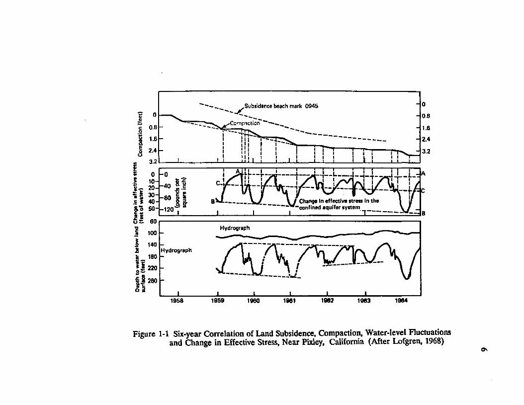
Figure 1-1 Six-year correlation of land subsidence, compaction,
water-level fluctuations and change in effective stress,
near Pixley, California 6
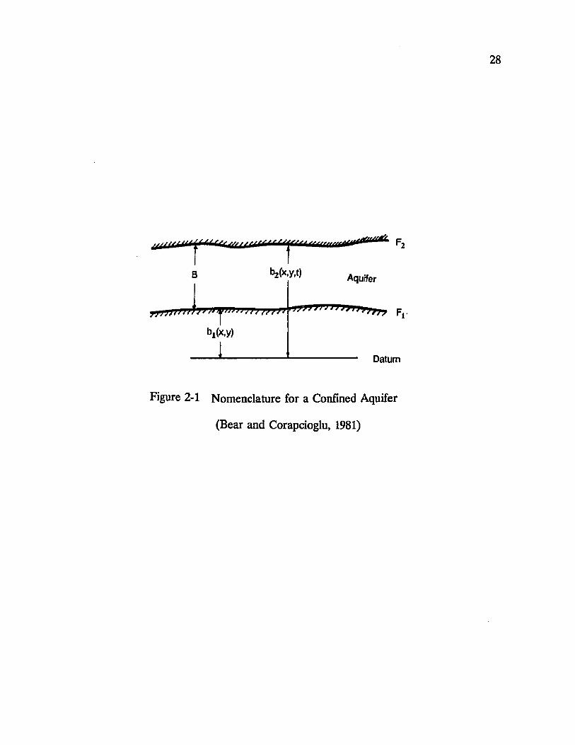
2RFigure 2-1 Nomenclature for a confined aquifer
Figure 2-2 Notation of parameters in an unconfined aquifer ^6
Figure 3-1 Comparison of analytical solution and simulation result 94
Figure 3-2 Comparison of analytical solution and simulation result 95
Figure 3-3 Idealized representation for example at Rocky Mountain
Arsenal with finite element mesh (after Voss, 1984) 96
Figure 3-4 Nearly steady-state conservative solute plume as simulated
for the Rocky Mountain Arsenal example by SUTRA
(Voss, 1984) 98
Figure 3-5 Nearly steady-state conservative solute plume as simulated
for the Rocky Mountain Arsenal example by STRALAN 99
Figure 3-6 Transient state conservative solute plume after 20 years
as simulated for the Rocky Mountain Arsenal example
by STRALAN 100
Figure 3-7 Transient state conservative solute plume after 100 years
as simulated for the Rocky Mountain Arsenal example
by STRALAN 101
Figure 4-1 Piezometric surface (feet MSL) in the Gonzales-
New Orleans aquifer, Fall 1963 (after Rollo, 1966) 109
Figure 4-2 Contours of land subsidence (in feet) between 1938 and
ix
Figure 4-3
Figure 4-4
Figure 4-5
Figure 4-6
Figure 4-7
Figure 4-8
Figure 4-9
Figure 4-10
Figure 4-11
LIST OF FIGURES (continued! Page
1964, New Orleans (from U.S. Coast and Geodetic Survey,
after Kazmann and Heath, 1968) 109
Land surface subsidence compared with water level in wells
along line A-A’ (after Kazmann and Heath, 1968) U0
Location map of the study area and its vicinity 115
Geologic cross sections along A-A" and B-B" in Figure 4-4
(after Dial and Sumner, 1988) 116
Thickness and coefficient of permeability of the Gonzales-
New Orleans aquifer (The '700-foot" sand), New Orleans
Area, Louisiana (after RoIIo, 1968) 118
Contours of water level (in meters below mean sea level) in
the Gonzales-New Orleans aquifer in 1961-1962
(after Rollo, 1968) U9
Contours of piezometric level (in meters, MSL) in the Gonzales-
New Orleans aquifer, Novenber 1985, New Orleans area
(based on data from the U.S. Geological Survey,
Louisiana office) 1^0
Contours of chloride content (in ppm) obtained from wells in the
Gonzales-New Orleans aquifer in 1961-1962 (after Rollo, 1966) 122
Subsidence in the New Orleans area, 1964-1985
(from Zilkoski and Reese, 1986) 126
Land subsidence compared with piezometric drawdown in the
127New Orleans area along line A-A’
Figure 4-12
Figure 4-13
Figure 4-14
Figure 4-15
Figure 4-16
Figure 4-17
Figure 4-18
Figure 4-19
Figure 4-20
LIST OF FIGURES (continued!Page
Average monthly pumpage from the Gonzales-New Orleans
aquifer in 1963 in New Orleans (after Rollo, 1963) 129
Model calibration. Piezometric drawdown (in meters) below
mean sea level in 1981-1982. (a) Observed data;
(b) Simulated result 138
Model calibration. Approximate positions of freshwater and
saltwater interface (250 ppm isochlor) in the Gonzales- 139
New Orleans aquifer in the vicinity of New Orleans, Louisiana
Model calibration. Comparison of drawdown (1981) in the
Gonzales-New Orleans aquifer along A-A’ cross section 140
Model calibration. Comparison of observed and simulated
chloride concentration (1961-1981) in the Gonzales-
New Orleans aquifer along A-A’ cross section 141
Model calibration. Comparison of land subsidence (1961-1981)
in the New Orleans area along A-A’ cross section 142
Simulated land subsidence (in centimeters) in the New Orleans
area between 1961 and 1981 145
Model verification. Piezometric drawdown (in meters) below
mean sea level in 1985-1986: (a) Observed data;
(b) Simulated result 147
Model verification. Approximate positions of freshwater and
saltwater interface (250 ppm isochlor) in the Gonzales-
New Orleans aquifer in the vicinity of New Orleans, Louisiana 148
xi
LIST OF FIGURES (continued!
Figure 4-21 Model verification. Comparison of drawdown (1985) in the
Gonzales-New Orleans aquifer along A-A’ cross section
Figure 4-22 Model verification. Comparison of observed and simulated
chloride concentration (1985) in the Gonzales-New
Orleans aquifer along A-A’ cross section.
Figure 4-23 Predicted piezometric drawdown (in meters) below mean sea
level in 1995 with different scenarios of pumping rates:
(a) 75 Mgal/d; (b) 100 Mgal/d
Figure 4-24 Model prediction. Approximate positions of freshwater and
saltwater interface (250 ppm isochlor) in 1995 in the
Gonzales-New Orleans aquifer in the vicinity of
New Orleans, Louisiana
Figure 4-25 Predicted land subsidence (in centimeters) in the New Orleans
area (1961-1995) with annual average pumping rate of
50 Mgal/d
Figure 4-26 Predicted land subsidence (in centimeters) in the New Orleans
area (1961-2010) with annual average pumping rate of
50 Mgal/d
Figure 4-27 Prediction of land subsidence with different scenarios of
pumping rates in 1995 and 2010 in the New Orleans area
along A-A’ cross section
Figure 4-28 Predicted piezometric drawdown (in meters) in the New
Orleans area in 1995 with annual average pumping rate of
140 Mgal/d
Page
149
150
153
154
155
157
158
165
Page
Figure 4-29 Predicted piezometric drawdown (in meters) in the New
Orleans area in 1995 with annual average pumping rate
of 230 Mgal/d 166
Figure 4-30 Contours of predicted land subsidence (in centimeters) in the
New Orleans area in 2005 with annual pumping rate of
140 Mgal/d if surface water supply is cut off by 4%
(subsidence is relative to 1961) 167
Figure 4-31 Contours of predicted land subsidence (in centimeters) in the
New Orleans area in 2005 with annual pumping rate of
230 Mgal/d if surface water supply is cut off by 9%
(subsidence is relative to 1961) 168
Figure 4-32 Model prediction with recharging wells. Approximate
positions of freshwater and saltwater (250
ppm isochlor) in the Gonzales-New Orleans aquifer
in the vicinity of New Orleans, Louisiana
(recharging rate is 10 Mgal/d) 1^1
xiii

ABSTRACT
Land subsidence and saltwater intrusion problems are encountered
concurrently or individually in many coastal areas, especially where heavy pumping
is exerted. In order to evaluate the extent and progress of these two phenomena in
quantity and quality, a two-dimensonal model, the STRALAN (Solute Transport
and Land Subsidence) model, is developed to simulate fluid movement, solute
transport and land subsidence in a non-homogenous, anisotropic, compressible and
sloping aquifer system.i
The governing equations of the model, i.e., the fluid mass balance equation,
solute mass balance equation and land subsidence equation for confined or
unconfined as well as for sloping aquifers are derived in detail. Hybridization of
finite element and finite difference methods is employed for the numerical solution
of the governing equations which describe the interdependent processes of fluid
density-dependent saturated ground water flow, solute transport and land subsidence
caused by changes of pressure due to pumping.
STRALAN model provides, as primary calculated results, piezometric
drawdown (or pressure), solute concentration and subsidence spatially and
temporally in the simulated subsurface system. It has a wide variety of options from
which one can select to simulate either a confined aquifer or unconfined aquifer;
either a horizontal or sloping aquifer; land subsidence only; saltwater intrusion only;
or both of the above; steady or transient state condition for ground water flow,
jriv

solute transport or land subsidence and many other options. Similar to a U.S.
Geological Survey model, the SUTRA model, STRALAN also can cope with single
chemical species transport including processes of solute sorption, production and
decay.
STRALAN model, is applied to the Gonzales-New Orleans aquifer, New
Orleans area, Louisiana, where saltwater intrusion and land subsidence are critical
issues. This case study includes: the calibration of the hydrogeologic parameters in
this 352 square-mile area; the verification of the model; and prediction of the
drawdown, chloride concentration and land subsidence in time and space in 1995 and
2010 with several management scenarios, including surface water supply cut-off
supplementary pumping and recharging well management.
The model is also verified by comparing the simulation result with an
analytical solution in terms of subsidence.
xv

CHAPTER 1
INTRODUCTION AND PURPOSE
1

2
Coastal ground water management is subject to the constraints of saltwater
intrusion and land subsidence associated with a lowering of the inland piezometric
head due to extensive pumping. The moving interface between fresh water and salt
water, whether it is sharp or dispersed, can be regarded as a dynamic boundary of
the aquifer varying in time and space. Saltwater encroachment may reduce the
potable ground water storage and influence the extraction of ground water.
Within the past two decades, analysis of an aquifer system containing both
fresh water and salt water was based on a number of different conceptual models.
Many computer models using these conceptual models have been developed for the
analysis, prediction and control of saltwater intrusion in coastal aquifer systems (Bear
and Verruijt, 1987; Willis and Finney, 1988). Based on the dynamic behavior of
fresh and salt water, these models can be classified into: (1) sharp interface models
in which the fresh water and salt water are considered as two immiscible fluids, and
the Dupuit assumption is valid so that the flows in the aquifer are essentially
horizontal (Shamir and Dagan, 1971; Kashef 1975; Wilson, Townley and Coasta,
1979; Bear and Kapuler, 1981); and (2) transition zone models in which the fluids
are miscible, and both horizontal and vertical movement of fluids occur in the flow
region caused by advection and hydrodynamic dispersion (Pinder and Cooper, 1970;
Lee and Cheng, 1974; Huyakom and Taylor, 1976; Volker and Rushton, 1982).
These model require the solution of the advective-dispersion-diffusion equation .
According to the dimensionality, saltwater intrusion models can also be
grouped into three categories (Reilly and Goodman, 1985): (1) two-dimensional
cross-sectional models with both sharp or dispersed interface (Wilson, Townley and
Coasta, 1979; Frind, 1982); two-dimensional areal models with a sharp or dispersed
interface in a heterogeneous and anisotropic aquifer (Voss, 1984); and (3) three-
dimensional models for either confined or unconfined aquifer (Guswa and LeBlanc,
1981; Huyakorn et al., 1987).
Yan, Adrian and Wang (1988) used the SUTRA model developed by Voss
(1984) to investigate the potential problems of saltwater intrusion within the 900 km1
Gonzales-New Orleans aquifer from 1961 to 1986. The simulated results of the
approximate position of the freshwater and saltwater dispersed interface (250 ppm
isochlor) during this period show good agreement with the available observation
data. These results were from the preliminary study in which the assumptions were
made that the aquifer was horizontal with constant rate pumping throughout the 20-
year simulation period.
Land subsidence often occurs in areas where there is intensive withdrawal of
ground water from an underlying aquifer or withdrawal of oil and gas from an
underlying reservoir (Bear and Corapcioglu, 1981a; 1981b; Bell, 1987). However,
subsidence is more commonly produced by the excessive pumping of a ground water
basin than in oil and gas fields (Corapcioglu, 1983). The subsidence is attributed not
only to the consolidation of the sedimentary deposits in which ground water is
present but also to the increasing effective stress due to the decrease in pore
pressure caused by pumping.
The amount of subsidence is governed by the various factors such as effective
pressure, the thickness and compressibility of the deposits or aquifer, the length of
time over which the increased loading is applied, and the rate and type of stress
(e.g., pumping) applied (Lofgren, 1968).
Many areas in the world experienced significant land subsidence due to
extensive pumping of ground water. THe areas of greatest extent and maximal
settling in the United States, and probably in the world, are found in California. A
maximum of 9 meters of subsidence was measured in San Joaquin Valley, where
large quantities of ground water have been pumped to support the valley’s immense
irrigation needs (Corapcioglu, 1983). In Tokyo (Japan), several million people live
in an area of 80 square kilometers subsided to 2.3 m below mean sea level (Poland,
1972). In some coastal cities in China, land subsidence is substantial (People’s Daily,
1988a; 1988b). In Shanghai (China), where over 10 million people live in an area
of 150 square kilometers, the maximum land subsidence due to pumping reached as
high as 2.63 meters in 22 years, averaging 12 cm/yr (People’s Daily, 1988a, Appendix
7). Land subsidence in Tianjin City , China, in 1987 was 4.3 cm, 1.9 cm less than
the previous year because of the effective management measures enforced by the
local government (People’s Daily, 1988b, Appendix 8). In Venice (Italy), the
subsidence is only 8 cm in 16 years. However, the ground surface is less than 1-2
meters above mean sea level (Poland, 1972). The environmental conditions
associated with subsidence may be more critical than the magnitude itself.
Other places where subsidence due to pumping is of significant importance
are Galveston, Texas; Houston, Texas; Santa Clara Valley, South Central Arizona;
Las Vegas (U.S.A.); Mexico City (Mexico); Osaka, Niigata, Chiba (Japan); Ravenna
(Italy); Taipei (Taiwan, China); Bangkok (Thailand); and London (England)
(Corapcioglu, 1983).

Lofgren (1979) recorded that 20 years of precise field measurements in the
San Joaquin and Santa Clara Valleys of California have indicated a close correlation
between hydraulic stresses induced by groundwater pumping and consolidation of the
water-bearing deposits (Figure 1-1). Kazmann and Heath (1968) also showed this
close correlation between piezometric drawdown and land subsidence in the New
Orleans area (Figure 4-3).
Based on the effective stress concept introduced by Terzaghi (1925), two basic
approaches toward solving land subsidence problems may be found in the literature.
In the first approach, a simultaneous solution is sought for the pressure in the water
and for the strain in the solid matrix (Biot, 1941). Based on Biot’s accomplishment,
several researchers further developed the coupled three-dimensional formulation in
which the governing equations included one fluid flow equation in terms of pressure,
or piezometric head, and three equilibrium equations in terms of vertical and
horizontal displacements. In the second approach, following Terzaghi’s concept
(1925), water pressure is first obtained by solving a simple partial differential
equation with water pressure in the aquifer as the only dependent variable. Once
the water pressure distribution is derived, the effective stress and the resulting strain
distribution are determined. Gambolati and Freeze (1973), Helm (1975), Bear and
Corapcioglu (1981a) applied this two-step approach to determine the vertical land
subsidence. Consequently, numerical solutions for the simultaneous solution of the
coupled partial differential equations have been developed by Ghaboussi and Wilson
(1973), Schrefler et al., (1977) and Lewis and Schrefler (1978) using finite element
methods. Safai and Pinder (1979) extended this approach to subsidence of
Subsidence beach mark 0945
0.8
0.B - 1.6
2.4
2.4 3.2
3.2
- ! -t8 - 20-"40
i!I O 5 0 --1 2 0
Change In effective stress in the confined aquifer system
Hydrograph100
140Hydrograph
- 180 I 220
1 260
19621959 1961 19641958 19631960
Figure 1-1 Six-year Correlation of Land Subsidence, Compaction, Water-level Fluctuations and Change in Effective Stress, Near Pixley, California (After Lofgren, 1968)

saturated-unsaturated porous media.
Bear and Corapcioglu (1981a) developed a three-dimensional mathematical
model based on the ground water mass conservation equation in a compressible
aquifer to estimate the vertical displacement of the aquifer due to pumping by
assuming that the horizontal length of the aquifer is much greater than its thickness.
The equation is then integrated over its thickness. By introducing a relationship
between changes in averaged piezometric head and corresponding changes in aquifer
thickness, a single equation is obtained for land subsidence. Subsequently, a
mathematical model for the areal distribution of drawdown, land subsidence, and
horizontal displacement caused by pumping from a deformable phreatic aquifer was
developed (Bear and Corapcioglu, 1983).
Most of the ground water modeling discussed in the literature were based on
horizontal aquifers. When a sloping aquifer is encountered, a three-dimensional
numerical model is recommended (Chapman, 1980). Modeling of unsteady flow in
sloping bedrock was developed by Frangakis and Tzimopoulos (1979). They studied
the effect of inclination of aquifers on the outflow rate for phreatic aquifers.
In regard to modeling techniques, Prickett (1975) and Bouwer (1978)
presented a survey of the literature. Numerical methods using digital computers are
of major interest in the survey because, in general, the flow equation and solute
transport equation have no closed form solutions that can be obtained analytically.
Finite difference techniques have been applied widely in groundwater modeling.
One of the earliest applications of this technique to a large scale geologic basin was
made by Fayers and Sheldon (1962). Eshet and Lougenbaugh (1965), Bittinger et

al. (1967) discussed various computing schemes that could be used to solve the finite
difference equations. Pinder and Bredehoeft (1968) developed a model which used
the alternating direction implicit method to solve the flow equation of a non-
homogeneous, isotropic, confined and leaky aquifer. A number of models using
finite difference method with different levels of sophistication have been presented
by Bredehoeft and Pinder (1970), Prickett and Lonquist (1971), Cooley (1971), Lin
(1972), Freeze (1972), Trescott et al. (1976), Ozbilgin et al. (1984) and many others.
Another technique which has become veiy popular in solving groundwater
flow equations is the finite element method. The most commonly used approach in
this technique is the Galerkin method which offers an alternative way of formulating
a problem for finite element solution without using variational principles. A
comprehensive discussion of this approach is given by Douglas and Dupont ( 1974).
Following the development presented by Zienkiewicz and Parekh (1970), Pinder and
Frind (1972) developed a model to solve two-dimensional transient groundwater flow
problems with fewer nodes, which proved to be more efficient than the finite
difference approach. Gray and Pinder (1974) studied the accuracy of the results and
computed efficiency by extending the Galerkin approximation to the time derivatives.
Wang and Anderson (1982), Huyakorn and Pinder (1983) provided systematic and
in-depth views on finite difference and finite element methods in groundwater
modeling and in solving subsurface flow problems. Voss (1984b) developed
AQUIFEM-SALT model using finite element methods to solve seawater intrusion
problems. As mentioned previously, he also developed the SUTRA model which is
a hybrid type of model combining finite difference and finite element methods to

solve saturated and unsaturated flow and solute transport problems. Other authors,
affilated with the U.S. Geological Survey, such as Larson (1978), Hutchinson et al.
(1981), Mantenffel et al. (1983), McDonald et al. (1984), Reilly (1984), Guswa et al.
(1981), Cooley (1985), Kuiper (1985) and many others-developed groundwater
models based on these two methods. A comparison of finite difference and finite
element methods was made by Gray (1983) who showed that the two techniques
have more similarities than casual inspection might reveal. He concluded that each
method has special features which may be desirable for a particular application,
hence superiority of one over the other cannot be drawn.
Though the existing numerous mathematical or numerical models for solving
groundwater flow and solute transport or for solving land subsidence have been
developed with different levels of sophistication, a model that incorporates both land
subsidence and solute transport (e.g. saltwater intrusion) has not yet been developed
for coastal aquifers which very likely are subject to these two problems at the same
time. The difficulty mainly lies in the complexity of solving two totally different
problems simultaneously with one model that interconnects the problem with one
dependent variable, i.e., the water pressure. This implies that the solutions of water
pressure, or piezometric head, solute concentration and land subsidence have to be
solved under the conditions of time-varying thickness, porosity, and compressibility
as well as concentration-dependent density. The complexity will be compounded
when sloping beds of a heterogeneous and anisotropic aquifer are considered. It is
the objective of this dissertation to develop such a model to solve the realistic
problems in coastal aquifers.

10
The major objectives of this dissertation research are :
1. To derive the three governing equations that depict the mechanisms of
groundwater flow, solute transport and land subsidence;
2. To develop a computer model that can simulate the drawdown, the solute
concentration and land subsidence in time and space by using the three governing
equations;
3. To apply the newly-developed model (the STRALAN model) to the study area,
the New Orleans area, to simulate the effect of pumping on the movement of ground
water, the dynamic position of the dispersed interface between fresh water and
saltwater in the Gonzales-New Orleans aquifer, and land subsidence spatially and
temporally.

CHAPTER 2
DERIVATION OF GOVERNING EQUATIONS
FOR
COMPRESSIBLE AND SLOPING AQUIFER
11

12
In this chapter, detailed derivation of a mathematical model for ground water
flow for a compressible aquifer is presented first, followed by the derivation of a
land subsidence equation based on Bear and Corapcioglu’s work (Bear and
Corapcioglu, 1981).
The basic assumptions involved in the derivation are: (1) Terzaghi’s
concept of effective stress, (2) horizontal flow in the aquifer, and (3) vertical
aquifer compressibility only. The last assumption is viewed to be a rational
estimate when dealing with regional problems in which horizontal extent is
relatively large compared to the aquifer thickness. By introducing a relationship
between changes in averaged piezometric head and the corresponding changes in
aquifer thickness, a single equation for land subsidence is obtained.
Futher derivation for these equations to accomodate sloping aquifer is
presented, thus providing a more general condition for engineering study.
Derivation for solute mass balance equations is also provided. While derivation
for confined aquifers is described in more detail, the derivation for unconfined
aquifers is also given as elaborately as possible.
Z 1 DERIVATION OF FLOW EQUATION FOR
COMPRESSIBLE AQUIFER
In an elemental control volume in a porous medium, the 3-dimensional
mass balance equation for transient flow can be derived based on the fact that

13
the net rate of fluid mass flow into the elemental control volume is equal to the
time rate of change of fluid mass storage within the element (Bear, 1979; Freeze
and Cherry, 1979):
d ( p v x) d(pVy) 3 ( p v t) a{p<£)+ --------- 4- = ----------------- (la)
3x ay a z a t
or
a(p<t>)v(py) + ------- = 0 (lb)
at
where v = Darcy velocity vector (v„ vp v,) and
Y = 4Y (V is ^ e actual velocity vector of the flow through the
porous medium);
p - fluid density;
4 = porosity of the solid matrix.
Equations (la) and (lb) do not take into account the dispersive flux and
molecular diffusion due to spatial variations in fluid density.
In a deforming porous medium, the relative Darcy velocity is:
Yr = Y - tfY, (2)
where V, = velocity vector of the solid matrix.
Based on Darcy’s law, y. can also be expressed as
Y, = - K v.(h') (3)
where h' is the piezometric head for a compressible fluid and
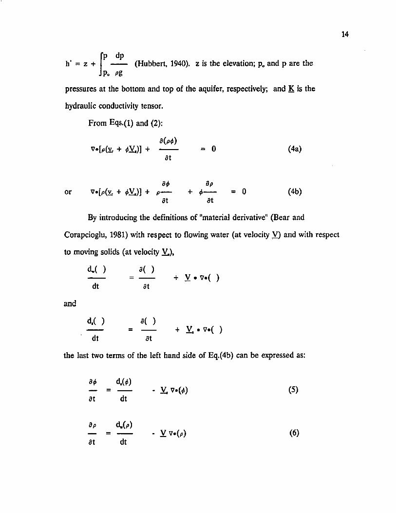
14
IP dp (Hubbert, 1940). z is the elevation; p„ and p are the
P0 Pg
pressures at the bottom and top of the aquifer, respectively; and K is the
hydraulic conductivity tensor.
From Eqs.(l) and (2):
v - M t + « £ ) ] + ------- = 0 (4a)dt
d $ d por + dV.)] + p— + $ ----- ~ 0 (4b)
at at
By introducing the definitions of "material derivative" (Bear and
Corapcioglu, 1981) with respect to flowing water (at velocity V) and with respect
to moving solids (at velocity V,),
<U ) 3( )dt at
and
d.( ) a( )
+ V . v .( )
+ y , . v*( )dt at
the last two terms of the left hand side of Eq.(4b) can be expressed as:
8 * d.(*)- = ------ - V, v .(*) (5)at dt
dp d,(p)— = ------- - V v .(p ) (6)at dt
Also, the first term of the left hand side of Eqn.(4b) can be expressed
follows by using the rules of derivative multiplication:
v»[p(Yr + m ] = p^*(Yt + *V.) + (v,. + <jV,)v*(p)
= pV«(vr) + p[7*(flSV,)] + v,7«(p) + £V,v«(p)
= pV*(vr) + p|>7*(V,) + V>7.(*)] + vrv . ( » + tfV,7*(p)
= pv*(vr) + ^p7.(V.) + pV,v«(^) + v j j * ( p ) + < f > V j 7 » ( p ) (7)
So, by using Eqs. (5), (6) and (7), Eq. (lb) can be written as:
pv.(yr) + <6oV»(Vt) + oV.7»(<&1 + vy (p ) + <AVtV>(o) +
d.(*) ( Wp -------- - oV,7»(<i) + <f> - <AVv*(p) = 0
dt dt
or
or
m ^ (p ) p7«(vr) + $pV*(V,) + p - ■ + ^ —
dt dt
v vYM p ) + ^Y,v.(p) - *(— ) 7 ( p ) = 0 (v V =—)
4 4
[v = because]
d,fa) dw(p)p7*(Yr) "1" <ioV»(Vt) + p + 4 ' + Yr^*(p) +
dt dt
^V,7*(p) - v,7®(p) - ^V,7*(p) = 0 (v Y = Y, + *V.)
therefore,(U p) d,(tf)

16
b d * ( p ) d ,d)v.(v,) + — * + --------- + *v.(V.) = 0 (8b)
p dt dt
Similar to the derivation of Eq. (lb), the solid mass balance
equation in 3-D is expressed as:
d[?,(l - <£)]v [a (1 - + --------------- = 0 (9)
at
where p , = density of the solid.
If p , is assumed constant, Eq. (9) can be written as:
3(1 - 4>)v .[(l - *)VJ + -------------- = 0 (10)
at
By manipulation of derivatives, this equation can be changed to:
a t(1 - *)v.(V,) + V,v*(l - *) - — = 0
at
and by using Eq. (5), we get
H d,(tf)(1 - 4>)V*QL) = — + V ,v .d ) a ------
at dt
therefore,
1 d .d )v.(V,) ---------- . (11)
(1 - 4 ) dt
Terzaghi’s (1925) concept of intergranular stress or effective
stress a is defined by
o = ex’ - p*I (12)
where a is the total stress vector; a is the effective stress; p is the pressure in the
17water and I is the identity tensor. Because the density of p , is assumed constant,
the pressure in the water that causes a stress on the solid particle will not
produce a deformation, i.e., the volume of solid particles remains constant.
Hence, d(Volf) = 0
The total stress £ at a point is shown as (Bear and Corapcioglu, 1981):
s = (1 - *)(&y - *pl (13)
where ( a , ) ' is the average stress in the solid.
Equating Eqs. (12) and (13),
£ = (1 * <£)(£,)' + $pl = £* + pi
This leads to
a = (1 - $0(£,)‘ - pi + tfpl
= (1 - *)(£,)* - (1 - *)pl
= (1 - *)[(£.)* - Pi] (14)
which causes the deformation of the solid matrix. If no change in the total stress
is assumed, then
d£ = 0
which implies
d£ = d(pl)
Assuming vetical compressibility, hence vertical deformation only,
d ^ = dp (15)
Recalling the definition of the compressibility of the solid matrix, a:
1 d(Vol) 1 d(Vol)a —
Vol dp Vol da’
where Vol is the volume of the porous solid matrix. Let Vol, be
the volume of the solid grains. Vol is equal to Vol, plus void space,
(16)

and because d(Vol.) = 0, so
d^ d[(Vol-Vol,)/Vol] 1 Vol.d(Vol-Vol,) -(Vol-Vol,)d(Vol)
dp dp dp (Vol)2 ^
1 VoI.d(Vol) - Vol.d(Vol,) - Vol.d(Vol) + Vol,.d(Vol) [ *-----------------------------------------------]dp (Vol)2
1 Vol,.d(Vol) - VoUd(Vol,)— • [ ]dp (Vol)2
1 Vol,*d(Vol) •dp (Vol)2
Vol, (1 - ^)*VolBecause =1 -<j>
Vol Vol
dtf 1 Vol,.d(Vol) (1 - <f>) d(Vol)so, — = — •-------------------------•-— -—
dp dp (Vol)2 Vol dp
1 d(Vol) 1 d*and — • --------- ------- • -----
Vol dp (1-^) dp
Substituting Eq. (20) into Eqn (16), one obtains
1 d</>
\ -<b da’
When dealing with moving solid, the compressibility of the solid
19
matrix is
d.(4) (22)
U d .(0
d & )Replace ■----- = a’*d,(ff) into Eq. (11) to obtain
W
1 d.(^) d.(a’) d,(p)V.(VJ = ---- . = a’ = a’------- (23)
1 -(/> dt dt dt
By definition, the compressibilty of water (in motion) is
1 cUp)b’ = — . (24)
p dp
So, the second term in Eq. (8b) can be written as
<Up) 4> < L ( p ) d*(p)
dt p dw(p) dt
d*(p)
dt(25)
Also, from Eq. (23), we have
d,(4) d,(p) = (1 - t y -------
dt dt
and
d,(p)
dt
(26)
(27)

20Add Eqs. (26) and (27):
d.(tf) d.(p)+ *v.(V.) = a ' (28)
dt dt
By substituting Eqs.(25) and (28) into Eq. (8b), we obtain
<Up) d.(p)v.(vr) + *b’------ + a *------ = 0 (29)
dt dtcL(p) d p
B ecause — + Y*vpdt dt
vand Vv«p = —vp
where v (Darcy velocity) is proportional to vp, so v»vp is proportional to
(vp)2, which is very small. Therefore, it is justifiable to assume that
dp v ap— » Vv«p (= —v*p), hence, <f>— » v v»pat 4> at
d,(p) apAlso, --------= — + V, *vp
dt at ap
With the same reason, we can assume that — » V, v*pat
With these two assumptions, Eq.(29) may be approximated by
ap apv»(v,) + ^b’— + a — — 0 (30)
at at
api.e., v*(vr) + (a’ + *b’)----- = 0 (31)
__________________at
a(p#)From Eq. (1), v^v + ------- 0 , we get
at
21
34 B ppV(v) + yvp + p — + 4>- ■■ ■ — 0 (32)
at at
Because yvp is proportional to (vp*Vp), which is very small, we can assume that
d p4 — » vV p . So, Eq. (32) becomes
at
3 4 B p*>v»(v) + p — + 4 ------= 0 (33a)
at at
or8 4 4 B p
v.(v) + — + —•------- 0 (33b)at P at
From Eq. (24),
1 cU p) 1 (U p) dt
p dp p dt dpb’ = — « - (34)
d*(p) apAgain, because = — + V*Vp,
dt at
B p B p— » V«Vp or 4 — » vVp can be assumed, andat at
dt at— = — . This is because pressure, p, is only dependent on time, t, at one dp ap
location.
Eq. (34) now can be approximated by
l ap at l Bpb’ ~ —•—•— = —•— -= b (35)
p at ap p ap
where b is the compressibilty of the water not in motion.

22Eq. (35) can also be written as:
1 dp ap—•— = B-p at at
4> dp apSo, — •— = </>n—
p at at(36)
From Eq. (26),
d,(*) d,(p) = (l-^)a’----
dt dtdt(37)
With the same reason shown above, we can approximate
d,(tf) d<t>
dt at
andd.(p) ap
dt at
Eq. (37) can be expressed as
d<f> ap— = (W )°------ (38)at at
a here is the approximation of a , because we are now using partial derivatives
rather than "material derivatives" for approximation.
By inserting Eqs. (36) and (38) into Eq. (33b), we obtain
ap ap7*(v) + (l-fll)a:—— + tpR— '—= 0
at at
which isap
7*(v) + [(l-0)a + *3} 0 (39a)at
23
or3p
v.(v) + Sop— = 0 (39b)dt
where Sop = (l-^)a + f a is the specific storativity with respect to pressure
changes. Also, because
Y = Vr + ^ V, ,
v«(v) = v«(vr) + v«[^V,]
= v .fc ) + & . Q Q + V,v(*) (40)
Eq. (33b) becomes
d<f> 4> d pv.(v,) + ^v»(V.) + Y,.7(^) + ---- + — ------ = 0 (41)
3t p at
d,(^) d<f>Because — r + V,«v(0)
dt 3t
m d,(p)and from Eq. (26), -------- (l-^)a’-------,
dt dt
Eq. (41) becomesd,(p) 4 d p
v*(v,) + W Q L ) (l-^)a’-------+ — —■ (42)dt p at
From Eq. (35), we get
1 d p 3p— = 6------ (43)
p dt dt
and from Eq. (23), we can get
d.(p)v.(V,) = Or* (44)
dt
Eq. (42) now becomes

24d /p) d /p) ap
v .fe ) + <f>a ------+ (l-^)a’— + <f>B — - 0 (45)dt dt at
which can be simplified as
d,(p) apv»(vr) + a 1- <j> s— = 0 (46)
dt at
d /p ) apAgain, because = — + V,«v(p), we can assume that
dt at
ap— » V,*v(p) at
So, we obtain from Eq. (46) a new form for approximation:
ap apv*(Yr) + a ------+ <f>& = 0 (47a)
at at
orap
?•& ) + («’+ ^b)-----= 0 (47b)_________________at
kpgAccording to Eq. (3), v, = -K*v(h'), where K = -------(/i = dynamic viscosity of
pwater), and
fp dp 17 | [ ------ ] = Vz + -----J p 0 P g P g
v(h‘) = vz + v | [ ---- ] = vz + — vp (48)p g
So, in Eq. (47b), the relative Darcy velocity v, can be written as:
k¥r = - —(Vp + pgVz) (49)
Eq. (48) can have another form for approximation:

25
Ph = z + —
f i g
So, by assuming z is a constant,
ah* 1 ap
at pg at
ap ah*then, — = p g — (50)
at at
By inserting Eq. (50) into Eq. (47b),
ah*v-fc) + pg(a’+^B)-----= 0 (51a)
at
or
ah*v.(vr) + s ; ----= 0 (51b)____________ at
where S0* = pg(a’+^is)
In summary, different assumptions lead to different forms of ground water
flow mass balance equations for compressible aquifers at a point as listed below:

26
Assumptions Flow equation Equation No.
ap ap ap» yvp; —» VTVp 7 ,(Yr) + (q’ + s’)— = 0 31
at at at
dp ap4>~ » vVp; b’~b; a%=a; v»(v) + — = 0 39bat at
a<j> ap— » V,v^; — » V,vp; where = (l-^)a +at at
dp ap ap4 > - » vVp; — » V,vp; V«(v,) + (a’ + e)— = 0 47bat at at
b = b’ ah'v.(y,) + so‘ — = 0 51b
at
where S0‘ = p g ( a + 4 > a )
Eqs. (31), (39b), (47b) and (51b) are all point equations in 3-Dimensions.
In order to transform the 3-D equations into those that have dependent variables
(pressure and effective stress) depending only on x, y and t (that is, 2-D
problems), the 3-D equations have to be integrated over the thickness of the
aquifer.

27
Figure 2-1 shows the configuration of a confined aquifer in which the
bottom boundary is assumed steady.
Functions of the boundary surface are:
Fi = F.(x,y,z) = z - b,(x,y) (52)
i.e., z = b,(x,y)
Similarly, z = b2(x,y,t)
F2 = Fj(x,y,z,t) = z - b2(x,y,t) (53)
Thickness of the aquifer B = b2 - bt = F2 - F2 (54)
For any moving boundary, the material derivative is again used:
dF aF = — + u«vF = 0 (55)dt at
where u is the speed of the vertical displacement of the boundary. When we
consider the flow of water and assume water density on both sides of the
boundary is constant (i.e. [/>]uj)» the condition of flux continuity to be satisfied at
the upper boundary is:
[p(v - = 0 (56a)
or [v - ^ u j^ n = 0 (56b)
where [v - ^u]UJ is the relative velocity of water flow across the boundary from the
upper side (subscript u) to the lower side (subscript 1) of the boundary; [ ]uj = [ ]u
- [ ],; and n is a unit vector outward normal to the boundary (Bear and
Corapcioglu, 1981).
Y " " ........... p2
Aquifer
rT T T rrrrrT T rrrrrr? Fr
B
m
bi(x.y)
_ 1 _ Datum
Figure 2-1 Nomenclature for a Confined Aquifer
(Bear and Corapcioglu, 1981)

vFSince by definition, n = ------ , Eq.(56b) can be reduced to
|vF |
[y - ^uh-vF = 0 (57)
For an impervious boundary, no water passes through the boundary:
v |u = 0
111. = o
So, [v - ^u]„j = [v - ^u]0 - [v - ^u],
= -[Y - ft], (58)
and since v = vr + ^V,, Eq. (57) can be written as
[v - to]ua»vF = -[v - £u],»vF = -[v, + ^(V, - u)],*vF = 0 (59)
If we also assume that F is a material surface with respect to the solid, the
following condition must also be satisfied, the derivative of which is similar to
that for the flow of water at the boundary:
[V, - u],*vF2 = 0 (60)
E q. (59) becomes:
y,*vF2 = 0 (61)
An alternate form of boundary conditions can be derived in terms of v
instead of v , :
From Eq. (58), [y, + $ ( ¥ , . - u)],«vF2 = 0
i.e. vF2»yr Ji + ^Y,|,*vF2 - u|,*vF2 = 0 (62)
Also from Eq. (55):
aF2 aF2u*vF2 = or u | j*vF2 -------
at at
Eq. (62) becomes:
30
3F2vFj-vJ, + ^Y,|,*vF2 + <j>-----= 0 (63)
at
which can also be written as:
3F2[yr|, + ^Y,|j *vf2 = - $ —
at
aF2i.e. [v, + *YJ,.vF2 = - 4 > ----- (64)
at
By inserting Eq. (2) into Eq. (64):
3F2y |,.vF2 = - ^ ------ (65)
at
for a stationary surface,
y[,*vF2 = 0
When the upper boundary is a phreatic surface, we can also use Eq. (57):
[v - ^u]UJ»vF - 0
i.e., [v - 0u]uvF3 - [v - 0u]!*vF2 = 0
v | u.v F 2 - (0 u ) [u.v F 2 - v |,.vF2 + (f tO I^ F , = 0 (66)
From Eq. (55):
3F2u»vF2 = -----
at
aF2i.e., u l^ v F j = ------
at
Eq. (66) can be rewritten as:

31
aF2i.e., v | u*vF2 - v | , .vF2 + [^]uj------= 0 (67)
at
where y |„*vF2 = -N = - Nvz is the rate of accretion and [^]ul can be
interpreted as effective porosity or specific yield. So Eq. (67) can be written as:
aF2
2.1.1. Integration Along the Thickness of a Confined Aquifer
. a h *From Eq. (51b), i.e., v » ( y ,) + S„’ — = 0, we can integrate this equation
along the thickness of the aquifer, taking into account the boundary conditions at
the top and bottom surface. The purpose of doing so is to obtain a quasi three
dimensional flow equation and land subsidence equation such that the dependent
variables are averaged values and are only functions of time and the planar
coordinates x and y. That is:
Y|,*vF2 = - Nvz + fo]UJ- (68)at
aF2= - N + [<f] aj-----
at
(69)

Before this integration can be performed, the following derivation is
essential. For an aquifer with thickness B = b2(x,y,t) - b,(x,y) and any vector,
A(x,y,z), the following derivation can be performed using the Newton-Leibnitz
rule. Assume A is continuous and has the partial derivatives with respect to x,y
the closed region R(x, < x <x2, y, < y < y2 and z, < z < z2).
For simplicity’s sake, first take the vector A as a two-dimensional vector
A(x,y). The upper and lower limits of the integral are b, and b2, respectively,
assuming b ,« x « b2.
Let u = b2(y), v = b^y), w = y
so that the integral F(y) =My)bi(y)
A(x,y)dx
uA(x,w)dx
= G(u,v,w)
where u, v, and w all depend on y. By the chain rule:
dF aG du a G dv aG dw
(70)
dy au dy 3v dy aw dy
where3G
au au
u[A(x,w)dx]
(71)
(72)
By a fundamental theorem of calculus:
d
dxf(x)dx = f(x)
so that Eq. (72) becomes:

33aG
-= A(u,w) = A[b2(y), y]
and
au
du d[b2(y)]= b/(y)
(73)
(74)dy dy
So the first term on the right hand side of Eq.(71) is
aG du = A[b2(y),y]b2’(y)
au dy
Eq.(71) is further developed by noting:
(75)
Also,
aG a
av av
= - A(v,w)
= - A[b,(y), y]
dv dEb^y)]
u aA(x,w)dx = — { -
v avA(x,w)dx)
u
(76)
(77)dy dy
The product of Eqs.(76) and (77) gives the second term of Eq.(71) as:
aG dv dbt(y)— •— = - A[b,(y), y ] = - Afb.O^yJb^y)av dy dy
(78)
By Leibnitz’s rule, we get
aG a
aw aw
uA(x,w)dx =
u aA(x,w)dx (79)
aw
and by replacing Eqs.(75), (78) and (79) into Eq.(71):
dF d
dy dy
H y )A(x,y)dx =
bL(y)
W y) 3A(x,y)
bi(y) aydx + A[b2(y), y]b2’(y)
- A[bj(y), y]bt(y) (80)

34Eq.(80) can be rearranged to:
C rw,Jb,(y)
'i(y) 3A(x,y) d rb2(y) dx = ------ | A(x,y)dx - A[b2(y), y]b2’(y)
(y) a y dy
+ A M y ) , y]b,’(y) (81)
In our problem, letting z, = b„ Zj = b2, i.e., « z « bj, we can proceed in a
similar manner to obtain
b t(x,y)v*A(x,y,z,t)dz = v.
■b2(x,y,t)
bt(x,y)A(x,y,z,t)dz
A[x,y,b2(x,y,t),t]b2’(x,y,t)
or
+ A[x,y,b1(x,y)]b1’(x,y)
v*b,
A(x,y,z)dz =bt
v»A(x,y,z)dz + A |M»7b2
- Al^.vb,
Therefore, v«A dz =bt b.
A dz - A |M«vb2 + A |bl«vb,
(82)
(83)
(84)
Let A’ = A(x,y), i.e. only two-dimensional coordinates are considered, Eq.(84)
becomes:
fbi fb2 9 A,I v*A(x,y,z)dz = I (v’*A’ + )dzJbi Jbj az
fb2 = v’« A’
JbiA’dz - A’lbj.vb, + A’j^.vb! + A,[b2 - A j bl (85)
where primed symbols designate components and derivatives in x- and y-direction
only. Using the vector derivative definition:
35
a(z-bj) a(z-b2) 3(z-b2)A |b2*vF2 = A |b2.v(z-b2) = A |bJ[ i + j + Js]
ax ay az
ab2 ab2 az ab2= A U 1 j + — k k]
ax ay az az
ab2 ab2 ab2- A U -(— i + — j + — k) + kj
ax ay az
= A U -vb2 + k]
= -A ’|Hvb2 + Aj|„2 (86)
ab2Note that k = 0, because b2 = b2(x,y,t) does not have z component.
az
Similarly,
A U .vF, = A |„.v(z-b,)
= - A’|„.vb, + A ,|„ (87)
where A’ = A j + A j
aA, aAy aAIand v« A i + — j + — k (i, ], k are unit vectors)
ax ay az
Insert Eqs.(86) and (87) into Eq.(85) and let A’ be the average over the thickness
of the aquifer:
1 fb2A’ = — A’(
B JbiA’dz
so that Eq.(85) becomes
£v*Adz = v’»BA’+ A |m. vF2 - A |bi*vF, (88)h i________________________________________

For any scalar h'(x,y,t), we can also follow the previous derivations [Eq.(71)
through Eq.(88)] and obtain
fb2(x,y,t) ah* a fb, ab2 ab,— dz = — h*dz - h‘|w — + h’L -----
Jbj(x,y) at at Jbx at at
a 3(Z-F2) a(z-F,)— (Bh*) •- h‘|b2-------- + Y»*L-------at at at
a az aF2 az— (Bh*) - h*|b2— + h’l,bl h |bi“ "at at at at
3Fj- h‘|bl------
at
a az aF2= — (Bh‘) - — (h‘|bI - h '|bl) + h*|u-----
at at at
aF,- h*|bl——
at
Assume a vertical equipotential for a confined aquifer, h. = h*|bl = h ' |b2,
then,
fb2 ah* a _ aF2 aFt_ d z = — (Bh-) + h’U h*|M— (89)
Jbj at at at at
- 1 P 2where h" = — I h’dz is the average piezometric head along the thickness ofB Jbt
the aquifer.
In general,
t>2(x>y.t).vh dz= v’(Bh*) + h’|wvF2 - h'jb.vFj (90)
. bi(x.y)
We can now evaluate Eq.(69), which is

37
’b2(x,y,t)v«(vr)dz +
bi(x,y)
*b2(x,y,t) ah*SQ*— dz = 0
b,(x,y) at(91)
Using Eq.(88), the first term of Eq.(91) is
v.(vr)dz = v’Bv/ + v,|b2.vF2 - vr|b,.vF, b,
(92)
For impervious boundaries (meaning a confined aquifer), Eq.(61) is valid, i.e.,
yrU*vF2 = 0
yr|bl.vF2 = 0
fb,So,
btv .fe jdz = v’*By/
Using Eq.(89), the second term of Eq.(69) is
■b2 ah* _ a(Bh’) aF2 aF,S0‘— dz = S0’[ ------- + h*|M h*|bl ]
b, st 3t at at
_ ah' aB aF2 aF,= S0*[B— + h '— + h*|b2— - h*|bl— ]
at at at at
_ aB aF2 aF,Because h*— + h '[b2------- h*|b,—
at at at
aB aF, aF2 _ aB a=h*[-------(---------- )] = h*[----------(F,-F2)]
at at at at at
aB aB= h*[----------- ] = 0
at at
and by assuming a vertical equipotential, h' = h*|bl = h '|b2 and
B = F, - F2, Eq.(95) therefore becomes
(93)
(94)
(95)

38
s ;fb2 ah' ah'
— dz = s; . b — b, at at
By replacing Eqs.(94) and (96) into Eq.(91), we obtain
ah*v’.(Byr’) + S0'.B ------= 0
at
(96)
(97)
where _ 1s; = —
B
rb» .S0 dz
bt
1h' = h* -----
Bh*dz
and v/ = yr’(x,y,t) =B
vr’(x,y,z,t)dz
1
B
K’ — •B
K’.v ’h d zbi
v’h'dzb,
K’ rb2= - —*[v’ h'dz + h’lu-vFj - h’lb^vF,]
B Jb,
K’= — .[v’(Bh') + h 'U .v F . - h 'I ^ F J
B
K’= — ♦[Bv’h' + hV B + h*|b2.vF 2 - h*|bl.vF J
B
K’» - — .[Bv’h' + h'(v’B + v.F 2 - vF,)]
B

39
K’= -----•{Bv’h* + h*[v’B - ?’(F,-F2)]}
B
= - K W h ' (98)
where K’ is the hydraulic conductivity vector averaged over the thickness of the
aquifer. Eq.(97) now becomes:
ah'- v’.(BK W ’h') + S ; .B — = 0 (99a)
at
ah'or v’.(B K W ’h') = S0‘.B — (99b)
___________________ at_
Again, the prime symbols indicate vector components and derivatives in the x and
y directions only.
In the above equation, i.e.,Eq.(99b),
- 1 _ _ Pv’h' a v’h = — v’p + v’z ( v h « z + — ) (100)
g p p g
ah' ah 1 ap azand b — - — — * + — (101)
at at ?g at at
where z = b, + B/2 indicates the average elevation of the mid-thickness of the aquifer.
To develop another form of integrated flow equation, we can integrate
Eq.(39) instead of Eq.(51b), i.e.,
T>2 3PT>2v*vdz +
b,Sop dz = 0 (102)
^ at
Again, similar to the derivation of Eq.(88),

40
rb2V*vdz = 7’
bi
rb2
b,vdz + v | m7F2 - v | bl7Fi
v’.Bv’ + v |b2.vF2 - v^vF ,
Similar to Eq.(65), we can obtain
y[b2'VF2 = - 4>2
and vlbj.vF! = - 4>r
aF22 TI™ Bi
aF,
at
Therefore, Eq.(103) becomes:
3F: aF,
1v»vdz = v’Bv’ - <f>2------+ <i>i—b, at at
The second term of Eq.(102) is
fb, S PS „— dz = s„bj at
= S,
*b2 ap— dz
b, at
fb2 a[(h-z)pg]op — dz
. b, at
rb2 ah fb2 d z[ — dz -Jb, at Jbi at
= sop[
where = [(l-^)a + ~ +
Eq.(106) is approximately equal to
dz ]Pg
PgS0p[\ ah _ a(Bh) aF2 al
—dz] = p g S ^ l + h ^ h |bl—b, at at at a
(103)
(104a)
(104b)
(105)
(106)
41
_ ah _ aB aF2 aF,= PfiSopJB■■■ — + h ■ + h)M------ h |bl------]
at at at at
_ ah aB a= pgSop{B— + h[----------(F,-F3)]}
at at at
= pgSop[B— ] (107)at
Combine Eq.(105) with Eqs.(106), (107) and (102), i.e., assuming vh* = vh, we
obtain
aF2 aF, _ ah7’,Bv’ - <f>2-+ <t>i — + PgSopB — = 0 (108)
at at at
Because the boundaries are impervious, <f> is very small,
Also, B = F, - Fj - b2 - b , , where b, = constant
Therefore Eq.(108) becomes
_aB _ ah'- v’Bv’ = 4>— + S^pgB— (109)
at at
Since the bottom surface is assumed stationary, z = b,(x,y), we can redefine a’
for vertical compressibilty only (i.e. no horizontal displacement, aA is constant)
1 d(Yol) 1 aB 1 aB 1 ab2
Vol da’ B d a B ap B dp
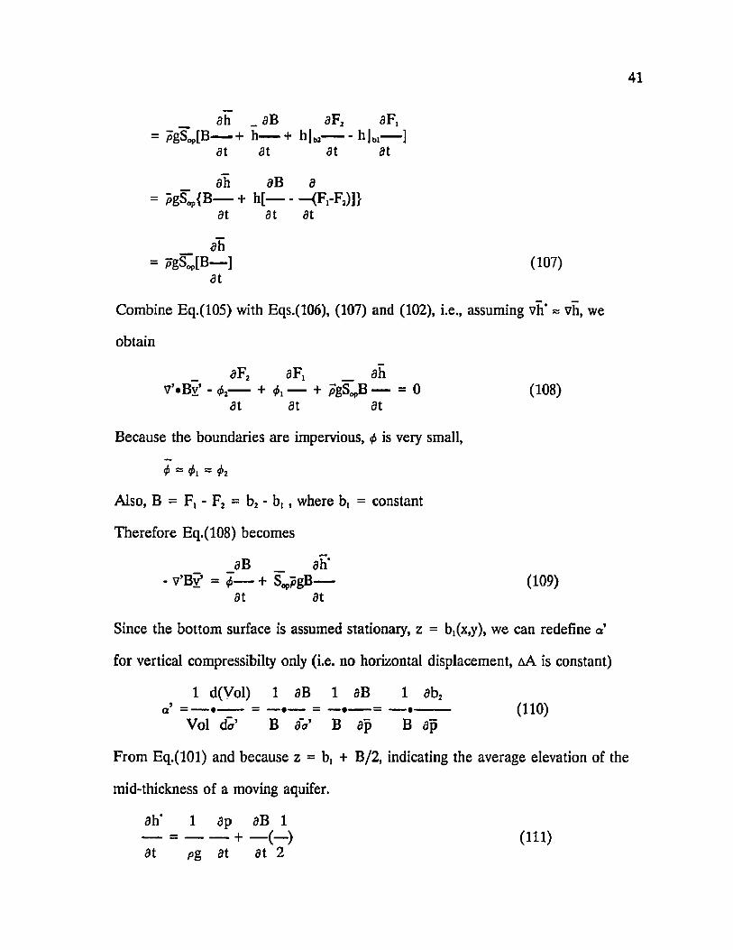
From Eq.(lOl) and because z = b, + B/2, indicating the average elevation of the
mid-thickness of a moving aquifer.
ah* l ap aB l— — ( - ) (111)at Pg at at 2

42
From Eq.(llO), we can refine E q .(lll) as :
ah* l aB 1 1 aB= (112a)
at pg at Bo’ 2 at
ah’ 1 1 aBi-e., — = (— + -------)-
at 2 a B p g at
ah a’Bpg + 2 aB— = (----------- ) - (112b)at 2 a B p g at
Therefore,
aB 2 ( a ' B p g ) ah'
at 2 + a ’Bpg at
a fBpg ah'= [-------------------]— (H3a)
1 + ( a ’B p g / 2 ) at
Since a’Bpg/2 « 1, Eq.(113a) becomes:
aB ah'— » a JB p g (113b)at at
Hence, Eq.(109) becomes:
ah’ ah*- v’Bv’ = 4 > ( a B p g )— + S^pgB —
at at
ah' _ _“ Bpg [tfa + S^]
at
ah'= Bpg [ $ a + (l-^)a’ + fl]
at
ah*= B [pg(a + fl)] (114)
at

43
ah’So, -v’«(Bv’) = S0’*B— (115)
at
where S0" = p g ( a + ?b)
Recall S0 = p g ( a + 4b), S0‘ = pg(a’ + £b) = S0" (116)
and Eq.(115) can be written as
— _ ah*^ .(K ’.Bv’h') = S0"B (117)
at
Because of the relation of Eq.(116), Eq.(117) can be expressed as:
_ _ ahv’«(K’Bv’h) = S0”B— (118a)
at
a*or v’.(K ’Bv’h) = S0’B— (118b)
at
This means that Eqs.(99b) and (117) can both be approximated by
ahv’.0C’Bv’h) = S„B— + Q (119)
__________________ at
where SD = S0* = S0” [L]1 is the average specific storativity; Q = Q(x,y,t) is the
pumping rate (+), or recharging rate (-), in terms of volume of water per unit
L3 Larea per unit time. [— = — ]
T .L 2 T

44
2.1.2, Integration Along the Thickness of an Unconfined Aquifer
In an unconfined aquifer, the upper boundary is the water table. We can
replace b2(x,y,t) by h(x,y,t), so that the thickness of the aquifer is
B = h - b, (120)
Following the same procedure used above and assuming also vertical
equipotentials, we can also obtain the following equation, the same as Eqs.(92)
and (96):
ahv’*Bvr + £ | b.vF2 - y ^ .v F , + S0*B — = 0 (121)
at
Because the bottom boundary is impervious,
VjI^^vFj = 0 [Same as Eq.(93)]
From Eq.(68):
aF2y |h«vF2 = - N + [*]UJ—
ataF2
y J ^ v F j = - N - Sy (*V,)|b2.vF2 (v Y=yr+ 0V,)at
ah= . N + Sy — - ( m [m-vF2 (F2=z-b2=z-h) (122)
at
where Sy = -[^]uj is the specific yield of the unconfined aquifer. Because
ah</>V,«vF2 « Sy— and h = h’, the third term on the right hand side of Eq.(122)
at
can be dropped out and Eq.(121) becomes:
ahv’By,’ - N = -(Sy + S0*B)— (123)
at

According to the definition of the averaged dependent variable along the
thickness of the aquifer, the total flow in the aquifer is:
Bvr’ =h(x,y,t)
bi(x,y)
fh
fhvrdz - (-K.vh’)dz
b.
-K’ vh'dzb,
= -K’{v h'dz + h '|hvF2 - h*|blvF,}
= -K’{vBh‘ + h '[hvF2 - h’U.vF,}
= -K’{Bvh* + h‘vB + h*|hvF2- h'l^vF,}
= -K’{Bvh‘ + h’[vB - v(F, - F3)]}
= -K’[Bvh*] = -K’[Bvh] = -K’(h - b,)vh
This approximation is made possible due to the assumption of
h « h - - h - | h*h*|«
Therefore, from Eq.(123), we can obtain:
— _ ah-v.K’(h - b,)7h - N = -[Sy + S/(h - b,)]-----
at
_ _ ahor v*[K’Bvh] + N = (Sy + Sn'B)—
at
If pumping or recharging is considered, then Eq.(125b) will be:
ah
(124)
(125a)
(125b)
v.[K’Bvh] = (Sy + S0*B)— - N + Q ______________________ at________
(126)
where positive Q means pumping and negative means recharging.
Since Sy » S„'B, we can further approximate Eq.(126) as :

46
ahv*[K’Bvh] = Sy — ± Q (assuming N = 0) (127)______________ at
2 2 DERIVATION OF LAND SUBSIDENCE EQUATION
2.2.1 Confined Aquifer
The basic idea of deriving a land subsidence equation is first to determine
the piezometric head distribution h = h(x,y,t) or the drawdown s - h(x,y,0) -
h(x,y,t) using Eq.(119) in Section 2.1 for a confined aquifer and Eq.(126) for an
unconfined aquifer. From the relationship derived as (E q.ll2a in Section 2.1),
ah* 1 aB 1 1 aB
at p g at Ba’ 2 at
ah* 1 aB 1 aB . — . (128)at 2 at a ’B p g at
1 aB a 1 a azwhere —•— = —(—B) = — (b, + B/2) = —
2 at at 2 at at
ab,This is because z = b, + B/2, b, = b,(x,y) is independent of time, i.e.— = 0.
at
So, when the piezometric drawdown is s=h(x,y,0)-h(x,y,t), Eq.(128) can be
rewritten as
ah' 1 aB as az 1 aB-------------------------------- . - (129)at 2 at at at a ’Bpg at
aB a[B°(x,y) - B(x,y,t)] aswhere — ----------------------- — , S = B°(x,y) - B(x,y,t) is the land subsidence.
at at at
47
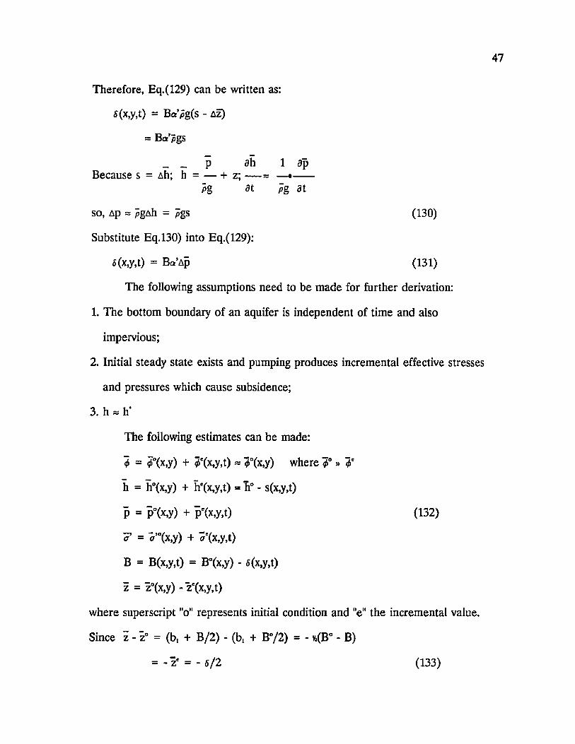
Therefore, Eq.(129) can be written as:
5(x,y,t) = Ba’pg(s - az)
= Ba’pgS
- _ P 3h 1 apBecause s = A h ; h = — + z; — ~ —•----------
pg 3t p g at
so, Ap » p g & h = p g s (130)
Substitute Eq.130) into Eq.(129):
5(x,y,t) = Ba’Ap (131)
The following assumptions need to be made for further derivation:
1. The bottom boundary of an aquifer is independent of time and also
impervious;
2. Initial steady state exists and pumping produces incremental effective stresses
and pressures which cause subsidence;
3. h « h*
The following estimates can be made:
4> = 4>°(x,y) + ^'(x,y,t) ~ ?°(x,y) where 4>° » 4>'
h = h°(x,y) + h'(x,y,t) - li0 - s(x,y,t)
P = P°(x,y) + P '(W ) (132)
a ’ = a’D(x, y) + ae(x,y,t)
B = B(x,y,t) = B°(x,y) - s(x,y,t)
z = z°(x,y) - ze(x,y,t)
where superscript "o" represents initial condition and "e" the incremental value.
Since z - z° = (b, + B/2) - (b, + B°/2) = - <B° - B)
= - ze = - s / 2 (133)

48
So, z* = 5/2 (134)
Total stress in the solid matrix can be assumed as a constant, i.e.,
<7 = - P
= 7°(x.y) + 5’e(x,y,t) - [p°(x,y) + p*(x,y,t)]
= constant
It also means that the total stress at any time is a constant, i.e.,
* = F°(x,y) - P°(x,y)] + [ o ’ \ x , y,t) - p*(x,y,t)]
= o ° + [a ‘(x,y,t) - p“(x,y,t)] (135)
Since a - a°, we have
CT,e(x,y,t) = p'(x,y,t) (136)
1 a(Vol) 1 aB 1 aB l 8BHence, a = ------------= —•----- = --------- -- — •------- (137)
Vol ay B a ? B d d ’c B ap*
ap* aB a(B° - 5) asa’B— = — --------------------- (138)
at at at at
and 5(x,y,t) = a’B[p(x,y,t) - p°(x,y] = a’Bp* (139)
6or p* = — (140)
a’B
5or a ’ = ------- (141)
Bp*
Eq.(139) is equivalent to Eq.(131). By inserting Eqs.(132), (136), (138) and
(139) into Eq.(119) of Section 2.1, we obtain the equation for the undisturbed
initial steady state:
v’.(K ’BvV) = 0 (142)
and the equation for transient state under pumping conditions:

49ah'
v’.(K ’Bvh') - Q(x,y,t) = S0B — (143)at
lBecause h' = — p' + z' and from Eqs.(132), (134) and (140),
Pg
ah' 1 ap' az'
at pg at at
l a s a s= __-------(— ) + — (— )
pg at a’B at 2
1 as s a l l as= [-------- •— + — •—(—)] + — •—
pga’B at pg«’ at B 2 at
1 1 as s a l= ( + —)— + •— (— )
pga’B 2 3t pgat’ at B
1 + %(pga’B) as s aB= [----------------]------------------— (144)
pga’B 3t pga’B2 at
pga’B SBecause-------- « 1 and — = 0 (145)
2 B2
Eq.(144) can be approximated as
ah' 1 as— « ------ . ----- (146)at pga’B at
1 asEq.(144) implies that— *— = 0, hence resulting in Eq.(146). This in turn
2 at
implies that the effect of changes in the aquifer’s axis (z) is negligible, because
Bz = — + b, and B = B° - s
2
az aB as— ^O (147)
at at at

50
In a 3-D space, with the same reasoning we have just gone through, we can
obtain:1 1 6 6
vhe = —*vp' + vze = —v*(— ) + v(—) pg p g a’B 2
1 1 1 1= (------- + — )vs + ---- 6V( ---- )
pga’B 2 p g a’B
1= ---------------- * V 6 (148)
Pga’B
Note that a’B may vary in x-y the plane. Because we have already assumed
1 1 » — in Eq.(146), andpga’B 2
3he 1 a s 8 6— = —•—(— ) + _ ( — ) at pg at a’B at 2
I l as a l d s= — [— . — + 6 —( )] + — (— )
pg a’B at at a’B at 2
I I 8 6 -1 aB -1 d a 8 6= —{— •— + fi[ •— + ------- •— ]} + —(—-)
pg a’B at a'B2 at B (a’)2 at at 2
1 1 as 1 1 aB l da’
pga’B 2 3t pga’B B 3t a* 3t
1 + li(pga’B) 8 6 1 1 aB 1 d a ’= [-----------------]---------- <5 [ •--- + —•—]
pga’B 3t pga’B B 3t a 3t
1 8 6 1 1 aB 1 3a’ pga’B= -------- --------- fi[—• + —• ] [ v « 1 ]
pga’B dt pga’B B at a’ at 2
1 8 6 1 aB 1 da’ [v = because]= ------- [-------5(-------- -- — )] (149)
pga’B at B at a’ at

51
In order to get the result of Eq.(146), the following comparison should be valid:
as 1 aB 1 da— » s ( —•-------+ —•— ) orat B at a* at
1 aB 1 3a’ 1 88(—• — + —•— ) « —•----- (150)
B at a at s at
Similarly,
1 1 1— VS » —VB + —Va (151)
S B a’
With the assumptions of Eqs.(145), (148), (150) and (151), Eq.(143) becomes:
I ’ __ 1 36v(— .vs) - Q(x,y,t) = S0— •------ (152)
pga pga at
- r Pgor, with K’ = ----- ,
p
Eq.(152) becomes:
k’ _ asv ( _ . v s ) - Q(x,y,t) = S¥ — (153)
pa* at
_ S0 _ Bwhere Sv = -------= ( 1 + <t>—) [Sc = pg(a’ + ?b)]
'pga a
_ k’and Q, = — is defined as the consolidation coefficient for an isotropic
fia
medium. Eq.(153) is thus expressed as:
asv ( O v s ) - Q = S¥ — (154)_________________at
which is the land subsidence equation for a confined aquifer.

52
2.2.2 Unconfined Aquifer
Recall the flow equation derived for unconfined aquifer in Eq.(126),
Section 2.1:
ahv[K’Bvh] = (Sy + S0*B) N ± Q (155)
at
This equation is approximated under the condition that the total stress in
the solid matrix is not varying with time. This is valid when the water table does
not vary remarkably during the operation period. Other assumptions are :
1. The entire aquifer is assumed to be composed of an averaged soft material
that behaves like a homogeneous deformable porous medium;
2. There is no time lag between pressure changes and subsidence;
3. Only vertical displacement takes place and vertical compaction is produced
only within the flow domain where changes in water pressure occur.
4. The phreatic surface (on which p=0) serves as the upper boundary of the flow
domain. No consideration is taken of the unsaturated zone.
5. The bottom boundary of the phreatic aquifer is fixed, i.e., b, = b,(x,y) =
bi(x,y,0).
With these assumptions, derivations for Eq.(l) through (141) in Section
2.1 to 2.2.1 are valid for the present case.
The deviation from steady state produced by pumping in an unconfined
aquifer is as follows:
ah'v(K’Bvh‘) = (Sy + S0B ) N ± Q
at(156)

53
where he is the deviation of piezometric head from steady state h°, i.e., h = h°+
1h' = s(x,y,t). Because he = —«p' + z' and from Eqs.(132), (134) and (140),
P g
we get the following result by manipulating the same derivation as that for Eq.
(146):
ah' 1 ap' az'
at pg at at
1 as. ------ (157)
pgct’B at
1and vh' ~ *vs (158)
pga’B
The assumptions made previously are all appropriate here. As a reminder, they
are:
pga’B 1
2
&— = 0 (159)B2
l aB l act l as(-—»-—■ + —• —■) « —-•
B at a’ at s at
By inserting Eqs.(157) and (158) into Eq.(156) and taking into account the
following factor:
k’pgK’ = --------, we obtain
p

54k’ 1 as
v( «7s) = (Sy + S0'B)----------- N +. Qpa’ pga’B 3t
SY S0‘ as= [-------+ ------ ]----- N ± Q (160)
pga’B pga’ 3t
As has been defined, S0' ~ S0 is the average specific storativity [= pg(a’+^n)] k*
and C v = — is the consolidation coefficient for an isotropic medium andf ia
s 0 s ;S, = — = — . Therefore, the land subsidence equation for an unconfined
pga’ pga’
aquifer is:
Sy as. v(Qv5) ± Q + N = (--------+ Sy) (161)
____________________ogq’B______ at
2 3 DERIVATION OF GROUND WATER FLOW EQUATION FOR SLOPING AQUIFER
2,3.1 Unconfined Aquifer
1. Assuming the flow is horizontal.
When the flow is assumed to be horizontal, Darcy’s equation is
supplemented by the Dupuit-Forchheimer assumptions which state:
(a) the free surface inclination is small so that streamlines can be taken as
horizontal and (b) the hydraulic gradient is equal to the slope of the free surface
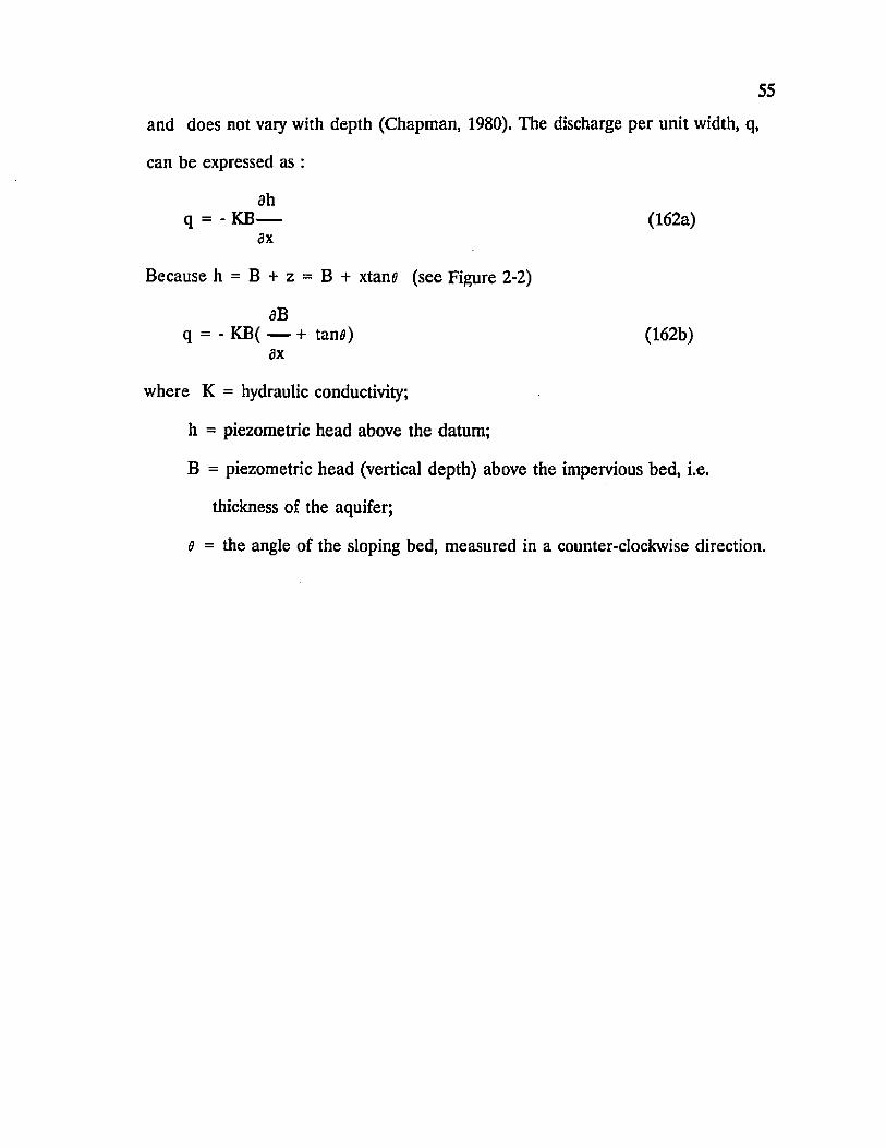
55
and does not vary with depth (Chapman, 1980). The discharge per unit width, q,
can be expressed as :
ahq = . KB— (162a)
ax
Because h = B + z = B + xtana (see Figure 2-2)
aBq = - KB( — + tana) (162b)
ax
where K = hydraulic conductivity;
h = piezometric head above the datum;
B = piezometric head (vertical depth) above the impervious bed, i.e.
thickness of the aquifer;
8 = the angle of the sloping bed, measured in a counter-clockwise direction.

56
h
x
pa' to bed
Bed
Figure 2-2 Notation of Parameters in an Unconfined Aquifer

57
By considering the inflow and outflow of an elemental control volume, the
mass balance equation can be derived in the same manner as that obtained in
Eq.(126) of Section 2.1, except that a "tan a" term has to be introduced in the
gradient term just as we obtained in Eq.(162b):
ahv[KB(vB + tana)] = [Sy + S0‘B] N + Q (163)
at
However, ground water flow is not always horizontal. In fact, many cases
suggest that it is non-horizontal, especially in the case of a sloping bed. Thus,
Eq. (163) often referred to as Boussinesq’s equation, is no longer valid in such
cases.
2. Assuming the flow is parallel to the bed.
In order to modify Eq.(163) to accomodate this condition, the following
relationship based on Figure 2-2 have to be establishe
h’ = (h - x*tana)cosa (164)
dh dh dh’ sin(a + a’)— = <— )/<— ) = -------------- (165)dh* dl dl sina'
By definition, the slope of the free surface of ground water is the tangent of the
streamline with respect to the axes parallel and perpendicular to a coordinate
system. If the coordinate system is selected to be the sloping bed and its
perpendicular line, then
dh’— = tana’ (166)ds
In this case, we are assuming that the streamline is parallel to the bed. The
Dupuit-Forchheimer assumption can be applied to this coordinate system. Thus,
the flow across a unit width of the thickness perpendicular to the bed is:
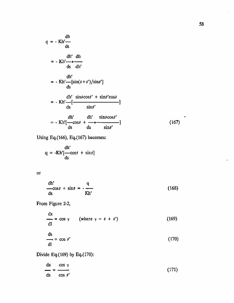
58
dhq = - Kh’—
ds
dh* dh = - Kh’— -----
ds dh’
dh’= - Kh’— [sin(0 + 0’)/sin0’]
ds
dh* sin0cos0’ + sin0’cos0= - Kh’— [------------------------------ ]
ds sine’
dh’ dh’ sin0cos0’= - Kh’[— cos0 + — ----------------- ] (167)
ds ds sin0’
Using Eq.(166), Eq.(167) becomes:
dh’q = -Kh’[— cosfl + sinfl]
ds
or
dh’ q— cosfl + sin0 = ------- (168)ds Kh’
From Figure 2-2,
dx— = cos 7 (where 7 = 0 + 0’) (169) dl
ds— = cos 0’ (170) dl
Divide Eq.(169) by Eq.(170):
dx cos 7
ds cos 0’(171)
59
From another perspective, taking into consideration Eqs.(164), (166)
and (171),
dh dx dhq = -Kh’— = - K(h -xtans)coss — •-
ds ds dx
cos-y dh= - K(h - xtans )coss •------- (172)
coss’ dx
Rearrange Eq.(172), and because cos 7 = cos(s + 0’),
dx -K coss’coss - sins’sins— = — (h - xtans )cosS(---------------------------- )dh q coss’
K sins’= — (h - xtanS)«(cos2s sinscoss)
q coss’
K sins’= (h - xtans)»(l - sin2s sinscoss)
q coss’
K K dh’= - - ( h - - xtans) - - < h - xtans )*(-sin2s ----- sins cos s)
q q ds
K K dh’ sins= - - ( h ■- xtans) -f —h’[-—coss + sins]------
q q ds coss
K K q dh’ q= - - ( h ■- xtans) •t- —h’(------)tans [y — c o s s + sins =: --------
q q Kh’ ds Kh’
K--------(h -• xtans) - tans [v = because]
So, dx K— + (h - xtans) + tans = 0 (173)dh q
60or
-K dx— (h - xtan*) = — + tan* (174)
q dh
dhMultiply (— ) to both sides of Eq.(174):
dx
-K dh dx dh— B(— ) = (— + tan*)(— )
q dx dh dx
dh= (1 + — tan*)
dx
Therefore,dh dh
q = -KB(— ) / (1 + — tan*) (175)dx dx
ah a aBBecause --------= — (B + xtantf) = — + tan*
ax ax ax
and when we are differentiating only with respect to the x direction,
dh ah— = — r so, Eq.(175) becomes dx ax
ah aBq = - KB— / [1 + (— + tan*)tan*]
ax ax
ah (aB/ax)sin*cos* + sin2*= - KB— / {1 + [-------------------------------- ]}
ax cos2*
ah cos2* + sin2* + (aB/ax)sin*cos*= - KB— / [--------------------------------------------- ]
ax cos2*
ah= - Kcos2*B— / [1 + (aB/ax)sin*cos*] (176)
ax
Because we assume that the streamlines are parallel with the bed, therefore
61
dB— « 1, and Eq.(176) becomes ax
dhq = - Kcos20B— (177a)
ax
aBor q = - KcoszaB(— + tanfl) (177b)
ax
It is obvious now that for a sloping unconfined aquifer, the advection term y or q
has to be corrected with a factor of cos20 as shown in Eq.(177a) when the
dependent variable is the piezometric head. Thus, the flow equation for the
unconfined sloping aquifer is:
ahv[KB(vh)cos20] = [Sy + S0'B] N ± Q (178)__________________________ at_________
ora ah a a(B + xtane) a aB sins
— (KB— ) = - [K B -----------------] - — [KB(— + ----- )]ax ax ax ax ax ax cos a
Therefore,a aB a(KB) ah
— (KB— )cos2fl + sinacosfl = [Sy + S„*B] N ± Qax ax ax at
(179)
In general, Eq.(179) can be expressed as
ahv[Kb(vB)cos20] + v(Kb)sinflcosfl =[Sy + S0*B]------ (180)
at
2.3.2. Confined Aquifer
In a confined aquifer, the streamlines of the flow are even more closely

parallel with the sloping bed. Therefore the derivation for the flow equation is
very much similar to that for the unconfined aquifer. However, we have to use
Eq.(119) in Section 2.1 instead of Eq.(126).
The resulting equation for a confined aquifer is:
ahv(KBvhcos20) = S0B— +. Q (181)___________________ at
or
ahv[KB(vB)cos20 + v(KB)sin*cosa] = S0'B— (182)
at
Eqs.(178) and (181) are the two forms of the flow equation used in the present
dissertation for modeling ground water, land subsidence and salt water
intrusion.
CHAPTER 3
COMPUTER MODEL DEVELOPMENT AND MODIFICATION
(STRALAN - SOLUTE TRANSPORT AND LAND SUBSIDENCE)
63
64
The newly developed model, the Solute Transport and Land Subsidence
(STRALAN) model, is based on the USGS’s SUTRA model in that it adopts the
basic numerical methodology SUTRA employs. When STRALAN is reduced to only
a solute transport function, STRALAN produces the same results as those SUTRA
does.
STRALAN has some other important new features:
a. The capability of solving ground water flow, solute transport and land subsidence
simultaneously or individually in a confined or an unconfined aquifer. In other
words, STRALAN can cope with compressible aquifers or time-dependent thickness
problems.
b. The capability of solving ground water flow, solute transport and land subsidence
for horizontal aquifers as well as for sloping aquifers.
c. The capability of direct input and output of drawdowns of piezometric head (or
water level) instead of input and output of pressures.
In this chapter, the three major governing equations are first presented in
terms of pressure, solute concentration and subsidence, respectively. The
methodology for solving these equations by hybridization of the finite element and
finite difference approach will be discussed. Then the structure of the computer
program will be discussed on a subroutine to subroutine basis. Lastly, two sets of
simulated results produced by STRALAN and SUTRA are compared. In addition,
a hypothetical example is presented with the purpose of comparing computer
simulated results with an analytical solution for only the case of land subsidence,
since several comparisons of analytical with simulation results have been done with

the SUTRA model (Voss, 1984).65
3.1 The Major Governing Equations
In Chapter 2, Eqs.(119) and (126) are the flow equations in a compressible
aquifer for confined and unconfined aquifer, respectively. For simplicity’s sake,
assume S„B represents the multiplier of the time derivative term for both equations.
That is, in the case of an unconfined aqufer, S0B = Sy + S0*B. The general 2-D
equation is thus expressed as:
ahv(KBvh) = SJB + Q (183)
at
Physically, this is the fluid mass balance expressed in volume of fluid (water) per unit
L L3area per unit time [— = — ].
t tL2
P &>gSince h = — + z, Sc = p g ( a + ^s), K ----- and g = -|g |vz,
pg M
kp[g| vpv(KBvh) = v[-------- *B(----------- + vz)]
p Isl
kHgl 1= v[------- «B---(vp + p |g |vz)
p p|gl
k= V[— B(vp - Pg)\
p
The right hand side of Eq.(183) is
ah ap 1S0B— + Q — S0B— •-------- + Q
at at p g

Multiply both sides of Eq.(183) by p , the fluid density, and note that Sc=p | g | S^’
where S^’ = Sop + 4 a = (l-^)a’ + 4 a + 4 a = a + f a [see Eq.(114) in Section
2.1].
Eq.(183) now becomes:
k p 3 pv[ B(vp - P g ) ] = pS^’B— + Qp (184)
n d t
In the derivation from Eqs.(l) to (51) in Section 2.1, the effect of solute
concentration (C) on the density was not taken into consideration. Actually, the
B(p4)term (p<j>) in the derivative in Eqs.(l) and (4a) is a function of pressure (p)
dt
and concentration (C). Individually, 4 is only a function of p, not C, and p is mainly
a function of C and temperature. Therefore, when temperature is constant,
d ( p 4 > ) B ( 4 p ) d p d(p^) dC = ,-------+ •--------
at ap at aC at
d<f> d p d p 3 C
ap at aC at
34 3 Vwin which— = — (------ ) = S^, the specific pressure storativity, wherein V„ is the
ap ap V
volume of voids in the solid matrix and V is the total volume of the matrix.
In the process of deriving the flow equation for compressible aquifers in the
last chapter, S^ has been replaced by S0 which is further approximated by S^’ in this
chapter. Obviously, Eq.(184) should be modified to take into consideration the3 p aC
effect of concentration on density. Therefore an extra term ^B— • shouldaC at
be added to the right hand side of Eq.(184). Note that this extra term has a B, the
thickness of the aquifer. This is because we are dealing with a control volume with
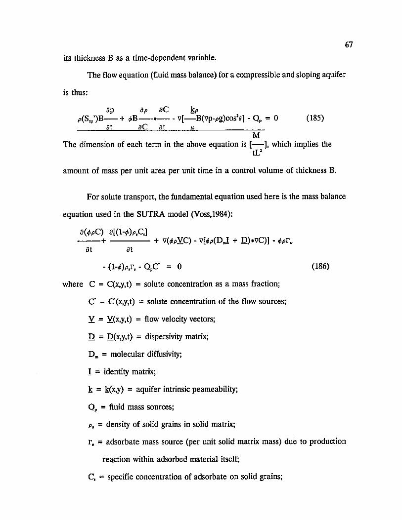
67
its thickness B as a time-dependent variable.
The flow equation (fluid mass balance) for a compressible and sloping aquifer
is thus:
dp d p d C k p/>(Sop’)B------+ tfB----- *---------------- v[— B(vp-pg)cosJfl] - Qp = 0 (185) at d C d t (i___________________
MThe dimension of each term in the above equation is [— ], which implies the
tL2
amount of mass per unit area per unit time in a control volume of thickness B.
For solute transport, the fundamental equation used here is the mass balance
equation used in the SUTRA model (Voss,1984):
d ( # p C ) a[(W )p,C(] h-------------------+ v(^pVC) - + D)*vC)] - <f>pTv
at at
- ( l - ^ , r , - QPC* = 0 (186)
where C = C(x,y,t) = solute concentration as a mass fraction;
C’ = C'(x,y,t) = solute concentration of the flow sources;
Y = V(x,y,t) = flow velocity vectors;
D = D(x,y,t) = dispersivity matrix;
Dm = molecular diffusivity;
I = identity matrix;
k = k(x,y) = aquifer intrinsic peameability;
Qp = fluid mass sources;
p t = density of solid grains in solid matrix;
r, = adsorbate mass source (per unit solid matrix mass) due to production
reaction within adsorbed material itself;
C, = specific concentration of adsorbate on solid grains;

68
r w = solute mass source in fluid (per unit fluid mass) due to production
reactions.
In cases of solute transport where adsorption does not occur, Eq.(186) is
reduced to:
d ( < i > p C ) + v(^pVC) - vfep(DJ + D).vC] - QPC‘ = 0 (187)
at
This equation contains the redundant fluid mass balance contribution, which is
d(p<f>)Y) + -------- Qp (188)
at
Multiply both sides of Eq.(188) by C:
8 ( p 4>)C + C v .(^V ) = CQP (189)
at
The first and second terms on the left hand side of Eq,(187) are
d ( p < f > C ) d ( p < f ) aC + v.(p^VC) = C + p<j>— + C*7 (p^Y) + p < f > V * v C
at at at
aC= p<f> .+ + CQP (190)
at
Substitute Eq.(190) into Eq.(187) to obtain
aCp<ji + p 4 y .v C - v[p*(DJ + D).vC] - QP(C* - C) = 0 (191)
at
Because we are now dealing with mass balance in a volume with time-dependent
thickness B, we have to modify the above equation by multiplying each term with B
except for the mass source term Qp. Also taking into account the effect of the
sloping aquifer on the ground water flow, i.e. the advection term, the solute mass

69balance can thus be expressed as:
aCp<f>B — + P 4>BVcos^.vC - v[p*B(DJ + D).vC] - QP(C‘ - C) = 0 (192) sjl-____________________________________________________
For a land subsidence equation, Eqns(154) and (161) of Section 2-2 in Chapter 2 can
be combined into a general form:
asv ( O w ) - S;— + Qp = 0 (193)____________ at___________
kwhere Q, ---- , p. = fluid viscosity and a = compressibility of the solid matrix.
I
Sv* = Sv = (1 + <f>----- ) for a confined aquifer;
ST' = (-------- + S„) for the unconfined aquifer and 5 = subsidence.Pga’B
Eqs.(185), (192) and (193) are the three governing equations used in the
STRALAN model. When a horizontal confined aquifer is considered without having
a land subsidence problem, the governing equations are reduced to the following two
equations used in the SUTRA model:
Flow equation:
3p 3p aC kppS^ — + t — v[— *(vp - Pg>] - Qp = 0 (194)
at aC at n
and
Solute Transport equation:
d Cp4,— + ^ V . v C - v [ p *[D J + D).vC] - QP(C‘ - C) = 0 (195)
at
70
As mentioned above, p , the density, is primarily dependent upon fluid solute
concentration and temperature. The density model employed by STRALAN is
identical to that used by SUTRA:
d pp = p ( C ) ~ p Q + ----- ( C - C 0) (196)
d Cd p
where p 0 is the base fluid density at base concentration C0 and — is a constantd C
value of density change with concentration.
3.2 Numerical Methods
STRALAN employs a hybridization of finite element and finite difference
methods to solve actually three physical models, one to simulate ground water flow,
the second to simulate the movement of a solute in the ground water and the third
to simulate the subsidence or compaction of the solid matrix from which water is
withdrawn.
The hybridization of the two numerical methods is used such that the time
discretization is based on a finite difference approximation for the time derivative
terms in the governing equations while other terms which describe fluxes of fluid
mass and solute mass are approximated with finite element methods. This hybrid
method is believed to be an efficient and economical approach which preserves the
mathematical elegance and geometric flexibility of finite element simulation, while
taking advantage of the finite difference efficiency.
In the numerical modeling, the aquifer is treated as a three dimensional
space. The third space dimension consists of a finite thickness of the aquifer which
71may vary in time and space. The hydrogeologic unit is divided into a mesh
consisting of a number of finite elements, quadrilateral in shape, each of which has
four comer nodes at the center of each vertical edge of the element.
In the spatial domain, three types of discretization are employed. Aquifer
parameters such as hydraulic conductivity, dispersivity, diffusivity, compressibility of
the solid matrix and fluid density are assigned or evaluated as averaged values along
the thickness of the aquifer in each element of the mesh (element-wise). The values
of dependent variables of fluid pressure (or piezometric head), solute concentration
and subsidence are computed at each node in the mesh (node-wise) with linear
change in value between adjoining nodes along element edges. The terms of the
time derivatives appearing in the governing equations and the value of specific
storativity are evaluated cellwise. Each cell is centered on a node and its boundaries
are half way between opposite sides of an element.
In the temporal domain, the simulation period is divided into a number of
discrete time steps. The time derivatives of fluid pressure (or piezometric head),
solute concentration and subsidence are approximated by a backward finite
difference method with an iterative process (Voss, 1984) and will be discussed in
detail later.
In the process of simulation, certain variables and terms in the three
governing equations are approximated through elementwise and nodewise
discretization. The result is that each equation is no longer exactly equal to zero i.e.,
ap dp aC kp0(p)=pSop’B + <f,B— . --------- v[— B(vp - pg)cos2*] - Qp * 0 (197)
at aC at p
aC0(C)=p^B-----+ P <f>BVcos’fUvC - v[p^B(DJ + D).vC] - QP(C‘-C) x 0 (198)
at

72
360 ( 6 ) = V (Q V 5 ) - s;-— + Qp * 0 (199)
at
where 0 ( ) is the result of approximating the terms of the equations and the
variables. In other words, 0 ( ) is the residual R(x,y,t) of the approximation.
The Galerkin method of weighted residuals (Pinder and Gray, 1977) uses a "basis
function" $;(x,y) to minimize the error of approximation of the equations over the
entire smulated region and during the entire time of simulation in order to
accurately reproduce the physical behavior predicted by the exact governing
equations:
R(x>y,t)$i(xiy)dV = o (i =1,NN)V
where V is the volume of the simulated region and NN is the number of nodes in
the mesh.
Eqn.(200) can be expanded as:
ap(pS^— )®,(x,y)B,(x,y,t)dA +
at
d p aC ( 4 — •— )^,(x,y)Bi(x,y,t)dA
A aC at
‘ kpv[— (vp - pg)]cos10$i(x,y)B1(x,y,t)dA - | QpdV -
A f1 - j *M P bc - p)]dV
= 0 (201)
Note that the integrals are manipulated over a volume of V at node i with a
thickness of B. Therefore, dV - Bi(x,y,t)dA. The last term is a boundary source
term which comes from a specified boundary pressure condition, wherein up is a
"conductance" and Pac(t) is the externally specified pressure boundary condition.

73When a very large value is assigned to up, p = pac which is the desired boundary
condition (Voss, 1984).
Numerical Approximation of Fluid Mass Balance fEq.1851
The residual of Eqn. (185) is evaluted through Eqn.(201), one term at a time.
The first term is:
apW — )*i(x,y)Bi(x,y,t)dA =
A at
apW )^(x,y)Bt(x,y,t)dydx (202)
at
apwhere S^’ and — are assigned cellwise, p is evaluated also at the elements
at
around cell i, and B is evaluated at the node centered at cell i. These terms take
on a constant value for the region of each cell i within a time period. For any cell,
Eq.(202) becomes:
apW ) . — ,
at$1(x,y)B1(x,y,t)dxdy (202a)
ap apwhere (pS^X and — ; are the values taken by ( p S ^ ) and — in cell i. The
at at
volume of cell i, denoted by Vj(t), can be expressed as:
V,(t) = $i(x,y)B(x,y,t)dxdy (203)J y Jx
Therefore, the first term of the weighted residual in Eqn.(197) takes on its discrete
approximation in space:
( ,V ^ fo y )H fc y ,t)d A = ( , s , v , (204)A at at

74The second term of Eqn.(201) is also approximted cellwise:
d p d C d p d C[(*— )— ]$i(x>y)Bi(x,y,t)dA = (<f>— ),(— )i V4 (205)
A aC at aC at
The third term of Eq.(201) which involves the divergence of fluid flux, is also
weighted with the basic function. In order to manipulate this term, the expanded
form of the divergence theorem, i.e., Green’s Theorem, can be applied. Green’s
Theorem is:
= j(W .n )H d r - j(v*W)HdV = |( W .n ) H d r - | (WvH)dV (206)
where H is a scalar and W is a vector, r is the boundary surface of the region, n
is a unit outward normal vector to the boundary. Applying Eq.(206) to the third
term of Eq.(201) and taking dV = Bdxdy into consideration, we get:
k p(v[(— ).(vp - p g ^ co s^H fo y iB ^ tJd x d y
A P
‘ k p[(— )(7P - pg)]cos2a •n$i(x,y)B,(x,y,t)dr
r P
+‘ k p
[(— )(7P - pg)]cos20 •v$1(x,y)Bi(x,y,t)dxdy (207)A M
The first term on the right of Eq.(207) is the fluid mass flux out across the region’s
boundary given by Darcy’s law:
k p^,v001 = - (— )(vp - Pg)cos20.n = qoul (208)
p
where voul is the actual outward velocity at the boundary normal to the surface. The
integral connotes the total flow across the bounding surface of a volume with

75
k = (209)
thickness B at node i, q0un(t) in the units of [M/s].
The second term on the right of Eq.(207) is approximated using a
combination of elementwise and nodewise discretizations. The intrinsic
peremeability matrix k has four components due to the assumption of two
dimensions:
k* K ,
kyx K
wherein k is discretized elementwise. The pressure is discretized nodewise:
NN
P(M,t) - Z p1(t)$,(x,y) (210)i = l
The approximation of (vp - pg) requires particular discretization which maintains the
consistency of vp and p g in terms of vertical variability (Voss, 1984). Thus, the
second term on the right of Eq.(207) is approximated as:
NN
I Pi(0j = i
k p[(— )cos*0V$j]v$1Bj(x,y,t)dydx
r
(211)k p{[— ]cos^(pg)>*v$iB1(x,y,t)dydx
Note that the mesh thickness B is time-dependent and is evaluated at each node
depending on a nodewise discretization:
NN
w O = ZB(x,y,t) = L Bt$i(x,y) i= l
(212)
The last two terms of Eq.(201) are approximated cellwise with a basis function for
weighting:

76
Qp $,(x,y)dV - [up(Pdc - p)].«i(x,y)dVV V
— - Qi - Ui(pi,Ci - p^ (213)
Qp and Uj(pnc - P, are discretizised cellwise:
NNv Qi M
Qp = L (— ) [— ]i= l V, tL2
(214)
NN
OpBC = Up(Pec - P ) = l [(— )(PaCi . pi)ji = l V,
(215)
Mwhere V; is the volume of cell i with thickness B and Qi(t) in [— ] is the total mass
source to cell i. Qp0C in [— -] is the fluid mass source rate due to the specifiedtL3
pressure defined at the boundary and Vj [L.t] is the pressure-based conductance for
the specified pressure source in cell i at the boundary. Eq.(201) can be rearranged
as follows:
M
NN
- Q i + UjPaa + qrN +DF; (216)
where: AF, = (p S ^V , (217)
(218)
k p[(— )cos2* •v«j]*v$1Bi(x,y,t)dydx (219)

D E =k p
[(— -)cosau*(pg)] •v*1Bi(x,y,t)dydx (220)y P
q>Ni = -qouTi (221)
BFjj and DF( require Gaussian integration, which is accomplished with the local
coordinates and converted to global coordinates.
The time derivatives in the above spatially discretized and integrated equation
are approximated by the finite difference method. The pressure term is
approximated as:
dp p r 1 - p"
dt Atatl(222)
The concentration term is approximated as:
dC C" - G°-'(223)
dt At0
This derivative is evaluated using information from the previous time step, as these
values are already known.
The density is evaluated based on C(t“), the value of concentration at the
beginning of the present time step. Because coefficients depend on the, as yet,
unknown values of p and C at the end of the time step, one or more iterations may
have to be employed to solve this non-linear problem based on projected pressure
and concentration:

78
Atn + ic r = Q° + (------ )(C" - C"'1) (225)
Atn
All coefficients dependent on p and C in Eqs.(216) through (221) are estimated at
time level tn+1 based on the most recent values of p and C. Iterations end when the
maximum change in p and C at any node reaches an acceptable tolerance limit
(Voss, 1984).
The weighted residual relations as expressed in Eq.(216) can be written in a
form which allows for solution of pressures, p"*1, at the end of the present time step:
NNAFf r -
( — ) p r + ) p r 1 B F ;jn+i + vpr1 = o r +Atn+l j f i
AF,D+I dCxiPsa"*1 + ■U.- + OF,-*1 + ( )Pl- - (C F ,-)(------ ,)■ (226)
Atn+t dt
where superscripts n or n + 1 denote the time level. Eq.(226) is exactly the form used
in the computer programming, except that Q( and q,Ni are combined into a single
term.
Numerical Approximation of Solute Mass Balance Equation (Eqn.192’1
Similar to the treatment of the fluid mass balance equation, the solute mass
balance equation is modified by adding a point source term QPBc(Qc-C) at points of
specific pressure (neglecting the production and adsorption terms for simplicity
sake):
aCO(C) = P$B----- + ^BYcos’tfvC - v .[„*B (D J + D)vC] - QP(C‘-C)
at
Qpbc(Cbc-C) / 0 (227)

79
where Cnc is the concentration of the flow at the points of specific pressure.
The residual of the approxmation of 0(C ) is forced to zero by the same approach
used for dealing with fluid mass balance equation:
0 (C ).$ i(x,y)dV = 0 (228)V
The first term of the expanded equation of Eq.(228) is:
flC[ ( p<t >)— ]Bi(x,y,t)$i(x,y)dxdy (229)
St
which results in:
3CM ,— iV, (230)
3t
The second term is the advection term which can be approximated as:
NN
[p^Vv^cos2* •$i(x,y)Bi(x,y,t)dydx (231)j l q o ) f . l
wherein V is evaluated at each Gauss point for each element with the approach
mentioned previously regarding the consistency of vp and pg. The third term of the
expanded Eqn.(228) is treated with Green’ theorem which results in:
{p^[DJ + D] • vC} •n$i(x,y)Bidr + {p^D j; + D]«vC}*V0,Bjdydx (232)Jr
The first term represents the diffusive and dispersive flux across the region’s
boundary at node i with thickness B. This term is denoted by floi™, which is equal
to - oIN1. The second term of Eq.(231) is approximated through nodewise
discretization and can be evaluated as:
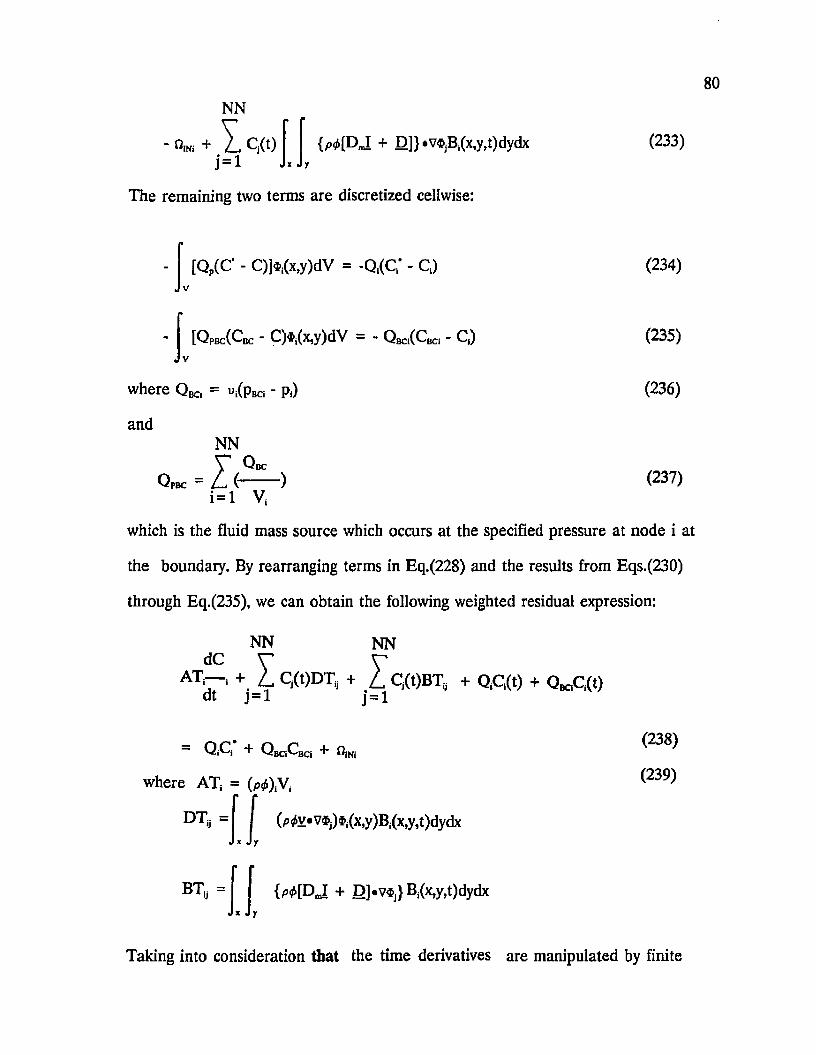
80NN
- Owi + Y , Cj(t) {pflitDJ + D]} *v$jBi(x,y,t)dydx (233)j = l !
The remaining two terms are discretized cellwise:
[Qp(C‘ - C)]*,(x,y)dV = -Q,(C,‘ - C,) (234)V
i
[Qpbc(Cbc ■ C)#i(x,y)dV — - Qbci(Cbci _ Q) (235)V
where - Pi) (236)
andNNr Qbc
Qpbc = Z (-------- ) (237)i= l V,
which is the fluid mass source which occurs at the specified pressure at node i at
the boundary. By rearranging terms in Eq.(228) and the results from Eqs.(230)
through Eq.(235), we can obtain the following weighted residual expression:
^ NN NN
ATV—, + I C,(t)DTa + £ C,(t)BT, + Q,C,(t) + Q„C,(t) dt j = l j= l
= Q C ’ + O C + n (238)Vi'-i T + nINl
where ATj = (p^V , 239^
(p • v$j) *i(x,y)Bi(x,y,t)dydxDT, = Ix J y
BT(J = {p tfD J + D].v$j}Bi(x,y,t)dydx
Taking into consideration that the time derivatives are manipulated by finite
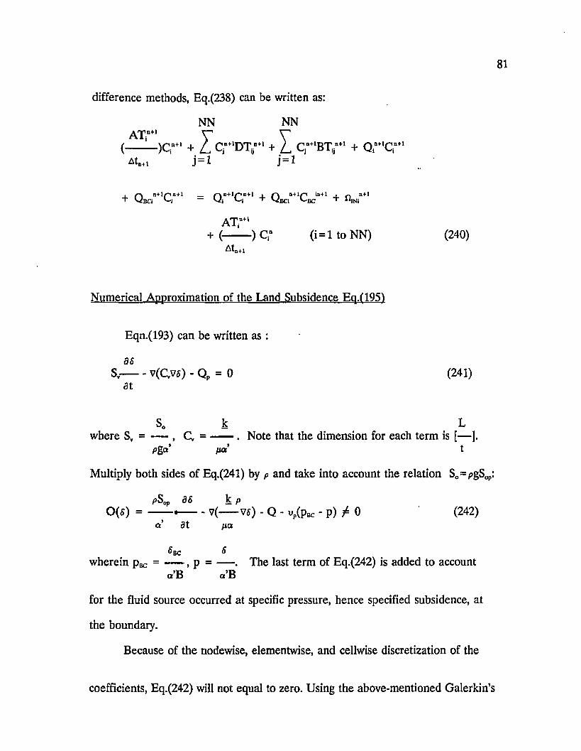
difference methods, Eq.(238) can be written as:
NN NNAT**1 V V
(— )Qn+i + L Cj-^DTi ' + l c ; +iBTljnti + oricri Atn+1 j = l j= l
, u + lp n + 1 f - v n + l / in + l j_ r v n + l f i in+l , 0 n+l" r W u c i '- '1 “ W * M W d c i V--BC t" **INi
ATD+l+ (— — ) Q" ( i= l to NN) (240)
Numerical Approximation of the Land Subsidence Eq.(1951
Eqn.(193) can be written as :
asS y v(C> « ) - Qp = 0 (241)
dt
where S¥ = — , Q -------. Note that the dimension for each term is [— ].Pga’ pas’ t
Multiply both sides of Eq.(241) by p and take into account the relation Sn=pgSop:
pS^ as k P0(5) = -------.-------v(------V5) - Q - ^(pBc - p) / 0 (242)
a’ 3t pa
5 nc Swherein puc = ----- , p = ----- . The last term of Eq.(242) is added to account
a’B a’B
for the fluid source occurred at specific pressure, hence specified subsidence, at
the boundary.
Because of the nodewise, elementwise, and cellwise discretization of the
coefficients, Eq.(242) will not equal to zero. Using the above-mentioned Galerkin’s

82
weighted residual formulation, Eq.(242) is integrated over the region V:
0(fi)$i(x,y)dV = 0 (243)
The first term of the expanded Eq.(243) is approximated as:
pS0P as(------ K_)$.(x,y)dV =
v ct at
p S v p d S(— — )®i(x,y)dzdydx
qj at
r p s « * a a(— ■— )$i(x>y)[
a’ atdz] dxdy
pS^aa(— •— )4>,(x,y)B(x,y,t)dxdy
a’ dt
(pSJ, as- ----- ,V, [Refer to Eq.(201)]
at(244)
The second term of the expanded Eq.(243) is approximated using Green’s
Theorem:
’ kp v( V5)4>i(x,y)dV = -
V p a ’
kp[(— -)v5]*n*,(x,y)dr
r pa’
* kp[(— -)v5] •v$i(x,y)dV
v pa’(245)
The first term on the right of Eq.(245) can be regarded as fluid mass flux out across
the region boundary at node i. This is because V5 is proportional to vhe, drawdown
of the piezometric head (refer to Section 2.2). Thus, this term can be assigned
as 'i'(t), such that,
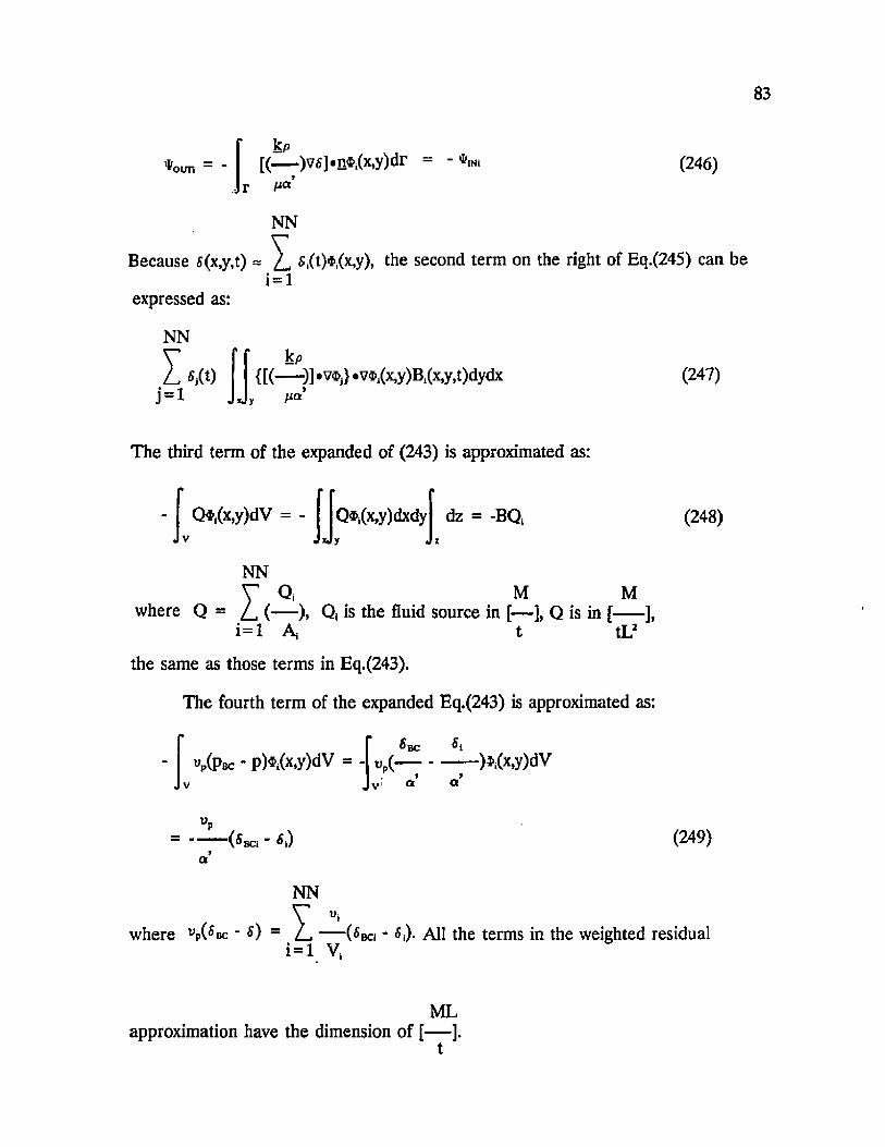
83
%OUT!
kp[(— )vfi]«n*i(x,y)dr = - 'I'iNi
r Ist*
NN
(246)
Because s(x,y,t) = L ^(t^.foy), the second term on the right of Eq.(245) can be i= 1
expressed as:
NN
j -1(t)
kp{[(---- )] • v«j} •v*1(x,y)Bi(x,y,t)dydx
y
(247)
The third term of the expanded of (243) is approximated as:
Q$,(x,y)dV = -
NN
Q$i(x,y)dxdy dz = -BQi (248)
V Qiwhere Q = (— ), Q, is
i= l
M Mthe fluid source in [— ], Q is in [----- ],
t tL2
the same as those terms in Eq.(243).
The fourth term of the expanded Eq.(243) is approximated as:
up(Pbc - pM (x,y)dV =>BC ” i
t>p(-------------- )5>,(x,y)dVa a
(249)
NN
where up(^bc - 0 = Z- — (fiBCi - & !)• All the terms in the weighted residual i= l V,
MLapproximation have the dimension of [— ].
t
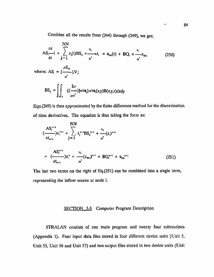
84
Combine all the results from (244) through (249), we get:
NN M . V
AS; i + ^ 5j(t)BS„ + ---- = *mi(t) + BQf + — S a ad t j - 1 a a ’
pSopwhere: AS, = (------ ),Vi;
(250)
BSij =' k P
{(— )]*v*j} •v$,(x,y)B(x,y,t)dxdyy m ’
Eqn.(249) is then approximated by the finite difference method for the discretization
of time derivatives. The equation is thus taking the form as:
NNA s r 1 v
(— ) s r + l s r ' B s : j = i
n+!At,n+l
+ — (*i)7a
0 + 1
ASjB+1 «,= (— k + - 7 (5Bc.)d+1 + b q “+i + * m r
Ata+i a’(251)
The last two terms on the right of Eq.(251) can be combined into a single term,
representing the inflow source at node i.
SECTION 3-3 Computer Program Description
STRALAN consists of one main program and twenty four subroutines
(Appendix 1). Four input data files stored in four different device units (Unit 5,
Unit 55, Unit 56 and Unit 57) and two output files stored in two device units (Unit
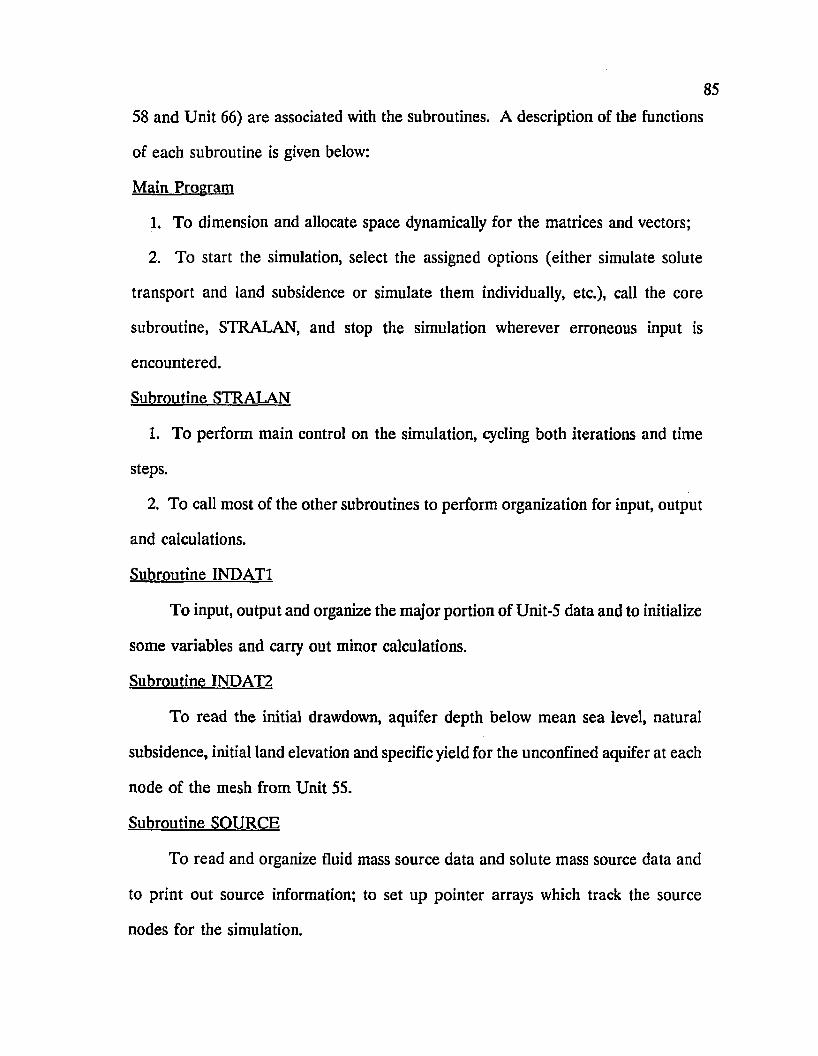
85
58 and Unit 66) are associated with the subroutines. A description of the functions
of each subroutine is given below:
Main Program
1. To dimension and allocate space dynamically for the matrices and vectors;
2. To start the simulation, select the assigned options (either simulate solute
transport and land subsidence or simulate them individually, etc.), call the core
subroutine, STRALAN, and stop the simulation wherever erroneous input is
encountered.
Subroutine STRALAN
1. To perform main control on the simulation, cycling both iterations and time
steps.
2. To call most of the other subroutines to perform organization for input, output
and calculations.
Subroutine INDAT1
To input, output and organize the major portion of Unit-5 data and to initialize
some variables and cany out minor calculations.
Subroutine 1NDAT2
To read the initial drawdown, aquifer depth below mean sea level, natural
subsidence, initial land elevation and specific yield for the unconfined aquifer at each
node of the mesh from Unit 55.
Subroutine SOURCE
To read and organize fluid mass source data and solute mass source data and
to print out source information; to set up pointer arrays which track the source
nodes for the simulation.

86
Subroutine BOUND
To read and organize specific pressure data, concentration data and specific
land subsidence data and print out the relevant information.
Subroutine OBSERV
1. To read and organize observation node data;
2. To save simulation results for the observation nodes on particular time steps;
3. To output simulation results at all observation nodes after completion of
simulation.
Subroutine CQNNEC
To read, organize and check data on node incidences (i.e. the order of the
node number on an element) and pinch node incidences (pinch nodes are those
nodes that are on an element that is reduced in size ) and to output these data.
Subroutine BANWID
To calculate the band width of the finite element mesh and check the value
specified by the user.
Subroutine NCHECK
To check that pinch nodes are not assigned with specific pressure,
concentration, subsidence or sources.
Subroutine INDAT3
1. To read initial conditions of pressure, concentration and subsidence from
Unit 57;
2. To initialize data for either warm or cold start of the simulation.
Subroutine PRISOL
1. To print initial conditions (pressure or drawdown, concentration and

87
subsidence);
2. To print out solutions for drawdown (pressure), concentration and
subsidence at the required time steps.
3. To print out information on time step, iterations and fluid velocity.
Subroutine ZERO
To fill a real array with a constant value.
Subroutine BCTIME
1. To specify time-dependent pressure, concentration, subsidence for the
boundary conditions by the user;
2. To specify time-dependent fluid mass sources and/or solute mass sources by
the user.
Data are read from Unit 56.
Subroutine ADSORB
To calculate values of equilibrium sorption parameters for linear, Freundlich
and Langmuir models.
Subroutine ELEMEN
To control and carry out all calculations for each element by obtaining element
information from subroutine BASIS2. Calculation includes Gaussian integration of
finite element integrals and element centroid velocities.
Subroutine BASIS2
To calculate values of basis functions, weighting functions, their derivatives,
Jacobians, transformation matrices between local and global coordinates and
parameters at a specific point in a quadrilateral finite element.

88Subroutine GLQBAN
To assemble results of elementwise integrations from subroutine ELEMEN
into a global banded matrix and global vector for the pressure, concentration and
subsidence equations.
Subroutine NODALB
1. To carry out all nodewise and cellwise calculations and to add nodewise and
cellwise terms to the global banded matrix and global vector for the pressure,
concentration and subsidence equations.
2. To add fluid source and solute mass source terms to the matrix equations.
Subroutine BCB
To implement specified pressure and specified concentration conditions and/or
subsidence by modifying the global flow, transport and subsidence matrix
equations.
Subroutine PINCHB
To implement pinch node conditions by modifying the global flow, transport
and subsidence matrix equations.
Subroutine SOLVEB
To solve the matrix equation by decomposing the matrix, modifying the right-
hand side and back-substituting for the solution.
Subroutine BUDGET
To calculate and print out fluid mass and solute mass budgets on each time
step or on particular time steps.
Subroutine STORE
To store the simulation results that may later be used to re-start the simulation.

Subroutine SUBPARM
To calculate new values for the aquifer thickness, porosity, storativity and
compressibility of the solid matrix under land subsidence condition.
3.4 Simulation Examples
This section provides a few simulation examples using STRALAN to
demonstrate some of its capabilities and to verify the accuracy of STRALAN model.
A detailed case study for the Gonzales-New Orleans aquifer in the New Orleans
area, Louisiana, is presented in the next chapter to demonstrate the application of
the full range capability of STRALAN model in simulating land subsidence and
saltwater intrusion.
The development of STRALAN model is largely based on SUTRA model.
The structure of the program and the results obtained should be identical to those
from SUTRA when it is reduced to only solving ground water flow and solute
transport problems. In fact, with the same data sets used for the Gonzales-New
Orleans aquifer to solve only saltwater intrusion problems, STRALAN gives identical
results as those obtained by SUTRA for both the drawdown and the chloride
concentration in time and space over 20 years of simulation period. A section of
STRALAN and SUTRA output for the saltwater intrusion problem is atttached as
Appendix 5a and 5b. Because of the similarity of both models in this respect, we
do not need to compare analytical results with those simulation results for
verification purposes. Such comparisons are already available (Voss, 1984).
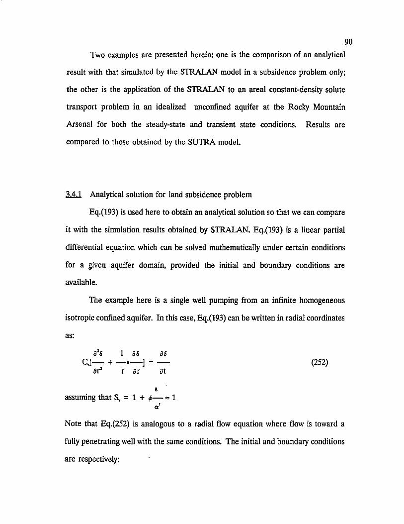
90Two examples are presented herein: one is the comparison of an analytical
result with that simulated by the STRALAN model in a subsidence problem only;
the other is the application of the STRALAN to an areal constant-density solute
transport problem in an idealized unconfined aquifer at the Rocky Mountain
Arsenal for both the steady-state and transient state conditions. Results are
compared to those obtained by the SUTRA model.
3.4.1 Analytical solution for land subsidence problem
Eq.(193) is used here to obtain an analytical solution so that we can compare
it with the simulation results obtained by STRALAN. Eq,(193) is a linear partial
differential equation which can be solved mathematically under certain conditions
for a given aquifer domain, provided the initial and boundary conditions are
available.
The example here is a single well pumping from an infinite homogeneous
isotropic confined aquifer. In this case, Eq.(193) can be written in radial coordinates
as:
a2s 1 as asC JL— + — ---- ] = ------ (252)
ar2 r ar at
Bassuming that Sv = 1 + <f>— « 1
a
Note that Eq.(252) is analogous to a radial flow equation where flow is toward a
fully penetrating well with the same conditions. The initial and boundary conditions
are respectively:
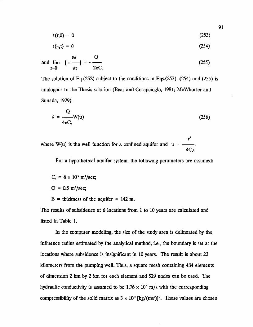
91s(r,0) = 0 (253)
S(®,t) = 0 (254)
d S Qand lim [ r — ] = -------- (255)
r-»0 ar 2*0,
The solution of Eq.(252) subject to the conditions in Eqs.(253), (254) and (255) is
analogous to the Thesis solution (Bear and Corapcioglu, 1981; McWhorter and
Sunada, 1979):
QS = W(u) (256)
4*C,
r2where W(u) is the well function for a confined aquifer and u =
4Qt
For a hypothetical aquifer system, the following parameters are assumed:
Q = 6 x 101 m2/sec;
Q = 0.5 m3/sec;
B = thickness of the aquifer = 142 m.
The results of subsidence at 6 locations from 1 to 10 years are calculated and
listed in Table 1.
In the computer modeling, the size of the study area is delineated by the
influence radius estimated by the analytical method, i.e., the boundary is set at the
locations where subsidence is insignificant in 10 years. The result is about 22
kilometers from the pumping well. Thus, a square mesh containing 484 elements
of dimension 2 km by 2 km for each element and 529 nodes can be used. The
hydraulic conductivity is assumed to be 1.76 x lO4 m /s with the corresponding
compressibility of the solid matrix as 3 x lO-4 [kg/(ms2)]'1. These values are chosen

Table 3-1 Calculated Subsidence for the Analytical Solution
Distance
Year 1 km 2 km 3 km 4 km 5 km 6 km
W(u) 6 (cm) W(u) S (cm) W(u) 6 (cm) W(u) 6 (cm) W(u) 6(cm) W(u) S (cm)
1 3.75 24.9 2.41 16.0 1.60 10.6 1.20 7.9 0.85 5.6 0.57 3.8
2 4.40 29.1 3.10 20.0 2.30 15.2 1.80 11.9 1.30 8.6 1.07 7.1
3 4.80 31.8 3.50 23.0 2.68 17.8 2.10 13.9 1.75 11.6 1.43 9.5
4 5.15 34.1 3.75 24.8 2.96 19.6 2.42 16.0 1.99 13.2 1.75 11.5
5 5.38 35.7 4.00 26.5 3.20 21.0 2.60 17.2 2.22 14.7 1.85 12.3
6 5.50 36.5 4.16 27.5 3.35 22.2 2.80 18.6 2.38 15.8 2.02 13.4
7 5.70 37.8 4.32 28.6 3.50 23.2 2.95 19.6 2.50 16.6 2.17 14.4
8 5.84 38.7 4.46 29.6 3.63 24.1 3.10 20.5 2.60 17.2 2.29 15.2
9 5.90 39.1 4.56 30.2 3.74 24.8 3.20 21.2 2.75 18.2 2.42 16.0
10 6.10 40.4 4.66 30.8 3.85 25.0 3.34 22.1 2.87 19.0 2.50 16.6

93
to match the value of C , which is 6 x 101 m2/s.
The results of the simulation are compared to those of the analytical solution
in two ways: one is the subsidence along a line at different distances from the well
after 10 years of pumping (see Figure 3-1); the other is the subsidence at 3 locations
(2,4, 6 km from the well) at different times (see Figure 3-2). The comparisons show
good agreement between the analytical solution and the simulation results. The
comparison between the analytical solution and the simulated results may have been
even closer if the grid sizes had been reduced near the well.
3.4.2 Example at Rociky Mountain Arsenal
A simplified representation of a rectangular unconfined aquifer at Rocky
Mountain Arsenal, Colorado is shown in Figure 3-3. The aquifer has a constant
transmissivity and two impermeable bedrock outcrops. The bottom bedrock is
assumed to be horizontal. This example is illustrated in the SUTRA manual (Voss,
1984). Regional flow is from south-east to north-west. Constant head is defined at
the top of Figure 3-3 and flow is discharged to the South Platte River at the bottom
of the rectangle, which is the boundary of specified head. Three wells pump water
from the aquifer at a rate of Qotrr (= 0.2 fp/s) each and a conservative contaminant
enters the system through a leaking waste isolation pond at a rate of QIN (= 1.0 ft3/s)
with concentration, C* (=1000 ppm). The natural background concentration of the
contaminant is C„ (=10 ppm).
The rectangular mesh consists of 16 x 20 elements, each of which is 1000 ft
by 1000 ft. The aquifer thickness, B, is actually changing with distance as the large
variation of constant heads suggests. The porosity is given as 0.2 and the hydraulic
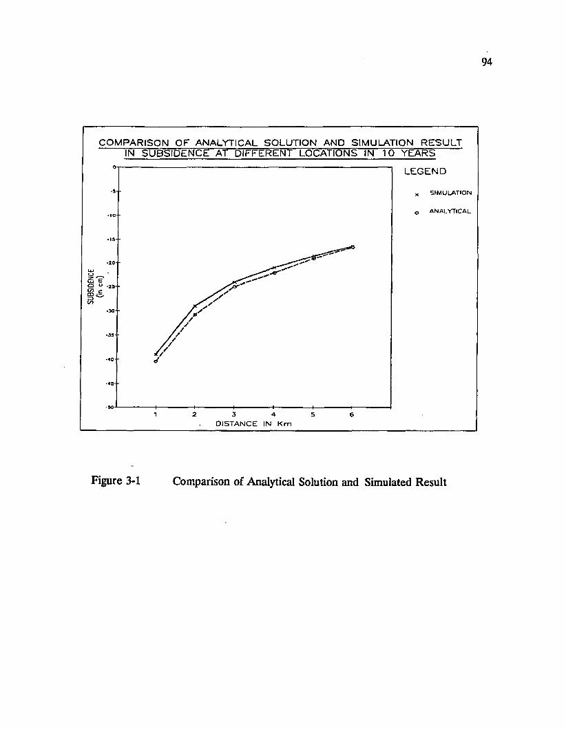
94
COM PARISON O F ANALYTICAL SOLUTION AND SIMULATION RESULT IN SU BSID EN CE AT DIFFERENT LOCATIONS IN 1 0 YEARS
■10- -
Q <J -as-- tn rmr>in
■
2 3 4 61 5
LEGEND
* S IM U LA TIO N
0 ANALYTICAL
D IS T A N C E IN K m
Figure 3-1 Comparison of Analytical Solution and Simulated Result
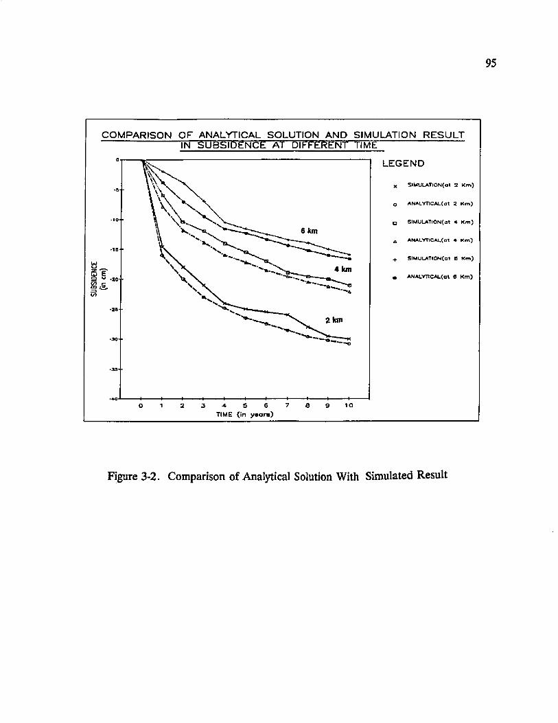
95
COM PARISON O F ANALYTICAL SOLUTION AND SIMULATION RESULT-------------------------- in s u b s i d e n c e a t D i p r e R E F r r r i M e -----------------------------
6 km
4 km£ § ■».. S jg,13(/)
S.,
2km
£ 6 7 8 9 10o 1 2 3 4
LEGEND
X S!MULATtON(ot 2 Km)
o ANAl.mCAL(at 2 Km)
a SIMULATION^ 4 Km)
a ANALYTIC AL,(at 4 Km)
+ SlMULATlOJ(at 6 Km)
• ANALYnCALCat 8 Km)
TIME {in y e a r s )
Figure 3-2. Comparison of Analytical Solution With Simulated Result
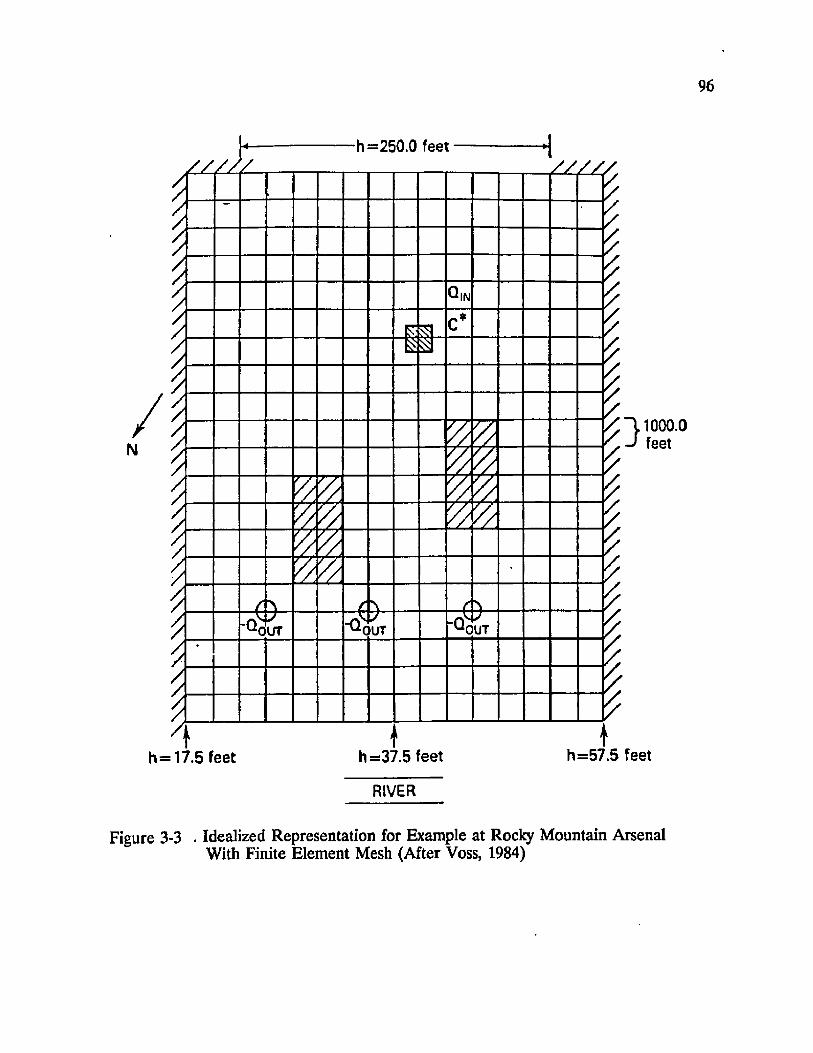
96
h -250.0 feet/ / A
1000.0feet
OUTOUTour
h=57.5 feet
RIVER
Figure 3-3 . Idealized Representation for Example at Rocky Mountain Arsenal With Finite Element Mesh (After Voss, 1984)

conductivity is set at 2.5 x 10'* (ft/s). Longitudinal and transverse dispersion
coefficients are 500 ft. and 200 ft., respectively.
No flow occurs across any boundary except where constant head is specified
at 250 ft. at the top of the mesh and where constant head is specified as changing
linearly between 17.5 ft. at the bottom left corner and 57.5 ft. at the bottom right
corner of the mesh. The initial pressures are arbitrary for steady-state simulation
of pressure. For transient state, they are set to values interpolated between the
specified heads with no pumping or recharging. Initial concentration is Ce (= 10
ppm).
Three scenarios are demonstrated here. One is the near steady-state and the
other two are transient state. A nearly steady-state solute plume for the conservative
solute is obtained after a 1000-year time step shown in Figure 3-4 by SUTRA and
Figure 3-5 by STRALAN. Note the the results are fairly close to each other. A 20-
year simulation and a 100-year simulation for the transient flow and transient solute
transport are performed by STRALAN and are shown in Figures 3-6 and 3-7. This
illustrates the transition state before the system reaches the steady state condition.
In this simulation, the storage coefficient is assumed as 0.12 and the thickness of the
aquifer is allowed to change in space and time.
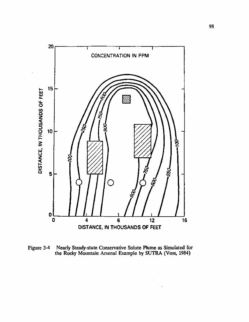
DIS
TAN
CE,
IN
THO
USA
ND
S OF
FE
ET
CONCENTRATION IN PPM
0 4 166 12DISTANCE, IN THOUSANDS OF FEET
Figure 3-4 Nearly Steady-state Conservative Solute Plume as Simulated forthe Roclcy Mountain Arsenal Example by SUTRA (Voss, 1984)

CONCENTRATION IN PPM
Injection wellLULL)U.LLOt/Joz<COD01 t-zLUoz<(-00Q
0 4 6 12 16DISTANCE, IN THOUSANDS OF FEET
Figure 3-5 Nearly Steady-state Conservative Solute Plume as Simulated forthe Rocky Mountain Arsenal Example by STRALAN.

DIS
TA
NC
E,
IN T
HO
USA
ND
S OF
FE
ET
Figure 3-6
100
CONCENTRATION IN PPM
750
500
250
100
0 4 6 12 16DISTANCE, IN THOUSANDS OF FEET
. Transient State Conservative Solute Plume After 20 years asSimulated for the Rocky Mountain Arsenal Example by STRALAN.
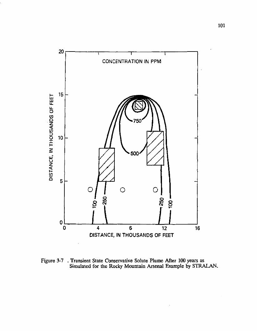
DIS
TA
NC
E,
IN T
HO
USA
ND
S OF
FE
ET
101
CONCENTRATION IN PPM
750
500
0 4 6 1612DISTANCE, IN THOUSANDS OF FEET
Figure 3-7 . Transient State Conservative Solute Plume After 100 years asSimulated for the Rocky Mountain Arsenal Example by STRALAN.
CHAPTER 4
A CASE STUDY:
LAND SUBSIDENCE AND SALTWATER INTRUSION
IN
NEW ORLEANS AREA
102

4.1 Introduction
103
Coastal cities and their vicinities often depend for their water supply on
ground water for municipal, industrial and agricultural purposes. The New Orleans
area, although it gets its domestic water supply from the abundant source of the
Mississippi River, withdraws a great amount of ground water for air conditioning,
cooling water for power generation, commercial purposes, industries, irrigation and
other uses (Rollo, 1966; Dial, 1983).
However, occasional widespread dry spells in the Mississippi River basin
causes extremely low river water and a curtailment of the river supply due to
elevated salt concentration. In addition, the accidental spills of harzardous chemicals
into the river results in the closure of water-supply intakes. Thus, a supplemental
emergency supply of ground water becomes increasingly important. For example,
the Department of Water, Jefferson Parish, is interested in developing a contingency
plan to withdraw an additional 50 percent of the present public water supply from
the Gonzales-New Orleans aquifer for emergency use (Dial and Tomaszewski, 1988).
Extensive pumping in the past decades has two significant consequences in
the New Orleans area: saltwater intrusion characterized by the northward movement
of the saltwater and fresh water interface (Malone et al., 1980); and land subsidence
at the rate of 1.0 to 2.0 cm/yr (Flanagan, 1989), excluding natural subsidence and
eustatic sea level rise. The development of ground water in this area is very likely
to exacerbate the already existing issues of saltwater intrusion and land subsidence.
Many investigations and studies of ground water in this area have been
conducted. The ealiest publication that discusses the ground water resources in New
104
Orleans area is the "The Biennial Report of the Board of Health to the General
Assembly of the State of Louisiana, 1890-1891". This publication contains lithologic
sections of a well drilled in 1854 and chemical analyses of water from several wells
in New Orleans. Decline of the ground water level due to increasing pumpage in
the developed area was recognised.
Harris (1904) documented some driller’s logs of wells and water level data for
the New Orleans area which are valuable to this day. In 1942, as a result of wartime
needs, two memorandum ground water reports were prepared by the U.S.Geological
Survey for this area. Eddards and others (1956) prepared a report that covered the
water resources in an extensive area of New Orleans and summarized ground water
information that had been collected up to that time. In 1963, a compilation of the
data obtained during field investigations in the Baton Rouge-New Orleans area was
published (Cardwell et. al., 1963).
Rollo (1966) conducted an in-depth investigation and evaluation of ground
water resources of the area along the Mississippi River in the Greater New Orleans
Area, south of Baton Rouge. Since virtually all the ground water withdrawals in the
Greater New Orleans area are from the Gonzales-New Orleans aquifer (also
referred to as the "700-foot" sand), this report evaluates in detail the potential of this
aquifer to meet future demands and investigates possible detrimental effects of these
demands on the water quality. Also, it outlines the alternative sources of ground
water that may be utilized advantageously in some parts of the area. Artificial
recharge as a method for decreasing future water-level declines and saltwater
enchroachment is discussed briefly and some of the advantages and disadvantages
were pointed out. In this report, Rollo outlined the underlying aquifers, i.e., the

105
Gramercy aquifer ("200-foot" sand), the Norco aquifer ("400-foot sand), the
Gonzales-New Orleans aquifer (700-foot" sand) and the "1200-foot" sand in terms of
their hydrogeologic properties, withdrawals, their interrelations, water-levels and
water quality.
Cardwell et. al. (1967) presented a report on the water resources of the Lake
Pontchartrain area. They concluded that for development purposes, the only fresh
water sources in the area comes from some of the deep aquifers beneath the
northern half of the lake. Dial (1983) again stressed the importance of the
Gonzales-New Orleans aquifer since about 10 times as much water is pumped from
this aquifer as the combined total from the other aquifers in this area. This aquifer
is described as widespread in area, relatively thick, of uniform texture and capable
of yielding large amount of water to high-capacity wells. In Orleans and Jefferson
parishes, it is heavily pumped as can be shown in Table 4-1. The figures in the table
imply the magnitude of pumpage is around 41-51 Mgal/d (million gallons per day)
in the past twenty years.
Dial and Sumner (1988) constructed a three-dimensional ground water flow
model for the New Orleans aquifer system. The aquifer system was simulated in the
model by four layers that represented the Gramercy, Norco, Gonzales-New Orleans
and "1200-foot" aquifers. The study area covers much of southeastern Louisiana and
southern Mississippi. Different pumping schemes were simulated to evaluate
possible future water-level declines and flow patterns. Simulation results also show
large vertical leakage as high as 34 Mgal/d in total entering the Gonzales-New
Orleans aquifer from the Norco (overlying) and the "1200-foot" (underlying) aquifers
under the 1981 pumping scheme. Most of this leakage occurs around the New
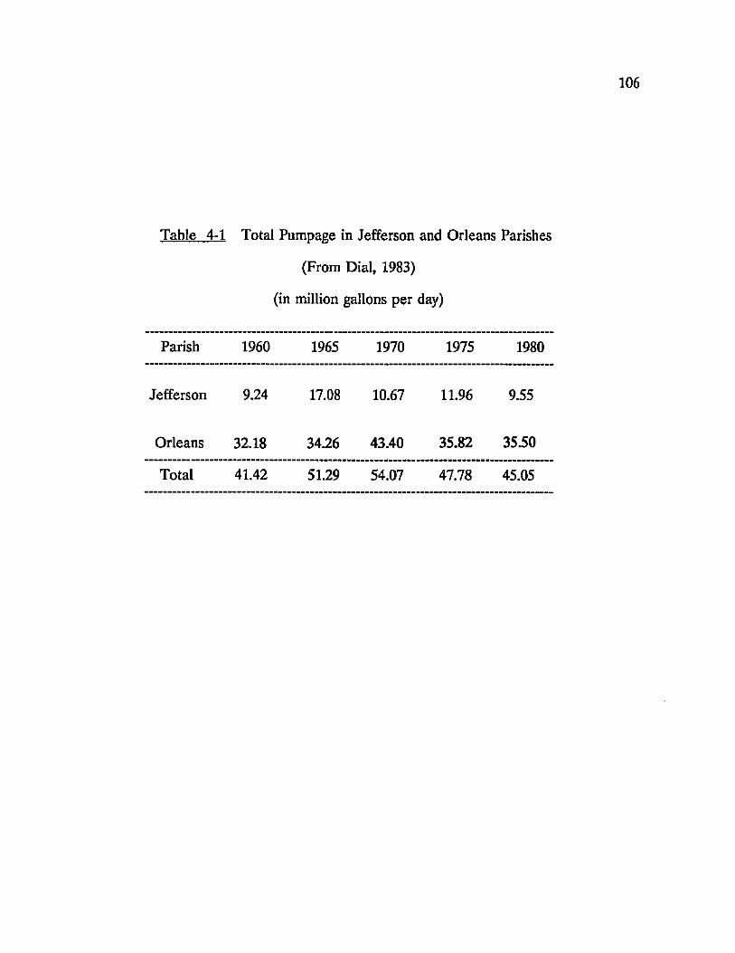
Table 4-1 Total Pumpage in Jefferson and Orleans Parishes
(From Dial, 1983)
(in million gallons per day)
Parish 1960 1965 1970 1975 1980
Jefferson 9.24 17.08 10.67 11.96 9.55
Orleans 32.18 34.26 43.40 35.82 35.50
Total 41.42 51.29 54.07 47.78 45.05

107
Orleans area where pumping is intensive.
Dial and Tomaszewski (1988) used the above three-dimensional finite-
difference ground water flow model to evaluate the effects of increased pumpage on
water levels and flow patterns in the Gonzales-New Orleans aquifer in a 50 square
mile region within northern Jefferson Parish. Simulation results indicate increases
in ground water velocity and vertical leakage from the adjacent aquifers.
Application of Darcy’s law, assuming no dispersion and density effects, indicates
the fresh water - saltwater interface will move northward at the rate of 150 to 500
ft/yr. While simulation results indicate significant vertical leakages, the increase of
chloride concentration due to leakages is not mentioned quantitatively.
Much of the land mass along the Louisiana coast was formed by deposition
of sediments eroded from inland drainage basins, transported through alluvial
channels, and deposited at the mouth of Mississippi River (Wang, 1984). During the
past 7000 years, the rate of maximum sedimentation (delta lobes) has shifted and
occupied various positions (Coleman, 1981). In recent years, in the lower Mississippi
River, the estimated annual sediment yield passing into the Gulf of Mexico has
declined from about 400 million metric tons prior to 1963 to the present load of 200
million metric tons (Keown et al., 1986), indicating a 50% reduction in sediment
transport.
Land subsidence in the Gulf Coastal Plain area has long been observed
during the past 50 years. It is generally accepted that sea level rise and subsidence
are responsible for much of the observed erosion and land loss in the coastal zone
of Louisiana (Gagliano et al., 1981).
In Louisiana coastal areas where the land elevations are already at or below
mean sea level, land subsidence associated with the eustatic sea level rise becomes
a critical problem. Gagliano et al. (1981) estimated the coastal land loss for the
Mississippi River deltaic plain was 120 km2 (40 square miles) per year.
Depressurization of deep geopressured aquifers is one of the main factors which
causes subsidence in Louisiana. Ground water and oil/gas withdrawals and
marshland reclamation by drainage are other potential causes (Trahan, 1984). In
the New Orleans area, land subsidence is quite significant. Lewis (1976) depicted
the subsidence dynamic situation in New Orleans, "The entire city is built on
land which is gradually sinking, and some of the city is built on land which is rapidly
sinking." Superimposed on the broad and slow tectonic subsidence (or natural
subsidence) in the New Orleans area, there is an obvious localized subsidence
associated with the lowering of the piezometric surface of the principal aquifer, the
Gonzales-New Orleans aquifer (Kazmann and Heath, 1968).
Many attempts have been made to estimate the natural subsidence. Kolb and
Van Lopik (1958) estimated 0.24 cm/yr (including an eustatic sea level rise of 0.1
cm/yr) in the Mississippi River deltaic plain, southern Louisiana. Saucier (1963)
estimated a subsidence rate of 0.39 foot per century (0.12 cm/yr) in the Pontchatrian
basin for the last 4,400 years. Based on this estimation, a regional subsidence of
approximately 6.71 cm (including eustatic sea level rise) between 1938 and 1964 in
the New Orleans area was expected.
Kazmann and Heath (1968) showed a close relationship between the
drawdown of piezometric surface in the "700-foot’ aquifer and the total land
subsidence (Figure 4-3) from 1938 to 1964 along a cross section A - A’ in Figures
4-1 and 4-2. The maximum subsidence along this cross section was as high as 1.7

109
LA K E PO N TCHA RTRAIN
NEW ORLEANS
l E V E L CON taOL
Figure 4-1. Piezometric Surface (Feet MSL) in the Gonzales-New Orleans Aquifer, Fall 1963 (after Rollo, 1966).
L A K E P Q N T C H A P T P A I N
NEW ORLEANS
-v. C 96
xx\ \ 3 Z O O \
Figure 4-2. Contours of Land Surface Subsidence (in feet) Between 1938 and 1964, New Orleans (from U.S. Coast and Geodetic Survey. After Kazmann and Heath,1968)

Subsidence (1938-1904)
W ater Level (March 1903)
W ater Level (Sept 1963
• a t(MSTISCf IKllCS t
Figure 4-3. Land Surface Subsidence Compared With Water Level in Wells Along Line A- A’ (After Kazmann and Heath,1968)
o
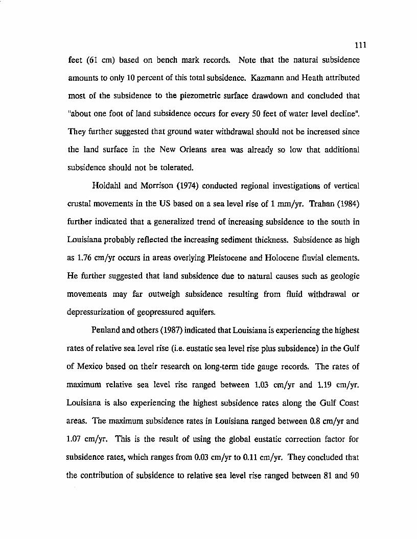
I l l
feet (61 cm) based on bench mark records. Note that the natural subsidence
amounts to only 10 percent of this total subsidence. Kazmann and Heath attributed
most of the subsidence to the piezometric surface drawdown and concluded that
"about one foot of land subsidence occurs for every 50 feet of water level decline".
They further suggested that ground water withdrawal should not be increased since
the land surface in the New Orleans area was already so low that additional
subsidence should not be tolerated.
Holdahl and Morrison (1974) conducted regional investigations of vertical
crustal movements in the US based on a sea level rise of 1 mm/yr. Trahan (1984)
further indicated that a generalized trend of increasing subsidence to the south in
Louisiana probably reflected the increasing sediment thickness. Subsidence as high
as 1.76 cm/yr occurs in areas overlying Pleistocene and Holocene fluvial elements.
He further suggested that land subsidence due to natural causes such as geologic
movements may far outweigh subsidence resulting from fluid withdrawal or
depressurization of geopressured aquifers.
Penland and others (1987) indicated that Louisiana is experiencing the highest
rates of relative sea level rise (i.e. eustatic sea level rise plus subsidence) in the Gulf
of Mexico based on their research on long-term tide gauge records. The rates of
maximum relative sea level rise ranged between 1.03 cm/yr and 1.19 cm/yr.
Louisiana is also experiencing the highest subsidence rates along the Gulf Coast
areas. The maximum subsidence rates in Louisiana ranged between 0.8 cm/yr and
1.07 cm/yr. This is the result of using the global eustatic correction factor for
subsidence rates, which ranges from 0.03 cm/yr to 0.11 cm/yr. They concluded that
the contribution of subsidence to relative sea level rise ranged between 81 and 90

112
percent. The rates of relative sea level rise are believed to be accelerating in
Louisiana and other Gulf states. The acceleration rates forecast that coastal
Louisiana will experience a 1.5 to 2 m rise in relative sea level rise in the next
century.
Ramsey and Moslow (1987) estimated an average rate of relative sea level
rise for the entire statewide region of 0.85 cm/yr based on 78 tide gauge records and
550 km of geodetic leveling in the span of 40 years (1942 - 1982). They indicated
that relative sea level rise accelerated during the last 20 years, which was 1.12 cm/yr,
2.5 times greater than for the first 20 years. The compactional subsidence, i.e., the
natural subsidence, accounts for approximately 80 % of the observed relative sea
level rise in Louisiana based on an eustatic correction of 0.23 cm/yr for the Gulf of
Mexico. They predicted that approximately 50 % of coastal Louisiana will be
converted to open water by the year 2037 if the present rate of relative sea level rise
persists.
Suhayda (1988) conducted analyses on sea level rise and subsidence, taking
into account the effects of fresh water run-off on tide gauge readings. He indicated
that subsidence was the dominant process causing wetland inundation. The eustatic
sea level rise was estimated at a rate of approximately 0.23 to 0.28 cm/yr. The
subsidence, caused by compaction of coastal sediments, was estimated at a rate of
0.3 to 1 cm/yr. The analysis showed fluid withdrawal from oil/gas reservoirs
appeared to have a localized influence on subsidence. However, considering the
wetlands of Louisiana as a whole, oil and gas extraction is believed not to have a
significant effect on subsidence.
An elaborate presentation of estimates of apparent movements of bench
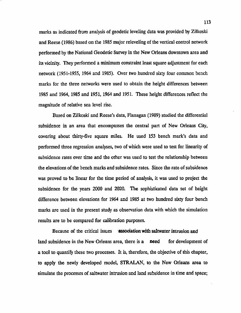
113
marks as indicated from analysis of geodetic leveling data was provided by Zilkoski
and Reese (1986) based on the 1985 major releveling of the vertical control network
performed by the National Geodetic Survey in the New Orleans downtown area and
its vicinity. They performed a minimum constraint least square adjustment for each
network (1951-1955, 1964 and 1985). Over two hundred sixty four common bench
marks for the three networks were used to obtain the height differences between
1985 and 1964,1985 and 1951,1964 and 1951. These height differences reflect the
magnitude of relative sea level rise.
Based on Zilkoski and Reese’s data, Flanagan (1989) studied the differential
subsidence in an area that encompasses the central part of New Orleans City,
covering about thirty-five square miles. He used 153 bench mark’s data and
performed three regression analyses, two of which were used to test for linearity of
subsidence rates over time and the other was used to test the relationship between
the elevations of the bench marks and subsidence rates. Since the rate of subsidence
was proved to be linear for the time period of analysis, it was used to project the
subsidence for the years 2000 and 2020. The sophisticated data set of height
difference between elevations for 1964 and 1985 at two hundred sixty four bench
marks are used in the present study as observation data with which the simulation
results are to be compared for calibration purposes.
Because of the critical issues association with saltwater intrusion and
land subsidence in the New Orleans area, there is a need for development of
a tool to quantify these two processes. It is, therefore, the objective of this chapter,
to apply the newly developed model, STRALAN, to the New Orleans area to
simulate the processes of saltwater intrusion and land subsidence in time and space;

114
and to evaluate the effects of additional pumpage on the aquifer behavior. As the
governing equations used in STRALAN are advective-dispersion-diffusion models,
it can handle the movement of dispersed miscible interfaces of saltwater and fresh
water. Also, the concentration-dependent density and sloping aquifer are taken into
account in this model to describe more realistically the flow and solute transport.
Specific objectives are discussed in detail in Section 4.3.
4.2 The Study Area
The study area encompasses 900 km1 (352 square miles) in the New Orleans
area, covering most of Jefferson and Orleans parishes and a part of St. Bernard and
Plaquemines parishes (Figure 4-4). The aquifer system underlying this area consists
of an alternating series of clay and sand beds. The four major water bearing
aquifers, deposited in the Holocene and Pleistocene times are the Gramercy, Norco,
Gonzales-New Orleans and the ''1200-foot" aquifers. These aquifers are separated
by beds of clays which a c t a s confining units. Two geohydrologic sections (A-A’ and
B-B’) through the study area show the interrelationship between aquifers and the
confining beds (Figure 4-5).
Water from the Gramercy aquifer, Norco aquifer and "1200-foot" aquifer
either contain high iron concentration or it is blackish, not suitable for domestic or
industrial uses (Rollo, 1966; Dial, 1983). The Gonzales-New Orleans aquifer, on the
other hand, produces good quality fresh water in most parts of the study area, hence
becomes the principal aquifer for withdrawal. This aquifer is widespread and
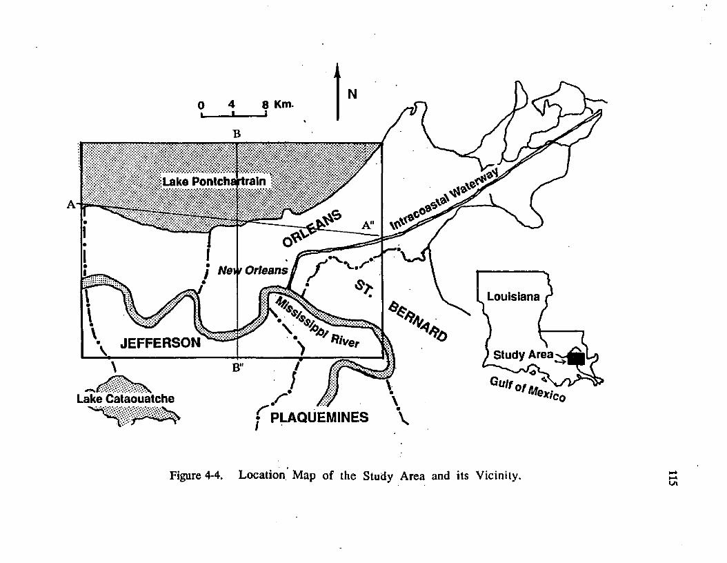
8 Km
Lake Pontcha rtraln
Wei f Orleans
Louisiana
f t i V iJEFFERSONStudy Area
Lake CataouatchePLAQUEMINES
Figure 4-4. Location M ap o f the Study A rea and its Vicinity.
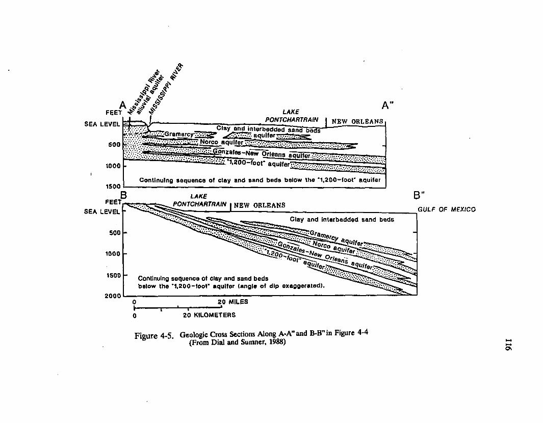
A £f eet ' ^ ^
SEA LEVEL k
LAKEPONTCHARTRAiN j NEW ORLEANS
500
1000I
1500I
FEET SEA LEVEL
r_ Clay and Interbedded sand bnrfay.-r/^v ^ i ^ ^ ; G ram arcy-v---.w? aquifer
Norco aquller^ g f ^ ^ - ^ vfionzales-N aw Orleans J y u l l m ...........
" ^ 2 0 0 -fo o t* aquIf erTTy!?...'■.v.1..-....T* ' ' " 1 '
Continuing sequence of clay and san d beds below the *1,200-foo t" aquifer
LAKEJ>O N TC H A R TR A IN jj iE W ORLEANS
Clay and in tarbedded sand beds
Continuing sequence of clay and sand bedsbelow the *1,2 0 0 -fo o t ' aquifer (angle of dip exaggerated).
20 MILES
B"GULF OF MEXICO
20 KILOMETERS
Figure 4-5. Geologic Cross Sections Along A-A" and B-B” in Figure 4-4 (From Dial and Sumner, 1988)

117
relatively thick. The thickness ranges from 30 to 90 meters (100 to 300 feet) with
an average value of 61 meters (200 ft) (Figure 4-6). It lies from about 150 to 260
meters (450 to 650 feet) below sea level. Regional dip of the aquifer is 25 to 50 feet
per mile (i.e. 0.27° to 0.54° of sloping angle) to the south (Hosman, 1972; also see
Figure 4-5). At aquifer-test sites in the study area, transmissivity ranges from 1115
m2/d (12,000 ft2/d ) to 2230 m2/d (24,000 ft2/d), and hydraulic conductivity ranges
from 20 to 32 m /d (Dial, 1983; Figure 4-6).
Water is heavily pumped from the Gonzales-New Orleans aquifer (see Table
4-1) because of its good quality and its capability of yielding large amount of water
to high capacity wells. Consequently, ground water is flowing toward the pumping
centers in the downtown area, the eastern and southern shore of Lake Pontchartrain
and cones of depression developed (Figures 4-7, 4-8). The locations of some of the
pumping wells are shown in Figure 4-9. Table 4-2 show the drawdowns in well water
level in the past 15 years in some wells. Extensive pumping also caused the
saltwater and fresh water interface to move northward resulting in increased salinity
in the area. The interface refers to the 250 ppm isochlor which serves as the limit
for drinking water standard (USEPS, 1976). Figure 4-9 plots the contours of chloride
content obtained from wells in the Gonzales-New Orleans aquifer in 1961-1962
(Rollo, 1966). Note that the approximate positions of the interface was located
immediately south of New Orleans city. Water quality in the Gonzales-New Orleans
aquifer varies greatly from north to south. Chloride concentrations range from north
to south between 48 to 2000 mg/1 (Figure 4-9). Color in the water from the
Gonzales-New Orleans aquifer ranges from 5 to 120 units (Dial and Tomaszewski,
1988). High color (50 to 120 units) can generally be found in fresh water zones.

THE STUDY AREA CONTOUR SHOWING THICKNESS OF THE *700-FOOT- SAND. CONTOUR INTERVAL SO FEET.
200
150 PERMEABILITY OF THE ‘700-FOOT SAND IN GALLONS PER DAY PER820
640
3 Miles
Figure 4-6. Thickness and coefficient of permeability of the Gonzales-New Orleans Aquifer (The "700-Foot" Sand) New Orleans Area, Louisiana (After Roilo, 1968)
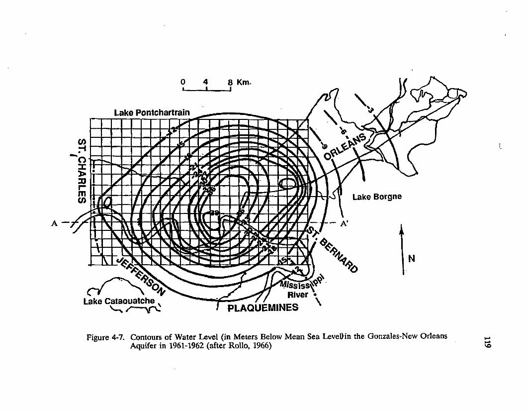
ST. CH
AR
LE
S
Lake Pontchartrain
Lake Borgne
fes iss^* River •
Lake CataouatchePLAQUEMINES
Figure 4-7. Contours of Water Level (in Meters Below Mean Sea Level) in the Gonzales-New Orleans Aquifer in 1961-1962 (after Rollo, 1966)

THE STUDY
LAKE
PONTCHARTRAIN/
m stsa rr iW M G V u ^
h—7 r a lrr N**
O r i f i IcMl*
3 Mik*
Figure 4-8. Contours of Piezometric Levelfin meters, MSL) in the Gonzales-New Orleans Aquifer November 5-6 1985, New Orleans Area{From US Geological Survey, Louisiana Office)

121
Table 4-2 Drawdowns in Well Level in the Past 15 Years(After Dial, 1983)
Well No. Parish Date of observation (month/year)
Drawdown (in feet, from mean sea level)
JF-64 Jefferson 09/1976 44.5
JF-156 Jefferson 05/1974 93.3
JF-158 Jefferson 01/1971 99.0
JF-161 Jefferson 02/1971 99.0
JF-166 Jefferson 01/1982 44.8
JF-167 Jefferson 01/1982 69.1
JF-168 Jefferson 08/1972 74.0
OR-186 Orleans 02/1970 143.0
OR-195 Orleans 07/1976 163.0
OR-198 Orleans 07/1978 110.0
OR-199 Orleans 01/1974 108.0
OR-200 Orleans 09/1976 130.0
OR-202 Orleans 05/1978 84.0
OR-203 Orleans 09/1981 81.7
OR-206 Orleans 10/1981 138.1
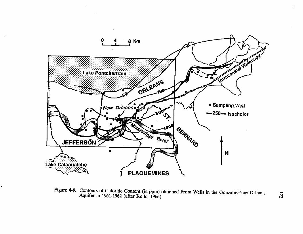
K m
Lake Pontchartrain
Sampling Well 250— Isocholor
• New Orleans•.
JE F FE R S 0N
Lake Cataouatche
PLAQUEMINES
Figure 4-9. Contours of Chloride Content (in ppm) obtained From Wells in the Gonzales-New Orleans Aquifer in 1961-1962 (after Rollo, 1966)

123
However, color in the water is generally not harmful to human health and most of
the water color can be reduced to less than 15 units by some approaches stipulated
by USEPA (USEPA, 1977). Table 4-3 shows the chloride concentration in some
observation wells.
Land subsidence in this area has reached 15 to 40 cm from 1964 to 1984
(Zilkoski and Reese, 1986; Figure 4-10) averaging from 0.75 to 2 cm/yr. With these
average values, subsidence from 1961-1981 is projected and compared with the actual
piezometric drawdown in 1981-1982 along A-A’ line (Figure 4-11). A-A’ line is
referred to Figure 4-7 and Figure 4-10. It shows the response of land subsidence to
the piezometric drawdown due to pumping.
4.3 Study Objectives
The major objective of this chapter is to use the STRALAN model to
simulate the effect of pumping on the movement of ground water, the dynamic
position of the dispersed interface between fresh water and saltwater in the
Gonzales-New Orleans aquifer, and land subsidence spatially and temporally. The
simulated results are then summarized and discussed to be used in decision making
for the management of water resources in this coastal area.
The objectives of the study are accomplished through the following steps:
1. Acquisition of all the hydrogeologic data and physical properties of the underlying
geologic formations and their areal distributions being used in the model as initial
and boundary conditions;

124
Table 4-3 Chloride Concentration in Some Observation Wells (U.S. Geological Survey Data)
Well No. Parish Date of Sampling Chloride concentration(month/day/year) (m g/1)
JF-25 Jefferson 06/28/1985 220
JF-64 Jefferson 06/18/1986 410
JF-149 Jefferson 05/19/1986 120
JF-152 Jefferson 06/28/1985 190
JF-160 Jefferson 09/24/1986 740
JF-162 Jefferson 05/08/1986 1500
JF-163 Jefferson 05/19/1986 120
JF-168 Jefferson 01/16/1986 78
JF-169 Jefferson 01/16/1986 60
JF-170 Jefferson 01/16/1986 48
JF-171 Jefferson 01/17/1986 340
JF-172 Jefferson 05/08/1986 84
JF-175 Jefferson 05/07/1986 100
JF-176 Jefferson 01/17/1986 88
JF-177 Jefferson 05/07/1986 59
JF-178 Jefferson 05/07/1986 1100
JF-180 Jefferson 05/14/1986 96
JF-182 Jefferson 10/03/1986 93
JF-183 Jefferson 10/02/1986 2400
JF-184 Jefferson 09/26/1986 63
JF-185 Jefferson 09/25/1986 87

125
Table 4-3 (continued)
Well No. Parish Date of Sampling Chloride Concentration(month/day/year) (m g/1)
JF-186 Jefferson 10/02/1986 150
OR-61 Orleans 01/07/1986 40
OR-125 Orleans 06/19/1985 600
OR-130 Orleans 01/06/1986 340
OR-131 Orleans 07/16/1985 320
OR-170 Orleans 06/19/1985 380
OR-171 Orleans 06/19/1985 560
OR-175 Orleans 06/26/1985 48
OR-179 Orleans 10/09/1986 63
OR-195 Orleans 04/30/1986 89
OR-203 Orleans 12/10/1985 360

THE STUDY AREA
LAKE
PONTCHARTRAIN ^
Figure 4-10. Subsidence in the New Orleans Area, 1964-1985 (from Zilkoski and Reese, 1986) (Subsidence in centimeters)

127
---io- i o - -
SUBSIDENCE (1 3 6 1 - 1 9 9 1 )
---- 20- 2 0 - -
S LlJ O h— o Lj % 2
CO
/ \/ DRAWDOWN ( 1 9 0 1 ) - - - 4 0- 4 0 - -
- 5 0 "
- 6 0- 6 0S 4 0 7 4 1 OS 1 4 2 1 5 9 1 7 6 1 9 3 2 1 0 2 2 7 2 4 4 2 6 1 2 7 0 3 1 2 3 4 6 3 3 0
NODE N U M B E R (A - A C R O S S S E C T I O N )
Figure 4-11. Land Subsidence Compared With Piezometric Drawdown in the
New Orleans Area Along Line A-A\

128
2. Delineation of the study area and selection of the proper size of the finite
element mesh being discretized in the simulation;
3. Calibration of the model with available data sets by adjusting the hydrogeologic
parameters and testing their sensitivities on the model results.
4. Preliminary verification of the model with another data set, using the calibrated
parameters;
5. Application of the calibrated model, STRALAN, to predict drawdown, fresh
water and saltwater interface and subsidence in future years with projected
pumpage to meet the firm and emergent^ demands.
4.4 Model Calibration and Verification
Application of the STRALAN model to the Gonzales-New Orleans aquifer
was performed under the following assumptions:
1. The flow was fully saturated in a heterogeneous, anisotropic, confined and sloping
aquifer with a dispersed interface between fresh water and salt water;
2. The processes of solute (salt) adsorption and desorption were not taken into
consideration;
3. There was no chemical or biological reaction causing solute (salt) production or
decay;
4. Monthly pumpage from the Gonzales-New Orleans aquifer in the study area did
not change its pattern in the last 25 years. The monthly pumpage exerted in the
model was based on this pattern (Figure 4-12) and the annual average pumpage
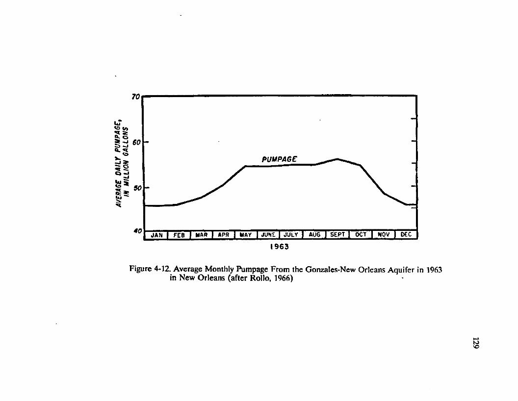
AVER
AGE
DAILY
PU
MPAG
E,
IN MI
LLION
GA
LLON
S
PUMPAGE
50
40 JAN j FEB I WAR | APR | MAY | JUNE | JULY | AUG 1 SEPT I OCT | NOV | D£C
1 9 6 3
Figure 4-12. Average Monthly Pumpage From the Gonzales-New Orleans Aquifer in in New Orleans (after Rollo, 1966)

130
(Table 4-1).
5. Natural subsidence (including the eustatic sea level rise) was evenly distributed
in the study area.
4.4.1 Construction of the Finite Element Mesh
The size of the study area was delineated by the availability of a relatively
constant pressure, explicitly depicted by the piezometric drawdowns (Figures 4-7 and
4-8) and the relatively pumping-induced subsidence-free boundaries during the past
25 years. The 900 km2 study area was then divided into 352 (16 x 22) quadrilateral
finite elements with 391 (17 x 23) nodes , and each node represents one of the four
edges of an element. Each node is assigned a specific integer number, starting from
the southwest corner of the rectangular grid with Node #1 and incrementing
northward by one (see Figure 4-14). The rectangular uniform grid ( l x l mi2) was
chosen based on the following reasons:
1. The observed data (piezometric drawdown and chloride concentration) and
hydrogeologic parameters (hydraulic conductivity, transmissivity, etc.) were sparsely
distributed (Figures 4-6,4-7, 4-8). Values in between the locations of the observed
or tested data were evaluated by interpolation;
2. The stability criteria were satisfied. The spatial stability criterion in the
STRALAN model depends on the value of a mesh Peclet number, Pem, defined as
(Voss, 1984):
| v | aLP™ ------------ (257)
Dm + «lM
where v is the velocity of flow which is in the order of 10-6 to 10'7 m/s; &L is the
length of the finite element (= 1 mile); a L is the longitudinal dispersivity (= 400 m);

131
and D„ is the molecular diffusivity (= 1.8 x 10 s m2/s).
The stability criterion for a diffusion type of equation is used in the
STRALAN model (McWhorter and Sunada, 1977; Illangasekare, 1978):
T.At 1 < ------------------------------------ (258)S(aL)2 2
w h e r e T = t r a n s m i s s i v i t y (0.0123 m 2/ s ) ; S = s t o r a g e c o e f f i c i e n t (= S0B); SD =
s p e c i f i c s t o r a t i v i t y (0.0006 1/m); a n d A t = t i m e s t e p i n t h e m o d e l (1 m o n t h ) .
3. The rationality of the grid size compared with other existing models. Dial and
Sumner (1988) used a 1 x 1 mi2 grid at the New Orleans area and a 25 x 11.25 mi2
grid in the vicinity of the boundaries for the three-dimensional model. Their total
study area was 23,000 square miles.
Based on the above-mentioned reasons, a 1 x 1 mi2 grid and A t = 1 month
were adequate for the simulation study.
4.4.2 Initial Condiiton and Boundary Condition
The available data from the 1961-1962 piezometric surface (Figure 4-7) and
the chloride concentration (Figure 4-9) in the Gonzales-New Orleans aquifer were
used as initial drawdown and concentration conditions. Initial subsidence at each
node was taken as zero.
The boundary condition was selected based on available information and the
absence of nearby physical well-defined boundaries such as impervious barriers.
During the past 25 years, the changes of the piezometric head along the northern,
southern and western boundaries of the study area were relatively small, except the
eastern boundary due to the development of pumping in 1980s (Figures 4-7, 4-8).

132
Therefore, in the simulation, a variable pressure head was specified at the eastern
boundary and constant pressure heads were imposed for the other boundaries. The
boundary condition for solute transport varied according to the flow boundary
conditions as chloride concentration was based on the advective-dispersion transport
mechanism. Only the natural subsidence was considered along the boundaries. No
pumping-induced subsidence was expected at those locations.
4.4.3 Vertical Leakage to the Gonzales-New Orleans Aquifer
Vertical leakage through the confining clay beds to the Gonzales-New Orleans
aquifer from the Norco and the "1200-foot" aquifers was estmated at 1 Mgal/d by
Rollo (1966). However, recent simulation studies by Dial and Sumner (1988), Dial
and Tomaszewski (1988) using the USGS Trescott model showed that the vertical
leakage was much higher.
Simulated vertical leakages from the Norco aquifer (overlying) and the "1200-
foot" aquifer to the Gonzales-New Orleans aquifer were 12.72 Mgal/d and 20.95
Mgal/d, respectively, for 1981, the annual pumpage of which was about 50 Mgal/d
(Dial and Sumner, 1988). However, the total study area was 23,000 square miles.
Most of the vertical leakage was supposed to occur around the New Orleans where
pumping was intensive.
In a smaller area of about 50 square miles in Northern Jefferson Parish, the
simulated vertical leakages would be 1.9 Mgal/d from the overlying layer and 1.6
Mgal/d from the underlying layer, totalling 3.5 Mgal/d, if an additional pumpage of
50 Mgal/d was exerted in this area (Dial and Tomaszewski, 1988). The results were
based on the combined effects of pumping in northern Jefferson Parish and Orleans

133
Parish on the east which had another 40 to 50 Mgal/d of pumpage. This implies
that the overall vertical leakages would be less than 3.5 Mgal/d if the pumpage in
Orleans Parish was not taken into consideration.
Using the above results, the vertical leakage adapted in the present study was
based on the following assumptions:
1. The same magnitude of vertical leakage would occur in the present study area
under the same pumpage as that which would have occurred in the northern
Jefferson Parish. That is to say, about 50 Mgal/d of pumpage would induce 3.5
Mgal/d of vertical leakage in an area of 50 square miles. Proportionally, a 90
square-mile pumping area in the present study area will induce 6.3 Mgal/d of
vertical leakage under 50 Mgal/d of pumpage.
2. The remaining 262 square miles are the outer fringe of the pumping area where
practically no pumping occurs. Vertical leakage in this outer area was assumed to
be 0.8 Mgal/d for every 50 square miles, a value resulting from the simulation under
present pumping rate in northern Jefferson Parish (Dial and Tomaszewski, 1988).
With these assumptions, the total vertical leakage to this area was estimated
at 10 Mgal/d.
4.4.4 Model Calibration
To calibrate the model parameters, sensitivity analyses were conducted for a
reasonable range of each parameter. The STRALAN model was run for 20 years,
from 1961-1981. The results of the simulation in terms of piezometric head
drawdown, chloride concentration and subsidence were compared with the
observation data. The set of parameters that produces the closest results to the
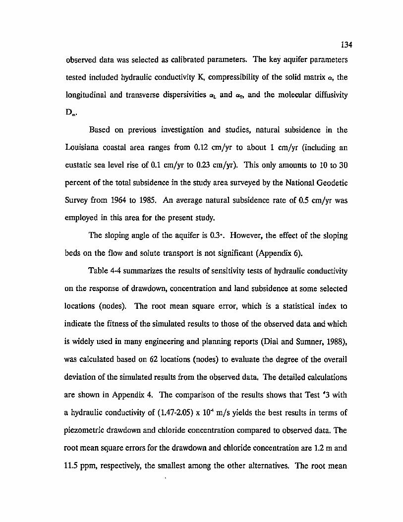
134
observed data was selected as calibrated parameters. The key aquifer parameters
tested included hydraulic conductivity K, compressibility of the solid matrix a , the
longitudinal and transverse dispersivities a L and % and the molecular diffusivity
D„.
Based on previous investigation and studies, natural subsidence in the
Louisiana coastal area ranges from 0.12 cm/yr to about 1 cm/yr (including an
eustatic sea level rise of 0.1 cm/yr to 0.23 cm/yr). This only amounts to 10 to 30
percent of the total subsidence in the study area surveyed by the National Geodetic
Survey from 1964 to 1985. An average natural subsidence rate of 0.5 cm/yr was
employed in this area for the present study.
The sloping angle of the aquifer is 0.3°. However, the effect of the sloping
beds on the flow and solute transport is not significant (Appendix 6).
Table 4-4 summarizes the results of sensitivity tests of hydraulic conductivity
on the response of drawdown, concentration and land subsidence at some selected
locations (nodes). The root mean square error, which is a statistical index to
indicate the fitness of the simulated results to those of the observed data and which
is widely used in many engineering and planning reports (Dial and Sumner, 1988),
was calculated based on 62 locations (nodes) to evaluate the degree of the overall
deviation of the simulated results from the observed data. The detailed calculations
are shown in Appendix 4. The comparison of the results shows that Test #3 with
a hydraulic conductivity of (1.47-2.05) x 10 m /s yields the best results in terms of
piezometric drawdown and chloride concentration compared to observed data. The
root mean square errors for the drawdown and chloride concentration are 1.2 m and
11.5 ppm, respectively, the smallest among the other alternatives. The root mean

Table 4-4 Results of Sensitivity Tests of Hydraulic Conductivity on Piezometric Drawdown, Chloride Concentration and Subsidence in 1981-1982
Sensitivity Tests 1 2 3 4 5
Hydraulicconductivity
(1.18-1.64) x 10^
(1.35-1.89) x 10^
(1.47-2.05) x 10*
(1.65-2.30) x 10-1
(1.88-2.63) x 10~*
(m/s)
Drawdown (DD) DD CON SUB DD CON SUB DD CON SUB DD CON SUB DD CON SUBCone. (CON) (m) (ppm) (cm) (m) i(ppm) (cm) (m) (ppm) (cm) (m) (ppm) (cm) (m) (ppm) (cm)Subsidence (SUB)
(1) (2) (3) (4) (5) (6) (7) (8) (9) (10) (11) (12) (13) (14) (15) (16)
Node Number
42 14.1 230.5 12.5 13.6 230.6 12.2 13.3 228.4 12.0 13.0 230.9 11.8 12.7 231.0 11.656 17.0 338.5 14.5 16.3 341.9 13.9 15.9 356.3 13.6 15.4 347.5 13.3 14.9 352.0 12.972 20.7 200.7 16.6 19.6 201.4 15.8 19.1 206.9 15.4 18.5 203.2 14.9 17.8 204.8 14.3
140 32.5 392.3 22.1 30.2 385.3 20.6 28.9 437.6 19.7 27.3 374.1 18.7 25.7 365.4 17.7174 34.2 330.7 18.9 31.8 326.5 17.6 30.5 346.8 16.9 28.9 319,8 15.9 27.3 314.8 14.9210 50.9 217.0 29.4 46.3 213.5 26.9 43.8 244.0 25.6 40.8 207.8 23.9 37.7 203.3 22.2244 44.8 465.8 23.9 41.0 461.2 22.2 39.1 487.0 21.1 36.6 455.1 20.0 34.0 450.3 18.8279 40.5 409.4 21.8 37.3 408.6 20.3 35.6 406.7 19.5 33.9 407.0 18.5 31.3 405.8 17.4332 29.8 349.5 26.6 28.1 348.2 25.5 27.1 351.5 24.9 25.9 346.2 24.1 24.7 344.6 23.4
Note: c t = 0.3 x 10* [kg/m-s2]'1; a L = 400m; a r = 4m; Dm = 1.8 x 10s [m2/s]; <p = 0.3
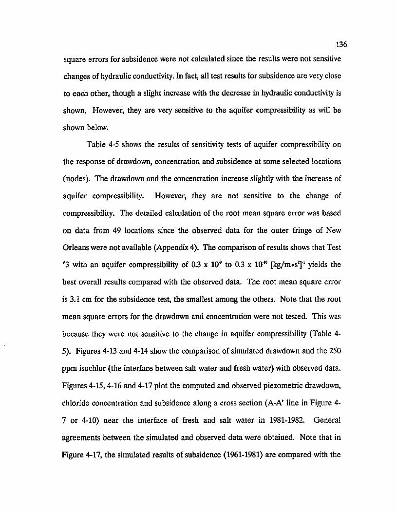
136
square errors for subsidence were not calculated since the results were not sensitive
changes of hydraulic conductivity. In fact, all test results for subsidence are veiy close
to each other, though a slight increase with the decrease in hydraulic conductivity is
shown. However, they are very sensitive to the aquifer compressibility as will be
shown below.
Table 4-5 shows the results of sensitivity tests of aquifer compressibility on
the response of drawdown, concentration and subsidence at some selected locations
(nodes). The drawdown and the concentration increase slightly with the increase of
aquifer compressibility. However, they are not sensitive to the change of
compressibility. The detailed calculation of the root mean square error was based
on data from 49 locations since the observed data for the outer fringe of New
Orleans were not available (Appendix 4). The comparison of results shows that Test
* 3 with an aquifer compressibility of 0.3 x 10* to 0.3 x 10'10 [kg/m*s2]'1 yields the
best overall results compared with the observed data. The root mean square error
is 3.1 cm for the subsidence test, the smallest among the others. Note that the root
mean square errors for the drawdown and concentration were not tested. This was
because they were not sensitive to the change in aquifer compressibility (Table 4-
5). Figures 4-13 and 4-14 show the comparison of simulated drawdown and the 250
ppm isochlor (the interface between salt water and fresh water) with observed data.
Figures 4-15, 4-16 and 4-17 plot the computed and observed piezometric drawdown,
chloride concentration and subsidence along a cross section (A-A* line in Figure 4-
7 or 4-10) near the interface of fresh and salt water in 1981-1982. General
agreements between the simulated and observed data were obtained. Note that in
Figure 4-17, the simulated results of subsidence (1961-1981) are compared with the

Table 4-5 Results of Sensitivity Tests of Aquifer Compressibility on Piezometric Drawdown, Chloride Concentration and Subsidence in 1981-1982
Sensitivity Tests 1 2 3 4 5
Aquifer 0.30 x 10¹⁰ 0.2 x 10* 0.3 x 10* 0.7 x 10* 3.0 x 10*compressibility -- 0.30 x 10¹¹ -0.2 x 10'10 --0.3 x 10'10 -0.7 x 10¹⁰ --3.0 x 10'10(kg/m ’s2) 1
Drawdown (DD) DD CON SUB DD CON SUB DD CON SUB DD CON SUB DD CON SUBCone. (CON) (m) (ppm) (cm) (m) (ppm) (cm) (m) (ppm) (cm) (m) (ppm) (cm) (m) (ppm) (cm)Subsidence (SUB)
(1) (2) (3) (4) (5) (6) (7) (8) (9) (10) (11) (12) (13) (14) (15) (16)
Node Number
72 19.1 206.9 10.5 19.1 206.9 13.6 19.1 206.9 15.4 19.2 206.9 22.6 19.4 207.2 63.9
140 28.9 437.1 10.9 28.9 437.4 16.5 28.9 437.6 19.7 28.9 438.3 32.8 29.3 442.7 107.4
174 30.5 346.5 8.9 30.5 346.7 13.8 30.5 346.8 16.9 30.6 347.4 28.7 31.0 350.6 96.3
210 43.8 243.3 11.5 43.8 243.7 20.3 43.8 244.0 25.6 44.0 245.2 46.3 44.7 252.1 165.1
227 42.2 490.2 21.3 42.2 490.9 29.5 42.2 491.3 34.3 42.3 493.4 53.5 43.0 505.1 163.2
244 39.0 486.2 11.1 39.0 486.7 17.4 39.1 487.0 21.1 39.1 488.3 36.2 39.7 495.7 121.7
279 35.5 406.4 10.9 35.6 406.6 16.3 35.6 406.7 19.5 35.7 407.2 32.1 36.1 409.8 104.4
332 27.1 351.3 18.6 27.1 351.5 22.5 27.1 351.5 24.9 27.2 351.9 34.1 27.4 353.6 86.8
Note: K = (1.47-2.05)xl0'4 [m/s]; a L = 400m; oT = 4m; Dro = 1.8 x 10‘5 [m2/s]; <p = 0.3
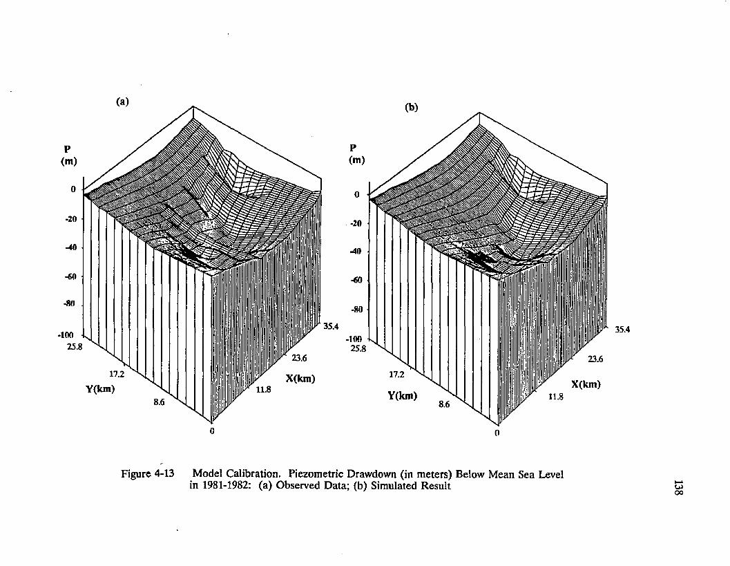
(m)(m)
-20
•40
-«0
•80 -80
35.4-100 -100
25.825.823.6 23.6
17.2 17.2X(ktn) X(km)Y(km) 11.8Y(km) 11.88.6 8.6
0
35.4
Figure 4-13 Model Calibration. Piezometric Drawdown (in meters) Below Mean Sea Level in 1981-1982: (a) Observed Data; (b) Simulated Result OJ
00

14
13
12
11
10
9
8
7
6
5
4
3
2
1
391
390
389
388
387
386
385
384
383
382
381
380
379
378
377
376
Simulated 1981 -1982
1961-1962Observed
1981 -1982
ice Pontchartrain
Ft
5Mississippi
Figure 4-14. Model Calibration. Approximate Positions of Freshwater and Saltwater Interface(250 ppm Isochlor) in the Gonzales-New Orleans Aquifer in the Vicinity of New Orl<Louisiana.

DRAW
DOWN
(IN
METE
RS)
140
L E G E N D
O B SE R V A T IO N ( 1 9 8 1 )
- 1 0 - -
SIMULATION {1 9B1)
V
- 3 5 - -
-40 - -
-45 - -
-506 40 74 108 142 159 176 193 210 227 244 261 278 312 346 380
NODE NUMBER (A - A C R O S S SE C T IO N )
Figure 4-15 Model Calibration. Comparison of Drawdown (1981) in the Gonzales-New Orleans Aquifer Along A-A’ Cross Section.
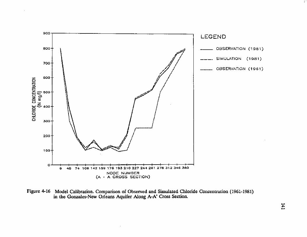
CHLO
RIDE
CONC
ENTR
ATIO
N (IN
mg/
l)900
L E G E N D
OBSERVATION ( 1 9 8 1 )BOO - -
SIMULATION ( 1 9 8 1 )
OBSERVATION ( 1 9 6 1 )
5 0 0 - -
4 0 0 - -
3 0 0 - -
200 “
6 4 0 7 4 1 0 S 1 4 2 1 5 9 1 7 6 1 9 3 2 1 0 2 2 7 2 4 4 2 6 1 2 7 S 3 1 2 3 4 6 3 8 0
NODE NUMBER (A - A CR O SS SECTION)
Figure 4-16 Model Calibration. Comparison of Observed and Simulated Chloride Concentration (1961-1981) in the Gonzales-New Orleans Aquifer Along A-A’ Cross Section.

SUBS
IDEN
CE
(IN CE
NTIM
ETER
S)
L E G E N D
OBSERVATlONC 1 9 6 4 - 1 9 » 4 )
- 1 0 '
SlMULATlON(1 9 6 1 - 1 9 6 1 )
StMULATlON(l 961 -1 985)
- 3 0 - -
-40--
- 5 0 * *
- 6 06 4-0 7 4 1 0 8 1 4 2 1 5 9 1 7 6 1 9 3 2 1 0 2 2 7 2 4 4 2 6 1 2 7 8 3 1 2 3 4 6 3 8 0
N O D E N U M B E R (A - A C R O S S S E C T IO N )
Figure 4-17 Model Calibratioa Comparison of Land Subsidence (1961-1981) in the Gonzales-New Orleans Area Along A-A’ Cross Section.

143observed data for 1964-1984. This can be done because it was shown that the
subsidence rate after the 1960s in this area was almost a constant (Flanagan,1989).
It is, therefore, reasonable to compare results over the same length of time (i.e. 20
years).
Table 4-6 shows minor changes in the responses of chloride concentration
with respect to major changes in dispersivity and molecular diffusivity. There is no
change in drawdown and subsidence with the changes of dispersivity and molecular
diffusivity since they are not related to these parameters as can be seen in the
governing equations.
Figure 4-18 plots the contours of simulated subsidence from 1961 to 1981.
Comparison of this figure to Figure 4-10 show good agreement between the
simulated results and the observed data.
The computer output for the calibration run is attached as Appendix 2.
4.4.5 Model Verification
Preliminary verification of the model was performed by using an independent
data set (1985-1986) with the calibrated parameters. The results of the calibration
run (1961-1981) were used as initial conditions for the 5-year (1981-1985) simulation.
Boundary conditions were the same as those in the calibration run except the eastern
boundary where pressures (or piezometric drawdown) changed in the 1980s.
Consideration was taken of the shifting of the main pumping centers from the
downtown area to the eastern part of the New Orleans area where development of
a power plant and other enterprises required a large increase in pumping ground
water. The monthly pumpage pattern was assumed to stay the same as that of the

Table 4-6 Results of Sensitivity Tests of Dispersivity and Molecular Diffusivityon Piezometric Drawdown, Chloride Concentration and Subsidence for Calibration Run (1961 - 1981)
SensitivityTests
1 2 3
Dn [m2/s] 1.0 x 10* 1.8 x 10J 1.8 x 10⁵
<*l [m] 0 0 400
otT [m] 0 0 4
Drawdown (DD) Cone. (CON) Subsidence(SUB)
DD(m)
CON(ppm)
SUB(cm)
DD(m)
CON(ppm)
SUB(cm)
DD(m)
CON(ppm)
SUB(cm)
Node No. 42 13.3 230.8 12.0 13.3 230.8 12.0 13.3 228.4 12.057 16.0 242.9 13.6 16.0 243.5 13.6 16.0 251.8 13.6105 19.5 274.3 15.5 19.5 274.6 15.5 19.5 284.9 15.5157 28.9 365.3 24.4 28.9 365.9 24.4 28.9 395.0 24.4174 30.5 321.5 16.9 30.5 323.2 16.9 30.5 346.9 16.9192 36.1 200.6 22.3 36.1 201.9 22.3 36.1 223.6 22.3256 21.8 205.5 10.1 21.8 205.3 10.1 21.8 199.3 10.1332 27.1 347.2 24.9 27.1 347.3 24.9 27.1 351.6 24.9
Note: K = (1.47 - 2.05) x 10^ [m/s]; a = 0.3 x 10* [kg/nvs2]'1; <f> = 0.3
-p.

THE STUDY AREASUBSIDENCE
LAKE
P0NTCHARTRA1N
10
Figure 4-18. Simulated Land Subsidence (in centimeters) in the New Orleans Area Between 1961 and 1981.

146
past 20 years. Vertical leakage from the Norco aquifer and the "1200-foot" aquifer
was also estimated at 10 Mgal/d and was included in the fluid mass sources, Qp
component in the governing equations. The comparisons of the simulated
peizometric drawdown and the 250 ppm isochlor (interface) position with observed
data are shown in Figures 4-19 and 4-20. Figures 4-21 and 4-22 plot the simulated
and observed piezometric drawdown and chloride concentration along the cross
section A-A’. Again, the simulated results show good agreement with the observed
data. Comparison of subsidence between simulated and observed data was not
performed for verification purpose because observed subsidence data for a period
of 5 years were not available. However, subsidence in 1985 was computed by the
model together with the drawdown and concentration (Appendix 3).
4.4.6 Model Prediction
The model was further used to predict piezometric drawdown, the saltwater
and freshwater interface position and subsidence. Three cases were studied:
(1) Prediction for the years 1995 and 2010 under three scenarios of pumping rates:
(a) the present rate of 50 Mgal/d; (b) an increase to 75 Mgal/d projecting future
development at the eastern part of New Orleans area only; (c) an increase to 100
Mgal/d expecting future development in both the downtown area and the eastern
part of New Orleans area.
Tables 4-7 and 4-8 summarize the predicted results in 1995 and 2010,
respectively, at some selected locations (nodes) within the area. The piezometric
drawdown, the predicted position of the interface and subsidence with
corresponding pumping rates in 1995 are shown in Figures 4-23, 4-24 and 4-25,
.8 X(km)Y(km) a 6
(m)
-20
-40
-8035.435.4
e 23.617.2
Y(km)X(km)
11.88.6
0
Figure 4-19 Model Verification. Piezometric Drawdown (in meters) Below Mean Sea Level in 1985-1986: (a) Observed Data; (b) Simulated Result
-p».
^
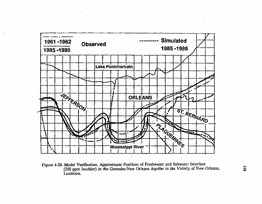
Simulated1985-1986
1961 -1962 Observed 1985-1986
Lake Pontchartraln
ORLEANS
Mississippi RiverL, I . I — I.. I
Figure 4-20. Model Verification. Approximate Positions of Freshwater and Saltwater Interface(250 ppm Isochlor) in the Gonzales-New Orleans Aquifer in the Vicinity of New Orleans, Louisiana.
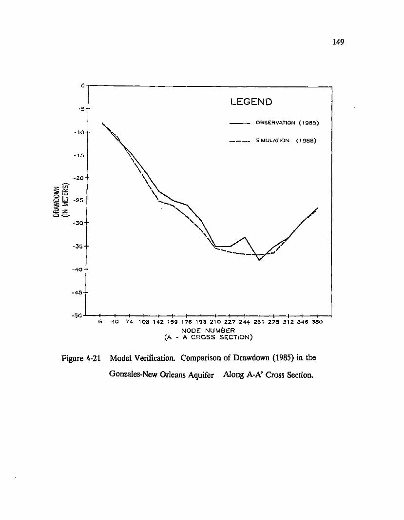
DRAW
DOWN
(IN
METE
RS)
149
-s-L E G E N D
-10-'
- 1 5 - -
- 2 0 - -
- 2 5 -
- 3 0 - -
- 3 5 - -
OSSERVATION ( 1 9 8 5 )
SIMULATION ( 1 9 8 5 )
,'N,
-40--
-45 - -
- 5 0 -6 40 74 108 142 159 176 193 210 227 244 261 278 312 346 380
NODE N U M BER (A - A C R O S S S E C T IO N )
Figure 4-21 Model Verification. Comparison of Drawdown (1985) in the
Gonzales-New Orleans Aquifer Along A-A’ Cross Section.

2000
1 8 0 0
1 6 0 0
1 4 0 0
1200
1QOO
8 0 0
6 0 0
4 0 0
200
0
4-22
L E G E N D
_ _ _ _ S im ulation
Observation
4------------ 1------------i-------------1------------1------------ 1------------ 1------------1------------ 1----------- ) ------------ 1------------ 1------------ 1------------1------------ 1—6 40 74 108 142 150 176 193 210 227 244 261 278 312 346
N ode N um ber (Along A - A C ross S e c tio n )
Model Verification. Comparison of Observed and Simulated Chloride Concentration (1985) in the Gonzales-New Orleans Aquifer Along A-A’ Cross Section.
(1 9 8 5 )
( 1 9 8 5 )

Table 4-7 Predicted Results of Piezometric Drawdown, Chloride Concentration and Subsidence in 1995 Under Projected Pumping Rates
Pumping Rates (Mgal/d)
50 75 100
Drawdown (DD) Cone. (CON) Subsidence(SUB)
(1)
DD(m)
(2)
CON(ppm)
(3)
SUB(cm)
(4)
DD(m)
(5)
CON(ppm)
(6)
SUB(cm)
(7)
DD(m)
(8)
CON(ppm)
(9)
SUB(cm)
(10)
Node No. 42 11.2 237.4 21.2 12.6 238.9 21.6 14.0 240.0 21.972 16.9 229.6 27.2 19.4 233.6 28.2 21.8 237.9 29.188 17.2 227.6 27.5 19.7 280.7 28.4 22.2 283.7 29.4
122 19.7 446.8 28.0 22.9 473.8 29.0 26.1 501.1 30.0140 24.3 442.7 33.0 29.6 485.5 34.5 35.0 530.1 35.9210 38.8 186.4 42.8 50.6 188.4 45.5 62.4 192.2 48.2227 39.6 578.4 58.7 51.5 631.5 61.4 63.3 687.0 64.1332 37.4 370.0 44.9 45.0 383.1 46.7 52.6 395.0 48.6350 41.2 309.3 40.4 49.5 333.3 43.1 57.7 353.5 45.9
(Note: Subsidence is relative to 1961)

Table 4-8 Predicted Results of Piezometric Drawdown, Chloride Concentration and Subsidence in 2010 Under Projected Pumping Rates
Pumping Rates (Mgal/d)
50 75 100
Drawdown (DD) DD CON SUB DD CON SUB DD CON SUBCone. (CON) (m) (ppm) (cm) (m) (ppm) (cm) (m) (ppm) (cm)Subsidence(SUB)
(1) (2) (3) (4) (5) (6) (7) (8) (9) (10)
Node No.42 11.2 241.3 29.6 12.6 244.7 30.6 14.0 247.8 31.572 16.9 257.6 37.4 19.4 269.5 39.8 21.9 282.1 42.188 17.2 287.2 37.7 19.4 294.9 40.1 22.2 302.7 42.5
122 19.7 465.3 38.4 22.9 524.9 40.9 26.1 581.6 43.4140 24.3 500.6 44.7 29.6 606.9 48.4 35.0 713.9 52.1210 38.8 161.3 58.0 50.6 179.1 64.8 62.4 205.2 71.5227 39.6 707.7 813 51.5 862.4 87.9 63.3 1023.5 94.5332 37.4 386.0 63.7 45.0 420.6 68.3 52.6 452.7 73.0350 41.2 281.0 58.9 49.5 328.3 65.8 57.7 359.0 72.5
(Note: Subsidence is relative to 1961)
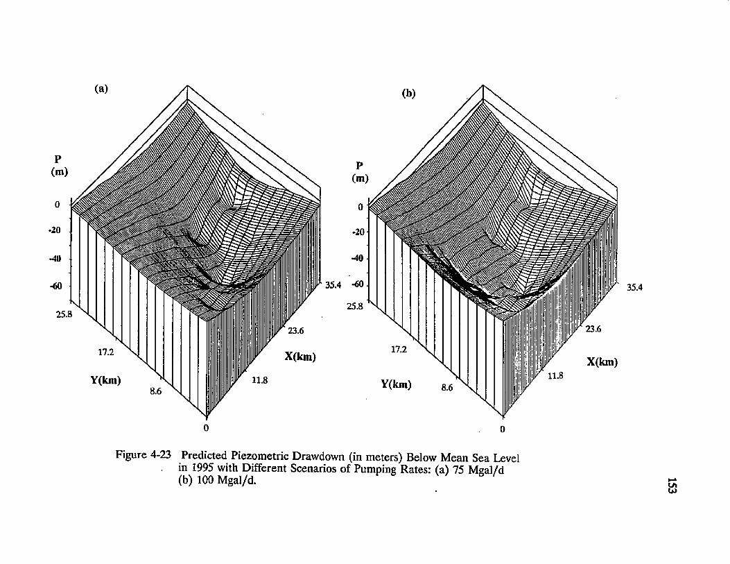
35,4 -60
r 23.6
35.4
Figure 4-23 Predicted Piezometric Drawdown (in meters) Below Mean Sea Level in 1995 with Different Scenarios of Pumping Rates: (a) 75 Mgal/d (b) 100 Mgal/d. inu>
11
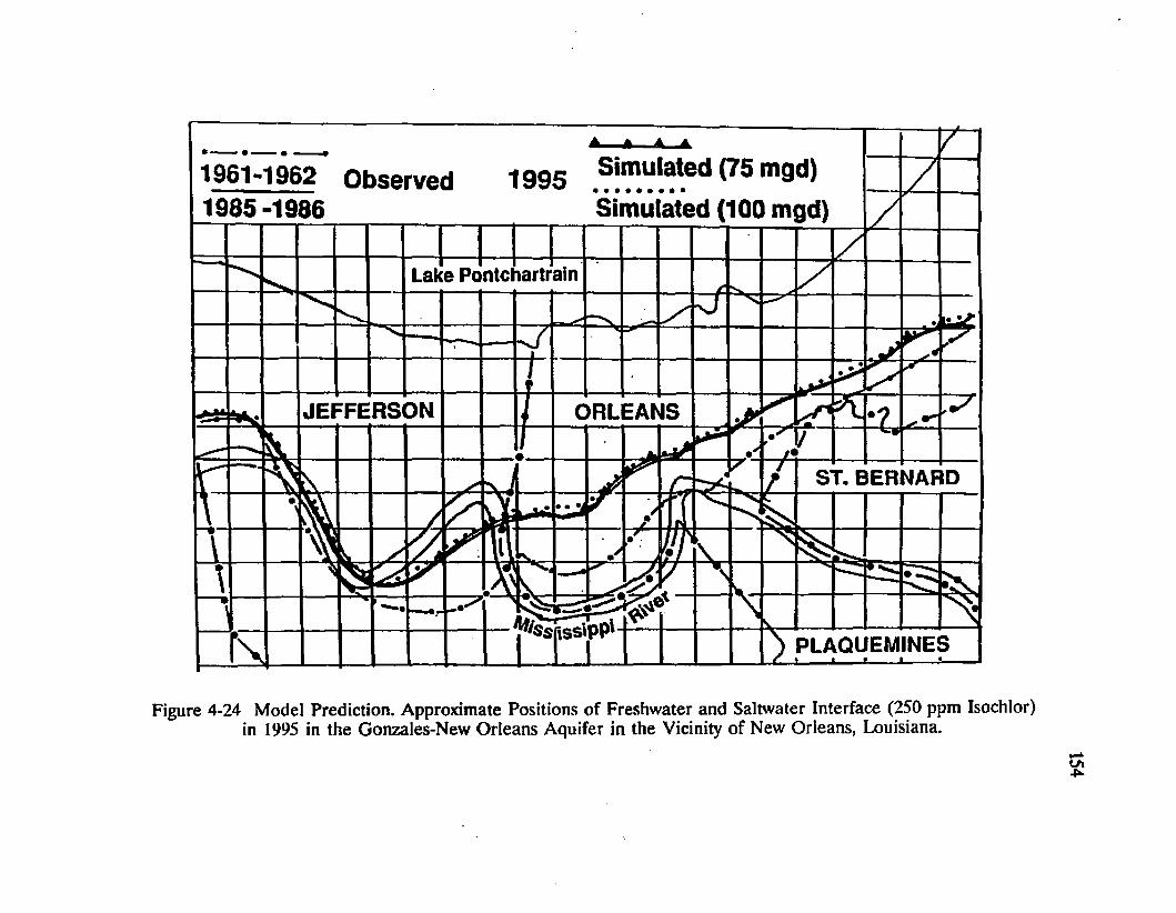
A * * A
1961-1962 O bserved 1995 Simulated (75 mgd) 1965-1986 Simulated (100 mgd)
r
lartrainLake Ponte
ORLEANS
ST. BERNARD
7®S$fiSS\pPlPLAQUEMINES
Figure 4-24 Model Prediction. Approximate Positions of Freshwater and Saltwater Interface (250 ppm Isochlor) in 1995 in the Gonzales-New Orleans Aquifer in the Vicinity of New Orleans, Louisiana.
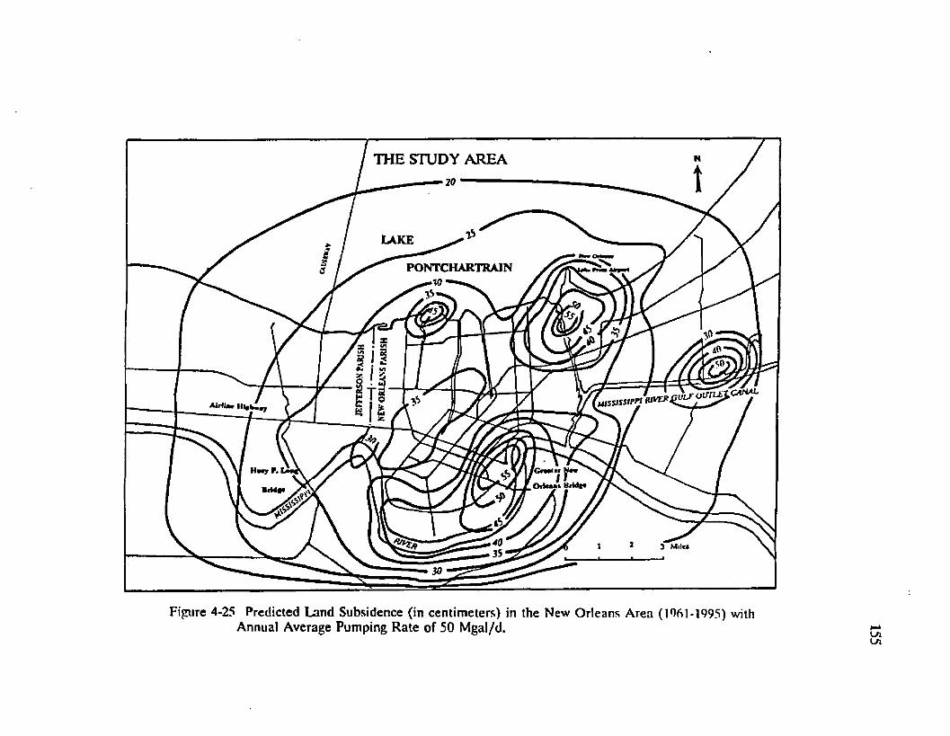
THE STUDY AREA
LAKE
PONTCHARTRAJN
U L f O lf fU ^ C A H A L
Figure 4-25 Predicted Land Subsidence (in centimeters) in the New Orleans Area (1%1-1995) with Annual Average Pumping Rate of 50 Mgal/d.

156
respectively. Note that the simulated drawdown in 1995 will increase significantly
under 75 and 100 Mgal/d, the concentration will increase slightly and the position
of the interface will move slightly northward with the increase of pumping rate, but
will remain stable as long as the pumping rate stays at the present rate. Maximum
subsidence in the downtown area will increase to about 58.7 cm (relative to 1961)
in 1995, showing an increase of 19 cm from 1985 and averaging 1.9 cm/yr. If the
present pumping rate of 50 Mgal/d remains stable to the year 2010, the drawdown
and the concentration will increase slightly as a whole. Figure 4-26 shows the
contours of subsidence in the year 2010 under an annual average pumping rate of
50 Mgal/d. An increase of about 48 cm will occur relative to 1985. Figure 4-27
plots the land subsidence under different pumping rates in 1995 and 2010.
(2) Prediction of piezometric drawdown, chloride concentration and subsidence in
response to additional pumpage when the surface water supply is cut off.
Jefferson and Orleans Parishes get their water supply mainly from the
Mississippi River. Table 4-9 is a list of actual withdrawal of water, both surface
water and ground water, for the two parishes in 1985 (Louisiana Department of
Transportation and Development, 1987).
In times of emergency such as chemical spills into the river or saltwater
wedge intrusion from the estuary during long dry spells, water intakes along the
river have to be shut down and the surface water supply has to be cut down to a
certain extent. An alternative to compensate for the inadequacy of the surface water
supply is to pump more water from the Gonzales-New Orleans Aquifer to meet the
overall demand of the users. Sue pumping schemes have been studied with respect
to the surface water supply cut off by: (1) 100%; (2) 50%; (3) 17%; (4) 12%; (5)

THE STUDY AREA
LAKE
PONTCHARTRAIN
so
Figure 4-26 Predicted Land Subsidence (in centimeters) in the New Orleans Area (1961-2020) with Annual Average Pumping Rate of 50 Mgal/d.
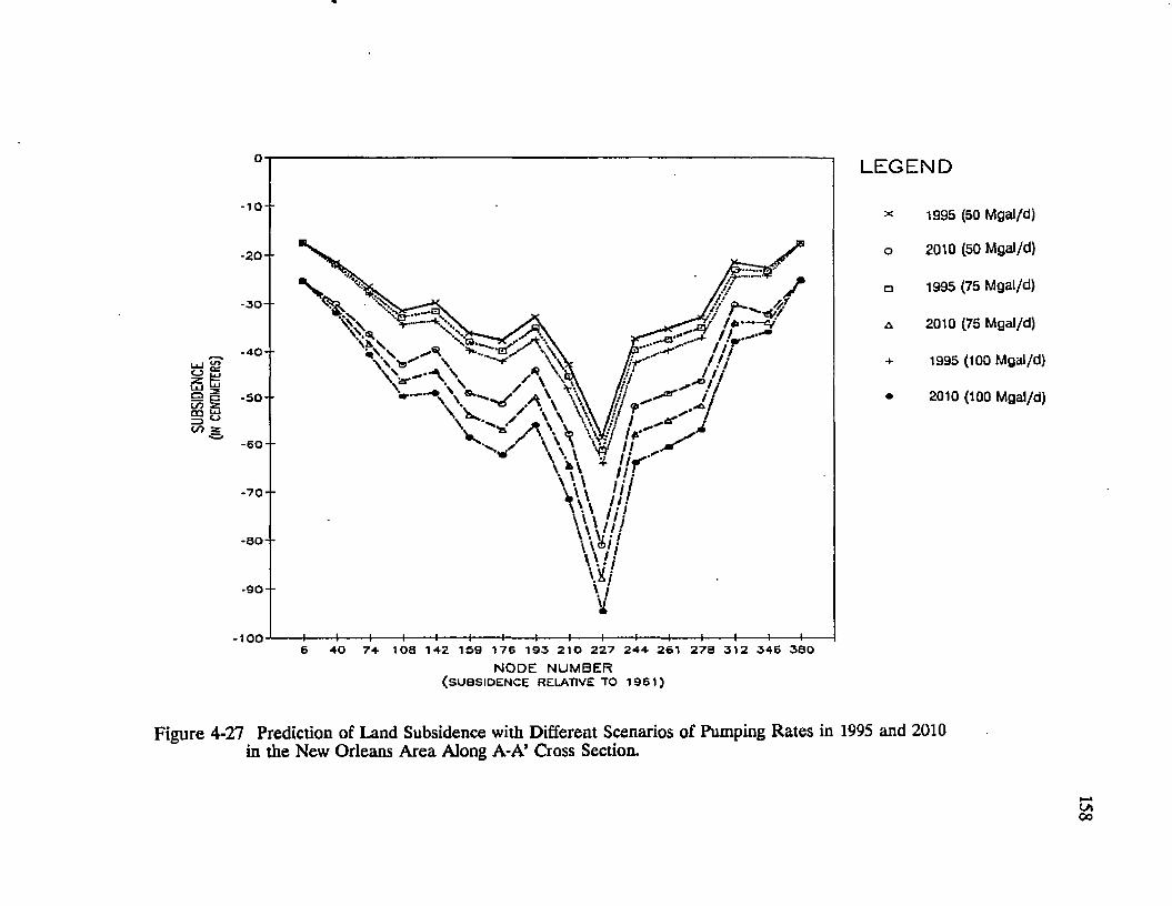
SUBS
IDEN
CE
(IN CE
NtlU
EIER
S)
o - -
- 1 0 - -
- 20 - -
- 3 0 "
- 4 0 - -
- 5 0 - -
- 6 0 - -
- 7 0 - -
- 8 0 "
- 9 0 - -
- 100 - -
-« av** \
\\\ / /* • / - \ N ' 4 / '/ i
\ * > \ \ k M /*•
-4- - + - - * - -+ - -+ - ■4- -4- - + - -+ - - + - -4- -4- -4- - + -
L E G E N D
4 0 7 4 10 8 1 4 2 1 5 9 1 7 6 1 9 3 2 1 0 2 2 7 2 4 4 2 6 1 2 7 8 3 1 2 3 4 6 3 8 0NODE NUMBER
(SU B SID E N C E RELATIVE TO 1 9 6 1 )
1995 (50 Mgal/d)
2010 (50 Mgal/d)
1995 (75 Mgal/d)
2010 (75 Mgal/d)
1995 (100 Mgal/d)
2010 (100 Mgal/d)
Figure 4-27 Prediction of Land Subsidence with Different Scenarios of Pumping Rates in 1995 and 2010 in the New Orleans Area Along A-A’ Cross Section.
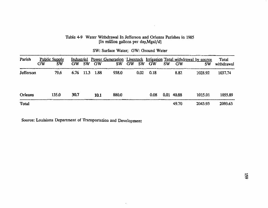
Table 4-9 Water Withdrawal In Jefferson and Orleans Parishes in 1985 [In million gallons per day,Mgal/d]
SW: Surface Water; GW: Ground Water
Parish Public Supplv GW SW
Industrial Power Generation Livestock Irrigation Total withdrawal bv source GW SW GW SW GW SW GW SW GW SW
Totalwithdrawal
Jefferson 79.6 6.76 11.3 1.88 938.0 0.02 0.18 8.82 1028.92 1037.74
Orleans 135.0 30.7 10.1 880.0 0.08 0.01 40.88 1015.01 1055.89
Total 49.70 2043.93 2093.63
Source: Louisiana Department of Transportation and Development

160
9%; and (6) 4%.
Table 4-10 displays the responses of piezometric drawdown, chloride
concentration in the Gonzales-New Orleans Aquifer and subsidence in the area to
additional pumpage in 20 years. The total pumping rate in the table includes the
regular ground water pumpage of 50 Mgal/d.
It is obvious that Alternatives 1 to 3 are absolutely impractical because the
piezometric drawdowns are large enough to deplete water totally in the aquifer,
considering the aquifer lies only 150 - 260 meters below mean sea level with 30-90
meters of thickness. The results of land subsidence and chloride concentration also
show very large values, the maximum of which are 6.25 m and over 2000 ppm of
chloride in the downtown area.
Comparison of Alternatives 4 to 6 yields the approximate maximum pumping
rate that will not cause adverse effects such as acceleration of local subsidence, total
depletion of the aquifer and deterioration of water quality. It can be seen that as
far as drawdown is concerned, Alternative 5 with a total pumpage of 230 Mgal/d
will not create drawdown that exceeds the "safety level" (i.e., the total depletion of
the aquifer). However, the chloride concentration will increase significantly in the
downtown area as compared to the present pumping status. Land subsidence in this
alternative averages 3 cm/yr, which is 1.5 times that of the normal subsidence rate.
Table 4-11 shows the responses at one of the locations near the downtown area
(Node #210) that yield maximum drawdown and subsidence under continuous
pumping for 30 days, 60 days, 180 days, 2 years, 10 years and 20 years.
Alternative 4 is not preferable also because the chloride concentration at
some locations may be as high as four times that which exists in the present situation

Table 4-10 Responses of Piezometric Drawdown, Chloride Concentration and Subsidence to Additional Pumpage to Supplement Surface Water Supply Shortage (20 years of simulation)
Alternatives 1 2 3
Total Pumpage 2100 [Mgal/d] 1050 [Mgal/d] 400 [Mgal/d]
% of Surface Water Supply Supplemented ( % )
100 50 17
Drawdown (DD) DD CON SUB DD CON SUB DD CON SUBCone. (CON) (m) (ppm) (cm) (m) (ppm) (cm) (m) (ppm) (cm)Subsidence(SUB)
(1) (2) (3) (4) (5) (6) (7) (8) (9) (10)
Node No.42 172.6 240.2 94.5 91.0 247.1 52.7 41.6 259.5 26.872 332.5 1356.2 224.6 171.4 906.8 117.9 74.3 440.1 52.4
140 735.0 2036.6 395.2 397.2 2061.9 203.9 152.0 2037.9 86.2191 816.2 1783.6 395.9 409.4 1778.6 205.6 168.5 1790.9 87.2210 1442.1 1991.7 625.3 705.1 1937.7 320.9 280.1 1474.2 132.5227 1334.2 2085.4 587.9 655.2 2091.8 307.3 261.6 2077.9 133.2244 1159.2 1926.8 453.3 572.9 1936.5 234.8 230.6 1758.6 98.7332 562.3 743.6 293.8 285.4 745.4 158.0 120.4 726.3 73.2350 491.8 538.4 297.1 251.2 531.8 157.1 107.6 514.3 70.4
Note: 1. Total pumpage include the regular pumpage of 50 Mgal/d;2. Subsidence is relative to 1985.

Table 4-10 Responses of Piezometric Drawdown, Chloride Concentration and Subsidence to Additional Pumpage to Supplement Surface Water Supply Shortage (20 years of simulation)
(continued)
Alternatives 4 5 6
Total Pumpage 300 [Mgal/d] 230 [Mgal/d] 140 [Mgal/d]
% of Surface Water Supply Supplemented
12 9 4
Drawdown (DD) DD CON SUB DD CON SUB DD CON SUBCone. (CON) <tn) (ppm) (cm) (m) (ppm) (cm) (m) (ppm) (cm)Subsidence (SUB)
(1) (2) (3) (4) (5) (6) (7) (8) (9) (10)
Node No.42 33.6 256.7 22.6 21.2 256.7 17.0 16.2 249.4 14.372 58.7 362.1 41.8 34.6 322.4 28.0 25.8 282.8 21.3
140 117.3 1935.8 67.2 63.1 1047.4 37.6 43.7 794.1 27.1191 130.1 1730.7 67.9 84.2 1561.5 44.8 57.3 1250.1 31.4210 213.1 1238.1 101.8 124.3 356.6 60.3 81.5 233.3 40.9227 199.4 1903.2 104.9 125.5 1546.7 69.0 82.5 1113.1 50.1244 176.3 1554.5 76.5 125.7 1703.3 55.4 82.8 1289.4 37.8332 94.1 693.6 59.4 92.3 557.1 52.5 64.9 547.2 39.1350 84.7 506.7 56.3 81.9 419.1 64.4 71.0 387.2 44.8
Note: 1. Total pumpage include the regular pumpage of 50 Mgal/d;2. Subsidence is relative to 1985.

Table 4-11 Piezometric Drawdown, Chloride Concentration andSubsidence with Different Pumping Rates At Node #210 For 30, 60, 180 Days, 2 years, 10 years and 20 years
Pumping Rates 140 [Mgal/d] 230 [Mgal/d] 300 [Mgal/d]
Drawdown (DD) Cone. (CON) Subsidence (SUB)
DD(m)
CON(ppm)
SUB(cm)
DD(m)
CON(ppm)
SUB(cm)
DD CON (m) (ppm)
SUB(cm)
Duration:30 days 79.5 214.1 0.26 120.6 214.1 0.30 206.2 250.4 0.39
60 days 80.2 218.0 0.51 121.7 218.4 0.58 208.5 350.2 0.85
180 days 81.2 227.0 1.32 123.0 226.4 1.74 210.5 380.3 2.94
2 years 81.3 229.3 5.1 123.8 227.3 7.1 211.4 491.2 10.2
10 years 81.4 230.4 21.0 124.0 234.0 20.8 212.2 726.6 50.9
20 years 81.5 233.3 40.9 124.3 356.6 60.3 213.1 1238.1 101.8
Average rate of subsidence (cm/yr) 2.0 3.0 5.0
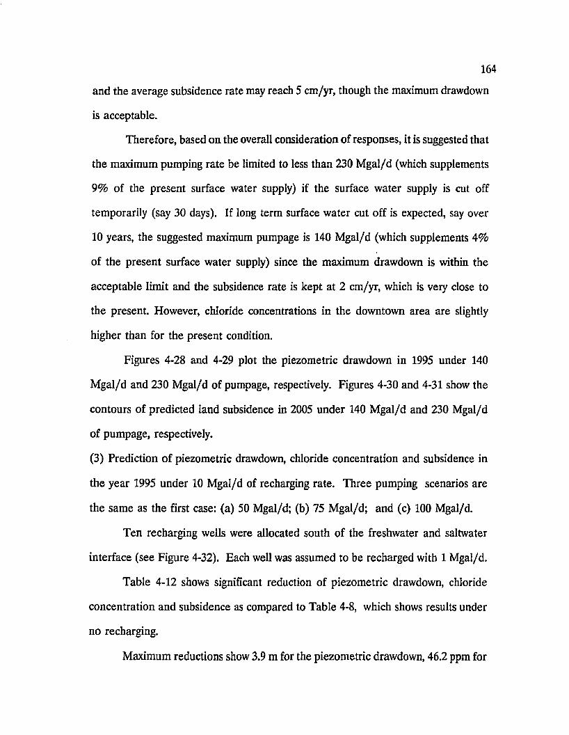
164
and the average subsidence rate may reach 5 cm/yr, though the maximum drawdown
is acceptable.
Therefore, based on the overall consideration of responses, it is suggested that
the maximum pumping rate be limited to less than 230 Mgal/d (which supplements
9 % of the present surface water supply) if the surface water supply is cut off
temporarily (say 30 days). If long term surface water cut off is expected, say over
10 years, the suggested maximum pumpage is 140 Mgal/d (which supplements 4 %
of the present surface water supply) since the maximum drawdown is within the
acceptable limit and the subsidence rate is kept at 2 cm/yr, which is very close to
the present. However, chloride concentrations in the downtown area are slightly
higher than for the present condition.
Figures 4-28 and 4-29 plot the piezometric drawdown in 1995 under 140
Mgal/d and 230 Mgal/d of pumpage, respectively. Figures 4-30 and 4-31 show the
contours of predicted land subsidence in 2005 under 140 Mgal/d and 230 Mgal/d
of pumpage, respectively.
(3) Prediction of piezometric drawdown, chloride concentration and subsidence in
the year 1995 under 10 Mgal/d of recharging rate. Three pumping scenarios are
the same as the first case: (a) 50 Mgal/d; (b) 75 Mgal/d; and (c) 100 Mgal/d.
Ten recharging wells were allocated south of the freshwater and saltwater
interface (see Figure 4-32). Each well was assumed to be recharged with 1 Mgal/d.
Table 4-12 shows significant reduction of piezometric drawdown, chloride
concentration and subsidence as compared to Table 4-8, which shows results under
no recharging.
Maximum reductions show 3.9 m for the piezometric drawdown, 46.2 ppm for
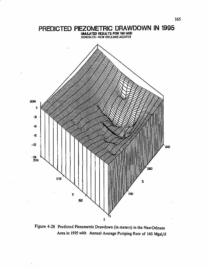
PREDICTED PIEZOMETRIC DRAWDOWN IN 1995SMJLATED RESULTS FOR 140 MGDGONZALES-NEW ORLEANS AQUIFER
m m
I71B6 \
35405
0
Figure 4-28 Predicted Piezometric Drawdown (in meters) in the New Orleans Area in 1995 with Annual Average Pumping Rate of 140 Mgal/d

PREDICTED PIEZOMETRIC DRAWDOWN IN 1995SMJLATED RESULTS FOR 230 MGDGONZALES-NEW ORLEANS AQUIFER
DROWN
£405
-15025749
Figure 4-29 Predicted Piezometric Drawdown (in meters) in the New Orleans Area
in 1995 with Annual Average Pumping Rate of 230 Mgal/d

THE STUDY AREA
20 -
LAKE
PONTCHARTRAIN*^
60
uississirrt culf
Ofl
1 Milei40
Figure 4-30 Contours of Predicted Land Subsidence (in centimeters) in the New Orleans Area in 2005 With Annual Pumping Rate of 140 Mgal/d If Surface Water Supply is Cut Off By 4% (Subsidence is Relative to 1961).
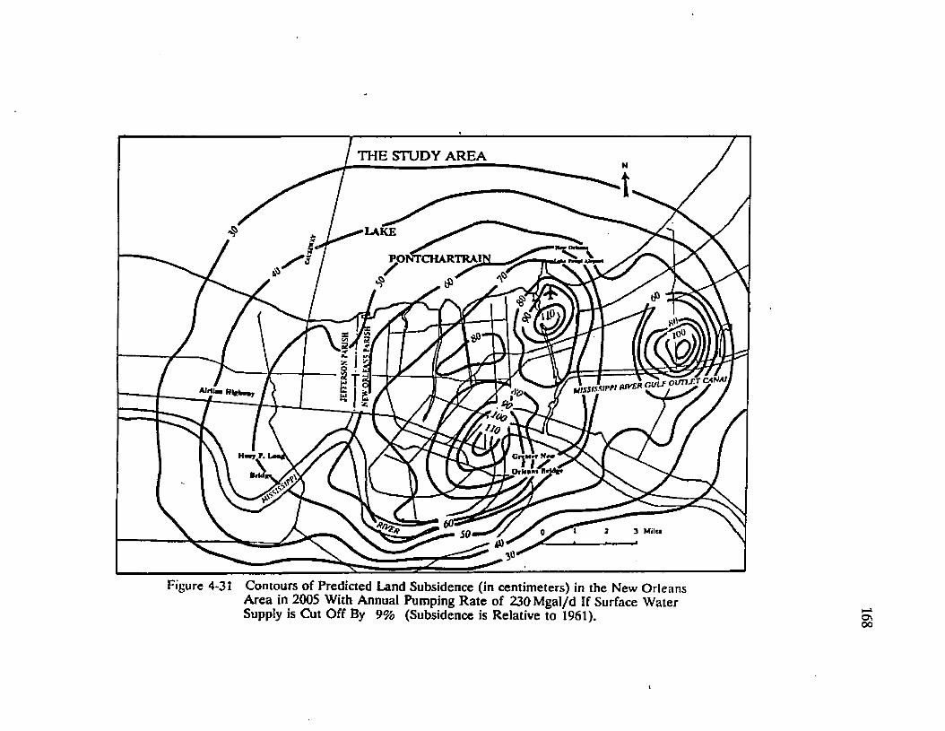
THE STUDY AREA
LAKE
PpNTCHARTRAr
( r i L f O V T U J < 2 * * 1
S Mila
Figure 4-31 Contours of Predicted Land Subsidence (in centimeters) in the New Orleans Area in 2005 With Annual Pumping Rate of 230Mga!/d If Surface Water Supply is Cut Off By 9% (Subsidence is Relative to 1961).
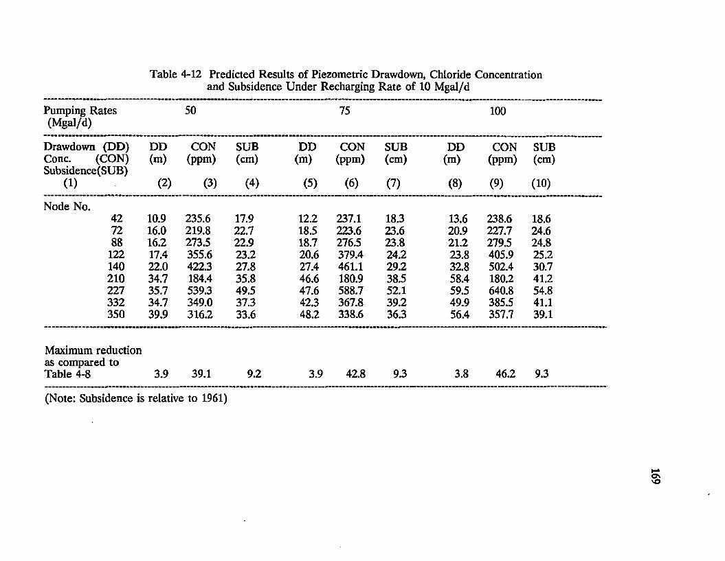
Table 4-12 Predicted Results of Piezometric Drawdown, Chloride Concentration and Subsidence Under Recharging Rate of 10 Mgal/d
Pumping Rates (Mgal/d)
50 75
1 o
! ©
! i
Drawdown (DD) DD CON SUB DD CON SUB DD CON SUBCone. (CON) (m) (ppm) (cm) (m) (ppm) (cm) (m) (ppm) (cm)Subsidence(SUB)
(1) (2) (3) (4) (5) (6) (7) (8) (9) (10)
Node No.42 10.9 235.6 17.9 12.2 237.1 18.3 13.6 238.6 18.672 16.0 219.8 22.7 18.5 223.6 23.6 20.9 227.7 24.688 16.2 273.5 22.9 18.7 276.5 23.8 21.2 279.5 24.8122 17.4 355.6 23.2 20.6 379.4 24.2 23.8 405.9 25.2140 22.0 422.3 27.8 27.4 461.1 29.2 32.8 502.4 30.7210 34.7 184.4 35.8 46.6 180.9 38.5 58.4 180.2 41.2227 35.7 539.3 49.5 47.6 588.7 52.1 59.5 640.8 54.8332 34.7 349.0 37.3 42.3 367.8 39.2 49.9 385.5 41.1350 39.9 316.2 33.6 48.2 338.6 36.3 56.4 357.7 39.1
Maximum reduction as compared toTable 4-8 3.9 39.1 9.2 3.9 42.8 9.3 3.8 46.2 9.3
(Note: Subsidence is relative to 1961)
170
the chloride concentration and 9.3 cm for the subsidence. Figure 4-32 shows that
by installing recharging wells, the movement of the interface will effectively be
obstructed to a certain degree no matter how much water is pumped. In fact, the
interface in the downtown area will retreat back approximately 0.2 to 0.75 mile to
the south. The distance which the interface retreats depends on the locations and
the amount of water recharged to the aquifer.
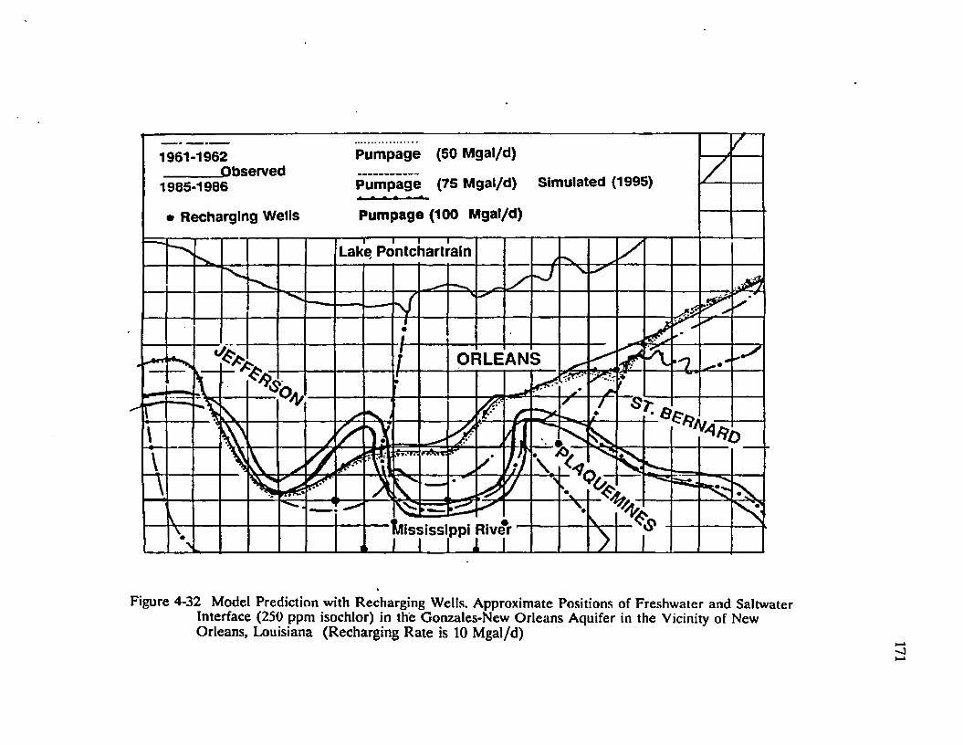
1961-1962_______Observed1985-1986
• Recharging Wells
Pumpage (50 Mgal/d)
Pumpage (75 Mgal/d) Simulated (1995)* - - -
Pumpage (100 Mgal/d)
v
i---------- 1— i— i
Lake Pontchartrain
ORLEANS
Jlississlppi RiverI I 1 I
Figure 4-32 Model Prediction with Recharging Wells. Approximate Positions of Freshwater and Saltwater Interface (250 ppm isochlor) in the Gonzales-New Orleans Aquifer in the Vicinity of New Orleans, Louisiana (Recharging Rate is 10 Mgal/d)
CHAPTER 5
SUMMARY AND CONCLUSIONS
172

173
Coastal aquifers are subject to compaction (subsidence) and saltwater
intrusion when ground water is heavily and extensively pumped for municipal,
industrial and other uses. Many coastal areas in the world are losing their coastal
shorelines at an alarming rate as high as 120 square kilometers annually, the
situation Louisiana is now experiencing. Concurrently, saltwater intrusion into the
coastal aquifers is almost inevitable. The main reasons that cause land subsidence
are the natural compaction of unconsolidated subsurface material, eustatic sea level
rise and man-induced factors such as withdrawal of water, oil and gas, and the main
reasons for saltwater intrusion to occur are the pumping of water from the aquifer
and the difference in density between salt water and fresh water. The need to
develop a model, based on the dynamics of fluid flow, solute transport and
subsidence, that enables the simulation of both the land subsidence and saltwater
intrusion is thus very pressing and very practical.
Three governing equations in the model, namely, the flow equation, the
advective-dispersion-diffusion equation and the land subsidence equation describe
the mechanisms of ground water flow, solute transport and solid matrix compaction
under withdrawal of water from a heterogeneous and anisotropic aquifer. These
three equations are derived in detail based on mass conservation taking into account
the compressibility of the aquifer and the sloping effect of the aquifer. By
integrating the three-dimensional equations over the thickness of an aquifer and
introducing a relationship between changes in averaged piezometric head and land
subsidence, a single partial differential equation in terms of land subsidence has
been obtained for pumping from a confined or unconfined aquifer.
Based on these three governing equations, the STRALAN computer model
174
was developed using a hybridization of finite element and integrated-finite difference
methodology as that adopted by the SUTRA model developed by Voss and others.
The Galerkin method of weighted residuals using "basis function" was used to
minimize the error of approximation over the volume of a three-dimensional space
domain. This model can be applied to solve simultaneously the land subsidence
problem and saltwater intrusion problem in a confined or unconfined, horizontal or
sloping aquifer. The applicability of the model was verified by comparison of the
simulated results with analytical solutions and by the simulation of ground water flow
and solute transport in a unconfined aquifer.
As a case study, STRALAN model was applied to the Gonzales-New Orleans
aquifer to examine the potentials of saltwater intrusion and land subsidence under
various pumping rates as required or proposed to meet the increasing demands of
ground water in the New Orleans area, Louisiana. The numerical model, calibrated
and verified with limited observed data set, provides a useful tool to quantify the
dynamic behavior of saltwater intrusion and subsidence in Louisiana coastal aquifer
systems.
Sensitivity analyses and statistical analyses (root mean squared error) were
performed to calibrate the various hydrogeologic parameters under time-vaiying
pumping rates with an estimate of 10 Mgal/d of vertical leakage from the overlying
and underlying aquifers. The results of the calibrated parameters are:
Hydraulic conductivity K : (1.47-2.05) x 10-4 m/s;
Transmissivity (= K B ) : (44.1-184.5) x 10J mJ/s;
Storage coefficient: 0.0004 - 0.0015
Aquifer compressibility o : 0.3 x 10* - 0.3 x 10'10 [m«s2/kg];
175
Longitudinal and transverse dispersivity : a L = 4 0 0 m and a T - 4 m;
Molecular diffusivity : 1.8 x 10 s m2/s.
Of the factors that affected the movement of ground water, solute transport
and land subsidence, the sensitivity study indicated that:
(1) The hydraulic conductivity is a dominant factor to control the degree of
drawdown. Under the same set of parameters, pumping rates and vertical
leakages from the adjacent aquifers, the smaller the hydraulic conductivity, the
larger the drawdown. A small change of hydraulic conductivity may translate to
a large change of drawdown. Hydraulic conductivity may have a slight inverse
effect on subsidence. The larger the hydraulic conductivity, the smaller the
subsidence. However, subsidence is only slightly sensitive to changes of hydraulic
conductivity. Related closely to the hydraulic conductivity is the sloping angle
of the aquifer which may produces sensitive results of piezometric drawdown.
This is because the sloping angle only appears in the advection term of the flow
and solute transport equations. However, since the sloping angle in the present
study is very small (-0.3°), the effect is minor.
(2) The aquifer compressibility is a dominant factor to control the degree of
subsidence. Under the same conditions of hydrogeologic parameters, pumping
rates and vertical leakages, the larger the compressibility, the larger the
subsidence. The drawdown and the chloride concentration are not sensitive to
changes of aquifer compressibility. However, increases in aquifer
compressibility result in slight increases in drawdown and chloride
concentration.
(3) Aquifer dispersivities and diffusivity play a relatively minor role in the transport

176
of solute. This may be attributed to the very low flow velocity which is in the
order of 10* to 10'7 m/s in the study area.
Results of the calibration run indicate average ground water velocities will
increase at the principal pumping centers which are the downtown New Orleans
area, Industrial Canal and University of New Orleans area, and the Michoud area.
Velocities may increase from the present velocity of 4.0 x 10'7 m/s to a maximum
of 6.5 x 10* m /s when the pumping rate is increased to 100 Mgal/d.
Calibration run for 20 years (1961-1981) shows that the simulated drawdown
in the study area ranges from 6 m to a maximum of 44.8 m in the northeastern part
of the downtown area. The simulated saltwater and freshwater interface shows a
northward movement of as much as 2 miles in 20 years at the west bank of the
Mississippi River near the downtown area. The simulated land subsidence in the
area ranges from 15 cm to 35 cm, averaging 0.75 cm/yr to 1.75 cm/yr.
Model predictions for the year 1995 and 2010 under 50, 75 and 100 Mgal/d
of pumpage show significant increases of drawdown with the increase in pumpage
but will remain stable with respect to the increase of time. Chloride concentrations
will increase slightly with the increase of pumpage and time at locations south of the
present interface. This implies that once the interface is arrested, it will not move
northward as long as the pumpage remains at the present rate.
Predicted results for land subsidence show maximum subsidence in the
downtown area will increase another 19 cm and 48 cm in the year 1995 and 2010,
respectively with 1985 as the starting point under the present pumping rate
condition.
Because the public-water supply from the Mississippi River is cut off at times

177
of chemical spills and/or intrusion of a saltwater wedge from the estuary, decision
makers have begun to consider the Gonzales-New Orleans aquifer as an alternative
source. Different percentages of surface water supply were being considered to be
supplemented by ground water. Simulated results indicate that the maximum
pumping rate should not exceed 230 Mgal/d for a short time period. This pumping
rate includes 9 % of the present surface water supply. If long term surface water
supply cut off is expected, the suggested maximum pumpage is 140 Mgal/d, which
includes 4% of the present surface water supply. The upper levels of
supplementation were selected such that the overall responses of piezometric
drawdown, chloride concentration and land subsidence would not induce significant
adverse effects such as total or partial depletion of the aquifer, significant northward
movement of the saltwater and freshwater interface or acceleration of subsidence
rate.
The degree and areal extent of saltwater intrusion and subsidence in the
Gonzales-New Orleans aquifer depends greatly on the location of pumping wells and
the amount of water pumped. The simulated results show that saline water will
intrude further northward in the southern part of the area where heavy pumping
activities occur north of the southern limit of the 250 ppm isochlor. Once the
advancing isochlor reaches these area of heavy pumping, the wells will arrest any
further movement of the interface resulting in the decrease of chloride concentration
in the northern parts of the study area. However, the water being pumped from
these wells having a heavy draft may not meet the drinking standard (USEPA, 1976).
Development of the recharging well system was intended to decelerate and
alleviate the rates of piezometric drawdown, land subsidence and northward
178
movement of the interface. It is a complicated planning and management problem.
The best effect of such a system not only depends on the location of wells but also
depends on the amount of water recharged to the aquifer from each well. The
application example show that the recharging wells located south of the current 250
ppm isochlor may stop the northward movement of the interface and decelerate the
rate of subsidence significantly. However, feasibility studies regarding the layout of
the recharging wells, the amount and duration of recharging, and the cost-benefit
analyses have to be conducted in detail before any decision can be made. It is
beyond the scope of this dissertation to commence such a detailed study.
The calibrated set of hydrogeologic parameters, such as hydraulic conductivity,
aquifer compressibility and dispersivity etc., is based on the comparison of simulated
results with the observed data set and the root mean squared error index. However,
more elaborate statistical and optimization approaches may be further studied.
Because of the complex simulation model to account for three main dependent
variables (i.e.,piezometric drawdown, solute concentration and subsidence) and five
parameters (i.e., hydraulic conductivity, aquifer compressibility, longitudinal and
transverse dispersivity and molecular diffusivity), it is expected that using any kind
optimization technique would require great amount of computer memory and
computer time. Future research on this topic in the same study area would be very
challenging.
In the optimal management of Louisiana coastal aquifer system, the predicted
positions of the dispersed interface between fresh water and salt water and the
predicted land subsidence under various pumping conditions will constitute important
physical constraints and the piezometric head will be one of the decision variables.
179
The need for such an optimization model is of crucial importance in the
development of a strategy to cope with the emergency interruption of surface water
supplies.
Lastly, because of the various approximate assumptions made in the
derivation of the governing equations and in the computer modeling, the results
obtained should be viewed as estimates of the true occurrences. However, for
engineering purposes, such estimates should be sufficient.

REFERENCES

181
1. Bear, J., 1979. "Hydraulics of Groundwater," McGraw-Hill, New York.
2. Bear, J. and Kapuler, I., 1981." A Numerical Solution for the Movement of an
Interface in a Layered Coastal Aquifer," J. Hydrol., Vol.50, pp. 273-298.
3. Bear, J. and Corapcioglu, M. Y., 1981a. "Mathematical Model for Regional Land
Subsidence Due to Pumping. 1. Integrated Aquifer SubsidenceEquations Based
on Vertical Displacement Only," Water Resources Research, Vol. 17, No.4,
pp. 937-946.
4. Bear, J. and Corapcioglu, M. Y., 1981b. "Mathematical Model for Regional Land
Subsidence Due to Pumping. 2. Integrated Aquifer SubsidenceEquations for
Vertical and Horizontal Displcements," Water Resources Research, Vol.17,
No.4, pp. 947-958.
5. Bear, J., and Verruijt, A., 1987. "Modeling Groundwater Flow and Pollution,"
D. Reidel Publishing Co., Boston, Mass., 414 pp.
6. Bell, F. G., 1987. "Ground Engineer’s Reference Book," Butterworths and Co.
(Publishers) Ltd.
7. Biot, M. A., 1941. "General Theory of Three-dimensional Consolidation," J.
Apply Physics, No. 12, pp. 155-164.
8. Bittinger, M. W., Duke, H. R. and Longenbaugh, R. A., 1967. "Mathematical
Simulations for Better Aquifer Management," Int. Assoc. Sci. Hydrology., Symp.
Artificial Recharge Management of Aquifers, Haifa, pp. 509-519.
9. Bouwer, H. 1978. "Groundwater Hydrology," McGraw-Hill Book Company,
480 p.

10. Bredehoeft, J. D. and Pinder, G. F. 1970. "Digital Analysis of Flow in
Multiaquifer Groundwater Systems: A Quasi Three-dimensional Model," Water
Resources Research, Vol 6, No.3, pp. 883-888.
11. Cardwell, G. T., Forbes, M. J., Jr., and Gaydos, M. W., 1967. "Water Resources
of the Lake Pontchartrain Area, Louisiana," Louisiana Department of
Conservation and Department of Public Works, Water Resources Bulletin 12,
105 p.
12. Cardwell, G. T., Rollo, J. R., and Long, R. A , 1963. "Basic Groundwater-Data
for the Mississippi River Parishes South of Baton Rouge, Louisiana,"
Louisiana Department of Public Works.
13. Chapamn, T. G. 1980. "Modeling Groundwater Flow Over Sloping Beds," Water
Resources Research, Vol.16, No.6, pp. 1114-1118.
14. Cooley, R. L., 1971. "A Finite Difference Method for Unsteady Flow in Variably
Saturated Porous Media: Application to Single Pumping Well," Water
Resources Research, Vol 7, No.6, pp. 1607.
15. Coleman, J. M., 1981. "Deltas: Processes of Deposition and Models for
Exploration. 2nd Ed.," Burgess, Minneapolis, MN.
16. Corapcioglu, M. Y. and Bear, J., 1983. "A Mathematical Model for Regional
Land Subsidence Due to Pumping. 3. Integrated Equations for a Phreatic
Aquifer," Water Resources Research, Vol.19, No.4, pp. 895-908.
17. Corapcioglu, M. Y. 1983. "Land Subsidence- A State-of-Art Review," In
Foundation of Transport Phenomena in Porous Media. The Hague. The
Netherlands.

183
18. Dial, D. C., 1983. "Ground-water data for the Mississippi River Parishes in the
Greater New Orleans Area, Louisiana," Louisiana Department of
Transportation and Development, Office of Public Works, Water Resources
Basic Records, Report No. 11, 47 p.
19. Dial, D. G, and Sumner, D. M., 1989 [in press]. "Geohydrology and Simulated
Effects of Pumpage on the New Orleans Aquifer System at New Orleans,
Louisiana," Louisiana Department of Transportation and Development Water
Resources Technical Report No. 46.
20. Dial, D. C. and Tomaszewski D. J., 1988. "Geohydrology, Water Quality, and
Effects of Pumpage on the New Orleans Aquifer System, Northern Jefferson
Parish, Louisiana," U.S. Geological Survey Water Resources Investigations
Report, No. 88-4097.
21. Douglas, J. Jr. and Dupont, T., 1974. "Colocation Methods For Parabolic
Equations in a Single Space Variable," Springer-Verlag. Berlin and New York.
22. Eddards, M. L., Kister, L. R,, and Scarcia, Glenn, 1956. "Water Resources of the
New Orleans Area, Louisiana," U.S. Geological Survey Circular 374, 41 p.
23. Eshett, A. and Longenbaugh, R. A., 1965. "Mathematical Model For Transient
Flow in Porous Media," Progress Report, Civil Engineering Dept., Colorado
State University, Fort Collins, Colorado.
24. Fayers, F. J. and Sheldon, J. W., 1962. "The Use of a High-speed Digital
Computer in the Study of the Hydrodynamics of Geological Basin," J. Geophys.
Research, Vol.67, No.6, pp. 2421-2431.
25. Flanagan, C. A., 1989. "Differential Subsidence in New Orleans," A Thesis for

184
Fulfillment of Master of Science, Department of Geography, Louisiana State
University.
26. Frangakis, C. N. and Tzimopoulos, C.,1979. "Unsteady Groundwater Flow on
Sloping Bedrock," Water Resources Research, Vol.15, No.l, pp. 176-179
27. Freeze, R. A., and Cherry, J. A.,1979. "Groundwater," Prentice-Hall,Englewood
Cliffs, NJ, 376p.
28. Frind, E. 0.,1982. "Simulation of Long-term transient density-dependent
Transport in Ground Water," Adv. Water Resources, No.5, pp. 73-88.
29. Gambolati, G. A, and Freeze, R. A., 1973. "Mathematical Simulation of the
Subsidence of Venice. 1, Theory," Water Resources Research. Vol.9, pp. 721-
733.
30. Gagliano, S. M., Meyer-Arendt, K. J., and Wicker, K. M., 1981. "Land Loss in
the Mississippi Deltaic Plain," Transactions, Gulf Coast Association of
Geological Societies, No.31, pp. 295-300.
31. Ghaboussi, J. and Wilson, E. L., 1973. "Flow of Compressible Fluid in Porous
Elastic Media," Int. J. Numer. Meth. Engr., Vol.5, pp. 419-442.
32. Gray, W. G. and Pinder, G. F., 1974. "Galerkin Approximation of the Time
Derivative in the Finite Element Analysis of Groundwater Flow," Water
Resources Research, Vol.10, No.4, pp. 821-828.
33. Gray, W. G.,1983. "Comparison of Finite Difference and Finite Element
Methods," In Foundations of transport Phenomena in Porous Media. The
Hague. The Netherlands.
34. Helm, D. C., 1975. "One-dimensional Simulation of Aquifer System Compaction

185
Near Pixley, California, 1. Constant Parameters," Water Resources Research,
V ol.ll, pp. 465-478.
35. Holdahl, S. R. and Morrison, N. L., 1974. "Regional Investigations of Vertical
Crustal Movements in the U.S., Using Precise Relevelings and Mareograph
Data," in R. Green, ed., Recent Crustal Movements and Associated Seismic and
Volcanic Activity: Tectonophysics, Vol 23, pp. 373-90.
36. Hubbert, M. K., 1940. "The Theory of Groundwater Motion," J. Geol.,
No.48, pp. 785-944.
37. Hutchinson, C. B., Johnson, D. M. and Gerhart, C., 1981. "Hydrogeology of Well
Field areas Near Tampa, Florida, Phase I - Development and Documentation
of a Two-dimensional Finite Difference Model for Simulation of Steady-state
Ground Water Flow," U.S. Geological Survey Open File Report, pp. 81-630,
129p.
38. Harris, G. D., 1904. "Underground Waters of Southern Louisiana, with
Discussions of their uses for Water Supplies and for Rice Irrigation," by M.L.
Fuller, U.S.Geological Survey Water Supply Paper 101, 98 pp.
39. Huyakom, P. and Taylor, C., 1976. "Finite Element Models for Coupled
Groundwater Flow and convective Dispersion," Proc. First Intrenational
Conference on Finite Elements in Water Resources, Princeton University,
N.J., Vol.l, pp. 131-151.
40. Huyakorn, P., Anderson, P. F., Mercer, J. W., 1987. "Saltwater Intrusion in
Aquifers: Development and Testing of a Three-dimensional Finite Element
Model," Water Resources Research, Vol.23, No.2, pp. 293-312.
186
41. Huyakorn, P. and Pinder, G., 1983. "Computational Methods in Subsurface
Flow," Academic Press.
42. Kazmann, R. G., and Heath, M. M., 1968. "Land Subsidence Related to Ground
Water Offtake," Transaction-Gulf Coast Association of Geological Societies, V.
XVIII, pp. 108-113.
43. Kashef, A. A. I.,1975. "Comparative study of fresh-salt water interfaces using
Finite Element and simple approaches," Water Resources. Bull.,Vol.ll,
No.4, pp. 651-665.
44. Keown, M. P., Durdean, E. A., and Causey, E. M., 1986. "Historic Trends in the
Sediment Flow Regime of the Mississippi River," Water Resources Research,
Vol.22, N o.ll, pp. 1555-1564.
45. Kolb, C. R., and Van Lopik, J. R., 1958. "Geology of the Mississippi River
-Deltaic Plain, Southeastern Louisiana," U.S. Army Corps of Engineers,
Waterways Experimental Station, Technical Report No.3-484, Vol. 1.
46. Kuiper, L. K.,1985. "Documentation of a Numerical Code for the Simulation of
Variable Density Ground-Water Flow in Three Dimensions," U.S.Geological
Survey. Water Resources Investigation Report 84-4302.
47. Larson, S. P., 1978. "Direct Solution Algorithm for the Two-dimensional
Groundwater Flow Model," U.S. Geological Survey Open-file Report 79-202,
22p.
48. Lee, C. H. and Cheng R. T.,1974. "On seawater enchroachment in coastal
aquifers," Water Resources Research, Vol.10, No.5, pp. 1039-1043.
49. Lewis, R. W. and Schrefler, B., 1978. "A Fully Coupled Consolidation Model of
187
the Subsidence of Venice," Water Resources Research, Vol. 14, pp. 223-230.
50. Lewis, P. F., 1976. "New Orleans: The Making of an Urban Landscape,"
Cambridge: Ballinger Publishing Co.
51. Lin, C. L., 1972. "Digital Simulation of the Boussinesq Equation for a Water
Table Aquifer," Water Resources Research, Vol.8, No.3
52. Lofgren, B. N., 1968. "Analysis of Stress Causing Land Subsidence," U.S.
Geological Survey Professional Paper 600-B, pp. 219-225.
53. Lofgren, B. N., 1979. "Changes in Aquifer System Properties With Groundwater
Depletion," In Evaluation and Prediction of Subsidence, ed. by Saxena, S.K.,
Proceedings Spec. Conf. ASCE.
54. Louisiana Department of Transportation and Development, 1987. "Pumpage of
Water in Louisiana, 1985," Water Resources Special Report No. 4. Department
of the Interior, U.S. Geological Survey in Cooperation with Louisiana
Department of Transportation, Office of Public Works.
55. Louisiana State Board of Health, 1892. Biennial Report of the Board of Health
to the General Assembly of the State of Louisiana 1890-1891: Baton Rouge,
Louisiana, Baton Rouge News Publishing Co., pp. 148-154.
56. McWhorter, D. B., Sunada, D. K., 1977. "Ground Water Hydrology and
Hydraulics," Water Resources Publications, Fort Collins.
57. Mantenffel, T. A., Grove, D. B. and Konikow, L. F., 1983. "Application of the
Conjugate-gradient Method to Groundwater Models," U.S.Geological Survey
Water Resources Investigations Report 83-4009, 24p.
58. Malone, R. F., Tittlebaum, M. E., Crane, S. M., Sanders, N. S., Alston, S.
188
R., 1980. "Water Related Problems in the Coastal Zone of Louisiana,"
Louisiana Water Research Institute. Technical Report No. 7 .
59. McDonald, M. G. and Harbaugh, A. W., 1984. "A Modular Three-dimensional
Finite Difference Ground Water Flow Model," U.S.Geological Survey Open-
file Rep. 83-875, 528 p.
60. Ozbilgin, M. M. and Dickerson, D. C., 1984. "Modification of the Finite
Difference Model for Simulation of the Two-dimensional Groundwater Flow
to Include Surface-ground Water Relationship," U.S. Geological Survey Water
Resources Investigations Report 83-4251, 98p.
61. Pinder, G, F., and Gray, W. G., 1977. "Finite Element Simulation In Surface and
Subsurface Hydrology," Academic Press, New York, NY., 295 pp.
62. Penland, S., Suter, J. R. and McBride, R. A., 1987. "Delta Plain Development
and Sea Level History in the Terreborne Coastal Region, Louisiana," Coastal
Sediments 1987, Water Wells Division/ASCE.
63. Penland, S., Ramsey, K., and McBride R. A., 1987. "Relative Sea Level Rise and
Subsidence Measurements in the Gulf of Mexico Based On National Ocean
Survey Tide Gauge Records. Estuarine and Coastal Management - Tools of the
Trade," Proceedings of the Tenth National Conference of the Coastal Society.
October 12-15, 1986. New Orleans, LA.
64. Pinder, G. F., and Cooper, H. H., 1970. "A numerical technique for calculating
the Transient position of the salt water front," "Water Resources Research,
Vol.6, No.3, pp. 875-882.
65. Pinder, G. F., and Bredehoeft, J. D., 1968. "Application of the Digital Computer

189
for Aquifer Evaluation," Water Resources Research, Vol.4, No.5, pp. 1069-1093.
66. Pinder, G. F., and Frind, E.O., 1972. "Application of Galerkin’s Procedure to
Aquifer Analysis," Water Resources Research, Vol.8, No.l, pp. 108-120.
67. People’s Daily, 1988a. January 22, 1988. Oversea Edition. No. 933.
68. People’s Daily, 1988b. January 26, 1988. Oversea Edition. No. 938.
69. Prickett, T. A., and Lonquist, G.G., 1971. "Selected Digital Computer
Techniques for Groundwater Resources Evaluation," 111. State Water Surv.
Bull. 55.
70. Prickett, T. A., 1975. "Modeling Techniques for Groundwater Evaluation," In
Advances in Hydrosciences, Vol.10, V.T.Chow (ed), Academic Press, New York,
pp. 1-143.
71. Poland, J. F., 1972. "Subsidence and Its Control in Underground Waste
Management and Environmental Implications," Edited by T.D. Cook, Memoir
No. 18, American Association of Petroleum Geologist 50-71 pp.
72. Ramsey, K. E., and Moslow, T. F., 1987. "A Numerical Analysis of Subsidence
and Sea Level Rise in Louisiana," Proceedings of Coastal Sediments ’87. ASCE,
New Orleans, Louisiana, pp. 1673-1687.
73. Reilly, T. E., 1984. "A Galerkin Finite Element Flow Model to Predict the
Transient Response of a Radially Symmetric Aquifer," U.S. Geological Survey
Water-Supply Paper No. 2198, 33p.
74. Reilly, T. E., and Goodman, A. S., 1985. "Quantitative Analysis of
Saltwater-Freshwater Relationships in Groundwater Systems- A Historical
Perspective," Journal of Hydrology, Vol.80, pp. 125-160.

190
Perspective," Journal of Hydrology, Vol.80, pp. 125-160.
75. Rollo, J. R., 1966. "Ground Water Resources of the Greater New Orleans Area,
Louisiana," Louisiana Department of Transportation and Development, Office
of Public Works, Water Resources Basic Records Report, No.9. 69 p.
76. Safai, N. M., and Pinder G., 1979. "Vertical and Horizontal Deformations in a
Desaturating Porous Medium," Advanced Water Resources, Vol.2, pp. 19-25.
77. Saucier, R. T., 1963. "Recent Geomorphic History of the Pontchartrain Basin,
Louisiana, Pt. A of U.S. Gulf Coastal Studies Technical Report No. 16,"
Louisiana State University Coastal Studies Institute Contribution 63-2, 114 p.
78. Schrefler, B. A., Lewis, R. W. and Norris, V. A., 1977. "A Case Study of Surface
Subsidence of the Polesine Area," Int. Numer. Anal. Meth. Geomech,, I, pp.
377-386.
79. Shamir U., and Dagan, G., 1971. "Motion of the seawater interface in coastal
aquifers: A numerical solution," Water Resources Research, Vol.7, No.3, pp.
644-657.
80. Terzaghi, K., 1925. "Erdbaumechanik auf bodenphysikalischer Grundlage Franz
Deuticke," Vienna.
81. Suhayda, J. N., 1988. "Subsidence and Sea Level. In Causes of Wetland Loss in
the Coastal Central Gulf Of Mexico," Vol II. Technical Narrative. Edited by
Turner, R.E., Coastal Ecology Institute, Center Of Wetland Resources,
Louisiana State University, U.S. Department of Interior, Mineral Management
Service.
82. Trahan, D. B., 1984. "Compressibility Phenomena in Subsidence," Proceedings

191
of the Engineering Foundation International Conference on Compressibility
Phenomena in Subsidence Held at Henniker, New Hampshire, USA. July 29-
August 31, 1984.
83. Trescott, P. C., Pinder, G.F., and Larson, S. P., 1976. "Finite Difference Model
for Aquifer Simulation in Two Dimensions With Results of Numerical
Experiments," U.S. Geological Survey Techniques of Water Resources
Investigations, Book 7, Chp Cl, 116p.
84. U.S. Environmental Protection Agency, 1977. Quality Criteria for Water, 1976:
U.S. Environmental Protection Agency, Washington D.C., 256 p.
85. U.S. Environmental Protection Agency, 1976. National Interim Primary Drinking
Water Regulations. Office of Water Supply, EPA 570/9-76-003.
86. Volker, R. E., and Rushton, K. R., 1982. "An Assessment of the Importance of
Some Parameters for Seawater Intrusion in Aquifers and a Comparison of
Dispersive and Sharp-interface Modeling Approaches," J.Hydrol., Vol.56, pp.
239-250.
87. Voss, C. I., 1984. "A Finite-element Simulation Model for Saturated and
Unsaturated Fluid-Density-Dependent Ground water Flow with Energy
Transport or Chemically-Reactive Single -Species Solute Transport,"
U.S.Geological Survey, Water-Resources Investigation Report 84-4369
88. Voss, C. I., 1984b. "Aquifem-Salt-A Finite-Element Model for Aquifers
Containing A Seawater Interface," U.S.Geological Survey, Water Resources
Investigation Report 84-4263.
89. Wang, F. G, 1984. "The Dynamics of a River-Bay-Delta System," Journal of

192
Geophysical Research. AGU, 89(C5), pp. 8054-8060.
90. Wang, H., and Anderson, M. P., 1982. "Introduction to Groundwater Modeling
- Finite Difference and Finite Element Methods," W.H.Freeman and Comp.
San Francisco.
91. Willis, R., and Finney, B. A., 1988. "Planning Model for Optimal Control of
Saltwater Intrusion," Journal of Water Resources Planning and Management.
ASCE, Vol. 114, No.2, pp. 163-178.
92. Wilson, J. L., Townley, L. R., and Coasta, A. S. D., 1979. "Mathematical
Development and Verification of a Finite Element Aquifer Flow Model
Aquifem-1," Massachusetts Institute of Technology, Cambridge, MA.
93. Yan, S. K., Adrian, D. D., and Wang, F. C., 1988. "Saltwater Intrusion in
Louisiana Coastal Aquifers," Journal of Water Resources Planning and
Management, ASCE (in review).
94. Zienkiewicz, O. C. and Parekh, C. J., 1970. "Transient Flow Problems: Two
Dimensional and Three Dimensional Analysis by Isoparametric Finite Elements,"
Int. J. Numer.Meth. Engr., Vol.2, pp. 61-71.
95. Zilkoski, D. B., and Reese, S. M., Jr., 1986. "Apparenet Subsidence in the
Vicinity of New Orleans as Indicated By Analysis of Geodetic Leveling Data.
Preliminary NOAA Technical Report, February 1986.

APPENDICES

oo
o
00
00
00
00
00
00
00
00
00
00
00
00
00
00
00
00
00
00
00
00
00
00
00
0
194
APPENDIX 1
LISTING OF THE "STRALAN" COMPUTER PROGRAM
STRALAN M A I N P R O G R A M VERSION 1989 - 1.0
GROUNDWATER FLOW, SOLUTE TRANSPORT AND LAND SUBSIDENCE SIMULATION MODEL
S T R A L A N
SATURATED TRANSPORT LAND SUBSIDENCE
->SATURATED GROUNDWATER FLOW->SINGLE SPECIES REACTIVE SOLUTE TRANSPORT->LAND SUBSIDENCE->TWO-DIMENSIONAL AREAL OR CROSS-SECTIONAL SIMULATION
WITH SLOPING AQUIFER ->EITHER CARTESIAN OR RADIAL/CYLINDRICAL COORDINATES ->HYBRID GALERKIN-FINITE-ELEMENT METHOD AND
INTEGRATED-FINITE-DIFFERENCE METHOD WITH TWO-DIMENSIONAL QUADRILATERAL FINITE ELEMENTS
->SOLUTION FOR STEADY STATE OR TRANSIENT CONDITION ->TIME-DEPENDENT OR SPECIFIED CONSTANT PRESSURE,
CONCENTRATION OR SUBSIDENCE ->TIME-DEPENDENT OR SPECIFIED CONSTANT FLUID SOURCE/
SINK->TIME-DEPENDENT OR SPECIFIED CONSTANT SOLUTE MASS
SOURCE/SINK ->FINITE-DIFFERENCE TIME DISCRETIZATION ->NON-LINEAR ITERATIVE, SEQUENTIAL OR STEADY-STATE
SOLUTION M0DE3 ->OPTIONAL HORIZONTAL OR SLOPING AQUIFER ->OPTIONAL CONFINED OR UNCONFINED AQUIFER ->OPTIONAL FLUID VELOCITY CALCULATION ->OPTIONAL SIMULATION LOCATION OUTPUT ->OPTIONAL GROUNDWATER FLOW WITH SOLUTE TRANSPORT
AND LAND SUBSIDENCE ->OPTIONAL GROUNDWATER FLOW WITH ONLY SOLUTE TRANSPORT ->OPTIONAL GROUNDWATER FLOW WITH ONLY LAND SUBSIDENCE ->OPTIONAL FLUID MASS AND SOLUTE MASS BUDGET * * * * * * * * * * * * * * * * * * * * * * * * * * * *

on
on
no
oo
oo
no
on
nn
ofi
nn
o
oo
oo
oo
oo
oo
no
oo
oo
oo
o195
THB STRALAN CODE WAS DEVELPOED BY SONG-KAI YAN FOR HIS PK.D DISSERTATION ENTITLED "LAND SUBSIDENCE AND SALT WATER INTRUSION IN COASTAL AREAS" AT THE C IV IL ENGINEERING DEPARTMENT, LOUISIANA STATE UNIVERSITY,BATON ROUGE,
LOUISIANA SPRING, 1989
IM PLICIT DOUBLE PRECISION (A -H ,0 - Z )COMMON/LGEM/ RM COMMON/LGEV/ RV COMMON/LGEMV/ IMVCOMMON/DIMS/ NN , NE, NIN, N B I, NB, NBHALF, NPINCH, NPBC, NUBC, NSBC,
1 NSOP, NSOPUMP, NSOU, NBCNCOMMON/CONTRL/ GNU, UP, DTMULT, DTMAX,ME,ISSFLO, ISSTRA ,ITCYC, NPORC,
1 NPCYC, NUCYC, NSCYC, NPRINT, IREAD,ISTORE, NOUMAT, IHEAD,ISLOPE, LAN,2 ISE T
COMMON/OBS/ NOBSN,NTOBSN, NOBCYC, ITCNT COMMON/ICONF/IUNCONCHARACTER*! T IT L E 1 ( 8 0 ) ,T IT L E 2 ( 8 0 ) ,T I T L E 3 ( 8 0 ) , T IT L E 4 ( 8 0 ) CHARACTER*? SIMULA1(2)CHARACTER*10 SIMULA2 DIMENSION KRV(100)
THB THREE ARRAYS THAT NEED BE DIMENSIONED ARE DIMENSIONED AS FOLLOWS:
DIMENSION RM( RMDIM), RV( RVDIM), IMV(IKVDIM)
RMDIM >= 3*NN*NBI
RVDIM >= ({ NNV*NN + (NEV+8)*NE + NBCN*4+ (NOBS-f 1) * {NTOBS+2 ) * 4 + NTOBS + 5 ) )
IMVDIM > s ( ( NE*8 + NN + NPINCH*3 + NSOP + NSOU + NBCN*3 + NOBS + NTOBS + 12 ) )
WHERE:
NNV = 39

no
flo
no
on
o
oo
oo
oo
oo
oo
oo
oo
oo
oo
oo
o NEV = 11NBCN = NPBC + NUBC + NSBC + 1
AND:
NN = NUMBER OF NODES IN FIN ITE ELEMENT MESH NE - NUMBER OF ELEMENTS IN FIN ITE ELEMENT MESH NBI = FULL BAND WIDTH OF MATRIX = 1+ 2 * (MAX DIFFERENCE
IN NODE NUMBER IN THE ELEMENT CONTAINING THE LARGEST NODE NUMBER DIFFERENCE IN THB MESH) * *
NOBS s NUMBER OF OBSERVATION NODES IN MESH NTOBS = MAXIMUM NUMBER OF TIME STEPS WITH OBSERVATIONS NPINCK = NUMBER OF PINCH NODES IN F IN IT E ELEMENT MESH NSOP = NUMBER OF FLUID MASS SOURCE NODES IN MESHNSOU = NUMBER OF SOLUTE MASS SOURCE NODESNPBC = NUMBER OF SPECIFIED PRESSURE NODES IN MESHNUBC = NUMBER OF SPECIFIED CONCENTRATION NODES IN MESHNSBC - NUMBER OF SPECIFIED LAND SUBSIDENCE NODES IN MESH
THE THREE ARRAYS MUST BE GIVEN DIMENSIONS JUST BELOW.
DIMENSION RH( 0 5 0 0 0 0 ) , RV(IOOOOO), IMV( 30 0 0 0 )
. . . . INPUT DATASETS 1AND 2 : INPUT DATA HEADING
. . . . { SET ME—- 1 FOR SOLUTE TRANSPORT# ME=+1 FOR LAND SUBSIDENCE
. . . . AND SOLUTE TRANSPORT)DO 99 1 = 1 ,2
99 READ( 5 , 1 0 0 ) SIM U LA l(I)READ( 5 , 1 0 1 ) SIMULA2
100 FORMAT(A7)1 0 1 FORMAT(A10)
WRITE( 6 , 1 1 0 )1 10 FORMAT(1H1,1 3 2 ( l H * ) / / / / 3 ( I X , 1 3 2 (1H *) / / / / ) / / / /
1 39X, ' SSSS TTTTTT RRRRR AA LL AA NN NN ' /2 39X, 'S 3 S T TT T RR RR AAAA LL AAAA NNN NN ' /3 39X, 'S S S S TT RRRRR AA AA LL AA AA NN NNN ' /4 39X, ' SS TT RR R AAAAAA LL AAAAAA NN NNN V5 39X, 'S S SS TT RR RR AA AA LL AA AA NN NN ' /6 39X, ' SSSS TT RR RR AA AA LLLLLL AA AA NN NN ' /7 7 ( / ) , 3 7 X , 'C I v I :L E N G I N E E R I N O8 ' D E P A R T M E N T ' / / , 3 9 X , ' L O U I S I A N A S T A T E '9 ' U N I V E R S I T Y ' / / / /* 3 IX,'SUBSURFACE SATURATED FLOW, SOLUTE TRANSPORT A N D ',* ' LAND SU B SID E N C E '/ /S5X ,'-V E R SIO N 1 9 8 9 - 1 . 0 ' / / /A 4 8 X , ' * DEVELOPED BY SONG-KAI YAN * ' ,B / / / / 3 ( / / / / l X , 1 3 2 ( l H * ) ) »
IF (S IM U L A 1 (1 ) .N B . 'S T R A L A N ') GOTO 115IF(SIM U LA 1( 2 ) .E Q .'SO L U T E '.A N D .SIM U L A 2.N E .'SU B SID E N C E ') GOTO 120 IF (S IM U L A 2.E Q .'SU B SID E N C E ') GOTO 140

197
115 WRITE( 6 ,1 1 6 )116 F O R M A T (1 H 1 / / / / /2 O X , '* * * * * ERROR IN FIRST DATA C A R D -- ' ,
1 DATA INPUT HALTED FOR CORRECTIONS * • * * * ' )STOP
120 ME=-1WRITE( 6 , 1 3 0 )
130 FORMAT ( 1 H 1 / /1 3 2 ( 1H*J / / / 2 0 X , ' * * * * S T R A L A N S O L U ' ,1 ' T E T R A N S P O R T S I M U L A T I O N * * * * * ' / /2 / 1 3 2 ( 1H*)/ )
GOTO 160140 ME=+1
WRITE{ 6 ,1 5 0 )150 FORMAT( 1 H 1 / / 1 3 2 ( 1 H * ) / / / I X , ' * * * * S T R A L A N ' ,
1 ' S O L U T E ' ,2 ' T R A N S P O R T A N D L A N D S U B S I D E N C E ' ,3 ' S I M U L A T I O N * * * * ' / / / 1 3 2 ( 1 H * ) / )
160 CONTINUECC ...........INPUT DATASET 3 : OUTPUT HEADING
READ( 5 , 1 7 0 ) T ITLE1 , TITLE2, T IT L E 3, TITLE4 170 FORM AT(80A1/80A1/80A1/80A1)
WRITE( 6 , 1 8 0 ) T IT L E 1 ,T IT L E 2 ,T IT L E 3 ,T IT L E 4 180 FORMAT ( / / / / I X , 131 ( l H - ) / / 2 6 X , 8 0 A l / / 2 6 X , 8 0 A l / / 2 6 X , 8 0 A l ,
1 / / 3 9 X , 8 0 A 1 / / 1 X , 1 3 1 ( 1 H - ) )CC ...........INPUT DATASET 4 AND 5 : SPECIFIED NODE, ELEMENT AND CONTROLC PARAMETERS
READ ( 5 , 2 0 0 ) NN , NE , NB I , NPINCH , NPBC, NUBC , NSBC, NS OP ,1 NSOPUMP,NSOU,NOBS,NTOBS
READ ( 5 , 2 0 0 ) IUNCON, ISSFLO , ISSTRA,IREAD, ISTORE , IHEAD, ISLOPE, LAN,1 ISET
200 FORMAT(1 6 1 5 )WRITE( 6 , 2 0 5 )
2 05 F O R M A T ( / / / / / 1 1 X , 'S I M U L A T I O N M O D E ' ,1 ' O P T I O N S ' / )
I F ( I S S T R A .E Q .1 . A N D .ISSFL O .N E .l) THEN WRITE( 6 , 2 1 0 )
210 FORMAT ( / / / /1 1 X , 'S T E A D Y -S T A T E TRANSPORT ALSO REQUIRES THAT ' ,1 'FLOW I S AT STEADY S T A T E . ' / /1 1 X , 'P L E A S E CORRECT ISSFLO ' ,2 'AND ISSTRA IN THE INPUT DATA, AND RERUN.' / / / / / / / /3 4 5 X , 'S I M U L A T I O N H A L T E D DUE TO INPUT ERROR')
ENDFILE(6)STOP
ENDIFI F ( IUN CO N .EQ .l) WRITE( 6 ,2 1 1 )I F ( IUNCON.EQ.0) WRITE( 6 ,2 1 2 )I F ( IS S F L O . EQ. + 1 . AND.ME. EQ. - 1 ) WRITE( 6 , 2 1 9 )I F (ISS F L O .E Q .+ l.A N D .M E .E Q .+1) WRITE( 6 , 2 2 0 )I F ( ISS FL O .E Q .O ) W R ITE(6 ,221)
2 1 1 FORMAT( 11X , ' - THIS SIMULATION IB FOR UNCONFINED AQUIFER')212 FORMAT (1 1 X , ' - THIS SIMULATION I S FOR CONFINED AQUIFER')219 FORMAT(11X,' - ASSUME STEADY-STATE FLOW FIELD CONSISTENT WITH ' ,
1 ' I N I T I A L CONCENTRATION CONDITIONS')220 FORMAT(11X,' - ASSUME STEADY-STATE FLOW FIELD CONSISTENT WITH ' ,
1 ' I N I T I A L TRANSPORT AND SUBSIDENCE CONDITIONS')

198
221 F O R M A T (11X ,A L L O W TIME-DEPENDENT FLOW F IE L D ')IF ( IS S T R A .E Q .+ l .A N D .M E .E Q .- l ) WRITE( 6 , 2 2 5 )I F ( ISST R A .E Q .+ l.A N D .M E .E Q .+ l) WRITE( 6 , 2 2 6 )I F ( ISSTRA. EQ. 0 . AND. ME. EQ. - 1 ) WRITE( 6 , 2 27)IF (ISST R A .E Q .O .A N D .M E .E Q .+ l) WRITE( 6 , 2 2 8 )
225 FORMAT( 1 IX , ' - ASSUME STEADY-STATE TRANSPORT')226 FORMAT(11X,' - ASSUME STEADY-STATE TRANSPORT AND SUBSIDENCE')227 FORMAT( 1 1 X , ' - ALLOW TIME-DEPENDENT TRANSPORT')228 FORMAT( 1 1 X , ' — ALLOW TIME-DEPENDENT TRANSPORT AND SUBSIDENCE')
I F ( IR E A D .E Q .- l ) W RITE(6 ,230)IF ( IR E A D .E Q .+ l ) W RITE(6 ,231)
230 FORM AT(11X,'- WARM START - SIMULATION I S TO BE ' ,1 'CONTINUED FROM PREVIOUSLY-STORED DATA')
2 3 1 F O R M A T (1 1 X ,C O L D START - BEGIN NEW SIMULATION')IF ( IS T O R E .E Q .+ l) W R IT E (6 ,240)I F {ISTORE. EQ. 0 ) W R ITE(6,241)
240 FORMAT( 1 1 X , ' - STORE RESULTS FOR THE FINAL TIME STEP ON U N I T - 6 6 ' , 1 ' AS BACK-UP AND FOR USE IN A SIMULATION RE-START')
2 4 1 FORMAT(11X,' - DO NOT STORE RESULTS FOR USE IN A 1 'RE-START OF SIMULATION')
IF ( I S L O P E . E Q .1) WRITE(6 ,2 4 2 )242 FORMAT( 1 1 X , ' - SLOPING AQUIFER')
I F ( M E .E Q . - l )1 WRITE( 6 , 2 4 5 ) NN,NE,NBI,NPINCH,NPBC/ NUBC,NSOP/ NSOPUMP,NSOU/2 NOBS,NTOBS
245 F O R M A T ( / / / /1 1 X , 'S I M U L A T I O N C O N T R O L ' ,1 ' N U M B E R S ' / / 1 1 X , 1 6 , 5X,'NUMBER OF NODES IN F I N I T E - ' ,2 'ELEMENT M E S H '/ l lX ,1 6 , 5X,'NUMBER OF ELEMENTS IN M ESH '/3 1 1 X ,1 6 , 5X,'ESTIMATED MAXIMUM FULL BAND WIDTH FOR M E S H '/ /4 1 1 X ,1 6 , 5X,'EXACT NUMBER OF PINCH NODES IN M E S H '/ /5 1 1 X ,1 6 , 5X,'EXACT NUMBER OF NODES IN MESH AT WHICH ' ,6 'PRESSURE I S A SPECIFIED CONSTANT OR FUNCTION OF T IM E ' /7 1 1 X ,1 6 , 5X,'EXACT NUMBER OF NODES IN MESH AT WHICH ' ,8 'SOLUTE CONCENTRATION IS A SPECIFIED CONSTANT OR ' ,9 'FUNCTION OF T I M E ' / / 1 1 X , 1 6 , 5X,'EXACT NUMBER OF NODES A T ' ,* ' WHICH FLUID INFLOW OR OUTFLOW I S A SPECIFIED CONSTANT',A ' OR FUNCTION OF T I M E ' / l l X , 1 6 , 5X,'EXACT NUMBER OF NODES A T ' ,A ' WHICH PUMPING RATE I S A SPECIIED CONSTANT'/A 1 1 X ,1 6 , 5X,'EXACT NUMBER OF NODES A T ' ,B ' WHICH A SOURCE OR SINK OF SOLUTE MASS I S A SPECIFIED ' ,C 'CONSTANT OR FUNCTION OF T I M E ' / / 1 1 X , 1 6 , 5X,'EXACT NUMBER OF ' ,D 'NODES AT WHICH PRESSURE AND CONCENTRATION WILL BE OBSERVED',E / 1 1 X , 1 6 , 5X,'MAXIMUM NUMBER OF TIME STEPS ON WHICH ' ,F 'OBSERVATIONS WILL BE MADE')
IF (M E .E Q .+ l )1 WRITE( 6 , 2 5 5 ) NN,NE,NBI,NPINCH,NPBC,NUBC,NSBC,NSOP,NSOPUMP,2 NSOU,NOBS,NTOBS
2 55 F O R M A T ( / / / / l I X , 'S I M U L A T I O N C O N T R O L ' ,1 ' N U M B E R S ' / / i l X , 1 6 , 5X,'NUMBER OF NODES IN F I N I T E - ' ,2 'ELEMENT M E S H '/ l l X , 1 6 , SX,'NUMBER OF ELEMENTS IN M ESH'/3 1 1 X ,1 6 , 5X,'ESTIMATED MAXIMUM FULL BAND WIDTH FOR M E S H '/ /4 1 1 X ,1 6 , SX,'EXACT NUMBER OF PINCH NODES IN M E S H '/ /5 1 1 X ,1 6 , SX,'EXACT NUMBER OF NODES IN MESH AT WHICH ' ,
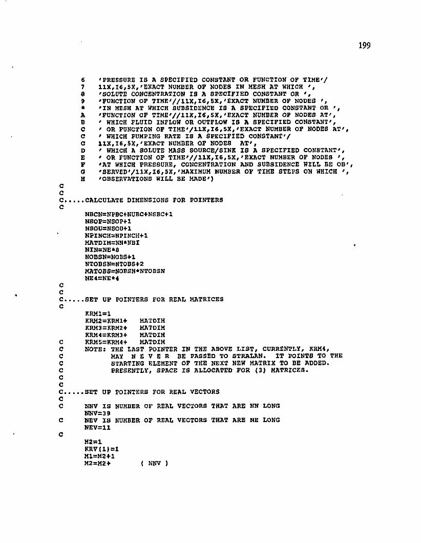
no
no
oo
oo
Qo
oo
oo
oo
oo
199
6 'PRESSURE I S A SPECIFIED CONSTANT OR FUNCTION OF T IM E '/7 1 1 X ,I6 ,5 X , 'E X A C T NUMBER OF NODES IN MESH AT WHICH ' ,8 'SOLUTE CONCENTRATION IS A SPECIFIED CONSTANT OR ' ,9 'FUNCTION OF T I M E ' / / I I X / 1 6 , 5X, 'EXACT NUMBER OF NODES ' ,* ' I N MESH AT WHICH SUBSIDENCE IS A SPECIFIED CONSTANT OR ' ,A 'FUNCTION OF T I M E ' / / 1 1 X , 1 6 , 5X,'EXACT NUMBER OP NODES A T ' ,B ' WHICH FLUID INFLOW OR OUTFLOW I S A SPECIFIED CONSTANT',C ' OR FUNCTION OF T IM E '/1 1 X ,I6 ,5 X , 'E X A C T NUMBER OF NODES A T ' ,C ' WHICH PUMPING RATE I S A SPECIFIED CONSTANT'/C 1 1 X ,I6 ,5 X , 'E X A C T NUMBER OF NODES A T ' ,D ' WHICH A SOLUTE MASS SOURCE/SINK I S A SPECIFIED CONSTANT',E ' OR FUNCTION OF T I M E ' / / 1 1 X , 1 6 , 5X,'EXACT NUMBER OF NODES ' ,F 'A T WHICH PRESSURE, CONCENTRATION AND SUBSIDENCE WILL BE O B ',0 'S E R V E D '/ l lX , 1 6 , 5X, 'MAXIMUM NUMBER OF TIME STEPS ON WHICH ' ,H 'OBSERVATIONS WILL BE MADE')
CALCULATE DIMENSIONS FOR POINTERS
NBCN=NPBC+NUBC+NS BC+1NSOP=NSOP+1NSOU=NSOU+1NPINCH=NPINCH+1MATDIM=NN*NBININ=NE*8NOBSN=NOBS+lNTOBSN=NTOBS+2MATOBS=NOBSN*NTOBSNNE4=NE*4
SET UP POINTERS FOR REAL MATRICES
KRM1=1KRM2=KRM1+ MATDIM KRM3=KRM2+ MATDIM KRM4=KRM3+ MATDIM KRM5=KRM4+ MATDIMNOTE: THE LAST POINTER IN THE ABOVE L I S T , CURRENTLY, KRM4,
MAY N E V E R BE PASSED TO STRALAN. I T POINTS TO THE STARTING ELEMENT OF THE NEXT NEW MATRIX TO BE ADDED. PRESENTLY, SPACE I S ALLOCATED FOR (3 ) MATRICES.
SET UP POINTERS FOR REAL VECTORS
NNV I S NUMBER OF REAL VECTORS THAT ARE NN LONG NNV=39
C NEV I S NUMBER OF REAL VECTORS THAT ARE NE LONGNEV=11
CM2—1KRV (1)=1M1=M2+1M2=M2+ { NNV )
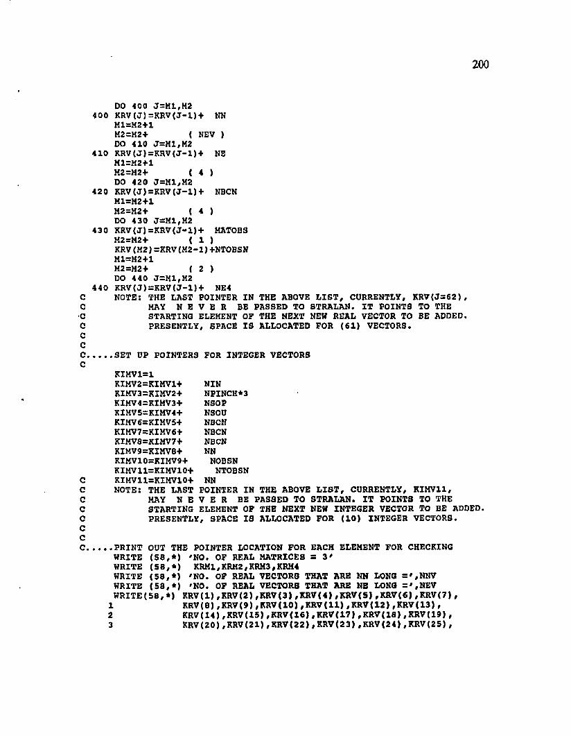
oo
no
oo
oo
n
oo
oo
oo
o200
DO 100 J=M1,M2 400 K R V (J)=K R V (J-1)+ NN
M1=M2+1M2=M2+ ( NEV )DO 410 J=M1,M2
410 KRV(J)=KRV(J - l ) + NE M1=M2+1M2=M2+ { 4 )DO 420 J=M1,M2
420 KRV(J)=K R V (J - l ) + NBCN M1=M2+1M2=M2+ ( 4 )DO 430 J=M1,M2
430 K RV<J)=KRV(J-1)+ MATOBS M2=M2+ ( 1 )KRV(M2)=KRV(M2-1)+NTOBSN M1=M2+1M2=M2+ ( 2 )DO 440 J=M1,M2
440 K R V (J)=K R V (J-1)+ NE4NOTE: THE LAST POINTER IN THE ABOVE L IS T , CURRENTLY, K R V (Js6 2 ) ,
MAY N E V E R BE PASSED TO STRALAN. IT POINTS TO THE STARTING ELEMENT OF THE NEXT NEW REAL VECTOR TO BE ADDED. PRESENTLY, SPACE IS ALLOCATED FOR (6 1 ) VECTORS.
. . SET UP POINTERS FOR INTEGER VECTORS
KIMV1=1KIMV2=KIMV1+ NIN KIMV3=KIMV2+ NPINCH*3 KIMV4=KIMV3+ NSOP KIMV5—KIMV4+ NSOU KIMV6=KIMV5+ NBCN KIMV7=KIMV6+ NBCN KIMV8=KIMV7+ NBCN KIMV9=KIMV8+ NN KIMV10—KIMV9+ NOBSN KIMV11=KIMV10+ NTOBSN KIMV11=KIMV10+ NNNOTE: THE LAST POINTER IN THE ABOVE L IS T , CURRENTLY, KIKV11,
MAY N E V E R BE PASSED TO STRALAN. IT POINTS TO THE STARTING ELEMENT OF THE NEXT NEW INTEGER VECTOR TO BE ADDED. PRESENTLY, SPACE IS ALLOCATED FOR (1 0 ) INTEGER VECTORS.
. . PRINT OUT THE POINTER LOCATION FOR EACH ELEMENT FOR CHECKING WRITE ( 5 8 , * ) 'NO. OF REAL MATRICES = 3 'WRITE ( 5 8 , * ) KRM1,KRM2, KRM3, KRM4WRITE ( 5 8 , * ) 'NO. OF REAL VECTORS THAT ARE NN LONG = ',N N V WRITE ( 5 8 , * ) 'NO. OF REAL VECTORS THAT ARE NE LONG = ' ,N £ V WRITE ( 5 8 , *) KRV(l) ,KRV(2) ,KRV(3) ,XRV(4) ,KRV(5) ,KRV(6) ,KRV(7) ,
1 KRV(8) , KRV(9) , KRV(1 0 ) ,K RV (11) ,K RV (12) , KRV(13) ,2 KRV(14) ,KRV(15) ,KRV(16) ,K RV (17) ,K RV (18) ,KRV(19) ,3 KRV(20) , KRV(21) , KRV(2 2 ) ,KRV(23> , KRV(2 4 ) ,KRV(25) ,
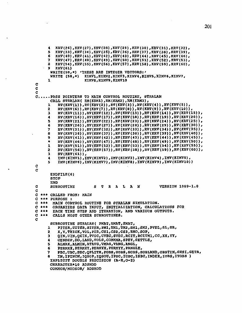
on
o o
o o
4 KRV(26)5 KRV(33)6 KRV(40)7 KRV(47)8 KRV(54)9 KRV(61)
WRITE(5 8 / WRITE (58
1
, KRV (27) , KRV( 2 8 ) , K R V ( 2 9 ) , KRV( 3 0 ) , KRV( 3 1 ) , K R V ( 3 2 ) , , KRV( 3 4 ) / KRV( 3 5 ) , KRV( 3 6 ) , K R V ( 3 7 ) , K R V ( 3 8 ) , K R V ( 3 9 ) , , KRV(41} , KRV( 4 2 ) , KRV( 4 3 ) , KRV( 4 4 ) , K R V ( 4 5 ) ,K R V (4 6 ) , /KRV (4 8 ) , KRV ( 4 9 ) , KRV ( 5 0 ) , K R V ( 5 1 ) , K R V ( 5 2 ) , K R V ( 5 3 ) , , KRV(55 ) , KRV( 5 6 ) ,K RV (5 7) ,K RV (5 8} , K R V ( 5 9 ) , K R V ( 6 0 ) ,
* ) 'THESE ARE INTEGER VECTORS: ', * ) KIMV1, KIKV2 , KIKV3, KIHV4 , KIMV5 , KIMV6 , KIMV7 ,
KIMV8, KIMV9, KIMV10
.PASS POINTERS CALL STRALAN(
RV{KRV( 1 ) ) RV( KRV( 6 ) ) RV(KRV(1 1 ) RV( KRV(1 6 ) RV( KRV(2 1 ) RV( KRV(2 6 ) RV(KRV(3 1 ) RV(KRV(3 6 ) RV(KRV(4 1 ) RV(KRV(4 6 ) RV(KRV(5 1 ) RV(KRV(5 6 ) RV(KRV(6 1 ) IMV(KIHVl) IMV(KIMVfi)
12345e7a9*12345
TO MAIN CONTROL ROUTINE/ STRALAN RH(KRHl) ,RM(KRH2) ,RM(KRM3) /
z RV ( KRV { 2 ) ) / RV(KRV( 3 ) ) , RV(KRV( 4 ) ) ,R V (K R V (5)) , RV ( KRV( 7 ) ) / RV(KRV( 8 ) ) ,R V (K R V (9 )) ,R V (K R V (1 0 )) ,,RV(KRV(12) ) ,RV(KRV(1 3 ) ) / RV(KRV(14 /RV(KRV( 1 7 ) ) /R V (K R V (18)) /RV(KRV(19 z RV ( KRV( 2 2 ) ) / RV( KRV( 2 3 ) ) / RV( KRV(24 ,RV(KRV{27)) / RV( KRV( 2 8 ) ) ,RV(KRV(29 z RV(KRV( 3 2 ) ) / RV(KRV( 3 3 ) ) , RV( KRV(34 z RV {KRV( 3 7 ) ) / RV( KRV( 3 8 ) ) ,RV(KRV(39 z RV (KRV( 4 2 ) ) / RV( KRV( 4 3 ) ) /RV(KRV(44 , RV(KRV( 4 7 ) ) /RV(KRV( 4 8 ) ) ,RV(KRV(49 , RV(KRV( 5 2 ) ) / RV( KRV( 5 3 ) > ,RV(KRV(54 z RV (KRV( 5 7 ) ) /RV(KRV( 5 8 ) ) ,RV(KRV(59
) ,RV(KRV{ 1 5 ) ) ) #R V ( K R V ( 2 0 ) ) ) , R V ( KRV( 2 5 ) ) ) #RV(KRV( 3 0 ) ) ) , R V ( K R V ( 3 5 ) ) ) , RV ( KRV( 4 0 ) ) ) , R V ( K R V ( 4 5 ) ) ) / R V ( K R V ( 5 0 ) ) ) / RV ( KRV( 5 5 ) ) ) /R V(KRV ( 6 0 ) )
IM V(K IM V 2) , I M V (K IH V 3) , I M V (R IM V 4) / IMV(KIMV5) , IMV (KIMV7 ) , IMV ( KIMV8 ) / IMV ( KIMV9) , IMV ( KIHV10 ) )
ENDFILE(6)STOPENDSUBROUTINEC
CC *** CALLED FROM: C * * *
s R A L A N VERSION 1 9 8 9 - 1 . 0
MAINPURPOSE :
C *** MAIN CONTROL ROUTINE FOR STRALAN SIMULATION.C *** ORGANIZES DATA INPUT, INITIALIZATION , CALCULATIONS FOR C *** EACH TIME STEP AND ITERATION, AND VARIOUS OUTPUTS.C *** CALLS MOST OTHER SUBROUTINES.C
SUBROUTINE STRALAN ( PMAT, UMAT, SMAT,1 PITER,U ITER/SITER,PM 1,U H1,U M 2,SM 1,SM 2, PVEL, S L , SR,2 X /Y ,T H IC K ,V O L ,P0R /C S1/C S2/C S3/R H O ,SO P,3 Q IN ,U IN , QUIN , PVEC , UVEC , SVEC , RCIT , RCITM1, CC , XX, YY ,4 CENDEP/DD,LAND,VOLS,COMMMA,SPEY,SETTLE,5 ALMAX, ALMIN, ATAVG, VMAG,VANG, ANGL,6 PERMXX,PERMXY, PERMYX,PERMYY, PANGLE,7 PBC , UBC, SBC, QPLITR, POBS , UOBS , SOBS , SOB LAND , OBSTIM, GXSI, GETA ,8 I N , IP IN C H , IQSOP,IQSOU, IP B C ,IU B C , ISB C,IN D EX , IO B 3, ITOBS )
IM PL IC IT DOUBLE PRECISION (A -H /O -Z )CHARACTER*10 ADSMOD COMMON/MODSOR/ ADSMOD

non
ono
o o
oo
oo
202
COMMON/ICONF/ IUNCONCOMMON/DIMS/ N N ,NE,N IN ,N BI, NB,NBHALF,NPINCH,NPBC,NUBC, NSBC,
1 NSOP,NSOPUMP,NSOU,NBCN COMMON/TIME/ DELT,TS£C,TMIN,THOUR,TDAY,TWEEK,TMONTH,TYEAR,
X TMAX,DELTP, DELTU, BELTS,DLTPM1, DLTUM1,DLTSM1, IT ,ITM AX ,IY RCOMMON/CONTRL/ GNU,UP,DTMULT,DTMAX,ME,ISSFLO,ISSTRA,ITCYC,NPORC,
1 NPCYC,NUCYC,NSCYC,NPRINT,IREAD,ISTORE,NOUMAT,IHEAD,ISLOPE,LAN,2 ISET
COMMON/PARAMS/ COMPFL,COMPMA,DRWDU,RHOS, DECAY,SIGMAW,1 RHOWO, URHOWO, VISCO, PRODF1, PRODS1,PRODFO, PRODS0 , CHIX, CHI2
COMMON/ITERAT/ RPM,RPMAX,RUM,RUMAX,RSM,RSMAX,ITER, ITRMAX,1 IPWORS, IUWORS, ISWORS
COMMON/KPRINT/ KNODAL,KELMNT, KINCID, KVEL,KBUDG, KPORS COMMON/OBS/ NOBSN,NTOBSN,NOBCYC,ITCNTDIMENSION QIN(NN),UIN(NN),IQSOP(NSOP),QUIN(NN),IQSOU(NSOU) DIMENSION IPBC(NBCN),PBC(NBCN),IUBC(NBCN),UBC(NBCN),
1 ISBC(NBCN), SBC(NBCN),QPLITR(NBCN)DIMENSION IN (N IN ) ,IP IN C H (N P IN C H ,3)DIMENSION X(NN), Y(N N),THICK(NN), RHO(NN),SOP(NN), COMMMA(NN),
1 POR(NN),PVEL(NN),SL(NN) ,SR (N N ),S P E Y (N N ), SETTLE(NN)DIMENSION PERMXX(NE) , PERMXY(NE) , PERMYX(NE), PERMYY(NE), PANGLE(NE),
X ALMAX(NE),ALMIN(NE),ATAVG(NE),VMAG(NE),VANG(NE),ANGL(NE),2 G X S I(N E ,4 ) ,G E T A (N E ,4 )
DIMENSION VOL(NN),PMAT(NN,NBI), PVEC(NN),UMAT(NN,NBI),UVEC(NN),X SMAT (NN,NBI) ,SVEC(NN) ,VOLS (NN) , SM2 (NN)
DIMENSION PMX(NN),UHX(NN),UM2(NN),SMX(NN), P IT E R (N N ), UITER(NN),X S IT E R (N N ), RCIT(NN),RCITM X(N N),CSX(NN),CS2(NN),CS3(NN )
DIMENSION CC(NN), INDEX(NN),XX(NN), YY(NN)DIMENSION POBS(NOBSN,NTOBSN), UOBS(NOBSN,NTOBSN),
X SOBS(NOBSN,NTOBSN), SOBLAND(NOBSN,NTOBSN),IOBS(NOBSN),2 ITOBS(NTOBSN),OBSTIM(NTOBSN)
DIMENSION CENDEP(NN),DD(NN),LAND(NN)
IT=0
.INPUT SIMULATION DATA FROM UNIT-5 (DATASETS 6 THROUGH X6B) CALL INDATX(X,Y, THICK,POR,ALMAX,ALMIN,ATAVG,PERMXX,PERMXY,
X PE RMYX , PERMYY , PANGLE , SOP , CENDEP , DD , LAND , ANGL , COMMMA)
.INPUT FLUID MASS, AND SOLUTE MASS SOURCES (DATASETS X7 AND 18)
CALL ZERO(QIN,NN, 0 . 0D0)CALL ZERO(UIN,NN,0 . 0D0)CALL ZERO(QUIN,NN,0.0D0)IF (N S O P -X . GT. 0 .OR. NSOU-X. GT. 0 )
X CALL SOURCE(QIN,UIN,IQSOP,QUIN,IQSOU,IQSOPT,IQSOUT)
.INPUT SPECIFIED P ,U AND S BOUNDARY CONDITIONS (DATASETS X 9,20 AND 2X)
IF (N B C N -X .G T.O ) CALL BOUND(IPBC,PBC,IUBC,UBC,ISBC,SBC,

VV VV
VV VV
OV V
WV
VW
V
V V
vv
203
1 IPBCT,IUBCT,ISBCT).SET FLAG FOR TIME-DEPENDENT SOURCES OR BOUNDARY CONDITIONS.WHEN IBCT=+5, THERE ARE NO TIME-DEPENDENT SPECIFICATIONS. IBCT=1QS0FT+IQS0UT+IPBCT+IUBCT+ISBCT
.INPUT OBSERVATION NODE DATA (DATASET 22)IF (N O B S N -l.G T .0) CALL OBSBRV(0,IOBS,ITOB3,POBS,UOBS,SOBS,
1 SOBLAND,OBSTIH, PVEC,UVEC,SM2,ISTOP,CENDEP,DD,RCIT, LAND)
.INPUT MESH CONNECTION DATA (DATASET 23)CALL CONNEC( IN , IPINCH)
.CALCULATE AND CHECK BAND WIDTH CALL BANWID(IN)
.CHECK THAT PINCH NODES HAVE NO SOURCES OR BOUNDARY CONDITIONS I F (NPINCH-1 .G T .0) CALL NCHECK(IPINCH,IQSOP,IQSOU,IPBC,IUBC,ISBC)
.INPUT INITIAL DRAWDOWN,DEPTH TO A Q U IFER,IN ITIAL LAND ELEVATION NATURAL SUBSIDENCE AND UNCONFINED AQUIFER'S SPECIFIC YIELD (READ UNIT 5 5 , DATASET 1 THROUGH 5)
CALL INDAT2(DD,CENDEP,LAND,SPEY,SETTLE)
.INPUT IN ITIA L OR RESTART CONDITIONS AND IN IT IA L IZ E PARAMETERS (READ UNIT-57 DATA OR UNIT-66 DATA FOR WARN START)
CALL INDAT3 (PVEC, UVEC, SVEC,PHI, UH1, UM2, S H I , SH2, CS1, C S 2 ,C S 3 ,S L ,S R , 1 RCIT, PBC , SBC, IPB C, IPBCT, ISBC , ISBCT, CENDEP, DD, POR)
.SE T STARTING TIME OF SIMULATION CLOCKTSEC—TSTART -------------- READ FROM SUBROUTINE INDAT3TSECP0=TSEC TSECU0=TSEC TSECS0=TSEC TMIN=TSEC/tiO. DO THOUR=TMIN/60. DO TDAY—THOUR/2 4 . DO TWEEK—TDAY/7. DO TMONTH=TDAY/3 0 . 4 37 5 DO TYEAR=TDAY/3 6 5 .2 5D0
.OUTPUT IN ITIA L CONDITIONS OR STARTING CONDITIONS I F ( IS S T R A .N E .l) CALL PRISOL( 0 , 0 , 0 , PVEC,UVEC,SH2, POR,
1VMAG, VANG,CENDEP,DD,LAND,RCIT)C SET SWITCHES AND PARAMETERS FOR SOLUTION WITH STEADY-STATE FLOW
I F ( I S S F L O .N E . l ) GOTO 1000 ML=0IF (M E .L E .0 ) ML—1 NOUMAT=0 ISSFLO=2 ITER=0DLTPM1=DELTP DLTUM1=DELTU IF (M E .L E .O ) GO TO 990 DLTSM1=DELTS BDELS=0.0D0
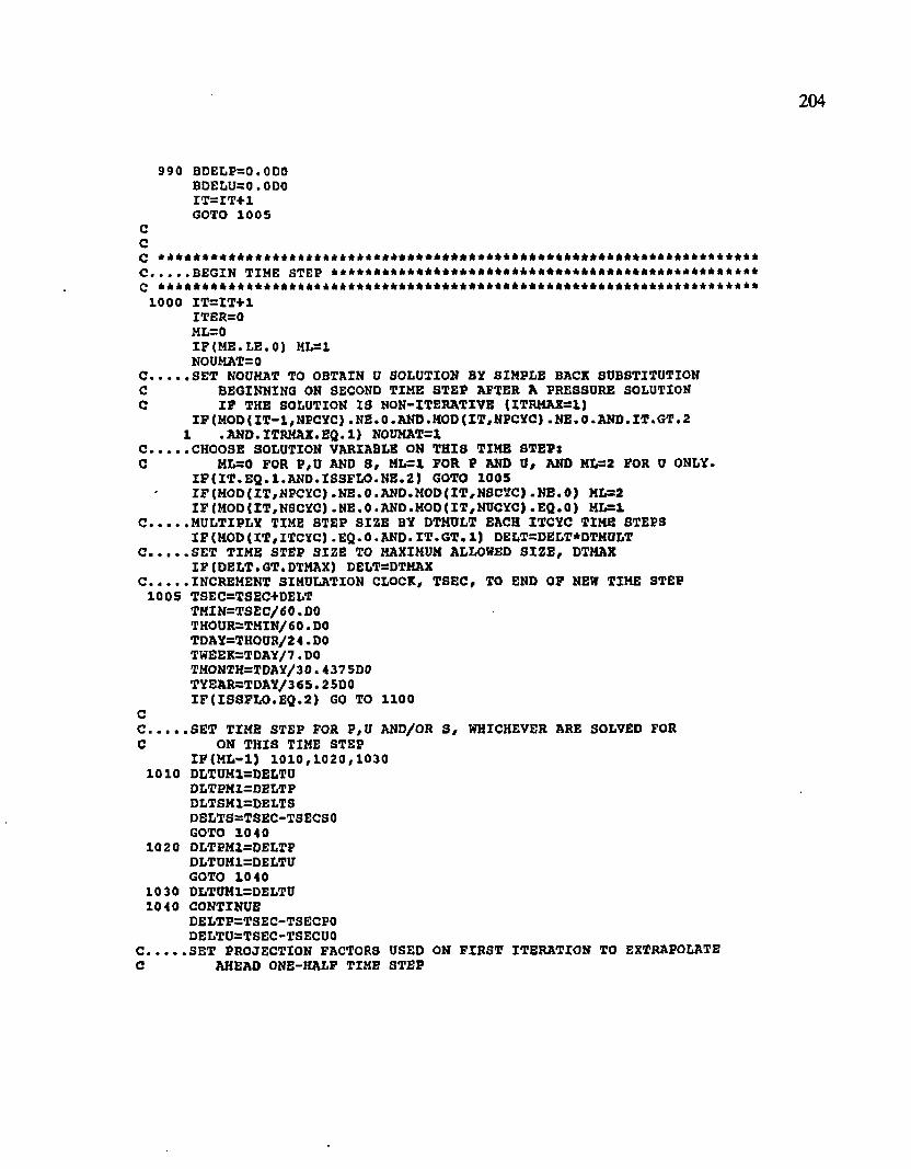
990 8DELP=0. ODO BDELU=O.ODO IT=IT+1 GOTO 1005
CCC *****************************************************************C BEGIN TIME STEP *********************************************C * * * * * * * * * * * * * * * * * * * * * * * * * * * * * * * * * * * * * * * * * * * * * * * * * * * * * * * * * * * * * * * * *
1000 IT = IT + 1 ITER=0 ML=0IF(M E.LE.O ) ML=1 NOUMAT=0
C..........SET NOUMAT TO OBTAIN V SOLUTION BY SIMPLE BACK SUBSTITUTIONC BEGINNING ON SECOND TIME STEP AFTER A PRESSURE SOLUTIONC I P THE SOLUTION IS NON-ITERATIVE (ITRMAX=1)
I F (MOD(IT-l,NPCYC) .NE.O.AND.MOD(IT,NPCYC) .N E .0 .A N D .IT .G T .2 1 .AND.ITRMAX.EQ.l) NOUMAT=l
C..........CHOOSE SOLUTION VARIABLE ON THIS TIME STEP:C ML=0 FOR P,U AND S , ML=1 FOR P AND 0 , AND ML=2 FOR U ONLY.
IF U T .E Q .l .A N D .IS S F L O .N E .2) GOTO 1005 IF(MOD(IT,NPCYC) .N E .0 .AND.MOD<IT,NSCYC) .NE.O) MLs2 IF (MOD(IT,NSCYC) .NE.O .AND. MOD(IT,NUCYC) .EQ.O) HL=1
C ..........MULTIPLY TIME STEP SIZE BY DTMULT EACH ITCYC TIME STEP3IF(M O D (IT ,IT C Y C ).E Q .O .A N D .IT .G T .1) DELT=DELT*DTMULT
C .......... SET TIME STEP SIZE TO MAXIMUM ALLOWED S IZ E , DTHAXI F (DELT.GT.DTMAX) DELT=DTMAX
C............ INCREMENT SIMULATION CLOCK, TSEC, TO END OF NEW TIME STEP1005 TSEC=TSEC+DELT
TMIN=TSEC/60. DO THOUR=TMIN/6 0 . DO TDAY=THOUR/24 .DO TWEEK=TDAY/7.D0TMONTH=TDAY/30.4 3 7 5D0TYEAR=TDAY/36 5 .2 5D0I F ( ISSFLO .EQ .2) GO TO 1100
CC SET TIME STEP FOR P,U AND/OR S , WHICHEVER ARE SOLVED FORC ON THIS TIME STEP
IF ( M L - l ) 1 0 1 0 ,1 0 2 0 ,1 0 3 01010 DLTUM1=DELTU
DLTPM1=DELTP DLTSH1=DBLTS DELTS=TSEC-TSECSO GOTO 1040
1020 DLTPM1=DELTP DLTUM1=DELTU GOTO 1040
1030 DLTUM1=DELTU 1040 CONTINUE
DELTP=TSEC-TSECPODELTU=TSEC-TSECUO
C SET PROJECTION FACTORS USED ON FIRST ITERATION TO EXTRAPOLATEC AHEAD ONE-HALF TIME STEP

BDELP=(DELTP/DLTPM1)*Q. SODO BDELU= ( DELTU/DLTUH1) * 0 .5 0 DO IF(ME.LE.O) GO TO 1045 BDELS=( DELTS/DLTSM1)* 0 . SODO BDELS1=BDELS+1.0D0
1045 BDELP1=BDELP+1.0D0 BD£LU1=BDELU+1. 0D0
C INCREMENT CLOCK FOR WHICHEVER OF P,U AND S WILL BE SOLVED FORC ON THIS TIME STEPCC
IF(M L-1) 1 0 6 0 ,1 070 ,1080 1060 TSECPO=TSEC
TSECUO=TSEC TSECSO=TSEC GOTO 1090
1070 TSECPO=TSEC TSECOO=TSEC GOTO 1090
1080 TSECU0=TSEC 1090 CONTINUE
CC ----------------------------------------------------- - - - - - - - - - - -C BEGIN ITERATION -------- - - - - - - - - - - - - - - - - ------- -----
1100 ITER=ITER+1C
IF(M L-1) 2 0 0 0 ,2 2 0 0 ,2 4 0 0C SHIFT AND SET VECTOR3 FOR TIME STEP WITH P,U AND S SOLUTIONS
2000 DO 2025 1 = 1 ,NN PITER(I ) =PVEC(I)PVEL(I)=PVEC(I)UITER{I ) =UVEC{I )SITER( I ) =SVEC( I )RCITM1(I ) =RCIT( I )
2025 RCIT ( I ) =RHOWO+DRWDU* (UITER ( I ) -URHOWO)DO 2050 IP=1,NPBC I= IA B S ( IP B C (IP ) )QPLITR(IP)=GNU*(PBC( IP ) -P IT E R ( I ) )
2050 CONTINUEI F ( IT E R .G T . l ) GOTO 2600 DO 2075 1 = 1 ,NNPITER(I)=BDELP1*PVEC(I)-BDELP*PH1(I)UITER(I ) =BDELU1*UVEC( I ) -BDELU*UM1(I)SITER(I)=BDELS1*SVEC(I)-BDELS*SM1(I)PM1( I ) =PVEC( I )SMI( 1 ) =SVEC(I)UM2(I)=UM1(I)
2075 UM1(I)=UVEC(I)GOTO 2600
C SHIFT AND SET VECTORS FOR TIME STEP WITH P AND U SOLUTION ONLY2200 DO 2225 1 = 1 ,NN
PVEL(I)=PVEC(I)PITER( I ) =PVEC( I )UITER(I)=UVEC(I)

OfiO
OO
o o
o
RCITM1(I)=RCIT(I)2225 RCIT( I ) =RHOWO+DRWDU*{UITER(I ) -URHOWO)
DO 2155 IP=1,NPBC X=IABS(IPBC(IP) )Q PLITR (IP)=G N U *(PB C (IP)-PITER (I))
2 1 5 5 CONTINUEIF ( IT E R .G T . l ) GOTO 2600 DO 2250 1 = 1 ,NNPITER(I)=BDELP1*PVEC(I)-BDELP*PM1(I)UITER(I)=BDELU1*UVEC(I) -BDELU*UM1(I)PM1(I)=PVEC(I)UH 2(I)=U H1(I)
2250 UM1(I ) =UVEC(I )GOTO 2600
C SHIFT AND SET VECTORS FOR TIME STEP WITH U SOLUTION ONLY2400 IF(NOUMAT.EQ.l) GOTO 2480
DO 2425 1 = 1 ,NN 2 4 2 5 UITER(I)=UVEC(I)
IF ( IT E R .G T . l ) GOTO 2600 DO 2 450 1 = 1 ,NN PITER(I }=PVEC(I )PVEL( I)=PV EC(I)UITER(I)=BDELU1*UVEC(I) -BDELU*UM1(I)
2450 RCITM 1(I)=RCIT(I)DO 2475 IP=1,NPBC I=IA B S(IPB C (IP) )Q PL IT R (IP)= G N U *(PB C (IP )-P IT E R (I))
2475 CONTINUE 2480 DO 2500 1 = 1 ,NN
UM2(I) =UM1(I)2500 UM1(I)=UVEC(I)2600 CONTINUE
INITIALIZE ARRAYS WITH VALUE OF ZEROMATDIM=NN*NBI IF (M L -1) 3 0 0 0 ,3 1 0 0 ,3 3 0 0
3000 CALL ZERO(PMAT,MATDIM,0.0D0)CALL ZERO( PVEC,NN,O.ODO)CALL ZERO(VOL,NN,0.0D0)CALL ZERO(SMAT,MATDIM,O.ODO)CALL ZERO(SVEC,NN,O.ODO)
GO TO 3300 3100 CALL ZERO(PMAT,MATDIM,O.ODO)
CALL ZERO(PVEC,NN,O.ODO)CALL ZERO(VOL,NN,O.ODO)
3300 IF(NOUMAT) 3 3 5 0 ,3 3 5 0 ,3 3 7 5 3350 CALL ZERO(UMAT,MATDIM,O.ODO)3375 CALL ZERO(UVEC,NN,0. ODO)
SET TIME-DEPENDENT BOUNDARY CONDITIONS, SOURCES AND SINKS FOR THIS TIME STEP
I F ( I T E R .E Q .1 . AND.IBCT.NE.5)
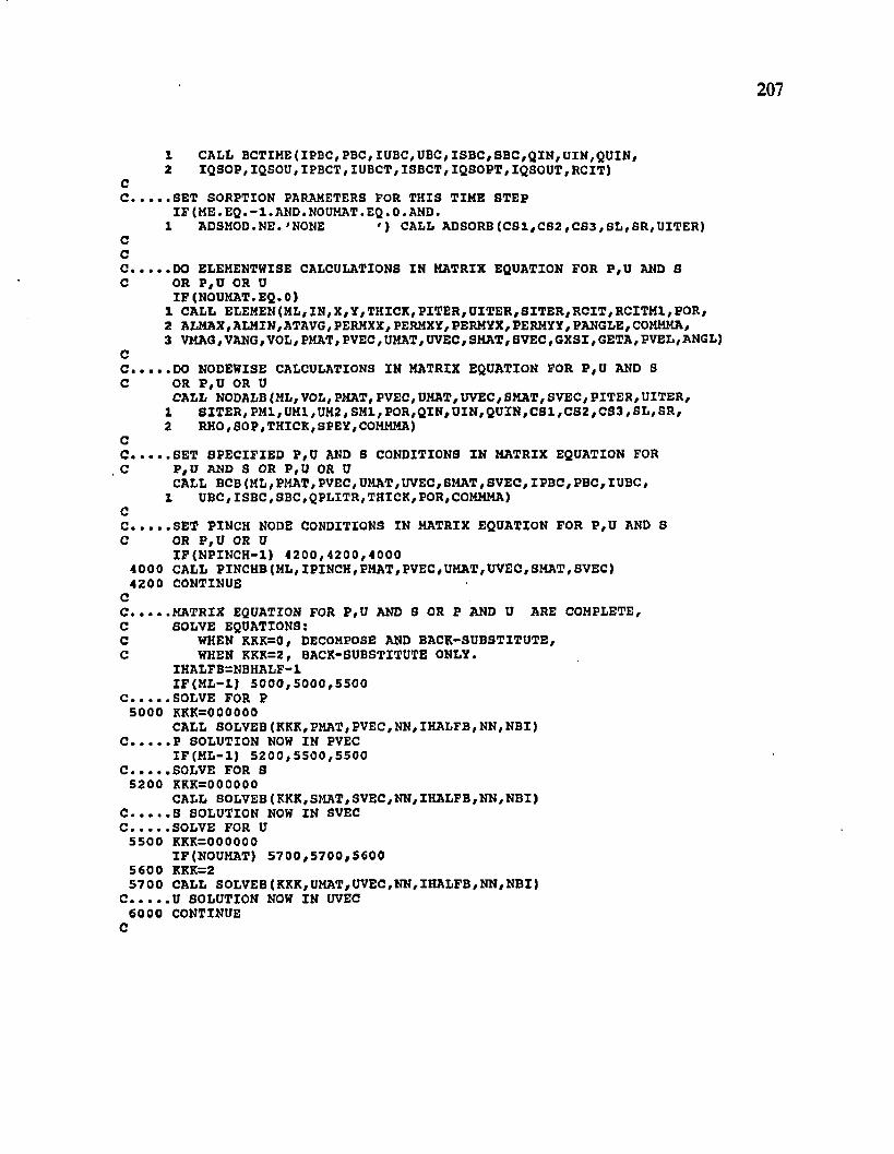
no
o o
o n
no
oo
o
no
o
oo
o
oo
o
on
o
oo
207
1 CALL BCTIME(IPBC,PBC,XUBC,UBC,ISBC,SBC,QIN,UIN,QUIN,2 IQSOP, IQSOU, IPBCT, IUBCT, ISBCT, IQSOPT, IQSOUT,RCIT)
.SET SORPTION PARAMETERS POR THIS TIME STEP IF(ME.EQ.-l.AND.NOUKAT.EQ.O.AND.
1 ADSMOD.NE.'NONE ' ) CALL ADSORB(CS1,CS2,CS3, SL,SR,UITER)
DO ELEMENTWISE CALCULATIONS IN MATRIX EQUATION FOR P,U AND SOR P ,U OR U IF(NOUMAT.EQ.O)
1 CALL ELEMEN(ML,IN,X,Y,THICK,PITER,UITER,SITER,RCIT,RCITM1, POR,2 ALMAX,ALMIN,ATAVG, PERMXX, PERMXY,PERMYX,PERMXY, PANGLE, COMMMA,3 VMAG, VANG, VOL, PMAT, PVEC, UMAT, UVEC, SMAT,SVEC,GXSI,GETA, PVEL, ANGL)
DO NODEWISE CALCULATIONS IN MATRIX EQUATION FOR P ,tf AND SOR P ,U OR UCALL NODALB (ML, VOL, PMAT, PVEC, UMAT,UVEC, SMAT, SVEC, PITER,UITER,
1 SITER,PM1,UM1,UM2, SM I,POR,Q IN,UIN,QUIN,CS1,CS2,CS3,SL,SR,2 RHO,SOP,THICK,SPEY,COMMMA)
SET SPECIFIED ? ,U AND S CONDITIONS IN MATRIX EQUATION FORP,U AND S OR P,U OR UCALL BCB (ML, PMAT, PVEC, UMAT, UVEC, SMAT, SVEC, IPBC, PBC, IUBC,
I UBC,ISBC,SBC,QPLITR,THICK,POR,COMMMA)
SET PINCH NODE CONDITIONS IN MATRIX EQUATION FOR P,U AND SOR P,U OR UIF(N PIN CH -I) 4 2 0 0 ,4 2 0 0 ,4 0 0 0
4000 CALL PINCHB(ML,IPINCH,PMAT,PVEC,UMAT,UVEC,SMAT,SVEC)4200 CONTINUE
MATRIX EQUATION FOR P,U AND S OR P AND U ARE COMPLETE,SOLVE EQUATIONS:
WHEN KKK=0, DECOMPOSE AND BACK-SUBSTITUTE,WHEN KKK=2, BACK-SUBSTITUTE ONLY.
IHALFB-NBHALF-1 IF(M L-L) 5 0 0 0 ,5 0 0 0 ,5 5 0 0
SOLVE FOR P5000 KKK=000000
CALL SOLVES(KKK,PMAT,PVEC,NN,IHALFB,NN,NBI> P SOLUTION NOW IN PVEC
IF(M L-1) 5 2 0 0 ,5 5 0 0 ,5 5 0 0 SOLVE FOR S5200 KKK=000000
CALL SOLVEB( KKK,SMAT,SVEC,NN,IHALFB, NN,NBI) S SOLUTION NOW IN SVEC SOLVE FOR U5500 KKK=000000
IF(NOUMAT) 5 7 0 0 ,5 7 0 0 ,5 5 0 0 5600 KKK=25700 CALL SOLVEB (KKK,UMAT,UVEC,NN,IHALFB,NN,NBI)
C U SOLUTION NOW IN UVEC6000 CONTINUE
C

208
C CHECK PROGRESS AND CONVERGENCE OP ITERATIONSC AND SET STOP AND GO FLAGS:C ISTOP =: -1 NOT CONVERGED - STOP SIMULATIONC ISTOP = 0 ITERATIONS LEFT OR CONVERGED - KEEP SIMULATINGC ISTOP = 1 LAST TIME STEP REACHED - STOP SIMULATIONc ISTOP = 2 MAXIMUM TIME REACHED - STOP SIMULATIONc IGOI = 0 P ,S AND U CONVERGED, OR NO ITERATIONS DONEc IGOI = 1 ONLY P HAS NOT YET CONVERGED TO CRITERIONc IGOI = 2 ONLY U HAS NOT YET CONVERGED TO CRITERIONc IGOI = 3 BOTH P AND U HAVE NOT YET CONVERGED TO CRITERIAc IGOI = 4 ONLY S HAS NOT YET CONVERGED TO CRITERIAc IGOI = 5 BOTH P AND S HAVE NOT CONVERGED TO CRITERIAc IGOI = 6 BOTH U AND S HAVE NOT CONVERGED TO CRITERIAc IGOI = 7 P,U AND S HAVE NOT CONVERGED TO CRITERIA
ISTOP=0IGOI=0I F (ITRMAX-1) 7 5 0 0 ,7 5 0 0 ,7 0 0 0
7000 RPM=0.D0 RUM=0.D0 RSM=0.D0 IPWORS=0 2tTWORS=0 ISWORS=0IP (M L - l ) 7 0 5 0 ,7 0 5 0 ,7 1 5 0
7050 DO 7100 1 = 1 ,NNRP=DABS(PVEC(I)-PITER(I) )IP(RP-RPH) 7 1 0 0 ,7 0 6 0 ,7 0 6 0
70 60 RPM=RPIPWORS=I
7100 CONTINUEIF(RFH.GT.RPMAX) IGOI=IGOI+l
7150 DO 7300 1 = 1 ,NNRU=DABS(UVEC(I ) -UITER( I ))IP(RD-RUM) 7 3 0 0 ,7 2 6 0 ,7 2 6 0
72 60 RUM=RUIUWORS=I
7 300 CONTINUEIP(RUM.GT.RUMAX) IGOI=IGOI+2 IF (M L -1) 7 0 1 5 ,7 3 5 0 ,7 3 5 0
7015 DO 7030 1 = 1 ,NNRS=DABS(SVEC(I)-SITER(I) )IF(RS-RSM) 7 0 3 0 ,7 0 3 5 ,7 0 3 5
7035 RSM=RSISWORS=I
7030 CONTINUEIP(RSM.GT.RSMAX) IGOI=IGOI+4
7350 CONTINUEI F ( IG O I. GT. 0 . AND. ITER.EQ. ITRMAX) ISTO P=-1 IF (IG O I,G T.0 .A N D .ISTO P.E Q .O ) GOTO 1100
C END ITERATION ----------------------------------------------------------------------------------- ---C --------------------------------------------------------- ------------------ ----------- -------------------------------------C
7500 CONTINUEI F ( ISTOP. NE. - 1 . AND.IT. EQ. ITMAX) ISTOP=l
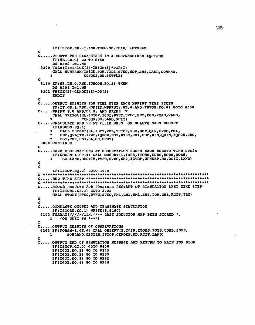
OU O
OO O
t) OO
OO O
CJ O
CJ o
O CJ
o u
oo
IF ( ISTOP. N E . - l . AND.TSEC.GE.TMAX) ISTOP=2
UPDATE THE PARAMETERS IN A COMPRESSIBLE AQUIFERIF(M E.LE.O ) GO TO B150 DO 8200 1 = 1 ,NN
8200 VOLS (I )= T H IC K (I) -THICK(I) *POR(I)CALL SUBPARH (THICK, POR,VOLS, SVEC, SOP, SM2 , LAND, COMMHA,
1 C£NDEP,DD,SETTLE)
8150 I F (ME. LE • 0 .AND. IUNCON. EQ. 1) THEN DO 8201 1 = 1 ,NN
8201 THICK{I)=CENDEP(I) -DD (I )ENDIF
OUTPUT RESULTS FOR TIME STEP EACH NPRINT TIKE STEPSIF(IT.GT.l.AND.MOD(IT,NPRINT) .NE.O.AND.ISTOP.EQ.O) GOTO 8000
PRINT P,U AND/OR S, AND MAYBE VCALL PRISOL ( ML , I STOP , IGOI, PVEC , UVEC , SM2 , POR, VMAG , VANG ,
1 CENDEP, DD, LAND, RCIT) CALCULATE AND PRINT FLUID MASS OR SOLUTE MASS BUDGET
IF(KBUDG. EQ.1 )1 CALL BUDGET(ML,IBCT,VOL,THICK,RHO,SOP,QIN,PVEC,PK1,2 PBC,QPLITR, IPBC, IQSOP, POR,UVEC, UM1, UM2 , UIN,QUIN, IQSOU, UBC,3 CS1,CS2,CS3,SL,SR,SPEY)
8000 CONTINUE
MAKE OBSERVATIONS AT OBSERVATION NODES EACH NOBCYC TIME STEPSIF(NOBSN-l.GT.O) CALL OBSERV(1,IOBS,ITOBS,POBS,UOBS,SOBS,
1 SOBLAND, OBSTIH, PVEC , UVEC, SM2 , 1STO P , CENDEP, DD , RCIT, LAND)
I F (ISTO P.EQ .0 ) GOTO 1000 *************** ******************************************************* . . . .E N D TIME STEP ****************************************************
STORE RESULTS FOR POSSIBLE RESTART OF SIMULATION LAST TIME STEP IF(1STORE. N E.1) GOTO S205CALL STORE (PVEC, UVEC,SVEC,PM1,UM1,SMI,SK2,POR,CS1,RCIT,PBC)
COMPLETE OUTPUT AND TERMINATE SIMULATIONIF (IS T O R E .E Q .1) WRITE(6,8100)
8100 FORMAT ( / / / / / / U X , '* * * LAST SOLUTION HAS BEEN STORED ' ,1 'ON UNIT 66 * * * ')
OUTPUT RESULTS OF OBSERVATIONS8205 IF (N O B S N -l.G T .0) CALL OBSERV(2,IOBS,ITOBS,POBS,UOBS,SOBS,
1 SOBLAND, OBSTIM, ISTOP, CENDEP, DD, RCIT , LAND)
.OUTPUT END OF SIMULATION MESSAGE AND RETURN TO MAIN FOR STOP I F (IST O P.G T .0) GOTO 8400 I F ( I G O I .E Q . l ) GO TO 8230 I F ( I G O I .E Q .2 ) GO TO 8260 IF ( IG O I .E Q .S ) GO TO 8292 I F ( I G O I .E Q .4) GO TO 8266

I F {IGOI•EQ.5) GO TO 8296 I F ( IGOI. EQ.6) GO TO 8300 IF<IGOI.EQ.7> GO TO 8370
8230 WRITE(6 /8 2 3 5 )823S F O R M A T ( / / / / / / / / l l X , 'SIMULATION TERMINATED DUE TO
1 'NON-CONVERGENT PRESSURE'/2 / n x , ' ********** ********** *** ** / ,3 * * * * * * * * * * * * * * * * * * * * * * * / )
RETURN 8260 WRXTE(6,8264)8264 F O R M A T (// / / / / / / l IX , 'S IM U L A T IO N TERMINATED DUE TO ' ,
1 'NON-CONVERGENT CONCENTRATION',2 / H X , *********** ********** *** ** *,3 *************** **************)
RETURN 8266 WRITE(6,8268)8268 FORMAT ( / / / / / / / /1 1 X , 'S IM U L A T IO N TERMINATED DUB TO ' ,
1 'NON-CONVERGENT,SUBSIDENCE',2 / 1 1 X , '* * ******** ********** *** ** *,3 *************** ************)
RETURN 8292 WRITE(6 ,8 2 9 4 )8294 F O R M A T ( / / / / / / / /1 1 X , 'SIMULATION TERMINATED DUE TO ' ,
1 'NON-CONVERGENT PRESSURE AND CONCENTRATION',2 / I 1 X , '********** ********** *** ** *,3 *************** ******** • • * **************)
RETURN 8296 WRITE(6 ,8 2 9 8 )8298 FO R M A T(//// / / / /11X ,'S IM U LA TIO N TERMINATED DUB TO ' ,
1 'NON-CONVERGENT PRESSURE AND SUBSIDENCE',2 / 1 1 X , '* * ******** ********** *** **3 *************** ******** *** ************)
RETURN 8300 WRITE(6 ,8 3 0 5 )8305 FO R M A T{////// / /11X ,'SIM U LA TIO N TERMINATED DUE TO ' ,
1 'NON-CONVERGENT CONCENTRATION AND SUBSIDENCE',2 / H X , ' ********** ********** *** **3 *************** ******** *** ************)
8370 WRITE(6 ,8 3 7 5 )8375 FO R M A T{////// / /11X ,'S IM U LA TIO N TERMINATED DUE TO ' ,
1 'NON-CONVERGENT PRESSURE,CONCENTRATION AND SUBSIDENCE',2 / H X , *********** ********** *** **3 *************** ******** *** ************)
C8400 IF (IS T O P .E Q .2 ] GOTO 8500
WRITE(6 ,8 4 5 0 )8450 F O R M A T < / / / / / / /H X , 'STRALAN SIMULATION TERMINATED AT COMPLETION ' ,
1 'OF TIME S T E PS '/2 1 1 X , '* * * * * ********** ********** ** ********** ' ,3 *** **** ******)
RETURN 8500 WRITE(6 ,8 5 5 0 )8550 FO RM AT(//////11X,'STRALAN SIMULATION TERMINATED AT COMPLETION ' ,
1 'OF TIME PERIOD'/2 1 1 X , '* * * * * ********** ********** ** **********
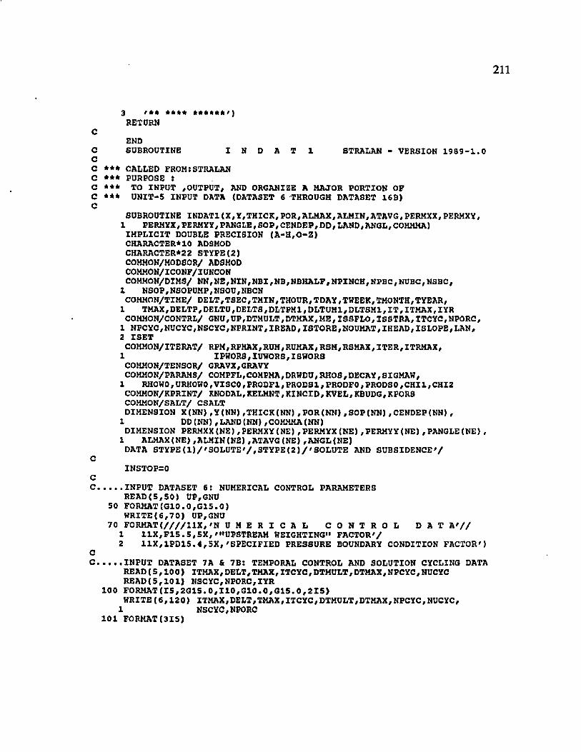
no
no
211
3 /** **** ***«**,)RETURN
CEND
C SUBROUTINE I N D A T X STRALAN - VERSION 1 9 8 9 -1 .0CC *** CALLED FROM:STRALAN C *** PURPOSE tC *** TO INPUT /OUTPUT/ AND ORGANIZE A MAJOR PORTION OF C *** UNIT-5 INPUT DATA (DATASET 6 THROUGH DATASET 16B)C
SUBROUTINE INDAT1 (X,Y,THICK, POR, ALMAX, ALMIN, ATAVG, PERKXX, PERMXY,1 PERMYX/PERMYY/PANGLE, SOP,CENDEP/DD, LAND, ANGL/COMMMA)
IMPLICIT DOUBLE PRECISION (A -H ,0-Z )CHARACTER*10 ADSMOD CHARACTER*22 STYPB(2)COMMON/HODSOR/ ADSMOD COMMON/ICONF/IUNCONCOMMON/DIMS/ NN,NE,NIN,NBI, NB, NBKALF,NPINCH,NPBC, NUBC, NSBC,
1 NSOP, NSOPUMP, NSOU, NBCNCOMMON/TIME/ DELT,TSEC,TMIN,THOUR,TDAY, TWEEK, TMONTH,TYEAR,
1 TMAX, DELTP,DELTU, DELTS, DLTPM1, DLTUM1, DLTSM1, I T , ITMAX, IYRCOMMON/CONTRL/ GNU, UP,DTMULT, DTMAX,ME, ISSFLO, ISSTRA, ITCYC, NPORC,
1 NPCYC,NUCYC,NSCYC,NPRINT, IREAD, ISTORE,NOUMAT, IHEAD, ISLOPE, LAN,2 I SET
COMMON/ITERAT/ RFM,RPMAX,RUM,RUMAX,RSM,RSMAX,ITER,ITRMAX,1 IPWORS/IUHORS,ISW0R3
COMMON/TENSOR/ GRAVX,GRAVYCOMMON/PARAMS/ COMPFL , COHPMA , DRWDU , RHOS , DECAY , SIGMAW ,
1 RHOWO , URHOWO , VISCO , PR0DF1, PRODS1, PRODFO , PRODSO , CHI 1 , CHI2COMMON/KPRINT/ KNODAL, KELMNT, KINCID, KVEL, KBUDG,KPORS COMMON/SALT/ CSALTDIMENSION X (NN) ,Y(NN) , THICK (NN) ,POR(NN) ,SOP(NNJ , CENDEP (NNJ ,
1 DD(NN),LAND(NN),COMMMA(NN)DIMENSION PERMXX(NE) , PERMXY (NE) , PERMYX (NE) , PERMYY (NE) , PANGLE (NE) ,
1 ALMAX (NE) , ALMIN(NE) , ATAVG (NE) ,ANGL(NE)DATA STYPE(1) / ' SOLUTE' / , STYPE(2 ) / ' SOLUTE AND SUBSIDENCE'/
CINSTOP=0
INPUT DATASET 6: NUMERICAL CONTROL PARAMETERSREAD( 5 ,5 0 ) UP,GNU
50 FORMAT(G10.0,G15.0)WRITE( 6 ,7 0 ) UP,GNU
70 F O R M A T (// / /11X , 'N U M E R I C A L C O N T R O L D A T A ' / /1 1 I X , F I 5 . 5 , 5X,'"UPSTREAM WEIGHTING" FACTOR'/2 11X ,1PD 15.4 , 5X,'SPECIFIED PRESSURE BOUNDARY CONDITION FACTOR')
. . . . I N P U T DATASET 7A & 7B: TEMPORAL CONTROL AND SOLUTION CYCLING DATA READ (5 , 100 ) ITMAX,DELT,TMAX, ITCYC, DTMULT, DTMAX, NPCYC, NUCYC READ( 5 ,1 0 1 ) NSCYC,NPORC,IYR
100 FORMAT( 1 5 , 2 G 1 5 .0 ,1 1 0 ,G 1 0 .0 ,G 1 5 .0 , 2 1 5 )WRITE (6 ,1 2 0 ) ITMAX, DELT,TMAX, ITCYC,DTMULT, DTMAX, NPCYC, NUCYC,
1 NSCYC,NPORC101 FORMAT(315)
nn
o o
1 2 0 FORMAT( 1 H 1 / / / / 1 1 X , 'T E M P O R A L C O N T R O L A N D ' ,1 ' S O L U T I O N C Y C L I N G D A T A ' ,2 / / 1 1 X , 1 1 5 / 5X,'MAXIMUM ALLOWED NUMBER OF TIME STEPS'3 /1 1 X ,1 P D 1 5 .4 , SX ,'IN ITIA L TIME STEP (IN SECONDS)'4 /1 1 X ,1 P D 1 5 .4 , 5X,'MAXIMUM ALLOWED SIMULATION TIME (IN SECONDS)'5 / / 1 1 X , I 1 5 ,5 X , 'T I M E STEP MULTIPLIER CYCLE (IN TIME STEPS)'6 / 1 1 X ,0 P F 1 5 ,5 , 5X,'MULTIPLICATION FACTOR FOR TIME STEP CHANGE'7 /11X,1PD15,4,5X,'MAXIMUM ALLOWED TIME STEP (IN SECONDS)'8 / / 1 1 X , 1 1 5 , 5X, 'FLOW SOLUTION CYCLE (IN TIME STEPS)'9 / 1 1 X , I 1 5 ,5 X , 'TRANSPORT SOLUTION CYCLE (IN TIME S T E PS)'* /11X,I15,5X ,'SU BSID ENCE SOLUTION CYCLE (IN TIME STEPS)'* / 1 1 X , 1 1 5 , 5X,'POROSITY SOLUTION CYCLE (IN TIME S T E P S ) ')
IF(NPCYC.GE.l.AND,NUCYC.GE.l.AND.NSCYC.GE.l) GOTO 140 WRITE( 6 ,1 3 0 )
130 F O R M A T (/ / lIX , '* * * * ERROR DETECTED : NPCYC,NUCYC,NSCYC AND ' ,1 'NPORC MUST ALL BE SET GREATER THAN OR EQUAL TO 1 . ' )
INSTOP=INSTOP-l 140 IF(NPCYC.EQ.l.OR.NUCYC.EQ.l.OR.NSCYC.EQ.l) GOTO 160
WRITE(6 ,1 5 0 )150 FO R M A T{//lIX , '* * * * ERROR DETECTED : EITHER NPCYC O R ',
1 ' NSCYC OR NUCYC MUST BE SET TO 1 . ' )INSTOP=INSTOP-l
160 CONTINUE SET MAXIMUM ALLOWED TIME STEPS IN SIMULATION FOR
STEADY-STATE FLOW AND STEADY-STATE TRANSPORT SOLUTION MODES I F ( ISSFLO. EQ.1 ) THEN
NPCYC=ITMAX+1 NUCYC=1 NSCYC=1 ENDIF
IF (IS S T R A • E Q .1) ITMAX=1
INPUT DATASET 8 : OUTPUT CONTROLS AND OPTIONSREAD (5 ,1 7 0 ) NPRINT, KNODAL, KELMNT, KINCID, KVEL, KBUDG, KPORS
170 FORMAT(1615)WRITE(6 ,1 7 2 ) NPRINT
172 F O R M A T (// / /11X , 'O U T P U T C O N T R O L S A N D ' ,1 ' O P T I O N S ' / / 1 1 X , 1 6 , 5X,'PRINTED OUTPUT CYCLE ' ,2 '{ I N TIME STEPS)')
I F (KNODAL.EQ.+l) WRITE(6,174)IF(KNODAL.EQ.O) WRITE(6,175)
174 FORMAT(/11X,' - PRINT NODE COORDINATES, THICKNESSES AND',1 ' POROSITIES')
175 FO RM A T(/IIX , ' - CANCEL PRINT OF NODE COORDINATES, THICKNESSES AND' 1 ' POROSITIES')
IF(KELMNT.EQ.+l) WRITE(6 ,1 7 6 )IF(KELMNT.EQ.O) WRITE(6,177)
176 F0RMAT(11X,' - PRINT ELEMENT PERMEABILITIES AND DISPERSIVITIES'}177 F O R M A T (l lX , '- CANCEL PRINT OF ELEMENT PERMEABILITIES AND ' ,
1 'D ISP E R S IV IT IE S ')IF fK IN C ID .E Q .+ l) WRITE(6 ,1 7 8 )IF(KINCID.EQ.O ) WRITE(6,179)
178 FORMAT ( 1 1 X , ' - PRINT NODE AND PINCH NODE INCIDENCES IN EACH ' ,1 'ELEMENT')
179 FORMAT(11X, ' - CANCEL PRINT OF NODE AND PINCH NODE INCIDENCES ' ,
213
1 ' I N EACH ELEMENT')IME=2IF (M E .L T .1) IME=i IF(K V EL.EQ .+l) WRITE{6 ,1 8 4 )I F ( KVEL.EQ.0) WRITE(6 ,1 8 5 )
184 FORMAT(/UX,' - CALCULATE AND PRINT VELOCITIES AT ELEMENT ' ,1 'CENTROIDS ON EACH TIME STEP WITH OUTPUT')
185 FORMAT(/11X,' - CANCEL PRINT OF VELOCITIES')IF(KBUDG.EQ.+l) WRITE(6 ,1 8 6 ) STYPE(IME)IF(KBUDG.EQ.O) WRITE(6 ,1 8 7 )
186 FORMAT(/11X,'- CALCULATE AND PRINT FLUID AND ' , A 6 , ' BUDGETS ' ,1 'ON EACH TIME STEP WITH OUTPUT')
187 FORMAT(/11X,'- CANCEL PRINT OF BUDGETS')CC INPUT DATASET 9: ITERATION CONTROLS
READ(5 ,1 9 0 ) ITRMAX, RPMAX, RUMAX, RSMAX 190 F0RMAT(I10,3G10.0)
IF(ITRMAX-1) 1 9 2 ,1 9 2 ,1 9 4192 WRITE(6 ,1 9 3 )193 F O R M A T (////11X , ' I T E R A T I O N C O N T R O L D A T A ' ,
1 / / 1 1 X , ' NON-ITERATIVE SOLUTION')GOTO 196
194 WRITE(6 ,1 9 5 ) ITRMAX, RPMAX, RUMAX,RSMAX195 F O R M A T < / / / / l IX , ' I T E R A T I O N C O N T R O L D A T A ' ,
1 / / 1 1 X , 1 1 5 , 5X,'MAXIMUM NUMBER OF ITERATIONS PER TIME S T E P ',2 /1 1 X ,1 P D 1 5 .4 , SX,'ABSOLUTE CONVERGENCE CRITERION FOR FLOW',3 ' SOLUTION'/IIX,1PD15. 4 , 5X,'ABSOLUTE CONVERGENCE CRITERION',4 ' FOR TRANSPORT S O L U T IO N '/ l lX ,1P D 15 .4 , 5X, 'ABSOLUTE',5 ' CONVERGENCE CRITERION FOR SUBSIDENCE')
196 CONTINUECC .INPUT DATASET 10: FLUID PROPERTIES
READ( 5 ,2 0 0 ) COMPFL,SIGMAW,RHOW0, URHOWO, DRWDU,VISC0, CSALTC ..............INPUT DATASET 11: SOLID MATRIX PROPERTIES
READ(5 ,2 0 0 ) COMPMA,RHOS 200 FORMAT(8G10.1)
IF (M E .E Q .+ l)1 WRITE( 6 ,2 1 0 ) COMPFL, COMPMA, VISC0, RHOS, RHOWO, DRWDU, URHOWO,2 SIGMAW
210 F O R M A T (1H 1/// /1 IX , 'C O N S T A N T P R O P E R T I E S O F ' ,1 ' F L U I D A N D S O L I D M A T R I X '2 / / 1 1 X ,1 P D 1 5 .4 , 5X,'COMPRESSIBILITY OF F L U ID '/1 1 X ,1 P D 1 5 .4 ,5 X ,3 'AVERAGE COMPRESSIBILITY OF POROUS K A TR IX '//11X ,1PD 15. 4 , 5X,5 'FLUID V IS C 0 S IT Y '/ /1 1 X ,1 P D 1 5 .4 , 5X,'DENSITY OF A SOLID GRAIN'* / /1 3 X , 'F L U I D DENSITY, RHOW'/13X,'CALCULATED BY STRALAN ' ,1 ' I N TERMS OF CONCENTRATION, U, AS: '/13X,'RHOW = RHOWO + ' ,2 'DRWDU*(U-URHOWO)'//11X,1PD1S.4 , 5X ,'FLU ID BASE DENSITY, RHOWO'3 /1 1 X ,1 P D 1 5 .4 , 5X,'COEFFICIENT OF DENSITY CHANGE WITH ' ,4 'CONCENTRATION, DRW D U '/llX ,1PD 15.4 , 5X,'CONCENTRATION,' ,5 ' URHOWO, AT WHICH FLUID DENSITY IS AT BASE VALUE, RHOWO'7 / / 1 1 X ,1 P D 1 5 .4 , 5X,'MOLECULAR DIFFUSIVITY OF SOLUTE IN FLUID')
I F (M E .E Q .- l )1 WRITE(6 ,2 2 0 ) COMPFL,COMPMA,VISC0,RHOS,RHOWO,DRWDU,URHOWO, SIGMAW
220 FO R M A T(1H 1////11X ,'C O N S T A N T P R O P E R T I E S O F ' ,1 ' F L U I D A N D S O L I D M A T R I X '
2 / /1 1 X ,1 P D 1 5 .4 , 5X,'COMPRESSIBILITY OP FLUID ' / 1 1 X , XPD15 . 4, SX,3 'COMPRESSIBILITY OP POROUS MATRIX'4 / /11X ,X PD 15 .4 ,5X ,'F L U ID VISCOSITY'4 / / 1 1 X ,1 P D 1 5 .4 , 5X,'DENSITY OF A SOLID GRAIN'5 / /1 3 X , 'F L U ID DENSITY, RHOW'/13X,'CALCULATED BY ' ,6 'STRALAN IN TERMS OF SOLUTE CONCENTRATION, U, A S : ' ,7 /13X,'RHOW = RHOWO + DRWDU*(U-URHOWO)'8 / / I I X ,1 P D 1 5 . 4,SX,'FLUID BASE DENSITY, RHOWO'9 /1 1 X ,1 P D 1 5 .4 ,5X,'COEFFICIENT OF DENSITY CHANGE WITH* 'SOLUTE CONCENTRATION, DRWDU'1 /11X,1PD15.4,5X ,'SOLUTE CONCENTRATION, URHOWO, ' ,4 'AT WHICH FLUID DENSITY IS AT BASE VALUE, RHOWO'5 / / I 1 X ,1 P D 1 S .4 , SX,'MOLECULAR DIFFUSIVITY OF SOLUTE IN FLUID')
CC INPUT DATASET 12: ADSORPTION PARAMETERS
READ(S,230) ADSMOD,CHI1,CHI2 230 FORMAT(A10,2G10.0)
IF (ADSMOD.EQ.'NONE ' ) GOTO 234WRITE(6 ,232} ADSMOD
232 FORMAT ( / / / / l IX , 'A D S O R P T I O N P A R A M E T E R S '1 //X6X,A10,5X,'EQUILIBRIUM SORPTION ISOTHERM')
GOTO 2 36234 WRITE(6 ,2 3 5 )235 F 0 R M A T (/ / / /1 1 X , 'A D S O R P T I O N P A R A M E T E R S '
1 //16X,'NON-SORBING SOLUTE')236 I F ( (ADSMOD.EQ.'NONE ' ) .OR.(ADSMOD.EQ.'LINEAR ' ) .O R .
1 {ADSMOD.EQ.'FREUNDLICH') .OR. (ADSMOD.EQ.'LANGMUIR ' ) ) GOTO 238WRITE(6 ,2 3 7 )
237 FORMAT(//11X,' * * * * ERROR DETECTED : TYPE OF SORPTION MODEL ' ,1 ' I S NOT SPECIFIED CORRECTLY.'/11X,'CHECK FOR TYPE AND ' ,2 'SPELLING, AND THAT TYPE IS LEFT-JUSTIFIED IN INPUT FIELD')
INSTOP=INSTOP-l238 IF(ADSMOD.EQ.'LINEAR ' ) WRITB(6,242) CHI12 42 FORMAT(11X,1PD15. 4 , 5X, 'LINEAR DISTRIBUTION COEFFICIENT')
IF(ADSMOD.EQ.'FREUNDLICH') WRITE(6,244) CHI1,CHI2244 FORMAT (11X,1PD15. 4 , 5X, 'FREUNDLICH DISTRIBUTION COEFFICIENT'
1 /1 1 X ,1 P D 1 5 . 4 , SX, 'SECOND FREUNDLICH COEFFICIENT')IF(ADSMOD.EQ.'FREUNDLICH'.AND.CHI2.LE.0.DO) THEN
WRITE(6 ,2 4 5 )245 FORMAT(11X,'* * * * ERROR DETECTED : SECOND COEFFICIENT ' ,
1 'MUST BE GREATER THAN ZERO')INSTOP=INSTOP-IENDIF
IF(ADSMOD.EQ.'LANGMUIR ' ) WRITE(6,246) CHI1,CHI2246 FORMAT( 11X, 1PD1S. 4 , 5X,'LANGMUIR DISTRIBUTION COEFFICIENT'
X /1 1 X ,1 P D 1 5 . 4 , 5X, 'SECOND LANGMUIR COEFFICIENT')CC INPUT DATASET 13; PRODUCTION OF SOLUTE MASS
READ(5 ,2 0 0 ) PRODFO, PRODSO, PRODF1, PRODS1 WRITE(6 ,2 5 0 ) PRODFO, PRODSO, PRODF1,PRODSX
250 FORMAT ( / / / /X X X , 'P R O D U C T I O N A N D D E C A Y O F ' , X ' S P E C I E S M A S S '//13X,'PRODUCTION RATE ( + ) ' /1 3 X ,2 'DECAY RATE ( - ) ' / / X I X , 1PD15. 4 , SX,'ZERO-ORDER RATE OF SOLUTE ' ,3 'MASS PRODUCTION/DECAY IN FL U ID '/11X ,X PD X 5.4 ,5X ,4 'ZERO-ORDER RATE OF ADSORBATE MASS PRODUCTION/DECAY IN ' ,

nn
n on
o
o
215
5 'IMMOBILE P H A S E '/ l lX ,1 P D 1 5 .4 ,5 X , 'FIRST-ORDER RATE OP SOLUTE3 'MASS PRODUCTION/DECAY IN F L U ID '/11X ,1PD 15. 4 , 5X,4 'FIRST-ORDER RATE OP ADSORBATE HASS PRODUCTION/DECAY IN5 'IMMOBILE PHASE')
INPUT DATASET 14: ORIENTATION OP COORDINATES TO GRAVITYREAD(5 ,2 0 0 ) GRAVX,GRAVY WRITE(6 ,3 2 0 ) GRAVX,GRAVY
320 F O R M A T (/ / / / l IX , 'C O O R D I H A T E O R I E N T A T I O N ' ,1 ' T O G R A V I T Y'//13X,'COMPONENT OP GRAVITY VECTOR',2 / 1 3 X , ' I N +X DIRECTION, GRAVX '/11X,1PD15.4,5X,3 'GRAVX = -GRAV * D{ELEVATION)/DX'//I3X,'COMPONENT OF GRAVITY',4 ' VECTOR'/13X,'IN +Y DIRECTION, GRAVY '/11X,1PD1S.4,5X,5 'GRAVY = -GRAV * D(ELEVATION)/DY')
INPUT DATASETS 15A, AND 1SB : NODEWISE DATAREAD(5 ,3 3 0 ) SCALX,SCALY,SCALTH,PORFAC,COMFAC
330 FORMAT(5X,5G10.0)DO 455 1 = 1 ,NNREAD(5 ,4 0 0 ) I I ,X ( I I ) ,Y ( I I ) ,T H IC K ( I I ) ,P O R ( I I ) ,C O M M M A (I I )
400 FORMAT(I5,5G10.0)X ( I I ) = X ( I I ) ‘ SCALX Y{I I ) =Y( I I ) ‘ SCALY T H IC K (II)= T H IC K {II)‘ SCALTH P O R (I I )= P O R ( I I ) ‘ PORFAC IP(ME.LE.O) GO TO 450 COMMMA(II)=COMMMA(II)*COMFAC
SET INITIAL SPECIFIC PRESSURE STORATIVITY, SOP.SOP( I I ) =COMMMA( I I ) +POR{I I ) ‘ COMPFL GO TO 455
450 I F ( IUNCON.EQ.1) SOP(II)=COMPMA+POR(II)‘ COMPFL IF{IUNCON.EQ.1) GO TO 455S O P ( I I ) = ( l .D O - P O R ( I I ) ) ‘ COMPMA+POR(II)‘ COMPFL
455 CONTINUE450 IF(KNODAL.EQ.O) WRITE(6,469) SCALX,SCALY,SCALTH,PORFAC469 FO RM AT(1H 1////11X ,'N O D E I N F O R M A T I O N ' / / 1 6 X ,
1 'PRINTOUT OF NODE COORDINATES, THICKNESSES AND POROSITIES ' ,2 'CANCELLED.'//16X,'SCALE FACTORS : ' / 3 3 X ,1 P D 1 5 . 4 , 5 X , 'X -S C A L E '/1 3 3X,1PD15. 4 , 5 X , ' Y-SCALE'/33X,1PD15.4,5X,'THICKNESS FACTOR'/2 33X ,1PD 15.4 , 5X,'POROSITY FACTOR')
IF(KNODAL.EQ.+l) WRITE(6 ,4 7 0 ) ( I , X ( I ) , Y ( I ) ,T H IC K (I ) ,P O R (I ) , I= 1 ,N N )470 FORMAT(1H1//11X,'N O D E I N F O R M A T I O N ' / / 1 3 X ,
1 'N O D E ' , 7 X , 'X ' , 1 6 X , 'Y ' , 17X,'THICKNESS', 6 X , 'P O R O S IT Y '/ /2 ( 1 1 X , I 6 , 3 (3X,1PD14. 5 ) , 6 X ,0 P F 8 .S ) )
INPUT DATASETS 16A AND 16B: ELEMENTWISE DATA402 READ(5 ,4 9 0 ) PMAXFA, PMINFA, ANGFAC, ALMAXF, ALMINF, ATAVGF, ANGLF 490 FORMAT( 10X,5G10. 0 , 2G5.0 )
IF(KELMNT.EQ.+l) WRITE(6 ,5 0 0 )500 FORMAT{1 H 1 / /6 X , 'E L E M E N T I N F O R M A T I O N ' / /
1 6 X , ' ELEMENT' , 4X,'MAXIMUM', 9X,'MINIMUM', 12X,2 'ANGLE BETWEEN',3X,' MAXIMUM',5X,' MINIMUM',5X,3 ' AVERAGE',5X, ' SLOPING'/17X,'PERMEABILITY', 4X,4 'PERMEABILITY',4X,'+X-DIRECTION AND',4 3X,'LONGITUDINAL',3X,'LONGITUDINAL',3X,' TRANVERSE', 4X,

on
o o
o o
o
5 3 X , ' ANGLE' / 45X, 'MAXIMUM PERMEABILITY' , 3X, 'DISPERSIVITY' ,6 3X ,'D ISPERSIV ITY ',3X , 'D ISP E R S IV IT Y '/53X , ' (IN DEGREES)'//)
DO 550 LL=1,NEREAD (5 ,5 1 0 ) L,PMAX,PMIN,ANGLEX, ALMAX (L) , ALMIN(L) , ATAVG (L) ,
1 ANGL(L)510 FORMAT ( 1 1 0 ,5G 10 .0 ,2G 5.0)
PMAX=PMAX*PMAXFA PMIN=PHIN*PMINFA ANGLEX=ANGLEX*ANGFAC ALMAX ( L) -ALMAX ( L) *ALMAXF ALMIN(L)=ALMIN(L) *ALMINF ATAVG(L)=ATAVG(L)*ATAVGF ANGL(L)=ANGL(L)*ANGLFI F ( KELMNT.EQ.+1) WRITE(6,520) L,PMAX,PMIN,ANGLEX,
1 ALMAX(L) , ALHIN(L) , ATAVG (L) , ANGL(L)520 FORMAT(6X,1 7 , 2X ,2 (1PD14. 5 , 2X ), 8 X ,5 (0 P F 1 0 .3 ,5X) )
. . . .R O T A T E PERMEABILITY FROM MAXIMUM/MINIMUM TO X/Y DIRECTIONS RADIAX=1.7 4 5 32 9 D-2 *ANGLEX SINA=DSIN{RADIAX)COSA=DCOS(RADIAX)SINA2=SINA*SINACOSA2=COSA*COSAPERMXX(L)=PMAX*COSA2+PMIN*SINA2 PERMYY (L) =PMAX*SINA2+PMIN*COSA2 PERMXY(L)=(PMAX-PMIN) *SINA*COSA PERMYX(L)=PERMXY(L)PANGLE(L)=RADIAX
550 CONTINUEIF(KELMNT.EQ.O)
1 WRITE (6 , 569) PMAXFA, PMINFA, ANGFAC, ALMAXF, ALMINF, ATAVGF, ANGLF569 FORMAT ( / / / / 1 1 X , ' E L E H E N T I N F O R M A T I O N ' / /
1 16X,'PRINTOUT OF ELEMENT PERMEABILITIES AND DISPERSIVITIES2 'CANCELLED.'//16X, 'SCALE FACTORS : ' / 3 3 X ,1 P D 1 5 .4 , 5X,'MAXIMUM '1 'PERMEABILITY FACTOR'/33X,1PD15. 4 , 5X,'MINIMUM PERMEABILITY ' ,2 'FA CT0R '/33X,1PD15.4,5X,'AN GLE FROM 4-X TO MAXIMUM DIRECTION',3 ' FACTOR'/33X,1PD15.4 , 5X,'MAXIMUM LONGITUDINAL DISPERSIVITY',4 ' FACTOR'/33X,1PD15.4 , SX,'MINIMUM LONGITUDINAL DISPERSIVITY',5 ' FACT0R'/33X,1PD15.4,5X,'TRANSVERSE DISPERSIVITY FACTOR'/,6 33X, 1PD 15.4 , 5X,'SLOPING ANGLE FACTOR')
END SIMULATION FOR CORRECTIONS TO UNIT-5 DATA IF NECESSARY605 IF(IN STO P.EQ.O) GOTO 1000
WRITE (6 ,9 9 9 )999 FORMAT ( / / / / / / / / 1 1 X , 'P L E A S E CORRECT INPUT DATA AND RERUN.',
1 / / / 2 2 X , ' S I M U L A T I O N H A L T E D ' ,2 / 2 2 X , '******************* * * * * * * * * * * * ')
ENDFILE(6)STOP
1000 RETURN END
C SUBROUTINE I N D A T 2 STRALAN - VERSION 1 9 8 9 -1 .

fio
oo
on
o
o no
o
oo
no
217
cC *** CALLED FROM STRALAN C *** PURPOSE !C *** TO READ THE INITIAL DRAWDOWN,AQUIFER DEPTH, NATURAL SUBSIDENCE,C *** INITIAL LAND ELEVATION AND UNCONFINED AQUIFER'S SPECIFICC *** YIELD AT EACH NODE IN AREAL FLOWC *** READ UNIT 55C
SUBROUTINE INDAT2 {DD,CENDEP,LAND, SPEY,SETTLE)IMPLICIT DOUBLE PRECISION <A-H,0-Z)COMMON/CONTRL/ GNU, UP, DTMULT, DTMAX, ME, ISSFLO, ISSTRA, ITCYC, NPORC,
1 NPCYC , NUCYC , NSCYC, NPRINT , IREAD , I STORE , NOUMAT , I HEAD , ISLOPE , LAN ,2 ISET
COMMON/D IMS/ NN,NE,NIN,NBI,NB, NBHALF, NP INCH , NPBC , NUBC , NS BC ,1 NSOP,NSOPUMP,NSOU,NBCN
COMMON/ICONF/ IUNCONDIMENSION DD{NN) , CENDEP (NN) ,LAND(NN) ,SPEY(NN) , SETTLE (NN)
. . . . I N P U T DATASET 1 TO 4
. . . .R E A D INITIAL DRAWDOWN, DD(I) AND DEPTH TO THE NODES, CENDEP(I)AT EACH NODE IN AREAL FLOW
IF (IH E A D .L E .0) GO TO 102 FOR UNCONFINED AQUIFER,CENDEP(I) IS THE VERTICAL DISTANCE
FROM THE MEAN SEA LEVEL TO THE IMPERVIOUS LAYER READ( 5 5 ,1 0 1 ) (D D (I) ,I=1 ,N N )READ( 5 5 ,1 0 1 ) (CENDEP(I), I=1,NN)
101 FORMAT(1 0 F 6 .1)102 I F ( I S E T .N E . l ) GO TO 105
READ( 5 5 ,1 0 3 ) SETFAC103 FORMAT(G15.6)
DO 10 1 = 1 ,NNREAD( 5 5 ,2 0 ) I I ,S E T T L E (I I )
20 FORMAT( 1 5 , G10.0)10 SETTLE(II)=SETTLE(II)*SETFAC
105 IF (L A N .N E .l) GO TO 106READ( 5 5 ,1 0 4) (LAND(I), 1 = 1 , NN)
104 FORMAT(6G12.6 )106 IF(IU NCON.NE.l) GO TO 200
INPUT UNCONFINED AQUIFER'S SPECIFIC YIELD:DATASET 5READ(55,198) (SP E Y (I) ,I= 1 ,N N )
198 FORMAT(4G15.4}200 RETURN
ENDSUBROUTINE S O U R C E STRALAN - VERSION 1 9 8 9 -1 .0
*** CALLED FROM STRALAN *** PURPOSE :*** TO READ AND ORGANIZE FLUID MASS SOURCE DATA AND *** SOLUTE MASS SOURCE DATA.
SUBROUTINE SOURCE(QIN,UIN,IQSOP,QUIN,IQSOU,IQSOPT,IQSOUT)IMPLICIT DOUBLE PRECISION (A -H ,0-Z )COMMON/DIMS/ NN, NE,NIN,NBI, NB, NBHALF,NPINCH,NPBC,NUBC, NSBC,
1 NSOP,NSOPUMP,NSOU,NBCN

COMMON/CONTRL/ GNU,UP,DTMULT,DTMAX,ME, ISSFLO,ISSTRA,ITCYC,NPORC1 NPCYC,NUCYC, NSCYC, NPRINT, TREAD, ISTORE, NOUMAT, IHEAD, ISLOPE, LAN,2 ISET
DIMENSION QINCNN),UIN(NN) ,IQSOP(NSOP),QUIN(NN),IQSOU(NSOU)CC ...........NSOPI IS ACTUAL NUMBER OF FLUID SOURCE NODESC...........NSOUI IS ACTUAL NUMBER OF SOLUTE MASS OR ENERGY SOURCE NODES
NSOPI=NSOP-lNSOUI=NSOU-lIQSOPT=lIQSOUT=lNIQP=0NIQU=0IF(NSOPI.EQ.O) GOTO 1000
50 WRITE (6 ,1 0 0 )100 F O R M A T (1H 1// / /1 IX , 'F L U I D S O U R C E D A T A '
1 / / / / 1 1 X , '* * * * NODES AT WHICH FLUID INFLOWS OR OUTFLOWS ARE '2 'SPECIFIED 'NODE NUMBER', 10X,3 'FLUID INFLOW(+)/OUTFLOW(-)',5X,'SOLUTE CONCENTRATION OF'4 /11X,'{M INUS IN D ICA TES',5X ,' (FLUID MASS/SECOND)',5 12X,'INFLOWING FLUID'/12X*'TIME-VARYING', 39X,6 '(MASS SOLUTE/MASS WATER)' / 1 2 X,'FLOW RATE O R '/12X ,7 'CONCENTRATION)' / / )
INPUT DATASET 17300 CONTINUE
READ(5 ,4 0 0 ) IQCP,QINC,UINC 400 FORMAT(I 1 0 , 2G15 .0 )
I F ( IQCP. EQ.0 ) GOTO 700 NIQP=NIQP+1 IQSOP(NIQP)=IQCP IF ( IQ C P .L T .0 ) IQSOPT=-l IQP=IABS(IQCP)QIN(IQP)=QINC U IN ( IQP)=UINC I F ( IQCP.G T.0) GOTO 450 WRITE(6 ,5 0 0 ) IQCP GOTO 600
4 50 IF(QINC.GT.O) GOTO 4 60 WRITE(6 ,5 0 0 ) IQCP,QINC GOTO 600
460 WRITE (6 ,5 0 0 ) IQCP,QINC,UINC 500 FO R M A T (11X ,I10 ,13X ,1PE 14 .7 ,16X ,1PE 14 .7)600 GOTO 300700 IF(NIQP.EQ.NSOPI) GOTO 890
C END SIMULATION IF THERE NEED BE CORRECTIONS TO DATASET 17W RITE(6,750) NIQP,NSOPI
750 F O R M A T {// / / l IX , 'T H E NUMBER OF FLUID SOURCE NODES READ, ' , 1 5 ,1 ' I S NOT EQUAL TO THE NUMBER SPECIFIED, ' , 1 5 / / / /2 11X,'PLEASE CORRECT DATA AND R E R U N ' / / / / / / / /3 2 2 X , 'S I M U L A T I O N H A L T E D ' /4 22X, ' __________________________________________' )
ENDFILE(6)STOP
890 IF (X Q SO PT .E Q .-l) WRITE{6,900)

oo
oo
on
oo
o
o no
o
o
219
900 F O R M A T (// / / l IX , 'T H E SPECIFIED TIME VARIATIONS ARE ' , 1 'USER-PROGRAMMED IN SUBROUTINE B C T I M E . ' )
1000 IF(NSOUI.EQ.O) GOTO 9000 1050 WRITE(6 ,1 1 0 0 )1100 FORMAT( / / / / / / / / 1 1 X , 'S O L U T E S O U R C E D A T A '
1 / / / / 1 1 X , '* * * * NODES AT WHICH SOURCES OR SINKS OF SOLUTE ' ,2 'MASS ARE SPECIFIED * * * * ' / / l lX , 'N O D E NUMBER',10X,3 'SOLUTE S O U R C E (+ )/S IN K (-) ' /1 1 X , ' (MINUS INDICATES', 5X,4 ' (SOLUTE MASS/SECOND) ' / 1 2 X , 'TIME-VARYING'/12X,5 'SOURCE OR S I N K ) ' / / )
INPUT DATASET 181300 CONTINUE
READ( 5 ,4 0 0 ) IQCU,QUINC IF(IQCU.EQ.O) GOTO 1700 NIQU=NIQU+1 IQSOU(NIQU)=IQCU IF(IQ CU .LT.O ) IQSOUT=-l IQU=IABS(IQCU)QUIN( IQU) —QUINC IF(IQCU.GT.O) GOTO 1450 WRITE(6 ,1 5 0 0 ) IQCU GOTO 1600
1450 WRITE(6 ,1 5 0 0 ) IQCU,QUINC 1500 FORMAT(11X,1 1 0 , 13X ,1PE14.7)1600 GOTO 13001700 IF(NIQU.EQ.NSOUI) GOTO 1890 END SIMULATION IF THERE NEED BE CORRECTIONS TO DATASET l a
WRITE(6 ,1 7 5 0 ) NIQU,NSOUI 1750 FO RM AT(////11X,'THE NUMBER OF SOLUTE SOURCE NODES READ, ' , 1 5 ,
1 ' IS NOT EQUAL TO THE NUMBER SPECIFIED, ' , 1 5 / / / /2 11X,'PLEASE CORRECT DATA AND R E R U N ' / / / / / / / /3 2 2 X , 'S I M U L A T I O N H A L T E D ' /4 22X, ' _________________________________________ ' )
ENDFILE(6)STOP
1890 IF (IQ S O U T .E Q .- l ) WRITE(6,900)
9000 RETURN
ENDSUBROUTINE B O U N D STRALAN - VERSION 1 9 8 9 -1 .0
*** CALLED FROM: STRALAN *** PURPOSE :*** TO READ AND ORGANIZE SPECIFIED PRESSURE DATA,CONCENTRATION DATA * * • AND SPECIFIED LAND SUBSIDENCE DATA.
SUBROUTINE BOUND(IPBC,PBC,IUBC,UBC,ISBC,SBC,IPBCT,IUBCT,ISBCT) IMPLICIT DOUBLE PRECISION (A -H ,0 -Z )COMMON/DIMS/ NN , NE , NIN,NBI, NB, NBHALF, NPINCH, NPBC, NUBC, NSBC,
1 NSOP, NSOPUMP, NSOU, NBCNCOMMON/CONTRL/ GNU, UP , DTMULT, DTMAX, ME, ISSFLO, ISSTRA, ITCYC, NPORC ,

on
o o
1 NPCYC,NUCYC, NSCYC,NPRINT, IREAD, ISTORE, NOUMAT, IHEAD, ISLOPE, LAN2 ISET
DIMENSION IFBC(NBCN), PBC(NBCN) ,IUBC(NBCN), UBC(NBCN), ISBC(NBCN) 1 SBC(NBCN)
IPBCT=1IUBCT=1ISBCT=1ISTOPP=0ISTOPU=0ISTOPS=0IPU=0WRITE( 6 , SO)
50 FORMAT ( 1 H 1 / / / / 1 1 X , 'B O U N D A R Y C O N D I T I O N S ' )IF(NPBC.EQ.O) GOTO 400 WRITE(6,100)
100 FORMAT(//11X,'* * * * NODES AT WHICH PRESSURES ARE',1 ' SPECIFIED 4 * * * ' / )
IF(ME) 1 0 7 ,1 0 7 ,1 1 4107 WRITE(6,108)108 FORMAT(11X, ' (AS WELL AS SOLUTE CONCENTRATION OF ANY'
1 / 1 6 X , ' FLUID INFLOW WHICH MAY OCCUR AT THE POINT'2 / 1 6 X , ' OF SPECIFIED P R E S S U R E )'/ /12X , 'N O D E ',18X , 'P R E SS U R E ',3 13X,'CONCENTRATION'//)
GOTO 120114 WRITE(0 ,1 1 5 )115 FORMAT(11X,' (AS WELL AS SOLUTE CONCENTRATION OF ANY'
1 / 1 6 X , ' FLUID INFLOW AND SUBSIDENCE WHICH MAY OCCUR AT THE '2 'P O IN T '/1 6 X , ' OF SPECIFIED P R E S S U R E )'/ /12X , 'N O D E ', 13X,3 ' PRESSURE' , 10X, ' CONCENTRATION', 16X,'SUBSIDENCE' / / )
INPUT DATASET 19120 IPU=IPU+1
IF(ME) 1 3 0 ,1 3 0 ,1 4 0 130 READ(5 ,1 5 0 ) IPBC(IPU),PBC(IPU) ,UBC(IPU>
GO TO 135140 READ(5,150) IPBC(IP U ) , PBC(IPU), UBC(IPU), SBC (IPU)150 FORMAT( 1 5 , 3G20 .0 )135 IF ( IP B C (IP U ) .L T .O ) IPBCT=-1
IF (IP B C (IP U ).E Q .O ) GOTO 180 IF(ME) 1 4 5 ,1 4 5 ,1 4 6
145 IF (IP B C (IP U ).G T .O ) WRITE(6 ,1 6 0 ) IP B C (IPU ),PB C (IPU ),U B C (IPU )GO TO 147
146 IF (IP B C (IP U ).G T .O ) WRITE(6,160) IP B C (IP U ) , P B C (IPU ), UBC(IPU),1 SBC(IPU)
147 IF (IP B C (IP U ) .L T .O ) WRITE(6,160) IPBC(IPU)160 FORMAT ( 11X, 15 , 6X, 1PD20 .1 3 , 6X, 1PD20 .1 3 , 6X, 1PD2Q . 13 )
GOTO 120 180 IPU=IPU-1
IP=IPUIF(IP .E Q .N PB C ) GOTO 200 ISTOPP=l
200 I F ( I P B C T .N E .- l ) GOTO 400 IF(ME) 2 0 5 ,2 0 5 ,2 1 5

no
no
on
205 WRITE(6 ,2 0 6 )206 FORMAT(//12X,'TIME-DEPENDENT SPECIFIED PRESSURE'/12X,'OR INFLOW '
1 ' CONCENTRATION INDICATED'/12X,'BY NEGATIVE NODE NUMBER')GOTO 400
215 WRITE{ 6 , 216)216 FORMAT(//11X,'TIME-DEPENDENT SPECIFIED PRESSURE'/12X,'OR INFLOW '
1 ' CONCENTRATION AND SUBSIDENCE INDICATED'/12X ,'B Y NEGATIVE',2 ' NODE NUMBER')
400 IF{NUBC• EQ.O) GOTO 1310
500 WRITE(6 ,1 0 0 0 )1000 F O R M A T (// / /11X , '* * * * NODES AT WHICH SOLUTE CONCENTRATIONS ARE ' ,
1 'SPECIFIED TO BE INDEPENDENT OF LOCAL FLOWS AND FLUID SOURCES'2 # * * ** '/ /12X ,'N O D E ',13X ,'C O N C E N T R A T IO N '//)
INPUT DATASET 201120 IPU—I P U t1
READ(5 ,1 5 0 ) IUBC(IPU), UBC(IPU)IF (IU B C (IP U ).L T .O ) IUBCT=-i IF (IU B C (IPU ).E Q .O ) GOTO 1180IF d U B C (IP U ) .GT.O) WRITE (6 , 1150) IUBC (IPU) ,UBC(IPU)IF (IU B C d P U ) .LT.O) WRITE(6 , 1150) IUBC(IPU)
1150 FORMAT(1 I X , 1 5 , 6X,1PD20 .1 3 )GOTO 1120
1180 IPU=IPU-1 IU = IP U -IPIF(IU.EQ.NUBC) GOTO 1200 ISTOPU=l
1200 IF ( IU B C T .N E .- l ) GOTO 20001205 WRITE(6 ,1 2 0 6 )1206 FORMAT(//12X,'TIME-DEPENDENT SPECIFIED CONCENTRATION'/12X,'IS ' ,
1 'INDICATED BY NEGATIVE NODE NUMBER')1310 IF(NSSC.EQ.O) GO TO 2000
INPUT DATASET 21IF(NUBC.EQ.O) IU=0
132 0 IPU=IPU+1READ(S,150) IS B C (IP U ), SBC(IPU)IF (IS B C (IP U ) .L T .O ) ISBCT=-1 IF (IS B C (IP U ).E Q .O ) GOTO 1380IF (IS B C (IP U ).G T .O ) WRITE(6 ,1 3 5 0 ) ISB C (IP C ),S B C (IPU )IF (IS B C (IP U ) .L T .O ) WRITE(6 ,1 3 5 0 ) ISBC(IPU)
1350 FORMAT(11X,1 5 , 6X ,1PD 20.13)GO TO 1320
1380 IPU=IPU-1IS = IP U - I P - IUIF(IS .E Q .N SB C ) GO TO 1400 ISTOPS=l
1400 I F ( I S B C T .N E .- l ) GO TO 20001405 WRITE(6 ,1 4 0 6 )1406 FORMAT(//11X,'TIME-DEPENDENT SPECIFIED SU B SID EN C E'/12X ,'IS • ,
1 'INDICATED BY NEGATIVE NODE NUMBER')
. . .E N D SIMULATION IF THERE NEED BE CORRECTIONS TO DATASET 1 9 ,2 0 OR 21 2000 IF(ISTOPP.EQ.O.AND.ISTOPU.EQ.O.AND.ISTOPS.EQ.O) GOTO 6000
oo u
uu
ou
uu
u
222
IF ( IS T O P P .E Q .l ) WRITE(6 ,3 0 0 0 ) IP,NPBC 3000 FORMAT(////lIX,'ACTUAL NUMBER OF SPECIFIED PRESSURE NODES',
1 ' READ, ' , 1 5 , ' , IS NOT EQUAL TO NUMBER SPECIFIED I N ' ,2 ' INPUT, ' , 1 5 )
IF (IS T O P U .E Q .l) WRITE(6 ,4 0 0 0 ) IU,NUBC4000 FORMAT{////XIX,'ACTUAL NUMBER OF SPECIFIED CONCENTRATION NODES',
1 ' READ, ' , 1 5 , ' , IS NOT EQUAL TO NUMBER SPECIFIED I N ' ,2 ' INPUT, ' , 1 5 )
IF(ME) 4 8 0 0 ,4 8 0 0 ,4 6 0 0 4600 IF (IS T O P S • EQ.1) WRITE(6 ,4 7 0 0 ) IS,N5BC4700 FORMAT(////XIX,'ACTUAL NUMBER OF SPECIFIED SUBSIDENCE NODES',
1 ' READ, ' , 1 5 , ' , IS NOT EQUAL TO NUMBER SPECIFIED I N ' ,2 ' INPUT, ' , 1 5 )
4800 WRITE(6 ,5 0 0 0 )5000 FORMAT(////11X,'PLEASE CORRECT DATA AND RERUN.' / / / / / / / /
1 2 2 X , 'S I M U L A T I O N H A L T E D ' /2 22X, ' _________________________________________ ' )
ENDFILE(6)STOP
I
6000 IF ( IP B C T .E Q .- 1 . OR.IUBCT.EQ. - 1 .O R.ISBCT.EQ.- 1 ) WRITE(6 ,7 0 0 0 )7000 FORM AT(////11X,'THE SPECIFIED TIME VARIATIONS ARE
1 'USER-PROGRAMMED IN SUBROUTINE B C T I M E . ' )
RETURNENDSUBROUTINE O B S E R V STRALAN - VERSION 1 9 8 9 -1 .0
*** CALLED FROM: STRALAN *** PURPOSE :*** (1 ) TO READ AND ORGANIZE OBSERVATION NODE DATA*** (2 ) TO MAKE OBSERVATIONS ON PARTICULAR TIME STEPS*** (3 ) TO OUTPUT OBSERVATIONS AFTER COMPLETION OF SIMULATION
SUBROUTINE OBSERV ( ICALL,IOBS, ITOBS, POBS, UOBS, SOBS, SOBLAND,1 OBSTIM,PVEC,UVEC,SM2, ISTOP,CENDEP,DD,RCIT,LAND)
IMPLICIT DOUBLE PRECISION (A -H ,0-Z )CHARACTER*14 UNAME(3)CHARACTER*10 UNDERSCOMMON/DIMS/ NN, NE, NIN,NBI, NB,NBHALF,NPINCH, NPBC, NUBC, NSBC,
1 NSOP,NSOPUMP,NSOU,NBCN COMMON/CONTRL/ GNU,UP,DTMULT, DTMAX,ME, ISSFLO, ISSTRA,ITCYC, NPORC,
1 NPCYC,NUCYC,NSCYC,NPRINT, IREAD,ISTORE,NOUMAT,IHEAD,ISLOPE,LAN,2 ISET
COMMON/TIME/ DELT, TSEC, THIN,THOUR,TDAY,TWEEK,TMONTH, TYEAR,1 TMAX , DELTP, DELTU, DELTS , DLTPM1, DLTUM1, DLTSM1, IT , ITMAX , IYR
COMMON/OBS/ NOBSN, NTOBSN,NOBCYC, ITCNT COMMON/SALT/ CSALTDIMENSION CENDEP (NN), DD (NN) , LAND (NN)DIMENSION INOB(16)DIMENSION IOBS (NOBSN) , FOBS (NOBSN,NTOBSN) , UOBS (NOBSN,NTOBSN) ,
1S0BS{ NOBSN, NTOBSN) , OBSTIM (NTOBSN) , ITOBS (NTOBSN) ,PVEC(NN) ,UVEC(NN) , 2SM2 (NN) ,RCIT(NN) , SOBLAND (NOBSN, NTOBSN)
DATA UNAME (1) / ' CONCENTRATION ' / , UNAME (2) / ' SUBSIDENCE' / ,

1 UNAME{3)/'LAND ELEVATION'/,UNDERS/' '/CC...........NOBS IS ACTUAL NUMBER OF OBSERVATION NODESC...........NTOBS IS MAXIMUM NUMBER OF TIME STEPS WITH OBSERVATIONS
NOBS=NOBSN-l NTOBS=NTOBSN-2 IF ( IC A L L - l ) 5 0 /5 0 0 /5 0 0 0
CC...........INITIALIZATION CALLC...........INPUT DATASET 223
50 CONTINUE C * * * * * * * * * ************************
ITCNT=0C *********************************
JSTOP=0 WRITE( 6 ,6 0 )
60 FORMAT( / / / / 1 IX , 'O B S E R V A T I O N N O D E S ' )READ(5 ,6 5 ) NOBCYC
65 FORMAT(110)WRITE( 6 ,7 0 ) NOBCYC
70 FORMAT(//11X,'* * * * NODES AT WHICH OBSERVATIONS WILL BE MADE', 1 ' EVERY',1 5 , ' TIME STEPS * * * * ' / / )
NTOBSP=ITMAX/NOBCYCIF(NTOBSP.GT.NTOBS) WRITE( 6 ,8 0 ) NTOBS,NTOBSP,ITMAX
80 FORMAT ( / / 1 1 X , ' - W A R N I N G - ' / 1 1 X ,1 'NUMBER OF OBSERVATION STEPS SPECIFIED ' , 1 5 ,2 ' , IS LESS THAN THE NUMBER POSSIBLE ' , 1 5 , ' , ' /3 11X,'WITHIN THE MAXIMUM NUMBER OF ALLOWED TIME STEPS, ' , 1 54 11X,'PLEASE RECONFIRM THAT OBSERVATION COUNTS ARE CORRECT.
IOB=0100 READ( 5 ,1 5 0 ) INOB 150 FORMAT(1615)
DO 200 J J = 1 ,1 6 IF ( IN O B (JJ ) .E Q .O ) GOTO 250 IOB=IOB+l IOBS(IOB)=INOB(JJ)
200 CONTINUEI F ( IOB.LT.NOBS) GOTO 100
250 I F ( IOB.NE.NOBS) JSTOP=lWRITE( 6 ,3 0 0 ) ( IO B S (JJ ) ,J J= l ,N O B S )
300 FORMAT( ( 1 0 X ,1 6 ( 2 X , I 5 ) ) )I F (JST O P.E Q .0) GOTO 400
C..........END SIMULATION IF CORRECTIONS ARE NECESSARY IN DATASET 23WRITE( 6 ,3 5 0 ) IOB,NOBS
350 FORM AT(////lIX ,'ACTUA L NUMBER OF OBSERVATION NODES',1 ' READ, ' , 1 5 , ' , IS NOT EQUAL TO NUMBER SPECIFIED I N ' ,2 ' INPUT, ' , I 5 / / / / 1 1 X , 'P L E A S E CORRECT DATA AND RERUN.',3 / / / / / / / / 2 2 X , ' S I M U L A T I O N H A L T E D ' /4 22X, ' _________________________________________ ' )
STOP400 RETURN
CC.......... MAKE OBSERVATIONS EACH NOBCYC TIME STEPS
500 CONTINUEIF(MOD(IT,NOBCYC).NE.0 . AN D .IT.GT.1 . AND.ISTOP.EQ.O) RETURN

224
I F ( I T .E Q .0) RETURN ITCNT=ITCNT+1 ITOBS( ITCNT)=IT OBSTIK( ITCNT)=TSEC 00 1000 JJ=l,NOB3 1 = 1 0 8 3 (J J )IF(IHEAD.EQ.O) GO TO 998DD( I)= C E N D E P (I)-PV E C (I) /( 9 • 81*R C IT (I) )FOB S (J J , ITCNT)=DD(I )GO TO 999
998 POBS(JJ,ITCNT)=PVEC(I)999 UOBS(JJ,ITCNT)=UVEC(I)
IF(HE.LE.O) GO TO 1001 SOBS (J J , ITCNT)=SH2( I )SOBLAND(JJ , ITCNT)=LAND(I)
C CONTROL LOWER LIMIT AND UPPER LIMITS OF CONCENTRATIONI F (SOBS ( J J , ITCNT) .L T .0 .5 D -0 6 ) SOBS ( J J , ITCNT) =0 . ODO
1001 IF(UOBS(JJ,ITCNT) .L T .O .00005) DOBS (J J , IT C N T )= 0 . ODO IF (UOBS ( J J , ITCNT) . GT.CSALT) DOBS ( J J , ITCNT) =CSALT
1000 CONTINUE RETURN
CC OUTPUT OBSERVATIONS
5000 CONTINUEIF (M E .E Q .l) GO TO 8000KN=1JJ2 = 0MLOOP=(NOBS+3) / 4 DO 7000 LOOP=1,MLOOP J J 1 = J J 2 + 1 J J 2 = J J 2 + 4I F ( LOOP. EQ. MLOOP) JJ2=NOBSWRITE(6 ,5 9 9 9 ) ( I O B S ( J J ) , J J = J J 1 , J J 2 )
5999 FORMAT(1H1///5X,'S I M U L A T I O N ' ,1 ' N O D E D A T A ' / / / 2 3 X , 4 ( : BX,'NODE ' , I 5 , 8 X ) )
WRITE(6 ,6 0 0 0 ) (U N D ER S,JJ=JJ1 ,JJ2)6000 FORMAT( 2 3 X ,4 ( i8 X , A10 , 8 X ))
I F (IHEAD. EQ.0 ) GO TO 6003W RITE(6,6004) (UNAME(MN),JJ=JJ1,JJ2)
6004 F0RMAT(/1X,'TIME S T E P ',4 X , 'T IM E (S E C ) ' , 4 ( :2X,'DRAWDOWN', 3X ,A 13)) GO TO 6005
6003 WRITE(6 ,6 0 0 1 ) (UNAME(MN),JJ=JJ1,JJ2)6001 FORMAT(/IX,'TIME S T E P ', 4X , 'T IM E (SE C )' , 4 ( :2X,'PRESSURE' , 3X ,A 13))6005 DO 6500 ITT=1,ITCNT
WRITE(6 ,6 1 0 0 ) ITOBS(ITT),OBSTIM (ITT),1 (F O B S (J J , IT T ) , U O B S ( J J , I T T ) , J J = J J l , J J 2 )
6100 FORMAT(5X,1 5 , 1X,1PD12. 5 , 8 (IX ,1 P D 1 2 • 5 ) )6500 CONTINUE 7000 CONTINUE
GO TO 10 8000 MN=1
MM=2 HP=3 J J 2 = 0MLOOP=(NOBS+1)/2
uu
ou
uo
u
225
DO 9000 LOOP=l,MLOOPJ J 1 = J J 2 + 1J J 2 = J J 2 + 2I F (LOOP.EQ. MLOOP) JJ2=NOBS W RITE(6,8100) ( I O B S ( J J ) , J J = J J 1 , J J 2 )
8100 FORMAT ( 1 H 1 / / / 5 X , 'S I H U L A T I O N ' ,1 - ' N O D E D A T A '/ / / 2 3 X ,2 ( :1 8 X , 'N O D E ' , I 5 , 1 2 X ) )
WRITE(6 ,8 2 0 0 ) (U N D ER S,JJ=JJ1 ,JJ2)8200 FORMAT( 2 3 X ,2 ( :1 8 X , A10 , 12X))
IF(IHEAD.EQ.O) GO TO 8600 IF (L A N .E Q .l) GO TO 8320WRITE (6 ,8 3 0 0 ) (UNAME(MN),UNAHE(MM),JJ=JJ1,JJ2)
8300 FORMAT ( / I X , 'TIME STEP' , 4X, 'TIME (SEC) ' , 2 ( : 5X, 'DRAWDOWN' ,1 5X ,A 13,5X ,A 13))
GO TO 87008320 WRITE(6 ,8 3 2 5 ) {UNAME(MN), UNAME(MP), J J = J J 1 , J J 2 )8325 FORMAT{/IX,'TIME S T E P ',4 X , 'T IM E (S E C ) ' , 2 (:5X,'DRAWDOWN',
1 5X,A13, 5X,A14))GO TO 8700
8600 IF (L A N .E Q .1) GO TO 8650WRITE ( 6 ,8 6 0 5 ) (UNAME(MN) , UNAME (MM) , J J = J J 1 , J J 2 )
8605 FORMAT(/IX,'TIME S T E P ',4 X , 'T IM E (S E C ) ' , 2 ( : 5X ,'PRESSURE',1 5X ,A 13 ,5X ,A 13))
GO TO 87008650 WRITE(6 , 8655) (UNAME (MN) , UNAME (MP) , J J = J J 1 , J J 2 )8655 F0RMAT(/1X,'TIME S T E P ',4 X , 'T IM E (S E C ) ' , 2 ( : 5X ,'PRESSURE',
1 5X ,A13,5X ,A14))8700 DO 8900 ITT=1,ITCNT
IF (L A N .E Q .l) GO TO 8850WRITE(6 ,8 8 0 0 ) ITOBS(ITT),O BSTIM (ITT),
1 (POBS(J J , IT T ) ,U O B S (JJ ,IT T ) , S O B S ( J J , I T T ) , J J = J J 1 , J J 2 )GO TO 8900
8850 WRITE (6 ,8 8 0 0 ) ITO BS(ITT),OBSTIM (ITT),1 (POBS ( J J , ITT) , UOBS ( J J , ITT) , SOBLAND ( J J , ITT) , J J = J J 1 , J J 2 )
8800 FORMAT(SX,1 5 , IX,1PD12•5 , IX , 1PD12. 5 ,6 X ,1 P D 1 2 . 5 , 4X,1PD 12. 5 ,1 5X,1FD12, 5 , 4X,1FD12. 5 , 4X,1PD 12.5 )
8900 CONTINUE 9000 CONTINUE
10 RETURN ENDSUBROUTINE C O N N E C STRALAN - VERSION 1 9 8 9 -1 .0
*** CALLED FROM: STRALAN * * * PURPOSE :*** TO READ , ORGANIZE, AND CHECK DATA ON NODE INCIDENCES AND *** PINCH NODE INCIDENCES.
SUBROUTINE CONNEC(IN,IPINCH)IMPLICIT DOUBLE PRECISION (A -H ,0 -Z )COMMON/DIMS/ NN, NE, NIN, NBI, NB, NBHALF, NPINCH, NPBC , NUBC , NSBC,
1 NSOP,NSOPUMP, NSOU, NBCNCOMMON/ KPRI NT/ KNODAL , KELMNT , KI NCI D , KVE L , KBUDG , KPORS DIMENSION IN (NIN),IPINCH(NPINCH,3)DIMENSION I IN (4 ) , IE D G E { 4 ) , IK (8 )DATA I K / 1 , 2 , 2 , 3 , 3 , 4 , 4 , 1 /

n a
2 2 6
cISTOP=0 IPIN=0IF(KINCID.EQ.O) WRITB(6,1)
1 FORMAT( 1 H 1 / / / /1 1 X , 'M E S H C O N N E C T I O N D A T A ' / /1 16X,'PRINTOUT OF NODAL INCIDENCES AND PINCH NODE ' ,2 'CONNECTIONS CANCELLED.')
I F (KINCID.EQ.+l) WRITE( 6 ,2 )2 FORM AT(1H1////1IX, 'M E S H C O N N E C T I O N D A T A ' ,
1 / / / 1 1 X , '* * * * NODAL INCIDENCES * * * * ' / / / )
. . . IN P U T DATASET 23 AND CHECK FOR ERRORS DO 1000 L=1,NE DO 4 1 = 1 ,4
4 IED GE(I)=0 READ( 5 ,1 0 ) LL, ( I I N ( I I ) ,1 1 = 1 ,4 )
10 FORMAT(516)C PREPARE NODE INCIDENCE LIST FOR MESH, IN .
DO 5 1 1 = 1 ,4 I I I = I I + ( L - 1 ) * 4
5 I N ( I I I ) = I I N ( I I )IF (IA B S fL L ) .E Q .L ) GOTO 25 WRITE( 6 ,2 0 ) LL
20 FORMAT(1 IX,'ELEMENT ' , 1 6 , 'INCIDENCE DATA IS NOT IN NUMERICAL', 1 ' ORDER IN THE DATA SET')
ISTOP=ISTOP+l 25 IF (L L .G E .O ) GOTO 500
CREAD( 5 ,3 0 ) (IE D G E (I) ,1 = 1 ,4 )
30 FORMAT(416)C PREPARE PINCH NODE INCIDENCE LIST FOR MESH, IPINCH.
DO 200 K = l , 4 I=IEDGE(K)IF ( I ) 2 0 0 ,2 0 0 ,1 0 0
100 IP IN = IP IN + 1IP IN C H (IP IN ,1)=1 KK1=2*K-1 KK2=KK1+1 KKK1=IK(KK1)KKK2=IK(KK2)IPINCH(I P I N , 2 ) = I I N (KKK1)IP IN C H (IP IN ,3 ) = I I N (KKK2)
200 CONTINUEC
500 M l = ( L - l ) *4+1 M4=Ml+3IF (K IN C ID .E Q .0) GOTO 1000 W RITE(6,650) L,(IN(M),M=M1,M4)
650 FORMAT(1 IX,'ELEMENT' , 1 6 , S X , ' NODES AT r ' , 6X,'CORNERS ' ,1 5 (1 H * ) , 4 1 6 , IX ,5 (1 H * ))
IF (L L .L T .O ) WRITE(6,700)(IEDGE(M ),M =1,4)700 FO RM AT(llX ,'EDGES',416)
C1000 CONTINUE
IF ( IP IN .E Q .O ) GOTO 5000
on
o o
oo
oo
o
on
IF(IPIN .EQ.N PIN CH -1) GOTO 1500 WRITE(6 ,1450} IPIN,NPINCH
1450 FO R M A T(//// / /IIX ,'A CTU A L NUMBER OF PINCH NODES,' , 1 4 ,1 ' , DIFFERS FROM NUMBER ALLOWED AS SPECIFIED IN INPUT, ' , 1 4 / /2 1 IX,'PLEASE CORRECT INPUT DATA AND/OR DIMENSIONS AND RERUN.'3 / / / / / / / / 2 2 X, ' S I M U L A T I O N H A L T S D ' /4 22X,_' _________________________________________ ' )
STOPI1500 CONTINUE
IF(KINCID.EQ.O) GOTO 5000 WRITE (6 ,3 0 0 0 )
3000 F O R M A T ( / / / / / / l I X , '* * * * PINCH NODE CONNECTIONS * * * * ' / / 7 X ,1 'PINCH NODE' , 1 7 X,'CONNECTED N O D E S '/ / / )
DO 4000 1 = 1 , IP IN 4000 WRITE(6 ,4 5 0 0 ) (IP IN C H (I ,N P ) ,N P = 1 ,3 )4500 F0RM A T(11X,I6 ,10X ,2I6)
5000 RETURN ENDSUBROUTINE B A N W I D STRALAN - VERSION 1 9 8 9 -1 .
*** CALLED FROM: STRALAN •* * PURPOSE :*** TO CALCULATE AND CHECK BAND WIDTH OF FINITE ELEMENT MESH.
SUBROUTINE BANWID(IN)IMPLICIT DOUBLE PRECISION (A -H ,0-Z )COMMON/DIMS/ NN,NE,NIN, NBI, NB, NBHALF, NPINCH,NPBC, NUBC, NSBC,
1 NSOP, NSOPUMP, NSOU,NBCNDIMENSION IN(NIN)
NBTEST=0NDIF=011= 0W RITE(6,100)
100 F O R M A T { / / / / l IX , '* * * * MESH ANALYSIS * * * * ' / / )
FIND ELEMENT WITH MAXIMUM DIFFERENCE IN NODE NUMBERSDO 2000 L=1,NE 11=11+1 IE L O = IN (II)IE H I= IN ( I I )DO 1000 1 = 2 ,4 11=11+1I F ( I N ( I I ) .L T . I E L O ) IELO =IN (II)
1000 IF ( I N ( I I ) .G T .X E K I ) IEH I=IN(XI)NDIFF=IEHI-IELO IF(ND IFF.GT.NDIF) THEN
NDIF=NDIFF LEM=L ENDIF
NBL=2*NDIFF+1IF(NBL.GT.N BI) WRITE(6 , 1500) L,NBL,NBI

1500 FORMAT(/13X,'ELEMENT ' , 1 4 , ' HAS BANDWIDTH ' , 1 5 ,1 ' WHICH EXCEEDS INPUT BANDWIDTH ' , 1 3 )
IF(NBL.GT.NBI) NBTEST=NBTEST+1 2000 CONTINUE
CC CALCULATE ACTUAL BAND WIDTH, NB.
NB=2*NDIF+1 NBHALF=NDIF+1 WRITE(6 ,2 5 0 0 ) NB,LEM,NBI
2500 FORMAT(//13X,'ACTUAL MAXIMUM BANDWIDTH, ' , 1 3 ,1 WAS CALCULATED IN ELEMENT ' , I 4 / 1 3 X , 7 ( 1 H - ) ,2 'INPUT BANDWIDTH IS ' , 1 3 )
IF(NBTEST.EQ.O) GOTO 3000C
WRITE (6 ,2 8 0 0 ) NBTEST 2000 FORMAT( / / / / / / 1 3 X,'INPUT BANDWIDTH IS EXCEEDED IN ' , 1 4 , ' ELEMENTS
1 /11X,'PLEASE CORRECT INPUT DATA AND RERUN.',2 / / / / / / / / 2 2 X , ' S I M U L A T I O N H A L T E D ' / ,3 22X, ' _________________________________________ ' )
ENDFILE(6)STOP
C3000 WRITE(6 ,4 0 0 0 )4000 FORMAT ( / / / / / / / / I X , 132 ( l H - ) / / / 4 2 X , 'E N D O F I N P U T ' ,
1 ' F R O M U N I T - 5 ' / / 1 3 2 ( 1 H - ) )RETURNEND
C SUBROUTINE N C H E C K STRALAN - VERSION 1989-1CC *** CALLED FROM: STRALAN C *** PURPOSE :C *** TO CHECK THAT PINCH NODES ARE NOT ASSIGNED SPECIFIED C *** PRESSURES, CONCENTRATIONS, SUBSIDENCES OR SOURCES.C
SUBROUTINE NCHECK(IPINCH,IQSOP,IQSOU,IPBC,IUBC,ISBC)IMPLICIT DOUBLE PRECISION (A -H ,0-Z )COMMON/DIMS/ NN,NE, NIN,NBI, NB, NBHALF, NPINCH, NPBC, NUBC, NSBC,
1 NSOP,NSOPUMP,NSOU,NBCN COMMON/CONTRL/ GNU,UP,DTMULT, DTMAX, ME, ISSFLO, ISSTRA,ITCYC,NPORC,
1 NPCYC, NUCYC , NSCYC , NPRINT , IREAD, I STORE , NOUMAT, IHEAD, I SLOPE , LAN,2 ISET
DIMENSION JQPX(30),JQUX(30) , J P X { 3 0 ) ,J U X (3 0 ) , J S X (3 0 )DIMENSION IPINCH(NPINCH,3 ) , IQSOP(NSOP), IQSOU(NSOU),
1 IPBC(NBCN), IUBC(NBCN),ISBC(NBCN)C
IQPX=0IQUX=0IPX=0IUX=0ISX=0NPIN=NPINCH-1 NSOPI=NSOP-l NSOUI=NSOU-l DO 1000 I=1 ,N PIN IP IN = IP IN C H (I ,1 )

an
no
nC..........HATCH PINCH NODES WITH FLUID SOURCE NODES
IF (N S O P I- EQ•0) GOTO 200 DO 100 IQP=l,NSOPIF (IP IN -IA B S (IQ SO P (IQ P )) ) 1 0 0 ,5 0 ,1 0 0
50 IQPX=IQPX+1JQPX( IQPX)=IPIN
100 CONTINUE2 00 IF(NSOUI.EQ.O) GOTO 400
C ..........HATCH PINCH NODES WITH SOLUTE HASS SOURCE NODESDO 300 IQU=l,NSOUI F ( IPIN-IABS(IQSOU(IQU) ) ) 3 0 0 ,2 5 0 ,3 0 0
250 IQUX=IQUX+1JQUX(IQUX)=IPIN
300 CONTINUE400 IF(NPBC.EQ.O) GOTO 600
C.............HATCH PINCH NODES WITH SPECIFIED PRESSURE NODESDO 500 IP=1,NPBCIF (IP IN -IA B S (IP B C (IP )> ) 5 0 0 ,4 5 0 ,5 0 0
450 IPX=IPX-i-lJP X ( IPX )= IP IN
500 CONTINUE€00 IF(NUBC.EQ.O) GOTO 800
C ............ HATCH PINCH NODES WITH SPECIFIED CONCENTRATION NODESDO 700 IU=1,NUBC IUP=IU+NPBCIF (IP IN -IA B S (IU B C (IU P )) ) 7 0 0 ,6 5 0 ,7 0 0
650 IUX=IUX+1JUX( IUX)=IPIN
700 CONTINUE800 IF(N SBC.EQ .0) GO TO 1000
HATCH PINCH NODES WITH SPECIFIED SUBSIDENCE NODES
DO 900 IS=1,NSBC ISP=IS+NPBCIF (IP IN -IA B S (IS B C (IS P ) ) ) 9 0 0 ,8 5 0 ,9 0 0
850 ISX=ISX+1JS X (IS X )= IP IN
900 CONTINUE 1000 CONTINUE
END SIMULATION IF CORRECTIONS TO UNIT-5 DATA ARE REQUIREDIF(IQ PX .EQ .Q ) GOTO 1300WRITE (6 ,1 2 5 0 ) (JQ P X (I) , I= 1 ,IQ P X )
1250 F O R M A T (/ / / / / I IX , 'T H E FOLLOWING NODES MAX NOT BE SPECIFIED A S ' ,1 ' FLUID SOURCE NODES : ' / 1 S X , 2 ( 2 0 1 6 / ) )WRITE(6 ,1 2 5 1 )
1251 FORMAT(/11X,'PLEASE REDISTRIBUTE SOURCES OR CHANGE THESE PINCH' 1 ' NODES TO NORMAL CORNER MESH NODES AND THEN RERUN.')
1300 IF(IQUX.EQ.O) GOTO 1400WRITE( 6 ,1 3 5 0 ) (JQ U X (I) ,I= 1 ,IQ U X )
1350 FO R M A T (// / / /11X , 'T H E FOLLOWING NODES MAX NOT BE SPECIFIED A S ' ,1 ' SOLUTE SOURCE NODES : ' / 1 5 X , 2 ( 2 0 1 6 / ) )
WRITE(6 ,1 2 5 1 )1400 I F ( I P X .E Q .0) GOTO 1600

on
oo
oo
oo
o
o
230
WRITE(6,1450) ( J P X ( I ) , 1 = 1 , IPX)1450 F O R M A T {// / / / l IX , 'T H E FOLLOWING NODES MAY NOT BE INPUT A S ',
1 ' SPECIFIED PRESSURE NODES : ' , / 1 5 X , 2 ( 2 0 1 6 / ) )WRITE(6 ,1 4 51)
1451 FORMAT{/IIX,'PLEASE REMOVE SPECIFIED PRESSURE RESTRICTION O R ',1 ' CHANGE THESE PINCH NODES TO NORMAL CORNER MESH NODES AND',2 ' THEN RERUN.' )
1600 IF(IU X .EQ .O) GOTO 1660WRITE(6 ,1 6 5 0 ) ( J U X (I ) , 1 = 1 , IUX)
1650 FO R M A T (//// /11X ,'T H E FOLLOWING NODES MAY NOT BE INPUT A S ' ,1 ' SPECIFIED CONCENTRATION NODES : ' , / 1 5 X , 2 ( 2 0 1 6 / ) )
WRITE(6 ,1 6 5 1 )1651 F0RMAT(/11X,'PLEASE REMOVE SPECIFIED CONCENTRATION RESTRICTION ' ,
1 'OR CHANGE THESE PINCH NODES TO NORMAL CORNER NODES AND',2 ' THEN RERUN.')
GOTO 16801660 I F ( IS X .E Q .0) GOTO 1680
WRITE(6 ,1 6 7 0 ) ( J S X ( I ) , I = 1 , I S X )1670 F O R M A T (/ / / / / l IX , 'T H E FOLLOWING NODES MAY NOT BE INPUT A S ',
1 ' SPECIFIED SUBSIDENCE NODES : ' , / 1 5 X , 2 ( 2 0 1 6 / ) )WRITE(6 ,1 6 7 1 )
1671 FORMAT(/11X,'PLEASE REMOVE SPECIFIED SUBSIDENCE RESTRICTION O R ',1 ' CHANGE THESE PINCH NODES TO NORMAL CORNER NODES AND',2 ' THEN RERUN.')
1680 IF(IQPX+IQUX+IPX+IUX+ISX) 1 8 0 0 ,1 8 0 0 ,1 7 0 0 1700 WRXTE(6,1750)1750 F O R M A T I / / / / / / / / 1 1 X , '3 I M U L A T I O N H A L T E D ' / ,
1 1 1 X , '_________________________________________ ' )ENDFILE(6)STOP
1800 RETURN ENDSUBROUTINE I N D A T 3 STRALAN - VERSION 1 9 8 9 - 1 .0
*** CALLED FROM: STRALAN *** PURPOSE :*** TO READ INITIAL CONDITIONS FROM U N IT -57 , AND TO *** INITIALIZE DATA FOR EITHER WARM OR COLD START OF *** THE SIMULATION.
SUBROUTINE INDAT3( PVEC,UVEC,SVEC, PM1,UM1, UM2, SMI, SM2, CS1, CS2,1 CS3,SL,SR,RCIT,PBC,SBC,IPBC,IPBCT,ISBC,ISBCT,CENDEP,DD,POR)
IMPLICIT DOUBLE PRECISION (A -H ,0-Z )COMMON/DIMS/ NN, NE, NIN,NBI, NB, NBHALF, NPINCH, NPBC, NUBC, NSBC,
1 NSOP,NSOPUMP,NSOU,NBCN COMMON/CONTRL/ GNU,UP,DTMULT,DTMAX,ME,ISSFLO,ISSTRA,ITCYC,NPORC,
1 NPCYC,NUCYC,NSCYC,NPRINT,IREAD,ISTORE,NOUMAT,IHEAD,ISLOPE,LAN,2 ISET
COMMON/TIME/ DELT, TSEC,TMIN,THOUR,TDAY,TWEEK,TMONTH,TYEAR,1 TMAX,DELTP,DELTU,DELTS, DLTPM1, DLTUM1, DLTSM1, I T , ITMAX,IYR
COMMON/PARAMS/ COMPFL, COMPMA, DRWDU, RHOS, DECAY, SIGMAW,1 RHOWO, URHOWO, VXSC0, PRODF1, PRODS1,PRODFO, PRODSO, CHI1 , CHI2
DIMENSION CENDEP(NN) , DD (NN) , POR(NN)DIMENSION PVEC (NN) ,UVEC(NN) / SVEC (NN) ,PM1(NN) ,UM1(NN) ,UM2 (NN) ,
1 SMl(NN)/SL(NN),SR(NN), CS1 (NN) ,CS2 (NN) ,CS3 (NN)/RCIT(NN) ,2 SM2 (NN) /PBC (NBCN) /SBC(NBCN) , IPBC (NBCN) , ISBC(NBCN)
CC
IF(IREAD) 5 0 0 ,5 0 0 ,6 2 0C INPUT INITIAL CONDITIONS FOR WARM START (UNIT-66 DATA)
500 READ(66,510) TSTART, DELTP,DELTU, DELTS 510 FORMAT(4G20.13)
READ(5 7 ,5 1 0 ) (PVEC(I),I=1,NN>READ(5 7 ,5 1 0 ) (UVEC(I), 1 = 1 , NN)I F (ME.LE.0) GO TO 520 READ(6 6 ,5 1 0 ) (SVEC(I), 1 = 1 , NN)READ(66,510) (S M I( I ) ,1 = 1 ,NN)READ(6 6 ,5 1 0 ) (S M 2(I) , 1 = 1 ,NN)READ(66,510) (P O R (I) ,1 = 1 ,NN)
520 READ(66,510) (PM1 ( I ) , 1 = 1 ,NN)READ(6 6 ,5 1 0 ) (UM 1(I),I=1,NN)READ(6 6 ,5 1 0 ) (C S 1 ( I ) , 1 = 1 ,NN)READ(6 6 ,5 1 0 ) (R C IT (I ) ,I= 1 ,N N )READ(6 6 ,5 1 0 ) (PBC(IP U ), IPU=1,NBCN)
C CALL ZERO(CS2,NN,0 .0D0)C CALL ZERO(CS3,NN,0. ODO)
CALL ZERO(SL,NN,0.ODO)CALL ZERO(SR,NN,0.ODO)DO 550 1 = 1 ,NN
550 UM2{I ) =UM1{I )GOTO 1000
CC...........INPUT INITIAL CONDITIONS FOR COLD START (UNIT-57 DATA)
620 READ(5 7 ,5 1 0 ) TSTARTCC...........CONVERT DRAWDOWN TO PRESSURE IF NECESSARY
I F ( IHEAD. EQ.0 ) GO TO 622 DO 10 1 = 1 ,NNPVEC( I ) = (CENDEP(I)-DD(I)) *9.81*RHOWO
10 CONTINUE GO TO 621
622 READ(5 7 ,5 1 0 ) (PVEC(I ) , 1 = 1 , NN)621 READ(57,510) (UVEC(I),I=1,NN)
IF (ME.LE.0) GO TO 625READ(5 7 ,5 1 0 ) (SV E C (I) , 1 = 1 , NN)
C...........START-UP WITH NO PROJECTIONS BY SETTING BDELP=BDELU=BDELS=1.D-16C IN PROJECTION FORMULAE FOUND IN SUBROUTINE STRALAN
DELTS=DELT*1. D16 625 DELTP=DELT*1.D16
DELTU=DELT*1. D16 IF ( IS S F L O .N E .l ) GO TO 627 DELTP=DELT DELTU=DELTIF (M E .L E .0 ) GO TO 627 DELTS=DELT
C........... INITIALIZE SPECIFIED TIME-VARYING PRESSURES TO INITIAL PRESSUREC VALUES FOR START-UP CALCULATION OF INFLOWS OR OUTFLOWS

nn
nn
no
on
oo
no
n
o
232
C {SET QPLITR=0)627 I F ( IPBCT) 6 8 0 ,7 4 0 ,7 4 0 680 DO 730 I P = 1 , NPBC
I= IP B C (IP )I F ( I ) 7 0 0 ,7 0 0 ,7 3 0
700 PBC(IP)=PVEC(-I)730 CONTINUE
C ..........INITIALIZE P , U, S, AND CONSISTENT DENSITY740 DO 800 1 = 1 ,NN
P H I( I ) =PVEC{I )UM1(I ) =UVEC{I )UM2(I)=UVEC{I)IF (HE.LE.0) GO TO 750 S H I(I)= S V E C (I)SH2(I)=SVEC{I)
750 RCIT(I)=RHOW04DRWDU*(UVEC(I)-URHOWO)800 CONTINUE
CALL ZERO(CS1,NN,0.ODO)CALL ZERO(CS2,NN,0 . ODO)CALL ZERO(CS3,NN,0 • ODO)CALL ZERO(SL,NN,O.ODO)CALL ZERO( SR,NN,0 .ODO)
1000 CONTINUE
SET STARTING TIHE OF SIHULATION CLOCK, TSECTSEC=TSTART
RETURNENDSUBROUTINE P R I S O L STRALAN - VERSION 1 9 8 9 -1 .0
*** CALLED FROH: STRALAN * * • PURPOSE :*** TO PRINT PRESSURE , CONCENTRATION AND LAND SUBSIDENCE*** SOLUTIONS AND TO OUTPUT INFORHATION ON TIHE STEP, ITERATIONS,*** AND FLUID VELOCITIES.
SUBROUTINE PRISOL (HL, ISTOP, IG O I, PVEC , UVEC, SH2 , POR, VMAG, VANG,1 CENDEP,DD,LAND,RCIT)
IHPLICIT DOUBLE PRECISION (A -H ,0 -Z )COMMON/DIMS/ NN, NE, NIN,NBI, NB, NBHALF, NPINCH, NPBC, NUBC, NSBC,
1 NSOP, NSOPUMP,NSOU, NBCNCOMMON/CONTRL/ GNU, UP, DTMULT, DTMAX, ME, IS SFLO, IS8TRA, ITCYC, NPORC,
1 NPCYC , NUCYC, NSCYC, NPRINT , IREAD, ISTORE , NOUMAT, IHEAD , ISLOPE , LAN,2 ISET
COMMON/TIME/ DELT, TSEC, TMIN, THOUR,TDAY, TWEEK, THONTH, TYEAR,1 TMAX,DELTP, DELTU, DELTS, DLTPM1, DLTUM1, DLTSM1, I T , ITMAX, IYR
COMMON/ITERAT/ RPM, RPMAX,RUM, RUMAX, RSM, RSMAX, ITER, ITRMAX, IFWORS,1 IUWORS,ISWORS
COMMON/KPRINT/ KCOORD,KELINF,KINCID,KVEL,KBUDG,KPORS COMMON/PARAMS/ COMPFL,COMPMA,DRWDU,RHOS, DECAY,SIGMAW,
1 RHOWO , URHOWO , VISCO , PRODF1, PRODS 1 , PRODFO , PRODS 0 , CHI 1 , CHI 2COMMON/SALT/ CSALTDIMENSION CENDEP(NN),DD(NN), LAND(NN)

no
n
o o
oo
o
o
233
DIMENSION PVEC(NN), UVEC(NN),SM2(NN), VMAG(NE)f VANS(NE),POR(NN),1 RCIT(NN)
... .O U T PU T MAJOR HEADINGS POR CURRENT TIME STEPI F ( I T . GT. 0 . OR. ISSFLO. EQ. 2 . OR. ISSTRA. EQ,1 ) GOTO 100 WRITE( 6 ,6 0 )
60 F O R M A T (1H 1/// /11X ,'I N I T I A L C O N D I T I O N S ' ,1 / H X , ' ___________________________________________ ' )
IF (IREAD. EQ. **1) WRITB(6,65)65 FORM AT(//11X,'INITIAL CONDITIONS RETRIEVED FROM STORAGE ' ,
1 'ON UNIT 5 5 . ' )GOTO 500
100 IF(IGOI.NE.O.AND.ISTOP.EQ.O) WRITE(6 ,1 5 0 ) IT E R ,IT 150 F O R M A T (// / / / / / /1 1 X , 'IT E R A T IO N ' , 1 3 , ' SOLUTION FOR TIME STEP ' , 1 4 )
I F {ISTOP.EQ .-1 ) WRITE( 6 ,2 5 0 ) XT,ITER 250 FORMAT(1H1//11X,'SOLUTION FOR TIHE STEP ' , 1 4 ,
1 ' NOT CONVERGED AFTER ' , 1 3 , ' ITERATIONS.')
I F ( ISTOP.GE.0) WRITE(6 ,3 5 0 ) IT 350 FORMAT(1H1//11X,'RESULTS FOR TIME STEP ' , 1 4 /
1 1 1 X , '_______________________________ ' )IF(ITRMAX.EQ.l) GOTO 500I F ( ISTOP.GE.O.AND.IT.GT.O) WRITE( 6 ,3 5 5 ) ITERIF(IT .EQ.O.AND.ISTOP.GE.O.AND.ISSFLO.EQ.2) WRITE(6,355) ITER
355 FORMATtllX,'(AFTER ' , 1 3 , ' ITERATIONS) : ' }WRITE( 6 ,4 5 0 ) RPM,IPWORS, RUM,IUWORS, RSM,ISWORS
450 FORMAT(//11X,'MAXIMUM P CHANGE FROM PREVIOUS ITERATION ' ,1 1 P D 1 4 .S , ' AT NODE ' ,I5/11X,'MAXIMUM U CHANGE FROM PREVIOUS ' ,2 'ITERATION ' , 1 P D 1 4 . 5 , ' AT NODE ' ,I5/11X,'MAXIMUM S CHANGE ' ,3 'FROM PREVIOUS ITERATION ' , 1PD14. 5 , 'AT NODE ' , 1 5 )
500 IF (IT .E Q .O .A N D .ISSFL O .E Q .2) GOTO 680 IF (IS S T R A .E Q .l) GOTO 800WRITE(6 ,5 5 0 ) DELT, TSEC,TMIN, THOUR, TDAY, TWEEK,
1 TMONTH, TYEAR550 FORMAT(///11X,'TIME INCREMENT ! ' , T 2 7 ,1 P D 1 5 .4 , ' SEC0NDS'//11X,
1 'ELAPSED TIME : ' ,T 2 7 ,1 P D 1 5 .4 , ' S E C O N D S ', /T 2 7 ,lP D 1 5 .4 , ' MINUTES'2 / T 2 7 , 1PD15. 4 , ' HOURS'/T27, 1PD15. 4 , ' DA Y S'/T27, 1PD15. 4 , ' WEEKS'/3 T 2 7 ,1 P D 1 5 .4 , ' MONTHS'/T27,1PD15.4 , ' YEARS')
. . . .O U T P U T PRESSURES OR DRAWDOWN FOR TRANSIENT FLOW SOLUTION ( AND POSSIBLY, VELOCITY)
IF (M L .E Q .2 . AND.ISTOP.GE.O) GOTO 700 IF(ISSFL O .G T .O ) GOTO 630
C*****CONVERT PRESSURE BACK TO HEAD(DRAWDOWN)IF(IHEAD.EQ.O) GO TO 649 DO 10 1 = 1 ,NNDD( I ) =CENDEP(I }- P V E C ( I ) / ( 9 . 8 1 * R C I T ( I ) )I F ( D D ( I ) .L T .O . ) D D (I)= 0 .0
10 CONTINUEWRITE(6 ,6 5 2 ) ( I ,D D ( I ) , I= 1 ,N N )GO TO 654
649 WRITE( 6 ,6 5 0 ) ( I ,P V E C (I ) , I= 1 ,N N )

« o
o oo
o oo
o o
o
234
650 FO R M A T(///11X ,'P R B 8 S 0 R E ' / / 8 X , 6 ( 'NODE', 17X)/1 ( 7 X , 6 d X , I 4 , l X , l P D 1 5 .8 ) ) )
652 FORMAT(///11X, 'D R A W D 0 W N ' / / 8 X , 6 ( 'NODE', 17X)/1 < 7 X ,6 (1 X ,H ,1 X ,1 P D 1 5 .8 ) ) )
654 IF(KVEL.EQ.1 .AMD.IT.QT.0) WRITE( 6 ,6 5 5 ) <L,VMAG(L),L=1,NE)IF(KVEL.EQ.1 . AND.IT.GT.0) WRITE( 6 ,6 5 6 ) (t,VAMG(L),L=1,NE)
655 FORMAT ( / / / 1 1 X , 'F L U I D V B L O C I T Y ' / /1 11X,'M A G N I T U D E AT CENTROID OF ELEMENT'//2 5X, 6 ( ' ELEMENT' , 1 4 X ) / ( 7 X ,6 ( 1 X ,I 4 ,1 X , 1PD 15.8) ) )
656 FO R M A T(///11X ,'P L U I D V E L O C I T Y ' / /1 11X, 'A N G L E IN DEGREES FROM +X-AXIS TO FLOW DIRECTION2 'AT CENTROID OF ELEMENT'//3 5 X ,6 ( ' ELEM ENT',14X)/(7X,6(IX, 1 4 , IX ,1PD15 .8 ) ) )
GOTO 700
OUTPUT PRESSURES FOR STEADY-STATE FLOW SOLUTION680 IF (IS S F L O .E Q .l ) GO TO 700
WRITE(6 ,6 9 0 ) ( I ,P V E C (I) ,I= 1 ,N N )690 FORMAT ( / / / 1 1 X , '8 T B A D Y - S T A T E P R E
1 ' S U R E ' / / 8 X , 6 ( 'NODE' , 1 7 X ) / ( 7 X , 6 ( 1 X , I 4 , I X , 1PD15 >8) ) )IF (IS S T R A .E Q .l) GO TO 800
.OUTPUT CONCENTRATIONS FOR TRANSIENT TRANSPORT SOLUTION
700 IF ( IS T O P .G T .l ) GOTO 1000 DO 20 1 = 1 ,NNIF (U V E C ( I ) .L T .0 .0 0 0 0 5 ) UVEC(I)=0.0 IF(UVEC(I).GT.CSALT) UVEC(I)=CSALT
20 CONTINUEWRITE(6 ,7 2 5 ) ( I ,U V E C (I) ,I= 1 ,N N )
725 FORMAT ( / / / 1 1 X , 'C O N C E N T R A T I O N ' / / 8 X , 1 6 ( 'N O D E ',1 7 X ) / (7 X ,6 (1 X ,I4 ,1 X ,1 P D 1 5 . 8 ) ) )
.OUTPUT SUBSIDENCE FOR TRANSIENT TRANSPORT SOLUTION
IF(M E.LE.O) GO TO 1000 DO 30 1 = 1 ,NN
30 I F ( S M 2 ( I ) .L T . 0 .00 0 0 0 1 ) S M 2 (I)= 0 .0 730 WRITE(6 ,7 3 5 ) ( I ,S M 2 ( I ) , 1 = 1 , NN)735 FORMAT < / / / H X , ' 8 U B S I D E N C E ' / / 8 X , 6 ( 'NODE', 1 7 X )/
1 (7 X ,6 (1 X ,I4 ,1 X ,1 P D 1 5 .8 ) ) )IF (L A N .N E .l) GO TO 837WRITE(6 ,7 3 6 ) (I,LAND(I) ,I=1,N N)
736 FORMAT ( / / / 1 1 X , ' L A N D E L E V A T I O N ' / /1 8 X ,6 ( 'N 0 D E ' ,1 7 X ) / ( 7 X ,6 ( 1 X , I 4 ,1 X ,1 P D 1 5 .8 ) ) )
GOTO 837
.OUTPUT CONCENTRATIONS FOR STEADY-STATE TRANSPORT SOLUTION
800 IF (IS S T R A .N E .1) GO TO 1000WRITE( 6 ,8 2 5 ) ( I ,U V E C (I) ,I= 1 ,N N )
825 FORMAT ( / / / 1 1 X , '8 T E A D Y - S T A T E C O N1 ' E N T R A T I O N ' / / 8 X , 6 ( 'NODE' , 1 7 X ) /2 (7 X ,6 (1 X ,I4 ,1 X ,1 P D 1 5 .8 ) ) )
C

no
oo
o
no
no
oo
on
nn
o
n
o oo
o
on
235
OUTPUT SUBSIDENCE FOR STEADY-STATE TRANSPORT SOLUTION
IF(H E.LE.O ) GO TO 1000 830 WRITE(6 ,8 3 5 ) ( I ,S M 2 ( I ) , 1 = 1 , NN)835 FO R M A T(///IIX , 'S T E A D Y - S T A T E S U B S ' ,
1 ' I D E N C E ' / / 8 X , 6 ( 'NODE' , 17X)/2 (7 X ,6 (1 X ,I4 ,1 X ,1 P D 1 5 .B )> )
837 IF(K PO R S.N E.l) GO TO 900
OUTPUT POROSITYIF(MOD(IT,NPORC). EQ.0)
1WRITE(6,B40) { I ,F O R ( I ) , I=1,NN)840 FO R M A T (///11X ,'P O R O S I T Y ' / / 8 X , 6 ( 'NODE', 1 7 X )/
1 (7 X ,6 ( 1 X , I4 ,1 X ,1 P D 1 5 .8 ) ) ) OUTPUT VELOCITIES FOR STEADY-STATE FLOW SOLUTION
900 IF (IS S F L 0 .N E .2 .0 R .Z T .N E .1 .0 R .K V E L .N E .l) GOTO 1000WRITE( 6 ,9 2 5 ) (L,VMAG{L),L=1,NE)WRITE( 6 ,9 5 0 ) (L,VANG(L),L=1,NE)
925 FORMAT { / / / 1 1 X , ' S T E A D Y - S T A T E1 ' F L U I D V E L O C I T Y ' / /2 11X ,'M A G N I T U D E AT CENTROID OF ELEMENT'//3 5 X ,6 ( ' ELEMENT', 14X)/ (7X, 6 ( IX , 1 4 , IX ,1P D 15. 8 ) ) )
950 FORMAT ( / / / l I X , 'S T E A D Y - S T A T E ' ,1 ' F L U I D V E L O C I T Y ' / /2 11X, 'A N G L E IN DEGREES FROM +X-AXIS TO FLOW DIRECTION ' ,3 'AT CENTROID OF ELEMENT'//4 5 X ,6 ( 'E L E M E N T ',1 4 X )/(7 X ,6 (IX ,1 4 , I X ,1 P D 1 5 .8 ) ) )
1000 RETURN
ENDSUBROUTINE Z E R O STRALAN - VERSION 1 9 8 9 -1 .0
*** CALLED FROM: STRALAN *** PURPOSE :*** TO FILL AN ARRAY WITH A CONSTANT VALUE.
SUBROUTINE ZERO(A,IADIM,FILL)IMPLICIT DOUBLE PRECISION (A -H ,0 -Z )DIMENSION A(IADIM)
FILL ARRAY A WITH VALUE IN VARIABLE 'F I L L 'DO 10 I=1,IADIM
10 A (I )= F IL L
RETURNENDSUBROUTINE B C T I M E STRALAN - VERSION 1 9 8 9 -1 .0
*** CALLED FROM: STRALAN *** PURPOSE :*** USER-PROGRAMMED SUBROUTINE WHICH ALLOWS THE USER TO SPECIFY:
00
00
00
00
00
00
00
00
00
00
00
00
00
00
00
00
00
0
236
C *** (1) TIME-DEPENDENT SPECIFIED PRESSURES, TIME-DEPENDENTC *** CONCENTRATIONS OF INFLOWS AND TIME-DEPENDENTC *** SPECIFIED SUBSIDENCE AT THESE POINTSc *** (2) TIME-DEPENDENT SPECIFIED CONCENTRATIONSc (3) TIME-DEPENDENT FLUID SOURCES AND CONCENTRATIONSc *** OF INFLOWS AT THESE POINTSc *** (4) TIME-DEPENDENT SOLUTE MASS SOURCEScc
** * DATA READ FROM UNIT 56SUBROUTINE BCTIME (IPBC, PBC, IUBC, UBC, ISBC, SBC, QXN, UIN, QUIN,
1 IQSOP, IQSOU, IPBCT, IUBCT,ISBCT,XQSOPT, IQSOUT, RCIT)IMPLICIT DOUBLE PRECISION (A -H ,0-2)COMMON/DIMS/ NN, NE , NIN , NBI, NB , NBHALF , NPINCH, NPBC , NUBC , NSBC ,
1 NSOP,NSOPUMP,NSOU/NBCNCOMMON/TIME/ DELT, TSEC, TMIN,THOUR, TDAY, TWEEK, TMONTH, TYEAR,
1 TMAX,DELTP,DSLTU , DELTS , DLTPH1, DLTUM1, DLT8M1, I T , ITMAX, IYRDIMENSION IPBC(NBCN) , PBC (NBCN) , lUBC(NBCN) , UBC(NBCN) , ISBC (NBCN) ,
1 SBC (NBCN) , QIN (NN) , UIN (NN) , QUIN (NN) , IQSOP (NSOP) , IQSOU (NSOU) ,2 RCIT(NN)
DIMENSION PPM( 1 2 ) ,PKY(20),PPN{391)
.DEFINITION OF REQUIRED VARIABLES
NN = EXACT NUMBER OF NODES IN MESH NPBC = EXACT NUMBER OF SPECIFIED PRESSURE NODESNUBC = EXACT NUMBER OF SPECIFIED CONCENTRATION NODESNSBC = EXACT NUMBER OF SPECIFIED SUBSIDENCE NODESIT = NUMBER OF CURRENT TIME STEPTSEC = TIME AT END OF CURRENT TIME STEP IN SECONDS TMIN = TIME AT END OF CURRENT TIME STEP IN MINUTES THOUR = TIME AT END OF CURRENT TIME STEP IN HOURS TDAY = TIME AT END OF CURRENT TIME STEP IN DAYS TWEEK = TIME AT END OF CURRENT TIME STEP IN WEEKS TMONTH = TIME AT END OF CURRENT TIME STEP IN MONTHS TYEAR = TIME AT END OF CURRENT TIME STEP IN YEARS IYR = NO. OF YEARS OF SIMULATION NEEDED FOR TIME-DEPENDENT
VARIABLES TO BE DISTRIBUTED TO EACH MOUTHPBC(IP) = SPECIFIED PRESSURE VALUE AT IP(TH) SPECIFIED
PRESSURE NODE USC(IP) = SPECIFIED CONCENTRATION VALUE OF ANY
INFLOW OCCURRING AT IP(TH) SPECIFIED PRESSURE NODE SBC(IP) = SPECIFIED SUBSIDENCE VALUE AT IP(IH) SPECIFIED NODE IPBC(XP) = ACTUAL NODE NUMBER OF IP(TH) SPECIFIED PRESSURE NODE
{WHEN NODE NUMBER I=IPBC(IP) IS NEGATIVE (I<0), VALUES MUST BE SPECIFIED FOR PBC AND UBC.)
UBC(IUP) = SPECIFIED CONCENTRATION VALUE AT IU(TH) SPECIFIED CONCENTRATION NODE (WHERE IUP=IU+NPBC)
IUBC(IUP) = ACTUAL NODE NUMBER OF IU(TH) SPECIFIED CONCENTRATION NODE (WHERE IUP=IU+NPBC){WHEN NODE NUMBER I=IUBC(IU) IS NEGATIVE (I<0),A VALUE MUST BE SPECIFIED FOR UBC.)

OO
OQ
OO
0
00(5
O
OO
OO
0
(1
00
00
o
o o
o o
o o
o o
o o
o o
o o
o o
o o
o o
o o
o o
237
IQSOP(IQP) = mode NUMBER OF IQP(TH) FLUID SOURCE NODE.(WHEN NODE NUMBER I=IQSOP(IQP) IS NEGATIVE ( I < 0 | , VALUES MUST BE SPECIFIED FOR QIN AND UIN .)
Q IN ( - I ) = SPECIFIED FLUID SOURCE VALUE AT NODE ( -1 )U IN (- I ) = SPECIFIED CONCENTRATION VALUE OF ANY
INFLOW OCCURRING AT FLUID SOURCE NODE ( -1 )
IQSOU(IQU) = NODE NUMBER OF IQU(TH) ENERGY OR SOLUTE MASS SOURCE NODE(WHEN NODE NUMBER I=IQSOU(IQU) IS NEGATIVE ( K O ) , A VALUE MUST BE SPECIFIED FOR QUIN.)
QUIN( - I ) = SPECIFIED SOLUTE MASS SOURCE VALUE AT NODE ( - 1 )PPM(I J )=MONTHLY PERCENTAGE OF TOTAL ANNUAL SOURCE/SINK VALUE
( I J = 1 ,1 2 ) (SELECT A MONTHLY PATTERN)PMY(K)= ANNUAL AVERAGE SOURCE VALUE (K=1,IYR) IN MGD QINMT= TOTAL MONTHLY SOURCE/SINK VALUE IN KG/S PPN(IQP)= NODAL FRACTION OF QINMT <IQP=1,NS0PUMP)
WHERE NSOPUMP=EXACT NUMBER OF PUMPING NODES
NSOPI IS ACTUAL NUMBER OF FLUID SOURCE NODES(INCLUDING PUMPING,RECHARGING AND VERTICAL SEEPAGE)
NS0PI=NS0P-1NSOUI IS ACTUAL NUMBER OF SOLUTE MASS SOURCE NODES NS0UI=NS0U-1
IF(IPBCT) 5 0 ,2 4 0 ,2 4 0
. . . .S E C T IO N (X ): SET TIME-DEPENDENT SPECIFIED PRESSURES ORCONCENTRATIONS OF INFLOWS AT SPECIFIED PRESSURE NODES
50 CONTINUEDO 200 IP=1,NPBCI - IP B C ( IP )I F ( I ) 1 0 0 ,2 0 0 ,2 0 0
100 CONTINUENOTE : A FLOW AND TRANSPORT SOLUTION MUST OCCUR FOR ANY
TIME STEP IN WHICH PBC( ) CHANGES.PBC( IP ) = {( ) )UBC(IP) = ( ( ) )
200 CONTINUE
238
c c
240 IF(IUBCT) 2 5 0 /4 4 0 /4 4 0 G ---------------------- --- --------------------------- --- ------ --- -------------- --- -----------------------------------
C SECTION ( 2 ) : SET TIME-DEPENDENT SPECIFIEDCONCENTRATIONS
250 CONTINUEDO 400 XU=1,NUBC IUPsIU+NPBC I=IUBC(IUP)I F ( I ) 3 0 0 /4 0 0 ,4 0 0
300 CONTINUENOTE : A TRANSPORT SOLUTION MUST OCCUR FOR ANY TIME STEP
IN HHICH UBC( ) CHANGES. IN ADDITION, IF FLUID PROPERTIES ARE SENSITIVE TO ' O ' THEN A FLOW SOLUTION MUST OCCUR AS WEL
UBC(IUP) = ( ( ) )400 CONTINUE
430 IF(ISBCT) 3 4 0 ,4 4 0 ,4 4 0
C---------------------------------------------------------------- -------------------------------------------------------------C..........SECTION ( 3 ) : SET TIME-DEPENDENT SPECIFIEDC SUBSIDENCE
340 DO 360 IS=1,NSBCISP=IS+XUP I= IS B C (IS P )I F ( I ) 3 3 3 ,3 6 0 ,3 6 0
333 CONTINUEC NOTE: A SUBSIDENCE SOLITION MUST OCCUR FOR ANY TIME STEF INC HHICH SBC( ) CHANGES.C SBC(ISP) = ( ( ) )
360 CONTINUEC ---------------- --- ------------------------------------------------------- --- --------------------------------------------C - ------------------------------------------ --- ------------------ ----------------------------------------------------CCCCCC
440 IF(IQ SO PT) 4 5 0 ,6 4 0 ,6 4 0C --------------------------------------------------------- --- --------------------------------------------------------C - - - - - - - - - - -----— - - - - - - - - - - - - - - - - - - - -C SECTION ( 4 ) : SET TIME-DEPENDENT FLUID SOURCES/SINKS,C OR CONCENTRATIONS OF SOURCE FLUIDC
450 CONTINUEI F ( I T . G T . l ) GO TO 455
CC . . . . . I N P U T MONTHLY PERCENTAGE OF THE TOTAL ANNUAL SOURCE/SINK VALUES C FROM UNIT 56
CC
CCCC
CCC
nn
no
n
qo
qo
oo
oq
o
oo
o
oo
oo
o
a
239
READ(5 6 ,1 0 ) (PPM (I),1 = 1 ,1 2 )10 FORMAT(12F6.1)
. . . . I N P U T ANNUAL VALUES OF SOURCE/SINK READ(56,20) (PMY(K),K=1,IYR)
20 FORMAT{1 0 F 5 .1)
. . . . I N P U T NODAL FRACTION OF MONTHLY QINMT(JUST PUMPING)DO 120 IQP=1,NSOPI I=IQSOP(IQP)IF ( I .G E .O ) GO TO 120 1=1ABS(I)READ{56,110) PPN(I)
110 FORMAT(G1S.4)120 CONTINUE45S IF(M O D (IT ,1 2 ) .N E .0) GO TO 101
NYR=IT/12 IJ= 1 2 GO TO 460
101 NYR=IT/12+1 IJ=M O D (IT,12)
460 DO 600 IQP=1,NSOPI I=IQSOP(IQP)I F ( I ) 5 0 0 ,6 0 0 ,6 0 0
500 CONTINUENOTE : A FLOW AND TRANSPORT SOLUTION MUST OCCUR FOR ANY
TIME STEP IN WHICH QIN( ) CHANGES.Q I N ( - I ) = ({ ) )I= IA B S( I )QINMT=PMY(NYR)*PPM(IJ) * R C I T ( I ) / (22 .8 2 4 3 7 4 * 1 0 0 .0 ) QIN(I)=-QINMT*PPN(I)NOTE : A TRANSPORT SOLUTION MUST OCCUR FOR ANY
TIME STEP IN WHICH UIN( ) CHANGES.U IN ( - I ) = {( ) )
600 CONTINUE
640 IF(IQSOUT) 6 5 0 ,8 4 0 ,8 4 0
. . . .S E C T IO N ( 5 ) : SET TIME-DEPENDENT SOURCES/SINKSOF SOLUTE MASS
650 CONTINUEDO 800 IQU=l,NSOUI I=IQSOU(IQU)I F ( I ) 7 0 0 ,8 0 0 ,8 0 0
700 CONTINUEC NOTE ; A TRANSPORT SOLUTION MUST OCCUR FOR ANY
no
oo
oo
o
on
oo
oo
o
o o
o o
o o
o o
o o
n TIME STEP IN WHICH QUIN( ) CHANGES. Q U IN (-I) = (( ))
800 CONTINUE
8 40 CONTINUE
RETURNENDSUBROUTINE A D S O R B STRALAN - VERSION 1 9 8 9 -1 .0
*** CALLED FROM: STRALAN *** PURPOSE :*** TO CALCULATE VALUES OF EQUILIBRIUM SORPTION PARAMETERS FOR *** LINEAR, FREUNDLICH, AND LANGKUIR MODELS.
SUBROUTINE ADSORB(CS1,CS2,CS3,SL,SR,U)IMPLICIT DOUBLE PRECISION (A -H ,0-Z )CHARACTER*10 ADSMOD COMMON/MODSOR/ ADSMODCOMMON/DIMS/ NN, NE , NIN, NBI, NB , NBHALF , NPINCH , NPBC , NUBC , NSBC ,
1 NSOP,NSOPUMP,NSOU,NBCNCOMMON/PARAMS/ COMPFL , COMPMA, DRWDU , RHOS , DECAY , SIGMAW ,
1 RHO WO , URHOWO, VISCO , PRODF1, PRODS 1 , PRODFO , PRODS 0 , CHI1, CHI2DIMENSION CSl(NN) ,CS2 (NN) ,CS3{NN) ,SL(NN) ,SR(NN) ,U(NN)
NOTE THAT THE CONCENTRATION OF ADSORBATE, C S ( I ) , IS GIVEN BY:C S ( I ) = S L ( I ) *U(I) 4- SR (I)
NO SORPTIONI F (ADSMOD.NE.'NONE ' ) GOTO 450DO 250 1 = 1 ,NN C S 1 ( I ) = 0 . DO C S 2 ( I )= 0 .D 0 C S 3 ( I ) = 0 . DO S L (I ) = 0 .D 0 S R ( I)= 0 .D 0
2 50 CONTINUE GOTO 2000
LINEAR SORPTION MODEL450 I F (ADSMOD.NE.'LINEAR ' ) GOTO 700
DO 500 1 = 1 ,NN CS1(I)=CHX1*RHOWO C S 2 ( I ) = 0 .DO CS3(I)=O.DO SL(I)=CHI1*RHOWO SR(I)=O.DO
500 CONTINUE
U O
O u
241
GOTO 2000
FREUNDLICH SORPTION MODEL700 IF(ADSMOD.NE.'FREUNDLICH') GOTO 950
CHCH=CHII/CHI2 DCHI2=1.D0/CHI2 RH2=RHOWO**DCHI2 C H I2F = {(l.D 0-C H I2) /C H I2)CH12=CHH**DCHI2 DO 750 1 = 1 ,NN I F ( U ( I ) ) 7 2 0 ,7 2 0 ,7 3 0
720 UCH=1.0D0 GOTO 740
730 UCH=U(I)**CHI2F 740 RU=RH2*UCH
CS1(I)=CHCH*RU C S 2 ( I ) = 0 .DO C S 3 ( I ) = 0 . DO SL(I)=CH12*RU S R ( I ) = 0 .DO
750 CONTINUE GOTO 2000
LANGMUIR SORPTION MODEL950 I F (ADSMOD.NE.'LANGMUIR ' ) GOTO 2000
DO 1000 1 = 1 ,NN DD=1. D0+CHI2 *RHOW0 *U(I )CS1(I)=(CHI1*RHOWO)/(DD*DD)C S 2 ( I ) = 0 .DO 0 3 3 ( I ) = 0 • DO S L ( I ) = C S 1 ( I )SR(I)=CS1(I)*CHI2*RHOWO*U(I)*U(I)
1000 CONTINUEC
2000 RETURN END
C SUBROUTINE E L E M E N STRALAN - VERSION 1 9 8 9 -1 .0CC *** CALLED FROM: STRALAN C *** PURPOSE :C *** TO CONTROL AND CARRY OUT ALL CALCULATIONS FOR EACH ELEMENT BY C *** OBTAINING ELEMENT INFORMATION FROM THE BASIS FUNCTION ROUTINE,C *** CARRYING OUT GAUSSIAN INTEGRATION OF FINITE ELEMENT INTEGRALS,C *** AND SENDING RESULTS OF ELEMENT INTEGRATIONS TO GLOBAL ASSEMBLY C *** ROUTINE. ALSO CALCULATES VELOCITY AT EACH ELEMENT CENTROID FOR C *** PRINTED OUTPUT.C
SUBROUTINE ELEMEN (M L,IN ,X,Y ,THICK ,PITER,U ITER,SITER,RCIT, RCITM1,1 POR , ALMAX, ALMIN, ATAVG, PERMXX, PERMXY , PERMYX, PERMYY , P ANGLE , COMMMA,2 VMAG , VANG , VOL, PMAT , PVEC , UMAT , UVEC, SHAT, SVEC , GXSI, GETA, PVEL , ANGL)
IMPLICIT DOUBLE PRECISION (A -H ,0-Z)COMMON/DIMS/ NN,NE,NIN,NBI,NB,NBHALF,NPINCH,NPBC,NUBC,NSBC,
1 NSOP,NSOPUMP,NSOU,NBCNCOMMON/TENSOR/ GRAVX,GRAVYCOMMON/PARAMS/ COMPFL, COMPMA, DRWDU, RHOS, DECAY, SIGMAW,

242
1 RHO WO , URHOWO , VISCO , PRODF1, PRODS 1 , PRODFO , PRODSO, CHI1, CHZ2COMMON/TIME/ DELT, TSEC, TMIN/THOUR,TDAY, TWEEK,TMONTH, TYEAR,
1 TMAX, DELTP,DELTU , DELTS, DLTPM1, DLTUM1, DLTSM1, I T , ITMAX,IYRCOHMON/CONTRL/ GNU, UP, DTMULT, DTMAX,ME, ISSPLO, ISSTRA,ITCYC,NPORC,
1 NPCYC, NUCYC,NSCYC, NPRINT, IREAD, ISTORE, NOUMAT, IHEAD, ISLOPE, LAM,2 ISET
COMMON/KPRINT/ KMODAL,KELMMT,KINCID,KVEL,KBUDG,KPORS DIMENSION IN(NIN) ,X(NN) ,Y(NN) , THICK (NN) , PITER (NN) ,COMMMA (NN) ,
X UITER(NN) , SITER(NN) ,RCIT(NN) ,RCITM1(NN) , POR(NN) , PVEL(NN) DIMENSION PERMXX (NE) , PERMXY(NE) , PERMYX(NE) , PERMYY (NE) , PANGLE (NE) ,
1 ALMAX(NE) , ALMIN(NE) ,ATAVG(NE) , VMAG (NE) ,VANG (NE) ,ANGL(NE) ,2 GXSI(NE,4 ) ,GETA(NE,4)
DIMENSION VOL (NN) ,?MAT(NN,NBX) ,PVEC(NN) ,UMAT (NN,NBI) ,UVEC(NN) ,1 SMAT(NN,NBI), SVEC(NN)
DIMENSION BFLOWE ( 4 , 4 ) , DFLOWE (4 ) ,BTRANE(4,4) , DTRANE ( 4 ,4 ) , VOLE (4) DIMENSION F (4 ,4 ) ,W (4 ,4 ) ,D E T (4 ) ,D F D X G (4 ,4 ) ,D F D Y G (4 ,4 ) ,B S U B E (4 ,4 ) ,
1 DWDXG( 4 , 4 ) , DWDYG(4 ,4 )DIMENSION RHOG( 4 ) ,V ISCG (4),PO RG (4), VXG( 4 ) ,VYG( 4 ) ,
1 RGXG{4),RGYG(4),VGMAG{4),THICKG(4)DIMENSION RXXG( 4 ) , RXYG( 4 ) , RYXG( 4 ) , RYYG(4)DIMENSION BXXG{4), BXYG(4) , BYXG(4) , BYYG( 4 ) ,EXG(4),EYG(4)DIMENSION SXXG( 4 ) , SXYG( 4 } , SYXG( 4 ) , SYYG(4)DIMENSION GXLOC( 4 } ,GYLOC(4)DATA GLOC/O<577350269189626D0/DATA IST O P/0 /,G X L O C /-l .D 0 , l .D O , l . D O , - 1 . D 0 / ,
1 GYLOC/-1 . DO, - 1 • DO, 1 • DO, 1 . DO/CC ...........DECIDE WHETHER TO CALCULATE CENTROID VELOCITIES ON THIS CALL
IVPRNT-0IF (MOD (IT,NPRINT) . EQ.O. AND. ML.NE. 2 . AND. IT .N E . 0) IVPRNT=1I F ( I T . E Q . l ) IVPRNT=1KVPRNT=IVPRNT+KVEL
CCC...........ON FIRST TIME STEP, PREPARE GRAVITY VECTOR COMPONENTS,C GXSI AND GETA, FOR CONSISTENT VELOCITIES,C AND CHECK ELEMENT SHAPES
I F ( I T . G T . l ) GO TO 2000C ...........LOOP THROUGH ALL ELEMENTS TO OBTAIN THE JACOBIANC AT EACH OF THE FOUR NODES IN EACH ELEMENT
DO 1000 L=1,NE DO 500 IL = 1 ,4
XLOC=GXLOC(IL)YLOC=GYLOC(IL)CALL BASIS2 (0000 ,L ,X L O C ,Y L O C ,IN ,X ,Y ,F (1 ,IL ) ,W (1 ,IL ) ,DET ( IL ) ,
1 DFDXG ( 1 , I L ) , DFDYG (1 , IL) , DWDXG ( 1 , I L ) , DWDYG ( 1 , I L ) ,2 PITER, UITER, SITER, PVEL,FOR,THICK,THICKG (IL ) ,VXG(IL) ,VYG (IL ) ,3 RHOG( I L ) , V ISC G (IL),FORG (IL), VGMAG(IL) ,4 PERMXX, PERMXY, PERMYX, PERMYY, C J 1 1 , CJ12 , C J2 1 , CJ22 ,5 GXSI,GETA,RCIT,RCITM1,RGXG(IL), RGYG(IL) )
GXSI(L,IL)=CJ11*GRAVX+CJ12*GRAVYGETA(L,IL)=CJ21*GRAVX+CJ22 *GRAVY
C............. CHECK FOR NEGATIVE- OR ZERO-AREA ERRORS IN ELEMENT SHAPESI F ( D E T ( I L ) ) 2 0 0 ,2 0 0 ,5 0 0
200 ISTOP=ISTOP+1
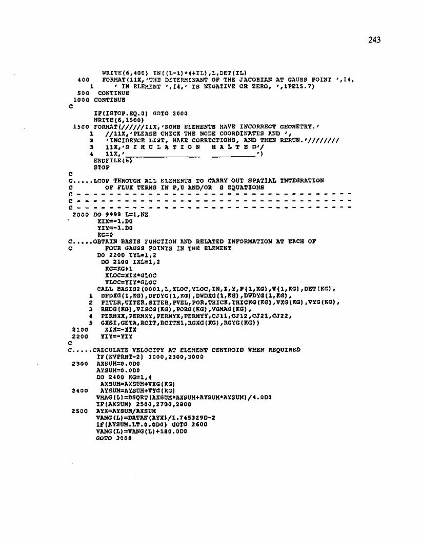
WRITE(6 ,4 0 0 ) IN ( (L - l ) * 4 + IL ) ,L ,D E T ( I L )400 FORMAT( 1 IX/'THE DETERMINANT OF THE JACOBIAN AT GAUSS POINT ' , 1 4 ,
1 ' IN ELEMENT ' , 1 4 , ' 19 NEGATIVE OR ZERO, ' , 1 P E 1 5 .7 )500 CONTINUE
1000 CONTINUEC
IF (IS T O P .E Q .0) GOTO 2000 WRITE(5 ,1 5 0 0 )
1500 FORHAT< / / / / / / 1 IX,'SOME ELEMENTS HAVE INCORRECT GEOMETRY.'1 / /11X ,'PL E A SE CHECK THE NODE COORDINATES AND2 'INCIDENCE L IST , MAKE CORRECTIONS, AND THEN RERUN.' / / / / / / / /3 1 1 X , 'S I H U L A T I O N H A L T E D ' /4 1 1 X , '_______________________ ______________' )
ENDFILE(6)STOP
CC...........LOOP THROUGH ALL ELEMENTS TO CARRY OUT SPATIAL INTEGRATIONC OF FLUX TERMS IN P,U AND/OR S EQUATIONSC - ----------------------------------------------------- --------- --------- ---- ----------- --------------------------------------------------------------C - ----------------------------- - - - --------------- -------------- ---------- --- ------------------c _ _ . - - - - - - - - - - - - - - - - - - - - - - - - - - - - - - - -
2000 DO 9999 L=1,NE XIX=-1. DO Y IY =-1. DO KG=0
C...........OBTAIN BASIS FUNCTION AND RELATED INFORMATION AT EACH OFC FOUR GAUSS POINTS IN THE ELEMENT
DO 2200 IYL=1,2 DO 2100 IXL=1,2
KG=KG+1 XLOC=XIX*GLOC YLOC=YIY*GLOC
CALL BASIS2( 0 0 0 1 ,L,XLOC,YLOC,IN,X,Y,F< 1 ,XG),W (1,KG), DET(KG),1 DFDXG(1,KG),DFDYG( 1 , KG), DWDXG( 1 , KG), DWDYG( 1 , KG) ,2 PITER,UITER, SITER, PVEL,FOR,THICK,THICKG (KG) ,VXG(KG) ,VYG(KG) ,3 RHOG(KG),VISCG(KG),PORG(KG), VGMAG(KG),4 PERMXX,PERMXY,PERMYX,PERMYY,CJU,CJ12 ,C J 2 1 ,C J 2 2 ,5 GXSI,GETA,RCIT,RCITM1,RGXG(KG), RGYG(KG) )
2100 XIX=-XIX2200 YIY=-YIY
CC CALCULATE VELOCITY AT ELEMENT CENTROID WHEN REQUIRED
IF(KVPRNT-2) 3 0 0 0 ,2 3 0 0 ,3 0 0 0 2300 AXSUM=0.0D0
AYSUM=0.0D0 DO 2400 KG=1,4
AXSUM=AXSUM+VXG(KG)2400 AYSUM=AYSUM+VYG(KG)
VMAG(L)=DSQRT(AXSUM*AXSUM+AYSUM*AYSUM)/4. 0D0 IF(AXSUM) 2 5 0 0 ,2 7 0 0 ,2 8 0 0
2500 AYX=AYSUM/AXSUMVANG(L)=DATAN(AYX)/I. 745329D-2 IF(AYSUM.LT.O.ODO) GOTO 2 600 VANG(LJsVANG(L)+ 1 8 0 .0D0 GOTO 3000

uu uu
uu u
o u
uo
o
244
2600
2700
2S00
• « • •
30003300
3400
4000
5200
5400
5600
5800
60006200
6100
6300
VANG(L)=VANG(L)- 1 8 0 . ODO GOTO 3000 VANG(L)= 9 0 . ODOIF(AYSUM.LT >0•ODO) VANG(L)= - 9 0 . ODO GOTO 3000 AYX=AYSUM/AXSUM VANG(L)=DATAN(AYX)/1.745329D-2
INCLUDE MESH THICKNESS IN NUMERICAL INTEGRATION DO 3300 KG=1,4 DET(KG)=THICKG(KG)*DET(KG)
CALCULATE PARAMETERS FOR FLUID MASS BALANCE AT GAUSS POINTS IF (M L -l) 3 4 0 0 ,3 4 0 0 ,6 1 0 0 DO 4000 KG=1,4
ROMG=RHOG(KG) / VISCG(KG )RXXG(KG)=PERMXX(L)*ROMG RXYG(KG) =PERMXY(L)*ROMG RYXG(KG)=PERMYX(L)*R0MG RYYG(KG)=PERMYY(L)*ROMG CONTINUE
ALPHA=ANGL(L)ACOS=COS(ALPHA)*COS(ALPHA)INTEGRATE FLUID MASS BALANCE IN A SATURATED
ELEMENT USING SYMMETRIC WEIGHTING FUNCTIONS DO 6000 1=1,4 DF=0.DO V0=0•DO DO 5400 KG=1,4 VO=VO+F(I,KG)*DET(KG)DF=DF+ ( (RXXG (KG) *RGXG (KG) +RXYG {KG) *RGYG (KG) ) *DFDXG (I, KG)
+ (RYXG (KG) *RGXG(KG) +RYYG (KG) *RGYG (KG) ) *DFDYG(I,KG) )*DET(KG)*ACOS
DO 5800 J=l,4 BF=0.D0DO 5600 KG=1,4BF=BF+((RXXG(KG)*DFDXG(J, KG) +RXYG(KG)*DFDYG(J,KG))*DFDXG(I,KG)
+ (RYXG(KG)*DFDXG(J,KG)+RYYG(KG)*DFDYG(J,KG))*DFDYG(I,KG)) *DET(KG)*ACOS
BFLOWE(I,J)=BF VOLE(I)=VO DFLOWE(I)=DF
CONTINUE
CALCULATE PARAMETERS FOR SOLUTE MASS BALANCE AT GAUSS POINTS DO 7000 KG=1,4
ESWG=PORG(KG)RHOCWG=RHOG(KG)ESRCG=ESWG*RHOCWGIF(VGMAG(KG)) 6 3 0 0 ,6 3 0 0 ,6 6 0 0EXG( KG)= 0 • ODO

(500
0 a
on
no
o
o o
o
245
EYG(KG)=O.ODO DXXG=0. ODO DXYG=0. ODO DYXG=O.ODO DYYG=0. ODO GOTO 6900
6600 EXG(KG)=ESRCG*VXG(KG)EYG(KG)=ESRCG*VYG(KG)
DI3PER3IVITY MODEL FOR ANISOTROPIC MEDIAWITH PRINCIPAL DISPERSIVITIES: ALMAX,ALMIN, AND ATAVG
VANGG=1> 57O796327D0IF (VXG(KG) *VXG(KG) .GT.O.DO) VANGG=DATAN(VYG(KG)/VXG(KG)) VKANGG=VANGG-PANGLE(L)DCO=DCOS(VKANGG)DSI=DSIN(VKANGG)
EFFECTIVE LONGITUDINAL DISPERSIVITY IN FLOW DIRECTION, ALEFFALEFF=0.ODOIF(ALMAX(L)+ALMIN(L)) 6 8 0 0 ,6 8 0 0 ,6 7 0 0
6700 ALEFF=ALMAX(L)*ALMIN(L)/(ALMIN(L)*DCO*DCO+ALMAX(L)*DSI*DSI)6800 DLG=ALEFF*VGMAG(KG)
DTG=ATAVG( L) *VGMAG(KG)
V2GMI=1.D0/(VGMAG(KG)*VGMAG(KG))V2ILTG=V2GMI*(DLG-DTG)VX2G=VXG(KG)* VXG(KG)VY2G=VYG(KG)*VYG(KG)
DISPERSION TENSORDXXG=V2GMI* ( DLG*VX2G+DTG*VY2G)DYYG=V2GMI*(DTG*VX2G+DLG*VY2G)DXYG=V2ILTG*VXG(KG)*VYG(KG)DYXG-DXYG
IN-PARALLEL CONDUCTIVITIES (DIFFUSIVITIES) FORMULA6900 ESE=ESRCG*SIGMAW ADD DIFFUSION AND DISPERSION TERMS TO TOTAL DISPERSION TENSOR
BXXG( KG)=ESRCG*DXXG+ESE BXYG( KG)=ESRCG*DXYG BYXG(KG)=ESRCG*DYXG
7000 BYYG(KG)=ESRCG*DYYG+ESE
INTEGRATE SOLUTE MASS BALANCE USING SYMMETRIC WEIGHTING FUNCTIONSFOR DISPERSION TERM AND USING EITHER SYMMETRIC OR ASYMMETRIC ASYMMETRIC WEIGHTING FUNCTIONS FOR ADVECTION TERM
DO 8000 1 = 1 ,4 DO 8000 J = l , 4 BT=0. DO DT=0.D0DO 7500 KG=1,4
BT=BT+( ( BXXG(KG) *DFDXG (J , KG)+BXYG( KG)*DFDYG(J , KG)) *DFDXG(I , KG)1 + (BYXG (KG)*DFDXG(J,KG)+BYYG(KG)*DFDYG(J ,K G ) ) *DFDYG(I , KG))2 *DET(KG)*ACOS
7500 DT=DT+(EXG(KG)*DFDXG(J,KG)+EYG(KG)*DFDYG(J, KG))1 *W(I,KG)*DET(KG)*ACOS
BTRANE( I , J ) =BT
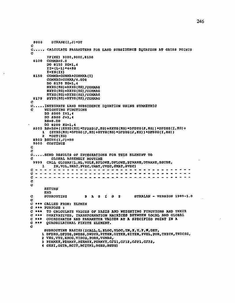
no
oo
n
noo
n
o o
o o
oo
246
8000 DTRANE(I , J)=DT
CALCULATE PARAMETERS FOR LAND SUBSIDENCE EQUATION AT GAUSS POINTS
IF(ME) 9 0 0 0 ,9 0 0 0 ,8 1 0 0 8100 COMMA=0.0
DO 8150 KG=1,4 1 1 = (L-l)*4+KG I = I N ( I I )
8150 COMMA=COMMA-f- COMMMA ( I )COMHAG=COMMA/4. ODO DO 8170 KG=1,4 SXXG(KG}=RXXG(KG) /COMMAG SXYG(KG) =RXYG(KG}/COMMAG SYXG(KG)=RYXG(KG)/COMMAG
8170 SYYG(KG)=RYYG(KG)/COMMAG
INTEGRATE LAND SUBSIDENCE EQUATION USING SYMMETRICWEIGHTING FUNCTIONS DO 8500 1= 1 ,4 DO 8500 J = l , 4 BS=O.DO DO 8200 KG=1,4
8200 BS=BS+ ( (SXXG (KG) *DFDXG(J,KG) +SXYG(KG) *DFDYG(J,KG) ) *DFDXG (I,KG) +1 (SYXG (KG) *DFDXG(J , KG)+SYYG (KG) *DFDYG (J , KG) ) *DFDYG(I,KG) )2 *DET(KG)
8500 BSUBE(I, J)=BS 9000 CONTINUE
SEND RESULTS OF INTEGRATIONS FOR THIS ELEMENT TOGLOBAL ASSEMBLY ROUTINE
9999 CALL GLOBAN(L,ML,VOLE,BFLOWE,DFLOWE,BTRANE,DTRANE,BSUBE, 1 IN , VO L, PMAT, PVEC, UMAT, UVEC, SHAT, SVEC)
RETURNEND
C SUBROUTINE B A S I 3 2 STRALAN - VERSION 1989-1.0CC *** CALLED FROM: ELEMEN C *** PURPOSE :C *** TO CALCULATE VALUES OF BASIS AND WEIGHTING FUNCTIONS AND THEIR C *** DERIVATIVES, TRANSFORMATION MATRICES BETWEEN LOCAL AND GLOBAL C *** COORDINATES AND PARAMETER VALUES AT A SPECIFIED POINT IN A C *** QUADRILATERAL FINITE ELEMENT.C
SUBROUTINE BASIS2(ICALL,L,XLOC,YLOC,IN,X,Y,F,W,DET,1 DFDXG, DFDYG, DWDXG , DWDYG, PITER, UITER, SITER, PVEL, POR, THICK, THICKG,2 VXG,VYG,RHOG,VISCG,PORG,VGMAG,3 PERMXX,PERMXY,PERMYX,PERMYY,CJ11,CJ12,CJ21,CJ22,4 GXSI,GETA,RCIT,RCITM1,RGXG,RGYG)

no
oo
oo
nn
no
on
n
247
IMPLICIT DOUBLE PRECISION (A-H,0-Z)COMMON/DIMS/ NN,NE, NIN,NBI, NB,NBKALF,NPINCH,NPBC,NUBC, NSBC,
1 NSOP,NSOPUMP,NSOU,NBCNCOMMON/CONTRL/ GNU,UP,DTHULT,DTMAX,ME, ISSFLO, ISSTRA, ITCYC,NPORC,
1 NPCYC,NUCYC,NSCYC,NPRINT,IREAD, ISTORE,NOUMAT, IHEAD, I SLOPE, LAN,2 ISET
COMMON/ PA RAMS/ COMPEL, COMPMA, DRWDU, RHOS , DECAY,SIGMAW,1 RHOHO , U RHO WO , VI SCO , PRODFX, PRODS1, PRODFO , PRODS 0 , CHI 1, CHI 2
COMMON/TENSOR/ GRAVX,GRAVY DOUBLE PRECISION XLOC,YLOCDIMENSION IN(NIN) ,X(NN) ,Y(NN) ,UITER(NN) , PITER (NN) ,PVEL(NN) ,
1 POR(NN) , PERMXX (NE) , PERMXY (NE) , PERMYX(NB) , PERMYY (NE) ,2 THICK(NN),SITER(NN)
DIMENSION GXSI(NE,4 ) ,GETA(NE,4),RCIT(NN),RCITM1(NN)DIMENSION F (4) ,W(4) ,DFDXG(4) ,DFDYG(4) ,DWDXG(4) ,DWDYG(4)DIMENSION F X (4 ) ,F Y (4 ) ,A F X (4 ) ,A F Y (4 ) ,
1 DFDXL(4), DFDYL(4),DWDXL(4),DWDYL(4),2 X D W (4),YDW (4),XIIX (4),YIIY (4)
DATA X IIX /-1 .D O ,+ 1 .D O ,+ 1 .D O ,-1 .D O /,X Y I I Y / - 1 . D O , - l .D 0 , + l .D 0 , + l .D 0 /
AT THIS LOCATION IN LOCAL COORDINATES, (XLOC,YLOC),CALCULATE SYMMETRIC WEIGHTING FUNCTIONS, F<I),SPACE DERIVATIVES, DFDXG(I) AND DFDYG(I), AND DETERMINANT OF JACOBIAN, DET.
XF1=1.DO-XLOC XF2=X•DO+XLOC YFX=X.DO-YLOC YF2=X.DO+YLOC
...CALCULATE BASIS FUNCTION, F.FX(I)=XFI FX(2)=XF2 FX(3)=XF2 FX(4)=XFX FY(X)=YFX FY(2)=YFX FY(3)=YF2 FY(4)=YF2 DO XO 1=1,4
XO F(I)=0.25QDQ *FX(I)*FY(I)...CALCULATE DERIVATIVES WITH RESPECT TO LOCAL COORDINATES.
DO 20 1=1,4DFDXL(I)=XIIX(I)*O.250D0*FY(I)
20 DFDYL(I)=YIIY(I)*0.250D0*FX(I)...CALCULATE ELEMENTS OF JACOBIAN HATRIX, CJ.
CJ11=0.DO CJ12=0.DO CJ21=0.DO CJ22=0.D0 DO 100 IL=1,4

ooo
non
oo
o oo
oo
oo
o
o
I I = ( L - 1 ) * 4 + I L I = I N ( I I )CJ11=CJ11+DFDXL(IL)*X(I)CJ12=CJ12+DFDXL(IL)*Y(I)CJ21=CJ21+DFDYL(XL)*X(I>
100 CJ22=CJ22+DFDYL(IL)*Y(I)
. . . .CALCULATE DETERMINANT OF JACOBIAN MATRIX. DET=CJ11*CJ22-CJ21*CJ12
... .R ETU R N TO ELEMEN WITH JACOBIAN MATRIX ON FIRST TIME STEF. IF(ICALL.EQ.O) RETURN
....CALCULATE ELEMENTS OF INVERSE JACOBIAN MATRIX, C I J . ODET=1.DO/DET CIJ11=+0DET*CJ22 CIJ12=-0DET*CJ12 CIJ21=-ODET*CJ21 CIJ22=+0DET*CJ11
....CALCULATE DERIVATIVES WITH RESPECT TO GLOBAL COORDINATES DO 200 1 = 1 ,4DFDXG(I)=CIJ11*DFDXL{I)+CIJ12 *DFDYL(IJ
200 DFDYG(IJ =CIJ21*DFDXL(I)+CIJ22 *DFDYL(I). . . . CALCULATE CONSISTENT COMPONENTS OF <RH0*GRAV) TERM IN LOCAL
COORDINATES AT THIS LOCATION, (XLOC,YLOC)RGXL=O.DO RGYL=0.D0 RGXLM1=0.D0 RGYLH1=0. DO DO 800 IL = 1 ,4I I - ( L - l ) * 4 + I L I = I N ( I I )ADFDXL=DABS(DFDXL(IL) )ADFDYL=DABS(DFDYL(IL) )RGXL=RGXL+RCIT(I)*GXSI(L,IL)*ADFDXL RGYL=RGYL+RCIT{I)*GETA(L,IL)*ADFDYL RGXLM1=RGXLM1+RCITM1(I)*GXSI(L,IL)*ADFDXL RGYLM1=RGYLMH-RCITM1(I) *GETA{L,IL)*ADFDYL
800 CONTINUE
....TRANSFORM CONSISTENT COMPONENTS OF (RHO*GRAV) TERM TO GLOBAL COORDINATES
RGXG=CIJ11*RGXL+CIJ12*RGYL RGYG=CIJ21*RGXL+CIJ22*RGYL RGXGM1=CIJ11*RGXLM1+CIJ12*RGYLM1 RGYGM1=CIJ 21*RGXLM1+CIJ2 2 *RGYLM1
....CALCULATE PARAMETER VALUES AT THIS LOCATION, (XLOC,YLOC)
PITERG=0.D0 UITERG=O.DO DPDXG=0. DO DPDYG=O.DO

oo
O
OO
OO
OO
Q
OO
O
oo
o
o o
oo
PORG=0. DO THXCKG=0. ODO DO 1000 IL = 1 ,4 I I = ( L - 1 ) * 4 +IL I = I N ( I I >DPDXG=DPDXG+PVEL(I)*DFDXG(IL)DPDYG=DPDYG+PVEL(I ) *DFDYG(XL)PORG=PORG+POR(I)*F(IL)THICKG=THICKG+THICK( I ) * F ( IL)PITERG=PITERG+PITER(I ) * ? ( IL)UITERG=UITERG+UITER(I)*F(IL)
1000 CONTINUE
SET VALUES FOR DENSITY AND VISCOSITY RHOG = FUNCTION(UITER)
RHOG=RHOWO+DRWDU* (UITERG-URHOW0) FOR SOLUTE TRANSPORT... VISCG IS TAKEN TO BE CONSTANT
VISCG=VISC0
CALCULATE CONSISTENT FLUID VELOCITIES HITS RESPECT TO GLOBALCOORDINATES, VXG, VYG, AND VGMAG, AT THIS LOCATION, (XLOC,YLOC> DENOM=l. D O /( PORG*VISCG)PGX=DPDXG-RGXGM1PGY=DPDYG-RGYGM1
ZERO OUT RANDOM BOUYANT DRIVING FORCES DUE TO DIFFERENCING NUMBERS PAST PRECISION LIMIT MINIMUM DRIVING FORCE IS l .D - 1 0 OF PRESSURE GRADIENT (THIS VALUE MAY BE CHANGED DEPENDING ON MACHINE PRECISION)
IF(DPDXG) 1 7 2 0 ,1 7 3 0 ,1 7 2 0 1720 I F (DABS (PGX/DPDXG) - 1 . 0D-10) 1 7 2 5 ,1 7 2 5 ,1 7 3 0 1725 PGX=0• ODO1730 IF(DPDYG) 1 7 5 0 ,1 7 6 0 ,1 7 5 01750 IF(DABS( PGY/DPDYG)- 1 . 0D -10) 1 7 5 5 ,1 7 5 5 ,1 7 6 0 1755 PGY=0. ODO1760 VXG=-DENOM* (PERMXX (L)*PGX+PERMXY(L) *PGY)
VYG=-DENOM* (PERMYX(L) *PGX+PERHYY (L) *PGY)VXG2=VXG*VXG VYG2=VYG*VYG VGMAG=DSQRT(VXG2+VYG2)
AT THIS POINT IN LOCAL COORDINATES, (XLOC,YLOC) ,CALCULATE ASYMMETRIC WEIGHTING FUNCTIONS, W ( I ) ,AND SPACE DERIVATIVES, DWDXG(I) AND DWDYG(I) .
ASYMMETRIC FUNCTIONS SIMPLIFY WHEN UP=0.0IF (U P .G T .1 . 0D-6.AND.N0UMAT.EQ.0) GOTO 1790 DO 1780 1 = 1 ,4 W(I )=F{I )DWDXG(I ) =DFDXG(I )DWDYG(I ) =DFDYG(I )
1780 CONTINUE RETURN WHEN ONLY SYMMETRIC WEIGHTING FUNCTIONS ARE USED
RETURN
CALCULATE FLUID VELOCITIES WITH RESPECT TO LOCAL COORDINATES,

C VXL, VYL, AND VLHAG, AT THIS LOCATION, (XLOC,YLOC) .17 90 VXL=CIJ11*VXG+CIJ21*VYG
VYL—C l J 12 *VXG+CIJ22 *VYQ VLMAG=DSQRT(VXL*VXL+VYL*VYL)
CAA=0. ODO BB=O.ODOIF(VLHAG) 1 9 0 0 ,1 9 0 0 ,1 8 0 0
1800 AA=UP*VXL/VLMAG BB=UP*VYL/VLMAG
C1900 XIXI=.750DO*AA*XF1*XF2
YIYI=.750DO*BB*YF1*YF2 DO 2000 1=1,4A FX <I)= .50D 0*FX (I)+X IIX (I>*X IX I
2000 A F Y (I)= . 50D O *FY (I)+Y IIY (I)*Y IY ICC CALCULATE ASYMMETRIC WEIGHTING FUNCTION, W.
DO 3000 1 = 1 ,4 3000 W (I)=AFX(I)*AFY(I)
CTHAAX=0. 5 0D 0-1 . 50D0*AA*XLOC THBBY=0.50D0-1.50D0*BB*YLOC DO 4000 1 = 1 ,4 XDW(I }=X IIX ( I ) *THAAX
4000 YDW(I)=YIIY(I}*THBBYCC...........CALCULATE DERIVATIVES WITH RESPECT TO LOCAL COORDINATES.
DO 5000 1 = 1 ,4DWDXL( I ) =XDW( I ) *AFY(I)
5000 DWDYL(I ) =YDW(I ) * AFX( X)CC ...........CALCULATE DERIVATIVES WITH RESPECT TO GLOBAL COORDINATES.
DO 6000 1 = 1 ,4DWDXG(I)=CIJ11*DWDXL(I)+CIJ12*DWDYL(X)
6000 DWDYG(I)=CIJ21*DWDXL(I)+CIJ22*DWDYL(I)CC
RETURNEND
C SUBROUTINE G L O B A N STRALAN - VERSION 1 9 8 9 -1 .CC *** CALLED FROM: ELEMEN C *** PURPOSE :C *** TO ASSEMBLE RESULTS OF ELEMENTWISE INTEGRATIONS INTO C *** A GLOBAL BANDED MATRIX AND GLOBAL VECTOR FOR GROUNDWATER C *** FLOW, TRANSPORT AND SUBSIDENCE EQUATIONS.C
SUBROUTINE GLOBAN(L,ML,VOLE,BFLOWE,DFLOWE, BTRANE,DTRANE,BSUBE,1 IN,VOL,PMAT, PVEC, UMAT, UVEC, SMAT,SVEC)
IMPLICIT DOUBLE PRECISION (A -H ,0-Z )COMMON/DIMS/ NN, NE , NIN, NBI, NB , NBHALF , NPINCH, NPBC , NUBC , NSBC ,
1 NSOP,NSOPUMP,NSOU,NBCNCOMMON/CONTRL/ GNU, UP, DTMULT,DTMAX, ME, ISSFLO, ISSTRA, ITCYC, NPORC,
1 NPCYC , NUCYC, NSCYC , NPRINT, IREAD, ISTORE, NOUMAT, IHEAD, I SLOPE , LAN,

2 ISETDIMENSION BFLOWE{4,4),DFLOWE(4) ,B T R A N E (4 ,4 ) ,B SU B E (4 ,4 ) ,
1 DTRANE(4,4),VOLE(4)DIMENSION VOL(NN) ,PMAT (NN/NBI) ,PVEC(NN) ,UMAT (NN,NBI) ,UVEC(NN) ,
I SMAT(NN,NBI), SVEC(NN)DIMENSION IN(NIN)
CC
N 1=(L -1)*4+1N4=Nl+3
CC ADD RESULTS OF INTEGRATIONS OVER ELEMENT L TO GLOBALC P-MATRIX AND P-VECTOR AND/OR S-MATRIX AND S-VECTOR
IF (M L -l) 5 0 ,1 2 0 ,1 5 0 50 IE=0
DO 100 II=N1,N4IE=IE+1IB = I N ( I I )VOL(IB)=VOL(IB) +VOLE(IE)FVEC{IB)=PVEC(IB)+DFLOWE(IE)JE=0DO 100 JJ=N1,N4 JE=JE+1JB=IN(JJ)-IB+NBHALFPMAT (IB ,JB ) =FMAT(IB, JB) +BFLOWE ( I E , JE )
100 SMAT(IB,JB)=SMAT(IB,JBJ+BSUBE(IE,JE)GO TO 150
120 IE=0DO 130 II=N1,N4IE=IE+1IB = I N ( I I )VOL(IB)=VOL(IB)+VOLE(IE)PVEC( IB ) =PVEC( IB ) +DFLOWE(IE)JE=0DO 130 JJ=N1,N4 JE=JE+1J B = IN (JJ)-IB+NBHALF
130 PMAT(IB,JB)=PMAT ( IB , JB)+BFLOWE(IE, JE )CC ..........ADD RESULTS OF INTEGRATIONS OVER ELEMENT L TO GLOBALC U-MATRIX
150 IF(NOUMAT.EQ.1) GOTO 300 IE —0DO 200 II=N1,N 4IE=IE+1I B = I N ( I I )
C ..........POSITION FOR ADDITION TO U-VECTORC UVEC( IB)=UVEC( IB )+ ( ( ))
JE=0DO 200 JJ=N1,N4 JE =JE+1J B = IN (JJ)-IB+NBHALF
200 UMAT (IB,JB)=UMAT(IB,JB) +DTRANE ( I E , J E ) +BTRANE ( I E , JE )C
300 CONTINUE
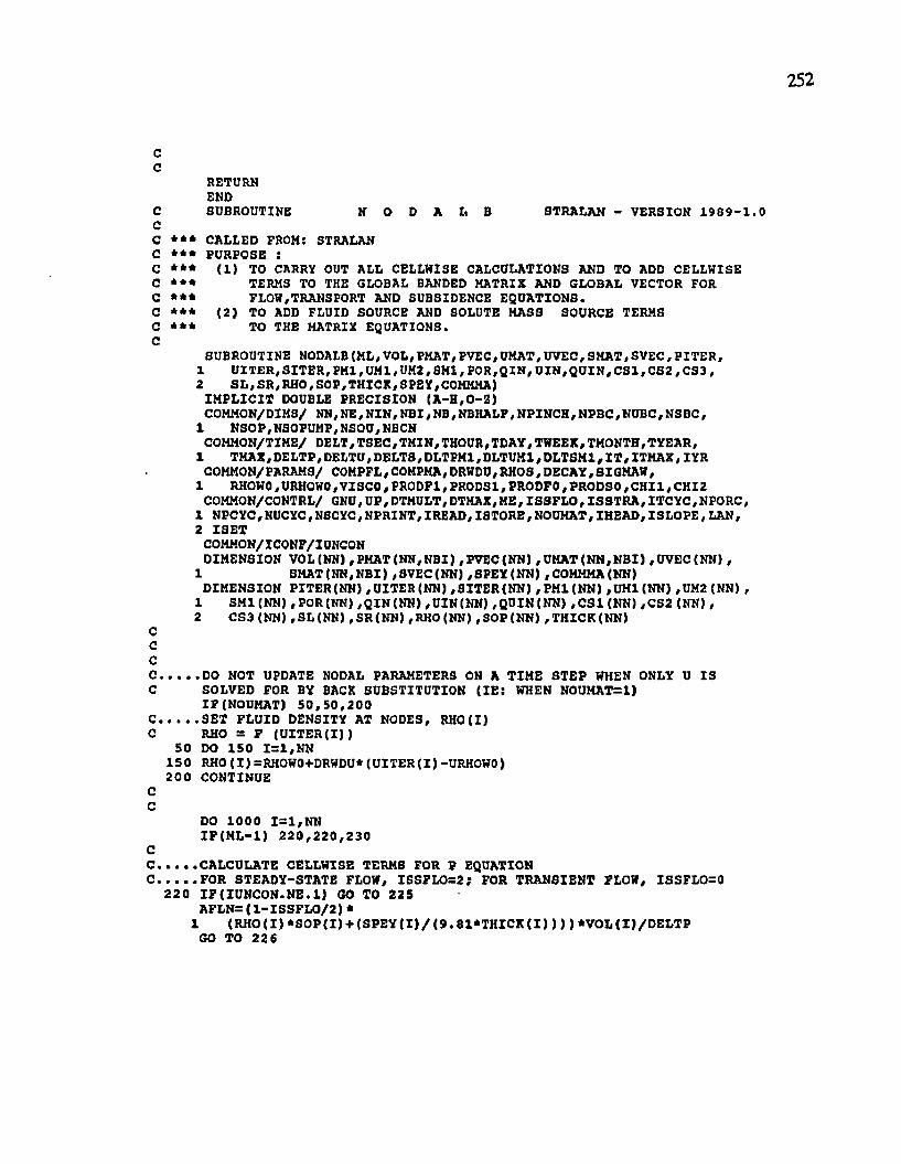
252
c c
RETURNEND
C SUBROUTINE N O D A I, B STRALAN - VERSION 1 9 8 9 -1 .0CC *** CALLED FROM: STRALAN C *** PURPOSE :C *** (1) TO CARRY OUT ALL CELLWISE CALCULATIONS AND TO ADD CELLWISEC *** TERMS TO THE GLOBAL BANDED MATRIX AND GLOBAL VECTOR FORC *** FLOW,TRANSPORT AND SUBSIDENCE EQUATIONS.C *** (2) TO ADD FLUID SOURCE AND SOLUTE HASS SOURCE TERMSC *** TO THE HATRIX EQUATIONS.C
SUBROUTINE NODALB{ML,VOL,PMAT,PVEC,UMAT,UVEC,SHAT,SVEC, PITER,1 UITER,SITER, PHI, UM1,UM2, SHI, POR,QIN, UIN, QUIN, C S1,CS2,CS3,2 SL,SR,RHO,SOP,THICK,SPEY,COMMMA)
IMPLICIT DOUBLE PRECISION (A-H,0-Z)COMMON/DIMS/ NN,NE,NIN,NBI,NB,NBHALF, NPINCH, NPBC, NUBC, NSBC,
1 NSOP,NSOPUMP,NSOU,NBCNCOMMON/TIME/ DELT,TSEC,TMIN,THOUR,TDAY,TWEEK,TMONTH,TYEAR,
1 TMAX , DE LT P , DELTU , DELT3 , DLTPM1, DLTUM1, DLTSM1, 1T , ITMAX , IYRCOMMON/PARAMS/ COM PFL , COMPMA , DRWDU, RHOS , DECAY , SIGMAW ,
1 RHOWO , URHOWO , VISCO , PR0DF1, PRODS1, PRODFO , PRODSO , CHI1, CHI2COMMON/CONTRL/ GNU, UP, DTMULT, DTMAX,ME, ISSFLO, ISSTRA, ITCYC,NPORC,
1 NPC YC , NUC YC , NSC YC , NPRI NT, I RE AD , IS TORE , NOUMAT , I HEAD, IS LOPE , LAN ,2 ISET
COMMON/ICONF/IUNCONDIMENSION VOL (NN) , PMAT (NN,NBI) ,FVEC(NN) ,UMAT (NN,NBI) ,UVEC(NN) ,
1 SHAT (NN,NBI) ,SVEC{NN) ,SPEY(NN) , COMMMA (NN)DIMENSION PITER (NN) , UITER(NN) ,SITER(NN) ,PM1(NN) ,UH1(NN) ,UM2 (NN) ,
1 SMI (NN) ,POR(NN) ,QIN(NN) ,UIN(NN) ,QUIN(NN) ,CS1 (NN) ,CS2 (NN) ,2 CS3 (NN) ,SL(NN) ,SR(NN) , RHO (NN) ,SOP(NN) , THICK (NN)
CCCC.............DO NOT UPDATE NODAL PARAMETERS ON A TIME STEP WHEN ONLY U ISC SOLVED FOR BY BACK SUBSTITUTION (IE : HHEN NOUMAT=l)
IF(NOUMAT) 5 0 ,5 0 ,2 0 0C............. SET FLUID DENSITY AT NODES, RHO(I)C RHO = F (U IT E R (I))
50 DO 150 1 = 1 ,NN150 RHO (I)=RHOWO+DRWDU*(UITER(I)-URHOWO)200 CONTINUE
CC
DO 1000 1 = 1 ,NN IF (M L - l) 2 2 0 ,2 2 0 ,2 3 0
CC..............CALCULATE CELLWISE TERMS FOR P EQUATIONC FOR STEADY-STATE FLOW, ISSFLO=2; FOR TRANSIENT FLOW, ISSFLO=0
220 IF(IU NCON.NE.l) GO TO 225 AFLN=( l- IS S F L O /2 ) *
1 (RHO(I) *SOP(I) + (S P E Y (I) /(9 .8 1 * T H IC K (I) ) ) ) *VOL(I)/DELTPGO TO 22 6
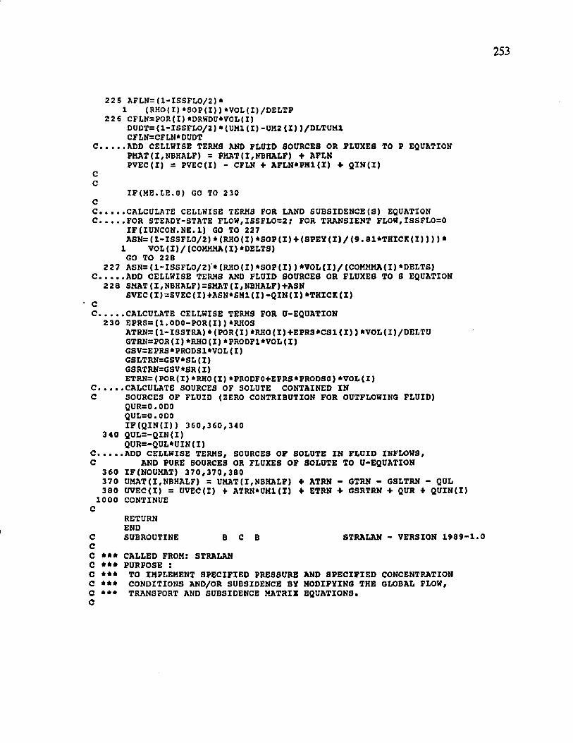
253
225 AFLN=( l-IS S F L O /2)*1 (RHO(I) *SOP(I) ) *VOL(I)/DELTP
226 CFLN=POR(I)*DRWDU*VOL( I )DUDT={l-IS S F L O /2 ) * {UM1( I ) -UM2{X) ) /DLTUM1 CFLN=CFLN*DUDT
C ADD CELLWISE TERMS AND FLUID SOURCES OR FLUXES TO P EQUATIONPMAT(I,NBHALF) = PMAT(I,NBHALF) + AFLN PVEC(I) = PVEC(I) - CFLN + AFLN* PHI ( I ) + Q IN (I)
CC
IF(ME.LE.O) GO TO 230CC CALCULATE CELLWISE TERMS FOR LAND SUBSIDENCE(S) EQUATIONC FOR STEADY-STATE FLOW,ISSFLO=2} FOR TRANSIENT FLOW,ISSFLO=0
IF(IUNCON.NE.1) GO TO 227ASN= ( l-IS S FL O /2) * (RHO ( I ) *SOF(I) + (SPEY(I) / {9 • 81*THICK(X)) ) ) *
1 VOL{I)/(COMMMA(I)*DELTS)GO TO 228
227 ASN= ( l-IS S F L O /2) * (RHO ( I ) *SOP ( I ) ) *VOL(I)/(COMMMA(I) *DELTSJC ADD CELLWISE TERMS AND FLUID SOURCES OR FLUXES TO 3 EQUATION
2 28 SMAT( I , NBHALF)=SMAT( I , NBHALF) +ASNSVEC(I)=SVEC{I)+ASN*SM1(I) -QIN (I)*THICK(I)
CC CALCULATE CELLWISE TERMS FOR U-EQUATION
230 EPRS=(I.ODO-POR(I)} *RHOSATRN= (1-ISSTRA) * (POR(I) *RHO(I)+EPRS*CS1( I ) ) *VOL(I)/DELTU GTRN=POR( I ) *RHO(I )* PRODF1*VOL( I )GSV=E PRS * PRODSI*VOL( I )GS LTRN=GSV * S L{I )GSRTRN=GSV*SR(I)ETRN= (POR(I) *RHO(I) *PRODFO+EPRS*PRODSO) *VOL(I)
C CALCULATE SOURCES OF SOLUTE CONTAINED INC SOURCES OF FLUID (ZERO CONTRIBUTION FOR OUTFLOWING FLUID)
QUR=0.0D0 QUL=0. ODOI F ( Q I N ( I ) ) 3 6 0 ,3 6 0 ,3 4 0
340 QUL=-QIN(I)QUR=-QUL*UIN(I)
C ADD CELLWISE TERMS, SOURCES OF SOLUTE IN FLUID INFLOWS,C AND PURE SOURCES OR FLUXES OF SOLUTE TO U-EQUATION
360 IF(NOUMAT) 3 7 0 ,3 7 0 ,3 8 0370 UMAT( I , NBHALF) = UMAT (I , NBHALF) + ATRN - GTRN - GSLTRN - QUL 380 UVEC(I) = UVEC(I) + ATRN*UM1(I) + ETRN + GSRTRN + QUR + QUIN(I)
1000 CONTINUEC
RETURNEND
C SUBROUTINE B C B STRALAN - VERSION 1 9 8 9 -1 .0CC *** CALLED FROM: STRALAN C *** PURPOSE :C * * * TO IMPLEMENT SPECIFIED PRESSURE AND SPECIFIED CONCENTRATIONC *** CONDITIONS AND/OR SUBSIDENCE BY MODIFYING THE GLOBAL FLOW,C *** TRANSPORT AND SUBSIDENCE MATRIX EQUATIONS.C
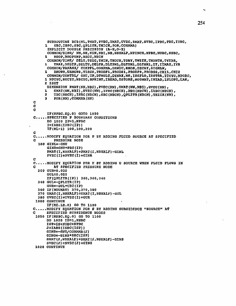
SUBROUTINE BCB(ML,PMAT,PVEC,UMAT,UVEC,SMAT, SVEC, IPBC,PBC, IUBC,1 UBC,ISBC,SBC,QPLITR,THICK,POR,COMMMA)
IMPLICIT DOUBLE PRECISION (A -H ,0-Z )COMMON/DIMS/ NN, NE, NIN, NBI, NB, NBHALF, NPINCH, NPBC, NUBC, NSBC,
1 NSOP,NSOPUMP,NSOU,NBCN COMMON/TIME/ DELT, TSEC, TMIN,THOUR,TDAY,TWEEK,TMONTH,TYEAR,
1 TMAX, DELTP,DELTU,DELTS, DLTPM1, DLTUM1, DLTSM1, IT,ITM AX,IYRCOMMON/PARAMS/ COMPEL,COMPMA,DRWDU,RHOS,DECAY,SIGMAW,
1 RHOWO, URHOWO, VISCO, PRODF1, PRODS1, PRODFO, PRODSO, C H I1, CHI2COMMON/CONTRL/ GNU, UP, DTMULT, DTMAX,ME,ISSFLO,ISSTRA,ITCYC,NPORC,
1 NPCYC,NUCYC,NSCYC,NPRINT,IREAD,ISTORE,NOUMAT,IHEAD,ISLOPE,LAN,2 ISET
DIMENSION PMAT(NN,NBI), PVEC(NN), UMAT(NN,NBI), UVEC(NN),1 SMAT(NN,NBI), SVEC(NN), IPBC(NBCN),PBC(NBCN),IUBC(NBCN),2 UBC(NBCN), ISBC(NBCN), SBC(NBCN), QPLITR(NBCN),THICK(NN),3 POR{NN) , COMMMA(NN)
CCC
IF(N PB C .EQ .0) GOTO 1050C ......... SPECIFIED P BOUNDARY CONDITIONS
DO 1000 IP=1,NPBC 1=1ABS(IPBC( I P ) )IF (M L -l) 1 0 0 ,1 0 0 ,2 0 0
CC..........MODIFY EQUATION FOR P BY ADDING FLUID SOURCE AT SPECIFIEDC PRESSURE NODE
100 GINL=-GNUGINR=GNU*PBC(IP)PMAT ( I , NBHALF) =PMAT( I , NBHALF)-GINL PVEC( I ) =PVEC( I ) +GINR
CC..........MODIFY EQUATION FOR U BY ADDING U SOURCE WHEN FLUID FLOWS INC AT SPECIFIED PRESSURE NODE
200 GUR=0. ODO GUL=0. ODOIF(Q PL IT R ( I P ) ) 3 6 0 ,3 6 0 ,3 4 0
3 40 GUL=-QPLITR( IP )GUR=-GUL*UBC(IP)
360 IF(NOUMAT) 3 7 0 ,3 7 0 ,3 8 0 370 UMAT( I , NBHALF) =UMAT( I , NBHALF) - GUL 380 UVEC(I)=UVEC(I)+GUR
1000 CONTINUEIF(M E.LE.O ) GO TO 1100
C..........MODIFY EQUATION FOR S BY ADDING SUBSIDENCE “ SOURCE" ATC SPECIFIED SUBSIDENCE NODES
1050 IF(NSBC.EQ.O) GO TO 1100 DO 1020 IS=1,NSBC ISP=IS+NUBC+NPBC J= IA B S (IS B C (IS P ))GINS=-GNU/COMMMA(J)GING=-GINS*SBC(ISP)SMAT(J , NBHALF) =SMAT(J , NBHALF)-GINS SVEC(J)=SV E C (J)+GING
1020 CONTINUE
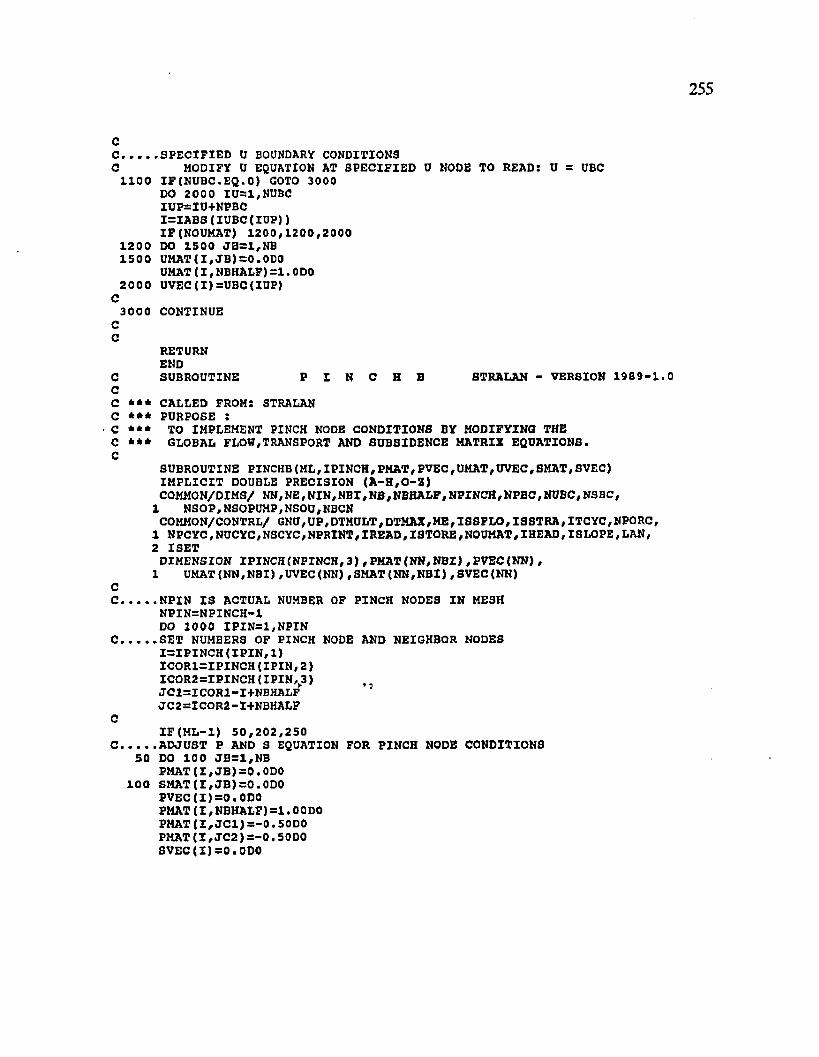
255
cC............SPECIFIED U BOUNDARY CONDITIONSC MODIFY U EQUATION AT SPECIFIED 0 NODE TO READ: U = UBC
1100 IF(NUBC. EQ. 0) GOTO 3000 DO 2000 IU-1,NUBC IUP=IU+NPBC I=IA B S(IU B C (IU P))IF(NOUMAT) 1 2 0 0 ,1 2 0 0 ,2 0 0 0
1200 DO 1500 JB=1,NB 1500 UMAT( I , J B )= 0 .ODO
UMAT( I , NBHALF)=1. ODO 2000 UVEC(I)=UBC{IUP)
C3000 CONTINUE
CC
RETURNEND
C SUBROUTINE P I N C H B STRALAN - VERSION 1 9 8 9 -1 .0CC *** CALLED FROM: STRALAN C *** PURPOSE :C *** TO IMPLEMENT PINCH NODE CONDITIONS BY MODIFYING THE C *** GLOBAL FLOW,TRANSPORT AND SUBSIDENCE MATRIX EQUATIONS.C
SUBROUTINE PINCHB(ML,IPINCH,PMAT,PVEC, UMAT,UVEC,SMAT,SVEC) IM PLICIT DOUBLE PRECISION (A -H ,0 -Z )COMMON/D IM S/ NN, NE , NIN, NBI, NB , NBHALF , NPINCH , NPBC , NUBC , NS BC ,
1 NSOP, NSOPUMP,NSOU, NBCNCOMMON/CONTRL/ GNU , UP , DTMULT, DTMAX, ME, ISSFLO, IS STRA , ITCYC, NPORC,
1 NPC YC, NUC YC , NSC YC , NPRINT , I READ , I STORE , NOUMAT ,IHEAD,I8LOPE, LAN,2 ISET
DIMENSION IPINCH (NPINCH, 3) , PMAT (NN, NBI) , PVEC (NN) ,1 UMAT (NN, NBI) ,UVEC(NN) , SMAT (NN, NBI) ,SVEC(NN)
CC ..........NPIN IS ACTUAL NUMBER OF PINCH NODES IN MESH
NPIN=NPINCH-1 DO 1000 IPIN =1,N PIN
C.......... SET NUMBERS OF PINCH NODE AND NEIGHBOR NODESI= IP IN C H (IP IN ,1 )ICORl=IPINCH (IP IN , 2 )ICOR2=IPIN CH (IPIN ,|3)JCl=ICORl-I+NBHALF J C 2=1COR2- I+NBHALF
CIF (M L -l) 5 0 ,2 0 2 ,2 5 0
C ..........ADJUST P AND S EQUATION FOR PINCH NODE CONDITIONS50 DO 100 JB=1,NB
PMAT(I, J B )= 0 .0D0 100 SMAT( I , J B )—0 .ODO
P V E C (I)= 0 .ODO PMAT(I , NBHALF)= 1 . OODO P M A T (I,JC 1 )—- 0 . 50D0 PMAT(I , J C 2 ) = - 0 . 50D0 S V E C (I)= 0 . ODO
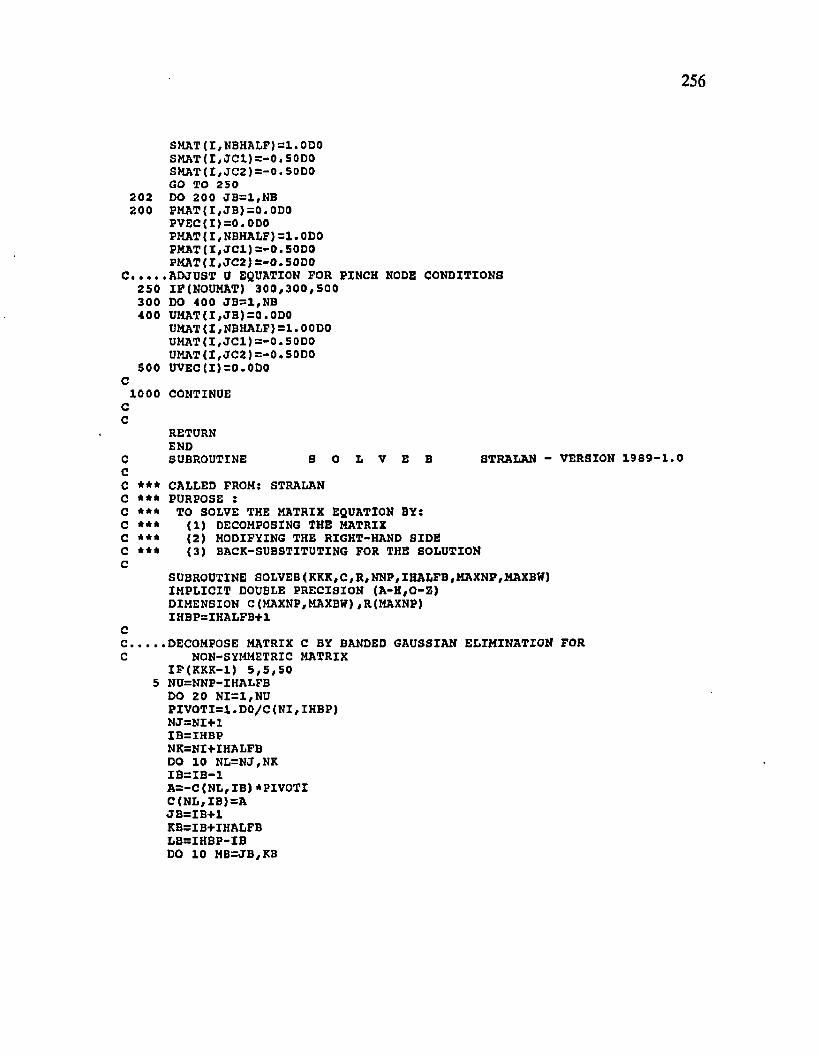
256
SMAT(I,NBHALF)= 1 .ODO SM A T(I,JC 1)=-0.50D O SMAT( I , JC 2 ) = - 0 .5 ODO GO TO 250
202 DO 200 JB=1,NB 200 PM AT{I,JB)=0.0D 0
PVEC(I ) = 0 .ODO PMAT( I , NBHALF)= 1 .ODO PM A T(I,JC 1)=-0 .50D 0 PM A T(I,JC 2)=-O .50D 0
C ADJUST U EQUATION FOR PINCH NODE CONDITIONS250 IF(NOUMAT) 3 0 0 ,3 0 0 ,5 0 0 300 DO 400 JB=1,NB 400 U M A T(I,JB)= 0 .ODO
UMAT{I,NBHALF}= 1. OODO U M A T(I,JC 1)= - 0 .5 ODO UM AT(I,JC2)=-0.50DO
500 UVEC{I ) = 0 .ODOC
1000 CONTINUECc
RETURNEND
C SUBROUTINE S O L V E B STRALAN - VERSION 1 9 8 9 -1 .0CC *** CALLED FROM: STRALAN C *** PURPOSE :C *** TO SOLVE THE MATRIX EQUATION BY:C *** (1 ) DECOMPOSING THE MATRIXC *** (2 ) MODIFYING THE RIGHT-HAND SIDEC *** (3 ) BACK-SUBSTITUTING FOR THE SOLUTIONC
SUBROUTINE SOLVEB(KKK,C,R,NNP,IHALFB,MAXNP,MAXBW)IMPLICIT DOUBLE PRECISION (A -K ,0-Z )DIMENSION C(MAXNP,MAXBff),R(MAXNP)IHBP=IHALFB+1
CC DECOMPOSE MATRIX C BY BANDED GAUSSIAN ELIMINATION FORC NON-SYMMETRIC MATRIX
IF(K K K -1) 5 ,5 ,5 0 5 NU=NNP-IHALFB
DO 20 NI=1,NU P IV O T I= l. DO/C(NI,IH BP)NJ=NI+1 IB=IHBP NK=NI+IHALFB DO 10 NL=NJ, NK IB = IB -1A = -C (N L ,IB )* PIVOTIC (N L ,IB )=AJB =IB +1KB=IB+IHALFBLBsIKBP-IBDO 10 MB=JB,KB
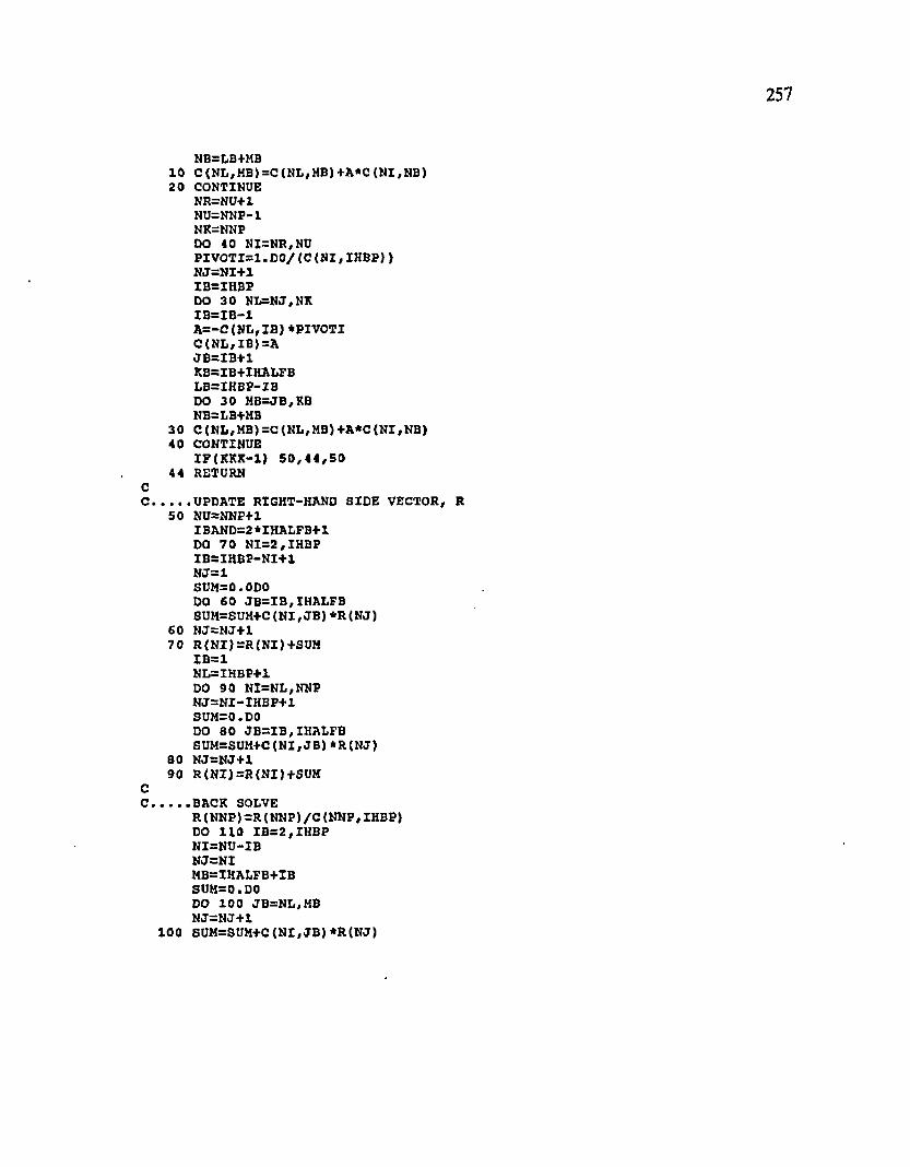
NB=LB+MB 10 C(NL,MB)=C(NL,MB)+A*C(MI,NB)20 CONTINUE
NR=NU+1 NU=NNP-1 NK=NNPDO 40 NI=NR,NUPIV O T I=l. D O /(C (N I, IH B P)>NJ=NI+1IB=IHBPDO 30 NL=NJ, NIC IB = IB -1A =-C(N L,IB)*PIVO TI C(NL,IB)=A JB=IB+1 KB=IB+IHALFB LB=IHBP-IB DO 30 MB=JB,KB NB=LB+HB
30 C(NL,MB)=C(NL,MB)+A*C(NI,NB)40 CONTINUE
IP (K K K -l) 5 0 ,4 4 ,5 0 44 RETURN
CC UPDATE RIGHT-HAND SIDE VECTOR,
50 NU=NNP+1IBAND=2*IHALFB+1 DO 70 N I= 2 , IHBP IB=IHBP-NI+1 NJ=1SUM=0. ODODO 60 JB=IB,IHALFB SUM=SUM+C(NI, JB )*R (N J)
60 NJ=NJ+1 70 R(NI)=R(NI)+SUH
IB =1NL=IHBP+1 DO 90 NI=NL,NNP NJ=NI-IHBP+1 SUM=0.D0DO 80 JB=IB,IHALFB SUM=SUM+C(NI,JB)*R(NJ)
80 NJ=NJ+1 90 R(NI)=R(NI)+SUM
CC BACK SOLVE
R(NNP)=R(NNP)/C(NNP,IHBP)DO 110 IB=2,IH B PNI=NU-IBNJ=NIMB=IHALFB+IB SUK=0. DO DO 100 JB=NL,MB N J=N J+l
100 SUM=SUM+C(NI,JB)*R(NJ)
257
R
OO
oo
oo
oo
oo
o
o
258
110 R(NI)=(R(NI)-SUM)/C(NI,IHBP) MB=IBAND DO 130 IB=NL,NNP NI=NU-IB NJ-NI SUM=O.DO DO 120 JB=NL,MB NJ=NJ+1
120 SUM=SUH+C(NI,JB)*R(NJ)130 R(NI)=(R(NI)-SUM)/C(NI,IHBP)
RETURNENDSUBROUTINE B U D G E T STRALAN - VERSION 1 9 8 9 -1 .0
*** CALLED FROM: STRALAN *** PURPOSE :*** TO CALCULATE AND OUTPUT FLUID HASS AND SOLUTE HASS BUDGETS
SUBROUTINE BUDGET (ML,IBCT, VOL,THICK,RHO,SOP,QIN,PVEC,PHI,1 PBC, QPLITR, IPBC, IQSOP, POR, UVEC, UM1, UH2 , UIN, QUIN, IQSOU, UBC,2 CS1,CS2,C S3,SL,SR,SPEY )
IMPLICIT DOUBLE PRECISION (A -H ,0 -Z )CHARACTER*10 ADSHOD COMMON/HODSOR/ ADSMODCOMMON/ICONF/IUNCONCOMMON/DIMS/ NN,NE,NIN,NBI,NB,NBHALF,NPINCH,NPBC,NUBC,NSBC,
1 NSOP,NSOPUMP,NSOU,NBCN COMMON/TIME/ DELT, TSEC, TMIN,THOUR,TDAY, TWEEK, TMONTH, TYEAR,
1 TMAX, DELTP, DELTU, DELTS, DLTPM1, DLTUM1, DLTSH1, IT , ITMAX, IYRCOMMON/CONTRL/ GNU, UP, DTHULT, DTMAX, ME, ISSFLO, ISSTRA, ITCYC,NPORC,
1 NPC YC, NUCYC , NSCYC , NPRINT , IREAD , ISTORE , NOUMAT , IHEAD, I SLOPE , LAN,2 ISET
COMMON/PARAMS/ COMPFL,COMPMA, DRWDU, RHOS, DECAY, SIGMAW,1 RHO W0 , URHOWO , VISCO , PRODF1, PRODS 1 , PRODFO , PRODSO , CHI1, CHI2
CHARACTER*13 UNAMEDIMENSION QIN(NN) ,UIN(NN) , IQSOP (NSOP) ,QUIN(NN) , IQSOU (NSOU) DIMENSION IPBC (NBCN) , UBC (NBCN) , QPLITR (NBCN) , PBC (NBCN)DIMENSION POR(NN) ,VOL(NN) ,PVEC(NN) ,UVEC(NN) , THICK (NN) ,
1 RHO(NN) , SOP (NN) , PM1 (NN) ,UH1(NN) ,UM2 (NN) ,SPEY(NN) ,2 C S l(N N ), CS2(NN),CS3(NN) ,SL(N N),SR(N N)
DATA UNAME/' CONCENTRATION'/
WRITE(6,10)10 FORMAT(1H1)...CALCULATE COMPONENTS OF FLUID HASS BUDGET 40 IF(ML-l) 50,50,1000 SO CONTINUE
stptot=o .doSTUTOT=0.DO QINTOT=0.DO DO 100 1=1,NN
■o o
259
TTHICK=THXCK(I)IP (.ME. LE. 0 . AND. IUNCON. NE. IJ TTHICK=1. DO IF (IUNCON.NE.1) GO TO 70STPTOT=STPTOT+(l-ISSFLO/2) *RHO(I) *VOL(I) *1 (SOP(I) +SPEY (0/(9 .81*THICK(I) ) +POR(I) )*(PVEC(I)-PHl(I))/DELTP GO TO 80
70 STPTOT=STPTOT+ (l-ISSFLO/2) *RHO(I) *VOL(I) *1 (SOP(1}+POR(I))*(PVEC(I)-PHI(I))/DELTP
80 STUTOT=STUTOT+(l-ISSFLO/2) *POR(I) *DRWDU*VOL(I)*1 {UH1(I)-UM2(I) )/DLTUM1 QINTOT=QINTOT+QIN(I)*TTHICK
100 CONTINUEC
QPLTOT=0.DO DO 200 IP=1,NPBC I=IABS(IPBC(IP))TTHICK=THICK(I)IF (HE. LE. 0 . AND. IUNCON.NE. 1) TTHICK=1. DO QPLITR(IP)=GNU*(PBC(IP)-PVEC(I))QPLTOT=QPLTOT+QPLITR(IP)*TTHICK
200 CONTINUE OUTPUT FLUID HASS BUDGET
WRITE ( 6 , 300) IT , ST PTOT, STUTOT, UNAME, QINTOT, QPLTOT 300 FORMAT { //1 1 X , 'F L U I D H A S S B U D G E T
1 ' STEP ' , 1 5 , ' , IN (M A S S /SE C O N D )'///11X ,1PD 15.7 , 5X,2 'RATE OF CHANGE IN TOTAL STORED FLUID DUE TO PRESSURE CHANGE',3 ' , INCREASE (+ )/DECREASE { -) ' , / l l X , l P D 1 5 . 7 ,5 X ,2 'RATE OF CHANGE IN TOTAL STORED FLUID DUE TO ' , A 1 3 , ' CHANGE',3 ' , INCREASE(+ )/DECREASE( - ) ' ,3 /1 1 X , 1PD15 . 7 , 5X, 'TOTAL OF FLUID SOURCES AND SINKS,4 'NET INFLOW(+ )/NET OUTFLOW( - ) '/1 1 X ,1 P D 1 5 .7 , 5X,5 'TOTAL OF FLUID FLOWS AT POINTS OF SPECIFIED PRESSURE, ' ,6 'NET INFLOW(+ )/NET OUTFLOW(-)')
I F ( IB C T .E Q .5} GOTO 600NSOPI=NSOP-1INEGCT=0DO 500 IQP=l,NSOPI I=IQ SO P(IQ P)I F ( I ) 3 2 5 ,5 0 0 ,5 0 0
32 5 INEGCT=INEGCT+1IF ( INEGCT.EQ.1) W RITE(6,350)
350 FORMAT (///22X,'TIM E-DEPENDENT FLUID SOURCES OR S IN K S '//2 2 X ,1 ' NODE',5X,'INFLOW( + ) /OUTFLOW( - ) '/ 3 7 X , ' (M ASS/SECOND)'//)
WRITE (6 ,4 5 0 ) - I ,Q I N ( - I )450 FORMAT (22X ,I5 ,10X ,1P D L 5 .7 )500 CONTINUE
600 IF(NPBC.EQ .O ) GOTO 1000 WRITE(6 ,6 5 0 )
650 FO R M A T(///22X ,'FLUID SOURCES OR SINKS DUB TO SPECIFIED PRESSURES', 1 / / 2 2 X , ' NODE' ,5X , ' I NFLOW(+)/OUTFLOW ( - ) ' / 3 7 X , ' (MASS/SECOND)'/)
DO 700 IP=1,NPBC I= IA B S (IP B C (IP ))

no
o
WRITE(6 ,4 5 0 ) I,Q PL IT R ( IP)7 00 CONTINUE
CC.......... CALCULATE COMPONENTS OF SOLUTE MASS BUDGET
1000 CONTINUEFLDTOT=O.DO SLDTOT=O.DO P1FTOT=O.DO P1STOT=O.DO POFTOT=O.DO P0STOT=0. DO QQUTOT=O.DO QIUTOT=O.DO
C...........SET ADSORPTION PARAMETERSIF(M E• E Q .- l •AND.ADSMOD.NE.'NONE ' )
1 CALL ADSORB(C81, C32, CS3, SL,SR,UVEC)DO 1300 I=1,NN TTHICK=THICK(I)IF{ME.LE.O.AND.IUNCON.NB.l) TTHICK=1.D0 ESRV=POR(I)*RHO(I)*VOL(I)EPRSV={ 1 .DO-POR( I ) ) *RHOS*VOL(I)DUDT=(1-ISSTR A )* (U V EC(I)-UM 1(I)) /DELTU FLDTOT=FLDTOT+ESRV*DUDT SLDT0T=SLDT0T+EPRSV*CS1(I) *DUDT P1FT0T=P1FT0T+ESRV*PR0DF1P1ST0T=P13T0T+EPRSV*PR0DS1*(SL(I)*UVEC(I)+SR(I)) PO FTOT=P 0FTOT+ESRV* PRODFO POSTOT=POSTOT+EPR3V*PRODSO QQUTOT=QQUTOT+QUIN( I ) *TTHICK I F ( Q I N ( I ) ) 1 2 0 0 ,1 2 0 0 ,1 2 5 0
12 00 QIUTOT—QIUTOT+QIN( I ) *UVEC(I) *TTKICK GOTO 1300
1250 QIUTOT=QIUTOT+QIN( I ) *UIN(I)*TTHICK 1300 CONTINUE
CQPUTOT=0. DO DO 1500 IP=1,NPBC 1=1ABS(IPBC( I P ) }TTHICK=THICK(I)IF(M E. LE. 0 . AND. IUNCON.NE. 1) TTHICK=1. DO IF (Q P L IT R (IP )) 1 4 0 0 ,1 4 0 0 ,1 4 5 0
1400 I= IA B S (IP B C (IP ))QPUT0T=QPUT0T-f QPLITR (IP ) *UVEC(I) *TTHICK GOTO 1500
14 50 QPUTOT=QPUTOT+QPLITR(IP)*UBC(IP)*TTHICK 1500 CONTINUE
.OUTPUT SOLUTE MASS BUDGET WRITE(6,1600) IT,FLDTOT,SLDTOT,P1FTOT,P1STOT,POFTOT,POSTOT,1 QIUTOT,QPUTOT,QQUTOT
1600 FORMAT<//HX,'S O L U T E B U D G E T AFTER TIME STEP ',151 ', IN (SOLUTE MASS/SECOND) '///11X,1VD15.7,5X, ' NET RATE OF ',2 'INCREASE<+)/DECREASE(-) OF SOLUTB'/H**lPD15.7,5X,3 'NET RATE OF INCREASE(+)/DECREASE(-) OF ADS0RBATE'/UX,1PD15.7

261
4 5X,'NET FIRST-ORDER PRODUCTION(+ ) /DECAY{-) OF SO L U T E '/llX ,5 1PD15. 7 ,5X ,'N E T FIRST-ORDER PRODUCTIONS)/DECAY ( - ) OF6 'ADSORBATE'/11X,IPD15. 7 , 5X ,'N ET ZERO-ORDER PRODUCTION( + ) / ' ,7 'DECAY( - ) OF S0L U T E '/11X ,1PD Z 5.7 ,5X ,'N E T ZERO-ORDER ' ,8 ' PRODUCTION (+ )/DECAY ( - ) OF ADSORBATE'/11X, 1PD15. 7 , 5X,9 'NET GAIN (+ )/LO SS(-} OF SOLUTE THROUGH FLUID SOURCES AND SINKS'* /1 1 X ,1 P D 1 5 .7 ,5 X , 'NET GAIN{+)/LOSS ( - ) OF SOLUTE THROUGH1 ' INFLOWS OR OUTFLOWS AT POINTS OF SPECIFIED PRESSURE'2 /1 1 X ,1 P D 1 5 .7 ,5 X , 'NET GAIN(+ )/L O S S ( - ) OF SOLUTE THROUGH3 'SOLUTE SOURCES AND SIN K S')
CC
NSOPI=NSOP-l IF(N SO PI.EQ .O ) GOTO 2000 W RITE{6,1650)
1850 FORM AT(///22X,'SOLUTE SOURCES OR SINKS AT FLUID SOURCES AND ' ,1 'S IN K S '/ /2 2 X , ' N O D E ',8 X ,'S O U R C E (+ )/S IN K (-) '/3 2 X ,2 ' (SOLUTE MASS/SECOND)' / )
DO 1900 IQP=l,NSO PI X=IABS(IQSOP(IQP))TTHICK=THICK(I)IF(M E. LE. 0 . AND.IUNCON.NE.1 ) TTHICK=1. DO IF (Q I N ( I ) ) 1 7 0 0 ,1 7 0 0 ,1 7 5 0
1700 QU=QIN(I)*UVEC(I)*TTHICK GOTO 1800
1750 QU=QIN(I)*UIN(I)*TTHICK 1800 WRITE(6 ,4 5 0 ) I,QU 1900 CONTINUE
C2000 IF(NPBC.EQ.O) GOTO 4500
WRITE(6 ,2 1 0 0 )2100 FORMAT(///22X,'SOLUTE SOURCES OR SINKS DUE TO FLUID INFLOWS OR ' ,
1 'OUTFLOWS AT POINTS OF SPECIFIED P R E S S U R E '//22X ,' NODE',8X,2 'SOURCE ( + ) /S I N K ( - ) '/ 3 2 X , ' (SOLUTE MASS/SECOND)'/)
DO 2400 IP~1,NPBCI= IA B S (IP B C (IP ))TTHICK=THICK( I )IF(M E. LE. 0 . AND. IUNCON. NE.1 ) TTHICK=1. DO IF (Q P L IT R (IP )) 2 2 0 0 ,2 2 0 0 ,2 2 5 0
2200 QPU=QPLITR(IP)*UVEC(I)*TTHICK GOTO 2300
2250 QPU=QPLITR(IP)*UBC(IP)*TTHICK 2300 WRITE(6 ,4 5 0 ) I,QPU 2400 CONTINUE
CIF (IB C T .E Q .S ) GOTO 4500NSOUI=NSOU-lINEGCT=0DO 3500 IQU=l,NSOUI I=IQSOU(IQU)I F ( I ) 3 4 0 0 ,3 5 0 0 ,3 5 0 0
3400 INEGCT=INEGCT+1 3450 IF (IN E G C T .E Q .1) WRITE(6 ,3 4 5 5 )3455 FORMAT(///22X,'TIME-DEPENDENT SOLUTE SOURCES AND S IN K S '//2 2 X ,
1 ' NODE' ,1 0 X , 'G A IN (+ ) /L O S S ( - ) '/3 0 X , ' (SOLUTE MASS/SECOND)' / / )

oo
no
on
oo
oo
oo
o
o n
oWRITE{6,3 490) -I ,Q U IN (-I)
3490 FORM AT(22X,I5,10X,1PD15.7)3500 CONTINUE
4500 CONTINUE
RETURNENDSUBROUTINE S T O R E STRALAN - VERSION 1 9 8 9 -1 .
*** CALLED FROM: STRALAN *** PURPOSE :*** TO STORE RESULTS THAT HAY LATER BE USED TO RE-START *** THE SIMULATION.
SUBROUTINE STORE {PVEC, UVEC, SVEC, PHI,UM1, S H I, SH2 , FOR/CS1,1 RCIT,PBC)
IMPLICIT DOUBLE PRECISION (A -H ,0 -Z )COMMON/DIMS/ NN,NE, NIN,NBI,NB,NBHALF,NPINCH,NPBC,NUBC,N8BC,
1 NSO P , NSOPUMP , NSOU, N3CNCOMMON/TIME/ DELT, TSEC, THIN, THOUR,TDAY, TWEEK, TMONTH, TYEAR,
1 TMAX, DELTP, DELTU, DELT8, DLTPML, DLTUH1 ,DELSH1, IT , ITMAX, IYRCOMMON/CONTRL/ GNU,UP,DTHULT,DTMAX,ME,ISSPLO,ISSTRA,ITCYC,NPORC,
1 NPCYC, NUCYC , MSCYC , NPRINT , IRE AD, ISTORE , NOUMAT , IHEAD, ISLOPB , LAN,2 ISET
DIMENSION PVEC (NN) ,UVEC(NN) ,SVEC(NN) ,PM1(NN) ,UH1(NN) ,SH1(NN) ,1 CSl(NN) ,RCIT(NN) ,PBC(NBCN) ,SH2 (NN) ,POR(NN)
REWIND UNIT-66 FOR WRITING RESULTS OF CURRENT TIME STEPREWIND(66)
STORE TIME INFORMATIONWRITE(66,100) TSEC,DELTP,DELTU,DELTS
100 FORMAT(4D20.10) STORE SOLUTION
WRITE(66,110) (PVEC(I) ,1=1,NN)WRITE(66,110) (UVEC(I),1=1,NN)IF (ME.LE.0) GO TO 200 WRITE(66,110) (SVEC(I) ,1=1,NN)WRITE(66,110) (SM1(I) ,I=1,NN)WRITE(66,110) (SH2(I),I=1,NN)WRITE(66,110) (POR(I),I=1,NN)
200 WRITE(66, 110) (PHI(I) ,1=1,NN)WRITE(66,110) (UH1(I) ,I=1,NN)WRITE(66,110) (CS1(I),I=1,NN)WRITE(66,110) (RCIT(I),I=1,NN)WRITE(66,110) (PBC(XP),IP=1,NBCN)
110 FORMAT(4 (1PD20.13) )C
ENDFILE(66)C
RETURNEND

263
C SUBROUTINE SUBFARM STRALAN- VERSION 1 9 8 9 -1 .0CC*** CALLED FROM: STRALANC*** PURPOSE:C*** TO CALCULATE NEW VALUES FOR THE AQUIFER THICKNESS, POROSITY,C STORATIVITY AND COMPRESSIBILITY OF THE MOVING! SOLIDC MATRIX UNDER LAND SUBSIDENCE CONDITION.
SUBROUTINE SUBPARM(THICK,POR, VOLS, SVEC, SOP, SM2, LAND, COMMMA,1 CENDEP,DD,SETTLE)
IMPLICIT DOUBLE PRECISION (A -H ,0 -Z )COMMON/ICONF/ IUNCONCOMMON/DIMS/NN, NE , NIN ,NBI, NB, NBHALF, NPINCH, NPBC,NOBC , NSBC,
1 NSOP,NSOPUMP,NSOU,NBCNCOMMON/ P ARAMS/COMPFL, COMPMA , DRWDU , RHOS , DECAY , SXGMAR, RHOWO ,
1 URHOWO, VISCO, PRODF1 , PRODS1, PRODFO, PRODSO, CHI1, CHI2DIMENSION THICK(NN),POR(NN),VOLS{NN), SVEC(NN), SOP(NN), SETTLE(NN),
1 SM2 (NN), LAND(NN), DD(NN), CENDEP(NN), COMMMA(NN)DO 10 1=1,NNI F ( IUNCON.EQ.l) THICK (I)=CEN D EP(I)-D D (I)THICK( I ) =THICK( I ) -SVEC(I )PO R(I) = (T H IC K (I)* 1 .DO *1.D O -V O L S(I)) /T H IC K (I)SOP( I ) =COMMMA(I ) +FOR( I )* COMPFL S M 2(I)=SVEC( I)+ S M 2 (I) +SETTLE(I)IF (L A N .N E .1) GO TO 10LA N D (I)=LAND (I)-SVEC(I)-SETTLE(I)
10 CONTINUE RETURN END
APPENDIX 2
COMPUTER OUTPUT OF THE CALIBRATION RUN
(1961 - 1981)
SSSS TTTTTT RRRRR AA LL AA NN NNs s s T TT T RR RR AAAA LL AAAA NHN HHSSSS TT RRRRR AA AA LL AA AA NN nnn
ss TT RR R AAA AAA LL AAA AAA NN NNHSS s s TT RR RR AA AA LL AA AA NN NN
SSSS TT RR RR AA AA LLLLLL AA AA HM NN
C I V I L E N G I N E E R I N G D E P A R T M E N T
L O U I S I A N A S T A T E U N I V E R S I T T
SUBSURFACE SATURATED FLOW, SOLUTE TRANSPORT AND LAND SUBSIDENCE
-VERSION 1989*1.0
• DEVELOPED 8T SOWG-KAI TAN *

• • • * S T R A L A N S O L U T E T R A N S P O R T A N D L A N D S U B S I D E N C E S I M U L A T I O N * * *
LAND SUBSIDENCE AND SALT WATER INTRUSION PROBLEMS
JEFFERSON PARISH ANO NEW ORLEANS PARISH AREA (352 SQUARE MILES)
DATA FILES: UNIT 5:-DATA5(S1); UNIT 5S:-DATA55(S1);UNIT 36:-DATA56(Sl);
UNIT 57 :- DATA57(S1); UNIT AA:- DATAAA(SI); AND UNIT 5B:- DATASB(SI)
S I M U L A T I O N MO D E O P T I O N S
• THIS SIMULATION IS FOR CONFINED AQUIFER• ALLOU TIME-DEPENDENT FLOW FIELD- ALLOW TIME-DEPENOENT TRANSPORT ANO SUBSIDENCE• COLO START - BEGIN NEW SIMULATION• STORE RESULTS FOR THE FINAL TIME STEP ON UNIT-66 AS BACK-UP ANO FOR USE IN A SIMULATION RE-START- SLOPING AQUIFER
S I M U L A T I O N C O N T R O L N U M B E R S
391 NUMBER OF NODES IN FINITE-ELENENT MESH352 NUMBER OF ELEMENTS IN MESH
37 ESTIMATED MAXIMUM FULL BAND WIDTH FOR MESH
0 EXACT NUMBER OF PINCH NODES IN MESH
76 EXACT HUMBER OF NOOES IN MESH AT WHICH PRESSURE IS A SPECIFIED CONSTANT OR FUNCTION OF TIME0 EXACT NUMBER OF NOOES IN MESH AT WHICH SOLUTE CONCENTRATION IS A SPECIFIED CONSTANT OR FUNCTION OF TIME
76 EXACT NUMBER OF NOOES IN MESH AT WHICH SUBSIDENCE IS A SPECIFIED CONSTANT OR FUNCTION OF TIME
391 EXACT NUMBER OF NOOES AT WHICH FLUID INFLOW OR OUTFLOW IS A SPECIFIED CONSTANT OR FUNCTION OF TIME81 EXACT NUMBER OF NODES AT WHICH PUMPING RATE IS A SPECIFIED CONSTANT0 EXACT NUMBER OF NOOES AT WHICH A SOLUTE NASS SOURCE/SINK IS A SPECIFIED CONSTANT OR FUNCTION OF TIME
47 EXACT NUMBER OF NOOES AT WHICH PRESSURE, CONCENTRATION AND SUBSIDENCE WILL BE OBSERVED240 HAKIHLH NUMBER OF TIME STEPS ON WHICH OBSERVATIONS WILL BE HADE
N U M E R I C A L C O N T R O L D A T A
0.50000 "UPSTREAM WEIGHTING" FACTOR1.00000-02 SPECIFIED PRESSURE BOUNDARY CONDITION FACTOR
K)ONLAI
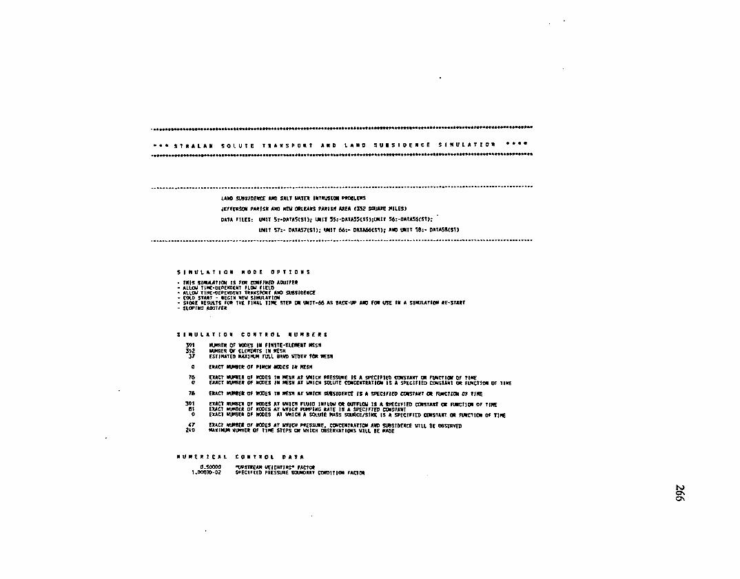
» • * s r i t i H s o i u t E T u i s r a n » ■ d i » * o s m s i o e i c e s i n i f u r i o s
LAM) SUBSIDENCE AM) SALT WATER INTRUSION PROBLEMS
JEFfFRSON PARISH ANO NEW ORLEANS P A * 1 511 AREA <352 SflUAtE NILES)
DATA FTLES: UNIT 5 t-DATA5<S1); UNIT 55;-DATA55t5l);UlttT 56:-DAfA56fSt);
UNIT 57;* DATA57(S1); UNIT £6;- DATAA6($1); AND UNIT SB:* 0ATA5SCS1)
S I M U L A T I O N M O D E O P T I O N S
* THIS S W L A T I C N IS TON COMFINEO AQUIFER- ALLOW TIHT-DEPEKDENT FLOW FtELD* ALLOW Tir«E*DEAEHOTH1 TRANSPORT ANO SUBSIDENCE* COLD S T M T * BEGIN NEW SIMULATION* SI ONE RESULTS FOB THE FINAL TIRE STEP ON UNIT-66 AS BACK‘UP ANO FOR USE TN A SIMULATION REDSTART- SLOPING ROUfFER
S I M U L A T I O N C O N T R O L N U M B E R S
391 NUMBER Of NODES IN FIN1TE*ELEMEKT MESfl352 NUMBER Of ELEMENTS IN MESH37 ESTIMATED NAXIWJN FULL BAND WIDTH FOR ME5N
0 ENACT NUMBER OF PINCH NODES IN MESH
76 ENACT NUMBER Of NOOES IN MESH AT WHICH PRESSURE IS A SPECIFIED CONSTANT OR FUNCTION Of TIME0 ENACT NUMBER OF NOOES IN MESH AT WHICH SOLUTE CONCENTRATION IS A SPECIFIED CONSTANT QR FUNCTION OF TINE
76 EXACT NUMBER OF NODES IN MESH AT WHICH SUBSIDENCE IS A SPECIFIED CONSTANT OR FUNCTION OF TIME
301 ENACT ffWBER Of NOOES AT WHICH FLUID 1NT10W OR OUTFLOW IS A SPECIFIED CONSTANT OR FUNCTION OF TIME61 EXACT NUMBER Of NOOES AT M I C H PUMPING RATE IS A SPECIFIED CONSTANT0 EXACT NUMBER OF NOOES AT WHICH A SOLUTE MASS SOURCE/SINK IS A SPECIFIED CON SI ANT OR FUNCTION OF T l «
47 EXACT NUMBER OF NODES AT WHICH PRESSURE, CONCENTRATION AND SUBSIDENCE U T U BE OBSERVED240 tUXINLM NUMBER OF TIME STEPS ON WHICH OBSERVATIONS WILL BE MADE
N U M E R I C A L C O N T R O L D A T A
0.50000 "UPSTREAM WEIGHTING* FACTOR1,00000-0? SPECIFIED PRESSURE BOUNDARY CONDITION FACTOR

T E M P O R A L C O N T R O L A ND S O L U T I O N C Y C L I N G D A T A
240 tMXIMUH ALLOWED NUMBER OF TIME STEPS2.59200*06 INITIAL TIME STEP (IN SECONDS)6.22060*09 MAXIMUM ALLOWED SIMULATION TIKE (IN SECONDS)
999 TIME STEP MULTIPLIER CYCLE (IN TIME STEPS)1.00000 MULTIPLICATION FACTOR FOR TIME STEP CHANGE
2.59200*06 MAXIMUM ALLOWED TIME STEP (IN SECONDS)
1 FLOW SOLUTION CYCLE (IN TIME STEPS)1 TRANSPORT SOLUTION CYCLE (IN TIME STEPS)1 SUBSIDENCE SOLUTION CYCLE (IN TIME STEPS)
120 POROSITY SOLUTION CYCLE (IN TIME STEPS)
O U T P U T C O N T R O L S A N O O P T I O N S
120 PRINTED OUTPUT CYCLE (IN TIKE STEPS)
- CANCEL PRINT OF NODE COORDINATES, THICKNESSES AND POROSITIES- CANCEL PRINT OF ELEMENT PERMEABILITIES AND DISPERSIVITIE5- CANCEL PRINT OF NODE AND PINCH NODE INCIDENCES IN EACH ELEMENT
• CANCEL PRINT OF VELOCITIES
- CANCEL PRINT OF BUDGETS
I T E R A T I O N C O N T R O L D A T A
NON-ITERATIVE SOLUTION
too>-o

C O N S T A N T P R O P E R T I E S O f F L U I D A N D S O L I D M A T R I X
<•70000-12 COMPRESSIBILITY Of FLUID3.00000-10 AVERAGE COMPRESSIBILITT OF POROUS MATRIX
1.00000-03 FLUIO VISCOSITY
2.(6000+03 DENSITY OF A SOLID CRAIN
FLUID DENSITY, RHCUCALCULATED BY STRALAN IN TERMS OF CONCENTRATION, U, AS:RHOU = RKOUO + DRUDU*(U-URHOUO)
9.98200+02 FLUID BASE DENSITY, RHOUO7.00000+02 COEFFICIENT OF DENSITY CHANCE WITH CONCENTRATION, DRMJU0.00000+00 CONCENTRATION, URHQUO, AT WHICH FLUIO DENSITY IS AT BASE VALUE, RHOUO
1.80000-05 MOLECULAR DIFFUSIVITY OF SOLUTE IN FLUID
A D S O R P T I O N P A R A M E T E R S
NON-SORBING SOLUTE
P R O D U C T I O N A ND D E C A Y OF S P E C I E S M A S S
PRODUCTION RATE (+)DECAY RATE (-)
0.00000+00 ZERO-OROER RATE OF SOLUTE MASS PRODUCT I ON/DECAY IN FLUID0.00000+00 ZERO-ORDER RATE OF ADSORBATE MA5S PRODUCTION/DECAY IN HWOBUE PHASEO.OQDOO+OO FIRST-ORDER RATE OF SOLUTE HASS PROOUCTION/DECAY IN FLUID0,00000+00 FIRST-ORDER RATE OF ADSORBATE HASS PRODUCTION/DECAY IN 1WMBILE PHASE
C O O R D I N A T E O R I E N T A T I O N T O G R A V I T Y
COMPONENT OF GRAVITY VECTOR IN +X DIRECTION, GRAVX
0.00000+00 GRAVX = -GRAV • DLELEVATJONI/OX
COMPONENT OF GRAVITY VECTOR IN +Y DIRECTION, GRAVY
0.00000+0D GRAVY = -GRAV • D(ELEVATION>/OY
toooo

N O D E I N F O R M A T I O N
PRINTOUT OF NODE COORDINATES, THICKNESSES AND POROSITIES CANCELLED.
SCALE FACTORS :1.6093D+03 1.60930+03 3.04800-01 3.00000-01
X-SCALE r-SCALETHICKNESS FACTOR POROSITY FACTOR
E L E M E N T I N F O R M A T I O N
PRINTOUT OF ELEMENT PERMEABILITIES ANO DISPERSIV1T1E5 CANCELLED.
SCALE FACTORS :2.50000-11 MAXIMUM PERMEABILITY FACTOR2.50000-11 MINIMUM PERMEABILITY FACTOR1.0000D+00 ANGLE FROM +X TO MRXIMJH DIRECTION FACTOR4.00000+02 MAXIMUM LONGITUDINAL DISPERSIVITY FACTOR4.D000O+02 MINIMUM LONGITUDINAL DISPERSIVITY FACTOR0.00000+00 TRANSVERSE DISPERSIVITY FACTOR2.30D0D-Q1 SLOPING ANGLE FACTOR
O nvo

RESU
LTS
FOR
TIKE
STEP
24
0
270
o o o f o - o o o o o c
s g l g s sao o o o o o o o o o o o o o o c o o e o o o o o o o o o o D O D o o o
o o a a o«3 ruN-3 rg r*W P(>^ ~ OiN•4<4K<0KimO'6<6K t^t/w nj
S R N ( M n « » d p ) O 4 m > r Q r o a t / ! « « f * N 4 Q K v ia 0 v to ^ q o ^ N N ^nNa3K>niinh<N>ocDO Odtn«anj'OK>qnioOipSin<OKO)KNODiooS rtK N F a v \« r«J <>«- m Fw f\jaiM<ov>inm O T-K 9>m^^'ONiA'04)N4^Qi/MOF>tAa(o<«<AMnminT*ivK)io)noN^(pi
Na)4O<0IAiA <qNNcm cm cm cm cm
W^»Q4d<0(MlD4Q4rMtt4Q,0NasfO<0IMa}*<tO<0N(g'4Q>4(Ma4O'£lNta<fO4)8 ^ (Mnin*f •f^i«4KNa9>DiOO^NrMKirt4inin<o,oNaKlQiQkB ^r,njnjfn«r«r
at8 S S o 8 S o 8 o 5 S s o S o o S o o S o o o o o 5 o o o o q o o o o o o o o o o o o o o o
g f i f i s s s g a i s § s £ § £ e s 3 | 3 2 s s s | ^ g f l s e g s g 2 3 i 3 8 e 3 g a s ° s sSfr<CaniAkA40«>4iA^pA|N240<fM{!!|infaiTii£tKfJ«0«SrK|Or>nf>c4IA&4ft^N4SKvKO^QtAW iE sifc g s^ ssa S S - 3 S K a s S § K ^ i S 3 OMlfM o m N N o m
iutAp*MoO>(A^NmO>in*-KQOkin<MKnoitflt*>Kn<Mn*BKnfrin*KrtftiAp>Knfrvt»>K(Afru>8 r ‘fNnn<#4tAiA4Ni<>iidi>oo^f*njFirtiv tfin*o*oKheoo>ooop>AiAitnKi4iAU>43«K.
OOOOBO OOOOQO OQO QOO DOO OOO OQO OOOO OOO OOO OOO OOO OOO
e*B8eejeeRS8§eegfias-------------------------- ------------K >oqrv
m o m <► * * ** <** o* •- ■- *- ^ ~ ~ <vr cm w rw o- * 1 *- Ki ai ki ** cm *» *- ki «*> ki im ki fM <m <m cmuw0<4rq<S>rO'6cM«9«fp-GrgiQ<4a'0CMa)«rO'QCM<&'*Q'QfMttWp<0rMcQ>*O'4cua9i4O'0cyB'*8 ^^NNn<l4t/iin'O^M9Q^OOf-«>(\iK)(4^^iA>a4P>KdO>$Oo*>>nj(gmn«iintn40^K
8 e s a g s s sCM 'Q«Bi/iQNytn w o K n o m oCM <Orf*h,t>Cur*
£ S
o a aD O Q O Q Q O O O O O O O O O O O O O O O O eO O O O O O O O O O O O O O O O O O C O + **++* + +*** + ***-»*+*« + * + * + *** + + + *« + **«4+** + ++ + *S S S fl^qiA4SS85 R s s s jK E E□ in « -o ^ n n r -
l '0 « S V a O & 0 * B^N N »0 'rM in irt> O N K (da3 0kO O ^*MIVKIinR§
3 § ' | 3 q Q '(MqNiAn^pN4RM«Nf4»<aN^PMi««o*;M49Mp>!n:ff-0i-g>tnMfrO>(>nt 3fM<MPy?Bc2N«9mp«>K3><*'Q'<0 (>>«-rocQcMP'CC>>Fi»ON-»4COrMp>*-anKl«)<S£jCinio«>K9>4k4«5»NMtnMiAOf>K)onKmu^O'mu^«ua4(MNA«>innis)& 4NOq**MNO|ONS<Ct<0'4PRin^iniOrtrtfrnrtv jeN»&DinOSqiAh>NO p>p>mui(oN^p»^K<cKfn>«!gincvcnitf^o<t0eotn^4Qpno*f efrm ajN aiA on SN«4>v4|ooaQNoqfOcgK>t<-K>cgro9&np>K](M4kroOr*S(dinP>^«qiN ’tN N d n ^ ^ A o > n n n J r iN 3 M N v * n p * sv r< i^ K ^ in N O $ 9 (ow jjjo>
^ • ^ • q s i iv J Q o a q *-OmsS*> ©CMMCMinKV0'V ^ 4) «f>«-4-c\jT*>-ni**(\jnj»>Nfviip;nN MNfuMcuNniv(vhr'
O o p D OO♦ +T♦♦♦ S ° S “ 8qf-M 'O N y
Z *»S JP S ni■-MJ ■■* O* Ml «J <oon'0**ivK in WNfr (V njin'CroQ 'i
3OO3
)M a'0 rV IO M O 4 M O M O '0 N 4 M O 4 C g 4 M A q N 4 M e4 'V hOnr'CMNinsf •jmin«Mva3QOHQO«>v*f>JKItOMMin«<flN ^^^^^^^^^-^^^*-r-»-*-i\|CMCM<\llNlMCMlMfMrOr'JCMlM
8 J 3 8a g o Q P ^OKICiiru ttuliKl<M&sT'Om<oo>r imQoCQNi/,in ^ ^ tn D Q < f^ q in if lB )3 0 (3 '(4 )p Q d O 3 o n < 0 Q M O > ino(NQ»-^NNrMinin'-aM(n(M>f >Q^*fiC0r^0tB<F N»»»“ fg^f-(ON«“
Q Q obgooopoQ O Q appopaaoD pgpaD aq*,N'*m4nl'!0»f)1KiAmaiQ8]^qqN4)KOOnQ^miAIM nKpaonKinMM^KNSoN^aMOav\<dn^iAOrtin 4MviCtf*SMOlOO>INIQ>VlOf*,«»*O^OMeqa^tf4 □ •liA'Ou’iNCsJiMoCOSin □T*o>(gKnvrg(\ji/Tf\|f-n«^(>D ' 2 4 < ^ n jn n j p < p o ! 0 » a i / i a o io l> i A ( O iA to K ^ K M a s i n (9M aM (O ioi^a(>0‘S < n io in io d 4 tO K N iA P 4 N P 4 tn ^ ^ Kr<tir(MciMMinfOa)u,iKiininniN^^<ii>iinokO(0»na(a<orfg r 'f-rg « -n iN T a nirgfinN^rtM (M M <M ivioniNnt<>nK )'ta
§ f f(\imn«r«fiA'0<CkN(0PQioO''N(Mnn inici>0*oF>dB}9>&a^vfljAiKt4MiniA<0K t«f>f f r'(-t-r'i-f iMfVrgAKMNNCgiMMNl'U

00*000000000*0 Z5Z 00*000000000*0 152 00*000000000*0 0S2 00*000000000*0 692 00*000000000*0 892 50-059822656*9 29290-025919989*1 992 90-015952952*2 592 90-060490028*9 992 90-021295266*2 £92 EO-OES992591*I 292 £0-081522259*1 192£0-002680812*1 OK £0-015005186*1 6E2 00*000000000*0 852 00*000000000*0 252 00*000000000*0 952 00*000000000*0 55200*000000000*0 9£Z 00*000000000*0 £52 80*000000000*0 252 00*000000000*0 152 50-052912862*9 052 50-080200599*6 62290-001205011*Z BZZ 90-06962£916*9 222 90-098861225*8 922 50-053025109*1 522 £0-099252922*1 922 £0-022258201*2 £22£0-095259521*2 22Z 00*000000000*0 122 00*080000000*0 022 00*000000000*0 612 00+000000000* 0 812 00+000000000*0 212oo*ooooooooo'o 9LZ 00*000000000*0 512 00*000000000*0 912 00*000000000*0 £12 50-055569690*5 212 50-019295596*8 11290-010292099*2 OIZ 90*092021525*9 602 £0-001009991*1 802 £0-029625222*1 202 50-086695298*1 90Z £0-096009286*1 50200*000000000*0 302 00*000000000*0 £02 00+800000000*0 202 00*000000000*0 102 00+000000000*0 002 00+000000000*0 66100*000000000*0 861 00*000000000*0 261 oo+aoooooooo’o 961 50-026966655*9 561 50-000652595*8 961 90-061099211*1 £6190-028615552*2 261 90-011922626*5 161 EO-01S21£562*1 061 E 0 -0 tl8 6 5 £ 5 9 'l 681 50-050S25062'1 891 00+000000000*0 28100*000000000*0 981 00*000000000*0 581 00+000000000*0 981 00*000000000*0 £81 00*000000000*0 281 00*000000000*0 18100*000000000*0 OBI 50-06Z599£0£*5 621 S0-0S9£92929*2 821 50-052085169*6 221 90-058996215*1 921 90-011562226*1 52190-028899899*£ 921 90-09EB9SZ96*9 £21 E0-02965E969*! 221 £0-002298899*I U 1 00*000000000*0 021 00+000000000*0 69100*000000000*0 891 00*000000000*0 291 00*000000000*0 991 00*000000000*0 591 00*000000000*0 991 00+000000000*0 £9150-005199598*9 291 50-022820250*8 191 50-056522296*6 091 90-019520550*1 651 90-059021516*1 851 90-016265056*5 25190-0ES6l2£Z2*2 9 5 1 £0*025506190*1 551 £0-055262609*1 951 00*000000000*0 551 oo+aooooaooo'o 251 00+000000000*0 151oo*ooooooooo*o 051 00*000000000*0 691 00*000000000*0 891 00*000000000*0 291 50-091221025*5 991 50-056526222 *2 59190-aS26?2 io i* i 991 90-02E086ESZ*! £91 90 - GB90666E5* 1 291 90-0£S5SB895*Z 191 90-019996525*9 091 90-066990921*6 651£0-OSB£OZ968*l B£1 £0-OB516£261‘Z 251 00+000000000*0 951 00*000000000*0 551 00*000000000*0 9E1 00*000000000*0 55100*000000000*0 2£l 00*000000000*0 151 00*000000000*0 0E1 00*030000000*0 621 50-091251599*9 821 S0-O6822991I*6 22150-OE£SIEB91*4 921 90-06611555E‘ l 521 90*058228508*1 921 90-008962029*2 521 90-0560£29S6*9 221 50-0199E5201*1 121£0-095955569*1 a z i 00*000000000*0 A ll 00+000000000*0 811 oo+aooDoaooo'o 211 00*000000000*0 911 00*000000000*0 51100*000000000*0 911 00+000000000*0 £11 50-095962282*5 211 50-020995069*9 111 50-025902290*8 O il 50-021229229*6 60190-062256261*1 BOL 90-01525E669* I 201 90-026021911*2 901 90-052929898*2 501 90-052552858*8 901 £0-086262881*1 50100*000000000*0 ZOl 00*000000000*0 101 00+000000000‘0 001 00+000000000*0 66 00+000000000*0 BA 00*000000000*0 2650-059509921*9 96 S0-09Z0£6Z£0*2 56 50-092619229*8 96 SO-026608609 *6 56 90-020920591*1 26 90-022165161*1 1690-009962181*1 06 90-aeOQ£6SB0‘ l 68 90-O£BO9O6O2*Z 88 90-058225209*5 28 90-0E2526£86‘6 98 00+000000000*0 5800*000000000*0 98 00*000000000*0 £8 00*000000000*0 28 00+000000000*0 18 00+000000000*0 08 50-085599129*5 6250-09062629£*B 82 9O-O6919S2E0*! 22 90-008866259*1 92 9O-O0EU8929* 1 52 90-056201058*1 92 90-061229221*2 £290-099£29690*2 22 90-029900222*£ 12 90-021515522*8 02 £0-050558900*1 69 00*000000000*0 89 00+000000000*0 2900*000000000*0 99 00*000000000*0 59 00*000000000*0 99 00*000000000*0 59 50-051820696*8 29 90-025519920*1 1990-069292855*1 09 90-089020969*1 65 90-088122510*2 85 90-012218815*2 25 90-095868595*5 95 90-002025929*5 5590-0519£2992*B 95 £0-099020191*1 £5 50-026£5 l68 l‘ l 25 00*000000000*0 IS oo+aoooaaooo'O OS 00*000000000*0 6900+000000000*0 89 00+000000000*0 29 00*000000000*0 99 90-059592620*1 59 90-022520255*1 99 90-052189020*2 £990-062lS£99Z*2 Z9 90-0B2565190*5 19 90-069595026*5 09 90-018EE9591 *9 65 90-088695290*6 85 £0-009026911*1 25£0-09Z2S699£*l 9£ £0-069589969*1 5E 00+000000000*0 9E 00+000000000*0 55 00*600000000*0 25 00*000000000*0 IE00*00oaooooo*o OE 90-09£B6B89£*1 62 90-0269E2682"! 82 90-012596926*1 2Z 90-019959991*2 92 90-005290109*2 5290-085229S12*£ 9Z 90-022551560*2 £Z 90-05990Z51Z"6 ZZ E0-09818EZ51* 1 12 £0-098696505*1 02 £0-062692295*1 61£0019528212*1 81 00*000000000*0 21 00*000000000*0 91 oo*aaooaoooo*o 51 00+000000000*0 91 00*000000000*0 £190-09S2S£Z12*1 Z1 90 -<H 1169582*1 11 90-090185926*1 01 90-089691521*2 6 90-099£256ZS*Z 8 90-015221260*5 290-flZ£A22Z96*6 9 £0-065896961*1 5 50-019550069*1 9 50-065125985*1 5 £0-028026589*1 2 50-010292996*1 1
300* BOON 1Q0N 300M 300N 300H
N 0 1 1 V I 1 H 3 3 N 0 3
00+009928095*6 065 10*081912880*1 685 10+025692892*1 8BE 10*020556992*I 285 10*009095809* 1 98500*019526925*810+092059599*1
165585
10*099090596*1 985 10+052658126*1 EBE 10+0595591£9*I 2BE 10+010020092*1 185 10+082925665*1 085 10+006512925*1 62510+091S9Z6E9* 1 825 10+022865255*I 225 10*026652592*1 925 00+096222196*8 525 00*065182025*6 925 10+052£20980*1 £2510*008958152*1 225 10+09S082299*1 125 10+052059259*1 025 10+055288992*1 695 10+090952568*1 895 10*029869956*1 29510+051855526* I 995 10+068518568*1 S9E 10*029592908* 1 995 10+086995262*1 59E 10*099222122’ I 295 10+005969919*1 19E10+025182015*1 095 10+026256825*1 655 10+09E2EB12E*1 855 10*000989920*1 255 10*026989912*1 955 l0+aa289896£ 't 55510+062D19E65'! 955 10+055925262*1 555 10*052E59266'1 25E 10+098295152*2 155 10+052865959*2 055 10+065029299*2 69£10*096520292*2 895 10+099915191*2 295 10+086622950*2 995 10+005555296*1 595 10+019666218*1 995 10+095992189*1 £9510+095992255*1 295 10*099292299*1 195 10*021295921*1 095 10*052105625*1 655 10+090902125*1 855 10+025081622*I 2EE10*029612256*1 955 10*052625002*2 SEE 10*010616005*2 9££ 10+069220906*2 5EE 10*0£2£B6912*3 255 10*011521519*2 1E£10+029661569*Z 055 10*052180155*2 625 10+092622ZOZ'Z 825 10*099299590*2 225 10+059286228*I 925 10+089522022*1 52510*021981525*1 925 10*092896652*1 E2£ 10+069199259*1 225 10*029690259* 1 125 10+000065558*1 0Z5 10+056B69960*2 6 l£10+089810595*2 Bl£ 10*025552189*2 215 10+059695198*2 915 10*022150596*2 515 10+018091998*2 915 10+020229582*2 51E10+062S062£9*2 Zl£ 10*098292559*2 l l£ 10*092228892*2 015 10*052829620*2 60E 10*098029968*1 805 10+055521922*1 20E10*05E09£0£5*1 905 10*Q29996EIS*1 50£ 10*051152522*1 905 10+OE5026956* 1 £05 10+085200012*2 205 10+092292205*2 10510*069999918*2 OOE 10+005995591 *5 662 10+082£26922*5 962 10+098815££2*£ 262 10+009222811*5 962 10*025255956*2 56210*089292052*2 962 10*022199515*2 £62 10+012559562*2 262 10*065988090*2 162 10+0596120BB*l 062 10+026629165*1 68210+028905225*1 882 10+056219692*1 292 10*082895150*2 982 10+095258662*2 582 10*091290219*2 982 10+098695866*2 £8210+015006985*£ 282 10+095598916*5 182 10*051628612*5 092 10*005099655*£ 622 10+081912555*5 822 10+090255090*5 222
272
o o o o o o Q o o o o o o o o o o o o o o o o o eo eo o o o o o o aao oP BQ4Pfi99Q°fl9 04QoppOfiOoa n^QrifrfiQaoinQoxrnr'tnS^tiinfr*CN64frOI>inO(QtAin4Ht04vKi/i<0^4 OOOCO'Ji/iO«3Qfvfgpn^q^»-K\D-p(DiflgeNNe{S4QMSNia4 0^otop^p<fd5a88Sgsp.SRSe5slt!asfcS£a3^ o.’ © « o* k «o o * 0 «) »*' i/J r» *• «■* fw *- u-> ■■c w
B ifoorgn^o^N e^o^M O sie^N Q jPtrt«Kr<>(0do>ao^^Ni«i»At(«iiA2OSNn»fgrgi‘vryrMrgrgp,ir>P,iKtPiK*t*tn»oro»ninKir*imK)o 3 S e o o o o o o o o o o o o o o o o o o ofigsea88seaaga8sse8geessiaiOo «)Mg»-p'P^r,tor»r prt**
^ ..JSSCE... _ — - . „argy"io (?-<>rw
. - ___ - . 4§n»e«ofl^KN(vo<<Sti«f4NN0 4(OOO eNNO(OdP)kn4Atf r-K>lM/ 4 • '’0D^&<eNNO^NOOP^N44QOS]^Q Sno>|<0O^>-OO'0OS(POini0O^KiAO^'NO*>Vo^Voi)&0'Ar»N'6«N'OKT'V«
“S iig s s
N*i<y i*«- u"»*c<o J rviAjru
F»l0 4&&b^v*NN^sf ««iAtn>P».KOQfg <m <m Kj is* *\ m m »«i k> f A in rt m in m m k> ki
s a g g 3 |g 3 g s 3 8 3 s |a s 3 a e s a s
e s 8 S 8 8 § s g a 5 g ° s § 8 g :a e a 8 f is^0*-Q*-pnotojoorgofos*ppipowi(Mfsjos.^(g(0QB9KQ4SQ'aKgtt OK>NH}NN>lQ<«fktAO{\Jsrg^4fi»fUCtAs(9IMk04^*'DMKqgM^QdMQinooQOOp«iD>$*fM4-itMMON»oo»gr\i4oSi^QnjMin4&0>ao&o5««OKi»oo^o<dnS <4f-noVNd^^oVf-*oaaoV»NNio(04«
4Nd*iP4(v«<io*dMC0 4O'0ni(04e<0iM(0 •0«NnnD<0>O<-<-NNKI«f uMn<dKSl]O
rg t v 1*4 fv fv eg rg <v « m n fo no to rn m r> fo ro no no m k>
Q40n4fiM40n<|fOK1>f044 04«rM44o o o o o o o o o o o o o o o o o o o o o o o
8 aS 5 3 8 8 S 8 g 8 8 8 8 8 S a 8 S g °8 gQfroF>4 0 4',>OS*fO<#(MO>fieO>r>gS3 onieQino2tngc>4Q>dinenOO<oi«ioo enjoffliAO<o«to^eoN>in9nNpi>fOi/>*' Q>»OO*Qli)4O9l4QNNO<0n9eNMfi0> QmQ ir<>ofnao (KO(N4QNKiein&K^«- 9 4 s ? j 0 'n^o^«*6n$04*iQ&>o^nir>i oeopoQ«ponirtoooaiANa»4n4NotneV40^no*-(wo>«-tMoioVoKf'aMN
v \ *- h - no p* wj —■ K no f t *- *» no » m r*» no <► »ft n* iA'O«kK(afrftoo<-NNKiM4inint0 4N«a hNivrMNNNNrt«(On(ni*»«WMnwminKi?i
040 0 40i04^inifOrt4inM4in44(n4 4oooooooeoodoQ Q eQ eoeoobd
J K1 > QJ ir'i v. _ ______---------------------------------- __>K»fcr>ot £*r\iifti/wOtiooODf^tnN'Oo&knNmOKhk^K^in0'-0p«Tp*’'f^^f‘5Q ^(9ipKIWuliKJMfggn5SdSfr>-»Kih<5io>-«^ko4f]dcQ
oVo04cl^4in»'K)Oi-IOkA^niA»,tUIAV>(U
>4 e <C oj so p < N aa«# o * 0 rj o *#• o -<j ru«Q %n o <oin9<4KN«P:>DO^rsiNnK)i|inin'OvNaDNrvNfMAJMNNnnKinnKiinnminnin^n^
! g a s 9 8 s s e a 8 8 a g e “
______ _ ..jpodfrOfxOidQ^rvQo^inr1□ iA^o(OOoCh»»Mv<rvi%r^</(Qf>ovfrKoo O O *a O C 0w O O iA 9‘l>*<<linfl> f Q h * * $ K '4 < C AoVlAOK4O<0N*B4K^4 4 sl>0f fn4l0lCiA
ViiA4 '^<063?00»"'"NK4fO'iym )oK.fLDt)‘pgrvfyrgpgryrsifgnnKiF KjKtrtKiKtfi KS Kiirtrnn
58a8g888S8S8eeaS8gS9Sa5n«>NNi-nx)r,&P^040tt5>oo<ofro> RNK»<Otfi<v4^^^<n$tna»D(r>«( 040S^f>1|^f.tn4mOoifloo<KNj5«D5& '0(0 n«rgt/MflJMDf-B}KirwOi/'S*nnO>c - Ln'*LA»-fv eorv<orgKk-oeo*-oo»-n arg
)oQ j00 4N^<Ch4j'{in0'{gK<<fO(> jOrD^Men(MOiritog«DfOOoAoon(n
s e e sonoruntntn
in n v
U4ND4O'ON04Q'Anja4p<OrV(Q«rO'ONO>4O4NB4Q!ON04O<O^a8 ^^Mnn>listin4'4KK«&aoe^NNKtr^4tniniA«NBefrChOv', ^nj
ssegsfigfcsessRgaes^sasssfasssfcesssssgissniO4Kii inkM4 4A4tf)^P''V"a>4i0 4f4N'0<d^&4k>*4Nt/trifk$4r<>
fiP£>6fi04P0K>«wr<-.rai ifkOrn
oo<dO<o<o 6Noo»^o»n<-o
tptA**Kin0>tA Kno&in n'»no<Mn KfO0>t/\"-K»o<>iA«’S.>in4KKClO»OOi»i*Nnn44(/«'0<O^NCM>00«kN(V|
> e b d o o o o o o o S o o o o S o o o o o o o o o o o o oQooopa
saasSssCi iacvj 'O
4*o^o>r
a ssa ee sa e sss se s sa ss ssseQN^KrvNtftofroJo^Kf oo>OKtvhi&in4 iop **R n Ji^ Q Q f mnotf-^ K p o
S«0 4D >ri^N pN N 4IO i-h»IA (M nj2N sN > « p«-rgn*.,/u-iL/>(\i&«-4g5Q*-nj*-p»-*-cC'Off3rycr>WMOOO **
p<Oino0 4 0N«ioom 'ienconDp^f
Ut40«ND<10<Onti-40 (V(e'f 0 4MtO<4fi4N<)^e,ON!04 0 4Ne48 ^r*ruruf^'kr'4inbi'OKKOttO>oa»^M rnn«r^tn2<2n-rba]i>ooo^fO«
»I\JN <j rg nj
S< O jro > }N K 4 « i(y i> 4 K n iq 4 a ^ o ^ * ’ N ^ 5 ^ B M N N p 4 4 f0 4nO fr«r o o » e O Q n i* - p i n ^ o « i^ iM r t ^ in < o r o > i r tO K ^ o ^ 4 0 r r t N M M i n ^ N h
q * > N iM r tn 'it f t in 4 « K i) iii> 9 0 » t« r x n n 4 t iiM A O K K o e » o a »•#•«§
>inin,0'i •of o > d5f\i rg **e •n«3«-n
>• •• iSy iru oc*C PJ LTk <i
s;
> 00000000000000000
issesssaeeeesssgas• '•oONSK^e^QOKioininnnr*fonM!VM^4»^o«rtfrN'in3a**DO>ndnrvO'dfr o<0 4 r s KI^Ok«t<>int«4'ONfM NNinOion «-tfwn«-rvc>torvsn i?OOrO£i'r‘0 »<fN^CnkooOQ*>ng»nA 4^0»njOOinOniinQ>>trv«K)4
>4M(O4e4N<4O<lru04O4ni«4p>ON«Q4O4(M« •# iin44NflVOPO<>«’Nnrt4tfinin^SM)Dpoo<-<-rv
esas8s8ass89ea5essaaSiAtiN P*^ioO O‘0 'a 4 4 o > * > v* P|«OV'OONryh* iri«(
BsifcissS^sasass0 00»DOONFO<ONPinNO
<4 n3 rgnn Qi rg w* *o
ooooooooo
8 9 8 3 8 8 8 '1g 5 <So iks —
rgo5C5£f0rt*6 •OsZg»O^QO r«-OC si njK®«#<> oG|ooo«-^o
w^K(nOun^Kn»in*>n;t??!Cr^nfri/t»Kn(KiArNn9>|A^Kinfrin^i|>tn S ^*>ig tong 4 in 4 < O K F > (0 & ^ o o ^ f> J N ^ n a in ^ 4 4 K Q (0 0 0>0'B^M
fU0iQ>i-4O*>,'0rt'**>iv>4oqnioni<f 0>KNinnst»>**mKi<gKniOKT^o(y»(>nbilfK innj«tinQ 'f^P>o < i i <f(OSio eor>j©K»©« «oj>ojojKi*©**-irto**3©<i «4«*-oru~iA tn4tnO (>(>r-aR »N tO n>a^K 444 0 ? O i f oruK ^^<oig KiMDinN»<cr>»okfgme(M<p):) 'tN>ON4o&inei->lfM

ss?23Ia^£s55S5ga?ss3a?2asciS!2Kic:N-lr«j m ru m <u ro m m iv tv m n iw ra hi m ro 10 r\i m (u rv i\» rg rw rg im ig nj m m rg ro ro
i i i j i i l i i i i p r ' ' ' ’"ioo ilooooo
WrwNrUWWWWWWWNWMWWMWJO
! i
:222222222222222222222
23sa33535cS555^=s3a?2asa5253ay23«wiN^ NN rvrvrvMMNNNrwrvMMM^ rijrvrvrvfuhihihJhirvrvrwra
S$iis3gSKS£aa»S^SS£8g5!3g3»SSaSiRi»S».lNrvrohihirvrvrvrs.trgtvhjrorurvftjivrvivfvfgrorjfVhjrurjhjrvruhiMrvtv
a S a a a a a a a sa S S a ia iis ssy a a sssa ssa ^ JItv ai ai rv rv f\» nj iv ro ro m m m rv rg rg rj n n> rv rv n m ru rv rv
i l .........sysasggsssessesaasgeassgass; 2222222222222222222222222222222222
^^N^^rvnjNN^M^^^hjpgrgrgrgrursjrgrgrorvhiAjrgrgrvfvigrgpg
^2222^2^2^^2^2^2^22222222222222
sa3; 2 2 2 2 2 2 2 2 2 2
2S33»£asSy«S3=223issSssa?2SS* b o a ' p o o ' ■ * * * ■ ■ • fyQ(>c!|!!iPS«lS»SE828§SS83SS93_5 2 3 2 2 2 2
s s a s a s s S s ^ s s s s H g a S a s ^ c ^
p l l l p l l l l s a i ?l i l i i l M __________225222222222222222222222222
| | g | | | | | P | p | | p l
22^2^5^2^2^^22^22^2222222
gipfSSK SSK gsa^Sissgsiss^gait vi I* *■* vi IK ^ ‘
222222222222222
s s s s s a S p ^ ______ao3SSSS8SBS3SSS3feggS9£5 2 2 5 2 2 5 2 2 2 2 2 2 2 2 2 2 2 2 2 2 2 2 '
SS33S«SS5SSB33s83^S3SS®52SSa
l i lp s i l
22222222222222 ;
SgaaSgSssgS5ss8S3!ggsa8sSgSS
£ L Z

5 5 5 5 5 S S S 5 5 S 5 5 5 5 5 5 5 5 5 5 5 5 5 5 5 5 5 5 5 58S83ggggSg£4£££gggift&^
ra oj f\i ra n n iv cm cm cm n im rv ru rg rv <m nj im rg r\t ru oj fu r\j ro ru f\t <g ru
iigRggfcgSSgRRggSgSftS&RS c s iiisNNOJn)IVlUNMMNNfVNNNNNN(VNNNtMig(\JIVIVNNCV)(VS ^^R K R K ^S I^gsR K K K Srt^^SgS5 5 5 5 o o 5 5 o 5 5 o 5 5 5 o o o 5 5 5 5 o 5 5 5 5 5 5 5 5sse se see ae sssse g se esee sssee ssss^{O4Qn*OrvK'OranF>iO>^ frN>i^nlO><Jc0nm(^n^p>r-s *OKi inQvf >o>of\JD& P 4 P ^ Ds* DinK’OpKtM'Pflu^&i/iftjcjb in0r>«{>^<0Qi^(>O(0tMDriJiADQnjinKn'0(>‘f'J>fFwrJicciKi ^QO‘Q(OrtQS5cOOtnK>Kl«pN^«!5tOQ6>P'0(>frmO>o>rs.Q Oi^*Ov4OM,w 7^N 0,ic^tr«4fl'O*aqK*oN»ifi4&Q(0&>o>o>
rsjr rMCMrJf rMCMCMrJrJrgnjrgrMCMrgrMcvcMrJrJrvJrijrJryryrjrMrJrvj
feS ^^«saS £saaR lR SK R S^SR E R S5ooo? f? ^ | | | | | p | | ^ 5 5 5 5 5 5 5 5
J cm nj cm cv fO ti nJ nJ r\J nj cv cm i\j cm cm cm cm <v ru r\j rJ cm
cm pa r j cm cm f*I cm cm cm c\J cm cm im cm isj cm cm eg cm cm cm cm cm cm r%J rv cm oj cm cm cm cm

S I M U L A T I O N N O D E D A T A
NODE 94
TINE step TIHECSEC) DRA1D0UN CONCENTRATION SUBSIDENCE1 5.184000+06 1.856080*01 8.000840-05 5.586400-04
24 6.480000+07 2.085490*01 8.043320-05 1.447130-024B 1.2700B0*08 2.131170+01 8.093180-05 2.968630-0272 1.892160*08 2.106300*01 8.139510-05 4.473830-0296 2.514240+08 2.127090*01 B.1B583D-05 5.998360-02
120 3.136320+08 2.129200*01 8.230580-05 7.523350-02144 3.758400+08 2.12923D*0t 8.273960-05 9.048790-02168 4.380480*08 2.129270*01 8.316100-05 1.057420-01192 5.002560*08 2.096100*01 8.353600-05 1.205800-01216 5.62464D+0S 2.106510*01 8.392780-05 1.357170-01240 6.246720+08 1.942600*01 B.42742O-05 1.503760-01
S I M U L A T I 0 N N O D E D A T A
NODE 138
TIME STEP 1 24 43 72 96 120
144 168 192 216 240
TIHE(SEC)5.184000*066.480000*071.270080*081.892160*082.514240*081.136320*083.758400*084.380480*085.002560*085.624640*086.246720*08
DRAUDOUN2.057020*012.2DS31D*012.23891D+012.223360*012.237590*012.239570*012.2401SD+012.240690*012.21945D+012.226660*012.120010*01
CONCENTRATION 1.500690*03 1.546280-03 1.601050-03 1.64949D-03 1.69631D-03 1.739320-03 1.778760-03 1.81481D-03 1.84407D-03 1.87342D-03 1.896700-03
SUBSIDENCE 5.313180-04 1.350830-02 2.756610-02 4.15031D-02 5.558360-02 6.966770-02 8.375530-02 9.784250-02 1.116220-01 1.25623D-01 1.392700-01
S I M U L A T I O N N O D E D A T A
NODE 188
TIME STEP TIHECSEC) DRAUDOUN CONCENTRATION SUBSIDENCE1 5.134000+06 2.113700*01 1.799990-03 4.186820-04
24 6.480000*07 2.126200*01 1.80333D-03 1.D0724D-0248 1.270080*08 2.128780*01 1.805500-03 2.016260-0272 1.692160+08 2.127400*01 1.80588D-03 3.024890-0296 2.514240+08 2.128540+01 1.80523D-03 4.013970-02
120 3.136320+08 2.128640+01 1.803760-03 5.043070-02144 3.758400+08 2.128610+01 1.801740-03 6.0521BD-02163 4.380480*08 2.128580*01 1.799370-03 7.061280-02192 5.002560+08 2.12669D+01 1.796470-03 8.069400-02216 5.624640*08 2.12723D+D1 1.79374D-03 9.07822D-02240 6.246720+08 2.1180SD+01 1.790530-03 1.008S9D-01
DRAUDOUN 1.727930*01 1.932500*01 1.973290+01 1.951070*01 1.969630*01 1.971500*01 1.971520+01 1.971540*01 1.941900*01 1.9511»*01 1.804730*01
NOOE
DRAUDOUN 2.345060*01 2.605220*01 2.657800*01 2.63071D+01 2.655160*01 2.658520*01 2.659520*01 2.66049D*01 2.623870*01 2.636470*01 2.452240*01
NODE
DRAUDOUN2.324570*012.482960+012.515640*012.498310*012.513280+012.515000*012.515220+012.515420+012.492070+012.499570*012.383590+01
CONCENTRATION7.000230-057.006160-057.011190-057.018620-057.023300-057.026800-057.030550-057.033200-057.034000-057.034330-057.032930-05
CONCENTRATION2.709380-043.28987D-044.009100-044.696360-045.401450-046.093480-046.769580-047.427010-048.005500-048.606530-049.126050-04
CONCENTRATION1.SD05SD-031.521250-031.545090-031.565090-031.583660-031.600020-031.614430-031.627110-031.63688O-031.646410-011.65360D-03
SUBSIDENCE5.372580-041.38251D-022.829700-024.262720-025.712530-027.162740-028.613330-021.006390-011.147830-011.291860-011.431750-01
SUBSIDENCE6.13457D-041.600360-023.29421D-024.967490-026.665200-028.363520-021.006240-011.176130-011.340780-011.50919D-011.671590-01
SUBSIDENCE4.954100-041.241420-022,521070-023.792290-025.073480-026.354890-027.636520-02S.91811D-021.017830-011,145380-011.270470-01
1B9
139

r . ** <o o» m ’O *>j £ ** 5!
0»<nui.r*WWM —-‘ ©'■Vi
PO o- O Im Vj la W Q> M £ H * - J\>OC»u1W^:p2#9SB3 NO^ut^rwiN^QOoni§§888gsssslt;
NNNIVtNNNMNNNr g J ' W X ' ^ ^ ^ ^ ^ W r i J ^
KKSSRSSseJS^gi^ c>ijhi^ncotJgui-*2£g o a a o o o o C Q O O
o o o o o o o q q o o C _» _*
r»^<ocp*-f 'J ,O N £ f'J {U00*rwOB«,' 0 & f ' J B # ' >-»Tr
o t w r u w N ^ * * o > w i
* ' r G S 5 ,J’ w ^ o - » j a g B 2S;£Misa£!S|iSS§ S S S 8 & I£ S § 9 3 «♦ 4 4 4 4 4 4 4 4 4 4 I H
g g g g g g g S S S S C
«s)tt o)o>pi 2 8 2 3181 o o S * ' f t J ? V j S j ^ O W § S »
i ^ g g s s g s l s♦ * ♦ ♦ ♦ ♦ ♦ ♦ ♦ i ±.0OOQOOOOOOOOC
n_* OCT> »r\j-0vii pu m oOi>»ja} OQir<JCD -*'0
Ofcuit/>#*oJuro-*«*DtirtI « f t t • # • I t «i^nJOO^VI^ONVOsl>r>NO0& P h )d o ^ S^OtUlfr>WN^OOO>nEfSSg8EJSBSS§«4 4 4 4 4 4 4 4 4 4 4 mp o o o p o o p p o o d5 5>Ca CBSSaovNO>w
Vi ?o — nj ?s» b b m w rt i£ wms h s s f a s a g a s s it7iawu'J W'Oari>N*'S3 3 S 3 8 3 3 S 3 S 3 S4 4 4 4 4 4 4 4 4 4 4 0OOOOOOQQOOOC
WUJUUWWWWWMWm <CC4'^0'U1f’WM-‘OOZglg:2823aag£3u i ^ ) S > a ! v v N 4 u ' M > o o o a o a o o o o o H
o o o o o e o o o o p j
o o o o o o S a a o o - *
o o e a a o o o g o b Q a 00a o o o o a o o z
a
oODACOOKDOOtttCDaOtS
W U M N N N M ^ p O f f lMNU1v<**>*(/lWW1QU<4
| i s 3 S 5 § ls l§ |b s o o o o o o o Q Q B
_* -* _t CO *4 &> KA W PU -* ** Cflkj — bo^wbguiki'oSs is s iS s - s s a s e ls s so sa e ss s1 ■ < 1 • 1 1 • ■ 1 < n o o o o o o o o o o g m
-• *> Wl « s s» Q » M \ ) O P P ^ 4 N S
a o ^ i P ^ u i u ^ O A ^ t i .3 3 - b - * - » r J W N U ' 0 -
3a33sSsS333S^^NNlUfiJWNIVIVJ
c n n ^ A o N ^ ^ ^ ^ S
33fgSBggsssso o a o o o o o o o p ^
NMIOfUNNNNMigM^| 4 l t t t t l l t 4 B
^ N 0 k,O 'C 'O 'O N 9 U 1^ %UlXsJhd^uS<J1MrJ9--a-0£g#>oo^jL4auiw-dr,—o S ^ o ^ y o ^ B c
4 « 4 > A 4 « A 0 * A A p l I
'6-giSlb*JQCDQ»*^^4QnfN p ' a ^ r u r j N ^ o o S cQ M F U - t U O N N O ? H
gsggseesssss
U « a 4 « ^ < p < < A , - a »a O N N S N P O O M W PNAMNO«AAnJOU<MCSEfSiSaSSSSSfg4 4 4 4 4 4 4 4 4 4 4 *o o o o o o o a o o o
J Ml 4 4 4 ^4 4 ^4 S
4 4 A A U ) W W Q O f f l rO N ^ U 'O U lM 'O O E ^ h M U i F p p ' O ^ H
. . _ r o A 4 Q A G « < o n
o o o d o a o D o o o H
ggggfeg»^gga
S3
W W U M U W U W l^ W M ^
S S 8 « i i l i K | 3 § i3 s i i i i § s4 4 4 4 4 4 4 4 4 4 4 1OO OOO O O O O O O
o* <*■ 0 b p* o» p* p* 0* O* *y i l f l f r f t N S A W ' f l 'O O J !^ P N N P b ' d ' O
s iw ll is sS8S
f'ryfLttOtnOQ'NNW^A^ f r W 0 5 0 « f , W N ® < 2
____ > O o o d o a e
o o o a o o o o o o p f i^ ^ B N N lV M I O M r O I '
33S38 sssS ssssss
*ji\j_*-*w*-*a»c>jp'rg^iW
N b ^ v i M ^ m v A W Q ^ V40aO>S>aW9<f'A,OVI
f i i f l i s s i g p□ o o o o o o o o o p mB 4 4 4 4 4 N N N N ^
9 L Z

277
fei i OO OOO OOO OO
VlM^Ovrph.Jr'irtfrrtao m erM F -v ^ o ^ n itR4*'>(v<finK«3*-V^^
SOOOOOOOOOOZOOPQQQOpOpQU u>w k/x w® rj*rtnj>0flrtCKs}inj>(QN IQQlA-*in'O(0io£>-rv0rt«£FOttO>OT*n>finSQO>o^H n^N rt^tfcO K io^^
> 0 O O D 0 0 D 0 0 C
sasgggssggss0^wK14KlMMWW«0 3 M Oipru^ninkavtinK wttn®KiOr-'f^cOirvr>jy; aKiDrN(MM4«rinOc
8 3 3 3 3 3 3 3 3 3 3 3M f i o e o o o a a p o o<LAK»OinSQK»»“KiK3tr»tt(OrM^o<Oa3w‘ir rv<NjvnH NlAp NOJKlOtVICOx © »r» *- R nt <z <9 y? c* £ U|IOt ,040^<0(0(^0 0'~|2N(VNf0n!f4NNrtinn
s 8b b b b b b b B o b o
SgsaesesiiesaSMPJ»oh»prgw»P'C'**2K<OC«Ki ti(Oa3rM>ll KOmtntnininiriMAtAN
i 4 4 I IsgsaeeesgeeaH-ina«fO|inrM<OHiu> nj3»inpiA«'S(uNN<dru>9>o>Qa}KK>ooiniA
N N f»KN K K K K N§
o o o o o o a o o o oX 4 4 4 * * 4 4 4 4 ' 4 4l a s s a e e e g e igS^*-4*fs.fyO)H)l>KTONllrtKMPJOOOOgwryssSpeccccses° ru rJ i>J *0 cO ru cj tvj r*3 rg nJ
333*23333*533 ls |g § ® s is ig i*-»cu*“iA«S«W4*rK»i£wz O n <OCQON4'ONiOP>O JO O O O rf'r^ i'f*^a^^K N N K SN SIsK
00000000000X 4 + 4 4 4 4 4 + 4 4 43 0 0 0 0 6 0 0 0 0 0 0 QONOSOQniArNul ain4rN4 4O>9^'O>0iw 5rnifOPUK^^^4^tAK^S £ S a f f i 3 3 3 3 S B 8
SN NNNNNN*-^^o o o o o o o o o oisgsgssesibssa <okA« — '
u i o o o o o o o o o o of i l lz o o o o p o a o a o PON9'fKiinpnK0‘4”'OOirtOBOi/ipcQii^fVonin
|uOo o o d d o o o o o
s s s g s a a s e g s gaMO>|i3*»»O N*0‘NKK> -<>Of NWCMfl tftf-iABorj^soNiflcoo*-<M
£8 3 3 3 3 3 3 3 3 3 3 3
igssgigiaagssQcBinfNjiogo^inKsj'O M»04NQiA«:aNtniA x&lpo»srfipl)(Qrsir«>rMS Ujfr^aQS K.<0'0lrtu>i |4s 0 go cd a eo co o to <o <0 (O A
O
8 3 3 3 3 3 3 3 3 3 3 3588838858888ttKu^rjiOfMKiooa^N*-UJOO'
K K hi N N K S KN N N§
iO Q O O O Q O O O O O
„ ________ - _ j eo o *-on<« ** *9 ** ^f\ir K?K?tOK?MMKJKIKI
9 CO CO © <9 GO G S o o o o o cI M444444+4 + »«*
S 8 8 8 S S S 8 3 8 S SlUOOO^Nri'l 4in<OK isfQpoj^'OciqftJvi'O M«offirHO KtLncoorM«z t-^KjNfOin^Nfno^tNj
|A<C«-«-CMKIK1>4tAi/\40
a.«—*^corjs00^e0ru>00ui ni<4N^t\J4<oO^'i ^ r-*-«-4-ryru
S o o o a o o o o o o o0 + 4 4 4 4 4 4 4 4 4 4S o p o p o p o o p p o M^Nf«n5^M{hwin«0«-it>Ko4-rus3'C'SJ
“RS*S6“” SSSfu rl r£ K? M kk*mo kj m ru
ntcih umffl Dtta)n)dti u e o o e O D O o o o oUJ 4444 4 4 4 4 4 4 4
£ 8 8 8 3 5 8 8 3 3 5 8UJOOO^Nn^aiftw^X4OOIV4'<flDdN4>0*-CO«5 *0> “K|UfcltOOP>J
m'Ov *»NrnfO"itnkn<,0
a . w - * r t o f v < Q o + r t a < v 6 c>
S o o o o o o o o o o o 04 ♦ + + ♦♦ ♦ ♦ * ♦ ♦8 8 8 5 8 8 8 8 5 8 8 8«N4hJ0c!?^lCl^I?b;B£WU'QiOO&O'0,4“NO
rJfOf'jpJrjrjrjfNjrJfgfy*■* -o N <0 a o9 to to « co <o a o o o o o o o o o o o oUl 4 4 4 4 4 4 + 444 +£ 8 8 3 3 5 3 8 8 3 3 8UjOOO’-NKl^^in'ON i<fnoNirOwQ<M<j|0 xQtON^^MintOOfM-J l-4“^Nt£)lPi^NfnO ON
lA 40 ~ +* <0 K? N* <■* m Y*
w R^h.eSrv^SSo^’j;pm 4>^r*p*NN

APPENDIX 3 COMPUTER OUTPUT OF THE VERIFICATION RUN
(1981 - 1985)
TIME UcffCHEilT EUPSED TIME :
"2.593Do*06 seconds 1.58110*08 SECONDS 2.63520*06 MINUTES 4.39200*04 HOURS 1.83000*03 DATS 2.61430*02 WEEKS 6.01230*01 MONTHS 5.01030*00 YEARS
0 R A U 0 0 U NNOOE MODE
1 3.779547290*00 27 8.30841318O+0Q 8
13 5.673228890*00 1419 7.057781780*00 2025 9.398438280*00 2631 5.616949330+00 3237 1.014444090*01 3843 1.041625260*01 4449 5.769293560*00 5055 1.32075213D+01 5661 1.135921450*01 6267 5.732302600*00 6873 1.54461053D*01 7479 1.238339430+01 6085 5.738503960*00 8691 1.77898023D+01 9297 1.277369100*01 98
103 1.424884800*01 104109 1.965242750*01 110115 1.300189860+01 116
NODE39
152127333945515763697581879399
105111117
6.151658170*00 7.912493500*00 3.370305360*00 8.5344B125D*00 8.553567070+00 3.791066770*00 1.092098130*01 9.194560490*00 3.366279790*00 1.313106100*01 9.700179660+00 1.165822110*01 1.522328700+01 1.022321690+01 1.64797554D+01 1.684070660*01 1.037353130*01 1.664496460+01 1.80135213D+01 1.04413774D*01
NOOE NOOE4 6.781441300+00 5
10 7.334462880+00 1116 2.936365740*00 1722 9.006511210*00 2328 7.978760160*00 2934 2.930B8049D+00 3540 1.099987780+01 4146 8.440427120+00 47S2 9.721368600*00 5358 1.296653970+01 5964 8.756452630*00 6570 1.593239650*01 7176 1.473796420+01 7782 9.145137570*00 B3B8 1.652287080+01 8994 1.59523184D+01 95
100 9.201481560*00 101106 1.717313700*01 107112 1.689356950+01 113118 9.157168510+00 119
MODE7.558536260*00 66.96609363D+00 122.S61079380+00 169.348300730+00 247.3264929BO+00 308.161310260+00 361.105564930*01 427.599049140+00 481.163663380*01 541.25618882D+01 607.792077710*00 661.643377110+01 721.40267561 D*01 788.068758460+00 841.655261160+01 901.499975990*01 967.949398860+00 1021 .95452714D+01 108 1.566191590*01 1147.660361700*00 120
8.088926300+006.348701070*006.054754570*009,516861970*006.533508930*009.205704070*001.085939670*016.700055950+001.287354820+011.200736500*016.S0586641D+001.626194480+011.322563190*016.919664900*001.748477880+011.393505500+016.453872340*002.021190230+011.431804260*011.57173491D+01

121 1.732177130 01 122 1.880019010*01 123 2.086006300 01 124 2.227082510*01 175 2.236468970*01 126 2.213856500*01127 2.11331337b 01 128 1.990210740*01 129 1.877788650 01 130 1.732988230-01 131 1.592904070*01 132 1.450495740*01133 1.310S762Q0 01 134 1.176761380*01 135 1.04619001D 01 136 9.371464130*00 137 1.747867880*01 138 1.908747140*01139 2.070377990 01 140 2.276367630*01 141 2.424179810 01 142 2.516096510*01 143 2.516845250*01 144 2.346141820*01US 2.177591380 01 146 2.037443300*01 147 1.692206880 01 148 1.744470070*01 149 1.592554720*01 150 1.441195420*01151 1.296441630 01 152 1.163199320*01 153 1.033368990 01 154 1.837951790*01 155 2.001967950*01 156 2.201615930*01157 2.39125304D 01 158 2.536397420*01 159 2.619486200 01 160 2.604053630*01 161 2.517804620*01 162 2.386297720*01163 2.246598340 01 164 2.094496240*01 165 1.937027230 01 166 1.771701400*01 167 1.606749360*01 168 1.445997400*01169 1.291627660 01 170 1.152531090*01 171 1.698794220 01 172 2.154495890*01 173 2.359344130*01 174 2.621419130*01175 2.791696800 01 176 2.860048970*01 177 2.633679520 01 178 2.746352930*01 179 2.623808730*01 180 2.499563070*01ia i 2.342992160 01 182 2.166913510*01 183 1.978802220 01 184 1.790387770*01 185 1.614982290*01 186 1.437463900*01167 1.255283930 01 188 1.916316130*01 169 2.236930020 01 190 2.540389500*01 191 2.636950120*01 192 3.073770820*01193 3.152825180 01 194 3.1625B5650*01 195 3.01902672D 01 196 2.672557040*01 197 2.716664910*01 198 2.556080010*01199 2.370333460 01 200 2.158772000*01 201 1.938892360 01 202 1.7356816tD*01 203 1.54185791D*01 204 1.151736970*01205 1.924575080 01 206 2.309118630*01 207 2.664270470 01 208 3.093644790*01 209 3.547960830*01 210 3.54631331D*01211 3.52435961D 01 212 3.291977270*01 213 3.131403180 01 214 2.964176240*01 215 2.787292750*01 216 2.558589340*01217 2.318127460 01 218 2.077064580*01 219 1.852065030 01 220 1.642289690*01 221 1.459884660*01 222 1.903482620*01223 2.300756040 01 224 2.722795370*01 225 3.115891810 01 226 3.4t6075950*0l 227 3.624078940*01 223 3.666283000*01229 3.570416540 01 230 3.437235340*01 231 3.268524540 01 232 3.038891670*01 233 2.759881830*01 234 2.451612080*01235 2.1B157473D 01 236 1.938986990*01 237 1.71918187D 01 238 1.508478930*01 239 1.672053860*01 240 2.284472260*01261 2.715926900 01 242 3.146889090*01 243 3.434322890 D1 244 3.678278770*01 245 3.797974420*01 246 3.945742720-01247 3.793022400 01 24B 3.604793300*01 249 3.577794010 01 250 2.898913840*01 251 2.556947560*01 252 2.264203080-01253 2.003985770 01 254 1.768933750*01 255 1.565400280 01 256 1.813596320*01 257 2.230847450*01 256 2.681140260-01259 3.093827120 01 260 3.432153310*01 261 3.684003010 01 262 3,977137970*01 263 4.099437030*01 264 4.076114790*01265 4.027822890 01 266 3.345298860*01 267 2.97012B14D 01 268 2.612806580*01 269 2.313739830*01 270 2.043423660*01271 1.799648800 01 272 1.570967150*01 273 1.727355860 01 274 2.139825620*01 275 2.564613420*01 276 3.04142653D*01277 3.7B317761D 01 278 3.644789460*01 279 3.72940355D 01 280 3.600067780*01 281 3.796839930*01 202 3.587307260-01263 3.298761160 01 2B4 2.941627590*01 285 2.625730990 01 286 2.333727250*01 287 2.059186390*01 288 1,808650860-01269 1.572398200 01 290 1.686839040*01 291 2.043985630 01 292 2.442606820*01 293 2.897889450*01 294 3.508772460*01295 3.658272720 01 296 3.514027230*01 297 3.567415760 01 296 3.551302540*01 299 3.439920350*01 300 3.217866990*01301 2.9220B0480 01 302 2.618078690*01 303 2.33194024D 01 304 2.057152S20*01 305 1.797269130*01 306 1.568462920*01307 1.620953D40 01 308 1.934753300*01 309 2.287288920 01 310 2.667956520*01 311 2.976306170*01 312 3.207133300*01313 3.346571430 01 314 3.445660360*01 315 3.482498420 01 316 3.400931120*01 317 3.215031270*01 318 2.908211680*01319 2.604857090 01 320 2.314158560*01 321 2.035692900 01 322 1.772543530*01 323 1.513304720*01 324 1.529570200 *01325 1.617961200 01 326 2.119261490*01 327 2.441851690 01 328 2.729818890*01 329 2.97507261 D*01 330 3.19K32B7D*01331 3.400004160 01 332 3.531679930*01 333 3.544189140 01 334 3.24871674D*01 335 2.898179300*01 336 2.583488510*01337 2.282786630 01 336 1 ,99741B53D*01 339 1.730018120 01 340 1.479254360*01 341 1.459864620*01 342 1.703056570*01343 1.963570210 01 344 2.241298810*01 345 2.521183090 01 346 2.777150930*01 347 3.013524020*01 348 3.264592140-01349 3.925428510 01 350 3.692960780*01 351 3.211051900 01 352 2.883693130*01 353 2.555016560*01 354 2.237536660*01355 1.943900590 01 356 1.674828070*01 357 1.419059500 01 358 1.370748970*01 359 1.595801680*01 360 1.823261820*01361 2.067622000 01 362 2.344004590*01 363 2.63953551D 01 364 2.847444460*01 365 3.031304880*01 366 3.167353130*01367 3.165B93960 01 366 3.176437380*01 369 2.8898631ID 01 370 2.526497130*01 371 2.161171930*01 372 1.873503680-01373 1.612128370 01 374 1.334737160*01 375 1.290547260 01 376 1.466113540*01 377 1.674756220*01 378 1.911770730*01379 2.133528610 01 3B0 2.509530580*01 361 2.794906240 01 382 2.951038550*01 363 3.076853690*01 384 3.093648820*01365 2.941262840 01 386 2.639118900*01 367 2.36421395D 01 388 2.042366630*01 369 1.789344630*01 390 1.540549530*01391 1.308804170 01
C O N C E M T R A I 1 0 HMCOE NOOE NOOE NODE NOOE NOOE
1 2.010875560-03 2 1.735374020-03 3 1.644134160-03 4 1.559076430-03 5 1.257696010-03 6 1.050536130-037 5.383176210-04 6 2.595234220-04 9 2.181296660-04 10 1.975949990-04 11 1.791231530-04 12 1.705417210-04
13 0.000000000*00 14 0.000000000*00 15 0.000000000*00 16 0.000000000*08 17 0.000000000*00 18 1.763627640-0319 1.611403530-03 20 1.352979350-03 21 1.18317117D-03 22 9.725292330-04 23 7.5160S557D-04 24 3.857951330-0425 2.626529570-04 26 2.184555550-04 27 2.003060480-04 26 1.626164090-04 29 1.411921550-04 30 5.712855770-0531 0.000000000*00 32 0.000000000*00 33 0.000000000*00 34 0.000000000*00 35 1.549608340-03 36 1.443460649-0337 1.173898610- 03 36 9,603608690-04 39 6.589111720-04 40 4.223699890-04 41 3.155654220-04 42 2.342764450-0443 2.078642390-04 44 1.598368760-04 45 1.094981500 04 46 0.000000000*00 47 0.000000000*00 48 0.000000000*0049 0.000000000*00 50 0.000000000*00 51 0.000000000*00 52 1.247477830-03 53 1.243687080-03 54 6.949875140-0455 6.162710730-04 56 3.614364800-04 57 2.640356910-04 56 2.076296020-04 59 1.734292620-04 60 1.39B135240-0461 1.10970947D 04 62 9.073208400-05 63 0.000000000*00 64 0.000000000*00 65 0.000000000*00 66 0.000000000*0067 0.000000000*00 68 0.000000000*00 69 1.087723140 03 70 6.502606100-04 71 3.6349315B0-04 72 2.127010720-0473 2.298513890 04 74 1.938105190-04 75 1.691S6035D 04 76 1.496864280-04 77 1.066312480-04 78 8.513088330-0579 5.39379255D 05 60 0.000000000*00 61 0.000000000*00 82 0.000000000*00 83 0.000000000*00 84 0.000000000*0085 0.000000000*00 66 6.137007240-04 B7 5.290947590-04 66 2.708072640-04 89 1.085107660-04 90 1.156466910-0491 1.160261160 •04 92 1.158323980-04 93 9.698728850-05 94 8.707924150-05 95 7.1B5B94310-05 96 6.341711490-0597 0.000000000*00 98 0.000000000*00 99 o . ooooooqdd*oo 100 0.000000000*00 101 0.000000000*00 102 0.000000000*00
103 6.920B6703D-04 104 7.604945260-04 105 2.778685790-04 106 2.103710990-04 107 1.501BS964D-04 108 1.170962670-04109 9.686271590 ■05 110 6.109423630-05 111 6.507990180 •05 112 5.850906420-05 113 0.000000000*DQ 114 o.ooooooodo*od115 0.000000000*00 116 0.000000000*00 117 0.000000000*00 118 0.000000000*00 119 0.000000000*00 120 1.220820040-03

280
3 o S 3 o S o | 3 S S 3 S § 3 o S 3
J 8 3 8 8 g 2 S g S 8 S 8 8 S 8 8 2 8 S J> 0 0 0 0 0 0 4
N-O Ck 'O O IM«-o 4s s sO o <c Q O *
^O O fy O '-O O O O O f lO O lO f 0 a Q < i e i P o o a o o N O i n > 0 '4 'fooaoii!iooN O O O Q >rO 'C aSOpO tlQ^O O^OOV'd '-OO fi a o o o o O D 'O o o j o j —o jSO h 4 O ^ O Q F O Q < i o m ^ 0 c
o * * ^ o n o o 4 o a ^ a ( \ j B o a^ o s o o r t d o ^ o o i v o ^ ^ o * 1
oo«*5 § —
2sas8ssB O n ^ O O — o o »- <> o n.— o •* q o o.O B ^ C n j■— o -O o <q
JIMOO'O — - ‘%h*Q• f r d r r i o a n
So a a a o o o p o a n i K o t v i ^ o o
o o4 m _ rv rw
00**>J r tOB 4 0(V<£ 4
ft*
E S ^ S S
OK QN’O^**
33S3^SS3S1JLSSf 111NlPOO^«f
t f N q_ <Snjt>krtAa^<n Q » i o 4 > r n o o c o ^ O ' 4 S ) n ■* - “ K m «o t r m
*n « IM KV 03
4f4<0 4 0«fM8}4Q 4Nt0 4 Q BNQ'fO B N Q 4 O 4 N 4 4Q>&NI04Q^lvn<f OBlMQ<jp cymm4mmo3N»ooCM>©*“*"ftJ<Niin44mm’£ K K .« )o o o o ^^ f ' jm m 4 4 m ^ 'a t»* * ‘*«So*
3g338SSS3Sg3S|3|g3g33S3aS33gS^|aSf3SS3S23£33S88e88Sg83S8888aiiR§SS8Sg8S28888e98a32S8agaaSRr a r i ^ o » o in o [ > f r o i r t O D ( > Q 6 f l Q M n p O 'O g f r K d ^ M S i A 'f l o ^ f N « r t q ^ ^ r lN f rN O N ^D kn«O tn N O |A O O 4 O SB O « * O >aN 4 aN » Q p n O A lD g 0 t/1 l> N k iQ d d ^^* *4onm o« Q 0»om mQ '0OO<2oooovnootooG C>pf% t^Q 'amo4Fnm h»< am £m c>oml> 0 r ‘ r 0 S S S r t i n e i f l o a ^ o a 9 0 4 S 3 i n n Q B ; P ^ f r Q 4 4 a ^ 4 C ! Q 4 k l > F K 4 h .< 4 p n m o v i D > a i A r o o o o a o o i P O i M < r 3 < ^ Q K « ) o h s O 'O o g < o o ? q n ^ r <nii/>po ^ O ^ V O i / \ rO O > rQ Q O O O O o d D < ^ O O lO O fK O Q f lp > { N O in 4 B n Q 4 ^ iA ^ K lS t ^ 0 < ( \ | 0 0 N 0 ' l N 0 $ g 0 < l 0 0 0 O 0 0 0 d < - 0 t n 4 o a 0 0 « ^ 0 Q 4 0 0 0 > - 0 n < & 0< - d ^ * > o V Q o K in d 4 0S>oao(ncS^fOo*->N d v V d * - p a a 3 » o K M lw<oiDNk>kViO'4
Vhn<OOkkco>0>OOr-ruiMmroau,'4Ji<0«Ndd»p>0«-i-njiMKiavr^ »*• — ** w* ~ ~ ~ w *- cm rsi fy rtf n* f* ftf tv rtf oj pu r>i pj nj rtf N N « K1 Kl »n n « M m m |SS m K> ki w
^ 5 9 d OM' t 9 ^ v ' 9 n p g ^ Q 0 * t 0 f i 4 0f<>4 0 n j e M ! f 0 { f ! 4 Q 4 ^ O 4 ^ r t 4 i n M 4 i / t O O O O O O O O O O Q O O O O O O O O O ao O O Q aO O O O O O O O O O O O O O O O O D O
88888828938888888388888383^8288388338383^82881r t@ 9 ^ S 4 ^ O 4 « A O ^ 9 0 B O a A i Q o o o n iv o 4 4 O M iA o n » o in f - g K < ip i i tN M '* p ? § <Q (? ^ ^ o o N O O g Q ^ 0 9 ^ o o < o o ^ p S '4 ^ g % in g f f Qg<OB2^[<{Bn^'‘ -*
?Q t e
>00000000o o o o a o o o a o o
v u r v n » r » n u n ^ o m a n i ( > o v i D ^ t f i(A«^Q>^»N40}>O^K06>eKlI>iAkO n jrg K O D 3 n 9 A O B ^N O > « iM 9 ^oSvt^ i(O oipm dQ ^> iO Ptn^tP tiO n
ftNnKini/vin4<mP>4moMMN4Ki
uiiOrgQ^aBN
fi22;!SSGf3SS«eesg$S3;iS
S 8 8 S g 8 3 8 2 2 8 S 3 2 2 8 3 3 S "‘0 2 ! q ~ S S S ' 8 S ^ K S P : S a o S ! i i f — - — -
, . t ingv V O<on g<><(B infiA t{k«ao r* s 4 5 3t D* 2 s £»■« ■* S4* ©^ p k a g o t io « Q Q k A h n g K .ru v ^ o > n N tA M O D rtdskQ '+Q O 'O kf *‘ “ “ -----LflOOtfip440B I n o o 5 o i a 0 0 k ! S o 4 O 4 Soodo»6on>fOpOONo5NQ04QONoonoiA^oK<BaiMOQOo5>ooviO'i. . _ . . _ _ _ __________________________________ __ _________G j 9 5 ^ 0 Q ^ o « in e Q Q o > > o 5 o o o 9 > Q i r t n o D 4 0 ! o C o < # g o 4 k p i V B K i r t « r g t r n O O O (0a4N O ^^O 3ooO O O nog 'lO 9O O 44D C ^Q M B Q w O 6i/linB ivniQ <liA 0 Q O i/ iQ K O O M 'O e n e g * ‘ Q O 4O O 4 O O $ O N B O < l> Q * >*‘ O ' '4 O B O n 4 O P IM B^ O O ^ O ^ ^ O f K O f ' f l o V g Q Q k O O i n O N r t a V N e V r o V p O o i ^ O k ^ N N B N K K
•4 0'firU(0«rD<<tN<0?f p4(Ui0>fD<4Ojqvf 0 (Mfl<|Q4N*3<f O'OAllOyO'OmaifS'eNIO W<fO<MI)<ilO^N<}4 04Aiqir0 4NaN«io»i’jvn«'flNN«5Soo^ruNK>rt«rv,iiP'0<f,»H(o^tto^^i'(Nfl^4in«,®^N® 8 o rcrji^ntr^i/itA i^N B aooo^F
3 ^ 3 2 8 3 2 2 3 8 3 2 2 2 8 9 8 3 3N 0ton$ i^N A 4-» & * 'ao> rg in r t ' -> -otf>K|4^<r’CdS<NiAQ<feO M aiM IV ^4 N » ^ 4 n O N > N ^ D tf1
vi|C«fO>«No4<OiA*, A d B k N > r d » m vt«tC ll4nf rB D A|Q«aCil04^N Qm
N N N n n N il>«KIIM4'*al}>*frVMOO>in
S93 J 9 ® ^ 0 |? l ^ 0 ^ ^ 0 ^ 6 O ^O O JO d^O »040M H tQ K I^O rt'|Q !f«»Q J!JH lJ J O O O O O O O O Q O O O O O O O O O O O oaO O O O O O O O O O O O O O O O O O O O O O
n o B i> ld ' ’ ^ O i A n d 4 r Q ^ ' r Q < | B Q l i 4 . . . > * o o ( M O N « ) o ^ g o ^ f r g ^ » 9 « ^ O K t 4 i n e
aN o 5 i ^ Q i r > i j ^ 5 v i > ( S o S a m o o n l o S £ i W 5 § S 2 - “ --------------a o ) n O ' f ^ o ^ a Q M O o n p o o o o p o d > a M n S O n g S B O N ^ Q I ]O O lA Q Q $ O Q « O O ^ Q k K l
r u o o b ^ S S 8 $ t i 9 $ NB o p a o o B o^ O O N O D W O000 ----m o o
•)6iA4O '*OQ^O $'0^O i«l '0 tnO ni ~ ~ o M K Q ^ * * g B > n o t f 'n ^ k *omoom'Opnopm«v-m O4u\OFKO9 OrtK'('0N
N b b ^ o o ' f > e » >' i > d f i 4 e V ao d « ' e , d c d o ) A d n i ' i d f > n o ^ f J o ^ ^ o f l ) * d < ^ N K v
noirtrKmbtn«i'krooifipNno>iA«-KrtQ>inpKnc>iA Kr>i>4nvknoiAf-Kiac> KNMO>lr4 in (A B S S Q Q 9 0 c ^ * « n jn M 4 4 ^ 4 'a k k B g tf te P '>MMnpn4tiAtntf<ki}e»*^^P»»*h<cyir«niNWNrMft*(Mftifti«fmMNNinnrtnnnKiMnM^rtrti^i!5
3o|iS83ooS8SSoS8|3Sg3|o3gS^S33S 2 2 8 8 8 8 2 8 8 2 8 3 8 8 8 8 8 3 2 8 8 8 8 5 8 8 8 8 2 8 9Zs0!2!C0f,goo >2^'i,0^90'tl 0( oo4ooNONKO>
o o o o a o o o o o o a o o o o o a o o8 2 2 2 8 3 2 8 6 3 3 8 8 2 8 3 2 3 8 3Ki '4«fr«-Qa<QMin|4 4 b * faloK^<Oi/iNfMpb»mc3l0(Vl4cd'0K>0'0 * - » Q r t 0 9 ' l v R f - ^ ^ K < f l B r 5 S ^ « ^m3<o<fc4£Jgj,e*»rtfiO'«h»om<>o«n~‘mm 4 Nmru
Cm«tffc%<dr».miM44©orn©*T® i r t« o iO N < io so 4 b » n k « 4 r hfON/i'f NN*linlQ4(>040<
I
1 0 0 0 0 0 4 0 0 0 ------5u------S . J tn o o o o ^ q o o K io o rw o o ja
•—omooKiQfc—
_ n j o m o o m o o c * 0 4 Q 4 _ 0 0 > 0 0 0 0 > O Q m 0 4 0 0 0 '4< V O ptO Q B O O dQ 4^Q
u 0 'T > * Q S 0 O n O O > IO 4 |f l0O o r * o S 4 0 0 ’- o o r « o N . '0 ~O O B C O r g a o N o o ^ O O in Oo o ^ n Q p a o iD O O < q o N > i in
2 3 3 3 3 2 3 2S 3 |s |sS ?N ^ tw k0 4 0 0
00000000000000000000
g s i s i i i g s g i i p i i p s gK )f-^^pO O *k<#'OOtn**>»«<«Otrt'’4 aq^>Kn|UiA^OJi<S<qp7 4rt<f9QS O ^ k A d k (> in 9 0 N h < Q h i^ '* p k m in « r iA q R N iA ^ p p 4 t i iA r t4 ' f > r O
NQ«f OON4«(p*OiMd^O jA*C<IO'0(MD«|l?'ONa4P«iM8,|fO<OAlO*>0<ON4<IQ4 lkU fu44Q ^M 0«>O 4njB 4O <ONti jO B j^ in ^ iK N o S (> c 3 D ^ » -n jm rt> i^ in 3 i^ .S tt» 0 O O ^ f 'jn jn « y in if l< iN C B n ^rM N nK i-4inir<0«K 009'00^'-^ ^ ^ ^ • ■ • - f ^ ^ ^ ^ f - ^ o iN N n jN N N rv N P iJ O J iv c j iw w fu N in n n n n M in in r t r t r tp n r t in r t a •-> -•-
Q O O O O O O O O Q O O O O O PO O O O
K K O N K D -«O O ^D O ^O N N O rM ttO ^<IO ^O O d'004SM O '4^4 '4"^^^n '04lM inD ^ r
^ k l ) « 0>OO^^Nl1 t f y tn < i0K >so» o rjrgftjf^cM»nm»*>F%r>nnMnm«nKiinKiK» a*KrtO0 ^NWO»trt^kpP‘« ! r t f i i i ,rt4 4mOOKKOOOOO^*

ioooooooooooSm i
S==5gssS5?SSSg5=saa3KaS^^S5al2aSSa3Sa33SSSIJ S S S S S S S S S S o c
jiiiSli^BsS»i»S8i^gSS»»SgSS»3S&sggiESRR3S3SS3SSS^Sio o S e o o o S o S o o o o o S o o o S fo o o o o o o S o e o o o o o S S o o e o S c
«g2SS»33Keagsggs§Sg3lg»SSS333SS^g3Sg!SS»«^gS5 5 5 5 5 = 5 5 5 5 : ? | | ? | |
l^^ sasssssssK sag ssssg: 5 5 5 S 5 5 S 5 5 5 5 5 S S 5 S 5 5
- ] § i l i p p § s
, , , m mNAfNNNNMMNMNMNt'
|^-tssas5tsia!scfcss«sfe^
Hi^ ^ ^
; S S S S S 5 S S S S S S S S 5 c| s a | | | s e | 8 | |
j*««jelSlii|iipSlsIllU . , ;SaKsS883CfcB§8S&aaiGi^
liiiililiiii
NNNM»iuiuri(uNr4iu<uturj<vf<Ifv<<in
|-*ssKsassKsaeisass||Ks 5 5 5 5 5 5 5 c
4iiiii!NNNNNNN nNAiNNnNNNNNNN
j^SSSRSSEfcSSKSfeSSS^S 5 5 5 5 5 5 5 5 5 5 5 5 5 5 5 5 5 5 5 5
! ? i l l ? l i s ? s i | | p p
NNNNrUPJNrgNNNNNNNNNNNn)
K s a s s s s s e j s s s s s s s ^ ^ - z a s x t t S M S t t S S S & s s
; S 5 5 5 5 S S 5 5 5 | | | | | | | 5 5 5 5 5 | | | | | | | | | | | ^ 5 | | | | 5 o 5 5 - S 5 5 5 S S 5 5 5 5 5 5 S 5 5 5 S S S 55 5 5 5 5
i i i i i im . 1S8H .... liiliiiiliili.
o rJiMrjiMpy iMfMrvfwrjfMfiipyrwfvry rj
~ $ 3 ^ ^ £ 2 s S S S ; = £ 3 § i $ a ^ ^
282
o o o a a o o o o o o o o o o Q o o o o o o o o e o o o o o o o o o o o a o o o o o e o o
_ J <> £► ryrNN 5) ^V\K*K^S.3>»U"*n3»“»—>-.a5l,'yr-’On- 4QK *r fypnO> <0«* ''0tn-i*t<-.gNt>t—DiOx/t O- ■/U'COC* ^K(Q(QK>NKO>t^h.&^S,&tAr^B]i^a(0/l&
8 8
jg figsssaases^ssassassggsggfiassgasgsaaassegsasKQAftpos^K)0(amQOi-OninruKio«r4^OiAdMO>rMKieMi9 3}innQ^i]a4Of]Khk --*- “ -“ *0.l«»*5*l*©d.o^,jrtryknrgKW«^sfKN>Cfl*»£O**Cw'i^^ryfV — ©.Ki >-»q5ryr»’<4K.«Q*i*in0p»Aj£tCO0<OG0rk*p'ip»ry(v#p>ift<o O
IIINrurvin«NNNNr,grgNruNhirurjNPiN(Nji>ifuAiNNni(virti(VAiN(vNN(VNrgivN(viripiiVNN4rN)ttiJO<OA|Hsfo<4MQ4OdlVied^O4r\iO*4O4N0^g4NC'fO>ONI)^O<Ory<lO4O ^fnM4tnin<O^KQUO&o^^rgrjf^>f'flAtn A^^QQ&OO^^l,gKin«r4tf'<<4KNO$
o o o o o a o o o o a o o o o o o o a o o o o a a o o a o o S o o o o e o o o o o o o e os s s se a a e s s f ..........................................................................**K '0O!>'NO '-<fisssssissisi:*>iAaoi«rtQiMfi«)oi r* CO & K CO V k Q N N £5888858888!
C'OQ^((SiA4NNf>1njK>4 4tfmkMKknv - 'CIS&4K(K^vK<>tfVtt<0^tQQ<9K3>NkSs«}»BSfrC88888588S S 88S 88888S S 888888888 !
ry tv tv fy rg iv ru iv rv rv rg rg rv ig rv eg «m ry tv rv pg rv rv tv ry rv rv iv rv (V ry iv f\i rv tv im ai aj ry ry rv rv rv «vi cm
N^K>'<i^iA<04n>KaO|O oO ', JMNKvwi<if
o o o o o o a o S o o o o o o o o o o o o o o o o o o o o o o o o o o o o o ao o o o o o ^
gasifiSseaeagsgssaaaasseasasRSsaaeaagssiassesseKQmO*>s( jsliA<ti/t^tn»ndinn9>S4doO>i-»'OOrtQQn'OONOflK«S<l^^ni4^ ^ 9 ,t!C5B(0tnQNv>N«; iAM4i(Q<0«rN^Mi0^QONn^OOnp>'0in»Kryin<0i0inMp O M 4 4 n ) P 'f r t a n p < o c O p n » M 4 tf i> i« tn i ,v « i n 5 n « g N « ] » ^ n S K 4 4 • * » |] S « « > n K
lsJiiigsJisisli.s£S.Sis£J.£ iiS2iIs^EIIslJ.lrvtv rvrvivfyrvrvrvryry rv tv igrgrvry tv (VAa fury igrvtvrvrv ryivrv tv ryrvrgrvry tv rgivrvryrv fyrgrg :£ 9 £ *** ® •* Q =f 5> '■o™ f? ‘♦ o *o< <o *# ® <4 rg S •* P *0 rv » -# © © rvco •# o ty « * p « iv t tNnKiggv\o<dNKQO<{>OO^(v(VJio^gi/Nin<OOKn0 frO>e«B^ftjrvM ^i|viin«^K «)o *- ^ ■•- *- #■- *- m <v n* rg ry rg iv iv rg rg rg rg m iv rg ftj rg ki ^ m n ** n n kim m m pi *n m
UiO o o o
o n < is v — ki tv rA « V»*- g k « ^ 4 K « »
83*335 * S § SK 4 0 S 9£ 3 jc3 kuNNmnio i ♦ « i (lAlAtfllA5“ si
u o a o ou ■ • i ■ l o p o i jON^u
m -O^WOj
B3333
C ?S 2J £JUOOOOa - ' ' - -
w a o u s w a o* ♦ ♦ 7 UJ * + * + +■ UJaaea § Sssaa 8£ oAmnm v5 3 * 3 3 33333
OOOOQOaaOOOOOOOOOOOOOOODOOOOOOQOOOOOOOOOQOOOO
<r»no<iNtnosassgs„ nj«ro3sf t>e*rv—;s8'-»K.s*0
_ ssgaagesaasaseasaassasgesggg. c.. . _ ., . — w.. - KoOtAnnn4 0>i*4^(M4Kr4QaKomi>A(<0 «Nui<Oti4ii9 u%2 fI t >" |r44kaNOvNOrOQrt^io»iONi>hny t/Nm*N<(g4f«NgNrgO<4g^D<in£ S $ ts |c a 5 |S S |S £ S S a g 3 S g |i£ 8 S S $ S & 3 3 8 l lg S S » £ ^88S S 8S 8888S 8888S 88888S 888S 88888888S 85888S 5Ntvrvtyrvrvry ry ivtvrvrvivcvrvivryrvry rvryrgrvrviviv(Vfvry*j«iAjrvivryryryiv(v Ajtyivivrviv
njNyi<rgtMA4AKo0 9oo^^iMKiinggi/Hi4 4 K S 0 » ^ o e ^ N ^ ^ ^ ^ rg rg (V rv ru rg rg rv iv rg ry rv rv ru rv ai iv »r> m 4 4 K qn
aOOOOOOOOOOOOOOOQOOOOQOOODOOOOOOOOOOOOOOOQOOO Ue5gg898ais8a8g38as2fiaa2gaa2aaa2ese88eaeggaa9e ai!£!3<tIP K 2 ‘V!£''?t*sr®Sri?,4»C®£ta??;flki>^gi£^^-NO(nAi^o;ncorv^»nntA©go|>k^ j
- r |Ci}$m o •
rvrvrvrvryivrvfvrvryfVAijfyrvrvrvrvrvrvruivtvrvryrvrvrvryrvrvrvivrvivrvAjrvrvryfyrvtviviyrv!N!P^o,ONd'(O 4N dgo4M €}go4A i4ge4(M 0gp4(M egO 4N iogO 4N Q go4 n igngg iA 4< oN K noooo^^N in ingg in 'O 4N N a9> 9’Oo>"(yivin»iginw>4«K0a rv tv tv iv tv tv rgrvrvrgrv tvigiv mrg ArKmmmnmnKiKirnKfiAKirtin
s a e s e s e g a s a g g s e s e»*-ON^wio*i*jmKinojOM(y
rg rg rv rg rg rv rg rv ru iv rg rv iv tv rv rg rg rv rg tv cv ty rg iv ai ai rg ai rg rv rg rg iv rv «g iv iv rg rg (v rv rg rg cv iv rg a
r k ?2 S w* *“ *■ ** <► ~ £■ *- k w o *- a* p* & »a *" £■ C & <£< ^ o* i/» ■- ia o gi s n t* tn w- *iM (vrm g«/iin44^ttcQo^o^^r*jrjM <jginm4KKa3oa>oe*-«-niiiNM gg44i4KiNO»^•“^■^^‘ •-^^•-^^•-•-^igrurvrvr'grgivrgrgrvrgrgrgfgrvNnKiMKiKimKNrtinKHnMKmmm
JOOOO1352? ~ S S £o»-rSd»-(wrt
83333‘*m « » Ih o o q f l SI « g w g ^ «
s3IS§“§ • • «Qr M%i
S38SS3«mnfiNrteO r tn n n
nw inn
u o o o osssesaoO Q K— 55 03^ 4> _S S K S S *
83333*t t l s e i *\^ p w r " 1
S S S S J
grgrgrgrv g O r
S q q o oQ ♦ ♦ ♦ *sesas*< — rgrsi ?g _ AccOrurVfM O O lAtA ir> 0<4 444
C S feS SUl • * • ♦ <w S 8 3 ^LUO OQi* s a s e s ^^ ^ ^ rg ir ta
M-ON-BOCOo o o o oUl ♦ ♦ * * <s s 8a au e a o * Ji a s e s ,K ^gnivi 3
irtUTT-^ftp -gdQ ui rx g 4 “ A.*-va30 ui < g g 4 "« w « „» V7 TI
ME
STEP
TIHE
(SEC
) D1
AUD0
M ccmcemtkaTi
om
subs
ioem
ce
draudCu
H CO
MCEk
TIIATIOM
SUBS
IDEN
CE1
S-18
4000
*DA
1.76
0940
*01
1.11
1070
-04
1.72
J57D
-01
1.79
551D
*01
1.12
6890
-0*
1.7*
7020
-01
24 6.
4800
00*0
7 1.
7484
10*0
1 1.
128S
70-0
4 1.
6568
20-0
1 1.
7789
20*0
1 1.
1477
40-0
4 1.
BB06
5D-0
1
*8 1.
270D
6O»0
B 1.748440 >01
1.14
7150
-04
1.99
241D
-01
1.77
8940
*01
.1,1
6952
0-04
2.
0167
90-0
160
1.58
112D
*Q6
1.74
8460
*01
1.15
6470
-04
2.05
9800
-01
1.77
6960
*01
1.16
0260
-04
2.08
4420
-01
283
uoodq u * i * < l a o a atu m ro o* tsi omOrutA— cor*® rn'IjK O ksesss>3h*OrgM»f«ro
a v >o n q
wSfi ° 80 ’ANO>9 0 il<ONQ 0 KJ -J m N
u jo o o oU 1 i i ix o o a avtaoi- 3J sr <3
2 3 8 3 8a^QQvs S a s s3 r- *- ry
IUOOQO
2 S 3 S 8s e a e su a^ N ndN*finirt23£3&£*■*££«viiA^ktn
<O
a it
o§
kQOOQlunN^inQjlOlAsfk-nuioKs c a s a *<
23S&NOOQ O NO 8} I*• 9* r* E -
UlQOOO U i * ■ • >Qoao iu«^S*r
a s s e s s 0 ‘l a s s a a
• ■Osnifi uj _!m^OO iu <o <o «o r* u • • < *ot gcoocoiQ g
Ox
IllOOOO
285SSOynt7i*f (
uj o o o oU i i « * IOQQOv)4ko*r<“dryin^m
UIOOOO
sasses s & s su»»*i »f rwjjj m® sr in <o K m ri<ck
t s e s sanjKi^f r*-aUJuB
C9- N. Ul OOJ.8
*3S oS S °f f i i 2OOOOU'Iss s_ ■ ■ * >dUl
g o o o o g « o x
i fiS 8 a 3inni»>« *- “ »*1 O* ■** ry ujS 'O'O'O u • • • * a ujI oi
UjOOOO
£ $ 3 3 ?2ft|saS
a*^nini
s s s s s aS^fV»TPU r ^O04l/iw X jtfim iA u«««)QU • i i iQUir — 0 §
288S SSnJrirnS1/5 O nj -.0 ® «
rjruKTM*
K 8S3S SI^ooriQui XN<#|^4 unnKiin lj i • > ■ a .
3 ~ " a l
^ a o o oi s s e s 3x^o333 c °fcKEe
OOOOO Ul ♦ ♦• * * <vigoQO vQ OOIVISo a o ^ j^00*7
i“* lu fW>* *l
eo o o xm »n m « o nj ru ru22££$°
S 8 8 3 SSo a o •- - * r o a ^ M Q S k n
300 00 « # * *
s s s e e *< *x yiy-im KNMrtlOO Q Q » » 0 Kimm
u 8 o o Su r » * f <e s s s sWOO D K JS a g e s^ •^ '♦ n i |n 3
a ^ 4 i i c !UJ N>4 3*4
SOQOO * ♦ * ♦
3 S ? ? § *5 3 3 3 3 oO <J m m in
• * * * tm
f lb K O B 1"u e o o S uj * ♦ ♦ ♦ <
v-*-*rNm3
3 0 0 0 0 Q ♦ ♦ ♦ *25 a o o a a3 e a s e■ o Q Q O Q
UJ ♦ + * ♦ «
- 8 § § su jo g o * ’ _ji a s s s► 4(Muia
f o o o o ♦ * ♦ ♦
3 3 3 3 *« N 4 < 0 4 0
u o o o oUJ ♦ * ♦ ♦ «s s s i sslsi=jU#(71
I/ISi!
S o o S o © * * ♦ ♦- 1 8 6 ’ 5isi mm . . . .x m o o o Q 0<O *ruu m y'kn m
ryryruru
0 8 8 3 3l l i l s "
flHC
STEP
TI
IC(S
EC)
DRAU
DOUN
CO
NCEN
TRAT
ION
SUBS
IDEN
CE
DSAt
CSS
CONC
ENTR
ATIO
N SU
BSID
ENCE
1 5.
1640
00*0
6 3.
1226
90*0
1 1.
5403
10-0
4 2.
3236
60-0
1 3.
2062
60*0
1 1.
1233
10-0
4 2.
0209
50-0
124
6.46
0000
*07
3.07
3570
*01
1.56
7530
-04
2.49
6500
-01
3.15
2650
*01
1.13
5000
-04
2.15
6420
-01
48 1.
2700
60*0
6 3.
0737
00*0
1 1.
5995
60-0
4 2.
6712
00-0
1 3.
1527
70*0
1 1.
1468
20-0
4 2.
2961
50-0
160
1.58
1120
*06
3.07
3770
*01
1.61
6330
-04
2.76
0630
-01
3.15
2630
*01
1.15
2500
-04
2.36
7050
-01
10-0
0021
9U
W-0
99B
BI.
‘£ 10
*OS1
29S'
£ 10
-06
6Z
«‘1
M-0
9ZZ
0S"*
10
*0Z
2£IS
'£
20*0
0000
7*9
W10
-00B
765‘
1 W
*0
79
6S
l‘£
10*0
Z9S
Z9'
£ 10-
Q£Z
2Z7‘
1 70
-0£1
Z97
*7
IO*0
9S02
S'E
90
*000
784*
5 1
30N
3ais
ens
ho
um
iw33
moj
w
oooh
yao a
sHsa
issn
s n
ou
vh
imjh
qj
ww
anm
(3
3s)3
«u
jois
3W
i
s1/1 (21—• o* rv m o a> x
*A— O* ♦* IV ftl OCDf'-A
vt
* ** •* VI Xc v t rv **-*-<
2 3 S B *r* -iooonise s is> + + ♦ * mp o o p nD O N ^ w
WlriWW in vim in
gooc*.oS2S5X c J o o S S
c Uipj tca^Cd Qi^ ■ i O e F x r-*poamggsss> * 4 ♦ ♦ me o o p n a o N f w
OMNMMlO( h > N O >
■4 *4^VAt • • (
2ggg;r * ^ p o o m
o S S S wS» ♦ 4 ♦ ♦ ma o o p o_ CD U> -*J 5>V
C ^ ro £*-*-• r - g o a m88883> 4 4 ♦ * mQ p o o n
a o N i S 'v
4 4 4 4 Q * ♦ ♦ * Qo o o o c 2 2 2 2 z
X O P O * ♦ * * o o o o
-Sj> vi
cyir-j Vl»-iCs n Cd a -m o o ^ xr» o o o n8 8 8 8 S
> + + + * m p p oen S p n F w
IV ry totywtAUig»D
o a a a i / i f l S N N t t i •j ««j m v» c
c o o q q O4 4 4 4 Q ooooc
cr»cA«4ni
oaajN-t-v
Z ^ ^ 0 tUI
e uirv 4 *-* -«OINQQ “ ■ J Q O l ' l r* «* ooo mKB8SS> 4 + * * m
Saopn O - g ^ w
v/imsngi uiu<yi o O° £ § S S £x g S S B S
4 4 4 4 go o o o c-ft ^ X
ftl “Jbes ^ - * - 0
® * 4 I I »C
CD N»W ^- o o P i r ^ O Q o m rp j a o g Ao a o o u
> * * + * m >p o o p n^ q Cb n & v
ru iuw N" 00 QO CO -O _ ""OfurtlKjan Qvi vi x- a »
x B a s e s x4 4 4 4 QO O O O C
I ^ d a o n S 0 < * * * nc> ui ru o mF h J ts i* * ,_ m w ry 'w*" rvi rvo**CB*>9 O 0 Q H
,g S E S 2
>r r ? S
ru-«Q<oSSgS£2w p r v p o *> —cc5m o o O o x
5 ° r t 3 __rvivrvrv2 2 » • • • o o o o
K ’P 3SUV 0 0 O 0 ^
_ o o o dQWMblki
*
- 1 - 4 -ovnV*US _ JvrvD*g«i - -SfSSSSg o e o x1 * 4 * 0o a o o m
M N *40aiO*^ o o u * *r f N O I 'Ogessse o o o n l
8 o o o ofll O * • • * , -, o a o o f n
nSooc"IV QBOOtfS §8883 ^ * ♦ ♦ ♦ ** . o o o o g
d q o o o z
wr* oirvS> Lrt-Oin«* </) OUDChM i / i N N a as s ss sa o o o i t l
CO _,8 _o ooa?V •* 4 ■ •
SoooOO O Jtlm ooa o oooo
& 8 8 8 8 5 14 4 4 4**OOOOODOOGOl
- r r r - s>25t££SOpO-*- NlS-T* lOO3 8 3 8 S. 4 1 . 0ooaom
E O18 o o o o S’w o d o o m o o o o x m o o o o —i j o e o o sI 8 8 8 8 ?
♦ ♦ ♦ ♦ - _ Q D O O C 0 O O D O I
-9 fy IV-*-*!.
Vs?
8 o o o o :
d a g S S• * • ■ c*> o o e o m
■n O
n i o o o o H-a o o o s nS S S S S ’
* ♦ ♦ * — O O O Q C O O O O O X
>
-h m iv rvrv 13
uir*r\)l«S
^ vr^urvoO O O O X t 4 ■ « O
O O P O f f l
^ S2g5& 1 38882m ♦ ♦ ♦ ♦ Zoooo
31 O-POO Z4 4 4 * n
r r . - . - j op.v<4.gi9^V*V*2tiT
S VJ O' r^fl O O 0 X
S 3 3 S S3 5 ? 3 S &s s s s go o o o ^ —■ ■* «*
— - - S■ i • » nSo o a mnwS s
3 2 | 3 33 S S S 5
^ r . - ^ r gB'HU* OW*0 V»M9 v*rv ui -•a-*o< *o o C iu m O O O O X
ui xd a v i< 4 OfO O O O C ♦ ♦ ♦ * 2o o o o
- siV f u o a cf l O « N H
e s ^ g is s s s s
i »u w - i 9u iv o u iwr u S v b oS S o S S* i i i n o o o a m
vnv*vn o n_ Miv/vry oi8 q8od? m ♦ ♦ ♦ * 2 r o o o o
PSN N rurux4 4 * * 0^w tvw rnfv a a d D5 8 3 S 2S g g g g
«*oaao> ffl•i*NWUlV)«viv»o-*O S O OpfJrvmo o o o xo o o o m
•^-oo o »u ^ U V* >= s s g s s , i“ + 4 T ♦ ro o o o
o o o o tCOOSfflOOOOESooo*j8 8 8 8 5
QDCM/I
_ u w v k n i8 3 3 3 8 !
oooo*
gsoom oo o xo o o a hoooox8 8 8 8 54 4 ♦ ♦ —oooooo o o o x
S'GNt®N(pr>u i N M ^V — •***ONOB 9 S 5 Si * i i r> o o o a m
S K S S S ,S S S S ^
OOOOmO Q O O SO G O O Ho o o o x8 8 8 8 54 4 4 4 4-*O O O O OO O O O X
UNO«Ov — i^Oirv mf f l y s a sS S 8 S 5
m
TIME STEP
TIMEtSEC)
DHAUDOlfll I
oSIEhTESTIOM
SUBSIDENCE DRA1B0UK
CONCENTRATION SUBSIDENCE
I 5.164000*06
3.217460*01 7.897IZD
-05 2.0139ZD
-01 3.069230*01
6.3850ZD-O
5 Z.314Z20-01
24 6.480000*07
3.162410*01 7.967690-05
2.15101O-01
3.016900*01 6.397230-05
2.48393D-01
48 1.270060*08
3.162530*01 S.07697D
-05 2.290220-01
3.01B990*01 6.406420-05
2.65715D-01
60 1.581120*08
3.162590*01 8.118900-05
2.358820-01 3.019030*01
6.40972D-05
2.74285D-01

285
s eo m
atoapoLUV< f ©ajo »«- — fN
s g o a oLuooN mO W r* f r i n- i ^ ^ r y nW Q F %n <a
05 »*\ «- rt m ni
Rt f
5 3 3 3 3o o a< gj ■+ %r ^
X ♦ * ♦ ♦ LUSags8 g' S o £ § £< O t^ iO r t K V 4 4 « | B ' * * *
< - k S 3f>dj>0KqXf-NAiS
5 «\roj rslryrufMfM
8
5 8 8 8 8t f O O O O
X * * ♦ ♦5 o q o o□ rsj %r ■»/
o KIOOOOg Z O O Q OH i o g n g9 BQ00IA
W & P J I O523-v
3 3 ° § 3 ?<Otrt N
tils j Otn m • *oi_*■' 8
S 3♦ i <
S Sr g / i D
? s -
5 3 3 3 3 £"sfies a■ **10<MCQ K- > ^ O K i yXCJrglM.-L o o< 0-0- . . . . o u j r - ~ 0 s
< i f _O Q J ' O O
• S ^ tn tn
£ 8 8 3 3U I B D O f JH 3 S S S^ ■- sf cs/in 3
u o o o oi k k k ka t o - a p \ » n — Z ui K rgOFFigmm3 ; - V V .
9 o o o oe s s s J
« o o ( ^ « t
S S f c S S "L ‘K»ryf\<»*_ . * • * Cj i x d t f 0 0 g
S
s s e s e *rvrjni n
£ 8 8 3 3W O O O v ~ ^
I S S S E
U O O O O o « I ■ •x o o o ourO CO •“ a o> 'O 'f ia ^ r g o a inuini^r cq ■* * s g t n « N
t U ' - v - ’ .
a o o o< S ^ 3 S 3[ sJWKI O■ 4 ^ g o u tcno*»n^ jo rgo O
j . . . . < _ Z 4 4 <00 Q
Ifl o S
So a o o* 4 * ♦S 8 S 3 S *< « ^ o o _HO0 Q0O
«$ 'O ’O oCVirUfMCM
s g s s su jo q o ^ u2 4 0 0 ^M 0 0 N 0 _^ ^ g n i in O
r z Z
& * * 4 0 Q141
a i * 4 B Q W N < 4 0 -
( L ^ < 1 0 O ui ru >» <o —
a.Ul
0in
■(
VI5 «
V i
uiJC %
Uls
►* ►* k>
. 8 8 8 8 C3 (0000 -1» o o o o & z o Q o a t l o o a a o i * . • . u; o o o O
k o o o o ^ 9 * ♦ * ♦ x5 a o o a orl o o oo incn!^K N HjKininmio o o o 3 rgncNON*
l/)QOOOI/lw B S o r c U j O O O f XSsgsssmm < « » . »■* " ° — " 5f - g < d ru ir3»

APPENDIX 4
1. CALCULATION OF THE ROOT MEAN SQUARED EERORS FOR THE
DRAWDOWNC„.ALTERNATIVE #1: K - (l.lB-1.64)E-4 M/S C...ALTERNATIVE #2: K - (lJM .B9)E-4 M/S
C, ALTERNATIVE #3: K - (1.47-2.Q5)&4 M/S
C...ALTERNATIVE #4: K - (1.65-2.30)E4 M/S
C....ALTERNATTVE #5: K = (1.88-2 63)E-1 M/S
C VERTICAL LEAKAGE = 10 MGD
1 DIMENSION J(62),U{62),V(62),W(62),X(62),Y(62),Z(62)A(62),
B{62j.C(62J,D(62j.E(62j
2 N = 623 DO 10 1 = 1, N
4 READC5.100) JCl).U(O.V(I)1W (Ij>X(I)1Y(I)1Z(I)
5 100 FORMAT(I3,6FB.2)
6 10 CONTINUE
7 WRITE(6,190)
8 190 FORMAT(lHl)
9 WRITE(6,200)10 200 FORMAT(//.6X.’NODE NUMBER\15X,,S IM U lA nO N '130X,’OBSERVATlON7
22X,'ALT.#l’,3X,'ALT.#2't3X1’ALT.#3',3X,’ALT.#4\
SX.’ALT.fSMZX/DATAVaOX/tALL IN PPM)')11 DO 20 I = l,N
12 WRJTE(6,300) J(I),U(I),V(I),W(I),X(I),Y(1),Z<I)
13 300 FORMAT(10X,I3JX2>F9.1,8X,F9.1)14 20 CONTINUE
15 DO 40 1 = 1,N
16 A(I) * (ABS(U(I)-Z(I)))* *2.0
17 B{l) = (ABS{V(I)-Z(I)))**2,018 C(I) = (ABS(W(I)-Z(I)))"2.0
19 D(I) = (ABS(X(I>Z(I)))‘*2.0
20 E(I)=(ABS(Y(I)-Z(I)))” 2.0
21 40 CONTINUE
22 SUMA=0,0
23 SUMB»0.0
24 SUMC=0.025 SUMD=0.0
26 SUME = 0.0
27 DO 50 1 = 1,N28 SUMA=5UMA + A(I)29 SUMB=SUMB + B(I)
30 SUMC«SL'MC+C(1)
31 SUMD = SUMD+D(I)32 SUME=SUME + E(I)
33 SO CONTINUE
31 RMSEA=SQRT(SUMA/N)
35 RMSEB = SQRT(SUM B/N)
36 R.MSEC » SORT(SUMC/N)
37 RMSED = SQRT(SUMD/N)

38 RMSEE=SQRT(SUME/N)
39 WRJTE(6,400) RMSEA,RMSEB,RMSEC,RMSED,RMSEE
40 400 FORM AT(/,lX,’ROOT MEAN'/IX,'SQUARED ERROR', 4X 5B U )41 STOP
42 END
NODE SIMULATION OBSERVATION
NUMBER DATAALT.#1ALT.#2 ALT.#3 ALT.#4 ALT.#5
(ALL IN METERS)
0 9 5 95 9 5 95 95 9.3B 10.8 10.8 10.8 10.8 10.8 11.0
23 11.6 11.3 11.3 11.1 11.0 12.0
26 11.6 11.4 11.3 11.2 11.0 12.2
27 10,9 10.7 10.6 105 10.4 12.0
40 14.1 13.6 135 13.0 12.7 135
42 14.1 13.6 13.3 13.0 12.7 13.0
44 12.7 12.3 12.1 11.8 115 12.0
46 10.6 10.3 10.2 10.0 9.8 11.0
55 16.7 16.1 15.7 15.2 14.8 145
56 17.0 16.3 15.9 15.4 14.9 155
59 165 15.8 15.4 14.9 14.4 15.0
61 14.8 14.1 13.8 13.4 12.9 14.2
71 20.8 19.8 19.3 18.6 17.9 19.0
72 20.7 19.6 19.1 185 17.8 20.0
B8 20.9 19,9 19.4 18.7 18.0 18.0
90 235 22.0 21.3 20.4 195 21.0
92 24.1 22.6 21.B 20.7 19.6 225
104 205 19.6 19.1 185 17.9 19.9
106 22.3 21.1 205 19.7 18.9 195
108 285 265 25.3 24.0 22.6 26.0
122 245 23.1 22.4 215 20.6 215
124 33.1 30.6 29.2 275 25.8 285
127 29.1 26.9 25.8 24.4 22.9 25.0
129 24.7 23.0 22.1 21.0 19.9 24,0
140 325 30.2 28.9 275 25.7 27,0
144 32.1 29.6 28.3 26.6 24.9 27.0
155 22.8 21.9 21.4 20.8 20.2 23.0
157 325 30.2 28.9 275 25.9 28.0
160 36.2 33.2 31.7 29.7 27.7 33.0
163 29.0 26.9 25.7 24.4 22.9 28.0
172 25.8 24.6 23.9 23.2 22.4 245
174 34.2 31.8 305 28.9 27.3 295
178 37.0 34.0 32.4 30.4 28.3 34.0
189 25.3 24.4 23.8 23.2 225 245
191 365 33.9 325 30.7 28.9 31.0
194 43.6 39.8 37.8 355 32.7 375
197 33.6 31.0 29.6 27.9 26.1 31.0
206 27.1 26.1 25.6 24.9 24.2 25.0
210 50.9 46.3 43.8 40.8 37.7 45.0
213 395 36.2 315 325 30.0 35.0
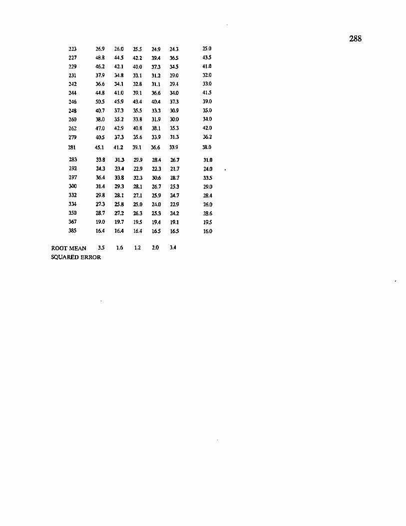
288223 26.9 26.0
227 48.8 443
229 46.2 42.1
231 37.9 34.8
242 36.6 34.1
244 44.8 41.0
246 503 45.9
248 40.7 37.3
260 38.0 35.2
262 47.0 42.9
279 403 37.3
281 45.1 41.2
283 33.8 313
292 24.3 23.4
297 36.4 33.8
300 31.4 29.3
332 29.8 28.1
334 273 25.8
350 28.7 273367 19.0 19.7
385 16.4 16.4
ROOT MEAN 33 1.6SQUARED ERROR
253 24.9 24.3 25.0
42.2 39.4 363 43 3
40.0 37.3 343 41.0
33.1 31.2 29.0 32.0
32.8 31.1 29.4 33.0
39.1 36.6 34.0 413
43.4 40.4 37.3 39.0
353 33.3 30.9 35.0
33.8 31.9 30.0 31.0
40.8 38.1 35.3 42.0
35.6 33.9 31.3 36,2
39.1 36.6 33.9 38.0
29.9 28.4 26.7 31.0
22.9 22.3 21.7 24.0
32.3 30.6 28.7 333
28.1 26.7 25.3 29.0
27.1 25.9 24.7 28.4
25.0 24.0 22.9 26.0
26.3 25.3 24.2 28.6
193 19.4 19.1 193
16.4 163 163 16.0
1.2 2.0 3.4
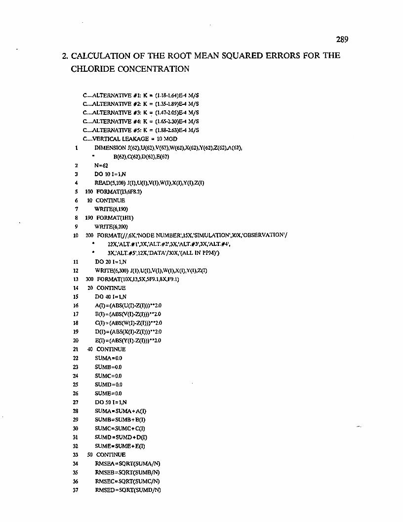
289
2. CALCULATION OF THE ROOT MEAN SQUARED ERRORS FOR THE
CHLORIDE CONCENTRATION
G...-ALTERNATTVE #1: K = (M 8-L64J& 4 M /S
G —ALTERNATIVE #2: K = (1.3S-1.89)E-4 M /S
G ...ALTERNA TIV E #3: K = (1.47-2.05)E4 M /S
G ...ALTERNA TIV E #4: K = (1.6S-2.30)&4 M /S
G ...ALTERNA TIV E #5 : K = (1.88-2.63)E-4 M /S
G....VERTICAL LEAKAGE = 10 MGD
1 DIMENSION J(62),U(62),V(62)>W (62)<X(62),Y(62)!Z(62)A(62),
B(62),C(62)ID(62}IE(62)
2 N=62
3 DO 10 I=1,N
4 READ(5,100) J(I),U (I),V (I)IW (I)IX(Q,Y(QIZ(I)
5 100 FORMAT(I3,6F8.2)
6 10 CONTINUE
7 WRITE<6,I90)
8 190 FO R M A T (lH l)
9 WRITE(fi|200)
10 200 FO R M A T(//,6X ,'N O D E NUM BER’,15X,'SIMULATION',30X,’OBSERV ATION'/
22X,’A L T .# r,3 X ,’ALT.#2',3X,’ALT.#3',3X,'ALT,#4',
3X,’ALT.#5’,12X,’DATA'/30X,'(ALL IN PPM )')
11 DO 20 1=1,N
12 W RJTE(61300) J(1),UCI),V(I),W(I),X(I)1Y(I),Z(1)
13 300 FORMAT(10X,13,5X,5F9.1,8X,F9.1)
14 20 CONTINUE
15 DO 40 1=1,N
16 A (I)= (A B S(U (I)-Z (I))}"2 .0
17 B (I)= (ABS(V(I)-Z(I))) • *2.0
18 C (I)= (ABS(W (I)-Z(I)))* *2.0
19 D (I)= (A B S(X (I)-Z(I)))' *2.0
20 E ( l)= (ABS(Y (I)-Z (I))) ” 2.0
21 40 CONTINUE
22 SUM A=0.0
23 SUM B=0,0
24 SUM C=0.0
25 SU M D=0.0
26 SU M E=0,0
27 DO 50 1=1,N
28 SU M A=SU M A+A(1)
29 SU M B =SU M B +B (I)
30 SU M C =SU M C +C (I)
31 SUM D = SU M D + D (I)
32 SU M E =SU M E +E (I)
33 50 CONTINUE
34 R M SEA =SQ RT(SU M A /N )
35 R M SEB =SQRT(SUM B/N )
36 R M SEC =SQRT(SUM C/N )
37 R M SED = SQ R T(SU M D /N )

38 RMSEE = SQRT(SUM E/N)
39 WRJTE(MOO) RMSEA.RMSEn.RMSEC.RMSED.RMSLE
40 400 FOILM ATf/.lX.'ROOTM KA.V/lX, SQUARED ERROR'. 4X 5I9 .I)
41 STOP
42 END
NODE SIMULATION OBSERVATION
NUMBER DATA
A L T #1 A L T # ’ ALT.#3 A L T #4 A LT#5
(ALL IN PPM)
6 10305 10325 994 2 1035.6 1038.0 1010.08 2540 254.9 252.9 256.1 257.0 262.0
23 701,8 705.9 7095 7125 718.0 715.026 217.9 217.7 216.6 2175 2175 220.027 199.3 199.2 197.7 199.0 198.9 203.040 3805 383.4 397.1 388.3 392.1 400.042 2305 230.6 228.4 230.9 231.0 227.044 1565 156.2 155.7 155.9 155.8 160.046 0.0 0.0 0.0 0.0 0.0 0.0SS 548.9 555.8 567,7 567.1 576.2 595.056 3385 341.9 356.3 3475 3510 350.059 165.8 166.0 169.4 166.3 166.7 170.061 107.1 107.1 107.1 107.1 107.1 111.071 3735 374.4 377.1 375.9 377.0 376.072 200.7 201.4 206.9 203.2 201.8 203.0as 267.6 267.6 270.9 2675 267.4 274.090 108.9 109.4 118.1 110.3 110.9 109.092 108.8 109.1 1145 109.7 110.0 115.0104 9185 912.1 883.8 901.8 894.0 390.0106 2085 208.4 211.6 208.3 2085 210.0ioa 117.8 117.6 119.3 117.3 117.1 119.0122 4995 4965 495.4 465.9 4505 4805124 180.9 180.2 180.4 1795 1785 1855127 78.6 78.4 81.1 78.2 77.9 75.0129 0.0 0.0 0.0 0.0 0.0 0.0140 3923 385.3 437.6 374.1 365.4 410.0144 113.9 113.7 110.1 113.3 113.0 110.0155 1070.9 1069.3 1061.9 1065.6 1061.7 1070.0157 371.0 368 4 395.0 364.0 3605 380.0160 98.7 98.8 99.6 9tf9 990 100.0163 505 50.4 OO 0.0 0.0 0.0172 15205 1521.1 1496.4 1523.4 1525.7 1510.0174 330.7 3265 346.8 319.B 3148 360.0178 75.2 75 5 74.7 75.4 755 75,0189 17313 1722.6 16535 17075 1695.9 1680.0191 574.8 562.1 597.9 541.2 524.7 590.0194 79.4 79.4 83.4 79.4 795 90.0197 0.0 0.0 0.0 0.0 0.0 0.0206 18675 1860.1 18475 1846.9 18355 1850.0
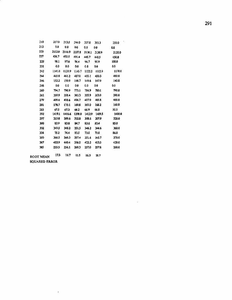
291
210 217.0 2135 244.0 207.8 203.3 250.0213 0.0 0.0 0.0 0.0 0.0 0.0223 2152.0 2146.9 2107.8 2138.1 2130.9 2120.0227 456.7 4525 491.4 445.7 4405 450.0229 98.1 97.6 96.4 96.7 95.9 100.0
231 0.0 0.0 0.0 0.0 0.0 0.0
242 1141.0 1133,9 1145.7 1122.2 1112.9 1170.0
244 465.8 461.2 487.0 455.1 450.3 480.0
246 152.2 150.9 148.7 149.6 147.9 140.0
248 0.0 0.0 0.0 0.0 0.0 0.0
260 794.7 790.9 773.1 784.9 780.1 790.0
262 359.9 358.4 3833 355.9 353.9 390.0
279 409.4 403.6 406.7 407.0 4050 400.0
281 170.7 170.1 169.8 169.0 168.2 160.0
283 675 67.3 66.2 66.9 665 50.0292 1419.1 1416.6 1398.0 1412.9 14095 1400.0297 3100 309.6 3150 308.6 307.9 320.0
300 83.9 830 84.7 83.6 83.4 85.0
332 3495 348.2 3515 346.2 344.6 360.0334 75.2 74.4 835 73.0 72.0 86.0350 3665 360,3 357.4 351.6 345.7 370.0
367 453.9 440.4 396.0 423.2 4135 420.0
385 2555 256.1 269.3 257.0 257.8 260.0
‘ MEAN 173 16.7 115 16.3 18.7
SQUARED ERROR
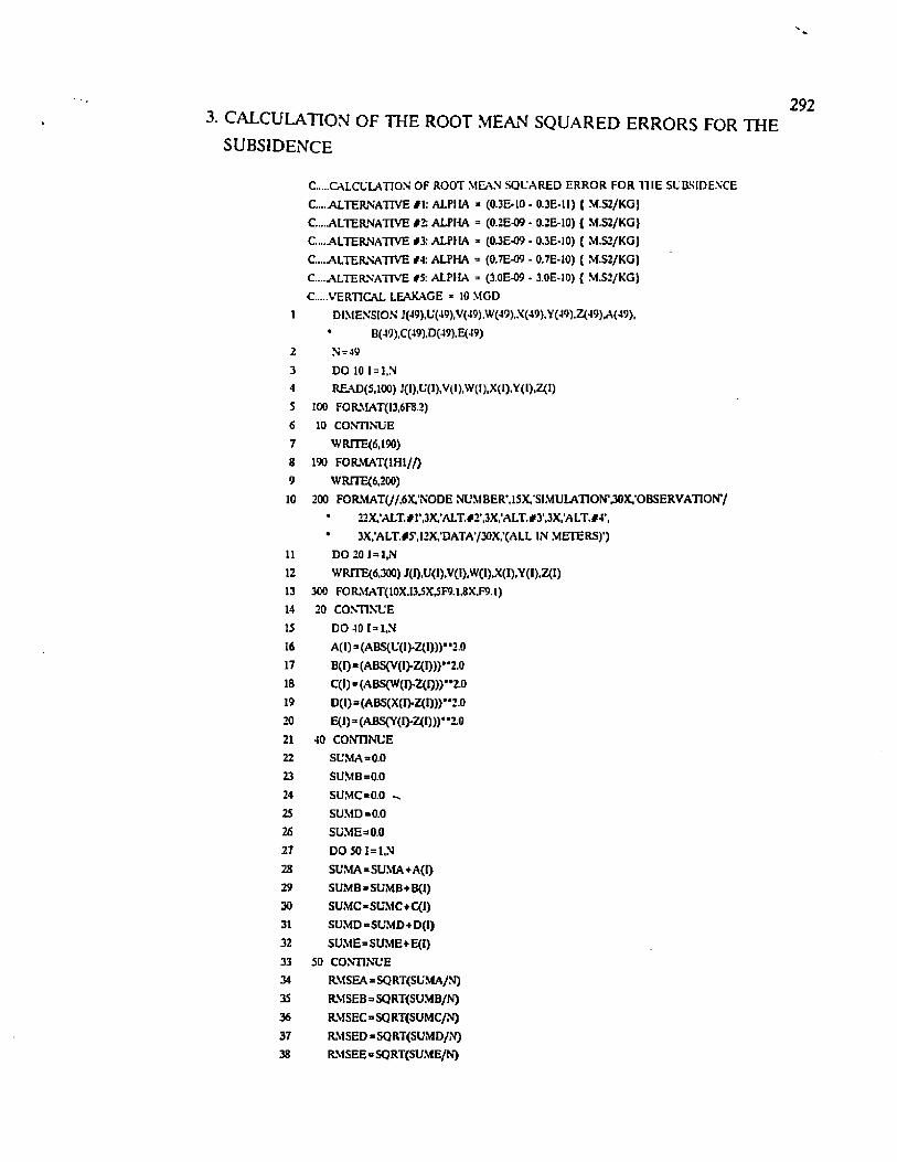
CALCULATION OF THE ROOT MEAN SQUARED ERRORS FOR THE SUBSIDENCE
C CALCULATION OF ROOT MEAN SQUARED ERROR FOR H IE SUBSIDENCE
C.... ALTERNATIVE #1: ALPHA * (0.3E-10 - 0.3E-11) { M.S2/KG}
C....ALTERNATIVE # 1 ALPHA = (0.2E-09 - 0.2E-10) { M.S2/KG}C....ALTERNATIVE #3: ALPHA * (0.3E-09 - 0.3E-IO) ( M.S2/KGJ
C...ALTERNATIVE #4: ALPHA => (0.7E-09 - 0.7E-10) { M.S2/KG)
C....ALTERNATIVE #5: ALPHA = (3.0E-09 ■ 3.0E-10) { M.S2/KG)
C VERTICAL LEAKAGE * 10 MGD1 DIM ENSION J(49),U (49),V (49).W (49).X (49),Y (49).Z(49).A (49),
B(49).C(49),D(49),E<49)
2 N = 49
3 DO 10 I = I,N4 R£AD (S,100) J(I),U (I),V H ),W (I),X (I),Y (I).Z<I)
5 100 FORMAT(I3,6F8.2)
6 10 CONTINUE
7 WRITE(6,190)S 190 FORVlAT(lHl//)
9 WRITE(6,200)10 200 FORMAT(//,6X,'NODE NUMBER\15X,‘SIMULATION\30X,’OBSERVATION7
22X,'ALT. # f 13X,’ALT.#2,,3X,,ALT. #3'.3XI,ALT. #4’,
3X,’ALT.#SM2X;DATA730X.’CALL IN MEIERS)')
11 D O 2 0 I = l,N
12 WRJTE(6,300) J(I).U(I).V(I).W(I),X(I)>Y(I).Z<I)13 300 FOR\UT(10X.I3SXI5F9.1,8X,F9.1)
14 20 CONTINUE
15 D O 4 0 I= l,N16 A(I) = (ABS{U(I)-Z(I)))"2.0
17 B(I) = (ABS(V(I)-Z(I)))"2.0
18 C(I) =(ABS(W(I)-Z(I)))**2.019 D(I)=(ABS(X(I>Z(I)))” 2.0
20 E(1) = (ABS(Y(I>Z(I)))*, 2.0
21 40 CONTINUE22 SUMA=0.0
23 SU M B=0.0
24 SUMC=0.0 ^
25 SUMD=0.0
26 SUME=>0.0
27 DO 50 I = 1.N
28 SUMA=SUMA+A(029 SUMB = SUMB+B(I)30 SUMC=SUMC+C(I)
31 SUMD»SUMD+D(I)
32 SUME=SUME+E(I)
33 50 CONTINUE
34 RMSEA= SQRT(SUMA/N)
35 RMSEB = SQRT(SUMB/N)
36 RVISEC = SQ RT(SUMC/N)
37 RMSED =5QRT(SUMD/N)38 R\1SEE=SQRT(SUME/N)

29339 WRITE(6,400) RMSEA,RMSEB,RMSEC,RMSED,RMSEE
40 400 FORMAT(/,1X,'ROOT MEAN'/IX,SQUARED ERROR'. 4X5F9.1)
41 STOP
42 END
NODE SIMULATION OBSERVATION
NUMBER DATAALT.#1 ALT. #2 ALT. #3 ALT. #4 ALT, #5
71 105 13.6 15.4 22.6 64.3 15.0
72 105 13.6 15.3 22.6 63.9 15.0
83 105 13.7 155 22.9 65.2 15.0
90 10.6 14.3 16.4 25.1 74.6 15.0
92 10.6 14.2 16.4 24.9 73.9 15.0
104 105 13.3 15.0 21.7 60.2 15.0
106 105 14.1 16.1 243 71.3 15.0
103 10.8 15.9 18.4 29.6 93.9 15.0
122 10.6 14.1 16.2 24.6 72.4 155
124 11.0 17.1 20.6 34.9 1165 155
127 10.8 15.3 18.0 28.8 905 15,0
129 10.6 13.9 15.9 23.8 69.2 15.0
140 10.9 165 19.7 32.8 107.4 15.0
144 6.9 12.0 15.0 27.1 96.0 17.0
15S 16.3 18.4 19.7 24.6 53.0 20.0
157 16.8 21.6 24.4 35.7 1005 20.0
160 11.0 16.9 205 345 U4.7 17.0
163 10.7 14.7 17.1 26.6 80,7 18.0
172 20.3 22.7 24.1 29.7 61.7 25.0
174 8.9 13.8 16.8 28.7 96.3 25.0
178 11.0 17.0 205 34.6 114.7 17.0
189 10.2 11.7 12.7 16.3 37.1 20.0
191 10.9 165 19.8 32.9 107.7 25.0
194 7.3 14.7 19.2 36.7 137.3 15.0
197 10.8 155 18.4 29.6 93.6 17.0
206 10.2 11.6 12.4 15.7 345 17.0
210 115 20.3 255 46.3 16S.1 25.0
213 11.0 17.4 21.0 35.8 120.2 18.0
223 20.2 21.4 22.2 25.4 42.9 20.0
227 21.3 295 34.3 535 163.2 35.0
229 7.3 14.7 19.1 365 136.1 15.0
231 10.9 165 19.8 32.9 107.6 17.0
242 18.6 22.4 24.7 33.8 85.4 24.0
244 11.1 17.4 21.2 36.2 121.7 24.0
246 5.4 13.3 17.9 36.6 143.0 20.0
248 15.0 21.1 24.6 38.8 120.0 25.0
260 10.7 15.2 17.8 28.2 875 17.0
262 7.2 13.9 17.9 33.7 124.3 20.0
279 10.9 16.3 195 32.1 104.4 20.0
231 11.1 17.3 20.9 35.6 1195 20.0
283 20.6 24.6 26.9 36.2 89.2 28.0
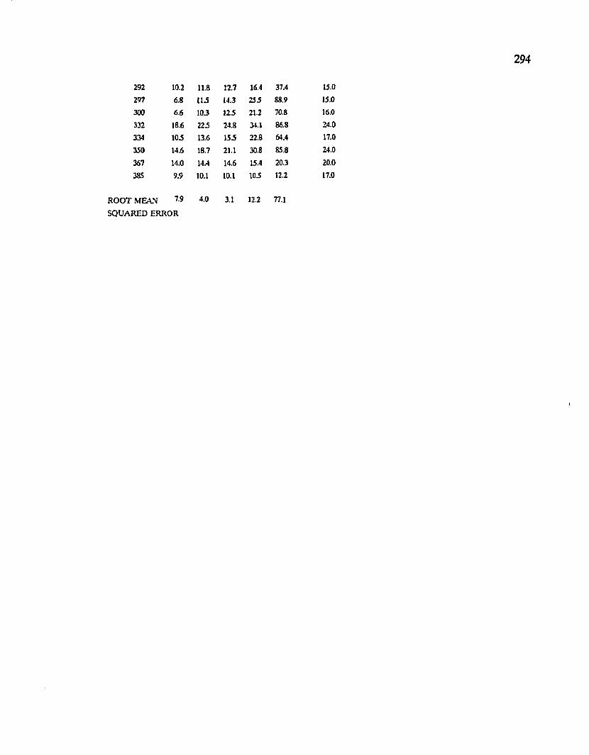
294
292 10.2
297 6.8
300 6.6
332 18.fi
334 10.5
350 14.6
367 14.0
385 9.9
ROOT MEAN 7 9 SQUARED ERROR
11.8 12.7 16.4
115 14.3 255
10.3 125 21.2
225 24.8 34.1
13.6 155 22.8
18.7 21.1 30.8
14.4 14.6 15.4
10.1 10.1 105
4.0 3.1 12.2
37.4 15.0
88.9 15.0
70.8 16.0
86.8 24.0
64.4 17.0
85.8 24.0
20.3 20.0
12.2 17.0
77.1

APPPENDIX 5a COMPUTER OUTPUT FOR SATLWATER INTRUSION
PROBLEM IN THE GONZALES-NEW ORLEANS AREA USING SUTRA MODEL
RESULTS F O R T IM E ST E P 240
T IM E IN C R EM EN T 25920D 406 SECONDS
ELA PSED T IM E : 6.2467D 4 08 SECONDS
L 0 4 U D 4 0 7 M INUTES
1.7352D+QS H O U R S
7.2300D403 DAYS
L0329D 403 W EEKS
2.37S4D402 MONTH IS
1.979SD401 YEARS
D R A W D O W N
N O D E N O D E N O D E NODI- N O D E N O D E
1 6.3Q577623D 4 00 2 6.98057332D 4 00 3 7.62843791D400 4 iB.24981861D400 S 8,851311670 4 00 6 9.437559891) i 00
7 1.00181776D + 01 8 1.07710B92D401 9 9.96198829D 4 00 10 9.34483855D 4 00 11 8.69201985D400 12 7.52303585111 («
13 6.33773337D+00 14 5.4356S896D 4 00 15 5.47772414D 4 00 ir. 3.89Q33825D400 17 3,20572627D 4 00 18 7.797466811 * u «
19 8.65663302D+00 20 9.5118205 ID 4 00 21 1.02009161D401 22 1.07344219D401 23 1.11827013D401 24 1.1591594111*01
25 1.1602S714D401 26 L125U744D4 01 27 1.05883198D 4 01 28 9.77036581D 400 29 8.B1743676D 400 30 7-80773O7KI1 * 00
31 6.95968193D 4 00 32 6.09S51766D 4 00 33 5 28388472D 4 00 34 4.6581B734D 400 35 8.87350503D 4 00 36 1.0S15477811,0)
37 1.18SU887D401 38 1.265478S1D401 39 L30244567D401 40 132391030D401 41 12385746111401 42 1,3234857311*01
43 1.27411387D401 44 1.20298275D401 45 1.US66922D401 46 1.019S5319D401 47 9.1869453611400 48 8.20UB031’ ! > * 00
49 7.25911299D400 50 6.32859132D400 51 5.33900898D400 52 985050698 D 4 00 53 1.28952I26D401 54 1.4855842111 Mil
55 154965971D + 01 56 156990599D+01 57 1578382310+01 58 156R29043D+01 59 152343920D+01 60 1.45552265D + 01
61 1371979640+01 62 U 7101803D +01 63 1.I618359ID +01 64 1.048346320+01 65 9.38372339D+00 66 831657254D+00
67 7.18481201D+00 68 6.2340308713+00 69 1.15S03649D+01 70 1.819259I5D+01 71 1.900I1470D+01 72 1.88875561D +01
73 1.8349986ID+01 74 1.85432327D+01 75 1.83963821D+01 76 1.78093421D+0! 77 1.688795070+01 78 I58194353D +01
79 1.46B62887D+01 80 1.33429247D+01 81 1.2031Q525D+01 82 1.076556020 + 01 83 954I43908D +00 84 8.24675786D+00
85 6.387598030+00 86 1336S8S42D+01 87 1,89853815D+01 88 1.91311497D+01 89 1.92187043D+01 90 2.09574872D+01
91 2.16228352D+01 92 2.13008075D+01 93 203423199D+01 94 1.912239I2D+01 95 1.78084585D +01 96 1.635B4B11D+01
97 1.48757842D+01 98 133893884D+01 99 1.19693711D+01 100 1.06126041D+01 101 'J.18296252D+00 102 7.82936048D+00
103 1.49008552D+01 104 1.88146136D +01 105 I.92678571D+01 106 2.02222839D+01 107 2.43202284D + 01 108 2.4754S641D+01
109 2.389188420 + 01 110 228386459D+01 U l 2.16722874D+01 112 1.9828745ID+01 113 1.814532140 + 01 114 1.64215769D+01
115 1.47822088D+0I 116 I3224127SD +01 117 1.17421931D+0I 118 1.030231060+01 119 8.76774557D+00 120 1.61825764D+01
121 1.91442197D+0I 122 2.197I923SD+01 123 260081620D+01 124 2.837818210+01 125 2.76454228D + 01 126 2.7227424SD+01
127 2.52157562D+0I 128 233913595D+01 129 2I7500456D +01 130 1.980212770+01 131 1.79590738D+01 132 1.617D0939D+0I
133 1.4476054011+01 134 1.28962723D+01 135 1.13942492D+01 136 9,964884110 + 00 137 1.740037000+01 138 2.074031420 + 01
139 2.39416046D +01 140 2.80693363D+01 141 3.0375B669D+01 142 3.139818320+01 143 2.991945910+01 144 2.75406890D+01
145 2.52339252D+01 146 232755534D+01 147 212857870D+01 148 1.93219950D+01 149 1.740049150+01 150 15S687408D+01
151 I.38735I94D +0I 152 123233603D+01 153 1.087I6232D+01 154 1.860S4733D+0I 155 2.10864943D+0I 156 256424553D +01
157 2.81949049D+01 158 3.03705296D+01 159 3.12776906D+01 160 3.074181530 + 01 161 2.92086251D +01 162 2.72487565D+01
163 2-52I91455D+0I 164 230606875D+01 165 209194676D +01 166 1,883009170 + 01 167 1.68574110D+01 168 150136745D+01
169 1..12977129D+01 170 1.17672764D+01 171 1.20960551D+01 172 2.345816330 + 01 173 2.62424419D+01 174 2.96927873D+0I
175 3.200707980+01 176 3323S2641D+01 177 3.29059415D +0I 178 3.14522278D + 01 179 2.941036620+01 180 2.76048507D+01
181 23033903017+01 1B2 226588430D+01 183 2034198460+01 184 13115803030 + 01 185 1.62097787D+OI 186 1.43I6S847D+01
187 1.24375040IJ+01 188 209500955D+01 189 2.335370600+01 190 2.762I7443D+01 191 3.152M177D+01 192 3.49341381 D + 01
193 3.66138979D+01 194 3.65188345D+01 195 3.431I5388D+01 196 3.149690790+01 197 2.89060489D+01 198 2.64999191D+01
199 2.40085I72D+01 200 2.152710I2D+01 201 1.91347912D+01 202 1.69977074D+01 203 1.49583664D + 01 204 1.30669993D+01
205 2.16660786D+01 206 2503988430+01 207 285981711D+01 208 334962222D+01 209 3.91099388D+01 210 421883709D+01
211 430176818D+01 212 3.67161021D+01 213 334258743D +01 214 3.050219S4D + 01 215 2.78323830D+01 216 250431489D+01
217 Z24161649D+01 218 1.99516486D +01 219 1.76834506D+01 220 1556I8995D + 01 221 134146749D+01 222 2.17180787D+01
223 250I07190D +01 224 2.88295816D+01 225 3.28336069D+01 226 3.66840168D+01 227 4.06304970D+01 228 4.12710070D+01
229 3.8591287013+01 230 356193990D +01 231 3.22275188D+0I 232 2.902448390 + 01 233 2585112190+01 234 230007455D+01
23S 2.04212166D+01 236 131062344D+01 237 159977883D+01 238 I.40003704D+01 239 2.168549790+01 240 2.47153582D+01
241 2.80078224D+01 242 3.17839144D+01 243 3.47756183D+01 244 3.76880567D+01 245 3.93173495D+01 246 4.17805743D+0I247 3.77403165D+OI 248 3.43992160D+01 249 3.05930034D+01 250 2.62947116D+01 251 232883661D+01 252 2.06491I28D+01
253 1.82903238D+01 254 1.61988125D+01 255 1.45446005D+01 256 2.15804485D+01 257 2.38161444D+01 258 2.68576525D+01
259 2.97682897D+01 260 3.27521540D+01 261 355318805D+01 262 3.92821596D +01 263 4.07012508D+01 264 3.97400772D+01
265 3.688I6394D+01 266 3.009314230+01 267 2.6269353ID+01 268 2.31769680D + 01 269 2.053I2813D+01 270 181758708D+0I
271 1.612717060*01 272 1.427S7645D+01 273 2.03545327D+01 274 2-22677451D + 01 275 2.4S988029D+01 276 2712564I2D+0I
277 2.97755R10D + 01 278 3.23484036D+01 279 3.44566436D+01 280 3.59606215D + D1 281 3.778265B9D+01 282 3284777H2D+01
283 2.92251745D+01 284 25S864576D+01 285 2.2639R62ID+01 286 2.009029820+01 287 I.77842023D+01 288 15749S713D+0I289 1.396207820+01 290 1R561461SD+01 291 2.04897381D+01 292 2.25133772D+01 293 246431946D+0I 294 2.68576023D+01
295 25781B757D+01 296 3.03338479D+01 297 3.14200174D+01 298 3.13689384D+01 299 3.Q5B25220D+01 300 27S209251D+01301 2.455488S3D+0I 302 2.178627080+01 303 1.93640064D + 01 304 1.71496619D+01 305 15I289965D + 01 306 1J35W591D +01307 1.701581160+01 308 1.866827610+01 309 2.04521237D + 01 310 27284127SD+01 311 2.40740883D + 01 312 257587489D+01313 2.7212412II) +01 314 22116859530+01 315 2870945610+01 316 2.79518590D+01 317 2.62534604D + 0I 318 232677196D+01319 2.0G979587D + 01 320 1H3921797D+G1 321 1.626403340+01 322 1.43304899D + 01 323 I24S03488D+01 324 1548532170+01
325 1.695355610+111 326 1.84516119D + 01 327 2.0I207906D+01 328 7166931310+01 329 231042915D + 01 330 2.446O6530D +01331 256230302D+0I 377 2.65651685D+0I 333 2.B3520775D+0I 334 2.45719321D+01 335 2173047860+01 336 1.936O9I66D + 01337 1.7203G598D+0I 338 1-51831970D+0I 339 IJ3139759D+01 340 1.178257100+01 341 1.42097148D+01 342 153259448D + 01343 1.657659660 + 111 >44 1.79530494D+0I 345 I.92414963D+01 346 203332879D+01 347 213332509D+01 348 2234800560+01349 2.404515680+01 350 25803407ID+0I 351 22Q526225D+01 352 1.98382569D+01 353 1.78520160D+01 354 159064093D+01355 1397055070+01 356 1.21746743D+01 357 1.03195347D+01 358 12R9S7473D+01 359 135I7R569D+01 360 1.48820728D+01361 1.602512530+01 362 1.7072Q576D+01 363 1.78516944D + 01 364 1.79922152D+01 365 1.88410491 D + 01 366 1.96I14I49D+01367 1.946R4075D + 01 368 1J19314233D+01 369 1.75272742D + 01 370 1.66076899D+OI 371 1.4680I6Q5D+01 372 12S486388D+01373 1.08975481D+01 374 9.35579426D+00 375 8.68724816D + 00 376 173632099D+01 377 I33357559D+01 378 1.42699488D+01379 151870644D+01 380 159650961D+0I 381 1.75253649D + 01 382 I.64321290D+01 383 I.9563I875D+0I 384 1.95I92412D+01385 1.66369423D+01 386 1.62343Z73D+01 387 1.73913597D+01 388 175438687D+G1 389 1.09262947D+0I 390 938005203D+00391 8.402602900+00
C O N C E N I R A T I O N
NODE NODE NODE NODE NODE NODE1 1.98749424D-03 2 1.71559347D-03 3 I.62930836D-O3 4 154407368D-03 5 124300592D-03 6 1.03887468D-03
7 5357407390-04 8 257541674D-04 9 216118629D-04 10 1.96435415D-04 11 1.77I37381D-04 12 I.68669335D-04
13 o.noooooooD-oo 14 O.OOOOOOOOD-OO 15 0.00000000D-00 16 0.00000000D4» 17 o.oomoonoD-oo 18 1.73S55602D-0319 1582255250-03 20 1320118400413 21 1.14513679D-03 22 957285070 D4M 23 7.20268279D-04 24 3.70069338D-0425 2605974210-04 26 217221289D-04 27 1.98841006D-04 28 1807144730-04 29 1396487670-04 30 O.OOOOOOOOD-OO
31 o.oooooonoD-oo 32 0.000000000-00 33 O.OOOOOOOOD-OO 34 O.OOOOOOOOD-OO 35 153042381D-03 36 I.41S62473D-0337 1.1427324504)3 38 92955832704)4 39 625529085D4M 40 3.937958S9D-04 41 3.04945629D-04 42 231096070D-0443 2.047710970-04 44 13575919704)4 45 1.044750550-04 46 O.OOOOOOOOD-OO 47 O.OOOOOOOOD-OO 43 O.OOOOOOOOD-OO49 O.OOOOOOOOD-OO 50 O.OOOOOOOOD-OO 51 O.OOOOOOOOD-OD 52 153727968D-Q3 53 1.20928463D-03 54 850730616D-O455 S.79639725D-04 56 353856868004 57 247558201 D-04 58 1.97764120D-O4 59 1.668142090-04 60 153834631D-OI61 I.07I242S7D4M 62 9.094256460415 63 O.OOOOOOOOD-OO 64 O.OOOOOOOOD-OO 65 O.OOOOOOOOD-OO 66 O.OOOOOOOOD-OO67 O.OOOOOOOOD-OO 68 0.000000000-00 69 1.07631390D-03 70 8.40496859D-04 71 3.77391832D-04 72 2.05457801 D-0473 2I5454S66D4M 74 1.86138367D-04 75 1.64804051D4M 76 1.46297260D-04 77 1.03734413D-04 78 859195990D-05

79 5.40695876D-05 80 O.OOOOOOOOD-OO 81 O.OOOOOOOOD-OO
85 O.nnoOOOOOD-OO 86 1.09633931D-03 87 5.4I6437I5D-04
91 1.1109250217-04 92 1.1O255067D-O4 93 9.417677SOD-05
97 O.OOOOOOOOD-OO 98 O.OOOOOOOOD-OO 99 O.OOOOOOOOD-OO
103 1.2894I483D-03 104 8.89533837D-04 105 2.71766609D-04
109 9.33317102D-OS 110 787907676D-05 111 6.32577807D-QS
115 O.OOOOOOOOD-OO 116 O.OOOOOOOOD-OO 117 O.OOOOOOOOD-OO
121 1.079547B3D-03 122 4.43137209D-04 123 2.44943360D-44
127 7.79148603D-OS 128 6.18101126D-05 129 O.OOOOOOOOD-OO
133 O.OOOOOOOOD-OO 131 O.OOOOOOOOD-OO 135 O.OOOOOOOOD-OO
139 7.87584740D-O4 140 3.61440484D-04 141 2.18679820D-W
145 7.78253914D-05 146 5.78433316D-05 147 O.OOOOOOOOD-OO
ISI O.OOOOOOOOD-OO 152 O.OOOOOOOOD-OO 153 O.OOOOOOOOD-OO
157 359119500D-04 158 1;79792381 D-04 159 1.0374167DD-04
163 5.00899366D-05 164 O.OOOOOOOOD-OO 165 O.OOOOOOOOD-OO
169 O.OOOOOOOOD-OO 170 O.OOOOOOOOD-OO 171 1.73069151D-03
175 1.88714149D-04 176 1J312S647D-04 177 9.70201071D-05
181 O.OOOOOOOOD-OO 182 O.OOOOOOOOD-OO 183 O.OOOOOOOOD-OO
187 O.OOOOOOOOD-OO 188 183011779D-03 189 1.69068691D-03
193 1.04901855D-04 194 7.95509566D-05 195 6.36508261 D-05
199 O.OOOOOOOOD-OO 200 O.OOOOOOOOD-OO 201 O.OOOOOOOOD-00
203 2.01060125D-03 206 1.83101936D-03 207 1.78315097D-03
211 8.6198666704)5 212 O.OOOOOOOOD-OO 213 O.OOOOOOOOD-OO
217 O.OOOOOOOOD-OO 218 O.OOOOOOOOD-OO 219 O.OOOOOOOOD-OO
223 2.I2797896D-03 224 1.77873708D-03 225 1.41382485D-03
229 95662S336D-OS 230 5.95924969D-0S 231 000000000D-00
23S O.OOOOOOOOD-OO 236 O.OOOOOOOOD-OO 237 O.OOOOOOOOD-OO
241 1.41597571 D-03 242 1.1O992O09D-O3 243 7.73831185D-04247 6.04217505D-05 248 O.OOOOOOOOD-OO 249 O.OOOOOOOOD-OO
253 O.OOOOOOOOD-OO 254 O.OOOOOOOOD-OO 255 C.OOOOOOOOD-00
259 1.02949524D-03 260 7.78636905D-04 261 4.86565408D-04
265 5.40691723D-OS 266 O.OOOOOOOOD-OO 267 O.OOOOOOOOD-OO
271 O.OOOOOOOOD-OO 272 O.OOOOOOOOD-OO 273 2.04954833D-03
277 7.92515080D-04 27B 622134374D-04 279 4.05535509D-04
283 6.63942555D-05 284 O.OOOOOOOOD-OO 285 O.OOOOOOOOD-OO
O.OOOOOOOOD-OO 83 O.OOOOOOOOD-OO 84 O.OOOOOOOOD-OO
2.67479788D-04 89 1.06620208D-04 90 I.11241339D-04
8.47938682D-05 95 7.08746231D-05 96 6-531921B8D-05
O.OOOOOOOOD-OO 101 O.OOOOOOOOD-OO 102 O.OOOOOOOOD-OO
2.08306729D-04 107 1.49624105D-04 108 1.16991631D-04
S.75133340D-05 113 O.OOOOOOOOD-OO 114 O.OOOOOOOOD-OO
O.OOOOOOOOD-OO 119 O.OOOOOOOOD-OO 120 1.79266320D-O3
1.78276128D-04 125 U3709690D-04 126 8.80437754D-05O.OOOOOOOOD-OO 131 O.OOOOOOOOD-OO 132 O.OOOOOOOOD-OO
O.OOOOOOOOD-OO 137 2^9391736D-03 138 1.92316411 D-03
IJ6073598D4M 143 1.29054348D-04 144 1.12837748D-04
o.ooooooooD-on 149 O.OOOOOOOOD-OO 150 O.OOOOOOOOD-OO
91|
155 1.06107616D-03 156 7.07582998D-04
9.91162806D-Q5 161 8.0065R846D-Q5 162 6.9I396163D-05O.OOOOOOOOD-OO 167 O.OOOOOOOOD-OO 168 O.OOOOOOOOD-OO
1.52669509D-03 173 6.4B055528D-04 174 3.12801422D-04
7J3437153D-05 179 5.26805543D-O5 180 O.OOOOOOOOD-OO
O.OOOOOOOOD-OO 185 O.OOOOOOOOD-OO 186 O.OOOOOOOOD-OO
1J0273007D-03 191 5.17882037D-O4 192 1.92529540D-O4
O.OOOOOOOOD-OO 197 O.OOOOOOOOD-OO 198 O.OOOOOOOOD-OO
O.OOOOOOOOD-OO 203 O.OOOOOOOOD-OO 204 O.OOOOOOOOD-OO
1.06541179D-03 209 5.219508I2D-04 210 2.01628815D-04
O.OOOOOOOOD-OO 215 O.OOOOOOOOD-OO 216 O.OOOOOOOOD-OO
O.OOOOOOOOD-OO 221 O.OOOOOOOOD-OO 222 2.20436092D-03
8.10856445D-04 227 4-38480788D-04 228 2.06192391D-04
O.OOOOOOOOD-OO 233 O.OOOOOOOOD-OO 234 O.OOOOOOOOD-OO
O.OOOOOOOOD-OO 239 2.03655332D-03 240 1.70610771 D-03
4.48565988D-04 245 2.65229797D-04 246 1.47369I60D-04O.OOOOOOOOD-OO 251 O.OOOOOOOOD-OO 252 O.OOOOOOOOD-OO
2.05128175D-03 257 1.68958963D-03 258 1.40118098D-03
3J3327942D-04 263 2J0289442D-04 264 9.99423070D-05
O.OOOOOOOOD-OO 269 O.OOOOOOOOD-00 270 O.OOOOOOOOD-00
1.645800R5D-03 275 1.42278215D-03 276 9.69721635D-04
2.79473803D-04 281 1.67898064D-04 282 8.19195384D-Q5
O.OOOOOOOOD-OO 287 O.OOOOOOOOD-OO 288 O.OOOOOOOOD-OO
82
8894
100IOS112118
124
130
136
142
148
134
160
166
172
178
184
190
196
202208214
220226
232
238
244250
236
262
268
274
280
286
289 O.OOOOOOOOD-OU 290 2.O4482380D-O3 291 1.63441074D-03 292 1.40871291 D-03 293 9.68244397D-04 294 7.88392182D-04
295 6.013957330-01 296 4.34484330D-04 297 3.077738700-04 298 1.87679129D-04 299 1.10854890D-Q4 300 833326881D-0S
301 7.52143209D-03 302 6.61220460D-05 303 O.OOOOOOOOD-OO 304 O.OOOOOOOOD-OO 305 O.OOOOOOOOD-OO 306 O.OOOOOOOOD-OO
307 2.0425057DD-03 308 1.61925885D-03 309 138612163D-03 310 1.0388I705D-03 311 8.02852203D-04 312 5.73214452D-04
313 4.90148566D-04 314 3,70917189D-04 315 2.41496753D-04 316 1.1918S935D-04 317 951B44793D-05 318 8.27114628D-05
319 7.206113570-05 320 O.OOOOOOOOD-OO 321 O.OOOOOOOOD-OO 322 O.OOOOOOOOD-OO 323 O.OOOOOOOOD-OO 324 2.03573070D-03
32S 1.618646900-03 326 138677099D-03 327 1.09422682D-03 328 8.69282699D-04 329 6.71018471D-04 330 5.83293324D-04
331 4.49087132D-04 332 3.4424173SD-04 333 1.94305496D-04 334 7.167S67D4D-05 335 7.78969280D-05 336 6.96709095D-05
337 6.77862235 D-05 338 S.31572257D-05 339 O.OOOOOOOOD-OO 340 O.OOOOOOOOD-OO 341 2.05584418D-03 342 1.75938313D-03
343 1.451300350-03 344 1.09635262D-03 345 8377211470-04 346 7J60S7911D-04 347 6.66601867D-O4 343 5.92489595D-04
349 4.881325640-04 350 3.43702465D-04 351 1.64327622D-04 352 9.43912720D-0S 353 8.68480308D-05 354 7.62896996D-05
355 6.734278520-05 356 5.44026381D-O5 357 O.OOOOOOOOD-OO 358 232497192D-03 359 2.11264367D-03 360 1.63742237D-03361 1.113207300-03 362 930637329D-04 363 8.12648797D-04 364 7.327746S8D-04 365 6.82355498D-04 366 5.8388I556D-04
367 4.101237890-04 368 1.97450113D-W 369 1.79834350004 370 7.77408167D-OS 371 7.45380531D-05 372 6.82111109D-05
373 6.7B825959D-05 374 5-86231312D-OS 375 2.40185047D-03 376 2.07099600D-03 377 1.62607839D-03 378 l.22979787D~03379 8543025920-04 380 7.93397646D-04 381 73I928992D-04 382 7.019213830-04 383 7.03694393D-04 384 3.38721567D-04385391
2582606.Vi 0-04
5.77785942D-0S
386 238206778 D-04 387 1.64011103D-04 388 7,938843120-05 389 6.83810818D-05 390 6.82193304D-05

APPENDIX 5b COMPUTER OUTPUT FOR SALTWATER INTRUSION PROBLEM IN TH E GONZALES-NEW ORLEANS AREA USING STRALAN MODEL
RESULTS F O R T IM E STEP 240
TIME INCREMENT 25920D+06 SECONDS
ELA PSED T IM E : 6.2467D+08 SECON DS
1.0411D + 07 M INUTES
1.7352D + 05 HO U RS
7.2300D + 03 DAYS 1,03290+03 W EEKS
2.3754D + 02 M ONTHS
1.9795D + 01 YEARS
D R A W D O W N
N O D E N O D E N O D E N O D E N O D E N O D E
1 6.30577623D + U0 2 6.98057332D + 00 3 7.62K43791D + 00 4 8.2498186ID + 00 S 8.851311670 + 00 6 9 437559800 + 00
7 1.00181776D + 01 8 1.07710B92D + 01 9 9.9619H829D + 00 10 9,344838550+00 11 8.692019850 + 00 12 7.52303585D + 00
13 6.33773337D ♦ 00 14 5.43565896D+00 15 5.47772414D + 00 16 3.8903382SD+00 17 3.20572627D + 00 18 7.7974668313 + 00
19 8.65663302D + 00 20 9.5U82051D+00 21 1.02U09161D + 0I 22 1.073442I9D+01 23 1.1182701311 +01 24 1.1591594)11 +01
25 1.16025714D + 01 26 I.I25U 744D + 01 27 1.05H83198D+01 28 9.77036581D+00 29 8.81743676D + 00 30 7.807736.181) +00
31 6.95968193D + 00 32 6.09B51766D+00 33 5.28388472D+00 34 4.65818734D+00 35 8.873505031) + 00 36 1.051547780 + 01
37 1.18SUB87D + 01 38 I.26S47851D + 01 39 1.30244567D + 01 40 1.32391030D + 01 41 1.338574610 + 01 42 1.323485710 + 01
43 1.2741I387D + 01 44 1.20298275D + 01 45 1.11566922D + 0I 46 I.019S53I9D+01 47 9.186944361) + 00 48 8.200803170 + 00
49 7.25911299D + 00 50 6.32859132D +00 51 S.33900898D + 00 52 9.6S050698D+00 S3 1.289521260 + 01 54 1.4855842ID+01
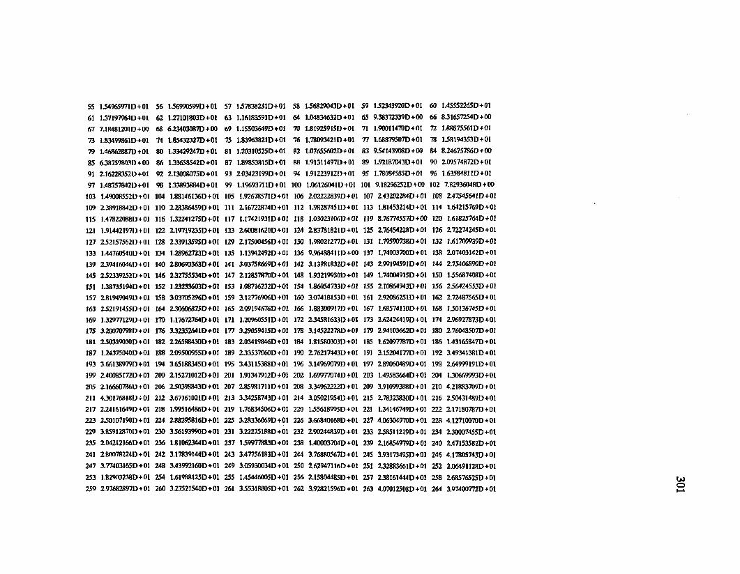
55 1.S496S971D+01
61 1.37197964D+01
67 7.184812010 + 00
73 1.83499861D+01
79 1.46862887D+01
85 6.38759803D+00
91 2162283520+01
97 1.48757842D+01
103 1.4900R552D+01
109 2.389188420 + 01
115 1.478220880 + 01
121 1.914421970+01
127 2521575620 + 01
133 1.447605400+01
139 2.394160460 + 01
145 252339252D+01
151 1587351940+01
157 28I949049D +01
163 2521914550+01
169 152977129D+0I
175 3.200707980+01
181 250339030D + 0!
187 1.24375040D+01
193 3.66138979D+01
199 2.40085I72D+01
205 2166607860+01
211 4.301768180+01
217 2.241616490+01
223 250107190D + 01
229 3.8S9128700 + 01
235 2042121660+01
241 2.800782240 +01
247 3.77403I65D+01
253 1.82903238D+01
259 2.976828970 + 01
56 15699Q599D+01
62 1-2710I803D+0!
68 623403087D+OG
74 1.85432327D+01
80 153429247D+01
86 133658542D+01
92 213008075D +01
98 1538938840+01
104 158146136D+01
110 228386459D+01
116 I52241275D +0I
122 219719235D+01
128 253913595D+01
134 128962723D+01
140 280693363D+01
146 232755534D+01
152 I23233603D +01
158 3.0370S296D+01
164 23060687JD +01
170 1.17672764D+01
176 3523526410+01
182 2265884300+01
188 209500955D +0I
194 3.6S188345D +01
200 2152710I2D +01
206 250398843D+01
212 3.67161021D+01
218 I.99516486D+01
224 288295816D+01
230 356193990D+01
236 1.81062344D+01
242 3.17839144D+01
248 3.43992160D+01
254 1.61988125D+01
260 3.27521540D+01
57 1J7838231D +0I
63 1.16183S91D+01
69 1.15503649D+0I
75 1.83963821D+01
81 1.20310525D+01
87 1.89853815D+01
93 203423199D+01
99 1.196937I1D+01
105 I.9267857ID +01
111 2.16722874D +01
117 1.17421931D+01
123 26G081620D+01
129 2.I7500456D+01
135 1.13W 2492D+0I
141 3.03758669D+01
147 2.12857870D+01
153 1.08716232D+01
1S9 3,12776906D+01
165 209194676D+01
171 1.209605S1D+01
177 3.290I59415D+OI
183 2.03419846D+01
189 2.33537060D+01
195 3.43115388D +01
201 1.91347912D+01
207 283981711D+01
213 334258743D+01
219 1.76834506D+01
225 3.28336069D+01
231 3.22275188D+01
237 159977883D+01
243 3.47756183D+01
249 3.05930034D+01
255 I.45446005D+01
261 3J5318805D +01
58 1568290430+01
64 1.04834632D+01
70 1.8192S915O+01
76 1.78093421D+01
82 1.07655602D + 01
88 1.91311497D + 01
94 1.912239120 + 01
100 1.06126O41D+0I
106 202222839D+01
112 1.982874510 + 01
118 1.03023106,0+01
124 283781821D+01
130 1.98021277D+01
136 9.96488411D+00
142 3.139818320+01
148 1.93219950D+01
154 1.860547330 +01
160 3.07418153D+01
166 1.883009170+01
172 2.345816331)+01
178 3.145222780+01
184 1.815803030 +01
190 2.762174430+01
196 3,149690790+01
202 1.699770740 + 01
208 3.34962222D+01
214 3.05021954D+01
220 155618995D+01
226 3.66840I68D +01
232 2902448390+01
238 1.40003704D+01
244 3.76880567D+01
250 2.62947116D+01
256 215B04485D+01
262 3.92821S96D+01
59 1J2343920D +0I
65 958372339D+00
71 1.90011470D+01
77 1.68879507D+01
83 954143908D+00
89 1.92187043D+01
95 1.78084585D+01
101 9.18296252D+00
107 243202284D+01
113 1.81453214D+01
119 8.76774557D+00
125 276454228D+01
131 1.79590738D+01
137 1.740037D0D+01
143 299194591D+01
149 1.740O4915D+01
155 210864943D+01
161 2.92086251D + 01
167 1.68574110D+01
173 2.62424419D+01
179 2.94103662D+01
185 1.620977B7D + 01
191 3.15204177D+01
197 2.89060489D+0I
203 1.49583664D+01
209 3.91099388D+01
215 278323830D+01
221 154146749D+01
227 4.06304970D+01
233 258511219D+01
239 2I6854979D +01
245 3.93173495D+01
251 252883661D+01
257 238161444D+01
263 4.07012508D+01
60 1.45552265D+01
66 B.316572S4D+00
72 1.88875561D+01
78 158194353D +0I
84 8.246757B6D+00
90 209574B72D+01
96 1.63584811D+01
102 7.82936048D+00
108 2475456410+01
114 1.64215769D+01
120 1.61825764D+01
126 272274245D+01
132 1.61700939D+01
138 2.07403142D + 01
144 2.75406890D+01
150 1J5687408D +01
156 256424553D+01
162 2.72487565D+01
168 U0136745D +01
174 296927873D+01
180 2760485070+01
186 1.43165847D+01
192 3.49341381D+01
198 264999191D+01
204 1J0669993D +01
210 4.21883709D+01
216 2504314R9D+01
222 217180787D+01
228 4.I2710070D+01
234 2J0007455D +01
240 247IS3582D +01
246 4.17805743D+01
252 2.06491128D +01
258 26857652SD+01
264 3.9740O772D+01

265 3.688163940+01 266 3.00931423D+01 267 267693531D+01 268 2317696R0D+01 269 2053128130+01 270 IBITSBTORO+Ol
271 1.612717061)4 01 272 1.42757645D + 0I 273 2.03S4J327D+01 274 2.226774510+01 275 2.459880290 + 01 276 2712564120+01
277 2 97755111(111« 0 | 278 3.234R4036D+0I 279 3.44566436D+0I 280 3.596062 ISO+01 281 3.77B265R9D+OI 282 3.28477782D+0I
281 2.922517450*01 284 2358645760+01 285 226198621D+01 286 2009029820 + 01 287 1.77842023D+0I 288 1574957130+01289 1396207820*01 290 1.856146150 + 01 291 2OW 7381D+01 292 2251337720+01 293 2464319460+01 294 2.685760230 + 01295 2.878187570*01 296 3.033384790+01 297 3.142001740+01 298 3.13689384D+0I 299 3.05825220D+01 100 2.75209251D+01101 2.455488530 * 01 102 2178627080+01 303 1.93640064D+01 304 1.71496619D + 01 305 1.S12B9965D+01 306 133504S91D+01.107 1.701581160 *01 KIR 1.866827610 + 01 309 2.04521237D+0I 310 222841275D+01 311 2.40740RR1O + 01 312 2575R7489D+01113 2.721241210*01 314 2816859510 + 01 315 2.87094561 D + 01 316 2.7951B590D+01 317 2.625346040+01 318 232677196D+01119 2.069795870+01 320 183921797D + 01 321 I.62640134D+0I 322 1.43304899D+01 32) 1.245034880+01 324 154853217D+01125 1.695355610+01 326 1JV45161I9D + 01 327 2.01207906D+01 328 2166931310+01 329 2.31042915D+01 330 244606530D+01111 2J623O102D+0I 312 2656516850 + 01 333 2.81520775D + 01 314 2.45719321D+01 315 2171047B6D + 01 336 1.91609166D+0I337 1.7203059BD+01 118 1518319700+01 339 1.331397590 + 01 340 1.I782S71OD+0! 341 1.42097I48D + 01 342 153259448D+0I341 1.657659660+01 344 1.79530494D+01 345 1.924149*30*01 346 203332879D+01 347 2.13332509D+01 348 2214800560+01349 2.4O45156HD+0I 350 2580340710+01 351 220526225D+01 352 1.98382569D + 01 151 I.78520160D+01 354 159064093D+0I355 1397055070 + 01 356 1.217467430 + 01 357 1.031953471)+01 358 1.28957473D + 01 359 1.3517H569D + 0J 360 l.4R820728D+nt161 I.60251253D + OI 162 1.707205760+01 363 1.785169440+01 364 1.799221S2D + 01 365 1.884104910 + 01 366 1.96114149D+01367 1.94684075D + 0I V<8 1 .R9314231D+QI 369 1.75272742D+01 370 1.660768990+01 371 1.468016050 + 01 372 1.25486388D+01373 1.0K975481D+OI 374 9.355794260 + 00 375 H.68724816D+00 376 1.23632099D+01 377 1331575590 + 01 378 I.42699488D+01179 1-SIR70M4DXII 180 159650961D + 0I 381 1.75151649D + 0I 382 1.643212900+01 383 1.9563IB75O + 01 184 1.951924120+01IBS391
[.661694210 +01
8.402602900 + 00
386 1.623432730 + 01 387 1.739I3597D + 0I 388 I.25438687D+01 389 I.1N262947D+ 01 390 9.38005203D+00
C O N C r. N r R A T I O N
NODE NOI1H NODF. NODE NODE NODE
1 1.9874942404)3 2 1.7155934704)1 3 1.6293083604)3 4 154407368D-03 5 1.243005920-03 6 1.0388746804)37 5.157407190-04 8 2575416740-04 9 21611862904)4 10 1.96435415D-04 11 1.7711718104)4 12 1.686693350-04
13 0.0000000004*1 14 0.0000000004)0 15 O.OOflOOOOOD4» 16 0.0000000004)0 17 O.OOOOOOOOD-OO IB 1.71R5560204)1
19 1582255250-01 20 1-1201184004)1 21 1.1441367704)3 22 9.3728507004)4 23 7.2026827904)4 24 3.700693380-04
25 2.605974210-04 26 2172212890-04 27 1.98841006D-04 28 1.80714473D-04 29 1.39648767D-04 30 0.00000000043)
31 o.ooonnoono-on 12 O.OOOOOOOOD-OO 33 OOOOOOOOOD-OO 34 O.OOOOOOOOD-OO 35 15301238! 04)3 36 1.4I562473O-03
17 1.1427324504)3 IB 9.295583270-04 39 6.2S5290RSD-04 40 3.9379585904)4 41 3.049456290-04 42 2J1 0960700-04
43 2.0477109704)4 44 15575919704)4 45 1.044750550-04 46 onooonoooD-oo 47 0.(33333331043) 48 0.000000000-00
49 0.000000000-00 SO 0.000000000-00 51 O.OOOOOOOOD-OO 52 1.237279680-03 53 1.2092846104)3 54 B.5073061604M
55 5.7963972304)4 56 3538568680-04 57 2.47558201 D-04 58 1.97764120D4M 59 1.668142(3) D-04 60 1.31834611D4M
61 1.071242570 4M 62 9.094256460-05 63 0.(333*33)004)0 64 0.(333333)00-00 65 0.00133333)043) 66 0.00000(3*1043)
67 n.oon 0000043) 68 0.00000000043) 69 1.0763119004)3 70 8.4049685904)4 71 3.7739181204M 72 2.054578010-01
73 2.15454566D4M 74 1.861383670-04 75 1.64H0405 ID-04 76 1.46297200D4H 77 I.0173W13O4M 7R 8.2919599004)5

79 5.40895876 D-06 80 O.OOOOOOOOD-OO 81 O.OOOOOOOOD-OO
65 O.OOOOOOOOD-OO 86 1.09633931D-03 87 5.4I6437I5D-0491 1.11092S02 D-04 92 1.10255067D-04 93 9.41767750D-05
97 0.00000000040 98 O.OOOOOOOOD-OO 99 O.OOOOOOOOD-OO
103 1.28941483D-03 104 8-89533837D-04 IDS 2.71766609D-04109 9.33317102D-QS 110 7.B7907676D-05 111 6J2577807D-0S115 O.OOOOOOOOD-OO 116 O.OOOOOOOOD-OO 117 O.OOOOOOOOD-OO
121 1.07954783D-03 122 4.43137209D-04 123 1 o *
127 7.791486Q3D-05 128 6.18101126D-0S 129 O.OOOOOOOOD-OO133 O.OOOOOOOOD-OO 134 0.0000000004)0 135 O.OOOOOOOOD-OO139 7.87584740D-O4 140 3,61440484D-04 141 2.1B679820D-04
145 7.78253914D-G5 146
9Q1w> 147 O.OOOOOOOOD-OO
151 O.OOOOOOOOD-OO 152 O.OOOOOOOOD-OO 153 O.OOOOOOOOD-OO
157 359U9500D-04 158 1.79792381D4J4 159 1.03741670D-04163 5.00899366D-05 164 O.OOOOOOOOD-OO 165 O.OOOOOOOOD-OO
169 000000000D-00 170 O.OOOOOOOOD-OO 171 1.73069151D-03175 1.88714I49D-G4 176 1J3125647D-04 177 9.7020I071D-05
181 O.OOOOOOOOD-OO 182 O.OOOOOOOOD-00 183 0.000000000-60187 O.OOOOOOOOD-OO 188 1.8301177913-03 189 1.69068691D-03
193 1.049018SSD-04 194 7.95509S66D-05 195 6.36508261D-05
199 O.OOOOOOOOD-OO 200 O.OOOOOOOOD-OO 201 OOOOOOOOOD-OO
205 2.01060125D-03 206 1^31019360-03 207 1.783I5097D-03
211 8^19866670-05 212 O.OOOOOOOOD-OO 213 O.OOOOOOOOD-OO
217 O.OOOOOOOOD-OO 218 0.000000000-00 219 O.OOOOOOOOD-OO
223 212797896D-03 224 1.77873708D-03 225 1.41382485D03
229 956625336D-05 230 5.95924969D-05 231 O.OOOOOOOOD-OO
235 O.OOOOOOOOD-OO 236 O.OOOOOOOOD-OO 237 O.OOOOOOOOD-OO
241 1.41597571 D 43 242 1.10992009D-03 243 7.7383118SD-04
247 6.01217505D-05 248 OOOOOOOOOD-OO 249 O.OOOOOOOOD-OO
253 OOOOOOOOOD-OO 254 O.OOOOOOOOD-OO 255 O.OOOOOOOOD-OO
259 1.02949524D-03 260 7.78636905D-04 261 4865654080-04
265 S.40691723D-05 266 O.OOOOOOOOD-OO 267 O.OOOOOOOOD-OO
271 O.OOOOOOOOD-OO 272 O.OOOOOOOOD-OO 273 204954833D-03
277 7.9251S080D-04 278 6.22I34374D-04 279 4.QS535S09D-CH
283 6.63942555D-05 284 O.OOOOOOOOD-OO 285 O.OOOOOOOOD-OO
OOOOOOOOOD-OO 83 O.OOOOOOOOD-OO 84 O.OOOOOOOOD-OO
2.67479788D04 69 1.06620208D-04 90 1.11241339D-04
8.47938682D-0S 95 7.08746231D-Q5 96 653192188 D-05
O.OOQOQOOOD-OQ 101 O.OOOOOOOOD-OO 102 O.OOOOOOOOD-OO
2.06306729D-04 107 1.49624105D-04 108 1.1699163 ID-04
S.7S133340D-OS 113 O.OOOOOOOOD-OO 114 O.OOOOOOOOD-OOO.OOOOOOOOD-OO 119 O.OOOOOOOOD-OO 120 1.79266320D-03
1.78276128D-04 125 1.33709690D-O4 126 B-B0437754D-OSO.OOOOOOOOD-OO 131 O.OOOOOOOOD-OO 132 O.OOOOOOOOD-OOO.OOOOOOOOD-OO 137 2.29391736D-03 138 1.9231641 ID-03
156073S98D-04 143 1-29054348D-O4 144 1.I2837748D-04O.OOOOOOOQD-OO 149 O.OOOOOOOOD-OO ISO O.OOOOOOOOD-OO
1.79275690D-03 155 1.06107616D-03 156 7.07582998D-04
9.911628060-05 161 8.006S8846D-05 162 6.91396163D-05O.OOOOOOOOD-OO 167 O.OOOOOOOOD-OO 168 O.OOOOOOOOD-OO
1.52669509D-03 173 6.4805S528D-04 174 3.I2801422D-047J3437153D-05 179 5.26805S43D-0S 1B0 O.OOOOOOOOD-OO
O.OOOOOOOOD-OO 185 O.OOOOOOOOD-OO 186 O.OOOOOOOOD-OO
130273007D-03 191 5.17882037D-04 192 1.92529540D-04
O.OOOOOOOOD-OO 197 O.OOOOOOOOD-OO 198 O.OOOOOOOOD-OOO.OOOOOOOOD-OO 203 O.OOOOOOOOD-OO 204 O.OOOOOOOOD-OO
1.06S41179D-03 209 5.21950612D-04 210 2.01628815D-04O.OOOOOOOOD-OO 215 O.OOOOOOOOD-OO 216 O.OOOOOOOOD-OO
O.OOOOOOOOD-OO 221 O.OOOOOOOOD-OO 222 2.20436O92D-03
8.10856445D-O4 227 433480788D-04 228 206192391 D-04O.OOOOOOOOD-OO 233 O.OOOOOOOOD-OO 234 O.OOOOOOOOD-OO
O.OOOOOOOOD-OO 239 2.03655332D-03 240 1.70610771 D-03
4.48565988D-04 245 2.65229797D-04 246 1.4736916QD-04O.OOOOOOOOD-OO 251 O.OOOOOOOOD-OO 252 O.OOOOOOOOD-OO
2.05128175D-03 257 1.68958963D-03 258 1.4011809BD-03
353327942D4M 263 2.20289442D-04 264 9.99423070D-05
O.OOOOOOOOD-OO 269 O.OOOOOOOOD-OO 270 O.OOOOOOOOD-OO
1.645S0085D-03 275 1.4227B215D-03 276 9.6972163SD-04
2.79473803D-04 281 1.67898064D-04 282 8.I9195384D-05
O.OOOOOOOOD-OO 287 O.OOOOOOOOD-OO 288 O.OOOOOOOOD-OO
82
8894
100
106
112118
124
130
136
142
148
154
160
166
172178
184
190
196202208
214
220226
232
238
244
250
256
262
268274
280
286
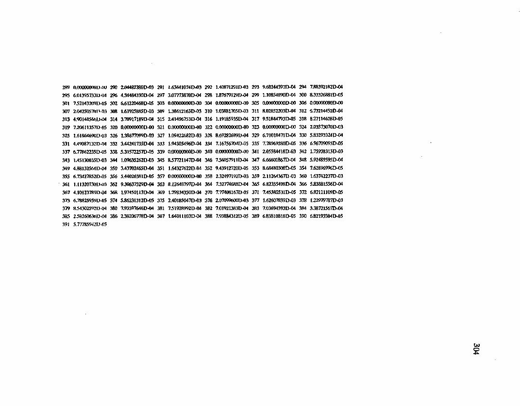
289 0.00000000(1-00 290 2.04482380D-03 291 1.63441074D-O3 292 1.40871291D-03 293 9.68244397D-04 294 7.B8392182D-04
295 6.01395733D-04 296 454484330D-04 297 3.07773870D-O4 298 1.8767912917-01 299 1.10854890D-04 300 8.33326881D-05
301 75214320911-05 302 6.61220460D-Q5 303 O.OOOOOOOOD-OO 304 O.OOOOOOOOD-OO 30S O.OOOOOOOOD-OO 306 O.OOOOOOOOD-OO
307 2.0425057011-03 308 1.61925885D-03 309 138612163D-03 310 1.03881705(1-03 311 B.028S2203D-O4 312 6.73214452D-04
313 4,9014856617-04 314 3.70917189D-O4 315 2.41496753D-04 316 1.19185935D-04 317 951844793D-05 318 8.27114628D-05
319 7.2061135711-05 320 0.000000000-00 321 O.OOOOOOOOD-OO 322 O.OOOOOOOOD-OO 323 O.OOOOOOOOD-OO 324 2.03573070D-03
325 I.61864690D-03 326 1.38677099D-03 327 1.09422682D-03 328 8.6928269911-04 329 6.71018471D-04 330 533293324D-04
331 4.49087132DJM 332 3.44241735D-04 333 I.9430S496D-04 334 7.16756701 D-05 335 7,78969280D-05 336 6.96709095D-05
337 6.77862235D-OS 338 5.315722S7D-05 339 O.OOOOOOOOD-OO 340 O.OOOOOOOOD-OO 341 2.05584418D-O3 342 1.759383I3D-03
343 1.45130O35D-O3 344 1.09635262D-03 345 857721147D-04 346 756057911D-04 347 6.66601867D-04 348 5.92489595D-04
349 4.8813256411-04 350 3.4370246SD-04 351 1.64327622D-04 352 9.43912720D-O5 353 8.68480308D-05 3S4 7.62896996D-05
355 6.73427852D-05 356 5.44026381D-05 357 O.OOOOOOOOD-OO 358 I32497192D-03 359 2.11264367D-03 360 1.63742237D-03
361 1.1I320730I1-O3 362 950637329D-04 363 8.12648797D-04 364 7J2774688D-04 365 6.82355498D-04 366 5.83881556D-04
367 4.10I23789D-W 368 1.97450113D-04 369 1.79834350D-04 370 7.77408167D-05 371 7.45380531D-OS 372 6.82U1109D-fi5
373 6.788259590-05 374 5.86231312D-05 375 2.40185047D-03 376 2.07099600D-03 377 1.62607B39D-O3 378 1.22979787D-03
379 854302592(1-04 380 7.93397646D-04 381 751928992D-04 382 7.01921383D-04 383 7.03694393D-04 384 3-38721567D-04
385391
25826063611-04
5.7778594211-05386 2.38206778D-04 387 1.64011103D-04 388 7.93884312D-05 389 6.83810818D-05 390 6.82193304D-OS
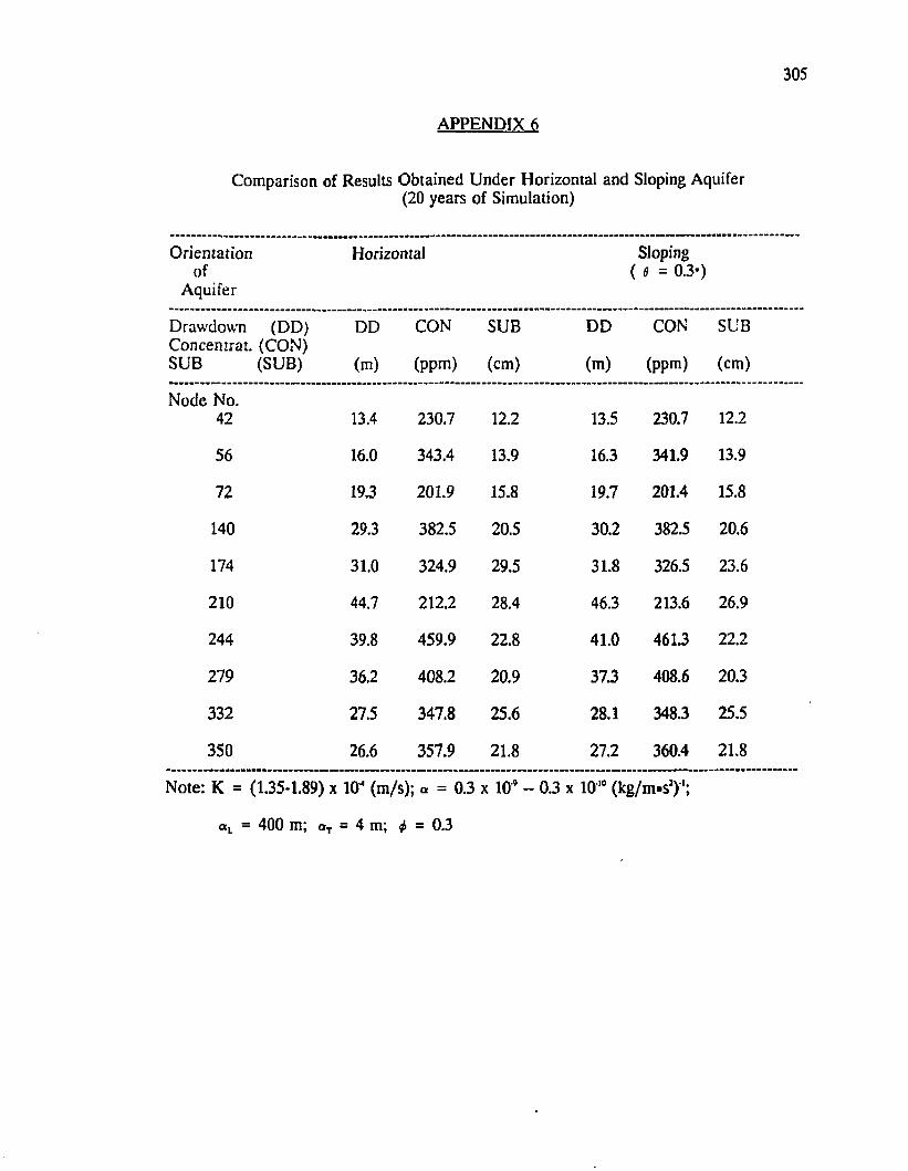
305
APPENDIX 6
Comparison of Results Obtained Under Horizontal and Sloping Aquifer(20 years of Simulation)
Orientation Horizontal Slopingof ( 9 = 0.3»)
Aquifer
Drawdown (DD) Concentrat. (CON) SUB (SUB)
DD
(m)
CON
(ppm)
SUB
(cm)
DD
(m)
CON
(ppm)
SUB
(cm)
Node No. 42 13.4 230.7 12.2 13.5 230.7 12.2
56 16.0 343.4 13.9 16.3 341.9 13.9
72 19.3 201.9 15.8 19.7 201.4 15.8
140 29.3 382.5 20.5 30.2 382.5 20.6
174 31.0 324.9 29.5 31.8 326.5 23.6
210 44.7 212.2 28.4 46.3 213.6 26.9
244 39.8 459.9 22.8 41.0 4613 22.2
279 36.2 408.2 20.9 37.3 408.6 20.3
332 27.5 347.8 25.6 28.1 348.3 25.5
350 26.6 357.9 21.8 27.2 360.4 21.8
Note: K = (1.35-1.89) x 10- (m/s); a = 0.3 x 10'9 - 0.3 x 10 '° (kg/m*sJ) ';
«L = : 400 m; aT = 4 m; <j> = 0.3

306
APPENDIX 7
B 7.K JK 3B K 3 : J12 R R R
s«ne»iE 0S 5ieA inw a. R®«*ueis BAH, « * « - * * * « in sft£ m , $ a:=F«w iisfte«sa£ .
tt**H®±ifi«g1S:JMf5=tt. fiAftjt u Z A f c P
* « e £ * . *®.*a«"
$ c ttlS*AaWH&»ftn, «iF*&8Pfl:T
» r p f 0 & t s , usT+issRiaitJsiaTifeiB m e-AAS^*Stft*JfijBiiE»MjSI-
m d & t * , A®, nt«, *«3?*kSffifcttSAf-fcffWtS, (H
sififc-M S^s.'f^saws. f lE t t ia ^ - . ^A ssT W w e. » « « * » * , m ® u G * * - n n w im 'p r n m w h f r t f A '
n N w * m , m zttA v .fcw ztE K
ig£/IK ?
Newspaper clipping from "People’s Daily", January 22, 1988. The heading is " Serious Shortage Situation of Water Resources in China. Red light warnings are blazing in two hundred cities". It points o u t:" In Shanghai, overdrafting of ground water resulted in land subsidence. Accumulative maximum subsidence since 1965 has reached 2.63 meters. Based on the same reason, Tianjin, Xian, Changzhou and Ningbuo cities are still experiencing land subsidence.

APPENDIX 8
n ~ + s . B i ie tw K if iiW J , ~ A > \n (ie«**«) xmam, , , . n -, ,
mmmuasafflsxfiiftfls, **«im BIR gI f t „ £ ® M iE « |ll i7 if iT *
misa*ttBEW itM ffiW iTF*#
& m m r ± & t n m , x
W, -*.A**F-8-*A£*tte,+ E * * , *}SE*F$iJE»M
«m
Newspaper clipping from "People’s Daily", January 26,1988. The heading is "Significant result in the control of land subsidence in Tianjin City". It reports: " Based on Tianjin governmental statistics, the land subsidence in this city is continuing to slow down in 1987. The average subsidence in the city proper is 43 mm, being reduced by 19 mm as compared to the previous year".

VITA
Song-kai Yan was born on January 12, 1942. He attended Presbyterian Boys’
School and St. Andrew School in Singapore from 1952 to 1956. In April 1956, he
was sent to China and attended Beijing No. 37 High School, from which he
graduated in 1959. In 1964, he obtained his B.Sc. in Civil Engineering from Beijing
Institute of Hydraulic Engineering.
He then served at Hai River Design Institute (later changed its name to
Tianjin Design Institute) under the Ministry of Water resources and Power as an
engineer. He came to the United States as a visiting scholar to Colorado State
University in 1981. He changed his status to graduate student, majoring in water
resources and hydrology and got his M.S. degree from the Department of Civil
Engineering, Colorado State University in 1983. He went back to China in 1983 and
served in the same agency for two years before coming to Louisiana State University
to pursue his Ph.D degree in Civil Engineering Department in 1986. During his stay
here at LSU, he also worked part time at Woodward-Clyde Consultants in Baton
Rouge up to now.
His professional experience includes planning and design of dams and
reservoir; river hydrology and hydraulics; ground water hydrology; water resources
planning and management; surface and ground water modeling; contaminant
transport; land subsidence modeling; saltwater intrusion modeling; ground water
assessment; hazardous waste permitting; data management and computer graphics.
308

Candidate:
M ajor Field:
Title of Dissertation:
DOCTORAL EXAMINATION AND DISSERTATION REPORT
Song-kai Yan
Civil Engineering
Land Subsidence and Saltwater Intrusion in Coastal Areas
Approved:
Major Professor and Chairman
if,Dean of the Graduate
EXAM INING CO M M ITTEE:
f
Date of Examination:
July 24, 1989