
Design, implementation and simulation of intrusion detection ...
54
MASARYKOVA UNIVERZITA FAKULTA INFORMATIKY Design, implementation and simulation of intrusion detection system for wireless sensor networks MASTER’ S THESIS Bc. Lumír Honus Brno, spring 2009
-
Upload
khangminh22 -
Category
Documents
-
view
3 -
download
0
Transcript of Design, implementation and simulation of intrusion detection ...
MASARYKOVA UNIVERZITA
FAKULTA INFORMATIKY
}w���������� ������������� !"#$%&'()+,-./012345<yA|Design, implementation and simulation of
intrusion detection system for wirelesssensor networks
MASTER’S THESIS
Bc. Lumír Honus
Brno, spring 2009

Declaration
Hereby I declare, that this paper is my original authorial work, which I have worked out by my own. Allsources, references and literature used or excerpted during elaboration of this work are properly citedand listed in complete reference to the due source.
Advisor: RNDr. Andriy Stetsko
ii

Acknowledgement
I would like to express my thanks to my supervisor RNDr. Andriy Stetsko and to Bc. Barbora Micenková.I am gratefull to Bc. Jana Jourová for moral support.
iii

Abstract
In this master’s thesis, a simple intrusion detection system (IDS) for wireless sensor networks is designedand implemented. The proposed IDS is based on watchdog monitoring technique and is able to detectselective forwarding attacks.
Besides, the improvements that make watchdog monitoring technique more reliable are describedand the results of simulations of the IDS on TOSSIM simulator are presented.
iv

Keywords
Wireless Sensor Networks, Intrusion Detection System, Watchdog Monitoring Technique
v
Contents
1 Introduction . . . . . . . . . . . . . . . . . . . . . . . . . . . . . . . . . . . . . . . . . . . 32 Wireless Sensor Networks . . . . . . . . . . . . . . . . . . . . . . . . . . . . . . . . . . . . 4
2.1 Applications . . . . . . . . . . . . . . . . . . . . . . . . . . . . . . . . . . . . . . . . . 42.2 Hardware Platforms . . . . . . . . . . . . . . . . . . . . . . . . . . . . . . . . . . . . . 52.3 Security Objectives . . . . . . . . . . . . . . . . . . . . . . . . . . . . . . . . . . . . . 62.4 Attacker model . . . . . . . . . . . . . . . . . . . . . . . . . . . . . . . . . . . . . . . 62.5 Possible Attacks . . . . . . . . . . . . . . . . . . . . . . . . . . . . . . . . . . . . . . . 7
3 TinyOS . . . . . . . . . . . . . . . . . . . . . . . . . . . . . . . . . . . . . . . . . . . . . . 83.1 Versions . . . . . . . . . . . . . . . . . . . . . . . . . . . . . . . . . . . . . . . . . . . 83.2 NesC . . . . . . . . . . . . . . . . . . . . . . . . . . . . . . . . . . . . . . . . . . . . 93.3 TinyOS Architecture . . . . . . . . . . . . . . . . . . . . . . . . . . . . . . . . . . . . 10
3.3.1 Boot Sequence . . . . . . . . . . . . . . . . . . . . . . . . . . . . . . . . . . . 103.3.2 Concurrency . . . . . . . . . . . . . . . . . . . . . . . . . . . . . . . . . . . . 113.3.3 Hardware Abstraction Architecture . . . . . . . . . . . . . . . . . . . . . . . . 11
4 Intrusion Detection Systems . . . . . . . . . . . . . . . . . . . . . . . . . . . . . . . . . . . 134.1 IDS Classification . . . . . . . . . . . . . . . . . . . . . . . . . . . . . . . . . . . . . . 134.2 Watchdog Monitoring . . . . . . . . . . . . . . . . . . . . . . . . . . . . . . . . . . . . 14
4.2.1 Regular Collisions . . . . . . . . . . . . . . . . . . . . . . . . . . . . . . . . . 154.2.2 Ambiguous Collisions . . . . . . . . . . . . . . . . . . . . . . . . . . . . . . . 154.2.3 Partial Dropping . . . . . . . . . . . . . . . . . . . . . . . . . . . . . . . . . . 174.2.4 Receiver Collisions . . . . . . . . . . . . . . . . . . . . . . . . . . . . . . . . . 174.2.5 Limiting The Transmission Power . . . . . . . . . . . . . . . . . . . . . . . . . 17
5 Radio Stack . . . . . . . . . . . . . . . . . . . . . . . . . . . . . . . . . . . . . . . . . . . . 195.1 Collection Tree Protocol . . . . . . . . . . . . . . . . . . . . . . . . . . . . . . . . . . 195.2 Active Message Layer . . . . . . . . . . . . . . . . . . . . . . . . . . . . . . . . . . . 215.3 Hardware Dependent Radio Stack on TMote Sky . . . . . . . . . . . . . . . . . . . . . 22
5.3.1 Receiving Message . . . . . . . . . . . . . . . . . . . . . . . . . . . . . . . . . 235.3.2 Transmitting a Message . . . . . . . . . . . . . . . . . . . . . . . . . . . . . . 26
5.4 TOSSIM . . . . . . . . . . . . . . . . . . . . . . . . . . . . . . . . . . . . . . . . . . . 275.4.1 Sending message . . . . . . . . . . . . . . . . . . . . . . . . . . . . . . . . . . 285.4.2 TOSSIM Shortcomings and Problems . . . . . . . . . . . . . . . . . . . . . . . 29
6 Implementation . . . . . . . . . . . . . . . . . . . . . . . . . . . . . . . . . . . . . . . . . 316.1 System Overview . . . . . . . . . . . . . . . . . . . . . . . . . . . . . . . . . . . . . . 316.2 Tapping communication . . . . . . . . . . . . . . . . . . . . . . . . . . . . . . . . . . 326.3 Scheduler . . . . . . . . . . . . . . . . . . . . . . . . . . . . . . . . . . . . . . . . . . 336.4 Statistics Manager . . . . . . . . . . . . . . . . . . . . . . . . . . . . . . . . . . . . . . 356.5 Detection Manager . . . . . . . . . . . . . . . . . . . . . . . . . . . . . . . . . . . . . 36
6.5.1 Selective Forwarding Engine . . . . . . . . . . . . . . . . . . . . . . . . . . . . 376.5.2 Advanced Selective Forwarding Engines . . . . . . . . . . . . . . . . . . . . . 38
1

6.6 Response Module . . . . . . . . . . . . . . . . . . . . . . . . . . . . . . . . . . . . . . 397 Deployment and Simulation . . . . . . . . . . . . . . . . . . . . . . . . . . . . . . . . . . . 40
7.1 Deployment on Tmote Sky . . . . . . . . . . . . . . . . . . . . . . . . . . . . . . . . . 407.2 Deployment on TOSSIM . . . . . . . . . . . . . . . . . . . . . . . . . . . . . . . . . . 407.3 Simulation . . . . . . . . . . . . . . . . . . . . . . . . . . . . . . . . . . . . . . . . . . 41
7.3.1 Error ratio . . . . . . . . . . . . . . . . . . . . . . . . . . . . . . . . . . . . . . 417.3.2 Advanced selective forwarding engine . . . . . . . . . . . . . . . . . . . . . . . 437.3.3 Simulation with attackers . . . . . . . . . . . . . . . . . . . . . . . . . . . . . . 45
8 Conclusion . . . . . . . . . . . . . . . . . . . . . . . . . . . . . . . . . . . . . . . . . . . . 46
2
Chapter 1
Introduction
The wireless sensor networks (WSNs) are often deployed in physically insecure environment where wecan hardly prevent attackers from the physical access to the devices. Since making nodes resistant tophysical tampering would make them much more expensive, we have to reckon that an attacker maycapture the nodes and retrieve the cryptographic material via physical tampering.
In this master’s thesis we will design and implement a simple intrusion detection system based onwatchdog monitoring technique. The intrusion detection system will be deployed on network that usesCollection Tree Protocol (CTP) for gathering data measured on nodes, and will be able to detect selectiveforwarding attacks. We will focus on problems that are related to watchdog monitoring technique andwe will present improvements in this technique that make watchdog monitoring technique more reliableon network with a large number of ambiguous collisions.
In the second chapter we will present the wireless sensor networks and describe the security objec-tives we would like to achive. Besides, the attacker models that should be taken into account in WSNwill be presented and the basic attacks that attackers can perform will be described.
We have implemented our intrusion detection system for nodes using TinyOS. In the third chapter,we will take a closer look on this operating system.
In the fourth chapter, we will give a brief overview over intrusion detection systems and look atwatchdog monitoring technique in detail. In addition, we will also describe problems that affect thewatchdog monitoring technique accuracy in the real environment and techniques that intruder may useto confuse our intrusion detection system.
In the next chapter, we describe the radio stack from the top to the bottom. We also compare hardwaredependent radio stack on physical nodes that uses CC2420 radio and radio stack on TOSSIM simulator.At last, we will point out the problems that make simulation of our IDS inaccurate and we will describethe steps that we had to do to improve it.
The sixth chapter is devoted to the description of our intrusion detection system. First, we will give abrief overview of system architecture and then we will describe individual components of the system.
In the seventh chapter we will give instructions on how to deploy our intrusion detection system andpresent the results of simulations on revised TOSSIM.
3

Chapter 2
Wireless Sensor Networks
A wireless sensor network is an ad-hoc network composed of a large number of small inexpensive devicesdenoted as nodes (motes). These nodes are battery-operated devices capable of communicating with eachother without relying on any fixed infrastructure.
Base Station (Sink)
Internal Node
Leaf Node
Figure 2.1: Wireless Sensor Network
A typical WSN (see Figure 2.1) consists of base station and nodes that sense the enviroment and senddata to the base station. The base station (also denoted as sink or gateway) is more powerfull than othernodes and serves as an interface to the outer world. When any node needs to send a message to the basestation that is outside of its radio range, it sends it through internal nodes. The internal nodes are thesame as others, but besides of local sensing they also provide forwarding service for others.
A typical wireless sensor node is equipped with one or more sensors that are capable of monitoringphysical or environmental conditions such as temperature, humidity, pressure, vibrations or light inten-sity. In addition, each node is equipped with a radio transceiver, an energy-efficient microcontroller, andan energy source, usually a battery. Due to energy constraints, the nodes are only capable of limitedamount of computation and signal processing.
Compared to a conventional approach that deploys a few expensive and sophisticated sensors, theWSN performs networked sensing using a large number of relatively unsophisticated and cheap sensors.We can summarize the advantages of the WSN approach as greater coverage, accuracy and reliability ata possibly lower cost [13].
2.1 Applications
The development of WSNs was originally motivated by military applications. As the predecessor ofWSNs we can consider the Sound Surveillance System – known as SOSUS. This “network” consistedfrom bottom mounted hydrophone arrays connected by undersea communication cables and was usedfor anti-submarine warfare during the cold war [25]. Military currently uses wireless sensor networks forinstance for battlefield surveillance – sensors could detect, classify and localize hostile forces 24-hours aday in all weather conditions.
4

2. WIRELESS SENSOR NETWORKS
Nowadays the WSNs are used in many industrial, civilian, environmental and commercial areas.Most of the current WSN applications fall into one of the following classes [13]:
• Event Detection and Reporting – Applications that fall into this class have a common charac-teristic: the occurrence of the events of interests is not regular. A WSN of such type is expectedto be inactive most of the time and activates only when the event occurs. Typical applications ofthis class are intrusion detection systems or forest fire detection systems.
• Data Gathering and Periodic Reporting – These applications are often used to monitor en-vironmental conditions such as temperature, humidity or lighting. These applications usuallyperiodically sense the environment and send measured values to a base stations.
• Sink-initiated Querying – Application of this type, rather than periodically reporting its mea-surements, waits for a base station (sink) query. That enables the base station (sink) to extractinformation at a different resolution or granularity, from different regions of space.
• Tracking-based Application – In many application areas we are interested in tracking the move-ments of some object. WSNs for this purpose combine some characteristics of the above threeclasses. For instance, when target is detected, the base station has to be notified promptly (eventdetection). Then, the base station may initiate queries to receive time-stamped location estimatesof target, so it can calculate trajectory (sink-initiated query) and keep querying the appropriateset of sensors [13].
2.2 Hardware Platforms
There are many types of sensor node hardware platforms. The platforms differ from each other, but wecan find several common denominators. First, it is a slow processor. With a few exceptions, contemporarysensor nodes contain a processor that operates on the frequency of order of megahertz. Second, it is alimited size of memory for the program and usually only few or tens kilobytes of RAM.
Although Moore’s law, that is also applicable to WSN, predicts that hardware for sensor networkswill be smaller, cheaper, and more powerful, there always will be compromises: nodes will have to befaster or more energy-efficient, smaller or more capable, cheaper or more durable [7]. Recently we cansee two trends: first, more powerful platforms such as IMote2 are introduced [33], and on the other handwe can see an effort to further miniaturization and price reduction [24].
Figure 2.2: Tmote Sky sensor mote [23]
For the purposes of the work a present-day node was used – Tmote Sky. The Tmote Sky has 8MHzTexas Instruments MSP430 F1611 microprocessor, and is equipped with 10kB RAM and 48kB of flash
5

2. WIRELESS SENSOR NETWORKS
memory. This 16-bit RISC ultra low power processor features extremely low active and sleep currentconsumption. The processor is in a sleep mode most of the time in order to minimize power consumption[23].
The TMote platform features the Chipcon CC2420 radio, which is an IEEE 802.15.4 compliant radio.The radio operates on the 2.4GHz unlicensed band and is capable of data rate of 250kbps [23].
The mote has integrated humidity, temperature and light sensors. This platform fully supports theTinyOS operating system.
2.3 Security Objectives
In WSNs we would like to provide similar security mechanisms as in other types of (wireless) networks,such as [27]:
• Data Confidentiality: Sensor networks are often used for gathering sensitive data. We wouldlike to ensure that the data is protected and will not leak outside of the sensor network.
• Data Authentication: We would like to have an opportunity to verify that received data reallywas sent by the claimed sender.
• Data Integrity: Data integrity property ensures that data has not been modified or altered byunauthorized party during transmission.
• Data Availability and Freshness: Sensor networks are often used to monitor time-sensitivedata events, therefore it is crucial to ensure that the data provided by the network are fresh andavailable at all times.
• Graceful Degradation: We would like the sensor network mechanisms to be resilient to nodecompromise. When a small portion of nodes become compromised, the performance of networkshould degrade gracefully.
In conventional computer networks, the message authentication, confidentiality, and integrity are usu-ally achieved by end-to-end security mechanisms such as SSH or SSL. The reason is that in conventionalnetworks end-to-end communication is the dominating traffic pattern [13].
By contrast, in sensor networks, many nodes are usually sending data to the single base station.In-network processing such as data aggregation, duplicate elimination, or data compression is very im-portant to be run in an energy-efficient manner. To achieve efficient in-network processing, the internalnodes need to access, modify, and possibly suppress the contents of messages. For this reason, it is oftennot possible to use the end-to-end security mechanisms between a sensor node and a base station [13].
2.4 Attacker model
According to the [14], we can distinguish mote-class and laptop-class attackers.A mote-class attacker can have access to one or several sensor nodes with similar capabilities as
other nodes in the network. Contrariwise, a laptop-class attacker has access to much more powerfuldevices, for example laptops, which may have more capable CPU, longer battery life or high-powerradio transmitter. It allows him to perform some attacks that are hardly feasible for a mote-class attacker(such as wormhole attack, see 2.5). He can also perform some mote-class attacks much more effectively,for example a single attacker might be able to jam the whole network.
6

2. WIRELESS SENSOR NETWORKS
Furthermore, attackers can be outsiders or insiders. An outsider attacker has no special access to anetwork. In contrast, an insider attacker can have access to cryptographic keys or other code used bynetwork and is a part of the network. For example, the insider can be a compromised node or a laptop-class adversary who stole cryptographic keys, code, and data from the legitimate nodes [27].
We assume that the attacker can easily become an insider because the wireless networks are usuallydeployed in physically insecure environment and the adversary is easily able to capture nodes and thenextract cryptographic primitives using the physical tampering [27]. Furthermore, we assume that theintruder can capture any node in the network, but generally only a limited number of them.
2.5 Possible Attacks
There are many types of attacks on WSNs, which have been described in [27, 5], but we focused partic-ularly on selective forwarding attacks.
In the case of wormhole attack, an attacker establishes a tunnel between two nodes, usually us-ing more powerful communication channel. Afterwards he is able to convince two nodes that they areneighbors or can offer a better route to a base station to the others.
In the sinkhole attack, a malicious node tries to draw as much as possible traffic from the particulararea by making itself look attractive with respect to the routing metric. As a result, the malicious nodeattracts all the traffic that is destined to a base station [15].
In the selective forwarding attack, a malicious node may refuse to forward some or all packets.This attack is most effective when the malicious node performs routing operations for a large part of thenetwork, therefore this attack is often preceded by sinkhole or wormhole attacks in order to increase themalicious node attractiveness.
7
Chapter 3
TinyOS
TinyOS is an open-source operating system designed for wireless embedded sensor networks [30]. It isa component-based, event-driven operating system, written in nesC programming language. The core ofthe operating system has a very small memory footprint and is expandable through various components.TinyOS has component library that includes frequently used components such as network protocols orsensor drivers.
An application connects components that needs through wiring specifications. Thus we can compilethe minimal-size operating system just with those components that applications really need.
TinyOS is not the only operating system applicable in wireless sensor networks, there are severalothers such as SOS [3], Contiki [6] or MANTIS [2], but it is probably the most popular, particularlyin the academic sphere. It has been adopted by thousands of developers worldwide and supports manyplatforms [4].
3.1 Versions
TinyOS 1.0 was released in September 2002. This first generation became very successful, but experi-ence revealed some shortcomings in design. In particular, there were problems with reliability of largerapplications that stem from the component composition and also porting applications to new platformswas very difficult.
Because TinyOS was well established and major changes had to be done, it was decided to create afresh start, rather than try to make changes in current mostly stable code. To avoid many problems thatwere in the first generation, TinyOS 2 have used a component hierarchy based on four design principles[19]:
• Telescoping Abstractions – The abstractions are logically split across hardware devices andhave a spectrum of fine-grayed layers. The highest layers are most simple and portable, whilethe lowest allow hardware specific optimizations.
• Partial Virtualization – Some abstractions, usually the top layers of telescoping abstraction, arevirtual or shared, while others, such as buses, are not. The virtualization simplifies applicationdevelopment.
• Static Binding and Allocation – Every resource and service is bound at compile time and allallocation is static. This means that components allocate all of the state they might possibly need.
• Service Distributions – A service distribution is a collection of components that are intendedto work together, providing unified and coherent API. An application wires only to the servicecomponents, leaving internal components to ensure that underlying implementations work prop-erly.
8
3. TINYOS
The first stable version of TinyOS 2, which is also referred to as T2, was released in November 2006.When we refer to TinyOS in this work, we mean the second generation.
3.2 NesC
NesC is a programming language designed to facilitate the structuring concepts and execution model ofTinyOS. It is an extension of C which guarantees the code will be efficient on the target microcontrollersthat are used in sensor networks [9].
NesC applications are built by writing and assembling components. The components are softwareunits that consist of a specification and an implementation. The specification states which interfacesthe component uses and which provides. In implementation, there is the logic behind the interfacesprogrammed.
Interfaces define a bidirectional relationship between components [19]. To connect two components,first of them has to provide an interface while the second has to use it. The connection is called wiring.
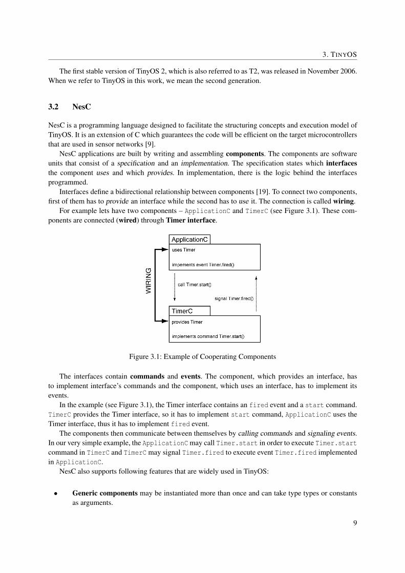
For example lets have two components – ApplicationC and TimerC (see Figure 3.1). These com-ponents are connected (wired) through Timer interface.
Figure 3.1: Example of Cooperating Components
The interfaces contain commands and events. The component, which provides an interface, hasto implement interface’s commands and the component, which uses an interface, has to implement itsevents.
In the example (see Figure 3.1), the Timer interface contains an fired event and a start command.TimerC provides the Timer interface, so it has to implement start command, ApplicationC uses theTimer interface, thus it has to implement fired event.
The components then communicate between themselves by calling commands and signaling events.In our very simple example, the ApplicationC may call Timer.start in order to execute Timer.startcommand in TimerC and TimerC may signal Timer.fired to execute event Timer.fired implementedin ApplicationC.
NesC also supports following features that are widely used in TinyOS:
• Generic components may be instantiated more than once and can take type types or constantsas arguments.
9
3. TINYOS
• Tasks are pieces of code whose execution takes some significant time, but which are not time-critical. Posted tasks are executed later by the TinyOS scheduler when the processor is idle.
• Atomic sections are time-critical pieces of code. They are implemented by disabling interrupts,therefore they should be as short as possible.
3.3 TinyOS Architecture
TinyOS is a component-based operating system. There is always a top-level configuration component1.In this top-level component it is defined which components will be used. Usually it includes the MainCcomponent, which is responsible for the hardware initialization and the boot sequence (see Section 3.3.1),and main application component. Besides these, the top-level component can also initialize needed ser-vice components, sensors, timers or radio abstractions and wire them to the application component.
The components initialized at a top-level configuration are able to further initialize other componentsthat they need, and there is always a path from the top-level component to any used component. Thisallows us to compile the minimal-size system only with components that have been referenced.
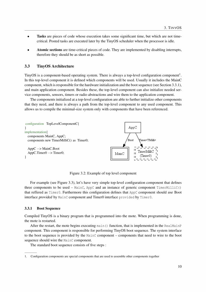
configuration TopLevelComponentC{}implementation{
components MainC, AppC;components new TimerMilliC() as Timer0;
AppC −> MainC.BootAppC.Timer0 −> Timer0;
}
Figure 3.2: Example of top level component
For example (see Figure 3.3), let’s have very simple top-level configuration component that definesthree components to be used – MainC, AppC and an instance of generic component TimerMilliC()that reffered as Timer0. Furthermore this configuration defines that AppC component should use Bootinterface provided by MainC component and Timer0 interface provided by Timer0.
3.3.1 Boot Sequence
Compiled TinyOS is a binary program that is programmed into the mote. When programming is done,the mote is restarted.
After the restart, the mote begins executing main() function, that is implemented in the RealMainPcomponent. This component is responsible for performing TinyOS boot sequence. The system interfaceto the boot sequence is provided by the MainC component – components that need to wire to the bootsequence should wire the MainC component.
The standard boot sequence consists of five steps :
1. Configuration components are special components that are used to assemble other components together
10
3. TINYOS
1. Platform Bootstrap: First, the very low-level hardware initialization is performed, such as set-ting processor mode. On most platforms there is no low-level initialization needed and platformbootstrap is just an empty function.
2. Scheduler Initialization: The scheduler is initialized in order to provide applications with pos-sibility to post their tasks.
3. Platform Init: Now TinyOS performs platform initializations that are specified in PlatformCcomponent. These initializations must usually follow in a very specific order due to hidden hard-ware dependencies. After the platform init is done, the scheduler performs all tasks that couldhave been posted during the platform init.
4. Software Init: The software init is now on. This means that all components (applications) thatare wired to the MainC.SoftwareInit perform their initialization function. At the end, the sched-uler performs the posted tasks again.
5. Start Main Loop: Before the main loop is started, the system interrupts are enabled and theBoot.booted is signaled to the applications.
3.3.2 Concurrency
There are two types of code in TinyOS, synchronous and asynchronous.The asynchronous code is initiated by the hardware interrupts and runs preemptively. It means that
whenever an interrupt is caught, the current code execution is interrupted and interrupt handler instantlybegins its execution. The interrupt can preempt tasks or other interrupts, but cannot preempt atomicsection. The functions called by asynchronous code must be asynchronous as well. The only way that anasynchronous code can execute a synchronous function is to post a task.
The synchronous code is only reachable from tasks. Because the tasks are not preempted by othertasks and run atomically with respect to each another, we can rely that no other task executes suddenlyand modifies our data. Tasks are executed by the task scheduler.
The task scheduler runs the posted tasks and switches processor to sleep mode when all tasks aredone. The standard scheduler has nonpreemtive FIFO scheduling policy, but it can be replaced for customone. In order to improve reliability, the scheduler has reserved slot for each possibly postable task. Thusthe task queue can never overflow and task posting will fail if and only if the task has already been posted[31].
3.3.3 Hardware Abstraction Architecture
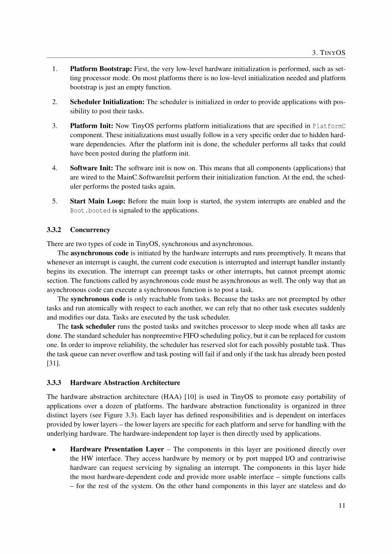
The hardware abstraction architecture (HAA) [10] is used in TinyOS to promote easy portability ofapplications over a dozen of platforms. The hardware abstraction functionality is organized in threedistinct layers (see Figure 3.3). Each layer has defined responsibilities and is dependent on interfacesprovided by lower layers – the lower layers are specific for each platform and serve for handling with theunderlying hardware. The hardware-independent top layer is then directly used by applications.
• Hardware Presentation Layer – The components in this layer are positioned directly overthe HW interface. They access hardware by memory or by port mapped I/O and contrariwisehardware can request servicing by signaling an interrupt. The components in this layer hidethe most hardware-dependent code and provide more usable interface – simple functions calls– for the rest of the system. On the other hand components in this layer are stateless and do
11
3. TINYOS
Figure 3.3: Hardware Abstraction Architecture [10]
not provide any substantial abstraction over the hardware beyond automating frequently usedcommand sentences [10].
• Hardware Abstraction Layer – The components in abstraction layer use the interfaces providedby HPL components. They try to build useful abstractions hiding the complexity associated withthe use of hardware resources. In contrast to HPL they are allowed to maintain state so they canbe used for performing arbitration and resource control.
Abstractions at the HAL level are tailored to the concrete device class and platform. To maintainthe effective use of resources, HAL interfaces are rich and expose the specific hardware features[10].
• Hardware Independent Layer – The highest tier of HAA takes the platform specific abstrac-tions provided by HAL and convert them to hardware independent interfaces. These interfacescan be used by cross-platform applications [10].
12

Chapter 4
Intrusion Detection Systems
It has become clear that we cannot achieve the satisfactory level of security only by using cryptographictechniques as these techniques fall prey to insider attacks in which the attacker has compromised andretrieved the cryptographic material of a number of nodes [15]. In order to counter this threat someadditional techniques such as intrusion detection system has to be deployed.
Intrusion detection system (IDS) is defined as a system that tries to detect and alert on attemptedintrusions into a system or network [11]. IDS is composed of IDS agents that runs on some or all nodes.
The IDS solutions developed for ad-hoc networks cannot be applied directly to sensor networksbecause the WSN has several specificities. In particular, the computing and energy resources are moreconstrained on WSN, thus there is not possible to have an active full-powered agent inside of every node.Also, the IDS must be simple and highly specialized to the specific WSN’s protocols and threats [26].
4.1 IDS Classification
There are three basic approaches in intrusion detection systems according to the used detection tech-niques [12].
• Misuse detection technique compares the observed behavior with known attack patterns (sig-natures). Action patterns that may pose a security threat have to be defined and stored in thesystem. The advantage of this technique is that it can accurately and efficiently detect instancesof known attacks, but it lacks an ability to detect an unknown type of attack.
• Anomaly detection – The detection is based on monitoring changes in behavior, rather thansearching for some known attack signatures. Before the anomaly detection based system is de-ployed, it usually must be taught to recognize normal system activity (usually by automatedtraining). The system then watches for activities that differ from the learned behavior by a sta-tistically significant amount. The main disadvantage of this type of system is high false positiverate. The system also assumes that there are no intruders during the learning phase.
• Specification based – The third technique is similar to anomaly detection – it is also based ondeviations from normal behavior, but the normal behavior is specified manually as a set of systemconstraints. Thus there is no learning phase which is particularly difficult in WSNs.
Furthermore, we can divide WSN’s networks into three categories according to IDS topology.
• Stand-alone – Each node operates an independent IDS agent that is responsible for detectingattacks. Individual agents do not cooperate with others and do not share any information. Theadvantage of this approach is its simplicity and the fact that an attacker is not able to forge anymisinformation because nodes don’t rely on others.
13

4. INTRUSION DETECTION SYSTEMS
• Cooperative – Each node still runs its own IDS, but the individual IDSs cooperate betweenthemselves.
Generally the main challenge of this approach is the question of how to deal with compromittedneighbors. We don’t want malicious node to be able to confuse others with some misinformation.In [16], the authors presented the voting algorithm which is based on the presumption that anattacker is not able to outnumber the legitimate nodes. The solution requires establishing of keymanagement in order to achieve votes authentication.
• Hierarchical – The network is divided into clusters with cluster head nodes. The cluster headhas the responsibility for communication with other cluster heads or base stations. The clusterheads can be more powerful or less energy constrained devices than the other nodes. The IDSthen only runs on the cluster head node.
4.2 Watchdog Monitoring
Watchdog monitoring technique [21, 26] is the way how to detect misbehaving nodes. It is based on thebroadcast concept of communication in sensor networks, where each node hears the communication ofsurrounding nodes even if it is not intended.
This technique depends on sufficient density of deployed nodes. In case of wireless sensor networksthe density of deployed sensors is usually high enough because of the requirements for graceful degra-dation – the network must continue to work even if a small portion of nodes fails.
A B C
Figure 4.1: Possible watchdogs
Suppose that node A wants to send a message to node C which is outside of its radio range. So itsends this message to the intermediate node B and node B forwards it to node C (see Figure 4.1). Let SA
be a set of all nodes that hear the message from A to B and SB be a set of nodes that hear a message fromB to C.
We can define a set of possible watchdogs of the node B as an intersection of SA and SB. This meansthat any node that lies in the intersection region is able to hear both messages and is able to decidewhether node B forwards messages from node A.
14

4. INTRUSION DETECTION SYSTEMS
4.2.1 Regular Collisions
When two nodes that are close to each other transmit packets at the same time, they will cause a collision.In result, the signals from both nodes interfere and none of these packets is successfully received.
In order to avoid this collisions, wireless sensor networks often follow Carrier Sense Multiple Ac-cess with Collision Avoidance (CSMA/CA) protocol for Media Access Control (MAC). Following thisprotocol, a node listens to a traffic on medium before trying to send own packet. Thus if two nodes thatare close enough want to send packet at the same time, the CSMA algorithm will prevent the one, whowants to start sending little bit later, to send it. The collision occurs only when both nodes begin transmitexactly at the same time.
4.2.2 Ambiguous Collisions
Let the node D be the watchdog for the node B (see Figure 4.2). The ambiguous collision [21] occurs atthe node D when the node B transmits a packet at the same time as the node E.
The nodes B and E are far apart enough to be able to send packets at the same time. This means thatthe node B considers channel to be clear (the radio signal is below its clear channel threshold) despitethe node E is transmitting a packet and vice versa the node E considers the channel to be free althoughthe node B is transmitting.
As a result, the node D (that is between them) do not hear any of these packets, because the signalsinterfere.
A B C
D
E F
Figure 4.2: Abmiguous collision
Particularly the node D do not hear packet that has been forwarded and it may suspect the node Bthat performs a selective forwarding attack. Therefore the node D cannot decide whether the node B ismisbehaving or not on the basis of a single observation.
We can distinguish two types of ambiguous collisions:
• At first, there are collisions where both signals (on Figure 4.2 from the node B and the node E)are similarly strong, and when they occur, the watchdog is unable to receive even one packet dueto radio interference. We can hardly fight against this type of collision.
• At second, there are collisions where the signal from the first node (B) is much stronger thanthe signal from the second one (E). If the first node (B) begins transmitting first, the watchdogsuccessfully captures the beginning bytes of the packet frame and starts receiving. It successfullyreceives the whole packet although the second node (D) interferes it during the transmission,
15
4. INTRUSION DETECTION SYSTEMS
because the signal-to-noise1 ratio is high enough during the whole transmission.
On the other hand, when the second node (E) starts transmitting first, the watchdog begins re-ceiving its packet. Then a stronger signal from the first node (B) interferes with the second one(E) and causes that signal-to-noise ratio becomes too low for successful reception. As a result,the watchdog (D) does not receive the packet from second node (E) due to radio interference andneither does not receive the packet from first node (B), because it did not capture the beginningbytes of the packet frame.
The number of ambiguous collisions in network exponentionally grows with a number of packetsthat are transmitted in network. That makes the watchdog technique unreliable in networks with moretraffic.
We can never completely avoid ambiguous collisions, but we can try to reduce the occurence ofambiguous collisions of second type. We have proposed a novel technique that is based on suppressingweak signals.
Suppressing Weak Signals
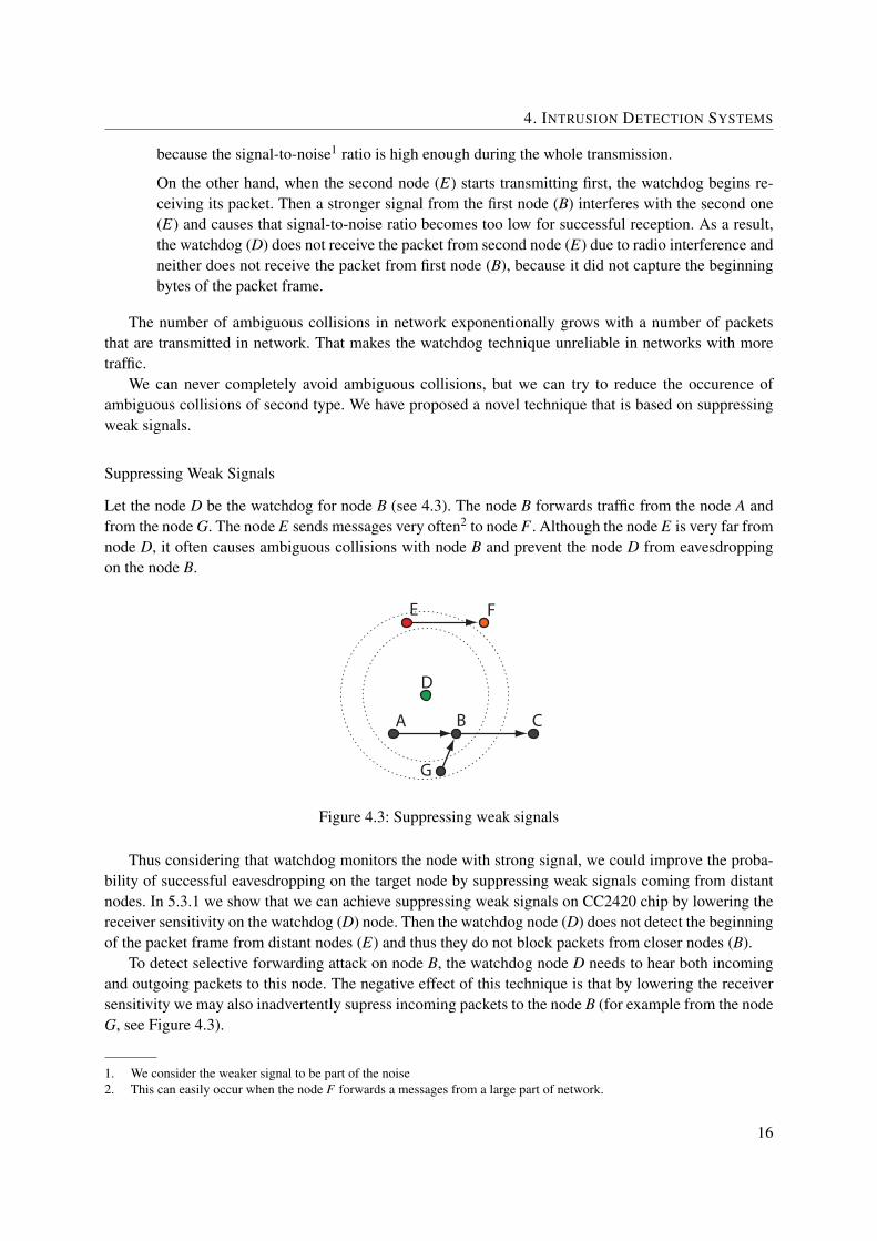
Let the node D be the watchdog for node B (see 4.3). The node B forwards traffic from the node A andfrom the node G. The node E sends messages very often2 to node F . Although the node E is very far fromnode D, it often causes ambiguous collisions with node B and prevent the node D from eavesdroppingon the node B.
A B C
D
E F
G
Figure 4.3: Suppressing weak signals
Thus considering that watchdog monitors the node with strong signal, we could improve the proba-bility of successful eavesdropping on the target node by suppressing weak signals coming from distantnodes. In 5.3.1 we show that we can achieve suppressing weak signals on CC2420 chip by lowering thereceiver sensitivity on the watchdog (D) node. Then the watchdog node (D) does not detect the beginningof the packet frame from distant nodes (E) and thus they do not block packets from closer nodes (B).
To detect selective forwarding attack on node B, the watchdog node D needs to hear both incomingand outgoing packets to this node. The negative effect of this technique is that by lowering the receiversensitivity we may also inadvertently supress incoming packets to the node B (for example from the nodeG, see Figure 4.3).
1. We consider the weaker signal to be part of the noise2. This can easily occur when the node F forwards a messages from a large part of network.
16

4. INTRUSION DETECTION SYSTEMS
Early Packet Dropping
We could also limit the occurrence of ambiguous collisions of the second type by early dropping thepackets from the nodes we don’t want to monitor.
On CC2420 we could achive early dropping packets by enabling hardware address recognition. Whenhardware address recognition is enabled, the node rejects the packet that does not match its addressimmediately after reading the address header. Thus the node does not have to receive the whole packet.
Unfortunately, CC2420 cannot be configured to have more than one hardware address. Therefore wewould have to change the watchdog hardware address to be the same as the address of the monitorednode.
4.2.3 Partial Dropping
A malicious node can also circumvent watchdog by dropping packets at lower rate than watchdog’sconfigured minimum misbehaving threshold. We cannot set the minimum misbehaving threshold toolow because due to ambiguous collisions the watchdog never hears all messages and false alarms wouldbe raised too often.
4.2.4 Receiver Collisions
In the receiver collision problem, node B forwards a packet, but the watchdog node D1 is not able toverify whether node C successfully received it or not (see Figure 4.4). When B is malicious, it can delayforwarding the packet until C is transmitting, and purposefully cause a collision [21].
We can try to detect this type of attack by monitoring the forwarding delays that are introduced bythe malicious node. The malicious node may know when C starts transmitting but usually it has to waituntil it happens. Unfortunately, the forwarding delays may be also caused by other factors, such as alocal CSMA collision.
Generally, by this attack, the attacker can only confuse a subset of all possible watchdogs, particularlyhe cannot confuse watchdogs that are close to node C (the node D2).
A B C
D1 D2
Figure 4.4: Receiver collisions
4.2.5 Limiting The Transmission Power
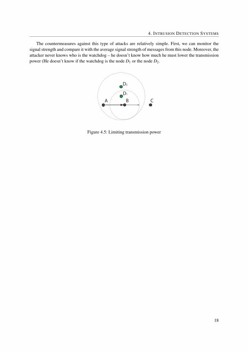
A malicious node can control the transmission power in order to confuse the watchdog (see Figure 4.5).The malicious node B can lower the transmitting power such that the signal is strong enough to be heardby watchdog D1, but too weak to be successfully received by the target node (C).
17
4. INTRUSION DETECTION SYSTEMS
The countermeasures against this type of attacks are relatively simple. First, we can monitor thesignal strength and compare it with the average signal strength of messages from this node. Moreover, theattacker never knows who is the watchdog – he doesn’t know how much he must lower the transmissionpower (He doesn’t know if the watchdog is the node D1 or the node D2.
A B CD1
D2
Figure 4.5: Limiting transmission power
18

Chapter 5
Radio Stack
The essential prerequisite for an implementation of an efficient intrusion detection system is to fullyunderstood how a network communication works. In this chapter, we will describe in detail the radiostack from the highest to the lowest layers. In particular, we will focus on time delays introduced byindividual layers.
Figure 5.1: Radio Stack
We will also compare the implementations of radio stack on the TMote Sky sensor nodes [23] andon the TOSSIM simulator [32], we will point out the differences between them and show that the currentsimulator implementation is not sufficiently precise for the purposes of accurate simulation of IDS thatuses a watchdog monitoring technique.
We can split the radio stack into three parts (see 5.1): we will consider the network protocol to bethe first one – in the work we will consider Collection Tree Protocol (CTP) [8], the second part will beActive Message Layer, and the third and the lowest part, the platform dependent implementation of theradio stack.
Generally, the applications can be wired directly to Active Message Layer that only allows them tobroadcast messages to their neighbors. The network protocol usually incorporates an advanced networklogic such as multi-hop delivery or routing support. In this work we assume that the applications useCollection Tree Protocol [8].
5.1 Collection Tree Protocol
The Collection Tree Protocol (CTP) is now probably the most common network protocol in TinyOS. Itis used in an environment where one needs to collect data from a large number of nodes to one or morebase stations. CTP builds one or more collection trees, which are rooted at the base stations. Each nodepicks a neighbor node to be its parent and in this way they form a tree. Whenever a node wants to send amessage to the base station, it simply sends it to its parent.
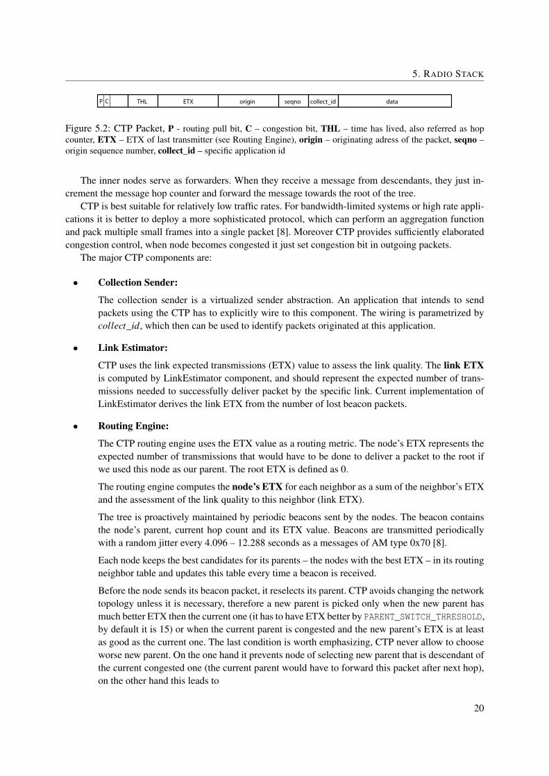
The CTP packet is shown in Figure 5.2. Together, the origin, seqno, collect_id, and THL fields denotea unique packet instance within the network [8].
19
5. RADIO STACK
THL origin seqno collect_id dataETXP C
Figure 5.2: CTP Packet, P - routing pull bit, C – congestion bit, THL – time has lived, also referred as hopcounter, ETX – ETX of last transmitter (see Routing Engine), origin – originating adress of the packet, seqno –origin sequence number, collect_id – specific application id
The inner nodes serve as forwarders. When they receive a message from descendants, they just in-crement the message hop counter and forward the message towards the root of the tree.
CTP is best suitable for relatively low traffic rates. For bandwidth-limited systems or high rate appli-cations it is better to deploy a more sophisticated protocol, which can perform an aggregation functionand pack multiple small frames into a single packet [8]. Moreover CTP provides sufficiently elaboratedcongestion control, when node becomes congested it just set congestion bit in outgoing packets.
The major CTP components are:
• Collection Sender:
The collection sender is a virtualized sender abstraction. An application that intends to sendpackets using the CTP has to explicitly wire to this component. The wiring is parametrized bycollect_id, which then can be used to identify packets originated at this application.
• Link Estimator:
CTP uses the link expected transmissions (ETX) value to assess the link quality. The link ETXis computed by LinkEstimator component, and should represent the expected number of trans-missions needed to successfully deliver packet by the specific link. Current implementation ofLinkEstimator derives the link ETX from the number of lost beacon packets.
• Routing Engine:
The CTP routing engine uses the ETX value as a routing metric. The node’s ETX represents theexpected number of transmissions that would have to be done to deliver a packet to the root ifwe used this node as our parent. The root ETX is defined as 0.
The routing engine computes the node’s ETX for each neighbor as a sum of the neighbor’s ETXand the assessment of the link quality to this neighbor (link ETX).
The tree is proactively maintained by periodic beacons sent by the nodes. The beacon containsthe node’s parent, current hop count and its ETX value. Beacons are transmitted periodicallywith a random jitter every 4.096 – 12.288 seconds as a messages of AM type 0x70 [8].
Each node keeps the best candidates for its parents – the nodes with the best ETX – in its routingneighbor table and updates this table every time a beacon is received.
Before the node sends its beacon packet, it reselects its parent. CTP avoids changing the networktopology unless it is necessary, therefore a new parent is picked only when the new parent hasmuch better ETX then the current one (it has to have ETX better by PARENT_SWITCH_THRESHOLD,by default it is 15) or when the current parent is congested and the new parent’s ETX is at leastas good as the current one. The last condition is worth emphasizing, CTP never allow to chooseworse new parent. On the one hand it prevents node of selecting new parent that is descendant ofthe current congested one (the current parent would have to forward this packet after next hop),on the other hand this leads to
20

5. RADIO STACK
• Forwarding Engine: The forwarding engine is responsible for the forwarding traffic as well asthe traffic generated on the node. It maintains the send queue of pending packets and schedulestheir transmitting. The forwarding engine is also responsible for detecting routing loops.
Packets in the send queue are sent out in FIFO order. The forwarding engine does not distin-guish between packets, the packets generated on the node are treated identically as packet beingforwarded.
When the forwarding engine wants to send a packet, it takes the first packet from the send queueand sends it to the parent. It does not remove the packet from the queue. If the link layer supportspacket acknowledgments, the forwarding engine enables them, and retransmits the packet thathas not been acked for maximum MAX_RETRIES times (default is 30 times) and drop packetonly after all these attempts fail. This feature significantly improves delivery reliability. Thepacket is dequeued from the send queue only after the sending has been successful or when alltransmission retries have been exhausted.
The forwarding engine controls the transmission scheduling. When the forwarding engine re-ceives a packet to forward, and the send queue is empty, and there is no any previous transmitback-off scheduled, the packet is sent out immediately. When the packet is successfully delivered(has been acked), the forwarding engine starts the back-off timer and does not allow to send nextpacket for 16 – 31 milliseconds. If the previous transmission wasn’t successful and the packetwas not acked, the forwarding engine waits for 8 – 15 milliseconds and then tries to retransmit.
5.2 Active Message Layer
The active message layer is the basic network HIL. Each platform must provide the ActiveMessageCcomponent.
Active message communication is virtualized through four components – AMReceiverC, AMSnooperC,AMSnoopingReceiverC, and AMSenderC. These components are generic and each of them takes an ac-tive message ID (AM type) as a parameter. The parameter distinguishes different applications (usuallyeach application has a unique AM type), and allows applications to communicate on separate channels.
Figure 5.3: Application Wiring Example
For example, lets have two application (see Figure 5.3). First application wires to AMReceiverC andAMSenderC and parametrizes these wirings with value of 0x01. Thus messages from this application willbe sent out with AM type of 0x01 and messages coming from network with AM type of 0x01 will be
21
5. RADIO STACK
forwarded to this application. Similarly messages from the second application will have AM type of 0x02and Active Message Layer will forward incoming messages with AM type of 0x02 to this application.
There are three reception abstractions: 1) AMReceiverC is signaled when received messages is des-tined to this node, 2) AMSnooperC is signaled when received is signaled to other node in network, 3)AMSnoopingReceiverC, that is signaled every time a message is received. Applications wire only to ab-stractions that they needs, in our example the Application 1 wires only to AMReceiverC because it doesnot need snooping messages destined to other nodes.
The AMSenderC is an abstraction for sending messages out. Each application that wires to this ab-straction has reserved slot in the sending queue implemented in AMQueueP.
The AMQueueP component implements the sending queue and is responsible for the exact order inwhich outgoing messages are serviced. By default, it goes in the round-robin fashion through messagesfrom the AMSenderC clients and forwards them to the underlying layer.
AMPacket Although it is not defined how the Active Message Packet should exactly be formatted(each hardware dependent implementations internally uses diferent format), each ActiveMessageC com-ponent has to provide AMPacket interface. Using these interface we can access Active Message Packetheaders. There are following headers: 1) destination that defines the destination node, 2) source statessource node of this message, 3) AMType states message Active Message type, 4) group refers to logicalnetwork identifier (there may exist a logical subnets in WSN, where nodes communicate only with nodesin the same subnet) [18].
5.3 Hardware Dependent Radio Stack on TMote Sky
The TMote Sky sensor node is based on the TMote platform. In the TMote platform, the Chipcon CC2420chip for radio communication is used [23]. The CC2420 is a 2.4 GHz IEEE 802.15.4 compliant RFtransceiver. It was designed for low-power and low-voltage wireless applications [1].
The CC2420 radio stack is organized in several layers:
• Active Message Layer
On the TMote platform, the Active Message Layer is provided by CC2420ActiveMessageP com-ponent. When sending a message, some details are filled in the packet header within this layer(packet type, destination address, packet source and destination pan – group – address) and thepacket is passed down onto the stack.
When receiving a message, this layer decides if the message is destined for the node and signalsit to the corresponding ReceiverC or SnooperC component.
• Unique Send/Receive Layer
When sending a message, this layer supplies each outgoing message with a unique data sequencenumber (dsn). The layer keeps an internal counter that increments by one for each packet andwrites it into dst byte in the packet header.
The data sequence numbering is utilized during packet receiving. The layer keeps the history ofthe data sequence numbers of the last RECEIVE_HISTORY_SIZE received messages. If the newlyreceived message matches a message in a recent history, it is dropped.
This layer ensures that higher layers never hear a single message twice. Particularly in the contextof watchdog monitoring, the watchdog never hears a packet that is being retransmitted becauseit was not delivered on the first try.
22
5. RADIO STACK
• Packet Link Layer
This optional layer is responsible for the automatic message retransmission and ensures reliablepacket delivery. Automatic retransmission is activated on a per-message basis, therefore we haveto set a flag for each outgoing message that should use this layer.
It is the most reliable when software acknowledgments are enabled, because it will fail if itreceives false-acknowledgments. More details can be found in [22].
• Low Power Listening Layer
This layer provides an asynchronous low-power listening implementations that defines the radioduty cycles. The radio is not listening all the time, but it is only turned on for defined intervals.The layer is disabled by default, it can be enabled by defining LOW_POWER_LISTENING.
• Low Pan Layer
The next layer provides compatibility with other networks using 6LowPAN protocol[20]. 6LoW-PAN is an acronym of IPv6 over Low power Wireless Personal Area Networks. TinyOS imple-ments this protocol in 6lowpan library that can be found in tos/lib/net/6lowpan.
6LoWPAN protocol is also supported in other WSN, which do not run TinyOS. Unfortunately,original TinyOS isn’t compatible with other 6LowPan networks. It uses network frames (calledT-Frames) that do not include the network byte identifier. Therefore I-Frames were developed toprovide interoperability as defined by 6LowPan specifications.
The 6LowPan layer is optional and it is only used when the interoperability with other 6LoW-PAN networks is required. It adds the network identifier byte to packets on the way out. Whilereceiving, the low pan layer detects whether the received packet belongs to TinyOS communica-tion. If not, the packet is signaled to 6LowpanSnoop interface instead of the default ones.
This layer can be enabled by compiling application with CC2420_IFRAME_TYPE macro.
• CSMA Layer
The CSMA layer should take control of access to the medium, but the current CSMA implemen-tation is integrated with code in CC2420TransmitP. At the current version, the CSMA layer onlycomputes random radio back-offs.
• TransmitP/ReceiveP Layer
These layers are responsible for interacting directly with the radio hardware. We will describethese layers in detail in the following section.
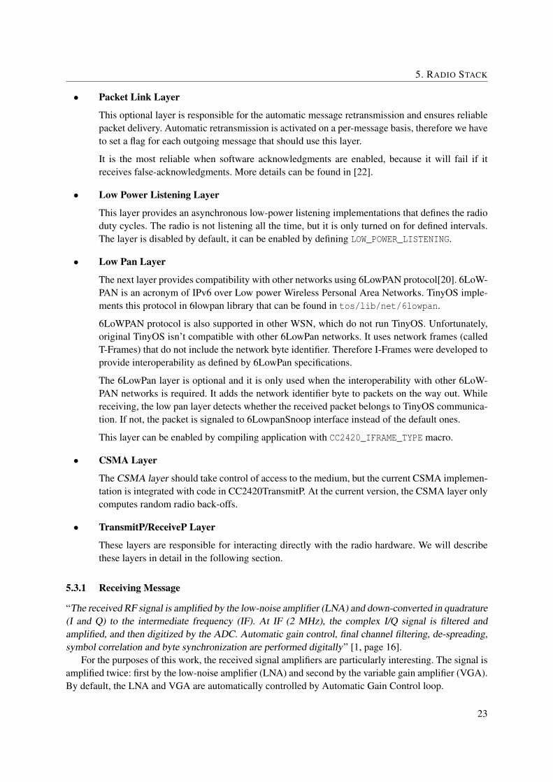
5.3.1 Receiving Message
“The received RF signal is amplified by the low-noise amplifier (LNA) and down-converted in quadrature(I and Q) to the intermediate frequency (IF). At IF (2 MHz), the complex I/Q signal is filtered andamplified, and then digitized by the ADC. Automatic gain control, final channel filtering, de-spreading,symbol correlation and byte synchronization are performed digitally” [1, page 16].
For the purposes of this work, the received signal amplifiers are particularly interesting. The signal isamplified twice: first by the low-noise amplifier (LNA) and second by the variable gain amplifier (VGA).By default, the LNA and VGA are automatically controlled by Automatic Gain Control loop.
23

5. RADIO STACK
LNA is used for initial amplification of the received signal. We found out that AGC keeps the LNAin high-gain mode most of the time (see 7.3).
The second amplifier (VGA) amplifies the signal just before it is processed by Analog/Digital Con-verter. AGC adjusts VGA in order to keep the received signal strength inside of the dynamic range of theAnalog/Digital Converter.
In 7.3 we have shown that we can disable the automatic mode of AGC and set the amplifiers manually.Using this technique, we can suppress weak signals that are coming from distant nodes.
Figure 5.4: Simplified diagram of demodulator [1]
After the signal is digitized by the ADC, it is processed by demodulator (see Figure 5.4). The mostimportant for our work is that now the RSSI and LQI values are derived.
• RSSI – Received signal strength indicator is an estimate of the average received signal strength.The CC2420 has a built-in received signal strength indicator whose value is always averagedover 8 period symbols. Usually, the received signal strength is measured when the transmissionstarts and then its value is written into the packet header.
• LQI – The link quality indication measurement is defined in [28] as the characterization of thestrength and/or link quality of received signal. The LQI value is required to be limited to range0 through 255, with at least 8 unique values.
CC2420 provides an average correlation value for each incoming packet, based on the 8 firstsymbols at the beginning of the packet. The correlation value has 7 bits and can be looked uponas a measurement of the “chip error rate”. Correlation value of about 110 indicates the maximumquality frame while the value of about 50 is typically the lowest quality frame detectable byCC2420 [1].
The current TinyOS implementation doesn’t perform any conversion of this value and takes itdirectly as LQI.
The CC2420 has several hardware pins that TinyOS utilizes to receive a packet. First it is SFD pin(Start Frame Delimiter pin). This pin is used both in receiving and transmitting mode. Simply put, theSFD pin is high when radio is busy (receiving or transmitting a message). Second, it is RXFIFO registerthat serves as receive buffer. Furthermore, there are FIFO and FIFOP pins1. These pins are used to assistthe microcontroller in supervising RXFIFO [1].
The pin activity during receiving is shown in Figure 5.5. The packet reception runs as follows:
1. When CC2420 detects the start of the frame delimiter, SFD pin goes up. This causes an interruptcaptured by CC2420TrasmitP but TinyOS uses this information only for packet time-stampingpurposes.
1. The function of these pins is very similar. By default settings, the only difference is that the FIFOP pin goes up a little bitlater when hardware address recognition is enabled. TinyOS only utilizes the FIFOP pin.
24
5. RADIO STACK
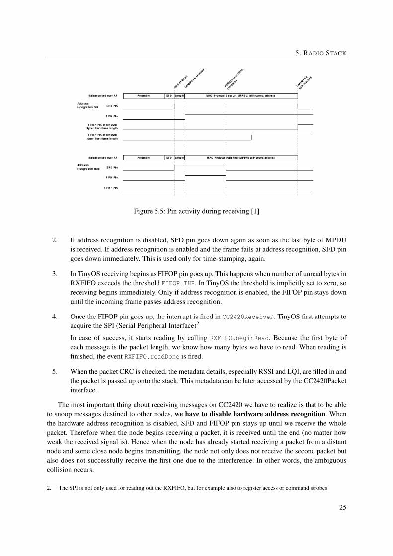
Figure 5.5: Pin activity during receiving [1]
2. If address recognition is disabled, SFD pin goes down again as soon as the last byte of MPDUis received. If address recognition is enabled and the frame fails at address recognition, SFD pingoes down immediately. This is used only for time-stamping, again.
3. In TinyOS receiving begins as FIFOP pin goes up. This happens when number of unread bytes inRXFIFO exceeds the threshold FIFOP_THR. In TinyOS the threshold is implicitly set to zero, soreceiving begins immediately. Only if address recognition is enabled, the FIFOP pin stays downuntil the incoming frame passes address recognition.
4. Once the FIFOP pin goes up, the interrupt is fired in CC2420ReceiveP. TinyOS first attempts toacquire the SPI (Serial Peripheral Interface)2
In case of success, it starts reading by calling RXFIFO.beginRead. Because the first byte ofeach message is the packet length, we know how many bytes we have to read. When reading isfinished, the event RXFIFO.readDone is fired.
5. When the packet CRC is checked, the metadata details, especially RSSI and LQI, are filled in andthe packet is passed up onto the stack. This metadata can be later accessed by the CC2420Packetinterface.
The most important thing about receiving messages on CC2420 we have to realize is that to be ableto snoop messages destined to other nodes, we have to disable hardware address recognition. Whenthe hardware address recognition is disabled, SFD and FIFOP pin stays up until we receive the wholepacket. Therefore when the node begins receiving a packet, it is received until the end (no matter howweak the received signal is). Hence when the node has already started receiving a packet from a distantnode and some close node begins transmitting, the node not only does not receive the second packet butalso does not successfully receive the first one due to the interference. In other words, the ambiguouscollision occurs.
2. The SPI is not only used for reading out the RXFIFO, but for example also to register access or command strobes
25

5. RADIO STACK
5.3.2 Transmitting a Message
In the current CC2420 radio stack implementation, the CC2420TransmitP component performs theCSMA algorithm and the CSMA layer only provides random radio back-offs.
The CSMA algorithm does not allow radio to begin transmitting while the channel is not free. TheCC2420 chip incorporates a special pin for this purpose – the CCA pin.
The CCA(Clear Channel Assessment) pin is only high if the node is not receiving valid dataand the strength of received signal is lower than the programmed carrier sense threshold. The car-rier sense threshold can be programmed by the RSSI.CCA_THR registers (default value is -77dB) andMDMCTRL0.CCA_HYST (default value is 2dB). The resulting carrier sense threshold is defined as:
CCA_THR−CCA_HYST
Thus the channel is clear when the receiving signal strength is lower than -79dB and the node is notreceiving any valid data.
Transmitting of a message runs as follows:
1. First, the CC2420TransmitP sets the radio transmission power and loads the outgoing messageinto the outbound tx buffer – TXFIFO.
2. When the TXFIFO buffer is loaded, the TXFIFO.writeDone() is signaled. If the CCA (ClearChannel Assessment) is not required, the CC2420TransmitP begins transmitting immediatelyby calling STXON.strobe().
3. Otherwise the CC2420CsmaP is asked to compute a random delay – the initial back-off as:
backo f f = random mod (31∗CC2420_BACKOFF_PERIOD)+CC2420_MIN_BACKOFF
For default values (CC2420_BACKOFF_PERIOD=10, CC2420_MIN_BACKOFF=10) this back-off lastsbetween 0.3125 and 10 milliseconds.
4. After the initial back-off, CCA is sampled. Even if the channel seems to be clear (CCA is high),sending is delayed by additional 0.21875 milliseconds, just for case that the first sample wastaken during the ack’s turn-around window.
If the channel was not clear, the CC2420CsmaP is asked to compute the congestion back-off. Thisback-off is computed as follows:
backo f f = random mod (7∗CC2420_BACKOFF_PERIOD)+CC2420_MIN_BACKOFF
For default values it takes from 0.3125ms to 2.5ms.
5. Finally, the attempt to send is now performed. CC2420TransmitP calls STXONCCA.strobe()which samples cca one more time and begins transmitting only if the channel is still clear. If thechannel is not clear, a new congestion back-off is scheduled.
6. When the packet is sent, SFD pin goes up as soon as the SFD field is completely transmitted(see Figure 5.6). This fires an interrupt that is used for timestamping packets. If SFD pin doesn’tgo up in 10 milliseconds, the CC2420TransmitP assumes that something is wrong, flushes thetransmit buffer and schedules retransmission.
26

5. RADIO STACK
Figure 5.6: Transmitting a message
7. When the complete MPDU is transmitted, SFD pin goes down again. If the message acknowl-edgment is not required, sending is finished. Otherwise, we wait 8ms for the ack. When theack comes, packet metadata is updated (ack bit, ack’s RSSI and LQI). Even if the ack doesn’tcome, success is signaled. The only way how to detect if the packet was acked is by interfacePacketAcknowledgements which is provided by ActiveMessageC.
At the end, it is important to point out that in default mode3 the node will never start transmittingwhen receiving valid data (even though a packet from distant node with weak signal).
It is also worth mentioning that a single clear channel test is not sufficient, the CC2420TransmitPalways tests channel twice.
5.4 TOSSIM
TOSSIM is a discrete event simulator. It keeps events sorted by the execution time in a queue and grad-ually executes them.
There are several radio models that we can use for network behavior simulation – some of themare included in TinyOS distribution (SimpleRadioModel, BinaryInterferenceModelC, CpmModelC),others were described in [17].
We have used the default TOSSIM radio model – CpmModelC. It is based on the Closest PatternMatching (CPM) algorithm. This model is based on statistical extraction from empirical noise data [17].According to the [17], the model should provide more precise simulation than others by exploiting time-correlated noise characteristics.
The TOSSIM radio stack consists of three layers:
• Active Message Layer
This is the top level of the TOSSIM radio stack. It provides Active Message communication forthe upper layers and also wires to the underlying network model. The responsibility of this layeris to fill in details into headers of outgoing messages (e.g. source address, destination address)and signal the incoming messages to the correct interface.
• Packet Layer Model – TossimPacketModelC
Packet-level radio model particularly provides the CSMA functionality. When the message isabout to be sent, this layer performs the basic CSMA algorithm, and passes the message to the
3. By setting CCA_MODE differently we may change the clear channel assessment algorithm to be less restrictive, but thisis the kind of behavior that we need at the watchdog node.
27

5. RADIO STACK
lower layer only when the channel is clear. It also keeps the state whether the node is currentlytransmitting a message.
When the gain radio model signals a received message, the TossimPacketModelC only checksif the node is transmitting another message. If not, it signals the message to the upper layer,otherwise it drops it. Unfortunately, this check is not sufficient as we will show in 5.4.2.
• Radio Gain Model - CpmModelC
The radio model basically performs two actions: first, it takes the message that is being sentout, and schedules the receive event for each node in the network. Second, when transmitting isfinished, it performs the scheduled receive events and decides if the message should be receivedand possibly signals the receive event to the upper layer.
5.4.1 Sending message
While the message is about to be sent, it is dispatched at the ActiveMessageC. The ActiveMessageConly fills the headers in and forwards the message to the TossimPacketModelC.
This TossimPacketModelC implements a basic CSMA algorithm. First it computes the initial back-off as:
backo f f =(random mod SIM_CSMA_INIT_HIGH−SIM_CSMA_INIT_LOW)+SIM_CSMA_INIT_LOW
SYMBOLS_PER_SEC
For default values (SIM_CSMA_INIT_HIGH = 620, SIM_CSMA_INIT_LOW = 20, SYMBOLS_PER_SEC= 65536) it takes between 0.30518 ms and 9.76577ms4.
After the back-off, the channel is sampled. First, environment noise is computed as
environment_noise = (logn
∑i=0
10rssii/10)∗ 10log10
where n states for a number of currently transmitting nodes and rssii is the received signal strength fromnode i. The channel is considered to be clear when the environment_noise is lower than clearTresholdvariable. The default value of clearThreshold variable is -72dB. By SIM_CSMA_MIN_FREE_SAMPLES itis defined how many free samples are needed before transmission is allowed to start (it is 1 sample bydefault).
If the number of needed free channel samples was not met, a new back-off value is computed as
E = EXPONENT_BASEiteration
backo f f =(random mod (SIM_CSMA_HIGH−SIM_CSMA_LOW)∗E)+SIM_CSMA_LOW
SYMBOLS_PER_SEC
The default value of SIM_CSMA_HIGH is 160 and the value of SIM_CSMA_LOW is 20. Compared to thecalculation of the initial CSMA back-off, a new parameter E is introduced. This parameter depends onthe iteration of the algorithm and on the defined EXPONENT_BASE. Because the default EXPONENT_BASEis 1, E is always equal to 1. Thus by default, the back-off timer is set from 0.30518 ms to 2.4414 ms.
If we do not need any more free samples, the transmit indicator is set to true and the transmission isscheduled after additional 0.1678 ms caused by RXTX_DELAY. Now the number of symbols to transmit iscomputed as
4. All times are internally converted to the number of simulator’s ticks
28

5. RADIO STACK
symbols =8∗ (SENDING_LENGTH+HEADER_LENGTH)BITS_PER_SYMBOL+PREAMBLE_LENGTH
When an ack is required, ack time is added
symbols = symbols+ACK_TIME
and at the end the duration is computed.
duration =symbols
SYMBOLS_PER_SEC
Finally the message is passed to the CPM model.First CPM goes through all the motes in the network and for each of them determines whether the
mote could successfully receive the message. A node may loose this message due to: 1) being off, 2) thesignal-to-noise ratio being too low, 3) being mid-reception (is currently receiving another message).
If the node is already receiving another message, the CPM model takes the new message as noise andtests if the signal-to-noise ratio of the previous message is still high enough.
Then the CPM model enqueues the message reception event to the events queue, no matter if themote is going to successfully receive this packet or not.
The reception event is performed after the transmission duration expires. The CPM model checksone more time if the packet could be delivered and then definitely drops the message or signals it to theupper layer.
5.4.2 TOSSIM Shortcomings and Problems
• Receives even when transmitting
When TOSSIM handles the reception event, it checks if it is not currently transmitting a packet.The problem is that TOSSIM checks if the node is not transmitting only at the end of receiving,not at the beginning or during it. This is not sufficient and may cause a false reception of messagethat was delivered only a little while after the node finished its transmission. Although most of themessage was received during the ongoing transmission, for TOSSIM the message is successfullyreceived.
This bug was reported and was confirmed by TOSSIM developers. We also developed a solutionthat fixes this misbehavior.
• Begins transmitting even when receiving valid data
In TOSSIM, the clear channel assessment algorithm only checks if the received signal strengthis under the CCA_THRESHOLD. By contrast, on CC2420, the CCA algorithm also requires that thenode must not be receiving valid data (considering default mode).
For example, when TOSSIM is receiving a packet with weak signal (i.e. -85dB), the channel isconsidered to be free (RSSI is under CCA_THRESHOLD). By contrast, the CC2420 would considerthis channel as busy.
To achieve more accurate simulation, we had to reimplement the clearChannel command in CPMmodel so that it took into into account if the node was receiving or not.
29

5. RADIO STACK
• Inaccurate CSMA algorithm
First, the CCA_THRESHOLD had to be changed from -72dB to -79dB to be the same as on theCC2420.
Second, the CC2420 radio always performs two CCA tests before it starts transmitting, the firsttest is scheduled by random back-off timer, the second is always 0.21875 milliseconds after thefirst one. We modified the TossimPacketModelC to achieve the same behavior for TOSSIM.
30
Chapter 6
Implementation
We have designed our intrusion detection system to be as small as possible but also to be easily extensiblefor new funcionality that would allow detecting more complex attacks.
Our IDS is composed from autonomous agents. Each node runs IDS agent. Most of the time eachagent sleeps and consumes only a minimum power. The agents are independent, they only notify otherswhen they detect intrusion. However other nodes do not trust this information and each node decidesabout intrusion on its own.
Each IDS agent can have one or more Detection Engines. The Detection Engines are replaceablecomponents that are used to detect attacks. Each Detection Engine is specialized to detect a specificattack using a specific technique.
At the same time an IDS agent may run only one Detection Engine. Each Detection Engine is activeonly for a certain period of time during which it monitors and analyzes traffic on a network. When thetime expires, the Detection Engine is replaced for another engine or the IDS agent is put to the sleepmode. The application of Detection Engine is called the test.
The sense of separate replaceable Detection Engines is possibility to share system resources betweenthem (particularly the very size-limited RAM memory). More details will be given in Section 6.5.
We have implemented two basic Detection Engines: the first one detects selective forwarding (seeSection 2.5) attacks and the second detects selective forwarding attacks using improved watchdog mon-itoring technique based on suppressing of weak signals (see 4.2.2).
6.1 System Overview
StaticsticsManager
AMTap
ResponseModule
CommModule
DetectionManager
Scheduler
Active Engine
Detection Engine2
SharedComponents
Boot.boot() AMReceiverC(0x77)
AMSenderC(0x77)
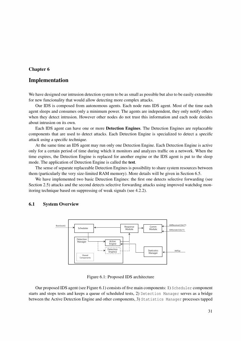
Figure 6.1: Proposed IDS architecture
Our proposed IDS agent (see Figure 6.1) consists of five main components: 1) Scheduler componentstarts and stops tests and keeps a queue of scheduled tests, 2) Detection Manager serves as a bridgebetween the Active Detection Engine and other components, 3) Statistics Manager processes tapped
31

6. IMPLEMENTATION
communication, manages a neighbor table and passes communication that belongs to monitored nodesto active Detection Engine 4) Response Module reacts on alerts raised by the Detection Engine or thatcame over the network 5) Communication Module facilitates comunication with other IDS agents.
The arrows on the Figure 6.1 represent relations (wirings) between componens. There are alsowirings to external components: 1) Scheduler uses Boot interface, 2) Statistics Manager uses AM-Tap interface (see Section 6.2), 3) Communication Module uses Send and Receive interfaces throughwhich sends and receives messages.
The following algorithm is a brief overview over the IDS agent funcionality. The individual compo-nents will be described in detail in following sections.
1. When the node boots, the Scheduler is initialized via Boot.booted event and starts the internalperiodic timer (IDSTimer).
2. Every time the IDSTimer fires and no test is currently performed, the Scheduler tries to take thefirst test from the tests queue. There may be two possibilities:
a) If there is a scheduled test in the tests queue, the first test it will be performed immediatelly.The Scheduler asks Detection Manager to activate Detection Engine that is required by this test.Then the Scheduler starts the chosen Detection Engine.
b) If the tests queue is empty, the new test is (spontaneously) scheduled with a some givenprobability P.
3. The Detection Engine cooperate with the Statistics Manager. The Statistics Manager holds thebasic information about neighbors and process all tapped communication.
4. When the Detection Engine find out that some attack is being performed, it raises an alert in theResponse Module.
5. The Response Module could react on this alert in several ways:
a) It may warn other nodes using the Communication Module
b) It may schedule an additional test to tests queue
6. When the time for the test expires, the Detection Engine is deactivated. The algorithm continuesat the point 2.
6.2 Tapping communication
Our IDS agent analyzes all messages in the node’s communication range. For this reason it needs to hearall network communication that is processed by the node. This includes both messages being receivedand snooped and messages that are being sent out.
Most applications and network libraries in TinyOS do not access a radio hardware directly, but theyuse virtualized radio abstractions – the AMSenderC to send messages out, the AMReceiverC to receivemessages destined to this node and the AMSnooperC for promiscuous hearing to messages that are notdestined to this node. They also can use AMSnoopingReceiverC to receive all packets whether destinedto this node or not.
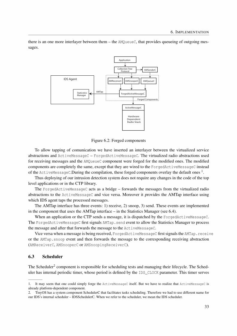
The radio abstractions for receiving (AMReceiverC, AMSnooperC, AMSnoopingReceiverC) are di-rectly wired to the ActiveMessageC component – the highest layer of the hardware dependent radiostack (see Section 5.2). The sending abstraction (AMSenderC) is not wired directly to the ActiveMessageC,
32
6. IMPLEMENTATION
there is an one more interlayer between them – the AMQueueC, that provides queueing of outgoing mes-sages.
Application
Collection Tree Protocol
ForgedActiveMessageC
AMReceiverC AMSnooperC AMQueueC
AMSenderC
IDS Agent
StaticsticsManager
AMTap
Forged Components
Hardware Dependent Radio Stack
ActiveMessageC
Figure 6.2: Forged components
To allow tapping of comunication we have inserted an interlayer between the virtualized serviceabstractions and ActiveMessageC – ForgedActiveMessageC. The virtualized radio abstractions usedfor receiving messages and the AMQueueC component were forged for the modified ones. The modifiedcomponents are completely the same, except that they are wired to the ForgedActiveMessageC insteadof the ActiveMessageC.During the compilation, these forged components overlay the default ones 1.
Thus deploying of our intrusion detection system does not require any changes in the code of the toplevel applications or in the CTP library.
The ForgedActiveMessageC acts as a bridge – forwards the messages from the virtualized radioabstractions to the ActiveMessageC and vice versa. Moreover it provides the AMTap interface usingwhich IDS agent taps the processed messages.
The AMTap interface has three events: 1) receive, 2) snoop, 3) send. These events are implementedin the component that uses the AMTap interface – in the Statistics Manager (see 6.4).
When an application or the CTP sends a message, it is dispatched by the ForgedActiveMessageC.The ForgedActiveMessageC first signals AMTap.send event to allow the Statistics Manager to processthe message and after that forwards the message to the ActiveMessageC.
Vice versa when a message is being received, ForgedActiveMessageC first signals the AMTap.receiveor the AMTap.snoop event and then forwards the message to the corresponding receiving abstraction(AMReceiverC, AMSnooperC or AMSnoopingReceiverC).
6.3 Scheduler
The Scheduler2 component is responsible for scheduling tests and managing their lifecycle. The Sched-uler has internal periodic timer, whose period is defined by the IDS_CLOCK parameter. This timer serves
1. It may seem that one could simply forge the ActiveMessageC itself. But we have to realize that ActiveMessageC isalready platform-dependent component.2. TinyOS has a system component SchedulerC that facilitates tasks scheduling. Therefore we had to use different name forour IDS’s internal scheduler – IDSSchedulerC. When we refer to the scheduler, we mean the IDS scheduler.
33

6. IMPLEMENTATION
as the internal IDS agent clock.The module holds a queue of scheduled tests – TestsQueue. Each test task is a structure of following
type:
typedef struct {uint8_t detection_engine ;uint8_t param;
} test_task_t ;
The first element of the type defines which Detection Engine will be used for this test and the secondelement is optional parameter that will be passed to the Detection Engine during the initialization. Thetest task can be scheduled by two ways: first, it can be scheduled by the response module in response toan alert or can be scheduled randomly – spontaneously.
The random test task is spontaneously enqueued with probabilitity P every time when the mainperiodic timer fires. The probability P is given as
P =START_THRESHOLD+n∗START_THRESHOLD_INC
65536where n is a number of cycles and START_THRESHOLD (default set to 2048), START_THRESHOLD_INC
(default set to 1024) are constants defined in IDS.h. Thus for the default values the probability that IDSspontaneously enqueue the test task is 3.125% at the beginning and it is increased by 1.5625% after eachunsuccesful attempt.
The IDS Scheduler has three states – SLEEP, INITIALIZING, RUNNING. Most time the schedulerspends in the SLEEP mode when no test is running and the IDS agent consumes minimum energy.
DequeueTest
DetectionEngine.evaluate
TestTimer.start
DetectionEngine.stop
DetectionEngine.start
Select Engine
RUNNINGINITIALIZING
Spontaneous Equeue
SLEEP
TestTimer.fired()
evaluateDone()
stopDone()
startDone()
TestsQueue not empty
TestsQueue empty
IDSTimer.fire()
Figure 6.3: IDS Scheduler
When the main periodic timer fires and Scheduler is in SLEEP mode, Scheduler checks if there areany tests in the TestsQueue. If not, it tries to enqueue new test spontaneously and goes to sleep.
If there is at least one scheduled test in the TestsQueue, the Scheduler begins to perform the first test inthe queue. It changes its internal state to INITIALIZING and then using the DetectionManager interfacechooses the required engine. Then it starts the engine itself by calling DetectionEngine.start().
After the engine is started up, it signals the DetectionEngine.startDone( run_time ), and asparameter passes how long it wants to run. The IDS scheduler changes its internal state to RUNNINGand sets the TestTimer to fire after the expiry of the required time.
When the TestTimer fires, the time for test has elapsed and scheduler calls DetectionEngine.stop()in order to stop the engine. The engine don’t have to stop immediately (for example, it may need to com-plete some tasks), but when it does, it signals the DetectionEngine.stopDone(). The scheduler thenstarts the third phase of Detection Engine lifecycle – the evaluation. It calls DetectionEngine.evaluate()
34
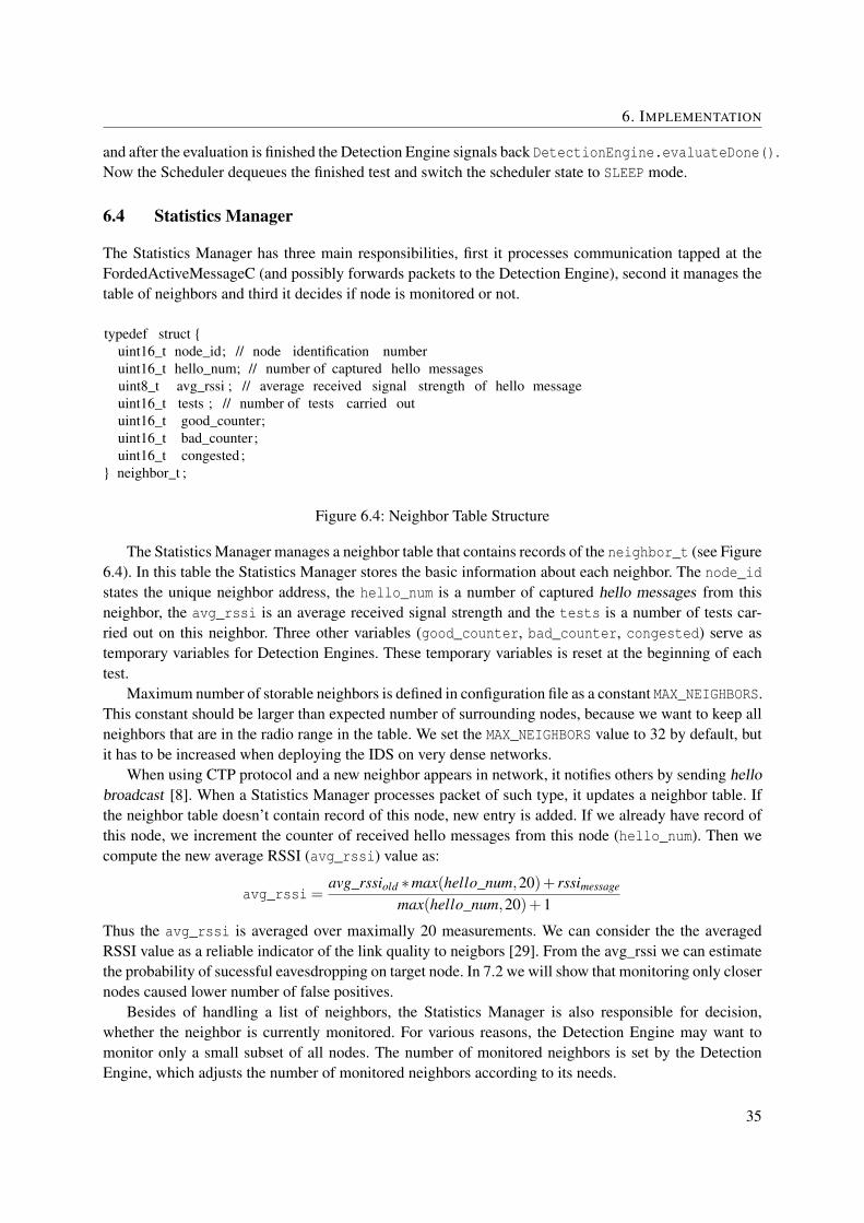
6. IMPLEMENTATION
and after the evaluation is finished the Detection Engine signals back DetectionEngine.evaluateDone().Now the Scheduler dequeues the finished test and switch the scheduler state to SLEEP mode.
6.4 Statistics Manager
The Statistics Manager has three main responsibilities, first it processes communication tapped at theFordedActiveMessageC (and possibly forwards packets to the Detection Engine), second it manages thetable of neighbors and third it decides if node is monitored or not.
typedef struct {uint16_t node_id; // node identification numberuint16_t hello_num; // number of captured hello messagesuint8_t avg_rssi ; // average received signal strength of hello messageuint16_t tests ; // number of tests carried outuint16_t good_counter;uint16_t bad_counter;uint16_t congested ;
} neighbor_t ;
Figure 6.4: Neighbor Table Structure
The Statistics Manager manages a neighbor table that contains records of the neighbor_t (see Figure6.4). In this table the Statistics Manager stores the basic information about each neighbor. The node_idstates the unique neighbor address, the hello_num is a number of captured hello messages from thisneighbor, the avg_rssi is an average received signal strength and the tests is a number of tests car-ried out on this neighbor. Three other variables (good_counter, bad_counter, congested) serve astemporary variables for Detection Engines. These temporary variables is reset at the beginning of eachtest.
Maximum number of storable neighbors is defined in configuration file as a constant MAX_NEIGHBORS.This constant should be larger than expected number of surrounding nodes, because we want to keep allneighbors that are in the radio range in the table. We set the MAX_NEIGHBORS value to 32 by default, butit has to be increased when deploying the IDS on very dense networks.
When using CTP protocol and a new neighbor appears in network, it notifies others by sending hellobroadcast [8]. When a Statistics Manager processes packet of such type, it updates a neighbor table. Ifthe neighbor table doesn’t contain record of this node, new entry is added. If we already have record ofthis node, we increment the counter of received hello messages from this node (hello_num). Then wecompute the new average RSSI (avg_rssi) value as:
avg_rssi =avg_rssiold ∗max(hello_num,20)+ rssimessage
max(hello_num,20)+1
Thus the avg_rssi is averaged over maximally 20 measurements. We can consider the the averagedRSSI value as a reliable indicator of the link quality to neigbors [29]. From the avg_rssi we can estimatethe probability of sucessful eavesdropping on target node. In 7.2 we will show that monitoring only closernodes caused lower number of false positives.
Besides of handling a list of neighbors, the Statistics Manager is also responsible for decision,whether the neighbor is currently monitored. For various reasons, the Detection Engine may want tomonitor only a small subset of all nodes. The number of monitored neighbors is set by the DetectionEngine, which adjusts the number of monitored neighbors according to its needs.
35

6. IMPLEMENTATION
The Statistics Manager always keep the monitored neighbors on first positions in the neighbor tableand keeps the number of currently monitored nodes. The Statistics Manager is able to decide if the nodeis monitored or not by checking only first monitoredNodes records in neighbor table instead of browsingthe whole (potentially large) table. This operation is time critical, because it has to be done every timea packet is processed and the processed packet is delayed until it is released by returning from AMTapevent.
When the processed packet is destined to a node that is monitored, the Statistics Manager by signalingStatisticsMngr.destinationMonitored passes the packet to the further evaluation to the DetectionEngine. Similarly, if the packet was sent by the monitored node, the StatisticsMngr.sourceMonitoredis signaled.
The Statictics Manager counts the number of messages that were destined to the node and howmany messages the node sent out. The Detection Engines can get this information by calling commandStatisticsManager.incoming and StatisticsManager.outgoing.
6.5 Detection Manager
The Detection Manager is a large subsystem that is composed of many components. It holds all DetectionEngine implementations and also components that are used by these Detection Engines (CtpStorage,MemoryManager). Moreover, it has also a special bridge component called DetectionManagerBridgeP.
The DetectionManagerBridgeP is a component that provides the external interfaces – Detection-Manager interface and DetectionEngine interface. The Scheduler that needs to wire to Detection Enginesdo not wire them directly but through this component.
• DetectionManager interface provides two commands: the selectEngine command and theenginesCount command. This interface is used by the Scheduler which uses the selectEnginecommand to select the active Detection Engine.
• DetectionEngine interface (in DetectionManagerBridgeP component) serves as a bridge toActive Detection Engine. For example when Scheduler calls start command, this component for-wards this call to the Detection Engine that is currently selected. Vice versa, when the DetectionEngine signals for example startDone, this component signals it back to the Scheduler.
The advantage of this approach is a possibility of simple addition of new Detection Engines. The newDetection Engine is specified only in Detection Manager configuration component.
Each Detection Engine has to provide DetectionEngine interface, which contains start, stop andevaluate commands and startDone, stopDone and evaluateDone events.
We can rely that only single Detection Engine will be active at the same time, thus we can let en-gines to share resources and memory between themselves, the Detection Manager ensures that only oneDetection Engine will access them at the same time.
The Detection Engines usually require a non-trivial ammount of operating memory for their activities,they for example often need to store packet signatures or even the whole packets. Unfortunatelly, theTinyOS do not support dynamic memory allocation and all memory has to be statically allocated at thecompile time. Therefore we introduced a minimalistic Memory Manager component, that allocates allthe memory, that we can spare for Detection Engines purposes, and components then can get pointerto this memory by calling MemoryMngr.malloc. The Memory Manager does not provide any memoryprotection, but allows two different engines to use the memory in different ways.
36
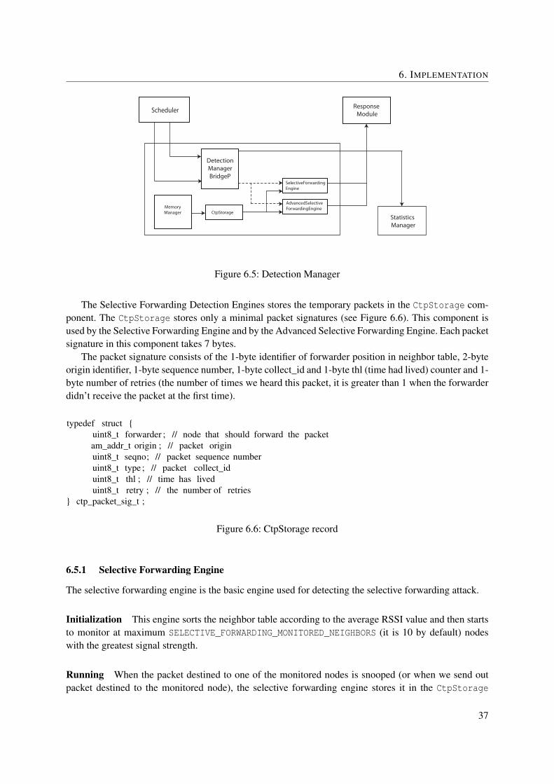
6. IMPLEMENTATION
SelectiveForwardingEngine
AdvancedSelectiveForwardingEngine
CtpStorageMemoryManager
Scheduler
Statistics Manager
Response Module
DetectionManagerBridgeP
Figure 6.5: Detection Manager
The Selective Forwarding Detection Engines stores the temporary packets in the CtpStorage com-ponent. The CtpStorage stores only a minimal packet signatures (see Figure 6.6). This component isused by the Selective Forwarding Engine and by the Advanced Selective Forwarding Engine. Each packetsignature in this component takes 7 bytes.
The packet signature consists of the 1-byte identifier of forwarder position in neighbor table, 2-byteorigin identifier, 1-byte sequence number, 1-byte collect_id and 1-byte thl (time had lived) counter and 1-byte number of retries (the number of times we heard this packet, it is greater than 1 when the forwarderdidn’t receive the packet at the first time).
typedef struct {uint8_t forwarder ; // node that should forward the packetam_addr_t origin ; // packet originuint8_t seqno; // packet sequence numberuint8_t type ; // packet collect_iduint8_t thl ; // time has liveduint8_t retry ; // the number of retries
} ctp_packet_sig_t ;
Figure 6.6: CtpStorage record
6.5.1 Selective Forwarding Engine
The selective forwarding engine is the basic engine used for detecting the selective forwarding attack.
Initialization This engine sorts the neighbor table according to the average RSSI value and then startsto monitor at maximum SELECTIVE_FORWARDING_MONITORED_NEIGHBORS (it is 10 by default) nodeswith the greatest signal strength.
Running When the packet destined to one of the monitored nodes is snooped (or when we send outpacket destined to the monitored node), the selective forwarding engine stores it in the CtpStorage
37

6. IMPLEMENTATION
component using the CtpStorage.insert command. The CtpStorage does not store the whole packet,but only its minimal signature, which is neccessary to re-identification of this packet and identifier ofnode which should forward this packet (see Figure 6.6). If we want to store a packet, but the CtpStorageis already full, we drop the oldest packet and increment the bad counter of the node that was supposed toforward this packet.
On TOSSIM simulator3 it may happen, that we hear the same packet that is already in CtpStorage.This can happen in the case, when the packet wasn’t received at the forwarder node on the first try and isbeing retransmitted. In this case we do not insert new packet into the CtpStorage, but only increment aretry counter at the previous one.
When we receive a packet sent by a node, that we are monitoring, we check if this packet signatureis stored in CtpStorage by calling CtpStorage.check. If we find such packet, we remove it from theCtpStorage and increment the monitored node’s good counter (see Section 6.4).
Thus when a node successfully forwards a packet, good counter is incemented by one. Conversely,when a node doesn’t forward a packet, bad counter is incremented.
In CTP, the node that is congested sets a congestion flag in the packet header. The congested node isthen allowed to drop packets. When the Selective Forwarding Engine detects a packet from monitorednode with set congestion flag, it increments congestion counter of corresponding node. The neighborwith non-zero congestion counter is not considered as the attacker.
When the selective forwarding engine called to stop, it does not stop instantly, but continues itswork for an additional STOP_INTERVAL miliseconds. In this period it does not insert new packets to theCtpStorage, but allows to check and remove the packets that were forwarded after the regular test periodelapsed.
Evaluation The selective forwarding engine first go throught all packets which weren’t forwarded andthus remained in the CtpStorage and for each found packet increments the bad counter of correspondingnode.
Then the selective forwarding engine sequentially goes through the monitored nodes and calculatesfor each node the error ratio:
err_ratio =bad_counter
bad_counter +good_counter∗255
If the error ratio is greater than threshold defined in SELECTIVE_FORWARDING_THRESHOLD, the se-lective forwarding engine raises an alert by calling Response.alert. We set the default value of theSELECTIVE_FORWARDING_THRESHOLD to 110.
6.5.2 Advanced Selective Forwarding Engines
The Advanced Selective Forwarding Engine works similar way as the basic, but it monitores only nodeswith a strong signal.
In initialization phase the Advanced Selective Forwarding Engine first checks, if the node servesas a forwarder. Each node that serves as forwarder is characterized by non-zero number of receivedpacket in sufficiently long interval. Thus the Advanced Selective Forwarding Engine first measures thenumber of messages that are incoming into this node in interval of 5 seconds. This is done by calling theStatisticsMngr.incoming() command twice in interval of 5 seconds.
3. On CC2420 radio, there is a Unique Receive Layer that prevents the watchdog from hearing retransmitted message, seeSection 5.3.
38

6. IMPLEMENTATION
When the difference between these two values is equal to zero, the node didn’t receive any mes-sage and is considered to not be a forwarder. Then the advanced selective forwarding engine reduce thesensitivity of receiver by calling RadioControl.setLowGainMode(TRUE).
If the node is a forwarder or the low gain mode is not successfully enabled, the Advanced SelectiveForwarding Engine won’t start.
Furthermore, the Advanced Selective Forwarding Engine works the same way as the basic.
6.6 Response Module
The response module is responsible for reaction taken after an alert is detected. The alert can be raisedby two ways: first, it can be called from the Detection Manager, or it may come from the network.
When the alarm is raised, the response module can perform several actions – it can schedule anadditional test, or it may broadcast message to other nodes to warn them.
In this thesis, we didn’t deal with reactions of the Response Module. The only reaction that theResponse Module carried out was logging the alert report.
39

Chapter 7
Deployment and Simulation
The implemented intrusion detection system is a library that can be linked to a any application. In order todeploy the IDS agent on any node the programmer only need to add the following rule into the Makefile.
CFLAGS += -I$(IDS_DIR)
The compiler then will include our IDS and will use the modified active message components insteadof the default ones.
7.1 Deployment on Tmote Sky
The TMote Sky sensor node [23] is based on the tmote platform. In fact, the tmote is just an alias for thetelosb platform in current TinyOS implementation.
The TMote Sky uses CC2420 radio [1]. To allow the mote to be able to promiscuously snoop thenetwork traffic, we have to disable address recognition. If the address recognition was enabled, the packetnot destined to the mote would be rejected too early and it would preclude us to use the watchdogmonitoring technique.
We disable the hardware address recognition by adding the following line into the Makefile:
CFLAGS+=-DCC2420_NO_ADDRESS_RECOGNITION
Compilation: We compile the program by typing:
$make tmote
Installation: If the compilation was successfull, we can install the program into the mote by typing:
$make tmote install [mote_id]
7.2 Deployment on TOSSIM
Compilation: The program can be compiled for simulation in TOSSIM by typing:
$make micaz sim
TOSSIM supports two programming interfaces – C++ and Python. The Python interface is generallyeasier to use, but it has a performation bottleneck – it is twice slower than C++ interface [32]. Because weneed to simulate our intrusion detection system in large networks, we use more efficient C++ interface.
For the purposes of IDS sumulation, we have created a simple program called tester.c1. We cancompile the tester.c program and link it against TOSSIM by typing:
1. It is included along with IDS source code
40

7. DEPLOYMENT AND SIMULATION
$g++ -g -c -o tester.o tester.c -I$(TOSDIR)/lib/tossim$g++ -o tester tester.o build/micaz/tossim.o build/micaz/sim.o \
build/micaz/c-support.o
7.3 Simulation
7.3.1 Error ratio
At first, we have tested proposed intrusion detection system without any deployed intruders. The aim ofthis simulation was to measure the natural error ratio of watchdogs in different enviroments.
The error ratios for selective forwarding attacks were defined asbad_counter
good_counter +bad_counter∗255
where bad_counter is a number of packets that weren’t forwarded and good_counter is a number ofpacket that were forwarded.
The error ratio will help us to estimate an ALERT_THRESHOLD for selective forwarding engines, thatwill lead to the acceptable number of false positives while maintaining the ability of IDS to detect selec-tive forwarding attack (see Section 2.5) with a low ratio of dropped packets.
In following simulations, we have set each node i to generate and send message using CTP every tseconds. We will refer this period t as a sensing rate.
First, we let the network initialize for one minute, and then performed ten one minute cycles. At eachcycle j, nodes i1, . . . , im, . . . , in that satisfied im mod 10 = j started their IDS agent and performed a basicselective forwarding test (thus during the simulation each node in network performed a single test).
For the purposes of these tests, the ALERT_THRESHOLD was set to 0. Therefore detection enginesraised an alert for each monitored node that forwarded some packets2 (even if forwarded all packets andhad error ratio equal to zero).
Note: We have to realize that it is not possible to repeat the simulation twice with the same results.There are several random factors we cannot eliminate (e.g. random noise, random CSMA back-offs,random CTP back-offs) that causes that network topology is always different. Therefore, even if wemonitor the same neighbors by the same watchdog in the same simulation time, every time we getdifferent results and particularly different number of alerts. For this reason we had to normalize thesimulations results to be able to compare individual simulations.
On following charts, the values on X-axis expresses the error ratios that are equal to or greater thanthe given value. For example the value of 100 includes all alarms with error ratio from 100 to 255.
Various sensing rate
At first, we measured an error ratio in relation to a number of messages that were generated and trans-mitted through the network. Each IDS agent was set to randomly choose 10 neighbors, whose averagerssi was under -86dB. We deployed 100 nodes in a topology defined in 15-15-tight-mica2-grid.txt(it is included in TinyOS-2.1.0 distribution and can be found in tos/lib/tossim/topologies). Thistopology is very dense, each node has more than 50 neighbors.
We tested three cases with different sensing period: 1) t = 5 seconds, 2) t = 2.5 seconds, 3) t = 1.250seconds.
2. With the possible exception of the nodes, that were congested and thus were allowed to drop packets.
41
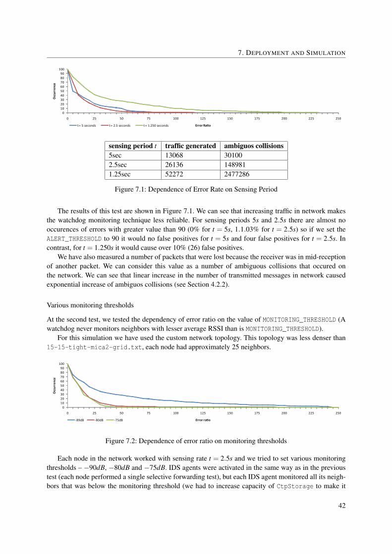
7. DEPLOYMENT AND SIMULATION
0102030405060708090
100
0 25 50 75 100 125 150 175 200 225 250
Occ
urre
nce
Error Ratiot = 5 seconds t = 2.5 seconds t = 1.250 seconds
sensing period t traffic generated ambiguos collisions5sec 13068 301002.5sec 26136 1489811.25sec 52272 2477286
Figure 7.1: Dependence of Error Rate on Sensing Period
The results of this test are shown in Figure 7.1. We can see that increasing traffic in network makesthe watchdog monitoring technique less reliable. For sensing periods 5s and 2.5s there are almost nooccurences of errors with greater value than 90 (0% for t = 5s, 1.1.03% for t = 2.5s) so if we set theALERT_THRESHOLD to 90 it would no false positives for t = 5s and four false positives for t = 2.5s. Incontrast, for t = 1.250s it would cause over 10% (26) false positives.
We have also measured a number of packets that were lost because the receiver was in mid-receptionof another packet. We can consider this value as a number of ambiguous collisions that occured onthe network. We can see that linear increase in the number of transmitted messages in network causedexponential increase of ambiguos collisions (see Section 4.2.2).
Various monitoring thresholds
At the second test, we tested the dependency of error ratio on the value of MONITORING_THRESHOLD (Awatchdog never monitors neighbors with lesser average RSSI than is MONITORING_THRESHOLD).
For this simulation we have used the custom network topology. This topology was less denser than15-15-tight-mica2-grid.txt, each node had approximately 25 neighbors.
0102030405060708090
100
0 25 50 75 100 125 150 175 200 225 250
Occ
urre
nce
Error ratio-89dB -80dB -75dB
Figure 7.2: Dependence of error ratio on monitoring thresholds
Each node in the network worked with sensing rate t = 2.5s and we tried to set various monitoringthresholds – −90dB, −80dB and −75dB. IDS agents were activated in the same way as in the previoustest (each node performed a single selective forwarding test), but each IDS agent monitored all its neigh-bors that was below the monitoring threshold (we had to increase capacity of CtpStorage to make it
42

7. DEPLOYMENT AND SIMULATION
possible).The results of this test are shown on figure 7.2. It is obvious that when we limit monitoring only to
nodes with stronger signal, an average error ratio is lower. On the other hand this reduces IDS perfor-mance, because each IDS agent can monitor only a limited subset of neighbors.
7.3.2 Advanced selective forwarding engine
The purpose of this experiment was to confirm the hypothesis that by reducing the sensitivity of thewatchdog’s receiver we can suppress weak signals from distant nodes and achieve more reliable eaves-dropping on near nodes.
In CC2420 radio, we can reduce the receiver sensitivity by lowering the signal amplification that isperformed before the signal is processed in analog digital convertor.
The simpliest way how to control the signal amplification that is performed is by setting the AGC-TRL register. By changing the value of this register, we can override the low-noise-amplifier settingsand manually set four modes – automatic, low-gain, medium-gain and high-gain. By default (automaticmode) the LNA gain mode is choosed by AGC (Automatic Gain Control) that dynamically adjust themode according to strength of received signal. In opposite, other modes set the LNA gain mode fixedlyand do not change it.
15m ~ -86dB
15m ~ -84dB
15m ~ -84dB
2m ~ -62dB
2
6
7
9
0
Figure 7.3: Nodes deployment
We deployed five nodes as shown in Figure 7.3. The node 0 represented the watchdog, the node 2that was only 2 meters from the watchdog and represented the close node we wanted to monitor. Theremaining three nodes (6,7,9) were 15 meters from the watchdog and represented the nodes we do notintend to eavesdrop on. All sending nodes were possitioned in such way to be sufficiently far from eachother to avoid the CSMA collisions.
The nodes 2,6,7,9 were set to send 500 messages in 10 seconds. Each message had 25 bytes andwas destined to node 0. We have disabled message acknowledgements and sent messages directly usingActive Message Layer without any message retransmions 3.
We have defined four receiver modes m0,m1,m2,m3. In the first mode m0 the watchdog’s low-noise-amplifier was controlled by AGC, in the m1 mode the LNA was set to low-gain, in the m2 to medium-gainand in the m3 to high-gain.
The node 0 (watchdog) always worked in one of these modes and counted the number of messagesnumi that were received from each node i during last 10 seconds interval. Because we know that eachnode has always sent 500 messages during the interval, we can calculate the packet receive ratio asPRRi = numi
500 .
3. This guarantees that each node send exactly 500 messages in 10 seconds
43

7. DEPLOYMENT AND SIMULATION
For each interval we periodically changed the mode in which node 0 worked in, and we repeated ineach mode more than 10 times. The averaged results are summarized in table 7.1.
node 2 node 6 node 7 node 9mode num2 PRR2 num6 PRR6 num7 PRR7 num9 PRR9
automatic 450.21 90.04% 328.29 65.66% 258.07 51.61% 251.29 50.26%low-gain 498.73 99.75% 1.93 0.39% 0.33 0.07% 0.53 0.11%medium-gain 472.27 94.75% 158.71 31.74% 59.93 11.99% 189.67 37.93%high-gain 448.14 89.63% 333.93 66.79% 224.57 44.91% 275.31 55.06%
Table 7.1: Packet receive ratio in different modes
In the automatic and high-gain mode4, the watchdog was able to receive around 90% of packets sentby the node 2 and approximately half of packets from the distant nodes.
In the medium-gain mode, the probability that packet from the close node will be successfully re-ceived had increased to 95%, in low-gain mode to almost 100%. This was achieved at the cost of smallernumber of received packets from the distant nodes.
In lower-gain modes, the watchdog often does not recognized the beginnings of messages that camefrom the distant nodes, thus it does not start receiving them. In result, the distant nodes did not “block”the watchdog so often and it was able to receive more packet from the close node.
In other words, the number of ambiguous collisions, that occured from the perspective of the watch-dog, was much smaller.
In conclusion, the experiment confirmed that the reducing of watchdog’s receiver sensitivity willimprove the accurancy of eavesdropping on close nodes.
Simulation
In this simulation, we have tested the difference between the basic selective forwarding engine and ad-vanced selective forwarding engine. An advanced selective forwarding engine tries to get benefit fromsuppressing weak signals.
We have simulated the IDS behavior on similar network as in the first test. The only difference wasthat we scheduled each node to perform two tests – the basic and advanced. Both tests were performedone after another, thus we can assume that both engines had same data.
0102030405060708090
100
0 25 50 75 100 125 150 175 200 225 250
Occ
urre
nce
Error ratioBasic Selective Forwarding Engine Advanced Selective Forwarding Engine
Figure 7.4: Advanced Selective Forwarding Engine
We can see on 7.4 that Advanced Selective Forwarding Engine had smaller number of occurencessof higher error ratio.
4. We can see that results achieved in the automatic mode are more or less the same as in the high-gain mode. This is due toAGC that for most of the time sets the linear-noise-amplifier to high-gain mode.
44
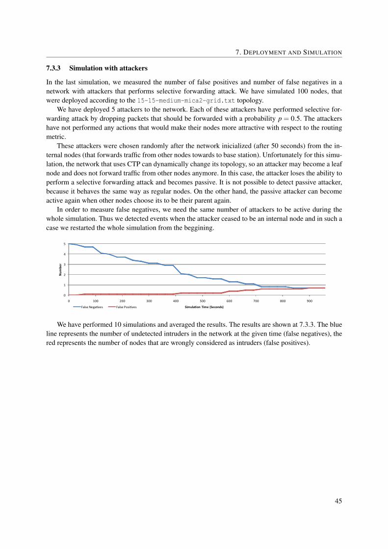
7. DEPLOYMENT AND SIMULATION
7.3.3 Simulation with attackers
In the last simulation, we measured the number of false positives and number of false negatives in anetwork with attackers that performs selective forwarding attack. We have simulated 100 nodes, thatwere deployed according to the 15-15-medium-mica2-grid.txt topology.
We have deployed 5 attackers to the network. Each of these attackers have performed selective for-warding attack by dropping packets that should be forwarded with a probability p = 0.5. The attackershave not performed any actions that would make their nodes more attractive with respect to the routingmetric.
These attackers were chosen randomly after the network inicialized (after 50 seconds) from the in-ternal nodes (that forwards traffic from other nodes towards to base station). Unfortunately for this simu-lation, the network that uses CTP can dynamically change its topology, so an attacker may become a leafnode and does not forward traffic from other nodes anymore. In this case, the attacker loses the ability toperform a selective forwarding attack and becomes passive. It is not possible to detect passive attacker,because it behaves the same way as regular nodes. On the other hand, the passive attacker can becomeactive again when other nodes choose its to be their parent again.
In order to measure false negatives, we need the same number of attackers to be active during thewhole simulation. Thus we detected events when the attacker ceased to be an internal node and in such acase we restarted the whole simulation from the beggining.
0
1
2
3
4
5
0 100 200 300 400 500 600 700 800 900
Num
ber
Simulation Time (Seconds)False Negatives False Positives
We have performed 10 simulations and averaged the results. The results are shown at 7.3.3. The blueline represents the number of undetected intruders in the network at the given time (false negatives), thered represents the number of nodes that are wrongly considered as intruders (false positives).
45

Chapter 8
Conclusion
We can divide the contribution of this work into three parts:
• We have designed and implemented a simple intrusion detection system that is able to detectselective forwarding attacks. The proposed intrusion detection system allows easy extensibilitythrough simple addition of new detection engines.
• We have improved reliability of watchdog monitoring technique on network with a large numberof ambiguous collisions. The technique is based on limiting the watchdog’s receiver sensitivityand allows the watchdog to suppress weak signals coming from distant nodes. As a result, thewatchdog is able to eavesdrop better on close neighbors because it does not hear distant nodes.
We have shown that this technique is feasible on CC2420 radio chip. By bypassing the automaticgain control loop we forced the radio receiver to amplify received signal lesser than in automaticmode. The watchdog node then does not recognize packet preambule (synchronization headersand frame delimiter) from distant nodes, therefore it does not start receiving packets from them.
In 7.3.2 we described an experiment that confirmed that the technique really works. In compari-son with the experiment without the use of this method, the receiver node lost fewer packets fromthe close mote and the packet receive ratio from that node significantly increased. The simulationpresented in 7.3.2 has shown that this technique would raise less false positives when we restrictwatchdog to monitor only the closest nodes.
• To be able to accurately simulate our intrusion detection system on TOSSIM simulator, we hadto modify the simulator. The simulator had several serious deficiencies. First, it had a bug thatallowed a node to receive message at the same time when it was transmitting another one. Thisbug was reported and it was confirmed by TOSSIM developers.
Second, the CSMA algorithm on TOSSIM was different from the one on CC2420. Particularly,it considered channel to be free even if the node was receiving valid data. Although the CC2420radio could be set to behave this way, by default it considers channel to be free only if the nodeis not receiving data.
All these deficiencies have been fixed and the simulation of the designed IDS has been success-fully performed on the TOSSIM simulator.
46
Bibliography
[1] CC2420 datasheet, Jan. 2008. Available at http://inst.eecs.berkeley.edu/~cs150/Documents/CC2420.pdf.
[2] Shah Bhatti, James Carlson, Hui Dai, Jing Deng, Jeff Rose, Anmol Sheth, Brian Shucker, CharlesGruenwald, Adam Torgerson, and Richard Han. MANTIS OS: an embedded multithreaded operat-ing system for wireless micro sensor platforms. Mob. Netw. Appl., 10(4):563–579, 2005.
[3] Han C., Kumar R. Rengaswamy, Shea R., Kohler E., and Srivastava M. SOS: A Dynamic OperatingSystem for Sensor Networks. In Proceedings of the Third International Conference on MobileSystems, Applications, and Services (Mobisys 2005), Seattle, Washington, June 2005.
[4] David E. Culler. TinyOS: Operating system design for wireless sensor networks. http://www.sensorsmag.com/sensors/article/articleDetail.jsp?id=324975.
[5] Ana Paula R. da Silva, Marcelo H. T. Martins, Bruno P. S. Rocha, Antonio Alfredo FerreiraLoureiro, Linnyer Beatrys Ruiz, and Hao Chi Wong. Decentralized intrusion detection in wire-less sensor networks. In Azzedine Boukerche and Regina Borges de Araujo, editors, Q2SWinet,pages 16–23. ACM, 2005.
[6] Adam Dunkels, Bjorn Gronvall, and Thiemo Voigt. Contiki - a lightweight and flexible operatingsystem for tiny networked sensors. In LCN ’04: Proceedings of the 29th Annual IEEE InternationalConference on Local Computer Networks, pages 455–462, Washington, DC, USA, 2004. IEEEComputer Society.
[7] Jeremy Elston and Deborah Estrin. Wireless sensor networks, chapter Sensor networks: A bridgeto the physical world, pages 3–21. 2004.
[8] Rodrigo Fonseca, Omprakash Gnawali, Kyle Jamieson, Sukun Kim, Philip Levis, and Alec Woo.The Collection Tree Protocol (CTP). http://www.tinyos.net/tinyos-2.x/doc/html/tep123.html.
[9] David Gay, Matt Welsh, Philip Levis, Eric Brewer, Robert Von Behren, and David Culler. The nesclanguage: A holistic approach to networked embedded systems. In In Proceedings of ProgrammingLanguage Design and Implementation (PLDI), pages 1–11, 2003.
[10] Vlado Handziski, Joseph Polastrey, Jan-Hinrich Hauer, Cory Sharpy, Adam Wolisz, and DavidCullery. Flexible hardware abstraction for wireless sensor networks. In Proceedings of SecondEuropean Workshop on Wireless Sensor Networks (EWSN 2005), Istanbul, Turkey, 2005.
[11] Richard Heady, George Lugar, Mark Servilla, and Arthur Maccabe. The architecture of a networklevel intrusion detection system. Technical report, University of New Mexico, Albuquerque, NM,August 1990.
47

8. CONCLUSION
[12] Krontiris Ioannis, Tassos Dimitriou, and Felix C. Freiling. Towards intrusion detection in wirelesssensor networks. In 13th European Wireless Conference, Paris, April 2007.
[13] Aravind Iyer, Sunil S. Kulkarni, Vive Mhatre, and Catherine P. Rosenberg. A Taxonomy-basedApproach to Design of Large-scale Sensor Networks. Kluwer, 2004.
[14] Chris Karlof and David Wagner. Secure routing in wireless sensor networks: attacks and counter-measures. Ad Hoc Networks, 1(2-3):293–315, 2003.
[15] Ioannis Krontiris, Tassos Dimitriou, Thanassis Giannetsos, and Marios Mpasoukos. Intrusion de-tection of sinkhole attacks in wireless sensor networks. In Miroslaw Kutylowski, Jacek Cichon,and Przemyslaw Kubiak, editors, ALGOSENSORS, volume 4837 of Lecture Notes in ComputerScience, pages 150–161. Springer, 2007.
[16] Ioannis Krontiris, Thanassis Giannetsos, and Tassos Dimitriou. LIDeA: a distributed lightweightintrusion detection architecture for sensor networks. In SecureComm ’08: Proceedings of the 4thinternational conference on Security and privacy in communication netowrks, pages 1–10, NewYork, NY, USA, 2008. ACM.
[17] Hyung June Lee, Alberto Cerpa, and Philip Levis. Improving wireless simulation through noisemodeling. In IPSN ’07: Proceedings of the 6th international conference on Information processingin sensor networks, pages 21–30, New York, NY, USA, 2007. ACM.
[18] Philip Levis. Packet protocols. http://www.tinyos.net/tinyos-2.x/doc/html/tep116.html.
[19] Philip Levis, David Gay, Vlado Handziski, Jan-Heinrich Hauer, Ben Greenstein, Martin Turon,Jonathan Hui, Kevin Klues, Cory Sharp, Robert Szewczyk, Joseph Polastre, Philip Buonadonna,Lama Nachman, Gilman Tolle, David Culler, and Adam Wolisz. T2: A second generation os forembedded sensor networks. Technical report, Telecommunication Networks Group, TechnischeUniversitat Berlin, 2005.
[20] 6LoWPAN – IPv6 over low-power wireless personal area networks. http://6lowpan.tzi.org/.
[21] Sergio Marti, T. J. Giuli, Kevin Lai, and Mary Baker. Mitigating routing misbehavior in mobile adhoc networks. In MobiCom ’00: Proceedings of the 6th annual international conference on Mobilecomputing and networking, pages 255–265, New York, NY, USA, 2000. ACM.
[22] David Moss and Philip Levis. Packet link layer. http://www.tinyos.net/tinyos-2.x/doc/html/tep127.html.
[23] Moteiv. Tmote sky datasheet, 2006. http://www.cs.uvm.edu/~crobinso/mote/tmote-sky-datasheet-102.pdf.
[24] Moteiv. Tmote mini datasheet, 2007. http://www.sentilla.com/pdf/eol/Tmote_Mini_Datasheet.pdf.
[25] John Pike. Sound surveillance system (sosus). online. http://www.globalsecurity.org/intell/systems/sosus.htm.
[26] Rodrigo Roman, Jianying Zhou, and Javier Lopez. Applying intrusion detection systems to wirelesssensor networks. In Proceedings of IEEE Consumer Communications and Networking Conference(CCNC ’06), pages 640–644, Las Vegas, USA, January 2006.
48

8. CONCLUSION
[27] Tanya Roosta, Shiuhpyng Shieh, and Shankar Sastry. Taxonomy of security attacks in sensor net-works and countermeasures. In In The First IEEE International Conference on System Integrationand Reliability Improvements. Hanoi, pages 13–15, 2006.
[28] IEEE Computer Society. IEEE standard 802.15.4a-2007, August 31, 2007.
[29] Kannan Srinivasan and Philip Levis. Rssi is under appreciated. In EmNets 2006, May 2006.
[30] TinyOS. http://www.tinyos.net/.
[31] TinyOS Core Working Group. TEP 106: Schedulers and Tasks. http://www.tinyos.net/tinyos-2.x/doc/html/tep106.html.
[32] TOSSIM tutorial. Avaiable at http://docs.tinyos.net/index.php/TOSSIM.
[33] Imote2 datasheet. online. http://www.xbow.com/Products/Product_pdf_files/Wireless_pdf/Imote2_Datasheet.pdf.
49