
Lightweight Intrusion Detection in Wireless Sensor Networks
202
LIGHTWEIGHT INTRUSION DETECTION IN WIRELESS SENSOR NETWORKS Am Fachbereich Informatik der Technischen Universität Darmstadt zur Erlangung des akademischen Grades eines Doktor-Ingenieurs (Dr.-Ing.) genehmigte Dissertationsschrift von dipl .- wirt.- inf. michael riecker Geboren am 26. März 1982 in Heilbronn, Deutschland Erstreferent: Prof. Dr.-Ing. Matthias Hollick Korreferent: Prof. Dr.-Ing. Felix Freiling Tag der Einreichung: 11. Mai 2015 Tag der Disputation: 22. Juni 2015 Darmstadt, 2015 Hochschulkennziffer D17
-
Upload
khangminh22 -
Category
Documents
-
view
1 -
download
0
Transcript of Lightweight Intrusion Detection in Wireless Sensor Networks

L I G H T W E I G H T I N T R U S I O N D E T E C T I O NI N W I R E L E S S S E N S O R N E T W O R K S
Am Fachbereich Informatikder Technischen Universität Darmstadt
zur Erlangung des akademischen Grades einesDoktor-Ingenieurs (Dr.-Ing.)
genehmigte Dissertationsschrift
von
dipl.-wirt.-inf. michael riecker
Geboren am 26. März 1982 in Heilbronn, Deutschland
Erstreferent: Prof. Dr.-Ing. Matthias Hollick
Korreferent: Prof. Dr.-Ing. Felix Freiling
Tag der Einreichung: 11. Mai 2015
Tag der Disputation: 22. Juni 2015
Darmstadt, 2015
Hochschulkennziffer D17


A B S T R A C T
Wireless sensor networks have become a mature technology. They are increasinglybeing used in different practical applications. Examples include the monitoring ofindustrial environments and light adaptation in tunnels. For such applications, attacksare a serious concern. A disrupted sensor network may not only have a financialimpact, but could also be safety-critical. Hence, the availability of a wireless sensornetwork is our key protection goal in this thesis. A special challenge lies in the fact,that sensor nodes typically are physically unprotected. Hence, insider attacks aresupposed to occur, e.g., by compromising the nodes and getting in possession of thecryptographic keys, thereby becoming a legitimate member of the network. As a result,mechanisms to detect attacks during operation are necessary.
Traditionally, intrusion detection systems are used to discover network anomalies.Due to severe resource-restrictions, building such a system for wireless sensor net-works is challenging; it has to be small in size. Therefore, it is important to reduce therequired information for intrusion detection. The majority of these systems designedfor wireless sensor networks is working decentralized, i.e., the nodes try to detectthe attacks locally, mostly by using some type of collaboration with other nodes. Sofar, the real-world effects of attacks on wireless sensor networks have not yet beenstudied widely. Consequently, state-of-the-art intrusion detection systems often needto analyze a large number of metrics for attack detection. The execution frequency ofthe detection algorithm is mainly periodic or constant. Another problem that needsfurther research, is the possibility of reducing the detection frequency. We also investi-gate the feasibility of performing intrusion detection without collaboration, in orderto enable the lightweight detection of denial-of-service attacks on wireless sensornetworks.
To overcome these shortcomings, in this work we conduct systematic measurementsin a real testbed in order to quantify the impact of denial-of-service attacks. Thisallows us to identify those metrics, which are significantly influenced by an attack,and thus are appropriate for attack detection. We present a fully localized intrusiondetection system, in which the nodes do not have to collaborate with each other. Basedon these results we propose two architectures, allowing the randomization of thedetection frequency. The advantage here is, that an adversary may not predict well inadvance, which node is responsible to perform intrusion detection at a certain pointin time.
The gathered data from the extensive measurements is analyzed with statisticalapproaches. The presented intrusion detection systems are evaluated in simulationsand prototypical implementations.


Z U S A M M E N FA S S U N G
Drahtlose Sensornetze werden zunehmend zur Unterstützung von unterschiedlichen,praktischen Anwendungen eingesetzt. Die Einsatzgebiete in der realen Welt, in de-nen drahtlose Sensornetze eine wichtige Rolle spielen, umfassen beispielsweise dieÜberwachung von industriellen Anlagen und die Lichtsteuerung in Tunnels. Für diesebeispielhaften Anwendungen stellen Angriffe eine große Gefahr dar. Das Ausfallendes Sensornetzes kann neben finanziellen auch sicherheitskritische Auswirkungenhaben. Daher ist das wichtigste Schutzziel in dieser Arbeit die Verfügbarkeit desdrahtlosen Sensornetzes. Eine besondere Herausforderung beim Gewährleisten derSicherheit ist durch die oftmals freie Zugänglichkeit zu den Sensorknoten gegeben.Daraus ergibt sich, dass von Insider-Angriffen ausgegangen werden muss, welche z.B.durch Kompromittierung der Knoten im Besitz gültiger kryptographischer Schlüsselund somit legitimer Teil des Netzes sind. Aus diesem Grunde sind Mechanismen zumErkennen von Angriffen auf das Sensornetz während des laufenden Betriebs nötig.
Traditionell werden Angriffserkennungssysteme zum Aufdecken von Netzwerk-anomalien eingesetzt. Aufgrund der starken Ressourcenbeschränkungen ist der Ent-wurf eines solchen Systems für drahtlose Sensornetze besonders herausfordernd;der Speicherbedarf muss klein sein. Deshalb ist es wichtig, die benötigten Informa-tionen zur Angriffserkennung zu reduzieren. Die überwiegende Mehrheit dieserSysteme für drahtlose Sensornetze arbeitet dezentral, d.h. die Knoten versuchen dieAngriffe lokal zu erkennen, wofür meistens eine Form von Kooperation mit ande-ren Knoten notwendig ist. Bisher wurden die realen Auswirkungen von Angriffenauf Sensornetze unzureichend untersucht, weshalb oft eine Vielzahl an Metrikenzur Angriffserkennung herangezogen werden muss. Die Ausführungshäufigkeit desErkennungsalgorithmus ist vorwiegend periodisch oder konstant. Ebenso lücken-haft erforscht ist die Möglichkeit zur Reduzierung der Ausführungshäufigkeit. DesWeiteren untersuchen wir, ob die Angriffserkennung ohne Kooperation mit anderenKnoten möglich ist, um Angriffe auf die Verfügbarkeit von drahtlosen Sensornetzenleichtgewichtig zu entdecken.
Um diese Lücken zu schließen, werden in dieser Arbeit systematische Messungenin einem realen Testbed durchgeführt, um die Auswirkungen von Angriffen auf dieVerfügbarkeit zu quantifizieren. Daraus resultieren Erkenntnisse, welche Metrikenbesonders von einem Angriff beeinflusst werden und sich somit gut zur Angriffserken-nung eignen. Wir stellen ein gänzlich lokal arbeitendes Angriffserkennungssystem vor,das ohne Kooperation mit anderen Knoten auskommt. Aufbauend auf den erhaltenenErgebnissen werden zwei Architekturen vorgeschlagen, welche die Ausführungshäu-figkeit des Angriffserkennnungsmechanismus randomisieren. Dadurch ist es für einenAngreifer schwerer vorherzusehen, welcher Knoten zu welchem Zeitpunkt Angriffeerkennen soll.
Die gewonnenen Daten aus den umfangreichen Messungen werden mittels statisti-scher Verfahren untersucht. Die vorgestellten Angriffserkennungssysteme werden inSimulationen und prototypischen Implementierungen evaluiert.


A C K N O W L E D G M E N T S
First of all, I would like to thank Prof. Matthias Hollick for giving me the opportunityto work in his group. Without his constant support, this thesis would not have beenpossible. I also thank Prof. Felix Freiling for being my co-referee and for havingmotivated me to do research in IT security. Additionally, I would like to thankProf. Stefan Katzenbeisser, Prof. Alejandro Buchmann, and Prof. Max Mühlhäuser fortheir contributions as members of my committee.
I would like to express my gratitude for the support to all the people I have workedwith, especially Dingwen Yuan, Sebastian Biedermann, Rachid El Bansarkhani, andSascha Hauke. I also want to thank my students for the productive cooperation, andour sometimes very long discussions. Thanks to my past and present colleagues atthe Secure Mobile Networking Lab as well as the Center for Advanced Security ResearchDarmstadt, it was a pleasure to work with you!
Finally, I would like to thank my wife Daria, my family and friends for believing inme.
Darmstadt, 2015 Michael


C O N T E N T S
1 introduction 3
1.1 Motivation . . . . . . . . . . . . . . . . . . . . . . . . . . . . . . . . . . . . 3
1.2 Goals . . . . . . . . . . . . . . . . . . . . . . . . . . . . . . . . . . . . . . . 4
1.3 Contributions . . . . . . . . . . . . . . . . . . . . . . . . . . . . . . . . . . 4
1.3.1 Measuring the Impact of Denial-of-Service Attacks . . . . . . . . 5
1.3.2 Token-based Intrusion Detection . . . . . . . . . . . . . . . . . . . 5
1.3.3 Mobile Agent-based Intrusion Detection . . . . . . . . . . . . . . 5
1.4 Outline . . . . . . . . . . . . . . . . . . . . . . . . . . . . . . . . . . . . . . 6
2 foundations 7
2.1 Wireless Sensor Networks . . . . . . . . . . . . . . . . . . . . . . . . . . . 7
2.1.1 Basics of Wireless Sensor Networks . . . . . . . . . . . . . . . . . 7
2.1.2 Hardware . . . . . . . . . . . . . . . . . . . . . . . . . . . . . . . . 8
2.1.3 Application Scenarios . . . . . . . . . . . . . . . . . . . . . . . . . 8
2.2 Security in Wireless Sensor Networks . . . . . . . . . . . . . . . . . . . . 9
2.2.1 Terminology . . . . . . . . . . . . . . . . . . . . . . . . . . . . . . . 9
2.2.2 Security Goals . . . . . . . . . . . . . . . . . . . . . . . . . . . . . . 10
2.2.3 Classes of Adversaries . . . . . . . . . . . . . . . . . . . . . . . . . 11
2.2.4 Attacks on Wireless Sensor Networks . . . . . . . . . . . . . . . . 12
2.2.5 Challenges . . . . . . . . . . . . . . . . . . . . . . . . . . . . . . . . 15
2.3 Summary . . . . . . . . . . . . . . . . . . . . . . . . . . . . . . . . . . . . . 16
3 related work and problem statement 17
3.1 Intrusion Detection Systems . . . . . . . . . . . . . . . . . . . . . . . . . . 17
3.1.1 Attacker Type . . . . . . . . . . . . . . . . . . . . . . . . . . . . . . 18
3.1.2 Attacker Capabilities . . . . . . . . . . . . . . . . . . . . . . . . . . 18
3.1.3 Detectable Attacks . . . . . . . . . . . . . . . . . . . . . . . . . . . 18
3.1.4 Architecture . . . . . . . . . . . . . . . . . . . . . . . . . . . . . . . 19
3.1.5 Collaboration . . . . . . . . . . . . . . . . . . . . . . . . . . . . . . 19
3.1.6 Detection Technique . . . . . . . . . . . . . . . . . . . . . . . . . . 20
3.1.7 Detection Frequency . . . . . . . . . . . . . . . . . . . . . . . . . . 20
3.1.8 WSN Topology . . . . . . . . . . . . . . . . . . . . . . . . . . . . . 20
3.1.9 Evaluation . . . . . . . . . . . . . . . . . . . . . . . . . . . . . . . . 20
3.2 State-of-the-art Intrusion Detection Systems . . . . . . . . . . . . . . . . . 21
3.2.1 Decentralized IDSs . . . . . . . . . . . . . . . . . . . . . . . . . . . 21
3.2.2 Centralized IDSs . . . . . . . . . . . . . . . . . . . . . . . . . . . . 26
3.2.3 Hybrid IDSs . . . . . . . . . . . . . . . . . . . . . . . . . . . . . . . 27
3.3 Performance and Security Metrics . . . . . . . . . . . . . . . . . . . . . . 28
3.4 Summary and Problem Statement . . . . . . . . . . . . . . . . . . . . . . 29
3.4.1 Systematic Methodology for Measuring the Impact of Denial-of-Service Attacks . . . . . . . . . . . . . . . . . . . . . . . . . . . . . 30
3.4.2 Novel Lightweight Intrusion Detection Systems . . . . . . . . . . 30
4 measuring the impact of denial-of-service attacks 33
4.1 Design . . . . . . . . . . . . . . . . . . . . . . . . . . . . . . . . . . . . . . 33
4.1.1 Testbeds . . . . . . . . . . . . . . . . . . . . . . . . . . . . . . . . . 34

4.1.2 Protocols Employed . . . . . . . . . . . . . . . . . . . . . . . . . . 40
4.1.3 Attack Implementations . . . . . . . . . . . . . . . . . . . . . . . . 40
4.1.4 Metrics . . . . . . . . . . . . . . . . . . . . . . . . . . . . . . . . . . 43
4.2 Methodology . . . . . . . . . . . . . . . . . . . . . . . . . . . . . . . . . . 45
4.3 Metric Assessment . . . . . . . . . . . . . . . . . . . . . . . . . . . . . . . 47
4.4 Results . . . . . . . . . . . . . . . . . . . . . . . . . . . . . . . . . . . . . . 48
4.4.1 Initial Tests . . . . . . . . . . . . . . . . . . . . . . . . . . . . . . . 48
4.4.2 Final Tests . . . . . . . . . . . . . . . . . . . . . . . . . . . . . . . . 59
4.5 IDS . . . . . . . . . . . . . . . . . . . . . . . . . . . . . . . . . . . . . . . . 72
4.5.1 Implementation . . . . . . . . . . . . . . . . . . . . . . . . . . . . . 72
4.5.2 Selected Model . . . . . . . . . . . . . . . . . . . . . . . . . . . . . 75
4.5.3 Evaluation . . . . . . . . . . . . . . . . . . . . . . . . . . . . . . . . 77
4.6 Discussion . . . . . . . . . . . . . . . . . . . . . . . . . . . . . . . . . . . . 81
4.7 Related Work . . . . . . . . . . . . . . . . . . . . . . . . . . . . . . . . . . 81
4.8 Summary . . . . . . . . . . . . . . . . . . . . . . . . . . . . . . . . . . . . . 82
5 token-based intrusion detection 83
5.1 System Overview . . . . . . . . . . . . . . . . . . . . . . . . . . . . . . . . 83
5.1.1 Network Model . . . . . . . . . . . . . . . . . . . . . . . . . . . . . 83
5.1.2 General Attacker Model . . . . . . . . . . . . . . . . . . . . . . . . 84
5.1.3 Specific Assumptions and Requirements . . . . . . . . . . . . . . 84
5.1.4 Patrol Overview . . . . . . . . . . . . . . . . . . . . . . . . . . . . 84
5.2 Patrol Architecture . . . . . . . . . . . . . . . . . . . . . . . . . . . . . . . 85
5.2.1 Basic Setup . . . . . . . . . . . . . . . . . . . . . . . . . . . . . . . 85
5.2.2 Security Mechanisms . . . . . . . . . . . . . . . . . . . . . . . . . . 85
5.2.3 Token Communication . . . . . . . . . . . . . . . . . . . . . . . . . 86
5.3 Token Distribution . . . . . . . . . . . . . . . . . . . . . . . . . . . . . . . 87
5.4 Proof-of-Concept Application: Energy-based IDS . . . . . . . . . . . . . 89
5.5 Evaluation . . . . . . . . . . . . . . . . . . . . . . . . . . . . . . . . . . . . 90
5.5.1 Testbed . . . . . . . . . . . . . . . . . . . . . . . . . . . . . . . . . . 91
5.5.2 Different Token Forwarding Strategies . . . . . . . . . . . . . . . 91
5.5.3 Detection Time . . . . . . . . . . . . . . . . . . . . . . . . . . . . . 93
5.5.4 Hitting Time . . . . . . . . . . . . . . . . . . . . . . . . . . . . . . . 96
5.5.5 Energy Consumption . . . . . . . . . . . . . . . . . . . . . . . . . 98
5.5.6 Discussion . . . . . . . . . . . . . . . . . . . . . . . . . . . . . . . . 98
5.6 Related Work . . . . . . . . . . . . . . . . . . . . . . . . . . . . . . . . . . 98
5.7 Summary . . . . . . . . . . . . . . . . . . . . . . . . . . . . . . . . . . . . . 99
6 mobile agent-based intrusion detection 101
6.1 System Overview . . . . . . . . . . . . . . . . . . . . . . . . . . . . . . . . 101
6.1.1 Mobile Agents used for Intrusion Detection . . . . . . . . . . . . 101
6.1.2 Attacker Model, Assumptions, and Requirements . . . . . . . . . 102
6.1.3 Energy-based Intrusion Detection . . . . . . . . . . . . . . . . . . 103
6.2 Practical Considerations of a Mobile Agent-Based IDS . . . . . . . . . . 104
6.2.1 Energy Consumption . . . . . . . . . . . . . . . . . . . . . . . . . 104
6.2.2 Agent Movement . . . . . . . . . . . . . . . . . . . . . . . . . . . . 105
6.3 Simulation Study . . . . . . . . . . . . . . . . . . . . . . . . . . . . . . . . 107
6.3.1 Initial Demonstration . . . . . . . . . . . . . . . . . . . . . . . . . 108
6.3.2 Determination of Parameters . . . . . . . . . . . . . . . . . . . . . 109

6.3.3 Detection Accuracy . . . . . . . . . . . . . . . . . . . . . . . . . . . 110
6.3.4 Influence of the History Size . . . . . . . . . . . . . . . . . . . . . 113
6.3.5 Influence of the Walking Strategy . . . . . . . . . . . . . . . . . . 113
6.3.6 Discussion . . . . . . . . . . . . . . . . . . . . . . . . . . . . . . . . 115
6.4 Related Work . . . . . . . . . . . . . . . . . . . . . . . . . . . . . . . . . . 115
6.5 Summary . . . . . . . . . . . . . . . . . . . . . . . . . . . . . . . . . . . . . 117
7 conclusions and outlook 119
7.1 Summary and Conclusions . . . . . . . . . . . . . . . . . . . . . . . . . . 119
7.2 Outlook . . . . . . . . . . . . . . . . . . . . . . . . . . . . . . . . . . . . . . 120
bibliography 123
list of acronyms 135
a appendix 137
a.1 Supplementary Results for Chapter 4 . . . . . . . . . . . . . . . . . . . . 137
a.1.1 Logistic Regression Models for the Initial Testbeds . . . . . . . . 137
a.1.2 Wilcoxon-Mann-Whitney Results for the Final Testbeds . . . . . 149
a.1.3 Logistic Regression Results for the Final Testbeds, All Nodes . . 169
a.1.4 Logistic Regression Results for the Final Testbeds, NeighboringNodes . . . . . . . . . . . . . . . . . . . . . . . . . . . . . . . . . . 174
a.2 Supplementary Results for Chapter 5 . . . . . . . . . . . . . . . . . . . . 179
b curriculum vitæ 181
c author’s publications 183
d erklärung laut §9 der promotionsordnung 185

L I S T O F F I G U R E S
Figure 2.1 Common structure of a sensor node . . . . . . . . . . . . . . . . . 8
Figure 3.1 IDS taxonomy (adapted from [BMS14]) . . . . . . . . . . . . . . . 18
Figure 4.1 Mote placement at the computer science building and sampledeployment in one office . . . . . . . . . . . . . . . . . . . . . . . 34
Figure 4.2 Topologies of the two initial testbeds with high transmission power 36
Figure 4.3 Topologies of the two initial testbeds with low transmission power 36
Figure 4.4 Mote placement final testbed 1 . . . . . . . . . . . . . . . . . . . . 38
Figure 4.5 Mote placement final testbed 2 . . . . . . . . . . . . . . . . . . . . 39
Figure 4.6 Final testbed 1 power table for high and low power . . . . . . . . 39
Figure 4.7 Final testbed 2 power table for high and low power . . . . . . . . 39
Figure 4.8 Jamming attack in a mesh WSN with low traffic and low trans-mission power (initial testbed 1) . . . . . . . . . . . . . . . . . . . 49
Figure 4.9 Jamming attack in a collect WSN with low traffic and hightransmission power (initial testbed 1) . . . . . . . . . . . . . . . . 49
Figure 4.10 Comparison of the effects of a blackhole attack in a low trafficcollect WSN, depending on the density (initial testbed 1) . . . . . 51
Figure 4.11 Count of metrics used in each model created for single nodesusing basic metrics - final testbeds . . . . . . . . . . . . . . . . . . 67
Figure 4.12 Count of metrics used in each model created for single nodesusing CTP metrics - final testbeds . . . . . . . . . . . . . . . . . . 70
Figure 4.13 Count of metrics used in each model created for single nodesusing mesh metrics - final testbeds . . . . . . . . . . . . . . . . . . 71
Figure 4.14 Mote placement in the IDS evaluation testbed . . . . . . . . . . . 77
Figure 4.15 False-positives for model 1 (constant jammer) . . . . . . . . . . . 78
Figure 4.18 Model 1 - constant jammer - detection rate . . . . . . . . . . . . . 79
Figure 4.16 False-positives for model 2 (blackhole) . . . . . . . . . . . . . . . 79
Figure 4.17 False-positives for model 3 (blackhole + random jammer) . . . . 80
Figure 4.19 Model 2 - blackhole - detection rate . . . . . . . . . . . . . . . . . 80
Figure 4.20 Model 3 - blackhole and random jammer - detection rate . . . . . 80
Figure 5.1 Sample states with transition probabilities . . . . . . . . . . . . . 89
Figure 5.2 Energy consumption of nodes 21 and 15 . . . . . . . . . . . . . . 91
Figure 5.3 Mote placement at the computer science building and sampledeployment in one office . . . . . . . . . . . . . . . . . . . . . . . 92
Figure 5.4 Received tokens and mean neighbor count (random sending),correlation coefficient 0.59 . . . . . . . . . . . . . . . . . . . . . . . 93
Figure 5.5 Received tokens and mean neighbor count (uniform sending),correlation coefficient 0.40 . . . . . . . . . . . . . . . . . . . . . . . 94
Figure 5.6 Detection times and false-positive rates for different windowsizes (one token, random sending) . . . . . . . . . . . . . . . . . . 96
Figure 5.7 Average hitting times and CDFs for the random sending (1 token) 97
Figure 5.8 Average hitting times and CDFs for the uniform sending (1 token) 97
Figure 6.1 Mesh and random topologies of a WSN with 12 nodes . . . . . . 104
xii

Figure 6.2 Average distribution of visits of a random walking agent . . . . . 106
Figure 6.3 WSN with 16 nodes and mesh topology . . . . . . . . . . . . . . 106
Figure 6.4 WSN with 16 nodes and random topology . . . . . . . . . . . . . 106
Figure 6.5 Average distribution of visits of an agent walking with threedifferent walking strategies in a mesh topology . . . . . . . . . . 107
Figure 6.6 Average distribution of visits of an agent walking with threedifferent walking strategies in a random topology . . . . . . . . . 107
Figure 6.7 Measured energy of a WSN with 12 nodes arranged in a mesh . 109
Figure 6.8 Energy slopes in a WSN with 12 nodes and random topology . . 110
Figure 6.9 Average migrations until detection of a flooding attack . . . . . . 111
Figure 6.10 Average migrations until detection of a blackhole attack . . . . . 112
Figure 6.11 Influence of the history size (WSN with 12 nodes in a randomtopology and a flooding attack) . . . . . . . . . . . . . . . . . . . . 113
Figure 6.12 Evaluation setup . . . . . . . . . . . . . . . . . . . . . . . . . . . . 114
Figure A.1 Count of metrics used in each model created for all nodes usingbasic metrics in the final testbeds . . . . . . . . . . . . . . . . . . . 169
Figure A.2 Count of metrics used in each model created for all nodes usingCTP metrics in the final testbeds . . . . . . . . . . . . . . . . . . . 172
Figure A.3 Count of metrics used in each model created for all nodes usingmesh metrics in the final testbeds . . . . . . . . . . . . . . . . . . 173
Figure A.4 Count of metrics used in each model created for all neighboringnodes using basic metrics in the final testbeds . . . . . . . . . . . 174
Figure A.5 Count of metrics used in each model created for all neighboringnodes using CTP metrics in the final testbeds . . . . . . . . . . . 176
Figure A.6 Count of metrics used in each model created for all neighboringnodes using mesh metrics in the final testbeds . . . . . . . . . . . 177
Figure A.7 Average hitting times and CDFs for the random sending (2 tokens)179
Figure A.8 Average hitting times and CDFs for the uniform sending (2 tokens)179
L I S T O F TA B L E S
Table 3.1 Overview of existing intrusion detection systems for wirelesssensor networks . . . . . . . . . . . . . . . . . . . . . . . . . . . . . 21
Table 3.2 Features used for intrusion detection . . . . . . . . . . . . . . . . 23
Table 4.1 Classification of the analyzed metrics for the different scenariosin the initial testbeds . . . . . . . . . . . . . . . . . . . . . . . . . . 48
Table 4.2 Influence of the network density on the initial testbeds . . . . . . 51
Table 4.3 Influence of the traffic intensity on the initial testbeds . . . . . . 52
Table 4.4 Factors and associated metrics for the collection tree protocol . . 54
Table 4.5 CTP, initial testbed 1, low power, low traffic, jamming . . . . . . 55
Table 4.6 CTP, initial testbed 1, high power, low traffic, jamming . . . . . . 56
Table 4.7 CTP, initial testbed 1, low power, high traffic, jamming . . . . . . 57
Table 4.8 CTP, initial testbed 1, high power, high traffic, jamming . . . . . 57
xiii

Table 4.9 Factors in the mesh protocol . . . . . . . . . . . . . . . . . . . . . 58
Table 4.10 CTP, initial testbed 1, low power, low traffic, blackhole . . . . . . 59
Table 4.11 Overall performance - basic metrics - final testbeds . . . . . . . . 60
Table 4.12 Basic metrics with attack detection over 0.75 in the final testbeds 60
Table 4.13 Overall performance - basic + CTP metrics - final testbeds . . . . 61
Table 4.14 Basic + CTP metrics with attack detection over 0.75 in the finaltestbeds . . . . . . . . . . . . . . . . . . . . . . . . . . . . . . . . . 62
Table 4.15 Detection rates CTP metrics - final testbed 1 . . . . . . . . . . . . 63
Table 4.16 Detection rates CTP metrics - final testbed 2 . . . . . . . . . . . . 64
Table 4.17 Comparison between the initial and the final tests: metrics ofgood quality for attack detection . . . . . . . . . . . . . . . . . . . 65
Table 4.18 Model quality - single nodes - basic metrics - final testbeds . . . 66
Table 4.19 Most often used basic metrics in all single node models - finaltestbeds . . . . . . . . . . . . . . . . . . . . . . . . . . . . . . . . . 67
Table 4.20 Model quality - single nodes - protocol specific metrics - finaltestbeds . . . . . . . . . . . . . . . . . . . . . . . . . . . . . . . . . 68
Table 4.21 Most often used CTP metrics in all single node models - finaltestbeds . . . . . . . . . . . . . . . . . . . . . . . . . . . . . . . . . 69
Table 4.22 Most often used mesh metrics in all single node models - finaltestbeds . . . . . . . . . . . . . . . . . . . . . . . . . . . . . . . . . 70
Table 4.23 Attacker neighbors . . . . . . . . . . . . . . . . . . . . . . . . . . . 72
Table 4.24 Model quality - neighboring nodes - basic metrics - final testbeds 73
Table 4.25 Model quality - neighboring nodes - protocol specific metrics -final testbeds . . . . . . . . . . . . . . . . . . . . . . . . . . . . . . 74
Table 4.26 IDS ROM and RAM usage . . . . . . . . . . . . . . . . . . . . . . 75
Table 4.27 Constant jammer models . . . . . . . . . . . . . . . . . . . . . . . 76
Table 4.28 Blackhole models . . . . . . . . . . . . . . . . . . . . . . . . . . . 76
Table 4.29 Blackhole and random jammer models . . . . . . . . . . . . . . . 76
Table 5.1 Patrol ROM and RAM footprint (bytes) . . . . . . . . . . . . . . . 90
Table 5.2 Experimental setup . . . . . . . . . . . . . . . . . . . . . . . . . . . 94
Table 5.3 Detection times for the flooding attack, depending on the for-warding strategy and the number of tokens . . . . . . . . . . . . 95
Table 5.4 Detection times for the blackhole attack, depending on the for-warding strategy and the number of tokens . . . . . . . . . . . . 96
Table 6.1 A summary of the major simulation results of this chapter . . . . 108
Table 6.2 Values used for attack simulation . . . . . . . . . . . . . . . . . . 111
Table 6.3 False-positive rate for the flooding attack . . . . . . . . . . . . . . 111
Table 6.4 False-positive rate for the blackhole attack . . . . . . . . . . . . . 113
Table 6.5 False-positive rate for the flooding attack, depending on thehistory size, migration time = 90s . . . . . . . . . . . . . . . . . . 114
Table 6.6 Detection, false positive (FP) and false negative (FN) rates forthe flooding attack . . . . . . . . . . . . . . . . . . . . . . . . . . . 114
Table A.1 CTP, initial testbed 2, low power, low traffic, jamming . . . . . . 137
Table A.2 CTP, initial testbed 2, high power, low traffic, jamming . . . . . . 137
Table A.3 CTP, initial testbed 2, low power, high traffic, jamming . . . . . . 137
Table A.4 CTP, initial testbed 2, high power, high traffic, jamming . . . . . 138
Table A.5 Mesh, initial testbed 1, high power, low traffic, jamming . . . . . 139

Table A.6 Mesh, initial testbed 1, low power, low traffic, jamming . . . . . . 139
Table A.7 Mesh, initial testbed 1, low power, high traffic, jamming . . . . . 140
Table A.8 Mesh, initial testbed 1, high power, high traffic, jamming . . . . . 140
Table A.9 Mesh, initial testbed 2, low power, low traffic, jamming . . . . . . 141
Table A.10 Mesh, initial testbed 2, high power, low traffic, jamming . . . . . 141
Table A.11 Mesh, initial testbed 2, low power, high traffic, jamming . . . . . 141
Table A.12 Mesh, initial testbed 2, high power, high traffic, jamming . . . . . 141
Table A.13 CTP, initial testbed 1, high power, low traffic, blackhole . . . . . 142
Table A.14 CTP, initial testbed 1, low power, high traffic, blackhole . . . . . 143
Table A.15 CTP, initial testbed 1, high power, high traffic, blackhole . . . . . 144
Table A.16 CTP, initial testbed 2, high power, low traffic, blackhole . . . . . 144
Table A.17 CTP, initial testbed 2, low power, high traffic, blackhole . . . . . 144
Table A.18 CTP, initial testbed 2, high power, high traffic, blackhole . . . . . 145
Table A.19 CTP, initial testbed 2, low power, low traffic, blackhole . . . . . . 145
Table A.20 Mesh, initial testbed 1, high power, low traffic, blackhole . . . . . 146
Table A.21 Mesh, initial testbed 1, low power, high traffic, blackhole . . . . . 146
Table A.22 Mesh, initial testbed 1, high power, high traffic, blackhole . . . . 147
Table A.23 Mesh, initial testbed 1, low power, low traffic, blackhole . . . . . 147
Table A.24 Mesh, initial testbed 2, high power, low traffic, blackhole . . . . . 148
Table A.25 Mesh, initial testbed 2, low power, high traffic, blackhole . . . . . 148
Table A.26 Mesh, initial testbed 2, high power, high traffic, blackhole . . . . 148
Table A.27 Mesh, initial testbed 2, low power, low traffic, blackhole . . . . . 148
Table A.28 Overall performance - basic + mesh metrics - final testbeds . . . 149
Table A.29 Basic + mesh metrics with attack detection over 0.75 in the finaltestbeds . . . . . . . . . . . . . . . . . . . . . . . . . . . . . . . . . 150
Table A.30 Detection rates basic metrics - final testbed 1 . . . . . . . . . . . . 151
Table A.31 Detection rates basic metrics - final testbed 2 . . . . . . . . . . . . 152
Table A.32 Detection rates mesh metrics - final testbed 1 . . . . . . . . . . . . 152
Table A.33 Detection rates mesh metrics - final testbed 2 . . . . . . . . . . . . 153
Table A.34 Detection rates basic metrics - high power - final testbeds . . . . 154
Table A.35 Detection rates basic metrics - low power - final testbeds . . . . . 155
Table A.36 Detection rates CTP metrics - high power - final testbeds . . . . . 156
Table A.37 Detection rates CTP metrics - low power - final testbeds . . . . . 156
Table A.38 Detection rates mesh metrics - high power - final testbeds . . . . 157
Table A.39 Detection rates mesh metrics - low power - final testbeds . . . . . 157
Table A.40 Detection rates basic metrics - high traffic - final testbeds . . . . 158
Table A.41 Detection rates basic metrics - low traffic - final testbeds . . . . . 159
Table A.42 Detection rates CTP metrics - high traffic - final testbeds . . . . . 160
Table A.43 Detection rates CTP metrics - low traffic - final testbeds . . . . . 160
Table A.44 Detection rates mesh metrics - high traffic - final testbeds . . . . 161
Table A.45 Detection rates mesh metrics - low traffic - final testbeds . . . . . 161
Table A.46 Detection rates basic metrics - inner attacker - final testbeds . . . 162
Table A.47 Detection rates basic metrics - both attackers - final testbeds . . . 163
Table A.48 Detection rates CTP metrics - inner attacker - final testbeds . . . 163
Table A.49 Detection rates CTP metrics - both attackers - final testbeds . . . 164
Table A.50 Detection rates mesh metrics - inner attacker - final testbeds . . . 164
Table A.51 Detection rates mesh metrics - both attackers - final testbeds . . 164

Table A.52 Detection rates basic metrics - no delay attacker - final testbeds . 165
Table A.53 Detection rates basic metrics - delayed attacker - final testbeds . 166
Table A.54 Detection rates CTP metrics - no delay attacker - final testbeds . 167
Table A.55 Detection rates CTP metrics - delayed attacker - final testbeds . . 167
Table A.56 Detection rates mesh metrics - no delay attacker - final testbeds . 168
Table A.57 Detection rates mesh metrics - delayed attacker - final testbeds . 168
Table A.58 Most often used basic metrics in models created for all nodes inthe final testbeds . . . . . . . . . . . . . . . . . . . . . . . . . . . . 169
Table A.59 Model quality - all nodes - basic metrics - final testbeds . . . . . 170
Table A.60 Most often used CTP metrics in models created for all nodes inthe final testbeds . . . . . . . . . . . . . . . . . . . . . . . . . . . . 171
Table A.61 Most often used mesh metrics in models created for all nodes inthe final testbeds . . . . . . . . . . . . . . . . . . . . . . . . . . . . 172
Table A.62 Most often used basic metrics in all neighboring nodes modelsin the final testbeds . . . . . . . . . . . . . . . . . . . . . . . . . . . 174
Table A.63 Most often used CTP metrics in all neighboring nodes modelsin the final testbeds . . . . . . . . . . . . . . . . . . . . . . . . . . . 175
Table A.64 Most often used mesh metrics in all neighboring nodes modelsin the final testbeds . . . . . . . . . . . . . . . . . . . . . . . . . . . 176

P R E V I O U S LY P U B L I S H E D M AT E R I A L
Various material is included in this thesis, which has previously been published inpeer-reviewed conferences and journals, but also in technical reports. To meet theregulations of the Computer Science department at TU Darmstadt, in what followswe list the chapters that include verbatim fragments from these publications.
Chapters 2 and 3 build upon “A Survey on Intrusion Detection in Wireless SensorNetworks” by Michael Riecker and Matthias Hollick. In Technical Report, TU Darmstadt,2011.
Chapter 4 builds upon “Measuring the Impact of Denial-of-Service Attacks onWireless Sensor Networks” by Michael Riecker, Daniel Thies and Matthias Hollick. InProceedings of the 39th IEEE Conference on Local Computer Networks (LCN), 2014. Besides,it contains data obtained in a Master’s thesis [Alm15], out of which a technical reporthas been published [RAH15]. Additional data has been obtained in another Master’sthesis [Thi12], and in a Bachelor’s thesis [Ban14].
Chapter 5 builds upon “Patrolling Wireless Sensor Networks: Randomized In-trusion Detection” by Michael Riecker, Dingwen Yuan, Rachid El Bansarkhani andMatthias Hollick. In Proceedings of the 10th ACM International Symposium on QoS andSecurity for Wireless and Mobile Networks (Q2SWinet), 2014.
Chapter 6 builds upon “Lightweight Energy Consumption Based Intrusion Detec-tion System for Wireless Sensor Networks” by Michael Riecker, Sebastian Biedermannand Matthias Hollick. In Proceedings of the 28th ACM Symposium On Applied Computing(SAC), 2013. An extended version has been published in the International Journal ofInformation Security, Volume 14, Issue 2, pages 155–167, 2015.
1


1I N T R O D U C T I O N
Well begun is half done.
Aristotle
1.1 motivation
In the early 1990’s, Mark Weiser introduced a vision called ubiquitous computing, avision of how we will live and interact with future computing environments [Wei91].He believed that computers would become almost invisible in use and envisionedthe installation of hundreds of wireless computing devices per person. A clear trendin computing is observable: a decrease in size is accompanied by an increase in thenumber of devices. At the beginning of the computing era, there was one computer,a mainframe, for many people. Later there was one computer, a so-called personalcomputer, for everyone. Currently, we see that everyone uses multiple computingdevices, such as tablets, mobile phones, and notebooks. This development has beenmade possible by the invention of small, lightweight, cheap, and mobile processorsthat are used (1) in everyday objects (embedded computing [Wol12]), (2) on the humanbody (wearable computing [Man97]), and (3) embedded in the environment (ambientintelligence [RAS08]). We also notice a shift in networking paradigms. Recently,smart things form networks, an example being wireless sensor networks. Thesenetworks bridge the gap between the real and the physical world by monitoring theenvironment with a variety of sensors, such as temperature, humidity, speed, etc.Hence, they show a context-sensitive behavior and are able to remember pertinentevents since they have a memory. The single devices communicate over the wirelesschannel. According to Marc Langheinrich [Lan05], one of the important drivers forubiquitous computing is Moore’s Law, which states that the processing speed andstorage capacity double every 18 months. However, Moore’s Law does not apply tobatteries. The capacity of a battery hardly increased over the past 30 years. Sincewireless sensor nodes are typically battery-powered, energy consumption is a criticalissue in all WSN applications.
Wireless sensor networks have become a technology, that may have a significantbusiness impact over the next five years [Pre14]. The sensor nodes are envisioned tobe connected in the Internet of Things [AIM10], allowing new business opportunities,even though many future applications are still unclear. According to Gartner’s forecast[Pre14], the number of sensors will increase dramatically to more than 26 billion unitsby 2020. The year 2014 has already been labelled "The Year of the Sensor" [Pre14].
From tracking industrial operations such as leakage detection and pipe pressuremeasurement [SBR10] to determining the occupancy and sleep patterns in a homewith the intention to reduce the energy consumption needed for heating, ventilationand cooling [LSS+
10], there is a wide range of real-life applications in which WSNs
3

4 introduction
play an important role. Guaranteeing security in such prominent applications is anissue.
Apart from attacks on the integrity and confidentiality of data, we also have todefend against threats to the availability of the WSN, such as denial-of-service (DoS)attacks. Wireless sensor networks are especially susceptible to denial-of-service attacksdue to the resource-constrained nature of sensor nodes. In this thesis, the availability isour key protection goal. Most of the security solutions proposed rely on cryptography,for instance, when securing the routing protocol and providing data confidentiality.Cryptography helps to provide a first level of security. However, often an attackerhas physical access to a node and can obtain the key material, thereby becoming alegitimate member of the network. As a result, a WSN must be able to detect insiderattacks, which is difficult without an intrusion detection system (IDS). Building sucha system is challenging, given the characteristics of wireless sensor nodes with lowprocessing power and a small amount of storage. Since an IDS must run together withthe regular application, it has to be small in size. Therefore, it is crucial to reduce therequired information for intrusion detection to the most useful one. Additionally, theoperation of the IDS ideally is limited and not performed continuously or periodically.The main advantage is that an attacker cannot know well in advance, which node inwhich part of the network will perform attack detection.
1.2 goals
As highlighted in our survey on intrusion detection in wireless sensor networks inChapter 3, the practical effects of denial-of-service attacks have not yet been studiedwidely. As a consequence, the decision on which features are relevant for intrusiondetection is rather arbitrary. Most existing solutions rely on different features withoutproper reasoning. Furthermore, the current state-of-the-art intrusion detection systemsare still resource-intensive. They typically require (1) to install an IDS on the nodespermanently, (2) to constantly perform intrusion detection possibly analyzing a largenumber of metrics, and (3) to collaborate with other nodes in order to identify anattack.
To overcome these shortcomings, the key objective of this thesis is to investigatethe effects of denial-of-service attacks and to design lightweight IDSs based on theobtained results, reducing the load of the nodes. In particular, the following goals areaddressed in this thesis:
. To develop a systematic approach for measuring the impact of denial-of-serviceattacks
. To show the feasibility of building lightweight IDSs for sensor networks
. To evaluate the designed systems with respect to common metrics
1.3 contributions
With the aim to overcome the identified shortcomings, the contributions we have madealigned to our research goals can can be summarized as follows.

1.3 contributions 5
1.3.1 Measuring the Impact of Denial-of-Service Attacks
We follow a systematic approach to analyze the impact of denial-of-service attackson the network behavior; therefore, we first identify a large number of metrics easilyobtained and calculated without incurring too much overhead. Next, we statisticallytest these metrics to assess whether they exhibit significantly different values underattack when compared to those of the baseline operation. The metrics look intodifferent aspects of the nodes and the network, for example, microcontroller and radioactivities, network traffic statistics, and routing related information. Then, to show theapplicability of the metrics to different WSNs, we vary several parameters, such astraffic intensity and transmission power. We consider the most common topologiesin wireless sensor networks such as central data collection and meshed multi-hopnetworks by using the collection tree and the mesh protocol. Finally, the metrics aregrouped according to their capability of distinction into different classes. In this work,we focus on jamming and blackhole attacks. Our experiments reveal that certainmetrics are able to detect a jamming attack on all nodes in the testbed, irrespectiveof the parameter combination, and at the highest significance value. This knowledgeallows us to build intrusion detection systems, that only focus on the most usefulfeatures for attack detection. After having obtained these initial results, we study thecombination of several metrics with regard to intrusion detection, applying a logisticregression. The created regression models are then used to implement a fully localizedintrusion detection system requiring no collaboration, showing that the models can begeneralized to different networks.
1.3.2 Token-based Intrusion Detection
Due to the resource-constraints of the nodes, it is desirable to reduce the tasks of eachnode to a minimum. We claim that even critical security functions such as intrusiondetection can be performed by means of randomizing the detection frequency withthe goal of making it more lightweight. To this end, we present Patrol, a systemwhich distributes the load caused by various tasks across the network. Patrol makesuse of tokens that are exchanged between nodes and activate a certain functionality,such as intrusion detection, temporarily. As a proof-of-concept, we design andimplement within Patrol a lightweight intrusion detection algorithm based on theenergy consumption of the nodes. We show that by analyzing the energy consumption,flooding attacks can be detected reliably. To illustrate these facts, we use a real-worldtestbed consisting of the widely-employed TelosB nodes.
1.3.3 Mobile Agent-based Intrusion Detection
Similar to Patrol, we again strive to randomize the detection frequency. However,in the system presented now we send the whole IDS routine through the network.In particular, we propose a lightweight, energy-efficient system which makes use ofmobile agents to detect intrusions based on the energy consumption of the sensornodes as a metric. A linear regression model is applied to predict the energy con-sumption. Simulation results indicate that denial-of-service attacks such as flooding

6 introduction
and blackhole can be detected with high accuracy, while keeping the number offalse-positives very low.
1.4 outline
The remainder of this thesis is structured as follows:
Chapter 2 “Foundations” presents a detailed introduction to wireless sensor networks.We specially cover security aspects and discuss challenges in guaranteeing security.
Chapter 3 “Related Work” summarizes related work to the fields of performance moni-toring and intrusion detection in wireless sensor networks. Besides, the shortcomingsof existing approaches are portrayed. We also reformulate the identified shortcomingsinto research questions, that we are going to address throughout this thesis.
Chapter 4 “Measuring the Impact of Denial-of-Service Attacks” describes a systematicway to analyze the real-world effects of attacks and presents the results we obtainedthrough our evaluation. Futhermore, we design a fully localized intrusion detectionsystem.
Chapter 5 “Token-based Intrusion Detection” introduces an intrusion detection systemthat makes use of tokens instructing the nodes to activate a specified functionality.
Chapter 6 “Mobile Agent-based Intrusion Detection” complements the randomized in-trusion detection systems proposed within this thesis by applying mobile agents thattransfer themselves and the audit data from node to node.
Chapter 7 “Conclusions and Outlook” gives the conclusion to this thesis, summarizingour contributions and discussing possible future work.

2F O U N D AT I O N S
Start where you are. Use what you have.Do what you can.
A. Ashe
This chapter presents an introduction to wireless sensor networks, the hardwareand application scenarios in Section 2.1. Next, Section 2.2 is devoted to discussingsecurity in wireless sensor networks. In particular, we present common adversariesand attacks that we typically have to defend against.
2.1 wireless sensor networks
Typically, wireless networks are based on infrastructure, such as GSM, UMTS, etc. Butwhat if no infrastructure is available or if it is too expensive to set up? In these cases,the solution is to use wireless ad hoc networks [Toh02]. They establish a networkwithout any infrastructure, solely using networking abilities of the devices. Thechallenges associated with ad hoc networks are, among others, the lack of centralorganization, the limited range of wireless communication, and the device mobility.In particular, the access to the medium must be decided in a distributed fashion, androutes need to be established. For many scenarios, the communication is multi-hop,because a sender cannot communicate directly with an intended receiver. Sometimes,mobility is an requirement which leads to a constantly changing topology. Wirelesssensor networks can be considered a subtype of wireless ad hoc networks, that focuson interacting with the environment.
2.1.1 Basics of Wireless Sensor Networks
About a decade ago, the era of small sensor nodes which are low-cost, low-power,and multifunctional has begun. The tiny nodes, also called motes, are deployed formonitoring real-world phenomena. As shown in Figure 2.1, they typically consistof a microcontroller, memory, radio chip, power unit, and one or more sensors formeasuring the environment. It is either possible to directly deploy them to specificpositions, e.g., inside the phenomenon, or to randomly distribute them in inaccessibleterrain, e.g., via aerial scattering. As a consequence, the position of a node may notbe known in advance. After deployment, the nodes form a self-organized networkand identify neighboring nodes. Usually, all data is flowing towards a central node,called the sink or base station. In order to reach this sink, the messages likely have tobe forwarded via multi-hop routing, since the radio chip is not powerful enough tocommunicate directly with the sink when the node is too distant.
The protocol stack used by the WSN is similar to the seven layers specified inthe OSI model, but does not adhere strictly to it. It consists of the application layer,transport layer, network layer, data link layer, and the physical layer. Because of
7

8 foundations
Microcontroller Communication Device Sensor(s)
Power supply
Memory
Figure 2.1: Common structure of a sensor node
the resource-constraints, the main design goal of the protocols developed for sensornetworks is energy-efficiency. We briefly describe the purpose of each layer [ASSC02]:
. Physical layer – responsible for modulation, transmission and receiving tech-niques
. Data link layer – responsible for medium access and ensuring reliable connections
. Network layer – responsible for routing the data supplied by the transport layer
. Transport layer – responsible for providing data to be transferred
. Application layer – responsible for specifying how the data will be provided
2.1.2 Hardware
The microcontroller is the core of a sensor node and has access to all modules. It isa general purpose processor with a low power consumption. Typical examples arethe Texas Instruments MSP430 and the Atmel ATMega. While the first has a 16-bitarchitecture, the latter is a slower 8-bit microcontroller, but offers a larger memory. Awidely used sensor node is the Telos node, which has been developed at the Universityof California, Berkeley [PSC05]. It has a MSP430F1611 microcontroller, 48 KB ROMand 10 KB RAM. As a radio chip, the CC2420 operating according to the IEEE 802.15.4standard is used. The radio operates in the 2.4 GHz band, providing data rates of upto 250 kbps. The low power consumption is achieved by sleeping most of the time. Atthe moment, these characteristics are common for default node platforms.
2.1.3 Application Scenarios
The above mentioned characteristics of sensor nodes allow their use in a plethora ofapplication scenarios. For example, Mao et al. [MMH+
12] deploy a sensor network formonitoring the CO2 emission in an urban area covering around 100 square kilometers.In order to establish connectivity among this wide area, relay nodes are necessary.The collection tree protocol (CTP) [GFJ+09] is used as routing protocol. Together withGreenOrbs [LHL+
11] (also using CTP) it is an example of a large-scale WSN consisting

2.2 security in wireless sensor networks 9
of thousands of nodes. GreenOrbs is deployed in a chinese forest for evaluating thecarbon sequestration ability, which is an opposite of carbon emissions.
In the logistics domain, Bijwaard et al. [BvKH+11] apply sensor networks in order
to monitor the cold chain of perishable goods such as fruits and pharmaceuticals.Sen et al. [SMR+
12] present a system to monitor road traffic queues in real-time. Itis able to classify the traffic states by measuring metrics such as signal strength andpacket reception rate in the communication between a transmitter-receiver pair.
Lu et al. [LSS+10] use sensors to determine the occupancy and sleep patterns in
a home with the intention to reduce the energy consumption needed for heating,ventilation and cooling.
Ceriotti et al. [CCD+11] describe a WSN which is a part of a closed-loop control
system. The WSN monitors the light conditions in a tunnel and sends the readingsto a control station dynamically adjusting the lamps intensity for improving tunnelsafety and reducing power consumption.
Recently, Wang et al. [WAL+14] take a new perspective on WSNs by modeling
social networks, such as twitter, as sensor networks where a human can be considereda sensor node.
2.2 security in wireless sensor networks
In this section, we present the definitions of important terms used in this work.Furthermore, we discuss important security goals. We also present typical adversariesand attacks in wireless sensor networks. Finally, we mention challenges associatedwith providing security.
2.2.1 Terminology
Throughout this thesis, we adapt the following definitions:
. Confidentiality – information must be kept secret from anyone but those whoare authorized [MOV96].
. Integrity – information should not be alterable by unauthorized or unknownmeans [MOV96].
. Availability – systems have to work promptly, and service to authorized users isnot denied [SB12].
. Authentication – corroboration of the identity of an entity (e.g., a node) orcorroborating the source of information (message authentication) [MOV96].
. Attack, intrusion – any attempt to access a service, resource, or information inan unauthorized way; it also applies to attempts at compromising confidentiality,integrity, or availability [WS04].
. Attacker, adversary – these terms are used synonymously to represent theoriginator of an attack [WS04].
10 foundations
. Denial-of-service – the result of an adversary intentionally and successfullypreventing any part of a WSN from functioning correctly or in a timely manner[WS04].
2.2.2 Security Goals
Clearly, in the mentioned applications in Section 2.1.3, security can be considered abaseline requirement. They require reliable data, i.e., an attacker shall not be ableto change the measured data of the sensor nodes. Otherwise, the systems are notworking as intended. It is also necessary to protect the WSNs from denial-of-service.This is especially important in safety-critical applications such as the lighting controlin tunnels [CCD+
11], where an adversary may disable switching on the light bydisrupting the network. Depending on the scenario, also confidentiality may bedesired. Mechanisms on how to provide these goals are described in what follows.
Confidentiality
As data is transmitted over the air, and not through a cable, listening to traffic is veryeasy. A straightforward countermeasure is to use cryptography. Symmetric algorithmssuch as AES are very resource-efficient and can be executed on sensor nodes withoutincurring too much overhead. However, especially in dense networks key distributionis a big issue [CA07]. Typically, in-network data processing to reduce the amount oftransmitted data is favorable [KEW02]. Hence, all nodes along a path need to sharea key at least with their direct neighbors. A single key for the whole network isinappropriate due to security reasons [ZSJ06]. A common assumption is that nodesare not tamper-proof because of cost-constraints, and therefore an adversary cangain access to the key material by physically compromising a node [WS04, WAR06].Even though asymmetric algorithms such as RSA and ECC have become feasible onresource-constrained nodes, their execution time is still much higher than that ofsymmetric algorithms [GKS05, LN08].
Integrity
Packets sent over the air can also easily be modified by an attacker. To combat this,methods such as message authentication codes or digital signatures can be applied[MOV96]. The same problems as with protecting confidentiality arise here as well.Since the data is the most valuable asset in a sensor network, integrity needs to beensured in all deployments.
Availability
The resource-constraints make wireless sensor networks highly susceptible to attacks,which render the network unavailable. These attacks are often referred to as denial-of-service attacks [WAR06]. In some cases, cryptographic protection can be exploited tocause denial-of-service, by letting the nodes perform expensive operations extensively.For example, Wang et al. [WDN07] tackle a specific problem related to public-key cryptography in WSNs. Since these operations are computionally expensive, anattacker could abuse broadcast authentication schemes using asymmetric cryptography

2.2 security in wireless sensor networks 11
to cause denial-of-service. This can be achieved by broadcasting fake messages, whosesignatures have to be checked by the nodes to exhaust the energy. The authors design ascheme that is a trade-off between two standard defense strategies, i.e., (1) forwardingthe message without authentication, and (2) verifying the message before forwarding.The principle of their approach is as follows. As soon as a node is receiving a lot offaked incoming broadcast messages, it will shift to defense strategy 2. Otherwise, itwill stick to the first strategy. The goal is to restrict the influence of DoS attacks tosmall parts of the network by dropping fake messages as soon as possible, while atthe same time keeping the delay of the successful reception of legitimate messagessmall. The scheme is evaluated in simulations.
Taking into account the fact that the focus of wireless sensor networks is to interactwith the environment, the question arises whether one or more security goals aremore important than others. As an exemplary scenario, we consider WSNs used inindustrial settings to automate processes, as presented in the work of Suriyachai et al.[SBR10]. The WSN described is deployed at an oil refinery in order to monitor theenvironment, such as pipe pressure and temperature. Based on the measurementsof the sensor nodes, actions can be taken with the assistance of actuator systems incase of safety-critical situations. For instance, shut-off valves are used in the pipes tostop operation. Hence, it is crucial that the sensed data arrives timely and unalteredat the sink, and that the availability of the WSN is very high. In particular, a potentialthreat is that an adversary maliciously changes the sensor data in order to causea negative effect with respect to the goal of the deployed WSN. Going back to theexample of industrial automation, false data may lead to defective products or eventhe destruction of machines. Similar issues apply to all other scenarios, impactingthe purpose of the WSN. These requirements shift the focus of the classical securitygoals from confidentiality, integrity and availability to the latter two. However, themajority of research to provide security in WSNs is concentrated on methods toguarantee confidentiality, such as key management schemes [EG02, ZSJ06] and cryptoimplementations [GKS05, SOS+
08, LN08].
2.2.3 Classes of Adversaries
The adversaries wireless sensor networks are exposed to are—until now—very differ-ent from Internet adversaries. First of all, attackers on the Internet do not need to be inphysical proximity. They can possibly attack with a large number of malicious nodesfrom different locations. Since very often standard applications are used, well-knownvulnerabilities might be exploited, e.g., with the assistance of security testing tools. Incontrast to that, the applications running on sensor nodes are typically tailor-made.
In what follows, we group adversaries in different categories. The grouping ofKarlof and Wagner [KW03] can be extended by the notion of passive and activeattackers:
. Outsider versus insider attacks – outsider attacks are performed by nodes whichare not part of the WSN; insider attacks are carried out by legitimate nodes ofthe WSN which behave against their specification.
. Passive versus active attacks – passive attacks are typically not noticeable by thevictim network, since they do not involve actions that affect the network. Exam-

12 foundations
ples include eavesdropping, i.e., listening to communication of other nodes, andtraffic analysis. In contrast to that, active attacks intentionally lead to changesin the target network. Examples include changing messages of others (manip-ulation, but also replaying), pretending to be someone else (impersonation),denying a communication (repudiation) and denial-of-service. Hence, it is easierto detect active attacks, whereas passive attacks mainly remain undetected.
. Mote-class versus laptop-class attacks – a mote-class attacker uses devices withsimilar capabilities to the sensor nodes for attacking the WSN; an adversarywith laptop-class capabilities will attack the WSN with more powerful deviceswith regard to bandwidth, processing power, memory, transmission range andenergy, as compared to the sensor nodes.
2.2.4 Attacks on Wireless Sensor Networks
Many of the traditional attacks in computer networks are also applicable to WSNs. Yet,the inherent characteristics of wireless sensor networks make them especially proneto attacks. As data is transmitted over the air, it is extremely easy for an adversary tosniff traffic. Having to meet stringent budget requirements, sensor nodes tend not tobe tamper-proof and as such offering no protection against node compromise. Unlessin traditional wired networks, there is often no firewall available.
The majority of attacks that current intrusion detection systems try to detect affectthe network layer. Nevertheless, sensor networks can be attacked on all available layers.In what follows, we present common attacks in WSNs with respect to the protocolstack described in Section 2.1.1 [KW03]. The majority of them are denial-of-serviceattacks.
Physical layer
Physical layer attacks mostly interfere with the sending, receiving, or broadcasting ofpackets on the lowest level. With jamming, physical node compromise, and cloningwe describe three severe attacks.
. Jamming
Jamming can occur at different layers. At the physical layer, it refers to theinterruption of wireless communication by emitting radio signals that fill awireless channel [WSS03]. To combat this attack, techniques such as channelhopping can be used [XTZ07].
. Node compromise
A very powerful physical attack is the node compromise. Since sensor nodesare likely to be placed in outside, unprotected environments, it is possible tocapture them, alter their memory, or in the worst case they can even be destroyed.Hence, an adversary might, for example, get access to the cryptographic keys,and become a legitimate member of the WSN. Furthermore, the attacker can alsoreprogram a node to behave in a different way. Benenson et al. [BCF08] describein detail the ways how a node can physically be captured. To protect againstnode compromise attacks one could, e.g., use a tamper-proof case. However, this
2.2 security in wireless sensor networks 13
would increase the costs dramatically and therefore is commonly consideredimpractical [WS04]. Instead, it is necessary to detect attacks during operation.
. Cloning
The replication of a compromised sensor node is referred to as cloning [CPMM11].Conti et al. [CPMM11] take a decentralized approach to clone detection, requir-ing a number of assumptions: (1) nodes are relatively stationary, (2) are aware oftheir own location, (3) are time-synchronized, and (4) use an ID-based publickey cryptosystem. Nodes continously identify clones and exclude them fromnetwork operation. In each run of the protocol, two steps are executed. First, arandom value is broadcasted by a centralized mechanism to all nodes. Second,each node signs and broadcasts a message containing its ID and geographiclocation. Upon reception of such a message, it is forwarded with a certainprobability to multiple pseudorandomly selected locations. After verifying thesignature and ensuring the message freshness, the destination checks for IDswith incoherent locations indicating a cloning attack. The authors consider anadversary able to compromise a certain fixed number of nodes, replicating atleast one into several clones. In addition, they assume that the adversary triesto prevent its detection by circumventing the detection protocol. The strongestadversary assumed can compromise nodes independent of their position, lever-aging information obtained about the detection protocol to compromise thosenodes, that give a high probability to remain undetected clones. The scheme isevaluated in simulations, showing that it is effective in attack detection given anadversary selectively dropping messages. Besides, it is shown that the algorithmoutperforms the similar approach proposed earlier by Parno et al. [PPG05] withrespect to efficiency and effectiveness.
Link layer
The link layer manages the medium access control, which is a frequent target of anattacker. In this section, we consider eavesdropping and jamming attacks. Otherattacks related to fairness issues are covered in [WAR06].
. Eavesdropping
The wireless communication medium allows to passively capture traffic withoutexposing an identity. Detection of such an eavesdropper is difficult. Hence, datashould be encrypted.
. Jamming
When jamming occurs at the link layer, the adversary sends packets withoutfollowing the carrier sense access rules of the medium access control. Theeffects of this attack are different. In some cases, the nodes will not sense afree channel, and therefore are not able to transmit packets. In other cases,the ongoing communication is interrupted, e.g., by causing collisions [WAR06].Typically, the adversary is able to prevent communication over the wirelessmedium. There are different attacker models, which are described in detail inSection 4.1.3. Jamming is also very energy-intensive for the attacker, which is thereason why devices other than sensor nodes are commonly used for attacking,

14 foundations
also allowing to transmit at a higher power. Similar to jamming at the physicallayer, countermeasures include, for example, frequency hopping.
Network layer
The network layer is essential for routing data, and hence is susceptible to a variety ofattacks. Data often has to be transferred using multi-hop routing. This mechanismassumes that the forwarding nodes are honest. However, if an attacker controls anode, he can change its behavior.
. Selective forwarding
In a selective forwarding attack, certain data packets are discarded by themalicious node instead of forwarding them. Neighboring nodes of the attackercan possibly detect this attack by monitoring the traffic flow, and consequentlyavoid the route via the compromised node.
. Message flooding
An attacker may inject packets at a very high rate at the network layer. Theanalysis of network traffic statistics can discover a message flooding attack.
. Sinkhole
In a sinkhole attack, traffic gets attracted by the attacker through a compromisednode. This may be exploited to enable further attacks, like selective forwarding.In general, the goal is to have an attacking node look like an ideal node withrespect to the routing metrics. Methods for attracting traffic include announcinga low hop-count or a high link quality to all destinations. In some cases the linkquality is indeed very high, for instance, if the attacker is using a powerful radio.If the link quality is low, the attacker may spoof it. This increases the chancesof the attacker to be part of the routing paths of its neighbors. An intrusiondetection approach for detecting sinkholes is described in [NLL06].
. Greyhole / Blackhole
A combination of selective forwarding and the sinkhole attack is called greyhole.Packets received by the attacker get dropped randomly. In case that all incomingdata packets are discarded, this attack is referred to as blackhole. An approachto detect blackhole attacks is presented by Krontiris et al. [KDF07].
. Wormhole
The attacker tunnels messages from one part of the network and replays themin another part via a low-latency link. Thus, two nodes might believe that theyare neighbors, even though they are multiple hops distant. Or, the wormholeconvinces nodes far away from the base station, that the route via the attacker isjust one or two hops away, effectively creating a sinkhole. An approach to detectwormholes is described in [DG10].
. Sybil
A sybil attack occurs, if an adversary represents multiple identities with only onephysical device. For example, the attacker may compromise routing or votingalgorithms. One solution to prevent sybil attacks are authentication mechanisms.

2.2 security in wireless sensor networks 15
Transport layer
The purpose of the transport layer is to manage end-to-end connections [ASSC02].With flooding and desynchronization, we present two transport layer attacks [WAR06].
. Connection flooding
If a protocol has to maintain the state of a connection, it becomes vulnerableto denial-of-service attacks. An attacker can cause resource exhaustion byrepeatedly making new connection requests. As a consequence, legitimate nodescannot successfully establish a connection. A countermeasure against this attackis to use client puzzles, i.e., the entity requesting the connection has to solve apuzzle in order to demonstrate its commitment to the connection. The intuitionbehind that is, that a connecting client does not spend energy for creatingunnecessary connections.
. Desynchronization
When an existing connection is disrupted, this is called a desynchronizationattack. For example, an adversary may claim in the name of a victim nodeto have missed some packets, causing the other honest node to retransmit themessages. The usage of packet authentication prevents such an attack.
Application layer
The application layer manages the application-related operations and gathers thesensor readings. The considered attacks are path-based denial-of-service and malicioussensor stimuli [RM08].
. Path-based Denial-of-Service
Usually, sensor nodes honestly forward the packets they receive to the basestation. An attacker injecting a large amount of data traffic leads to a waste ofthe network bandwidth, and will also drain energy of the nodes on the paths.A combination of packet authentication and anti-replay protection is able toprevent this attack [RM08].
. Sensor stimuli
When a detected event results in communication, an attacker may trigger falseevents by physically stimulating the sensors, e.g., by using a lighter, in order tooverwhelm the network with messages. Mechanisms such as rate-limiting canreduce the effects of this attack [RM08].
2.2.5 Challenges
Some of the security goals can be achieved by using cryptography, for instance, whensecuring the communication against eavesdropping. However, certain characteris-tics unique to wireless networks require the usage of intrusion detection systems,monitoring the network during operation. Nodes may be deployed in unattendedenvironments, where they could be physically captured and cryptographic materialcompromised. As a result, an insider attacker can bypass cryptographic mechanisms.

16 foundations
Besides, due to the wireless medium, it is difficult to prevent denial-of-service attackssuch as jamming [PIK11]. This is another factor that motivates the need for intrusiondetection systems.
Intrusion detection, and providing security in general, is a challenging task in aWSN for several reasons. First of all, the communication is multi-hop, i.e., nodesare required to forward traffic from their neighbors, which implies a notion of trust.The topology of the network is very often not known a priori and subject to regularchanges, allowing an attacker to insert his own nodes, but also creating routing errorswhen no adversary is present, e.g., due to node failure or mobility. Many frequentlyused nodes have severe constraints in CPU, memory, bandwidth, and energy. Due tothese resource limitations, traditional techniques used in wired networks cannot beapplied without modifications. For example, the amount of audit data is restricted bylow storage, and complex computation is impossible. Another issue is the wirelesscommunication, information can be retrieved or inserted easily by an attacker. Thereis no central point (except for the base station) which receives all traffic directly withno hops in-between, rendering classic IDS architecture (network-based [MHL94] andhost-based [WS02]) unsuitable. In addition, transmitting data is very costly in termsof energy for the sensor nodes and thus should be minimzed. These factors altogetherrequire intrusion detection systems specifically tailored to wireless sensor networks.
Even when confidentiality and integrity is guaranteed, a WSN cannot fulfill itstask if it suffers from denial-of-service, and thus is not available to authorized users[WS04]. Because denial-of-service attacks may severely reduce the value of a WSN,and in some scenarios also threaten the health and safety of people, we focus on thistype of attack.
2.3 summary
Wireless sensor networks have become an indispensable technology in many applica-tion areas. Within this chapter, we have highlighted their unique characteristics thathave to be taken into account when designing security solutions for them. We alsodiscussed common security threats that we have to defend against. In particular, weidentify denial-of-service attacks to be a major concern.
3R E L AT E D W O R K A N D P R O B L E M S TAT E M E N T
All things are the same except for thedifferences, and different except for thesimilarities.
T. Sowell
After having outlined the threats wireless sensor networks are exposed to andmotivating the need for IDSs to detect attacks during operation, we examine thecurrent state-of-the-art approaches in this field. We present an IDS taxonomy tocompare different solutions. In this thesis, we focus on systems specifically developedfor wireless sensor networks.
Firstly, we address the field of intrusion detection in Sections 3.1 and 3.2. We thenturn our attention to the problem of measuring the impact of attacks on networkoperation in Section 3.3. Related work which is specific to our contributions will bediscussed subsequently in each corresponding chapter.
3.1 intrusion detection systems
The field of intrusion detection in computer systems was mainly influenced by theseminal works in [And80, Den87]. Wireless sensor networks differ greatly fromtraditional networks. For that reason, IDSs tailored to wireless sensor networks havebeen introduced, which are now the focus of our survey. This work is an extendedversion of [RH11].
A taxonomy allows to compare different intrusion detection systems. Each systemconsiders a special type of attacker with possibly different capabilities. The systemmay be dedicated to a specific attack or could be applicable to multiple attacks. Thearchitecture allows detecting the attacks using some type of detection technique at agiven detection frequency. For the decision on whether there is an attack or not, oftena type of collaboration is needed. The IDS has certain requirements regarding thewireless sensor network. The analyzed intrusion detection systems are evaluated insimulations and/or implementations. Therefore, we believe that an intuitive taxonomyshould answer the following questions:
. Who is the attacker?
. What is the attacker capable to do?
. What type of attacks can be detected?
. What is the architecture of the IDS?
. Is collaboration needed?
. How are attacks detected?
17

18 related work and problem statement
IDS
Attacker capabilties
Colluding nodes
Attacker type
Internal
External
Node compromise
Mote-class
Laptop-class
Detectable attacks
Specific
General
Architecture
Centralized
Decentralized
Hybrid
Detection technique
Rule-based
Anomaly-based
Hybrid
Detection frequency
WSN topology Evaluation
Event-based
Periodic
Continuous
Clustered
Tree
Unrestricted
Simulation
Implementation
Collaboration
Yes
No
Figure 3.1: IDS taxonomy (adapted from [BMS14])
. At which frequency is intrusion detection performed?
. What type of WSNs can run the IDS?
. How is the IDS evaluated?
The IDS taxonomy to answer these questions is shown in Figure 3.1. It is similarto related work [BMS14], however, we believe that it is important to include theattacker capabilities an IDS is designed for, as well as the attacks the IDS can defendagainst. Note that the presented taxonomy is not fixed; new categories may be added,depending on the future development in this area. We now describe the individualelements in detail.
3.1.1 Attacker Type
A main dimension to characterize an attacker is the internal versus external distinction.External attacks are performed by nodes which are not part of the WSN, whereasinternal attacks are carried out by legitimate nodes of the WSN which behave againsttheir specification. Typically, internal attacks are harder to detect.
3.1.2 Attacker Capabilities
A mote-class attacker uses devices with similar capabilities to the sensor nodes forattacking the WSN; an adversary with laptop-class capabilities will attack the WSNwith more powerful devices with regard to bandwidth, processing power, memory,transmission range and energy, as compared to the sensor nodes.
In most of the proposed IDSs it is assumed that an attacker may compromise a nodeand gain access to the cryptographic material. Sometimes it is possible that multiplenodes collude in performing the attack. However, a common assumption is that themajority of nodes is well behaving.
3.1.3 Detectable Attacks
The purpose of an IDS is per definition the detection of an attack. Some systems aretargeted to detect a particular attack, while others try to identify general malicious

3.1 intrusion detection systems 19
behavior. In the latter case the challenge is to distinguish truly malicious behaviorfrom temporal anomalies or from unknown behavior.
3.1.4 Architecture
Intrusion detection systems can be classified according to their architecture intocentralized and decentralized, as well as hybrid systems, each of which has specificadvantages/disadvantages.
As the term decentralized implies, intrusions are detected locally by the sensornodes. The nodes are equipped with an IDS and monitor their environment. Havingan incomplete picture of what is going on in the network, decentralized solutionsmight be unable to detect certain attacks. In addition, the nodes cannot apply powerfulstatistical analysis methods and the amount of audit data is limited, due to the resourcerestrictions. However, if those systems are designed in a lightweight fashion (e.g., lowcommunication overhead), decentralized IDSs are suitable for WSNs. Besides, thedecentralized architecture is more resilient in case of an attack.
In a centralized system, all information relevant for intrusion detection has to betransferred to a single point, typically the base station. Intrusion detection is onlyperformed at the base station, which is assumed to be more powerful in terms ofmemory and processing power than sensor nodes and thus allowing for more sophis-ticated detection methods. Centralized systems have a global view of the network,offering the possibility to detect attacks that would have remained undiscovered inother architectures. However, the amount of control/reporting traffic is increased. Achallenge is to find a trade-off between reporting frequency and detection accuracy.Besides, a centralized architecture creates a single point of failure and is of specialinterest to an attacker.
Hybrid IDSs are a combination of centralized and decentralized IDSs, i.e., in thisarchitecture, intrusion detection is performed both locally and globally. In our opinion,hybrid IDSs are a promising avenue for further research. They can exploit advantagesof both approaches while at the same time minimizing the disadvantages.
3.1.5 Collaboration
While in some approaches nodes need to collaborate with their neighbors to spotthe attacker, others are capable of that without cooperation. Cooperating with othernodes and using several monitoring nodes enables to cope with malicious motesthat try to hide from detection and give wrong intrusion alerts. In our definition,the term collaboration comprises (1) the need for cooperating with other nodes, e.g.,for identifying the attacker; (2) monitoring the communication of other nodes; or (3)analyzing exchanged information in the network which is not purely node-centric,such as routing information. In addition, centralized systems are assumed to alwaysuse collaboration, because the data from various nodes is analyzed.

20 related work and problem statement
3.1.6 Detection Technique
There are two predominant approaches an intrusion detection system can follow. Thefirst approach is rule-based detection [IKP95], where signatures containing typical attackcharacteristics are used to detect known attacks. Thus, it works in a similar way asvirus detection using signatures. The big advantage of this approach is, that it candetect known attacks with an accuracy of 100%. However, novel attacks cannot bedetected at all. The second approach to intrusion detection is called anomaly detection[GDMV09]. A profile of the normal network behavior is created, and deviations of thisbehavior (anomalies) will be detected. Anomaly detection techniques are based on theassumption that regular behavior in a sensor network is the usual case, and attacksoccur only with low frequency. An anomaly or outlier is an observation that differs fromthe majority. It can be identified by analyzing either the sensor data itself or trafficwithin the network. Clearly, this approach is much more flexible than rule-baseddetection, as it may detect new types of attacks. This advantage comes at the cost ofpossible false alarms. False alarms might arise from the fact, that the normal operationchanged slightly or the regular behavior has not been covered completely, such thatsupposed anomalies are also adhering to system specification.
3.1.7 Detection Frequency
The frequency at which intrusion detection is performed influences how much over-head is introduced on the responsible nodes. In our survey, we identify four differentdetection frequencies:
. Event-based: the algorithm is activated when a certain event is triggered, e.g.,packet reception
. Periodic: after a concrete time interval has passed, the IDS functionality isexecuted
. Continuous: in this case, intrusion detection is performed without interruption
. Random: a node is selected in random intervals to perform attack detection
From an energy consumption perspective, continous monitoring is the most expen-sive. The energy consumption of the remaining three options depends on the settingsand the specific WSN application.
3.1.8 WSN Topology
An IDS may require a particular topology. In our survey, we describe works that eitherneed a clustered WSN, a tree topology, or are not limited to a specific topology.
3.1.9 Evaluation
The proposed IDS can be evaluated in simulation, implementation, or a combinationof both. Whereas simulations are very useful to analyze scalability issues, implemen-tations can better assess the actual behavior in real-world.

3.2 state-of-the-art intrusion detection systems 21
Table 3.1: Overview of existing intrusion detection systems for wireless sensor networks
Pape
r
Year
Det
ecta
ble
atta
cks
Arc
hite
ctur
e1
Col
labo
rati
on
Det
ecti
onte
chni
que
Det
ecti
onfr
eque
ncy
WSN
Topo
logy
2
Eval
uati
on3
[OM05] 2005 Specific D Yes Anomaly-based Event-based U S
[dSMR+05] 2005 Specific D Yes Rule-based Periodic U S
[RZL06] 2006 n/a D Yes n/a n/a U n/a
[LNLP06] 2006 Specific D Yes Anomaly-based Periodic U S
[NLL06] 2006 Specific C Yes Anomaly-based Periodic U S
[KDF07] 2007 Specific D Yes Rule-based Periodic U S
[SCK07] 2007 Specific D Yes Rule-based Periodic C S
[LCC07] 2007 General D Yes Anomaly-based Periodic U S
[LKP07] 2007 Specific D Yes Anomaly-based Periodic U None
[GZC07] 2007 General C Yes Anomaly-based Periodic U I
[KDGM08] 2008 Specific D Yes Rule-based Periodic U S + I
[YT08] 2008 General D Yes Anomaly-based not specified U None
[KBG+09] 2009 n/a D Yes n/a n/a U S + I
[WFK+09] 2009 Specific C Yes Rule-based Periodic T S
[DG10] 2010 Specific D No Rule-based Event-based U S + I
[HHJ10] 2010 Specific D Yes Rule-based Continuous C S
[VJU+12] 2012 General D Yes Rule-based Periodic C I
[RWV13] 2013 General H Yes Hybrid Periodic U I
[KE14] 2014 Specific D Yes Rule-based Continuous C S
Abbreviations:1 C = Centralized, D = Decentralized, H = Hybrid2 U = Unrestricted, C = Clustered, T = Tree3 S = Simulation, I = Implementation
3.2 state-of-the-art intrusion detection systems
We have grouped important IDSs proposed for wireless sensor networks according toour taxonomy and present them in what follows. For an overview of the analyzedintrusion detection systems, please refer to Table 3.1.
3.2.1 Decentralized IDSs
Onat and Miri [OM05] follow a cooperation-based approach to intrusion detection,assuming static nodes and a tree-based routing protocol. The nodes identify abnormalbehavior of their neighbors with regard to two features, the average receive power (indBm) and the average packet arrival rate (in packets/unitTime). In their algorithm, theydefine a main packet buffer length N, and only the last N packets received from eachneighbor are used to calculate the statistics to describe the normal behavior. Deviationsfrom normal behavior are then identified as intrusions. The approach is able to detectnode impersonation and resource depletion attacks. The algorithm proposed by

22 related work and problem statement
Onat and Miri, however, needs a training phase in which the normal behavior ofa node is learned. During this phase, no intrusions can be detected. In evaluatingthe results for the packet arrival rate, Onat and Miri state that the mechanism onlyworks for networks with uniform traffic patterns, where, e.g., nodes measure a certainphenomenon in fixed intervals. If, however, only the changes in the phenomenon areobserved and reported, this mechanism might fail. As an example let us consider asensor that observes changes to the temperature and reports them to the sink. Duringthe day, the temperature might not change at all, but in the morning and evening, thechanges are bigger. Thus, the method would not work as there is no homogeneoustraffic pattern.
Another decentralized approach to intrusion detection tailored to wireless sensornetworks is proposed by da Silva et al. [dSMR+
05]. Special monitor nodes areresponsible for intrusion detection, however, the authors provide no guidance onwhere to place these monitor nodes, and on the optimal number. It also remainsunclear, when a monitor node is activated. Their algorithm consists of three phases:data acquisition, rule application, and intrusion detection. In the data acquisitionphase, the monitor node overhears messages and stores important information to beused for analysis in the following phase. Information is considered important, if itis useful for the rule application. The rule application phase evaluates the storedinformation according to predefined rules. A message failing one of the rules resultsin the incrementation of a failure counter. Besides, this specific message is no longersubject to evaluation of other rules because of resource restrictions. The authorsargue, that this strategy reduces the detection latency. As they mention, there is atrade-off between accuracy, processing cost, and runnnig time. The smaller the buffersize (no. of messages processed during rule application), the larger is the number offalse-positives. Finally, in the last phase, an attack is detected if the number of failuresis greater than an expected value. The expected value is based on a failure history(expected amount of occasional failues) for each node in the neighborhood, which iskept by the monitor node.
In [RZL06], Roman et al. introduce a technique for monitoring neighbors, calledspontaneous watchdogs. The authors propose a general IDS architecture for static sensornetworks, consisting of local agents and global agents. Local agents monitor only localactivities and the packets sent and received by the node itself. Global agents overhearthe communication of their neighbors, and can also behave as watchdogs. Sincethe operation of global agents is more costly in terms of energy, the global agentis activated only with a probability of 1n , where n is the number of nodes fulfillingcertain requirements (spontaneous watchdog). In case a local or global agent detectsa possible intrusion, an alert is sent to the base station. They do not a provide anevaluation of their approach, no implementation or simulation exists.
Loo et al. [LNLP06] present a method to detect routing attacks in sensor networks.They use a clustering algorithm to build a model of normal traffic behaviour, whichin turn is applied to detect abnormal traffic. Thus, this approach is able to detectunseen attacks, as it is not based on rules. Their intrusion detection scheme does notrequire communication between sensor nodes, which significantly reduces the powerconsumption. A wide range of routing attacks can be detected. In their approach, eachnode is equipped with an IDS which should work independently and detect intrusionslocally. The only information used is the node’s own routing table, and all packets

3.2 state-of-the-art intrusion detection systems 23
the node received. They identified a set of twelve features to detect routing anomaliesin a variety of routing protocols. These features are listed in Table 3.2. Feature 1 isused to detect anomalies in data traffic, which could be signs for a denial-of-serviceattack. Features 2,3, and 4 can be used to detect sinkhole attacks, as sinkholes mayrequire the nodes to request routes. In a similar way, features 5, 6, and 7 indicate asinkhole attack due to the manipulation of the routing protocol. Route error attackscan be detected using features 8 and 9. The last three features recognize path changesof the nodes to the base station, again to detect sinkhole attacks.
Table 3.2: Features used for intrusion detection [LNLP06]
No. Feature Description Attack
1 No. of Data Packets Received DoS
2 No. of Route Requests Received Sinkhole
3 No. of Route Requests Sent Sinkhole
4 No. of Route Requests Dropped Sinkhole
5 No. of Route Request Replies Received Sinkhole
6 No. of Route Request Replies Forwarded Sinkhole
7 No. of Route Request Replies Sent Sinkhole
8 No. of Route Errors Received DoS
9 No. of Route Errors Sent DoS
10 No. of Updates on Route to Base Station Sinkhole
11 Mean of Hop Count to Base Station Sinkhole
12 Standard Deviation of Hop Count to Base Station Sinkhole
Krontiris et al. [KDF07] design an IDS to detect the blackhole and the selectiveforwarding attack using only partial and localized information. Every node monitorsits neighborhood, i.e., it promiscuously listens to the channel and temporally buffersthe overheard packets. Within a defined window of time, the monitor node checkswhether the overheard packets have been forwarded or not. Collaboration with itsnearest neighbors is required to detect the attacker. They follow a rule-based approach(rate of messages dropped above a certain threshold) to detect deviations from normalbehavior; the attacker node is identified, if more than half of the watchdog nodes raisean alert for this node. This approach is extended in [KDGM08], in order to detectsinkhole attacks. It is specifically designed to work with the MintRoute [WTC03]protocol of TinyOS [HSW+
00], having link quality estimates as the routing cost metric.The architecture remains the same as in [KDF07], i.e., every node has its own IDSclient which communicates with others in order to reach a conclusion on an intrusionevent. A difference in detecting sinkhole attacks now is, that the nodes do not have tostore overheard packets or any other information in their memory, as the rules of theIDS client are applied to temporarily buffered packets. In this paper, they introducerules to detect the sinkhole attack. A node checks for each overheard route updatepacket, if the sender field is different from its own node ID and if it is the ID of one ofits neighbors. When this is not the case, an alert is produced, as route update packetsshould only originate from a legitimate sender. If a rule is satisfied, it is possible toconclude that the attacker is a neighboring node, since the route update packets areonly broadcasted locally. To identify the attacker, nodes must cooperate, as the senderfield is altered. Nodes broadcast a list with the IDs of their neighbors as an alert

24 related work and problem statement
message. Upon receiving this message, a node removes all node IDs from the list ofpotential attackers, that are not part of its own neighbors. Thus, its own neighbor listand the list of node IDs in the alert message are intersected. This process continues, asthe result is stored and used for the intersection with the next alert the node receives.As soon as there is only one node left in the result, this node will be identified as theattacker. Depending on the topology, it might be the case that the attacker cannot beidentified. This is referred to as false-negative. In their experiments, the false-negativerate decreases with the network density.
The collaboration of sensor nodes is more generalized in [KBG+09], in which the
approach does not focus on specific attacks, but rather on cooperative techniques.The problem of intrusion detection is formally defined and necessary and sufficientconditions on the solvability of the cooperative intrusion detection are identified.However, they only investigated the case of a single attacker. Their implementationdemonstrates, that the algorithm is lightweight enough to run on sensor nodes.
Su et al. [SCK07] propose a security system called eHIP which combines intrusionprevention and intrusion detection. They assume a time-synchronized, static cluster-based WSN, in which data is routed through the cluster heads to the sink. To preventintrusions, they use two authentication mechanisms, one for control messages (suchas routing messages) and one for sensed data. The reason for this approach is toconserve energy efficiently, as from a security point of view these types of messagesare of different importance. As control messages should be highly secured, a keyed-hashing message authentication code (HMAC) is applied to them on the basis ofhop-by-hop security. That means, each intermediate node has to verify a controlmessage by checking the HMAC code and re-generating a new one for the verifiedcontrol message until it arrives at the destination node. Regarding the delivery ofsensed data, each intermediate node needs to authenticate the data sender. Otherwise,an attacker could send bogus data which would be forwarded and thus deplete energy.The HMAC computation and transmission consumes much time and energy, but asthey assume sensed data is not as sensitive, they use an energy-efficient one-timekey chain to authenticate the sender. As a second line of defense they implementa collaboration-based intrusion detection system monitoring cluster heads as wellas member nodes. A cluster head aggregates the data from other nodes and thusrequires more security. In cluster head monitoring, the member nodes cooperate todetect misbehavior, whereas the cluster head is responsible for monitoring the membernodes. The authors claim that attacks like packet dropping, packet duplicating, andpacket jamming can be detected, but no details are given. Their simulation focuses onenergy-efficieny and makes no statements about detection accuracy.
An insider attacker detection algorithm using only localized information is pre-sented by Liu et al. [LCC07]. It explores the spatial correlation existent among thenetworking behaviors of sensors in close proximity. In a typical sensor network,neighboring sensors should have similar communication and computation workloads.Deviations from these characterics thus indicate a malicious behavior. In their ap-proach, each sensor monitors the behavior of its immediate neighbors. The algorithmconsiders multiple attributes simultaneously in node behavior evaluation, withoutrequiring prior knowledge of what normal/abnormal behavior is. A node is consid-ered malicious, if its behaviour is significantly different from that of nodes in thesame neighborhood. In that case, a report is generated and sent to the base station.

3.2 state-of-the-art intrusion detection systems 25
Generally, the algorithm consists of four phases: first local information is collected,second the collected data is filtered, third initial outliers using Mahalanobis distancesare identified, and fourth the majority vote to obtain a final list of outlying sensors isapplied. Filtering the data is necessary to remove falsified information by an attacker.This is achieved by assigning a trust value to each neighbor in the range [0,1], where avalue closer to 1 indicates a higher possibility that the node is a normal sensor. Thetrust value is computed according to the degree of the node’s deviation from theneighborhood activities.
In [LKP07], Li et al. use monitoring nodes, observing the quantity of packetswhich are erroneously received. The approach requires a training phase, in which themonitor node learns the number of "regular" collisions, i.e., collisions during normaloperation without attack. The detection algorithm uses Wald’s Sequential ProbabilityTest (SPRT) [Wal04] to conclude from a given set of observed samples (collision/nocollision) whether there is indication for a jamming attack or not. An evaluation ofthe approach is missing.
Yu and Tsai [YT08] develop a framework of a machine learning based intrusiondetection system. Their system is not limited to particular attacks. Each node runs anintrusion detection agent and overhears the traffic of its neighbors. The first componentof the intrusion detection agent is called Local Intrusion Detection Component (LIDC)and detects if the node itself is attacked by analyzing local features. The Packetbased Intrusion Detection Component (PIDC) monitors the neighbor nodes to find theattacker. To build the detection model, they apply a rule-learner called SLIPPER [CS99]which is then used to classify observed traffic into normal and abnormal traffic. Whereasa single rule for itself might not have a high detection accuracy, the accuracy based onthe complete set of rules is very high. The detection model has been evaluated on adataset that was constructed from raw TCP data for a wired local area network. Noevaluation is given for the proposed framework for WSNs.
The proposed decentralized algorithm by Dimitriou and Giannetsos [DG10] is inves-tigating connectivity information to find evidence that no attack is being conducted.If, after the start-up has finished, a node overhears packets that include the IDs ofunknown nodes, these nodes are put in a list of suspected nodes. The individualnodes then have to check whether the suspected nodes are legitimate and should beincluded in the neighborhood information or not. This is done by finding a short pathto a suspected node which excludes all other suspected nodes. The existence of suchan alternative path proves that no wormhole is present and that the suspected nodecan be added to the neighborhood list. Otherwise, the suspected node is removedfrom the neighborhood. However, in rare cases the algorithm may not be able to finda short path to legitimate nodes and hence treat them as attacked nodes. It is shownthat the algorithm always prevents the wormhole attack.
The decentralized approach proposed by Hai et al. [HHJ10] concentrates on clusteredsensor networks and is able to detect several routing attacks, based on neighborknowledge and routing rules. In their architecture, every node has an IDS agent andbelongs to a single cluster. There are two intrusion modules, a local and a global IDSagent. The local agent monitors sent and received packets by the node. In addition,a list about malicious nodes in the network (blacklist) is kept. The global agentmonitors the communication of the neighboring nodes. In order to detect anomalies,the overheard communication is checked using pre-defined rules (similar to those in

26 related work and problem statement
[dSMR+05]) and two-hop neighbor knowledge. Alerts are sent to the cluster head,
who decides if there is an attack or not. An anomalous event is considered an attack, ifthe number of alerts concerning a specific node is greater than a certain threshold. Inthat case, the attacker is isolated from the cluster by sending a blacklist update to thenodes. The used pre-defined rules detect selective forwarding, sinkhole, hello flood,and wormhole attacks. Nodes with a low trust value cannot take part in intrusiondetection.
Regarding detectable attacks, research focused so far on developing specific solutionsto defend against individual attacks [VJU+
12]. To overcome this limitation, Valeroet al. [VJU+
12] present a security framework called Di-Sec that only applies toclustered heterogeneous WSNs consisting of low-end nodes together with high-end nodes serving as cluster heads. It works similar to virus detection engines:illegitimate behavior is specified in so-called Detection and Defense Modules (DDMs)and checked against the actual behavior observed through the Monitoring-Core (M-Core) [VUV+
12]. The default DDMs supplied with Di-Sec can detect jamming, sybil,selective forwarding, and internal attacks aiming at modifying the sensed values. Adomain specific language can be used to develop own defense mechanisms. TheM-Core is constantly given all information a node has or receives. This includes,for instance, the numbers of received and lost packets, the neighbors, and even allincoming packets not necessarily addressed to the node.
Karapistoli and Economides [KE14] design an IDS for ultra-wideband (UWB) sensornetworks. In their approach, the WSN is divided into clusters which are re-organizedeach round by assigning new cluster heads. Nodes are assigned a trust value; untrust-worthy nodes cannot be elected a cluster head. Cluster heads are supposed to monitorthe cluster members, while three cluster members are in charge of monitoring thecluster head. The monitoring nodes need to store each collected/overheard packetand evaluate it against pre-defined rules. When a node is found to be malicious, thelocation is obtained by invoking an UWB ranging-based localization algorithm.
3.2.2 Centralized IDSs
Ngai et al. [NLL06] propose an algorithm to detect sinkhole attacks, even in presenceof colluding nodes. The first step consists of estimating the attacked area and thusfinding a list of suspected nodes. They assume, that the base station has a roughunderstanding on the location of nodes, e.g., obtained through various localizationmechanisms. The base station can detect data inconsistencies using the followingstatistical method. Let X1, ...,Xn be the sensing data collected in a sliding window,and X be their mean. Define f(Xj) as
f(Xj) =
√((Xj−X)2
X
)Then a node is suspected, if f(Xj) is greater than a certain threshold, because the
data from this node is different from others in the same area. Hereafter, the basestation can estimate the position of the sinkhole and circle a potentially attacked areacontaining all suspected nodes. The radius of the circle is chosen to cover all suspectednodes. In a second step, the intruder will be identified. This is accomplished byanalyzing the routing pattern in the affected area. In detail, the base station broadcasts
3.2 state-of-the-art intrusion detection systems 27
a request message containing the IDs of all affected nodes. The request includes atimestamp to prevent replay attacks and is signed with the private key of the basestation. On receiving the request, the affected node replies with its own ID, the IDof the next-hop node and the routing cost (e.g., hop-count) to that node. The replymessage is sent along the reverse path in the broadcast, as the next-hop and routingcost could already be affected by the attack. At the base station, the routing pattern isthen analyzed by constructing a tree using the next-hop information. In a sinkholeattack, all network traffic flows towards the same destination which reveals the identityof the intruder. With some adjustments, the authors are able to deal with multiplemalicious nodes. As a first measure, symmetric encryption is used to avoid alterationof packets during transmission. Every node has an individual key shared with the basestation. In addition, path redundancy is introduced by forwarding reply messages toa certain number of neighbors. Multiple malicious nodes may collaborate and provideincorrect routing information like hop-count in order to expose a non-malicious nodeas intruder. However, the base station can detect this inconsistency by calculating thedifference between the hop-count which is supplied by a node and the count of edgesfrom the node to the current root.
Gupta et al. [GZC07] design a centralized IDS which collects and analyzes appli-cation data as well as management information. The latter information is collectedthrough a separate routing protocol either periodically or event-based, in case ananomaly has already been detected from application data. A decision tree is appliedto identify attacks from the collected data.
Wang et al. [WFK+09] propose a scheme to detect packet droppers and modifiers
in wireless sensor networks. They require tree-based routing towards the sink withchanging topology from round to round. Each node adds special bits to messages inorder to allow the sink to calculate the individual packet dropping rate, having tobe aware of the topology and the parents of all nodes. Besides, each packet needsto be encrypted. Three different algorithms can then identify the packet droppingnodes. Existing en-route filtering schemes [YLLZ04, ZSJN04] can be integrated todetect packet modifiers. The scheme is evaluated only in simulations.
3.2.3 Hybrid IDSs
Raza et al. [RWV13] design an IDS specifically for the Internet of Things, i.e., internet-connected 6LoWPAN networks. Processing-intensive IDS modules run on the 6LoW-PAN Border Router (6BR), which connects 6LoWPAN networks with the Internet. Inaddition, the corresponding lightweight modules are executed on the nodes. Apartfrom IDS functionality, a distributed mini-firewall is provided. Three main modulesrun on the 6BR: a module collecting information about the network (parent and neigh-bor information for each node as well as information to reconstruct the destinationoriented directed acyclic graph used in the routing protocol [RWV13]), an intrusiondetection module, and a firewall module. Similary, two corresponding lightweightmodules are installed on the nodes: a module to map information to the 6BR, anda module for the centralized firewall. The authors present algorithms to detect in-consistencies in the routing graph, selective forwarding, and sinkhole attacks. Thefirewall can block manually specified external hosts as well as hosts that are found tobe malicious by the nodes in real-time.

28 related work and problem statement
3.3 performance and security metrics
The research area quality of service in wireless sensor networks is a very active one.Much attention is paid to metrics such as delay, throughput, and duty cycle. However,the systematic quantification of the effects of denial-of-service attacks on WSNs hasbeen neglected in the field literature.
Several works investigate link quality metrics, for example, to combat interferenceor to improve the quality of service. Liu et al. [LC11] introduced a link estimatorbased on machine learning techniques. Their models can predict the link quality byusing a combination of PHY parameters (Signal to Noise Ratio (SNR), Link QualityIndicator (LQI), and Received Signal Strength Indicator) and the Packet ReceptionRate (PRR) as input. Boano et al. [BZV+
10] investigate the combination of PRR, SNRand LQI into a single, more robust metric to estimate the link quality. Boano et al.[BVN+
11] also developed JamLab, a system to generate accurate interference, andanalyzed the impact of interference on the packet reception rate. All these works arenot concerned with attack detection.
Dong et al. [DLHZ13] conduct a study on the packet delivery performance in alarge-scale WSN, and identify the underlying causes of the losses with the packetdrops due to an exceeded retransmission threshold being the most relevant. Theynote that the link quality is greatly affected by the environment, e.g., temperature andhumidity. Hence, this behavior has to be taken into account when designing intrusiondetection algorithms.
Marfievici et al. [MMP+13] present a case study on the impact of environmental
factors on outdoor wireless sensor networks. In particular, the effects of the vegetationas well as seasonal and daily variations on the packet delivery rate are studied.Wennerström et al. [WHR+
13] conduct a similar study analyzing the influence ofmeteorological conditions on the packet reception ratio and the signal strength ofoutdoor wireless sensor networks.
Also Zhao et al. [ZG03] conducted a study on packet delivery performance indense wireless sensor networks. Even though they take into account interferingtransmissions at the MAC layer occuring during normal operation, an intended attackis not considered. Another work dealing with packet delivery performance waspresented in [HHW09]. Hauer et al. evaluated the effects of WLAN interference onpacket delivery performance in IEEE 802.15.4 body area networks.
Xu et al. [XTZW05] analyzed several detection approaches for jamming attacks.They used three different metrics to distinguish between jamming and normal orcongested traffic: (1) the averaged received signal strength indicator (RSSI), (2) thecarrier sense time, and (3) the packet delivery ratio (PDR). The authors concluded thatthe combination of PDR and RSSI is able to detect jamming attacks reliably. Thesesame authors extended their work on jamming attacks in [XTZ07], and examinedthe impact of jamming attacks on the packet delivery ratio as well as implementedchannel surfing techniques to cope with interference.
Recently, Lu et al. [LWW11] introduced a system to detect jamming attacks intime-critical networks. They proposed a new metric for performance quantificationcalled the message invalidation ratio. Eventually, a message is regarded as invalidif the message delay is greater than a certain threshold. They studied the impact ofjamming attacks on this particular metric.

3.4 summary and problem statement 29
Despite some of these works address the impact of jamming attacks on packetdelivery performance, they lack a comprehensive analysis of other mote-level metrics,such as energy consumption or routing-related information. In addition, they are notconcerned with different classes of denial-of-service attacks, such as blackhole attacks.
3.4 summary and problem statement
Relying only on intrusion detection systems in securing systems is not sufficient.Security sometimes is regarded as a standalone component within the whole system,providing security in a separate module. However, this approach is considered aflawed approach in establishing network security. Instead, to build a secure system,security needs to be integrated into each component. Otherwise, the unprotectedcomponents become an attack vector [PSW04].
Several works are concerned with intrusion prevention. Sun et al. [SLX+09] design
a secure network access control system, restricting network access only to eligiblesensor nodes. Luk et al. [LMPG07] present a system to secure the communicationof sensor nodes. While jamming is commonly considered an attack, Martinovic et al.[MPS09] use it as security primitive to prevent sensor nodes from receiving fake data.Wood et al. [WSZ07] focus on a mote-class adversary mounting four different types ofjamming attacks. To combat these attacks and to allow the network to operate whilethe attack is ongoing, they propose four countermeasures. The general idea behindthem is to hide messages from the jammer.
Using technologies such as 6LoWPAN [HC08] it is possible to connect sensornetworks to the internet. Hence, these devices will also face security threats that aretypically defended against with firewalls. To the best of our knowledge, Hossain andRaghunathan [HR10] present the first firewall system for wireless sensor networks.This system is a stateless, rule-based firewall similar to a traditional packet-filterfirewall. Firewall policies can be created using a rule definition language. For energysaving reasons, the rules are transformed into executable binary code.
The research area of monitoring and debugging wireless sensor networks is a veryactive one. Even though the majority of works do not focus on attack detection,they can help preventing bugs, and thus hinder an attacker from exploiting them.Sundaram et al. [SEZ10] present a technique for debugging WSN applications byencoding and recording the control-flow. Upon fault detection, the recorded trace maybe sent to the base station for analysis and reproducing the fault. This work focuseson node-level faults. Recently, Sundaram and Eugster [SE13] develop a solutionsupporting distributed diagnosis of complex failures that are the result from nodeinteraction. Another distributed system is presented by Liu et al. [LMZL11], wherenodes collaborate in diagnosis tasks. A hardware-software approach that requires nomodification to the application or the operating system was proposed by Tancreti etal. [THBR11]. Systems that monitor the health of WSNs are able to identify, e.g., nodefailures, isolated nodes, and traffic anomalies [KBT13, RRV07, RB06, RM09]. A securenetwork monitoring system with randomly selected monitoring nodes whose identityis not exposed is presented by Yu and Li [YL08].
oDuring the last years, a couple of intrusion detection systems have been proposed,
which are targeted at WSNs. In this chapter, we have surveyed the most important

30 related work and problem statement
contributions in this area. The majority of them are decentralized solutions, in whichthe sensor nodes are responsible for detecting intrusions. A first unsolved challengeremains in finding suitable features to build the detection model upon. Those featuresshould be able to discriminate well between normal and abnormal behavior. Secondly,the proposed systems are still rather heavyweight: a variety of features needs to beanalyzed in a mostly periodic or continuous fashion. Besides, the large majority ofcurrent intrusion detection systems require some type of collaboration. To the best ofour knowledge, the only exception is the IDS proposed by Dimitriou et al. [DG10].However, this system is limited to detect wormhole attacks.
We now discuss both shortcomings and formulate the arising research questions weare going to address in this thesis.
3.4.1 Systematic Methodology for Measuring the Impact of Denial-of-Service Attacks
As our survey on related work in the field of performance and security monitoringhas shown, the main research interest until now was on the behavior of quality ofservice metrics during normal operation of the sensor network. Intended attacks aremostly not considered at all. Besides, these works lack a comprehensive analysis ofother metrics provided by the nodes, which could possibly be helpful in identifyingattacks.
What is missing so far, is an understanding of the real-world effects of denial-of-service attacks on wireless sensor networks. It is this understanding that would allowus to build effective intrusion detection systems by analyzing the behavior of the WSNwith regard to those metrics, that are significantly influenced by attacks. We striveto base the decision of an intrusion detection system whether the network faces anattack or not on the most discriminating metrics for efficiency reasons.
Thus, we identify two main research questions:
. How can the impact of attacks be measured in a systematic fashion?
. Which metrics are the most influenced and thus the most appropriate for attackdetection?
Addressing these questions paves the way to practical lightweight intrusion de-tection systems, taking only the most appropriate metrics into account. As detailedin Chapter 4, we answer the aforementioned research questions by presenting asystematic approach for measuring the impact of denial-of-service attacks.
3.4.2 Novel Lightweight Intrusion Detection Systems
Furthermore, the current state-of-the-art intrusion detection systems are still ratherheavyweight:
. A large number of different metrics needs to be analyzed in order to detect anattack.
. Typically, it is required to install an IDS on the nodes permanently, and toconstantly perform intrusion detection.

3.4 summary and problem statement 31
. Nodes rely on collaboration for attack detection.
The following open issues are to be resolved:
. Are lightweight IDSs feasible? How can the load of the nodes be reduced? Iscollaboration always required?
. Which performance can be achieved?
Answering these questions is essential in enabling lightweight IDSs. In Chapters 5
and 6 we present two novel IDSs investigating the trade-off between detection fre-quency and detection time, the first system using a randomly activatived, pre-deployedattack detection algorithm while the latter applies mobile agents. Furthermore, inChapter 4, we propose a fully localized IDS that does not need collaboration at all.
The literature review we have conducted in this chapter served as the basis for thedefinition of our problem statement. It is specified along two key research directions.Firstly, we aim at establishing a methodology that can be used universally to assesthe quality of metrics for identifying an attack. Secondly, our objective is to designlightweight IDSs. The contributions of this thesis are aligned to the identified researchquestions and will subsequently present answers to the questions mentioned in thischapter, which are refinements of the goals of this thesis as mentioned in Section 1.2.


4M E A S U R I N G T H E I M PA C T O F D E N I A L - O F - S E RV I C E AT TA C K S
Measurement is the first step that leads to controland eventually to improvement. If you cannotmeasure something, you cannot understand it. Ifyou cannot understand it, you cannot control it. Ifyou cannot control it, you cannot improve it.
H. Harrington
The decision on which features are relevant for intrusion detection is crucial. Toidentify the most pertinent features, we need to develop an understanding of thereal-world effects of attacks on WSNs. In this chapter, we describe a systematic way toanalyze these effects in a testbed consisting of TelosB motes, which has been publishedin [RTH14], but has been extended in this thesis. For this purpose, we collect alarge number of local metrics under various combinations of parameters, such astopology and traffic intensity. The jamming and blackhole attacks we carry out are twobenchmark denial-of-service attacks, which operate on the link and the network layer,respectively. By using statistical tests, we identify those metrics deviating significantlyin an attacking scenario as compared to normal working conditions. The metrics areclassified according to their distinction capabilities.
Our work contributes to evaluate the effects of attacks against WSNs in a systematicway. Particularly, (1) in the case of denial-of-service attacks, we identify metricswhich are able to differentiate between attacking and non-attacking scenarios. (2) Ourresults lay the foundation for developing lightweight intrusion detection systems forWSNs, focusing on the most suitable metrics. (3) Using logistic regression models, weimplement a fully localized intrusion detection system.
The remainder of this chapter is organized as follows. In Section 4.1, we present oursystem design. Section 4.2 is devoted to describe our exhaustive scheme to analyzewhether a metric is appropriate to detect an attack. In Sections 4.3 and 4.4, we assessour procedure, and thus we classify metrics according to their response to attackdetection. The proposed IDS is presented in Section 4.5, before discussing the work ofthis chapter in Section 4.6. Related work is mentioned in Section 4.7. Finally, someconcluding remarks are given in Section 4.8.
4.1 design
A number of factors might influence a WSN under attack. For example, in a denseWSN the attack effects should propagate faster. In a systematic fashion, we controlthe topology, the intensity of the normal data traffic in a WSN, and the transmissionpower in order to understand the impact of these factors on the metrics, and thus onattack detection. We consider two DoS attacks, one prohibiting other communication(jamming) and one misdirecting the traffic (blackhole).
33

34 measuring the impact of denial-of-service attacks
3312
11
10924
87
54
6
21
3
5
6
4
21
E118
E119
E117
D110 D108
D113
D106
D1113
27 303213
Initial Testbed 2
Initial Testbed 1
5
1
42
4
10 12
7
14
Figure 4.1: Mote placement at the computer science building and sample deployment in oneoffice (image source: http://www.tudunet.tu-darmstadt.de)
In what follows, we describe in detail the testbeds we use, the underlying protocols,attack implementations and the metrics we analyze.
4.1.1 Testbeds
Our measurements are carried out in the TUDµNET1, a federation of wireless sensornetwork testbeds deployed at various buildings of the Technische Universität Darm-stadt. We performed initial tests to pre-test our assumption that a large number ofmetrics is significantly influenced by denial-of-service attacks in two small testbeds,followed by measurements in two larger testbeds, thereby considering additionalattacker models. Subsequently we present the test setups.
Initial Tests
We have selected two different initial testbeds, i.e., subgroups of TelosB motes withinthe TUDµNET (Figure 4.1 is showing the mote placement in the corresponding offices;the attacker has node ID 14 in initial testbed 1 and node ID 7 in initial testbed 2).These motes provide a MSP430 MCU and a CC2420 radio chip. We run the operatingsystem Contiki [DGV04] using ContikiMAC. The first initial testbed contains 14
motes, located in neighboring office rooms of the computer science building. Thesecond initial testbed is located at a different place of the TUDµNET to compensatefor environmental influences or interferences, and to show the applicability of theanalyzed metrics to other WSNs. This second initial testbed consists of 7 sensor nodes.
1 http://www.tudunet.tu-darmstadt.de

4.1 design 35
The main difference between the two initial testbeds is the environment influencingthe networks. While one initial testbed is located in office rooms with few people, thesecond is, among others, located in a pool room with frequently moving people andother interference resulting in a more challenging environment with respect to factorssuch as link quality. We vary a number of parameters such as:
. Topology (mesh/collect) - With the mesh and the collection tree protocol2 [GFJ+09],we consider two of the most widely-used protocols in WSNs.
. Traffic (high/low) - We want to analyze the impact of different traffic intensitieson the detection capabilities of the metrics.
. Transmission power (high/low) - To vary the average node degree, we use twodifferent transmission power settings.
. Attack (jamming/blackhole/no attack) - The influence of two different DoS attackson the metrics is analyzed, and compared to an attack free scenario.
To generate data traffic in the mesh network, messages containing a timestamp areexchanged between a random source and destination node on a regular basis. Thenodes in the collect network periodically transmit messages to the base station. Theintervals between the transmissions are set to 4 (for high traffic) and 10 seconds (forlow traffic). Thus, each node either generates 6 or 15 packets per minute. Each packethas a message size of 6 bytes.
The varied transmission power leads to new topologies with changing networkdensity. The CC2420 radio chip allows to set it to a value in the range of 1 (minimum)to 31 (maximum). For the first testbed, the transmission power is set to 10 (-11 dBm)for the “low power” setting, and to 16 (-6 dBm) for the “high power” setting. In thesecond testbed, the configuration is set to 8 (-13 dBm) and 16 (-6 dBm), because thesecond WSN is smaller and the distance between nodes is reduced.
During the series of measurements, each node periodically collects local metrics andmakes them available through its serial port. The local collecting cycle time is set to 4
seconds which corresponds to the high traffic setting. Note that all metric values aremeasured for the duration of the collecting cycle and then reset. The TUDµNET allowscollecting all serial outputs in one centralized SQL database. This approach offersthe advantage that all the metrics are collected over an out-of-band communicationchannel. Thus, the artificial traffic and our measurement collection do not interferewith each other.
Figures 4.2 and 4.3 depict the topologies of the two testbeds depending on thetransmission power. Nodes are labeled with an ID number. Each arc connecting twonodes is labeled with the minimum transmission power value required to establish apath between both nodes. In the first collect testbed, node 13 is the base station. Inthe second collect testbed, the base station is located at node 1. When running themesh protocol, base stations are not needed. The adversaries are placed close to theinner nodes of the two testbeds. To compensate for specific measurement errors ortemporary anomalies, we perform three different test-runs at different daytimes foreach combination of the testbed parameters topology, traffic flow, transmission power
2 In the remainder of this document we use the terms collect protocol as well as collection tree protocolinterchangeably.

36 measuring the impact of denial-of-service attacks
Figure 4.2: Topologies of the two initial testbeds with high transmission power (each arcconnecting two nodes is labeled with the minimum transmission power valuerequired to establish a path between both nodes) [Thi12]
and attack. Each test-run has a duration of 15 minutes. We have chosen the test-runduration after assessing the time the network requires to reach steady state, whichis about 1 minute. Overall, there are 144 measurement test-runs performed in bothtestbeds, providing about 3 million data samples.
Final Tests
For the final tests, we have selected two larger independent testbeds consisting ofTelosB motes. The first testbed (referred to as final testbed 1) is located in neighboringoffice rooms of the computer science building, containing 37 motes in total (seeFigure 4.4). The second testbed (referred to as final testbed 2) is located at a differentbuilding to take environmental influences or interferences into account. Besides, weare able to show that the analyzed metrics are applicable to different WSNs. Thissecond testbed consists of 35 sensor nodes (see Figure 4.5). The main differencebetween the two testbeds is the environment in which they are deployed, having animpact on the networks. The first testbed faces a challenging environment with a lotof interference and poor link quality, since it is deployed in a large number of officerooms separated through doors and walls, and a pool room with frequently movingpeople. In contrast to that, the second testbed is deployed in a large rectangular hall.
Figure 4.3: Topologies of the two initial testbeds with low transmission power (each arcconnecting two nodes is labeled with the minimum transmission power valuerequired to establish a path between both nodes) [Thi12]

4.1 design 37
Common problems such as unidirectional links and a constantly changing topologyare observed in our testbeds. Hence, many challenges of real-world deployments areaddressed. Besides the parameters considered in the initial tests, we now also vary:
. Attack (constant jamming/random jamming/reactive jamming/blackhole/blackhole withrandom jamming/blackhole with reactive jamming/no attack) - In general, we considertwo different DoS attacks, namely jamming and blackhole. Three differentjammers are implemented. Also, we analyze the combination of both attacks.
. Attacker location (inner/outer and inner) - The location and the number of attackersinfluence the metrics.
. Attack delay (no delay/delay) - Depending on when the attack starts, the metricsare influenced differently.
To resemble a real deployment, we again generate artificial data traffic. The intervalsbetween the transmissions are set to 3 (for high traffic) and 10 seconds (for low traffic).Thus, the artificial traffic varies between 6 and 20 transmitted packets per minute ineach node. Each packet has a message size of 100 bytes, including the header. We havechosen the packet size according to [SMR+
12]. For the final testbed 1, the transmissionpower is set to 9 (-12 dBm) for the “low power” setting, and to 15 (-7 dBm) for the“high power” setting. In the final testbed 2, the configuration is set to 4 (-21 dBm) and8 (-13 dBm). In Figures 4.4 and 4.5, the base stations are marked in blue, while theattackers are marked in red.
Figure 4.6 shows heatmaps of the nodes in the final testbed 1 representing therequired power to reach a specific neighbor under various transmission powers. Greyareas are not reachable by the node. The respective heatmaps for the final testbed 2
are given in Figure 4.7.The attacker location parameter can be set to inner, which means the attacker is
placed near the sink in the CTP or near the center of the WSN in mesh networks.Hence, the attacker can reach a large number of neighbors and heavily influence thenetwork. If the parameter is set to both, then two attackers are placed in the testbed,the first having the same position as in the inner setting, the second being placed onthe outer limits of the networks. For the combined attackers, the blackhole will alwaysbe placed near the sink/center.
Regarding the attack delay, when using no delay, the adversary will immediatelyattack when the test-run starts. The delay setting, in contrast, allows the network toestablish its operation without attack. Then, 7.5 minutes after the start of the test-run,the attacking begins. Note that the attacking nodes remain silent until they start theirattacks, and do not take part in the WSN operation. Otherwise, this would lead todifferent metric values.
Each test-run is repeated two times and has a duration of 20 minutes, out of which15 minutes are actually used for measuring. As the initial test-runs have shown, theactual starting time of a job can be slightly different for the individual nodes. Thereason is that flashing the nodes lasts for a varying amount of time.

38 measuring the impact of denial-of-service attacks
3331
323029
282624
2523
2119
2220
1715
1816
09
10
1311
14120605
0807
01
511E
711E
911E
811E
E112 D110 D108
D113
D106
E111 D111
E108
03
27
36
��
5150221E
121E
601E
701E
��
53
��
E123E125
�� E126
12 39
E101E102
E104
Figure 4.4: Mote placement final testbed 1 [Alm15]

4.1 design 39
1
2
6
�
�
11
12
13
14
16
17
19
20
21
22
24
25
26
27
28
29
31
32
33
35
36
38
39
��
49
51
53
54
55
56
57
58
Figure 4.5: Mote placement final testbed 2 [Alm15]
Figure 4.6: Final testbed 1 power table for high (left) and low (right) power [Alm15]
Figure 4.7: Final testbed 2 power table for high (left) and low (right) power [Alm15]
40 measuring the impact of denial-of-service attacks
4.1.2 Protocols Employed
We have chosen the mesh and collection tree protocol topologies, because they areamong the most relevant protocols in WSNs. They are common for a lot of practicaldeployments [LHL+
11, CCD+11], and are used in scenarios such as central data
collection and meshed multi-hop networks.
Collect Protocol
The collect protocol [GFJ+09] is used in data collection scenarios and provides mecha-nisms for building up a tree-based topology within the WSN. It also yields reliablehop-by-hop data packet forwarding to the base station at the root. Therefore, thecollect protocol has desirable properties such as tracking network information andmessage delivery state, for example, packet successful reception. Furthermore, ithas built-in methods for collecting statistical network data, which we use as protocolspecific metrics in our analysis.
With the progress of IPv6 as a communication standard for wireless sensor networks[VD10], new routing protocols such as RPL [WTt12] may become the standard inwireless sensor networks. Our methodology can then be applied to analyze the impactof attacks on this technology as well.
Mesh Protocol
The mesh protocol is implemented by Contiki’s Rime stack and allows sendingmessages using multi-hop routing to specific destinations in the WSN. For findingthe best route to the destination, each node manages an own routing table containingthe next-hop neighbor for a specific receiver. However, the multi-hop forwardingmechanism cannot ensure packet delivery, since no acknowledgement packets are sentat the reception of data. Hence, the mesh protocol provides support for less metricsthan the collect protocol.
4.1.3 Attack Implementations
An analysis of the literature reveals that the question of security has been mainlytackled from the cryptographic point of view, with a focus on data integrity andconfidentiality. For instance, besides standard symmetric algorithms which runvery efficiently on the resource-constrained nodes, also public-key cryptography hasbecome feasible [WGE+
05, LN08]. Still, given the often unattended nature of sensornodes, it is reasonable to assume an attacker physically compromising the nodes andgaining access to the cryptographic key material. Therefore, defense mechanismsagainst threats to the availability of the WSN, such as denial-of-service (DoS) attacks,and mechanisms to provide operational security are needed. Hence, we consider two(standard) denial-of-service attacks, operating on layer 1 and layer 3. First, we analyzea physical layer jamming as it is a simple but still powerful attack. Then, we evaluate ablackhole attack. We implement both attacks in the collection tree and mesh protocol,respectively.
The jamming attack is carried out in three different ways: constantly, randomly, andreactively. The constant jammer is the simplest attack model, in which the attacker uses

4.1 design 41
the radio communication to constantly keep sending packet after packet. This resultsin the radio channel being blocked for all neighboring nodes.
The random jammer operates in a similar way, except that the intervals betweenjamming and sleeping are chosen randomly. The size of those intervals influences thenetwork disturbance, which can range from light to heavy.
The reactive jammer is the most sophisticated attacker model we consider. Ratherthan proactively flooding the channel, this attacker will jam certain packets reactivelyupon sensing traffic.
The implemented jammers are independent of the network protocols used in theWSN.
Constant Jamming
Jamming is a denial-of-service attack on the availability of the communication channel.One of the most simple jammers is the constant jammer. This type of attackerconstantly sends packets on the used channel. Every regular node in range of thejammer’s signal will postpone sending data until the jammer stops. The reason forthis is, that collisions occur with two concurrent transmitters. These collisions make itimpossible to correctly reconstruct the sent information because of the overlappingsignals. Hence, the regular nodes do not send when the channel is busy. As aconsequence, all nodes in transmission range of the jammer are effectively renderedout-of-service.
In our implementation on the TelosB motes, we directly access the physical layertransmitting method provided via the radio chip. Using this method, the jammingnode directly transmits the jamming packets to the environment. In our initial tests,only this type of jammer is evaluated.
Random Jamming
The constant jammer is the basis for the random jammer, the only difference beingthat the intervals between jamming and non-jamming are random. Hence, the regularnodes can successfully transfer messages from time to time, until the jamming blocksthe communication again.
Reactive Jamming
A reactive jammer becomes active upon sensing a packet on the channel, trying tocause packet collision. For that purpose, it constantly listens to the channel. If theattacker senses that a packet is being transmitted he will instantly start sending apre-defined packet. If this is done fast enough, this single packet will cause a collisionon the network layer. The node whose transmission is being targeted will sense thiscollision and try to send the packet again, leading to another counter-packet sentfrom the reactive jammer. This process will continue until the maximum number ofretransmissions on the regular node is reached, or the reactive jammer does not sendits packet fast enough. The repeated retransmissions of the packet will increase thebattery consumption.
We expect this attack to be hard to detect, since the jammer is active only occasionally.With no ongoing traffic, the attacker is silent. In addition, a successful collision will

42 measuring the impact of denial-of-service attacks
hide the jammer because of the channel being inaccessible. However, if the jammerfails to send its packet fast enough, its transmission can be observed.
Contiki Modifications
Contiki employs various mechanisms in order to ensure a fair and robust networkperformance. Hence, certain features have to be disabled or modified to allow thejammers to operate. We have made changes to the following parts:
. Watchdog
. CC2420 network stack
. Clear channel assessment (CCA)
. Energysaving
Watchdog: The watchdog regularly checks all running processes for loops causingconstant CPU consumption. Upon finding such a process stuck in a loop, the mote getsrebooted by the watchdog. The constant listening to the radio channel, as performedby all jammers, leads to the watchdog rebooting the mote repeatably every 2 to 3
seconds. Disabling the watchdog prevents this behavior.CC2420 network stack: By default, the CC2420 network stack does not support
jamming, because turning off the radio is considered beneficial. Hence, this function isdisabled in order to allow a constantly listening jammer. Besides, the sending processhad to be realized in an efficient way. Since the jammer always uses the same packetto cause denial-of-service, continuously removing and allocating a new packet is notnecessary. Instead, just one packet is allocated on start-up which is used repeatedly fortransmission, and never changed or freed. This is especially necessary for the reactivejammer, because allocating a new packet would consume too much time before itcould be sent.
Clear channel assessment: If sending a packet would lead a collision, the CCAprevents the transmission. With the assistance of the CCA, a mote can detect anongoing transmission, and pause its own transmission until the channel is free again.However, this behavior is the opposite to the intended behavior of the jammer, andtherefore the CCA is disabled.
Energysaving: As motes are often battery-powered, decreasing the energy con-sumption is crucial. Contiki’s default energysaving routines cause the mote to sleepregularly. In order to keep the jammer always active, this feature is deactivated.
Blackhole
A blackhole node tries to attract all the neighborhood traffic. Instead of forwarding thistraffic to the destination, it discards all incoming data packets. The implementationsof this attack on the routing protocol need to be specifically adapted to mesh andcollect networks. In the case of a mesh network, the blackhole node advertises routeannouncements with the best routing metric to all destinations and also replies toroute requests by handling the incoming requests as the desired final destinationand replying on behalf of it. The collect protocol also requires some modificationsfor attracting the traffic. The blackhole node periodically broadcasts announcement

4.1 design 43
messages with routing information which are used for selecting the parent node. Inparticular, it sets its own announcement routing metric to one in order to trick theother nodes into selecting it as parent. Since the base station has announcementvalue zero, a blackhole setting this value to zero would be suspicious. The routingmetric is not only announced directly, but is also piggybacked onto outgoing dataor acknowledgement packets. In addition, the blackhole will modify the routinginformation sent by other nodes, setting its costs again to one.
Containing blackhole attacks is possible by using secure routing protocols [WFSH06],but preventing jamming attacks is difficult. Taking into account the characteristicsof jamming and blackhole attacks in both collect and mesh networks, it is possibleto develop specific detection approaches. However, we are interested in the actualimpact of these attacks on real wireless sensor networks.
4.1.4 Metrics
We identify an exhaustive list of metrics that have been selected based on two maincriteria. First, we focus on metrics that are already provided by the node or theused protocols. Second, the metrics should be calculatable in a lightweight manner.These choices stem from efficiency reasons, as we envision the metrics to be used inlightweight IDSs. In our experiments, metrics can be divided into three categories:basic metrics, collection tree specific metrics, and mesh network specific metrics. Dueto the lack of acknowledgments in the mesh protocol, metrics such as the packetdelivery rate are missing for this type of network. In the following, we describe ourmetrics that were directly provided by Rimestats/Energest in detail.
Basic Metrics
All sensor nodes can obtain basic metrics, independently of the underlying protocol.
. B01 - Received Signal Strength Indicator (RSSI): RSSI represents the current radiosignal power measured at the receiver and is typically expressed in dBm.
. B02/B03 - Transmit/Listen time: It represents the amount of time the radio chip isin transmitting/listening mode during a specific time period. We measure thetime with a timer of 8192 Hz.
. B04/B05 - Transmit/Listen duty cycle: It depicts the usage of the transmit and listentime as percentage values with respect to the entire measurement period.
. B06/B07 - Transmitted/Received packets on network layer: The packet rate metrics atthe network layer contain counters for all outgoing and incoming packets.
. B08/B09 - Transmitted/Received packets on MAC layer: It counts the outgoing andincoming packets on the MAC layer.
. B10 - Packets with invalid CRC checksum: It counts, how often a received packet isdiscarded because of an invalid CRC checksum.
. B11 - Energy consumption by radio activities: It is calculated as
energyr = (l · 18.8+ t · 17.4+ i · 0.426) · v

44 measuring the impact of denial-of-service attacks
where energyr is the current energy consumption of the radio activities, l is thelisten time, t is the transmit time, i is the idle time, and v is the current operatingvoltage. The specific values are taken from the CC2420 manual.
. B12 - Radio load percentage: This metric also represents the uptime of the radio.It is given as the percentage value of the uptime with respect to the entiremeasurement period.
. B13 - Energy consumption by MCU activities: It is calculated as
powerMCU = m · 0.5 · v
where powerMCU is the current energy consumption of the MCU, m is theMCU uptime, and v is the current operating voltage. The specific values aretaken from the MSP430 manual.
. B14 - MCU load percentage: This metric represents the percentage value of theMCU uptime with respect to the entire measurement period.
. B15 - Contention drop: This metric counts the number of times the node fails tosend a packet due to a busy channel.
. B16 - Pending packets: This is a boolean metric indicating whether the node hasunprocessed packets in the incoming packet buffer.
. B17 - Too short packets: When received packets are shorter than the footer (alsocalled trailer) plus the checksum, this counter is increased.
. B18 - Too long packets: Similar to “Too short Packets”, this metric counts allreceived packets that have a greater size than specified in the packet header.
Metrics of the Collection Tree Protocol
The collection tree protocol provides additional routing statistic measurements whichcan be used as possible detection metrics:
. CTP01/CTP02 - Transmitted/Received data packets: These counters represent theamount of transmitted/received data packets using the collection tree protocol.
. CTP03/CTP04 - Transmitted/Received acknowledgement packets: It counts the amountof transmitted and received ACK packets.
. CTP05- Received duplicate packets: It describes the amount of received duplicatedata packets.
. CTP06 - Dropped packets by queue overload: If the queue buffer for incoming datapackets is overloaded, the next arriving packets will be discarded. This metriccounts the occurrences of this event.
. CTP07 - Packet delivery rates (PDR): The PDR describes the fraction of successfullytransmitted data packets.

4.2 methodology 45
. CTP08 - Changing parent node: If a sensor node is not able to communicate directlywith the base station, it will connect to a parent node which then forwards itsdata traffic. The amount of changes is counted by this metric.
. CTP09 - Parent congestion: It counts the number of occurences the parent wascongested and had to be changed.
. CTP10 - Link estimation of best neighbor: A node defines its parent node bychoosing the neighbor with the lowest routing costs. The routing costs arecalculated by either the link estimation or by the header information of incomingpackets. This metric estimates the link quality to the best neighboring node.
. CTP11 - Best neighbor: It represents the current best neighboring node based onits CTP routing score (rtmetric).
. CTP12 - Number of neighboring nodes: This value represents the number ofreachable nodes in the neighborhood.
Metrics of the Mesh Protocol
The mesh protocol used in the testbed is based on a simple broadcasting of normaldata messages. The following metrics are derived:
. M01 - Number of direct neighbors in the routing table: It represents the numberof reachable nodes in the neighborhood. It is identified by those routing tableentries having the same value for the next hop and the destination.
. M02 - Number of entries in the routing table: This metric contains the number of allentries in the routing table, and not only the direct neighbors as in the previousmetric.
Having detailed the metrics we study under two different denial-of-service attacks,we will now illustrate a systematic way to assess the metric behavior. This assessmentcan also be applied for evaluating additional metrics in arbitrary protocols. Note thatthe metrics B18 - Too long packets, CTP09 - Parent congestion, and CTP11 - Best neighborhave not been analyzed in the initial tests.
4.2 methodology
In this chapter, we quantify the effects of denial-of-service attacks in WSNs on avariety of metrics. Our work aims at establishing a comprehensive scheme to findout if there are metrics more susceptible to exhibit an altered behavior under attackthan others. Also, we want to rank a set of metrics fitting typical WSNs according totheir response in case of attack. This will be further applied to develop an intrusiondetection system in Section 4.5.
To determine whether the metric measured values under attack deviate significantlyfrom those in an attack-free scenario, we perform statistical tests. We inspect thecumulative distribution function and perform the Kolmogorov-Smirnov test at asignificance level of α = 0.05 to check for normality. Both analyses show that there isevidence enough to assume the data not to be normally distributed and, hence, we

46 measuring the impact of denial-of-service attacks
carry out a non-parametric test. We have chosen the so-called Wilcoxon-Mann-Whitneytest [UKK+
12] to contrast whether there are statistically significant differences betweenattack and attack-free scenarios. The Wilcoxon-Mann-Whitney test is the analogue ofthe t-test without the assumption of normality. We use the open-source statistic toolR3 for all tests.
Before starting the evaluation process, we first have to preprocess the collecteddata. We introduce a binary label (attack/no attack) to distinguish between valuesin an attack/normal scenario. Furthermore, we have to remove the first minute ofeach test-run, since the WSN is unbalanced during start-up, leading to wrong metricvalues. For instance, the PDR (computed over intervals of 4 seconds) in the collectprotocol cannot be calculated, as no packets have been sent yet. Next, we groupthe obtained information during the test-runs according to every combination ofparameters separately for each metric and for each node. With a significance level ofα = 0.05 we test the null hypothesis that the attack values and the normal values haveidentical data distributions, and note the corresponding p-values. Therefore, if thep-value is less than the significance value, we reject the null hypothesis. The lowerthe p-values are, the more differ attack values from normal values. We also calculatefor each run and for each node the arithmetic mean and standard deviation of thedifferent metrics. Note that for the final tests, we test with a significance level of α =0.01.
Using the Wilcoxon-Mann-Whitney test, we are able to detect significant changes inindividual metrics. However, the combination of several metrics might also be helpfulin detecting attacks. For example, the detection capability of the transmit duty cyclemetric is higher in wireless sensor networks with high traffic, as shown in Section 4.4.In contrast to that, the listen duty cycle metric has a better distinction capability inlow traffic WSNs. Thus, the combination of these two metrics might be a relevantmetric as well. Therefore, we apply a logistic regression to study such effects.
The sequence of the analysis we conduct is given by:
1. Model creation
2. Estimation of the logistic regression function
3. Assessing the model fit
4. Interpretation of the regression coefficients
First, we create the models using the AIC criterion [Aka72], which proved to providereliable models that do not suffer from overfitting [SH06]. The models describe therelationship between the independent metrics and the dependent variable indicatingthe presence of an attack. Our goal is the reduction of the number of independentmetrics during model creation. Therefore, we start with the null model containing onlythe constant term. For each metric we now perform a univariate logistic regression.The metric with the smallest AIC value is added to the model. Simultaneously,we check whether removing a metric from the current model leads to a reductionof the AIC value. The final model has the smallest deviation and, hence, the bestexplanatory power. For every combination of the varied parameters, the models in the
3 http://www.r-project.org

4.3 metric assessment 47
initial testbeds have been created for each node individually, as well as for all nodescombined together. In our final testbeds, we also consider models that only take thedata of the direct neighbors of the attacker into account.
The result of our logistic regression analysis are those metrics that best representthe observed data. With the likelihood-ratio test we check the statistical significanceof the chosen metrics as a group, i.e., we check whether the metrics can distinguishbetween attack and no attack. Then, we perform an analysis of variance (also calledANOVA) in order to assess how well the specified models represent the observed data.Finally, we assess the model fit of each model with the assistance of McFaddens-R2
[LHS00] which allows to compare the quality of all models.
4.3 metric assessment
In order to assess the quality of a metric for distinguishing between attack and noattack, we classify them into four categories, namely A, B, C, and D metrics. Thisis done independently for the collect and mesh protocol, as they provide differentmetrics. As explained before, the p-values are determined by performing the Wilcoxon-Mann-Whitney test. The classification is performed for each attack in the followingway:
. Class A - These metrics are able to detect the attack in both traffic intensities,both transmit power settings, on all nodes in both testbeds, and with highestsignificance value (minimum and maximum p-values are lower than 2.2 · 10−16,which indicates that the null hypothesis is rejected at all possible significantvalues α = 0.1, 0.05, 0.01, ...).
. Class B - Metrics which can detect the attack in both traffic intensities, bothtransmit power settings, and having a minimum significance level lower than2.2 · 10−16 in both testbeds.
. Class C - Metrics that identify an attack in both traffic intensities, and bothtransmit power settings.
. Class D - All remaining metrics that are capable to disclose the attack.
This classification allows us to identify widely applicable metrics for attack detection(Class A), while others are only suited for specific scenarios or specific nodes (ClassesB, C, and D). We admit that our classification is biased towards globally effectiveattacks and is dependent on the network size as well as on the strength of the attack.Thus, in a larger network there might be no Class A metrics at all, which is true forour final testbeds. Still, it gives us a more fine-grained view on the impact of theimplemented attacks on our inital testbeds. Regarding the results of the final testbeds,we assess the quality of the metrics in a different way. In this case, we present thedetection rates of each metric, i.e., in how many cases the metric showed significantlydifferent values under attack.

48 measuring the impact of denial-of-service attacks
Table 4.1: Classification of the analyzed metrics for the different scenarios in the initial testbeds.Sc. 1: Jamming (Collect), Sc. 2: Jamming (Mesh), Sc. 3: Blackhole (Collect), Sc. 4:Blackhole (Mesh)
ID Metric Class
Sc. 1 Sc. 2 Sc. 3 Sc. 4
B01 RSSI B B C C
B02 Transmit time B B C C
B03 Listen time A A C D
B04 Transmit duty cycle B B C C
B05 Listen duty cycle B B B C
B06 NET Sent pkts B B B C
B07 NET Received pkts B B B C
B08 MAC Sent pkts B B B D
B09 MAC Received pkts B B B C
B10 Invalid CRC C C C D
B11 Radio energy B B B C
B12 Radio load B B B C
B13 MCU energy B B B C
B14 MCU load B B B C
B15 Contention drop D D D D
B16 Pending pkts C D - -
B17 Too short pkts D - - -
CTP01 Sent data pkts B N/A B N/A
CTP02 Received data pkts B N/A B N/A
CTP03 Sent ACK pkts B N/A B N/A
CTP04 Received ACK pkts B N/A - N/A
CTP05 Received duplicates C N/A C N/A
CTP06 Dropped pkts D N/A D N/A
CTP07 Packet delivery rate A N/A B N/A
CTP08 Changing parent D N/A D N/A
CTP10 Link estimation B N/A B N/A
CTP12/M01 No. of neighbors A A B C
M02 No. of routing entries N/A A N/A C
4.4 results
In this section we present the evaluation results for our initial tests in the smallertestbeds, as well as for our final tests in the larger testbeds. We particularly investigatethe influence of the network density and the traffic intensity on the metric behavior.
4.4.1 Initial Tests
We find that several metrics are well-suited to detect the implemented attacks. FromTable 4.1 we observe that the metrics in the collect topology constantly perform asgood as the metrics in the mesh topology, and in some cases better (an entry inthe table marked with “-” indicates there is not enough evidence to reject the nullhypothesis; an entry marked with “N/A" signifies that the corresponding metric isnot available in this protocol). In the collection tree protocol setting, the implemented

4.4 results 49
1 2 3 4 5 6 7 8 9 10 11 12−0.5
0
0.5
1
1.5
2
2.5
3
3.5
4
4.5
node id
coun
t of n
eigh
bors
baseline, power 10
jamming, power 10
Figure 4.8: Jamming attack in a mesh WSN with low traffic and low transmission power (initialtestbed 1); the neighbor count is shown for every node
traffic is more deterministic because all traffic is destined to the sink, whereas in themesh protocol we use broadcast messages to different destinations. Thus, metricsrelated to network traffic statistics perform better in the collection tree protocol.
The main finding is that jamming attacks have a more significant global influenceon the metrics than blackhole attacks, which tend to be locally restricted. Class Ametrics are only available for jamming attacks. For example, the number of neighborsis significantly reduced. The most affected nodes are in the direct neighborhood of thejammer, having a neighbor count of zero whenever the WSN is jammed, as shown inFigure 4.8 (in all subsequent figures the error bars show the standard deviation of themetric values). While this metric can be obtained in both collect and mesh networks,another metric which is only available for collect networks also reaches class A quality,
1 2 3 4 5 6 7 8 9 10 11 12−20
0
20
40
60
80
100
node id
PD
R
baseline, power 16
jamming, power 16
Figure 4.9: Jamming attack in a collect WSN with low traffic and high transmission power(initial testbed 1); the PDR is shown for every node

50 measuring the impact of denial-of-service attacks
namely the packet delivery rate. As shown in Figure 4.9, in an attack-free scenario thePDR is almost 100% for all nodes. In contrast, under a jamming attack, the PDR dropsto zero, i.e., no packets can be transferred successfully. In a wireless sensor networkwith higher traffic, the average PDR in a normal scenario is reduced due to the higheramount of collisions. Besides, the PDR is also able to detect blackhole attacks, but inthis case the effects of the attack are more local. The PDR is especially reduced fornodes that are not the direct neighbors of the base station and hence have to routetheir data via other nodes. In such a situation, the blackhole is effectively causingdenial-of-service by dropping packets.
There is also a large number of Class B metrics that are heavily influenced bythe attacks. Unsurprisingly, metrics covering traffic related information such as thenumber of sent/received packets are helpful in detecting the attack. However, not allnodes in the testbeds are affected in the same significant way, as some are more distantfrom the attack. Next, we want to give insights on the impact of selected parameterson the metrics’ attack detection capability.
Influence of the Network Density
We now investigate the influence of the network density on the metric distinctioncapabilities between an attacking scenario and the normal operation. Therefore, wedescribe the behavior of those metrics that are able to identify the attack in onenetwork density setting, but fail to do so in the other density setting. We performthis analysis separately for the different network protocols and the different attacks.From now on, we call a network using the high transmission power a dense network.A network operating with the low transmision power setting is called a sparse network.An overview of the results is presented in Table 4.2, in which we list the minimump-value we calculated across all nodes in both testbeds, if we were able to reject thenull hypothesis that the attack and the normal values of this metric have identicaldata distributions. Otherwise, p is greater than 0.05, which means that the metric inthis density setting cannot differentiate between attack and normal operation.
jamming We start with analyzing the influence of the network density under ajamming attack on the metrics in the collect topology. If we compare the dense to thesparse WSN, we notice four differences. First, the jamming attack affects the sparseWSN stronger and thus causes parent changing events (rows d1 and d4). The effectsof the jamming on the routing metric are more severe and influence the reachabilityof nodes. Second, the dense WSN is subject to a greater message dropping due tocontention, because there is higher traffic than in a sparse network (row d2). Third, ina sparse network the count of invalid packets because of short packet size is higher(row d3). The jamming attack has a greater chance to corrupt messages because asparse network does not suffer as much from contention as a dense WSN. The samereasoning explains the last difference. In a sparse wireless sensor network, there areno dropped packets due to queue overload in an attack-free scenario, since the overalltraffic is lower. Consequently, packet dropping indicates the presence of jammingattacks (row d5).
Regarding the mesh topology, the results are similar: in a dense network, thenumber of messages dropped due to contention (row d11) and the number of pendingpackets (row d10) is higher.

4.4 results 51
Table 4.2: Influence of the network density on the initial testbeds
Row Metric Topology Traffic Attack p for Sparse WSN p for Dense WSN
d1 Parent change Collect Low Jamming p < 1.6 · 10−10 p > 0.05
d2 Contention Collect Low Jamming p > 0.05 p < 3.9 · 10−6
d3 Too short pkts Collect High Jamming p < 6 · 10−4 p > 0.05
d4 Parent change Collect High Jamming p < 7.3 · 10−15 p > 0.05
d5 Dropped pkts Collect High Jamming p < 2.2 · 10−16 p > 0.05
d6 Parent change Collect Low Blackhole p < 1.2 · 10−6 p > 0.05
d7 Parent change Collect High Blackhole p < 5.1 · 10−7 p > 0.05
d8 Contention Collect High Blackhole p > 0.05 p < 1 · 10−6
d9 Dropped pkts Collect High Blackhole p < 2.2 · 10−16 p > 0.05
d10 Pending pkts Mesh Low Jamming p > 0.05 p < 2.2 · 10−16
d11 Contention Mesh Low Jamming p > 0.05 p < 6.4 · 10−5
d12 Contention Mesh Low Blackhole p > 0.05 p < 6 · 10−5
d13 Listen time Mesh Low Blackhole p < 5.4 · 10−5 p > 0.05
d14 MAC Sent pkts Mesh Low Blackhole p < 7.7 · 10−5 p > 0.05
d15 Contention Mesh High Blackhole p < 3.6 · 10−12 p > 0.05
blackhole Concerning the collect protocol, the blackhole causes a higher numberof parent changing events in the sparse network due to the lower number of possibleparents (rows d6 and d7). As Figure 4.10 shows, nodes that are not direct neighborsof the blackhole (node IDs 1-6) exchange their parent ID with the attacker. We alsofind that in an attack-free sparse network there is a low number of dropped messagescaused by queue overload. A blackhole increases this count in a sparse network by
1 2 3 4 5 6 7 8 9 10 11 12−5
0
5
10
15
20
25
node id
coun
t of p
aren
t cha
nge
blackhole, power 16
blackhole, power 10
Figure 4.10: Comparison of the effects of a blackhole attack in a low traffic collect WSN,depending on the density (initial testbed 1); the count of parent changing eventsis shown for every node
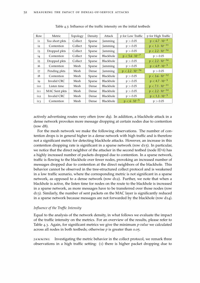
52 measuring the impact of denial-of-service attacks
Table 4.3: Influence of the traffic intensity on the initial testbeds
Row Metric Topology Density Attack p for Low Traffic p for High Traffic
i1 Too short pkts Collect Sparse Jamming p > 0.05 p < 6.7 · 10−4
i2 Contention Collect Sparse Jamming p > 0.05 p < 1.3 · 10−11
i3 Dropped pkts Collect Sparse Jamming p > 0.05 p < 2.2 · 10−16
i4 Contention Collect Sparse Blackhole p < 5.6 · 10−7 p > 0.05
i5 Dropped pkts Collect Sparse Blackhole p > 0.05 p < 2.2 · 10−16
i6 Contention Mesh Sparse Jamming p > 0.05 p < 6.9 · 10−5
i7 Pending pkts Mesh Dense Jamming p < 2.2 · 10−16 p > 0.05
i8 Contention Mesh Sparse Blackhole p > 0.05 p < 3.6 · 10−12
i9 Invalid CRC Mesh Sparse Blackhole p > 0.05 p < 4.7 · 10−5
i10 Listen time Mesh Dense Blackhole p > 0.05 p < 7.1 · 10−11
i11 MAC Sent pkts Mesh Dense Blackhole p > 0.05 p < 2.2 · 10−14
i12 Invalid CRC Mesh Dense Blackhole p > 0.05 p < 1.3 · 10−5
i13 Contention Mesh Dense Blackhole p < 6 · 10−5 p > 0.05
actively advertising routes very often (row d9). In addition, a blackhole attack in adense network provokes more message dropping at certain nodes due to contention(row d8).
For the mesh network we make the following observations. The number of con-tention drops is in general higher in a dense network with high traffic and is thereforenot a significant metric for detecting blackhole attacks. However, an increase in thiscontention dropping rate is significant in a sparse network (row d15). In particular,we notice that the direct neighbor of the attacker in the second testbed (node ID 6) hasa highly increased number of packets dropped due to contention. In a sparse network,traffic is flowing to the blackhole over fewer nodes, provoking an increased number ofmessages dropped due to contention at the direct neighbors of the blackhole. Thisbehavior cannot be observed in the tree-structured collect protocol and is weakenedin a low traffic scenario, where the corresponding metric is not significant in a sparsenetwork, as opposed to a dense network (row d12). Further, we note that when ablackhole is active, the listen time for nodes on the route to the blackhole is increasedin a sparse network, as more messages have to be transferred over those nodes (rowd13). Similarly, the number of sent packets on the MAC layer is significantly reducedin a sparse network because messages are not forwarded by the blackhole (row d14).
Influence of the Traffic Intensity
Equal to the analysis of the network density, in what follows we evaluate the impactof the traffic intensity on the metrics. For an overview of the results, please refer toTable 4.3. Again, for significant metrics we give the minimum p-value we calculatedacross all nodes in both testbeds; otherwise p is greater than 0.05.
jamming Investigating the metric behavior in the collect protocol, we remark threeobservations in a high traffic setting: (1) there is higher packet dropping due to

4.4 results 53
contention (row i2) and (2) due to queue overload (row i3), and (3) the number oftoo short messages is higher (row i1). Thus, the jamming attack has a more severenegative effect on these three metrics, since more messages flow through the network.
Correspondingly, also the mesh protocol exhibits a higher packet dropping rate dueto contention under high traffic (row i6). Besides, with low traffic and under normaloperation, no pending packets are observed. A jamming attack increases the numberof pending messages (row i7). In a high traffic wireless sensor network, this metric isnot significant, as we also have pending packets without attack.
blackhole Focussing on the collect protocol, a high traffic results in more mes-sages dropped due to queue overload (row i5), since a higher count of messages hasto be transferred over fewer links. When the traffic is low, the number of messagesdropped due to contention is significantly increased during a blackhole attack becauseof the malicious node blocking the channel with its route announcements (row i4).
Again, we observe similar results in the mesh protocol. In a high traffic setting, thenumber of packets dropped due to contention (row i8) and the number of packetswith bad CRC checksum (row i9) is higher. This holds for nodes on the route tothe blackhole, which experience an increased traffic flow. In contrast to the sparsenetwork, the number of packets dropped due to contention is not significant in adense high traffic WSN. Also without attack this number is relatively high, as opposedto the low traffic WSN experiencing a significant increase under a blackhole attack(row i13). Given high traffic, the number of packets with bad CRC checksum (row i12)and the count of sent packets on the MAC layer (row i11) is higher when comparedto the low traffic WSN. Besides, in a high traffic WSN the listen time is reduced fornodes that are exposed to the blackhole dropping packets, while with low traffic thereis no significant difference (row i10).
Logistic Regression
The results of the logistic regression analysis lay the foundation for a simple, lightweightintrusion detection system. The general process of attack detection contains the fol-lowing steps:
Given: Regression coefficients β0, . . . ,βk and
Given: data set x1, . . . , xk
Step 1: Creation of the logit model
Step 4: η = β0 +β1 · x1 + ·+βk · xk
Step 2: Calculation of the logit η
Step 3: Calculation of the logistic function
Step 4: Π̂i = 11+e−η
Step 4: Decision
Step 4: If Π̂i > 0.5 −→ Attack detected

54 measuring the impact of denial-of-service attacks
The single steps of this algorithm will be explained in the next subsection using asimple example. For better readability, the values of the regression coefficients are notshown in the following results.
jamming results To begin, we focus on the initial testbed 1. Table 4.4 representsthe relation between the factors in the logistic regression model and the associatedmetrics in the collection tree protocol. It serves as the basis for all subsequentlypresented results.
Table 4.4: Factors and associated metrics for the collection tree protocol
Factor Metric
β1 B01 - RSSI
β2 B03 - Listen time
β3 B02 - Transmit time
β4 B16 - Pending pkts
β5 B06 - NET sent pkts
β6 B07 - NET received pkts
β7 B08 - MAC sent pkts
β8 B09 - MAC received pkts
β9 B18 - Too long pkts
β10 B17 - Too short pkts
β11 B15 - Contention drop
β12 B10 - Invalid CRC
β13 B11 - Radio energy
β14 B13 - MCU energy
β15 CTP12 - No. of neighbors
β16 CTP11 - Best neighbor
β17 CTP10 - Link estimation
β18 CTP09 - Parent congestion
β19 CTP08 - Changing parent
β20 CTP03 - Sent ACK pkts
β21 CTP01 - Sent data pkts
β22 CTP02 - Received data pkts
β23 CTP04 - Received ACK pkts
β24 CTP05 - Received duplicates
β25 CTP06 - Dropped pkts
β26 CTP07 - Packet delivery rate
β27 B14 - MCU load
β28 B04 - Transmit duty cycle
β29 B05 - Listen duty cycle
β30 B12 - Radio load
Table 4.5 shows the significant factors as well as the model quality for the jammingattack in a CTP network with low power and low traffic intensity. The models havebeen created per node, and including all nodes simultaneously, as can be seen inthe last row. The second column contains those metrics, that have been used inthe logit model. They are labelled as βi; the corresponding names can be found

4.4 results 55
Table 4.5: CTP, initial testbed 1, low power, low traffic, jamming
Node Factors Analysis of variance LR-test R2
11 β15 1, 25e− 8 < 1179, 31 764, 83 > 3, 84 1
13 β26 4, 41e− 8 < 1176, 20 762, 77 > 3, 84 1
14 β15 1, 25e− 7 < 1175, 17 762, 11 > 3, 84 1
15 β15 6, 38e− 8 < 1176, 20 762, 82 > 3, 84 1
16 β15 2, 01e− 8 < 1178, 27 764, 16 > 3, 84 1
17 β15 3, 02e− 8 < 1175, 17 762, 11 > 3, 84 1
23 β26 6, 71e− 9 < 1178, 27 764, 11 > 3, 84 1
25 β26 7, 10e− 9 < 1178, 27 764, 11 > 3, 84 1
26 β26 7, 27e− 9 < 1178, 27 764, 16 > 3, 84 1
28 β17 7, 16e− 8 < 1175, 17 762, 11 > 3, 84 1
30 β17 6, 39e− 9 < 1176, 20 762, 82 > 3, 84 1
31 β17 6, 39e− 9 < 1177, 24 763, 49 > 3, 84 1
all nodes β15 1, 27e− 6 < 13486, 47 9159, 60 > 3, 84 1
in Table 4.4. The analysis of variance is presented in the third column, comparingthe -2 log likelihood value (first term) to the value of the chi-squared distribution(second term). The relation < indicates, that we cannot reject the null hypothesis, andhence the model is perfectly fit. Otherwise, the relation 6< leads to the rejection ofthe null hypothesis. The fourth column contains the results of the likelihood-ratiotest, assessing the significance of the chosen regression coefficients when separatingthe two groups. The first term represents the value of the reduced, i.e., the chosenmodel, whereas the second term is the chi-squared value. If the null hypothesis isrejected (first term < than the second term), the chosen metrics are significant for theseparation of the groups. Details on these tests can be found in [Men02]. The fifthcolumn shows the quality criterion McFaddens-R2, indicating how well the model fitsthe observed data. A value greater than 0.2 leads to an acceptable model fit, and avalue greater than 0.4 to a perfect model fit [LHS00]. These boundaries are commonin statistics. In the following, we use the term model fit synonomously for the analysisof variance, the likelihood-ratio test, and the McFaddens-R2.
From Table 4.5 we observe that in this setting only single metrics are needed forattack detection. The metrics are all specific to the CTP. The most often used metricis the number of neighbors metric, followed by the packet delivery rate and the linkestimation.
We now describe the attack detection examplarily for node 23, given the generalprocess as outlined before.
Input: β0 = 26.0131,β26 = −0.5215, x26 = −1
Step 1: Regression model η = β0 +β26 · x26
Step 2: Logit η = 26.0131− 0.5215 · (−1) = 26.5346
Step 3: Logistic regression function Π̂i = 11+e−η
Step 4: Π̂i = 11+e−26.5346 = 1

56 measuring the impact of denial-of-service attacks
Step 4: Decision 1 > 0.5 −→ Attack detected
Table 4.6: CTP, initial testbed 1, high power, low traffic, jamming
Node Factors Analysis of variance LR-test R2
11 β15 1, 24e− 8 < 1147, 21 743, 75 > 3, 84 1
13 β26 7, 82e− 9 < 1146, 18 743, 05 > 3, 84 1
14 β26 8, 05e− 9 < 1148, 25 744, 44 > 3, 84 1
15 β26 1, 81e− 8 < 1033, 19 661, 09 > 3, 84 1
16 β15 2, 59e− 8 < 1145, 14 742, 36 > 3, 84 1
17 β15 1, 63e− 8 < 1147, 21 743, 75 > 3, 84 1
23 β26 6, 72e− 9 < 1147, 40 743, 75 > 3, 84 1
25 β26 9, 90e− 9 < 1146, 18 743, 05 > 3, 84 1
26 β17 1, 25e− 8 < 1147, 21 743, 75 > 3, 84 1
28 β17 6, 22e− 9 < 1146, 18 743, 05 > 3, 84 1
30 β17 6, 22e− 9 < 1147, 21 743, 75 > 3, 84 1
31 β3,β17 1, 52e− 8 < 1145, 14 743, 05 > 3, 84 1
all nodes β8,β13,β15 9, 06e− 6 < 13019, 86 8844, 85 > 3, 84 1
With high power and low traffic, the significant metrics (number of neighbors,packet delivery rate, link estimation) remain the same in most cases, as can be seen inTable 4.6. Exceptions are node 31 as well as the analysis over all nodes, requiring twoand three metrics per model, respectively.
Given low power and high traffic, we see that the packet delivery rate and thenumber of neighbors are the most often used metrics (Table 4.7). Moreover, the basicmetric MAC received pkts is able to detect an attack on node 31.
Similar results are obtained for the high power in combination with high trafficintensity. The packet delivery rate and the link estimation occur very often in thegenerated models as shown in Table 4.8.
To summarize, in about 96 percent of the cases, a single metric is sufficient forsuccessful attack detection in the inital testbed 1. Regarding the used metrics, the CTPspecific metrics link estimation, number of neighbors, and packet delivery rate are themost significant metrics. Besides, integrating the number of received packets on theMAC layer into the model helps achieving better results in some cases. Throughoutall parameter combinations we achieve a perfect model fit, and the chosen metrics aresignificant for the separation of the groups.
Next, we turn our attention to the initial testbed 2. In this setup, the number ofreceived packets on the MAC layer is most frequently used in the models. In addition,the packet delivery rate is a highly significant metric, as it was in the initial testbed1. However, the number of neighbors and the link estimation do not appear as oftenas before, they are only relevant in a setting with low power and low traffic intensity.The results are shown in Appendix A.1.1.
In summary, ordered descendingly according to the number of occurences, the mostrelevant metrics across both initial testbeds for detecting the jamming attack using theCTP are:
. Packet delivery rate

4.4 results 57
Table 4.7: CTP, initial testbed 1, low power, high traffic, jamming
Node Factors Analysis of variance LR-test R2
11 β15 6, 62e− 8 < 1147, 21 743, 75 > 3, 84 1
13 β15 3, 07e− 8 < 1145, 14 742, 36 > 3, 84 1
14 β15 2, 17e− 8 < 1144, 10 741, 67 > 3, 84 1
15 β15 1, 88e− 8 < 1145, 14 742, 36 > 3, 84 1
16 β15 2, 99e− 8 < 1146, 18 743, 05 > 3, 84 1
17 β3,β15 3, 91e− 8 < 1146, 18 743, 75 > 5, 99 1
23 β26 6, 45e− 9 < 1148, 25 744, 44 > 3, 84 1
25 β26 6, 45e− 9 < 1148, 25 744, 44 > 3, 84 1
26 β26 6, 45e− 9 < 1148, 25 744, 44 > 3, 84 1
28 β26 5, 18e− 9 < 960, 51 600, 51 > 3, 84 1
30 β26 6, 22e− 9 < 1147, 21 743, 75 > 3, 84 1
31 β8 1, 35e− 8 < 1146, 18 743, 05 > 3, 84 1
all nodes β1,β8,β15 7, 28e− 5 < 12946, 10 8793, 23 > 7, 81 1
Table 4.8: CTP, initial testbed 1, high power, high traffic, jamming
Node Factors Analysis of variance LR-test R2
11 β26 7, 56e− 9 < 1148, 25 744, 44 > 3, 84 1
13 β4,β10,β17,β19 8, 23e− 9 < 1145, 14 744, 44 > 9, 84 1
14 β26 6, 63e− 9 < 1146, 18 743, 05 > 3, 84 1
15 β26 9, 67e− 9 < 1147, 21 743, 75 > 3, 84 1
16 β26 1, 80e− 6 < 1148, 25 744, 44 > 3, 84 1
17 β17 1, 17e− 8 < 1148, 25 744, 44 > 3, 84 1
23 β17 8, 38e− 9 < 1147, 21 743, 75 > 3, 84 1
25 β17 6, 29e− 9 < 1147, 21 743, 75 > 3, 84 1
26 β17 6, 30e− 9 < 1147, 21 743, 75 > 3, 84 1
28 β17 6, 23e− 9 < 1148, 25 744, 44 > 3, 84 1
30 β17 6, 22e− 9 < 1146, 18 743, 05 > 3, 84 1
31 β26 6, 54e− 9 < 1147, 21 743, 75 > 3, 84 1
all nodes β15 1, 25e− 6 < 13141, 09 8927, 04 > 3, 84 1
. Link estimation
. Number of neighbors
. MAC received pkts
. NET received pkts
. Transmit time
Hence, the results of the logistic regression analysis are similar to those of theWilcoxon-Mann-Whitney test.
For interpreting the results of the jamming attack in the mesh protocol, Table 4.9relates metrics to factors. In general, the number of metrics in each model is increased,

58 measuring the impact of denial-of-service attacks
Table 4.9: Factors in the mesh protocol
Factor Metric
β1 B01 - RSSI
β2 B03 - Listen time
β3 B02 - Transmit time
β4 B16 - Pending pkts
β5 B06 - NET Sent pkts
β6 B07 - NET Received pkts
β7 B08 - MAC Sent pkts
β8 B09 - MAC Received pkts
β9 B18 - Too long pkts
β10 B17 - Too short pkts
β11 B15 - Contention drop
β12 B10 - Invalid CRC
β13 M01 - No. of neighbors
β14 M02 - No. of routing entries
β15 B11 - Radio energy
β16 B13 - MCU energy
β17 B14 - MCU load
β18 B04 - Transmit duty cycle
β19 B05 - Listen duty cycle
β20 B12 - Radio load
compared to the CTP setting. The relevant metrics are similar, and include thefollowing, ordered decreasingly:
. MAC received pkts
. Number of routing entries
. NET received pkts
. Number of neighbors
. Radio energy
The detailed results are presented in Appendix A.1.1.
blackhole results The models created for the blackhole attack require moremetrics, and hence are more specific. Besides, the model quality is worse than for thejamming attack. This holds for both initial testbeds and both protocols. We examplarilyshow the results for the initial testbed 1 using the CTP with low traffic intensity andlow power (see Table 4.10). Further results are given in the Appendix A.1.1. In thisexample, the CTP specific metrics link estimation, packet delivery rate, and the numberof neighbors are among the most relevant metrics. At least one of these metrics isincluded in each model. Regarding the basic metrics, the number of received packetson the network layer as well as the number of sent packets on the MAC layer aresignificant.

4.4 results 59
Table 4.10: CTP, initial testbed 1, low power, low traffic, blackhole
Node Factors Analysis of variance LR-test R2
11
β8,β13 : β15,β17,60, 20 < 1166, 88 734, 73 > 22, 36 0, 96
β19,β21,β23,β25 : β29
13
β2,β3,β5 : β8,β11,β13,453, 12 < 1159, 64 536, 21 > 27, 59 0, 70
β14,β17,β20,β23,β26 : β29
14
β1,β6 : β8,β11,β15,716, 19 < 1161, 71 403, 29 > 22, 36 0, 52
β17,β18,β25,β26,β29,β3015 β15,β26 2, 01e− 6 < 1173, 10 761, 39 > 5, 99 1
16 β17,β26 5, 00e− 6 < 1177, 24 764, 16 > 5, 99 1
17
β1 : β3,β6,β7,β11,β15,400, 49 < 1160, 67 764, 16 > 24, 99 0, 74
β17,β18,β21,β25,β26,β28,β29
23
β1,β3,β4,β6,β7,β11,β14,6, 56e− 4 < 1160, 67 764, 11 > 28, 87 1
β15,β17 : β21,β23,β26 : β28,β3025 β7,β17,β19,β20,β26,β27,β30, 4, 70e− 6 < 1172, 06 764, 11 > 14, 07 1
26 β17 6, 48e− 8 < 1178, 27 764, 16 > 3, 84 1
28
β1,β2,β4 : β10,β12,β13 : β15,505, 01 < 1156, 53 510, 32 > 31, 41 0, 67
β17,β23 : β26,β28,β29
30
β1,β3 : β8,β13 : β15,β17,641, 27 < 1159, 64 442, 14 > 27, 59 0, 57
β19 : β21,β23,β26,β28
31
β1,β6 : β8,β14,β15,261, 01 < 1164, 81 662, 99 > 22, 36 0, 83
β17,β20,β23,β26,β29
all nodesβ1,β4 : β8,β11 : β13,β15,
11492 < 13463, 34 3412, 26 > 33, 92 0, 37β17 : β21,β23,β26 : β30
4.4.2 Final Tests
In this section we analyze the metrics in the larger final testbeds. We start withevaluating the Wilcoxon-Mann-Whitney tests before creating the logistic regressionmodels.
Basic Metrics
The overall performance of the basic metrics can be seen in Table 4.11, showing thedetection rate aggregated for all attacks, scenarios and nodes. The detection rate isdefined as the sum of all significant Wilcoxon-Mann-Whitney tests that could detectthe six different attacker models for each single metric. The most influenced metricsrelate to the number of sent and received packets, as well as energy consumption.
Table 4.12 takes a closer look at how well the better metrics performed in detectingthe specific attacks. In this case, we define an attack to be successfully detected ifmore than 75% of all the calculated Wilcoxon-Mann-Whitney tests for this attack havebeen significant. An interesting observation is the last metric NET sent packets, whichdid not have a detection rate of more than 75% in Table 4.11. Instead, the detectionrate was only 66%. However, it is well-suited to detect the constant and the randomjammers. In contrast to that, the similar overall performing metric transmit time isnot listed in Table 4.12. This indicates that the metric NET sent packets performs very

60 measuring the impact of denial-of-service attacks
Table 4.11: Overall performance - basic metrics - final testbeds
Metric Detection rate
B09 - MAC received pkts 0.84
B11 - Radio energy 0.83
B07 - NET received pkts 0.83
B12 - Radio load 0.83
B08 - MAC sent pkts 0.80
B13 - MCU energy 0.80
B14 - MCU load 0.79
B05 - Listen duty cycle 0.79
B01 - RSSI 0.78
B04 - Transmit duty cycle 0.76
B02 - Transmit time 0.67
B06 - NET sent pkts 0.66
B03 - Listen time 0.57
B10 - Invalid CRC 0.39
B15 - Contention drop 0.37
B16 - Pending pkts 0.22
B18 - Too long pkts 0.22
B17 - Too short pkts 0.00
Table 4.12: Basic metrics with attack detection over 0.75 in the final testbeds
Metric Con
stan
tja
mm
er
Ran
dom
jam
mer
Bla
ckho
le+
Ran
dom
jam
mer
Bla
ckho
le+
Rea
ctiv
eja
mm
er
Bla
ckho
le
Rea
ctiv
eja
mm
er
B09 - MAC received pkts X X X X X X
B11 - Radio energy X X X X X X
B07 - NET received pkts X X X X X X
B12 - Radio load X X X X X X
B13 - MCU energy X X X X X X
B14 - MCU load X X X X X -
B01 - RSSI X X X X X -
B08 - MAC sent pkts X X X X - -
B04 - Transmit duty cycle X X X X - -
B05 - Listen duty cycle X X X - - -
B06 - NET sent pkts X X - - - -
good in two cases, while the metric transmit time has a more constant detection rate,but is of lower quality for each attack.

4.4 results 61
Table 4.13: Overall performance - basic + CTP metrics - final testbeds
Metric Detection rate
CTP12 - Number of neighbors 0.89
B09 - MAC received pkts 0.86
CTP10 - Link estimation 0.85
B05 - Listen duty cycle 0.85
B11 - Radio energy 0.84
CTP07 - Packet delivery rate 0.84
B07 - NET received pkts 0.84
CTP11 - Best neighbor 0.84
B12 - Radio load 0.84
B08 - MAC sent pkts 0.83
B13 - MCU energy 0.83
B14 - MCU load 0.82
B06 - NET sent pkts 0.81
B04 - Transmit duty cycle 0.79
B01 - RSSI 0.77
CTP04 - Received ACK pkts 0.75
CTP01 - Sent data pkts 0.73
CTP09 - Parent congestion 0.73
CTP02 - Received data pkts 0.69
CTP03 - Sent ACK pkts 0.69
B02 - Transmit time 0.68
B03 - Listen time 0.63
CTP06 - Dropped pkts 0.49
B15 - Contention drop 0.45
B10 - Invalid CRC 0.43
B18 - Too long pkts 0.32
CTP05 - Received duplicates 0.25
CTP08 - Changing parent 0.23
B16 - Pending pkts 0.22
B17 - Too short pkts 0.00
The constant jammer and the random jammer are the two most often detectedattacks. They affect the majority of metrics. The combined attacker models withthe blackhole attack and the random or reactive jammer are also detected by a largenumber of metrics. Finally, the blackhole attack and the reactive jammer showed theleast amount of metrics suitable for detection. Regarding the blackhole attack, this isconsistent with the results obtained in our initial tests. The reactive jammer is difficultto detect globally.
CTP Metrics
Table 4.13 shows the overall performance of the basic metrics together with the CTPspecific metrics.
The CTP metric number of neighbors shows the best performance, having a detectionrate of 0.89. Regarding the detected attacks, there are 18 metrics which can identify

62 measuring the impact of denial-of-service attacks
an attack over all nodes with a probability of p > 0.75 (Table 4.14 shows the resultsaveraged over both final testbeds). Note that the performance of many basic metricsobtained using the CTP has increased. In detail, these are NET sent packets, transmitduty cycle, MAC sent packets, MCU load and listen duty cycle. This is due to theability of the CTP to notify a sender whether a packet has successfully arrived or not,leading to a performance increase for metrics related to packet transmission.
Table 4.14: Basic + CTP metrics with attack detection over 0.75 in the final testbeds
Metric Con
stan
tja
mm
er
Ran
dom
jam
mer
Bla
ckho
le+
Ran
dom
jam
mer
Bla
ckho
le+
Rea
ctiv
eja
mm
er
Bla
ckho
le
Rea
ctiv
eja
mm
er
CTP12 - Number of neighbors X X X X X X
B09 - MAC received pkts X X X X X X
CTP10 - Link estimation X X X X X X
B05 - Listen duty cycle X X X X X X
B11 - Radio energy X X X X X X
CTP07 - Packet delivery rate X X X X X X
B07 - NET received pkts X X X X X X
CTP11 - Best neighbor X X X X X X
B12 - Radio load X X X X X X
B13 - MCU energy X X X X X X
B14 - MCU load X X X X X X
B08 - MAC sent pkts X X X X - X
B04 - Transmit duty cycle X X X X X -
B06 - NET sent pkts X X X X - -
CTP01 - Sent data pkts X X X - - -
CTP04 - Received ACK pkts X X X - - -
B01 - RSSI X X X - - -
CTP09 - Parent congestion - - X X - -
Mesh Metrics
As the mesh protocol only provides two additional network metrics and is lacking theadvanced features of the CTP, the mesh metrics perform similar to the basic metrics.The results can be found in Appendix A.1.2.
Influence of the Testbed
The data in our final tests has been obtained in two physically separated locations. Inthis section, we analyze the influence of this parameter on the detection capabilities.Examplarily, we show the results for the CTP metrics in the final testbed 1 (Table 4.15)and in the final testbed 2 (Table 4.16). Further results are presented in Appendix A.1.2.

4.4 results 63
We observe the trend that a denser network like the final testbed 2 improves thedetection. This is especially true for the constant jammer, the best metric having adetection rate of 0.99. In contrast to that, the detection of the blackhole attack remainsmainly unchanged (even a slight tendency for better detection in the sparser finaltestbed 1 is noticeable). The reason for these results is given by the attack characteris-tics. Jamming can create more damage, if the network is denser, by rendering morenodes unavailable. Regarding the blackhole attack, changes to the topology (causedby the attacker) can be observed better, if the network is sparser.
Table 4.15: Detection rates CTP metrics - final testbed 1
Metric Con
stan
tja
mm
er
Ran
dom
jam
mer
Rea
ctiv
eja
mm
er
Bla
ckho
le
Bla
ckho
le+
Ran
dom
jam
mer
Bla
ckho
le+
Rea
ctiv
eja
mm
er
CTP12 - Number of neighbors 0.87 0.85 0.83 0.88 0.90 0.87
CTP07 - Packet delivery rate 0.87 0.80 0.80 0.84 0.78 0.83
CTP10 - Link estimation 0.74 0.76 0.78 0.78 0.88 0.88
CTP11 - Best neighbor 0.78 0.77 0.79 0.78 0.86 0.84
CTP09 - Parent congestion 0.70 0.63 0.66 0.65 0.78 0.75
CTP04 - Received ACK pkts 0.74 0.64 0.62 0.64 0.77 0.74
CTP03 - Sent ACK pkts 0.65 0.64 0.66 0.65 0.70 0.73
CTP02 - Received data pkts 0.65 0.64 0.66 0.65 0.70 0.73
CTP01 - Sent data pkts 0.74 0.65 0.57 0.62 0.72 0.71
CTP06 - Dropped pkts 0.43 0.43 0.47 0.42 0.48 0.46
CTP05 - Received duplicates 0.27 0.19 0.18 0.24 0.24 0.31
CTP08 - Changing parent 0.20 0.16 0.13 0.16 0.22 0.19
Influence of the Density
The density within a specific testbed has only a minor influence on the metrics. Theresults can be found in Appendix A.1.2.
Influence of the Traffic Intensity
The traffic intensity may have different effects on the metrics, depending on the specificattack. For example, the blackhole is highly dependent on the number of packetssent by other nodes. The results can be found in Appendix A.1.2. We notice thatthe detection rates mainly increase for all attacks when more traffic is sent. This isexpected, as an attacker can stronger influence the network given higher traffic.

64 measuring the impact of denial-of-service attacks
Table 4.16: Detection rates CTP metrics - final testbed 2
Metric Con
stan
tja
mm
er
Ran
dom
jam
mer
Rea
ctiv
eja
mm
er
Bla
ckho
le
Bla
ckho
le+
Ran
dom
jam
mer
Bla
ckho
le+
Rea
ctiv
eja
mm
er
CTP12 - Number of neighbors 0.99 0.86 0.78 0.83 0.87 0.81
CTP10 - Link estimation 0.93 0.83 0.81 0.84 0.85 0.81
CTP11 - Best neighbor 0.86 0.83 0.79 0.80 0.83 0.81
CTP07 - Packet delivery rate 0.92 0.79 0.80 0.76 0.79 0.80
CTP04 - Received ACK pkts 0.92 0.85 0.64 0.67 0.84 0.67
CTP01 - Sent data pkts 0.97 0.87 0.59 0.60 0.85 0.65
CTP09 - Parent congestion 0.74 0.73 0.71 0.71 0.73 0.73
CTP03 - Sent ACK pkts 0.73 0.69 0.65 0.63 0.69 0.64
CTP02 - Received data pkts 0.73 0.69 0.65 0.63 0.69 0.64
CTP06 - Dropped pkts 0.51 0.50 0.50 0.48 0.50 0.49
CTP08 - Changing parent 0.40 0.32 0.20 0.22 0.29 0.23
CTP05 - Received duplicates 0.42 0.21 0.20 0.23 0.29 0.17
Influence of the Attacker Location and Start
In general, two attackers increase the detection rates, which is expected. The startof the attack, however, did not show significant differences in detection rates. Eventhough in the setting with no delay, an attacker has higher chances to prevent a WSNfrom operating, the attack effects are still strong enough when starting the attack inthe middle of the test-run. In other settings, different from our setup, this behaviormay change. The results are presented in Appendix A.1.2.
Comparison to the Initial Tests
The results obtained with the larger testbeds are similar to those of the smaller testbeds.The large majority of metrics, that reach at least class B quality in the initial tests,are also among the best metrics with attack detection over 0.75 in the final tests (seeTable 4.17). Minor differences occur due to the size of the networks, some metricsare only influenced significantly if they are direct neighbors of the attacker. Metricsmarked as N/A have not been analyzed in the initial tests. Hence, we have shownthat our identified metrics are widely applicable for attack detection.
Logistic Regression
In our final tests, there are three different groups of models that have been createdand evaluated using a logistic regression:

4.4 results 65
Table 4.17: Comparison between the initial and the final tests: metrics of good quality forattack detection
Final Tests Initial Tests
Best neighbor N/A
Link estimation Link estimation
Listen duty cycle Listen duty cycle
- Listen time
MAC received pkts MAC received pkts
MAC sent pkts MAC sent pkts
MCU energy MCU energy
MCU load MCU load
NET received pkts NET received pkts
NET sent pkts NET sent pkts
No. of neighbors No. of neighbors
Packet delivery rate Packet delivery rate
Parent congestion N/A
Radio energy Radio energy
Radio load Radio load
Received ACK pkts Received ACK pkts
- Received data pkts
RSSI RSSI
- Sent ACK pkts
Sent data pkts Sent data pkts
Transmit duty cycle Transmit duty cycle
- Transmit time
. Single nodes:This analysis is the similar to the Wilcoxon-Mann-Whitney evaluation, because alogistic regression model is created for each single node.
. All nodes:In an attempt to create generally applicable models, we used the data of allnodes as input.
. All neighboring nodes:The last group consists of models, that only take the data of the direct neighborsof the attacker into account.
For assessing the model fit, we now concentrate on McFaddens-R2, because itis considered the most appropriate for logistic regression [Men02]. The calculatedMcFaddens-R2 classifies the models in three categories:
. Bad models: returned a McFaddens-R2 of < 0.2
. Acceptable models: a McFaddens-R2 in the interval [0.2 − 0.4] indicates anacceptable model fit
. Perfect models: a value of > 0.4 for the McFaddens-R2 represents a perfectmodel fit

66 measuring the impact of denial-of-service attacks
Our analysis showed that the models created for all nodes do not perform well,because there are nodes too distant from the attacker to be influenced significantly(see Appendix A.1.3). Hence, in the following we concentrate on the single andneighboring nodes. For each of the remaining two groups an overview is givenabout the model quality for the specific attacks. In addition, the metrics are rankedaccording to the number of occurences in the models. Finally, we show how manymetrics are included per model. A high count of metrics indicates that the models arevery specific, and detection in different settings may be difficult.
Single NodesUsing the data of individual nodes as input, we create separate logistic regression
models for each node.
Table 4.18: Model quality - single nodes - basic metrics - final testbeds
Mesh CTP
Count Percent Count Percent
JammingCnst Bad model 59 0.056 33 0.032
Acceptable model 106 0.100 118 0.115
Perfect model 891 0.844 873 0.853
Sum usable models 997 0.944 991 0.968
JammingRnd Bad model 37 0.035 39 0.038
Acceptable model 160 0.152 172 0.168
Perfect model 859 0.813 813 0.794
Sum usable models 1019 0.965 985 0.962
JammingReact Bad model 191 0.181 148 0.145
Acceptable model 281 0.266 315 0.308
Perfect model 584 0.553 561 0.548
Sum usable models 865 0.819 876 0.855
SingleBlackhole Bad model 174 0.165 125 0.122
Acceptable model 311 0.295 298 0.291
Perfect model 571 0.541 601 0.587
Sum usable models 882 0.835 899 0.878
BlackholeReactJamming Bad model 132 0.250 46 0.090
Acceptable model 209 0.396 156 0.305
Perfect model 187 0.354 310 0.605
Sum usable models 396 0.750 466 0.910
BlackholeRndJamming Bad model 34 0.064 22 0.043
Acceptable model 107 0.203 102 0.199
Perfect model 387 0.733 388 0.758
Sum usable models 494 0.936 490 0.957
basic metrics Table 4.18 shows the results when using only the basic metrics inthe CTP and mesh setting. A usable model is defined as a model of at least acceptablequality. The basic metrics obtained from the CTP runs show a mean percentage ofabout 0.92 usable models, while this rate is reduced to about 0.87 in the mesh runs.
Table 4.19 presents the most frequently used basic metrics in the regression models.The results are similar to the Wilcoxon-Mann-Whitney test, especially metrics relatedto network traffic are very useful.

4.4 results 67
Table 4.19: Most often used basic metrics in all single node models - final testbeds
Metric Occurences (%)
B06 - NET sent pkts 84.4
B07 - NET received pkts 80.5
B01 - RSSI 67.5
B08 - MAC sent pkts 64.9
B13 - MCU energy 57.1
B09 - MAC received pkts 56.5
B11 - Radio energy 53.2
B04 - Transmit duty cycle 51.9
B05 - Listen duty cycle 46.7
B03 - Listen time 37.6
B10 - Invalid CRC 36.6
B02 - Transmit time 36.3
B12 - Radio load 32.4
B14 - MCU load 31.1
B15 - Contention drop 30.9
B18 - Too long pkts 23.8
B16 - Pending pkts 12.9
B17 - Too short pkts 6.4
0 5 10 15 200
500
1000
1500
metrics per model
coun
t
Figure 4.11: Count of metrics used in each model created for single nodes using basic metrics -final testbeds
We now analyze how many metrics are included in each generated model. Fig-ure 4.11 shows the distribution, the majority of models do not need more than 10
metrics. There are also models requiring only one metric and having at least anacceptable model fit. The metric no. of sent packets on the MAC layer occurs in almost400 models as a single metric, and thus is well-suited to differentiate between attack

68 measuring the impact of denial-of-service attacks
and no-attack. In addition, the metrics MCU energy and radio energy appear as singlemetrics in a smaller number of models (about 25 models in total). Taking a closer lookat which attacks can be detected by solely using the no. of sent packets on the MAClayer as metric, we find that it can detect a constant jammer reliably.
Table 4.20: Model quality - single nodes - protocol specific metrics - final testbeds
Mesh CTP
Count Percent Count Percent
JammingCnst Bad model 92 0.087 1 0.001
Acceptable model 121 0.115 9 0.009
Perfect model 843 0.798 1014 0.990
Sum usable models 964 0.913 1023 0.999
JammingRnd Bad model 104 0.098 1 0.001
Acceptable model 280 0.265 22 0.021
Perfect model 672 0.636 1001 0.978
Sum usable models 952 0.902 1023 0.999
JammingReact Bad model 310 0.294 6 0.006
Acceptable model 430 0.407 42 0.041
Perfect model 316 0.299 976 0.953
Sum usable models 746 0.706 1018 0.994
SingleBlackhole Bad model 269 0.255 6 0.006
Acceptable model 463 0.438 41 0.040
Perfect model 324 0.307 977 0.954
Sum usable models 787 0.745 1018 0.994
BlackholeReactJamming Bad model 121 0.229 1 0.002
Acceptable model 194 0.367 8 0.016
Perfect model 213 0.403 503 0.982
Sum usable models 407 0.771 511 0.998
BlackholeRndJamming Bad model 29 0.055 0 0.000
Acceptable model 99 0.188 5 0.010
Perfect model 400 0.758 507 0.990
Sum usable models 499 0.945 512 1.000
protocol metrics From Table 4.20 we observe that using the CTP metrics, alarge number of usable models can be created for all tested attacks. The metrics of themesh protocol have more difficulties to detect the reactive jammer, the blackhole, aswell as a combination of both. The results of the Wilcoxon-Mann-Whitney tests alsousing single nodes as input are similar.
Table 4.21 shows the relevant metrics using the CTP. Out of the CTP specific metrics,the number of neighbors and the packet delivery rate appear in many models.
An interesting finding is, that the metric sent ACK pkts is never included in thelogistic regression models, but it had a detection rate of 0.69 according to the Wilcoxon-Mann-Whitney test. This means that other metrics capture the effects of this metric aswell.
Including the CTP metrics during model creation leads to a large number of modelscontaining only one metric, as can be seen in Figure 4.12. Metrics such as the packetdelivery rate have the ability to detect attacks without further metrics.

4.4 results 69
Table 4.21: Most often used CTP metrics in all single node models - final testbeds
Metric Occurences (%)
B06 - NET sent pkts 59.3
B07 - NET received pkts 57.9
B01 - RSSI 49.6
B08 - MAC sent pkts 44.8
B13 - MCU energy 42.7
B11 - Radio energy 40.6
B09 - MAC received pkts 40.0
B04 - Transmit duty cycle 35.8
B05 - Listen duty cycle 34.4
CTP12 - Number of neighbors 31.7
CTP07 - Packet delivery rate 28.9
B12 - Radio load 28.2
B10 - Invalid CRC 27.5
B14 - MCU load 26.2
B03 - Listen time 26.0
B02 - Transmit time 25.8
CTP11 - Best neighbor 24.8
B15 - Contention drop 22.0
CTP10 - Link estimation 19.3
B18 - Too long pkts 15.8
CTP09 - Parent congestion 15.5
CTP02 - Received data pkts 11.7
CTP04 - Received ACK pkts 11.6
CTP01 - Sent data pkts 9.6
B16 - Pending pkts 8.2
CTP08 - Changing parent 5.5
CTP06 - Dropped pkts 5.3
B17 - Too short pkts 4.1
CTP05 - Received duplicates 4.0
CTP03 - Sent ACK pkts 0.2
Regarding the mesh metrics, their overall performance is very similar to those ofthe basic metrics (see Table 4.22). The two mesh metrics are frequently used in themodels, but the basic metrics transmitted and received packets on the network layerare more significant.
Comparing the number of metrics per model to the CTP setting, we notice that theamount of models using only one metric is significantly reduced (see Figure 4.13).This is because also the basic metrics are influenced by the higher level checks of theCTP for packet successful reception. Using the mesh protocol, the positive influenceof these mechanisms is lacking.
All Neighboring NodesThe models created for single nodes turned out to be very good. The only drawback
is, that they are very node specific. To solve this problem and to obtain more generallyusable metrics, the logistic regression function was given the aggregated data of all

70 measuring the impact of denial-of-service attacks
0 10 20 300
500
1000
1500
metrics per model
coun
t
Figure 4.12: Count of metrics used in each model created for single nodes using CTP metrics -final testbeds
Table 4.22: Most often used mesh metrics in all single node models - final testbeds
Metric Occurences (%)
B06 - NET sent pkts 59.4
B07 - NET received pkts 58.1
B01 - RSSI 50.0
B08 - MAC sent pkts 44.5
B13 - MCU energy 41.8
B11 - Radio energy 40.5
B09 - MAC received pkts 39.1
M02 - No. of routing entries 37.8
B04 - Transmit duty cycle 35.1
M01 - No. of direct neighbors 34.9
B05 - Listen duty cycle 33.7
B12 - Radio load 28.3
B10 - Invalid CRC 27.9
B14 - MCU load 25.9
B03 - Listen time 25.7
B02 - Transmit time 25.3
B15 - Contention drop 21.6
B18 - Too long pkts 16.2
B16 - Pending pkts 8.1
B17 - Too short pkts 4.0
nodes as input. However, the model quality turned out to be bad because of the rangeof the attack on the network. Whereas the direct neighbors of the attacker exhibitsignificant changes in their metrics when under attack, the very distant nodes may not

4.4 results 71
Figure 4.13: Count of metrics used in each model created for single nodes using mesh metrics- final testbeds
0 5 10 15 200
200
400
600
800
metrics per model
coun
t
detect any changes in the network at all. Including these distant nodes in the modelcreation phase proved to be a disadvantage, as can be seen in Appendix A.1.3.
Therefore, in this section we analyze the logistic regression models created takingonly the neighboring nodes of the attacker into account. Table 4.23 shows all the nodeswhich are one-hop away from an attacker.
The most often used metrics in the models created for neighboring nodes are similarto the single node setting. However, they typically require more metrics per model.This holds for basic, CTP, as well as mesh metrics. The corresponding results areshown in Appendix A.1.4. The most promising models are obtained when usingprotocol-specific metrics, especially CTP metrics. Figure A.5 reveals that severalmodels using the CTP require less than 6 metrics per model and thus outperform themesh metrics as shown in Figure A.6.
basic metrics The amount of usable models for detecting an attack, when fo-cussing on the basic metrics, is shown in Table 4.24. Except for the models created forthe constant as well as the random jamming, the amount of usable models is reducedcompared to the models created for single nodes.
protocol metrics Table 4.25 shows that the CTP produces perfect models moreoften than using the mesh. Even though also the mesh protocol is able to detect thejammers, the amount of usable models for blackhole and combined blackhole attackersis low. These results are in line with the initial tests, showing that the mesh protocolmetrics cannot offer a good blackhole detection, even when using a combination ofmultiple metrics.

72 measuring the impact of denial-of-service attacks
Table 4.23: Attacker neighbors
Final testbed 1
Node Attacker
6 5
7 5
10 23
14 23
16 23
19 23
20 23
21 23
24 23
25 23
26 23
27 23
28 23
29 23
30 23
31 23
32 23
Final testbed 2
Node Attacker
11 27
12 27
17 27
19 27
20 27
21 27
22 27
25 27
26 27
28 27
29 56
32 56
33 56
35 56
36 27
38 56
49 56
51 56
53 56
54 56
57 56
58 56
4.5 ids
We now describe the fully localized IDS, which does not rely on collaboration. There-fore, we present the system, its storage requirements, its computation time, andits energy consumption in Section 4.5.1. Next, we discuss the models selected forintrusion detection in Section 4.5.2. Finally, we evaluate the IDS in Section 4.5.3.
4.5.1 Implementation
In this section, we implement an IDS on the nodes based on the usage of the previouslycreated logistic regression models. Hence, we do not calculate the models on thenodes, but let them evaluate the existing models using the steps already presented inSection 4.4.1:

4.5 ids 73
Table 4.24: Model quality - neighboring nodes - basic metrics - final testbeds
Mesh CTP
Count Percent Count Percent
JammingCnst Bad model 0 0.000 0 0.000
Acceptable model 0 0.000 0 0.000
Perfect model 32 1.000 32 1.000
Sum usable models 32 1.000 32 1.000
JammingRnd Bad model 5 0.156 5 0.156
Acceptable model 20 0.625 18 0.563
Perfect model 7 0.219 9 0.281
Sum usable models 27 0.844 27 0.844
JammingReact Bad model 21 0.656 25 0.781
Acceptable model 7 0.219 3 0.094
Perfect model 4 0.125 4 0.125
Sum usable models 11 0.344 7 0.219
SingleBlackhole Bad model 26 0.813 19 0.594
Acceptable model 5 0.156 10 0.313
Perfect model 1 0.031 3 0.094
Sum usable models 6 0.188 13 0.406
BlackholeReactJamming Bad model 16 1.000 9 0.563
Acceptable model 0 0.000 7 0.438
Perfect model 0 0.000 0 0.000
Sum usable models 0 0.000 7 0.438
BlackholeRndJamming Bad model 8 0.500 11 0.688
Acceptable model 0 0.000 5 0.313
Perfect model 8 0.500 0 0.000
Sum usable models 8 0.500 5 0.313
Given: Regression coefficients β0, . . . ,βk and
Given: data set x1, . . . , xk
Step 1: Creation of the logit model
Step 4: η = β0 +β1 · x1 + ·+βk · xk
Step 2: Calculation of the logit η
Step 3: Calculation of the logistic function
Step 4: Π̂i = 11+e−η
Step 4: Decision
Step 4: If Π̂i > 0.5 −→ Attack detected
Implementing these steps requires only a single funtion, resulting in few lines ofcode. This function is given the current metric readings. A for loop iterating over allmetric readings is needed in order to calculate the logit model. Calculating the logisticfunction is performed in three steps. The first step involves inverting the sign of the

74 measuring the impact of denial-of-service attacks
Table 4.25: Model quality - neighboring nodes - protocol specific metrics - final testbeds
Mesh CTP
Count Percent Count Percent
JammingCnst Bad model 0 0.000 0 0.000
Acceptable model 0 0.000 0 0.000
Perfect model 32 1.000 32 1.000
Sum usable models 32 1.000 32 1.000
JammingRnd Bad model 2 0.063 0 0.000
Acceptable model 20 0.625 12 0.375
Perfect model 10 0.313 20 0.625
Sum usable models 30 0.938 32 1.000
JammingReact Bad model 22 0.688 15 0.469
Acceptable model 6 0.188 9 0.281
Perfect model 4 0.125 8 0.250
Sum usable models 10 0.313 17 0.531
SingleBlackhole Bad model 28 0.875 9 0.281
Acceptable model 3 0.094 6 0.188
Perfect model 1 0.031 17 0.531
Sum usable models 4 0.125 23 0.719
BlackholeReactJamming Bad model 16 1.000 4 0.250
Acceptable model 0 0.000 5 0.313
Perfect model 0 0.000 7 0.438
Sum usable models 0 0.000 12 0.750
BlackholeRndJamming Bad model 8 0.500 3 0.188
Acceptable model 0 0.000 5 0.313
Perfect model 8 0.500 8 0.500
Sum usable models 8 0.500 13 0.813
logit model, before e−η is calculated. For that purpose, an extra math library has to beloaded in Contiki for providing floating point arithmetics. Finally, the logistic functionis calculated and evaluated by an if-condition.
ROM and RAM Usage
One key aspect of the developed IDS is to be lightweight. Hence, the additional ROMand RAM consumption which is introduced by the IDS is measured in this section.Table 4.26 compares the ROM and RAM consumption of the baseline Contiki withoutIDS to the IDS used with a different amount of metrics.
The increase of about 8056 bytes when adding the IDS is mainly due to the neededmath libraries for floating point arithmetic. Every metric which is added leads to anincrease of about 20 to 38 bytes. This increase per metric is slightly different, becausethe applied compiler parameters and optimizations affect the firmware image size.Per metric, the RAM usage increases by 4 bytes, which corresponds to the neededamount for one variable of the type double. Given that the required math library isnot already loaded, an IDS image which makes use of one metric leads to an increaseof the firmware size by about 26 % as compared to the baseline image. However, anoption is to import only the code for the powf() function instead of the whole library.

4.5 ids 75
Table 4.26: IDS ROM and RAM usage
Image ROM in bytes RAM in bytes
Contiki without IDS 30164 6848
IDS with 1 metric 38220 6852
IDS with 2 metrics 38280 6856
IDS with 3 metrics 38320 6860
IDS with 5 metrics 38382 6868
IDS with 10 metrics 38586 6888
IDS with 15 metrics 38776 6908
IDS with 20 metrics 38956 6928
IDS with 25 metrics 39088 6948
Each added metric increases the image slightly by about 0.1%. In our setting, the nodestarted to refuse to boot with an amount of 700 metrics.
IDS Computation Time and Energy Consumption
We measure the clock ticks needed for the IDS function call, using between 1 and25 different metrics. It takes four to five clock ticks to perform this task, which isbetween about 31 ms and 39 ms. The most expensive computation is the floating pointarithmetic to exponentiate using powf(). Next, we measure the additional energyconsumption of the IDS. The lowest energy consumption was obtained for one metric,resulting in about 330 µJ per IDS function call. If 25 metrics are used, the energyconsumption is about 463 µJ. In cases when the result of the calculated logit modelwas largely negative, the powf() call simply returned the value 0 without actuallycalculating. In such situations, the energy consumption highly decreased to about100 µJ.
4.5.2 Selected Model
In order to evaluate the applicability of different models for attack detection, we havechosen them according to the number of metrics used and the resulting model quality.We expect models with few metrics to perform better in a similar, but different testingenvironment than the environment they have been created for. The main performancemetrics are the false-positive as well as the detection rates. In addition, we analyzethe time it takes to detect the attack. The scenario we investigate has the followingproperties:
. Testbed: Final testbed 1
. Protocol: CTP
. Transmission power: High
. Traffic intensity: Low
This testbed was chosen because the environment is more challenging, and thereforethe attack detection is harder. With the CTP, we expect to be able to detect the blackholeattack better than with the mesh protocol.

76 measuring the impact of denial-of-service attacks
We concentrate on detecting the constant jammer, the blackhole, as well as thecombination of blackhole and random jammer. For each of these attacker models, wefocus on logistic regression models that have been created by analyzing the data ofthe direct neighbors of the attacker.
Constant Jammer
As we can observe from Table 4.27, two out of the four available models involve justone metric for attack detection, while at the same time they achieve a perfect modelquality. These single metrics are respresented by the packet delivery rate and thenumber of sent packets on the MAC layer, respectively. The packet delivery rateexhibits significantly different values when the attack occurs. However, there is a highvariation for each node, which is not the case for the number of sent packets on theMAC layer. Hence, we choose the bold printed model in Table 4.27 for evaluation.
Table 4.27: Constant jammer models
Parameter Model quality Count of used metrics
Inner attacker, no delay 0.99 1: CTP07 - Packet delivery ratio
Inner attacker, delay 0.99 1: B08 - MAC sent pkts
Both attackers, no delay 0.94 18
Both attackers, delay 0.84 24
Blackhole
For the blackhole attack, we again selected a model with a perfect model quality, thistime using more than one metric. This bold printed model is shown in Table 4.28.
Blackhole and Random Jammer
The number of available models is reduced to two when using the combined attackers.While both models require a similar amount of metrics, only the first model has aperfect model quality. The details of the selected bold printed model are shown inTable 4.29.
Table 4.28: Blackhole models
Parameter Model quality Count of used metrics
Inner attacker, no delay 0.99 6
Both attackers, no delay 0.73 22
Inner attacker, delay 0.51 16
Both attackers,delay 0.28 21
Table 4.29: Blackhole and random jammer models
Parameter Model quality Count of used metrics
Both attackers, no delay 0.47 20
Both attackers, delay 0.07 21

4.5 ids 77
4.5.3 Evaluation
Figure 4.14: Mote placement in the IDS evaluation testbed
3331
323029
282624
2523
2119
2220
1715
1816
09
10
1311
14120605
0807
01
511E
711E
911E
811E
E112 D110 D108
D113
D106
E111 D111
E108
03
27
36
��
5150221E
121E
601E
701E
��
53
��
E123E125
�� E126
12 39
E101E102
E104
02
35
37
52
Next, we deploy the selected models to real sensor nodes. We use a similar, butdifferent (see below for a description) testbed for our experiments. The testbedparameters for evaluating the IDS models are as follows:

78 measuring the impact of denial-of-service attacks
1 2 3 6 7 8 10 11 12 13 14 15 16 17 18 19 20 21 22 24 25 26 30 31 32 33 36 37 50 51 52 530
0.3
0.6
0.9
node id
fals
e−po
sitiv
e ra
te
Figure 4.15: False-positives for model 1 (constant jammer)
. Testbed: Similar to final testbed 1
. Protocol: CTP
. Transmission power: High
. Traffic: Low
. Attacker location: Outer and inner
. Attack delay: No delay
. Repetitions: 5
Note that the evaluated models partly have been created with different parameters.There is also a change in the network topology, because four nodes have been replaced,as shown in Figure 4.14. Nodes marked in green have been added, while nodes markedin orange have been removed, as compared to the final testbed 1. The attacking nodesremain the same. We start the evaluation with running the IDS in a setting withoutattackers, in order to determine the false-positive rates. The detection function isalways called after a node has updated its metrics, i.e., every 4 seconds. Each test-runhas a duration of 15 minutes and is repeated five times for each scenario.
Neutral Runs
The false-positive rate for each model is tracked directly from the start of the test-run,including the initialization phase where the network is established. Since there is noattacker present, no attack should be detected.
model 1 - constant jammer - false-positives The false-positive rate forthe constant jammer detection model is depicted in Figure 4.15. For most of the nodeswe achieve a false-positive rate of 0%.
model 2 - blackhole - false-positives Although only a few good regres-sion models have been created for the blackhole attack, the false-positive rate is ingeneral low (see Figure 4.16). Recall that the blackhole was one of the attacks that aredifficult to detect with the Wilcoxon-Mann-Whitney test.

4.5 ids 79
model 3 - blackhole + random jammer - false-positives The modelresulting from the combination of blackhole and random jammer included 20 metrics.Still, the false-positive rate shown in Figure 4.17 is rather low.
Attack Runs
This section is devoted to describe the evaluation of the the attack runs, with a presentattacker. The detection rate is defined as percentage of correctly identified attacks,given the periodic metric measurements, and is averaged over the 5 different test-runs.Nodes marked with a "*" are neighbors of an attacker.
1 2 *3 *6 *7 *8 10 *11 12 *13 *14 15 *16 17 18 *19 20 *21 22 24 *25 *26 *30 31 32 33 36 37 50 51 52 530
0.3
0.6
0.9
node id
averagedetectionrate
Figure 4.18: Model 1 - constant jammer - detection rate
attack detection - model 1 - constant jammer The constant jammercan reliably be detected on certain nodes, as can be seen in Figure 4.18. The outerattacker at node 5 influenced its neighbors significantly, while the attacker at node 23
was difficult to detect. The density around node 5 is lower, indicating that the modelis able to better identify the attacker if fewer normal traffic is observed. The detectiontime of the neighboring node 3 is about one minute, measured from the start of thetest-run. After the network has stabilized (which takes about one minute), the attackis almost instantly detected.
attack detection - model 2 - blackhole The detection of the blackholeattack performs quite well, a large number of nodes detect the attack as shown inFigure 4.19. This is especially true for the neighboring nodes of the attacker, but alsosome non-neighbors identified the attack. The detection time is very similar to the
1 2 3 6 7 8 10 11 12 13 14 15 16 17 18 19 20 21 22 24 25 26 30 31 32 33 36 37 50 51 52 530
0.3
0.6
0.9
node id
fals
e−po
sitiv
e ra
te
Figure 4.16: False-positives for model 2 (blackhole)

80 measuring the impact of denial-of-service attacks
1 2 3 6 7 8 10 11 12 13 14 15 16 17 18 19 20 21 22 24 25 26 30 31 32 33 36 37 50 51 52 530
0.3
0.6
0.9
node id
fals
e−po
sitiv
e ra
te
Figure 4.17: False-positives for model 3 (blackhole + random jammer)
constant jammer. During the first minute, the detection alternates between true andfalse, and then stabilizes.
1 2 *3 *6 *7 *8 10 *11 12 *13 *14 15 *16 17 18 *19 20 *21 22 24 *25 *26 *30 31 32 33 36 37 50 51 52 530
0.3
0.6
0.9
node id
averagedetectionrate
Figure 4.19: Model 2 - blackhole - detection rate
1 2 *3 *6 *7 *8 10 *11 12 *13 *14 15 *16 17 18 *19 20 *21 22 24 *25 *26 *30 31 32 33 36 37 50 51 52 530
0.3
0.6
0.9
node id
averagedetectionrate
Figure 4.20: Model 3 - blackhole and random jammer - detection rate
attack detection - model 3 - blackhole and random jammer The de-tection rates for the combination of blackhole and random jammer are very low. Thisis due to the large number of metrics that are needed in the model, it cannot begeneralized to other wireless sensor networks. Yet, the nodes near the random jammerat node 5 did detect the attack, as shown in Figure 4.20. In contrast to that, theblackhole at node 23 has not been detected.
4.6 discussion 81
4.6 discussion
Except for the metric dealing with too short packets, all other metrics we testedwith the Wilcoxon-Mann-Whitney test are at least able to detect the jamming attack.The distinction capabilities in the case of a blackhole attack are a little worse, as themetric classification exhibits. The reason for these results is the different types ofattacks. Jamming targets the physical or low layer communication medium, whilethe blackhole is an attack on the routing algorithms at higher layers. Therefore, itis difficult to find indications for a blackhole at the lower layers. One of the bestblackhole metrics in the collect network is the link estimation, which measures thelink quality to the neighbors with expected transmissions to the sink as cost metric.Routing algorithms make use of these values on higher layers. Therefore, the linkestimation provides information about network anomalies with regard to manipulatedvalues. For this reason, the metric might also have detection capabilities for sinkholesand wormholes, being also based on the same traffic attracting scheme.
The received packet rate on the MAC layer, counting all received regular packetsusing the radio chip, is another metric that can detect jamming attacks. The imple-mented attacker uses regular packets for the jamming, which is the reason for thehighly increased values in the jamming scenarios. If a jammer uses a random signalwithout any packet structure, this metric might be unsuitable for jamming detection.
Regarding the results of the IDS using logistic regression models, we have shownthat some models are general enough to detect attacks in different networks thanthey have been created for. We want to emphasize that the same IDS image wasuploaded to all nodes, which has been created taking into account the data of theneighbors of the attacker. If a node-specific model would have been used in the sametestbed the data has been gathered with, we expect even better results with regardto false-positives and detection rates. However, it may be limited to very similarnetworks.
As we have seen, in the final tests it was necessary to change the metric classificationthat has been originally applied in the initial tests. In larger testbeds, dependingon the attack, there are nodes that are too distant from the attacker, and hence theirmetrics are not influenced significantly. For the same reason, including such nodes inthe model generation of the logistic regression is a disadvantage. It was further shown,that in many cases the combination of metrics leads to better results with regard toattack detection. However, in certain scenarios, e.g., using the CTP, a single metric caneffectively differentiate between attack and no attack. If many metrics are included ina model, there is a higher probability that it is overfitted to the training data. Fromthe above mentioned observations we can derive guidelines on how to design theIDS: (1) when building the model, the focus should be on nodes that are close to theattacker, and (2) models with fewer metrics should be preferred over models with abetter statistical model quality, but with a larger number of metrics, if it is desired tocreate a model that can be applied to slightly different networks.
4.7 related work
Apart from the works mentioned in Chapter 3, the closest approach to ours hasrecently been presented in [PAS+
14]. The authors detect jamming attacks in IEEE
82 measuring the impact of denial-of-service attacks
802.11 networks with the assistance of a machine learning algorithm. Similar to us, theyanalyze the impact of jamming attacks on the system performance by investigating sixmetrics that are either directly influenced by the attacks, or that support the attackdecision. However, the paper does not focus on identifying the most significant metricsfor attack detection. In a training phase, data is collected and then provided to themachine learning algorithms for model creation. The authors focus on a classifiercalled Random Forests, which is based on decision trees. The detection accuracy isimproved by including all metrics in the learning process instead of a single metric.Deploying the created models to the devices allows an on-the-fly jamming detection.
4.8 summary
In this chapter, the effects of DoS attacks on a large number of distinct performanceand network metrics in WSNs are studied in a systematic way. We identify widelyapplicable metrics and verify that they show a significantly different behavior underattack when compared to the baseline operation. The local metrics are able to detectjamming and blackhole attacks in a lightweight and practical way, since they areeasily obtained without incurring too much overhead. Most of the metrics are alreadycalculated by the lower network layers. Hence, it is possible to directly implementthe intrusion detection mechanisms in the operating system of the sensor nodes tolocally detect network anomalies. Unlike our proposed intrusion detection systems inChapters 5 and 6, this system is immediately working and does not require a start-upphase. There is no need for communication with other nodes, it is fully localized.Using models with few metrics proved to be more accurate than using models withmultiple metrics. While the overhead of the IDS is very low, attackers can be detectedreliably. We have shown that some of the created logistic regression models generalizeto WSNs with similar, but different topologies and setups.
We identify the packet delivery rate as a decisive metric to distinguish betweenattacking and normal scenario. Other highly significant metrics for jamming detectionare the listen time and the number of neighbors; both can detect the attack on allnodes in the initial testbeds, and across all combinations of parameters. The effects ofthe blackhole attack are more locally restricted, yet we find several highly significantmetrics that are able to detect the attack on selected nodes. Examples include thenumber of sent/received data packets, the link estimation of the best neighbor, andthe radio energy consumption.
We focused on lightweight detection of two denial-of-service attacks, however, ourapproach to identify the quality of the metrics will also work to identify attacksother than DoS, thus paving the way to practical lightweight IDSs in wireless sensornetworks.
5T O K E N - B A S E D I N T R U S I O N D E T E C T I O N
Without deviation from the norm,progress is not possible.
F. Zappa
After having identified useful features for intrusion detection in wireless sensor net-works in Chapter 4, in the following two chapters we focus on novel IDS architectures.
Recently, applications such as distributed data mining [FCG10] or volcanic earth-quake timing using wireless sensor networks [LTZ+
13] have been introduced thatrequire the execution of resource-intensive algorithms. As a consequence, the energyremaining for performing intrusion detection is reduced. Our work in this chapteris based on [RYBH14] and aims at reducing the workload of the nodes by addingrandomization to the execution of tasks. For example, heavyweight operations areonly carried out upon special triggering. For that purpose we introduce Patrol, asystem based on tokens passed around the network, which instruct the nodes toexecute special tasks. After visiting a node, the token continues its walk through thenetwork. As a proof-of-concept, we develop a lightweight, decentralized intrusiondetection algorithm, analyzing a single metric which proved to be useful in detectingdenial-of-service attacks such as blackhole and flooding. In detail, a profile of thenormal energy consumption of each node is calculated. We show that even withrandomized intrusion detection, flooding and blackhole attacks can be detected veryfast. Using Patrol, the nodes only temporally perform intrusion detection, reducingcomputational effort and distributing load across nodes.
The remainder of this chapter is organized as follows. In Section 5.1, we present thesystem overview. Section 5.2 is devoted to describing Patrol in detail. Therefore, weshow our basic setup, the security mechanisms we have implemented, and the tokencommunication. We then analyze the token distribution from a mathematical point ofview in Section 5.3. Next, in Section 5.4, we propose an efficient intrusion detectionalgorithm and show that the energy consumption can be used as a sole metric forthe detection of flooding attacks. In Section 5.5, we evaluate the Patrol architectureand the intrusion detection system. Directly related work is discussed in Section 5.6.Finally, some concluding remarks are outlined in Section 5.7.
5.1 system overview
This section is devoted to the presentation of the network and attacker models, theassumptions and requirements, and the brief description of Patrol.
5.1.1 Network Model
Our system design is suited for arbitrary wireless sensor networks, we do not imposeany restrictions on node capabilities, topology, or routing protocols. Each node has to
83

84 token-based intrusion detection
be aware of its neighbors. We consider a network in which each node can eventuallybe reached, i.e., all nodes need to be connected. The base station is required for thetoken management.
5.1.2 General Attacker Model
We assume that an attacker can delete tokens from the network, which would preventthe execution of the desired functionality. It is also possible that the adversaryreplays tokens in order to cause DoS by letting the nodes perform the specified tasksexhaustively. We further assume that the base station cannot be compromised.
5.1.3 Specific Assumptions and Requirements
Leveraging tokens, we have specific assumptions and requirements. At the systemstart-up, a node can hold an arbitrary number of tokens. Every token has a uniquename. Thus, we are able to differentiate between tokens. This allows the use ofmultiple tokens possibly activating different functionalities.
As a proof-of-concept application, we introduce a novel and lightweight IDS in-tended to detect DoS attacks such as jamming and blackhole. The primary goal isto minimize the computations for intrusion detection. Similarly, the communicationoverhead must be kept at a reasonable level, i.e., we transmit audit data only to thedirect neighborhood of each node. We assume that the power consumption is relativelyconstant, and that an adversary can mount attacks influencing the power consumption.Therefore, our IDS is not applicable for each WSN scenario. It is most appropriatefor environmental monitoring settings with regular measurement and transmittingpatterns as in [TPS+
05]. However, it may not be suited for area surveillance, whereintensive event-based activity may trigger false detection.
Furthermore, we assume that the attacker may compromise a node and is able toalter its energy readings. However, he cannot change the transmitted data of othernodes without physically capturing them. We also assume that the majority of nodesis well-behaving. The attacker can employ multiple, possibly colluding maliciousnodes at different locations and may also change their positions. Note that Patrolcan be extended with other intrusion detection algorithms that cover different typesof attacks. The assumptions and requirements outlined above are specific to theproof-of-concept application.
5.1.4 Patrol Overview
Patrol relies on tokens being exchanged between nodes. Upon receiving a token, anode will activate a pre-deployed algorithm. In the remainder of this chapter we focuson activating IDS functionality, however, Patrol is not limited to security tasks. Ourdesign has several advantages:
. Each node may perform intrusion detection, we do not require dedicated securitynodes.
. The load is distributed across all nodes in the network.

5.2 patrol architecture 85
. Multiple intrusion detection algorithms can be activated via different tokens,allowing a very flexible configuration of desired functionalities.
. The token authorizes a node for attack detection.
All messages are authenticated and integrity-protected. Further information aboutthe security mechanisms are given in Section 5.2.2. Patrol has been implemented onContiki [DGV04].
5.2 patrol architecture
We now present Patrol in detail. Therefore, after showing the basic setup, we describethe lightweight security mechanisms used to protect Patrol. Finally, we explain theimplementation of the token communication.
5.2.1 Basic Setup
Tokens are assigned to the nodes by the base station. We assume that each nodehas at least one neighbor and at least one node holds a token. When a user-defineddelay has passed, the token is transmitted to a random node. However, differentforwarding strategies can be applied as well (see Section 5.5.2). Our architectureallows one or more tokens to be used at the same time. The underlying applicationwe use for testing our architecture relies on (1) broadcasting the energy consumptionto all direct neighbors of a node (required for our intrusion detection algorithm), and(2) broadcasting regular dummy traffic to resemble a real deployment (unicastingwould make no difference). The messages sent are protected, details are given in whatfollows.
5.2.2 Security Mechanisms
The messages of the nodes are authenticated and integrity-protected using hashchains, which automatically renew themselves. Every node knows all the hashchain anchors (h0) of its direct neighbors, which can be used to authenticate them.Every protected message has a prepended initialization vector (IV) of 8 bytes andan appended hash chain value of 20 bytes. The data itself and the hash chain valueare encrypted using Salsa20/20 [Ber08] (256 bit key) to ensure integrity (throughinherent diffusion of the algorithm) and authentication (through hash chain value).The message secrecy is also guaranteed through Salsa20/20, but is of minor importancein our system. The individual pseudo-random IV for every message consists of themessage type and a pseudo-random number. We use SHA-1 as the hash algorithm.The Salsa20/20 routines consume about 5454 bytes, while SHA-1 requires about 2690
bytes. En-/Decrypting 64 bytes with Salsa20/20 takes about 6 ms on the TelosB motes.Approximately the same amount of time is needed for hashing 20 bytes with SHA-1.We choose Salsa20/20 for efficiency reasons, the AES implementation on the TelosBmote needs more ROM and is consistently slower than Salsa20/20 [Ber08].
The keys and hash chain anchors are initially distributed by the nodes at the start-up.We assume that this distribution is secure and that the nodes are aware of their poten-tial neighbors, e.g., by using common protocols such as the collection tree [GFJ+09]

86 token-based intrusion detection
and the mesh protocol, or by relying on the routing information provided by theemployed application. Alternatively, the keys/hash chains can be predeployed, whichwould further reduce the code size. The integration of standard key managementschemes such as LEAP+ [ZSJ06] is also possible.
We propose the following mechanisms as countermeasures to an attacker deletingand replaying tokens. A node sends an authenticated status message to the sinkindicating that it received a token. Whenever a system-defined threshold is passedwithout seeing such a status message, a new token has to be generated by the basestation. Hence, it is not possible to remove all tokens without being detected, giventhat an adversary cannot compromise the whole network. Less overhead would beintroduced, if instead of sending status messages, each token would be assigneda time to live mechanism. When a token reaches the end of its lifetime, it simplystops forwarding itself and a new token is created by the base station. To protectagainst replay attacks, sequence numbers are used. Besides, each node only accepts awell-defined number of tokens within a given period.
5.2.3 Token Communication
In our architecture, it is necessary to define one or more nodes that hold tokensinitially before the start-up. These nodes act as token distributors and send the tokensto one of their direct neighbors. Currently, we choose this neighbor randomly. If anattacker compromises a node holding the token and does not forward it, this wouldbe detected by Patrol since we expect a status message from each node upon tokenreception.
As we test our system in a real-world testbed, we are facing the problem of unidi-rectional links, e.g., A can reach B, but the opposite link is not functional. Therefore,in our sample application presented in Section 5.4, we maintain a neighbor list createdfrom the broadcast messages each node overhears. Tokens are only accepted if theyare sent by a node in the neighbor list, which is maintained independently from therouting protocol and updated frequently. The node must receive a message from theneighbor regularly, otherwise the neighbor is removed from the list. However, in ourinitial tests, not all tokens could be transmitted successfully due to the unidirectionallink.
To compensate for this and other interference, we add two mechanisms. First, weunicast the token with the highest transmission power provided by the CC2420 radiochip (0 dBm). Second, after sending the token we wait for acknowledgment. In casethat the acknowledgment does not arrive, we repeat the token sending for at most twotimes. If the whole process of token sending fails, we instruct the initial receiver todrop the token—if it was received— by sending so-called token-cancel packets for atmost three times. Then we try to pass the token on to another node.
The adding of token-cancel packets achieves a higher probability that both commu-nication sides share the same token state, given a unidirectional link. For example,consider node A sending a token to node B. When the link is unidirectional and wedo not use token-cancel packets, it is possible that node B actually received the tokenwhile node A considers it is not accepted. Since links are bursty, given the token istransferred successfully, it is also very likely that the token-cancel packets are receivedsuccessfully. Hence, both sides will have the consensus that the token should not be

5.3 token distribution 87
transferred over this link. Besides, a node checks if it has a specific token already.When that is the case, it will reject the token. As a consequence, intrusion detection isnot performed consecutively on one node.
Patrol with CTP
When adapting Patrol to be used with the collection tree protocol, there are somechallenges caused by the characteristics of CTP which will be covered in what follows.
Patrol and the sample application are based on broadcasting and unicasting. Indetail, the topology is highly connected due to the broadcasted messages and thisimplies a rather large neighborhood. The token distribution relies on the neighborhoodtable, to be precise, the node holding the token chooses a node in its neighborhoodand sends the token via unicast. Compared to such a large neighborhood, CTP triesto build up a topology which is minimally connected, this means that the perfecttopology is achieved if every node is reachable by at most one link. Hence, theproblem is that a node’s nighborhood consists of only one other node, which is itsparent. Thus, the token can only be sent to the parent and finally it will reach the basestation, in other words, a dead end.
The main issue to solve is a node’s lack of information regarding the neighborhood.A possible solution is to propagate information about the topology. This can be doneat lower layers, for example, the network layer, or at higher layers by establishing acommunication channel and providing neighborhood information via messages. Wehave chosen the latter one, since we did not want to change the original CTP code forcompatibility reasons.
In our implementation, the first step is to change Patrol’s original communications,which are based on broadcasting, to the unicast-based CTP, therefore resulting in CTPforming the network.
The next step is to generate a node’s neighborhood table to look up the possiblerecipients of the token. This neighborhood table has to be updated with addressesof the node’s parent and children. The addresses of the children can be obtained if achild reports its address to the parent. This is realized in the following way:
. Establish a new communication channel based on unicast
. Look up the parent’s address
. Send the own address to the parent
Afterwards, the parent node will receive the addresses of all children and can addthem to the neighborhood table.
5.3 token distribution
We start this section by presenting a proper mathematical framework in order tomodel the token distribution induced by our proposal. Due to the structure of wirelesssensor networks and the fact, that the WSN topology can be modeled by a directedgraph, we adopt the Markov Chain model. In particular, we denote a directed graphby G = (V ,E) consisting of a finite set of states V = {Ni | i ∈ N}, |V | = d < ∞ eachassociated to a single sensor node in the sensor network. Two nodes Ni and Nj are

88 token-based intrusion detection
said to be neighbors, if there exists at least one directed edge ei,j ∈ E defining a linkbetween two of them.
According to our token-based approach, as indicated above, any sensor nodeNi ∈ V in the network that holds a token is required to forward it after some fixedtime period to a neighbor Nj. The Markov Chain model is applied for selecting thenext neighbor, which receives the token in the next transition. More specifically, eachneighbor obtains the token with probability pi,j, where pi,j = P(Xt = Nj | Xt−1 = Ni)denotes the transition probability of transmitting the token from node Ni to Nj. Inorder to keep track of the token, we introduce the random variable Xt, which pointsto the position of the token after the t-th move. As a consequence of the Markovproperty (memoryless property), we have P(Xt+1 = Nij | Xt = Nij−1) = P(Xt+1 =
Nij | Xt = Nij−1 , . . . ,X0 = Ni0), which particularly states that the transition probabilityof any move depends only on the actual state and not on previous moves. In manymathematical applications one considers the so-called transition matrix P containingall transition probabilities, with zeros on the diagonal because forwarding the tokento oneself is prohibited. The row i of matrix P is filled with the transition probabilitiespi,16j6d from state Ni to any neighbor Nj represented by column j:
P =
p1,1 . . . p1,d
.... . .
...
pd,1 . . . pd,d
.
The dimension d of the matrix is equal to the number of nodes. Furthermore, theentries within a row sum up to 1. The initial state at the beginning of the algorithmis chosen uniformly at random over the set of states V with p0,j = 1/d. As a result,we obtain the initial vector ~v(0) = (v
(0)0 , . . . , v(0)d ) = ( 1d , . . . , 1d) that is filled at position
1 6 j 6 d with the probability for the state Nj to be selected in the initial phase. Ingeneral, ~v(n) is filled with the probabilities of any state to be chosen after the n-thmove. This vector can efficiently be determined via
~v(n) = P ·~v(n−1) = Pn ·~v(0) .
Hence, the quantity ~v(n)j represents the probability of node Nj receiving the token
after the n-th transition. In this work, we also wish to determine the minimum numberof steps expected to move from state Ni to Nj. We start by defining mathematicalobjects known from statistics. Thus, let Hj = inf{t ∈N : Xt = Nj} denote the hittingtime of the state Nj and
hji = P(H
j <∞ | X0 = Ni)
denote the probability of hitting Nj when starting from Ni. From this, one can deducethe expected number of steps (hitting time)
tji = E(Hj | X0 = Ni)
from Ni to Nj. The hitting probability is obtained by solving the following system ofequations
hji =
1 for Ni = Nj∑Nl∈S
hjl · pi,l for Ni 6= Nj .
(5.1)

5.4 proof-of-concept application : energy-based ids 89
N1
N2 N3
N4
0.4
0.6
0.5 0.50.4
0.6
0.20.8
Figure 5.1: Sample states with transition probabilities
As for the expected hitting time, it is required to solve
tji =
0 for Ni = Nj
1+∑Nl∈S
tjl · pi,l for Ni 6= Nj .
(5.2)
To illustrate this approach exemplarily, consider the graph depicted in Figure 5.1. Theindicated numbers correspond to the different hitting probabilities.
For instance, in order to determine the hitting time and hitting probability of thestate N3, we have to build the systems of equations according to 5.1 and 5.2 using theabbreviations hi := h3i and ti := t3i , which gives us:
h3 = 1 t3 = 0
h1 = 0.4 · h2 + 0.6 · h4 t1 = 1+ 0.4 · t2 + 0.6 · t4h2 = 0.5 · h1 + 0.5 · h4 t2 = 1+ 0.5 · t1 + 0.5 · t4h4 = 0.8 · h3 + 0.2 · h1 t4 = 1+ 0.8 · t3 + 0.2 · t1
A solution to these equations reveals the hitting probabilities hi and hitting times ti for1 6 i 6 4 from stateNi to stateN3. The complexity to solve such a system of equationsis bounded by O(d2), where d denotes the dimension of the matrix. Following this,the overall complexity raises to O(d3) when computing the corresponding quantitiesfor all nodes in V . Based on this method, the base station can compute the expectednumber of steps to reach a certain state after each move of the token. We note thatdue to changing links in a WSN, the corresponding quantities need to be recomputedover time.
5.4 proof-of-concept application: energy-based ids
Common for many of the proposed intrusion detection systems for WSNs is thelarge number of features that need to be analyzed in order to detect an attack. Forexample, Liu et al. [LCC07] present an insider attacker detection algorithm usinglocalized information, relying on the spatial correlation among networking behaviorsof sensors in close proximity. In their approach, each sensor monitors the behavior ofits immediate neighbors with respect to the packet dropping rate, the packet sendingrate, the forwarding delay time, and the actual sensor readings. Based on our resultsobtained in Chapter 4, we keep attack detection lightweight by focusing examplarilyon the energy consumption as a single metric in order to detect denial-of-serviceattacks.
Using the Patrol architecture, we develop an IDS which lets the nodes periodicallycollect the energy that has been consumed by the radio component for sending

90 token-based intrusion detection
and receiving packets. The radio energy consumption is obtained using Energest,the software-based power profiling of Contiki [DGV04]. Each node independentlystores and broadcasts its energy consumption in a certain time interval to the directneighbors of the node. Thus, we take into account that the load is not distributedevenly across nodes, for example, nodes close to the base station often receive andforward comparatively more messages.
To determine what a normal power consumption rate is for each node, we require atraining phase (called warm-up phase) in which we assume that no attacker is present.In this phase, we collect all broadcasted energy values for each node and calculatethe mean µt. Besides, the standard deviation σt is computed. Hence, we have aprofile of the normal power consumption of each node. After the warm-up phase,we calculate the actual µa out of the last n energy values received. We call n thewindow size. We check whether µa falls within the range of µt ± k × σt√
n, where
k is the parameter defining how big the interval is for values considered as normal(we call k the detection tolerance; a larger k is more conservative in detection). If itis not, we consider the value to be an outlier. Table 5.1 presents the costs of Patroland the proof-of-concept application in terms of storage. We observe that the securitymechanisms add ROM overhead of 9066 bytes and RAM overhead of 1504 bytes. Still,the required amount of ROM and RAM are easily provided by state-of-the-art sensornodes.
To illustrate the influence of flooding attacks on the nodes’ energy consumption,we perform a 45 minutes test-run in which node 22 is the attacker (the descriptionof the testbed is given in Section 5.5). Figure 5.2 shows the energy consumption oftwo different nodes, one being close to the attacker, the other being distant. While theattack has no impact on the distant node 15, the increase in energy consumption issignificant for node 21. These results confirm that analyzing the energy consumptionis helpful for detecting denial-of-service attacks.
5.5 evaluation
In this section we evaluate Patrol and its IDS implementation with respect to the mainmetrics: the detection and hitting times. First, we provide details about the testbedused. Next, we introduce a different token forwarding strategy, uniform sending, aimedat a more evenly distributed token visit frequency. We then describe the influenceof critical parameters of the intrusion detection system on the detection and hittingtimes. A discussion on the energy consumption of the IDS concludes the evaluation.
Table 5.1: Patrol ROM and RAM footprint (bytes)
Type ROM ∆ROM RAM ∆RAM
Contiki + Patrol 24894 - 6978 -
Contiki + Patrol w/Security 33960 9066 8482 1504

5.5 evaluation 91
0 5 10 15 20 25 30 35 40 450
0.5
1
1.5
2
2.5
3
3.5x 10
4
21
15
time (min)
ener
gy c
onsu
mpt
ion
(µJ)
Figure 5.2: Energy consumption of nodes 21 (direct neighbor of the attacking node 22) and 15
(very distant from the attacker); the attack is started after 30 minutes
5.5.1 Testbed
We use the TUDµNET [GGSB13] for our measurements, a federation of wirelesssensor network testbeds deployed at various buildings of the Technische UniversitätDarmstadt. We have selected one testbed at the computer science building, withTelosB motes running the operating system Contiki [DGV04] (Figure 5.3 is showingthe mote placement in the corresponding offices). These motes have a MSP430 MCUand a CC2420 radio chip. The testbed contains 20 motes, out of which 15 motes arewell-behaving nodes and 5 are potential attackers.
The setup for the experiments is as follows. Each node generates dummy trafficconsisting of packets of 10 bytes sent every 60 seconds with the transmission powerset to level 11, which equals −10 dBm. A randomly selected attacker is triggeredafter 30 minutes, broadcasting messages of 90 bytes at the rate of 1 packet/s witha transmission power of 0 dBm using level 31. The aggressiveness of the attackerinfluences the detection time. The warm-up phase requires 30 energy samples tobe collected before calculating µ and σ. Beginning at the system’s start-up, weimmediately send tokens at the highest transmission power (0 dBm). In test-runsusing only one token, node 25 is the initial token holder. When we use two tokens,nodes 25 and 15 are in posession of the tokens. The delay between token sendings isset to 60 seconds.
5.5.2 Different Token Forwarding Strategies
We first provide an analysis of the random sending followed by the introduction ofanother sending strategy. Let G = (V ,E) be a connected graph which has n nodes andm edges. When starting a random walk on G at node v0, we visit its next neighborwith probability 1/d(v0), where d(v0) is the degree of v0. Given the fact that the

92 token-based intrusion detection
transition from one node to another is independent of the preceding and succeedingtransitions, we can assume a Markov chain. For this Markov chain, let M = (pij)i,j∈Vbe the matrix of transition probabilities from i to j with
pij =
1/d(i) if i, j ∈ E
0 otherwise(5.3)
As shown in Equation 5.3, every edge is passed through with the same frequency, i.e.2m, since π(i)pij = 1/(2m) for i, j ∈ E, given a stationary distribution [Lov96]. Yet wefind that in the real testbed this condition is not always true because of unmodeledeffects such as contention, unidirectional links, and varying link quality. In a 12-hourtest-run we investigate the relationship between the mean neighbor count and thenumber of received tokens. From Figure 5.4 we conclude that a higher number ofneighbors generally leads to a higher amount of received tokens. The correlationcoefficient is about 0.59, hence, nodes with very low degrees, such as nodes 20 and 24,are unprivileged by tokens. For example, node 25 receives the token approx. 50 timesmore often than node 24. However, even though node 28 has almost twice the amountof neighbors than node 30, it receives a token about half as often. To compensate forthis uneven number of visits, we modify the random forwarding strategy to achieve amore evenly distributed visit frequency for all nodes. Let the neighbors of a node bedenoted by ni, i = 1, ...,L. Since we know the degree of all neighbors (the neighbor
33
30
1024
7
4
6
21
3
E112 D110 D108
D113
D106
E111 D111
2732
11
42
14
9
10
101212
113
2114
32115 321
32116 32118
6321 632121
632120 632122
6321 632125
632124 632126 632128
632127 6321
632133
55
Figure 5.3: Mote placement at the computer science building and sample deployment in oneoffice (Image source: http://www.tudunet.tu-darmstadt.de)

5.5 evaluation 93
0
20
40
60
80
100
120
rece
ived
toke
ns
9 10 12 13 15 16 18 20 21 24 25 26 28 30 330
2
4
6
8
10
mea
n ne
ighb
or c
ount
node id
Figure 5.4: Received tokens and mean neighbor count (random sending), correlation coefficient0.59
count is included in every broadcasted energy message), we can select ni as nexttoken destination according to the probability
p =1
d(ni)
L∑j=1
1
d(nj)
assigning each node a similar chance to get the token. This forwarding strategy iscalled uniform sending. Figure 5.5 shows that this strategy achieves a slightly bettertoken visit distribution. The correlation coefficient is reduced to about 0.40. Eventhough in the new test-run the mean neighbor count of node 24 is reduced from about1.7 to about 0.9 when compared to random sending, it receives a token three timesmore often. Nevertheless, we could not achieve a truly uniform sending due to theconditions of the communication channel, especially because of the bad link quality.We leave the detailed analysis of other forwarding strategies for future work.
5.5.3 Detection Time
We now investigate how long our system takes to detect the flooding attack. The usedparameters are listed in Table 5.2. We vary the detection tolerance k, the window size,the forwarding strategy, and the number of tokens.
Initially we start with experiments having a window size of 30 and random sendingof one token. Each experiment has a duration of 60 minutes and is repeated fivetimes with a randomly selected attacker. The first parameter we vary is the detectiontolerance k. As expected, reducing k from two to one improves the detection time

94 token-based intrusion detection
0
20
40
60
80
100
120
rece
ived
toke
ns
9 10 12 13 15 16 18 20 21 24 25 26 28 30 330
2
4
6
8
10
mea
n ne
ighb
or c
ount
node id
Figure 5.5: Received tokens and mean neighbor count (uniform sending), correlation coefficient0.40
(on average 136 seconds for k = 1, random sending), while a higher k value leads todetection times that are about 20 seconds higher. Thus, we keep k fixed to one in allfuture experiments. Table 5.3 compares the detection times with regard to the twodifferent forwarding strategies and different number of tokens. A higher number oftokens could improve the detection time by performing intrusion detection more oftenat different nodes. We observe that the use of uniform sending improves the detectiontime on average by about 20%. It achieves significantly better results when the attackeris located at corner positions and is flooding nodes that have a low degree, since thetoken is sent more often into such areas as compared to random sending. Otherwise,
Table 5.2: Experimental setup
Parameter Value
No. of nodes 15
Initial token holder(s) Node 25 (15)
Warm-up phase 30 samples
Window size 10, 20, 30 samples
Detection tolerance k 1, 2
Start token sending immediately
Token sending delay 60 sec
Forwarding strategy random, uniform
Start flooding after 30 min

5.5 evaluation 95
the detection time is similar to random sending. Even though there is a relativelylarge variance in the results induced by the randomness of token sending, the usageof two tokens significantly reduces the detection times. The corresponding confidenceintervals do not overlap. However, the drawback of using two tokens is an increase inenergy consumption. While the average total energy consumption of the WSN overall nodes and covering a period of 45 minutes is about 19 Joule with one token, thisnumber increases to about 24 Joule with two tokens. Due to interference and a verypoor link quality in the testbed, the tokens need to be retransmitted multiple times,resulting in an increased energy consumption. Similar results are obtained for randomsending.
In all test-runs, multiple nodes detect the flooding attack. Uniform sending has apositive effect on the number of detector nodes: while a randomly sent token leads toabout 6 nodes that can detect the intrusion, on average about 8 nodes can do so witha uniformly sent token. No false-positives occured over all settings.
The effects of the window size on the detection accuracy and detection time whensending one token randomly are studied in the following. Figure 5.6 illustrates theresults. By reducing the window size from 30 to 10, we achieve on average a detectiontime of about 98 seconds in the latter case. However, this improvement comes at thecost of a false-positive rate of 40%.
Finally, we analyze the trade-off between our proposed random intrusion detectionand constant detection. Therefore, we compare the implemented outlier detectionalgorithm when it is activated without tokens. This means, whenever a node receivesan energy message, given that the warm-up phase ended, it will perform intrusiondetection. The mean detection time in this setup is reduced to about 55 seconds, whichis slightly better than sending two tokens uniformly.
Blackhole Attack
With the same setup described before, we have also tested Patrol using the CTP andmesh protocol, and performing a blackhole attack. Again, each experiment has aduration of 60 minutes and is repeated five times with a randomly selected attacker.The attack implementation remains the same as described in Section 4.1.3.
The general trends observed for the flooding attack are also true in sensor networksrunning the CTP and mesh protocol: uniform sending performs better than randomsending, and the usage of two tokens reduces the detection time. Table 5.4 shows theresults for the CTP and mesh protocol, respectively. While the detection times of theblackhole attack in a mesh WSN are similar to those of a flooding attack as presented
Table 5.3: Detection times for the flooding attack, depending on the forwarding strategy andthe number of tokens
No. of Tokens Attack Forwarding Avg. Detection Time (sec)
1 Flooding Random 136
1 Flooding Uniform 110
2 Flooding Random 82
2 Flooding Uniform 66

96 token-based intrusion detection
10 20 3050
100
150
window size
avg
dete
ctio
n tim
e (s
ec)
10 20 300
20
40
fals
e po
sitiv
e ra
te (
%)
false positive rate
avg detection time
Figure 5.6: Detection times and false-positive rates for different window sizes (one token,random sending)
before, the detection times of the blackhole attack when using the CTP are about twiceas high compared to the mesh setting. This is because in the collection tree protocolsetting, the implemented traffic is more deterministic since all traffic is destined to thesink. Hence, also the energy consumption is more deterministic and the blackholeattack does not influence it as much as in the mesh protocol.
5.5.4 Hitting Time
As explained in Section 5.3, the hitting time is defined as the timespan between twoconsecutive token receptions at the same node. We investigate the influence of theforwarding strategy on hitting times. The two test-runs each last for 12 hours during
Table 5.4: Detection times for the blackhole attack, depending on the forwarding strategy andthe number of tokens
No. of Tokens Attack Forwarding Avg. Detection Time (sec)
1 Blackhole (Mesh) Random 111
1 Blackhole (Mesh) Uniform 94
2 Blackhole (Mesh) Random 82
2 Blackhole (Mesh) Uniform 71
1 Blackhole (CTP) Random 276
1 Blackhole (CTP) Uniform 203
2 Blackhole (CTP) Random 227
2 Blackhole (CTP) Uniform 166

5.5 evaluation 97
5 10 15 20 25 30 350
50
100
150
200
250
300
350
400
node id
aver
age
hit t
ime
(min
)
0 100 200 300 4000
0.2
0.4
0.6
0.8
1
hit time (min)
F(x
)
Figure 5.7: Average hitting times and CDFs for the random sending (1 token)
5 10 15 20 25 30 350
50
100
150
200
250
300
350
400
node id
aver
age
hit t
ime
(min
)
0 100 200 300 4000
0.2
0.4
0.6
0.8
1
hit time (min)
F(x
)
Figure 5.8: Average hitting times and CDFs for the uniform sending (1 token)
which no attacker is present. Figures 5.7 and 5.8 show the average hitting time andthe corresponding CDF with one token sent randomly and uniformly. If there is novisible hitting time for a node, it means that this node was not active in our tests.
While the average hitting time for 90% of the nodes is similar for the two forwardingstrategies, the maximum hitting time for nodes with a low degree (node IDs 20, 24, 33)is reduced when sending uniformly. Besides, node 24 is visited five times by a tokensent uniformly, but only once by a token sent randomly. Hence, we achieve a slightlybetter connected network with regard to tokens. Similar results are obtained withtwo tokens being used, as shown in Appendix A.2. Again, we observe that uniformsending outperforms random sending with regard to nodes with a low degree, becausethose nodes are visited more often within shorter time. In addition, the use of twotokens instead of just one decreases the average hitting time. Since we are interestedin the frequency of performing intrusion detection, we do not differentiate between atoken visiting a node twice, and two different tokens visiting a node.
We argue that our system is scalable to the number of nodes in the network, sincewe can increase the number of tokens proportional to the network size. In WSNsconsisting of a larger number of nodes, this could achieve that all areas are includedin intrusion detection.

98 token-based intrusion detection
5.5.5 Energy Consumption
We designed our system to be energy-efficient. In the following, we elaborate on theenergy consumption of the intrusion detection system.
Regarding the communication overhead, the application layer payload of a token is30 bytes, and that of an energy packet is 35 bytes, both including security mechanisms.The actual energy consumption depends on the chosen settings. This includes, e.g.,the transmission power, the number of tokens, the delay between token forwarding,and the delay between sending energy messages. All communication is restricted tothe local neighborhood.
The execution time of the outlier detection algorithm is in the order of µs. Therefore,this energy consumption is negligible. However, computationally more expensivealgorithms may be applied within Patrol as well, since we are able to randomize thedetection process.
In summary, the introduced overhead is tolerable in resource-constrained WSNs.
5.5.6 Discussion
In Chapter 6, we study the application of mobile agents for intrusion detection[RBH13]. The agents contain the code for intrusion detection and move through thenetwork, carrying the energy status of the nodes and estimating the expected powerconsumption with the assistance of a linear regression model. This approach is notas scalable as the token-based approach proposed in this chapter. The size of theagent reaches about 1 KB in a 12-node network because not only code, but also allrequired energy readings have to be transferred through the whole WSN, creating amuch larger communication overhead. In contrast to that, Patrol transfers small tokenmessages and limits the transmission of energy readings to the direct neighbors of anode. Besides, we significantly reduce the detection time.
However, there are also advantages of using mobile agents instead of the token-based approach. Since the agent does not need to be stored permanently, storage canbe saved, e.g., for a larger amount of application data. Similarly, the agent can bechanged more easily, without the need for reprogramming the nodes.
Compared to the state-of-the-art intrusion detection systems presented in Chapter 3,our randomized solutions cannot easily be evaded by an attacker. He cannot predictwell in advance and at exactly which point in time a node will perform intrusiondetection. In addition, an advantage lies in the flexibility our approaches offer withrespect to changes during operation, and to the requirements of the WSN. Thetopology is completely irrelevant, as opposed to IDSs only working with clusteredor tree-structured wireless sensor networks. In our case, randomizing the detectionfrequency leads to a small increase of the detection time. However, the main challengeour proposed IDSs face is the communication overhead.
5.6 related work
Patrol allows randomizing the execution of the sensor nodes’ tasks. In this thesis wefocus on attack detection by developing a lightweight intrusion detection algorithmbased on the nodes’ energy consumption. Multiple authors have already used energy

5.7 summary 99
consumption as a metric for intrusion detection. However, there is little related workin the area of sensor networks. Nash et al. [NMHH05] analyze several parameters intheir IDS such as CPU load and disk access for estimating the power consumptionof mobile computers with the assistance of a linear regression model. Therefore, thecomplexity of the applied linear regression is quite high.
Buennemeyer et al. [BNC+08] also focus on mobile devices, and take a power
profiling approach for intrusion detection. Given a dynamically adapting thresholdvalue, their system generates an alert in case of abnormal current changes. The factthat battery readings need to be transmitted to a central point renders the systemnot applicable for wireless sensor networks, due to the significant communicationoverhead. Moreover, the amount of data that needs to be analyzed in order to create areliable profile is high. Finally, at the central server, attack traffic is correlated withSnort alerts. As a result, the combination of anomaly detection with a rule-based IDSleads to a high complexity.
Furthermore, a plethora of intrusion detection systems have been presented inthe last years. However, as our survey on intrusion detection in Chapter 3 hasshown, no approach directly related to wireless sensor networks is concerned withrandomization, and existing systems have strong requirements. In [dC14], a differenttype of randomization as compared to our intrusion detection systems is investigatedfor the case of mesh networks.
5.7 summary
In this chapter we present Patrol, a flexible system for WSNs aimed at reducingthe load of nodes. Patrol allows to randomize the execution of tasks, even those ofsecurity-critical functions. It relies on tokens which are exchanged in the network.Upon receiving a token, a node performs a specified task. Otherwise, the node doesnot have to spend energy for possibly heavyweight operations. As proof-of-concept,we propose and implement a lightweight intrusion detection algorithm analyzing theenergy consumption of the network within Patrol. It can detect flooding and blackholeattacks on a large number of nodes in the testbed, within a reasonable detection time.Two different strategies for forwarding the token are presented and compared: randomand uniform sending. The latter achieves better detection times by assigning eachnode a similar chance to get a token. We analytically and experimentally investigatethe frequency of performing intrusion detection, showing the feasibility of reducing it.


6M O B I L E A G E N T- B A S E D I N T R U S I O N D E T E C T I O N
A person does not grow from theground like a vine or a tree, one is notpart of a plot of land. Mankind haslegs so it can wander.
R. Payne
As we have seen in Chapter 3, the existing intrusion detection systems differ notonly in architecture, but in applied detection techniques and detectable attacks. Someare not limited to particular malicious behavior, while others can only detect specificattacks like sinkholes or wormholes. In the approach of Liu et al. [LCC07], eachsensor monitors the behavior of its immediate neighbors, identifies outliers usingMahalanobis distances, and applies a majority vote to create the final list of outlyingsensors. Consequently, this approach requires significant computational effort whichcan be too heavyweight in certain situations. Valero et al. [VJU+
12] present a securityframework which analyzes all information a node has or receives. This includes,for instance, the numbers of received and lost packets, the neighbors, and even allincoming packets not necessarily addressed to the node. This variety of analyzedfeatures is common for many of the proposed IDSs.
In Chapter 5, we show the feasibility of randomizing the attack detection process,using a pre-installed intrusion detection algorithm. Hence, the storage costs are fixed.If it is desired to reduce these costs, an alternative is to send the IDS routine throughthe network. This approach is investigated in what follows. The proposed intrusiondetection system in this chapter is characterized by a mobile agent, which moves fromnode to node, carrying the battery status of the nodes. The battery status is usedto estimate the expected power consumption based on past observations, with theassistance of a linear regression model. This work is based on [RBH13] and [RBBH14].
The remainder of this chapter is organized as follows. We first present our system,its requirements and assumptions in Section 6.1. Then, the usage of mobile agents inwireless sensor networks is discussed in Section 6.2. After reporting simulation resultsin Section 6.3, we summarize directly related work in Section 6.4. Finally, Section 6.5concludes the chapter.
6.1 system overview
This section presents our system, states the assumptions, and describes the methodapplied for intrusion detection.
6.1.1 Mobile Agents used for Intrusion Detection
As it was shown in Chapter 3, one possible classification of current intrusion detectionsystems for WSNs is according to their architectural design (1) decentralized, (2)
101

102 mobile agent-based intrusion detection
centralized, and (3) hybrid systems. The majority of IDSs work in a decentralizedfashion, where intrusions are detected locally by the sensor nodes. Therefore, thenodes must install an IDS such as Di-Sec [VJU+
12], which consumes about 13 KBout of 48 KB ROM provided by a default node platform such as TelosB. In someapproaches nodes need to collaborate and overhear each other’s communication,spending a significant amount of energy. Another drawback is that decentralizedsolutions might be unable to detect certain attacks, as a single node has only localknowledge (including its direct neighborhood).
In a centralized system, all information relevant for intrusion detection has tobe transferred to a single point, typically the base station. This can create a largecommunication overhead and is subject to a single point of failure.
Hybrid IDSs are a combination of centralized and decentralized IDSs. However,they are still in their infancy for wireless sensor networks.
In the following, we propose a new IDS architecture based on mobile agents. Ourdesign has features that respect the unique requirements of sensor networks:
. Efficiency: The mobile agent must not be stored permanently by a node. Itcarries only necessary data and may delete obsolete information.
. Flexibility: Instead of reprogramming all sensor nodes, a mobile agent is easilychanged. Multiple agents can be used with different IDS functionality.
Compared to our token-based approach presented in Chapter 5, the difference isthat we do not store the IDS functionality permanently on each node. Even thoughalso Patrol allows the execution of different intrusion detection algorithms, they needto be pre-deployed.
6.1.2 Attacker Model, Assumptions, and Requirements
We require our IDS to be very lightweight and energy-efficient. To achieve this goal,different design alternatives are possible. In this chapter, we focus on reducing thepermanent storage costs needed for the IDS, whereas in Chapter 5 we reduce thecommunication overhead. Besides, both systems randomize the detection frequency.Complex computations for attack detection should be avoided. Instead of analyzingmultiple features, we again focus examplarily on the energy consumption as a singlemetric capable of detecting many types of DoS attacks. We further require the mobileagent itself and the data it carries to be of reasonable size. For this purpose, the numberof energy readings needed to decide whether a node is under attack is minimized.Similarly, the data representation has to be chosen appropriately.
We assume an adversary mounting attacks that influence the power consumption,which is supposed to be relatively constant under normal conditions. We also assumethat the attacker may compromise a node and alter its readings, but he cannot changethose of other nodes without physically capturing them. Deviations from normalpower consumption must be strong enough to be detectable. For example, the attackermight launch a flooding attack, causing a large number of additional messages to betransferred. Even though an attacker might try to evade detection by flooding at avery low rate, we argue that in a DoS scenario an aggressive attacker is more realistic.
We further assume that agents are transmitted as regular messages and can beexecuted on the nodes. In order not to create new attack vectors, we assume means

6.1 system overview 103
to ensure the integrity of the mobile agents and the carried data. For instance, themessages of the nodes can be authenticated and integrity-protected using automaticallyrenewing hash chains, as implemented and described in Chapter 5. As a result, everyprotected message has a prepended initialization vector of 8 bytes and an appendedhash chain value of 20 bytes.
Another assumption is that an attacker cannot remove a mobile agent withoutevidence, i.e., missing agents can be detected by the sensor network for example withthe assistance of beacon messages. A node sends an authenticated status messageto the sink indicating that it received a mobile agent. Whenever a system-definedthreshold passed without seeing such a status message, a new mobile agent has tobe generated. In our simulations, the usage of beacon messages proved to providereliable results (this is again similar to Patrol).
In the case of an attack, a warning should be generated and transmitted to the basestation. As we focus on intrusion detection, this part is beyond the scope of this thesis.
6.1.3 Energy-based Intrusion Detection
In Chapter 4, we propose a systematic way to analyze the impacts of flooding andblackhole attacks on the network behavior. We statistically test a large number ofmetrics to assess whether their values under attack are significantly different fromnon-attack values. In our experiments we find several metrics appropriate for attackdetection, one of them being the energy consumption, which is the basis of this system.
Instead of sending data to other nodes and/or the base station for intrusion analysis,our proposed IDS is based on mobile agents that visit nodes and collect their energystatuses. Our system thus exchanges the overhead of installing a local IDS with theoverhead of sending/receiving an agent. We then use a linear regression model topredict the normal energy consumption for each node independently, i.e., we takeinto account that the energy consumption varies across nodes, e.g., nodes near thebase station often exhibit higher load. If a node’s energy consumption is deviatingsignificantly, i.e., it consumes either too much or too little energy, a warning isgenerated. The idea of analyzing the energy consumption is similar to the sampleIDS developed within Patrol. However, in the statistics-based approach in Chapter 5,we calculate a range of the normal energy consumption. Now, we attempt to predictthe changes in the energy consumption. We want to emphasize that our system isnot limited to the energy as metric for intrusion detection; other metrics such as thepacket delivery rate might be applied as well.
Linear Regression
To determine a range in which the energy consumption of a node should fall, weapply a linear regression model. The mobile agent produces a data set denoted
D = {(xij,yij)|i = 1, 2, ...; j = 1, 2, ...,M}
Each xij corresponds to the energy status of node j at the ith visit, and yij correspondsto the energy status predicted at the (i− 1)th visit. For each node j, we learn a target

104 mobile agent-based intrusion detection
(a) WSN with 12 nodes and mesh topol-ogy
(b) WSN with 12 nodes and random topology
Figure 6.1: Mesh and random topologies of a WSN with 12 nodes
function fj which maps the observations x into the prediction y. As we assume a linearrelation between x and y, we can write the general form of the regression equation as
fj(x) = bj + ajx = y (6.1)
In Equation 6.1, the parameter bj is the y intercept of the linear model, and aj is theslope. We minimize the sum of the squares of the differences between the predictedand the actual values. At the ith visit, bj and aj are calculated using the last K pairsof (x,y). The slope is calculated as
aj =K∑it=i+1−K xtjytj −
∑it=i+1−K xtj ∗
∑it=i+1−K ytj
K∑it=i+1−K x
2tj − (
∑it=i+1−K xtj)
2
The intercept is then given by
bj =
∑it=i+1−K ytj −
∑it=i+1−K ajxtj
K
This linear regression with ordinary least squares has a time complexity of O(MK).The effect of the size of K (called history size) on the detection time is studied inSection 6.3.
6.2 practical considerations of a mobile agent-based ids
We now analyze the usage of mobile agents in a sensor network in terms of energyconsumption and agent movement.
6.2.1 Energy Consumption
To show that mobile agents can be used in sensor networks, we analyze their energyconsumption.
As pointed out by Piotrowski et al. [PLP06], a TelosB node has about 6750 J of usableenergy. If we assume the agent to be 1 KB of size and using the power consumption

6.2 practical considerations of a mobile agent-based ids 105
per bit as presented in [PLP06], we conclude that receiving one agent needs 1851 µJ,while sending one agent consumes at most 1712 µJ at highest transmission speed and0 dBm transmit power. These costs only involve the radio energy.
Regarding an implementation of our IDS on real sensor nodes, certain aspects needto be considered. Apart from the mobile agent code itself, the energy values have to betransmitted alongside. In order to distinguish the agent code from regular data, e.g.,sensor readings, the virtual channel concept of Contiki’s Rime communication stackcan be exploited. Packets containing the agent and the collected data may be taggedwith a special identifier, that allows the receiving node to determine if it received aregular packet or an agent packet. A 4 bytes field for the total energy consumptionand an index to identify specific readings can be used. The index field can also have alength of 4 bytes, leading to a total memory amount of 8 bytes for one energy reading.The security mechanisms will add an additional overhead of 28 bytes, as describedin Section 6.1.2. That means, if the history size is set to 3, the data section of themobile agent reaches 1296 bytes in a 12-node network. Therefore, fragmentation isneeded, and the environmental conditions should guarantee a high packet deliveryrate. Otherwise, this system may not be very efficient, and approaches such as Patrolcould be advantageous.
6.2.2 Agent Movement
One crucial design decision in a mobile agent based system is the agent movement.By default, the agent in our system performs a random walk, but we also analyzedifferent movement strategies which are more sophisticated. To start, we present basicfacts and simulation results about how often a node is visited by the mobile agent indifferent topologies when walking randomly.
Random Walk
A random walking agent is similar to a token forwarded randomly, and hence, theanalytical considerations in Section 5.3 apply here as well.
In our experiments, we simulate a network with 12 sensor nodes arranged (1)in a mesh and (2) in a random topology, an example is shown in Figure 6.1a andFigure 6.1b, respectively. The arrows indicate a link between two nodes, i.e., the nodesbeing in transmission range of each other. From Figure 6.2 we observe the influenceof the node degree; for instance, node 1 is visited approx. twice as often by the mobileagent as node 2 in the random topology. This is due to the higher degree of node1. Similar results are obtained for the mesh topology, in which a node at the border(like node 8) is not visited as regularly as a node in the center (like node 5). As aconsequence, an attack started by a node with a low degree is likely to take more timeto be detected. However, nodes with many links are more attractive to an attacker, asthe effects of an attack propagate faster.
Other Walking Strategies
Since the random walk is favouring nodes with a high node degree, we want to analyzemodified walking strategies with more evenly distributed node visits. Again, we taketwo different topologies into account, the mesh topology as shown in Figure 6.3
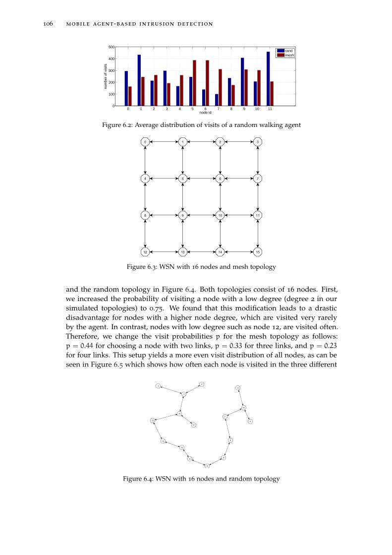
106 mobile agent-based intrusion detection
0 1 2 3 4 5 6 7 8 9 10 110
100
200
300
400
500
node id
num
ber
of v
isits
randmesh
Figure 6.2: Average distribution of visits of a random walking agent
Figure 6.3: WSN with 16 nodes and mesh topology
and the random topology in Figure 6.4. Both topologies consist of 16 nodes. First,we increased the probability of visiting a node with a low degree (degree 2 in oursimulated topologies) to 0.75. We found that this modification leads to a drasticdisadvantage for nodes with a higher node degree, which are visited very rarelyby the agent. In contrast, nodes with low degree such as node 12, are visited often.Therefore, we change the visit probabilities p for the mesh topology as follows:p = 0.44 for choosing a node with two links, p = 0.33 for three links, and p = 0.23for four links. This setup yields a more even visit distribution of all nodes, as can beseen in Figure 6.5 which shows how often each node is visited in the three different
Figure 6.4: WSN with 16 nodes and random topology
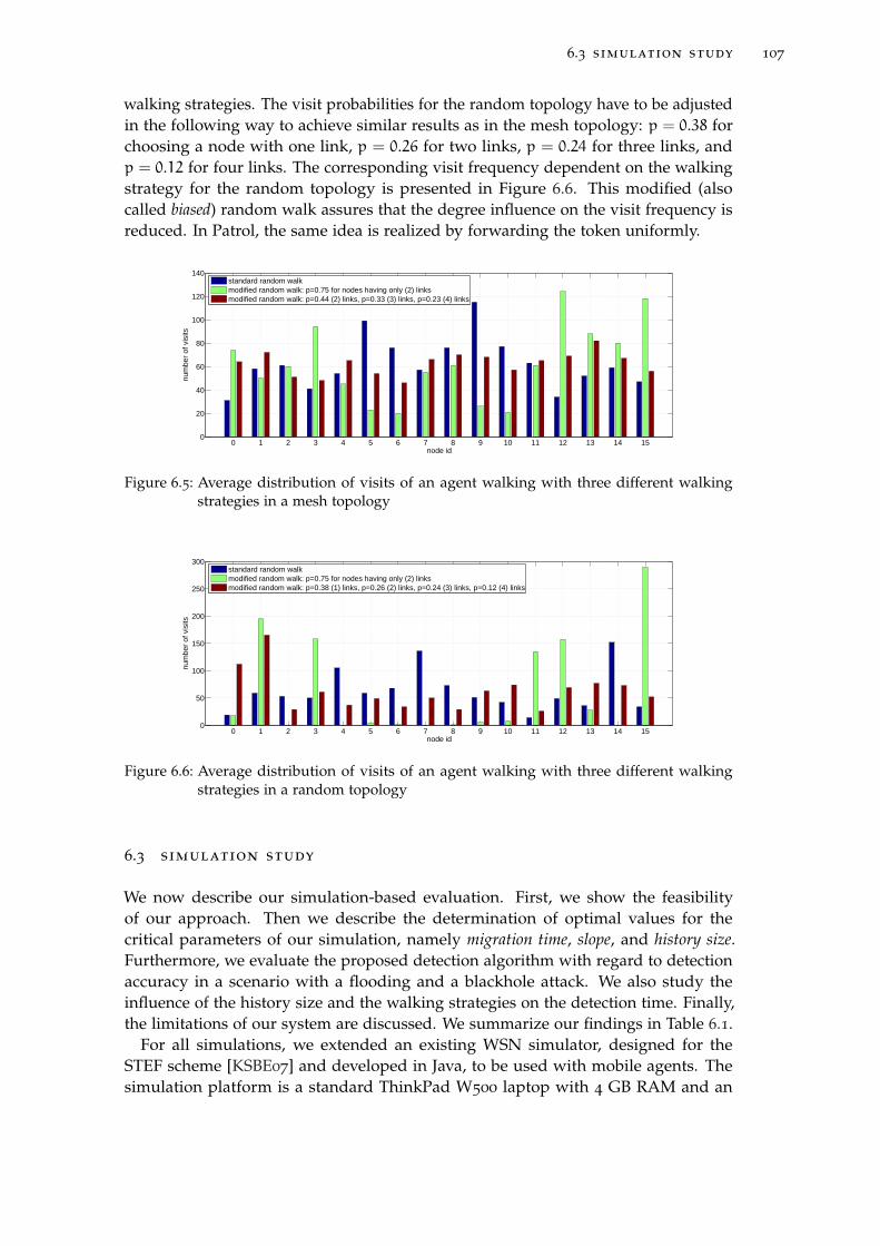
6.3 simulation study 107
walking strategies. The visit probabilities for the random topology have to be adjustedin the following way to achieve similar results as in the mesh topology: p = 0.38 forchoosing a node with one link, p = 0.26 for two links, p = 0.24 for three links, andp = 0.12 for four links. The corresponding visit frequency dependent on the walkingstrategy for the random topology is presented in Figure 6.6. This modified (alsocalled biased) random walk assures that the degree influence on the visit frequency isreduced. In Patrol, the same idea is realized by forwarding the token uniformly.
0 1 2 3 4 5 6 7 8 9 10 11 12 13 14 150
20
40
60
80
100
120
140
node id
num
ber
of v
isits
standard random walkmodified random walk: p=0.75 for nodes having only (2) linksmodified random walk: p=0.44 (2) links, p=0.33 (3) links, p=0.23 (4) links
Figure 6.5: Average distribution of visits of an agent walking with three different walkingstrategies in a mesh topology
0 1 2 3 4 5 6 7 8 9 10 11 12 13 14 150
50
100
150
200
250
300
node id
num
ber
of v
isits
standard random walkmodified random walk: p=0.75 for nodes having only (2) linksmodified random walk: p=0.38 (1) links, p=0.26 (2) links, p=0.24 (3) links, p=0.12 (4) links
Figure 6.6: Average distribution of visits of an agent walking with three different walkingstrategies in a random topology
6.3 simulation study
We now describe our simulation-based evaluation. First, we show the feasibilityof our approach. Then we describe the determination of optimal values for thecritical parameters of our simulation, namely migration time, slope, and history size.Furthermore, we evaluate the proposed detection algorithm with regard to detectionaccuracy in a scenario with a flooding and a blackhole attack. We also study theinfluence of the history size and the walking strategies on the detection time. Finally,the limitations of our system are discussed. We summarize our findings in Table 6.1.
For all simulations, we extended an existing WSN simulator, designed for theSTEF scheme [KSBE07] and developed in Java, to be used with mobile agents. Thesimulation platform is a standard ThinkPad W500 laptop with 4 GB RAM and an

108 mobile agent-based intrusion detection
Table 6.1: A summary of the major simulation results of this chapter
Objective Section Conclusion
Feasibility 6.3.1 By launching a flooding attack we show thatthe energy consumption is a feasible metric fordetecting intrusions.
Parameters 6.3.2 We determine optimal parameters for our simu-lated network. They are unique for each WSN.
Detection Accuracy 6.3.3 Flooding and blackhole attacks can be detectedwith a low false-positive rate.
History Size 6.3.4 Larger history sizes increase the detection time.
Walking Strategy 6.3.5 A biased random walk can improve the detec-tion time.
Intel Core 2 Duo T9600. The simulated sensor nodes correspond to TelosB nodes; theirenergy consumption rates were obtained from [PSC05]. Currently, we only simulatethe energy consumption of the radio chip CC2420 as this is the largest energy driverin a WSN. As routing protocol we implement AODV, which is a reactive routingprotocol and therefore is challenging for the IDS, because the energy consumptionmay fluctuate. As a consequence, this could lead to false-positive detection results.The agent has a size of 1 KB.
6.3.1 Initial Demonstration
Simulations were performed to analyze the influence of a flooding attack on the energyconsumption of all nodes in the network. The goal is to detect attacks based on theenergy consumption on either the malicious node itself or indirectly on its neighbors.The simulated WSN consists of 12 nodes arranged in a mesh topology (see Figure 6.1a;the arrows indicate a link between two nodes, i.e., the nodes being in transmissionrange of each other) with each node sending one random message per minute. After128 minutes, node 3 starts an attack by flooding an additional message with a randomdestination to the WSN every minute.
Figure 6.7 shows the energy consumption (averaged over four test-runs) of eachnode. A very important finding is that this attack does not only influence the energyconsumption of the malicious node itself, but it also affects all other nodes. Theincrease in energy consumption is especially significant for the direct neighbors ofthe attacking node, namely nodes 2 and 7. Those nodes receive a considerably highernumber of messages than before launching the attack. Thus, the performed floodingattack can be detected not only by analyzing the energy slope of the malicious nodeitself, but also by monitoring other nodes in the WSN which have abnormal energyconsumptions. This is important, as the attacker is likely to report fake data to themobile agent.

6.3 simulation study 109
6.3.2 Determination of Parameters
To reliably detect attacks, we need to determine meaningful values for the parametersused in our approach, in particular the warm-up phase and the slope limit, which shouldnot be exceeded without triggering an alert.
Before calculating the energy slopes, we need a warm-up phase expressed as thenumber of agent migrations, in which the mobile agent collects multiple energy valuesfrom each visited node. The warm-up phase should guarantee that the agent collectsas many energy readings of each node as required by the history size. Because theagent moves randomly, the number of migrations has to be higher than the number ofnodes multiplied by the size of the history. Additionally, as shown in Section 6.2.2,the visit frequency depends on the node degree. To account for this, we need anothermultiplier k. In our simulations, k = 2 led to a high probability of collecting sufficientenergy values from all nodes, and is therefore used in the rest of this chapter. Thus,we calculate the number of agent migrations needed before starting the detectionmechanism following Equation 6.2.
warmupmigrations = numbernodes × sizehistory × k (6.2)
Next, we have to determine a value for the slope limit, which is divided intoupper and lower slope limit to also take attacks into account causing a lower energyconsumption by, e.g., discarding packets. Exceeding or falling below those limits isregarded an anomaly. For this purpose, we performed additional simulations. Thesimulated sensor network consists of 12 randomly placed nodes. Each node injectsone random message per minute into the network. Every minute, the agent migratesrandomly from node to node. The history size is set to three, which means the agentcarries the measured energy values of the last three visits of each node.
Figure 6.8 shows the current slopes of the collected energy values calculated byour randomly migrating agent (averaged over four test-runs). Immediately after thestart, the WSN is not balanced, and there are relatively high slopes in the energyconsumption due to the nature of the managing phase of the underlying routingprotocol. Since we use AODV, the nodes need to establish routes and create routingtables after the start-up, resulting in a message overhead.
Figure 6.7: Measured energy of a WSN with 12 nodes arranged in a mesh

110 mobile agent-based intrusion detection
After the warm-up phase, which lasts for 72 migrations following Equation 6.2,the WSN becomes more balanced and the average slope of all nodes is stabilizing.Considering the results of Figure 6.8, we choose a value of 0.3 for the upper slope limit,i.e., the limit that applies to attacks increasing the energy consumption. Furthermore,we use a lower slope limit of 0.02, i.e., the minimal slope each node should have;otherwise an attack might be underway. Such an attack resulting in an abnormallow energy consumption could be a blackhole attack (see Section 6.3.3). It is possibleto reduce the slope range, however, this could lead to an increased number of false-positives.
6.3.3 Detection Accuracy
To evaluate the effectiveness of our approach, we measure the detection accuracywhen performing a flooding and a blackhole attack. The false-positive rate is thereforetracked and we determine the average number of migrations until detection. Asa false-positive in the flooding attack scenario, we count all cases in which a nodethat is not the attacking node itself or a direct neighbor is reported as anomalous.Therefore, the false-positive rate is rather pessimistic, as effects of the attack mightalso propagate to 2-hop neighbors. Regarding the blackhole attack, a false-positive isreported whenever a node other than the attacker is wrongly identified as suspicious.Throughout all simulations in both attacking scenarios we were always able to detectthe attack, i.e., the true-positive rate is 100%.
In our simulations, we vary the number of nodes from 8 to 16. Another parameterwe vary is the migration time of the agent.
Flooding Attack
We performed a flooding attack in WSNs with 8 and 16 nodes arranged in a randomtopology; an example topology is shown in Figure 6.1b in Section 6.2.2. Each node istransmitting one message per minute. The parameters used are listed in Table 6.2.
Immediately after the warm-up phase, a randomly selected node starts a floodingattack by unicasting an additional random message every minute. Our agent uses
Figure 6.8: Energy slopes in a WSN with 12 nodes and random topology

6.3 simulation study 111
Table 6.2: Values used for attack simulation
No. of nodes Warm-up History size Slope limit
8 48 migrations 3 0.3
16 96 migrations 3 0.3
different migration times of 30s, 60s, and 90s. Moreover, the false-positive rate istracked. Figure 6.9 shows the averaged results of the simulations (for each network sizeand for each migration time we performed 12 different test-runs). The false-positiverate can be observed in Table 6.3.
In our initial tests (not shown here), we found that a high migration rate led toa higher false-positive rate. This was due to the fact that the mobile agent needscomparatively more energy for its own operation, thereby interfering with the normalenergy consumption of the wireless sensor network. To compensate for this, we letthe agent subtract its own energy consumption from the nodes’ energy readings.Therefore, the agent keeps track of the number of visits of each node, as the nodesthemselves do not consider the agent’s energy consumption. Table 6.3 and Figure 6.9show that in all configurations a low false-positive rate in combination with a usefuldetection time is achieved. For instance, with a migration time of 30s, it takes about 5
migrations in a 8-node network until detection while at the same time the false-positive
Table 6.3: False-positive rate for the flooding attack
No. of nodes 30s 60s 90s
8 8.3% 8.3% 8.3%
16 8.3% 8.3% 0%
30 60 900
5
10
15
20
migration time (sec)
ave
rag
e m
igra
tio
ns u
ntil d
ete
ctio
n
WSN with 8 nodes
WSN with 16 nodes
Figure 6.9: Average migrations until detection of a flooding attack
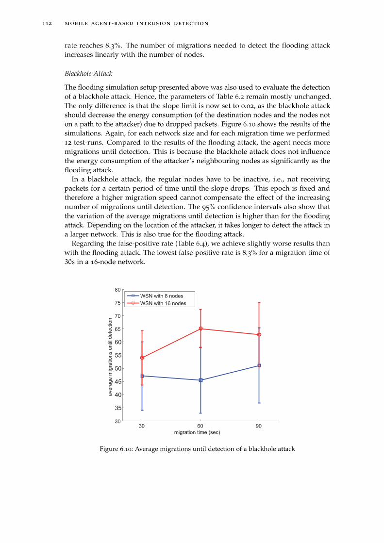
112 mobile agent-based intrusion detection
rate reaches 8.3%. The number of migrations needed to detect the flooding attackincreases linearly with the number of nodes.
Blackhole Attack
The flooding simulation setup presented above was also used to evaluate the detectionof a blackhole attack. Hence, the parameters of Table 6.2 remain mostly unchanged.The only difference is that the slope limit is now set to 0.02, as the blackhole attackshould decrease the energy consumption (of the destination nodes and the nodes noton a path to the attacker) due to dropped packets. Figure 6.10 shows the results of thesimulations. Again, for each network size and for each migration time we performed12 test-runs. Compared to the results of the flooding attack, the agent needs moremigrations until detection. This is because the blackhole attack does not influencethe energy consumption of the attacker’s neighbouring nodes as significantly as theflooding attack.
In a blackhole attack, the regular nodes have to be inactive, i.e., not receivingpackets for a certain period of time until the slope drops. This epoch is fixed andtherefore a higher migration speed cannot compensate the effect of the increasingnumber of migrations until detection. The 95% confidence intervals also show thatthe variation of the average migrations until detection is higher than for the floodingattack. Depending on the location of the attacker, it takes longer to detect the attack ina larger network. This is also true for the flooding attack.
Regarding the false-positive rate (Table 6.4), we achieve slightly worse results thanwith the flooding attack. The lowest false-positive rate is 8.3% for a migration time of30s in a 16-node network.
30 60 9030
35
40
45
50
55
60
65
70
75
80
migration time (sec)
ave
rag
e m
igra
tio
ns u
ntil d
ete
ctio
n
WSN with 8 nodes
WSN with 16 nodes
Figure 6.10: Average migrations until detection of a blackhole attack

6.3 simulation study 113
Table 6.4: False-positive rate for the blackhole attack
No. of nodes 30s 60s 90s
8 16.6% 16.6% 16.6%
16 8.3% 16.6% 16.6%
6.3.4 Influence of the History Size
One way to optimize our IDS and keep it as lightweight as possible, is to change thehistory size, i.e., the number of readings needed from each node to predict the energyconsumption. In simulations for a 12-node WSN we varied the history size from 2 to3 and 4, while performing a flooding attack. Figure 6.11 presents the results showingthat the average number of migrations until detection increases with the history size.A smaller history size is able to reflect the change in the energy consumption morequickly, thereby generating an anomaly alert faster than a larger history size. Thedrawback is a higher false-positive rate (see Table 6.5).
6.3.5 Influence of the Walking Strategy
Attacks that affect nodes with a low degree could potentially take more time to bedetected by a random walking agent as compared to different walking strategies.Therefore, we now investigate the influence of the walking strategy on the detectiontime.
2 3 4
0
5
10
15
20
history size
ave
rag
e m
igra
tio
n u
ntil d
ete
ctio
n
Figure 6.11: Influence of the history size (WSN with 12 nodes in a random topology and aflooding attack)

114 mobile agent-based intrusion detection
Table 6.5: False-positive rate for the flooding attack, depending on the history size, migrationtime = 90s
History size False-positive rate
2 33.3 %
3 8.3%
4 0%
Table 6.6: Detection, false positive (FP) and false negative (FN) rates for the flooding attack
Topology Walking strategy Migrations FP FN
Mesh Random 86 18.75% 6.25%
Mesh Biased Random 37 6.25% 0%
The setup for the simulations evaluating different walking strategies is as follows.The mesh wireless sensor network consists of 16 nodes, the topology of which is thesame as shown in Figure 6.3 in Section 6.2.2. Each node is transmitting one messageevery two minutes, the agent migrates every 30 seconds, the slope limit is 1.0, andthe history size is set to three. The warm-up phase lasts for 256 migrations, after 320
migrations we start the flooding by letting node 0 send one additional message everyminute. If an intrusion was detected during the period the warm-up phase ended andbefore the attack started, we count this event as false-positive. Cases, in which a nodethat is neither a direct neighbor of the attacker nor the attacker itself was found tobe suspicious, also count as false-positive. If we did not detect an intrusion within576 migrations, this event is counted as false-negative (see also Figure 6.12). Theprobabilities for the biased random walk were defined as p = 0.44 for choosing a nodewith two links, p = 0.33 for three links, and p = 0.23 for four links. Each experimentis repeated 16 times.
The results can be found in Table 6.6. In such a setting, having a more isolated nodebe the attacker, the biased random walk achieves significantly better results, givena mesh topology. The average number of migrations needed to detect the attack isreduced by about 43%. Besides, we were always able to detect the attack within 576
migrations. We achieve similar results for a random topology.
Figure 6.12: Evaluation setup

6.4 related work 115
6.3.6 Discussion
In this chapter we show that mobile agents can be used in WSNs to detect intrusionsreliably. However, our proposed approach has some limitations which we discuss inthe following:
. The system presented herein is not suited for every WSN scenario. While itworks very well in environmental monitoring settings with regular measurementand transmitting patterns as in [TPS+
05], the opposite is true for example in areasurveillance scenarios, where a detected event is resulting in intense activity.
. The assumption of the linearity of the energy consumption may not always holdin a real-world testbed, in which we face problems with unreliable and burstylinks. As a consequence, such behavior could result in an increased false-positiverate.
. An attacker with physical access could change the agent and let nodes executehis own code. Since we assume that nodes can be physically compromised, atrusted base station is required to prevent such an attack. One possibility to doso is by using public-key cryptography, which has become feasible in wirelesssensor networks [LN08]. The base station signs the agent code with its privatekey. As per assumption all sensor nodes know the public key of the base station,they can verify that the code has not been changed.
. The low amount of storage available on today’s standard nodes limits theapplicability of our system to comparatively small WSNs.
. Transferring huge agents requires a large amount of energy. Hence, reducingthe size of the agent by using middleware such as Agilla [FRL05] is a promisingdirection.
. Our approach is not supposed to be a general security framework capable ofdefending against all types of attacks, such as sybil or data manipulation attacks.Attacks that have no influence on the energy consumption remain undetected.
6.4 related work
Our work covers several aspects: (1) the mobile agent paradigm, (2) the usage ofmobile agents to detect intrusions, and (3) the energy consumption as a possiblemetric for attacks. The combination of these techniques is unique in wireless sensornetworks. In this section we discuss related work for these aspects.
Mobile Agents in WSNs
With Agilla, a middleware for wireless sensor networks was presented by Fok etal. [FRL05] which allows the development and usage of mobile agents. Instead ofdeploying pre-installed applications, mobile agents perform the desired tasks. Theymodel each agent as an autonomous entity, but provide inter-agent communication.
The mobile agent-based computing model has been evaluated in the context ofcollaborative processing in WSNs in the work of Qi et al. [QXW03]. The authors

116 mobile agent-based intrusion detection
use the execution time and the energy consumption as metrics for evaluating theperformance of the client/server-based and mobile agent-based models. In theirsimulations they found that even though both the execution time and the energyconsumption grow as the number of nodes increases, the growth is much faster forthe client/server model. They conclude that the mobile agent-based model is notconsistently performing better than the client/server-based model, but it may beadvantageous depending on the use case.
Intrusion Detection using Mobile Agents
Applying mobile agents for intrusion detection has been widely researched; severalworks exist. Helmer et al. [HWH+
03] designed an intrusion detection system fortraditional networks employing static as well as mobile agents. Stationary agentsreside at each monitored component, gathering information, e.g., from system logsand providing this information in a common format. Mobile agents travel betweenmonitored components, classify the data collected from the static agents as normaldata and data signifying an intrusion, and pass this information to so-called mediators.Mediators manage the mobile agents and further use data mining techniques to relatesingle events to a specific attack.
Kachirski and Guha [KG02] proposed a mobile agent-based intrusion detectionsystem for wireless ad hoc networks. They use different sensor types to performspecific functions. While few nodes have agents for network packet monitoring, everynode’s agent monitors the host itself for suspicious activities such as unusual useroperations (e.g., invalid login attempts). On a host-level basis, decisions on the threatlevel of an intrusion are made individually. Certain nodes collaborate in order to makedecisions about intrusions affecting the network level. For the purpose of respondingand resolving an intrusion, each node is equipped with an action module.
Sparta is a system able to detect intrusions and security policy violations in a network[KT01]. A pattern language is introduced allowing the user to define intrusion patternsin a declarative manner. The approach to spot these patterns is fully distributed,utilizing mobile agents to correlate event data gathered on the single hosts.
All three approaches mentioned above were not designed for WSNs and createsignificant overhead.
Energy Consumption
Some authors have already used the energy consumption as a metric for intrusiondetection. Nash et al. [NMHH05] presented an IDS for mobile computers that usesseveral parameters like CPU load and disk read and write access to estimate the powerconsumption. The linear regression they used is therefore quite complex, while ourmodel only needs one variable: the energy status of a node. Moreover, their systemdetermines the energy consumption on a per process basis. This renders the IDSvulnerable to attacks that distribute the workload to many different processes.
Buennemeyer et al. [BNC+08] developed an IDS that creates a power profile for
mobile devices, generating an alert in case of abnormal current changes. The thresholdvalue is adapted dynamically to account for false-positives and false-negatives. Batteryreadings are transmitted to a central point, which would cause significant overhead inWSNs. In order to create a reliable profile, a large amount of data has to be sent and

6.5 summary 117
analyzed, whereas we require only the last three energy readings from each node forreliable attack detection. At the central server, attack traffic is correlated with Snortalerts. Thus, their system is very complex as it combines anomaly detection with arule-based IDS. Another drawback of the last two approaches lies in the necessity torun an IDS agent on every node. In contrast, our system takes into account specificWSN requirements (typically, nodes run a single application, have severe resourcerestrictions, sleep most of the time, etc.) by developing a lightweight method forintrusion detection.
Shen et al. [SHS+12] proposed an intrusion detection scheme comparing the energy
consumptions of different sensor nodes in clustered WSNs. It can differentiate thetypes of DoS attacks such as selective forwarding and wormhole attacks with theassistance of energy thresholds. Nodes are required to send messages containing theirremaining energy to the base station. The energy consumption of all nodes is thenpredicted at the base station by using markov chains. The scheme looks for nodeswhich spend significantly more energy than the other nodes. In their work, theyassume that the energy consumption is similar for all nodes, which is an unrealisticassumption.
6.5 summary
In this chapter we propose a novel lightweight IDS for wireless sensor networks. Weneither require nodes to monitor their environment and collaborate with each other,nor do we need to transfer audit data to a central point. Instead, we use a mobileagent that collects energy readings and raises an alert if sudden changes occur. Thefeasibility of reducing the intrusion detection functionality using mobile agents inwireless sensor networks has been demonstrated.


7C O N C L U S I O N S A N D O U T L O O K
You rarely achieve finality. If you did,life would be over, but as you strive newvisions open before you.
E. Roosevelt
7.1 summary and conclusions
Providing security in wireless sensor networks during operation involves addressingmultiple challenges, especially the reduction of complexity and resource-requirementsin intrusion detection. Throughout this thesis, we have contributed to solve thischallenge by providing solutions along two key directions. In our first researchdirection, we have studied the practical effects of DoS attacks on wireless sensornetworks. Albeit important for attack dection, this aspect has mainly been neglectedby existing works. Moreover, in our second research direction, we have reduced theintrusion detection frequency and built extensible and lightweight systems that allowintrusion detection at a low cost.
Particulary, we have introduced a systematic approach for evaluating attack effectson the network behavior. Therefore, we have identified a large number of localnode metrics, that can be easily obtained and calculated without incurring too muchoverhead. Next, we have statistically tested these metrics to assess whether theyexhibit significantly different values when the network is attacked. The metrics wehave analyzed look into different aspects of the motes and the network, for example,MCU and radio activities, network traffic statistics, and routing related information.In our experiments, we have varied several parameters to show that the metricsare applicable to different WSNs, such as traffic intensity and transmission power.Using the collection tree and the mesh protocol, we have considered two of the mostcommon applications in wireless sensor networks, such as central data collection andmeshed multi-hop networks. Finally, we have analyzed the metrics with regard totheir capability of distinction. Our results show that certain metrics can be used solelyto detect a jamming attack, while in some scenarios a combination of metrics needs tobe analyzed. Even though we have focused on jamming and blackhole attacks, ourmethodology can be applied to other metrics and attacks as well. Besides, we havepresented a fully localized IDS, which only analyzes node-specific metrics. In contrastto existing works, we do not require any form of collaboration.
Because of severe resource-restrictions, it is desirable to reduce the tasks of eachmote to a minimum. We have proposed two intrusion detection systems that addressthe conflict between energy consumption and detection frequency. In detail, we haveshown that even critical security functions, an example being intrusion detection, canbe performed by means of randomizing the detection frequency at the cost of a slightlyincreased detection time. To this end, we have presented a system distributing the load
119

120 conclusions and outlook
which is caused by various tasks across the network. This system utilizes tokens whichare exchanged between nodes. Upon reception of such a token, a certain functionality,such as intrusion detection, is activated temporarily. As a proof-of-concept, we havedesigned and implemented a lightweight intrusion detection algorithm based on theenergy consumption of the nodes. We have shown by experimentation in a real-worldtestbed that we can dectect flooding and blackhole attacks very fast also withoutconstant intrusion detection.
We have finally proposed a second intrusion detection system, which is similar tothe first one in the sense that we randomize the detection frequency. However, in thissystem we are exchanging the whole IDS routine in the network. The central buildingblock is a mobile agent which migrates from node to node and contains code as wellas data used for intrusion detection. It carries the energy status of the nodes anddetects intrusions by analyzing the energy consumption with a linear regression model.Consequently, this approach exchanges the overhead of storing an IDS permanentlywith the communication overhead of transferring the mobile agent. We have shownin simulations that denial-of-service attacks such as flooding and blackhole can bedetected with high accuracy, while keeping the number of false-positives very low.
In summary, this thesis contributes to the lightweight detection of denial-of-serviceattacks on wireless sensor networks. Our solutions are flexible, configurable, andextensible which allows them to be used in a large number of scenarios due to therelatively weak requirements. All contributions are motivated by the low power andlow computational capabilities of state-of-the-art sensor nodes.
7.2 outlook
The contributions of this thesis lay the foundations for lightweight intrusion detectionin wireless sensor networks. In what follows, we shed light on a variety of newresearch directions and challenges:
. powerful sensor nodes
The development of nodes with more powerful processing capabilities, such asthe ARM microcontroller, allows the usage of algorithms for intrusion detectionthat are very sophisticated. To give an example, the application of traditional ma-chine learning operators such as decision trees or support vector machines mightbecome feasible on sensor nodes. However, these microcontrollers consumemuch energy, thus energy-efficiency is still important.
. attackers everywhere
With the progress of the Internet of Things (IoT), security becomes even morean issue. IPv6 over Low-power Wireless Personal Area Network (6LoWPAN)[KMS07, HT11] enables the connection of sensor nodes with the untrusted Inter-net. Hence, an attacker can get access to the nodes from virtually everywhere;he no longer needs to be in physical proximity. In the same way, the numberof potential attackers increases. To tackle this problem, new IDSs need to bedeveloped taking into account the architecture in the IoT: (1) the edge nodeconnecting 6LoWPAN networks with the Internet is assumed to be always acces-

7.2 outlook 121
sible, (2) end-to-end message security is required, and (3) sensor nodes have aglobally unique IP address [RWV13].
. detecting false data
A characteristic feature for many WSNs is the high density of deployed sensornodes. Especially in industrial control scenarios, the number of sensors can reach35.000 [SBR10]. This redundancy is necessary to account for the high criticalityof the system and allows us to exploit this fact for detecting false data. Nodesin close proximity should exhibit highly correlated observations. Besides thisspatial correlation, the measured physical parameters typically are temporallycorrelated. Measured processes are well-defined and executed repeatedly.
One possibility to exploit the spatio-temporal relationship between node readingsis to perform statistical anomaly detection at the sink. This central point canleverage the global view it has on all nodes in the network and apply powerfulmachine learning algorithms to first build a model of normal readings, and thenclassify new observations based on historical data [NSBJ11].
Alternatively, the usage of decentralized algorithms to detect data anomaliesrequiring little memory and processing power is promising. First proposals todistributed data mining in WSNs have been made [BSG+
06, BHL07, R0̈7, FCG10].However, their focus is rather on false data caused by measurement errorsand node failures. Attackers that intentionally change the data to create aspecific malfunctioning are not considered. In addition, their memory andcommunication overhead might still be too high in certain scenarios.
. intrusion response
Once an attack has been detected, it is necessary to take corrective action. Achallenge associated with this is how to inform the network operator while thenetwork is under attack, e.g., no communication over the wireless links mightbe possible.
In conclusion, wireless sensors are widely used in the real-world, yet a numberof open challenges especially in the domain of security persist. To the best of ourknowledge, real WSN deployments are still missing intrusion detection functionality.


bibliography 123
bibliography
[AIM10] L. Atzori, A. Iera, and G. Morabito: The internet of things: A survey.Computer Networks, 54:2787–2805, 2010.
[Aka72] H. Akaike: Information theory and an extension of the maximum likelihoodprinciple. In Proceedings of the 2nd International Symposium on InformationTheory, 1972.
[Alm15] L. Almon: Practical decentralized intrusion detection in wireless sensor net-works. Master’s thesis, Technische Universität Darmstadt, 2015.
[And80] J. P. Anderson: Computer security threat monitoring and surveillance. Techni-cal report, James P. Anderson Company, 1980.
[ASSC02] I. Akyildiz, W. Su, Y. Sankarasubramaniam, and E. Cayirci: Wireless sensornetworks: a survey. Computer Networks, 38:393–422, 2002.
[Ban14] M. E. Bansarkhani: Statistische analyse der auswirkungen von denial-of-serviceangriffen auf drahtlose sensornetzwerke. Master’s thesis, Technische Univer-sität Darmstadt, 2014.
[BCF08] Z. Benenson, P. M. Cholewinski, and F. Freiling: Wireless Sensor NetworkSecurity, chapter Vulnerabilities and Attacks in Wireless Sensor Networks,pages 22–43. IOS Press, 2008.
[Ber08] D. J. Bernstein: The salsa20 family of stream ciphers. In New Stream CipherDesigns. Springer Berlin / Heidelberg, 2008.
[BHL07] L. Bettencourt, A. Hagberg, and L. Larkey: Separating the wheat fromthe chaff: Practical anomaly detection schemes in ecological applications ofdistributed sensor networks. In Proceedings of the 3rd IEEE InternationalConference on Distributed Computing in Sensor Systems (DCOSS). SpringerBerlin / Heidelberg, 2007.
[BMS14] I. Butun, S. Morgera, and R. Sankar: A survey of intrusion detection systemsin wireless sensor networks. IEEE Communications Surveys & Tutorials,16:266–282, 2014.
[BNC+08] T. K. Buennemeyer, T. M. Nelson, L. M. Clagett, J. P. Dunning, R. C.
Marchany, and J. G. Tront: Mobile device profiling and intrusion detectionusing smart batteries. In Proceedings of the 41st Hawaii International Conferenceon System Sciences (HICSS), 2008.
[BSG+06] J. Branch, B. Szymanski, C. Giannella, R. Wolff, and H. Kargupta: In-
network outlier detection in wireless sensor networks. In Proceedings of the 26thInternational Conference on Distributed Computing Systems (ICDCS), 2006.
[BvKH+11] D. Bijwaard, W. van Kleunen, P. Havinga, L. Kleiboer, and M. Bijl: Industry:
Using dynamic wsns in smart logistics for fruits and pharmacy. In Proceedingsof the 9th ACM Conference on Embedded Networked Sensor Systems (SenSys),2011.

124 bibliography
[BVN+11] C. Boano, T. Voigt, C. Noda, K. Römer, and M. Zuniga: Jamlab: Augmenting
sensornet testbeds with realistic and controlled interference generation. InProceedings of the 10th International Conference on Information Processing inSensor Networks (IPSN), 2011.
[BZV+10] C. Boano, M. Zuniga, T. Voigt, A. Willig, and K. Römer: The triangle
metric: Fast link quality estimation for mobile wireless sensor networks. InProceedings of the 19th International Conference on Computer Communicationsand Networks (ICCCN), 2010.
[CA07] Y. Cheng and D. P. Agrawal: An improved key distribution mechanism forlarge-scale hierarchical wireless sensor networks. Ad Hoc Networks, 5:35–48,2007.
[CCD+11] M. Ceriotti, M. Corra, L. D’Orazio, R. Doriguzzi, D. Facchin, S. Guna,
G. Jesi, R. Lo Cigno, L. Mottola, A. Murphy, M. Pescalli, G. Picco, D. Preg-nolato, and C. Torghele: Is there light at the ends of the tunnel? wirelesssensor networks for adaptive lighting in road tunnels. In Proceedings of the 10thInternational Conference on Information Processing in Sensor Networks (IPSN),2011.
[CPMM11] M. Conti, R. D. Pietro, L. V. Mancini, and A. Mei: Distributed detection ofclone attacks in wireless sensor networks. IEEE Transactions on Dependableand Secure Computing, 8(5):685–698, 2011.
[CS99] W. W. Cohen and Y. Singer: A simple, fast, and effective rule learner. InProceedings of the 16th National Conference on Artificial Intelligence (AAAI),pages 335–342, 1999.
[dC14] R. do Carmo: Active Intrusion Detection for Wireless Multihop Networks.PhD thesis, Technische Universität Darmstadt, 2014.
[Den87] D. Denning: An intrusion-detection model. IEEE Transactions on SoftwareEngineering, SE-13:222–232, 1987.
[DG10] T. Dimitriou and A. Giannetsos: Wormholes no more? localized wormholedetection and prevention in wireless networks. In Proceedings of the 6th IEEE In-ternational Conference on Distributed Computing in Sensor Systems (DCOSS),2010.
[DGV04] A. Dunkels, B. Gronvall, and T. Voigt: Contiki - a lightweight and flexibleoperating system for tiny networked sensors. In Proceedings of the 29th IEEEConference on Local Computer Networks (LCN), 2004.
[DLHZ13] W. Dong, Y. Liu, Y. He, and T. Zhu: Measurement and analysis on the packetdelivery performance in a large scale sensor network. In Proceedings of the 32ndIEEE International Conference on Computer Communications (INFOCOM),2013.
[dSMR+05] A. P. da Silva, M. Martins, B. Rocha, A. Loureiro, L. B. Ruiz, and H. C.
Wong: Decentralized intrusion detection in wireless sensor networks. In Proceed-ings of the 1st ACM International Workshop on Quality of Service & Securityin Wireless and Mobile Networks (Q2SWinet), 2005.

bibliography 125
[EG02] L. Eschenauer and V. D. Gligor: A key-management scheme for distributedsensor networks. In Proceedings of the 9th ACM Computer and CommunicationsSecurity Conference (CCS), 2002.
[FCG10] P. A. Forero, A. Cano, and G. B. Giannakis: Consensus-based distributed lin-ear support vector machines. In Proceedings of the 9th International Conferenceon Information Processing in Sensor Networks (IPSN), 2010.
[FRL05] C.-L. Fok, G.-C. Roman, and C. Lu: Rapid development and flexible deploy-ment of adaptive wireless sensor network applications. In Proceedings of the 25thIEEE International Conference on Distributed Computing Systems (ICDCS),2005.
[GDMV09] P. Garcia-Teodoro, J. Diaz-Verdejo, G. Macia-Fernandez, and E. Vazquez:Anomaly-based network intrusion detection: Techniques, systems and challenges.Computers & Security, 28:18–28, 2009.
[GFJ+09] O. Gnawali, R. Fonseca, K. Jamieson, D. Moss, and P. Levis: Collection treeprotocol. In Proceedings of the 7th ACM Conference on Embedded NetworkedSensor Systems (SenSys), 2009.
[GGSB13] P. E. Guerrero, I. Gurov, S. Santini, and A. Buchmann: On the selectionof testbeds for the evaluation of sensor network protocols and applications. InProceedings of the 14th IEEE International Workshop on Signal ProcessingAdvances in Wireless Communications (SPAWC), 2013.
[GKS05] G. Gaubatz, J.-P. Kaps, and B. Sunar: Public key cryptography in sensornetworks revisited. In Security in Ad-hoc and Sensor Networks. SpringerBerlin / Heidelberg, 2005.
[GZC07] S. Gupta, R. Zheng, and A. M. K. Cheng: Andes: an anomaly detectionsystem for wireless sensor networks. In Proceedings of the 4th IEEE InternationalConference on Mobile Ad-hoc and Sensor Systems (MASS), 2007.
[HC08] J. W. Hui and D. E. Culler: Ip is dead, long live ip for wireless sensor networks.In Proceedings of the 6th ACM Conference on Embedded Networked SensorSystems (SenSys), 2008.
[HHJ10] T. H. Hai, E.-N. Huh, and M. Jo: A lightweight intrusion detection frameworkfor wireless sensor networks. Wirel. Commun. Mob. Comput., 10(4):559–572,2010.
[HHW09] J.-H. Hauer, V. Handzinski, and A. Wolisz: Experimental study of the impactof wlan interference on ieee 802.15.4 body area networks. In Proceedings of the8th European Conference on Wireless Sensor Networks (EWSN), 2009.
[HR10] M. Hossain and V. Raghunathan: Aegis: A lightweight firewall for wirelesssensor networks. In Proceedings of the 6th IEEE International Conference onDistributed Computing in Sensor Systems (DCOSS), 2010.
[HSW+00] J. Hill, R. Szewczyk, A. Woo, S. Hollar, D. Culler, and K. Pister: System
architecture directions for networked sensors. SIGPLAN Not., 35(11):93–104,2000.

126 bibliography
[HT11] J. Hui and P. Thubert: Compression format for ipv6 datagrams over ieee802.15.4-based networks. In RFC 6282, September 2011.
[HWH+03] G. Helmer, J. S. K. Wong, V. Honavar, L. Miller, and Y. Wang: Lightweight
agents for intrusion detection. Journal of Systems and Software, 67:109–122,2003.
[IKP95] K. Ilgun, R. Kemmerer, and P. Porras: State transition analysis: a rule-basedintrusion detection approach. IEEE Transactions on Software Engineering,21:181–199, 1995.
[KBG+09] I. Krontiris, Z. Benenson, T. Giannetsos, F. C. Freiling, and T. Dimitriou:
Cooperative intrusion detection in wireless sensor networks. In Proceedings ofthe 6th European Conference on Wireless Sensor Networks (EWSN), 2009.
[KBT13] M. Keller, J. Beutel, and L. Thiele: The problem bit. In Proceedings of the 9thIEEE International Conference on Distributed Computing in Sensor Systems(DCOSS), 2013.
[KDF07] I. Krontiris, T. Dimitriou, and F. C. Freiling: Towards intrusion detectionin wireless sensor networks. In Proceedings of the 13th European WirelessConference (EW), 2007.
[KDGM08] I. Krontiris, T. Dimitriou, T. Giannetsos, and M. Mpasoukos: Intrusiondetection of sinkhole attacks in wireless sensor networks. In Algorithmic Aspectsof Wireless Sensor Networks, volume 4837, pages 150–161. Springer Berlin /Heidelberg, 2008.
[KE14] E. Karapistoli and A. A. Economides: Adlu: a novel anomaly detection andlocation-attribution algorithm for uwb wireless sensor networks. EURASIPJournal on Information Security, 3(1), 2014.
[KEW02] B. Krishnamachari, D. Estrin, and S. Wicker: The impact of data aggregationin wireless sensor networks. In Proceedings of the 22nd International Conferenceon Distributed Computing Systems Workshops (ICDCSW), 2002.
[KG02] O. Kachirski and R. Guha: Intrusion detection using mobile agents in wirelessad hoc networks. In Proceedings of the IEEE Workshop on Knowledge MediaNetworking (KMN), 2002.
[KMS07] N. Kushalnagar, G. Montenegro, and C. Schumacher: Ipv6 over lowpowerwireless personal area networks (6lowpans): Overview, assumptions, problemstatement, and goals. In RFC 4919, August 2007.
[KSBE07] C. Krauß, M. Schneider, K. Bayarou, and C. Eckert: Stef: A secure ticket-based en-route filtering scheme for wireless sensor networks. In Proceedingsof the 2nd International Conference on Availability, Reliability and Security(ARES), 2007.
[KT01] C. Krügel and T. Toth: Sparta - a mobile agent based intrusion detection system.In Proceedings of the 1st IFIP Conference on Network Security (I-NetSec), 2001.

bibliography 127
[KW03] C. Karlof and D. Wagner: Secure routing in wireless sensor networks: attacksand countermeasures. Ad Hoc Networks, 1:293–315, 2003.
[Lan05] M. Langheinrich: Personal privacy in ubiquitous computing. PhD thesis,ETH Zurich, 2005.
[LC11] T. Liu and A. Cerpa: Foresee (4c): Wireless link prediction using link features.In Proceedings of the 10th International Conference on Information Processingin Sensor Networks (IPSN), 2011.
[LCC07] F. Liu, X. Cheng, and D. Chen: Insider attacker detection in wireless sensornetworks. In Proceedings of the 26th IEEE International Conference on ComputerCommunications (INFOCOM), 2007.
[LHL+11] Y. Liu, Y. He, M. Li, J. Wang, K. Liu, L. Mo, W. Dong, Z. Yang, M. Xi,
J. Zhao, and X.-Y. Li: Does wireless sensor network scale? A measurementstudy on greenorbs. In Proceedings of the 30th IEEE International Conferenceon Computer Communications (INFOCOM), 2011.
[LHS00] J. J. Louviere, D. A. Hensher, and J. D. Swait: Stated Choice Methods:Analysis and Applications. Cambridge University Press, 2000.
[LKP07] M. Li, I. Koutsopoulos, and R. Poovendran: Optimal jamming attacks andnetwork defense policies in wireless sensor networks. In Proceedings of the 26thIEEE International Conference on Computer Communications (INFOCOM),2007.
[LMPG07] M. Luk, G. Mezzour, A. Perrig, and V. Gligor: Minisec: A secure sensornetwork communication architecture. In Proceedings of the 6th InternationalConference on Information Processing in Sensor Networks (IPSN), 2007.
[LMZL11] K. Liu, Q. Ma, X. Zhao, and Y. Liu: Self-diagnosis for large scale wirelesssensor networks. In Proceedings of the 30th IEEE International Conference onComputer Communications (INFOCOM), 2011.
[LN08] A. Liu and P. Ning: Tinyecc: A configurable library for elliptic curve cryp-tography in wireless sensor networks. In Proceedings of the 7th InternationalConference on Information Processing in Sensor Networks (IPSN), 2008.
[LNLP06] C. E. Loo, M. Y. Ng, C. Leckie, and M. Palaniswami: Intrusion detectionfor routing attacks in sensor networks. International Journal of DistributedSensor Networks, 2:313–332, 2006.
[Lov96] L. Lovász: Random walks on graphs: a survey. In Combinatorics, Paul Erdös isEighty. Janos Bolyai Mathematical Society, 1996.
[LSS+10] J. Lu, T. Sookoor, V. Srinivasan, G. Gao, B. Holben, J. Stankovic, E. Field,
and K. Whitehouse: The smart thermostat: Using occupancy sensors to saveenergy in homes. In Proceedings of the 8th ACM Conference on EmbeddedNetworked Sensor Systems (SenSys), 2010.

128 bibliography
[LTZ+13] G. Liu, R. Tan, R. Zhou, G. Xing, W.-Z. Song, and J. M. Lees: Volcanic
earthquake timing using wireless sensor networks. In Proceedings of the 12thInternational Conference on Information Processing in Sensor Networks (IPSN),2013.
[LWW11] Z. Lu, W. Wang, and C. Wang: From jammer to gambler: Modeling and detec-tion of jamming attacks against time-critical traffic. In Proceedings of the 30thIEEE International Conference on Computer Communications (INFOCOM),2011.
[Man97] S. Mann: Wearable computing: a first step toward personal imaging. Computer,30:25–32, 1997.
[Men02] S. Menard: Applied logistic regression analysis. Sage, 2002.
[MHL94] B. Mukherjee, L. T. Heberlein, and K. N. Levitt: Network intrusion detection.IEEE Network, 8:26–41, 1994.
[MMH+12] X. Mao, X. Miao, Y. He, X.-Y. Li, and Y. Liu: Citysee: Urban co2 monitoring
with sensors. In Proceedings of the 31st IEEE International Conference onComputer Communications (INFOCOM), 2012.
[MMP+13] R. Marfievici, A. Murphy, G. Picco, F. Ossi, and F. Cagnacci: How envi-
ronmental factors impact outdoor wireless sensor networks: A case study. InProceedings of the 10th IEEE International Conference on Mobile Ad hoc andSensor Systems (MASS), 2013.
[MOV96] A. J. Menezes, P. C. V. Oorschot, and S. A. Vanstone: Handbook of appliedcryptography. CRC Press, 1996.
[MPS09] I. Martinovic, P. Pichota, and J. B. Schmitt: Jamming for good: A freshapproach to authentic communication in wsns. In Proceedings of the 2nd ACMConference on Wireless Network Security (WiSec), 2009.
[NLL06] E. C. H. Ngai, J. Liu, and M. R. Lyu: On the intruder detection for sinkholeattack in wireless sensor networks. In Proceedings of the 8th IEEE InternationalConference on Communications (ICC), 2006.
[NMHH05] D. C. Nash, T. L. Martin, D. S. Ha, and M. S. Hsiao: Towards an intrusiondetection system for battery exhaustion attacks on mobile computing devices. InProceedings of the 3rd IEEE International Conference on Pervasive Computingand Communications Workshops (PerCom Workshops), 2005.
[NSBJ11] K. Nyalkalkar, S. Sinhay, M. Bailey, and F. Jahanian: A comparative study oftwo network-based anomaly detection methods. In Proceedings of the 30th IEEEInternational Conference on Computer Communications (INFOCOM), 2011.
[OM05] I. Onat and A. Miri: An intrusion detection system for wireless sensor networks.In Proceedings of the 3rd IEEE International Conference on Wireless And MobileComputing, Networking And Communications (WiMob), 2005.
bibliography 129
[PAS+14] O. Punal, I. Aktas, C.-J. Schnelke, G. Abidin, K. Wehrle, and J. Gross:
Machine learning-based jamming detection for ieee 802.11: Design and experi-mental evaluation. In Proceedings of the 15th IEEE International Symposiumon A World of Wireless, Mobile and Multimedia Networks (WoWMoM), 2014.
[PIK11] K. Pelechrinis, M. Iliofotou, and S. V. Krishnamurthy: Denial of serviceattacks in wireless networks: The case of jammers. IEEE CommunicationsSurveys & Tutorials, 13:245–257, 2011.
[PLP06] K. Piotrowski, P. Langendoerfer, and S. Peter: How public key cryptogra-phy influences wireless sensor node lifetime. In Proceedings of the 4th ACMWorkshop on Security of Ad hoc and Sensor Networks (SASN), 2006.
[PPG05] B. Parno, A. Perrig, and V. Gligor: Distributed detection of node replicationattacks in sensor networks. In Proceedings of the 26th IEEE Symposium onSecurity and Privacy (S&P), 2005.
[Pre14] S. Prentice: The five smart technologies to watch. http://www.gartner.com,2014. Last access: December 3, 2014.
[PSC05] J. Polastre, R. Szewczyk, and D. Culler: Telos: enabling ultra-low power wire-less research. In Proceedings of the 4th International Symposium on InformationProcessing in Sensor Networks (IPSN), 2005.
[PSW04] A. Perrig, J. Stankovic, and D. Wagner: Security in wireless sensor networks.Communications of the ACM, 47:53–57, 2004.
[QXW03] H. Qi, Y. Xu, and X. Wang: Mobile-agent-based collaborative signal andinformation processing in sensor networks. Proceedings of the IEEE, 91:1172–1183, 2003.
[R0̈7] K. Römer: Distributed mining of spatio-temporal event patterns in sensornetworks. Technical report, ETH Zurich, 2007.
[RAH15] M. Riecker, L. Almon, and M. Hollick: Lightweight detection of denial-of-service attacks on wireless sensor networks. Technical report, TechnischeUniversität Darmstadt, 2015.
[RAS08] C. Ramos, J. C. Augusto, and D. Shapiro: Ambient intelligence - the nextstep for artificial intelligence. IEEE Intelligent Systems, 23:15–18, 2008.
[RB06] S. Rost and H. Balakrishnan: Memento: A health monitoring system for wire-less sensor networks. In Proceedings of the 3rd Annual IEEE CommunicationsSociety Conference on Sensor, Mesh and Ad Hoc Communications and Networks(SECON), 2006.
[RBBH14] M. Riecker, S. Biedermann, R. E. Bansarkhani, and M. Hollick: Lightweightenergy consumption based intrusion detection system for wireless sensor net-works. International Journal of Information Security, 2014.
[RBH13] M. Riecker, S. Biedermann, and M. Hollick: Lightweight energy consumptionbased intrusion detection system for wireless sensor networks. In Proceedings ofthe 28th ACM Symposium On Applied Computing (SAC), 2013.

130 bibliography
[RH11] M. Riecker and M. Hollick: A survey on intrusion detection in wireless sensornetworks. Technical report, Technische Universität Darmstadt, 2011.
[RM08] D. R. Raymond and S. F. Midkiff: Denial-of-service in wireless sensor net-works: Attacks and defenses. IEEE Pervasive Computing, 7:74–81, 2008.
[RM09] K. Römer and J. Ma: Pda: Passive distributed assertions for sensor network.In Proceedings of the 8th International Conference on Information Processing inSensor Networks (IPSN), 2009.
[RRV07] M. Ringwald, K. Römer, and A. Vitaletti: Passive inspection of sensor net-works. In Proceedings of the 3rd IEEE International Conference on DistributedComputing in Sensor Systems (DCOSS), 2007.
[RTH14] M. Riecker, D. Thies, and M. Hollick: Measuring the impact of denial-of-service attacks on wireless sensor networks. In Proceedings of the 39th IEEEConference on Local Computer Networks (LCN), 2014.
[RWV13] S. Raza, L. Wallgren, and T. Voigt: Svelte: Real-time intrusion detection inthe internet of things. Ad Hoc Networks, 11:2661 – 2674, 2013.
[RYBH14] M. Riecker, D. Yuan, R. E. Bansarkhani, and M. Hollick: Patrolling wirelesssensor networks: Randomized intrusion detection. In Proceedings of the 10thACM International Symposium on QoS and Security for Wireless and MobileNetworks (Q2SWinet), 2014.
[RZL06] R. Roman, J. Zhou, and J. Lopez: Applying intrusion detection systems towireless sensor networks. In Proceedings of the 3rd IEEE Consumer Communi-cations and Networking Conference (CCNC), 2006.
[SB12] W. Stallings and L. Brown: Computer Security - Principles and Practice.Pearson, 2012.
[SBR10] P. Suriyachai, J. Brown, and U. Roedig: Time-critical data delivery in wirelesssensor networks. In Proceedings of the 6th IEEE International Conference onDistributed Computing in Sensor Systems (DCOSS), 2010.
[SCK07] W.-T. Su, K.-M. Chang, and Y.-H. Kuo: ehip: An energy-efficient hybrid intru-sion prohibition system for cluster-based wireless sensor networks. ComputerNetworks, 51:1151–1168, 2007.
[SE13] V. Sundaram and P. Eugster: Lightweight message tracing for debugging wire-less sensor networks. In Proceedings of the 43rd Annual IEEE/IFIP InternationalConference on Dependable Systems and Networks (DSN), 2013.
[SEZ10] V. Sundaram, P. Eugster, and X. Zhang: Efficient diagnostic tracing for wire-less sensor networks. In Proceedings of the 8th ACM Conference on EmbeddedNetworked Sensor Systems (SenSys), 2010.
[SH06] L. Sachs and J. Hedderich: Angewandte Statistik. Springer Berlin / Heidel-berg, 2006.

bibliography 131
[SHS+12] W. Shen, G. Han, L. Shu, J. Rodrigues, and N. Chilamkurti: A new
energy prediction approach for intrusion detection in cluster-based wirelesssensor networks. In Green Communications and Networking, volume 51 ofLecture Notes of the Institute for Computer Sciences, Social Informatics andTelecommunications Engineering, pages 1–12. Springer Berlin / Heidelberg,2012.
[SLX+09] K. Sun, A. Liu, R. Xu, P. Ning, and D. Maughan: Securing network access
in wireless sensor networks. In Proceedings of the 2nd ACM Conference onWireless Network Security (WiSec), 2009.
[SMR+12] R. Sen, A. Maurya, B. Raman, R. Mehta, R. Kalyanaraman, N. Vankadhara,
S. Roy, and P. Sharma: Kyun queue: A sensor network system to monitorroad traffic queues. In Proceedings of the 10th ACM Conference on EmbeddedNetworked Sensor Systems (SenSys), 2012.
[SOS+08] P. Szczechowiak, L. Oliveira, M. Scott, M. Collier, and R. Dahab: Nanoecc:
Testing the limits of elliptic curve cryptography in sensor networks. In WirelessSensor Networks. Springer Berlin / Heidelberg, 2008.
[THBR11] M. Tancreti, M. S. Hossain, S. Bagchi, and V. Raghunathan: Aveksha: Ahardware-software approach for non-intrusive tracing and profiling of wirelessembedded systems. In Proceedings of the 9th ACM Conference on EmbeddedNetworked Sensor Systems (SenSys), 2011.
[Thi12] D. Thies: Metrics for intrusion detection in wireless sensor networks. Master’sthesis, Technische Universität Darmstadt, 2012.
[Toh02] C.-K. Toh: Ad hoc mobile wireless networks: protocols and systems. PrenticeHall, 2002.
[TPS+05] G. Tolle, J. Polastre, R. Szewczyk, D. Culler, N. Turner, K. Tu, S. Burgess,
T. Dawson, P. Buonadonna, D. Gay, and W. Hong: A macroscope in theredwoods. In Proceedings of the 3rd ACM Conference on Embedded NetworkedSensor Systems (SenSys), 2005.
[UKK+12] B. Ur, P. G. Kelley, S. Komanduri, J. Lee, M. Maass, M. L. Mazurek,
T. Passaro, R. Shay, T. Vidas, L. Bauer, N. Christin, and L. F. Cranor:How does your password measure up? the effect of strength meters on passwordcreation. In Proceedings of the 21st USENIX Security Symposium (Security),2012.
[VD10] J.-P. Vasseur and A. Dunkels: Interconnecting Smart Objects with IP: TheNext Internet. Morgan Kaufmann, 2010.
[VJU+12] M. Valero, S. S. Jung, A. S. Uluagac, Y. Li, and R. Beyah: Di-sec: A dis-
tributed security framework for heterogeneous wireless sensor networks. InProceedings of the 33rd IEEE International Conference on Computer Communi-cations (INFOCOM), 2012.
[VUV+12] M. Valero, S. Uluagac, S. Venkatachalam, K. Ramalingam, and R. Beyah:
The monitoring core: A framework for sensor security application development.

132 bibliography
In Proceedings of the 9th IEEE International Conference on Mobile Ad hoc andSensor Systems (MASS), 2012.
[Wal04] A. Wald: Sequential Analysis. Dover, 2004.
[WAL+14] D. Wang, M. T. Amin, S. Li, T. Abdelzaher, L. Kaplan, S. Gu, C. Pan,
H. Liu, C. C. Aggarwal, R. Ganti, X. Wang, P. Mohapatra, B. Szymanski,and H. Le: Using humans as sensors: An estimation-theoretic perspective. InProceedings of the 13th International Conference on Information Processing inSensor Networks (IPSN), 2014.
[WAR06] Y. Wang, G. Attebury, and B. Ramamurthy: A survey of security issues inwireless sensor networks. IEEE Communications Surveys & Tutorials, 8(2),2006.
[WDN07] R. Wang, W. Du, and P. Ning: Containing denial-of-service attacks in broadcastauthentication in sensor networks. In Proceedings of the 8th ACM InternationalSymposium on Mobile Ad Hoc Networking and Computing (MobiHoc), 2007.
[Wei91] M. Weiser: The computer for the 21st century. Scientific American, 265:94–104, 1991.
[WFK+09] C. Wang, T. Feng, J. Kim, G. Wang, and W. Zhang: Catching packet droppers
and modifiers in wireless sensor networks. In Proceedings of the 10th IEEE In-ternational Conference on Sensing, Communication, and Networking (SECON),2009.
[WFSH06] A. D. Wood, L. Fang, J. A. Stankovic, and T. He: Sigf: A family of config-urable, secure routing protocols for wireless sensor networks. In Proceedings ofthe 4th ACM Workshop on Security of Ad Hoc and Sensor Networks (SASN),2006.
[WGE+05] A. S. Wander, N. Gura, H. Eberle, V. Gupta, and S. C. Shantz: Energy
analysis of public-key cryptography for wireless sensor networks. In Proceed-ings of the 3rd IEEE International Conference on Pervasive Computing andCommunications (PerCom), 2005.
[WHR+13] H. Wennerström, F. Hermans, O. Rensfelt, C. Rohner, and L.-A. Norden:
A long-term study of correlations between meteorological conditions and 802.15.4link performance. In Proceedings of the 10th IEEE International Conference onSensing, Communication, and Networking (SECON), 2013.
[Wol12] M. Wolf: Computers as components: principles of embedded computing systemdesign. Morgan Kaufmann, 2012.
[WS02] D. Wagner and P. Soto: Mimicry attacks on host-based intrusion detectionsystems. In Proceedings of the 9th ACM Conference on Computer and Commu-nications Security (CCS), 2002.
[WS04] A. D. Wood and J. A. Stankovic: A taxonomy for denial-of-service attacks inwireless sensor networks. In Handbook of Sensor Networks: Compact Wirelessand Wired Sensing Systems. CRC Press, 2004.

bibliography 133
[WSS03] A. Wood, J. Stankovic, and S. Son: Jam: a jammed-area mapping service forsensor networks. In Proceedings of the 24th IEEE Real-Time Systems Symposium(RTSS), 2003.
[WSZ07] A. Wood, J. Stankovic, and G. Zhou: Deejam: Defeating energy-efficientjamming in ieee 802.15.4-based wireless networks. In Proceedings of the 4thIEEE International Conference on Sensing, Communication, and Networking(SECON), 2007.
[WTC03] A. Woo, T. Tong, and D. Culler: Taming the underlying challenges of reliablemultihop routing in sensor networks. In Proceedings of the 1st InternationalConference on Embedded Networked Sensor Systems (SenSys), 2003.
[WTt12] T. Winter, P. Thubert, and the ROLL Team: Rpl: Ipv6 routing protocol forlow-power and lossy networks. http://www.rfc-editor.org/info/rfc6550,2012.
[XTZ07] W. Xu, W. Trappe, and Y. Zhang: Channel surfing: Defending wireless sensornetworks from interference. In Proceedings of the 6th International Conferenceon Information Processing in Sensor Networks (IPSN), 2007.
[XTZW05] W. Xu, W. Trappe, Y. Zhang, and T. Wood: The feasibility of launchingand detecting jamming attacks in wireless networks. In Proceedings of the 6thACM International Symposium on Mobile Ad Hoc Networking and Computing(MobiHoc), 2005.
[YL08] L. Yu and J. Li: Spymon: Hidden network monitoring for security in wirelesssensor networks. In Proceedings of the 5th IEEE International Conference onMobile Ad hoc and Sensor Systems (MASS), 2008.
[YLLZ04] F. Ye, H. Luo, S. Lu, and L. Zhang: Statistical en-route filtering of injectedfalse data in sensor networks. In Proceedings of the 23rd IEEE InternationalConference on Computer Communications (INFOCOM), 2004.
[YT08] Z. Yu and J. J. Tsai: A framework of machine learning based intrusion detectionfor wireless sensor networks. In Proceedings of the IEEE International Conferenceon Sensor Networks, Ubiquitous, and Trustworthy Computing (SUTC), 2008.
[ZG03] J. Zhao and R. Govindan: Understanding packet delivery performance in densewireless sensor networks. In Proceedings of the 1st International Conference onEmbedded Networked Sensor Systems (SenSys), 2003.
[ZSJ06] S. Zhu, S. Setia, and S. Jajodia: Leap+: Efficient security mechanisms for large-scale distributed sensor networks. ACM Transactions on Sensor Networks,2(4), 2006.
[ZSJN04] S. Zhu, S. Setia, S. Jajodia, and P. Ning: An interleaved hop-by-hop authentica-tion scheme for filtering of injected false data in sensor networks. In Proceedingsof the 25th IEEE Symposium on Security and Privacy (S&P), 2004.


L I S T O F A C R O N Y M S
CCA Clear Channel Assessment
CTP Collection Tree Protocol
DoS Denial-of-Service
FN False Negatives
FP False Positives
IDS Intrusion Detection System
IoT Internet of Things
MCU Microcontroller
PDR Packet Delivery Rate
QoS Quality-of-Service
WSN Wireless Sensor Network
135


AA P P E N D I X
a.1 supplementary results for chapter 4
a.1.1 Logistic Regression Models for the Initial Testbeds
CTP, Jamming, Initial Testbed 2
Table A.1: CTP, initial testbed 2, low power, low traffic, jamming
Node Factors Analysis of variance LR-test R2
2 β6,β8 8, 60e− 9 < 1222, 76 794, 91 > 5, 99 1
3 β26 6, 70e− 9 < 1222, 76 794, 24 > 3, 84 1
4 β26 9, 25e− 9 < 1222, 76 794, 24 > 3, 84 1
5 β15,β17 3, 11e− 8 < 1223, 80 795, 62 > 5, 99 1
8 β26 8, 79e− 9 < 1224, 83 795, 65 > 3, 84 1
all nodes β8,β17,β26 3, 29e− 7 < 5907, 21 3974, 66 > 7, 81 1
Table A.2: CTP, initial testbed 2, high power, low traffic, jamming
Node Factors Analysis of variance LR-test R2
2 β7,β8,β20 7, 85e− 8 < 1253, 79 816, 44 > 7, 81 1
3 β6,β8 2, 84e− 8 < 1257, 93 818, 45 > 5, 99 1
4 β8 1, 09e− 6 < 1254, 82 815, 74 > 3, 84 1
5 β8 4, 74e− 8 < 1252, 76 814, 40 > 3, 84 1
8 β6,β8 3, 01e− 8 < 1254, 82 816, 39 > 5, 99 1
all nodes β6,β8 1, 14e− 5 < 6064, 58 4081, 44 > 5, 99 1
Table A.3: CTP, initial testbed 2, low power, high traffic, jamming
Node Factors Analysis of variance LR-test R2
2 β26 2, 00e− 8 < 1223, 80 794, 97 > 3, 84 1
3 β26 6, 71e− 9 < 1221, 73 793, 56 > 3, 84 1
4 β8 2, 07e− 8 < 1221, 73 793, 58 > 3, 84 1
5 β8 4, 43e− 8 < 1223, 80 794, 94 > 3, 84 1
8 β26,β28 1, 06e− 8 < 1224, 83 796, 33 > 5, 99 1
all nodes β26,β8 1, 02e− 6 < 5906, 20 3973, 37 > 5, 99 1
137

138 appendix
Table A.4: CTP, initial testbed 2, high power, high traffic, jamming
Node Factors Analysis of variance LR-test R2
2 β15 1, 35e− 8 < 1193, 80 774, 85 > 3, 84 1
3 β3,β6,β7,β17 6, 32e− 8 < 1201, 04 781, 61 > 9, 49 1
4 β8,β13,β27 5, 66e− 8 < 1201, 04 780, 94 > 7, 81 1
5 β3,β17,β26 1, 32e− 8 < 1195, 87 777, 57 > 7, 81 1
8 β8 2, 08e− 7 < 1203, 11 780, 94 > 3, 84 1
all nodes β8,β13,β27 1, 73e− 6 < 5791, 45 3895, 95 > 9, 49 1

appendix 139
Mesh, Jamming, Initial Testbed 1
Table A.5: Mesh, initial testbed 1, high power, low traffic, jamming
Node Factors Analysis of variance LR-test R2
11
β1,β5,β6,β8,118, 53 < 1156, 53 697, 11 > 18, 31 0, 92
β12 : β14,β15,β17,β1813 β1,β6 : β8,β12 : β14,β15 : β18 31, 90 < 1149, 28 736, 06 > 19, 68 0, 98
14 β6 : β8,β15 7, 64e− 8 < 1171, 03 761, 77 > 9, 49 1
15 β1,β3,β5,β6,β8,β12,β14 : β20 3, 55e− 5 < 1155, 50 758, 30 > 23, 68 1
16 β6 : β8 6, 79e− 8 < 1156, 53 751, 37 > 7, 81 1
17 β6 : β8 4, 52e− 8 < 1157, 57 752, 05 > 7, 81 1
23 β6,β8,β13 1, 60e− 7 < 1158, 60 752, 05 > 7, 81 1
25 β8,β14 1, 03e− 6 < 1161, 71 754, 14 > 5, 99 1
26 β3,β6,β13,β19 1, 64e− 7 < 1165, 85 758, 30 > 9, 49 1
28 β6,β8,β19 6, 61e− 7 < 1183, 45 769, 36 > 7, 81 1
30 β13 8, 44e− 8 < 1161, 71 753, 45 > 3, 84 1
31 β8 6, 84e− 8 < 1161, 71 753, 45 > 3, 84 1
all nodes β1 : β6,β8,β10 : β14 : β20 996, 59 < 14438, 95 9331, 22 > 28, 87 0, 95
Table A.6: Mesh, initial testbed 1, low power, low traffic, jamming
Node Factors Analysis of variance LR-test R2
11 β4,β6,β8,β13,β14,β17,β20 541, 04 < 1175, 17 413, 51 > 14, 07 0, 60
13
β1,β3,β6,β7,β9,755, 23 < 1178, 27 309, 00 > 19, 68 0, 45
β12,β14,β15,β17,β18
14
β3,β7,β8,553, 51 < 1177, 24 409, 12 > 18, 31 0, 60
β12 : β14,β15,β16,β19,β2015 β6,β8,β11,β13,β16,β17 662, 04 < 1176, 20 352, 58 > 14, 07 0, 52
16 β3,β7,β12,β14,β17,β19,β20 641, 56 < 1181, 38 365, 02 > 15, 51 0, 53
17 β1,β2,β4,β6,β7,β13,β14 378, 22 < 1180, 34 496, 32 > 15, 51 0, 72
23 β8,β12,β13,β16,β17,β20 566, 42 < 1175, 17 400, 02 > 14, 07 0, 59
25 β8,β12,β14,β15,β20 641, 07 < 1176, 20 362, 70 > 12, 59 0, 53
26 β13,β16,β17,β19 583, 38 < 1180, 34 391, 38 > 11, 07 0, 57
28 β1,β8,β12,β16 570, 05 < 1194, 83 405, 24 > 11, 07 0, 59
30 β1,β8,β14,β15,β17 664, 47 < 1181, 38 352, 46 > 11, 07 0, 51
31 β1,β12,β13,β15 : β17 652, 33 < 1183, 45 359, 63 > 12, 59 0, 52
all nodes β1,β6,β8,β11 : β15,β17 : β19 9971, 80 < 14705, 52 3921, 28 > 22, 36 0, 44

140 appendix
Table A.7: (Mesh, initial testbed 1, low power, high traffic, jamming
Node Factors Analysis of variance LR-test R2
11 β1,β5,β6,β8,β12 : β14,β17,β20 170, 07 < 1195, 87 697, 53 > 18, 31 0, 89
13 β3,β6,β8,β12 : β16,β19,β20 147, 75 < 1189, 66 705, 22 > 19, 68 0, 91
14 β8 2, 74e− 8 < 1190, 69 722, 86 > 3, 84 1
15 β1,β3 : β8,β13 : β16,β20 45, 55 < 1176, 20 748, 68 > 22, 36 0, 97
16 β6,β8,β12 : β14 6, 57e− 5 < 1200, 00 781, 87 > 11, 07 1
17 β8 2, 17e− 8 < 1196, 90 777, 02 > 3, 84 1
23 β8 1, 06e− 8 < 1198, 97 778, 40 > 3, 84 1
25 β6,β8 1, 67e− 8 < 1191, 73 774, 23 > 5, 99 1
26 β8 6, 32e− 8 < 1191, 73 773, 52 > 3, 84 1
28 β6,β8 3, 88e− 8 < 1218, 63 792, 23 > 5, 99 1
30 β8,β13 1, 49e− 7 < 1190, 69 733, 55 > 5, 99 1
31 β6,β8 2, 25e− 8 < 1188, 62 772, 15 > 5, 99 1
all nodes β1,β4 : β8,β11 : β20 1167, 10 < 14839, 80 9520, 46 > 27, 59 0, 94
Table A.8: Mesh, initial testbed 1, high power, high traffic, jamming
Node Factors Analysis of variance LR-test R2
11 β8,β17 1, 11e− 7 < 1192, 76 775, 58 > 7, 81 1
13
β1,β5,β6,β8,8, 95e− 5 < 1167, 92 763, 10 > 16, 92 1
β13,β14,β15,β16,β1914 β6 : β8 7, 58e− 8 < 1183, 45 796, 31 > 7, 81 1
15 β1,β6,β8,β12,β14 : β16,β18 : β20 27, 41 < 1173, 10 754, 24 > 19, 68 0, 98
16 β7,β8,β17 6, 63e− 8 < 1188, 62 773, 46 > 9, 49 1
17 β6,β8 2, 27e− 8 < 1172, 06 761, 07 > 5, 99 1
23 β6,β17,β19 7, 07e− 8 < 1188, 62 772, 76 > 7, 81 1
25 β8,β15 1, 10e− 7 < 1182, 41 767, 86 > 5, 99 1
26 β14,β19 1, 50e− 7 < 1185, 52 769, 99 > 5, 99 1
28 β5,β6,β8,β10,β13,β14,β17,β20 98, 75 < 1178, 27 719, 95 > 15, 51 0, 94
30 β1,β14 1, 29e− 7 < 1184, 48 769, 25 > 5, 99 1
31 β8,β14 4, 87e− 8 < 1177, 24 764, 44 > 5, 99 1
all nodes β1,β6,β8,β12 : β18,β20 877, 89 < 15066, 96 9816, 13 > 21, 03 0, 96

appendix 141
Mesh, Jamming, Initial Testbed 2
Table A.9: Mesh, initial testbed 2, low power, low traffic, jamming
Node Factors Analysis of variance LR-test R2
2 β2,β13 7, 47e− 8 < 1205, 18 783, 94 > 7, 81 1
3 β8 1, 11e− 6 < 1214, 49 788, 76 > 3, 84 1
4 β8 1, 22e− 8 < 1212, 44 632, 05 > 3, 84 1
5 β1,β8,β14 4, 43e− 8 < 1212, 42 788, 76 > 7, 81 1
8 β8 3, 80e− 8 < 1214, 49 788, 74 > 3, 84 1
all nodes β1,β2,β14,β18,β19 4, 68e− 5 < 6807, 35 4586, 76 > 11, 07 1
Table A.10: Mesh, initial testbed 2, high power, low traffic, jamming
Node Factors Analysis of variance LR-test R2
2 β13,β16 2, 08e− 7 < 1188, 62 771, 22 > 5, 99 1
3 β14 1, 88e− 8 < 1190, 69 771, 87 > 3, 84 1
4 β13 2, 91e− 8 < 1190, 69 771, 95 > 3, 84 1
5 β14 3, 42e− 8 < 1192, 76 773, 34 > 3, 84 1
8 β14 3, 33e− 8 < 1188, 62 770, 56 > 3, 84 1
all nodes β14,β16,β18 6, 23e− 6 < 6874, 29 4360 > 7, 81 1
Table A.11: Mesh, initial testbed 2, low power, high traffic, jamming
Node Factors Analysis of variance LR-test R2
2 β14 3, 81e− 8 < 1234, 14 801, 97 > 3, 84 1
3 β13 7, 40e− 8 < 1228, 97 798, 49 > 3, 84 1
4 β14,β18 1, 28e− 7 < 1233, 11 801, 97 > 5, 99 1
5 β14 3, 42e− 8 < 1222, 76 794, 26 > 3, 84 1
8 β13 5, 19e− 8 < 1228, 97 798, 48 > 3, 84 1
all nodes β14,β18 1, 67e− 6 < 7107, 54 4794, 38 > 5, 99 1
Table A.12: Mesh, initial testbed 2, high power, high traffic, jamming
Node Factors Analysis of variance LR-test R2
2 β13 5, 59e− 8 < 1206, 21 783, 26 > 3, 84 1
3 β8 9, 68e− 9 < 1206, 21 783, 26 > 3, 84 1
4 β8 5, 16e− 8 < 1020, 74 642, 24 > 3, 84 1
5 β13,β14 4, 86e− 8 < 1204, 14 782, 56 > 5, 99 1
8 β8 7, 48e− 8 < 1205, 18 782, 56 > 3, 84 1
all nodes β6,β14,β19 2, 23e− 6 < 6783, 01 4571, 04 > 7, 81 1

142 appendix
CTP, Blackhole, Both Initial Testbeds
Table A.13: CTP, initial testbed 1, high power, low traffic, blackholeNode Factors Analysis of variance LR-test R2
11
β6,β9,β13,β15,β17,β19,β20,941, 12 < 1135, 82 273, 19 > 21, 03 0, 37
β23,β26 : β28,β30
13
β1 : β5,β7,β13,β15,β17,β18,71, 38 < 1129, 60 708, 06 > 28, 87 0, 95
β21,β23,β24,β26 : β28,β30
14
β1 : β4,β6,β8,β11,β12,β15,β17,1149, 50 6< 1129, 60 168, 98 > 28, 87 0, 23
β18,β23,β24,β26,β27,β29,β3015 β3,β6,β8,β11,β15,β21,β26, 968, 30 < 1141, 00 260, 29 > 15, 51 0, 34
16
β1,β2,β4,β6 : β8,β11,1266, 30 6< 1133, 75 109, 91 > 22, 36 0, 14
β14,β15,β17,β20,β26
17
β2,β5 : β8,β15,β17,β18467, 67 < 1132, 71 508, 53 > 22, 36 0, 69
,β20,β26,β27,β30
23
β1,β5,β7,β8,β15,β17 : β20,766, 15 < 1132, 71 359, 28 > 22, 36 0, 48
β23,β26,β28,β29
25
β4 : β7,β10,β12,β14,β15,β17,825, 34 < 1129, 60 329, 69 > 26, 30 0, 44
β18,β20,β23,β26,β28,β29
26
β2,β3,β5 : β8,β12,β15,965, 53 < 1129, 60 259, 59 > 26, 30 0, 35
β17 : β19,β21,β23,β26,β30
28
β1,β5,β8,β10,β12,β13,183, 99 < 1130, 64 648, 98 > 22, 36 0, 88
β15,β19,β24,β26 : β29
30
β1,β2,β5,β8,β13 : β15,763, 30 < 1135, 82 362, 10 > 21, 03 0, 49
β20,β23,β26,β28,β30
31
β5 : β7,β9,β13,β15,β17,791, 80 < 1129, 60 346, 46 > 26, 30 0, 47
β20,β21,β23,β25,β27 : β30
all nodesβ1,β4 : β6,β8,β11 : β15,β17 : β19,
15409, 00 6< 13103, 71 1210, 58 > 32, 67 0, 14β23,β25 : β30

appendix 143
Table A.14: CTP, initial testbed 1, low power, high traffic, blackholeNode Factors Analysis of variance LR-test R2
11
β5,β7,β13 : β15,103, 50 < 1134, 78 690, 61 > 19, 68 0, 93
β17,β18,β21,β27,β30
13
β1 : β3,β5 : β8,β11,β12,300, 28 < 1122, 35 590, 14 > 31, 41 0, 80
β14,β15,β17,β18,β20,β25 : β2914 β15,β17 1, 72e− 7 < 1142, 03 740, 97 > 5, 99 1
15
β1 : β3,β7,β12,β14,413, 43 < 1128, 57 534, 95 > 26, 30 0, 72
β15,β17 : β21,β25,β28,β29
16
β6 : β8,β12,β14,β15,β17,147, 32 < 1131, 68 669, 39 > 25 0, 90
β18,β20,β21,β23,β25 : β28
17
β1 : β3,β5,β7,β8,β11,224, 10 < 1128, 57 630, 31 > 27, 59 0, 85
β14,β15,β17,β20,β23 : β26,β30
23
β1,β4,β6,β7,β11,β14,259, 37 < 1135, 82 641, 76 > 22, 36 0, 83
β15,β17,β18,β20,β24,β26,β27
25
β1,β6,β7,97, 79 < 1137, 89 695, 55 > 19, 68 0, 93
β13 : β15,β17,β21,β23,β29
26
β1,β5,β6,β11 : β15,125, 47 < 1131, 68 681, 01 > 26, 30 0, 92
β17,β19 : β21,β23,β28,β29
28
β1,β5 : β8,β15,β17,98, 83 < 949, 08 551, 10 > 21, 03 0, 92
β21,β23,β26,β27,β29
30
β1,β2,β6,β8,β14,625, 77 < 1134, 78 430, 86 > 22, 36 0, 58
β15,β20,β23,β24,β28 : β30
31
β1,β5,β8,β14,β15,β17,469, 80 < 1132, 71 507, 46 > 22, 36 0, 68
β19,β20,β23,β26,β28,β29
all nodesβ1,β5 : β8,β11 : β15,
8733, 00 < 12971, 81 4420, 62 > 33, 92 0, 50β17 : β21,β23 : β25,β27,β29,β30

144 appendix
Table A.15: CTP, initial testbed 1, high power, high traffic, blackholeNode Factors Analysis of variance LR-test R2
11
β1,β4,β5,β7,β8,311, 95 < 1133, 75 587, 77 > 23, 68 0, 79
β12,β13,β15,β17,β18,β20,β23,β26
13
β1,β5 : β7,β13 : β15,375, 68 < 1135, 82 556, 60 > 22, 36 0, 75
β17,β20,β21,β23,β26,β27
14
β1 : β3,β6,β7,β13 : β15,278, 81 < 1132, 71 604, 34 > 25 0, 81
β17,β18,β20,β23,β27 : β29
15
β2,β5 : β8,β10,β14,902, 45 < 1132, 71 293, 22 > 26, 30 0, 39
β15,β17 : β19,β23,β26 : β28
16
β1,β6,β8,β10,β11,β13,702, 53 < 1132, 71 393, 17 > 26, 30 0, 52
β15,β17 : β19,β23,β24,β26,β28,β3017 β17 5, 60e− 8 < 1148, 25 744, 44 > 3, 84 1
23
β1,β2,β5 : β8,β11,207, 34 < 1131, 68 640, 08 > 26, 30 0, 86
β13 : β15,β17,β19,β23,β24,β26,β29
25
β1,β3,β6,β8,β15,119, 95 < 1136, 86 683, 08 > 18, 31 0, 92
β17,β20,β21,β26,β2826 β17 6, 35e− 9 < 1147, 21 743, 75 > 3, 84 1
28
β1 : β3,β5,β6,β8,β11,β12,β13,2, 92e− 5 < 1130, 64 744, 44 > 28, 87 1
β15,β17,β20,β21,β23,β26 : β29
30
β3,β7,β8,β14,β15,β17,β20,242, 79 < 1134, 78 622, 35 > 22, 36 0, 84
β21,β23,β24,β27,β28,β30
31
β1 : β3,β6,β13 : β15,β17,596, 58 < 1135, 82 445, 45 > 21, 03 0, 60
β20,β22,β28,β30
all nodesβ1 : β4,β6,β7,β13,
11233, 00 < 13122, 90 3311, 23 > 31, 41 0, 37β15,β17 : β20,β23 : β29
Table A.16: CTP, initial testbed 2, high power, low traffic, blackholeNode Factors Analysis of variance LR-test R2
2
β1,β2,β6,β7,β11,β13 : β15,755, 37 < 1224, 83 427, 37 > 25 0, 53
β20,β23,β26 : β28,β303 β15 6, 77e− 9 < 1244, 48 808, 44 > 3, 84 1
4
β1,β5,β7,β8,β13,β15,86, 72 < 1228, 97 761, 69 > 19, 68 0, 95
β20,β21,β23,β28,β29
5
β1 : β3,β5,β8,β13,517, 02 < 1225, 87 545, 25 > 21, 03 0, 68
β15,β19,β21,β23,β28
8
β1,β5 : β7,β11,β13 : β15,β17,48, 15 < 1226, 90 782, 31 > 25 0, 97
β19,β20,β23,β26,β28,β29
all nodesβ1,β6 : β8,β11 : β15,β17,β20,
3429, 10 < 5571, 18 2314, 13 > 31, 41 0, 57β21,β23,β24,β26 : β31
Table A.17: CTP, initial testbed 2, low power, high traffic, blackholeNode Factors Analysis of variance LR-test R2
2 β6,β8,β14,β15,β21,β23,β26,β27 59, 34 < 1217, 59 765, 98 > 15, 51 0, 96
3 β1,β5,β6,β13,β15,β26 1, 98e− 5 < 1217, 59 794, 24 > 12, 59 1
4
β1 : β3,β5,β6,β13 : β15,193, 76 < 1211, 39 698, 06 > 22, 36 0, 88
β17,β19,β20,β23,β28
5
β1,β5 : β7,β14,156, 58 < 1215, 52 717, 33 > 18, 31 0, 90
β15,β17,β23,β26,β28
8
β2,β3,β7,β13 : β15,β17,27, 72 < 1209, 32 781, 11 > 25 0, 98
β19 : β21,β23,β24,β26 : β28
all nodesβ1 : β3,β5,β6,β8,β11,β14,
2292, 60 < 5890, 97 2829, 11 > 31, 41 0, 71β15,β17 : β21,β23,β24,β26,β28,β29

appendix 145
Table A.18: CTP, initial testbed 2, high power, high traffic, blackholeNode Factors Analysis of variance LR-test R2
2 β1,β2,β6,β7,β13 : β15,β23,β26 671, 71 < 1235, 18 472, 52 > 18, 31 0, 58
3
β1,β5 : β8,β13,β15,β17,328, 84 < 1241, 38 651, 82 > 25 0, 80
β20,β21,β23,β26,β29,β304 β1,β6,β13,β15,β20,β23,β26 : β28 90, 14 < 1246, 55 770, 45 > 16, 92 0, 94
5 β2,β3,β6,β15,β17,β23,β27,β29 31, 32 < 1238, 28 793, 60 > 15, 51 0, 98
8 β1 : β30 2162, 60 6< 1226, 90 −268, 47 6> 36, 42 −0, 33
all nodesβ1 : β3,β5,β6,β8,β11,β13,
4124, 00 < 6022, 96 2000, 27 > 27, 59 0, 49β15,β17,β20,β21,β23,β26 : β28
Table A.19: CTP, initial testbed 2, low power, low traffic, blackhole
Node Factors Analysis of variance LR-test R2
2 β15 1, 37e− 8 < 1223, 80 794, 91 > 3, 84 1
3 β15,β17 3, 13e− 8 < 1220, 70 793, 56 > 5, 99 1
4
β1 : β3,β5,β6,β8,β14,β15,222, 36 < 1203, 11 681, 70 > 28, 87 0, 86
β17 : β21,β23,β24,β28 : β305 β17,β19,β26 2, 60e− 7 < 1221, 73 794, 94 > 7, 81 1
8
β1,β2,β5,β6,45, 63 < 1215, 52 772, 83 > 18, 31 0, 97
β14,β17,β18,β20,β23,β30
all nodesβ1 : β8,β11,β13,β15,β17,β18, 2566, 70 < 5883, 86
2688, 59 > 33, 92 0, 68β20,β21,β23,β24,β26,β28 : β30

146 appendix
Mesh, Blackhole, Both Initial Testbeds
Table A.20: Mesh, initial testbed 1, high power, low traffic, blackhole
Node Factors Analysis of variance LR-test R2
11 β4 : β8,β10,β13,β16,β17,β18,β19 1437, 70 6< 1173, 10 49, 74 > 21, 03 0, 06
13 β2,β3,β6,β8,β13,β15,β17 1475, 00 6< 1162, 74 20, 60 > 14, 07 0, 03
14
β1,β2,β7,β8,β10,1484, 10 6< 1172, 06 24, 58 > 18, 31 0, 03
β12,β13,β15,β16,β1915 β2,β3,β8,β11,β13,β17,β18 1510, 10 6< 1173, 10 10, 17 6> 14, 07 0, 01
16 β1 : β3,β6 : β8,β12,β13,β15,β18 1441, 90 6< 1167, 00 44, 08 > 18, 31 0, 06
17
β1,β2,β5,β7,β9,1366, 90 6< 1162, 74 76, 79 > 18, 31 0, 1
β13,β14,β15,β16,β18
23
β2,β3,β5 : β7,β10,1414, 00 6< 1161, 71 53, 30 > 19, 68 0, 07
β12,β13,β15,β16,β1925 β4,β5,β7,β8,β12 : β16,β18 1397, 50 6< 1171, 03 67, 78 > 19, 68 0, 09
26
β2,β5,β7,β8,1402, 50 6< 1171, 17 68, 00 > 19, 68 0, 09
β11,β14 : β16,β19,β2028 β1,β6,β7,β13 : β16,β18 1453, 00 6< 1196, 90 56, 03 > 16, 92 0, 07
30 β1,β2,β4 : β8,β13,β14,β16,β19 1378, 50 6< 1156, 53 67, 73 > 19, 68 0, 09
31
β1,β5 : β8,β10,β11,1342, 80 6< 1150, 32 82, 04 > 21, 03 0, 11
β13,β14,β15,β16,β18all nodes β1,β2,β4 : β8,β10 : β16 19507, 00 6< 14606, 56 187, 73 > 25 0, 02
Table A.21: Mesh, initial testbed 1, low power, high traffic, blackhole
Node Factors Analysis of variance LR-test R2
11 β2,β3,β10 : β14,β15 : β17,β19,β20 1506, 70 6< 1191, 73 27, 80 > 21, 03 0, 04
13 β6,β10,β12,β13,β15,β18,β19 1527, 20 6< 1184, 48 9, 22 6> 14, 07 0, 01
14 β2,β3,β5 : β7,β10,β15 : β20 1483, 10 6< 1178, 27 30, 62 > 21, 03 0, 04
15 β1 : β3,β6,β7,β16,β18,β19 1515, 00 6< 1185, 52 17, 43 > 16, 92 0, 02
16 β1,β2,β6,β14,β17 : β20 1494, 00 6< 1195, 87 34, 20 > 15, 51 0, 04
17 β5,β6,β8,β10,β11,β17 : β20 1489, 30 6< 1185, 52 30, 27 > 16, 92 0, 04
23 β1 : β3,β6 : β8,β15,β16 1365, 10 6< 1189, 66 94, 45 > 15, 51 0, 12
25 β1,β5,β8,β11,β14 : β16 1328, 90 6< 1183, 45 108, 42 > 15, 51 0, 14
26
β1,β5,β7,β8,β11,1369, 40 6< 1180, 34 88, 13 > 19, 68 0, 11
β13,β15,β16,β19,β2028 β1,β4 : β8,β10,β11,β13 : β16,β19 1395, 70 6< 1207, 25 95, 07 > 23, 68 0, 12
30
β1 : β3,β5,β6,β8,1361, 10 6< 1181, 38 93, 70 > 21, 03 0, 12
β11,β16,β18 : β2031 β2,β5 : β7,β11,β13 : β16,β19,β20 1347, 00 6< 1173, 05 95, 19 > 21, 03 0, 12
all nodes β1,β5 : β8,β10 : β17,β19 19510, 00 6< 14824, 66 337, 06 > 25 0, 03

appendix 147
Table A.22: Mesh, initial testbed 1, high power, high traffic, blackhole
Node Factors Analysis of variance LR-test R2
11 β4,β8,β13 : β16 1485, 30 6< 1182, 41 28, 72 > 14, 07 0, 04
13 β1,β6,β13,β14,β15,β16,β19 1457, 90 6< 1174, 13 36, 85 > 14, 07 0, 05
14
β1,β3,β4,β7,β8,1439, 40 6< 1173, 10 47, 54 > 18, 31 0, 06
β13,β16,β18,β20
15
β1,β3,β4,β6,β7,1436, 80 6< 1172, 06 48, 18 > 18, 31 0, 06
β13,β14,β15,β16,β19
16
β1,β3,β4,β7,1433, 40 6< 1180, 34 54, 72 > 16, 92 0, 07
β11,β13,β14,β15,β1617 β1,β6,β8,β13,β15,β16 1425, 60 6< 1179, 31 55, 83 > 18, 31 0, 07
23 β5 : β7,β10,β11,β13,β15,β16,β19 1437, 70 6< 1180, 34 53, 25 > 18, 31 0, 07
25 β2,β5 : β8,β10,β12,β14 : β20 1371, 90 6< 1162, 74 77, 84 > 25 0, 10
26
β2,β5,β7,β8,1449, 60 6< 1178, 27 45, 89 > 18, 31 0, 06
β10,β13,β15,β16,β1828 β1 : β5,β7,β8,β13,β15,β16,β18 1436, 00 6< 1185, 52 58, 97 > 21, 03 0, 08
30 β1,β2,β7,β8,β11,β13 : β16,β19 1452, 80 6< 1174, 13 42, 15 > 15, 68 0, 05
31
β2,β3,β5,β7,1374, 60 6< 1167, 92 77, 13 > 19, 68 0, 1
β13,β15,β16,β18 : β20all nodes β1 : β7,β11,β12,β14 : β19 19863, 00 6< 15067, 97 327, 28 > 26, 30 0, 03
Table A.23: Mesh, initial testbed 1, low power, low traffic, blackhole
Node Factors Analysis of variance LR-test R2
11 β4,β5,β13,β14,β17,β18,β20 1456, 30 6< 1389, 12 165, 15 > 15, 51 0, 18
13 β1 : β3,β7,β13 : β16 1519, 30 6< 1393, 25 135, 68 > 16, 92 0, 15
14 β1,β6,β8,β11,β13 : β16,β18,β19 1444, 30 6< 1389, 12 172, 10 > 19, 67 0, 19
15 β2,β4,β6 : β8,β14 : β16,β18 1509, 80 6< 1382, 93 134, 23 > 18, 31 0, 15
16 β3 : β8,β11 : β14,β19,β20 1426, 70 6< 1393, 25 154, 24 > 21, 03 0, 21
17
β1 : β3,β5,β7,1458, 40 6< 1392, 22 166, 99 > 19, 68 0, 19
β8,β12 : β14,β18,β1923 β1,β5 : β8,β13,β14,β16 1315, 10 < 13489, 12 235, 42 > 15, 51 0, 26
25
β3 : β6,β8,β10,1231, 20 < 1380, 86 273, 88 > 21, 03 0, 31
β12 : β14,β16,β18,β1926 β1,β5 : β8,β12 : β14,β16,β18,β19 1326, 30 < 1389, 12 231, 95 > 21, 03 0, 26
28
β1 : β3,β5 : β9,1295, 30 < 1401, 51 255, 68 > 23, 68 0, 28
β12 : β14,β15,β16,β20
30
β1,β3 : β7,β10,1157, 50 < 1388, 09 317, 26 > 23, 68 0, 35
β13,β14,β16,β18 : β2031 β1,β2,β5 : β8,β12 : β14,β16,β18 1315, 50 < 1387, 06 233, 72 > 19, 67 0, 26
all nodes β1,β2,β4 : β8,β11 : β15,β17,β19 19265, 00 6< 17418, 44 1998, 21 > 25 0, 17

148 appendix
Table A.24: Mesh, initial testbed 2, high power, low traffic, blackhole
Node Factors Analysis of variance LR-test R2
2 β1 : β3,β5 : β8,β13 : β16,β18 1212, 10 6< 1210, 35 188, 22 > 22, 36 0, 24
3 β5 : β8,β13 : β16,β18,β20 1125, 20 < 1211, 39 230, 94 > 19, 67 0, 29
4 β2,β3,β5,β7,β8,β12 : β16 1130, 60 < 1210, 35 227, 55 > 19, 67 0, 29
5 β1,β2,β5 : β8,β13 : β16,β18 : β20 850, 73 < 1208, 28 368, 16 > 23, 68 0, 46
8 β1,β5,β6,β8,β12 : β14,β16,β17 1256, 70 < 1210, 35 163, 79 > 18, 31 0, 21
all nodes β1 : β7,β13,β14,β17 : β19 8533, 90 6< 7047, 71 493, 66 > 22, 36 0, 10
Table A.25: Mesh, initial testbed 2, low power, high traffic, blackhole
Node Factors Analysis of variance LR-test R2
2 β1,β3,β8,β11,β13,β14,β18 2899, 80 6< 2411, 66 150, 52 > 15, 51 0, 09
3
β1,β5,β6,β8,2799, 50 6< 2411, 66 201, 29 > 16, 92 0, 13
β13,β14,β16,β18,β19
4
β1 : β3,β5,β8,2776, 00 6< 2225, 15 77, 39 > 15, 51 0, 05
β13,β14,β16,β18,β195 β1,β7,β11,β13,β14,β17,β18,β20 2890, 30 6< 2408, 59 153, 87 > 16, 92 0, 10
8
β1,β4,β8,β13,2915, 00 6< 2413, 71 144, 94 > 16, 92 0, 09
β14,β15,β16,β18,β19all nodes β1,β13 : β15,β17,β19 18360, 00 6< 13941, 09 297, 14 > 14, 07 0, 03
Table A.26: Mesh, initial testbed 2, high power, high traffic, blackhole
Node Factors Analysis of variance LR-test R2
2 β3,β5,β11,β13,β14,β16 : β18 1112, 40 < 1228, 97 247, 48 > 16, 92 0, 31
3
β1,β5,β8,β11,1379, 00 6< 1228, 97 114, 19 > 16, 92 0, 14
β13,β14,β16,β18,β194 β5,β7,β8,β13 : β15,β20 1143, 90 6< 1044, 61 85, 60 > 15, 51 0, 13
5
β1,β3,β6,β8,1283, 30 6< 1227, 94 162, 01 > 18, 31 0, 20
β11,β13,β14,β17,β188 β2,β5,β8,β13 : β16,β19 1175, 60 < 1231, 04 217, 21 > 16, 92 0, 27
all nodesβ1,β3,β5,β7,β11,β13,
8802, 00 6< 6962, 53 291, 67 > 21, 03 0, 06β14,β15 : β17,β19,β20
Table A.27: Mesh, initial testbed 2, low power, low traffic, blackhole
Node Factors Analysis of variance LR-test R2
2
β1,β2,β4,β5,1257, 80 6< 1198, 97 156, 42 > 19, 68 0, 20
β7,β13 : β15,β17,β20
3
β1,β5 : β7,β10,β12,1249, 30 6< 1205, 18 164, 81 > 19, 68 0, 21
β14,β16,β18,β20
4
β1 : β3,β5 : β7,β11,881, 93 < 1200, 00 346, 42 > 22, 36 0, 44
β13,β14,β15 : β17,β195 β1 : β3,β6,β7,β10,β13 : β16 1429, 30 6< 1206, 21 75, 52 > 19, 68 0, 10
8 β5 : β8,β12,β14,β18,β19 1280, 40 6< 1208, 28 149, 26 > 15, 51 0, 19
all nodes β1,β5 : β8,β10,β12 : β15,β17 : β20 8533, 60 6< 7000, 00 463, 08 > 25 0, 10

appendix 149
a.1.2 Wilcoxon-Mann-Whitney Results for the Final Testbeds
Table A.28: Overall performance - basic + mesh metrics - final testbeds
Metric Detection rate
B11 - Radio energy 0.85
B12 - Radio load 0.84
B07 - NET received pkts 0.84
B09 - MAC received pkts 0.84
M02 - No. of routing entries 0.83
B01 - RSSI 0.82
B13 - MCU energy 0.80
B08 - MAC sent pkts 0.80
M01 - No. of direct neighbors 0.79
B14 - MCU load 0.78
B04 - Transmit duty cycle 0.75
B05 - Listen duty cycle 0.75
B02 - Transmit time 0.68
B06 - NET sent pkts 0.54
B03 - Listen time 0.52
B10 - Invalid CRC 0.37
B15 - Contention drop 0.30
B16 - Pending pkts 0.23
B18 - Too long pkts 0.13
B17 - Too short pkts 0.00

150 appendix
Table A.29: Basic + mesh metrics with attack detection over 0.75 in the final testbeds
Metric Con
stan
tja
mm
er
Ran
dom
jam
mer
Bla
ckho
le+
Ran
dom
jam
mer
Bla
ckho
le+
Rea
ctiv
eja
mm
er
Bla
ckho
le
Rea
ctiv
eja
mm
er
B11 - Radio energy X X X X X X
B12 - Radio load X X X X X X
B07 - NET received pkts X X X X X X
B09 - MAC received pkts X X X X X X
M02 - No. of routing entries X X X X X X
B01 - RSSI X X X X X X
B08 - MAC sent pkts X X X X X -
B13 - MCU energy X X X X X -
M01 - No. of direct neighbors X X - X X -
B14 - MCU load X X X X - -
B05 - Listen duty cycle X X X - - -
B04 - Transmit duty cycle X X X - - -

appendix 151
Influence of the Testbed Location
Table A.30: Detection rates basic metrics - final testbed 1
Metric Con
stan
tja
mm
er
Ran
dom
jam
mer
Rea
ctiv
eja
mm
er
Bla
ckho
le
Bla
ckho
le+
Ran
dom
jam
mer
Bla
ckho
le+
Rea
ctiv
eja
mm
er
B09 - MAC received pkts 0.83 0.76 0.74 0.77 0.83 0.82
B11 - Radio energy 0.83 0.79 0.73 0.76 0.82 0.80
B01 - RSSI 0.80 0.76 0.75 0.76 0.83 0.81
B07 - NET received pkts 0.82 0.74 0.75 0.75 0.83 0.81
B12 - Radio load 0.82 0.77 0.71 0.74 0.81 0.79
B13 - MCU energy 0.78 0.74 0.72 0.74 0.79 0.77
B08 - MAC sent pkts 0.83 0.74 0.71 0.72 0.76 0.76
B14 - MCU load 0.78 0.73 0.71 0.72 0.77 0.77
B04 - Transmit duty cycle 0.79 0.70 0.69 0.71 0.78 0.76
B05 - Listen duty cycle 0.77 0.72 0.62 0.67 0.77 0.72
B02 - Transmit time 0.68 0.64 0.59 0.63 0.72 0.66
B06 - NET sent pkts 0.69 0.63 0.54 0.57 0.65 0.62
B03 - Listen time 0.61 0.56 0.42 0.46 0.54 0.49
B10 - Invalid CRC 0.41 0.29 0.31 0.31 0.36 0.37
B15 - Contention drop 0.28 0.17 0.28 0.26 0.28 0.25
B18 - Too long pkts 0.21 0.11 0.12 0.15 0.20 0.22
B16 - Pending pkts 0.40 0.19 0.08 0.03 0.10 0.03
B17 - Too short pkts 0.00 0.00 0.00 0.00 0.00 0.00

152 appendix
Table A.31: Detection rates basic metrics - final testbed 2
Metric Con
stan
tja
mm
er
Ran
dom
jam
mer
Rea
ctiv
eja
mm
er
Bla
ckho
le
Bla
ckho
le+
Ran
dom
jam
mer
Bla
ckho
le+
Rea
ctiv
eja
mm
er
B11 - Radio energy 0.92 0.85 0.78 0.77 0.91 0.77
B12 - Radio load 0.92 0.86 0.78 0.77 0.91 0.75
B09 - MAC received pkts 0.92 0.88 0.73 0.76 0.89 0.77
B07 - NET received pkts 0.92 0.88 0.73 0.76 0.89 0.75
B05 - Listen duty cycle 0.93 0.91 0.71 0.71 0.91 0.73
B08 - MAC sent pkts 0.93 0.83 0.74 0.71 0.84 0.75
B13 - MCU energy 0.89 0.78 0.76 0.76 0.82 0.76
B14 - MCU load 0.89 0.76 0.75 0.76 0.81 0.75
B04 - Transmit duty cycle 0.82 0.76 0.70 0.70 0.74 0.70
B01 - RSSI 0.87 0.74 0.68 0.72 0.73 0.66
B06 - NET sent pkts 0.84 0.83 0.48 0.51 0.80 0.56
B02 - Transmit time 0.68 0.67 0.61 0.60 0.66 0.64
B03 - Listen time 0.75 0.76 0.41 0.44 0.68 0.46
B15 - Contention drop 0.65 0.31 0.42 0.28 0.55 0.62
B10 - Invalid CRC 0.72 0.41 0.33 0.39 0.36 0.31
B16 - Pending pkts 0.80 0.38 0.09 0.05 0.38 0.07
B18 - Too long pkts 0.46 0.24 0.15 0.23 0.28 0.21
B17 - Too short pkts 0.01 0.00 0.00 0.00 0.01 0.00
Table A.32: Detection rates mesh metrics - final testbed 1
Metric Con
stan
tja
mm
er
Ran
dom
jam
mer
Rea
ctiv
eja
mm
er
Bla
ckho
le
Bla
ckho
le+
Ran
dom
jam
mer
Bla
ckho
le+
Rea
ctiv
eja
mm
er
M02 - No. of routing entries 0.85 0.80 0.76 0.78 0.82 0.80
M01 - No. of direct neighbors 0.86 0.77 0.76 0.80 0.78 0.78

appendix 153
Table A.33: Detection rates mesh metrics - final testbed 2
Metric Con
stan
tja
mm
er
Ran
dom
jam
mer
Rea
ctiv
eja
mm
er
Bla
ckho
le
Bla
ckho
le+
Ran
dom
jam
mer
Bla
ckho
le+
Rea
ctiv
eja
mm
er
M02 - No. of routing entries 0.93 0.86 0.71 0.79 0.88 0.74
M01 - No. of direct neighbors 0.92 0.75 0.69 0.71 0.66 0.68
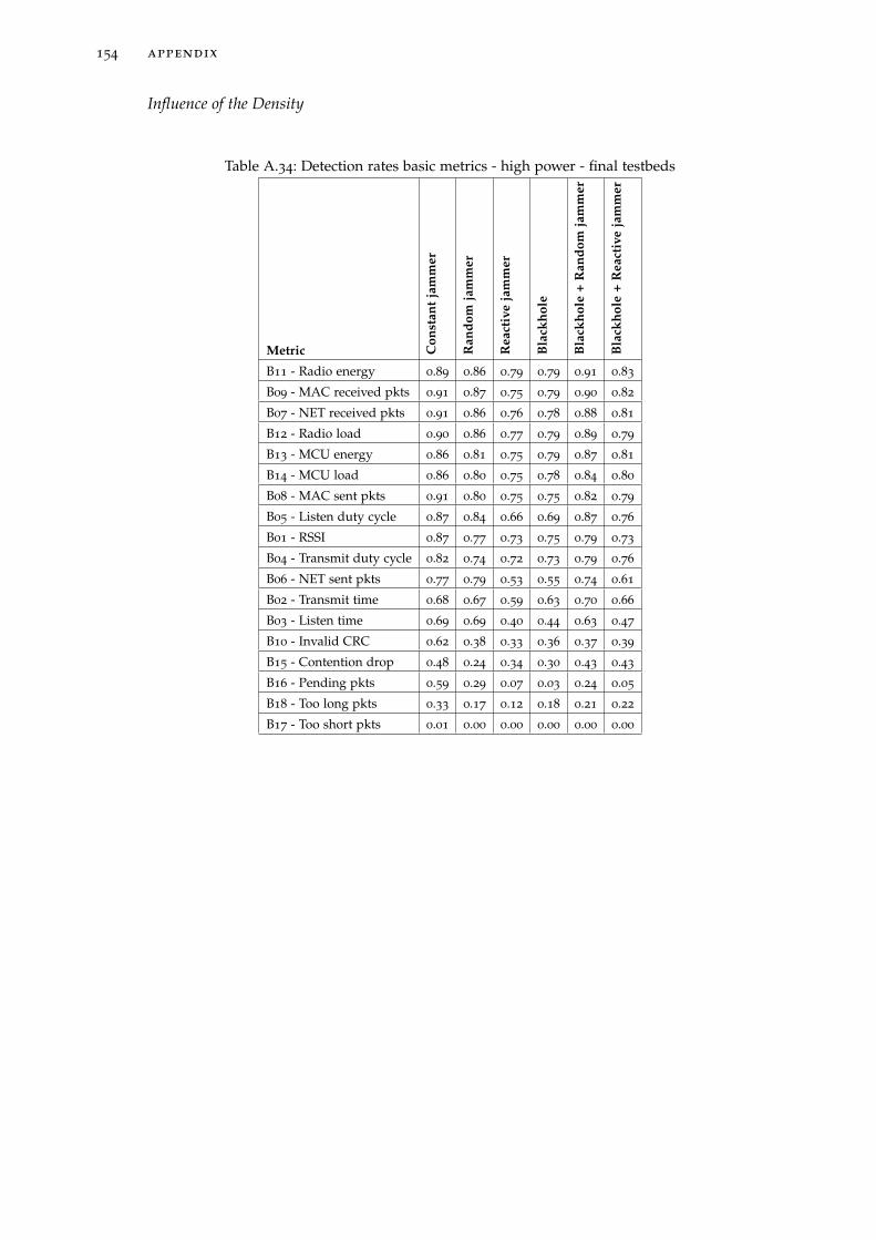
154 appendix
Influence of the Density
Table A.34: Detection rates basic metrics - high power - final testbeds
Metric Con
stan
tja
mm
er
Ran
dom
jam
mer
Rea
ctiv
eja
mm
er
Bla
ckho
le
Bla
ckho
le+
Ran
dom
jam
mer
Bla
ckho
le+
Rea
ctiv
eja
mm
er
B11 - Radio energy 0.89 0.86 0.79 0.79 0.91 0.83
B09 - MAC received pkts 0.91 0.87 0.75 0.79 0.90 0.82
B07 - NET received pkts 0.91 0.86 0.76 0.78 0.88 0.81
B12 - Radio load 0.90 0.86 0.77 0.79 0.89 0.79
B13 - MCU energy 0.86 0.81 0.75 0.79 0.87 0.81
B14 - MCU load 0.86 0.80 0.75 0.78 0.84 0.80
B08 - MAC sent pkts 0.91 0.80 0.75 0.75 0.82 0.79
B05 - Listen duty cycle 0.87 0.84 0.66 0.69 0.87 0.76
B01 - RSSI 0.87 0.77 0.73 0.75 0.79 0.73
B04 - Transmit duty cycle 0.82 0.74 0.72 0.73 0.79 0.76
B06 - NET sent pkts 0.77 0.79 0.53 0.55 0.74 0.61
B02 - Transmit time 0.68 0.67 0.59 0.63 0.70 0.66
B03 - Listen time 0.69 0.69 0.40 0.44 0.63 0.47
B10 - Invalid CRC 0.62 0.38 0.33 0.36 0.37 0.39
B15 - Contention drop 0.48 0.24 0.34 0.30 0.43 0.43
B16 - Pending pkts 0.59 0.29 0.07 0.03 0.24 0.05
B18 - Too long pkts 0.33 0.17 0.12 0.18 0.21 0.22
B17 - Too short pkts 0.01 0.00 0.00 0.00 0.00 0.00

appendix 155
Table A.35: Detection rates basic metrics - low power - final testbeds
Metric Con
stan
tja
mm
er
Ran
dom
jam
mer
Rea
ctiv
eja
mm
er
Bla
ckho
le
Bla
ckho
le+
Ran
dom
jam
mer
Bla
ckho
le+
Rea
ctiv
eja
mm
er
B09 - MAC received pkts 0.89 0.82 0.76 0.79 0.87 0.83
B11 - Radio energy 0.91 0.83 0.77 0.78 0.87 0.79
B12 - Radio load 0.89 0.82 0.76 0.77 0.88 0.79
B07 - NET received pkts 0.89 0.80 0.76 0.78 0.89 0.81
B08 - MAC sent pkts 0.91 0.81 0.74 0.73 0.83 0.77
B01 - RSSI 0.86 0.77 0.74 0.78 0.81 0.79
B05 - Listen duty cycle 0.88 0.83 0.71 0.73 0.86 0.73
B13 - MCU energy 0.86 0.76 0.76 0.76 0.79 0.77
B14 - MCU load 0.86 0.73 0.75 0.75 0.79 0.77
B04 - Transmit duty cycle 0.84 0.76 0.71 0.72 0.78 0.75
B02 - Transmit time 0.73 0.68 0.64 0.64 0.73 0.68
B06 - NET sent pkts 0.80 0.71 0.52 0.56 0.76 0.60
B03 - Listen time 0.72 0.67 0.45 0.49 0.61 0.51
B10 - Invalid CRC 0.54 0.33 0.33 0.36 0.37 0.31
B15 - Contention drop 0.47 0.24 0.37 0.25 0.43 0.45
B18 - Too long pkts 0.36 0.19 0.16 0.20 0.28 0.21
B16 - Pending pkts 0.63 0.29 0.10 0.05 0.26 0.06
B17 - Too short pkts 0.00 0.00 0.00 0.00 0.00 0.00
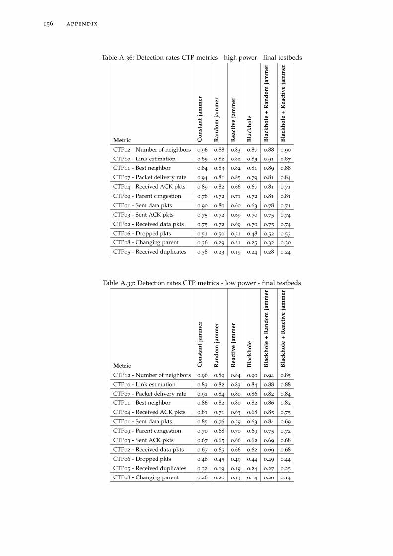
156 appendix
Table A.36: Detection rates CTP metrics - high power - final testbeds
Metric Con
stan
tja
mm
er
Ran
dom
jam
mer
Rea
ctiv
eja
mm
er
Bla
ckho
le
Bla
ckho
le+
Ran
dom
jam
mer
Bla
ckho
le+
Rea
ctiv
eja
mm
er
CTP12 - Number of neighbors 0.96 0.88 0.83 0.87 0.88 0.90
CTP10 - Link estimation 0.89 0.82 0.82 0.83 0.91 0.87
CTP11 - Best neighbor 0.84 0.83 0.82 0.81 0.89 0.88
CTP07 - Packet delivery rate 0.94 0.81 0.85 0.79 0.81 0.84
CTP04 - Received ACK pkts 0.89 0.82 0.66 0.67 0.81 0.71
CTP09 - Parent congestion 0.78 0.72 0.71 0.72 0.81 0.81
CTP01 - Sent data pkts 0.90 0.80 0.60 0.63 0.78 0.71
CTP03 - Sent ACK pkts 0.75 0.72 0.69 0.70 0.75 0.74
CTP02 - Received data pkts 0.75 0.72 0.69 0.70 0.75 0.74
CTP06 - Dropped pkts 0.51 0.50 0.51 0.48 0.52 0.53
CTP08 - Changing parent 0.36 0.29 0.21 0.25 0.32 0.30
CTP05 - Received duplicates 0.38 0.23 0.19 0.24 0.28 0.24
Table A.37: Detection rates CTP metrics - low power - final testbeds
Metric Con
stan
tja
mm
er
Ran
dom
jam
mer
Rea
ctiv
eja
mm
er
Bla
ckho
le
Bla
ckho
le+
Ran
dom
jam
mer
Bla
ckho
le+
Rea
ctiv
eja
mm
er
CTP12 - Number of neighbors 0.96 0.89 0.84 0.90 0.94 0.85
CTP10 - Link estimation 0.83 0.82 0.83 0.84 0.88 0.88
CTP07 - Packet delivery rate 0.91 0.84 0.80 0.86 0.82 0.84
CTP11 - Best neighbor 0.86 0.82 0.80 0.82 0.86 0.82
CTP04 - Received ACK pkts 0.81 0.71 0.63 0.68 0.85 0.75
CTP01 - Sent data pkts 0.85 0.76 0.59 0.63 0.84 0.69
CTP09 - Parent congestion 0.70 0.68 0.70 0.69 0.75 0.72
CTP03 - Sent ACK pkts 0.67 0.65 0.66 0.62 0.69 0.68
CTP02 - Received data pkts 0.67 0.65 0.66 0.62 0.69 0.68
CTP06 - Dropped pkts 0.46 0.45 0.49 0.44 0.49 0.44
CTP05 - Received duplicates 0.32 0.19 0.19 0.24 0.27 0.25
CTP08 - Changing parent 0.26 0.20 0.13 0.14 0.20 0.14

appendix 157
Table A.38: Detection rates mesh metrics - high power - final testbeds
Metric Con
stan
tja
mm
er
Ran
dom
jam
mer
Rea
ctiv
eja
mm
er
Bla
ckho
le
Bla
ckho
le+
Ran
dom
jam
mer
Bla
ckho
le+
Rea
ctiv
eja
mm
er
M02 - No. of routing entries 0.92 0.87 0.71 0.81 0.91 0.78
M01 - No. of direct neighbors 0.91 0.80 0.74 0.78 0.74 0.76
Table A.39: Detection rates mesh metrics - low power - final testbeds
Metric Con
stan
tja
mm
er
Ran
dom
jam
mer
Rea
ctiv
eja
mm
er
Bla
ckho
le
Bla
ckho
le+
Ran
dom
jam
mer
Bla
ckho
le+
Rea
ctiv
eja
mm
er
M02 - No. of routing entries 0.92 0.84 0.79 0.81 0.84 0.81
M01 - No. of direct neighbors 0.93 0.76 0.76 0.78 0.75 0.75

158 appendix
Influence of the Traffic Intensity
Table A.40: Detection rates basic metrics - high traffic - final testbeds
Metric Con
stan
tja
mm
er
Ran
dom
jam
mer
Rea
ctiv
eja
mm
er
Bla
ckho
le
Bla
ckho
le+
Ran
dom
jam
mer
Bla
ckho
le+
Rea
ctiv
eja
mm
er
B09 - MAC received pkts 0.89 0.83 0.78 0.82 0.90 0.85
B11 - Radio energy 0.88 0.84 0.79 0.80 0.90 0.81
B07 - NET received pkts 0.87 0.80 0.79 0.81 0.90 0.84
B12 - Radio load 0.89 0.84 0.79 0.80 0.89 0.79
B01 - RSSI 0.87 0.82 0.78 0.81 0.87 0.82
B13 - MCU energy 0.88 0.80 0.79 0.81 0.83 0.82
B14 - MCU load 0.89 0.78 0.79 0.80 0.83 0.81
B08 - MAC sent pkts 0.91 0.80 0.77 0.75 0.84 0.80
B05 - Listen duty cycle 0.88 0.82 0.73 0.70 0.85 0.72
B04 - Transmit duty cycle 0.81 0.76 0.76 0.74 0.80 0.79
B06 - NET sent pkts 0.80 0.76 0.57 0.59 0.75 0.64
B02 - Transmit time 0.67 0.66 0.63 0.62 0.73 0.68
B03 - Listen time 0.69 0.69 0.45 0.52 0.64 0.55
B10 - Invalid CRC 0.56 0.32 0.35 0.38 0.35 0.40
B15 - Contention drop 0.48 0.25 0.36 0.30 0.47 0.46
B16 - Pending pkts 0.61 0.28 0.10 0.06 0.27 0.07
B18 - Too long pkts 0.28 0.14 0.13 0.22 0.24 0.26
B17 - Too short pkts 0.00 0.00 0.00 0.00 0.00 0.00
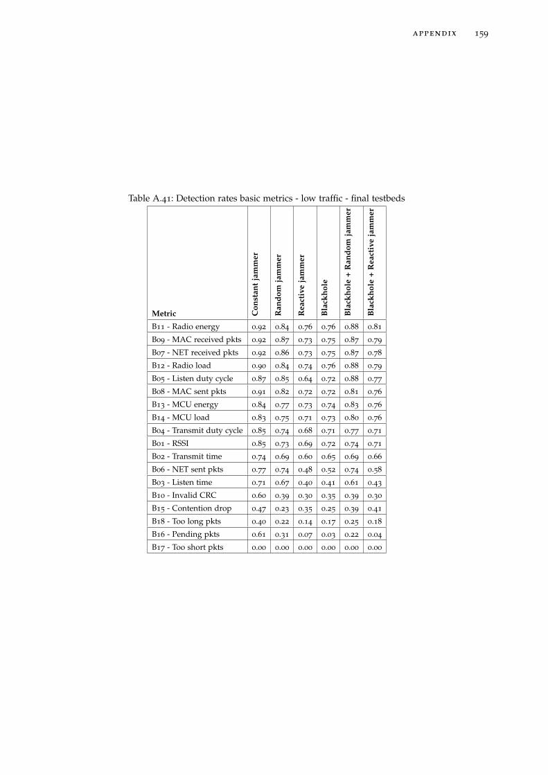
appendix 159
Table A.41: Detection rates basic metrics - low traffic - final testbeds
Metric Con
stan
tja
mm
er
Ran
dom
jam
mer
Rea
ctiv
eja
mm
er
Bla
ckho
le
Bla
ckho
le+
Ran
dom
jam
mer
Bla
ckho
le+
Rea
ctiv
eja
mm
er
B11 - Radio energy 0.92 0.84 0.76 0.76 0.88 0.81
B09 - MAC received pkts 0.92 0.87 0.73 0.75 0.87 0.79
B07 - NET received pkts 0.92 0.86 0.73 0.75 0.87 0.78
B12 - Radio load 0.90 0.84 0.74 0.76 0.88 0.79
B05 - Listen duty cycle 0.87 0.85 0.64 0.72 0.88 0.77
B08 - MAC sent pkts 0.91 0.82 0.72 0.72 0.81 0.76
B13 - MCU energy 0.84 0.77 0.73 0.74 0.83 0.76
B14 - MCU load 0.83 0.75 0.71 0.73 0.80 0.76
B04 - Transmit duty cycle 0.85 0.74 0.68 0.71 0.77 0.71
B01 - RSSI 0.85 0.73 0.69 0.72 0.74 0.71
B02 - Transmit time 0.74 0.69 0.60 0.65 0.69 0.66
B06 - NET sent pkts 0.77 0.74 0.48 0.52 0.74 0.58
B03 - Listen time 0.71 0.67 0.40 0.41 0.61 0.43
B10 - Invalid CRC 0.60 0.39 0.30 0.35 0.39 0.30
B15 - Contention drop 0.47 0.23 0.35 0.25 0.39 0.41
B18 - Too long pkts 0.40 0.22 0.14 0.17 0.25 0.18
B16 - Pending pkts 0.61 0.31 0.07 0.03 0.22 0.04
B17 - Too short pkts 0.00 0.00 0.00 0.00 0.00 0.00

160 appendix
Table A.42: Detection rates CTP metrics - high traffic - final testbeds
Metric Con
stan
tja
mm
er
Ran
dom
jam
mer
Rea
ctiv
eja
mm
er
Bla
ckho
le
Bla
ckho
le+
Ran
dom
jam
mer
Bla
ckho
le+
Rea
ctiv
eja
mm
er
CTP12 - Number of neighbors 0.95 0.88 0.82 0.86 0.89 0.88
CTP10 - Link estimation 0.84 0.81 0.83 0.84 0.86 0.86
CTP07 - Packet delivery rate 0.91 0.81 0.83 0.82 0.79 0.83
CTP11 - Best neighbor 0.82 0.79 0.80 0.81 0.85 0.83
CTP01 - Sent data pkts 0.88 0.79 0.67 0.70 0.88 0.78
CTP04 - Received ACK pkts 0.83 0.73 0.67 0.67 0.85 0.77
CTP09 - Parent congestion 0.73 0.68 0.71 0.71 0.74 0.79
CTP03 - Sent ACK pkts 0.56 0.63 0.65 0.61 0.63 0.62
CTP02 - Received data pkts 0.56 0.63 0.65 0.61 0.63 0.62
CTP06 - Dropped pkts 0.55 0.61 0.63 0.58 0.61 0.59
CTP05 - Received duplicates 0.10 0.06 0.05 0.07 0.09 0.10
CTP08 - Changing parent 0.01 0.02 0.02 0.03 0.02 0.02
Table A.43: Detection rates CTP metrics - low traffic - final testbeds
Metric Con
stan
tja
mm
er
Ran
dom
jam
mer
Rea
ctiv
eja
mm
er
Bla
ckho
le
Bla
ckho
le+
Ran
dom
jam
mer
Bla
ckho
le+
Rea
ctiv
eja
mm
er
CTP12 - Number of neighbors 0.96 0.89 0.85 0.91 0.94 0.87
CTP10 - Link estimation 0.88 0.83 0.81 0.83 0.93 0.88
CTP11 - Best neighbor 0.88 0.86 0.83 0.82 0.89 0.88
CTP07 - Packet delivery rate 0.94 0.83 0.83 0.83 0.84 0.85
CTP03 - Sent ACK pkts 0.85 0.74 0.69 0.72 0.81 0.80
CTP02 - Received data pkts 0.85 0.74 0.69 0.72 0.81 0.80
CTP04 - Received ACK pkts 0.87 0.80 0.62 0.68 0.81 0.69
CTP09 - Parent congestion 0.75 0.72 0.70 0.69 0.82 0.74
CTP01 - Sent data pkts 0.87 0.78 0.53 0.56 0.74 0.62
CTP08 - Changing parent 0.61 0.48 0.32 0.36 0.50 0.41
CTP05 - Received duplicates 0.60 0.36 0.34 0.41 0.46 0.39
CTP06 - Dropped pkts 0.42 0.34 0.37 0.35 0.40 0.38

appendix 161
Table A.44: Detection rates mesh metrics - high traffic - final testbeds
Metric Con
stan
tja
mm
er
Ran
dom
jam
mer
Rea
ctiv
eja
mm
er
Bla
ckho
le
Bla
ckho
le+
Ran
dom
jam
mer
Bla
ckho
le+
Rea
ctiv
eja
mm
er
M02 - No. of routing entries 0.95 0.90 0.79 0.86 0.93 0.82
M01 - No. of direct neighbors 0.92 0.79 0.77 0.78 0.75 0.79
Table A.45: Detection rates mesh metrics - low traffic - final testbeds
Metric Con
stan
tja
mm
er
Ran
dom
jam
mer
Rea
ctiv
eja
mm
er
Bla
ckho
le
Bla
ckho
le+
Ran
dom
jam
mer
Bla
ckho
le+
Rea
ctiv
eja
mm
er
M02 - No. of routing entries 0.89 0.80 0.72 0.77 0.82 0.77
M01 - No. of direct neighbors 0.92 0.78 0.73 0.78 0.74 0.72

162 appendix
Influence of the Attacker Location and Start
Table A.46: Detection rates basic metrics - inner attacker - final testbeds
Metric Con
stan
tja
mm
er
Ran
dom
jam
mer
Rea
ctiv
eja
mm
er
Bla
ckho
le
B11 - Radio energy 0.88 0.81 0.77 0.76
B09 - MAC received pkts 0.86 0.83 0.76 0.78
B12 - Radio load 0.87 0.81 0.76 0.75
B07 - NET received pkts 0.86 0.82 0.75 0.76
B13 - MCU energy 0.82 0.76 0.76 0.78
B01 - RSSI 0.83 0.78 0.74 0.76
B08 - MAC sent pkts 0.87 0.77 0.74 0.72
B14 - MCU load 0.82 0.74 0.75 0.75
B04 - Transmit duty cycle 0.80 0.73 0.72 0.71
B05 - Listen duty cycle 0.82 0.76 0.65 0.67
B02 - Transmit time 0.67 0.64 0.61 0.60
B06 - NET sent pkts 0.72 0.70 0.50 0.54
B03 - Listen time 0.62 0.63 0.42 0.46
B10 - Invalid CRC 0.53 0.36 0.33 0.33
B15 - Contention drop 0.46 0.24 0.29 0.24
B16 - Pending pkts 0.49 0.19 0.08 0.04
B18 - Too long pkts 0.31 0.17 0.14 0.16
B17 - Too short pkts 0.00 0.00 0.00 0.00
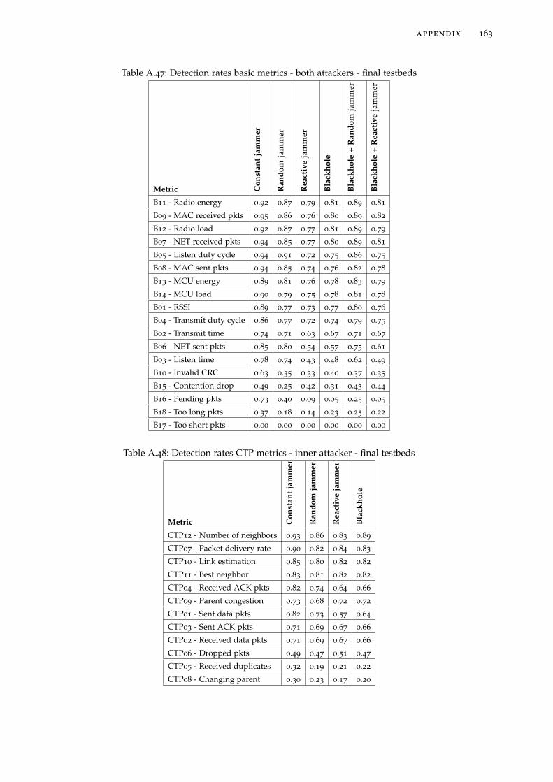
appendix 163
Table A.47: Detection rates basic metrics - both attackers - final testbeds
Metric Con
stan
tja
mm
er
Ran
dom
jam
mer
Rea
ctiv
eja
mm
er
Bla
ckho
le
Bla
ckho
le+
Ran
dom
jam
mer
Bla
ckho
le+
Rea
ctiv
eja
mm
er
B11 - Radio energy 0.92 0.87 0.79 0.81 0.89 0.81
B09 - MAC received pkts 0.95 0.86 0.76 0.80 0.89 0.82
B12 - Radio load 0.92 0.87 0.77 0.81 0.89 0.79
B07 - NET received pkts 0.94 0.85 0.77 0.80 0.89 0.81
B05 - Listen duty cycle 0.94 0.91 0.72 0.75 0.86 0.75
B08 - MAC sent pkts 0.94 0.85 0.74 0.76 0.82 0.78
B13 - MCU energy 0.89 0.81 0.76 0.78 0.83 0.79
B14 - MCU load 0.90 0.79 0.75 0.78 0.81 0.78
B01 - RSSI 0.89 0.77 0.73 0.77 0.80 0.76
B04 - Transmit duty cycle 0.86 0.77 0.72 0.74 0.79 0.75
B02 - Transmit time 0.74 0.71 0.63 0.67 0.71 0.67
B06 - NET sent pkts 0.85 0.80 0.54 0.57 0.75 0.61
B03 - Listen time 0.78 0.74 0.43 0.48 0.62 0.49
B10 - Invalid CRC 0.63 0.35 0.33 0.40 0.37 0.35
B15 - Contention drop 0.49 0.25 0.42 0.31 0.43 0.44
B16 - Pending pkts 0.73 0.40 0.09 0.05 0.25 0.05
B18 - Too long pkts 0.37 0.18 0.14 0.23 0.25 0.22
B17 - Too short pkts 0.00 0.00 0.00 0.00 0.00 0.00
Table A.48: Detection rates CTP metrics - inner attacker - final testbeds
Metric Con
stan
tja
mm
er
Ran
dom
jam
mer
Rea
ctiv
eja
mm
er
Bla
ckho
le
CTP12 - Number of neighbors 0.93 0.86 0.83 0.89
CTP07 - Packet delivery rate 0.90 0.82 0.84 0.83
CTP10 - Link estimation 0.85 0.80 0.82 0.82
CTP11 - Best neighbor 0.83 0.81 0.82 0.82
CTP04 - Received ACK pkts 0.82 0.74 0.64 0.66
CTP09 - Parent congestion 0.73 0.68 0.72 0.72
CTP01 - Sent data pkts 0.82 0.73 0.57 0.64
CTP03 - Sent ACK pkts 0.71 0.69 0.67 0.66
CTP02 - Received data pkts 0.71 0.69 0.67 0.66
CTP06 - Dropped pkts 0.49 0.47 0.51 0.47
CTP05 - Received duplicates 0.32 0.19 0.21 0.22
CTP08 - Changing parent 0.30 0.23 0.17 0.20

164 appendix
Table A.49: Detection rates CTP metrics - both attackers - final testbeds
Metric Con
stan
tja
mm
er
Ran
dom
jam
mer
Rea
ctiv
eja
mm
er
Bla
ckho
le
Bla
ckho
le+
Ran
dom
jam
mer
Bla
ckho
le+
Rea
ctiv
eja
mm
er
CTP12 - Number of neighbors 0.99 0.91 0.84 0.88 0.91 0.87
CTP10 - Link estimation 0.86 0.83 0.83 0.86 0.89 0.87
CTP07 - Packet delivery rate 0.95 0.83 0.82 0.82 0.81 0.84
CTP11 - Best neighbor 0.86 0.83 0.81 0.81 0.87 0.85
CTP04 - Received ACK pkts 0.88 0.79 0.65 0.69 0.83 0.73
CTP01 - Sent data pkts 0.93 0.83 0.62 0.61 0.81 0.70
CTP09 - Parent congestion 0.75 0.72 0.69 0.69 0.78 0.77
CTP03 - Sent ACK pkts 0.71 0.68 0.67 0.67 0.72 0.71
CTP02 - Received data pkts 0.71 0.68 0.67 0.67 0.72 0.71
CTP06 - Dropped pkts 0.48 0.49 0.49 0.46 0.51 0.49
CTP05 - Received duplicates 0.38 0.22 0.18 0.26 0.27 0.25
CTP08 - Changing parent 0.32 0.26 0.17 0.20 0.26 0.22
Table A.50: Detection rates mesh metrics - inner attacker - final testbeds
Metric Con
stan
tja
mm
er
Ran
dom
jam
mer
Rea
ctiv
eja
mm
er
Bla
ckho
le
M02 - No. of routing entries 0.87 0.85 0.76 0.81
M01 - No. of direct neighbors 0.90 0.76 0.75 0.77
Table A.51: Detection rates mesh metrics - both attackers - final testbeds
Metric Con
stan
tja
mm
er
Ran
dom
jam
mer
Rea
ctiv
eja
mm
er
Bla
ckho
le
Bla
ckho
le+
Ran
dom
jam
mer
Bla
ckho
le+
Rea
ctiv
eja
mm
er
M02 - No. of routing entries 0.97 0.86 0.75 0.81 0.87 0.79
M01 - No. of direct neighbors 0.93 0.80 0.75 0.79 0.74 0.76

appendix 165
Table A.52: Detection rates basic metrics - no delay attacker - final testbeds
Metric Con
stan
tja
mm
er
Ran
dom
jam
mer
Rea
ctiv
eja
mm
er
Bla
ckho
le
Bla
ckho
le+
Ran
dom
jam
mer
Bla
ckho
le+
Rea
ctiv
eja
mm
er
B11 - Radio energy 0.90 0.84 0.79 0.81 0.90 0.82
B09 - MAC received pkts 0.90 0.85 0.76 0.80 0.88 0.84
B12 - Radio load 0.89 0.85 0.79 0.79 0.90 0.80
B07 - NET received pkts 0.90 0.85 0.77 0.80 0.88 0.81
B13 - MCU energy 0.85 0.79 0.76 0.79 0.85 0.82
B08 - MAC sent pkts 0.91 0.81 0.75 0.75 0.84 0.79
B14 - MCU load 0.86 0.77 0.76 0.78 0.83 0.82
B05 - Listen duty cycle 0.89 0.84 0.71 0.72 0.88 0.76
B01 - RSSI 0.86 0.78 0.74 0.78 0.80 0.77
B04 - Transmit duty cycle 0.82 0.74 0.72 0.74 0.78 0.77
B02 - Transmit time 0.70 0.67 0.65 0.66 0.74 0.66
B06 - NET sent pkts 0.78 0.76 0.53 0.58 0.74 0.60
B03 - Listen time 0.71 0.68 0.46 0.50 0.63 0.49
B10 - Invalid CRC 0.59 0.38 0.34 0.40 0.37 0.39
B15 - Contention drop 0.49 0.23 0.40 0.29 0.44 0.43
B18 - Too long pkts 0.33 0.18 0.15 0.23 0.25 0.24
B16 - Pending pkts 0.62 0.29 0.10 0.04 0.24 0.04
B17 - Too short pkts 0.00 0.00 0.00 0.00 0.00 0.00
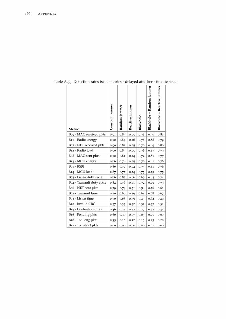
166 appendix
Table A.53: Detection rates basic metrics - delayed attacker - final testbeds
Metric Con
stan
tja
mm
er
Ran
dom
jam
mer
Rea
ctiv
eja
mm
er
Bla
ckho
le
Bla
ckho
le+
Ran
dom
jam
mer
Bla
ckho
le+
Rea
ctiv
eja
mm
er
B09 - MAC received pkts 0.91 0.85 0.75 0.78 0.90 0.81
B11 - Radio energy 0.90 0.84 0.76 0.76 0.88 0.79
B07 - NET received pkts 0.90 0.82 0.75 0.76 0.89 0.80
B12 - Radio load 0.90 0.83 0.75 0.76 0.87 0.79
B08 - MAC sent pkts 0.90 0.81 0.74 0.72 0.81 0.77
B13 - MCU energy 0.86 0.78 0.75 0.76 0.81 0.76
B01 - RSSI 0.86 0.77 0.74 0.75 0.81 0.76
B14 - MCU load 0.87 0.77 0.74 0.75 0.79 0.75
B05 - Listen duty cycle 0.86 0.83 0.66 0.69 0.85 0.74
B04 - Transmit duty cycle 0.84 0.76 0.71 0.72 0.79 0.73
B06 - NET sent pkts 0.79 0.74 0.51 0.54 0.76 0.61
B02 - Transmit time 0.70 0.68 0.59 0.61 0.68 0.67
B03 - Listen time 0.70 0.68 0.39 0.43 0.62 0.49
B10 - Invalid CRC 0.57 0.33 0.32 0.32 0.37 0.31
B15 - Contention drop 0.46 0.25 0.32 0.27 0.42 0.44
B16 - Pending pkts 0.60 0.30 0.07 0.05 0.25 0.07
B18 - Too long pkts 0.35 0.18 0.12 0.15 0.25 0.20
B17 - Too short pkts 0.00 0.00 0.00 0.00 0.01 0.00

appendix 167
Table A.54: Detection rates CTP metrics - no delay attacker - final testbeds
Metric Con
stan
tja
mm
er
Ran
dom
jam
mer
Rea
ctiv
eja
mm
er
Bla
ckho
le
Bla
ckho
le+
Ran
dom
jam
mer
Bla
ckho
le+
Rea
ctiv
eja
mm
er
CTP12 - Number of neighbors 0.97 0.89 0.83 0.87 0.91 0.90
CTP10 - Link estimation 0.87 0.82 0.86 0.86 0.91 0.90
CTP11 - Best neighbor 0.84 0.81 0.82 0.85 0.89 0.90
CTP07 - Packet delivery rate 0.91 0.84 0.84 0.81 0.83 0.83
CTP04 - Received ACK pkts 0.85 0.78 0.69 0.70 0.81 0.75
CTP01 - Sent data pkts 0.89 0.79 0.67 0.65 0.80 0.69
CTP09 - Parent congestion 0.74 0.70 0.75 0.71 0.77 0.78
CTP03 - Sent ACK pkts 0.71 0.69 0.67 0.67 0.73 0.70
CTP02 - Received data pkts 0.71 0.69 0.67 0.67 0.73 0.70
CTP06 - Dropped pkts 0.48 0.46 0.49 0.45 0.49 0.50
CTP05 - Received duplicates 0.36 0.21 0.19 0.29 0.28 0.26
CTP08 - Changing parent 0.31 0.25 0.16 0.23 0.27 0.25
Table A.55: Detection rates CTP metrics - delayed attacker - final testbeds
Metric Con
stan
tja
mm
er
Ran
dom
jam
mer
Rea
ctiv
eja
mm
er
Bla
ckho
le
Bla
ckho
le+
Ran
dom
jam
mer
Bla
ckho
le+
Rea
ctiv
eja
mm
er
CTP12 - Number of neighbors 0.95 0.88 0.84 0.90 0.92 0.85
CTP07 - Packet delivery rate 0.93 0.80 0.82 0.84 0.80 0.85
CTP10 - Link estimation 0.85 0.82 0.79 0.81 0.88 0.85
CTP11 - Best neighbor 0.85 0.84 0.80 0.78 0.85 0.81
CTP04 - Received ACK pkts 0.85 0.75 0.60 0.65 0.85 0.70
CTP09 - Parent congestion 0.74 0.70 0.66 0.70 0.79 0.75
CTP01 - Sent data pkts 0.87 0.78 0.53 0.61 0.82 0.71
CTP03 - Sent ACK pkts 0.71 0.68 0.67 0.65 0.71 0.71
CTP02 - Received data pkts 0.71 0.68 0.67 0.65 0.71 0.71
CTP06 - Dropped pkts 0.48 0.49 0.51 0.47 0.52 0.47
CTP05 - Received duplicates 0.34 0.21 0.19 0.20 0.27 0.23
CTP08 - Changing parent 0.31 0.24 0.18 0.16 0.25 0.18

168 appendix
Table A.56: Detection rates mesh metrics - no delay attacker - final testbeds
Metric Con
stan
tja
mm
er
Ran
dom
jam
mer
Rea
ctiv
eja
mm
er
Bla
ckho
le
Bla
ckho
le+
Ran
dom
jam
mer
Bla
ckho
le+
Rea
ctiv
eja
mm
er
M02 - No. of routing entries 0.90 0.87 0.77 0.82 0.87 0.85
M01 - No. of direct neighbors 0.92 0.78 0.71 0.81 0.76 0.79
Table A.57: Detection rates mesh metrics - delayed attacker - final testbeds
Metric Con
stan
tja
mm
er
Ran
dom
jam
mer
Rea
ctiv
eja
mm
er
Bla
ckho
le
Bla
ckho
le+
Ran
dom
jam
mer
Bla
ckho
le+
Rea
ctiv
eja
mm
er
M02 - No. of routing entries 0.93 0.84 0.74 0.80 0.88 0.74
M01 - No. of direct neighbors 0.92 0.78 0.79 0.76 0.73 0.72

appendix 169
a.1.3 Logistic Regression Results for the Final Testbeds, All Nodes
Table A.58: Most often used basic metrics in models created for all nodes in the final testbeds
Metric Occurences (%)
B06 - NET sent pkts 91.9
B07 - NET received pkts 90.8
B01 - RSSI 83.9
B14 - MCU load 82.7
B08 - MAC sent pkts 82.4
B04 - Transmit duty cycle 81.6
B11 - Radio energy 80.4
B09 - MAC received pkts 78.1
B13 - MCU energy 77.0
B10 - Invalid CRC 75.8
B18 - Too long pkts 74.7
B05 - Listen duty cycle 74.3
B15 - Contention drop 73.5
B12 - Radio load 67.8
B16 - Pending pkts 67.4
B03 - Listen time 62.0
B02 - Transmit time 61.7
B17 - Too short pkts 31.0
0 5 10 15 200
20
40
60
metrics per model
coun
t
Figure A.1: Count of metrics used in each model created for all nodes using basic metrics inthe final testbeds

170 appendix
Table A.59: Model quality - all nodes - basic metrics - final testbeds
Mesh CTP
Count Percent Count Percent
JammingCnst Bad model 6 0.188 8 0.250
Acceptable model 2 0.063 5 0.156
Perfect model 24 0.750 19 0.594
Sum usable models 26 0.813 24 0.750
JammingRnd Bad model 12 0.375 17 0.531
Acceptable model 15 0.469 10 0.313
Perfect model 5 0.156 5 0.156
Sum usable models 20 0.625 15 0.469
JammingReact Bad model 25 0.781 32 1.000
Acceptable model 3 0.094 0 0.000
Perfect model 4 0.125 0 0.000
Sum usable models 7 0.219 0 0.000
SingleBlackhole Bad model 28 0.875 31 0.969
Acceptable model 0 0.000 1 0.031
Perfect model 4 0.125 0 0.000
Sum usable models 4 0.125 1 0.031
BlackholeReactJamming Bad model 14 0.875 14 0.875
Acceptable model 0 0.000 2 0.125
Perfect model 2 0.125 0 0.000
Sum usable models 2 0.125 2 0.125
BlackholeRndJamming Bad model 6 0.375 11 0.688
Acceptable model 0 0.000 5 0.313
Perfect model 10 0.625 0 0.000
Sum usable models 10 0.625 5 0.313

appendix 171
Table A.60: Most often used CTP metrics in models created for all nodes in the final testbeds
Metric Occurences (%)
B07 - NET received pkts 91.4
B06 - NET sent pkts 91.4
B08 - MAC sent pkts 82.9
B01 - RSSI 81.7
B13 - MCU energy 78.0
B11 - Radio energy 77.8
B14 - MCU load 75.6
B04 - Transmit duty cycle 75.4
B09 - MAC received pkts 74.3
B05 - Listen duty cycle 73.1
B10 - Invalid CRC 70.7
B18 - Too long pkts 69.5
B15 - Contention drop 67.0
B12 - Radio load 67.0
B03 - Listen time 63.4
B16 - Pending pkts 60.9
B02 - Transmit time 59.7
CTP12 - Number of neighbors 46.3
CTP11 - Best neighbor 46.3
CTP07 - Packet delivery rate 45.1
CTP09 - Parent congestion 43.9
CTP10 - Link estimation 43.7
CTP04 - Received ACK pkts 41.4
CTP02 - Received data pkts 41.2
CTP01 - Sent data pkts 39.0
CTP06 - Dropped pkts 38.8
CTP05 - Received duplicates 31.7
B17 - Too short pkts 28.0
CTP08 - Changing parent 26.8
CTP03 - Sent ACK pkts 1.2
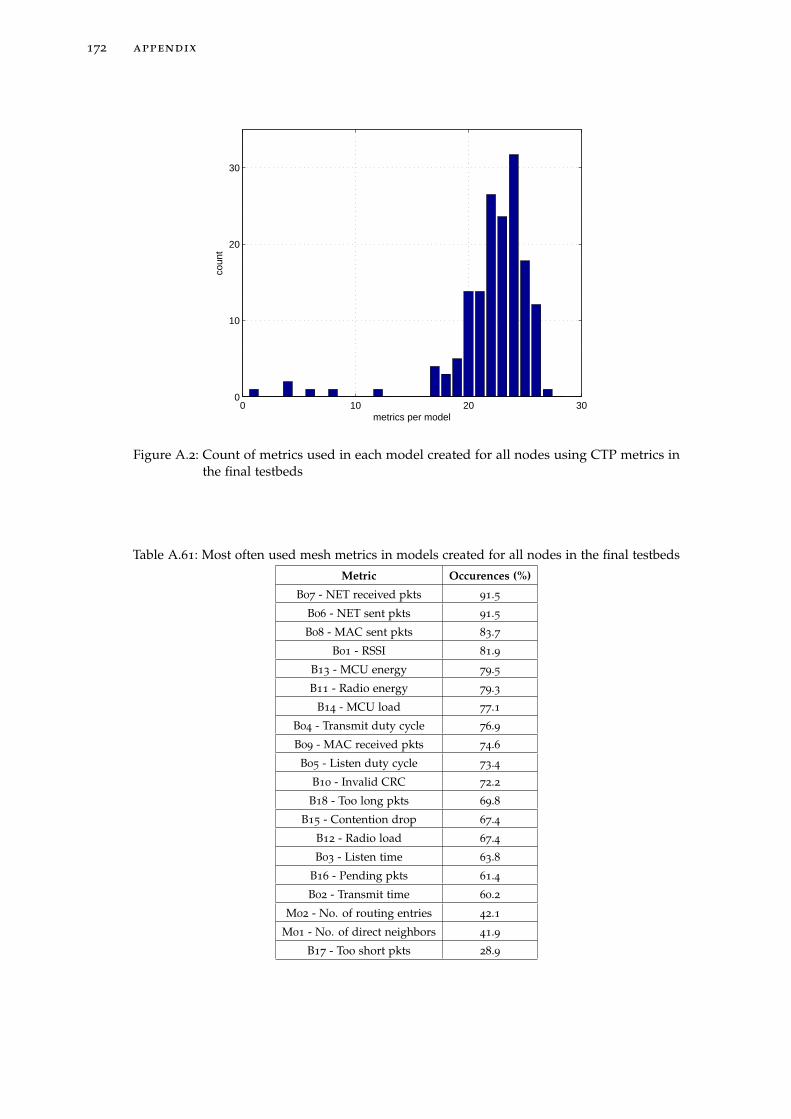
172 appendix
0 10 20 300
10
20
30
metrics per model
coun
t
Figure A.2: Count of metrics used in each model created for all nodes using CTP metrics inthe final testbeds
Table A.61: Most often used mesh metrics in models created for all nodes in the final testbeds
Metric Occurences (%)
B07 - NET received pkts 91.5
B06 - NET sent pkts 91.5
B08 - MAC sent pkts 83.7
B01 - RSSI 81.9
B13 - MCU energy 79.5
B11 - Radio energy 79.3
B14 - MCU load 77.1
B04 - Transmit duty cycle 76.9
B09 - MAC received pkts 74.6
B05 - Listen duty cycle 73.4
B10 - Invalid CRC 72.2
B18 - Too long pkts 69.8
B15 - Contention drop 67.4
B12 - Radio load 67.4
B03 - Listen time 63.8
B16 - Pending pkts 61.4
B02 - Transmit time 60.2
M02 - No. of routing entries 42.1
M01 - No. of direct neighbors 41.9
B17 - Too short pkts 28.9

appendix 173
0 5 10 15 20 250
10
20
30
metrics per model
coun
t
Figure A.3: Count of metrics used in each model created for all nodes using mesh metrics inthe final testbeds

174 appendix
a.1.4 Logistic Regression Results for the Final Testbeds, Neighboring Nodes
Table A.62: Most often used basic metrics in all neighboring nodes models in the final testbeds
Metric Occurences (%)
B06 - NET sent pkts 96.5
B07 - NET received pkts 96.0
B01 - RSSI 85.0
B08 - MAC sent pkts 83.9
B04 - Transmit duty cycle 79.3
B11 - Radio energy 78.1
B09 - MAC received pkts 77.0
B13 - MCU energy 75.8
B10 - Invalid CRC 71.2
B05 - Listen duty cycle 71.0
B15 - Contention drop 64.3
B18 - Too long pkts 64.0
B03 - Listen time 60.9
B14 - MCU load 56.8
B12 - Radio load 55.1
B02 - Transmit time 55.1
B16 - Pending pkts 51.7
B17 - Too short pkts 28.7
0 5 10 15 200
20
40
60
metrics per model
coun
t
Figure A.4: Count of metrics used in each model created for all neighboring nodes using basicmetrics in the final testbeds

appendix 175
Table A.63: Most often used CTP metrics in all neighboring nodes models in the final testbeds
Metric Occurences (%)
B06 - NET sent pkts 89.5
B07 - NET received pkts 88.3
B08 - MAC sent pkts 78.5
B01 - RSSI 78.5
B04 - Transmit duty cycle 73.6
B11 - Radio energy 72.3
B09 - MAC received pkts 68.7
B13 - MCU energy 67.4
B05 - Listen duty cycle 66.2
B14 - MCU load 61.3
B10 - Invalid CRC 61.0
B18 - Too long pkts 58.8
B02 - Transmit time 55.2
B15 - Contention drop 53.9
B12 - Radio load 53.7
B03 - Listen time 53.5
CTP12 - Number of neighbors 44.1
B16 - Pending pkts 43.9
CTP11 - Best neighbor 42.9
CTP10 - Link estimation 42.9
CTP07 - Packet delivery rate 40.4
CTP09 - Parent congestion 38.0
CTP04 - Received ACK pkts 35.5
CTP02 - Received data pkts 33.1
CTP01 - Sent data pkts 29.4
CTP06 - Dropped pkts 29.1
B17 - Too short pkts 24.5
CTP05 - Received duplicates 23.3
CTP08 - Changing parent 18.4
CTP03 - Sent ACK pkts 0.1

176 appendix
0 10 20 300
5
10
15
20
25
metrics per model
coun
t
Figure A.5: Count of metrics used in each model created for all neighboring nodes using CTPmetrics in the final testbeds
Table A.64: Most often used mesh metrics in all neighboring nodes models in the final testbeds
Metric Occurences (%)
B06 - NET sent pkts 90.3
B07 - NET received pkts 87.9
B08 - MAC sent pkts 78.3
B01 - RSSI 78.3
B04 - Transmit duty cycle 73.4
B11 - Radio energy 73.0
B09 - MAC received pkts 68.6
B13 - MCU energy 67.4
B05 - Listen duty cycle 66.2
B14 - MCU load 61.4
B10 - Invalid CRC 61.2
B18 - Too long pkts 59.0
B02 - Transmit time 55.4
B15 - Contention drop 54.4
B12 - Radio load 54.2
B03 - Listen time 53.0
M02 - No. of routing entries 45.7
B16 - Pending pkts 43.3
M01 - No. of direct neighbors 43.1
B17 - Too short pkts 24.0
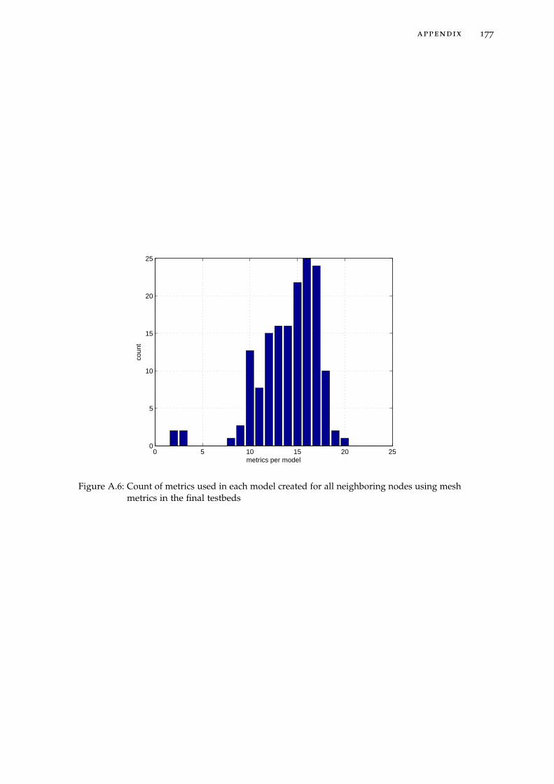
appendix 177
0 5 10 15 20 250
5
10
15
20
25
metrics per model
coun
t
Figure A.6: Count of metrics used in each model created for all neighboring nodes using meshmetrics in the final testbeds


appendix 179
a.2 supplementary results for chapter 5
5 10 15 20 25 30 350
50
100
150
200
250
300
350
400
node id
aver
age
hit t
ime
(min
)
0 100 200 300 4000
0.2
0.4
0.6
0.8
1
hit time (min)
F(x
)
Figure A.7: Average hitting times and CDFs for the random sending (2 tokens)
5 10 15 20 25 30 350
50
100
150
200
250
300
350
400
node id
aver
age
hit t
ime
(min
)
0 100 200 300 4000
0.2
0.4
0.6
0.8
1
hit time (min)
F(x
)
Figure A.8: Average hitting times and CDFs for the uniform sending (2 tokens)


BC U R R I C U L U M V I TÆ
personal details
Name Michael Riecker
Date of Birth 26 March 1982
Place of Birth Heilbronn, Germany
Nationality German
education
since 07/2010 Technische Universität Darmstadt, Darmstadt, GermanyDoctoral candidate at the Department of Computer Science
03/2007 – 08/2007 Eidgenössische Technische Hochschule Zürich, SwitzerlandGuest student with a focus on IT Security
10/2002 – 03/2009 University of Mannheim, GermanyStudies of Business InformaticsDegree: Diplom-Wirtschaftsinformatiker (Dipl.-Wirt.-Inf.), M.Sc. equivalent
08/1992 – 06/2001 Elly-Heuss-Knapp-Gymnasium Heilbronn, GermanyDegree: Allgemeine Hochschulreife (Abitur)
work experience
since 07/2010 Technische Universität Darmstadt, Darmstadt, GermanyResearch associate at the Secure Mobile Networking Lab andat the Center for Advanced Security Research Darmstadt
04/2009 – 06/2010 Protiviti GmbH, Frankfurt, GermanyIT Consultant
10/2007 – 07/2008 SAP Deutschland AG & Co. KG, Walldorf, GermanyWorking student in the area consulting public sector
09/2006 – 02/2007 PricewaterhouseCoopers AG WPG, Stuttgart, GermanyInternship in the area process assurance
03/2004 – 09/2005 University of Mannheim, GermanyStudent assistant for computer and network administration
12/2001 – 09/2002 Klinikum Heilbronn, GermanyCommunity service at the hospital of Heilbronn
teaching activities
since 07/2010 Technische Universität Darmstadt, Darmstadt, GermanyTeaching assistant for the lecture “Network Security”
181

182 curriculum vitæ
since 07/2010 Technische Universität Darmstadt, Darmstadt, GermanyCoordinator of the seminar “Selected Topics in Network Se-curity”
since 07/2010 Technische Universität Darmstadt, Darmstadt, GermanyTutor for various Bachelor and Master theses as well as semi-nars and lab exercises
Darmstadt, 11 May 2015

CA U T H O R ’ S P U B L I C AT I O N S
main publications
1. Michael Riecker, Dingwen Yuan, Rachid El Bansarkhani, Matthias Hollick. Pa-trolling Wireless Sensor Networks: Randomized Intrusion Detection. In Proceed-ings of the 10th ACM International Symposium on QoS and Security for Wireless andMobile Networks (Q2SWinet), 2014.
2. Michael Riecker, Daniel Thies, Matthias Hollick. Measuring the Impact of Denial-of-Service Attacks on Wireless Sensor Networks. In Proceedings of the 39th IEEEConference on Local Computer Networks (LCN), 2014.
3. Michael Riecker, Sebastian Biedermann, Rachid El Bansarkhani, Matthias Hollick.Lightweight Energy Consumption Based Intrusion Detection System for WirelessSensor Networks (Extended version of ACM SAC 2013 paper). In InternationalJournal of Information Security, Volume 14, Issue 2, pages 155–167, 2015.
4. Michael Riecker, Matthias Hollick. Weniger ist Mehr: Leichtgewichtige Metrikenzur Erkennung von Denial-of-Service Angriffen in Drahtlosen Sensornetzen. InProceedings of the 12th GI/ITG KuVS Fachgespräch Drahtlose Sensornetze (FGSN),2013.
5. Michael Riecker, Sebastian Biedermann, Matthias Hollick. Lightweight EnergyConsumption Based Intrusion Detection System for Wireless Sensor Networks.In Proceedings of the 28th ACM Symposium On Applied Computing (SAC), 2013.
6. Michael Riecker, Ana Barroso, Matthias Hollick, Sebastian Biedermann. OnData-centric Intrusion Detection in Wireless Sensor Networks. In Proceedings ofthe IEEE International Conference on Cyber, Physical and Social Computing (CPSCom),2012.
7. Michael Riecker, Rainer Thome, Dingwen Yuan, Matthias Hollick. A SecureMonitoring and Control System for Wireless Sensor Networks. In Proceedings ofthe 37th IEEE Conference on Local Computer Networks (LCN), 2012.
8. Michael Riecker, Ana Barroso, Matthias Hollick. It’s the Data that Matters! Onthe Detection of False Data in Wireless Sensor Networks. In Proceedings of the 6thEssener Workshop “Neue Herausforderungen in der Netzsicherheit”, 2012.
9. Michael Riecker, Walther Müller, Matthias Hollick, Karsten Saller. A SecureMonitoring and Control System for Wireless Sensor Networks. In Proceedings ofthe 10th GI/ITG KuVS Fachgespräch Drahtlose Sensornetze (FGSN), 2011.
183

184 publications
co-authored publications
1. Dingwen Yuan, Michael Riecker, Matthias Hollick. Making ’Glossy’ NetworksSparkle: Exploiting Concurrent Transmissions for Energy Efficient, Reliable,Ultra-low Latency Communication in Wireless Control Networks. In Proceedingsof the 11th European Conference on Wireless Sensor Networks (EWSN), 2014.
2. Dingwen Yuan, Michael Riecker, Matthias Hollick. HOPSCOTCH: An Adaptiveand Distributed Channel Hopping Technique for Interference Avoidance inWireless Sensor Networks. In Proceedings of the 37th IEEE Conference on LocalComputer Networks (LCN), 2012.

DE R K L Ä R U N G L A U T § 9 D E R P R O M O T I O N S O R D N U N G
Ich versichere hiermit, dass ich die vorliegende Dissertation selbständig und nur unterVerwendung der angegebenen Quellen und Hilfsmitteln verfasst habe. Alle Stellen,die aus Quellen entnommen wurden, sind als solche kenntlich gemacht. Die Arbeithat in gleicher oder ähnlicher Form noch nicht zu Prüfungszwecken gedient.
Darmstadt, 11. Mai 2015
Dipl.-Wirt.-Inf. MichaelRiecker

186