EFFECT OF DIFFERENT PATTERNS OF INJECTION WELL SYSTEMS ON SALTWATER INTRUSION IN COASTAL AQUIFERS

Tenth International Water Technology Conference, IWTC10 2006, Alexandria, Egypt

1019

EFFECT OF DIFFERENT PATTERNS OF INJECTION WELL

SYSTEMS ON SALTWATER INTRUSION IN COASTAL AQUIFERS

Hamdy A. EL-Ghandour*, Mahmoud A. EL-Gamal**, Tarek A. Saafan**, and

Hossam A. Abdel-Gawad***

* Assistant Lecturer, ** Professor, *** Associate Professor Irrigation and Hydraulics Dept., Faculty of Engineering, Mansoura University

El-Mansoura, Egypt ABSTRACT This research investigates and compares three various patterns of external injection well systems on the final position of the interface toe. These patterns are: 1) One row of injection wells, 2) Double rows of injection wells with different locations, and 3) Staggered rows of injection wells. This paper also studied the effect of different rates of injection and variable distances from the coast on seawater interface movement. The results were compared with the results for other researchers. Finally this research studied the effect of the rainfall percolation on the behavior of the interface toe. This research deals with hypothetical coastal confined and unconfined aquifers under steady state conditions. The finite element method was applied for the groundwater flow equation under assumption of steady sharp interface in homogenous aquifer. A computer program named NUMERICAL with FORTRAN (77) language was used after several modifications to solve the mathematical concepts of the problem. Analytical method was used to verify the computer program. The Image theory and the superposition principle were the main tools used through the analytical procedures. Keywords: Coastal Unconfined and Confined Aquifer - Well System - Analytical Solution - Numerical Solution - Image Theory - Superposition Principle. INTRODUCTION Coastal aquifers constitute an important source of freshwater, especially in arid and semi-arid zones, which border the sea. Many coastal areas are heavily urbanized, a fact which makes the need for freshwater even more acute. So that increased extraction of freshwater from these aquifers; to meet growing demands; decreases the percentage of freshwater spilled out to the seaside. Consequently the saltwater encroachment reach several kilometers inland, wells may become contaminated with seawater causing the problem of saltwater intrusion. Proper management schemes are necessary using injection well systems to tackle the problem of saltwater intrusion.

Tenth International Water Technology Conference, IWTC10 2006, Alexandria, Egypt 1020

Saafan [15] presented a mathematical solution for the problem of seawater intrusion into fresh water through homogenous isotropic unconfined coastal aquifers taking into consideration the distribution of pumping intensities of fresh and salt water. He derived a new formula to calculate the movement of the interface between fresh and saltwater based on aquifer thickness, effective porosity, relative specific weight and hydraulic conductivity. He found that the numerical results were in very good agreement with the experimental data for other researchers. Kashef [8] derived a theoretical formula based on theory of image, which represented the resultant total head at confined coastal aquifer. He studied the effect of recharge well batteries of different patterns on the degree of saltwater retardation in coastal confined aquifers. The batteries were located at various distances parallel to the shoreline; each battery consists of equally spaced recharge wells of a certain number and all wells start operation at the same time. It was found that, the optimum location of the batteries should lie between 0.7L and L, where L is initial length of the intruded saltwater wedge. Mahesha [9] studied also the transient effect of battery of injection wells on seawater intrusion into coastal confined aquifers. He used a quasi three-dimensional areal finite element model depending on sharp interface. He studied various conditions by changing the well spacing and intensity and duration of fresh water injection. He concluded that, spacing between wells, injection rate and duration control the repulsion of the saline wedge. Mahesha [10] presented a steady state solution for the motion of the fresh water/seawater interface due to a series of injection wells in confined aquifer using a sharp interface finite element model. The model was used to perform the parametric studies on the effect of location of the series of injection wells, spacing of well and fresh water injection rate on the sea water intrusion. It was found that the reduction of seawater intrusion (up to 60- 90 %) could be achieved through proper selection of injection rate and spacing between the wells. Also, he studied the effect of double series of injection wells and compared with the single series. He found that a double series is slight better than single series. Also, he found that the staggered system of wells in the series is slightly better than the straight well system for long spacing. Mahesha and Nagraja [11] used a one-dimensional sharp interface finite element model for parametric studies on the transient behavior of seawater intrusion due to the linear variation of the surface source level. They concluded that through a phreatic aquifer there is a general relationship between interface motion and linear variation of the surface source level that influences the motion of the interface. Mahesha [12] studied the transient motion of freshwater/seawater interface in coastal aquifers due to a constant lowering of fresh water levels at inland location by using a one-dimensional sharp interface finite element model. It was found that in a phreatic aquifer the advancement of the interface dependent on the rate, location, and period of fresh water level variations. Mahesha [13] studied the control of seawater intrusion by a series of seawater extraction wells alone and combination with the freshwater injection wells in confined aquifer using a vertically integrated two-dimensional sharp interface model in steady state. It was found that the combination of an injection


1021

barrier with an extraction barrier produced excellent results to the individual cases for larger well spacing and small rates of injection. El-Ganainy et al. [3] investigated the effect of pumped well on saltwater intrusion in coastal aquifer by using a quasi-3D steady state areal finite element model. Their studies based on sharp interface assumption in confined and unconfined aquifers. They also studied three applications, an infinite row of wells, double infinite rows of staggered wells, and effect of rainfall percolation. El-Ganainy et al. [4] presented an automatic calibration for saltwater intrusion by using indirect approach. Subroutines NAG are coupled with SWICHA for investigating flow and salt transport parameters. The SWICHA model developed by Lester (1991) is a three-dimensional finite element model and subroutines NAG are optimization subroutines depend on the least square technique which based on Gauss- Newton method. They concluded that, the three dimensional model was moresensitive to flow parameter (hydraulic conductivity) rather than salt transport parameter (Dispersion coefficient). El-Ganainy et al. [5] analyzed and compared simulation results of two-dimensional and three-dimensional finite element models by performing a sensitivity analysis in confined aquifer. The main objective of this research is to compare among 1) One row of injection wells, 2) Double rows of injection wells with different locations, and 3) Staggered rows of injection wells. Also the effect of rain percolation on the behavior of the freshwater/saltwater interface is studied. THE GOVERNING EQUATIONS For the unconfined and confined aquifers shown in figure (1), the following assumptions were taken into consideration: 1) The sharp interface model is used, 2) The Dupuit’s assumption is employed to vertically integrate the flow equation, reducing it from three-dimensional geometry to two-dimensional geometry, 3) Steady state condition is adopted, 4) The Ghyben-Herzberg assumption of stagnant salt water is utilized to interpret the interface location, 5) The wells fully penetrate the aquifer thickness, 6) The impervious bed of the aquifer was considered horizontal, and 7) Wells must be located only within the fresh water zone. The sharp interface concept was adopted within the present research. Hence, the governing equations represent the unsteady interaction between fresh water and salt water can be written as follows [1]: For freshwater:

( ) ( )t

hN

t

hS

NQ

x

hBk

xsf

fwfi

ffij

i ∂∂+−

∂∂

++=+∂∂

∂∂ α

ααθ

αβ 11)*( (1-a)


For saltwater:

( )t

hN

t

hS

N

x

hBk

xfs

si

ssij

i ∂∂

−∂

∂

++=∂∂

∂∂

αα

α1)*( (1-b)

where: xi: Coordinate axes in x and y directions; Kij: Permeability tensor component (L/T); B: Saturated thickness (L); hs, hf: Vertically averaged piezometric head for salt and fresh water regions respectively (L); N: Porosity; Ss, Sf: Storage coefficient for salt and fresh water regions respectively (Ss=Sf); α: Excess density ratio equal to (γs-γf)/ γf , (γf: specific weight (F/L3)); θ: Coefficient (=0 for confined aquifer and =1 for unconfined aquifer); t: Time (T); f, s: Subscripts refer to freshwater and saltwater respectively; and Qwf: Rate of injection freshwater (if β = +1)or rate of pumping freshwater (if β = -1) (L3/T). Based on the previous assumptions, equations (1-a) and (1-b) can be reformed as follows: For freshwater zone:

0.0)*( =+∂∂

∂∂

wfi

ffij

i

Qx

hBk

xβ (2-a)

For saltwater zone:

0.0)*( =∂∂

∂∂

i

ssij

i x

hBk

x (2-b)

It is expected to build a mathematical model for solving the two equations (2-a) and (2-b) simultaneously as done by Elganainy et al. [3]. Unknown piezometric heads corresponding to saltwater can be determined directly from the stagnant condition of the salt water. Due to the static condition of the salt water, an expected zero velocities must be calculated at any point within the salt-water zone, consequently:

0.0* =∂∂=

i

ssijsi x

hBKQ (3)

where Qsi are the quantities of water that flow in x and y direction (L3/T). From equation (3):

0.0=∂∂

i

s

x

h (4)


1023

0.0=∂∂

x

hs and 0.0=∂∂

y

hs (5)

hs = constant (6)

(Equal to the distance from the pre specified datum to the Mean sea level). Equation (2-a) can be rewritten as follows:

PRy

hKB

yx

hKB

xf

ff

f −=∂

∂∂∂−

∂∂

∂∂− )()( (7)

Minus sign in the above equation indicates that, the flow occurs in direction of decreasing head, P represents the rate of uniform evaporation (L/T) or point pumping (L3/T), and R represents the intensity of uniform rainfall percolation (L/T) or point recharge of fresh water (L3/T). In the case of adopting well system, the variables P and R must be multiplied by Dirac function to apply a concentrated load (pumping or recharging) at a pre specified point within the studied domain. The Dirac function concentrates the pumping or recharging rates at the Cartesian coordinates of the well. Equation (7) is a nonlinear elliptic partial differential equation. Strack [16] described how the nonlinear equation (7) could be reformulated to linear form without any relaxation by replacing the dependent variable h with the potential φ. Hence equation (7) can be rewritten in the following form:

PRy

Kyx

Kx

−=∂∂

∂∂−

∂∂

∂∂− )()(

φφ (8)

From figure (1-a) for unconfined aquifer, the potential φ as proved by Strack [16] and Cheng et al. [2] can be written as follows:

2/)( 22 sdh −=φ For zone (I) (9)

εφ 2/)( 2dh −= For zone (II) (10) and for confined aquifer, figure (1-b), can be written as follows:

22

2

)1(SBd

BsBh −−+=φ For zone (I) (11)

[ ]2)1()1(2

1sdBsh

s−−+

−=φ For zone (II) (12)

where: s= ρs / ρf ; ε= (s-1)/s= (ρs-ρf )/ ρf ; ρs is the density of saltwater (M/L3); ρf is density of freshwater (M/L3); h is the piezomtric head (L); d is the depth of the mean


sea level from the impervious bed (L), and B is the thickness of the confined aquifer (L). It must be noticed that, the linearized form of Strack equation based on a compulsory assumption of existence horizontal impervious bed for the aquifer under consideration. Two zones of fresh water and salt water are separated at toeφ as stated by Cheng et al. [2] as follows:

2

2

)1(d

sstoe

−=φ for unconfined aquifer (13)

2

2

)1(B

stoe

−=φ for confined aquifer (14)

Equation (8) is a time independent partial differential equation, and that equation in combination with suitable boundary conditions, can be simulated to boundary value problems. Boundary value problem means that the dependent variable (the potential φ) or its derivatives, is known along boundaries of the domain under study. The following boundary conditions are used in the present research as follows:

0.0=∂∂n

φ (on sides IJ, LK) for confined and unconfined aquifers (15)

(Neumann B.C)

k

q

nu=

∂∂φ

(on sides IL) for confined and unconfined aquifers (16)

(Neumann B.C) εφ 2/2BC= (on sides JK) for unconfined aquifer (17)

(Dirichlet B.C)

2

)1(2 −= sCDφ (on sides JK) for confined aquifer (18)

(Dirichlet B.C) in which, qu represents uniform rate of discharge per unit width of the aquifer (L2/T), BC is the seepage face of fresh water above (M.S.L) for unconfined aquifer calculated from BC=qnet/K [7], qnet is the net uniform discharge flow to the sea and equal to [qu*YD-Σ Qw pumping +Σ Qw injection]/YD and CD is the seepage face of fresh water below (M.S.L) for confined aquifer calculated from CD=(0.741*q)/(K*ε) [14]. The seepage faces around different wells are ignored within the present study. FINITE ELEMENT SOLUTION Starting about the mid 1960’S very powerful numerical technique named the finite element method has been applied to numerous problems of flow through porous media


1025

[1]. This method can handle any domain with complex boundaries. Also, heterogeneity and anisotropic characteristics can easily be included. The idea of the finite element method is to discretize the domain under consideration to number of rectangular elements. Rectangular elements “bounded with four nodes” were chosen in the present work. A trial function must be assumed to simulate the dependent variable within different elements. This trial function is usually assumed as a polynomial with a degree specified from number of nodes per element. A weak form for the governing equation should be constructed. Galerkin form is selected, by minimizing the residuals of the selected weak solution at different nodes; the unknown dependent variables can be estimated. As the result of using Finite Element Method, the summation for all element procedures has the following matrix form:

ANxN φ Nx1 = BNx1 (19) Where: A is a square matrix for the coefficient known as stiffness matrix; φ is the unknown vector of potential; and B is a vector which contains the external source or sink of water and flux concentration known as load vector. In the Finite Element program the system of linear equations were solved by using “modified form of Gauss-Seidal iteration method”. MODEL VERIFICATION A FORTRAN program consists of a main program and five subroutines was used after several modifications to apply the previous concepts, El-Ghandour [6]. Figure (2) shows the flow chart for the main program. To verify the present code and the methodology, the program has been tested against problems, which have analytical solutions. Theory of image in combination with the principle of superposition was considered to calculate the analytical solutions of the test problem [7].


�

Sectional view for unconfined and confined aquifers

c- Plan of the studied domain

Fig. (1). Definition Sketch of salt-water intrusion in coastal confined and unconfined aquifers

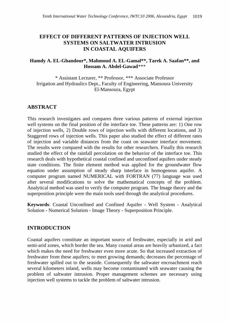
ANALYTICAL SOLUTION (THEORY OF IMAGE) This problem can be solved analytically for homogeneous isotropic rectangular coastal aquifer with horizontal bed. This can be achieved by using the image method together with the superposition principle. Figure (3) shows the principle of the image theory for one pumping well w located at coordinate (xw, yw). To take into consideration the effect of different boundaries an image well must be added. For a constant potential head boundary (jk) the image of the pumping well w is a recharging well with the same strength, while for impervious boundary (ij) , (lk) the image well is a pumping one with the same strength. Due to existence of impervious boundary (ij) opposite to the impervious boundary (lk) infinite number of mirror images is created. By superposition the drawdown in a potential φ, at any observation point (x, y) in the studied aquifer (ijkl), can be given by summation of the drawdowns for the original

0=∂∂

n

φ

0=∂∂n

φ

Uniform discharge qu

φ =constant

L k

J I

Sharp interface

a- Unconfined aquifer b- Confined aquifer

Zone II Zone I Zone II Zone I Impervious bed Impervious bed

A B

C D

A B C

D

Water table

Piezometric surface Injection well

h d h

d Z

X X

Z

qu qu

M.S.L M.S.L

Impervious bed

Impervious bed

YD

Ground level


1027

well w plus drawdown for different image wells as follows, Appendix (III) (El-Ghandour [6]):

( )( )( )( )

( )( )( )( )( )( )( )( )

+++++++++

++++= ∑

∞

=1 62524232

61514131ln

2212

2111ln*

4 n

w

yxyxyxyx

yxyxyxyx

yxyx

yxyx

k

Q

πφ (20)

where:

x1=(x-xw)2 , x2=(x+xw)2 y1=(y-yw)2 , y2=(y+yw)2

y3=(y-2n(YD-yw)-(2n-1)yw)2 , y4=(y+2n(YD-yw)+(2n-1)yw)2 y5=(y-2n(YD-yw)-(2n+1)yw)2 , y6=(y+2n(YD-yw)+(2n+1)yw)2,

and Qw is the discharge of well w (L3/T), k is the hydraulic conductivity of aquifer (L/T), xw and yw are coordinates of a well w (L), YD is the length of the aquifer in y-direction (L), and n =Nm*5, Nm is the number of mirrors. The potential φ due to uniform discharge through the boundary il with constant strength/ unit width qu can be represented as:

xK

quo += φφ (21)

where: φo represents the initial value of φ at boundary jk, calculated from equations (17), (18) for unconfined and confined aquifers respectively, and equal to zero if there is no seepage face at the sea coast. From the superposition principle the drawdown in φ for all wells plus the effect of uniform discharge qu, can be represented by using equations (20) and (21) as follows:

++= xK

quoφφ

( )( )( )( )

( )( )( )( )( )( )( )( )

+++++++++

++++

∑∞

=1 6252423261514131

ln22122111

ln*4 n

w

yxyxyxyx

yxyxyxyx

yxyx

yxyx

k

Q

π

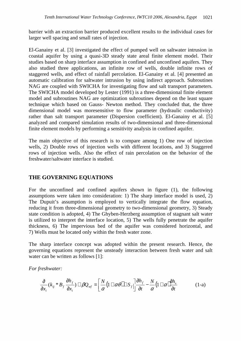
(22) NUMBER OF MIRRORS AGAINST ACCURACY OF THE ANALYTICAL SOLUTION The present problem includes two opposite impervious boundaries ij , kl, Figure (3). This produces an infinite number of mirrors, which creates multiple image wells, within the analytical solution, Equation (22). It is necessary to determine the numerical (actual) number of mirrors that can be adopted during the solution process, without sacrifying the accuracy of the analytical solution. Figure (4) shows the relationship between the relative value of potential φ (value of potential for n>1 / value of potential


for n=1) and n for a one pumping well w. Potential φ was calculated according to the average value of potentials at all nodes. From figure (4) it can be noticed that, the relative value converges quickly to constant value as n increases. For the present study, the value of n was taken equal to 250.

Start Read input data

Determine of maximum Number of non-Zero

element per row.

Generate mesh for rectangular

domain.

MSH2DR

Set initial guess for potential flow φ by using theory of image equation

(4-1)

Calculate of conductivity matrix

Put non zeros element in one vector and determine

the corresponding location in another vector

Apply Dirichlet and Neumann B.C equations

(3-17) to (3-20)

Add different magnitudes of the

sources or the sinks through the load

vector

ITER = 0 ITER = ITER+1

Stop Write Results

SNIM

Solution of equations by using approximate

Gauss –Seidel Iteration method

Determine of the distance of toe from the

coast

Determine of salt water and fresh water regions

and calculate heads END Do

Do I = 1,N node │φ i+1(N)- φi(N)│

>tol 2 a

COEFF

NO

a

Fig. (2). Flow chart for the main program

yes


1029

Pumping well Recharging well Impervious boundary Sea coast Image line To infinity STEPS OF THE ANALYTICAL SOLUTION A FORTRAN program was written to perform the analytical method. The following steps were used for verification the numerical program.

1. Discretize the aquifer to number of elements. 2. Use the analytical procedure to calculate different potentials at all nodes

through the discretized domain. 3. Recalculate the potentials at different nodes using the FEM. 4. Determine the relative absolute average errors in potentials between the

analytical and numerical methods, using the following equation:

yw

xw

Sea

w

x

y j k

l i

YD

Fig.(3). Image well system for a pumping well located within coastal aquifer ijkl

Fig. (4). Effect of number of mirrors on the accuracy of analytical solution

1.00

1.02

1.04

1.06

1.08

1.10

1.12

1.14

1.16

1.18

0 50 100 150 200 250 300 350 400 450 500

n

pote

ntia

l due

to n

>1/

pot

entia

l for

n=1

YD=2000 m

Y

XD=2000m

qu=0.6m3/d/m

X

xW=1000 m

Qwf =100m3/d

K=100m/d

ρs=1025 kg/m3

ρf=1000 kg/m3

d=14.52 m

yW=1000 m

w


nerror

n

i A

NA∑=

−

= 1 φφφ

(23)

where: φA is the potential at node i calculated from analytical solution; φN is the potential at node i calculated from numerical solution; and n is the number of nodes through the studied domain. TEST CASE: INJECTION (RECHARGING) WELLS This case studied the position of the interface toe along the coast (y-coordinate) as a result of system of injection wells. For this purpose an example was considered, and the solutions were obtained for a single and multiple injection wells located at a distance x = 1000 m from the coast. Figures (5-a) and (5-b) show the domain, which included different data, used for one and multiple injection wells. The vertical cross section is the same as in figures (1-a, b) for unconfined and confined aquifers respectively. From the results, the initial (no well) and final (for 1 well and 10 wells), steady-state locations of the interface toe were calculated using both FEM and the analytical method. The results from analytical and numerical methods were compared for unconfined and confined aquifers as shown in figures (6) and (7). The relative absolute average errors between numerical and analytical results were calculated as: For unconfined aquifer: • 0 injection well: error = 1.75*10-5 • 1 injection well: error = 1.7*10-4 • 10 injection wells: error = 2.39*10-4 For confined aquifer: • 0 injection well: error = 1.61*10-5 • 1 injection well: error = 1.71*10-4 • 10 injection wells: error = 2.41*10-4


1031

YD=2000 m

y

Fig. (5-a). Plan of the tested domain for one well

x XD=2000m

xw=1000 m

Qwf =100m3/d

qu=0.6m3/d/m K=100m/d

ρs=1025 kg/m3

ρf=1000 kg/m3

d=14.52 m

yw=1000 m

YD=2000 m

y

Fig. (5-b). Plan of the tested domain for multiple wells

x

Sp

Sp

XD=2000m

xw=1000 m

Sp=200 m

Qwf =50m3/d

qu=0.6m3/d/m

K=100m/d

ρs=1025 kg/m3

ρf=1.000 kg/m3

d=14.52 m

Sp/2

0.0

200.0

400.0

600.0

800.0

1000.0

1200.0

1400.0

1600.0

1800.0

2000.0

0.0 50.0 100.0 150.0 200.0 250.0 300.0 350.0 400.0 450.0 500.0

Xtoe,m

Y,m

• • • • Analytical Numerical FEM

10 wells 1 well No well

Fig. (6). Comparison between interface toe produced from the FEM and the analytical method for different injection well systems (unconfined aquifer)


CASE STUDY (1): INJECTION (RECHARGING) WELLS In this case study the FEM was used to perform a parametric study on the effect of: 1) the location for row of injection wells parallel to the coast, 2) spacings between them, and 3) the fresh water injection rate on the seawater intruded into coastal unconfined and confined aquifers. Effective variables in this analysis were identified and grouped into the following non-dimensional parameters:

WL’ =WL /Lo (24)

Sp’ = (Sp /Lo)*100 (25)

Qf ’= Qwf /(αKd2) (26)

Qf r’ = Qwf*(Nw) /(qu* YD) (27)

P = [(Lo-Lt) /Lo]*100 (28) Where: WL is the perpendicular distance from sea side to the well system (L); Qwf is the recharge rate into a well (L3/T); Nw is the number of wells (dimensionless); P is the reduction percentage of seawater intrusion; Lo is the initial steady length of intrusion from the interface toe to the coast (L); Lt is the average final steady length of intrusion from the interface toe to the coast (L); WL`, Sp`, Qf `, and Qfr ` are non-dimensional parameters for representing location of the studied row of injection wells, spacing between these wells, rate of injection for one well, and total rate of injection relative to total recharge into aquifer respectively, and α=( γs- γf)/ γf where, γs, γf are the specific weights of salt and fresh water respectively (F/L3).

0.0

200.0

400.0

600.0

800.0

1000.0

1200.0

1400.0

1600.0

1800.0

2000.0

0.0 50.0 100.0 150.0 200.0 250.0 300.0 350.0 400.0 450.0 500.0

Xtoe,m

Y,m

• • • • Analytical Numerical FEM

10 wells 1 well No well

Fig. (7). Comparison between interface toe produced from the FEM and the analytical method for different injection well systems (confined aquifer)


1033

In the present study the following conditions are considered: 1. One row of injection wells. 2. Double rows of injection wells with different locations. 3. Staggered rows of injection wells.

The results that obtained from the study of the above three conditions were compared with that presented by Mahesha [9]. 1- Single row of injection wells Figure (8) shows a definition sketch for the domain under study. The vertical cross section is the same as in figures (1-a, b) for unconfined and confined aquifers respectively. Different input data used to solve this problem are mentioned within figure (8). Figures (9) and (10) show a sectional view at y =1000m for unconfined and confined aquifers respectively, the continuos lines represent initial position of the piezometric heads and the corresponding interface location for the case without injection. Water injected from a row of wells that has different locations. The wells are located at perpendicular distance from the coast equal to 450m, 900m, and 1800m for unconfined aquifer and equal to 440m, 880m, and 1760m for confined aquifer. Initial position of the interface toe was found at distance equal to 450m and 440m for the unconfined and confined aquifers respectively. The locations of different rows of injection wells are settled at distances greater than or equal to the location of interface toe. From these two figures (9) and (10), it can be noticed that, the piezometric head increases from seaside towards inland with a specified rate till the injection well system. This rate decreases significantly upstream the injection well system. This logical behavior is due to the linear relationship between the gradient of the potential ∂φ/∂ x and the total discharge rate flows out to the seaside. Consequently, a higher upstream piezometric heads must be determined, as shown in the figures (9) and (10), as the injected well system moves away from the coast. For constant injection rates from different injection systems shown in figures (9) and (10), it can be noticed that, the final position of the interface is constant for all cases independently of the location of the injected well system. Figures (11) and (12) show the reduction of seawater intrusion due to a row of single injection wells located at the location of the initial interface toe before recharging for unconfined and confined aquifers respectively. These relationships are useful for estimating the reduction of seawater intrusion under a specified well spacing and injection rates. From these figures it can be shown that, increasing the total amount of injected fresh water decreases the intruded zone with decreasing rate for the specified number of wells. From these figures it can be noticed that, the curves in the present


study, Figures (11) and (12), have the same trend as that presented by Mahesha [9] for confined aquifer. Figure (13) represents a comparison between the computed results and some data given by Mahesha [9]. Although there is small difference in depth of the confined aquifer in the present study from Mahesha research, the results in this figure show a good configuration to Mahesha analysis. Noting that, Q΄f in the study case ranges from 0 to 7.5 while this range in case of Mahesha research varied between 0 and 0.4. These curves, in figures (11) and (12), can be assembled in one curve for unconfined aquifer, figure (14), and for confined aquifer, figure (15), by using Q΄fr (percentage of injected water to total uniform flow at upstream side of the aquifer) for horizontal coordinate, equation (27), instead of Q΄f. Hence, it is evident that as much as 90% reduction of seawater intrusion is possible by choosing the appropriate injection rate.

Fig. (9). Sectional view through injection well in unconfined aquifer at y=1000m

0.01.02.03.04.05.06.07.08.09.0

10.011.012.013.014.015.016.017.018.019.020.0

0.0 200.0 400.0 600.0 800.0 1000.0 1200.0 1400.0 1600.0 1800.0 2000.0

x,m

h,m

Initial steady state Final steady state, WL=450 m Final steady state, WL=900 m Final steady state, WL=1800m

Sp’=44.44%, Nw=11 Qf’=0.9486

WL=450m WL=900 m WL=1800 m

Fig. (8). Definition sketch of the studied domain

YD=2000 m

y

x

Sp

Sp

XD=2000m

WL

qu=0.6m3/d/m

K=100m/d

ρs=1025 kg/m3

ρf=1000 kg/m3

d=14.52 m

B=14.52 m

Sea side


1035

Fig. (11). Relationship between (P %) and (Qf’) for a single row of injection wells at WL/Lo=1 for unconfined aquifer

0

10

20

30

40

50

60

70

80

90

100

0.0 0.2 0.4 0.6 0.8 1.0 1.2 1.4 1.6 1.8 2.0 2.2 2.4 2.6 2.8 3.0 3.2 3.4 3.6 3.8

Qf'

P% Sp’=11.11%, Nw=41

Sp’=22.22%, Nw=21 Sp’=44.44%, Nw=11 Sp’=55.56%, Nw=9

Fig. (10). Sectional view through injection well in confined aquifer at Y=1000m

WL=1760 m

0.01.02.03.04.05.06.07.08.09.0

10.011.012.013.014.015.016.017.018.019.020.0

0.0 200.0 400.0 600.0 800.0 1000.0 1200.0 1400.0 1600.0 1800.0 2000.0

x,m

h,m

Initial steady state Final steady state, WL=440 m Final steady state, WL=880 m Final steady state, WL=1760m

Sp’=45.45%, Nw=11 Qf’=0.9486

WL=440 m WL=880 m

0.0

10.0

20.0

30.0

40.0

50.0

60.0

70.0

80.0

90.0

100.0

0.0 0.4 0.8 1.2 1.6 2.0 2.4 2.8 3.2 3.6 4.0 4.4 4.8 5.2 5.6 6.0 6.4 6.8 7.2 7.6

Qf'

P% Sp’=9.1%, Nw=51

Sp’=18.2%, Nw=26 Sp’=45.45%, Nw=11 Sp’=91.1%, Nw=6

Fig. (12). Relationship between (P %) and (Qf’) for a single row of injection wells at WL/Lo=1 for confined aquifer

(1) (2)


Fig. (14). Assembled curves for reduction of seawater intrusion for a single row of injection wells at WL/Lo=1 for unconfined aquifer

0

10

20

30

40

50

60

70

80

90

100

0.0 1.0 2.0 3.0 4.0 5.0 6.0 7.0 8.0 9.0 10.0 11.0 12.0 13.0 14.0

Qfr'

P% Sp’=11.11%, Nw=41

Sp’=22.22%, Nw=21 Sp’=44.44%, Nw=11 Sp’=55.56%, Nw=9

Fig. (15). Assembled curves for reduction of seawater intrusion for a single row of injection wells at WL/Lo=1 for confined aquifer

0.0

10.0

20.0

30.0

40.0

50.0

60.0

70.0

80.0

90.0

100.0

0.0 1.0 2.0 3.0 4.0 5.0 6.0 7.0 8.0 9.0 10.0 11.0 12.0 13.0 14.0 15.0 16.0 17.0

Qfr'

P% Sp’=9.1%, Nw=51

Sp’=18.2%, Nw=26 Sp’=45.54%, Nw=11 Sp’=91.1%, Nw=6

0.0

10.0

20.0

30.0

40.0

50.0

60.0

70.0

80.0

90.0

100.0

0.00 0.05 0.10 0.15 0.20 0.25 0.30 0.35 0.40

Qf'

P%

Fig. (13). Comparison between the computed results and some data given by Mahesha [9] for confined aquifer.

Sp’=9.1 %, Nw=51 Sp’=10.0 % ( Mahesha data) Sp’=18.2 %, Nw=11 Sp’=17.75 % (Maesha data)

(1) (2)


1037

2- Double rows of injection wells under different combinations In this section, double series of wells with lesser injection rates are presented with the following combinations. Figure (16) shows a definition sketch of the domain under study, the location of the well system and the data used within this case.

• For unconfined aquifer WL1’, WL2’= (0.67 & 0.78), (0.67 & 1.0), (0.78 & 1.0), (0.67 & 0.89) and (0.89 & 1.0), for the relative well spacing Sp’ = 11.11%, 22.22%, 44.44% and 55.56%.

• For confined aquifer WL1’, WL2’= (0.73 & 0.82), (0.73 & 0.91), (0.73 & 1.0), (0.82 & 1.0) and (0.91 & 1.0), for the relative well spacing Sp’= 9.1%, 18.2%, 45.45% and 91.1%.

The number of wells considered for this case is taken equal to twice the number of wells for the single series and the rate of injection is taken equal to half the rate of injection for single series of wells. A comparison is made between the previous combinations of wells as stated in the previous paragraph based on their performance. Reductions of seawater intrusion achieved according to the studied wells system are plotted in Figures (17) and (18) for unconfined and confined aquifers respectively. From these two figures it can be noticed that, all curves are the same. The same relationship between total injection rate and percentage of intrusion was previously recognized for the case by using only one row of wells, (figures (14) and (15)). This indicates that, the percentage of the sharp interface toe reduction is only dependent on the total magnitude of injected water and there is no effect for the location of the wells and spacing between wells on the sharp interface toe. It must be noticed that the injection well system is always located in the fresh water zone. From figures (14), (15) and figures (17), (18) it is noticed that, both the relationships between (P%) and (Qfr’) give small deviations between values for both confined and unconfined aquifers. This could be due to the same dimensions for both aquifers. Mahesha [9] presented the same relationship for confined aquifer, but he used Qf΄ (the dimensionless rate of injection for one well), instead of Qfr’ (the total injected water for the well system) in this study. He found that, the location of the system of well has an effect on the reduction of seawater intrusion. Also, he stated that, the double series of wells performed marginally better than the single series. His results differ from that noticed in the present work. This may be due to the use of unsteady philosophy to reach the final solution at the steady condition. In this case the final solution for steady condition will be interrupted with the accuracy constraints of the solution process.


�

Longitudinal section for unconfined and confined aquifers

c- Plan of studied domain

Fig. (17). Relationship between (P%) and (Qfr ’) under different well combinations for unconfined aquifer

0.0

10.0

20.0

30.0

40.0

50.0

60.0

70.0

80.0

90.0

100.0

0.0 1.0 2.0 3.0 4.0 5.0 6.0 7.0 8.0 9.0 10.0 11.0 12.0 13.0 14.0

Qfr'

P%

WL1/Lo, WL2/Lo 0.67, 0.78 0.67, 1.0 0.78, 1.0 0.67, 0.89 0.89, 1.0

Sp’=11.11%, Nw=82 Sp’=22.22%, Nw=42

Sp’=44.44%, Nw=22 Sp’=55.56%, Nw=18

Recharging well


YD=2000 m

Y

X

Sp

Sp

XD=2000m

WL1

K=100m/d

ρs=1025 kg/m3

ρf=1000 km/m3

d=14.52 m

B=14.52 m

Sea side

Sp

Sp

WL2

qu=0.6m3/d/m

a- Unconfined aquifer b- Confined aquifer

Zone II Zone I Zone II Zone I Impervious bed Impervious bed

Water table Piezometric surface

Recharging well

d d qu qu

M.S.L M.S.L

Ground level

Interface Interface


1039

3- Staggered rows of injection wells In the present section, the staggered well system is considered and its effect is analyzed. Figure (19) shows a sketch including configuration of the well system and different data used. The vertical cross section is the same as in figures (16-a, b) for unconfined and confined aquifers respectively. The location of staggered well system was suggested at distance equal to WL1=Lo, WL2=1.33Lo from the coast for unconfined aquifer and WL1=1.02Lo, WL2=1.36Lo from the coast for confined aquifer. The results were compared to the corresponding results for well system with the same total injection rate and consist from one row only. The straight well system is located at distance from the seaside equal to Lo and 1.02Lo for unconfined and confined aquifers respectively. Lo represents initial position for interface toe from the seaside for unconfined and confined aquifers receptively. From the results Lo equal to 450.0m for unconfined aquifer and 440.0m for confined aquifer. Performance of the straight and the staggered system of wells were compared and shown in figures (20) and (21) for unconfined and confined aquifers respectively. From these figures it can be noticed that, the effect of a straight well system is the same as the staggered well system. This means that, there is no increasing effect of staggered well system on the reduction of seawater intrusion as stated by Mahesha [9] for confined aquifer. From figures (20) and (21) it was noticed that, both the relationships between (P%) and (Sp’) give nearly the same value for both confined and unconfined aquifers. This could be due to the same dimensions for both aquifers.

Fig. (18). Relationship between (P%) and (Qfr ’) under different well combinations for confined aquifer

0.0

10.0

20.0

30.0

40.0

50.0

60.0

70.0

80.0

90.0

100.0

0.0 1.0 2.0 3.0 4.0 5.0 6.0 7.0 8.0 9.0 10.0 11.0 12.0 13.0 14.0 15.0 16.0 17.0

Qfr'

P% WL1/Lo, WL2/Lo

0.73, 0.82 0.73, 0.91 0.73, 1.0 0.82, 1.0 0.91, 1.0

Sp’=9.11%, Nw=102 Sp’=18.2%, Nw=52

Sp’=45.54%, Nw=22 Sp’=91.1%, Nw=12


Fig. (20). Relationship between (P%) and (Sp’) for straight and staggered wells (unconfined aquifer)

Qf’= 0.15

0.11

0.076

0.038

0.0

10.0

20.0

30.0

40.0

50.0

60.0

70.0

0.0 20.0 40.0 60.0 80.0 100.0 120.0

SP'

P%

– – – Straight Staggered

Fig. (21). Relationship between (P%) and (Sp’) for straight and staggered wells (confined aquifer)

Qf’= 0.15

0.11

0.076

0.038

0.0

10.0

20.0

30.0

40.0

50.0

60.0

70.0

0.0 20.0 40.0 60.0 80.0 100.0 120.0

SP'

P%

– – – Straight Staggered


YD=2000 m

y

x

Sp

XD=2000m

WL1

K=100m/d

ρs=1025 kg/m3

ρf=1000 kg/m3

d=14.52 m

B=14.52 m

Sea side

Sp

Sp/2

WL2

qu=0.6m3/d/m


1041

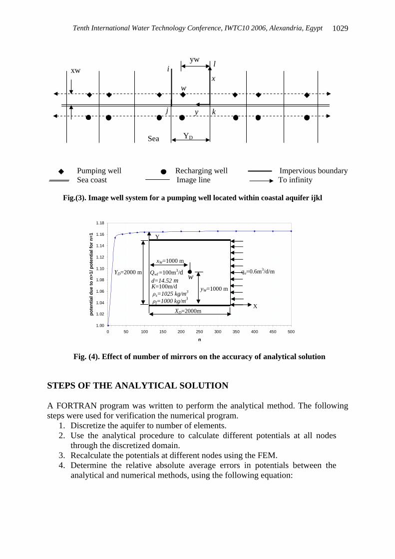
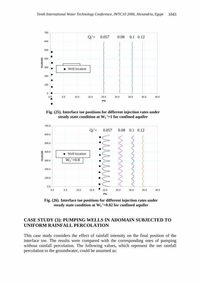
CASE STUDY (2): DIFFERENT RATES OF INJECTION AND VARIABLE DISTANCE FROM THE This section demonstrates the shape of the interface toe for different injection rates and different positions from the coast for unconfined and confined aquifers. Figure (22) shows the definition sketch of the domain and it demonstrates the meaning of the parameters and different data used through this case. The vertical cross section is the same as in figures (1-a, b) for unconfined and confined aquifers respectively. Figures (23) to (26) show the positions of the saline wedge toe (in plan) for different situations. From these figures it can be noticed that, the interface toe moves to the seaside as the total amount of injected water increases. In general the interface toe has a semi straight line parallel to the sea coast for injected wells located far from the sea side as shown in figures (23) and (25). As the injected wells move to the seaside the interface toe deviates to be undulated as shown in figures (24) and (26). This behavior is due to both the increase of the injected water in every well and its approach to the interface toe. The undulation behavior presented in previous figures (23) to (26) was assured by the results of Mahesha [9] for confined aquifer. Noticing that, the number of wells in the present study is equal to 10 wells while, it is equal to 4 wells in Mahesha’s research. It is clear that for any injection rate from a well system at a parallel distance from the coast, a retarded interface toe with insignificantly undulation will occur for a well system located at distance equal to or greater than the initial interface toe. The effect of local stress from every injection well will vanish as the injected water moves to the seaside. This means that, after a limited distance from the well system, the injected water will be distributed uniformly along the width of the aquifer, neglecting any change in the well system configuration, as shown in figures (23) and (25).

qu=0.6m3/d/m


YD=2000 m

y

x

Sp

Sp

XD=2000m

WL

K=100m/d

ρs=1025 kg/m3

ρf=1000 kg/m3

d=14.52 m

B=14.52 m

Sea side

Sp

Sp

Sp=200 m


Fig. (23). Interface toe positions for different injection rates under steady

state condition at W ’=1 for unconfined aquifer

0.0

50.0

100.0

150.0

200.0

250.0

300.0

350.0

400.0

450.0

500.0

0.0 5.0 10.0 15.0 20.0 25.0 30.0 35.0 40.0

P%

Y/L

0X10

0

WL’=1

Qf’= 0.057 0.08 0.1 0.12

Well location

Fig. (24). Interface toe positions for different injection rates under steady state condition at WL ’=0.78 for unconfined aquifer

0.0

50.0

100.0

150.0

200.0

250.0

300.0

350.0

400.0

450.0

500.0

0.0 5.0 10.0 15.0 20.0 25.0 30.0 35.0 40.0

P%

Y/L

0X10

0

Qft’= 0.08 0.1 0.12

WL’=0.78

Well location


1043

CASE STUDY (3): PUMPING WELLS IN ADOMAIN SUBJECTED TO UNIFORM RAINFALL PERCOLATION This case study considers the effect of rainfall intensity on the final position of the interface toe. The results were compared with the corresponding ones of pumping without rainfall percolation. The following values, which represent the net rainfall percolation to the groundwater, could be assumed as:

Fig. (25). Interface toe positions for different injection rates under steady state condition at WL ’=1 for confined aquifer

0

100

200

300

400

500

600

700

0.0 5.0 10.0 15.0 20.0 25.0 30.0 35.0 40.0

P%

Y/L

0X10

0

WL’=1

Qf’= 0.057 0.08 0.1 0.12

Well location

Fig. (26). Interface toe positions for different injection rates under steady state condition at WL ’=0.82 for confined aquifer

0.0

100.0

200.0

300.0

400.0

500.0

600.0

700.0

0.0 5.0 10.0 15.0 20.0 25.0 30.0 35.0 40.0

P%

Y/L

0X10

0

WL’=0.8

Qf’= 0.057 0.08 0.1 0.12

Well location


1. 200 m3/d 2. 300 m3/d 3. 400 m3/d 4. 500 m3/d

Figure (27) shows a definition sketch of the studied domain including different data. The vertical cross section is the same as in figures (1-a, b) for unconfined and confined aquifers respectively.

The non-dimensional parameters that used in this case are Qfr

’ and A. Definitions of these parameters are shown in equations (4-8) and

A = ((Lt-Lo) /Lo)*100 (29) in which, A is the advancing percentage of seawater intrusion; Lo is the initial position of interface toe from the coast in case of there is no a rainfall percolation (L) and Lt is the final position of the interface toe from the sea coast (L). Tables (1) and (2) give a percentage of a reduction in initial position of interface toe as a result of presence different values of rainfall densities. The following equation was adopted to calculate the percentage of reduction as a result of presence rainfall percolation:

Reduction = [(Lo -Lor)/Lo]*100 (30) in which, Lor: initial position of interface toe from the coast in case of there is a rainfall (L).

Rainfall


YD=2000 m

y

x

Sp

Sp

XD=2000m

WL

K=100m/d

ρs=1025 kg/m3

ρf=1000 kg/m3

d=14.52 m

B=14.52 m

Sea side

Sp

Sp

qu=0.6m3/d/m


1045

Table (1). Reduction of interface toe for unconfined aquifer due to percolation rate

Rate of percolation (Pr) Loorr Loo Reduction 200 m3/d 391.37m 450.14m 13.03 % 300 m3/d 366.92m 450.14m 18.46 % 400 m3/d 345.11m 450.14m 23.31 % 500 m3/d 325.6m 450.14m 27.64 %

Table (2). Reduction of interface toe for confined aquifer due to percolation rate

Rate of percolation (Pr) Loorr Loo Reduction 200 m3/d 381.7m 439.16m 13.08 % 300 m3/d 357.8m 439.16m 18.53 % 400 m3/d 336.52m 439.16m 23.37 % 500 m3/d 317.49m 439.16m 27.71 %

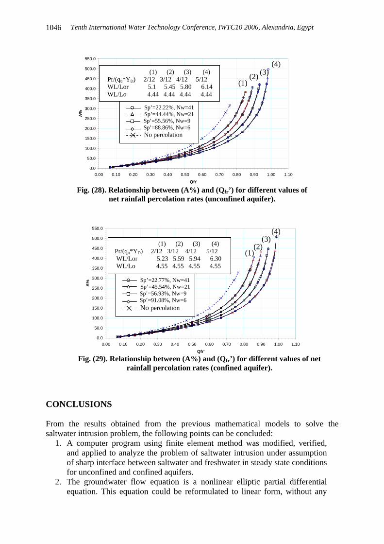
From the above two tables it can be noticed that, increasing the net rainfall percolation intensity increases the percentage of reduction in seawater intrusion and decreases the intrusion zone. This behavior is the same as achieved by using injection wells only. Figures (28) and (29) show the relationship between (Qfr’) and (A%) for different net rainfall percolation rates (Pr) and for different spacings between the wells, for unconfined and confined aquifers respectively. The dotted line represents the advancement of saline wedge without percolation. From these figures it can be noticed that: • The percentage of advancing seawater intrusion due to pumping from a well

system depends on the rate of pumping and net rainfall percolation rate. • Increasing the rate of pumping increases the intrusion. • Increasing the percolation rate of rainfall decreases the advancing of

interface toe, for constant value of total rate of pumping. • For the same percentage of seawater intrusion advancement, increasing

percolation rate of rainfall increases the allowable rate of pumping.


CONCLUSIONS From the results obtained from the previous mathematical models to solve the saltwater intrusion problem, the following points can be concluded:

1. A computer program using finite element method was modified, verified, and applied to analyze the problem of saltwater intrusion under assumption of sharp interface between saltwater and freshwater in steady state conditions for unconfined and confined aquifers.

2. The groundwater flow equation is a nonlinear elliptic partial differential equation. This equation could be reformulated to linear form, without any

Fig. (28). Relationship between (A%) and (Qfr ’) for different values of net rainfall percolation rates (unconfined aquifer).

0.0

50.0

100.0

150.0

200.0

250.0

300.0

350.0

400.0

450.0

500.0

550.0

0.00 0.10 0.20 0.30 0.40 0.50 0.60 0.70 0.80 0.90 1.00 1.10

Qfr'

A%

(1) (2)

(3) (4)

(1) (2) (3) (4) Pr/(qu*Y D) 2/12 3/12 4/12 5/12 WL/Lor 5.1 5.45 5.80 6.14 WL/Lo 4.44 4.44 4.44 4.44

Sp’=22.22%, Nw=41 Sp’=44.44%, Nw=21 Sp’=55.56%, Nw=9 Sp’=88.86%, Nw=6 No percolation

Fig. (29). Relationship between (A%) and (Qfr ’) for different values of net rainfall percolation rates (confined aquifer).

0.0

50.0

100.0

150.0

200.0

250.0

300.0

350.0

400.0

450.0

500.0

550.0

0.00 0.10 0.20 0.30 0.40 0.50 0.60 0.70 0.80 0.90 1.00 1.10

Qfr'

A%

(4)

(1) (2)

(3) (1) (2) (3) (4) Pr/(qu*Y D) 2/12 3/12 4/12 5/12 WL/Lor 5.23 5.59 5.94 6.30 WL/Lo 4.55 4.55 4.55 4.55

Sp’=22.77%, Nw=41 Sp’=45.54%, Nw=21 Sp’=56.93%, Nw=9 Sp’=91.08%, Nw=6 No percolation


1047

relaxation by replacing the dependent variable of piezometric heads with the potential as described by Strack [16]. This transformation has no relaxation, but it is constrained for steady flow and horizontal impervious bed of the aquifer.

3. The problem of saltwater intrusion could be solved analytically by using theory of image. This method was constrained for homogenous steady ground water with straight boundaries and horizontal impervious bed.

4. A new formula was presented using the theory of image to calculate the potentials, Equation (20).

5. The number of mirrors used to represent the two opposite impervious boundaries ij, kl, figure (1), affects the accuracy of the analytical solution. Sufficient number of mirrors (250) must be taken to satisfy the accuracy requirement.

6. The percentage of a sharp interface toe reduction is only dependent on the total magnitude of injected water and there is no effect for the location of the wells and spacing between wells on the final position of the interface toe.

7. Increasing the total amount of injected fresh water decreases the intrusion zone.

8. As the injected wells move to the seaside the interface toe goes to be undulated.

9. Increasing the value of rainfall intensity increases the reduction of saltwater intrusion and decreases the intrusion zone.

REFERENCES

[1] Bear, J., (1979), “Hydraulics of Groundwater” McGraw-Hill Inc, p. 569.

[2] Cheng, A. H-D, Holand, D., Naji, A., and Ouazar, D., (2000), “Pumping Optimization in Saltwater-Intruded Coastal Aquifers”, Water Resources Research, 36(8), pp. 2155-2165.

[3] El-Ganainy, M. A., El-Fitiany, F. A., El-Afify, M. M., and Shuluma, Z. M., (1995), “Effects of Pumped Well on Saltwater Intrusion in Coastal Aquifers”, Alexandria Engineering Journal, 34(1), pp. C65-C74.

[4] El-Ganainy, M. A., El-Fitiany, F. A., White, J. K., El-Afify, M. M., and Shuluma, Z. M., (1996), “Automatic Calibration for Saltwater Intrusion Problems by Using Optimization Technique”, Alexandria Engineering Journal, 35(2), pp. E1-E11.

[5] El-Ganainy, M. A., El-Fitiany, F. A., White, J. K., El-Afify, M. M., and Shuluma, Z. M., (1996), “Sensitivity Analysis for 2D and 3D Models for Saltwater Intrusion Problems”, Alexandria Engineering Journal, 35(3), pp. E13-E19.

[6] El-Ghandour, H. A., (2005), “Analysis and Optimization of Salt Water Intrusion in Coastal Aquifers”, M.Sc. Thesis, Faculty of Engineering, Mansoura University, Egypt, p. 177.

[7] Hunt, B., (1983), “Mathematical Analysis of Groundwater Resources”, Butterworths, p. 271.


[8] Kashef, A. I., (1976), “Control of Saltwater Intrusion by Recharge Wells”, Journal of Irrigation and Drainage Division, 102(4), pp. 445-456.

[9] Mahesha, A., (1996), “Steady-State Effect of Freshwater Injection on Seawater Intrusion”, Journal of Irrigation and Drainage Engineering, ASCE, 122(3), pp. 149-154.

[10] Mahesha, A., (1996), “Transient Effect of Battery of Injection Wells on Seawater Intrusion”, Journal of Hydraulic Engineering, ASCE, 122(5), pp. 266-271.

[11] Mahesha, A., and Nagraja, S. H., (1995), “Effect of Surface Source Variation on Seawater Intrusion in Aquifers”, Journal of Irrigation and Drainage Engineering, ASCE, 121(1), pp. 109-113.

[12] Mahesha, A., (1995), “Parametric Studies on the Advancing Interface in Coastal Aquifers Due to Linear Variation of the Freshwater Level”, Water Resources Research, 31(10), pp. 2437-2442.

[13] Mahesha, A., (1996), “Control of Seawater Intrusion through Injection-Extraction Well System”, Journal of Irrigation and Drainage Engineering, ASCE, 122(5), pp. 314-317.

[14] Rummer, R. R., Jr., and Harleman D. R. F., (1963), “Intruded Saltwater Wedge in Porous Media”, Journal of Hydraulic Division, ASCE, 89(6), pp. 193-220.

[15] Saafan, T. A., (1995), “Mathematical Solution of Seawater Intrusion into Freshwater in Unconfined Coastal Aquifers”, 5th International Conference “Environmental Protection is A Must”, Apr. 1995, Alexandria, pp. 497-509.

[16] Strack, O. D. L., (1976), “A Single-Potential Solution for Regional Interface Problems in Coastal Aquifers”, Water Resources Research, 12, pp. 1165-1174.

EFFECT OF DIFFERENT PATTERNS OF INJECTION WELL SYSTEMS ON SALTWATER INTRUSION IN COASTAL AQUIFERS

Documents

Transcript of EFFECT OF DIFFERENT PATTERNS OF INJECTION WELL SYSTEMS ON SALTWATER INTRUSION IN COASTAL AQUIFERS