LABORATORY MANUAL - SRM University

1

LABORATORY MANUAL

PROGRAMME: B.Tech SEMESTER /YEAR:VI SUBJECT CODE: BM0312 SUBJECT NAME:BIO SIGNAL PROCESSING

Prepared By: Name: U.Snekhalatha

Designation: Assistant Professor

DEPARTMENT OF BIOMEDICAL ENGINEERING

SCHOOL OF BIOENGINEERING, FACULTY OF ENGINEERING & TECHNOLOGY

SRM UNIVERSITY (UNDER SECTION 3 of UGC ACT 1956)

KATTANKULATHUR-603203 Tamil Nadu, India

2

INDEX

Exp No.

Title of the experiment

Page

1 2 3 4 5 6 7 8 9

10

11

12

Representation of basic signals Linear convolution Autocorrelation and cross correlation FFT and IFFT Difference equation Representation Digital IIR Butterworth filter-LPF & HPF Digital IIR chebychev filter-LPF & HPF Design of FIR filter using windowing technique Upsampling and downsampling Analysis of ECG Analysis of EEG Analysis of PCG

3 9 18 28 42 51 55 59 69 75 79 83

3

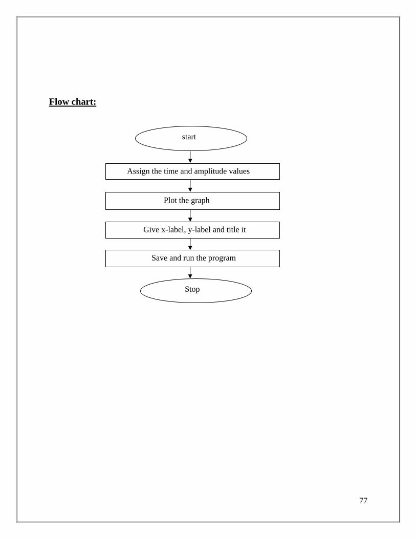
Flow chart:

start

Assign the time and amplitude values

Plot the graph

Stop

Save and run the program

Give x-label, y-label and title it

4

Exp No: 01 REPRESENTATION OF BASIC SIGNAL Aim: To represent the basic signals like impulse, unit step, unit ramp,sinusoidal, cosine and exponential using mat lab software Algorithm:

Start the mat lab software Assign the time and amplitude values Plot the graph Give the x label and y label and title it Save and run the program

Program: Representation of Basic signals %Unit Impulse Signal% n1=input('Enter the no of samples'); x1=[-n1:1:n1]; y1=[zeros(1,n1),ones(1,1),zeros(1,n1)]; subplot(2,3,1); stem(x1,y1); xlabel('Time Period'); ylabel('Amplitude'); title('Unit Impulse Signal'); %Unit Step Signal% n2=input('Enter the no of samples'); x2=[0:1:n2]; y2=ones(1,n2+1); subplot(2,3,2); stem(x2,y2); xlabel('Time Period'); ylabel('Amplitude'); title('Unit Step Signal'); %Unit Ramp Signal

5

n3=input('Enter the no of samples'); x3=[0:1:n3]; subplot(2,3,3); stem(x3,x3);

Representation of basic signals

6

xlabel('Time Period'); ylabel('Amplitude'); title('Unit Ramp Signal'); %Exponential Signal% n4=input('Enter the length of the signal'); a=input('Enter the value of a:'); x4=[0:1:n4]; y4=a*exp(x4); subplot(2,3,4); stem(x4,y4); xlabel('Time Period'); ylabel('Amplitude'); title('Exponential Signal'); %Sinusoidal Signal x5=[-pi:0.1:pi]; y5=sin(2*pi*x5); subplot(2,3,5); plot(x5,y5); xlabel('Time Period'); ylabel('Amplitude'); title('Sinusoidal Signal'); %Cosine Signal x6=[-pi:0.1:pi]; y6=cos(2*pi*x5); subplot(2,3,6); plot(x6,y6); xlabel('Time Period'); ylabel('Amplitude'); title('Cosine Signal')

9

Result: Thus, the basic signals were represented using MAT LAB Flow chart:

start


Plot the graph

Stop


Give x-label , y-label and title it

10

Exp No: 2 LINEAR CONVOLUTION Aim: To find the linear convolution of x(n) and h(n) Algorithm:

Assign the variables to the input sequence and impulse sequence. Assign the lower and upper limits for both input and impulse sequence Assign the time and amplitude Perform convolution using the function ‘conv’ Plot the input ,impulse and output sequence Give the x label and y label and title it Save and run the program

Program: x=input('enter the sequence for x(n):') h=input('enter the sequence for h(n):') u1=input('enter the upper limit for x(n):') l1=input('enter the lower limit for x(n):') u2=input('enter the upper limit for h(n):') l2=input('enter the lower limit for h(n):') a=l1:1:u1 subplot(2,2,1); stem(a,x); xlabel('time'); ylabel('amplitude'); title('x(n)'); b=l2:1:u2; subplot(2,2,2); stem(b,h); xlabel('time'); ylabel('amplitude'); title('b(n)'); y=conv(x,h); c=(l1+l2):1:(u1+u2); subplot(2,2,3);

11

stem(c,y); xlabel('time'); ylabel('amplitude' title('y(n)');

12

Representation of Linear Convolution

Input sequence x(n)=[1,2,3,4] Impulse sequence h(n)=[1,2,1] Convoluted sequence= [1, 4, 8, 12, 11, 4]

13

Input sequence x(n)=[1,2,4,6,2] Impulse sequence h(n)=[2,4,6,8] Convoluted sequence= [2, 8, 22, 48, 68, 76, 60, 16]

14

Input sequence x(n)=[1,1,1,-1,1,1] Impulse sequence h(n)=[0,1,2,3] Convoluted sequence= [0,1,3,6,4,2,0,5,3]

17

Result: Thus, the linear convolution of two signals is represented using MAT LAB.

Flow chart:

Start


Plot the graph



Stop

18

Exp No:3 Autocorrelation And Cross Correlation Aim: To perform autocorrelation and cross- correlation of given sequences in MATLAB. Algorithm:

Start MATLAB. Enter the input sequence. Give X‐label and Y‐label and title it. Save and run the program. Stop/Halt the program.

Program: %Auto Correlation% x= input (‘Enter any sequence’); subplot(3,2,1); stem(x); xlabel(‘Time period’); ylabel(‘Amplitude’); title(‘Input sequence’); y=xcorr(x); subplot(3,2,2); xlabel(‘Time period’); ylabel(‘Amplitude’); title(‘Auto correlation’);

20

%Cross correlation% x=input(‘Enter any sequence’); subplot(3,2,1); stem(x); xlabel(‘Time period’); ylabel(‘Amplitude’); title(‘Input sequence’); h=input(‘Enter any sequence’); subplot(3,2,2); stem(h); xlabel(‘Time period’); ylabel(‘Amplitude’); title(‘Impulse sequence’); y=xcorr(x,h); subplot(3,2,3); stem(y); xlabel(‘Time period’); ylabel(‘Amplitude’); title(‘Cross correlation’);

26

Result: Thus, the autocorrelation and cross- correlation was performed using MATLAB

27

Flow chart:

Start


Plot the graph



Stop

28

Ex.No.4 FFT and Inverse FFT Aim: To find FFT and IFFT of the given sequence using MATLAB. Algorithm:

Start the MATLAB. Assign the time and amplitude values. Plot the graph. Give the X-label and Y-label values and title it. Save and run the program. Stop/Halt the program.

Program: %Fast Fourier Transform% x=input('enter the input sequence'); n=input('enter the length of the sequence'); subplot(2,1,1); stem(x); xlabel('time'); ylabel('amplitude'); y1=fft(x,n); subplot(2,2,2); stem(y1); xlabel('time'); ylabel('amplitude'); title(‘Fast fourier Transform’);

30

%Inverse Fast Fourier Transform% x=input('enter the input sequence'); n=input('enter the length of the sequence'); subplot(3,1,1); stem(x); xlabel('time'); ylabel('amplitude'); title(‘input sequence’); xk=ifft(x,n); magxk=abs(xk); anglexk=angle(xk); k=0:1:n-1; subplot(3,1,2); stem(k,magxk); xlabel('time'); ylabel('amplitude'); title('mag plot'); subplot(3,1,3); stem(k,anglexk); xlabel('time'); ylabel('amplitude'); title('phase plot');

40

Result: Thus, the FFT and IFFT were programmed using MATLAB.

41

Flow chart:

Start


Plot the graph



Stop

42

Ex.No.5 DIFFERENCE EQUATION Aim: To represent the difference equation using MATLAB. Algorithm:

Start the MATLAB. Assign the time and amplitude values. Plot the graph. Give the X-label and Y-label values and title it. Save and run the program. Stop/Halt the program.

Program: a=input('enter the input'); b=input('enter the input'); x=linspace(0,2*pi,100); y=sin(x); subplot(2,3,1); plot(y); xlabel('time period'); ylabel('amplitude'); title('sine wave'); e=rand(size(x)); subplot(2,3,2); plot(e); xlabel('time period'); ylabel('amplitude'); title('noise signal'); subplot(2,3,3); t=y+e; plot(x,t); xlabel('time period');

43

y(n)+y(n-1)+y(n-2)=x(n)

ylabel('amplitude');

44

title('distorted sinewave'); subplot(2,3,4); zplane(b,a); title('pole-zero plot'); xlabel('time period'); ylabel('amplitude'); subplot(2,3,5); z=filter(b,a,y); plot(z); xlabel('time period'); ylabel('amplitude'); title('filtered signal');

45

y(n)+3/4y(n-1)+1/8y(n-2)=x(n)

47

3) y(n)+1/4y(n-1)+1/2y(n-2)=x(n)+1/2x(n-1)

49

Result:

Thus, the difference equations were programmed using MATLAB.

50

Flow chart:

start


Plot the graph

Stop



51

Exp No: 05 DIGITAL BUTTERWORTH IIR FILTER Aim: To Design digital Butterworth IIR filter using Mat Lab Algorithm:

Start the mat lab software Assign the variable for pass band ripple ,stop band ripple, pass band and stop band frequency

Determine the order of filter using the required formula. Find the filter co-efficient a and b Assign the time and amplitude Plot the magnitude and phase angle. Give the x label and y label and title it Save and run the program

Program:

%LPF% rp=input('enter the pass band ripple'); rs=input('enter the stop band ripple'); wp=input('enter the pass band frequency'); ws=input('enter the stop band frequency'); fs=input('enter the sampling frequency'); w1=2*(wp/fs); w2=2*(ws/fs); [n,wn]=buttord(w1,w2,rp,rs); [b,a]=butter(n,wn); w=0:0.01/pi:pi; [h,om]=freqz(b,a,w); m=20*log10(abs(h)); an=angle(h); subplot(2,2,1); plot((om/pi),m); xlabel('time'); ylabel('amplitude'); title('magnitude plot of lpf'); subplot(2,2,2); plot((om/pi),an);

52

xlabel('time'); ylabel('amplitude'); title('angle plot of lpf');

53

LOW PASS FILTER Enter the pass band ripple=0.5 Enter the stop band ripple=50 Enter the pass band frequency=1500 Enter the stop band frequency=2500 Enter the sampling frequency=7500

HIGH PASS FILTER

Enter the pass band ripple=0.5 Enter the stop band ripple=50 Enter the pass band frequency=1500 Enter the stop band frequency=2500 Enter the sampling frequency=7500

54

%HPF% rp1=input('enter the pass band ripple'); rs1=input('enter the stop band ripple'); wp1=input('enter the pass band frequency'); ws1=input('enter the stop band frequency'); fs1=input('enter the sampling frequency'); w3=2*(wp1/fs1); w4=2*(ws1/fs1); [n,wn]=buttord(w1,w2,rp,rs); [b,a]=butter(n,wn,'high'); w=0:0.01:pi; [h,om]=freqz(b,a,w); m1=20*log10(abs(h)); an1=angle(h); subplot(2,2,3); plot((om/pi),m1); xlabel('time'); ylabel('amplitude'); title('magnitude plot of hpf'); subplot(2,2,4); plot((om/pi),an1); xlabel('time'); ylabel('amplitude'); title('angle plot of hpf');

Result: Thus, the digital Butterworth IIR filter was designed using Mat Lab

55

Flow chart:

start


Plot the graph

Stop



56

Exp No: 05 DIGITAL CHEBYSHEV IIR FILTER Aim: To Design digital Chebyshev IIR filter using Mat Lab Algorithm:

Start the mat lab software Assign the variable for pass band ripple ,stop band ripple, pass band and stop band frequency

Determine the order of filter using the required formula. Find the filter co-efficient a and b Assign the time and amplitude Plot the magnitude and phase angle. Give the x label and y label and title it Save and run the program

Program: %LPF% rp=input('enter the pass band ripple'); rs=input('enter the stop band ripple'); wp=input('enter the pass band frequency'); ws=input('enter the stop band frequency'); fs=input('enter the sampling frequency'); w1=2*(wp/fs); w2=2*(ws/fs); [n,wn]=cheb1ord(w1,w2,rp,rs); [b,a]=cheby1(n,rp,wn); w=0:0.01/pi:pi; [h,om]=freqz(b,a,w); m=20*log10(abs(h)); an=angle(h); subplot(2,2,1); plot((om/pi),m); xlabel('time'); ylabel('amplitude'); title('magnitude plot of lpf'); subplot(2,2,2); plot((om/pi),an); xlabel('time');

57

ylabel('amplitude'); title('angle plot of lpf');

58

LOW PASS FILTER

Enter the pass band ripple=0.5 Enter the stop band ripple=50 Enter the pass band frequency=1500 Enter the stop band frequency=2500 Enter the sampling frequency=7500

59

HIGH PASS FILTER Enter the pass band ripple=0.5 Enter the stop band ripple=50 Enter the pass band frequency=1500 Enter the stop band frequency=2500 Enter the sampling frequency=7500

60

%HPF% rp=input('enter the pass band ripple'); rs=input('enter the stop band ripple'); wp=input('enter the pass band frequency'); ws=input('enter the stop band frequency'); fs=input('enter the sampling frequency'); w1=2*(wp/fs); w2=2*(ws/fs); [n,wn]=cheb1ord(w1,w2,rp,rs); [b,a]=cheby1(n,rp,wn,'high'); w=0:0.01/pi:pi; [h,om]=freqz(b,a,w); m=20*log10(abs(h)); an=angle(h); subplot(2,2,1); plot((om/pi),m); xlabel('time'); ylabel('amplitude'); title('magnitude plot of hpf'); subplot(2,2,2); plot((om/pi),an); xlabel('time'); ylabel('amplitude'); title('angle plot of hpf');

Result: Thus, the digital Chebyshev filter was designed using Mat Lab

61

FLOWCHART

START

Assign the values for the variables

Give X-label and Y-label and title it


STOP

62

EX NO. 8 DESIGN OF FIR FILTER USING WINDOWING TECHNIQUE AIM: To design an FIR filter using Hamming ,hanning and blackmann windowing techniques. ALGORITHM:

Assign the variable for pass band ripple ,stop band ripple, pass band and stop band frequency

Determine the order of filter using the required formula. Find the filter co-efficient b Assign the time and amplitude Plot the magnitude and phase angle for LPF.HPF,BPF&BSF. Give the x label and y label and title it

.

PROGRAM:

%Hamming window% rp=input('enter the PB ripple'); rs=input('enter the SB ripple'); fp=input('enter PB frequency'); fs=input('enter SB frequency'); f=input('enter sampling frequency'); wp=2*(fp/f); ws=2*(fs/f); num=-20*log10(sqrt(rp*rs))-13;

63

HAMMING WINDOW

Inputs: Enter the PB ripple: 0.05 Enter the SB ripple: 0.04 Enter PB frequency: 1200 Enter SB frequency: 1700 Enter sampling frequency: 9000

64

den=14.6*(fs-fp)/f; n=ceil(num/den); n1=n+1; if(rem(n,2)~=0); n1=n; n=n-1; end; y=hamming(n1); %LPF b=fir1(n,wp,y); [h,o]=freqz(b,1,256); M=20*log10(abs(h)); subplot(2,2,1); plot(o/pi,M); ylabel('gain indB'); xlabel('(a) normal frequency'); %HPF b=fir1(n,wp,'high',y ); [h,o]=freqz(b,1,256); m=20*log10(abs(h)); subplot(2,2,2); plot(o/pi,m); ylabel('gain in dB'); xlabel('(b) normal frequency'); %BPF wn=[wp,ws]; b=fir1(n,wn,y); [h,o]=freqz(b,1,256); m=20*log10(abs(h)); subplot(2,2,3); plot(o/pi,m); ylabel('gain in dB'); xlabel('(c) normal frequency'); %BSF b=fir1(n,wn,'stop',y); [h,o]=freqz(b,1,256); m=20*log10(abs(h)); subplot(2,2,4); plot(o/pi,m); ylabel('gain in dB')

65

BLACKMAN WINDOW


66

xlabel('(d) normal frequency');

%BLACKMAN WINDOW% rp=input('enter the PB ripple'); rs=input('enter the SB ripple'); fp=input('enter PB frequency'); fs=input('enter SB frequency'); f=input('enter sampling frequency'); wp=2*(fp/f); ws=2*(fs/f); num=-20*log10(sqrt(rp*rs))-13; den=14.6*(fs-fp)/f; n=ceil(num/den); n1=n+1; if(rem(n,2)~=0); n1=n; n=n-1; end; y=blackman(n1); %LPF b=fir1(n,wp,y); [h,o]=freqz(b,1,256); M=20*log10(abs(h)); subplot(2,2,1); plot(o/pi,M); ylabel('gain indB'); xlabel('(a) normal frequency'); %HPF b=fir1(n,wp,'high',y ); [h,o]=freqz(b,1,256); m=20*log10(abs(h)); subplot(2,2,2); plot(o/pi,m); ylabel('gain in dB'); xlabel('(b) normal frequency'); %BPF wn=[wp,ws]; b=fir1(n,wn,y);

67

HANNING WINDOW


68

[h,o]=freqz(b,1,256); m=20*log10(abs(h)); subplot(2,2,3); plot(o/pi,m); ylabel('gain in dB'); xlabel('(c) normal frequency'); %BSF b=fir1(n,wn,'stop',y); [h,o]=freqz(b,1,256); m=20*log10(abs(h)); subplot(2,2,4); plot(o/pi,m); ylabel('gain indB'); xlabel('(d) normal frequency'); %HANNING WINDOW% rp=input('enter the PB ripple'); rs=input('enter the SB ripple'); fp=input('enter PB frequency'); fs=input('enter SB frequency'); f=input('enter sampling frequency'); wp=2*(fp/f); ws=2*(fs/f); num=-20*log10(sqrt(rp*rs))-13; den=14.6*(fs-fp)/f; n=ceil(num/den); n1=n+1; if(rem(n,2)~=0); n1=n; n=n-1; end; y=hanning(n1); %LPF b=fir1(n,wp,y); [h,o]=freqz(b,1,256); M=20*log10(abs(h)); subplot(2,2,1); plot(o/pi,M);

70

ylabel('gain indB'); xlabel('(a) normal frequency'); %HPF b=fir1(n,wp,'high',y ); [h,o]=freqz(b,1,256); m=20*log10(abs(h)); subplot(2,2,2); plot(o/pi,m); ylabel('gain in dB'); xlabel('(b) normal frequency'); %BPF wn=[wp,ws]; b=fir1(n,wn,y); [h,o]=freqz(b,1,256); m=20*log10(abs(h)); subplot(2,2,3); plot(o/pi,m); ylabel('gain in dB'); xlabel('(c) normal frequency'); %BSF b=fir1(n,wn,'stop',y); [h,o]=freqz(b,1,256); m=20*log10(abs(h)); subplot(2,2,4); plot(o/pi,m); ylabel('gain indB'); xlabel('(d) normal frequency'); RESULT: Thus, the FIR filter was designed using the windowing (Hamming, Hanning and Blackman) technique.

71

FLOWCHART

START

Assign the values for the variables

Give X-label and Y-label and title it


STOP

72

EX NO. 9 UPSAMPLING AND DOWNSAMPLING AIM: To design an Upsampling and dowunsampling of signals using matlab ALGORITHM:

Assign the variable for length of the sinusoidal sequence and sampling factor.

Generate a sinusoidal waveform

Increase the sampling rate by interpolating zeros according to sampling factor.

Plot the graph.

PROGRAM: %Up sampling% N=input('enter the length of sinusoidal sequence'); L=input('enter the length of sampling factor'); n=0:0.01:N-1; x=sin(2*pi*n); y=zeros(1,L*length(x)); y([1:L:length(y)])=x; subplot(2,2,1);

73

UPSAMPLING

Enter the length of sinusoidal sequence: 9 Enter the length of sampling factor: 1

74

stem(n,x); xlabel('time'); ylabel('amplitude'); title('input signal'); subplot(2,2,2); stem(n,y(1:length(x))); xlabel('time'); ylabel('amplitude'); title('upsampling'); %Downsampling% N=input('enter the length of sinusoidal sequence'); M=input('enter the length of sampling factor'); n=0:0.05:N-1; x=sin(2*pi*n); y=x([1:M:length(x)]); subplot(2,2,1); stem(n,x); xlabel('time'); ylabel('amplitude'); title('input signal'); subplot(2,2,2); stem(y); xlabel('time'); ylabel('amplitude'); title('downsampling');

75

DOWNSAMPLING

Enter the length of sinusoidal sequence: 7 Enter the length of sampling factor: 3

76

RESULT: Thus, the up-sampling and down-sampling of signals were performed using MATLAB.

77

Flow chart:

start


Plot the graph

Stop



78

Exp No: 10 Analysis of ECG Aim: To analyze the ECG signal using Mat Lab Algorithm:

Generate the ECG signal Generat the random noise . Add ECG and random noise signal Filter with an averaging filter. Obtain FFT for the ECG signal Plot the graph Give the x label and y label and title it Save and run the program

Program:

x=[0,0,0,0.5,0.7,0.8,0.7,0.5,0,0,-1,-1.5,1,2,4,6,4,2,1,-1,-2,-4,0,0,0,0,0.2,0.4,0.8,0,0,0,0,0,0,0,0.5,0.7,0.8,0.7,0.5,0,0,-1,-1.5,1,2,4,6,4,2,1,-1,-2,-4,0,0,0,0,0.2,0.4,0.8,0,0,0,0,0,0,0,0.5,0.7,0.8,0.7,0.5,0,0,-1,-1.5,1,2,4,6,4,2,1,-1,-2,-4,0,0,0,0,0.2,0.4,0.8,0,0,0,0,0,0,0,0.5,0.7,0.8,0.7,0.5,0,0,-1,-1.5,1,2,4,6,4,2,1,-1,-2,-4,0,0,0,0,0.2,0.4,0.8,0,0,0,0,0,0,0,0.5,0.7,0.8,0.7,0.5,0,0,-1,-1.5,1,2,4,6,4,2,1,-1,-2,-4,0,0,0,0,0.2,0.4,0.8,0,0,0,0,0,0,0,0.5,0.7,0.8,0.7,0.5,0,0,-1,-1.5,1,2,4,6,4,2,1,-1,-2,-4,0,0,0,0,0.2,0.4,0.8,0,0,0,0] subplot(3,2,1); plot(x); xlabel('time'); ylabel('amplitude'); title('ecg'); e=randn(80,1); subplot(3,2,2); plot(e); xlabel('time'); ylabel('amplitude'); title('random noise'); y=conv(x,e); subplot(3,2,3); plot(y); title('nosiy signal'); h=[1 1 1 1 1 1]/6; y1=conv(h,y);

79

subplot(3,2,4); plot(y1); xlabel('time'); ylabel('amplitude'); title('fitered output'); y2=fft(y1); subplot(3,2,5);

80

ECG Signal:

81

stem(y2); xlabel('time'); ylabel('amplitude'); title('y2');

Result: Thus, the ECG signal was analyzed using Mat Lab

82

Flow chart:

start


Plot the graph

Stop



83

Exp No: 11 Analysis of EEG Aim: To analyze the EEG signal using Mat Lab

Algorithm:

Generate the EEG signal Generate the random noise . Add EEG and random noise signal Filter with an averaging filter. Obtain FFT for the EEG signal Plot the graph Give the x label and y label and title it

Program: x=[0,0.5,1,0,0.5,1,0,0.5,1,0,0.5,1,0,0.5,1,0,0.5,1,0,0.5,1,0,0.5,1,0,0.5,1,0,0.5,1,0,0.5,1,0,0.5,1,0,0.5,1,0,0.5,1,0,0.5,1,0,0.5,1,0,0.5,1,0,0.5,1,0,0.5,1,0,0.5,1,0,0.5,1,0,0.5,1,0,0.5,1,0,0.5,1,0,0.5,1,0,0.5,1,0,0.5,1,0,0.5,1,0,0.5,1,0,0.5,1,0,0.5,1,0,0.5,1]; subplot(3,2,1); plot(x); xlabel('time'); ylabel('amplitude'); title('eeg'); e=randn(80,1); subplot(3,2,2); plot(e); xlabel('time'); ylabel('amplitude'); title('random noise'); y=conv(x,e); subplot(3,2,3); plot(y); title('nosiy signal'); h=[ones(1,26)]/26; y1=conv(h,y); subplot(3,2,4); plot(y1); xlabel('time'); ylabel('amplitude'); title('fitered output'); y2=fft(y1); subplot(3,2,5); stem(y2); xlabel('time'); ylabel('amplitude'); title('y2');

84

EEG Signal

85

Result: Thus, the ECG signal was analyzed using Mat Lab

Flow chart:

86

Exp No: 12 Analysis of Pulse Waveform

start


Plot the graph

Stop



87

Aim: To analyze the Pulse Waveform using Mat Lab Algorithm:

Generate the pulse signal Generate the random noise . Add pulse and random noise signal Filter with an averaging filter. Obtain FFT for the pulse signal Plot the graph Give the x label and y label and title it

Program:

x=[0,1,2,2,5,3.2,3.4,3.6,3.5,3.4,3.2,3.5,1,0.01,0.02,0.01,0.1,0.2,0,1,2,2,5,3.2,3.4,3.6,3.5,3.4,3.2,3.5,1,0.01,0.02,0.01,0.1,0.2, 0,1,2,2,5,3.2,3.4,3.6,3.5,3.4,3.2,3.5,1,0.01,0.02,0.01,0.1,0.2, 0,1,2,2,5,3.2,3.4,3.6,3.5,3.4,3.2,3.5,1,0.01,0.02,0.01,0.1,0.2, 0,1,2,2,5,3.2,3.4,3.6,3.5,3.4,3.2,3.5,1,0.01,0.02,0.01,0.1,0.2] subplot(3,2,1); plot(x); xlabel('time'); ylabel('amplitude'); title('eeg'); e=randn(80,1); subplot(3,2,2); plot(e); xlabel('time'); ylabel('amplitude'); title('random noise'); y=conv(x,e); subplot(3,2,3); plot(y); title('nosiy signal'); h=[ones(1,26)]/26; y1=conv(h,y); subplot(3,2,4); plot(y1); xlabel('time'); ylabel('amplitude'); title('fitered output'); y2=fft(y1); subplot(3,2,5); stem(y2); xlabel('time'); ylabel('amplitude'); title('y2');

88

Pulse Waveform

89

Result: Thus, the pulse waveform was analyzed using Mat Lab

LABORATORY MANUAL - SRM University

Documents

Transcript of LABORATORY MANUAL - SRM University