Fundamentals of Image Processing Laboratory Manual

Fundamentals of Image Processing Laboratory Manual

Enrollment No. _______________

Name of the student:_________________________________

Government Engineering College, Rajkot

Government Engineering College, Rajkot 5

GOVERNMENT ENGINEERING COLLEGE, RAJKOT

CERTIFICATE

This is to certify that Mr/Miss

____________________________________Enrollment No. _____________

of B.E. (E.C.) SEM-VIII has satisfactorily completed the term work

of the subject Fundamentals of Image Processing prescribed by

Gujarat Technological University during the academic term

January-2013 to April-2013.

Date: Signature of the faculty

Lab Manual of Fundamentals of Image Processing Page 26

List of Experiments Sr. No.

Name of Experiment

1. Write program to read and display digital image using MATLAB or SCILAB

2. Write a program to perform convolution operation for 1D and 2D data in MATLAB/SCILAB

3. To write and execute programs for image arithmetic operations 4. To write and execute programs for image logical operations 5. To write and execute program for geometric transformation of image 6. To understand various image noise models and to write programs for

image restoration 7. Write and execute programs to remove noise using spatial filters 8. Write and execute programs for image frequency domain filtering 9. Write a program in C and MATLAB/SCILAB for edge detection using

quick mask 10. Write a program in C and MATLAB/SCILAB for histogram calculation

and equalization. (Without using standard functions) 11. Write and execute programs of image manipulation Zoom and Shrink

12. To process image using image processing toolbox

13. Write and execute program to watermark given image

14. Write and execute program for image morphological operations erosion and dilation.

15. To write and execute program for wavelet transform on given image and perform inverse wavelet transform to reconstruct image.

Instructions to the students:

Solve exercise given at the end of each practical, write answers and execute it

Write and execute all programs either in MATLAB or SCILAB. You can cut and paste results of image processing in soft copy of this lab manual. Write all the programs in separate folder. Prepare your folder in your laptop/computer.

Do not use standard MATLAB functions whenever specified. Write program yourself without using standard functions

Get signature of staff regularly after completion of practical and exercise regularly. Show your programs when faculty asks for it.

Prepare separate notebook to solve the assignments

Government Engineering College, Rajkot Page 27

EXPERIMENT NO. 6

AIM: To understand various image noise models and to write programs for image restoration Introduction: Image restoration is the process of removing or minimizing known degradations in the given image. No imaging system gives perfect quality of recorded images due to various reasons. Image restoration is used to improve quality of image by various methods in which it will try to decrease degradations & noise. Degradation of images can occur due to many reasons. Some of them are as under:

Poor Image sensors Defects of optical lenses in camera Non-linearity of the electro-optical sensor; Graininess of the film material which is utilised to store the image Relative motion between an object and camera Wrong focus of camera Atmospheric turbulence in remote sensing or astronomy Degradation due to temperature sensitive sensors like CCD Poor light levels

Degradation of images causes:

Radiometric degradations; Geometric distortions; Spatial degradations.

Model of Image Degradation/restoration Process is shown in the following figure.

Spatial domain: g(x,y)=h(x,y)*f(x,y) + (x,y)

Frequency domain: G(u,v)=H(u,v)F(u,v)+N(u,v)

G(x,y) is spatial domain representation of degraded image and G(u,v) is frequency domain representation of degraded image. Image restoration applies different restoration filters to reconstruct image to remove or minimize degradations.


Program:

% Experiment No. 6 % To add noise in the image and apply image restoration % technique using Wiener filter and median filter % EC Department, GEC Rajkot clear all; close all; [filename,pathname]=uigetfile({'*.bmp;*.tif;*.tiff;*.jpg;*.jpeg;*.gif','IMAGE Files (*.bmp,*.tif,*.tiff,*.jpg,*.jpeg,*.gif)'},'Chose Image File'); A= imread(cat(2,pathname,filename)); if(size(A,3)==3) A=rgb2gray(A); end subplot(2,2,1); imshow(A);title('Original image'); % Add salt & pepper noise B = imnoise(A,'salt & pepper', 0.02); subplot(2,2,2); imshow(B);title('Image with salt & pepper noise'); % Remove Salt & pepper noise by median filters K = medfilt2(B); subplot(2,2,3); imshow(uint8(K)); title('Remove salt & pepper noise by median filter'); % Remove salt & pepper noise by Wiener filter L = wiener2(B,[5 5]); subplot(2,2,4); imshow(uint8(L)); title('Remove salt & pepper noise by Wiener filter'); figure; subplot(2,2,1); imshow(A);title('Original image'); % Add gaussian noise M = imnoise(A,'gaussian',0,0.005); subplot(2,2,2); imshow(M); title('Image with gaussian noise'); % Remove Gaussian noise by Wiener filter L = wiener2(M,[5 5]); subplot(2,2,3); imshow(uint8(L));title('Remove Gaussian noise by Wiener filter'); K = medfilt2(M); subplot(2,2,4); imshow(uint8(K)); title('Remove Gaussian noise by median filter'); Exercise:

[1] Draw conclusion from two figures in this experiment. Which filter is better to remove salt and pepper noise ?

____________________________________________________________________________________________________________________________________________________________________________________________________________________________________________________________________________________


[2] Explain algorithm used in Median filter with example

__________________________________________________________________________________________________________________________________________________________________________________________________________________________________________________________________________________________________________________________________________________________________________________________________________________________________________________________________________________________________________________________________________________________________________________________________________________________________________________________________________________________________________________ [3] Write mathematical expression for arithmetic mean filter, geometric mean filter, harmonic mean filter and contra-harmonic mean filter

__________________________________________________________________________________________________________________________________________________________________________________________________________________________________________________________________________________________________________________________________________________________________________________________________________________________________________________________________________________________________________________________________________________________________________________________________________________________________________________________________________________________________________________________________________________________________________________________________________________________________________________________________________________________________________________________________________________________________________________________________________________________________________________________________________________________________________________________________________________________________________________________________________________________________________________________________________________________[3] What is the basic idea behind adaptive filters? ___________________________________________________________________________________________________________________________________________________________________________________________________________________________________________________________________________________________________________________________________________________________________________________________________________________________________________________________________________________________________


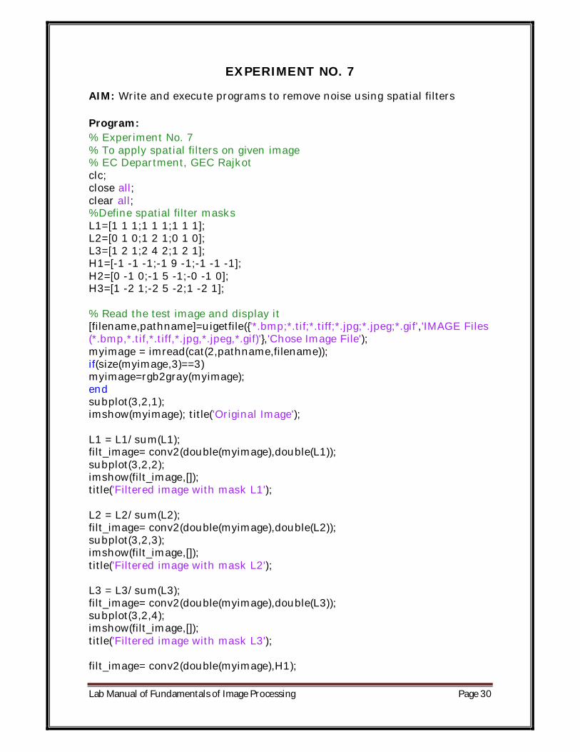
EXPERIMENT NO. 7

AIM: Write and execute programs to remove noise using spatial filters Program: % Experiment No. 7 % To apply spatial filters on given image % EC Department, GEC Rajkot clc; close all; clear all; %Define spatial filter masks L1=[1 1 1;1 1 1;1 1 1]; L2=[0 1 0;1 2 1;0 1 0]; L3=[1 2 1;2 4 2;1 2 1]; H1=[-1 -1 -1;-1 9 -1;-1 -1 -1]; H2=[0 -1 0;-1 5 -1;-0 -1 0]; H3=[1 -2 1;-2 5 -2;1 -2 1]; % Read the test image and display it [filename,pathname]=uigetfile({'*.bmp;*.tif;*.tiff;*.jpg;*.jpeg;*.gif','IMAGE Files (*.bmp,*.tif,*.tiff,*.jpg,*.jpeg,*.gif)'},'Chose Image File'); myimage = imread(cat(2,pathname,filename)); if(size(myimage,3)==3) myimage=rgb2gray(myimage); end subplot(3,2,1); imshow(myimage); title('Original Image'); L1 = L1/sum(L1); filt_image= conv2(double(myimage),double(L1)); subplot(3,2,2); imshow(filt_image,[]); title('Filtered image with mask L1'); L2 = L2/sum(L2); filt_image= conv2(double(myimage),double(L2)); subplot(3,2,3); imshow(filt_image,[]); title('Filtered image with mask L2'); L3 = L3/sum(L3); filt_image= conv2(double(myimage),double(L3)); subplot(3,2,4); imshow(filt_image,[]); title('Filtered image with mask L3'); filt_image= conv2(double(myimage),H1);


subplot(3,2,5); imshow(filt_image,[]); title('Filtered image with mask H1'); filt_image= conv2(double(myimage),H2); subplot(3,2,6); imshow(filt_image,[]); title('Filtered image with mask H1'); figure; subplot(2,2,1); imshow(myimage); title('Original Image'); % The command fspecial() is used to create mask % The command imfilter() is used to apply the gaussian filter mask to the image % Create a Gaussian low pass filter of size 3 gaussmask = fspecial('gaussian',3); filtimg = imfilter(myimage,gaussmask); subplot(2,2,2); imshow(filtimg,[]),title('Output of Gaussian filter 3 X 3'); % Generate a lowpass filter of size 7 X 7 % The command conv2 is used the apply the filter % This is another way of using the filter avgfilt = [ 1 1 1 1 1 1 1; 1 1 1 1 1 1 1; 1 1 1 1 1 1 1; 1 1 1 1 1 1 1; 1 1 1 1 1 1 1; 1 1 1 1 1 1 1; 1 1 1 1 1 1 1]; avgfiltmask = avgfilt/sum(avgfilt); convimage= conv2(double(myimage),double(avgfiltmask)); subplot(2,2,3); imshow(convimage,[]); title('Average filter with conv2()'); filt_image= conv2(double(myimage),H3); subplot(3,2,6); imshow(filt_image,[]); title('Filtered image with mask H3');


Exercise:

[1] Write mathematical expression of spatial filtering of image f(x,y) of size MN using mask W of size ab.

_______________________________________________________________________________________________________________________________________________________________________________________________________________________________________________________________________________________________________________________________________________________________________________________________________________________________________________________________________________________________________________________________________________________________________________________________________________________________________________________________________________________________________________________________________________________________________________________

[2] What is need for padding? What is zero padding? Why it is required? ___________________________________________________________________________________________________________________________________________________________________________________________________________________________________________________________________________________________________________________________________________________________________________________________________________________________________________________________________________________________________________________________________________________________________________________________________________________________________________________________________________________________________________________________________________________________________________________________________________________________________________________________________________________________________________________________________________________________________________________________________________________________________________________________________________

[3] What is the effect of increasing size of mask? ___________________________________________________________________________________________________________________________________________________________________________________________________________________________________________________________________________________________________________________________________________________________________________________________________________________________________________________________________________________________________


EXPERIMENT NO. 8

AIM: Write and execute programs for image frequency domain filtering

Introduction: In spatial domain, we perform convolution of filter mask with image data. In frequency domain we perform multiplication of Fourier transform of image data with filter transfer function.

Fourier transform of image f(x,y) of size MxN can be given by:

Where, u = 0,1,2 ……. M-1 and v = 0,1,2……N-1

Inverse Fourier transform is given by:

Where, x = 0,1,2 ……. M-1 and y = 0,1,2……N-1

Basic steps for filtering in frequency domain:

Pre-processing: Multiply input image f(x,y) by (-1)x+y to center the transform

Computer Discrete Fourier Transform F(u,v) of input image f(x,y) Multiply F(u,v) by filter function H(u,v) Result: H(u,v)F(u,v) Computer inverse DFT of the result Obtain real part of the result Post-Processing: Multiply the result by (-1)x+y


Program:

% EC Department, GEC Rajkot % Experiment 8 Program for frequency domain filtering clc; close all; clear all; % Read the image, resize it to 256 x 256 % Convert it to grey image and display it [filename,pathname]=uigetfile({'*.bmp;*.tif;*.tiff;*.jpg;*.jpeg;*.gif','IMAGE Files (*.bmp,*.tif,*.tiff,*.jpg,*.jpeg,*.gif)'},'Chose Image File'); myimg=imread(cat(2,pathname,filename)); if(size(myimg,3)==3) myimg=rgb2gray(myimg); end myimg = imresize(myimg,[256 256]); myimg=double(myimg); subplot(2,2,1); imshow(myimg,[]),title('Original Image'); [M,N] = size(myimg); % Find size %Preprocessing of the image for x=1:M for y=1:N myimg1(x,y)=myimg(x,y)*((-1)^(x+y)); end end % Find FFT of the image myfftimage = fft2(myimg1); subplot(2,2,2); imshow(myfftimage,[]); title('FFT Image'); % Define cut off frequency low = 30; band1 = 20; band2 = 50; %Define Filter Mask mylowpassmask = ones(M,N); mybandpassmask = ones(M,N); % Generate values for ifilter pass mask for u = 1:M for v = 1:N tmp = ((u-(M/2))^2 +(v-(N/2))^2)^0.5; if tmp > low mylowpassmask(u,v) = 0; end if tmp > band2 || tmp < band1; mybandpassmask(u,v) = 0;


end end end % Apply the filter H to the FFT of the Image resimage1 = myfftimage.*mylowpassmask; resimage3 = myfftimage.*mybandpassmask; % Apply the Inverse FFT to the filtered image % Display the low pass filtered image r1 = abs(ifft2(resimage1)); subplot(2,2,3); imshow(r1,[]),title('Low Pass filtered image'); % Display the band pass filtered image r3 = abs(ifft2(resimage3)); subplot(2,2,4); imshow(r3,[]),title('Band Pass filtered image'); figure; subplot(2,1,1);imshow(mylowpassmask); subplot(2,1,2);imshow(mybandpassmask);

Exercise:

[1] Instead of following pre-processing step in above program use fftshift function to shift FFT in the center. See changes in the result and write conclusion.

%Preprocessing of the image for x=1:M for y=1:N myimg1(x,y)=myimg(x,y)*((-1)^(x+y)); end end

Remove above step and use following commands. myfftimage = fft2(myimg);

myfftimage=fftshift(myfftimage);

Conclusion: ______________________________________________________________________________________________________________________________________________________________________________________________________________________________________________________________________________________________________________________________________________________________________________________________________________________________


_________________________________________________________________________________________________________________________________________________________________________________________________________________________________________________________________________________________________________________________________________________________

[2] Write a routine for high pass filter mask ___________________________________________________________________________________________________________________________________________________________________________________________________________________________________________________________________________________________________________________________________________________________________________________________________________________________________________________________________________________________________________________________________________________________________________________________________________________________________________________________________________________________________________________________________________________________________________________________________________________________________________________________________________________________________________________________________________________________________________________________________________________________________________________________________________ [2] Write a routine for high pass filter mask ___________________________________________________________________________________________________________________________________________________________________________________________________________________________________________________________________________________________________________________________________________________________________________________________________________________________________________________________________________________________________________________________________________________________________________________________________________________________________________________________________________________________________________________________________________________________________________________________________________________________________________________________________________________________________________________________________________________________________________________________________________________________________________________________________________


EXPERIMENT NO. 9

AIM: Write a program in C and MATLAB/SCILAB for edge detection using quick mask Introduction: MATLAB Code using standard function: % Experiment 9 % Program for edge detection using standard masks % Image Processing Lab, EC Department, GEC Rajkot clear all; [filename,pathname]=uigetfile({'*.bmp;*.tif;*.tiff;*.jpg;*.jpeg;*.gif','IMAGE Files (*.bmp,*.tif,*.tiff,*.jpg,*.jpeg,*.gif)'},'Choose Image'); A=imread(filename); if(size(A,3)==3) A=rgb2gray(A); end imshow(A); figure; BW = edge(A,'prewitt'); subplot(3,2,1); imshow(BW);title('Edge detection with prewitt mask'); BW = edge(A,'canny'); subplot(3,2,2); imshow(BW);;title('Edge detection with canny mask'); BW = edge(A,'sobel'); subplot(3,2,3); imshow(BW);;title('Edge detection with sobel mask'); BW = edge(A,'roberts'); subplot(3,2,4); imshow(BW);;title('Edge detection with roberts mask'); BW = edge(A,'log'); subplot(3,2,5); imshow(BW);;title('Edge detection with log '); BW = edge(A,'zerocross'); subplot(3,2,6); imshow(BW);;title('Edge detection with zerocorss'); MATLAB Code for edge detection using convolution in spatial domain % EC Department, GEC Rajkot % Experiment 9 % Program to demonstrate various point and edge detection mask % Image Processing Lab, EC Department, GEC Rajkot clear all; clc; while 1 K = menu('Choose mask','Select Image File','Point Detect','Horizontal line detect','Vertical line detect','+45 Detect','-45 Detect','ractangle Detect','exit') M=[-1 0 -1; 0 4 0; -1 0 -1;] % Default mask switch K case 1,


[namefile,pathname]=uigetfile({'*.bmp;*.tif;*.tiff;*.jpg;*.jpeg;*.gif','IMAGE Files (*.bmp,*.tif,*.tiff,*.jpg,*.jpeg,*.gif)'},'Chose GrayScale Image'); data=imread(strcat(pathname,namefile)); %data=rgb2gray(data); imshow(data); case 2, M=[-1 -1 -1;-1 8 -1;-1 -1 -1]; % Mask for point detection case 3, M=[-1 -1 -1; 2 2 2; -1 -1 -1]; % Mask for horizontal edges case 4, M=[-1 2 -1; -1 2 -1; -1 2 -1]; % Mask for vertical edges case 5, M=[-1 -1 2; -1 2 -1; 2 -1 -1]; % Mask for 45 degree diagonal line case 6, M=[2 -1 -1;-1 2 -1; -1 -1 2]; % Mask for -45 degree diagonal line case 7, M=[-1 -1 -1;-1 8 -1;-1 -1 -1]; case 8, break; otherwise, msgbox('Select proper mask'); end outimage=conv2(double(data),double(M)); figure; imshow(outimage); end close all %Write an image to a file imwrite(mat2gray(outimage),'outimage.jpg','quality',99); Exercise: Get mask for “Prewitt”, “Canny”, “Sobel” from the literature and write MATLAB/SCILAB program for edge detection using 2D convolution as used in practical number 3. __________________________________________________________________________________________________________________________________________________________________________________________________________________________________________________________________________________________________________________________________________________________________________________________________________________________________________________________________________________________________________________________________________________________________________________________________________________________________________________________________________________________________________________


________________________________________________________________________________________________________________________________________________________________________________________________________________________________________________________________________________________________________________________________________________________________________________________________________________________________________________________________________________________________________________________________________________________________________________________________________________________________________________________________________________________________________________________________________________________________________________________________________________________________________________________________________________________________________________________________________________________________________________________________________________________________________________________________________________________________________________________________________________________________________________________________________________________________________________________________________________________________________________________________________________________________________________________________________________________________________________________________________________________________________________________________________________________________________________________________________________________________________________________________________________________________________________________________________________________________________________________________________________________________________________________________________________________________________________________________________________________________________________________________________________________________________________________________________________________________________________________________________________________________________________________________________________________________________________________________________________________________________________________________________________________________________________________________________________________________________________________________________________________________________________________________________________________________________________________________________________________________________________________________________________________________________________________________________________________________________________________________________________________________________________________________________


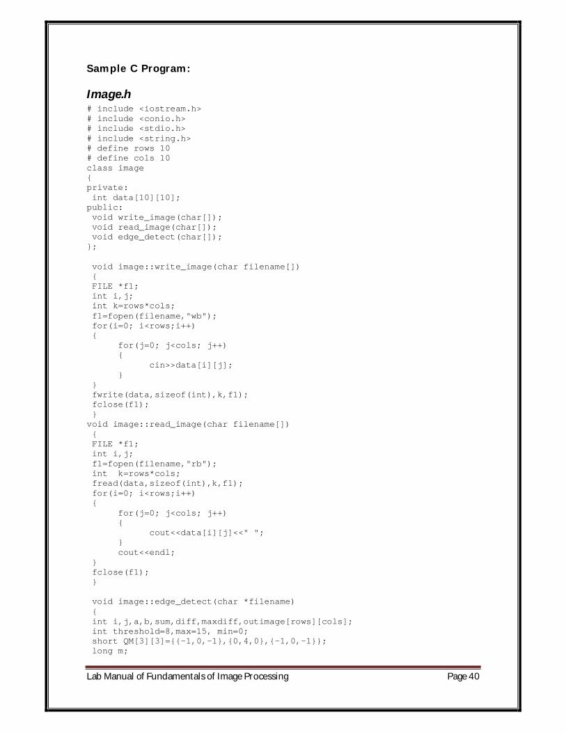
Sample C Program:

Image.h # include <iostream.h> # include <conio.h> # include <stdio.h> # include <string.h> # define rows 10 # define cols 10 class image { private: int data[10][10]; public: void write_image(char[]); void read_image(char[]); void edge_detect(char[]); }; void image::write_image(char filename[]) { FILE *f1; int i,j; int k=rows*cols; f1=fopen(filename,"wb"); for(i=0; i<rows;i++) { for(j=0; j<cols; j++) { cin>>data[i][j]; } } fwrite(data,sizeof(int),k,f1); fclose(f1); } void image::read_image(char filename[]) { FILE *f1; int i,j; f1=fopen(filename,"rb"); int k=rows*cols; fread(data,sizeof(int),k,f1); for(i=0; i<rows;i++) { for(j=0; j<cols; j++) { cout<<data[i][j]<<" "; } cout<<endl; } fclose(f1); } void image::edge_detect(char *filename) { int i,j,a,b,sum,diff,maxdiff,outimage[rows][cols]; int threshold=8,max=15, min=0; short QM[3][3]={{-1,0,-1},{0,4,0},{-1,0,-1}}; long m;


FILE *f1; f1=fopen(filename,"rb"); int k=rows*cols; for(i=0; i<rows;i++) { for(j=0; j<cols; j++) outimage[i][j]=0; } fread(data,sizeof(int),k,f1); for(i=1; i<rows-1;i++) { for(j=1; j<cols-1; j++) { sum=0; for(a=-1; a<2; a++) { for(b=-1;b<2;b++) sum=sum+data[i+a][j+b]*QM[a+1][b+1]; } if(sum<0) sum=0; if(sum>16) sum=15; outimage[i][j]=sum; } } cout<<"\nEdge detection using Quick mask:"<<endl; for(i=0; i<rows;i++) { for(j=0; j<cols; j++) printf("%02d ", outimage[i][j]); cout<<endl; } fclose(f1); }

Image.cpp # include "d:\image\image.h" void help(); void main(int argc, char* argv[]) { image I; char file_name[30]; clrscr(); if(argv[1]) { if(!argv[2]) { printf("Enter file name: "); scanf("%s",file_name); } else { strcpy(file_name,argv[2]); } if(!strcmp(argv[1],"write")) {I.write_image(file_name);} else if(!strcmp(argv[1],"read")) {I.read_image(file_name);} else if(!strcmp(argv[1],"edge")) { I.edge_detect(file_name); }


else if(!strcmp(argv[1],"hist")) { } else {help();} } else {help();} } void help() { printf("\n\t\t Image Processing Tutorial !"); printf("\t\t\tUsage :\n"); printf("\t\t\timage <operation> <filename>\n"); printf("\t\t\tFor example :\n "); printf("\t\t\timage write data : To write image in \"data\" file\n"); printf("\n\t\t\tOther Operations:\n"); printf("\n\t\t read: read image\n"); printf("\n\t\t edge : Edge detection\n"); printf("\n\t\t hist : display histogram of image\n"); }

Output:

Original Image of size 1010: Edge detection after applying quick mask:

1 1 1 1 1 1 1 1 1 1

1 1 1 1 1 1 1 1 1 1

1 1 1 1 1 1 1 1 1 1

1 1 1 9 9 9 9 1 1 1

1 1 1 9 9 9 9 1 1 1

1 1 1 9 9 9 9 1 1 1

1 1 1 9 9 9 9 1 1 1

1 1 1 1 1 1 1 1 1 1

1 1 1 1 1 1 1 1 1 1

1 1 1 1 1 1 1 1 1 1

Exercise:

[1] Modify above program for edge detection using kirsch, prewitt & sobel mask

[2] Add member function LPF() to image class for spatial filtering of given image

Hint: Use following low pass convolution mask for low pass filtering

1/6 *

010121010

00 00 00 00 00 00 00 00 00 00

00 00 00 00 00 00 00 00 00 00

00 00 00 00 00 00 00 00 00 00

00 00 00 15 16 16 15 00 00 00

00 00 00 16 00 00 16 00 00 00

00 00 00 16 00 00 16 00 00 00


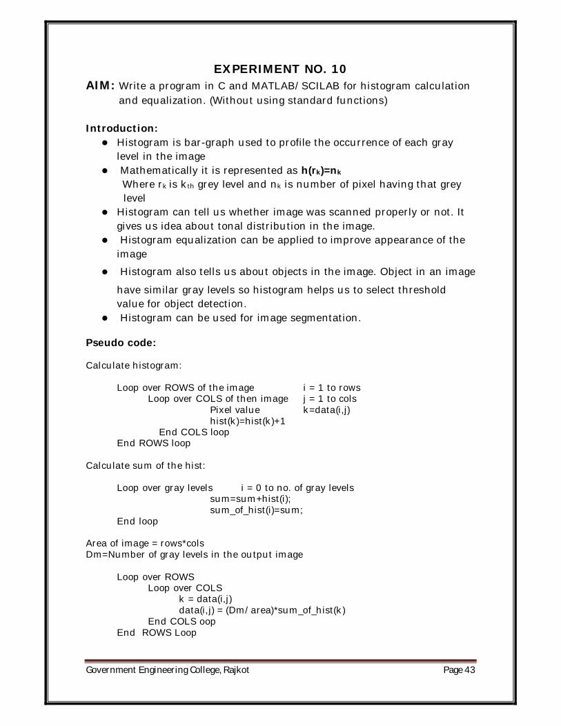
EXPERIMENT NO. 10 AIM: Write a program in C and MATLAB/SCILAB for histogram calculation and equalization. (Without using standard functions) Introduction:

Histogram is bar-graph used to profile the occurrence of each gray level in the image

Mathematically it is represented as h(rk)=nk Where rk is kth grey level and nk is number of pixel having that grey level

Histogram can tell us whether image was scanned properly or not. It gives us idea about tonal distribution in the image.

Histogram equalization can be applied to improve appearance of the image

Histogram also tells us about objects in the image. Object in an image

have similar gray levels so histogram helps us to select threshold value for object detection.

Histogram can be used for image segmentation. Pseudo code: Calculate histogram: Loop over ROWS of the image i = 1 to rows Loop over COLS of then image j = 1 to cols Pixel value k=data(i,j) hist(k)=hist(k)+1 End COLS loop End ROWS loop Calculate sum of the hist: Loop over gray levels i = 0 to no. of gray levels sum=sum+hist(i); sum_of_hist(i)=sum; End loop Area of image = rows*cols Dm=Number of gray levels in the output image Loop over ROWS Loop over COLS k = data(i,j) data(i,j) = (Dm/area)*sum_of_hist(k) End COLS oop End ROWS Loop


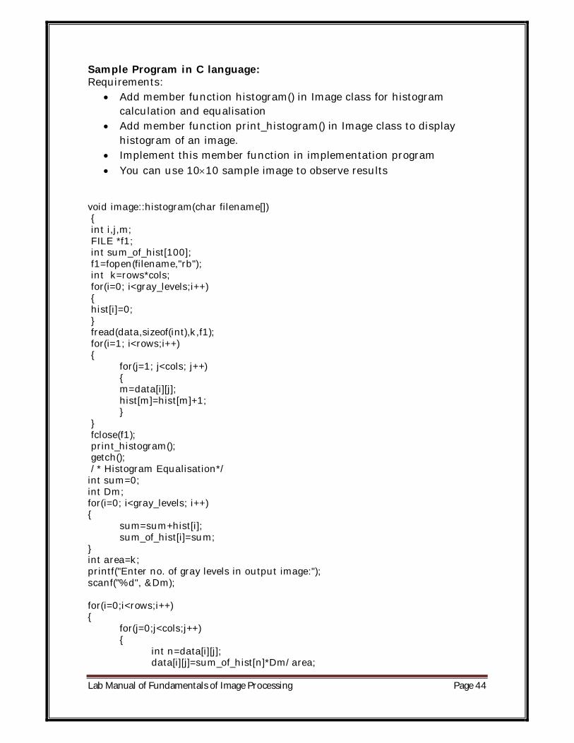
Sample Program in C language: Requirements:

Add member function histogram() in Image class for histogram calculation and equalisation

Add member function print_histogram() in Image class to display histogram of an image.

Implement this member function in implementation program You can use 1010 sample image to observe results

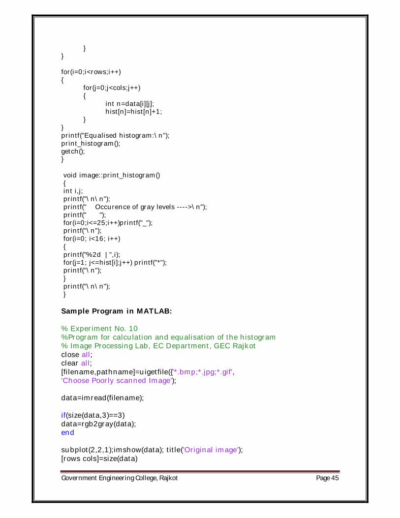
void image::histogram(char filename[]) { int i,j,m; FILE *f1; int sum_of_hist[100]; f1=fopen(filename,"rb"); int k=rows*cols; for(i=0; i<gray_levels;i++) { hist[i]=0; } fread(data,sizeof(int),k,f1); for(i=1; i<rows;i++) { for(j=1; j<cols; j++) { m=data[i][j]; hist[m]=hist[m]+1; } } fclose(f1); print_histogram(); getch(); /* Histogram Equalisation*/ int sum=0; int Dm; for(i=0; i<gray_levels; i++) { sum=sum+hist[i]; sum_of_hist[i]=sum; } int area=k; printf("Enter no. of gray levels in output image:"); scanf("%d", &Dm); for(i=0;i<rows;i++) { for(j=0;j<cols;j++) { int n=data[i][j]; data[i][j]=sum_of_hist[n]*Dm/area;


} } for(i=0;i<rows;i++) { for(j=0;j<cols;j++) { int n=data[i][j]; hist[n]=hist[n]+1; } } printf("Equalised histogram:\n"); print_histogram(); getch(); } void image::print_histogram() { int i,j; printf("\n\n"); printf(" Occurence of gray levels ---->\n"); printf(" "); for(i=0;i<=25;i++)printf("_"); printf("\n"); for(i=0; i<16; i++) { printf("%2d |",i); for(j=1; j<=hist[i];j++) printf("*"); printf("\n"); } printf("\n\n"); } Sample Program in MATLAB: % Experiment No. 10 %Program for calculation and equalisation of the histogram % Image Processing Lab, EC Department, GEC Rajkot close all; clear all; [filename,pathname]=uigetfile({'*.bmp;*.jpg;*.gif', 'Choose Poorly scanned Image'); data=imread(filename); if(size(data,3)==3) data=rgb2gray(data); end subplot(2,2,1);imshow(data); title('Original image'); [rows cols]=size(data)


myhist=zeros(1,256); % Calculation of histogram for i=1:rows for j=1:cols m=double(data(i,j)); myhist(m+1)=myhist(m+1)+1; end end subplot(2,2,2);bar(myhist); title('Histogram of original image'); sum=0; %Cumulative values for i=0:255 sum=sum+myhist(i+1); sum_of_hist(i+1)=sum; end area=rows*cols; %Dm=input('Enter no. of gray levels in output image: '); Dm=256; for i=1:rows for j=1:cols n=double(data(i,j)); data(i,j)=sum_of_hist(n+1)*Dm/area; end end %Calculation of histogram for equalised image for i=1:rows for j=1:cols m=double(data(i,j)); myhist(m+1)=myhist(m+1)+1; end end subplot(2,2,3);bar(myhist);title('Equalised Histogram'); subplot(2,2,4);imshow(data); title('Image after histogram equalisation');


Program output:

Original image

0 100 200 3000

500

1000

1500Histogram of original image

0 100 200 3000

1000

2000

3000Equalised Histogram Image after histogram equalisation

Note for the students: Results on images are not shown in every experiment the lab manual (Except Experiment 10). Students are advised to run program on test images and get print out of original and processed images for the sample programs and exercise programs

Fundamentals of Image Processing Laboratory Manual

Documents

Transcript of Fundamentals of Image Processing Laboratory Manual