Justifying Kubo’s formula for gapped systems at zerotemperature: a brief review and some new results

Joscha Henheik and Stefan Teufel∗

February 21, 2020

Abstract

We first review the problem of a rigorous justification of Kubo’s formula fortransport coefficients in gapped extended Hamiltonian quantum systems at zerotemperature. In particular, the theoretical understanding of the quantum Halleffect rests on the validity of Kubo’s formula for such systems, a connection thatwe review briefly as well. We then highlight an approach to linear response theorybased on non-equilibrium almost-stationary states (NEASS) and on a correspond-ing adiabatic theorem for such systems that was recently proposed and workedout by one of us in [51] for interacting fermionic systems on finite lattices. In thesecond part of our paper we show how to lift the results of [51] to infinite systemsby taking a thermodynamic limit.

Keywords. Linear response theory, Kubo formula, adiabatic theorem, non-equilibrium stationary state.

AMS Mathematics Subject Classification (2010). 81Q15; 81Q20; 81V70.

1 Introduction

In this article we discuss the problem of “proving Kubo’s formula” for gapped extendedquantum systems at zero temperature, with transport theory in (topological) insulatorsas the main application in mind. Note that in this context various expressions are re-ferred to as “Kubo’s formula”, namely the general Kubo formula (KF) for the responsecoefficients of arbitrary observables on the one hand, and the double commutator for-mula (DCF) for the current response on the other. Thus also different mathematicalproblems have been subsumed under the label “proving Kubo’s formula”. As to be de-tailed below, much attention has been given to the problems of showing that KF impliesDCF for the conductance or conductivity and to showing that DCF implies (fractional)

∗Fachbereich Mathematik, Eberhard-Karls-Universitata Auf der Morgenstelle 10, 72076 Tubingen, Germanya E-mail: stefan.teufel@uni-tuebingen.de

1

arX

iv:2

002.

0866

9v1

[m

ath-

ph]

20

Feb

2020

quantisation of Hall conductance resp. conductivity (see e.g. the recent review [4] andreferences therein). Less work has been directed towards a rigorous justification of KFfor such systems starting from first principles. As the present work will be mainlyconcerned with this second problem, let us briefly recall the main challenges such ajustification faces.

In the context of Hamiltonian quantum systems, the linear response formalism forstatic perturbations answers the following question: How does a system described bya Hamiltonian H0 that is initially in an equilibrium state ρ0 respond to a small staticperturbation εV ? Or somewhat more precisely: What is the change

tr(ρεA)− tr(ρ0A) = ε σA + o(ε)

of the expectation value of an observable A caused by the perturbation εV at lead-ing order in its strength |ε| � 1? Here ρε denotes the state of the system after theperturbation has been turned on adiabatically and σA is called the linear response co-efficient for A. The answer clearly hinges on the problem of determining ρε. Whilein some situations one expects that ρε remains an equilibrium state also for the per-turbed Hamiltonian Hε = H0 + εV , Kubo [33] developed linear response theory forsituations, where the system is driven into a non-equilibrium state ρε. As emphasizedby Simon in “Fifteen problems in mathematical physics” [49], the latter situation typ-ically occurs in applications to transport theory and this deviation from equilibriummakes the justification of Kubo’s formula a difficult mathematical problem that is stillnot solved in satisfactory generality. Also in this work we will not even discuss the gen-eral problem but instead focus on the rather special situation of particle transport ingapped Hamiltonian systems (i.e. insulators) at zero temperature. In this case all cur-rents are dissipation-less (direct currents vanish, while Hall currents are geometric andthus dissipation-less) and, as we will argue, a rigorous justification of Kubo’s formulapurely on the level of Hamiltonian dynamics without involving any form of dissipationis possible.

The linear response formalism (which we briefly review in Section 2) rests on theassumption that a small perturbation (|ε| � 1) that is adiabatically switched on altersthe initial equilibrium state of a system only a little (ρε ≈ ρ0). In a nutshell, theproblem of proving Kubo’s formula will thus be to prove that a system initially inan equilibrium state ρ0 is adiabatically driven by a small perturbation into a non-equilibrium state ρε close to ρ0. This problem goes beyond standard perturbationtheory, since the small perturbation acts over a very long (macroscopic) time, and thusthis assumed small change of the state is not a trivial consequence of the smallness ofthe perturbation; instead, proving this assumption requires an adiabatic type theorem.However, even if we work at zero temperature and assume that ρ0 is the gapped groundstate of H0, the problem goes also beyond standard adiabatic theory. Indeed, thestandard adiabatic theorem is only of rather limited use here for three reasons. First,it is only applicable as long as the perturbation does not close the spectral gap; thenit asserts that ρε equals the gapped ground state of Hε = H0 + εV and thus remainsan equilibrium state. But, as emphasized before, in transport theory this assumption

2

is often not satisfied and ρε is expected to be a non-equilibrium state; for example,the band gap in a typical insulator is of order 10eV, while a macroscopic sample ofsuch a material stays insulating for applied voltages that are larger by many orders ofmagnitude. Secondly, even if one assumes that the spectral gap above the ground stateremains open, the usual adiabatic theorem is not directly applicable for two reasons:its standard version estimates the difference between ρε and the ground state of Hε

in the operator norm; in order to obtain the required estimates with respect to localtrace norms, additional and potentially non-trivial propagation estimates need to beestablished. Finally, for extended interacting systems the approximation error in theadiabatic theorem deteriorates when the system size grows and it can not be appliedfor macroscopic systems. As a consequence, proving Kubo’s formula even in the simplecase of gapped Hamiltonian systems at zero temperature has been an open problem ofmathematical physics for quite some time.

Recently Bachmann et al. [8] proved an adiabatic theorem for extended interactinglattice systems with error estimates for local traces that are uniform in the system size,thereby solving the second and third problem. In [51] one of us solved also the firstproblem by proving a version of the adiabatic theorem that remains valid even when theperturbation closes the spectral gap. In a nutshell, the idea in [51] is that perturbationsby slowly varying but not small potentials (modelling small fields acting on large regionsof space) close the spectral gap, but leave intact a local gap structure, thereby drivingthe system into a non-equilibrium almost-stationary state (NEASS). The adiabatictheorem in [51] states that if such a perturbation is switched on adiabatically, thenthe state of the system evolves into a uniquely determined NEASS associated with theperturbed Hamiltonian that has an explicit asymptotic expansion in powers of ε; [51]also applies to interacting extended lattice systems and provides error estimates thatare uniform in the system size. This NEASS approach was motivated by and is basedon ideas which we called space-adiabatic perturbation theory almost 20 years ago, seefor example [45, 46, 52], and allows not only to prove validity of Kubo’s formula, butalso to evaluate it in a straightforward way. The latter point is illustrated in [37], wherewe compute the spin-Hall conductivity in topological insulators.

The rest of this note is structured as follows. Section 2 first recalls the formal deriva-tion of Kubo’s formula in the context of Hamiltonian quantum systems and highlightsthe different mathematical problems arising from it. In particular, we try to clarify thedifferent meanings that the phrase “proving Kubo’s formula” acquired in the past. Wethen try to provide a concise and structured overview of the mathematical literature inthis area.

In Section 3, we discuss the extension of the results in [51] to infinite systems. Weshow that NEASSs exist as states on the quasi-local algebra of the infinite systems andare automorphically equivalent to the ground state of the unperturbed Hamiltonian,then state a version of a corresponding adiabatic theorem, and finally obtain from therea rigorous justification of an infinite volume version of Kubo’s formula. Proofs and gen-eralizations of the results presented in Section 3 will be given elsewhere [29].

3

Acknowledgements: I (S.T.) would like to thank Yosi Avron, Sven Bachmann, Horia

Cornean, Giuseppe De Nittis, Wojciech De Roeck, Alexander Elgart, Martin Fraas, Jurg

Frohlich, Vojkan Jaksic, Max Lein, Giovanna Marcelli, Domenico Monaco, Gianluca Panati,

Marcello Porta, and Marcel Schaub for sharing their insights and ideas about this complex

topic with me and/or for critically commenting on some of my own ideas.

2 Linear response: heuristics, problems, and results

In this section we first recall the standard derivation of the general Kubo formula forHamiltonian quantum systems and static perturbations. We then highlight the stepsin the derivation that require a more careful justification. In Subsections 2.1–2.3 wediscuss some existing (mostly) mathematical literature addressing the different aspectsof the problem.

Consider a quantum system described by the self-adjoint Hamiltonian H0 on someHilbert space H that is bounded from below and subject to a perturbation εV with|ε| � 1 such that also Hε = H0 + εV is self-adjoint. The simplest example to keepin mind would be a single atom perturbed by a small external field, while relevant totransport theory are for example Hamiltonians describing fermions on a lattice withshort range interactions subject to a perturbation by a small external field. Assumethat initially, i.e. before the perturbation is applied, the system is in an equilibriumstate ρ0, i.e. ρ0 ∼ e−βH0 if the temperature T = (kBβ)−1 is positive, or ρ0 equal to theground state of H0 if the temperature is zero. The objective of linear response theoryis to determine the change of expectation values of observables A linear in the strengthof the applied perturbation,

〈A〉ρε − 〈A〉ρ0 := tr(ρεA)− tr(ρ0A) = ε σA + o(ε) . (2.1)

Here ρε is the state of the system after the perturbation has been turned on and σA isthe linear response coefficient for the observable A with respect to the perturbation V .The question is now: What is the state ρε? To answer this question, one gets back tofirst principles and models the time-dependent switching of the perturbation by solvingthe corresponding time-dependent Schrodinger equation. Assume that the switchingoccurs during the time interval [−1, 0] and the Hamiltonian at time t is

Hε(t) = H0 + f(t) εV

with a smooth switching function f : R → [0, 1] such that f(t) = 0 for t ≤ −1 andf(t) = 1 for t ≥ 0. Then the state of the system at time t is given by the solution ρε(t)to the time-dependent Schrodinger equation (we choose units where ~ = 1)

i ddtρε(t) = [Hε(t), ρε(t)] with ρε(t) = ρ0 for all t ≤ −1 . (2.2)

Hence, if one measures the observable A at time t ≥ 0 after the perturbation is fullyswitched on, one should use the state ρε = ρε(t) in (2.1). Standard time-dependent

4

perturbation theory yields

ρε(t) = ρ0 − ε i

∫ t

−∞f(s) eiH0(s−t) [V, ρ0] e−iH0(s−t)ds+R(ε, f, t) ,

with a remainder term R(ε, f, t) that is o(ε) in a sense to be discussed, and thus

〈A〉ρε(t) − 〈A〉ρ0 = −ε i

t∫−∞

f(s) tr(eiH0(s−t) [V, ρ0] e−iH0(s−t) A

)ds + tr(R(ε, f, t)A) .

As the perturbation acts only during a finite time-interval, one might expect1 thatlimε→0 ε

−1tr(R(ε, f, t)A) = 0 and thus that (2.1) indeed holds with

σA = σfA(t) = −i

t∫−∞

f(s) tr(eiH0(s−t) [V, ρ0] e−iH0(s−t) A

)ds . (2.3)

However, the response coefficient σfA defined in this way would generically depend on theswitching function f and also on the time t, even for t ≥ 0. In particular, one could nothope for a simple universal formula for it. But one expects in many relevant situationsthat response coefficients are independent of experimental details like the exact way ofhow to turn on an external perturbation or the time at which the measurement takesplace after the perturbation has been turned on. Thus, from a practical view-point,(2.3) is clearly an unsatisfactory definition.

One solution to this problem is provided by taking an adiabatic limit: Since the time-scale on which the perturbation is applied is typically long compared to the internaltime-scales of the quantum system, one considers (2.2) in the adiabatic limit, i.e. oneconsiders the limit of slow switching. Introducing the adiabatic parameter 0 < η � 1,the adiabatic Schrodinger equation

i ddtρε,η(t) = [Hε(ηt), ρε,η(t)] with ρε,η(t) = ρ0 for all t ≤ −1/η , (2.4)

describes the same switching process but stretched to the longer time-interval [−1/η, 0].The hope is now that in the adiabatic regime η � 1 the response coefficient

σf,ηA (t) := −i

t∫−∞

f(ηs) tr(eiH0(s−t) [V, ρ0] e−iH0(s−t) A

)ds (2.5)

becomes independent of f , η, and also of t, whenever t ≥ 0. Replacing moreoverthe generic switch function f by an exponential function and evaluating at t = 0,the integral in (2.5) becomes the Laplace transform of the Heisenberg time-evolution

1As to be discussed below, already the proof of this step can be technically quite demanding forseveral reasons, one being the control of the trace norm of R(ε, f, t) instead of the operator norm.

5

and thus the resolvent of its generator, the Liouvillian V 7→ LH0(V ) := [H0, V ]. Onethereby arrives at the general Kubo formula (KF) for the linear response coefficient ofan observable A,2

σKuboA := −i lim

η→0+

0∫−∞

eηs tr(eiH0s [V, ρ0] e−iH0sA

)ds

= limη→0+

tr((LH0 − iη)−1([V, ρ0])A

). (2.6)

This heuristic derivation immediately leads to two questions:

(A) Under which assumptions on the model (Hamiltonian H0, perturbation V , ob-servable A, initial state ρ0) does the right hand side of (2.6) lead to a well definednumber σKubo

A and how can it be evaluated more explicitly for current observablesto obtain, for example, the double-commutator formula (DCF) sometimes calledKubo-Streda formula?

(B) Assuming that (2.6) leads to a well defined number σKuboA , under which additional

assumptions on the model (Hamiltonian H0, perturbation V , observable A) isσKuboA a universal linear response coefficient? I.e., when is it true that for all

smooth switching functions f and all times t ≥ 0 one has

〈A〉ρε,η(t) − 〈A〉ρ0 = ε · σKuboA +R(ε, η, f, t) (2.7)

with

limε→0

supη∈Iε

R(ε, η, f, t)

ε= 0 (2.8)

for some interval Iε ⊂ (0,∞) of admissible time-scales η. As we will argue,for dissipation-less currents, because of tunnelling, it is not expected that thesupremum in (2.8) can be replaced by a limit η → 0 in general, cf. also Theorem 3.3and the remark afterwards. Moreover, for extended interacting systems one alsoneeds to show that (2.8) holds uniformly in the number N of particles, i.e. that

limε→0

supη∈Iε

supN∈N

R(ε, η, f,N, t)

ε= 0 (2.9)

as otherwise the estimate may deteriorate and become worthless in the thermo-dynamic limit.

From now on we only discuss the situation of gapped Hamiltonians at zero temperature.Still, the mathematical difficulty of both problems (A) and (B) depends very much onvarious details of the specific model under consideration:

2It should be noted that in general the limit η → 0 in (2.6) need not exist and sometimes η > 0is taken as an empirical parameter that controls the strength of dissipation in the system. However,in our setting of gapped systems at zero temperature the limit η → 0 in (2.6) is expected and can beshown to exist in many models.

6

(i) Does H0 describe particles on a lattice or in the continuum? Lattice Hamiltoniansare typically bounded self-adjoint operators, while continuum Schrodinger oper-ators are unbounded. The same distinction then holds for the associated currentobservables.

(ii) Are the particles interacting or non-interacting? For non-interacting particles onecan consider the one-body Hamiltonian on an infinite domain; then controllingestimates uniformly in the number of particles is no issue. Interacting systemsneed to be first analyzed on finite domains and the thermodynamic limit becomesa nontrivial step.

(iii) Is H0 assumed to have a spectral gap at the Fermi energy resp. above the groundstate, or only a mobility gap? The first situation occurs typically if H0 is (asmall perturbation of) a periodic non-interacting Hamiltonian, while the secondsituation is expected to occur for generic random Hamiltonians.

(iv) Does the perturbation V close the spectral resp. mobility gap? Perturbing by aconstant electric field E, i.e. by a linear potential V (x) = x ·E will typically closeall spectral or mobility gaps of H0, no matter how small ε is. On the other hand,for any bounded perturbation V the gap remains open for ε small enough.

(v) Is the observable under consideration local or extensive? In the latter case somenotion of trace per unit volume needs to be established in order to handle infinitedomains or the thermodynamic limit.

All aspects in the above list have been addressed in some form or another for prob-lem (A). Although (A) is not the main focus of this note, we briefly sketch the problemin Subsection 2.1 and mention some literature. Problem (B) has attracted much lessattention. In Subsection 2.2 we first discuss the problem on a heuristic level and thenmention the few existing mathematical results. Subsection 2.3 collects references tofurther mathematical works in the context of linear response for extended quantumsystems.

2.1 Evaluating Kubo’s formula for the current observable

Evaluating Kubo’s formula (2.6) for current observables can be tricky. To see this, firstnote that on finite domains Λ ⊂ Rd the total current response always vanishes becauseof conservation of total charge. This follows also easily by evaluating Kubo’s formula:Let the perturbation V be the potential of a constant electric field of unit strengthpointing in the ith coordinate direction, i.e. V = Xi with Xi the ith component ofthe position operator and the observable A the current in the jth coordinate direction,

7

A = Jj := i[H0, Xj] = iLH0(Xj). Then a naive evaluation of (2.6) yields

σKuboij = i lim

η→0tr((LH0 − iη)−1([Xi, ρ0])LH0(Xj)

)= i lim

η→0tr([Xi, ρ0](LH0 + iη)−1(LH0(Xj))

)(2.10)

= i tr ([Xi, ρ0]Xj) = −i tr (ρ0 [Xi, Xj]) = 0 .

Whenever Xi and Xj are trace class, which is the case in lattice models on boundeddomains, then the above computation is perfectly valid and, as expected, the currentresponse vanishes. In order to see a nontrivial current response, one thus either workson an infinite domain, or on a domain with a torus geometry, or considers only local cur-rents. In the latter cases, to avoid finite size or boundary effects, one eventually wouldlike to take a thermodynamic limit as well. Thus, in all cases, additional mathematicalchallenges appear when trying to evaluate Kubo’s formula.

2.1.1 The double-commutator formula and quantization for non-interactingsystems on infinite domains

For non-interacting fermionic systems one can directly work with the one-body Hamil-tonian H0. Then, at zero temperature, the initial state is given by the correspondingFermi projection ρ0 = χ(−∞,µ](H0). In order to evaluate extensive observables like thecurrent as densities, one needs to establish the notion of a trace per unit volume τ whichis cyclic for operators in suitable trace or Hilbert-Schmidt classes. For random ergodicsystems, a corresponding mathematical formalism has been worked out by Bellissard,van Elst, and Schulz-Baldes [11] in the discrete case (see also the work of Aizenman andGraf [2] for a different perspective), by Bouclet, Germinet, Klein, and Schenker [12] forrandom Schrodinger operators, and by De Nittis and Lein [18] for a large abstract classof operators including all previous ones.

Even in the discrete case the position operators are unbounded and, in particular,not in any trace per unit volume class. As a consequence, the naive computation(2.10) fails to produce the correct result. For a correct evaluation of Kubo’s formulaone observes that, since ρ0 is now a projection, in the first line of (2.10) only theoff-diagonal part

XODi := ρ0Xi(1− ρ0) + (1− ρ0)Xiρ0

contributes, which can be shown to be periodic resp. covariant for periodic resp. randomergodic Hamiltonians. And then simple algebra shows that also Xj can be replaced byXODj . From this one finds as in (2.10) the celebrated double-commutator formula for

the conductivity tensor

σKuboij = −i τ

(ρ0

[XODi , XOD

j

])= i τ (ρ0 [[ρ0, Xi], [ρ0, Xj]]) . (2.11)

A version of this formula in terms of an integral of derivatives of Bloch functions overthe Brillouin torus appeared first in the work of Thouless, Kohmoto, Nightingale, andden Nijs [53] for periodic Hamiltonians. The authors of [53] realized that the resulting

8

expression is quantized, leading to the first understanding of the integer quantum Halleffect in terms of a microscopic model and to a Nobel prize in physics for David Thoulessin 2016. The explicit form of (2.11) in terms of a double commutator was first given byAvron, Seiler, and Simon [6] and its interpretation as the Chern number of a complexline bundle over the Brillouin torus by Simon in [48]. One should mention that atthe same time as [53] independently also Streda [50] found a formula for the Hallconductivity from which he could conclude quantization (see also Subsection 2.3).

However, while expressing the Hall conductivity explicitly in terms of a topologicalquantity was a major step towards a microscopic understanding of the integer quantumHall effect, an important ingredient was still missing: In order to understand the quan-tized plateaux appearing in experiments, disorder and the resulting Anderson-localizedstates appearing in the gap need to be taken into account. On a rigorous level for infi-nite domains, this was first achieved by Bellissard, van Elst, and Schulz-Baldes in [11]based on the earlier idea by Bellissard [10] to use the framework of non-commutativegeometry for extending the work of TKNN to non-periodic systems with mobility gap.More precisely, in [11] not only a C∗-algebraic framework is developed that allows toderive the double-commutator formula from Kubo’s formula and to show that it agreeswith Streda’s formula, but it is also shown that if the Fermi energy lies in a mobilitygap, then the double-commutator formula leads to a quantized result for the Hall con-ductivity and a zero result for the direct conductivity. To understand why the latterremains exponentially small as a function of the inverse temperature when droppingthe idealization of zero temperature is an important problem in its own, cf. [3].

Bouclet, Germinet, Klein, and Schenker [12] set up linear response theory and derivethe double-commutator formula for random Schrodinger operators. Here the main chal-lenge was to develop the algebraic-analytic framework for defining the trace per unit vol-ume and associated trace ideals. The authors also derive Kubo’s formula starting fromtime dependent perturbation theory, however, with two caveats: First, (2.8) is shownonly for fixed adiabatic parameter η. Uniformity in η for systems with mobility gap isstill a completely open problem. Second, the linear time-dependent perturbing poten-tial εf(t)Xi is replaced by a time-dependent vector potential A(t) = ε

∫ t−∞ f(s)ds ei.

While formally the two problems are related by a time-dependent gauge-transformation,translating their results back to the original setting is technically demanding because ofsubtle domain issues. Moreover, as we will argue below, understanding linear responsein the gauge with linear electric potential also sheds some light on the physics.

Based on the mathematical framework developed in [12], Klein, Lenoble, and Muller[32] also evaluated Kubo’s formula for the AC-conductivity and rigorously found Mott’sformula for its asymptotic behavior at low frequencies. Finally, De Nittis and Lein[18] further generalized the framework of [12] to cover an extremely general class ofunbounded operators.

9

2.1.2 The double-commutator formula and quantization for interacting sys-tems

For interacting systems one starts out with a family of Hamiltonians HΛ0 parametrized

by finite domains Λ. As explained above, if one is interested in a non-trivial currentresponse, Λ should be taken as a torus, i.e. the cube [−L/2, L/2]d is understood withsuitable periodic boundary conditions. One fixes the density % by relating the numberof particles to the volume |Λ| = Ld as N/|Λ| = %. The initial equilibrium state atzero temperature is now the ground state ρ0 of H0. In all the mathematical resultsto be discussed in the following, one assumes that the ground state is separated bya gap from the remainder of the spectrum uniformly in the size of the system. Thisassumption corresponds to the gap assumption for the one-body Hamiltonian and nomathematical results analogous to the ones presented below exist for interacting systemswith a mobility gap above the ground state.

Historically the first work on understanding quantization of charge transport interms of a microscopic model for interacting particles is Niu and Thouless [43]. Theyderive an expression for the transported charge in one cycle from the adiabatic responseof such a system under periodic driving by an external field. This expression has againthe interpretation of a Chern number of a line bundle over a two-dimensional torus. Onedirection on the torus is time (one period), the other is a complex phase characterizingthe boundary conditions. Only by averaging over time and over boundary conditionsquantization can be concluded. However, assuming that in the thermodynamic limit thevalue of the transported charge is independent of the chosen boundary condition, alsoquantization of transported charge without averaging would follow for large systems.

Shortly after, in 1985 Niu, Thouless, and Wu [44], and independently Avron andSeiler [5] formulated similar arguments showing quantization of a suitably averaged Hallconductivity resp. conductance for interacting electron systems. While Niu et al. con-sider the conductivity and average over a family of boundary conditions parametrizedby a two-torus, Avron and Seiler come back to Laughlin’s original argument for theconductance and average over a flux torus. In both works the averaging over the cor-responding torus yields again a double-commutator formula for the conductivity resp.conductance that has the geometric meaning of a Chern number and implies quantiza-tion. Also, in both works the validity of Kubo’s formula (2.6) is taken for granted.

Only 30 years later Hastings and Michalakis [27] were able to prove rigorously thatin the case of Hall conductance the averaging over the flux torus is not needed for largesystems. More precisely, they show that the Hall conductivity for a gapped Hamiltonianis quantized up to terms that are asymptotically smaller than any inverse power of thesize L of the system. Recently, the argument was considerable simplified and generalizedby Bachmann, Bols, De Roeck, and Fraas [7].

A different and more general perspective on the (fractional) quantum Hall effect wasdeveloped in a series of works by Frohlich and collaborators (see e.g. [23] and the recentreview [22]). They show that the large-scale properties of two-dimensional electrongases with vanishing longitudinal resistivity are governed by effective Chern-Simons

10

gauge theories. From the latter fact all the phenomenology of (fractional) quantum Hallsystems can be derived. The assumption of vanishing longitudinal resistivity (which isequivalent to vanishing longitudinal conductivity in two-dimensional systems) followsfrom Kubo’s formula when assuming a (mobility) gap. Thus proving Kubo’s formulaseems relevant also to their approach.

Yet another route to proving quantization of Hall conductivity in interacting latticesystems was taken by Giuliani, Mastropietro, and Porta [24]. They start from a gappedperiodic system of non-interacting fermions (for which quantization of Hall conductivityis understood since the work of Thouless et al. [53]) and use cluster expansion techniquesto show that the Hall conductivity does not change when a sufficiently small interactionbetween the electrons is added to the Hamiltonian. While validity of Kubo’s formulais taken for granted also here, this approach does not assume stability of the spectralgap under small perturbations.

2.2 Justifying Kubo’s formula for gapped Hamiltonian sys-tems

In this section we address Problem (B) in some more detail. We start with someheuristics and then briefly describe existing results.

2.2.1 Justifying Kubo’s formula: Heuristics

Under what conditions do we expect Kubo’s formula (2.6) to yield a universal responsecoefficient in the sense that (2.7) holds uniformly as expressed in (2.8) or (2.9)? The ideabehind the adiabatic switching procedure is that for 0 < η � 1 the state ρε,η(t) of thesystem (as determined by the Schrodinger equation (2.4)) follows closely a curve Πε(t)of (almost)-stationary states for the instantaneous Hamiltonians Hε(t) = H0 + f(t)εVat all times. If Πε(t) depends only on the instantaneous Hamiltonian Hε(t) and noton f and η, this would explain why the response of the system after the perturbationεV is fully applied is independent of time t ≥ 0 and of the details of the switchingprocedure, i.e. of f and η. Moreover, the derivation of Kubo’s formula also rests on theassumption that ρε,η(t) deviates only little from ρ0. Hence, for linear response theoryto work as intended, there should be non-equilibrium (almost-)stationary states Πε(t)for Hε(t) (let us call them NEASS in the following) that are small perturbations of ρ0

such that ρε,η(t) ≈ Πε(t) in an appropriate sense for η sufficiently small.If the perturbation εV does not close the spectral gap of H0, then the instantaneous

ground state of Hε(t) is the natural candidate for Πε(t). Indeed, in this case theadiabatic theorem of quantum mechanics implies immediately that limη→0 ρε,η(t) =Πε(t) in norm. But this means that for 0 < η � 1 the state ρε,η(t) of the systemfollows a curve of equilibrium stationary states and ends up in the zero temperatureequilibrium state of the perturbed Hamiltonian Hε = Hε(0). While proving (2.6) with(2.9) is still a highly non-trivial task in this case (as to be discussed below), from aphysics perspective this result falls short of justifying linear response in its intended

11

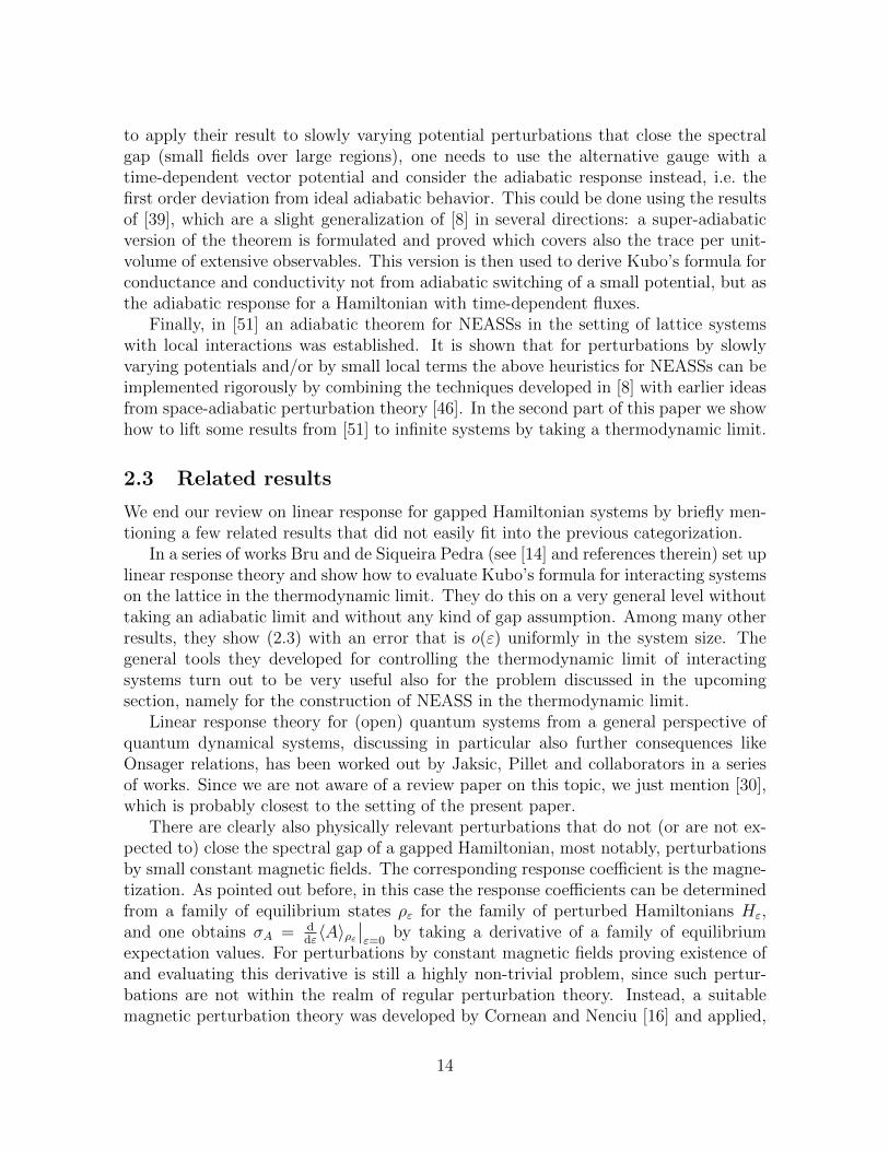
Figure 1: Transitions from the occupiedbands into the unoccupied bands are stronglysuppressed: To make a transition into an un-occupied state, an electron in the occupiedband (black dot) must either overcome theenergy gap g (vertical arrow) or tunnel a dis-tance of order g/ε (horizontal arrow).

generality. As emphasized in the introduction, linear response theory is designed toprovide response coefficients specifically also in those cases, where the system is drivenout of equilibrium.

As we will explain next, in our setting of gapped Hamiltonians H0 (describing in-sulating materials) there is indeed a clear and simple physical picture that suggeststhe existence of NEASS for Hε(t) even when a perturbation εV being the (possiblyunbounded) potential of an external small electric field closes the spectral gap of H0.Assume for simplicity that H0 is a periodic one-body operator in dimension d = 1and that the Fermi energy µ lies in a spectral gap of size g. Then in the initialstate ρ0 all one-body states with energy smaller than µ are occupied and it takesat least energy g to excite one electron from the filled bands to an empty band. Ifone applies a voltage ∆U over a distance L modeled by the addition of a potentialV∆U,L(x) = ∆U

L

(xχ[0,L](x) + Lχ[L,∞)(x)

), then for ∆U > g the perturbed Hamiltonian

will no longer have a spectral gap at µ. Still, the local field strength ε := ∆UL

in theregion [0, L] is small if L is a macroscopic distance. For an electron in the Fermi seathat is localized in a microscopic region around the point ` ∈ [0, L] the addition of thepotential might result in a substantial shift ε` in energy, but it still experiences a smallforce of order ε. And in order to make a transition into an unoccupied state, it stillneeds to either overcome the energy gap of size g, or tunnel a large distance of orderg/ε, see Figure 1. Thus, as long as g/ε is large, the state ρ0 is still an almost-stationarystate for the perturbed Hamiltonian Hε = H0 + V∆U,L. However, ρ0 is certainly neitherclose to the ground state nor to any other type of equilibrium state of Hε. Note thatthis heuristic picture still remains valid when local interactions between the electronsare taken into account.

At this point let us briefly mention the analogy to shape resonances in the caseof finite systems. As the simplest example consider the hydrogen atom in a constantelectric field, i.e. the Stark Hamiltonian. No matter how small the electric field is, thespectrum of the Stark Hamiltonian is the whole real line. However, when the field isof order 0 < |ε| � 1, then the ground state of the hydrogen Hamiltonian is close to ashape resonance of the Stark Hamiltonian that is stable for very long times. And whenone adiabatically turns on a small electric field, one expects the initial ground stateof a hydrogen atom to adiabatically evolve into this resonance. Note that adiabatictheorems for resonances have been established e.g. in [1, 20], although for technical

12

reasons they do not cover the case of the Stark Hamiltonian.The situation described above for extended non-interacting periodic systems is very

similar: instead of a simple ground state the unperturbed state ρ0 is the spectral pro-jection of H0 onto an infinite dimensional spectral subspace separated by a gap fromthe rest of the spectrum. And the NEASS described above could be seen as an infinitedimensional resonance for Hε. For interacting extended systems, the analogy is evenstronger, as ρ0 is indeed the gapped ground state of H0 and the corresponding NEASScould also be called a resonance of Hε.

Thus, in order to prove Kubo’s formula also for perturbations that close the spectralgap, one needs to first understand the NEASSs (or “resonances”) of Hε described above,and then to prove an adiabatic type theorem for NEASSs. This was done in [51], andin Section 3 corresponding results in the thermodynamic limit are discussed.

2.2.2 Justifying Kubo’s formula: Mathematical results

The first work concerned with a rigorous justification of Kubo’s formula in the sensejust described, and that we know of, is by Elgart and Schlein [21]. They considernon-interacting electrons on R2 described by the Landau Hamiltonian with smoothand bounded potential and the Fermi energy in a gap of the Hamiltonian. They deriveKubo’s formula for what is often referred to as conductance in this context by proving anappropriate adiabatic theorem. Note that for computing the conductance, one appliesthe electric field and measures the current only locally, i.e. one replaces Xi and Xj

in our discussion of conductivity above by G(Xi) and G(Xj), where G : R → [0, 1]is a smooth step function with compactly supported derivative G′. This results intwo technical simplifications: no notion of trace per unit volume is needed, and theperturbation is bounded and therefore the gap remains open for ε sufficiently small.Thus in [21] the standard adiabatic expansion with open gap can be applied and themain technical challenge is to prove the propagation estimates needed for controllingthe error in local trace norms (see also [36]). It is also worthwhile to mention thatin [21] the adiabatic parameter η and the perturbation parameter ε are identified,η = ε, i.e. the adiabatic limit and the small field limit are taken simultaneously. In [38]we prove Kubo’s formula for the Hall conductivity for gapped magnetic SchrodingerHamiltonians using the NEASS approach. This requires to deal with the fact that thedomain of Hε(t) = H0 + εf(ηt)Xj changes at time t = −1/η and to prove propagationestimates for time-dependent Stark-type Hamiltonians.

A breakthrough for interacting lattice systems was recently achieved by Bachmann,De Roeck, and Fraas [8]. They prove the first adiabatic theorem for extended latticesystems with local interactions that yields error estimates in local trace norms uniformlyin the size of the system. This uniformity was the main mathematical challenge andthe main innovation. Their proof exploits locality of interactions in the form of Lieb-Robinson propagation bounds [35] and the local inverse of the Liouvillian introducedby Hastings and Wen [28] (see also [9]). However, Bachmann et al. [8] require thespectral gap not only for H0, but also for the perturbed Hamiltonians Hε(t). In order

13

to apply their result to slowly varying potential perturbations that close the spectralgap (small fields over large regions), one needs to use the alternative gauge with atime-dependent vector potential and consider the adiabatic response instead, i.e. thefirst order deviation from ideal adiabatic behavior. This could be done using the resultsof [39], which are a slight generalization of [8] in several directions: a super-adiabaticversion of the theorem is formulated and proved which covers also the trace per unit-volume of extensive observables. This version is then used to derive Kubo’s formula forconductance and conductivity not from adiabatic switching of a small potential, but asthe adiabatic response for a Hamiltonian with time-dependent fluxes.

Finally, in [51] an adiabatic theorem for NEASSs in the setting of lattice systemswith local interactions was established. It is shown that for perturbations by slowlyvarying potentials and/or by small local terms the above heuristics for NEASSs can beimplemented rigorously by combining the techniques developed in [8] with earlier ideasfrom space-adiabatic perturbation theory [46]. In the second part of this paper we showhow to lift some results from [51] to infinite systems by taking a thermodynamic limit.

2.3 Related results

We end our review on linear response for gapped Hamiltonian systems by briefly men-tioning a few related results that did not easily fit into the previous categorization.

In a series of works Bru and de Siqueira Pedra (see [14] and references therein) set uplinear response theory and show how to evaluate Kubo’s formula for interacting systemson the lattice in the thermodynamic limit. They do this on a very general level withouttaking an adiabatic limit and without any kind of gap assumption. Among many otherresults, they show (2.3) with an error that is o(ε) uniformly in the system size. Thegeneral tools they developed for controlling the thermodynamic limit of interactingsystems turn out to be very useful also for the problem discussed in the upcomingsection, namely for the construction of NEASS in the thermodynamic limit.

Linear response theory for (open) quantum systems from a general perspective ofquantum dynamical systems, discussing in particular also further consequences likeOnsager relations, has been worked out by Jaksic, Pillet and collaborators in a seriesof works. Since we are not aware of a review paper on this topic, we just mention [30],which is probably closest to the setting of the present paper.

There are clearly also physically relevant perturbations that do not (or are not ex-pected to) close the spectral gap of a gapped Hamiltonian, most notably, perturbationsby small constant magnetic fields. The corresponding response coefficient is the magne-tization. As pointed out before, in this case the response coefficients can be determinedfrom a family of equilibrium states ρε for the family of perturbed Hamiltonians Hε,and one obtains σA = d

dε〈A〉ρε

∣∣ε=0

by taking a derivative of a family of equilibriumexpectation values. For perturbations by constant magnetic fields proving existence ofand evaluating this derivative is still a highly non-trivial problem, since such pertur-bations are not within the realm of regular perturbation theory. Instead, a suitablemagnetic perturbation theory was developed by Cornean and Nenciu [16] and applied,

14

for example, in [13] to derive and compute magnetic response coefficients in gappednon-interacting periodic systems. For mobility gapped systems on the lattice, magneticresponse was considered also in [47]. We are not aware of any adiabatic theorem appli-cable to the adiabatic switching of a time-dependent constant magnetic field, even inthe gapped case.

Let us finally mention Streda’s formula from [50]. Streda argued that in two di-mensional systems the Hall conductivity equals the magnetic response for the particledensity, i.e. σ12 = d

dBτ(ρB)

∣∣B=0

in infinite non-interacting systems. Bellissard [10]showed that for discrete mobility gapped systems this definition gives the same valueas the double-commutator formula, see also [47]. For unbounded Bloch-Landau Hamil-tonians, Streda’s formula was recently proved by Cornean, Monaco, and Moscolari [15],see also [17]. We are not aware of similar results on magnetic response for interactingsystems.

3 Linear response for interacting fermions in the

thermodynamic limit

In this section we show how the results of [51] on the justification of Kubo’s formulausing NEASSs for finite gapped systems at zero temperature can be lifted to infinitesystems in the thermodynamic limit. It turns out that under suitable assumptions theNEASS Πε discussed in the previous section exists also as a state on the algebra AΓ ofquasi-local observables for the infinite system and that Πε is automorphically equivalentto the ground state ρ0 of the unperturbed Hamiltonian H0. Moreover, an adiabatictheorem that allows to formulate and prove Kubo’s formula for the infinite systemholds as well. To avoid technicalities, and because of limited space, we report here onlythe results for the special case of Hamiltonians of the form Hε(t) = H0 + εf(t)V andomit the proofs. The general statements and their proofs will be reported elsewhere [29].There we use results for controlling the thermodynamic limit that were worked out onlyquite recently in [14, 41].

3.1 Fermions on the lattice: the mathematical framework

We consider fermions with s ∈ N internal degrees of freedom (which could be thespin) on the lattice Γ := Zd. Let P0(Γ) = {X ⊂ Γ : |X| <∞} denote the set offinite subsets of Γ. Then, for each X ∈ P0(Γ), the corresponding one-particle Hilbertspace is hX := `2(X,Cs), the N -particle Hilbert space is its N -fold anti-symmetric

tensor product HX,N :=∧Nj=1 hX , and the fermionic Fock space is FX :=

⊕s|X|N=0 HX,N ,

where HX,0 := C. All these Hilbert spaces are finite-dimensional and thus all linearoperators on them are bounded. The local C∗-algebras AX = L(FX) are generated bythe identity element 1X and the creation and annihilation operators a∗x,i, ax,i for x ∈ X

15

and 1 ≤ i ≤ s, which satisfy the canonical anti-commutation relations (CAR), i.e.

{ax,i, ay,j} = {a∗x,i, a∗y,j} = 0, {ax,i, a∗y,j} = δx,yδi,j1X ∀x, y ∈ X, 1 ≤ i, j ≤ s .

Here, {A,B} = AB + BA denotes the anti-commutator of A and B. If we haveX ⊂ X ′, AX is naturally embedded as a sub-algebra of AX′ . We denote by ANX ⊂ AXthe sub-algebra of elements commuting with the number operator NX =

∑x∈X a

∗xax :=∑

x∈X∑s

i=1 a∗x,iax,i. As elements of ANX contain even numbers of creation and annihi-

lation operators, it holds that [ANX ,ANX′ ] = {0} whenever X ∩X ′ = ∅. For the infinitesystem, the local C∗-algebra is defined by the inductive limit

AlocΓ :=

⋃X∈P0(Γ)

AX and its closure is denoted by AΓ := AlocΓ

‖·‖.

In order to define families of operators that are sums of local terms, one uses the conceptof “interactions”. In the following we consider sequences of Hamiltonians defined ondomains of the form Λ(k) = {−k, ...,+k }d with k ∈ N. A corresponding interactionΦ = {ΦΛ(k) }k∈N for a fermionic system on the lattice Γ is defined as a family of maps

ΦΛ(k) : {X ⊂ Λ(k) } → ANΛ(k) , X 7→ ΦΛ(k)(X) ∈ ANX ⊂ ANΛ(k)

with values in the self-adjoint operators. The advantage of considering different mapsΦΛ(k) for different k ∈ N instead of restrictions Φ|Λ(k) of a single map Φ : P0(Γ)→ Aloc

Γ

is the possibility to implement boundary conditions in order to model discrete tube ortorus geometries. For example, a hopping term a∗(k1,x)a(−k1,x) might only appear in theinteraction for the Hamiltonian for that specific value of k in order to connect oppositepoints on the boundary of Λ(k). Moreover, we will also allow for different metricsdΛ(k)(·, ·) on each Λ(k) depending on the intended geometry. For example, for a torusgeometry opposite points on the boundary of Λ(k) are considered neighbors and theirdistance is set to one, while for a cube geometry their distance is 2k.

The associated family of self-adjoint operators A = {AΛ(k)}k∈N0 corresponding toan interaction Φ is defined by

AΛ(k) = AΛ(k)(Φ) =∑

X⊂Λ(k)

ΦΛ(k)(X) ∈ ANΛ(k).

We will consider Hamiltonians H0 that are operator-families given by interactions ΦH0

that are exponentially localized in the following sense: We say that an interaction isexponentially localized with rate a > 0, if for all n ∈ N

supk∈N‖ΦΛ(k)‖a,n := sup

k∈Nsupx,y∈Γ

∑X∈P0(Γ):x,y∈X

Λ(k)-diam(X)n exp(a · dΛ(k)(x, y)) ‖ΦΛ(k)(X)‖ <∞ .

In this definition we used implicitly that for any interaction Φ the maps ΦΛ(k) canbe extended to maps on all of P0(Γ) by declaring ΦΛ(k)(X) = 0, whenever X ∩ (Γ \

16

Λ(k)) 6= ∅. This new mapping is called the extension of ΦΛ(k) and is denoted bythe same symbol. Similarly, given ΦΛ(k) and Λ(l) ⊂ Λ(k), we define the restrictionΦΛ(k)|Λ(l) : {X ⊂ Λ(l) } → ANΛ(l) by

ΦΛ(k)|Λ(l)(X) = ΦΛ(k)(X) ∀X ⊂ Λ(l).

For the perturbation V we will consider families of potentials v = { vΛ(k) : Λ(k)→ R }k∈Nthat satisfy a uniform Lipschitz condition of the following type,

Cv := supk∈N

supx,y∈Λ(k)

|vΛ(k)(x)− vΛ(k)(y)|dΛ(k)(x, y)

<∞ ,

and call them for short Lipschitz potentials. With such a potential v we associate thecorresponding operator-family Vv = {V Λ(k)

v }k∈N defined by VΛ(k)v =

∑x∈Λ(k) v

Λ(k)(x)a∗xax.

Since in our definitions the functions ΦΛ(k) resp. vΛ(k) defining an interaction resp. apotential can be, in principle, completely independent for different domains Λ(k), weneed to impose additional assumptions in order to guarantee the existence of a ther-modynamic limit for all objects appearing in our construction.

Definition 3.1. (a) An exponentially localized interaction Φ = {ΦΛ(k) }k∈N is said tohave a thermodynamic limit if it satisfies the following Cauchy-property:

∀n ∈ N ∃M0 ∈ N ∀M ≥M0 ∀δ > 0 ∃K ≥M ∀l, k ≥ K :∥∥∥(ΦΛ(l) − ΦΛ(k)

) ∣∣Λ(M)

∥∥∥a,n≤ δ .

A family of operators is said to have a thermodynamic limit if and only if thecorresponding interaction does.

(b) A Lipschitz potential v = { vΛ(k) }k∈N is said to have a thermodynamic limit if itis locally eventually independent of k, i.e. if

∀M ∈ N ∃K ≥M ∀l, k ≥ K : vΛ(l)|Λ(M) = vΛ(k)|Λ(M).

For a potential v that has a thermodynamic limit, the point-wise limits vΛ(k)(x)k→∞−−−→

v∞(x) exist for all x ∈ Γ and the limiting function v∞ carries all important informationabout the potential as far as the thermodynamic limit is concerned.

A relevant example for a Hamiltonian H0 that is exponentially localized and has athermodynamic limit is

HΛ0 =

∑(x,y)∈Λ2

a∗x T (x Λ− y) ay +∑x∈Λ

a∗xφ(x)ax +∑{x,y}⊂Λ

a∗xaxW (dΛ(x, y)) a∗yay − µNΛ . (3.1)

Here we assume that the kinetic term T : Γ→ L(Cs) is an exponentially fast decayingfunction with T (−x) = T (x)∗, the potential term φ : Γ→ L(Cs) is a bounded functiontaking values in the self-adjoint matrices, and the two-body interaction W : [0,∞) →L(Cs) is exponentially decaying and also takes values in the self-adjoint matrices. Note

17

that x Λ− y in the kinetic term in (3.1) refers to the difference modulo Λ(k) if Λ(k) issupposed to have a torus geometry.

The most relevant Lipschitz potentials we have in mind are the linear potentialv

Λ(k)D (x) := xi for some i ∈ {1, . . . , d} if the metrics dΛ(k) correspond to a cube geometry

(think of Dirichlet boundary conditions on the box) or the saw-tooth potential

vΛ(k)P (x) :=

xi if xi ∈ [−k

2, k

2]

k − xi if xi ∈ (k2, k]

−k − xi if xi ∈ [−k,−k2)

for the torus geometry. Note that CvD = CvP = 1 and that both potentials have athermodynamic limit and converge point-wise to the same function v∞(x) = xi. Aswe will see, they also define the same response coefficients in the thermodynamic limitwhen added to a gapped Hamiltonian of the type (3.1).

The following proposition can be proved exactly as Theorem 3.5 in [41] using alsoTheorem 3.4 and Theorem 3.8 from the same reference. It shows, that the propertyof having a thermodynamic limit for the interaction resp. the potential guarantees alsothe existence of a thermodynamic limit for the associated evolution operators.

Proposition 3.1. Thermodynamic limit of Cauchy-interactions [41]Let H0 and H1 be operator-families that are associated with two exponentially localizedinteractions and let v be a Lipschitz potential with associated operator-family Vv, allhaving a thermodynamic limit. Let V := Vv +H1.

(a) Let Hε := H0 + εV for some ε ∈ R. Then there exists a unique one-parametergroup t 7→ eiLHε t : AΓ → AΓ of automorphisms such that for all A ∈ Aloc

Γ

eiLHε t[A] = limk→∞

eiHΛ(k)ε tA e−iH

Λ(k)ε t

(b) Let f : R → R be smooth and put Hε,η(t) := H0 + εf(ηt)V for some ε ∈ R.Denote by UΛ(k),η(t, t0) the evolution family generated by Hε,η(t), i.e. the solutionto the Schrodinger equation

i ddtUΛ(k),η(t, t0) = HΛ(k)

ε,η (t)UΛ(k),η(t, t0) with UΛ(k),η(t0, t0) = Id .

Then there exists a unique co-cycle of automorphisms Uηt,t0 : AΓ → AΓ such thatfor all A ∈ Aloc

Γ

Uηt,t0 [A] = limk→∞

UΛ(k),η(t, t0)∗AUΛ(k),η(t, t0) .

The main additional assumption on the Hamiltonian H0 that we need is the gapassumption: We say that the operator-family H0 = {HΛ(k)

0 }k∈N has a simple gappedground state, if there exists L ∈ N such that for all k ≥ L and corresponding Λ(k) the

smallest eigenvalue EΛ(k)0 of the operator H

Λ(k)0 is simple and the spectral gap is uniform

18

in the system size, i.e. there exists g > 0 such dist(EΛ(k)0 , σ(H

Λ(k)0 ) \ {EΛ(k)

0 }) ≥ g > 0for all k ≥ L.

In addition, we require that also the sequence of ground states ρΛ(k)0 has a ther-

modynamic limit. To formulate this condition, recall that a normalized positive linearfunctional ω on the C∗-algebra AΓ is called a state. Here normalized means ω(id) = 1and positive means ω(A∗A) ≥ 0 for all A ∈ AΓ. By the Banach-Alaoglu theorem, theset of states EAΓ

is weak∗-compact. If B is a subalgebra of AΓ and ω is a state on B,then there exists a state ω on AΓ which extends ω by the Hahn-Banach theorem. Inthis way, the states B 7→ tr(ρ

Λ(k)0 B) can be extended to the whole algebra AΓ and are

denoted by the same symbol ρΛ(k)0 . To avoid the extraction of subsequences, we will

assume that the sequence of ground states (ρΛ(k)0 )k∈N converges to a unique limiting

point ρ0 ∈ EAΓ.

(A1) Assumptions on H0.Let H0 be the Hamiltonian of an exponentially localized interaction that has a thermo-dynamic limit. We assume that H0 has a gapped ground state such that the sequence ofground states (ρ

Λ(k)0 )k∈N0 converges in the weak∗-topology to a state ρ0 on AΓ.

(A2) Assumptions on the perturbation.Let V = Vv + H1, where v is a Lipschitz potential and Vv denotes the correspondingoperator-family, and H1 is the Hamiltonian of an exponentially localized interaction,both having a thermodynamic limit.

Note that for non-interacting Hamiltonians H0 of the type (3.1) on a torus, i.e. withW ≡ 0, condition (A1) is satisfied whenever the chemical potential µ lies in a gap of thespectrum of the corresponding one-body Hamiltonian operator on the infinite domain,a condition that can be checked easily. And it was recently shown in [26, 19], that forsufficiently small W 6= 0 the spectral gap remains open.

We have now all prerequisites to formulate our main results on the existence andproperties of NEASS for interacting systems in the thermodynamic limit. They are alladaptions of corresponding results for finite systems proved in [51]. As they are notsimple corollaries of [51] but require some careful adaptions, their proofs will be givenelsewhere [29].

The first theorem states that under Assumptions (A1) and (A2) there exists aNEASS for the perturbed Hamiltonian Hε = H0 + εV close to the ground state of H0

(cf. Theorem 3.1 in [51]).

Theorem 3.1. Existence of NEASSsLet the Hamiltonian Hε = H0 + εV satisfy (A1) and (A2). Then for any ε ∈ [−1, 1]there exists a near-identity automorphism αε of AΓ such that the state Πε defined by

Πε(A) := ρ0(αε[A]) for all A ∈ AΓ

is almost-invariant in the following sense: for any n ∈ N there exists a constant Cn > 0

19

such that for all finite X ⊂ Γ, A ∈ ANX ⊂ AΓ, and ε ∈ [−1, 1]∣∣Πε(eiLHε t[A])− Πε(A)

∣∣ ≤ Cn |ε|n(1 + |t|2d) |X|3 ‖A‖ . (3.2)

By near-identity we mean that αε is of the form αε = eiεLSε for an almost exponentiallylocalized operator family Sε that has a thermodynamic limit.

The next theorem is a special case of a more general adiabatic theorem for NEASS,cf. Theorem 5.1 in [51]. It shows that when adiabatically switching on the perturbation,then the initial ground state of H0 dynamically evolves up to small errors into thecorresponding NEASS Πε for the perturbed Hamiltonian Hε as long as the adiabaticparameter η is small but not too small (see also Proposition 3.2 in [51]).

Theorem 3.2. Adiabatic switchingLet the Hamiltonian Hε = H0 + εV satisfy (A1) and (A2). Let f : R→ R be a smooth“switching” function with f(t) = 0 for t ≤ −1 and f(t) = 1 for t ≥ 0, and defineHε,η(t) := H0 + εf(ηt)V . Let Uηt,t0 be the Heisenberg time-evolution on AΓ generated byHε,η(t) with adiabatic parameter η ∈ (0, 1].

Then for any n > d there exists a constant Cn such that for any finite X ⊂ Γ andA ∈ ANX ⊂ AΓ and for all t ≥ 0∣∣∣ρ0(Uηt/η,−1/η[A])− Πε(A)

∣∣∣ ≤ |ε|n+1 + ηn+1

ηd+1Cn (1 + td+1) |X|2 ‖A‖ , (3.3)

where Πε is the NEASS of Hε constructed in Theorem 3.1.

Note that (3.3) shows that, as long as the adiabatic parameter η satisfies 1� η �|ε|

n+1d+1 for some n > d, the initial ground state ρ0 of H0 evolves, up to a small error,

into the NEASS Πε that is independent of the form of the switching function f andof η. Slower switching must be excluded, because, in general, the NEASS is an almost-invariant but not an invariant state for the instantaneous Hamiltonian. Its life-timedepends on the strength of the perturbation, i.e. on ε, and it is thus not surprising thatthe relevant time scale for the adiabatic switching process depends on ε as well.

In order to compute response coefficients, we need to expand Πε in powers of ε (cf.Proposition 3.1 in [51]).

Proposition 3.2. Asymptotic expansion of the NEASSUnder the assumptions of Theorem 3.1 there exist linear maps Kj : Aloc

Γ → AΓ, j ∈ N,such that for any n ∈ N there is a constant Cn such that for any finite X ⊂ Γ andA ∈ ANX ⊂ AΓ it holds that∣∣∣∣∣Πε(A)−

n∑j=0

εj ρ0(Kj[A])

∣∣∣∣∣ ≤ Cn |ε|n+1 |X|2 ‖A‖ .

20

The constant term is K0 = 1AΓ, which shows that αε is indeed a near-identity automor-

phism when |ε| � 1. The linear term K1 is a densely defined derivation on AΓ thatsatisfies

ρ0(K1[A]) = − limk→∞

⟨[IH

Λ(k)0

(V Λ(k)), A]⟩

ρΛ(k)0

= limk→∞

tr

(L−1

HΛ(k)0

([V Λ(k), ρΛ(k)0 ])A

)(3.4)

for every A ∈ AlocΓ . Here I

HΛ(k)0

is a local version of the inverse Liouvillian introduced

in [28] and from the first expression in (3.4) it follows that ρ0(K1[A]) depends on Vvonly through the limiting function v∞.

Finally, we can combine the previous results in order to formulate our main the-orem about linear and higher order response for gapped interacting systems in thethermodynamic limit (cf. Theorem 4.1 in [51]).

Theorem 3.3. Linear and higher order responseUnder the same assumptions as in Theorem 3.2, let again Uηt,t0 be the Heisenberg time-evolution on AΓ generated by Hε,η(t) with adiabatic parameter η ∈ (0, 1]. For A ∈ AΓ

define the total response as

Σε,η,fA (t) := ρ0(Uηt/η,−1/η[A])− ρ0(A) ,

and for j ∈ N the jth order response coefficient as σA,j := ρ0(Kj[A]), where the Kj’s weredefined in Proposition 3.2 and σA,1 is explicitly given by (3.4), i.e. by the thermodynamiclimit of Kubo’s formula (2.6).

Then for any n,m ∈ N there exists a constant Cn,m independent of ε, such that forany finite X ⊂ Γ and A ∈ ANX ⊂ AΓ and all t ≥ 0

supη ∈

[|ε|m, |ε|

1m

]∣∣∣∣∣Σε,η,f

A (t)−n∑j=1

εjσA,j

∣∣∣∣∣ ≤ |ε|n+1Cn,m (1 + td+1) |X|2 ‖A‖ . (3.5)

Note that the condition that η ∈ [|ε|m, |ε| 1m ] for some m ∈ N makes sure that the

switching is neither too slow (η ≥ |ε|m) nor too fast (η ≤ |ε| 1m ). Too slow switching

would be switching on time-scales longer than the life-time of the NEASS, while toofast switching would no longer allow for an expansion of the total response in powersof ε.

While we believe that this result and the NEASS approach in general are an im-portant contribution to the mathematical understanding of linear response theory fortransport in gapped Hamiltonian systems, there are still several open questions: An ob-vious conjecture would be that our results remain valid if one replaces the gap conditionfor the local Hamiltonians in Assumption (A1) by a gap condition for the Hamiltonianfor the infinite system (in the GNS representation). At least for the case that V ∈ AΓ,

21

we expect that the methods recently developed in [40] can be used to adapt our proofsaccordingly.

A presumably much harder but physically more interesting problem is to justifyKubo’s formula for current response in situations where H0 no longer has a spectralgap but only a mobility gap. Even for non-interacting systems we know of no resultsin this direction yet.

References

[1] W. Abou Salem and J. Frohlich: Adiabatic theorem for quantum resonances.Comm. Math. Phys. 273:651–675 (2007).

[2] M. Aizenman and G.-M. Graf: Localization bounds for an electron gas. Journal ofPhysics A: Mathematical and General 31:6783 (1998).

[3] G. Androulakis, J. Bellissard, and C. Sadel: Dissipative dynamics in semiconduc-tors at low temperature. Journal of Statistical Physics 147:448–486 (2012).

[4] J. Avron: Why is the Hall conductance quantized? Solution of an open math-physproblem. Open Problems in Mathematical Physics http://web.math.princeton.edu/~aizenman/OpenProblems_MathPhys/17_Avron.pdf (2017).

[5] J. Avron and R. Seiler: Quantization of the Hall conductance for general, multi-particle Schrodinger Hamiltonians, Phys. Rev. Lett. 54: 259–262 (1985).

[6] J. Avron, R. Seiler, and B. Simon: Homotopy and quantization in condensedmatter physics, Phys. Rev. Lett. 51: 51–53 (1983).

[7] S. Bachmann, A. Bols, W. De Roeck, and M. Fraas: A many-body index forquantum charge transport. Comm. Math. Phys. Online First (2019).

[8] S. Bachmann, W. De Roeck, and M. Fraas: The adiabatic theorem and linearresponse theory for extended quantum systems. Comm. Math. Phys. 361:997–1027(2018).

[9] S. Bachmann, S. Michalakis, B. Nachtergaele, and R. Sims: Automorphic equiv-alence within gapped phases of quantum lattice systems. Comm. Math. Phys.309:835–871 (2012).

[10] J. Bellissard: C∗-algebras in solid state physics. 2D electrons in a uniform magneticfield. In Operator Algebras and Application. D.E. Evans and M. Takesaki (1988).

[11] J. Bellissard, A. van Elst, and H. Schulz-Baldes: The noncommutative geometryof the quantum Hall effect. J. Math. Phys. 35:5373–5451 (1994).

22

[12] J. Bouclet, F. Germinet, A. Klein, and J. Schenker: Linear response theory formagnetic Schrodinger operators in disordered media. J. Func. Anal. 226:301–372(2005).

[13] P. Briet, H. Cornean, and B. Savoie: A Rigorous Proof of the Landau-PeierlsFormula and much more. Ann. H. Poincare 13:1–40 (2012).

[14] J.-B. Bru and W. de Siqueira Pedra: Lieb–Robinson Bounds for Multi-Commutators and Applications to Response Theory. Springer Briefs in Math. Phys.13, Springer (2016).

[15] H. Cornean, D. Monaco, and M. Moscolari: Beyond diophantine Wannier dia-grams: Gap labelling for Bloch-Landau Hamiltonians. arXiv:1810.05623 (2018).

[16] H. Cornean and G. Nenciu: On eigenfunction decay of two dimensional magneticSchrodinger operators. Commun. Math. Phys. 192:671–685 (1998).

[17] H. Cornean, G. Nenciu, and T. Pedersen: The Faraday effect revisited: Generaltheory. J. Math. Phys. 47:013511 (2006).

[18] G. De Nittis and M. Lein: Linear Response Theory: An Analytic-Algebraic Ap-proach. Springer Briefs in Mathematical Physics Vol. 21, Springer (2017).

[19] W. De Roeck and M. Salmhofer: Persistence of exponential decay and spectralgaps for interacting fermions. Comm. Math. Phys. , Online First (2018).

[20] A. Elgart and G. Hagedorn: An adiabatic theorem for resonances. Commun. PureAppl. Math. 64:1029-1058 (2011).

[21] A. Elgart and B. Schlein: Adiabatic charge transport and the Kubo formula forLandau-type Hamiltonians. Commun. Pure Appl. Math. Math. 57:590–615 (2004).

[22] J. Frohlich: Chiral anomaly, topological field theory, and novel states of matter.Rev. Math. Phys. 30:1840007 (2018).

[23] J. Frohlich and T. Kerler: Universality in quantum Hall systems. Nucl. Phys. B354:369–417 (1991).

[24] A. Giuliani, V. Mastropietro and M. Porta, Universality of the Hall conductivityin interacting electron systems, Comm. Math. Phys. 349:1107–1161 (2017).

[25] G.M. Graf: Aspects of the integer quantum Hall effect. In Proceedings of Symposiain Pure Mathematics 76: 429, American Mathematical Society (2007).

[26] M. Hastings: The Stability of Free Fermi Hamiltonians. J. Math. Phys. 60: 042201(2019).

23

[27] M. Hastings and S. Michalakis: Quantization of Hall conductance for interactingelectrons on a torus. Comm. Math. Phys. 334:433–471 (2015).

[28] M. Hastings and X.-G. Wen: Quasiadiabatic continuation of quantum states: Thestability of topological ground-state degeneracy and emergent gauge invariance.Phys. Rev. B 72:045141 (2005).

[29] J. Henheik and S. Teufel. In preparation 2020.

[30] V. Jaksic, Y. Ogata, and C.-A. Pillet: The Green-Kubo formula for locally inter-acting open fermionic systems. Ann. Henri Poincare, 8:1013–1036 (2006).

[31] T. Kato: On the adiabatic theorem of quantum mechanics. J. Phys. Soc. Jap. 5:435–439 (1950).

[32] A. Klein, O. Lenoble, and P. Muller: On Mott’s formula for the ac-conductivity inthe Anderson model, Annals of Math. 549–577 (2007).

[33] R. Kubo: Statistical-mechanical theory of irreversible processes. I. General theoryand simple applications to magnetic and conduction problems, J. Phys. Soc. Japan12:570–586 (1957).

[34] R. Laughlin: Anomalous Quantum Hall Effect: An Incompressible Quantum Fluidwith Fractionally Charged Excitations, Phys. Rev. Lett. 50:1395–1398 (1983).

[35] E. Lieb and D. Robinson: The finite group velocity of quantum spin systems.Comm. Math. Phys. 28:251–257 (1972).

[36] G. Marcelli: Improved energy estimates for a class of time-dependent perturbedHamiltonians. arXiv:1904.11300 (2019).

[37] G. Marcelli, D. Monaco, G. Panati, and S. Teufel: A new approach to transportcoefficients in the quantum (spin) Hall effect. In preparation (2020).

[38] G. Marcelli and S. Teufel. In preparation (2020).

[39] D. Monaco and S. Teufel: Adiabatic currents for interacting electrons on a lattice.Rev. Math. Phys. 31:1950009 (2019).

[40] A. Moon and Y. Ogata: Automorphic equivalence within gapped phases in thebulk. arXiv:1906.05479 (2019).

[41] B. Nachtergaele, R. Sims, and A. Young: Quasi-locality bounds for quantum latticesystems. I. Lieb-Robinson bounds, quasi-local maps, and spectral flow automor-phisms. J. Math. Phys. 60:061101 (2019).

24

[42] G. Nenciu: On asymptotic perturbation theory for quantum mechanics: almostinvariant subspaces and gauge invariant magnetic perturbation theory. J. Math.Phys. 43:1273–1298 (2002).

[43] Q. Niu and D.J. Thouless. Quantised adiabatic charge transport in the presenceof substrate disorder and many-body interaction. J. Phys. A: Math. Gen. 17:2453–2462 (1984).

[44] Q. Niu, D.J. Thouless, and Y.-Sh. Wu: Quantized Hall conductance as a topolog-ical invariant. Phys. Rev. B 31:3372–3377 (1985).

[45] G. Panati, H. Spohn, and S. Teufel: Effective dynamics for Bloch electrons: Peierlssubstitution and beyond. Commun. Math. Phys. 242:547–578 (2003).

[46] G. Panati, H. Spohn, and S. Teufel: Space-adiabatic perturbation theory. Adv.Theor. Math. Phys. 7:145–204 (2003).

[47] H. Schulz-Baldes and S. Teufel: Orbital polarization and magnetization for inde-pendent particles in disordered media. Comm. Math. Phys. 319:649–681 (2013).

[48] B. Simon: Holonomy, the quantum adiabatic theorem, and Berry’s phase. Phys.Rev. Lett. 51:2167–2170 (1983).

[49] B. Simon: Fifteen problems in mathematical physics. Perspectives in Mathematics,Birkhauser, Basel 423 (1984).

[50] P. Streda: Theory of quantised Hall conductivity in two dimensions. J. Phys. C15, L717 (1982).

[51] S. Teufel: Non-equilibrium almost-stationary states and linear response for gappedquantum systems. Comm. Math. Phys. 373:621–653 (2020).

[52] S. Teufel: Adiabatic Perturbation Theory in Quantum Dynamics. Lecture Notesin Mathematics 1821, Springer (2003).

[53] D.J. Thouless, M. Kohmoto, M. Nightingale, and M. den Nijs: Quantized Hall con-ductance in a two-dimensional periodic potential. Phys. Rev. Lett. 49:405 (1982).

25