Electromagnetism II, Final Formula Sheet

MASSACHUSETTS INSTITUTE OF TECHNOLOGYPhysics Department

Physics 8.07: Electromagnetism II December 18, 2012Prof. Alan Guth

FORMULA SHEET FOR FINAL EXAMExam Date: December 19, 2012

∗∗∗ Some sections below are marked with asterisks, as this section is. The asterisksindicate that you won’t need this material for the quiz, and need not understand it. It isincluded, however, for completeness, and because some people might want to make useof it to solve problems by methods other than the intended ones.

Index Notation:

�A · �B = �AiBi , A× �Bi = εijkAjBk , εijkεpqk = δipδjq − δiqδjp

detA = εi1i2···inA1,i1A2,i2 · · ·An,in

Rotation of a Vector:

A′i = RijAj , Orthogonality: RijRik = δjk (RTT = I)

j=1 j=2 j=3

i=1

cosφ − sinφ 0Rotation about z-axis by φ: Rz(φ)ij = i=2 sinφ cosφ 0

i=3 0 0 1

Rotation about axis n by φ:∗∗∗

R(n, φ)ij = δij cosφ+ nin (1

j − cosφ) n

− εijkˆk sinφ .

Vector Calculus:∂

Gradient: (∇� ϕ)i = ∂iϕ , ∂i ≡∂xi

Divergence: ∇ ·� �A ≡ ∂iAi

Curl: (∇×� �A)i = εijk∂jAk

2 ∂2ϕLaplacian: ∇ ϕ = ∇ ·� (∇� ϕ) =

∂xi∂xi

Fundamental Theorems of Vector Calculus:

Gradient:∫ �b

∇� ϕ · d�, = ϕ(�b) )a

− ϕ(�a�

Divergence:∫

∇ ·� � �Ad3x =V

∮A

S

· d�a

where S is the boundary of V

Curl:∫

(�S

∇× �A) · d�a =∮

�A d�,P

·where P is the boundary of S

8.07 FORMULA SHEET FOR FINAL EXAM, FALL 2012 p. 2

Delta Functions:∫ϕ(x)δ(x− x′) dx = ϕ(x′) ,

∫ϕ(�r )δ3(�r − �r ′) d3x = ϕ(�r ′)∫

d dϕϕ(x) δ(x− x′) dx =

dx−

dx

∣δ(

∣x=x′

x x )δ( ig(x)) =

∑ −, g(x

∣0|g ( i) =′ xi)

∣i

|

∇ ·�(

�r − �r ′= 2 1

= 4πδ3(�r�r �r ′ 3

)−∇

�r �r ′ − �r ′)| − | | − |rj xj 1 δij 3rirj 4π

∂i

(j2

)∂i

(3

)= ∂i∂

( )=

−δ 3

r≡ + δ

r− ij (�r)

r r3 3

3(�d∇ ·� · r)r − �d 8π= − (� · ∇�d )δ3(�r )

r3 33(�d · r)r − �d 4π∇×� =

r3− �d

3×∇� δ3(�r )

Electrostatics:

�F = �qE , where1 ∑ (�r − �r ′) q�E(�r ) = i 1

4πε0 i |�r − �r ′|3 =4πε0

∫(�r − �r ′)

ρ(�r ′) d3x| 3′

�r − �r ′|ε0 =permittivity of free space = 8.854× 10−12 C2/(N·m2)1

= 8.988 109 N m2/C2

4πε0× ·∫ �r 1

∫ρ(�r ′)

V (�r ) = V ( ��r 0)− E(�r ′) · d�,′ = d3x′�r 0

4πε0 |�r − �r ′|ρ∇ ·� �E = � � � �, Eε0

∇× = 0 , E = −∇V

∇2 ρV = − (Poisson’s Eq.) , ρ = 0 =⇒ ∇2V = 0 (Laplace’s Eq.)

ε0Laplacian Mean Value Theorem (no generally accepted name): If ∇2V = 0, then

the average value of V on a spherical surface equals its value at the center.

Energy:

1 1 1W =

∑ qiqj 1x d3 ρ(�r )ρ(�r ′)

=∫

d3 x′2 4πε0 rij 2 4πε0

ij|�r − �r ′|

1W =

2

∫ i=j

d3 1xρ(�r)V (�r ) = ε

2 0

∫ ∣∣�E∣∣2 d3x

�


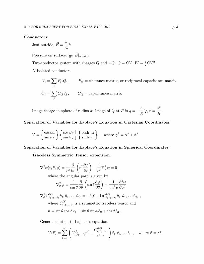
Conductors:σ

Just outside, �E = nε0

Pressure on surface: 1σ2 | �E|outside

Two-conductor system with charges Q and −Q: Q = CV , W = 1CV 22

N isolated conductors:

Vi =∑

PijQj , Pij = elastance matrix, or reciprocal capacitance matrixj

Qi =∑

CijVj , Cij = capacitance matrixj

a a2

Image charge in sphere of radius a: Image of Q at R is q = − Q, r =R R

Separation of Variables for Laplace’s Equation in Cartesian Coordinates:

{cosαx

}{cosβy

}{cosh γz

V = sinαx sinβy sinh γz

}where γ2 = α2 + β2

Separation of Variables for Laplace’s Equation in Spherical Coordinates:

Traceless Symmetric Tensor expansion:

∇2 1 ∂ ∂ϕ 1ϕ(r, θ, φ) =

2 ∂r

(r2

∂r

)+

r r2∇2

θ ϕ = 0 ,

where the angular part is given by2

2 1 ∂ ∂ϕ 1 ∂ ϕ∇θ ϕ ≡ sin θ +sin θ ∂θ

(∂θ

)sin2 θ ∂φ2

∇2 (�) ˆ ˆ (�)θ Ci 2...i

ni� 1ni1i 2 . . . ni� = −,(,+ 1)Ci1i2...ini1 ni� 2 . . . ni� ,

where (�)Ci1i2...i�

is a symmetric traceless tensor and

n = sin θ cosφ e1 + sin θ sinφ e2 + cos θ e3 .

General solution to Laplace’s equation:

∞ �)

( ) =∑(

(�) C′(

� + i1i2...iV �r Ci ...i r�

i

)ri1 2 �ˆ

r�+1 1 ri2 . . . ri� , where �r = rr�=0


Azimuthal Symmetry:∞

BV ( �

�r ) =(A� r

� +){ zi1 . . . zi� } ri1 . . . rir�+1 �

�=0

where

∑{ . . .} denotes the traceless symmetric part of . . . .

Special cases:

{ 1 } = 1

{ zi } = zi

{ z z } = z z − 1i j i j δij3

{ z z z } = z z z − 1i j k i j k ziδjk + zjδik + zkδij5

{ z z 1izj zkzm } = izj zk zm

(− (

zizjδkm + zizkδ

)mj + zizmδjk + zjzk7

ˆ δim

+ zj zmδik + zk zmδ 1ij + δijδkm jk35 + δikδjm + δimδ

Legendre Polynomial / Spherical H

)armo

(nic expansion:

)

General solution to Laplace’s equation:∞

V (�r ) =∑ ∑� (

B�mA�m r� +

r�+1�=0 m=−�

)Y�m(θ, φ)

2π π

Orthonormality:∫

dφ∫

sin θ dθ Y�∗ θ, φ Y θ, φ δ δ′m′( ) �m( ) = �′� m′m

0 0

Azimuthal Symmetry:∞

( ) =∑(

� B+ �

V �r A� r

)P�(cos θ)

r�+1�=0

Electric Multipole Expansion:

First several terms:1 �

r[ Q p ˆ 1 r

V (�) = +· r r

+ i jQ +

4πε0 r r2 2 ijr3

· · ·]

, where

Q =∫

d3x ρ(�r) , pi =∫

d3x ρ(�r ) x 3i Qij =

∫d x ρ(�r)(3xixj−δij |�r |2) ,

1 p��Edi (�r ) = �p

( · r) 1 3(p� · r)r − p� 1− =4πε0

∇r2 4πε0 r3

− p3 iδ

3(�r )ε0

1 1∇×� � ( ) = 0 ∇ ·� � ( �Edip �r , Edip(�r ) = ρdip �r ) = − p� )ε0 ε

· ∇δ3(�r0


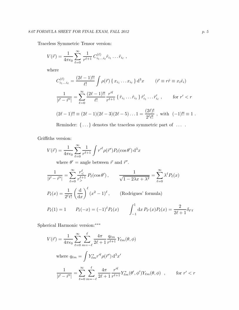
Traceless Symmetric Tensor version:

1 ∞(

∑ 1) = (�)

V �r C4πε0 r�+1 i1...i

r� i1 . . . ri� ,

�=0

where

(�) (2,Ci ...i =

− 1)!!∫

ρ(�r ) { xi1 . . . xi� } d3x (�r ≡ rr ≡ xie1 �ˆ

,! i)

1 ∞ (2, 1)!! r′�=

−r . . . r r′ . . . r′ , for r′ < r|�r − �r ′|

∑,!

=0

{ ir�+1 1 i�

�

} i1 i�

(2,)!(2,− 1)!! ≡ (2,− 1)(2,− 3)(2,− 5) . . .1 = , with (

2�,!−1)!! ≡ 1 .

Reminder: { . . .} denotes the traceless symmetric part of . . . .

Griffiths version:

1 ∞V (�r ) =

∑ 1∫

�r′ ρ(�r ′)P�(cos θ′) d3x

4πε0 r�+1�=0

where θ′ = angle between �r and �r ′.

1 ∑∞ r� 1 ∞= < P (cos θ′) , = λ�P (x)|�r − �r ′ � √| r�+1

> 1− 2λx+

∑�

λ2�=0 �=0

1P�(x) =

(d

)�

(x2 − 1)� , (Rodrigues’ formula)2�,! dx

1 2P�(1) = 1 P (−x) = (−1)�� P�(x)

∫dxP�′(x)P�(x) = δ

2 + 1 �′�−1 ,

Spherical Harmonic version:∗∗∗

1 ∑∞ � 4π q�mV (�r ) =

4πε0�=0 m

∑Y

2,+ 1 �m(θ, φ)r�+1

=−�

where q 3�m =

∫Y ∗ ��mr′ ρ(�r ′) d x′

1 ∞ � 4π r′�=

∑ ∑Y�m

∗ (θ′, φ′)Y�m(θ, φ) , for r < r|�r − �r ′| 2,+ 1 r�+1′

�=0 m=−�


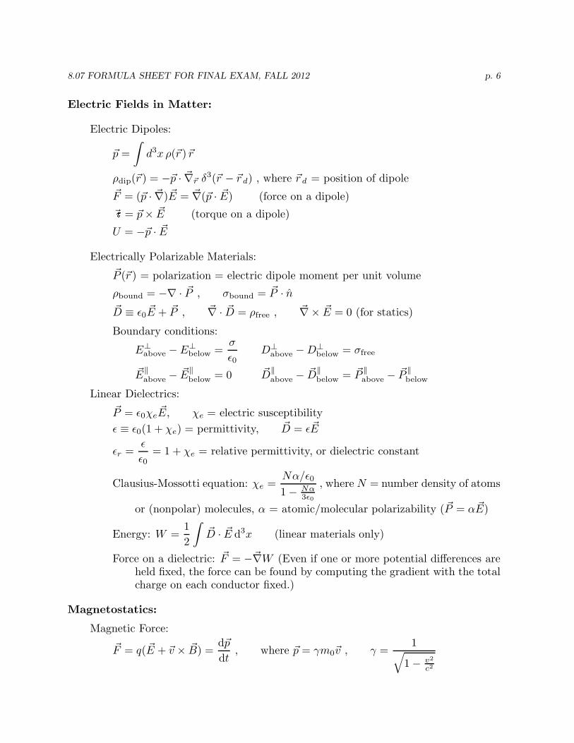
Electric Fields in Matter:

Electric Dipoles:

�p =∫

d3x ρ(�r )�r

ρdip(�r ) = −p� · ∇� �r δ3(�r − �rd) , where �rd = position of dipole

�F = (p� · ∇� ) �E = ∇� (p� · �E) (force on a dipole)

� = �p× �E (torque on a dipole)

U = −p� · �E

Electrically Polarizable Materials:�P (�r ) = polarization = electric dipole moment per unit volume

ρbound = −∇ · �P , σ = �bound P · n

�D ≡ � � � � � �ε0E + P , ∇ ·D = ρfree , ∇× E = 0 (for statics)

Boundary conditions:σ

Eab⊥

ove − Ebe⊥

low = Dab⊥

ove −Dbe⊥

low = σfreeε0

�E‖ ‖ � ‖ �ab − � �

ove E‖below = 0 �D

‖ ‖above −Dbelow = Pabove − Pbelow

Linear Dielectrics:�P = �ε0χeE, χe = electric susceptibilityε ≡ ε0(1 + χe) = permittivity, �D = �εE

εεr = = 1 + χe = relative permittivity, or dielectric constant

ε0

Nα/εClausius-Mossotti equation: 0

χe = ,Nα

where N = number density of atoms1−

3ε0

or (nonpolar) molecules, α = atomic/molecular polarizability (�P = �αE)

1Energy: W =

2

∫�D · �E d3x (linear materials only)

Force on a dielectric: �F = −∇� W (Even if one or more potential differences areheld fixed, the force can be found by computing the gradient with the totalcharge on each conductor fixed.)

Magnetostatics:

Magnetic Force:dp� 1� = ( � + × �F q E �v B) = , where p� = γm0�v , γ =dt

√1− v2

c2


� � � � �F =∫

Id,×B =∫

J ×B d3x

Current Density:

Current through a surface S: IS =∫

�J · d�aS

∂ρCharge conservation: =

∂t−∇ ·� �J

Moving density of charge: �J = ρ�v

Biot-Savart Law:

�µ r ′) �� ( 0

∫d,′ × (�r − � µ

) = = 0∫

K(�r ′) (�r �r ′)B �r I

4π |3× −

da′|�r − �r ′ 4π |�r − �r ′|3

µ= 0

∫ �J(�r ′)× (�r − �r ′)d3x

4π |�r − �r ′|3

where µ0 = permeability of free space ≡ 4π × 10−7 N/A2

Examples:µ I

Infinitely long straight wire: �B = 0φ

2πrInfinitely long tightly wound solenoid: �B = µ0nI0 z , where n = turns per

unit lengthµ IR2

Loop of current on axis: �B(0, 0, z) = 0z

2(z2 +R2)3/2

1Infinite current sheet: �B(�r ) = �µ0K × n , n = unit normal toward �r

2

Vector Potential:

µ (�r ′�A(r ) = 0

∫ �J )� d3 ′ , � = ∇×� �

coul x B A , ∇ ·� �A4π |�r − �r ′| coul = 0

∇ ·� �B = 0 (Subject to modification if magnetic monopoles are discovered)

Gauge Transformations: �A′( � � � � ��r ) = A(�r ) + ∇Λ(�r ) for any Λ(�r ). B = ∇ × A isunchanged.

Ampere’s Law:

∇×� �B = �µ0J , or equivalently∫

�BP

· d�, = µ0Ienc


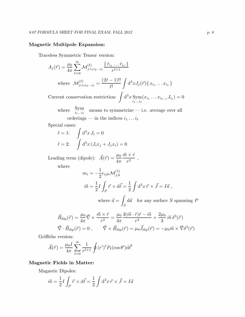
Magnetic Multipole Expansion:

Traceless Symmetric Tensor version:

µ∞

r . . . rAj(�) =

0 ( )r

∑�j;i1i2...i�

{ i

4M i1 �

}π r�+1

�=0

(�) (2,where Mj i i d3

; ...i =− 1)!!

∫xJj1 2 �

(�r ),!

{ xi1 . . . xi� }

Current conservation restriction:∫

d3x Sym(xi1 . . . xi� J−1 i�) = 0i1...i�

Symwhere means to symmetrize — i.e. average over alli1...i�

orderings — in the indices i1 . . . i�Special cases:

, = 1:∫

d3x Ji = 0

, = 2:∫

d3x (Jixj + Jjxi) = 0

µLeading term (dipole): �A(�r ) = 0 m� × r

,4π r2

where1

mi = − ε2 ijkM(1)

j;k

1m� = I

∫1

�r × d�, =∫

d3 �x�r2 P 2

× J = I�a ,

where �a =∫

d�a for any surface S spanning PS

µ0 m� × r µ m µ� �Bdip(�r ) = ∇× = 0 3(m� · r)r − � 2+ 0

mδ� 3(�r )4π r2 4π r3 3

∇ ·� � ( ) = 0 ∇×� � ( ) = � ( ) = − ×∇�Bdip �r , Bdip �r µ0Jdip �r µ0m� δ3(�r )

Griffiths version:

µ�A(�r ) = 0I∞ 1

(r′)�P (cos θ′4 � )d�,′π

∑r�+1

�=0

∮

Magnetic Fields in Matter:

Magnetic Dipoles:1 1� �m� = I

∫�r

P

× d, =2

∫d3x�r

2× J = I�a


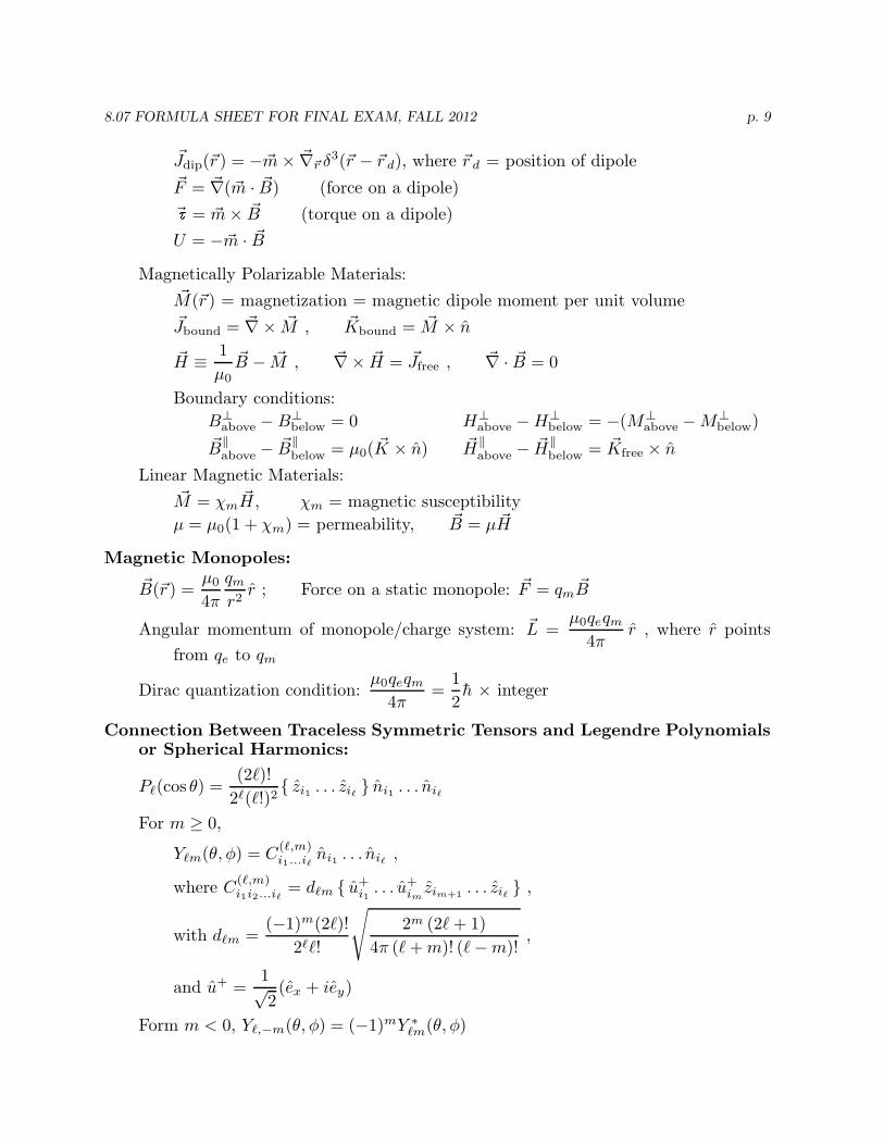
�Jdip(�r ) = −m� ×∇� �r δ3(�r − �r d), where �r d = position of dipole

� = ∇� �F (m� ·B) (force on a dipole)� = m� × �B (torque on a dipole)

U = −m� · �BMagnetically Polarizable Materials:

�M(�r ) = magnetization = magnetic dipole moment per unit volume�Jbound = ∇×� �M , �Kbound = �M × n

1�H ≡ �B M0

− � , �µ

∇× �H = �Jfree , ∇ ·� �B = 0

Boundary conditions:Bab

⊥ove −Bbe

⊥low = 0 Hab

⊥ove −Hbe

⊥low = −(Mab

⊥ove −Mbe

⊥low)

�B‖ − �B

‖ = µ0( �K × n) �H‖ �

above below above −H‖ �below = Kfree × n

Linear Magnetic Materials:�M = �χmH, χm = magnetic susceptibility= (1 + ) = permeability, � �µ µ0 χm B = µH

Magnetic Monopoles:µ�B( 0 qm � ��r ) = r ; Force on a static monopole: F = q4 mBπ r2

µ q qAngular momentum of monopole/charge system: � m

L = 0 er , where r points

4πfrom qe to qm

µ q q 1Dirac quantization condition: 0 e m = h r

4 2× intege

π

Connection Between Traceless Symmetric Tensors and Legendre Polynomialsor Spherical Harmonics:

(2,)!P�(cos θ) = { zi1 . . . z n

2�(,!) i2 �} i1 . . . ni�

For m ≥ 0,(�,m)

Y�m(θ, φ) = Ci ...i ni1 . . . ni� ,1 �

where (�,m)C +i i ...i = d�m { ui . . . u+1 2 � 1

ˆi zm im+1 . . . zi� } ,

( 1)with d�m =

− m(2,)!2�,!

√2m (2,+ 1)

,4π (,+m)! (,−m)!

and u+ 1= √ (e

2x + iey)

Form m < 0, Y�,−m(θ, φ) = (−1)mY�m∗ (θ, φ)


More Information about Spherical Harmonics:∗∗∗

2 + 1 ( − m)! Pm imφ Y£m(θ, φ) = (cos θ)e£4π ( + m)!

where Pm(cos θ) is the associated Legendre function, which can be defined by £

d£+m

Pm(x) = (−1)m

(1 − x 2)m/2 (x 2 − 1)£ £ 2£ £+m! dx

Legendre Polynomials:

√

SPHERICAL HARMONICS Ylm(θ , φ)

Y00 = 1

4π

l = 1

l = 0

cos θ Y10 = 4π

3

sin θeiφ Y11 = - 8π

3

l = 2 sin θ cosθeiφ Y21 = - 8π

15

( cos2θ Y20 = 4π

5

sin2 θe2iφ Y22 = 2π

1514

32

1 2 )

l = 3

sin2 θ cos θe2iφ Y32 = 2π

105

( cos3θ

Y31 = 4π

21

sin3 θe3iφ Y33 = - 4π

3514

52

14

14

3 2 cos θ)

- sinθ (5cos2θ -1)eiφ

Y30 = 4π

7

Image by MIT OpenCourseWare.


Maxwell’s Equations:

1 �∂B(i) ∇ ·� �E = ∇×�ρ (iii) �E =

ε0− ,

∂t1 �∂E

(ii) ∇ ·� �B = 0 (iv)∇×� �B = �µ0J +c2 ∂t

1where µ0ε0 =

c2

Lorentz force law: �F = q( �E + �v × �B)

∂ρCharge conservation: =

∂t−∇ ·� �J

Maxwell’s Equations in Matter:

Polarization �P and magnetization �M :

ρb = −∇ ·� � � � � � � �P , Jb = ∇×M , ρ = ρf + ρb , J = Jf + Jb

Auxiliary Fields:

�B�H ≡ Pµ

− � �M , D ≡ �ε0E + �0

Maxwell’s Equations:

�∂B(i) ∇ ·� � = ρf (iii)∇×� �D E = − ,

∂t�∂D

(ii) ∇ ·� �B = 0 (iv)∇×� � = �H Jf +∂t

For linear media:1�D = � �εE , H = �Bµ

where ε = dielectric constant, µ = relative permeability

�∂D�Jd ≡ = displacement current∂t

Maxwell’s Equations with Magnetic Charge:

1 �∂B(i) ∇ ·� �E = �

ε∇×�

e (iii) �ρ E = −µ0Jm0

− ,∂t

1 �∂E(ii) ∇ ·� � ∇×�µ0ρm (iv) �B = �B = µ0Je +

c2 ∂t

1Magnetic Lorentz force law: �F = qm

(�B − �v

c2× �E

)


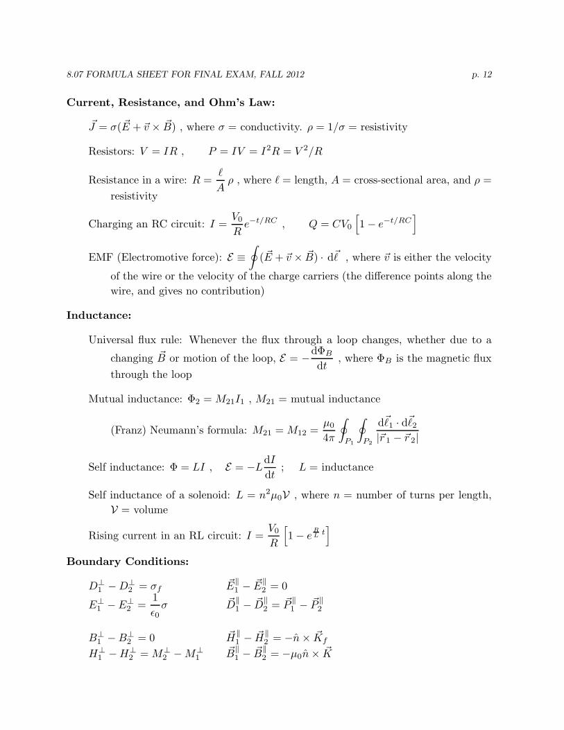
Current, Resistance, and Ohm’s Law:

�J = �σ(E + �v × �B) , where σ = conductivity. ρ = 1/σ = resistivity

Resistors: V = IR , P = IV = I2R = V 2/R

,Resistance in a wire: R = ρ , where , = length, A = cross-sectional area, and ρ =

Aresistivity

VCharging an RC circuit: I = 0

e−t/RC , Q = CV[1− e−t/RC

0R

]

EMF (Electromotive force): E ≡∮( �E + �v × �B) · d�, , where �v is either the velocity

of the wire or the velocity of the charge carriers (the difference points along thewire, and gives no contribution)

Inductance:

Universal flux rule: Whenever the flux through a loop changes, whether due to adΦ

changing � BB or motion of the loop, E = − , where ΦB is the magnetic flux

dtthrough the loop

Mutual inductance: Φ2 = M21I1 , M21 = mutual inductance

µ d�, d�,(Franz) Neumann’s formula: 2

M = 021 M

4π

∮P1

∮1

12 =·

P2|�r 1 − �r 2|

dISelf inductance: Φ = LI , E = −L ; L = inductance

dt

Self inductance of a solenoid: L = n2µ0V , where n = number of turns per length,V = volume

VRising current in an RL circuit: I = 0

[1− R

e tL

R

Boundary Conditions:

]

D1⊥ −D2

⊥ = �σf E1‖ − �E2

‖ = 01

E1⊥ − E2

⊥ = �σ D‖ � ‖

P‖ �D = � P

‖ε 10

− 2 1 − 2

B1⊥ −B2

⊥ = 0 �H1‖ − �H2

‖ = − �n×Kf

H1⊥ −H2

⊥ = M2⊥ −M1

⊥ �B1‖ − �B2

‖ = −µ0n× �K


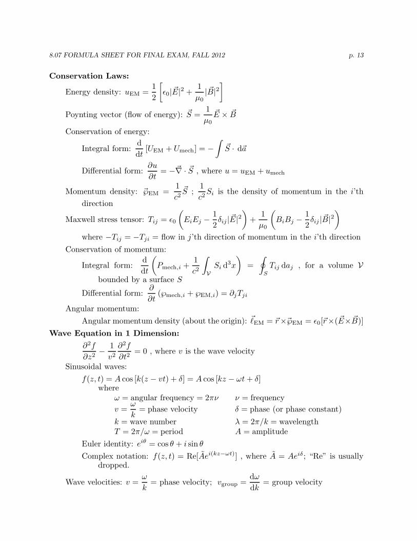
Conservation Laws:1

Energy density: uEM =[

1� �ε 20 E

2| |2 +

µ0|B|1

]

Poynting vector (flow of energy): �S = � �E Bµ0

×Conservation of energy:

dIntegral form: [ �U

d EM + Umech] =t

−∫

S · d�a∂u

Differential form: = ∇ ·�∂t

− �S , where u = uEM + umech

1 1Momentum density: �℘EM = �S ; Si is the density of momentum in the i’th

c2 c2direction

1Maxwell stress tensor: T = ε

(E E − δ | �E|2 1

ij 0 i j 2 ij

)+

µ0

(1

BiBj − δ2 ij | �B|2

)where −Tij = −Tji = flow in j’th direction of momentum in the i’th direction

Conservation of momentum:d 1

Integral form: Pt

(mech,i + S v

d i d3x = Tij daj , for a olumec2

b

∫V

) ∮S

Vounded by a surface S

∂Differential form: (℘mech,i + ℘EM,i) = ∂jTji

∂tAngular momentum:

Angular momentum density (about the origin): �,EM = �r×�℘EM = ε0[�r×( �E× �B)]Wave Equation in 1 Dimension:

∂2f 1 ∂2f− = 0 , where v is the wave velocity∂z2 v2 ∂t2

Sinusoidal waves:f(z, t) = A cos [k(z − vt) + δ] = A cos [kz − ωt+ δ]

whereω = angular frequency = 2πν ν = frequency

ωv = = phase velocity δ = phase (or phase constant)

kk = wave number λ = 2π/k = wavelengthT = 2π/ω = period A = amplitude

Euler identity: eiθ = cos θ + i sin θComplex notation: f(z, t) = Re[Ae˜ i(kz−ωt)] , where A = Aeiδ; “Re” is usually

dropped.ω dω

Wave velocities: v = = phase velocity; vgroup = = group velocityk dk

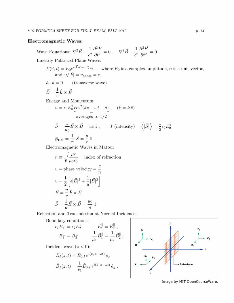
V1

Bl

ER BR

V1

El ET

BT

V2

X

Z

Y

Interface



agnetic Waves:

1 � �2 ∂2E 1 ∂2B

Equations: ∇ �E − = 0 , ∇2 �B − = 0c2 ∂t2 c2 ∂t2

rly Polarized Plane Waves:

� ( ˜ �E �r, t) = E ei(k·�r−ωt)

0 n ,ˆ where E0 is a complex amplitude, n is a unit vector,and ω/|�k| = vphase = c.

n · �k = 0 (transverse wave)1�B = �k × Ec

Energy and Momentum:u = ε E2

0 cos2

0 (kz − ωt+ δ) , (�k = k z)

1S

︸averages

� = � �E B = uc

︷︷to 1/2

︸1× z ,ˆ I (intensity) =

⟨|�S|

⟩= ε0E

2

µ0 2 0

1 u��℘EM = S = zc2 c

Electromagnetic Waves in Matter:

n ≡√

µε= index of refraction

µ0ε0c

Electrom

Wave

Linea

v = phase velocity =n

1 1u =

[ε| �E

2|2 +

µ| �B|2

n

]�B = k

c× �E

1 uc�S = � �E ×B = zµ n

Reflection and Transmission at NormalBoundary conditions:

ε1E1⊥ = ε2E2

⊥ �E1‖ = �E2

‖

1 1B1

⊥ = B2⊥ �B

‖µ 1 =

1 µ2

Incident wave (z < 0):

�EI(z, t) = E0,I ei(k1z−ωt) ex

1�BI(z, t) = E z0 ei(k1,I

−ωt) eyv1

Incidence:

,

�B‖2 .

.


Transmitted wave (z > 0):

�E (z, t) = E ei(k2zT 0,T

−ωt) ex

1�B (z, t) = E ωtT ei(k2z

0,T− ) ey .

v2

Reflected wave (z < 0):

�E (z, t) = E iR 0,R e (−k1z−ωt) ex

1�B (z, t) = ˜− E ei(−k1z−ωt)R 0,R ey .

v1ω must be the same on both sides, so

ω c ω c= v1 = , = v2 =

k1 n1 k2 n2

Applying boundary conditions and solving, approximating µ1 = µ2 = µ0 ,

˜ n1 − n2 2n= ˜ = 1

E0,R E En1 +

0,I E ˜0,T 0,I

n2

(n1 + n2

)

Electromagnetic Potentials:

�∂AThe fields: � = ∇×� � �B A , E = −∇� V −

∂t

∂ΛGauge transformations: � �A′ = A+∇� Λ , V ′ = V −

∂t

1Coulomb gauge: ∇ ·� �A = 0 =⇒ ∇2V = − ρ (but �A is complicated)

ε0

1 ∂VLorentz gauge: ∇ ·� �A = − =

c2 ∂t⇒

2 1 1�V = − ρ , 2 ∂2

A = − �µ0J , where 2 2

ε 2 20

≡ ∇ −c ∂t

2 = D’Alembertian

Retarded time solutions (Lorentz gauge):

1∫

3 ρ( ��r ′, tr) 1∫

3 J(�r ′, tr)t) = d ′ �V (�r , x , A(�r , t) = d x′

4πε0 |�r − �r ′| 4πε0 |�r − �r ′|where

tr = t|�r − �r ′|−

c


Lienard-Wiechert Potentials (potentials of a point charge):

1 qV (�r , t) =

4πε0 |�r − �r p|µ

( 0

(1− �vp

c · ˆq�v�A �r , t) = p =

)�vp

V4π |�r − �r |( (�r , t)

1− �vp cp

) 2c · ˆ

where �rp and �vp are the position and velocity of the particle at the retardedtime tr, and

�r �r� = �r − �rp , = |�r − p

�r p =−| , ˆ |�r − �rp|

Fields of a point charge (from the Lienard-Wiechert potentials):

q �r �r�E(�r , t) =| − p|

c2 v2 �u �r �r4πε ( (

p− ))p �u �a· 3 ( ) + ( )

�u � r p− )× (

0 r �− p ×

1

[ ]�B( ��r , t) = ˆ

c× E(�r , t)

where �u = c ˆ − �vp

Radiation:

Radiation from an oscillating electric dipole along the z axis:

p(t) = p0 cos(ωt) , p0 = q0d

Approximations: d � λ � r,

p0ω cos θV (r, θ, t) = −

( )sin[ω(t− r/c)]

4πε0c r

µ�A(�r , t) = − 0p0ω sin[ω(t4πr

− r/c)] z

µ p� = − 0 0ω2 sin θ 1

cos[ ( )] ˆ � �E ω t r/c θ , B(�r , t) = r E(�r , t)4π

(r

)−

c×

1 p ω n 2µ 2 si θ

Poynting vector: �S = ( � � 0E × ) = 0

B

{ ( )cos[ω(t r/c

µ0 c 4π− )]

r

}r

⟨ ⟩ (µ p2ω4

)sin2 θ

tensity: I = � = 0 0 1In S r ,ˆ using

32π2c r2

⟨cos2

⟩=

2

µ p2ω4

Total power: 〈P 〉 =∫ ⟨

�S⟩· d�a = 0 0

12πc


Magnetic Dipole Radiation:

Dipole moment: m� (t) = m0 cos(ωt) z , at the origin

µ ω20m0

(sin θ�E = −

)1

cos[ × �ω(t− r/c)]φ ,ˆ �B(�r , t) = r E(�r , t)4πc r c

mCompared to the electric dipole radiation, 0

p , θ φ0 →c

→ −General Electric Dipole Radiation:

µ0 1E ¨ µ� ( ) = [(ˆ ¨· )ˆ− ] � � 0

�r , t r �p r �p , B(�r , t) = r × E(�r , t) =4πr c

− [r ¨4πrc

×�p ]

Multipole Expansion for Radiation:The electric dipole radiation formula is really the first term in a doubly infinite

series. There is electric dipole, quadrupole, . . . radiation, and also magneticdipole, quadrupole, . . . radiation.

Radiation from a Point Particle:

When the particle is at rest at the retarded time,q�Erad = [ ˆ ( ˆ �a

4 p)]πε c20 |�r − �r ′ × ×|

1 µ q2a2 sin2 θPoynting vector: � � 0

Sra = 2d Erad ˆ = ˆ

µ|

20c

|16π c

(2

)where θ is the angle between �ap and ˆ .

µ q2a2

Total power (Larmor formula): P = 0

6πc(valid for �vp = 0 or |�vp| � c)

Lienard’s Generalization if �vp = 0:

µ q2∣ 2

γ6 20

(2

∣�v × �a∣ )∣ µ0q dpµ dpµ

P = a − ∣ ∣ =6πc ∣ c ∣ 6πm2

0c dτ dτ

Fo︸r relativis

︷︷ts on

Radiation

︸ly

Reaction:

Abraham-Lorentz formula:µ�Frad = 0q

2

�a6πc

The Abraham-Lorentz formula is guaranteed to give the correct average energyloss for periodic or nearly periodic motion, but one would like a formulathat works under general circumstances. The Abraham-Lorentz formulaleads to runaway solutions which are clearly unphysical. The problem ofradiation reaction for point particles in classical electrodynamics apparentlyremains unsolved.

�


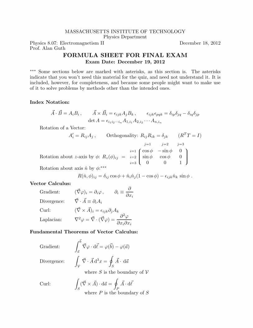
Vector Identities:

Triple Products

Products Rules

Second Derivatives

A . (B x C) = B . (C x A) = C . (A x B)

A x (B x C) = B(A . C) - C(A . B)

∆ (f g) = f ( ∆ g) + g ( ∆ f)

∆ (A . B) = A x ( ∆ x B) + B x ( ∆ x A) + (A . ∆)B + (B . ∆)A

∆ (f A) = f ( ∆ . A) + A . ( ∆ f)

∆ x (f A) = f ( ∆ x A) - A x ( ∆ f)

∆ (A x B) = B . ( ∆ x A) - A . ( ∆ x B)

∆ (A x B) = (B . ∆)A - (A . ∆)B + A ( ∆ . B) - B( ∆ . A)

∆ . ( ∆ x A) = 0

∆ x ( ∆ x A) = ∆ ( ∆ . A) - ∆2A

∆ x ( ∆ f) = 0


MIT OpenCourseWarehttp://ocw.mit.edu

8.07 Electromagnetism IIFall 2012 For information about citing these materials or our Terms of Use, visit: http://ocw.mit.edu/terms.

http://ocw.mit.edu

http://ocw.mit.edu/terms

Electromagnetism II, Final Formula Sheet

Documents

Transcript of Electromagnetism II, Final Formula Sheet