Journal of Geophysical Research: Atmospheres

RESEARCH ARTICLE10.1002/2013JD020803

Key Points:• Global spatio-temporal

regression-kriging daily temperatureinterpolation

• Fitting of global spatio-temporalmodels for the mean, maximum, andminimum temperatures

• Time series of MODIS 8 dayimages as explanatory variables inregression part

Correspondence to:M. Kilibarda,kili@grf.bg.ac.rs

Citation:Kilibarda, M., T. Hengl, G. B. M.Heuvelink, B. Gräler, E. Pebesma, M.Percec Tadic, and B. Bajat (2014),Spatio-temporal interpolation of dailytemperatures for global land areas at1 km resolution, J. Geophys. Res. Atmos.,119, doi:10.1002/2013JD020803.

Received 27 AUG 2013

Accepted 28 JAN 2014

Accepted article online 3 FEB 2014

This is an open access article underthe terms of the Creative CommonsAttribution-NonCommercial-NoDerivsLicense, which permits use and dis-tribution in any medium, providedthe original work is properly cited,the use is non-commercial and nomodifications or adaptations are made.

Spatio-temporal interpolation of daily temperatures for globalland areas at 1 km resolutionMilan Kilibarda1, Tomislav Hengl2, Gerard B. M. Heuvelink3, Benedikt Gräler4, Edzer Pebesma4,Melita Percec Tadic5, and Branislav Bajat1

1Department of Geodesy and Geoinformatics, Faculty of Civil Engineering, University of Belgrade, Belgrade, Serbia,2ISRIC-World Soil Information, Wageningen, Netherlands, 3Soil Geography and Landscape Group, Wageningen University,Wageningen, Netherlands, 4Institute for Geoinformatics, University of Münster, Münster, Germany, 5Meteorological andHydrological Service, Zagreb, Croatia

Abstract Combined Global Surface Summary of Day and European Climate Assessment and Datasetdaily meteorological data sets (around 9000 stations) were used to build spatio-temporal geostatisticalmodels and predict daily air temperature at ground resolution of 1 km for the global land mass. Predictionsin space and time were made for the mean, maximum, and minimum temperatures using spatio-temporalregression-kriging with a time series of Moderate Resolution Imaging Spectroradiometer (MODIS) 8 dayimages, topographic layers (digital elevation model and topographic wetness index), and a geometrictemperature trend as covariates. The accuracy of predicting daily temperatures was assessed usingleave-one-out cross validation. To account for geographical point clustering of station data and get amore representative cross-validation accuracy, predicted values were aggregated to blocks of land of size500 × 500 km. Results show that the average accuracy for predicting mean, maximum, and minimum dailytemperatures is root-mean-square error (RMSE) = ±2◦C for areas densely covered with stations and between± 2◦C and ± 4◦C for areas with lower station density. The lowest prediction accuracy was observed at highaltitudes (> 1000 m) and in Antarctica with an RMSE around 6◦C. The model and predictions were builtfor the year 2011 only, but the same methodology could be extended for the whole range of the MODISland surface temperature images (2001 to today), i.e., to produce global archives of daily temperatures(a next-generation http://WorldClim.org repository) and to feed various global environmental models.

1. Introduction

Records from near-surface weather stations are the foundation of climate research [Peterson and Vose, 1997].They are important not only because of their high reliability and accuracy but also because they are theonly available records of spatial and temporal variation of climatic variables before the first satellite basedobservations became available in the 1960s (M. Kilibarda et al., Publicly available global meteorological datasets: sources, representation, and usability for spatio-temporal analysis, International Journal of Climatology,in review, 2014).

Station observations are commonly used to predict climatic variables on raster grids (unvisited locations),where the statistical term “prediction” is used here to refer to“spatial interpolation” or “spatio-temporal inter-polation” and should not be confused with “forecasting.” In-depth reviews of interpolation methods usedin meteorology and climatology have recently been presented by Price et al. [2000], Jarvis and Stuart [2001],Tveito et al. [2006], and Stahl et al. [2006]. The literature shows that the most common interpolation tech-niques used in meteorology and climatology are as follows: nearest neighbor methods, splines, regression,and kriging, but also neural networks and machine learning techniques.

One of the first global monthly land surface temperature grids at 0.5◦ (decimal degrees) resolution wasproduced by Legates and Willmott [1990]. Leemans and Cramer [1991] further generated grids at the sameresolution for mean monthly temperature, precipitation, and cloudiness using a triangulation network fol-lowed by smooth surface fitting. New et al. [1999, 2000] and Mitchell and Jones [2005] used thin-plate splinesto produce global images covering global land areas excluding Antarctica at 0.5◦ resolution for nine climaticvariables. Hijmans et al. [2005] used a thin-plate smoothing spline on a collection of public meteorologicaldata sets of monthly records to produce global (land mass) climatic images at 1 km resolution for the periodfrom 1960 to 1990. Becker et al. [2012] recently mapped monthly precipitation for the whole world using an

KILIBARDA ET AL. ©2014. The Authors. 1

Journal of Geophysical Research: Atmospheres 10.1002/2013JD020803

empirical interpolation method based on angular distance weighting at resolutions of 0.25◦, 0.5◦, 1.0◦, and2.5◦, using data from the Global Precipitation Climatology Centre.

The first global terrestrial gridded data set of average daily temperature, daily temperature range, and dailyprecipitation was developed by Piper and Stewart [1996] and is intended for use in terrestrial biosphericmodeling. Daily station observations for the year 1987 were interpolated to a 1◦ × 1◦ grid (longitude, lati-tude) using a nearest neighbor interpolation technique. Global daily predictions of meteorological variableswere produced by Kiktev et al. [2003] and Alexander et al. [2006], who used an angular distance weighingtechnique to interpolate extreme daily precipitation and temperature indices onto a 2.5◦ latitude by 3.75◦

longitude grid. Caesar et al. [2006] mapped daily maximum and minimum temperature anomalies usingthe same method and the same output resolutions as Alexander et al. [2006]. Haylock et al. [2008] pro-duced European coverage maps of daily mean, minimum, and maximum temperatures and precipitationwith 0.25◦ and 0.5◦ resolution using the European Climate Assessment and Dataset Project (ECA&D). Thesemaps were generated by first estimating monthly averages; daily anomalies from those averages werethen interpolated using kriging and added back to the monthly estimates [Haylock et al., 2008]. Van denBesselaar et al. [2011] mapped sea level pressure for Europe using the same data source and global kriging.Di Luzio et al. [2008] presented a method for mapping daily precipitation and temperature across contermi-nous USA at 2.5 arc min (around 4 km) for the period 1960–2001. Their method also combines interpolation(inverse distance weighting) of daily anomalies from gridded monthly estimates, here estimated usingParameter Elevation Regressions on Independent Slopes Model.

Hofstra et al. [2008] compared six interpolation methods for prediction of daily precipitation mean, min-imum, and maximum temperature, and sea level pressure from station data in Europe in relation to thelong-term monthly mean (1960–1990). Global kriging on anomalies (from the long-term monthly mean)showed the best overall performing result. Geostatistical interpolation methods (various types of kriging)are considered to be state-of-the-art statistical approaches to spatial and spatio-temporal analysis [Cressieand Wikle, 2011]. A method known as “regression-kriging” (RK) (also known as kriging with external driftand/or universal kriging) has been widely recognized as a flexible and a well-performing technique for unbi-ased spatial prediction of meteorological and environmental variables [Carrera-Hernández and Gaskin, 2007;Haylock et al., 2008; Hengl et al., 2012].

An extension from spatial to spatio-temporal models is a logical evolution of statistical models for mappingspatially and temporally correlated meteorological data. However, fitting of spatio-temporal RK models andprediction using spatio-temporal covariates is more than just the smoothing of station data. The insightsobtained from the modeling process and predictions are much richer and allow one to distinguish sourcesof variability. The model makes the relationships with covariates explicit and can be used to distinguishbetween purely temporal, purely spatial and spatio-temporal components of variability. Moreover, it pre-dicts values using spatio-temporal observations in spatial (e.g., as daily map), temporal (e.g., trend line atmeteorological stations), and for a time series of spatial grids [Pebesma, 2012].

To the best of our knowledge, researchers have not yet attempted to interpolate global daily values of mete-orological variables using spatio-temporal regression-kriging with a time series of remote sensing-basedcovariates and at detailed resolution (1 km). Such an attempt poses many challenges, both from a method-ological and technological perspective. For example, the global land mass contains about 149 million pixelsat 1 km resolution and predicting daily values for 10 years would result in about 4 TB of data. The fitting ofgeostatistical models with millions of point pairs and accompanied predictions on such HUGE grid stackscan only be accomplished by code optimization to avoid RAM memory overload and to speed up processingthrough tiling and parallel processing.

In this article, we present an automated mapping framework for producing predictions of daily mean,minimum, and maximum air temperatures using spatio-temporal regression-kriging. The framework isimplemented in the R environment for statistical computing and uses the gstat [Pebesma, 2004] and stats[R Development Core Team, 2012] packages. As inputs we use a collection of publicly available daily recordsfrom the National Climatic Data Center’s (NCDC’s) Global Surface Summary of Day and the European ClimateAssessment & Dataset and a time series of MODIS LST 8 day images and topographic layers as covariates.The research reported here focuses on the year 2011 but without modification the methodology can beextended to the whole period for which MODIS LST images are available (2001 to present). The input data

KILIBARDA ET AL. ©2014. The Authors. 2

Journal of Geophysical Research: Atmospheres 10.1002/2013JD020803

sets and methods are described in section 2. The results of model fitting, cross validation, and validation arepresented in section 3, whereas summary results are given in the discussions section (section 4).

2. Methods and Materials2.1. Measurements at Ground Stations2.1.1. NCDC’s Global Surface Summary of DayThe Global Surface Summary of Day (GSOD) data set is produced and archived at NOAA’s National ClimaticData Center (NCDC) under the code NCDC DSI-9618 (http://www.ncdc.noaa.gov/). The input data used inbuilding the GSOD are the Integrated Surface Data (NCDC DSI-3505), which includes global hourly dataobtained from the U.S. Federal Climate Complex that contains about 27,000 stations.

GSOD is probably the largest publicly available international meteorological station data set. It containsdaily measurements for a list of 11 meteorological parameters of several climatic variables (since 1929):mean, minimum, and maximum temperatures (precision of 0.1◦F); mean dew point (0.1◦F), mean atmo-spheric pressure and mean sea level pressure (0.1 mb); mean visibility (0.1 mi); mean wind speed, maximumsustained wind speed, and maximum wind gust (0.1 knots); precipitation amount (0.01 in); snow depth(0.1 in); and an indicator (class) for occurrence of fog, rain, or drizzle, snow or ice pellets, hail, thunder, andtornado/funnel cloud. This data set is continuously being updated so that the latest daily summary data areusually available within 1–2 days after the observations were made.2.1.2. European Climate Assessment and DatasetThe largest European publicly available meteorological data set is the European Climate Assessment andDataset (ECA&D) project. The idea of the ECA&D project was to provide a uniform analysis methodologyfor a daily observational series from 62 countries and 6596 European and Mediterranean meteorologicalstations [Klein Tank et al., 2002].

The ECA&D data set contains measurements of the following meteorological variables and their parameters:minimum, mean, and maximum temperature (precision of 0.1◦C), humidity (1 %), mean sea level pressure(0.1 hPa), mean wind speed (0.1 m/s), wind direction (degrees), maximum wind gust (0.1 m/s), precipitationamount (0.1 mm), snow depth (1 cm), cloud cover (oktas), and sunshine duration (0.1 h).2.1.3. The Global Historical Climatology NetworkThe Global Historical Climatology Network-Monthly (GHCN-M) temperature data set was developed in theearly 1990s [Vose, 1992]. A second version was released in 1997 following extensive efforts to increase thenumber of stations and length of the data record [Peterson and Vose, 1997]. GHCN-M version 3 released in2011 focused on improving four issues [Lawrimore et al., 2011]: (a) consolidating duplicate station records,(b) improving station coverage, especially during the 1990s and 2000s, (c) enhancing quality control, and (d)applying a new bias correction methodology that does not require use of a composite reference series.

The current version 3 contains monthly mean temperature, monthly maximum temperature, and monthlyminimum temperature.2.1.4. Merged and Cleaned Global Station Data SetGSOD and ECA&D daily meteorological data sets were merged to produce a merged global station dataset. In case both sources have the same location the station with most observations was kept; in case of thesame number of observations GSOD was taken. The final merged data set contains around 9000 stationsfrom GSOD and around 500 from ECA&D.

A large portion of the station data had missing values, but all stations were used in the interpolation pro-cedure. Even though the meteorological services responsible for collecting the data also perform a basicquality control, a small portion of the stations from the merged data set contained obvious gross errors andneeded to be cleaned. The gross errors were detected using the following procedure: An initial spatio-temporal model (described in section 2.3) was first fitted using all data, followed by analysis of cross-validation predictions at the station locations. Large cross-validation root-mean-square errors indicatedwhich stations might have gross data errors. This was usually confirmed with abrupt jumps in observationvalues in time series plots, thereby showing observations against the cross-validation prediction error.

We decided to remove all stations that had an absolute cross-validation residual larger than ± 15◦C, as theseclearly contain errors in the data set. Using the 15◦C threshold, we removed around 300 stations for eachtemperature variable (minimum, mean, and maximum temperature). After all data filtering, the final setcontained about 9000 stations from merged GSOD and ECA&D data sets.

KILIBARDA ET AL. ©2014. The Authors. 3

Journal of Geophysical Research: Atmospheres 10.1002/2013JD020803

The number of stations per region are as follows: North and South America approximately 3100 stations,Europe approximately 2500, Africa approximately 750, Asia approximately 1600, Australia approximately450, and Antarctica approximately 20.

2.2. Covariates: Remote Sensing Images and DEM Derivatives2.2.1. National Aeronautics and Space AdministrationThe Moderate Resolution Imaging Spectroradiometer (MODIS) images of the Terra and Aqua EarthObserving System platforms provide retrieval of atmospheric and oceanographic variables using varioustechniques. There are many data products from MODIS observations describing land (temperature and landcover), oceans (sea surface temperature and optical thickness), and atmosphere (water vapor, cloud prod-uct, and atmospheric profiles) that can be used for studies at different spatial scales, ranging from local toglobal. Land surface temperature (LST) data and images obtained from MODIS thermal bands that are dis-tributed by the Land Processes Distributed Active Archive Center of the U.S. Geological Survey are very oftenused in meteorological studies [Coll et al., 2009].

In addition to the MODIS data at level 2 or higher, there are also MODIS level 1 data that are distributedthrough the Level 1 and Atmosphere Archive and Distribution System (LAADS) portal hosted at the GoddardSpace Flight Center. The MODIS LST data are available on a daily basis and have spatial resolutions of 1×1 km[Coll et al., 2009]. The nominal accuracy of the MODIS LST product is reported to be ±1 K. Some validationstudies reported accuracy statistics smaller than 1 K in clear sky conditions within the temperature rangeof −10◦C to 50◦C [Yoo et al., 2011]. MODIS LST data and/or images are one of the most often used and bestdocumented publicly available remote sensing products in the world.

In this work, we only use level 3 MODIS LST 8 day composite images (MOD11A2) to improve the spatialprediction of mean, minimum, and maximum daily temperature, despite the fact that daily daytime andnighttime MODIS LST images are also available (MOD11A1). The intention was to find covariates that areexhaustively known over the spatio-temporal domain to obtain complete prediction over landmass. Evenusing the MODIS 8 day composites did not completely fulfill this requirement, so remaining gaps had to befilled using splines.

The original MODIS images still contained 0–15% of missing pixels due to clouds or other reasons. Thesemissing pixels were replaced using the System for Automated Geoscientific Analyses Geographic Informa-tion System (SAGA GIS) function Close Gaps. This function uses spline interpolation as a robust method forfilling gaps in areas with sparse or irregularly spaced data points [Neteler, 2010]. Furthermore, the 8 dayimages were also disaggregated in the time dimension through the use of splines for each pixel.

The original 8 day MODIS LST images were also converted from Kelvin to degrees Celsius using the formulaindicated in the MODIS user’s manual [Wan et al., 2004].2.2.2. DEM DerivativesThe elevation data used in this study were obtained from the WorldGrids.org portal. The data set is derivedas a combination of the publicly available Shuttle Radar Topography Mission 30+ and ETOPO data sets andis commonly referred to as DEMSRE. DEMSRE comes with an accompanying processing script providingdetailed instructions for layer reproduction. DEMSRE is the main source of many geomorphometric lay-ers on the WorldGrids.org portal, such as slope, potential incoming solar radiation, topographic wetnessindex, etc.

The topographic wetness index combines local upslope contributing area and slope, (TWI = ln(A∕ tan(𝛽)),where A (m2) is the contributing area and tan(𝛽) the slope (𝛽 is the angle of the raster cell relative to thehorizontal plane). It is commonly used to quantify topographic control on hydrological processes [Sorensenet al., 2006] but can also be used as an indicator of cold air accumulation [Bader and Ruijten, 2008]. Methodsof computing TWI differ primarily in the way the upslope contributing area is calculated. The SAGA WetnessIndex is based on a modified catchment area calculation implemented in SAGA GIS [Böhner et al., 2008].

The process of computing the SAGA Wetness Index for global land areas is very time consuming. Computa-tions require several days to complete even if a strong PC configuration is used. To achieve such processing,it is necessary to tile the DEM at continental level, reproject to equal area projection, compute SAGAWetness Index for each tile and build a mosaic for the global landmass. The Global SAGA Wetness Indexused in this study was produced by the authors. The processing script is available via the WorldGrids.orgdata portal.

KILIBARDA ET AL. ©2014. The Authors. 4

Journal of Geophysical Research: Atmospheres 10.1002/2013JD020803

2.3. Spatio-Temporal Regression-KrigingConsider the problem of describing the spatio-temporal process of a continuous variable Z, where Z variesover space and time, e.g., temperature varies in space from one location to another and in time from onepoint in time to another. The statistical model of such a process is typically composed of the sum of a trendand a stochastic residual [Burrough, 1998; Heuvelink and Griffith, 2010; Hengl et al., 2012]:

Z(𝐬, t) = m(𝐬, t) + 𝜀′(𝐬, t) + 𝜀′′(𝐬, t) (1)

where 𝐬, t are the space-time coordinates, m is the trend, 𝜀′(𝐬, t) is the spatio-temporal correlated stochasticcomponent, and 𝜀′′(𝐬, t) is the uncorrelated noise. Z is observed at a finite set of points in space and time.An interpolation technique is required in order to predict Z at an unobserved location or time. Geostatisticalinterpolation starts by defining the model that describes the degree of variation of the variable of interestin space and time, followed by characterizing its relationship with explanatory variables. These explanatoryvariables are often denoted as covariates.

The global trend of Z is taken as a function of covariates known over the spatio-temporal domain, e.g.,part of the variation of temperature can be explained with static covariates such as latitude, elevation andTWI, and time dependent covariates such as day of year, and with space and time dependent covariatessuch as MODIS LST. It is convenient to represent the relationship between the dependent variable and thecovariates using a linear model. The linear trend model is given by

m(𝐬, t) =p∑

i=0

𝛽ifi(𝐬, t), (2)

where the 𝛽i are unknown regression coefficients, the fi covariates that must be exhaustively known overthe spatio-temporal domain, and p is the number of covariates. Covariate f0 is taken as unity, resulting in 𝛽0

representing the model intercept.

The linear model for the mean daily temperature is given as a multiple linear regression on the covariatelayers (described in section 2.2). In addition to these covariate layers, we assume that the global daily tem-perature is a function of geometric position of a particular location on Earth and day of the year. We call thisa geometric temperature trend. The geometric temperature trend for the mean temperature was modeled asa function of the day of year and latitude (𝜙):

tgeom = 30.4 cos𝜙 − 15.5(1 − cos 𝜃) sin |𝜙|, (3)

where 𝜃 is derived as

𝜃 = (day − 18) 2π365

+ 21−sgn(𝜙)π. (4)

The number 18 represents the coldest day in the Northern and warmest day in the Southern Hemisphereand was derived empirically by graphical inspection of mean daily temperature plots from stations in theNorthern and Southern Hemispheres. The sgn denotes the signum function that extracts the sign of a realnumber. Parameters 30.4◦C and 15.5◦C of the geometric temperature trend were calculated by least squaresfitting on circa 44 million daily temperature observations from 2000 to 2011. These two numbers are, in fact,similar to the mean annual temperature on the equator and the mean global Earth temperature.

The linear model for the minimum daily temperature uses the same covariates as the linear model for meandaily temperature. The geometric temperature trend for minimum daily temperature was

tgeom = 24.2 cos𝜙 − 15.7(1 − cos 𝜃) sin |𝜙|, (5)

The geometric temperature trend for maximum daily temperature was

tgeom = 37 cos𝜙 − 15.4(1 − cos 𝜃) sin |𝜙|, (6)

Parameters 24.2◦C and 15.7◦C in equation (5) and 37◦C and 15.4◦C in equation (6) were also derived by themethod of least squares estimation using 11 years of observations (from 2000 to 2011).

KILIBARDA ET AL. ©2014. The Authors. 5

Journal of Geophysical Research: Atmospheres 10.1002/2013JD020803

In recent years, many covariate layers with fine resolution have become available and regression models canoften explain a significant part of the observed variation. However, in practice, the trend cannot explain allvariation even though covariates are spatially, temporally, and spatiotemporally varying. The residuals ofthe regression model might show spatio-temporal dependencies, which indicates that a spatio-temporalvariogram may be estimated from the residuals at observation locations and used to interpolate the resid-uals using kriging. To make this explicit, we write the variable of interest as a sum of the trend and space-time residual:

Z(𝐬, t) = m(𝐬, t) + V(𝐬, t), (7)

where V is a zero-mean stochastic residual.

To proceed with estimation of the spatio-temporal covariance structure of V , we assume it stationary andspatially isotropic. In other words, we assume that the variance of V is constant and that the covariance of Vat points (𝐬, t) and (𝐬+𝐡, t+u) only depends on the separation distance (h, u), where h is the Euclidean spatialdistance |𝐡|. These assumptions might be difficult to fulfil for the random field Z but are more plausible forthe residuals. The spatio-temporal covariances are usually described using a spatio-temporal variogram,which measures the average dissimilarity between data separated in the spatio-temporal domain using thedistance vector (h, u) defined as

𝛾(h, u) = 12𝔼(V(𝐬, t) − V(𝐬 + 𝐡, t + u))2 (8)

where 𝔼 denotes mathematical expectation.

The residual V may be thought of as comprising three components: spatial, temporal, and spatio-temporalinteraction [Heuvelink et al., 2012]. The sum-metric variogram structure that considers these three compo-nents as mutually independent is defined as [Heuvelink et al., 2012]

𝛾(h, u) = 𝛾S(h) + 𝛾T (u) + 𝛾ST (√

h2 + (𝛼 ⋅ u)2), (9)

where 𝛾(h, u) denotes the semivariance of V with h units of distance in space and u units of distance in time,𝛾S, 𝛾T are purely spatial and temporal components, and 𝛾ST is the space-time interaction component. Thespatio-temporal anisotropy ratio 𝛼 converts units of temporal separation (u) into spatial distances (h). Thespatio-temporal sum-metric variogram model can be seen as a surface with ten parameters; three parame-ters for each variogram component (sill, nugget, and range) and the spatio-temporal anisotropy parameter𝛼. Semivariances (and covariances) can be calculated for any spatio-temporal separation distance (h, u) oncethese parameters are estimated from the observed residuals. In turn, these can be used in spatio-temporalkriging to compute the best linear unbiased predictor (i.e., with minimum expected mean-squared error)for any space-time point where V (and Z) was not observed. The formulas of kriging in the spatio-temporaldomain do not differ fundamentally in a mathematical or statistical sense from those of spatial kriging[Heuvelink et al., 2012]:

V(𝐬0, t0) = 𝐜0𝐓𝐜−1𝐕, (10)

where 𝐜 is the n × n variance-covariance matrix of the residuals at the n observation space-time points,as derived from the spatio-temporal variogram, 𝐜0 is a vector of covariances between the residuals atthe observation and prediction points, 𝐓 denotes matrix transpose, and 𝐕 is a vector of residuals (seeequation (7)) at the n observation points.

The final prediction of variable Z at location (𝐬0, t0) is defined as

z(𝐬0, t0) = m(𝐬0, t0) + V(𝐬0, t0). (11)

where m(𝐬0, t0) is the estimated multiple linear regression trend. The regression coefficients are esti-mated in the usual way, using where possible generalized least squares or ordinary least squares[Pinheiro and Bates, 2009].

Note that regression-kriging specifically implies that the regression modeling and residual kriging parts areaddressed separately: We first produce predictions for the regression part (see equation (2)), followed by

KILIBARDA ET AL. ©2014. The Authors. 6

Journal of Geophysical Research: Atmospheres 10.1002/2013JD020803

extracting residuals for all observations and next fit a global sum-metric variogram model. The residuals arethen interpolated and added to the predicted trend.

Spatio-temporal regression-kriging has made a breakthrough in the past decade with theoretical conceptsand various real-world applications [Gething et al., 2007; Heuvelink and Griffith, 2010; Heuvelink et al., 2012;Gräler et al., 2011; Hengl et al., 2012]. Here, we extend the spatio-temporal regression-kriging framework thatcombines ground observations with MODIS 8 day images, as was presented in a Croatian case study [Henglet al., 2012], to a global data set and hyper-resolution data. We implemented the statistical methodology inthe R environment for statistical computing [R Development Core Team, 2012] by combining functionalityof the gstat package (geostatistical modeling), rgdal and raster packages (raster data loading and analysis),and snowfall package (cluster computing). We used the gstat package [Pebesma, 2004] that can work withspatio-temporal data sets defined in the spacetime package [Pebesma, 2012] for space-time variogrammodel fitting. The sample variograms were estimated with spatial lags of 50 km and time lags of 1 day.Because this is a global point data set, all distances were calculated as great circle distances in the WGS84coordinate reference system.

2.4. Accuracy AssessmentTwo approaches were applied for assessing the accuracy of the predictions made for the daily temperatureof the global land surface as obtained with spatio-temporal regression-kriging. These were (1) cross vali-dation and (2) comparison with GHCN-M monthly data. For validation using GHCN-M data, we predictedvalues at daily resolution and aggregated these predictions to monthly averages. Stations from the GHCN-Mdata set that were closer than 50 km to any station used in this study were excluded in order to avoid stationoverlap and to increase the independence of the validation data to obtain more objective results.

For cross validation, we used leave-one-out cross validation. The method works as follows: The modelpredicts a complete annual time series of daily temperature at all stations using only observations fromneighboring stations (i.e., the 35 nearest observations in space were sampled for the current day and theday before and after the current, resulting in a collection of around 105 observations that do not includeany data from the target station itself ). The predicted values were compared with the actual observations ofthe target stations to derive cross-validation statistics. The final accuracy of the model is assessed using theroot-mean-square error (RMSE):

RMSE =

√√√√ 1m

⋅m∑

j=1

[T(𝐬j, tj) − T(𝐬j, tj)]2 (12)

where T(𝐬j, tj) − T(𝐬j, tj) is the difference between the cross-validation prediction and the observed tem-perature at space-time point (𝐬j, tj), and m is the number of observations for the station. The derived RMSEper station were then exported to KML and HTML formats to allow for visual exploration of error statistics inspace and time. These visualizations can be accessed via the http://dailymeteo.org website.

Because stations are heavily clustered (M. Kilibarda et al., in review, 2013), the global RMSE mostly dependson the accuracy in areas with a high station density. In order to obtain a more objective measure of accu-racy that accounts for clustering the block aggregated RMSE for 500 × 500 km blocks of land prepared insinusoidal equal area projections was also computed and analyzed. The regression-kriging cross-validationstatistics were first calculated in the WGS84 coordinate reference system using geodetic line distances andwere then reprojected to sinusoidal projection for the block aggregation.

3. Results3.1. Mean Daily Temperature Interpolation3.1.1. Linear Regression for Mean Daily TemperatureFigure 1 shows the geometric trend values against observed temperatures for two example stations. Sur-prisingly, the geometric temperature trend already explains 75% of the daily temperature variation with astandard error of ±5.7◦C.

Figure 1 shows the disaggregated MODIS LST 8 day layer (MODIS spline) against observed temperature fortwo stations. The linear regression model using only MODIS LST spline images explains 80% of the variabilityin mean daily temperature values for the year 2011. Thus, MODIS LST spline images are significant estimatorsof the daily temperature with an average precision (i.e., standard error) of ±5.2◦C. Again, this precision is

KILIBARDA ET AL. ©2014. The Authors. 7

Journal of Geophysical Research: Atmospheres 10.1002/2013JD020803

Figure 1. Mean daily temperature observation in 2011 (gray solid line) and multivariate linear model of mean daily tem-perature (red dashed line) on MODIS LST spline (black dashed line), geometric temperature trend (black dotted line),elevation, and topographic wetness index. (top) Philadelphia, USA (𝜆= −75,𝜙 =39.993). (bottom) Bunbury, WesternAustralia (𝜆 =115.65, 𝜙 = −33.35).

lower than the one reported by Wan et al. [2004] because we use 8 day composites and not daily MODIS LSTimages in order to reach full land coverage.

The DEM and TWI layers also appeared to be significant covariate layers even though we expected thatMODIS LST would account for the variation of temperature with elevation. We suspect that the main rea-son that part of the elevation dependency was not explained by MODIS LST is due to the fact that this isa cloud-free product: It is likely to underestimate winter temperatures (due to strong radiative cooling incloud-free situations) and overestimate summer temperatures [Van De Kerchove et al., 2013]. As a conse-quence, during winter days/nights surface observed temperatures would be higher under clouds due tosuppressed radiative cooling, and the MODIS LST gap-filling procedure that we employed would proba-bly underestimate temperature in these areas. During summer, under clouds in mountains, the observed

Figure 2. Scatterplot showing the general relationship between mean daily temperature and multivariate linear modelprediction of mean daily temperature. The dashed line is the 1:1 relationship.

KILIBARDA ET AL. ©2014. The Authors. 8

Journal of Geophysical Research: Atmospheres 10.1002/2013JD020803

Figure 3. Fitted (left) sum-metric model and (right) sample variogram of residuals from multiple linear regressionof mean daily temperature on MODIS, geometric temperature trend, elevation, and topographic wetness index. Thevariogram surface is presented in (top) 2-D and (bottom) 3-D.

surface temperature would be lower, while the gap-filling procedure would result in higher temperatures.Since these two processes are mainly elevation dependent, this effect can be corrected for with DEM andTWI covariate layers.

The final multiple linear model with four covariates explains 84.2% of the variation and has a residual stan-dard deviation of ±4.6◦C. Figure 1 shows plots of modeled against observed temperature for the samestations as used in previous figures.

Figure 2 presents the general relationship between the observed temperature and linear model on thefull data set used for spatio-temporal modeling. Note that the residuals are in general normally distributedaround the regression line and that no heteroscedasticity can be observed.

3.1.2. Spatio-Temporal Variogram Model for Mean Daily TemperatureThe right-hand side of Figure 3 shows the 2-D and 3-D sample space-time variogram. The fitted model(10 variogram parameters described in section 2.3 with the fit.StVariogram function in gstat) is shown in theleft-hand side of Figure 3. Table 1 summarizes the parameter estimates of the sum-metric variogram model.Note that all variogram components were modeled as spherical functions.

Table 1. Parameters of the Fitted Sum-Metric Variogram Model forMean Daily Temperature Regression Residuals, Each Component (SeeEquation (9)) Was Modeled Using a Spherical Function

Nugget Sill Range Parameter Anisotropy Ratio

Spatial 1.934 14.13 5903 kmTemporal 0 0 0 daysSpace-time 0.474 9.065 2054 km 497 km/d

Figure 3 indicates that regressionresiduals have clear correlations bothin space and time, and therefore,spatio-temporal kriging of residu-als is certainly applicable. The fittedspatio-temporal variogram parame-ters of the mean daily temperature

KILIBARDA ET AL. ©2014. The Authors. 9

Journal of Geophysical Research: Atmospheres 10.1002/2013JD020803

Figure 4. Map of mean daily temperature, interpolated by using spatio-temporal regression-kriging on the GSOD andECA&D stations observation. The map is Robinson projection.

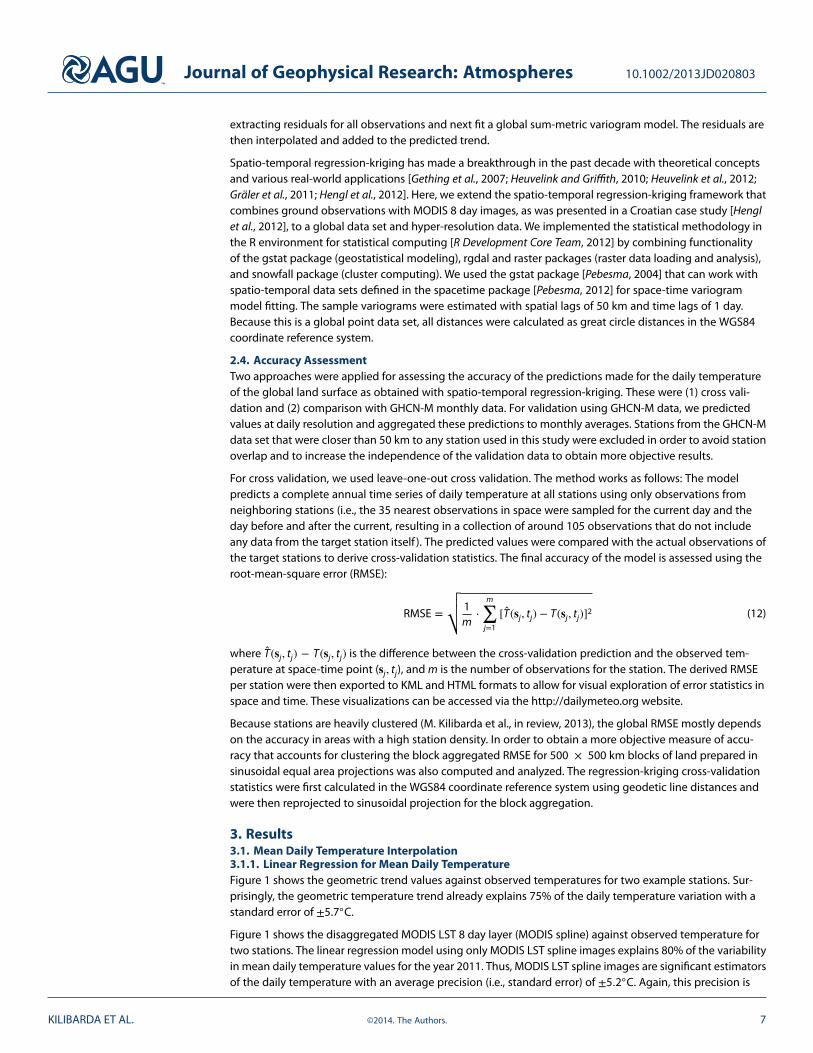
residuals show a significant purely spatial variogram component, while the purely temporal componentis zero and temporal variability is only contained in the space-time interaction component. This suggeststhat the temporal pattern in mean temperature is probably already sufficiently captured by the regressionmodel. The short-distance variation (nugget effect) in both the purely spatial and spatio-temporal compo-nent indicates that the model cannot yield better precision than ± 1.5◦C globally (for interpolation at dailyresolution). The range parameters are very large (especially the pure spatial range) showing that the residu-als are correlated along large distances up to 6000 km. In kriging the local neighborhoods must be selectedin a way that respects the spatial and temporal variogram ranges. Thus, only a few temporal instanceswill be selected, while the spatial selection spans several hundreds of kilometers. This is also captured bythe spatio-temporal anisotropy, which shows that stations with a temporal lag of 1 day exhibit a similarcorrelation as stations that are about 500 km apart.3.1.3. Accuracy Assessment: Mean Daily TemperatureAn interpolated map of daily mean temperature for the 1 and 2 January of 2011 is shown in Figure 4.Daily maps for the year 2011 at 1 km spatial resolution in GeoTiff format are available for download viahttp://www.dailymeteo.org. The mean daily temperature map of coterminous USA for the first 4 days inJanuary 2011 is presented in Figure 5.

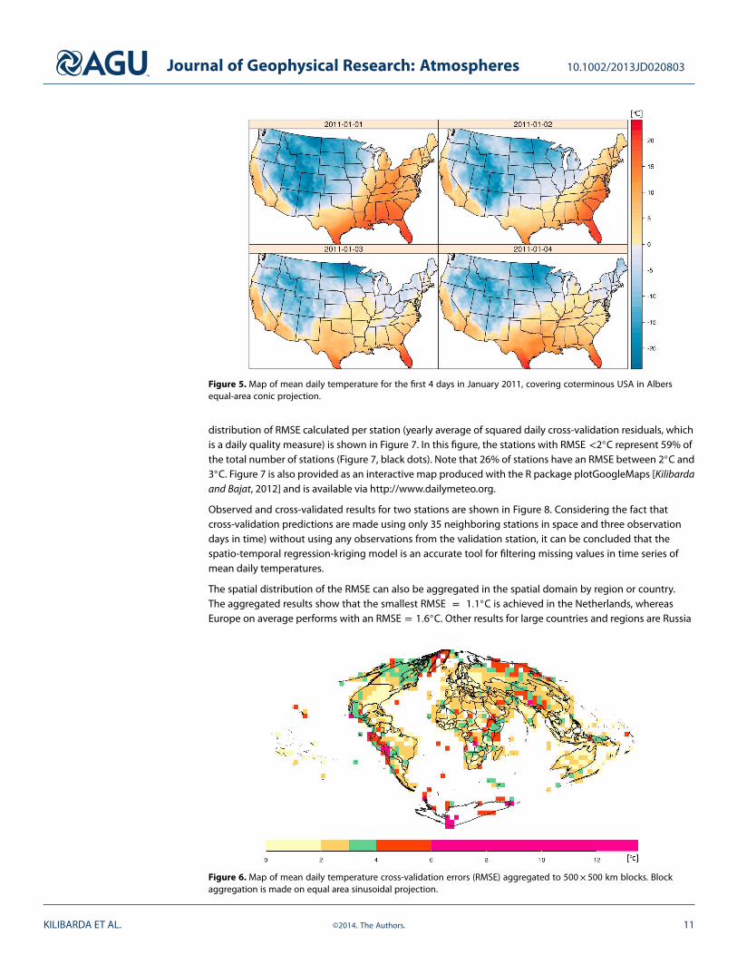
The cross-validation results on the complete data set yield RMSE = 2.4◦C for global land areas includingAntarctica, with an R-square of 96.6%. The block aggregated RMSE results show that the average accuracyis a bit worse (RMSE = 2.8; see also Figure 6). As mentioned previously, the global block aggregated RMSEgives a more objective global measure of accuracy. Thus, the actual RMSE is half a degree larger than theRMSE calculated as an unweighed mean from all stations.

The monthly RMSE obtained from cross validation of monthly aggregated observations withcross-validation prediction is 1.7◦C. This is an important result because it indicates that the model can beused for monthly image production (aggregation of daily gridded data). The yearly RMSE is 1.4◦C. The spatial

KILIBARDA ET AL. ©2014. The Authors. 10

Journal of Geophysical Research: Atmospheres 10.1002/2013JD020803

Figure 5. Map of mean daily temperature for the first 4 days in January 2011, covering coterminous USA in Albersequal-area conic projection.

distribution of RMSE calculated per station (yearly average of squared daily cross-validation residuals, whichis a daily quality measure) is shown in Figure 7. In this figure, the stations with RMSE <2◦C represent 59% ofthe total number of stations (Figure 7, black dots). Note that 26% of stations have an RMSE between 2◦C and3◦C. Figure 7 is also provided as an interactive map produced with the R package plotGoogleMaps [Kilibardaand Bajat, 2012] and is available via http://www.dailymeteo.org.

Observed and cross-validated results for two stations are shown in Figure 8. Considering the fact thatcross-validation predictions are made using only 35 neighboring stations in space and three observationdays in time) without using any observations from the validation station, it can be concluded that thespatio-temporal regression-kriging model is an accurate tool for filtering missing values in time series ofmean daily temperatures.

The spatial distribution of the RMSE can also be aggregated in the spatial domain by region or country.The aggregated results show that the smallest RMSE = 1.1◦C is achieved in the Netherlands, whereasEurope on average performs with an RMSE = 1.6◦C. Other results for large countries and regions are Russia

Figure 6. Map of mean daily temperature cross-validation errors (RMSE) aggregated to 500× 500 km blocks. Blockaggregation is made on equal area sinusoidal projection.

KILIBARDA ET AL. ©2014. The Authors. 11

Journal of Geophysical Research: Atmospheres 10.1002/2013JD020803

Figure 7. Map of mean daily temperature cross-validation errors (RMSE) averaged per year for each station. Red circlesindicate cross-validation outliers with RMSE > 6. Clusters of red circles indicate problematic areas, partly present of grosserror in observation time series.

(approximately 2.4◦C), USA 1.8◦C, South America 3.1◦C, while Antarctica has the largest RMSE with 5.9◦C. Aninteractive map of spatially aggregated RMSE at country level is available via http://www.dailymeteo.org.

The RMSE on the GHCN-M data is 1.5◦C and the spatial distribution of RMSE calculated per year (yearly aver-age of squared monthly validation residuals) for each station is shown in Figure 9 (an interactive map isavailable at http://www.dailymeteo.org). This map shows that 48% of the predicted points have a predictionaccuracy smaller than 1◦C. GHCN-M stations at a monthly resolution have an accuracy between 1 and 2◦Cfor 40% of the points.

3.2. Minimum Daily Temperature Interpolation3.2.1. Linear Regression Model for Minimum Daily TemperatureThe geometric temperature trend explains about 72% of the minimum daily temperature variations for2011, with a standard error of ±6◦C. Figure 10 shows the geometric trend against observations. The results

Figure 8. Comparison of mean daily temperature observations in 2011 (gray solid line) and space-timeregression-kriging cross-validation prediction of mean daily temperature (black dashed line). (top) Philadelphia, USA(𝜆 = −75, 𝜙 = 39.993). (bottom) Bunbury, Western Australia (𝜆 = 115.65, 𝜙 = −33.35).

KILIBARDA ET AL. ©2014. The Authors. 12

Journal of Geophysical Research: Atmospheres 10.1002/2013JD020803

Figure 9. Map of the validation errors (RMSE) averaged per year for each station, calculated by using GHCN-M stationswhich were not used for model and prediction.

of regression modeling based on MODIS LST spline images explains 70% of the variability in minimum dailytemperature values for the year 2011, with an average precision of ±6.3◦C, thus performing somewhatworse than for the mean temperature.

DEM and TWI layers also showed to be highly significant covariates for minimum daily temperature. The finallinear model with four covariates explains 77% of the variation, with a standard error of ±5.5◦C. Figure 10shows a plot of the modeled geometric trend for minimum daily temperature and MODIS LST spline valuesagainst observed temperature for the same stations.3.2.2. Spatio-Temporal Variogram Model for Minimum Daily TemperatureThe spatio-temporal variogram is modeled in the same way as was described for mean daily temper-ature. The variogram for minimum daily temperature has similar parameters as those obtained for themean daily temperature (see Table 2 and Figure 11). Again, there is no purely temporal component. The

Figure 10. Minimum daily temperature observation in 2011 (gray solid line) and multivariate linear model of minimumdaily temperature (red dashed line) on MODIS LST spline (black dashed line), geometric temperature trend (black dotline), elevation, and topographic wetness index. (top) Philadelphia, USA (𝜆 = −75, 𝜙 = 39.993). (bottom) Bunbury,Western Australia (𝜆 = 115.65, 𝜙 = −33.35).

KILIBARDA ET AL. ©2014. The Authors. 13

Journal of Geophysical Research: Atmospheres 10.1002/2013JD020803

Table 2. Parameters of the Fitted Sum-Metric Variogram Model for Min-imum Daily Temperature Regression Residuals, Each Component (SeeEquation (9)) is Modeled Using a Spherical Variogram Function

Nugget Sill Range Parameter Anisotropy Ratio

Spatial 3.695 22.682 5725 kmTemporal 0 0 0 daysSpace-time 1.67 9.457 1888 km 485 km/d

purely spatial component has a range of 5725 km at any time separation. Temporal variability of resid-uals is contained in the spatio-temporal interaction variogram component. The nugget parts of thesecomponents sum to around 3.5◦C2, which is larger than in the mean temperature case and suggeststhat short-range variability in space and time of minimum temperature regression residuals is signifi-cantly larger than for the mean temperature. This suggests that extreme temperatures are being harderto predict.3.2.3. Results of Accuracy Assessment for Minimum Daily TemperatureThe results of cross validation for minimum temperature produced RMSE = 2.7◦C for global land areasincluding Antarctica, with an R-square of 94.2%. Monthly RMSE obtained from the cross validation ofmonthly aggregated observations and cross-validation prediction is 2◦C, yearly RMSE is 1.7◦C. The spa-tial distribution of RMSE calculated per station (yearly average of squared daily cross-validation residuals,daily quality measure) for each station is shown in Figure 12, where the stations with RMSE <2◦C represent40% of the total number of stations (black dots), 2◦C< RMSE <3◦C occurs for 35% (blue dots), 23% have3◦C< RMSE <6◦C, and 200 stations have an RMSE >6◦C.

Figure 11. Fitted (left) sum-metric model and (right) sample variogram of residuals from multiple regression of minimumdaily temperature observation on MODIS, geometric temperature trend, elevation, and topographic wetness index. Thevariogram surface is presented in (top) 2-D and (bottom) 3-D manner.

KILIBARDA ET AL. ©2014. The Authors. 14

Journal of Geophysical Research: Atmospheres 10.1002/2013JD020803

Figure 12. Map of minimum daily temperature cross-validation errors (RMSE) averaged per year for each station. Redcircles indicate cross-validation outliers with RMSE > 6. Clusters of red circles indicate problematic areas, partly presentof gross error in observation time series.

The spatial distribution of RMSE also shows lower accuracy than predictions of the mean temperature ingeneral. The aggregated results show that the smallest RMSE = 1.4◦C is achieved in the Netherlands, Europewithout Russia (approximately 2.7◦C) has RMSE of around 2.3◦C, USA 2.3◦C, South America 3.1◦C, Antarcticahas again the highest RMSE = 4.7◦C.

3.3. Maximum Daily Temperature Interpolation3.3.1. Linear Regression Model for Maximum Daily TemperatureThe geometric temperature trend in the linear model explains 75% of maximum daily temperature variationfor 2011 with a standard error of ±6.6◦C. Figure 13 shows the geometric trend compared against observa-tion. The geometric trend results are comparable to the results of modeling the mean temperature and arehence better than the results for modeling the minimum daily temperature case.

Figure 13. Maximum daily temperature observation in 2011 (gray solid line) and multivariate linear model of maximumdaily temperature (red dashed line) on MODIS LST spline (black dashed line), geometric temperature trend (black dottedline), elevation, and topographic wetness index. (top) Philadelphia, USA (𝜆= −75,𝜙=39.993). (bottom) Bunbury, WesternAustralia (𝜆 =115.65, 𝜙 = −33.35).

KILIBARDA ET AL. ©2014. The Authors. 15

Journal of Geophysical Research: Atmospheres 10.1002/2013JD020803

Table 3. Parameters of the Fitted Sum-Metric Variogram Model for MaximumDaily Temperature Regression Residuals, Each Component (See Equation (9))is Modeled Using a Spherical Variogram Function

Nugget Sill Range Parameter Anisotropy Ratio

Spatial 2.8722 8.314 4930 kmTemporal 0 0 0 daysSpace-time 1.750 11.175 2117 km 527 km/d

Regression modeling with only MODIS LST spline images already explains 84.5% of the variability in max-imum daily temperature values for the year 2011 with an average precision of ±5.2◦C. MODIS LST 8 dayimages are the best predictor for the maximum daily temperature when compared to actual mean andminimum daily temperatures. DEM and TWI layers also were significant covariate layers for the maximumdaily temperature. The final linear model with four covariates explains 86.7% of the variation, with a stan-dard deviation of ±4.8◦C. Figure 13 shows the modeled linear regression line, the geometric trend forthe maximum daily temperature, and the MODIS LST spline values against observed temperature for thesame stations.3.3.2. Spatio-Temporal Variogram Model for Maximum Daily TemperatureTable 3 (see also Figure 14) summarizes the parameters of the spatio-temporal variogram model. All com-ponents of the variogram are spherical functions. The nugget effect of the purely spatial component isrelatively large as was observed before for the minimum temperature, showing that this model cannotachieve a better accuracy than the model for the mean daily temperature.3.3.3. Results of Accuracy Assessment for Maximum Daily TemperatureResults of cross validation for maximum daily temperature on the complete data set gave an RMSE =2.6◦C for global land areas including Antarctica, with R-square 95.9%. Monthly RMSE obtained from cross

Figure 14. Fitted (left) sum-metric model and (right) sample variogram of residuals from multiple linear regression ofmaximum daily temperature on MODIS, geometric temperature trend, elevation, and topographic wetness index. Thevariogram surface is presented in (top) 2-D and (bottom) 3-D.

KILIBARDA ET AL. ©2014. The Authors. 16

Journal of Geophysical Research: Atmospheres 10.1002/2013JD020803

Figure 15. Map of maximum daily temperature cross-validation errors (RMSE) averaged per year for each station. Redcircles indicate cross-validation outliers with RMSE > 6. Clusters of red circles indicate problematic areas, partly presentof gross error in observation time series.

validation of monthly aggregation of observation and cross-validation prediction is 1.9◦C, and yearlyRMSE is 1.6◦C. The spatial distribution of RMSE calculated per station (yearly average of squared dailycross-validation residuals, daily quality measure) for each station is shown in Figure 15, where the stationswith RMSE<2◦C are 41% of the total number of stations (black dots), 41% has 2◦C< RMSE <3◦C (blue dots),16.6% have 3◦C< RMSE <6◦C, and 106 stations have RMSE >6◦C.

The spatial distribution of RMSE also shows a lower accuracy than for the mean daily temperature. Theaggregated results show that the best RMSE = 1.3◦C is achieved in the Netherlands. Europe without Russiaachieves around 2.1◦C (Russia approximately 2.7◦C), USA 2.1◦C, South America 3.2◦C, and Antarctica has thehighest RMSE = 5◦C.

3.4. Accuracy of the Prediction Models Without Satellite DataTable 4 shows the results of the accuracy assessment with and without using MODIS LST 8 daily images.Sections 3.1.1, 3.2.1, and 3.3.1 show that MODIS LST is the most important covariate in the linear model,and without using any other covariates it explains the biggest part of the variation. Table 4 also shows thatthe influence of MODIS LST is significant in the linear model for all dependent variables, despite the fact thatthe accuracy of the regression-kriging for mean and minimum temperature is almost the same with andwithout using MODIS. Apparently, the spatio-temporal kriging of the regression residual can compensate forthe less accurate linear model. The total accuracy of the spatio-temporal regression-kriging is significantlyhigher with MODIS for the maximum temperature. The important influence of MODIS in this case is alsoobvious from visual comparison of Figures 1, 10, and 13, where MODIS values are most strongly correlatedwith maximum daily temperature. The influence of topography is obvious in the temperature estimates athigher elevations.

Table 4. Accuracy Assessment Parameters for Multiple Linear Regression and Spatio-Temporal Regression-Kriging Model With MODIS LST Images VersusWithout MODIS LST Images Used as Covariate

Regression Part Spatio-Temporal Regression-Kriging

R-Square (Without RMSE (Without R-Square (Without RMSE (WithoutR-Square (%) Standard Error (◦C) MODIS) (%) MODIS) (◦C) R-Square (%) Standard Error (◦C) MODIS) (%) MODIS) (◦C)

TMEAN 84.2 4.6 75 6.2 96.6 2.39 96.3 2.47TMIN 77.0 5.5 72.3 6.0 95.9 2.70 94.2 2.77TMAX 86.7 4.8 75.2 6.3 96.4 2.60 87.5 4.20

KILIBARDA ET AL. ©2014. The Authors. 17

Journal of Geophysical Research: Atmospheres 10.1002/2013JD020803

4. Discussion and Conclusions

In this paper we have demonstrated how dense publicly available ground station meteorological datatogether with a time series of remote sensing images and covariates at 1 km resolution can be used topredict mean, minimum, and maximum daily temperature for the global landmass in space and time. Theobtained global models for mean, minimum, and maximum temperature were further used to produce grid-ded images of daily temperatures at high spatial and temporal resolution. We achieved an average globalprediction accuracy of about 2–3◦C for daily temperature prediction when assessed using cross validation(which confirms the results of some local studies by Hengl et al. [2012], Heuvelink et al. [2012], and Neteler[2010]). This is promising as it indicates that highly accurate maps of daily temperatures can be producedat high spatial resolution using global spatio-temporal models. Figures 7, 12, and 15 also show that theoutliers are distinctly grouped in areas that are poorly covered with meteorological stations and in moun-tainous regions, i.e., areas frequently covered with clouds or snow. This agrees with findings of Neteler[2010], who experienced similar difficulties in working with dynamic snow cover on mountain tops.

During the model fitting, we discovered that the GSOD point data sets still contain many artifacts and possi-ble gross errors. We removed a small portion of obvious errors, but it is likely that there are still many grosserrors in GSOD. It was beyond the scope of this study to identify and remove all errors. Station data filter-ing should probably be performed by the organizations that collected the data because they have expertknowledge on the measurements and stations. In that context, a methodology based on cross validationcould be used as a tool to detect stations with potential errors. For example, stations with residuals beyondsome threshold could be iteratively removed in a series of cross validations until no station with a resid-ual larger than the threshold can be found. Furthermore, by overlaying the point data and WorldGrids.orgcovariates, we were able to detect stations with inaccurate spatial locations. This is especially importantfor stations in mountainous regions, which proved to be very important for model building as the error ofpredicting temperature increases with elevation.

When we tested the models using the GHCN-Daily data (quality controlled data set with 13,395 stations),we obtained similar results for maximum daily temperature with R-square of 95.2% and RMSE =2.83◦C (fordetails see interactive map at http://dailymeteo.org). For minimum daily temperature (13,380 stations),R-square was 94.2% and RMSE=2.84◦C. In this paper, the intention was to analyze three temperature param-eters, namely, minimum, maximum, and mean daily temperature. That lead us to choose GSOD over theGHCN-D since GHCN-D still does not have the mean temperature included. But comparing the documenta-tion and quality control procedures for GSOD and GHCN-D, we would probably recommend GHCN-D as themore suited data set for spatio-temporal analysis of the minimum and maximum daily temperature.

Our original idea was to overlay daily air temperature values (minimum, maximum, and mean) with daily LSTimages (MOD11A1 product) and build calibration models (spatio-temporal regression) for actual tempera-ture above ground. However, the MOD11A1 product contains so many gaps (often >50% of the coveragecontains missing pixels) due to cloud cover and atmospheric disturbances, so that we have finally decidedto work only with MOD11A2 products. If a remote sensing image contains >50% of missing pixels, then thiscould lead to geostatistical models which are incomplete and unrepresentative. At this stage we also didnot consider using the quality flag (i.e., number of days used to estimate the MOD11A2 LST value) in themodel building, so this could be an area where predictions could be further improved. Maybe more elab-orate procedure could also be developed to address the problem of missing pixels in the daily LST imagesdue to clouds, but for the moment we do not see much potential in developing global spatio-temporalgeostatistical models with so incomplete data.

It is worth noting that the presented global regression-kriging models can also be used to produce maps ofassociated uncertainty at high spatio-temporal resolution. Moreover, by using a global geostatistical model,unbiased prediction of daily air temperatures for any place on the global land mask can be obtained (at 1 kmresolution) and for any day of the year for the period from the beginning of the MODIS mission until today.This is probably impossible using e.g., mechanical interpolators such as splines.

Our results also showed that the geometric temperature trend (equation (3)) is a crucial covariate. Alone, itcan explain more than 70% of the temperature variation. This indicates that a similar model without remotesensing images can be made for the daily temperature interpolation for the period for which no MODISimages are available. In that context, the fitted spatio-temporal global models for mean, minimum, and

KILIBARDA ET AL. ©2014. The Authors. 18

Journal of Geophysical Research: Atmospheres 10.1002/2013JD020803

maximum daily temperature can also be used as a tool for disaggregation of MODIS 8 day images todaily images and for the calibration of land surface temperatures (conversion from land surface toair temperature).

Daily interpolation and spatio-temporal interpolation were performed for several days and producedcomparable RMSE. The similarity was confirmed by Spadavecchia and Williams [2009], who also did notachieve a significant increase in interpolation performance for spatio-temporal interpolation of temperaturecompared with mechanical spatial interpolation methods such as splines. However, we believe here thatgeostatistical techniques are superior to mechanical techniques particulary because they allow for an objec-tive quantification of uncertainty. As Spadavecchia and Williams [2009] suggest: “spatia-temporal techniquesare useful, particularly in the provision of spatia-temporal uncertainty estimates.”

Another important advantage of the integrated spatio-temporal modeling is that a single regression modeland a single semivariogram based on the complete space-time data set are valid for the whole year, whilepurely spatial models require 365 regression models and 365 semivariograms, using only data records avail-able for a single day. This is much more labor intensive and makes quality checking difficult. Besides theelegance of the spatio-temporal model (estimation of just one model for the whole phenomenon), thespatio-temporal model is also advantageous because temporal trajectories of predictions and simulationslook much more realistic (the models described in this paper can be obtained by installing the meteo pack-age for R created and maintained by the authors of this article). If separate spatial interpolation is done forevery day, time series at prediction locations may show abrupt jumps that have no physical basis.

The presented computational framework could now be used to produce a global archive of the mean, min-imum, and maximum temperature images. The daily maps of temperature could serve as raster files in asimilar fashion as climate layers from the WorldClim.org project [Hijmans et al., 2005]. This would require ahuge data storage and serving capacities, considering the amount of output pixels (10 years by 365 daysby 7–10 meteo variables plus uncertainty maps). Furthermore, globally fitted models of daily temperaturescan be used for regional or local studies, e.g., where a limited number of ground observation stations areavailable so that some reference global model of spatio-temporal variability is required.

ReferencesAlexander, L. V., et al. (2006), Global observed changes in daily climate extremes of temperature and precipitation, J. Geophys. Res., 111,

D05109, doi:10.1029/2005JD006290.Bader, M. Y., and J. J. Ruijten (2008), A topography-based model of forest cover at the alpine tree line in the tropical Andes, J. Biogeogr.,

35(4), 711–723, doi:10.1111/j.1365-2699.2007.01818.x.Becker, A., P. Finger, A. Meyer-Christoffer, B. Rudolf, K. Schamm, U. Schneider, and M. Ziese (2012), A description of the global land-surface

precipitation data products of the Global Precipitation Climatology Centre with sample applications including centennial (trend)analysis from 1901–present, Earth Syst. Sci. Data Discuss., 5(2), 921–998, doi:10.5194/essdd-5-921-2012.

Böhner, J., T. Blaschke, and L. Montanarella (Eds.) (2008), SAGA — Seconds Out, vol. 19, 113 pp., Hamburger Beiträge zur PhysischenGeographie und Landschaftsökologie, Hamb.

Burrough, P. (Ed.) (1998), Principles of Geographical Information Systems, 2nd ed., 220 pp., Oxford Univ. Press, Oxford.Caesar, J., L. Alexander, and R. Vose (2006), Large-scale changes in observed daily maximum and minimum temperatures: Creation and

analysis of a new gridded data set, J. Geophys. Res., 111, D05101, doi:10.1029/2005JD006280.Carrera-Hernández, J., and S. Gaskin (2007), Spatio temporal analysis of daily precipitation and temperature in the Basin of Mexico, J.

Hydrol., 336(3), 231–249.Coll, C., Z. Wan, and J. M. Galve (2009), Temperature-based and radiance-based validations of the V5 MODIS land surface temperature

product, J. Geophys. Res., 114, D20102, doi:10.1029/2009JD012038.Cressie, N., and C. K. Wikle (2011), Statistics for Spatio-Temporal Data, Wiley, N. J.Di Luzio, M., G. L. Johnson, C. Daly, J. K. Eischeid, and J. G. Arnold (2008), Constructing retrospective gridded daily precipitation and

temperature datasets for the conterminous United States, J. Appl. Meteorol. Climatol., 47(2), 475–497, doi:10.1175/2007JAMC1356.1.Gething, P., P. Atkinson, A. Noor, P. Gikandi, S. Hay, and M. Nixon (2007), A local space-time kriging approach applied to a national

outpatient malaria data set, Comput. Geosci., 33(10), 1337–1350, doi:10.1016/j.cageo.2007.05.006.Gräler, B., L. Gerharz, and E. Pebesma (2011), Spatio-temporal analysis and interpolation of PM10 measurements in Europe, ETC/ACM

Technical Paper, 10.Haylock, M. R., N. Hofstra, A. M. G. Klein Tank, E. J. Klok, P. D. Jones, and M. New (2008), A European daily high-resolution gridded data set

of surface temperature and precipitation for 1950–2006, J. Geophys. Res., 113, D20119, doi:10.1029/2008JD010201.Hengl, T., G. B. Heuvelink, M. Percec Tadic, and E. J. Pebesma (2012), Spatio-temporal prediction of daily temperatures using time-series

of MODIS LST images, Theor. Appl. Climatol., 107, 265–277, doi:10.1007/s00704-011-0464-2.Heuvelink, G. B. M., and D. A. Griffith (2010), Space-time geostatistics for geography: A case study of radiation monitoring across parts of

Germany, Geog. Anal., 42(2), 161–179, doi:10.1111/j.1538-4632.2010.00788.x.Heuvelink, G. B. M., D. A. Griffith, T. Hengl, and S. J. Melles (2012), Sampling Design Optimization for Space-Time Kriging, pp. 207–230, John

Wiley, Oxford, doi:10.1002/9781118441862.ch9.Hijmans, R. J., S. E. Cameron, J. L. Parra, P. G. Jones, and A. Jarvis (2005), Very high resolution interpolated climate surfaces for global land

areas, Int. J. Circuit Theory Appl., 25, 1965–1978, doi:10.1002/joc.1276.

AcknowledgmentsThis study is fully supported by theresearch projects TR 36035: Spatial,ecological, energy, and social aspectsof settlements’ development andclimate changes interrelationships,funded by the Ministry of Educationand Science of the Republic of Serbia,WorldGrids.org data portal has beendeveloped as a part of the GlobalSoil Information Facilities projectthat provides tools for collating andserving global soil data developedjointly by ISRIC-World Soil Informationand collaborators.

KILIBARDA ET AL. ©2014. The Authors. 19

Journal of Geophysical Research: Atmospheres 10.1002/2013JD020803

Hofstra, N., M. Haylock, M. New, P. Jones, and C. Frei (2008), Comparison of six methods for the interpolation of daily, European climatedata, J. Geophys. Res., 113, D21110, doi:10.1029/2008JD010100.

Jarvis, C. H., and N. Stuart (2001), A comparison among strategies for interpolating maximum and minimum daily air temperatures. PartII: The interaction between number of guiding variables and the type of interpolation method, J. Appl. Meteorol., 40(6), 1075–1084.

Kiktev, D., D. M. Sexton, L. Alexander, and C. K. Folland (2003), Comparison of modeled and observed trends in indices of daily climateextremes, J. Clim., 16(22), 3560–3571.

Kilibarda, M., and B. Bajat (2012), Plotgooglemaps: The R-based web-mapping tool for thematic spatial data, Geomatica, 66(1), 37–49,doi:10.5623/cig2012-007.

Klein Tank, A. M. G., et al. (2002), Daily dataset of 20th-century surface air temperature and precipitation series for the European ClimateAssessment, Int. J. Climatol., 22(12), 1441–1453, doi:10.1002/joc.773.

Lawrimore, J. H., M. J. Menne, B. E. Gleason, C. N. Williams, D. B. Wuertz, R. S. Vose, and J. Rennie (2011), An overview of the Global His-torical Climatology Network monthly mean temperature data set, version 3, J. Geophys. Res., 116, D19121, doi:10.1029/2011JD016187.

Leemans, R., and W. P. Cramer (1991), The IIASA database for mean monthly values of temperature, precipitation, and cloudiness on aglobal terrestrial grid, International Institute for Applied Systems Analysis, Laxenburg, Austria.

Legates, D., and C. Willmott (1990), Mean seasonal and spatial variability in global surface air temperature, Theor. Appl. Climatol., 41(1-2),11–21, doi:10.1007/BF00866198.

Mitchell, T. D., and P. D. Jones (2005), An improved method of constructing a database of monthly climate observations and associatedhigh-resolution grids, Int. J. Climatol., 25(6), 693–712, doi:10.1002/joc.1181.

Neteler, M. (2010), Estimating daily land surface temperatures in mountainous environments by reconstructed MODIS LST Data, RemoteSens., 2(1), 333–351, doi:10.3390/rs1020333.

New, M., M. Hulme, and P. Jones (1999), Representing twentieth-century space-time climate variability. Part I: Development of a 1961–90mean monthly terrestrial climatology, J. Clim., 12, 829–856, doi:10.1175/1520-0442(1999)012<0829:RTCSTC>2.0.CO;2.

New, M., M. Hulme, and P. Jones (2000), Representing twentieth-century space-time climate variability. Part II: development of 1901-96monthly grids of terrestrial surface climate, J. Clim., 13, 2217–2238, doi:10.1175/1520-0442(2000)013<2217:RTCSTC>2.0.CO;2.

Pebesma, E. (2012), Spacetime: Spatio-temporal data in R, J. Stat. Software, 51, 1–30.Pebesma, E. J. (2004), Multivariable geostatistics in S: The gstat package, Comput. Geosci., 30(7), 683–691, doi:10.1016/j.cageo.2004.03.012.Peterson, T. C., and R. S. Vose (1997), An overview of the Global Historical Climatology Network temperature database, Bull. Am. Meteorol.

Soc., 78(12), 2837–2849, doi:10.1175/1520-0477(1997)078<2837:AOOTGH>2.0.CO;2.Pinheiro, J., and D. Bates (2009), Mixed-Effects Models in S and S-PLUS, Statistics and Computing, Springer, New York.Piper, S. C., and E. F. Stewart (1996), A gridded global data set of daily temperature and precipitation for terrestrial biospheric modeling,

Global Biogeochem. Cycles, 10(4), 757–782, doi:10.1029/96GB01894.Price, D. T., D. W. McKenney, I. A. Nalder, M. F. Hutchinson, and J. L. Kesteven (2000), A comparison of two statistical methods for spatial

interpolation of Canadian monthly mean climate data, Agric. For. Meteorol., 101(2), 81–94.R Development Core Team (2012), R: A Language and Environment for Statistical Computing, 1731 pp., R Foundation for Statistical

Computing, Vienna, Austria. ISBN 3-900051-07-0.Sorensen, R., U. Zinko, and J. Seibert (2006), On the calculation of the topographic wetness index: Evaluation of different methods based

on field observations, Hydrol. Earth Syst. Sci. Discuss., 10, 101–112.Spadavecchia, L., and M. Williams (2009), Can spatio-temporal geostatistical methods improve high resolution regionalisation of

meteorological variables? Agric. For. Meteorol., 149(6), 1105–1117.Stahl, K., R. Moore, J. Floyer, M. Asplin, and I. McKendry (2006), Comparison of approaches for spatial interpolation of daily air tem-

perature in a large region with complex topography and highly variable station density, Agric. For. Meteorol., 139(3), 224–236,doi:10.1016/j.agrformet.2006.07.004.

Tveito, O., M. Wegehenkel, F. van der Wel, and H. Dobesch (2006), Spatialisation of climatological and meteorological information withthe support of GIS (Working Group 2), The Use of Geographic Information Systems in Climatology and Meteorology, Final Report.pp. 37–172.

Van De Kerchove, R., S. Lhermitte, S. Veraverbeke, and R. Goossens (2013), Spatio-temporal variability in remotely sensed land surfacetemperature, and its relationship with physiographic variables in the Russian Altay Mountains, Int. J. Appl. Earth Obs. Geoinf., 20, 4–19.

Van den Besselaar, E. J. M., M. R. Haylock, G. van der Schrier, and A. M. G. Klein Tank (2011), A European daily high-resolutionobservational gridded data set of sea level pressure, J. Geophys. Res., 116, D11110, doi:10.1029/2010JD015468.

Vose, R. S., O. R. N. L. E. S. Division., G. C. R. P. (U.S.), U. S. D. of Energy. Office of Health, E. Research., C. D. I. A. C. (U.S.), and I. MartinMarietta Energy Systems (1992), The Global Historical Climatology Network: Long-Term Monthly Temperature, Precipitation, Sea LevelPressure, and Station Pressure Data, Carbon Dioxide Information Analysis Center, Oak Ridge National Laboratory; Available to thepublic from N.T.I.S., Oak Ridge, Tenn.; Springfield, VA.

Wan, Z., Y. Zhang, Q. Zhang, and Z.-L. Li (2004), Quality assessment and validation of the MODIS global land surface temperature, Int. J.Remote Sens., 25(1), 261–274, doi:10.1080/0143116031000116417.

Yoo, J.-M., Y.-I. Won, Y.-J. Cho, M.-J. Jeong, D.-B. Shin, S.-J. Lee, Y.-R. Lee, S.-M. Oh, and S.-J. Ban (2011), Temperature trends in theskin/surface, mid-troposphere and low stratosphere near Korea from satellite and ground measurements, Asia-Pac. J. Atmos. Sci., 47,439–455, doi:10.1007/s13143-011-0029-4.

KILIBARDA ET AL. ©2014. The Authors. 20