A STUDY OF 30 KM TO 200 KM METEOROLOGICAL ...

~NASA CONTRACTOR

REPORT

A STUDY OF 30 KM TO 200 KM METEOROLOGICAL ROCKET SOUNDING SYSTEMS

VOLUME I - LITERATURE AND DATA REVIEW

!by B mce Bollermunn

i ! Prepared by

j SPACE DATA CORPORATION Ark .

Gem-ie C. Marshall Space Flight Center

NATIONAL AERONAUTICS AND SPACE ADMINISTRATION l WASHINGTON, D. C. . MAY 1970

TECH LIBRARY KAFB, Ni

I 111111 HIII I Ill lllll lllll lll~ Ill IllI 1. Report No.

NASA CR-1529 (Part 1) 2. Government Accession No. 3. Recipiel 0Clbllb83

4. Title and Subtitle VOLUME I: A STUDY OF 30 KM TO 200 KM METEOROLOGICAL ROCKET SOUNDING SYSTEMS Part I: Literature and Data Review

7. Author(s)

Bruce Bollermann 0. Performing Organization Report No.

10. Work Unit No. 9. Performing Organization Name and Address

Space Data Corporation 11. Contract or Grant No.

Phoenix, Arizona I NAS8-20797

12. Sponsoring Agency Name and Address NASA-George C. Marshall Space Flight Center Marshall Space Flight Center, Alabama 35812

13. Type of Report and Period Covered

CONTRACTORREPORT 14. Sponsoring Agency Code

Contract Monitor: R. E. Turner 15. Supplementary Notes

Distribution of this report is provided in the interest of information exchange. Responsibility for the contents resides in the author or organization that prepared it.

16. Abstract

This report reviews the contemporary literature on meteorological rockets and associated systems, to determine the accuracies and limitations of the current meteorological rocket systems from available data, and to determine the adaptability of the more complex geophysical rocket experiments to simplified, economical, routine meteorological rocket soundings. This literature review covers the various system requirements and techniques used in obtaining meteorological measurements of the 30 km to 200 km region of the atmosphere. In addition to the detailed descriptions of the various rocket vehicles, telemetry, sensors, decelerators and other related equipment, this review also includes a study of the gun probe systems.

This study report is presented in two books: Book 1 contains an introduction, a discussion of systems requirements and a description of the various sensing techniques; Book 2 contains details of the rocketsonde decelerator techniques, telemetry and tracking equipment, descriptions of the rocket vehicles, gun probe systems and a summary of the report. The two books are printed under separate cover, and are labeled Volume I.

7. Key Words (Suggested by Author(s)) 18. Distribution Statement

19. Security Classif. (of this report) 1 20. Security Classif. ( this page)

Unclassified - Unlimited

1 21. No. of Pages 1 22. Price*

Unclassified Unclassified 426 $3.00

‘For sale by the Clearinghouse for Federal Scientific and Technical Information

Springfield, Virginia 22151

FOREWORD

Most of the material in this report has been taken directly from the current literature; thus, to avoid frequent interruptions in the text, references have been omitted. Instead, acknowledgements are made preceding Book 1 for the primary investigators and authors whose works have been abstracted and whose data are presented. A bibliography of the digested literature follows the conclusion of Book 2.

This survey was made under Contract NAS8-20797 with the Aerospace Environment Division, Aero-Astrodynamics Laboratory, Marshall Space Flight Center. Mr. Robert E. Turner was the Contract Monitor.

ACKNOWLEDGEMENTS

Special recognition is expressed to the Meteorological Working Group of the Inter-Range Instrumentation Group, Range Commander's Conference, whose efforts brought about the formation of the Meteor- ological Rocket Network, and consequently the widespread distribution of its valuable data to the scientific community. The Network has grown worldwide, and has directly influenced developments in rocket meteorology.

Appreciation is expressed to Mr. Robert E. Turner and Mr. 0. E. Smith of the Aerospace Environment Division, Aero-AstrodynamicS Laboratory, NASA-Marshall Space Flight Center for their support and guidance in presenting this study, and to Mr. Edgar Schaefer for the many illustrations and Mr. David Gironda and staff of the Space Data Corporation for editorial assistance.

iii

TABLE OF CONTE,NTS

Chapter

FOREWORD ....................................

ACKNOWLEDGEMENTS ..........................

1 INTRODUCTION

1.1 GENERAL ...........................

1.2 ATMOSPHERIC PARAMETERS. .......... 3 1.2.1 General ............................ 3 1.2.2 Atmospheric Motion. .................. 5 1.2.3 Atmospheric Temperature. ............. 7

1.3 MEASUREMENT CONSIDERATIONS ......

1.4 MEASUREMENT SYSTEMS .............

9

13

2 SYSTEM REQUIREMENTS

2.1 GENERAL ........................... 16

2.2 MISSILE AND SPACE VEHICLE SUPPORT., 17 2.2.1 Launch Vehicle Requirements. ......... 17 2.2,. 2 In-Flight Requirements. ............... 19 2.2.3 Re-Entry Requirements. ............... 19 2.2.4 Hypersonic Glide Vehicle Requirements. . 25

2.3 METEOROLOGICAL RESEARCH .......... 32 2.3.1 Synoptic Data ................. i ...... 32 2.3.2 Aeronomy ............................ 33 2.3.2.1 General ............................. 33 2.3.2.2 Density Structure ..................... 34 2.3.2.3 Atmospheric Composition .............. 34 2.3.2.4 Ionospheric Winds .................... 35 2.3.2.5 Ozone .............................. 35 2.3.2.6 Thermal Radiation. ................... 36 2.3.2.7 WaterVapor ......................... 36

Pase

. * . 111

. . . 111

1

IV

2.3.2.8 Electron Density and structure of Ionosphere . . . . . . . . . . . . . . . . . . . . . . . .

2.3.2.9 Electric Currents in the Atmosphere. . . . . .

2.4

2.5

2.6

SPECIAL PROJECT REPORT . . . . . . . . . . . . .

METEOROLOGICAL MEASUREMENT REQUIREMENTS . . . . . . . . . . . . . . . . . . . . . .

METEOROLOGICAL ROCKET SYSTEM REQUIREMENTS . . . . . . . . . . . . . . . . . . . . .

3 ATMOSPHERIC SENSORS

3.1 GENERAL ........................... 46

3.2 WIND MEASUREMENT TECHNIQUES .... 47 3.2.1 High Altitude Wind Patterns. .......... 47 3.2.2 Wind Measurement Error .............. 52 3.2.3 Chaff .............................. 72 3.2.4 Rocketsonde Decelerators. ............ a2 3.2.5 Falling Sphere ....................... 90 3.2.6 Rocket Grenades ..................... 94 3.2.7 Chemical, ..Trails ..................... 100 3.2.7.1 Sodium Vapor Trails. ................. 103 3.2.7.2 Trimethyl Aluminum Trails. ............ 118 3.2.7.3 Gun Launched Trails. ................. 126 3.2.7.4 Summary ............................ 127 3.2.8 Rocket Response Sensing ............. 130 3.2.9 Stokes Flow Parachute ............... 130

3.3

3.3.1 3.3.2 3.3.3

TEMPERATURE MEASUREMENT TECHNIQUES ....................... General ............................ Thermistor Mounts Descriptions. ...... Theoretical Analysis of Temperature Measurement Error Sources. .......... General ............................ Papers on Theoretical Temperature Corrections. ........................ Flight Test Data ..................... Improvements for Altitudes Above 60 Km.

132 132 138

3.3.3.1 3.3.3.2

155 155

3.3.4 3.3.5 t

163 227 248

36 37

38

39

44

V

3.4

3.4.1 3.4.2 3.4.3

3.4.3.1 3.4.3.2 3.4.3.3 3.4.3.4 3.4.4 3.4.5 3.4.6

3.5 3.5.1 3.5.2 3.5.3 3.5.4 3.5.4.1 3.5.4.2 3.5.4.3 3.5.4.4 3.55 3.5.5.1 3.5.5.2 3.5.5.2.1 3.5.5.2.2 3.5.5.2.3 3.5.5.3 3.5.5.3.1 3.5.5.3.2 3.5.5.3.3 3.5.5.3.4 3.5.5.4 3.5.5.4.1 3.5.5.4.2

PITOT PROBE DENSITY MEASUREMENTS. . Introduction. ........................ Aerobee - Hi Experiment .............. Nike-Apache Experiments. ............ Sparrow - Arcas Experiment ........... General ............................ Theory ............................. System Description. ................. Results ............................ Impact Pressure Gauges .............. General ............................ Transport Property Gauges. ........... General ............................ PiraniGauge ........................ Havens Gauge ...................... Ionization Vacuum Gauges. ........... General ............................ Thermionic Ionization Gauges. ........ Glow Discharge Ionization Gauges. .... Radioactive Ionization Gauges. ........ Force Measurement Gauges ........... General ............................ Vibrating Diaphragm Pressure Transducer ......................... 363

FALLING SPHERE DENSITY MEXURt?JCNT . TECHNIQUES. ...................... 25.4 General ............................ 25< Theoretical ......................... 253 Papers on Various Falling Sphere Designs ........................... 259 Inflatable Nylon Sphere. ............. 259 Rigid Aluminum Spheres .............. 2h2 Inflatable Melinex Sphere. ........... 266 Inflatable Mylar Spheres ............. 266 Active Rigid Sphere. ................. 287 Active Inflatable Sphere. ............. 292 Passive Inflatable Sphere. ............ 29 7

308 308 308 322 325 325 329 333 342 342 342 347 347 349 349 350 350 352 355 358 361 361

3.6 3.6.1 3.6.2 3.6.3

SONIC GRENADES ................... 369 General ............................ 369 DOVAP Systems. .................... 378 Basic Data Reduction. ............... 384

vi

3.7 OZONE SENSORS AND TECHNIQUES ... 392 3.7.1 Spectrometric Technique ............. 392 3.7.2 Chemical Techniques ............... 393 3.7.3 Chemiluminescent Technique ........ 395 3.7.4 Miscellaneous Techniques .......... 397

3.8

3.8.1 3.8.2 3.8.3 3.8.4 3.8.5

WATER VAPOR MEASUREMENT TECHNIQUES ..................... Mechanical Hygrometers. .......... Electric Hygrometers. .............. Dew Point Techniques. ............. Spectrographic Techniques .......... Miscellaneous Techniques ..........

400 400 400 401 401 402

3.9 ATMOSPHERIC COMPOSITION ....... 403

3.10 3.10.1 3.10.2 3.10.3 3.10.4 3.10.5

ELECTRON DENSITY ................ General. ......................... Radio Propagation Techniques ....... Langmuir Probe Techniques .......... Resonance Probe Techniques. ........ Standing Wave Impedance Probe Technique ......................... Mobility Spectrometer Technique ...... Rocket Design ............... I ......

405 405 407 408 408

3.10.6 3.10.7

409 409 412

3.11

3.11.1 3.11.2

SOLAR AND TERRESTRIAL RADIATION FLUX SENSORS ..................... Radiometers ....................... Spectrometers. ....................

413 413 414

3.12

3.12.1 3.12.2 3.12.3 3.12.4 3.12.5

3.13

3.13.1 3.13.2 3.13.3

MISCELLANEOUS DENSITY MEASUREMENT TECHNIQUES, ....................... 4 15 Spinning Wire Densitometer. .......... 4 15 Radiation Absorption. ................ 4 15 Beta Ray Sensor. .................... 421 X-Ray Backscatter ................... 421 Molecular Fluorescence. ............. 422

MISCELLANEOUS PRESSURE MEASUREMENT TECHNIQUES .......... 423 DiaphramGages ..................... 423 Hypsometers. ....................... 424 Electrical Gages ..................... 425

vii

LIST OF *FIGURES

1.1 INTRODUCTION - GENERAL Figure

1.1-1 Stations launching meteorological rockets. . .

Page

2

1.2 ATMOSPHERIC PARAMETERS

1.2-l

1.2-2

Simultaneous measurement of windspeed at two sites. . . . . . . . . . . . . . . . . . . . . . . . . . . . . . . Stratospheric temperature at different stations

1.3-l

1.4-l

1.3 MEASUREMENT CONSIDERATIONS

Regions of the atmosphere. . . . . . . . . . . . . . . .

Meteorological Rocket temperature and wind sensing system. . . . . . . . . . . . . . . . . . . . .

10

14

2.2 MISSILE AND SPACE VEHICLE SUPPORT

2.2-l

2.2-2

2.2-3 2.2-4 2.2-5 2.2-6 2.2-7 2.2-a 2.2-9

2.2-10

Typical large launch vehicle frequency response due to a Sinusoidal Gust.. . . . . . . . Effects of Aerodynamic Forces on the reentry path of an aerospace vehicle.. . . . . . . . . . . . . Reentry corridor for an aerospace vehicle. . . Errors in aerodynamic velocity. . . . . . . . . . . . Errors in performance coefficients. . . . . . . . . Errors in determining heat transfer coefficients Potential hypersonic glide corridor. . . . . . . . . Altitude Thermal Limit. . . . . . . . . . . . . . . . . . . . Thermal Margin decrease with free stream density data............................ Hypersonic glide profile. . . . . . . . . . . . . . . . . .

la

2.6 METEOROLOGICAL ROCKET SYSTEMS REQUIREMENTS

2.6-1 Ninty-nine percent west -to-east component statistical model prpfiles for four U.S. Launch sites . . . . . . . . . . . . . . . . . . . . . . . . . . . . . . . . . . . 45

6 a

21 21 23 24 24 26 27

29 30

viii

3.2-1

3.2-2

3.2-3

3.2-4

3.2-5

3.2-6

3.2-7

3.2-a 3.2-9

3. Z-10

3. 2-11

3.2-12

3.2-13

3. 2-14

3.2-15

3.2-16 3.2-17

3.248 3. 2-19

3.2-20

3.2-21

3.2 WIND MEASUREMENT TECHNIQUES

Mean Zonal (East-West) Wind Components (m/set) for Northern Hemisphere. . . . . . . . . . . . . . . . . . Idealized envelopes of Wind Speed for Winter Months................................. Idealized envelopes of Wind Speed for Summer Months.. . . . . . . . . . . . . . . . . . . . . . . . . Probable Maximum Wind Speed Envelope from 60 to 200 Kilometers.. . . . . . . . . . . . . . . . Wind Speed Envelopes Obtained from Sodium Vapor Trail Measurements at Wallops Island, Va.. . . . . . . . ../......................... Wind Shear Envelopes Obtained from Sodium Vapor Trail Measurements for 500 meter Altitude Layers. . . . . . . . . . . . . . . . . . . . . . . . . . Wind Shear Envelopes Obtained from Sodium Vapor Trail Measurements for 1000 meter Altitude Layers. . . . . . . . . . . . . . . . . . . . . . . . . . Wind Speed Reversal Pattern.. . . . . . . . . . . . . Correlation of 60 Km Level Wind Speed Reversal Amplitude with Half-periods. . . . . . . Wind Shear Error vs. Altitude for 15-foot Arca s Parachute. . . . . . . . . . . . . . . . . . . . . . . . . Plot of Height vs. Horizontal Parachute and Wind Speeds in a Sinusoidal Wind Field. . . : . Frequency Response of Arcas Parachute vs. Wavelength at Various Heights. . . . . . . . . . . . Plot of Height vs. Horizontal Speed and Fall Speed of Arcas Parachute. . . . . . . . . . . . . Plot of Height vs. Horizontal Parachute and Wind Speeds of Arcas Parachute.. . . . . . . Computed Wind Speeds from Observed Parachute Speeds........................ Chaff Descent Rates.. . . . . . . . . . . . . . . . . . . . Theoretical Fall Rates for 0.25 mill Mylar Chaff.................................. Super Loki Chaff Fall Rate vs. Altitude. . . . . Chaff Descent Profile - WSMR Flight Test Series................................. Drag Coefficient of an Infinite Single Cylinder. . . . . . . . . . . . . . . . . . . . . . . . . . . . . . . Low and High Density Chaff Wind Sensitivity

48

49

50

51

53

54

55 58

59

66

67

68

69

70

71 74

75 77

78

79 al

ix

3.2-22 3.2-23 3.2-24

3.2-25

3.2-26 3.2-27 3.2-28 3.2-29 3.2-30

3.2-31

3.2-32

3.2-33

3.2-34 3.2-35 3.2-36

3.2-37

3.2-38

3.2-39

3.2-40 3.2-41

3.2-42

3.2-43 3.2-44

3.2-45

3.2-46 3.2-47 3.2-48

3.2-49

Typical Super Loki Dart Wind Measurement. . a3 High Altitude Wind Data. . . . . . . . . . . . . . . . . . a4 Typical Arcas and Loki Parachute Descent Profiles, #l ,...................**...... 85 Typical Arcas and Loki Parachute Descent Profiles, #2 . . . . . . . . . . . . . . . . . . . . . ..a.... 86 Typical Hasp Parachute Descent Profiles.. . . a7 Loki-Dart Starute Descent Profile. . . . . . . . . . 88 Starute Descent, WSMR 7 June 68.. . . . . . . . a9 Loki-Dart Starute Wind Profile. . . . . . . . . . . . . 91 Verticle Profile of Uncorrected and Corrected Parachute and Chaff Wind Components, #l. . 92 Verticle Profile of Uncorrected and Corrected Parachute and Chaff Wind Components, #2 . . 93 Altitude vs. Descent Time for Chaff, Robin, Starute, and Parachute.. . . . . . . . . . . . . . . . . . 95 East-West Wind for 2 Robin Balloons Launched one Minute Apart. . . . . . . . . . . . , . . . . . . . . . . . . 96 Viper-Dart Wind Profile-Robin Sensor. . . . . . . 97 Rocket Grenade Technique of Measuring Winds 99 Grenade Wind Profile and Estimated Error (Wallop Island). . . . . . . . . . . . . . . . , . . . . . . . . , 101 Grenade Wind Profile Measurement Error (Fort Churchill). . . . . . . . . . . . . . . . . . . . . . . . . . 101 Grenade Wind Profile and Estimated Errors (Point Barrow) #l. . . . . . . . . . . . . . . . . . . . . . . . . 102 Grenade Wind Profile and Estimated Errors (Point Barrow) #2. . . . . . . . . . . . . . . . . . . . . . . . . 102 Sodium Vapor Technique of Measuring Winds. 104 Wind Speed Curves Obtained from Sodium Vapor Trail Measurements, #l.. . . . . . . . . . . . 105 Wind Speed Curves Obtained from Sodium Vapor Trail Measurements, #2.. . . . . . . . . . . . 106 Sodium Vaporizer Configuration.. . . . . . . . . . . 108 Relation of a Photographed Object to Optical Axis for a Typical Camera Lens.. . . . . . . . . . . 113 Relation of a Projected Object to Optical Axis Using the Same Lens for Projection. . . . 113 Trimethylaluminum Payload Details. . . . . . . . 119 TMA/TEA Manifold.. . . . . . . . . . . . . . . . . . . . . . 121 Photo of TMA Trail Release Experiment Taken from Mexico Beach, Florida 1963. . . . . 123 Cloud Diameter-Brightness History. . . . . . . . . 124

X

3.2-50 Light Emission from Cloud vs. Time.. . . . . . . 125 3.2-51 Average Profiles for Nov 66 Over Yuma

and Nov 65 over Barbados. . . . . . . . . . . . . . . . . 128 3.2-52 Meridional Wind Contours for Nov 18-19

1966................................... 129 3.2-53 Descent Trajectory of the Dart Winddrifter. . 131

3.3-l 3.3-2

3.3-3

3.3-4

3.3-5 3.3-6 3.3-7

3.3-8 3.3-9 3. 3-10 3.3-11 3.3-12

3.3-13

3.3-14 3.3-15 3.3-16 3.3-17

3.3-18

3.3-19

3.3-20

3.3-21 3.3-22

3.3 TEMPERATURE MEASUREMENT TECHNIQUES

Typical Temperature Distribution with Altitude Mean Temperature Profiles at Latitudes 200 N & 750N and Longitude 90°W, January.. . . Mean Temperature profiles at Latitudes 200N & 7S0N and Longitude 90°W, July. . . . . . . . . Calculated values of Radiation Temperature Error for ML-419 and lo-mill Bead Thermistors Evolution of a Rocketsonde Thermistor Mount Rocketsonde Temperature Profiles. . . . . . . . . . Datasonde Temperature Measurement of the Atmosphere.............................. Hasp Temperature Measurements, #l. . . . . . . Hasp Temperature Measurements, #2. . . . . . . Instrumented Dart Temperature Profiles. . . . . Datasonde Thermistor Response.. . . . . . . . . . Comparison of Old and New Thermistor Mounting Systems. . . . . . . . . . . . . . . . . . . . . . . Loop Thermistor Mount Radiation Shielding Effect................................. Thermistor Mount - STS - 1 Instrument. . . . . Details of Loop Thermistor Mount.. . . . . . . . Temperature correction with Altitude (OR) Temperature vs. Altitude profile (Arca s) from Wagner’s Investigation.. . . . . . . . . . . . . Theoretical Thermal Time Constant for lo-mill Bead Thermistor.. . . . . . . . . . . . . . . . . Radiative Temperature Error for a lo-mill Diameter Spherical-Bead Thermistor. . . . . . . . Diffuse Reflectance of Krylon Coating on a PyrexDisc............................ Thermal Model. . . . . . . . . . . . . . . . . . . . . . . . . . Temperature vs. Altitude from Ballard’s Investigation............................

133

134

135

136 142 143

144 145 146 148 149

150

151 154 156 171

174

176

177

179 183

191

xi

3.3-23 3.3-24

3.3-25

3.3-26 3.3-27

3.3-28

3.3-29

3.3-30

3.3-31

3.3-32

3.3-33 3.3-34 3.3-35 3.3-36 3.3-37

3.3-38

3.3-39 3.3-40

3.3-41

3.3-42

3.3-43 3.3-44 3.3-45 3.3-46 3.3-47 3.3-48 3.3-49 3.3-50

Principal Modes of Heat Transfer. ......... Transmissivity vs. Wavelength of the Mylar Film .............................. Temperature vs. Altitude from Rubio and Ballard’s Investigation. ................... Temperature rise of Irradiated Thermistors. .. Measured Response of Thermistors to Radiation, #l.. ......................... Measured Response of Thermistors to Radiation, #2 ........................... Measured Response of Thermistors to Radiation, #3 ........................... Measured Response of a Thinistor to Radiation. .............................. Measured Heat Transfer Coefficients for Thermistor Beads and Wires in Still Air ................................ Heat Transfer Coefficients of Thermistors Deduced from Dissipation Rate ............ Measured Time Constants of Thermistors . . , Measured Recovery Factors of Thermistors. . Lag Errors of Thermistors ................. Measured Time Constant ................... Tentatively Defined Flow Regions of Gas Dynamics., ......................... Modified Recovery Factor in Free Molecular Flow. .................................. Derived Pressure Height Errors. ........... Typical Temperature Profile Obtained with the Old Post Thermistor Mount. ........... Flight Test Results-Thermistor Mount Comparisons ........................... Typical PWN-8B Qualification Flight Test Temperature Results-Eglin ................ Loki Dart Temperature Profile-Cape Kennedy Loki Dart Flight Test Series-Eglin. ........ Rocketsonde Temperature Profiles. ......... Rocketsonde Temperature Profiles. ......... Sequential Datasonde Flights. ............. Loki Dart Flight Test Series-WSMR. ....... Starute Descent Rate Profile .............. Estimated Boundary Layer Recovery and Thermistor Response Lag Temperature ......

192

197

200 203

204

206

207

208

209

210 211 212 214 215

220

222 . 224

228

229

230 231 232 233 234 235 237 238

239

xii

3.3-51 3.3-52

3.3-53

3.3-54

3.3-55

3.3-56

3.3-57

3.3-58

Arcasonde vs. WOX-4A Data. . . . . . . . . . . . . . Overlapping Temperature Profiles, Churchill #l . . . . . . . ..s.................. Overlapping Temperature Profiles, Churchill #2. . .: . . . . . . . . . . . . n . . . . . . . . . . . Overlapping Temperature Profiles, Ascension Island.. . . . . . . . . . . . . . . . . . . . . . . Overlapping Temperature Profiles, Wallops Island.. . . . . . . . . . . . . . . . . *. . . . . . . Comparison of Temperatures Measured with Black and White Thermistors and the computed True Temperature. :. . . . . . . . . . . . . . Heat Transfer Comparison Between Large and Small Spherical Thermistors. . . . . . . . . . . Temperature Radiation Error vs. Thermistor Size. . . . . . . . . . . . . . . . . . . . . . . . .

240

242

243

244

245

250

251

253

3.4 FALLING SPHERE DENSITY MEASUREMENT TECHNIQUES

3.4-l 3.4-2 3.4-3 3.4-4

3.4-5 3.4-6

3.4-7 3.4-8

3.4-9

3.4-10 3.4-11

3.4-12 3.4-13

3.4-14 3.4-15

Falling Sphere Forces.. . . . . . . . . . . . . . . . . . . Falling Sphere Cordinate System. . . . . . . . . . . Typical Point-Robin Program.. . . . . . . . . . . . . Density Profile from Two Independent Radar Tracks of the Robin Sphere. . . . . . . . . . Typical Examples of Robin Fall Velocities. . Typical Robin Fall Conditions Expressed. in Mach and Reynolds Numbers., . . . . . . . . . ;. . Drag coefficients of a Sphere.. . . . . . . . . . . . Drag Coefficient of the Sphere as a Function of Reynolds and Mach Numbers.. . . . . . . . . . . Maximum Total Error in CD Calculated from Errors of Measurement Compared to Statistical Results.. . . . . . . . . . . . . . . . . . . . . . Rigid Sphere-Block Diagrm of Ground Station Rigid Sphere Drag Acceleration vs. Elapsed Time-Nike Apache....................... Density vs. Geometric Altitude-Nike Apache Block Diagram of Instrumented Inflatable Sphere Accelerometer Package. . . . . . . . . . . . . Telemetry Record for Altitudes 85 to 120 Km. Vector Sum of the X,Y, and Z Components of Acceleration of the Sphere. . . . . . . . . . . . . .

255 257 271

276 277

278 280

283

284 291

293 294

295 296

299

. . . xl11

3.4-16 3.4-17 3.4-18 3.4-19 3.4-20 3.4-21

3.5-l

3.5-2

3.5-3 3.5-4

3.5-5 3.5-6 3.5-7 3.5-8 3.5-9 3.5-10 3.5-11 3.5-12 3.5-13 3.5-14 3.5-15 3.5-16 3.5-17 3.5-18 3.5-19

3. 5-‘20 3.5-21 3.5-22

3.5-23

3.5-24

Two Typical Arcas Robin Density\ Profiles. .. Viper Dart Robin Descent Profile. .......... Viper Dart Robin Descent Velocity. ......... Viper Dart Robin Density Profile. .......... Viper Dart Robin Density - Time Sequence. . Typical Robin and Robinette Sphere Descent Data ...........................

3.5 PITOT PROBE DENSITY MEASUREMENTS

Mechanical and Electrical Configuration of the Pitot Static Tube. .................... Impact and Static Pressure Data Before Aerodynamic Corrections were Applied. ..... Environment and Pressure Chamber Notation. Final Pressure and Density Values for Three Pitot-Static Tube Flights ................. Original Nike-Apache Probe. ............. Pitot Probe Mod I Payload Configuration. .. Nike-Apache Pitot Probe. ................ Nike-Apache Pitot Probe Temperature Profile Denpro Ground Equipment-Block Diagram ... Sparrow - HV Arcas ...................... Denpro payload. ........................ Denpro Telemetry Block Diagram. ......... Impact Pressure Pitot Probe Assembly. ..... Pitot Probe Arrangement. ................. Sparrow - HV Arcas Denpro Sequence of Events Denpro Flight #IS, Altitude - Density Profile Summary of Pressure Gauge Ranges ......... Havens Double Bellows Gauge. ............ Inverted Bayer-Alpert Thermionic-Ionization Gauge .................................. Cold-Cathode Discharge Ionization Gauge. . Radioactive Ionization Gauge. ............ Simplified Sketch of the Vibrating Diaphram Transducer ............................. Basic Pressure-Measuring System, Showing Simplest Mode of Use ................... Performance Curves Obtained for Air and Helium, Corrected for Mechanical and

302 303 304 305 306

307

309

312 316

321 323 326 327 328 335 337 338 339 340 341 345 346 348 351

353 356 359

365

366

Electrical Losses. . . . . . . . . . . . . . . . . . . . . . . . 367

xiv

3.5-25 Time Constant Plotted Against Pressure. . . . . 368

3.6 SONIC GRENADES

3.6-l 3.6-2 3.6-3 3.6-4 3.6-5 3.6-6 3.6-7 3.6-8

3.6-9 3.6-10

3.6-11

Rocket-Grenade Experiment. .............. Grenade Experiment Instrumentation. ....... Grenade Payload Structure. ............... Schematic Diagram of Grenade. ........... Typical Sound-Ranging Record. ........... Four-Station Dovap Instrumentation. ....... Single-Station Dovap (SSD) Instrumentation. Continuous-Phase Interferometer Instru- mentation .............................. Single-Station Dovap Antenna Array. ....... Pictoral Representation for Fitting the Wavefront. ............................. Rocket Grenade Temperature Curves. .......

370 372 374 375 377 379 381

382 383

386 390

3.7 OZONE SENSORS AND TECHNIQUES

3.7-l

3.7-2

3.7-3

3.7-4 3.7-5

Ozone Densities as a Function of Altitude as Computed from Photometer Data. . . . . . . . . Schematic Diagram of Dry Chemiluminescent Ozonesonde............................. Schematic Diagram of a Rocket-Borne Ozonesonde............................. Vertical Distribution of Ozone#l. . . . . . . . . . . . Vertical Distribution of Ozone #2. . . . . . . . . . .

394

396

398 399 399

3.10-l

3.10 ELECTRON DENSITY

Schematic of Basic Principle to Measure Electron and Ion Density. . . . . . . . . . . . . . . . . . 411

3.12

3.12-1

MISCELLANEOUS DENSITY MEASUREMENT TECHNIQUES

3.12-2 3.12-3

Spin Rate Deterioration of the Spinning Wire Densitometer. . . . . . . . . . . . . . . . . . . . . . . . . . . . Lyman Alpha Signals.. . . . . . . . . . . . . . . . . . . . Spectral Sensitivity Curve of a Photometer Detector. . . . . . . . . . . . . . . . . . . . . . . . . . . . . . .

416 418

420

xv

LIST OF TABLES

2. SYSTEM REQUIREMENTS

Error Allowances Affecting Hypersonic Glide Vehicles................................. Eastern Test Range Support Requirements. . . . . Pacific Missile Range Support Requirements. . NASA/MSFC Requirements for Large Launch Vehicles................................. Combined Meteorological Rocket Measure- ment Requirements.. . . . . . . . . . . . . . . . . . . . . . .

2-l

2-2 2-3 2-4

2-5

3-l 3-2

3-3

3-4

3-5 3-6 3-7 3-8

3-9

3-10

3-11

3-12

3-13

3-14 3-15 3-16

3. ATMOSPHERIC SENSORS

60 Kilometer Wind Data Summary. ........... Summary of the More Severe Wind Speed Reversal Patterns at 60 Kilometers (200,0001) Levels ................................... Wind Measurement Errors for Various Fall Velocities. ............................... Descent System Velocities and Ballistic Coefficients Required for Various Wind Measurement Errors ....................... Summary of Wind Measurement Chaff. ....... Physical Characteristics of Thermistors. ..... Measured Absorptivities of Thermistors. ..... Tabular Summary of Temperature Corrections to Rocketsonde Thermistors ................ Theoretical Results at 60 Km for an Australian Instrument, #l.. .......................... Theoretical Results at 60 Km for an Australian Instrument, #2. .......................... Theoretical Results at 60 Km for the Delta-I Instrument. .............................. Theoretical Results at 60 Km for the Arcasonde Instrument, #l.. .......................... Thermal Behavior of a Model Thin Film Thermistor Mount ......................... Difference Temperature vs. Altitude. ........ Accuracy of Temperature Measurement. ...... Behavior of a Thermal Model at one-half the Fall Rate .................................

31 40 41

42

43

56

60

63

64 73

139 141

164

168

170

173

181

184 185 186

188

xvi

3-17

3-18

3-19

3-20

3-21

3-22

3-23

3-24

3-‘25

3-26 3-27 3-28 3-29 3-30

3-31

3-32 3-33

3-34 3-35

3-36 3-37 3-38

Accuracy of Temperature Measurements for a Thermal Model at one-half the Fall Rate. . . . Theoretical Results at 60 Km for the STS-I Instrument, #l . . . . . . . . . . . . . . . . . . . . . . . . . . . . Theoretical Analysis Results for Post Mounted Thermistor Delta-l instrument at 65 ‘Km. . . . . . . Theoretical Analysis Results for”Film Mounted Thermistor STS-1 Instrument’at 65 Km. . . . . . . . Theoretical Results at 60 ‘Km for the Arcasonde Instrument, #2 I’. . . . . . . . . . . . . . . . . . . . . . . . . . TheoreticaI’Results at 60 Km for the STS-1 Instrument, #2.. . . . . . . . . . . . . . . . . . . . . . . . . . . Theoretical Results at 60 Km for a lo-mill Aluminum Coated Thermistor.. . . . . . . . . . . . . . . Temperature Errors of lo-mill Krylon Coated Thermistor Using 0. 6cm Lead Length.. . . . . . . Temperature Errors of 5 -mill Aluminized Thermistor Using 1.5cm Lead Length. . . . . . . . Summary of Falling Sphere Designs. . . . . . . . . . RMS Error with AN/FPS-16. . . . . . . . . . . . . .*. . . RMS Error with AN/MPS-19 . . . . . . . . . . . . .’ .‘. . Time of Fall for one-meter Diameter Robin. . . Drag Coefficient Used when Mach Number Exceed 2.5 . . . . . . . . . . . . . . . . . . . . . . . . . . . . . Drag Coefficient Used when Mach Number is Less than 2.5.......................... Values of Atmospheric Measurements . . . . . . . . Weight Breakdown Comparison of Robin & Robinette . . . . . . . . . . . . . . . . . . . . . . . . . . . . . . . . Rocket Flight Data for Aerobee-Hi . . . . . . . . . . . Effect of Horizontal Atmospheric Winds on the Density Obtained from the Impact Pressure Measurement. . . . . . . . . . . . . . . . . . . . . . . . . . . . . Summary of Error Sources in Pitot-Tube Method Denpro Rawin Set vs. Radar Trajectory Data. . Denpro Reduced Density Data . . . . . . . . . . . . . .

189

193

194

195

198

199

202

216

217 260-61 273 273 275

288

289 298

301 311

315 331 343 344

xvii

1.

INTRODUCTION

1.1 General.

Although various rocket-borne meteorological measurement systems have been used on a limited basis, only two, the Arcas and theLoki, have been used for routine soundings. This is due to’the complexity and high cost of the other systems. The systems in routine use are those which employ fairly inexpensive rocket vehicles and inexpensive payloads. With these low-cost systems, there has been a good deal of confusion and disagreement regarding the measurement fidelity, accuracy and reproducibility of the results. The more sophisiticated systems, which so far have been only used on a research basis, are supposed to yield superior measurements, but their cost has been prohibitive for routine meteorological soundings.

This study of the current state-of-the-art measurement techniques and systems has been conducted with consideration toward designing advanced 30 km to 200 km systems for routine meteorological soundings. Encompassing not only the sensor and measurement techniques, this study also considers the vehicle, telemetry, tracking and data acquisition aspects as well. Fairly sophisticated systems , such as accelerometer falling spheres, rocket grenades, pitot probes, and chemical trails have been used to obtain thermodynamic data above 60 km and wind data above 85 km. A tentative goal of the meteorological rocket community is to reduce the complexity and cost of such systems for routine meteorological soundings. Preliminary systems designs, including vehicles, telemetry and sensor payloads of the most promising sensor systems, are presented as a step toward this goal. Systems which include multiple payloads may have an advantage and have been considered wherever applicable.

The importance of using low cost rocket systems for routine soundings may be appreciated by referring t’o the number of meteor+ logical rocket stations as shown in Figure 1. l-l. To conduct soundings on even a semi-synoptic basis from such a vast network of stations will be prohibitive in cost unless the expendable flight systems are quite inexpensive and relatively easy to handle.

-l-

“B I I/’ LEGEWD -

0 . I . ;’

f rb. . EXISTING FKILITIES

. A PROPOSED OR UNDER CONSl-RUCl-lON. 60- : M=MURDO SOUND

,& ” 64 . . ..-._ _... -c . . .._ ~ i 0

, i I I I I I ( , , ._ b, 120 I20

1 1 1 , , , , , f/j, 1 , * , , , , , , , , , , , 120 co @ 60

FIGURE 16 t-1 STATIONS LAUNCHING METEOROLOGICAL ROCKETS

-2-

1.2 Atmospheric Parameters.

l_ 2”. 1 General

The region between 30 and 100 km is postulated to be the seat,of many phenomena that directly relate to the rest of the-atmosphere’, and it appears to be a link between the part of the atmosphere that is most sensitive to solar changes and the dense lower atmosphere. The flow and the thermal structure in the upper stratosphere (30-50 km), the mesosphere, (SO-80 km), and lower ionosphere appear to be as complex as those noted on synoptic charts for the lower regions. There are moving disturbances and at certain times there are dramatic and violent changes in the flow that appear to start at the higher levels and progress downward. One such phenomenon, known as ” stratospheric explosive or sudden warming”, occurs in the late winter or early spring and has been observed on a number of occasions. During an “explosive warming”, air temperatures in the polar stratosphere near 30 km may rise 40° C in only a few days time. The change in temperature is accompanied by a strong wind change in the same region. Present evidence indicates that the warming at the highest levels occurs first, suggesting that the extreme warming phenomenon is propagated downward, possibly from about 50 km,

The region from 30-80 km is more difficult to explore than layers of the atmosphere higher up. This layer is too high to be reached by presently available balloons, too low for exploration by satellites and high flying rockets, and not readily amenable to indirect probing as can be done in the ionosphere above. Because of this, it is the most neglected region of the atmosphere, yet changes within this region are bound to have important effects upon the behavior of the ionosphere above and possibly the stratosphere and troposphere below. Enough is known about this region now to state in broad terms the temperature structure and circulation pattern as a function of season, latitude and altitude.

A well pronounced semi-annual variation of the wind and horizontal temperature gradient has been deduced from observations at 80 to 100 km, suggesting that in some respects the lower ionosphere is coupled with the regions above, where a similar semi-annual effect has been observed from satellite drag measurements.

Above 80 km, a significant change begins to take place. The

-3-

production of atomic oxygen by photodissociation begins to become a significant factor in the gross aspects of composition. Another factor, that must eventually affect the composition of the upper atmosphere somewhere above 100 km, is diffusive separation, a name given to the process by which heavier gases tend to distribute themselves at lower levels than the lighter ones, In the limit of diffusive equilibrium, each gas is separately distributed according to a hydrostatic equilibrium based on its own molecular weight. Such a condition is countered by mixing, and air is believed to be well mixed below 100 km.

The details of the decrease of mean molecular weight with altitude above 80 km are not well determined. Atmospheric composition is a matter of great interest in itself, and in addition, a knowledge of the mean molecular weight, M, is necessary to deduce values of kinetic temperature, T, from measurements of pressure or density . The temperature is never directly measured at such high elevations. Above 80 km the pressures, densities, and the ratios T/M are better determined than either T or M separately.

From data which has so far been gathered, it has become apparent that there are a number of additional areas for investigation such as the following:

1. The relations and mechanisms operating between and within the various regions of the atmosphere

2. The circulation and dynamics of the upper atmosphere

3. The relation between the general circulation and the sudden stratospheric warmings

4. The geographic and seasonal variations in the structure of the atmosphere

5. The relationships between solar-energy input and the variations of the structure and circulation in the upper atmosphere

It has also been found that the observed variability of the atmospheric structure, especially that of the vertical wind profile, increases the difficulty of applying the small amount of data available to the design and operation of launch vehicles.

-4-

1.2.2 Atmospheric Motion.

The persistent large-scale circulation systems characteristic of the lower mesophere change their behavior rather abruptly at higher altitudes. A sharp boundary seems to separate the circulation below 80 kilometers from the circulation in the regions where ionization of the atmosphere and dissociation of oxygen occur. This boundary, near 80 kilometers, suggests that the physical causes of atmospheric motions are quite different in the two regions. The winds below 80 kilometers conform to the pattern of uniform zonal flow, and reverse regularly with the season. They are interrupted only by occasional breakdowns during the Spring transition. Above this altitude, however, the flow is no longer uniform and exhibits no regular seasonal pattern. Some features are common to most of the wind profiles taken above 80 km; i.e. , their strong but highly variable winds are sandwiched between zones of relative calm, resulting in extreme wind shears. Thus far, every sounding conducted has shown these wind shears between 90 and 110 kilometers. Above 120 kilometers, greater uniformity has been found, but observations at these altitudes are too few to derive any definite circulation patterns. The strong shear zones which have been found to exist in the region from 70 to 120 kilometers, have been most reasonably explained as internal gravity waves that originate in the lower atmosphere and increase greatly in amplitude as they propagate upward. Other manifestations of internal gravity waves have been found in oscillations of temperature with altitude in the ionospheric E-region, in the occurrence of sporadic E in strong shear regions, and in traveling disturbances in the ionosphere.

Some evidence has been found for large-scale circulation of the atmosphere. Such circulation is certainly to be expected as a result of the latitudinally non-uniform heating of the upper atmosphere. The details of the circulation are not as yet clear, but near 150 kilometers the winds appear to flow toward the equator.

In the lower thermosphere, strong wind shears have been observed. The shear zones are frequently associated with reversals in the wind that tend to occur with spacings of a few kilometers. Two examples of the wind reversals are shown in figure 1.2-l. These are simultaneous measurements made at two stations separated by 900 kilometers.

-5-

EAST - WEST COMPONENT I

‘. NORTH - SOUTH COMPONENT

40 60 80 WEST EAST I SOUTH NORTH

V,, m/s- REGGAN Vyr m/set ---- HAMMAGUIR

FIGURE 1.2-1 SIMULTANEOUS MEASUREMENT OF WINDSPEED AT TWO SITES (REGGAN, 26O N, 5O E; AND HAMMAGUIR, 30° N, 3O W) 900 KILOMETERS APART

1.2.3. Atmospheric Temperatures.

Observed temperatures in the stratosphere at many locations confirm the belief that the absorption of solar radiation by ozone near the SO-kilometer level provides the dominant heat source between the troposphere and the thermosphere. A large variation in the temperature profile of the 60-90 kilometer region exists between high and low latitudes and between winter and summer in the temperate and nor-them latitudes. The temperature at the mesopause is variable, generally having its maximum value at high latitudes in winter and its minimum in summer. At high latitudes in summer, the temperature is especially low, near 140° K. These very low temperatures are associated with the presence of noctilucent clouds.

A remarkable discovery has been the so-called explosive or sudden warming phenomena. These were, in most cases, strongest at the top of the balloon ascents and occurred mostly during the winter (January and February). In 1957, this phenomenon was observed, and the temperature at high elevations within a few days rose very sharply by about 45O to 65O K. Figure 1.2-2 shows the temperature change. Associated with the sudden warming phenomenon is a complete change in the entire upper-air circulation patter. The normal pressure pattern during the winter shows a low-pressure center near the poles, with more or less concentric isobars from the pole to the subtropics. During a disturbance such as this, the simple pattern is replaced by alternating high and low-pressure systems and high pressure over the pole. After the disturbance, the winter pattern is gradually restored. This pattern did not drift with the stratospheric winter westerlies, as expected, but from east to west.

Some of the rocket launches at Fort Churchill in the winter occurred at the time of the 1958 sudden-warming phenomenon. Be- fore the sudden warming was observed at the top level of the balloon ascents, the wind pattern observed by the rocket experiments changed completely, and the temperature at 45 kilometers rose SO0 K over a three-day period; that is, a few days earlier than at balloon level. The mechanism causing the large temperature increases to start at high levels and progress to lower levels is not known.

From the rocket soundings it was observed that at Fort Churchill a breakdown of the winter circulation in the mesosphere and upper stratosphere precedes sudden warmings at lower levels. Also, there is a systematic seasonal variation of pressure, temperature, and density at high latitudes, with variations by a factor of 2 in density between winter and summer at 60 kilometers.

-7-

-10 - -10 -

-20 - -20 -

-30 - -30 -

E 0 Ft Churchill, Canada, 10 mb Ft Churchill, Canada, 10 mb

d do- .& I +20

+30

+40 /* /*

+50 --e-m_ --e-m_ / / +60

Salem, Oregon, 1Omb . Marsarssuaq, Greenland, 25mb Marsarssuaq, Greenland, 25mb I

, , , ,~

I I I

10 20 30 5 10 10 20 30 5 15

January 1957 February Jonuory 1957 Fdmory

FIGURE 1.2-2

STRATOSPHERIC TEMPERATURE CURVES AT DIFFERENT STATIONS IN JANUARY AND FEBRUARY 19!3

1.3 Measurement Considerations.

A number of potential methods exist by which atmospheric data may be obtained. The choice of a particular technique, however, is influenced by several factors such as: the highest altitude of interest, the desired frequency of observations, economical considerations, and the confidence that can be placed in the application of the simple laws of physics throughout the region of the measurement. The selection of peak altitude to which data is to be obtained by direct probing seriously influences the size and hence cost of a suitable vehicle and payload. The desired frequency with which measurements are to be made exerts a strong influence upon altitude selection. This arises since unit cost of both vehicle and payload is closely related to desired altitude. Hence, in applying cost-performance tradeoffs, considerable influence is exerted by the choice between a program which is designed to produce relatively infrequent data of high caliber and sophistication against a program which is designed to obtain synoptic data on a frequent and routine basis.

The various altitude regions of the atmosphere are indicated in Figure 1.3-l. Quite obviously the balloon rawinsonde system in current use is the most desirable system to employ to an altitude as high as possible because of its extremely low cost. Practical limitations of the balloon vehicle, however, generally limit the useful altitude to which soundings are now made to about 30 kilometers. Current development work may increase the altitude to about 40 kilometers. The only questionable disadvantage in such equipment is the large horizontal displacement which occurs during flight, thus preventing the possiblity of obtaining a nearly vertical profile.

Above foreseeable balloon altitudes the rocket or gun probe becomes the major vehicle of interest. Unit sounding cost then becomes a major factor in routine employment. A large cost increase over rawinsondes occurs not only in the vehicle, but in the instrumented payload as well. Moreover, cost increases exponentially with the desired measurement altitude. Hence, in exploring the atmosphere above practical balloon altitudes on a routine basis, it becomes important to assess costs versus altitude. Here, the state- of-the-art in available sensors plays an important role because of their cost: and because their size, weight, and geometry place requirements upon the vehicle. For example, immersion thermometry can be employed to measure atmospheric temperature up to 65 kilometers. An inexpensive bead thermistor of negligible size and weight

-9-

REGIONS OFTHE ATMOSPHERE H+

H2

O>N

N2, 0

TEMPERATURE -

FIGURE 1.3-l REGIONS OF THE ATMOSPHERE

-lO-

I-

is used as the sensor and telemetry requirements are easily met with small, light instruments. Hence, simple and relatively inexpensive vehicles can be employed. If it is desired to obtain data from 100 km with a single sounding, the entire nature of the measuring technique may change. The sensors become larger, heavier, considerably more expensive and the vehicle becomes appreciably more expensive.

A major problem area to be considered is the nature of the atmosphere as a gas from 30 kilometers upward. The atmosphere is generally conceded to be of constant composition from sea level to an altitude in the order of 100 kilometers. To be safe, 80 kilometers is often assumed. Hence, below 80 kilometers the molecular weight is assumed constant and the mean free path of atmospheric molecules is small compared with the dimensions of most measuring devices. Between 80 and 120 kilometers, a transition region, dissociation of oxygen begins and molecular mean free path becomes comparable and may exceed dimensions of measuring devices. Above 120 kilometers the molecular weight is definitely unknown, mean free paths are much larger than practical measuring devices, and instrumentation becomes complex with a resultant impact upon vehicle cost. Thus, it appears that a logical peak altitude to synoptic measurements should be at approximately 100 kilometers. With this ceiling, instrumentation can be relatively small, simple and inexpensive. Hence, rocket vehicles or gun-launched projectiles of acceptable cost can be employed.

Below 100 kilometers the equation of state for an ideal gas can be used along with the hydrostatic equation to determine the profiles of two of the therodynamic parameters of the atmosphere from a measured profile of the third parameter. The equation of state,

P= $ rT 0

can be combined with the hydrostatic equation,

(1)

to derive expressions for density and pressure in terms of a known set of values at a given altitude and a measured temperature profile as

-ll-

(3)

(4)

where

z =

P q

f =

T =

R =

M =

g =

r =

altitude, geometric (m)

atmospheric pressure, dynes/m2

atmospheric density

atmospheric temperature, degrees K

universal gas constant, 8.317 X lo7 erg mole -1 -1 deg

molecular weight of dry air, 28.966 from sea level to 80 km

acceleration due to gravity, m/set -2

lapse rate, - dT dZ

and the subscript “0” refers to a known condition at a given altitude. With the above expressions, an accurate measurement of the altitude profile for one of the thermodynamic parameters permits the calculation of the other two. It is generally conceded that for practical purposes the values for R, M and g are constant to 80 km and their variation does not cause appreciable error in the reduced data to an altitude of 100 km altitude region. Above this altitude one or more individual measurements will most likely be required for each parameter of interest and the attractiveness of routine soundings diminishes.

-12-

1.4 Measurement Systems.

.

During the late 1940’s special rocket systems were developed to implement atmospheric research: however, these systems were comparatively complex and the individual experiments frequently. suffered from having to conform to the flight characteristics of the rocket vehicle. Structural parameters of the atmosphere which had only been hypothesized were placed on a firm experimental basis through measurements made with these rocket systems. In 1950 it became apparent that a few sporadic soundings with expensive rocket techniques left much to be desired relative to a complete understanding of the earth’s atmosphere. The impossibility of employing the costly rocket systems then available for any semblance of a synoptic atmosphere study gave great impetus to the development of small low-cost rocket vehicles which could lift meteorological sounding devices to altitudes above 30 km. Consequently the trend in the development of sounding rockets in the succeeding years has been in the direction of small, lower-cost, easy-to-handle systems, so that a greater number of soundings could be made at a cost that is not prohibitive. This period of redesign brought about the utilization of rocket sounding techniques similar to the familiar radiosonde sounding techniques for determining atmospheric temperature and wind velocity as functions of altitude. Rather than attempting to measure temperature with the sensing element attached to a moving rocket, a technique. was employed whereby an instrument package consisting of a temperature sensing device, parachute and small transmitter is transported to an altitude of approximately 70 km where the instrument package is separated from the burned-out rocket and then descends on a radar- reflective parachute. Figure 1.4-l shows the basic components of such a system. The upper altitude limit of 70 km for reliable temperature and wind data has been imposed by the excessive fall velocity of the parachute-borne instrument at altitudes above this level. Consequently, above this level the temperature sensor fails to reach thermal equilibrium and the parachute fails to respond to changes in the horizontal component of the wind velocity.

The first attempts at synoptic rocket soundings of the atmosphere with these temperature and wind sensing systems were limited geograph- ically . Rocketsonde data were gathered exclusively at only a few missile ranges because of the need for adequate launching facilities, uninhabited impact areas and accurate radar-tracking systems. In October 1959, the Meteorological Rocket Network (MRN) was formed and since that time more than 6,000 rocketsonde observations of the

-13-

,. P ‘>

60.0

TIME- SECONDS

FIGURE 1.4-l METEOROLOGICAL ROCKET TEMPERATURE AND WIND SENSING SYSTEM

-14-

temperature and wind structure have been obtained to altitudes of approximately 65 km.

Thus the last few years have seen the development of small rockets of relatively low cost which have permitted the first steps toward the establishment of high altitude synoptic meteorological measurements. The present trend is to place the temperature and wind sensing systems into even smaller payload packages with the attendant utilization of smaller sounding rocket systems which will further decrease the present-day cost of a stratospheric sounding. The rocketsonde techniques for the measurement of wind and temperature in the stratosphere have steadily improved. A large part of that presently known about the structure of the atmosphere between 30 and 80 km has been determined through the use of these rocket sounding devices. Further knowledge of the dynamic physical processes which occur in this region and which probably affect the global weather pattern is likely to be attained through the use of similar small, low-cost meteorological rockets.

The first-generation meteorological rocket has a proven network capability for reliably probing the atmosphere between 30 and at least 60 km, to measure winds and either pressure, temperature or density as a function of height. It has consisted of nearly a self-contained system utilizing ground equipment of moderate cost and complexity, and has been suitable for use at locations other than major rocket ranges.

There is a need for a second-generation meteorological rocket network capable of reliably probing the atmosphere between 30 and 100 km or higher, to measure winds and either pressure, temperature or density as a function of height, and electron density. If possible, it should be a self-contained system not requiring complex ground equipment and not limited to use at major rocket ranges with expensive radar support requirements. This program will involve a new and imaginative approach to the sensors utilized, since no system presently exists that could make all these measurements from a reasonably small rocket, although the individual techniques are probably at hand.

-15-

2.

SYSTEM REQUIREMENTS

2.1 General.

Although the requirements for meterological rocket systems vary from one government agency to another and from one program to another, a review of these requirements is presented to indicate requirements for meterological .rockets in the future. The need for atmospheric data above balloon sonde altitudes has been stated rather generally by various agencies. However, there has been very little presented in the literature in the way of specific requirements. There appear to be three rather broad requirements categories for atmospheric data. The se categories are: missile and space vehicle support, meterological research, and special project support. Require- ments for each of these atmospheric data categories are presented briefly in the following sections.

The requirements for meteorological rocket systems are strongly dependent upon the atmospheric measurements requirements. These measurement requirements must be stated in terms of the parameters to be measured, the altitude region, and the number of soundings required. At1 three of these factors strongly influence the design requirements of the meteorological rocket systems. A more detailed discussion of these factors is presented in the sections which follow.

-16-

2.2 Missile and Space Vehicle Support.

2.2.1 .Launch Vehicle Requirements.

To obtain maximum performance our lar er missiles and launch a vehicles are designed so that structural weig t is kept to a minimum.

For instance, approximately ninety percent of the Saturn V vehicle is fuel, with only two percent of the weight being devoted to structural members. Most of these large vehicles can neither be considered rigid nor perfectly elastic and, therefore, atmospheric parameters can have an appreciable effect on the vehicle performance and reliability. Structural failures may result from sudden changes in steady-state air loads. A primary problem of launch vehicle performance occurs when the dynamic pressure builds up, due to the increasing velocity of the missile, and an angle of attack suddenly is created by a horizontal wind field. The first effect of these forces on the vehicle is to produce a pitching moment. The stabilization system of the missile guidance and control section tries to counter- act this pitching moment by means of swivel rocket nozzles or verniers. The net effect is to produce a bending moment in the launch vehicle as a result of the opposing moment initiated by the guidance and control corrections. Since most of the larger vehicles have a very small amount of lifting surfaces, they have minimum aerodynamic dampening. Also, since these vehicles are primarily thin-walled cylinders, they have very low structural dampening. If a vehicle is presented a series of wind shears in phase with various resonant bending modes, by virtue of the velocity of the vehicle through the atmosphere, the combination of the control system response and bending resonances can cause structural failure. Figure 2.2-l presents a typical large vehicle frequency response due to a sinusoidal gust load. Vehicle bending resonances typically can increase vehicle bending by a factor of ten above the steady-state values. Critical cycle periods for the larger vehicles appear to be from 0.5 to 1 second. It has been estimated that approximately fifty percent of the structural capability of a typical large vehicle is required to resist wind and wind shear loads. The gross wind field has been found to be the largest source of lateral loads for a typical large vehicle. It has been found that wind loads can jeopardize stage separation up to 90 km. Density is another atmospheric parameter which affects the performance of a missile. Density may vary by as much as seventy percent and may affect the thrust, drag, aerodynamic moments, and aerodynamic heating of a large launch vehicle.

-17-

FIGURE 2.2-l

Typical Large Lcwnch Vehicle Frequency Response Due to a Sinusoidal Gust

t 4-o 60

u) (RADIANS/SECOND)

Where-Z = Instantaneous Nose Deflection ZO= Steady State Nose Deflection

-18-

2.2.2 In-Flight Requirements.

Although the in-flight requirements for meteorological data for a large missile are not as stringent as those during the launch and reentry phases, there are a few requirements worthy of mention. Satellite velocities decay due to drag at altitudes as high as 200 km. Therefore, the knowledge of densities to this altitude would enable the prediction of drag decay for a given satellite which operates within this region. For telemetry frequencies below 100 megacycles, there appears to be considerable attenuation through the D region. Therefore, with measurements of electron and charged particle densities in the D-region, one could predict the communications attenuation for a given mission.

Infra-red horizon detectors have been proposed as a means of space vehicle guidance. Knowledge of the infra-red characteristics of the earth’s horizon is essential in the design of such space vehicle guidance and control systems. This knowledge can be gained by a comprehensive measurement program which would determine the radiative properties of the earth’s horizon as viewed from space over the appropriate range of geographic, seasonal and temporal conditions, and which would produce sufficient data to establish an acceptable level of statistical confidence. The infra-red horizon profile depends upon the vertical distributions of temperature and various absorbing constituents. The 15 micron carbon dioxide absorption band has been proposed for horizon definition, because the carbon dioxide mixing ratio in the atmosphere is relatively constant compared to other possible gaseous absorbers, such as water vapor or ozone. A major factor which affects the earth’s horizon radiance profile is the atmospheric temperature profile from sea level to 90 km. For space vehicle orientation and guidance using the earth’s horizon as a reference, knowledge of the temperature profile to an altitude of 90 km is necessary.

2.2.3 Reentry Requirements.

Density data are considered a must for most reentry experiments and reentry missions. It has been found that atmospheric density variations affect the reentry process up to an altitude as high as 125 km. For instance, the variation in atmospheric density between the altitudes of 45 km and 100 km during a Scout reentry test made as much as a twenty-two percent difference in the heating rate during reentry. It has been found that a six percent variation in density causes a four percent change in the aerodynamic heating rates. During the reentry phase of a typical missile, accurate winds, density and temperature are required

-19 -

to determine force, moment, lift and drag coefficients, as well as the Mach number. Significant variations in density during reentry may significantly alter a programmed equilibrium glide path and consequently may place the vehicle and a crew in jeopardy.

Future manned reentry glide vehicles must enter the sensible atmosphere at very small reentry angles, and the descent paths must be relatively shallow. Consequently, the flight path will encompass a good portion of the earth’s atmosphere, and the natural environmental factors will have an effect on the success of the mission. Figure 2.2-2 illustrates some of the aerodynamic factors that affect the reentry range and determine how long an individual vehicle will be subjected to the reentry environment. In this case, the reentry vehicle is assumed to have a constant weight: drag ratio and reentry trajectories are plotted as functions of the lift : drag ratios. The benefits derived from the ability to vary the aerodynamic characteristics of the vehicle are obvious.

The problem of guiding the vehicle from an orbiting altitude to a landing field is complicated by several factors. First, the landing field is essentially a moving target. Second, the atmosphere may vary throughout the entire glide trajectory. And finally, certain of the performance coefficients do not remain constant during reentry, but vary with Mach number. The vehicle must be capable of man- euvering within the reentry flight corridor to compensate for the limitations imposed by the effects due either directly or indirectly to the natural environment. These limitations include maximum lift, maximum heat flux and maximum dynamic pressure. These limits are illustrated in Figure 2.2-3. The lowest allowable flight path in the corridor is limited by the maximum heating rate or by the maximum dynamic pressure. Both of these have significant contributions from the ambient density. The high limit of the corridor is determined by the maximum attainable lift, which is a function of density, and by the inherent stability of the vehicle at high angles of attack.

Although one of the standard atmospheres may be used to determine a safe flight corridor, if at the time of reentry there are large deviations from this standard, the behavior of the vehicle may depart significantly from the nominal flight path. It is possible for these deviations to become so large that the mission and crew might be placed in jeopardy. For these reasons, accurate environmental data are required so that the optimum flight path can be programmed.

-2o-

FIGURE 2.2-2 Effects of Aerodynamic Forces on the Re-Entry Path of an Aerospace Vehicle

RANGE - STATUTE MILES X 103

FIGURE 2.2-3 Re-Entry Corridor for an Aerospace Vehicle

MAXIMUM

VELOCI-W (FT/SEC X f03) (Harmon, bare)

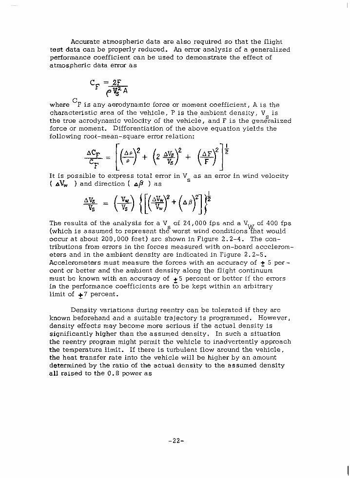
Accurate atmospheric data are also required so that the flight test data can be properly reduced. An error analysis of a generalized performance coefficient can be used to demonstrate the effect of atmospheric data error as

where ‘F is any aerodynamic force or moment coefficient, A is the characteristic area of the vehicle, P is the ambient density, V is the true aerodynamic velocity of the vehicle, and F is the gen&alized force or moment. Differentiation of the above equation yields the following root-mean-square error relation:

*‘F - [(Tr+ (2#+ (#I’ cF

It is possible to express total error in Vs as an error in wind velocity ( AV, > and direction ( AP ) as

The results of the analysis for a V of 24,000 fps and a V of 400 fps (which is assumed to represent thg worst wind conditionsyhat would occur at about 200,000 feet) are shown in Figure 2.2-4. The contributions from errors in the forces measured with on-board accelerometers and in the ambient density are indicated in Figure 2.2-5. Accelerometers must measure the forces with an accuracy of + 5 per - cent or better and the ambient density along the flight continuum must be known with an accuracy of + 5 percent or better if the errors in the performance coefficients are to be kept within an arbitrary limit of +7 percent.

Density variations during reentry can be tolerated if they are known beforehand and a suitable trajectory is programmed. However, density effects may become more serious if the actual density is significantly higher than the assumed density. In such a situation the reentry program might permit the vehicle to inadvertently approach the temperature limit. If there is turbulent flow around the vehicle, the heat transfer rate into the vehicle will be higher by an amount determined by the ratio of the actual density to the assumed density all raised to the 0.8 power as

-22-

ERROd IN AERODYNAMIC VELOCITY

0.9

0.7

0.3

0.1

I -

I -

RADIANS

0.6

ERROR IN WIND DIRECTION

DEGREES

q3 -350

I I I I I I 0 5 10 15 20 25

ERROR IN WIND SPEED ( 9 x 100)

FIGURE 2.24 ERRORS IN AERODYNAMIC VELOCITY

-23-

FIGURE 2.2-5 ERRORS IN PERFORMANCE COEFFICIENTS

6

8

gFlGURE 2.2-6 ERROR IN DETERMINING HEATTRANSFER COEFFICIENTS F 25 X

4 /

z 4 b

ERROR IN DENSITY (apX 100)

P

I 2 3 4

ERROR IN WALL TEMPERATURE (2 x loo)

-24-

If the actual density during reentry is 50 percent greater than the assumed density, the heat transfer will be about 38 percent higher than programmed. A typical example of heat transfer errors due to atmospheric effects is shown in Figure 2.2-6.

In general, a knowledge of atmospheric density within a 5 percent accuracy is required for reentry vehicles in the forseeable future.

2.2.4 Hypersonic Glide Vehicle Requirements.

The analysis of the aerodynamic data from the flight test of a hypersonic glide vehicle is highly dependent on an adequate description of the atmosphere through which that vehicle flies. The hypersonic glider maintains flight by balancing the inertial forces applied to it with the aeordynamic forces generated by its motion through the atmosphere. At orbital speeds, the glider is completely supported by the centrifugal force. As the glider speed decreases, the aerodynamic forces take over its support. The glider tends to fly a density-velocity function where all the forces are in equilibrium. This is called the equilibrium glide condition. As in any other mechanical system, the glider tends to seek equilibrium but generally will oscillate about it in a long-period harmonic motion.

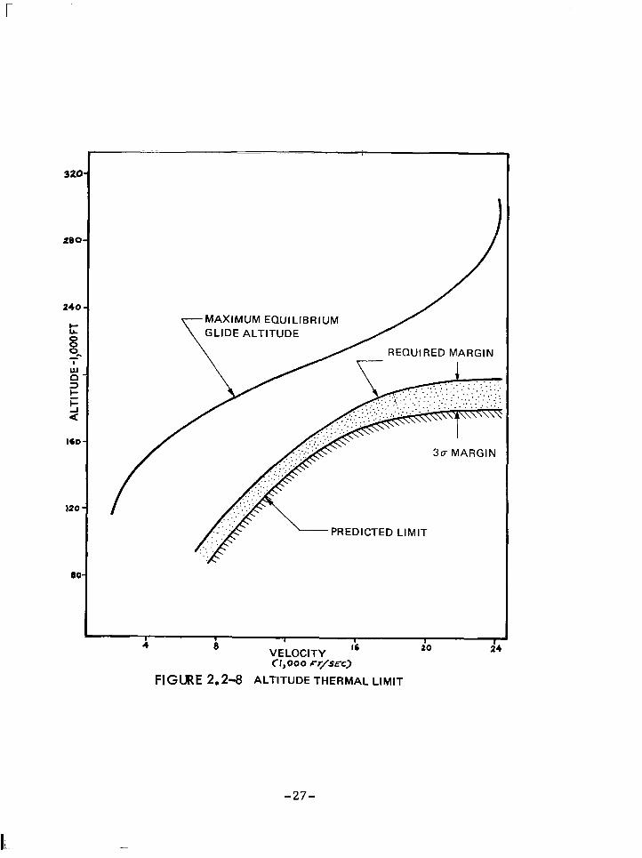
The flight regime of hypersonic glide vehicle as shown in Figure 2.2-7 well beyond the state-of-the-art in ground test facilities, and so there can be significant uncertainties as to the exact location of the flight limits. The principal limit in this regime is the temperature limit of the vehicle structure. This limit can be expressed as a function of density and velocity. Figure 2.2-8 illustrates this limit as the minimum flight altitude of the operational envelope of the vehicle. Because of uncertainties in the exact location of this limit, the exact temperature capabilities of the structural material, and in the capability to control the vehicle away from the limit, an altitude margin is added to the temperature limit condition. It is desirable to more precisely locate this limit during a test program, and in so doing, reduce the margin. This could result in an expansion of the operational envelope of the vehicle. It would also increase the confidence in flight safety.

The way in which these limits are more precisely “fixed” in flight

-25-

I

THE HYPERSONIC

GLIDE REGIME

FLIGHT VELOCITY - 1,000 FEET PER SECOND

FIGURE 2.2-7 POTENTIAL HYPERSONIC GLIDE CORRIDOR

-26-

r

240-

t MAXIMUM EQUILIBRIUM

Q

GLIDE ALTITUDE

2 REQUIRED MARGIN 8

EC z F 2

320-

200-

ISO- 3~ MARGIN

no-

PREDICTED LIMIT

80-

I I 4 8 I I 1 VELOCITY ”

I 20 24

<I,000 F+EC>

FIGURE 2.2-8 ALTITUDE THERMAL LIMIT

-27-

test is to measure the temperatures of the vehicle surfaces and combiae these measurements with measurements of velocity and free stream density to form a coefficient which is then used to extrapolate to the limit temperature condition. This provides a new altitude margin as indicated in Figure 2.2-9.

With adequate density data, the altitude.margin could be reduced by forty percent. This would mean an increase in the basic research information the vehicle could gather through exploration of a wider density-velocity regime, an increase in lateral range envelope of the vehicle through the ability to fly at greater bank angles, and an increase in the confidence for safe flights through better definition of the actual location of the limits.

Figure 2.2-10 presents, in pictorial form, the profile of typical hypersonic glide flights with L/D varying from 0.3 to 3.0. Such flights could extend for from 1,000 to 9,000 miles and last for six to sixty minutes. The extensive ranges and times are characteristic of the horizontal reentry of a lifting body.

Meteorological data supports two roles in hypersonic glide flight test . In the research role, it supplies the basis for interpreting the effects of the local environment on the full vehicle configuration, a role that the wind tunnel facilities can no longer completely fill. In the operational role, it supplies information for more accurately “fixing” the actual limits of the vehicle, thereby increasing research flexibility and flight safety. The accuracy of meteorological data to fulfill these needs is presented in Table 2-1.

-28-

.5 .6

I

RANGE OF POTENTIAL I ------ -

c DECREASE IN MARGIN

.7 .a

RELATIVE ALTITUDE MARGIN

.9 1

(Harmon, Moore)

FIGURE 2.2-9 THERMAL MARGIN DECREASE WITH FREE STREAM DENSITY DATA

-29-

(Harmon, Moore)

FIGURE 2.2-10 HYPERSONIC GLIDE PROFILE

-3o-

Allowable RMS Error

Meteorological Measurement

Density 1.7% - 0%

Wind Velocity 240 ft/sec-7 50 f t/set

Temperature

Viscosity

22,000 ft/sec 280 kft to 210 kft

505% - 5.8%

2.2% - 1.7%

5,000 ft/sec 160 kft to 100 kft

1.7% -0%

50 ft/sec-30 ft/sec

5.5% - 5.8%

2.2% - 1,7%

(Harmon, Moore)

TABLE 2-l

ERROR ALLOWANCES AFFECTING HYPERSONIC GLIDE VEHICLES

-31-

2.3 Meteorological Research.

2.3-l Synoptic Data.

A better understanding of the entire atmosphere is essential to advance our ability to construct mathematical and dynamic models of the atmosphere. These models should lead to better forecasting and possible modification of weather and climate from the earth’s surface up to the higher levels. In addition, knowledge of wind systems and the energy balance of the atmosphere above 100 millibars has become of increasing practical and scientific importance. This stems from the great expansion that has taken place recently in the atmospheric sciences, as well as the realization that significant energy transfer takes place in the atmosphere, not only horizontally, but also vertically. Furthermore, the ionosphere is known to be under solar control, and the effects of solar changes on the entire atmosphere can therefore only be studied by obtaining a three- dimensional synoptic picture of the atmosphere to about 100 km. This should include studies of the general circulation, perturbations, and the role of trace constituents such as ozone, water vapor, and particulates that are known to be important agents in the energy balance of the upper atmosphere. Recent instrumental developments make it possible now to routinely carry out synoptic sounding programs to measure the vertical distribution of ozone and the net radiation flux in the atmosphere. Measurements of stratospheric water vapor are also becoming possible on a quasi-synoptic basis.

Major goals in the establishment of a synoptic meteorological rocket network are aimed at providing information as follows:

(1) The climatology of the upper atmosphere - the variation of space and time of the parameters of state and motion of the atmosphere.

(2) The morphology of the disturbances in the upper atmosphere - the thermostructure and flow patterns in the horizontal and vertical.

(3) The relation between stratospheric circulation and temperature field and the distribution of ozone and water vapor.

(4) Radiative processes in the upper atmosphere, particularly in relation to ozone and water vapor distribution.

-32-

(5) The incidence and nature of clouds and aerosols in the upper atmosphere.

(6) The relation between solar activity and the composition, motion and temperature fields of the upper atmosphere.

There has been recent interest in conducting routine soundings to determine electron and other charged particle densities in the lower regions of the ionosphere. The D region lies between 60 and 80 km and is usually very low in charged particle content. Enhanced solar activity creates radio blackcuts in this region which is stimu- lated by solar radiation of a few Angstrom units in wavelength. The E region is located at about 100 km and is affected by soft X-rays. An intense additional ionization of a patchy character often appears in the E region ani is known as sporadic E. Ultraviolet radiation less than an 800-A wavelength supplies energy to promulgate the Fl region at an altitude of about 150 km. This region coalesces with the 300 km F2 region during the nighttime.

Disruption of radio communication by sporadic E disturbances has definitely been linked to wind shear action occurring at an altitude of about 60 miles. High velocity winds blowing in opposite directions above and below atmospheric levels of zero wind velocity and acting with the earth’s magnetic field pull electrons into thin layers about one-third of a mile thick. These reflect radio signals normally reaching the much higher F layer. The measured electron density profiles show the thin layers are associated with an east- west wind shear.

2.3.2 Aeronomy .

2.3. 2.1 General. Aeronomy deals with the physical, chemical and electrical properties of the atmosphere as follows: temperature (neutral, electron and ionic) and density structure, winds, composition (neutral and ion), electron density profiles, photochemical reactions that result in molecular dissociation, ionization and the creation of chemical species (such as oxides of nitrogen), diffusion of the lighter constituents, and, in general, the response of the atmosphere to solar input, particularly in the high energy portion of the spectrum.

The atmosphere in the region of about 80 - 300 km is influenced greatly by solar radiation in the ultraviolet and X-ray portion of the spectrum. This input of solar energy is responsible for the ionization

-33-

and photochemical reactions that give rise to the low-energy plasma called the ionosphere. The rate coefficients for many, if not most, of the photochemical reactions postulated to occur are not known by direct measurements, but are inferred from equilibrium conditions and certain laboratory experiments. The magnitude of these coefficients , however, may be debated over a range of several orders of magnitude. Thus far it has not been possible to perform laboratory experiments scaled well enough to the real atmosphere, or to produce satisfactory gradients of the several variables in laboratory vessels, to settle some of the debate. The upper atmosphere is its own best model, and understanding it will only come through more perfect description of all phases of the complex atmospheric processes by definitive experiments.

Aeronomy experiments have generally utilized the larger, more sophisticated and more costly instrumentation and rocket systems for relatively few soundings per year.’ In some cases there has been a desire to miniaturize and simplify the instrumentation for use with the smaller, lower cost rocket systems so that numerous soundings can be conducted. On the other hand, the meteorologists have expressed a desire to borrow the measurement techniques of the aeronomist and conduct soundings on somewhat of a synoptic basis. Thus, there appears to be an interest by both disciplines in the concepts such as a rocket ozonesonde network, an electron density rocket network’and perhaps other. For this reason, a brief mention is made in the following sections of primary subject matters in aeronomy of potential interest to the meteorologist.

2.3.2.2 Density Structure. A few scientific workers in the field of aeronomy are conducting experiments to determine the atmospheric density structure up to satellite regions by means of sounding rockets. The accelerometer falling sphere, pitot probe, and exploding grenades have been primary experiments. The absorption profile of appropriate solar emissions in the ultraviolet and X-ray spectrums are being made to measure density profiles from 80 to 160 km. Advanced instrumentation concepts such as backscattering measurements are being developed to measure densities above 100 km

2.3.2.3 Atmospheric Composition. The atmosphere below 90 to 100 km is well mixed and can be treated, in terms of the hydrostatic equation, as one gas with a molecular weight of about 29. At about 100 km, the number density of the atmosphere becomes small enough so that the mean free path becomes long, and diffusion processes begin to occur. In addition, dissociation produces atomic

-34-

oxygen (mass 16) in considerable quantity and the mean molecular mass of the atmosphere drops sharply. This drop has a profound effect on the density and temperature structure. There are also many ion species present, and in order to balance the electrical equation of the atmosphere, an inventory of the ions and their concentration is needed.

Paul Massen filters, the Bennet rf mass spectrometer and magnetic spectrometers are used to study the low ionosphere and also the relative concentrations of H , He and 0 to altitudes where upward diffusion of the light constituents become appreciable.

2.3.2.4 Ionospheric Winds. Very intense winds are observed in the ionospheric regions. As this region is ionized and under geomagnetic control, the winds in low and medium latitudes are quite stratified and have been found to correlate well with Sporadic E. Three ionospheric wind measurement techniques in use are as follows:

(a) Meteor trail observations - are made by radar or radio propagation observations.

(b) Explosive grenades - this technique is being used routinely to about 90 km, and it has recently been shown that at quiet sites, using somewhat larger grenades, detection could be extended to explosions at 115 km. The grenade experiment gives temperatures directly and winds are obtained from determining the angle of arrival of the sound pulses at the ground by a spaced microphone array.

(c) Photography of luminous trails - Trimethyl- aluminum and sodium vapor released from rockets above 90 km at twilight produce luminous trails by fluorescence with sunlight of long enough presistance to yield good wind shear and wind direction measurements.

2.3.2.5 Ozone. Ozone is one of the important minor constituents of the earth’s atmosphere and is produced mainly in the stratosphere. The close connection between ozone and weather processes provides an indirect method for the study of the atmosphere. The distribution of ozone may be used to infer the kinematics of the stratospheric circulation and possibly the location and mode of stratosphere-to-troposphere energy transfer.

-35-

Another aspect of ozone studies is the radiation balance of the stratosphere. Radiation processes are thought to account for the thermal structure of the stratosphere to a great extent. The three components mainly responsible for the absorption of short and long wave solar radiation are water vapor, carbon dioxide and ozone. The ozone maximum generally is at around 25 km and it can be said that the temperature structure (inversion or isothermal) of the stratosphere is partly explained by absorption of radiation by ozone.

Ozone variations occur on several time scales. There exist definite seasonal variations of ozone with a maximum in spring and a minimum in summer. There are irregular day-to-day variations about the monthly mean that are related to weather variations, and there is an increase in the total amount of ozone with latitude.

2.3.2.6 Thermal Radiation. The value of atmospheric net radiation soundings to determine radiative flux, flux divergence and cooling rates has been previously stated, and the importance of surface radiation measurements to assess energy transfer at the lower boundary of the atmosphere has long been known. When obtained simultaneously in time and space, these radiation measurements will describe the principal components of the radiation budget. A knowledge of this budget is essential in understanding not only the zonal variation and transformation of energy in the atmosphere, but interactions between the upper and lower atmosphere as well.

2.3.2.7 Water Vapor. Little is known about the concentration and variability of water vapor above the tropopause. Observations of the OH bands have been made by airglow workers and some estimations have been made of water vapor in the stratosphere and above by horizon photographs from rockets and balloons, but direct measurements are few. So far the measurement technique is a complex matter for directly measuring high altitude water vapor, so that the actual atmospheric concentration is being measured rather than water outgassing from the balloon sounding.

2.3.2.8 Electron Density and Structure of the Ionosphere. A number of scientific workers have been conducting rocket-borne experiments in the exploration of ionspheric electron density profiles, electron temperatures, ionic and neutral composition. There has been a significant amount of scientific interest in the synoptic

-36-

probing of the D and E regions on somewhat of a routine basis with relatively small rocket systems.

2.3.2.9 Electric Currents in the Atmosphere. In the equatorial regions, electric currents flow in the atmosphere at heights of approximately 100 km as a result of winds stemming from solar tidal and heating effects. In the aurora1 zones during times of magnetic and ionospheric storms, electric currents flow as a result of induction processes stemming from incoming particle bombardment. It is possible to measure directly these current systems and, explore their configuration with magnetometers carried on small rockets. Exploration of these systems is planned by various scientists.

-37-

2.4 Special Project Support.

From time to time there are special projects which require high altitude meteorological support. A particular project, regarded as the first operational use of meteorological rockets, was the requirement to determine high altitude winds for Joint Task Force Eight during the atmospheric atomic bomb tests in order to predict fallout patterns. High altitude acoustical ducting studies by the Army at WSMR required special collection of high altitude temperature and wind data. High altitude balloon projects have required meteorological rocket data to predict flight paths of the balloons. A most recent example of special project support is that given to the canal construction project in the Panama Canal Zone to predict dispersion and intensity of the shock waves that would result from simultaneous nuclear excavations across the entire isthmus.

-38-

2.5 Meteorological Measurement Requirements.

Meteorological measurement requirements have been stated for rocket soundings by various government agencies. Since these requirements differ slightly, representative examples are presented with a view toward consolidating the requirements to be used as guidelines for future meteorological rocket systems design. A majority of the firm requirements come from the larger missile ranges as support requirements for the large missile and space vehicle programs. In general the accuracy requirements for these programs are more stringent than those for the synoptic measurements taken primarily for meteorological research programs. Of course, many research workers in the aeronomy field would like to obtain even greater measurement precision than that required for missile range support. Compromises among the various requirements should be made so that sounding rocket systems may be economically used to satisfy the needs of the various disciplines with each particular flight. Thus, a typical meteorological rocket launching may supply data for range support and the missile engineer, the research meteorologist for his statistical model building and the aeronomist for his research datum points.

Typical missile range support requirements are listed in Table 2-2 for the Eastern Test Range and in Table 2-3 for the Pacific Missile Range. In addition, NASA Marshall Space Flight Center requirements for large launch vehicles are presented in Table 2-4. It must be noted that the missile range requirements change from time to time because of the particular flight test programs contemplated during a given period. Aeronomy research measurement requirements are not presented since they tend to vary from experimenter to experimenter depending upon his particular instrumentation capability.

As a guide to meteorological rocket system design, a suggested list of measurement requirements is presented in Table 2-5. This list constitutes a compromise among the various requirements previously stated with a view toward what might be considered as economically feasible for rocket systems used routinely.

-39-

TABLE 2-2

EASTERN TEST RANGE SUPPORT REQUIREMENTS

Density

Parameter

Temperature

Altitude

25-90 km

25-120 km

Location

Launch

Re-entry

Pressure 25-90 km

25-120 km

Launch

Re-entry

o-55 km Launch

25-90 km Launch

30-70 km

25-120 km

Re-entry

Re-entry

Wind Velocity Vector

25-90 km

O-40 km

25-120 km

Launch

Re-entry

Re-entry

Electron Density 80-500 km

500-900 km

Launch

Launch

Accuracy (RMS)

0.5% (OK)

0.5% (OK)

0.5%

0.5%

1.0%

1.6%

0.5%

1.6%

10 mps or 10%

10 ft./set or 10%

10%

10%

5%

-4o-

TABLE 2-3

PACIFIC MISSILE RANGE SUPPORT REQUIREMENTS

Temperature 30-64 km + lo CRMS error

Computed Density:

58-64 km 3.25 % RMS error

50-58 km 2.75 % RMS error

below 50 km 2.25 % RMS error

Winds 30-64 km 3-7 Knots RMS error

Special Support Density 30-100 km

-41-

TABLE 2-4

NASA MARSHALL SPACE FLIGHT CENTER

REQUIREMENTS FOR LARGE LAUNCH VEHICLES

Altitude Region 30-90 km Class I & II at 250 km intervals Requirements

Temperature 1.1 % rms

Pressure 1.2 % rms

Density 1.6 % rms

Winds Total Vector Error 10 m/s rms

Class III Requirements

0.5 % rms

0.5 % rms

0.8 % rms

5 m/s rms

Altitude Region 80-500 km at 10 km Intervals

Electron Density

Requirements Class I & II

10 %

Requirements Class III

5%

-42-

TABLE 2-5

COMBINED METEROLOGICAL ROCKET

MEASUREMENT REQUIREMENTS

Parameter

Temperature

Density

Pressure

Winds

Ozone

Electron Density

Altitude Reaion

30-65 km

65-90 km

30-65 km

65-100 km

30-65 km

65-100 km

30-65 km

65-100 km

30-65 km

50-200 km

RMS error

lo c

3O c

2%

5%

2%

5%

5%

10 %

5%

7%

-43-

2.6 Meteorological Rocket Systems Requirements. ,

In addition to the measurement requirements discussed in the previous sections, there are additional requirements for meteorological rockets which are to be used routinely in missile support and meteorological rocket network operations.

The first and foremost requirement is that of low cost. Today wind and temperature measurements are being conducted routinely to an altitude of 65 km with the Loki Dart vehicle with a complete system cost of approximately $800.00 including sensor and telemetry. A year ago this same set of data was obtained at a cost of over $2,000 with the Arcas vehicle. As the measurement altitude is raised, it can be expected that the measurement techniques will become more sophisticated and costly, and the carrier vehicle will no doubt become more costly. However, fairly accurate density data have been collected to an altitude of 90 km with the Viper Dart Robin system for approximately $3,000. It appears that the cost of a complete meteorological rocket system including sensor and telemetry should be kept well under $3,000 to be considered for routine use.

A second most important requirement for a meteorological rocket is low sensitivity to winds at the launch site. While it is true that launch angles can be corrected for wind effects by wind-weighting techniques, most missile ranges are restricted by geography so that only a limited amount of correction can be applied. When wind corrections exceed range boundaries, the launch must be cancelled with the resulting loss of data. Ninety-nine percentile wind profiles from the major missile ranges are presented in Figure 2.6-l. Future meteorological rocket vehicles should be designed with these wind profiles in mind. When a vehicle apogee of loo-150 km is considered at a range such as White Sands, a + 20° azimuth range boundary must be-held. This appears to be a good design range boundary azimuth deviation for consideration with the wind profiles of Figure 2. 6-l.

The logistic considerations of vehicle size, weight and complexity together with the payload complexity are fairly important in the design of a meteorological rocket system. A two-man crew should be able to load and launch the rocket vehicle without any extensive ground-handling equipment. The payload should not require any extensive calibration at the launch site to conduct the routine launchings. Only for the less frequent high altitude soundings should more than a two man crew be considered. Since meteorological rockets are to be used in fairly large quantities, rocket size and weight become important in terms of shipping costs and storage space.

-44-

28

24

20

-.-.B PACIFIC MISSILE RANGE, CI

--~-~~~~“**~*~~ WHITE SANDS, NM.

---- WALLOPS ISLAND, VA.

CAPE KENNEDY, FLA.

-20 0 20 WIND SPEED, M/SEC

40 60 80 100

FIGURE 2.6-l 99PERCENT WEST-TO-EP;ST-CPMPONENT:STATISTICAL-MODEL PROFILES FOR FOUR U.S. LAUNCH SITES

3.

ATMOSPHERIC SENSORS

3.1 General.

There have been numerous experimental sounding rocket flights utilizing a wide variety of sensing techniques to obtain high altitude atmospheric measurements. Temperature profiles have been routinely determined from 30 km to 65 km altitudes by immersion thermometry with miniature bead thermistors. Wind profiles have also been routinely determined as high as 65 to 85 km with passive radar targets such as chaff, inflatable spheres and parachutes. The remaining measurement techniques have been used only on a research basis with merely a few soundings per year because of complexity, cost and the requirement for fairly large and costly sounding rocket vehicles. Essentially all of these measurement techniques are reviewed in the following sections to establish accuracies over the particular measurement regions and to determine the adaptability of the more complex research measurement techniques to the smaller low cost meteorological rocket systems.

-46-

3.2 Wind Measurement Techniques

3.2.1 High Altitude Wind Patterns.

Prior to describing the various wind measurement techniques used in the high altitudes, it is worthwhile to review the expected, wind patterns in these regions. Figure 3.2-l presents a typical wind latitude distribution up to 100 km. It has been discovered that a strong easterly flow predominates from 40 to 70 km during the summer, and that this pattern is reversed to a strong westerly flow from 50 to 80 km during the winter. During the spring and fall transition periods there is a rather rapid change in the wind flow pattern during a period of a few weeks. Wind speeds may occur in the stratosphere and above which are on the order of twice those observed in the maximum wind layer near 10 km altitude; wind shears appear to be of a larger order of magnitude than those observed in the lower altitudes. The wind conditions, although highly persistent for the winter and summer, may have pronounced day to day variations.

Wind speed envelopes and expected shear values from 30 to 80 km are presented for the Winter months in Figure 3.2-2 and for the Summer months in Figure 3.2-3. Although the wind flow is consistently from the east in the Spring and Summer and from the west in the Fall and Winter at about the 60 km altitude level, large wind speed variations occur over periods of several days. Vertical wind she rs have been found at about 50 km to be on the order of 0.030 set -3 .

Although the wind information in the 80-200 km region of the atmosphere is quite limited, sufficient data is available to draw some tentative conclusions of the wind flow characteristics. Figure 3.2-4 presents a probable maximum wind speed profile from 60 km to 200 km. Up to about 200 km the largest variations in wind speed and direction with altitude are between 90 and 125 km. The wind speed can change by as much as 128 m/set in an 8 km altitude change, and

’ 100 m/set in 3 kilometers; the wind direction backs or veers by as much as 300 degrees in a 7 km change and 180 degrees in 1 kilometer of altitude. Above 125 km, the directions change very little with altitude. The probable maximum wind speed increases in steps from near 230 m/set at 80 km to 500 m/set at 400 km. In the 80 to 200 km altitude region the highest wind shears with altitude are between 85 and 125 km with peak values occurring between 95 to 110 km. The largest maximum wind shears occur near 100 km with maximum values decreasing above and below this altitude. The peak shear values near 100 km calculated for the 500, 1000, 3000 and 5000 Fllayers were, respectively, 0.131, 0.086, 0.053 and 0.035 set . Above 125 km to at

-4 7-

(km) Ntbde

90 70 60 50 40 S”M3iER 20 10

LATITOUDE 10

-I-u 20

WI i?TER 40 50 60 70 go

FIGURE 3.2-l MEAN ZONAL (EAST-WEST) WIND COMPONENTS (qhec) FOR NORTHERN HEMISPHERE AFTER BATTEN (1961)

-

f

50% 95% 99%

f

120 160 200

Wind Speed (m/set)

FIGURE 3.2-2 IDEALIZED ENVELOPES OF WIND SPEED FOR WINTER MONTHS CAPE KENNEDY, FLORIDA AND POINT MUGU, CALIFORNIA

60 - 60 km Radon ProMAe Wind Build-Up Rates

Ah Shear AW (ml bc~‘l (m/sac)

1000.06 60 2000 .04 80 3000 .03 90

-49-

60

5a

FI

(km) Altitude, h

80 120

Wind Speed (m/set)

46 - 65 km Region Probable Wind Build-Up Rates

Ah Shear AW (ml Isec~‘) (m/set) 1000 .040 40 2000 .025 50 3000 .020 60

160

GURE 3.2-3 IDEALIZED ENVELOPES OF WIND SPEED FOR SUMMER MONTHS CAPE KENNEDY, FLORIDA AND POINT MUGU, CALIIFORNIA

-5o-

180

180

60+ I .

100 150 200 250 300 350 400 450 500

Wind Speed (m/set)

FIGURE 3.2-4 PROBABLE MAXIMUM WIND SPEED ENVELOPE FROM 60 to 200 km

-51-

east 200 km it appears that the wind si:ars with altitude are quite small, being in the order of 0.005 set . There is evidence, too, that the wind shears to at least 250 km are even smaller.

Judging from the gradual veering or backing of the wind vector with altitude, there appears to be organized circulation in the 80- 200 km region.. Moreover, the marked daily variation in wind vector gives evidence of migratory anticyclones and cyclones. Some abrupt changes in wind velocity with altitude are also evident and may be caused by front-like discontinuities and/or marked sloping anticyclones and cyclones.

There is evidence of transition in the zonal direction flow during spring and autumn in the 70-80 km and 110-160 km regions. The 80-110 km region is ill-defined in this respect. From about 140 to 200 km it appears that the wind vector veers or backs through these transitional periods without much diminution of magnitude.

Typical wind speed envelope for data above 85 km is presented in Figure 3.2-5. Wind shear envelopes for the same altitudes for 500 meter and 1,000 meter layers are shown in Figures 3.2-6 and 3.2-7. It is apparent that the wind shears are large between 85 and 125 km with peak values occurring between 95 and 110 km. The highest maximum wind shears occur near 100 km with maximum values decreasing above and below this altitude. The peak shear values near 100 km for the 500, and 1,000 were respectively, 0.131 and 0.086, set -l. Above 125 km the wind shears become quite small, of the order of 0.005 set -’ , .with only slight variation with altitude.

3.2.2 Wind Measurement Errors

Wind measurement error is a function of the average wind speed in a given altitude layer, the wind shear across the given altitude layer, and the presence of reversal patterns and changes in wind direction through the altitude layer. The specification of wind measurement accuracy, therefore, is a complex problem. The most feasible approach toward establishing design specifications is against the more severe, but relatively common, values for wind speed, wind shear and reversals. Table 3-l presents a summary of 60 km (200,000 feet) wind data to be expected in Eastern and Western United States. Also presented are suggested levels for wind sensor design criteria. Mean wind speeds at the 60 km level vary from 40 m/set to 65 m/set with the one-percent probability level as high as 120 m/set. Mean

-5 2-

iz 126

Y w ; 120

5 a

115

66

--

/” <,’ I

20 40 60 I loo 120 140 160 160

Wind Speed (m/sac) 2oo (Dubin)

I

FlGlJRE 3.2-5 WIND SPEED ENVELOPES OBTAINED FROM SOOIUM VAPOR, TRAIL MEASUREMENTS AT WALLOPS ISLAND. VIRGINIA

-53-

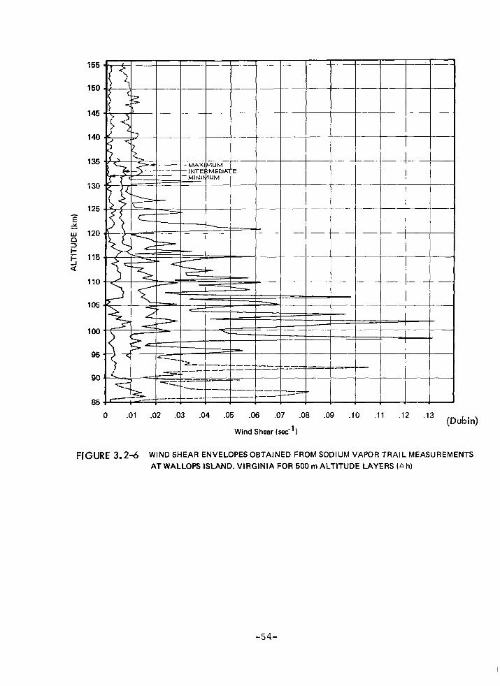
140

125

2 w 120 2 l- F 115 ;i

110

100

95

90

85

0 .Ol .02 .03 .04 .05 .06 .07 .08 .09 .lO .11 .12

Wind Shear (sacs’) .13 (Dubin)

FIGURE 3.24 WIND SHEAR ENVELOPES OBTAINED FROM SODIUM VAPOR TRAIL MEASUREMENTS AT WALLOPS ISLAND. VIRGINIA FOR 500 m ALTITUDE LAYERS [Ah)

-54-

135

130 f

T 125 Y Lu 5 + 120

5 a

115

110

90

85 0 .Ol .02 .03 .04 .05 .06 .07 .m

Wind Shear (sec.‘) (Dubin)

FIGURE 3.2-T WIND SHEAR ENVELOPES OBTAINED FROM SODIUM VAPOR TRAIL MEASUREMENTS AT WALLOPS ISLAND, VIRGINIA FOR 1000 m ALTITUDE LAYERS (Ah)

-55-

TABLE 3-l 60 KM Wind Data Summary

Probability Wind Speed Probability Wind Shear Location Season PJ) (m/s=) w m set -1 km-l

Western U.S. Winter 50 65 50 7

Summer 50 40

Eastern U.S. Annual 50 50 50 8

1 120

Winter 1 30

Summer 1 45

Wind Sensor Design 10 100 10 20 Gi teria

-5 6-

wind shears at the 60 km level are about 8 m/set/km with the one- percent probability level as high as 45 m/set/km. It is recom- mended that the lo-percent probability level of wind speed and wind shear be used for wind sensor design criteria as 100 m/set (328 ft/sec) and 20 m/set/km (20 ft/sec/ 1,000 feet) respectively up to the 60 km altitude level.

The specification of wind speed reversals is more complex than for wind speeds and wind shears since a reversal pattern contains two relatively independent variables, i.e. , a period and an amplitude. A wind speed reversal pattern is best described and defined in Figure 3.2-8. Where T/2 is defined as the half-period in altitude units, i.e. , kilometers or 1,000 feet increments, and A is defined as the amplitude in wind speed units, i. e. , m/set or ft/sec. Table 3-2 is a summary of the more severe wind speed reversal patterns at the 60 km (200,000 feet ) level for the various geographical locations and periods of the year. These data are derived from rocket ejected chaff since chaff winds at this altitude are the most accurate available. The most severe patterns for measurement accuracy are the large amplitude, short period patterns. In order to estimate the ten-percent probability of occurrence pattern, the amplitudes were plotted against the respective half-period values in Figure 3.2-9. Since a correlation was apparent, a regression mean was determined along with the respective percentile limits,.’ The ten- percent probability pattern was determined as the intersection of the two most severe 32-percentile, limits. The resulting wind speed reversal pattern has an amplitude of 30 knots (15 m/set or 50 ft/sec) and a half-period of 6,000 feet or 1,830 meters.

A summary of the wind measurement criteria suggested for wind sensor design for altitudes up to 60 km is as follows:

Design Altitude 200,000 feet

10 % Probability level

Wind Speed 328 ft/sec

Wind Shear 20 ft/sec/l, 000 ft

Wind Reversal

Amplitude 50 ft/sec

Half -Period 6,000 ft.

-5 7-

WIND SPEED, u

FIGURE 3.2-8 WIND SPEED REVERSAL PATTERN

-58-

60

0 0 5 10 15 20 25 30

HALF PERIOD (X ~CI-~ FT)

FIGURE 3.2-9 CORRELATION OF 60 km LEVEL WIND SPEED REVERSAL AMPLITUDE WITH HALF-PERIODS

TABLE 3-2

SUMMARY OF THE MORE SEVERE WIND SPEED REVERSAL PATTERNS AT 60 KM

Location Month

AMR Feb.

AMR Feb.

AMR Feb.

AMR Feb.

AMR Feb.

AMR Feb.

AMR Feb.

WSMR Jan.

WSMR Jan.

WSMR Jan.

WSMR Dec.

WSMR Dec.

WSMR April

WSMR April

WSMR April

WSMR April

WSMR April

WSMR April

WSMR Sept.

WSMR Sept.

WSMR Sept.

WSMR Sept.

WSMR Sept.

(200,000 FT) LEVELS

Half Period, T/2 (ft)

6,000

6,000

6,000

10,000

8,000

10,000

16,000

2,000

20,000

10,000

12,000

25,000

8,000

22,000

6,000

10,000

8,000

8,000

8,000

20,000

6,000

5,000

12,000

Amplitude, A (knots)

30

25

21

18

58

31

36

13

31

12

21

65

60

22

18

40

25

12

30

45

25

30

38

-6O-

II

TABLE 3-2, cont’d.

Location

WSMR

WSMR

WSMR

WSMR

WSMR

WSMR

WSMR

WSMR

WSMR

PMR

PMR

PMR

PMR

PMR

PMR

PMR

Kwajelein

Kwajelein

Month

Sept. 8,000 25

Sept. 6,000 40

Oct. 25,000 35

Nov. 18,000 20

Nov. 10,000 16

Nov. 16,000 45

Nov. 12,000 30

Nov. 6,000 30

Nov. 6,000 18

Jan. 6,000 30

Jan. 6,000 12

Jan. 4,000 20

Oct. 10,000 15

Nov. 10,000 25

Nov. 6,000 25

Nov. 8,000 22

April 4,000 22

April 4,000 14

Half Period T/2 (ft)

Amplitude A (knots)

-61-

Accuracy, rms

Wind Speed + 10 ft/sec

Wind Direction + 5 degrees

The ability of a falling object to respond to a given wind shear is primarily a function of its descent velocity. It has been found for meteorological wind sensors that the drag coefficient does not significantly change through the region of interest. The wind measurement error can be expressed as :

where CD= drag coefficient

m = sensor mass

S = reference area

W = horizontal wind velocity

X = horizontal coordinate

Z = vertical coordinate

For I? - We< 5 and ? - W relatively constant through a given altitude layer, the above expression can be simplified to

Z ;ci -w=-$*o1

dW where CY=- dZ

g= wind shear or gradient

Table 3-3 presents theoretical wind measurement errors for various fall velocities.

A review of chaff-derived winds obtained at the 200,000-foot level reveal that the 90 % wind shear level through a 1 ,OOO-feet altitude layer for annual data over the United States is about 20 ft/sec per 1,000 feet or 0.020 set -l, Table 3-4 has been constructed to indicate the descent system velocities and ballistic coefficients

-62-

TABLE 3-3

WIND MEASUREMENT ERRORS FOR VARIOUS FALL VELOCITIES

x - W=aZ2/g g=9.7 m/set' z>> A-w

(Z) WIND SHEAR (cf) (units/set)

FALL VELOCITY (m/set) 0.01 0.02 0 .0.3 0.04 0.05 0.10 _- .~ -.

10 0.1 0.2 0.3 0.4 0.5 1.0

20 0.4 0.8 1.2 1.6 2.1 4.1

30 0.9 1.9 2.8 3.7 4.6 9.0

40 1.6 3.3 4.9 6.6 8.0 17.Q

50 2.6 5.2 8.0 10.0 13.0

60 3.7 7.0 11.0 15.0 19.0

70 5.1 10.0 15.0 20.0

80 6.6 13.0 20.0 26.0

90 8.0 17.0 25.0

100 10.0 21.0 31.0

110 12.0 25.0

120 15.0 30.0

(Leviton)

-63-

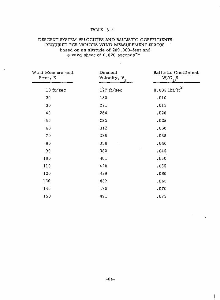
TABLE 3-4

DESCENT SYSTEM VELOCITIES AND BALLISTIC COEFFICIENTS REQUIRED FOR VARIOUS WIND MEASUREMENT ERRORS

based on an altitude of ZOO,OOO-fe$ and a wind shear of 0.020 seconds

Wind Measurement Descent Error, E Velocity, Vz

10 ft/sec 1’27 ft/sec

20 180

30 221

40 254

50 285

Ballistic Coefficient w/cDs

0.005 lbf/ft’

.OlO

.015

.020

.025

60 312

70 335

80 358

90 380

100 401

110 420

120 439

130 457

140 475

150 491

.030

.035

.040

.045.

A50

.055

.060

.065

.070

.075

-64-

required to satisfy various wind measurement error requirements. Typical wind shear lag error vs altitude is shown in Figure 3.2.10 for the Arcas parachute system.

An example of a response or lag error is ‘presented in Figure 3.2.11 whi2h assumes a wind sensor with a ballistic coefficient of 0.555 lb/ft has been dropped into a sinusoidal wind field. The lag of the sensor is indicated by the dashed curve. The frequency response of this sensor is plotted for different altitudes against wavelength (in altitude ) in Figure 3.2- 12.

Another example of response lag is the ballistic motion of the wind sensor immediately after being ejected from the rocket. Figure 3.2-l 3 shows the ballistic motion of the Arcas parachute after an 80 km deployment. Figure 3. 2-14 presents theoretical trajectories for the same conditions assuming a real wind profile and deployment from rest and with a 300 m/set horizontal velocity. The possible lag errors can be quite large.

To correct wind sensor lag effects, WSMR and the University of Texas have jointly developed a data reduction technique which accounts for the sensor acceleration and velocity terms by com- puterizing the basic equation of motion.

Where W = wind velocity

X = sensor horizontal coordinate

Z = sensor vertical coordinate

g = acceleration due to gravity

Utilizing this technique a typical correction is shown in Figure 3.2-15.

-65-

200

190

180

130

120

110

100 10 20 30 40 50 60 70

ERROR IN KNOTS

F[ GURE 3e2-10 WIND SHEAR ERROR VS. ALTITUDE FOR 15-FOOT ARCAS CHUTE (Ref: Beyenand Thiele, 1961)

-66-

I

al

7(

6C

50

40

30

-10 -8 -6 -4 -2 0 2 4 6 6 10 1 I I--I r, I I I I I

A-ASSUMED REAL WIND

B-PARACHUTE PROFILE WITH ZERO IMPARTED SPEED AT APOGEE

-lb -8 !.;-I -6 -: -2 0 2 4 6 6 1 10 I

(Ammons) HORIZONTAL SPEED (m set-1)

FIGURE 3.2-1.1 PLOT OF HEIGHT VS. HORIZONTAL PARACHUTE AND WIND SPEEDS

-67-

1.0

.9

.8

.7

.6

; .5

ea .4 z

.3

.2

.l

0

1.0

.9

.8

.7

.6

.4

3 .

.2

.1

0

Z = 70 km Z = 70 km

~ Z=3Okm

WAVELENGTH, L(km) (Olsen)

FI’GURE 3.2-12 FREQUENCY RESPONSE OF ARCAS PARACHUTE VS WAVELENGTH AT VARIOUS HEIGHTS

-68-

I , . , . ,

7 0

6 0

4 0

3 0

1 0 0 2 0 0 . 3 0 0

I l oo

I 2 0 0

I 3 0 ° ( O l s e n )

A - H O R IZO N T A L S P E E D W ITH Z E R O R E A L W IND A N D I M P A R T E D S P E E D O F 3 0 0 m set- l A T A P O G E E

B - F A L L S P E E D F O R S A M E C O N D I T I O N S

H O R IZO N T A L S P E E D A N D F A L L S P E E D ( m s e e - ‘)

FIG U R E 3 . 2 - 1 3 P L O T O F H E I G H T V S . H O R IZO N T A L S P E E D A N D F A L L S P E E D O F A R C A S P A R A C H U T E

-69-

60

50

40

30

I B - PARACHUTE PROFILE WITH ZERO IMPARTED WIND SPEED AT APOGEE

C - PARACHUT 300 m set- f

PROFILE WITH IMPARTED SPEED

AT APOGEE

HORIZONTAL SPEED (m set-1)

IO0 (Olsen)

FIGURE 3.2-14 PLOT OF HEIGHT VS. HORIZONTAL PARACHUTE AND WIND SPEEDS

- 70 -

300 200 loo 0 100 200 300 400 500

250

225

. t 200

E . % 2 i= 2

175

150

lb0

*

70

2

60 E

5 52

.N

100

-. -. . . .

-. -. *. .

-. .

It . * .

.

: . . .

it’ P *3

v-Corp.

(* ) Parachute Speed cx, *c) Wind Speed

(N-E) - 50 (m 15( I-

I 1 I I 1 I ,

10’0 --or

._-- _

3bo 2ob 1ok I I

20 I

300 400 500

(feet sec’l) (Olsen)

.

FIGURE 3.2-15 COMPUTED WIND SPEEDS FROM OBSERVED PARACHUTE SPEEDS

-71-

3.2.3 Chaff

Chaff with a very low ballistic coefficient, i.e. , high drag- to-weight ratio, has been used to successfully gather wind data in the region up to 85 km. The chaff payload and carrier vehicle can be quite inexpensive, and measurements can be made with standard range radar. The measurements’ are not restricted to any particular period of the day, and data reduction is,already automated by the use of developed computer programs. For these reasons the chaff technique has been a primary wind sensing system for altitudes to 85 km.

Disadvantages of chaff as a wind sensor are the limited altitude layer of measurement and the lengthy dwell time of the dis- bursed chaff cloud. After deployment, the chaff cloud gradually spreads as it descends, so that after a relatively short period the radar starts to hunt for local target concentrations or clusters. Thus radar error eventually increases beyond a useful value. A chaff cloud that is sensitive in the higher altitude portion of a sounding generally becomes unreliable as a radar target after approximately a 20 km descent. To avoid this problem, the Navy has employed two and three different fall rate chaff payloads for a single sounding. This technique has worked with some success but two or three radars must be used, and frequently there is a certain amount of confusion among the radar oper- ators. After the useful descent period of the chaff clouds, the dis- bursed target clutters the airspace for lengthy periods and interferes with radar tracking of subsequent missions. This has been an ob- jection to chaff at some of the large missile ranges.

Various kinds of chaff have been used for high altitude wind determination with meteorological rockets as indicated in Table 3-5. The heavier density chaff has been used to obtain soundings in the regions below 60 km, and the lighter density chaff has been used to gather wind data as high as 86 km. Typical fall rate data is presented in Figure 3.2-16 which demonstrates both a chaff density and size effect upon the fall rate profiles.

Since fall rate is the primary factor in determining the sensitivity of a wind sensor, the fall rate characteristics of chaff are of primary importance. Acceptable fall rates may be obtained up to an altitude of about 86 km by utilizing the 0.25 mil thickness Mylar chaff. Theo- retical fall rate profiles for this chaff are presented in Figure 3.2-17 for various deployment altitudes. Upon ejection from the rocket vehicle, the chaff accelerates to its equilibrium or terminal velocity

-72-

TABLE 3-5

SUMMARY OF WIND MEASUREMENT CHAFF

I U W I

Chaff Type Chaff Cross- Cross-Section Section Shape Dimensions Density Region of Use

n

Mylar

Nylon

Glass

Aluminum

Copper

Flat Strips

Circular

Elliptical

Flat Plate

Circular

0.25 mil x 0.1” 86.6 lb/fP 285,000 ft to 200,000 ft

3.5 mil dia. 71.2 lb/ft’ 260,000 ft. to 180,000 ft

12 mil dia 71.2 lb/ft3 235,000 ft. to 150, 000 ft

0.6 mil dia x 1.15 mil dia 173 lb/ft3 --

0.45 mil x 8 mil 170 lb/ft3 --

5 mil dia. 556 lb/ft3 180,000 ft. to 100,000 ft.

10 mil dia. 556 lb/ft3 115,oooft. to 50,000 ft.

The above chaff can be cut to a length compatible with the particular radar to be used. Usually one-half or one-quarter wavelength is used.

Radar Band

C

S

X

Radar Frequency

5500 mc

2700 mc

9000 mc

l/2 Radar Wavelength l/4 Radar Wavelength

2,727 cm 1.364 cm

5.555 cm 2.778 cm

1.667 cm 0.833 cm

280

260

240

T t 0 220

0” w= ” 200 “d

z p 180 -1 Q

160

140

120

loo

80 - 6 6 10

-

-

-

/

I

/

-

-

-

-

-

-

-

c

/

-

,I’

-

-

-

-

-

Descent Velocity (Ft/Sec)

FI GURt/3.2-16 CHAFF DESCENT RATES

- 74 -

160

140

120

100

2 If

80

Y 0 -’ Y I

$ 60

I- i= a

40

20

0

MO.2 Km

121.9 Km ngee

106.7 Km mgee

91.4 Km

---

7’

-~~

mgee

mgee

a

200,000 Ft

100,000 Ft .

Rate of Descent - Meters/Set

FIGURE 3.2-17 Theoretical Fall Rates -- For 0.25 Mill Mylar Chaff

-75: .

value to the altitude where the drag force equals the chaff dipole weight. As the ejection altitude is increased above the region where the chaff becomes wind sensitive, the maximum fall rates become greater. Thus, it is advantageous to deploy the chaff payload just slightly above its wind sensitive region. Higher altitude ejection results in loss of wind data because of the increased fall rate. The actual descent rate profile for a 122 km (400,000 foot) ejection of 0. 25 mil Mylar chaff in Figure 3.. 2-l 8 illustrates this effect . The\ comparable altitude vs time profile is presented in Figure 3.2-19.

The problem of extending chaff wind measurements above 86 km (285,000 feet) is significant. Either the density or the size of currently available chaff must be reduced to extend the measurement altitude. The size effect has been studied to some extent, and theoretical descent profiles for 3.5 mil and 12 mil diameter nylon chaff is presented in Figure 3.2-16. As the chaff cross-section size becomes smaller and the Reynolds number becomes smaller, the drag coefficient increases as indicated in Figure 3.2-20: Theo- retically , at least, by utilizing smaller diameter cross-section dimensions than are currently available, reduced fall rates at the higher altitudes could be obtained, and the chaff wind measurements could be extended in altitude.

Dispersion detracts significantly from the usefulness of chaff. Two problems directly resulting from dispersion are signal return deterioration and tracking inaccuracies as the radar beam moves about through the chaff cloud. During tracking operations it has been noted that chaff disperses over areas of 1,000 to 5,000 yards within 10. minutes after deployment. Radar observations of 0.0 12” nylon chaff indicate that these chaff payloads disperse over areas of greater than 35 cubic miles within 20 minutes of deployment and over 50 cubic miles in 30 minutes. Usually the radar shows two or more particular areas within the chaff cloud that reflect substantially more energy, and one may assume that these bright spots will vary with time. Dispersion is a function of several parameters, including fall, velocity, turbulence, wind shear, and vertical motions, all of which may vary with time. Of the two problems resulting from dispersion, signal return deterioration is generally the lesser problem.

There has been some question regarding the effect of chaff wave length and radar polarization on signal return. There is definite evidence from observed signal returns at the radar that it is not necessary to match chaff dipole and radar wave length exactly. X-band chaff

-76-

180

160

140

120

2 100

4 3 z 80 I

0” 2 i= a

60

40

20

0

f

Rate of Descent - Meters/Set

hlf l,OOO Ft.

200,000 Ft.

100,000 Ft.

FIGURE 3.2-18 SUPER LOKI e4.20 MAY 1968 8 CHAFF FALL RATE VS. ALTITUDE

-77-

ALTITUDE VS. TIME

2 300 u. 0 8

I 200

4 2 .g

2 100

_m 100 KM _ _--_---

I

Time - Seconds

FIGURE 3.2-19 CHAFF DESCENT PROFILE - WSMR FLIGHT TEST SERIES

-7a-

6 _.

3 t

--- -

*

-Ii!

2

I

- _ .

I 0.01 e 34 -

i -

\

PIH -

-

Reynolds Number

FIGURE 3.2-20 DRAGcOEFFICIENT OF AN INFINITE SINGLE CYLINDER

-79-

can be tracked with S-band radar with only an approximate 10 % loss in signal return compared with S-band chaff signal return. Similar results were obtained when X-band and C-band radar were used with S-band chaff. Polarization appears interchangeable since similar signal levels were observed on a single parcel of chaff whether circular, horizontal, or vertical polarization was applied. From this it might be inferred that, as the chaff falls, it is randomly oriented with respect to the radar.

The ability of a falling object to sense variations in the horizontal wind field is a direct function of its fall velocity. Chaff sensor accuracy considerations are similar to those of parachutes except that the slip and glide problem is replaced by dispersion. The parachute presents a point source target, but the chaff payload soon covers many cubic miles of area, and the radar beam tends to wander throughout the cloud. Significant tracking improvement can be attained with radars utilizing “A” or “I” scopes by a manual range track. Since the operator has a visual monitor of the target area cross section, he can easily keep the range gate in the approximate center. However, it does not appear feasible to use a manual mode in azimuth and elevation, since only by scanning the cloud by moving the antenna can centering be accomplished.

The tracking instrumentation accuracy is another factor which can lead to significant errors. The precision quoted for the AN/FPS-16 radar is + 0.2 mils in azimuth and + 15 yards in slant range. As a result ofythe random nature of most-of these errors, the accuracy of mean wind speeds will surpass instantaneous velocities.

Comparative data have shown that the correlation between data derived from parachutes, spheres, and chaff is satisfactory for general applications, with the largest differences occurring in the north-south components at very light wind speeds. This effect appears to be characteristic of many of the high-altitude wind measurements, and is to be expected in the predominantly zonal flow encountered at high altitudes. In general, the response of optimized chaff provides wind data to 80 kilometers with reasonable accuracy. While chaff dipoles respond more rapidly to the detailed structure of the wind field at high altitudes, the data are degraded by dispersion of the sensor within a short period of time.

An insight into the effect of fall rate on chaff wind sensitivity may be gained by comparing a low density chaff wind profile with a wind profile derived from a higher density chaff as in Figure 3.2-21.

-8O-

r

165

160

155

150

% 145

X

t 140

z 0 i5 135 I

130

125

12c

11:

11c

\ B \’ ‘. \ ‘.

J ‘:

\: \:.

,

Zonal Wind Speed (KTS) FIGURE 3.2-21 LOW AND HIGH DENSITY CHAFF WIND SENSITIVITY

Wind profiles at Cape Kennedy, Florida, 25 August i%O. Comparison of the winds as computed from the 1 -minute horizontal dir- placements of slow-falling nylon‘chaff (solid line) and fast-falling cqpu chaff (dashed line). The dotted line is the wind determined from the nylon chaff when averaged aver approximately the same height increment as was used fa the capper chaff.

-81-

The 12 mil/nylon chaff shows a much greater amount of detail than does the 10 mil/copper chaff. In addition there is a bias even when the nylon chaff data is smoothed and compared to the copper chaff data.

Since reasonably good wind data are being routinely gathered with either parachutes or other discrete deceleration targets in conjunction with temperature measurement sonde flights to altitudes slightly above 64 km (2 10,000 feet ) , the primary use for chaff data is above this altitude. Cajun Dart and more recently Super Loki Dart vehicles with the 0.25 mil/mylar chaff have been routinely used for wind data up to 87 km (285,000 feet ). An example of these wind data is presented in Figure 3.2-22. Ejecting this chaff at a higher altitude would be useless since the fall velocity will become excessive. Initial flight tests of the Super Loki system at WSMR resulted in chaff ejection at 122 km (400,000 feet ) altitudes. An example of the resulting wind profiles is shown in Figure 3.2-23 together with a lower altitude ejection of the same chaff type. The lower altitude deployment shows a greater wind shear just above 70 km and appears to be more sensitive down to 67 km.

The primary improvement needed in measuring the winds with chaff is a slower fall velocity above 87 km (285,000 feet) to extend the measurement altitude limit. This may be done by either decreasing the chaff density or size.

3.2.4 Rocketsonde Decelerators

The two basic decelerators which have been used routinely as rocketsonde wind sensors have been fairly standard-shaped parachutes and the Starute. A 15-foot diameter silk parachute is used with the Arcas system, a 7.6 foot diameter silk parachute has been used with the Loki system: and a 6-foot square silk parachute has been used with the Hasp system. More recently a ram-air inflated mylar balloon-parachute, called the Starute, has been used with the Loki system to obtain slower and more stable descents. Rather complete descriptions and performance data has been presented for these decelerators in Section 6.

The Arcas and Loki parachute descent curves are presented in Figures 3.2-24 and 3.2-25. The Hasp parachute descent curves are presented in Figure 3.2-26. Typical Loki Starute descent curves are shown in Figure 3.2-27 for a 68 km (225,000 foot) deployment and in Figure 3.2-28 for ‘a 7 6 km (248,000 feet) deployment. The wind lag error is a function of only the fall velmity and can be estimated for

-82-

WI ND VELOCITY -(EAST - WEST COMPONENT)-FPS

85

70

65

11846 GMT)

2

z 0

Wind From West

‘8 Wind From East

290

280

270 7

0

260 X

El Y

250 “a 2 c

240 <

230

220

Wind Velocity (East-West Component)-MPS

FIGURE 3.2-22 TYPICAL SUPER LOKl DART WIND IvIEASUREMENT

-83-

5 40 . . x a -40

30 / 30

20 40 30 20 10 10 20 30

,20 40 40 30 20 10 0 10 20 30 40

WEST EAST I NORTH - SOUTH

FIGURE 3.2-23 HIGH ALTITUDE WIND DATA 6 MAY 1968

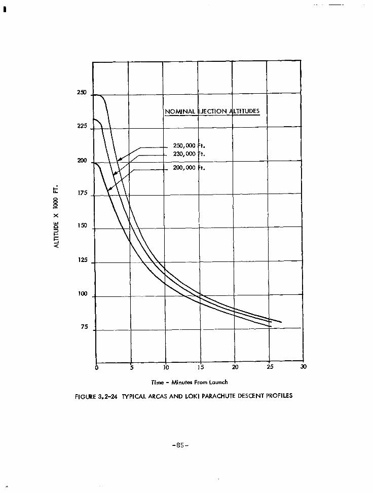
225

200

175

150

125

100

75

0 /

JOMINAL

250,000 230,000

200,000

1ECTlON I

Time - Minutes From Launch

FlGLlRE 3.2-24 lYPlCAL ARCAS AND LOKI PARACHUTE DESCENT PROFILES

-85-

I W 0,

I

200

180

160

140

120

100

80

FALL RATE ALTIT

0 100 200 300 400 500 600 700 800 900

Fall Rate - Feet Per Second

FIGURE 3.2-25 lYPlCAL ARCAS AND LOKI DART PARACHUTE DESCENT RATES

15

KY<

SO

Fall Velocity (ft/sec)

)*-

t 0

I

10 20 30

Time After Launch (Minutes)

FIGURE 3.2-26 TYPICAL HASP PARACHUTE DESCENT PROFILES

-87-

135.420-

l-

0 ~~ -

360 720 1080 1440

Time - Seconds

FIGURE 3.2-27 LOKI-DART STARUTE DESCENT PROFIlE

-aa-

240

230

220

170

7 i

w)

----

i

\ \ 3

---I <’

.

2

r

;

---a-- ---- T: APOGEE

--. A--

Apogee 247,000 Ft. Deployment 242,OCO Ft. on Uplsg

0 300 400 Flight Time (Set)

FIGURE 3.2-28 STARUTE DESCENT WSMR 7 JUNE 1968

-a9-

each of the above systems by combining the data from the fall velocity curves with the equation:

as described in Section 3.2.2.

Since the Loki Starute has the slowest descent rates among the current rocketsonde decelerators, it should be superior as a wind sensor, A typical Loki Starute wind profile is presented in Figure 3.2-29.

The Army at WSMR has developed a computer technique to correct rocketsonde wind data for sensor lag. This technique is based upon the equations of motion for a falling object as described in Section 3.2.2. Figure 3.2-30 presents typical data for both the uncorrected and corrected rocketsonde winds as compared to chaff winds which were determined at about the same time. At the top of the profile of the raw data the ballistic motion of the rocket is apparent. This evidently has been accurately corrected as the final data agrees quite well with the chaff winds. An extreme example of the effect of rocket vehicle motion is presented in Figure 3.2-31 where the rocket was launched at a low elevation angle to obtain a large component of horizontal velocity at ejection. Again, the computer program appears to have corrected the data quite adequately.

3.2.5 Fallinq Sphere

Although the falling sphere technique has been used primarily to obtain atmospheric density profiles, upper altitude wind profiles may be derived from the lighter weight inflatable sphere flights. Details of the various falling sphere designs and performance are presented in Section 3.4, so they will not be repeated here. Only the factors dealing with wind determination will be presented in this section.

Inflatable falling sphere flight data have been used to obtain high altitude wind profiles as a by-product of the density determination. The advantage of the sphere over chaff as a wind sensor is that it presents to the radar a discrete high-signal-return target instead of a cloud within which clusters are formed. Therefore, the radar data are more accurate with the sphere since the random searching errors are minimized. Also, since the sphere drag coefficients are known,

-9o-

210

200

190

180

170

160

150

140

130

120

110

100

90

80

70

60

50

40

30

20

10

0

AL1

10 1 ----m-m-

50 60 70 &I 90 100 110 120 130 140 150 160 170

Absolute Wind Velocity - Knots

FIGURE 3.2-29 LOKI DART STARUTE WIND PROFILE

-91-

70

65

60

P Y 55

z

2 L

50

45

y’ /

146 --) *. *. 114 -

I 30 50 70 90 20 40 60 80

Wind Speed (@ec) (0 ken)

FIGURE 3.2-30 Vertical profile of Uncorrected and Corrected Parachute and Chaff Wind Components for White Sands Missile Range, N. M., on 18 February 1966.

-9 2-

UNCORRECTED ------ CORRECTED --- CHAFF

188 - 188 - 128 - 128 -

20 40 60 20 40 60 80

Wind Speed (NSec) (Olsen)

FIGURE 3.2-31 Vertical profile of Uncorrected and Corrected Parachute and Chaff Wind Components far White Sands Missile Range, N.M., on 19 January 1966

a more complete set of equations of motion may be used in the computer data reduction program, and the winds can be more accurately calculated. These equations of motion are presented in Section 3.4 . Generally, the spheres collapse at an altitude of 120,000 to 140,000 feet, and the more simplified acceleration correction expression of Section 3.2.2 is used below the collapse level. A disadvantage of the sphere technique is that the fall rates at the higher altitudes are considerably greater than for properly selected chaff as indicated in Figure 3.2-32. This causes the sphere to have a greater lag error than the chaff in the raw data. Therefore, at high altitudes the raw sphere data contains a good deal of sensor lag error. For sphere ejections at rocketsonde altitudes of 65 km the sphere fall velocities are comparable to rocketsonde velocities and the raw wind data is also comparable. The computerized reduction of the sphere data therefore improves the accuracy somewhat over rocketsonde data.

A great deal of fine structure in the wind profile (in scales less than 1 km) is apparent from the falling sphere flights at altitudes under 40 km. Figure 3.2-33 presents a typical example of wind profile fine structure from duplicate flights launched one minute apart. Higher altitude wind data profiles from three Robin spheres launched one hour apart from the Viper Dart vehicle are presented in Figure 3. 2-34.

The heavier accelerometer falling sphere systems do not appear to offer good wind data capability because of their higher weight-to- drag ratios and, therefore, high fall rates. Although the accelerometers yield rather precise acceleration data, the accelerations due to the wind are most likely infinitesimal as compared with the drag deceleration, and the systems response to the wind is poor.

3.2.6 Rocket Grenades.

The rocket grenade technique, which relies upon acoustic measurements of sequential grenade explosions, has been used to determine atmospheric winds and temperatures up to an altitude of 90 km. Although this method can yield quite precise measurements, both wind and temperature data are averaged over altitude layers which are a few kilometers thick. Thus, the fine-structure of the atmosphere is not measured. Since n+ 1 grenades are required to measure average values for n altitude layers, eleven grenades would be required to give 2 km averages over the 65 km to 85 km region. This payload would be rather expensive and require a fairly large and expensive vehicle such as the Nike Apache. A further disadvantage of this method is the requirement for a complex ground station setup and a quite complex and time-consuming data reduction technique.

-94-

400

350

300

250

t Y I

iz 200 I) k 5 Q

150

100

50

0 200 400 t

r

Descent Time - Seconds

?TARU?-&

DARACh’UTE ‘ARACHUTE -ROB/N

FIGURE 3.2-32 ALTITUDE VS. DESCENT TIME FOR CHAFF, ROBIN, STARUTE, AND PARACHUTE

35, 35, I I 8 8 0 0 20 20 4-o 4-o 60 60 80 80 0 0 20 20 40 40 60 60 (Wr (Wright) eight)

East - West Wind (kterq/Secod)

FIGURE 3.2-33 EAST-WEST WIND FOR TWO ROBtN BALLOONS LAUNCHED 1 MINUTE APART

-96-

90

80

70

40

(E

HF Ai LPF

iG

I

E

EE N

- rl’ 8 HI

East Wind - Meters/Second 120 (Wright)

FIGURE 3.2-34 VIPER-DART WIND PROFILE - ROBIN SENSOR

-97-

In addition to a sound-ranging microphone array, either a DOVAP or radar and ballistic camera installation is needed to acquire the basic data. This technique does not appear to be readily adaptable to routine meteorological support requirements.

The rocket grenade experiment is described in some detail in Section 3.6, therefore, only the wind determination considerations are presented here.

In the region of the atmosphere between 30 and 90 km, the rocket-grenade method has been a source of wind measurements. This method employs a rocket that carries a number of grenades in its nose cone. The grenades are ejected from the rocket’s nose cone at various altitudes and explode almost immediately. When the grenades explode, a spherical wave-front is generated as shown in Figure 3.2-35. Due to the wind movement in the atmosphere, the wave-front is distorted as it propagates toward the ground. When the wave-front arrives at the surface of the earth, ground-based microphones record the sound. By mathematically tracing the explosion back to its point of origin, a wind profile of the traversed media can be constructed.

The average winds in a medium between two high-altitude grenade explosions are determined by measuring exactly the time of explosion of each grenade, the time and direction of arrival of each sound wave at a number of ground-based microphones, and the exact position of each grenade explosion. The position and time data of each grenade explosion can be obtained from a single station DOVAP (Doppler Velocity And Position) transmitter-receiver and a single ballistic camera. From the recorded data of the doppler shift in the 73.8 MC radiation transmitted from the moving rocket to the ground, the slant range to the rocket (the grenade detonation position relative to the rocket is known) can be determined very accurately; and, from the use of the camera, the direction cosines of the grenade explosion can be obtained. The azimuth position and altitude of the grenade are then established. The time of explosion is observed on the DOVAP cycle-count record as an electro-magnetic radiation interference pattern resulting from the explosion; and, the time of arrival of the sound wave is recorded by each of five microphones arranged in a shape of a symmetric cross. Generally, three microphones are sufficient to determine the angle of arrival of the wave front.

An error analysis indicates that temperature errors generally are less than lo K, and that the wind error is about 1 m/set, if the

-98-

ff Rocket

Sound Wave Front

. Sound / 2 Ray Path

/ I

FIGURE 3.2-35 ROCKET-GRENADE TECHNIQUE OF MEASURING WINDS

-99-

error in determining the coordinates of the grenade explosions is less than 5 meters. The accuracy of determining the temperatures and winds is limited by the random errors inherent in measuring the arrival times of the low-frequency soundwaves at the microphones. For explosions below 75 km, a time error of 2-3 milliseconds is probable, which will result in an uncertainty of the soundwave angle of about 0.1 degrees. The resulting error for temperatures in this case will generally be .less than + 3OK; for wind speed and direction, the errors are about f 5 m/se; and f lS”, respectively. For explosions at higher altitudes sound arrivals at the ground may be so weak that arrival-time errors in some cases may’be as large as S-10 milliseconds. The resulting temperature errors may increase to about t lOoK, while a wind-speed error of about 15 lm/sec may be expected. The existence of vertical winds in the layers is not considered in these calculations, as the speeds of such winds are known to be negligible compared with the velocity of sound.

For grenade explosions at altitudes higher than 50 or 60 km, the calculations must allow for the fact that acoustic energy at these levels propagates as a shockwave rather than a soundwave over a substantial portion of its path (finite-amplitude effect). This correction is small.

The highest altitude from which sound returns can be received with present explosive charges and existing sound-ranging techniques is about 90 km. The LGP-30 computer is used to derive temperatures and winds from the coordinates, arrival times and explosion times. For error estimates, it is desirable to compute one data point several times under varying input conditions; here a high-speed computer is particularly useful.

Typical examples of grenade wind profiles and the estimated errors are presented in Figures 3.2-36 through 3.2-39.

3.2.7 Chemical Trails.

Chemical trails released in the upper atmosphere have an advantage for wind sensing at very high altitudes because of the extremely low ballistic coefficient of the particles which form the trails. Sodium vapor trails are visible from 40 km to 160 km during twilight hours, but can only be seen up to about 60 km during day- light hours. They are thus limited to periods of dawn and dusk. Trimethyl aluminum releases can be seen during both twilight and

nigtittime hours, but the lowest altitude of their use is 90 km.

-lOO-

Error - M/Set (‘/-) Error - w.Sec (+/-)

0 10 20 30 40 50 I I I I I 1

00 0 4080 120 160 200

Wind Speed - M/Set Wind Speed - hZ/Sec FIGURE 3.2-36 Grenade Wind Profile and Estimated FIGURE 3.2-37 Grenade Wind Profile Measurement

Error (WALLOPS ISLAND) Error (FORT CHURCHILL)

70

10

0

I I I I I

40 80 120 160 1’20 l&I 200 200

Error - M/Set (+/-) ERROR - M/SEC (+/-)

90

80

70

60

50

40

30

20

10

0 I 0 0 40 80 40 80 120 160 120 160 200 200

Wind Speed - M/Set Wind Speed - EvZ/Sec

FIGURE 3.2-38 Grenade Wind Profile and Estimated Errors (PT. BARROW)

2 E 3 P

0 1p 20 3.0 +I WIND1 SPEE& Y

60

50

40

30 _

20

FIGURE 3.2-39 Grenade Wind Profile and Estimated Errors (PT. BARROW)

In addition to the objectionable time-of-day sampling period res- trictions of the chemical trails is the complex data gathering network of photographic equipment and complex, data reduction techniques which must be utilized to extract wind data from the photographs. At the current state of development of the chemical trails technique, this method appears to be limited to research programs rather than operational support.

4.2.7.1 Sodium Vapor Trails. Direct wind measurements in the upper atmosphere above 110 km are very scarce. In the past few years measurements have been obtained up to an altitude of 230 km by ejecting a continuous sodium vapor trail into the earth’s upper atmosphere from a rocket.

The trail extends over a large altitude range allowing the determination of a relatively complete wind profile. The lower limit is determined by aerodynamic effects since the initial injection of the sodium vapor may cause rocket instability during the early part of the flight. The upper limit of the trail is determined by the capability of the vehicle and the payload weight. The positions of the trail at various altitudes and times are obtained from an analysis of photographs taken simultaneously from at least two widely separated locations, and three or more are desirable. This technique is illustrated in Figure 3. 2-40.

The exact locations of distinct points on the ejected cloud are usually determined by placing three projectors on a scale model site and focusing the corresponding negatives simultaneously on a screen. The height of the point on the vapor trail is determined by a special table designed to take into account the ground coordinates. To make certain that the projectors are correctly oriented, a star field is photographed just before launching the rocket. From the projected image positions of the stars, the projectors can be aligned relative to one another as were the cameras in the field. Typical wind speed and direction profiles derived from sodium vapor trails are presented in Figures 3. 2-41 and 3.2-42.

The sodium generators consist of a canister or vaporizer filled with thermite intimately mixed with metallic sodium pellets, and thermal squibs to ignite the mixture upon signal from a timer unit. The function of the sodium vaporizers is to eject a constant stream of sodium vapor from the rocket during its flight. The heat from burning iron-oxide aluminum thermite is used to vaporize metallic sodium. The thermite reaction is as follows:

-103-

Rocket

-~ -- W& --- - .Y

CameF---- -- --- --

FIGURE 3.240 SODIUM VAPOR TECHNIQUE OF MEASURING WINDS

-lU4-

I

16 SEPTEMBER 1 ,61

150

130

125

iz 5 120

5

3 115

! ! ! ! I 60 8b 100 120 140 l&O

s lr\ IL.

Wind Speed (M/Set) (uuoln)

FIGURE 3.2-41 Wind Speed Curves Obtained From Sodi urn Vapor Trai I Measurements

at WALLOPS ISLAND, VIRGINIA

-105-

A 155

145-.

140

130-

125

115

110

105

loo-.

95

90

85

Wind Direction (Degrees) Wind Direction (Degrees) CD CD ubin)

FIGURE 3.2-42 Wind Direction Curves obtained From Sodi urn Vapor Trai I Measwements at WALLOPS ISLAND, VIRGINIA

-106-

Fe0 -I- 2 3

2AI -+ -AIi03 + 2 Fe

The sodium is extruded into small pellets and mixed with the thermite. The mixture is then tightly packed into a cylindrical steel container which is sealed except for vent holes.through which the sodium vapor escapes. The them-rite reaction goes well when sufficient energy is available for the sodium vapor to attain about 1000° C. The available heat from the thermite is 198 kcal/ reaction weight. The heat, including estimated losses, required to raise the cannister and thermite mixture to 1000° C is 110 kcal/reaction weight of thermite. The heat required to vaporize sodium at 1000° C is 32 kcal/ mole of sodium vapor. Then approximately 3.2 grams of thermite is required to vaporize one gram of sodium at 1000° C. The rate of burning of the vaporizer may be varied by varying the thermite-to- sodium ratio of the mixture. The burning rate is also dependent upon the granular size of the aluminum powder, the packing pressure, and the vaporizer configuration.

To ensure favorable operation of the rocket vehicle, the vaporizers are not ignited below 80 km or about 60 set after ground launch. The peak of the trajectory is reached at about 240 sec. Thus, the vaporizers burn for at least 3 minutes in order to eject sodium over the entire altitude range. From previous experiments it is known that a vaporizer of this type will burn 3 to 4 times longer in a rocket at high altitude than a similar vaporizer alone on the ground at atmospheric pressure. Thus the required ground burning time of the vaporizer is about one minute. Previous experience indicates that a cylinder 6” in diameter and 12” long with 3 equally spaced 3/4” diameter holes near the top could be packed to burn the desired time. A sketch of the sodium vaporizers flown is shown in Figure 3.2-43.

Commercial grade thermite has been found to be unsatisfactory for this type of vaporizer -- the grain size is larger than desirable. The ratio of aluminum to iron-oxide may vary in different orders of small quantities and is, however,relatively simple. Red iron oxide, Fe203, is readily available in 200 mesh powder. Since sodium is to be added to the thermite, the oxide should be dried before use.

Several grades of fine ground aluminum are available. A 100 mesh powder was selected for use in the vaporizer then-r-rite. Smaller mesh powder would speed up the reaction if care was taken to ensure

-107-

Thermite

Vaporizer p Shell

Vent Hole

Starter Ther mi te

Sodium Pellets Mixed with Main Charge Thermi te

Fitting to Main Body of ASP Vehicle

FIGURE 3.2-43 SODIUM VAPORIZER CONFIGURATION

-108-

that excessive surface oxidation of the fine particles did not occur. The thermite reaction requires a mixture of 76 % Fe203 by weight and 24 % A12. When Sodium is added to the mixture, A1203 is still the most stable oxide that is formed: however, calculations show that Na20 may also be produced. Then the overall reaction may be as follows:

Fe203 -I- 2 Al --f A1203 + Fe

w3 Nat A1203 + 6 Na

Thus, if sufficient aluminum were present, the formation of sodium- oxide would be minimized. To insure that this situation exists, the amount of aluminum is increased, and the main charge of thermite is mixed in the proportions: 73% Fe O3 by weight and 27 % A12. The requirements for vaporizing one 6 ilogram of sodium are then as follows:

Chemicals Weiqht (kg)

Sodium, pellets, approximately l/4 in. diameter 1.0

Iron oxide, red, Fe203, 200 mesh powder 2.19

Aluminum, granular, approximately 100 mesh 0.810

Total weight 4.0

Useful determination of cloud position by triangulation photography requires photographic equipment which can simultaneously take pictures from widely spaced sights at accurately known times. Accurate knowledge of the photographic site position and the direction of pointing are also required. Because of the necessity for large numbers of exposures and the importance of synchronization and timing, automatic cameras using roll film are desirable. A suitable motor- driven magazine for 70-mm roll film is available commercially. Camera bodies and backs can be designed to accommodate these magazines. Lenses with 80-mm focal length and a speed of f/2.8, mounted with self -cocking shutters suitable for solenoid operation, are appropriate. These units, when properly assembled, are capable of automatic operation on any desired program.

Programming is done with a system of microswitches and cams mounted on a motor driven shaft. Synchronous motors are used so that

-109-

all control systems remain synchronizedif started together. In field use the motors at all sites are started together, for example, from a radio time signal. A printed circuit commutator is fastened to the rotating shaft and produces coded timing signals which are absolute if the starting time is known and the system is initially at zero time of the code. Accurately timed star photographs taken after installation, allow accurate determination of the viewing direction. Any azimuth or zenith motions which are subsequently required are done in the five degree steps and recorded by the data chamber. At an established time prior to the shoot, the timing units are synchronized with WWV signals. The cameras from all sites will then operate simultaneously when turned on. The operator must also check lens openings and filters on each camera. When the cameras are turned on, operation is automatic except for lens openings and pointing which are hand operated.

During the twilight period when the cloud may be photographed, the sky brightness is rapidly changing. Thus, care must be taken to adjust exposure time accordingly, in order to maintain a low background density on the negative. Background light is reduced to a mini-mum by a careful selection of film and filters, but adjustment for the changes that occur during cloud observations must be made. This can be done with neutral density filters or by adjusting lens openings. Due to the wide altitude range of the sodium trail, the firing time must be carefully determined for maximum observational time.

Accurate film calibration is not required for an analysis of wind data. Emulsion characteristics need to be determined only to the extent required to insure good contrast between the trail and the background. Accurate calibration, however, is highly desirable for the analysis of diffusion data. Two methods have been used. in the laboratory, a sodium lamp and neutral density filters were used to obtain relative curves of emulsion density vs. incident energy. Absolute values were obtained from solar photographs with neutral density filters. In the field, lunar photographs with filters were used. Satisfactory relative values have been determined from both methods, but the absolute calibration leaves much to be desired. A continuing effort is being made to improve the accuracy.

Motions of specific portions of the generatied clouds are determined by several methods. At least two photographs taken simultaneously from two separate locations are required. To perform quantitative measurements from the photographs, they must contain

-llO-

a star background or other information to define coordinates (such as azimuth angle and zenith angle) on the plate. It is also necessary to be able to find specific points in the cloud from each photograph so that the required direction angles can be determined. This procedure for hand computation is well known and details of it will not be discussed here. In practice it has many disadvantages:

1. If the photographs are taken from widely separated sites (as required if high accuracy is to be obtained), it is often difficult to know which cloud features of one photograph are associated with the various features of the second photograph.

2. Regions of the cloud which are diffuse (void of salient features such as a rapid change in direction or non- uniformity of the trail) can not be studied.

3. The calculations, although straight-forward, are very time consuming if done by hand. Even if programmed for a computer, the problem of reading off input data is quite time consuming.

If two photographic sites are separated by a distance, such that the angle between them and the cloud is a few degrees, the photographs are sufficiently similar in nature so that stereo methods may be utilized. This method has been employed in experiments utilizing Aerobee rockets. A stereo display is useful in that it provides a qualitative view of the cloud in three dimensions. For quantitative work, however, it suffers from several deficiencies. The small baseline required does not permit high accuracy: again, only distinctive features may be studied, and it breaks down completely in the regions above about 130 km where cloud dimensions become large in a short interval of time.

Because of these reasons it is preferable to use a wide baseline for the distribution of photographic stations, with distances between stations of between 100 and 200 km. Although the stereo method is not applicable in this case, high resolution is obtained for the purpose of triangulation, particularly at ionspheric altitudes. In reducing data, a method of projection preserving the observing geometry has been found effective.

A model projection system using transparent positive copies, has been used for most of the data reduction. The projection model consists of a projector for each field photographic site and model

-lll-

camera positions oriented with respect to one another as the field cameras were oriented with respect to one another, but with a reduced scale. It is then necessary to form a projected image for each model camera position which bears identical angular relations between points on the projected image and the model camera position as had existed in the field between corresponding points in the sky and the respective field camera position. With the projectors thus arranged, small nylon filaments or strings may be drawn between a point on the cloud ant its respective model camera position for each projected image. The string crossing from the various camera sites thus corresponds in the model to the point’s position in the cloud.

Using the same lens for projection as was used for photography, and if there has been no change in the film dimensions during the development process, it can be shown that angles in the model equal to those in the field are attained when the projection lens is placed one focal length behind the model camera position with the projection optical axis passing through the model camera position and with this axis parallel to the optical axis of the field camera. This is depicted in Figure 3.2-44 and 3.2-45. It may be noted that the angle between photographed object and projected object with their respective optical axes is independent of the projection screen distance. The identical lens is used for both photography and projection. f is the lens focal length. Alpha is the angle between the object and the optical axis and is the same for both photography and projection.

Projectors were built which could be rotated in both azimuth and zenith angle about a point (the model camera position) and with the projector optical axis passing through this point. An adjustment on the negative carrier was incorporated to provide focus and an adjustment on the lens carrier to account for film shrinkage. If shrinkage occurs, the lens to model camera position must be slightly larger than the lens focal length.

It is generally not possible to project onto flat screens because the geometry of the system and camera field angles are such that there is considerable overlap of the projected images. Even where geometry permits, it would be cumbersome to project on flat screens, since the screen must be roughly perpendicular to the projector optical axis which changes rather frequently. During photography of the cloud, the cameras are changed in azimuth and zenith by 5 degree steps to keep the cloud within the camera’s field of view. As a projection screen, a spherical structure which is one half of a hemisphere of 7 ft radius may be constructed of masonite and the

-112-

Field

Photographed r Object

L Optical

Film Plane

FIGURE 3.24 Relation of Photographed FIGURE 3.245 Relation on Projected Object Object to Optical Axis far to Optical Axis using the Same A Typical Camera Lens Lens for Projection

Projected

Projected lmwe

Projection Lens l

Model Camera Position

(Dubin)

-113-

__. ,,, . . . .._ ._-. - --.-1mm1.1.1.1 I

interior painted flat white. A large room may be uitlized for the projection equipment. Model camera positions are laid out on a large aluminum sheet which are later used as a template for hold- ing the projector bases in position while they are cemented to the floor.

Measurements in ground coordinates as well as height to the model features or string crossings may be accomplished by means of a specially built table. The table contains precision screws for the x and y ground coordinates and a precision gear mechanism for the height or z coordinate. The table is oriented so that the horizontal measurements are along the north-south and the east-west lines and the zero of coordinates carefully placed with respect to the camera and launch positions.

Diffusion Processes. The rate of cloud growth is a measure of the coefficient of diffusivity at the height in question. Measurements of cloud diameters as a function of time can be utilized to determine this parameter. It is necessary, however, to combine the measurements with an analytical expression which predicts the cloud dynamics and which involves the coefficient of diffusivity. Density of the photographed image is a function of the number of atoms in a column along the line of sight. Permissible exposures are set to a large extent by the existing background and the range of exposures required is greater than the linear portion of the density versus log exposure curve. Therefore, many corrections must be applied before measured photographic density can be related to cloud dimensions.

The rate of cloud expansion is a measure of the diffusivity. Examination of a photograph shows that the expansion rate increases over orders of magnitude between the 80 km level and the rocket zenith above 200 km. The photograph image density near the cloud edges is a function of the number of emitting atoms along a line of sight.

In regions over which the coefficient of diffusivity is reasonably constant with height and in which the motion is free of significant shears, diffusion in a coordinate system moving uniformly with the ambient media is considered. The equation of diffusion

DA’p= - 6P

bt (3)

is considered to hold whether the coefficient of diffusivity, D, is due

-114-

to turbulent or to molecular process and where p is the density of trace particles and t is the time. That is, if the diffusion is turbulent, the eddy size is small compared to the cloud dimensions. If this were not the case, one would observe the cloud tearing and breaking into swirls and pieces as individual large-scale eddies distort it.

The sodium vapor released from the generator is at about 800° C and has a slight positive pressure. Large vents are used so that little internal pressure is expected to develop and, hence, very little jet action. The vapor will undergo an initial expansion until it is in equilibrium with the ambient and will expand by diffusive processes afterwards. The cloud diameter at which equilibrium is attained will be at least 5 or so mean free-path lengths at the height in question before the released sodium can be considered to have reached temperature equilibrium. The diameter must also be such that the density of sodium throughout the cloud is less than the ambient density before the excess pressure has been expended. About one hundred mole of sodium are ejected over the entire pathlength. Of the order of 10 78

atoms per cm of trajectory ilsl ;~;~~~;a~~; fiz;~z. A; 2dOi;ze;he number density is aboutlAO I which would contain 10 ambient molecules is only about 40 meters. However, the mean free path is one to a few hundred meters. Since the velocity of the sodium atoms is of the order of 500 meters/set, equilibrium should be obtained in a few seconds, even at 200 km.

Any initial distribution of trace atoms soon becomes Gaussian by diffusive processes. Furthermore, it is expected that when equilibrium is attained the distribution will be Gaussian, since the velocities of the ejected atoms are thermal,

For spherical geometry a solution to the diffusion equation is

2 -r

4Dt

p(r,t)= Const e 3/2

(Dt)

where p is the number density of the contaminating atom at position, r, and at times, t, and D is the diffusivity. If there are N total contaminating atoms in the cloud, then

-115-

P (r , t) = N ~,,z e

(4 W

The time, t, appearing in the equation is not necessarily the release time of the contamination, but it is found in practice that the two times are very nearly the same.

Since photographic density is a function of the number of atoms per unit area, n, along the line of sight, it is convenient to compute this parameter. Where a is the radial distance from the cloud center to the line of sight and x is a running coordinate along this line.

-(a2+ x 2

)

N=

00

N

3/2 / (47r Dt) -oo

4 Dt

e dx

2

N = e

4~ Dt

When, over a short time interval, N can be ‘considered a constant (negligible chemical recombination ) and during which a contour of photographic film density at the cloud edge, constant n, can be followed, the contour will be observed to expand in time, reach a maximum radius, and subsequently shrink. The maximum radius is obtained when ia/lt of the above- eltpression Is zero. Under these - conditions

-116-

a2 max = 4 D tmax = N radius nr e

The contour disappears, or shrinks back to the origin when a= 0 or at time

t disapp. = N = e tmax

ns radius

The contours of image density at the cloud edges are determined by means of a densitometer. The largest of uncertainty in such measurements is the film sensitivity. To avoid this difficulty and to permit the use of relative measurements a value of N/n= e amax was assigned for each contour.

To obtain diffusion models for a continuous generation of vapor, it is necessary to consider cylindrical geometry. Where n, D, a and t have previous meanings and the total number of atoms per unit path length along the cylinder is M, then

n= M e

(4~ Dt> l/2

2 a = ZDtmax= 1

max 27r e

The cross section of the cloud at a specific height is assumed to be cylindrical, and the distribution of sodium is assumed to be Gaussian. Below about 180 km, computation shows that the cloud center is optically dense over the time interval measurements were made. The number of optical path lengths through the cloud center is roughly computed, and the surface brightness of the cloud center is thus computed. This brightness is quite insensitive to the optical thickness as long as it is greater than several optical path lengths. A difference exposure is thus determined between the cloud center and

-117-

the background. Densitometer traces are made across the cloud -image following a line which represents a constant height. The absolute calibration curve for the film is then examined to see the relationship between image density of the background and of the cloud center versus log exposure. If this relationship can be assumed linear throughout the range of difference exposure, a slope for the line is determined. From this slope, image densities as determined from the densitometer can be related to the number of atoms per unit area, n, near the cloud edges. When n is small (less than 1011 corresponding to one optical thickness), there is a linear relation between it and cloud surface brightness.

3.2.7.2 Trimethyl Aluminum Trails. The release of trimethyl aluminum at altitudes from 90 to 200 km provides a chemiluminous trail which is photographable for one to several minutes. This trail permits wind motions to be observed in the night. A mixture of 80 % trimethyl aluminum (TMA) and 20 % triethyl aluminum (TEA) is contained in the cylindrical section of a rocket payload. At a preset time after launch, a valve is opened and the liquid TMA/TEA is forced by nitrogen pressure through an orfice into the ambient atmosphere for a period of about 100 seconds along the vehicle trajectory between 90 km and apogee. About half of the liquid vaporizes instantly on release forming a glowing trail. The residue forms a cloud of frozen particles which move along a ballistic trajectory until reentry into the 100 km altitude region where a large diffuse glow forms as it slowly vaporizes. Photography with K-24 cameras (f2.5 175 mm lens) and Royal XPan film permits 5 second exposures to show trail images for one to ten minutes after release depending on the altitude region and the quantity of chemical released per km of trail. A gross payload of 9 kg carries 2 kg of TMA/TFA: a gross payload of 23 kg carries 8 kg of TMA/TEA. Typically, release of the 2 kg payload over 90 and 160 km aboard a Nike Apache with an apogee of 175 km resulted in adequate brightness for three minutes of photography providing the film was prefogged to 0. 3 density.

The canister as shown in Figure 3.2-46 consists of a 7” aluminum cylinder with a l/4” wall forming the payload. A l/4” thick flat disk was brazed to seal the front end and a second “flat” disk screwed into place to seal the other end. A free piston was placed into the cylinder forming two compartments. Both the piston and the second disk were gasketted with Vinton A O-rings to eliminate leakage. A single threaded port was located in the rear end and two ports in the forward end. On the forward end of the cylinder was mounted a gravity-actuated timer set for 70 seconds after launch. It was arranged

-118-

m , Programmer

)--A,-Orifice Plate

Viton “A” O-Ring

I- (6) N2

(Allen)

FIGURE 3.246 TMA PAYLOAD DETAILS

-119-

to close a switch connecting a battery with an explosive operated valve mounted on one of the two forward ports. Outboard of the valve and mounted in the cylinder skin were two 0.040 inch diameter orifice plates. A remotely operated safety-arming switch was also mounted in the battery-timer-valve electrical circuit.

The mixture of TMA and TEA was purchased in 25 lb or 100 lb containers. (U. S. suppliers include Texas Alkyl Corp. and Ethyl Corp.) This is a spontaneously flammable liquid with a toxic smoke. Loading of the canisters can be done either by the supplier or the user in the laboratory or in the field. The chemical can be flushed with kerosene and when diluted to one part TMA/TEA to five parts kerosene is no longer spontaneously flammable. Only after dilution with kerosene can a TMA fire be extinguished by a CO2 extinguisher.

A manifold was constructed as in Fig. 3.2-47. Dry nitrogen at 15 atmos pressure, a container of kerosene, a vacuum line, and a long vent tube (to a down wind area where a small fire could be tolerated) were attached, as well as the TMA tank and the payload to be filled. The canister was first pressure tested to 15 atm. Both the liquid (front) cavity and the gas (rear) cavity were flushed with kerosene and N2. The liquid cavity was evacuated to 1 mm Hg and flushed with approximately 1 lb. of TMA/TEA. The liquid cavity was then filled with approximately 4.25 lb. of TMA/TEA. A pressure gage attached to the rear port indicated when the liquid cavity was filled. Approximately 0.25 lb. of TMA/TEA was vented to allow for thermal expansion of the liquid. Prior to disconnecting the payload, the manifold interface plumbing was flushed with kerosene to minimize burning. After the TMA/TEA was loaded, the gas cavity was pressurized with 10 atm N2. Resistance strain gages bonded to the canister skin monitored pressure after the payload was attached to the rocket.

The following engineering modifications have been incorporated into the later designs:

1. Eliminate the piston from the canister and depend upon spinning the payload to 6 rps (and/or coning of the payload) to provide separation of gas and liquid. Liquid will exit from the forward end of the tank adjacent to the tank inside diameter. (Note: L. B. Smith of Sandia Corporation has conducted successful releases with this approach.)

2. Eliminate the vacuum pump from the TMA loading manifold. The N2 and kerosene flush are adequate.

-120-

I Vacuum I

12

13

Vent

(Allen)

Valve Legend

1 vent 8 Purge 2 N2 200 PSI 9 Vent 3 Vacuum Imm Hg 10 Puyload 4 Pressus Gage O-300 PSI 11 TMA/TEA 5 Vacuum Gage - 30 in Hg 12 N2 - 200 PSI 6 Np 75 PSI 13 Vent 7 Ksrosene

FIGURE 3,247 TMqhLA MANIFOLD

-1 a-

About 1100 g of liquid TMA (8 x 10 24

molecules) were contained in an inner cylindrical vessel of 1811 - cm3 volume mounted within an outer sleeve forming the payload skin. The void space in the inner vessel was pressurized with nitrogen to 25 atm. A heating tape wrapped around the inner vessel permitted heating of its contents to 70° C before launch. It was calculated that during flash vaporization at this temperature about 40 percent of the liquid would vaporize and the remainder would freeze. A shaped charge was mounted around the inner vessel which cut it open upon initiation with a squib when the rocket attained the proper altitude. Two 1.2 cm-diameter portholes were drilled through the outer skin of the payload to allow the escape of the liquid and vapor into the atmosphere.

The release was initiated at 94-km altitude, but about 15 set were required for the liquid to escape through the portholes as the rocket climbed to 10 2 km altitude. A luminous cylindrical trail about 20 km long developed along the rocket trajectory with maximum diameters of 2 km at 7 set, 3 km at 22 set, and 7 km at 100 sec. At about loo-km altitude the trail was visible to the naked eye and photographable for about 1000 seconds. Photography permitted triangulation of the cloud from which diffusion, turbulence, and wind data may be obtained.

Figure 3.2-48 is a montage of selected photographs taken from Mexico Beach, Florida, 120 km east of the release area, with a K-24 camera (175 mm, f/2.5, 5-set exposure) and Royal XPan film. Times (after release) are noted on each frame, and approximate altitudes are noted along the left side of the figure. A CsN03-Al burner was carried in the same payload and may be seen leaving a trail at higher altitudes.

The film image diameter of the K-24 images and the growth rate were measured with a densitometer at various film densities and are plotted in Figure 3.2-49, From the known slant range the actual cloud diameter was computed. A similar diagram was prepared for image area versus time, and a calibrated sensitometric strip permitted photometric estimates to be made of image brightness, total energy flux, and photon yields from the cloud. The actual surface brightness of the cloud equivalent to each density contour is included in Figure 3.2-49. The energy of all wave lengths emitted by the cloud was assumed to be as effective in film darkening as the 4500 and 4600 A radiation used to prepare the sensitometric strip. Figure 3.2-50 shows the radiated energy of the cloud, peaking at 2 kw and averaging 1 kw over the first

Over the total cloud life about 200 kw set = 2 x 10 1 2 100 szc.;ds2, ergs effective photons were emitted. However, because

-122-

FIGURE 3.2-48 PHOTO OF TMA TRAIL RELEASE EXPERIMENT TAKEN FROM MEXICO BEACH, FLORIDA, 1963

-123-

-2.0 1.6

iEiAyek~ 97 AGE DIA M M 2 4 6 .OUD DIA K M 2 4 6 (Rosenberg)

FIGURE 3.249 CLOUD DIAMETER - BRIGHTNESS HISTORY

-124-

20 40 60 80 100

(Rosenberg)

Time After Release, Seconds

FIGURE 3.240 LIGHT EMISSION FROM CLOUD VS. TIME

-125-

the radiation was more intense in the red and infrared where film sensitivity is less (or nil) , it is estimated that 1 to 2 x 1O24 photons were actually produced.

Approximately 8 x 10 24 molecules of TMA were released, of

which about 3 x 1024 were available as vapor (5 x lO24 molecules froze). The quantum yield is thus 0.3 to 0.6 photon per vaporized TMA molecule.

Another interesting estimate is the approximate over-all reaction rate, which may be derived from the following considerations. The maximum brightness of 10W2* ’ erg/cm2 steradian set occurs at 37 set (Figure 3.2-50). At this time, the cloud brightness falls to l/e of its maximum at a diameter of 1.5 km = lo5 * 2cm. The cloud is considered to be a cylinder 20 km long and 1.5 km in diameter, with a constant composition throughout this volume. This yields only an approximation to the actual concentration distribution, and the accuracy of the rate constant calculated below is therefore restricted to an order of magnitude. The volumetric emission must then average 10B7* 3 erg/cm3 ster set, or in a 4 geometry 10S6* 2 erg/cm3 set, throughout the cylinder volume of 1016* 5 cm3. The cylinder thus emits a total of 10 lo. 3 erg/set equal to 2 kw, in agreement with Figure 3.2-50. The gaseous TMA (3 x lO24 molecules over this volume, averaging 108* b

may be considered to be spread

a concentration of about 10 l2 * 5 molecules/cm3 and reacting with

oxygen atoms/cm3 (at loo-km altitude). The total photon yield is 10m6* 2 ergs/cm3 set x 1011 * 3 photons/erg x 4 total emitted photons per film-recorded photon, or 105*5 photons/cm3sec. If the reaction is between TMA atomic oxygen, a nominal rate equation may be written as 8= I([ 01 (TMA) , where d is the photon flux/cm3sec. Inserting the above values yields a value for k of the order of 10-15cm3 /set, a relatively slow reaction rate constant.

Regardless of the emission mechanism, the high photon yield of TMA and the simplicity of providing a trail release offer an excellent opportunity for synoptic measurements of ionospheric winds, shears, turbulence, and diffusion constants throughout the night. At present, laboratory studies of the reaction mechanism and experiments to investigate the complete altitude range in which TMA gives a persistent glow are planned.

3.2.7.3 Gun Launched Trails. Gun launched projectiles have been used to create TMA trails to gather wind data between the altitudes of 90 km to 140 km. Each projectile carries a 2.5 kg mixture of 80 % trimethyl aluminum (TMA) and 20 % triethyl

-126-

aluminum (TEA) in a cylindrical cavity. Forward of the TMA/TEA mixture and separated by a poston is nitrogen at lo-bars pressure. A fluid-delay valve is initiated by the gun-launch acceleration and opens for TMA/TEA release at 45 seconds, hhen the vehicle reaches 85-90 km the chemical reacts with atomic ‘oxygen and creates a luminous trail that can persist as long as 15 minutes and can be seen more than 340 km away.

These camera sites consisting of two K-46 cameras mounted on a pedestal with associated battery-operated control units are used. During each 30 second cycle of operation, the cameras take pictures with 3-, 6-, and g-second exposures, and each frame of film is marked with the time of exposure, the number of the shot, and the site location in binary code. Measurements from two or three sites can be combined to obtain coordinates of the trail as a continuous space curve at l- or 2-minute intervals. To obtain wind profiles, it is assumed that the vertical winds are essentially zero; the two velocity components of the horizontal wind are then computed from the space coordinates of the trail at different times with an estimated accuracy off 3 m/set. Typical wind profiles derived from the gun projectile trails are presented in Figure 3.2-51 with typical meridional wind contours presented in Figure 3.2-52.

3.2.7.4 The trail release techniques Sm have become a powerful research tool for upper altitude wind determination. In fact, no other rocket borne experiment has obtained as much detailed wind structure data as these experiments. So far, there has been no other technique found practical to obtain quasi-synoptic measurements above 90 km. The major drawback to this technique is the complex ground equipment and data reduction required. An additional disadvantage is that the measurements must be made from dusk to dawn and clear visibility is required for the data acquisition. Certainly the payloads are simple and should be low in cost, and the carrier vehicles could be small enough to be classified as meteorological rockets. Data reduction may ultimately be automated to the extent that the trail technique could be considered on an operational basis.

As far as the value of chemical releases in the operational determination of diffusion coefficients is concerned, a great deal more research is needed. The radial growth of TMA clouds in the 40-to-50 km region has been found to be several hundred times that expected for molecular diffusion. Shear-associated turbulence has been found to be a most important mass transport mechanism in this altitude region.

-127-

125,

120,

115.

110-

105,

100;

95~

I I

P

-40 0 40

v NS (m/s)

125

120

115

110

105

100

95

B \

\

/

l YPG NOV. 18-19, 1966 0 BARBADOS NOV. 17-18, 1965

n BARBADOS NOV. 22-23, 1965

FIGURE 3.2-51 AVERAGE PROFILES FOR NOVEMBER 1966 OVER YUMA AND NOVEMBER 1965 OVER BARBADOS

A

I I I I I I I I

I I I

1900 2000 2100 2200 2300 2400 0100 0200 0300 0400 0500 1800

Time - MST

FIGURE 3.2-52 MERIDIONAL WIND CONTOURS FOR NOV. 18-19, 1966

3.2.8 Rocket Response Sensing. ,Two methods have been used to determine winds from the flight characteristics of rocket vehicles. One technique uses a combination of the velocity vector of the missile relative to the ground, the missile axis altitude angles as provided by gyros, and the angle of attack of the missile as shown by a sensor on the nose cone. A second technique uses perturbations in on-board recorded pressure data from a spinning rocket in combination with data on the rocket trajectory and aspect. These techniques are much more complex than the passive techniques but permit an almost instantaneous wind profile measurement to be made to very high altitudes. The spinning rocket technique has only been used above about 80 km.

Wind measurements using rocket response methods require extensive ground computations of the telemetered results and relatively large and complex rockets, and so these methods are more readily suited to research studies than to operational synoptic observations.

3.2.9 Stokes Flow Parachute

The Stokes flow parachute design concept has been rather completely described in Section 4.4. The advantage of this concept is the relatively slow rates theoretically obtainable at altitudes up to 100 km as indicated in Figure 3.2-53. This concept takes advantage of the extremely high drag coefficients obatainable in the Stokes flow region of low Reynolds numbers by utilizing very small filament diameters spaced fairly far apart to form an open mesh canopy. If forth- coming flight tests prove this concept to be feasible, it may be the greatest advance in high altitude wind determination with excellent prospects for use with a routine meteorological rocket sounding system.

-130-

100

@JJ

10

I-- -

r /

/

1’L 0

R-t---+----A--

- 47 - 0.771 ,

/ f

1.042 - 0.96: 6” 0.590 0.104 l .OOC 70 0.357 0.365 LOO< 80 0.201 1.600 l .OOC 90 0.081 10.10 LOO< 100 0.0378 64.0 0.492

. 1000 :8’ -7 -6 -5

-4

,3

.2

$00

-2 ,7 4 5

-4

.3

2

.lO -0 -3 -1 -6

4

,4

-3

-2

-1

/

20 40 00

ALTITUDE (KILOMETERS) (Astro Reseach)

FIGURE 3.2-53 DESCENT TRAJECTORY OF THE “DART” WINDDRIFTER

-131-

3.3 Temperature Measurement Techniques

3.3.1 General

A typical atmospheric temperature distribution with altitude is shown in Figure 3.3-l. Significant variation in the temperature profile may occur as indicated in Figures 3.3-2 and 3.3-3 which present temperature profiles for different latitudes and seasons. A fairly accurate measurement of the temperature profile, is important not only for the temperatures themselves, but also for the density and pressure profiles which may be derived from them.

Various techniques have been considered to measure atmospheric temperature in the 30 to 100 km region, but the simplicity and economy of the small bead thermistor have been the stimulus for its use as the primary sensor to an altitude of 65 km. Indirect measurements by sonic grenades, pitot probes and accelerometer falling spheres have produced reasonably good temperature data from 40 km to 90 km, but the expense involved in these techniques is too great for routine sounding purposes. Passive inflatable sphere techniques have proven to be economical, but the temperature profiles have not as yet been accepted as being sufficiently accurate.

Since the grenade, pitot probe and falling sphere techniques have been covered in some detail in other sections of this report, they will not be reviewed here. A brief review of other temperature measurement techniques will be presented in the following paragraphs, and the remaining sections will concentrate on the wealth of data which has been generated within the last few years from the miniature bead thermistor as a rocketsonde sensor.

In radiosonde work the standard temperature element is the 3-centimeter long 0.030-inch diameter ceramic rod thermistor, the ML-419. At elevations below 25 km it has good response characteristics and is not overly sensitive to radiation errors. Above 25 km the rod thermistor shows increasing radiation error as indicated in Figure 3.3-4, and excessive lag characteristics. For this reason, it has not been considered a suitable sensor for rocketsonde uses and has been replaced by the small lo-mil bead thermistor. The smaller bead hasa fast response time and reasonably good temperature accuracy can be achieved to 65 km provided the bead is properly mounted to reduce conduction of heat from the sonde structures. The bead thermistors frequently are coated to reduce their sensitivity to radiation. In the rocketsonde the bead thermistor usually has a

-132-

I

100

60

gj 40

I- i= a

20

Temperature

FIGURE 3.3-l TYPICAL TEMPERATURE DISTRIBUTION WITH ALTITUDE

-133-

90

80

70

60

50

10

I

---I- < I

160 180 200 220 240 260 280 300

Terrperature, OK

75O N

3 I

75O N

FIGURE 3.3-2 Mean Temperature Profiles at Latitudes 20° N and 750 N and Longitude 90” W, January

-134-

90

80

70

60

40

d 30

z F a 20

10

*-20’N h

1 I I 170 190 210 230 2 0 270 290 3 3

Temperature, OK

FIGURE 3.3-3 Mean Tenperahre Profiles at Latitudes 20°N and 750N ,and Longitude 5W”W, July

-135-

50

40

0

g 30

3 P

4 20

2 5 q 10

0

c

q Rod - Day n Rod - Night 0 Bead - Day l Bead - Night

I I I I I I I I I I I

-12 -11 -10 -9 -8 -7 -6 -5 -4 -3 -2 -1 0 +l -

Sensor Error - OK

FIGURE 3.3-4 Calculated Values of Radiation Temperature Error For ML 419 Rod and 0.010~Inch-Diameter Bead Thermistors (Refs.: Rod, Data from Shaw, 1959; Data from Wagner, 1961)

-136-

reflective coating and is freely exposed to the air stream, Indications are that this element can give useful measurements to around 65 km. At rocketsonde levels up to 55 km, the small bead thermistor is expected to indicate the temperature to within 5O C, uncorrected for radiation effects. Radiation corrections are standard in Weather Bureau radiosonde practice at lower altitudes and probably could be used with rocketsonde units. A great deal of information is presented for the rocketsonde thermistor in the sections which follow.

Some experiments have been carried out using 1-mil resistance wire element, 25 centimeters long, as the temperature sensor. The small cross section of this sensor can be shown to be the optimum choice to minimize errors up to an altitude of about 60 km. Above this altitude, the molecular me&n free path becomes greater than the diameter of the sensor, and heat transfer efficiencies decrease. Correction terms would have to be applied to temperature measurements at these very high altitudes to compensate for this decrease in heat efficiency. In addition, the small resistance change of this element with temperature requires fairly complex and costly telemetry elec- ronics. Although the British and Australians use the resistance wire technique, it is believed that equally as good temperature data can be obtained with the bead thermistor at a considerable savings in telemetry cost and complexity. In addition, a properly mounted thermistor can circumvent the aforementioned mean-free-path problem, and measurements can be extended to higher altitudes.

Although thermocouples have been suggested as temperature elements,they are severely limited for rocketsonde use by their small output currents, the need for a known reference, and their slow response.

Sonic thermometers are based on the relation between the velocity of sound and air temperature and have the advantage of measuring a property of the air rather than the property of a probe which is assumed to be in equilibrium with the air. Sonic thermometers are not without problems, however. Wind effects are a major problem, as is the need for mechanical stability in the apparatus. Changes in the characteristics of the sound generator and receivers with variations in air density and temperature also must be overcome. Some research flights using balloon- borne sonic thermometers have been made, but the units are very much in the experimental stages. Sonic thermometers have been costly and complex. It has also been found that radiation heating of the air gap between the crystal oscillators is a major source of error. To an altitude of 65 km, the sonic thermometer cannot compete with the thermistor. Above this altitude, they may become useful and worthwhile if thermistor

-137-

techniques can not be extended upward. However, the sonic thermometer requires sufficient air density to transmit the sonic energy, and an altitude of 90 km is probably an upper limit to its use as in the case of the sonic grenades.

Temperature determinations using infrared techniques are un- common in meteorology and references to their use in the atmosphere seem to be few. The reason for making specific reference to this scheme is because it may offer a means of measuring ambient atmospheric temperatures from a rapidly moving rocket probe. Instrumen- tation has been developed in which an infrared detector senses the radiation from a narrow cone of the atmosphere, which is long relative to the thermally disturbed layer around the vehicle, and thus the sensor is independent of the disturbances caused by the motion of the vehicle through the atmosphere. In theory then, the received radiation can be translated into a free air temperature. This supersonic infrared measuring instrument was designed for supersonic aircraft use. Some laboratory test data are available but no flight data have been reported. No mention was found of adaptation of this instrument to rocket probe measurements.

3.3.2 Thermistor Mounts Descriptions

The so-called lo-mil bead thermistor has been used in routine rocketsonde soundings for the last eight years to obtain atmospheric temperature profiles above the radiosonde altitude levels. In the beginning of their use with rocketsondes reasonably accurate profiles were obtained to about 45 km, and this ceiling has been gradually raised to 65 km by improvements in the sounding systems and mounting arrangements for the thermistors. It appears that a further increase in sensing altitude can be accomplished by reducing the sensor fall velocity and the radiation heating errors since smaller and faster response thermistors are now becoming available.

The term lo-mil bead thermistor is a bit of a misnomer since it implies a sphericaily-shaped sensor with a lo-mil diameter. Actually, various sizes of thermistors have been employed in the rocketsonde applications under the label of lo-mil bead thermistors, and they all have been oblate spheroids (football-shaped) with volumes and masses considerably different from those to be expected from the nomenclature. In fact, for a given thermistor type and manufacturer there is a great difference in thermistor size as indicated in Table 3-6 by Thompson. Because of these large variations, corrections to the raw temperature data, which is currently becoming a popular technique, should be made on an individual basis for the size of the actual thermistor which.

-138-

Table 3-6 Physical Characteristics of Thermistors [ Thompson, 1966 1

Number

____

G-2

G-3

G-4

G-5

G-6

G-9

G-10

G-11

G-12

G-7

G-8

F-l

F-2

F-3

VB-1

VB-2

GB-2

V5Bl

V5B2

R-l

T-l

V-w

X2047

t1

,t

,,

L5OOC

l,

41A5

11

45CD5

TX1711

,l

FNlA5

Nom Diam

mils

Minor Diam . --~ mils

15

11

1,

,t

18.3

14.8

12.4

15.6

15.6

13.5

l,

15

11

10

11

10

11

15

5

,t

10

16.0

14.9

12.2

11.8

13.2

13.2

14.4

10.1

10.7

14.9

4.7

4.6

10.1

a = Lead wire cross section area b= Semi-minor axis at ellipse

%= Projected area of thermistor

ky=Surface area of thermistor

a

lo-:

cm .-

2.64

2.28

2.18

2.34

2.28

2.11

b

10’:

cm

2.33 1.94 7.45 6.00

1.88 1.35 5.08 3.38

1. 58 1.08 3.94 2.27

1.98 1.45 5. 52 3.84

1.98 1.42 5.42 3.74

1.72 1.14 4.30 2.62

2.28 2.03

2.44 1.89

2.03 1.54

1.65 1.50

3.00 1.67

2.96 1.68

2.48 1.83

2.19 1.29

1.94 1.36

2.75 1.90

1.18 0.60

1.16 0.59

A’ T:

3

T

3 1

4r 1o-: cm2

1.45 5. 59

1.45 5.38

0.98 3.64

0.78 3.01

1.57 5.47

1.56 5.43

1.42 5.30

0.88 3.11

0.82 3.00

1.64 6.00

0.22 0.76

0.21 0.73

35.1 116

76 152

.

Vol.

1o-5 3 cm

3.94

3.64

2.03

1.55

3.50

3.49

3.48

1.53

1.50

4.15

0.18

0.17

15.5

is flown. In addition, a closer control over the radiation reflective coatings for the thermistors should be employed, since a great deal of variation in coating quality exists as indicated in Table 3-7 by Thompson.

Despite the variance in thermistor size, shape and coating quality, it appears that reasonably accurate temperature measurements are currently being made to about 60 km without correction of data, and the largest improvement has been in the method of mounting the thermistors to the sonde. Figure 3.3-5 illustrates the evolution of a rocketsonde thermistor mount. Initially, relatively long (1.2 cm) thermistor lead wires were connected both electrically and mechanically to rather large diameter wire posts and a heavy wire guard was placed about the assembly to prevent physical damage to the thermistor during deplayment from the rocket. With this arrangement rather warm temperatures were obtained in the stratopause region and above. When the wire guard was removed from the assembly, the temperature data became more reasonable, but was still too warm in the stratopause and above. Hollow plastic mounting posts were next used with a slight improvement in the higher altitude temperature profiles, but the data was still 7-8’C, too warm in the stratopause and not useable above. Next a plastic frame with a 1-mil mylar film was developed by Atlantic Research Corporation under a NASA contract. This mount was developed to thermally isolate the thermistor from conducting heat paths, sources and sinks to reduce the thermal time constant of the sensor system, and to reduce the temperature bias due to conduction along the mounting structures. Quite reasonable temperatures, were obtained in the stratopause with this mounting arrangement. Figures 3.3-6 and 3.3-7 indicate the kinds of temperature profiles which were obtained with the above thermistor mounting configurations. It is interesting to note that the WOX-1A Hasp instrument utilizes a rather heavy plastic mount with a hole across which the thermistor is suspended. This evidently represents quite a heat source as indicated by the Hasp temperature profiles in Figures 3.3-8 and 3.3-9.

Flight test measurements of the Arcas system showed that the mechanical structures at the sensor end of the sonde measured between 40° C and SO0 C and did not lose appreciable heat until descent down to about 100,000 feet altitudes. The Space Data Corporation instrumented Loki Dart flights showed temperatures of 80°C to 100°C for the sonde structures at the sensor- end.. Since at the high altitudes above the stratopause the Loki data was on the average 3O -So warmer than the Arcas, infrared radiation heat transfer calculations were

-140-

Table 3-7 Meausred Absorptivities of Thermistors [ Thompson, 1966 1

Number

G-2

G-3

G-4

G-5

G-6

G-11

G-7

G-8

F-l

F-2

F-3

VB-1

VB-2

GB-2

r5B-1

ir5B-2

T-l

R-l

Nom. Diam.

15 mil

15 mil

15 mil

15 mil

15 mil

15 mil

15 mil

15 mil

10 mil

10 mil

10 mil

10 mil

10 mil

15 mil

5 mil

5 mil

10 mil

Coating

Al

Al

Al

Al

Al

Al

Al/Quartz

Al/Quartz

Al

Al

Al

None

None

None

None

None

Al

8 ST

.15

.22

.17

.13

. 10

.21

.85

.72

.83

.54

.57

.93

.95

.88

1.07

.95

.95

.08

e S W

.12

.14

.19

.ll

.15

.45

.63

.61

.39

.45

.45

.27

.29

.31

.31

.30

.13

Visual Condition Bead

good

good

good

good

good

good

poor

poor

bad

poor

poor

black

black

black

black

black

black

ext.

Leads

good

good

good

good

good

good

bad

bad

poor

poor

poor

fair

fair

poor

fair

fair

exe .

good

1

ST = Absorptivity for solar radiation: Thermistor

e SW = Absorptivity for solar radiation: Thermistor leads

-141-

0 A Port Mounts with Wire Shield

(

i ,ii’ !I

@ Frame 8, Mylar Mount

0 6 Post Mounts without Wire Shield

Mylar Loop Mount

Ime Mount

FIGURE 3.34 EVOLUTION OF THE ROCKETSONDE THERMISTER MOUNT

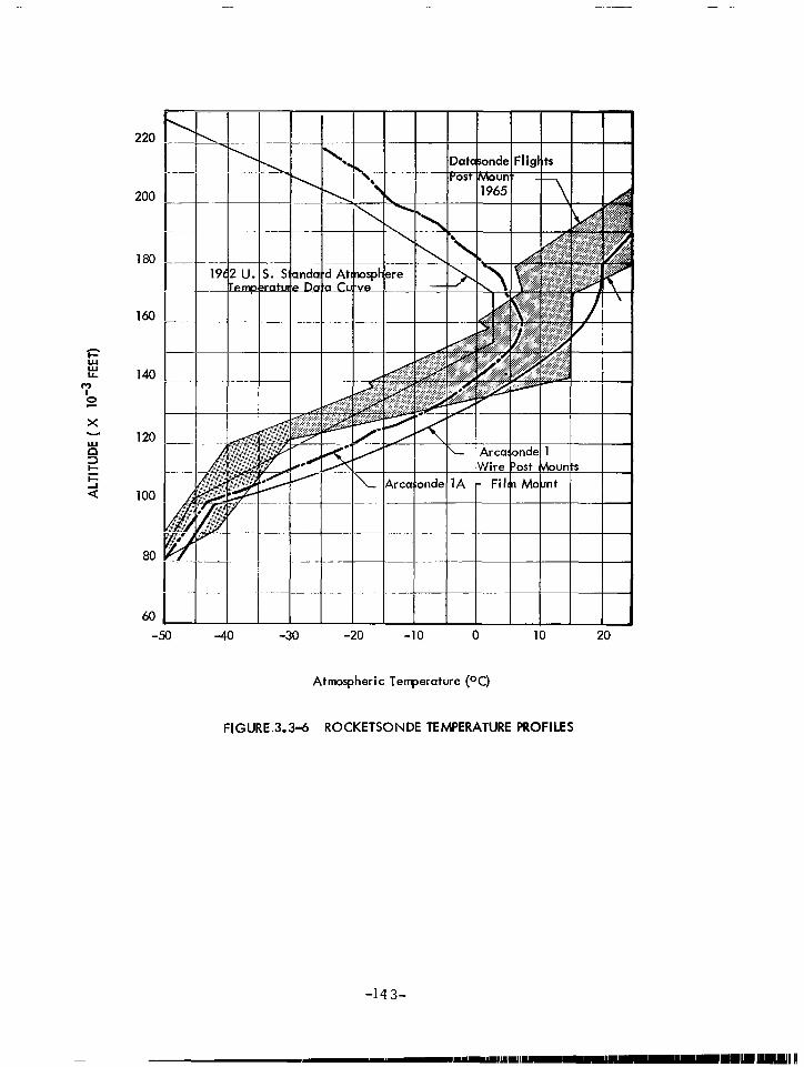
200

180

160

c

i 140 ‘:

0

x

2

120

E a 100

80

60 -40 -30 -20 -10 0 10 20

Atmospheric Temperature (OC)

FIGURE.3.3-6 ROCKETSONDE TEMPERATURE PROFILES

-14 3-

I bhmosdhere /

160 1 I I I I I I

14.0

120

a I D -I I_ I ! /4-

80 _

Terrperature (oC) %

FIGURE 3.3-7 DATASONDE TEMPERATURE MEASUREMENT OF THE ATMOSPHERE

-144-

100

80

20

0

Ba I I oonsonde

160 200 240

Temperature (OK)

FIGURE 3.3-8 HASP TEMPERATURE MEASUREMENTS

-145-

100

80

I- i= 2

40

.20

0

I 1 I I

.

Bal loonsonde

I 160 200 240 280

Temperatwe (OK)

Fl GURE 3.3-9 HASP TEMPERATURE MEASURE ME NTS

-14 6-

made. These calculations indicated that such a bias might be due to radiation heating of the thermistor by the hot sonde structures. An experimental flight test series was conducted with three different thermistor mount designs as shown in Figure 3.3-5 and described as follows:

C. Standard (1” long) plastic frame film mount.

D. Extra long (2”) plastic frame film mount.

E. Loop film mount.

The flight test results for these three mounts are presented in Figure 3.3-10 together with a typical profile for an old post mount. It is apparent that the loop mount cooled to -19O C, the long mount to -15O C and the standard mount to -12O C whereas the old post mount would record a temperature of about f 15O C at the 55 km (185,000 feet) altitude level. Response of these mounts is indicated in the heat loss curves of Figure 3.3-11. Since radiation heating decreases with distance from the sonde, the long mount registered about 3O C cooler than the standard after deployment. The major difference between the loop mount and the frame mount is the screening effect of the former. The back or inside surface of the loop mount is aluminized to reflect the infrared radiation from the sonde surfaces and to screen the thermistor from any view of the hot sonde as indicated in Figures 3.3-12 and 3.3-13. Theoretical calculations indicate a temperature increase of about 8O C at 55 km (185,000 feet) for the standard frame mount due to infrared radiation heating from the sonde structures. The flight test difference of 7O C indicates that the loop mount technique essentially eliminates this source of measurement error. Secondary advantages of the loop mount are that heat conduction paths from the heavier structures such as the plastic frames are considerably lengthened and the mount presents a mechanically resilient structure to protect the thermistor from mechanical shock and vibration.

A brief description of the various thermistor mounts which have been successfully flight tested is as follows:

1. Arcas-Deltrasonde Wire Mount.

Thermistor - 2.54~10~~ cm diameter Krylon coating, a= . 1, surface area - 3.2~10~~ cm’, thermistor lead lead length = 0.6cm, lead diameter = 2.54~10’~ cm. Mount-two cylindrical solid metal posts approximately 1.5cm in length.

-14 7-

240

220

140

120

100

80

. . ..I -3 ,

/ r’ /’ , k /

40 -

‘:c -. . .

/: 4 & . . .

I -20 -1

Flight Series 52 * PMR - San Nicholas Island 23 Jati 1967 -- 1400-1510 PST

* #6074 Loop Mount

--- Arcasonde lA-Mylar Film Frame Mount

---- Old Dart Plastic Post Moun

.._._.................. Arcasonde 1 - Wire post Mount * --------x6062 Standard Mount

* ---.- #&I31 Long Standard Mount

Atmospheric Temperatures (oC)

FIGURE 3.3-10 INSTRUMENTED DART TEMPERATURE PROFILES

-148-

-

80

60

40

9 2 2 20

0

-20

-40

1

I I I I I I

Post Mount 18/,000 Ft

I 20 30 4b I 50 6b I 70

Time From Payload Ejection (Seconds)

FIGURE 3.3-l 1 DATASONDE THERMISTOR RESPONSE

-149-

THIN FILM MYLAR.

Datasonde Radiation

Plastic Frame Mount

OLD STYLE MOUNT IN PLASTIC FRAME

Heat Conduction Thru Plastic Frame Mount

Radiation Datasande .-

NOTE: Thermistor has 360° exposure to radiated and conducted heat From the instrument.

FIGURE 3.3-12 COMPARISON OF OLD AND NEW THERMISTOR MOUNTING SYSTEMS

-150-

Sonde Descending After Ejection From Rocket Vehicle

Meteorological - Sonde

Radiating Heat

Aluminum Coating Reflects Back Radiated Heat

Radiation-Free Zone

Thermistor

FIGURE 3.3-13 Loop Thermistar Mount Radiation Shielding Effect

-151-

2. AFCRL Long Lead Wire Mount.

Flown with Arcas and Loki Dart. Thermistor - various thermistor types and various thermistor coatings were considered. Thermistor diameters varied from 1. 27x10w2cm (5 mil) to 3. 81x10m2cm (15 mil). Thermistor lead lengths were varied from 0.5 cm to 2.0 cn Emissivities of thermistor and thermistor leads were determined . Thermistor Mount - two cylindrical wires of varying lengths, wire diameter 2.54x10-3cm, attached to support posts. Instrument - Calculations were performed for the Delta-l instrument considered by Wagner and for a 1. 27x10e2cm thermistor with leads 1.5 cm in length.

1.

3. Arca s - Arcasonde 1A Film Mount.

Thermistor - 2. 54x10B2cm diameter, aluminum coating, solar absorption coefficient a = .07, surface area

= 3. 2x10V3cm2, thermistor lead length 1.6 mm, lead diameter = 2. 54x10m3cm. Thermistor mount - Mylar film 5 x 10S3cm in thickness, 0.06 solar absorption coefficient, surface area = 7.3 cm2 with silver strips for electrical conduction which also form a resonant line to filter the R.F. from the thermistor. Mylar film supported by solid phenolic posts. Thermistor mounted at a distance of 3.8 cm from instrument body. Instrument - circular body shape 4.8 cm diameter as considered to be constant at 40° C.

A 1-mil thick film of Mylar is firmly bonded to a l/16 inch-thick U-shaped phenolic board. This assembly is suitably masked, then inverted U-shaped films of silver about 40,000 hgstrom thickness are vacuum deposited on opposite surfaces. One leg of each U-shape is exactly opposite a corresponding leg of the other U-shape. These two opposed legs are deposited for a critical length to form a transmission line which is resonant at the transmitter frequency. This results in an effective short-circuit for any of the transmitter radio-frequency power absorbed by the electrical portion of the mount. The bead thermistor is soldered to the deposited film at the top center between the two opposed silver films. The remaining outside legs of the U-shapes serve as electrical conductors to an external measuring circuit.

The bead thermistor has a temperature characteristic such that

-152-

its resistance is 117,600 ohms at -25O C; 36,130 ohms at O” C; 8,570 ohms at 25’ C and 1.253 megohms at -65O C. The silver film strips are approximately 2mm wide and are 22 mm in length.

4. Arca s - STS Film Mount.

Thermistor - 2. 54x10-2cm diameter, aluminum coating, solar absor tion coefficient equal to 0.1, surface area = 3.2x10- 5 cm2, thermistor lead length of 3mm, lead

diameter 2. 54x10W3cm. Thermistor 1.8 cm from instrument bod Thermistor mount - Mylar film 1 x 10 -ydm in thickness solar absorption coefficient equal to 0.05 in the 0.25 tb 2.5 micron region of solar spectrum, aluminum coated on both surfaces (400 A thickness), surface area of 3.2 cm2 film mass of 4.5~10~~ grams, specific heat of 0.2 Cal/gram b

K. Mylar film supported by hollow nylon posts. Instrument - circular in cross-section with 6.4 cm diameter as seen by thermistor, long wave emissivity 1.0, maximum measured temperature of the instrument body 40° C.

The thermistor mounting configuration is shown in the drawing of Figure 3.3- 14. The dimensions of the thermistor mount were chosen so as to give a maximum height and width consistent with insuring that the thermistor and mount could not be swept off by the nose cone at the same time of instrument expulsion. The thermistor mount is constructed from a commercially available mylar polyester aluminized film 1 x 10 -3cm thick which is stretched between two hollow cylindrical support posts of type 6/6 nylon tubing, 3. 2 mm outside diameter. The support post wall thickness is that giving a minimum mass-to-area ration consistent with giving sufficient strength to support the film and thermistor at the time of maximum stress during rocket launch and instrument expulsion. The thickness of the thermistor mount plate was also reduced to a minimum value consistent with necessary rigidity and strength. It is made from woven glass fabric and epoxy resin, Mil Spec Mil-P- 18177C Type GEE. The mounting posts are glued into holes drilled in the mounting plate.

The aluminum coating of the mylar is removed with a sodium hydroxide solution after the film is properly masked, thus producing insulating strips at the center and at the two edges of the film mount. The mylar film is then stretched between

-15 3-

l30ARV THERMAL CONVUCTZVZTY IcaL/&x. cm. WJ 7.4x10-4

SPEClFZC HEAT b2uLlgham W)

DENSZTY &wlb/cm. 3)

PUST FILM

5.9x10-4 3.6~10'~

0.4 0.2

1.1 7.4

FIGURE 3.3-14 THERMISTOR MOUNT - STS-1 INSTRUMENT

-154-

the posts and secured by means of an epoxy glue. The leads of the thermistor (3mm in length) are joined to the top edge of the mylar film mount, one on each side of the center insulating strip. They are joined to the film by inserting the end of each thermistor lead into a tiny hole which is punched through the mylar and are then secured in place by a small amount of silver paint. The electrical connection to the modulator circuit of the instrument package are secured to the lower edge of the film in a similar manner. A small capacitor (0.001 uf) is connected so as to shunt the radio- frequency voltage which is induced in the leads by the field of the transmitter tube. The thermistor, mount, and mount plate are then secured to the instrument so that the thermistor is at a null point of the radio frequency field, thus minimizing the heating of the thermistor bead due to the absorption .of radio frequency energy from the instrument transmitter.

5. Loki Dart - Datasonde Loop Film Mount.

Thermistor - 2.54 x 10 -2 cm diameter, aluminum coating, solar absorption coefficient equal to 0.1, surface area 3.2 x 10-3cm2, thermistor lead length 3 mm, lead diameter 2.54 x 10e4cm. Thermistor 2.30 cm from instrument body. Thermistor mount - loop of mylar film 2.54 x 10V3cm thickness , 1000 8 aluminum coating on inside surface of loop. Instrument - Circular cross-section, i-inch diameter, maximum measured temperature 90° C. The Datasonde loop mount is illustrated in Figure 3.3-15.

3.3.3 Theoretical Analyses of Temperature Measurement Error Sources.

3.3.1 General Since the year 19 63 a great deal has been written about the error sources and magnitudes of error for the rocketsonde bead thermistor measurements. Most of the papers have been theoretical studies with some experimental inputs related to the heat transfer characteristics of the bead thermistors and their mounting arrangements at the altitudes between 30 km and 65 km. Ballard has written an excellent review of seven of the primary papers as follows:

-155-

Thin Film Mylar

\

Bead Thermistor

ver Pri’nted- rcuit Path

Nichrome L ads

\

Phenolic Base Plate

Aluminum Layer1

FIGURE 3.3-15 DETAILS OF LOOP THERMISTOR MOUNT

-156-

(1)

(2)

(3)

(4)

(5)

(6)

(7)

(8)

A Reviewof Seven Papers Concerning the Measurement of Temperature in the Stratosphere and Mesophere. Harold N. Ballard, ECOM - 5125 Atmospheric Sciences Laboratory, White Sands Missile Range, New Mexico, May, 1967.

An&vestigat&n in.& the Response and Corrections to a Thermistor and a Platinum Wire Resistance Thermometer, Ph. 0. Pearson, Weapons Research Establishment, Australian Defence Scientific Service, Salisbury , South Australia, March, 19 64.

Temperature Corrections to a Bead Thermistor in the Upper Atmosphere, A. D. Hind, Weapons Research Establishment, Australian Defence Scientific Service, Salisbury, South Australia, May, 1966.

Theoretical Accuracy of a Meteoroloqical Rocketsonde Thermistor, N. K. Wagner, Journal of Applied Meteor- ology, August, 1964.

Research conducted under contract with U. S. Army Signal Missile Support Agency, White Sands Missile Range, New Mexico.

An Improvement of Atmospheric Temperature Measure- ments Above 30 km by Means of the Bead Thermistor Mountinq Arranqement, Wm. A Drews , prepared for NASA under contract NASl-1611, January, 1966.

The Measurement of Temperature in the Stratosphere ..~ and Me sophere, Harold N. Ballard, USAECOM Report 5056, May, 19 66, Journal of Applied Meteorology, February, 19 67.

Time Response and Aerodynamic Heating of Atmospheric Temperature Sensing Elements, Robert Rubio and Harold N. Ballard, AMS Conference on the Dynamic Structure of the Atmosphere, 8-10 November, 1966.

The Accuracy of Miniature Bead Thermistors in the Meas- urement of Upper Air Temperatures, Donald C. Thompson, Scientific Report No. 1, prepared by Dep’t. of Meteorology M. I. T. for Air Force Cambridge Research Laboratories, 1 October, 1966.

-157-

Ballard’s review and the individual papers have been studied, and the major results are reported herein. Two additional papers not specifically included in Ballard’s review are also reported herein. They are as follows:

(9) Corrections for Meteorological Rocket Temperature Sound- ings On an Individual Basis. Robert M. Henry, NASA Langley Research Center, March, 1967.

(101 A Survey for NOL of Hiqh Altitude Temperature Sensors and Associated Problems. Wm. Finley Wright, Wright Instruments, Inc . Final Report’ - 1961 Contract N-60921-6136, 1961.

The various theoretical error analyses for rocketsonde bead thermistor measurements are based upon the basic equations which describe radiation, conduction and convection modes of heat transfer. Differences that exist among the results of the various authors are primarily due to differences in the physical characteristics of the sounding systems analyzed, and to some degree by differences in the assumptions and values chosen for pertinent parameters of the heat transfer equations.

The basic modes of heat transfer can be described by four equations as follows:

Conduction

where

. \ tit H

cd = kAcE (1) .

H cd= rate of heat transfer by conduction

k = thermal conductivity of the medium

AC = cross-section area of element considered

dt dx= temperature gradient along the element

Convection H cv

= MS’ (Te-T) (2)

where .

H cv

= rate of heat transfer by convection

h = convection heat transfer coefficient

-158-

AS = surface area of element considered

Te = temperature of the environment

T = temperature of the element

Long Wave Radiation .

Hr = crc AsT (3)

where .

Hr = rate of heat transfer by long wave

radiation

W= Stefan-Boltzmann constant

C = emissivity of surface of considered

As = surface area of element

T = temperature of element

Solar Radiation (0.25P to 2.5P )

H sr

= n a ACT

element

(4)

. where HSr= rate of heat transfer by solar radiation

n = a pure number

a = absorption coefficient for element considered

AC = cross-section area exposed to solar radiation

J = 3.3 x 1o-2 Cal-cm -2

set solar constant

If the heat transfer from the atmosphere to the thermistor is considered to take place in the relatively thin boundry layer of thickness 6 surrounding the element, then by combining equations

-159-

(1) and (2), h= k/6 . The Nusselt number is defined by Nu hd

where d is a characteristic dimension of the element, i.e. , k

the dizmeter of the thermistor. By combining the above expressions, 6 =Tii--

and equation (2) can be rewritten as, .

H = N”tka cv ( *dt ) (Ta - T> (5)

where subscripts t and a refer to the thermistor and air respectively. If aerodynamic heating is considered,.

(6)

where Taer = temperature rise of element where the only heat transfer is from aerodynamic heating

r = recovery factor

v = velocity of the element

Cp = specific heat at constant pressure of the air

The quantity r is a measure of the ratio of the viscosity of the medium to its thermal conductivity and is related to the Prandtl number Pr .= cccp/k where ~1 and k are the medium viscosity and thermal conductivity, respectively. Thus, from equations (5) and (6), the rate of heat transfer by the process of convection in an environment which is aerodynamically heated by the passage of a spherical thermistor through it, is then given by

. H = N”tka

- T cv dt

( rdt2)

C

Ta+ rv2 2c

t P 1 [

= htAst Ta+ rv2 2c

P

(7)

If the configuration for attaching the thermistor to the instrument package is in the form of two wires of uniform cross-section A thermal conductivity k, and length L, and if these mounting cw’

wires are considered to transfer heat to or from the environment by the process of convection, then equations (1) and (2) may be combined to give the rate of heat transfer by conduction along the lead wires from the thermistor (or from the thermistor to the thermistor mount ) .

-160-

Thus equation (1) becomes, for the two wire supports,

. H =

cd -2kwAcw (dTw/dx)x = L

. 2 H

cd = -kw ( =dw

2 ) B {(T s- Ta) sinhBL

+[ (‘tmTa) - Ts-Ta coshBL

sinhBL ( ‘I coshBL

(84

(8b)

where B = (2/dw) X dw

If the wires are such that BL is small, then equation (8b) becomes

(84

By combining the above expressions to describe the rocketsonde thermistor which is descending in the atmosphere an overall heat transfer equation can be generated as,

mtc dT/dt = (10) t

Solar Radiation Convection

‘bet 1 + F(Te+ &G] P

Conduction

+bAcw I: dTw,~~+rRa~~ti~quency wsorption~~

-161-

Here mt and ct are the mass and specific heat of the thermistor respectively , dTt/dt is the time rate of change of the thermistor temperature, eeb, Cea, and cl are the emissivities of the environment below, environment above and the instrument respectively, fl, f2, and f3 are fractional numbers representing the fractional portion of the thermistor surface area Ast exposed to the radiation from the environment below and above and from the instrument, while T,b, Tea, Ti, and Tt are the temperatures of the environment below, environment above, instrument and thermistor respectively. The numbers f2 .f2 .f3 = 1; i.e., flAst+f3Ast=Ast. Tohmic is the temperature rise due to ohmic heating, and H,f is the heat transferred by rf field of the sonde transmitter. For a well- designed sonde both of these quantities are negligible. Equation (10) is not amenable to solution in closed form. To evaluate the contributions of each term to the total heat transfer rate, values must be assigned to each quantity in the equation. Each investigator assigned values to the various emissivities and temperatures. The position of the thermistor relative to the instrument usually determines the values assigned to fl, f2, and f3. Values for n and a were assigned while values for h and r were calculated as functions of altitude. The velocity component v was determined from radar data concerning the particular instrument and parachute.

The time constant of the sensing system depends on both the thermistor and the mounting configuration, and of course ,‘ varies significantly with altitude. is given by m&St ,

The time constant 7t of the thermistor where St is the total heat transfer coefficient

or dissipation factor. The time constant rt is the ratio of heat energy absorbed by the thermistor per degree Kelvin to the rate of energy transfer per degree Kelvin. If heat transfer by the process of convection is considered as the only means of heat transfer to or from the thermistor, then the time constant of the thermistor is given by

(11)

If heat transfer to or from the thermistor by processes other than convection is considered, then expressions for the time constant of the thermistor are of the form

mtCt = ?= s mtCt t 4c+ Ast T; + 2kwAcw

/ Lw+ ht Ast (12)

-162-

or, mc

Tt= s t t mtCt (13)

t [ 2kwAcw B cothBL + htAst 1

The expression for the total heat transfer coefficient St in the denominator of Equation (12) is that derived by Ballard for the heat transfer process of radiation, conduction, and convection with the thermistor having leads of short length (6mm - 3mm) while the denominator of Equation (13) gives the dissipation factor of the thermistor, as derived by Thompson, for the heat transfer processes of conduction and convection with the thermistor leads of long length (10mm - 20mm). If the quantity BL, becomes small then the two equations are identical for the processes of conduction and convection.

3.3, 3.2 Papers on Theoretical Temperature Corrections. A brief review of each of the aforementioned papers is presented in the following sections. The various heat transfer rates for an altitude of 60 km as determined by the individual authors are presented as follows:

Symbol .

H

‘sr . Hev . Hed

gob

HI-f

Heat Transfer Rate

due to long wave radiation

due to short wave radiation

due to convection from atmosphere

due to conduction through mount

due to ohmic heating

due to t-f heating

The corresponding temperature corrections are also presented.

Paper (1) , Ballard. This paper presents a review and analysis of papers (2) through (8), and many of the results are presented in the following sections on the individual papers. A summary of the results of Ballard’s review is presented in Table 3-8.

The temperature correction values stated for long wave radiation appear to agree in general and indicate that the long wave

-163-

TABLE 3-8

TABULAR SUMMARY OF TEMPERATURE CORRECTIONS TO ROCKETSONDE THERMISTORS

(DIAMETER 2.54 x 102cm) ALTITUDE 60 km [Ballard]

Investigator iI Ii i Ii iI iI Total Correction

lr sr aer cd ohm rf Correction 50 km

Pearson -0. 1°C - 5.. 5Oc -0.2Oc -0.5Oc ? - 5.6’C -2.8’C (Observed)

Bind (Aust. Inst.) -0.2Oc -3.oOc -7. o”c -1.7Oc -l.lOC ? -13. o”c -2.8’C

Wagner (Delta -1) ~0. O°C -1.6’C - 5. 1°C -10. O°C -3.8’C ? -20.5Oc - 5. o”c

Drews (Arcasonde) -0.4Oc -2. o”c -7.6’C 0 -2.7Oc 0 -12.7Oc / -2.lOC

Ballard (STS-1) -0.4Oc -1. o”c -3.3Oc 0 -0.5Oc 0 -5.2’C -2.6’C (Observed)

Rubio & Ballard (Arcasonde) +1. o”c -3Oc -3.9Oc 0 -l.OOC 0 -6.9’C -2.lOC

---------------------

(STS- 1) -0.4Oc (Observed) -3Oc -3.9Oc 0 -0.5Oc 0 x-7.8’C -2. 1°C

Thompson (10 mil thermistor- 1.5 lead Igth. +0.4Oc -3. 1°C -9Oc -1Oc -0.2Oc 0 -13.7Oc* - 3Oc --------------------_I

(Delta - 1) +2.7’C -2.2Oc -8.7’C I-5.9’C 1 -3.l’C 0 -16.6’C ( -3.4’C * Lag correction of approximately -0.7’C is included.

The maximum solar radiation correction is included in the total correction value.

,

radiation correction is of the order of +_ 0.4OK depending upon the instrument studied and values chosen for the pertinent parameters. An exception is a correction of + 2.7O C as determined by Thompson for the Delta - 1 instrument.

The various values for the solar radiation correction -appear\ to be in general agreement with the values varying from - lo C to - 3. lo C depending upon the thermistor coating, mounting, configuration, and whether or not solar irradiation of the thermistor mount was considered in the calculations.

In daytime rocketsonde temperature soundings, temperature oscillations with peak-to-peak magnitudes from lo C to 3o C at 60 km are usually observed. These temperature oscillations dimin- ish in amplitude with decreasing altitude and do not appear on nighttime firings.

The temperature correction for heat conduction from the instrument body to the thermistor varies from a value of zero for the Arcasonde and STS instruments (film mounts) to a value of -5. go C and -10. O” C for the Delta - 1 instrument (post mounts) as determined by Thompson and Wagner, respectively. Since Thompson considered convective heat transfer for the lead wires in his calculations and Wagner did not, it would be expected that the temperature correction as determined by Thompson would be lower than that found by Wagner. The data indicates that the correction magnitude for heat conduction is determined by the mounting configuration. Pearson found a correction value of -0.2OC for a wire length of 2.54 cm (2.54 x 10m3cm diameter), Thompson found a value of -1. O°C for a wire length of 1.5 cm (2.54 x 10W3cm diameter) while the heat conduction corrections for the Arcasonde and STS instruments, which utilize thermistor mounts in the form of thin films, were found to be zero. All calculations indicate that a properly designed thermistor mount will reduce the heat conduction correction to a negligible value.

The ohmic heating correction is dependent upon the magnitude of the thermistor current at a particular value of thermistor resistance. This correction is therefore variable depending upon the electrical characteristics of the instrument and upon the total heat transfer coefficient for the instrument thermistor. This in turn is dependent upon the particular thermistor mounting arrangement utilized. The authors of the various papers appear to agree that, if the electrical power dissipated across the thermistor is less than 10 microwatts

-165-

throughout the temperature range of interest, then the corresponding correction is no more than -0. So C. The ohmic heating corrections for the various instruments studied indicate that the ohmic heating corrections varied from -0.2O C to -3.8O C at an altitude of 60 km andfurther indicate that an electrical power dissipation of less than 10 microwatts across the thermistor, for instruments actually constructed, is not always easy to achieve.

The effect of absorption of r.f. energy from the rocketsonde thermisJor was considered by each investigator. The question mark in the Hrf column indicates that. the magnitude of the effect was not known but would be investigated and that the magnitude of the correction would be made small by proper placement of the thermistor in the electromagnetic field of the transmitter.

Aerodynamic heating appears to be the largest source of rocketsonde temperature measurement error as the corrections varied from -3.3O K to -9. O” K among the various authors. Al- though the temperature rise due to aerodynamic heating would be rv2 for an isolated thermistor, when radiation and lead conduction 2 CP heat transfer is taken into act e net temperature rise due to aerodynamic heating is X G where St is the total heat transfer coefficient including the m&nting system. Recovery factor values, r, used by the investigators use,d a velocity of about 125 m/set except Pearson who used 200 m/set. .Some of the authors did not account for other than convective heat transfer away from the thermistors of the input heat produced by aerodynamic heating. Thus the variation in the aerodynamic heating corrections may be explained.

All of the studies indicate that for a properly designed instrument the two major sources of measurement error are caused by aerodynamic heating (4OK to go K at 60 km) and solar radiation (<3OKat 60 km). The total correction at 50 km was found to decrease to 2’ K to 3O K at 50 km and to be negligible at 40 km and below.

Long lead wire mounts suggested by Pearson and Thompson were investigated by Ballard, and approximately 20°K temperature increases were found to be due to r.f. heating. Evidently the long lead wires make good antennae.

-166-

Paper (2) Pearson. This paper presents a theoretical heat transfer analysis with the incident radiation from the sun and earth taken as J = 12 x 10m2 watts/cm2 with the conditions as follows:

n (1) Thermistor -2.54 x lo-‘cm diameter, aluminum coating,

a = .l, surface area = 2.0 x 10m3cm2.

(2) Mount -2 cylindrical wires, 2.54 cm in length, 2.54 x 10B3cm diameter, a = .1

(3) Instrument - hemispherical body shape as seen by thermistor, 7.6 cm in diameter, aluminum coating = . 1, body temperature 24O C.

(4) Atmospheric Temperatures Assumed - 1959 ARDC Atmos- phere, long wave emissivities - 0.8

The calculations involved convective transfer of heat from the thermistor mounting wires and recommendations were given as follows:

(1) supported by 0.001 inch (2.54 x 10 -3) d’ iameter wires at least 1 inch (2.54 cm) long.

(2) silvered for low emissivity

(3) mounted at least 1 inch (2.54 cm) in front of the parent body

(4) situated as close to the stagnation point as possible while satisfying requirement 3

(5) and that the power used for measurement shall be as low as practically possible (approximately 10 watts) unless pulsed so that the peak power may be increased considerably.

Under these conditions the error in temperature should be less than l.ll” C up to 150,000 ft. (46 km), 2.83O C from 150,000 - 180,000 ft. (46 - 55 km) and less than 5.5S” C from 180,000 - 200,000 ft. (55 - 60 km). A breakdown of Pearson’s corrections for an altitude of 60 km is presented in Table 3-9.

Paper (3) Hind The theoretical calculations included the convective heat transfer from the thermistor leads and deviations of the thermistor from a spherical shape. Assumed values

-167-

TABLE 3-9

Theoretical Results at 60 km for an Australian Instrument [Pearson]

Quantity

.

Hlr

‘sr

‘aer

‘cd

Ii ohm

mtct

htAt

st

mc/hA tt tt

mtct’St V

rv2/2c P

Values

2 p watts

I -

110 watts P

4~ watts

10 p watts

27 /” joules/OK

5. 5 /^ watts /OK

20 /” watts/OK

5 set

1.4 set

200 m/set

2o”c

Corresponding Total Temperature Temperature Corrections Correction

-0. 1°C

- 5.5Oc

-0.2Oc

-0.5Oc

-6.3’C

-5.6’C

Temperature Correction at 50 km -2.8’C.

were as follows:

(1) Thermistor - 2.54 x 10m2cm diameter, Krylon coating, a= .2

(2)

(3)

(4)

(5)

Mount - 2 cylindrical wires, length unknown, 2.54 x 10W3cm diameter. Mount and thermistor are on an extendable probe.

Instrument Body - configuration not known, body temperature 25O C.

Atmospheric Temperatures Assumed - 1962 Standard Atmosphere .

J = 1.25 Solar Constant. Solar Constant = 14 10 -2

wSatts/cm2.

The results of this analysis are presented for 60 km in Table 3-10. Temperature correction with altitude is presented in Figure 3.3-16.

The total heat transfer coefficient value is important as it is in the denominator of all other correction equations. All values of the heat transfer coefficient were calculated assuming the bead thermistor was a sphere. In practice the thermistor tends to be an ellipsoid with the diameter of its axes 0.010 and 0.014 inches. As the value of the heat transfer coefficient is proportional to the diameter squared, an error of up to 30% in the thermal balance correction could be introduced by assuming a spherical bead of 0.011 inch diameter. For night firings, the heat balance factors tend to cancel leaving only a small correction and hence this 30% error will only cause an error of 0.8O C. Assuming an error of the same order introduced by heat flow along the wires and infrared radiation, the total heat balance error will be f 2OR ( + lo C) at 200,000 ft (60 km) falling to + 1°R ( + 0. So CT at 16OyOOO ft. (50 km). For daytime firings an error &e to the solar input correction of up to 1°R (0. So C) at 200,000 ft (60 km ) is to be expected. The correction due to the response time of the thermistor is also dependent on the heat transfer coefficient; hence an error of + lo C is possible during the largest temperature lapse rates.

The total correction error will be + 2O C at 200,000 ft (60 km) falling to + 0.5O C at 150, 000 ft (46 km). Combining this with the measurem&rt error, the overall error will be + 2.3O C at 200,000 ft (60 km) falling to + 0.8O C at 150,000 ft (4% km) and then remaining constant at + 0.8O C to 90,000 ft (27 km).

-169-

TABLE 3-10

Quantity

.

Hlr

Rsr H aer H cd I; ohm

Theoretical Results at 60 km of an Australian Instrument [Hind]

“tCt

htAt

st

mtCt’htAt

mtct’St

V

rv2/2c P

Corresponding Temperature Corrections Values

1.7~ watts

11 p watts

51 /L” watts

12 p watts

8 /” watts

28 /” joules/OK

5.7 ,u- watts/OK

7.3 /“” watts/OK

-0.2Oc

-3. o”c

-7. o”c

-1.7Oc

-1. 1°C

4.9 set

3.8 set

122 m/set

9Oc

Temperature Correction at 50 km -2.8’C

Total Temperature Correction

-13. o”c

* Note: If the solar radiation effect

is corrected as indicated under Remarks concerning this study, Hind’s solar radiatioa correction at 60km is -0.6 C; his total eytime corrections 9 -10.6 C at 60km and -0.4 C at 50 km.

200

190

180

170

160

150

140

130

120 0 4 8 12 16 20

Temperature Correction (OR)

FIGURE 3.3-16 TEMPERATURE CORRECTION WITH ALTITUDE (OR)

-171-

The temperature correction has been shown applied to a particular firing. The possibility of having a standard correction, to be applied to all firings, was considered but rejected on the grounds that the error involved could be too large. The velocity of the sonde has been found to vary, being dependent on the ejection height, and the aerodynamic heating correction differs by up to 30% from one firing to the next. Other variable factors include thermistor diameter, air density, thermistor temperature, and lapse rate, all of which can affect the final correction.

The corrections can be extended to heights above 200,000 ft. (60 km), but their accuracy will decrease due to the increased velocity, increased response time and decreased value of heat transfer coefficient. Above 220,000 ft. (65 km), the thermistor will be in “intermediate flow” for which the heat transfer coefficients are not accurately known. Assuming that the sonde was ejected sufficiently high to allow the thermistor to begin measuring the air temperature, the expected errors would be ( + 4.5O C) at 210,000 ft (62 km) and ( + 7.50 C) at 220,000 ft (65 km).

Paper (4) Wagner. The calculations for this paper did not include the convective transfer of heat nor radiation effects for the thermistor leads. Assumed value for the analysis are as follows:

(1) Thermistor - 2.54 x 10S2cm diameter, Krylon coating, a = 1, surface area - 3.2 x 10S3cm 2, thermistor lead length = 0.6 cm., lead diameter = 2.54 x 10W3cm.

(2) Mount - two cylindrical solid metal posts approximately 1.5 cm in length.

(3) Instrument - circular body shape, 6.4 cm in diameter as seen by the thermistor, long wave emissivity - 1.0, body temperature 25O C at 65 km decreasing to 15O C at 30 km.

(4) Atmospheric Temperatures Assumed - 1962 Standard Atmosphere

(5) J, = .045 Cal/cm2 set = 19 x 10 -2 2 watts/cm .

The results of this analysis are presented in Table 3-11 for an altitude of 60 km, and a typical sounding is presented in Figure 3.3-17. It can be seen that the lead conduction error and ohmic heating terms are quite large compared. to the other analyses. This is due to the

-172-

I $ w I

TABLE 3-11

Theoretical Results at 60 km for the Delta - I Instrument [Wagner]

Quantity

. Hlr

‘sr Ii . aer H cd

‘ohm

m tCt hA t t

st mc/hA tt tt m c /S tt t V

rv2/2c P

Values

0 p watts

15/u watts

58p watts

z 115/u/watts

43p watts

27’~ joules/OK

7.5,~ watts/OK

11.5~ watts/OK

3.6 set

Corresponding Temperature Corrections

o”c

-1.6’C

-5. 1°C

-10. o”c

-3.8’C

Total Temperature Correction

2.3 set

125 m /set

7.9Oc

Temperature Correction at 50 km -5. o”c

80

60

2 ‘r 50 2

i 3 40 z W

z F

30

<

20

10

0

Stc ROI Da

3

-

: : : : : i a. *. *..

ion: WSE :et Type: ?: 16 Fek !: 17: 10

I 1

I I _I I I I

=.* 1962 U.S. Sta ldard Atmo:;phere *.

-. -. ‘. -. -*.. ‘. =.*

: 1 /’ c’

De ta-1 Instrument

-100 -80 -60 -40 -20 0 +20 40 +60 +80 +lOO

Temperature (“C)

FIGURE 3.3-17 Temperature Vs. Altitude Profile (ARCAS) From Wagner’s Investigation

-174-

older short wire mount and Delta instrument measuring circuits. I? The short thermistor leads were attached to the relatively hot and large diameter metal mounting posts, which conducted a good deal of heat from the sonde to the thermistor and also resulted in a long thermal time constant. Thermal time constants for an isolated lo-mil bead thermistor have been presented by Wagner in Figure 3.3-18. As a result of deviations in the shape of the thermistor from a true sphere, an increase in the time constant up to 11% may be experienced.

The time constant of the sensor is r = C/h where C is the heat capacity of the bead and h is the coefficient of convective heat transfer for the various flow regions. C is a function of the specific heat of the ceramic material used for the bead and its volume. The coefficient of convective heat transfer to a sphere may be calculated from

h = (Nu k A)/d

The Nusselt number in continuous flow for Reynolds numbers less than 20 is given by

Nu”= 2+ 0.37 (Re) 0.6 (Pr) l/3

and in the slip flow regime for Mach numbers less than unity

Nu = Nu”

1 + 3.42 (Ma/Re Pr) Nu”

Re = p dV/L,

Pr = Cpp/k

From solutions of these equations, the time constant of a spherical bead was found to be very nearly a linear function of the thermistor diameter above 50 km.

Radiative temperature errors for a lo-mil spherical bead thermistor for various solar absorptivities is presented in Figure 3.3-19. The physical characteristics of the glass-coated bead were investigated at length by Wright Instrument, Inc. in its 19 6 1 report to the Naval Ordnance Laboratory. They found the sensor to be a prolate spheroid of average characteristics as follows:

-175-

loo- I 90 Free Molecular Flow

80. t Transi tiona I

-l-L- ..-- :-+:-... ,c r:-, -...-rL--& .dcL L-Z-Lb :, rL, ADnr ,,,e ““,,“,l”,, “I IIIIIC: LVIIJIUIII Wllll IlCqJlll III lllci r\RYL

standard atmosphere for a IO-mil-diameter spherical- bead thermistor.

Time Constant (Seconds) (Wagner)

FIGURE 3.3-18 Theoretical Thermal Time Constant for IO-mil Diameter Bead Thermistor

-176-

100

90 a b

:

C d

80 e

Curve ;: 02 0.1 -

d” 0.2 0.4 - e 0.7 f 1.0

I I

0 10 20 30 40 50 60 70

Tenperatwe Error (OC) (Wagner)

FIGURE 3.3-19 Rkiiative temperature error for a IO-mil-diameter spherical&ad thermistor in the ARDC standard atmosphere. Each cwve represents a specific value for the solar absorptivity as shown in the table at the lower right.

-177-

volume 16.8 X 10B6cm3

weight 65.6 x 10m6gm

density 3.9gm cm -3

specific heat 0.12 cal OC-l gm -’

projected area

total surface area

8.94 x 10 -4

cm2

2.98 x 10zm3cm2

To lessen the effect of incident solar radiation, the bead is given a very thin coating of white Krylon No 1502 (pigment 89% Ti02).

The diffuse reflectance of 11 coats of KRYLON No. 1502 on a Pyrex disc is plotted in Figure 3.3-20. Measurements between 200 milimicrons and 2 microns were made referencing Mg CO3 in a Perkin- Elmer model 350 spectrometer while the 2 micron to 15 micron measurements were made using a Perkin-Elmer model 13 spectrometer and an 800°C holhram. It is obvious that in the visible region this coating provides not only a good reflective coating, but also one with a known reflectance which remains constant throughout flight, thereby permitting the effect of solar radiation to be accounted for in reduction of data. One notes also that this coating is almost black for the long wave lengths, i.e. , the blackbody temperatures experienced by the bead during flight. Both the theoretical treatment and the laboratory measurements of (Ballard 1961) have shown thermistors coated with Krylon to be optimum in their ability to respond to atmospheric temperatures after being ejected from a hot nose cone environment, and to more effectively dissipate the heat generated internal to the bead by the measuring current during descent. The examination of sensors removed from instrument packages recovered after normal soundings revealed no apparent change in either coating or calibration of the Krylon-coated bead thermistors.

Paper (5) Drews Heat transfer calculations for the original thin film thermistor mount were performed on the IBM 7090 computer by the solution of five first order differential equations. The assumed values for the sensor configuration are as follows:

(1) Thermistor - 2.54 x 10S2cm diameter, aluminum coating, solar absorption coefficient a = .07, surface area = .32 x 10V3cm2 lead diameter = 2.54 4

thermistor lead length 1.6 mm, 10m3cm.

-178-

.7-

.6- ‘t; .5-

5 t; .4-

2 2 .3-

e 3 .2- k E l-

KRYLON if1502

Ol I1

I 1

1 10

Wave Length - Microns

FIGURE 3.340 DIFFUSE REFLECTANCE OF KRYLON COATING ON PYREX DISC

-179-

(2) Thermistor mount - Mylar film 5 x 10 -3

cm in thickness, 0.06 solar absorption coefficient, surface area = 7.3 cm with silver strips for electrical conduction which also form a resonant line to filter the R.F. from the thermistor. Mylar film supported by solid phenolic posts. Thermistor mounted at a distance of 3.8 cm from instrument body.

(3) Instrument - circular body shape 4.8 cm in diameter as seen by thermistor, emissivity 0.80, body temperature considered to be constant at 40° C.

(4) Atmospheric Temperatures Assumed - 1962 Standard Atmosphere.

(5) J, = .045 Cal/cm2 set = 10 x 10V2 watts/cm2

The results of this analysis are presented in Table 3-12. These data indicate that the thin film mount is quite effective in isolating the thermistor from conduction errors from the hot sonde structures , and the temperature of the thermistor leads are shown to be lower than that of the thermistor throughout the entire sounding . The effect of halving the descent rate of the system at 60 km was shown to reduce the temperature error at this altitude by a significant margin i.e. , from 12. 1°K to 6.5OK. The effect of lowering the initial temperature of the thermistor at deployment was found to have a negligible effect for data below 60 km.

To reduce radiative effects it is necessary to reduce the size of the thermistor as much as is practical and to provide a surface which is highly reflective to long wave radiation. However, at atmospheric pressures where the mean free molecular path is comparable to or larger than the sensor dimensions, heat transfer by conduction becomes a strong function of pressure. At altitudes above 60 km, this condition is realized, and conductive heat transfer is significantly reduced as altitude is increased. Thus, there is a tradeoff between reducing the sensor size to reduce radiative effects and increasing the sensor size to increase conductive heat transfer. This assumes that the thermistor is thermally isolated from its mounting structures.

Since heat conduction from the thermistor mounting posts in the older designed instruments was found to be a major source of measurement error, thermal isolation of the thermistor from its mounting structures was a design goal of the program that Drews reported.

-180-

TABLE 3-12

Theoretical Results at 60 km for the Arcasonde Instrument [Drews]

Corresponding Temperature Corrections

Total Temperature Correction Quantity

.

Hlr H sr . H aer . H cd . H Ohm

vt

Values

w2 pwatts

11 /“watts

57 p watts

~Opwatts

2 0 p watts

34 ,LL joule s/OK

7.5 y- watts/‘K

7.5 ,u watts/OK

4.5 set

4.5 set

125 m/set

htAt

S. t

mc/hA tt tt

mtct’st V

rv2/2c P 7.6’C

Temperature Correction at 50 km (-2. l°C)

-=0.4Oc

-2, o”c

-7.6’C

-2JOC 1 -12.7’C

Because of the fragile nature of the bead and its leads, it was felt that mere extension of lead length, as a means of achieving thermal isolation, would be unsuitable, Moreover, it was known that the leads are highly absorptive to solar radiation and, further, that long leads became an effective antenna at the telemetering frequency thus causing absorption of electromagnetic energy by the bead. To circumvent these problem areas, a thin mylar film was used to achieve thermal isolation of the thermistor. Electrical leads were formed on the film by vacuum deposition of two silver bands. The mylar is relatively transparent to incident solar energy and the silver leads, which form the measuring circuit, are reflective. Thus thermistor leads, which are solar absorptive would be kept very short, about l/8-inch. The two deposited silver strips, formed a radio frequency transmission line, l/4 wavelength, at the telemetered frequency. This arrangement provides an effective short circuit across the thermistor for RF energy while still allowing connections to the silver leads for the purpose of measuring the thermistor resistances.

The thermal model used in the theoretical error analysis is shown in Figure 3.3-21. An ejection altitude of 70 km was assumed in the calculations. The results are summarized for the standard Arcas parachute fall rates in Tables 3-13 through 3-15 with the symbols defined as follows:

Z = altitude - kilometers

TT = temperature of thermistor

TL = temperature of thermistor leads

TM = temperature of Mylar film

TS = temperature of silver film

TP = temperature of phenolic posts

TR = recovery temperature

TA = ambient atmospheric temperature

The results of this analysis indicate that the temperature of the thermistor leads TL as well as the temperature of the deposited silver film TS maintain a close relation to the temperature of the thermistor TT throughout the flight. The temperature of the mylar film TM very quickly reaches thermal equilibrium with the recovery temperature TR and, by 5 6 kilometers, is in equilibrium with the atmospheric temperature. These results imply that the thermistor and the

-182-

THERMIsI-OR

r- l -HERMIS7DR

IWsrRUMENT PACbaQE

SENSOR DEVICE

THEPJML RESETANCE OF LEAD

4 RADIATION 7-0

SPACE

THE!ShIAL .-.-.-. ..--

INSTRUMENT PACKAGE

Ti’3WK

(Drews)

FIGURE 3.3-21 THERMAL MODEL

Z&d TT(OK) TL(OK) TS(OK) TM(OK) TP(OK) TR(‘K) TA(OK)

70 313 313 313 313 313 248.9 219.7 69 295.2 293.1 292.4 295.3 312.9 249.3 223.6 68 281.4 279.8 279.5 282.5 312.7 250.1 227.5 67 272.1 271 .O 270.0 273.3 312.6 251.2 231.4 66 266.7 265.9 266.0 267.0 312.4 252.7 235.3 65 264.2 263.6 263.7 262.8 312.2 254.4 239.2 64 263.6 263.1 263.3 260.3 312.1 256.4 243.1 63 264.3 263.9 264.1 259.1 311.9 258.6 247.0 62 265.7 265.3 265.6 258.9 311.7 261 .O 250.9 61 267.3 266.9 267.2 259.4 311.5 262.6 253.8 60 267.9 267.4 267.7 260.0 311.3 263.4 255.8 59 268.3 267.9 268.2 260.7 311.1 264.4 257.7 58 268.9 268.5 268.8 261.4 310.9 265.4 259.7 n 269.7 269.3 269.6 262.2 310.7 266.6 261.6 56 270.6 270.2 270.5 263.1 310.4 267.9 263.6 55 271.7 271.3 271.6 264.1 310.2 269.3 265.6 54 272.9 272.5 272.8 265.1 309.9 270.7 267.5 53 274.2 273.8 274.1 266.3 309.7 272.2 269.5 52 275.0 274.6 275.0 267.4 309.4 273.1 270.6 51 274.5 274.1 274.5 267.8 309. I 272.8 270.6 50 274.1 273.1 274.1 267.8 308.8 272.5 270.6 49 273.7 273.3 273.7 267.8 308.3 272.3 270.6 48 273.3 273.0 273.4 267.8 307.8 272.0 270.6 47 272.1 271.7 272.1 267.5 307.2 270.8 269.5 46 269.1 268.6 269.1 265.8 306.3 267.9 266.8 45 266.1 265.7 266.1 263.8 305.0 265.0 264.1 44 263.1 262.7 263.2 261.6 303.4 262.1 261.3

TABLE 3-13

THERMAL BEHAVIOR OF MODEL THIN FILM THERMISTOR MOUNT (Drews)

-184-

TABLE 3-14

Zh)

70

68

66

64

62

60

58

56

54

52

50

48

46

44

DIFFERENCE TEMPERATURE VS. ALTITUDE (Drews)

TT-TA(OK)

93.3

53.9

31.4

20.5

14.8

12.1

9.2

7.0

5.4

4.4

3.5

2.7

2.3

1.8

TL-TA(OK)

93.3

52.3

30.6

20.0

14.4

11.6

8.8

6.6

5.0

4.0

3.1

2.4

1.8

1.4

TS-TA(OK)

93.3

52.0

30.7

20.0

14.7

11.9

9.1

6.9

5.3

4.4

3.5

2.8

2.3

1.9

TM-TA(OK)

93.3

55.0

31.7

17.2

8.0

4.2

1.7

-0.5

-2.4

-3.2

-2.8

-2.8

-1.0

0.3

TP-TA(OK)

93.3

85.2

77.1

69.0

60.8

55.5

51.2

47.0

42.4

38.8

38.2

37.2

39.5

42.1

TR-TA(OK)

29.2

22.6

17.4

13.3

10.1

7.6

5.7

4.3

3.2

2.5

1.9

1.4

1.1

0.8

-185-

TABLE 3-15

ACCURACY OF TEMPERATURE MEASUREMENT [Drews]

Z (km) TT-TA (Deg.

TT-TR (Deg.)

70 93.3 64.1

68 53.9 31.3

66 31.5 14.0

64 20.5 7.2

62 14.8 4.7

60 12.1 4.5

58 9.2 3.5

56 7.0 2.7

54 5.3 2.2

52 4.4 1.9

50 3.4 1.6

48 2.7 1.3

46 2.3 1.2

44 1.8 1.0

ERROR mTR)

ERROR (V/O

12.5 23.7

5.53 13.4

2.80 8.44

1.80 5.9

1.71 4.74

1.37 3.55

1.0 2.66

0.81 1.98

0.69 1.63

0.59 1.26

0.48 1.0

0.45 0.86

0.38 0.69

-186-

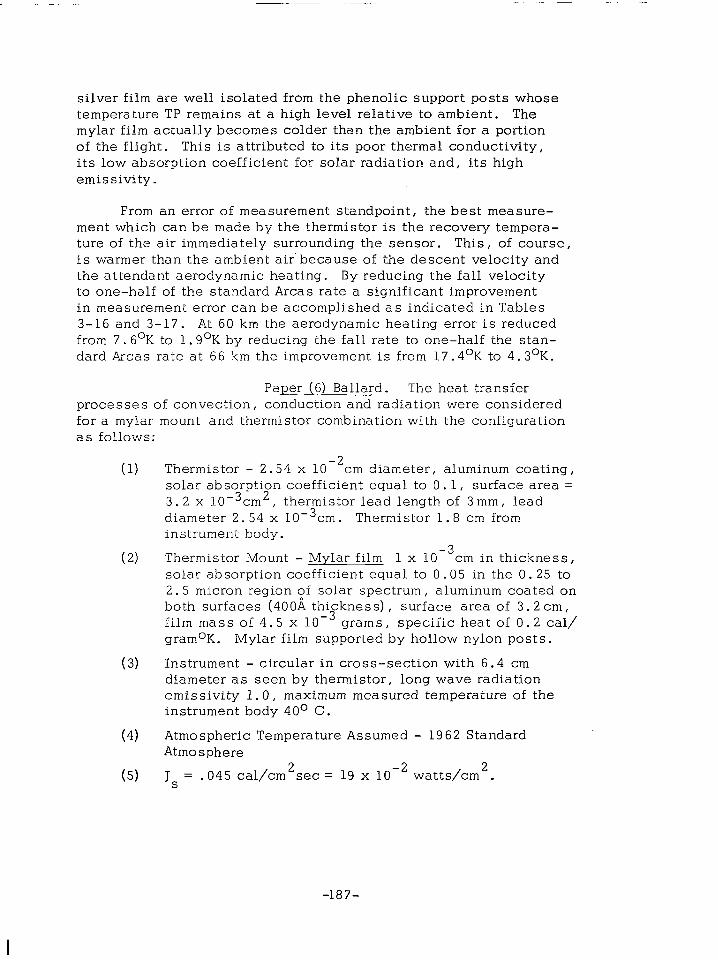
silver film are well isolated from the phenolic support posts whose temperature TP remains at a high level relative to ambient. The mylar film actually becomes colder than the ambient for a portion of the flight. This is attributed to its poor thermal conductivity, its low absorption coefficient for solar radiation and, its high emissivity.

From an error of measurement standpoint, the best measurement which can be made by the thermistor is the recovery temperature of the air immediately surrounding the sensor. This, of course, is warmer than the ambient air’because of the descent velocity and the attendant aerodynamic heating. By reducing the fall velocity to one-half of the standard Arcas rate a significant improvement in measurement error can be accomplished as indicated in Tables 3-16 and 3-17. At 60 km the aerodynamic heating error is reduced from 7. 6OK to 1.9OK by reducing the fall rate to one-half the standard Arcas rate at 66 km the improvement is from 17.4OK to 4.3OK.

Paper (6) Ballard. The heat transfer processes of convection, conduction and radiation were considered for a mylar mount and thermistor combination with the configuration as follows:

(1)

(2)

(3)

(4)

(5)

Thermistor - 2.54 x 10m2cm diameter, aluminum coating, solar absorption coefficient equal to 0.1, surface area = 3.2 x 10-3cm2, thermistor lead length of 3 mm, lead diameter 2.54 x 10m3cm. Thermistor 1.8 cm from instrument body.

Thermistor Mount - Mylar film 1 x 10 -3 cm in thickness, solar absorption coefficient equal to 0.05 in the 0. 25 to 2.5 micron region of solar spectrum, aluminum coated on both surfaces (4OOi thickness), surface area of 3.2 cm, film mass of 4.5 x 10B3 grams, specific heat of 0.2 cal/ gramOK. Mylar film supported by hollow nylon posts.

Instrument - circular in cross-section with 6.4 cm diameter as seen by thermistor, long wave radiation emissivity 1.0, maximum measured temperature of the instrument body 40° C.

Atmospheric Temperature Assumed - 1962 Standard Atmosphere

Js = .045 cal/cm2sec = 19 x 10B2 watts/cm’.

-187-

Z

70

68

66

64

62

60

58

56

54

52

50

48

46

44

TT -

313

256.7

249.4

253.2

258.7

262.3

264.8

267.6

270.6

273.2

272.7

272.3

268.2

262.5

TABLE 3-16

BEHAVIOR OF A THERMAL

AT ONE-HALF THE FALL

TL

313

255.7

249.0

252.8

258.3

261.9

264.4

267.2

270.2

272.8

272.3

272.0

267.9

262.1

TS -

313

255.9

249.2

253.1

258.6

262.3

264.8

267.6

270.6

273.3

272.8

272.4

268.4

262.6

TM TR TA

313 227.0 219.7

266.2 233.1 227.5

252.6 239.6 235.3

250.7 246.4 243.1

253.1 253.4 250.9

256.2 257.7 255.8

258.4 261.1 259.7

260.7 264.7 263.6

263.0 268.3 267.5

265.4 271.3 270.6

265.8 271.1 270.6

266.0 271.0 270.6

264.2 267.1 266.8

260.6 261.5 261.3

MODEL

RATE

(Drews)

-188-

TABLE 3-17

ACCURACY OF TEMPERATURE MEASUREMENTS FOR A THERMAL

MODEL AT ONE-HALF THE FALL RATE

Z TT-TA TT-TR

70 93.3 86

68 29.2 23.6

66 14.1 9.8

64 10.1 6.8

62 7.8 5. 3

60 6.5 4.6

58 5.1 3.7

56 4.0 2.9

54 3.1 2.3

52 2.6 1.9

50 2.1 1.6

48 1.7 1.3

46 1.4 1.1

44 1.2 1.0

ERROR %

ERROR --S--TX

IO. 1 12.80

4.1 6.00

2.76 4.15

2.09 3.10

1.79 2.55

1.42 1.97

1.1 1. 52

0.86 1.16

0.70 0.96

0.59 0.77

0.48 0.63

0.41 0.52

0.38 0.46

(Drews)

-189-

Flight test data from two nighttime firings are compared with a daytime firing in Figure 3.3-22. The daytime firing exhibited periodic temperature oscillations of lo to 3O K at 60 km, and the nighttime traces showed no evidence of such oscillations.

It is presumed that the daytime oscillations are then due to the incident solar radiation being periodically excluded from the thermistor due to the swinging parachute. The lowest temperature observed during one oscillation period is determined and taken as the atmospheric temperature. According to the assumption of short wave solar energy incident at the rate of J+35% to include reflected energy which is always present, a maximum value of 0.8O C should be subtracted from the lowest temperature observed during one oscillation period at about the 60 km altitude level.

The results of the theoretical analysis are presented in Table 3-18. The calculated values for the thermistor and film dissipation factors at 65 km were 16 and 5200 microwatts (OK)-’ respectively, with corresponding time constants of 1.8 and 0.7 sec. The transmittance-wavelength study in the spectral region from 0.2 to 2.5 microns for the mylar film indicated that the temperature increase in the thermistor due to the absorption of solar radiation when mounted on the aluminum-coated mylar film is approximately 1C (approximately 4C for uncoated mylar).

By employing the thin-film mount rather than the older post mounting arrangement and employing a low sensor measurement current, Ballard found that the temperature correction at 65 km could be reduced from 36OK to 5OK. A heat transfer analysis of the older post-mounted Delta 1 Arcas sonde was conducted in accordance with the model of Figure 3.3-23. The results are presented for 65 km in Table 3-19.

Improvements were made in the Delta 1 instrument to reduce the temperature measurement errors by using a thin-film thermistor mount, and reducing the electrical power dissipated by the measurement current in the thermistor. The resulting instrument was renamed STS-F and the results of the heat transfer analysis for a 65 km altitude are presented in Table 3-20.

‘The film will more rapidly come to temperature equilibrium with the atmosphere than does the thermistor. The combined film- thermistor dissipation is less than the film, alone, and the combined time constant is therefore greater. The value of 16~~ peroK for

-190-

l- - . . . ‘.

* . .

M.lCORFlECTED -I-EMPERATURE

962 us. STANDARD ATMOS.

I I 0 1

-100 -80 -,

STATION WSMR, N.M. ROCKET TYPE ARCAS

-.. . . I . ..* “..., ‘.., . . - (i 4) .,

‘,i I

:..,_

>.. . .._._, . .._

..__

I I

/ -40 -,

‘/ ‘/

- . - . ‘._,

. . . . .._ ‘....

I .‘..,.

. . I 1

1 0 +20 i-40

Temperature (Oc)

DATE Dec. 15, 1966 TIME 21:24 Night---STS-16s DATE Dec. 16, 1966 TIME 00554 Night---STS-34 DATE Dec. 20, 1966 TIME 11.07 Day ---STS-11s

FIGURE 3.3-22 TEMPERATURE VS. ALTITUDE FROM BALLARD’S INVESTIGATION

-191-

--.-II m,,,.,, IlmlllB II rnllil I I III 1111 I II III1 I

HEAT TRANSFER PROCESSES FOR A ROCKETSONOE

ALTITUDE SSKM-DELTA1 ROCKETSONDE-

THERMISTOR

SPHERICAL BEAD

Cp-SPECIFlC “EAT OF +1R ,CONSTPlNT PRESSURE,

. I.0XI07cm2 see-2 .1(-’ K - THERMAL CONOUCTl”lTY OF LEAD WRE

= ,074 cm, cm-’ .dW Y-ELECTRICAL POWER ACROSS THERMlSTOR

- 70 L *Ott. ,9 - CROSS-SEC710N*L AREA OF LEAD WIRE

$CHANSE IN TEMPERAT”RElr .a,,, OF POWER T.hrnlC f . 5, x l0-&,2

..I6 ‘C/r IOll, Tbm - TEMPERATURE OF ENWROHMENT BELOW K - LENGTH OF LEPlO WRE . , cm

J,-SOLAR CONSTANT. ,043 co, cm-z s.c-‘lJt35X) T,,- TEMPERATURE OF ENWRONMENT ABOVE c - swcmz HEAT 0F THERMISTOR

.- STEFAN SOCTZM&,,N CONSTdNT T,, -TEMPERATURE OF WSTRUMEHT ABOVE . .I8 501 gm-’ .I(-’

A- THERMlSTOR SURFACE AREA. 322X IO-’ ,,z T - THERYlSTOR TEYPERATVRE Y - THERY~STOR MASS . 3.9 x 10-5 q,n

s . o- ASSORPT!ON COEFFlClENT FOR AL”MIN”U. _, T. - THERMlSTOR SVPPORT TEMPERATURE [ 4rb.T.’ +y+hA]

:. : 5’. T, -TEMPERATURE OF ~MMEo~ATE EHWRONMENT r - TlME COHSTANT . y . 3.1 ,.c

“._ .: .:

,. ;

FIGURE 3.3-23 PRINCIPAL MODES 0F HEAT TRANSFER /JAMARD_I

-19 2-

I z W I

TABLE 3-18

Theoretical Results at 60 km for the STS-1 Instrument [ Ballard ]

Quantity Values


;I lr .

+7 -c(-17) p watts

Hsr(thermistor)

Ii (film 4OOA sr aluminum coat-

15/u,watts

3000 p watts -1Oc

ing>

Raer . Hcd(from ins-

trument)

Rohm

mtCt

htAt

st

“tCdhtAt

mtct’St V

rv2/2c P

60 p watts

= 0 /u.watts

-3.3Oc

10 p watts

2’7 ,u joules/OK

7.5 ,u watts/OK

18.5 /“watts/OK

3.5 set

-0.5Oc

1.4 set

125 m/set

7.9Oc

Temperature Correction at 50 km -2.6’C*

* NOTE :

I -5.2’C

If the solar radiation effect is corrected as indicated under Remarks concerning this study, the solar radiation correction at 60km is (-0.8’C) and the total $aytime correction is (- 5.0 C) at 60 km and -1.9’C at 50 km.

TABLE 3-19

Theoretical Analysis Results

for Post Mounted Thermistor

Delta I Instrument at 65 km

Energy Steades State Input Error

Long Wave Radiation (pw -2 -0.3 OK

Solar Radiation (pw) +15 + 1.7 “K

Mount Conduction (yw, + 160 -I- 1?.8OK

Electrical Heating $4 + 70 + 7.8’K

Convection 5 bw per OK

Boundary Layer Temperature Increase 15’K + 15’K

Convective Heat Transfer Coefficient

-2 -1 o -1 4X1010 Cal-cm -set K

Recovery Factor Fall Velocity

Dissipation Factor

Time Constant

1.10 165 m/set

9p w peroK

3.1 set

-194-

TABLE 3-20

Theoretical Analysis Results for

Film Mount Thermistor

STS-1 Instrument at 65 km

Energy Input

Long Wave Radiation negligible

Solar Radiation (for direct incident)

Film 28,000/1.w Thermistor 15/&w Equilibrium 45/u/ w

Mount Conduction negligible

Steady State Error

+ 5,5’K + l.O’K + 3.0°K

Electrical Heating negligible

Film Dissipation Factor, Sf 5200,~ w per OK

Film Time Constant, f 0.7 set

Film - Thermistor Dissipation Factor, Stm 16,~ w per OK

Film - Thermistor Time Constant, Stm 1.8 set -4

Film Convective Heat Transfer Coefficient 1.3x10 cal-set -cm-2-oK-1

Thermistor Convective Heat Transfer -4 Coefficient 4.0x10 cal-set-cm

-2 0 -1 - K

-195-‘

I _.....-_. ---.-..-. . . . . . .I

the film.-thermistor combination is a significant improvement over the post mounted thermistor value of 9pw per OK for the Delta 1.

The analysis shows that the thermistor and film mount are essentially isolated from the instrument structures with respect to heat transfer, and the effects of long wave radiation, mount conduction and electrical heating have been made negligible. Solar radiation effects have been increased from the previous value of 1.7OK at 65 km to +3. O°K for normal direct incidence. Rotation of the sonde during descent should reduce this latter value depending on solar radiation incidence and sonde rotation or oscillation rate. The transmittance of clear mylar film in the 0.2 to 2.4,~ region is presented in Figure 3.3-24. By coating the mylar film with a thin aluminum .layer ,. the absorption of direct incidence solar radiation should be reduced to a 1°K error at 65 km.

Paper (7) Rubio and Ballard. Aerodynamic heating corrections for the Arcasonde and STS-1 thin-film mylar thermistor mounts described and analyzed in Papers (5) and (6) have been determined in the present paper. The results are presented in Tables 3-21 and 3-22 for a 60 km altitude. The corrections for both instruments are essentially the same, being about 5OK at 60 km and 2OK at 50 km. However, an interesting temperature profile plot is presented for the Arcasonde as shown in Figure 3.3-25 where ‘excessive fall rates and aerodynamic heating were experienced at 70 km.

Paper (8) Thompson This paper deals with a combined theoretical study and experimental program dealing with various sizes of thermistors and various lead lengths. The ranges of the parameters were as follows:

(1) Thermistor - Various thermistor types and various thermistor coatings were considered. Thermistor diameters varied from 1.27 x 10B2cm (5 mil) to 3. 81x10-2cm (15 mil) . Thermistor lead lengths were varied from 0.5 cm to 2.0 cm. Emissivities of thermistor and thermistor leads were determined.

(2) Thermistor Mount - two cylindrical wires of varying lengths, wire diameter 2.54 x 10-3cm, attached to support posts.

‘(3) Instrument - Calculations were performed for the Delta 1 instrument considered by Wagner and for a 1.27 x 10m2cm thermistor with leads 1.5 cm in length.

-19 6-

100

80

60

40

20

0

TRANSMITTANCE - CLEAR MYLAR FILM - THICKNESS 0.001 CM

,2 0.2 0.6 0: 8 110 I

Wavelength (Microns)

FIGURE 3.3-24 TRANSMlSSlVll-Y VS WAVELENGTH OF THE MYLAR FILM

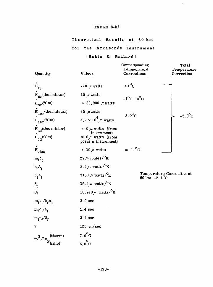
TABLE 3-21

Theoretical Results at 60 km

for the Arcasonde Instrument

[ Rubio & Ballard1

Quantity Values


.

Hlr . Hsr(thermistor)

Hsr (film)

Raer(thermistor)

;Iaer(film) .

Hcd(thermistor)

Rcd(film)

‘ohm

mtCt

htAt

hfAf

st

sf

“tCtjhtAt

-20 pwatts

15 bwatts

= 33,000 pwatts

+ 1°C 1 -1Oc 3Oc

65 pwatts

4.7 x 104p watts -3.9Oc

= O/u- watts (from instrument)

= 0~ watts (from posts & instrument)

x 2Opwatts

29p joules/OK

8.4/c” watts/OK

7 150,~ watts/OK

2 6.4~ watts/OK

10,970p watts/OK

3.9 set

vt/St

mf Cf’8f V

1.4 set

3.1 set

125 m/set

b - 5. o”c

z-l.OC -J

Temperature Correction at 50 km -2. l°C

rv2/2c (therm)

‘(film)

7.9Oc

6.6OC

-198-

Quantity

* Hlr Rsr(thermistor)

Hsr(film)

Raer(thermistor)

fiaer(fiW

Rcd(thermistor)

Hcd(film)

Rohm

“tCt

“tAt

hfAf

St

Sf

mtct’ht*t

mtct’St m c /S tt f V

rv2 /2 c (therm)

(film)

TABLE 3-22

Theoretical Results at 60 km

for the Arcasonde Instrument

[ Rubio & Ballard 1

Values


+ 7* (-17)~ watts -0.4OC++l. ooc

15p watts -lOC+- 3OC (oscillation magnitude)

2880,~ watts

6 5 /CL watts -3.2’C

2.9 X lO/lc watts -4.3Oc

x OF watts (from instrument)

x O/LL watts (from posts & instrument)

= 10/u watts

29p joules/OK

8.4,~ watts/4c

4460 ,P watts/OK

20.4~ watts/OK

6877~ watts/OK

3.9 set

-0.5Oc

1.4 set

0.5 set

125 m/set

7.9Oc

6.9’C

-3.9Oc

Temperaturs Correction at 50 km -2.1 c

-199-

Temperature (OC)

STATION WSMR, N.M. ROCKET TYPE ARCAS DATE 8 JUNEmIME 1 l:55 LT ARCASONDE 1A DATE 8 JUNE 1966 TIME 13.08 LT STS - 1

FIGURE 3,3-25 TEMPERATURE VS. ALTITUDE FROM RUB10 AND BALLARD’S INVESTIGATION!

-2oo-

(4) Atmospheric Temperatures As sumed - 19 6 2 Standard Atmosphere

(5) Solar Radiation - Corrections included the effects of direct and reflected solar irradiation incident upon the thermistor and leads.

At 60 km the values of the derived dissipation factors varied from 1.2 to 1.0 for lead lengths from 1.85 to 1.00 cm, thermistor diameters from 5 mils to 15 mils and for aluminum-coated and uncoated thermistors. The calculations include the convective heat transfer and radiation effects for the thermistor lead wires. Table 3-23 presents the analysis results for a 10 mil aluminum-coated thermistor with 1.5 cm leads. Lead diameter was taken as 2.54 x lo-‘cm, solar absorptivity as o. 15 and solar elevation angle as 40 degrees.

Lead wire radiation and convection effects were found to be fairly important for relatively long lead wires. A reflective coating for the lead wires was suggested. The advantage of the long lead wires is to reduce conduction errors caused by heat flowing from the sonde structures to the thermistor through short leads. It appears that the thin-film mounts accomplish the same objective, but that radiation effects would be larger and aerodynamic heating corrections would be more complex. The radiation error should depend on the orientation of the film with respect to the direct and reflected radiation, and the aerodynamic heating should probably depend on the orientation of the foil with respect to the airflow. In free molecule flow the recovery factor for a flat plate varies by a factor of nearly 2 between flow parallel to and flow normal to the plate. Due to parachute swing at high altitude the orientation would not be known at a given time. (A comment appropriate here is that with the instrumented Loki Dart system, PWN-8B, having the stability of the Starute descent device and the loop thermistor mount, the geometry is much more favorable for predicting aerodynamic heating than indicated in the previous statements).

Thompson found that for relatively long uncoated thermistor leads, the temperature rise due to solar radiation falling on the lead wires is of the same order of magnitude as that due to the radiation intercepted by the bead. The temperature rise for various thermistor diameters and lead lengths irradiated in a vacuum are presented in Figure 3.3-26. The variation of this radiation effect with pressure is indicated in Figure 3.3-27. The effect of

-2Ol-

TABLE 3-23

Quantity

.

Hlr

‘sr I-i aer

‘cd li ohm

mtCt

Theoretical Results at 60 km for a lo-mil aluminum coated,

Diameter 2.54 X 10m2cm, lead length 1. 5 cm [ Thompson ]

Values


M -7 p watts + 0.4Oc

53 p watts - 3.1°C

154/” watts - 9Oc

:

-12.9Oc

17/c” watts -1. o”c

3.0~ watts -0.2Oc

z 30~ joule s/OK

M 6,~ watts/OK

x 1’7~ watts/OK

= 5 set

M 2 set

125 m/set

8.5’C

Lag Error -0.7Oc

700

600

500

4o”

3o”

2o”

100

00 0 8

Effective Thermistor Diameter in Mils. (Thompson)

Lead lengi d=2Ocm

/

d = 1.5 cm

/

d = l.Ocm

d ~0.5 cm

7

/

/

FIGURE 3.3-26 TEMPERATURE RISE OF IRRADIATED THERMISTORS

(In V acuumTI. J = 2.0 cal/cm2/min. L/W Radiation Neglected)

-203-

3o”

250

5Oc

C

NUMBER

TYPE

COATING

LEAD LENGTH

A. Whole of leads exposed.

B. Bead only exposed.

G-6

X2047

Al

1.45 cm

70 Km

J = 2.0 cal cm -2 min -’

Pressure, mm Mercury (Thompson)

FIGURE 3.3-27 MEASURED RESPONSE OF THERMISTOR TO RADIATION

dirty or contaminated lead wires under solar radiation is shown in. Figure 3.3-28. The effect of thermistor size on radiation errors is shown in Figure 3.3-29. It is seen that the smaller thermistor has a smaller radiation error temperature rise due to its superior convective heat transfer characteristics at the higher pressures, This advantage is reduced at the higher altitudes. where the thermistor dimensions approach the mean free path of the air molecules.

The radiation response of a thinistor is presented in Figure 3.3-30. This thinistor was 0.0008 inches thick and the upper side of the plate had a flat black finish perpendicular to the radiation. If the thinistor had been given a 90% reflective coating, the sea level temperature rise should be about 2.4OK. The advantage of the thinistor comes in at the high altitudes where mean free path limitations occur for the beads and the convective heat transfer coefficient is superior.

Measured heat transfer coefficients for thermistor beads and wires in still air are presented in Figure 3.3-31 and for thinistors and beads in Figure 3.3-32. It can be seen that the heat transfer coefficients are greater for the smaller dimensions sensors than for the large sensors.

The thermal time constant, T , is defined as the time required for a sensor to achieve 1 - & = 63% of a step change in ambient temperature. The thermal time constants of the rocketsonde thermistors are inversely related to the dissipation constant or convective heat transfer coefficient. Measured time constants for various thermistor sizes are presented in Figure 3.3-33. Although the thermal time constants and dissipation rates are improved with increased ventilation speeds in the lower atmosphere, the experimental data indicates that there is no effect at pressures less than 1.0 mm Hg.

High speed air flow or ventilation rate, however, does cause an aerodynamic heating temperature rise of the sensor. Measured recovery factors for various thermistor sizes are presented in Figure 3.3-34. Notice that recovery factors greater than 1.0 were determined between 45 km and 70 km. The recovery factor is given by

Tr - To r=TF - To

where To = ambient absolute temperature of the air

Ts = stagnation absolute temperature of the air

Tr = thermistor absolute temperature

-205-

60’ I I I I

NUMBER G-5 G-8 TYPE X2047 L5oOC COATING Al AI/Quartz LEAD LENGTH 1.30 cm 1.29 cm

J = 2.0 cal cmB2 min-’

Lead Wires

.lO

Pressure, mm Mercury

10

(Thompson)

FIGURE 3.3-28 MEASURED RESPONSE OF THERMISTORS TO RADIATION

t I I I I t-

I I - A. Whole of leads exposed.

B. Bead only exposed.

O0

-2 -1 J = 2.0 cai cm min

1 NUMBER GB-2 45CD5 NONE 1.26 cm

TYPE / COATING I LEAD LENGTH

NOM. DIAM.

Pressure, m m mercwy

-

FIGURE 3.3-29 MEASURED RESPONSE OF THERMISTORS TO RADIATION

h .

V5B-1 TX171 8 NONE 1.38 cm 5 mils

-

(Thompson)

.OOl .OOl .Ol .Ol -

=F VECO Ft\llA5 THINISTOR

Black face normal to lamp.

J - 2.0 cal cm -2 -1 min

0.1 Pressure, mm mercury

1.0 lo (Thompson)

FIGURE 3.3-30 MEASURED RESPONSE OF THINSTOR TO RADIATION

10-2

b I

$

f 10’3

I’

1o-4

I

0 0 1 mil Lead Wires

d---A 15 mil Beads

.OOl .Ol 0.1

Pressure, mm mercury lo (Thompson)

FIGURE 3.3-31 MEASURED HEAT TRANSFER COEFFICIENTS FOR THERMISTOR BEADS AND WIRES IN STILL AIR

10-l -_

_ 0 .--------a 5 mil Thermistor Beads

x---x 10 mil Thermistor Beads

h- A Veto FNlA5 Thinistor

10’2 T 1

10-4

,---

,-

I

50

U. S. Std. Atmos. 1962 km

I I

40 30

Pressure, mm mercury. (Thompson)

FIGURE 3.3-32 HEAT TRANSFER COEFFICIENTS OF THERMISTORS DEDUCED FROM DISSIPATION RATE

100

10

1

0.1

: STILL AIR)

&--A x.-----x -’ +ia- . : STILL AIR) T-l G-5 ‘jB-2’ V5B-1

FNlA5 X2047 41A5 TX1 718 1.0 cm 1.30 cm 1.11 cm 1.38 cm

Iumber

rYPe -cad Length Vom. Diam. Vom. Diam.

I I &---A x.-----x iTJ--+J

T-l G-5 V5B-1 FNlA5 X2047 41A5 TX1 718 1.0 cm 1.30 cm 1.11 cm 1.38 cm

.---P=O .---P=O

U. S. Std. Atmos., km I I111111 1

1 -01 0:1 l:o 10

80 /O 60 3lJ

IJ. S. Std. Atmos., km I I I111111 -El-- , -----

1 -01 0:1 l:o 10

Pressure, mm mercury (Thompson)

FIGURE 3.3-33 MEASURED TIME CONSTANTS OF THERMISTORS

1.5 --

0 X 0 a Number V5B-3 VB-3 G-l 3 G-12 v5 xfg-4

Type TX1765 41A5 X2047 X2047 TX1766 Nom. Diam. 5 mils 10 mils 15 mils 15 mils 5 mil. 4lead - Coating None None Al Al None Lead Length 1.0 cm 1.0 cm 1.85 cm 1.0 cm 1.0 cm

0.5 1

+

- m I I I I , I I I /O 60 su 40 30

U. S. Std. Atmos, km o- ’ -‘mm’! I I I

0.1 1.0 10 lb0 7&I

Pressure, mm mercury (Thompson)

FIGURE 3.3-34 MEASURED RECOVERY FACTORS, r, OF THERMISTORS

and Ts - = 1 f v-1 To -

M2 9

where r = ratio of specific heats of air

M = Mach number

For thermistors operating in the high-altitude rarefied gas region of the atmosphere recovery factors greater than 1 are possible. This result has been shown theoretically for free-molecule flow where the size of the sensor is small compared to the mean free path. However, for the small thermistors used currently with rocketsondes, the free-molecule flow conditions are met only above 85 km. The upper altitude region of current rocketsondes puts the thermistors into the transitional or slip-flow region depending on the value of the Knudsen number, Kn = x/D where A is the mean free molecule path, and D is a characheristic dimension of the sensor.

Computations show that for aluminized thermistors the long wavelength radiation errors are quite small below 70 km, if an assumed instrument package temperature of only 27O C is used. ( On-board temperature measurements of sonde structures show temperatures as high as 100° C. Space Data calculations show a significant error, 4O - 5O K, due to infrared heating from sonde surfaces at 60 km.)

Sensor lag errors below 55 km appear to be negligible as indicated in Figure 3.3-35. However, lag becomes important above 60 km, and the 5-mil thermistor with a faster time constant offers an advantage over the larger thermistors, that is, until it runs into mean free path problems previously mentioned. It is interesting to note that the added mass of aluminized thermistors increases their time constant values over the equivalent black beads as indicated in Figure 3.3-36. Thus, a tradeoff between radiation and lag errors might dictate the use of uncoated beads for a particular sounding system to minimize overall error. This tradeoff would be a function of maximum measurement altitude and the sonde descent velocity.

A systhesis of temperature measurement errors assuming Arcas rate profiles for a lo-mil Krylon-coated thermistor is presented in Table 3-24 and for a 5-mil aluminized thermistor is presented in Table 3- 25.

-213-

. ov

---- 15 mi I Thermistor

-Mm-- 10 mil Thermistor

5 mil Thermistor

Initial Temperature Difference lOOoCat70km Arcasonde Fall Rate

-

.U. S. Std. Atmos., Km.

1 I I I I I I I

I I I I I I, I’

y-j 1 I ‘1. J rT I ‘4

FIGURE 3.3-35 LAG ERRORS OF THERMlSiORS

-214-

1-m 1 .Aluminized Bead -

-. Blckzad ----

0. 1 -: I I I I I I I 90 80 65 50 30 15

Altitude, KM

FIGURE 3.3-36 MEASURED TIME CONSTANT

-215-

TABLE 3-24

Temperature Errors of 10 mil Krylon-coated

Thermistor Using 0.6 cm Lead Length

Alt Aero Cond L/W Bad S/W Bad Meas Lag Total Wagner

km OC OC OC OC Oc Oc Oc OC

65 17.7 14.8 -5.6 3.6 4.5 -1.4 33.6 33.5

60 8.7 5.9 -2.7 2.2 3.1 -0.6 16.6 19.0

55 4.7 1.7 -2.3 1.4 2.1 -0.2 7.4 7.5

50 2.2 0.5 -1.8 0.9 1.6 0 3.4 5.0

45 1.0 0.3 -1.1 0.6 1.4 0.1 ,2.3 4.5

40 0.4 0.1 -0.6 0.6 1.0 0 1.4 3.5

35 0.2 0.1 -0.3 0.4 0.7 0 1.1

-216-

TABLE 3-2 5

Temperature Errors- of 5 mil Aluminized

Thermistor Using 1. 5 cm Lead Length

Alt Aero Cond L/W Rad S/W Rad Meas Lag Total

km OC OC OC OC OC OC OC

65 17.7 0.9 -0.7 5.4 0.5 -0.6 23.2 + 4.0

60 8.7 0.2 -0.5 2.9 0.4 -0.2 11.5 ‘r 2.0

55 4.7 0 -0.4 1.6 0.4 -0.1 6.2 t 1.1

40 2.2 0 -0.3 1.0 0.3 0 3.2 ‘_ 0.6

45 1.0 0 -0.2 0.7 0.2 0 1.7 _+ 0.5

40 0.4 0 -0.1 0.5 0.1 0 0.9 _’ 0.3

35 0.2 0 -0.1 0.4 0 0 0.5 +, 0.2

30 0.1 0 0 0.3 0 0 0.4 + 0.2

25 0 0 0 0.3 0 0 0.3 +, 0.1

20 0 0 0 0.2 0 0 0.2 +, 0.1

-217-

As a summarization of Thompson’s paper, comments are offered as follows:

a. At very high altitudes for long lead wire mounts the radiation absorbed by the leads is as important as that absorbed by the bead. As much attention should be directed to the reflectivity of the lead wires as to the bead itself.

b. The reflectivity of aluminized beads is quite variable from unit-to-unit, and a greater manufacturing control is needed to assure better uniformity. Surface imper- fections in the coating appears to be the major cause for the great variability. It may be desirable to use uncoated thermistors to improve both the surface uniformity and to reduce the thermal time constant at high altitudes.

C. The 5-mil thermistor may be used instead of the larger thermistors to reduce the thermal time constant and reduce the sensor lag.

d. Good temperature measurements can be made to 65 km with present equipment if the thermistors are mounted to eliminate conduction errors, if -the observed descent velocities are used to apply aerodynamic heating corrections, and if a greater uniformity in the reflective coatings for the thermistors is achieved.

Paper (9) Henry. Corrections for meteorological rocket temperature soundings are derived so that the actual trajectory data and measured temperature profile from a given sounding are used to obtain a higher degree of accuracy and help to extend the useful altitude range of the measurements. It is shown that the thin-film mount produces a larger reduction in the correction magnitudes, and indications are that reasonable temperatures can be obtained with the thin-film mount at considerably higher altitudes than presently considered.

Although the original purpose of the thin-film mount was to achieve thermal isolation of the thermistor from the telemetry. package, it is found that the large area of the thin film also serves as a very effective heat exchanger with the atmosphere. The heat transfer from the film which is conducted through the lead wires dominates the transfer of heat to and from the thermistor at the hrgh

-218-

altitudes. In fact, at altitudes approaching 100 km the bead- wire-film system approaches the behavior of a pure thin-film thermistor.

Radiation corrections are a bit more complex for the thin- film mount since there is a dependence on the solar flux incidence angle. Even for the thermistor alone, radiation corrections are not reliable as the value of the albedo is quite variable with geographic conditions, season, and cloud cover. As a result, it will be difficult to make radiation corrections which are meaningful and reflective coatings or radiation shields will be required to extent current measurement altitudes towards 100 km.

Aerodynamic heating is the primary source of temperature measurement error with current decelerator systems. The aerodynamic heating correction is somewhat reduced with the thin- film mount at the higher altitudes because it is in the continuum flow region with a recovery coefficient of 0.9 while the bead thermistor is in the slip-flow region with a recovery coefficient of 1.1 . Aerodynamic heating corrections should be done with accurate radar digital data and an allowance for the effect of the wind in influencing the air stream velocity by the sensor should be made.

Henry’s paper in included in its entirety as Appendix A, since techniques and concepts discussed may prove useful in extending the altitude of current temperature measurements and therefore advance the meteorological sounding performance capability.

Paper (10) Wright This paper presents a great deal of miscellaneous facts and experimental data bearing on the subject of rocketsonde temperature measurements. Since this was one of the earliest papers in the field, much of the data has been quoted by more recent investigators. Thus, a great deal of the data has been already presented in the reviews of the first nine papers. Additional information from this paper is presented in the following paragraphs.

The Knudsen number, Kn = - Ei is genera w

taken as an indicator of fluid flow regime. Since Kn =’ 1.48 me , a plot of Mach number versus Reynold’s number can be used to define the various flow regimes as in Figure 3.3-37. Generally, for Kn > 4.5 free molecule flow is assumed to exist.

-219-

2.0

t

M - =lO Re

\/G-L 20 M

a- Free N olecule Flow Region

I

I I I Transi ion and SI p - -Cbntinuum-:

Region Region

Reynolds Nurrber (Wright)

FIGURE 3.3-37 TENTATIVELY DEFINED FLOW REGIONS OF GAS DYNAMICS

The aerodynamic heating stagnation temperature is given by

To =T 00 00 (1+? S2)

where T is the free stream temperature

Y is the ratio of specific heats for air

S is the speed ratio

and the surface equilibrium temperature, Tr, for an object can be calculated from

r= Tr - Tm

T;-Tm

where r is the conventional recovery factor.

A plot of a modified recovery factor,

r-l y+ 1 =- Y r

= 1.72 rforair

against the speed ratio

s F 1 y/2 M is presented in Figure 3.3-38 which presents the effect of shape upon aerodynamic heating. At 45 km the recovery factor for the Arcas parachute descent rate is 1.7 for a cylinder (lead wires) and 1.5 for a sphere (idealize thermistor shape). The aerodynamic heating rise will therefore be about 2. O” K for the bead and 2.6O K for the lead wires. At 60 km the calculated heating rise is 8. So K for the bead and 10. O” K for the lead wires. Actually the uncertainty and variability in the bead thermistor shape and size does not permit an accurate correction for aerodynamic heating. Furthermore, orientation of the flat-plate thin-film thermistor mount with respect to the flow significantly affects the aerodynamic heating rates of these mounts.

The error in-the pressure profile which is derived from a temperature profile is a function of the original or starting pressure

-221-

II I I I Ill II I I

5 I I I I I I I I I

Flat plate. Thermal contact,8=?kz _ 4

3 --.,

2 G.

Cylinder

‘-4. Sphere . 0. l * . . . . . ..__

Flat plate, thermal contact 0 = 0

1

0

I--

J I I I I I I I I

0 2 4 6

Speed Ratios

8 10 (Wright)

d

FIGURE 3,3-38 MODIFIED RECOVERY FACTOR IN FREE MOLECULAR FLOW

-222-

point accuracy, the temperature measurement accuracy, and altitude. Figure 3.3-39 presents the error in pressure height in percent as a function of altitude for various percentage temperature profile errors. The starting pressure point was assumed to be exact at 25 km.

A critique of Paper (6) by Thompson:

On the Errors of a Thin-Film Mounted Rocketsonde Thermistor. Donald C . Thompson. Journal of Applied Meteorology - Vol. 7, -- 306, April 1968.

In this paper Thompson challenged Ballard’s analysis and results for a thin-film mounted thermistor. Ballard’s expressions (3.1) and (3.4) ‘for the dissipation factors Sf and St, for the thin film and mounted thermistor respectively.were questioned as (3.1) did not appear to contain allowance for the proper emissivity for for the clear 0.00 l-inch mylar film and (3.4) did not include convection or radiation effects for the thermistor lead wires. Ballard’s expressions are as follows:

Sf = .Zkol_

4~ Af Te3+ 7 -+ hfAf

[ Ballard EQ 3.11

for 65 km:

sf = 2000 pw -t 3 pw + 3200 P w

= 5200 aw/og

S tmg4~AtTz + 5 + thtAt [ Ballard Eg 3.4 ]

for 65 km:

S tm = 1 /Lw f 10 pw + 5 pw

16 PW /%

mf cf +f = Sf

- = 0.7 seconds at 65 km [ Ballard Eg 3.3 ]

7 - mt ct

tm S = 1.8 seconds at 65 km

tm

-223-

-..- - _.-- -----------Ye ,,.. .: : I; .: *; I ,:r,. I. .

.--------T-y-~

:’ ,y?- \?;;j-;1

-, - -,,-,._.w -.e .I be_ --c _e__.. .L._

90

80

70

60 2 g 50 4 z I i!i 40

2 5 6 30

20

I 1 Y I A I _

IN TEMPERjd:RE AT / T

/ / ’

/ I 53%

// /i/s”/0

/ , -I 1 ;I I

/ / / / /

/ / 0 / / i

1 / / 50% 11, ’

’ // 0

Ill ,’ /’ / 0

II/ / I’ 0

/’ I I I .’ / /- ii /‘. 1 -,I ,’ /

IJ / ’ II/,’ / i/i / p:- k

/ /

/

Pressure Assumed Exact at 25 KM I I I I I I

5 10 15 20 25 30

Error in Pressure Height (%) OT X 100 T

FIGURE 3.3-39 DERWED PRESSURE HEIGHT ERRORS

-224-

where

Af =

k =

ff=

w=

u =

Te =

M*=

Cf =

Mt =

ct =

xm =

K =

B =

hf =

ht =

At =

Tf =

?rn =

film area (3.2 cm2)

therm?1 conductivity for Mylar (3.6 x 10 -4 cal

set cm -l°Kel)

cross-sectionai-area of film (1.3 x 10 -3 cm2)

half width of the film (1.3 cm)

1.38 x 10 -12 cal’ set -1 cm -20 -4

K

environmental temperature (240’ K at 65 km)

film mass (4.52 10 -3

9-m)

film specific heat (0.2 cal gm -1 OK -1 1

thermistor mass

thermistor specific heat

thermistor lead length

thermal conductivity of lead wires

cross-sectional area of lead wires

convective heat transfer coefficient for film

convective heat transfer coefficient for thermistor

surface area of thermistor

time constant of film

time constant of film mounted thermistor

Also Thompson questioned the validity of using the minima of an oscillating temperature record because of the more or less constant radiation from below the thermistor, and changing heat transfer characteristics of the sensor with changing airflow direction.

-225-

Thompson also pointed out that the addition of a 400 A aluminum film to the mylar may increase the solar radiation absorption.

Since Thompson predicted an aerodynamic heating error of 12 to 15OK at 65 km, he indicated that Ballard’s total error of 6.2O K was much too small, and the total error should be significantly greater than 15O K.

Ballard’s reply to the comments of Thompson were rather complete and detailed. Some of the answers are presented in the following paragraphs.

The true aerodynamic heating correction is not as large as Thompson’s prediction which includes only the convective heat transfer considerations per rv2/ 2 Cp. Actually, conduction from the thermistor to the film and<radiation from the film must be taken into account per htAt rk-3 1.

S tm L 2 -1

Ballard demonstrated that the lead length effects mentioned by Thompson are negligible with the short 3mm leads employed with the thin-film mounts. A solution of the complete ‘heat transfer equations using reasonable values for the various input parameters shows a negligible difference from the results of the abridged equations.

When the long wave emissivity of mylar, E = 0.70, is taken into consideration, Ballard’s original correction estimates are revised as follows:

(1) 65 km altitude, originally’-6.2°K, revised - 7.9OK

(2) 60 km altitude, originally - 3.8OK, revised - 4.8’K

(3) 50 km altitude, originally - 1. 1°K, revised - 1. 1°K

Ballard found the 400 A aluminum coating on the mylar film to be beneficial as it was helpful in distributing the heat from the thermistor over the surface of the film by conduction. Since the aluminum coating is only one-hundreth of the mylar mass, the temperature rise of the film due to absorbed radiation has been found to be only a few tenths of a degree. The predicted solar radiation corrections are -4.5OK at 65 km, -2.5OK at 60 km and -1.2OK at 50 km. This value agrees quite well with the amplitudes of the observed temperature oscillations.

-226-

The equilibrium temperatures of the’film and mounted thermistor are within 0.5’K of each other at all altitudes up to 65 km.

3.3.4 Fliqht Test Data

A few typical examples of temperature profiles obtained from rocketsonde flights are presented to illustrate the effect of the thermistor mounting arrangement, the effect of aerodynamic heating, the reproducibility of the profiles and the comparison with other sounding systems.

In the early days of the Arcas and the instrumented Loki Dart, rather heavy post mounts were used with fairly long thermistor lead wires. The resulting temperature profiles were as shown in Figure 3.3-40. The temperatures in the stratopause and above were considerably warmer than the ambient. More recently improvements have been made to reduce the heat conduction along the mounting structure and thermistor lead wires as indicated in Figure 3.3-41. The WOX - 1A still uses a solid supporting structure, but the length of lead wire for this particular sounding was larger than usual and the temperature profile shows an improvement over the standard WOX - 1A results. The improvement in the mylar loop mount over the more standard frame mount is in the reduction of long wave radiation from the sonde structures.

The Air Force has standardized the instrumented Loki Dart system as Meteorological Probe PWN - 8B with a loop mylar mount for the thermistor sensor and a stable and slow descending Starute ram-air decelerator (ballistic coefficient 0.030 lb/ft2). Typical results with this system are presented in Figure 3. 3-42. A comparison of two flights 4 l/2 hours apart are presented in Figure 3.3-43. The profiles of five flights taken over a two-day period are shown in Figure 3. 3-44. Comparisons between the Arcasonde 1A and the Loki Dart are shown in Figures 3.3-45 and 3.3-46. The profiles of four Loki Dart flights taken a half hour apart are shown in Figure 3.3-47. It is interesting to note that the 22492 hours flight shows a typical aerodynamic heating hump at about 208,000 feet, and that all the curves indicate obvious aerodynamic heating effects above 205,000 feet. The reproducibility of all the profiles below this altitude appears to be within + 3.5OK. From previous ground and flight testing of the telemetry system it has been demonstrated that the telemetry error is less than + 0.5OK.

The effect of aerodynamic heating is more pronounced as

-227-

1 U. S. Standad

,tmaspht zre, 1962 /

I I

20(

18[

16(

14(

12( 8 0

X t lot I

x 2 i= d

8c

6(

4t

20

0

A

I--

) --

)--

I--

)--

I--

)--

I--

--f

? <

4

instrumented Dart 2Dec64 133OMST WSMR Flight 114

Terrperoture - Degrees Centigrade

FIGURE 3.3-40 TYPICAL TEMPERATURE PROFILE OBTAINED WITH OLD POST THERMISTOR MOUNT

- 228 -

h . h

E . c

210

200

190

180

170.

160

I I I I

Loop Mylar Mount PMR 23 Jan 67

--- Frame Mylar Mount PMR 23 Jan 67

-.- WOX-IA Mount PMR 29 Feb 68

Datasonde Mylar Loop Mount

J DatTsonde Mylar Frame Mount

Temperature ( o c)

FIGURE 3.341 FLIGHT TEST RESULTS -- Thermirta Mount Comparisons

Mount

-229-

200

190

180

s 8

170 X

t

140

130

120 1 -30 -20 -10 0 10 20

Temperature (“C)

FIGURE 3.3-42 Typical PWN-8B Qualification Flight Test Terqmratve Results Eglin AFB Site D-3 - 12-1767 LD - 12-17-2 Sodo 7104

-230-

Altitude V.S. Temerature 19 July, 196’8

200

160

120

100

80

60

40

20

0. 0 -

19

Rawinsc 1115 -.

Jiy, 1968 .OKI - 30 z

--- 1

-f

LOK 1402

t- ~--

.

:e \

%t 1 40 1

Rawil -19 JL

onde I, 1968

\ \

Temperature - Degrees Centigrade

:

FIGURE 3.343 LOKI DART TEMPERATURE PROFILE-CAPE KENNEDY

--231-

h .

t

8. C

230 -40 -30 -20 -10 0

225 \ .

210

200

190

140

Temperature (Oc)

FIGURE 3.3-44 LOKI DART FLIGHT TEST SERIES -- 20, 21 APRIL 68 SITE D-3 EGLIN AFB

-232-

I

60 -i-- DAT&&=KEThNDE 28/h ARCAS

58 DATE/TIME ROCKETSONDE 28/l 8042 DATA! DATE/TIME RADIOSONDE AUG 1968

56 -j STATION RADIOSONC I I

54-

52 -

50 - ----

48-

46 -

44-

42 -

40 -

38 -

36 -

34-

32 -

30-

28 -

26 -

24 -

22-

20 -

18 -

16-

14 -

c

-

-

-

- / .z - /

- . r

rTASONDl

Rubio Correctis

(ARCA

:AS

Teqmratue - Degrees Centigrade

b i ‘\. . :.. . P - . . : ;;

1

FIGURE 3.3-45 ROCKETSO.NDE TEMPERATURE PROFILE

-233-

60 ROCKETSONDE:

48

46

44

42

40

38

36

34

32

28

28

26

24

22

20

18

16

14

t

+

h I 40 -30 -10 -

Temperatlrre - Degrees Centigrade

FIGURE 3.3-46 ROCKETSONDE TEMPERATURE PROFILE

-234-

I I I I I II

8 0 140 -7

f

i. \‘. .’

so--

4oi -60 -50 -40 -30 -a 40 0 -Ido t20 +30 +40 +so +60

TEMPERATURE (“C)

FIGURE 3,347 SEQUENTIAL DATASONDE FLlGHTS (One-Half Hour Apart)

PACIFIC MISSILE RANGE-SAN NICHOLAS ISLAND - 10 JULY 1968

-235-

payload deployment from the rocket vehicle occurs at a higher altitude. Three profiles of Loki Dart systems launched from the White Sands Missile Range illustrates this point in Figure 3.3-48. The 4 June, 1968 flight had an apogee just slightly above 200,000 feet. The 6 June, 1968 flight had an apogee of about 220,000 feet. The 7 June, 1968 flight had an apogee of 248,000 feet. Progres- sively each flight shows warmer data above 190,000 feet as apogee descent rates for the higher ejection altitudes. The descent rate profile for the 7 June, 1968 flight is presented in Figure 3.3-49.

A fairly crude analysis of the aerodynamic heating effect upon a typical temperature profile was conducted by combining boundary layer temperature and sensor lag with a typical digital computer trajectory program. The results of this analysis for an isolated thermistor, typical parachute descent rate and a 215,000 feet deployment are presented in Figure 3.3-50. The aerodynamic heating hump at about 190,000 feet which is predicted by this computer analysis is prevalent on rocketsonde flights which have high apogee altitudes. The apogee alitiude to produce this effect is dependent upon the ballistic coefficient of the descent system and the sensor lag. The reason for this effect is that from apogee the descent system is accelerated downward by gravity with an attendant increase in velocity until the drag force equals the weight of the system. Actually, the decelerator overshoots the terminal velocity, and then decelerates back to terminal velocity which it follows for the remainder of the flight.

The latest rocketsonde instrument to be developed is the WOX-4A which is to be used as a replacement for the WOX-1A for the Navy Hasp system. The WOX-4A is a smaller and lighter weight (6 oz) instrument than has previously been flown as a rocketsonde. This instrument was initially flight tested with the Air Force Starute and the Space Data loop mount with the results compared against the Arcasonde which was flown on the same day. The results are presented in Figure 3.3-5 1.

. It is interesting to note that at 200,000 feet the Arcasonde data is 9. O°K warmer than the two WOX-4A data. This is most likely due to the slower fall rate of the WOX-4A system and the screening effect of loop mount against infrared heating from the sonde surfaces. The ballistic coefficient of the Starute - WOX-4A system is 0.021 lb/ft2, while the ballistic coefficient of the parachute-Arcasonde system is 0.055 lb/ft2. Equilibrium fall rates at 200,000 feet are 275 ft/sec and 500 ft/sec respectively.

-236-

240

230

220

210

200

190

h 180

t’

5. 170

V

x 160

2 i= 150 2

140

130

120

110

100

90

80 75

1 -1

Temperature (OC)

‘. / /‘. -- T ---

-- -T---

FIGURE 3.348 LOKI DART FLIGHT TEST SERIES 4, 6, 7 JUNE 68 SMR WSM

-237-

Deployment 242,000 Ft. on Upleg Apogee 247,000 Ft.

VERTICAL VELOCITY (fps)

0 100 200 300 400 500 600

230

180

160 .

150

100 2bo 3bo 4bo

Flight Time (Set)

FIGURE 3.3-49 STARUTE DESCENT WSMR 7 June 1968

-238-

160

A pi --

THERMISTO < TEMPERATURq *

. I - .

Tl-A ’

l! U. 5. STAq[:

Temperature (Degrees C)

FIGURE 3.3-50 Estimated Boundary Layer Recovery and Thermistor Response Lag Temperature for a 215,000 Feet Instrumented Dart Deployment [Bol lermann]

I- Ei LL

I

200K

15’OK

180K

170K

160K

15OK

140K

130K

120K

1lOK

1OOK

90K

80K

70K

I I I I I. I

FIGURE 3.3-51 ARCASONDE VS. WOX4A DATA

-240-

Overlapping temperature profiles derived from radiosondes, rocketsondes and either the grenade experiment or pitot probes have been plotted in Figures 3.3-52 through 3.3-55. It appears that good agreement, at least in the gross sense, generally occurs between the rocketsonde and radiosonde data in the region of overlap. The rocketsonde data also agrees with the grenade and pitot data up to 50-55 km. Above this altitude the raw rocketsonde data diverges to the warm side as is expected from a combination of aerodynamic heating and radiation errors. These comparisons have been made with the Arcasonde system, however, and the altitude ceiling for agreement may be raised with the PWN-8B instrumented Loki Dart system. Also, if the theoretical corrections discussed in Section 3.3.3 are applied to the rocketsonde data, the altitude of agreement would certainly extend higher.

Two diurnal series of rccketsonde and balloon-borne hypsometer radiosonde temperature measurements through the overlap region of approximately 20- to 32 km altitude were conducted. The average temperature difference through this altitude regime was found to be 1.25O C in one series and 1.27’C in the other. This systematic difference is attributed almost wholly to excessive infrared cooling of the radiosonde rod thermistor, and it is concluded that the remaining variability between the rocketsonde’ and radiosonde temperatures, with standard deviations of 1.77O C at 21 km, 1. OO°C at 27 km and 2.75OC at 31 km, results essentially from time and space variability between the comparative measurements. In both of these series and in the data reported by Quinlan, et al. , the mean temperature difference of just over l°C is biased toward colder radiosonde temperatures, and, presumably, this difference is largely due to an average radiosonde error of approximately l°C caused by excessive cooling of the rod thermistor through infrared radiation (Ney, et. al., 1961). The infrared radiation effect on the aluminized bead thermistor is negligible, but the error relative to the rod thermistor, according to Ney, et al. , increases from l°C at approximately 19 mb (27 km) to 10°C at approximately lmb (48 km). Increasing divergence between the rocketsonde and radiosonde temperaturesat about this rate is observed on occasions when higher level balloon data are available (Teweles, 1966). An additional error of one- or two-tenths of a degree resulting in a colder radiosonde temperature measurement can be accounted for as a result of the relatively;long time constant of the rod thermistor and the negative laps rate in the overlap region. From the foregoing then, the mean data do not indicate a significant instrumental

-241-

I00

60

40

20

0

Temperature ( OK ) (Smith)

FlGlJRE 3.3-52 OVERLAPPING TEMPERATURE PROFILES CHURdHILi, 10 FEBRUARY 1966, 0710 GMT’\*!

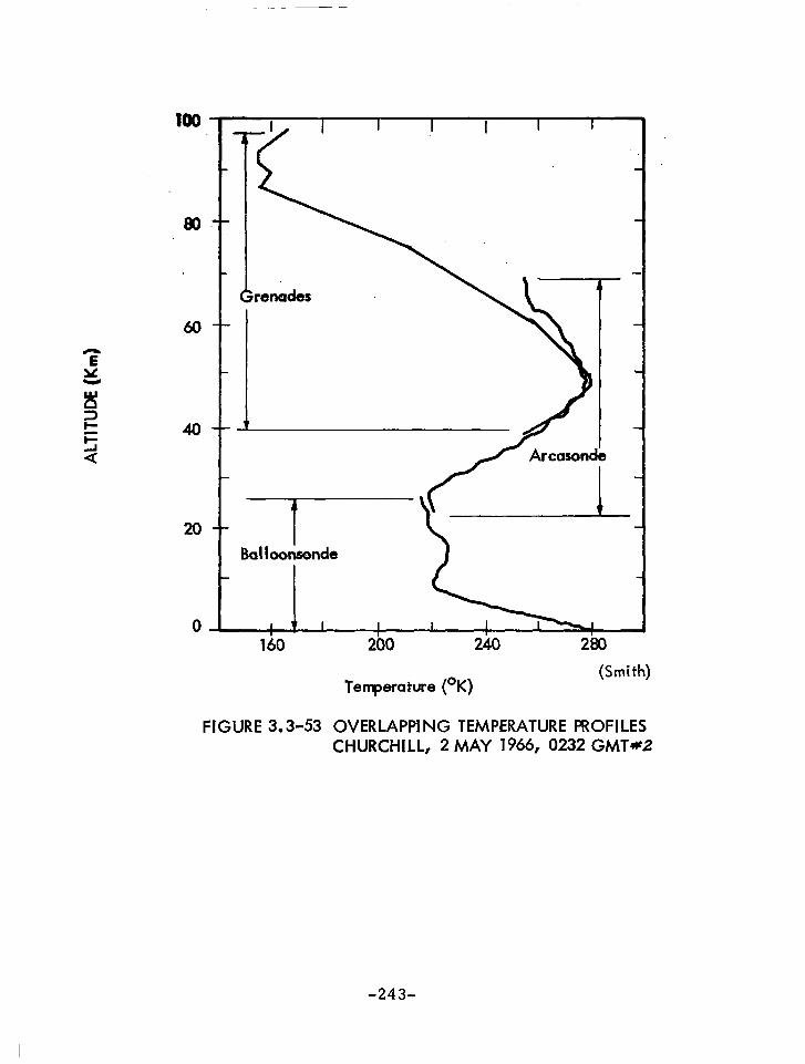
00

60

40

20

0

Temperature (OK) (Smith)

FIGURE 3.343 OVERLAPPING TEMPERATURE PROFILES CHURCHILL, 2 MAY 1966, 0232 GMT*2

-243-

loo

80

60

40

20

0

-

Pi tot

I

Ba I I oonsonde

I 1 8 l&l

I I 1 200 240 2atI

Temperature eK)

FIGURE 3.3-54 OVERLAPPI NG TEMPERATURE PROFILES ASCENSION, 27 FEBRUARY 1966, 1652 GMT

-244-

100

80

60

I I I I

r Pi tot

20

0 160 260 240 280

(Smith)

Temperature (OK)

FIGURE 3.3-55 OVERLAPPING TEMPERATURE PROFILES WALLOPS ISLAND, 27 AUGUST 1966, 1911 GMT

-245-

disagreement that is unaccounted for, and such individual differences that did occur may therefore be attributed primarily to time and space variability.

Finger, et al. , have compared a sample of overla.pping rocketsonde and rawinsonde temperatures at Fort Churchill curing November 1960. They conclude the following: At the beginning of the period there is considerable difference, throughout the area of overlap, between reported rawinsonde temperatures and those measured during the single rocketsonde .observation. During the middle of the period, however, the compatibility appears to be good with differences of 5OC or less - the deviations again increase as rawinsonde temperatures remain relatively cold.

In the 24-32 km region the rocketsondes yield slightly warmer temperatures than those of the radiosonde but are not statistically different. The statistical tests on the temperatures show that the rocketsondes may give a more representative picture of the thermal structure in the upper atmosphere due to their greater sensitivity.

Comparisons have recently been made between instrumented dart and radiosonde temperature measurements in the overlap region of about 80,000 feet (25:5 km). For a limited number of flights, it has been found that the instrumented darts generally yield warmer temperatures than the radiosondes at this altitude. Experience at WSMR indicates that the radiosondes generally measure slightly colder temperatures at 80,000 feet than the various kinds of rocketsondes used for routine soundings.

To investigate a possible bias in the rocketsonde vs radiosonde measurements, temperature data from “Meteorology Data Report, Meteoroloqical Rocket Network Firings, World Data Center A, Volume IV, Number 7, July 19 67 ” (the latest available) has been statistically analyzed with the results as follows:

Altitude Level 24.5 km

Difference Between Rocket and RAoB 5f Average

1 - R,

Standard Deviation Q = 2.437’X

-246-

These comparisons included all of the launching sites which were active in July 1967, and the majority of rocket systems were the Arcas-Arcasonde sensor.

From this analysis it appears that there is no constant bias between the rocketsondes and the radiosondes at an altitude level of 80,000 ft. Approximately 99% of the differences lie within the interval from -7. 31°C to +7. 31°C, and 95% of the differences lie between -4.87OC to 4.87OC. Therefore, one can expect these kinds of differences routinely.

There does appear to be a bias b etween rocketsonde and radiosonde temperatures at altitudes above the 30 Km level with the radiosondes measuring colder. Radar height determination error for the rocketsonde is negligible, and recent radar tracking results of the RAOB at WSMR indicate a height error of only about 1,000 feet (a 0.55OC). Therefore, there must be a bias in the sensor portion of the measurement, and it has been proposed to fly a rod and a bead thermistor together on a RAOB flight for a comparison between these sensors.

A possible source of error might be the downwash from the radiosonde balloon and/or radiosonde package. These components

-247-

precede the sensor during ascent on balloon flights and have previously been bathed in the cold tropopause for an appreciable period of time. They no doubt have been cold-soaked prior to ascent to 80,000 feet. The rocketsonde sensors precede the

j remaining descent system (sonde and parachute) so there should be no downwash effect for them. Rather precise checks of the instrumented dart telemetry system have been made by flying low temperature coefficient resistors. These results indicate that the rocketsonde telemetry error should be no greater than + 0.5Oc.

3.3.5 Improvements for Altitudes above 60 km.

The temperature measurement capability of current rocketsonde systems is limited to about 60 to 65 km. Of course, theoretical correction factors can be applied to data above these altitudes. But as the correction factors increase, so do their uncertainties, and even the corrected data may not be accurate. The major sources of error above 60 km consist of aerodynamic heating, radiation and sensor lag. Suggestions for reducing the effect of these error sources are presented in the following paragraphs.

The only way to reduce the aerodynamic heating error is to reduce the fall rate of the decelerator system, i.e. , reduce the ballistic coefficient. This may be accomplished by reducing the weight of the payload or increasing the drag of the decelerator either by more efficient designs or increased sizes. Improvements have been made in the last few years. The Arcasonde parachute system has a ballistic coefficient of 0.055 lb/ft2, the Loki Dart PW,N -8B - Starute system has a value of 0.0 30 lb/ft2 and the WOX - 4A Starute system has a value of 0.02 1 lb/ft2. A large Starute in a proposed Super Loki system promises to reduce the ballistic coefficient to 0.018 lb/ft2 in the near future. Since the ballistic coefficient of the thin-film mylar decelerators alone (without payload) are about 0.010 lb/ft2, a reduction below this

.value is not very likely with the conventional designs. The Stokes flow parachute concept discussed in Section 4.4 appears to be the most likely technique to reduce the aerodynamic heating error to extend the temperature measurements to the maximum limit.

The sensor lag error may be reduced by reducing the sensor time constant which is the same as increasing the dissipation factor. Convective heat transfer in the continuum flow region

-248-

increases as the thermistor size becomes smaller; the radiation errors and the time constant are both reduced. However, the mean free path limitations are encountered as altitude is increased so there is a definite altitude limit for the use of smaller thermistors. The most likely way to increase the altitude limit of current systems is to employ a thin-film thermistor or thinistor to improve the convective heat transfer and dissipation factor. The mean free path criteria should offer no real limitations to such a sensor. However, as altitude is increased, the limiting factor will be radiation, and steps must be taken to reduce this source of error.

Various radiation screens have been proposed but the simplest appears to be a thin layer of aluminized mylar arranged in an appropriate geometry so as to block incident radiation from the sonde, sun and remaining environment. This screen should be able to reflect most of the incident radiation, and that which is absorbed should be convected to the atmosphere quite efficiently since it has been shown that the thin mylar film has an excellent dissipation factor even at high altitudes. Therefore, the temperature rise of the screen should be negligible and the thinnistor should be relatively free of radiation error.

An interesting technique to eliminate radLation errors has been proposed by Glenn E. Daniels , NASA-MSFC, which entails the use of two or more sensors of different susceptibility to radiation error and extrapolating the results to zero error. Tests have been conducted on the ground and on radiosonde flights with thermocouples and thermistors of different emissivities. Figure 3.3-5 6 presents the results of a typical radiosonde flight test. The results have proven to be quite promising as true air temperatures have been obtained by extrapolating the data from sensors exposed to the sun. The major problem is in accurately determining the emissivities of the sensors, especially so for the miniature rocketsonde thermistors. Daniels has suggested for rocketsonde applications to use bead thermistors of different sizes, i.e. , a 5-mil bead and a 15-mil bead, with the same emissivity, i. e. , uncoated for better uniformity. A larger bead will have a greater radiation error than a smaller bead because of boundry layer effects. As indicated in Figure 3.3-5 7, the radiation input is proportional to the square of the diameter of the sensor, but the convective heat transfer is proportional to the square of the diameter of the sensor plus the boundary layer thicknesses. The ratio between (sensor diameter) 2 and (sensor diameter plus boundary layer thicknesses ) 2 is a measure of the radiation error. This ratio is greater for a larger diameter sensor than for a small

-249-

h

.

t

110 I I I I I I I I I

Preliminary True Temperature

Thermistor (White)

--Thermistor (Black)

Terrgerature (“C) (Daniels)

FIGURE 3.3-56 Comparison of Temperatures Measured with Black and White Thermistors and the Computed True Temperature

-250-

FlGURE3.3~57 HEAT TRANSFER COMPARISON BETWEEN LARGE AND SMALL SPHERICAL THERMISTORS

LARGE THERMISTOR

h-, Heat Transferred By Radiation

H v D2 t-a- Y

Hc cc ?(D+26)”

Radiation Errar&r 0~ &

Heat transfer By Convection

BOUkhlj

Layer

Thickness

*red

hr cc+!?

hc a T(d+2S)”

Radiation Error, er CC hr

2

Rod Lotion Error Comparison Of Larqe and Small Thermistors

diameter. Daniels suggests that by extrapolating the resulting temperatures from a small and large thermistor of equal emissivities down to zero size, the air temperature can be derived without significant radiation error. Laboratory data reported by Thompson has been used to construct Figure 3.3-58 which is a plot of radiation error vs thermistor size. It is apparent that the extrapolated value does not quite reach the O°K error level, but indicates rather 0.12OK at zero thermistor diameter. This is certainly an improvement over using the data directly from either a lo-mil or 15-mil diameter therm- i stor . The fact that the extrapolated value does not go through the zero error level may be due to experimental error on other extraneous factors in the laboratory data.

A possible extension of this concept might be the use of two thin-film thermistors with different thicknesses of reflective aluminum coatings. By judicious choice of the aluminum coating thicknesses, the amount of radiant heat energy absorbed in the coating and distributed by conduction to the film may be found to depend on coating thickness. Thus the results from two thinnistors could be extrapolated to zero coating thickness.

-252-

I

[ [ Data From Data From 1 1 Thompson pp 206 Thompson pp 206

VACUUM TEST VACUUM TEST

ALUMINUM COATED THERMLSTo ALUMINUM COATED THERMLSTo

Esw= E Lw= 0.15

J= 2.0 C~I - cm-5 min’ Esw= E Lw= 0.15

J= 2.0 cal- cm-5 min-’

1 I I 1 I

5 10 15

Thermistor DiameCer (Mils)

FIGURE 3.348 TEMPERATURE RADIATION ERROR VS. THERMISTOR SIZE

-253-

3.4 Falling Sphere Density Measurement Techniques.

3.4.1 General.

The use of falling spheres to obtain density measurements above 30 km has been investigated by a number of experimenters. In general, the spheres employed have been either small diameter rigid spheres, containing accelerometers and telemetry instrumentation, or larger diameter inflatable spheres, being either passive or instrumented with accelerometers and/or telemetry. Combinations of these characteristics serve particular goals. For example, a sphere with internal accelerometers requires no ground radar tracking: an inflatable sphere with accelerometers is sensitive at great altitudes; an inflatable passive sphere must be tracked by radar but is inexpensive and easy to build. The density is calculated from the equations of motion for a sphere traversing the atmosphere with the necessary parameters supplied by radar data from the passive spheres, or by accelerometer and telemetry data from the active spheres.

3.4.2 Theoretical.

The forces acting on a sphere falling in an air mass (shown in Figure 3.4-l) are as follows:

1.

2.

3.

4.

Buoyancy Force (vB P g) The direction of this force is along a line from the center of the earth to the sphere, and pointing away from the earth.

Weight (mg) The direction of this force is along a line from the center of the earth to the sphere, and pointing toward the earth.

Draq Force (l/2 P v2CDA) The direction of this force is along the velocity vector (relative to air) but in the opposite direction.

Coriolis Acceleration (2wxV) If the coordinates of the sphere are referred to those in a system fixed to the earth, the sphere coordinates rotate with the earth coordinates, and the equations of motion must include the effect of Coriolis acceleration.

-254-

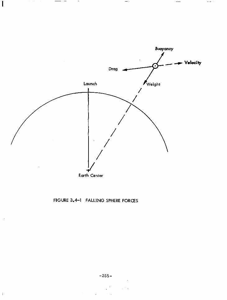
I

Drag

Launch

/ . + Earth Center

FIGURE 3.4-l FALLING SPHERE FORCES

-255-

The equation of motion expressed in vector form is:

1 P Cb Av2 a= % P g

+g+ z + 2wxv

m m

where:

a =

VB =

P =

g =

m =

CD=

A=

v =

w =

acceleration of the sphere as measured with respect to a coordinate system attached to the earth (See Figure 3.4-2)

volume of the sphere

atmospheric density

acceleration of gravity

mass of the sphere

drag coefficient of the sphere

cross sectional area of the sphere

velocity of the sphere with respect to the wind velocity

rotational velocity of the earth

The equation of motion can be expressed in x,y,z components as follows;

‘GE - “DA [VI (A-Wx) + g,; (l- ‘BP ) - (R 2 - a,$ 2m m Y

(1)

(2)

i’= - PCDA [V] (i-Ws) + gs (l-2$) (l- ‘BP ) - (nyi-nxi) (3) 2m m

i;= - [VI (i’-Wy) +gs: ( livBp ) - (‘xi- %” ) m

(4)

-256-

-*

Eorthl Center

FIGURE 3.4-2 FALLING SPHERE COORDINATE SYSTEM

Sphere

-257-

where,

A# 9, 2, = components of velocity with respect to axis attached to earth.

x, Y, z, = components of position with respect to axis attached to earth,

w,c ,,, A, V, VBt m, p previously defined

WX, Wy, Wz = components of wind velocity with respect to axis attached to earth.

r = radios of the earth

h = altitude of sphere above the earth

gs = acceleration of gravity at earths surface (launch site)

R X, nY, “z = components of earth’s angular velocity about axis attached to earth.

v= (2-wx)2+(jl-wy)2+(i-wz)2

= sphere velocity relative to the wind

Solving these equations (2,3,4) for , Wx, WY yeilds:

p = m [gs (I- r zh) - i’- (nxk2 2) 1 C D A [ v 1 (.?I- Wz) + VB gs(l-2a-lJ

2 r

wx=;r- (&Wz) [G-gs$ (l-V< )+ (Rz;-Oy;) 1 . . .

(5)

(6) ‘i-g, (1-2h-) (l- VB P )+ (nz&- RxL )

r m

wy= +- (i-viz) [i’-gst (l-‘BP ) + (oZf-oxi) 1 m (7)

;-gs (1-2h) (I& ’ ) + ( fZzG- Oxk ) r m

-258-

3.4.3 Papers on Various Falling Sphere Designs.

Several falling sphere designs have been flight tested over the last ten years. A brief summary of the major characteristics of these/designs is presented in Table 3-26. A brief review of each of these basic designs is presented in the following sections.

3.4.3.1 Inflatable Nylon Sphere Bartman, F.L. “Falling Sphere Method for Upper Air Density and Temperature. ” J. Atm. & Terr. Phys., Spec. Suppl. Vol. 1, 1954, pp. 98-107.

Nylon spheres, 1.2 meters in diameter when inflated and weighing approximately 2.3 kg, were ejected from Aerobee rockets. The spheres carried internal miniature doppler transceivers, and the velocity and acceleration trajectories were measured by DOVAP. Densities and temperatures have been calculated for the trajectory between 65.5 to 50.3 km altitude. Maximum velocity through the range was 5 73 m/set; maximum acceleration was 11 m/set. Presumably the sphere began to collapse at about 50 km. Possible errors due to ignoring wind effects may range from 1% for a horizontal wind, to 10% for a vertical wind. Errors in velocity and acceleration ranged from 2 or 3 to perhaps 5%. Drag coefficient errors were estimated at from 2-5%. Temperature errors were estimated at less than 5%.

Bartman,F.L., Chaney, L.W., Jones, L.M.,Liu, V.C. “Upper-Air Density and Temperature by the Falling-Sphere Method. ” Journal of Applied Physics, Vol. 27, NO. 7. July 1956, pp. 706- 712.

Nylon spheres, 1. 2 meters in diameter and weighing 2.3 to 0.9 kg, were ejected from Aerobee rockets and inflated with nitrogen. The spheres contained a miniature doppler velocity and position transponder and antenna which, together with the DOVAP ground system was used to determine the sphere trajectory, position, velocity, and acceleration. From these data and the drag coefficient, density was calculated. In turn, with the use of the hydrostatic equation and the equation of state of a gas, temperatures were obtained. The trajectory peaks ranged from about 57.9 to 123.4 km. Sphere ejection occurred from about 40.2 to 121.6 km. Velocities ranged from 32.3 to 174.3 m/set. Density data were obtained for altitudes of 32.3 to 81.7 km. Temperature data were obtained for altitudes of 32.3 to 64.9 km. Sources of error in the calculated density are: neglect of winds, and errors in measuring velocity,

-259-

TABLE 3-26

SUMMARY OF FALLING SPHERE DESIGNS

Sphere Type

cperimenters Diamete Radar Sphere Reflector Instrumentation

Weight Cross-Sect Area to Wt. Ratio cm,

1.2m 2.3Kg

17.8 CIT 5 Kg 0.050

17.8 CIT 5 Kg 0.050 <

2m 450 gm

.~

69.8 :

2.74 m 9 Kg 6.55 :

lm -._.. - 110 gm

Sloan 7 lm 98 gm

71.5 1

80.4

1.2 m

0.66 m

144 gm 78.5

50 gm 68.7

ion

‘gm

5 None

,080 None

,080 Beacon

Surface None

Inflatable Nylon

Bartman i

Schulte, Jones, 2

Peterson et al.

Faire, 3 Champion

Pearson 4

Faucher 5

Wright, 6 Leviton

Peterson 8

Doppler Transciever

Transit Time Accelerometer 5x10-39

Rigid Aluminum

Transit Time Accelerometer 5x10-59

Inflatable Melinex

Inflatable Mylar

Linear Accelerometer 0.002 g

Internal None

Surface None

Surface None

Surface None

-260-

TABLE 3-26 (cont.)

i

2

3

4

5

- -.

6

7

8

Gmd-Stn. Rocket Instrumentatior Vehicle

DOVAP

Specialized Telemetry

Specialized Telemetry

Radar

Telemetry

Radar

Radar

Radar

-

Aerobes T T

123 Km 32-82 Km

Nike- Cajun

100 Mi 100 mi

I Nike- Apache

200 Km

Long Tom

116 Km

Aerobec Nike- Cajun

-_ Arca s ,

450 Kft

70 Km I Loki Dart

125 Km

&wee Measurement Altitude Altitude.

35-85 Km 35-85

35-115 Km

- .-

73 - 98

-___ 40 - 60 Km

40 -90th

30 - 130 Km

30 - 120 Km

i 1

_ -

Density Accuracy

5%

3% to 5%

5%

Comments

3 Improved

--I

T----- 5

6

-t I

8 L

-261-

acceleration, drag coefficient, mass and maximum cross-sectional area of the sphere. The last two are negligibly small. Tempera- tures calculated have additional errors due to errors in measured densities in the altitude range. The results show good agreement with the Rocket Panel Data. The errors of the DOVAP tracking system were larger than anticipated because of the spin of the transponder antenna, but techniques can probably be developed to reduce these errors.

3.4.3.2 Rigid Aluminum Spheres Jones, L. M. , Transit-time accelerometer, Rev. Sci. Instr., 27, 374-377 (1956)

An omnidirectional transit-time accelerometer is used for measuring the drag acceleration of spheres dropped from rockets. In the device, a bobbin is periodically caged and released within a cavity. The time for the bobbin to traverse the distance to the cavity, which distance is the same in any direction, is

-3 lemetered

and measured . The accelerometer range is about 5 x 10 g to 5 g. Systematic errors and standard deviations over the range are about 1%. The accelerometer was used successfully in a rocket flight in which the drag acceleration of a 7-inch-diameter sphere was measured.

Jones, L.M., Schaefer, E. J. and Schulte, H.F. .“Upper-Air Densitees and Temperatures from Eight IGY Rocket Flights by the Fallinq-Sphere Method. ” IGY Rocket Report Series No. 5, 1 Dec. 1959.

A falling sphere with an internal omni-directional transit- time accelerometer was developed and used for measuring upper- air density and temperature . A sphere is ejected from a rocket at approximately 56 km altitude during the upleg portion of its trajectory; its velocity is sufficient to attain a peak altitude of about 160 km. Ten IGY firings used the Nike-Cajun rocket: one sphere was carried in an Aerobee. Spheres 17.8 cm in diameter and weighing approximately 5 kg were launched. Modifications of the first version of the small-sphere experiment were in the electronics of the sphere-to-ground station telemetry system which arose from the decision to use a pulse position (time) code modulation for telemetering the accelerometer data. In this method a 10 - p sec. 400-me/s pulse with a peak power of about 32 watts is transmitted at the instant the accelerometer bobbin is released, and a second such impulse is transmitted at the instant of bobbin contact. Pulses are received and recorded along with

an accurate time-base on multichannel magnetic tape at the ground station. The pulse system permits direct playback of the recorded telemetered data into electronic counters for measurement of the accelerometer times. This falling-sphere method performs best in a middle range of altitudes - 30 to 80 km. In this range, the raw accelerometer data plots smoothly with very few missing points. The drag coefficients used vary between 0.9 and 1.1.

The basic data consist of bobbin release times (when the bobbin is at the center of the accelerometer cavity) and bobbin contact times (when the bobbin touches the cavity walls). The difference between release time’ and contact time is the transit time which is in the range .Ol < t < 1 set approximately. The maximum acceleration experienced by the sphere is about 10 times gravity (10 g) corresponding to a minimum accelerometer transit time of about 10 milliseconds. The maximum transit time of nearly 1 sec. is determined by the recycling period of the accelerometer caging mechanism.

The results of these experiments were density and temperature data from about 90 km down to 20 km. Certain difficulties are encountered at each end of the altitude range which, in some cases, affect the altitude calculations throughout. At the high altitudes the drag acceleration becomes very small and ultimately the threshold of accelerometer sensitivity is passed. Two difficulties are present at low altitudes. First maximum accelerations occur at approximately 80,000 ft (25 km) and approach 10 g’s in magnitude. The operation of the accelerometer under these conditions is marginal due to lack of power for centering the bobbin. Second, it is believed that the drag-coefficient data may be in error at a Mach number of 1.3 or less. In this range the drag-coefficient curve falls away rather sharply from a value of one, which suggests that the characteristics of the flow about the sphere may be changing. When the drag coefficient becomes less than one at low Mach numbers, it is not considered to be reliable for the analysis of falling-sphere data. This sets a lower limit of about 60,000 ft, (18 km) to the densities derived by the falling-sphere method.

Schulte, H.F.; Robinson, D.A. and Wagener, J.L., “Falling-Sphere Experiment for Upper-Air Density: Instrumentation Developments. ” The Univ. of Mich. , Office of Res. Admin. , Final Report 03558-6-F, Ann Arbor, April 1962.

-263-

Development of the instrumentation for the accelerometer version of the falling-sphere experiment for upp-air density and temperature was continued. A new accelerometer was designed and tested in the laboratory. It was smaller, lighter and con- sumed less power than the previous version. Further, the design successfully dispensed with the “cat’s-whisker” bobbin contactor. Sphere balance was improved with the aid of a static balance machine. Transistorized sphere circuitry was also designed, built, and tested. It incorporated an electronic (instead of motor- driven), intervalometer to operate the accelerometer. It also employed a discretionary caging circuit to permit measuring long transit times, and it generated start and stop pulses of different widths to permit pulse discrimination in the playback system. Four rigid machined spheres, 17.8 cm in diameter, weighing 5 kg, and accelerometers were built for test flight.

Faire, A.C., “AFCRL Rigid Falling Sphere Program, ” Air Force Cambridge Research Laboratories, Hanscom Field, Bedford, Mass., June 1963.

A new verison of the 7-inch falling-sphere method for measuring atmospheric density, similar in principle to an earlier sphere experiment developed by the University of Michigan, contains innovations that have increased accelerometer threshold sensitivity from 10s3 g to 4 x 10B5 g, and extended the useful range of altitude measurements from 90 km to 110 km.

The AFCRL 7-inch sphere contains an omnidirectional accelerometer that operates on the time-of-flight principle. The sphere is ejected from a Nike-Cajun rocket at approximately 60-km altitude. Drag acceleration information is telemetered from the sphere on the upleg portion of the trajectory until the threshold limit of accelerometer sensitivity is reached (approximately 4 x 10V5g at about llO-km altitude). As the sphere experiences reentry conditions at approximately 35-40 km, drag accelerations of the order of 5 g are observed.

The major refinements have been in the components of sphere instrumentation: accelerometer, electronic timing circuits, modulator, transmitter and antenna, and power supply. A complete re-design of sphere electronics was necessary for compatibility with the new accelerometer which operates over a wider dynamic range than previous models. All circuits have been transistorized except the

-264-

transmitter. All operational time sequences are controlled by a timer circuit, including the accelerometer cycle and sphere telemetry. Temperature compensation and optimum design criteria have been used to obtain high stability over long periods. The timer triggers pulses that subsequently permit translation of sphere telemetry information into drag acceleration data: it also initiates a sub-modulator signal and an over-ride circuit. The sub-modulator signal consists of 4 micro-seconds pulses that modulate the sphere transmitter at a repetition frequency that varies from approximately 90 to 120 pulses/second depending on the internal temperature of the sphere. The sub-modulator signal contributes no direct geophysical information, but it increases the ease and reliability of sphere tracking by producing an audible tone when demodulated by the ground-based receivers. The override circuit is preset to provide a synthetic impact signal greater than the longest transit-time measurement expected. Since the preset value of the override time is known, data resulting from this source are easily distinguished from actual transit-time measurements obtained at high altitudes. In the sphere transmitter, the isolation between oscillator and output provides excellent frequency stability. The use of 730 MC as telemetry frequency eliminates the degradation and loss of signal due to antenna breakdown that occurred when the telemetry frequency was 400 MC.

There are three modifications in ground-station instrumentation: 1) The use of redundant ground sites increases reliability and enhances data recovery: 2) Three types of pulse-width discrimi- nators help to minimize spurious signals due to atmospheric noise and man-made interference; 3) Direct data readout capability provides a complete inflight record of experimental data.

Density profiles can be obtained from sphere data without the use of radar or similar tracking aids. The accuracy of the results is somewhat reduced by the uncertainties in peak altitude. Radar tracking contributes to accuracy and accelerates data reduction. Two factors impose limitations on measurements at greater altitudes: 1) the “dry contact” problem that results from poor electrical conductivity between bobbin and cavity at impact, and 2) the initial velocity imparted to the bobbin at the time of release.

-265-

3.4.3.3 Pearson, P. H.O., “An Appraisal of the Falling Sphere Method of Density Measurements Using External Measuring Methods, ” Department of Supply, Australian Defense Scientific Service, Weapons Research Establishment, Technical Note SAD8 2, October 19 61.

A series of inflatable s area-to-mass ratios up to 8m 5

heres of various materials, with /kg were released at heights of

90 to 150 km from rockets fired at Woomera, Australia. They were tracked by reflection doppler, transponder doppler, and FPS-16 radar. Reflection doppler demands at least two l-meter diameter sphere with a metallized surface; a 2-meter sphere would have a theoretical range of 150 km. Transponder doppler is as accurate as the reflector type and has a range of at least 160 km. With FPS-16 radar, a 2-meter sphere would give a maximum range of 213 km. The two Doppler tracking methods measured velocity, from which acceleration and position were calculated; FPS-16 radar gave position only, from which velocities and acceleration were calculated. A number of trajectories using various values of the sphere cross-sectional area to mass ratio and release altitudes were computed on an IBM 7090 digital computer. These were assessed, and results showed that the height at which minimum density error occurred was function of A/m ratio and to a lesser extent the maximum altitude of the sphere. Accepting basic instrumentation estimates, both Doppler and FPS-16 radar systems were able to measure density with less than 5% error from 30 to 100 km. A knowledge of the magnitude of vertical winds was important in assessing density error. All results assumed a probable horizontal wind velocity of 30 m/set. and a vertical wind velocity of either 0 or 15 m/set. The maximum height of 100 km to which density can be measured by this method with less than 5% error is limited by the practical problem of constructing a sphere with a cross-sectional A/m ratio greater than 10 m2/kg. With the FPS-16 tracking system, the errors are greater than with the Doppler systems, even assuming 25% smoothing of position error.

3.4.3.4 Inflatable Mylar Spheres Faucher, G.A.; R.W. Procunier and C.N. Stark, Flight information and experi: mental results of inflatable falling sphere system for measuring

pper air density, GRD Research Notes, No 63, AFCRL 685, August ;961

-266-

A Nike-Cajun rocket was fired for the purpose of ejecting an inflatable sphere with accelerometers and telemetry at 300,000 ft. The objective was to measure the drag acceleration of the sphere above 300,000 ft. for use in calculating air-density measurements. The drag acceleration is measured with three linear accelerometers which measure acceleration along three mutually perpendicular axes from within the sphere. The density calculated from this flight was 1.46 x 10mg slugs/ft3 at 107 km. A secondary objective was to obtain an engineering evaluation of a system to eject and inflate a 9-ft-diameter sphere.

Faucher, G.A.; Prdcunier, R. W. and Sherman, F.S., “Upper Atmosphere Density Obtained from Falling Sphere Draq Measurements. ” Space Physics Laboratory, Project 6690. Air Force Cambridge Research Laboratories, Office of Aerospace Research, United States Air Force, Hanscom Field, Mass., December 19 62.

The density profile versus altitude from 95-130 km was obtained from drag measurements made directly from within a falling sphere. An Aerobee 150 sounding rocket, containing an inflatable sphere of 1-mil mylar laminated with dacron scrim, was launched from Eglin Gulf Test Range. Sphere ejection occurred at 87 km. The inflated sphere had a diameter of 2.74 m, contained a 6.8 kg instrument package, and weighed nearly 9 kg in all. Information was telemetered continuously during the flight by internal electronics and measuring instruments: Three subcarrier channels of orthogonal acceleration measurements, three time-shared accelerometers’, plus two temperature measurements on a fourth subcarrier frequency. The main sensors were six Donner 4310 linear accelerometers aligned to measure the X,Y,Z components of acceleration of the sphere from which drag is obtained. Basically the accelerometer was composed of seismic system and associated position-error detector, a restoring mechanism, and a servo error-signal amplifier. Measurements obtained by this method were supplemented by tracking systems for velocity and position. The rocket and sphere were tracked by two AN/FPS- 16 and one AN/MPS-19 radars: one AN/FPS-16 was used in skin tracking and sphere MATTS (Multiple Airborne Target Trajectory System) stations tracked the telemetry signals beacon. MATTS data provided accurate sphere time-space positioning which were used in the density calculations. These data check with optical tracking. The mass m accelerated by the drag force and the sphere cross-sectional area A were known: drag acceleration aD and sphere velocity V were measured; and the coefficient of drag CD or

.

-267-

the atmospheric density p could therefore be calculated if one was assumed or determined independently. The authors believe at this time that the drag coefficients available are more accurate than the present estimates of atmospheric density in the altitude range investigated. The sources of error in the calculated density were: drag coefficient data, neglect of winds, calculation of the trajectory, and in measured values of A, m, and AD. Drag acceleration aD is the source of greatest error at present. The uncertainty in aD arises not from the measuring instrument but from the interpretation of telemetered data to obtain true drag acceleration.

Leviton, R. , and W. E. Palmquist, ROBIN--a meteoroloqical sensor, presented at the A& 15th Annual Meeting, Wash- ington, D.C., December 5-8, 19 60, 1469-60

A sphere has been designed as a sensor for the Arcas meteo- ological sounding rocket to provide information on such meteorological parameters as wind velocity, density, pressure, and temperature for operational soundings between 100,000 and 200,000 ft. The sphere, designated as ROBIN (Rocket Balloon Instrument) mylar, is one meter in diameter and contains a built-in corner reflector of l/4-mil-aluminized mylar. It is packaged inside the ARCAS nose cone with approximately 35cc of llqusd isopentane. Somewhat above 200,000 ft. the balloon is ejected from the nose cone and inflates to a superpressure of about 12 mb. The falling sphere is then tracked by ground radar down to lQ0, 000 ft. Range, time and angular data allow computation of the wind information. Since density is a function of fall velocity, drag coefficient and the physical characteristics of the sphere, it can be calculated. With the knowledge of density and height, pressure and temperature data can be computed. Assumption of a drag coefficient value in the region of operation appears to be valid, and errors in the system for all calculations are tolerable. The use of the ROBIN sphere promises to be a relatively inexpensive and reliable method of obtaining operational meteorological data from a rocket.

Leviton, R. , “The ROBIN Falling Sphere. ” Extracted from IRIG Document No. 105-60, “Initiation of the Meteorological Rocket Network, Revised August 1961. ”

A new meteorological rocket sounding system using a small, super-pressured, inflatable plastic sphere as a payload sensor

-268-

I

was developed by the Air Force Cambridge,Research Laboratories, Hanscom Field, Mass. With the Arcas meteorological rocket carrier, the Robin is designed to meet an Air Force requirement for a reliable, simple, low-cost method of sounding the atmosphere at heights of 30 to 60 km. A Robin sphere, 1 meter in diameter, weighing 118 grams, and containing an internal-corner reflector but no electronic equipment or moving parts, was ejected from the Arcas at about 60 km and tracked by ground radar. Sphere position data from tracking radar were reduced to the desired meteorological parameters. Methods of reducing the meteorological data from the Arcas-Robin system have been developed, both for a precise computer evaluation of all the parameters, as well as a manual field-type reduction. A complete independent error analysis of the entire system is being investigated to determine its operational suitability. Wind-tunnel tests have been conducted to ensure the use of the most accurate drag-coefficient values in the data reduction process.

Engler, N.A. “Development of Methods to Determine Winds, Density, Pressure, and Temperature from the ROBIN Fall- ing Balloon. ” Dayton, Ohio, University of Dayton Research In- stitute, October 1962.

Given the space-time coordinates of a falling sphere (Robin), computer programs have been devised to compute the winds, density, pressure, and temperature of the ambient atmosphere as a function of altitude. The programs were compared with regard to time required to compute and overall accuracy. The technique chosen was a linear, least-square fit over 31 space-time coordinates, each spaced in time by l/2 second, to find velocities and then another linear, least-square fit over seven of these velocities, each spaced in time by 1 second, to find accelerations. Overlapping data were used so that a velocity and acceleration was determined for each second of balloon descent from approximately the altitude of first radar contact down to 50 km. From 50 km to the end of the radar tracking, 30.5 km, a velocity and acceleration was determined for each second of balloon descent from approximately the altitude of first radar contact down to 50 km. From 50 km to the end of the radar tracking, 30.5 km, a velocity and acceleration was determined for each two-second interval. Pressure was computed from the hydrostatic law; temperature from the gas law. A computer program, written in both Algol and Fortran, read in one pass the space-time coordinates furnished radar tracking, computed, and

-269-

printed out the following as a function of time: altitude in meters, east wind in m/set, north wind in m/set, vertical acceleration in m/sec2, temperature in degrees Kelvin, wind speed in knots, wind direction in degrees, vertical velocity in m/set, density in kg/m3, pressure in millibars. With the advancement of computer techniques, least-square fitting procedures can be used to obtain velocities and accelerations from the raw data. This is preferred over finite-differencing methods which are inherently unstable. The method proposed in this report required a computer of the class of a Burroughs 220 or higher, such as an IBM 7090. A computer of less storage capacity, such as Burroughs 205 or IBM 650, can handle the computation of winds effectively, but not the winds and density, pressure, and temperature. No reliable hand method can be used unless one is seeking only gross averages. The method presented in this report has two advantages: 1) it is inexpensive and 2) results can be derived more rapidly than by other methods.

Wright, John B. The Robin Falling Sphere. The Meteorological Rocket Network. MWG , RCC Document 111-64.

A detailed description of the Robin has been presented previously . Some of the major factors involved in the analysis of the Robin 70 km flight data are presented here.

Figure 3.4-3 shows a flow diagram of the steps required at one typical altitude point using somewhat simplified equations; i.e., thecoriolis terms used in the actual computer program have been deleted here for clarity. First, before starting these main computations, the horizontal and vertical velocities and accelerations of the balloon are found by means of least-squares fitting of straight lines to 31 one-half second space points and to 7 one second velocity points and assigning velocity and acceleration values to the midpoints of the respective intervals. In order to start the computations, it is also necessary to bring down from the previous high altitude point, the values of density and Wz (component of horizontal wind in the z-direction) as first approxi- mations. WX and WY are computed, then W, and a convergence check of W, is made as a final step. If a 1% convergence value is not obtained, the small loop indicated is traversed using the computed W,. When convergence is indicated, the value of V (the balloon’s velocity with respect to the air) is computed: then using the drag coefficient from the previous higher point as an approximation, the first calculation of density is made. The hydrostatic equation is then used to calculate pressure and the gas law to calculate

-270-

POINT AI FROM SMOOTHING PROGRAM THIS POINT 0 ROBIN CONSTANTS

An,h,X ij; Y+i: eii

L I .5 CD AV (?-W,,t &$)VB

I I I I

WHEN f CONV. IS YES R”;;N;~;~M f P T WE~J w,, w ff

(Wright)

FIGURE 3.4-3 TYPICAL POINT ROBIN PROGRAM

-271-

temperature. Because Mach and Reynolds numbers serve to define the aerodynamic flow conditions of the sphere and hence its drag coefficient, these numbers are calculated using the velocity, density, and temperature. A drag coefficient table, the result of a series of wind tunnel tests, is entered and the proper drag coefficient obtained. A check of density in the meantime probably indicates no convergence with the previous higher altitude density and a loop back to the start of the chart is indicated. Cal- culated values, rather than previous point values, are used in progressing down the chart again, and at the density step the drag coefficient previously obtained from the table is used. When convergence with the previously computed density is indicated, the final values of density, pressure, temperature, and wind parameters are printed out for this particular altitude. It should be noted that the balloon’s horizontal displacement as a function of time, X or Y, is not taken to be the wind velocity as with most wind sensors in current use. Instead, the equations indicated are used wherein the long terms after the minus signs represent the lack of response or lag in the balloon to immediately respond to wind changes.

A complete error analysis of the current Robin system was made during the development of the data program. (Engler . ) Table 3-27 indicates the RMS errors for the various parameters when a precision radar (AN/FPS-16) is utilized for tracking a rigid sphere at 0 .l second to 0.5 second sampling rate. In addition, at the start of the computations where the initial temperature estimate might be in error by lo%, a corresponding 2.5% density error would occur which would decre:l se very rapidly with altitude. If a radar of lesser accuracy, such as the AN/MPS-19 radar, is used (standard angle errors of approximately 1.5 mils instead of 0.1 mils) , errors occur of the magnitudes shown in Table 3-28.

With the collapse of the balloon from a rigid spherical shape to a nondescript shape, the meteorological parameters may no longer be deduced, although the winds may be calculated by using somewhat simplified equations. The determination of Robin balloon collapse is made within the computer program by a “lambda check”, whereby parameters of balloon motion, which in turn may be associated with density lapse rate, are calculated internally throughout the fall. When the limits of the lambda term are exceeded, the program then shifts to a calculation of -wind terms only.

-272-

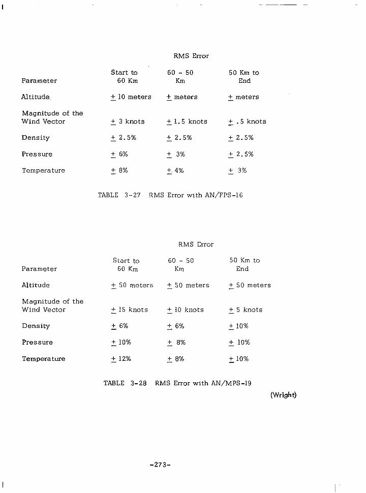
I

Parameter

Altitude

Magnitude of the Wind Vector

Density

Pressure

Temperature

RMS Error

Start to 60 - 50 50 Km to 60 Km Km End

+ 10 meters + meters + meters - -

+ 3 knots -

+ 2.5% -

+ 6%

+ 8%

+ 1.5 knots + .5 knots

+ 2.5% + 2.5% -

+ 3% + 2.5% -

f 4% + 3% - -

TABLE 3-27 RMS Error with AN/FPS-16

Parameter

Altitude

Magnitude of the Wind Vector

Density

Pressure

Temperature

Start to 60 Km

+ 50 meters -

+ 15 knots -

+ 6%

+ 10% -

+ 12% -

RMS Error

60 - 50 Km

+ 50 meters

50 Km to End

+ 50 meters -

+ 10 knots -

+ 6%

+ 8%

+ 8% -

+ 5 knots -

+ 10% -

+ 10%

+ 10% -

TABLE 3-28 RMS Error with AN/MPS-19

(Wright)

-273-

Another method of determining balloon collapse, most applicable for quick field use, is to time the sphere through fixed altitude layers. Table 3-29 has been based on many successful flights and shows the time corridor for a rigid, 115-120 gram, l- meter diameter Robin to fall through lO,OOO-foot altitude layers. A collapsed sphere requires a longer time to fall than indicated in the table.

A third method of determining sphere quality involves observation of the strength of radar signal return, the character of the return in which the corner-reflector pattern in a rigid sphere may be seen, and the level of the range and angle error signals.

A typical density profile from the Robin p,rogram is plotted in Figure 3.4-4. The two lines, which have been plotted as a function of density and altitude, represent the measured density as obtained from two independent radars tracking the same Robin sphere. The two profiles shown differ by less than 2 percent or within the system accuracy.

Leviton, Robert; Wright, John 6. , Accuracy of Density from the Robin Falling Sphere. GRD Research Note No. 73, AFCRL 1095, December 1961.

An examination of the density equation shows that the accuracy of any calculated density data depends on the accuracy of the value of drag coefficient used, the accuracy of the measurement of fall velocity and acceleration, and the tolerance to which the sphere is fabricated. Data in the form of azimuth and elevation angles and slant range were obtained from the AN/FPS-16 radars as a function of time. Errors expressed are so-called standard deviation (one sigma) values.

Typical Robin fall velocities are shown in Figure 3.4-5. A range of velocities is possible at any altitude following the attainment of terminal velocities because of the varying balloon weights and variations in atmospheric density. The drag coefficient of a sphere subjected to motion through a gas can be shown to be a function of Mach and Reynolds Numbers. These two parameters define conditions which, if duplicated in model testing, will assure similarity to fullscale conditions. Figure 3.4-6 shows the Mach and Reynolds number ranges of the Robin balloon.

-274-

ALTITUDE Thousand TIME, LAYERS, Feet Seconds

From

240

230

220

210

200

190

180

170 160

160 150

150

140

130

120

110

To -

230

220

12-15

13-16

210 14-17

200 16-19

190 19-24

180 23-28

170 29-32

35-40

43-49

140

130

120

110

100

53-60

65-75

Approx. 89

Approx. 113

Approx. 145

(Wright)

TABLE 3-29

Time of Fall for l-Meter Diameter Robin

-275-

. - --.- -

(Wright)

Altitude - Km

FIGURE 3.4-4 DENSITY PROFILE FROM TWO INDEPENDENT RADAR TRACKS OF THE ROBIN SPHERE

-276-

300

I v 200 % I

2 3

. ri

100

0 1

- -~ -

I

/ -T- -

Am

7 \

Walla

.-=

\

\

I

--

Robin Fl

- Hollc

!k

6

I Rate

lan

Altitude (Km)

-~

t

\

(Levi ton)

FIGURE 3.4-5 TYPICAL EXAMPLES OF.ROBIN FALL VELOCITY

-277-

(Leviton)

Reynolds Number, R

FIGURE 3.4-6 TYPICAL ROBIN FALL CONDITIONS EXPRESSED IN MACH AND REYNOLDS NUMBERS

-278-

Wind tunnel tests to evaluate the drag coefficient of the Robin sphere were necessary for various Mach and Reynolds numbers because no previous experimental work had been done for the Robin flow conditions. The preliminary drag coefficients thus obtained and used in the density calculations appear in Figure 3.4-7.

An analysis of the over-all test equipment accuracy, including all pressure gages and optical instruments, yields RMS errors in drag coefficient ranging from 2 percent at high altitude, to 1 percent at low altitude conditions.

The computation of density involves a reiterative process because the drag coefficient must be obtained as a function of M and R, that are in turn functions of density and temperature, both unknowns. Therefore, starting at the highest altitude point, an assumption is made that the pressure corresponds to that of the a Standard Atmosphere. Thus an unknown error is introduced into both temperature and pressure at the highest point. However, for succeeding points decreasing in altitude, the pressure is calculated using the hydrostatic equation; the error, while still included as a constant amount, decreases in percentage. If the above error of 10 percent occurs at 70 km, the corresponding error turns out to be only 2.5 percent at 60 km in both temperature and pressure. The corresponding drag-coefficient error is then about 2 percent. Hence it would appear that perhaps the top 10 to 15 km of density profile is subject to larger error than experienced below this point. If data are not reported until 60 km, although the sphere is ejected at a higher altitude and calculations begun, this assumption of a standard T and P does not result in too significant an error. The total drag error, assuming a pressure and temperature error of 10 percent at 70 km, can be said to approach 3 percent at 60 km while still only 1.5 percent at 50 km and 1 percent at 30 km.

The evaluation of the velocity and acceleration terms has been the subject of considerable study and experimentation by the University of Dayton Research Institute. A technique of curve- fitting has been evolved which, it is believed, will smooth out noise but will not eliminate real variations. Consideration of error in the velocity and acceleration terms has been made by evaluating the sample variance of some shots from the equations used in smoothing . Comparison then with the theoretical variance due to radar error (angles ?O.l-mil and slant range + 5 yards RMS error) indicates that the sample variance is in the same order of magnitude as the

-279-

1.2

1.0

.8

.6

.4

.2

0

From Vcriable - Density Wind - Tunnel Tests at

100 1000 loo00 100,000 Reynolds Number, R (Wright)

FIGURE 3.4-7 DRAG COEFFICIENTS OF A SPHERE

-280-

theoretical, or that errors due to smoothing are minimized. The errors due to radar, smoothing, and all data handling sources are thus included in the sample variances. The errors are briefly summed below:

Z ,V; 0.2m/sec absolute error, 0.13 of 1% error at 60 km, 1.3% error at 30 km;.. 2 , 0.0 5 m/sec2 absolute error, 0.5 of 1% error at 60 km, (Z + g) at 30 km

Various dimensional prope,rties of the balloon are maintained by manufacturing tolerance and inspection. The weight is measured to within 0.5 gram. Diameter tolerance is 0.5 of 1 percent. Thus manufacturing errors lead to a mass-to-area ratio that is known within 0.8 of 1 percent on a standard error analysis basis. The acceleration due to gravity, g , is corrected for both latitude and altitude in the computaions. For all practical purposes the error in g, can be treated as.negligible. The Coriolis effect is so small (Cf = 0.1 of 1% of Z ) that it is not considered in this analysis. z

The maximum value of the buoyancy term, VLg, is in the order of 5 percent of the other group of terms at the lowest altitude and even smaller at higher altitudes. Therefore, any small error would be negligible in the total effect on density, and it ‘too can be ignored in the over-all error evaluation.

In summarizing the errors associated with the Robin density calculation, it can be seen that the total RMS error at 60 km is essentially that of the estimated drag coefficient error, or 3 percent. At the lower levels RMS evaluation of the various errors (velocity, acceleration, dimensional, and drag) turn out to be about 2 percent.

In the preceding discussion, the assumption was made that vertical winds are nonexistent. If, however, a vertical wind of 0.5 m/set is used in the density calculation, then the computed densities will be in error by about 4 percent at an altitude of 30 km and 2 percent at 40 km, with decreasing error in the higher levels.

While the preceding analysis indicates the Robin technique is capable of determining atmospheric density from 60 km down to 30 km with an accuracy of 2 to 3 percent it should be stressed that this is so only with a high precision tracking radar and a sophisticated data reduction technique. The assumption is also

-281-

made that the Robin sphere is fully inflated at all times. Exper- ience has shown that occasionally an uninflated balloon is ejected and tracked.

Helmut G. Heinrich, Aerodynamic Drag Characteristics of Spherical Balloons (RobAn) Descendinqfrom 70 km Altitude, University of Minn. , March 19 64.

The accuracy of the atmospheric density calculated from the descent velocity of a spherical Robin balloon depends significantly on the validity of the coefficient of aerodynamic drag utilized in the computation. Since the drag coefficient is a function of Reynolds and Mach numbers, which also include the density, an iteration process was performed in order to establish the range of interest expressed in Reynolds and Mach numbers. For this range, the drag coefficient of a sphere was measured with an approximate error limitation of +2%. Also, the variation of the drag coefficient caused by de&tions from the spherical form was measured. The lift and the induced drag due to rotation of the sphere were calculated.

The drag coefficient of a descending sphere depends upon Mach and Reynolds numbers which occur during the descent, and an iteration must be performed since these values are dependent upon atmospheric temperature and density. When released from altitudes of 70 km and 100 km respectively the maximum fall velocities of the Robin sphere will be 200 meters and 400 meters per second. The Reynolds number will range between 100 and 10,000 while the Mach number varies from 1.2 to 0.02. Since data were not available with these combined regions, wind tunnel determinations were made. The resulting drag coefficient values are shown in Figure 3.4-8. The results of a statistical error analysis for the wind tunnel data are presented in Figure 3.4-9.

In the process of the error calculation it became evident that the error due to sphere deflection and distortion would contribute significantly ‘to the drag coefficient error. Therefore, small deviations from the spherical form will cause more error in the density determination than the wind tunnel values. Also, sphere spin will introduce error due to induced drag and lift forces.

Peterson, J.W. and McWatters, K. D. , “The Measure- ment of Upper-Air Density and Temperature by Two Radar-Tracked Falling Spheres. ” The University of Michigan, Office of Research

-282-

-

(Heinrich)

FIGURE 3.4-8 THE DRAG COEFFICIENT OF THE SPHERE AS A FUNCTION OF REYNOtDS AND MACH NUMBERS IN THE REGION OF INTEREST

.Ol

0

From Statistical Analysis

O .l .2 .3 .4 .5 .6 .7 .8 .9 1.0 Mach Number (Heinrich)

FIGURE 3.4-9 Maximum Total Error in CD Calculated from Errors of Measurement Conpared to Statistical Results

-284-

Administration, Technical Report 0359 8-13-T, Ann Arbor, March 1963.

An inexpensive technique was developed for probing the atmosphere at relatively high levels with a lightweight, radar- tracked sphere similar to Robin. For economy, the sphere deployment system was designed for compatibility with rocket payloads devised for other purposes. Two such systems were developed: the first employed dual pods arranged on the Nike-Cajun tail section for rearward deployment of two inflatable spheres. The second system employed a single tube in the Nike-Cajun nose cone for forward deployment of a single inflatable sphere. The nose cone carried the principal payload of the rocket, 11 grenades for measuring winds and temperature by a propagation of sound technique. Two sphere designs were used: a l-m diameter sphere with metallized internal-corner reflector, and a 1.2-meter diameter sphere with metallized envelope. Of four flights at Wallops Island, Virginia, in June and September 1961, and March and June 19 62, two resulted in data which were processed to obtain pressure, density, and temperature profiles. In June 1961, Nike-Cajun rocket 10.50 carried one each of the two sphere designs. The two ejections occurred at approximately 122 km. FPS-16 radar acquired the l-m corner-reflector sphere (the larger radar target) and tracked it until deflation at approximately 38-km altitude. The second sphere was then acquired but not tracked.

Atmospheric density was derived, based on the aerodynamic drag equation for a sphere falling through still air. Velocity was derived by a least-squares fit to a parabola to each of the radar coordinates-range, azimuth, and elevation, which are functions of time. Altitude was preferred over time as a smoothing parameter since its physical significance is more readily interpreted. FPS-16 radar data were provided at a rate of 10 data points per second. to reduce the amount of computer (IBM 7090) memory storage, the data were condensed by taking l/2-set averages of the l/10-set data below 57 km. The speed of sound and the viscosity were derived from U.S. Standard Atmosphere, 1962. A temperature profile was derived from the gas equation of state. The presence of variable horizontal winds has a slight influence on the vertical motion of the sphere. At low altitudes, the influence of vertical wind on the motion of the sphere is larger and cannot, unfortunately, be separated from density effects. The error in density measurements due to vertical winds depends on sphere velocity.

-285-

Peterson, J.W., Hansen, W. H. , McWatters , K.D. , Bonfanti, G. , Atmospheric Measurements Over Kwajalein Using Falling Spheres, University of Michigan, ORA Project 05436, January 19 65.

Inflatable spheres of mass 50 grams and diameter 66cm were deployed from Nike-Cajun rocket on the ascending part of the trajectory and tracked by the Tradex radar. Density and temperature profiles were derived from the tracking data from as low as 32 km to as high as 120 km. Horizontal wind profiles were also derived to 70 km.

As the sphere falls from its highest altitude where drag is measurable, about 120 km, to the altitude of sphere deflation, about 30 km, a wide range of aerodynamic parameters is covered. At the highest altitude, where the Knudsen number is large, the theoretical free-molecule flow equation for diffuse reflection is used

cD 1+ 2s2 e-s2 +(2 + ;$- - 1 erf (S)

FM=@S3 2s4 + 2*

3sW

The speed ratio S is the ratio of sphere velocity to the most probable molecular velocity,

s = v/dTzF

The temperature T is computed from the derived density profiles by an iterative process. The speed ratio SW depends on the temperature of the sphere wall. It is assumed that there is no significant transfer of heat to the sphere surface during its brief flight, so that the sphere wall temperature, T, = 300’K. Speed ratio and Mach number are related by the formula

S= $‘M d

where Y =1.4. The variabili.ty of molecular weight with altitude is not included in this analysis. Below 108 kilometers, the Knudsen number becomes smaller than unity, and measured sphere drag coefficients become applicable. These measured values indicate that the variability of drag coefficient with Mach number is not large for Mach numbers in the range 2 to 4. A drag-coefficient function of Reynolds number, independent of Mach number, is

-286-

therefore used. Table 3-30 shows the values of CDR used. Near Knudsen number of 1, use of either the free-molecular formula or the wind-tunnel measurements requires an extrpolation. In this range, the drag coefficient is found by the formula

‘D - ‘DR = l for K> 10

‘DFM-‘DR

1 =- +3,-l u3 0.1 < K < 10 2 T 7

= 0 K < 0.1

where u=loglo K. When K = 1, the formula reduces to

cD = L (CD + CD 1

2 R FM

Knudsen number, Mach number, and Reynolds number are related by the formula

K = 1.26 fi M/Re

As the sphere falls into the dense air at low altitudes, the drag increases until the sphere velocity becomes subsonic. Drag coefficients have been measured by Heinrich for Mach numbers less than 0.9 at the necessary Reynolds numbers (Engler, 1962). The supersonic and subsonic drag-coefficient functions from the above sources are relatively accurate. At transonic Mach numbers the drag coefficient abruptly changes by a factor of 2 approximately. Unfortunately, data for this area are more scanty. The measurements by May (1957) are used here. The Mach number falls from 2.0 to 1.0 between 78 and 72 km, approximately. Transonic Mach numbers always occur at a specific altitude, which is a function of sphere mass-to-area ratio and air density. Table 3-31 shows the drag coefficients used at low altitude when Mach number is less than 2.5.

3.4.4 Active Rigid Sphere - A 7” diameter, rigid aluminum sphere containing an omnidirectional accelerometer has been successfully employed by AFCRL in obtaining accurate density measurements up to 120 km. Ejection of the sphere (10 lb) was approximately

-287-

TABLE 3-30

Drag Coefficient Used When Mach Number Exceeds 2.5

Re

50

70

100

150

200

300

500

700

900

1000

1500

2000

cDR

1.73

1. 61

1.51

1.40

1.34

1.28

1.214

1.178

1.153

1.143

1.107

1.080

Re

3000

4000

5000

6000

7000

8000

9000

10000

15000

20000

30000

40000

C DR

1.050

1.030

1.017

1.006

.999

.990

. 985

.980

.965

.950

. 950

.950

For small Reynolds number an extrapolation is used.

C DR

= 2.5 - .023267 Re + .00015734 Re2 Re 50

-288-

TABLE 3-31

Drag Coefficient Used When Mach Number is Less Than 2.5

Mach Number

200

300

500

704

900

1000

1500

2000 k 2 3000

2 4000

-2 5000 a ii 6000 2 7000

8000

9000

10000

15000

20000

30000

40000

0 .390 .485 .530 .620 ,685 .750 .800 .850 ,900 1.0 1.2 1.4 1.6 1.8 2.0 2.5

.410 .410 .411 .428 .447 .480 .506

.418 .418 .418 .437 .453 .486 .511

.443 .443 .442 .454 .468 .493 .520

.435 .435 .446 .454 ,468 .489 .516

.427 .427 .44O ,450 .463 .486 .516

.426 .426 ,442 .450 .463 .486 ,516

.430 .430 .442 ,450 .463 .486 .516

.435 .435 .442 .450 .463 .486 .516

,441 .441 .441 .450 .463 ,486 .516

.446 ,446 0446 .450 .463 ,486 .516

.452 ,452 ,452 .452 .463 .486 .516

.457 .457 .457 .457 .463 .486 ,516

.474 ,474’ .474 .474 .474 ,486 .516

.482 .482 .482 .482 .482 .486 ,516

.491 .491 .491 ,491 .491 .486 .516

.494 .494 .494 .494 .494 .486 ,516

1.107 1.193 1.232 1.264 1.290 1.310 1.340

1.047 1.133 1.172 1.204 1.230 1.250 1.280

.981 1.067 1.106 1.138 1.164.1.184 1.214

.945 1.031 1.070 1.102 1.128 1.148 1.178

,528 .565 .598 .920 1.006 1.045 1.077 1.103 1.123 1.153

.538 -574 * 608 ,912 .996 1.035 1.067 1.093 1.113 1.143

.561 .600 .640 .885 .960 ,999 1.031 1.057 1.077 1.107

.568 .611 .656 ,863 .933 .972 1.004 1.030 1.050 1.080

.570 .619 .668 .838 ,903 ,942 .974 1.000 1.020 1.050

.572 .623 .674 .882 .883 .922 .954 .980 1.000 1.030

.577 .626 .678 .811 .870 .909 .941 .967 ,987 1.017

.583 .629 ,680 .801 .859 .898 .930 .956 .976 1.006

a587 ,633 .683 .796 ,852 .891 .923 ,949 .969 ,999

.588 .635 .684 .788 .843 .882 .914 .940 .960 .990

.590 ,637 .687 .784 .838 .877 .909 .935 .955 .985

.592 .639 .689 .780 .833 .872 .904 .930 .950 .980

.597 .647 .695 .768 ,818 .857 ,889 .915 .935 .965

.602 ,652 .700 .755 .803 .842 ,874 .900 .920 .950

-608 :659 .708 .755 ,803 ,842 .874 .900 .920 .950

.612 .‘,65 .713 .757 .803 .842 .874 .900 .920 .950

.

at 60 km on the ascending portion of the flight and reached a peak altitude of 150 km with the Nike-Cajun, and 200 km with the Nike- Apache rockets.

The accelerometer consisted of a 1” gold plated spherical bobbin (reference mass) enclosed in a 1.125” spherical cavity within the 7” sphere. The surface of the cavity was covered with a switch matrix which initiated a 10 P -set pulse when contacted by the bobbin. When this occurred, the bobbin was centered by hydraulic actuating pins which were spring loaded to return, thus releasing the bobbin and initiating a 20 P-see pulse. The cycle was repeated after each contact or when a pre-determined time had elapsed.

The time between the 20 P -set and 10 CL -set signals was the fall time, T , of the bobbin which is related to the drag acting on the 7” sphere by:

aD

where:

aD

S

7

aD

P

= 2s (8) rl

drag acceleration

fall distance

fall time

1 PV ’ A 2

CD (defined previously) m (9)

4ms

V2 r2AC (10) D

.A transmitter within the sphere was used for tracking. How- ever, nonconventional telemetry equipment was necessary for accurate determination of the sphere trajectory and velocity because of the frequency used with the small transmitter. A block diagram of the required ground station telemetry is presented in Figure 3.4-10.

The weight of the payload for this system was approximately

730 MC/SEC

Wound Counter Clockwise

4 PULSE DECODER UNIT

Y Noise Limiter, Pulse Width Discriminator, Signal VTVM, Time Base Hold Off Circuit, Pulse Amplifier

b

Pre-Amp Rcvr. c #2 - #2

r I

h

1 Recorder 1

Note: SIMPLIFIED BLOCK DIAGRAM OF MAIN GROUND STATION. Oppositely wound IO-turn helix antennas feed separate pre-amplifiers and receivers. The effects of f d’ outputs of the receivers are electronically mixed in the decoder unit.

1 ,.:I,.

a rng are minimized when the video

- ’ ]$tzt$cher

Th time base is held off in the decoder unit until rocket lift off Noise limiters and a pulse width discriminator improve the signal

(Faire)

FIGURE 3.4-10 RIGID SPHERE - BLOCK DIAGRAM OF GROUND STATION

63 lb., the sphere approximately 10 lb. Reduction in size would at present further restrict the transmitter needed for telemetry.

The major disadvantage of this system is the high cost of the payload and the unconventional ground-station equipment.

The type of accelerometer used in the sphere has been found capable of measuring accelerations down to 5 x 10D5g.

The density data obtained from this technique has been best between 35-80 km with increased scattering of data as altitude increases. However, good mean curves have been plotted up to 115 km. A typical drag acceleration profile is presented in Figure 3.4-11 and density profile in Figure 3.4-12.

3.4.5 Active Inflatable Sphere.

An inflatable sphere (9’ diam .) , instrumented with transit time accelerometer, has been used to obtain density data above 300,000 ft. The payload was approximately 70 inches long and 7.25 inches in diameter. The sphere was contained in a 31 inch cylindrical section, while the remaining portion of the payload contained the timing and monitoring instrumentation and telemetry.

The sphere, made of 1-mil mylar, contained 3 accelerometers (each measuring acceleration along mutually perpendicular axes), a transmitter and associated electronics. A block diagram of the sphere instrument package is presented in Figure 3.4-13. The instrumentation was supported at the center of the sphere by an inflatable cylindrical strut 4 inches in diameter. Inflation of the sphere and strut was accomplished by evaporization of volitile liquids released at ejection (approximately 100,000 ft. on the ascending portion of the flight).

The density was obtained with the drag acceleration (a ) supplied by the accelerometers. However, the densities tha ? were measured were found to be approximately 30% below the ARDC 1959 standard value,

A much more accurate and operational measurement of density has been obtained from a l-meter, solid strut, inflatable sphere between 88 and 128 km. A typical telemetry record is shown in Figure 3.4 -14.

-292-

FIGURE 3.4-l 1

. . . *. , * . ; . . . . . ‘. . . . . .

.**‘a . I . ** ’ :-

?I?

I *

3

*. .*

350 400 450 500 5sJ

Elapsed Time (Set} (Faire)

RIGtD SPHERE DRAG ACCELERATION VS. ELAPSED TtME NIKE APACHE

104

5

2

10-S

5

2

IO-6

5

2

&$ 10-T

-s 5 3

I 2 s: lb c

2 104

I i3 5

2

lo-9 5

2

l Upleg Sphere Data 0 Downleg Sphere Data

---U. S. Standard Atmosphere, 1962 I I I I

=i

I I I I I I I I I 4

Geometric Altitude (km)

FIGURE 3.4-12 DENSITY VS. GEOMETRIC ALTITUDE - NIKE APACHE

I

s: G-l I

COLLAPSIBLE TUFturnLE

Accelerometer Package For Inflatable Sphere

r i!

. ACCELEROMETER. L +-.4g

_ 225MC r TRANSMITTER L _

t 4

- 5 VOLT REF. L r

AL I

v - 14.5KC

I

L r SUBCARRIER A

I I

L

D-CT0 D-C CONVERTER

6V DC SILVERCELLS

FIGURE 3.4-l 3 BLOCK DIAGRAM OF INSTRUMENTED INFLATABLE SPHERE ACCELEROMETER PACKAGE e (Faucher)

Time After Launch - Seconds

355 350 345 340 33s 330

I a

I ’ I I I ’ I I

” Axis f Zevo ” G

X COMPONENT OF ACCELERATION -

SUBCARRIER 22.0 KC

Zevo”G” Axis n 7

ACCELERATION SUB- - CARRIER 14.5 KC Zevo ” G” Axis

z COMPONENT OF ACCELERATION SUB- - CARRIER 10.S KC

I I 85 9s 105 115

Altitude - Kilometers

FIGURE 3.4-14 TELEMETRY RECORD FOR ALTITUDE 85 TO 120 KM

The sphere, weighing 3.27 kg, and made from a laminate of 0.6-ounce dacron scrim and 1-mil Mylar, was ejected at near apogee on the ascending portion of the flight. Apogee was 180 km with 40% of the payload weight (45.5 kg) being instrumentation for evaluation of vehicle performance. A typical drag acceleration profile is presented in Figure 3.4-15 and typical atmospheric measurement data are presented in Table 3-32.

The accuracy of the measured accelerations is better than 2% at the lower altitude (90 km), 5% at 115 km, and 10% at 128 km. The main source of error in the density results is believed to be the uncertainty in the drag coefficient data. The derived density is inversely proportional to the assumed drag coefficient. In the free molecule flow, this error is estimated to be no more than 4 or 5 % owing mainly to uncertainties in surface temperature. The estimated probable error of CD values below 105 km are approximately 4 or 5%. There are no firm guidelines for estimating error in the interpolation regime between free molecule and continuum flow. Nevertheless, the method of establishing the interpolation curves, their generally reasonable appearance, and the fact that they span only a relatively narrow gap between well-known anchor points leads to predictions of probable errors of only a few percent.

Atmospheric motion can cause an uncertaint 3

.due to its ability to increase or decrease the magnitude of V in the density formula. The effect of this motion is minimized by the relatively high speed of the sphere experiment during the measurement phase. The error induced by the component of the wind normal to the flight vector would be less than 1% for 100 m/set. The error induced by the component coincident with the flight vector would be approximately 1% for 5 m/set. Since the flight vector is only 150 from vertical, uncertainties due to atmospheric motions should not be greater than 1% or 2%.

3.4.6 Passive Inflatable Sphere

The Robin (Rocket balloon instrument) falling sphere was developed by AFCRL to provide a reliable, simple, and low cost operational method of sounding the atmosphere. The sphere is inflated to a super-pressure of lo-12 mb by vaporization of 35 cc of isopetane. Ejection from the rocket vehicles has occurred as high as 125 km. Successful flights have been flown with Arcas, Loki Dart and Viper Dart Vehicles.

-297-

TABLE 3-32

Values of Atmosphere Measurements

Molecular Scale Atmospheric Pressure, Drag Sphere Drag

Altitude, Temperature, Density P, Acceleration, Velocity ,V, Coefficient kM TM, OK g/cm 3 dynes/cm2 aD m/sec2 m/set cD

88 195 3.806 -9 2.130 +0 9.400 -1 1343 1.14 89 195 3.214 1.799 8.130 1336 1.18 90 195 2.705 1.514 7.000 1329 1.22 91 193 2.306 1.278 6.100 1322 1.26 92 190 1.970 1.074 +o 5.270 1314 1.29 93 188 1.667 8.996 -1 4.550 1307 1.33 94 185 1.420 7.540 3.920 1300 1.36 95 186 1.181 6.306 3.320 1293 1.40 96 185 9.910 -10 5.262 2.850 1285 1.45 97 187 8.210 4.407 2.400 1278 1.49 98 187 6.870 3.688 2.040 1271 1.53 99 190 5.690 3.103 1.720 1263 1.58

100 192 4.720 2.601 1.450 1256 1.62 101 193 3.960 2.194 1.230 1248 1.66 102 198 3.260 1.853 1.030 -1 1240 1.71 103 198 2.760 1.569 8.800 -2 1232 1.75 104 204 2.270 1.329 7.400 1224 1.81 105 209 1.890 1.134 -1 6.250 1216 1.86 106 212 1.590 9.676 -2 5.300 1208 1.90 107 223 1.300 8.322 4.400 1200 1.95 108 237 1.060 7.211 3.650 1192 2.00 109 246 8.900 -11 6.285 3.070 1184 2.05 110 259 7.420 5.517 2.600 1176 2.11 111 273 6.210 4.866 2.200 1169 2.16 112 289 5.230 4.339 1.880 1161 2.22 113 303 4.460 3.879 1.620 1154 2.27 114 320 3.800 3.491 1.400 1147 2.33 115 336 3.270 3.154 1.220 1140 2.39 116 349 2.850 2.855 1.070 -2 1132 2.44 117 362 2.510 2.608 9.450 -3 1125 2.48 118 376 2.210 2.385 8.400 1118 2.53 119 406 1.880 2.191 7.300 1110 .2.62 120 420 1.680 2.025 6.590 1102 2.69 121 438 1.490 1.873 5.880 1094 2.75 122 456 1.330 1.741 5.300 1086 2.81 123 471 1.200 1.622 4.800 1078 2.87 124 489 1.080 1.516 4.350 1068 2.93 125 502 9.830 -12 1.417 3.980 1060 3.00 126 515 9.000 1.330 3.660 1052 3.06 127 530 8.200 1.248 3.350 1044 3.12 128 521 7.560 1.170 -2 3.100 -3 1036 3.18

(Faucher)

-298-

loo E .,

10” 1

10-Z =

10-3 9

‘r, lt

110

” b :t,. .

Geometric Altitude (KM)

1:

:<:. . l . _

*$J

. . .

1

130

(Faucher)

FIGURE 3.4-15 VECTOR SUM OF THE X, Y, AND Z COMPONENTS OF ACCELERATION OF THE SPHERE

-299-

Tracking by conventional radar is used to provide the necessary parameters for density determination. High precision radar is needed, however, to provide accurate determination of density (to within 2-3%).

The Robin is relatively inexpensive and applicable to low cost vehicles as a method of density (and wind) determination. Fairly accurate data up to 90 km can be obtained with this method. Typical Arcas Robin density profiles are presented in Figure 3.4-16.

Standard Robin spheres have been ejected from the Spart-ow- Arcas two-stage vehicle at altitudes of 150 km and from the Viper- Dart vehicle at altitudes of 125 km. Although data has not been obtained from the Sparrow-Arcas flights, reasonably good density profiles were obtained to 90 km with the Viper Dart. A typical Viper Dart Robin descent profile is shown in Figure 3.4-17 with the corresponding descent velocity profile in Figure 3.4-18. A typical density profile is shown in Figure 3.4-19 and the densities from three successive Viper Dart Robin flights approximately one hour apart are presented in Figure 3.4-20. Development work is continuing to increase the performance of the Viper Dart vehicle to 140 km so that accurate density profiles can be obtained to 100 km. The advantage of the Viper Dart system is low cost (less than $3,000) and low vehicle wind-sensitivity.

A comparison of the weight breakdown for the l-meter diameter Robin and Robinette spheres is presented in Table 3-33. The Robinette uses l/2-mil aluminized Mylar for the sphere structure to form a radar reflector in order to eliminate the weight of the internal corner reflectors and spring supports of the Robin. The effective radar cross-section of the Robinette is somewhat less than that of the Robin, but the AN/FPS-16 radars have been able to track it. A comparison of the descent profiles is shown in Figure 3.4-21. Providing the radar signal return is adequate, the Robinette should give slightly better accuracies than the Robin because of its lighter weight.

-3oo-

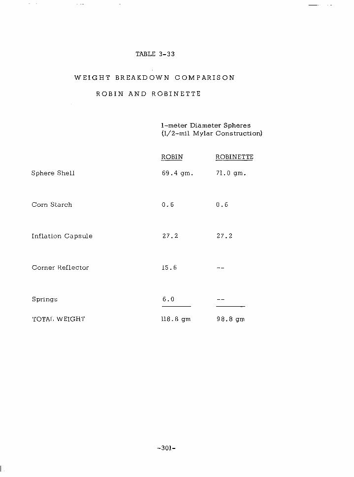
TABLE 3-33

Sphere Shell 69.4 gm. 71.0 gm.

WEIGHT BREAKDOWN COMPARISON

ROBIN AND ROBINETTE

l-meter Diameter Spheres (l/2-mil Mylar Construction)

Corn Starch

Inflation Capsule

Corner Reflector 15.6 --

Springs

TOTAL WEIGHT

ROBINETTE

0.6

27.2

0.6

27.2

6.0 --

118.8 gm 98.8 gm

-3Ol-

Arms-Robin

10 May 1961

-Shot No. 61-0115 CDT --shot No. 62-0215 CDT

( \v 1959 Atmosphere

Density, .p KS/m3 (Leviton)

FIGURE 3.4-16 TWO TYPICAL ARCAS ROBIN DENSITY PROFILES

-302-

344240

258180

- . t

5 172120 I- i= 2

Flight Time (Set)

FIGURE 3.4-17 VIPER DART ROBIN DESCENT PROFILE

-303-

7300’

5840 ’

4380 ’

280 3 -

840

Flight Time (SW)

FIGURE 3.4-18 VIPER DART ROBIN DESCENT *LOCIM

-304-

I I I1111 tOBIN 40-0218-l 1 18 FEB 1968 - 18072 .GLIN-D-3-RDR 27

-

I 0.1

DENSITY, 9’

-

-

-

-

-2 -

-

-

-

-

JP

m

,J ,J

3

(Wright) FIGURE 3.4-19 VIPER DART ROBIN DENSITY PROFILE

11 , I A I I AL717fIDt 1

@ RADAR27 X RADAR23

*18 1630

*19 #20 1700 1730 1800 1830

TIME, HOURS GMT (Z) (Wright)

FIGURE 3.4-20 VIPER DART ROBIN DENSITY TIME SEQUENCE

-306-

320

310

300

290

280

270

260

250

240

230

220

210

200

190

180

170

160

150

140

130

120

I I \!

0 40 80 120 160 $0 240

tte Spher IS Island B-l -229(

R v

e

t

Descent Time (Set)

NOL

0 400 440 480 520 560

FIGURE 3.4-21 TYPICAL ROBIN AND ROBINETTE SPHERE DESCENT DATA

-307-

3.5 Pitot Probe Density Measurement.

3.5.1 Introduction.

Atmospheric density profiles can be determined from ram pressure measurements at the nose of a rapidly ascending sounding rocket. In an early (1952) experiment; atmospheric density was computed from a measurement of the ,impact pressure at the nose of the rocket and atmospheric ambient pressure was computed from a pressure measurement at that position along the body of the rocket where the surface pressure was roughly equal to the ambient atmospheric pressure. In this method the entire rocket body was used as though.it were a pitot-static tube. At high altitudes, where the mean free paths of the component gases of the atmosphere were larger than the rocket diameter and where the spinning rocket was moving sidewise, the pressure at a gage opening located on the side of the rocket experienced a “spin modulation. ” This gage accurately measured the ambient atmospheric pressure twice during each rocket spin period. The ambient atmospheric density was computed from the maximum pressure excursion measured during each spin period. At a later date (1956-8) Aerobee-Hi rockets were flown with improved instrumentation to obtain density profiles from 20 km to 110 km. Horizontal wind profiles were also obtained from 80 km to 115 km. These flights supplied sufficient redundant data to demonstrate the accuracy of the density measurements, and it became apparent that the instrumentation complexity and redundancy could be reduced to obtain reasonable density profiles from 20 km to 80 km with smaller rockets and lower cost instrumentation by the measurement of impact pressure alone with relatively simple pressure sensors. Since the Aerobee-Hi experiments by Ainsworth, Fox and LaGow represent the classic configuration with rather complete instrumentation and measurements, they are described in some detail in the next section.

3.5.2 Aerobee-Hi Experiment.

(a) Instrumentation. The mechanical and electrical configuration of the pitot-static tube and its gages are shown in Figure 3.5-l. Gage A was a commercial capsule-potentiometer unit with a full-scale pressure of 760 mm Hg. Gages B and C were specially developed for pitot-static tube use because there were no gages available with sufficient range, accuracy, stability, rugged- ness, and insensitivity to over-pressure, and with sufficiently fast pressure response. Gages B and C incorporated diaphragm

-308-

I 0” W I

HEMISPHERE D = 8.9 CM d2’0.38CM 1 k -j td3’0.3204

8 20 HOLES 0

;

;-e-L,-,.OD

NOSE CONE Lj = 6.0 D

i-4- L2’7.OD c

t

IMPACTPRESSURE GAGES

STATIC PRESSURE SPIN PRESSURE GAGES GAGE

T3

GAGEAO-760mmHg

GAGE 80-20

GAGE C 0 - 0.20

MEASURED PRESSURES 20.Omm to

5XlOammHg

PITOT STATIC TUBE

(Ainsworth)

FIGURE 3.5-l MECHANICAL AND ELECTRICAL CONFIGURATION OF THE PITOT-STATIC TUBE

pressure sensors with ranges of 20 mm Hg and 0.2 mm Hg, respectively . Jhey were used to measure pressures from 20 mm Hg to 5 (10) mm Hg. Gage C was also used with an ac amplifier to measure spin pressure modulations having an amplitude as small as 1o-5 mm Hg. Since all gages used mechanical pressure sensors, measurements of true pressure were obtained irrespective .of the composition of the gas within the gage. Pitot-static tube shell and instrument temperatures were measured at positions T to T . The problems of slow pressure response and gage outgass&g at6 the higher altitudes were reduced by mounting the gages inside the pitot-static tube shell adjacent to the respective chambers.

The impact and static pressures changed by as much as 25 per cent per second, but due to the proximity of the gages to their chambers and due to suitable gage design, the pressure lag at the gages was less than 0.5 per cent. Gage and chamber pressure- response time constants were made as small as possible. The interior surfaces of the gages, the surfaces of the chambers, and the exterior surface of the pitot-static tube were highly polished and repeatedly outga ssed. No evidence of residual gas was seen in the measurements, although a residual gas pressure of 10-4mm Hg at 110 km would have been readily detected.

Rocket trajectory was obtained by means of Dovap and the trajectory error was less than 0.05 km on the ascent and 0.10 km on the descent. The basic flight information is presented in Table 3-34.

Rocket aspect was obtained by means of an optical aspect system and a single magnetometer. Canting of the rocket fins gave the rocket a final spin of 1.71 rps. The rocket’s precession cone had a vertex angle of 32.8 + 0 .l” and the precession period was 89.6 2 0.1 sec.

(b) Impact Pressure. The impact pressure measurements obtained in flight are shown in Figure 3.5-2.

At low altitudes-, impact pressure was converted to density by means of the Rayleigh pitot formula for a diatomic gas:

P = (0.144Pi - 0.066 P)/ [VT] 2, [g/m3=mm Hg/(km set-1) ‘] (1)

-310-

TABLE 3-34

Rocket Flight Data for Aerobee-Hi #NN3.15F Launched October 31, 1958, at 1359 CST

Altitude, km

Ascent Descent Time, Time,

set set

Rocket Speed, km/set

Knudsen Reynolds Number Number

% ReD

Mean Free Path X

cm

(Ainsworth)

20 30.0

25 43.2

30 46.9

35 50.0

40 53.0

45 56.0

50 59.1

55 62.0

60 65.4

65 68.7

70 72.0

75 75.4

80 78.8

85 82.4

90 86.0

95 89.8

100 93.6

105 97.6

110 101.7

403.3

400.2

397.0

393.8

390.4

387.0

383.6

380.0

376.3

372.5

368.7

364.7

360.6

1.05

1.27

1.52

1.71

1.69

1.67

1. 64

1.61

1.58

1.55

1.52

1.48

1.45

1.42

1.38

1.35

1.31

1.28

1.24

1.04 X 1O-5 5.69 X lo5 9.31 x 10-5

2.38 2.94 2.13 X 1O-4

5.14 1.63 4.59

1.12 X 1O-4 8.33 X lo4 9.98

2.36 3.90 2.11 x 10-3

5.14 1.72 4.59

1.12 X 1O-3 7.27 X lo3 9.98

2.24 3.46 2.00 x 10-2

4.24 1.77 3.79

7.75 1.01 6.92

1.46 X 1O-2 5.60 X lo2 1.30 x 10-l

2.98 2.71 2.66

6.45 1.29 5.76

1.29X 10-l 5.88X 101 1.15 x 100

2.62 2.99 2.33

5 79 5.15

1.24 X 10’ 1.55 x 101

2.77 2.46

5.76 5.12

-311-

103

1oZ

10’

3

SI

100

i lo=

3

B

E lo-:

lo-:

lo-’

FT CHURCHILL.CAN. ! FT CHURCHILL.CAN. ! W ” N) W ” N)

k’& **-*y k’& **-*y AERC$E; - H:I$N 3.16 F AERC$E; - H:I$N 3.16 F OCT . 958 59CST OCT . 958 59CST

-*.. -*.. -5 -5

*... *... =., =., -... -... *-.. *-..

a*. a*. -.. -.. f2 “‘S.. f2 “‘S.. l . . . l . . .

‘*. ‘*. *... *... *... *... . *.. . *.. *. *. -. -. . . . .

k3 k3 *5 *5 .a.* .a.* ‘*. ‘*. .._ .._

. . . . *.._ *.._ -... -... ‘... ‘... -.. -..

a. a. -... -... ‘... ‘... IMPACT IMPACT -*.. -*.. . . . . -...* -...*

*-.* *-.* PRESSURE PRESSURE t4 t4 * ._ * ._ * *.. * *..

**.* **.* -.* -.* STATIC STATIC ’ -‘. . . . ’ -‘. . . . *.. *.. PRESSURE ‘*Q... PRESSURE ‘*Q...

-*. -*. *..* *..* k5 k5 . . . . . . ., .,

-. -. 5%. 5%. a.. a.. *a.. *a..

**..... **..... *.. *.. . . . . *... *... -... -...

t8 t8 ** . . ** . . . . . .

*... *... *. . *. . . . . . -. -. . . . . k20 k20

. . . .

EST. MAX ERROR (%) EST. MAX ERROR (%) - : - : . .

I I I I I I 1 1 50 50 60 60 70 70 80 80 90 90 100 100 110 110

FLIGHT TIME (SEC) (Ainsworth)

FIGURE 3.5-2 IMPACT AND STATIC PRESSURE DATA BEFORE AERO- DYNAMIC CORRECTIONS WERE APPLIED. (Per Ains- worth, Fox, and LaGow)

-312-

where Pi is the ideal impact pressure, P is the ambient pressure, and VT is the wind created by the motion of the rocket along its trajectory.

A number of corrections to the measured impact pressure were required in order to obtain the ideal impact pressure as follows: (1) The first correction was required because of the high gas temperatures which exist in the vicinity of the nose of the pitot-static tube at high Mach numbers. These high temperatures cause a reduction in the ratio of the specific heats which causes the measured impact pressure to be greater than the ideal impact pressure. The values of the measured impact pressure were determined to be greater than the ideal impact pressure by from 0.25 to 0.65 per cent in the region from 20 to 30 km and by approximately 0.8 per cent in the region from 32 to 80 km; (2) a second correction to the measured impact pressure was a reduction in value of 0.2 to 0.5 per cent to correct for pressure lag within the gage and its chamber: (3) a third correction was for impact chamber orifice size. The size of the orifice of this particular impact chamber caused the measured impact pressure to be lower than the ideal impact pressure by less than 0. 3 per cent in the region of continuum flow; (4) a fourth correction to the measured impact pressure was for viscous effects. Starting at 72 km and at a Reynolds number with respect to diameter (ReD) of 700, correction was about 1 per cent at 82 km and 9 per cent at 89 km where an abrupt transition to free molecular flow began; (5) a fifth correction to the measured impact pressure was for rocket angle of attack, a , and was based on wind-tunnel tests of the angle of attack sensitivity of the pitot-static tube. With this correction (1) becomes

COS 1'2a) -O.O66P] / [VT]' (2)

The cosine term presents an approximate correction which is accurate to about 2 5 per cent at a = 13O. Maximum correction to Pi was about + 0.7 per cent at 90 km. At 80 km and below, the correction was less than + 0.2 per cent; (6) atmospheric winds must also be accounted for in the use of (2). Atmospheric wind vector W must be added to the rocket-wind vector VT to obtain the total wind vector V which replaces Vt in (2). The angle /3 between V and the rocket’s longitudinal axis is the effective angle of attack and must be used in (2) to replace a , the actual angle of attack. The calculation of the effect of atmospheric winds upon the computed density is simplified if W is separated into WV and WH, its

-313-

vertical and horizontal components, and the’ effect on (2) of each component is considered separately.

The first-order correction to (2) for the vertical atmospheric wind component is made by replacing the denominator by

[ lvTi -IwvI cos $1 2l where # is the angle between the

vertical wind vector and the rocket’s longitudinal axis. From Table 3-34 and Figure 3.5-2 it can be seen that a vertical wind of 7 m/set would cause a negligible change in the rocket’s angle of attack but would require a 1 per cent correction to the denominator of (2).

Root mean square values of the vertical wind in the region 80 to 100 km have an upper limit of 1 to 2 m/set. With this assumption the rms error in the density measurements due to vertical winds would be 0.15 to 0.3 per cent.

To reduce the effect of the horizontal wind on the impact pressure measurement, the zenith angle of the trajectory at the beginning of flight should be kept small. The correction of -2.8 per cent at 75 km (see Table 3-35) is associated with an initial zenith angle of about go. The correction would be reduced to -1.7 percent for an initial zenith angle of 4. So.

The transition of the measurement of impact pressure to conditions of free molecular flow is characterized by a reduction of impact pressure to approximately one-half of the extrapolated value for conditions of continuum flow.

Conversion from free molecular flow impact pressure to ambient density was obtained from the following considerations. Figure 3.5-3 depicts a region containing a gas characterized by mass density P , number density n, temperature T, mean molecular mass M, a most probable thermal velocity u, mean free path X , and a mass velocity V relative to the region inside a cavity where the several properties are designated by corresponding primed symbols. The direction of the mass velocity intersects the orifice surface of the cavity at angle Y . The orifice has area A and a diameter d << X . Outside dimensions of the cavity and the gas density within the cavity are such that a gas molecule approaching the orifice experiences negligible interference from gas molecules given off from the cavity’s exterior surface or emerging from the

-314-

TABLE 3-35

The Effect of Horizontal Atmospheric Winds on the Density Obtained from

the Impact Pressure Measurement (for NN3.15F)

Fictitious Wind

Correction to hL_kmF Iwl,m/_sec Azimuth, degrees P, % --

20 30 40 50 60 70 75 80 85 90 95 100 105 110

37 125 50 110 61 105 70 80 120 120 110 190 110 125 Measured values of the horizontal winds are used for computing the correction for 80 to 100 km.

+.9 +1.0 +1.1 +1.1 +2.3 +0.6 -2.8 -2.4 +0.6 +1.4 -0.6 -0.3 -0.4 -1.2

-315-

V

M: v; X’

FIGURE 3.5-3 ENVIRONMENT AND PRESSURE CHAMBER NOTATION

-316-

orifice. Under these conditions, the number rate of flow of gas molecules into the cavity is given by

exp ( -S2) + S x d-c

l+erf (S)]

= (~nu/2~ 1 F (S) ,-.

(3)

(4)

where erf (S) = 2 r 1

L s- -x e dx 0 (5)

S = ( IV/ sinr )/IA)= IV1 sinr )/(BRTM -1 l/2

) (6)

and the gas constant is

R = 8.312 X lo7 (ergs) (deg-1K) (g-mole-‘)

S is taken as positive when V is directed into the orifice and negative when V is directed away from the orifice.

Inside the cavity are gas molecules having the outside region as their source, and, in addition, there are molecules evolved during outgassing of the interior walls of the cavity. When the mean free path A’ of gas in the cavity is greater than the interior dimensions of the cavity and when the orifice ,diameter is small compared with the interior dimensions of the cavity, so that gas entering from the outside region has adequate time to acquire the temperature T of the gage wall, then (4) may be used to compute the return rate of flow N of outside-region gas molecules from the cavity.. Since V =0, F (S) = 1 and (4) becomes

N’ = Ad u’/ZF (7)

Under equilibrium conditions the rates of outside-region mass flow into the chamber and out of the chamber are equal and require that

NM = N’M’ (8)

Equations 4 and 7 and the equation of state are used in (8) to obtain the pressure ratio

P’ / P = (M/M’) 1’2(T1/T) 1’2 F (S) (9)

Should equilibrium be sharply disturbed by a large wind gradient or by a rapid change in mean molecular mass, the time required

-317-

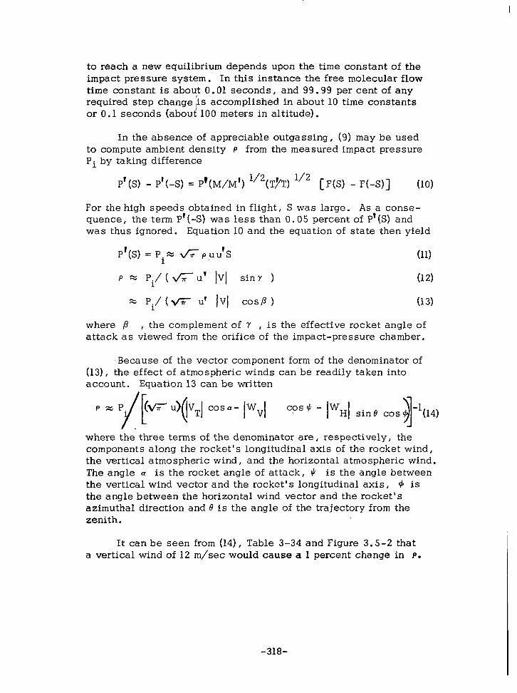
to reach a new equilibrium depends upon the time constant of the impact pressure system. In this instance the free molecular flow time constant is about 0.01 seconds, and 99.99 per cent of any required step change ,is accomplished in about 10 time constants or 0.1 seconds (about 100 meters in altitude).

In the absence of appreciable outgassing, (9) may be used to compute ambient density P from the measured impact pressure Pi by taking difference

P’(S) - P’(-S) = P’(M/M’) qTyT) 112 [F(S) - F&S)] (10)

For the high speeds obtained in flight, S was large. As a conse- quence, the term P’(-S) was less than 0.05 percent of P’(S) and was thus ignored. Equation 10 and the equation of state then yield

P’(S) = PiM XKpuu’s (11)

P 25 Pi/(&u’ IV] sin7 ) (12)

= Pi/ (fi ur Iv] COSP ) (13)

where P the complement of Y , is the effective rocket angle of attack as iiewed from the orifice of the impact-pressure chamber.

Because of the vector component form of the denominator of (13), the effect of atmospheric winds can be readily taken into account. Equation 13 can be written

‘OSa- I”Vl ‘os ’ - Iw~I sine cos

where the three terms of the denominator are, respectively, the components along the rocket’s longitudinal axis of the rocket wind, the vertical atmospheric wind, and the horizontal atmospheric wind. The angle a is the rocket angle of attack, $ is the angle between the vertical wind vector and the rocket’s longitudinal axis, $ is the angle between the horizontal wind vector and the rocket’s azimuthal direction and 8 is the angle of the trajectory from the zenith.

It can be seen from (14), Table 3-34 and Figure 3.5-2 that a vertical wind of 12 m/set would cause a 1 percent change in P.

-318-

Since the maximum vertical wind cited by Murgatroyd was 10 m/set the effect of vertical winds on the computed p is small. Horizontal winds were measured and the corrections to p shown in Table 3.35 were made.

(c) Static Pressure, Spin Pressure and Derived Temperature. The static pressure measurements and their interpretation is more complex than for the ram or total pressure measurements depend upon probe geometry, static port position, Mach number, angle of attack, wind, and horizontal wind. In general, the static pressure corrections are greater than for the ram pressure and the resulting density measurements are not as accurate. The spin pressure data were used to determine horizontal winds above 80 km by the phase of the spin pressure maximum and the peak-to- peak amplitude. The maximum Gind speed computation error was less than 10 percent.

In free molecular flow, ambient density was also obtained from the amplitude by using (10) with

A Ps of the spin-pressure modulation envelope

P’(S) - P’(-s) = A Ps

Equation 12 then becomes

P = aPs/< u’ /VI sinY) (16)

= APs/~T u’ vN) (17)

Since the spin chamber orifice is turned 90’ from the impact chamber orivice, Y as used in (16) is the effective angle of attack of the rocket and not the complement of the effective angle of attack as was the case in its use in (12).

Spin pressures were also used for computing ambient pressure. In continuum flow, ambient pressure points occur at approximately 30° on either side of the spin-pressure maximum. The average separation of ambient pressure curves determined from static pressure and spin pressure was less than 4 percent between 50 and 70 km, and no systematic separation of the two curves was observed.

Ambient temperature was computed from:

-319-

(1) the ratio of pressure to density as given by the equation of state T = MP/RP (18)

(2) the pressure profile using T = -MgR-l dh/d (InP)

'.

(19)

where g is the acceleration due to gravity, and (3) the density profile using

P= T,M p1 TM I I

(20)

Above 100 km no ambient pressure measurements were made, and the temperature was computed from the density data alone.

(d) Results. In the region between 20 and 30 km the validity of the density measurements is indicated by their agreement with the density computed from the radiosonde measurements. In the region between 30 and 85 km the validity of the measurements is suggested by their consistency as indicated by the close agreement between the measured and computed values of pressure and density.

Final density and pressure profiles for the flights with the pitot-static tube are shown in Figure 3.5-4.

The data obtained from the pitot-static tube flights indicate that the use of impact pressure measurements to determine density is a promising method for synoptic measurements of atmospheric structure in the region from 20 to 80 km. The method has the following advatages; (1) It is possible to make continous measurements from 20 to 80 km by means of ava.ilable instruments which are small, simple, and light in weight. (2) For the most recently developed pressure sensors, the impact pressure measurement error at 80 km will be less than 2 per cent. (3) Impact pressure measurements are not sensitive to rocket spin; thus spin may be used to reduce the maximum rocket angle of attack to the extent that no angle-ofattack correction to the impact pressure is required, (4) Vertical winds are small and have a small effect on the impact pressure. The effect on the impact pressure of horizontal winds can be kept small by means of a nearly vertical ascent trajectory. (5) High- speed machine computation of density based on equation 1 is tech- nically feasible. The term 0.066P may be obtained from a standard

-320-

5

2

102

5

2

10’

5

2

m’ of ‘O-0 f 5 5

f 2

t ‘O-l 5

z z 2

E n lo-2

5

2

lo-3

5

2

1w4

WHITE SANDS, NM. (330 N) - = ROCKET PANEL

ii --K I

\ . \

MAXIMUM ERROR(PERCENT) - (OCT. 31, 1958 ONLV)

f I 8 3 3 3 4 5

I

30 40 50 60 70 80 90 100 110 ALTITUDE ABOVE SEA LEVEL (KM) (Ainsworth)

5

2

1 o-5

FIGURE 3.54 FINAL PRESSURE AND DENSITY VALUES FOR TtiE THREE PITOT-STATIC TUBE FLIGHTS

-321-

atmosphere, since at high Mach numbers the variations in this term are of fourth order in the numerator of (1). With reasonable care in trajectory selection, the rocket‘s departure speed can be substiluted without appreciable error for IVTl , and thus the term

I I vT can be computed instantaneously from single station Dovap or radar tracking equipment.

3.5.3 Nike Apache Experiments.

In the Nike-Apache experim,ents , two radioactive ionization pressure gauges are installed to measure ram or total pressures and static or ambient pressure as the Nike-Apache ascends. The gauge outputs are telemetered to ground-based receiving and recording equipment. A trajectory of the rocket is provided by radar tracking, Doppler tracking, or both, to determine the altitude of the measurements. The measured experimental parameters are ram pressure, static pressure, and velocity and position of the payload in space. The ram pressure is related to density by the Rayleigh equation and the equation of state in the continuum region and by a modified thermal transpiration equation in the free-molecular- flow region. The ambient pressure is measured directly in the continuum region and is corrected for the thermal transpiration effect in the free-molecular flow region. The temperature profile can be computed utilizing the pressure and density profil,es and the equation of state or by integrating density using a form of the hydrostatic equation. The basic data reduction and measurement principles are the same as reported in Section 3.5.2.

The original Nike-Apache probe configuration is shown in Figure 3.5-5. The hemispherical shape of a Prandtl-Pitot offers the least sensitivity to the influence of attack angle upon realization of the ideal impact pressure. Moreover, the particular tube which has been flown on Aerobee vehicles has been tested and attack angle sensitivity determined. The diameter of the probe is established by considerations of required orifice size, chamber response time, and desired altitude of measurements. At the maximum altitude of interest (110 km) the mean-free -path of the air molecules is in the order of 50 centimeters while at 80 km it is in the order of 0.5 centimeters. The region between these limits is one during which a transition from continuum to free molecular flow occurs for practical sized probes.

Ideally, to avoid the complication of computing the transpir-

:322-

I cf.3 Kl w I

INSTRUMENTATION WIND CHAMBER ORIFIC AMBIENT PRESSURE CHAMBER ORIFICE

RAM AND AMBIENT GAUGE HOUSING

NIKE-APACHE PROBE

(Smith)

FIGURE 3.54 ORIGINAL NIKE-APACHE PROBE

ation effect and installing temperature gauges, the diameter of the probe should be very large. Thus would an ideal relation between probe dimension and mean-free-path for continuum flow be pre- served to very high altitude. Practically, however., the required diameter would place enormous requirements upon the vehicle. The 8.3’ centimeter (3.5 inches) diameter used on Nike-Cajun and Nike- Apache is a good compromise from the standpoint of measurement altitude versus mean-free-path, as well as from the standpoint of gauge dimensions and chamber response time.

The length of the pitot tube is of concern from the standpoints of rocket performance and location of the orifice relative to surfaces which might tend to perturb the measured impact pressure. A gauge location of 2.0 calibers forward of the flare between the pitot tube and the telemetry module of the Nike-Apache system enabled an unperturbed measurement of static pressure.

The theory and the work of others clearly indicated that up to about 85 km, the ‘determination of ideal impact pressure alone is adequate for the computation of density, pressure, and temperature of the atmosphere, provided that accurate determination of free stream velocity is made. The corrections which must be made to the measured impact pressure to realize such simplicity have been previously discussed. They can be reasonably well defined beforehand, and therefore could be resolved into a single constant or a correction versus altitude curve for the system. This will e- normously reduce data reduction time and will enable the computations to be made with a relatively simple computer program. The constancy of Mach number and low angle of attack imply that there is no need for instrumentation to measure angle of attack and that the function

u+1 ( Y+i) 2M2 1

r-1 2

[ 4rM2 - 2Y +2

l- in equation (6) , can be assigned a constant value with negligible error. Moreover, in the continuum flow region, below 85 km, it is unnecessary to provide instrumentation to measure ambient pressure or to measure any ambient air temperatures since both parameter,s can be deduced from the computed density.

Above 85 km, where transition from continuum flow is likely to begin, equation (5)) has been applied to adjust the measured impact pressure before computing density. The mean molecular mass at 100 km was equal to that at sea level and at 120 km was 0.99

-324-

times that at sea level. Hence it appears that negligible error will result if no adjustment is made for a variation in m_ in equation (S), at least at 110 km.

In the free molecular flow region, impact chamber temperature must be known to determine density. Aerodynamic heating of the Aerobee and Nike-Apache probes considerably raises the temperature of the probes, and the temperature must be measured. A new Nike- Apache configuration is being developed with a protective nose cone to reduce the aerodynamic heating of the probe to a negligible value. The payload configuration is shown in Figure 3.5-6. At an altitude of about 30 km the nose tip is blown off to expose the ram pressure probe. By this timefhe dynamic pressure will be down to a reasonable value and the aerodynamic heating will not be appreciable. Therefore, the sensor cavity temperature will remain essentially at the preflight value and the temperature measurement can be eliminated. The Mach number and angle of attack profiles for this Nike- Apache configuration are presented in Figure 3.5-7. A typical pitot probe temperature profile is presented in Figure 3.5-8.

The reported accuracies in density measurement for the Nike- Apache pitot-static probes are + 1% up to 84 km, + 4% from 85km to 100 km and + 10% or more for altitudes above 100 km.

3.5.4 Sparrow-Arcas Experiment (Denpro).

3.5.4.1 General. The previous pitot probe experiments reported in Sections 3.5.2 and 3.5.3 indicated that ac- ceptably accurate density profiles could be obtained as high as 80 km with the measurement of ram pressure and vehicle velocity, providing that certain error sources could be held to a minimum. Thus, by the elimination of the extra pressure gauges used for static and spin pressure measurement and elimination of attitude measuring instrumentation, the payload could be reduced in size, weight and complexity for routine use. In addition, a small, low cost rocket vehicle could be employed to replace the relatively expensive Aerobee and Nike-Apache. The Denpro program took advantage of these findings and reduced the scale and complexity of the instrumentation to the Sparrow-Arcas vehicle size. In addition, the AN/GMD-2 meterorological ground station telemetry was used for both trac’king and data aquisition to further reduce cost and eliminate the need for radar or other specialized tracking equipment.

-325-

0 8.37 19.98 30.93 44.55 53.68 56.402

6.5” O.D.

AMP. SECTION T. M. SECTION SENSOR SECTION DOVAP SECTION

FIGURE 3.545 PITOT PROBE MOD I PAYLOAD CONFIGURATION

60C

sot

l 400

ti

8 ; 3oc

2

2OC

100

0

. ANGLE OFATTACK (DEGREES) NEGLECTING GYROSWPIC EFF-ECT 2 4 6 8 IO 12 14 16 18 20 22 24 26 i

i 2 3 4 5 6

MACH NUMBER .

FIGURE 3.5-7 NIKE APACHE PITOT PROBE

-327-

120

100

80

z 60

x 2 F < 40

20

0

-

-

-

-

-

-

-

B

1

1’ I’

all

60

Temperature (OK) (Smith)

FIGURE 3.5-8 NIKE APACHE PITOT PROBE TEMPERATURE PROFILE CHURCHILL, 7 AUGUST 1966, 0949 GMT

-328-

3.5.4.2 .Theorv. For the continuum-flow region the Rayleigh pitot-static tube equation for supersonic flow and the equation of state for an ideal homogeneous gas may be combined, with some assumptions, to yield a simple expression for ambient density in terms of a measured impact pressure and a deduced air stream velocity. The relation developed for ambient density, ‘a, is

P 1521.1 P = i

a kilograms/meter3

I 1 v 2

for 3.5< M< 7.2 where M=Mach number

‘a = the ambient density

P i

= the ideal impact pressure

I I v = the free stream velocity

For the free molecular flow region, the interpretation of the impact pressure must be modified owing to the change in flow conditions which is related to the disappearance of shock phenomena. In this region the transpiration effect is given by

a

F (S) = e -s2 + s AJ-T--- (1 + erf S)

S = v cosa the ratio of the component of rocket C MO velocity normal to the orifice to the

most probable particle velocity

a = effective rocket angle of attack

Combining this expression with the equation of state for an ideal and homogeneous gas yields, for ambient density in the free molecular flow region,

-329-

Pi =Pi/dT V cosa

where K = universal gas constant

Ti= the gas temperature at Pi

m = mean molecular mass of the gas

a = effective attack angle

This expression results from simplifying assumptions regarding the vehicle velocity, angle of attack and effect of atmospheric winds upon the measured impact pressure.

A number of factors must be considered, in order to use the above simplified expressions to compute density from impact pressure with a reasonable degree of accuracy. These factors include the vehicle speed, angle of attack, the effect of atmospheric winds, outgassing effects, transducer error, heating effects and viscous effects due to tube shape, Reynolds number and impact pressure deficiency compared to ideal pressure because of orifice size. In general, it was found that corrections to the measured data were less than 1 percent with the exception of the viscous effects where the required correction in the free molecular f1o.w region was 9 percent. A summary of the sources and probable magnitudes of error in the density determination is presented in Table 3-36 and discussed as follows:

(a) Rocket Vehicle Speed. The more general expression for density in‘ the continuum flow region is

P = a

‘i

1

Y+l (y+ 1)2M2 1 ‘-’ 2

V2 .4yM2 -2y+2

where Pa= ambient density

-330-

1.

2.

3.

4.

5.

6.

7.

8.

9.

10.

11.

12.

13.

TABLE 3-36

Summary of Error Sources in Pitot-Tube Method

(Per Denpro Final Report by Atlantic Research Corp. 1965)

Effect on Error Source Computed Density

Angle of Attack Lowers

Vehicle Speed Equation (4)

Atmospheric Winds Vertical Increases

Atmospheric Winds Horizontal Increases

High Gas Temperature Increases

Chamber Response Increases

Orfice Size Decrease

Viscous Effects Decrease

Gage Pressure Hysteresis Increases

Gage Thermal Response --

Acceleration Sensitivity --

Outgassing Effect Increases

Gage Accuracy --

Magnitude of Correction

+o.z%

0

-0.15 to -0.3%

-2.0

-0.8%

-0.2 to -0.5%

+0.3%

t-1.0% +9.0%

2.0 to 10%

--

0

‘t 0.5%

Remarks

Garrection applies if attack angle is less than 10 degrees

Correction applies for relatively constant Mach number range

Correction must be estimated

Correction must be estimated

Varies with altitude

For membrane gage

During continuum flow region

Continuum flow Free molecular flow

Gages are calibrated for correction

Error can be calibrated out

Drag acceleration after thrust phase can be calibrated out

Prudent design and preflight pre- cautions eliminate significant errors

Error analysis from lab calibration will determine correction

Pi = ideal impact pressure

Y = ratio of specific heats ( Cp/Cv)

M= free stream

V = free stream

Examining the function of the

Mach number

velocity

denominator: -1

Y+l 2 2 7-1

(“/+l) M 2 4yM2 I -2y+2

and assuming that Y has a constant value of 1.4, it is apparent that this part is a weak function of Mach number and approaches a constant value of about 1.3 for values of M greater than about 3. However, as M decreases below 3, significant changes occur which must be accounted for in the solution of (6). Hence, in order to simplify data reduction processes, it is desirable to maintain a high Mach number and a limited range thereof throughout the altitude region of interest.

b) Angle of Attack and Wind Effects. The term P. refers to an ideal impact pressure which would be developed at a’ zero degree angle of attack of the pitot probe. Flight path angle variation and both horizontal and vertical winds cause the ideal impact pressure to be different from the actual measured impact pressure, and the velocity term to be different from the vehicle velocity. As the vehicle ascends an attack angle develops gradually between the longitudinal axis of the probe body and a tangent plane to its flight path. Under this situation it was determined that measured values of P. can be adjusted with acceptable accuracy to correct values by dividing them by the cosine of a , the attack angle. It can be shown that for attack angles in the order of 10 degrees or less, the required correction is in the order of 0.2 per cent. To achieve such low angles, however, the peak altitude capability of the vehicle usually must exceed, by far, the maximum measurement altitude.

-332-

The actual values used for V are intended to be the air stream velocity, not merely the rocket probe veldcity. Based upon a few measurements of winds, it was determined that the maximum error in computed ‘density, as a result of vertical wind components, may be 1.5 per cent, but the root-mean-square error would be 0.1 to 0.3 per cent. Corrections to be applied for horizontal components are a strong function of such parameters as flight path angle, initial zenith angle, and precession cone.angles. Ideally, to minimize resulting errors from unknown horizontal winds, a rocket probe should be insensitive to low altitude winds so that high launch angles can be used and be capable of achieving payload apogee values far in excess of measuring altitudes to maintain high flight path angles, and be spin stabilized to reduce precession angles to small values. It is interesting to note that spin stabilization is deleterious at the higher altitudes since it causes a divergence in the angle of attack as the flight path angle begins to flatten out.

(4 Outgassing Errors.

Measured impact pressures can be affected by the presence of gas molecules which are foreign to the ambient atmosphere. Such gas interference can stem from out-gassing of impact chamber walls, gas escaping from the interior of the vehicle, and gas evolv- ing from hot exterior surfaces. Difficulties from this effect are likely to become particularly troublesome near the upper region of the desired altitude, above 80 kilometers, where residual gas pressure should be below 10s4 mm Hg. Special treatment of surfaces and rigorous out-gassing of all surfaces near the orifice prior to flight can reduce errors due to this contamination.

(4 Gage Errors.

The normal gauge errors of accuracy, bias, repeatability, stability and range sensitivity, in addition to response time, acceleration sensitivity, thermal sensitivity, zero stability and hysteresis are source of errors in the basic impact pressure measurement. These factors vary with the Particula; sensor gauge used.

3.5.4.3 System Description. Design goals for the Sparrow-Arcas Denpro system have been stated as follows:

a. A low cost pitot probe ram pressure system to measure density between the altitude limits of ram 150,000 feet to 350,000 feet with telemetry compatible with the basic AN/GMD-2

-333-

meterorological ground station equipment.

b. A minimum velocity of about 3,000 feet per second should be obtained at the maximum measuring altitude desired, 350,000 feet. Thus, voltage analogs of impact pressure that would be well above background noise could be obtained from the pressure gauge, even at maximum measuring altitude.

C. Impact dispersion and wind effect upon the flight system should allow launchings to be made at high effective flight angles in order to minimize horizontal wind perturbance of the data.

d. The vehicle roll and pitch characteristics, coupled with other aerodynamic performance features, should result in a small angle-of -attack, preferably less than ten degrees, throughout the measuring period.

A basic AN/GMD-1B was employed for tracking the rocket- borne telemetry transmitter and detecting the modulation data contained in the tracking signal. Modifications were made to the basic equipment as follows:

a. The provision for a preamplifier of the tunnel diode type at the input of the Rawin receiver.

b. Removal of Meteorological Recorder AN/TM@5 from the ground system and substituting a seven channel magnetic tape recorder for telemetered data.

C. Addition of Transmitter T-456 ( ) /GMD-2 and Signal Comparator CM63 ( )/GMD-2 to the Rawin set to provide for measurement of slant range.

d. Addition of circuitry and comp0nent.s necessary for detecting and recording both positive and negative polarity pulsed data.

e. Addition of control features and auxiliary timing data to enable accurate data reduction and payload acquisition after lift-off-of the vehicle. A block diagram of the modified ground equipment is presented in Figure 3.5-9.

The Denpro vehicle consists of the Sparrow-Arcas two-stage

-334-

-

403MC 82KC MOD /

T-TRACK TAPE

RECORDER WlPS

POS PULSE SIGNALS

c:

TPl DUAL LOW

NEG PULSE SIGNALS PULSE AGC - - AMP PASS c

SEPARATOR FILTER TP2

RANGING

PRINTSYNC PULSES

cf ZOPPS I

A I CONTROL

t I I-l L a-J CONTROL RECORDER SPINNER

A c-57, - MOTORS

TIME DELAY

t

1 ALTERNATE I - PULSE POWER

l- GEN RELAY

--- J l-s 65 I 1

START SWITCH

1690MC PULSE & 82 KC MOD

FIGURE 3.5-9 DENPRO GROUND EQUIPMENT BLOCK DIAGRAM

solid-propellant sounding rocket with 4. S-inch diameter 32. a-inch long payload section as shown in Figure 3.5-10. The payload section as shown in Figure 3.5-11 consists of a cylindrical telemetry section with turnstile antennas for the 1680 mHz transmitter and the 403 mHz ranging receiver and a hemisphere pitot nose tip surrounded by a protective plastic nosecone. The payload weight is approximately 14 pounds. A block diagram of the telemetry section is presented in Figure 3.5-12.

The impact pressure probe is depicted in Figure 3.5-13 and the major components of the assembly are shown in Figure 3.5-14. Beginning at the leading surface, a stainLess steel hemisphere is attached to a machine tapered aluminum body of 6.5-inches length. The hemisphere is 3. S-inches in diameter and contains a 0.7-inch orifice at its center. To the inside edge of the orifice is silver soldered, a stainless steel sphere of 1.5-inches diameter, and 0.02-inches wall thickness. Absolute pressure gauges are connected to the sphere through 0.25-inch diameter steel tubing by silver soldering. The pressure gauges are mounted upon an aluminum support plate which is held to the tapered outer body at about its mid-section. Beneath the mounted gauges is installed the nose cone ejection timer which is physically attached to an aluminum baseplate. The latter contains the pyrotechnic release mechanism for nose cone ejection.

Pressure gauges employed for this program were designed and manufactured by the Decker Corporation, Bala-Cynwyd, Pennsyl- vania , and were of the metal’diaphragm type. Two gauges were used in the probe: a low pressure gauge having a pressure range of O-200 microns Hg, and a high pressure gauge having a pressure range of 0 - 30 millimeters Hg . The variable sensed as a function of impact pressure is the electrical capacitance existing between the diaphragm, which is at case potential, and a circular flat electrode. Two different methods were employed to measure this varying capacity during the program. The first employed an ionization bridge. Following major difficulties in obtaining long term stability of gauge output and having traced the problem to the ionization bridge, the second approach was to employ a lumped constant reactance bridge. The latter resulted in a major improvement in the long term stability of the gauge assembly. Both the ionization and the lumped constant bridges were excited by a high frequency source, operating at approximately 200 kilocycles, which was supplied by the gauge manufacturer and was installed in the telemetry package.

-336-

I W W v I

spclrrow MK6hbd3 Rocket Motor

/

HV-ARCAS Rocket Motor

/ TM Impact Pressure Section Prulpz Section

152.4 -..j

FIGURE 3.5-10 SPARROW-HV ARCAS (WITH 14 POUND PAYLOAD)

Protective Plastic Nose Cone

403 mHz Ranging Receiver

/- Antenna

1680 mHz Transmitter Antenna

FIGURE 3.5-l 1 DENPRO PAYLOAD

-338-

I W

z I

* I

Pressure - Vol Lage -

Sensor(s) 4 Gage Controlled

Electronics Blocking Modu later - 1680 MC Transmitter

Oscillator cc

I 1

i

Resistance Controlled

Blocking &xi I lator t

403Mc Supermgees4 ive - Tuned

Amplifier

28 Volt Battery H Power

Pack Converter

--

FIGURE 3.5-12 DENPRO TELEMETRY BLOCK DIAGRAM

. . ‘_’

Styp Compression Spri:g Pito\t Tube

Retaining Ti m,er Pin, ,Piston Assembly

FIGURE 3.5-14 PITOT PROBE ARRANGEMENT

The sequence of events.during a typical flight is presented in Figure 3.5 -15 . The protective nose cone is ejected at 150,000 feet to expose the impact pressure probe to the ram pressure of the atmosphere. Up to this point the nose cone is used to protect the probe from deleterious aerodynamic heating as a severe temperature rise of the metal probe would seriously affect measurement accuracy. Measurements are made with the high pressure gauge to an altitude (210,000 feet) where the gauge sensitivity becomes poor, and the low pressure gauge data is used from that altitude to 350,000 feet.

3.5.4.4 Results. As indicated in Table 3-37, good agreement between the radar and GMD-2 was obtained for both altitude and velocity. For a reasonable telemetry ranging signal-to-noise ratio, the velocity obtained with the GMD-2 was accurate to 0.5%. The vehicle maintained a velocity between Mach 3 and 4 throughout the measure region, and an angle of attack below loo was maintained up to 350,000 feet. Vehicle attitude was at . least 750 from the horizontal throughout the measurement region, and therefore, the error in density due to horizontal winds should have been negligible. The high pressure gauge yielded valid data to 85 km. However, a major problem area was that the low pressure gauge sensitivity varied from unit-to-unit as much as 0.3 volt full scale to 30 volts full scale. The sixteenth flight in the development program yielded density data to the highest altitude. The results are presented in Table 3-38 and the density profile is plotted in Figure 3.5-16. The greater reduction in density above 280,000 feet than indicated by the 1962 Standard Atmosphere curve is believed to be due to transition from continuum to free-molecular flow.

3.5.5 Impact Pressure Gauqes.

3.5.5.1 General. Although the ambient atmospheric pressure varies from 1 mm Hg at 45 km to 10e4 mm Hg at 110 km, impact pressure for a well-designed pitot probe system should vary from about 30 mm Hg to about 10m3 mm Hg throughout this altitude range. Therefore, the impact pressure gauge sensitivity requirements include this range of pressures, and it would be advantageous if a single gauge could be found which would suffice for the entire range. Also, considering the velocity requirements for the vehicle and the timewise rate of change of the impact pressure, it appears that a gauge time constant of about 23 milliseconds is required at 45 km for 0.5% accuracy and 2 seconds at 110 km for about r. 5% accuracy. In addition, the gauge should not be adversely

-342-

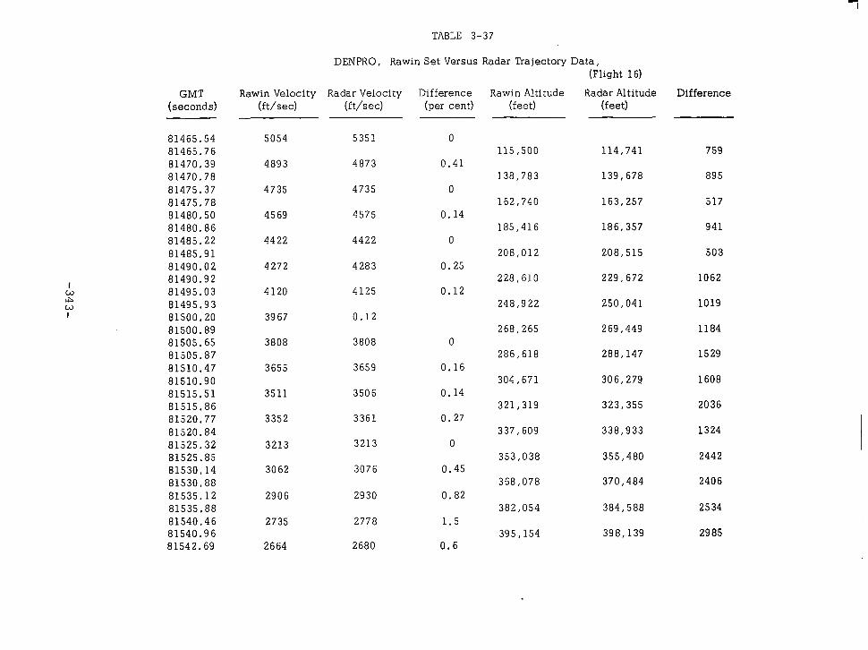
GMT Rawin Velocity Radar Velocity Difference Rawin Altitude (seconds) (ft/sec) (ft/sec) (per cent) (feet)

81465.54 81465.76 81470.39 81470.78 81475.37 81475.78 81480.50 81480,86 81485.22 81485.91 81490.02 81490.92 81495.03 81495.93 81500.20 81500.89 81505.65 81505.87 81510.47 81510.90 81515.51 81515.86 81520.77 81520.84 81525.32 81525.85 81530.14 81530.88 81535.12 81535.88 81540.46 81540.96 81542.69

5054 5351

4893

4735

4569

4422

4272

4120

4873

4735

4575

4422

4283

4125

0.12

0

0.41

0

0.14

0

0.25

0.12

3967

3808

3655

3511

3352

3213

3062

3808

3659

3506

3361

3213

3076

115,500 114,741

138,783 139,678

162,740 163,257

185,416 186,357

208,012 208,515

228,610 229,672

248,922 250,041

268,265 269,449

286,618 288,147

304,671 306,279

321,319 323,355

337,609 338,933

353,038 355,480

368,078 370,484 2906 2930

2735 2778

2664 2680

0

0.16

0.14

0.27

0

0.45

0.82

1.5

0.6

382,054 384,588

395,154 398,139

TABLE 3-37

DENPRO, Rawin Set Versus Radar Trajectory Data, (Flight 16)

Radar Altitude (feet)

Difference

759

895

517

941

503

1062

1019

1184

1529

1608

2036

1324

2442

2406

2534

2985

Altitude (ft)

Velocity (ft/sec)

Impact Pressure (mm Hs)

Ambient Pressure

(mm Hq) Density

(lb/ft2)

137,855 4873 39.6 1.65 1.58-4

142,142 4855 34.6 1.39 1.40-4

145,016 4845 30.3 1.24 1.22-4

154,480 4785 21.4 8.60-l 8.89-5

158,218 4757 19.1 7.46-l 8.03-S

174,356 4650 9.70 4.05-l 4.26-5

198,474 4479 3.56 1.58-1 1.68-S

213,577 4370 1.79 3.47-2 8.86-6

216,985 4349 1.54 7.31-2 7.68-6

234,933 4211 6.67-l 3.23-2 3.56-6

255,083 4062 2.78-l 1.17-2 1.60-6

267,948 3963 1.23-l 5.72-3 7.55-7

281,954 3845 3.70-2 2.60-3 2.34-7

298,460 3713 2.5-3 1.03-3 1.42-8

313,600 3592 6.0-4 4.6-4 2.42-9

TABLE 3-38 DENPRO

Reduced Density Data,

(Flight 16 Gage No. 5, OP 7158B. )

-344-

LqT Apogee (200 Set)

Second-Stage Burnout (38.0 Set)

\

nd Separation (2.3 Set) K

I mpg~(~2 Set) . .

///////f//////Y//

FlGuRE 3.5-15 SPARROW-HV ARCAS (DENPRO) SEQUENCE OF EvENTs

-345-

‘“-3FF=

- 10-5 EL I I

I I I I

t I I I

80 li0

1 I

*

I I I I- I I I

I ALTITUDE (thousands of feet)

40 50

FIGURE 3.516 DENPRO Flight Number 16, Altitude-Density profile

- 346 -

affected by charged particle concentration as the D and E region electron desities are traversed. The remainder of this section presents a review of current vacuum gauges and gauging techniques which have been considered for the pitot probe. A summary chart is presented in Figure 3.5 -17. Examination of the chart indicates that there are several gauges which could be used in this pressure range. These are the Alphatron, Densitron, Membrane, Vibrating Diaphragms ,Pirani, and Bayard-Alpert in combination with others. Gauges such as capacitance diaphragm transducers, inductance diaphragm transducers and the Bourdon tube are primarily low altitude pressure sensors and are limited to pressure measurement above 10-l mm Hg.

3.5.5.2 Transport Property Gauges.

3.5.5.2.1 General. These gauges measure vacuum in terms of the transport properties of the gas, i.e. , viscosity or thermal conductivity. Those gauges which measure thermal conductivity are more commonly used. Thermal gauges are usually nonlinear and are sensitive to gas type, variations in ambient temperature, and gas concentration. Thermal gauges are divided into three classifications: thermocouple, Pirani, and thermistor.

Thermocouple gauges utilize a wire filament which is heated electrically at a value of power which is usually constant and the resulting temperature is measured. ure the range from 1 to 10B3

These gauges ordinarily meas- torr, although extensions of each end of

the range by more than one order of magnitude have been demonstrated.

The heated wire itself is used as the temperature indicator in Pirani gauges, and the resistance of the wire is measured in a bridge circuit. A permanently evacuated compensating gauge is sometimes used in Pirani-type gauges. With these modifications, the sensitivity has been extended to the lo-’ torr range.

The third classification, the thermistor gauge, is similar in principle to the Pirani gauge, except that the heated element is a semiconductor bead instead of a metal wire. Thermistor gauges are normally used as one arm in a bridge circuit, and a permanently evacuated compensating gauge frequently forms a second arm of the bridge. The pressure-measuring range of thermistor gauges is similar to that of the Pirani gauge.

-347-

I Pirani (Hot Wire)

A 1 I A

Alphatroa (Radioactive Source) 4

tron (Radioactive Source) I I

I I A

Membrane (Ionization Type Dector) . . A 1 I 4

Vibrating Diaphragm

I

10’ 10” 10-3 10-5

MM of Mercury

10’7 10-Y 10-l’

50 80 120 Altitude (KM)

230 520 1000

FIGURE 3.5-17 SUMMARY OF PRESSURE GAUGE RANGES

All thermal gauges are limited by the fact that the pressure- dependent heat transfer becomes smaller than the heat transfer due to radiation as the vacuum level improves. Small changes in the radiation cooling of the heated element produce output variations which tend to mask the pressure effects, thus imposing a lower limit for pressure measurement. The common types are listed below:

(1) Pirani gauge - an increase of pressure from the zero point causes a decrease in the temperature of a heated filament of material having a large temperature coefficient of resistance, thus unbalancing a Wheatstone bridge circuit (or the circuit is adjusted to maintain the filament temperature constant).

(2) Thermocouple gauge - the decrease in temperature of a heated filament as the pressure rises is indicated by decreased electromotive force in a thermocouple circuit having the junction in thermal contact with the center of the heated filament.

(3) Thermistor gauge - a form of Pirani gauge employing a thermistor as the heated element.

(4) Bimetallic strip gauge - deflection of bimetallic strip with changing temperature indicates the changes in pressure.

3.5.5.2.2 Pirani Gauqe. Thermal conductivity , or Pirani gauges, measure pressure by monitoring the resistance change of a heated wire element. Changes in air pressure surrounding the wire element change the rate at which heat is lost by the element. Pirani gauges are commercially available which measure pressure down to 10m3 mm/Hg.

The Pirani type gauge is rejected principally because of its very low output voltage (thermocouple type) and its large response time (approximately 100 millisec) at very low pressures. To evaluate response time requirements the analysis below is give.

3.5.5.2.3 Havens Gauqe. The Havens gauge, developed at the Naval Research Laboratory, is a modification of the thermal conductivity gauge. It measures pressures down to 10-S mm/Hg.

The gauge works on the principle that an alternating current

-349-

signal can be obtained from the normally direct-current Pirani gauge by cyclically changing the pressure at a given frequency, At low ambient pressures, the compression of the bellows does not affect the temperature of the gas within the bellows significantly. The cyclical changes of the bellows will result in alternating voltage output from the resistance element, and the amplitude of the alternating voltage will be proportional to the change in ambient pressure. The eccentric shaft of the small motor, Figure 3.5-18, changes the volume of the bellows about 20 percent at a frequency of about 20 cycles per second.

The use of two bellows assures that the eccentric shaft is working against the same pressure in each bellow, regardless of the outside pressure. The outside pressure is communicated to the pressure chambers by a small hole(s) which restrict the rate of gas flow so that the gas does not flow completely out of the chamber when the bellows are compressed. Since the pressure inside the bellows chamber is changed about 40 times per second, the average pressure within the bellows will be at equilibrium with the outside pressure. The peak-to-peak alternating voltage developed across the resistance elements within the bellows will vary directly with the outside pressure. At a pressure of 0.6 mm/Hg, a change of 20 percent in the bellows pressure changes the voltage across the resistance by 0. 27 volts.

Pressure measurements by thermal conductivity gauges are subject to error due to the variation of atmospheric composition, with the resulting variations of specific heat of the gas surrounding the heated wire.

3.5.5.3 Ionization Vacuum Gauge.

3.5.5.3.1 General. A vacuum gauge has been developed consisting of a means to ionize the gas molecules and a means of correlating the number and type of ions pro- ’ duced with the pressure of the gas. Various types of ionization gauges are distinguished according to the method of producing the ionization. The common types are as follows:

(1) Hot cathode ionization gauge - The ions are produced by collisions with electrons emitted from a hot filament or cathode and accelerated by an electric field. Also called hot filament ionization gauge, ionization gauge, or simply ion gauge. The Bayard-

-350-

n

MOTOR

rAlR INLET

I I I

-AV- -AV-

FIGURE 3.5-18 HAVENS DOUBLE BELLOWS GAUGE

-351-

Alpert ionization gauge employs a tube with an electrode structure designed to minimize X-ray-induced electron emission from the ion collector.

(2) Cold cathode ionization gauge - The ions are produced by a cold cathode discharge; usually in the presence of a magentic field which lengthens the path of the electrons between cathode and anode. The discharge tube is a transparent tube in which the color and form of a cold cathode discharge (without the presence of a magnetic field) gives an indication of the pressure and the nature of the gas. The Philips ionization gauge or Penning gauge, is a cold cathode ionization gauge in which a magnetic field is directed parallel to the axis of an,annular electrode, normally the anode, located between two plate electrodes perpendicular to the axis. Var- ious modifications of the Penning gauge are named after the inven- tors, and certain types are referred to as magnetron vacuum gauges.

(3) Radioactive ionization gauge - the ions are produced by radiations, usually alpha particles, emitted from a radioactive source.

3.5.5.3.2 Thermionic-Ionization Gauses. Thermionic or hot cathode-ionization gauges ionize the gas in the gauge with electrons obtained from a heated filament. For a, specific electron emission current, the ion current reaching the collector is taken as a measure of pressure. These gauges are in general use in the inverted Bayard-Alpert form shown in Figure 3.5-19, or in a modification of this basic arrangement. The central electrode of a Bayard-Alpert gauge is the ion collector which operates at ground potential, while the filament is maintained at 25 to 50 volts above ground potential, and is heated to produce electron emission at a desired current level, often about 10 milli- amperes. The electrons so produced are accelerated through an additional potential of about 150 volts. Subsequently , the electrons are collected on the electron collector which is usually called the grid.

There are several important features of the Bayard-Alpert type of thermionic gauge. Due to its relatively open construction, the gauge can be used as a nude gauge, and it need not appreciably modify the gas temperature in the sensing zone. Again, the open construction causes the electrons to make a number of passes through the grid area prior to being collected. The resulting in-

-352-

Filament +45v

Ion Collector, Ground Potential

-“Grid”, Electron Collector, -I-200V

Vacuum Seals

FIGURE 3.5-19 INVERTED BAYARD-ALPERT THERMIONIC-IONIZATION GAUGE

Inverted Bayard-Alpert form of the thermionic or hot-cathode ionizutlon gage which operates by ionizing the gas in the gage by electrons obtained from a heated filament; the measure of pressure is the ion cwrent reaching the collector at a specific electron emission current.

-353-

creased path length increases the probability of ionization and thus increases the sensitivity of the gauge. 1 In addition, the Bayard- Alpert gauge was designed to reduce the X-ray limit, and the small collector serves this function. The X-ray limit refers to a spurious output current which is superimposed on the ion current and is in- distinguishable from it. When soft X-rays generated by the impact of electrons on the grid strike the ion collector, electrons are-ejected from it photoelectrically to form the output current. The X-ray current limits the pressures that can be measured, and is equivalent to a pressure reading in the lo-l1 torr range in a Bayard-Alpert type gauge. Earlier gauges which had a cylindrical collector outside the grid experienced an X-ray limit of about 10m8 torr.

Vacuum technology uses the term “X-ray limit” in two different senses. The term therefore requires some qualification. In the first case, the X-ray limit may refer to the lowest pressure indication which may be obtained in a gauge when all the output current is due to X-ray-induced photoemission and there is an absence of gas. The second meaning which is sometimes used is that the X-ray limit refers to the pressure level at which the X-ray current is a substantial part, for example, 10 percent of the total ion collector current.

A number of modifications have been made in the Bayard- Alpert gauge. Filaments, which are usually made of tungsten, have been fabricated of thoriated iridium, and rhenium. Both of these substances will briefly withstand the oxidation accompanying acci- dental release to atmospheric pressure, although thoriated iridium! tends to poison in the presence of hydrocarbon vapors. Operational stability has been improved with the addition of an outer grid or shield surrounding gauge structure to establish a fixed wall potential. Another modification introduced closed grid ends and increased sensitivity by a factor of 2.5 to 5. In addition, a modulator electrode has been incorporated to permit separate measurements of the ion current and X-ray current. The modulator is an additional electrode adjacent to the ion collector, and can be switched at will from grid potential to ground potential. When the modulator potential is switched, the ion and X-ray photoelectric currents are both changed by fixed, but different, ratios. The observed change in total current following switching may be analyzed to determine the ion current percentage of this total current.

A number of experimental hot-cathode gauges have been

-354-

developed which differ to various extents from the Bayard-Alpert gauge. The modifications usually attempt to reduce the X-ray limit, or the effect of the hot filament or both, The location of an additional electrode (which is negatively biased) may suppress the photoelectron current from the X-rays by repelling the photoelectrons and forcing them to return to the ion collector. Since photoelectrons ejected from the suppressor can reach the ion collector and appear as a negative X-ray current, the suppressor must be shielded from the X-rays. A second modification used a magnetic field to increase the electron path length, which in turn increases the sensitivity of the gauge.

The Bayard-Alpert gauge is good for pressure as high as about 10-l mm Hg., and therefore any system would require an additional gauge of different type to cover the dynamic range. Being of an ionization type it is subject to the same disadvantages as the other gauges of this type and therefore is eliminated for this application.

3.5.5.3.3 Glow Discharqe Ionization Gauges. Direct observation of a glow discharge in a strong electric field has been used to estimate vacuum levels from 10 to 10s2 torr. The addition of a fluorescent screen enables the gauges to be used at pressures as low as low5 torr. Ordinary glow discharges tend to be extinguished when the pressure falls below 10s3 to 10m5 torr.

Several types of cold-cathode-discharge have been constructed for high-ar;_i ultra-high-vacuum applications. Figure 3. S-20 illustrates the operation of such a gauge. A high voltage of 1 to 10 kilovolts is applied between the cylindrical anode and the flat cathodes. At the same time, a magnetic field is applied parallel to the axis of the anode. The discharge is initiated by a few electrons which must be supplied from another source such as cosmic ray particles, field emission, or perhaps an auxiliary filament. After the discharge starts, electrons are supplied from the ionization of the gas molecules, and by secondary emission as ions impact on the cathodes. These electrons are constrained to take helical paths along magnetic field lines, and cannot readily reach the anode without undergoing collisions with gas molecules or other particles, further ionizing the gas and releasing additional electrons. The gas ions are not appreciably restrained by the magnetic field and are collected at the cathode. A measurement of the

-355-

Magnetic Field 1 - 2 Kilogauss

Current Meter

FIGURE 3.540 COLD-CATHODE DISCHARGE IONIZATION GAUGE

A cold-cathode discharge gage uses a magnetic field to sustain the discharge. To initiate the discharge, a few electrons must be supplied initially from an outside source, perhaps an auxiliary filament.

-356-

current between the anode and the cathode indicates the degree of vacuum.

An early cold cathode gauge design, known as a Penning or Philips gauge, which used a loop of wire as the anode, operated on the same principle. Some of the disadvantages of these gauges are that the discharge may be unstable under some circumstances, and it is difficult to maintain the discharge at pressures below lo-’ torr . Modified versions of the Penning gauge are commercially available in which the discharge is almost completely enclosed in a cylindrical anode. If the anode voltage and the magnetic field strength can be properly selected, the discharge can be stabilized to permit operation in a ultrahigh vacuum. Another design, the Redhead gauge, incorporates the features previously mentioned, plus a perforated anode cylinder. Auxiliary cathodes are used as guard rings to prevent field emission currents from contributing to the measured cathode current. One form of the cold-cathode gauge is called a magnetron gauge. In this gauge, the anode is a rod located on the axis of a cylindrical cathode such that the radial d. c. field is perpendicular to the magnetic field. The magnetron- gauge discharge may tend to oscillate. However, there is little reported data on the effect of this phenomenon on gauge readings.

Cold-cathode-gauge characteristics vary as a function of geometry and operating condition. These gauges possess a high sensitivity ranging from 1 to 10 amp/torr, and a high pumping speed. In fact, ion pumps are basically joined assemblies of Penning- type gauges. Values of the steady-state pumping speed range from 0.1 to 0.5 liter/set for air at sensitivities of 2 to 10 amp/torr.

Of course, there are some differences between the pumping mechanism in ion pumps and in gauges. That is, gauges seldom contain an active metal such as titanium which is intentionally sputtered to promote pumping, as in the case of the ion pump. In addition, the quoted pumping speeds are somewhat dependent on the condition and history of the gauge and are widely variable functions of sensitivity. One reason for the discrepancies in the quoted data may be due to the relatively long saturation process reported for a gauge pumping air. It has been estimated that at a pressure of 1 x 10mg torr, the time to reach saturation will equal 20,000 to 30,000 hours. During this time period, the pumping speed decreases by a factor of about 2.

-357-

.- ... ....... --- - .._. ......... ... .. .._. - I

The response of cold-cathode gauges is not generally a linear function of pressure. The output current I is related to the pressure P

I = Pn

where n varies from 1.1 to 1.4, and is a function of gas type, magnetic field strength, voltage, gauge geometry, and materials of construction. The exponent n has been reported to show a pressure dependence in the Redhead gauge by changing from a value of ap imately 1.0 to 1.5 - 1.7 as the pressure is reduced below 2 x 10’ P

rox- ’

ton-.

3.5.5.3.4 Radioactive Ionization Gauges. Most high-vacuum gauges operate by ionizing the gas and then measuring the ion current collected. The ionization in radioactive gauges is produced by alpha radiation from radium within the gauge. Because of the fact that alpha particle sources of sufficient intensity to produce an easily measurable ion current at very-high-vacuum values are either dangerous or too large, radioactive gauges are limit d in range. The alpha radiation gauge yields readings in the 10 -2

range, and the experimental tritium gauge extends the readings to the lo-’ range. These gauges can be used at high pressures up to 1 atmosphere.

Ionization gauges measure the number of free ions produced by a flow of electrons in a diffuse gas. The relative numbers of free ions formed by a constant electron source is a function of the density and composition of the gas within the ionization gauge.

The Alphatron is typical of the radioactive, cold-cathode type of ionization gauge. A radioactive isotope within the gauge provides a constant source of ionizing radiation. The instrument is essentially a modification of the electrostatic detectors used to count radioactive particles.

In the operating instrument (See Figure 3.5-21) a voltage is applied to both the wall and wire electrode of the gauge. Gas atoms entering the gauge are ionized by the radioactive isotope, and the ionized gas atoms are then attracted to the wall of the gauge. The drift of these ionized particles lowers the voltage between the two charged elements of the gauge. When this voltage drops to a pre-set point, the chamber is recharged to its original voltage. The frequency of recharge is proportional to the rate of

-358-

Shell of Rocket

Lb \ ,, ,, s

Radioactive Source

0 0 0

FIGURE 3.5-21 RADIOACTIVE IONIZATION GAUGE

-359-

ion formation.

The use of ionization gauges of the Alphatron type is based on the following assumptions:

a. The devices are insensitive to acceleration changes.

b. They provide rapid discrete responses to density changes of a homogenous medium.

c. By suitably switching the voltage drops for recharging the instrument, it can be used to measure density directly

to altitudes of about 200 milometers.

d. Sources of error in the technique include:

The devices measure only the relative number of ions formed.

Ion formation is affected by the composition as well as the density of the gas being measured.

e. External ion sources (e. g. , the ions in the F and D layers of the upper atmosphere) will interfere with the ion counts obtained by the instrument.

f. Gas density is temperature dependent.

cr. The instrument may not be at temperature equilibrium with the atmosphere.

h. Density measurements are probably correct to within an order of magnitude up to 250 kilometers.

The Alphatron, developed at the University of Michigan, has much to offer for this application in terms of simplicity of construction and rapid response time. Its chief disadvantages are the low output 10’3

current obtainable, an apparent low pressure limit of mm Hg , and a potential hazard of its radioactive source.

Moreover, as with all ionization-type gauges, its calibration is subject to a change in the gas composition and the presence of external radiation. A main disadvantage of this gauge, however, is the low output current obtainable which results in a requirement for complex and expensive electronic supporting equipment. More-

-360-

over , switching of circuits at very low current levels is required to be made automatically during the flight in order to accommodate the dynamic range of pressures experienced, thus placing a burden upon reliability of electrical performance. Because of the required proximity of the electronics to the gauge, the final assembly becomes quite long and does not lend itself to the proposed,rocket assembly.

The Densitron is the result of additional work at Michigan to improve the Alphatron. While the lower pressure limit of this gauge has been extended 4 to 10e4 mm Hg, the same disadvantages as were described for the Alphatron apply.

3.5.5.4 Force Measuring Gauges.

3.5.5.4.1 General. These gauges respond to pressure changes within the gauge envelope, and are often used for differential pressure measurements. The mechanical measurement of fort s by thin diaphragms, ordinarily limited to pressures above 10 -5 torr, has been used experimentally and in several commercial gauges. Gauges of this type are relatively expensive due to the complexity of the readout equipment required to detect the very small motion of the diaphragm at low pressures. Additionally, hysteresis in the diaphragm is a problem.

The principle that gas damping varies as a function of pressure is the basis for several devices designed for the measurement of low pressures. The first of these had a thin glass disk suspended on a wire between two horizontal plates. The disk is set in rotation, and torsion in the support wire produces a restoring force that causes the disk to oscillate. The rate of decrease of the oscillation is observed optically. This type of gauge was found to be useful down to about 0.35 x 10S3 mm Hg.

Quartz fiber gauges consist of thin quartz fiber supported at one end and set in oscillation by plucking, tapping the support, or other means. The rate of vibration decay is observed optically. This type of gauge is useful down to as low as 5 x lo-’ mm Hg. Gauges that use a continuously rotating disk or cylinder to cause a force on a restrained disk or cylinder in close proximity have been used. The torque on the restrained disk or cylinder depends on viscous drag and is a measure of the pressure. Gauges of this type have been found useful down to about lOa mm Hg.

-361-

All these gauges are mechanical, most are very slow in response, and none are suitable for continuous pressure indication except the continuously rotating type.

A vibrating wire pressure transducer based on the variation of gas damping on the wire as a function of pressure has been developed . This transducer used a tensioned wire suspended in a transverse magnetic field as the sensing element. The wire was used as a frequency selective filter in the feedback loop of an electronic amplifier and was thus maintained in continuous, constant-amplitude vibration at the transverse mechanical resonant frequency of the tensioned wire. A continuous electrical output that was a function of the pressure was developed. The device was useful for pressures down to 10m3 mm Hg and had a response time of a fraction of a second. Variations in internal damping of the wire as a function of temperature and time were limitations in its usefulness.

A pressure transducer system based on the gas damping of a vibrating metal ribbon has been developed and marketed under the name “Reva” by Arthur Pfeiffer, GmbH , Wetzlar , Germany. The corrugated ribbon is suspended in a magnetic field and is electronically maintained in continuous vibration, A continuous electrical indication of pressure is provided. The device is larger and more fragile than the vibrating diaphragm gage.

For pressure measurements in the higher ranges, transducers operating on the principle of the deflection of a diaphragm as a measure of the pressure difference are often used with various methods of registering the deflection. Some common ways to provide an electrical output are strain gages, vibrating wire, variable capacitance effects, variable reluctance effects, and linear variable differential transformers. For sensing small pressures, the diaphragm must be large and of very thin material, and the sensing element must not require appreciable force. Because of this re- striction, deflecting diaphragm transducers that have been most successful for measuring in the range of a few mm Hg have used either the variable capacitance or variable reluctance effects. Be- cause this is a differential method, a high-vacuum reference pressure is needed on one side of the diaphragm for accurate low-pressure measurements. To achieve sufficient sensitivity with this type of gage, the diaphragm frequently is too thin to withstand a

-362-

differential pressure of l-atm pressure and is thus subject to damage from over-pressure. The same considerations apply to variable- reluctance, differential pressure gages in which the diaphragm forms a portion of a magnetic circuit, Commercial variable-capacitance differential pressure sensors and associated electronics for use in the range of a few mm Hg have been marketed by several companies. Sensitivity to pressure changes of 2X10B4 mm Hg and long term sta- bilities on the order of 10e2 mm have been reported. Variable- reluctance differential pressure gages useful in the mm Hg range also have been marketed by several companies. Sensitivity and accuracy of a few microns Hg have been reported with this type of device. Response speeds of the transducer and associated electronics of several milliseconds for both types have been achieved. Compared to the vibrating diaphragm gage, these devices have a smaller range, which does not extend to as low a pressure; they are generally larger; and they have larger internal volume, which limits response speed at low pressures. An advantage of these units is that the reading is independent of the gas composition and temperature. Additionally, a solid state pressure transducer capable of measurements ranging from sea level pressure to 10m6 torr has been under development. This piezo junction effect gauge features a sensor consisting of a p. n. junction fabricated in the apex of a silicon needle. However, this technique is presently in its early research stage and possesses limitations that require additional research before corrections will be possible.

3.5.5.4.2 Vibrating Diaphram Pressure Transducer. A vibrating diaphram pressure transducer of apparent merit for the pitot probe application has been developed by John Dimeff et. al. at the NASA Ames Research Center for wind tunnel application. This instrument measures absolute gas pressure between low5 and 10v3 mm Hg. When used with appropriate electronic circuitry, continuous pressure indication is possible with an accuracy of 1 percent over most of the range.

The transducer measures pressure by sensing the damping effect of the gas on the vibration of a thin metal diaphragm. The diaphragm is under radial tension and is electrically maintained in continuous vibration at its mechanical resonant frequency. The Ames device is small, relatively rugged, and reliable. It also has fast response, is not subject to damage by overpressure, does not require a vacuum reference, and lends itself readily to automatic operation.

-363-

Figure 3.5-22 is a simplified sketch of the transducer which is composed of a thin, metallic diaphragm under radial tension, between two closely spaced, insulated metal plates. The two metal plates provide a means of electrically forcing and detecting the diaphragm’s vibration. The space between the plates and the diaphragm is filled with gas at the pressure to be measured. Gas damping causes a loss of energy from the diaphragm, and this loss is sensed by its effect on the diaphragm damping factor. The electrical power required for a given amplitude of vibration is therefore a measure of the gas pressure.

Figure 3.5-23 shows a simplified arrangement of the transducer and associated electronics. The forcing plate of the transducer is supplied with a d. c. potential and an a. c. voltage from an electronic oscillator set at the mechanical resonant frequency of the tensioned diaphragm. The electrostatic forcing function thus generated causes the diaphragm to vibrate synchronously with the a. c. driving voltage and at an amplitude which is a function of the driving signal and the diaphragm damping factor Q. The diaphragm’s vibration causes a corresponding periodic variation in the capacitance between the diaphragm and the sensing plate that may be detected and used to indicate the vibration’s amplitude. Since the power required for a given amplitude of vibration is a function of the damping on the diaphragm, which in turn is a function of the gas pressure, the power can be monitored as an indication of the pressure.

A typical gage performance curve is shown in Figure 3.5-24, and the time constant is plotted against pressure in Figure 3.5-25.

-364-

+

Gas Inlet

FIGURE 3.5-22 SIMPLIFIED SKETCH OF THE VIBRATING DIAPHRAGM TRANSDUCER

-365-

---

Forcing Plate Sensing Plate Transducer ,

J Indicator b Indicator 1

-y 1

Vibrating Diaphragm

FIGURE 3.5-23 BASIC PRESSURE-MEASURING SYSTEM, SHOWING SIMPLEST MODE OF USE

-366-

10’ 8, ,,o,ium 0 Exprimmt

105 - Theory

/ Air 0 Experiment -

/ -- Theory

104 -~ I I I I to-5 lo-4 10-3 10-e 10-l 100 IO’ 10” 10”

Pressure - mm Hg

FIGURE 3..5-24 PERFORMANCE CURVES OBTAINED FOR AIR AND HELI-UM, CORRECTED FOR MECHANICAL AND ELECTRICAL LOSSES

-367-

0.

0.01

0.001 lJlLLw- 10-4 10-3

Pressure, mm Hg

FIGURE 3.5-25 TIME CONSTANT PLOTTED AGAINST PRESSURE

-368-

3.6 Sonic Grenades

3.6.1 General.

Sonic grenade experiments have been used in a number of studies of upper atmospheric temperature and winds and have apparently given good measurements of the mean temperature in successive layers of the upper atmosphere. In this technique, explosive grenades are fired at known points along a rocket trajectory. The resultant sound pulses are recorded on a ground array of microphones. Differences in pulse arrival time and firing location are translated into mean temperature and wind conditions in the layers between grenade explosions, The resolution obtainable with this technique depends upon the spacing of the grenade explosions.

Rocket grenade techniques can give temperature data to within 5oC, as well as an indication of wind conditions, but the size of the rocket, the complexity of the equipment and the calculation procedures would seem to rule out this technique for routine use and probably limit the use of grenade techniques to special research studies only.

Temperature and winds are measured by sound ranging on successive explosions of grenades ejected from rockets as indicated in Figure 3.6-l. The experimental data required for determination of temperature and winds are (1) exact time and position of the grenade explosions, (2) the time of travel to the ground, and (3) the angle of arrival of sound waves at an array of ground transducers. In addition to temperature and winds, these experiments yield density and pressure by calculation.

Ground equipment consists of a ballistic camera to provide angular direction at the time of grenade explosion and DOVAP for determination of accurate slant range and explosion time. Time and direction of the arriving sound waves are monitored by an array of five transducers positioned in the shape of a symmetrical cross with approximately 500 meters between each transducer.

For explosions below 75 kilometers, it is reported that errors in the average temperature of the layer between data points are generally less than + 3K. For wind speed and direction, it is reported that errors are about + 5m/sec.

The grenade experiment is based on measuring the average

-369-

BAL CA

-

.LIST ,MER

a Li!+ 3 ‘I( .A

‘G12

50

45

40

RADAR -a. ..I- ------._.- IVIJ RECOF

LAUNCHER

7 DOVA P

FIGURE 3.6-l ROCKET-GRENADE EXPERIMENT

-370-

velocity of sound, traveling to the ground, when produced by a grenade exploded at various altitudes. The atmospheric temperature in the region of the grenade explosion is determined by the variation of sound velocity with the altitude of the grenade explosion.

The calculations for the experiment yields the average temperature in the layer between grenade detonations. The average temperature is assumed to exist throughout the layer.

Possible errors for the grenade experiment include:

a. Variations with altitude of the specific heat or water vapor of the atmosphere introduce errors in the calculation of temperature, from the above equation.

b. The accuracy of the measurements is limited by the sound- ranging network’s accuracy to determine the time of arrival of the sound waves at the individual microphones.

C. The grenade experiment is probably accurate to about 5O for determination of temperature to an altitude of about 9 0 kilometers. Above about 95 kilometers, sound waves cannot be generated with sufficient energy to reach ground stations.

The use of high-altitude grenade explosions to obtain atmospheric data is based upon the propagation of sound energy through the atmosphere. Average temperatures and winds for the interval between two explosions are determined by measuring exactly the time and position of each explosion and the time when each soundwave arrives at various ground-based microphones. This method can be expanded to n-l data points for n explosions, thus, the greater the number of grenades exploded, the greater the number of data points for determining temperatures and wind profiles.

The grenades are carried aloft in a Nike-Cajun rocket and detonated at predetermined altitude intervals during the ascent of the rocket to altitudes of approximately 90 km. The rocket position is accurately determined by a combination of radar, DOVAP (Doppler Velocity and Position), and optical-tracking systems as shown in Figure 3.6-2. An analysis of these coordinates and the arrival time of the sound waves yields the direction and magnitude of the sound- velocity vector in the layer between two explosions. This vector is

-371-

TRACKING TRANSPONDER -----------------------------------

F~=Q;C~

( NoMINAL)

I L,,,-,-,-,--,-,-------------- --.- -

i\

f\ 73.6 MC (NOMINAL)

4 $3.6 MC (NOMINAL)

G

GROUND RECEIWNG STATION r ---s-------s---- + 4 --e-s -- 1

36.8 MC ~NOMINAL)

5

I i . i 36.8 Mc(NOMINAL) i A DC. VOLTAGE I-

(Smith)

DOVAP Tracking Transponder Operation

FIGURE 3.6-2 GRENADE EXPERIMENT INSTRUMENTATION

-372-

a measure of the temperature and wind in the layers.

The payload structure as shown in Figure 3.6-3 consists of the grenade section with nosecone, timer, photocell assembly, DOVAP and battery section. The nosecone forms an integral unit with the cylindrical grenade section which is composed of 12 cylindrical tubes held in place by plastic resin. The timer and photocell assembly contain three infa-red-sensitive lead sulfide (Pbs) photocells, a photocell amplifier, and an electrical-mechanical timer to provide for grenade ejection.. The photocells are for detection of the flash from the grenade explosions. The DOVAP and battery section contains the batteries which furnish power to the photocell amplifier and the timer and a transponder which receives and retransmits the tracking signals emitted from a ground based DOVAP transmitter.

Detonation of the grenades is accomplished by a lanyard-operated device located in the bottom end of the grenade cylinder as shown in Figure 3. 6-4. The grenade is ejected through the nosecone covering by the explosion of two 3 gram black-powder charges contained in the lanyard end of the grenade. When the grenade reaches the end of the 14-foot lanyard, the firing pin is pulled and the grenade explodes.

The DOVAP T-1OA tracking transponder consists of a receiver, frequency-doubler, 2 watt transmitter and a 30-KC FM subcarrier- oscillator. The transponder operates in conjunction with the ground stations to provide accurate velocity measurements. A continuous- wave 36.8 MC signal is beamed to the transponder receiver from the ground transmitter. The received signal is doubled (73. ~-MC) by the frequency doubler and retransmitted to the ground receiver. The amount by which these two frequencies deviate from an exact value of two is measure of the relative velocity between the rocket and the ground station. The frequency of the subcarrier-oscillator contains the telemetered information, consisting of amplified electrical signals caused by the response of the photocells on the rocket to the infa-red light from the grenade explosions, and a voltage-step function, which monitors grenade-timer switch positions.

The sound-ranging system consists of at least 5 microphones arranged in a symmetrical pattern, a recording oscillograph, a tape recorder and appropriate amplification timing, an.d interconnecting circuitry. The microphones are in a horizontal plane with equal distances between them of approximately 400 meters. To reduce the

-373-

INSTRUMENTATION SECTION COVER

PHOTOCELL

GRENADE SECTION

2 LB GRENADES

PHOTOCELL DOVAP TRACKING

TRANSPONDER

FIGURE 3.6-3 PAYLOAD STRUCTURE

-374-

RIVETS LEAD AZIDE DETONATOR SHEAR RIVETS GRENAbE RELEASE

I

TOP BULKHEAD

\

LANYARD ASSEMBLY

GRENADE TUBE FIRING PIN \ RIVETS

/ \ \ \ \

SORTING JACK (FOR SHIPPING OR STORXE

FIGURE 3.6-4 SCHEMATIC DIAGRAM OF GRENADE

noise level due to wind and atmospheric pressure fluctuations, the microphones are mounted below ground level and covered by a large canvas screen and a wooden baffle plate.

The telemetry data is received on the ground by recording the demodulated Doppler tracking signal. The telemetry ground station consists of an AM receiver, and FM discriminator, and a tape recorder. The single-channel telemetry data containing grenade-flash times and timer performance information is received in the form of an amplitude-modulated 73.6 MC DOVAP signal. A typical sound range- ing record is shown in Figure 3.6-5.

The DOVAP system, a continuous-wave tracking system utilizing the Doppler frequency shift, provides a highly accurate method of determining the position of each grenade explosion by integrating the velocity of the rocket over the whole flight path. The rocket-grenade experiment can use DOVAP tracking in any of three combinations.

(1) Three or more DOVAP receiving stations,

(2) Single-station DOVAP (SSD) receiver with interferometer antenna array, or

(3) Single-station DOVAP receiving using conventional antenna in conjunction with a ballistic camera,

-376-

TIMIN( CHAUNE

MIKE NO.0

- . . . _ 77 :L

MIKE NO. 2 ---/--

MIKE NO.4 ---

MIKE NO.5 ---C-w ----

FIGURE 3.6-5 TYPICAL SOUND-RANGING RECORD

-377-

3.6.2 DQVAP Systems

A block diagram of a typical ground station is shown in Figure 3.6-6. An operational ground station generally uses two receivers to receive the 73.6kHz signal from the rocket: one receiver operates through a left-hand circularly polarized helical antenna, the other through a right-hand antenna. Each of the signals is independently heterodyned with the ground-transmitter signal, in order to obtain a measure of the component of the doppler shift introduced by the roll of the rocket. The difference frequencies (resulting from heterodyning the signals from each helical antenna with the original signal) are recorded on magnetic tape along with a timing signal.

The difference frequencies are integrated over time for each receiver. By comparing the results produced by the left-hand and right-hand polarized antenna at one station, the rocket’s position can be defined as the surface of an ellipsoid of revolution whose foci are located at the receiving and transmitting stations respectively. If this integration is performed manually, it requires accurate count- ing of the cycles for each receiver up to the peak altitude of the rocket. In the case of a 4-station experiment this would be about 640,000 cycles. Three receiving stations (the intersection of three ellipsoids) theoretically will provide information sufficient to pin- point the position of the rocket at any time; operationally, however, at least four stations are used, to statistically improve the accuracy of the solution. The accuracy of a four-station system is generally better than + 15 meters with the rocket at an altitude of 90 km. Disadvantages of this system are the long baselines required between receiver (20- 30 km) and the large number of cycles to be counted.

The DOVAP system yields the position of the center of the transponder antennas rather than of the grenade explosion. The grenade is designed so that the explosion oc,curs within less than 5 meters from the rocket, a negligible distance, and the location of the transponder antenna at the time of the grenade explosion can therefore be taken as the position of the explosion. In addition, roll rate of the rocket can be measured from the periodic fading of the signal received through a simple dipole antenna.

The Single-Station DOVAP (SSD) rocket-tracking system uses the doppler effect measured at one receiving station to define one ellipsoidal surface, and a square array of antennas to define the direction cosines to the rocket by means of interferometer techniques.

-378-

SIGNAL 73.6 MC 73.6 MC

\ / LEFT HELICAL

ANTENNA

t RECEIVER

TRANSMITTER SIGNAL - 36.8 MC

\ DIPOLE

ANTENNA

-T- In i- ‘-1 RECEIVER w x2 m -SIGNAL -

ROCKET I-

SIGNAL _ I RIGHT HELICAL RIGHT DOPPLER

SIGNAL-

TIME

FIGURE 3.6-6 FOUR-STATION DOVAP INSTRUMENTATION

-379-

I

The doppler frequency is obtained by the method described previously. The receiving station automatically compares the phase of the signals received at each antenna, and the direction cosines as well as the roll correction are thus determined electronically without resort to manual techniques: The SSD therefore eliminates the disadvantages of the multistation DOVAP mentioned above.

Figure 3. 6-7 illustrates the instrumentation plan of the single doppler-receiver station. A single circularly polarized turnstile antenna, instead of the left-hand and right-hand helical antennas of the multistation DOVAP, is used to receive both the left-hand and right-hand signals; the resulting signal is heterodyned with the doubled transmitter signal to produce twice the doppler frequency, which is recorded on magnetic tape. In order to obtain a “quick look” at the range component of the trajectory, the signal is also fed through a tracking filter into an automatic cycle-counter that produces lists of cycle counts and time on paper tape.

The SSD system uses two continuous-phase interferometers, each of which measures and records a phase difference in the arrival of the signal from the rocket at two ground-receiver antennas. The instrumentation of the interferometer is shown in Figure 3.6-8. Two ground-receiver antennas located 214 feet apart in the north- south direction and two receiver antennas located 214 feet apart in the east-west direction (all located in a horizontal plane) form the interferometer antenna array. The SSD receiver is located in the center of the array (Figure 3.6-g).

The signal from the rocket is considered to be a plane wave; the normals to.the wavefront through the receivers can be considered as ray paths along which the signal has a sinusoidal variation. The ray paths from the rocket are parallel as they arrive at each pair of receivers. The signal is received at each receiver antenna, then amplified and combined in a phase detector which measures the difference in electrical phase of the two received signals. A recording is made of the phase difference between the output of each pair of receiver. The phase differences are a direct measure of the direction cosine of the wavefront. The accuracy of this system is comparable in the radial component to the accuracy of the multistation system, but is less in the direction cosines.

-380-

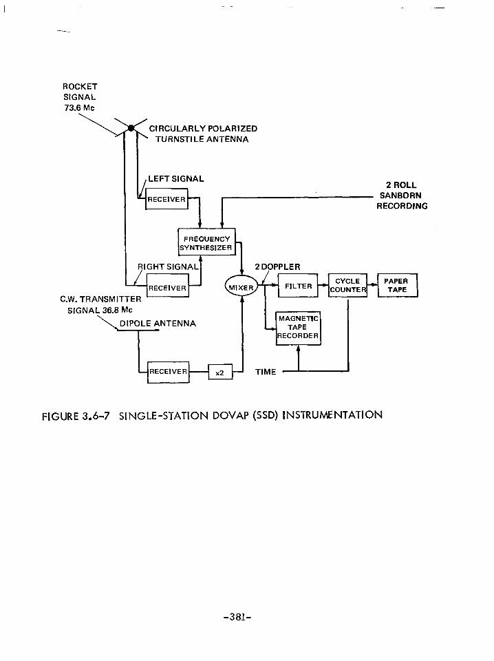
ROCKET SIGNAL 73.6 MC

CIRCULARLY POLARIZED TURNSTILE ANTENNA

LEFT SIGNAL 2 ROLL

SANBORN RECORDING

1 1 .

FREQUENCY SVNTHESIZER

4 RIGHT SIGNAL

C.W. TRANSMITTER

FILTER - CYCLE - PAPER

COUNTER TAPE

SIGNAL 36.6 MC I DIPOLE ANTENNA

TIME -

FIGURE 3.6-7 SINGLE-STATION DOVAP (SSD) INSTRUMENTATION

-381-


1


CIRCULARLY POLARIZED TURNSTILE ANTENNA

1 RECEIVER .

TIME - SANBORN

b RECORDING AGC *

FIGURE 3.6-8 CONTINUOUS-PHASE INTERFEROMETER INSTRUMENTATION

-382-

NORTH RECEIVER

WEST RECEIVER

SOUTH ?ECElVER

SSD DOPPLER RECEIVER

EAST RECEIVER

FIGURE 3.6-9 SINGLE-STATION DOVAP ANTENNA ARRAY

-383-

3.6.3 ” Basic Data Reduction

Besides the initial parameters - angles of arrival of the sound wavefront at the center of the ground-microphone array; the times of explosion of the “upper” and “lower” grenades and the position coordinates of these grenades - certain additional data must be available to facilitate the computation of temperatures and winds. These are: a measurement of temperature (within + 0.25’C) at the ground in the vicinity of the microphones; the surface-wind vector in the same area (within + 2.5 m/set); as well as standard radiosonde observations of temperature in the general area of the experiment, up to about the altitude of the lowest grenade. If, in addition to this, a measurement is available of pressure or density at the surface, profiles of pressure and density may be calculated up to the altitude of the highest grenade explosion. An exact geodetic survey of all ground-station locations (Figure 3.6-1) is also required.

The location of each microphone in relation to all others must be known within + 0.2 meters. The precision of the survey for the other (nonacoustic) ground system varies with the tracking system used, but generally the relative location of each element for each tracking system (for example, DOVAP antennas) must be known within + 0.5 meters. As the DOVAP tracking system in particular oper- ateson the principle of tracing the rocket’s trajectory back to its origin (the launcher), the rocket launcher must be included in this survey.

If a ballistic-camera system is used, an absolute survey is required in addition to the relative one mentioned above: the position of each camera must be known within about 30 seconds of latitude . An absolute time measure must also be provided (within + 0.1 set) during exposure of the star trails. For all other systems, relative timing must be provided at all recording stations, with a precision of 0.005 set over the period from launch to the time of soundwave arrival (usually 500 set) , and with a precision of 0.0005 set at the sound-ranging station only during the period of each soundwave arrival at the microphone array (usually 1 set).

The times of grenade explosions are read directly off the records of the rocket borne or ground flash-detector outputs. .Once these times are known, the grenade coordinates may be read off or interpolated from trajectory tables produced by the various tracking’ systems. If FPS-16 radar tracking is used, the trajectory can be

-384-

obtained in the form of punched cards or digital magnetic tape.

For the other tracking systems, more or less laborious manual steps will be necessary to produce a trajectory.

Direction cosines of the sound wavefront are mathematically derived from the times of arrival at each microphone. These times are read off the sound-ranging records. Since the position of each microphone is known, a plane or spherical wavefront is analytically fitted through the set of spacetime microphone coordinates.

A least-square solution for a plane wave may be derived from the arrival times and coordinates of more than three microphones. An array is shown with the wavefront at time t = Q passing through the microphones in Figure 3.6-10. Microphone 0 is chosen as the origin of the righthand Cartesian system. All coordinates and times are referenced to microphone 0, and it is assumed that the time of passage of the wavefront through microphone 0 is measured precisely. The distance r. from microphone i, to the wavefront should thus be: r. = c t. whe:e t. is the observed time of arrival of the soundwave at dicrop 9-l one i and ‘c is the speed of sound on the ground. The direction cosines for the wate normal can be obtained from a least-square bit of the wavefront tangent to all spheres r.. 1

The normal equations of the least-spuare solution are obtained from the following analytic expression for the distance d. between the plane wavefront and the surface of a sphere of radius’r. around microphone i with the coordinates (XiYiZi); di is measured Along the direction of the normal to the plane:

d, = X.a +YiP +Z iY -r 1 1 i (1)

where (i = 1,2,.. . . ,5) and a, P, Y are the direction cosines of the wave normal. The best fit for the plane wave is obtained when the sum of the squares of the distances di is a minimum, i.e. ,

,S x di’ = 8 2 di2 = 0 8a SP (2)

since a2+p2+ y =l 2

(3)

-385-

X = NORTH

FIGURE 3.6-10 PICTORIAL REPRESENTATION FOR FITTING THE WAVEFRONT

-386-

d. in equation (1) becomes a function of a , p, Y and the known co- o+dinates X., Y., Z. and r. only. Using equation (1) and summing up for all micr&ph6nes1 (i = 1?2,3. . .) , solutions are obtained for the two unknowns a and p from the two equations (equation 2), and the solution for Y from equation (3).

By solving these equations for the direction cosines, the plane wave through microphone 0 is uniquely determined, considering that the wave must travel in a downward direction. The wavefront may be more conventionally expressed in terms of elevation and azimuth angles, rather than in terms of direction cosines:

+ p =--,ee= X- arcos a a

where e is the elevation angle of the sound source and 9 the qzimuth angle counted counterclockwise from north to the direction from which the sound arrives. As a further refinement, a spherical wavefront may be fitted to the microphone coordinates Xi, Yi, Zi, r.. 1

The fitting of the wavefront is a lengthy manual computation because the number of microphones is always greater than four and the number of explosions in any firing is greater than 10. The procedure has therefore been programmed on a small digital computer (LGP-30) which can compute the wavefront for one explosion in less than one minute.

The method of calculating average temperatures and winds in a horizontal layer between the explosions Gl and G2 , is described briefly below. It can be extended to the calculation of n-l temperature and wind values between n explosions.

The soundwave traveling from grenade Gl to the microphone is displaced by the horizontal wind blowing between the level of grenade Gl and the ground. This displacement (the vector quantity vi) is proportional to the time tl that the wave spends in the medium between the grenade and the ground. The same consideration holds for the soundwave from grenade G composed of a term WT (the pro 2’

where the displacement $ is uct of w , the average horizontal-

wind vector in the layer between G and G , and T , the time the soundwave spends in this layer) an 5 a term’ v* (the displacement of the wave from G2 due to winds below Gl):

-38s

5 = ET+V* (1’) The time t the sound s

elapsing between the explosion of G2 and the arrival of rom G2 at the ground may be written as

t2= T+t+ (2’)

where t * is the time the soundwave from G ‘spends in the medium below the altitude of G1.

2

Generally, the approximation t* sin e2 = ti sin ef (3’ ) will hold, where el and e2 are the average elevation angles along the

relationships between thg v’ls and t’s soundpath from G1 and G , respectively. Because of the proportional

J* sin e 2 = v1 sin e 1 (4’ 1

The terms t calculated #

and t2 are measured quantities, and vl and$ can be rom the exact coordinates of the grenade explosions, the

temperature and wind field below G , and the angles at which the soundwaves arrive at the microphor!e array. These parameters are measured. Thus, the unknowns v*, t*, T and w can be calculated from equations (1’ -4’ ) and the average wind in the layer between G1 and G2 is determined.

After determining the wind in the layer, Snell’s law may be used to compute c, the speed.of sound in the layer between G1 and G2:

C csc e 1 +W 9

= Co csc e2 (5’ 1

where co is the speed of sound at the microphone array, and m+ is that component of the wind in the.layer which acts within the plane of the southpath trajectoryfrom G2. At the surface of the earth, the wind is assumed to be zero: e is the average zenith angle of the soundpath from G2 within ths! layer between G1 and G expressed by: 2’

case = H 1 (6’ )

CT where H is the difference in height between G and G . Hence, c can be calculated from Equations (5’ and 6’ )l. The tsmperature T

-388-

in the layer is related to c by the equation

(7’ 1

where R = universal gas constant “p/v C = ratio of specific heats of the medium between G1 and G , M = mean molecular weight of the medium. These parameters should b2e available from independent measurements, so that T can be calculated from equation (7’ ) .

An error analysis indicates that temperature errors generally are less than 1°K, and that the wind error is about 1 m/set, if the error in determining the coordinates of the grenade explosions is less than 5 meters. The accuracy of determining the temperatures and winds is limited by the random errors inherent in measuring the arrival times of the low-frequency soundwaves at the microphones. For explosions below 75 km, a time error of 2-3 milliseconds is probable, which will result in an uncertainty of the soundwave angle of about 0.1 degrees. The resulting error for temperatures in this case will generally be less than + 3’K; for wind speed and direction, the errors are about + 5 m/set and + 15O, respectively . For explosions at higher altitudes, sound arrivals at the ground may be so weak that arrival-time errors in some cases may be as large as 5 - 10 milliseconds. The resulting temperature errors may increase to about 2 lOoK, while a wind-speed error of about 1 m/set may be expected. The existence of vertical winds in the layer between G1 and G2 is not considered in these calculations, as the speeds of such winds are known to be negligible compared with the velocity of sound. Typical overlapping temperature profiles are illustrated in Figure 3.6-11.

For grenade explosions at altitudes higher than 50 or 60 km, the calculations must allow for the fact that acoustic energy at these levels propagates as a shockwave rather than a soundwave over a substantial portion of its path (finite-amplitude effect).

The highest altitude from which sound returns can be received, with present explosive charges and existing sound-ranging techniques, is about 90 km. The LGP-30 computer is used to derive temperatures and winds from the coordinates, arrival times, and explosion times. Computationally, the largest effort lies in the determination of vl and 7 which is done by ray-tracing the soundwave up to Gl and G2, re&ectively. For error estimates, it is desirable to compute one data point several times under varying input conditions; here a high-speed computer is particularly useful.

-389-

0 0 160 200 240 280

TEMPERATURE (OK)

6 MAY 1961,180O EST, WALLOPS ISLAND, VA.

160 200 240 280 TEMPERATURE (OK)

6 MAY 1961,180O EST, WALLOPS ISLAND, VA.

80

-c’60 Y

$ P 2 40

20

a 160 200 240 280

TEMPERATURE (OKI 6 JUNE 1982,2006 EST, WALLOPS ISLAND, VA.

160 200 240 280 160 200 240 280 TEMPERATURE (OK) TEMPERATURE (OKI

13 JULY 1961,1707 EST, WALLOPS ISLAND, VA. 23 MARCH 1902,lBM EST, WALLOPS ISLAND, VA.

80

E 60 /’

Y

!z W g 40.

HASP SONDE -/ /

20

280 160 200 240 TEMPERATURE (OK)

16 FEBRUARY 1961,2126 EST, WALLOPS ISLAND, VA.

20 FEBRUARY 1963,1847 EST, WALLOPS ISLAND, VA.

80

60

$ 2 40 I

2c

C

-

-

-

-

- R AC q-q---J

1 16( I 200 240 280

TEMPERATURE (OK)

(Smith)

FIGURE 3.6-l 1 ROCKET GRENADE TEMPERATURE PROFILES

Density and pressure can be calculated from the temperature profile, provided the pressure or density is known at a given level at the bottom of the temperature profile with the aid of the following relation:

In pi = In pi-l + g (hi -hi-i ) R (Ti--TiLl)

where:

R=

g=

Pi =

hi =

Ti =

and ‘i =

where:

universal gas constant

gravitational constant which is assumed to vary inversely with the wquare of the altitude

pressure at level i

altitude of level i

temperature of level i

P: A R Ti

‘i = density at level i

-391-

3.7 Ozone Sensors and Techniques.

Several techniques have been successfully employed in measuring upper atmospheric ozone concentrations. One technique utilizes the strong absorption of the ultraviolet spectrum by ozone, Another technique makes use of the reaction of ozone with a solution of potassium iodide. Others have been based on the heat of ozone decomposition, the emission of light due to the decomposition of ozone on the surface of a chemiluminescent disk, and radiactivity re:Eased when ozone is passed over a quinol clathrate containing Kr .

3.7.1 Spectrometric Technique.

The spectrometric determination of ozone has been the basis ,of a number of different instruments. These instruments, based on the fact that ozone absorbs strongly in the ultraviolet part of the spectrum, measure the amount of ozone between the source of illumination, usually the sun, and the receiving sonde. Various investigators have used different absorption bands in their instruments. The usual practice is to measure the intensity of the solar spectrum in two or more bands, with one band in the region where ozone absorbs moder- ately well and another band in a region of no ozone absorption. The amount of ozone in the light path is a function of the light intensities in these bands, and the concentration is determined from the rate of change with height of the total amount of ozone.

There is one commercially available ozonesonde based upon the spectrographic technique. It is known as the Paetzold Ozonesonde and is manufactured by Springer, A. G. in Germany. This instrument was widely used during the I .G .Y. This ozonesonde is an optical measuring type of apparatus making use of the light absorption of ozone in the ultraviolet to ‘determine ozone concentrations in the upper atmosphere. The measurement by the sonde is the total amount of ozone between the instrument and the sun, and ozone concentration is determined by the change in the total ozone measurement with a change in altitude of the sonde. The intensities of two ultraviolet regions of the solar spectrum are measured, one of which is moder- ately absorbed by ozone. The telemetered signal from the sonde consists of the light intensities in these two ultraviolet bands, the zero and calibration voltages, and a pressure measurement. Sunlight enters the instrument through a magnesium oxide-lined quartz ball located on top of the instrument and illuminates the area of an aperture at the base of the globe. A motor drive alternately places one

-39 2-

II -. -- .-

of four surfaces in the aperture. These are two opaque stops and two filters, a 3100-A ultraviolet filter and a 3750-A blue filter. The ratio of the filtered light intensities is indicative of the total ozone. Light passing through either filter in the aperture is chopped and then falls on a photocell producing an AC signal. This signal is amplified and rectified and then indicates on a galvanometer. The indicator arm of the galvanometer moves across a rotating drum which contains con- tacts on its surface such that the position of the arm is translated into a Morse-code signal. The signal is a pulsed 600 cps tone. The drum makes one revolution for each of the four positions of the filter wheel. Revolutions during the two opaque positions are used to transmit a zero-set and a battery-checking voltage. During each rotation of the drum two signals are sent, one from’the galvanometer circuit and one from an aneroid pressure transmitter. On the receiving end, timing marks are included in the record. These are needed so that corrections for solar angle can be included in the evaluation.

The data reduction includes the following steps. First a time- altitude evaluation is made to determine the levels for ozone evaluation. Then a set of smoothed values of the secant of the solar zenith angle is carefully prepared. When the data have been smoothed, the ozone calculations can be made.

Data evaluation starts with an estimate of the amount of ozone between the sonde and the sun at the maximum altitude of the sounding, and then determining increments downward in layers of 1 or 2 km. Smoothed values of the recorded data are used. Provided the sounding reaches 20 km or more, interference from scattered skylight can be neglected in the initial calculation. The local ozone concentration is determined as a derivative of the total ozone concentration with corrections for such factors as the rate of change in the angle of the sun. The large number of terms in the equations used to evaluate the data tend to magnify any local fictitious fluctuations in the smoothed data. Figure 3.7-l presents a typical ozone profile derived from photometer data. The probability accuracy of the total ozone amount indicated is no better than 5 percent. The instrument is easy to operate in the field with minimum checkout required,

3.7.2 Chemical Techniques.

Chemical determinations of ozone concentrations have been based upon the reaction of ozone with a solution of potassium iodide. One sonde determines ozone concentration using an automatic

-393-

- 2630A -- 2620A me-- 268OA

10’0 10 1’

NUMBER DENSITY ( MOLECULES/CM3)

FIGURE 3.7-l OZONE DENSITIES AS A FUNCTION OF ALTITUDE AS COMPUTED FROM PHOTOMETER DATA

titration approach. The chemical reagent techniques do not, however, appear to be applicable to meteorological rocket systems.

3.7.3 Chemiluminescent Technique.

A most promising technique is based on the amount of light e- mitted by a chemiluminescent disk as a result of the decomposition of ozone on the surface. The light due to the ozone decomposition is measured by a photomultiplier tube, and i.ts output can be calibrated in terms of the ozone concentration. This technique can be used with standard radiosonde equipment. This ozonesonde will provide a continuous measurement of the ozone content in the atmosphere during a parachute descent. Measurements can be obtained from altitudes of about 65 kilometers down to and including the ozone peak in the vicinity of 20 kilometers. Previous ozonesondes have taken measurements only at a relatively few discrete points. A system which has been brought to the flight-test stage of development uses an active ozone-chemiluminescent material (rhodamine B absorbed on fine silica gel). The luminance of the material is a function of the amount of ozone present in the gas sampled and pressure of the gas. The luminance is measured by a photomultplier tube. The gas from the free atmosphere is drawn across the detector disk into an evacuated chamber through a small tube which regulates the flow. The pressure differential is maintained by the increasing atmospheric pressure as the ozonesonde descends through the atmosphere. This basically simple device is attached to suitable telemetry which re- ports the signal from the photomultiplier tube to the ground station. Thus, the sampling system will have no moving parts, use no power, and operate continuously.

A balloon-borne chemiluminescent ozonesonde in current use is 5 x 5 x 6 inches and weighs 1100 gms. It uses 0.4 W of power. Considering Figure 3.7- 2, ambient air is drawn in at A, passes between the chemiluminescent disc B and the face of the photomultiplier tube, C. The air flow is maintained by a breather pump composed of a fixed dish, D, and a moving disc, E, sealed together by the rubber diaphragm, F. The lever, G, riding on a cam, H, operates the pump to bring in 100 ml of air in a 15-second intake stroke. Dur- ing this intake the luminescent reading is taken. The ozone reaction is observed to be complete and no signal occurs on the return exhaust stroke which flushes the chamber. Cam H turns at l/2-rpm providing three ozone measurements and one reading of the “dark

. I’ current”. when air aspiration does not occur. Amplifiers I and J

-395-

G

t

D

A 4 ’

-

1, C WI‘-J-

1’ ‘B

Note: A, air intake; B, chemiluminescent disc; C, photomultiplier tube (znt 6467); D, breather pump, outside dish; E, breather pump, inside dish; F, rubber sheet; G, lever; H, cam, 0.5 rpm; I, amplifier; J, audio- frequency modulator, 40 to 200 cps, controlled by ozone; K, radiosonde transmitter; L, radiosonde modulator, control led by pressure, temperature, and humidity; M, switch, operated by cam drive every I5 seconds.

FIGURE 3.7-2 SCHEMATIC DIAGRAM OF DRY CHEMILUMINESCENT OZONESONDE

-396-

prepare the signal of the photomultiplier for transmission by the radiosonde transmitter K. The switch, M, connects a standard radiosonde sensor unit to the transmitter in between ozone readings. The telemetry is a a-minute sequence consisting of three 15-.second ozone transmissions and one 15-second photomultiplier zero reference with these four readings being separated by 15-second transmissions from the radiosonde package.

Although the chemiluminescent technique can readily be applied to meteorological rockets, the determination of the air sample size or throughput is a problem. Mr. Wendell Smith at NASA-GSFC. utilizes a rather large evacuated ballast tank into which a calculated rate of air flows during sonde descent with a parachute. He currently uses the Nike-Cajun vehicle. Mr. Jagis Randhawa uses the smaller Arcas vehicle with a considerably smaller ballast volume as indicated in Figure 3.7-3. Typical ozone profiles derived from soundings made with this system at Tartagal, Argentina are presented in Figures 3.7-4 and 3.7-5.

3.7.4 Miscellaneous Techniques

Another reaction-effect ozone measuring technique is the Armour Research Foundation method in which the heat of ozone decomposition is measured and expressed as a function of the ozone concentration. In this instrument the sensor cell is built around a thermistor detector. In the sensor cell the decomposition rate of the ozone is greatly enhanced by coating the thermistor with a catalyst. Hopcalite, a synthetic mixture of copper and manganese oxides, is used as the catalyst in this unit.

A radioactive clathrate technique has been developed by Tracerlab. In this system ozone can be measured by passing the gas stream over a quinol clathrate containing Kr38 and measuring the amount of radio- activity released.

-397-

Sensor Substrate

Sensitive Face

7Photomultiplier

Power Pack, Neon Lamps for Regulatior

Hermetic Connector

Cable

I Air Entry (Shock mounting,

Modulator Path insulation, and light shielding)

(Randhawa)

FIGURE 3.7-3 SCHEMATIC DIAGRAM OF ROCKET-BORNE OZONESONDE

-398-

-

65 I-- 60 -- 55 a-

3 5o

G I- F 45 I- a

40 ‘-

35 - 1 3 5 7

Ozone (Cm/Km) x 10m3

FIGURE 3.74 Vertical distribution of ozone at Tartagal, Argentia, on Noveher 11, 1966, 1106 local time

10

0

i i I I

1 1 5 5 9 9 13 13 17 17 21 21 25 25 29 29

OZONE ( Cm/Km) x 10-3

FIGURE 3.7-5 Vertical distribution of ozone at Tartagal, Argentia on Nover&er 12, 1966, 1031 local time. Dashed line is the data from Heritq and Borden (1965).

3.8 Water Vapor Measurement Techniques

Measurement of water vapor has been included in routine atmospheric soundings for many years, but there has been general dissatisfaction with the techniques used. This dissatisfaction had led to considerable effort to develop a wide variety of different measuring techniques.

Available observation techniques fall into several types: mechanical elements, such as hair and goldbeater’s skin; electric elements which include the present standard lithium chloride and carbon strip sensors; dew point or frost point instruments; spectrographic techniques; and refractive index measuring instruments.

3.8.1 Mechanical Hygrometers

Certain materials undergo a dimensional change with changes in relative humidity. Hair and various animal membranes have been used as hygrometers for many years. Some early U. S. upper air sounding instruments incorporated sensors of this type, and sensors of this type are still used in various foreign atmospheric sounding instruments. Improvements in these sensors, such as are incorporated in Europe in the folled or Frankenberger hair hygrometer, have improved the operating characteristics of these elements, but they still do not equal currently available electric hygrometers. In addition, their mode of operation does not permit convenient insertion into the United States audio-modulated transmitting circuit.

3.8.2 Electric Hygrometers

The standard U.S. radiosonde hygrometer is an electrolytic strip,in which the hygroscopic lithium chloride coating’s resistance decreases with increased relative humidity. This element has a high lag coefficient at low temperatures and is considered useless in the higher levels reached by the present balloonsondes. In addition, if the element picks up liquid water droplets it is subject to a washout effect, and in a direct current circuit specific care must be taken to protect the element from polarization effects.

A carbon film strip has recently been adopted by some meteorological agencies as a standard hygrometer element. In this element the resistance increases as the humidity increases. This carbon strip has no washout problem, has somewhat faster response, and shows less of a temperature effect than the lithium chloride element;

-4oo-

but it has other problems. Uniform production of the carbon element is apparently difficult, and the elements have shown a sensitivity to their storage environment.

In addition to lithium chloride and carbon, a number of other strip coatings have been studied as electric hygrometers. These include plastic resins, aluminum oxide, and barium fluoride, but no field trail data have been obtained on these elements. Early laboratory studies of the barium fluoride element at the sational Bureau of Standards were particularly encouraging, but the element was found to deteriorate rapidly in storage. When this characteristic could not be overcome, further development of this element was abandoned.

3.8.3 Dew Point Techniques

Dew point, or frost point techniques, have been used to determine humidity when more precise measurements were needed than could be obtained with the electric element and where more complex equipment could be used. In the dew point technique, an air stream impinges against a small thermostated mirrored surface. The mirror is cooled until dew or frost forms, and a stable dew formation is maintained by controlling the mirror temperature through the use of a sensing and control circuit. The temperature of the mirrored surface is taken as the dew point of the air stream. The optical control system needed to sense the dew formation, and the mirror refrigera- tion system, have required that these dew point measurement units be relatively larger; however, recent improvements have aimed at reducing the size of this equipment. These developments have included Peltier-effect cooling and beta gaging techniques to measure the frost deposit. These improvements are aimed at permitting dew point instruments to be used in rocketsonde measurements.

3.8.4 Spectrographic Techniques

Water vapor measurements have been made using the infrared absorption bands of water and spectrographic techniques. One method uses the sun as a source and the changes in water vapor concentration between the ascending instrument and ‘the sun is inferred from changes observed in the infrared water vapor spectra. ‘This instrumentation requires sun-following techniques and complex equipment. The data are limited by the fact that water vapor at any particular level must be estimated from the rate of change of the observed value for the whole path between the instrument and the sun.

-401-

These spectrographic techniques have been particularly useful in rocket probe studies to very high altitudes.

Infrared techniques with a self-contained illumination source have been designed and; built for surface use and have been postulated for aircraft soundings. Size, complexity, and sensitivity are interrelated and are not favorable for a ready adaption of IR techniques to atmospheric sounding programs.

3.8.5 Miscellaneous Techniques

There are two other techniques used for atmospheric humidity determinations which do not fit convenientIy into the above categories. These are a radiation absorbing instrument using the 1215-A Lyman- alpha line of hydrogen, and instruments using changes in the microwave refractive index to determine the relative humidity of the atmosphere.

The Lyman-alpha hygrometer uses a small glowtube containing hydrogen which radiates in the Lyman-alpha wavelength. The radiation traverses a 4-cm. measuring path and enters a nitric oxide gas photoionization chamber. Where other parameters are fixed, the resulting ionization current is dependent on the intensity of the radiation, which in turn is determined by the water vapor density’ in the traversed path. Other atmospheric gases have negligible effects. This instrument has been tested in aircraft sounding operations and may be satisfactory for other potential types of sounding techniques.

Microwave hygrometers are based upon the fact that a cavity resonater in microwave frequencies can be made sensitive to the contribution which water vapor makes in the refractive index of atmospheric air. Several types of refractometers have been developed and, while the equipment is fairly complex, the instrument may be a useful research tool to determine moisture content of the high atmosphere, providing sufficient sensitivity can be attained by the apparatus.

-402-

3.9 Atmospheric Composition

The atmosphere below approximately 90-100 km is well mixed and can be treated, in terms of the hydrostatic equation, as one gas with a molecular weight of about 29. At about 100 km, the number density of the atmosphere becomes small enough so that the mean free path becomes long, and diffusion processes begin to occur. In addition, dissociation produces atomic oxygen (mass 16) to considerable quantity and the mean molecular mass of the atmosphere drops sharply. This drop has a profound effect of the density and temperature structure. There are also many ion species present and in order to balance the electrical equation of the atmosphere, an inventory of the ions and their concentration is needed.

At NRL, the Bennet r-f mass spectrometer and magnetic spectrometers are used to study the low ionosphere and also the relative concentrations of H+ , He+ and O+ to altitudes where upward diffusion of the light constituents become appreciable.

The Bennet radio-frequency mass spectrometer can be used to obtain spectra of atmospheric composition above 100 kilometers. Ions are formed by the bombardment of air molecules with 45-volt electrons in the ion cage. These ions, drawn out and collimated by grids, are accelerated by a negative sweep potential into the analyzer section. This negative sweep potential is modified by a small constant-bias voltage applied to grids. Ions not receiving the maximum incremental energy per state in the analyzer are turned back by a positive stopping potential applied a grid. The desired ions have sufficient energy to overcome this positive potential and reach the collector.

The mass of the ions arriving in the collecting assembly can be represented as follows:

M = 0.266V

s2f2

where

M= mass in atomic mass units

S = spacing between grids of analyzer section in centimeters

f = frequency in megacycles

-403-

V= potential in volts

Variation of either frequency or voltage will sweep the tube over a range of atomic mass units. The sweep rate is limited to the frequency response of the telemetering system in use. With a radio- frequency of 3.9 megacycles and a sweep varying between -250 and -25 volt, the instrument will cover the range between 48 and 5 atomic mass units.

-404-

3.10 Electron Density

3.10.1 General

The ionosphere consists of a partially ionized plasma with an electron density varying from as little as 1 cmB3 at altitudes of 50 km above the earth’s surface to as much as lo7 cm -3 at about 300-km altitude. Being electrically neutral, the plasma contains equal numbers of electrons and positive ions. The electrically conducting properties of this plasma produce effects important at both radio frequencies and direct current.

The conductivity is very strongly affected by the magnetic field of the earth, which causes the electrons to gyrate around the field lines with a frequency of about 1.4 MHz.

A further complication is introduced by the effects of collisions of electrons with the neutral atmosphere. Since the collision frequency is proportional to the density of the neutral gas, it varies through the ionosphere from about 100 to lo8 set-l, the latter collision rate effectively inhibiting electron motion at all but the highest radio frequencies.

Sounding rockets have proved their worth for ionospheric investigation, as is evidenced by the increasing numbers fired in recent years. Rocket experiments are extremely suitable for studying propagation of radio waves into the ionosphere. A radio wave propagated from the ground undergoes change in both amplitude and polarization, due to the changing properties of the ionospheric plasma. By placing a radio receiver in a rocket, one may take a vertical section of the radio-propagation path and accurately measure the detailed changes in the properties of the signal with altitude. By this means the successive absorption, refraction, and reflection of as many as three different modes of ionospheric propagation may be traced at a single frequency, and the electron densities may be easily measured from as low as 10 up to lo5 cm -3.

Ionosonde measurements had shown that three distinct layers were present: the D-layer, having a maximum electron density of about lo4 cm -3 at 80 km, the E-layer, having a maximum density of about lo5 cm -3 at 120 km, and the F2-layer, having a maximum density of lo6 to lo7 cm -3 at about 300 km. A fourth, the F-l layer, was known to occur sometimes at an altitude of about 180 km.

-405-

To maintain electrical neutrality in the plasma, each electron must be accompanied by a positive ion. Rocket and satellite measurements have shown that the positive ions in the D-, E-, and F-l layers are primarily molecular oxygen and nitric oxide and in the F-2 layer are primarily atomic oxygen, while m.uch of the topside ionosphere above about 500 km consists of electrons and protons (atomic hydrogen ions). In addition, many minor constituents are present and have important chemical effects.

The properties of the ionosphere vary markedly with position on the earth’s surface. Certain regions have a quite singular behavior. For example, the region near the magnetic equator, where the magnetic field of the earth prevents the electrons from diffusing vertically, differs radically from temperate latitudes, and these a- gain differ from cne polar regions.

The Sporadic E-layer is an anomalous enhancement of the E- layer ionization, extending over about a loo-km radius horizontally and having the ability to reflect radio signals of much higher frequency than is normally the case. At temperate latitudes, it is believed that electrodynamic effects, produced by upper-atmosphere winds and ionization arising from meteoric atoms, may play a role either separately or in combination. Another such sporadic phenomenon is the occurrence of enhanced D-region ionization on some winter days, seemingly associated with increased temperatures in the stratophere, although the casual relation between these phenomena is unclear.

In the ionosphere, ultraviolet radiation from the sun dissoci- ates molecular oxygen into atomic oxygen, a very reactive gas, which in turn generates ozone and oxides of nitrogen in the 60-100 km altitude range. Above 100 km the atomospheric density is low enough that the atomic oxygen has a very long lifetime, and becomes the predominant constituent of the atmosphere above 200 km.

Shorter wavelength ultraviolet light has the ability to ionize the atmosphere, i. e. , strip an electron from any gas ‘particle. Each wavelength has a certain photon energy associated with it; the excess of this energy over that required to ionize the particle appears usually as kinetic energy of the generated photoelectron. Photoelectron energies of 10 electron volts are typical in the F-layer.

A number of electron density and electron temperature measurement techniques are currently employed with sounding rocket flights.

-406-

A review is made of the various techniques in the following sections.

3.10.2 Radio Propagation Techniques

Propagation systems are dependent upon the interaction of ionospheric plasma with the propagation of electromagnetic radiation between a moving vehicle and ground stations. Measurements are made of the amplitude, phase or polarization of the wave. The electron density is determined from these measurements by use of the known relations for wave propagation in a magnetoionic medium. One advantage of this technique over other methods of direct measurement of electron density is that the propagation path usually passes through a region of the ionosphere not yet disturbed by the passage of the rocket, except for the insignificant path length in the immediate vicinity of the rocket. In interpreting the data, however, it is necessary to assume that the ionosphere is horizontally stratified, because the intersection of the ray path with a fixed horizontal plane will, in general, move as the rocket ascends. Vehicle motion and changes in path aspect have a larqe influence on the results. This effect is much more serious on the descent of the rocket than on ascent.

Radio propagation systems that have been developed are as follows:

a) Dispersive Doppler Technique - This technique is applicable in the E-region and where collision frequencies are small. Its use depends on the doppler frequency shift from a moving vehicle on the local index of refraction.. The radio wave is split into two modes, ordinary and extraordinary, and the beat frequency of each mode becomes the basic quantity measured at the ground. In the analysis of data, use is made of the usually undesirable rocket spin. The dispersive doppler technique is the best tested method available and yields excellent accuracy compared to ionosondes data. Above 100 km this method will give the same results as langmuir probes, while below 100 km, the results give a more reliable estimate of electron density than found with the langmuir probe.

b) Differential Absorption and Phase- This method utilizes measurements of signal amplitude and relative phase of a received signal. It can be used in regions of much lower electron densities where difficulties arise for the dispersive doppler technique. The technique is simple to carry out, but does not determine both the electron density and collision frequency.

-407-

c) LF Field Strength Measurements - Use is made here of the frequency in the LF range, being highly absorbed in the D-region during the day. It is capable of giving sensitive measurements of low lying ionization.

d) Pulse Delay - The influence of the ionospheric plasma on the group velocity of an HF pulse is employed to determine plasma concentrations.

3.10.3 Lanqmuir Probe Technique

An electrode is inserted into the plasma and the current to it is determined as a function of the electrode potential. From the resulting current-voltage characteristic the electron energy distribution and the electron density are obtained. When the, electrode is exactly at the potential of the plasma, the electron current to it is determined by the random thermal motions of the electrons in the gas.

Langmuir probes of many different configurations have been successfully used in ionospheric measurements. The most ideal application is in the E-Region of the ionosphere. The technique is based on the measurement of the flux in charges to a conducting surface. For sounding rocket applications a spherical geometry probe is preferred. This experimental method is relatively simple, but difficult to justify, experimentally. Below 90 km the theory behind this’ method is invalid because the mean free path is not large compared with Debye length and negative ions are present in significant numbers. The basic weakness is poor time resolution. Also, interactions between the vehicle and the ionosphere must be under- stood. Data analysis procedures are usually tedious but straight forward.

3.10.4 Resonance Probe Technique

In Japan, many resonance probes have been flown with the Kappa rockets with successful results. The present resonance probe has many mechanical parts to change the frequency, rf voltage and DC voltages. However, the improvement of this system to a new electronic one is now in progress. A new type of resonance probe, therefore, will be used in the future.

When a high frequency voltage is supplied to plasma, electrons in the plasma move easily corresponding to that high frequency. These

-408-

excited electrons come into a sheath around,a sounding probe, and make increase of DC probe current. The characteristic curve is, therefore, shifted. The plasma electrons have a proper frequency named plasma frequency. Therefore, the amount of shift of probe characteristic varies remarkably according to the supplied frequency. Quali- tatively speaking, the current increase at constant probe voltage, or the voltage shift at constant probe current in the frequency range, being fairly lower than plasma frequency, is rather constant and is determined by the electron temperature of the plasma. The deviation becomes large when the supplied frequency approaches to the plasma frequency; and becomes maximum when the supplied frequency just coincides with the plasma frequency. Then, it decreases to zero according to the increase of supplied frequency exceeding the plasma frequency. An electron density is determined by the frequency of the resonance peak which is found from the deviation of the characteristic probe current. Reduction of data for this technique is very simple.

3.10.5 Standing Wave Impedance Probe Technique

The standing wave impedance probe determines the antenna impedance by measuring voltages existing on a section of an artificial transmission line connecting low level rf oscillators to the antenna. The telemetering of these voltages to the ground allows the standing wave existing on the antenna feed line to be recreated. Once the standing wave is known, the terminating impedance on the line is uniquely defined. The frequency range of these measurements is dic- tated by the range of plasma frequencies to be measured and is between 1 and 15 MC.

This technique involves the determination of the antenna impedance by measuring voltages existing on a section of an artificial transmission line connecting low level rf oscillators to the antenna. A weak point is the need of accurate knowledge of the free space impedance which cannot be recalibrated easily during flight, resulting in the need for a careful pre-flight calibration. Resonable information on electron concentration can be obtained from impedance probes. While absolute accuracies are questionable, relative accuracy is excellent. Data handling and electronic instrumentation are relatively simple.

3.10.6 Mobility Spectrometer Technique

A new type of ion mobility spectrometer has been developed

-409-

for direct measurements of the mobility spectrum of small atmospheric ions in the altitude range between 30 km and 80 km. The instrument used in wind tunnel experiments consists essentially of 16 concentric capacitors assembled in series and, at the same time, electrically insulated from each other.

A simplified schematic planar configuration of this instrument is shown in Figure 3.10-l. It consists of a plate capacitor to which a sinusoidal voltage is applied. At the entrance of this capacitor an electrical filter is inserted through which ions can enter only through a small section of the filter (“gate”).

If a sinusoidal voltage (V = Vo sin wt ) is applied between the condenser plates, the x component of the path of the ions entering through the gate is:

-k V, coswt+A =-- ' dw

where :

A= determined mainly by the value of voltage V at the time the ion enters the instrument

k= ion mobility

vo= maximum amplitude of applied ac voltage

d= separation of the condenser plates

&I= frequency of the applied ac voltage

The y component of the ion path is:

y= ut

where:

U= velocity of the air flow

(2)

The electrons, because of their very high velocity, will impinge on the receiving electrode, and the ions will not. The result will be a current i that will be proportional to the number of electrons. If Vo is increased, the amplitude of the ions will also be great enough

-4lO-

i

ELECTRON PATH

-ION GATE

-ION FENCE

DRIVING ELECTRODE

IONS AND ELECTRONS ENTER ONLY THROUGH ION GATE ION FENCE: NO ELECTRON OR ION CAN PASS AT ANY TIME

FIGURE 3.10-l SCHEMATIC OF BASIC PRINCIPLE TO MEASURE ELECTRON AND ION DENSITY

-4ll-

to impinge on the electrode, in which case, the current i will be proportional to the electron plus ion concentration.

The current i flowing to the measuring electrode is given by:

i=mFve T

T (3)

where:

M= concentration of electron and/or ions impinging on the measuring electrode

F= surface area of the slit (ion gate) through which the electrons and ions enter the instrument

v= average velocity of the air passing through the ion gate

e= elemental charge

7/T fraction of time for which ion gate is open ( T = effective time during which ,ion gate is open: T = period of ac driving voltage).

The success of in situ measurements depends on the knowledge of the flow velocity of the air mass and on whether or not laminar flow prevails throughout the measuring region of the instrument.

3.10.7 Rocket Desiqn

A payload of 5-20 lb represents adequate capability for a majority of experimental systems. Costs for the rocket can be low and the means of launch, simple and inexpensive.

-412-

3.11 Solar and Terrestrial Radiation Flux Sensors

Neither solar nor terrestrial radiation flux measurements have been common in upper air meteorological studies, and there has been relatively little instrumental development of specific sensors for radiation profile measurements. The available sensors for upper air studies are patterned closely after sensors used in ground level radiation measurements. There are two general classes of sensors: .radiometers typified by an absorbing black surface and a means of measuring its temperature, and spectrophotometers measuring radiation intensity either as a function of wavelength or in specific spectral bands.

3.11.1 Radiometers

The most frequently used radiometer design for profile measurements is the flat plate in which either upward or downward radiation flux is measured by properly oriented surfaces, and net radiation at the level of the instrument is determined from the difference between an upward and a downward-facing sensor.

Another radiometer design which has been used in a number of vertical sounding studies is termed the “black ball. ” It consists of thermistor in the center of a 6-inch diameter blackened dodecahedron constructed of balsa wood and black paper. Another larger dodecahedron covered with infrared transparent Mylar surrounds the first and reduces convection errors. In this radiation sensor the thermistor indicates a temperature which is representative of the total infrared flux striking the black ball without differentiating the direction of the source of the radiation. There have been some questions raised about the relation of black ball temperatures to the radiational heating of the atmosphere.

In all the radiometer designs the indicated temperature is dependent not only on the radiation but also on heat conduction to other parts of the apparatus and convection losses to the air. Various designs have been used to eliminate errors from these sources. Careful insulation usually takes care of the conduction losses. Convection problems have been approached either by enclosing the element in a sealed container with transparent windows for exposure to the radiation (such as the Mylar dodecahedron around the black ball) or by adding heat to the element in such a way that the radiation temperature could be determined independently of the heat and convective losses.

-413-

3.11.2 Spectrometers

Some studies have been carried out in which only certain parts of the spectra were measured. The meteorological measurements which have been in this category have usually been solar intensity and the albedo or the reflective capacity of the earth and lower layers. of the atmosphere in the range of visible light. Studies of specific absorption bands in the atmosphere have also been made. This has been done usually in order to determine the concentrations of the absorbing materials such as ozone or water vapor, and so these studies are not primarily radiation studies.

Radiation profile measurement techniques are currently limited to balloonsonde radiometers in which radiometer temperatures are transmitted by the sonde and to fairly complex spectrophotometer studies with either balloon-borne or rocket probe instruments. Both types of studies have been carried out on a research basis and there has not been much standardization between individual research groups. There is one commercial source in Germany of radiation sonde and albedo sonde units for balloon observations but details of their performance are not available. The general paucity of radiation sounding instruments seems to reflect the fact that there has been relatively little support of the work in this field. No radiation measurements using a rocketsonde have been reported, and there are no references to instruments which are designed for this purpose.

Since the basic temperature sensors used in the radiometers are capable of giving very accurate results, the performance of the various designs will be a direct function of the degree with which the design solves problems such as convection loss, conduction, lag, etc.

-414-

3.12 Miscellaneous Density Measurement Techniques

3.12.1 Spinning Wire Densitometer

A rather unique method to obtain high altitude density measurements has been studied by Minneapolis Honeywell, Inc. under an AFCRL contract. Like the falling sphere method, this technique measures the decelerating effect of atmospheric drag on a structure to determine ambient density, In this case, however, the effect is not measured in the ‘fall rate deceleration. Instead, the effect is measured in the angular deceleration of the spin rate, which is monitored by telemetry instrumentation.

The payload, consisting of a 5 or 6-inch long center body, 1.5- inches in diameter, contains a battery, transmitter and a rotation sensor. Thin wires 5-7 mil by 14 inches long are mounted around the center body. During ascent the payload is spun by an electric motor to approximately 10,000 rpm and released at apogees between 120 and 130 kilometers. A photo-optical or magnetometer sensor indicates the period of rotation, which increases as the spin rate deteriorates. The consecutive, minute changes in the period of rotation provide highly accurate measurements of the decelleration effects. An example of the spin rate deterioration is presented in Figure 3.12-l.

Since changes in mass, weight or geometry do not take place during descent, standard fall rate tables can be used to establish time- altitude coordinates during descent. Therefore, radar is not required to track the payload after apogee separation. Radar could possibly be completely eliminated if reliable trajectories were established.

Although several flights have been made, test results were not obtained due to telemetry and tracking failures. While this payload is rather simple and inexpensive, computer reduction of the data would be necessary . This method may offer greater accuracy than the falling sphere method since changes in the period of rotation are very precise. However, wind effects and attitude misalignment may inflict inaccuracies in this device so further study may be required before a substantially reliable technique is developed.

3.12.2 Radiation Absorption.

The radiation absorption technique of measuring upper atmospheric density makes use of a photocell which is sensitive to a single spectral line. The radiation to which the photocell is sensitive is strongly

-415-

80

60

Spin Rate (RPM)

FIGURE 3.12-1 SPIN RATE DETERIORATION

OF THE SPINNING WIRE DENSITOMETER

-416-

absorbed by the air between the rocket and the light source, usually the sun.

When the rocket is in the lower atmosphere there is little photocell response because of the absorption of radiation by the air overhead. But as the rocket rises to sufficiently high altitudes (95 km), the detector is subjected to full sunlight. The precession of the rocket causes amplitude variations in the signal as shown in Figure 3.12-2.

Once the absorption coefficient of air for the radiation is known, and a correction for the aspect angle (between the detector and a direct line to the sun) has been determined, the density of air between the rocket and the sun can be determined. The rate of change of overhead air is a direct measure of atmospheric density.

The absorption method of measuring atmospheric density is basically the application of calorimetry to the atmospheric structure problem. In classical calorimetry the amount of a colored chemical substance in an unknown solution is determined by placing the unknown solution in an absorption cell of adjustable depth and by varying the depth until the color of the unknown matches that of a standard absorbing solution. Then, provided the absorption coefficients are independent of concentration, the concentration , c, times the cell depth , d, of the unknown is equal to the csds product for the standard. Another approach to calorimetry is the photometric measurement of attenuation of light produced in an absorbing solution. For monochromatic light, the intensity of light traversing a column of solution is given by Beer’s law l=loeBkcd wh ere 1, is the light measured with no solution in the absorbing column, c is the concentration, d the column depth, and k is the absorption coefficient for the material at unity concentration. The variation of 1 with depth thus determines the concentration of the desired colored material.

The photometric measurement of light attenuation in the atmosphere is directly applicable to sounding rocket techniques. Nature has provided a most convenient and relatively stable light source for this measurement, the sun. The flight trajectory of a rocket through the atmosphere automatically provides the needed variation of absorbing path d. Conveniently, in the region below the E region, the atmosphere is well mixed and of constant composition as far as major constituents are concerned; hence, the measurement of the density of one constituent is equivalent to measuring the total density. In addition, since the density decreases rapidly with height, relatively modest altitudes are needed for the attainment of effectively zero

-417-

I

85 KM 90 KM --------------------___c______

95 lcL..----x---, ---------- --

zLL.k?~M---x--~--M2~~~A

110 KM ----------------------A---

i&L----i.lL,----uaxM

--

150 KM -------------------- -.

- 155 KM -------------------------- ---

-0 KM

\/ 165 KM v ---------m---------P ----

FIGURE 3.12-2 Lyman Alpha signals from Aerobee 35 Flight: From a section of telemetering record obtained in Aerobee NRL 35. The telemetering record shows the ionization current passed by a far U.V. photo-ionization chamber as a function of time. The photo-ionization current produces a negative deflection of the telemetering trace. The vertical lines are half second timing markers. The peaks in ionization current occur when the photo-ionization chamber looks toward the sun. The lack of response below 90 km is due to air absorption of the incident ultraviolet radiation. The minimum on response at 150 km is caused by rocket procession which at this time causes the photo-ionization chamber to look “above” the sun at a large angle. The detector is responding to Lyman x radiation from the sun.

-418-

I --.--~

optical depths for several useful radiation bands: as a result it is possible to measure both density and total over-head air mass.

To carry out a calorimetric measurement of atmospheric density one must carry out a photometric measurement in a region of the spectrum where air is absorbent. Most of these optical measurements have used the sun as the light source and have been carried out in the ultraviolet and soft X-ray portions of the solar spectrum. In the soft x-ray region and the vacuum ultraviolet below 900A,; N, 0, N2 an; 02 all absorb radiation; in the vacuum ultraviolet from 1000 to 2000 A, absorption is almost exclusively due to 02 and various minor constituents such as H20 and 03. The measurements that were made in the past have been by-product results of programs to measure the spectral distribution of solar emission. They have utilized two types of radiation measurements. One method makes use of spectrograph dispersal system and either photographic or photoelectric recording. The spectrum at one altitude is compared with that at a higher altitude, and the amount of absorbing matter between them is computed. Such spectrograms provide the first direct measurement of the altitude distribution of ozone in the atmosphere. The method is a powerful one since each portion of the spectrum has different absorption coefficients, all of which can be utilized in interpreting the results. The method is not suitable for synoptic measurements since it generally requires complex instrumentation, including a solar pointing control and considerable data analysis.

The other method involves use of narrow band photometers. This method is practical for synoptic measurements since the instrumentation is simple and lends itself to the direct calculation of either density or an overhead air mass in a previously chosen range. The method consists of mounting one or more standarized narrow-band X-ray or ultraviolet photometers looking out from a rocket. The response of such a photometer is shown in Figure 3.12-3. A photocell sensitive to visible light is also flown to measure how closely the photometer looks to the sun throughout the flight. This per-mist correction of the photometer response for aspect; that is, for the directness of the view toward the sun. Finally, the method calls for an accurate measurement of rocket altitude. The basic measurement consists of a determination of the altitude at which the photometer response, 1: of its response above the atmosphere (response at peak for adeqstely high flight). Since the reduction of the incident light intensity to & requires the same fixed slant air mass,always between the standard detector and the sun, a correction for the elevation angle of the sun gives the residual over-

-419-

8

6

Wave1 eng th (Angstroms)

FIGURE 3.12-3 SPECTRAL SENSITIVI-IY CURVE OF A PHOTOMETER DETECTOR used to measure density in E region. The detector is a Geiger counter with a thin plastic window.

-420-

head air mass. Alternatively, the rate of change of the detector response with altitude gives a direct measure of density.

The optical method has some advantages over other rocket methods of measuring density. It is not nearly as affected by rocket outgassing, since it utilizes the whole column of air between the sun and rocket in the measurement. Secondly, each photometer does not require absolute calibration, as do most pressure gages, since the readings at peak are compared with those at lower altitude. It is only necessary that the relative spectral responses be reproducible from detector to detector. Finally the aspects problem is no more difficult than that for internally housed pressure gages. When densities are measured by absorption methods, it is necessary to measure the angle between detector and sun; when pressure gages are used it is necessary to measure the angle of attack of the rocket with respect to its trajectory .

3.12.3 Beta Ray Sensor

In theory, if a radioactive source is used to obtain beta particles and a detector or counter is mounted nearby but shielded from particles coming directly from the source, the detector should respond to beta particles scattered from collisions with atoms in the atmosphere. The scattering is proportional to the number of atoms in the atmosphere and thus is a measure of density. A beta ray gage has been developed and used for balloon flights. This device utilizes the forward scattering of beta particles to obtain a direct measurement of gas density. The system is operable from 45,000 to 140,000 ft. , and over this range the density is measured to within 1%. The device weighs 5.5 lbs. , and uses the standard 1680 mc radiosonde transmitter. It is compatible with existing ground equipment.

A modified version of the balloon-borne device described above is designed to operate in a meterological sounding rocket as a parachute deployed dropsonde. It is operable over the range from 45,000 to 220,000 ft. The density is measured to within 10% at the top part of this range and better than 1% from 150,000 ft. down.

3.12.4 X-Ray Backscatter

An X-ray backscatter gage has been designed for a very fast response time and operates at very high altitudes. It utilizes a technique employing an electron beam to generate x-rays at some

-4 21-

I -- ----- -. ..,.,, . . . . .,

distance from the rocket. The observed x-rays, generated via electron- gas atom interaction, provide a direct measure of density in terms of atoms per unit of volume. Advantages of the system are that it senses the atmosphere at some distance from the vehicle thus avoiding errors due to degassing and it is independent of the temperature and degree of ionization or dissociation of the gas and its chemical form. The operable range of the present system is from 100 to 200 km. The upper altitude range can probably be increased to 300 km. Accuracy varies from 12% at the upper part of the range to 1% at the low end.

3.12.5 Molecular Fluorescence

The molecular fluorescence technique constitutes a direct measurement of molecular density. So far, this technique has required large and heavy payloads which have been much too expensive for a routine meteorological rocket application. The characteristics of the present devices are as follows:

Weight 20 lb

Diameter 6.3 in

Length 23 in

cost $20,000

These payloads cannot sustain more than 100 g accelerations without damage. They require standby electric power for storage, and must be evacuated below 10S5 tm before flight. The instrumentation consists of rather delicate components, i. e. , electron gun and photomultiplier tube filaments, and precision measurements, i.e. , photomultiplier current, must be made. Also the optical and mechanical alignments must be precise. In addition, the composition of the gas being measured will affect the measurement. Therefore, measurements above 80 km will be suspect.

Although the developers are proposing a scaled-down lower cost instrument, major cost reductions are dependent upon low cost photomultiplier tube, logarithmic amplifier, 20 kv supply, and 28v- 4 amp- l/2 hr storage batteries. For synoptic soundings, sunlight must be excluded by a sun sensor and either a mechanical shutter or electronic switching of the photomultiplier. The proposed size is 4-inch diameter, 20-inch length and 7-lb weight, The cost for production quantities is not likely to be less than $2,500 and this does not appear to be attractive for routine soundings.

-422-

3.13 Miscellaneous Pressure Measurement Techniques

Upper atmosphere pressure measurements have been a standard part of radiosonde units since the development of the sounding system. The standard sensor has been an aneroid capsule used either as a direct pressure transducer or as a baroswitch controlling the transmission of various elements in the sonde. However, in recent years rocketsondes and even the high performance balloonsondes have gone beyond the re.gions of the atmosphere where accurate performance of aneroid capsules can be expected, and considerable development has gone into other pressure sensors. The developments have included the hypsometer, ionization and thermo-conductivity gages, and techniques for calculation of pressure from other ambient parameters. On-board rocket probe gages have generally been electrical gages such as the ionization gage.

3.13.1 Diaphraqm Gaqes

The aneroid capsule has been a standard pressure sensor in meteorological work for many years in the lower levels of the atmosphere. At high altitudes and lower pressures, particularly below 10 mb, the errors in the aneroid sensor are apt to be larger than can be accepted for meteorological work. This fact has almost excluded this sensor from use in rocketsonde and rocket probe studies.

Diaphragm gages have been used on an experimental basis in some rocketsonde work in the form of a single contact switch. The signal from such a sensor can be used as a base level from which to start the calculation of pressure levels from temperature and altitude data. In this type of usage, and where the base level can be in the lower part of the rocketsonde range, good accuracy can be achieved both for the base level pressure and for the calculated pressure sounding.

Diaphragm gages also have been used in some rocket probe studies particularly for measuring such features as ram pressure, where the motion of the rocket increases the pressure on the gage. Ram pressure measurements are particularly useful because through the use of the pitot-tube formula the ambient density, P , can be calculated. This expression is

P =k P

v2

-423-

where p is the ram pressure, V is the rocket velocity, and k is a constant. This is a simplified expression of the Rayleigh supersonic pitot-tube equation and is applicable to conditions with Reynolds numbers greater than 50 and mean free paths much less than the diameter of the pitot- tube.

3.13.2. Hypsometers

At levels above 10 mb the hypsometers are considered by many as being the best solution for accurate pressure measurement. The hypsometer operates on the basis that the temperature of a boiling liquid is dependent upon the pressure on the surface of the liquid. This relationship between the boiling point and the pressure is given’by the Clapeyron-Clausius equation:

dp= L dT T A&

where P is pressure, T, is temperature, L is the latent heat of the phase change, and A v is the difference in volume of the phases. The hypsometer is particularly valuable for low pressure radiosonde determinations because it becomes increasingly sensitive with decreasing pressure and because the temperature measurement coming from the sensor can be readily handled by the radiosonde transmitter and receiver.

Two types of hypsometers have been designed for upper atmospheric work, one for ascending soundings and one for descending soundings. The ascending type will, with proper design, keep itself in a self-boiling condition. This unit has been adopted by some military agencies for standard use in special high altitude radiosonde flights. For descending soundings such as for rocketsonde use, the hypsometer must start out at a lower boiling temperature and compensate for the fact that as it descends the boiling temperature rises. This necessitates the addition of heat to the hypsometer during the descent if it is to indicate correctly. This requirement for additional heat as a function of increasing atmospheric pressure presents one serious design problem in the development of the rocketsonde hypsometer unit. Other difficulties are those due to the tumbling and accelerations which the rocket-deployed unit must withstand.

-424-

3.13.3 Electrical Gages

Low pressure measurements have been made in the laboratory for many years using a variety of gages, which for convenience have been classified as electrical gages since they involve more complex electrical and electronic circuitry than the other sensors. These gages have been particularly useful in rocket probe measurements where their rapid response and accuracy at low pressures were well suited to a variety of measurements. The many possible uses for pressure sensors in rocket probes is indicated by the variety of configurations in which they can be used to determine not only pressure but also density, temperature, and wind.

The most common gages have been ionization and thermal conductivity gages. In general, they have been designed for measurement above 30 km, but some have been made which could cover a wide range of altitude starting at surface pressures.

Perhaps the most frequently used ionization gage has been the Alphatron in which a radioactive source supplies the ionization current. The gage essentially measures the number of free ions produced by a flow of electrons in a diffuse gas, and the relative number of free ions formed by the radioactive isotope electron source is a function of the density and composition of the gas in the gage. The accuracy of the Alphatron is given as 2 percent from 760 to 10m3 mm Hg. The Alphatron is typical of the radioactive, cold-cathod type of ionization gage. A radioactive isotope within the gage provides a constant source of ionizing radiation. The instrument is essentially a modification of the electrostatic detectors used to count radioactive particles.

In operating the instrument a voltage is applied to both the wall and wire electrode of the gage. Gas atoms entering the gage are ionized by the radioactive isotope, and the ionized gas atoms are then attracted to the wall of the gage. The drift of these ionized particles lowers the voltage between the two charged elements of the gage. When this voltage drops to a pre-set point, the chamber is recharged to its original voltage. The frequency of recharge is proportional to the rate of ion formation.

The use of ionization gages of the Alphatron type is based on the following assumptions:

a. The devices are insensitive to acceleration changes.

-425-

b. They provide rapid discrete responses to density changes of a homogenebus medium.

C. By suitably switching the voltage drops for recharging the instrument, it can be used to measure density directly to altitudes of about 200 kilometers.

Sources of error in the technique include:

a. The devices measure only the relative number of ions formed.

b. Ion formation is affected by the composition as well as the density of the gas being measured.

C. External ion sources (e.g. , the ions in the F and D layers of the upper atmosphere) will interfere with the ion counts obtained by the instrument.

d. Gas density is temperature dependent.

e. The instrument may not be at temperature equilibrium with the atmosphere.

f . I Density measurements are probably correct to within an order of magnitude up to 250 kilometers.

-426- NASA-Langley, 1970 - 20

A STUDY OF 30 KM TO 200 KM METEOROLOGICAL ...

Documents

Transcript of A STUDY OF 30 KM TO 200 KM METEOROLOGICAL ...