Journal of Communications Contents - CiteSeerX

Journal of Communications ISSN 1796-2021 Volume 7, Number 4, April 2012 Contents REGULAR PAPERS An Interactive Video Streaming Architecture Featuring Bitrate Adaptation Ivan Alen Fernandez, Christophe De Vleeschouwer, George Toma, and Laurent Schumacher An Accurate Localization Technique for Wireless Sensor Networks Using MUSIC Algorithm Ahmed R. Kulaib, Raed M. Shubair, Mahmoud A. Al-Qutayri, and Jason W. P. Ng A Survey of Communication Sub-systems for Intersatellite Linked Systems and CubeSat Missions Paul Muri and Janise McNair A Practical Study of Jointly Exploiting Multiple Image Compression Techniques for Wireless Multimedia Sensor Networks Moad Y. Mowafi, Fahed H. Awad, Eyad S. Taqieddin, and Omar Q. Banimelhem Performance of Downlink CDMA-SFBC Over Weibull Fading Channels Taimour Aldalgamouni, Amer M. Magableh, and Salsabeel Al-Theiabat Outage Performance of Dual-Hop UWB Transmissions Using a Multiple-Antenna Relay with Antenna Selection versus Single-Antenna Relay Selection Kiattisak Maichalernnukul An Effective Replication Technique Using Rateless Codes for Unstructured P2P Networks Keiichi Endo, Ryosuke Hamabe, Dai Okano, and Kaname Amano

265

281

290

309

321

329

349

An Interactive Video Streaming ArchitectureFeaturing Bitrate Adaptation

Ivan Alen Fernandez, Christophe De VleeschouwerICTeam, Universite Catholique de Louvain, Belgium

George Toma, Laurent SchumacherFUNDP Namur, Belgium

Email: ivan.alen,[email protected],[email protected]

Abstract— This paper describes an interactive and adaptivestreaming architecture that exploits temporal concatenationof H.264/AVC video bit-streams to dynamically adapt to bothuser commands and network conditions. The architecturehas been designed to improve the viewing experience whenaccessing video content through individual and potentiallybandwidth constrained connections. On the one hand, theuser commands typically gives the client the opportunity toselect interactively a preferred version among the multiplevideo clips that are made available to render the scene,e.g. using different view angles, or zoomed-in and slow-motion factors. On the other hand, the adaptation to thenetwork bandwidth ensures effective management of theclient buffer, which appears to be fundamental to reducethe client-server interaction latency, while maximizing videoquality and preventing buffer underflow. In addition touser interaction and network adaptation, the deploymentof fully autonomous infrastructures for interactive contentdistribution also requires the development of automaticversioning methods. Hence, the paper also surveys a numberof approaches proposed for this purpose in surveillance andsport event contexts. Both objective metrics and subjectiveexperiments are exploited to assess our system.

Index Terms— interactive streaming, clip versioning, RoIextraction, bitrate adaption, H.264/AVC.

I. INTRODUCTION

Streaming services are becoming the highlight of value-added mobile services. Lately, the number of streamingapplications developed on smart and cell phones increaseddramatically, to give access to more and more multime-dia contents. Based on the latest developments of thewireless data network, and the adoption of compressiontechnologies such as H.264 [1]–[3], several media playershave been designed and implemented for mobile handsets.In addition, due to the massive diversification of mobileusers, and because of the shortage of mobile networkbandwidth, the concept of client profile has been earningmore and more importance. Its default purpose is to offer

This paper is based on “Browsing Sport Content Through an In-teractive H.264 Streaming Session,” by I. A. Fernandez, F. Chen, F.Lavigne, X. Desurmont, and C. De Vleeschouwer, which appeared inthe Proceedings of the 2nd International Conference on Advances inMultimedia (MMEDIA), Athens, Greece, June 2010. c© 2010 IEEE.

This work was supported in part by Walloon Region projects Sportic,Walcomo and Belgian NSF.

Manuscript received April 15, 2011; revised July 15, 2011; acceptedOctober 15, 2011.

different streaming quality levels and different contents tothe clients, depending on the purchased services.

This paper introduces an integrated architecture tosupport service diversification through adaptive and inter-active streaming capabilities. The proposed system aimsat offering personalized experience when accessing highresolution video content through individual and poten-tially bandwidth constrained connections. Fundamentally,the underlying architecture relies on the concatenation ofpre-encoded clips to adapt to a pre-defined set of usercommands, as well as to the network conditions. On theone hand, the user commands typically give the clientthe opportunity to select interactively a preferred optionamong the multiple video clips that are made available torender a given scene, e.g using different view angles, ordifferent zoomed-in and slow-motion factors. On the otherhand, adaptation to the network bandwidth is obtainedthrough intelligent and dynamic switching between themultiple versions of the content that have been generatedby encoding the same video at different quality (andthus bitrate) levels. The implementation of an effectiveswitching strategy adapts the bit-rate of the deliveredstream to the available bandwidth of the current link.It ensures accurate control of the client buffer, which isfundamental to reduce the client-server interaction latencywhile maximizing video quality and preventing bufferunderflow.

Now that we have introduced the main principlesof our proposed architecture, we detail the motivationsunderlying our investigations, and stress the argumentsthat make our work original, relevant and timely.

The need for interactive mobile streaming solutionsnaturally arose from the two following observations. Atfirst, due to mobile network bandwidth limitation, it isoften not possible to transmit large rate video streams,which in turns constraints the resolution of the streamedvideo images. On the other hand, content produced forconventional wired broadcast or captured by surveillancenetworks is gaining in resolution. As a consequence, thiscontent has to be down-sampled to be accessed throughmobile networks, thereby losing a lot of its value. Apossible solution might be to manually produce a secondversion of the content that is dedicated to low resolutionaccesses. However, this solution is expensive and not ap-

JOURNAL OF COMMUNICATIONS, VOL. 7, NO. 4, APRIL 2012 265

© 2012 ACADEMY PUBLISHERdoi:10.4304/jcm.7.4.265-280

propriate in many application scenarios (e.g. surveillanceor real-time post-production of broadcast content). Forthose cases, the only alternative is to design automaticvideo processing systems that produce low resolutioncontent out of the native high-resolution content. Simpledown-sampling of the native content is not appropriatesince it results in the loss of many visual details. Apreferred solution consists in cropping the initial con-tent, to focus on Regions-of-interest (RoI). Such kindof automated tools have already been investigated inthe literature [4]–[9], and a general conclusion is thatnone of the existing method is 100% reliable in theway it defines RoIs. Therefore, human supervision of theprocess is always required to check that the automaticcontent adaptation system behaves properly. Besides, insome cases, more than one region are likely to be ofinterest for the user. Our interactive framework proposesto circumvent those issues by allowing the end-user todecide about the rendering option he/she would like tovisualize among a finite set of options that have been pre-computed based on automatic systems. Conversely, theabove observation also reveals that the recent advances inautomatic analysis and production of content [10]–[13] of-fer an unprecedented opportunity to deploy interactive andpersonalized services at low cost. In particular, the abilityto identify the spatial regions or the temporal actions ofinterest in a video directly supports the automatic creationof several options to render an event, e.g. by skipping non-interesting actions or zooming on RoIs. Hence, no manualpre-processing of the content is required any more beforeactual exploitation of the interactive infrastructure.

Our paper develops and assesses the integrated com-ponents involved in the deployment of an interactive andadaptive streaming solution. The main contributions of thepaper include:

• The design of the adaptive streaming architecture,based on the temporal concatenation of pre-encodedvideo clips. In practice, client-transparent switch-ing between versions is enabled by splitting eachproduced video in short clips that are temporallypipelined by the server, based on user’s requests,network conditions estimation or video content meta-data and interaction strategies. From the client’sperspective, everything happens as if a single pre-encoded video was streamed by the server. This isin contrast with the solution developed in [14],which supports continuous interactive Pan/Tilt/Zoomnavigation while streaming high-resolution content,but therefore relies on dedicated spatial-random-access-enabled video coding.

• The development of control mechanisms, to adaptthe streaming rate to network bandwidth. A numberof works have already addressed the problem ofadapting the sending rate of a streaming session tomatch the observed network conditions. Our workfundamentally differs from those earlier contribu-tions by the fact that it puts a strong emphasison maintaining a small client buffer all along the

streaming session, thereby reducing the interactionlatency1. This is obtained through the definition ofan original and cautious probing strategy combinedwith careful analysis of the RTCP feedbacks.

• The definition of interactive commands, and the de-velopment of automatic methods to extract multiplerendering options out of a single high-resolutionvideo. Such automatic versioning methods are in-deed required to support the deployment of fullyautonomous infrastructures for interactive contentdistribution. To address this issue, we survey someof our earlier contributions [15], [16] to explainhow different video streams can be extracted out ofhigh resolution content in a fully automatic mannerboth in the videosurveillance [17]–[20] and sportbroadcast context [21]–[24]. Spatial and temporaladaptations are considered. Spatially, we crop thehigh resolution content to extract a lower resolutionimage that focuses on some automatically detectedRoI(s). This solution provides an alternative to theregular sub-sampling of the initial content. Tem-porally, the automatic segmentation of the eventinto semantically meaningful actions or events cansupport fluent and efficient browsing across thevideo sources. Notably, a significant advantage ofthe interactive access scenario, compared to the fullyautomatic creation of personalized content, is thatit gives the last decision about the way to visionthe content in the hands of the final user. This isespecially important since most video analysis toolsremain prone to errors. Subjective tests have beenconsidered to assess the experience offered to end-users by the proposed interactive architecture. Theydemonstrate the relevance of the approach.

The remaining of the paper is organized as follows:Section II presents the proposed architecture for interac-tive video streaming, through client-transparent temporalconcatenation of pre-encoded video clips. In Section III,we describe the algorithm for bit-rate adaptation. SectionIV introduces the interaction commands, together withautomatic tools to version video surveillance and broad-cast content. Finally, Section V presents some qualitativeand quantitative results to validate our system. Section VIconcludes.

II. INTERACTIVE BROWSING ARCHITECTURE

The main objective of our architecture is to offer inter-activity to any client of a mobile video streaming sessionusing an H.264/AVC compliant player. At the same time,the architecture supports bit-rate adaptation, so as tomatch dynamic bandwidth constraints while maximizingplayback quality. Both capabilities are offered based on a

1Reducing latency by trashing the client buffer when the user sendsa clip switching command is not a desired solution since it would resultin a waste of resources. It would also significantly increase the systemcomplexity, due to the need to inform the client about the actual fractionof the buffer that should be trashed to save latency while preservingtransparent and continuous streaming.

266 JOURNAL OF COMMUNICATIONS, VOL. 7, NO. 4, APRIL 2012

© 2012 ACADEMY PUBLISHER

generic content pipelining feature. As depicted in Figure 1the communication is established with the client throughthe Real Time Streaming Protocol (RTSP). Video isforwarded using the RTP protocol. RTCP feedbacks arethen used for dynamic bit-rate adaptation, while RTSPcommands interpretation supports interactive browsingcapabilities. In this section, we briefly introduce thedifferent modules involved in the architecture. Additionaldetails regarding bitrate adaptation and content versioningfor interactive streaming will be presented in Sections IIIand IV, respectively.

A. Architecture of the Streaming Server

The architecture on the server side is composed of3 main components: the content segmentation and ver-sioning unit, the streaming server and the session controlmodule.

1) The Enhanced Content Creation Unit fills the VideoContent Database, without actively taking part afterwardsin the streaming system. Its purpose is threefold:

• It analyses the TV like video content to identify RoIsand produce several versions (replay, quality, viewangle etc.) and zoomed-in alternatives of the content.

• It divides the video sequences in small pieces thatare encoded based on H.264 according to the re-quirements explained in sections II-B and IV.

• It generates the metadata (shown in Section II-C)that are required to model and define the interactiveplaying options and quality versions associated tothe different clips. Therefore, the metadata informa-tion is used by the session control to monitor thestreaming session in response to the interactive userrequests.

2) The Streaming Server Module is the core ofthe system, which supports client-transparent interactivestreaming through on-the-fly content pipelining. Client-transparent temporal content pipelining allows the serverto stream multiple successive video streams in a singlesession, without negotiating with the client the estab-lishment of a new streaming session. Hence, with thisfeature the server is able to change the streamed contentwhile maintaining a unique output stream and keeping theexisting session uninterrupted. As a result, both a temporaland computational gain are achieved as the client does notneed to establish more than one streaming session. Thestreaming server delivers all the data content through theReal-time Transport Protocol (RTP).

3) The Session Control Module determines, at everymoment, which video clip has to be transmitted next. Thisunit consequently decides the video clips that are concate-nated based on requests from the client, the estimatednetwork status and on alternative versions offered by theenhanced content creation unit. Therefore, the sessioncontrol is an essential part of the system, as it monitorsalmost any information flowing through the system.

Figure 1. Diagram of the architecture’s workflow

B. Temporal Content Pipelining

Temporal content pipelining is the technique that allowsa streaming server to juxtapose multiple streams in asingle continuous sequence, so that multiple streams canbe forwarded to the client through a unique and fluentstreaming session. The key for implementing this func-tionality is the session control module using the advancedfeatures of the H.264 codec [25], regarding the encodingparameters transmission.

The H.264 standard defines two kinds of parametersets: sequence parameter sets (SPS) and picture parametersets (PPS). The first applies to a wide range of frames,while the latter only applies to specific ones. EveryNetwork Adaptation Layer (NAL) unit containing datainformation includes in its header a parameter linkingit to a PPS, which in turn links to a specific SPS. Inour architecture, all clips are encoded independently fromeach other. Since the first NAL unit of an H.264 segmentalways contains the SPS and the PPS, multiple sequencescan be transmitted consecutively without any interruption,and the output is still compliant to the H.264 standard.When necessary, on the client’s side, a unique sequenceis received, which however, is built step by step bythe server. The SPS are updated between two pipelinedsegments.

C. Session Control and Metadata

The session control processes the user’s feedback, theRTCP statistics, and uses the metadata associated to theclips, to decide which clip should be delivered next.As described in Section IV, the metadata information isgenerated by the content (segmentation) and versioningunit, and is stored within a Extensible Markup Language(XML) file.

From a semantic point of view, we distinguish twodifferent cases on the server side, depending on whetherstorytelling continuity has to be ensured or not whenswitching between clips. When temporal continuity isrequired, clip switching can only occur at the intersec-tion between two consecutive clips. Those instants aredepicted with vertical dashed lines in Figure 2. For thisreason, the sequences have to be divided in very smallclips, as each clip has to be completely delivered beforeswitching. Otherwise the browsing capabilities would



Figure 2. Metadata considered structures

only be offered on a coarse granularity basis. In casesfor which temporal continuity is not required, as happenswhen the user wants to skip some non-relevant content,any buffered data in the server is discarded, so as to startreading the new clip file as soon as possible, therebyreducing to the minimum the overall latency associatedto the switching mechanism. Like in the previous cases,the playback proceeds without causing any decoding errorand the streaming behaviour is not damaged, performingthe switching flawlessly.

From a functional point of view, two different kindsof temporal relationships between clips are envisioned,as depicted in Figure 2. Case A typically correspondsto an optional inclusion of a replay within the stream.The sequence playback is resumed after the additionalcontent without any offset. The same relationship can beconsidered if target advertising is inserted in the streamaccording to the user preferences. In contrast, case Bconsiders contending versions, which means that only oneversion is actually included in the output stream. As anexample, possible contending alternatives include videosat different resolutions (zooming), fast-forward/regularspeed mode, and different video quality versions. Hence,this case is extensively exploited to react to the in-teraction commands sent by the client. In Section IV,we define those commands, and survey a number ofsolutions that can be used to automatically generate themultiple rendering options that are of interest to the user,when visualizing high-resolution surveillance or sportevent content. In addition, this case B also provides thepossibility to switch between different quality (and thusbit-rate) levels, depending on the bandwidth limitationand in a completely transparent way for the user. InSection III, we explain in details how network probingcan be implemented to infer the state of the networkby increasing the burstiness of sent-out packets. We alsodescribe how RTCP feedback monitoring can be exploitedto decide at which rate the content should be forwardedby the server. Those two aspects are fundamental to adaptto mobile network fluctuations, thereby preserving videoquality while limiting the size of the client buffer, andthus the interaction latency.

D. Interactivity with Video Player

The system’s interactivity relies on the RTSP com-mands that are exchanged between the server and theclient. This communication channel is already establishedand can be used to obtain feedback from the client.The user must be able to send a switching command,which induces a system response according to its content.

The browsing features are then triggered by sending theappropriate request to the server.

A standard RTSP message is used by the client playerto communicate its feedback. The considered RTSP com-mand in our architecture is OPTIONS, as described in[26]. Combined with the header Require, it provides anefficient and simple way to signal user’s feedback duringthe transmission. A specific value in the field of thisheader such as “Switching-feature”, directly associates theRTSP command with the browsing capabilities of ourserver. A new line in the header, starting like “Switching-Parameter: ” signals and conveys the different possiblerequests of the user (zooming, replay or fast forwardmode). The mentioned interactive requests are associatedone-by-one to new-functional buttons of the player’sinterface. These buttons consequently trigger a RTSPcommand from the user side when they are pressed. As analternative, many clients such as the VLC Video Player,implement a seek function by sending the commandPLAY with a parameter called Range [26]. Not only doesit trigger a stream playback, but it may also seek insidethe stream. While our server has been designed to attendsuch request, the browsing capabilities are further limitedby this scenario. As an example, in a multi-angle camerascenario, the user has to send several requests to switch inbetween all the available sequences in round-trip withoutbeing able to access directly to the desired one.

III. AUTOMATIC BIT-RATE ADAPTATION THROUGHVERSION SWITCHING

To ensure a good user experience when streaming inwireless networks, it is necessary to adapt the streamingrate to frequent bandwidth variations. The video bit-rateshould be reduced in the presence of congestion or a lowquality link, but should be kept as high as possible tomaximise the image quality. This section investigates thecontrol problem in the particular case of our proposedinteractive streaming framework. In Section III-A wepresent previous work related to stream adaptation andmotivate why a new technique is needed to improve inter-action delay, besides received video quality. Section III-Bshows how congestion or signal degradation is detected.Eventually, Section III-C introduces our proposed rateadaptation algorithm, which prevents client buffer star-vation in presence of congestion (to preserve playbackfluency), while keeping the streaming rate close to theavailable bandwidth. Sections III-D and III-E explainthe proposed probing mechanism used to determine theavailable bandwith and to keep a reasonably small bufferto preserve interactivity.

A. Motivation of the Chosen Adaptation Algorithm

In an interactive streaming scenario, there are twoelements that contribute to improve the user’s experience:• The received video quality;• The reactivity of the streaming system to user inter-

actions.



Maximising the received video quality is a challengingtask, especially in the context of varying mobile networkconditions. This means that in the case of bandwidth con-strained connections the playback should remain smoothwithout re-buffering or jerkiness and when the networkallows, the viewer should receive the best achievableimage quality. This translates into the ability to select theappropriate encoding rate of the chosen content, based onthe available throughput.

A number of bit-rate adaptation techniques have al-ready been proposed in the literature, but they generallydon’t care about interactivity. Even more, some of thesesolutions like the ones presented in [27], [28] and [29]require a custom-built client which would limit the use ofthe adaptive streaming framework to those specific media-players.

We propose a bit-rate adaptation algorithm that attemptto maximize both the received video quality and thesystem reactivity. In an interactive system, it is essentialto keep the reaction time as low as possible, the delaybetween a request at the client side and the consequenceof that action in terms of played content should beminimised. This delay has 3 contributions:

1) The server side delay, if the request arrives just afterthe initial frames of a clip (temporal consistency istargeted).

2) The end-to-end (E2E) delay, from the server to theclient through the network

3) The time required to empty the pre-roll buffer, sincethere is no remote possibility to flush the videobuffer of a player.

The first contribution depends on how the video streamis split into clips to support interactive services. Asexplained in Section II-C, we recommend to use shortclips, thereby reducing the upper bound of this delayto 700 ms. More details about this issue can be foundin [15]. The second component is imposed by networkat hand and is independent of the server and the client.The third component of delay depends on the client bufferfullness when an interaction command is launched by theuser. It can be reduced by trying to keep the client bufferlevel as low as possible. This can only be achieved inthe presence of fine rate adaptation mechanisms. Thosemechanisms have a double objective: they attempt tomaximize the streaming rate while preventing the bufferto become empty when the network conditions becomeworse. Working with a small buffer makes the problemespecially challenging since it increases the risk of inter-rupting the playback. Hence, rate adaptation is severelyconstrained by interactivity, which imposes to keep smallbuffers.For this reason, in Section III-C we propose anoriginal probing mechanism that empties the buffer toa certain level by a pause in the transmission, the so-called gap, while the following burst of packets bringsback the buffer to its normal position. This approachallows to probe the network because, during the burst,data is forwarded at a faster instantaneous rate than theaverage streaming rate. Both the congestion detection and

the network probing methods are further described below.

B. Estimating Network State

Network conditions are estimated from the informationsent back by the client through the periodic RTCP reports.Specifically, the Receiver Reports (RR) and the SenderReports (SR) from the RTCP protocol will be used tocompute the RTT, jitter, packet loss and average through-put.

The RTT2 can be computed by the server using themethod presented in [30]. A fast increase in the RTTsuggests that congestion is about to take place in one ormore links across the network path. Because the variationnature of the instantaneous RTT is spiky, two variableswill be used to characterize its evolution: a smoothedRTT and the RTT deviation. The formulas are inspiredby the method adopted to compute TCP Retransmissiontimer [31], but have been modified so as to:• Know whether the deviation increases or decreases• Increase the impact of the instantaneous measure-

ments compared to past reportsThe formulas write as follows:

SmoothedRTT

= (1− α) ∗ SmoothedRTT

+α ∗ InstantRTT (1)Deviation

= (1− β) ∗ Deviation+β ∗ (InstantRTT − SmoothedRTT ) (2)

where α and β are both 0.5.The network state is then inferred from the evolution of

the Deviation parameter over a specific number of consec-utive RTCP reports. As a rule of thumb, we consider thata network encounters congestion once the Deviation valueis higher than 100 ms for two consecutive reports. The restof the paragraph illustrates the empirical study that hasled to this rule. Figures 3 and 4, plot the formulas in (1)and (2), along with the instantaneous RTT in two distinctscenarios. In Figure 3, the Network Emulator (NetEm)Linux module is used to reduce the network bandwidthto the video bitrate, for a limited time period. In Figure 4,the RTT distribution is based on measurements in live 3Gnetworks [32]–[34]. We focus on GPRS measurementsas they exhibit the largest RTT variations. One observesthat the Deviation only goes above 60-70ms (in absolutevalue) when the current transmission rate is close to themaximum available bandwidth, but remains under thisvalue in absence of congestion even in the case of aGPRS connection, whereas the jitter is higher than inother mobile networks. Also, the authors of [35] havereported that in 90% of the cases, the jitter was smallerthan 100ms in their measurements.

Consequently, if the absolute Deviation value is higherthan 100 ms for two consecutive reports, this should be

2Despite being a two-way time measurement, the RTT is regarded asa good estimate of the E2E delay.



-400

-200

0

200

400

600

800

1000

1200

0 50 100 150 200 250 300 350

RT

T (

ms)

RTCP RRs

Raw RTT Smooth RTT Deviation

Figure 3. RTT evolution in a congested network. Bandwidth reductionapplied at 90s and removed at 300s.

-200

-100

0

100

200

300

400

500

0 50 100 150 200 250 300 350

RT

T (

ms)

RTCP RRs

Raw RTT Smooth RTT Deviation

Figure 4. RTT evolution in GPRS network.

interpreted as a sign of congestion. To increase decisionrobustness, a large number of RTCP RRs should betaken into consideration. However, when the media clientsupports a standard implementation of the RTP/RTCPprotocol, it sends RTCP reports every 5 s (like VLC,QuickTime). Waiting for more than 2 reports would there-fore lead to a reaction time longer than 10 s, which is notacceptable. Hence, in practice, decision about congestionstate is taken based on two observations of large RTTdeviation.

As explained above, alternative clues for congestiondetection lie in the fields of the receiver report that arerelated to lost packets, namely the fraction loss and thecumulative loss. The first represents the ratio between thenumber of lost packets and expected number of packetssince the emission of the last RR or SR, while the latterrepresents the number of lost packets since the beginningof the session.

A combination of the two reports will be used todecide about congestion and to consider a down-switch inthe transmission rate. Specifically, using the current andprevious RRs, the server can compute the total numberof lost packets for the reporting interval:

nr lost packets = current cumulative report−previous cumulative report (3)

This value, combined with the fraction loss providesinsight into the loss status. Congestion is inferred when asufficient number of packets has been lost on a sufficient

long history, or equivalently when a sufficient number ofpackets have been lost on a sufficient recent history. Inpractice, congestion is assumed when packet loss ratio ishigher than 10% and the total number of lost packetsbetween the current and the previous RTCP report ishigher than 10 packets. These threshold parameters werechosen after several simulations under a QDisc limitedEthernet network and in a real WiMax and WiFi accessnetworks. Also, the results presented in [35] and [32]–[34]were taken into consideration

C. Adaptation Algorithm

As stated in Section II-C, the Streaming Server Modulehas the ability to switch between different H.264 encodedclips, meaning that it can seamlessly switch betweenversions of the same video encoded at different rates.We therefore define a down-switch as the change in thestreaming chain to a lower quality encoding and theup-switch the change to a higher quality encoding. Theadaptation algorithm is based on congestion detection andnetwork probing mechanism. Our proposed scheme is pre-sented in Figure 5 as a Finite State Machine (FSM) withthree main phases: Initialisation, Probing and Normal.

Figure 5. Adaptation algorithm

1) Initialisation state: This is the initial phase of thealgorithm, it includes the RTSP negotiation and networkdiscovery, when the server collects statistics about thecurrent state of the network. The first two RTCP reportsare used for the initialisation of SmoothedRTT andDeviationRTT . In this phase, the server sends the videoencoded at a bitrate that is close to the quality requestedby the user.

2) Normal Xk state: In this state the server sends themedia at a constant rate of Xk kbps and analyses theRTCP reports, where k ∈ 1..N and N is the numberof supported bitrate versions. From here, depending on



network conditions, the server can remain in the samestate, can pass to Xk−1 through a down-switch or can goto the Probing state to assess whether there is enoughbandwidth to up-switch to Xk+1. Consequently, it isnecessary to define possible bitrates for the Xk states andthe moments when a change of state is needed.

According to [27], a Fast bitrate Decrease Slow bitraterestore Up (FDSU) approach is the most suitable way toassess network congestion. Using this method, the serverswitches to a clip encoded at approx. 60% of the currentencoding, avoiding severe image degradation. However,a slow bitrate increase implies producing many qualityversions of the same content, which puts a burden on thepost processing and storage of several versions. Hence,we will use a Fast bitrate Decrease Fast bitrate restoreUp (FDFU) approach. This approach implies that thenumber of Xk states can be reduced to 3. For examplein a cellular environment, each state would be definedto encompass the average rate of a cellular generation,e.g. EDGE (140 kbps), UMTS (200 kbps) and HSPA(350 kbps), as measured in [36].

A down-switch is performed when the network band-width cannot support the current streaming rate. As ex-plained in Section III-B, this means that is should betriggered when the RTT Deviation is higher than 100msfor 2 consecutive RTCP reports, or when packet lossratio is higher than 10% and the total number of lostpackets between current and previous RTCP reports ishigher than 10 packets. To increase the responsiveness ofthe algorithm, if the deviation exceeds 300 ms, the serverwill immediately down-switch to a lower rate becausesuch high values indicate severe network congestion.The server repeats the down-switch only if the deviationcontinues to increase.

After a configurable number of RTCP reports, theserver will go into the probing state only if the networkdoes not have signs of congestion.

3) Probing state: This is an auxiliary state, in whichsilent gaps and bursts of RTP packets alternate in order toestimate whether additional bandwidth is available in thenetwork. The main idea behind this technique is to sendthe video frames at a higher rate (burst) to put the networkunder stress. If the bandwidth limit is close to the currentbitrate, the packets sent at a higher rate would queue in thenetwork buffers and the RTCP would report high RTTs atthe server. Consequently, from the RTT values reported inthe RTCP reports, the streaming server can assess whetherthe available network bandwidth is high enough to switchto a higher bitrate. If this is the case, then the servershould switch from Xk kbps to Xk+1 kbps. Otherwise itwill resume regular streaming at Xk kbps.

The advantage of this probing technique compared tothe tools that compute the available network bandwidthby sending packet trains or packet chirps (for instanceabing [37], pathchirp [38] or Wbest [39]) is that it doesnot send extra data over the network. In addition, there isno need for deploying a tool on the client side to analysethe packets.

A possible drawback of the proposed approach is thefact that the amount of data which can be sent at a fasterrate is limited due to the risk of client buffer overflow. Toovercome this issue, the burst of RTP packets has to befollowed or preceded by a pause in the transmission, theso-called gap). This allows the data from the buffer to beconsumed, or to refill the buffer to its average occupancyrespectively. If we choose to have the burst first, followedby the gap, we minimize the risk of emptying the clientbuffer, but increase the average size of the buffer duringthe probing process which impairs interactivity.

Since we aim to reduce the interaction time as muchas possible, we did choose to pause the transmission firstand then send the burst to probe the network.

D. Choosing burst and gap size for probing period

When probing the network, we would like to knowif the current available bandwidth allows to switch tothe next encoding rate, which should be at about 60%higher than the current rate, according to FDFU approach.However, since streaming closely to the bandwidth limitcould lead to high RTT and packet loss, we have decidedto up-switch only when the bandwidth limit is almosttwice as high as the current streaming rate.

Because we want to have a neutral impact on the bufferafter a complete probing cycle, the length of the gap isstrictly related to the length of the burst. We thereforedefine the Gap, in seconds, as below:

Gapduration

= (BurstLength) ∗1

FPS− (BurstLength − 1)

∗ 1

FPS∗ 1

ProbingFactor

(4)

where BurstLength represents the probing durationexpressed in number of frames, FPS is the video frame-rate and the ProbingFactor represents the frame-rateincrease. For example, for a 25fps video, if we stream attwice the rate (the ProbingFactor would be 2, streamingat 50 fps, but keeping the same presentation time, so theframes would be displayed at the correct speed to theviewer) for 31 frames, the 32nd frame would represent theGap of 660 ms. We have discovered however that sendingthe video at twice the frame-rate, does not put a significantload on the network because the burst period is shortcompared to the Gap. The ProbingFactor was increasedto 4, with the same BurstLength of 32 frames whichreturned a Gap of 970 ms. We could not increase theProbingFactor further because the Gap would increaseeven more and the media player buffers would need ahigher playout value which would affect interactivity.Moreover, for most conventional players, the maximumgap we can make before emptying the buffer is about 1sfor robust transmission. As depicted in Figure 6, to stresseven more the network, the probing cycle is repeated 6times which covers the period of 2-3 RTCP reports.



Figure 6. Probing cycle

E. Definition of up-switch thresholds

After each probing cycle, the server has to decidewhether to up-switch or not, based on the RTT deviationobserved from the RTCP reports. As derived in Annex A,one can associate the expected available bandwidth to theobserved deviation in RTT. As explained in Section III-Dwe aim to switch up only when the available bandwidth istwice as high as the current encoding rate. The mathemat-ical derivations in Annex A, when parametrized based onactual network measurements, reveal that if the deviationobserved after probing is smaller than 100ms, there isa 90% chance that the available bandwidth is equal orhigher than twice the rate. Hence, we have adopted athreshold of 100ms in RTT deviation to decide whetherto up-switch (deviation below threshold) or not (deviationabove threshold).

IV. AUTOMATIC CONTENT DEFINITION ANDVERSIONING

In previous sections, we have presented a an adaptivestreaming framework that gives the user the opportunity toswitch interactively between multiple versions of a visualcontent. However, in addition to user interaction andnetwork adaptation, the deployment of fully autonomousinfrastructures for interactive content distribution also re-quires the development of automatic versioning methods.Hence, this section completes the picture by introducinga number of approaches proposed for this purpose in twodifferent scenarios: sport event broadcasting and videosurveillance. Typically, the (automatically) produced low-resolution versions include a sub-sampled version of thenative video, plus one or several zoomed-in (and cropped)versions, each one focusing on one (of the) RoI(s) de-tected in the native high-resolution video. In terms ofinteractive functionalities, users can select the originalvideo which offers a general view of the scene or selectvideos that focus on specific RoIs. In some applicationscenarios, replays of hot spots actions are also proposedto the user.

A. Interactive commands and browsing options

In the soccer video context, three browsing capabilitiesare offered: alternative fast forward mode, replay ofhotspots and zooming over the RoI. Figure 7 presents the

interaction strategy supported by our framework, initiallyintroduced in [15].

Figure 7. Switching control strategy. Dashed arrows represent potentialrequests from the user, while continuous arrows depict automatic con-nections between versions based on the interaction strategy. The centralsegment corresponds to an important action of the match.

Fast forward mode is available for the user duringall the playback. When this mode is active, the videoreplay of the involved actions is skipped. Every timethe playback reaches a highlight segment of the game,the fast-forward mode is automatically switched to reg-ular mode catching the attention of the user. Zoom-inis available in regular mode for far camera shots. Theviewer has always the faculty to decide the mode thathe/she considers convenient to receive. At the beginningof every new segment the user can request the replay ofthe segment that has been displayed previously. After therepeated segment is displayed, the playback of the currentsegment where the replay was requested is recoveredwithout any offset.

For video surveillance, automatic RoI extraction meth-ods are used in order to extract the moving objects of thescene. Examples of such methods are presented in [16],[40] and [41]. Alternative videos are then generated bycropping the areas of the image containing the objectsof interest. An example is depicted in Figure 8. The lastcolumn contains the available video versions at a giventime instant.

Figure 8. New ”zoomed versions” of video stream. First row is theoriginal video stream. Second row is created when a first mobile objectappears in the scene. Third row is created when a second object isdetected and tracked (the abandoned luggage). Forth row is the streamthat includes the two mobile objects.



B. Temporal consistency and division in shots, clips andsegments

To provide the temporal browsing capabilities, differentlevels of division granularity are considered. Starting fromthe native raw content, our system automatically splitsit into non-overlapping and semantically consistent seg-ments. Each segment is then divided into shots, based onconventional view boundary detection. Shots are finallysplit in small clips. These clips support our browsingcapabilities during the whole playback in a temporallyconsistent way, following the metadata considerationsdescribed in II-C. Hence, switching between versionsshould be allowed between shots, meaning that a bound-ary between shots should also define a boundary betweenclips. The same holds for segments.

In the surveillance context, the shot denotes the entirevideo sequence, and segments are segmented based onactivity detection. In the sport broadcast context, a shotis defined as a portion of the native video that has beenproduced with constant or smoothly evolving cameraparameters. This approach is based on average differ-ence between consecutive histogram-features as alreadydescribed in [15]. Afterwards, the shots are classified indifferent view types: replays, non-grass close-up viewsand close, medium or far grass view camera. At the end,far views are computed in order to obtain an alternativezoomed-in version that is stored in the enhanced contentcreation unit. Interested readers may refer to [15] for moredetails about shot definition, and view type classification.They can also refer to [16] for the automatic generationof zoomed-in versions in case of far view.

Figure 9 presents an example of our framework appliedto soccer game. The resolution of a football game videoextracted from TV broadcasting is automatically adaptedto a small device screen. The zoomed-in sequences areoffered to the user as an alternative replacing the originalsegments upon request.

(a) (b)

Figure 9. Original and processed zoom versions of the same frame.

Finally, segments are defined as shots closely relatedin terms of story semantic, e.g., shots for an attackingaction in football. Proposed by the authors in [42], se-mantically meaningful segmentation is achieved based ona general diagram of state transition, which consists in oneround of offense/ defence as described in Figure 10. Forcompleteness, we note that audio or video analysis tools[43] have been designed to highlight key actions automat-ically, thereby offering additional browsing granularity.We conclude that many algorithms do already exist to

fed or interactive framework in a fully automatic manner,making its practical deployment realistic, since manualintervention is not required to create dedicated interactivecontent.

H ER O SC EN E

C LOSE

KIC K-OF F T YPEà C OR N ERà PLAC E-KIC Kà KIC K-OF F

F AR

M ED IU M

GAM E PLAY H ER O SC EN E

C LOSE

F EAT U R E

R EPLAY

R EPLAY

Repeat zero or m ore tim es Repeat zero or m ore tim es

O r

Figure 10. General structure of a gameplay and view types.

V. TESTS AND RESULTS

A. Performance evaluation of the proposed platform

In this section we perform 3 types of tests to showthe improvements in interactivity delay and in quality ofexperience over the same solution without rate adaptation.Although scalability tests have not been made, being aVoD platform, it inherits the typical VoD scalability issueswhere multicast and broadcast techniques are not used.

1) Convergence speed of the Rate Adaptation algo-rithm: In the first experiment we test the reactivity of thealgorithm, with the parameters presented in section III-C. The set-up consists 2 PCs, one hosting the modifiedversion of a LiveMedia555 streaming server and theother hosting VLC media player, connected via 100MbpsEthernet interfaces. The available bandwidth between thetwo can be reduced using the Linux Traffic Control tool,to simulate congestion or signal degradation in wirelessnetworks. During several streaming sessions the availablebandwidth was reduced close to, or below the currentstreaming rate and the reaction time between bandwidthreduction and an actual down-switch was registered. Thecumulative distribution function for the delay is plottedin Figure 11, where 3 cases can be distinguished:• when the bandwidth drops to a value closer to the

current streaming rate, the down-switch delay is inaverage equal to 10s, which represents the durationof approximatively 2 RTCP reports.

• when the bandwidth drops to a value at least 20%lower than the current streaming rate, the systemreacts faster, in about 5-6s, which represents theduration of about 1 RTCP report.

• the bandwidth drops during probing, the down-switch delay is approximatively 10s as well, theduration of 2 RTCP reports

Table I summarizes the performance of the adaptationalgorithm in case of a decrease in the available bandwidth.

Bandwidth Bandwidth Bandwidth Bandwidth dropsdrop level = current rate < current rate while probingAvgerage 11.4s 6.4s 10.5s

reaction time (2 RTCP RR) (1 RTCP RR) (2RTCP RR)

TABLE I.SUMMARY OF DOWN-SWITCH REACTION TIME



0

0.2

0.4

0.6

0.8

1

0 2 4 6 8 10 12 14 16

cdf

Delay (s)

Delay CDF

BWD = streaming rate BWD < streaming rate

BDW drops while probing

Figure 11. CDF for the down-switch delay

The reaction time directly depends on the frequency ofthe RTCP reports, and the results obtained in this paperpresent the worse case scenario, where the media playerused sends 1 RTCP report every 5s.

The up-switch delay depends on the probing frequency,which was fixed to each 6 RTCP reports for the du-ration of the tests, and on the probing success. So ifthe bandwidth allows it, the system would choose ahigher streaming rate after 8 RTCP (probing frequency +probing duration ) reports, the equivalent of approx 40s.If frequent feedback is used, for example 1 RTCP RReach second, the reaction time would be reduced to 8s.Probing success percentage is given in Table II. We canobserve that even in the ideal case when the bandwidth isalmost twice as high (195%) as the current rate, we havean up-switch success of only 71%. This means that in30% of the cases the quality should have been increasedby the server, but it was not. The reason is that the videorate is not perfectly constant and it might happen thatduring probing the actual bandwidth limit may be smallerand therefore higher deviation may result. In the case of150% and 165% the success rate is 50% which can beconsidered as a false positive because we only want toincrease the quality when available bandwidth is twice ashigh. This event is not a harmful one though because thenetwork should be able to support the higher rate for awhile and in a moving scenario the signal strength willcontinue to increase so no harm was done in the end.The most important is the low percentage of up-switchingin the worst case scenario (120% limit) when the serverincreases the video quality introducing congestion in thenetwork.

Bandwidth 120% 150% 165% 195%limit (QDisc)

Up-switch 16% 49% 51% 71%success rate

TABLE II.UP-SWITCH SUCCESS RATE

Compared to the adaptive streaming solution proposedin [44], although we did not have access to theirplatform to test it in similar conditions, we can see thatperformance is similar when detecting a bandwidth drop

(approx. 6s delay) but going back to the original qualitytakes longer in our solution. This may be influenced bythe frequency of the RTCP reports, which is not specifiedin [44]. The adaptation algorithm is implemented toachieve a trade off between fast reactivity and stabilityand without imposing special restrictions to the mediaplayer. During down-switch, by design, the system reactsfaster, because increased RTT reflects a problem and wewant to avoid high delays and packet loss. The up-switchtakes longer because frequent switching in video qualityis not desired.

2) Tests in a WiMax Access Network: Because theplatform is intended to be used with clients connected ina wireless environment, two test scenarios were prepared,first with the client connected in a WiMax access Networkand second with the client connected to a WiFi router. TheWiMax setup is presented in Figure 12.

Figure 12. WiMax setup

For this test, where available 3 different versions ofthe content on the server: first encoded at 2.5Mbps,second at 1.7Mbps and the lowest quality encoded at800Kbps. Since the capacity of our WiMax channel isabout 6.5Mbps, we simulated a drop in the availablebandwidth by sending additional UDP cross traffic overthe air interface at a rate of 4.5Mbps. The duration of thebandwidth limitation is set to about 25s, similar to thethroughput variations observed in [45] at driving speed.

Figure 13. Throughput evolution during WiMax test

In Figure 13 when the cross traffic is sent (red line inthe figure), the total throughput (the black line) reachesthe maximum capacity of 6.5Mbps, which is not enoughto send the whole 7Mbps of data (2.5Mbps video +4.5Mbps cross traffic). The server decides to switch to thenext lower encoding quality after approx 10s and will up-switch back in another 40s, after the bandwidth limitationhas passed. If we compare the RTT evolution to the case



where no rate adaptation was used in Fig. 14, we can seethat the maximum value of RTT is lower and also thecongestion period is minimised. In this way interactivityspeed is not affected suffered and also the packet loss rateis kept to 0 so the QoE was maximised. In Table III, wehave the average of the RTT during the congestion periodobtained from 4 different runs of the same experiment.

Experiment type Average RTT during cross trafficWith Adaptation 270ms

Without Adaptation 650ms

TABLE III.AVERAGE RTT DURING CONGESTION

Figure 14. RTT evolution in the WiMax test

3) Tests in a WiFi Access Network: In the WiFi test, theclient was connected to a WiFi 802.11g router configuredin NAT mode with port forwarding enabled to allow UDPtraffic. Although a multi hop experiment has not beenconsidered in this paper, experiments performed in [46]show that delay evolution is similar to the one observed insingle hop paths. The streaming session started near theaccess point, then the PC was moved away about 20mfrom the router loosing line-of-sight and then returned tothe initial position. During this mobility test, the signalwas not lost, but suffered degradation so the availablebandwidth decreased with distance and increased backagain when the client approached the WiFi router. In thiscase, the content versions available on the server wereencoded at 380Kbps, 240Kbps and 180Kbps. Again, theexperiment was ran once with the rate adaptation enabledand once without adaptation with the results shown infigures Fig. 15 and Fig. 16

We can see again that the RTT was kept low to improvethe interactivity delay and that packet loss was alsolimited by the switch to a lower encoding, more suitedto the network conditions. Compared to the WiMax andQdisc tests, packet loss was more severe in the WiFienvironment and it affected the image quality even if theavailable bandwidth was higher than the streaming rate.

In Table IV, we have the average packet loss during thewhole streaming session obtained from 5 different runs ofthe same experiment.

Figure 15. Loss rate during WiFi test

Figure 16. RTT evolution during WiFi test

Experiment type Average packet lossWith Adaptation 3.6%

Without Adaptation 8.2%

TABLE IV.AVERAGE LOSS RATE FOR THE WHOLE STREAMING SESSION

B. Cost of Compression Induced by Segmentation, andSwitching Latency

The streaming abilities are implemented using theliveMedia library that has been extended to deliver H.264files. Our tests have revealed that the fact that the videosequence is segmented in small clips, as described inSection II, does not penalize the fluency of the streamingplayback. On the server side, although clips have tobe pipelined dynamically in the transmission buffer, theprocessing load is not dramatically increased, and thecorrect rhythm of delivery of RTP packets is preservedeven during the probing stage.

However, slight bitrate cost and some constraints areapplied over the encoder H.264, in order to enable adap-tive streaming and video content segmentation:

1) The overall compression speed is clearly damagedas the encoding process of every sequence is dividedin the multiple clips and several alternative versions areprovided. Nevertheless, the scenarios we consider arebased on on demand video content. Hence, all the clipsare preprocessed and included in the video database inadvance, and because of this, the performance is notdamaged.

2) Every new clip has to start with a new InstantaneousDecoding Refresh (IDR) frame, penalizing the encodingflexibility. Therefore, the segmentation in multiple pieces



of every sequence constraints the maximum size of theGOP (Group of Pictures) to the size of the encodedclips. Moreover, bitrate overhead is resulting from theuse of IDR refresh frames. For this reason, a trade-offbetween the time of the system’s response to the user’sfeedback, and the size of the clip has to be achieved, asevery clip has to be completely delivered before startingto send the new one (due to the constraint of switchingbetween versions in a temporally consistent way). If theclips are short, the system switches the playback veryfast independently of the instant when the user’s requestis received. However, the penalty in terms of bitrateincreases when the clip size decreases (GOP is also smallincreasing the bitrate). The opposite result occurs if theclips are longer. In our simulations we used sequencesencoded at 25 fps and clip segmentation approximatelyevery 15 frames. On the one hand, using 1 GOP per clip, aGOP of 15 frames is good enough in order not to penalizethe global bitrate. The global loss in quality in PSNR inthe luminance and chroma is less than 0.5 dBs respect toencoding the same sequence without the GOP constraintacross several bitrate configurations (as depicted in Figure17). On the other hand, the maximum latency in the serverdue to the clip segmentation is less than 700 milliseconds,as in the worst of the cases, the server has just sent the firstframe of a new clip when receiving the request to switchthe content. This delay is a good approach as dependingon the Round Trip Time (RTT) of the wireless networkand the pre-roll buffer of the player, the minimal delay isalready in the order of 2 seconds. This cost is also lowwhen measuring the quality loss with other techniquessuch as Structural similarity (SSIM). In this case, whenhandling very low bitrates (150-600 kbps) the loss candrop until 0,002 meanwhile for higher bitrates (1200-2000kbps) this difference is lower than 0,0005.

3) Finally, it is also important to consider the incrementof bitrate due to the SPS and PPS headers that are usedin every new video clip. In the case that all the videosequence is encoded once, they have to be sent to theclient just one time at the beginning. This is not thecase when the sequence is split in several clips as in

Figure 17. Video quality comparison in the luminance component whenapplying or not the GOP constraint. Red line represents a sequenceencoded with GOP 15, while the blue line depicts the same sequenceencoded without GOP restrictions. The Bitrate is computed for differentQPs.

our framework. In Table V we include the increment ofbitrate for different video resolutions at different levelsof quality (by modifying the quantization parameter: QP).As we can observe, the cost of the headers is very low andalmost negligible for higher quality encoding parameters(QP=16). The size of the header is almost constant inevery case, independently of the encoding parameters thatare being used. Hence, when the quality of the image isincreased at the cost of spending bitrate, the related cost ofthe headers gets lower and lower. The video segmentationoccurs again approximately every 15 frames.

Sequence Quantization Bitrate incrementdimensions Parameter (%)

176x144 16 0,86176x144 32 5,95352x288 16 0,68352x288 32 5,73720x576 16 0,76720x576 32 3,84

TABLE V.INCREMENT OF BITRATE USING VIDEO SEGMENTATION DUE TO THE

REQUIRED SPS AND PPS HEADERS TO SYNCHRONIZE THE DECODER

The global interaction delay has also been measuredthrough several tests (100 samples per case). This delayis considered as the difference between the time the userpresses de request button and the new content starts to bedisplayed in the player. Hence, it sums up the time neededto forward the client request to the server, the time elapsedbefore the server gets the opportunity to switch betweenclips (this is proportional to the clip duration), and thebuffer size (we assume no buffer flushing). As shownin Table VI the global delay depends on the probingstrategy, and is decreased thanks to the proposed adaptivestreaming strategy. Pausing the delivery of content beforea new probing attempt increases the margin of time theserver has to switch to another clip, due to a client request.Obviously, during the pause, one should take care not toempty the pre-roll buffer of the client, which is regulatedfrom the beginning of the video transmission. In contrast,if the probing is implemented by increasing the deliveryrate before pausing the system, the interaction delay isincreased compared to a system without probing (see lastline of Table VI).

Experiment type Average delayWithout Adaptation 2.28 s

With our model 2.18 sWith burst before pause 2.44 s

TABLE VI.AVERAGE GLOBAL DELAY TO THE USER REQUEST.

C. Validation of the Interactive Features Through Subjec-tive Tests

Our platform was tested through questionnaires an-swered by 20 different people. Te viewers were askedto exploit the interactive features of our system in dif-ferent video sequences related to sport content and videosurveillance respectively. The soccer demo contained 10minutes of a match with some highlights of a match. The



video surveillance sequence, of similar duration, consistedon scenes in open air parking where different people andvehicles pass by. From the results of the experiments, wedepict the satisfaction of the viewers with our browsingcapabilities and the way they handle them when they getused to the platform. The latest was approached by asecond round of demos after filling the questionnaire.

In soccer, the three browsing features were valued by atleast 90% of the viewers as very or quite profitable (5 or4 out of 5 in our score ranking). The interaction strategywas also generally approved. Some users might still preferthe non zoomed-in version proposed by default for farview shots or the resumption of a segment after a replayon demand from its beginning. The transparent switchingfrom fast forward to regular mode at the beginning ofa highlight was well appreciated for all. The favouritefeature was the replay (65% of the users) while zoom-in(out) was the most used according to our records of. Themain complaint of the users was that the zooming factor,although well centered over the RoI, had only one leveland should be more aggressive to be distinguished fromthe original version. Nevertheless, this issue is associatedto computer vision algorithms and not to the proposedpractical functionalities.

In video surveillance, all the users considered very orquite profitable the capacity of selecting single RoIs fromthe general view and focusing over them. Also the usersdo not perceive any loss of quality when dealing with HDsequences where the view is split in 4 different camerasand they can focus the one with an available RoI. Theround-trip strategy is clear for all but 80% consider it notpractical when dealing with many RoIs at the same timedue to the limitations of the GUI. Most of the viewers alsoappreciate the video contents based on focusing over twoor more RoIs (85%) and the original view alternative inwhich the detected RoI is compressed with higher qualitythan the background (95%).

In global, all the testers considered the video stream-ing fluent enough compared to other standard streamingservers. No one could notice any issue devoted to thechange of rate delivery due to the bitrate adaptationalgorithm as the video rate did not change or got any-how stuck. Temporally consistency was also generallyapproved and well appreciated. 40% of the users stillnoticed some small video artefacts in some occasions afterpressing a button for an request. This factor just relatedto the video player performance was still not consideredas damaging (not ranked in any case more than 3 out of 5in our scale). The interaction delay was considered a veryimportant factor for 85% of the viewers and particularlycritical in video surveillance. Finally, 70% of the usersconsidered that the video player interface could be slightlyimproved. Although considered simple and handy, fora 55% of the users the GUI should be more intuitive.More buttons or plots over the video should then be usedfor a more direct, easier and clearer navigation over thedifferent content alternatives.

VI. CONCLUSION

In this paper, we described a flexible interactive stream-ing system, over one underlying key mechanism: temporalcontent pipelining, which allows to switch the videocontent at whichever point of the playback in a tempo-rally consistent way. This mechanism uses the client’sfeedback, requiring only one open streaming session peruser and no advanced implementation mechanisms. Fur-thermore, we implement a streaming quality adaptationalgorithm based on the RTCP feedback received from theclient. In this algorithm, rather than just focusing on itsgeneral purpose, a novel probing technique embedded todecrease the interaction delay of our interactive system.Experimental results validate our adaptive rate algorithmand show that the video segmentation does not haveany effect in the fluency of the streaming playback andin addition, the bitrate is not significantly increased.Therefore, the browsing features do not damage the globalperformance of the system. We also present three differ-ent switching capabilities when streaming video soccercontent: zooming over RoIs, fast forward and additionalreplays selection. All together, subjectively increases theperceived quality of the streaming experience. The profitsof our architecture mainly rely on supporting personalizedcontent selection according to the interaction with theviewer and the automatic video quality adaptation. Fi-nally, our framework is also able to include, for example,targeted advertising just by implementing the conceptof client profile. In addition to the interactive selectionof versioned video segments, the architecture is alsodesigned to allow the insertion of promotional or anyother kind of content in the middle of the main streamingplayback. Later, the playback can be resumed directlywithout any kind of offset, interruption or efficiency cost.Hence, our interactive architecture can be extended tooffer support to multiple streaming applications. In thispaper we focus on adapting broadcasting TV soccer andvideo surveillance content for smart phone terminals andwireless networks.

APPENDIX

A. Definition of up-switch thresholds

Let T0 be the outage probability that the availablebandwidth B is greater or equal to twice the bit rate of thevideo sequence R. We would then look for the deviationthreshold d0 such that

P [B ≥ 2R|dev ≤ d0] ≥ T0 (5)

Conversely, one could set the deviation threshold d0 andcompute the outage probability T0.

In the qdisc set-up, we have measured thedeviation in i = 6 different scenarii (Bi ∈1.2, 1.35, 1.5, 1.7, 1.85, 2R). We therefore know

P [dev ≤ d0|B = Bi] =

d0∫−∞

Tdev|B=Bi(dev) ddev(6)

= cdfdev|B=Bi(d0) (7)



We can regard those six scenarii as a sampling of thefrequency domain, so as to write the average cdf as

P [dev ≤ d0]= P [dev ≤ d0|B = B1]P [B < B1,2]

+5∑

i=2

P [dev ≤ d0|B = Bi]P[B(i−1),i ≤ B < Bi,(i+1)

]+P [dev ≤ d0|B = B6]P [B ≥ B5,6] (8)

whereBi,j =

Bi +Bj

2(9)

Returning to (5), we can write

P [B ≥ 2R|dev ≤ d0] = 1− P [B < 2R|dev ≤ d0](10)

This last conditional probability can be transformedthanks to the Bayes formula into

P [B < 2R|dev ≤ d0]

=P [B < 2R] P [dev ≤ d0|B < 2R]

P [dev ≤ d0](11)

In (11), P [B < 2R] depends on the wireless set-upunder consideration. Extrapolating from downstream UDPthroughput from [47], one could possibly model the avail-able bandwidth from UDP streaming as an exponentialdistribution parametrised to C, the nominal capacity ofthe wireless set-up, such that

P [B < 2R] = 1− exp

[−(3

C

)2R

](12)

Based on relations (6-8) and on the bandwidth model (12),we would get

P [dev ≤ d0|B < 2R]

= P [dev ≤ d0|B = B1]P [B < B1,2]

+5∑

i=2

P [dev ≤ d0|B = Bi]P[B(i−1),i ≤ B < Bi,(i−1)

]+P [dev ≤ d0|B = B6]P [B5,6 ≤ B < 2R] (13)

=1− exp

[−(3C

)1.275R

]cdfdev|B=B1

(d0)

+

exp

[−(3C

)1.275R

]− exp

[−(3C

)1.425R

] cdfdev|B=B2(d0)

+

exp

[−(3C

)1.425R

]− exp

[−(3C

)1.6R

] cdfdev|B=B3(d0)

+

exp

[−(3C

)1.6R

]− exp

[−(3C

)1.775R

] cdfdev|B=B4(d0)

+

exp

[−(3C

)1.775R

]− exp

[−(3C

)1.925R

] cdfdev|B=B5(d0)

+

exp

[−(3C

)1.925R

]− exp

[−(3C

)2R]

cdfdev|B=B6(d0)(14)

P [dev ≤ d0]= P [dev ≤ d0|B < 2R]

+ cdfdev|B=B6(d0)P [B ≥ 2R] (15)

= P [dev ≤ d0|B < 2R]

+ exp

[−(3

C

)2R

]cdfdev|B=B6

(16)

0

0.2

0.4

0.6

0.8

1

-600 -400 -200 0 200 400

cdf

RTT Deviation [ms]

Deviation CDF after Probing

qdisc 200%qdisc 185%qdisc 170%qdisc 150%qdisc 135%qdisc 120%

Figure 18. CDFs for the six scenarios

0

0.1

0.2

0.3

0.4

0.5

0.6

0.7

0.8

0.9

1

10 100 1000 10000 100000

P[B

> 2

R |

dev

< d

_0]

R [kbps]

3G - d_0 = 50 ms3G - d_0 = 100 ms3G - d_0 = 200 ms

WiMAX - d_0 = 50 msWiMAX - d_0 = 100 msWiMAX - d_0 = 200 ms

WiFi b - d_0 = 50 msWiFi b - d_0 = 100 msWiFi b - d_0 = 200 ms

WiFi g - d_0 = 50 msWiFi g - d_0 = 100 msWiFi g - d_0 = 200 ms

Figure 19. Probability that there is enough bandwidth to upswitch s.t.observed deviation. C is worth respectively 3 Mbps (3G), 6 Mbps (IEEE802.16 - WiMAX), 11 Mbps (IEEE 802.11b - WiFi) and 54 Mbps (IEEE802.11g - WiFi)

Looking at Fig. 18, we can measure Table VII:

Margin 50 ms 100ms 200ms1.2 .2 .3 .51.35 .3 .4 .71.5 .4 .6 .91.7 .6 .75 .951.85 .6 .8 1

2 .7 .85 1

TABLE VII.DEVIATION SAMPLES FROM FIG. 18

Injecting values of Table VII into relations (14) and(16), we can plot the probability (10) in Fig. 19. For adeviation d0 = 50 ms, an upswitch has a 90% success rateprovided the streaming rate R is lower than 300 kbps in3G networks, 500 kbps in WiMAX scenario, 1 Mbps inWiFi b and 5 Mbps in WiFi g. Considering a sequenceat 1 Mbps streamed on a 3G network, the upswitch hasa 30% success rate if the observed deviation is up to200 ms, whereas this rate increases to 40% if the deviationis as low as 50 ms.



REFERENCES

[1] A. Argyriou and V. Madisetti, “Streaming h.264/avc videoover the internet,” in Consumer Communications and Net-working Conference, Jan. 2004, pp. 169–174.

[2] M. F. Sayit and T. Tunah, “Video streaming with h.264over the internet,” in Signal Processing and Communica-tions Applications, Apr. 2006, pp. 1–4.

[3] Z. Li and Z. Zhang, “Real-time streaming and robuststreaming h.264/avc video,” in Third International Con-ference on Image and Graphics, Dec. 2004, pp. 353–356.

[4] J.Lu, G.Lafruit, and F.Catthoor, “Fast reliable multi-scalemotion region detection in video processing,” in ICASSP,vol. 1, April 2007, pp. 689–692.

[5] P.Baccichet, X.Zhu, and B.Girod, “Network-awareh.264/avc region-of-interest coding for a multi-camerawireless surveillance network,” in Picture Coding Symp.,April 2006.

[6] T. Bae, T. C.Thang, D.Y.Kim, Y.M.Ro, J.W.Kang, andJ.G.Kim, “Multiple region-of-interest support in scalablevideo coding,” in ETRI Journal, vol. 28, April 2006, pp.239–242.

[7] C. DeVleeschouwer, T. Nilsson, K. Denolf, and J. Bor-mans, “Algorithmic and architectural co-design of amotion-estimation engine for low power video devices,”IEEE Trans. on Circuits and Systems for Video Technology,vol. 12, Dec. 2002.

[8] R. Sutter, K.DeWolf, S.Lerouge, and R.VandeWalle,“Lightweight object tracking in compressed video streamsdemonstrated in region-of-interest coding,” EURASIP, pp.59–75, January 2007.

[9] A. Senior, A. Hampapur, Y.-L. Tian, L. Brown, S. Pankanti,and R. Bolle, “Appearance models for occlusion handling,”Image and Vision Computing, vol. 24, no. 11, pp. 1233–1243, November 2006.

[10] J. You, G. Liu, and L. Sun, “A multiple visual modelsbased perceptive framework for multilevel video summa-rization,” IEEE Transactions on Circuits and Systems forVideo Technology, vol. 17, no. 3, pp. 273–285, March2007.

[11] A.Cavallaro, O.Steiger, and T.Ebrahimi, “Semantic videoanalysis for adaptive content delivery and automatic de-scription,” in IEEE Tran. on CSVT, vol. 15, October 2005,pp. 1200–1209.

[12] A. G. Money and H. Agius, “Video summarization: aconceptual framework and survey of the state of the art,”Journal of Visual Communication and Image Representa-tion, vol. 19, pp. 121–143, 2008.

[13] B. T. Truong and S. Venkatesh, “Video abstraction: Asystematic review and classification,” in ACM Trans-actions on Multmedia Computing, Communication andApplicationl, vol. 3, 2007.

[14] A. Mavlankar and B. Girod, “Spatial-random-access-enabled video coding for interactive virtual pan/tilt/zoomfunctionality,” Circuits and Systems for Video Technology,IEEE Transactions on, vol. 21, no. 5, pp. 577–588, 2011.

[15] I. A. Fernandez, F.Chen, F.Lavigne, X.Desurmont, andC. DeVleeschouwer, “Browsing sport content through aninteractive h.264 streaming session,” in MMEDIA, Athens,June 2010.

[16] I. A. Fernandez, F.Lavigne, X.Desurmont, and C. De-Vleeschouwer, “Worthy visual content on mobile throughinteractive video streaming,” in ICME:2010 IEEE Inter-national Conference on Multimedia and Expo, Singapore,July 2010.

[17] W. You, M. S. H. Sabirina, and M. Kima, “Real-timedetection and tracking of multiple objects with partialdecoding in h.264/avc bitstream domain,” in SPIE, vol.7244, Feb. 2009.

[18] W.Wang, J.Yang, and W.Gao, “Modeling backgroundand segmenting moving objects from compressed video,”IEEE transactions on circuits and systems for video tech-nology, vol. 18, pp. 670–681, May 2008.

[19] A. Gyaourova, C. Kamath, and S.-C. Cheung, “Blockmatching for object tracking,” University of CaliforniaRadiation Laboratory-TR, vol. 200271, October 2003.

[20] D.J.Thirde, M.Borg, V.Valentin, L. Barthelemy, J.Aguilera,G.Fernandez, J.M.Ferryman, F.Bremond, M.Thonnat, andM.Kampel, “People and vehicle tracking for visual surveil-lance,” in VS 06: Proceedings of the IEEE InternationalWorkshop on Visual Surveillance. ACM, Mai. 2006.

[21] X. Yu and D. Farin, “Current and emerging topics in sportsvideo processing,” in IEEE International Conference onMultimedia and Expo (ICME), 2005.

[22] Y. Takahashi, N. Nitta, and N. Babaguchi, “Video summa-rization for large sports video archives,” Multimedia andExpo, IEEE International Conference on, vol. 0, pp. 1170–1173, 2005.

[23] L. Sun and G. Liu, “Field lines and players detectionand recognition in soccer video,” in IEEE InternationalConference on Acoustics, Speech and Signal Processing(ICASPP), 2009, pp. 1237–1240.

[24] D. Tjondronegoro, Y. Chen, and B. Pham, “Highlightsfor more complete sports video summarization,” IEEETransactions on Multimedia, vol. 11, pp. 22–37, 2004.

[25] ITU-T, “H.264: Advanced video coding for generic audio-visual services,” Series H : Audiovisual and multimediasystems, 2005.

[26] H. Schulzrinne, A. Rao, and R. Lanphier,“Real time streaming protocol (rtsp),” RFC 2326(Proposed Standard), Apr. 1998. [Online]. Available:http://www.ietf.org/rfc/rfc2326.txt

[27] A. Z. Sarker, “A study over adaptive real time video overlte,” in Ph.D. thesis, Lulea University of Technology, 2007.

[28] T. Schierl and T. Wiegand, “H.264/avc rate daptation forinternet streaming,” in 14th International Packet VideoWorkshop (PV), Irvine, CA, USA, December 2004.

[29] I. RealNetworks, “Helix mobile server rate control formobile networks,” 2008.

[30] H. Schulzrinn, S. Casner, R. Frederick, , and V. Jacobson,“Rtp: A transport protocol for real-time applications,” inTech. Rep., IETF RFC 3550, July 2003.

[31] V. Paxon and M. Allman, “Computing tcps retransmissiontimer,” in Tech. Rep., IETF RFC 2988, November 2000.

[32] M. P. Farrera, M. Fleury, K. Guild, and M. Ghanbari,“Measurement and analysis study of congestion detectionfor internet video streaming,” in Journal of Communica-tions, vol. 5, no. 2, pp. 169–177, February 2010.

[33] J. Fabini, W. Karner, L. Wallentin, and T. Baumgartner,“The Illusion of Being Deterministic -Application-LevelConsiderations on Delay in 3G HSPA Networks,” in NET-WORKING ’09: 8th International IFIP-TC 6 NetworkingConference. Berlin, Heidelberg: Springer-Verlag., 2009,pp. 301–312.

[34] P. R. Maierhofer, F. Ricciato, A. D’Alconzo, R. Franzan,and W. Karner, “Network-wide measurements of tcp rtt in3g,” in TMA 09: First International Workshop on TrafficMonitoring and Analysis. Berlin, Heidelberg: Springer-Verlag., 2009, pp. 17–25.

[35] K. Jang, M. Han, S. Cho, H.-K. Ryu, J. Lee, Y. Lee,and S. Moon, “3g and 3.5g wireless network performancemeasured from moving cars and high-speed trains,” inMICNET ’09 Proceedings of the 1st ACM workshop onMobile internet through cellular networks, Beijing, China,2009.

[36] W. Eklof, “Adapting video quality to radio links withdifferent characteristics,” in Master of Science Thesis,Sweden, 2008.



[37] J. Navratil and R. L.Cotrell, “Abwe: A practical approachto available bandwidth estimation,” in Stanford LinearAccelerator Center (SLAC), 2003.

[38] V. Ribeiro, R. Riedi, R. Baraniuk, J. Navratil, andL. Cotrell, “pathchirp: Efficient available bandwidth es-timation for network paths,” in Passive and Active Mea-surement Workshop, 2003.

[39] M. Li, M. Claypool, and R. Kinicki, “Wbest: a band-width estimation tool for ieee 802.11 wireless networks,”in In Proceedings of 33rd IEEE Conference on LocalComputer Networks (LCN), Montreal, Quebec, Canada,October 2008.

[40] I. A. Fernandez, P.R.Alface, T.Gan, R.Lauwereins, andC. DeVleeschouwer, “Integrated h.264 region-of-interestdetection, tracking and compression for surveillancescenes,” in PV 10: 18th International Packet Video Work-shop, Hong Kong, December 2010.

[41] X. Desurmont, A. Bastide, J. Czyz, C. Parisot, J.-F.Delaigle, and B. Macq, “A general purpose system fordistributed surveillance and communication,” in IntelligentDistributed Video Surveillance Systems. S.A Velastin andP Remagnino Eds, 2006.

[42] F. Chen and C. D. Vleeschouwer, “A resource allo-cation framework for summarizing team sport videos,”in IEEE International Conference on Image process-ing(ICIP), Cairo, Egipt, 2009.

[43] J. Li, T. Wang, W. Hu, M. Sun, and Y. Zhang, “Soccerhighlight detection using two-dependence bayesian net-work,” in IEEE International Conference on Multimediaand Expo (ICME), 2006.

[44] T.Schierl, T. Wiegand, and M. Kampmann, “3GPPCompliant Adaptive Wireless Video Streaming UsingH.264/AVC,” in IEEE International Conference on ImageProcessing. ICIP 2005. .

[45] R. Gass and C. Diot, “An experimental performancecomparison of 3g and wi-fi,” in 11th Passive and ActiveMeasurement Conference (PAM 2010), Zurich, 2010.

[46] G. Gommand, L.Schumacher, and G. Toma, “Perfor-mance Evaluation of Indoor Internet Access over a TestLTE Mini-Network,” in The 14th International Sympo-sium on Wireless Personal Multimedia Communications,WPMC’11 , October 2011.

[47] A. Balasubramanian, R. Mahajan, and A. Venkataramani,“Augmenting mobile 3g using wifi: Measurement, systemdesign and implementation,” in MobiSys 2010, San Fran-cisco, USA, 2010.

Ivan Alen Fernandez received his M.Sc.Telecommunications Engineering degree fromthe University of Vigo (Spain), in 2009.

As a part of his studies, he developed hisMaster Thesis on video coding (H.264) andmotion detection & tracking in the multimediagroup of the research institute IMEC (Bel-gium) in 2008-2009. He was research assis-tant at the Universite Catholique de Louvain(UCL), between 2009 and 2011. His main in-terest topics include video networking, security

and cryptography. He has also worked at Vodafone Spain as trainee in2008 in the Radio Networks Department and currently he is QualityControl Manager in critical software development (Daintel) for ICUs inDenmark.

Christophe De Vleeschouwer received theElectrical Engineering degree and the Ph.D. degree from the Universite Catholique deLouvain (UCL) Louvain-la-Neuve, Belgium in1995 and 1999 respectively.

He is currently a permanent Research As-sociate of the Belgian NSF and an assistantprofessor at UCL. He was a senior researchengineer with the IMEC Multimedia Informa-tion Compression Systems group (1999-2000),and contributed to project with ERICSSON.

He was also a post-doctoral Research Fellow at UC Berkeley (2001-2002), and at EPFL (2004). His main interests concern video and imageprocessing for communication and networking applications, includingcontent management and security issues. He is also enthusiastic aboutnon-linear signal expansion techniques, and their use for signal analysisand signal interpretation. He is the co-author of more than 20 journalpapers or book chapters. He did coordinate the FP7-216023 APIDISEuropean project (www.apidis.org), and several Walloon region projects,respectively dedicated to video analysis for autonomous content produc-tion, and to personalized and interactive mobile video streaming.

George Toma received his engineer degreeat the Polytechnic University of Bucharest,Romania in automatic control, in 2007.

He is currently a PhD student at FUNDP -The University of Namur, Belgium. He wasa research assistant at the same universitybetween 2007 and 2010. His research topicsinclude adaptive streaming techniques, qualityassessment of streaming sessions and perfor-mance evaluation of wireless access networks.

Laurent Schumacher received his M.Sc. EE.Degree from the Faculte Polytechnique deMons, Belgium, in 1993 and his Ph.D. degreefrom the Universite catholique de Louvain,Belgium, in 1999. Since 2003, he has beena professor at FUNDP - The University ofNamur, Belgium, after a post-doctoral stayat Aalborg Universitet, Denmark. His currentresearch interests include performance evalu-ation of cellular systems (LTE and beyond)and SIP/IMS signalling. Prof. Schumacher is

a member of the IEEE Computer Society and the ACM.



An Accurate Localization Technique for WirelessSensor Networks Using MUSIC Algorithm

A. R. Kulaib 1, R. M. Shubair 1, M. A. Al-Qutayri 1, and Jason W. P. Ng 2

1 College of Engineering, Khalifa University, Sharjah, UAEEmail: akulaib, raed.shubair, [email protected]

2 Etisalat BT Innovation Centre, Abu-Dhabi, UAEEmail: [email protected]

Abstract— Wireless Sensor Networks (WSNs) are used incivilian as well as military applications to support a widerange of services. Combining sensor data with locationinformation increases the range of applications, and theaccuracy of data interpretation. There are several localiza-tion techniques that are presented in the literature. Thesetechniques are classified into centralized and distributeddepending on where the computational effort is carried out.In this paper, MUltiple SIgnal Classification (MUSIC) isused to localize the position of sensor nodes based on theintersection of different beams. Computer simulations showthat the algorithm provides high localization accuracy atreasonable noise levels.

Index Terms— Adaptive Beamforming, Localization, Wire-less Sensor Network.

I. INTRODUCTION

Sensor nodes usually consist of low power processor,small amount of memory, wireless transceiver, and asensor board. The size and price of sensor nodes de-creased significantly over the past few years to the pointthat it is possible to build large WSNs. Such networksare becoming increasingly important as they enable theplacement of sensors as close as possible to the event,which in turn provides better signal quality. However,the sensor data by itself, in many applications, is of lowvalue unless the spatial information is known. This isbecause; the lack of location information can result inan incorrect interpretation of data. As a result, researchinterest in WSN localization has recently increased sig-nificantly. WSNs are used in wide range of applications,such as habitat monitoring, smart environments, and targettracking. These applications require exact localization ofnodes with respect to a global coordinate system in orderto provide meaningful information and to be able toefficiently route data through the network [1], [2].

Localization is basically the process of determining thephysical coordinates of a group of sensor nodes. In WSNs,nodes that have known coordinates are called beaconnodes or anchor nodes. These nodes provide their globalcoordinates either by hard coding it or by fitting themwith a GPS receiver. Using anchor nodes simplifies thetask of assigning coordinates to ordinary nodes. However,

Manuscript received January 10, 2012; accepted March 27, 2012.

anchor nodes usually use a GPS, which is expensive,cannot be used indoor, and may face some difficultiesif they are placed near obstacles such as tall buildings.The GPS also consumes significant battery power whichis a limited resource in WSNs. Another option is toprogram the nodes with their locations before deployment.This method is impractical for large scale networks andimpossible if nodes are deployed over a wide area suchas those dropped from an aircraft [1]. The coordinatesin a network can either be absolute (global) or relative(local). Absolute location can be obtained using anchornodes, while relative location can be determined usingsignal processing techniques such as multilateration ortriangulation [2], [3].

It is worth noting, that this paper is extension of the pa-per published in [4], and the classification of localizationalgorithms has been presented in [5].

This paper is organized as follows. The next sectionhighlights some location discovery approaches, and sec-tion III classifies the localization algorithms. Then adap-tive beamforming algorithms are explained in section IV.After that, the simulation results obtained from combiningWSN and beamforming to pinpoint the position of sensornodes is presented in V. Finally, section VI presents theconclusions of this study and the future directions.

II. LOCATION DISCOVERY TECHNIQUES

There are three basic localization techniques that areused as a base to a more advanced techniques [6], [7]:

• Trilateration: This method determine the positionof a node from the intersection of 3 circles of 3anchor nodes that are formed based on distancemeasurements between its neighbours. The radius ofthe circle is equal to the distance measurement asshown in Fig. 1. However, in a real environment,the distance measurement is not perfect; hence, morethan three nodes are required for localization.

• Triangulation: This method is used when the direc-tion of the node rather than the distance is estimated.It uses trigonometry laws of sines and cosines tocalculate the nodes position based on the angle in-formation from two anchor nodes and their positionsas shown in Fig. 2.



Figure 1. Trilateration technique [6].

Figure 2. Triangulation technique [6].

• Maximum Likelihood Multilateration: Trilatera-tion technique cannot accurately estimate the po-sition of a node if the distance measurements arenoisy. A possible solution is to use the MaximumLikelihood (ML) estimation, which includes distancemeasurements from multiple neighbour nodes asshown in Fig. 3. This method intends to minimizethe differences between the measured distances andestimated distances.

Several localization or ranging techniques that areused to localize the position of sensor nodes have beenproposed in the literature, they include Time of Arrival(ToA), Received Signal Strength (RSS), Radio Hop Count(RHC), and Angle of Arrival (AoA) [1], [3], [6], [8], [9].

Figure 3. Multilateration technique [6].

A. Time of Arrival Technique

ToA is defined as the earliest time at which the signalarrives at the receiver. It can be measured by adding thetime at which the signal is transmitted with the timeneeded to reach the destination (time delay). The timedelay can be computed by dividing the separation distancebetween the nodes by the propagation velocity. In ToA,the nodes have to be synchronized and the signal mustinclude the time stamp information [3]. To overcome theserestrictions, Round-trip Time of Arrival (RToA) and TimeDifference of Arrival (TDoA) are developed.

RToA is similar to ToA but it doesnot require a com-mon time reference between nodes. It works by recordingthe time of transmission at node ‘A’ according to its ownclock, then node ‘B’ records the reception time in itsown time reference and transmits back to node ‘A’ aftersome time interval. Finally, node ‘A’ records the time ofreception and uses the recorded timings to determine thedistance between the two nodes [3].

TDoA is a well known technique to measure dis-tance between nodes. TDoA techniques can be classifiedinto two main types: multi-node TDoA, and multi-signalTDoA. The multi-node TDoA uses ToA measurementsof signals transmitted from multiple anchor nodes. Threesynchronized anchor nodes are required to accuratelylocate a node as shown in Fig. 4. This technique worksby measuring the difference in time between a pair ofanchor nodes. This difference defines a hyperbola onwhich node ‘S’ should lie. Two hyperbola are sufficientto pin point the location of node ‘S’. On the otherhand, the multi-signal TDoA uses two different kinds ofsignals that have different propagation speeds to estimatethe distance to another node. This technique requiresadditional equipments, a microphone and a speaker. Inthis technique it is possible to use ultrasound or audiblefrequency without changing the algorithm. It operates bysending a radio message and waiting for fixed intervaltdelay and then produces a signal with a fixed pattern(chirps) using its speaker. On the other side, a node willregister the current time tradio when it detects the radiosignal, then turns on their microphones and waits untilit detects a chirp to register the current time (tsound).Finally, the distance between the two nodes is calculatedusing (1), that is based on the fact that sound (ssound)travels significantly slower than radio (sradio) waves inair as shown in Fig. 5.

d = (sradio − ssound) ∗ (tsound − tradio − tdelay) (1)

TDoA can also be measured based on the fact that thedistances between the transmitter and different receiversare different. This means that the transmitted signal isdelayed in time based on the distance to the receiver.The time delay between two receivers can be obtainedby computing the correlation between the two signals.The location of the peak in the cross correlation output isused to estimate the TDoA. Moreover, it is recommended



S

AB

C

TDoA(B-A)

TDoA(C-A)

Figure 4. Multi-node time difference of arrival method.

A

B

Radio

Sound

tdelay

tdelay

tsound

d / (sradio – ssound)

tradio

Figure 5. Multi-signal time difference of arrival method.

to use the generalized cross correlation, since it is lessvulnerable to noise, interference, and multipath [10].

B. Received Signal Strength Technique

RSS is a common technique in localizing sensor nodes;this is due to the fact that almost all nodes have theability to measure the strength of the received signal.RSS technique benefits from the fact that radio signalsdiminish with the square of the distance from the signal’ssource. In other words, the node can calculate its distancefrom the transmitter using the power of the receivedsignal, knowledge of the transmitted power, and the path-loss model. The operation starts when an anchor nodebroadcasts a signal that is received by the transceivercircuitry and passed to the Received Signal StrengthIndicator (RSSI) to determine the power of the receivedsignal. The RSS measurements of node i and j at time tcan be calculated using the following equation [6]:

P ijR (t) = P i

T − 10η log(dij) +Xij(t) (2)

where P iT is a constant due to the transmitted power and

the antenna gains of the sensor nodes, η is the attenuationconstant, dij is the distance between the two nodes, andXij(t) is the uncertainty factor due to multi-path andshadowing.

In addition, a technique similar to RSS called po-tentiometer can be used for sensor localization. Thistechnique works by increasing the signal power in stepsuntil the node receives three replies. Then it sends thedata to a central receiver to compute the position of thesensor node using triangulation [11].

Localization

in WSNs

Centralized

Localization

Distributed

Localization

Relaxation-

Based

Coordinate

System

Stitching

Anchor-

Based

Hybrid

Localization

Error Propagation

Aware

Localization

Interferometric

Ranging Based

Diffusion GradientBounding

Box

Figure 6. Classification of WSN localization algorithms.

C. Radio Hop Count Technique

RHC technique exploits the fact that if two nodes cancommunicate then the distance separating them is lessthan R, where R is the maximum range of their radios.For instance, if si and sj are two nodes in a networkthen hij is the hop count that represents the shortest pathbetween the two nodes, and dij is the distance between thetwo nodes, which is less than Rhij . In order to get a betterestimate of the distance (3) is used if the expected numberof neighbours per node is known (nl) and is between5 and 15. Above 15 nodes dh approaches R, Thus, dijbecomes approximately equal to hijdh [1].

dh = R

(1 + e−nl −

1∫−1

e−nlπ (acos t−t

√1−t2)dt

)(3)

D. Angle of Arrival Technique

AoA technique can obtain angle data using radio arraymethods. It can estimate the AoA using multiple ordirectional antennas. In multiple antennas, it operates byanalysing the time or phase difference between the signalsat different array elements that have known locations withrespect to the centre element. For example, the differencein arrival time ∆t between two antenna elements isformulated in (4), where δ is the antenna separation,v is the velocity of the RF signal, and θ is the angleat which the signal arrives. In directional antennas, itoperates by computing the RSS ratio between severaldirectional antennas that are placed carefully, in orderto have an overlap between their main beams. The AoAmeasurement from two anchor nodes can be combinedwith their locations (tringulation) to estimate the locationof the node [3], [8].

∆t = δ/(v cos θ) (4)

An alternative method is the beamforming techniquethat is used in array signal processing and is described insection IV.

III. CLASSIFICATION OF LOCALIZATIONALGORITHMS

Localization algorithms can be classified based ondifferent criteria, such as single-hop vs. multi-hop, anchor



vs. non-anchor, centralized vs. distributed etc. In thispaper the localization algorithms are categorized into twomain types, namely centralized and distributed algorithmsas in Fig. 6 [1], [7].

A. Centralized Algorithms

Centralized algorithms require plenty of computationalpo-wer in order to run their operations on central ma-chines. This high amount of computational power en-ables the algorithms to execute complex mathematicaloperations. This advantage comes with a communicationcost, since all sensor nodes in the network will sendtheir data to the central receiver and computed positionsare sent back to respective nodes. There are differenttypes of centralized algorithms depending on the waythey process data at the central receiver. Such algorithmsinclude Semidefinite Programming (SDP) [12] and Multi-dimensional Scaling (MDS) [13]. This paper concentrateson distributed algorithms as they are considered moreefficient than centralized ones.

B. Distributed Algorithms

Distributed algorithms run their operations using thecomputational power of each node. This type requiresmassive inter-node communication and parallelism to beable to perform similar to centralized systems. Distributedalgorithms can be divided into six main groups, which areanchor-based, relaxation-based, coordinate system stitch-ing, hybrid localization, interferometric ranging basedlocalization, and error propagation aware localizationalgorithms.

The first group is the anchor-based distributed algo-rithms. As the name implies, this type of algorithm usesanchors to find the position of unknown nodes. Thenodes start by obtaining a distance measurement to fewanchors and then determines their location based on thesemeasurements. There are several anchor-based algorithmsin the literature, such as diffusion [14], bounding box [15],gradient [16], and Approximate Point In Triangle (APIT)[17] algorithms.

The diffusion algorithm [14] is a simple algorithm thatonly uses radio connectivity data. It assumes that thenode is most probably at the centroid of its neighbours’positions. There are two different alternatives to thisalgorithm. The first option developed by Bulusu et al [18]averages the positions of all anchors that can communi-cate with the node using radio, in order to localize theposition of that node. The second option developed in [14]considers both anchors and normal nodes in determiningthe position of the node at centre. The advantage of thealgorithm in [14] is that it requires fewer anchors thanthe one in [18].

The bounding box algorithm [15] calculates the posi-tion of the node based on the ranges to several anchors.Each anchor has a box and the intersection between theseboxes determines the position of the node as shown inFig. 7. The box of an anchor is placed at the centre of the

Figure 7. An example of the intersection of bounding boxes.

Figure 8. Gradients propagation of one anchor placed at the lower rightcorner [1].

anchor position. Its size depends on the distance betweenthe node and the anchor, where the width and height istwice the distance between the node and the anchor. Thisalgorithm is used when sensor nodes cannot perform alot of computation, and when the node is close to thecentre of their anchors, since the accuracy is higher insuch situation.

Another approach is the gradient algorithm [16] whichstarts by sending a message from anchor nodes to theirneighbours. This message contains the anchor positionand a count set to one. Then each node will send the samemessage to it neighbours after incrementing the counter.After that each node will keep the lower counter valueand will use it to calculate the estimated distance usingradio hop count technique. Finally, multilateration is usedto compute the position of each node by combining theestimated distance from all anchor nodes. The gradientpropagation of one anchor is shown in Fig. 8, where eachdot represents a node, and the color of the node representsits gradient value. This algorithm can easily adapt to theaddition or death of normal nodes or anchors. However,it requires substantial node density to reach an acceptableaccuracy level.

A different approach is the APIT algorithm [17] thatis based on an area approach which forms trianglesof arbitrary anchors. Each node selects three anchorsin its radio coverage area, and then decides if it isinside or outside the triangle based on signal strength



Figure 9. Illustartion of Approximate Point In Triangle (APIT).

measurements with nearby non-anchor neighbours. Aftertesting all triangle combinations, the node position is thecentroid of the intersection region of the anchor trianglesas shown in Fig. 9. The advantage of this algorithm isthat it requires smaller amounts of computation and lesscommunication when compared to other anchor basedalgorithms. However, it requires longer range anchors,relatively high ratio of anchors to nodes, and RSS hasto be calibrated.

The second group is relaxation-based distributed al-gorithms [19]. This group fuses the computational advan-tages of distributed schemes with the precision of central-ized schemes. It starts by estimating the position of thenodes using one of the above distributed techniques. Thenthe positions are refined from position estimates of theirneighbours, which are considered temporary anchors. Therefining step is performed using local neighbourhood mul-tilateration or an equivalent technique called the springmodel [20], which represents distance between nodes withresting springs. It uses an optimization technique that willchange nodes position in every iteration, until all nodeshave zero forces acting on them. The advantages of thisalgorithm is its ability to operates without anchors, itis fully distributed, and concurrent. However, it cannotguarantee avoiding local minima, especially in larger scalenetworks.

The third group is coordinate system stitching algo-rithms [21]. It consists of three main steps. The firststep is to split the network into small overlapping sub-regions which are usually a single node and its one-hop neighbours. In the second step a local map of eachsubregion is computed. Finally, the third step places all thesubregions into a single global coordinate system using aregistration procedure. The first two steps in this processdiffer between one algorithm and another while the thirdstep is common for all.

The fourth group is hybrid localization algorithms. Itsimply combines two existing techniques to get a betterperformance, such as using both multidimensional scalingand proximity based map [22].

The fifth group is interferometric ranging based local-

ization algorithms. It works by creating an interferencesignal using two transmitters emitting radio waves simul-taneously at slightly different frequencies. The signal willarrive at the two receivers with a phase offset, whichis a function of the relative positions of four nodes.The advantage of this algorithm over other algorithms isits high accuracy with long range measurements, but itrequires a considerably larger set of measurements, thusit is limited to small networks [23].

Finally, the error propagation aware localization isimportant since error propagation can degrade the per-formance of an algorithm. There are two types of error,range and position error. Combining information abouterror characteristic with the algorithm can result in in-creasing the accuracy and the robustness of the algorithm.The basic idea of the algorithm is that nodes use theavailable information to transform into anchors in aniterative method, taking in consideration the minimizationof position error and error propagation. The advantageof this algorithm is that it is more precise than otherlocalization schemes, since its uses ranging and positioninformation obtained from each involved anchor [24].

IV. ADAPTIVE BEAMFORMING ALGORITHMS

Beamforming is a technique used in array signal pro-cessing for a wide range of applications such as radar,sonar, communications, medical imaging, astronomy, andacoustics [25]. Beamforming uses spatial filters to formbeams, hence the name. The beamformer is used toperform spatial filtering to separate signals that haveoverlapping frequency contents but originate from dif-ferent spatial locations [26]. There are two main typesof beamformers; data-independent and data-dependent,the latter is called adaptive beamformers. The differencebetween the two methods is that weight vectors in adap-tive beamformers are selected as a function of data. Theadaptive beamformers are widely used, because they canhave better resolution and can reject interference [25].The operation of an adaptive filter is based on a recursivealgorithm, which enables the filter to perform well inenvironment where relevant signal characteristics are notcompletely known. Initially the recursive algorithm startswith initial conditions that are determined according tothe information that is known about the environment.If the environment is stationary the recursive algorithmwill settle down after some iteration. However if theenvironment is non-stationary, the algorithm provides atracking capability, where it can track variations in timein the statistics of the input data, if the variations areadequately slow [27].

The choice of an adaptive algorithm depends on manyfactors such as the cost of the system, computationalcost, performance, and robustness. It also depends onthe application and the environment. Thus, the solutionfor one application may not be suitable for another.Therefore, it is recommended to study the environmentbefore selecting or developing a new algorithm [27]. Ageneral block diagram of the adaptive beamformer is



w1*

w2*

wN*

∑y(k)

x1(k)

xN(k)

x2(k)

Adaptive Beamforming

Algorithm

Antennas

Signal

d

Interference

Figure 10. Adaptive beamformer block diagram.

shown in Fig. 10. The beamformer output is representedby [26]:

y(k) =N∑l=1

w∗l xl(k) (5)

where w is an N dimensional weight complex vectors (Nis the number of antennas), and x(k) is the array snapshotwith time index k.

In this study, MUltiple SIgnal Classification (MUSIC)algorithm proposed by Schmidt [28] is used to detect thedirection of the incident signal. The MUSIC angular orspatial spectrum is defined as:

P (θ) =a(θ)Ha(θ)

a(θ)HVnVHn a(θ)

(6)

where matrix A contains the steering vectors a(θ), and Vn

is the matrix of eigenvectors corresponding to the noisesubspace of matrix R (covariance matrix):

R =1

K

K∑k=1

x(k)x(k)H (7)

where (•)H denotes the Hermitian function.Orthogonality between Vn and a minimizes the denom-

inator which in turn gives rise to peaks in the MUSICspectrum. Those peaks will correspond to the directionsof arrival of the signals impinging on the sensor array.

MUSIC algorithm has a high storage and computationalload requirements due to the exhaustive search throughall possible steering vectors to estimate the directions ofarrival. Other versions of the MUSIC algorithm have beenintroduced to reduce the storage and computational loadrequirements, such as Root MUSIC and Estimation ofSignal Parameters via Rotational Invariance Technique(ESPRIT). In addition, Minimum Variance DistortionlessResponse (MVDR) beamformer with Variable Loading(VL) can be used at the receiver side to direct the beamtoward the target and reduce the consumed power [29].

The optimal MVDR beamformer is based on the fol-lowing criterion: min

wwHRw subject to wHv0 = 1, which

leads to the following solution:

wopt ,R−1v0

vH0 R−1v0(8)

where R is an N × N complex matrix (covariancematrix) of x(k), and v0 is the nominal steering vector.v0 is usually replaced by the estimated steering vector inpractice:

v = v0 + e (9)

where e is the error vector due to array perturbations andAoA mismatch. The error e is assumed to be an inde-pendent complex Gaussian with zero mean and variance(σ2

e ).Replacing the inverse of the covariance matrix R−1 in

(8) by R−1

leads to the SMI weight vector in (10). R iscalculated by averaging the outer product of K snapshotsas in (7).

wSMI , R−1

v

vHR−1

v(10)

R−1

is not a good substitute for R−1; especially whenK < N . The is due to the fact that R is not a full rankand hence cannot be inverted directly. This problem canbe solved by modifying the sample covariance matrix tobe diagonally loaded (R + γI) by a loading level γ > 0,which is calculated to satisfy the quadratic constraint withequality ∥w∥2 ≤ T . As a result, the optimization and theweighting vector are modified as:

minw

wHRw subject to wHv = 1, ∥w∥2 ≤ T (11)

where T is the quadratic norm threshold.

wDL , (R + γI)−1vvH(R + γI)−1v

(12)

However, in VL the norm of the weighting vector isconstrained according to wHR

−1w ≤ T ′. As a result, the

optimization problem is modified as:

minw

wHRw subject to wHv = 1, wHR−1

w ≤ T ′ (13)

VL levels for the eigenvalues of R is formed due tothe difference in this quadratic constraint. Consequently,the weighting vector is modified as:

wV L =(R + δR

−1)−1v

vH(R + δR−1

)−1v=

(R2+ δI)−1Rv

vH(R2+ δI)−1Rv

(14)

where δ is the VL level (δ = γ2). The parameter δ iscalculated so that wHR

−1w = T ′.

The Diagonal Loading (DL) technique induces a trade-off between the ability of the beamformer to adaptivelycancel interference and reduce noise as well as sidelobesuppression. For instance, when the loading value is toolarge, the beamformer fails to suppress strong interfer-ences, since it concentrates on suppressing white noise.On the other hand, VL performance and robustness isbetter than DL, because it has the ability to load the



0 45 90 135 180 225 270 315 360−70

−60

−50

−40

−30

−20

−10

0

Estimated Angle of Arrival in degrees using MUSIC algorithm

Rel

ativ

e P

ower

(in

dB

)

θ2

θ1

θ3

Figure 11. Estimated AoA in degrees using MUSIC algorithm for threedifferent angles

eigenvalues of the covariance matrix depending on theirmagnitudes, with lesser loading for large eigenvalues andgreater loading for small eigenvalues.

V. SIMULATION RESULTS

A WSN environment is modelled in Matlab, whereany number of sensor nodes can be placed randomly inan environment whose size can be specified by the user.This code has been combined with the MUSIC algorithm.This step enables the system to detect the position of sen-sor nodes from the intersection between various beams.However, an ambiguity can occur when two sensors areon the same line. This problem can be either solved byusing circular antenna array or by increasing the numberof sensor nodes used for localization.

To test the algorithm, each sensor node is assumed tohave three antennas that forms a linear antenna array.These antennas are separated equally by 0.5λ whereλ = c/f (c = 3 × 108 & f = 1 × 109). The numberof snapshots/samples taken for the incoming signals isset to 50. The algorithm is tested under different Signalto Noise Ratio (SNR) levels. At SNR=20dB, the AoA ismeasured accurately, which in turn result in an accuratesensor node localization. The system can still work inan acceptable manner when the SNR is reduced to 0dB.However, lowering the SNR to lower levels can make thesensor node localization process more difficult, since theAoA measurement is affected by high levels of noise.

Four sensor nodes are placed randomly in an environ-ment. The selected target is represented with a red dot,while the black squares represent the other sensor nodes.These sensor nodes receives a signal from the target whichis processed using MUSIC algorithm to determine thedirection of the target. Fig. 11 shows the relative powerin dB versus the estimated AoA in degree for three angles(θ1, θ2, and θ3) which represent the direction of thetarget with respect to the sensor nodes that are representedwith squares as shown in Fig. 12, 13, and 14. The AoAmeasurement, is used to draw a line from the sensornode toward the target. Two lines (solid and dotted) are

0 2 4 6 8 100

1

2

3

4

5

6

7

8

9

10

11

x−axis(m)

y−ax

is(m

)

S1

S2

S3

Figure 12. WSN localization using MUSIC (SNR=20dB). Desired nodelocation is determined by the largest number of intersections

0 2 4 6 8 100

1

2

3

4

5

6

7

8

9

10

11

x−axis(m)

y−ax

is(m

)

S1

S2

S3

Figure 13. WSN localization using MUSIC (SNR=0dB). Desired nodelocation is determined by the largest number of intersections

0 2 4 6 8 100

1

2

3

4

5

6

7

8

9

10

11

x−axis(m)

y−ax

is(m

)

S1

S2

S3

Figure 14. WSN localization using MUSIC (SNR=-20dB). Desired nodelocation is determined by the largest number of intersections



drawn from each sensor node, due to the symmetry ofthe antenna geometry. Fig. 12, 13, and 14 shows theeffect of reducing the SNR level on the performance ofthe algorithm. In these figures, there are intersections atpoints that have no sensors. However, the points that havemore intersections will have a higher probability of nodeavailability.

VI. CONCLUSIONS

Localization is an important aspect of WSNs as manyapplications use such information to deliver their ser-vices. The performance of any localization algorithm isaffected by several factors such as the amount of resourcesavailable in the network (e.g. memory, processing power,and battery life), the nodes density, the shape of thenetwork, and the environment where sensor nodes aregoing to be deployed. Therefore, it is important to studyall those factors before designing the algorithm. In thisstudy, a MUSIC algorithm has been implemented andused to localize a group of sensor nodes that are randomlyplaced in an environment. This algorithm requires at leastthree antennas to be able to localize the direction of thetransmitted signal accurately, and steer the beam toward it.However, most sensor nodes provide only one antenna. Apossible solution to this problem is to form antenna arraysfrom the different sensor nodes. This will be investigatedin the further work.

REFERENCES

[1] I. Stojmenovic, Handbook of sensor networks: algorithmsand architectures. John Wiley and Sons, Oct. 2005.

[2] C. Raghavendra, K. Sivalingam, and T. Znati, WirelessSensor Networks. Kluwer Academic, July 2004.

[3] H. Wymeersch, J. Lien, and M. Win, “Cooperative local-ization in wireless networks,” Proceedings of the IEEE,vol. 97, no. 2, pp. 427–450, 2009.

[4] A. R. Kulaib, R. M. Shubair, M. A. Al-Qutayri, andJ. W. P. Ng, “Robust localization techniques for wirelesssensor networks using adaptive beamforming algorithms,”27th International confrence in Applied ComputationalElectromagnetics, 2011.

[5] A. R. Kulaib, R. Shubair, M. Al-Qutayri, and J. W. P. Ng,“An overview of localization techniques for wireless sensornetworks,” Innovations in Information Technology, 2011.

[6] I. Akyildiz and M. Vuran, Wireless Sensor Networks. JohnWiley & Sons Inc, Aug. 2010.

[7] A. Pal, “Localization algorithms in wireless sensor net-works: Current approaches and future challenges,” Net-work Protocols and Algorithms, vol. 2, no. 1, pp. 45–74,2010.

[8] N. Patwari, J. Ash, S. Kyperountas, A. Hero, R. Moses, andN. Correal, “Locating the nodes: cooperative localizationin wireless sensor networks,” IEEE Signal ProcessingMagazine, vol. 22, no. 4, pp. 54–69, 2005.

[9] G. Mao, B. Fidan, and B. Anderson, “Wireless sensornetwork localization techniques,” Computer Networks, pp.2529–2553, 2007.

[10] F. Gustafsson and F. Gunnarsson, “Positioning using time-difference of arrival measurements,” ICASSP, vol. 6, pp.553–556, 2003.

[11] M. Terwilliger, “Localization in wireless sensor networks,”Ph.D. dissertation, Western Michigan University, Kalama-zoo, MI, USA, 2006.

[12] L. Doherty, K. Pister, and L. Ghaoui, “Convex positionestimation in wireless sensor networks,” Twentieth AnnualJoint Conference of the IEEE Computer and Communica-tions Societies, vol. 3, pp. 1655–1663, 2001.

[13] Y. Shang, W. Ruml, Y. Zhang, and M. Fromherz, “Lo-calization from mere connectivity,” Proceedings of the4th ACM international symposium on Mobile ad hocnetworking & computing, pp. 201–212, 2003.

[14] S. Fitzpatrick and L. Meertens, “Diffusion based localiza-tion,” private communication, 2004.

[15] S. Simic and S. Sastry, “Distributed localization in wire-less ad hoc networks,” University of California TechnicalReport, 2002.

[16] J. Bachrach, R. Nagpal, M. Salib, and H. Shrobe, “Ex-perimental results for and theoretical analysis of a self-organizing global coordinate system for ad hoc sensornetworks,” Telecommunication Systems, vol. 26, no. 2, pp.213–233, 2004.

[17] T. He, C. Huang, B. Blum, J. Stankovic, and T. Abdelzaher,“Range-free localization schemes for large scale sensornetworks,” Proceedings of the 9th annual internationalconference on Mobile computing and networking, pp. 81–95, 2003.

[18] N. Bulusu, V. Bychkovskiy, D. Estrin, and J. Heidemann,“Scalable, ad hoc deployable rf-based localization,” 2002.

[19] C. Savarese, J. Rabaey, and J. Beutel, “Locationing indistributed ad-hoc wireless sensor networks,” ICASSP,vol. 4, pp. 2037–2040, 2001.

[20] N. Hari, H. Balakrishnan, E. Demaine, and S. Teller,“Anchor-Free distributed localization in sensor networks,”MIT Laboratory for Computer Science, Technical Report,2003.

[21] D. Moore, J. Leonard, D. Rus, and S. Teller, “Robustdistributed network localization with noisy range measure-ments,” Proceedings of the 2nd international conference onEmbedded networked sensor systems, pp. 50–61, 2004.

[22] K. Cheng, K. Lui, and V. Tam, “Localization in sensornetworks with limited number of anchors and clusteredplacement,” IEEE Wireless Communications and Network-ing Conference, pp. 4425–4429, 2007.

[23] N. Patwari and A. Hero, “Indirect radio interferometriclocalization via pairwise distances,” Proceedings of 3rdIEEE Workshop on Embedded Networked Sensors, pp. 26–30, 2006.

[24] N. Alsindi, K. Pahlavan, and B. Alavi, “An error prop-agation aware algorithm for precise cooperative indoorlocalization,” IEEE Military Communications Conference,pp. 1–7, 2006.

[25] J. Li and P. Stoica, Robust Adaptive Beamforming. Hobo-ken, NJ: John Wiley, 2006.

[26] B. V. Veen and K. Buckley, “Beamforming: a versatileapproach to spatial filtering,” IEEE ASSP Magazine, vol. 5,no. 2, pp. 4–24, Apr. 1988.

[27] S. Haykin, Adaptive Filter Theory, 4th ed. Prentice Hall,Sept. 2001.

[28] R. Schmidt, “Multiple emitter location and signal pa-rameter estimation,” IEEE Transactions on Antennas andPropagation, vol. 34, no. 3, pp. 276–280, 1986.

[29] J. Gu and P. Wolfe, “Robust adaptive beamforming usingvariable loading,” Fourth IEEE Workshop on Sensor Arrayand Multichannel Processing, pp. 1–5, 2006.



Ahmed Kulaib earned a B.Eng degree inElectronic Engineering at Khalifa Universityin 2007. His senior graduation project wasentitled determination of fresh concrete water-to-cement ratio using monopole probes at mi-crowave frequencies. Soon after graduation hecontinued his higher education in the sameuniversity, and he was awarded an M.Sc. byresearch degree in 2009. His master projectwas in the area of acoustics, where binauralmicrophones were used to localize the position

of a sound source. Recently he started his PhD degree in the field ofWireless Sensor Networks specifically in array signal processing. He iscurrently a Ph.D. student and a teaching assistant at Khalifa universitysince Sept 2009. He has several publications in referenced internationalconferences. Mr. Kulaib is an IEEE student member since 2004.

Raed Shubair received his B.Sc. degree withDistinction and Class Honors from KuwaitUniversity, Kuwait, in June 1989 and his Ph.D.degree with Distinction from the Universityof Waterloo, Canada, in February 1993, bothin Electrical Engineering. From March 1993to August 1993 he was a Postdoctoral Fellowat the Department of Electrical and ComputerEngineering, University of Waterloo, Canada.In August 1993 he joined Khalifa University ofScience, Technology and Research (formerly

Etisalat University College), UAE, where he is currently an AssociateProfessor at the Communication Engineering Department and Leaderof the Communication & Information Systems Research Group. Hiscurrent research interests include adaptive array and multi-channelprocessing, smart antennas and MIMO systems, as well as appliedand computational electromagnetic modelling of RF and microwavecircuits for wireless communications. He has published over 80 papersin refereed technical journals and international conferences. He hasbeen a member of the technical program, organizing, and steeringcommittees of numerous international conferences and workshops. Heorganized and chaired a number of technical sessions in internationalconferences including IEEE Symposium on Antenna and Propaga-tion (AP-S), IEEE Symposium on Electronics, Circuits and Systems(ICECS), Progress in Electromagnetics Research Symposium (PIERS),and Applied Computational Electromagnetics Symposium (ACES). Dr.Shubair was elevated to IEEE Senior Member grade back in 2001. Hewas honoured by the Applied Computational Electromagnetics Society(ACES) for his valuable contributions to the ACES society in 2005. Inrecognition of his distinguished research record, Dr. Shubair was electedto become Fellow of MIT Electromagnetics Academy in 2007. Dr.Shubair received several research grants and scholarships from CanadaNational Science and Engineering Research Council (NSERC), CanadaNational Research Council (NRC), and Ontario Graduate Scholarship(OGS). Dr. Shubair is a founding member of the IEEE UAE SignalProcessing and Communications Joint Societies Chapter as well asIEEE UAE Engineering in Medicine and Biology Society Chapter. Hecurrently acts as Symposium Vice-Chair of the 2008 IEEE CanadianConference on Electrical and Computer Engineering: Communicationsand Networking Symposium. Dr. Shubair is Editor for the Journal ofCommunications, Academy Publisher. He is listed in Who’s Who inElectromagnetics and in several editions of Who’s Who in Science andEngineering.

Mahmoud Al-Qutayri received the B.Engdegree from Concordia University, Montreal,Canada, the M.Sc. degree from University ofManchester, U.K., and the Ph.D. degree fromthe University of Bath, U.K., all in electricaland electronic engineering in 1984, 1987, and1992, respectively. From 1992 to 1996, he wasa Senior Lecturer at DeMontfort University,Leicester, U.K. He subsequently joined KhalifaUniversity (formerly Etisalat College of Engi-neering), Sharjah, UAE, where he is currently

a Professor in the Department of Electrical and Computer Engineering.He has published numerous technical papers in international journalsand conferences in his fields of research, which include application ofreconfigurable computing to signal processing systems, smart embeddedsystems, and design and test of mixed-signal integrated circuits. Prof.Al-Qutayri is a senior member of the IEEE and a member of the IET, andholds the Chartered Engineer status from the U.K. Engineering Society.

Jason Ng is a Chief Researcher in EBTIC, ajoint research and innovation centre betweenBT, ETISALAT and KUSTAR. He joined BTin 2004, within the Pervasive ICT centre underBT Group CTO. Jason received his PhD fromthe Imperial College of Science, Technologyand Medicine, and MBA (Distinction) from theWarwick Business School. Jason has recentlyauthored a leading research book, entitledSpace-Time Array Communications, aimed atbridging the knowledge gap in the advances

of smart wireless communications. He was the inventor for the low-cost disposable RFIT (Radio Frequency Identification and Tracking)technology, which was transferred to CET Technologies Ltd for commer-cialisation; the pioneer for the Neurodynamics UWB system, which wasspun-off as a company named Cellonics Incorporated; and the innovatorfor the Telecare intelligence platform, which has been trialled andimplemented via Liverpool Direct Limited a joint venture between BTand Liverpool City Council. Jason has received a number of awards inrecognition of his outstanding scholastic achievements and technologicalbreakthroughs proposed in his fields of research. He holds a number ofpatents and publications, and was the author of several notable softwarepackages. Jason is involved in the lecturing, tutoring and supervisionfor the PhD/MBA/MSc programmes. He is also actively involved intechnical chairs, technical program committees, and review panels forinternational conference and journal publications, and is in the projectreview commission for the Swiss-Indian cross-governments co-operativeresearch. Jason is a fellow of IET, a senior member of IEEE, and aChartered Engineer (CEng).



A Survey of Communication Sub-systems forIntersatellite Linked Systems and CubeSat

MissionsPaul Muri, Janise McNair

Department of Electrical and Computer Engineering, University of FloridaP.O. Box 116130, Gainesville, FL 32611 USA

Email: [email protected], [email protected]

Abstract— Intersatellite links or crosslinks provide directconnectivity between two or more satellites, thus eliminatingthe need for intermediate ground stations when sendingdata. Intersatellite links have been considered for satelliteconstellation missions involving earth observation and com-munications. Historically, a large satellite system has neededan extremely high financial budget. However, the advent ofthe successful CubeSat platform allows for small satellitesof less than one kilogram. This low-mass pico-satellite classplatform could provide financially feasible support for largeplatform satellite constellations. This article surveys pastand planned large intersatellite linking systems. Then, thearticle chronicles CubeSat communication subsystems usedhistorically and in the near future. Finally, we examine thehistory of inter-networking protocols in space and openresearch issues with the goal of moving towards the nextgeneration intersatellite-linking constellation supported byCubeSat platform satellites.

Index Terms— Satellites, Earth Observing Systems, SatelliteCommunication, Satellite Constellations, Wireless Networks

I. INTRODUCTION

In 1954, the United States Navy started relaying signalsoff the moon. This simple reflection experiment led to theworld’s first space communications satellite system: Com-munication Moon Relay (CMR). CMR allowed Hawaii tocommunicate with Washington, DC [1]. For many yearsafter, satellite systems were simple relays consisting of aground station to satellite uplink channel, and a satelliteto ground station downlink channel. Following simplerelay systems, a constellation of satellites that commu-nicated directly with one another was designed. Insteadof simple uplinks and downlinks between a satellite andits ground station, these systems would use satellite-to-satellite relays known as crosslinks. Crosslinks allowedfor less ground stations. Also, frequencies that are quicklyattenuated in the atmosphere could be used, making thelink undetectable and unjammable from the ground. Insection II, this paper surveys the frequency, protocol,application, and orbit of satellite systems launched thatfeatured a crosslink. With CubeSats seen as a viableplatform for intersatellite communications, the reportdetails frequency allocation, protocol, application, orbit,and communication subsystems used for all CubeSats in

Manuscript received Jan 12, 2012; accepted March 25, 2012

section III. In section IV, open research issues such asinternet protocol layering, delay tolerant networking lay-ering, radio frequency allocation, optical communications,applications, and orbital properties are analyzed.

II. INTERSATELLITE LINKING COMMUNICATIONSUB-SYSTEMS

Intersatellite links have appeared in certain large plat-form satellite constellations for over 30 years. Exam-ples of these large communication relay constellationsinclude TDRSS and Iridium. More recently, CubeSatshave changed the communication philosophy from long-range point-to-point propagations to a multi-hop networkof small orbiting nodes [2]. Separating system tasksinto many dispersed sensor nodes can increase overallconstellation coverage, system survivability, and versatil-ity [3]. However, to understand the challenges involved insatellite networking, large-platform intersatellite linkingsystems were chronicled and listed in table I. Details ofthe frequency, protocol, application, and orbit of all theintersatellite linked satellite systems are presented in thissection.

TABLE I.HISTORY OF INTERSATELLITE LINKING (ISL) SYSTEMS

Launch Year(s) Satellite(s) ISL Frequency

1972-1978 OSCARs 6, 7, 8 146 MHz1976 LES-8 and 9 36, 38 Ghz1983-2013 TDRSS C, Ku, Ka1985-1995 Luch UHF, Ka1994 ETS-6 2, 23, 32 GHz, Optical1997 Navstar Block IIR UHF1997 Iridium 23 GHz1998 Comets (ETS-7) 2 GHz1994-2003 MilSTaR I/II 60 GHz1998 Spot-4 Optical2001 Artemis S, Ka Optical2002 Envissat S-band2002 Adeos-II 2 GHz, 26 GHz2005 OICETS Optical2010 AEHF SV-1 60 GHz2015 Iridium Next 23 GHz



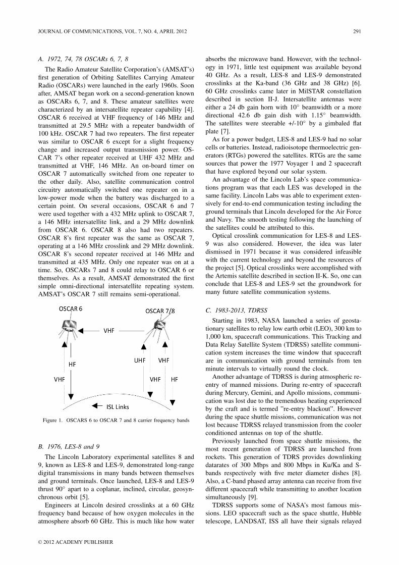
A. 1972, 74, 78 OSCARs 6, 7, 8

The Radio Amateur Satellite Corporation’s (AMSAT’s)first generation of Orbiting Satellites Carrying AmateurRadio (OSCARs) were launched in the early 1960s. Soonafter, AMSAT began work on a second-generation knownas OSCARs 6, 7, and 8. These amateur satellites werecharacterized by an intersatellite repeater capability [4].OSCAR 6 received at VHF frequency of 146 MHz andtransmitted at 29.5 MHz with a repeater bandwidth of100 kHz. OSCAR 7 had two repeaters. The first repeaterwas similar to OSCAR 6 except for a slight frequencychange and increased output transmission power. OS-CAR 7’s other repeater received at UHF 432 MHz andtransmitted at VHF, 146 MHz. An on-board timer onOSCAR 7 automatically switched from one repeater tothe other daily. Also, satellite communication controlcircuitry automatically switched one repeater on in alow-power mode when the battery was discharged to acertain point. On several occasions, OSCAR 6 and 7were used together with a 432 MHz uplink to OSCAR 7,a 146 MHz intersatellite link, and a 29 MHz downlinkfrom OSCAR 6. OSCAR 8 also had two repeaters.OSCAR 8’s first repeater was the same as OSCAR 7,operating at a 146 MHz crosslink and 29 MHz downlink.OSCAR 8’s second repeater received at 146 MHz andtransmitted at 435 MHz. Only one repeater was on at atime. So, OSCARs 7 and 8 could relay to OSCAR 6 orthemselves. As a result, AMSAT demonstrated the firstsimple omni-directional intersatellite repeating system.AMSAT’s OSCAR 7 still remains semi-operational.

Figure 1. OSCARS 6 to OSCAR 7 and 8 carrier frequency bands

B. 1976, LES-8 and 9

The Lincoln Laboratory experimental satellites 8 and9, known as LES-8 and LES-9, demonstrated long-rangedigital transmissions in many bands between themselvesand ground terminals. Once launched, LES-8 and LES-9thrust 90 apart to a coplanar, inclined, circular, geosyn-chronous orbit [5].

Engineers at Lincoln desired crosslinks at a 60 GHzfrequency band because of how oxygen molecules in theatmosphere absorb 60 GHz. This is much like how water

absorbs the microwave band. However, with the technol-ogy in 1971, little test equipment was available beyond40 GHz. As a result, LES-8 and LES-9 demonstratedcrosslinks at the Ka-band (36 GHz and 38 GHz) [6].60 GHz crosslinks came later in MilSTAR constellationdescribed in section II-J. Intersatellite antennas wereeither a 24 db gain horn with 10 beamwidth or a moredirectional 42.6 db gain dish with 1.15 beamwidth.The satellites were steerable +/-10 by a gimbaled flatplate [7].

As for a power budget, LES-8 and LES-9 had no solarcells or batteries. Instead, radioisotope thermoelectric gen-erators (RTGs) powered the satellites. RTGs are the samesources that power the 1977 Voyager 1 and 2 spacecraftthat have explored beyond our solar system.

An advantage of the Lincoln Lab’s space communica-tions program was that each LES was developed in thesame facility. Lincoln Labs was able to experiment exten-sively for end-to-end communication testing including theground terminals that Lincoln developed for the Air Forceand Navy. The smooth testing following the launching ofthe satellites could be attributed to this.

Optical crosslink communication for LES-8 and LES-9 was also considered. However, the idea was laterdismissed in 1971 because it was considered infeasiblewith the current technology and beyond the resources ofthe project [5]. Optical crosslinks were accomplished withthe Artemis satellite described in section II-K. So, one canconclude that LES-8 and LES-9 set the groundwork formany future satellite communication systems.

C. 1983-2013, TDRSS

Starting in 1983, NASA launched a series of geosta-tionary satellites to relay low earth orbit (LEO), 300 km to1,000 km, spacecraft communications. This Tracking andData Relay Satellite System (TDRSS) satellite communi-cation system increases the time window that spacecraftare in communication with ground terminals from tenminute intervals to virtually round the clock.

Another advantage of TDRSS is during atmospheric re-entry of manned missions. During re-entry of spacecraftduring Mercury, Gemini, and Apollo missions, communi-cation was lost due to the tremendous heating experiencedby the craft and is termed ”re-entry blackout”. Howeverduring the space shuttle missions, communication was notlost because TDRSS relayed transmission from the coolerconditioned antennas on top of the shuttle.

Previously launched from space shuttle missions, themost recent generation of TDRSS are launched fromrockets. This generation of TDRS provides downlinkingdatarates of 300 Mbps and 800 Mbps in Ku/Ka and S-bands respectively with five meter diameter dishes [8].Also, a C-band phased array antenna can receive from fivedifferent spacecraft while transmitting to another locationsimultaneously [9].

TDRSS supports some of NASA’s most famous mis-sions. LEO spacecraft such as the space shuttle, Hubbletelescope, LANDSAT, ISS all have their signals relayed



from TDRSS to NASA ground terminals [10]. TDRSShas three main command and control ground terminal lo-cations at White Sands (WSGT) in New Mexico, Goddard(GRGT) in Greenbelt, Maryland, and Guam (STGT) asshown in figure 2.

Figure 2. NASA’s TDRSS. The three ground terminals are Goddard(GRGT), White Sands (WSGT) and Guam (STGT).

D. 1985-1995, Luch

The Luch Satellite Data Relay Network, also referredto as Altair and Geliois, is considered Russia’s answerto NASA’s TDRSS. Until this series of geosynchronousRussian relay satellites, cosmonauts were in contact withground stations only when flying over the Soviet Unionor through communication ships at sea. To mitigate thefive million dollars a week cost of keeping communicationships at sea, the geosynchronous satellites could relaycommunications to ground control at all times [4]. Aseries of five Luch satellites were launched from 1985 to1995. The platform bus was called: Cosmos 1700, 1897,1987, 2054 from 1985 until 1989 then Luch 16, and Luch1 from 1994 and 1995.

Frequencies reported for use by the Luch satellitesare: 15.05 GHz and 13.52 GHz to and from low-orbitsatellites, 700 MHz and 900 MHz to and from low-orbitsatellites, 14.62 GHz for uplinks from control stations;and 10.82 Ghz, 11.32 GHz, and 13.7 GHz for downlinksto control stations. These frequencies have been used forcommunications, including voice and television signals,with the Mir space station, and the Buran reusable launchvehicle. The Luch satellites also have other uses such asteleconferencing. Antenna beamwidths are 0.5 for 13 and15 GHz links, 5 for 700 MHz to 900 MHz links, and 1

for 11 GHz and 14 GHz links [11].A further three satellites, Luch-5A (2011), Luch-5B

(2012) and Luch-4 (2013), are planned for launch to re-build the system and provide the Russian Orbital Sectionof the International Space Station with relay coverage.

E. 1994, ETS-6

The Experimental Test Satellite (ETS-6) was developedand launched by NASDA, Japan’s National Space De-velopment Agency, renamed to JAXA, Japan AerospaceExploration Agency after 2003. The satellite had anS-band, Ka-band, and optical intersatellite link. ETS-6included an S-band of similar specifications to that ofNASA’s TDRSS to have compatibility.

ETS-6’s S-band antenna was built as a phased ar-ray with 19 elements to receive from two spacecraftand transmit to one simultaneously with a 1000 kmrange. Downlink and uplink channels used 20 GHz and30 GHz carriers respectively. All transmissions usedphased shift keying (PSK) with code division multipleaccess (CDMA). Typical rates were 300 kbps with amaximum datarate of 1.5 Mbps [12].

ETS-6 also had a crosslink channel transmitting at23 GHz and receiving at 26 GHz. This carrier had amaximum datarate of 10 Mbps [12], and was designedfor compatibility with NASA TDRSS advanced now inorbit on TDRS 8 to 10 and ESA’s relay satellite systemdiscussed in section II-K.

ETS-6 had another communication payload that trans-mitted at 38 GHz and received at 43 GHz. The payloaddemonstrated ground communication with low power500 mW small antenna 30 cm diameter dish earth termi-nals with datarates of 64 kbps to 512 kbps. Intersatellitecommunication experimented with this payload was alsoemulated from earth terminals with a maximum datarateof 10 Mbps [4]. This transceiver used a 40 cm dishantenna.

The last experimental payload for ETS-6 was an opti-cal transmitter to demonstrate laser intersatellite linkingcommunication with a maximum datarate of 1 Mbps. Theground station used an argon laser to uplink, then ETS-6downlinked with a GaAlAs diode laser. A fine pointingmechanism pointed ETS-6’s transceiver to an accuracy of0.0001 [13].

F. 1997, Navstar Block IIR and IIF GNSS

To the authors’ knowledge, ISLs in GNSSs have onlybeen launched starting with the US GPS Navstar blocksIIR and IIF. These satellites use the UHF band forcrosslink transmissions. There have been plans for ISLsto appear in many other navigational satellite systemsfrom many space agencies including Glonass from Russia,Galileo from ESA, Compass from China, Japan’s QZSS,and India’s Indian Regional Navigational Satellite Systemor IRNSS.

GPS Navstar Block IIR and IIF satellites use theUHF ISLs for gathering neighboring satellite distancesand constellation status. Navstar satellites broadcast theconstellation’s ephemeris, a table of the GPS constella-tion satellites positions at the given time. Satellites notequipped with the links only receive this information bythe ground terminal with an average contact frequency of12 hours. Frequent ephemeris updates through ISLs canallow the Navstar system to have automated navigation.



G. 1997, IridiumIn 1997, Motorola Inc. built a constellation of LEO

satellites called Iridium to provide global satellite phonecoverage. The Iridium constellation is operated with satel-lites that can intersatellite link, providing satellite callsand digital data to traverse through Iridium satellitesinstead of a cellular phone’s network of base stations.

The constellation includes 66 Iridium satellites and sixspares orbiting in low earth orbit [14]. 7.5 km/second isthe approximate orbital velocity for Iridium satellites, andLEO satellites in general.

Figure 3. Iridium constellation generated by the satellite constellationvisualization ”SAVI” (credit: SAVI)

Each Iridium satellite can have up to four simulta-neous crosslinks with a carrier frequency ranging from13.18 GHz to 13.38 GHz, and a datarate of 10 Mbit/s [14].Six satellites are contained in eleven orbital planes. Satel-lites in the same plane can link north and south or eastand west with neighboring orbital planes. The polar orbitscreate two cross-seams. A cross-seam is where one planeorbits south to north and the neighboring plane orbitsnorth to south. As a result, the satellites only link withneighbor planes orbiting in the same direction due toa high Doppler shift. Iridium satellites orbit from poleto pole in approximate 100 minutes [15]. The Iridiumsatellite density at the North and South poles givesexcellent coverage for research facilities.

For processing, each Iridium satellite is equipped withseven Motorola/Freescale PowerPC 200 MHz 603E pro-cessors [16]. The four crosslink antennas each have a ded-icated processor. Each Iridium satellite is controlled withtwo processors, with one being a spare. An extra processorwas installed late in the design phase for processing phonecalls and resource management. A custom backplanenetwork connects the seven processors together.

Satellite phone hand-offs are done from neighboringorbital planes when a satellite moves over the horizon. At

the equator where the orbital planes are spread farthest,the user may notice a quarter-second gap where the hand-off occurs about every seven minutes. Different channelsand timeslots can be transferred within the same call froma satellite in the same spot beam.

The Iridium system has control segments at groundstations that can access the public telephone systemthrough telephony gateways in Arizona and Hawaii [16].Iridium satellites can receive updated frames and routingtables when in line of sight of these gateways. The newtables can then be sent on to the neighboring Iridiumsatellites so the whole constellation is rapidly updated.

Satellite phones with a line of sight can uplink directlyto Iridium satellites to make a call. The phone’s signalis received by a 48 spot beam antenna with 16 beamsdivided in three sectors that handles 1100 simultaneousphone calls [16]. The developers of Iridium previouslyconducted government studies in the late 1980s con-cluding that high datarate optical crosslinks were morecomplicated and higher risk than microwave. In the end,microwave crosslinks were chosen because at the timethey have more than enough bandwidth for the systemand support the mass and power budget allocated for each680 kg Iridium satellite.

H. 1998, The proposed Teledesic System

In 1995, an ambitious intersatellite linking communica-tion system known as Teledesic was proposed. The orig-inal proposal called for 840 active satellites in LEO [17].Due to funding issues, the proposal was changed to 288active satellites at MEO. The constellation was to have 24satellites in 12 orbital planes. Teledesic allocated the Ka-band spectrum for use with non-geostationary satellites.Each satellite had 3-axis stabilization with an antenna onthe bottom and solar panels on top. This system wasone of the first to design satellites as compatible buseswith over 20 different launch systems. Such flexibilityis needed when launching hundreds of satellites. TheTeledesic terminals also were flexible by allowing avariety of communication protocols including IP, ISDN,and ATM.

In February 1998, a test satellite named Teledesic T1was launched. Teledesic T1 weighed 120 kg and useddownlink frequencies of 18.8 GHz to 19.3 GHz anduplink frequencies of 28.6 GHz to 29.1 GHz [17]. EachTeledesic cell had a max rate of 64 MBps. However,after the commercial failing of the Globalstar system (46operational satellites), work was suspend on Teledesic in2002.

I. 1998, COMETS (ETS-7)

Conducted by the Japanese National Space Develop-ment Agency (JAXA after 2003), the Communicationsand Broadcasting Engineering Test Satellite (COMETS)built upon technology from ETS-6 satellite from sec-tion II-E [18]. Both the ETS-6 satellite and the COMETSsatellite had roughly the same mass.



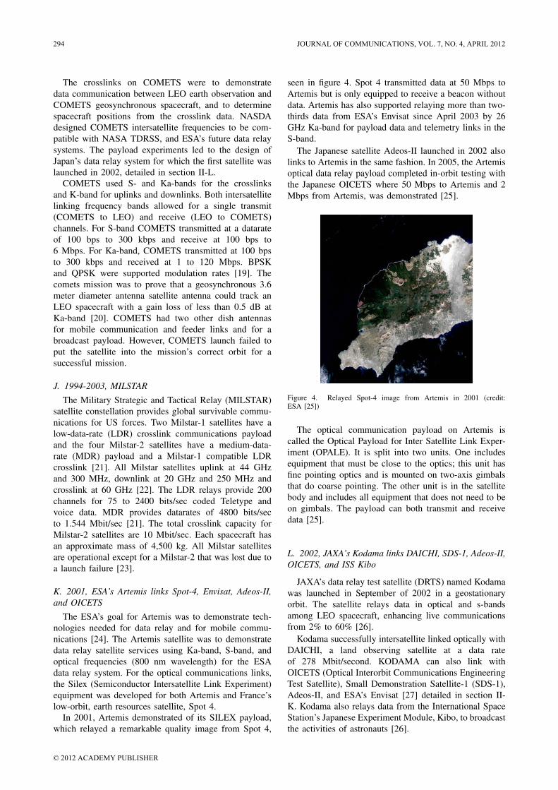
The crosslinks on COMETS were to demonstratedata communication between LEO earth observation andCOMETS geosynchronous spacecraft, and to determinespacecraft positions from the crosslink data. NASDAdesigned COMETS intersatellite frequencies to be com-patible with NASA TDRSS, and ESA’s future data relaysystems. The payload experiments led to the design ofJapan’s data relay system for which the first satellite waslaunched in 2002, detailed in section II-L.

COMETS used S- and Ka-bands for the crosslinksand K-band for uplinks and downlinks. Both intersatellitelinking frequency bands allowed for a single transmit(COMETS to LEO) and receive (LEO to COMETS)channels. For S-band COMETS transmitted at a datarateof 100 bps to 300 kbps and receive at 100 bps to6 Mbps. For Ka-band, COMETS transmitted at 100 bpsto 300 kbps and received at 1 to 120 Mbps. BPSKand QPSK were supported modulation rates [19]. Thecomets mission was to prove that a geosynchronous 3.6meter diameter antenna satellite antenna could track anLEO spacecraft with a gain loss of less than 0.5 dB atKa-band [20]. COMETS had two other dish antennasfor mobile communication and feeder links and for abroadcast payload. However, COMETS launch failed toput the satellite into the mission’s correct orbit for asuccessful mission.

J. 1994-2003, MILSTAR

The Military Strategic and Tactical Relay (MILSTAR)satellite constellation provides global survivable commu-nications for US forces. Two Milstar-1 satellites have alow-data-rate (LDR) crosslink communications payloadand the four Milstar-2 satellites have a medium-data-rate (MDR) payload and a Milstar-1 compatible LDRcrosslink [21]. All Milstar satellites uplink at 44 GHzand 300 MHz, downlink at 20 GHz and 250 MHz andcrosslink at 60 GHz [22]. The LDR relays provide 200channels for 75 to 2400 bits/sec coded Teletype andvoice data. MDR provides datarates of 4800 bits/secto 1.544 Mbit/sec [21]. The total crosslink capacity forMilstar-2 satellites are 10 Mbit/sec. Each spacecraft hasan approximate mass of 4,500 kg. All Milstar satellitesare operational except for a Milstar-2 that was lost due toa launch failure [23].

K. 2001, ESA’s Artemis links Spot-4, Envisat, Adeos-II,and OICETS

The ESA’s goal for Artemis was to demonstrate tech-nologies needed for data relay and for mobile commu-nications [24]. The Artemis satellite was to demonstratedata relay satellite services using Ka-band, S-band, andoptical frequencies (800 nm wavelength) for the ESAdata relay system. For the optical communications links,the Silex (Semiconductor Intersatellite Link Experiment)equipment was developed for both Artemis and France’slow-orbit, earth resources satellite, Spot 4.

In 2001, Artemis demonstrated of its SILEX payload,which relayed a remarkable quality image from Spot 4,

seen in figure 4. Spot 4 transmitted data at 50 Mbps toArtemis but is only equipped to receive a beacon withoutdata. Artemis has also supported relaying more than two-thirds data from ESA’s Envisat since April 2003 by 26GHz Ka-band for payload data and telemetry links in theS-band.

The Japanese satellite Adeos-II launched in 2002 alsolinks to Artemis in the same fashion. In 2005, the Artemisoptical data relay payload completed in-orbit testing withthe Japanese OICETS where 50 Mbps to Artemis and 2Mbps from Artemis, was demonstrated [25].

Figure 4. Relayed Spot-4 image from Artemis in 2001 (credit:ESA [25])

The optical communication payload on Artemis iscalled the Optical Payload for Inter Satellite Link Exper-iment (OPALE). It is split into two units. One includesequipment that must be close to the optics; this unit hasfine pointing optics and is mounted on two-axis gimbalsthat do coarse pointing. The other unit is in the satellitebody and includes all equipment that does not need to beon gimbals. The payload can both transmit and receivedata [25].

L. 2002, JAXA’s Kodama links DAICHI, SDS-1, Adeos-II,OICETS, and ISS Kibo

JAXA’s data relay test satellite (DRTS) named Kodamawas launched in September of 2002 in a geostationaryorbit. The satellite relays data in optical and s-bandsamong LEO spacecraft, enhancing live communicationsfrom 2% to 60% [26].

Kodama successfully intersatellite linked optically withDAICHI, a land observing satellite at a data rateof 278 Mbit/second. KODAMA can also link withOICETS (Optical Interorbit Communications EngineeringTest Satellite), Small Demonstration Satellite-1 (SDS-1),Adeos-II, and ESA’s Envisat [27] detailed in section II-K. Kodama also relays data from the International SpaceStation’s Japanese Experiment Module, Kibo, to broadcastthe activities of astronauts [26].



M. 2010, AEHF

To replace an aging Milstar system detailed in sec-tion II-J, the Advanced Extremely High Frequency(AEHF) is being launched as communication satellitesgeostationary orbits. Currently only one satellite, AEHFSV-1, is launched [28]. The AEHF system operates at44 GHz uplink (EHF band) 20 GHz downlink [28], and60 GHz crosslink compatible with Milstar-2’s 10 Mbps to-tal crosslink capacity detailed in section II-J and 60 Mbpscapacity with other AEHF satellites.

Also similar to the Milstar satellites, AEHF satellitesare equipped with security features including resistantjamming, encryption, and frequency-hopping. The AEHFsystem can detect a jamming source and then applyadaptive antennas to transmit nulls toward sources. AEHFis compatible Milstar’s low and medium data rates andalso high a higher signaling method with a data rate ofup to 8.192 Mbit/sec [28].

N. 2015, Iridium Next

As an update to the Iridium system, detailed in sec-tion II-G, the Iridium Next satellite constellation wasannounced in 2007. The constellation is the same asIridium with 66 operating LEO satellites. This second-generation Iridium design will emphasize data transmis-sion [29]. Since the satellite can be controlled froma single ground point, other companies have partneredwith Iridium to incorporate on-board camera and sensorpayloads. The estimated launch data for the constellationstart in 2015 [29].

Gateway ground stations for Iridium NEXT in Tempe,Arizona and Wahiawa, Hawaii [16] will control the con-stellation with uplinking from the Ka-band 19.4 GHz-19.6 GHz and downlinking 29.1 GHz-29.3 GHz. ISLswill use the Ka-band ranging from 23.18 GHz to23.38 GHz [29]. Mobile satellite phones from the groundusers or hot-spot stations will use the L-band rangingfrom 1616 MHz to 1626.5 MHz to uplink to the satelliteconstellation. The frequency license rules for the user’slocation will determine the exact L-band frequency [29].Normal satellite phone datarates for Iridium NEXT arereported at 1.5 Mbit/sec. Users can also purchase largerequipment to use the premium high-speed Ka-band ser-vice of 8 Mbit/sec [29]. Iridium NEXT will also becompatible with the original Iridium constellation.

III. CUBESAT COMMUNICATION SUB-SYSTEMS

Starting in 1999, the CubeSat was an idea to stan-dardize a platform for low-cost pico-satellite missionsand experiments, particularly at the university level. TheCubeSat name is given from the pico-satellite’s cube-likestructure of 1 kg mass and 10 cm a side. A standardizedstructure allows CubeSats to share in launches with stan-dard tubes shown in figure 5, and called Poly PicosatelliteOrbital Deployers also known as P-PODs. The CubeSatplatform is seen as the most feasible direction to takeintersatellite links in the future. Thus, this section IIIsurveys all CubeSat communication subsystems.

Figure 5. Poly Picosatellite Orbital Deployers or P-POD holds three1U CubeSats (credit: Cal Poly)

Over the past eight years, the CubeSat platform hasflown successfully for many educational and scientific lowearth orbiting satellite missions. To further CubeSat mis-sion applications, a focus needs placed on inter-satellitenetworking that could improve the overall datarate anddownlink time window of a CubeSat to ground terminal.Universities are developing a new robust, ad-hoc, longdistance, high data rate protocol for CubeSats. However,in order to create this CubeSat protocol, a study ofevery inter-satellite linking mission and CubeSat missioncommunication system is presented in this report. Specialfocus is put on the data downlinking transceiver andcommunication protocol used.

A. 2003, Eurockot LV, Pletsak, Russia

Coordinated by University of Toronto’s Space FlightGroup in 2003, the Nanosatellite Launch System (NLS)provides a low-cost launch service for nanosatellites [31].The first batch of six CubeSats were launched into apolar sun-synchronous orbit at 810 km [30]. The Cube-Sats launched from Plesetsk, Russia [30]. The launchintegration effort for three 1U satellites was known asNanosatellite Launch service 1 (NLS1). NSL1 CubeSatsincluded AAUSat from Aalborg, DTUSat from Denmark,and CanX-1 from University of Toronto. The three satel-lites were launched from the first P-POD. NLS2 launchedQuakeSat, a 3U CubeSat from Stanford University, whichtook up an entire second P-POD. Also on the Eurockot,two Tokyo Pico-satellite Orbital Deployers or T-PODs,deployed CUTE-I from Tokyo Tech. and XI from TokyoUniversity.

The two communication system characteristics thatwere common among the six CubeSats were the useof the AX.25 Link Layer Protocol specification and thefrequency range from 432-438 MHz for their beacons anddownlink. The only deviation from the AX.25 protocolwas the CanX-1 satellite due to a proprietary natureof the information it was collecting and the additionof the PacSat layer to QuakeSat-1. However, CanX-1Radio contact was never established. The choice of theAX.25 protocol allows amateur radio operators worldwideto collect information from the satellites and enhancethe ground station effort. By utilizing the amateur radiocommunity, the satellites could potentially transmit more



TABLE II.HISTORY OF CUBESAT DATA TRANSMITTERS BY LAUNCH DATE 2003-2005 [30]

Launch Date/Location Satellite(s) Size Frequency Power Protocol Baud Rate/Modulation

June 30, 2003 AAU1 CubeSat 1U 437.475 MHz 500 mW AX.25, Mobitex 9600 baud GMSKEurockot DTUsat-11 1U 437.475 MHz 400 mW AX.25 2400 baud FSK

Plesetsk Cosmodrome CanX-12 1U 437.880 MHz 500 mW Custom 1200 baud MSKRussia Cute-1 (CO-55) 1U 437.470 MHz 350 mW AX.25 1200 baud AFSK

QuakeSat-1 3U 436.675 MHz 2 W AX.25 w/Pacsat 9600 baud FSKXI-IV (CO-57) 1U 437.490 MHz 1 W AX.25 1200 baud AFSK

October 27, 2005 XI-V (CO-58) 1U 437.345 MHz 1 W AX.25 1200 baud AFSKSSETI Express NCube-2 1U 437.505 MHz 1 W AX.25 1200 baud AFSK

Plesetsk Cosmodrome 2279.5 MHz 2 WRussia UWE-1 1U 437.505 MHz 1 W AX.25 1200/9600 baud AFSK

data, thus provide more utility, if the data could beeffectively re-assembled by the ground station [32].

QuakeSat-1 used PacSat Protocol Suite, part of theUoSAT and Microsat File transfer protocols. The suitedefines file transfer protocols for use by LEO PacketRadio Satellites (PACSATs). Published in 1990, was thefirst digital store and forward packeting protocol used forCubeSats [33].

Generally, CubeSats use Commercial Off-the-Shelf(COTS) radios, and modify them for use in space.The only published exception from the use of COTSequipment on this mission was the Japanese CubeSatXI-IV, which used a transceiver and beacon that wasdeveloped within the University. However, the first threedevelopment versions of the satellite integrated a COTStransceiver until the flight model was ready [34].

The results from the first batch of CubeSats have beenmixed. The two Japanese satellites, Cute-1 and XI-IV,were successful, as they sent telemetry data until Decem-ber 2008 and March 2009 respectively. The 3U QuakeSat-1 with PacSat can also be considered a success becauseit worked for more than seven times the design life of sixmonths, and provided significant usable data. QuakeSat-1 also demonstrated the use of deployable solar panelsfor a higher maximum transmitting power. CanX-1 andDTUsat-1, however, never functioned on orbit and AAU1had a significantly decreased lifetime, due to battery pack-aging problems, and a degraded communications systemthat led to only beacon packets being transmitted for thelife of the satellite [35]. The most notable characteristicfor the launch is the use of dedicated beacon transmittersby the two Japanese satellites Cute-1 and XI-IV. Thesesatellites also utilized dedicated antenna designs for thetransceiver and the beacon, monopoles for Cute-1, anddipoles for XI-IV [34].

B. 2005, SSeti Express, Pletsak, Russia

Upon the success of the first CubeSat launch moreeducational CubeSat projects were started. Sponsored bythe European Space Agency Education office, a micro-satellite called SSeti Express was launched in 2005 in asun-synchronous polar low earth orbit [30]. Although theSSETI Express microsatellite failed almost immediately

after launch, three CubeSats including XI-V (Universityof Tokyo), NCube-2 (University of Oslo and others),and UWE-1 (University of Wurzburg) were successfullylaunched [30]. These CubeSats, known as NLS3, broughttogether many universities across Europe, and educatedhundreds of students [31].

The CubeSats all operated in the Amateur Band andused the amateur AX.25 protocol to simplify the groundstation operation and increase the number of worldwidedownlink points. Though the types of transceivers areunknown, it is known that NCube-2 and UWE-1 utilizedcommercial transceivers and the XI-V satellite family(identical to XI-IV in every aspect) continued to use thetransceivers and beacons developed within the Universityof Tokyo.

NCube-2, with a UHF and experimental S-band trans-mitter, never transmitted to its ground station, and wasdeclared dead on orbit. XI-V and UWE-1 both functionedas intended and utilized monopole antennas for theircommunications subsystem. Again, the Japanese SatelliteXI-V used a separate beacon to provide redundancy [30].

UWE-1 was designed to test TCP/IP protocols in spaceand the effects of low bandwidth, long path delays, anddropped packets [34]. The main processor performed allthe TNC functions, packeting all the data into the AX.25frame [36]. It then sent these frames using a 6-packprotocol (similar to KISS) to the TNC. This allowed themain processor to control the Data Link Layer settingsof the radio, improving system performance. Numerousother ground stations around the world received thesebeacons and forwarded the data on to the university [34],but the CubeSat stopped functioning in November 2005,about three weeks after launch [30].

C. 2006, M-V-8, Uchinoura, Japan

Single CubeSat launches have been rare. However, Cute1.7 + APD was a 2U CubeSat that was individuallylaunched by Tokyo Tech from Japan and tested an upgradeto the Tokyo Pico-satellite Orbital Deployer (T-POD) thatcould accommodate 2U CubeSats. CUTE 1.7 + APD hada highly elliptical orbit from 250-280 km in perigee heightand 750 km in apogee height. This resulted in a short life-time of over two months [30]. The CubeSat demonstrated



TABLE III.HISTORY OF CUBESAT DATA TRANSMITTERS BY LAUNCH DATE 2006-2008


February 21, 2006 MV8 Cute-1.7 APD 2U 437.505 MHz 300 mW AX.25 SRLL 1200 AFSK/9600 GMSK

July 26, 2006 Ion 2U 437.505 MHz 2 W AX.25 1200 baud AFSKDNEPR-1 Failed Sacred 1U 467.870 MHz 400 mW AX.25 1200 baud AFSK

Baikonur, Cosmodrome KuteSat Pathfinder 1U 437.385 MHz 500 mW AX.25 1200 baud AFSKKazakstan Ice Cube-1 1U 437.305 MHz 600 mW AX.25 9600 baud FSK

Ice Cube-2 1U 437.425 MHz 600 mW AX.25 9600 baud FSKRincon1 1U 436.870 MHz 400 mW AX.25 1200 baud AFSKSEEDS 1U 437.485 MHz 450 mW AX.25 1200 baud AFSKHauSat1 1U 437.465 MHz 500 mW AX.25 1200 baud AFSKNcube1 1U 437.305 MHz 1 W AX.25 9600 baud GMSKMerope 1U 145.980 MHz 500 mW AX.25 1200 baud AFSK

AeroCube-1 1U 902-928 MHz 2 W AX.25 9600 baud GFSKCP1 1U 436.845 MHz 500 mW AX.25 15 baud DTMFCP2 1U 437.425 MHz 1 W AX.25 1200 baud AFSK

Mea Huaka (Voyager) 1U 437.405 MHz 500 mW AX.25 1200 AFSK

December 16, 2006 Wallops, US GeneSat-1 3U+ 2.4 GHz 1 W Proprietary 15 kbps

April 17, 2007 CSTB1 1U 400.0375 MHz 1 W Proprietary 1200 baud AFSKDNEPR-2 AeroCube-2 1U 902-920 MHz 2 W Proprietary 38.4 kbaud

Baikonur Cosmodrome CP4 1U 437.325 MHz 1 W AX.25 1200 baud FSKKazakstan Libertab-1 1U 437.405 MHz 400 mW AX.25 1200 baud AFSK

CAPE1 1U 436.245 MHz 1 W AX.25 9600 baud FSKCP3 1U 437.845 MHz 1 W AX.25 1200 baud FSK

MAST 3U 2.4 GHz 1 W Proprietary 15 kbps

April 28, 2008 Delfi-C3 (DO-64) 3U 435.55 MHz 200 mW Linear 40 KHz widebandSatish Dhawan, India Seeds-2 (CO-66) 1U 437.485 MHz 450 mW AX.25 1200 baud AFSK

CanX-2 3U 2.2 GHz 500 mW NSP 16-256 kbps BPSKAAUSAT-II 1U 437.425 MHz 300 mW AX.25 SRLL 1200 AFSK/9600 GMSK

Cute 1.7 APD-II 3U+ 437.475 MHz 2 W AX.25 w/Pacsat 9600 baud FSKCompass-1 1U 437.405 MHz 300 mW AX.25 1200 baud AFSK/MSK

August 3, 2008 Falcon 1 Failed PREsat 3U 437.845 MHz 1 W AX.25 1200 baud FSKOmelek, Marshall Islands NanoSail-D 3U 2.4 GHz 1 W Proprietary 15 kbps

use of a tether, an avalanche photodiode, a magnetictorque attitude control system (ACS), and a computerfrom a personal digital assistant. During the flight timeCUTE 1.7 successfully transmitted about one megabyteof mission information to the ground station [30].

CUTE-1.7+APD downlinked at 430 MHz and receiveduplink at 1200 MHz. The L-band uplink was used asa public personal message box for space. The mes-sage box performed at store and forward experiment bytransmitting stored messages for a duration of time toamateur radio ground stations. CUTE-1.7+APD was alsoknown as OSCAR-56 because it was an operational digitalrepeater [30].

D. 2006, DNEPR-1 Failure, Baikonur, KazakhstanThis large sun-synchronous orbit launch was aboard

a Dnepr rocket and contained five P-PODs housing 14CubeSats. Unfortunately, about two minutes into thelaunch the Dnepr failed and all the CubeSats were lost.

Common characteristics among the CubeSats was theuse of the AX.25 protocol within the 432-438 MHzband. The only deviations from the standard within the

launch were the MEROPE by Montana State Universitywhich utilized the AX.25 protocol at a significantly lowerfrequency (144-146 MHz range) [37] and the AeroCube-1 that operated in the amateur band between 902-928 MHz [30]. Most of the satellites utilized monopoleor dipole antennas. Notable exceptions were the use ofa patch antenna by ICE Cubes 1 and 2 from CornellUniversity and the incorporation of an active antennaarray on Mea Huaka from the University of Hawaii aspart of the experimental payload [38]. This batch ofsatellites also began to incorporate the use of an attitudecontrol system. At least eight of the satellites includedmagnetorquers, hysteresis rods, or electronic propulsionsystems in the satellite [30]. The use of stabilizing devicesin CubeSats could significantly improve the capabilitiesof the communications subsystem and allow a link tobe closed with a reduction in power using a higherdata rate [39]. Attitude control could also contribute todirectionally pointing CubeSat links allowing for highergain antennas.



E. 2006, Minotaur-1, NASA Wallops, VA, USA

GeneSat-1 was a joint project between NASA andacademia that sought to evaluate biological payload ex-periments in a CubeSat [40]. GeneSat-1 was launchedby a Minotaur rocket to an altitude of 415 km circularorbit [30].

The primary telemetry, tracking, and command linkfor GeneSat was a Microhard MHX-2400 frequencyhopping spread spectrum Radio operating at 2.44 GHzand transmitted through a patch antenna. GeneSat alsoused a beacon operating in the Amateur Band from 432-438 MHz to serve as a risk reduction for the MicrohardRadio, and to provide amateur radio operators the op-portunity to collect satellite information [40]. GeneSat1was successful and downloaded the 500 kb required forits primary mission and continues to transmit beaconinformation [34]. NASAs GeneSat-1 3U platform bus,seen in figure 6, has been used in NASAs later PharmaSat,PREsat, O/OREOS, and NanoSail-D CubeSats.

Figure 6. The GeneSat-1 bus has been replicated for future NASACubeSats such as PharmaSat, PRESat, and NanoSail-D1/-D2. (credit:NASA/ARC)

F. 2007, DNEPR-2, Baikonur, Kazakhstan

Unlike the first Dnepr launch, this DNEPR LV launchsuccessfully deployed three P-PODs in space, droppingthe satellites in a polar sun-synchronous. The fourth majorCubeSat launch contained several unique elements asBoeing entered the fray of the CubeSat community withtheir entry of CTSB-1 and Tethers Unlimited launchedthree tethered CubeSats known as MAST. AerospaceCorporation also launched their second CubeSat andCalifornia Polytechnic Institute launched CP3 and CP4,their third and fourth CubeSat [41].

Satellites CTSB-1, AeroCube-2, and MAST utilizedproprietary packet protocols for their missions. Thesemissions were also unique in their use of the fre-quency spectrum and the licensing requirements associ-ated. CTSB-1 used an experimental license that operatedat 400 MHz, AeroCube-2 used ISM license between 902-928 MHz [41], and MAST used the same transceiver asGeneSat-1, a Microhard MHX2400 transceiver operatingat 2.4 GHz.

The remaining satellites in the flight continued to usethe AX.25 protocol along with frequencies within theUHF band. These satellites have had a mixed rate ofsuccess. Essentially all of the satellites have establishedcommunications with the ground. The exceptions wereCAPE, which was integrated with a non-functioning re-ceiver due to time constraints and Libertad-1, which hada non-functioning ground station when it was launchedand the university personnel were not able to completerepairs in time to communicate with the satellite [34].The remainder had down linked telemetry from severalhundred kilobytes to several megabytes over the courseof a year [34].

G. 2008, PSLV-C9 Satish Dhawan Space Centre, India

The first launch of multiple CubeSat outside of the for-mer Soviet Union was supported as Nanosatellite LaunchSystems 4 and 5 (NLS4 and NLS5) [31]. The launchconsisted of satellites from Canada, Europe, and Japan.The satellites were launched using an eXperimental PushOut Deployer (X-POD), a launch system built for cus-tom dimensions from pico-satellite to large nanosatelliteclasses.

Notably, Delfi-C3 from Delft University of Technologyin Holland was deployed to test wireless link data transferwithin the satellite and new thin film solar cells. NihonUniversity deployed SEEDS, a satellite similar to onedestroyed in the DNEPR Launch Vehicle failure discussedin section III-D.

Every satellite within the fifth batch used the 432-438MHz portion of the AM band for part of its communica-tions subsystem. CanX-2 also used the 2.390-2.450 GHzportion of the Amateur band for an additional downlinkusing a modified AX.25 protocol that the design teamnamed the Nanosatellite Protocol (NSP) [42]. CanX-2 used two patch antennas for the S-Band transceiverand a quad-canted turnstile antenna for the downlink inthe 70 cm band [30]. CUTE 1.7 + APD II used theAmateur frequencies available from 1240-1300 MHz forits uplink and maintained the AX.25 protocol for itstransmissions [42]. According to AMSAT, all the satelliteslaunched in the fifth batch are still in operation andtransmitting to the ground station, except Compass-1,which is semi-operational as of September 2011.

H. 2008, Falcon-1 Failure, Omelek Island

In August of 2008, SpaceX’s Falcon 1 rocket was usedto launch the US Air Force’s Trailblazer satellite alongwith two 3U CubeSats from NASA called NanoSail-Dand PRESat. However, two minutes and forty seconds intothe launch the Falcon’s 1st stage hit the 2nd stage. As aresult, the entire rocket and payload flew off course intothe Pacific Ocean.

NASA’s Ames Research Center built the NanoSail-DCubeSat to study the use of a solar sail for deorbiting. Thesatellite was designed to have an elliptical orbit with anapogee of 685 kilometers and perigee of 330 kilometers.



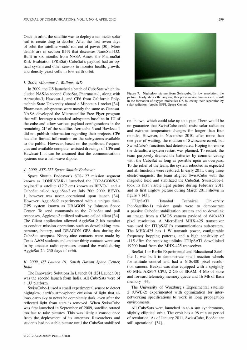
Once in orbit, the satellite was to deploy a ten meter solarsail to create drag to deorbit. After the first seven daysof orbit the satellite would run out of power [30]. Moredetails are in section III-N that discusses NanoSail-D2.Built in six months from NASA Ames, the PharmaSatRisk Evaluation (PRESat) CubeSat’s payload had an op-tical system and other sensors to monitor health, growth,and density yeast cells in low earth orbit.

I. 2009, Minotaur-1, Wallops, MD

In 2009, the US launched a batch of CubeSats which in-cluded NASAs second CubeSat, Pharmasat-1, along withAerocube-3, Hawksat-1, and CP6 from California Poly-technic State University aboard a Minotaur-1 rocket [34].Pharmasats subsystems were mostly the same as Genesat.NASA developed the Microsatellite Free Flyer programthat will leverage a standard subsystem baseline in 1U ofthe cube and allow various payload configurations in theremaining 2U of the satellite. Aerocube-3 and Hawksat-1did not publish information regarding their projects. CP6has also limited information on the subsystems availableto the public. However, based on the published frequen-cies and available computer assisted drawings of CP6 andHawksat-1, it can be assumed that the communicationssystems use a half-wave dipole.

J. 2009, STS-127 Space Shuttle Endeavor

Space Shuttle Endeavor’s STS-127 mission segmentknown as LONESTAR-1 launched the ”DRAGONSATpayload” a satellite (12.7 cm) known as BEVO-1 and aCubeSat called AggieSat-2 on July 20th 2009. BEVO-1, however was never operational upon launch [34].However, AggieSat2 experimented with a unique dual-GPS system known as DRAGON by Johnson SpaceCenter. To send commands to the CubeSat and pollresponses, Aggiesat-2 utilized software called client [34].The Client application allowed AggieSat 2 lab memberto conduct mission operations such as downlinking tem-perature, battery, and DRAGON GPS data during theCubeSat overpass. Ninety-nine contacts were made byTexas A&M students and another thirty contacts were sentin by amateur radio operators around the world duringAggieSat-2’s 230 days of orbit.

K. 2009, ISI Launch 01, Satish Dawan Space Center,India

The Innovative Solutions In Launch 01 (ISI Launch 01)was the second launch from India. All CubeSats were ofa 1U platform.

SwissCube-1 used a small experimental sensor to detectnightglow, earth’s atmospheric emission of light that al-lows earth sky to never be completely dark, even after thereflected light from stars is removed. When SwissCubewas first launched in September of 2009, satellite rotatedtoo fast to take pictures. This was likely a consequencefrom the deployment of its antennas. Researchers andstudents had no stable picture until the CubeSat stabilized

Figure 7. Nightglow picture from Swisscube. In low resolution, thepicture clearly shows the airglow, this phenomenon luminescent, resultin the formation of oxygen molecules O2, following their separation bysolar radiation. (credit: EPFL Space Center)

on its own, which could take up to a year. There would beno guarantee that SwissCube could resist solar radiationand extreme temperature changes for longer than fourmonths. However, in November 2010, after more thanone year of waiting, the rotation of Swisscube eased, butSwissCube’s functions had deteriorated. Hoping to restorethe defaults, a system restart was planned. To restart, theteam purposely drained the batteries by communicatingwith the CubeSat as long as possible upon an overpass.To the relief of the team, the system rebooted as expectedand all functions were restored. In early 2011, using threeelectro-magnets, the team aligned SwissCube with themagnetic field and stabilized the CubeSat. SwissCube-1took its first visible light picture during February 2011and its first airglow picture during March 2011 shown infigure 7 [43].

ITUpSAT1 (Istanbul Technical UniversityPicoSatellite-1) mission goals were to demonstratea passive CubeSat stabilization system and to downlinkan image from a CMOS camera payload of 640x480pixel resolution. A MicroHard MHX-425 transceiverwas used for ITUpSAT1’s communications sub-system.The MHX-425 has 1 W transmit power, configurablefrequency hopping patterns, and a high sensitivity of-115 dBm for receiving uplinks. ITUpSAT1 downlinked19200 baud from the MHX-425 transceiver.

BeeSat-1 or Berlin Experimental and Educational Satel-lite 1, was built to demonstrate small reaction wheelsfor attitude control and had a 640x480 pixel resolu-tion camera. BeeSat was also equipped with a sprightly60 MHz ARM-7 CPU, 2 Gb of SRAM, 4 Mb of storeand forward telemetry memory queue and 16 Mb of flashmemory [44].

The University of Wurzburg’s Experimental satellite2 (UWE-2) experimented with optimization for inter-networking specifications to work in long propagationenvironments.

All CubeSats were launched in to a sun synchronous,slightly elliptical orbit. The orbit has a 98 minute periodof revolution. As of January 2011, SwissCube, BeeSat arestill operational [34].



TABLE IV.HISTORY OF CUBESAT DATA TRANSMITTERS BY LAUNCH DATE 2009-2011 [34]


May 19, 2009 PharmaSat 3U 2.4 GHz 1 W Proprietary 15 kbpsMinotaur-1 CP6 1U 437 MHz 1 W CC1000 AX.25 1200 baud AFSK

Wallops, US HawkSat-I 3U 425 GHz 1 W MHX-425 NSP 1200 baud AFSKAeroCube-3 1U 900 MHz 2 W Freewave FHSS Proprietary

July 30, 2009 STS-127 Aggiesat-2 1U 436.25 MHz 1 W AX.25 1200 baud AFSK

September 23, 2009 SwissCube 1U 437.505 MHz 1 W AX.25 FSK 1200 baudISILaunch 01 ITUpSat1 1U 437.325 MHz 1 W Custom GFSK 19.2 kbps

India UWE-2 1U 437.385 MHz 500 mW AX.25 FSK 9600 BPSBeeSat 1U 436 MHz 500 mW AX.25 4800 and 9600 GMSK

May 20, 2010 Hayato (K-Sat) 1U 13.275 GHz Custom 10kbps/1 MbpsJapanese H-IIA Waseda-Sat1 1U 437.485 MHz 1 W AX.25 9600 baud FSK

Japan Negai 1U 427.305 MHz 1 W AX.25 1200 FSK

July 12, 2010 TISat-1 1U 437.305 MHz 400 mW Custom CW 110 WPMPSLV-C15 India StudSat 1U 437.505 MHz 450 mW AX.25 9600 baud FSK

November 20, 2010 O/OREOS 3U 437.305 MHz 1 W AX.25 1200 FSKSTP-S26 RAX1 3U 437.505 MHz 2 W AX.25 9600 baud FSK

Kodiak, Alaska 2.4 GHz 2 WNanoSail-D2 3U 437.275 MHz 1 W AX.25 1200 baud FSK

August 12, 2010 Perseus (4) 1.5U PI PI PI PIFalcon 9-002 QbX (2) 3U PI PI PI PI

Capa Canaveral SMDC-ONE 3U UHF PI PI PIMayflower 3U 437.600 MHz 900 mW AX.25 1200 AFSK

March 4, 2011 E1P 1U 437.505 MHz 1 W KISS/Custom 1200 FSKTarus XL Failure Hermes 1U 2.4 GHz 1 W MHX-2420 56.2 kbpsVandenberg, CA KySat 3U 436.790 MHz 1 W AX.25 1200 FSK

Oct 12, 2011 India JUGNU 3U 437.275 MHz 500 mW CW 20 WPM

Oct 28, 2011 DICE-1/2 1.5U 460/465 MHz 2 W PI 1.5 MbpsElana3 M-Cubed 1U 437.485 MHz 1 W AX.25 9600 GMSK

Vanderburg, CA RAX-2 3U 437.345 MHz 2 W AX.25 9600 FSK2.4 GHz 2 W

E1P-2 1U 437.505 MHz 850 mW AX.25 1200 FSKAubieSat-1 1U 437.475 MHz 708 mW CW 20 WPM

L. 2010, Japanese H-IIA F17, Tanegashima Space Centre

Three 1U CubeSats Hayato, Waseda-SAT2, and Nagaiwere launched from the Yoshinobu Launch Complex atthe Tanegashima Space Centre [34]. Two JAXA Picosatel-lite Deployers or J-PODs released the CubeSats. Hayatoand Negai shared a J-POD and Waseda-SAT was storedin a second J-POD. These satellites were launched inextremely low earth orbits of 300 km. Hayato contained adielectric patch antenna for X-band communication and apantograph space boom of 60 cm for space weather studyof water vapor in the earth’s atmosphere. Waseda-SAT2was launched for earth observation and to test the use ofextending paddles to provide attitude control. Negai waslaunched to perform an orbital FPGA experiment. Nagaialso returned images of the Earth.

M. 2010, PSLV-C15, Satish Dhawan Space Centre

Supported as NLS6 [31] TISat and the Indian StudSatwere launched into a 700 km sun-synchronous orbit [34].

The Studsat took images of earth’s surface with a res-olution of 90 meters. TISat-1 is experimented with thedurability of exposed thin bonding wires and printedcircuit board tracks. TISat-1 also developed in-house allbaseband modulation schemes in firmware. Both TIsat-1and StudSat are currently operating with amateur radiostations around the world.

N. 2010, STP-S26, Kodiak, Alaska

Launched from Kodiak Island Launch Complex,Alaska, RAX-1, O/OREOS and NanoSail-D2 piggy-backed on the Formation Autonomy Spacecraft withThrust, Relay, Attitude, and Cross-link (FASTRAC).

The goal of the RAX-1 mission to the experimentmeasuring the plasma instabilities in the lower polar ther-mosphere that can amount magnetic field-aligned irreg-ularities. magnetic field-aligned irregularities in between80 to 400 km can jam wireless communication signals ofspacecraft downlinking to ground stations. RAX1 used astandard 2 watt UHF AX.25 communication sub-system



to downlink data back to a ground terminal in Michigan.Due to an aberration in RAX-1’s solar panels, the CubeSatwas unable to generate power after several months. How-ever, during operation RAX-1 was able to downlink bi-static radar measurements never attempted at this altitude.RAX-2 is being rebuilt for a NASA’s Elana 3 launch,detailed in section III-R.

NASA’s O/OREOS or Organism Organic Exposure toOrbital Stresses is a 3U CubeSat built to study microor-ganisms’ health in space. Microorganisms health data isdownlinked using UHF AX.25, so amateur radio stationsaround the world can receive and forward the packets toNASA website for study [45]. O/OREOS also send datathrough s-band transmission to NASA over a microhardMHX-2420 transceiver [45]. O/OREOS was built with amechanism of two aluminum plates that separated with aspring. This mechanism increases the device’s volume by60%, creating drag, to slowly deorbit the CubeSat. Thisis shown in figure 8.

Figure 8. NASA’s expanded CubeSat O/OREOS. Key: 1. UHF trans-mitter, 2. Microhard MHX-2420, 3. ACS, 4. Expanded deorbit device,5. Solar Cells, 6) Lithium Ion Batteries (credit: NASA [45]).

Last, NASA’s NanoSail-D2 30-square-meter sail haswas unfurled and the satellite has lowered its altitude. Infact, NanoSail-D2’s can be seen at observatories. Orbitalattitude, sail direction of pointing, and solar activity allaffects NanoSail-D2’s ascent rate [46].

O. 2010, Falcon 9-002, Cape Canaveral, FL

The last CubeSat launch for 2010 was done froma Falcon-9 rocket. Eight CubeSats piggybacked on anevaluation mission for SpaceX’s Dragon C1 capsule toprovide supplies to the ISS in the future.

Two P-PODs contained four 1.5U satellites from LosAlamos National Laboratory called Perseus. The onlyknown communication includes successful testing oftwo-way communication, three-way communication (twoground stations and a satellite), and collection of teleme-try [34].

Another two P-PODs contained two 3U QbX satellitefrom the NRO’s Colony-1 program [34]. No informationhas been further published.

One P-POD housed an experimental US Army com-munications 3U CubeSat known as SMDC-ONE. SMDC-ONE uses a UHF transceiver to poll sensors to collect dataand relay the data to ground terminals [34].

The last P-POD housed 3U CubeSat known asMayflower-Caerus. The CubeSat was built as a jointmission. One unit of the 3U of the CubeSat was Caerusfrom the University of Southern California. The other twounits made up Mayflower from Novaworks of NorthropGrumman. The CubeSat has experimental propulsion sys-tems and eight extra solar panels that deploy as twoarrays, the CubeSat downlinks using the UHF band toamateur radio stations [34]. The CubeSat re-entered theatmosphere during December of 2010.

P. 2011, Tarus XL Failure, Vanderburg AFB, CA

NASA’s ELaNA is an Educational Launch ofNanosatellites program where CubeSat launch are coor-dinated by piggybacking along with larger satellites. OnMarch 4, 2011, NASA’s Glory satellite, Kentucky Space’sKySat-1, Hermes, and Explorer-1 prime were launchedfrom a Tarus rocket. Unfortunately during separation fromthe rocket, all the satellites were lost including NASAsGlory satellite set to monitor climate change [34].

KySat-1 carried a secondary technology demonstrationpayload; investigating the use of S-band communicationat high bandwidths [34].

Hermes had an experimental high-speed payload usingan MHX-2420 transceiver that would have allowed theCubeSat to downlink with a datarate of 115.2 kbits/secwithout FEC under ideal conditions. With FEC, the bau-drate drop to 57.6 kbit/sec, still much fast than the UHF1200 baud system. The CubeSats was to have downlinkeddata of near magnetic fields and temperatures.

Explorer-1 [Prime], also known as E1P and Electra,was a re-flight mission of Explorer 1, the first Americansatellite, using modern technology. A second Explorer-1’ F2 is built for launch on NASA’s Educational Launchof Nanosatellites (Elana) 3 detailed in section III-R.

Q. 2011, Jugnu, Satish Dawan Space Center, India

Built by the Indian Institute of Technology Kanpur,Jugnu is a 3U CubeSat to demonstrate Micro ImagingSystem, a near infrared camera to monitor crop irrigation.For tracking the Jugnu uses a GPS receiver and inertialmeasurement unit (IMU). The CubeSat uses UHF CWsignals and radio amateurs have been reporting receivingsignals since late 2011.

R. 2011, Elana, Vandenberg AFB, CA

On October 28th, 2011 three P-PODs carrying sixpiggybacked CubeSats on a Delta II launched success-fully from Vandenberg Air force Base. All three P-PODsdeployed successfully and ground operators around theworld are tracking the CubeSats. As of the evening ofOctober 28th, signals from Aubiesat-1, E1P-2 and RAX-2 had been received.



The Dynamic Ionosphere CubeSat Experiment (DICE)is a CubeSat mission with the goal to map the geo-magnetic SED (Storm Enhanced Density) plasma bulgeand plume formations in earths ionosphere. DICE-1 andDICE-2 are two identical 1.5U spin-stabilized spacecraftthat downlink to a USRL ground station. DICEs’ L-3Cadet transceiver can downlink at a maximum datarateof 1.5 Mbps [47].

Michigan Multipurpose Minisat’s (M-Cubed) objectiveis to obtain a mid resolution sole from a single Cube-Sat [48]. Data and commands are transmitted using theAstroDev Lithium 1 radio. A dedicated receiver willoperate at all times, while the dedicated transmitter willbe operated only to send a beacon signal or transmitpicture data. Both receiver and transmitter are the samecomponent, AstroDev Lithium 1s, hard-wired to theirindependent tasks [48].

Radio Aurora Explorer 2 (or RAX2) is a redesignedversion of RAX1 to overcome to power problems thatoccurred in the first launch. Significant changes fromRAX1 to RAX2 include seven solar cells per panel insteadof eight allowing increased photo-diodes as sun-sensors.The communication sub-system is identical to RAX1 insection III-N.

Explorer 1 [PRIME] 2’s (E1P2) Geiger-MuellerCounter will send telemetry using a custom KISS pro-tocol. Any TNC capable of operating in KISS mode candecode the beacon. The connection of a KISS TNC tothe E1P Telemetry Decoder is accomplished via a serialconnection. The transmitter used onboard the spacecrafthas a crystal oscillator that suffers from extreme tem-perature fluctuations. This means that general purposeDoppler correction software used by many amateurs isunsuitable for tuning the E1P downlink. The unstableoscillator causes the downlink frequency to shift from thecenter frequency up to +/-12 kHz. To allow the receivingstation to decode a packet, a tracking tone at 2200 Hz isdownlinked. The EP1 staff then wrote software for ICOMradios to automatically tune to the wavering frequencyusing ICOM’s CI-V connection.

AubieSat-1 is a 1U CubeSat built by students of theAuburn University to demonstrate gamma ray monitor-ing instruments during thunderstorms at high altitudes.AubieSat-1 uses CW to downlink all data [34].

S. Planned CubeSat Launches

Table V lists all the upcoming CubeSats and launch sta-tuses. Many CubeSats are demonstrating ground-breakingtechnologies in LEO. For example, OUFTI-1 is testing anamateur radio digital communication protocol known asD-STAR. D-STAR stand for Digital Smart Technologiesfor Amateur Radio.

D-STAR is a VHF/UHF/1.2 GHz digital voice anddata protocol that can use an Ethernet connection at128 kbps and a digital data and digital voice at 4.8 kbps inGMSK transmission. To improve these protocols further, astudy done by Ronan concluded that adding delay tolerantnetworking over an AX.25 or D-star protocol [49].

TABLE V.SUMMARY OF FUTURE CUBESAT MISSIONS

CubeSat Launch Status

UWE-3 Vega Booster Feb 2012e-st@r Vega Booster Feb 2012Goliat Vega Booster Feb 2012AtmoCube Vega Booster Feb 2012PW-Sat 1 Vega Booster Feb 2012ROBUSTA Vega Booster Feb 2012UNICubeSAT Vega Booster Feb 2012XaTcobeo Vega Booster Feb 2012OUFTI-1 Vega Booster Feb 2012FITSAT-1 JAXA ISS Sept 2012WE WISH JAXA ISS Sept 2012RAIKO JAXA ISS Sept 2012Firefly Elana4 2012TJ CubeSat Elana4 2012CINEMA Elana4 2012Phonesat-V1 Early 2012Firebird Awaiting launch availabilityF-1 Awaiting launch availabilityLightSail-1 Awaiting launch availabilityNEE-01 Pegasus Awaiting launch availabilityERPSat01 Awaiting launch availabilityAalto-1 Awaiting launch availabilitySTRAND-1 Under DevelopmentMaSat-1 Under DevelopmentChasqui-I Under DevelopmentICube-1 Under DevelopmentUAPSAT Under DevelopmentESTCube-1 Under DevelopmentCubeSTAR Under Development

Also notably for future launches, Surrey Satellite Tech-nology Ltd has developed the Surrey Training Researchand NanoSatellite Development (STRaND-1) satellite, a3U CubeSat containing an android Nexus-1 cellphonepayload to demonstrate 802.11 communications in LEO.The expected launch is in early 2012. Besides a smart-phone payload, STRaND-1 will also demonstrate minia-ture reaction wheels for attitude control and pulse plasmathrusters [50].

Also of note, FITSAT-1 (aka NIWAKA) will belaunched from the ISS Kibo module September 2012 asshown in figure 9. When launched FITSAT-1 will be thefirst using a 5.8 GHz band to transmit high-speed digitaldata at a rate of 115.2 kbps. A UHF AX.25 transceiverwill be used for telemetry and telecommand purposesand a UHF CW beacon will also be provided. FITSAT-1 will be deployed along with the satellites RAIKO andWEWISH into a very low earth orbit of 350 km. Thefollowing downlink frequencies have been coordinatedby the IARU Satellite Frequency Coordination Panel:CW 437.250 MHz, FM 437.445 MHz, high-speed data5.84 GHz.

NASA Ames’ PhoneSat-V1 (version 1) is a technologydemonstration mission intended to prove that a smart-phone can be used to perform functions required of a



Figure 9. Jaxa’s ISS Kibo Robot Arm CubeSat used for Deployment(credit: JAXA)

spacecraft bus. The satellite is built around the Nexus Onesmartphone that will be running the Android operatingsystem and enclosed in a standard 1U CubeSat structure.The main function of the phone is to act as the onboardComputer, but the mission will also utilize the phone’smemory card for data storage, five mega-pixel camerafor earth observation, and 3-axis accelerometer and 3-axismagnetometer for attitude determination. The satellite willoperate on battery power only with a mission lifetime ofapproximately one week with a Stensat UHF (440 Mhz)downlink only using AFSK AX.25 packet. A very lowearth orbit of 390 km with a launch on a Taurus IIfrom Wallops Flight Facility is planned for early 2012.A frequency of 437.425 MHz has been coordinated.

For a commercial testing, PhoneSat V1 has been val-idated in a thermal-vacuum from -35C to 40C and onsub-orbital rocket launches up to 10 km in the summer of2010. The source code for Autonomous Vehicle ControlSystem (AVCS) software is licensed under the Apache2.0 license and is made available via GitHub instead ofNASA Open Source Agreement (NOSA). The hope is tostimulate an open source toolkit for CubeSat to get thehacker community involved in space.

Many future CubeSat sub-systems such as Universityof Florida’s SwampSat and NASA Ames’ PhoneSat V1have been tested through high-altitude balloon (HAB)launches up to 30 km. HAB launches are a cost effectivemethod to show semi-flight heritage without losing theentire satellite system. Balloon launches provide testinganalogous to space. The balloon launches are useful longdistance radio tests and simulate tumbling with a cleanRF line of sight signal. The environment is operationallysimilar to orbital flight. Figure 10 shows a test forSwampSat communication sub-system.

IV. INTER-NETWORKING ISSUES IN SPACE

The majority of intersatellite missions discussed insection II are closer to a tape-recorded bit stream, thana packeting format for communications. However, there

Figure 10. University of Florida’s High-Altitude Balloon Launch (HAB)for SwampSat’s communication sub-system, summer 2011

have been recent missions with packet communicationprotocol in space. In 1996, NASA JPL gave the UnitedKingdom’s Defense Evaluation and Research Agency’s(DERA) STRV-1b satellite an IP address, simple pingcapability, and used FTP with CCSDS [51].

In 2000, NASA Goddard flew an IP stack on SSTLUoSAT12. SSTL’s UoSAT12 flew on-board 10 MbpsEthernet and developed a High-Level Data Link Control(HDLC) for AX.25 IP stack that uploaded to the satel-lite later to experiment with internet communications inspace. UoSAT12 had a web server in space that inte-grated with the Internet. Through the experiment, it waslearned that the Ethernet processors drew high amounts ofpower so they haven’t flown since. Since UoSAT12 usedstandard Open Systems Interconnection (OSI) protocols,SSTL’s disaster monitoring constellation (DMC) was ableto use a terrestrial Internet router with small modificationsfor space. Cisco systems put a Cisco router in LEO onthe DMC alongside imaging payloads in 2003.

Human Internet access will require an Internet protocolbecause people are an unpredictable traffic generator andthe Internet protocol is built to cope with unpredictabletraffic. So, a Cabletron router flew on the ISS Russianmodule. The Russian agency experimented with a com-mercial product by simply making the cables more ro-bust. The orbiting communications adapter tunnels acrossNASA’s TDRSS satellites. In 2001, NASA experimentedwith VoIP and a Cisco soft phone from Atlantis. In 2003,the Communications and Navigation Demonstration OnShuttle (CANDOS) was tested on-board Columbia. InJanuary 2003, NASA and Space Dev launched the LEO



CHIPSat using FTP and TCP/IP. In 2007, MidSTAR-1 and CFESat launched using experiment ConfigurableFault Tolerant Processors (CFTPs) and FPGAs for com-munications. In 2009, the Cisco Internet Routing in Space(IRIS) was launched in geostationary orbit on IntelSat-14.Still, CubeSats in the last eight years and that are plannedto launch in the next two years utilize transceivers thatcontinue to operate with the AX.25 protocol.

A. Internet Protocol Layering

The Interplanetary Internet was an effort announced in1998 by Vint Cerf of TCP/IP fame. Vint Cerf workedwith Adrian Hooke of NASA Jet Propulsion Lab (JPL)and set up CCSDS (Consultative Committee for SpaceData Systems) in 1982. CCSDS is an OSI standardssubgroup that sets communication standards for spaceenvironments. One challenge for the CCSDS is thatsatellite and spacecraft communication design predatesmodern computer networking. One common thread of theISL systems in section II use a tape-recorded bit streamand not a packeting format. As a result, it is very difficultto handle and move data around a space Internet. Hookis interested in moving toward packets and networking.Given that deep has very long probation delays, a lot ofterrestrial protocols such as TCP itself don’t work becausethey time out. Cerf and Hook collaborated and have hada public forum on how NASA should design space inter-networking.

Inside NASA JPL, the development of space protocolshas been done by Scott Burleigh [52]. Burleigh developedCCSDS CFDP, the Bundle Protocol for Delay TolerantNetworking, and the Licklider transport protocols thattransports the bundle. NASA carefully adopts these proto-cols and keeps the legacy CCSDS base because of the riskinvolved in space communications. CCSDS File DeliveryProtocol (CFTP) is like the Bundle protocols because itlayers over everything such as TCP and UDP. CFTP liteis in use by the Messenger Mercury probe and the DeepImpact comet mission (DINET) EPOXI-1 [52]. There’snow a heritage of LTP with a bundle layer running overit. Licklider LTP is known as a lite version CFDP. Asa result the JPL approach takes CCSDS protocols anddevelops over them for very long communication missionto Mars and asteroids for deep space networking. NASAhas proven this approach by networking NASA rovers torelay through ESA orbiters to downlink data from Marsto earth.

Keith Hogie at NASA Goddard has an alternativeengineering approach to space inter-networking. In net-working, we often use OSI layers for modularity, allowingquicker development. Hogie has developed for CCSDS anumber of times, and noticed that with CCSDS commu-nication every layer must be optimized to get the mostout of deep space links. CCSDS is not truly layeredor modular. For example, if introducing turbo coding orLDPC in the lower physical layer in the CCSDS stack, theframing changes. So, framing and everything all the wayup the stack would need reimplemented. So, an alternative

approach is to use commercial standards particularly IPover standard frame relay over ISO standard HDLC (se-rial/HDLC/FR/IP). AX.25 runs over HDLC as well. Hogiedemonstrated this first in Uosat-12 and then CANDOSColumbia mission in the payload bay. Also, HDLC canbe layered over the CCSDS, where CCSDS is treated asthe channel. As a result, CCSDS and a layer stack can becomplimentary [53].

The modular approach is not as optimized but couldwork when engineering development resources are notavailable, particularly at the university level. For a uni-versity CubeSat project, using network IP layers makessense because a CubeSat is looked at as educational opensource tool. Universities would naturally like to redevelopsmall areas of stack layers for every subsequent launch.Second, most of the stacks would already be simulatedand developed, so layers could be implemented faster andcheaper. Third, CubeSats would not be launched for deepspace, CubeSats would be in LEO where the IP layeringapproach has been successfully experimented with onCANDOS, DMC, and ISS. Perhaps a CubeSat stack couldbe layered as S-band RF / modem / HDLC / Frame Relay/ IP / UDP / DTN lite protocol for CubeSat.

B. Delay Tolerant Networking Layering

The bundle DTN protocol can compliment the CCSDSdeep space protocol and near-earth orbit commercialprotocol stack layers as a layer that runs over both. TheDTN layer may do what the Internet did in the 1970s bylayering over all networks by ignoring the properties ofthe lower layer and sitting on top. IP is very useful inoperational use in space networks because its understood,implemented, and reusable. The DMC used IP on theground stations and in orbit. However, due to asymmetriclinks and different transport layer like UDP should replaceTCP. As a NASA DTN-IP debate progressed, it wasdecided that there room for both IP and DTN, so it is amatter of finding the best solution for the application [53].

Some problems with DTN bundling have been learnedfrom experiments in space. First, if the communicationsystem does not implement the optional bundle protocolsecurity suite, there is no error detection at all. If you do,everything is considered an attack. This is a reliabilityissue because there is no error detection, and reusingsecurity to give reliability is not ideal.

Also, it was decided that every spacecraft should havea clock and that clock should resynchronize with theground. However, bundles are set with expiring timesmeaning when the bundle arrives with a missed set clockthe bundle agent would drop the entire bundle. If thespacecraft has an incorrect time, the protocol cannot makea time correction because the spacecraft’s clock is inthe past. In addition, every bundle agent is expected toknow current UTC. This has limits in space because thespacecraft clocks drift with temperature. Synchronizationis a problem. Bundles can be dropped when expiring.



C. Radio Frequency Allocation

The majority of CubeSat projects in last eight yearsand that are planned to launch in the next two years stillutilize transceivers and beacons that continue to downlinkin the UHF band and utilize the AX.25 protocol with nointer-satellite links. A smaller fraction do plan to operateat frequencies up to 5.8 GHz and as low as 145 MHz.

In the near future, CubeSat programs could use higherfrequencies in either the C-Band or X-Band and furtherreduce the size and mass of the transceiver and the an-tenna and gain additional bandwidth to support payloadsthat have a significant data downlink requirement. Thedesigners would have to consider the utility of addi-tional bandwidth and decreased size and weight againstincreased power requirements to close the link with theground station as the energy-per-bit is decreased for thesame power consumption. As CubeSat power generationsystems become more effective and the satellites achievethree-axis stability, higher operating frequencies becomeincreasingly feasible while permitting smaller componentsand increased antenna gain. However, designers mustaccount for the increased gain trade off with beamwidth.In which case, a highly precise pointing mechanismin the attitude determination control systems would berequired [54]. With this new technology an update to theAX.25 protocol is needed to further CubeSat mission ca-pability such as mission needing clusters or constellations.

D. Optical Communications

Larger optical communication payloads have beentested and proved in Artemis, Spot-4, Envisat, Adeos-II, OICETS, Kodama, DAICHI, and SDS-1 at extremelyhigh wireless data rates. However, the technology hasnot fit in the CubeSat form [55]. However, NASA hasrecently invested in demonstration of a small opticalmodem technology for small satellites. Since optical linkscan be easily blocked by cloud coverage that makesISLs in the optical spectrum even more important. Thus,combining an optical intersatellite links between smallLEO spacecraft with larger geosynchronous relays evenmore advantageous. The first step would be to producea prototype to demonstrate that this technology could bepackaged for the CubeSat platform. A first step is plannedfor NASA’s Laser Communication Relay demonstration.The mission is to determine if a reliable, cost-effectiveoptical transceiver can be built with a similar mass andpower as an RF system.

High-rate communications could revolutionize spacescience and exploration. Space laser communicationscould enable applications that need high bandwidth suchas imaging. The data throughput goal for the opticaldownlink is 100 Mbps. To compare, data from the Marsorbiter is sent back at a rate of 6 Mbps.

E. Application and Orbital Properties

Many conclusions can be drawn from analyzing largeISL systems application and orbital properties. First,

a satellite application dictates a constellation’s spe-cific topology design. Geosynchronous systems such asTDRSS, Luch, DRTS, and ESA’s relay have made usedof linking LEO spacecraft such as Hubble, Space Shuttleand ISS. CubeSats have always been launched for LEOs.As an LEO spacecraft, a CubeSat may pass over a groundstation ten minutes at a time, three times in 24 hours atbest. Linking to a geosynchronous point could providenearly round-the-clock communication coverage.

Figure 11. Diagram of the SSRGT constellation. The right-most linesnear the North Pole crossing to the left most near the South Polerepresent the six sinks orbiting path. The left-most line near the northpole crossing to the right-most near the south pole represents the ninesensing satellites orbiting path. [56]

In some cases, multiple candidate constellation typesmay be appropriate for the same task. Traditionally, tominimize deployment cost, the constellation types wereselected to minimize the number of satellites given theconstellation’s coverage requirements. However, whendesigning constellations of multiple satellites that commu-nicate over inter-satellite links, the constellation’s networkperformance (i.e., the quality of the inter-satellite links)should become a criterion for constellation selection. Forexample, a net topology study was done simulating twoLEO constellation types, the flower constellation andthe sun-synchronous repeating ground track (SSRGT)constellation shown in figure 11, both of which areappropriate for earth observation [56].

V. CONCLUSION AND FUTURE WORK

This article surveyed every intersatellite linking systemlaunched analyzing the frequency, protocol, applicationand orbit in section II. One common thread was thatevery ISL system transmitted bit streams forwarded bydummy relays satellites instead of packets routed bycognitive nodal satellites. Another commonality was thatthese large satellite systems have historical needed anextremely high financial budget for a limited amount ofrelay points. However, the advent of the CubeSat platformcould provide a financially feasible network of manyLEO nodes to support future satellite constellations. So,



section III describes the frequency, protocol, application,orbit and communication subsystems used for all past andnear future CubeSat launches. The section concludes thatmost CubeSat systems use the amateur band UHF/VHFfrequencies with AX.25 or CW protocols. However, manyCubeSats are experimenting with higher data-rates andproprietary protocols in the s-band. So, section IV exam-ined the history of space inter-networking protocols andopen research issues such as internet protocol layering,delay tolerant networking layering, radio frequency allo-cation, optical communications, applications, and orbitalproperties.

For future work, NASA and CCSDS will continueto develop the Internet protocol layer for space. TheWireless and Mobile Systems (WAMS) lab at the Uni-versity of Florida is supporting NASA’s efforts for delaytolerant network layering of small satellites. Also a Cen-ter for High-performance and Reconfigurable Computing(CHREC) is designing a fault-tolerant FPGA ability forreconfigurable cognitive small-satellite nodes. Last, theSpace Systems Group (SSG) is building a prototypecontrol moment gyroscope system to precisely point aCubeSat in a particular direction with an accuracy of1. Addressing these issues allows us to reach the goalof a next generation intersatellite-linking constellationsupported by CubeSat platform satellites.

ACKNOWLEDGMENT

We thank NASA Office of Chief Technologist’s SpaceTechnology Research Fellowship for supporting thiswork. This article’s conclusions and recommendations donot necessarily reflect the views of the National Aeronau-tics and Space Administration.

REFERENCES

[1] E. Barker, “Obituary: James H. ”Trex” Trexler, 1918-2005,” in Bulletin of the American Astronomical Soci-ety, ser. Bulletin of the American Astronomical Society,vol. 39, Dec. 2007, pp. 1084–+.

[2] V. Lappas, G. Prassinos, A. Baker, and R. Magnuss,“Wireless sensor motes for small satellite applications,”Antennas and Propagation Magazine, IEEE, vol. 48, no. 5,pp. 175 –179, oct. 2006.

[3] O. Brown and P. Eremenko, “Fractionated space architec-tures: A vision for responsive space,” in Proceedings ofthe 4th Responsive Space Conference, Los Angeles, CA,American Institute of Aeronautics and Astronautics, 2006.

[4] M. Donaldson, P. Anderson, L. Bartamian, CommunicationSatellites, Fifth Edition. AIAA: Aerospace Press Series,Los Angeles, CA, 2007.

[5] L. J. Collins, L. R. Jones, D. R. McElroy, D. A. Siegel,W. W. Ward, and D. K. Willim, “LES-8/9 communica-tions system test results,” in 7th Communications SatelliteSystems Conference, 1978, pp. 471–478.

[6] F. J. Solman, C. D. Berglund, R. W. Chick, and B. J.Clifton, “The K/a/-band systems of the Lincoln experimen-tal satellites LES-8 and LES-9,” in 7th CommunicationsSatellite Systems Conference, 1978, pp. 208–215.

[7] W. W. Ward, D. M. Snider, and R. F. Bauer, “A reviewof seven years of orbital service by the LES-8/9 EHF in-tersatellite links,” in ICC ’83 - Integrating Communicationfor World Progress, 1983, pp. 1171–1180.

[8] J. L. Stone, Jr. and S. C. Daughtridge, “Satellite exchangein the TDRSS constellation - Techniques and results,” in13th AIAA International Communication Satellite SystemsConference and Exhibit, D. K. Banks & D. Robson, Ed.,1990, pp. 529–536.

[9] D. W. Elwell, A. J. Levine, and D. W. Harris, “The trackingand data relay satellite system - An historical perspective,”in AIAA 14th International Communication Satellite Sys-tems Conference and Exhibit, R. R. Kunath, R. Q. Lee,K. S. Martzaklis, K. A. Shalkhauser, A. N. Downey, &R. Simons, Ed., Mar. 1992, pp. 588–595.

[10] S. Vaughn and R. Sorace, “Demonstration of the tdrska-band transponder,” in MILCOM 2000. 21st CenturyMilitary Communications Conference Proceedings, vol. 2,2000, pp. 1055 –1065 vol.2.

[11] P. Clark, “Russian geosynchronous orbit satellites,” Jour-nal of the British Interplanetary Society, 2001.

[12] M. Tanaka, Y. Matsumoto, S. Yamamoto, K. Suzuki,and Y. Arimoto, “Antenna pattern measurementof s-band active phased array on ets-vi,”Electronics and Communications in Japan (Part I:Communications), vol. 80, no. 4, pp. 29–38, 1997.[Online]. Available: http://dx.doi.org/10.1002/(SICI)1520-6424(199704)80:4¡29::AID-ECJA4¿3.0.CO;2-3

[13] K. E. Wilson, J. R. Lesh, K. Araki, and Y. Arimoto,“Overview of the Ground-to-Orbit Lasercom Demonstra-tion (GOLD),” in Society of Photo-Optical InstrumentationEngineers (SPIE) Conference Series, ser. Society of Photo-Optical Instrumentation Engineers (SPIE) Conference Se-ries, G. S. Mecherle, Ed., vol. 2990, May 1997, pp. 23–30.

[14] S. Pratt, R. Raines, C. Fossa, and M. Temple, “An opera-tional and performance overview of the iridium low earthorbit satellite system,” Communications Surveys Tutorials,IEEE, vol. 2, no. 2, pp. 2 –10, quarter 1999.

[15] P. Lemme, S. Glenister, and A. Miller, “Iridium(r) aeronau-tical satellite communications,” Aerospace and ElectronicSystems Magazine, IEEE, vol. 14, no. 11, pp. 11 –16, nov1999.

[16] C. Fossa, R. Raines, G. Gunsch, and M. Temple, “Anoverview of the iridium (r) low earth orbit (leo) satellitesystem,” in Aerospace and Electronics Conference, 1998.NAECON 1998. Proceedings of the IEEE 1998 National,jul 1998, pp. 152 –159.

[17] M. A. Sturza, “Architecture of the teledesic satellite sys-tem,” 1998.

[18] T. Oshima, H. Morikawa, K. Oshida, C. Ohuchi, M. Shi-mada, and K. Kameda, “Planned experiments using thecommunications and broadcasting engineering test satellite(comets),” in Satellite Communications - ECSC-3, 1993.,3rd European Conference on, nov 1993, pp. 236–240.

[19] M. Ohkawa, T. Takahashi, H.-B. Li, K. Iigusa, andH. Wakana, “Comets 21-ghz advanced satellite broad-casting experiments-evaluation of trellis-coded 8-psk per-formance,” Broadcasting, IEEE Transactions on, vol. 46,no. 2, pp. 144 –151, jun 2000.

[20] Y. Hase, N. Obara, H. Saito, and C. Ohuchi, “Slot ar-ray antenna system for comets advanced mobile satcomexperiments,” in Vehicular Technology Conference, 1996.’Mobile Technology for the Human Race’., IEEE 46th,vol. 1, apr-1 may 1996, pp. 353 –356 vol.1.

[21] D. Griffith, R. Johnson, M. Unkauf, and A. Moy, “Mod-eling performance improvements in milstar mdr networkswith demand assigned multiple access (dama),” in MilitaryCommunications Conference Proceedings, 1999. MILCOM1999. IEEE, vol. 2, 1999, pp. 1353 –1357 vol.2.

[22] A. Einhorn and J. Miller, “Spectrum management issuesrelated to the aehf system,” in Military CommunicationsConference, 2007. MILCOM 2007. IEEE, oct. 2007, pp.1–7.



[23] W. Leonard, “Milstar and dod teleport,” in MILCOM2000. 21st Century Military Communications ConferenceProceedings, vol. 2, 2000, pp. 1181 –1186 vol.2.

[24] M. R. Garcia-Talavera, Z. Sodnik, P. Lopez, A. Alonso,T. Viera, and G. Oppenhauser, “Preliminary results of thein-orbit test of artemis with the optical ground station,”vol. 4635, no. 1, pp. 38–49, 2002. [Online]. Available:http://dx.doi.org/doi/10.1117/12.464083

[25] Z. Sodnik, B. Furch, and H. Lutz, “Optical intersatellitecommunication,” Selected Topics in Quantum Electronics,IEEE Journal of, vol. 16, no. 5, pp. 1051 –1057, sept.-oct.2010.

[26] M. Matsuoka and S. Kodama, “Coseismic displacementmeasurement of the 2010 el mayor, mexico earthquakeby subpixel correlation from optical satellite images,” inGeoscience and Remote Sensing Symposium (IGARSS),2011 IEEE International, july 2011, pp. 4010 –4013.

[27] H. Shimoda, “Overview of gcom,” in Geoscience andRemote Sensing Symposium (IGARSS), 2011 IEEE Inter-national, july 2011, pp. 4134 –4137.

[28] L. Mallette, “An introduction to satellite based atomic fre-quency standards,” in Aerospace Conference, 2008 IEEE,march 2008, pp. 1 –9.

[29] S. Lcev, “High-gain mobile satellite antennas,” in Mi-crowave and Telecommunication Technology (CriMiCo),2011 21th International Crimean Conference, sept. 2011,pp. 996 –998.

[30] B. Klofas and J. Anderson, in A Survey of CubeSatCommunication Systems, 2008.

[31] F. Pranajaya and R. Zee, “The generic nanosatellite bus:From space astronomy to formation flying demo to re-sponsive space,” in Advances in Satellite and Space Com-munications, 2009. SPACOMM 2009. First InternationalConference on, july 2009, pp. 134 –140.

[32] A. Addaim, A. Kherras, and E.-B. Zantou, “Design of atelecommand and telemetry system for use on board ananosatellite,” in Electronics, Circuits and Systems, 2007.ICECS 2007. 14th IEEE International Conference on, dec.2007, pp. 455 –458.

[33] R. Diersing, “Characterization of the pacsat file broadcastsystem,” in Telesystems Conference, 1993. ’CommercialApplications and Dual-Use Technology’, Conference Pro-ceedings., National, jun 1993, pp. 71 –79.

[34] B. Klofas, “Cubesat communications survey update,” inSummer Developers’ Workshop, 2011., August 2011.

[35] L. Alminde, M. Bisgaard, D. Vinther, T. Viscor, andK. Ostergard, “Educational value and lessons learned fromthe aau-cubesat project,” in Recent Advances in SpaceTechnologies, 2003. RAST ’03. International Conferenceon. Proceedings of, nov. 2003, pp. 57 – 62.

[36] K. Schilling, “Design of pico-satellites for education insystems engineering,” Aerospace and Electronic SystemsMagazine, IEEE, vol. 21, no. 7, p. 9, july 2006.

[37] G. Hunyadi, D. Klumpar, S. Jepsen, B. Larsen, andM. Obland, “A commercial off the shelf (cots) packetcommunications subsystem for the montana earth-orbitingpico-explorer (merope) cubesat,” in Aerospace ConferenceProceedings, 2002. IEEE, vol. 1, 2002, pp. 1–473 – 1–478vol.1.

[38] T. Fujishige, “Active antennas for cubesat applications,” inProceedings of the 16th Small Satellite Conference, 2002.

[39] J. Wertz, Space Mission Analysis and Design. Springer-Verlag, 1999.

[40] I. Mas, “A flight-proven 2.4 ghz ism band satellites,” inProceedings of the 21st Small Satellite Conference, 2007.

[41] C. Clark, A. Chin, P. Karuza, D. Rumsey, and D. Hinkley,“Cubesat communications transceiver for increased datathroughput,” in Aerospace conference, 2009 IEEE, march2009, pp. 1 –5.

[42] T. Tuli, “Low cost ground station design for nanosatellitemissions,” in Proceedings of the 2006 AMSAT NorthAmerican Space Symposium, 2006.

[43] N. de Rooij, S. Gautsch, D. Briand, C. Marxer, G. Mileti,W. Noell, H. Shea, U. Staufer, and B. van der Schoot,“Mems for space,” in Solid-State Sensors, Actuators andMicrosystems Conference, 2009. TRANSDUCERS 2009.International, june 2009, pp. 17 –24.

[44] H. Kayal, F. Baumann, K. Briess, and S. Montenegro,“Beesat: A pico satellite for the on orbit verification ofmicro wheels,” in Recent Advances in Space Technologies,2007. RAST ’07. 3rd International Conference on, june2007, pp. 497 –502.

[45] G. Minelli, “O/oreos nanosatellite: A multi-payload tech-nology demonstration,” in SmallSat 2010. Connecting theDots Conference Proceedings, June 2010, pp. 1–13.

[46] D. Rowland, M. Collier, J. Sigwarth, S. Jones, J. Hill,R. Benson, M. Choi, D. Chornay, J. Cooper, S. Feng,N. Gill, C. Goodloe, L. Han, H. Hancock, F. Hunsaker,N. Jones, J. Keller, J. Klenzing, I. Kleyner, T. Moore,K. Ogilvie, R. Pfaff, T. Price, J. Roman, M. Rodruiguez,P. Rozmarynowski, M. Saulino, S. Sheikh, K. Simms,A. Yew, E. Young, J. Kujawski, M. Boudreaux, J. Casas,D. Myre, and B. Smith, “Science of opportunity: Helio-physics on the fastsat mission and stp-s26,” in AerospaceConference, 2011 IEEE, march 2011, pp. 1 –12.

[47] G. Crowley, C. S. Fish, G. S. Bust, C. Swenson, A. Bar-jatya, and M. F. Larsen, “Dynamic Ionosphere CubesatExperiment (DICE),” AGU Fall Meeting Abstracts, pp.A6+, Dec. 2009.

[48] D. Rowland, M. Collier, J. Sigwarth, S. Jones, J. Hill,R. Benson, M. Choi, D. Chornay, J. Cooper, S. Feng,N. Gill, C. Goodloe, L. Han, H. Hancock, F. Hunsaker,N. Jones, J. Keller, J. Klenzing, I. Kleyner, T. Moore,K. Ogilvie, R. Pfaff, T. Price, J. Roman, M. Rodruiguez,P. Rozmarynowski, M. Saulino, S. Sheikh, K. Simms,A. Yew, E. Young, J. Kujawski, M. Boudreaux, J. Casas,D. Myre, and B. Smith, “Science of opportunity: Helio-physics on the fastsat mission and stp-s26,” in AerospaceConference, 2011 IEEE, march 2011, pp. 1 –12.

[49] J. Ronan, K. Walsh, and D. Long, “Evaluation of adtn convergence layer for the ax.25 network protocol,”in Proceedings of the Second International Workshopon Mobile Opportunistic Networking, ser. MobiOpp ’10.New York, NY, USA: ACM, 2010, pp. 72–78. [Online].Available: http://doi.acm.org/10.1145/1755743.1755757

[50] C. Bridges, S. Kenyon, C. Underwood, and V. Lappas,“Strand-1: The world’s first smartphone nanosatellite,” inSpace Technology (ICST), 2011 2nd International Confer-ence on, sept. 2011, pp. 1 –3.

[51] R. J. Blott, N. S. Wells, and M. Cosby, “The strv familyof spacecraft,” Air & Space Europe, vol. 2, no. 1, pp. 53– 60, 2000.

[52] J. Jackson, “The interplanetary internet [networked spacecommunications],” Spectrum, IEEE, vol. 42, no. 8, pp. 30– 35, aug. 2005.

[53] “Forum,” Spectrum, IEEE, vol. 42, no. 10, p. 8, oct. 2005.[54] P. Muri, O. Challa, and J. McNair, “Enhancing small

satellite communication through effective antenna systemdesign,” in MILITARY COMMUNICATIONS CONFER-ENCE, 2010 - MILCOM 2010, 31 2010-nov. 3 2010, pp.347 –352.

[55] S. Alluru and J. McNair, “An optical payload for cube-sats,” in SmallSat 2010. Connecting the Dots ConferenceProceedings, June 2010, pp. 1–13.

[56] P. Muri and J. McNair, “Topology design and performanceanalysis for networked earth observing small satellites,” inMilitary Communications Conference Proceedings, 2011.MILCOM 2011. IEEE, November 2011, p. 1940.



AUTHORS’ BIOGRAPHIES

Paul Muri studies small satellite communica-tion protocols as a NASA Space TechnologyResearch Fellow. He earned a B.S. and M.S.in electrical engineering from the University ofFlorida in 2008 and 2010, respectively. Paulcontinues as a Ph.D. student in the Wirelessand Mobile Networks (WAM) lab under Dr.Janise McNair. A WAM lab member since2008, he has researched video communica-tions over a hybrid network, satellite antennadesign, and wavelength division multiplexing

local area networks for avionics. When not in Gainesville, Paul hasworked internships for NASA, Motorola, and Schlumberger.

Janise McNair is a Professor leading theWireless And Mobile Systems Laboratory atthe University of Florida’s Department of Elec-trical & Computer Engineering. She earned aB.S. and M.S. in electrical engineering fromthe University of Texas in Austin in 1991 and1993. In 2000, she earned a Ph.D. in electricaland computer engineering from the GeorgiaInstitute of Technology. Her current researchinterests are next generation cognitive smallsatellite networks addressing security, routing

and medium access control.



A Practical Study of Jointly Exploiting Multiple Image Compression Techniques for Wireless

Multimedia Sensor Networks

Moad Y. Mowafi, Fahed H. Awad, Eyad S. Taqieddin, Omar Q. Banimelhem Multimedia Networking Research Laboratory (MNRL)

Jordan University of Science and Technology/Department of Network Engineering and Security, Irbid, Jordan Email: mowafi, fhawad, eyadtaq, [email protected]

Abstract—In Wireless Multimedia Sensor Networks, the amount of multimedia traffic generated by the source nodes and relayed throughout the network towards the sink nodes is relatively vary large. As a result, the overall network performance and operational lifetime rely heavily on the efficiency and the complexity of the compression techniques used. However, known compression techniques have either high efficiency or low complexity but not both, which causes an imbalance in the distribution of the available network resources and hence shortens the network lifetime. In this work, a testbed to experimentally evaluate the performance and energy consumption of image compression and transmission was developed. Based on the testbed, the JPEG and JPEG2000 image compression algorithms were simultaneously embedded and evaluated with the purpose of jointly utilizing the features of both algorithms in order to facilitate a balanced tradeoff between the application performance requirements and the current network status. The analysis of the results verified that, in practical implementations of Wireless Multimedia Sensor Networks, using more than one compression technique by the same source node is feasible and has the potential of utilizing the capabilities of each technique based on the given situation. Index Terms—Imote2, JPEG, JPEG2000, TinyOS, experimental evaluation, WMSN

I. INTRODUCTION

The rapid advances in microelectronics and wireless communications have enabled the manufacturing and deployment of tiny wireless sensor nodes in complex and remote environments. These nodes are usually equipped with self-discovery and self-organizing capabilities that allow them to autonomously form a Wireless Sensor Network (WSN). In some applications, these sensor nodes are integrated with cameras and microphones that generate multimedia data. As a result, researchers have shed the light on Wireless Multimedia Sensor Networks (WMSNs) that suit a wide range of vision-based audio-based applications, such as object tracking, environmental monitoring, localization, and video surveillance [1].

The processing and transmission of multimedia data require relatively large amounts of energy and bandwidth. Therefore, the bandwidth-limited and energy-constrained nature of WMSNs mandates efficient processing and transmission of multimedia data.

In WMSN applications, there is a performance tradeoff between processing and transmitting of multimedia data. For example, in an image sensor node, the captured raw image may be either transmitted as is or it may be compressed at the source node before transmission. Because of the resource limitations of the sensor nodes, the second choice is usually preferred.

Image compression techniques use different coding algorithms in order to reduce the image size. The comparison between these techniques usually uses three performance metrics, which are the compression complexity, represented by the compression time and energy consumption, the compression efficiency, represented by the compression ratio (CR) and image quality, and the transmission cost, in terms of time and energy.

Several research projects examined the image compression and transmission for WMSN. Most of these projects focused on the JPEG [2] and JPEG2000 [3] compression algorithms and their variants. The common goal of most of these projects was to lower the compression complexity of the given algorithm in order to reduce the overall energy consumption. This was done by either optimizing the algorithm itself on the source node or by distributing the compression tasks on other nodes. However, the performance evaluation used in most these projects was simulation-based, while only a few of them were experimental.

The goal of this study is to investigate the possibility of utilizing the features of different compression algorithms, embedded simultaneously into the source node, in order to adapt the compression complexity and the compression efficiency to the application requirements and the network conditions. In order to achieve this goal, a testbed was developed in order to run the experiments and obtain the performance metrics. As part of the testbed, the JPEG and JPEG2000 algorithms were embedded into the TinyOS-based Imote2 platform [4,5,6].

Manuscript received February 7, 2012; accepted March 27, 2012. This work was funded by the Jordan University of Science and

Technology, Research Project No. 69/2011.



The remainder of this paper is organized as follows. A discussion of the related work is presented in Section II. In Section III, the developed testbed is discussed in details. The experimental evaluation and the obtained results are presented in Section IV. The analysis of the results is discussed in Section V. The paper is concluded is Section VI.

II. RELATED WORK

In this section, a review of the previous work related to this research is presented. In [7], a customized version of JPEG that targeted the compression complexity in resource-constrained platforms was introduced. The performance of the proposed algorithm was experimentally evaluated, where stored standard images were compressed and transmitted using the Mica2, MicaZ, and Telos WSN platforms. The results demonstrated the compression/transmission energy tradeoff for different processor/radio combinations.

A JPEG-like compression algorithm was proposed and evaluated by simulation using the instruction set of the Telos WSN platform [8]. The results showed a tradeoff between energy consumption and image distortion.

In [9], a performance analysis of JPEG2000 over the IEEE802.15.4 WSN standard was presented. The relationship among the compression parameters, image quality, and network throughput was studied through simulation. The results showed that many parameters and features of JPEG2000 must be tuned to adapt the compression to the IEEE802.15.4 constraints.

An adaptive algorithm based on JPEG2000 was proposed in [10]. The algorithm selects the optimal image compression parameters to minimize the total energy consumption in a multi-hop WSN, given the network conditions and image quality constraints. The performance of the proposed algorithm was evaluated by simulation that is based on measured data. These data represent the energy consumption of the used JPEG2000 coder running on a StrongARM processor. The results showed that the energy consumed in compression has a fairly significant portion of the total consumed energy.

The work in [11] proposed a distributed image compression algorithm based on JPEG2000 as a means to overcome the computation and/or energy limitation of individual nodes by sharing the processing of tasks. The proposed distributed algorithm was compared with the centralized algorithm by simulation with respect to two performance metrics: the total energy consumption and the system lifetime. As in [10], the energy consumption for the JPEG2000 coder was measured on a StrongARM processor, which was then used in the simulation. The results showed that the proposed scheme prolongs the system lifetime compared to the centralized image compression.

A distributed image compression algorithm based on JPEG was proposed in [12] in order to overcome the computation and energy limitation of individual nodes. This was accomplished by assigning image compression tasks to nodes other than the source node. The proposed distributed algorithm was compared with the centralized

algorithm by simulation in terms of network lifetime. The results showed that the proposed algorithm extends the network lifetime compared to the centralized algorithm.

In [13], the use of Zigbee networks for image transmission was experimentally tested. Compressed images were pre-stored in the nodes, thus no actual image compression was performed. A comparison between JPEG and JPEG2000 was performed in terms of two performance metrics: the number of bytes received in error per image and the Peak Signal-to-Noise Ratio (PSNR). The results showed that JPEG2000 images encoded into multiple quality layers are more error-resilient while high PSNR is maintained and that JPEG2000 is more suitable in low rate sensor networks.

The work in [14] proposed a methodology to reduce the energy consumption of a visual sensor node based on the balance between compression and transmission tasks. In order to select the best compression algorithm, the compression time of five algorithms including JPEG and JPEG2000 was estimated by simulation on the PC. To validate the simulation results, one of the algorithms was implemented on a sensor node with a low-power microcontroller in order to estimate the compression and communication times. The scaling factor between the PC-based and the microcontroller-based execution time was used to estimate the compression time of the other compression algorithms.

In our previous work in [15], an experimental evaluation of JPEG on the TinyOS-based Imote2 platform was presented. The results showed a tradeoff between the compression and transmission costs.

The research presented in this paper surpasses the prior art mentioned above in several aspects. The evaluation was experimental; unlike the pure simulation of hardware platforms as in [8] and [9] or the use of measured data from a single node in simulation as in [10]. The testbed that was designed and used in the experiments consists of hardware (i.e.; the Imote2 platform) that is specifically designed for WMSN with enough resources to capture, store and compress images using more than one simultaneously embedded compression algorithms; unlike the resource-limited hardware platforms used by others (e.g.; MICAz and Telos) that use pre-stored images as in [7]. The goal of this work was to optimize the whole process of compressing and transferring images via a network by utilizing the benefits of more than one compression algorithm rather than focusing on a single algorithm, trying to optimize the compression parameters as in [10], distributing and delegating the compression tasks to neighbor nodes as in [11] and [12], or evaluating the performance of the compression algorithm itself as in [15]. Finally, while the work in [13] and [14] considered more than one algorithm, the performance of the compression algorithm itself was either not evaluated [13] or estimated by simulation on the PC [14].

III. TESTBED SETUP

As mentioned before, a testbed was developed in order to provide an experimental environment to evaluate the performance of the JPEG and JPEG2000 compression



algorithms on the Imote2 platform and obtain the various performance metrics. The testbed presented in [15] was redesigned with new features and components following the guidelines proposed in [16]. It consists of four main hardware units: 1) The Camera Node (CN), which is the multimedia

source node responsible of capturing, compressing, and transmitting the image data.

2) The Base Station (BS), which runs and manages the different tools for user interface, data storage and analysis, and the communication with the CN. The BS consists of the following components: a. The User Interface Module (UIM). b. The Communication Module (CM). c. The Storage Unit (SU). d. The Data Analysis Unit (DAU).

3) The Gateway (GW), which connects the CN to the PC and relays the information back and forth between them.

4) The Current Measurement Module (CMM), which is used to measure the energy consumption of the CN during the different phases of operation.

Fig. 1 shows the block diagram of the various testbed components and their corresponding connections. The following sections provide details about each component.

A. The Camera Node The CN is a WSN source node with an integrated

image sensor. It is responsible of capturing, compressing, and sending image data to the GW via the WSN. In this work, the CN is an Imote2 WSN platform connected to an Imote2 Multimedia Board (IMB400) [17], which supports image capturing via an integrated camera module.

In our testbed, the CN was setup to be used in one of two modes: a pre-stored image mode and image-capture mode. In the pre-stored image mode, a raw image is saved into the memory of the CN. The image is then compressed and sent by the CN. On the other hand, in the image-capture mode, the CN captures a new image before it is being compressed and sent. The choice between the two modes and the features of the image capturing and/or compression are determined through a command message sent to the CN node by the UIM via the GW.

For this work, existing implementations of the JPEG and JPEG2000 standards are embedded into the CN, simultaneously. The JPEG implementation uses the Independent JPEG Group’s (IJG) library [18], which allows the user to specify the quality of the JPEG image using a quality-setting scale, called the quality factor (Q), which ranges between 1 and 100. A Q of 1 produces the smallest file size, but with the worst image quality, whereas a Q of 100 produces the largest file size with the best image quality. On the other hand, the JPEG2000 is implemented using the OpenJPEG library [19]. The user has the option to either specify the desired quality of a JPEG2000 image using a PSNR value (in dB) or to specify a target compression ratio using a factor of compression.

B. The Gateway

The GW is another Imote2 WSN platform connected to the BS through the CM. It is in charge of forwarding the command messages from the BS to the CN via the WSN. When an image is sent back from the CN to the BS, the GW relays it to the SU through the CM.

The communication between the GW and the CN is implemented using the Collection Tree Protocol (CTP) [20], which supports multi-hop routing via the WSN. However, in this work, only single-hop communication was experimentally tested.

C. The User Interface Module The UIM is a JAVA-based GUI used by the user to

choose a stored- or captured-image mode and specify the features of the image capturing and compression to be performed by the CN. Through the UIM, image requests are initiated with the desired image resolution (i.e.; VGA, QVGA, CIF, or QCIF), image format (i.e.; raw, JPEG, or JPEG2000), and/or the targeted image quality or compression ratio. Each request is sent through the GW to the CN in the form of a command message that includes the desired configuration parameters. Upon the receipt of the command message, the CN retrieves the raw image stored in its memory or captures a new image with the required resolution, then processes it based on the required format, quality, and/or compression ratio. After being sent back by the CN to the BS, the image information and analysis are passed to UIM via the DAU in order to be displayed to the user and/or to be used for constructing the next command message to the CN.

D. The Communication Module The CM is responsible of connecting the different

testbed components together. It passes the command messages from the UIM to the CN via the GW and both the image data from the CN via the GW and the energy consumption data from the CMM to the SU. Different

Figure 1. The block diagram of the testbed.



ports on the BS are used for each stream of data and the CM listens to each of them separately.

E. The Current Measurement Module The CMM is directly connected to the load (i.e.; the

CN and its associated hardware) to accurately measure the operational current draw. The readings of the CMM are stored in the SU along with timestamps to indicate the time, at which each measurement was taken. These timestamps help in determining the various phases, through which the CN is going (i.e.; compression, radio on/off, transmission, etc.) and to identify the current requirements of each phase.

One approach for current measurement is to place a resistor in series with the load. Using Ohm’s law, the value of the voltage on the resistor will yield the value of the current. This approach, however, results in power dissipation through the resistor, which will affect the overall performance of the system. Moreover, a small current will result in a small voltage across the resistor and hence, inaccurate results are obtained. To overcome these problems, the CMM, shown in Fig. 2, was developed to accurately measure the current draw (ILoad).

The idea here is that ILoad is translated to a voltage, Vsense, when it passes through the 1.0 Ω resistor, R sense. This voltage is too small to be accurately measured as it falls within the error range of an Analog-to-Digital Converter (ADC). Therefore, the AD620 instrumentation amplifier [21] is used to amplify Vsense in order to be accurately measured. The gain of the amplifier, G, is determined using the resistor RG as follows:

𝐺 = 49.4 𝑘Ω𝑅𝐺

+ 1 (1)

In this work, a gain of 25.7 was achieved using RG = 2.0 𝑘Ω. The resulting output voltage (Vout) is:

𝑉𝑜𝑢𝑡 = 𝐺 × 𝑉𝑠𝑒𝑛𝑠𝑒 (2)

The load in Fig. 2 consists of an Imote2 platform, including: the microcontroller, the radio board, and the IMB400 board. The power modes of these components (i.e.; ON, OFF, active, sleep, etc.) determine the instantaneous current draw, which is usually in the millimeter range.

The output of the 12-bit ADC on the MDA300CA sensor board [22] is passed by the MicaZ mote [23], which in turn sends the readings to the SU through the CM. Note that the MicaZ may be connected to the BS wirelessly or through a cable.

F. The Storage Unit The SU is used to store the received images, to keep

records of the events taking place in the system, and to log the CMM readings. All these data are passed through the CM.

The CMM readings are stored along with timestamps that indicate when each reading was taken. Additionally, a log file with information about the image request time, capture time, compression time, and transmission start/end time, is also stored. By using this information, it is possible to map these times to the logged information from the CMM and thus, the corresponding current draw can be accurately determined.

G. The Data Analysis Unit The DAU is used in the computation of the CR and the

PSNR image parameters during the experiments. These values are based on the stored raw and JPEG-compressed images. The values are then fed to the UIM as input parameters of the requested JPEG2000 images that are sent to the CN via a command message, as will be shown in Section IV.

Moreover, the DAU contains scripts for extracting data from the stored log files. In the energy computation, it is essential to know the duration of time, through which a node is in any of the possible states (e.g.; transmitting vs. processing) as well as to determine the current draw. These data are readily available and need only to be parsed.

By knowing the period through which a certain value of current is drawn, the energy may be calculated using

E = (Vbat – Vsense) × ILoad × 𝛥t (3)

where 𝛥t is the time spent in performing an operation.

IV. EXPERIMENTAL EVALUATION AND RESULTS

In this section, the performance of the JPEG and JPEG2000 image compression and transmission is experimentally evaluated using the testbed presented in Section III.

The performance metrics used are: the compression complexity, in terms of compression time and energy, the compression efficiency, in terms of compression rate and distortion, and the transmission cost, in terms of transmission time and energy.

The following sections describe the conducted experiments and the corresponding results.

Figure 2. Current Measurement Module



Figure 4. Rate-distortion comparison for the stored image

Figure 5. Comparison of the compressed image file size for the stored image

0 0.5 1 1.5 2 2.5 3 3.5 4 4.520

25

30

35

40

45

50

Bit Rate (bpp)

PS

NR

(dB

)

JPEGJPEG2000

A. Experiment 1: Pre-Stored Standard Image Compression

In this experiment, a standard raw image was pre-stored in the CN for the purpose of examining the testbed and verifying the relative performance of the embedded JPEG and JPEG2000 algorithms in terms of rate-distortion and compression time; as compared to the well-known results reported in the literature. Hence, the IMB400 is turned off during this experiment.

This experiment was performed based on the following procedure: 1) The standard gray scale Baboon image (see Fig. 3)

with 256×256 pixels and 8 bits per pixel (bpp) was pre-stored inside the flash memory of the CN. The UIM sends a request message to the CN to compress the stored image using the JPEG algorithm for specific values of the quality factor (Q). In this experiment, Q values from 2 to 96 with increments of 2 were used. For each case, the CN measures the compression time and sends it to the BS along with the compressed image for storage and further analysis and statistics.

2) The DAU determines the CR and the PSNR for each obtained JPEG-compressed image in order to be used as inputs to the JPEG2000 algorithm.

3) The obtained CR and PSNR values are used as follows: a. For each CR value, the UIM sends a request

message to the CN, including the CR value, to be used along with the raw image, as inputs to the JPEG2000 algorithm in order to obtain a JPEG2000-compressed image with a size (i.e.; a CR) similar to that of the JPEG image. The purpose of this step was to compare the relative rate-distortion behavior of the two algorithms and verify the correctness of embedding the compression libraries into the CN as compared to the results reported in the literature.

b. Similarly, for each obtained PSNR value, the UIM sends a request message to the CN, including the PSNR value, to be used along with the raw image, as inputs to the JPEG2000 algorithm in order to obtain another JPEG2000-compressed image with a quality (i.e.; a PSNR) similar to that of the JPEG image. The purpose of this step was to measure and compare the relative compressed image size and the compression time of the two algorithms for the same image quality.

For each case, the CN measures the compression time and sends it to the BS along with the compressed image for storage and further analysis and statistics.

4) The received performance data are passed to the DAU to analyze and draw the performance curves.

Fig. 4 shows the obtained rate-distortion curves for JPEG and JPEG2000. The JPEG2000 achieves an average of 2.25dB more than JPEG (about 8-10% on

average). Similar behavior was reported in [24,25,26]. Fig. 5 shows the relative compression efficiency in

terms of compressed image file size for JPEG and JPEG2000 with similar PSNR values. The results show that the file size of the JPEG2000 image can be less than that of a JPEG image, with similar quality, by 25% to 75%.

Figure 3. The standard baboon raw image used in Experiment 1

20 25 30 35 40 450

5

10

15

20

25

30

35

40

45

PSNR (dB)

File

siz

e (K

B)

JPEGJPEG2000



The compression times for JPEG and JPEG2000, as measured during this experiment, demonstrated that the compression time of JPEG2000 is almost constant at around 5.4 seconds regardless of the compression ratio, whereas for JPEG, it increases very slowly (ranges between 0.33 to 0.43 seconds) with respect to bit rate. Hence, JPEG has shown to be around an order of ten times faster than JPEG2000. Note that this result is implementation-dependent. For example, in [26], the relative compression time of three different implementations of JPEG2000 ranged from three to ten times more than that of JPEG, depending on the level of optimization. It is worth noting here that the standard JPEG2000 implementation used in this work was used as is without any optimization.

Fig. 6 and Fig. 7 show sample compressed images and their corresponding performance measures representing the cases discussed in Experiment 1.

Fig. 6 shows the received JPEG image ( Fig. 6a) and the corresponding JPEG2000 image ( Fig. 6b) with similar

file size (i.e.; similar CR). At CR=28 (i.e.; Q=6), the PSNR values as well as the visual perception indicate that the JPEG2000 provides better image quality than JPEG.

Fig. 7 shows the received JPEG image ( Fig. 7a) and the corresponding JPEG2000 image ( Fig. 7b) with similar quality (i.e.; similar PSNR). For PSNR=27.3 (i.e.; Q≈40), the file size of the JPEG2000 image is less by 35%.

B. Experiment 2: Captured Image Compression and Transmission

In this experiment, the CN was used to capture a new image then measure and compare the performance of image compression and transmission using the embedded JPEG and JPEG2000 algorithms in terms of compression complexity and energy efficiency. The purpose of this experiment was to examine the applicability of jointly utilizing both compression algorithms for practical use in WMSN. Therefore, the focus of this experiment was on compressed images with low bit rate (less than 1 bpp).

This experiment was very similar in concept to that of Experiment 1. However, they differed in the following:

(a) (b)

Figure 6. Sample received images with similar compression ratio from Experiment 1 for (a) JPEG with Q=6, PSNR=22.7 dB, File Size =2239 B and (b) JPEG2000 with CR=28, PSNR=23.9 dB, File Size =2291 B

(a) (b) Figure 7. Sample received images with similar quality from Experiment 1 for (a) JPEG with Q=40, PSNR=27.6 dB, File Size=9727 B and (b) JPEG2000 with PSNR=27.3dB, File Size=6327 B



Figure 9. Rate-distortion comparison for the captured image

0.1 0.2 0.3 0.4 0.5 0.6 0.7 0.8 0.9 122

24

26

28

30

32

34

36

38

40

42

Bit Rate (bpp)

PS

NR

(dB

)

JPEGJPEG2000

Figure 8. The captured raw image used for Experiment 2

1) The CN is attached to the CMM in order to log the current draw and the timestamps during the experiment.

2) The UIM sends a request to the CN to capture an image using the IMB400 multimedia sensor board before performing the compression.

3) One single image is captured at the beginning of the experiment and is used throughout the stages of the experiment in order to have a fair comparison of the algorithms. This raw image is sent to the BS as the reference image for quality analysis and comparison. Fig. 8 shows the captured raw image used in this experiment, of which the size was 320×240 with 8 bpp.

Fig. 9 shows the rate-distortion curves of the captured image for low bit rates. This figure confirms the superiority of JPEG2000 over JPEG at low bit rates. For example, JPEG2000 achieves an average of 4.25dB more than JPEG for bit rates up to 0.5 bpp. In other words, it achieves a much smaller image size than JPEG given the same image quality as shown in Fig. 10. For example, for PSNR of 30dB, the JPEG2000-compressed image is about 56% smaller than the JPEG-compressed image. This reduction in image size has a significant impact on the transmission time and energy.

Fig. 11 shows the compression and transmission times

for JPEG2000 and JPEG. The compression time of the two algorithms is almost independent of the bit rate. However, the transmission time is highly dependent on the bit rate. As a result, the compression and transmission energy consumption follow the same behavior, as seen in Fig. 12. Note here that the transmission time of JPEG2000 at low bit rates is much smaller than JPEG due to the corresponding difference in the yielded file sizes.

22 24 26 28 30 32 34 36 38 40 420

1

2

3

4

5

6

7

8

9

10

File

siz

e (k

Byt

e)

PSNR (dB)

JPEGJPEG2000

Figure 12. JPEG and JPEG2000 energy consumption

Figure 11. JPEG and JPEG2000 compression and transmission time

Figure 10. Comparison of the compressed image file size for the captured image



V. JOINT UTILIZATION OF JPEG AND JPEG2000

In this section, the experimental results obtained in Section IV are discussed and analyzed. Based on that, the potential of jointly utilizing JPEG and JPEG2000 in WMSN is presented.

In order to maximize the network lifetime, a tradeoff between the performance requirements of the WMSN application and the instantaneous overall distribution of the available network resources such as the nodes’ remaining energy; has to be continuously maintained.

We show here that the JPEG2000 still has the potential to be practically utilized in WMSN even with the straightforward JPEG2000 implementation (i.e.; with no optimization) used in this work. Without loss of generality, having both algorithms implemented in the same source node may facilitate the possibility of adaptively utilizing the features of either algorithm based on a number of factors. These factors include, but are not limited to, the network status (such as the level of congestion and the length of the routing path), the application performance requirements (such as the end-to-end delay and the image quality), and the status and distribution of the remaining energy of the nodes.

Even with its relatively high compression complexity, JPEG2000 has an important feature that makes it very attractive, which is its relatively high compression efficiency, especially at low bit rates, that are highly suitable in most WMSN applications [13].

On the other hand, even though the compression complexity of JPEG is relatively low (about 93% less compression time and energy than JPEG2000, as shown in Fig. 11 and Fig. 12, respectively), its corresponding compression efficiency is low too, especially at low bit rates. That is, the obtained image quality and file size are worse than those of JPEG2000. This can be clearly observed in Fig. 9 and Fig. 10, where JPEG2000 can improve the image quality by 2.5% to 27.5% and reduce the image file size by 25% to 75%, respectively. As a result, this reduction in file size is directly reflected on the transmission cost as observed in Fig. 11 and Fig. 12, where the transmission delay of the, even higher-quality, JPEG2000 image is reduced by 17% to 77% and the corresponding transmission energy is reduced by 12% to 77%, respectively.

Thus, it is obvious from the analysis of the results that the compression complexity gain offered by JPEG is, to some extent, comparable to the compression efficiency gains offered by JPEG2000, especially at very low bit rates, which are the most of interest to WMSN applications [13]. This analysis has only been discussed, so far, in the context of a static single-hop star network topology, where the source node captures and compresses the image and transmits it directly to the BS. However, this topology is not practical in real life WMSN applications due to the relatively high cost of transmission power incurred and the congestion at the star hub caused by the heavy multimedia traffic. The same applies to 2-hop clustered topologies, where the cluster-heads would be quickly exhausted. For that reason, multi-hop with disjoint multi-path routing is

mostly preferred for WMSN’s [27], especially for those applications that rely on remote sensing. In this topology, the energy-delay tradeoff is an important factor in extending the network lifetime while retaining reasonable performance. This can be achieved by distributing the traffic relaying task on as many parallel disjoint paths as possible, while maintaining balanced remaining energy among the nodes. However, the availability of such parallel disjoint paths relies heavily on the distribution of the nodes and hence the number of neighbor nodes the BS and each source node has [28]. Therefore, the utilization of the existing paths depends on the path forming strategy used by the routing algorithm.

To clarify the relative impact of multi-hop routing on the performance of transferring a compressed image from a source node to the BS, we investigate two extreme multi-hop routing scenarios: pipelined and non-pipelined routing paths. Scenario 1. Pipelined routing path with the following characteristics: 1. A dedicated node-disjoint path. 2. No packet collision or error, hence no

retransmissions, occur. 3. No other nearby active nodes that may contend for

channel access. This allows for a perfect pipeline. Note, however, that for two nodes on the path to transmit in parallel, they must be at least two hops apart. Otherwise, a collision would occur at the middle node. For that reason, no pipelining would be at all possible with less than four hops. To illustrate, consider a 5-hop routing path with four relay nodes connecting the source node and the BS; as shown in Fig. 13.

Assuming that the compressed image file is divided into p equal-size packets and that the transmission delay of each packet is tp, the routing delay, Tr, of the image over a 4-hop path can be defined as:

𝑇𝑟 = (3𝑝 + 1)𝑡𝑝 (4)

In general, for an h-hop routing path, the routing delay can be defined as:

𝑇𝑟 = [3𝑝 + (ℎ − 3)]𝑡𝑝 (5)

where ℎ ≥ 3. Hence, the total delay needed to compress and deliver the image to the BS via an h-hop routing path is defined as:

𝑇 = 𝑇𝐶𝑜𝑚𝑝 + [3𝑝 + (ℎ − 3)]𝑡𝑝 (6)

where 𝑇𝐶𝑜𝑚𝑝 is the image compression time. Fig. 14 shows the total delay needed to compress and

transfer the image used in Experiments 2 based on Scenario 1, as a function of the number of hops; using the measured values of p, tp, and Tcomp. It is worth noting here that the total time values for the single-hop case in Fig. 14 were taken from the experimentally measured values in Experiment 2.

Thus, in Scenario 1, the number of hops has a negligible impact of the relative performance of the two algorithms and hence the compression complexity is the most dominant factor.



Figure 13. Pipelined multi-hop routing path

Scenario 2. Non-pipelined routing path with the following characteristics: 1. A dedicated node-disjoint path. 2. No packet collision or error, hence no

retransmissions, occur. 3. Many other nearby active nodes along the path that

contend for channel access and disable the pipelining. This is equivalent to a store-and-forward of the complete image.

In this case, the total delay is defined as:

𝑇 = 𝑇𝑐𝑜𝑚𝑝 + ℎ × 𝑝 × 𝑡𝑝 (7)

Fig. 15 shows the total delay needed to compress and transfer the image used in Experiment 2 based on Scenario 2. The most importance observation in Fig. 15(a) is that the total delay of JPE2000 surpasses that of JPEG after a certain path length; depending on the bitrate used. That is, after a number of hops (call it a cross-over path length), the compression complexity gain of JPEG was exceeded by the compression efficiency gain of JPEG2000. Note that the cross-over path length increases as the bitrate decreases since the transmission cost the compressed image is inversely proportional to the compression ratio.

Figure 14. Total delay for Scenario 1

(a)

(b)

Figure 15. Total delay for Scenario 2

Fig. 15(b) shows the percent improvement/degradation

of JPEG2000 on the total delay, compared to JPEG, as a function of the path length. Even though JPEG2000 is 70% worse than JPEG with a single-hop, it becomes better than JPEG beyond 4 to 6 hops and to achieve up to 55% improvement at a 15-hop path. Note here that, even though the cross-over path length of the lower bitrates is higher, the rate of its performance improvement is much faster.

On the other hand, in practical multi-hop routing and due to the broadcast and error-prone nature of the wireless link, there are several factors that influence the routing performance such as the channel access contention, packet collision, acknowledgements, and retransmissions. Even if a dedicated disjoint path is used, the surrounding in-range active nodes would still slow down the packet flow, especially with intense multimedia traffic and would increases the chances of packet collision and retransmission. Therefore, in-transit packets would get accumulated and queued in the relay nodes’ buffers waiting for an opportunity to be transmitted along the path. This in turn restricts the pipelining functionality of the routing path. Thus, the practical multi-hop routing

P1

P1

P1

P1

P1

P2

P2

P2P2

P2

P3P3

P3P3

P3

P4

P4

S R1 R2 R3 R4 BS

t0

t1t2

t3t4

t5

t6

t7

t8

t9t10

1 3 5 7 9 11 13 150

2

4

6

8

10

12

Number of Hops

Tota

l Tim

e (S

ec)

JPEG: BR=0.29 bppJPEG: BR=0.64 bppJPEG: BR=1.02 bppJPEG2000: BR=0.29 bppJPEG2000: BR=0.64 bppJPEG2000: BR=1.02 bpp

1 3 5 7 9 11 13 150

5

10

15

20

25

30

35

40

45

50

Number of Hops

Tota

l Tim

e (S

ec)


1 3 5 7 9 11 13 15-80

-60

-40

-20

0

20

40

60

Number of Hops

JPE

G20

00 T

ime

Impr

ovem

ent/D

egra

datio

n (%

)

BR=0.29 bppBR=0.64 bppBR=1.02 bpp



delay would be in-between the two scenarios used; rather closer to Scenario 2.

As discussed above, even though the relative delay of compressing and transferring an image is highly dependent on several network parameters such as the congestion level and the node distribution, the length of the routing path may or may not have a significant impact on it. On the other hand, the corresponding relative overall energy cost is more critical and decisive than the delay. The reason is that, regardless of how fast the packets are delivered through the network, the number of hops traversed has a direct and tenacious impact on the overall transmission energy consumed. That is, even for non-congested routing path of Scenario 1, the JPEG2000 high energy cost of compression will be shortly surpassed by the JPEG high energy cost of transmission; as seen in Fig. 16(a). In this case, the cross-over path length ranges between 3 and 5, which is shorter than that caused by the total delay even for congested routing path of Scenario 2.

Finally, Fig. 16(b) shows that the corresponding percent improvement on consumed energy that JPEG2000 achieves can be up to 70% with 15-hop path; compared to JPEG.

Based on the discussion above, in practical WMSN’s with multi-hop routing, the use of a single compression algorithm at the source node may not allow for optimal compromise among the different performance metrics. For example, if JPEG is only used, then the advantage of the low-cost compression gained by the source node will shortly vanish as the number of hops along the routing path exceeds a few; since the transmission cost of the relatively large image file will be multiplied by the number of hops. Consequently, the relay nodes would be exhausted much faster than the source node. On the other hand, if JPEG2000 is only used, then the high-cost compression paid by the source node will shortly be compensated for by the saving on transmitting the relatively small file. In this case, the source nodes would die much faster than the relay nodes.

In conclusion, if both algorithms are made available at the same source node, then the two can be used adaptively and cooperatively by the BS and the source node based on different network parameters such as the hop count, the nodes’ remaining energy, and/or the application performance requirements such as the end-to-end delay and the image quality.

VI. CONCLUSION

In this work, the applicability of jointly utilizing the advantages of different image compression techniques in wireless multimedia sensor networks is investigated. The purpose of this study is to adapt the cost of image compression and transmission to the required image quality and network status. To that end, a general-purpose testbed was developed in order to easily implement and test different image compression techniques and compare their relative complexities and performances. Through this testbed, standard performance metrics, such as the compression complexity and efficiency and the transmission cost, can be measured, stored, and analyzed.

(a)

(b)

Figure 16. Total energy consumption for both Scenario 1 and Scenario 2

As part of the testbed, the JPEG and JPEG2000

algorithms were embedded simultaneously into the TinyOS-based Imote2 platform, where their performances and energy consumption were concurrently measured and compared. The results confirmed that jointly utilizing more than one compression algorithm is feasible.

As a future work, the practical scenarios, including the different routing and channel access parameters such as path setup and maintenance processes, packet collisions, traffic intensity, and node distribution, will be modeled, simulated, and then verified using the testbed.

REFERENCES

[1] I. F. Akyildiz, T. Melodia, and K. R. Chowdhury, “A Survey on Wireless Multimedia Sensor Networks,” Computer Netwroks, vol. 51:4, 2007, pp. 921–960.

[2] G.K. Wallace, “The JPEG Still Picture Compression Standard,” Commun. of the ACM, 34:4, 1991, pp. 30-44.

[3] C. Christopoulos, A. Skodras, and T. Ebrahimi, “The JPEG2000 Still Image Coding System: An Overview,” IEEE Trans. on Consum. Electron. 46:4, 2000, 1103-1127.

[4] L. Nachman, J. Huang, J. Shahabdeen, R. Adler, and R. Kling, “IMOTE2: Serious Computation at The Edge,” in Proceedings of IEEE International Wireless

1 3 5 7 9 11 13 150

500

1000

1500

2000

2500

3000

Number of Hops

Tota

l Ene

rgy

Con

sum

ptio

n ( µ

J)


1 3 5 7 9 11 13 15-80

-60

-40

-20

0

20

40

60

80

Number of Hops

JPE

G20

00 E

nerg

y Im

prov

emen

t/Deg

rada

tion

(%)

BR=0.29 bppBR=0.64 bppBR=1.02 bpp



Communications and Mobile Computing Conference (IWCMC), Crete Island, Greece, 2008, pp. 1118–1123.

[5] Imote2 Datasheet. [Accessed: 20 October 2011] <http://www.memsic.com/support/documentation/wireless-sensor-networks/category/7-datasheets.html?download=134%3Aimote2>.

[6] J. Hill, R. Szewczyk, A. Woo, S. Hollar, D. Culler, and K. Pister, “System Architecture Directions for Networked Sensors,” ACM SIGPLAN Notices, 35:11, 2000, 93–104.

[7] D. Lee, H, Kim, M. Rahimi, D. Estrin and J.D. Villasenor, “Energy-Efficient Image Compression for Resource-Constrained Platforms,” IEEE Trans. on Image Process. 18:9, 2009, pp. 2100–2113.

[8] L. Makkaoui, V. Lecuire, J-M. Moureaux, “Fast Zonal DCT-Based Image Compression for Wireless Camera Sensor Networks,” in IEEE International Conference on Image Processing Theory, Tools and Applications (IPTA '10), Paris, France, 2010, pp. 126-129.

[9] P. Andrea, C. Scavongelli, S. Orcioni, and M. Conti, “Performance Analysis of JPEG 2000 over 802.15.4 Wireless Image Sensor Network,” in Proceedings of the Workshop on Intelligent Solutions in Embedded Systems, Crete, Greece, 2010, pp. 55-60.

[10] H. Wu and A. A. Abouzeid, “Power Aware Image Transmission in Energy Constrained Wireless Networks,” in Proceedings of the International Symposium on Computers and Communications (ISCC '04), Alexandria, Egypt, 2004, pp. 202–207.

[11] H. Wu and A. A. Abouzeid, “Energy Efficient Distributed Image Compression in Resource-Constrained Multihop Wireless Networks”, Comput. Commun, 28:14, 2005, pp. 1658–1668.

[12] Y. Xiaobo, S. Lijuan, and W. Ruchuan, “Distributed Image Compression Algorithm in Wireless Multimedia Sensor Networks,” ZTE Communications, 8:1, 2010, pp. 50-54.

[13] G. Pekhteryev, Z. Sahinoglu, P. Orlik, and G. Bhatti, “Image Transmission over IEEE 802.15.4 and Zigbee Networks,” in Proceedings of IEEE International Symposium on Circuits and Systems (ISCAS '05), Kobe, Japan, May 2005, pp. 3539–3542.

[14] L. Ferrigno, S. Marano, V. Paciello, and A. Pietrosanto, “Balancing Computational and Transmission Power Consumption in Wireless Image Sensor Networks,” in Proceedings of the IEEE International Conference on Virtual Environments, Human-Computer Interfaces, and Measurement Systems (VECIMS '05), Giardini Naxos, Italy, 2005, pp. 61–66.

[15] M. Mowafi, F. Awad, E. Taqieddin, O. Banimelhem, “Experimental Evaluation of Image Compression and Transmission for TinyOS-Based Imote2 Platform,” in Proceedings of the 7th International Conference on Innovations in Information Technology (Innovations '11), Abu Dhabi, United Arab Emirates, 2011, pp. 173–178.

[16] I. F. Akyildiz, T. Melodia, and K. R. Chowdhury, “Wireless Multimedia Sensor Networks: Applications and Testbeds,” in Proceedings of the IEEE, 96:10, 2008, pp. 1588-1605.

[17] IMB400 Datasheet. [Accessed: 20 October 2011] <http://www.memsic.com/support/documentation/wireless-sensor-networks/category/7-datasheets.html?download=139%3Aimote2-multimedia>.

[18] The Independent JPEG Group’s JPEG Software. [Accessed: 20 October 2011] <http://www.ijg.org>.

[19] The OpenJPEG Library. [Accessed: 20 October 2011] <http://www.openjpeg.org >.

[20] R. Fonseca, O. Gnawali, K. Jamieson, S. Kim, P. Levis, and A. Woo. “TEP 123: The Collection Tree Protocol,” Aug. 2006.

[21] The AD620 Datasheet. [Accessed: 20 October 2011] <http://www.analog.com/static/imported-files/data_sheets/AD620.pdf>.

[22] The MDA300 Datasheet. [Accessed: 20 October 2011] <http://www.memsic.com/support/documentation/wireless-sensor-networks/category/7-datasheets.html?download=141%3Amda300>.

[23] The MicaZ Datasheet. [Accessed: 20 October 2011] <http://www.memsic.com/support/documentation/wireless-sensor-networks/category/7-datasheets.html?download=148%3Amicaz>.

[24] S. Grgic, M. Mrak, and M. Grgic, “Comparison of JPEG Image Coders,” in Proceedings of the 3rd International Symposium on Video Processing and Multimedia Communications, Zadar, Croatia, 2001, pp. 79-85.

[25] M. Rabbani and R Joshi, “An Overview of the JPEG2000 Still Image Compression Standard,” Signal Process: Image Commun., vol. 17, 2002, pp. 3-48.

[26] H. Man, A. Docef, and F. Kossentini, “Performance Analysis of the JPEG2000 Image Coding Standard,” Multimed. Tools and Appl., vol. 26, 2005, pp. 27-57.

[27] E. Gurses, O. B. Akan, “Multimedia Communication in Wireless Sensor Networks”, Ann. of Telecommun. 60, 2005, pp. 799-827.

[28] F. Awad, O. Banimelhem, and N. Al-Rousan. “The Potential of Using Network Coding with Geographical Forwarding Routing for Wireless Multimedia Sensor Networks,” in Proceedings of the 11th IEEE International Conference on Scalable Computing and Communications, Pafos, Cyprus, 2011, pp. 9 - 14.

Moad Y. Mowafi received the B.Sc. and M.Sc. degrees in Electrical Engineering from Jordan University of Science and Technology, Irbid, Jordan, and Ph.D. degree in Computer Engineering from The University of New Mexico, Albuquerque NM, USA, in 1996, 1998, and 2003, respectively. Presently he is an Assistant Professor

with the Department of Network Engineering and Security, Jordan University of Science and Technology, Irbid, Jordan. His research interests include Multimedia Networking, Wireless Networks, and Wireless Multimedia Sensor Networks.

Fahed H. Awad received his B.Sc. degree in Electrical Engineering from the Jordan University of Science and Technology (JUST), Irbid, Jordan in 1990 and his M.Sc. and Ph.D. degrees in Electrical Engineering from the University of Wisconsin Milwaukee (UWM) in 1994, and 2002, respectively. He worked as a Teaching and Research Associate at UWM (1992-1996), a

Senior Network Design Engineer in the cellular service provider industry (1996-2001), a Senior Research Scientist at Rockwell Automation HQ, Milwaukee, Wisconsin, USA (2001-2004), an Assistant Professor at the Department of Computer Engineering at JUST (2004-2009), and he is currently an Assistant Professor and a Chairman at the Department of Network Engineering and Security at JUST (since 2009). His research interests are in the areas of wireless networking and robotics applications.



Eyad S. Taqieddin received his BSc in Electrical Engineering from Jordan University of Science and Technology (JUST) in 1999. He received his M.Sc. and Ph.D. in Computer Engineering from the University of Missouri-Rolla in 2002 and 2007, respectively. Currently, he is an Assistant Professor at the Department of Network Engineering and Security at JUST. His research interests include

Wireless Multimedia Sensor Networks, Network Security, and Embedded Systems.

Omar Q. Banimelhem received his BSc and M.Sc. in Electrical Engineering from Jordan University of Science and Technology (JUST), Irbid, Jordan in 1995 and 1998 respectively. He received his Ph.D. in Electrical and Computer Engineering from Concordia University, Montreal, Canada in 2006. From 2006 to 2009, he worked as an Assistant Professor at the department of Computer

Engineering at JUST. Currently he is working as an Assistant Professor, Department of Network Engineering and Security, Irbid, JUST. His research interests focus on Computer Networks, Wireless Multimedia Sensor Networks and Artificial Intelligence Applications.



Performance of Downlink CDMA-SFBC OverWeibull Fading Channels

Taimour Aldalgamouni1, Amer M. Magableh2, and Salsabeel Al-TheiabatElectrical Engineering Department

Jordan University of Science and TechnologyIrbid, Jordan 22110

Email: [email protected]; 2 [email protected]

Abstract—In this paper, we consider code division multipleaccess (CDMA) - space frequency block coded (SFBC) downlinksystem and evaluate its performance over independent andidentically distributed (i.i.d) Weibull fading channels. Specifically,we drive closed form bit error rate (BER) expressions for theM-ary quadrature amplitude modulation (MQAM) and M-aryphase shift keying (MPSK). We study the outage probability ofthe system by numerically inverting the Laplace transform ofthe cumulative distribution function of the instantaneous signalto noise ratio. The derived expressions are evaluated consideringdifferent amounts of channel estimation error, different M-ary size, different fading severities and different SFBC forms.Numerical results are provided to show the tradeoff between thedifferent system parameters. The derived expressions can be usedto assign channels to different users in a cross-layered fashionbased on the conditions of their channels.

Index Terms—Code division multiple access (CDMA), Spacefrequency block code (SFBC), Orthogonal frequency divisionmultiplexing (OFDM), Multiple input multiple output (MIMO),Weibull fading channel, BER, Estimation error.

I. INTRODUCTION

Wireless communication links equipped with multiple an-tennas at both transmitter and receiver known as (MIMO)systems are gaining popularity in the next generation wirelessnetworks. MIMO systems can be used to increase the diversitygain of the link to overcome the fading nature of the wirelesschannel or can be used to increase the bit rate of the sys-tem through spatial multiplexing. Therefore, MIMO systemshave been adapted in many communication systems such asWiMAX, IEEE802.11n and 3GPP long term evolution.

Moreover, space time block codes (STBC) are used to getmaximum diversity gain. Several STBCs have been designed[1]–[3] in order to get maximum diversity gain in MIMOsystems. The use of orthogonal STBCs allows low complexitymaximum likelihood (ML) decoding. Orthogonal frequencydivision multiplexing (OFDM) technique is used to divide thefrequency selective fading channel into multiple flat fadingsub-channels. It is also used to mitigate the effects of ISI [4],and to support variable rates for different users. The advan-tages of OFDM and STBC can be combined together in whatis known as space frequency block coding (SFBC). OFDM canbe also combined with code division multiple access (CDMA)producing what is called multi-tone (MT)-CDMA [5]. In MT-CDMA spreading is done in the time domain using spreading

Manuscript received February 21, 2012; revised March 25, 2012.

codes with lengths larger than the number of OFDM tones andhence the system can serve larger number of users comparedto direct sequence (DS)-CDMA [5]. In the literature, there areseveral schemes that combine MIMO with OFDM, STBCs,and CDMA. In [6], J. young et al. proposed an adaptiveconstrained minimum mean square error (CMMSE) receiverfor single carrier STBC-CDMA systems. In [7], Vook et al.proposed a cyclic prefix single carrier CDMA system withantenna diversity at both the transmitter and the receiver. In[8], Auffray and Helard studied the performance of multi-carrier (MC)-CDMA combined with STBC over Rayleighfading channel for one or two transmit antennas. In [9], Torabiet al. derived closed form expressions for the bit error rate(BER) of SFBC-OFDM system over Rayleigh fading channels.In [10], Aldalgamouni et. al. proposed and studied the BERperformance of CDMA-SFBC downlink system over Rayleighfading channel.

Most of the previous works in the literature studied the BERperformance over Rayleigh fading channels. Digital communi-cations over Weibull fading channels has recently received theinterest of several researchers (see, for example [11]–[15]). Itwas found in [16]–[19] that the Weibull distribution has theflexibility to fit experimental fading channel measurements forboth indoor and outdoor environments. The Weibull and theNakagami-m models have been recommended by the IEEEVehicular technology society committee on radio propagationto theoretically study slope changes in the tail of the modeldistribution to compensate for some of the weaknesses of theRayleigh distribution [18].

Several numerical methods have been suggested to computethe outage probability of orthogonal STBC systems overgeneralized fading channels. In [20], Alouini et al. evaluatedthe outage probability of diversity systems with maximal-ratio combining (MRC) over generalized fading channelsusing a moment generating function-based technique. Theirapproach is based on numerical inversion of Laplace transformwhich was originally presented in [21]. In [22], the authorsintroduced a general and simple Fixed-Talbot algorithm tonumerically invert the laplace transform.

In this paper, we adapt the downlink CDMA-SFBC systemwhich was proposed in [10] to combine the advantages ofMIMO, STBC, OFDM and CDMA systems in one system.

The adapted CDMA-SFBC system exploits time, space,code, and frequency diversities of the channel which will



greatly improve reception. We analyze the performance ofthe system assuming independent and identically distributed(i.i.d) Weibull fading channels. We derive and evaluate closedform expressions for the BER of the system considering M-ary quadrature amplitude modulation (MQAM) and M-aryphase shift keying (MPSK) modulation techniques. Theseexpressions show the effects of channel estimation errors,fading severity, number of transmit and receive antennas andthe alphabet size of the modulation scheme on the BER per-formance. In our analysis, we assume the effects of frequencyselectivity in fading channels are neglected; this assumptionis acceptable when the cyclic prefix is larger than the delayspread of the channel and the spreading codes resolve thefrequency selective channels [23]. The derived expressions canbe used to assign channels to different users in a cross-layerfashion. Moreover, we study the outage probability perfor-mance of the system by numerically inverting the Laplacetransform of the cumulative distribution function (CDF) ofthe instantaneous signal to noise ratio (SNR) using the simpleand accurate algorithm presented in [21]. The reminder of thispaper is organized as follows: the system model is shown andexplained in Section II. BER performance for MQAM andMPSK downlink CDMA-SFBC systems over Weibull fadingchannel are studied in Sections III and IV respectively. Perfor-mance over Rayleigh fading channel is illustrated in SectionV. Outage probability is presented in Section VI. Numericalresults are provided in Section VII while concluding remarksare drawn in Section VIII.

II. SYSTEM MODEL

The system model considered in this paper is illustrated inFigure 1. It shows a downlink system, i.e. from the base stationto the mobile station, for one user only with MT transmit andMR receive antennas. At the transmitter side, the data bits arefirst converted from serial to parallel and then modulated usingMQAM/MPSK modulator where M = 2b and b is the numberof allocated bits per symbol to generate a signal vector S.The generated vector S includes L×Rc information symbolswhere L is equal to the total number of available OFDM tonesand Rc is the rate of the STBC code.The signal vector S is then provided as an input to theSTBC encoder. The STBC encoder is defined by its q ×MT

generating matrix. The STBC encoder generates MT blocks,S1 . . . SMT

. Each one of these blocks has a length of Land consists of F sub-blocks, such that F = L/q andeach sub-block has a length of q. Then, using inverse fastFourier transform (IFFT), OFDM modulation is performedon S1 . . . SMT

. This process generates blocks X1 . . . XMT

which will be assigned a Walsh orthogonal function w1 thentransmitted by its corresponding antenna.For Alamouti’s scheme with two transmit antennas [1],we will have S = [s (0) s (1) . . . s (L− 1)]

T , S1 =[s (2K)− s∗ (2K + 1)]

T and S2 = [s (2K + 1) s∗ (2K)]T

where 0 ≤ K ≤ F−1. The ( .)∗ and ( .)T denote the complexconjugate and the vector transpose operators respectively.OFDM tones are assigned to symbols such that the firstsymbol transmitted from each antenna is transmitted on the

first tone, the second symbol transmitted from each antenna istransmitted on the second tone and so on. See Table 1.

TABLE IFREQUENCY MAPPING

Subcarrier Antenna 1 Antenna 2

2K s(2K) s(2K + 1)2K + 1 −s∗(2K + 1) s∗(2K)

The slow variation of the fading channel in usual indoorenvironments allows us to assume the channel to be a quasi-static Weibull fading channel (i.e. the channel remains fixedfor the duration of one OFDM block).

The envelope of Weibull fading channel has the followingprobability density function (pdf), [24]:

fX (x) =βxβ−1

Ωexp [

−xβ

Ω], x ≥ 0 (1)

where β represents the fading parameter and Ω is the meanof xβ (i.e. E[xβ ]). At the receiver, the signal will be multipliedby its corresponding Walsh function, and then filtered by alow pass filter (LPF). OFDM demodulation is done using fastFourier transformation (FFT).The STBC decoder utilizes thechannel state information (CSI) to decode the received signaland generate an estimate of the transmitted signal (S) usingML detection. Following that, the signal will be demodulatedby the MQAM/MPSK demodulator and converted into serialformat.

III. BER PERFORNACE OF THE DOWNLINKCDMA-SFBC MQAM SYSTEM OVER WEIBULL

FADING CHANNEL

Assuming MQAM modulation with Gray coding and M =2b, the instantaneous BER of the Kth sub-channel can beexpressed as in [25]:

BERMQAM [qK] = 2

(1− 1√

2b

)b

erfc

(√1.5γ [qK]

2b − 1

)(2)

Where erfc(x) is the complementary error function i.e.erfc(x) =

∫∞x e−t2dt. γ[qK] is the instantaneous SNR derived

in [10] as

γ [qK] =γs∑MT

i=1

∑MR

j=1 |Hi.j [qK]|2RcMT (γsσ2

e + 1)(3)

Where Hi.j(qK) is the discrete Fourier transform (DFT)of the Weibull channel coefficient between the ith transmitand the jth receive antennas of the intended user, which isassumed to be the first user.

γs =Ps

σ2n

Where Ps is the symbol power at the transmitter and σ2n is the

variance of the additive white Gaussian noise (AWGN). σ2e is

the variance of channel estimation error. Interested readers arereferred to [10] for detailed information.



In this paper and considering the Kth sub-channel, we usethe approximate expression which is given by [26] and [27]:

BERMQAM [qK] = 0.2exp

(−1.6γ [qK]

2b − 1

)(4)

Now, the average BER can be obtained by integrating over thepdf of the output SNR denoted by γ as follows:

BERMQAM =1

L

L−1∑K=0

∫ ∞

0

. . .

∫ ∞

0

BERMQAM [qK]

× P (γ1,1) . . . P (γMT ,MR) dγ1,1 . . . dγMT ,MR

(5)

Where γi,j is the instantaneous SNR for the channel linkbetween the ith transmit and the jth receive antennas.

γi,j [qK] =γs|Hi,j [qK]|2

MTRc (γsσ2e + 1)

(6)

Since |Hi,j [qK]| is Weibull distributed with parameters (β, Ω)then, |Hi,j(qK)|2 is also a Weibull distributed random variablewith parameters (β/2,Ω). Therefore γi,j is also Weibull

distributed with parameters(β/2, (αγi,j)

β2

). i.e.

P (γi.j) =β/2(

αγi.j

) β2

γi.jβ/2−1exp

[−(

γi.jαγi.j

) β2

]γ ≥ 0 (7)

where α = 1

Γ(1+ 2β )

, and γi.j is the average SNR given by

γi.j =γs

MTRc (γsσ2e + 1)

Ω2β Γ

(2

β+ 1

)(8)

Substituting (8) into (7) and (3) into (4) and then using theresults in (5) yields:

BERMQAM=1

L

L−1∑K=0

∫ ∞

0

. . .

∫ ∞

0

.2exp

(−1.6γ

2b − 1

)×

β/2(αγ1,1

) β2

γ1,1β/2−1exp

[−(

γ1,1αγ1,1

) β2

]. . .

× β/2(αγMT ,MR

) β2

γMT ,MR

β/2−1×exp

[−(

γMT ,MR

αγMT ,MR

) β2

]× dγ1,1 . . . dγMT ,MR

(9)

Assuming i.i.d Weibull fading channels then, γi,j for alli, j are equal, and we let γi,j = γ. Note that each term in thesummation in (9) is not a function of K . Then using the resultin [28, eq. 2.24.1.1], we can write the average BER expressionas follows:

BERMQAM = 0.2

⎛⎜⎝ ll/k+12

√k(2π)

(l+k−2)/2(

1.6αγ(2b−1)

)l/k⎞⎟⎠

MTMR

×

⎡⎢⎣Gk,ll,k

⎛⎜⎝ ll

(αγ)l(

1.6(2b−1)

)lkk

∣∣∣∣∣ Δ(l, 1− l

k

)Δ(k, 0)

⎞⎟⎠⎤⎥⎦MTMR

(10)

where Gp,qm,n

(x∣∣∣ aibi

)is the Meijer’s G-function defined in

[29], and we used β2 = l

k such that gcd(l, k) = 1 andΔ(n, ξ) = ξ/n, (ξ + 1)/n, ..., (ξ + n− 1)/n.

IV. BER PERFORMNACE OF THE DOWNLINKCDMA-SFBC MPSK SYSTEM OVER WEIBULL

FADING CHANNEL.

In this section, we use the exponential approximation of theBER of MPSK given in [26]:

BERMPSK [qK] = 0.2exp

(−7γ [qK]

21.9b + 1

)(11)

Following the same steps as in the previous section, theaverage BER of MPSK is obtained as follows:

BERMPSK = 0.2

⎛⎜⎝ l(l/k+0.5) (αγ)−l/k

√k(2π)

l2k−1

(7

(21.9b+1)

)l/k⎞⎟⎠

MTMR

×

⎡⎢⎣Gk,ll,k

⎛⎜⎝ ll

(αγ)l2

(7

(21.9b+1)

)lkk

∣∣∣∣∣ Δ(l, 1− l/k)Δ (k, 0)

⎞⎟⎠⎤⎥⎦MTMR

(12)

V. PERFORMANCE OVER RAYLEIGH FADINGCHANNEL

The performance of SFBC-CDMA over Rayleigh fadingchannel can be obtained from the expressions derived inSection III and Section IV as a special case by letting thefading parameter equal to two (i.e. β=2) , as follows: For theMQAM system (10) can be simplified to:

BERMQAM=0.2

⎛⎝2b − 1

1.6αγG1,1

1,1

⎛⎝2b − 1

1.6αγ

∣∣∣∣∣∣ 00

⎞⎠⎞⎠MTMR

(13)also, (12) can be simplified to

BERMPSK=

0.2

⎛⎝21.9b + 1

7αγG1,1

1,1

⎛⎝21.9b + 1

7αγ

∣∣∣∣∣∣ 00

⎞⎠⎞⎠MT MR

(14)

From [29]

(1 + x)−e

=1

Γ(e)G1,1

1,1

(x

∣∣∣∣∣ 1− e0

)(15)

Using (15) and substituting for γ by (8) yields,

BERMQAM =

0.2

(1 +

1.6γsMTRc (2b − 1) (γsσ2

e + 1)

)−MT MR

(16)

and for MPSK

BERMPSK =

0.2

(1 +

7γsMTRc (21.9b + 1) (γsσ2

e + 1)

)−MT MR

(17)

Which are the same expressions derived in [10].



VI. OUTAGE PROBABILITY EVALUATION

Outage probability is an important performance criterion ofwireless communication systems. It is defined as the probabil-ity that the instantaneous SNR falls below a certain predefinedthreshold, i.e.

Pout = P [0 ≤ γ ≤ γth] =

∫ γth

0

p (γ) dγ (18)

The authors in [20] evaluated the outage probability of diver-sity systems over generalized fading channels by numericallyinverting the Laplace transform of the CDF of the instan-taneous SNR. Their approach was based on the numericalinversion technique of the Laplace transform developed in[21].

Following their work, Pout can be evaluated using

Pout =

2−Q eA2

γth

Q∑q=0

(Q

q

)N+q∑n=0

(−1)n

ζnR

⎡⎣Φt

(−A+2πni

2γth

)A+2πni2γth

⎤⎦+ E (A,Q,N) (19)

ζn =

2 n = 01 n = 1, 2, · · · , N

R [.] denotes the real part of a complex argument,E(A,Q,N) corresponds to the overall discretization and se-ries truncation error terms and it is approximately boundedby

|E (A,Q,N)| e−A

1− e−A+

∣∣∣∣2−Q eA/2

γth

∣∣∣∣×∣∣∣∣∣∣Q∑

q=0

−1(N+1+q)

(Q

q

)R

⎡⎣Φt

(−A+2πi(N+q+1)

2γth

)A+2πi(N+q+1)

2γth

⎤⎦∣∣∣∣∣∣ (20)

The constants A, N and Q are selected to achieve a certainpredefined accuracy. This approach applied the Euler summa-tion technique to accelerate the alternating series convergence.Φ (s) is the MGF of the SNR of the given distribution.

In [22] a new Fixed-Tablot based algorithm has been pro-posed to numerically invert the Laplace transform in a simplerand more efficient way. These approaches can be applied toWeibull fading channel.

Remember here that γi,j is the instantaneous SNR for thechannel link between the ith transmit and the jth receiveantennas and it is given by (6). Again assuming i.i.d Weibullfading channels then, γi,j for all i, j are equal, and γi,j = γwhere γi.j is the average SNR given by (8). For uncorrelatedfading, the MGF of the total SNR is the product of the MGFsof each individual branch SNR,

Φt (s) =

MTMR∏i,j=1

Φγi,j(s) (21)

Where Φt (s) is the MGF of the total SNR.

Φγi,j(s) is the MGF of the SNR between the ith transmit

and the jth receive antennas.

Following the assumption of uncorrelated fading,

Φt (s) = (Φγ (s))MT MR (22)

Φγ (s) =

∫ ∞

0

e−γsp (γ)dγ (23)

By substituting for p (γ) in (23) yields

Φγ (s) =β/2

(αγ)β2

∫ ∞

0

γβ/2−1e−γs

exp

[−(

γ

αγ

) β2

]dγ

(24)By expressing the exponential function as a Meijer’s G-

function [30, (8.4.3.1)]:

exp (−αxc) = G0110

(αxc

∣∣∣∣ −0)

(25)

equation (24) becomes:

Φγ (s) =β/2

(αγ)β2

∫ ∞

0

γβ/2−1e−γs

G0110

((γ

αγ

) β2

∣∣∣∣∣ −0)dγ

(26)Then using the integral in [28, (2.24.1.1)] yields to:

Φγ (s) =lk

(aγ)lk

×√kll/k−

12

(2π)l+k−2

2 slk

×Gkllk

(ll

(aγ)lslkk

∣∣∣∣∣ Δ(l, 1− l/k)

Δ (k, 0)

)(27)

Where

α =1

Γ(1 + 2

β

) , γ =γs

MT (γsσ2e + 1)

Ω2β Γ

(2

β+ 1

)(28)

Hence, substituting (27), in (22) yields:

Φt (s) =

(lk

(aγ)lk

×√kll/k−

12

(2π)l+k−2

2 slk

)MTMR

×(Gkl

lk

(ll

(aγ)lslkk

∣∣∣∣∣ (l, 1− l/k)

(k, 0)

))MTMR

(29)

Substituting (29) in (19) and (20), the outage probabilitycan be computed using some mathematical packages such asMaple.

VII. NUMERICAL RESULTS

In this section, we evaluate the derived BER and outageprobability expressions for the downlink CDMA-SFBC systemover a wide range of system parameters. These parameters in-clude channel estimation error variance, alphabet size, numberof transmit and receive antennas, and fading severity.

In Fig. 2, we provide the BER performance for the downlinkCDMA-SFBC system over Weibull multipath fading for dif-ferent coherent modulation techniques with different numberof antennas considering β = 2, which corresponds to theRayleigh channel model, showing a good match with thepreviously obtained results for Rayleigh in Fig.3 [10].

In Fig.3, the BER performance for QPSK modulation tech-nique with dual antenna reception (MR = 2) is evaluated



for different values of the fading parameter with estimationerror variance of 0.01. As expected, as the value of the fadingparameter increases, which means less fading, the performanceof the system will improve. For instance, when β increasesfrom 2 to 6 at γ= 30 dB the BER goes down from approx-imately 1 × 10−4to 1 × 10−9 which is a great improvement.Fig.4 provides the BER performance curves versus the averageSNR for different values of the fading parameter, estimationerror, and antennas configurations. Note that controlling theantenna configurations and estimation errors for given channelseverity conditions can significantly compensate for the BERdegradation caused by the multipath fading. For instance,for the 4T×2R communication system, the BER degradationcaused by the use of Rayleigh fading channel (β = 2) can becompensated for by raising the diversity order of the system.

Fig.5 shows the BER performance of QPSK versus channelestimation error variance for different antenna configurations,different amounts of fading, and different average SNR.

Fig.6 shows the BER versus the alphabet size for differentvalues of fading parameters. It is well shown that thereis degradation in the system performance by increasing themodulation order, we can compensate for this degradation byincreasing the diversity order.

In the subsequent figures, we consider the MQAM modula-tion technique. For instance, Fig.7 shows the BER of MQAMfor different modulation orders demonstrating the effect ofincreasing the M-ary size for a CDMA-SFBC downlink systemwith 2 × 2 antenna configuration at a given fading parameterand estimation error. It is clearly observed that increasingthe modulation order will degrade the BER performanceas expected. On the other hand, the effect of the channelestimation error σ2

e is described in Fig.8 showing that theBER performance curves would be negatively affected byincreasing σ2

e since the STBC decoder requires accurate CSI todecode the received signal. It is noteworthy mentioning that theobtained curves in Fig.7 and Fig.8 match exactly the curvespreviously published for the Rayleigh case in the literaturesince β = 2 corresponds to Rayleigh fading [10].In Fig.9, the BER performance curves of the 2 × 2 4-QAMmodulation technique are presented for different values of thefading parameter β and for σ2

e= 0.01. In general, as the fadingparameter β increases the performance of the system improvessince the amount of fading decreases. The previously obtainedresults indicate that the derived BER expression can be usedin adaptive modulation algorithms. For instance, if the severitylevel of the fading channel increases, then the modulationorder needs to be adaptively decreased and the estimation ofthe channel state information necessitates to be more accurate.On the other hand, if we have less fading then more bits can betransmitted, i.e., larger modulation order, and the estimation ofthe channel state information can be more flexible, and hencesimpler structure can be implemented at the receiver side.

The outage probability versus the normalized average SNRof CDMA-SFBC systems is presented in Fig. 10, consideringdifferent fading parameters, namely; β = 4 and β = 2(Rayleigh case). These curves were generated using the MGF-based approach developed in [20] which relies on the Eulersummation-based algorithm for the Laplace inversion of CDFs

Fig. 1. CDMA-SFBC Downlink System Model.

[21], with A set to 10ln10 23.026 to generate a dicretizationerror less than 10−10, which is negligible amount as comparedto the outage probability. The parameters N and Q were set to15 and 11 respectively. The provided numerical curves indicatethat the outage probability significantly improves when thefading parameter increases. For instance, the curves for β = 4case is sharper than those for β = 2. In addition to that, itis well-known that the outage performance improves as thediversity order increases.

Finally, Fig.11 demonstrates the outage performance versusthe average SNR with different system configurations (dif-ferent number of antennas at both sides) showing the effectof channel estimation error σ2

e , and fading parameter on theperformance curves.

VIII. CONCLUSION

In this paper, we considered CDMA-SFBC system in thedownlink transmission and we evaluated the BER and the out-age probability performance metrics considering the Weibullmultipath fading channel.Closed-form expressions for the BER considering coherentMQAM and MPSK modulation techniques were also derived.The expressions were evaluated for a wide range of the averageSNR, channel estimation error variance, modulation alphabetsize, and different values of the Weibull fading parameter.The outage probability was also evaluated using the MGF-based approach which was developed in [20] and relyingon the so-called Euler summation-based algorithm for theinversion of CDFs [21]. It was shown numerically that theperformance of the system is improved as the fading parameterincreases, while a noticeable degradation was observed withincreasing the channel estimation error variance and the size ofmodulation alphabet. We believe that the obtained expressionsalong with the obtained curves could be helpful for researchersinterested in this area.



0 5 10 15 20 25 30 3510

−8

10−6

10−4

10−2

100

SNR [dB]

BE

R

SISO 16QAMSISO 8PSKSISO 4PSK1x2 4PSK1x2 8PSK2x2 4PSK2x2 8PSK1x2 16QAM2x2 16QAM

σe2=0.01

β=2

Fig. 2. BER versus SNR showing the effect of different modulation techniqueon different downlink systems over Weibull fading channel with β = 2 andσ2e = 0.01.

0 5 10 15 20 25 30 3510

−10

10−8

10−6

10−4

10−2

100

SNR [dB]

BE

R o

f 1x2

QP

SK

β=1β=2β=3β=4β=5β=6

σe2=0.01

Fig. 3. BER performance of 1X2 QPSK downlink CDMA-SFBC systemversus SNR showing the effect of increasing β with σ2

e = 0.01.

REFERENCES

[1] S. M. Alamouti, A simple transmit diversity technique for wirelesscommunications, IEEE Journal on Selected Areas in Communications,Vol. 16, pp. 1451-1458, 1998. doi:10.1109/49. 730453..

[2] V. Tarokh, H. Jafarkhani, and A. R. Calderbank, Space-time block codesfrom orthogonal designs, IEEE Transactions on Information Theory, Vol.45, pp. 1456-1467, 1999. doi: 10.1109/18.771146.

[3] V. Tarokh, H. Jafarkhani and A. R. Calderbank, Space-time blockcoding for wireless communications: performance results, IEEE Journalon Selected Areas in Communications, Vol. 17, pp. 451-460, 1999.doi:10.1109/49.753730.

[4] X. Xiang-Gen, Precoded OFDM systems robust to spectral null channelsand vector OFDM systems with reduced cyclic prefix length, IEEEInternational Conference on Communications,2000, ICC 2000, Vol. 2,pp. 1110-1114, 2000.

[5] S. Hara and R. Prasad, ”Overview of multicarrier CDMA,” Communica-tionsMagazine, IEEE, vol. 35, pp. 126-133, 1997.

[6] J. Young-Ho, H. Seung-Chul, K. Seong Rag, and Y. H. Lee, “Anadaptive CMMSE receiver for space-time block-coded CDMA systems

0 5 10 15 20 25 30 3510

−12

10−10

10−8

10−6

10−4

10−2

100

SNR [dB]

BE

R o

f QP

SK

4TX2R, β=6

4TX2R, β=2

SISO, β=6

Fig. 4. The performance of BER of QPSK system versus SNR includingthe effect of channel estimation error over Weibull fading channel for β = 2,and β = 6.

0 0.02 0.04 0.06 0.08 0.110

−12

10−10

10−8

10−6

10−4

10−2

100

BE

R o

f 4P

SK

σe2

2Tx2R,β=6,SNR=5 dB2Tx2R,β=3,SNR=5 dB2Tx2R,β=6,SNR=10 dB2Tx2R,β=3,SNR=10 dB2Tx2R,β=6,SNR=20 dB2Tx2R,β=3,SNR=20 dB

Fig. 5. BER performance for 4PSK versus channel estimation error variancefor different SNR and different values of β.

in frequency-selective fading channels,” IEEE Transactions on VehicularTechnology, vol. 53, no. 3, pp. 587–600, May. 2004.

[7] F. W. Vook, T. A. Thomas, and K. L. Baum, Cyclic-prefix CDMA withantenna diversity, IEEE 55th Vehicular Technology Conference, 2002.VTC Spring 2002. Vol. 2, pp. 1002-1006, 2002.

[8] J. M. Auffray and J. F. Helard, Performance of multicarrier CDMAtechnique combined with space-time block coding over Rayleigh channel,IEEE Seventh International Symposium on Spread Spectrum Techniquesand Applications, 2002, Vol. 2, pp. 348-352, 2002.

[9] M. Torabi, S. Aissa and M. R. Soleymani, On the BER performance ofspace-frequency block coded OFDM systems in fading MIMO channels,IEEE Transactions on Wireless Communications, Vol. 6, pp. 1366-1373,2007.

[10] T. Aldalgamouni, A.Elhakeem, CDMA-SFBC downlink performance,Springer Int J Wireless Inf Networks, March 2009; 16:68-80. Doi10.1007/s10776-009-0089-x.

[11] M. S. Alouini and M. K. Simon, “Performance of generalized selectioncombining over Weibull fading channels,” in Proc. IEEE Veh. Technol.Conf., Atlantic City, NJ, Oct. 2001, pp. 1735–1739.



2 3 4 5 610

−3

10−2

10−1

100

bits/symbol (b)

BE

R o

f MP

SK

σ2=0.01

SNR=5dB

3TX2R

1TX2R

Fig. 6. BER performance for MPSK versus number of bits per symbol ofdifferent downlink systems over Weibull fading channel for both β = 2 andβ = 6, respectively.

0 5 10 15 20 25 30 3510

−8

10−6

10−4

10−2

100

SNR[dB]

BE

R

2Tx2R 4QAM2TX2R 8QAM2Tx2R 64QAM

σe2= 0.01

β = 2

Fig. 7. Effect of M-ary size on downlink BER over Weibull fading channelwith β = 2 and σ2

e = 0.01 for the 2TX2R case.

[12] N. C. Sagias, D. A. Zogas, G. K. Karagiannidis, and G. S. Tombras,“Performance analysis of switched diversity receivers in Weibull fading,”Electron. Lett., vol. 39, pp. 1472–1474, Oct. 2003.

[13] N. C. Sagias, P. T. Mathiopoulos, and G. S. Tombras, “Selection diversityreceivers in Weibull Fading: Outage probability and average signal-tonoise ratio,” Electron. Lett., vol. 39, pp. 1859–1860, Dec. 2003.

[14] J. Cheng, C. Tellambura, and N. C. Beaulieu, “Performance of digitallinear modulations on Weibull slow-fading channels,” IEEE Trans. Com-mun., vol. 52, pp. 1265–1268, Aug. 2004.

[15] N. C. Sagias, D. A. Zogas, G. K. Karagiannidis, and G. S. Tombras,“Channel capacity and second-order statistics in Weibull fading,” IEEEComm. Lett., vol. 8, pp. 377–379, Jun. 2004

[16] Hashemi H, The indoor radio propagation channel, Proc. IEEE, July1993; 81: 943-968.

[17] Babich F, Lombardi G, Statistical analysis and characterization of theindoor propagation channel, IEEE Trans. Commun., Mar. 2000; 48: 455-464.

[18] Shepherd N H, Radio wave loss deviation and shadow loss at 900 MHz,IEEE Trans. Veh. Technol., June1977; 26: 309-313.

[19] Adawi N S et al., Coverage prediction for mobile radio systems operatingin the 800/900-MHz frequency range, IEEE Trans. Veh. Technol., Feb.1988; 37: 3-72.

0 5 10 15 20 25 30 3510

−10

10−8

10−6

10−4

10−2

100

SNR[dB]

BE

R o

f 2T

x2R

4Q

AM

σe2 =0.05

σe2 =0.01

σe2 =0.005

σe2 =0.001

β=2

Fig. 8. Effect of channel estimation error variance on downlink BER overWeibull fading channel with β = 2 and the 2TX2R case.

0 5 10 15 20 2510

−14

10−12

10−10

10−8

10−6

10−4

10−2

100

SNR[dB]

BE

R o

f 2T

x2R

4Q

AM

β = 2

β = 3

β = 4

β = 5

β = 6

σe2 = 0.01

Fig. 9. Effect of fading severity on downlink BER over Weibull fadingchannel with σ2

e = 0.01 for the 2TX2R case.

[20] Y. C. ko, M. S. Alouini and M. K. Simon, “Outage probability of di-versity system over generalized fading channels” IEEE Trans. Commun.,vol. 48, no. 11, pp. 1783- 1787, Nov. 2000.

[21] J. Abate and W. Whitt, “Numerical inversion of laplace transforms ofprobability distribution,” ORSA J. Computing, vol. 7, pp. 36-43, 1995.

[22] R. C. Palat, A. Annamalia and J. H. Reed, “An efficient method forevaluating information outage probability and ergodic capacity of OSTBCsystem” IEEE Communications letters, vol. 12, no. 3, Mar. 2008, pp. 191-193.

[23] T. S. Rappaport, Wireless Communications: Principle and Practice, 2nded. PTR, Prentice Hall, NJ, pp. 192-197, 2002.

[24] N. C. Sagias, “Gaussian Class Multivariate Weibull Distributions: The-ory and Applications in Fading Channels” IEEE Trans. Inf. Theory, vol.51, no. 10, pp. 3608–3618, Oct. 2005.

[25] J. G. Proakis, Digital communications, 3rd ed. McGraw-Hill, pp. 257-284, 1995.

[26] C. Seong Taek and A. J. Goldsmith, Degrees of freedom in adaptivemodulation: a unified view, IEEE Transactions on Communications, Vol.49, pp. 1561-1571, 2001. doi:10.1109/ 26.950343.

[27] S. Ye, R. S. Blum, and L. J. Cimini Jr., Adaptive modulation forvariable-rate OFDM systems with imperfect channel information, IEEE



0 5 10 15 200

0.1

0.2

0.3

0.4

0.5

0.6

0.7

0.8

0.9

1

10log γ− / γth

Out

age

Pro

babi

lity

Siso, B=43TX1R, B=42Tx2R, B=4Siso, B=23TX1R, B=22Tx2R, B=2

σe2=0.01

Fig. 10. Outage probability versus the normalized average SNR for differentCDMA-SFBC downlink systems for β = 4 and β = 2 Weibull fadingchannel, σ2

e = 0.01, and γth = 10 dB.

0 5 10 15 200

0.1

0.2

0.3

0.4

0.5

0.6

0.7

0.8

0.9

1

10log γ− / γth

Out

age

Pro

babi

lity

SISO, B=2, σ2e= 0

2Tx2R, B=2,σ2e= 0

SISO, B=4,σ2e= 0

2Tx2R, B=4,σ2e= 0

Siso, B=2,σ2e= 0.01

2TX2R, B=2,σ2e= 0.01

2Tx2R, B=4,σ2e= 0.01

SISO, B=4,σ2e= 0.01

Fig. 11. Outage probability versus the normalize SNR for γth = 10 dB,for β = 4 and β = 2 with σ2

e = 0 and σ2e = 0.01.

55th Vehicular Technology Conference, 2002. VTC Spring 2002, Vol. 2,pp. 767-771, 2002.

[28] Prudnikov A P, Brychkov Y A, Marichev O I, Integrals and Series,Gordon and Breach Science Publishers, 3rd ed, 2000.

[29] V.S. Adamchik, O. I.Marichev,“The algorithm for calculating integralsof hyper geometric type functions and its realization in reduce system”.1990.

[30] Gradshteynand I S, Ryzhik I M, Table of Integrals, Series, and Products,New York: Academic, 6th ed., 2000.-



Outage Performance of Dual-Hop UWBTransmissions Using a Multiple-Antenna Relaywith Antenna Selection versus Single-Antenna

Relay SelectionKiattisak Maichalernnukul

Faculty of Information Technology, Rangsit University, Pathumthani, ThailandEmail: kiatti [email protected]

Abstract— This paper presents one-way and two-way ultra-wideband (UWB) relay systems using a multiple-antennarelay with antenna selection and those using single-antennarelay selection. In particular, amplify-and-forward (AF) anddetect-and-forward (DTF) relaying schemes are consideredfor these systems. The exact formulae for the end-to-endsignal-to-noise ratio (SNR) outage probabilities of the one-way AF and one-way DTF relay systems are derived. Inorder to minimize these outage probabilities, the optimalpower allocation strategies are presented. The SNR expres-sions for the received signals in the two-way AF and two-wayDTF relay systems are derived to evaluate the system outageperformance and to determine the corresponding optimalpower allocation. Based on the above results, we quantify theeffects of the number of antennas and the number of relayson the outage probabilities of the systems using the multiple-antenna relay with antenna selection and those using thesingle-antenna relay selection, respectively. We also com-pare such outage probabilities obtained with equal powerallocation and the ones obtained with the aforementionedoptimal power allocation strategies. Furthermore, the effectof spatial correlation at the multiple-antenna relay on theoutage performance is studied. We find that in general,using the multiple-antenna relay with the antenna selectionprovides more outage gain than using the single-antennarelay selection for all the considered systems except the two-way DTF systems.

Index Terms— ultra-wideband (UWB), relay system, outageprobability, antenna selection, relay selection

I. INTRODUCTION

In the past few years, ultra-wideband (UWB) impulseradio (IR) has received significant attention due to itspotential to deliver high data rates over short distances andto overlay spectrum with licensed narrowband radios [1],[2]. Because UWB-IR systems make use of extremelywide frequency bands where various legacy narrowbandsystems operate, their transmit power spectral density(PSD) is restricted according to the Federal Communi-cations Commission (FCC) regulations [3], which leadsto limited system coverage. One viable solution to thislimitation is to employ relays as used in conventionalcellular systems [4].

The potential for extending the coverage of the UWB-IR systems or improving their reliability through relaying

Manuscript received March 3, 2012; accepted March 27, 2012.

has been demonstrated by many researchers [5]–[12].While the work in [5]–[10] assumes that the relay(s)has (have) a single transmit/receive antenna1, we inves-tigated the benefits of multiple-antenna deployment atthe relay(s) in [11], [12]. Such deployment is feasibleif the space at the relays is available as in fixed relaynetworks, see, e.g., [13]. In [12], we also presented aperformance comparison of a dual-hop relayed UWBtransmission system using a single relay with multipletransmit/receive antennas (referred to as the multiple-antenna relay hereafter) and the one using multiple relays,each of which has one transmit/receive antenna (referredto as the single-antenna relay hereafter). This compari-son showed that increasing the number of antennas atthe multiple-antenna relay can generally yield a greaterperformance improvement than increasing the numberof single-antenna relays. However, the gain obtained bydeploying the multiple antennas comes at the price ofhardware complexity. This is because the complexity andcost of the radio front end scale with the number ofantennas [14], [15]. A possible way to reduce them whilenot sacrificing the gain too much is antenna selection. Thefirst contribution in this paper is that we present the exactend-to-end signal-to-noise ratio (SNR) outage analysis ofdual-hop UWB relay systems using a multiple-antennarelay with the antenna selection over a UWB multipathfading channel. Even though the main idea of this relayingscheme already exists in the narrowband relay systems(e.g., [16]), the unique properties of UWB-IR systems,such as high multipath resolution (which implies a largenumber of resolvable paths) and carrierless transmis-sion [1], make the analyzed performance of the aboveUWB relay systems (where only a subset of the resolvablepaths can be practically utilized owing to complexityconstraints [17]) different from that of their narrowbandcounterparts. We also derive the optimal power allocationbetween the source and the relay to further enhance thesystem outage performance.

Recently, opportunistic relaying (also known as selec-tion relaying), in which only the best relay(s) is (are)

1Throughout this paper, “transmit/receive antenna” means the antennawhich can be used for reception as well as transmission.



Figure 1. One-way half-duplex UWB relay system using: (a) a multiple-antenna relay with antenna selection; (b) the best relay among Qavailable single-antenna relays.

chosen to be active among all available relays, has gainedgreat interest since it suffers from no performance losswith less complexity compared to the deployment ofall these relays [18]–[20]. In the literature, only a fewpapers have applied this simple technique to multihoprelayed UWB communications [21]–[23]. In [21], [22],the opportunistic relaying was presented in the form ofan efficient routing strategy for UWB ad hoc networksthrough cross-layer design. The work in [23] consideredsuch relaying in UWB multiband orthogonal frequencydivision multiplexing (OFDM) systems. To the best of ourknowledge, the performance of dual-hop UWB-IR sys-tems with the relay selection has not been investigated yetin a UWB multipath environment. Hence, in this paper,we evaluate the performance of the systems in terms ofend-to-end SNR outage probability, assuming that anyof the available relays possesses one transmit/receiveantenna. To minimize the system outage probabilities, therelay selection schemes combined with optimal powerallocation are proposed. Note that the number of antennasused for per-hop data transmissions in these systems is thesame as that in the systems using the multiple-antennarelay with the antenna selection (see the grey antennasin Figs. 1(a) and 1(b)). Both kinds of systems are of thesame complexity roughly. We will compare their outageperformance. In the comparison, spatial correlation be-tween the antennas [24] at the multiple-antenna relay istaken into account.

Up to this point, we have considered only one-way half-duplex2 communication scenarios. Most practical commu-nications, however, are two-way in nature: the destinationalso has some data to send to the source. In order

2Relaying transmissions can be classified into two main categories,namely full-duplex relaying and half-duplex relaying. The full-duplexrelaying allows the relay to receive and transmit at the same time inthe same frequency band, whereas reception and transmission for thehalf-duplex relaying are usually performed in time-orthogonal channels.Although the former relaying achieves higher spectral efficiency thanthe latter one, the large difference in power levels of the receivedand transmitted signals at the relay make it practically difficult toimplement [25].

Figure 2. Two-way half-duplex UWB relay system using: (a) a multiple-antenna relay with antenna selection; (b) the best relay among Qavailable single-antenna relays.

to improve the performance of source and destinationtransmissions simultaneously, we next extend the dual-hop UWB systems using the multiple-antenna relay withthe antenna selection and those using the single-antennarelay selection to the case of two-way relaying (alsoknown as bidirectional relaying) [26]–[29]. For clarity,the system model is shown in Fig. 2. In the first phase,both source and destination are scheduled to transmitsimultaneously while the relay receives. In the secondphase, the relay is scheduled to transmit while the sourceand destination receive. The main idea is that the sourceand destination, respectively, can cancel the interference(generated by their own transmissions) from the signalsthey receive from the relay, to recover the transmissionsfrom the destination and source. Unlike prior work ontwo-way relaying which is mostly devoted to studying therelevant sum-rate performance in the narrowband context,this paper focuses on analyzing the outage performance ofthose two-way UWB relay systems. The power allocationstrategies ameliorating the outage performance are intro-duced as well. It should be pointed out that our criteria forthe antenna and relay selection in such systems similarlyfollow the criteria in the case of one-way relaying (seeSections III and IV), and thereby differ from the criteriaconsidered in the previous work, see, e.g., [29].

The remainder of the paper is organized as follows: InSection II, the UWB channel model and the UWB relaysystem model are described. Sections III and IV presentthe relay systems using a multiple-antenna relay withantenna selection and those using single-antenna relayselection, respectively, both with their outage analysis andoptimal power allocation. The extension of these systemsto the case of two-way relaying is given in Section V.Section VI provides the numerical results, and Section VIIconcludes the paper.

Notation: ∗ denotes the convolution. | · | and sign( · )denote the absolute value and sign operator, respectively.We use the notations fX(x; a, b) and FX(x; a, b) to referto the probability density function (PDF) and cumulativedensity function (CDF) of the random variable X possibly



with parameters a and b, respectively. E[ · ], Var[ · ], andCov[ · , · ] denote the expectation, variance, and covarianceoperators, respectively. The subscripts S, R, and D denotethe source, relay, and destination in a relay system,respectively. U( · ), g(· , ·), Γ(· , ·), and Kn( · ) denotethe Heaviside step function, lower and upper incompleteGamma functions, and n-th order modified Bessel func-tion of the second kind defined in [30, eq. (17.13.93)], [30,eq. (8.350.1)], [30, eq. (8.350.2)], and [30, eq. (8.432)],respectively.

( ··)

is the binomial coefficient defined in [30,p. xliv].

II. CHANNEL AND SYSTEM MODELS

In the literature on UWB channel models, there existboth dense and sparse multipath channels. In a densemultipath channel, observed for example in office andindustrial environments [31], [32], each resolvable de-lay bin contains significant energy, and a tapped-delay-line (TDL) model with regularly-spaced arrival timesof resolvable multipath components (as shown in (1))gives a good approximation for the exact channel model.In some other environments, e.g., [33], [34], a sparsemultipath channel has been observed, i.e., not everyresolvable bin contains energy, and the arrival times aredescribed as a continuous-time stochastic point process.The IEEE 802.15.3a/4a channel modeling subgroup pro-posed a modified Saleh-Valenzuela model as a referencechannel model for such environments [35], [36]. In thismodel, the multipath arrivals were grouped into twodifferent categories: a cluster arrival and a ray arrivalwithin a cluster. Hence, it is much more complex than theaforementioned TDL model. In this paper, the theoreticalanalysis builds only on the TDL model (i.e., the case ofdense channels) for analytical convenience. In Section VI,however, it will be shown that the performance trends inthe cases of dense and sparse channels are similar.

Adopting the TDL model, we describe the channelimpulse response (CIR) for a UWB transmission linkas [31], [37]–[39].

h(t) =

Lt−1∑l=0

αlδ(t− lTg) =√G

Lt−1∑l=0

φlδ(t− lTg) (1)

where Lt is the number of multipath components, l isthe path index, αl is the l-th path channel coefficient, Tg

is the minimum multipath resolution, φl is the energy-normalized channel coefficient with E

[∑Lt−1l=0 φ2

l

]= 1,

and G is the total multipath gain. The minimum multipathresolution Tg is equal to the width of the unit-energymonocycle pulse g(t) used to convey data, as any twopaths whose relative delay is less than the pulse width arenot resolvable. The gain G is the reciprocal of the pathloss, which is modeled as a function of the link distanceand given in [31, eq. (1)]. We assume that φlLt−1

l=0 aremutually independent [39], and denote φl as φl = θlυl,where θl = sign(φl) and υl = |φl|. The variable θl takesthe signs +1 and −1 with equal probability to accountfor the signal inversion due to reflection. The variable υl

obeys the Nakagami-m distribution [31], [39] with thePDF given by

fυl(x;m, ηl) =

2x2m−1

ηml (m− 1)!exp

(−x2

ηl

)U(x) (2)

where ηl = Ωl/m, and Ωl = E[υ2l ] is exponentially

decreasing with the excess delay, i.e., Ωl = ϖΩl−1 whereϖ < 1 is a constant. The value of ϖ is determined bythe communication scenario. Throughout this paper, weassume that m is an integer and fixed for all the pathindexes. The first assumption on m is necessary for thefollowing theoretical analysis,3 whereas the second oneis just for analytical convenience. Define χl = φ2

l = υ2l .

Hence, χl follows the Gamma distribution whose PDFand CDF, respectively, are

fχl(x;m, ηl) =

xm−1

ηml (m− 1)!exp

(− x

ηl

)U(x), (3)

Fχl(x;m, ηl) =

1− Γ(m, x

ηl

)(m− 1)!

U(x)

=

[1− exp

(− x

ηl

)m−1∑k=0

1

k!

(x

ηl

)k]U(x).

(4)

We consider two half-duplex dual-hop relayed UWBtransmission systems: the one equipped with a relaypossessing M transmit/receive antennas as shown inFig. 1(a); and the one equipped with Q single-antennarelays as shown in Fig. 1(b). In both figures, the sourceand destination have one transmit antenna and one re-ceive antenna, respectively. Throughout this paper, perfecttiming and synchronization among the source, relay(s),and destination are assumed, and antipodal modulationsignaling is used at the source and relay(s). Let hSq,j(t)denote the CIR from the transmit antenna of the sourceto the j-th receive antenna of the q-th relay, and lethqD,j(t) denote the CIR from the j-th transmit antennaof the q-th relay to the receive antenna of the destination.Similar notations apply to the variables αl, φl, andG contained in the corresponding CIR h(t), as shownin (1). Then, we have that αSq,j,l =

√GSq,j,lφSq,j,l and

αqD,j,l =√

GqD,j,lφqD,j,l. These channel coefficients areassumed to remain constant over the duration of the datatransmission at both hops (i.e., the first and second phasesin Fig. 1). Without causing confusion, we replace theindex q with the subscript R and drop the index j in therelevant notations when considering them in Figs. 1(a)and 1(b), respectively. To make further analysis tractable,we assume that ΩSq,j,l = ΩSq,j′,l and ΩqD,j,l = ΩqD,j′,l

for all l and j = j′. We ignore the direct link between thesource and destination owing to the larger distance andadditional path loss compared with the links between the

3This assumption may or may not be empirically true [40]. How-ever, the channel modeled accordingly may still serve as a reasonableapproximation to realistic UWB channels [39], [41]. Therefore, ouroutage analysis still provides insights into the performance of UWBrelay systems.



source and relay and between the relay and destination.

III. DUAL-HOP UWB SYSTEMS USING AMULTIPLE-ANTENNA RELAY WITH ANTENNA

SELECTION

In these systems (see Fig. 1(a)), it is assumed thatthe relay has partial knowledge of the channels for thelinks from the source to the relay (denoted as S→Rlink) and from the relay to the destination (denoted asR→D link),4 i.e., the relay knows the channel coeffi-cients αSR,j,lM, L−1

j=1,l=0 and αRD,j,lM, L−1j=1,l=0, where L <

Lt. Let us denote u = arg maxj∈1,...,M

Ej where Ej =∑L−1l=0 α2

SR,j,l, and denote w = arg maxj∈1,...,M

E ′j where

E ′j=∑L−1

l=0 α2RD,j,l. Notice that u may or may not be equal

to w. Based on the above assumption, the relay selectsonly the u-th receive antenna to receive the transmittedsignal from the source in the first phase. Likewise, in thesecond phase, only the w-th transmit antenna is selectedby the relay to transmit a processed version of its receivedsignal to the destination. In the following, we focus ontwo kinds of relaying schemes: amplify-and-forward (AF)relaying and detect-and-forward (DTF) relaying.5

A. Amplify-and-Forward Relaying

In the first phase, the source transmits the binary databit b as [44]

xS(t) = b√

Ef,S

Nf∑i=1

g(t− (i− 1)Tf ) (5)

where Nf is the number of transmitted pulses that rep-resent the data bit, Tf is the pulse repetition period,Ef,S = Eb,S/Nf is the energy per pulse, and Eb,S isthe energy of the data bit. Because the transmitted signalpropagates through a UWB multipath channel describedin (1), the pulse repetition period is chosen such thatTf ≥ LtTg to preclude intersymbol interference (ISI).6

At the u-th receive antenna of the relay, a Rake receiverwith L fingers, whose correlators use the pulse g(t)as a template, is employed. The purpose is to achievemultipath diversity. Corresponding to the l-th finger, thecorrelator output can be written as

yR,u,l(i) = b√Ef,SαSR,u,l + nR,u,l(i); l = 0, . . . , L− 1;

i = 1, . . . , Nf

(6)

where nR,u,l(i) is the additive white Gaussian noise(AWGN) with zero mean and double-sided PSD N0/2.

4The reason behind the partial CIR considerations is as follows. Intypical UWB environments, the number of multipath components canbe on the order of several tens [34]. From a practical point of view, onlya subset of the multipath components can be exploited at the transmitteror receiver side [42].

5DTF is also referred to as uncoded decode-and-forward [43].6For this non-ISI case, the AF scheme presented here is optimal. In the

presence of ISI, which is beyond the scope of this paper, the presentedAF scheme is suboptimal and some alternative relaying schemes, e.g.,the filter-and-forward scheme in [45], would likely be preferable.

As the relay knows the channel coefficients αSR,u,lL−1l=0 ,

the Rake combining output is given by

zR =

Nf∑i=1

L−1∑l=0

αSR,u,l yR,u,l(i). (7)

Due to the availability of the channel coefficientsαRD,w,lL−1

l=0 , a pre-Rake filter [46] with L taps (alsocalled pre-Rake fingers) can be used at the w-th transmitantenna of the relay to exploit multipath diversity in thesecond phase. The transmitted signal from the relay isthus represented by

xR,w(t)

= zR

√Ef,R

E ′w

Nf∑i=1

L−1∑l=0

αRD,w,L−1−lg(t−(i+Nf−1)Tf−lTg)

(8)

where zR = zR/√

NfEu(Eb,SEu+N0/2), Ef,R =Eb,R/Nf is the energy per pulse, and Eb,R is the energyof zR. In the above equation, the Rake combining outputzR is normalized to be zR to ensure that the transmittedsignal at the relay has the same average power as the oneat the source if Ef,R is equal to Ef,S. Note from (8) thatthe normalized output zR is modulated at the relay withthe time-reversed version of the partial CIR for the R→Dlink. This results in a strong peak of the received signalat the destination and, therefore, only a matched filter(matched to the UWB pulse g(t)) is needed to receivethis path [46], [47]. To gain a better understanding, let usfirst consider the received signal at the destination afterpassing through the matched filter and sampling, i.e.,

yD,l(i) = zR

√Ef,R

E ′w

αRD,w,l ∗ αRD,w,L−1−l + nD,l(i);

l = 0, . . . , L− 1; i = 1, . . . , Nf

(9)

where nD,l(i) is the AWGN with the same statisticalproperties as nR,u,l(i). One can show that the termαRD,w,l ∗ αRD,w,L−1−l achieves its peak at l = L − 1.As a result, the destination only needs

yD,L−1(i) = zR

√Ef,R

E ′w

L−1∑l=0

α2RD,w,l + nD,L−1(i);

i = 1, . . . , Nf

(10)

to form the decision variable for the data bit b, which isgiven by

zD =

Nf∑i=1

yD,L−1(i). (11)

After some straightforward calculations, the overall end-to-end SNR, i.e., the SNR of zD, is found to be

γ =ϱS Eu ϱR E ′

w

ϱS Eu + ϱR E ′w + 1

(12)

where ϱS =Eb,SN0/2

and ϱR =Eb,RN0/2

are the transmittedSNRs at the source and relay, respectively. In Appendix



A, the CDFs and PDFs of Eu and E ′w are provided,

and it is shown that for an arbitrary L, the closed-formexpressions of these functions can be found only in spatialuncorrelation case. We focus on this case in the sequel,while the more general case, i.e., spatial correlation case,will be considered in Section VI.

Now, we derive the end-to-end SNR outage probability,which is used as the performance metric. This outageprobability is given by

Pout = Pr [γ ≤ γth] (13)

where γth is a prespecified SNR threshold. By insert-ing (12) into (13), we get

Pout = Pr[

ϱS Eu ϱR E ′w

ϱS Eu + ϱR E ′w + 1

≤ γth

]=

∫ ∞

0

Pr[

ϱS ϱR E ′w x

ϱS x+ ϱR E ′w + 1

≤ γth

]fEu(x) dx

=

∫ γthϱs

0

Pr[E ′w (ϱSϱR x−ϱRγth)≤γth(ϱS x+1)

]fEu(x) dx

+

∫ ∞

γthϱs

Pr[E ′w (ϱSϱR x−ϱRγth)≤γth(ϱS x+1)

]fEu(x) dx

=

∫ γthϱs

0

fEu(x) dx+

∫ ∞

γthϱs

FE′w

(γth(ϱS x+ 1)

ϱSϱR x− ϱRγth

)fEu(x) dx

= J1 + J2

(14)

where

J1 = FEu

(γth/ϱS

)= 1+

M∑v=1

(−1)v(M

v

)L−1∑l1=0

mSR∑k1=1

· · ·L−1∑lv=0

mSR∑kv=1

v∏p=1

Ξkp

(γth

ϱS

)A1

e−A2γth

ϱS ,

(15)

J2 is shown at the top of the next page, Ξkp , Ξ′k′p′

,

An4n=1, and ∆(l, k,mSR, ΦSR,ℓL−1ℓ=0 ) are defined in

Appendix A. The detailed derivation of J2 is given inAppendix B.

To get an insight into the effect of some parameters(e.g., the number of antennas M ) on the system perform-ance from (14), we consider the following special case:

For L = 1, mSR = mRD = 1, ϱS = ϱR = ϱ, ΦSR,0 =ΦRD,0 = Φ, and ϱΦ >> 2Mγth, (14) simplifies to

Pout ≈[1− exp

(− γth

ϱΦ

)]M×

[1 +M

M−1∑v=0

(−1)v

v+1

(M−1

v

)exp

(− (v+1)γth

ϱΦ

)](17)

where we have used [48, eq. (9.6.9)] and [30, eq. (1.111)].It is obvious from (17) that increasing the number ofantennas decreases the outage probability. In more generalcases, the benefit of multiple-antenna deployment will bedemonstrated by numerical examples in Section VI.

B. Detect-and-Forward Relaying

In the first phase, the transmitted signal at the sourceand the received signal at the relay are the same as (5)and (6), respectively. The relay performs the data de-tection by producing the estimate of the transmitted bitas (7) and making a hard decision on it. The detected bitis given by bR = sign(zR). This hard decision resultsin superior performance compared to the AF relayingscheme, as will be seen in Section VI. For the secondphase, the transmitted signal at the relay and the receivedsignal at the destination can be expressed, respectively,as (8) and (10) with zR being replaced by bR. Finally,the decision variable can be obtained as (11). It isstraightforward to show that the received SNRs for theS→R link and R→D link are, respectively,

γSR = Eu ϱS, (18a)γRD = E ′

w ϱR. (18b)

Accordingly, the end-to-end SNR outage probability canbe derived as follows:Pout = Pr [min(γSR, γRD) ≤ γth]

= 1− Pr [γSR > γth]Pr [γRD > γth]

= 1−

[∫ ∞

γth/ϱS

fEu(x)dx

][∫ ∞

γth/ϱR

fE′w(x)dx

]= 1−

[1− FEu

(γth/ϱS

)][1− FE′

w

(γth/ϱR

)]= 1−

[M∑v=1

(−1)v(M

v

)L−1∑l1=0

mSR∑k1=1

· · ·L−1∑lv=0

mSR∑kv=1

v∏p=1

Ξkp

(γth

ϱS

)A1

e−A2γth

ϱS

]

×

M∑v′=1

(−1)v′(M

v′

)L−1∑l′1=0

mRD∑k′1=1

· · ·L−1∑l′v′=0

mRD∑k′v′=1

v′∏p′=1

Ξ′k′p′

(γth

ϱR

)A3

e−A4γth

ϱR

.(19)

In the special case of L = 1, mSR = mRD = 1, ϱS =ϱR = ϱ, and ΦSR,0= ΦRD,0= Φ, (19) reduces to

Pout = 1−

[1−

(1− exp

(− γth

ϱΦ

))M]2, (20)

which indicates that the outage probability decreasesmonotonously with the number of antennas M .

C. Optimal Power Allocation

In this subsection, we will find the optimal powerallocation between the source and relay, which minimizesthe outage probability for the aforementioned systems.We assume that the source and relay use Eb,S=ζEb andEb,R = (1 − ζ)Eb for their transmissions, respectively,where Eb is the transmitted bit energy for the whole relaysystem and 0 < ζ < 1. Recollect that ϱS =

Eb,SN0/2

and

ϱR =Eb,RN0/2

. Thus, we have

ϱS = ζ ϱtot , (21a)ϱR = (1− ζ) ϱtot (21b)

where ϱtot =Eb

N0/2is the total transmitted SNR.



J2 = ML−1∑l=0

mSR∑k=1

∆(l, k,mSR, ΦSR,ℓL−1ℓ=0 )

exp

(− γth

ΦSR,l ϱS

) k−1∑c=0

1

c !

(γth

ΦSR,l ϱS

)c+

1

ΦkSR,l(k−1) !

×

[M−1∑v=1

(−1)v(M− 1

v

) L−1∑l1=0

mSR∑k1=1

· · ·L−1∑lv=0

mSR∑kv=1

v∏p=1

ΞkpΓ

(A1+k,

γth

ϱS

(A2+

1

ΦSR,l

))(A2 +

1

ΦSR,l

)−A1−k

+ 2M∑

v′=1

(−1)v′(M

v′

)L−1∑l′1=0

mRD∑k′1=1

· · ·L−1∑l′v′=0

mRD∑k′v′=1

v′∏p′=1

Ξ′k′p′

(γth

ϱS

)k(γth

ϱR

)A3

√A4ΦSR,l

ϱS

ϱR

(1+

1

γth

)exp

(−A4γth

ϱR− γth

ΦSR,l ϱS

)

×A3∑

j1=0

(A3

j1

)[ϱR

A4ΦSR,l ϱS

(1+

1

γth

)]j12

k−1∑j2=0

(k−1

j2

)[A4ΦSR,l

ϱS

ϱR

(1+

1

γth

)]j22

Kj2−j1+1

(2

√A4γth(γth+1)

ΦSR,l ϱS ϱR

)

+ 2M−1∑v=1

M∑v′=1

(−1)v+v′(M−1

v

)(M

v′

)L−1∑l1=0

L−1∑l′1=0

mSR∑k1=1

mRD∑k′1=1

· · ·L−1∑lv=0

L−1∑l′v′=0

mSR∑kv=1

mRD∑k′v′=1

v∏p=1

v′∏p′=1

ΞkpΞ′k′p′

(γth

ϱR

)A3(γth

ϱS

)A1+k

×

√A4ϱS

ϱR

(1 + 1/γth

A2+1/ΦSR,l

)exp

(−A4γth

ϱR− γth

ϱS

(A2+

1

ΦSR,l

)) A3∑j3=0

(A3

j3

)[ϱR

A4ϱS

(A2+

1

ΦSR,l

)(1+

1

γth

)]j32

×A1+k−1∑j4=0

(A1+k−1

j4

)[A4ϱS

ϱR

(1 + 1/γth

A2+1/ΦSR,l

)]j42

Kj4−j3+1

(2

√(A2+

1

ΦSR,l

)A4γth(γth+1)

ϱSϱR

)].

(16)

1) AF System: From (13), it is clear that maximizingthe end-to-end SNR, γ, results in minimizing the outageprobability of the AF system. Our aim is then to derive theoptimal ζ, which maximizes γ in (12). Substituting (21)into (12) and letting the derivative of (12) with respect toζ equal zero, we obtain the optimal ζ as

ζopt =

1+ϱtot E ′

w−√(1+ϱtot E ′

w) (1+ϱtot Eu)ϱtot (E ′

w − Eu), Eu = E ′

w

0.5, Eu= E ′w.

(22)Note that: 1) when Eu > E ′

w, 1 + ϱtot E ′w <√

(1+ ϱtot E ′w) (1+ ϱtot Eu) < 1 + ϱtot Eu; and 2) when

Eu < E ′w, 1 + ϱtot Eu <

√(1+ ϱtot E ′

w) (1+ ϱtot Eu) <1+ϱtot E ′

w. Therefore, it is easily checked that ζopt in (22)is always in the interval (0, 1). Recall that the relay knowsthe channel coefficients αSR,u,lL−1

l=0 and αRD,w,lL−1l=0 .

Hence, ζopt in (22) can be readily calculated at the relay,and transmitted to the source through a noiseless feedbacklink.

2) DTF System: It is seen from (19) that the outageprobability of the DTF system can be minimized bymaximizing the term min(γSR, γRD). Since γSR and γRDin (18) are monotonically increasing functions of ϱS andϱR in (21), respectively, the optimal ζ which maximizesmin(γSR, γRD) can be found by substituting (21) into (18),and equating γSR and γRD in (18). This optimal ζ isobtained as

ζopt =

(1 +

EuE ′w

)−1

, (23)

which does not depend on ϱtot, unlike (22), and is alwaysin the interval (0, 1) due to the fact that 0 < Eu/E ′

w < ∞.It can be realized at the relay and source in the same wayas in the AF case. In Section VI, it will be shown that

under the same energy constraint, i.e., Eb,S +Eb,R = Eb,the AF and DTF systems with optimal power allocationhave superior outage performance compared to those withequal power allocation, respectively.

IV. DUAL-HOP UWB SYSTEMS USING THE BESTSINGLE-ANTENNA RELAY

In these systems (see Fig. 1(b)), it is assumed that eachavailable single-antenna relay has partial knowledge of itsown channels towards the source and the destination, i.e.,the q-th relay knows the channel coefficients αSq,lL−1

l=0

and αqD,lL−1l=0 , where L < Lt. Based on this assump-

tion, only the “best” relay is chosen to be active amongall Q potential relays.7 Details of the protocol for suchselection can be found in [18], [49]. In what follows, wedescribe AF and DTF relaying schemes for such systems.

A. Amplify-and-Forward Relaying

In the AF relaying scheme, the data transmission fromthe source to the best relay can be described by (5)-(7),where the subscript R is replaced by the index of thisrelay, denoted as q⋆, and the antenna index is dropped.Meanwhile, the data transmission from the best relay tothe destination can be described by (8)-(11) with the samemodifications as before. Let us denote Eq =

∑L−1l=0 α2

Sq,l

and E ′q =

∑L−1l=0 α2

qD,l. The CDF and PDF of Eq can bewritten as (67) and (68), respectively, where the subscriptR is replaced by the index q. Similarly, the CDF and PDFof E ′

q are obtained as these two equations, respectively,both with mSR being replaced by mqD, and ΦSR,ℓ (and

7We limit our discussion on such selection to proactive selec-tion [18]. Proactive means that the relay selection is performed prior tothe source transmission.



ΦSR,l) being replaced by ΦqD,ℓ (and ΦqD,l). Now the bestrelay can be represented by its index:

q⋆ = arg maxq∈1,2,...,Q

γq (24)

where γq =ϱS Eq ϱq E′

q

ϱS Eq+ϱq E′q+1 is the overall end-to-end SNR

corresponding to the q-th relay, and ϱq =Eb,q

N0/2is the

transmitted SNR at this relay. From (13) and (24), wecan derive the end-to-end SNR outage probability for theAF relaying scheme as follows:

Pout = Pr [γq⋆ ≤ γth]

= Pr[

maxq∈1,2,...,Q

γq ≤ γth

]=

Q∏q=1

Pr[

ϱS Eq ϱq E ′q

ϱS Eq + ϱq E ′q + 1

≤ γth

] (25)

where

Pr[

ϱS Eq ϱq E ′q

ϱS Eq + ϱq E ′q + 1

≤ γth

]=

∫ γthϱs

0

fEq (x) dx+

∫ ∞

γthϱs

FE′q

(γth(ϱS x+ 1)

ϱSϱq x− ϱqγth

)fEq (x) dx

= 1− 2L−1∑l=0

mSq∑k=1

∆(l, k,mSq, ΦSq,ℓL−1ℓ=0 )

×L−1∑l′=0

mqD∑k′=1

∆(l′, k′,mqD, ΦqD,ℓ ′L−1ℓ ′=0)

× γthk

(k − 1)!(ΦSq,l ϱS

)k√

ΦSq,l ϱS

ΦqD,l′ϱq

(1+

1

γth

)

× exp

(− γth

(1

ΦSq,l ϱS+

1

ΦqD,l′ϱq

)) k′−1∑i1=0

γthi1

i1!(ΦqD,l′ϱq

)i1×

i1∑i2=0

(i1i2

)[ΦqD,l′ϱqΦSq,l ϱS

(1+

1

γth

)]i22

k−1∑i3=0

(k−1

i3

)

×[ΦSq,l ϱS

ΦqD,l′ϱq

(1+

1

γth

)]i32

Ki3−i2+1

(2

√γth(1 + γth)

ΦSq,l ϱS ΦqD,l′ϱq

).

(26)

The first and second equalities in (26) are obtained byfollowing (14) and the same analysis approach as in [50,Subsection III-A], respectively.

B. Detect-and-Forward Relaying

Let q⋄ be the index of the best relay for the DTFrelaying scheme. The description of the data transmissionsfrom the source to the q⋄-th relay and from this relay tothe destination can be done as in the preceding schemeexcept that q⋆ is substituted by q⋄, and zq⋄ is substitutedby bq⋄ = sign(zq⋄) since the relay makes a hard decisionon zq⋄ . The best relay can be represented by its index:

q⋄ = arg maxq∈1,2,...,Q

[min(γSq, γqD)] (27)

where γSq = Eq ϱS and γqD = E ′q ϱq are the received

SNRs for the first and second hops, respectively, both

corresponding to the q-th relay. Consequently, we obtainthe end-to-end SNR outage probability as

Pout = Pr [γq⋄ ≤ γth]

= Pr[

maxq∈1,2,...,Q

[min(γSq, γqD)] ≤ γth

]=

Q∏q=1

Pr [min(γSq, γqD) ≤ γth]

(28)

where

Pr [min(γSq, γqD) ≤ γth]

= 1−[1− FEq

(γth/ϱS

)][1− FE′

q

(γth/ϱq

)]= 1−

L−1∑l=0

mSq∑k=1

∆(l, k,mSq, ΦSq,ℓL−1ℓ=0)

Γ(k, γth

ΦSq,lϱS

)(k − 1)!

×

L−1∑l′=0

mqD∑k′=1

∆(l′, k′,mqD, ΦqD,ℓ ′L−1ℓ ′=0)

Γ(k′, γth

ΦqD,l′ϱq

)(k′− 1)!

(29)

and the first equality in (29) is obtained by following (19).

C. Optimal Power Allocation

Since each available single-antenna relay in the abovesystems has partial knowledge of its own channels to-wards the source and the destination, the relay selectioncan be combined with the optimal power allocation be-tween the source and relay, which is described as follows.

1) AF System: First, following the same procedure asin Subsection III-C.1, the optimal ζ which maximizes γqin (24) is obtained at the q-th relay as

ζopt,q =

1+ϱtot E ′

q−√(1+ϱtot E ′

q) (1+ϱtot Eq)

ϱtot (E ′q − Eq)

, Eq = E ′q

0.5, Eq= E ′q.

(30)As in Subsection III-C.1, we can check that 0 < ζopt,q <1. From (21) and (30), the end-to-end SNR γopt,q =

ζopt,q(1−ζopt,q) Eq E′q ϱ2

totζopt,qEq ϱtot+(1−ζopt,q) E′

q ϱtot+1 can be computed at the q-threlay. Only the relay with the largest value of this SNRis chosen as the active relay.8 Finally, this relay sends itsoptimal ζ to the source via an error-free feedback channel.

2) DTF System: Initially, following the same pro-cedure as in Subsection III-C.2, the optimal ζ whichmaximizes the term min(γSq, γqD) in (27) is obtained atthe q-th relay as

ζopt,q =

(1 +

EqE ′q

)−1

. (31)

As in Subsection III-C.2, we can check that 0 < ζopt,q <1. From (18), (21), and (31), either the received SNR forthe first hop γSq = ζopt,q Eq ϱtot or the one for the secondhop γqD = (1−ζopt,q) E ′

q ϱtot is then calculated at the q-threlay (because γSq and γqD are equal). The relay with the

8In practice, such relay selection can be realized using the protocolsuggested in [49] with certain parameter modification.



largest value of the calculated SNR is chosen as the activerelay. Lastly, the optimal ζ for this relay can be conveyedto the source through an error-free feedback channel. It isevident that the relay selection criteria with optimal powerallocation are basically different from those described inSubsections IV-A and IV-B.

V. EXTENSION TO TWO-WAY RELAYING

A. Two-Way UWB Relay Systems Using a Multiple-Antenna Relay with Antenna Selection

The system model is shown in Fig. 2(a), where thechannels are assumed to be reciprocal.9 For these systems,we follow the assumption of partial channel knowledge atthe relay and the antenna selection criterion in Section III.

1) Amplify-and-Forward Relaying: As mentioned be-fore, the antenna index u may or may not be equal to theantenna index w. First, we consider the case when u = w.Let b[1] and b[2] be the transmitted binary bits of thesource and destination, respectively. For the first phase,the transmitted signal at the source can be modeled as (5)with b being replaced by b[1], and the transmitted signalat the destination can be modeled as (5) with b beingreplaced by b[2] and the subscript S being replaced by thesubscript D. As in Subsection III-A, Rake reception isperformed at the u-th antenna of the relay. The correlatoroutput corresponding to the l-th finger is given by

yR,u,l(i) = b[1]√Ef,SαSR,u,l+b[2]

√Ef,DαDR,u,l+nR,u,l(i);

l = 0, . . . , L− 1; i = 1, . . . , Nf

(32)

where the second term is treated as noise. Hence,the Rake combining output can be written asz[1]

R =∑Nf

i=1

∑L−1l=0 αSR,u,l yR,u,l(i). Meanwhile,

additional Rake reception is performed at the w-th antenna of the relay. The correlator output isthe same as (32) except that u is replaced byw and the first term is treated as noise instead.The corresponding Rake combining output isz[2]

R =∑Nf

i=1

∑L−1l=0 αDR,w,l yR,w,l(i).10

In the second phase, the relay transmits z[1]R and z[2]

R atthe w-th and u-th antennas, respectively, as

xR,w(t)

= z[1]R

√E[1]

f,R

E ′w

Nf∑i=1

L−1∑l=0

αRD,w,L−1−lg(t−(i+Nf−1)Tf−lTg),

(33a)xR,u(t)

= z[2]R

√E[2]

f,R

Eu

Nf∑i=1

L−1∑l=0

αRS,u,L−1−lg(t−(i+Nf−1)Tf−lTg)

(33b)

9The experimental results in [51] show that the reciprocal theorem isindeed valid for a UWB multipath environment.

10Recollect that the relay knows αRD,w,lL−1

l=0, and αDR,w,l =

αRD,w,l owing to the channel reciprocity assumed.

where z[1]R = z[1]

R

/√NfEuB1 with B1 = Eb,SEu +

Eb,DI 2/Eu+N0/2 and I =∑L−1

l=0 αSR,u,lαDR,u,l, andz[2]

R = z[2]R

/√NfE ′

wB2 with B2 = Eb,DE ′w+Eb,SI ′2/E ′

w+

N0/2 and I ′ =∑L−1

l=0 αSR,w,lαDR,w,l. In the aboveequation, z[1]

R and z[2]R are normalized for the same reason

as zR in (8). Similar to (10), the received signal at thedestination, after passing through the matched filter andsampling, which is used to form the decision variable forb[1] can be expressed as

yD,L−1(i) = z[1]R

√E[1]

f,R

E ′w

L−1∑l=0

α2RD,w,l

+ z[2]R

√E[2]

f,R

Eu

L−1∑l=0

αRS,u,lαRD,w,l

+ nD,L−1(i); i = 1, . . . , Nf .

(34)

After some manipulations, we have

yD,L−1(i) = b[1]

√Eb,SE[1]f,REu E ′

w

B1+ I ′I ′′

√Eb,SE

[2]f,R

Eu E ′w B2

+ b[2]

I√

Eb,DE[1]f,RE ′

w

Eu B1+ I ′′

√Eb,DE

[2]f,RE ′

w

Eu B2

+ nD,L−1(i)

+

√E[1]

f,RE ′w

NfEu B1

Nf∑i=1

L−1∑l=0

αSR,u,lnR,u,l(i)

+ I ′′

√E[2]

f,R

NfEu E ′w B2

Nf∑i=1

L−1∑l=0

αDR,w,lnR,w,l(i)

(35)

where I ′′ =∑L−1

l=0 αRS,u,lαRD,w,l. By assuming thatE[1]

f,R, E[2]f,R, αSR,u,lL−1

l=0 , αSR,w,lL−1l=0 , αRD,u,lL−1

l=0 ,and αRD,w,lL−1

l=0 are known at the destination, the

self-interference component, i.e., b[2]

[I√

Eb,DE[1]f,RE′

w

Eu B1+

I ′′

√Eb,DE

[2]f,RE′

w

Eu B2

], can be subtracted from yD,L−1(i) to

obtain

yD,L−1(i) = b[1]

√Eb,SE[1]f,REu E ′

w

B1+ I ′I ′′

√Eb,SE

[2]f,R

Eu E ′w B2

+

√E[1]

f,RE ′w

NfEu B1

Nf∑i=1

L−1∑l=0

αSR,u,l nR,u,l(i) + nD,L−1(i)

+ I ′′

√E[2]

f,R

NfEu E ′w B2

Nf∑i=1

L−1∑l=0

αDR,w,l nR,w,l(i).

(36)

Then, the decision variable for b[1] is given by

zD =

Nf∑i=1

yD,L−1(i). (37)



Through some tedious but straightforward calculations,we obtain the SNR of this decision variable as

γ[1] =ϱS Eu ϱ[1]

R E ′w + S

ϱS Eu + ϱ[1]R E ′

w + 1 +N(38)

where S = ϱS ϱ[2]R

(ϱSE2

u+ϱDI 2+Eu

ϱDE′2w +ϱSI′2+E′

w

)(I′I′′

Eu

)2, N = ϱD

EuI 2+

ϱ[2]R E ′

w

(ϱSE2

u+ϱDI 2+Eu

ϱDE′2w +ϱSI′2+E′

w

)(I′′

Eu

)2, ϱD =

Eb,DN0/2

is the trans-

mitted SNR at the destination, and ϱ[1]R =

E[1]b,R

N0/2and ϱ

[2]R =

E[2]b,R

N0/2are the transmitted SNRs (corresponding to b[1] and

b[2], respectively) at the relay. Similarly, given that thesource knows E[1]

f,R, E[2]f,R, αDR,u,lL−1

l=0 , αDR,w,lL−1l=0 ,

αRS,u,lL−1l=0 , and αRS,w,lL−1

l=0 , the SNR of the decisionvariable for b[2] is

γ[2] =ϱ[2]

R Eu ϱD E ′w + S ′

ϱ[2]R Eu + ϱD E ′

w + 1 +N ′(39)

where S ′ = ϱ[1]R ϱD

(ϱDE′2

w +ϱSI′2+E′w

ϱSE2u+ϱDI 2+Eu

)(I I′′

E′w

)2and N ′ =

ϱSE′wI ′2+ ϱ[1]

R Eu(ϱDE′2

w +ϱSI′2+E′w

ϱSE2u+ϱDI 2+Eu

)(I′′

E′w

)2.

It is quite straightforward to extend the above analysisto the case when u = w. The difference from the above-described case of u = w is that the Rake combiningoutputs z[1]

R and z[2]R are derived from the same antenna

of the relay in the first phase, and then transmitted at thisantenna in the second phase as the sum of all the termson the right-hand sides of (33a) and (33b). Accordingly,we have I ′′ = I ′ = I in (33)-(39).

As in [52], we assume that, in the two-way AF system,an outage occurs when both γ[1] and γ[2] fall below theprespecified SNR threshold γth. The outage probability isthus written as

Pout = Pr[max(γ[1], γ[2]) ≤ γth

]. (40)

Unfortunately, it is difficult, if not impossible, to find theclosed-form expression of (40). In this case, the outageprobability is determined by means of simulations.

2) Detect-and-Forward Relaying: Let us first considerthe case when u = w. For the first phase, the descriptionof the data transmissions from the source and destinationto the relay can be done as in the two-way AF relayingscheme. However, the relay makes hard decisions on theRake combining outputs z[1]

R and z[1]R , yielding b[1]

R =sign(z[1]

R ) and b[2]R = sign(z[2]

R ). For the second phase,the transmitted signals at the relay and the received signalat the destination can be expressed, respectively, as (33)and (34), both with z[1]

R being replaced by b[1]R and z[2]

Rbeing replaced by b[2]

R . Using the assumption that thedestination knows E[2]

f,R, αSR,u,lL−1l=0 , and αRD,w,lL−1

l=0 ,

the interference term b[2]R

√E[2]

f,R

/Eu∑L−1

l=0 αRS,u,lαRD,w,l

can be subtracted from yD,L−1(i) or not depending onwhether the relay detects b[2] correctly.11 More precisely,after generating b[2]

√E[2]

f,R

/Eu∑L−1

l=0 αRS,u,lαRD,w,l and

11Different from most work on two-way relaying [26]–[28], we donot assume that the relay can detect b[1] and b[2] without errors.

subtracting it from yD,L−1(i), the destination obtains

yD,L−1(i)=

b[1]R

√E[1]

f,R

E ′w

L−1∑l=0

α2RD,w,l+nD,L−1(i), b

[2]R =b[2]

b[1]R

√E[1]

f,R

E ′w

L−1∑l=0

α2RD,w,l+

(b[2]

R − b[2])√E[2]

f,R

Eu

×L−1∑l=0

αRS,u,lαRD,w,l+nD,L−1(i), b[2]R =b[2].

(41)Finally, the decision variable for b[1] is given by (37). Itis straightforward to show that the received SNRs for theS→R link and R→D link are, respectively,

γ[1]SR =

ϱS Eu1 + ϱDI 2

Eu

, (42a)

γ[1]RD =

ϱ[1]

R E ′w , b[1]

R = b[1]

ϱ[1]R E ′

w

1 +4ϱ[2]

R I′′2

Eu

, b[1]R = b[1]. (42b)

Likewise, given that the source knows E[1]f,R,

αDR,w,lL−1l=0 , and αRS,u,lL−1

l=0 , the received SNRs forthe D→R link and R→S link are obtained, respectively,as

γ[2]DR =

ϱD E ′w

1 + ϱSI′2

E′w

, (43a)

γ[2]RS =

ϱ[2]

R Eu , b[2]R = b[2]

ϱ[2]R Eu

1 +4ϱ[1]

R I′′2

E′w

, b[2]R = b[2]. (43b)

The extension of the above analysis to the case whenu = w is fairly straightforward. The difference from theabove-described case of u = w is that the Rake combiningoutputs z[1]

R and z[2]R are derived from the same antenna

of the relay in the first phase, and then transmitted at thisantenna in the second phase as the sum of all the termson the right-hand sides of (33a) and (33b), both with z[1]

Rbeing replaced by b[1]

R and z[2]R being replaced by b[2]

R .Therefore, we have I ′′ = I ′ = I in (42) and (43).

Analogous to (40), we have

Pout = Pr[max

(min(γ[1]

SR, γ[1]RD), min(γ

[2]DR, γ

[2]RS))≤ γth

].

(44)Since the outage probability in (44) is not available inclosed-form, it is computed via simulations.

3) Optimal Power Allocation: In what follows, weassume that ϱS = ϱD = ζ ϱtot and ϱ[1]

R = ϱ[2]R = (1−ζ) ϱtot.

We first derive the optimal power allocation between thesource and relay, which minimizes the outage probabilityfor the two-way AF system. For analytical tractability,we assume that ϱtot is large enough such that ϱSE2

u +ϱDI 2 + Eu ≈ ϱSE2

u + ϱDI 2 and ϱDE ′2w + ϱSI ′2 + E ′

w ≈ϱDE ′2

w + ϱSI ′2. Hence, the SNR γ[1] in (38) can be



approximated as

γ[1] ≈ C3(1− ζ)ζ

C2ζ + C1, γ[1]

ap (45)

where C1 = ϱtot E ′w

[1 +(E2u+I 2

E′2w +I′2

)(I′′

Eu

)2]+ 1, C2 =

ϱtot

[Eu + I2

Eu− E ′

w − E ′w

(E2u+I 2

E′2w +I′2

)(I′′

Eu

)2], and C3 =

ϱ2tot

[Eu E ′

w +(E2u+I 2

E′2w +I′2

)(I′I′′

Eu

)2]. Let ζ [1]

ap be the optimal

ζ, which maximizes γ[1]ap in (45). It is easy to show that

ζ [1]ap =

√C1 (C1 + C2)− C1

C2, C2 = 0

0.5 , C2 = 0.(46)

Since C1 + C2 > 1, it can be verified that ζ [1]ap in (46)

is always in the interval (0, 1). Similarly, the SNR γ[2]

in (39) can be approximated as

γ[2] ≈ C ′3(1− ζ)ζ

C ′2ζ + C ′

1

, γ[2]ap (47)

where C ′1 = ϱtot Eu

[1 +(E′2w +I′2

E2u+I 2

)(I′′

E′w

)2]+ 1, C ′

2 =

ϱtot

[E ′w + I′2

E′w− Eu − Eu

(E′2w +I′2

E2u+I 2

)(I′′

E′w

)2], and C ′

3 =

ϱ2tot

[Eu E ′

w +(E′2w +I′2

E2u+I 2

)(II′′

E′w

)2]. The optimal ζ, which

maximizes γ[2]ap in (47), is given by

ζ [2]ap =

√C ′

1 (C′1 + C ′

2)− C ′1

C ′2

, C ′2 = 0

0.5 , C ′2 = 0.

(48)

It is clear that γ[1]ap in (45) and γ[2]

ap in (47) cannot besimultaneously maximized. The optimal ζ, which minim-izes the outage probability in (40), can be approximatelyobtained as

ζopt ≈

ζ [1]

ap , γ[1]ap > γ[2]

ap

ζ [2]ap , γ[1]

ap ≤ γ[2]ap .

(49)

In Subsection V-A.1, we assume that αSR,u,lL−1l=0 ,

αSR,w,lL−1l=0 , αRD,u,lL−1

l=0 , and αRD,w,lL−1l=0 are

known at the source, relay, and destination. Thus, ζoptin (49) can be readily calculated there.

Next, we determine the optimal power allocation for thetwo-way DTF case. For analytical tractability, we presumethat the relay detects the data bits b[1] and b[2] correctly.Under this assumption, we denote γ[1]

RD in (42b) and γ[2]RS

in (43b) as γ[1]ideal,RD = ϱ[1]

R E ′w and γ[2]

ideal,RS = ϱ[2]R Eu,

respectively. Let ζ [1]ideal be the optimal ζ, which maximizes

min(γ[1]SR, γ

[1]ideal,RD). This optimal value can be found by

equating γ[1]SR in (42a) and γ[1]

ideal,RD, yielding

ζ [1]ideal =

√D2

1 + 4 E ′w D2 −D1

2D2(50)

where D1 = Eu+ E ′w −D2 and D2 =

ϱtot E′wI2

Eu. Note that

D2 > 0 and D21 + 4 E ′

w D2 < (Eu + E ′w + D2)

2. Then,

it is easily checked that ζ [1]ideal in (50) is always in the

interval (0, 1). Likewise, the optimal ζ, which maximizesmin(γ[2]

DR, γ[2]ideal,RS), is given by

ζ [2]ideal =

√D′2

1 + 4 Eu D′2 −D′

1

2D′2

(51)

where D′1 = Eu + E ′

w − D′2 and D′

2 = ϱtot EuI′2

E′w

. Itis obvious that min(γ[1]

SR, γ[1]ideal,RD) and min(γ[2]

DR, γ[2]ideal,RS)

cannot be maximized at the same time. The optimal ζ,which minimizes the outage probability in (44), can beapproximately obtained as

ζopt ≈

ζ [1]

ideal, min(γ[1]SR, γ

[1]ideal,RD) > min(γ[2]

DR, γ[2]ideal,RS)

ζ [2]ideal, min(γ[1]

SR, γ[1]ideal,RD) ≤ min(γ[2]

DR, γ[2]ideal,RS).

(52)Recall that the relay knows αSR,u,lL−1

l=0 , αSR,w,lL−1l=0 ,

αRD,u,lL−1l=0 , and αRD,w,lL−1

l=0 , while the source anddestination know αSR,u,lL−1

l=0 and αRD,w,lL−1l=0 but

not αSR,w,lL−1l=0 and αRD,u,lL−1

l=0 . Therefore, the relaycomputes ζopt in (52), and transmits it to the source anddestination through noiseless feedback links.

B. Two-Way UWB Relay Systems Using the Best Single-Antenna Relay

The system model is shown in Fig. 2(b), where thechannels are assumed to be reciprocal. For these systems,we follow the assumption of partial channel knowledgeat the relay in Section IV.

1) Amplify-and-Forward Relaying: Let q• be the indexof the best relay for this relaying scheme. The descriptionof the data transmissions in the first and second phasescan be done as in the special case (i.e., u = w ) of theAF scheme in Subsection V-A.1, except that the antennaindex u (= w ) is dropped, and the subscript R is replacedby the index q•. The best relay can be represented by itsindex:

q• = arg maxq∈1,2,...,Q

[max(γ[1]q , γ[2]

q )] (53)

where

γ[1]q =

ϱS Eq ϱ[1]q E ′

q + Sq

ϱS Eq + ϱ[1]q E ′

q + 1 +Nq

(54)

with Sq = ϱS ϱ[2]q

(ϱSE2

q+ϱDI 2q +Eq

ϱDE′2q +ϱSI 2

q +E′q

)(I 2q

Eq

)2, Nq = ϱD

EqI 2q +

ϱ[2]q E ′

q

(ϱSE2

q+ϱDI 2q +Eq

ϱDE′2q +ϱSI 2

q +E′q

)(Iq

Eq

)2, Iq =

∑L−1l=0 αSq,lαDq,l,

ϱ[1]q =

E[1]b,q

N0/2, and ϱ

[2]q =

E[2]b,q

N0/2, and

γ[2]q =

ϱ[2]q Eq ϱD E ′

q + S ′q

ϱ[2]q Eq + ϱD E ′

q + 1 +N ′q

(55)

with S ′q = ϱ[1]

q ϱD

(ϱDE′2

q +ϱSI 2q +E′

q

ϱSE2q+ϱDI 2

q +Eq

)(I 2q

E′q

)2and N ′

q =

ϱSE′qI 2q + ϱ[1]

q Eq(ϱDE′2

q +ϱSI 2q +E′

q

ϱSE2q+ϱDI 2

q +Eq

)(Iq

E′q

)2. The corresponding

outage probability is given by Pout = Pr[max(γ[1]

q• , γ[2]q• ) ≤

γth

], which has no closed-form expression and is obtained

by means of simulations.



2) Detect-and-Forward Relaying: Let q∗ be the indexof the best relay for the two-way DTF scheme. Thedescription of the data transmissions in the first andsecond phases can be done as in the special case (i.e.,u = w ) of the DTF scheme in Subsection V-A.2, exceptthat the antenna index u (= w ) is dropped, and thesubscript R is replaced by the index q∗. The best relaycan be represented by its index:

q∗= arg maxq∈1,2,...,Q

[max

(min(γ[1]

Sq , γ[1]qD), min(γ

[2]Dq, γ

[2]qS ))]

(56)where

γ[1]Sq =

ϱS Eq1 +

ϱDI 2q

Eq

, (57a)

γ[1]qD =

ϱ[1]q E ′

q , b[1]q = b[1]

ϱ[1]q E ′

q

1 +4ϱ[2]

q I2q

Eq

, b[1]q = b[1], (57b)

and

γ[2]Dq =

ϱD E ′q

1 +ϱSI2

q

E′q

, (58a)

γ[2]qS =

ϱ[2]q Eq , b[2]

q = b[2]

ϱ[2]q Eq

1 +4ϱ[1]

q I2q

E′q

, b[2]q = b[2]. (58b)

The outage probability for this relaying scheme is givenby Pout= Pr

[max(min(γ[1]

Sq∗ ,γ[1]q∗D), min(γ

[2]Dq∗ ,γ

[2]q∗S))≤ γth

],

which is computed via simulations.3) Optimal Power Allocation: The above relay selec-

tion can be combined with the optimal power allocationbetween the source and relay, as in Subsection IV-C.Let us first consider the two-way AF case. Followingthe same procedure as in Subsection V-A.3, the high-SNR approximation of γ[1]

q in (54) is obtained as γ[1]ap,q =

P3,q(1−ζ)ζP2,qζ+P1,q

, and the optimal ζ maximizing γ[1]ap,q is

ζ [1]ap,q =

√

P1,q (P1,q + P2,q)− P1,q

P2,q, P2,q = 0

0.5 , P2,q = 0

(59)

where P1,q = ϱtot E ′q

[1 +(E2q+I 2

q

E′2q +I 2

q

)(Iq

Eq

)2]+ 1, P2,q =

ϱtot

[Eq +

I 2q

Eq− E ′

q − E ′q

(E2q+I 2

q

E′2q +I 2

q

)(Iq

Eq

)2], and P3,q =

ϱ2tot

[Eq E ′

q +(E2q+I 2

q

E′2q +I 2

q

)(I 2q

Eq

)2]. Since P1,q + P2,q > 1, it

can be verified that ζ [1]ap,q in (59) is always in the interval

(0, 1). Similarly, the high-SNR approximation of γ[2]q

in (55) is given by γ[2]ap,q =

P ′3,q(1−ζ)ζ

P ′2,qζ+P ′

1,q, and the optimal ζ

maximizing γ[2]ap,q is

ζ [2]ap,q =

√

P ′1,q

(P ′1,q + P ′

2,q

)− P ′

1,q

P ′2,q

, P ′2,q = 0

0.5 , P ′2,q = 0

(60)

where P ′1,q = ϱtot Eq

[1 +(E′2q +I 2

q

E2q+I 2

q

)(Iq

E′q

)2]+ 1, P ′

2,q =

ϱtot

[E ′q +

I 2q

E′q− Eq − Eq

(E′2q +I 2

q

E2q+I 2

q

)(Iq

E′q

)2], and P ′

3,q =

ϱ2tot

[Eq E ′

q +(E′2q +I 2

q

E2q+I 2

q

)(I 2q

E′q

)2]. It is straightforward to show

that the optimal ζ maximizing the term max(γ[1]q , γ[2]

q )in (53) is approximately

ζopt,q ≈

ζ [1]

ap,q , γ[1]ap,q > γ[2]

ap,q

ζ [2]ap,q , γ[1]

ap,q ≤ γ[2]ap,q.

(61)

At the q-th relay, max(γ[1]q , γ[2]

q ) is then computed us-ing (54), (55), (59)-(61). Only the relay with the largestvalue of this maximum is chosen as the active relay.12 Forthe same reason as in the AF scheme in Subsection V-A.3,the optimal ζ in (61) corresponding to the active relay canbe calculated at the source and destination.

Next, we introduce the relay selection with optimalpower allocation for the two-way DTF scheme. For ana-lytical tractability, we presume that any of the availablerelays detects the data bits b[1] and b[2] correctly. Underthis assumption, we denote γ[1]

qD in (57b) and γ[2]qS in (58b)

as γ[1]ideal,qD = ϱ[1]

q E ′q and γ[2]

ideal,qS = ϱ[2]q Eq, respectively.

Following the same procedure as in Subsection V-A.3,the optimal ζ, which maximizes min(γ[1]

Sq , γ[1]ideal,qD), is

obtained as

ζ [1]ideal,q =

√W 2

1,q + 4 E ′q W2,q −W1,q

2W2,q(62)

where W1,q = Eq +E ′q −W2,q and W2,q =

ϱtot E′qI

2q

Eq. Note

that W2,q > 0 and W 21,q+4 E ′

q W2,q < (Eq+E ′q+W2,q)

2.Thus, it is easily checked that ζ [1]

ideal,q in (62) is alwaysin the interval (0, 1). Similarly, the optimal ζ, whichmaximizes min(γ[2]

Dq, γ[2]ideal,qS), is given by

ζ [2]ideal,q =

√W ′2

1,q + 4 Eq W ′2,q −W ′

1,q

2W ′2,q

(63)

where W ′1,q = Eq + E ′

q − W ′2,q and W ′

2,q =ϱtot EqI 2

q

E′q

. Itis straightforward to show that the optimal ζ maximizingthe term max

(min(γ[1]

Sq , γ[1]qD) , min(γ

[2]Dq, γ

[2]qS ))

in (56) isapproximately

ζopt,q ≈

ζ [1]

ideal,q, min(γ[1]Sq , γ

[1]ideal,qD) > min(γ[2]

Dq, γ[2]ideal,qS)

ζ [2]ideal,q, min(γ

[1]Sq , γ

[1]ideal,qD) ≤ min(γ[2]

Dq, γ[2]ideal,qS).

(64)At the q-th relay, max

(min(γ[1]

Sq , γ[1]qD) , min(γ

[2]Dq, γ

[2]qS ))

istherefore calculated using (57), (58), (62)-(64). Only therelay with the largest value of this maximum is chosenas the active relay. For the same reason as in the DTFscheme in Subsection V-A.3, this active relay sends itsoptimal ζ in (64) to the source and destination via error-free feedback channels.

12Such relay selection can be practically realized using the protocolsuggested in [49] with certain parameter modification.



30 31 32 33 34 35 3610

−4

10−3

10−2

10−1

100

SNR (dB)

P out

Q=1, M=1, theoreticalQ=1, M=1, simulationQ=1, M=2, theoreticalQ=1, M=3, theoreticalQ=1, M=4, theoreticalQ=1, M=4, simulationQ=2, M=1, theoreticalQ=3, M=1, theoreticalQ=4, M=1, theoreticalQ=4, M=1, simulation

Figure 3. Outage probabilities of the one-way AF systems in symmetricchannels (d = 4 m, ζ = 0.5).

VI. NUMERICAL RESULTS

In this section, some numerical examples of the resultsderived in this paper are presented. In Figs. 1(a) and 2(a),it is assumed that the source and destination are separatedby a distance of 8 meters (m), and the multiple-antennarelay is located in a line between them. Let d denotethe distance from the source to the relay (in m), andhence the distance from the relay to the destinationis 8 − d m. The total multipath gains GSR and GRDare calculated according to the UWB path loss modeldescribed in [31, eq. (1)]. Recall that the antenna indexj is dropped for notational simplicity. In generating theUWB energy-normalized channel coefficients φSR,lL−1

l=0

and φRD,lL−1l=0 , we assume that Tg = 2 ns, Lt = 50,

mSR = mRD = 2, ΩSR,0 = ΩRD,0 = 0.054, and ϖSR =ϖRD =0.95 [39]. These parameter settings are also usedin Figs. 1(b) and 2(b), where the subscript R is replacedby the relay index q since the Q single-antenna relaysare considered in lieu of the multiple-antenna relay. Tosimplify simulations, we assume that Nf = 1. Unlessstated otherwise, the number of Rake/pre-Rake fingers(L) is chosen to be 10, which is a good compromisebetween performance and complexity [47], [53], and theSNR threshold (γth) is set to be 10 dB.

A. One-Way Relay Systems

Fig. 3 shows the theoretical outage probabilities of theone-way AF systems using the multiple-antenna relaywith the antenna selection (i.e, Q = 1 and M > 1,and computed with (14)-(16)), and those using the bestrelay among the Q available single-antenna relays (i.e.,Q > 1 and M = 1, and computed with (25) and (26)).For comparison, the simulated outage curves are alsoplotted. The abscissa indicates the total transmitted SNR(ϱtot). In this figure, we consider the symmetric channelcase where the relays are located halfway between thecorresponding source and destination, i.e., d = 4 m, andassume equal power allocation between the source andthe (best) relay, i.e., ζ = 0.5 in (21). The theoretical

27 28 29 30 31 32 3310

−4

10−3

10−2

10−1

100

SNR (dB)

P out

Q=1, M=1, theoreticalQ=1, M=1, simulationQ=1, M=2, theoreticalQ=1, M=3, theoreticalQ=1, M=4, theoreticalQ=1, M=4, simulationQ=2, M=1, theoreticalQ=3, M=1, theoreticalQ=4, M=1, theoreticalQ=4, M=1, simulation

Figure 4. Outage probabilities of the one-way DTF systems in sym-metric channels (d = 4 m, ζ = 0.5).

and simulated outage curves of the baseline AF system(i.e, Q = 1 and M = 1) are also included in the figure.We can see that the theoretical results perfectly matchtheir simulation counterparts, which verifies the outageprobability formulae in (14)-(16) and in (25) and (26). Theoutage performance of the AF systems using the multiple-antenna relay with the antenna selection improves as Mincreases. Furthermore, the outage probabilities of the AFsystems using the single-antenna relay selection decreasewith the increase of Q. When the product of Q andM is fixed, i.e., when QM = 2, 3, and 4, respectively,the AF system using the multiple-antenna relay withthe antenna selection performs better than that using thesingle-antenna relay selection. This also holds true forthe case of optimal power allocation, as will be seen inFig. 5. Basically, this is due to the fact that the multiple-antenna relay has an additional degree of freedom inchoosing the best transmit and receive antennas. Theperformance gap between the two systems increases withQM . Similar performance trends can be observed in theone-way DTF systems as illustrated in Fig. 4 (where thetheoretical outage probabilities are computed with (19)for Q = 1 and M > 1, and computed with (28) and (29)for Q > 1 and M = 1). Comparing Fig. 4 with Fig. 3,one can see that the DTF systems using the multiple-antenna relay with the antenna selection are superiorto their AF counterparts. The superiority of the formersystems is because of the additional signal processing,i.e., the hard decision, at the relay. For the same reason,the DTF systems using the single-antenna relay selectionachieve a lower outage probability compared to their AFcounterparts.

Fig. 5 depicts the outage performance comparisonsbetween the aforementioned AF systems with equal powerallocation (ζ = 0.5) and those with optimal powerallocation (ζopt in (22) for Q = 1 and M = 4, andζopt,q in (30) for Q = 4 and M = 1), when ϱtot = 33dB. The outage results for the latter systems can onlybe obtained through simulations, as the optimal powerallocation requires partial knowledge of the corresponding



0 1 2 3 4 5 6 7 810

−5

10−4

10−3

10−2

10−1

100

Pou

t

d (m)

Q=1, M=4, ζ=0.5, theoreticalQ=1, M=4, ζ=0.5, simulationQ=1, M=4, ζ

opt, simulation


opt, simulation

Figure 5. Impact of power optimization on the performance of theone-way AF systems.

0 1 2 3 4 5 6 7 8

10−5

10−4

10−3

10−2

10−1

100

Pou

t

d (m)


opt, simulation


opt, simulation

Figure 6. Impact of power optimization on the performance of theone-way DTF systems.

instantaneous CSI [see (22) and (30)]. From Fig. 5, itis clear that the optimal power allocation for both theAF system with Q = 1 and M = 4, and the one withQ = 4 and M = 1 enhances the system performance,especially when the relay is very close to the source (dapproaches 0 m) or the destination (d approaches 8 m).However, at the halfway point between the source anddestination (d = 4 m), the gains of optimizing the powerallocation are minimal. As a result, when the relay islocated in the vicinity of this point, using equal powerbetween the source and relay is a good strategy. In Fig. 6,we compare the outage probabilities of the DTF systemswith equal power allocation (ζ = 0.5) and those withoptimal power allocation (ζopt in (23) for Q = 1 andM = 4, and ζopt,q in (31) for Q = 4 and M = 1),when ϱtot = 30 dB. In contrast to the results in Fig. 5,a substantial improvement in the outage performance ofthe DTF systems by optimizing the power allocation isobserved when the relay is near the midpoint betweenthe source and destination (d is between 3 m and 5 m).Both figures show that in all the considered systems, the

35 36 37 38 39 40 41 42 43 44 4510

−4

10−3

10−2

10−1

100

SNR (dB)

Pou

t

AF, ρ=0, theoreticalAF, ρ=0.5, theoreticalAF, ρ=0.5, simulationAF, ρ=0.9, theoreticalDTF, ρ=0, theoreticalDTF, ρ=0.5, theoreticalDTF, ρ=0.5, simulationDTF, ρ=0.9, theoretical

Figure 7. Effect of the spatial correlation coefficient ρ on the perform-ance of the one-way AF and DTF systems (d = 4 m, ζ = 0.5, Q = 1,M = 4, L = 1).

27 28 29 30 31 32 33 34 35 36 37 3810

−4

10−3

10−2

10−1

100

SNR (dB)

P out

AF, Q=1, M=4, ρ=0

AF, Q=1, M=4, ρ=0.3

AF, Q=1, M=4, ρ=0.5

AF, Q=1, M=4, ρ=0.9

AF, Q=4, M=1

DTF, Q=1, M=4, ρ=0

DTF, Q=1, M=4, ρ=0.2

DTF, Q=1, M=4, ρ=0.5

DTF, Q=1, M=4, ρ=0.9

DTF, Q=4, M=1

Figure 8. Effect of the spatial correlation coefficient ρ on the per-formance of the one-way AF and DTF systems (d = 4 m, ζ = 0.5,L = 10).

best position for the relay is the halfway point betweenthe source and destination.

The spatial correlation between the antennas at themultiple-antenna relay is not taken into account so far.From a practical point of view, it is important to in-vestigate how such correlation affects the correspondingsystem performance. In Appendix A, the CDFs and PDFsof Eu and E ′

w for the spatial correlation case with L = 1are provided. Based on these functions, the theoreticaloutage probabilities of the AF and DTF systems usingthe multiple-antenna relay with the antenna selection areobtained by numerically computing the third line of (14)and the fourth line of (19), respectively. Fig. 7 illustratesthe effect of the spatial correlation, represented by ρ (seeAppendix A), on these outage probabilities with M = 4and L = 1, assuming ζ = 0.5 and d = 4 m. Thesimulated outage curves are also included to comparewith the theoretical outage curves. It can be seen thatthe outage performance degrades as the spatial correlationincreases. As mentioned in Appendix A, there are noclosed-form expressions for the CDFs and PDFs of Eu and



30 31 32 33 34 35 3610

−4

10−3

10−2

10−1

100

SNR (dB)

Pou

t

Q=1, M=1

Q=1, M=2

Q=1, M=3

Q=1, M=4

Q=2, M=1

Q=3, M=1

Q=4, M=1

Figure 9. Outage probabilities of the two-way AF systems in symmetricchannels (d = 4 m, ζ = 0.5).

28 29 30 31 32 33 3410

−2

10−1

100

SNR (dB)

Pou

t

Q=1, M=1

Q=1, M=2

Q=1, M=3

Q=1, M=4

Q=2, M=1

Q=3, M=1

Q=4, M=1

Figure 10. Outage probabilities of the two-way DTF systems insymmetric channels (d = 4 m, ζ = 0.5).

E ′w in the spatial correlation case with L > 1. To obtain

the outage results for this case, we apply the simulationapproach presented in [54, Subsection 2.4] (see the givenreference for details). The simulation results for M = 4and L = 10 are shown in Fig. 8. For comparison, thesimulated outage curves of the systems using the bestrelay with Q = 4 and L = 10 are also included. We canobserve that, in the outage probability range of interest,the AF and DTF systems using the multiple-antenna relaywith the antenna selection are superior to those using thesingle-antenna relay selection when ρ ≤ 0.3 and ρ ≤ 0.2,respectively. The spatial correlation in UWB channels de-pends primarily on antenna spacing [24]. Thus, deployingthe multiple-antenna relay with the antenna selection is abetter option although the antenna spacing at the relayneeds to be carefully designed.

B. Two-Way Relay Systems

In Figs. 9-12, all the results are obtained via simula-tions. Fig. 9 shows the outage probabilities of the two-way AF systems using the multiple-antenna relay withthe antenna selection (computed with (40)) and those

0 1 2 3 4 5 6 7 810

−3

10−2

10−1

100

d (m)

Pou

t

Q=1, M=4, equal power allocation

Q=1, M=4, proposed power allocation

Q=1, M=4, optimal power allocation




Figure 11. Impact of power optimization on the performance of thetwo-way AF systems.

0 1 2 3 4 5 6 7 810

−7

10−6

10−5

10−4

10−3

10−2

10−1

100

d (m)

Pou

t







Figure 12. Impact of power optimization on the performance of thetwo-way DTF systems.

using the single-antenna relay selection (computed withPr[max(γ[1]

q• , γ[2]q• ) ≤ γth

]). In this figure, equal power

allocation (i.e., ϱS = ϱD = ϱ[1]R (or ϱ[1]

q ) = ϱ[2]R (or ϱ[2]

q ) =0.5 ϱtot) and d = 4 m are assumed, and the outagecurve of the baseline two-way AF system (i.e, Q = 1and M = 1) is also plotted. Similar to the one-wayAF cases, increasing the numbers of antennas and relaysimproves, respectively, the outage performance of thetwo-way AF systems using the multiple-antenna relaywith the antenna selection and those using the single-antenna relay selection. Furthermore, with the same valueof QM , the former systems outperform the latter ones.

Fig. 10 plots the outage probabilities of thetwo-way DTF systems (computed with (44) forQ = 1 and M > 1, and computed withPr[max(min(γ[1]

Sq∗ , γ[1]q∗D), min(γ

[2]Dq∗ , γ

[2]q∗S)

)≤ γth

]for

Q > 1 and M = 1) under the same parameter settingsas in Fig. 9. Somewhat surprisingly, in the high SNRregime, the two-way DTF system with Q = 1 and M = 4performs even worse than that with Q = 2 and M = 1.This is in contrast to the results for the one-way DTFsystems in Fig. 4. Note that there exist outage floors



22 24 26 28 30 32 34 3610

−4

10−3

10−2

10−1

100

SNR (dB)

Pou

t

Q=1, M=1Q=1, M=2Q=1, M=3Q=1, M=4Q=2, M=1Q=3, M=1Q=4, M=1Q=1, M=2 (all ant.)

Figure 13. Outage probabilities of the one-way AF systems in an IEEE802.15.3a UWB channel (CM1, d = 4 m, ζ = 0.5).

in the two-way DTF systems, which is mainly due tothe erroneous data bit detection at the relay. ComparingFigs. 9 and 10, we observe that the two-way AF systemshave lower outage probabilities than their two-way DTFcounterparts at high SNRs, say more than 32 dB. FromFigs. 3, 4, 9, and 10, it is evident that the two-way relayingschemes are inferior to the one-way relaying schemes interms of their outage probabilities.

Fig. 11 compares the outage performance of the two-way AF systems using the equal power allocation strategy,and the power allocation strategies proposed in Subsec-tions V-A.3 and V-B.3 (i.e., ϱS = ϱD = ζ ϱtot andϱ[1]

R (or ϱ[1]q ) = ϱ[2]

R (or ϱ[2]q ) = (1 − ζ) ϱtot where ζ is

equal to ζopt in (49) for Q = 1 and M = 4, and ζ isequal to ζopt,q in (61) for Q = 4 and M = 1), whenϱtot = 32.5 dB. As a reference, we also plot the outagecurves corresponding to the case where Eb,S, E[1]

b,R (orE[1]

b,q), E[2]b,R (or E[2]

b,q), and Eb,D are all optimized subjectto the constraint Eb,S + E[1]

b,R (or Eb,S + E[1]b,q) = E[2]

b,R +

Eb,D (or E[2]b,q+Eb,D) = Eb. Such power optimization can

only be achieved by exhaustive search and, therefore, ismuch more time-consuming compared with our proposedpower allocation strategies. The results in Fig. 11 showthat the proposed strategies are beneficial, particularlywhen the relay is located near the source or the destina-tion. Fig. 12 illustrates the effectiveness of our proposedpower allocation strategies for the two-way DTF cases(i.e., ζopt in (52) for Q = 1 and M = 4, and ζopt,q in (64)for Q = 4 and M = 1), when ϱtot = 32 dB. Recollectthat these strategies are derived based on the assumptionthat there are no data detection errors at the relay, butwe do not make this assumption in our simulations. Theoutage probabilities obtained with such strategies may beworst than those obtained with the equal power allocationstrategy. However, we find in our simulation trials that ifthis case happens, the outage performance difference isvery small and can be neglected, e.g., the performancedifference between the system with Q = 1,M = 4 usingζ = 0.5 and the one using ζopt when d = 3 m in Fig. 12.

20 22 24 26 28 30 32 3410

−4

10−3

10−2

10−1

100

SNR (dB)

Pou

t

Q=1, M=1Q=1, M=2Q=1, M=3Q=1, M=4Q=2, M=1 Q=3, M=1Q=4, M=1Q=1, M=2 (all ant.)

Figure 14. Outage probabilities of the one-way DTF systems in anIEEE 802.15.3a UWB channel (CM1, d = 4 m, ζ = 0.5).

C. System Performance in an IEEE 802.15.3a UWBChannel

While the above performance results are based onthe TDL channel model suited for dense multipath en-vironments, it is worthwhile to investigate the outageperformance of the aforementioned UWB relay systemsin sparse multipath channels. As discussed in Section II,a sparse channel model such as the IEEE 802.15.3achannel model is relatively complicated, which prohibitsthe theoretical performance analysis of those systems.Therefore, we present simulation results instead. In oursimulations, we consider the symmetric channel casedescribed previously and assume equal power allocationbetween the source and the (best) relay. According tothe IEEE 802.15.3a channel model, the source-relay andrelay-destination links (line-of-sight, 4 m) belong to chan-nel model CM1 [35] where the sampling time is chosento be 2 ns, and the path loss model of [55] is assumed.13

Figs. 13 and 14 show the simulated outage probabilities ofthe one-way AF and one-way DTF systems, respectively,with the same SNR threshold and number of Rake fingersas before. Comparing Figs. 3 and 13 (or Figs. 4 and 14),we see that the performance benefits of the antenna selec-tion at the multiple-antenna relay (Q = 1 and M > 1) andof the single-antenna relay selection (Q > 1 and M = 1)in the IEEE 802.15.3a channel are more pronounced thanin the dense multipath channel. For instance, at BER =10−3, the one-way AF system with Q = 1 and M = 4has a 3.3-dB SNR gain compared to that with Q = 1 andM = 1 in the former channel, but has a 2-dB SNR gainin the latter channel. However, the relative performanceof the one-way AF (or one-way DTF) system with Q = 1and M > 1, and that with Q > 1 and M = 1 remainsthe same for the two distinct channels. Similar trends can

13Notice that the path loss model for the IEEE 802.15.3a channelmodel is different from that for the TDL channel model. This leadsto different SNR ranges of interest in the outage results for the samesystem but different channel models. For example, the SNR range ofinterest in Fig. 3 is from 22 to 36 dB, while that in Fig. 13 is from 30to 36 dB.



22 24 26 28 30 32 34 3610

−4

10−3

10−2

10−1

100

SNR (dB)

Pou

t

Q=1, M=1Q=1, M=2Q=1, M=3Q=1, M=4Q=2, M=1Q=3. M=1Q=4, M=1

Figure 15. Outage probabilities of the two-way AF systems in an IEEE802.15.3a UWB channel (CM1, d = 4 m, ζ = 0.5).

also be observed in the two-way AF (or two-way DTF)systems, as illustrated in Fig. 15 (or Fig. 16).

Note that the simulated outage curves of the one-wayAF and one-way DTF systems using the two-antennarelay, where both antennas are used14 for reception aswell as transmission (labeled with “all ant.”), are includedin Figs. 13 and 14, respectively. These systems are morecomplex and expensive than the one-way AF and one-wayDTF systems using the multiple-antenna relay with single-antenna selection, respectively, because 1) the complexityand cost of the radio front end scale with the numberof antennas used [14], [15] and 2) the total number ofRake/pre-Rake fingers used in the former systems (i.e.,20) is twice that used in the latter systems (i.e., 10). It canbe seen from both figures that, in the high SNR regime,the two-antenna relay systems (without such antennaselection) yield worse performance than the four-antennarelay systems with the antenna selection, and comparableperformance to the three-antenna relay systems with theantenna selection. In practice, it would thus be preferableto use only the best transmit antenna and best receiveantenna in UWB multiple-antenna relay systems.

VII. CONCLUSION

In this paper, we have presented one-way and two-way UWB relay systems using a multiple-antenna relaywith antenna selection, and those using single-antennarelay selection. Our focus is on AF and DTF relayingschemes for these systems. We have derived the exactexpressions for the end-to-end SNR outage probabilitiesof one-way AF and one-way DTF relay systems overa UWB dense multipath channel. With the objectiveof minimizing these outage probabilities, the optimalpower allocation strategies are developed. We also havepresented the SNR expressions for the received signalsin two-way AF and two-way DTF relay systems. Basedon these expressions, the power allocation strategies,which approximately minimize the corresponding outage

14For details, see, e.g., [12].

22 24 26 28 30 32 34 3610

−2

10−1

100

SNR (dB)

Pou

t

Q=1, M=1Q=1, M=2Q=1, M=3Q=1, M=4Q=2, M=1Q=3, M=1Q=4, M=1

Figure 16. Outage probabilities of the two-way DTF systems in anIEEE 802.15.3a UWB channel (CM1, d = 4 m, ζ = 0.5).

probabilities, are proposed. The numerical results haveshown that for the one-way AF, one-way DTF, and two-way AF systems, using the multiple-antenna relay withthe antenna selection generally offers more outage im-provement than using the single-antenna relay selection.However, this conclusion is not valid for the two-way DTFsystems. We have examined the performance gains of theaforementioned power allocation strategies over the equalpower allocation strategy, and demonstrated how thesegains are affected by the relative position of the relaywith respect to the source and destination.

APPENDIX

A. CDFs and PDFs of Eu and E ′w

Referring back to Section II, let us first considerthe case that the channel coefficients αSR,j,lMj=1 arestatistically independent and so are αRD,j,lMj=1. We referto this case as spatial uncorrelation case. In order to findthe CDF and PDF of Eu = max

j∈1,...,MEj , we need to find

the CDF and PDF of Ej=∑L−1

l=0 ξj,l where ξj,l = α2SR,j,l.

For notational simplicity but without causing confusion,hereafter we omit the antenna index j while keepingthe antenna indexes u and w. Let us define ΦSR,l =GSRηSR,l = GSRΩSR,l/mSR and ΦRD,l = GRDηRD,l =GRDΩRD,l/mRD for ease of exposition. Using (3), (4) andwith the help of [56, eq. (7)], we obtain

fξl(x;mSR,ΦSR,l) =xmSR−1

ΦmSRSR,l(mSR−1)!

exp

(− x

ΦSR,l

)U(x)

(65)and

Fξl(x;mSR,ΦSR,l) =

1− Γ(mSR,

xΦSR,l

)(mSR − 1)!

U(x)

=

[1− e

− xΦSR,l

mSR−1∑v=0

1

v!

(x

ΦSR,l

)v]U(x).

(66)



Applying Theorem 1 in [57], the PDF and CDF of E canbe derived, respectively, as

fE(x)=L−1∑l=0

mSR∑k=1

∆(l, k,mSR, ΦSR,ℓL−1ℓ=0 ) fξl(x; k,ΦSR,l),

(67)

FE(x)=L−1∑l=0

mSR∑k=1

∆(l, k,mSR, ΦSR,ℓL−1ℓ=0 )Fξl(x; k,ΦSR,l)

(68)where

∆(l, k,mSR, ΦSR,ℓL−1ℓ=0 )=

(−1)(L−1)mSR ΦkSR,l

[(mSR−1)!]L−1∏L−1

ℓ=0 ΦmSRSR,ℓ

×mSR∑i1=k

i1∑i2=k

· · ·iL−3∑

iL−2=k

[(2mSR−i1−1)! (iL−2+mSR−k−1)!

(mSR−i1)! (iL−2−k)!

×(

1

ΦSR,l− 1

ΦSR,L−2+U(L−2−l)

)k−iL−2−mSR

×(

1

ΦSR,l− 1

ΦSR,0+U(−l)

)i1−2mSRL−3∏p=1

(mSR+ip−ip+1−1)!

(ip−ip+1)!

×(

1

ΦSR,l− 1

ΦSR,p+U(p−l)

)ip+1−ip−mSR].

(69)

Following [57, eq. (8)], we can calculate∆(l, k,mSR, ΦSR,ℓL−1

ℓ=0 ) recursively as

∆(l,mSR − k,mSR, ΦSR,ℓL−1ℓ=0 ) =

mSR

k

L−1∑p,ℓ=0

ℓ=l

1

Φp+1SR,l

×(

1

ΦSR,l− 1

ΦSR,ℓ

)−(p+1)

∆(l,mSR−k+p+1,mSR,ΦSR,ℓL−1ℓ=0)

(70)

with ∆(l, k,mSR, ΦSR,ℓL−1ℓ=0 ) =

1∏L−1

ℓ=0,ℓ=l

ΦmSRSR,ℓ

∏L−1p=0,

p =l

(1

ΦSR,p− 1

ΦSR,l

)−mSR

. Using (65)-

(68) and [58, Ex. 8-2], and defining

Ξk =1

(k − 1)! Φk−1SR,l

mSR∑c=k

∆(l, c,mSR, ΦSR,ℓL−1ℓ=0 ),

(71)the CDF and PDF of Eu can be expressed, respectively,asFEu(x)

=

[1+

M∑v=1

(−1)v(M

v

)L−1∑l1=0

mSR∑k1=1

· · ·L−1∑lv=0

mSR∑kv=1

v∏p=1

ΞkpxA1e−A2x

]U(x),

(72)

fEu(x)=M

L−1∑l=0

mSR∑k=1

∆(l, k,mSR,ΦSR,ℓL−1ℓ=0 )

xk−1

ΦkSR,l(k−1)!

× exp

(− x

ΦSR,l

)[1 +

M−1∑v=1

(−1)v(M − 1

v

)×

L−1∑l1=0

mSR∑k1=1

· · ·L−1∑lv=0

mSR∑kv=1

v∏p=1

ΞkpxA1e−A2x

]U(x)

(73)

where A1 =∑v

p=1kp − v and A2 =∑v

p=11

ΦSR,lp.

Similarly, the CDF and PDF of E ′w are obtained as (72)

and (73), respectively, both with mSR, ΦSR,ℓ (and ΦSR,l),lpvp=1, kpvp=1, Ξkp , A1, and A2 being replaced bymRD, ΦRD,ℓ′ (and ΦRD,l′), l′p′v

′

p′=1, k′p′v′

p′=1, Ξ′k′p′

=1

(k′p′−1)! Φ

k′p′

−1

RD,l′

∑mRDc′=k′

p′∆(l′, c′,mRD,ΦRD,ℓ′L−1

ℓ′=0), A3 =∑v′

p′=1k′p′− v′, and A4 =

∑v′

p′=11

ΦRD,l′p′

, respectively.

Next, we consider the so-called spatial correlation casewhere the channel coefficients αSR,j,lMj=1 are statis-tically correlated and so are αRD,j,lMj=1. Let us definethe correlation coefficient between ξj,l and ξj′,l as ρj,j′ =Cov[ξj,l, ξj′,l]

/√Var[ξj,l]Var[ξj′,l], and the one between

ξ′j,l and ξ′j′,l as ρ′j,j′ = Cov[ξ′j,l, ξ′j′,l]/√

Var[ξ′j,l]Var[ξ′j′,l]

where ξ′j,l = α2RD,j,l. The coefficients ρj,j′ and ρ′j,j′

represent the spatial correlation between two neighboringreceive antennas and that between two neighboring trans-mit antennas, respectively, both at the relay. For analyticalsimplicity, we assume that ρj,j′ = ρ′j,j′ = ϱ|j−j′|,where 0 ≤ ρ ≤ 1 and j, j′ = 1, 2, . . . ,M . Typically,equispaced linear antenna arrays are of this form of spatialcorrelation. Under this assumption and for the case ofL = 1, the CDF of Eu is given by [59, eq. (15)]

FEu(x)=(1− ρ)mSR

(mSR−1)!

∞∑i1=0

∞∑i2=0

· · ·∞∑

iM−1=0

[M−1∏v=1

ρiv

iv! (mSR+iv−1)!

]

×

g(mSR+i1,

x

ΦSR,0(1− ρ)

)g(mSR+iM−1,

x

ΦSR,0(1− ρ)

)

×M−1∏c=2

g(mSR+ic+ic−1,

(1 + ρ)x

ΦSR,0(1−ρ)

)/(1+ρ)mSR+ic+ic−1

U(x).

(74)

From (74), we can obtain the PDF of Eu as (75), shown atthe top of the next page. Likewise, the CDF and PDF ofE ′w are obtained as (74) and (75), respectively, both with

mSR being replaced by mRD and ΦSR,0 being replaced byΦRD,0. To the best of our knowledge, however, there areno closed-form expressions for the CDFs and PDFs of Euand E ′

w in the case of L > 1.

B. Derivation of J2

Using (72) and (73), the integral J2 in (14) can berewritten as

J2 = J3 + J4 + J5 + J6 (76)

where the expressions of Jn6n=3 are given, respectively,in (77)-(80) on the page after the next page. The secondequalities in (77) and (78) are obtained by using [30, eq.(3.381.3)], while the ones in (79) and (80) are obtainedby changing the limits of integration and using [30, eq.(1.111)] and [30, eq. (3.471.9)]. Combining (76)-(80)gives (16).



fEu(x) =

xmSR−1

ΦmSRSR,0(mSR − 1)!

exp

(− x

ΦSR,0(1− ρ)

) ∞∑i1=0

∞∑i2=0

· · ·∞∑

iM−1=0

[M−1∏v=1

ρiv

iv! (mSR + iv − 1)!

]

×

[(x

ΦSR,0(1−ρ)

)i1g(mSR+iM−1,

x

ΦSR,0(1−ρ)

)+

(x

ΦSR,0(1−ρ)

)iM−1

g(mSR+i1,

x

ΦSR,0(1−ρ)

)]

×M−1∏c=2

g(mSR + ic + ic−1,

(1 + ρ)x

ΦSR,0(1− ρ)

)/(1 + ρ)mSR+ic+ic−1

+ exp

(− ρ x

ΦSR,0(1−ρ)

)g(mSR + i1,

x

ΦSR,0(1−ρ)

)g(mSR + iM−1,

x

ΦSR,0(1−ρ)

)×

M−1∑p=2

(x

ΦSR,0(1−ρ)

)ip+ip−1 M−1∏c=2,c =p

g(mSR + ic + ic−1,

(1 + ρ)x

ΦSR,0(1−ρ)

)/(1 + ρ)mSR+ic+ic−1

U(x).

(75)

REFERENCES

[1] M. Z. Win and R. A. Scholtz, “Impulse radio: How itworks,” IEEE Commun. Lett., vol. 2, no. 2, pp. 36–38,Feb. 1998.

[2] S. Roy, J. R. Foerster, V. S. Somayazulu, and D. G. Leeper,“Ultrawideband radio design: The promise of high-speed,short-range wireless connectivity,” Proc. IEEE, vol. 92,no. 2, pp. 295–311, Feb. 2004.

[3] Federal Communications Commission (FCC), “First reportand order in the matter of revision of part 15 of thecommission’s rules regarding ultra-wideband transmissionsystems,” Tech. Rep. ET Docket 98-153, FCC 02-48, Apr.2002.

[4] R. Pabst, B. H. Walke, D. C. Schultz, P. Her-hold, H. Yanikomeroglu, S. Mukherjee, H. Viswanathan,M. Lott, W. Zirwas, M. Dohler, H. Aghvami, D. D.Falconer, and G. P. Fettweis, “Relay-based deploymentconcepts for wireless and mobile broadband radio,” IEEECommun. Mag., vol. 42, no. 9, pp. 80–89, Sep. 2004.

[5] C. Cho, H. Zhang, and M. Nakagawa, “A UWB repeaterwith a short relaying-delay for range extension,” in Proc.IEEE WCNC, vol. 2, Atlanta, GA, Mar. 2004, pp. 1154–1158.

[6] T. Q. S. Quek, M. Z. Win, and M. Chiani, “Distributed di-versity in ultrawide bandwidth wireless sensor networks,”in Proc. IEEE VTC, vol. 2, Stockholm, Sweden, May 2005,pp. 1355–1359.

[7] C. Abou-Rjeily, N. Daniele, and J.-C. Belfiore, “On thedecode-and-forward cooperative diversity with coherentand non-coherent UWB systems,” in Proc. IEEE ICUWB,Waltham, MA, Sep. 2006, pp. 435–440.

[8] C. Cho, H. Zhang, and M. Nakagawa, “A short delay relayscheme using shared frequency repeater for UWB impulseradio,” IEICE Trans. Fundam. Electron. Commun. Comput.Sci., vol. E90-A, no. 7, pp. 1444–1451, Jul. 2007.

[9] S. Zhu and K. K. Leung, “Cooperative orthogonal MIMO-relaying for UWB ad-hoc networks,” in Proc. IEEEGLOBECOM, Washington, DC, Nov. 2007, pp. 5175–5179.

[10] C. Abou-Rjeily, N. Daniele, and J.-C. Belfiore, “Onthe amplify-and-forward cooperative diversity with time-hopping ultra-wideband communications,” IEEE Trans.Commun., vol. 56, no. 4, pp. 630–641, Apr. 2008.

[11] K. Maichalernnukul, T. Kaiser, and F. Zheng, “Rake fingersversus multiple antennas for UWB relay systems – Whichone is better?” in Proc. IEEE ICUWB, vol. 1, Hannover,Germany, Sep. 2008, pp. 63–66.

[12] ——, “Performance investigation of a UWB relay systemusing multiple relays with multiple antennas in IEEE

802.15.3a channel,” in Proc. IEEE VTC, Barcelona, Spain,Apr. 2009, pp. 1–6.

[13] A. Adinoyi and H. Yanikomeroglu, “Cooperative relayingin multi-antenna fixed relay networks,” IEEE Trans. Wire-less Commun., vol. 6, no. 2, pp. 533–544, Feb. 2007.

[14] A. F. Molisch and M. Z. Win, “MIMO systems withantenna selection,” IEEE Microwave Mag., vol. 5, no. 1,pp. 46–56, Mar. 2004.

[15] S. Sanayei and A. Nosratinia, “Antenna selection in MIMOsystems,” IEEE Commun. Mag., vol. 42, no. 10, pp. 68–73,Oct. 2004.

[16] J.-B. Kim and D. Kim, “End-to-end BER performance ofcooperative MIMO transmission with antenna selection inRayleigh fading,” in Proc. ACSSC, Pacific Grove, CA, Oct.2006, pp. 1654–1657.

[17] J. D. Choi and W. E. Stark, “Performance of ultra-wideband communications with suboptimal receiver inmultipath channels,” IEEE J. Sel. Areas Commun., vol. 20,no. 9, pp. 1754–1766, Dec. 2002.

[18] A. Bletsas, H. Shin, and M. Z. Win, “Cooperative com-munications with outage-optimal opportunistic relaying,”IEEE Trans. Wireless Commun., vol. 6, no. 9, pp. 3450–3460, Sep. 2007.

[19] E. Beres and R. Adve, “Selection cooperation in multi-source cooperative networks,” IEEE Trans. Wireless Com-mun., vol. 7, no. 1, pp. 118–127, Jan. 2008.

[20] A. Adinoyi, Y. Fan, H. Yanikomeroglu, and H. V. Poor,“On the performance of selection relaying,” in Proc. IEEEVTC, Calgary, Canada, Sep. 2008, pp. 1–5.

[21] B. Radunovic and J.-Y. Le Boudec, “Optimal power con-trol, scheduling, and routing in UWB networks,” IEEE J.Sel. Areas Commun., vol. 22, no. 7, pp. 1252–1270, Sep.2004.

[22] S. Zhu and K. K. Leung, “Distributed cooperative routingfor UWB ad-hoc networks,” in Proc. IEEE ICC, Glasgow,Scotland, Jun. 2007, pp. 3339–3344.

[23] W. P. Siriwongpairat, A. K. Sadek, and K. J. R. Liu,“Bandwidth-efficient OFDM cooperative protocol withapplications to UWB communications,” in Proc. IEEEWCNC, New Orleans, GA, Apr. 2006, pp. 1729–1734.

[24] W. Q. Malik, “Spatial correlation in ultrawideband chan-nels,” IEEE Trans. Wireless Commun., vol. 7, no. 2, pp.604–610, Feb. 2008.

[25] J. N. Laneman, D. N. C. Tse, and G. W. Wornell, “Co-operative diversity in wireless networks: Efficient protocolsand outage behavior,” IEEE Trans. on Inform. Theory,vol. 50, no. 12, pp. 3062–3080, Dec. 2004.

[26] P. Larsson, N. Johansson, and K.-E. Sunell, “Coded bi-directional relaying,” in Proc. IEEE VTC, vol. 2, Mel-bourne, Australia, May 2006, pp. 851–855.



J3 = ML−1∑l=0

mSR∑k=1


ΦkSR,l(k−1)!

∫ ∞

γthϱs

xk−1 exp

(− x

ΦSR,l

)dx

= M

L−1∑l=0

mSR∑k=1

∆(l, k,mSR, ΦSR,ℓL−1ℓ=0 ) exp

(− γth

ΦSR,l ϱS

)k−1∑c=0

(γth

ΦSR,lϱS

)cc !

,

(77)

J4 = ML−1∑l=0

mSR∑k=1


ΦkSR,l(k−1)!

M−1∑v=1

(−1)v(M− 1

v

)L−1∑l1=0

mSR∑k1=1

· · ·L−1∑lv=0

mSR∑kv=1

v∏p=1

Ξkp

×∫ ∞

γthϱs

xA1+k−1 exp

(−(A2 +

1

ΦSR,l

)x

)dx

= ML−1∑l=0

mSR∑k=1


ΦkSR,l(k−1)!

M−1∑v=1

(−1)v(M− 1

v

)L−1∑l1=0

mSR∑k1=1

· · ·L−1∑lv=0

mSR∑kv=1

v∏p=1

Ξkp

× Γ

(A1+k,

γth

ϱS

(A2+

1

ΦSR,l

))(A2 +

1

ΦSR,l

)−A1−k

,

(78)

J5 = ML−1∑l=0

mSR∑k=1


ΦkSR,l(k−1)!

M∑v′=1

(−1)v′(M

v′

)L−1∑l′1=0

mRD∑k′1=1

· · ·L−1∑l′v′=0

mRD∑k′v′=1

v′∏p′=1

Ξ′k′p′

×∫ ∞

γthϱs

xk−1

(γth(ϱS x+ 1)

ϱS ϱR x− ϱRγth

)A3

exp

(− x

ΦSR,l− A4γth(ϱS x+ 1)


)dx

= 2M

L−1∑l=0

mSR∑k=1


ΦkSR,l(k−1)!

M∑v′=1

(−1)v′(M

v′

)L−1∑l′1=0

mRD∑k′1=1

· · ·L−1∑l′v′=0

mRD∑k′v′=1

v′∏p′=1

Ξ′k′p′

×(γth

ϱS

)k(γth

ϱR

)A3

√A4ΦSR,l

ϱS

ϱR

(1+

1

γth

)exp

(−A4γth

ϱR− γth

ΦSR,l ϱS

) A3∑j1=0

(A3

j1

)[ϱR

A4ΦSR,l ϱS

(1+

1

γth

)]j12

×k−1∑j2=0

(k−1

j2

)[A4ΦSR,l

ϱS

ϱR

(1+

1

γth

)]j22

Kj2−j1+1

(2

√A4γth(γth+1)

ΦSR,l ϱS ϱR

),

(79)

and

J6 = ML−1∑l=0

mSR∑k=1


ΦkSR,l(k−1)!

M−1∑v=1

M∑v′=1

(−1)v+v′(M− 1

v

)(M

v′

)

×L−1∑l1=0

L−1∑l′1=0

mSR∑k1=1

mRD∑k′1=1

· · ·L−1∑lv=0

L−1∑l′v′=0

mSR∑kv=1

mRD∑k′v′=1

v∏p=1

v′∏p′=1

Ξkp Ξ′k′p′

×∫ ∞

γthϱs

xA1+k−1

(γth(ϱS x+ 1)


)A3

exp

(−(A2+

1

ΦSR,l

)x− A4γth(ϱS x+ 1)


)dx

= 2ML−1∑l=0

mSR∑k=1


ΦkSR,l(k−1)!

M−1∑v=1

M∑v′=1

(−1)v+v′(M− 1

v

)(M

v′

)

×L−1∑l1=0

L−1∑l′1=0

mSR∑k1=1

mRD∑k′1=1

· · ·L−1∑lv=0

L−1∑l′v′=0

mSR∑kv=1

mRD∑k′v′=1

v∏p=1

v′∏p′=1

ΞkpΞ′k′p′

(γth

ϱS

)A1+k(γth

ϱR

)A3

√A4ϱS

ϱR

(1 + 1/γth

A2+1/ΦSR,l

)

× exp

(−A4γth

ϱR− γth

ϱS

(A2+

1

ΦSR,l

)) A3∑j3=0

(A3

j3

)[ϱR

A4ϱS

(A2+

1

ΦSR,l

)(1+

1

γth

)]j32

×A1+k−1∑j4=0

(A1+k−1

j4

)[A4ϱS

ϱR

(1 + 1/γth

A2+1/ΦSR,l

)]j42

Kj4−j3+1

(2

√(A2+

1

ΦSR,l

)A4γth(γth+1)

ϱSϱR

).

(80)



[27] P. Popovski and H. Yumo, “Wireless network coding byamplify-and-forward for bi-directional traffic flows,” IEEECommun, Lett., vol. 11, no. 1, pp. 16–18, Jan. 2007.

[28] B. Rankov and A. Wittneben, “Spectral efficient protocolsfor half-duplex fading relay channels,” IEEE J. Sel. AreasCommun., vol. 25, no. 2, pp. 379–389, Feb. 2007.

[29] T. J. Oechtering and H. Boche, “Bidirectional regenerativehalf-duplex relaying using relay selection,” IEEE Trans.Wireless Commun., vol. 7, no. 5, pp. 1879–1888, May2008.

[30] S. Gradshteyn and I. M. Ryzhik, Table of Integrals, Series,and Products, 6th ed. NY: Academic Press, 2000.

[31] D. Cassioli, M. Z. Win, and A. F. Molisch, “The ultra-wide bandwidth indoor channel: From statistical model tosimulations,” IEEE J. Sel. Areas Commun., vol. 20, no. 6,pp. 1247–1257, Aug. 2002.

[32] J. Karedal, S. Wyne, P. Almers, F. Tufvesson, and A. F.Molisch, “Statistical analysis of the UWB channel in anindustrial environment,” in Proc. IEEE VTC, Los Angeles,CA, Sep. 2004, pp. 81–85.

[33] A. F. Molisch, J. R. Foerster, and M. Pendergrass, “Chan-nel models for ultrawideband personal area networks,”IEEE Pers. Commun. Mag., vol. 10, no. 6, pp. 14–21, Dec.2003.

[34] A. F. Molisch, D. Cassioli, C.-C. Chong, S. Emami,A. Fort, B. Kannan, J. Karedal, J. Kunisch, H. G. Schantz,K. Siwiak, and M. Z. Win, “A comprehensive standard-ized model for ultrawideband propagation channels,” IEEETrans. Antennas Propag., vol. 54, no. 11, pp. 3151–3166,Nov. 2006.

[35] J. R. Foerster, “Channel modeling sub-committee reportfinal,” Tech. Rep. IEEE P802.15-02/490r1-SG3a, Feb.2003.

[36] A. F. Molisch, K. Balakrishnan, D. Cassioli, C.-C. Chong,S. Emami, A. Fort, J. Karedal, J. Kunisch, H. G. Schantz,U. Schuster, and K. Siwiak, “IEEE 802.15.4a channelmodel – final report,” Tech. Rep. IEEE 802.15-04-0662-02-004a, Nov. 2004.

[37] M.-G. Di Benedetto and G. Giancola, Understanding UltraWide Band Radio Fundamentals. NJ: Prentice-Hall PTR,2004, ch. 8.

[38] H. Liu, R. C. Qiu, and Z. Tian, “Error performance ofpulse-based ultra-wideband MIMO systems over indoorwireless channels,” IEEE Trans. Wireless Commun., vol. 4,no. 6, pp. 2939–2944, Nov. 2005.

[39] T. Kaiser, F. Zheng, and E. Dimitrov, “An overviewof ultra-wide-band systems with MIMO,” Proc. IEEE,vol. 97, no. 2, pp. 285–312, Feb. 2009.

[40] A. F. Molisch, “Ultrawideband propagation channels –Theory, measurement, and modeling,” IEEE Trans. Veh.Technol., vol. 54, no. 5, pp. 1528–1545, Sep. 2005.

[41] F. Zheng and T. Kaiser, “On the evaluation of channelcapacity of UWB indoor wireless systems,” IEEE Trans.Signal Process., vol. 56, no. 12, pp. 6106–6113, Dec. 2008.

[42] D. Cassioli, M. Z. Win, F. Vatalaro, and A. F. Molisch,“Low complexity Rake receivers in ultra-wideband chan-nels,” IEEE Trans. Wireless Commun., vol. 6, no. 4, pp.1265–1275, Apr. 2007.

[43] T. Wang, A. Cano, G. B. Giannakis, and J. N.Laneman, “High-performance cooperative demodulationwith decode-and-forward relays,” IEEE Trans. Commun.,vol. 55, no. 7, pp. 1427–1438, Jul. 2007.

[44] L. Yang and G. B. Giannakis, “Analog space-time cod-ing for multiantenna ultra-wideband transmissions,” IEEETrans. Commun., vol. 52, no. 3, pp. 507–517, Mar. 2004.

[45] H. Chen, A. B. Gershman, and S. Shahbazpanahi, “Filter-and-forward distributed beamforming for relay networks infrequency selective fading channels,” IEEE Trans. SignalProcess., vol. 58, no. 3, pp. 1251–1262, Mar. 2010.

[46] K. Usuda, H. Zhang, and M. Nakagawa, “Pre-Rake per-formance for pulse based UWB system in a standardizedUWB short-range channel,” in Proc. IEEE WCNC, vol. 2,Atlanta, GA, Mar. 2004, pp. 920–925.

[47] S. Imada and T. Ohtsuki, “Pre-Rake diversity combiningfor UWB systems in IEEE 802.15 UWB multipath chan-nel,” in Proc. Joint UWBST & IWUWBS, Kyoto, Japan,May 2004, pp. 236–240.

[48] M. Abramowitz and I. A. Stegun, Handbook of Mathemat-ical Functions with Formulas, Graphs, and MathematicalTables. NY: Dover Press, 1970.

[49] A. Bletsas, A. Khisti, D. P. Reed, and A. Lippman, “Asimple cooperative diversity method based on network pathselection,” IEEE J. Sel. Areas Commun., vol. 23, no. 4, pp.659–672, Mar. 2006.

[50] K. Maichalernnukul, T. Kaiser, and F. Zheng, “Perform-ance of dual-hop MIMO ultra-wideband transmissions:Preliminary results,” in Proc. CISS, Baltimore, MD, Mar.2009, pp. 118–123.

[51] R. C. Qiu, C. Zhou, N. Guo, and J. Q. Zhang, “Timereversal with MISO for ultrawideband communications:Experimental results,” IEEE Antennas Wireless Propag.Lett., vol. 5, no. 1, pp. 269–273, Dec. 2006.

[52] K.-S. Hwang, Y.-C. Ko, and M.-S. Alouini, “Two-wayamplify and forward relaying with adaptive modulation,”in Proc. IWCMC, Leipzig, Germany, Jun. 2009, pp. 1370–1374.

[53] Y. Ishiyama and T. Ohtsuki, “Performance comparison ofUWB-IR using Rake receivers in UWB channel models,”in Proc. Joint UWBST & IWUWBS, Kyoto, Japan, May2004, pp. 226–230.

[54] O. H. Bustos, A. G. Flesia, and A. C. Frery, “Generalizedmethod for sampling spatially correlated heterogeneousspeckled imagery,” EURASIP J. Applied Signal Process.,vol. 2, pp. 89–99, 2001.

[55] S. S. Ghassemzadeh and V. Tarokh, “UWB path loss char-acterization in residential environments,” in Proc. IEEEMTT-S IMS, vol. 1, Jun. 2003, pp. 365–368.

[56] E. Al-Hussaini and A. Al-Bassiouni, “Performance ofMRC diversity systems for the detection of signals withNakagami fading,” IEEE Trans. Commun., vol. 33, no. 12,pp. 1315–1319, Dec. 1985.

[57] G. K. Karagiannidis, N. C. Sagias, and T. A. Tsiftsis,“Closed-form statistics for the sum of squared Nakagami-m variates and its applications,” IEEE Trans. Commun.,vol. 54, no. 8, pp. 1353–1359, Aug. 2006.

[58] A. Papoulis, Probability, Random Variables, and StochasticProcesses. NY: McGraw-Hill, 1991.

[59] V. A. Aalo and T. Piboongungon, “On the multivariate gen-eralized Gamma distribution with exponential correlation,”in Proc. IEEE GLOBECOM, St. Louis, MO, Nov. 2005,pp. 1229–1233.

Kiattisak Maichalernnukul received the B.E. and M.E. degreesfrom Chulalongkorn University, Thailand, in 2002 and 2004, re-spectively, and the Dr.-Ing. degree from University of Hannover,Germany, in 2010, all in electrical engineering.

From 2005 to 2006, he was a Research Assistant withthe National Electronics and Computer Technology Center,Thailand. From 2007 to 2011, he was a Scientific Assistantwith the Institute of Communications Technology, Universityof Hannover. Since July 2011, he has been a Lecturer withRangsit University, Thailand. His research interests are inthe areas of communication theory and signal processing forwireless communications.



An Effective Replication TechniqueUsing Rateless Codes

for Unstructured P2P NetworksKeiichi Endo, Ryosuke Hamabe, Dai Okano, Kaname Amano

Graduate School of Science and Engineering, Ehime University, Matsuyama, JapanEmail: [email protected]

Abstract— It is possible to recover the original data froma certain amount of encoded data by using rateless codes,which are utilized for multicast streaming. In this paper,we propose an effective replication technique using ratelesscodes for unstructured P2P networks. More specifically, wepropose a method to spread and find chunks generated fromfiles efficiently. Through simulation experiments, we showthat the proposed technique achieves high search successratio and shortens the time required to obtain a file.

Index Terms— unstructured P2P networks, content sharingsystems, replication, rateless codes, erasure codes

I. INTRODUCTION

Various Internet services are available today owing tothe rapid growth of the Internet. Many of these servicesuse the client/server (C/S) model in which a computerreceiving the service (a client) is connected to a dedicatedcomputer providing the service (the server). This modelis based on the relationship between a master and aservant. The C/S model allows client data to be centrallymanaged on the server and thus has the advantage ofbeing easy to design as a business model. In recent years,the rapid migration of everyday household connectionsto broadband has made it possible for such Internetservices to transfer large volumes of content, and high-quality sophisticated services are expected in connectionwith these large-volume communications in the corporateworld. It is extremely costly for the C/S model to providesuch advanced services; the costs arise from the need toprovide backup servers and to invest in equipment thatcan keep pace with the newest advances in processingcapacity and can support an increasing number of clients.Quite simply, it is becoming more and more difficult toprovide stable services using the C/S model.

A new network model that is currently attracting muchattention is the peer-to-peer (P2P) model. In this networkmodel, computers (peers) on the network communicateand share files on an equal footing with each peer servingas both a server and a client. As a result, traffic is notconcentrated only at the server unlike the case in the C/Smodel, thereby reducing the cost required for investing innew equipment.

Manuscript received March 14, 2012; accepted March 28, 2012.

This paper discusses the use of rateless codes forreplica placement on P2P networks and the distributedplacement of multiple chunks generated from files onnetwork peers. We propose a technique to distribute andfind chunks efficiently. Through a simulation that permitsthe participation and removal of peers, we demonstratethe superiority of our proposed technique in terms of thetime it takes to efficiently search for and obtain files.

This paper is structured as follows. In Section II,we will outline the P2P model and discuss existingsearch methods and replica placement techniques usedin unstructured P2P networks. In Section III, we willdiscuss erasure codes, with a focus on rateless codes. InSection IV, we will explain our proposed technique, and inSection V, we will present the results of our simulationexperiments. Finally, in Section VI, we will summarizeour research and discuss future research topics.

II. P2P MODEL

The P2P model is structured such that peers communi-cate on an equal footing. Because each computer switchesits role between a server and a client while exchanginginformation in this model, processing is not concentratedon a specific server as in the case of the C/S model.As a result, we can reduce the possibility of computerperformance forming a bottleneck in the network, andprovide improved defect resistance and traffic distribution.

P2P models are classified into two types: hybrid P2Pmodels in which a server manages the entire networktopology and index information, and pure P2P modelsin which there is no management server. In this paper,we concentrate only on pure P2P models because themanagement server may become a bottleneck in hybridP2P models. Pure P2P models can be categorized intotwo: structured P2P models, which conduct the routingof search queries on an overlay network, and unstructuredP2P models, which do not perform this kind of routing.

In structured P2P models, it is possible to search moreefficiently by constructing a topology for data searches,which is based on a specific algorithm. Distributed hashtables (DHTs) [1] are often used in structured P2Pnetwork designs. Chord [2], content-addressable network(CAN) [3], Pastry [4], and Tapestry [5] are representativeexamples of DHTs.



Requester

1st hop

Requester

2nd hop 3rd hop

Figure 1. Example of flooding search.

In contrast, unstructured P2P networks do not imposerestrictions on the topology, file placement, or the size ofthe network. Our research contributes to the literature onunstructured P2P networks.

A. Search methods for unstructured P2P networksFlooding [6] and k-walker random walk [7] are com-

mon search methods for unstructured P2P networks. Weexplain the flooding method in this subsection.

Flooding is a search method in which a peer that hasa search request (the search request peer) sends a searchrequest message (query) to all directly connected peers(adjacent peers), and each peer that receives the query inturn forwards the query to all its adjacent peers exceptthe sender of the query (Figure 1). The actual procedureis described below.

1) The search request peer sends queries to all adjacentpeers. The time-to-live (TTL) indicating the maxi-mum number of transfers is set in these queries.

2) A peer receiving a query performs the followingprocesses:

a) If the peer has a file that matches the query, itsends a response message to the search requestpeer.

b) The TTL of the query is reduced by 1.c) If the TTL is 1 or greater, the peer forwards

the query to all adjacent peers other than thesender of the query, except that it does notforward any query that has previously beenreceived.

An advantage of unstructured P2P networks is that theycan perform flexible searches, i.e., searches in which it ispossible that there are multiple files matching the query,such as partial match searches and full text searches.Flexible searches are difficult in structured P2P networks.Moreover, because there is a high degree of freedomin the network structure, unstructured P2P networks arealso superior with respect to extensibility and fault re-sistance, and they are comparatively easy to implement.Disadvantages of unstructured P2P networks include thepossibility of files disappearing from the network owingto the removal of peers and the possibility of failing todiscover a file that actually exists in the network. We studytechniques for placing replicated files on unstructured P2Pnetworks to address these disadvantages.

Requester

Possessor

Copy

Figure 2. Example of owner replication.

Requester

Possessor

Copy

Copy

Copy

Figure 3. Example of path replication.

B. Replication technique for unstructured P2P networks

Replication techniques resolve the aforementioned dis-advantages of unstructured P2P networks by placing repli-cas of files on peers. We describe two such techniques.

1) Owner replication: In the owner replication tech-nique [6], the file downloaded by the search request peeris published to the network in the same way as the originalfile. Since replicas are not placed on any other peers, filesspread slowly. Figure 2 provides an example of replicaplacement using the owner replication technique.

2) Path replication: In the path replication technique[6], the file downloaded by the search request peer ispublished on the network in the same way as the originalfile, similar to the owner replication technique. Replicasof the target file are then placed on all the peers alongthe query forwarding route (search path) from the searchrequest peer to the peer in which the target file is found,and the placed files are published on the network. Figure3 provides an example of replica placement using the pathreplication technique.

The path replication technique allows a file to spreadmore quickly than the owner replication technique. How-ever, high-degree peers (peers with many adjacent peers)have a high probability of appearing on search paths inthis technique, which makes it more likely that replicasare placed on high-degree peers, thus increasing load onhigh-degree peers.

III. ERASURE CODES

In this section, we discuss erasure codes, which areerror-correcting codes used in the proposed techniquewhen creating chunks that are placed on a network after



a target file is downloaded. Then, we discuss our researchon several P2P systems that use erasure codes.

A. Reed-Solomon codes and rateless codes

The Reed-Solomon code [8] is an error-correcting codethat uses Galois field arithmetic. This code is used invarious fields, including DVDs and QR codes. However,a disadvantage of this code is that encoding and decodingcalculations take a long time. Furthermore, when encod-ing, it is necessary to determine the number of redundantblocks to be added, and packet loss must therefore beestimated when this code is used for communications.

There have been several encoding formats proposedfor rateless codes [9], in which it is not necessary todetermine the number of generated encoded blocks. Theserateless codes are used for applications such as multicaststreaming [10]–[12]. When a sender continually multi-casts encoded packets using rateless codes, the receivercan recover the original data when a certain amount ofdata is received, regardless of the quality of communica-tion (the packet loss rate).

Luby transform (LT) codes [13] are a type of ratelesscodes. In LT codes, a degree d is initially chosen atrandom according to a probability distribution pd (d =1, . . . , k). Next, d blocks are chosen from k data blocksat random and an encoded block is created using theEXCLUSIVE-OR of these blocks. By repeating this pro-cedure, it is possible to create any number of encodedblocks. LT decoding utilizes the fact that the encodedblocks are created using the EXCLUSIVE-OR of somedata blocks. For example, when the encoded blocks C1 =I3, C2 = I1 ⊕ I2 ⊕ I3, C3 = I1 ⊕ I3 created from datablocks I1, I2, and I3 are received, it is possible to firstrecover I3 from C1, then recover I1 from C3 ⊕ I3, andfinally recover I2 from C2 ⊕ I1 ⊕ I3. If robust solitondistribution [14] is used for the probability distribution pd,it is possible to limit the overhead required for decodingto approximately 5% [9].

In our research, we assume the use of LT codes. Whenseveral encoded blocks are created from k fixed-size datablocks of a file and are placed on peers in the network,the file can be restored by collecting any (105/100)k ofthese blocks. (In our research, we refer to encoded blocksas “chunks,” each chunk being the same size as a datablock.) Furthermore, the use of rateless codes makes itpossible to place additional chunks from the same file ondifferent peers. If (105/100)k chunks generated from thesame file are collected, the file can be restored even if thechunks were created by different peers.

B. P2P systems using erasure codes

Previous research on structured P2P systems usingerasure codes includes Rodrigues et al., [15] and Ribeiroet al. [16] Research on unstructured P2P systems that useerasure codes includes Cuenca-Acuna et al. [17] and Linet al. [18] However, each of these studies focuses on theuse of erasure codes for the objective of improving the file

search success ratio; load distribution benefits resultingfrom the distributed placement of chunks created usingerasure codes have not been confirmed.

In this paper, we focus not only on the file searchsuccess ratio but also on the time required to obtain afile, thus verifying the benefits of load distribution. Weadopt a selection algorithm in which among the peersthat have chunks of the target file, priority is given to thepeers that can provide the chunks quickly. We comparedownload wait times of cases in which the files are placedon peers as is, cases in which the files are simply dividedand placed on peers as chunks as in the case of BitTorrent[19], and cases in which the chunks placed on peers arecreated using erasure codes.

IV. PROPOSED TECHNIQUE

In our research, peers that wish to acquire a file useflooding to conduct searches, in which there may bemultiple files conforming to the query. We propose atechnique for collecting addresses of peers that may becandidates for chunk placement during the flooding. Wealso propose a technique for adding the addresses of peerson which other chunks created from the same file havebeen placed to chunks. We describe these techniques inthe following subsections.

A. Adding address information to chunks

Before chunks are placed, they are augmented with peeraddress information that indicates where the other chunksthat were created at the same time will be placed. Then,when one peer owning a chunk of a file is found, itsaddress information can be used to identify other peerson which chunks were placed at the same time.

B. Chunk placement list

One possible technique for determining where to placefile chunks after a file has been received is the pathreplication technique in which chunks are placed on peersin the search path. Another possible technique choosesamong the peers adjacent to the search request peer.The path replication technique is not realistic because itconcentrates the load on high-degree peers. In addition,it is inappropriate to use the concept of a search path inour technique because our technique allows to downloadchunks from peers identified through address informationthat has been added to chunks rather than from peersdiscovered by flooding.

Since the technique that places chunks on peers thatare adjacent to the search request peer entails that anypeer on which the chunk is placed can connect to anotherthrough one peer (two hops), adding address informationto chunks is not effective. Furthermore, in cases wherethere are only a small number of adjacent peers, multiplechunks are placed on the same peer, and this prevents afast spreading of the chunks.

In this research, we propose a technique in which a“chunk placement list” containing the addresses of peers



that are chunk placement candidates is maintained by eachpeer, and the locations of placing chunks created from anobtained file are selected at random from this list. (If itis discovered that a chosen peer has been removed fromthe network, the peer is deleted from the list and anotherpeer is selected.) The chunk placement list of a newlyparticipating peer initially consists of the addresses ofadjacent peers, and when the peer searches for a file, peersobtained from “flooding using flagged queries” are addedto the chunk placement list.

The procedure for flooding using flagged queries is asfollows:

1) The search request peer sends a flagged query to alladjacent peers.

2) A peer that receives a flagged query processes it inone of the following ways. (In addition, if a peerhas a file or chunk that satisfies the query, it sendsa response message to the search request peer as innormal flooding.)

• If the TTL of the query is 0, the peer reportsits own address to the search request peer anddoes not forward the query.

• If the TTL is 1 or greater and the peer has pre-viously received the query, the peer randomlychooses one peer address from its own chunkplacement list, reports that address to the searchrequest peer, and does not forward the query.

• In all other cases, the peer forwards the queryto all adjacent peers other than the sender of thequery, and the search proceeds. At this point, aflagged query is sent to one randomly chosenadjacent peer and unflagged queries are sent toall other adjacent peers.

3) A peer that receives an unflagged query processesit in the same way as normal flooding.

The idea behind this procedure is that the chunk place-ment list maintained by each peer can store addresses ofpeers that are distant (on the overlay network) from thatpeer. As peers have large lists of candidate peer addresses,the distributed placement of chunks is made possible.

Considering the possibility that a peer may participatein the network for a long period of time, it may benecessary to limit the number of addresses that can bestored in the chunk placement lists (with old addressesdeleted first in the case of overflow) or to set an expirytime. However, we do not impose such restrictions on thesimulation carried out for our research.

V. SIMULATION

We test the performance of our proposed techniqueby conducting simulation experiments using a programwritten in C++. In this section, we first explain the modelthat we use to create the network. Then, we explain thesimulation parameters, and finally, we present the resultsof the simulation.

A. Network model

It is known that real-world networks have the follow-ing three properties: scale-free (the degree distributionof peers follows the power law), small-world (SW; theaverage distance between peers is small), and clustered(the cluster coefficient is sufficiently large). In the Watts-Strogatz model [20], it is possible to create a networkthat is small-world and clustered, but the property ofbeing scale-free is not met. The Barabasi-Albert model[21] does not support clustering, and the growth anddeactivation model [22] does not satisfy the small-worldproperty. The SW growth and deactivation model [23] cancreate a network that satisfies all three properties. Thismodel creates a network as follows.

1) Create a complete graph composed of m0 (≥ 1)peers in activated states.

2) Add new peers in activated states with m (≤ m0)links to the network. Each link connects the newpeer and the peer selected by a) with a probabilityof µ (0 < µ < 1) and b) with a probability of 1−µ.

a) Select a peer at random from all peers withthe probabilities proportional to their degrees.

b) Select a peer at uniform random from peers inactivated states.

If there is already a link that connects the newpeer and the selected peer, the selection process isrepeated.

3) Among the m0 + 1 peers in activated states (in-cluding the newly added peer), select one at randomwith the probabilities inversely proportional to theirdegrees, and put it in a deactivated state.

4) Repeat steps 2 and 3 until the determined numberof peers is reached.

We use this model to create a network for conductingour simulation experiments.

B. Simulation conditions

For our simulation experiments, we use the SW growthand deactivation model with m0 = 3, m = 3, and µ =0.4, creating a network containing 5000 peers. There are50 search keywords, and 10 unique files conform to oneof these keywords. (No files match multiple keywords.)When the simulation is initialized, each of the 500 filesis placed on a randomly selected peer.

The simulation progresses by clock ticks (each clocktick is called a “phase”) and the following operations arecarried out for each peer on the network in each phase.

1) Send a search request with a probability of 1.5%using the flagged-flooding search with the TTL setto 3. (One of the 50 search keywords is selectedat random with equal probabilities.) Next, placefiles or chunks on other peers according to a chunkplacement technique.

2) Remove the peer from the network with a probabil-ity of 1%.

If a peer is removed from the network in step 2, anew peer (a peer without any files or chunks and with



an initialized chunk placement list) participates in thenetwork. The new peer is connected to the adjacent peersof the removed peer, so the network topology during theexperiment remains unchanged.

If a file (or chunks generated from a file) conformingto the search query is not found in step 1, the search fails.When conforming files are found, the search request peerselects a file to download from those files at random withequal probability. If the selected file is discovered in theform of a chunk, the chunks necessary for restoring thefile are also collected using the address information in thediscovered chunk, and the file is restored. Because it ispossible that peers identified in the address informationhave been removed from the network or do not have thedesired chunks any longer, a query is sent to each peer tocheck whether it has the desired chunks. At the same time,the predicted download completion time for downloadingthe chunk from that peer is calculated from the currentfile send status of that peer. It is then possible to prioritizethe selection of a peer from which to download, choosingthe peer that can provide the chunk in the shortest time.In our simulation, the transmission speed for each peeris fixed, so it is easy to calculate the predicted downloadcompletion time. In a real system, however, it will benecessary to have a method (such as a test transmissionof a partial chunk) for roughly estimating the downloadcompletion time. In the case where a file is to be directlydownloaded and the same file is found on multiple peers,one of the peers from which the file can be quicklydownloaded is selected as is the case of a chunk.

Each peer uploads a file or chunk in response to arequest from another peer. In order to observe the effectsof the wide distribution of files and chunks on load dis-tribution, we add a restriction that prevents simultaneousuploading to multiple peers. Thus, while a peer is upload-ing to a search request peer, if an upload request arrivesfrom another peer, the latter peer is made to wait until thecurrent upload is complete. (The length of this wait timeis used as one of our evaluation indices.) Furthermore,uploading to a search request peer has priority over replicaplacement such that a peer carries out replica placementonly when it is not currently uploading to a search requestpeer. If a peer receives an upload request from a searchrequest peer while it is placing a replica, the uploadrequest has priority and is processed, and after that iscomplete, the replica placement is restarted. The timestaken for uploading one file and one chunk are countedas 20 phases and 1 phase, respectively (that is, the size ofa chunk is 1/20 the size of a file). No restriction is placedon the download side, and so it is possible for a peer tosimultaneously download from multiple peers.

C. Simulation results and discussion

This subsection presents the results of the simulationexperiments and discusses the effectiveness of our pro-posed technique. The simulation is run 10 times underthe same condition while reconstructing a network, andthe averages for these simulations are plotted on a graph.

The x-axis of the graph represents the phases, and thefollowing three evaluation index values are plotted foreach area, where an area represents 50 phases.

1) Search success ratioThe “search success ratio” is defined as the ratio ofthe searches in which at least one file (or sufficientchunks for restoring the file) among the 10 filesconforming to the keyword is found.

2) Recall ratioWhen a search is successful, the “recall ratio” isthe ratio of discovered files (or sufficient chunksfor restoring files) to the 10 files conforming tothe keyword. For example, a recall ratio of 0.3indicates that on average, three files conforming tothe keyword are found.

3) Average queueing timeThe “average queueing time” is defined as theaverage wait time from when a file is requesteduntil the download begins. (In the case of a filethat must be reconstructed from chunks, the waittime is defined as the longest time for any of thechunks to be downloaded.)

1) Comparison of file placement techniques: First,we perform a simulation experiment (Experiment 1) toinvestigate the efficiency of a technique that uses chunkplacement lists as compared with representative replicaplacement techniques for placing files such as ownerreplication and path replication. As shown below, wechange the number of replicas and placement peers afterobtaining the files, and we compare the performance.

• FileOR: Owner replication (the search request peerpublishes the obtained file).

• FilePR: Path replication (In addition to owner repli-cation, replicas are placed on all peers in the searchpath).

• File1AR: In addition to owner replication, onereplica of the obtained file is placed on an adjacentpeer of the search request peer.

• File2AR: In addition to owner replication, two repli-cas of the obtained file are placed on two adjacentpeers of the search request peer.

• File1LR: In addition to owner replication, one replicaof the obtained file is placed on a peer in the chunkplacement list of the search request peer.

• File2LR: In addition to owner replication, two repli-cas of the obtained file are placed on two peers inthe chunk placement list of the search request peer.

Figure 4 shows the search success ratios, Figure 5shows the recall ratios, and Figure 6 shows the averagequeueing times for Experiment 1.

FileOR, which does not place replicas on peers otherthan the search request peer, has extremely low searchsuccess and recall ratios compared to the other tech-niques. There is no major difference between the othertechniques. The search success and recall ratios tend toincrease with the number of replica placements. It isknown from a preliminary experiment that the numberof replica placements (not including a file published by



0

0.2

0.4

0.6

0.8

1

0 200 400 600 800 1000

Searc

h s

uccess r

atio

Phase

FileOR

FilePR

File1AR

File2AR

File1LR

File2LR

Figure 4. Search success ratio in Experiment 1.

0

0.2

0.4

0.6

0.8

1

0 200 400 600 800 1000

Recall

Phase

FileOR

FilePR

File1AR

File2AR

File1LR

File2LR

Figure 5. Recall ratio in Experiment 1.

the search request peer) in FilePR is between one andtwo.

There is a large difference between the average queue-ing time for FilePR and for other techniques. In FilePR,as replicas are placed on peers in the search path, manyreplicas are placed on high-degree peers that tend to be inthe query’s transmission path. Moreover, in searching withflooding, there is a high probability that a query arrives ata high-degree peer. For this reason, although a mechanismfor selecting the optimal peer for the download is adopted,file upload requests are concentrated in high-degree peersand this increases the wait time.

In Experiment 1, no clear difference is observedbetween the techniques for placing on adjacent peers(File1AR, File2AR) and the techniques based on chunkplacement lists (File1LR, File2LR). However, these tech-niques are demonstrated to be superior to owner replica-tion (FileOR) and path replication (FilePR).

2) Comparison of chunk placement techniques: Weexecute a simulation experiment (Experiment 2) to verifythe effectiveness of our proposed technique when placingchunks. To demonstrate the effectiveness of the proposedtechnique using rateless codes, the performance of theproposed technique is compared with the case in whichfile replicas are placed and the case in which a file is split

0

50

100

150

200

250

300

0 200 400 600 800 1000

Queuein

g tim

e [phase]

Phase

FileOR

FilePR

File1AR

File2AR

File1LR

File2LR

Figure 6. Average queueing time in Experiment 1.

into 20 equal-sized blocks numbered 1-20. Those blocksare also referred to as chunks. Address information isadded to this type of chunks, similar to the technique us-ing rateless codes. Once 20 chunks with different numbersare collected, the file can be restored, even if they werecreated by different peers. The technique using ratelesscodes has an overhead of 5% as described above, and thefile can be restored when any 21 chunks created from thesame file are collected.

For each of the three placement techniques, we considerthe case where files and chunks are placed on adjacentpeers and the case where files and chunks are placed onpeers appearing in the chunk placement list. We performa comparison of the following six techniques. (Since thesize of one file is the same as the size of 20 chunks, thesetechniques are compared fairly in terms of the replicaplacement volumes.)

• File1AR: In addition to owner replication, onereplica of the obtained file is placed on an adjacentpeer of the search request peer.

• ChunkD20AR-20: In addition to owner replication,20 chunks created by splitting the obtained file areplaced on adjacent peers of the search request peer.

• ChunkR20AR-21: In addition to owner replication,20 chunks created using rateless codes are placed onadjacent peers of the search request peer.

• File1LR: In addition to owner replication, one replicaof the obtained file is placed on a peer in the chunkplacement list of the search request peer.

• ChunkD20LR-20: In addition to owner replication,20 chunks created by splitting the obtained file areplaced on peers in the chunk placement list of thesearch request peer.

• ChunkR20LR-21: In addition to owner replication,20 chunks created using rateless codes are placedon peers in the chunk placement list of the searchrequest peer (proposed technique).

Figure 7 shows the search success ratios, Figure 8shows the recall ratios, and Figure 9 shows the averagequeueing times for Experiment 2.

Our proposed technique (ChunkR20LR-21) produces



0

0.2

0.4

0.6

0.8

1

0 200 400 600 800 1000

Searc

h s

uccess r

atio

Phase

File1AR

ChunkD20AR-20

ChunkR20AR-21

File1LR

ChunkD20LR-20

ChunkR20LR-21

Figure 7. Search success ratio in Experiment 2.

0

0.2

0.4

0.6

0.8

1

0 200 400 600 800 1000

Recall

Phase

File1AR

ChunkD20AR-20

ChunkR20AR-21

File1LR

ChunkD20LR-20

ChunkR20LR-21

Figure 8. Recall ratio in Experiment 2.

the best search success and recall ratios, which suggeststhat this technique distributes the chunks in a highly effi-cient manner. Despite placing the same volume of repli-cas, the performance of the chunk placement techniquefor placing chunks created by splitting a file is inferiorto that of the file placement technique. This is becausewhen a chunk is absent owing to the removal of peers, itis not easy to find a chunk with the same number. In thecase of the technique using rateless codes, it is possibleto mitigate the decrease in search success and recallratios because a file can be restored as long as chunkscreated from identical files are collected. Compared withChunkR20AR-21, the proposed technique (ChunkR20LR-21) allows chunks to be distributed on more differentpeers, thus improving the search success and recall ratios.

ChunkR20LR-21 also has the best average queueingtime performance. The wait time in early stages is re-duced, and there is almost no wait after the distributionsettles down. Since it is necessary to collect chunkswith all numbers in technique ChunkD20LR-20, chunksmust frequently be downloaded from a peer in whichrequests are concentrated. In contrast, this requirementcan be avoided with a high degree of probability inChunkR20LR-21. Furthermore, queueing time can bereduced in ChunkR20LR-21 because it is possible to

0

20

40

60

80

100

120

140

0 200 400 600 800 1000

Queuein

g tim

e [phase]

Phase

File1AR

ChunkD20AR-20

ChunkR20AR-21

File1LR

ChunkD20LR-20

ChunkR20LR-21

Figure 9. Average queueing time in Experiment 2.

distribute chunks in ChunkR20LR-21 more effectivelythan in ChunkR20AR-21, thus producing a larger poolof peers from which chunks can be downloaded. Ofthe two techniques for placing chunks created by split-ting a file, ChunkD20LR-20 produces better results thanChunkD20AR-20, confirming that queueing time can bereduced by using a chunk placement list.

In this experiment, by enhancing rateless codes throughthe addition of address information to chunks and chunkplacement lists to peers and by making it possible torestore a file if a certain number of chunks createdfrom identical files are collected, our proposed tech-nique demonstrated superior performance on all the per-formance indices. Furthermore, the proposed techniquedemonstrated superior performance in spite of the severecondition where the number of chunks required to restorea file exceeds the number of chunks placed at a time. Thisfact shows that the proposed technique, which utilizesrateless codes, is highly effective.

VI. SUMMARY

In this paper, we proposed an effective technique forreplica placement using rateless codes in an unstructuredP2P network. In particular, we proposed a technique forcollecting peer addresses that are candidates for chunkplacement when searching with flooding and a techniquethat augments a chunk with the addresses of peers inwhich other chunks created from the same file have beenplaced. We ran a simulation considering the participationand removal of peers, demonstrating the superiority ofour proposed technique with respect to the search successratio, the recall ratio, and queueing time.

Future research topics include designing a way toreduce the communication load by eliminating unneces-sary chunk placement in cases where chunks are alreadysufficiently distributed. It would also be beneficial tostudy a technique for effectively utilizing rateless codesin structured P2P networks as well.

REFERENCES

[1] E.K. Lua, J. Crowcroft, M. Pias, R. Sharma, and S.Lim, A survey and comparison of peer-to-peer overlay



network schemes, IEEE Communications Surveys, Vol.7,No.2, pp.72–93, 2005.

[2] I. Stoica, R. Morris, D. Karger, M.F. Kaashoek, andH. Balakrishnan, Chord: A scalable peer-to-peer lookupservice for Internet applications, Proc. SIGCOMM ’01,pp.329–350, 2001.

[3] S. Ratnasamy, P. Francis, M. Handley, and R. Karp, Ascalable content-addressable network, Proc. SIGCOMM’01, pp.161–171, 2001.

[4] A. Rowstron and P. Druschel, Pastry: Scalable, distributedobject location and routing for large-scale peer-to-peersystems, Proc. Middleware 2001, pp.329–350, 2001.

[5] B.Y. Zhao, J.D. Kubiatowicz, and A.D. Joseph, Tapestry:An infrastructure for fault-tolerant wide-area location androuting, U. C. Berkeley Technical Report UCB/CSD-01-1141, 2000.

[6] Q. Lv, P. Cao, E. Cohen, K. Li, and S. Shenker, Search andreplication in unstructured peer-to-peer networks, Proc.ACM ICS ’02, 2002.

[7] N. Bisnik and A. Abouzeid, Modeling and analysis ofrandom walk search algorithms in P2P networks, Proc.HOT-P2P 2005, 2005.

[8] I.S. Reed and G. Solomon, Polynomial codes over certainfinite fields, Journal of the Society for Industrial andApplied Mathematics, Vol.8, No.2, pp.300–304, 1960.

[9] D.J.C. MacKay, Fountain codes, IEE Proceedings - Com-munications, Vol.152, No.6, pp.1062–1068, 2005.

[10] C. Wu and B. Li, rStream: Resilient and optimal peer-to-peer streaming with rateless codes, IEEE Transactions onParallel and Distributed Systems, Vol.19, No.1, pp.77–92,2008.

[11] T. Schierl, S. Johansen, A. Perkis, and T. Wiegand, Rate-less scalable video coding for overlay multisource stream-ing in MANETs, Journal of Visual Communication andImage Representation, Vol.19, No.8, pp.500–507, 2008.

[12] T. Gasiba, W. Xu, and T. Stockhammer, Enhanced systemdesign for download and streaming services using Rap-tor codes, European Transactions on Telecommunications,Vol.20, No.2, pp.159–173, 2009.

[13] M. Luby, LT Codes, Proceedings of the 43rd Symposiumon Foundations of Computer Science, 2002.

[14] D.J.C. MacKay, Information theory, inference, and learn-ing algorithms, Cambridge University Press, 2003.

[15] R. Rodrigues and B. Liskov, High availability in DHTs:Erasure coding vs. replication, Lecture Notes in ComputerScience, Vol.3640, pp.226–239, 2005.

[16] H.B. Ribeiro and E. Anceaume, Exploiting rateless codingin structured overlays to achieve data persistence, Proc.the IEEE 24th International Conference on Advanced In-formation Networking and Application (AINA 2010), 2010.

[17] F.M. Cuenca-Acuna, R.P. Martin, and T.D. Nguyen, Au-tonomous replication for high availability in unstructuredP2P systems, Proc. the 22nd International Symposium onReliable Distributed Systems (SRDS ’03), 2003.

[18] W.K. Lin, C. Ye, and D.M. Chiu, Decentralized replicationalgorithms for improving file availability in P2P networks,Proc. the 15th IEEE International Workshop on Quality ofService (IWQoS 2007), 2007.

[19] B. Cohen, Incentives build robustness in BitTorrent, Proc.the 1st Workshop on Economics of Peer-to-Peer Systems,2003.

[20] D.J. Watts and S.H. Strogatz, Collective dynamicsof ‘small-world’ networks, Nature, Vol.393, No.6684,pp.440–442, 1998.

[21] A.-L. Barabasi and R. Albert, Emergence of scaling inrandom networks, Science, Vol.286, No.5439, pp.509–512,1999.

[22] K. Klemm and V.M. Eguıluz, Highly clustered scale-freenetworks, Physical Review E, Vol.65, No.3, pp.036123-1–036123-5, 2002.

[23] K. Klemm and V.M. Eguıluz, Growing scale-free networkswith small-world behavior, Physical Review E, Vol.65,No.5, pp.057102-1–057102-4, 2002.

Keiichi Endo was born in Osaka, Japanin 1980. He received his B.S. degree inEngineering, M.S. and Ph.D. in Infor-matics from Kyoto University, Japan, in2003, 2005, and 2008, respectively.

He is currently a Senior Assistant Pro-fessor at the Graduate School of Sci-ence and Engineering, Ehime University,Japan. His current research interests are

in the area of peer-to-peer and wireless networks.Dr. Endo is a member of IPSJ, IEICE, and JSIAM.

Ryosuke Hamabe was born in Kagawa,Japan in 1988. He received his B.S. de-gree in Engineering from Ehime Univer-sity, Japan in 2010.

He is currently a graduate student atthe Graduate School of Science and En-gineering, Ehime University, Japan. Hiscurrent research interests are in the areaof peer-to-peer networks.

Mr. Hamabe is a student member of IEICE.

Dai Okano had B.Eng. and M.Eng. inApplied Physics, Dr.Eng. in InformationScience and Technology from the Univer-sity of Tokyo.

He is currently an Associate Professorat the Graduate School of Science andEngineering, Ehime University, Japan.His research interests are in Mathematics,Computations, and their applications.

Dr. Okano is a member of JSIAM, IPSJ, and SIAM. Hereceived the 40th Anniversary Best Paper Award in 2000 fromIPSJ.

Kaname Amano completed the B.Eng.and the M.Eng. in 1971 and 1974 fromKyoto University, Japan; then the Dr.Eng.in 1978 from Hokkaido University, Japan.

He is currently a Professor at the Grad-uate School of Science and Engineer-ing, Ehime University, Japan. His cur-rent research area includes computationalmathematics, cognitive psychology and

computer science.Prof. Amano is a member of MSJ, JSIAM, IPSJ, JPA, SIAM,

etc. He received the 30th Anniversary Best Paper Award in 1990and 40th in 2000 from IPSJ, and the Best Paper Award in 1996from JSIAM.



Call for Papers and Special Issues

Aims and Scope. Journal of Communications (JCM) is a scholarly peer-reviewed international scientific journal published monthly, focusing on theories, systems,

methods, algorithms and applications in communications. It provide a high profile, leading edge forum for academic researchers, industrial professionals, engineers, consultants, managers, educators and policy makers working in the field to contribute and disseminate innovative new work on communications.

JCM invites original, previously unpublished, research, survey and tutorial papers, plus case studies and short research notes, on both applied and theoretical aspects of communications. These areas include, but are not limited to, the following topics: • Signal Processing for Communications • Multimedia Processing and Communications • Communication QoS and Performance Modeling • Cross-layer Design and Optimization • Communication and Information Theory • Communication Software and Services • Protocol and Algorithms for Communications • Wireless Communications and Networking • Wireless Ad-hoc and Sensor Networking • Broadband Wireless Access • Cooperative Communications and Networking

• Optical Communications and Networking • Broadband Networking and Protocols • Internet Services, Systems and Applications • P2P Communications and Networking • Pervasive Computing and Grid Networking • Communication Network Security • Cognitive Radio Communications and Networking • Hardware Architecture for Communications and Networking • Parallel and Distributed Computing • Satellite and Space Communications • Emerging Communication Technology and Standards

Special Issue Guidelines

Special issues feature specifically aimed and targeted topics of interest contributed by authors responding to a particular Call for Papers or by

invitation, edited by guest editor(s). We encourage you to submit proposals for creating special issues in areas that are of interest to the Journal. Preference will be given to proposals that cover some unique aspect of the technology and ones that include subjects that are timely and useful to the readers of the Journal. A Special Issue is typically made of 8 to 12 papers, with each paper 8 to 12 pages of length, and the papers include:

• A Guest Editorial; • 2-3 Invited Survey papers from world well-known scientists in the specific area; • 6-10 Research papers reflecting the latest advances in the specific area. The following information should be included as part of the proposal: • Proposed title for the Special Issue • An initial version of Call for Papers with specific topics covered in the Special Issue • Name, contact, position, affiliation, and biography of the Guest Editor(s) • Tentative time-table for the call for papers and reviews • Potential authors and topics for the Invited Survey papers • List of potential reviewers • Plans for advertising the Call for Paper and attracting high-quality paper submissions If a proposal is accepted, the guest editor will be responsible for: • Submitting a final “Call for Papers” to be included on the Journal’s Web site. • Distribution of the Call for Papers broadly to various mailing lists and sites. • Leading a fair and strict review process for the paper submissions, collecting 2-3 reviews for each paper before the final decision making.

Authors should be informed the Author Instructions. • Providing JCM the completed and approved final versions of the papers formatted in the Journal’s style, together with all authors’ contact

information. • Writing a one- or two-page introductory editorial to be published in the Special Issue. In the Guest Editor Team building process, it is highly recommended that a world well-known scientist (e.g., IEEE or ACM Fellow) in the area is

involved in this effort to promote the visibility of the Special Issue in the society. On the other hand, it is suggested to consider the geographic coverage of the team. Due to conflict-of-interest, the Guest Editors are not encouraged to submit their own papers to the Special Issue. Recommended Papers from an International Conference

JCM accept recommendations from well-known International conferences. The conference organizer can recommend the best papers (top 5% of

the accepted papers) to be considered in either JCM regular issue or a JCM special issue. A fast-track review process would be conducted by a JCM Editor for these recommended papers and the final decisions are made based on the review feedback.

The following information should be included as part of the proposal: • The name of the conference/workshop, and the URL of the event • A brief description of the event, including: number of submitted and accepted papers, and number of attendees. If these numbers are not yet

available, please refer to previous events. First time conference would NOT be considered. • Tentative time-table for the paper submission. If a proposal is accepted, the conference organizer needs to submit the following items at a later stage: • The list of the best papers (top 5% of the accepted papers) for recommendation • The submitted conference paper draft and review feedbacks If a conference contributes more than 5 papers that are finally accepted by JCM, the organizer would be invited to serve as a Guest Co-Editor of a

JCM annual Special Issue, “SI on the Latest Advances in Communications and Networking”, and these accepted papers would be included in the same Special Issue. Otherwise, the accepted papers would be published in JCM regular issues.

More information is available on the web site at http://www.academypublisher.com/jcm/.

Journal of Communications Contents - CiteSeerX

Documents

Transcript of Journal of Communications Contents - CiteSeerX