JERS-1 SAR and Landsat-5 TM image data fusion - UCL ...

JERS-1 SAR and Landsat-5 TM image data fusion: an

application approach for lithological mapping

by

Abdullah Khzara M. Al-Mahri

A thesis submitted to the University of London for the Degree of Doctor of Philosophy in

Electronic and Electrical Engineering

Department of Electronic and Electrical Engineering

University College London

July 1999

ProQuest Number: 10609798

All rights reserved

INFORMATION TO ALL USERS The quality of this reproduction is dependent upon the quality of the copy submitted.

In the unlikely event that the author did not send a com p le te manuscript and there are missing pages, these will be noted. Also, if material had to be removed,

a note will indicate the deletion.

uestProQuest 10609798

Published by ProQuest LLC(2017). Copyright of the Dissertation is held by the Author.

All rights reserved.This work is protected against unauthorized copying under Title 17, United States C ode

Microform Edition © ProQuest LLC.

ProQuest LLC.789 East Eisenhower Parkway

P.O. Box 1346 Ann Arbor, Ml 48106- 1346

Abstract

Satellite image data fusion is an image processing set of procedures utilise either for

image optimisation for visual photointerpretation, or for automated thematic

classification with low error rate and high accuracy. Lithological mapping using remote

sensing image data relies on the spectral and textural information of the rock units of the

area to be mapped. These pieces of information can be derived from Landsat optical TM

and JERS-1 SAR images respectively. Prior to extracting such information (spectral and

textural) and fusing them together, geometric image co-registration between TM and the

SAR, atmospheric correction of the TM, and SAR despeckling are required. In this

thesis, an appropriate atmospheric model is developed and implemented utilising the dark

pixel subtraction method for atmospheric correction. For SAR despeckling, an efficient

new method is also developed to test whether the SAR filter used remove the textural

information or not. For image optimisation for visual photointerpretation, a new method

of spectral coding of the six bands of the optical TM data is developed. The new spectral

coding method is used to produce efficient colour composite with high separability

between the spectral classes similar to that if the whole six optical TM bands are used

together. This spectral coded colour composite is used as a spectral component, which is

then fused with the textural component represented by the despeckled JERS-1 SAR using

the fusion tools, including the colour transform and the PCT. The Grey Level Co

occurrence Matrix (GLCM) technique is used to build the textural data set using the

speckle filtered JERS-1 SAR data making seven textural GLCM measures.

For automated thematic mapping and by the use of both the six TM spectral data and the

seven textural GLCM measures, a new method of classification has been developed using

the Maximum Likelihood Classifier (MLC). The method is named the sequential

maximum likelihood classification and works efficiently by comparison the classified

textural pixels, the classified spectral pixels, and the classified textural-spectral pixels,

and gives the means of utilising the textural and spectral information for automated

lithological mapping.

2

I dedicate this work to my mother, my wife, my son Saud,

and my daughter Haifa.

3

Declaration

I hereby declare this Ph.D. thesis is my own work and has not been submitted before as

a thesis to any University department or Educational institute. Every part of this thesis is

my own work except where otherwise indicated.

Abdullah K. Al-Mahri

4

A cknow ledgem ents

My grateful thanks go to my supervisor Professor Hugh Griffiths firstly for introducing

me to the field of radar remote sensing and secondly for his continuous advice and

constructive discussions during the period of the preparation of this thesis. I am most

grateful also to my wife Laila for her patience and understanding and for her sharing with

me the hard days of being a postgraduate student.

Thanks also go to King Abdulaziz City for Science and Technology (KACST) for giving

me the opportunity and sponsoring me to carry out this work. Thanks also go to MITI/

NASD A, ERSDAC for allowing me to use their SAR data of JERS-1.

Thanks also go to Richard Bullock and Dr. Lluis Vinagre, my colleagues of the Antennas

and Radar group for responding when help or advice was needed.

5

L ist o f contents

Abstract 2

Acknowledgements 5

List of contents 6

List of figures 9

List of tables 16

Chapter 1-Introduction 19

1.1 Materials used in the study 21

1.2 Objectives of the thesis 22

1.3 The test site 22

1.3.1 Physiography of the test site 23

1.3.2 Lithology of the test site 23

Chapter 2- Platforms and sensors 30

2.1 Landsat-5 30

2.2 JERS-1 32

2.2.1 JERS-1 SAR image construction 35

2.3 Interaction of electromagnetic waves with matter 40

Chapter 3- Synthetic Aperture Radar 52

3.1 Historical background 52

3.2 Geometry of imaging radar 54

3.3 Pulse compression 56

3.4 Azimuth compression and the synthetic aperture technique 58

3.5 The SAR radar equation 70

3.6 Ambiguities in SAR 71

3.7 Geometric distortions in SAR 73

3.8 SAR data processing 79

Chapter 4- Pre-processing of optical TM and JERS-1 SAR data 82

4.1 The JERS-1 SAR 16-bit to 8-bit compression 83

4.2 Mosaicking and image to image registration 84

4.3 Atmospheric correction of the optical TM data 91

6

4.4 SAR speckle reduction 98

4.5 SAR speckle filters 102

4.6 Results and comparison of speckle filters 106

4.7 Conclusions and remarks 113

C hapter 5- JERS-1 spatial information extraction 115

5.1 Parameters controlling SAR for texture and lineation detection 117

5.2 Previous studies in texture, and texture analysis in geology 120

5.3 Strategy used in this study for texture enhancement 126


Chapter 6- Image data fusion - Optimisation for visual analysis 139

6.1 Introduction 139

6.2 Models of data fusion 142

6.3 Background and previous work in image data fusion 145

6.4 The colour composite band selection/reduction - A new solution 154

6.5 Using the spectral unit as a method of TM spectral coding 157

6.5.1 Properties of the spectral coding algorithm 158

6.5.2 Procedure of producing the spectral coded image 160

6.5.3 Results of using the spectral coded image of TM data and creating

colour composite 161

6.6 Comparison between the spectral coded colour composite and the

traditional methods of colour composite selection 168

6.7 Image fusion using colour transform 179

6.8 TM and SAR colour transform fusion 185

6.9 Data fusion using the principal component transform 202


Chapter 7- Image data fusion for automated mapping 210

7.1 The maximum likelihood classifier 211

7.2 The post classification filtering 212

7.3 Previous work in classification 213

7.4 The sequential approach of classification used for both the spectral

and textural input data. 219

7

7.5 Classification results 223

7.6 Accuracy estimation 235


Chapter 8- Conclusions 245

8.1 Ideas for further work 247

Appendix 249

References 264

8

List of figures

Figure 1.1

Figure 1.2

Figure 1.3

Figure 1.4

Figure 1.5

Figure 1.6

Figure 1.7

Figure 2.1

Figure 2.2

Figure 2.3

Figure 2.4

Figure 2.5

Figure 2.6

Figure 2.7

Figure 2.8

Figure 3.1

Figure 3.2

The area of study as shown by NOAA 12 AVHRR band 2.

Geologic map of the test site.

A photograph shows the Jurfayn complex (in dark green) and

the Atiyah monzogranite (light brown).

Nutaysh formation.

Nutaysh overlies Musayr.

Bad’ formation.

The Sabkhah as photographed during the test site field work.

JERS-1 SAR observation geometry.

Spectral reflectance of rock sample taken from Al’ Bad

formation.

Spectral reflectance of sample collected from Nutaish

Formation.

Measured spectral reflectance of a sample taken from Atiyah

monzogranite.

Spectral reflectance measurement of sample taken from

Jurfayn complex.

The spectral reflectance of Sabkhah deposits.

The spectral reflectance of the gravel sheet deposits.

Locations of rock unit classes of the study area marked on TM

band 5.

(a) Basic geometry of imaging radar, (b) viewing the geometry

from azimuth, the ground swath is clearly demonstrated as a

function of the beamwidth.

(a) Reconstruction of linear frequency modulated JERS-1

SAR signal. The bandwidth ( A f ) 15 MHz is represented by

the y-axis and centred at the frequency ( / 0) of 1275 MHz. The

frequency is decreasing along the x-axis (the dispersion) in 35

9

Figure 3.3

Figure 3.4

Figure 3.5

Figure 3.6

Figure 3.7

Figure 3.8

Figure 3.9

Figure 3.10

Figure 3.11

Figure 3.12

Figure 3.13

Figure 3.14

Figure 3.15

Figure 3.16

Figure 3.17

Figure 3.18

Figure 4.1

Figure 4.2

Figure 4.3

Figure 4.4

microsecond, (b) The waveform of the JERS-1 SAR FM

signal.

SAR co-ordinate system.

Echo phase changes as a function of x.

Doppler frequency as a function of x.

SAR imaging geometry.

Synthetic aperture technique using long synthetic array.

Range curvature and range walk.

The depth of focus.

Synthesising the aperture using Doppler technique. The upper

figure is representing the Doppler shift.

Doppler equi-distances and equi-Doppler of Synthetic

Aperture Imaging Systems.

The oblate ellipsoid model of the Earth.

(a) Satellite yaw displacement, and (b) pitch displacement.

Target location error as a result of the target location,

comparison between ground range and slant range image.

Geometric distortion in SAR images.

SAR image processing data flow diagram.

SAR processing using FFT correlator.

shows a schematic presentation of the JERS-1 SAR and

Landsat-5 TM optical data of the study area.

JERS-1 SAR range illumination angles variations.

a: The JERS-1 registered, mosaicked and contrast averaged 4

SAR scenes of the study area.

b: The reference Landsat 5 optical TM band 5 image. Band 5

has been selected because of its high contrast where control

points can be selected easily.

Theoretical scattering of the model /T3 which precisely

matches scattering of the area of study. Note that the scattering

10

Figure 4.5

Figure 4.6

Figure 4.7

Figure 4.8

Figure 4.9

Figure 5.1

Figure 5.2

Figure 5.3

Figure 5.4

Figure 5.5

Figure 5.6

in band 1 is 44.5% and decrease exponentially to approach

zero in the infra-red wavelengths. The axis y = the percentage

probability.

Speckle formation of a distributed targets A and B separated

by distance d. The SAR returns amplitude fluctuate with width

equal to Ah/dv .

Original JERS-1 SAR 3-look image after applying Balance

Contrast Stretching Technique.

Frost 3 by 3 filtered image, note how speckle is removed.

Frost 5 by 5 filtered image, speckle is removed completely but

with very little textural information loss.

The speckle image extracted through the Frost 3 by 3 filtering

process, note that there are no recognised textural or shape

patterns indicating no textural information loss.

SAR illumination angle and lineation orientation relationships.

Binary filters implemented on the FFT transformed images,

the size of the filter has to be equal to the size of the image.

Black = zero, white = 1. (a) lowpass-filter, (b) highpass-filter,

(c) bandpass-filter,(d) cut pass filter, (e) directional filter

eliminates all 45 degree lineation features, and (f and g) are

wedge-ring intersection filters of different angles.

GLCM of an image of grey level gn ranges from 0-3. If the

image is 8 bit, the GLCM will be 256 by 256 in dimension.

The #(i,j) entry refers to the number of times grey level in the

image of intensity I and j in the GLCM separated by a distance

d and angle 0 have been neighbours. Note that the GLCM is

symmetrical along its diagonal (i.e. #(i,j) = #(j,0)-

GLCM texture measure of Inverse Difference Moment.

GLCM texture measure of contrast.

GLCM texture measure of dissimilarity.

11

Figure 5.7

Figure 5.8

Figure 5.9

Figure 5.10

Figure 6.1

Figure 6.2

Figure 6.3

Figure 6.4

Figure 6.5

Figure 6.6

Figure 6.7

Figure 6.8

Figure 6.9

Figure 6.10

Figure 6.11

GLCM texture measure of mean.

GLCM texture measure of Entropy.

GLCM texture measure of angular second moment ASM.

GLCM texture measure of correlation.

All possible information which can be collected by remote

sensing platforms.

Configuration of fusion models (A) the multispectral model,

(B) the multispectral / multisensor fusion model.

A theoretical image set consists of four bands, band-1 shows

clear feature (class-a), band-2 shows feature b, band-3 shows

feature c, and band-4 shows feature d.

Figure 6.4 A grey scaled TM spectral coded image after

applying 5x5mode filter and scaled to 8-bit.

Pseudo-colour coded image of the spectral coding of the 6 TM

image data.

Class ellipsoids of the test site using the TM spectral coded

image plotted on the abscissa and the TM albedo and

topographic information image plotted in the ordinate.

Representing a pixel vector of colour composite using the

spectral code value, the albedo-topographic information, and

the range value. Pixel number 3 in table 6.1 is taken for the

representation.

a colour composite using spectral code of the 6 TM bands, the

albedo-topographic image, and the range image displayed in

red, green, and blue respectively. Automatic stretching has

been applied on the green and blue bands only.

Colour composite of TM bands 3,2, and 1 displayed in red,

green, and blue respectively. Data is firstly BCET stretched.

Colour composite using bands 4, 3, and 2 displayed in red,

green, and blue respectively. Data are stretched using BCET.


12

Figure 6.12

Figure 6.13

Figure 6.14

Figure 6.15

Figure 6.16

Figure 6.17

Figure 6.18

Figure 6.19

Figure 6.20






The RGB colour model (modified from [60])

The IHS model (modified from [118]).

IHS => RGB TM spectral coded colour composite transformed

image. The image created using the intensity component (I) as

the albedo-topographic information image, the hue component

(H) as the spectral coded image after being histogram

equalised, and finally the saturation component (S) as the

range image.

Fused colour composite of the test site. The spectral coded

image assigned to red, 5 by 5 Frost filtered and stretched SAR

assigned to green, and range image assigned to blue.

Reverse IHS => RGB fused colour composite image using the

TM spectral coded image as hue, the SAR image as intensity,

and the range image as saturation components.

RGB => IHS => RGB fused colour composite image using the

6 TM spectral coded image as red, albedo-topographic

information image as green, and range image as blue. The

intensity output image result is replaced by SAR image, and a

reverse procedure is applied to reconstruct a RGB model. The

replaced SAR is 5 by 5 Frost filter and automatic stretched.

RGB => IHS => RGB fused colour composite image using TM

bands 7, 5, and 1 as red, green, and blue respectively. The

intensity output image result is replaced by SAR image, and a

reverse procedure is applied to reconstruct a RGB model. The

13

Figure 6.21

Figure 6.22

Figure 6.23

Figure 6.24

Figure 6.25

Figure 7.1

Figure 7.2

Figure 7.3

Figure 7.4

replaced SAR is 5 by 5 Frost filter and automatic stretched.

Brovey transformed colour composite image using the six TM

spectral coded image, albedo and topographic information

image, the range image, and finally the JERS-1 SAR after

being 5 by 5 Frost filtered. All images are automatically

stretched (except the spectral coded image).

Brovey transformed colour composite image using the TM

spectral bands 7, 5, 1, and the JERS-1 SAR after being 5 by 5

Frost filtered and automatically stretched. The TM bands are

BCET stretched.

Reversed principal components transformed applied on the six

TM spectral coded colour composite image after replacing the

first principal component by the JERS-1 SAR after being 5 by

5 Frost filtered and automatically stretched.

Reversed principal components transformed colour composite

image using the TM spectral bands 7, 5, 1, and replacing the

first principal component by the JERS-1 SAR after being 5 by

5 Frost filtered and automatically stretched.

An interpretation lithologic map of the test site

Flow diagram shows the MLC sequential classification scheme

used to lithologically classify the test site.

The classified image pixels of stage zero sequential

classification using textural information only. Classification is

poor but many pixels are classified correctly.


classification using spectral information only. Classification is

reliable but many pixels are classified incorrectly based on

geologic point of view.


classification using the textural-spectral information.

Classification is good but many pixels are biased and may be

14

Figure 7.5

Figure 7.6

Figure 7.7

Figure 7.8

Figure 7.9

Figure 7.10

classified incorrectly. This classified image is the basic image

for sequential classification tests.

The classified image pixels of stage one sequential

classification. Biased pixels are detected and set to black, non

biased pixels set to their appropriate classes and no further test

will be carried out on these pixels.

The detected biased pixels of stage one sequential

classification. Biased pixels are detected and set to black, non

biased pixels set to white, note that the black pixels represent

patterns such as rock boundaries (spectrally contaminated

classes), valley deposits, and geometric and systematic errors,

e tc ..

Sequential classified pixels of stage 2 showing the texturally

classified pixels which agree to have the same class of the

spectrally classified pixels. This image also show the correctly

classified pixels texturally.

Final classified pixels of stage 3 sequential classification.

Pixels which are negatively biased are set to black

(unclassified).

Final classified pixels of stage 3 sequential classification.

Pixels which are negatively biased are set to their source of

texturally-spectrally classified image.

An integrated lithologic map of the test site used as a reference

data (ground truth) for accuracy estimation of the classified

images previously produced in section 7.5.

15

List of tables

Table 2.1

Table 2.2

Table 2.3

Table 2.4

Table 4.1

Table 5.1

Table 6.1

Table 6.2

Table 6.3

Table 6.4

Table 6.5

Table 6.6

Table 6.7

Table 6.8

The optical spectral bands of the TM imaging system.

JERS-1 main characteristics.

JERS-1 SAR system characteristics.

Levels of corrections of JERS-1 SAR images.

Calculations of atmospheric scattering of the test site.

Textural signature separability table of the test site training

classes after using The co-ocurrence texture measure of the

SAR image data. The Transformed Divergence separability test

algorithm is used to calculate training class separability.

A numerical example of applying the spectral coding method.

The Transformed divergence separability test of class pairs of

the training areas using the TM spectral coded colour composite

image data (Albedo-topographic image and the range image are

automatically stretched).

Transformed divergence separability test using all TM bands

(1-5,7) between the training areas of the test site. BCET is

applied firstly on the image data

The first, second, and worst bands combination of the six TM

bands after applying BCET.

Separability measure of the lithologic classes using bands

combination 3,2,1 of the TM image data. Data are BCET

stretched.

Separability measures between class pairs of the test site using

the bands combination 4,3, and 2 of TM data. BCET is firstly

applied.


the bands combination 5,3, and 1 of TM data. BCET is firstly

applied.


16

Table 6.9

Table 6.10

Table 6.11

Table 6.12

Table 6.13

Table 6.14

Table 6.15

Table 6.16

Table 6.17

the bands combination 7, 4, and 1 of TM data. BCET is firstly

applied.


the bands combination 7, 5, and 1 of TM data. BCET is firstly

applied.

Transformed divergence separability test of the lithologic

training areas of the test site using IHS => RGB where I = the 6

TM spectral coded image after being histogram equalised, I =

albedo-topographic information image, and finally S = the range

image. Data are automatic stretched after restoring to RGB

model.

Transformed divergence separability test of the training

lithologic classes in the fused colour composite shown in figure

6.17.

Transformed divergence separability test results applied on the

fused IHS => RGB colour composite image using the TM

spectral coded image as hue, the SAR image as intensity, and

the range image as saturation components.


classes using the image constructed in figure 6.19.


classes using the image constructed in figure 6.20.

Transformed divergence separability test of Brovey transformed

fused images of the six TM spectrally coded image, the albedo-

topographic information image, the range image, and the JERS-

1 SAR image after Frost fdtered. All images were automatically

stretched except the spectral coded image.

Transformed divergence separability test of Brovey transformed

images using bands 7, 5, 1, and JERS-1 SAR.

Transformed divergence separability test of the reversed

principal component transform using the input image data: the

17

Table 6.18

Table 7.1

Table 7.2

Table 7.3

Table 7.4

Table 7.5

Table 7.6

Table 7.7

six TM spectral coded image; the albedo and topographic

information image; and the range image. The first principal

component output is replace by 5 by 5 Frost and automatic

stretched image.

Transformed divergence separability test of the reversed

principal component transform using the input image data of

TM bands 7, 5, and 1. The first principal component output is

replace by 5 by 5 Frost filtered and automatic stretched image.

Transformed divergence separability test using both of all TM

bands (1-5,7) and the seven GLCM textural measures between

the training areas of the test site. The TM data is BCET

stretched and the GLCM measures are automatically stretched.

Statistics of stage zero classification results using the seven

GLCM textural measures alone, the six TM optical data alone,

and the combined textural-spectral data.

Statistics of each stage during the sequential classification of

lithologic units of the test site.

Classification accuracy confusion matrix of every lithologic unit

of the test site using textural classification.


of the test site using the spectral classification.


of the test site using textural-spectral classification.


of the test site using the sequential classified image where

biased pixels are filled by the textural-spectral classified image.

18

1.0 Introduction

Images acquired from Landsat-1, launched in 1972, have largely replaced the traditional

techniques of mapping by aerial photography where the scanning system aboard the

satellite showed for the first time information from an extended region of the infrared

wavelength in which aerial photography films cannot be employed [1]. Consequently, the

application of such an imaging system has had a strong impact in many disciplines,

including forest inventory, urban planning, coastal mapping, and geological mapping. As

a result of this success, remote sensing has become more oriented towards the use of

orbital Earth monitoring satellites, including the Landsat series, SPOT series, ERS SAR,

and multifreqency/multipolarisation radar imaging satellites including the Shuttle

imaging radar missions and more recently RADARSAT, which was launched in the

middle of 1995.

In the case of geological mapping, orbital remote sensing satellites play a key role for

precise and detailed regional mapping, which includes scales of 1:100,000,1:50,000 and

even 1:20,000 sheet maps using high spatial resolution satellites employing data fusion

techniques, where data from different sources are combined and visually or automatically

assessed using the spectral behaviour of the imaged lithologic units. Parallel to the

spectral behaviour, or spectral signature, the lithologic unit texture is found to be a

characteristic of paramount importance for geological mapping, where every rock type

found has its own potential resistivity and way of behaviour against external processes

such as weathering, erosion and tectonic fracturing. Such information (spectral and

textural signature) is the subject of this thesis, which shows how the spectral and textural

information can be extracted, manipulated, and combined to produce two sets of image

data, one set for direct manual or visual photo-interpretation and the second for automatic

pattern recognition to directly create a lithologic map.

Two raw image data sets have been used in this work. One data set was acquired by the

Thematic Mapper of Landsat-5, and this data is dedicated to the extraction of spectral

information. The second data set is the radar imagery acquired by the JERS-1 SAR, and

19

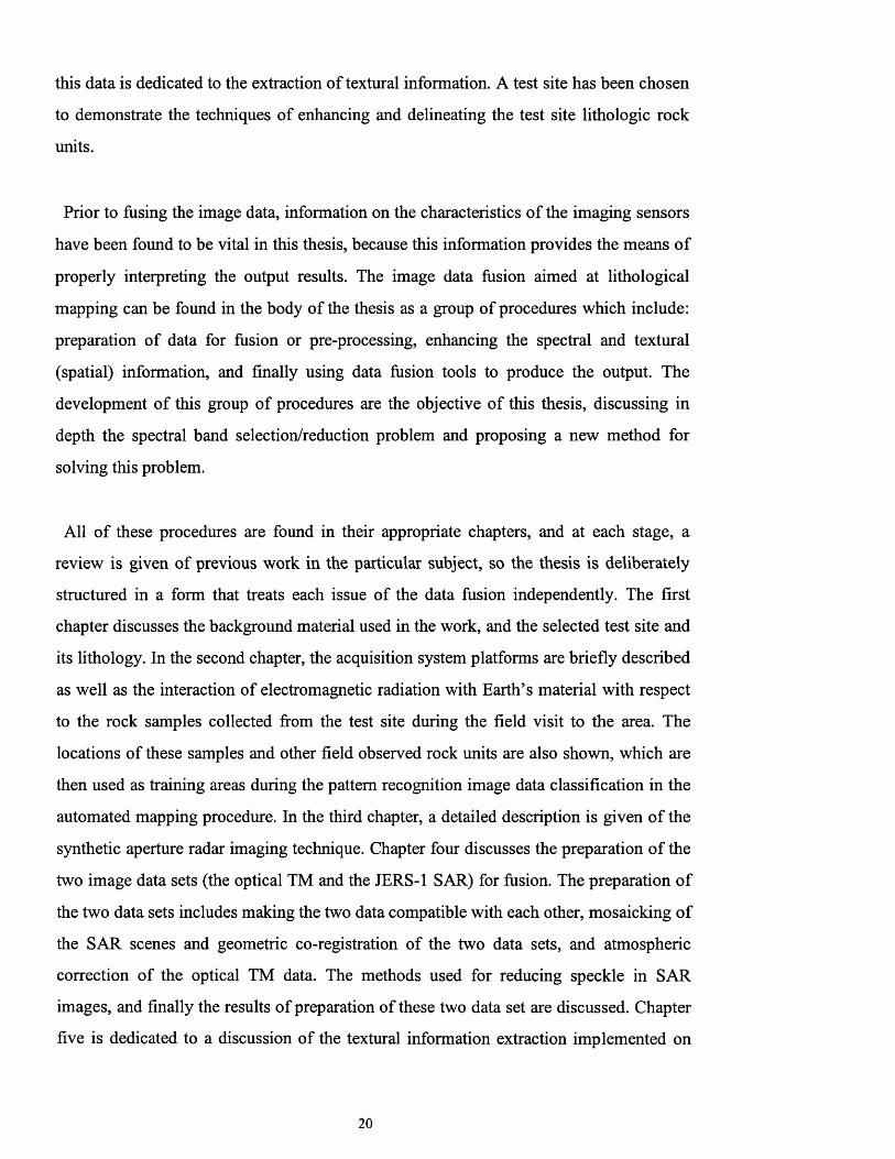
this data is dedicated to the extraction of textural information. A test site has been chosen

to demonstrate the techniques of enhancing and delineating the test site lithologic rock

units.

Prior to fusing the image data, information on the characteristics of the imaging sensors

have been found to be vital in this thesis, because this information provides the means of

properly interpreting the output results. The image data fusion aimed at lithological

mapping can be found in the body of the thesis as a group of procedures which include:

preparation of data for fusion or pre-processing, enhancing the spectral and textural

(spatial) information, and finally using data fusion tools to produce the output. The

development of this group of procedures are the objective of this thesis, discussing in

depth the spectral band selection/reduction problem and proposing a new method for

solving this problem.

All of these procedures are found in their appropriate chapters, and at each stage, a

review is given of previous work in the particular subject, so the thesis is deliberately

structured in a form that treats each issue of the data fusion independently. The first

chapter discusses the background material used in the work, and the selected test site and

its lithology. In the second chapter, the acquisition system platforms are briefly described

as well as the interaction of electromagnetic radiation with Earth’s material with respect

to the rock samples collected from the test site during the field visit to the area. The

locations of these samples and other field observed rock units are also shown, which are

then used as training areas during the pattern recognition image data classification in the

automated mapping procedure. In the third chapter, a detailed description is given of the

synthetic aperture radar imaging technique. Chapter four discusses the preparation of the

two image data sets (the optical TM and the JERS-1 SAR) for fusion. The preparation of

the two data sets includes making the two data compatible with each other, mosaicking of

the SAR scenes and geometric co-registration of the two data sets, and atmospheric

correction of the optical TM data. The methods used for reducing speckle in SAR

images, and finally the results of preparation of these two data set are discussed. Chapter

five is dedicated to a discussion of the textural information extraction implemented on

20

the JERS-1 SAR, and its importance for geological mapping. In chapter six, where the

data are now prepared for image fusion, a full definition of data fusion is established. The

colour composite band selection/reduction problem is discussed and a new method of

colour composite production is established and implemented to extract the spectral

information from the optical TM data. The spectral and spatial or textural data are then

combined and fused using fuser tools such as colours transform and principal component

transforms. The output data of these techniques are used for visual photo-interpretation to

lithologically delineate the test site. In chapter seven the automated classification is

implemented on the two manipulated spectral and textural information of the image data.

Chapter eight presents the conclusions, as well as some suggestions for future work.

The literature review presented in this thesis forms an important part because firstly it

shows the previous work of the particular subject, but secondly and most importantly it

served as the source of ideas and inspiration during the preparation of this thesis work.

1.1 Materials used in the study

Two satellites image data sets are used in the work in their digital format: Landsat TM

data and JERS-1 SAR data. The data from both satellites were acquired in the same year

in 1992. This is to insure there are no temporal changes in the test site between the two

data, the seasonal changes are usually not high because the area of study is arid and the

lack of vegetation throughout the year. A geologic map compiled by Clark in 1987 [2] in

parallel with two large 40 by 40 inches hard copy colour composite images (one is

natural colour and one is infrared) are used as ground truth based data. Field checks and

sample collection have also been carried out for ground truth verifications and training

areas selection registering their geographic coordinates using hand held GPS. A

spectrometer has also been used to measure the spectral reflectance of the collected

samples and compared with the TM data which helped to select the training areas

properly.

21

The software/hardware used in this thesis work is a combination of pre-processing of

the data (image co-registration) using MERIDIAN® VAX/VMS platform, and processing

techniques which are prepared essentially through PC based C-Programming and

EASI/PACE® image processing software. MATLAB® UNIX based system is also used

for many of the graphical outputs.

1.2 Objectives of the thesis

The main thesis objective is to implement, test, modify, and improve the image

processing techniques used for image data fusion for lithological mapping and apply

these techniques on a selected test site. In particular, this includes: the geometric co

registration between the two data sets; test of speckle filter reduction applied on the SAR

data; atmospheric correction of the optical TM data; implementing texture analysis on

SAR data used for lithology; colour composite selection, and developing a new method

of colour composition with high separability between the spectral classes; a test of colour

transforms and principal component transforms used for introducing the spatial

information with spectral information; and finally a test of automated mapping

(classification) and introducing a new method of classification using both of textural and

spectral information. Other secondary objectives include: production of a lithologic map

of the test site because the previous work carried out by Clark in 1987 [2] of the same

area is not accurate, and finally; a major literature review on image processing techniques

used for image data fusion.

1.3 The test site

The test site occupies nearly a quarter of the A1 Bad’ quadrangle in the north-western

part of Saudi Arabia (Lat. 28° 13.6" - 28° 28.6“ N and Long. 34° 47" - 35° 04“ E). It has an

area of around 852 km2 and lies in the north western Midyan Terrain exactly adjacent to

the eastern part of the Gulf of Aqaba. Figure 1.1 shows the area of study and the location

of the test site.

22

Figure 1.1. The area o f study as shown by NOAA 12 A VHRR band 2.

1.3.1 Physiography of the test site

The test site is physiographically divided into two units [2]. The first is the lowland

which is the Afal plain, which occupies the lower and eastern part o f the area and is

distinguished by its very low re lie f . The second unit is the upland zone in the west. It is

called the Maqnah Massif, and is composed o f sedimentary rocks underlain by

Proterozoic rocks o f the Arabian Shield. Some o f these Proterozoic rocks are exposed in

many areas in this zone. This zone is distinguished by its varying heights, ranging from

200 to 700 metres above sea level.

1.3.2 Lithology of the test site

As interpreted by Clark [2], the oldest rocks in the test site are a metamorphic rock unit

represented by the H egaf formation. Younger igneous rocks in the test site are

represented by Jurfayn, Atiyah, and Haql rock units. All these metamorphic and igneous

rocks belongs to the Arabian Shield, which covers most o f the west, north-west, and

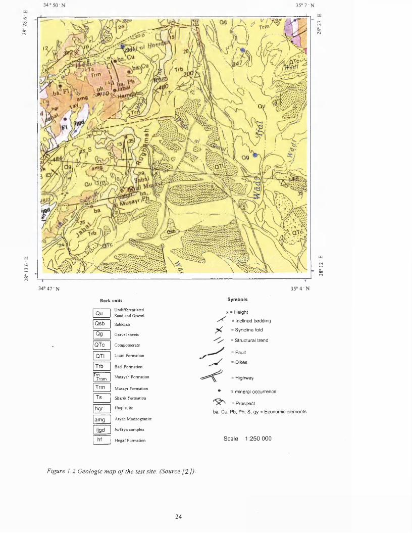
south-west o f Saudi Arabia. Figure 1.2 shows a detailed geologic map o f the test site as

previously compiled by Clark in 1987 [2].

23

28“

13.6

E 28

° 28

.6

Rock units S ym b ols

Qu

Qsb

QgQTc

QTI

Trbfrn

Tmm

Trm

Ts

hgr

amg

'jgdhf

Undifferentiated Sand and Gravel

Sabkhah

Gravel sheets

Conglomerate

Lisan Formation

Bad’ Formation

Nutaysh Formation

Musayr Formation

Sharik Formation

Haql suite

Atyah Monzogranite

Jurfayn complex

Hegaf Formation

x = Height

= Inclined bedding

X = Syncline fold

= Structural trend

= Fault

= Dikes

= Highway

• = mineral occurrence

= Prospect

ba, Cu, Pb, Ph, S, gy = Economic elements

Scale 1:250 000

Figure 1.2 Geologic map o f the test site. (Source [2 ])■

24

28°1

2 E

28°2

1-

The metamorphic Heqaf formation which is partly exposed in the test site, and located

in the far west o f the geologic map in figure 1.2, consists o f a variety o f highly folded

volcanic rocks consisting of meta-andesite and meta-basalt, few meta-rhyolite,

amphibolite, and mafic schist. They are subordinated by epiclastic rocks w hich are

metamorphosed to greenschist facies [2]. The Heqaf formation thickness is unknown, but

could be several thousands o f metres.

The igneous rocks in the test site are basically intrusive; the oldest o f which is the

Jurfayn complex. It is distinguished as irregular in shape, medium to low relief and

traversed by numerous mafic and felsic composite dikes. Its mineralogy is granodiorite. It

is located in the western part o f the test site in Magna M assif and can also be found in the

north-east o f the test site. Younger and larger granitic bodies are mostly located in the

western part but are also exposed in the north-east o f the test site and belong to a unit

called Atiyah monzogranite. The Atiyah monzogranite is massive with medium to coarse

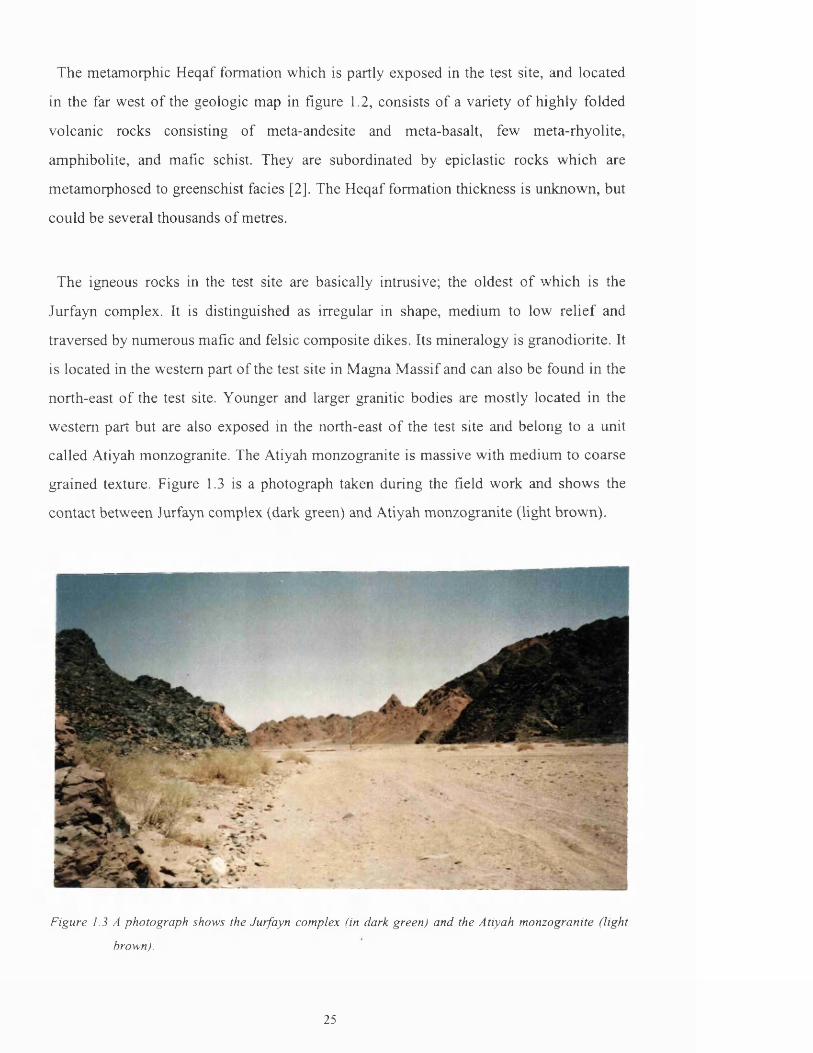
grained texture. Figure 1.3 is a photograph taken during the field work and shows the

contact between Jurfayn complex (dark green) and Atiyah monzogranite (light brown).

Figure 1.3 A photograph shows the Jurfayn complex (in dark green) and the Atiyah monzogranite (light

brown).

25

Sedimentary rocks in the test site are all Cenozoic in age. They outcrop in both the

Maqna Massif and the Afal plain. The oldest sedimentary rock unit in the test site is the

Sharik formation, dated to the Oligocene. The Sharik formation, located in the north

western part of the test site, is composed of red-tinted conglomerate, sandstone and

subordinate siltstone. It is poorly consolidated and unconformably overlies the

Proterozoic basement in many places.

Miocene rocks in the test site are represented by what is called the Raghama group. The

group is subdivided into the Musayr formation at the bottom, the Nutaysh formation in

the middle, and the Bad’ formation at the top. The Musayr formation overlies the Sharik

formation locally but also overlies the basement rocks and forms a major unconformity in

the north-western part of the test site. The Musayr formation lithology varies from reef

limestone, limestone interbedded with sandstone, to conglomerate and sandstone. The

thickness of the formation is about 100 to 130 metres. The Nutaysh formation overlies

conformably the Musayr formation. It is characterised by distinct lateral facies changing

from coarse detrital to fine grained shallow marine sedimentary rocks. Its lower part

consists of an alternating sequence of yellow marl, sandstone, and red limestone which

changes laterally to conglomerate and sandstone. Its upper part is fine grained,

variegated, and composed of marl and subordinate gypsum, sandstone, and siltstone. The

thickness of this formation is recorded to be 400 metres, and it dips from east to west [2].

Figures 1.4 and 1.5 are photographs taken during the field work and show the Nutaysh,

and Nutaysh overlies Musayr formation (Nutaysh is a creamy tan in colour and overlies

the light-red bedded layers of Musayr).

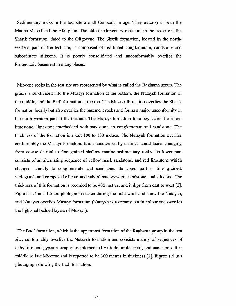
The Bad’ formation, which is the uppermost formation of the Raghama group in the test

site, conformably overlies the Nutaysh formation and consists mainly of sequences of

anhydrite and gypsum evaporites interbedded with dolomite, marl, and sandstone. It is

middle to late Miocene and is reported to be 300 metres in thickness [2]. Figure 1.6 is a

photograph showing the Bad’ formation.

26

The deposits that fill the Afal plain are named the Lisan formation. This has some

economic importance as a source o f water, oil, and gas reservoirs. It is about 3000 metres

thick, consisting o f poorly consolidated yellow to red sandstone, conglomerate, and

gypsum. This formation unconformably overlies the Bad’a formation in the west [2].

Figure 1.4 Nutaysh formation.

Figure 1.5 Nutaysh overlies Musayr

27

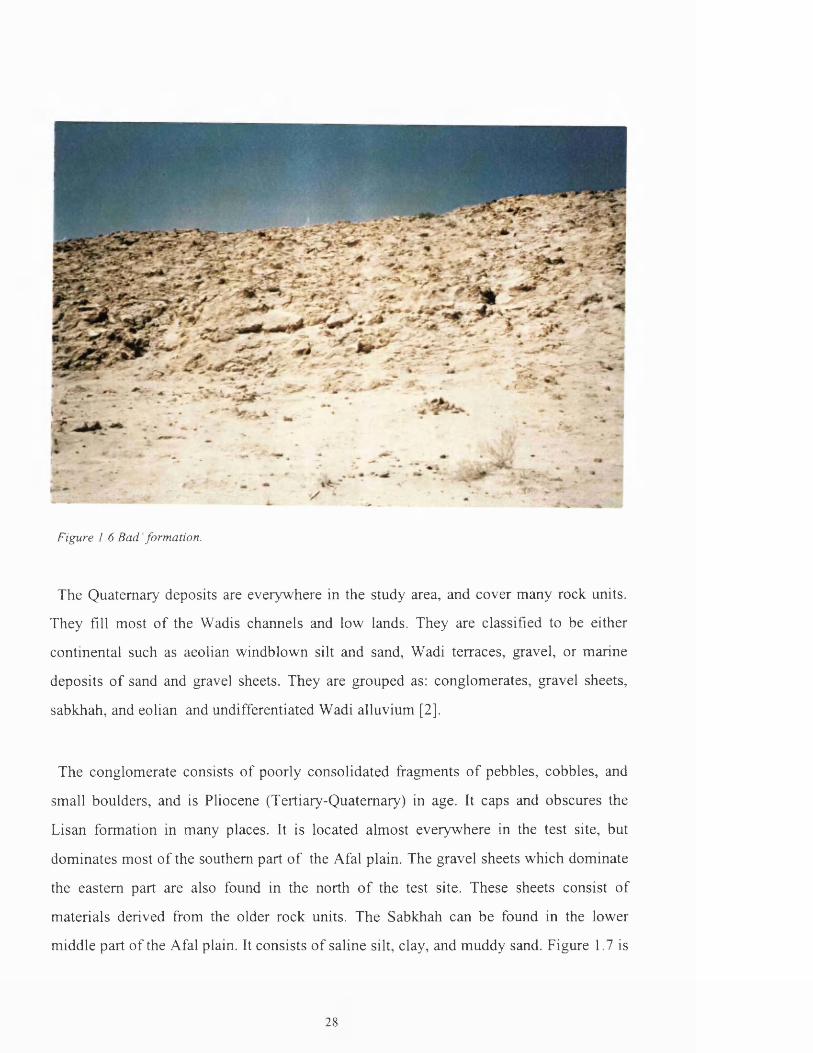
Figure 1.6 Bad'form ation.

The Quaternary deposits are everywhere in the study area, and cover many rock units.

They fill most o f the Wadis channels and low lands. They are classified to be either

continental such as aeolian windblown silt and sand, Wadi terraces, gravel, or marine

deposits o f sand and gravel sheets. They are grouped as: conglomerates, gravel sheets,

sabkhah, and eolian and undifferentiated Wadi alluvium [2].

The conglomerate consists o f poorly consolidated fragments o f pebbles, cobbles, and

small boulders, and is Pliocene (Tertiary-Quaternary) in age. It caps and obscures the

Lisan formation in many places. It is located almost everywhere in the test site, but

dominates most o f the southern part o f the Afal plain. The gravel sheets which dominate

the eastern part are also found in the north o f the test site. These sheets consist o f

materials derived from the older rock units. The Sabkhah can be found in the lower

middle part o f the Afal plain. It consists o f saline silt, clay, and muddy sand. Figure 1.7 is

28

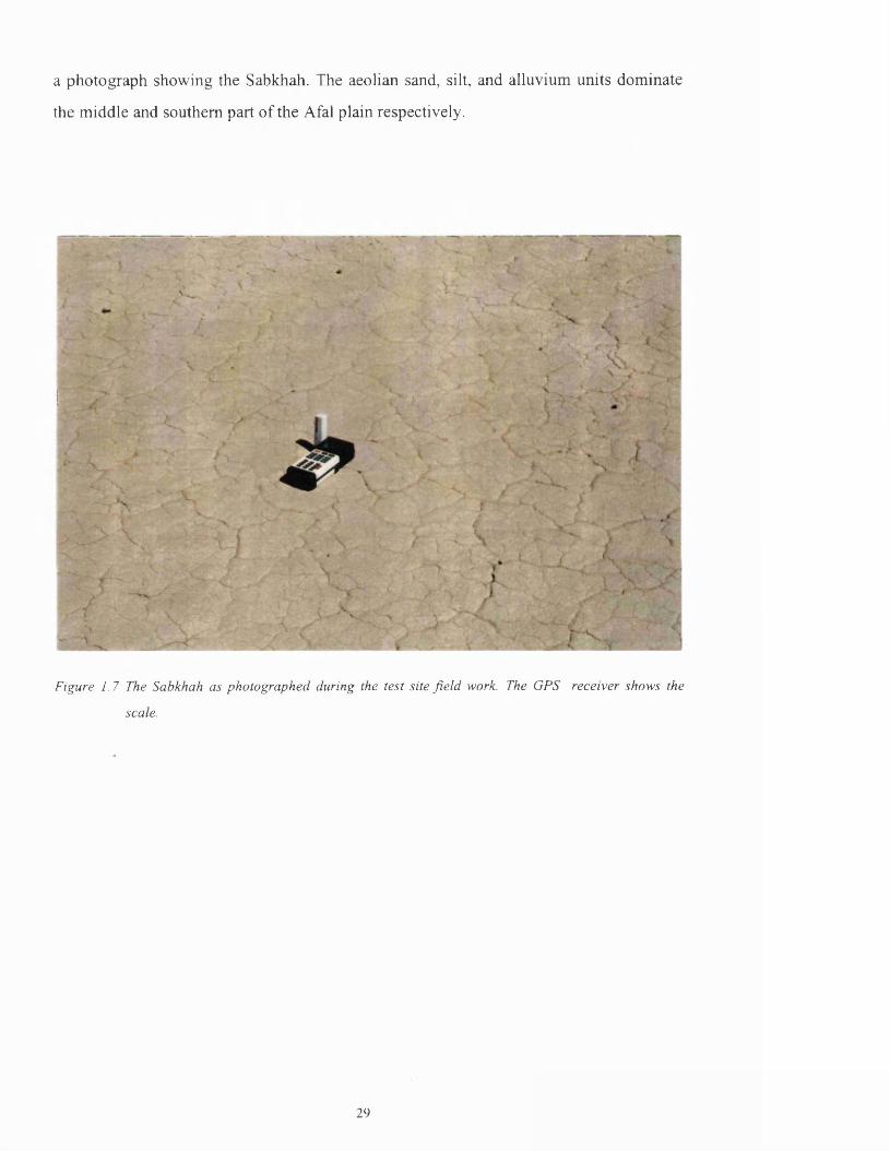
a photograph showing the Sabkhah. The aeolian sand, silt, and alluvium units dominate

the middle and southern part o f the Afal plain respectively.

Figure 1.7 The Sabkhah as photographed during the test site f ie ld work. The GPS receiver shows the

scale.

29

2.0 Platforms and sensors

As mentioned in section 1.1, two image data sets were used in this study. The first data

set is the optical imagery data acquired by the Landsat-5 Thematic Mapper, and the

second is the SAR imagery data acquired by the Japanese satellite JERS-1 SAR system.

This chapter describes both satellites and the properties of their sensors.

The basics of the interaction between electromagnetic radiation, atmosphere, and the

rock units of the study area are also discussed in this chapter. Results from spectral

reflectance measurements of the rock units collected using a portable spectrometer from

the study area during the field visit are presented. The spectrometer measures the spectral

reflectance of the collected rock samples using 861 optical channels. These spectral

reflectances are then used and compared with the reflectance of the TM image data for

photo-interpretation in the primary stage of rock unit delineation, and for selecting the

training areas representing the lithologic spectral classes.

2.1 Landsat-5

The Landsat program started with the 1972 launch of Landsat-1, which carried the

scanning optical system, MSS. The program continued with the launch of Landsat-2 and

3, carrying optical systems similar to MSS. The Landsat series further continued with the

launch of Landsat-4 and 5 in 1982 and 1984 respectively, which are both characterised

by an advanced scanning optical system called the Thematic Mapper. In that time and in

terms of spectral information, the TM imaging system was superior to other optical

orbiting imaging systems and is widely used by Earth remote sensing scientists and

geologists in particular [3].

The Thematic Mapper systems aboard Landsat-4 and 5 are identical, and acquire images

using the same principle of the previous MSS optical system. The differences lie in the

higher spatial resolution, of pixel size of 30 by 30 metres, and the spectral resolution

30

represented by seven spectral bands extending from the visible to short, mid, and thermal

infrared. Table 2.1 shows the TM imaging system spectral band characteristics and their

main applications.

Band Wavelength Main application

Band-1 0.45-0.52pm

(Blue)

Used for water penetration, forest type, and soil

vegetation mapping

Band-2 0.52-0.60pm

(Green)

Used to measure green reflectance peak of vegetation

and discrimination

Band-3 0.63-0.69 pm

(Red)

Used for Chlorophyll absorption aiding in plant species

differentiation

Band-4 0.76-0.90pm

(NRIR)

Water-Land boundary and soil moisture mapping

Band-5 1.55-1.75pm

(MIR)

Snow/cloud differentiation, soil moisture, and

vegetation mapping

Band-6 10.4-12.5pm

(Thermal)

Thermal band, used for thermal mapping (Not used in

this study)

Band-7 2.08-2.35pm

(MIR)

Mineral and rock types mapping

Table 2.1 The optical spectral bands o f the TM imaging system [4J.

The imaging technique of the TM system relies on a scanning mirror, which rotates

normal to the satellite orbit with total field of view (FOV) of 14.95 degrees, giving a

swath width equal to 185 km. The mirror reflects the light collected from the Earth’s

surface to the system optics, which in turn projects the reflected light to the band

detectors which measure the intensity of the projected reflected light. The measured

radiance is converted to digital form through the onboard A/D converter, recorded in the

satellite’s data storage system and then telemetred to the ground receiving stations.

31

Except in the thermal band (band 6), the instantaneous field of view (IFOV) of the TM

bands is 0.043 mrad. where every band employs 16 detectors. The thermal band employs

only 4 detectors and has an IFOV of 0.17 mrad. This results in 30 metre spatial resolution

in the bands 1-5, and 7. Band 6 has a lower resolution equal to 120 metres.

The Landsat satellites are all sun-synchronous and near polar orbital. For example,

Landsat-5 has an inclination angle of 98.2 degrees with nominal altitude of 705 km and

crosses the equator from north to south of each orbit at 9:45 a.m. local time, passing the

same area every 16 days [4].

2.2 JERS-1

JERS-1, or Fuyo-1, is the first Japanese Earth Resources Satellite. It was launched in

February 1992 by the National Space Development Agency of Japan (NASDA). The

satellite mission was designed to perform many tasks, including the establishment of the

Japanese Earth Resources integrated observation system and the observation of the Earth

using Synthetic Aperture Radar (SAR), simultaneously with optical visible and near

infrared imaging systems [5].

As common for Earth observing satellites, the JERS-1 system is divided into two parts:

one is the satellite itself which collect the data and transmits it or records it through its

two Mission Data Transmitters (MDT) or the Mission Data Recorder (MDR), when there

are no ground receiving stations linked with the satellite. The second part is the ground

segment of the system, which is the tracking and control system. This controls the

satellite orbit and attitude, in addition to the data acquisition and processing system

which links to the ground receiving stations that receive the data, process it, and

distribute it to the users [5].

32

The JERS-1 satellite carries two observation sensors: the SAR sensor and the optical

OPS sensor. The SAR is designed specifically for Earth resources exploration,

topographic mapping and geological surveying. The optical OPS system is designed for

water quality and vegetation surveying, environment preservation, and stereoscopic

viewing through bands 3 and 4. Table 2.2 shows the JERS-1 main specifications.

Spacecraft Altitude 568 km over the equator

Period (7) 96 minutes

Inclination angle 97.67 degree

Orbit Sun-synchronous

Recurrent period 44 days and 659 revolutions

Mean local time at descending node 10:30-11:00 AM

Distance between adjacent orbit

Earth track

60.7 km

Mission equipments SAR,OPS,2HDTs,lHDR.

Spacecraft weight 1340 kg

Communication links 2GHz for telemetry & 8 GHz

image data

Operational duration 2 years

Table 2.2 JERS-1 main characteristics [5].

The geometrical aspect of the JERS-1 SAR observation system is shown in figure 2.1,

the SAR system transmits microwave pulsed signals downwards perpendicular to the

spacecraft flight direction. The received radar echoes are then telemetred to the ground by

the mission data transmitter MDT, after being detected and digitised onboard the

spacecraft. The SAR system onboard JERS-1 transmits 1505-1600 linear frequency

modulated chirped pulses per second from its antenna and receives the reflected echoes

33

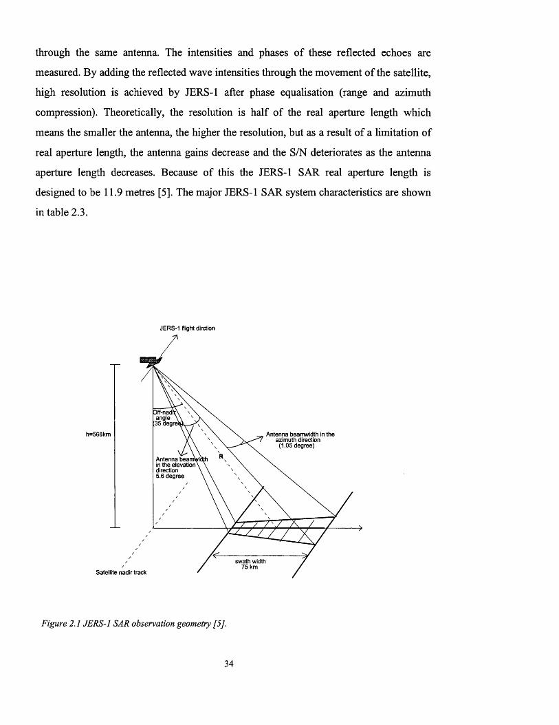
through the same antenna. The intensities and phases of these reflected echoes are

measured. By adding the reflected wave intensities through the movement of the satellite,

high resolution is achieved by JERS-1 after phase equalisation (range and azimuth

compression). Theoretically, the resolution is half of the real aperture length which

means the smaller the antenna, the higher the resolution, but as a result of a limitation of

real aperture length, the antenna gains decrease and the S/N deteriorates as the antenna

aperture length decreases. Because of this the JERS-1 SAR real aperture length is

designed to be 11.9 metres [5]. The major JERS-1 SAR system characteristics are shown

in table 2.3.

JERS-1 flight dirction

DfT-nadrt\ angle \

[35 aegrel

Antenna beamwidth in the azimuth direction

(1.05 degree)

h=568km

Antenna beamwidth in the elevation \ \ direction \ \ 5.6 degree \

swath width 75 km

Satellite nadir track

Figure 2.1 JERS-1 SAR observation geometry [5J.

34

Title Performance Remarks

Observation frequency 1275 MHz (L band

0.235m)

Bandwidth 15MHz

Polarisation H-H

Off-Nadir angle 35 degrees

Range resolution 18 metre (At swath centre 3

Azimuth resolution 18 metre multilook)

Swath width 75 Km

Transmission Power 1100-1500 Watts

Pulse width ( r ) 35 jus

PRF 1505.8Hz, 1530.1Hz

1555.2Hz, 1581.0Hz

1606.0HzAntenna gain 33.5 dB At the beam centre

Beam angle in range 5.6 degree Observed 5.4 degree

Beam angle in azimuth 1.05 degree Observed 0.98 degree

Side-lobe level (both in

range and azimuth -11.5dBAntenna length/width 11.92/2.2 metre

Table 2.3 JERS-1 SAR system characteristics (Source:[5])

2.2.1 JERS-1 SAR image construction

The first step used to construct the JERS-1 SAR imagery is performing range

compression, in which each echo is correlated with a replica of the transmitted pulse (the

matched filter). This is achieved in the frequency domain by a Fast Fourier Transform

(FFT) approach.

35

The JERS-1 SAR system onboard transmits down-chirped signals with a carrier

frequency ( f 0) with pulse repetition frequency (PRF) and pulse width (t).

The JERS-1 SAR transmitted signal is:

f ( x ) = c o s 2 + - r - X /)/ (2 .1)

where:

— t / 2 < t < t / 2

CR = the chirp rate

Ignoring the antenna pattern and the path attenuation, the amplitude of the received

signal is normalised to 1. The received reflected and scattered signal is calculated using

the equation:

0 2 j n [ ^ ( t - t r ) 2 - f 0 * t r + d ( t ) * ( t - t r ) ]S B = e 2 (2.2)

Equation (2.2) is used for range compression, and the matched filter used for the

compression is defined by:

where :

T T

t — tr = the two-way propagation delay.

d(t) = the Doppler component resulting from the satellite motion.

j [ - 2 x ( k / 2 x t 2 )] (2.3)

where:

- T / 2 < t < T /2

36

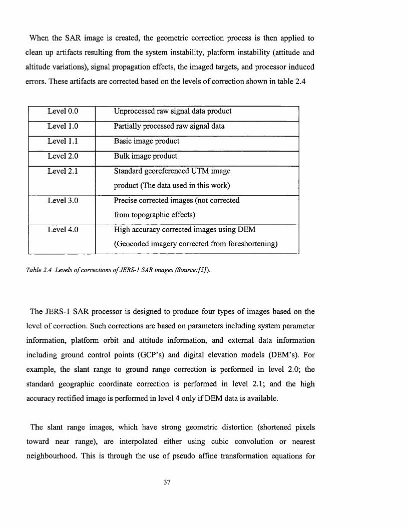
When the SAR image is created, the geometric correction process is then applied to

clean up artifacts resulting from the system instability, platform instability (attitude and

altitude variations), signal propagation effects, the imaged targets, and processor induced

errors. These artifacts are corrected based on the levels of correction shown in table 2.4

Level 0.0 Unprocessed raw signal data product

Level 1.0 Partially processed raw signal data

Level 1.1 Basic image product

Level 2.0 Bulk image product

Level 2.1 Standard georeferenced UTM image

product (The data used in this work)

Level 3.0 Precise corrected images (not corrected

from topographic effects)

Level 4.0 High accuracy corrected images using DEM

(Geocoded imagery corrected from foreshortening)

Table 2.4 Levels o f corrections o f JERS-1 SAR images (Source: [5]).

The JERS-1 SAR processor is designed to produce four types of images based on the

level of correction. Such corrections are based on parameters including system parameter

information, platform orbit and attitude information, and external data information

including ground control points (GCP’s) and digital elevation models (DEM’s). For

example, the slant range to ground range correction is performed in level 2.0; the

standard geographic coordinate correction is performed in level 2.1; and the high

accuracy rectified image is performed in level 4 only if DEM data is available.

The slant range images, which have strong geometric distortion (shortened pixels

toward near range), are interpolated either using cubic convolution or nearest

neighbourhood. This is through the use of pseudo affine transformation equations for

37

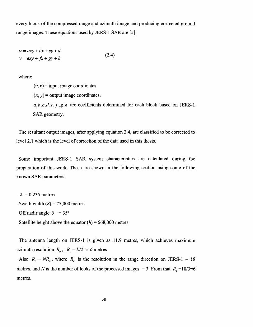
every block of the compressed range and azimuth image and producing corrected ground

range images. These equations used by JERS-1 SAR are [5]:

u = axy + bx + cy + dr u (2*4)v = exy + f x + gy + h

where:

(w,v) = input image coordinates.

(x,y) = output image coordinates.

a ,b ,c ,d ,e , f ,g ,h are coefficients determined for each block based on JERS-1

SAR geometry.

The resultant output images, after applying equation 2.4, are classified to be corrected to

level 2.1 which is the level of correction of the data used in this thesis.

Some important JERS-1 SAR system characteristics are calculated during the

preparation of this work. These are shown in the following section using some of the

known SAR parameters.

X = 0.235 metres

Swath width (S) = 75,000 metres

Off nadir angle 6 =35°

Satellite height above the equator (h) = 568,000 metres

The antenna length on JERS-1 is given as 11.9 metres, which achieves maximum

azimuth resolution Ra , Ra = L/2 » 6 metres

Also Rr = NRa , where Rr is the resolution in the range direction on JERS-1 = 18

metres, and N is the number of looks of the processed images = 3. From that Ra =18/3=6

metres.

38

Antenna height (width) = W =M 0.235 x 568,000

= 2.17 metre. The systemS cos 6 75,000 x cos(3 5)

designers made it 2.20 metres.

Maximum PRF = —— —- = 3486.8H z .2Ssm 0

Therefore PRF should be <3.48 kHz.

The satellite velocity can be measured over the equator, based on the equation:

where

gs = Earth gravitational attraction = 9.81 metre/sec2.

R = radius of the Earth = 6380,000 metres.

v= satellite velocity.

r = satellite height measured from the centre of the Earth.

From the equation, the velocity (v) is:

9.81 x (6380,000)7.5809 km/sec.

To calculate the satellite period (T)

l 7 i rT = ----- =5758.6 seconds = 95.977 minutes.

v

Minimum PRF of the2v

radar is > — = 1.26 kHz.

Azimuth footprint FaLcosO

= 13.596 km (note that it is equal to the length of the

synthetic array).

39

FSatellite integration time T = — =1.79 second.

v

cSystem bandwidth (B) = - — -—r~z— 14.52MHz. The system designers made it

2 x Rr sin 6

15MHz.

The leading edge of the returned echo (/,) arrived at time (accounted after transmission)

2 ht, = -------- where 8 is the angle between the near range and the satellite nadir. The

ccosd

leading edge equation is used to avoid the received echoes from the satellite nadir.

.'. tx = 7.1 x 10-3 seconds

hX2BSatellite range curvature M r = ------ ;----- = 3.324 unit range resolution

5 c \ 6 cR 2 cos0 5

2 N 2L2 2(3)2 (12)2Depth of focus (F)= — -— = ------- ------=11.03 km.

F X 0.235

2 XhBProcessing complexity PT (if time domain is used) = — r; =3.394 x 1010

(L) cos#

operation/sec.

Processing complexity (if frequency domain is used) =Bx log]0(PT)= 1 5 7 x l0 6

operation/sec.

2.3 Interaction of electromagnetic waves with matter

When electromagnetic solar radiation interacts with matter, either in its gas, liquid, or

solid state, a variety of energy exchange mechanisms occur between the matter and the

solar radiation, which depend upon the wavelength (i.e. photon energy) and the energy

levels of the matter’s structure. This occurs because the electrons of the matter which are

in a stationary state are put into motion, leading to an exchange of energy between the

wave and matter.

40

In the case of isolated atoms, the energy levels are related to the orbits and spins of the

electrons, called the electronic levels. For molecules (e.g. gases), additional rotational

and vibrational energy levels exist as a result of bond interaction. The rotational and

vibrational energy levels correspond to the dynamics of the constituent atoms relative to

each other. Rotational excitations occur only in gases where the molecules are free to

rotate [6].

In the visible and infrared region of the spectrum, where the energy is in the range of 0.2

to 3.0 eV, vibrational and electronic transitions occurs. The gases show well defined

absorption as spectral lines and these lines are broadened due to the temperature and the

pressure.

The Earth’s atmosphere interacts with electromagnetic waves, leading to a limitation on

the spectral regions that can be used for remote sensing. This is because the atmosphere

and/or the ionosphere absorb or highly attenuate these spectral regions and hence remote

sensing sensors are usually designed to operate in specific regions of the electromagnetic

spectrum away from the spectral absorption regions. The regions used for remote sensing

are called “atmospheric windows”.

For active remote sensing such as radar imaging systems, the ionosphere blocks any

transmission to or from the Earth surface below about 10 MHz. In the rest of the radio

frequency region up to 10 GHz, the atmosphere is effectively transparent, but there are a

number of strong absorption bands in the microwave region basically associated with

water vapour and oxygen [6]. At a frequency of 22 GHz the transmission of the

microwave signal is reduced to less than 15% as a result of the water vapour in the

atmosphere and transmission is completely blocked at 180 GHz . Oxygen has similar

effects by blocking the frequencies 50-60 GHz and near 120 GHz [7].

In the submillimetre and far-infrared region of the electromagnetic solar spectrum, the

atmosphere is almost opaque, as a result of absorption of the radiation by the atmospheric

41

constituents. In the visible and near infrared region of the spectrum, the atmosphere has

many opaque windows, resulting from electronic and vibrational processes which occur

due to the presence of water vapour and carbon dioxide molecules. In the ultraviolet

region of the spectrum, the atmosphere is completely opaque due to the ozone absorption

layer in the upper atmosphere [6].

Solid matter shows a wide variety of energy transfer interactions including molecular

vibration, ionic vibration, crystal field effects, charge transfer, and electronic conduction.

Spectral absorption of rocks and minerals is an important subject in the field of geologic

remote sensing because it is the key factor of manual photo-interpretation and mapping

using the image data. The spectral absorption of rocks and minerals is caused by the

transition between the energy levels of the atoms and molecules of the minerals which

form rocks. The transition may result from processes which are mainly vibrational or

electronic.

Vibrational transitions occurs as a result of small displacement of the atoms from their

original positions. In the visible and near-infrared wavelengths, the vibrational processes

occur in minerals containing hydroxyl ions (OH ) or water molecules (H20 ) either

bounded in the mineral structure or as fluid inclusions. Due to water molecules,

absorption occurs in the infrared at wavelengths of 1.45 pm and 1.9pm. If the water

molecules are well defined and are ordered in the mineral structure, a sharp and narrow

absorption feature can be depicted in the spectral signature of the rock. A broad

absorption shape is caused by water molecules unordered in the mineral framework [6]

and generally, both absorptions occur simultaneously.

Most of the silicate minerals group contain hydroxyl ions (OH' ) in their structures,

vibrational absorption features occur in such minerals (e.g. Al-O-H) in the infrared bands

centred at 1.6pm and 2.2pm [8], The best example of such phenomena can be

42

demonstrated by clay minerals, which are very important indicators of alteration zones.

TM bands 5 and 7 are usually used for mapping these minerals.

Carbonate minerals ( C032- ions) also show the vibrational absorption features resulting

from the Ca-0 bond. This process can be depicted in many wavebands in the mid

infrared spectrum including 1.9pm, 2.0pm, 2.16pm, and 2.35pm [8]. An example of the

carbonate minerals are the Calcite and Dolomite, which are the main constituents of

Limestone, which is abundant in the sedimentary rocks found in the selected test site.

The electronic processes are associated with the electronic energy levels where every

electron in an atom only occupies a single quantised orbit with a specific energy level.

Such processes occur as a result of crystal field, charge transfer or conduction band

effects.

When the atoms are introduced into a crystal lattice, they split into many different

energy levels because of the influence of the crystal field and hence show absorption

features of specific wavelengths. The most common elements from which minerals are

formed are silicon, oxygen, and aluminium, and these show little or no electronic

transition in the visible and near-infrared wavelength. In the presence of the transition

metal elements, especially iron which is common in most igneous and metamorphic

rocks, they show a crystal field absorption effect in the visible and infrared. The mineral

Hematite is the best example [9].

The charge transfer absorption effects result from the movement of the electrons

between the neighbouring cations or between cations and ligands (e.g. Fe-O) as a result

of the excitation of the incident wavelength. It is distinguished by its narrow band and is

common in most iron bearing minerals, and needs high energy such as within the visible

wavelength.

43

The conduction band transition absorption effect occurs when electrons in the crystal

lattice become delocalised and wander freely throughout the lattice. This effect is very

common in most metallic mineral crystals, giving them high electric conductivity. These

minerals are opaque as a result of this effect, and always show absorption features in the

visible wavelength. Generally speaking the electronic processes can easily be depicted in

the visible wavelengths and are mainly broad spectral bands

The spectral reflectance of rocks and minerals were intensively studied by Hunt and

Salisbury for silicate minerals in 1970, and carbonates in 1971. They also studied oxides

and hydroxides in partnership with Lenhoff in 1971. They studied igneous rocks in 1973

and 1974. Their work introduced the basics of image interpretation for remote sensing to

geologists.

To some extent, data collected by remote sensing satellites is considerably inferior to

such laboratory measurements. This is as a result of many factors, including the influence

of the atmosphere, soil, and vegetation; grain size and mixtures of minerals; desert

varnish or coating which influences arid areas; humidity and temperature; organic

content; and texture. In the case of radar imaging systems, other factors such as the

viewing angle, dielectric properties, polarisation and texture, all contribute to

modification of the spectral signatures.

In the following section the laboratory spectral measurements for the rock samples

collected during the field visit of the study area are discussed. The rock samples were

carefully selected to represent the lithologic rock units of the test site. The portable field

reflectance spectrometer (PFRS) used in this work is very similar to that described by

Kahle [8] and measures the reflectance of the samples in 861 channels ranging from

0.314pm to 2.534pm of the electromagnetic spectrum. The spectrometer is supported by

a portable notebook computer which records the output data digitally and stores it on its

hard disk. In this work, the output results of the rock samples reflectance were then

transferred to a floppy disk, read using MATLAB software, and displayed graphically

44

with the x-axis representing the wavelength in micrometres and the y-axis representing

rock sample reflectance. The location of every selected rock sample was recorded using

the Global Positioning System (GPS) and the corresponding spectral reflectance of this

location in the TM image data compared with the sample spectral reflectance read by the

spectrometer. The location of every sample is used as a training area representing the

rock unit, and hence used for the transformed divergence separability test between

classes. Furthermore the selected classes are used for automated mapping (classification)

procedure, other training areas have been selected based on their spectral similarities to

the measured spectral reflectance of the rock samples. Figure 2.8 shows the location of

rock samples collected and selected training areas.

1- A1 Bad’ rock sample reflectance.

The sample of A1 Bad’ is taken from undisturbed surface selected from the northern part

of A1 Bad’ formation with geographic coordinates measured by the GPS of 28° 26.37' N

and 35° 00.115' E. This coordinate is used as a spectral reference point and one of the

training area of A1 Bad’ class in the TM image data. The spectral reflectance of AT Bad

as shown in figure 2.2 exactly mimics the Gypsum spectral reflectance. It has two distinct

vibrational absorption features at 1.45 pm and 1.9pm due to the presence of water. The

absorption feature around 0.5pm is due to electronic process resulting from desert

varnish (iron oxides) occurring on the rock sample surface.

During the literature review in this thesis, it has been found that an image plate1 shown

by Drury [9] visually misinterpreted the A1 Bad’ formation using TM data as Lava flow.

If band 7 of the TM image data is used for the interpretation and compared with the other

TM spectral bands to trace where the absorption features occur, the interpretation of Al’

Bad rock unit will definitely be Gypsum, even without referring to figure 2.2 shown or

collecting rock samples from the study area.

1 A colour plate in Drury [9] (figure 3.41) showing the Gulf o f Aqaba. Landsat 4 TM colour composite o f bands 7, 5, 4 displayed in red, green, and blue respectively. The Al Bad’ formation is shown as light blue and marked by the letter D and interpreted as silicic lava flows.

45

Spectral reflectance of Bad'

100

0.5 2.5

Figure 2.2 Spectral reflectance o f rock sample taken from Al B ad’ formation.

2- Spectral reflectance of Nutaysh Formation

The Nutaish rock sample was taken from an area located in the northern part of Nutaysh

formation at 28° 27.804' N and 34° 55.434' E. The area location is also marked as a TM

spectra reference of the formation and one of the training areas for classification

procedure. The collected sample consists of dark to medium brown siltstone, and the

reflectance of the rock sample is shown in figure 2.3.

Spectral reflectance of Nutaysh

100

a>ocCD

Oa>

c=a>cr

0 0.5 1.5 2 2.5 3wavelength in micrometre

Figure 2.3 Spectral reflectance o f sample collected from Nutaysh Formation.

46

The absorption features which can be distinguished in the Nutaysh’s sample spectral

reflectance show weak reflectance along the spectrum (low albedo) with distinct

electronic absorption feature around the wavelength 0.5pm due to weathering (i.e. desert

varnish). A small vibrational absorption feature occurs at 1.9pm due to water and Si-0

bond.

3- Spectral reflectance of Atiyah monzogranite

A medium to coarse grained red granitic sample is taken from Atiyah Monzogranite to

represent the rock unit. The sample is taken from location with geographic coordinates of

28° 26.742' N and 34° 50.49' E and this location is also marked as a spectral reference of

the rock unit and selected as one of the training area in the TM data. In the measured

spectral reflectance of the sample as shown in figure 2.4, a clear electronic absorption

feature occurs due to desert varnish around the wavelength 0.5pm. Another electronic

absorption feature occurs at 0.9pm due to iron. Low albedo also characterises the rock

sample.

Spectral reflectance of Atiyah

100

a>ocOST jaia)cr

0 0.5 1.5 2 2.5 3Wavelength in micometre

Figure 2.4 Measured spectral reflectance o f a sample taken from Atiyah monzogranite.

47

A vibrational absorption features occurs in the rock sample at 1.9pm and is due to water

molecules and Si-0 bond which is usually occurs in the silicate minerals (i.e. water

molecules associated with Mica minerals in the rock sample). Another small vibrational

feature occurs at 2.2pm as a result of O-H bearing silicates.

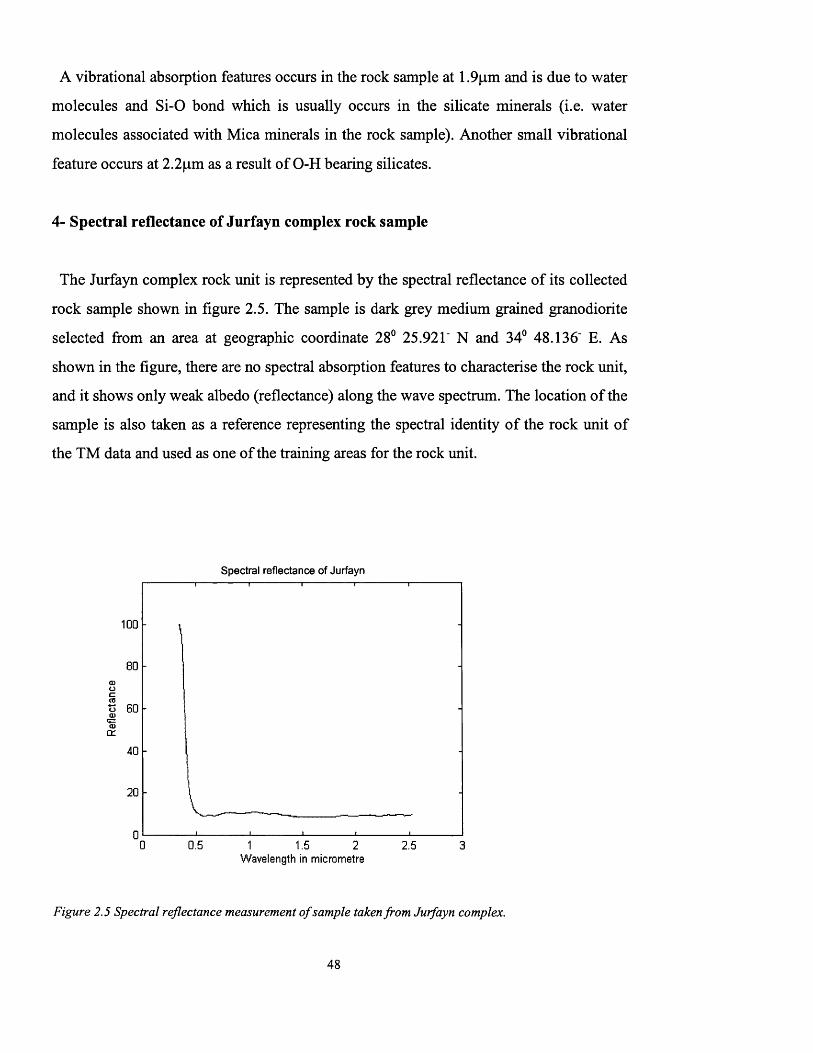
4- Spectral reflectance of Jurfayn complex rock sample

The Jurfayn complex rock unit is represented by the spectral reflectance of its collected

rock sample shown in figure 2.5. The sample is dark grey medium grained granodiorite

selected from an area at geographic coordinate 28° 25.921' N and 34° 48.136' E. As

shown in the figure, there are no spectral absorption features to characterise the rock unit,

and it shows only weak albedo (reflectance) along the wave spectrum. The location of the

sample is also taken as a reference representing the spectral identity of the rock unit of

the TM data and used as one of the training areas for the rock unit.

Spectral reflectance of Jurfayn

100

80

60

40

20

00 0.5 1.5 2 2.5 3Wavelength in micrometre

Figure 2.5 Spectral reflectance measurement o f sample taken from Jurfayn complex.

48

5- The spectral reflectance of the Sabkhah deposits

The measured reflectance of a friable sample taken from the Sabkhah at geographic

coordinates 28° 16.343" N and 34° 55.045' E is shown in figure 2.6. The sample is creamy

white in colour and consists mainly of clay, silt, and evaporitic minerals (i.e. salt and

gypsum). Three distinct vibrational absorption features can be depicted in the measured

spectra of the sample due to the presence of water molecules at 1.45 pm, 1.9pm and O-H

bearing minerals absorption feature at 2.2pm. The geographic location of the sample is

marked to be used as a training area in the TM image data. Higher albedo is characteristic

of the rock sample.

Spectral reflectance of Sabkhah100

a»ocoa)a>cr

0 0.5 1.5 2 2.5 3Wavelength in micrometre

Figure 2.6 The spectral reflectance o f Sabkhah.

6- The spectral reflectance of the gravel sheets deposits.

The gravel sheets deposits are represented by a friable sample to measure its spectral

reflectance. The sample consists mainly of a mixture of sand, pebbles, and cobbles

varying in shape, size, and origin. The sample is taken north of the middle of the test

area at location 28° 25.572' N and 35° 00.401'. This location is also selected as a spectral

49

reference and one of the training areas of the gravel sheets deposits. Figure 2.7 shows its

measured reflectance, which is characterised by low reflectance (low albedo) along the

measured wavelength mainly due to the metamorphic and igneous source of this sample.

No strong absorption feature can be depicted in the measured reflectance of the sample.

Spectral reflectance of gravel sh eets

100

CDOCCOoCD

0)tr

0.5 2.5Wavelength in micrometre

Figure 2.7 The spectral reflectance o f the gravel sheets deposits.

Beside the rock unit locations marked as a spectral reference areas during the field work,

other areas spectrally similar to the marked areas in the TM (and SAR after being

registered with TM) image data are also marked as training areas, representing the

individual rock classes. Pixels of these classes are always statistically analysed using the

Transformed Divergence (TD) separability test after implementing data fusion and/or an

image processing algorithm. The locations of these training areas and the GCPs are

shown in figure 2.8. The Transformed Divergence separability measures of the training

areas is used as judgement for fusion evaluations. The Transformed Divergence

algorithm is described in appendix A-4.

50

Figure 2.8 Locations o f rock unit classes o f the study area marked on TM band 5, these classes are (1 =

B a d ’), (2= Nutaysh), (3= Musayr), (4= Atiyah), (5= Jurfayn), (6 = Lisan), (7 = Sabkhah), (8=

conglom erate + gravel), ( 9 - Gravel sheets), (10=Aeolian silt and sand), (11= Alluvium). The

(*s) sign represent the location where the sam ple has been taken fo r laboratory spectral

measurement and also the measured GCP coordinates.

51

Scale 1:204084

3.0 Synthetic Aperture Radar

In chapter 2, the Landsat 5 TM and the JERS-1 SAR have been described. The

acquisition and image construction of the optical TM data is simple and straightforward,

and has been discussed briefly in chapter 2. The generation of SAR images is somewhat

complicated, and this chapter is devoted to a description of the techniques underlying the

method of SAR image generation, including the geometrical aspects of the SAR.

3.1 Historical background

Radar has long been recognised as a tool for detection, tracking, and ranging of targets

such as aircraft and ships. It uses radio waves to detect the presence of objects and

identify their position. The word RADAR is an acronym of RAdio Detection And

Ranging, firstly introduced by the US Navy in 1940. The first record of discovery of

radar, after 15 years of the discovery and study of generation, reception, and scattering of

electromagnetic radiation carried out by Hertz, was in 1903, when a German scientist

demonstrated a radar system for ship collision avoidance [7]. In 1922, Marconi

recognised the value and importance of radar for the detection and tracking of ships. The

first airborne pulsed radar system operating at carrier frequency of 60MHz was

developed by the NRL (Naval Research Laboratory) in the US in 1934. In parallel, radar

systems for tracking and detection of aircraft were developed in Great Britain and

Germany during the early 1930s. By 1935, each of these countries had successfully

demonstrated the capability of tracking aircraft targets using short pulse ranging

measurements. In 1937, Sir Robert Watson-Watt built the first operational radar network,

which was used to track aircraft across Western Europe, and this network was used in

World War II [7]. During the War, improvements in these systems were carried out by

the US, Great Britain, and Germany, which include the development of high frequency

hardware and systems, high peak power microwave transmitters, and the development of

image display systems such as the CRT, B-Scan, and PPI. In 1950, films were used to

record the CRT display of the pulse echoes.

52

Side Looking Airborne Radar (SLAR) was the second step in the development of radar

technology and was firstly introduced and intended for use for military reconnaissance

purposes [10]. In the mid-1960s the first high resolution SLAR (10-20 metre resolution)

became available for scientific applications. The first mapping project using radar

(SLAR) was in 1967 in the Darien province in Panama. Scientists have increased their

studies of SLAR since this time for geoscience applications. These systems were then

used extensively for rapid reconnaissance mapping with scales of 1:250,000 for non

previously mapped areas, and especially for tropical vegetation covered areas such as

Brazil, Venezuela, Panama, Guatemala, Nigeria, and parts of Indonesia, the Philippines,

Colombia, Peru, and USA [10].

The first SAR system was developed by the Goodyear research group in Litchfield,

Arizona, where the research group pursued Wiley’s Doppler beam sharpening concept

(called squint mode SAR). The SAR system was carried aboard a DC-3 aeroplane in

1953. The system operated at 930MHz with a real aperture beamwidth of 100° using

Yagi antennas. The first strip map SAR images were produced through a collaboration

between a research group in the University of Michigan and the US Army in 1958 [7].

Seasat was the first satellite-borne SAR system, developed by NASA and became

operational in July 1978. The satellite had a 100 day lifetime, and supplied scientists with

hundreds of radar images of the Earth’s surface [11]. The Shuttle Imaging Radar (SIR)

series was then introduced in NASA programs after the success of the Seasat SAR. The

SIR-A mission was carried out in 1982, and the system was designed by JPL of NASA

primarily for geological and land applications. The system was equipped with an optical

recorder and fixed antenna elevation angle of 45° off-nadir. This was followed by the

SIR-B mission in 1984, with a steerable antenna with off-nadir angles ranging from 15°

to 60°. The system was fully digital, with selectable quantization of 3-6 bits per sample

[7]. The SIR-C system was developed jointly with NASA by Germany and Italy, and the

system was flown in 1993 and 1994 with L, C, and X bands recording nine channels (L

and C bands HH, HV, VH, VV, and X-band VV) capability.

53

Recently, Canada, Japan, and Europe have also made their contributions in imaging

SAR satellites, through Radarsat of Canada, the ERS series of the European Space

Agency, and the JERS-1 satellite of Japan. Furthermore, future plans for monitoring the

Earth by SAR, thermal, and optical sensors flown by satellites are underway,

collaboratively between NASA, ESA, and NASDA of Japan. This is an international

remote sensing program called the Earth Observing System (EOS) and plans for placing

in orbit a series of remote sensing platforms carrying a wide variety of instruments

spanning the electromagnetic spectrum [10].

The Synthetic Aperture Radar is characterised by its coherency, which retains both

phase and magnitude of the backscattered echo signal. Its high resolution is achieved by

synthesising in the signal processor an extremely long antenna aperture. This is

performed digitally in the ground segment processing by compensating the quadratic

phase characteristic associated with what is effectively near field imaging by the long

synthetic array. From this, SAR is capable of achieving a resolution independent of the

platform altitude, which gives the system enormous value in remote sensing and space

observation. SAR is characterised by day and night, all-weather imaging capability, its

spatial resolution is independent of sensor altitude and wavelength (but the signal gain

should be taken into account), the SAR signal (i.e. frequency, pulse length, direction, and

modulation) can be explicitly controlled, and the data characteristics collected by the

SAR allow the geophysical properties of the imaged targets to be determined.

3.2 Geometry of imaging radar

A simplified and general geometry of an imaging radar is shown in figure 3.1. The radar

system is carried on a platform moving at constant speed vs and constant altitude h. The

radar beam is directed perpendicular to the flight path and downwards towards the

Earth’s surface at a pointing angle or look angley (measured from the beam centre

relative to vertical or nadir track). Neglecting the Earth’s curvature, the radar signals

strike the surface at incident angle 7 7 .

54

SAR antenna

Look angle

[—TNadir track

Foot print

(a)

R m AR,

(b)

Figure 3.1 (a) Basic geometry o f imaging radar, (b) viewing the geometry from azimuth, the ground

swath is clearly demonstrated as a function o f the beamwidth (Source: [7]) .

The radar system transmits pulses of electromagnetic energy of wavelength X. The

return echoes are then sampled for future time coherent signal processing. In figure 3.1,

the ground swath width Wg (ground range) is established by the antenna width w0,

which determines the elevation beamwidth 6':

r radians (3.1)

The antenna length la also determines the azimuth beamwidth 6a by the relation:

X61 =~r radians (3.2)

* a

If Rm is the slant range from the radar to the midswath, then:

OR XR„ws = COS 77 w a COS Tj

(3.3)

Also the swath width wg in equation (3.3) can be rewritten as:

hO.w

8 cos2 y(3.4)

55

The ground resolution of the radar is defined as the minimum distance between two

points that can be distinguished as separate by the system. If r is the radar pulse length,

the minimum slant range separation of two resolvable points is:

ARs = c t /2 (3.5)

where :

c= speed of radar signal propagation

t = — and B is the bandwidth of the radar signal (3.6)B

ARs c t cThe resolution in the range direction A/? = —— = — — ;— (3.7)

g siny 2 siny 25 sin y

hQa h iThe resolution in the azimuth direction AR = = (3.8)

cosy la cosy

Equation 3.8 is applicable in Real Aperture Radar (RAR), where the resolution in the

azimuth direction depends on the length of the imaging system antenna ( la) and the

satellite height from the Earth’s surface (h). In the case of synthetic aperture radar (SAR),

a different technique is used to increase range and azimuth resolutions, which is by the

use of range or what are called pulse compression and azimuth compression or

correlation respectively.

3.3 Pulse Compression

Pulse compression refers to the implementation of a matched filter used in the radar

system [12]. Two types of pulse compression are commonly used to increase the radar

range resolution; one is frequency modulation (FM), the second is phase coding [13]. The

frequency modulation FM is called chirping, and is widely used in SAR imaging

systems.

56

The technique of linear FM or chirping is simply to keep the carrier signal f 0 linearly

changing either increasing or decreasing throughout the pulse from f 0 to / 0 ± A/ . If f 0

is increasing (i.e. f 0 + Af) , the modulation is called up chirp. If f 0 is decreasing it is

called down chirp and this method is used in JERS-1 SAR. Figure 3.2 shows the linear

FM modulation of down chirping of the JERS1 SAR.

1279

1275

OS 1273

/Is" 1271

1269

126720 25 30 350 5 10 15

(a) Time (microsecends)

a>"O

o_£<

t=o Time t- T(b)

Figure 3.2 (a) Reconstruction o f linear frequency modulated JERS-1 SAR signal. The bandwidth ( A f )

15 MHz is represented by the y-axis and centred at the frequency ( f Q) o f 1275 MHz. The

frequency is decreasing along the x-axis (the dispersion) in 35 microsecond, (b) The

waveform o f the JERS-1 SAR FM signal.

57

Since r = 1 / B before chirping, the bandwidth B after chirping is:

5 = | ( / „ + A / ) - / 0|

= |A/| (3.9)

From equation 3.9, it is clear that the bandwidth is independent of the pulse length t .

Thus large t and large B can be constructed using the chirping technique, allowing high

range resolution (i.e. small ARs) to be achieved.

3.4 Azimuth compression and the synthetic aperture technique

High resolution in the azimuth direction cannot be achieved using the RAR technique,

because of its dependence upon la and h. To achieve high azimuth resolution, the

synthetic aperture technique is used, which makes the azimuth resolution independent of

la and h. Altitude is still a major factor in determining the power required to record a

detectable echo and so determines the size of the antenna.

The synthetic aperture technique relies on making the target stay in the radar beam for a

significant amount of time, and observing the target from a sequence of locations

throughout the platform movement. For simplicity, assumptions have been made such as

ignoring the motion of the platform through transmission-reception of the echoes, Earth

rotation, and assuming a straight path for the platform movement. From figure 3.3, the

range from the satellite to the target is r, and the closest range is r0 [14].

Xr + — 0 2 r

(3.10)

Platform

TargetFigure 3.3 SAR co-ordinate system (source:[14]).

The two-way phase of the sequence of echoes is

2 r(j)(x) = - — x 2 7t

A

2 r 2x— x 2n + ---- x 2 nA, 2 r k

2 7DC2

r„/1 (3-11)

Equation 3.11 represents a quadratic variation of phase, and can be shown in figure 3.4.

*

Figure 3.4 Echo phase changes as a function ofx (source: [14]).

59

Also, the phase variation can be considered as a function of time t to give the Doppler

frequency f D, therefore equation 3.11 can be reconstructed as:

l7ZV2t 2m = * o - — t - (3-12)roA

and

= J _ d jf

D 2 n dt

2v2t 2vx= — T = - T (3-13)r A r A

So this quadratic variation of phase as show in figure 3.4 is a linear varying in Doppler.

This is shown in figure 3.5.

J DA \

Figure 3.5 Doppler frequency as a function o f x. The extremes o f the footprint o f the SAR antenna are

± r0A / 21 a and the limits o f the Doppler frequency are ± V / la (source: [14]).

From figure 3.5, it is clear that matching the phases of the echoes is a frequency domain

matched filtering process, and can be seen as similar to matched filtering of a chirp signal

60

in the pulse compression process. For this reason, this process is referred as azimuth

compression (or azimuth correlation) [14].

The range and azimuth resolution of focused aperture synthesis can be calculated in

several ways. A simplified method is shown in figure 3.6 [14].

synthetic aperture length

AR,

1

Figure 3.6 SAR imaging geometry (source: [14]).

The net path error is:

S = ( R - Z ) - ( R l - Z I)

= ( Z , - Z ) - ( R , - R ) (3.14)

Rf = R 2 + — (3.15)

jR, = R.2 \ 1/2

1 +4 R'

= Rr 2 a

l + ^ v + ...v

= R + — 8 R

Z 2 =(R + AR ) 2 +Afi„2

(3.16)

(3.17)

61

Z = (R + ARe)a r :

\ ! + (r + a r y j

1/2

= (/?+ A ff)AR]

1 + ---------5- t t +., 2 (R + A R V

= (R + A/? ) +

and finally:

AR:2(R + AR2)

Zf =(R + ARg)2 + [ ^ - A R s

Z t =(R + ARg) 1 +- AR,

, \ 1/2

= (R + ARZ) 1 +

X

( R - A R g)J

2 A-AR,

2(R + A R V+.

(3.18)

(3.19)

= (R + ARe) +f - A R ,

2 (R + A R J(3.20)

So, equation 3.14 can be rewritten as:

- A R aj - A R 0

2 (R + ARg)

X*Ra

8 R

x :2 (R + ARg) 8 R(R + ARg)

%ARa ARgZ2(3.21)

2 R 8 R

The terms of equation 3.21 can be set separately to XI 8 which is 7r 12 (or two-way

phase error). Then:

%ARa X XR—— = — => AR„ = ± -— (azimuth resolution)

2R 8 a AZ(3.22)

62

ARe%2 X XR2 5— = — => AR = ± — -z-

8 R 2 8 g x(range resolution) (3.23)

The maximum aperture lengthy depends on the SAR antenna beamwidth in the

azimuth direction 0a, which depends on the antenna length la as shown in equation 3.2,

and from figure 3.7:

<r

Flight direction

->

xn

PX

Figure 3.7 Synthetic aperture technique using long synthetic array.

RXx = R0a = —

l a

From equation 3.22, the azimuth resolution is:

AR XR Ia L AR = — = — x — = —

* 2% 2 XR 2

and the range resolution in equation 3.23 becomes:

21 2A f l = - f -

g X

(3.24)

(3.25)

(3.26)

From equation (3.25), the achievable resolution is half of the antenna real aperture as a

result of the larger synthetic aperture x •

63

From figure 3.7, the resulting echoes (after adding their proper phase shifts) are then

added together as long as the point P is still in the radar beam. If all received echoes are

added without using their proper phase shifts, the echoes received are called unfocused to

the point P and the azimuth resolution in this case is ARa = 4lXh which is still better

than the RAR technique [11].

An important factor to be taken into account during the processing for aperture synthesis

is the range migration or what is known as range curvature and range walk. This is

because the range between the satellite and the target P during the formation of the

synthetic aperture technique does not change linearly. From figure 3.8, and assuming the

antenna is exactly boresighted, then:

Satellite orbit

Satellite ground track

Figure 3.8 Range curvature and range walk.

r = V(*)J + O 0 2 (3-27)

x @Note that vt is the distance equal to — and is equal to r ~^~.

rx =r2 = V(r) 2 +(vt)2

64

The range curvature rc =r] —r.

( y t f r202 r' r 2 r 8 r

rX2 ~ 32R 2

The maximum range curvature rmc is:

rX2rmc = n R 2w sin6, ln whlch 9 1S ^ look anSle-

hX2B 16cR2 cos0

The depth of focus FD as shown in figure 3.9 is:

Figure 3.9 The depth o f focus.

When N looks are used to process an image, the depth of focus becomes [11]:

Fd = 2 N 2l2a IX (3.32)

The range walk rw results when the target is not at boresight and tilted by an angle ft

which leads to f * r2, then:

r, = ^ ) 2 + [W 2 (y 9 y )2]

1 0* ,

e2 se= r[1 + 1 “ + 2 ] (3'33)

i Q* ,r2 =»tl+2(-^ + y ) ]

e2 ee* r[1 + T 2 ] (3 3 4 )

The range walk is then rw = r, - r2.

n - r 2 =rpea

= rXpil„ (3.35)

66

Synthesising the SAR aperture through utilising the process in terms of the Doppler

shift f D can also leads to the same result as shown in equation 3.25, for example, when

the satellite flies towards the target P, the target enters the radar beam and the Doppler

shift f D is positive. The shift then decreases until it becomes zero when the target P lies

exactly in the centre of the radar beam, and then becomes negative as the satellite flies

away from the point P [11]. This can be illustrated by figure 3.10.

x 0 x1 x2 xn

PX

Figure 3.10 Synthesising the aperture using Doppler technique. The upper figure represents the Doppler

When a neighbouring target P ' is displaced from P by a distance xi which is equal to Ra

along the azimuth direction, the Doppler history will be a replica of P with time

displacement td

Rtd = ~ - (3.37)V

and the shortest time displacement that can be measured is:

= I J 2v (3.38)

From (3.37) and (3.38), the finest possible resolution in azimuth ARa is:

R~ = v.t.

Y k2 v

I(3.39)

which is exactly the same as equation 3.25. A similar results for azimuth resolution can

also be derived using change of aspect angle AO .

An important property of synthesising the SAR aperture is what is called points of equi

distances and equi-Doppler in the radar scene. This property can be used as a coordinate

system for the imaged area. Figure 3.11 shows equi-distance and equi-Doppler of

synthetic aperture imaging system.

68

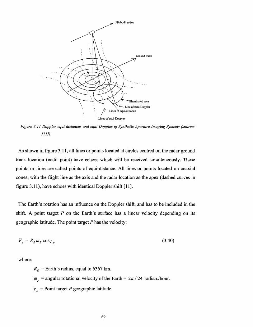
Flight direction

Ground track

""Il lu m in a te d area

Line o f zero DopplerLines o f equi-distance

Lines o f equi-Doppler

Figure 3.11 Doppler equi-distances and equi-Doppler o f Synthetic Aperture Imaging Systems (source:

III])-

As shown in figure 3.11, all lines or points located at circles centred on the radar ground

track location (nadir point) have echoes which will be received simultaneously. These

points or lines are called points of equi-distance. All lines or points located on coaxial

cones, with the flight line as the axis and the radar location as the apex (dashed curves in

figure 3.11), have echoes with identical Doppler shift [11].

The Earth’s rotation has an influence on the Doppler shift, and has to be included in the

shift. A point target P on the Earth’s surface has a linear velocity depending on its

geographic latitude. The point target P has the velocity:

VP = RE^ E cosr P (3.40)

where:

Re = Earth’s radius, equal to 6367 km.

mp = angular rotational velocity of the Earth = 2 /r/24 radian./hour.

y = Point target P geographic latitude.

69

. Vn = — x 6367 x cosr km/hour. p 24 p

= 0.463 cosyp km/sec.

The Doppler shift resulting from the velocity of the point target P by the Earth’s rotation

(0.463 cos y p km/sec) should be added in addition to the Doppler shift caused by the

satellite movement for precise synthetic array. The velocity of the point target caused by

the Earth’s rotation is equal to zero if located at the poles and equal to REmE if located

on the equator.

3.5 The SAR radar equation

At the raw data level (i.e. before compression), the received peak power Pr from a

target of radar cross section a is:

N n = the average thermal noise power (assuming a white stationary Gaussian

process).

G = antenna gain.

a = target radar cross section.

Pt = peak transmitted power.

In equation (3.41), ambiguity noise and speckle (discussed in 4.4) are considered an

inherent part of the received signal. At the image level, the received power from a point

target P. is:

(3.41)

where:

P = n 2Pr + nN,n (3.42)

70

where:

n = the product of range and azimuth samples integrated during the compression

XRprocessing. n = tfr PRF noting that t is the pulse time duration and

2 vR

f r is the range sampling frequency.

In the case of a distributed target where the received power is assumed to be the mean

power averaged over all the elementary scatterers of a statistically homogenous area, the

radar equation for the raw data is:

PtG2X2R R ( T ncTB.r a 0 p

(4;r)JR 32sin0Pr = / a _\3 r>3 n + N n (3-43)

where:

<j 0 = the backscatter coefficient.

B = the 3dB azimuth antenna power beamwidth.

At the image level, the radar equation for a distributed target is the same as equation

(3.43) with the replacement of the received power Pr of a point target with the received

power of the distributed target. Thus the radar equation becomes:

PtG2X2R R c r QcTBBp = 2_i p- + nN (3 4 4 )

' (4^ ) 3 3 2 sin 0 ( ’

3.6 Ambiguities in SAR

Because SAR uses repetitive pulses, its performance is limited by the presence of

ambiguities. These ambiguities are related to the range and azimuth, other ambiguities

are related to the system design and the SAR processing [11]. For example, in order to do

the synthetic processing it is important to make an adequate sampling of the Doppler

spectrum.

PRF > 2f D => PRF >2v / la (3.45)

71

Equation 3.45 is the Nyquist criterion for the sampling of the synthetic aperture and

indicates that a sample should be taken every time the satellite moves half of the antenna

length.

Successive pulses should be far enough apart from each other so that they will not be

received simultaneously, leading to range ambiguity.

c> wg where wg is the swath width (3.46)

2 PRF

w„ =8 cos 9

cwn cos2 9P R F < v n ; x — w <3-47>2 Ah sin 9

From 3.45 and 3.47, the limits of PRF to avoid ambiguities are:

2v cwn cos2 9— < PRF < . (3.48)I 2 Ah sm 9

Equation 3.48 leads to an important relation involving the antenna area:

4 Xhv sin 9w°l° > w a ( 3 49>ccos 9

The left side of the relation (3.49) represented by wa and la determines the swath width

and the resolution in the same time. In the right side of the relation, h and v determine the

orbit characteristics, where X and 9 determine the frequency and the look angle

respectively [1 1 ].

72

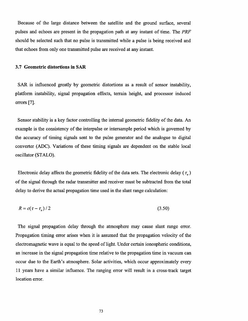
Because of the large distance between the satellite and the ground surface, several

pulses and echoes are present in the propagation path at any instant of time. The PRF

should be selected such that no pulse is transmitted while a pulse is being received and

that echoes from only one transmitted pulse are received at any instant.

3.7 Geometric distortions in SAR

SAR is influenced greatly by geometric distortions as a result of sensor instability,

platform instability, signal propagation effects, terrain height, and processor induced

errors [7].

Sensor stability is a key factor controlling the internal geometric fidelity of the data. An

example is the consistency of the interpulse or intersample period which is governed by

the accuracy of timing signals sent to the pulse generator and the analogue to digital

converter (ADC). Variations of these timing signals are dependent on the stable local

oscillator (STALO).

Electronic delay affects the geometric fidelity of the data sets. The electronic delay ( re)

of the signal through the radar transmitter and receiver must be subtracted from the total

delay to derive the actual propagation time used in the slant range calculation:

R = c ( r - T e) / 2 (3.50)

The signal propagation delay through the atmosphere may cause slant range error.

Propagation timing error arises when it is assumed that the propagation velocity of the

electromagnetic wave is equal to the speed of light. Under certain ionospheric conditions,

an increase in the signal propagation time relative to the propagation time in vacuum can

occur due to the Earth’s atmosphere. Solar activities, which occur approximately every

11 years have a similar influence. The ranging error will result in a cross-track target

location error.

73

cArAr = - — (3.51)

2 sin 77

w here:

Ar =slant-range timing error.

rj = the grazing angle.

Another type of error may result from the drift of the spacecraft clock. Any offset

between the spacecraft clock and the clock used to derive the ephemeris file from the

spacecraft tracking data will result in target location errors [7].

Exact target location can be determined by simultaneous solution of three equations: the

range equation, the Doppler equation, and the Earth model equation.

The range equation: R = \RS - (3.52)

where Rs and Rt are the sensor and the target position vectors respectively.

The Doppler equation: f DC = j ^ ( V s - F () x (Rs - R,) (3.53)

where:

f d c =Doppler centroid frequency.

Vs and Vt are the sensor and the target velocity vectors.

The target velocity can be derived from the relation: Vt = coE x Rt where coE = Earth

rotational velocity vector and Rt = RE cos y p.

74

The Earth model equation; Usually an oblate ellipsoid model is used to model the Earth’s

shape. Figure 3.12 shows the oblate ellipsoid Earth model:

* 2t + y 2t(RE + h y

(3.54).

z

Centre ®f Eai

Satellite

e

SAR isodoppler contour

X

Figure 3.12 The oblate ellipsoid model o f the Earth (source: [7]).

where RE is the radius of the Earth at the equator = 6378.137km, h is the local target

elevation relative to the assumed model, and Rp is the polar radius = 6356.752km.

The latitude of the point (P) is yp :

Beside the location errors, satellite altitude and position errors are very common in

SAR. They can be classified as yaw, pitch, and roll errors [11]. The satellite yaw error

occurs as a result of the satellite displacement or rotation around its vertical axis (figure

3.13 a). Such error has a significant effect because it displaces the antenna footprint away

from zero Doppler and the return radar echo will be displaced by a frequency:

(3.55)

75

2 vAfy = — sm0 sin a

A(3.56)

Satellite pitch error is similar to the yaw error but the displacement angle occurs relative

to the satellite’s nadir point (Figure 3.13 b). The received signal will have an additional

Doppler shift Af equal to:

Figure 3.13. (a) Satellite yaw displacement, and (b) pitch displacement (Source:[11])

If the yaw and pitch angles of the satellite are known, the correction is straightforward,

if not the clutter lock system may be used for the correction. The clutter lock system

measures the shift and adds or subtracts it from the original shift [1 1 ],

The roll error results from the movement or rotation of the satellite around its horizontal

axis. A small roll of the satellite does not affect the location of the imaged swath. If the

roll is large, a range-dependant variable gain can be used to compensate the weighting

factor added by the antenna pattern on the echo shape [1 1 ].

2 v . h f p = ~ s m a (3.57)

SatelliteSatellite

76

For the target elevation error correction, the radius of the assumed oblate ellipsoid earth

model should be adjusted by the elevation of the target (h). An error may occur in the

effective slant-range as a result of estimating the target height which leads to error in the

target location [7], This is shown in figure 3.14.

SatelliteAR = Ah cos t] Ar = Ah tan rj

Ah

A r

Figure 3.14. Target location error as a result o f the target location (Source: [7]).

For example, assuming a grazing angle of 35°, and assuming the target height Ah is 5

metres, the target location error in the range direction is 7.14 metres. This is because

SAR is a ranging device and produces a cross-track reflectivity map based on the sensor

to target range distance. For smooth surfaces, there is an inherently non-linear

relationship 1 / sin 77 between the sensor-to-target range and the cross-track target

position in the image [7]. Figure 3.15 shows this relationship. Since the angle varies

across the swath, the ground distance for each sample is not uniform, which results in the

near-range appearing compressed with respect to the far-range. Only for smooth surfaces

can the slant-range spacing and ground-range spacing be related by sin rj.

77

Ground range image

Near-range

r Slant range image

Far-range

Figure 3.15 comparison between ground range and slant range image (Source:[7]).

Because natural terrain surfaces deviate from smooth surfaces, additional geometric

distortions occur. These distortions are foreshortening, layover, and shadowing (figure

3.16).

Foreshortening distortion occurs when the hill or the mountain is viewed by the radar

beam and ( a < //), the side of the hill or the mountain facing the radar beam will be

shortened and the other side will be stretched. Layover distortion is similar to that of

foreshortening but with a >r j (i.e. steep terrain). Shadowing occurs when the ground

area is not visible to the radar.

For such distortions, it is extremely difficult to correct SAR data without using a DEM

and incident angle map for each pixel in the DEM. In the rectified image, shadows will

be filled by an intensity value equal to that of the thermal noise power [7].

Another source of geometric distortions is specular point migration. This occurs as a

result of rounded hilltops where the predominant scatterer location is dependent on the

incident angle of the transmitted wave. When the incident angle is perpendicular to the

hilltop strong backscatter occurs.

78

Radar beam

Radar image plane

(1) Foreshortening distortion

Radar beam

Radar image plane

(2) Layover

Radar beam

Radar image plane

(3) Shadow effects

Figure 3.16. Geometric distortion in SAR images (Source: [7]).

3.8 SAR data processing

As mentioned earlier in this chapter, the formation of each pixel involves the

combination of data from many thousands of echoes (synthetic array elements) and the

platform is orbiting at high speed determining the swath width elements and the sensor

resolution. These parameters lead to a high data handling rate [11].

The received data are processed in the ground receiving station by correlating in the

SAR processor using a two dimensional reference function as a matched filter. Optical

processors or digital processors can be used to perform the image construction derived

from the signals. Optical processors were used in the early SAR imaging developments,

where each echo is downconverted to baseband and biased in its amplitude to keep it

positive then intensity modulated to be displayed on a CRT. The phase variation of the

echoes is matched by a Fresnel zone plate and the echoes are then recorded as lines which

79

form an image on a film. The film is then illuminated by laser beam. Several lenses are

used in the optical processing technique for range corrections (e.g. range walk and

curvature). The Seasat SAR and SIR-A SAR data were processed in an optical fashion.

Limitations of optical processors are related to dynamic range, the radiometric

calibrations and the delay involved in the development and handling of film [1 1 ].

\A j\SAR signal

Rangecompression

vk_____corner turning

Azimuthcompression

Detection & look summation

Look summed image lines

Figure 3.17 SAR image processing data flow diagram.

With the advent of fast digital electronics, a number of SAR processing algorithms have

been developed to reduce the data handling by the use of digital processors. The main

advantage of such processors is their high speed of processing and the ease of access to

the pixel phase of the data [11]. A schematic diagram showing the fundamental SAR

processing operations is shown in figure 3.17.

To illustrate the processing of SAR received signals to construct the image, a point

target response is used within either the time domain or the frequency domain. The

necessary parameters for the compression algorithms, including the pulse replica,

Doppler centroid, FM rate and number of looks are determined before the processing for

range compression. These are dynamically estimated with the use of other data such as

platform attitude and orbit for azimuth compression. Algorithms for SAR processing are

much more complicated than this short description, and can be found in many SAR text

books. A good article describing SAR processing techniques is by Barber, 1985 [15]. The

following describes two methods of processing, the time domain and the frequency

domain processing.

80

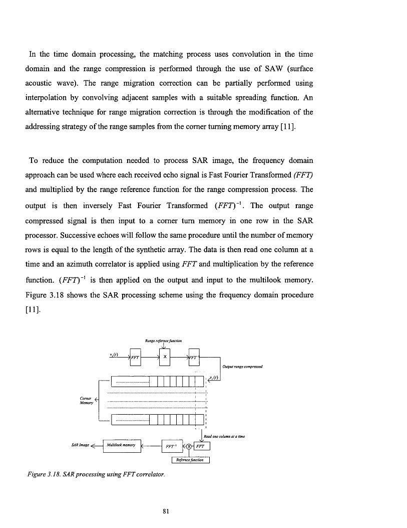
In the time domain processing, the matching process uses convolution in the time

domain and the range compression is performed through the use of SAW (surface

acoustic wave). The range migration correction can be partially performed using

interpolation by convolving adjacent samples with a suitable spreading function. An

alternative technique for range migration correction is through the modification of the

addressing strategy of the range samples from the comer turning memory array [1 1 ].

To reduce the computation needed to process SAR image, the frequency domain

approach can be used where each received echo signal is Fast Fourier Transformed (FFT)

and multiplied by the range reference function for the range compression process. The

output is then inversely Fast Fourier Transformed (FFT)'1. The output range

compressed signal is then input to a comer turn memory in one row in the SAR

processor. Successive echoes will follow the same procedure until the number of memory

rows is equal to the length of the synthetic array. The data is then read one column at a

time and an azimuth correlator is applied using FFT and multiplication by the reference

function. (FFT)~] is then applied on the output and input to the multilook memory.

Figure 3.18 shows the SAR processing scheme using the frequency domain procedure

[11].

v,(/) } FFT

Range refernce function- \ t_

-)FFT~

Corner Memory

M ‘)

Output range compressed

SAR Image ^ Multilook memory

Read one column at a time

FFT

Refernce function

Figure 3.18. SAR processing using FFT correlator.

81

4.0 Pre-processing optical TM and JERS-1 SAR data

Image analysis is the fundamental aim of satellite digital data, performed using

computer aided decision making algorithms for classification purposes or manual photo

interpretation. Such analysis cannot be achieved without making certain geometric and

radiometric corrections. In general, image data is downloaded to the ground receiving

stations directly from satellites, with many artifacts due to the sensor itself. These

include: system noise, line dropouts and stripping, platform yaw, pitch and roll, orbit

ellipticity, system field of view and viewing angle geometry. Natural artifacts arise from

Earth rotation and atmospheric effects. These limitations in the recorded data are usually

corrected in the receiving ground stations throughout a clean up set of procedures in the

primary stage of correction, and produce what is called raw data. If desired, a higher level

o f correction can be achieved if the relevant parameters are available, these parameters

include: the system; the atmosphere; and the imaged area.

In this work, the optical data is provided from the Saudi Centre of Remote Sensing

(SCRS) of King Abdulaziz City of Science and Technology (KACST) in Saudi Arabia.

The radar data is provided by the National Space Development of Japan (NASDA).

SCRS provided a 6500bpi 2-CCT’s radiometrically and geometrically (level-5) corrected

Landsat-5 Thematic Mapper (TM) data acquired at 7.35 a.m. (GMT) on the 8 th of June

1992 of the satellite descending node of orbit number 43988. The Sun elevation angle

was 62.15° and the Sun azimuth was 95.22° during the image acquisition. The test site is

covered by quad-2 and quad-4 of the image scene of the Landsat-5 of path number 174

and row number 40 of the Landsat-5 satellite’s world reference system (WRS). The

JERS-1 SAR data has been provided by NASDA in 4- 6500bpi CCT’s which cover the

study area through the JERS-1 paths of 252 and 253 and rows of 252 and 253 for both

paths (4-full scenes). Data was acquired in descending node of the satellite and processed

in October 1992. The exact acquisition date and time was not shown in the header files in

the CCT’s and could not be obtained. Radiometric and geometric pre-processing

correction of the SAR raw data has been performed previously by NASDA/ERSDAC of

Japan. The pre-processing level of the SAR data is 2.1.

82

Further pre-processing for both SAR and TM data has been performed in this thesis

work to achieve compatibility between the two data sets. These pre-processing

procedures are divided into two stages. The first stage includes: the SAR 16-bit to 8 -bit

compression, SAR to TM image registration, and SAR mosaicking, all of which have

been performed in an early stage of this thesis work in the SCRS using the hardware and

software facilities available. Meridian image processing software has been used to

perform the first stage. After that, one selected test site of size 1024 pixels x 1024 lines

from the area of study was transferred from the SCRS SVAX mainframe and backed up

to 3.5" floppy disks, occupying more than 7.34 Mbyte for both of the JERS-1 and TM

data. The second stage of the pre-processing is the optical TM atmospheric correction

and the JERS-1 SAR despeckling, all of which have been performed in the Electronic &

Electrical Engineering Department at UCL using PV-Wave and MATLAB software on

SUN workstations. Intensive C programming work, and EASI/PACE image processing

software were also used for data fusion and image analysis at a later stage of the thesis.

4.1 The JERS-1 SAR 16-bit to 8-bit compression

JERS-1 SAR images recorded from NASDA in CCT’s are 16-bit (2 bytes for each

recorded pixel); this data is not compatible with the optical Landsat-5 TM data which is

8 -bit (256 levels) in its dynamic range. For this reason, 16-bit to 8 -bit conversion is

needed for the SAR data to make it statistically compatible with the TM during the

processing and/or analysis in a later stages of the work.

There are many methods which can be used for conversions. One method takes the

square root of every pixel value in the 16 bit SAR image and stores the results in an 8 bit

file after rounding off. The drawback of this method is the bad grey level distribution of

the resultant output image (i.e. low image variance) [16], but it gives suppressed speckle

noise [17]. Another method is using a simple linear operation for the conversion based on

dividing every single pixel in the 16 bit SAR image by 256 and rounding the result to an

integer. The most appropriate method is finding the maximum and the minimum of the

input 16 bit SAR image and assigning them to 255 and 0 respectively. A simple division

83

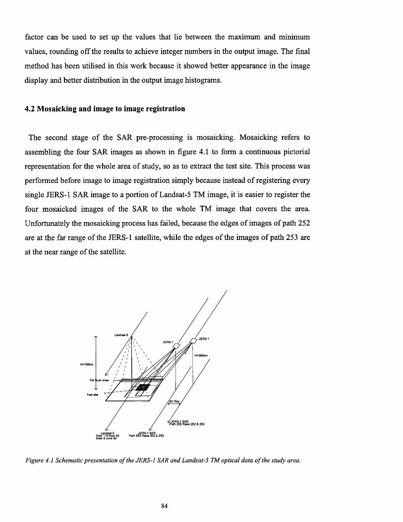
factor can be used to set up the values that lie between the maximum and minimum

values, rounding off the results to achieve integer numbers in the output image. The final

method has been utilised in this work because it showed better appearance in the image

display and better distribution in the output image histograms.

4.2 Mosaicking and image to image registration

The second stage of the SAR pre-processing is mosaicking. Mosaicking refers to

assembling the four SAR images as shown in figure 4.1 to form a continuous pictorial

representation for the whole area of study, so as to extract the test site. This process was

performed before image to image registration simply because instead of registering every

single JERS-1 SAR image to a portion of Landsat-5 TM image, it is easier to register the

four mosaicked images of the SAR to the whole TM image that covers the area.

Unfortunately the mosaicking process has failed, because the edges of images of path 252

are at the far range of the JERS-1 satellite, while the edges of the images of path 253 are

at the near range of the satellite.

s705km

TM i can

Test site

Landsat-5 Path 174 Raw 40

JERS-1 SAR Path 253 Raws 252 & 253

Figure 4.1 Schematic presentation o f the JERS-1 SAR and Landsat-5 TM optical data o f the study area.

84

This failure of the mosaicking process occurred due to the differences in the

illumination angles of the scene borders along the range. This problem cannot be solved

without using a digital elevation model (DEM) to rectify the distortion and remove the

topographic effects. Unfortunately a DEM was not available for the test site, so for this

reason a decision has been taken to register every single SAR image to its adjacent

portion of the TM with the use of intensive control points. This was especially important

in the mountainous areas and along the mosaicking borders where the illumination angle

varies from near range and far range. Figure 4.2 shows how the illumination angles varies

from near range to far range in the JERS-1 SAR case.

Earth surface

VFigure 4.2. JERS-1 SAR range illumination angles variations .

From figure 4.2, the near range incident angle /?, and far range incident angle /?2 are

calculated as follows, noting that 568km, 0X =32.2°, 02 =37.8°, RE = 6380km.

From figure 4.2:

Re H p + Re

sintfj sin/?!

Re H p + Re

sin#, sin/?2

f t = 35.47°

P2 = 41.87°

(4.1)

(4.2)

85

The SAR images were registered with the reference image of Landsat TM, where the

SAR spatial resolution is reduced to 28.5 metres, and hence the variation between the far

range and near range angles was also reduced.

In the literature there are two types of geometric correction technique: geometric

rectification and geometric registration. Geometric rectification is a process of producing

an image in its planimetric form. This process involves the uses of accurate map co

ordinates and digital elevation models to correct image distortions in three dimensions.

Geometric registration is the translation and rotation alignment process by which two

image sets of like geometries whose objects in the two images are positioned coincident

with each other [18,19].

Two steps have to be performed throughout the registration or rectification technique.

One is spatial interpolation, and the second is intensity interpolation. Throughout the

spatial interpolation, the pixel location (measured as row and column in the image) has

its location co-ordinates in the reference image (e.g. TM) based on a relation which

should be identified (e.g. equations 4.3 and 4.4). This process is called spatial

interpolation and produces an empty mesh (new output image grid) of output that is

identical in its co-ordinates to the reference image. This procedure involves defining

control points in the reference image and finding the co-ordinates of these points in the

image to be registered (e.g. SAR). Affine parameters of the relation (e.g. equations 4.3

and 4.4) have also to be calculated to translate the image either to x-y direction, image

scale change, skew correction, and rotation [20]. These parameters are based on the

“warping equations” which could be first order with three affine coefficients, second

order with six affine coefficients, or third order equations with ten affine coefficients.

The second order equations have been used in this work, as suggested by Cheng et. al.

[21] after investigation of many types of rectification algorithms using images from many

satellite platforms including SAR and optical data. Cheng showed that the second order

of polynomial equation for co-registration gives less RMS error. The equations of the

spatial interpolation are as follows:

8 6

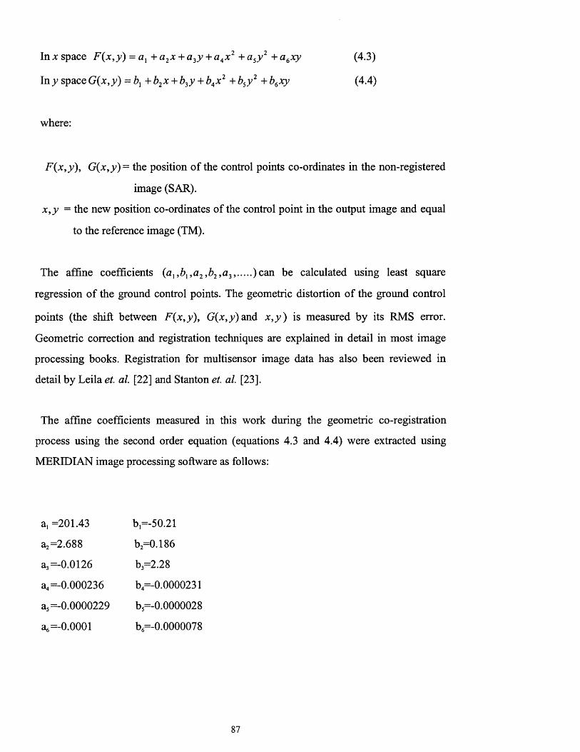
In x space F{x,y) = a{ + a2x + a3y + a4x 2 + asy 2 + a6xy

In y space G (x,y) = 6, + b2x + b3y + b4x 2 + b5y 2 + b6xy

(4.3)

(4.4)

where:

F{x9y), G(x,y)= the position of the control points co-ordinates in the non-registered

image (SAR).

x ,y = the new position co-ordinates of the control point in the output image and equal

to the reference image (TM).

The affine coefficients (a],bl ,a2,b2,a3, )can be calculated using least square

regression of the ground control points. The geometric distortion of the ground control

points (the shift between F (x ,y ), G ^ ,;;) and x , y ) is measured by its RMS error.

Geometric correction and registration techniques are explained in detail in most image

processing books. Registration for multisensor image data has also been reviewed in

detail by Leila et. al. [22] and Stanton et. al. [23].

The affine coefficients measured in this work during the geometric co-registration

process using the second order equation (equations 4.3 and 4.4) were extracted using

MERIDIAN image processing software as follows:

a, =201.43

a2=2.688

a3 =-0.0126

a4 =-0.000236

a5 =-0.0000229

a6 =-0.0001

b,=-50.21

b2=0.186

b3=2.28

h,=-0.0000231

b5=-0.0000028

b,=-0.0000078

87

Once the output image grid is created by the above process, it has to be filled by the

intensity interpolation as the second step of registration technique. The intensity

interpolation is usually called resampling. It refers to reading the pixel intensity values in

the unregistered input image and locating their proper position on the output image grid.

There are many methods that can be used for intensity interpolation, including: nearest

neighbour interpolation, bilinear interpolation, and cubic interpolation. Geologists prefer

the nearest neighbour interpolation filling because it does not alter the original pixel

brightness values. This method has been applied in this thesis work.

The registration process was successfully applied with total of 280 ground control

points (GCPs) for the four whole scenes of JERS-1 SAR (70 GCP for each SAR scene).

Spatial resolution has been reduced from the original 18 metres to 28.5 metres as a result

of registration matching to the Landsat optical TM.

SAR images in paths 252 and 253 have a different range of brightness level values. The

images of path 253 have less contrast compared with the images of path 252. This must

be corrected before mosaicking can take place. To solve this problem, histograms of the

side-lap area (around 17% side-lap) between the two paths have been compared and a

Look-Up-Table (LUT) for each histogram has been produced. The two LUT’s have been

averaged to produce a common LUT. The common LUT is then applied to all images of

paths 252 and 253. This is a popular solution for solving contrast differences in the

mosaicked images. The results of the registered, mosaicked, and contrast averaged JERS-

1 SAR scenes were satisfactory. The mosaicking procedure was successful except that

small contrast differences could be noticed only in the lower left part between images

253/253 and 252/253 of the test site as shown in figure 4.3 a. The reference image of

Landsat-5 optical TM data is also shown in figure 4.3 b.

111P

Figure 4.3 a: The JERS-I registered, mosaicked and contrast averaged 4 SAR scenes o f the study area.

”.MITI/NASDA retain ownership o f d a ta ”.

Scale 1:204084

89

Figure 4.3 b: The reference Landsat 5 optical TM band 5 image. Band 5 has been selected because o f its

high contrast where control points can be selected easily.

Scale 1:204084

90

4.3 Atmospheric correction of the optical TM data

The atmosphere influences the amount of reflected or emitted electromagnetic energy

that is sensed by optical imaging systems, and modifies and scatters the signals being

used and makes the acquired images blurred and poorly contrasted. Absorption of the

signals by the atmosphere is usually not counted in the atmospheric correction procedures

because remote sensing imaging systems are designed to operate away from the

absorption windows of the atmosphere [24].

It has been found that the atmosphere has an effect on the measured reflected waveband

from the target (i.e. pixel brightness value) where the Sun is the source of the

electromagnetic energy. If the atmosphere is absent, the measured reflected waveband is

only a function of the energy from the Sun reflected from the target and the reflectance

properties of the target itself. Because the atmosphere is present, the reflectance is

modified.

The Sun radiates electromagnetic wave energy termed the spectral irradiance ( E M),

which describes how much power density is available incrementally across the

wavelength range. At the Earth’s surface, if this surface is diffuse (i.e. scattered

uniformly in all direction), the measured energy reflected from the surface is called the

radiance (L). The target which reflects this energy has reflectance properties (R) which

describe the proportion of the incident energy which is reflected. With the assumption of

no atmospheric effects and the target being diffuse, the measured radiance scattered is:

L = E ^ c o s Q k X R / 7t (4.5)

where 6 = the solar zenith angle measured from normal.

Because the atmosphere is present, the following parameters should be taken into

account and calculated to obtain the atmospheric correction. These parameters are :

91

a) Atmospheric transmittance along two pathways; one is from the Sun to the target or

pixel ( Te), and the other is from the target to the imaging system (7^). Both are

measured from the normal.

b) Sky irradiance, which is diffuse reflection caused by the atmospheric constituents

and also from the surrounding targets or pixels ( ED).

c) Path radiance, which is scattering due to the atmosphere direct to the imaging system,

or the surrounding targets direct to the imaging system ( Lp), or both.

d) Various effects due to: temperature, relative humidity, atmospheric pressure, and

visibility, all of which should be measured during the time of image acquisition, to

extract what is so called the total normal optical thickness of the atmosphere ( r )

knowing that Te = e~TSecff and 7 = e~Tsec<t>.

From the above parameters, the final atmospheric correction equation becomes:

RTL = — ± \E u T e co&ObX + E D] + Lp (4.6)

7t L J

This equation should be used in combination with the equation of radiance-digital value

conversion for the atmospheric correction process. The radiance-digital value conversion

is used aboard the satellite in the digitising process to convert radiance to digital pixel

values and to extract the reflectance of the target ( R ). The equation of radiance to digital

value conversion is:

L = Ck + (4.7)

where :

92

C = Digital brightness value of the pixel.

k =L - L ■max nun

CL.

Z,max and are the maximum and minimum measurable radiances of the sensor, and

are usually given by the manufacturer during the ground spectral response tests for each

band. CL* is the maximum digital value in the digitiser.

Application of the above procedure is sometimes difficult for atmospheric correction,

because the atmospheric parameters cannot be always gathered at the time of image

acquisition. For that reason, atmospheric correction has become an important subject in

optical remote sensing, and many alternative techniques have been suggested. Crippen

[25] described the atmospheric correction methods in the literature and classified them

into four methods. These are (1) atmospheric measurements and modelling combined

with knowledge of the sensor calibration, (2) radiance - to - reflectance conversion, (3)

the regression method, and (4) the dark - pixel subtraction method. Another method used

is the image histograms zero shift which is known as the simplest way of haze removal

approximation, its drawback is inaccuracy and image data may be overcorrected and the

band-to-band spectral relationship may be lost because of no specific atmospheric model

is selected.

Throughout this work, it has been found that the dark - pixel method shows a very good

approximation for atmospheric correction. The method is simple and straightforward and

does not need the use of ground measurements during the time of image acquisition,

which makes this method the most practical.

The dark - pixel subtraction method developed by Chavez [26] was used. Modifications

o f the method were made in this thesis including: selecting the appropriate atmospheric

model and; using the exact spectral response of the TM imaging system. The TM spectral

response was demonstrated by Markham and Barker [27] during the ground measurement

and calibration process of the TM system.

93

The method developed by Chavez is based on the assumption that images being sensed

should have black pixels as a result of shadows, and these shadows should have zero

values in their pixel brightness values in the visible spectral band images. However, the

atmospheric scattering adds a constant value (radiance) to these pixels, and this radiance

should be appropriately measured and subtracted.

Scattering of the electromagnetic energy in the atmosphere is an additive component

and is wavelength dependent. It is mainly due to molecules of 0 2, C 02, 0 3 and H20 , and

is called Rayleigh scattering. This type of scattering is inversely proportional to the

fourth power of the wavelength S » AT4, which means that the shorter wavelengths (i.e.

visible light) scatter much more than the longer wavelengths (i.e. infrared light). It occurs

in a very clear atmosphere and is the cause of the blue appearance of the sky. Particles in

the atmosphere ranging from 0.01 to 0.1 wavelengths in size, such as smoke, haze, and

fumes particles also cause scattering, and this type of scattering is called aerosol or Mie

scattering. Mie scattering is inversely proportional to the wavelength S « A-1 but this

scattering is not as strong as Rayleigh but is still wavelength dependent. When the

particles are larger than the wavelength, scattering is no longer wavelength dependent

and complete scattering occurs in all bands [24,26].

From the scattering types where the relation varies between the power of -4 and -1,

Chavez [26] determined new scattering models using the power law. These models are

shown as follows: very clear atmosphere = A/4; clear atmosphere = X'2; moderate

atmosphere = X4; hazy atmosphere = A/0 7; and very hazy atmosphere = A/0 5. Chavez also

suggested that the selection of the atmospheric model of an imaged area for atmospheric

correction is based upon the magnitude of the brightness values of the shadows in one of

the visible bands. This can be taken from the image histogram, such as band 1 of TM (as

used in this thesis), and this value is named the starting haze value, and assumes that it

reflects the atmospheric condition at the time of data acquisition.

94

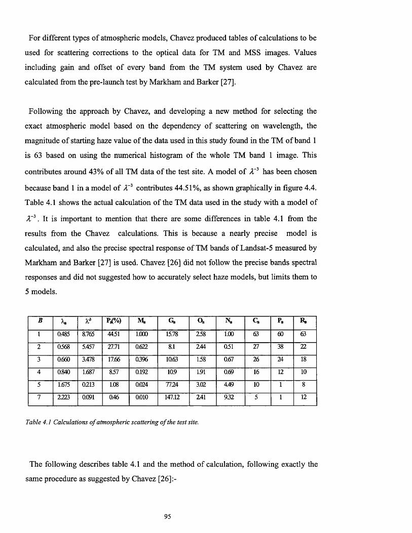
For different types of atmospheric models, Chavez produced tables of calculations to be

used for scattering corrections to the optical data for TM and MSS images. Values

including gain and offset of every band from the TM system used by Chavez are

calculated from the pre-launch test by Markham and Barker [27],

Following the approach by Chavez, and developing a new method for selecting the

exact atmospheric model based on the dependency of scattering on wavelength, the

magnitude of starting haze value of the data used in this study found in the TM of band 1

is 63 based on using the numerical histogram of the whole TM band 1 image. This

contributes around 43% of all TM data of the test site. A model of AT3 has been chosen

because band 1 in a model of AT3 contributes 44.51%, as shown graphically in figure 4.4.

Table 4.1 shows the actual calculation of the TM data used in the study with a model of

AT3. It is important to mention that there are some differences in table 4.1 from the

results from the Chavez calculations. This is because a nearly precise model is

calculated, and also the precise spectral response of TM bands of Landsat-5 measured by

Markham and Barker [27] is used. Chavez [26] did not follow the precise bands spectral

responses and did not suggested how to accurately select haze models, but limits them to

5 models.

B K U % ) Gb O* N„ Q PB Rb

1 0.485 8.765 4451 1.000 15.78 258 1.00 63 60 63

2 0368 5.457 27.71 0.622 8.1 2.44 051 27 38 22

3 0.660 3.478 17.66 0396 10.63 158 0.67 26 24 18

4 0.840 1.687 857 0.192 105 151 0.69 16 12 10

5 1.675 0213 1.08 0.024 7724 3.02 4.49 10 1 8

7 2223 0.091 0.46 0.010 147.12 2.41 932 5 1 12

Table 4.1 Calculations o f atmospheric scattering o f the test site.

The following describes table 4.1 and the method of calculation, following exactly the

same procedure as suggested by Chavez [26]:-

95

B = band number of Landsat-5-TM.

XB = centre of spectral response of Landsat-5 TM band B.

AT3 = selected atmospheric model.

PB % - theoretical magnitude of scattering of band B in percent = ^ 3 x 100.

i h Y 1M B = multiplication factor = " 3 .( 4 )

Gb = TM sensor gain of band B.

Ob = TM sensor offset of band B.

g b= normalisation factor = ——.G,

CB = calculated haze value from the image histogram.

PB = predicted magnitude of scattering after applying equation 4.9.

CB= real magnitude of scattering after applying equation 4.10.

Scattering model of the area of study

c 40

§ 30

£2 0

° 15

■8 10

2.50.5Wavelength in micrometer

Figure 4.4. Theoretical scattering o f the model A~3 which precisely matches scattering o f the area o f

study. Note that the scattering in band 1 is 44.5% and decreases exponentially to approach

zero in the infra-red wavelengths. The axis y is percentage probability.

96

Many factors contribute to the digital brightness value recorded by the optical imaging

system, including system gain and offset, sun elevation angle during image acquisition,

and slope conditions of image. The output digital brightness equation of the image is

[26]:

BVij,B = 0 B x R ij,B + (4-8)

where:

BVijB = output brightness value of a target (pixel) of band B at i j position.

Ri j B = input target (pixel) radiance of band B at i,j position.

Predicted haze values for other bands after taking the haze of band 1 as a starting haze

value are calculated based on the equation:

Pb =(C] - O b) x M b (4.9)

where:

PB = predicted haze value of band B.

Cj = starting haze value of band 1.

Finally, the correct haze value to be subtracted from every band can be calculated by the

following equation:

Rb = ( N b x Pb) + Os (4.10)

where:

Rb= final correct haze value of band B.

When the final haze values are calculated from equation 4.10 for every band, all of these

values must be subtracted from their corresponding bands of the image scene to account

97

for the scattering. All of these values of final scattering calculation (shown in table 4.1)

were subtracted from the imagery bands of the test site.

Geologic applications require atmospheric correction especially, because haze generally

affects the image processing techniques. These include colour displaying, linear

combination such as data rationing, subtraction, multitemporal fusion techniques, spectral

signature extension, and spectral relationships between bands [26, 28].

4.4 SAR speckle reduction

In the JERS-1 SAR image used in this study, further pre-processing correction is needed

to eliminate the speckle in the image. This kind of noise greatly reduces the image quality

and makes photo or machine interpretability less effective.

Ford [29] studied SAR images intended for geological mapping and found that there are

three factors controlling the interpretability: the spatial resolution; the image speckle; and

the range of contrast. The spatial resolution and the range of contrast of the JERS-1 SAR

data used in this study is adequate, but speckle is extensively present in the data. This

speckle should be removed because it obscures the real reflectivity differences of the

geological features.

Speckle is a random effect present in all active coherent imaging systems such as radar,

and is fundamentally a result of the fluctuation in the target echoes. Noise is also present

in radar images and due to receiver system such as thermal noise; small surface scatterers

which are less than the pixel resolution; the antenna viewing position; man made

constructions; the atmosphere; and the specular reflection of ground surfaces where the

reflected signals return perpendicularly to the antenna as strong echoes. Speckle and

noise make contributions to the degradation of the radar images [10] and characterise

radar images with a granular appearance which highly reduce SAR image interpretability.

98

Ulaby et. al. [30] and Elachi [11] described how speckle occurs as a result of adding

many echo returns from the scatterers. The returns are added vectorially from the

elementary vectors of each return of the single scatterer to form a single vector which has

amplitude V and phase (j) of the total echo. The phase fai of each elementary single

vector is related to the distance between the SAR antenna and the scattering points. When

the satellite moves, all phases fai will change, leading to a change in the composite

amplitude V . As a result of many observations of the same target recorded during the

satellite movement, fluctuations in the amplitude V of the target scatterers leads to

speckle or fading. To overcome this problem, the amplitudes V's may be spatially

averaged.

Mathematically, the received amplitude V from two scatterers A and B separated by a

distance d observed by a constantly moving platform over period t and velocity v can

change dramatically, causing the speckle or fading. If the viewing angle 6 is small, the

received amplitude is:

Graphically, equation (4.11) shows how speckle can be created as a result of amplitude

fluctuation. This is shown in figure 4.5. From the figure:

I n d v t(4.11)

(4.12)

1ri =r0- - d s m e (4.13)

As derived by Ulaby et. al. [30], the first null away from the origin occurs when:

X 2s m* = - => * « -

and similarly 02 « — .

JERS-1 SAR speckles representation3000

2500

2000

I 1500

1000

500

105 106 107 106The angle theta with respect to vt

109 110

JERS-1 SAR

A B a____

Figure 4.5 Speckle formation o f a distributed targets A and B separated by distance d. The SAR returns

amplitude fluctuate with width equal to Xh / dv .

The width of the lobe, which is the spacing between the two nulls (02 - 6X), is equal to

X——. The spacing between the two nulls along the flight path Ax is:2d

A* = r;A0 = ^ . (4.14)

too

From equation (4.14), the spacing is proportional to the wavelength used for the

imaging system and the distance r0, and also inversely proportional to the spacing

between the scatterers d.

There are two stages of treatment for speckle reduction. One is called pre-image speckle

reduction, or incoherent averaging of multiple looks or frames during the SAR image

construction. The second is called the post-image speckle reduction, and involves the

techniques of using spatial filtering to smooth images which have been formed through

multi-look processing [30,31].

Multi-look processing can be accomplished by partitioning the samples of the coherent

imaging period or signal history into M frames to form images, where the number of

samples for each frame is 1/M of the original single-look image. The azimuth resolution

is then reduced by a factor of M. For example, if M is 4, the result is a 4-look image and

the SNR is increased by a factor M1/2 [10]. In other words, it is the process of squaring

the pixels of the azimuth direction or averaging the pixels in the range line, as the

resolution in the range direction is much coarser than the azimuth direction in the original

single-look image. So the resulting pixels cover a square area on the ground, but with less

spatial resolution. If they are averaged, images with less speckle can be achieved. Such a

method is especially effective when the image or area of interest is homogenous [31].

Early attempts to eliminate or at least suppress speckle used is the spatial filtering as a

second stage or post-image speckle reduction. Such filters were originally non-speckle

specific [32] and have been used for noise reduction in general, being very well known in

the image processing literature. These include mean, median, and low pass filters. Their

disadvantage is in altering high frequency image features such as texture and edges,

which occurs because they are not designed for radar images. Such filters used by Blom

et. al [33] and Mueller et. al. [34], The median filter works well if two iterations are

used, but it makes the image blocky in appearance. The mean filter can also be used, but

it blur the images and smooth the edges, which is not advisable for Earth science

applications.

101

Recently, advanced types of spatial filters designed specifically for removing SAR

speckle and (to some extent) retain edges, boundaries, and preserve textures became

available as a result of increased work on radar images. Among the most well known

filters are the: Lee filter [17,35-36]; Frost filter [37]; and Kuan filter [38]. Lately Lopez

et. al. [39] revised and modified these filters to speed up the processing time and preserve

the echoes of strong scatterers, by assuming that the SAR image can be categorised into:

flat homogenous areas, for which low pass filter is used (e.g. the mean grey level of the

filter window); the second category is heterogeneous areas in which the speckle should

be filtered by the original filter algorithm; and the third category is areas of isolated point

targets (e.g. strong backscatterers), and in this case the filter should preserve the observed

(original) grey values.

4.5 SAR Speckle filters

The SAR spatial filters were proposed specifically to achieve high quality images based

on removing speckle and retaining subtle texture and boundary features. They commonly

utilise convolving odd square boxes and use the local statistics (e.g. local mean and

variance). The Rayleigh fading statistic (called contrast) is used in the filter algorithms by

assuming it is UN where N is the number of looks in the SAR image. If the SAR number

of looks is not known, it can be calculated as cr / ju where cr and fj. are the standard

deviation and mean of the SAR image respectively [16]. This value can be calculated

precisely if a small flat homogenous window in the image is used. The following is a

brief description of these filters.

A) Lee filter

The Lee filter was the first convolving spatial filter designed for speckle; it is a square

odd moving window. Lee [17, 35-36] proposed this filter designed for additive,

102

multiplicative, and both additive and multiplicative noise1 in images. In the case of SAR

imagery the noise is a multiplicative component as for all types of coherent

monochromatic illumination systems [17, 40]. The rougher the areas in an image are the

noisier they are and the implementation of the Lee filter algorithm is different based on

the type of noise. As mentioned earlier, the Rayleigh fading statistic (contrast) is needed

for Lee filter processing. As assumption is that the noise is uniformly distributed and its

mean is equal to unity (i.e.l) for multiplicative noise and zero for additive noise.

In the case of multiplicative noise, where the degraded returned signal results from a

non-linear combination of noise and signal, the processed central pixel in the Lee filtered

window CP0Ut is based on the equation [41]:

CPm = fiw+ K x (CPln - / I X / O (4.15)

where:

juw = mean grey level in the filter window.

fj, = mean value of the multiplicative noise = 1 on the assumption that the

noise is uniformly distributed.

CPin = central pixel value in the filter window to be processed.

K = gain factor, equal to:

a 2 / ju1 K = 1 - H

M»2

a 2 = variance of the filtered window.

<j2 = multiplicative noise variance = 1/N.

Lee [42] has improved this filter to remove speckle along edges and boundaries and

determine the edge orientation through slight modification of the above algorithm. He

1 Lee [17] proved that SAR speckle is multiplicative, based on the fact that the local standard deviation isdirectly proportional to the local mean.

103

uses the idea of subdividing the filter window into small window subsets of 3 by 3 pixel

size so as use their local variance thresholds for processing.

B) Frost filter

Frost et. al. [37] designed a spatial filter aimed at SAR speckle elimination. The derived

filter algorithm is based upon the scene reflectivity estimated by convolving the observed

image with the impulse response of the SAR system. The impulse response of the SAR

system is obtain by minimising the mean square error (MSE) between the observed

image and the scene reflectivity model, which is assumed to be an autoregressive process

[31].

The Frost filter window is an odd but not necessarily square kernel. A damping constant

(K) is required for the filter, which controls the damping rate of the impulse response

function. The implementation of the filter consists of determining a circularly symmetric

filter with a set of weighting values M for each pixel based on the equation [41]:

M t =e~AxT (4.16)

where:

A = K x ( a 2wl ft l)

T = absolute value of the pixel distance from the central pixel to its neighbours

in the filter window.

K = damping factor (e.g. 1).

a l = variance of the grey-level in the filter window.

juw = mean grey level of the filter window.

The output of a processed central pixel in the moving filter window is CP0Ut:

104

C P ~ = —.------- (4 .17)

/=1

where:

Pj......Pn = the grey level of each pixel in the filter window.

M v ...M n = weightings as defined in equation (4.16).

The important characteristics of the filter are: preserving linear features and edge

structures; brightening the foreslopes of terrain; and averaging pixels in the homogeneous

regions as it works as a low pass filter in these regions. It also performs well on low

contrast edges [37].

The damping factor should be carefully selected; if large values are used, edges will be

preserved better but at the expense of the speckle smoothing effect. If small values are

used, the smoothing effect will be increased but lineation and textural features will be

altered or decreased.

C) Kuan Filter

Kuan et a l [38] proposed his filter by transforming the multiplicative noise model into

a signal dependent additive noise model. He assumes that the multiplicative noise model

is only a rough approximation for fully developed speckle. The minimum mean square

error (MMSE) criterion was then applied to the additive noise model. The filter is very

similar to the Lee filter but its algorithm uses a different weighting function. The Kuan

filter algorithm is:

CPom = CP,: X W+ X (1 - W) (4.18)

105

where:

N = number of looks.

juw = mean grey level in the filter window.

a l = variance of the filter window.

CPin = input central pixel in the moving filter window.

CPout = output central pixel in the moving filter window.

D) Lopes modifications on the speckle filters

Lopes et. al. [39] introduced the concept that the SAR scene can be categorised into

three classes. The first class is homogenous areas of the scene which are characterised by

the coefficient of variation of the filter window: if CVW is smaller or equal to 1 / V a then

only a low pass filter (LPF) is applied to such areas (i.e. CP0Ut = /uw). The second scene

class is heterogeneous areas, and in this case either the Lee or Frost filter should be

applied to remove speckle. The third class is areas of high signal reflectivity which may

represent areas of isolated point targets, and in this case the original observed values

Similarly Shi et. al. [31] modified the Kuan filter using the same concept, modifying the

original algorithm based on assuming the scene reflectivity to be gamma distributed

rather than Gaussian distributed as was suggested by Kuan [38].

4.6 Results and comparison of speckle filters

As a result of the importance of speckle removal issue in this thesis, where the data will

be prepared for data fusion at a later stage, after processing for textural enhancement in

the next chapter. All the speckle filters just described were carefully tested, and one has

been selected based on maximum reduction of speckle together with minimum loss of

textural information. Another consideration taken into account for selecting the speckle

should be preserved; such areas should not be filtered

106

filter is that the filtered image should have large variance (better grey level distribution),

since the image variance is usually an indicator of information content.

The modified versions of these filters suggested by Lopes et. a l [39] and Shi et. a l [31]

were also tested but excluded because extracting point targets in the SAR image is only

important for calibration procedures. Furthermore, these point targets shown in the

filtered image make photo-interpretation less effective because they appear as large as up

to 7 by 7 pixels of white spots in the image.

The SAR input image has been initially contrast stretched using the Balance Contrast

Enhancement Technique (BCET) [43] with controlled mean set to 127. This contrast

stretching (see appendix A-2) improves the image appearance and makes it occupy the

whole range of grey levels. Contrast stretching using the BCET method gave better

results in the speckle filtering. Throughout using each speckle filter algorithm, two

images were produced, one being the filtered image and the second the speckle itself. The

speckle image is used as an indicator of textural information loss and can be visually

evaluated. Any patterns or shapes which are present in the speckle image output indicates

a loss of textural information. This method of evaluation has been found effective and is

proposed for the first time in this thesis. The algorithm used to produce the speckle image

is:

^ sp e c k le ~ ( I i n p u t ^ ^ f i l t e r d ) X ^ (4*19)

where:

I input= input SAR image before filtering.

I filtered = output SAR image after filtering using SAR speckle filter.

1 speck, o u t p u t SAR speckle.

S = scaling factor

107

During evaluation of the Lee filter it was found that the processing time was rapid and

speckle was suppressed, but at the expense of textural information loss, especially in

large filter windows. The Kuan filter gave similar results to the Lee filter, but takes more

time to process and shows darker background in the filtered image. The Frost filter gave

the best results, with no textural loss especially when the filter is 3 by 3 in window size.

When the filter window becomes bigger, little textural information is found in the

speckle output image but with total removal of speckle. The output of the Frost filtered

image shows larger variance compared with the Lee and Kuan filtered images. The

processing time is the only drawback of this type of filter, but is not critical in this work.

The original contrast stretched non filtered image is shown in figure 4.6. The Frost 3 by 3

filtered image is shown in figure 4.7. Figure 4.8 shows the 5 by 5 Frost filtered image;

note that the speckle is washed out completely from the image. Finally the speckle image

produced by the 3 by 3 Frost filter is shown in figure 4.9. Note that there are no

recognised textural or shape patterns in this image.

108

Figure 4.6 Original JERS-1 SAR 3-look image after applying BCET stretching. ’’MITI/NASDA retain

ownership o f the data ’’

Scale 1:204084

109

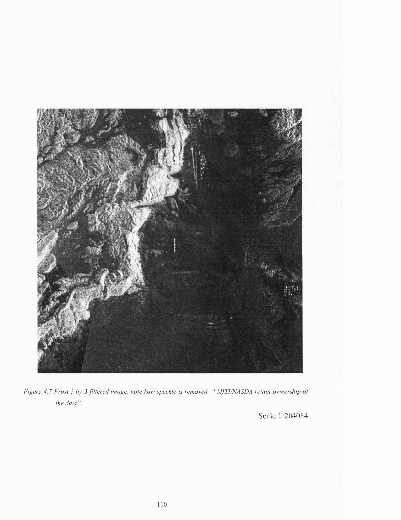
Figure 4 . 7 Frost 3 by 3 filtered image, note how speckle is removed. “ MITI/NASDA retain ownership o f

the data

Scale 1:204084

1 1 0

Figure 4.8 Frost 5 by 5 filtered image, speckle is rem oved com pletely with very little textural information

loss. “MITI/NASDA retain ownership o f the data

Scale 1:204084

i l l

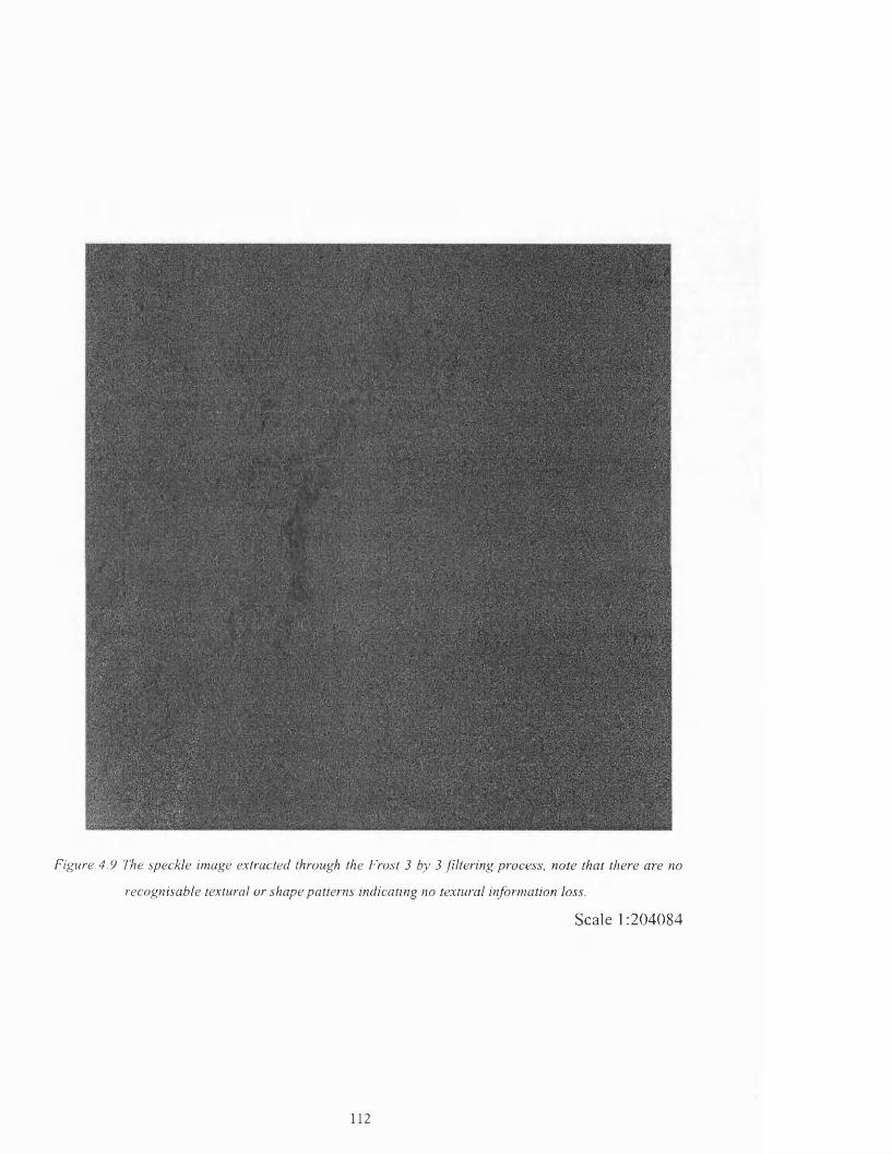
Figure 4.9 The speckle image extracted through the Frost 3 by 3 filtering process, note that there are no

recognisable textural or shape patterns indicating no textural information loss.

Scale 1:204084

1 1 2

4.7 Conclusions and remarks

The most important step in preparing image data for fusion from different imaging

sources is the image to image registration. It is simple to register two images having

similar geometry and source, or two different radar images from different sources with

similar imaging geometry. The problem arises when registering optical TM or MSS

images with SAR images. The difficulty is for two reasons: one is that the geometrical

aspects in acquiring the data from the sensors are different, in that the SAR is side-

looking whereas the TM is nadir-looking. The second is that the SAR image pixel

brightness depends on the surface roughness and the dielectric constant of the target,

whereas the optical TM image pixel brightness depends on the reflectance of the target.

For these reasons the data is not correlated, and accurate subpixel registration is difficult

to achieve. The only way to produce accurate registration is by using a DEM illuminated

by the same sun angle as the Landsat TM image, then the Landsat TM image is cross

correlated with the illuminated DEM to derive the residual translational misregistration

[7]. If this process is used, the SAR and TM images can be precisely registered. For data

with relatively flat terrains or oceans, or those for which no precision DEM is available,

the normal warping transformation equations can be used and precise registration can be

achieved.

Speckle in SAR images should be treated carefully because speckle reduces the image

interpretability either for manual photo-interpretation or for direct automated mapping

(classification). For that reason, speckle image production and visual evaluation is

produced in this thesis as a new idea for speckle filter efficiency. It is a simple method

and believed to be an important step of evaluation.

Atmospheric correction using the modified Chavez method of dark-object subtraction

technique is simple and easy to implement. It is reasonable approach for haze removal

because of the selection of appropriate atmospheric model. Other methods mentioned

earlier in this chapter either difficult to implement or inaccurate (i.e. histogram shift

113

method). Reason of using such an adequate method of atmospheric correction will be

shown clearly in chapter 6.

As depicted in the JERS-1 SAR images shown previously in figures 4.6-4.8, vertical

white lines can be found in the upper part and in the centre of the SAR scene. This type

of error is a system error, probably caused by the Antenna Gain Control (AGC). This

type of error could not be corrected because it is irregular in shape and not exactly

vertical (not in the same column line) and hence could not be modelled to be removed.

114

5.0 JERS-1 SAR spatial information extraction

The first step of data fusion after the data has been pre-processed is enhancing and

extracting the spatial information component. In a further stage, the extracted spatial

component is fused with the enhanced and extracted spectral information component for

lithological mapping of the test site of the area of study. The spatial information

enhancement can be accomplished by the use of a texture analysis technique.

Texture analysis is a rather recent but rapidly growing field in digital image

processing, because of its importance in simulating the strong visual perception of human

vision for both organised and unorganised patterns. From a geological point of view, the

most important information which can be extracted from digital image data are the

spectral and textural information, and both are employed for identifying rock types.

Spectral information describes the average band-to-band tonal variations in a multiband

image set, whereas textural information describes the spatial distribution of tonal values

within a single band, and reveals the topographic and lithologic differences in the imaged

terrain [44].

An accepted definition of texture is that given by Haralick [45]. He defined texture as

two decomposable basic dimensions. The first dimension describes the local properties of

pixels, and is termed the tonal primitive. The second dimension is related to the spatial

organisation of the tonal primitive. The tonal primitives refer to a maximum connected

set of pixels (i.e. regions) having a specific tonal properties such as the average tone,

maximum and minimum tone. The tonal region can be evaluated in terms of area and

shape. The spatial organisation refers to the layout of the tonal primitives and can be

described as random, or with dependence upon one or n neighbouring primitives.

Qualitatively, image texture can be evaluated visually as having one or more of the

properties of fitness, coarseness, smoothness, granulation, randomness, lineation, or

being mottled, irregular, or hummocky. Each of these textural shapes is translated into

some property of the tonal primitives and the spatial interaction between these primitives

[45].

115

The linear features which are classified as textural features are all features perceived

by the human eye as straight lines or curved lines in the image, when their length is at

least twice their width. Generally, and from a geological point of view, linear features can

be classified as: relief features or relief change features; tonal features or tonal boundaries

such as lithological boundaries; texture features such as texture lines or boundaries; and

finally pattern features such as pattern boundaries or pattern displacement features [46].

Geologic interpretation of lines and lineation in remote sensing is always

controversial, and there is no consensus interpretation as to whether the line feature could

be geomorphologic or geologic (i.e. structural), and it is up to the user to determine the

origin of such surface undulations in the image. Short [47] addressed this problem and

studied the reliability of geologic lineation extraction from satellite images. Recent trends

in extraction of structural geologic lineation utilise other complementary data, such as

geophysical data (i.e. aeromagnetic and gravity data) and extensive field visits to ensure

that the extracted lines are purely geologic. For this reason, lineation extraction and

mapping has been excluded in this work. For visual interpretation purposes, it is useful to

know that lineation lies in three distinct classes: the first class is fractures such as joints

and faults, and mainly exist in textural and relief change features. The second class is

lithological contacts and can be identified as textural or tonal boundaries. The third class

is folds and can be distinguished in images as sinuous lines, and may occur in tonal,

textural, or pattern boundaries. In geomorphologic image photointerpretation, low hills

usually have little dissection and are generally smooth with convex surfaces, while high

hills are highly dissected and have permanent ridge crests [46]. Mountain texture is

distinguishable from hill texture by the extent of radar shadowing. Mountains are

characterised by large shadows which may cover more than half of the mountain area,

whilst hills cover less than half of the area. Fine grained sedimentary rocks such as

claystone and shale show fine texture, while coarser grained sedimentary rocks show

coarser texture. A massive texture with rugged and peak divides is a clear indicator of

igneous rocks [48]. Parameters such as spatial resolution, radar wavelength, incident

angle, and environment govern the above rules for texture and texture analysis.

116

5.1 Parameters controlling SAR for texture and lineation detection

Recognition and mapping of geological features in radar imagery is dependent upon

many parameters such as wavelength, polarisation, spatial resolution, angle of

illumination and look direction [49], slope changes, surface roughness and microrelief,

environment, rock types, dielectric properties [50], speckle noise, and the textural and

lineation enhancement technique used.

Wavelength is an important parameter in textural analysis because texture is highly

dependent on the SAR wavelength used. An example is that if a shorter wavelength is

used, the imaged surfaces will be dominated by diffuse scattering and will be shown as a

rough surface. If the surface is imaged by longer wavelength the surface will be depicted

as smooth surface and hence its texture will be shown as dark and smooth. Polarisation

also influences texture, for example like polarised waves are most sensitive to the spatial

frequency corresponding to the Bragg resonant condition, and for rough surfaces the

returned SAR signal is a result of a mixture of surface and subsurface contribution [51].

Jaskolla et. a l [3] claimed that the usefulness of L-band is restricted for lithologic

discrimination as a result of the roughness criterion, and is not sensitive to the textural

construction of natural rock surfaces.

Spatial resolution of the image used for textural analysis is rather vital. If the textural

feature of the ground is less than the pixel size, the textural feature will not be depicted

by the imaging system. Moreover, because textural analysis studies show how the pixel is

interrelated to its neighbouring group of pixels, the imaging system aimed at textural

analysis must have a ground resolution pixel size much smaller than the textural feature.

Effective spatial resolution, image scale, and look direction have been studied by

Yamagushi [52] for lineation detection in SAR images. He concluded that the optimum

detectability is a function of spatial resolution of the imaging system Rs , image scale

S f , and the human visual system which cannot physically differentiate more than a few

lines within 0.1mm width. Thus he formed his rule of optimum detectability of lineation

which must satisfy the criterion Rs x Sf = 0.1 mm. From this, the scale of image product

117

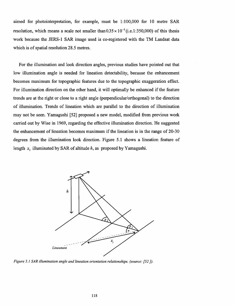
aimed for photointerpretation, for example, must be 1:100,000 for 10 metre SAR

resolution, which means a scale not smaller than0.35 x 10-5 (i.e. 1:350,000) of this thesis

work because the JERS-1 SAR image used is co-registered with the TM Landsat data

which is of spatial resolution 28.5 metres.

For the illumination and look direction angles, previous studies have pointed out that

low illumination angle is needed for lineation detectability, because the enhancement

becomes maximum for topographic features due to the topographic exaggeration effect.

For illumination direction on the other hand, it will optimally be enhanced if the feature

trends are at the right or close to a right angle (perpendicular/orthogonal) to the direction

of illumination. Trends of lineation which are parallel to the direction of illumination

may not be seen. Yamagushi [52] proposed a new model, modified from previous work

carried out by Wise in 1969, regarding the effective illumination direction. He suggested

the enhancement of lineation becomes maximum if the lineation is in the range of 20-30

degrees from the illumination look direction. Figure 5.1 shows a lineation feature of

length illuminated by SAR of altitude h, as proposed by Yamagushi.

Lineament

Figure 5.1 SAR illumination angle and lineation orientation relationships, (source: [52 ]).

118

From figure 5.1, the lineation length-imaging system height ratio x t / h as proposed by

Yamagushi [52] is :

x t / h = (cot/?, - cot f32) / cosa (5.1)

The x t / h becomes maximum when a lies in the range of 20 to 30 degrees.

The surface roughness parameter can be estimated easily using the Rayleigh criterion

which separates Rayleigh scattering from diffuse scattering of the ground surfaces. The

criterion of Rayleigh scattering [53] is:

(5 -2)

where:

hT— height of terrain irregularities

0 = incidence angle

In the case of the JERS-1 SAR, hT= 3.58cm, which means that rock sizes or

topographic features with less than 3.58cm height will show Rayleigh scattering (smooth

surface) and features with height of more than 3.58cm will show diffuse scattering (rough

surface). If the ground surface is covered by dry sand or aeolian deposits that usually

occur in the hyper arid areas, scattering may occur from the subsurface bedrock and may

be calculated from equation 5.2, substituting 6 = sin-1 and X = where s is

the dielectric constant of the penetrated sediments [53]. In the test site, field work

investigation showed the study area is arid (but not hyper arid) as a result of its closed

location to the sea as shown previously in figure 1.1. Furthermore, visual investigation to

SAR data of the test site did not shows any subsurface penetration.

119

Rough surfaces give strong backscattering, as a result of the increased number of

scatterers and comer reflectors. Such surfaces also cause a geometric distortion as a result

of foreshortening, layover and shadowing. The resultant SAR image usually shows very

bright V shaped features with many dark areas appearing in the image. Such surfaces

may not reflect a proper texture when analysed for rock identification. To overcome this

problem, a proper SAR image geometric correction using DEM and calibrated

backscattered SAR signals must be made [33].

Environment influences the texture appearance of the imaged surfaces. An example is

that if the area of study is humid, the SAR backscatter will be weak as a result of strong

absorption of the SAR signal due to the presence of water in the ground sediments. Also

in a humid environment, soil and vegetation will cover the rock units and hence the

geologic features will be obscured. In arid land, rock texture analysis using SAR is ideal

because no soil or vegetation covers the rock units, and the backscatter will be much

stronger as a result of the absence of water in the sediments. Furthermore, and because

weathering is not linearly constant, which affects physically more of areas of higher

altitude and chemically more of low lands, and hence different texture of the same rock

unit may show some differences as a result of topographic attitude.

Texture analysis for geological mapping is not very successful compared with other

image texture applications such as urban mapping or forest inventory. The problem arises

because geologists mainly classify rock types based on parameters such as mineralogical

contents of the rock type, palaeontological content, age, and geographic location, which

may not always coincide with the texture appearance of the rock type.

5.2 Previous studies in texture, and texture analysis in geology

Multispectral imaging systems and SAR have over the past two decades led to the

phasing out of black and white aerial photography. Surprisingly, texture analysis is still

of paramount importance when used for geological photointerpretation, with computer

classification as a parallel effort using spectral information. This is because texture gives

120

valuable spatial information and the same image processing techniques used for black

and white photographs can be used for multispectral optical and SAR image data.

Most image processing techniques used for texture analysis can be classified as follows

[54]: The Fourier power spectrum, the co-occurrence grey level matrix second order

statistics, or what is called the Haralick Grey Level Co-occurrence Matrix (GLCM), the

grey level difference statistics and finally, the grey level run length statistics. Other

techniques which use different kernel size and weight (i.e. filtering), such as that shown

by Moore [55] or Laws microstructure filters [56], are also available, but have not been

tested or used in this work.

The Fourier power spectrum texture enhancement technique has been previously used

when texture is a function of wavelength and direction [57]. High spatial frequencies in

an image represent rigid terrain or coarse texture, and low frequencies represent flat

terrain or smooth texture. The technique relies on transforming the image into the

spectral domain using a two dimensional FFT, and convolving the resultant spectrum

image with a 2 dimensional filter, and finally reconstructing the convolved image by the

use of the inverse FFT. It has been found that the FFT power spectrum method is

powerful for enhancing periodic textural features such as sand dunes or any repetitive

structures. High relief (rigid) and low relief terrains can also be enhanced using this

method, as can lineation enhancement. Weszka et. al. [54] at that time introduced

different kind of filters implemented on the FFT transformed images because the

previously known filters used in the Fourier power spectrum are known to be only

sensitive to the size (spatial frequency of the image) or to the orientation of the spatial

information, but not to both together in the same time. These filters designed by Weszka

are the intersections of the combination of rings and wedges at different angles and

lengths. The traditional FFT filters and the filters of ring and wedge intersections are

shown in figure 5.2.

The other textural analysis techniques mentioned earlier are implemented in the spatial

domain using neighbourhood pixel statistical measures (i.e. local property values). The

121

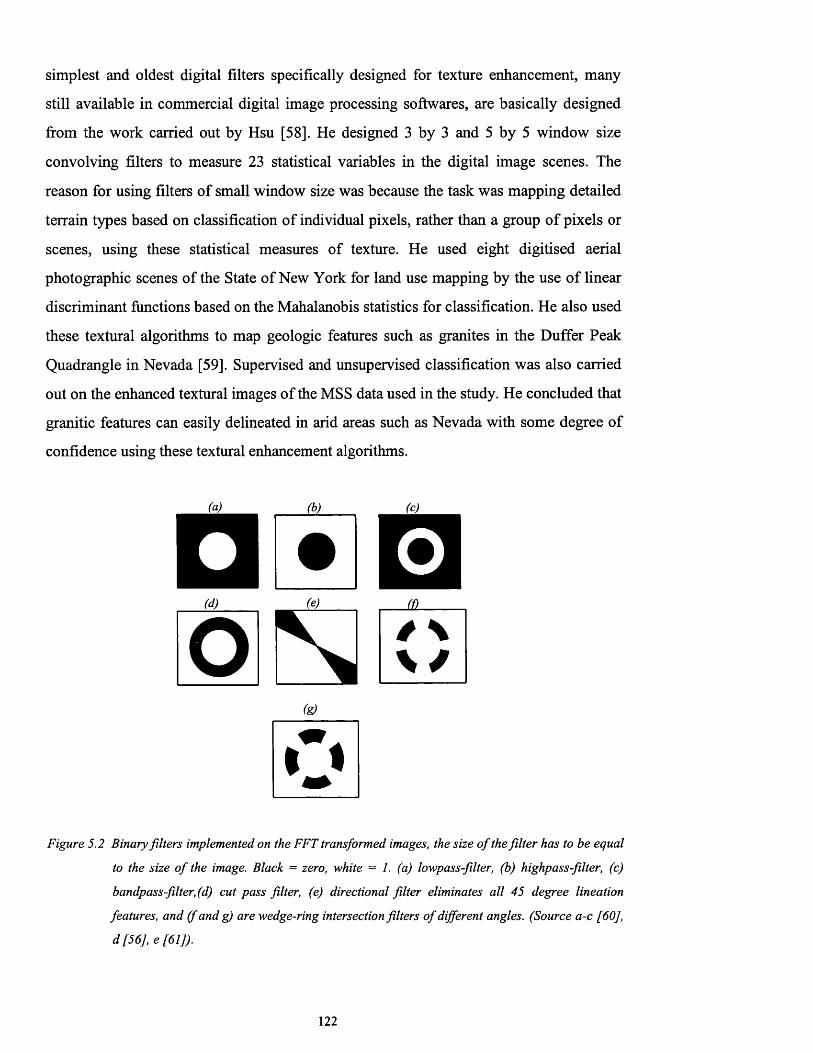
simplest and oldest digital filters specifically designed for texture enhancement, many

still available in commercial digital image processing softwares, are basically designed

from the work carried out by Hsu [58]. He designed 3 by 3 and 5 by 5 window size

convolving filters to measure 23 statistical variables in the digital image scenes. The

reason for using filters of small window size was because the task was mapping detailed

terrain types based on classification of individual pixels, rather than a group of pixels or

scenes, using these statistical measures of texture. He used eight digitised aerial

photographic scenes of the State of New York for land use mapping by the use of linear

discriminant functions based on the Mahalanobis statistics for classification. He also used

these textural algorithms to map geologic features such as granites in the Duffer Peak

Quadrangle in Nevada [59]. Supervised and unsupervised classification was also carried

out on the enhanced textural images of the MSS data used in the study. He concluded that

granitic features can easily delineated in arid areas such as Nevada with some degree of

confidence using these textural enhancement algorithms.

(g)

Figure 5.2 Binary filters implemented on the FFT transformed images, the size o f the filter has to be equal

to the size o f the image. Black = zero, white = 1. (a) lowpass-filter, (b) highpass-filter, (c)

bandpass-filter, (d) cut pass filter, (e) directional filter eliminates all 45 degree lineation

features, and (f and g) are wedge-ring intersection filters o f different angles. (Source a-c [60],

d [56], e [61]).

122

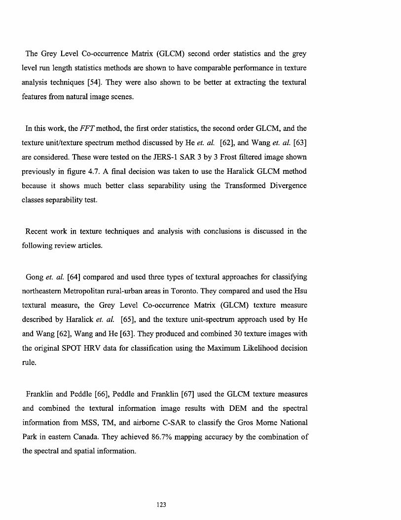
The Grey Level Co-occurrence Matrix (GLCM) second order statistics and the grey

level run length statistics methods are shown to have comparable performance in texture

analysis techniques [54], They were also shown to be better at extracting the textural

features from natural image scenes.

In this work, the FFT method, the first order statistics, the second order GLCM, and the

texture unit/texture spectrum method discussed by He et. al. [62], and Wang et. al. [63]

are considered. These were tested on the JERS-1 SAR 3 by 3 Frost filtered image shown

previously in figure 4.7. A final decision was taken to use the Haralick GLCM method

because it shows much better class separability using the Transformed Divergence

classes separability test.

Recent work in texture techniques and analysis with conclusions is discussed in the

following review articles.

Gong et. al. [64] compared and used three types of textural approaches for classifying

northeastern Metropolitan rural-urban areas in Toronto. They compared and used the Hsu

textural measure, the Grey Level Co-occurrence Matrix (GLCM) texture measure

described by Haralick et. al. [65], and the texture unit-spectrum approach used by He

and Wang [62], Wang and He [63]. They produced and combined 30 texture images with

the original SPOT HRV data for classification using the Maximum Likelihood decision

rule.

Franklin and Peddle [66], Peddle and Franklin [67] used the GLCM texture measures

and combined the textural information image results with DEM and the spectral

information from MSS, TM, and airborne C-SAR to classify the Gros Mome National

Park in eastern Canada. They achieved 86.7% mapping accuracy by the combination of

the spectral and spatial information.

123

In 1990, He and Wang [62], Wang and He [63] developed a new approach for texture

analysis, namely the texture-spectrum measure. The advantage of this measure is in its

simplicity, using only a 3 by 3 window measurement which is not affected by direction of

orientation measurement. Texture units are produced and the texture spectrum is

extracted to be used as an input in classification procedure. This method showed a 97.5%

overall accuracy of classifying natural textural scenes in the Brodatz album.

Digital processing of orbital SAR images to enhance geologic structure of the Mazinaw

Lake area in the Canadian Shield has been evaluated by Masuoka et. al. [68] using SIR-B

and Seasat SAR data. Many pre-processing procedures were used prior to image

enhancement techniques, including speckle reduction using k-nearest neighbour filter and

illumination azimuth biasing reduction using 3 different look direction images co

registered together, to enhance all possible directions of lineation. A variety of edge

enhancement operators were tested in their work, including Laplacian, Moore-Waltz,

Compass (Prewitt edge mask), Roberts, and Sobel edge enhancement filters. They found

that a modified version of a Moore-Waltz filter is the appropriate filter for edge

enhancement. Colour composites were also produced using the statistical Principal

Component Transform (PCT) of the three different look images and were utilised for

manual photointerpretation.

Haralick et. al. [65] addressed a new method for texture feature extraction using the

Grey Level Co-occurrence Matrix (GLCM). This method uses a matrix called the co

occurrence matrix derived from statistics based on the neighbouring pixels. These

statistics summarise the relative frequency distribution of how often one grey level will

appear in a specified spatial relationship to another grey level on the image under

investigation. In their study, they showed the power of GLCM to categorise many

features based on their texture in many kinds of data, including micrographs,

panchromatic aerial photographs, and multispectral satellite images. Haralick [45] also

surveyed and evaluated most of the textural enhancement approaches, including the

GLCM technique.

124

Using the Fourier Transform technique for texture analysis, Excell et. al. [69] showed

that the Fourier textural technique only gives good performance with textural features of

a strongly periodic nature. In their work, they extracted and separated the dust clouds

from the agricultural fields using a specifically designed filter implemented on a Fourier

transformed image of Landsat TM band 4 in the south-east of Iraq.

As a result of the increased popularity of the GLCM method, recent studies in texture

analysis discuss mostly the usefulness of this method and its application in many

disciplines, including geologic mapping. Marceau et. al. [70] raised the issue of GLCM

decision requirements concerning the number of variables which should be taken into

account when GLCM is used. These variables include the spatial resolution, the spectral

band used, the quantization level, the size of the moving window, the interpixel distance

(id) and angle direction {a) during the co-occurrence computation, and finally the GLCM

statistical measures used. In their study, they measured the influence of such variables on

the improvement of classification accuracy to map Bonaventure in the Baie des Chaleurs

in Canada using SPOT XS data. The results of their work show that large (enough)

window sizes are most effective because they capture the textural patterns of classes.

Care in selecting the window size is vital, because if a window of small size is chosen the

textural patterns may not be captured. If a large window size is selected, pixels from

other classes may be misclassified. A similar investigation has been carried out by

Baraldiet et. al. [71], testing the most relevant statistical measures of the GLCM. They

showed that among the 14 statistical measures originally proposed by Haralick, the most

effective GLCM statistical measures are energy, contrast, variance, correlation, entropy,

and inverse difference moment.

Shanmugan et. a l [44] were one of the early users of the GLCM texture enhancement

method on SAR data, to classify large scale geological formations over Tennessee, USA,

using Seasat SAR data. They successfully classified many sedimentary rock types

including shale, sandstone, and siltstone through combining and averaging the 0, 45, 90,

and 135 degree orientations of the GLCM calculation. Scatterograms of their GLCM

125

statistical measures show very good separability of the classes, which demonstrates the

usefulness of this method.

5.3 Strategy used in this study for texture enhancement

In the data fusion process which will be discussed in the following chapters, two main

image outputs will be prepared from the fused data. The first output is analogous i.e.

texturally and spectrally fused colour images specifically adapted for photointerpretation.

The second image set output is a fused image data set prepared for automated mapping

using multivariate analysis (i.e. computer classified image where all rock type classes of

the study area are delineated automatically).

In the first analogous output, the textural image component is the original registered and

despeckled (5 by 5 Frost filtered) SAR image. This image was shown in figure 4.8. The

decision has been taken to use this image simply because the textural information in the

SAR image is naturally exaggerated for visual depiction, and only one textural image has

to be used in the image processing fuser tools (i.e. colour and principal component

transforms) which separate the spatial from the spectral information and combine them

back after proper processing. The second fused outputs used for automated mapping are:

a data set of both enhanced spectral and textural information; a data set of textural

information component which is extracted using the GLCM method; a spectral

information data set which is enhanced using BCET, these are shown in chapter 7.

Based on the two dimensional co-occurrence matrix such as that shown in figure 5.3,

Haralick [45,48,65] used this matrix for a fixed distance (d) and angular spatial

relationship ( 0 ) between the image pixels, and produced what is called the Grey Level

Co-occurrence Matrix GLCM. From the GLCM, many second-order statistical measures

can be calculated and a new images can be constructed from these measures which

reflects the neighbouring pixel relationships (and so reveals image texture). The

derivation of the GLCM texture analysis is simplified in the following section:

126

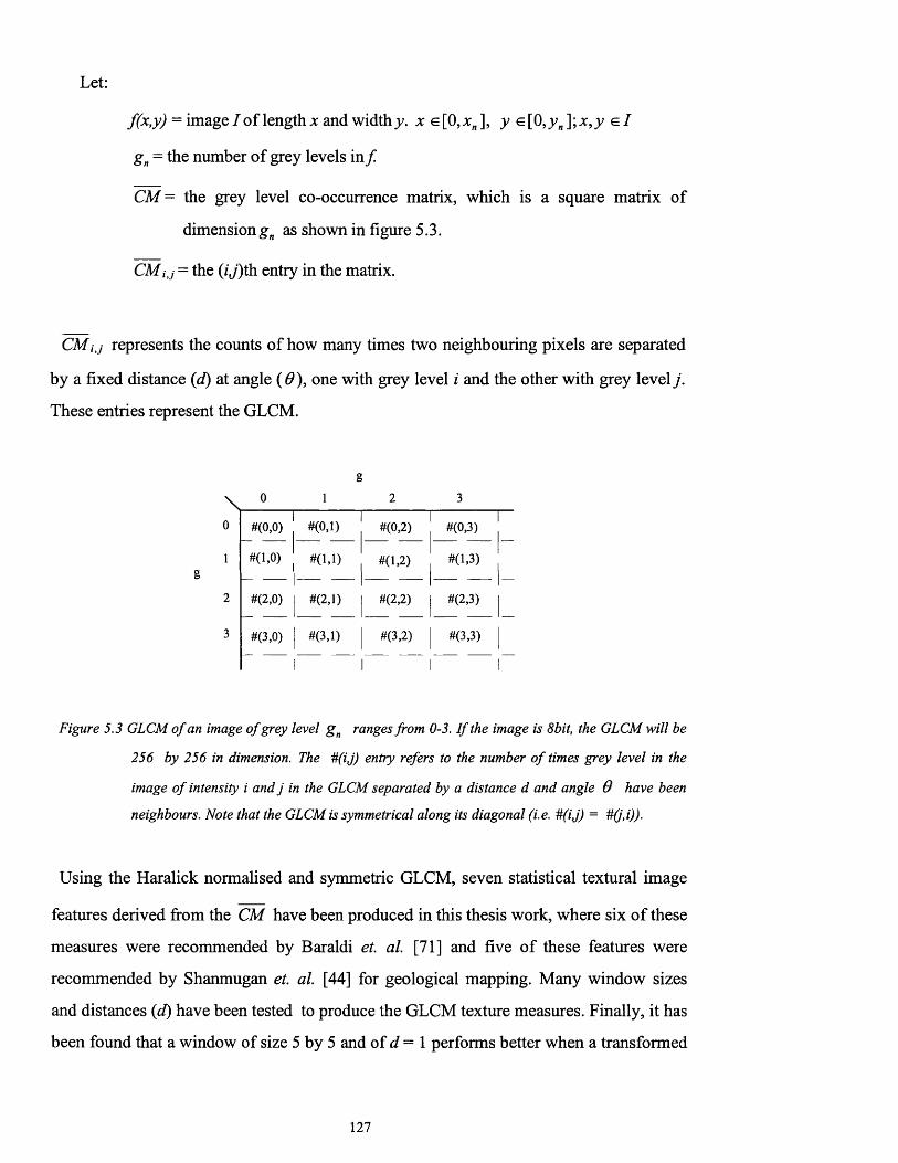
Let:

f(x,y) = image I of length x and width y. x e [0, xn ], y e [0, y n ]; x, y e I

gn = the number of grey levels in f

CM= the grey level co-occurrence matrix, which is a square matrix of

dimension^ as shown in figure 5.3.

CMij = the ( if)th entry in the matrix.

CMitJ represents the counts of how many times two neighbouring pixels are separated

by a fixed distance (d) at angle (0), one with grey level i and the other with grey level j.

These entries represent the GLCM.

0 1 2 3

#(0,0) #(0,1) #(0,2) #(0,3)

#(1,0) ( #(1,1) #(1,2) #(1,3) ^

#(2,0) #(2,1) #(2,2) #(2,3)

#(3,0) #(3,1) #(3,2) #(3,3)

1

Figure 5.3 GLCM o f an image o f grey level g n ranges from 0-3. I f the image is 8bit, the GLCM will be

256 by 256 in dimension. The #(i,j) entry refers to the number o f times grey level in the

image o f intensity i and j in the GLCM separated by a distance d and angle 0 have been

neighbours. Note that the GLCM is symmetrical along its diagonal (i.e. # (ij) = #(j,i)).

Using the Haralick normalised and symmetric GLCM, seven statistical textural image

features derived from the CM have been produced in this thesis work, where six of these

measures were recommended by Baraldi et. al [71] and five of these features were

recommended by Shanmugan et. a l [44] for geological mapping. Many window sizes

and distances (d) have been tested to produce the GLCM texture measures. Finally, it has

been found that a window of size 5 by 5 and of d = 1 performs better when a transformed

127

divergence separability test is used on the training areas of the test site. Angles 0 of 0, 45,

90, and 135 degrees are combined and averaged. The seven GLCM statistical measures

used are as follows:-

Sn- 1 Sm- 1

1 - The Inverse Difference Moment = T Yw^[i + e-y)2]

The Inverse Difference Moment (IDM) texture parameter measures the image

homogeneity, for example it gives large values for areas with small grey level

differences, and it is inversely correlated with the textural measures of contrast and

energy shown in equations (5.4) and (5.8). Figure 5.4 shows the output image of IDM

texture measure. The bright patches along mountain ranges in the figure represent high

homogeneity as a result of specular reflection of the SAR signals.

Sn- 1 Sm- 1___2- The contrast = X I \ C M ( i , j ) x ( i - j f (5.4)

/=0 j =0

The contrast texture parameter measures the differences between the highest and lowest

spatial frequency values in a contiguous set of pixels (i.e. window). Figure 5.5 shows the

output image of this measure.

ffn-1 ffm -1 _______

3- Dissimilarity = ' Z ' Z C M ( i J ) x \ i - j \ (5.5)7 = 0 j =0

Figure 5.6 shows the output image of the texture measure of dissimilarity.

w-1 1____4- Mean = Z I C M ( i j ) x ( i ) (5.6)

7=0 j =0

Figure 5.7 shows the output image of the mean texture measure.

ffn-l ffm-1 ___ ___5- Entropy = - ^ CM (i,j) x log (CM (i,j)) (5.7)

1=0 j =0

The entropy parameter measures the disorder of the image or the image randomness

[67]. For example, when the image is not texturally uniform, the entropy is very high

because the entries of the GLCM have small values. The angular second moment and

128

entropy measures are inversely correlated. Figure 5.8 shows the output image of the

entropy texture measure.

&i-l ___6- Angular second moment= £ Z C M ( / J ) 2 (5 .8 )

i=o y=o

The angular second moment is sometimes called the texture energy [41], and measures

the texture uniformity. For example, high ASM or energy values occur when the grey

level distribution over a window is constant or repetitive (i.e. periodic). Figure 5.9 shows

the output image of ASM texture measure.

7- Correlation = ^ x (, ^ ) x (7 ^»=n ;=n Oi= 0 j =0

The correlation texture parameter is a measure of the grey tone linear dependencies in

the image. High correlation values mean that there is a linear relationship between the

grey levels of pixel pairs in the window. Figure 5.10 shows the output image of the

texture measure of correlation.

129

Figure 5.4 GLCM texture measure o f Inverse Difference Moment, ”MITI/NASDA retain ownership o f the

data

Scale 1:204084

130

Figure 5.5 GLCM texture measure o f contrast, "MITI/NASDA retain ownership o f the data

Scale 1:204084

131

Figure 5.6 GLCM texture measure o f dissimilarity, ’’MITI/NASDA retain ownership o f the data

Scale 1:204084

132

Figure 5 . 7 GLCM texture measure o f mean, "MITI/NASDA retain ownership o f the data

Scale 1:204084

133

Figure 5.8 GLCM texture measure o f Entropy, ’’MITI/NASDA retain ownership o f the data

Scale 1:204084

134

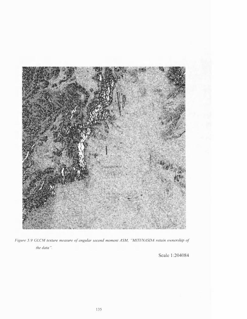
mmJ 7*>M*

■ ,w ?>* • ■*i '

^ c* ‘ • * ? '**-4*.' * ? i •I . .V :>1:.,- - i : .v >.

: a

Figure 5.9 GLCM texture measure o f angular second moment ASM, "MITI/NASDA retain ownership o f

the data ”.

Scale 1:204084

135

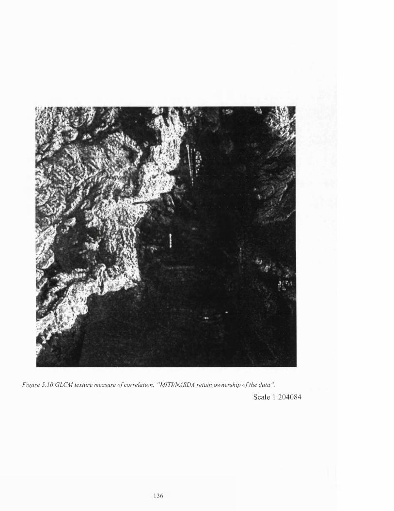
Figure 5.10 GLCM texture measure o f correlation, "M1TI/NASDA retain ownership o f the data

Scale 1:204084

136

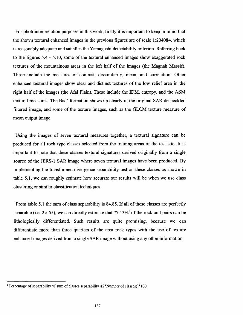
For photointerpretation purposes in this work, firstly it is important to keep in mind that

the shown textural enhanced images in the previous figures are of scale 1:204084, which

is reasonably adequate and satisfies the Yamagushi detectability criterion. Referring back

to the figures 5.4 - 5.10, some of the textural enhanced images show exaggerated rock

textures of the mountainous areas in the left half of the images (the Magnah Massif).

These include the measures of contrast, dissimilarity, mean, and correlation. Other

enhanced textural images show clear and distinct textures of the low relief area in the

right half of the images (the Afal Plain). These include the IDM, entropy, and the ASM

textural measures. The Bad’ formation shows up clearly in the original SAR despeckled

filtered image, and some of the texture images, such as the GLCM texture measure of

mean output image.

Using the images of seven textural measures together, a textural signature can be

produced for all rock type classes selected from the training areas of the test site. It is

important to note that these classes textural signatures derived originally from a single

source of the JERS-1 SAR image where seven textural images have been produced. By

implementing the transformed divergence separability test on these classes as shown in

table 5.1, we can roughly estimate how accurate our results will be when we use class

clustering or similar classification techniques.

From table 5.1 the sum of class separability is 84.85. If all of these classes are perfectly

separable (i.e. 2 x 55), we can directly estimate that of the rock unit pairs can be

lithologically differentiated. Such results are quite promising, because we can

differentiate more than three quarters of the area rock types with the use of texture

enhanced images derived from a single SAR image without using any other information.

1 Percentage o f separability =[ sum of classes separability /(2*Numner o f classes)]* 100.

137

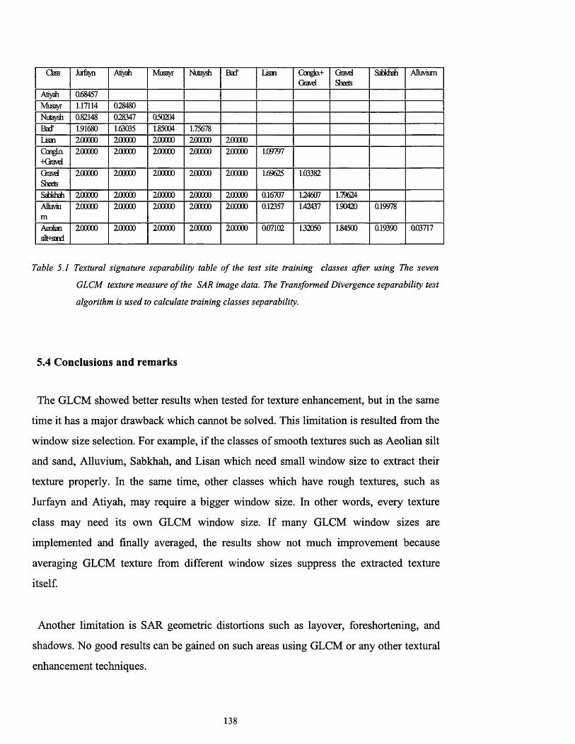
Class Jurfayn Atiyah Musayr Nutaydi Bad’ Lisan Conglo.+Gravd

GravdSheets

Sabkhah Alluvium

Atiyah 0.68457Musayr 1.17114 028480Nutaydi 0.82148 028347 030204Bad’ 1.91680 1.63035 1.85004 1.75678Lisan 200000 200000 200000 200000 200000GongLo.-+Gravd

200000 200000 200000 200000 200000 1.09797

GravdSheets

200000 200000 200000 200000 200000 1.69625 1.03382

Sabkhah 200000 200000 200000 200000 200000 0.16707 124607 1.79624AHuvium

200000 200000 200000 200000 200000 0.12357 1.42437 150420 0.19978

AeoliansOtfsand

200000 200000 200000 200000 200000 0.07102 132050 1.84500 0.19390 0.03717

Table 5.1 Textural signature separability table o f the test site training classes after using The seven

GLCM texture measure o f the SAR image data. The Transformed Divergence separability test

algorithm is used to calculate training classes separability.


The GLCM showed better results when tested for texture enhancement, but in the same

time it has a major drawback which cannot be solved. This limitation is resulted from the

window size selection. For example, if the classes of smooth textures such as Aeolian silt

and sand, Alluvium, Sabkhah, and Lisan which need small window size to extract their

texture properly. In the same time, other classes which have rough textures, such as

Jurfayn and Atiyah, may require a bigger window size. In other words, every texture

class may need its own GLCM window size. If many GLCM window sizes are

implemented and finally averaged, the results show not much improvement because

averaging GLCM texture from different window sizes suppress the extracted texture

itself.

Another limitation is SAR geometric distortions such as layover, foreshortening, and

shadows. No good results can be gained on such areas using GLCM or any other textural

enhancement techniques.

138

6.0 Image data fusion - optimisation for visual analysis

This chapter describes in detail the use of data fusion as an optimisation tool for visual

analysis. The definition of image data fusion, the reasons for data fusion, and the data

fusion models are firstly given.

6.1 Introduction

Data fusion generally refers to a scientific set of procedures which process, manipulate,

and identify objects and locate their position using data from a number of sources. It has

been developed in the fields of both imaging and non imaging remote sensing, and aims

to solve diverse sets of problems having common characteristics. In non-imaging

systems, data fusion employs mathematical and statistical algorithms upon the input from

multiple readings of the sensor(s) from an object, to determine its identity and position.

These mathematical and statistical approaches include clustering and classification

algorithms [72]. In imaging remote sensing systems, additional procedures are used to

manipulate and optimise data for visual and automated analysis.

Possibly the best example of data fusion system is the human brain, which combines all

the collected information from the sensing organs, then analyses this in conjunction with

a constantly corrected and updated database amassed from experience. The fused data is

then used to identify and/or locate the object being sensed [72]. In imaging remote

sensing, and in particular data fusion, refers to the technique of integrating different

image data sets with the use of image processing techniques such as: preparing and

optimising the data for integration (i.e. geometric correction, atmospheric and radiometric

correction between the different data sets); visual analysis between the data sets such as

colour composition; colour and statistical transforms such as red-green-blue intensity-

hue-saturation (RGB <> IHS) transform; Brovey transform; principal component

transform and reverse principal component transform (PCT <> PCT'1) and finally; the use

of classification techniques between the different image data sets. In the literature, data

fusion can be found under many terms, such as distributed sensing, data integration, data

139

synergism, data merging etc. Nowadays, data fusion techniques span many industrial,

medical, military, and civilian applications in modem human life.

In the science of remote sensing, for both types of active and passive imaging systems,

the remote sensing instrument measures the intensity of the reflected, scattered, or

emitted (i.e. thermal sensing) radiation from an object. This is directly related to the

physical and chemical properties of the object being imaged as a result of scattering and

absorption of the radiation field. From this phenomenon, and ignoring atmospheric

influences and systems instability, the measured quantity (i.e. radiance, intensity, power,

amplitude, etc.) can be expressed by the following relationship [73]:

E = R(X,X,Y,Z,0,</>,T,P) (6.1)

where:

E = measured energy from the imaged object as a function of the parameters

(Z,x,Y,z,o,<t>,T,P).

R = reflection, emission, or scattering radiation of the object.

X = wavelength used for imaging the object.

X, Yt Z = spatial co-ordinates of the object being imaged.

0,(1) = view direction of the sensor with respect to the object (i.e. elevation angle

and azimuth viewing angle).

T = imaging acquisition time.

P = polarisation of the sensor (only if an active imaging system is used).

From the above relation, it is obvious that the maximum possible information from the

imaged object can be evaluated in only five terms. These terms are known as the object

signature. The object signature can be defined (if a two dimensional form is used for

simplicity) as the behaviour of the object being imaged, determined by one constant

parameter and changing one of the other parameters. The five signatures that define the

object, as proposed by Gerstl [73], are shown in figure 6.1 and are discussed in more

detail in the following section.

140

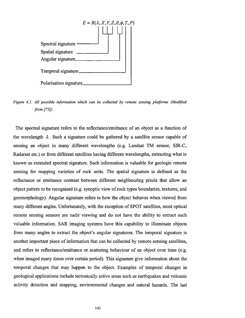
E = R {A ,X ,Y iZ,0,</>,T,P)

Spectral signature

Spatial signature Angular signature.

U

Temporal signature.

Polarisation signature.

Figure 6.1. All possible information which can be collected by remote sensing platforms (Modified

from:[73]).

The spectral signature refers to the reflectance/emittance of an object as a function of

the wavelength X . Such a signature could be gathered by a satellite sensor capable of

sensing an object in many different wavelengths (e.g. Landsat TM sensor, SIR-C,

Radarsat etc.) or from different satellites having different wavelengths, extracting what is

known as extended spectral signature. Such information is valuable for geologic remote

sensing for mapping varieties of rock units. The spatial signature is defined as the

reflectance or emittance contrast between different neighbouring pixels that allow an

object pattern to be recognised (e.g. synoptic view of rock types boundaries, textures, and

geomorphology). Angular signature refers to how the object behaves when viewed from

many different angles. Unfortunately, with the exception of SPOT satellites, most optical

remote sensing sensors are nadir viewing and do not have the ability to extract such

valuable information. SAR imaging systems have this capability to illuminate objects

from many angles to extract the object’s angular signatures. The temporal signature is

another important piece of information that can be collected by remote sensing satellites,

and refers to reflectance/emittance or scattering behaviour of an object over time (e.g.

when imaged many times over certain period). This signature give information about the

temporal changes that may happen to the object. Examples of temporal changes in

geological applications include tectonically active areas such as earthquakes and volcanic

activity detection and mapping, environmental changes and natural hazards. The last

141

piece of information that can be collected by remote sensing satellites is the polarisation

signature. This information can be achieved only through the use of active remote

sensing imaging systems such as imaging radar. The optical remote sensing platforms

cannot be used for such a purpose because they use sunlight as the main source for

sensing, which is unpolarised [73].

Using of the signature information that can be collected by remote sensing, the goals of

the data fusion techniques are:

1- Maximising the ability to visualise and simply interpret such information in the

image data set.

2- Using only the valuable information which leads to identifying the object being

imaged and extracting its identity and position.

3- Removing the data redundancy by utilising the data fusion techniques as a method of

optimisation either for visualisation or classification techniques (i.e. minimising data

volume while maximising information content).

4- Employing all possible information available to deduce new information about the

object being imaged.

6.2 Models of data fusion

Data fusion can be of many models based on the data derivation, including platform

sensors and wavelengths configuration. As shown previously in chapter 4, registration

between these data is vital, and constitutes a very important part of the fusion

preparation. The registration can be of two types, either registration between bands

onboard the platform, or registration on the ground using ground truth information such

as maps or previously geocoded images with the aid of digital elevation models. In the

case of onboard registration between bands, it can be achieved only between different

bands using the same sensor and platform and the same viewing geometry. An example

of such registration is the Landsat data, SPOT data, and multifreqency/polarisation

airborne and spacebome SAR data. Such registration is highly accurate because the

142

viewing geometry between bands in the sensor is the same. Registration on the ground

between bands with different sensors and platforms is more complicated, and usually less

accurate if compared with onboard registration. Examples of the latter type of registration

include registration between optical and SAR data, and registration between bands from

the same sensor from different times for temporal studies.

The data fusion models are:-

1- The multispectral model

2- The multispectral/multisensor model

3- The multitemporal model

4- Model of fusion with ancillary data (i.e. ground truth, GIS etc.)

The multispectral fusion model refers to that of the same sensor which collects data in

different wavelengths at the same acquisition time. In this model, registration between

these data is achieved aboard the platform. Spectral signatures of targets can be achieved

based on the response of each band to the target. The number of bands used are important

in this model to achieve better spectral signature representation. Polarisation signature

can also be included if an active imaging system is used. Examples of such a model

include all type of sensors that collect data in many wavebands simultaneously, such as

Landsat series, SPOT series, SIR-C, Radarsat, etc.. Figure 6.2 (a) shows this

configuration.

The multispectral/multisensor model refers to the combination of many imaging sensor

data where some or all of these sensors are multispectral. Valuable information about the

imaged features (signatures) can be gained in this configuration, but the information

could be redundant (i.e. correlated) and hence data should be carefully manipulated. High

capacity storage is also needed because of the huge amount of such data. The registration

is vital in this model and can only be achieved on the ground using ground truth data

such as control points or maps. In this thesis, data is collected using this model. Another

version of this fusion model is the multisensor model which can be represented by having

143

many data sets of the same features or area using many different platforms, either using

the same wavelength or in different wavebands. Different viewing angles can also be

used but practically not desirable because of the registration difficulty. Spectral and

angular signatures can be collected through this configuration. The polarisation signature

can also be acquired if the sensors are active and able to transmit and receive polarised

signals. Figure 6.2 (b) shows this configuration. The multitemporal model refers to any of

the previously mentioned models but gathering information at different times or periods

to monitor and/or achieve temporal variation of a target(s).

Models of fusion with ancillary data may include any configuration with the above

models with additional information such as ground based information incorporated. Such

ground based data may includes ground surveying, GIS data, geophysical imaging or

non-imaging data, and geochemical data. Experimental results using this fusion model

are shown by Carrete [61], Karpuz et. a l [74], and Hutchinson [75].

Sensor 1 Sensor 1 Sensor 2 Sensor N

Band BandBand Band BandBand Band

Fusion Process

FeatureIdentification

(b)

Band 1 Band.. Band. BandrBand 2

Fusion Process

Featureidentification

Figure 6.2. Configuration o f fusion models (a) the multispectral model, (b) the m ultispectral/m ultisensor

fusion model.

144

6.3 Background and previous work in image data fusion

A review of image data fusion literature has led to the conclusion that there are three

trends in this field. The first trend involves the enhancement of patterns and objects

(neglecting the patterns or objects background) either using single or colour composite

image by the use of hierarchical techniques or what are called multiresolution pyramidal

methods [76-80]. The second trend involves the visual enhancement of multisensor and

multispectral image data sets, and finally the third trend involves classification schemes

of multisensor and multispectral image data.

The aim of this work involves both of the second and third trends in image data fusion,

where the two image data sets are used (Landsat-5 TM and JERS-1 SAR). These are

fused for both visual interpretation and classification schemes for lithological mapping.

The spatial information has been extracted previously from the SAR data and has been

presented in chapter 5.

In this chapter, basic data fusion techniques previously used for visual enhancement will

be discussed. A new simple technique is developed which solves the band

selection/reduction problem, this technique has been modified and integrated based on

the work carried out by He and Wang [62] and Wang and He [63] for textural analysis.

Output results of this method are supported by qualitative and quantitative analysis.

Chapter 7 will discuss the issue of data fusion through the use of image processing

classification techniques.

Data fusion tools used for visual enhancement schemes have been grouped in this thesis

into the following methods: data fusion by image processing colour composition, data

fusion by image processing arithmetic combination, data fusion by image processing

colour transforms, and data fusion using the multivariate principal component transform

(PCT).

145

The earliest and simplest form of data fusion tool was through the production of colour

composites. The colour composite is a fusion process because we combine three different

image layers, either from the same sensor or from different sensors, and assign them to

the primary colours of red, green, and blue. Arithmetic image combination data fusion

refers to the technique of image addition, subtraction, multiplication and division

between different image bands, and to combining the outputs to produce colour

composites. One of the well known data fusion tools of this kind is the Brovey transform.

The colour transform tool is another effective method for data fusion, because it gives

flexibility to the user to take a full control over the spectral and spatial components of the

fused images. Finally, the PCT data fusion tool is the most effective method [81] used for

visual enhancement. The following is a literature review of data fusion methods used for

visual optimisation.

Daily et. a l [82] were some of the pioneers who used image data fusion techniques

studying surficial geologic units in Death Valley in California, using dual polarised L

band airborne SAR and Landsat-2 MSS images. Firstly they co-registered the data set

using tie points, and then linearly combined all Landsat MSS bands to produce one band

component called the total intensity Landsat MSS image. The SAR bands of co-polarised

VV and cross polarised VH were used with the total intensity image to produce a colour

composite image for the final visual interpretation. They claimed that MSS and SAR data

are complementary, and that MSS data cannot be used alone for rock spectral signatures

because rocks are usually coated by desert varnish (staining). At that time, reasonable

results were achieved in their work.

Pohle, and van Genderen [83-84] discussed the benefits and types of image fusion

techniques. They investigated the appropriate fusion techniques for mapping the northern

Netherlands as a calibration site, then applied the technique to map Bengkulu, Sumatra in

Indonesia. They used Landsat TM, SPOT, and ERS-1 SAR data. The six bands of TM

(excluding the thermal band) were transformed using the standardised principal

component transform. The second and third principal components were used, and the first

principal component was replaced by SPOT panchromatic 10 metre resolution band data

146

to enhance the spatial resolution and to preserve the spectral information of the TM data.

At the same time, the ERS-1 SAR band is also used as a band replacement for the first

PCT to provide the textural information of the SAR and the spectral information of the

TM data. A reverse PCT procedure is then used and the output images are displayed as a

fused colour composite for visual analysis. They also contributed to work carried out by

Van Zuidam [85] using data fusion techniques for coastal environmental studies of the

Wadden Sea in Netherlands. High resolution aerial black and white photographs, SPOT,

ERS-1 SAR, and Landsat TM data were used in this study. Colour transformation from

RGB to IHS was used. Image replacement was used in the intensity component (I) by

another appropriate image, such as SAR and a high spatial resolution image. The output

is then retransformed back to the RGB colour space and displayed as a colour composite.

Lichtenegger [86] studied the northern part of the Isle of Anglesey in the Irish Sea using

the colour combination fusion technique with Seasat SAR and Landsat TM data. He

linearly combined the TM visible bands and assigned their output to the green gun of the

computer monitor. The Seasat SAR image was assigned to red, and the band 5 of TM

was assigned to blue, producing a colour composite. He claimed that he achieved good

results with his fusion technique, but with some registration mismatches between the two

data sources of TM and Seasat SAR data especially in the high elevation areas due to the

foreshortening effects of the SAR. He also, with other contributors [87] demonstrated the

importance of data fusion technique in land use mapping in Tunisia. They used Landsat

TM, MSS, SPOT HRV and Seasat SAR data, after data registration and Frost filtering of

the SAR image were applied. They assigned the TM band 4 to the red gun as a vegetation

information of the area of study. A linear combination of TM bands 2 and 3/2 used as

optical brightness were assigned to the green gun. The Seasat SAR used for surface

roughness and dielectric properties were assigned to the blue monitor gun. A colour

composite was produced for visual interpretation.

Nezry et. a l [88] studied the tropical vegetation biomass of the Sumatra island of

Indonesia, using combined remote sensing data of SIR-B L-band SAR and SPOT

multispectral data. After the image to image registration process, SAR filtering was

147

applied using a window of 11 by 11 pixels to reduce speckle effects. The final stage of

the processing was using a pattern recognition technique by combining the SAR and the

optical data to classify the surface units of the study area.

Yesou et. al. [81] showed similar investigation work to that carried out by Pohle and

van Genderen mentioned earlier; they used Seasat SAR and SPOT data to produce a

geological map of Armorican massif in west France. After registration of the two image

sets using around 32 tie points (GCPs), polynomial warping and Lee filtering for SAR

despeckling, many fusion techniques were assessed, including PCT, fusion using linear

combination, and fusion by colour IHS transform. They claimed that the linear transform

fusion gives poor results, but the PCT on the 4 bands (SPOT and SAR) show good

performance for visual analysis.

A traditional method of manual and visual analysis using multi-scale and multi-source

of data was carried out by Raymond et. a l [89] by using SPOT and airborne L band 1.5

metre resolution SAR data and aerial photographs. They studied the geologic structure

for oil exploration in Herault, south of France. An intensive field investigation and

manual interpretation of the data using drainage pattern analysis and multi-scale imagery

was performed. Their method of study led to a discovery of hidden faults in the study

area.

Rothery et. al. [90] and Rothery [91] studied the geology of the Socompa volcano in

north Chile. They used Landsat TM, and the MOMS-1 20 metre resolution optical

instrument flown on STS 11 mission of the Space Shuttle in 1983. The optical MOMS-1

data acquired at low solar elevation angle shows enhanced textural information as a result

of shadow effects. The TM data was used for good rock discrimination. Utilising

information from both sensors, they co-registered the data set for fusion techniques after

sampling the MOMS-1 data to 30 metre resolution and using 20 tie points for a first order

polynomial transform. Three methods of data fusion for visual enhancement were tested

in their work. The first method was performing PCT on the TM bands 4, 5, and 7 and the

first PC image was set to a uniform value (i.e. 90), then a reverse PCT was used. The new

148

output images were then multiplied by the MOMS band and colour composite has been

produced. The second and third method are fusion using the colour transform of the

colour models RGB-IHS, and RGB-YIQ respectively. The I and Y images were set to

uniform values then a reverse procedure has been performed to achieve RGB images

without spatial information. The spatial information was then added to the RGB images

by multiplying them with the MOMS-1 image. The results of the three methods show

very good enhancement for visual analysis. A detailed study of MOMS-1 and

comparison of this instrument with TM and SPOT has been shown by Henkel et. al. [92].

Franklen et. al. [93] fused image data from the same sensor of SPOT HRV

(multispectral 3 bands 20 metre resolution and single band panchromatic 10 metre) to

achieve higher spatial resolution of the multispectral data. A 9% improvement on the

classification accuracy of vegetation communities in Southwest Yukon in Canada has

been achieved by the use of PCT, colour transform, and regression between the

panchromatic and the multispectral data. In their study, they show that only 56%

classification accuracy was achieved with colour composition. A 54% classification

accuracy was achieved by using regression between the panchromatic band and the 3

multispectral bands. Fusing using the PCT achieved 59%, and finally 65% accuracy if the

colour transform RGB-IHS algorithm is used.

Geological mapping of the northwest of Aswan in Egypt was shown by Rast [94] using

data fusion of SIR-A SAR and Landsat MSS after co-registration between the two image

data sets. Previous geological maps were also used as ground truth data. Two fusion

techniques are used through colour transform and linear combination between the MSS

bands. In his first approach he combined the information of ratioing the MSS bands of

4/5 as a hue component, 6/7 as a saturation component and the SIR-A SAR as the

intensity component and then displayed them as colour composites. The second approach

involved is using the hue and saturation component of the transformed MSS colour

composite. The intensity component is the SAR image. In his work he showed an

improved application of radar and optical data for geoscientific mapping.

149

Paris and Kwong [95] studied the effectiveness of combining Landsat TM and SIR-B L-

band SAR data to study the vegetation biomass of Fresno County in California. The data

was co-registered using normal tie points. A linear progressive transformation was

applied on the data to quantitatively extract percent ground cover of green vegetation of

their study area.

Forest type discrimination has also been studied by Leckie [96] using data fusion

techniques of a test site near Chalk river, Ontario, Canada. The data used are 8 dual bands

of airborne X and C- SAR bands. The visible and near-infrared data were also acquired

for the study area using an airborne 9 band Daedalus scanner. Median filtering was

applied on SAR data to reduce speckle. The SAR and optical data were then co-registered

using third order polynomial transform with a 33 tie points. Spectral signatures of

vegetation classes have been achieved because of the amount of data used (8 SAR bands

and 9 optical bands). Fusion has been achieved using Maximum likelihood classification

of the data sets with accuracy of 74 percent.

As the fusion technique can improve the spatial resolution integrity, Cliche et. al. [97]

used a linear combination fusion algorithm between SPOT HRV panchromatic and

multispectral modes. The results of their processing were similar to those of high

resolution colour infra-red airphotos. Chavez [98] used a similar fusion technique and

applied it between 4 metre spatial resolution panchromatic digitised aerial photographs

and Landsat TM satellite images. The technique is to firstly geometrically duplicate TM

pixels 7 times (expand every TM pixel 7 times in the x and y directions) and then the

expanded image is smoothed to remove the blocky pattern. The second step is image co

registration between both data sets. The fusion is then accomplished by using linear

combination between the digitised aerial photograph and every single band of TM.

Images are then displayed as colour composites. Welch et. al. [99] also showed similar

results in their fusion technique between SPOT multispectral data and Landsat TM data.

City of Atlanta TM and SPOT images were chosen for the demonstration. After co

registration between the data set, a linear combination between bands was used for

150

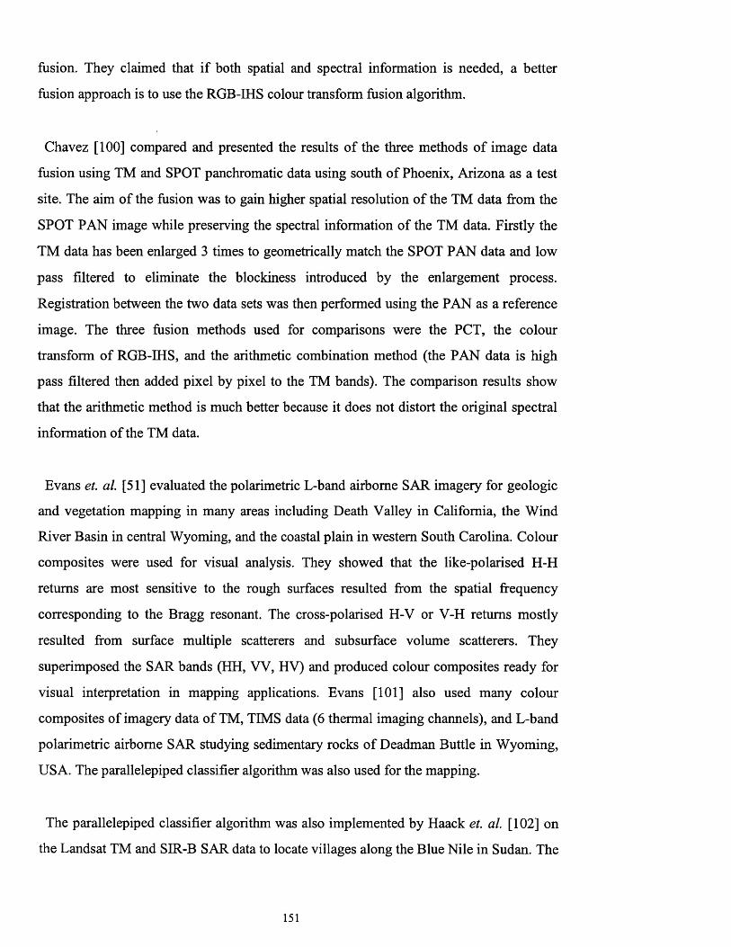
fusion. They claimed that if both spatial and spectral information is needed, a better

fusion approach is to use the RGB-IHS colour transform fusion algorithm.

Chavez [100] compared and presented the results of the three methods of image data

fusion using TM and SPOT panchromatic data using south of Phoenix, Arizona as a test

site. The aim of the fusion was to gain higher spatial resolution of the TM data from the

SPOT PAN image while preserving the spectral information of the TM data. Firstly the

TM data has been enlarged 3 times to geometrically match the SPOT PAN data and low

pass filtered to eliminate the blockiness introduced by the enlargement process.

Registration between the two data sets was then performed using the PAN as a reference

image. The three fusion methods used for comparisons were the PCT, the colour

transform of RGB-IHS, and the arithmetic combination method (the PAN data is high

pass filtered then added pixel by pixel to the TM bands). The comparison results show

that the arithmetic method is much better because it does not distort the original spectral

information of the TM data.

Evans et. a l [51] evaluated the polarimetric L-band airborne SAR imagery for geologic

and vegetation mapping in many areas including Death Valley in California, the Wind

River Basin in central Wyoming, and the coastal plain in western South Carolina. Colour

composites were used for visual analysis. They showed that the like-polarised H-H

returns are most sensitive to the rough surfaces resulted from the spatial frequency

corresponding to the Bragg resonant. The cross-polarised H-V or V-H returns mostly

resulted from surface multiple scatterers and subsurface volume scatterers. They

superimposed the SAR bands (HH, VV, HV) and produced colour composites ready for

visual interpretation in mapping applications. Evans [101] also used many colour

composites of imagery data of TM, TIMS data (6 thermal imaging channels), and L-band

polarimetric airborne SAR studying sedimentary rocks of Deadman Buttle in Wyoming,

USA. The parallelepiped classifier algorithm was also used for the mapping.

The parallelepiped classifier algorithm was also implemented by Haack et. a l [102] on

the Landsat TM and SIR-B SAR data to locate villages along the Blue Nile in Sudan. The

151

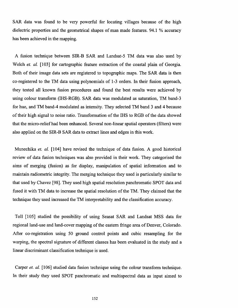
SAR data was found to be very powerful for locating villages because of the high

dielectric properties and the geometrical shapes of man made features. 94.1 % accuracy

has been achieved in the mapping.

A fusion technique between SIR-B SAR and Landsat-5 TM data was also used by

Welch et. a l [103] for cartographic feature extraction of the coastal plain of Georgia.

Both of their image data sets are registered to topographic maps. The SAR data is then

co-registered to the TM data using polynomials of 1-3 orders. In their fusion approach,

they tested all known fusion procedures and found the best results were achieved by

using colour transform (IHS-RGB). SAR data was modulated as saturation, TM band-3

for hue, and TM band-4 modulated as intensity. They selected TM band 3 and 4 because

of their high signal to noise ratio. Transformation of the IHS to RGB of the data showed

that the micro-relief had been enhanced. Several non-linear spatial operators (filters) were

also applied on the SIR-B SAR data to extract lines and edges in this work.

Munechika et. al. [104] have revised the technique of data fusion. A good historical

review of data fusion techniques was also provided in their work. They categorised the

aims of merging (fusion) as for display, manipulation of spatial information and to

maintain radiometric integrity. The merging technique they used is particularly similar to

that used by Chavez [98]. They used high spatial resolution panchromatic SPOT data and

fused it with TM data to increase the spatial resolution of the TM. They claimed that the

technique they used increased the TM interpretability and the classification accuracy.

Toll [105] studied the possibility of using Seasat SAR and Landsat MSS data for

regional land-use and land-cover mapping of the eastern fringe area of Denver, Colorado.

After co-registration using 50 ground control points and cubic resampling for the

warping, the spectral signature of different classes has been evaluated in the study and a

linear discriminant classification technique is used.

Carper et. al. [106] studied data fusion technique using the colour transform technique.

In their study they used SPOT panchromatic and multispectral data as input aimed to

152

increase the spatial resolution of the multispectral data from 20 to 10 metres and preserve

the original colour appearance. They showed that the replacement image (the

panchromatic) should be correlated to the intensity component of the multispectral data

otherwise subtle intensity differences may be obscured.

Grasso [107] showed the significance of fusion technique for thematic mapping and

geologic mapping in particular. He demonstrated the impact of digital image processing

upon remote sensing geologists and compared the recent developments with the

traditional methods of using aerial photographs for geological mapping. In his work, he

claimed that the aerial photographs still play an important role in the field of geology

because of their high spatial resolution which is not revealed by satellites such as Landsat

TM data. From this point of view, data fusion is the best method for extracting both

spatial and spectral information between aerial photographs and Landsat TM images. The

colour transform fusion method is shown to be the best method for geologic application

purposes. Registration accuracy between the two data sets is very important and any error

in the co-registration will lead to mismatch between the spectral and spatial information

during the IHS transformation.

The IHS method of merging has been studied extensively as a merging method for

imagery data from different sources. Daily [108], for example, implemented this method

for a single Seasat SAR image using filtering and colour transform to produce colour

composite image. Harries [109] used this method as a good integration method of SAR

data with other data including geophysical, thematic, and other radar data. Also the IHS

method has been used as a good fusion method with colour shaded or colour thematic

maps with imagery data [110].

Vrabel [111] used many known methods of data fusion including two new approaches

to increase the spatial image resolution using optical airborne data. In the study, the new

algorithms which include the colour normalisation (CN) technique (i.e. similar to the

153

Brovey transform fusion method) and Sparkle method1 were used and compared. Results

show both of which performed significantly better than IHS or arithmetic transforms.

6.4 The colour composite band selection/reduction problem - A new solution

From the literature review given in the previous section, it is now clear that maximum

visual enhancement is achieved by the use of colour composite. Three bands are firstly

selected and then transformed using the image data fusion tools (i.e. image processing

techniques) with either the colour transform, PCT, or arithmetic procedure then an other

image component (SAR, SPOT PAN, or digitised airphoto.) is introduced during the

transformation process. The procedure relies on the manipulation of the spectral

information gained by the original three bands selected from the original image set. The

induced fourth band represents the spatial and textural information where each is brought

together after the transformation procedure and displayed for visual interpretation.

The above procedure will not make any confusion about the selection if the spectral data

set consists only of three image bands such the case of SPOT multispectral data because

the whole image data set will be used. If the case is more than three spectral bands, a

problem will arise on the band selection and the user will argue for which bands should

be used as the basic spectral information.

The colour composite band selection issue has been mentioned in the introduction of

chapter one as a description of the problems in attaining the goal of this thesis. In this

section, this problem will be discussed in detail and a new solution is introduced in the

next section (section 6.5).

Suppose theoretically we have an image set that consists of four spectral bands, where

every band consists of a pronounced spectral feature (i.e. class) as shown in figure 6.3.

To select a colour composite from these four bands for visual assessment there are two

1 The Sparkle algorithm is a proprietary algorithm developed by the Environmental Research Institute of Michigan (ERIM). There is no detailed explanation about it in Verbel’s work.

154

problems. The first is that there are four groups of band combinations (Appendix A -l) for

producing the colour composite. Secondly, a serious problem is that any band

combination method will cause one of the spectral features (class) to be missing when the

colour composite is displayed. Practically, such theoretical assumption of the images set

shown in figure 6.3 may not occur in real life remote sensing images, but definitely

occurs as a less recognition (visually and/or automated) of some of the classes during the

colour composite band combination selection scheme.

3

¥Figure 6.3 A theoretical image set consists o f four bands, band-1 shows clear feature (class-a), band-2

shows feature b, band-3 shows feature c, and band-4 shows feature d.

The problem of band selection for colour composite production has been raised

previously by Chavez et. a l [112], Sheffield et. a l [113] and Liu et. a l [114] and can be

solved statistically by the correlation between the image bands (Appendix A-3). Another

method is the use of the transformed divergence separability test, which is believed to

give reasonable results for both visual and automated assessments [115], but its drawback

is it works only with pair of classes and hence every class pair may have different band

combination. This is shown in the separability test tables throughout this thesis and in

section 6.6 in particular.

155

Referring back to the assumed theoretical image set in figure 6.3, any suggested method

using the works of [112-115] will not give useful results because one spectral

information of a feature or class will not be present in the selected colour composite,

whatever the selection is. If the statistical method of selection is used in such theoretical

example, the optimum selection will be bands 2, 3, and 4 because the correlation between

these bands is the lowest. Band 1 will be the lowest rank for combination selection

because the spectral feature in band 1 is spatially smaller compared with other features in

band 2, 3, and 4. This is because the correlation is taken between bands as whole (the

whole image pixels are used), and hence such methods are image dependent which is

another drawback.

Solutions such as arithmetic image combination, PCT between bands, or even colour

transform are available to the user for displaying such data sets and producing a colour

composite. If such an approaches are used, the following have to be taken in account:-

1- The band arithmetic may produce a new data set in addition to the original data.

Furthermore, the spectral information of the new data set, may be altered, modified,

or changed from the original.

2- The PCT procedure will not give good results if the original data are not highly

correlated1 [116], because some spectral information will be found in the lower

spectral component images. Also if the original data are highly correlated, difficulty

in visual analysis results from colour saturation and distortion of the output data.

3- A colour transform cannot be implemented if more than 3 bands are used, unless the

procedure is done repeatedly, good results may not be guaranteed.

If the image data set consists of more than 4 spectral bands, such as the case of this

thesis work, the situation becomes difficult and solution of this problem is important. The

spectral information of every feature must be extracted within every image to produce

only three new images that can be displayed and assessed. These new images can be used

1 If data is not correlated, PCT should not be used because PCT is a decorrelation procedure and PCT in this case has no meaning.

156

as a basis for fusion such as introducing spatial or textural information. The new

suggested method of solving this problem is shown in the next section.

6.5 Using the spectral unit as a method of TM spectral coding

It has been mentioned in chapter 5 (p. 124) that He and Wang [62] and Wang and He

[63] developed a method of textural measure, which is based on a simple algorithm

named the “texture unit” to extract the texture spectra. An approach has been developed

for the first time in this thesis adopting the same logic of He and Wang’s work with some

modification to extract the TM spectral units as a coding method of the six TM bands.

The algorithm is shown as follows:

Let the spectral unit number of every pixel vector in n bands be limited by the three

values 0.0, 0.5, or 1.0 based on the test of this pixel vector value with its vector mean

such as:

UP • =x,y,i

0.0 i f x . < uV x ,y 9t *^x ,y ti

0.5 i f x ■ = juV x,y,i r*x>y,i

1.0 i f x ■ > aJ x ,y,i f* x ,y j

(6.2)

where:

UP j = the spectral unit number of pixel at location x and y, in the band

number i where i=l ,2,... ,N.

ju j = the mean vector reflectance of the same pixel location. It is equal to

1 ^— 2 ^ BVi ’ and is the brightness value of the pixel at band i.^ 1 = 1

Because UP j has three possible unit values (i.e. 0.0, 0.5, or 1.0), the number of

possible codes in total are 3^ (i.e. 729 code for TM data). To code this pixel vector (its

spectral code) the following equation is used:

157

1 NSpectral code = UPxyi x 3,_1

S J=1(6.3)

where:

S is a scaling factor

In this work, the scaling factor is used to ensure the output TM spectral coded image

does not exceed 8-bits. But at this step, it is recommended not to use the scaling factor

and left to equal unity (i.e. S=l). Scaling can be used after creating the spectral coded

image using equations 6.2 and 6.3, and the output spectral coded is stored in 32 bit image

file.

To simplify the process, table 6.1 shows a numerical example of the method of coding

applied on 10 pixel vectors of TM bands 1-5, and 7 noting that the mean of every pixel

vector has been set to an integer value.

PixelNo.

B1 B2 B3 B4 B5 B7 Mi UP, UP2 UP, u p . UP5 u p , Scode

1 99 112 115 121 137 109 115 0 0 05 1 1 0 11252 55 39 61 66 87 92 67 0 0 0 0 1 1 3243 30 157 79 101 121 144 106 0 1 0 0 1 1 3274 0 0 0 0 0 0 0 05 05 05 05 05 05 1825 181 181 181 181 181 181 181 05 05 05 05 05 05 1826 0 42 84 126 168 210 105 0 0 0 1 1 1 3517 210 186 126 84 42 0 105 1 1 1 0 0 0 138 255 0 0 0 0 0 255 05 0 0 0 0 0 059 0 130 135 140 145 150 91 0 1 1 1 1 1 36310 0 100 135 225 170 170 138 0 0 0 1 1 1 351

Table 6.1. A numerical example o f applying the spectral coding method.

6.5.1 Properties of the spectral coding algorithm

1- Referring back to the numerical example shown in table 6.1, it has been pointed out

(in theory) the maximum number of codes is 729 numerical values. Practically, such

158

number of combinations cannot be achieved because the minimum code value is 0.5

and the maximum value is 363 (i.e. pixel number 8 and 9 respectively). This results in

727 combinations (i.e. (364 x 2)-l).

2- Another important property in the spectral coding method is that similar spectral

shapes have similar spectral code values; this is shown in pixels number 4 and 5 in the

numerical example in table 6.1, where pixels with different topographic-albedo

information have the same code number.

3- A proper atmospheric correction method should be used to ensure all shadow pixels

have the code number 182 (i.e. pixel number 4). If a loose method of atmospheric

correction is used or the data is over corrected, shadow pixels may bias from the code

number 182 and hence show different spectral class code. For that reason the dark-

pixel subtraction method is used in this work (shown in 4.3) to ensure the data is

atmospheric corrected properly.

4- Pixels of albedo-topographic information and shadow pixels have similar spectral

code number, and hence the output spectral coded image has no topographic

information, this is because // . is used in equation 6.2.

5- The spectral coding method adopted here is sensitive to any biased pixels (i.e. noise).

Such spectral code may coincide with other spectral code; this is shown in pixel vector

6 and 10 where pixel vector number 10 has noise in band 1 (zero) and band 4 (255).

6- There is no hardware that can display more than 8-bit image in one graphic plane card.

Hence, if the data is not scaled (which is desired) but viewed in the computer screen, it

will automatically be scaled to 8-bit resulting of the mixing of some spectral coded

pixels which visually results in the loss of some spectral information.

7- To find the S value for scaling to 8-bit image (equation 6.3), one method is setting S =

1.42 (i.e. 363/255) but this method may result in the loss of coding. With minimum

159

loss of information, one method can be proceeded by producing the spectral code

image and storing it in 32 bit image file, then subtracting the spectral coded image

from its minimum code value (i.e. shifting the spectral coded image histogram to zero

value), then calculating the maximum code value and dividing it by 255 and finally,

rounding off the output and saving it in 8 bit image.

8- The more bands used, the wider range of coding, reflecting reasonable results. This is

based on the rule 3N where N is the number of bands. For example coding the 6 TM

bands is more appropriate than coding SPOT multispectral 3 bands.

6.5.2 Procedure of producing the spectral coded image

The following is the procedure of producing the spectral coded TM image

1- stretch the optical TM images to occupy the intensity range value (0-255) using

BCET. BCET is used to make sure the bands used are equally stretched in mean,

minimum, and maximum.

2- calculate the mean image using the 6 TM bands. Real numbers should be rounded off

to integer values. The mean image is named in this work the albedo-topographic

information image.

3- create a six floating point numerical variable (i.e. al,a2,a3,..., a6) to calculate and

store the spectral unit numbers UPl , UP2, ...., UP6 using equation 6.2.

4- create the spectral coded image using equation 6.3 and assign the output to 32 bit

output image.

5- convolve the spectral coded image by using the mode filter (either 3x3 or 5x5) to

neglect biased coded pixels (spectrally contaminated pixels) which are geographically

located within the same coded class or window.

160

6- scale (if desired) the image produced by step 4 to an 8-bit image.

6.5.3 Results of using the spectral coded image of TM data and creating colour

composite

Figure 6.4 shows the TM spectral coded image after scaling. The image is displayed in

grey scale. Spectral pseudo-colour coded image is also displayed and shown in figures

6.5. The spectrally TM pseudo-colour coded image can be evaluated visually after

assigning every specific pixel’s intensity values to a specific colour for an easy and quick

visual assessment. The drawback may result from the high number of spectral coded

classes. Figure 6.5 shows the spectral pseudo-colour coded image with 158 class. The

number of classes have been calculated from the image histogram.

161

Figure 6.4 A grey scaled TM spectral coded image after applying 5x5mode fd te r and sca led to 8-bit.

162

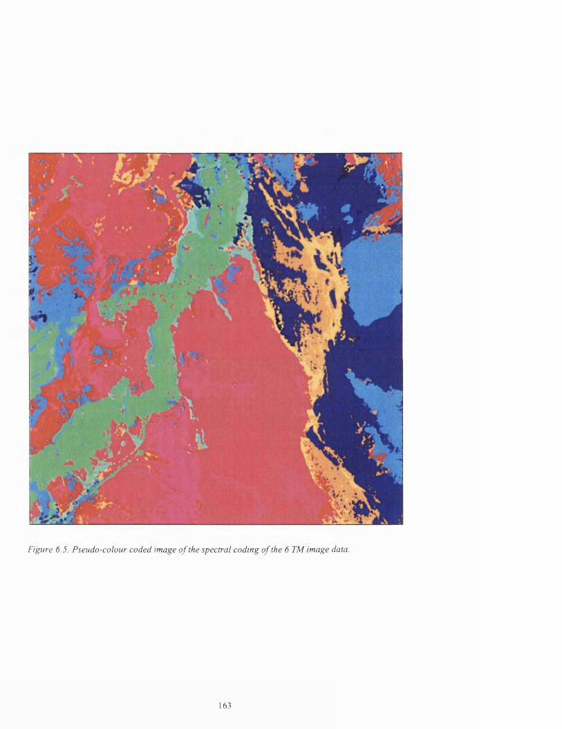
Figure 6.5. Pseudo-colour coded image o f the spectral coding o f the 6 TM image data.

163

The classes separability analysis (represented by class ellipsoids) using both of the

spectral coded image and the albedo-topography information image shows a promising

result, which is shown in figure 6.6, in which every class ellipsoid2 shows good

separability.

255TM

SSabkhahAeolianP

ectr

LisanMusayr

a1 -192

Gravel + Sandcoded

1mage

-128Nutaysh

Bad'Atiyah

-64

AlluviumGravel sheetsJurfayn

25519264 128

TM albedo + Topography image

Figure 6.6 Class ellipsoids o f the test site using the TM spectral coded image plotted on the abscissa and

the TM albedo and topographic information image plotted in the ordinate.

2 Class ellipsoids is a graphical representation of separability. They can be drawn using the covariance matrices and the eigenvectors o f the classes. The eigenvectors and values o f the inverse covariance matrix o f classes define the direction and length o f the major and minor ellipse axes.

164

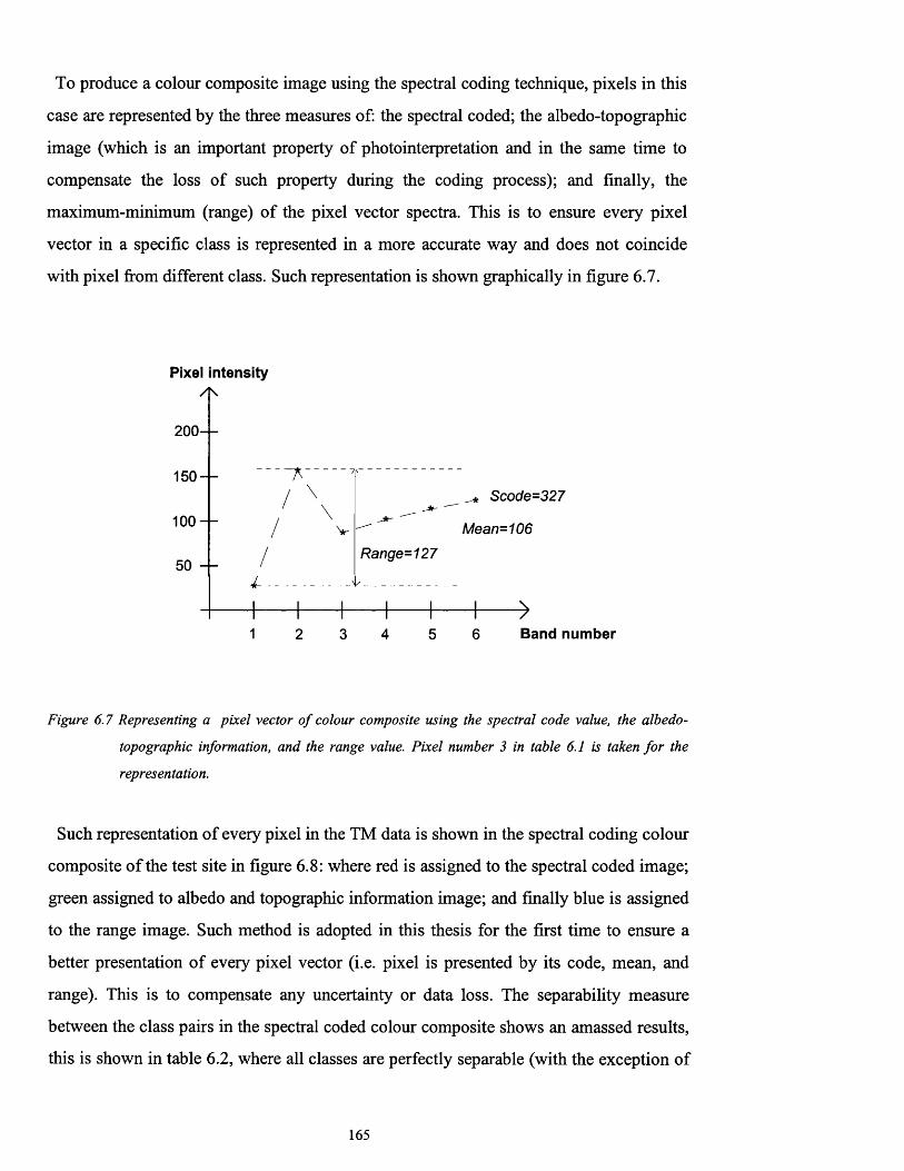
To produce a colour composite image using the spectral coding technique, pixels in this

case are represented by the three measures of: the spectral coded; the albedo-topographic

image (which is an important property of photointerpretation and in the same time to

compensate the loss of such property during the coding process); and finally, the

maximum-minimum (range) of the pixel vector spectra. This is to ensure every pixel

vector in a specific class is represented in a more accurate way and does not coincide

with pixel from different class. Such representation is shown graphically in figure 6.7.

Pixel intensity

200 - -

150 - -Scode=327

100 - - Mean=106

Range=12750 - -

1 2 3 4 5 6 Band number

Figure 6.7 Representing a pixel vector o f colour composite using the spectral code value, the albedo-

topographic information, and the range value. Pixel number 3 in table 6.1 is taken fo r the

representation.

Such representation of every pixel in the TM data is shown in the spectral coding colour

composite of the test site in figure 6.8: where red is assigned to the spectral coded image;

green assigned to albedo and topographic information image; and finally blue is assigned

to the range image. Such method is adopted in this thesis for the first time to ensure a

better presentation of every pixel vector (i.e. pixel is presented by its code, mean, and

range). This is to compensate any uncertainty or data loss. The separability measure

between the class pairs in the spectral coded colour composite shows an amassed results,

this is shown in table 6.2, where all classes are perfectly separable (with the exception of

165

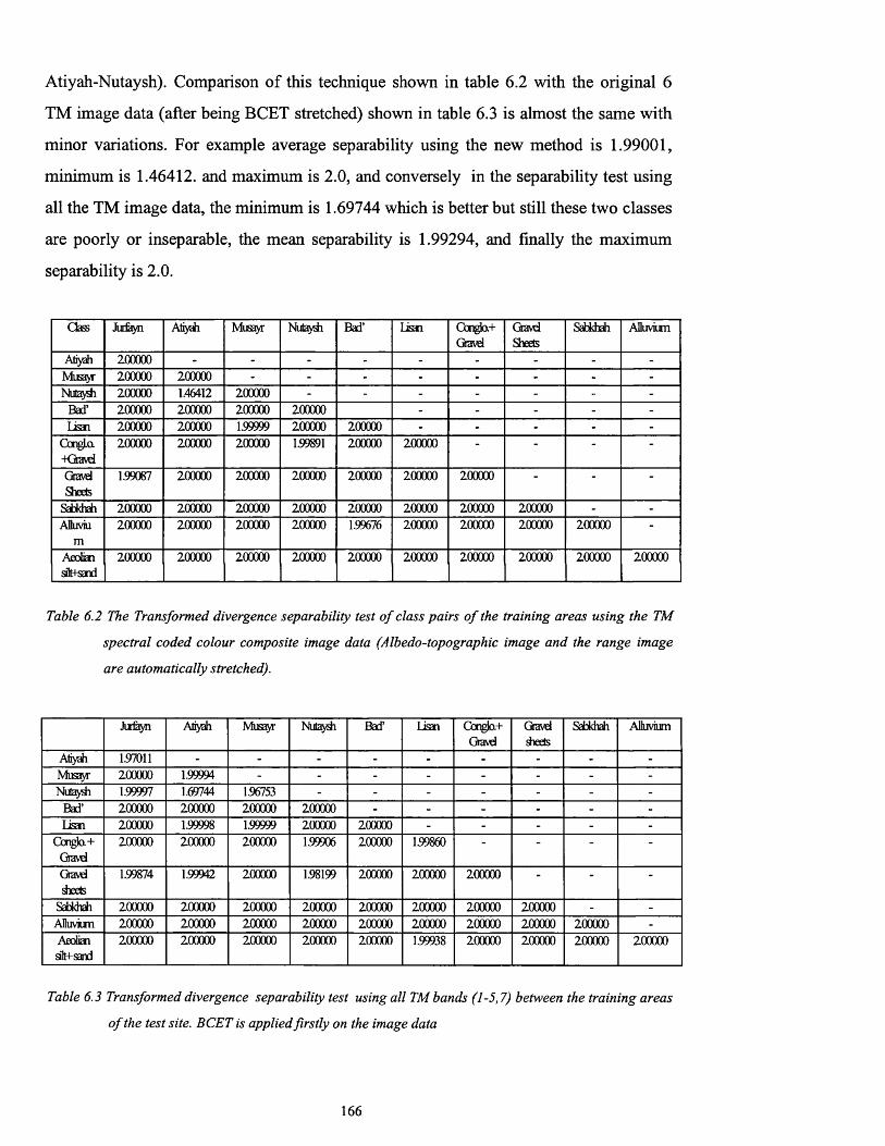
Atiyah-Nutaysh). Comparison of this technique shown in table 6.2 with the original 6

TM image data (after being BCET stretched) shown in table 6.3 is almost the same with

minor variations. For example average separability using the new method is 1.99001,

minimum is 1.46412. and maximum is 2.0, and conversely in the separability test using

all the TM image data, the minimum is 1.69744 which is better but still these two classes

are poorly or inseparable, the mean separability is 1.99294, and finally the maximum

separability is 2.0.

Class Jurfayn Atiysh Musayr Nutaydi Bad’ Lisan Gcngta.+Gravel

GravdSheets

Sabkhah Alluvium

Atiyah 200000 - - - - - - - - -

Musayr 200000 200000 - - - - - - - -Nutajdi 200000 1.46412 200000 - - - - - - -

Bad’ 200000 200000 200000 200000 - - - - -Lisan 200000 200000 159999 200000 200000 - - - - -

CongLo.-Kjravd

200000 200000 200000 159891 200000 200000 “ “ ■ ■

GravdSheets

159087 200000 200000 200000 200000 200000 200000 " ■ -

Sabkhah 200000 200000 200000 200000 200000 200000 200000 200000 - -AHuviu

m200000 200000 200000 200000 1.99676 200000 200000 200000 200000 ■

Aeoliansflt+sand

200000 200000 200000 200000 200000 200000 200000 200000 200000 200000

Table 6.2 The Transformed divergence separability test o f class pairs o f the training areas using the TM

spectral coded colour composite image data (Albedo-topographic image and the range image

are automatically stretched).

Jurfayn Atiyah Musayr Nutaydi Bad’ Lisan Gonglo.+Gravd

Gravddieets

Sabkhah Alluvium

Atiyah 1.97011 - - - - - - - - -

Mus /r 200000 1.99994 - - - - - - - -Nutaydi 1.99997 1.69744 156753 - - - - - - -

Bad’ 200000 200000 200000 200000 - - - - - -Lisan 200000 159998 1.99999 200000 200000 - - - - -

Conglo.+Gravd

200000 200000 200000 159906 200000 1.99860 - - - -

Gravdsheets

1.99874 1.99942 200000 158199 200000 200000 200000 - - -

Sabkhah 200000 200000 200000 200000 200000 200000 200000 200000 - -

Alluvium 200000 200000 200000 200000 200000 200000 200000 200000 200000 -

Aeoliansifct-sand

200000 200000 200000 200000 200000 1.99938 200000 200000 200000 200000

Table 6.3 Transformed divergence separability test using all TM bands (1-5,7) between the training areas

o f the test site. BCET is applied firstly on the image data

166

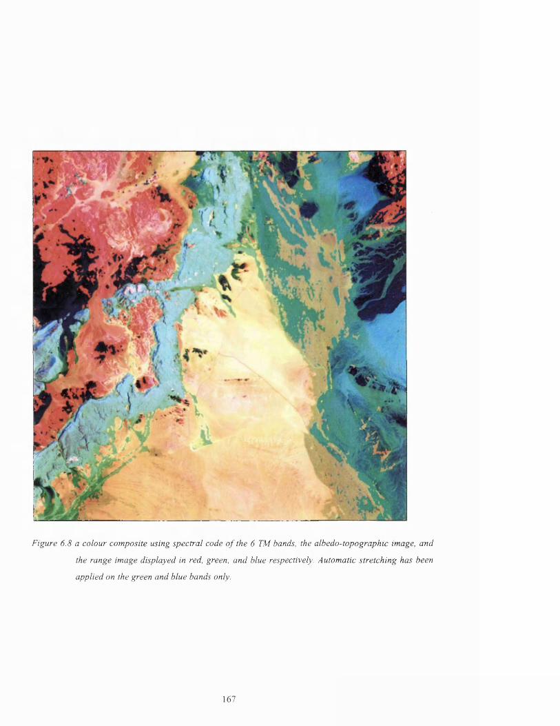
Figure 6.8 a colour com posite using spectral code o f the 6 TM bands, the albedo-topographic image, and

the range image displayed in red, green, and blue respectively. Automatic stretching has been

applied on the green and blue bands only.

167

6.6 Comparison between the spectral coded colour composite and the traditional

methods of colour composite selection

In this section, a random set of colour composites of the test area are displayed,

compared visually and quantitatively assessed, and in addition the best colour composite

selection is examined using the methods discussed earlier using Chavez et. al. [112],

Sheffield et. al [113], and Liu et. al [114] after being contrast enhanced using the BCET

developed by Liu [43,114] to ensure no colour bias occur between the displayed bands.

From the covariance matrix of the six TM bands used (shown in appendix B-l), the

following in table 6.4 shows the first best two ranks of bands combination and the last

(worst) bands combination for colour composites. The full ranking of the colour

composite bands combination table is shown in appendix B-2.

Rank Determinant Band comb. OIF Bands comb. IOBS Bandcomb.

1 550945300 1,5,7 60.555 1,5,7 0.660283 1,5,72 517319600 2,5,7 54.450 2,5,7 0.696099 1,4,7

20 2039992 2,3,4 39.309 2,3,4 0.963189 2,3,4

Table 6.4 The first, second, and worst bands combination o f the six TM bands after applying BCET.

In the case of colour composite of TM bands 3,2, and 1 displayed in red, green, and blue

respectively (natural colour composite) shown in figure 6.9, some of the rock units are

distinguishable. These rock classes are: Jurfayn (dark bluish-green); Atiyah (brown); and

Bad’ formation (creamy whitish in colour), and finally the Sabkhah (white). Separability

measure using these three bands is shown in table 6.5 with minimum separability

0.68844, average separability 1.93057, and maximum separability is 2.0. Quantitatively,

eight of the classes pairs using this colour composite combination are poorly to

inseparable (i.e. pairs less than 1.9).

168

Gass Jurfayn Atiyah Musayr Nutaydi Bad’ Lisai Gongkx+Gravd

GravdSheets

Sabkhah Alluvium

Atiyah 1.7081 - - - - - - - - -Musayr 1.77180 152826 - - - - - - - -Nutaydi 1.71503 1.76086 0.68844 - - - - - - -

Bad’ 159980 159991 158191 159584 - - - - - -Lisan 200000 200000 159999 200000 159878 - - - - -

CongLo.-K3ravd

200000 200000 157632 159828 159997 151921 - - - -

GravdSheets

1.81597 199296 123188 1.73032 1.99999 200000 199868 - - -

Sabkhah 2.00000 200000 200000 2.00000 159061 2.0000 200000 2.00000 - -AHuviu

m200000 200000 200000 200000 1.99998 199412 200000 200000 200000 -

AeoliansOt+sand

200000 200000 200000 200000 1.98818 1.99856 200000 200000 200000 199716

Table 6.5 Separability measure o f the lithologic classes using bands combination 3,2,1 o f the TM image

data. Data are BCET stretched.

169

Figure 6.9. Colour com posite o fT M bands 3,2, and 1 displayed in red, green, and blue respectively. Data is

firstly BCET stretched.

170

Using a combination of TM bands 4,3, and 2 (as the lowest rank of bands combination)

displayed in red, green, and blue respectively as shown in figure 6.10, do not visually

show much differences from 3,2, and 1 bands combination for lithological point of view.

It shows only clear vegetation farms (palm trees found during the field visit) in the upper

part of the image. Quantitatively and by the use of the separability test of lithological

classes pairs as shown in table 6.6, the minimum separability is 1.10912, the average

separability is 1.94607, and the maximum separability is 2.0. Some improvement of

separability has been achieved using this band combination compared with the natural

colour band combination, but still there are seven pair of classes which are poorly

separable.

Class Jurfayn Atiyah Musayr Nutaydi Bad’ Lisan Ccngla+Gravd

GravdSheets

Sabkhah Alluvium

Atiyah 1.83494 - - - - - - - - -Musayr 1.96549 1.92757 - - - - - - - -Nutaydi 1.78885 1.79328 1.10912 - - - - - - -

Bad’ 199999 199940 1.96141 199460 - - - - -Lisan 200000 200000 1.99989 200000 199878 - - - - -

CongLo.-Kjravd

200000 200000 196720 198927 199998 1.97466 “ - “

GravdSheets

1.77548 1.98616 1.88288 1.13811 200000 200000 199973 “ - “

Sabkhah 200000 200000 200000 200000 199361 200000 200000 200000 - -AHuviu

m200000 200000 200000 200000 1.99999 1.99999 1.99997 200000 200000 “

AeoliansQt+sand

200000 200000 200000 200000 1.95579 199793 200000 200000 200000 1.99998

Table 6.6. Separability measures between class pairs o f the test site using the bands combination 4,3, and

2 o f TM data. BCET is firstly applied.

171

Figure 6.10 Colour com posite using bands 4, 3, and 2 displayed in red, green, and blue respectively. Data

are stretched using BCET.

172

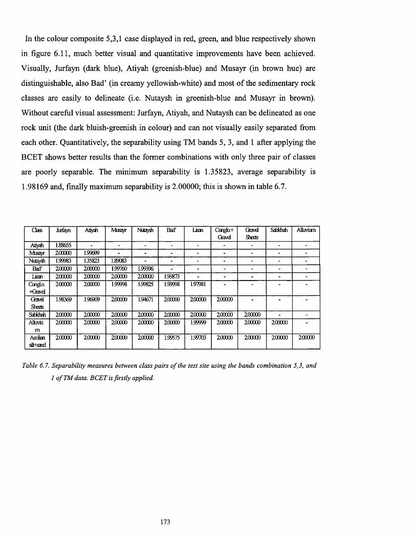
In the colour composite 5,3,1 case displayed in red, green, and blue respectively shown

in figure 6.11, much better visual and quantitative improvements have been achieved.

Visually, Jurfayn (dark blue), Atiyah (greenish-blue) and Musayr (in brown hue) are

distinguishable, also Bad’ (in creamy yellowish-white) and most of the sedimentary rock

classes are easily to delineate (i.e. Nutaysh in greenish-blue and Musayr in brown).

Without careful visual assessment: Jurfayn, Atiyah, and Nutaysh can be delineated as one

rock unit (the dark bluish-greenish in colour) and can not visually easily separated from

each other. Quantitatively, the separability using TM bands 5,3, and 1 after applying the

BCET shows better results than the former combinations with only three pair of classes

are poorly separable. The minimum separability is 1.35823, average separability is

1.98169 and, finally maximum separability is 2.00000; this is shown in table 6.7.

Class Jurfayn Atiyah Musayr Nutaydi Bad’ Lisan Conglo.+Gravd

GravdSheets

Sabkhah Alluvium

Atiyah 1.88655 - - - - - - - - -Musayr 200000 159699 - - - - - - - -Nut sh 1.99983 135823 1.89083 - - - - - - -

Bad’ 200000 200000 1.99760 1.99396 - - - - - -Usan 200000 200000 200000 200000 159873 - - - - -

GongLo.-Kjravd

200000 200000 159998 1.99825 159998 1.97981 “ - “

GravdSheets

1.98369 1.96909 200000 1.94671 200000 200000 200000 ■

Sabkhah 200000 200000 200000 200000 200000 200000 200000 200000 - -AHuviu

m200000 200000 200000 200000 200000 1.99999 200000 200000 200000 '

Aeoliansflt+sand

200000 200000 200000 200000 1.99575 1.99703 200000 200000 200000 200000

Table 6.7. Separability measures between class pairs o f the test site using the bands combination 5,3, and

1 ofT M data. BCET is firstly applied.

173

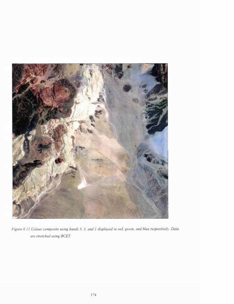
Figure 6.11 Colour com posite using bands 5, 3, and 1 d isplayed in red, green, and blue respectively. Data


174

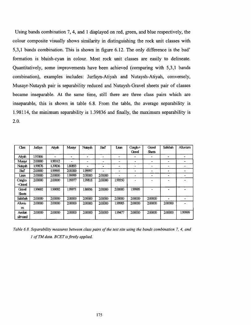
Using bands combination 7, 4, and 1 displayed on red, green, and blue respectively, the

colour composite visually shows similarity in distinguishing the rock unit classes with

5,3,1 bands combination. This is shown in figure 6.12. The only difference is the bad’

formation is bluish-cyan in colour. Most rock unit classes are easily to delineate.

Quantitatively, some improvements have been achieved (comparing with 5,3,1 bands

combination), examples includes: Jurfayn-Atiyah and Nutaysh-Atiyah, conversely,

Musayr-Nutaysh pair is separability reduced and Nutaysh-Gravel sheets pair of classes

became inseparable. At the same time, still there are three class pairs which are

inseparable, this is shown in table 6.8. From the table, the average separability is

1.98114, the minimum separability is 1.39836 and finally, the maximum separability is

2 .0 .

Gass Jurfayn Atiyah Musayr Nutaydi Bad’ Lisan Conglo.+Gravd

GravdSheets

Sabkhah Alluvium

Atiyah 151866 - - - - - - - - -Musayr 200000 159312 - - - - - - _ _

Nutaysh 159876 139836 1.80893 - - - - - - -Bad’ 200000 159995 200000 1.99997 - - - - - -Lisan 200000 200000 1.99999 200000 200000 - - - - -

GongLo.-Kjravd

200000 200000 1.99977 1.99818 200000 1.99550 - *

GravdSheets

159692 159092 159971 1.86936 200000 200000 159995 “ - “

Sabkhah 200000 200000 200000 200000 200000 200000 200000 200000 - -ADuviu

m200000 200000 200000 200000 200000 1.99985 200000 200000 200000 “

Aeoliansilt+sand

200000 200000 200000 200000 200000 1.99477 200000 200000 200000 159999

Table 6.8. Separability measures between class pairs o f the test site using the bands combination 7, 4, and


175

Figure 6.12 Colour com posite using bands 7 , 4, and 1 displayed in red, green, and blue respectively. Data


176

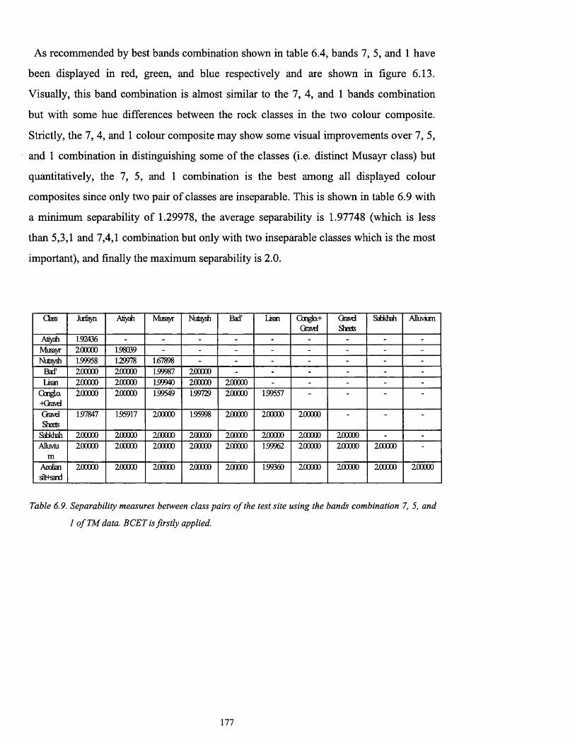
As recommended by best bands combination shown in table 6.4, bands 7, 5, and 1 have

been displayed in red, green, and blue respectively and are shown in figure 6.13.

Visually, this band combination is almost similar to the 7, 4, and 1 bands combination

but with some hue differences between the rock classes in the two colour composite.

Strictly, the 7, 4, and 1 colour composite may show some visual improvements over 7, 5,

and 1 combination in distinguishing some of the classes (i.e. distinct Musayr class) but

quantitatively, the 7, 5, and 1 combination is the best among all displayed colour

composites since only two pair of classes are inseparable. This is shown in table 6.9 with

a minimum separability of 1.29978, the average separability is 1.97748 (which is less

than 5,3,1 and 7,4,1 combination but only with two inseparable classes which is the most

important), and finally the maximum separability is 2.0.

Gass Jurfayn Atiyah Musayr Nutaydi Bad’ Lisan Cong}a+Gravd

GravdSheets

Sabkhah Alluvium

Atiysh 1.92436 - - - - - - - - -Musayr 200000 158039 - - - - - - - -Nutaydi 1.99958 129978 1.67898 - - - - - - -

Bad’ 200000 200000 1.99987 200000 - - - - - -Lisan 200000 200000 1.99940 200000 200000 - - - - -

OcngLo.+Gravd

200000 200000 1.99549 159729 200000 1.99557 “ “ ■ “

GravdSheets

1.97847 155917 200000 1.95998 200000 200000 200000 “ - “

Sabkhah 200000 200000 200000 200000 200000 200000 200000 200000 - -AHuviu

m200000 200000 200000 200000 200000 1.99962 200000 200000 200000 "

Aeoliansflt+sand

200000 200000 200000 200000 200000 1.99360 200000 200000 200000 200000

Table 6.9. Separability measures between class pairs o f the test site using the bands combination 7, 5, and


177

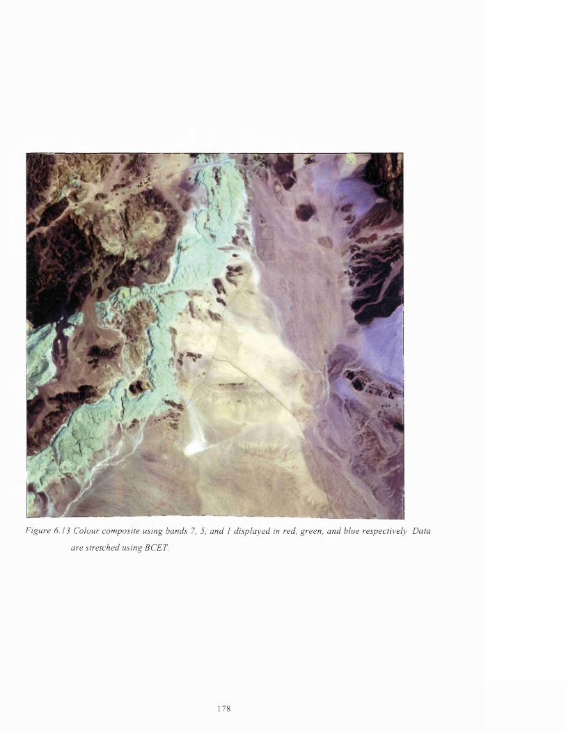
Figure 6.13 Colour com posite using bands 7, 5, and 1 d isplayed in red, green, and blue respectively. Data


178

6.7 Image fusion using colour transform

Colour is known to be a powerful descriptor that simplifies object identification and

extraction from a scene. In visual image analysis performed by humans, the motivation

for colour is that the human eye can discriminate thousands of colour shades, but only

around twenty shades of grey level [60].

Image processing of colours can be divided into two major areas, full colour and

pseudo-colour processing. In the first instance, the three image layers are assigned to the

three primary colours or the three monitor guns and superimposed on the image layers to

produce a coloured image (i.e. fig. 6.9-6.13). The pseudo-colour processing can be

achieved by assigning a shade of colour or colours to a particular monochromatic

intensity or range of intensities of a single layer of image (i.e. fig. 6.5).

Colours that human beings perceive from an object are determined by the nature of light

reflected from the object. A body that reflects light which is relatively balanced in all

visible wavelengths appears white to the observer, whereas objects that absorb all visible

wavelengths appear black. Objects that reflect part of the visible wavelength appear as

the colour associated with that wavelength in the visible electromagnetic spectrum.

Characterisation of light is an important subject in the colour science. If the light is

achromatic (void of colours), its attribute is only its intensity and can be expressed by a

scalar measure of grey level ranging from black, to greys, and finally white. Chromatic

light spans the electromagnetic energy spectrum from approximately 400 to 700 nm.

[60].

Three basic quantities are used to describe the quality of chromatic light source:

radiance, luminance, and brightness. Radiance is the total amount of energy that flows

from the light source, and is usually measured in Watts. Luminance, which is measured

in lumens (lm), is the amount of energy that the observer can perceive from the light

source, (e.g. the observer is unable to perceive energy in the infrared or microwave, in

179

this case the luminance would be zero, but they have their significant energy of radiance).

Brightness is a subjective descriptor that is particularly difficult to measure, it embodies

the achromatic notation of intensity and is one of the key factors in describing colour

sensation [60].

All colours can be simplified as combinations of what are called the primary colours,

red = 700nm, green = 546nm, and blue = 435.8nm in wavelengths. These colours can be

added in equal amounts to produce the secondary or complementary colours of light

which are: magenta = red and blue, cyan = green and blue, and yellow = red and green. If

the three primary colours are added equally, this will give the additive component of

colours which is white. If the three secondary colours are added equally, this will give the

subtractive component of colours which is black.

The characteristics which are used to distinguish one colour from the other are

brightness, hue, and saturation. As already indicated, brightness embodies the achromatic

notion of intensity. Hue is an attribute associated with the dominant wavelength in the

mixture of light, thus hue represents dominant colours as perceived by an observer.

Saturation refers to the relative purity or the amount of white light mixed with the hue.

An example is that pure spectrum colours are fully saturated, whereas pink colours (red +

white) or lavender (violet + white) are less saturated, with the degree of saturation being

inversely proportional to the amount of white light added.

If hue and saturation are taken together they are called the colour chromaticity, and

therefore a colour may be characterised by its brightness and chromaticity. The amount

of red, green, and blue needed to form any particular colour are called the tristimulus

values and are denoted as X , Y, and Z respectively. A colour can then be specified by its

trichromatic coefficients x,y, and z. These coefficients are:-

where x, y, and z are red, green, and blue trichromatic coefficients respectively, and the

sum of these coefficients is equal to 1 as shown from the above equations.

Colours can be represented by many proposed models. These models are oriented either

toward the hardware (such as for colour monitors and printers) or toward applications

where colour manipulation is the goal. The hardware oriented models most commonly

used in practice are the RGB (red, green, blue) model for colour monitors and for most

colour video cameras. Another hardware oriented model is the CMY (cyan, magenta,

yellow) model which is basically used for colour printers, and finally the YIQ model,

which is the standard model used for colour TV broadcast (Y corresponds to luminance, I

and Q are two chromatic components called in-phase and quadrature respectively) [60].

A model used for colour image manipulations is the IHS (intensity, hue, saturation)

model. The advantage of this model is its ability to separate the spatial component (I)

from the spectrum component (H and S) of the manipulated colour.

The colour models most often used in image processing are the RGB and the IHS

models. The YIQ model is less important in image processing, where the CMY is used

basically in hardcopy image production. A transform between the RGB model and the

IHS model is mostly used for multispectral and multisensor image fusion purposes. The

RGB and IHS models will be discussed in the following paragraphs to simplify the

understanding of fusion using colour transform techniques.

The RGB model is simply based on a three dimensional Cartesian coordinate system as

shown in figure 6.14. Each colour appears in its primary spectral components of red

(1,0,0), green (0,1,0), and blue (0,0,1) in the three comers of the colour cube. The

secondary colours of cyan (0,1,1), magenta (1,0,1), and yellow (1,1,0) are at the other

three comers. Black is at the origin (0,0,0), and white (1,1,1) is at the comer farthest from

the origin.

B

Cyan(0,1,1)

(0,0,1)Blue

Magenta( 1,0,1)

(0,1,0)Blaclc.Green

Grey scale

( 1,0,0'Red

R

Figure 6.14. The RGB colour model (modified from [60]).

The grey scale extends from black to white along the line jointing these two points. The

colours are points on the comers of the cube, and are defined by vectors extending from

the origin. For simplification, all colour values have been normalised from zero to one

and all values are assumed to be in the range of 0 and 1.

Images in the RGB colour model consist of three independent image layers, one for

each primary colour. When fed into an RGB monitor, these three images combine in the

phosphor screen to produce a colour composite image. Thus the use of the RGB model

for image processing makes sense when the images are expressed in terms of three colour

layers [60],

182

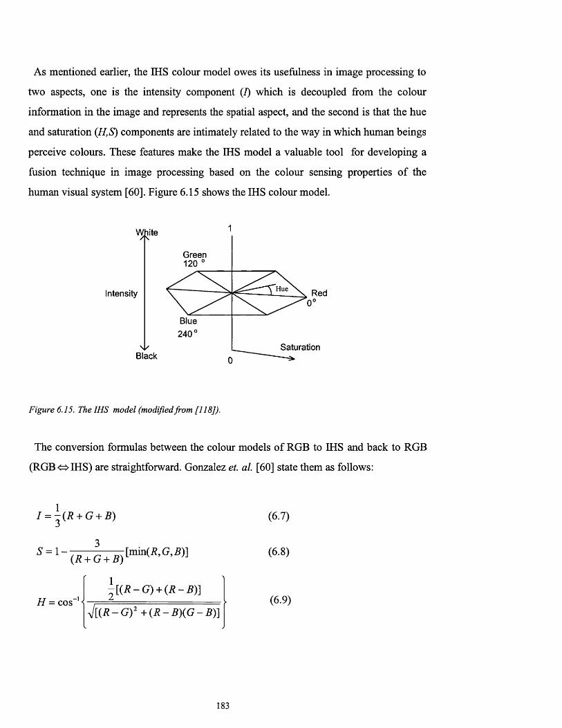
As mentioned earlier, the IHS colour model owes its usefulness in image processing to

two aspects, one is the intensity component (I) which is decoupled from the colour

information in the image and represents the spatial aspect, and the second is that the hue

and saturation (H,S) components are intimately related to the way in which human beings

perceive colours. These features make the IHS model a valuable tool for developing a

fusion technique in image processing based on the colour sensing properties of the

human visual system [60]. Figure 6.15 shows the IHS colour model.

White

Green 120 0

Hue RedIntensity

Blue240°

SaturationBlack

Figure 6.15. The IHS model (modifiedfrom [118]).

The conversion formulas between the colour models of RGB to IHS and back to RGB

(RGB <=> IHS) are straightforward. Gonzalez el. al. [60] state them as follows:

I = - ( R + G + B)

S = l -(.R + G + B)

1

[min(R,G,5)]

H = cos[ (R -G ) + (R - B ) ]

J [ ( R - G ) 2 + ( R - B ) ( G - B ) ]

(6.7)

(6.8)

(6.9)

183

The conversion back to red, green, and blue is dependent on the angle of the hue as

shown in figure 6.15 and can be transferred to the pixel brightness value interval. The

conversion formulas are as follows [60]:

1- When 0°<H< 120°

(//ranges from 0 to 85 in brightness values of 8 bit images).

r = 1 +ScosH

cos(60 - H)

g = \ - ( r + b)

(6.10)

(6.11)

(6 .12)

2 - When 120°<//< 240°

(H ranges from 85 to 170 in brightness values of 8 bit images)

H = H - 120°

r = f ( l - S )

g 1 +ScosH

cos(60° - H )

b = l - ( r + g)

(6.13)

(6.14)

(6.15)

(6.16)

3- When 240°< H < 360°

(H ranges from 170 to 255 in brightness values of 8 bit images)

H = H - 240°

ScosH

1

1 +cos(60° - H )

g = -3 ( l - S )

(6.17)

(6.18)

(6.19)

184

r = l - ( g + b) (6.20)

Based on the trichromatic coefficients shown previously in equations 6.4-6.6, another

important spatial-spectral fusion technique has been derived [4] called the Brovey

transform [119]. It uses the selected three bands for colour display as RGB and uses the

fourth image which is SAR or Panchromatic aerial photograph. The following

transformation equations are used for the fusion process:

where:

R , G, and B = red, green, and blue layers.

I = the image intended to be included with the spectral data, such as the SAR

image or aerial photograph.

One important characteristic of both RGB <=> IHS is that it is scene independent (every

pixel is manipulated independently from the other scene pixels. The Brovey transform

also has this characteristic because both are pixel basis (not scene basis).

6.8 TM and SAR colour transform fusion

The objective of image data fusion for geologic remote sensing is to combine both of

the spatial and spectral information. By the use of the TM spectral colour coded

composite, the whole spectral information available in the six TM image data set has

been preserved in such three image layers (the TM spectral coded colour composite), this

is shown for comparison in tables 6.2 and 6.3. As mentioned in section 6.7, one

(6.21)

G \(6.22)

(6.23)

185

important characteristic of the IHS model is the separation of the spatial component (I)

from its spectral components (H and S). This spatial component or image can be replaced

it by the JERS-1 SAR spatial information image, which contains the textural information.

Another fusion tool that separate the image spectral and spatial components from each

other using the colour transform is the colour chromaticity method which is represented

by the Brovey transform. Such methods have been discussed theoretically and then will

practically implemented on the TM spectral colour coded composite and SAR images. A

visual and quantitative analysis will then be given on the output results using both

techniques, and in the same time, the colour composite of bands 7, 5, and 1 is also colour

fused with the SAR data and compared visually and quantitatively with the new output

results.

Referring back to the TM spectral coded colour composite image (figure 6.8) in section

6.5.3, strictly, it might be possible to restore this image to simulate normal colour

composites, this is because most remote sensing geologists are well familiar with colour

composites photo-interpretation. Furthermore, the spatial information in figure 6.8 is less

pronounced if compared with normal colour composites. To restore such an image, by

assigning the spectral coded image to the hue component (H) after applying histogram

equalisation on this image, the topographic-albedo information image to the intensity

component (I), and the range image to the saturation component (S) after being

automatically stretched, then reversing these components to RGB (IHS => RGB), a new

image can be produced with better (to some extent) spatial information representation,

and at the same time preserving the spectral information which is represented by the

spectral coded image. Such an image is shown in figure 6.16. From the image and from

the photo-interpretation point of view, rock units are shown as follows: In the upper left

comer of the image, Jurfayn is shown up as dark green; Atiyah is saturated dark brown;

Musayr is violet-pinkish; and Nutaysh is brown. Bad’ (extending from the upper, middle,

to lower left comer) is light greenish-yellowish in colour. Quaternary and surficial

deposits are also shown clearly in the image. For example: Lisan formation (in the lower

centre of the image) is pinkish with nearly flat topographic relief with horizontal

lineation; Alluvium deposits (in the lower left comer) is shown as light brownish; gravel

186

sheets deposits are blue (and orange as an interclass variation); conglomerate and gravel

lithologic unit (in the left and upper left of the image) is light green; Sabkhah (in the

lower middle) is light creamy yellowish to orange in colour; and finally the aeolian silt

and sand unit (in the centre of the image) is in saturated pink-magenta with smooth

surface. Comparatively, quantitative analysis of this image (figure 6.16) represented by

table 6.10 with the original spectral coded colour composite (figure 6.8) represented by

table 6.2 shows some improved separability between the classes pair Gravel sheets-

Jurfayn from 1.99087 to 1.99933 but some of the classes separability is slightly reduced.

The maximum reduction is Atiyah-Nutaysh from 1.46412 to 1.14619, the slight reduction

still made the classes well separable. From the separability table 6.10, the minimum

separability is 1.14619, the average separability is 1.98278, and the maximum

separability is 2.0. One class pair (Atiyah-Nutaysh is still inseparable).

Class Jurfayn Aliyah Musayr Nutaydi Bed' Lisan Gongkx+Gravd

GravdSheets

Sabkhah Alluvium

Atiyah 200000 - - - - - - - - -Musayr 200000 200000 - - - - - - - -Nutaydi 200000 1.14619 200000 - - - - - - -

Bad’ 200000 200000 200000 200000 - - - - - -Lisan 200000 200000 200000 200000 200000 - - - - -

CongLo.-Kjravd

200000 200000 200000 1.99939 200000 1.99842 “ - “

GravdSheets

1.99933 1.95452 200000 1.95531 200000 200000 200000 - “

Sabkhah 200000 200000 200000 200000 200000 200000 200000 200000 - -ADuviu

m200000 200000 200000 200000 159999 200000 200000 200000 200000

Aeoliansflt+sand

200000 200000 200000 200000 200000 200000 200000 200000 200000 200000

Table 6.10 Transformed divergence separability test o f the lithologic training areas o f the test site using

IHS => RGB where I = the 6 TM spectral coded image after being histogram equalised, I =

albedo-topographic information image, and finally S = the range image. Data are automatic

stretched after restoring to RGB model.

187

Figure 6.16 IHS = > RGB TM spectral coded colour com posite transformed image. The image created

using the intensity component (I) as the albedo-topographic information image, the hue

component (H) as the spectral coded image after being histogram equalised, and finally the

saturation component (S) as the range image.

188

JERS-1 SAR image data can be introduced (fused) with the TM spectral image data for

visual assessment (in particular) creating a colour composites in many ways. In this

thesis, one method is introducing it directly by replacing the albedo-topographic

information image when the TM spectral coded colour composite is used, in this case, the

method of fusion is by the use of colour composite (data from both sensors displayed in

RGB) without using colour transform; or by the use of colour transform either by

introducing the SAR data as an intensity component (I) and reversing the IHS to RGB

(equations 6.10 - 6.20); or by the use of Brovey transform (equations 6.21 - 6.23) which

can also be used using both SAR and the TM spectral colour coded composite.

In the first method, the spectral coded image is assigned to red, the JERS-1 SAR image

assigned to green after implementing 5 by 5 Frost filter and stretching, and finally the

range image is stretched and assigned to blue. This image is shown in figure 6.17 and the

separability test measure between the lithologic classes is shown in table 6.11. Visually,

most of the rock units are pronounced either spectrally or texturally or both. Examples

include: Jurfayn (in green colour), Bad’ (in cyan-light blue), Conglomerate and gravel

(right side of the image) is in cyan-greenish colour, Gravel sheets in violet to dark blue in

colour, Alluvium in the lower left side of the image is in red, Lisan is in dark pinkish-red.

Some of the rock unit classes are difficult to delineate and/or mixed (in colour) to other

classes, these include Atiyah, Musayr, Nutaysh, and Sabkhah.

189

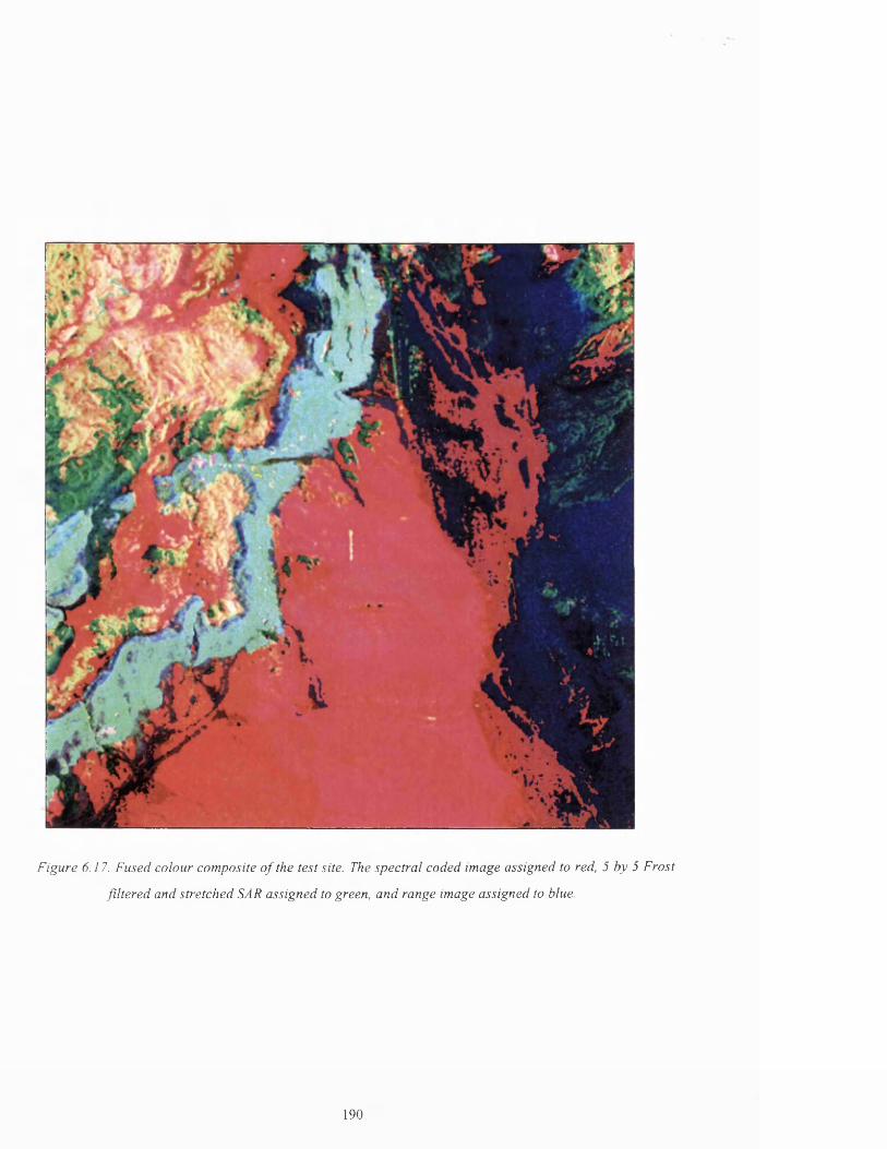
Figure 6 .17 . Fused colour com posite o f the test site. The spectral coded image assigned to red, 5 by 5 Frost

fd tered and stretched SAR assigned to green, and range image assigned to blue.

190

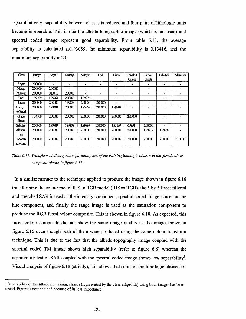
Quantitatively, separability between classes is reduced and four pairs of lithologic units

became inseparable. This is due the albedo-topographic image (which is not used) and

spectral coded image represent good separability. From table 6.11, the average

separability is calculated asl.93089, the minimum separability is 0.13416, and the

maximum separability is 2.0

Gass Juriayn Atiyah Musayr Nutaydi Bad’ Lisai Oonglo.+Gravd

GravdSheets

Sabkhah Alluvium

Atiyah 200000 - - - - - - - - -

Musayr 200000 200000 - - - - - - - -Nutaydi 200000 0.13416 200000 - - - - - - -

Bad’ 199109 1.99964 200000 199995 - - - - - -

Lisan 200000 200000 199883 200000 200000 - - - - -CongLa-Kjravd

200000 193494 200000 1.95365 200000 1.99999 - - - -

GravdSheets

134100 200000 200000 200000 200000 200000 200000 - - -

Sabkhah 200000 199987 199999 1.99999 200000 1.85167 0.99511 200000 - -

Afluvium

200000 200000 200000 200000 200000 200000 200000 1.99912 199999 “

Aeoliansilt+sand

200000 200000 200000 200000 200000 200000 200000 200000 200000 200000

Table 6.11. Transformed divergence separability test o f the training lithologic classes in the fused colour

composite shown in figure 6.17.

In a similar manner to the technique applied to produce the image shown in figure 6.16

transforming the colour model IHS to RGB model (IHS => RGB), the 5 by 5 Frost filtered

and stretched SAR is used as the intensity component, spectral coded image is used as the

hue component, and finally the range image is used as the saturation component to

produce the RGB fused colour composite. This is shown in figure 6.18. As expected, this

fused colour composite did not show the same image quality as the image shown in

figure 6.16 even though both of them were produced using the same colour transform

technique. This is due to the fact that the albedo-topography image coupled with the

spectral coded TM image shows high separability (refer to figure 6.6) whereas the

separability test of SAR coupled with the spectral coded image shows low separability3.

Visual analysis of figure 6.18 (strictly), still shows that some of the lithologic classes are

3 Separability o f the lithologic training classes (represented by the class ellipsoids) using both images has been tested. Figure is not included because o f its less importance.

191

well pronounced (spectrally and texturally) while others may be depicted either texturally

or spectrally, but not both. The classes that can be differentiated spectrally and texturally

are: Jurfayn; Bad’; Musayr; and Lisan. Classes that can be differentiated spectrally only

are: the Gravel sheets; Lisan; and Alluvium (the brown colour in the lower left part in the

image). Classes have similar spectral properties but can be differentiated texturally only

are: Jurfayn with conglomerate and gravel; and to some extent Nutaysh with Atiyah.

Quantitatively, the transformed divergence separability test applied on the lithologic

classes using this fused colour composite image is shown in table 6.12. Separability

values are reduced intensively making six pairs of classes inseparable. From the table, the

average separability is 1.92137, the minimum separability is 0.07992, and the maximum

separability is 2.0

Class Jurfayn Atiyah Musayr Nutaydi Bad’ Lisan CongJa+Gravd

GravdSheets

Sabkhah Alluvium

Atiyah 1.82197 - - - - - - - - -Musayr 200000 1.99864 - - - - - - - -Nutaydi 1.69222 0.07992 199732 - - - - - - -

Bad’ 200000 200000 200000 200000 - - - - - -Lisan 200000 199999 199908 200000 200000 - - - - -

CangLo.-Kjravd

1.96736 196643 199995 196483 200000 199869 - -

GravdSheets

129685 1.98652 200000 1.98431 200000 1.99999 1.99176 " - “

Sabkhah 200000 200000 1.99997 200000 200000 1.67661 129133 200000 - -AHuviu

m200000 200000 200000 200000 200000 200000 200000 200000 200000

AeoliansDt+sand

200000 200000 199997 200000 200000 200000 200000 200000 1.96158 200000

Table 6.12 Transformed divergence separability test results applied on the fused IHS =$ RGB colour

composite image using the TM spectral coded image as hue, the SAR image as intensity, and

the range image as saturation components.

192

:

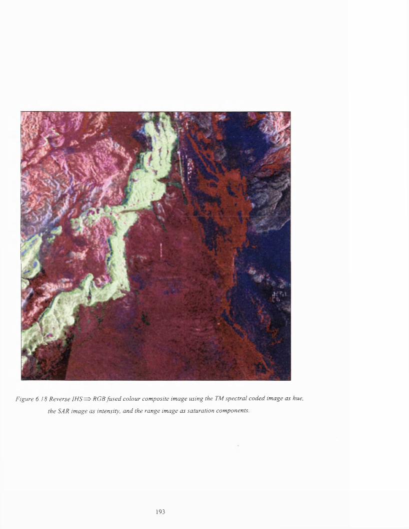
Figure 6.18 Reverse IHS = > RGB fused colour composite image using the TM spectral coded image as hue,

the SAR image as intensity, and the range image as saturation components.

193

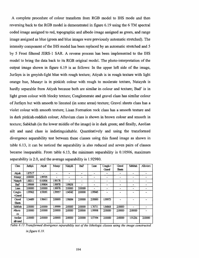
A complete procedure of colour transform from RGB model to IHS mode and then

reversing back to the RGB model is demonstrated in figure 6.19 using the 6 TM spectral

coded image assigned to red, topographic and albedo image assigned as green, and range

image assigned as blue (green and blue images were previously automatic stretched). The

intensity component of the IHS model has been replaced by an automatic stretched and 5

by 5 Frost filtered JERS-1 SAR. A reverse process has been implemented to the IHS

model to bring the data back to its RGB original model. The photo-interpretation of the

output image shown in figure 6.19 is as follows: In the upper left side of the image,

Jurfayn is in greyish-light blue with rough texture; Atiyah is in rough texture with light

orange hue, Musayr is in pinkish colour with rough to moderate texture, Nutaysh is

hardly separable from Atiyah because both are similar in colour and texture; Bad’ is in

light green colour with blocky texture; Conglomerate and gravel class has similar colour

of Jurfayn but with smooth to lineated (in some areas) texture; Gravel sheets class has a

violet colour with smooth texture; Lisan Formation rock class has a smooth texture and

in dark pinkish-reddish colour; Alluvium class is shown in brown colour and smooth in

texture; Sabkhah (in the lower middle of the image) is in dark green; and finally, Aeolian

silt and sand class is indistinguishable. Quantitatively and using the transformed

divergence separability test between these classes using this fused image as shown in

table 6.13, it can be noticed the separability is also reduced and seven pairs of classes

became inseparable. From table 6.13, the minimum separability is 0.10506, maximum

separability is 2.0, and the average separability is 1.92980.

Class Jurfayn Atiyah Musayr Nut di Bad’ lisan Gongk).+Gravd

GravdSheets

Sabkhah Alluvium

Atiyah 1.87517 - - - - - - - - -Musayr 200000 1.99705 - - - - - - - -Nutaydi 1.88311 0.10506 1.99178 - - - - - - -

Bad’ 1.99999 199804 1.99978 1.99838 - - - - - -Lisan 200000 200000 1.99978 200000 200000 - - - - -

CongLo.-Kjravd

199962 193091 1.99957 1.94542 200000 199945 “ " ■

GravdSheets

134489 1.98411 200000 1.98684 200000 200000 1.99973 - “

Sabkhah 200000 200000 1.99999 200000 200000 1.76711 1.84868 200000 - -Alluviu

m200000 200000 200000 200000 200000 1.99998 200000 200000 200000 *

Aeoliansik+sand

200000 200000 200000 200000 200000 137194 200000 200000 1.91236 200000

Table 6.13 Transformed divergence separability test o f the lithologic classes using the image constructed

in figure 6.19.

194

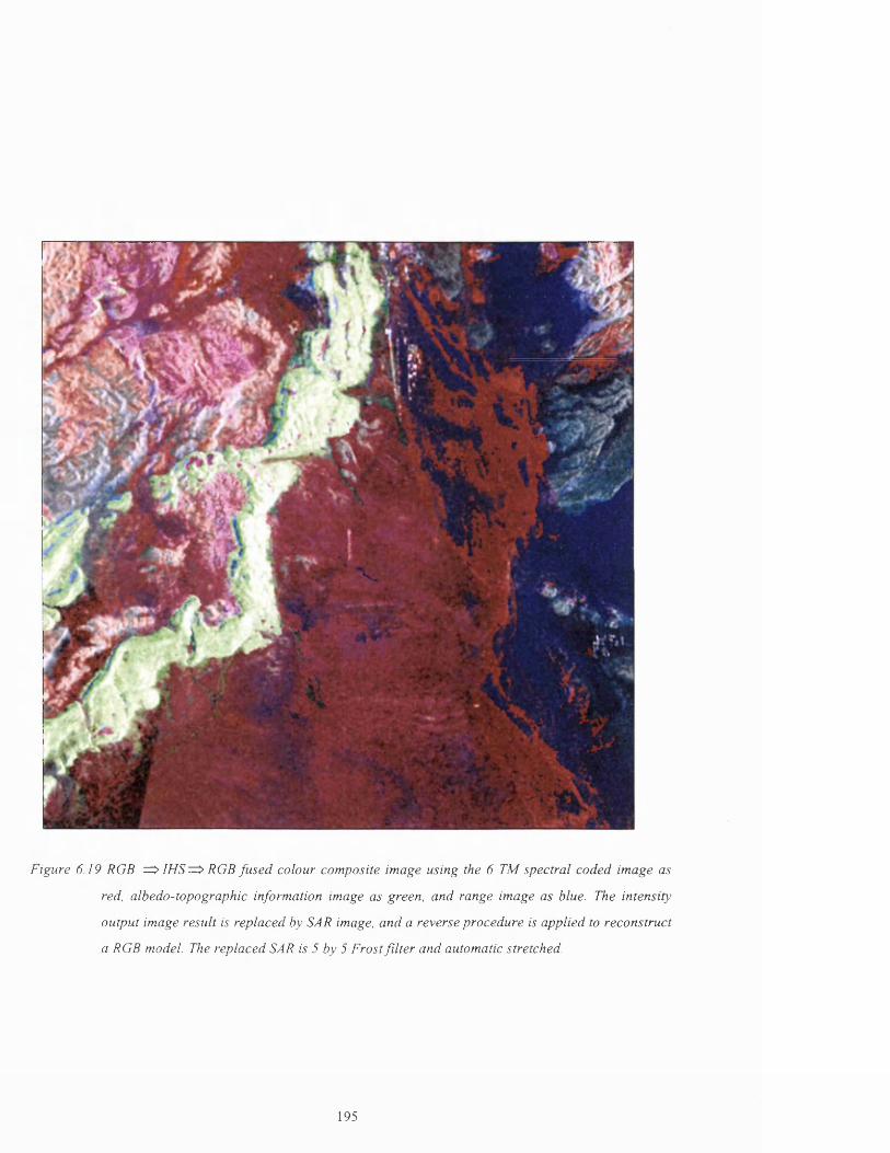
Figure 6.19 RGB = > IHS = > RGB fu sed colour com posite image using the 6 TM spectral coded image as

red. albedo-topographic information image as green, and range image as blue. The intensity

output image result is replaced by SAR image, and a reverse procedure is applied to reconstruct

a RGB model. The replaced SAR is 5 by 5 Frost f ilte r and automatic stretched.

195

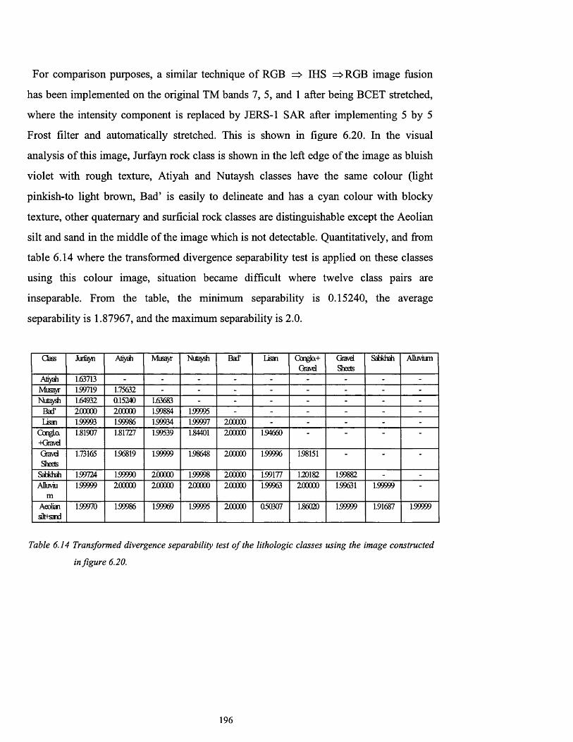
For comparison purposes, a similar technique of RGB => IHS =>RGB image fusion

has been implemented on the original TM bands 7, 5, and 1 after being BCET stretched,

where the intensity component is replaced by JERS-1 SAR after implementing 5 by 5

Frost filter and automatically stretched. This is shown in figure 6.20. In the visual

analysis of this image, Jurfayn rock class is shown in the left edge of the image as bluish

violet with rough texture, Atiyah and Nutaysh classes have the same colour (light

pinkish-to light brown, Bad’ is easily to delineate and has a cyan colour with blocky

texture, other quaternary and surficial rock classes are distinguishable except the Aeolian

silt and sand in the middle of the image which is not detectable. Quantitatively, and from

table 6.14 where the transformed divergence separability test is applied on these classes

using this colour image, situation became difficult where twelve class pairs are

inseparable. From the table, the minimum separability is 0.15240, the average

separability is 1.87967, and the maximum separability is 2.0.

Class Jurfayn Atiyah Musayr Nufaydi Bad’ Lisan Gongkx+Gravd

GravdSheets

S e b khdi Alluvium

Atiyah 1.63713 - - - - - - - - -Musayr 1.99719 1.75632 - - - - - - - -Nutaydr 1.64932 0.15240 1.63683 - - - - - - -

Bad’ 200000 200000 1.99884 199995 - - - - - -Lisan 1.99993 1.99986 1.99934 199997 200000 - - - - -

GongLo.-Kjravd

1.81907 1.81727 199539 1.84401 200000 194660 - - “

GravdSheets

1.73165 196819 199999 198648 200000 1.99996 1.98151 " -

Sabkhah 1.99724 199990 200000 1.99998 200000 1.99177 120182 1.99882 - -ADuviu

m1.99999 200000 200000 200000 200000 1.99963 200000 1.99631 1.99999

AeoliansOt+sand

1.99970 1.99986 199969 199995 200000 060307 1.86020 199999 1.91687 1.99999

Table 6.14 Transformed divergence separability test o f the lithologic classes using the image constructed

in figure 6.20.

196

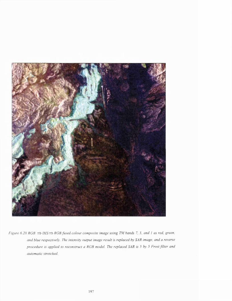
Figure 6.20 RGB = > IH S=> RGB fu sed colour com posite image using TM bands 7 , 5, and 1 as red, green,

and blue respectively. The intensity output image result is replaced by SAR image, and a reverse

procedure is applied to reconstruct a RGB model. The replaced SAR is 5 by 5 Frost f ilte r and

automatic stretched.

197

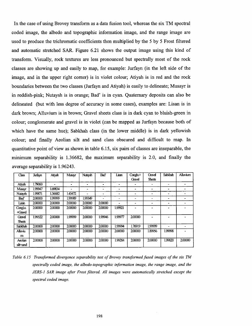
In the case of using Brovey transform as a data fusion tool, whereas the six TM spectral

coded image, the albedo and topographic information image, and the range image are

used to produce the trichromatic coefficients then multiplied by the 5 by 5 Frost filtered

and automatic stretched SAR. Figure 6.21 shows the output image using this kind of

transform. Visually, rock textures are less pronounced but spectrally most of the rock

classes are showing up and easily to map, for example: Jurfayn (in the left side of the

image, and in the upper right comer) is in violet colour; Atiyah is in red and the rock

boundaries between the two classes (Jurfayn and Atiyah) is easily to delineate; Musayr is

in reddish-pink; Nutaysh is in orange; Bad’ is in cyan. Quaternary deposits can also be

delineated (but with less degree of accuracy in some cases), examples are: Lisan is in

dark brown; Alluvium is in brown; Gravel sheets class is in dark cyan to bluish-green in

colour; conglomerate and gravel is in violet (can be mapped as Jurfayn because both of

which have the same hue); Sabkhah class (in the lower middle) is in dark yellowish

colour; and finally Aeolian silt and sand class obscured and difficult to map. In

quantitative point of view as shown in table 6.15, six pairs of classes are inseparable, the

minimum separability is 1.36682, the maximum separability is 2.0, and finally the

average separability is 1.96243.

Class Jurfayn Atiyah Musayr Nut di Bad’ Lisan Gonglo.+Gravd

GravdSheds

Sabkhah Alluvium

Atiyah 1.79060 - - - - - - - - -Musayr 1.99947 1.69834 - - - - - - - -Nutaysh 1.99871 136682 1.43472 - - - - - - -

Bad’ 200000 199999 1.99989 199349 - - - - - -Lisan 200000 200000 200000 200000 200000 - - - - -

CcngLo.+Gravd

200000 200000 200000 200000 200000 199921 “ ■ “

GravdSheds

199322 200000 1.99999 200000 1.99946 1.99977 200000 “ ■ “

Sabkhah 200000 200000 200000 200000 200000 1.99994 1.76919 199999 - -ADuviu

m200000 200000 200000 200000 200000 200000 200000 1.89956 1.99998 "

AeoliansOtfsand

200000 200000 200000 200000 200000 1.99284 200000 200000 1.99820 200000

Table 6.15 Transformed divergence separability test o f Brovey transformed fused images o f the six TM

spectrally coded image, the albedo-topographic information image, the range image, and the

JERS-1 SAR image after Frost filtered. All images were automatically stretched except the

spectral coded image.

198

Figure 6.21 Brovey transformed colour com posite image using the six TM spectral coded image, albedo and

topographic information image, the range image, and fina lly the JERS-1 SAR after being 5 by 5

Frost filtered. All images are automatically stretched (except the spectral coded image).

199

In comparison, the Brovey transform image fusion technique has been applied on the

original TM images of bands 7, 5, and 1 after being BCET stretched. The 5 by 5 Frost

filtered and automatically stretched SAR is used as the intensity component image. The

output results are shown in figure 6.22. Texturally, this image shows slightly better

results than figure 6.21. Conversely, and from the spectral point of view, figure 6.21

shows up better visual results especially when it comes to delineate the Quaternary

deposits. Quantitatively, as shown in table 6.16, seven class pairs are inseparable, the

minimum separability is 0.86249, average separability is 1.89369, and maximum

separability is 2.0

Gass Jurfayn Atiyah Musayr Nito/sh Bad’ Lisan Oonglo.+Gravd

GravdSheets

Sabkhah Alluvium

Atiyah 1.62175 - - - - - - - - -Musayr 1.99901 1.19963 - - - - - - - -Nutaydi 1.98054 0.86249 1.14596 - - - - - - -

Bad’ 1.99994 1.94933 159141 153461 - - - - - -Lisan 200000 200000 1.99974 200000 200000 - - - - -

CongLo.+Gravd

200000 200000 200000 1.99857 200000 1.73908 “ " - “

GravdSheets

1.95960 1.99809 200000 1.99942 200000 200000 1.99996 - -

Sabkhah 200000 200000 200000 200000 200000 1.99981 1.43981 200000 - -ADuviu

m200000 200000 200000 200000 200000 1.99992 1.99978 157543 200000

Aeoliansib+sand

200000 200000 200000 200000 200000 0.88820 152351 200000 1.94737 200000

Table 6.16 Transformed divergence separability test o f Brovey transformed images using bands 7, 5, 1,

and JERS-1 SAR.

2 0 0

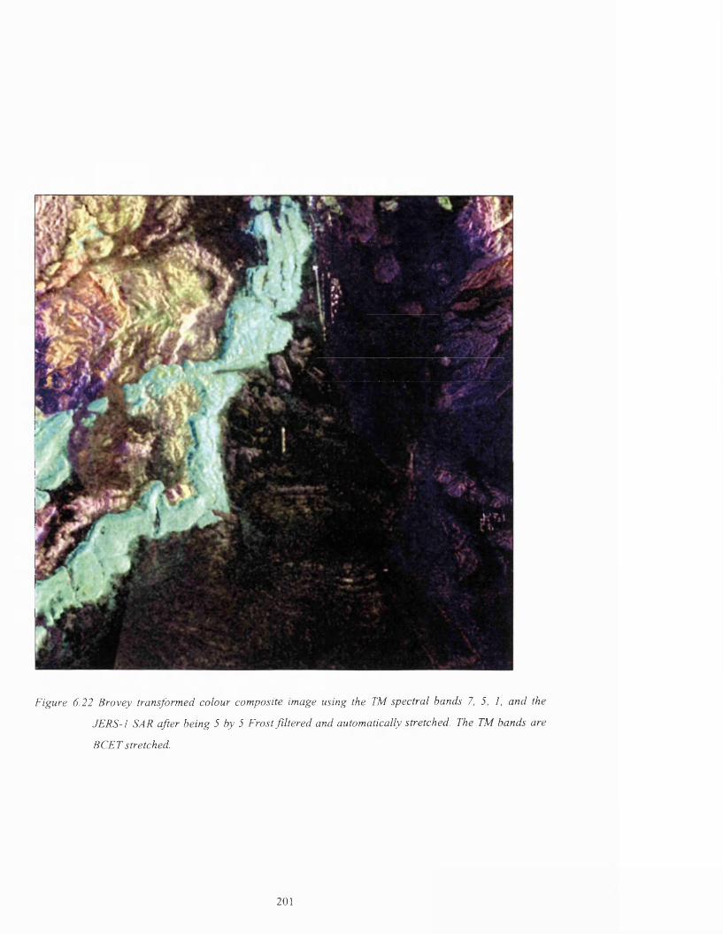
Figure 6.22 Brovey transformed colour com posite image using the TM spectral bands 7 , 5, 1, and the

JERS-l SAR after being 5 by 5 Frost filte red and automatically stretched. The TM bands are

BCET stretched.

201

6.9 D ata fusion using the principal com ponent transform

The principal component transform (PCT) is a well known technique used in statistics

as a multivariate analysis method used for highly correlated data [116]. The technique

uses the eigenvectors of the covariance matrix (or the correlation matrix if the PCT is

standardised to reduce the lower PCs noise) as multiplication factors to produce a new

uncorrelated data set. The mathematical derivation of the PCT is shown in appendix A-5.

The principal component transform in multispectral/multisensor image data fusion relies

on the dominant information in whole spectral bands (i.e. topographic and spatial

information) being gathered in the first principal component transformed image. This

characteristic means that the PCT is a valuable technique for separation of the spatial

from the spectral information. Its drawback is that it is scene dependent as a result of

using the covariance or correlation matrix, and hence two adjacent PC transformed

scenes cannot be mosaicked because these scenes will not be matched because of their

colour differences.

There are two ways to use the PCT technique to display the fused image data as a colour

composite image. One is neglecting the first principal component and using only the

second and the third principal components, replacing the first principal component by the

SAR image. The second is performing the PCT on the selected colour composite and

replacing the first PC with the SAR image and then reversing the SAR, the second and

the third PCs by the use of the transpose matrix of the eigenvectors of the original input

bands to achieve (to some extent) the original colour composite but with the insertion of

the SAR image.

The second method used for the PCT fusion has been used on the spectral coded colour

composite image with the insertion of the 5 by 5 Frost filtered SAR image. Figure 6.23

shows the reversed PCT of the spectral coded colour composite data set after replacing

the first principal component by the 5 by 5 Frost filtered SAR image. From figure 6.23,

2 0 2

to some extent, the texture of the rock classes is well presented as well as the spectral

information of many rock units. Conversely, some of the rock classes may be difficult to

differentiate, these include: Jurfayn; Atiyah; and Nutaysh. Other rock units are clearly

demonstrated, these include: Musayr (in magenta to light blue); Bad’; and the Quaternary

deposits which can be differentiated texturally rather than spectrally. Quantitatively,

separability test of this method of fusion is shown in table 6.17. From the table, seven

class pairs are inseparable, the average separability is 1.92666, the minimum separability

is 0.76478, and finally the maximum separability is 2.0.

Gass Jurfayn Atiyah Musayr Nutaydi Bad’ Lisan Gcngla-iGravel

GravelSheets

Sabkhah Alluvium

Atiyah 0.76478 - - - - - - - - -Musayr 200000 1.85017 - - - - - - - -Nulaydi 1.99534 129954 1.58817 - - - - - - -

Bad’ 200000 1.99999 153321 159137 - - - - - -Lisan 200000 200000 200000 200000 200000 - - - - -

GongLa-KJravd

200000 200000 159992 159985 1.99999 1.99688 " " ■

GravdSheets

159490 1.89767 1.99622 1.88799 200000 200000 159974 “ - "

Sabkhah 200000 200000 200000 200000 200000 200000 200000 200000 - -ADuviu

m200000 200000 200000 200000 200000 0.77459 1.99991 200000 200000

Aeoliansiltfsand

200000 200000 200000 200000 200000 1.99704 200000 200000 200000 1.99926

Table 6.17 Transformed divergence separability test o f the reversed principal component transform using

the input image data: the six TM spectral coded image; the albedo and topographic information

image; and the range image. The first principal component output is replace by 5 by 5 Frost and

automatic stretched image.

203

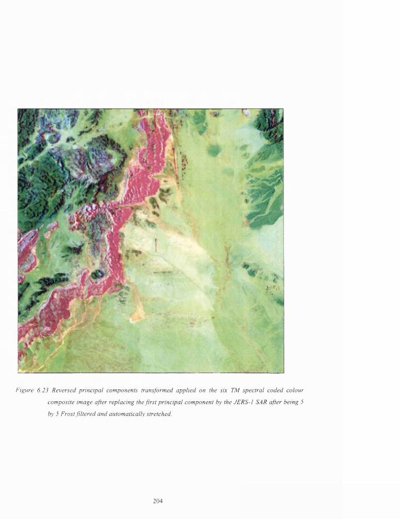
■*—T---------r

Figure 6.23 Reversed principal components transformed applied on the six TM spectral coded colour

com posite image after replacing the first principal component by the JERS-1 SAR after being 5

by 5 Frost filte red and automatically stretched.

204

In figure 6.24 for comparison purposes, and using the same technique but using the

original TM bands 7, 5, and 1 after being BCET stretched. The output image may shows

better representation of the rock classes (spectrally and texturally), an example is the

Jurfayn rock unit which became more distinguishable comparing with figure 6.23, other

rock classes also clear and easily to map as well as in figure 6.23. Quantitatively and

from table 6.18, there are eight pairs of classes still inseparable (comparing with seven

pairs in table 6.17), the minimum separability is 0.50371, the average separability is

1.89907, and the maximum separability is 2.0.

Gass Jurfayn Atiyah Muss/r Nutaydi Bad’ Lisan Congb.+Gravd

GravdSheets

Sabkhah Alluvium

Atiyah 1.76207 - - - - - - - - -Musayr 159882 120285 - - - - - - - -Nutaydi 1.81987 050371 153904 - - - - - - -

Bad’ 159890 155643 159609 159163 - - - - - -Lisan 200000 159984 1.99940 159996 200000 - - - - -

CangLo.-K3ravd

1.99726 158081 159831 155805 200000 1.95095 " -

GravelSheets

1.96181 158617 1.99908 1.97773 200000 1.99813 154308 “ ■ “

Sabkhah 200000 200000 200000 200000 200000 159166 157666 1.99663 -AHuviu

m200000 200000 200000 200000 200000 1.99971 200000 200000 1.99990

Aeoliansiltfsand

200000 1.99974 1.99979 1.99987 200000 056898 1.84031 1.98850 1.96700 1.99992

Table 6.18 Transformed divergence separability test o f the reversed principal component transform using

the input image data ofTM bands 7, 5, and 1. The first principal component output is replace by

5 by 5 Frost filtered and automatic stretched image.

205

Figure 6.24 Reversed principal components transformed colour composite image using the TM spectral

bands 7 , 5, 1, and replacing the firs t principal component by the JERS-1 SAR after being 5 by 5

Frost filte red and automatically stretched.

206

As a result of producing the colour composites, the spectral coded colour composite, the

fused colour composites, a visual analysis of these images supported by previous field

visit, a new proposed lithologic map of the test site is given in figure 6.25 noting that

most of the rock units are delineated using the six TM spectral coded colour composite,

the reversed IHS => RGB TM spectral coded colour composite, and the fused image data

with SAR. The displayed colour composites were also taken into account during the

construction of the lithologic map.


From the images and the separability test tables shown throughout this chapter, it is

possible to come up with the following conclusions and hints:-

1- Visual recognition of classes and separabilities between pair of classes vary from one

colour composite combination to another, but some classes become well separable

(visually and quantitatively) with low colour combination ranks using the statistical

methods of colour composite selection. The best example is the colour combination of

TM bands 4, 3, and 2 (the lowest ranking) gives very good results visually and

quantitatively in separation between the class pair Atiyah-Nutaysh with separability of

1.79328 (table 6.6). This number could not be gained even using all TM data when

tested for separability.

2- The best colour composite band combination shown was the TM bands 7, 5, and 1. In

this combination there are two pairs of classes are inseparable. This leads to the idea

of not using colour composites for automated mapping (classification), unless all pairs

of classes are perfectly separable.

3- The use of all the spectral image data (all 6 TM bands) does not necessary increase

classes separability. An example is band combination 4, 3, and 2 for class pair Atiyah-

Nutaysh and the same class pair using all TM data (table 6.3).

4- The new method of the six TM spectral colour coding technique shows a good way of

producing colour composites. No colour composite bands combination can show good

207

separability as the new method of producing spectral colour coded composite. For

comparison, the colour composite of combination 4, 3, and 2 shows seven pair of

classes are inseparable, the colour composite 5, 3, and 1 shows three pair of classes

inseparable, even the best colour composite combination using bands 7, 5, and 1 gives

two pair of classes inseparable. In the case of the new method of spectral colour coded

composite, it shows only one pair of classes is inseparable but this is due to the nature

of this pair of classes (inseparable using all bands or using any combination, but may

vary from combination to combination).

5- Colour transform, and PCT technique for data fusion reduce (quantitatively) the

separability between classes, this is due to increasing the class dispersion (standard

deviation) during the transformation process.

6- Quantitatively, the fused spectral coded colour composite with SAR image data shows

better separabilities (less inseparable class pairs) compared with the fused colour

composite of bands 7, 5, and 1 when fused with SAR.

7- All fused colour composite should not be used as input for automated mapping

(classification).

8- The spectral coding method for producing colour composite is new and sound

approach for colour composite production. It is a simple and fast procedure, but its

limitation is of very little loss of class pairs separability which means it is not an error

free method.

208

L egend

6

5

4

3

2

1

/ .7 .',A A

A A

» &=°•TsI51

■+- +*

Lisan

Bad* 11

Nutaysh 10

Musayr 9

Atiyah 8

Jurfayn 7

o © ©

Aeolian silt and sand

SabkhahConglomerate and gravel

Gravel sheets

Alluvium

Figure 6.25 An interpretation lithologic map o f the test site.

Scale 1:204084

209

7.0 Image data fusion for automated mapping

The motivation of image data fusion for multisensor imaging systems is for visual

optimisation and automated mapping with accurate classification. For visual

optimisation, the goal is to generate an interpretation of the scene not obtainable with

data from a single imaging sensor, investigated in chapter 6. For automated mapping

(classification), the goal is to reduce uncertainty associated with the data from individual

sensors, and hence reduce the classification error rate.

The scheme of image data fusion as an aid to accurate classification in this thesis

involves many steps. Firstly and by the use of all image data from both sensors (6 TM

image bands and 7 GLCM texture measures, the 6 TM spectral bands, and the 7 GLCM

texture measures), the transformed divergence separability test results were assessed to

obtain general idea of the accuracy of the results. The second step is the use of the

classifier with the use of new approach of selecting the classified pixels based on the

sequential maximum likelihood classification. Traditional post-classification smoothing

procedures for the classified pixels during classification were also used. All of these steps

will be discussed in the appropriate sections and the previous work in image data fusion

for classification is also given in this chapter.

7.1 The maximum likelihood classifier

Image classification refers to the automatic labelling of every image pixel to a specific

thematic group, based on the comparison of the pixel signature to specific statistical

characteristics (classes). The result is a thematic map showing all types and geographic

location and distribution of these classes. Important steps have to be carefully followed in

the remote sensing image classification procedures, including the appropriate

classification scheme or level of details, the selection of training areas and their sizes, the

proper manipulation for the input spectral and spatial input images and test of classes

separability, the selection of the classification algorithm and the post classification

filtering and finally the classification accuracy assessment [18].

2 1 0

The labelling process in image classification can be achieved using two methods, one

where the information classes are selected by the user and their statistics are determined,

called supervised classification. The second method is that the computer itself determines

clusters or groups of pixels having distinguishable and common statistical characteristics,

and this method is called unsupervised classification. Unsupervised classification is

usually used when there is no information about the classes in the studied images and it is

usually not preferable because the classes created are thematically unknown and variable.

Many clustering algorithms are used in unsupervised classification, including the

ISODATA algorithm which is based on the split and merge in the iteration procedures.

Other algorithms include the clusters means such the k-means clustering algorithm, and

finally an algorithm called the Narendra-Goldberg clustering algorithm which uses the

peaks and valleys of the multidimensional histogram created from the «-bands used

[142].

Within supervised classifiers, three types are well known. These are the minimum

distance to the mean, the parallelepiped classifier and the maximum likelihood classifier.

The minimum distance to mean classifier (sometimes termed the centroid classifier)

assigns each pixel to the closest class mean. Its drawback is that it does not take into

account the classes variability, which causes a dispersion in the class cluster. The second

(parallelepiped) classifier uses the class dispersion (the standard deviation) and the mean

of the class cluster. It gives better results than the minimum-distance-to-mean but its

problem comes when the dispersion of the classes clusters are overlapped and in this case

the labelled pixels which exist in these overlapped areas will be uncertainly classified.

The third classifier is the maximum likelihood decision rule classifier which uses the

mean, the dispersion and the correlation between classes clusters. The maximum

likelihood classifier (MLC) is the most appropriate and accurate labelling algorithm used

in image classification [18,41,142].

The maximum likelihood classification may use a discriminant function rule such as

the Mahalanobis distance, as shown in equation (7.9), which is applied in this thesis. The

process of the MLC is classifying the entry pixel vector X to the class C if and only if:-

2 1 1

Pc > Pt where i = 1, 2, 3, 4 , C possible classes.

Pc = - 0 . s \ x - t i ] T[Cov] ' 1[ x - f t ] - f e o g 2 * } - ( a 5 1 o g |0 , |) (7.9)

where:

Ht = vector mean of the class i.

Covi = covariance matrix of the class i.

n = number of image channels used.

= determinant of the covariance Covi .

For example, to classify the unknown pixel vector X into a class, the MLC decision

rule computes the values Pc for each class previously defined, and then assigns the pixel

vector X to the class that has largest value to that class.

The a priori information (i.e. a weighting represents the probability associated with

each class) can be included in the MLC discriminant function by the user for each class

to bias some classes over the others. It can be included in the equation (7.9) as +log(Pr/)

where

WtPr,. = —----- , W is a weighting number introduced for every class i .

«=i

7.2 The post classification filtering

The classified image is usually contaminated by single pixels or very small groups of

pixels that are classified to a class that is surrounded by a larger class. These pixels are

called island themes [41] and are usually a classification error which may result from

contaminated spectral signatures, imaging system errors, shadowing, or the

misregistration between the bands used. Many techniques can be used to filter these

2 1 2

errors out. The well known filters used are the mode filter and the sieve filter. The mode

filter replaces the pixel’s brightness value by its most frequent occurring value (i.e. its

surrounding) within a specified window. The sieve filter is more sophisticated for

removing the island themes, by merging the small group of pixels by their largest ones

and preserve edges in the same time. Both these filters have been tested, and it was found

that the sieve filter is most adequate because it preserves the linear or the small elongated

theme classes.

7.3 Previous work in classification

Several methods have been used in the past to classify multisource data. The following

shows some of this work.

Kaufman and Pfeiffer [120] compared image optimisation versus classification

procedures using two different test sites. One is the south of Saudi Arabia, and the second

is the Rhine-Graben area in Germany. They found that for applications where structural

information is the goal (i.e. geology), the optimised image products are preferred because

relief information is preserved. Classification is superior if the goal is identifying surface

signatures over wide areas.

Mettemicht [121] discussed the problem of how to deal with insufficient discrimination

among classes using fused SPOT XS and ERS-1 SAR image data in the Flevoland area

of the Netherlands. A combination of supervised and unsupervised (clustering) is used for

training area selection to form a hybrid strategy for maximum likelihood classification.

He claimed that the training areas selection is a very important part in classification and

any inadequate method used in training class selection could led to an erroneous class

determination.

A new statistical classification approach based on the Bayesian method of multi-source

image data fusion, taking into account the temporal changes during the image acquisition

has been proposed by Solberg et. a l [122]. The performance of this approach showed

213

significant improvements in the error rate by testing it using Landsat TM and ERS-1

SAR for land-use classification over an area of Kjeller, Norway.

Munechika et. al. [104] used a simple mathematical combination method (termed the

ratio method) between Landsat TM and SPOT XS and Panchromatic image data. This

method was used to improve the radiometric image integrity. Results show visually

improved images and improvement in classification accuracy of 6% using a maximum

likelihood classifier. Images from Rochester, New York were used in the study.

Revision of combination techniques of satellite images and ancillary data to improve

classification has been illustrated by Hutchinson [75]. These techniques include:

preclassification scene stratification, classification modification (i.e. modifying prior

probabilities) and postclassification class sorting. He found that the stratification method

is deterministic and cannot accommodate gradations between strata (areas), and because

this method of combination is performed before classification, incorrect classification can

invalidate the entire classification. The modified priors combination used during the

classification needs intensive sampling, which is somewhat beyond that which is

conducted in normal spectral classification. The postclassification sorting is a new

technique and is used in geographic information systems. As suggested, it is conceptually

simple and easily implemented but it is also deterministic. However, it offers some

advantages in that it only deals with only problem classes, and errors resulting from the

sorting role can be corrected easily.

Lozano-Garcia et. a l [123] studied the effects of combining SAR with optical data,

investigating if there are any improvements in the classification results using combined

SIR-B SAR with different viewing angles, and Landsat TM data mapping the forest

cover east of the Lake City, Florida. Firstly, they found in the preliminary results that the

performance of per-pixel classifier algorithms will not be satisfactory if speckle is not

removed from the SAR data, hence a median filter with two iterations was applied to the

SAR data. In the training process, two methods were used for TM, and combined TM and

SAR. For the TM data alone, clustering was used to develop training statistics. In the

214

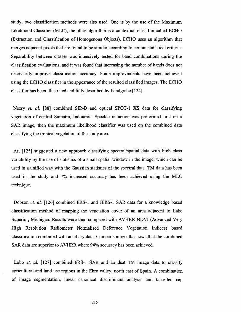
study, two classification methods were also used. One is by the use of the Maximum

Likelihood Classifier (MLC), the other algorithm is a contextual classifier called ECHO

(Extraction and Classification of Homogenous Objects). ECHO uses an algorithm that

merges adjacent pixels that are found to be similar according to certain statistical criteria.

Separability between classes was intensively tested for band combinations during the

classification evaluations, and it was found that increasing the number of bands does not

necessarily improve classification accuracy. Some improvements have been achieved

using the ECHO classifier in the appearance of the resulted classified images. The ECHO

classifier has been illustrated and fully described by Landgrebe [124].

Nezry et. al. [88] combined SIR-B and optical SPOT-1 XS data for classifying

vegetation of central Sumatra, Indonesia. Speckle reduction was performed first on a

SAR image, then the maximum likelihood classifier was used on the combined data

classifying the tropical vegetation of the study area.

Ari [125] suggested a new approach classifying spectral/spatial data with high class

variability by the use of statistics of a small spatial window in the image, which can be

used in a unified way with the Gaussian statistics of the spectral data. TM data has been

used in the study and 7% increased accuracy has been achieved using the MLC

technique.

Dobson et. al. [126] combined ERS-1 and JERS-1 SAR data for a knowledge based

classification method of mapping the vegetation cover of an area adjacent to Lake

Superior, Michigan. Results were then compared with AVHRR NDVI (Advanced Very

High Resolution Radiometer Normalised Deference Vegetation Indices) based

classification combined with ancillary data. Comparison results shows that the combined

SAR data are superior to AVHRR where 94% accuracy has been achieved.

Lobo et. al. [127] combined ERS-1 SAR and Landsat TM image data to classify

agricultural and land use regions in the Ebro valley, north east of Spain. A combination

of image segmentation, linear canonical discriminant analysis and tasselled cap

215

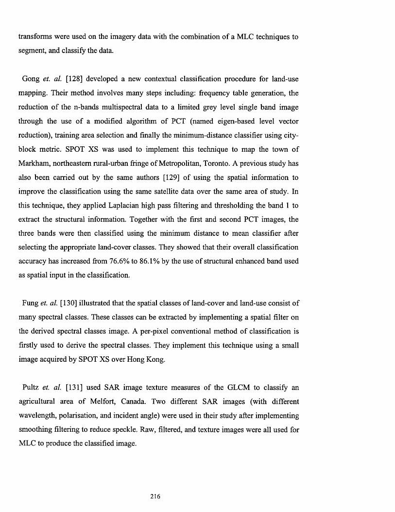
transforms were used on the imagery data with the combination of a MLC techniques to

segment, and classify the data.

Gong et. al. [128] developed a new contextual classification procedure for land-use

mapping. Their method involves many steps including: frequency table generation, the

reduction of the n-bands multispectral data to a limited grey level single band image

through the use of a modified algorithm of PCT (named eigen-based level vector

reduction), training area selection and finally the minimum-distance classifier using city-

block metric. SPOT XS was used to implement this technique to map the town of

Markham, northeastern rural-urban fringe of Metropolitan, Toronto. A previous study has

also been carried out by the same authors [129] of using the spatial information to

improve the classification using the same satellite data over the same area of study. In

this technique, they applied Laplacian high pass filtering and thresholding the band 1 to

extract the structural information. Together with the first and second PCT images, the

three bands were then classified using the minimum distance to mean classifier after

selecting the appropriate land-cover classes. They showed that their overall classification

accuracy has increased from 76.6% to 86.1% by the use of structural enhanced band used

as spatial input in the classification.

Fung et. al. [130] illustrated that the spatial classes of land-cover and land-use consist of

many spectral classes. These classes can be extracted by implementing a spatial filter on

the derived spectral classes image. A per-pixel conventional method of classification is

firstly used to derive the spectral classes. They implement this technique using a small

image acquired by SPOT XS over Hong Kong.

Pultz et. al. [131] used SAR image texture measures of the GLCM to classify an

agricultural area of Melfort, Canada. Two different SAR images (with different

wavelength, polarisation, and incident angle) were used in their study after implementing

smoothing filtering to reduce speckle. Raw, filtered, and texture images were all used for

MLC to produce the classified image.

216

Benediktsson e t a l [132] added one step ahead in multisource classification by

comparing statistical classification methods with neural network methods. They modified

the statistical Bayesian classification algorithm by adding the concept of reliability

weightings based on the separability of the features. They finally compared the statistical

measures including the minimum-distance to mean, MLC and the modified Bayesian

classifier with the neural network classifier using the delta rule and generalised delta rule

algorithms. Comparisons have been made on MSS image data, elevation data, and slope

and aspect data over a mountainous small area in Colorado. The results of their work

showed that neural network method employing the generalised delta rule has a great

potential as a pattern recognition method for multisource remote sensing data, but its

drawback is complexity in computation and its learning time which can be long if a large

amount of data is used. The modified Bayesian statistical method works well for

combining multisource data and gave significant improvement in the overall

classification accuracy.

A complex mountainous environment classification has been undertaken using three

stages of operation as proposed by Franklin et a l [133-134]. These stages include

quadtree segmentation where the image is subdivided into four equal quads successively,

then each quad is tested for homogeneity after the successive partitioning. If the quad

passes the test, the entire quad is then classified. If the quad fails, further partitioning is

made, and so on until the one pixel level is reached. The homogeneity test uses the

coefficient of variation and range statistics. The second stage of classification is the

minimum-distance-to-mean classifier. In this stage, pixels that have not been segmented

in the first stage may be handled by the second step using the per-pixel classifier. In stage

three of the classification process, where some pixels may not be correctly identified in

prior stages, a new test including ancillary information or by examining their spectral

curves or classify them as borders if they exist between two classes. They tested their

approach using a mountainous area south of Yukon, Canada, using SPOT XS and DEM

data.

217

The knowledge based expert system is currently one of the new trends for image

classification using combined spectral and spatial information. Johnsson [135] showed a

good example of such a technique using SPOT image data for land-use classification.

The steps within such a technique are rather long, involving spectral classification,

determination of size and neighbour relations for the segments in the spectrally classified

image, and rule-based classification of the image segments into land-use categories. In

the rule-based classification phase, the image segments are treated as objects with a set of

properties. Such a technique involves a conversion from a raster format to a list of objects

and vice versa.

Usually, non-classified pixels which show salt and pepper appearance of the classified

images are removed using modal spatial filtering technique. Wang et. al. [136] used a

new filtering technique as post processing on the classified image to remove such

unclassified pixels and small polygons, and at the same time preserving class edges,

comers, and small linear classes. They used a convolution filter of size one pixel inside a

larger window frame (i.e. 3 by 3, 4 by 4, etc.) which process unclassified pixels based on

their surrounding classes. Many iterations can be implemented on the classified scene.

They demonstrated their technique using airborne C-band multipolarisation data acquired

over agricultural area south of Ontario, Canada. Classification has been carried out using

the MLC algorithm.

Wang et. al. [137] proposed a new error assessment methodology in classification

accuracy which resulted from the uncertainties in training areas by the use of many

training trails and calculating the RMSE (Root Mean Square Error) pixels. Accuracy is

then converted to percentage by dividing the RMSE pixels by the entire image pixels.

Image classification accuracy assessment and factors controlling the accuracy has been

reviewed in detail by Congalton [138]. He reported that as recently as the early 1980s

many classification studies only report a single number to express the accuracy of

classification as an overall accuracy. Such a number is misleading because it does not

show accuracy within every class or category. He recommends the use of the error matrix

218

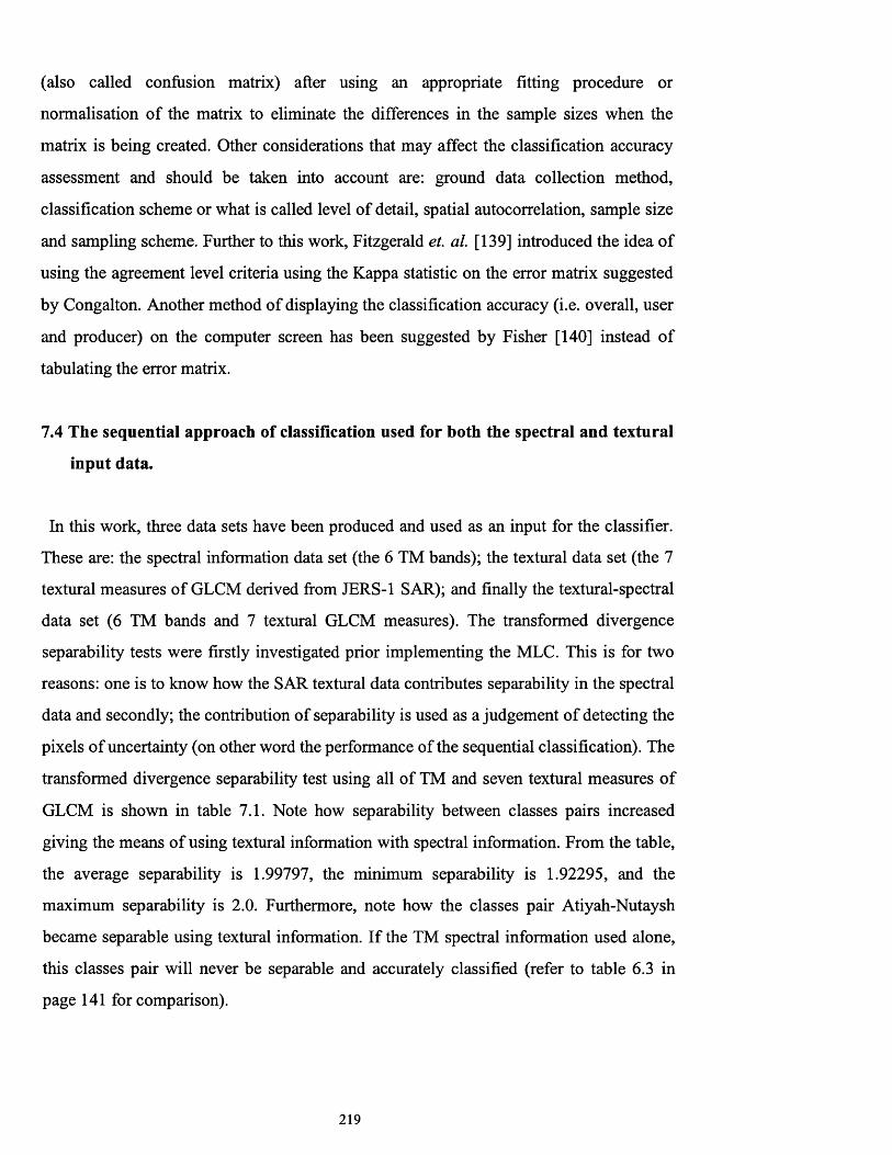
(also called confusion matrix) after using an appropriate fitting procedure or

normalisation of the matrix to eliminate the differences in the sample sizes when the

matrix is being created. Other considerations that may affect the classification accuracy

assessment and should be taken into account are: ground data collection method,

classification scheme or what is called level of detail, spatial autocorrelation, sample size

and sampling scheme. Further to this work, Fitzgerald et. a l [139] introduced the idea of

using the agreement level criteria using the Kappa statistic on the error matrix suggested

by Congalton. Another method of displaying the classification accuracy (i.e. overall, user

and producer) on the computer screen has been suggested by Fisher [140] instead of

tabulating the error matrix.

7.4 The sequential approach of classification used for both the spectral and textural

input data.

In this work, three data sets have been produced and used as an input for the classifier.

These are: the spectral information data set (the 6 TM bands); the textural data set (the 7

textural measures of GLCM derived from JERS-1 SAR); and finally the textural-spectral

data set (6 TM bands and 7 textural GLCM measures). The transformed divergence

separability tests were firstly investigated prior implementing the MLC. This is for two

reasons: one is to know how the SAR textural data contributes separability in the spectral

data and secondly; the contribution of separability is used as a judgement of detecting the

pixels of uncertainty (on other word the performance of the sequential classification). The

transformed divergence separability test using all of TM and seven textural measures of

GLCM is shown in table 7.1. Note how separability between classes pairs increased

giving the means of using textural information with spectral information. From the table,

the average separability is 1.99797, the minimum separability is 1.92295, and the

maximum separability is 2.0. Furthermore, note how the classes pair Atiyah-Nutaysh

became separable using textural information. If the TM spectral information used alone,

this classes pair will never be separable and accurately classified (refer to table 6.3 in

page 141 for comparison).

219

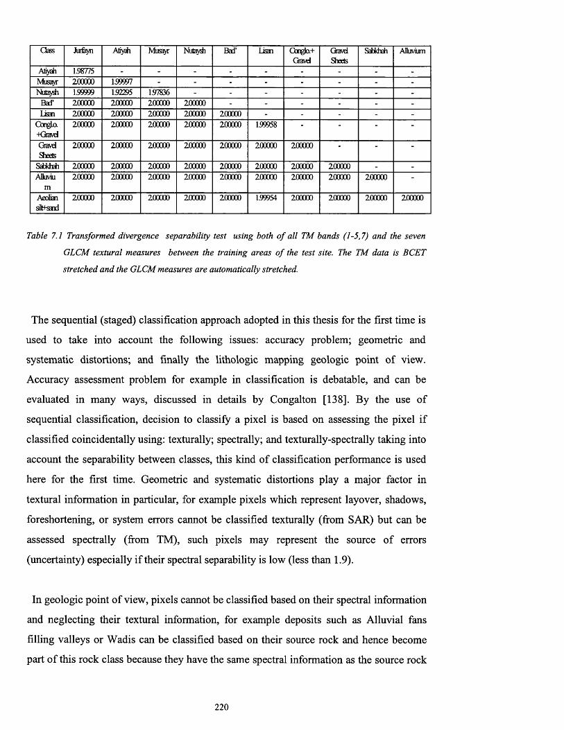
Gass Jurfayn Atiyah Mus r Nutaydi Bad’ Usan Oonglo.+Gravd

GravdSheets

Sabkhah Alluvium

Atiyah 158775 - - - - - - - - -

Musayr 200000 1.99997 - - - - - - - -Nutaysh 1.99999 152295 157836 - - - - - - -

Bad’ 200000 200000 200000 200000 - - - - - -Usan 200000 200000 200000 200000 200000 - - - - -

GongLo.+Gravd

200000 200000 200000 200000 200000 159958 - - - -

GravdSheets

200000 200000 200000 200000 200000 200000 200000 - - -

Sabkhah 200000 200000 200000 200000 200000 200000 200000 200000 - -

ADuvium

200000 200000 200000 200000 200000 200000 200000 200000 200000 -

Aeoliansit+sand

200000 200000 200000 200000 200000 159954 200000 200000 200000 200000

Table 7.1 Transformed divergence separability test using both o f all TM bands (1-5,7) and the seven

GLCM textural measures between the training areas o f the test site. The TM data is BCET

stretched and the GLCM measures are automatically stretched.

The sequential (staged) classification approach adopted in this thesis for the first time is

used to take into account the following issues: accuracy problem; geometric and

systematic distortions; and finally the lithologic mapping geologic point of view.

Accuracy assessment problem for example in classification is debatable, and can be

evaluated in many ways, discussed in details by Congalton [138]. By the use of

sequential classification, decision to classify a pixel is based on assessing the pixel if

classified coincidentally using: texturally; spectrally; and texturally-spectrally taking into

account the separability between classes, this kind of classification performance is used

here for the first time. Geometric and systematic distortions play a major factor in

textural information in particular, for example pixels which represent layover, shadows,

foreshortening, or system errors cannot be classified texturally (from SAR) but can be

assessed spectrally (from TM), such pixels may represent the source of errors

(uncertainty) especially if their spectral separability is low (less than 1.9).

In geologic point of view, pixels cannot be classified based on their spectral information

and neglecting their textural information, for example deposits such as Alluvial fans

filling valleys or Wadis can be classified based on their source rock and hence become

part of this rock class because they have the same spectral information as the source rock

2 2 0

class. By the use of the sequential classification, such pixels should be assessed spectrally

(alone) and texturally (alone) and if they are classified to a particular class in both

assessments, then it is believed that these pixels belong to this particular class, if not,

other assessment is carried out using textural-spectral information against spectral

information. If the assessment does not coincide, these pixels are either preferred to left

unclassified (zero filled) or filled by the textural-spectral classified image with high

degree of certainty (based on table 7.1) but not sure to be classified correctly.

The sequential classification approach used in this thesis is a logical decision making

using the MLC. It works as follows: In stage zero, classify the image based on its spectral

information (layer-1); classify the image based on its textural information (layer-2) and

finally; classify the image based on its spectral-textural combined information (layer-3).

If the pixel for example is classified texturally-spectrally (layer-3) which has high

separability as shown in table 7.1 to a specific class and found spectrally (alone) still to

belong to the same class (less separability as shown in table 6.3) then, this pixel is

believed to belong to this particular class and should be classified to this class

(coincidence of texture-spectral combined information with spectral information alone).

All pixels in the image will first pass this test and the classified pixels will be stored

(layer-4). In the second stage or sequence, only pixels which did not meet this criteria

will go to the second test or stage which is if these pixels are classified texturally alone

(low in separability as shown in table 5.1) but coincide with spectral classification (layer-

1) which gives high separability, then these pixels will be classified to their particular

classes. Pixels which do not coincide to this criteria will be left to zero-fill. In the third

stage of test, pixels which are not classified in the earlier stages will be left unclassified

(because not relying on textural information alone (low separability), spectral information

alone (higher separability but not taking into account the geological point of view). The

only choice will be classified based on the textural-spectral information (very good

separability which came originally from the spectral information). Such pixels may be

taken as “not sure but may be truly classified” and can be used (strictly) as the source of

errors and statically calculated for data fusion classification performance. A schematic

diagram of this sequential classification is shown in figure 7.1.

22 1

Spectral data set Textural-spectral data set

Textural data set

Stage 0

Classify(textural-spectral)

Layer-3

Classify(Spectral)

Layer-2

Classify (Textural) Layer-1

Sievefilter

Sievefilter

Sievefilter

StatisticsLayer-3=Layer-2Stage 1

Layer-4Stage 2

No

Layer-5

Layer-1 =Layer-2Statistics

Stage 3 NoFill with layer-3 Unclassified

Statistics

Figure 7.1 Flow diagram shows the MLC sequential classification scheme used to lithologically

classify the test site.

It is important to note that the use of sequential classification is an attempt to benefit

from the correctly classified pixels from textural-spectral data set which could be biased

texturally either negatively or positively and make this bias only positively through the

information of the spectral data set. If the pixels are found to be biased negatively, other

information is used for compensation, this information is the coincidence of texture

2 2 2

information with spectral information data sets and replace these negatively biased

pixels. If these pixels are still biased, there is no more information about them and either

left unclassified or replaced by their original source. This method is not attempt of

preference texture over spectral information or even textural-spectral information, it is

only how to benefit from the two sensors represented by the three data sets in a

constructive way.

7.5 Classification results

Running the sequential classification using MLC produces three types of data; the

primary classified images (stage zero), the classified pixels of stage one and two

represented by partially classified image; and the statistical calculations for each stage

which include the number of classified pixels for each class, and the number of pixels not

classified (i.e. no. of biased pixels). After stage 2 and in the final stage, two classified

images are produced, one is the classified image produced in stage two combined with

stage 1 but filling the unclassified pixels in this stage by the classified pixels produced in

stage zero from the textural-spectral data set. The second classified image in this stage is

the combined classified images in stage 1 and stage 2 with zero-fills of the negatively

biased pixels

From stage zero, figure 7.2 represents the classified image based on the seven GCLM

textural measures produced previously in chapter 5. As a result of low separability

between many classes pairs, the classified image is poor but it is believed that there are

many pixels are classified correctly. This is shown in figure 7.7 when the texturally

classified pixels coincide with the spectrally classified pixels. Figure 7.3 shows the

classified image using six TM optical spectral data only, and figure 7.4 shows the

classified image using the combined information of spectral and textural data (7 GLCM

textural measures and 6 TM spectral). Statistics of each classification are collected,

combined and given in table 7.2.

223

lithologic class

name

Number ofPixels

(Textural C.)

Number ofPixels

(Spectral G)

Number ofPixels

(Textural-spectral Q

Jurfayn 80482 27906 21425

Atiyah 38835 63414 70690

Musayr 114545 78207 71226

Nutaysh 67475 83461 71336

Bad’ 54465 183077 175582

Lisan 72780 170073 172830

Cong.+Gravel 109490 117810 132058

Gravel sheets 121634 53450 58560

Sabkhah 101359 1594 1477

Alluvium 204985 215658 213126

Aeolian silt+sand 82526 53926 60266

i 1048576 1048576 1048576

Table 7.2 Statistics o f stage zero classification results using the seven GLCM textural measures alone, the

six TM optical data alone, and the combined textural-spectral data.

224

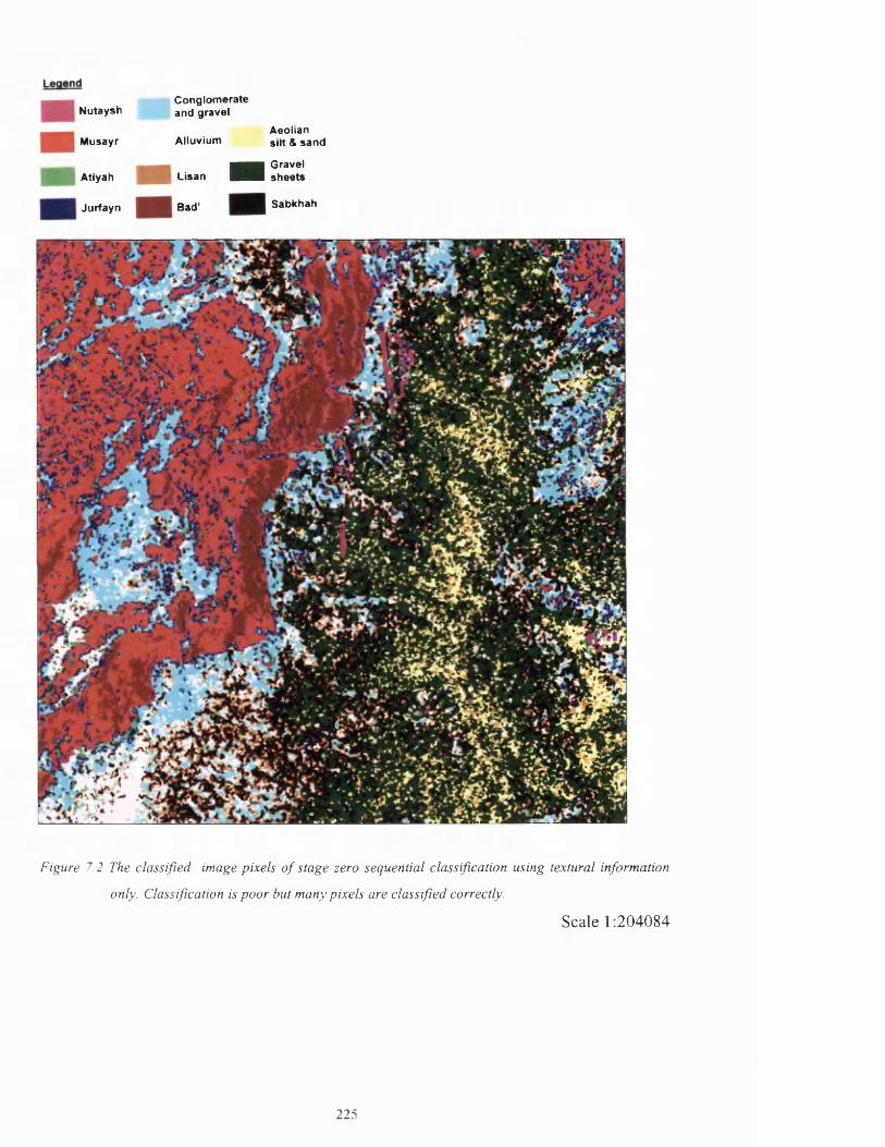
Nutaysh

Musayr

Atiyah

Jurfayn

Conglom erateand gravel

Alluvium

Lisan ■Bad'

Aeoliansilt & sand

Gravelsheets

Sabkhah

Figure 7.2 The classified image pixels o f stage zero sequential classification using textural information

only. Classification is poor but many pixels are classified correctly.

Scale 1:204084

225

Legend

Nutaysh

Musayr

Atiyah

■ J u r f a y n


Alluvium

Lisan

Bad'

Aeoliansilt & sand

Gravelsheets

Sabkhah

Legend

Nutaysh

Musayr


Alluvium

Atiyah Lisan

Jurfayn Bad'

Aeoliansilt & sand

Gravelsheets

Sabkhah

Figure 7.4 The classified image pixels o f stage zero sequential classification using the textural-spectral

information. Classification is good but many pixels are biased and may be classified

incorrectly. This classified image is the basic image fo r sequential classification tests.

Scale 1:204084

227

In stage one sequential classification, the textural-spectral classified image (figure 7.4)

will pass through the test of comparison with the spectrally classified image (figure 7.3)

to detect the biased pixels and separate them for test from the classified image. Pixels

which pass the test represent the spectral information alone will be preserved, pixels fails

in this test are the biased pixels. This is shown in figures 7.5 and 7.6. Figure 7.5 shows

the pixels passed the test and assigned to their particular classes. Figure 7.6 shows the

biased pixels, the image is displayed in its binary form (black and white, black=fail,

white=pass) for better visualisation. Note that these failed pixels are concentrated in the

rock boundaries, valleys deposits, geometric co-registration shifts, system errors (i.e.

AGC resulted from SAR system), or non lithologic materials which not included or

represented by their training areas such as small farms, roads etc..

228

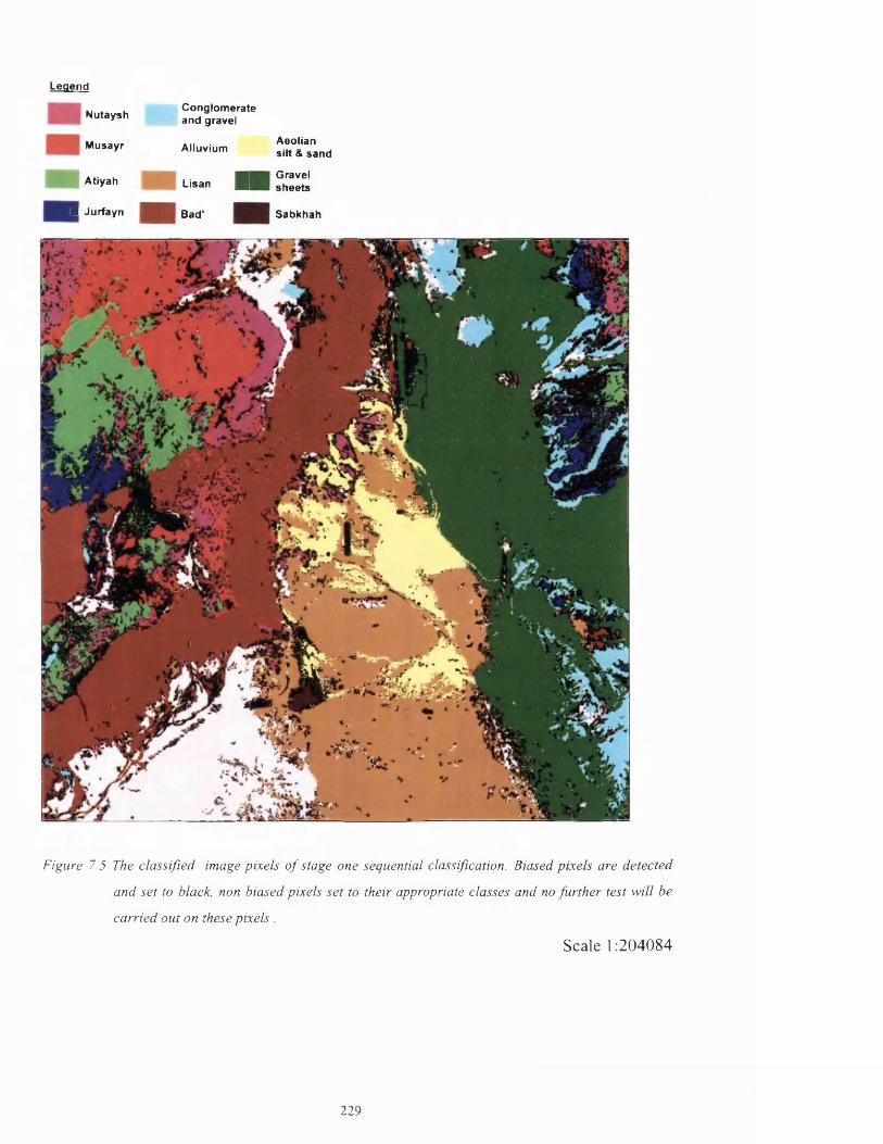
Legend

Nutaysh

Musayr

Atiyah

■ Jurfayn


Alluvium

Lisan M

Bad'

Aeoliansilt & sand

Gravelsheets

Sabkhah

Figure 7.5 The classified image pixels o f stage one sequential classification. Biased pixels are detected

and se t to black, non biased pixels se t to their appropriate classes and no further test w ill be

carried out on these pixels .

Scale 1:204084

229

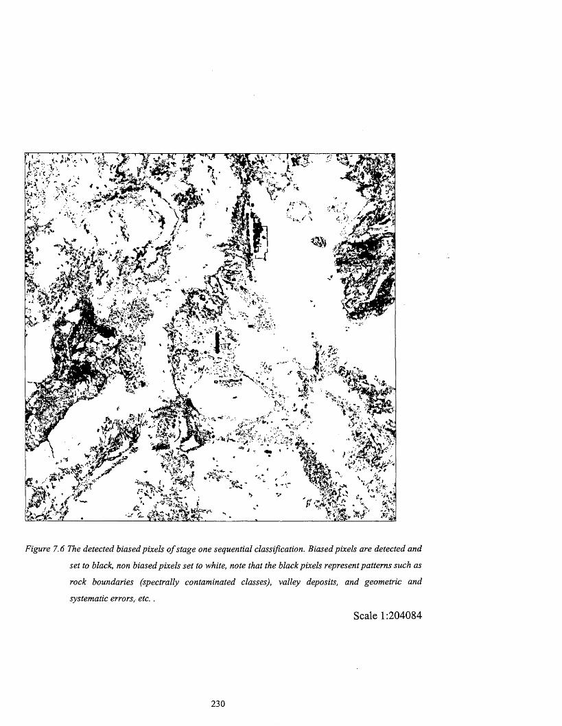
Figure 7.6 The detected biased pixels o f stage one sequential classification. Biased pixels are detected and

set to black, non biased pixels set to white, note that the black pixels represent patterns such as

rock boundaries (spectrally contaminated classes), valley deposits, and geometric and

systematic errors, etc. .

Scale 1:204084

230

After detecting and separating these biased pixels in the first stage, the correct texturally

classified pixels have been detected in stage two from the texture classified image by

using a similar test between the texturally classified image (figure 7.2) against the

spectrally classified image (figure 7.3) and pixels which agree to have the same class are

separated and assigned to their appropriate classes, pixels fail to agree in the test are set

to black, this is shown in figure 7.7. After producing this image, and in stage three, the

biased pixels of figure 7.6 will be replaced by pixels of figure 7.7. If the replaced pixels

are still black (unclassified), two choices are available, either set them as negatively

biased (unclassified or black) as shown in figure 7.8, or replace them by their original

classes values in the textural-spectral classified image (figure 7.9).

The collected statistics during stages one, two, and three are shown in table 7.3. By

simple calculation using stage 1, 2, and the final image produced in the final stage as

shown in figure 7.9, every class performance is calculated after detecting the negatively

biased pixels. The overall performance of this kind of classification is also given by

dividing the summation of all classified pixels in stages 1 and 2 by the whole number of

pixels giving a figure of 88.9% performance.

Lithologicclasses

Stage 1 Stage 2 2 Stages Biased(negative)

Final %Performance

Jurfayn 19500 563 20063 1634 21697 92.4Atiyah 59066 83 59149 13123 72272 81.8Musayr 66510 361 66871 4172 71043 94.1Nutaysh 54167 272 54439 12557 66996 81.2

Bad’ 159499 48 159547 15797 175344 91.0Lisan 158478 253 158731 11572 170303 93.2

Cong.+Grvl 101241 373 101614 29130 130744 77.7Grvl sheets 45225 289 45514 13778 59292 76.7

Sabkhah 1280 1 1281 56 1337 95.8Alluvium 213442 979 214421 5040 219461 97.7

Aeolian silt + sand

50818 71 50889 9198 60087 84.7

Not yet classified

119350 116057 116057 116057 0 Overall = 88.9

Table 7.3 Statistics o f each stage during the sequential classification oflithologic units o f the test site.

231

Legend

NutayshConglom erateand gravel

Musayr AlluviumAeolian silt & sand

Atiyah LisanGravelsheets

Jurfayn Bad' Sabkhah

Figure 7.7 Sequential classified pixels o f stage 2 showing the texturally classified pixels which agree to

have the same class o f the spectrally classified pixels. This image also show the correctly

classified pixels texturally.

Scale 1:204084

232

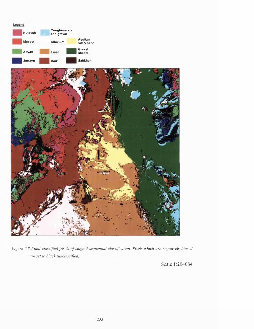
Conglom erateNutaysh an<j grave|

Musayr Alluvium

Atiyah

Jurfayn

Lisan

Bad'

Aeoliansilt & sand

Gravelsheets

Sabkhah

Figure 7.8 Final classified pixels o f stage 3 sequential classification. Pixels which are negatively b iased

are set to black (unclassified).

Scale 1:204084

233

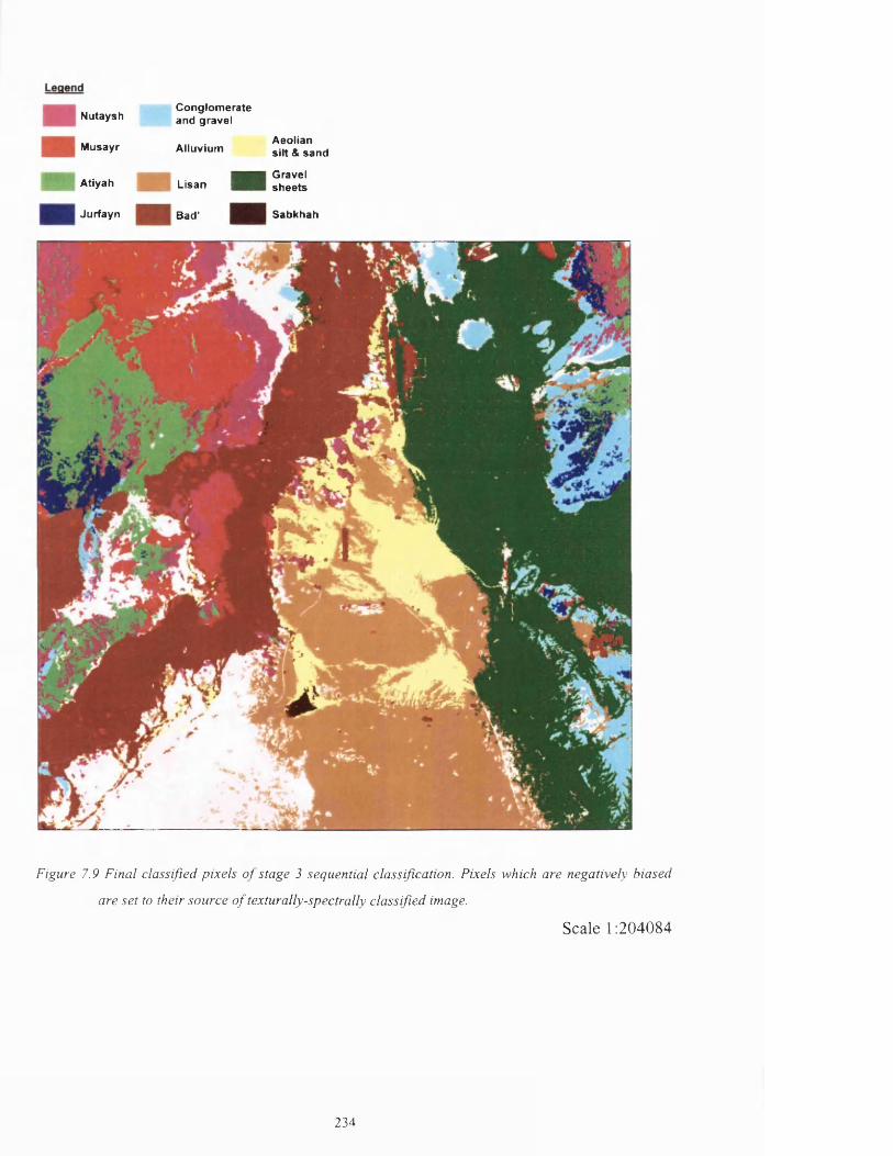
C onglom erateNutaysh and grave|

Musayr

Atiyah

Jurfayn

Alluvium

Lisan

Bad'

Aeoliansilt & sand

Gravelsheets

Sabkhah

Figure 7.9 Final classified pixels o f stage 3 sequential classification. Pixels which are negatively biased

are set to their source o f texturally-spectrally classified image.

Scale 1:204084

234

7.6 Accuracy estimation

Estimation of accuracy is an important final stage of every project and reveals the

improvements and merits of the techniques used. In particular, the classification accuracy

in remote sensing is vital and is the actual judgement of the success of the work. At the

same time it is problematic especially in this work as a results of the following: The map

produced by Clark [2] is not accurate when investigated during the field work; some of

the lithologic classes of the test site have been renamed and/or reclassified (i.e. the

Quaternary deposits) and finally; some of the lithologic boundaries are either not

recognised in Clark’s map, incorrectly mapped, or could not be detected during the

photo-interpretation procedure when fused images are produced in chapter 6. As a result

of that, a new map has been produced as an integrated lithologic map combining the map

produced by Clark [2] and the map produced in chapter 6 as an interpretation of the

images produced (i.e. figure 6.25). This integrated map has been digitally scanned,

formatted to exactly match the classified images, and every lithologic class has been

assigned to a specific colour exactly the same as the classified images. This integrated

lithologic map is shown in figure 7.10.

It is important to notice the following issues related to the integrated map used as a

ground truth data:

1- The integrated lithologic map is used as a ground truth verification to estimate the

classification accuracy. At the same time it is believed that this map is far from the

100% accuracy figure. 100% accurate ground truth data is rarely valid in remote

sensing [138].

2- The classification accuracy results used in this work are estimated as a bottom line

(i.e. worst conditions) and it is believed that the results are much better than the

accuracy figure given for each class or the overall accuracy.

3- All image pixels are used for the classification accuracy estimation. Training areas

used for classification are also included, this gives the accuracy estimation is full and

inclusive accuracy estimation.

235

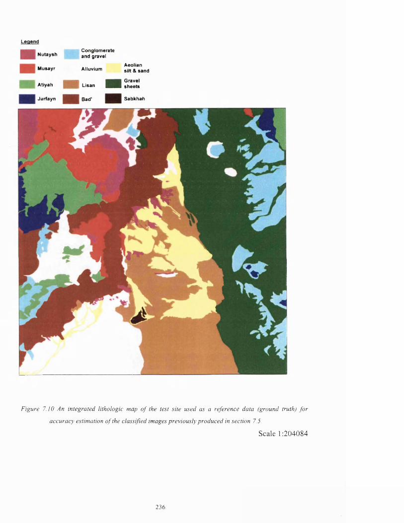
Legend

Nutaysh

Musayr

Atiyah

Jurfayn

Conglomerateand gravel

Alluvium

Lisan

Bad'

Aeoliansilt & sand

Gravelsheets

Sabkhah

Figure 7.10 An integrated lithologic map o f the test site used as a reference data (ground truth) fo r

accuracy estimation o f the classified images previously produced in section 7 . 5 .

Scale 1:204084

236

Accuracy assessment scheme in this work has been applied to investigate the

performances of the followings: the texturally classified image (shown in figure 7.2); the

spectrally classified image (shown in figure 7.3); the textural-spectral classified image

(shown in figure 7.4) and finally; the sequentially classified image where negatively

biased pixels are set to the textural-spectral classified image (this is shown in figure 7.9).

The other important reason for such investigation is to compare accuracies between the

four classified images.

Accuracy of the textural classified image as expected, is low which only reveal less than

30 percent overall accurately classified pixels ( around 304087 pixels). This is because

the textural separability between the lithologic classes is low and the reference data (the

integrated map) is not very accurate. The error accuracy matrix calculated for the textural

image is shown in table 7.4 (including the omission or producer’s accuracy and the

commission or user’s accuracy of each class). The method of producing the error matrix

is simple and straightforward, it is described in detail by Congalton [138].

The accuracy of classification of the spectral data is shown in table 7.5. As shown in

figure 7.3, lithologic classes patterns are shown clearly, which simply reflects the

advantage of the spectral data used in this work. The overall accuracy is estimated of a

figure of 75.3% (789577 pixels of the imaged test site). This figure of overall accuracy is

not believed to be low because the original reference data (the integrated digitised map)

is not accurate.

In the case of the textural-spectral classified image (figure 7.4) and its high separability

property between its classes. The estimated overall accuracy of this classified image is

76.921% meaning around 806575 pixels of the whole image pixels are correctly

classified. The error accuracy matrix of the texturally-spectrally classified image is

shown in table 7.6.

Finally and in table 7.7, and using the sequentially classified image shown previously in

figure 7.9. The overall accuracy is improved (but not in a recognised figure) showing

237

overall accuracy of 76.994% accurate (around 807340 pixels of the test site). This small

accuracy improvement (+ 0.073% or + 765 pixels) is believed to be an important

indicator of the use of the sequential classification method used in this thesis because of

two reasons: firstly it proves the logic of using the sequential classification is correct and

beneficial for lithologic mapping; secondly is that the sequential classification is a good

method of confirming if the classified pixels (in stage zero) are correctly classified or not,

and only the correctly classified pixels (i.e. 807340 pixels) are selected in the final stage

of the sequence.

238

Com

mis

sion

%

1lll 7.5%

10.7

%24

.3%

10.4

% nO 0 s i—H

oo 23.6

%38

.6%

17.8

%0.

5% 50%

12%

2 Ro

ws

or E

Col

umns

10

4857

6O

vera

ll ac

cura

cy

29%

£oPiw

l1l1 70

337

2235

312

9663

6794

354

451

4932

498

262

1387

4999

502

2562

5761

735

Cla

ssifi

ed

imag

e da

ta

Aeo

lian

1543

938

109

1577 32 4987

1034

797

9610

602

3068

174

7778

089

9.6%

Allu

vium

3996

2026 O

Os 2962 25

1390

419

690

1039

230

013

1280

1433

320

2452

43

52.2

%

Sabk

hah

VO o © o o 93 42 o 541

1030 32 1744

31%

Gra

vel

s.94

0739

7228

1613

56 voVO

4270

1310

224

788

8144

1380

336

3585

459

29%

Con

g+G

vl71

3337

9825

4591

226

1376

137

973

4980

622

330

7644

856

1467

84

25.8

%

Lis

an99

156

697 45

0 o

1164

113

903

8548

2683

674

527

1635

315

3912

7.5%

Bad

’12

011

3273

4143

2 C"VOr ft J-<N 47

434

<N(N 13

86 i"-

CO 322 69 o

1379

62

34.4

%

Nut

aysh

8213

2177

1474

471

1911

6526

6

ooVO 81

6043

6 o <N

4308

3

16.5

%

Mus

ayr

9956

2086

3158

310

486

2424 95 624

8701 08

120 Os

1—H

6617

4

44.7

%

Atiy

ah11

774

2403

2624

313

088

2675 53 374 oovoooo 52 <N O

6474

2

3.7%

£.Ctf

5307

1114

9193

5526

504

33 140

3143

146

256

22[

2538

4

21%

Inte

grat

edM

ap 11I11

Jurf

ayn

Atiy

ahM

usay

rN

utay

shB

ad’

Lis

anC

ong+

Gvl

Gra

vel

s.Sa

bkha

hA

lluvi

umA

eolia

n£

Col

umn

Om

issi

on%

Com

mis

sion

%

IIII

51.7

% x °o'-CScor- 68

%37

.5%

72.2

%80

.2%

74.6

%71

.2%

83.2

%92

.3%

86.8

%E

Rows

or

EC

olum

ns

1048

576

Ove

rall

accu

racy

75

.3%

E R

ow IIII 2885

463

552

7672

081

192

1835

1416

8373

1137

16|

5388

314

1622

3717

5363

9

Clas

sifie

d im

age

data

Aeo

lian

o o r-VOl—H

COO

1278

715

714

1556 Os

CO<N

1052

4657

878

089

59.6

%

Allu

vium

coVOco 32

337

881

2757

8511

618

1165

5

o

2066

3845

224

5243

84.2

%

Sabk

hah

© O o o 523

in o o11

78 o 38 1744

67.5

%

Gra

vel

s.13

172

5593

428

8996 5064 o

1944

3837

9

o

1110

1

o85

459

45%

Con

g+G

vl

©

2632

1413

215

897

1646

010

367

8487

448

0 or -oooo 55

1467

84 x °ox00

•n

Lis

an o o 780

214

1617

1351

3880

42 o o

2305 VO

00•n 15

3912 xOOX

00

oo

Bad

’63

H00 1775

1026

1326

38 ooooool-Hl-H 34

5 <n

183

448

1379

62

96.1

%

Nut

aysh

o

1278

4434

3046

214

2410

8140

57 86 o o 249

4308

3 xOOXr--©

Mus

ayr

VO

2516

1 52

117

7054

3879 COr-~ 382

25 o Osr-H CO

6617

4 x °Oxt | OOr-"

Atiy

ah56

246

543

2530

1341

492

9 o com 1“" o o o

6474

2

71.9

%

Jurf

ayn

1492

047

73 34 2976 99 o <N

2181 o 432 o

2538

4

58.7

%

Inte

grat

edM

ap

11ll1

Jurf

ayn

Atiy

ahM

usay

rN

utay

shB

ad’

Lis

anC

ong+

Gvl

Gra

vel

s.Sa

bkha

hA

lluvi

umA

eolia

nE

Col

umn

Om

issi

on%

ROao

J3VJ

beR

-R■V-*

RS.OSi)►So

- R

b50£'o'■aaR•S

R*OUbSsooaR•S•Co

00-2K,*>-oe5

240

Com

mis

sion

%

1111

62.5

%65

.2%

71.6

%44

.5%

75.2

% ox

00I"- 76%

76.7

%89

.2%

92.6

% NO0s*

■'too

£ Ro

ws

or E

Col

umns

10

4857

6O

vera

ll ac

cura

cy

76.9

21%

£ R

ow 1111 2119

772

596

7075

767

169

1755

8717

0810

1309

1759

505

1336

2185

7460

128

Cla

ssifi

ed

imag

e da

ta

Aeo

lian

o o 218

149

9547

1449

725

20 78 464

5061

378

089

64.8

%

Allu

vium

109

283

226

652

9447

9885

1029

111

113

o

2025

7466

324

5243

82.6

%

Sabk

hah

o o o o <Nvn vo - o11

92 o 393

1744

68.3

%

Gra

vel

s.72

8695

1049

747

6227

83

906

3393

4561

9

o

1070

3

o85

459

53.4

%

Con

g+G

vl

o

5166

1076

852

6711

715

1084

599

382

774 o

1830

1037

1467

84

67.7

%

Lis

an o o 254 VO

2252

1339

63|

8381 o o

2357

6529

1539

12

87%

Bad

’53

<NCOv-H 17

5214

3313

2089

| 13

4320

5 99

133

715

1379

62

95.7

%

Nut

aysh

o

1224

4135

2987

521

9256

546

7026

1 o 160

4308

3

69.3

%

Mus

ayr

2617

5065

077

7541

8610

267

764 o 1—H

00 oo1—H

6617

4

76.5

%

Atiy

ah49

347

374

2208

1299

311

30 © 252

292 o o o

6474

2

73.1

%

Jurf

ayn

1325

262

90 49 4087 94 o r-"

1174 o m o

2538

4

52.2

%

Inte

grat

edM

ap IIIII

Jurf

ayn

Atiy

ahM

usay

rN

utay

shB

ad’

Lis

anC

ong+

Gvl

Gra

vel

s.Sa

bkha

hA

lluvi

umA

eolia

nE

Col

umn

Om

issi

on%

Com

mis

sion

%

l111

61.6

%65

.4%

71.6

%44

.5%

75.3

%78

.6%

76%

76.6

%89

.2%

92.6

%84

.3%

E Ro

ws

or E

Col

umns

10

4857

6O

vera

ll ac

cura

cy

76.9

94%

E R

ows

llll

2169

7 ZLZZL 7104

3 96699

1753

4417

0303

1307

4459

292

1337

2194

6160

087

Cla

ssifi

ed

imag

e da

ta

Aeo

lian

0 0 218 O n■'sf1—H 95

3314

457

2528 CO 78 473

5065

078

089

64.9

Allu

vium r-

<N 276 r“H

<N(N 64

293

6494

9310

115

1112

8

0

2032

35 <N

NO

2452

43

82.9

%

Sabk

hah

O 0 O 0<NIT) NO 0

| 11

93 0

| 39

217

44

1

vO0^'s t;00NO

Gra

vel

s.76

44|

9389

493

4761

2725

698

3330

4542

7

0

1082

10

8545

9

53.2

%

| C

ong+

Gvl

^

0

5167

1076

552

68

|11

657

\ I 9I80I 99

454 ILL 0

1849

1037

1467

84

OOr+NO

Lis

an 0 0 254

176

2247

1339

5583

81 0 0

2421

6478

1539

12

87%

Bad

’54 m

1759

1416

1320

8642 13

4221

9 99 COCO 71

413

7962

95.7

%

Nut

aysh

0

1224

4172

2984

221

8656

746

7325

9

0ON

l-H

4308

3

69.3

%

Mus

ayr

■*r

| 25

7850

877

7606

4169 86

665

65 0 97 mi-H

6617

4

76.9

%

Atiy

ah50

847

268

2234

1306

211

31 0 248 i—W

O n<N

0 0 0

6474

2

73%

Jurf

ayn

1336

062

39 50 4074 94 0

1129 0

l-Hm 0

2538

4

52.6

%

Inte

grat

edM

ap 1l11l

Jurf

ayn

Atiy

ahM

usay

rN

utay

shB

ad’

Lis

anC

ong+

Gvl

Gra

vel

s.Sa

bkha

hA

lluvi

umA

eolia

nE

Col

umn

Om

issi

on%

►o'1

!►.

V►O£<UIP

"535D&

K3O’OtnO■sl>0•S§<s>

■S (N■'t<N

O►«

bSU5

'o '•iS is <3 S1 -I1 ■§ ^ ■ s .

I>3•x •—S ' ^S *3 8a o,« ^

•2 ^ t3 ^8 aOj •*«.

J lu ~t \K

►O£!

7.7 C onclusions and rem arks

The sequence or staged classification works in a method of comparison between the

texturally-spectrally classified pixels with spectrally classified pixels to detect the biased

(positively or negatively) pixels and perform a small test to find out if the biased pixels

are positive or negative (stage one). If positive, then they are saved, if the bias is

negative, other pixels derived from a logically constructive comparison (texture against

spectral) are replaced. If the comparison of texture against spectral fails, either the

original classified pixels derived back, or lifted unclassified. It works as priorities, the

more class pixels classified in the earlier stage, the better performance can be gained in

this particular class. Conversely, the less pixels classified in this stage for a particular

class, the less performance can be achieved. Table 7.3 shows this characteristic. This is a

general rule in classes performance, but the classes pixels left unclassified after the third

stage is the key of the classes performance.

Pixels left unclassified may be classified based on their textural-spectral information

which is still high in separability (table 6.1). Such pixels are believed to be source of

errors resulting on relying on their biased spectral information rather than textural

information. This is shown in figure 7.6 where pixels of system errors, Valley deposits,

and classes boundaries show clearly in this figure. This give rise to an easy way of

calculating the performance of both of each class and overall performance of the whole

image.

Care in selecting the test site training areas and their sizes is an important key factor in

classification. To select a training area, comparison between the measured spectral data

collected from the rock samples with the TM data is important. This is to insure both of

data has similar shapes. If bias occur, the selected training area may contain contaminated

pixels which gives a wider spread in the class standard deviation resulting in reduction of

transformed divergence separability test figure. The size of the training area representing

each class should meet the criteria Z > 5(n2 + n) where Z is the number of pixels of each

243

class and n is the number of image bands used [41]. This is for a better representation of

class statistics used in MLC.

Because texture with spectral information are used in the sequential classification, and it

is believed that the spectral information derived from TM sensor is reliable. The textural

information should be presented in a better way, this include geometric correction,

speckle reduction, and the algorithm used to enhance texture. If such factors achieved,

performance of the sequential classification will increase.

Sequence or staged classification works only with two or more than two types of

information (signatures) collected from the same sensor or different sensors. Because it is

based on comparison between pixels information, accurate registration between these

pixels (if two or more sensors used) is an important part of data preparation for fusion.

Thus, misregistration may increase dramatically the error rate during classification.

The sequential classification can work in a different way of steps, for example it can

work as the spectral versus textural first, then textural-spectral versus spectral second,

and fill biased pixels in the first step by pixels of the second step. If there are still biased

pixels, fill these zero pixels by the textural-spectral classified original source. Such

method has been tested in this work and showed nearly identical results (visually and

statistically) to the method used here.

Finally, the sequential classification is simple and easy method. It is proved in this

thesis that it is a good way to benefit from two imaging sensors information.

244

8.0 C onclusions

The main objective of this thesis has been to show the usefulness of satellite image data

fusion using the JERS-1 SAR textural information and the Landsat-5 optical spectral

information, and employing both for lithological mapping using a selected test site

located in the north west of Saudi Arabia. This site was composed of varieties of igneous,

sedimentary, and surficial lithological units of age range from Proterozoic to recent

Cenozoic eras. A reasonable geologic knowledge of this site has been built based on a

field visit, spectral analysis of the collected rock samples, a previously compiled

geological map, and many processed colour composites and fused colour composites

used for visual interpretation.

In order to utilise the two data sets from the optical TM and the SAR image data, many

aspects have been demonstrated to carry out the data fusion and create a constructive

feedback for both utilising and interpreting the fused image data. These aspects include:

reviewing the theoretical background of the nature of the two imaging systems and their

benefits for geologic mapping, preparing the two image data sets and making them

suitable for fusing, and finally extracting the valuable spatial and spectral information for

the fusing techniques.

The aspects mentioned above can be termed the information feedback and pre

processing for image data fusion. The pre-processing includes the atmospheric correction

of the optical data, the geometric co-registration of the SAR image data to the optical TM

data and finally the speckle removal of the SAR image data.

An intermediate step between the pre-processing and image data fusion is the extraction

of the textural information from the SAR image data, since the SAR is inherently

sensitive to the shapes and structures of lithologic features surfaces. The Grey Level Co

occurrence Matrix (GLCM) works better than other spatial enhancement techniques. This

judgement is based on the statistical Transformed Divergence separability tests upon the

predefined lithologic features selected during the field work in the test site.

245

Image data fusion is broadly divided into two parts based on its benefit: one is data

fusion aimed at maximising the visual interpretability of the image data. From a

geological point of view this can be achieved if both the spectral and textural information

of the geologic units in the image data are enhanced and displayed. The second part is

maximising the lithological units separabilities using both spectral and textural

information to be automatically recognised. This is through the use of a discriminant

function, and makes the computer directly decide to spatially label every pixel to its

relevant rock unit class based on a learning procedure. The learning procedure is feeding

the computer with the rock unit’s multivariate statistics. This method is the classification

process by the use of supervised maximum likelihood decision rule and the resultant is a

thematic map delineating all rock type classes.

An effort has been made in this thesis to develop a new method to solve the problem of

selecting which spectral bands are used to represent the spectral information component

in the colour composite displayed images where there are twenty possible combination of

the optical TM data and all of these combinations can be used for visual interpretation.

The newly developed method is named the spectral coding method,

Because spectral information is represented by colours in the colour composite, and

these colours only show up if the spectral information used in the primary colours of red,

green, and blue. The spectral TM coded image, the albedo-topographic image (the mean

reflectance of the six TM data) image, and the range image (maximum-minimum pixel

vector value) are used as a TM spectral colour coded composite technique which shows

up a colourful image and at the same time preserve the maximum separability between

classes if the whole TM six bands are used together.

A set of fuser tools have been applied on the spectral colour coded composite image,

where these tools work as a splitting mechanism mediator to split the spectral

information from its spatial information and then induce the inherently maximised spatial

information available in the SAR image. These tools include the RGB-HSI-RGB, the

246

PCT, and the chromaticity Brovey transform techniques. The spectral colour coded

composite image and the fuser tools are a group of procedures dedicated for image data

fusion aimed at visual interpretation. These procedures are tested on the selected test site

and results show that the visual interpretability makes recognition of the rock classes

easy.

In the second part of image data fusion aimed at classification, the two image data set

(the 6 optical TM bands and the 7 textural measures produced by the GLCM) are treated

separately, and in combination intending to benefit from both data sources for better

(confirmed) classification results. A new method of classification is used and named the

sequential classification. The sequential classification is a method of implementing the

classifier (i.e. MLC) on the spectral image data derived from the TM data, the seven

textural GLCM measure data derived from JERS-1, the textural-spectral combined image

set of enhanced spatial and spectral information using the Mahalanobis distance, and a

final thematic maps are automatically produced using these three data sets. The accuracy

assessments of the produced thematic maps proved that the textural data set is

incomparable with the spectral data accuracy assessment. The spectral data derived from

TM is much better, but the textural data set is useful for the sequential classification.

8.1 Ideas for further work

The TM spectral colour coding technique is a new method to build spectrally coded

colour composite production where the image dimensionality is reduced, and at the same

time the feature’s spectral separability is preserved. The method works very well in the

case of TM data because there are only six optical spectral image bands. It works for any

kind of application because the key factor of spectral information for visual interpretation

is preserved. Problems may arise if spectral coding is implemented on hyperspectral

image data because the code number will exponentially increase leading to new issues

such as storage and scaling. In such case, the spectral coding algorithm should modified

to suite such kind of data.

247

For geological mapping where lithological and structural mapping are combined

together, it is believed that the DEM’s are important information which should be

included. Such data can be utilised to extract the terrain attitudes and aspects (i.e. slope,

watershed, drainage patterns, etc.) which may help with the combination of the lithologic

maps to delineate automatically the structural features. Reliable rules are critically

needed to establish such an idea for automated geological mapping and may be through

the use of advanced sequential classification (i.e. hierarchical).

248

Appendix (A)

A -l B and com bination:

Combinations are a special case of permutations, where a combination neglects the

order of permutation arrangement [117]. Suppose we have n bands combined in r number

(i.e. r items together).

The number of possible combination is nCr .

nC_ =rri\\ r j r\(n — r)\

(A.1)

where:

n\= factorial of n.

r\= factorial of r.

(n — r)\ = factorial of ( n - r ) .

We can code the combination table in C programming easily as follows:

a) If three pixel triplet is needed to create colour composite (3D-DCVR):-

/* Let n = number of bands used = 6, r = 3 (i.e colour composite of pixels of band Q, R,

and S */

int n=6;

int Q, R, S;

249

for (Q=l;Q<n-l;Q ++){

for (R=Q+1; R<n; R++){

for (S=R+l;S<n+l;S++){

printf("\n%d\t%d\t%d",Q,R,S); /* print the combination table */

>}}

A-2 Balance Contrast Enhancement Technique (BCET)

The BCET technique was proposed by Liu [43], Liu and Moore [114] to avoid colour

bias when a colour composite is displayed. The method is simply refer to a special

contrast stretching of the image while at the same time allowing the output image

minimum, maximum and mean to be user specific. Two methods can be used, one is

using a segment of parabola curve derived from the input image, the other method is

similar to that of the first but using a segment of cubic curve. In this work, data is

stretched by the use of a parabolic curve. The mathematical derivation is as follows [43]:-

The parabolic equation is:

Y= A ( X - B ) 2 +C (A.2)

where:

Y= output image pixel.

X= input image pixel.

A, B, and C are coefficients.

To derive A, B, and C coefficients, we have to calculate the following from the input

image pixels x t . Let:

250

h = maximum pixel value of input image = Max( x t)

/ = minimum pixel value of input image = Min( x t)

1 ^e = mean value of input image pixels = — / Ax,

A 1=1

If the user works with 8 bit images, the maximum H and minimum L will be set to 255

and zero respectively. The output image mean E will be set by the user selected value.

* = ^ | > , 2 (A.3)

T = (h2 x E) - 255R + 25512 (A.4)

K = 2[(A x E ) - (255e) + (255/)] (A.5)

The coefficients can be calculated as:

255 , xA ~ (h - l ) (h + l - 2 B ) (A'6)

(A.7)

C = - A ( l - B ) 2 (A. 8)

Note that most of the time the above method of stretching works well but under some

circumstances it may not gives the desired mean as a result of the nature of the input

image. Such a situation can be resolved if clipping factors are taken from the input image

histogram tails. More information about this problem is discussed in Liu’s work detailed

in the references [43,114],

A-3 Band selection

Band selection for colour composite production can be problematic as a result of which

combination scheme is desired. Users may prefer testing image combination visually or

implementing some statistical calculations, these statistical approaches are:-

251

a) OIF band selection method

Chavez et. a l [112] were the first people to address the colour composite band selection

problem and its solution statistically. She used the equation below for best colour

composite bands. The method is named the optimum index factor (OIF). The maximum

OIF between any three bands from the combination table is referred to be the best

combination:

2 > ,OIF = - f 3----- (A.9)

£ | c ‘.ji=1

where:

<ji — standard deviation of band i .

Ci . = correlation coefficient between bands i and j.

b) Sheffield and Chase method.

Sheffield and Chase [113] developed another method of best bands selection for colour

composite. It performs better than the Chavez method. The method can be simplified as

follows :-

Stepl- Produce the main variance - covariance matrix of all bands used.

Step2- From the main variance - covariance matrix, produce all the 3 by 3 covariance

matrix which represents all possible combinations of bands. Note that the

matrices are symmetrical along their diagonals.

Step3- Evaluate the third order determinant for every matrix and use bands of the

maximum determinant matrix as the best bands for colour composite

combination.

252

c) Index o f optimal band selection (IOBS) method

This method was developed by Liu and Moore [114] for best band triplet selection. It

shows better performance than the Sheffield and Chase determinant method and the OIF

method of Chavez, because results from both methods are affected by the contrast

stretching of the bands used. The IOBS for best colour composite is the minimum value

produced by the equation below from the combination table.

IOBS = Max(Cuj, Clk , CJJt + C l + Cj,t (A. 10)

where:

C, j ,Cik , Cj k = correlation coefficients of the three bands i,j, and k.

A-4 Separability measure between classes

Separability or discrimination measure between classes refers to how the class pairs in

the data set are not similar or coincide (degree of overlap). This can be calculated from

the class statistics by many methods with a high degree of accuracy. The class refers to

the intensity of pixels value of a specific geographic homogenous area selected by the

user in the image set.

In the one channel case, separability between pair of classes can be measured based

simply on their means and standard deviations. Separability (S) between class z and class

j is then [32]:

S =ui - Uj

O ’ + cr .I J

where:

(A .ll)

253

ui ,uj = means of classes i and j.

<7i , <7 j = standard deviation of classes i and j.

Such a separability measure of a single band can also be evaluated visually by plotting

the class means on the abscissa and the class standard deviations on the ordinate. It is

important that classes are assumed to be Gaussian distributed and values of S from the

above equation give 90% correct separation (correct classification) if S exceeds 1.5 [143]

When many bands are used, the separability measure becomes more computationally

intensive, especially when we have n bands, m classes, r combinations and bearing in

mind that the evaluation is pairwise. In this case the number of evaluations becomes

nCrx mC2 [24] and it becomes impossible to evaluate the separability measure manually.

There are three measures of separability between pairs of classes, these include: the

divergence measure, the Jeffries-Matusita (JM) distance measure (also called the

Bhattacharrya distance) and finally the Transformed Divergence measure. The

Divergence measure is sometime quite misleading as the result of the divergence

increases quadratically with separation between classes [24].

The most popular method of separability measure is the Transformed Divergence (TD)

measure, it is more computationally economical and performs as effectively as the JM

method.

The TD measure of pair of classes i and j on n bands is [41]:

TDtJ = 2 x (1 - e 'D, jla) (A. 12)

where :

Dij = 0.5 x [u{ —UjY x [Covi + CoVj]-1 x [ut - Uj]

+ 0.5x Trace[[Covj x CoVj]~x + [CoVj x CovJ-1 - 2 x 7 ]

254

\ui - Uj]T = transpose matrix of mean vectors of classes i and j where every

class consists of n channels.

[Cov; , CoVj ]_1 = Inverse matrix of covariances of classes i and j .

Trace[...] = Trace of the matrix [...], it is equal to the sum of the diagonal

elements of the matrix [...].

1= The identity matrix.

The TD separability measure between pair of classes can ranges from 1.000 to 2.000 in

its magnitude, such ranges are classified as:-

0.000 <TD < 1.000 = Very poor separability.

1.000 <TD < 1.900 = Poor separability.

1.900 <TD< 2.000 = Good separability.

A-5 The principal component transform

Since the multispectral and multisensor data are multidimensional, they can be

constructed in a vector space with as many axes as there are spectral components or

sensor components [24]. These components, or vectors, are equal to the number of

sensors or spectral bands associated with each pixel. A particular pixel in an image can

be plotted as a point in such space with co-ordinates that correspond to the appropriate

spectral component (e.g. scatterogram). Figure A. 1 shows a plot of three layers of image

means.

255

x2

x3

^ xl

Figure A. 1 Three dimensional presentation o f mean vector consists o f three components or layers.

The mean value of such a vector in one layer or spectral band x l is:

^ = (A. 13)K i= 1

where:

k = number of individual pixels.

x l = pixel brightness value in band 1.

i = pixel number

The mean between three vectors xlpc2 and x3 is:

Mxi

Mx2A s

(A. 14)

The variance a x] of the vector x l is:

1 k(A. 15)

256

The corrected sum of product SPxlx2 between pair of vectors such as x l and x2 is:

kSP*U2 = Z W - n x2) (A. 16)

i=1

The Covariance Covxl x2 between a pair of vectors such as x l and x2 is:

SPX] 2CovxI,x2 = y Z Y (A. 17)

The correlation Cx] x2 between the two vectors x l and x2 is:

C ° V x\ x2cxU2=-H^r (A18>X ( J x \ <Jx2

From the covariance and correlation between every pair of vectors (spectral or sensor

bands), we can create covariance and correlation matrices, their order being equal to the

number of vectors or bands. These matrices are symmetric (e.g. equal to their transpose).

The covariance matrix of n vectors is:

Covxl,x2 ,x3 , ,xn

CovxlM Covx] x2 Covx] x3....Covxl xn

Covx2iXl Covx2 x2 Covx2 x2....Covx2xn

CoK 3.x, CovAx2 Cov, 3 CovxXxn

Cov,,, ,, Cov,n>,2 Cov,, , 3....Cov,„ „

(A. 19)

Note that the covariances between the same vectors are equal to their variances. For

example the covariance of vector x l and vector x l is the variance of the vector x l :

257

Covx l ,x l = <Tx l (A.20)

and also:

Covx u2 = Covx2x, (A.21)

The correlation matrix between n vectors is:

Cx\,x2 ,x3 , ,xn

c c c cW l.j t l ^ x l , x 2 ^ x l , x 3 xl,xn

c c c c^ x 2 ,x l x2,x2 x 2 ,x 3 ..........^ x 2 ,x n

c c c cx3,xl ^ x 3 ,x 2 x3 ,x3 .........^ x3,xn

C , C o c , cxn,x1 xn,x 2 xn,x 3 xn,xn

(A.22)

The correlation between the same vectors Cxhx] = Cx2 x2 =..... = Cxn xn = 1. The value of

the correlation matrix elements range from -1 to 1. If the correlation between a pair of

vectors (e.g. bands) is close to -1, this means the data is highly inversely correlated (one

is increasing and the other is decreasing or vice versa). If the value is zero, this means no

correlation at all exists between the vector pairs. If the value is 1 or close to it, the vector

pairs or band pairs are highly correlated.

Naturally, remote sensing multispectral and multisensor imaging data are highly

correlated because of the identity (spectral response) of the same ground targets are

closely similar in many cases and the topographic relief (scene albedo) gives the same

spectral response for whatever band used. This means there is a redundancy in the data.

To overcome this, data sets or vectors can be translated through their mean vectors to

258

produce new sets of bands which are uncorrelated, and more than 90% of the data set

variances will be moved to the first few new translated vectors. This leads to compressing

the information (e.g. variances) and remove the redundancy and the rest of the translated

components that are low in information and mainly consist of noise. This method of

translation is called the Karhunen-Loeve or Principal Component Transform [18,24,60].

The PCT is widely used as a multispectral/multisensor data fusion technique and as a

method of image data compression, decorrelation. Recently it has been applied as a good

fuser technique because the common information in the data set such as image albedo

will goes to the first PCT component and this component can be replaced by another

image.

The PCT of the data is based on translating the data sets through their eigenvectors of

the covariance matrix. This can be shown in the following:

Let A = the covariance matrix = CovxX xl xl xn

x ^ 0

X = eigenvalues or the latent roots of the matrix A .

A x x = Ax (A.23)

The corresponding solution of the equation A.23 is called the eigenvectors of A .

Expressing this in the covariance matrix to get the eigenvalues and eigenvectors:

259

CovxUxl CovxU2 Covxlx3......Covxha xl xlC o V , 2 . , l C ° V x2,x2 C o V x 2 ,x 3 .........C ° V x2,x„ x2 x2

C o V x 3 ^ C o V x3,x2 C o V x i .x 3 .........C o V x i .x , X x3 = X x3

_ C ° V xn,x 1 C ° V xn,x2 C ° V x ^ l ...........C ° V xx,xnxn xn

= Covxlxlx l + Covxlx2x 2 + Covxlx }xl+ .......Covxtxnxn = Axl

Covx2xlx l + C o v x2 x2 x 2 + Covx2x3x 3+.......Covx2xllxn = Ax 2

C°vx2Mx\ + Covx3xlx2 + Covx3x3x 3+.......Covxixl:xn = Ax 3

Covr„ .xl + Covr„ r,x2 + CovY„ r,x3+ Covr„ xn = Axnxn,x l xn ,x i xn ,xi xn,xn

This simplifies to:

(CovXI Xt - A.)xl + Covxtx2x2 + CovxU,x 3+.... +Covx, „xn =

Covx2 xlx \ + (Covx2x2 - X)x2 + Covx2x3x3+...+Covx2xnxn =Covx3 x,xl + Covx3x2x2 + (Covx2 x2 - A)x3+....+Covx2 xrixn =

Covxn,xix l + Cov»M x2 + Cov»,i3^3+ +(Covx„ x„ - A)xn =

(C°vx,.xi - A ) CovxU2 Covxi x3......Covx] sn xl VCovx2xl (Covx2x2 - A ) Covx2x3.....Covx2xn x2 0C°vx3,x i Covx3x2 (Covx3x3 - A ) ...........Covx3xn X x3 — 0

C°Vxn.xI C° Vxn,x2 C° Vxn,x3....... (.C° Vx»,x„ ~ X ) xn 0

^ ~ A > 2 > 3

From (A.23)

(A.24)

(A.25)

260

A x x - A x = 0 (A.26)

Because we cannot subtract matrices from scalar numbers such as X , we introduce the

unit m atrix /[117]:

( A - A I )x = 0 (A.27)

where I = unit matrix which is I = A x A~l

For this set of homogeneous linear equations (the right hand constants are all zeros), and

to have a non-trivial solution, IA - Al\ must be zero.

\A -M \ =

(CoviU1 - / 1 ) CovxXx2 Covxlx3 Covxl a

Covx2M (Covx2x2- Z ) Covx2x} Covx2x„

Covx3x, Covx3 xl (Covx3x3~ l ) Covx3 xn

Covxnx, Covx7]xl Cov (Cov - A )

= 0 (A.28)

\A - A I | is called the characteristic determinant of A and \A - Al\ =0 is the characteristic

equation. On expanding the determinant, this gives a polynomial of degree n which is the

number of spectral bands. The solution of the characteristic equation gives the values of

X which are the eigenvalues or the new image variances of the transformed data set.

The eigenvalues obtained from the characterised determinant of the covariance matrix

A have corresponding solutions of x called the eigenvectors (equation no. A.23). These

eigenvectors are column matrices. The corresponding solution for the highest value of X

is the first eigenvectors column and so on for the rest of X s and their corresponding

eignvector solutions. The eigenvectors can be aligned in columns corresponding to their

values of^, s in descending order as shown below:

261

- 1,2 ■1,3 E u

2,1 ^2,2 - 2,3 *2 ,3,1 5 - 3,2 5 ■3,3 5 (A.29)

3. E nji_

where: A, > > A, >......> .

The values inside the columns of equation A.29 can be presented together in a matrix

called the modal matrix.

The translation of the data sets is then performed from the values of equation A.29 and

by implementing the equation below (A.30) where results are stored in a new image set.

(A.30)k = l

where:

NPi J Xk = output pixel value in the position of i,j of the component k,

Ei j jLk = eignvector values of component k,

BVijk = input pixel value in the position i,j in all spectral bands k.

I f equation A.30 is applied to the transpose of eigenvectors of X s, the resultant imagery

components will be uncorrelated and are equal in their variances. This is called the

decorrelation stretching technique [90]. It is frequently used by many remote sensing

geologists to achieve colourful images as spectral enhancement technique. One of the

methods used in PCT data fusion is replacing the first principal component by the SAR

262

image data then reversing the PC transformation after transposing the eignvector matrix

using equation A.30 to produce an equal number of images fused with the SAR data.

A-6. The variance-covariance matrix of the test site is shown in table A-6.

- Band 1 Band 2 Band 3 Band 4 Band 5 Band7Band 1 1890.06 - - - - -Band 2 1532.91 1348.08 - - - -Band 3 1571.31 1411.28 1526.17 - - -Band 4 1499.33 1381.30 1515.43 1545.16 - -Band 5 1758.41 1689.67 1883.97 1972.30 2849.40 -Band 7 1350.98 1191.71 1310.19 1343.17 1984.11 1906.79

Table A-6 TM data set variance-co variance matrix. BCET applied prior calculation.

The following show the output results of best bands combination of the test site using

the statistical methods explained previously in A-3.

RANK DETERMINANT BANDS OIF BANDS IOBS BANDS

1 550945300 01 05 06 60.555 01 05 06 0.660283 01 05 062 517319600 02 05 06 54.450 02 05 06 0.696099 01 04 063 493574000 01 04 06 53.956 03 05 06 0.707481 02 05 064 419800900 03 05 06 53.321 01 04 06 0.746328 01 03 065 324950400 01 03 06 52.980 04 05 06 0.761359 03 05 066 266732800 04 05 06 52.878 01 04 05 0.780404 01 02 067 185866000 01 04 05 52.554 01 03 05 0.797073 02 04 068 169051400 01 02 06 52.481 01 03 06 0.800558 01 03 059 167481200 01 03 05 51.768 01 02 05 0.808660 04 05 06

10 129242200 02 04 06 51.281 01 02 06 0.809931 01 04 0511 109171600 01 02 05 48.207 02 04 06 0.825239 02 03 0612 50767690 02 03 06 48.097 03 04 06 0.829750 01 02 0513 49741310 02 04 05 47.871 02 03 06 0.840472 03 04 0614 45492350 03 04 06 46.977 02 03 05 0.881120 02 04 0515 30201340 02 03 05 46.900 02 04 05 0.895387 01 02 0416 18858880 01 02 04 46.553 03 04 05 0.903108 02 03 0517 16538050 03 04 05 43.684 01 03 04 0.918619 01 03 0418 11120940 01 03 04 42.759 01 02 04 0.931608 03 04 0519 8144984 01 02 03 41.562 01 02 03 0.941377 01 02 0320 2039992 02 03 04 39.309 02 03 04 0.963189 02 03 04

263

References

[1] Berger, Z., 1994, Satellite Hydrocarbon Exploration: Interpretation and IntegrationTechniques, Springer-Verlag Publishing Company.

[2] Clark, M. D., 1987, Geological map o f the Al Bad' quadrangle (with report), sheetGM-81 C, Kingdom of Saudi Arabia, Ministry of Petroleum and Mineral Resources, Directorate General of Mineral Resources.

[3] Jaskolla, F., and Rast, M., 1988, Comparative geological evaluation of differentremote sensing data of the Huggar Mountains (Algeria), In: Proc. 4th International Colloquium on Spectral Signatures o f Objects in Remote Sensing, Aussois, France, 18-22 January 1988 (ESA SP-287).

[4] Lillesand, T. M., and Kiefer, R. W., 1994, Remote Sensing and Image Interpretation(third edition), John Wiley & Sons.

[5] JERS-1 Data Users Handbook, 1994, NASDA.

[6] Elachi, R., 1987, Introduction to the Physics and Techniques o f Remote Sensing, JohnWiley & Sons.

[7] Curlander, J. C., and McDonough, N. C., 1991, Synthetic Aperture Radar, Systems &Signal Processing, John Wiley & Sons, Inc.

[8] Kahle, A. B., 1986, Measuring spectra in arid lands; In: Desert and Arid Lands, Ed.by El-Baz, F., 1986, Martinus Nijhoff Publishers.

[9] Drury, S. A., 1987, Image Interpretation in Geology, Allen & Unwin Press.

[10] Leberl, F. W., 1990, Radargrammetric Image Processing, Artech House Inc.

[11] Elachi, R., 1988, Spaceborne Radar Remote Sensing: Applications and Techniques, IEEE Press.

[12] Skolnik, M. I. (Editor), 1970, Radar Handbook, McGraw-Hill.

[13] Levanon, N., 1988, Radar Principles, John Wiley & Sons.

[14] Griffiths, H.,1998, Synthetic Aperture Radar: Tutorial, IEEE Radar Conference, Dallas, Texas, May 14, 1998.

[15] Barber, B. C., 1985, Theory of digital imaging from orbital synthetic-aperture radar, Int. J. Remote Sensing, V.6, N. 7, 1009-1057.

264

[16] Sieber, A. J., 1985, Statistical analysis of SAR Images, Int. J. Remote Sensing, V.6, N.9.

[17] Lee, J. S., 1986, Speckle suppression and analysis for synthetic aperture radar images, Optical Engineering, V. 25, N. 5, 636-643.

[18] Jensen, J. R., 1986, Introductory Digital Image Processing: a Remote Sensing Perspective, Prentice-Hall.

[19] Haralick, R. M., 1973, Glossary and index to remotely sensed image pattern recognition concepts, Pattern Recognition, V.5, 391-403.

[20] Billingsley, F. C., Data processing and reprocessing, Chapter 17 in the Manual o f Remote Sensing, R. N. Colwell (Editor), Fall Church.

[21] Cheng, P., Toutin, T., and Pohl, C., 1995, A comparison of geometric models for multisource data fusion, In: Proc. Geolnformatics'95, Hong Kong, V.I., 11-17.

[22] Leila, M. G., and Manjunath, B. S., 1996, Registration techniques for multisensor remotely sensed imagery, Photogrammetric Engineering and Remote Sensing, V.62, N. 9, 1049-1056.

[23] Stanton, S. Y., and Gilbert, J. R., 1984, Registration of a synthetic aperture radar image to thematic mapper imagery for remote sensing applications, IEEE Transactions on Geoscience and Remote Sensing, V. GE 22, N. 6, 557-563.

[24] Richards, J. A., 1986, Remote Sensing Digital Image Analysis: An Introduction, Springer-Verlag, Berlin.

[25] Crippen, R. E., 1987, The regression intersection method of adjusting image data for band ratioing, Int. J. Remote Sensing, V.8, N.2, 137-155.

[26] Chavez, P. S., 1988, An improved dark-object subtraction technique for atmospheric scattering correction of multispectral data, Remote Sensing o f Environment V.24, 459-479.

[27] Markham, B. L., and Barker, J. L., 1985, Spectral characterization of Landsat thematic mapper sensors, Int. J. Remote Sensing, V.6, N.5, 697-716.

[28] Vincent, R. K., 1973, Spectral ratio imaging methods for geological remote sensing from aircraft and satellites, In: Proc. American Society o f Photogrammetry, Management and Utilization o f Remote Sensing Data Conference, Sioux Falls, SD, 377-397.

265

[29] Ford, J. P., 1982, Resolution versus speckle relative to geologic interpretability of spacebome radar images: a survey of user preference, IEEE Transactions on Geoscience and Remote Sensing, V.GE-20, N.4, 434-444.

[30] Ulaby, F. T., Moore, R. K., and Fung, A. K., 1982, Microwave Remote Sensing Active and Passive, Volume II: Radar Remote Sensing and Surface Scattering and Emission Theory, Artech House Publishing Company.

[31] Shi, Z, and Fung, K. B., 1994, A comparison of digital speckle filters, IGARSS, V. 1- 4, CH.734, 2129-2133.).

[32] Dipack, R. P., and Aschbacher, J., 1993, Evaluation and performance tests of selected SAR speckle filters, In: Proc. International Symposium Operationalisation o f Remote Sensing ”, 19-23ed April 1993, ITC, Enschede, The Netherlands.

[33] Blom, R. G., and Daily, M., 1982. Radar image processing for rock-type discrimination. IEEE Transactions on Geosciences and Remote Sensing. GE-20, N.3, 343-351.

[34] Mueller, P. W., and Hoffer, R. N., 1989, Low-pass spatial filtering of satellite radar data, Photogrammetric Engineering and Remote Sensing, V.55 N.6, 887-895.

[35] Lee, J. S., 1980, Digital enhancement and noise filtering by use of local statistics, IEEE Transactions on Pattern Analysis and Machine Intelligence, V.PAMI-2, N. 2, 165-168.

[36] Lee, J. S., 1983, A simple speckle smoothing algorithm for synthetic aperture radar images, IEEE Transactions on Systems, Man, and Cybernetics, V. SMC-13, N. 1, 85-89.

[37] Frost, V., Stiles, J. A., Shanmugan, K. S., and Holtzman, J. C., 1982, A model for radar images and its application to adaptive digital filtering of multiplicative noise, IEEE Transactions on Pattern Analysis and Machine Intelligence, V.P AMI-4, N. 2, 157-165.

[38] Kuan, D. T., Sawchuk, A. A., Strand, T. C., and Chavel, P., 1987, Adaptive restoration of images with speckle, IEEE Transactions on Acoustics, Speech, and Signal Processing, V. ASSP-35, N. 3, 373-382.

[39] Lopes, A., Touzi, R., and Nezry, E., 1990, Adaptive speckle filters and scene heterogeneity, IEEE Transactions on Geoscience and Remote Sensing, V. 28, N. 6, 992-1000.

[40] Tur, M., Chin, C., and Goodman, J. W., 1982, ‘When is speckle noise multiplicative ?.’, Applied Optics, V. 21, N. 7, 1157-1159.

266

[41] PCI, Inc., 1995, EASI/PACE User Manuals, version 6.0: PCI Incorporated, Toronto, Ontario, Canada, variously paged.

[42] Lee, J. S., 1981, Refined filtering of image noise using local statistics, Computer Graphics, and Image Processing, V.15, 380-389.

[43] Liu, G., J., 1991, Balance contrast enhancement technique and its application in image colour composition, Int. J. Remote Sensing, V. 12, N. 10, 2133-2151.

[44] Shanmugan, K. S., Narayanan, V., Frost, V., Stiles, J., and Holtzman, J. C., 1981, Textural features for radar image analysis, IEEE Transactions on Geoscience and Remote Sensing, V. 19, N.3, 153-156.

[45] Haralick, R. M., 1979, Statistical and structural approaches to texture, In: Proc. IEEE, V.67, N.5, 786-804.

[46] Stefouli, M., and Osmaston, H. A., 1984, The remote sensing of geological linear features using Landsat: matching analytical approaches to practical applications, In: Proc. Remote Sensing Society Annual Conference, Satellite Remote Sensing Review, Reading, 1984, 227-236.

[47] Short, N. M., 1987, Accuracy of lineaments mapping from space, Internal Publication, NASA Goddard Flight Centre.

[48] Haralick, R. H., 1986, Statistical image texture analysis, Chapter 11 in Handbook o f Pattern Recognition and Image Processing, Edited by Young, T. Y., and Fu King- Sun, Academic Press.

[49] Rudant, J. P., Deroin, J. P., and Polidori, 1994, Multi-resolution analysis of radar images and its application to lithological and structural mapping; Larzac (South France) test site, Int. J. Remote Sensing, V.15, N. 12, 2451-2468.

[50] Elachi, C., 1980, Spacebome imaging radar: geologic and oceanographic applications, Science, V.209, N.4461.

[51] Evans, D. L., Farr, T. G., Ford, J. P., Thompson, T. W., and Werner, C. L., 1986, Multipolarization radar images for geologic mapping and vegetation discrimination, IEEE Transactions on Geoscience and Remote Sensing, V. GE 24, N.2, 246-257.

[52] Yamaguchi, Y., 1985, Image-scale and look-direction effects on the detectability of lineaments in radar images, Remote Sensing o f Environment, V.17, 117-127.

[53] McCauley, J. F., Schaber, G. G., et al, 1982, Subsurface valleys and geoarchaeology of the eastern Sahara revealed by shuttle radar, Science, V.218, 1004-1020.

267

[54] Weszka, J. S., Dyer, C. R., and Rosenfeld, A., 1976, A comparative study of texture measures for terrain classification, IEEE Transactions on Systems, Man, and Cybernetics, V.SMC-6, N. 4, 269-285.

[55] Moore, G. K., 1983, Objective procedures for lineament enhancement and extraction, Photogrammetric Engineering and Remote Sensing, V. 49, N. 5, 641- 647.

[56] Pratt, W. K., 1991, Digital Image Processing, John Wiley & Sons Publishing Company.

[57] Low, A., 1991, Introductory Computer Vision and Image Processing, McGraw-Hill Publishing Company.

[58] Hsu, Shin-y., 1978, Texture tone analysis for automated land-use mapping, Photogrammetric Engineering and Remote Sensing, V. 44, N. 11, 1393-1404.

[59] Hsu, Shin-y, 1986, Rock Type Discrimination with AI-Based texture analysis algorithms, In: Proc. o f Annual Meeting o f ASPRS/AGSM, (Washington, 1986), 169-178.

[60] Gonzalez, R. G., and Woods, R. E., 1992, Digital Image Processing, Addison- Wesley Publishing Company.

[61] Carrere,V.,1990, Development of multiple source data processing for structural analysis at regional scale, Photogrammetric Engineering and Remote Sensing, V.56, N.5, 587-595.

[62] He, D. C., and Wang, L., 1990, Texture unit, texture spectrum, and textural analysis, IEEE Transactions on Geoscience and Remote Sensing, V.28, N.4, 509-512.

[63] Wang, L., and He, D. C., 1990, A new statistical approach for texture analysis, Photogrammetric Engineering and Remote Sensing, V. 56, N. 1, 61-66.

[64] Gong, P., Marceau, D. J., and Howarth, P. J., 1992, A comparison of spatial feature extraction algorithms for land-use classification with SPOT HRV data, Remote Sensing o f Environment, V. 40, 137-151.

[65] Haralick, R., Shanmugam, K., and Dinstein, I., 1973, Textural features for image classification, IEEE Transactions on Systems, Man, and Cybernetics, V.3, N.6, 611- 621.

[66] Franklin, S., and Peddle, D., 1990, Classification of SPOT HRV imagery and texture features, Int. J. Remote Sensing, V.l 1, N.3, 551-556.

268

[67] Peddle, D., and Franklin, S. E., 1991, Image texture processing and data integration for surface pattern discrimination, Photogrammetric Engineering and Remote Sensing, V. 57, N. 4, 413-420.

[68] Masuoka, P., Harris, J., and Lowman, P., 1988, Digital Processing of orbital radar data to enhance geologic structure: examples from the Canadian Shield, Photogrammetric Engineering and Remote Sensing, V.54, N.5, 621-632.

[69] Excell, P. S., Campbell, D., Dodd, A., Newby, S., and Stevens, R., 1989, Classification of quasi-periodic textures in thematic mapper scenes using Fourier transforms, In: Proc. o f the 15th Annual Conference o f the Remote Sensing Society, 123-128.

[70] Marceau, D., Howarth, P., Dubois, J., and Gratton, D., 1990, Evaluation of the gray- level co-occurrence matrix method for land-cover classification using SOPT imagery, IEEE Transactions on Geoscience and Remote Sensing, V.28, N.4, 513- 519.

[71] Baraldi, A., and Parmiggiani, F., 1995, An investigation of the textural characteristics associated with gray level co-occurrence matrix statistical parameters, IEEE Transactions on Geoscience and Remote Sensing, V.33, N.2, 293- 304.

[72] Hall, D. L., 1992, Mathematical Techniques in Multisensor Data Fusion, Artech House.

[73] Gerstl, S. A., 1990, Physics concepts of optical and radar reflectance signatures, A summary review, Int. J. Remote Sensing, V.l 1, N.7, 1109-1117.

[74] Karbuz, M. R., Olesen, D.R.O., Gabrielsen, R.H., and Herrevold, T., 1993, Application of multiple data sets to structural studies on Varagner Peninsula, Northern Norway, Int. J. Remote Sensing, V .l4,N.5, 979-1003.

[75] Hutchinson, C. F., 1982, Techniques for combining Landsat and ancillary data for digital classification improvement, Photogrammetric Engineering and Remote Sensing, V.48, N .l, 123-130.

[76] Toet, A., van Ruyven, L. J., and Valenton, J. M., 1989, Merging thermal and visual images by a contrast pyramid, Optical Engineering, V. 28, N. 7, 789-792.

[77] Toet, A., 1992, Multi-scale contrast enhancement with application with image fusion, Optical Engineering, V. 31, 1026-1031.

[78] Burt, P. J., 1985, Merging images through pattern decomposition, SPIE Applied Digital Image Processing, V. 575, N. 3, 173-181.

269

[79] Burt, P. J., and Kolczynski, R. J., 1993, Enhanced image capture through fusion, In: IEEE 4th Int. Conference in Computer Vision, V. 4, 173-182.

[80] Wilson, T. A., Rogers, S. K., and Kabrisky, M., 1997, Perceptual-based image fusion for hyperspectral data, IEEE Transactions on Geoscience and Remote Sensing, V. 35, N. 4, 1007-1017.

[81] Yesou, H., Besnus, Y., Rolet, J., Pion, J. C., and Aing, A., 1993, Merging Seasat and SPOT imagery for the study of geological structures in a temperate agricultural region, Remote Sensing o f Environment, V.43, 265-279.

[82] Daily, M. I., Farr, T., and Elachi, C., Schaber, G., 1979, Geologic interpretation from composited radar and Landsat imagery, Photogrammetric Engineering and Remote Sensing, V.45, N.8, 1110-1116.

[83] Pohl, C., and van Gendren, J.L., 1993, Geometric integration of multi-image information, In: Proc. Second ERS-1 Symposium-Space at the Service o f our Environment, Hamburg, Germany, ESA SP-361.

[84] Pohl, C., and van Genderen, J. L., 1994, Multisensor fusion: optimization and operationalisation for mapping applications. SPIE Proceedings, Conference on Signal Processing, Sensor Fusion & Target Recognition III, Orlando, Florida, USA, 4-6 April 1994, P. 17-25.

[85] Van Zuidam, R. A., Pohl, C., and van Genderen, 1994, Synergy of remotely sensed data for coastal environmental studies: The Ameland-Waddensea example, Northern Netherlands, Second Thematic Conference on Remote Sensing fo r Marine and Coastal Environments, New Orleans, Louisiana, 323-334.

[86] Lichtenegger, J., 1991, Combining optical/infrared and SAR images for improved remote-sensing interpretation, ESA Bulletin, N.66, 119-121.

[87] Lichtenegger, J., Dallemand, J. F., Reichert, P., and Rebillard, P., 1991, Multi-sensor analysis for land use mapping in Tunisia, Earth Observation Quarterly B. N.33, 1- 6 .

[88] Nezry, E, Mougin, E., Lopes, A., and Gastellu-Etchegorry, 1993, Tropical vegetation mapping with combined visible and SAR spacebome data, Int. J. Remote Sensing, V.14, N .ll, 2165-2184.

[89] Raymond, D., Deffontaines, B., and Rudant, J. P., 1994, Morphostructural analysis, radar and SPOT image interpretation as tools for petroleum exploration: an example from the Gabian-Pezenas area (Herault, Southern France), Int. J. Remote Sensing, V.15, N.12, 2469-2479.

270

[90] Rothery, D. A., and Francis, P. W., 1987, Synergistic use of MOMS-01 and Landsat TM data, Int. J. Remote Sensing, V.8, N.3, 501-508.

[91] Rothery, D. A., 1988, MOMS-1 used synergistically with Landsat TM, In: Proc. 4th International Colloquium on Spectral Signatures o f Objects in Remote Sensing, Aussois, France, 18-22 January 1988 (ESA SP-287, April 1988).

[92] Henkel, J., Terhalle, U., and Zilger, J., 1988, Digital analysis of MOMS-1, Landsat- TM and SPOT data of the Nakuru area (Kenya), In: Proc 4th International Colloquium on Spectral Signatures o f Objects in Remote Sensing, Aussois, France, 18-22 January 1988 (ESA SP-287, April 1988).

[93] Franklin, S. E., and Blodgett, C. F., 1993, An example of satellite multisensor data fusion, Computers & Geosciences, V.19, N.4, 577-583.

[94] Rast, M., 1985, Digital combination of SAR and MSS optical data for identification of spectral signatures, In: Proc. 4th International Colloquium on Spectral Signatures o f Objects in Remote Sensing, Les Arcs, France, 16-20 Dec. 1985 (ESA SP-247).

[95] Paris, J. F., and Kwong, H. H., 1988, Characterization of vegetation with combined thematic mapper (TM) and shuttle imaging radar (SIR-B) image data, Photogrammetric Engineering and Remote Sensing, V.54, N.8, 1187-1193.

[96] Leckie, D. G., 1990, Synergism of synthetic aperture radar and visible/infrared data for forest type discrimination, Photogrammetric Engineering and Remote Sensing, V.56, N.9, 1237-1246.

[97] Cliche, G., Bonn, F., and Teillet, P., 1985, Integration of the SPOT panchromatic channel into its multispectral mode for image sharpness enhancement, Photogrammetric Engineering and Remote Sensing, V.51, N.3, 311-316.

[98] Chavez, P.S., 1986, Digital merging of Landsat TM and digitized NHAP data for 1:24,000 scale image mapping, Photogrammetric Engineering and Remote Sensing, V.52, N.10, 1637-1646.

[99] Welch, R., and Ehlers, M., 1987, Merging multiresolution SPOT HRV and Landsat TM data, Photogrammetric Engineering and Remote Sensing, V.53, N.3, 301-303.

[100] Chavez, P. S., Sides, S. C., and Anderson, J. A., 1991, Comparison of three different methods to merge multiresolution and multispectral data: Landsat TM and SPOT panchromatic, Photogrammetric Engineering and Remote Sensing, V.57, N.3, 295-303.

[101] Evans, D., 1988, Multisensor classification of sedimentary rocks, Remote Sensing o f Environment, V.25, 129-144.

271

[102] Haak, B. N., and Slonecker, E. T., 1994, Merged spacebome radar and thematic mapper digital data for locating villages in Sudan, Photogrammetric Engineering and Remote Sensing, V.60, N.10, 1253-1257.

[103] Welch, R., and Ehlers, M., 1988, Cartographic feature extraction with integrated SIR-B and Landsat TM images, Int. J. Remote Sensing, V.9, N.5, 873-889.

[104] Munechika, K. C., Wamick, J.S., Salvaggio, C., and Schott, J.R., 1993, Resolution enhancement of multispectral image data to improve classification accuracy, Photogrammetric Engineering and Remote Sensing, V.59, N .l, 67-72.

[105] Toll, D., 1985, Analysis of digital LANDSAT MSS and SEASAT SAR data for use in discriminating land cover at the urban fringe of Denver, Colorado, Int. J. Remote Sensing, V.6, N .7 ,1209-1229.

[106] Carper, W. J., Lillesand, T. M., and Kiefer, R. W., 1990, The use of intensity-hue- saturation transformations for merging SPOT panchromatic and multispectral image data, Photogrammetric Engineering and Remote Sensing, V.56, N.4, 459-467.

[107] Grasso, D. N., 1993, Applications of the IHS color transformation for 1:24,000 scale geologic mapping: a low cost SPOT alternative, Photogrammetric Engineering and Remote Sensing, V.59, N .l, 37-80.

[108] Daily, M., 1983, Hue-saturation-intensity split-spectrum processing of Seasat radar imagery, Photogrammetric Engineering and Remote Sensing, V.49, N.3, 349-355.

[109] Harris, J. R., and Murray, R., 1990, IHS transform for the integration of radar imagery with other remotely sensed data, Photogrammetric Engineering and Remote Sensing, V.56, N.12, 1631-1641.

[110] Edwards, K., and Davis, P. A., 1994, The use of intensity-hue-saturation transformation for producing colour shaded relief images, Photogrammetric Engineering and Remote Sensing, V.60, N.l 1, 1369-1374.

[111] Vrabel, J., 1996, Multispectral imagery band sharpening study, Photogrammetric Engineering and Remote Sensing, V.62, N.9, 1057-1083.

[112] Chavez, P., Berlin, G. L., and Sowers, L. B., 1982, Statistical method for selecting Landsat MSS ratio, Journal o f Applied Photographic Engineering, V .l, 23-30.

[113] Sheffield, C., and Chase, C., 1985, Selecting band combination from multispectral data, Photogrammetric Engineering and Remote Sensing, V. 51, N.6, 681-687.

272

[114] Liu, G., J., and Moore, J., 1989, Colour enhancement and shadow suppression techniques for TM images, In: Proc. 7th thematic conference on remote sensing for exploration geology, Calgary, Alberta, Canada, 901-915.

[115] Haack, B., and Jampolar, S., 1995, Colour composite comparisons for agricultural assessments, Int. J. Remote Sensing, V. 16, N. 9, 1589-1598.

[116] Sharma, S., 1996, Applied Multivariate Techniques, John Wiley & Sones, Inc.

[117] Stroud, K. A., 1995, Engineering Mathematics, 5th edition, The Macmillan Press Ltd.

[118] Foley, J. D., vanDam, A., Feiner, S. K., and Hughes, J. F., 1996, Computer graphics: Principles and Practice (second edition in C), Addison-Wesley Publishing Company.

[119] PCI, Inc., 1995, EASI/PACE, (Technical support personal communication), Toronto, Ontario, Canada.

[120] Kaufman, H., and Pfeiffer, B., 1988, Image optimization versus classification- an application oriented comparison of different methods by use of thematic mapper data, Photogrammetria, V.42, 311-324.

[121] Mettemicht, G., 1995, Dealing with insufficient discrimination among informational categories: SPOT XS and ERS-1 data fusion, In: Proc. Annual Conference o f Remote Sensing Society, 11-14 Sept. 1995, Southampton. U.K. 1267- 1273.

[122] Solberg, A. H., Jain, A. K., and Taxt, T., 1994, Multisource classification of remote sensed data: fusion of Landsat TM and SAR images, IEEE Transactions on Geoscience and Remote Sensing, V. 32, N.4, 768-777.

[123] Lozano-Garcia, D. F., and Hoffer, R. M., 1993, Synergistic effects of combined Landsat TM and SIR-B data for forest resources assessment, In. J. Remote Sensing, V. 14, N. 14, 2677-2694.

[124] Landgrebe, D. A., 1980, The development of a spectral-spatial classifier for Earth observational data, Pattern Recognition, V. 12, 165-175.

[125] Arai, K., 1993, A classification method with a spatial-spectral variability, Int. J. Remote Sensing, V. 14, N. 4, 699-709.

[126] Dobson, M. G., Ulaby, F., and Pierce, L. E., 1995, Land-cover classification and estimation of terrain attributes using Synthetic Aperture Radar, Remote Sensing o f Environment, V. 51, 199-214.

273

[127] Lopo, A., Chic, O., and Casterad, A., 1996, Classification of Mediterranean crops with multisensor data: per-pixel versus per-object statistics and image segmentation, Int. J. Remote Sensing, V. 17, N. 12, 2385-2400.

[128] Gong, P., and Howarth, P. J., 1992, Frequency-based contextual classification and gray-level vector reduction for land-use identification, Photogrammetric Engineering and Remote Sensing, V. 58, N. 4, 423-437.

[129] Gong, P., and Howarth, P., 1990, The use of structural information for improving land-cover classification accuracies at the Rural-Urban fringe, Photogrammetric Engineering and Remote Sensing, V. 56, N. 1, 67-73.

[130] Fung, T., and Chan, K., 1994, Spatial composition of spectral classes: A structural approach for image analysis of heterogeneous land-use and land-cover types, Photogrammetric Engineering and Remote Sensing, V. 60, N. 2, 173-180.

[131] Pultz, T. J., and Brwon, R. J., 1987, SAR image classification of agricultural targets using first- and second- order statistics, Canadian Journal o f Remote Sensing, V. 13, N. 2, 85-91.

[132] Benediktsson, J., Swain, P., and Ersoy, O., 1990, Neural network approaches versus statistical methods in classification of multisource remote sensing data, IEEE Transactions on Geoscience and Remote Sensing, V. 28, N. 4, 540-551.

[133] Franklin, S., E., and Wilson, B. A., 1991, Spatial and spectral classification of remote-sensing imagery, Computer & Geosciences, V. 17, N. 8, 1151-1172.

[134] Franklin, S., E., and Wilson, B. A., 1992, A three-stage classifier for remote sensing of mountainous environments, Photogrammetric Engineering and Remote Sensing V. 58, N. 4,449-454.

[135] Johnsson, K., 1994, Segment-based land-use classification from SPOT Satellite data, Photogrammetric Engineering and Remote Sensing, V. 60, N. 1, 47-53.

[136] Wang, D., He, D.-C, and Benie, B., 1995, A line-preserving post-processing technique for maximum likelihood classification of SAR images, Int. J. Remote Sensing, V. 16, N. 11,2081-2087.

[137] Wang, M., and Howarth, P., 1993, Modelling errors in remote sensing image classification, Remote Sensing o f Environment, V. 45, 261-271.

[138] Congalton, R. G., 1991, A review of assessing the accuracy of classification of remotely sensed data, Remote Sensing o f Environment, V. 37, 35-46.

[139] Fitzgerald, R. W., and Lees, B. G., 1994, Assessing the classification accuracy of multisource remote sensing data, Remote Sensing o f Environment, V. 47, 362-368.

274

[140] Fisher, P. F., 1994, Visualisation of the reliability in classified remotely sensed images, Photogrammetric Engineering and Remote Sensing, V. 60, N. 7, 905-910.

[141] Press, W., Flannery, B., Teukolsky, S., and Vetterling, W., 1988, Numerical Recipes in C, Cambridge University Press.

[142] Mather, P. M., 1989, Computer Processing o f Remotely Sensed Images, An Introduction, John Wiley & Sons.

[143] Dobson, M. C., Pierce, L., Sarabandi, K., Ulaby, F. T., and Sharik, T., 1992, Preliminary analysis of ERS-1 SAR for forest ecosystem studies, IEEE Transactions on Geoscience and Remote Sensing, V.30, N.2, 203-211.

Programming References

Including the references 57, 118, and 141, the references listed below have been used during the programming work of this thesis.

- Lindley, C. A., 1991, Practical Image Processing in C, John Wiley & Sons.

- Stroo, E., (editor), 1990, The Waite Group’s Microsoft Quick C Programming,Microsoft Press.

- The Math Works Inc. 1992, “MATLAB, high performance numeric computation andvisualization software. Reference guide”.

275

JERS-1 SAR and Landsat-5 TM image data fusion - UCL ...

Documents

Transcript of JERS-1 SAR and Landsat-5 TM image data fusion - UCL ...