tm^mmmttmmmmm^^^^- - DTIC

.., ., .,......._., ,,.,T_^^. ..-_-.-., -L--;r ---:■---,

ivxmein»« immm

STABILITY AND CONTROL. VOLUME II. CONTROL FLIGHT TEST THEORY

Air Force Flight Test Center Edwards Air Force Base, California

July 1974

AD-A011 562

STABILITY AND

DISTRIBUTED BY:

KJLTi National Technical Information Service U. S. DEPARTMENT OF COMMERCE

tm^mmmttmmmmm^^^^- i.a-rna.-iiirtWi-i.ir I - ■

,,.

THIS DOCUMENT IS BEST QUALITY AVAILABLE. THE COPY

FURNISHED TO DTIC CONTAINED

A SIGNIFICANT NUMBER OF

PAGES WHICH DO NOT

REPRODUCE LEGIBLY,

Uiili

AFFTC-TIH-74-2

to iß

t r.

o STABILITY AND CONTROL

Volume LTof II

Stability and Control Flight Test Theory

•

July 1974

Final Report

1

This document has been approved for public release and resale; its distribution is unlimited .

^•mrairnou si fÜENT A

Approved tor public r«l«oa«i Distribution Unlimited

\

USAF TEST PILOT SCHOOL AIR FORCE FLIGHT TEST CENTER

EDWARDS AFB, CALIFORNIA

(TV D D O

'"• n!?JR\ siUL 3 1975

UiilbLi/ i. —i L i j »-.a»1

B

IIMII—IIIMIII llll A; -jjf.iitijsJi- ?—* 5-&3

This handbook was submitted by the USAF Test Pilot School of the Air Force Flight Test Center under Job Order Number SC4000.

This report has been reviewed and cleared for open publication and/or public release by the AFFTC Office of Information in accordance with AFR 190-17 and DODD 5230.9. There is no objection to unlimited distribution of this report to the public at large, or by DDC to the National Technical Information Service.

This handbook has been reviewed and is approved for publication:

c

I

WJU JOSEPH A. GUTHRIE, JR.'

'Col<$/el, USAF Commandant, USAF Test Pilot School

ft

When U.S. Government"drawings, specifications, or other data are used for any purpose than a definitely related government procurement operation, the government thereby incurs no responsibility nor any obligation whatsoever; and the fact that the government may have formulated, furnished, or in any way supplied the said drawings, specifications, or any other data is not to be regarded by implication or otherwise, as in any manner li- censing the holdej. or any other person or corporation to conveying any rights or permission to manufacture, use or sell any patented invention that may in any way be related thereto.

*

Do not return this copy; retain or destroy.

mmmm sssm . — ■jjii MM!»«

F"fT;'l"" :'M

UNCLASfiTFTEn

o

SECURITY CLASSIFICATION OF TH,$ PAGE f»W»»o Data J tntered)

REPORT ÜJCUMEMTATION PAGE READ INSTRUCTIONS BEFORE COMPLETING FORM

1. REPORT NUMBER

AFFTC-TIH-74-2 2. GOVT ACCESSION NO. 1. RECIPIENT'S CATALOG NUMBER

4. TITLE (•«nd Sut>tftieJ

STABILITY AND CONTRCij Volume IIof II - Stability and Control Flight Test Theory

S. TYPE OF REPORT ft PERIOD COVERED

Final

6. PERFORMING ORG. REPORT NUMBER

7. AUTHORS 8. CONTRACT OR GRANT NUMBER'e)

». PERFORMING ORGANIZATION NAME AND ADDRESS

USAF Test Pilot School Air Force Flight Test Center Edwards AFB, California 93523

10. PROGRAM ELEMENT, PROJECT, TASK AREA ft WORK UNIT NUMBERS

PEC 65805F JON SC4000

II. CONTROLLING OFFICE NAME AND ADDRESS 12. REPORT OATE

July 74 13. NUMBER OF PAGES

389 1*. MONITORING AGENCY NAME * ADDRESSflf different from Confrollin« Office; 1S. SECURITY CLASS, fof 'hie report)

I5e. DECLASSIFICATION/OOWNGRADING SCHEDULE

16. DISTRIBUTION STATEMENT (ol thla Report)

This document has been approved for public release and resale; its distribution is unlimited.

17. DISTRIBUTION STATEMENT (of (he «ostrect entered In Black 30, II different from Report;

1*. SUPPLEMENTARY NOTES

19. KEY WORDS (Continue on revert* elde It neceaaery and Identity by block number)

aircraft stall control systems flight test spins lateral-directional static stability stability dynamics differential equations control maneuverability equations of motion gyrations roll coupling lonqitudinal static stability 20. ABSTRACT (Continue on reveree elde It neceaaery end Identity by block number)

This handbook has been compiled by the instructors of the USAF Test Pilot School for use in ehe Stability and Control portion of the School's course. Most of the material in Volume I of this handbook has been extracted from several reference books and is oriented towards the test pilot. The flight test techniques and data reduction methods in Volume II have been developed at the Air Force Flight Test Center, Edwards Air Force Base, California.

DO,: FORM

AN 73 1473 EDITION OF 1 NOV 65 IS OBSOLETE UNCLASSIFIED SECURITY CLASSIFICATION OF THIS PAGE (When Date Entered)

'qkjÜÄJ^*****' '

mjjmmmm jMaOifl'll'. ,,**,:,<,r.;™r.^*K..:;.,ZJ!llfrlf.uri

PREFACE Stability and Control is that branch of the aeronautical sciences

that is concerned with giving the pilot an aircraft with good handling qualities. As aircraft have been designed to meet greater performance specifications, new problems in Stability and Control have been encountered. The solving of these problems has advanced the science of Stability and Control to the point it is today.

This handbook has been compiled by the instructors of the USAF Test Pilot School for use in the Stability and Control portion of the School 's course. Most of the material in Volume I of this handbook has been extracted from several reference books and is oriented towards the test pilot. The flight test techniques and data reduction methods in Volume II have been developed at the Air Force Flight Test Center, Edwards Air Force Base, California. This handbook is primarily intended to be used as an academic text in our School,, but if it can be helpful to anyone in the conduct of Stability and Control testing, be our guest.

t JOSEPH A. GUTHRIE, JR.

'Colcfc/el, USAF Commandant, USAF Test Pilot School

~—77 ■V"»:i1*.--.■.,'.■-■•,■•!-:■-.-r ..■■.■-i"'.a6*'^™—"*7.--

u

table off contents Page No.

Chapter 1

DIFFERENTIAL EQUATIONS

LIST OF ABBREVIATIONS AND SYMBOLS 1.1

1.1 Introduction 1.2

1.2 Review of Basic Principles 1.3

1.2.1 Direct Integration 1.3

1.2.?. First Order Equations 1.5

1.2.2.1 Separation of Variables 1.6

1.2.2.2 Exact Differential Equation 1.7

1.2.2.3 First Order Linear Differential Equations . .1.8

1.3 Linear Differential Equations and Operator Techniques . . .1.9

1.3.1 Transient Solution 1.11

1.3.1.1 Case 1

1.3.1.2 Case 2

1.3.1.3 Case 3

1.3.1.4 Case 4

Roots Real and Unequal 1.14

Roots Real and Ejual 1.15

Roots Purely Imaginary 1.15

Roots Complex 1.17

1.3.2 Particular Solutior. 1.18

1.3.2.1 Forcing Function = a Constant 1.19

1.3.2.2 Forcing Function = a Polynomial 1.20

1.3.2.3 Forcing Function = an Exponential 1.21

1.3.2.4 Forcing Function = an Exponential (Special Case) 1.22

1.3.3 Solving for Constants of Integration 1.26

1.4 Applications 1.28

1.4.1 First Order Equation 1.28

1.4.2 Second Order Equation 1.32

1.4.2.1 Roots Real and Unequal 1.32

1.4.2.2 Roots Real and Equal 1.33

1.4.2.3 Roots Purely Imaginary 1.34 1.4.2.4 Roots Complex Conjugates 1.34

1.4.3 Second Order Linear Systems 1.35

1.4.3.1 Case 1

1.4.3.2 Case 2

1.4.3.3 Case 3

5=0, Undamped . .... 1.39

0 < c < 1, Underdamped „ 1.40

5=1, Critically Damped 1.40

Preceding page blank

IJüIIIWIIMHHMW"1*1

■^MW

F-'-g^-jf^rî-^r.r^jMj^.1^^1,1 i|j ,_.■.,, j^.îiîgaiij.j i,i;flHijmijmjTOHawwWil'W,l J.JH'J' .". "TtFr^f-srea

1.4.3.4 Case 4

1.4.3.5 Case 5

1.4.3.6 Case 6

1.4.3.7 Case 7

Page No.

t > 3, Overdamped 1.40

C < ), Unstable 1.41

Z = -1, unstable 1.41 ; < -1, unstable 1.41

1.4.3.8 Damping 1.43 1.4.4 Analogous Second Orcer Linear Systems 1.44

1.4.4.1 Mechanical .lystem 1.44 1.4.4.2 Electrical System 1.45

?..4.4.3 Servomechanisms 1.46

1.5 Laplace Transforms 1.47

1.5.1 Finding the Laplace Transform of a Differential Equation .... , 1.49

1.5.2 Partial Fractions

1.5.2.1 Case 1

1.5.2.2 Case 2

1.5.2.3 Case 3

1.5.2.4 Case 4

1.54

Distinct Linear Factors 1.54

Repeated Linear Factors 1.54

Distinct Quadratic Factors 1.54

Repeated Quadratic Factors 1.55

1.5.3 Heaviside Expansion Theorems for any F(s) 1.57

1.5.3.1 Case 1

1.5.3.2 Case 2

1.5.3.3 Case 3

1.5.3.4 Case 4

Distinct Linear Factors 1.57 Repeated Linear Factors 1.58

Distinct Quadratic Factors 1.59

Repeated Quadratic Factors (and i\ny Other Case) 1.60

1.5.3.5 Procedures 1.60

1.5.4 Properties of Laplace Transforms 1.62

1.5.5 Transfer Function 1.68 1.6 Simultaneous Linear Differential Equation 1.70

1.6.1 Solution by Means of Determinants and Operator Notation 1.71

1.6.2 Solution by Means of Laplace Transforms 1.72

1.7 Problem Set I 1.77

1.8 Solution to Problem Set I 1.78

1.9 Problem Set II 1.85

1.10 Solution to Problem Set II .1.87

1.11 Problem Set III 1.100

1.12 Solution to Problem Set "11 1.101

1.13 Problem Set IV 1.106

1.14 Solution to Problem Set IV 1.107

MMM ■fo^^Wwî^-^.*,;.^.;!...,:^... -W-.--.fv.

\

Page No.

1.15 Problem Set V 1.119

1.16 Solution to Problem Set V 1.120

Chapter 2

EQUATIONS OF MOTION


2.2 Terms and Symbols 2.1

2.2.1 Terms . . , 2.1

2.2.2 Symbols 2.2

2.3 Ove rview 2.6

2.4 Basics 2.7

2.4.1 Coordinate Systams 2.7

2.4.2 Vector Defintions 2.9

2.4.3 Euler Angles - Transformation From the Moving Earth Axis System to the Body Axis System 2.10

2.4.4 Assumptions 2.15

?. .5 Right-Hand Side of Equation 2.15

2.5.1 Linear Force Relation 2.16

2.5.2 Moment Equations 2.17

2.6 Left-Hand Side of Equation 2.23

2.6.1 Terminology 2.23

2.6.2 Some Special-Case Vehicle Motions 2.23

2.6.3 Preparation for Expansion of the Left-Hand Side . . . 2.24

2.6.4 Initial Breakdown of the Left-Hand Side 2.25

2.6.5 Aerodynamic Forces and Moments 2.25

2.6.6 Expansion by Taylor Series 2.29

2.6.7 Effects of Weight 2.30

2.6.8 Effects of Thrust 2.31

2.6.9 Gyroscope Effects 2.32

2.7 Reduction of Equations to a Usable I orm 2 «32

2.7.1 Normalization of Equations , ... 2.32

2.7.2 Stability Parameters 2.33

2.7.3 Simplification of the Equations 2.34

2.7.4 Longitudinal Equations 2.34

2.7.5 Stability Derivatives 2.38

•

-»i.

.- "■-* ■■■r,.^^-'

Page No.

Chapter 3

LONGITUDINAL STATIC STABILITY

3.1 Definition of Longitudinal Static Stability 3.1 3.2 Analysis of Longitudinal Static Stability 3.1 3.3 The Stability Equation 3.2

3.4 Examination of the Wing, Fuselage, and Tail Contribution to the Stability Equation 3.4

3.5 The Neutral Point 3.13 3.6 Elevator Power 3.14 3.7 Stability Curves 3.15 3.8 Flight Test Relationship 3.16 3.9 Limitation to Degree of Stability 3.17 3.10 Stick-Free Stability 3.18 3.11 Stick-Free Stability Equations 3.21 3.12 Stick-Free Flight Test Relationship 3.22 3.13 Apparent Stick-Free Stability 3.25

3.14 High Speed Longitudinal St .tic Stability 3.31

Chapter 4

MANEUVERABILITY

4.1 Maneuvering Flight 4.1

4.2 The Pull Up Maneuver 4.2

4.3 Aircraft Bending 4.8 4.4 The Turn Maneuvering 4.8

4.5 Recapitulation 4.11

4.6 Stick-Free Maneuvering 4.11

4.7 Effect of Bobweights and Springs 4.15 4.8 Aerodynamic Balancing 4.16

4.9 eg Restrictions 4.17

Chapter 5

LATERAL-DIRECTIONAL STATIC STABILITY


5 .2 Cn. - Static Directional Stability or Weathercock

Stability 5.2

5.2.1 Vertical Tail Contribution to Cnß 5.4

*

■ÜttrüMiMiai-«Miiiiinr i i i i Mm m*m*.

$

Page No,

5.2.2 Fuselage Contribution to Cno . . 5.8 p

5.2.3 Wing Contribution to Cn 5.10

5.2.4 Miscellaneous Effects of Cn. 5.11 p

5.3 Cn* - Rudder Power 5.12 °r

5.4 Rudder Fixed Static Directional Stability .... 5.12

5.5 Rudder Free Directional Stability . 5.14

5.6 Cn»_ - Yawing Moment Due to Lateral Control Deflection „ .5.18

5.7 CnD •• Yawing Moment Due to Roll Rate 5.19

5.8 Cn - Yaw Damping 5.21

5.9 Cr0 - Yaw Damping Due to Lag Effects in Sidewash 5.21 P

5.10 High Speed Aspects of Static Directional Stability .... 5.22

5.11 Static Lateral Stability 5.24

5.12 CJU - Dihedral Effect 5.25 p

5.12.1 Wing Sweep 5.28

5.12.2 Wing Aspect Ratio 5.30

5.12.3 Wing Taper Ratio 5.31

5.12.4 Tip Tanks 5.32 5.12.5 Partial Span Flaps 5.32

5.12.6 Wing-Fuselage Interference 5.33

5.12.7 Vertical Tail 5.34

5.13 Cj,^ - Lateral Control Power 5.35

5.14 Irreversible Control Systems 5.37

5.15 Reversible Control Systems 5.38

5.16 Rolling Performance 5.40

5.17 Roll Damping Co 5.43

5.18 Rolling Moment Due to Yaw Rate - Cs, 5.43

5.19 Rolling Moment Due to Rudder Deflection - CJU 5.44

5.20 Rolling Moment Due to Lag Effects in Sidewash - CJU . . .5.46

5.21 High Speed Considerations of Static Lateral Stability . . 5.46

Chapter 6

DYNAMICS


6.2 Dynamic Stability 6.2

6.2.1 Example Problem 6.5

r"

\ ) Page No.

6.2.1.1 Static Stability Analysis 6.5

6.2.1.2 Dynamic Stability Analysis 6.5 6.2.2 Example Problem 6.6

6.2.2.1 Static Stability Analysis 6.6 6.2.2.2 Dynamic Stability Analysis 6.6

6.3 Examples of First and Second Order Dynamic Systems . . . .6.6

6.3.1 Second Order System with Positive Damping 6.6

6.3.2 Second Order System with Negative Damping 6.8

6.3.3 Unstable First Order System , 6.10

6.3.4 Additional Terms Used in Dynamics 6.11

6.4 The Complex Plane 6.12 ^

6.5 Handling Qualities 6.13 »

6.5.1 Free Response 6.15 6.5.2 Pilot Rating Scales , 6.15

6.5.2.1 Major Category Defintions ..... 6.19

6.5.2.2 Experimental Use of Rating of Handling Qualities 6.20

6.5.2.3 Mission Definition 6.20

6.5.2.4 Simulation Situation 6.20 <*♦ 3.5.2.5 Pilot Comment Data , . 6.21 "^ 6.5.2.6 Pilot Rating Data 6.22

6.5.2.7 Execution of Handling Qualities Experiments . 6.23

6.6 Control Inputs 6.24

6.6.1 Stop Input 6.24

6.6.2 Pulse 6.25

6.6.3 Doublet 6.26

6.7 Equations of Motion 6.26

6.7.1 Separation of the Equations of Motion 6.27 •

6.8 Longitudinal Motion 6.28

6.8.1 Example Problem 6.29

6.8.2 Longitudinal Motion Modes 6.30 w

6.8.3 Short Period Approximation Equations 6.31

6.8.4 Phugoid Approximation Equations 6.32

6.8.5 Equation for n/a 6.36

6.9 Lateral Directional Motion Modes 6.36

6.9.1 Roll Mode 6.36

6.9.2 Soira.l Mode 6.37

mUMUJMi Bü 'ivi-ii rtn'-Vir -■■ --■■ ■^^■- -^--■■■■-■ -^-'

■■•'*'i Page No.

6.9.3 Dutch Roll Mode 6.38

6.9.4 Asymmetric Equations of Motion 6.38

6.9.5 A(S) for Asymmetric Motion 6.39

6.9.6 Approximate Roll Mode Equation 6.40

6.9.7 Spiral Mode Stability 6.40

6.9.8 Dutch Roll Mode Approximate Equations 6.41

6.9.9 Coupled Roll-Spira] Mode 6.41

6.10 Stability Derivatives 6.42

6.10.1 Introduction 6.42

6.10.2 Particular Stability Derivatives 6.43

6.10.2.1 CM 6.43 ct

6.10.2.2 CM 6.43 6.10.2.3 Ci& S.44

6.10.2.4 Ci 6.44

6.10.2.5 C'Ng 6.45

6.10.2.6 CNr 6.45 6.11 Pilot Examination of Second Order Motion 6 .45

6.11.1 Estimation of w^ 6.45

6.11.2 Estimation of 5 6.46

6.12 References 6.48

f

Chapter VII

POST-STALL GYRATIONS/SPINS

LIST OF ABBREVIATIONS AND SYMBOLS

REFERENCES


7.1.1 Definitions 7.1 7.1.2 Susceptibility and Resistance to Departures and

Spins 7.4

7.1.3 Spin Modes 7.5

7.1.4 Spin Phases 7.6

7.2 The Spinning Motion 7.7 7.2.1 Description of Flightpath 7.8

7.2.2 Aerodynamic Factors 7.].0

1 2 .3 Aircraft Mass Distribution 1 ,'. »

7.3 Equations of Motion 7. 7


•*""' •*""<•' iwHiliMW

-^TK^vy»Tyy*'ftWiiy*<tlBW"»P'^<lw^ ■■''.^',:«"iw!«T?^SS;""',"! >':■-i^^SHe"*""?»'?'''^'?"- ■"f'w,»??**»!,i

Page No.

7.3.2 Governing Equations 7.17

7.3.3 Aerodynamic Prerequisities 7.20 7.3.4 Estimation of Spin Characteristics 7.24

7.3.5 Gyroscopic Influences 7.27

7.3.6 Spin Characteristics of Fuselage Loaded Aircraft . . 7.32

7.3.7 Sideslips 7.3-*

7.4 Inverted Sping 7.35 7.4.1 Angle of Attack in Inverted Spin 7.35 7.4.2 Roll and Yaw Directions in an Inverted Spin 7.36 7.4.3 Applicability of Equations of Motion ........ 7.37

7„5 Recovery ........ 7.38 7.5.1 Terminology 7.38

7.5.2 Alteration of Aerodynamic Moments 7.39

7.5.3 Use of Inertial Moments 7.40

7.5.4 Other Recovery Means 7,41

7.5.5 Recovery from Inverted Spins 7.42

Chapter 8

ROLL COUPLING

8.1 Introduction . . . 0 8.1

8.2 Inertial Coupling 8.2

8.3 The Ixz Parameter 8.4

8.4 Aerodynamic Coupling , 8.6 8.5 Autorotationai Rolling 8.9

8.6 A Mathematical Analysis of Roll Divergence 8.9

8.7 Conclusions 8.13

Chapter 9

CONTROL SYSTEMS


9.2 Servomechanisms 9.4

9.3 Boosted Control Systems 9.6

9.4 Powered Control Systems .... 9.8

9.5 Aircraft Feel Systems 9.11

9.6 Mechanical Characteristics of Control Systems 9.11

9.7 Artificial Feel Systems 9.13

9.8 Artificial Feel System Response 9.18

9.9 Control System Examples 9.19

10

.... _ ... ....... .J...... ., iâH^W??^"'^^'''^'''^'^^ **■ 'r .;::■,..■ - j _ , . ^ _ , ■ -^^î/^--- '■''■ ''^- '^^

mmm

Ü CHAPTER

DIFFERENTIAL EQUATIONS

v»

(REVISED MAY 1975)

list off abbreviations and symbols Item

x,y,z

t

P

j

Vyt'zt x ,y ,z

P- P P

n

ud

s

L

L-1

X(s) ,Y(s) ,Z(s)

A

Definition

variables

time in seconds

differential operator with dimensions of (seconds)

constant equal to /^T

angular constant in radians

constant equal to lim (1 + x) - 2.71828. x ■+■ 0

transient solution to differential equation

particular (steady state) solution to differential equation

the dot notation indicates differentiation with

• dx respect to time, as in x = 3^

time constant in seconds

time to half amplitude in seconds

damping ratio

undamped natural frequency in radians per second

damped frequency in radians per second

Laplace variable with dimensions of (seconds)

Laplace transform

inverse Laplace transform

Laplace transform of x(t), y(t), z(t)

-1

symbol used for definitions, such as x = 5äf means x

is defined as dx dT

• & dx at

1.1

1

yJttiiMliariîHrii--;..x.-:-*!;^^ ::

' ■^WSr'--f'Ä?-»«-^"i ^-«0-v-i^i;^-; -,^.-r^-.v..j*^5» v-'^j1""~->Sf,-' ■■w'^'.T^^r^'-w >■■"■? — -!„=: ( .TjJT — .-

Was/

1.1 INTRODUCTION

The theory of differential equations is a subject of considerable scope, ranging from the rather simple and obvious through the abstract and not so obvious. One can spend a lifeime studying the subject, and a few people have. We have neither the time, nor perhaps the inclination for such devotions. Our purpose is to cover those aspects of the theory of differential equations which are of direct application to work at the school.

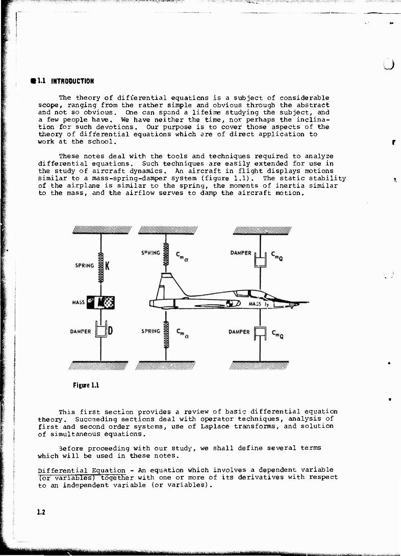
These notes deal with the tools and techniques required to analyze differential equations. Such techniques are easily extended for use in the study of aircraft dynamics. An aircraft in flight displays motions similar to a mass-spring-damper system (figure 1.1). The static stability of the airplane is similar to the spring, the moments of inertia similar to the mass, and the airflow serves to damp the aircraft motion.

Figure 1.1

This first section provides a review of basic differential equation theory. Succseding sections deal with operator techniques, analysis of first and second order systems, use of Laplace transforms, and solution of simultaneous equations.

3efore proceeding with our study, we shall define several terms which will be used in these notes.

Differential Equation - An equation which involves a dependent variable (or variables) together with one or more of its derivatives with respect to an independent variable (or variables).

1.2

ma mmm - --

"*'*^-* "rv*'l-" .

Solution - Any function, free of derivatives, which satisfies a differential equation is said to be a solution of the differential equation.

Ordinary Differential Equation - A differential equation which involves derivatives with respect to a single independent variable is called an ordinary differential equation.

Order - The ntn derivative of a dependent variable is called a derivative of order n, or an ntn order derivative. The order of a differential equation is the order of the highest order derivative present.

Degree - The exponent of the highest order derivative is called the degree of the differential equation.

Linear Differential Equation (ordinary, single dependent variable) - A differential equation in which the dependent variable and its derivatives appear in no higher than the 1st degree, and the coefficients are either constants or functions of the independent variable, is called a linear differential equation.

Linear System - Any physical system that can be described by a linear differential equation is called a linear system.

General Solution - A solution of a differential equation of order n which contains n arbitrary constants will be called a general solution of the differential equation.

1.2 REVIEW OF BASIC PRINCIPLES

Before investigating operator notation and Laplace transforms, let's review the more basic methods of solving differential equations.

il2.1 DIRECT INTEGRATION

To solve a differential equation we seek a mathematical expression, relating the variables appearing in the differential equation, which qualifies as a solution under the definitions given above. A first thought or inspiration may be: since we are presented with an equation containing derivatives, a solution may be obtained by antidifferentiating or integration. This process removes derivatives and provides arbitrary constants.

EXAMPLE

Given

£ - * ♦ «

rewriting

dy = (x + 4)dx

1.3

IDIt^j nugmfrjim^gi

fy'.T- ;". .■,'■.. .-7*1 v-zjf^^vjxe^z-:.?*^-»■.- ■■ ■ ^7^* -- T ^*jt^:n ii^wf^p**»^?''1«' ■"?. ^'..vr^»^ '■'^■■^^fa^^TPW^^^^.- ■*,." .? - - tf"^E^'*tT»^37«W5-!^lfS '^ !i?W"19!Wgi»;L !! V* |ij^' --I *-yJ^T^T**'V*r?>*T'■-

integrating

dy = (x + 4)dx + C

gives us

2 y = *— + 4x + C Z~

EXAMPLE

Given

(1.1)

W

d y =-4- = x + 4 dx^

Assume

2 * d y _ dy

d7 3x~

where

ax

then

d(y') -air1* * + 4

or d(y') = (x + 4)dx + c

then

.i = dy „ x' cfx T~ + 4x + C,

integrating again

2 j~ T 4x 1- u1; dx + C_ dy = (y- + 4x + CJ dx +

giving

1.4

x 2 y - g— + 2x + cxx + c2 (1.2)

BMiiriiirimti v n ■,-, tur » ,f--'-'-^^^.J.-^^.. ^.

■7^™JT'V f\T" rrr' *■> =T ■'<as:.T*

Jfc Equations 1.1 and 1.2 qualify as general solutions under the defi-

nition stated earlier.

Life is full of disappointments and we would soon learn that this direct application of the integration process would fail to work in many cases.

EXAMPLE

2xy + (x2 + cos y) g£ = 0 (1.3)

: or

;■

ay =

dy =

-2xy

x + cos y

-2xy dx + C x + cos y

(1.4)

o We cannot perform the integration of the term to the right of the

equal sign in equation 1.4. Equation 1.3 can be solved, however, using straightforward techniques. (x^ + sin y = c is a general solution.) We emphasize the word "technique" since the solution may rely upon novel approaches, special groupings, or "judicious arrangements" and, perhaps, witchcraft or conjuring. The former require extensive experience arid maturity within the discipline, and the latter talents are rarely endowed by nature. We shall study a few special differential equations which are easy to solve and have wide application in the analysis of physical problems.

»1.2.2 FIRST ORDER EQUATIONS

We shall consider briefly the first order ordinary differential equation. Suppose we represent such an equation by

F(y\ y, x) = 0

where

y dx

This is concise notation used by mathematicians to denote a differential equation containing an independent variable x, a dependent variable y, and the derivative of y witn respect to x. The equation may contain the derivative in differential form.

EXAMPLES

dy _ cE

= x + y

1.5

■ IWM

i-;-.; jj-T ~>^!^^!?^5£!^7fBe»^^ ^^t^^^^sBS^-'»'^^^^ ■»^.E,'-.'--■; >.--( ■"- »7» *>gf^* i?»'w'BiiEE£i^

3x dx + 4y dy = 0

y. = x + y

dy _ x - y cos x dx sin x + y

r First order differential equations may be solved by

1. Separating variables and integrating directly.

2. Recognizing exact forms and integrating directly. 4

3. Finding an integrating factor (fudge factor) which will make the equation exact.

4. Inspection, rearrangement of terms, etc., to use method 1 or 2, or a combination of the two.

These methods are thoroughly treated in all elementary differential equations texts. A brief review of methods 1 and 2 is given below.

• 1.2.2.1 SEPARATION OF VARIBLES

When a differential equation can be put in the form | »

f1(x)dx + f2(y)dy = 0 (1.5)

where one term contains functions of x and dx only, and the other functions of y and dy only, the variables are said to be separated. A solution of equation 1.5 can then be obtained by direct integration

f1(x)dx + f2(y)dy = C (1.6)

where C is an arbitrary constant. Note, that for a differential equation 4 of the first order there is one arbitrary constant. In general, the number of arbitrary constants is equal to the order of the differential equation.

EXAMPLE ,

2 cty = x + 3x + 4 3x y + 6

(y +6) dy = (x2 + 3x + 4) dx

(y + 6)dy = (x2 + 3x + 4)dx + C

2 3,2 Y , r x . 3x

1.6

iiMüMBiiaüiMwiiiiwM i ii iiiiMüiiiir--■ -

TH??E*::*,r,^\7'r"" v' ""WWP ""-*,"?F'»Tv.

•1.2.2.2 EXACT DIFFERENTIAL EQUATION

Associated with each suitably differentiable function of two variables f(x,y) there is an expression called its tot^l differential, namely,

df - Üdx + If <* Conversely, if the differential equation

M(x,y)dx + N(x,y)dy = 0

has the property that

(1.7)

(1.8)

M(x,y) = || and N(x,y) = |i

then it can be rewritten in the form

Ji dx + |i dy = df = 0 3x 3y J

from which it follows that

f(x,y) = C

is a solution. Equations of this sort are said to be exact, since, as they stand, their left members are exact differentials.

A differential equation

M(x,y) dx + N(x,y) dy = 0

is exact if and only if

3M = 3N 3y 8x

(1.9)

If the differential equation

M(x,y) dx + N(x,y) dy = 0

is exact, then for all values of k,

f x f y Ja M(x,y) dx +Jb N(a,y) dy = k

is a solution of the equation.

(1.10)

1.7

MPFysrgiPBja'^rT'-i 'i-s^m-^v^!m,t»*'imi'_mp^^www'^^w, is 'm-*? >7T?»3^T^»w^yffW»»^^?grr»Tr:\^ ' i wpyjllj \<WmBIJAW

Ü EXAMPLE

Show that the equation

(2x + 3y - 2)dx + (3x - 4y + l)dy - 0

is exact and find a general solution.

Applying the test, we find

M _ 3(2x + 3y - 2) _ - 3y 3y

W = a(3x - 4y + 1) = ., 9x 3x

Since the two partial derivatives are equal, the equation is exact. Its solution can be found by means of equation 1.10.

r x ry Ja (2x + 3y - 2)dx +Jh (3a - 4y + l)dy = k

(x" + 3xy - 2x) + (3ay -2y + y) = k

(x2 + 3xy - 2x) - (a2 + 3ay - 2a) + (3ay - 2y2 + y) - (3c*b - 2b2 + b) = k

x2 + 3xy - 2x - 2y2 + y = k + a2 - 2a + 3ab - 2b2 + b = K

•1.2.2.3 FIRST ORDER LINEAR DIFFERENTIAL EQUATIONS

We conclude the discussion of first order equations by considering the followino form

% + R(x) y - 0 3x" (1.11)

where R(x) may be a constant. To solve, merely separate variables.

& + R(x) dx ■ 0 y

integrating

1.8

f & s - |R(X) dx + C

where

C' = In C

- - - ■■- —-—*-*—»- äaajJÜSaS^^-i.;,^-,^..-..-. . «::.».* ^^^»^..„^..ttfcjB.y.i.-Jn«

-*-„*.--r ■-■-.-.■,—<>--TT_, '^^W';:^'^r"wi- ■.. r ."»•->rj;"7-wwi ?.,-:? T-'. :-*.",i;--.-i

Thus

In y = - 'R(x) dx + In C

or

y = Ce - R(x) dx

If R is a constant, then

y = Ce'Rx (1.12)

We might conclude from this result that a first order differential equation of form 1.11 with constant coefficients may be solved quite simply. This is true and the solution will always have the form of equation 1.12.

EXAMPLE

g+2y-o (1.13)

then we have directly

o y = Ce l~2< x (1.14)

which is the general solution. It is quickly recognized t.iat the solution is easily obtained by plugging the negative of the coefficient of y into the position indicated by the small square.

PROBLEMS: Set I, Nos. 1 and 2, page 1.76.

11.3 LINEAR DIFFERENTIAL EQUATIONS AND OPERATOR TECHNIQUES

is A form of the differential equation that is of particular interest

n-1 Ady.A,a y, , A_ dy , . £/% (1.15)

. , A0 are all functions of If the coefficient expressions An, An_i, . x only, then equation 1.15 is called a linear differential equation. If the coefficient expressions An, . . . , A0 cire all constants, then 1.15 is called a linear differential equation with constant coefficients.

1.9

iüHifc ■HMM ^■^'-■^•Jiiwrriifiiffl[BiifalJiBirill]iiiwlti-ff-tl ■■ ■■■■,-„

^4r'»<>*r>!^^,n-lV.^»±*^^™tr * ' TT»-^*SCTW«'F'«siKT'tWWWiraHKK^ ■ TJ»I^l^jt||J»Wll!!i,

EXAMPLE U

dx xy = sin x

is a linear differential equation.

EXAMPLE

<=[-y + 6 Ä + 9y - e* dx* 37

is a linear differential equation with constant coefficients. Linear differential equations with constant coefficients occur frequently in the analysis of physical systems. Mathematicians and engineers have developed simple and effective techniques to solve this type of equation by using either "classical" or operational methods. When attempting to solve a linear differential equation of the form

Ady.A .d y , n—£- + n-1 ——4- + , n , n-1 dx dx + A, i + V - f (x) (1.16)

it is helpful to examine the equation

A dny

dx + A

an-l

n-1 dx rwT +AlI+ V = 0 (1.17)

u

1.17 is the same as 1.16 with the riqht hand side zero. We shall refer to 1.16 as the general equation and equation 1.17 as the complementary or homogeneous equation. Solutions of equation 1.17 possess a useful property known as superposition, which may be briefly stated as follows: Suppose yi(x) and y2(x) are distinct so]utions of 1.17. Then any linear combination of y^(x) and Y2(x) 1S also a solution of 1.17. A linear

combination would be C^y^(x) + C2y2(x)«

EXAMPLE

ü - 5 *y + o7 a*

6y = 0

e x is a solution, and that y2<x) = e x It can be verified that y^(x) is another solution which is distinct from y^(x). Using superposition,

3x 2x then, y(x) = c.e + c0e is also a solution.

1.10

■"■ MNM^Hita

-<s^r^^-f-^7?-'7 •'<'"'^ -.--i-v —'! — ■■[-■:.;■: -■■■;■'^■nr^"^:^r-^*~^ *£&&*&£*'*?•;■?• - '!rr^-"w^n'jr^.T^^:7^rm^;--

o Equation 1.16 may be interpreted as representing a physical system

where the left side of the equation describes the natural or designed state of the system, and where the right side of the equation represents the input or forcing function.

One might logically pursue the following line of reasoning in attempting to find a solution to the problem described by equation 1.16.

A general solution of 1.16 must contain n must satisfy the equation.

arbitrary constants and

2. The following statements are justified by experience:

a. It is reasonably straightforward to find a solution to the complementary equation 1.17, containing n arbitrary constants. Such a solution will be called the transient solution. Physically, it represents the response present in the system regardless of input.

b. There are varied techniques for finding a solution of the differential equations due to this forcing function. Such solutions do not, in general, contain arbitrary constants. This solution will be called the particular or steady state solution.

3. If we take the transient solution which describes the response already existing in the system, and then add on the response due to the forcing function, it would appear that a solution so written would blend the two responses and describe the total response of the system represented by 1.16. In fact, the definition of a general solution is satisfied under such an arrangement. This is simply an extension of the principle of superposition. The transient solution contains the correct number of arbitrary constants, and the particular solution guarantees that the combined solutions satisfy the general equation 1.16. Call the transient solution yt and the particular solution yp. A general solution of 1.16 is then given by

y = yt + yp (1.18)

H.3.1 TRANSIENT SOLUTION

Equation 1.13 is a complementary or homogeneous first order linear differential equation with constant coefficients. We recognized a quick and simple method of finding a solution to this equation. We also recognized that the solution was always of exponential form. We might hope that solutions of higher order equations of the same family would take the same form.

Let us examine a second order differential equation with constant coefficients to determine if

y = emx (1.19)

is a solution of the equation

ay" + by' + cy = 0 (1.20)

1.11

MMMHM IMtosa^iAmj ■-■■■-■ KJMHSAiUUiäM

F!T35I^55^!!3^^ir*?"-"':''?:-'" ~;--.™"'vW^'^~-^W"»w^»!W«»Wlip^- .— r"^~*~^^^~rpXS!^»r*$£^'l*-r,',-s t». nigmyigpii^.i^y,,^^, . ,.

mv Substituting y = e we have

2 mx , . mx , mx n am e + bme + ce = 0

or

(am2 + bm + c)emx = 0 (1.21)

mx , n Since e ? 0

2 am + bm + c = 0 (1.22)

and

-b + y/l b - 4ac ml,2 " —"Ti (1-23)

Substituting these values into our assumed solution we force it to become a solution.

m, x irux yt = C^ l + C2e l (1.24)

When working numerical problems it is not necessary to take the deriva-

tives of e x, if we remember that the d y/dx is replaced by iu . This will be true for any order differential equation with constant coefficients .

We have included the subscript "t" on y to indicate that 1.24 represents the transient solution. From the foregoing it is seen . c we have succeeded in extending the method for first order complementary equations to higher order complementary or homogeneous equations. Again we note that we have traded off an integration problem for an algebra problem (solving equation 1.22 for the m's).

Differential or derivative operators can be defined and manipulates to play the same role as m above.

If we designate an operator p, p2, . . . , pn as follows:

d 2 d n_d MOC\ p = 3x-'p =TT' •••'!? = —n (1'25)

dx dx

P(y) =% p2(y) = ^J pn(y) - ^J (1.26) dx dx dxn

1.12

J

in munim

^^■"vw.J.T'V-'-^" v.-Vs.;:-..:r*-Tii?.; ~-~-y-".r'.w^?^ %,&*****»*• K '^ff&W' '■ ""•-'"■■ -'" '^KVfr^TTtffij&tiPgl&r™??:^, A ~-~?--x-^^F*&^rt^jyj:?™vrrs-;-'-?-rv ■. •

then 1.20 may be written

ap2(y) + bp(y) + cy = 0 (1.27)

or, since the derivative operates linearly (each term in succession),

(ap + bp + c)y = 0 (1.28)

and the operator expression (ap + bp + c) has the same algebraic structure as 1.22. The operator expression in 1.26 is a polynomial with precisely the same form as the polynomial on the left side of 1.22, hence it is often solved directly for the constants required in the solution of 1.19. In this case, the transient solution 1.24 would appear

p.x , P„x = c,eFl + c~e 2 (1.29)

There are cases for which 1.24 and 1.29 are not entirely satisfactory in providing a solution, but this will be discussed later. Tb= m's or p's may be real, imaginary, or complex numbers.

EXAMPLE

§4 + dy _ 2y = 0 dx7 dx

Using operator notation,

(p2 + p - 2)y = 0

p2 + p - 2 = 0

p = 1, -2

y = c,ex + c9e -2x

We shall now consider the various cases for solutions of the complementary (homogeneous) equation.

Consider the equation

I dx

ad4+b| + cy 0 (1.30)

We have seen above that the solution of this differential equation is equivalent to solving the characteristic equation

ap^ + bp + c = 0 (1.31)

1.13

mrnrnm. Tim-

.JS^

u The general solution of 1.30 is of the form

xt « Cle Pxx

+ c-e p2x

(1.32)

where c^ and 03 are arbitrary constants, and pi and P2 are solutions of the characteristic equation 1.31. Pecall from algebra that a characteristic equation can yield complex roots, imaginary roots, or real roots,

that is, p. - = [-b +~\/b - 4 ac]/2a) . We will consider the solution

1.32 for various values of the constants in equation 1.31 and consider changes in the form of the solution which may be desirable or necessary.

•1.3.1.1 CASE 1: ROOTS REAL AND UNEQUAL

If p^ and P2 are real and unequal the desired form of solution is just as is

EXAMPLE

Ü + 4 p- - 12y = 0 ^7 dx

(P + 4p - 12)y = 0 (in operator form)

solving

p2 + 4p - 12 = 0

gives

-4 + /16 + 48' P =

-4 + 8 = —

2

or

P = -6, 2

and

y = c.e + c»e 2x

is the required solution.

1.14

1^.,^^^. .,■-.,,....^i^^,^,,^..^.^.^.,,.

d •1.3.1.2 CASE 2: ROOTS REAL AND EQUAL

If p, and P2 are real and equal we run into trouble.

EXAMPLE

d y dx

- 4 dy 3x" + 4y = 0

(P - 4E > + 4)y = 0 (in o

solving,

P = 4 + /IS - 16 4

" 2" ~ 2

2

Ü

or p = 2. But this gives only one value of p. If we try to use 1.32 2x all we get is y - cje but we need two arbitrary constants to have a

transient solution like 1.30. If we are really alert, we may notice that the operator expression (p2 - 4p + 4) can be written (p -2)(p - 2), or (p - 2)2, which is a polynomial expression with a repeated factor.

2x 2x (that is, p = 2; 2 is the solution.) We can then write y = C]_e + C2e as the transient solution. This is really no better than our first

2x attempt, y = cê , since c^ and C2 can be combined into a single arbitrary constant.

y - Cje -2X i. „ «2X _ /„ X r. ^2X - „ ~2X v c,e = (c. + c_)e = c,e

To solve this problem, simply multiply one of the arbitrary constants 2x 2x by x. Now write: y = cê + C2xe . We can no longer "lump" the two

2x coefficients of e together. The solution now contains two arbitrary constants, and it is easily verified that

2x , 2x y. = c,e + c-xe

is a transient solution of the problem above.

•1 3.1.3 CASE 3: ROOTS PURELY IMAGINARY

EXAMPLE

A If

in operator form

(p2 + l)y = 0

1.15

MMMM HUM |t|MMM||>^ L.-—L.i.'i .1.. . ■.-u-iji. UiÄu>kd.dUîJ«i^

Solving,

0 + /0 - 4 P = = + /=r

In most engineering work we refer to /^T as j, it is denoted by i.). Now,

P - + j

and the solution is written

(In mathematical texts

yt = c^e3* + c2e

-:|X (1.33)

This is a perfectly good solution from a mat- * natical standpoint, but it is unwieldy and unsuggestive to engineers. A mathematician by the r.ame of Euler worked out this puzzle for us by developing an equation called Euler's identity.

e3 = cos x + j sin x (1.34)

This equation can be restated in many ways geometrically and analytically, and can be verified by adding the series expansion of cos x to the series expansion of j sin x. Now 1.33 may be expressed

y = c, (cos x + j sin x) + c_ [cos (-x) + j sin (-x)]

= (c. + c_) cos x + j (c, - c~) sin x (1.35)

or

y^ = c, cos x + c. sin x Jt 3 4 (1.36)

Equation 1.36 has another interesting form. Let

*t *,/ C3 + °4

■ff7^' COS X +

y sin x

2 . 2 c3 + c4

(1.37)

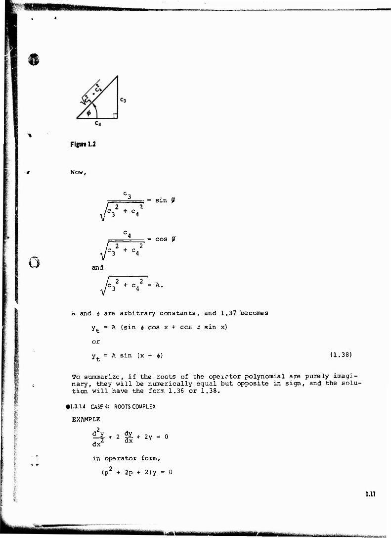
Now consider a right triangle with sides labeled as follows;

1.16

mammm

n

Figure 1.2

Now,

v^7^ » = sin 9

i 2 L 2 c3 + C4

- = cos 0

and

/c32 + c4

2 = A.

A and 4> are arbitrary constants, and 1.37 becomes

y. = A (sin $ cos x + cos 4> sin x)

or

y = A sin (x + $) (1.38)

To summarize, if the roots of the opeictor polynomial are purely imaginary, they will be numerically equal but opposite in sign, and the solution will have the form 1.36 or 1.38.

•1.3.1.4 CASF4: ROOTS COMPLEX

EXAMPLE

«4 + 2 % + 2y - 0 dxz ax-

in operator form,

(p2 + 2p + 2)y = 0

1.17

u Solving,

-2 + /r^T p = ^

or

= -1 + /IT

p = -1 + j, - 1 -j

and

yt = C;Le (-1 + j)x + e(-l -j)x (1.39)

Equation 1.39 may be written

yt - e -x ~3X i ~-3x c,eJ + c~e J

or, using the resile 1.36 and 1.38,

yt »e

or

c, cos x + c. sin x 3 4

A sin (x + $)

(1.40)

(1.41)

Note, also, that 1.38 could be written in the form

y = A cos (x + e), where 9 » <f> - 90°

PROBLEMS: Set I, No. 3, page 1.76; Set II, a only, page 1.85.

• 1,3.2 PARTICULAR SOLUTION

The particular solution, for our work here, will be obtained by the method of undetermined coefficients. (There are other methods which may be used.) This method consists of assuming a solution of the same general form as the input (forcing function), but with undetermined coefficients. Substition of this assumed solution into the differential equation then enables us to evaluate these coefficients. The method of undetermined coefficients applies when the forcing function or input is a polynomial, terms of the form sin ax, cos ax, eax, or combinations of sums and products of these. The complete solution of the linear differential equation with constant coefficients is then given by 1.18 (that is, the solution tc the complementary equation (transient solution), plus the particular solution).

1.18

-i™,^..*,..!....

{$ A few remarks are appropriate regarding the second order linear

differential equation with constant coefficients. Although the equation is interesting in its own right, it is of particular value to us because it is a mathematical model for several problems of physical interest.

?I+b-g+ cy - F(x) dx

(mathematical model)

m d x j. m —n- + dt

dx 3t

+ Kx = F(t) (describes a mass spring (1.42) d'mper system)

'^♦»8S + &-«<« (describes a series LRC electrical circuit)

Equation 1.42 are all the same mathematically, but are expressed in different notation. Different notations or symbols are employed to emphasize the physical parameters involved, or to force the solution to appear in a form that is easy to interpret. In fact, the similarity of these last two equations may suggest how one might design an electrical circuit to simulate the operation of a mechanical system.

Consider the equation

,2 7 ^ i. _

a? al4+b^+cy= f(x) dx

(1.43)

We now must solve for the special solution (particular solution) which results from a given input, f(x). This particular solution can be found by using various techniques, but we will consider only one, the method of undetermined coefficients. This method consists of assuming a solution form with unspecified constants (undetermined coefficients), and solving for the values of the constants which will satisfy the given differential equation. The method is be.*-t described by considering examples.

•1.3.2.1 FORCING FUNCTION - A CONSTANT

dx (1.49)

The input is a constant (trivial polynomial), so we assume a solution 2 2 of form y = K. Obviously, d~K/dx = 0, and dK/dx = 0.

Substituting,

0 + 4(0) + 3K = 6

y = K = 2

1.19

(HM ÜMM «MH«HMMW< ■um MBjjaääattMEiiMi

r .< t-r~** - a>- .; ■

Therefore, yp = 2 is a particular solution. We note that we can solve the equation

£l + 4 p. + 3y = 0

in operator form 2

(p + 4p + 3)y = 0

or

P = -1, -3

and the transient solution is

-x . -3x yt = c^e + c2e

The general solution of 1.44 may be written

y = cne"x + c,e~3x

transient particular solution (or steady state)

solution

•1.3.2.2 FORCING FUNCTION - A POLYNOMIAL

EXAMPLE 2

ly + 4 $L + 3y = x2 + 2x (1.45) d~7 dx

Now the form of f(x) for 1.45 is a polynomial of second degree, so we assume a particular solution for y of second degree (that is, let y =

Ax2 + Bx + C).

Then

dy

and

3-E = 2Ax + B dx

-^X = 2A

1.20

0

w*

■■■^^■■■HBBSHflilMiriianiiiMiiM^aMMM^MMMNaa« ,-a..~.„:-. ...:,. ... ,,,.„

I

o

Substituting into 1.45,

(2A) + 4 (2Ax + B) + 3 (Ax2 + Bx + C) = x2 + 2x

or

(3A) x2 + (8A + 3B) x + (2A + 4B + 3C) = x2 + 2x

Equating like powers of x,

x2: 3A = 1

A = 1/3

x: 8A + 3B = 2

3B = 2 - 8

B = - 2/9

x°: 2A + 4B + 3C = 0

3C = 8/9 - 2/3

C = 2/27

Therefore,

y = 1/3 x2 - 2/9 x + 2/27

The general solution of '1.45 is given by

y = c-je'* + c2e"3x + 1/3 x2 - 2/9 x + 2/27

since the transient solution is the same as for 1.44. As a general rule, if tha forcing function is a polynomial of degree n, assume a polynomial solution of degree n.

•1.3.2.3 FORCING FUNCTION = AN EXPONENTIAL

EXAMPLE

I dx 1^ + 4 *L + 3y = e2x (1.46)

2x The forcing function is e so we assume a solution of the form

y = Ae 2x

1.21

mmmm—m^m,* ■■-■— ■"■-■■■"--■- ■i JJ-J»'.. ■.-. IX.. s,l:...»■■■...,:.. ■■... . i>.v. .'.'„

- TI»^ ';^-~r ■■■-■--.;

3x" (Ae2x) = 2Ae 2x

* (Ae2x) = 4Ae2x

dx'

Substituting in 1.46,

4Ae2x + 4(2Ae2x) + 3(Ae2x) = e2x

e2x (4A + 8A + 3A) = e2x

The coefficients on both sides of the equation must be the same. There- fore, 4A + 8A + 3A = 1, or 15A = 1, and A = 1/15. The particular solu-

tion of 1.46 then is ¥p = 1/15 e 2x The transient solution is still the same as for 1.44. A final example will illustrate a pitfall sometimes encountered using this method.

•1.3.2.4 FORCING FUNCTION - AN EXPONENTIAL (SPECIAL CASE)

EXAMPLE

H ♦«£ ♦ * - •■ dx (1.47)

I )

The forcing function is e , so we assume a solution of the form y = Ae

Then

dx

and

d (Ae-X) = Ae-X

dx

Substituting

1.22

Ae"x + 4(-Ae~x) + 3(Ae"X) = e"X

(A - 4A + 3A)e"x = e~x

(0)e"x = e"x

■MM ■-'-1 i iüüa—^-^.^-.-.-..'.■: ,, i.,-i,W^-.^,,..,....

ijp Obviously, this is an incorrect statement. To find where we made our mistake, let's review our procedures.

To solve an equation of the form

(p + a) (p + b)y » e -ax

we solve the homogeneous equation to get

(p + a) (p + b)y = 0

p = -a, -b

y* = c.e"ax + c-e .-bx 2*

If we assume y = Ae P

then

y - Yt + Yp = cie'aX + c2e_bX + Ae = (ci + A)e_ax + c2e"bx

= c,e + c2e

- y*

However, we have already seen that yt is the solution only when the right side of the equation is zero, and will not solve the equation when we have a forcing function. Therefore, we assume a particular solution.

yp = Axe -ax

then

-ax -bx -ax -ax -bx Y = Y + Yt = of + c2e "A + Axe aA = (Cj_ + Ax)e aA + c2e "Ä t yfc

Similarly, we could have the equation

(p + aj) (p - aj) y = sin ax

with transient solution

y. = c1 sin ax + c2 cos ax

If we assume y = A sin ax + B cos ax P

then

y = y + y = (c. + A) sin ax + (c2 + B) cos ax

■MM. •üMMMH "■*">">" - HMüih .....

1.23

+ (c2 + B) cos ax

= c, sin ax + c. cos ax = y.

Therefore, we assume

y - Ax sin ax + Bx cos ax

and

y = (c, + Ax) sin ax + (c, + Bx) cos ax ^ y.

Note the following, however, with the equation

(p + a - jb) (p + a + jb)y = sin bx

u

yt - e -ax

(c. sin bx + c» cos bx)

we can assume y = B sin bx + C cos bx P

then

y = c^ sin bx + c„e cos bx + B sin bx + C cos bx

-ax -ax y = (c^ + B) sin bx + (c2e aA + C) cos bx ft y

Similarly, if

(p + a - jb) (p + a + jb)y = e -ax

we could assume

» -ax y = Ae P

In our example above, equation 1.47, a valid solution can be found -x by assuming Y = Axe , then

^ (Axe~x) = A(-xe"x + e"x)

and

ax (Axe_X) A(xe'X - 2e"X)

1.24

— mM^immmmim ,^...v>-..,^ „^^..„,. ,,, ..^f^j-^-^^—,..u..-„

■»SW"S^JK*™ -^^fvl^^^ ^r>^w«^T^";'. ^jfw.W-.r'wssr^",- - ..- ■■■ ^^»'^^«•^,^:^i'«T,i"^^^t^:^;-:;,'^WrvVi:,T'""'Tr":''-*: ' "' ^"■^ ' ■ ■- '"■'■ '"'■•'.' : .-■--..., ■.:Tr';i;wW( ^j^.^.-;,^,-^»-^^^^;

9 Substituting

A(xe"x - 2e"x) + 4A(-xe"x + e"x) + 3(Axe~x) = e"x

(A - 4A + 3A)xe"X + (-2A + 4A)e"X = e"X

and

(0)xe"x + 2Ae"x = e'x

A ■ 1/2

Thus,

yp = (1/2)xe -x

)

4> 4*r

is a particular solution of 1.47, and the general solution is given by:

y = C;Le'x + c2e"3x + 1/2 xe"x

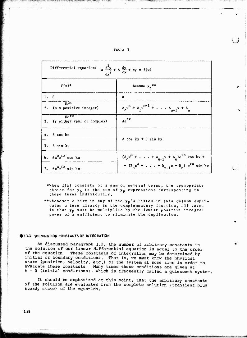
The key to successful application of the method of undetermined coefficients is to assume the proper form for a trial particular solution. Table 1 summarizes the results of this discussion.

PROBLEMS: Set II, 1-5, b only, page 1.85.

1.25

tmm^mmm ■—■■■■■» ■■ ■ i—

^?J^v*;T-wvr^.:.,p -"vimjfi^zr 75**ffiPS^P ■■■^^...,--■:-:.:J-..^ ■--.t-w^-'v^**™^, 7^s-i~r.*r--Trv--r!^'-yjt-v 7-.

Table I

u

2 Differential equation: d y . , dy , £/x n a —£ + b -p + cy ■ f (x)

dx

f(x)* Assume y ** P

1. ß A

ßxn

2. (n a positive integer) Ax + A, x +...A ,x + A o 1 n-1 n

ßerx

3. (r either real or complex) A rx

Ae

4. ß cos kx A cos kx + B sin kx

5. ß sin kx

c a n rx i 6. ßx e cos kx (Ax +...+A ,x + A )e cos kx + o n-1 n

n rx + (B x + . . . + B .x + B ) e sin kx

o n-1 n i o n rx . , 7. ßx e sin kx

*When f(x) consists of a sum of several terms, the appropriate choice for yp is the sum of yp expressions corresponding to these terms individually.

**Whenever a term in any of the yp's listed in this column dupli- cates a term already in the complementary function, all terms in that yp must be multiplied by the lowest positive integral power of x sufficient to eliminate the duplication.

M.3.3 SOLVING FOR CONSTANTS OF INTEGRATION

As discussed paragraph 1.2, the number of arbitrary constants in the solution of our linear differential equation is equal to the order of the equation. These constants of integration may be determined by initial or boundary conditions. That is, we must know the physical state (position, velocity, etc.) of the system at some time in order to evaluate these constants. Many times these conditions are given at t = 0 (initial conditions), which is frequently called a quiescent system.

It should be emphasized at this point, that the arbitrary constants of the solution are evaluated from the complete solution (transient plus steady state) of the equation.

1.26

■:- Ji-w.„u-.>...^i-^.

""" ' ' ———— ""' ' 1

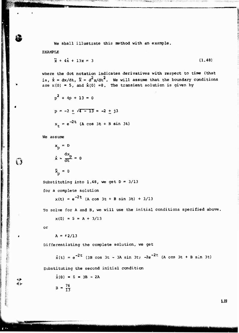
We shall illustrate this method with an example.

EXAMPLE

x + 4x + 13x = 3 (1.48)

where the dot notation indicates derivatives with respect to time (that

is, x = dx/dt, x = d'x/dt2. We will assume that the boundary conditions are x(0) = 5, and x(0) =8. The transient solution is given by

p + 4p + 13 = 0

o

r I 4»

p - -2 + /4 - 13 = -2 + j3

x = e (A cos 3t + B sin 3t)

We assume

Xp=D

dx

x = 0 p

Substituting into 1.48, we get D = 3/13

for a complete solution

x(t) = e"2t (A cos 3t + B sin 3t) + 3/13

To solve for A and B, we will use the initial conditions specified above,

x(0) = 5 = A + 3/13

or

A = ^2/13

Differentiating the complete solution, we get

x(t) = e"2t (3B cos 3t - 3A sin 3t; -2e"2t (A cos 3t + B sin 3t)

Substituting the second initial condition

x(0) = 8 = 3B - 2A

76 B = re

1.21

L )

I

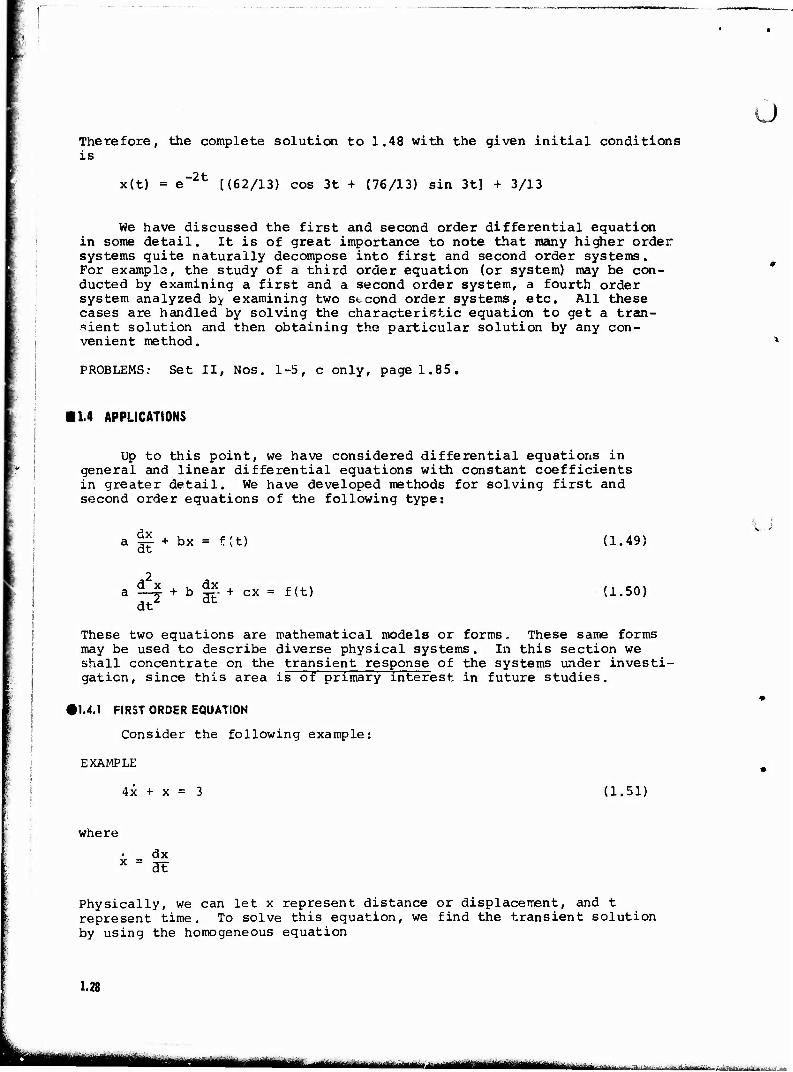
Therefore, the complete solution to 1.48 with the given initial conditions is

x(t) = e~2t [(62/13) cos 3t + (76/13) sin 3t] + 3/13

We have discussed the first and second order differential equation in some detail. It is of great importance to note that many higher order systems quite naturally decompose into first and second order systems. For example, the study of a third order equation (or system) may be conducted by examining a first and a second order system, a fourth order system analyzed by examining two stcond order systems, etc. All these cases are handled by solving the characteristic equation to get a transient solution and then obtaining the particular solution by any convenient method.

PROBLEMS: Set II, Nos. 1-5, c only, page 1.85.

11.4 APPLICATIONS

Up to this point, we have considered differential equations in general and linear differential equations with constant coefficients in greater detail. We have developed methods for solving first and second order equations of the following type:

a ^ + bx = f(t) (1.49) at

a i-£ + b ~ + ex = f (t) (1.50) dt

These two equations are mathematical models or forms„ These same forms may be used to describe diverse physical systems. In this section we shall concentrate on the transient response of the systems under investigation, since this area is of primary interest in future studies.

H.4.1 FIRST ORDER EQUATION

Consider the following example:

EXAMPLE

4x + x = 3 (1.51)

where

• _ dx x " at

Physically, we can let x represent distance or displacement, and t represent time. To solve this equation, we find the transient solution by using the homogeneous equation

1.28

tmmm^ ..^^*^<«^^^ i(MjBM||gM|MMjM[|M) ^ ^ ^ ^^

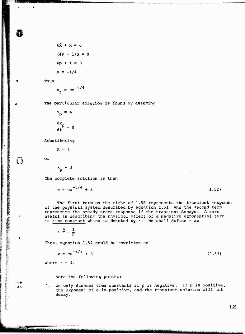
n 4x + x = 0

(4p + l)x = 0

4p + 1 = 0

p = -1/4

Thus

xt = ce -t/4

The particular solution is found by assuming

xp = A

dx, P =

alT

o

Substituting

A = 3

or

x = 3 P

The complete solution is then

-t/4 J -, x = ce ' +3 (1.52)

The first term on the right of 1.52 represents the transient response of the physical system described by equation 1.51, and the second term represents the steady state response if the transient decays. A term useful in describing the physical effect of a negative exponential term is time constant which is denoted by ■>., We shall define T as

x - - I " P

Thus, equation 1.52 could be rewritten as

x = ce ' +3 (1.53)

wnere = 4,

4P

Note the following points:

We only discuss time constants if p is negative. If p is positive, the exponent of e is positive, and the transient solution will not decay.

1.29

— -- ■

ri&t- ... - i a i i» » STVI i • i .»i^ati»i^^i»fc

2. If p is negative, T is positive.

3. T is the negative reciprocal of p, so that small numerical values of p give large numerical values of T (and vice versa).

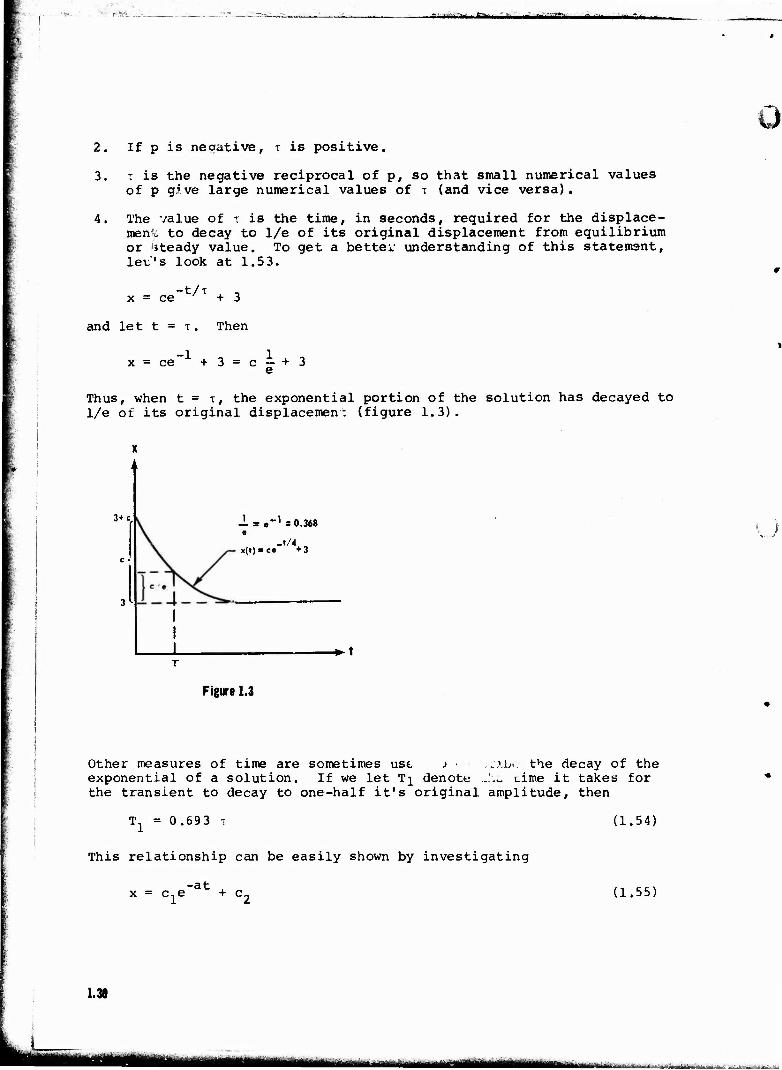
4. The value of t is the time, in seconds, required for the displacement to decay to 1/e of its original displacement from equilibrium or (steady value. To get a better understanding of this statement, let's look at 1.53.

x = ce +3

and let t = T. Then

-1 x = ce + 3 = c - + 3 e

Thus, when t = T, the exponential portion of the solution has decayed to 1/e of its original displacement (figure 1.3).

x 11

3+c 1 = «-' =0.348 e

x(t)»ce" +3

-**t

Figure 1.3

Other measures of time are sometimes ust > ■ .„'xbc the decay of the exponential of a solution. If we let T^ denote .:.~ cime it takes for the transient to decay to one-half it's original amplitude, then

T = 0.693 T

This relationship can be easily shown by investigating

-at x = c,e + c.

(1.54)

(1.55)

1.30

m mm mmttmm ia>Milafc^-:- ■" ' ■ ' ■ ■■■•■■ ' r '- ■

it Im M i ■; im ■ r

n From our definition, T = * /». We are looking for Tx, the value of t at which xt = 1/2 xt(0). Solving

xt = Cf -at

-aT, 1/2 xfc{0) = 1/2 cx «= c^e "*1

e"aTl = 1/2

In 1/2 = aT.

I"

if - »

. -in 1/2 = ,693 . >693T

x a a

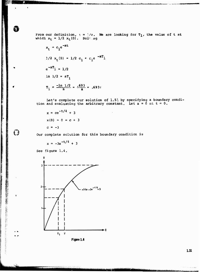
Let's complete our solution of 1.51 by specifying a boundary condition and evaluating the arbitrary constant. Let x = 0 at t = 0.

x = ce"t/4 + 3

x(0) = 0 = c + 3

c = -3

Our complete solution for this boundary condition is

x = .3e-fc/4 + 3

See figure 1.4.

X

3

Figure 1.4

1.31

mgj^yjj - ..JH... ,„.„..,.,.,. MMüMayi „ ,, ,,, ,, H'-irai

»1.4.2 SECOND ORDER EQUATION

Consider an equation of the form 1.50. The characteristic equation (operator equation) can be written:

ap +bp + c = 0 (1.56)

The roots of this quadratic equation determine the form of the transient solution as we have seen in paragraph 1.3. We will now discuss physical implications of the algebraic property of the roots.

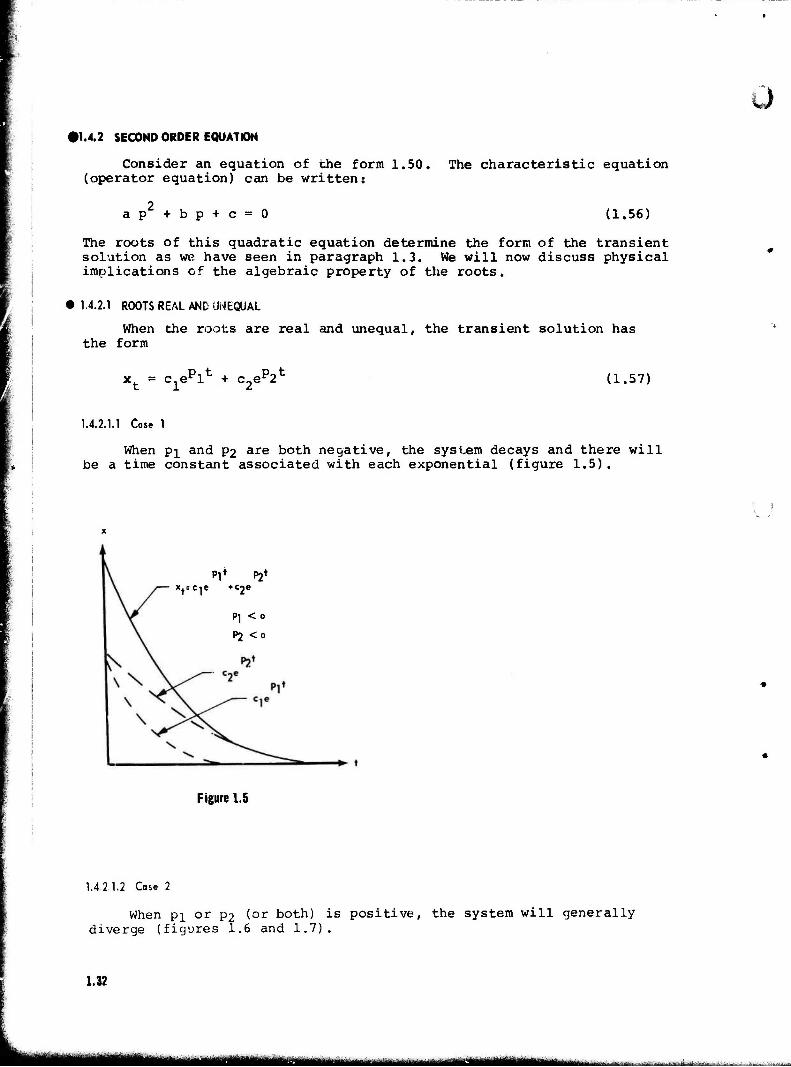
1.4.2.1 ROOTS REAL AND UNEQUAL

When the roots are real and unequal, the transient solution has the form

xf = c;,eplt + c_ep2t (1.57)

1.4.2.1.1 Case 1

When pi and P2 are both negative, the system decays and there will be a time constant associated with each exponential (figure 1.5).

Pi* P2* x}=cie +C2e

Pi < o

P2 <o

Figure 1.5

1.4 2.1.2 Case 2

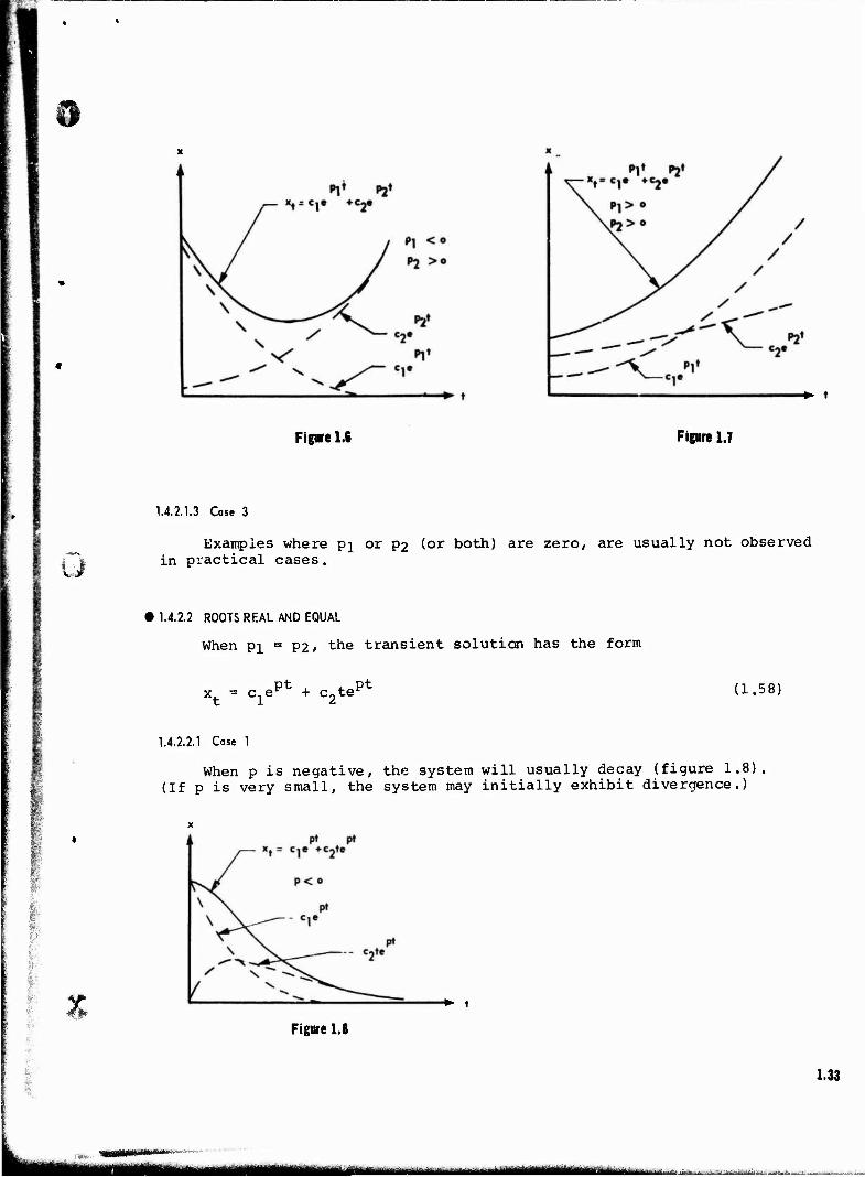
When pi or P2 (or both) is positive, the system will generally diverge (figures 1.6 and 1.7).

1.32

MiMüyttBka m -■■■-

ü

*■ t

Figure 1.6 Figure 1.7

u

1.4.2.1.3 Case 3

Examples where pj or P2 (or both) are zero, are usually not observed in practical cases.

• 1.4.2.2 ROOTS REAL AND EQUAL

When pi = P2, the transient solution has the form

pt , 4_„pt x. - c.e^ + c-te^ (1.58)

1 I

Vfp

1.4.2.2.1 Case 1

When p is negative, the system will usually decay (figure 1.8) (If p is very small, the system may initially exhibit divergence.)

Figure 1.8

•> t

1.33

Mi ., „|iMtiMMtM,|, „I,, |

u 1.4.2.22 Cose 2

When p is positive, the system will diverge.

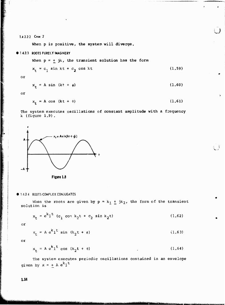
• 1.4.2.3 ROOTS PURELY IMAGINERY

When p = + jk, the transient solution has the form

x = c. sin kt + c« cos kt

or

or

x = A sin (kt + $)

x. = A cos (kt + 6)

(1.59)

(1.60)

(1.61)

The system executes oscillations of constant amplitude with a frequency k (figure 1.9).

xf= Asin(kt + ^>)

Figure 1.9

• 1 4,2.4 ROOTS COMPLEX CONJUGATES

When the roots are given by p = k-^ + 3^-2' tne f°rin of tne transient solution is

K I

k, t x. = e 1 (c, co'5 k?t + c_ sin k„t)

or

or

x = A eklfc sin (k2t + d>)

x = A eklfc cos (k2t + 6)

(1.62)

(1.63)

(1,64)

The system executes periodic oscillations contained in an envelope k t given by x = + A e 1

1.34

HI Miami in BjUjaiMl^i^^.^...^. ; :.^.l„„„;, ....:, ... ... .. .-.

4»

i i

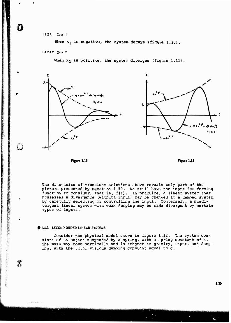
1.4 2.4.1 Cose 1

When kj is negative, the system decays (figure 1.10).

1.4.2.4.2 Cose 2

When k^ is positive, the system diverges (figure 1.11).

"s. kit . ^^y-'H-A« »in(k2» + 0>)

'

I*

^t +■ t

*<1t

\ X

Figure 1.10 Figure Lll

fe

The discussion of transient solutions above reveals only part of the picture presented by equation 1.50. We still have the input for forcing function to consider, that is, f(t). In practice, a linear system that possesses a divergence (without input) may be changed to a damped system by carefully selecting or controlling the input. Conversely, a nondi- vergent linear system with weak damping may be made divergent by certain types of inputs.

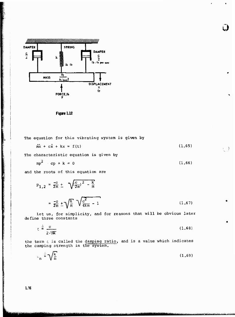
1.4.3 SECOND ORDER LINEAR SYSTEMS

Consider the physical model shown in figure 1.12. The system consists of an object suspended by a spring, with a spring constant of k. The mass may move vertically and is subject to gravity, input, and damping, with the total viscous damping constant equal to c.

5

1.35

» «

DAMPER

MASS lb

ft'»"2

i FORCE.Ib

Figure 1.12

Ö

SPRING I | F"^ DAMPER

m f U/h ! ih/hp"t,e

]T DISPLACEMENT

x ft

The equation for this vibrating system is given by

mi + ex + kx = f(t)

The characteristic equation is given by

2 mp cp + k = 0

and the roots of this equation are

(1.65)

(1.66)

-. /,c «2 pl,2 ~ 2m t Y^> -c

m

2m m

2 . - l 4km

(1.67)

Let us, for simplicity, and for reasons that will be obvious later define three constants

= c

2^mir (1.68)

the term c, is called the damping ratio, and is a value which indicates the damping strength in the system.

n V m (1.69)

1.16

Inii^i^^iy- ^w mm ■^»»i..^-^,.,.',. na ». aaaaaai

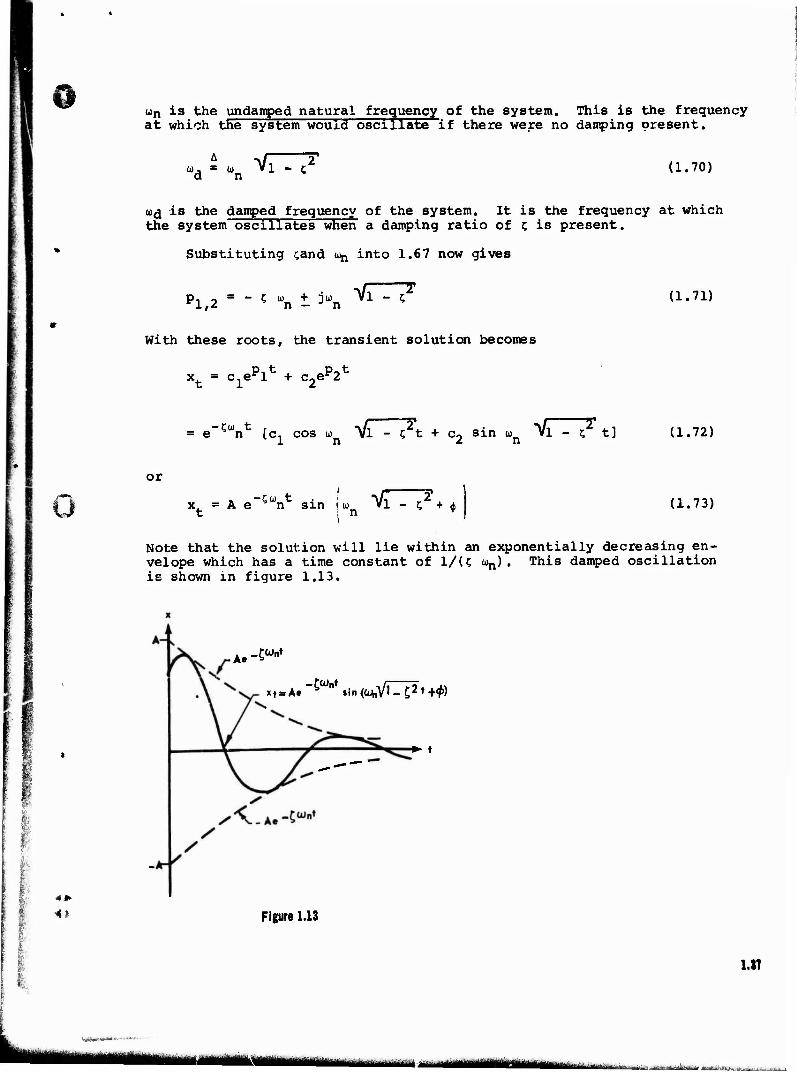
ö wn is the undamped natural frequency of the system. This is the frequency at which the system would oscillate if there were no damping present.

">d a un Vl " < (1.70)

w$ is the damped frequency of the system. It is the frequency at which the system oscillates when a damping ratio of c is present.

Substituting ;and 1^ into 1.67 now gives

pl,2 = ~ ; wn t jun "^ " c* (1,71)

With these roots, the transient solution becomes

xfc = c^V + c2ep2t

— tW t r = e s n [c. cos . öD Vl - ?t + c- sin u z n vrr^t c t] (1.72)

or

I

I

41

-tu t x. = A e n sin 1u t i n VT cr* (1.73)

Note that the solution will lie within an exponentially decreasing envelope which has a time constant of 1/U wn) . This damped oscillation is shown in figure 1.13.

-.At-*""*

xt. At "^ »in ((M,V'-C2t +<*>>

► t

Figure 1.13

1.3T

IIIMI 11

\sJ If we divide equation 1.65 by m we obtain

. c • . k f(t) x+-x+-x= ' mm m

or, rewriting using wn and x, defined by 1.68 and 1.69

x + 2 x. w x + u,2 x = ^^- (1.74) n n m

Equation 1.74 is a form of 1.65 that is most useful in analysing the behavior of any linear system.

A general second order physical system can be compared with mass- spring-damper system. The equation defining the system was

mx + cx + kx = f(t) (1.65)

where we defined the parameters

w ~ \l - i undamped natural frequency

-, damping ratio 2 /mk~

From equation 1.71 we see that the numerical value of t, is a powerful factor in determining the type of response exhibited by the: system.

PROBLEMS: Set II, 1-5, d only, page 1.86.

Let us now consider the physical problem and analyze the various conditions possible. The magnitude and sign of x,, the damping ratio, determine the response properties of the system.

There are five distinct cases which are given names descriptive of the response associated with each case.

1. x, = 0, undamped

2. 0 < x, < 1, underdamped

3. x, ~ 1, critically damped

4. c > 1/ overdamped

5 . x < 0, unstable

We shall now examine each case, making use of equation 1.71

Pi o = " < u„ t 3wn y1 " ^ (1.71) '1,2 - " <- wn

1.38

tmm i ^^.^^^—........... te»ghflMj>MMimBM

$ • 1.4.3.1 CASE 1: i • 0, UKDAMPED

For this condition, the roots of the characteristic equation are

Pl,2 = t K

giving a transient solution of the form

x. = c. cos w t + c_ sin u t t 1 n 2 n

(1.75)

(1.76)

or

x. = A sin (io t + i) t n (1.77)

showing the system to have the transient response of an undamped sinusoidal oscillation with frequency wn. (Hence, the designation of wn as the "undamped natural frequency.") Figure 1.9 shows an undamped system.

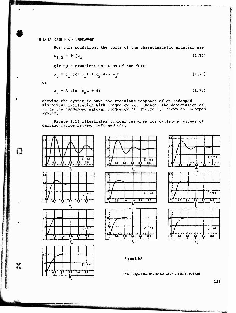
Figure 1.14 illustrates typical response for differing values of damping ratios between zero and one.

i

1.5

1(1 / ~x ,« 7 /..

C, 0.4

0.5 10 IS 2.0 2.5 [ . 1 , . 1 1

w 53To ii fo p

1.5

10

.5 (,= 0.3

0.5 10 15 2 0 15

1.5

1.0

.5

0

C= 0.6

0. i 1

5 1.0 1.1 2.0 2.6

t n 1

n 1 n

1.0

"#

1.0

.a

0

LO

.5

0

<- 0.7

..c:

0.8

.... c

0.9

.... 0. ! 0 \ . Y *.» 0.5 10 1

1 1 ... « ' V V ... 1 o ii io it til

4*

Lt

C i.o

91 1 . .JL_._

0 112, *

. y

Figure 1.14«

CAL Report No. IH-1857-F-l-Franklin F. Eckhart

1.39

*™jii->iifr in ininriiii-

• 1.4.3.2 CASE 2: 0 < £<1, UNDERDAMPED

For this case, p is given by equation 1.71 and the transient solution has the form

o

xt = A e ~ n sin (a> Jl - c, t + <|>) (1.78)

This solution shows that the system oscillates at the damped frequency, aid, and is bounded by an exponentially decreasing envelope with time constant 1/U «n) • Figure 1.14 shows the effect of increasing the damping ratio from 0.1 to 1.0.

• 1.4.3.3 CASE 3: i = 1, CRITICALLY DAMPED

For this condition, the roots of the characteristic equation are

Pi T = - W 1,2 n

which gives a transient solution of the form

(1.79)

— U t , -Ü) t x. = c.e n + c-te n (1.80)

This is called the critically damped case and generally will not overshoot. It should be noted, however, that large initial values of x can cause one overshoot. Figure 1.14 above shows a response when r, = 1.

• 1.4.3.4 CASE 4: ? >1, OVERDAMPED

In this case, the characteristic roots are

'1,2 n - n ,2 -1 (1.81)

which shows that both roots are real and negative. This tells us that the system will have a transient which has an exponential decay without sinusoidal motion. The transient response is given by

Z - xfc = C;Le n L

U 1) + c2e n

c + JlC - 1)

(1.82)

This response can also be written as

xt = C;Le-t/Tl + c2e-t/T2 (1.83)

whe re T1 and T2 are time constants for each exponential term.

This solution is the sum ox two decreasing exponentials, one with time constant ij an^ tne other with time constant T2« The smaller the value of T, the quicker the transient decays. Usually the larger the

1.40

tm — i ■ -■-- -- MM^MilH

sr-w im i nwBwmii in ii in tmmtmmmmamm^m^mKtm

value of c, the larger TI is compared to T£. For the case s > 1, T2 is small in comparison to TI and can be neglected. The system then behaves like a first order system (that is, the effect of mass can be neglected). This can be seen most readily from equation 1.83. Figure 1.5 shows an overdamped system.

• 1.4.3.5 CASE 5: -1< i < 0, UNSTABLE

For this case, the roots of the characteristic equation are

»1,2 = * ;jn t jun V* - ^ (1.84)

These roots are the same as for the underdamped case, except that the exponential term in the transient solution shows an exponential increase with time.

x = e-?wn [o, cos u J1 - x, t + c2 sin ui J1 - r, t] (1.85)

\ 1 u

Whenever a term appearing in the transient solution grows with time (and especially an exponential growth), the system is generally unstable. This means that whenever the system is disturbed from equilibrium, the disturbance will increase with time. Figure 1.11 shows an unstable system.

• 1.4.3.6 CASE 6: : = -1, UNSTABLE

For this case, the roots of the characteristic equation are

Pl,2 = + un

and

tt = e(u)nt)(ci + c2 t)

• 1.4.3.7 CASE 7: '.< -1, UNSTABLE

This case is similar t^. case 4, except that the system diverges. See figure 1.7.

!£■■■

ft

I 4*

1,2

EXAMPLE

Given

'x + 4x = 0

from equation 1.74

• = 0

n - n n'

1.41

and

w = 2 n

The system is undamped with a solution

x = A sin (2t + <j>)

where A and <> are determined by substituting the boundary conditions into the complete solution.

; EXAMPLE

i Given

x + x + x = 0 I j from equation 1.73

i , ! CD = 1 n |

and

| t. = 0.5

we also know from equation 1.70 that

ud = un /x>1 " ^ = °'87

The system is underdamped with a solution I

x = Ae"0,5t sin (0.87t + *) S t i

EXAMPLE

I Given

I £ + x + x = 0 4

We multiply 4 to get the equation in the form of equation 1.74.

Then

x + 4x + 4x = 0

and

u) —2 n

t = 1

1.42

mmmttomi*m*M*±M^i~^^...,.,. m ..■_,.. tttaatm^imimtltltmmmiimtm

s The system is critically damped and has a solution given by

x. - c e~ + c2te~

EXAMPLE

Given

x + 8x + 4x = 0

we get

w =2 n

and

c, = /■

The system is overdamped and has a solution

-7.46t . -0.54t x, = c.e + c»e t 1 2

EXAMPLE [ <*■*■ \ u Given

•• • x - 2x + 4x = 0

From equation 1.74

u = 2 n

and

C = -0.5

From equation 1.70

* /. 2 to , = U ä / 1 - 5 d n V

The solution is unstable (negative damping) and has the form

x = Aefc sin (1.7 t + *)

• 1.4.3 8 DAMPING (See figure 1.14)

The best damping ratio for a system is determined by the intended use of the system. If a fast response is desired, and the size and number of overshoots is inconsequential, then we would use a small value of z, . If it is essential that the system not overshoot, and we are not too concerned about response time, we could attempt to use a critically

1.4

damped (or even an overdamped) system. The value c = 0.7 is often referred to as the optimum damping ratio since it gives a small overshoot and a relative quick response. It should be noted that "optimum damping ratio" will change as the requirements of the physical system change.

PROBLEMS: Set II, e only, page 1.86-.

• 1.4.4 ANALOGOUS SECOND ORDER LINEAR SYSTEMS

• 1.4.41 MECHANICAL SYSTEM

The second order equation we have been working with represents the mass-spring-damper system of figure 1.12 and has a differential equation given by

mx + cx + kx = f(t) (1.86)

where

m = mass

c = damping coefficient

k = spring constant

and we defined

(1.87)

(1.83)

1 j /*' 0) n V m

c ; =

2/mTc

and thus

2cw c n m

Equation 1.86 may then be rewritten,

x + £. x + - x = f. (t) (1.89) mm 1

where

f(t) f, (t) = Uvw m

or

X + 2 C w X + a 2 X = f. (t) (1.90 n n l

1.44

9 • 1.4.4.2 ELECTRICAL SYSTEM

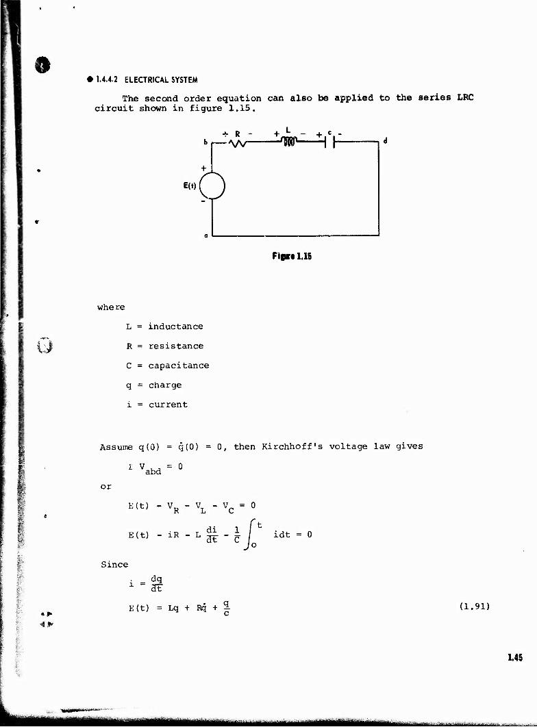
The second order equation can also be applied to the series LRC circuit shown in figure 1.15.

+ R - b, VV-

E(t) 0 + L - + e -W 1 |-

where

Fipre 1.15

u L = inductance

R = resistance

C = capacitance

q = charge

i = current

Assume q(0) = q(0) = 0, then Kirchhoff's voltage law gives

abd

or

I * B(t) - VR - VL - Vc = 0

E(t) - iR - L di 1 ar " c idt = 0

Since

i = d(3 1 at

4* E(t) = Lq + Rq + (1.91)

1.45

.^^^u^Maäiiä^itmtaailmtttimmätta^mim^^^^^..-,.^ .... — -_._... ..

We now define

i—

1 xn ~ M EC

2 /E7C

2C- « f n L

Using these parameters, equation 1.91 can be written

q + 2c q + u» 2q = E. (t) = ^ (1.92) ^ n n ^ l Li

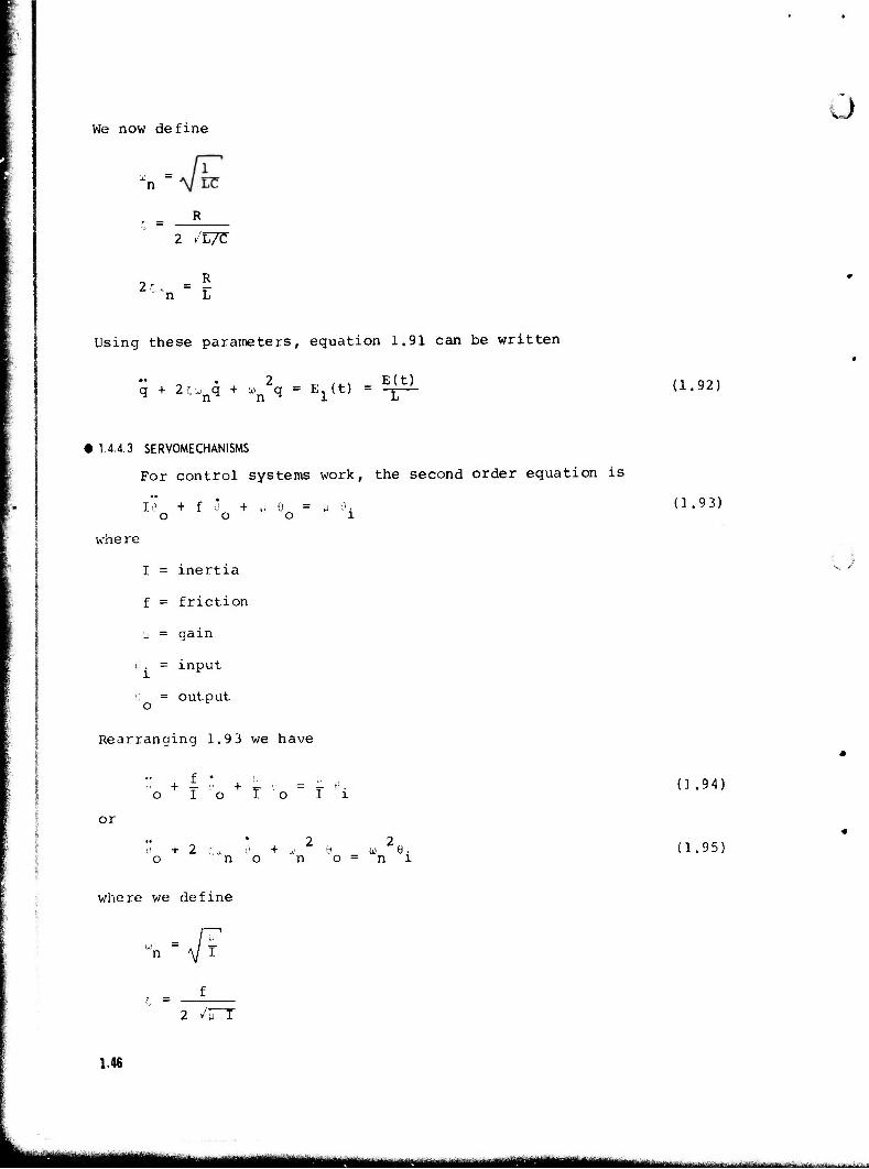
• 1.4.4.3 SERVOMECHANISMS

For control systems work, the second order equation is

i" + f ö + u 0 = vi 0. (1.9 3) o O O 1

whe re

I = inertia

f = friction

u = gain

0. = input

9 = output

Rearranging 1.9 3 we have

o I o I o 1 i U.»«J

or

i + 2 r. n + u, 2 ü a) 2e. (1.95) o no no=ni

where we define

wn " \ r

f

2 /*

1.46

"M,*rtM>lt*,M^- '^M°M^ - - ^~~~ ifl^ka.1^ti^a.J^:^J.^Mjri.itt.w.:^.a-1 jfl-,.. ■ -:,■■ ■... ■■■--■. , , ■ ^

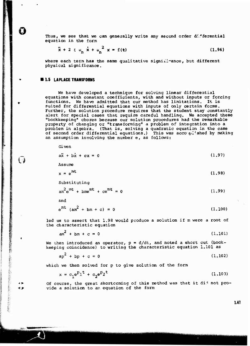
o Thus, we see that we can generally write any second order differential equation in the form

X+2£d)X+(D X n n f(t) (1.96)

where each term has the same qualitative significance, but different physical significance.

l.S LAPLACE TRANSFORMS

We have developed a technique for solving linear differential equations with constant coefficients, with and without inputs or forcing functions. We have admitted that our method has limitations. It is suited for differential equations with inputs of only certain forms. Further, the solution procedure requires that the student stay constantly alert for special cases that require careful handling. We accepted these "bookkeeping" chores because our solution procedures had the remarkable property of changing or "transforming" a problem of integration into a problem in algebra. (That is, solving a quadratic equation in the case of second order differential equations.) This was acco iplvshed by making an assumption involving the number e, as follows:

G

Given

ax + bx + ex = 0

Assume

mt x = e

(1.97)

(1.98)

Substituting

2 mt , , mt , mt n am e + bme + ce =0 (1.99)

and

emt (am2 + bm + c) =0 (1.100)

led us to assert that 1.98 would produce a solution if m were a root of the characteristic equation

am + bm + c = 0 (1.101)

e •■■'

1 I

* » 4.P

We then introduced an operator, p = d/dt, and noted a short cut (bookkeeping coincidence) to writing the characteristic equation 1.101 as

ap + bp + c = 0

which we then solved for p to give solution of the form

x = c,eplt + c,ep2

(1.102)

(1.103)

Of course, the great shortcoming of this method was that it di5 not provide a solution to an equation of the form

1.41

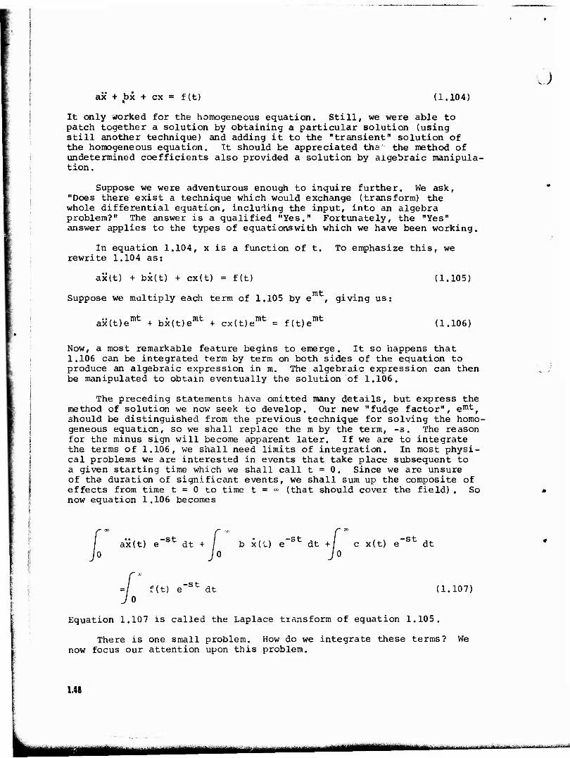
ax + bx + ex = f(t) (1.104)

It only worked for the homogeneous equation. Still, we were able to patch together a solution by obtaining a particular solution (using still another technique) and adding it to the "transient" solution of the homogeneous equation. It should be appreciated tha the method of undetermined coefficients also provided a solution by algebraic manipula- tion .

Suppose we were adventurous enough to inquire further. We ask, "Does there exist a technique which would exchange (transform) the whole differential equation, including the input, into an algebra problem?" The answer is a qualified "Yes." Fortunately, the "Yes" answer applies to the types of equations with which we have been working.

In equation 1.104, x is a function of t. To emphasize this, we rewrite 1.104 as:

ax(t) + bx(t) + cx(t) = f(t) mt

(1.105)

Suppose we multiply each term of 1.105 by e , giving us

■ •,. . mt , , •,. . mt , ,,> mt _ ,.. mt ax(t)e + bx(t)e + cx(t)e = f(t)e (1.106)

Now, a most remarkable feature begins to emerge. It so happens that 1.106 can be integrated term by term on both sides of the equation to produce an algebraic expression in m. The algebraic expression can then be manipulated to obtain eventually the solution of 1.106.

The preceding statements have omitted many details, but express the method of solution we now seek to develop. Our new "fudge factor", emt, should be distinguished from the previous technique for solving the homogeneous equation, so we shall replace the m by the term, -s. The reason for the minus sign will become apparent later. If we are to integrate the terms of 1.106, we shall need limits of integration. In most physical problems we are interested in events that take place subsequent to a given starting time which we shall call t = 0. Since we are unsure of the duration of significant events, we shall sum up the composite of effects from time t = 0 to time t = <=° (that should cover the field) . So now equation 1.106 becomes

ax(t) e~St dt + b x(t) e~St dt +/ c x(t) e~st dt

f(t) e~st dt (1.107)

Equation 1.107 is called the Laplace transform of equation 1.105.

There is one small problem. How do we integrate these terms? We now focus our attention upon this problem.

1.48

MM HÜB ■-»■->■■■ ■ ■■ ■'— ■■*'■

•

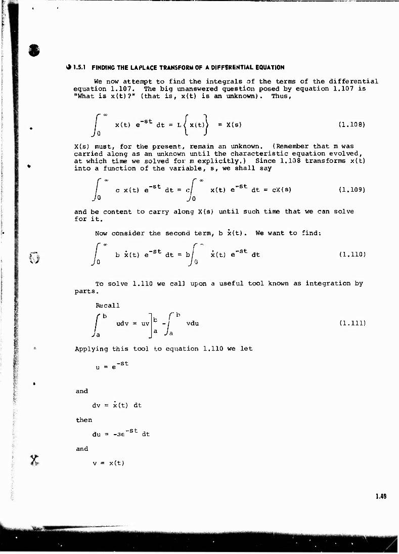
Si 1.5.1 FINDING THE LAPLACE TRANSFORM OF A DIFFERENTIAL EQUATION

We now attempt to find the integrals of the terms of the differential equation 1.107. The big unanswered question posed by equation 1.107 is "What is x(t)?" (that is, x(t) is an unknown). Thus,

r u x(t) e"St dt = L< x(t)> = X(s) (1.108)

X(s) must, for the present» remain an unknown. (Remember that m was carried along as an unknown until the characteristic equation evolved, at which time we solved for m explicitly.) Since 1.10 8 transforms x(t) into a function of the variable, s, we shall say

c x(t) e"st dt = cj x(t JO

) e"St dt = cX(s) (1.109)

and be content to carry along X(s) until such time that we can solve for it.

Now consider the second term, b i(t). We want to find:

/ b x(t) e"st dt = b/ x(t) e"st dt 1: (1.110)

To solve 1.110 we cal] upon a useful tool known as integration by parts,

Recall

r b udv = uv

r» I vdu (1.111)

Applying this tool to equation 1.110 we let

-st u = e

and

dv = x(t) dt

then

du = -se at

J£ and

v = x(t)

1.49

Putting these values into 1.111 and integrating from t = 0 to t = »,

x(t)e~st dt = x(t)e"st

i " f "x(t)[-se-stl

0 ~/0 L J dt

= x(t)e"stL + s|0 x(t)e"st dt

u v/

= x(t)e'st 0 + sX(s)

Now

x(t)e -stlQ = lim x J t ■*• °°

(t)e"St - x(0)

-st

(1.112)

(1.113)

and we shall assume that the term e f3W "dominates" the term x(t) as

t -> °° .

-St Thus, lim x(t)e =0, an£ equation 1.111 becomes

x(t)e"Stdt = &''- x(0) + sX(s) = sX(s) - x(0) (1.114)

Equations 1.109 and 1.114 can be abbreviated by using the letter L to signify Laplace transformations.

L{ x(t) } = X(s)

L{ cx(t) } = cX(s)

L{ x(t) } = sX(s) - x(0)

L{ bx(t) } - b[sX(s) - x (0)]

(1.115)

(1.116)

Equation 1.116 can be extended to higher order derivatives. Such an extension gives

L{ax(t)} - a [s*X(s) - sx(0) - x(0>] (1.117)

Returning to equation 1.107, we note that we have found the Laplace transforms of all the terms except the forcing function. To solve this transform, the forcing function must be specified. We shall consider a few typical functions and illustrate, by example, the technique for finding the Laplace transform.

EXAMPLE

f(t) = A = constant

Then

L{A} =/0 a Ae_stdt = ^. ' e~st(-sdt) =

A -st — e s

1.50

•- 1

n or

L{A} = | (1.118)

EXAMPLE

f(t) = t

Then

L{t} =L te~stdt

To integrate by parts, we let

u = t

dv = e"stdt

Then

du = dt

1 0"st

v = - -e

u Substituting into 1.110

-s-*- -te te

s-dt = -H- e"stdt

= 0 -st = 0 + ~1 s

i m

or

Lit) =

EXAMPLE

1 "2" s

f(t) = e 2t

(1.119]

Then , 2t , / 2t -st,. Lie 1 =L e e dt e(2"s)tdt -r~7

or

T ; 2t, 1 Lf-e } = r^-z (1.120)

1.51

^jjj^^^VJl^

■III I I

EXAMPLE

f(t) = sin at

Then f oo ' —st

L{sin at} = lQ sin at e dt

Integrate by parts, letting

u = sin at

dv = e"stdt

Then

du = a cos at dt

1 „-st v = - — e s

Substituting into 1.111

)

sin t e -st _ -(sin at) (e"st) + -/ cos at e"stdt 0 SJ 0 v->

or

. sin at e~stdt = 0 + - / cos at e"stdt 0 s/0

(1.121)

-st The expression cos at e dt can also be integrated by parts, letting

u = cos at

and

dv = e~stdt

du = -a sin at dt

1 -st v = - e

s

Giving

, -st,, - (cos at) (e cos at e dt = — ;

-st, a -st sin at e dt

1.52

mm^m - —- —- - ~*-~~-***-*»~*-*^ a'-1"' it.^^.^Lu^uL^^i-M..,

o or

f0 cos at e"stdt = g- - | Usin t} (1.122)

Substituting 1.122 into 1.121 gives

L{ >in at} = 0 + - - - LCsin at} s s T ~ T s s L{sin at}

which "obviously" yields

L{sin at} = -~ T sz + aT

(1.123)

Also note that 1.121 may be written as

L{sin at} = — L{cos at} s

which yields

L{cos at} = ~2 5- s + a

The Laplace transforms of more complicated functions may be quite tedious to derive, but the procedure is similar to that above. Fortu- nately, it is not necessary to derive Laplace transforms each time we use them. Extensive tables of transforms exist in most advanced mathematics and control system textbooks.

We originally asserted that the Laplace transform was going to assist in the solution of a differential equation. The technique is best described by an example.

EXAMPLE

;.;■■■:

Given

2t x + 4x + 4x = 4e

with conditions x(0) = 1, x(0) = -4. Taking the Laplace transform of the equation gives

s2X(s) -sx(0)- x(0) + 4 [sX(s) - x(0)] + 4X(s) = 4

=T

♦ or

[s2 + 4s + 4] X(s) + [-s + 4 - 4] = i 2

Solving for X(s),

X(s) = —?—~2s + 4 . (1.124) (s - 2)(s + 2)Z

In order to continue with our solution, it is necessary that we discuss partial fraction expansions.

PROBLEMS: Set III, pagt 1.100.

• 1.5.2 PARTIAL FRACTIONS

The method of partial fractions enables us to separate a complicated rational fraction into a sum of simpler fractions. Suppose we are given a fraction of two polynomials in a variable, s. Suppose the fraction is proper (the degree of the numerator is less than the degree of the domi- nator). If it is not proper, we make it proper by dividing the fraction and then consider the remainder expression. There occur several cases:

• 1.5.2.1 CASE 1: DISTINCT LINEAR FACTORS

To each linear factor such as (as + b), occurring once in the demoninator, there corresponds a single partial fraction of the form, A/(as + b), where A is a constant to be determined.

EXAMPLE

7s - 4 -ABC , 125> s(s - 1) (s + 2) - i + i~^"T + s~+~T U.l^b)

• 1.5.2.2 CASE 2: REPEATED LINEAR FACTORS

To each linear factor, (as + b), occurring n times in the demoninator there corresponds a set of n partial fractions.

EXAMPLE

s2 - 9s + 17 _ A B C ,, ,-,, il-2)2(s+l) " TF^TT + TT^TT + "^17 (1'126)

(where A, B, and C are constants to be determined)

• 15.2 3 CASE 3: DISTINCT QUADRATIC FACTORS

To each irreducible quadratic factor, as^ + bs + c, occurring once in the denominator, there corresponds a single partial fraction of the form, (As + B)/(as2 + bs + c), where A and B are constants to be determined.

1.54

—mutämum """--■"*»-■-—<■■-

Q EXAMPLE

38 + 53 + 8

(s + 2) (s2 + 1)

A . B8 + C + 2 s* + 1

(1.127)

• 1.5.2.4 CASE 4: REPEATED QUADRATIC FACTORS

To each irreducible quadratic factor, as2 + bs + c, occurring n times in the denominator, there corresponds a set of n partial fractions.

EXAMPLE

10 s + s + 36

(s - 4) (s2 + 4)

A . BS + C . Ds + E 7 " g-TT + _2 . ; + 7T2-7TT2" (1.128)

+ 4 (s + 4)'

u

(where A, B, C, D, and E are constants to be determined)

The "brute-force" technique for finding the constants will be illustrated by solving 1.128. Start by finding the common denominator on the right side of 1.128.

10 s2 + s + 36 A(s2 + 4)2 + (Bs + C) (s - 4) (s2 + 4) + (Ds + E) (s - 4) = —. _

,s - 4)(s2 + 4)2 (s - 4)(s2 + 4)2

(x.129)

Then set the numerators equal to each other

10 s2 + s + 36 = A(s2 + 4)2 + (Bs + C) (s2 + 4) (s - 4) + (Ds + E) (s - 4)

(1.130)

and, without justifying the statement, we shall assert that 1.130 must hold for all values of s. Now substitute enough values of s into 1.130 to find the constants.

1. Suppose s = 4, then 1.130 becomes

(10)(16) + 4 + 36 = 400A

and

A = 1/2

2. Suppose s = 2j, then 1.130 becomes

-40 + 2j + 36 = -4D + 2jE - 8jD - 4E

-4 + 2j = -4(D + E) + 2j (E - 4D)

A- The real and imaginary parts must be equal to their counterparts on tne opposite side of the equal sign, thus

1.58

■*m*f**' "«"*»■

(D + E) =1

and

E - 4D = 1

or

D = 0

and

E = 1

3. Now let s = 0, then 1.130 becomes

36 = 16A - 16 (C) - 4E

and from above

A = 1/2, E = 1

hence

36 = 8 - 16C - 4

and

C = -2

4. Let s = 1, then 1.130 becomes

47 = 25 (1/2) + (B - 2) (-15) - 3

94 = 25 - 30B +60-6,

or

Th B = -1/2

Then 1.129 may be written

10 S + S + 36T = 1/2 (-L,) - 1/2 (4-tJL) +

(s - 4) (s2 + 4) 's~^~T; 1 ' ' —3 X s+4 (s + 4)

Let's continue with our attempt to solve the differential equation

2t x + 4x + 4x = 4e

We have transformed the equation (and substituted initial conditions) to get

X(s) = 2s + 4

(s - 2) (s + 2) (1.124)

1.56

mm !!■■■ II ■■ wm gjygH| .: ^^...^. .. ^ ...;^1,_^.^S„,;-.. ,-:-w-.. ■ . ;.■.... ...,.-■., .■ ..

'S We now expand by partial fractions

s - 2s + 4

(s - 2) (s + 2) - A _ + g _ +

1 s~^~T + ITT +

(s + 2)' (1.132)

Taking the common demoninator, and setting numerators equal

s2 - 2s + 4 = A(s + 2)2 + B(s + 2) (s - 2) + C.(s - 2) (1.133)

We can now substitute different values of s into this equation and solve for the constants. An alternate method of solving for these constants exists, however, and we will demonstrate this new approach. If we multiply out the right side of 1.133 we get

s2 - 2s + 4 = As2 + 4As + 4A + Bs - 4B + Cs - 2C

= (A + B)s2 + (4A + C)s + (4.* - 4B - 2C)

Now the coefficients of like powers of s on both sides of the equation must be equal (that is, the coefficient of s2 on the left side equals the coefficient of s2 on the right side, etc.) Equating gives

s2 : 1 = A + B

s1 : -2 = 4A + C

0 4A - 4B - 2C

Solving, we get

A = 1/4

B = 3/4

C = -3

Substituting into 1.132, we get

;(s) = 1/4 L~T| + 3/4 1 s + 2; -3

s +~2~ (1.134)

• 1.5.3 HEAVISIDE EXPANSION THEOREMS FOR ANY F (i)

#*

• 1.5.3 1 CASE 1 DISTINCT LINEAR FACTORS

If the denominator F(s) has a distinct linear factor, (s - a), we find the constant for that factor by multiplying F(s) by (s - a), and then evaluate the remainder of F(s) at s = a.

1.51

i LÄSE;.'■:..*

tttt ttMMHHlMtt ätifc* ■■AlaiM&*jJ4&B& u^-^.i.ia/ih«

F(S) = s - a + ...

u

A = (s - a) F(s) s = a

EXAMPLE

F(s) = 7s - 4 *+^JU + c s(s - 1)(s + 2) " s s - 1 s + 2

A = sF(s) s = 0

73-4 is - IMS + 2)

B = (s - l)F(s) s = 1

7s - 4 s(s + 2)

s = 0

s = 1

(-D(2) = 2

7-4 TTTTJT = l

C = (s + 2)F(s)

See case 4 also.

s = -2

7s - 4 s(s - 1) s » -2

-14 - 4 (-2)(-3) = -3

'1.5.3.2 CASE 2: REPEATED LINEAR FACTORS

If the denominator of F(s) has any repeated linear factors, they must be treated in a special manner.

F(s) = Z

(s - a)11 (s - a)n "~"1' (s - a) n~^T + ' *' • + TF-^-aT

Let *(s) = (s - a)" F(s)

Then

A = <i>(s) s = a

B = d<j)(s)/ds s = a

C = 2j d2<Ms)/ds2

Z k! ^^

s «s a

s = a

'Note: This formula is good for all constants except A above,

1.58

IMMBtel ■ ■'

iitu**..'-;.«-^... .-,..■, **.-. ■;ii,.,t,T.-.tat^uJ--.aik/.

$

where k = 1, 2, ..., n - 1

where the derivatives of J7(s) are obtained by using

d ,u._ vdu - udv a? (v> 7

For example,

F(S) = _JL-T4?_L!Z_ . ^ + _!__. + c (s - 2)2 (s + 1) s + 1_r (s - 2)2 s " 2

A = (s + 1) F(s) . s " 9s "*• 17

-1 (s - 2)T

Js - -1

1 + 9 + 17

<-3)2 27

B = *(s) - 2« + 17 S + 1

= 2

4-18+17 = 1

s = 2

_ _ d»(s) c " -as-

s = 2

(s + 1)(2s - 9) - (S* - 9s + 17)(1) 5

(s + ir s = 2

- (3) (-5) - (4 - 18 + 17) _ -18 ,

See case 4 also.

• 1.5.3.3 CASE 3: DISTINCT QUADRATIC FACTORS

If the denominator of F(s) contains a distinct quadratic factor (s + a)2 + b^, we will again multiply F(s) by (s + a)2 + b , and evaluate the remainder of F(s) , 4>(s) , at s = -a + jb and use real and imaginary parts of <Ms) to obtain the two constants.

F(s) = As + B 3 ? (s + a)z + bz

4*

Let

♦ (s) = (s + a)2 + b2 F(s)

and compute

♦ + j*A " *(s) s = -a + jb

1.59

i - • - fiMrutt r» ii> ftirtiiJiiriiiii'irniii

Then

A = l B = r l

For example,

W

F(s) = 4S +r

19s + 32

(s + 2) [(s + 3r + 4J (s + 3) As + B C

TTA ' s +T

l>r + j*i = Ms) _ 4s + 19s + 32

s + 2 s = -3 + j2 s = -3 + j2

_ -5 - jlO -1 - j2 _ - . .. " -l * j2 ' rr-r-jT = -3 + D4

= -3 = 4 a = 3 b = 2

A = j- = 2 B = -6 + 12

= 3

See case 4 also.

• 1.5.3.4 CASE 4: REPEATED QUADRATIC FACTORS (AND ANY OTHER CASE)

Procedures similar to those used in the previous cases exist for this case but they are too cumbersome for most applications. The following procedures will work for any combination of linear and quadratic factors:

F(s) 10s + s + 36

(s - 4) (s2 + 4)

A , Bs + C , Ds + E 1 ~ s~^S + 2 . I + ,_2 . .,2 (S~ + 4)'

Put the right-hand s. de of the equation over a common denominator and then set the two numerators equal.

10s2 + s + 36 = A(s2 + 4)2 -i- (lis +C) (s - 4) (s2 + 4) + (Ds + F.) (s - 4)

(1.135)

which will be a true equation for al] values of s.

• 15 35 PROCEDURES

The following steps may be done in any order, and in combination with the procedures in cases 1 through 3.

1.60

iiiii i ii in—ii—iii» .!■■*,-,*■ ■■'li-jj-<^w....Äfc:«i.^ia.^.JM.:F........... , .^;*.l.^^,.*i.-**£Ji

*•■: - •" "^^WBBWteWfl

D 1. Since equation 1.135 is true for .^11 values of s. choosing specific

values of s, five in this case, and substituting into equation 1.135 will give you five equations in five unknowns, which can be solved simultaneously for the constants.

2. Expand the right hand side of equation 1.135 and find the coefficients of each power of s. These coefficients must be the same on both sides of the equation (that is, s4: B = 0; s°: 4A - 16C -4E = 36) .

3. Let s equal an imaginary or complex number and substitute into equation 1.135. The real parts on both sides of the equation must be equal, and so must the imaginary parts.

Examining equation 1.135, we will use a combination of procedures. First, find A by using case 1

A = (s - 4) F(s) 10(16) + 4 + 36 _ 7.00 „ 1 A 777~T~772 4W J s = 4 (16 + 4)

*•>■■■-.

1

I

G

If we let s = j2, the only non-sero term will be the one with D and E. Letting s be a complex number will give us two equations for D and E, which we can solve simultaneously.

10(j2)2 + j2 + 36 = (j2D + E)(j2 - 4)

-4 + j2 = -4D - 4E -j8D + j2E

Now set real and imaginary parts equal.

-4D -4E = -4 -8D + 2E = 2

-2D -2E = -2 -8D + 2E = 2

Adding the two equations together gives:

-10D = 0

D = 0

Then

2E = 2

E = 1

4»

To find C, let s -- 0 in equation 1.135

36 = 16A - 16C - 4E = 16(1/2) - 16C - 4(1)

16C =8-4 - 36 = -32

C = -2

16)

To find B, let s = 1

10+ 1 + 36 = 25A + (B +C)(-3)(5) + (D + E)(-3)

47 = 25(1/2) - 15B - 15(-2) - 3

15B = 12 1/2 + 30 - 3 - 47 = 42 1/2 - 50 = -7 1/2

B = - 1/2

An alternate way to find B is to calculate the coefficient of s4 on the right-h3nd side of equation 1.135, and then set it equal to the coefficient of s4 on the Left hand side of the equation. Then we get

A + B = 0

B = -A = - 1/2

To complete our solution, we must convert (transform) back into the time domain. The operation which converts a function X(s) back to a function of time is called the inverse Laplace transformation.

L"1 <L{x(t) }) = L-1 {X(s)} = x(t) (1.136)

The inverse Laplace transformation can be solved directly

xlt) C + j«

2TJ X(s)estds , C - j»

(where C is a real constant)

(1.137)

This integral, 1.137, is hardly ever used because the Laplace transform is unique and, therefore, generally X(.>) can be recognized as the Laplace transform of some known x(t). In practice, tables of transform pairs (as found in most mathematics texts) will suffice to find the inverse of X(s) (see table II, page 1.106, for some transform pairs).

Using a suitable transform table, the inverse of 1.134 can easily be found to give us a solution

x(t) 1/4 e2t + 3/4 e"2t 3te -2t (1.130)

PROBLEMS; Set IV, A, page 1.106.

• 1.5.4 PROPERTIES OF LAPLACE TRANSFORMS

The Laplace transform of some f(t), a function of time, is defined as

Li. f (t) I = F(s) f (t)e"stdt (1.139)

1.62

MM IM

II111 I I mi Ml I MllliniMTM——MIHIIHII■HUM IM I—I

41 where

s = o + ju> (a complex number)

The strength of the Laplace transform is that it converts linear differential equations with constant coefficients into algebraic equations in the s-domain. All that remains to do is to take the inverse transform of the explicit solutions to return to the time domain. Al- though the applications at the school will consider time as the independent variable, a linear differential equation with any independent variable (such as distance) may be solved by Laplace transforms.

There are several important properties of the Laplace transform which should be included in this discussion.

In the general case it can be shown that

-.n L LML sn F(s) -

dt' n cn-l,,n. n-2 df(0) , . dn"1f(0) s r(0) + s —rr— + .. . + —r—

dt'

u

(1.140)

It is obvious that for quiescent systems (that is, initial conditions zero)'

M£|^> = snF(s) (1.141)

This result enables us to write down transfer function by inspection.

Another significant transform is that of an indefinite integral.

In the general case

f(t)dtJ F(s) f (t)dt t = 0+ f (t)dt t = 0+ n- + ..

Equation 1.140 allows us to transform Integro-differential equations such as those arising in electrical engineering.

For the case where all integrals of f(t) evaluated at 0+ are zero, our transform becomes

'III- f (t)dt' n\ _ F(s) (1.143)

A third useful property of the Laplace transform arises if we consider the Laplace transform of the product of some exponential and any other function of time.

1.63

,uai^!M^jim'm

^ - «MMMM^Ma

L <e"at f(t) e"at f(t)e-S fcdt =/ °° f(t)e-(s + a)t dt

(1.144)

It is apparent that this is the' same form as the transform of f(t), except tha; the transformed independent variable is (s + a) rather than s. We conclude therefore that

L {e"at f(t)} = L{f(t) } = F(s + a) (1.145) (s •* s + a)

It is important to note at this point, that the transform of the product of two functions of time is not equal to the product of the individual transforms. In symbolic form,

L (f(t) g(t) } j F(s) G(s) (1.146)

The L{f(t) g(t)} must be solved for directly by the definition cf the Laplace transform»

The last property we will consider is the Laplace transform of a pure time delay. A pure time delay of the function f(t) can be represented mathematically as

f(t - a) u(t - a) (1.147)

,j

where a is the length of delay and u(t - a) is the unit step defined as

u(t - a) = 1 , (t - a) > 0

0 , (t - a) 0

For such a time delay

as L'f (t - a) u(t - a) } = e I,{ f (t) } (-1 .148)

We shall now demonstrate the usefulness of the Laplace transform by solving several example problems.

KXAWM.K

f.olve the given equation for x(t),

x -4 <>x = 1

when x (;>) ■ ] .

(1.149)

U4

■— - ■ ^.i.-^.-:..,.■ ;i^j^j.w-1^-|-|,vii^nt'i^iifV ■■■-■■ - -■■t^-^.hi

ü By Laplace

L{x} = sX(x) - x(0)

L{2x} = 2X(s)

Thus

L{1} = ±

(s + 2) X(s) = ±- + 1

u

I I 4>

B_ s + 2"

X(s) =iTi±Ti2T=s1 +

Solving,

A = 1/2

and

B - 1 - 1/2 = 1/2

x(8, = Ul + ^2, xis; — 1- - + 2

Inverse transforming gives

x(t) = 1/2 - 1/2 e~2t

EXAMPLE

Given

x + 2x = sin t, x(0) = 5

solve for x(t).

Taking the transform of 1.151

sX(s) - x(0) + 2X(s) TTi

and

X(s) = 1

"+T

(1.150)

(1.151)

(1.152) (s + 1) (s + 2)

Expanding the first term on the right side of the equation gives

— I -^ AS- + L 4 —£. (s2 + 1) (s + 2) s2 + 1 S +^

16*

Taking the common denominator and equating numerators gives

1 = (As +B)(s + 2) + C(s2 + 1)

Substituting values of s leads to

A - -1/5

B = 2/5

C = 1/5

and substituting back into 1.152 gives

)

X(s) =4ZL£+ V5_+:V5n.+ s* + 1 sz + 1 2—7 T _2 . , x mr T r+T

Inverse transforming gives our solution

x(t) = -1/5 cos t + 2/5 sin t + 5 1/5 e

EXAMPLE

Given

x + 5x + 6x = 3e"3t, x(0) = x(0) = 1

solve for x(t).

-2t (1.153)

a.154) , )

Taking the transform of 1.154

s2X(s) - sx(0) - x(0) + 5sX(s) - 5x(0) + 6X(s) = —|-«. S + 3

or

X(s) = s + 9s + 21

(s + 3) (s + 5s + 6)

Factoring the denominator,

Y,e, _ s + 9s + 21 X(s) " (s + 3)(s + 2){s + 3) (1.155)

's + 9s + 21

(s + 3)2(s + 2) (1.156)

1.66

tmm Mtirrr • r

o B

irr (s + 3) y-rf (1.157)

Finding the common denominator of 1.157, and setting the resultant numerator equal to the numerator of 1.156,

s2 + 9s + 21 = A(s + 3)(s + 2) + B(s + 2) + C(s + 3)2

which can be solved easily for

A = -6

B = -3

C = 7

Now X(s) is given by

X(s) = s4-T ^—2" + iT7 s + 3 (s + 3)Z s + Z

which can be transformed to

x(t) = -6e~3t - 3te~3t + 7e"2t

EXAMPLE

Given

*x + 2x + lOx - 3t + 6/10

x(0) = 3

x(0) = - 27/10

solve for x(t).

(1.158)

Transforming 1.159 and solving for X(s) gives

Mb

$

4*

X(s) 3s3 + 3.38^ + 0.6s + 3 _ A +

s2 (s2 + 2s + 10) S

B , Cs + D __. + _» s s + 2s + 10

where

A = 0

B = 0.3

C = 3

D = 3

LIT

Thus,

x(s, = ?-i3 + -, 3s + 3

s s" + 2i + 10 (1.160)

4 )

To make our inverse transforming a bit easier, let's rewrite 1.160 as

(s + 1) X(s) = ^! + 3 5 j- (s -» ir + 3

(1.161)

which is readily transformable to

-t x(t) = 0.3t + 3e cos 3t (1.162)

PROBLEMS: Set IV, B, page 1.106.

• 1.5.5 TRANSFER FUNCTION

Before beginning simultaneous differential equations, we shall define the transfer function of a system. Consider the following equation with initial conditions as shown.

ax + bx + ex = f(t)

x(0) = x(0) = 0

If we take the Laplace transform of 1.163, we get

as2X(s) + bsX(s) + cX(s) = F(s)

or

X(s) Flu

(1.163)

(1.164)

as + bs + c

Since equation 1.163 represents a system whose input is f(t) and whose output is x(t), we shall define

X(s) = output transform

F(s) = input, transform

We can then define the transfer function of the system, TF, as

TF X(s) FTST

(1.165)

For our exa pie,

TF = ; i. ] 6 7) as' + bs H

168

n Note that the denominator of the transfer function is algebraically the same as the characteristic equation of 1.163. We have already seen, in paragraph 1.6.1 on operator notation, that the characteristic equation completely defines the transient solution, and that the total solution is only altered by the effect of the particular solution due to the input (or forcing function). Thus, from a physical standpoint, the transfer function completely characterizes a linear system.

The transfer function has several properties which we wish to ex- ploit. Sucpose that we have two systems characterized by the differential equations

ax + bx + ex = f(t) (1.168)

and

dy + ey + gy = x(t) (1.169)

From the equations it can be seen that the first system has an input f(t), and an output x(t). The second system has an input x(t) and an output y(t). If we take Laplace transforms at 1.168 and 1.169 we get (assuming all initial conditions are equal to zero)

(as + bs + c) X(s) = F(s) (1.170)

o and

(ds2 + es + g) Y(s) = X(s)

Finding the transfer functions,

X(s) 1 TF1 " fTiT

(1.171)

(1.171) as + bs + c

TF2 " XW " ds + es + g (1.173)

Now, both of these systems can be represented schematically as shown in figure 1.16.

F(«r TF]

SYSTEM 1

-*-X(s)

X

X(s). TF2

SYSTEM 2

Figure 1.16

Y(s)

1.69

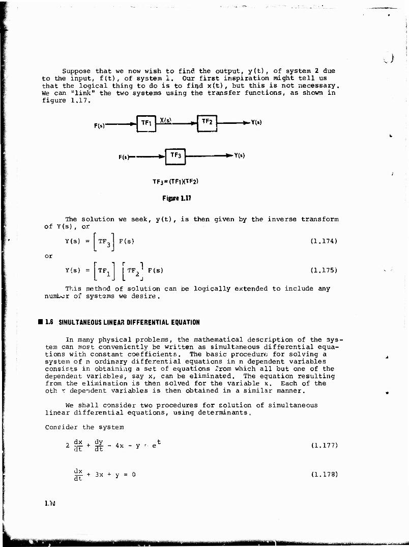
Suppose that we now wish to find the output, y(t), of system 2 due to the input, f(t), of system 1. Our first inspiration might tell us that the logical thing to do is to find x(t) , but this is not necessary, We can "link" the two systems using the transfer functions, as shown in figure 1.17.

F(0" ■0 X(sl TF2 ■*-Y(s)

F(*h TF3 -^Y(s)

TF3 = (TFD(TF2)

Figure LIT

The solution we seek, y(t), is then given by the inverse transform of Y(s) , or

or

Y(s) =

Y(s) =

TF.

TF,

F(s)

j T'- F(s)

(1.174)

(1.175)

This method of solution can oe logically extended to include any numbor of systems we desire.

1.6 SIMULTANEOUS LINEAR DIFFERENTIAL EQUATION

In many physical problems, the mathematical description of the system can most conveniently be written as simultaneous differential equations with constant coefficients. The basic procedure for solving a system of n ordinary differential equations in n dependent variables consists in obtaining a set of equations from which all but one of the dependent variables, say x, can be eliminated. The equation resulting from the elimination is then solved for the variable x. Each of the oth r dependent variables is then obtained in a similar manner.

We shall consider two procedures for solution of simultaneous linear differential equations, using determinants.

Consider the system

dt dt y •■ (1.177)

dx dt

+ 3x y = 0 (1.178)

no

mmm tmm warn ujBinaa

ö Using operator notation, they become

2(p - 2)x + (p - l)y = efc

(p + 3)x + y = 0

(1.179)

(1.180)

• 1.6.1 SOLUTION BY MEANS OF DETERMINANTS AND OPERATOR NOTATION

Recall that for a determinant of second order the value of the determinant is given by

a b

c d = ad - cb

And then rewrite these equations in the following form

pl x + P2Y = fl(t)

(1.176)

(1.131)

P3 x + p4y = f2(t) (1.182)

I

where the p's denote the polynomial operators which act en x and y.

Our solution for x can be given by Cramer's rule

P3 . P4

fl(r-

f2(t)

(1.183)

Jv

and our solution for y can be expressed as

Pl P2

y

p3 p4j i

fx(t)

f2(t)

(1.184)

To solve the system given by equations 1.179 and 1.180, we write these equation in determinant form

2(p - 2) (p - 1

(P + 3)

which is expanded to

(p2 + 1) A -•• -e*

(p - 1)

1

(1.185)

(1.186)

.71

.— .— fflm'ii •■II...---.W». .,

giving a solution

x(t) = c. cos t + c2 sin t - 1/2 e (1.187)

Solving for y,

2(p - 2) (p - 1)

(P + 3) 1

which can be expanded to

(p2 + l)y = 4efc

giving a solution

y(t) = c3 cos t + c. sin t + 2e

2(p - 2)

(P + 3)

(1.188)

(1.189)

(1.190)

We know by examining 1 187 and 1.190 that extraneous constants are present, and to eliminate them we substitute back into equation 1.178 and see that

(J2 + 3c1 + c3) cos t + (3c2 - c1 + c4) sin t = 0 (1.191;

Since 1.191 must hold for all values of t, the terms in parenthesis must vanish, giving

c- = -(3c, + c„)

and

c4 = cl " 3c2

When these values are substituted in 1.190, we obtain the general solution,

• 1.6.2 SOLUTION BY MEANS OF LAPLACE TRANSFORMS

A very effective meanr of handling simultaneous linear differential equations is to take the Laplace transform of the set of equations and reduce the problem to a set of algebraic equations which can be solved explicitly for the dependent variable in s. This method is demonstrated below.

Given the set of equations

3 ci!| + x + i-l + 3y = f(t) dt dt

(1.192)

17?

)

HHH "****"*■"'-' ■"ii.i»H.»imliH-*" ■- ■•'—"■■ -■■■■--—■-•

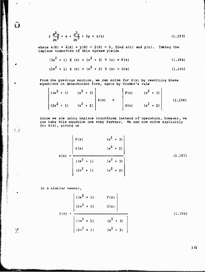
y 2l4+x + i4+2y = q(t)

dt dt

where x(0) = i(0) = y(0) = y(0) = 0, find x(t) and y(t). Laplace transform of this system yields

(3s2 + 1) X (s) + (s2 + 3) Y (s) = F(s)

(2s2 + 1) X (s) + (s2 + 2) Y (s) = G(s)

(1.193)

Taking the

(1.194)

(1.195)

From the previous section, we can solve for X(s) by rewriting these equations in determinant form, again by Cramer's rule

(3s2 + I) (s2 + 3)

(2s2 + 1) (s2 + 2)

X(s)

F(s)

G(s)

(s" + 3)

(s2 + 2)

(1.196)

I ^

I

i W

Since we are using Laplace transforms instead of operators, however, we can take this equation one step further. We can now solve explicitly for X(s), giving us

X(s)

F(s)

G(s)

(3s' + 1)

(2s" + 1)

(s* + 3)

(s' + 2)

(s* + 3)

(s^ + 2)

(1.197)

■ ?v

In a similar manner,

Y(s)

(3s" + 1)

(2s" + 1)

(3s" + 1)

(2s + 1)

F(s)

G(s)

(s" + 3)

(s* + 2)

(1.198)

173

mut^MJältllttttlllMtmimi^

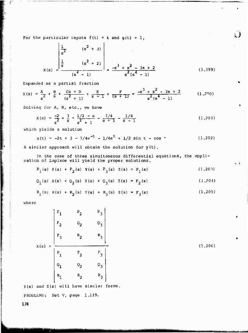
For the particular inputs f(t) = t and g(t) = 1,

X(s)

1 ~7 s

1 s

(s* + 3)

(s* + 2) -s3 + s2 - 3s + 2

(s" - 1)

Expanded as a partial fraction

X(s)

2, 4 s (s

ABCS + D, E F

7 ■ "^TIT i_rT Tmr

i)

-s3 + s2 - 3s + 2

s2(s4 - 1)

Solving for A, B, etc., we have

s s + 1

which yields a solution

7/4 1/4 s + 1 s - 1

(1.399)

(1.200)

x(t) = -2t + 3 - 7/4e-t - l^e1 + 1/2 sin t - cos ^

A similar appioach will obtain the solution for y(t).

In the case of three simultaneous differential equations, the cation of Laplace will yield the proper solutions.

P,(s) X(s) + P2(s) Y(s) + P3(s) Z(s) = F1(s)

Q1(s) X(S) + Q2(s) Y(s) + Q3(s) Z(s) = F2(s)

R. (s) X(s) + R^(s) Y(s) + R,(s) Z(s) = F., (s)

(1.203)

(1.202)

appli-

(3 .201)

(3.204)

(1.205)

J

where

X(s) =

\ R2 R3

Y(s) and Z(s) will have similar forms,

PROBLEMS: Set V, page 1.119.

1.14

(1.206)

MM - ■■■ ■

$

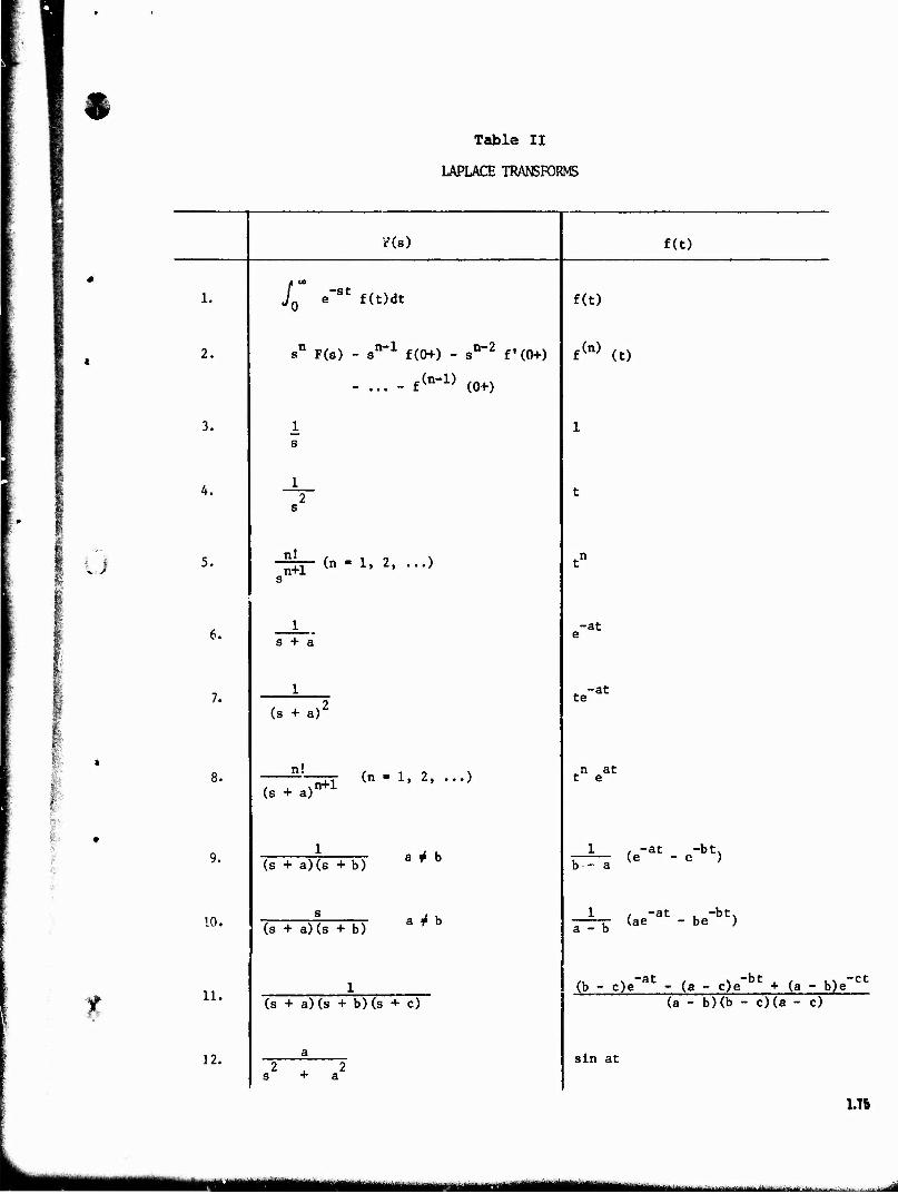
B? * BE *

U

IK.

•?'•

'

1.

3.

4.

5.

6.

7.

10.

11.

12.

Table II

LAPLACE TRANSFORMS

?(■)

X, e"St f(t)dt

sn F(s) - 3n-1 f(0+) - sn"2 f•(0+)

- ... - ffr-» (0+)

n! n+1 (n - 1, 2, ...)

+ a

(s + a)'

(s + a) n+1 (n - 1, 2, ...)

(s + a)(s + b)

(s + a)(s + b)

a i b

a 4 b

(s + a)(s + b)(s + c)

2^2 s + a

f(t)

f(t)

f(n) (t)

-at

te •at

j\ at t e

1 , -at -btx (e - e ) b•- a

1 . -at , -bt, (ae - be ) a - b

(b - c)e"at - (a - c)e~bt » (a - b)e~ct

(a - b)(b - c)(a - c)

sin at

1.7b

"Ae"tm--itw-" - '"^"--'iiiiiMrilii^iiiiinin^iiii i maMlBl

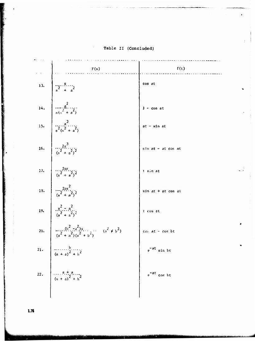
Table II (Concluded)

13.

14.

15.

16.

17.

IS.

19.

20.

21.

22.

F(s) f(t)

s "y"""'"2 s + a

cos at

2 a

'1 2 s(.-, + a )

] - cos at

3 a

2, 2 j. 2N s (s + a ) at - sin at

9 3 2a , 2 . 2.2 (s + a )

sin at - at cos at

2as "/ 2""'"2.2 (s + a )

t sin at

9 2 Zas

/• 2 u. 2,2 (s + a ) sin at + at cos at

2 2 s - a 2 2 2 t cos at

2 2 Or -a')s

2 2 2 b2)

(a2 * b2) co; at - cos bt

b

(s + a)2 + i.2 "at , w c sin bt

s + a 2 2

(s + a) + b e cos bt

1.76

maum—

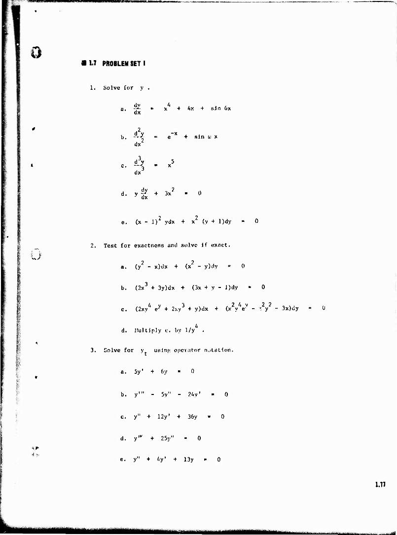
0 H PROBLEM SET I

1. Solve for v .

dx x + Ax + sin 6x

b. A. d*2

e + sin a: x

d37 c. -J dx

d. v 4* + 3x2 dx

e. (x - l)2 ydx + x (y + l)dy

U 2. Test for exactness and solve if exact.

2 2 (y - x)dx + (x - y)dy

b. (2x + 3y)dx + (3x + y - J)dy

c. (2xyA ey + 2xy3 + y)dx + (x2yV - 'V - 3x)dy « 0

d. I!u.Uip]y c. by 1/y .

I §

3. Solve for y usinp, operator notation.

a. 5y' + 6y

b. y'" - 5y" - 24y'

! S: c. y" + 12y' + 36y

4w

d. y" + 25y"

e. y" + 4y' + 13y

1.77

am HHM IMWWl

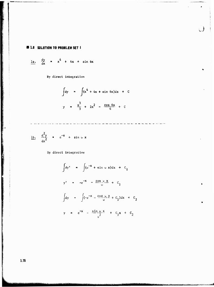
1.8 SOLUTION TO PROBLEM SET I

la. -f- — dx x + Ax + sin 6x

By direct integration

Jdy » f< (x + Ax + sin 6x)dx + C

x , „ 2 cos 6x , „ y = -v + 2x - —-r~ + C

-i e + sin w x


/*" (e + sin (u x)dx + C.

-x cos u x , _ _c - — + Q

dy = (-e •- -- + C )dx 4 C„

*±"-f-X- + CjX + C2

1.78

ii Minr " "**-^-- —....

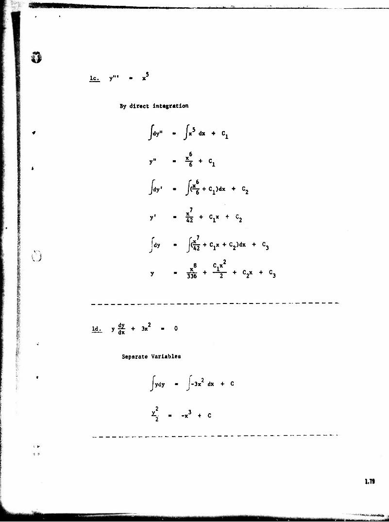
lc. y"


Jdy" - J, x dx + C,

H + Cl

Jar - /< <T + Ci)dx + C2

42 + C1X + C2

I O fdy - J< (fj + c!x + c2)dx + C3

8 C.x'

336 + "V + V + C3

1 *■■

Id, ,£ * 3»2

Separate Variables

lydy - f-3x2 dx + C

-x + C

1.79

■MB ■— i ■

le. (x - l)2 ydx + x2 (y + l)dy

Separate Variables

Ü

JL + JL dy i^^dx x

ja ♦ i;

f,x - 2x + lv. , . _!( _ )dX + C J x

-((i.l + -A)dx + c

y + Iny ■ -x + 21nx + - + C x

2 2 2a. (y - x)dx + (x - y)dy » 0

M - (y - x) N ■ x - y

-— ■ 2y 3y y

3N 3x

2x

9y 3y ^>Not Exact

2b. (2x + 3y)dx + (3x + y - l)dy - 0

2x + 3y 3x + y - 1

1.80

MHi m ----- -

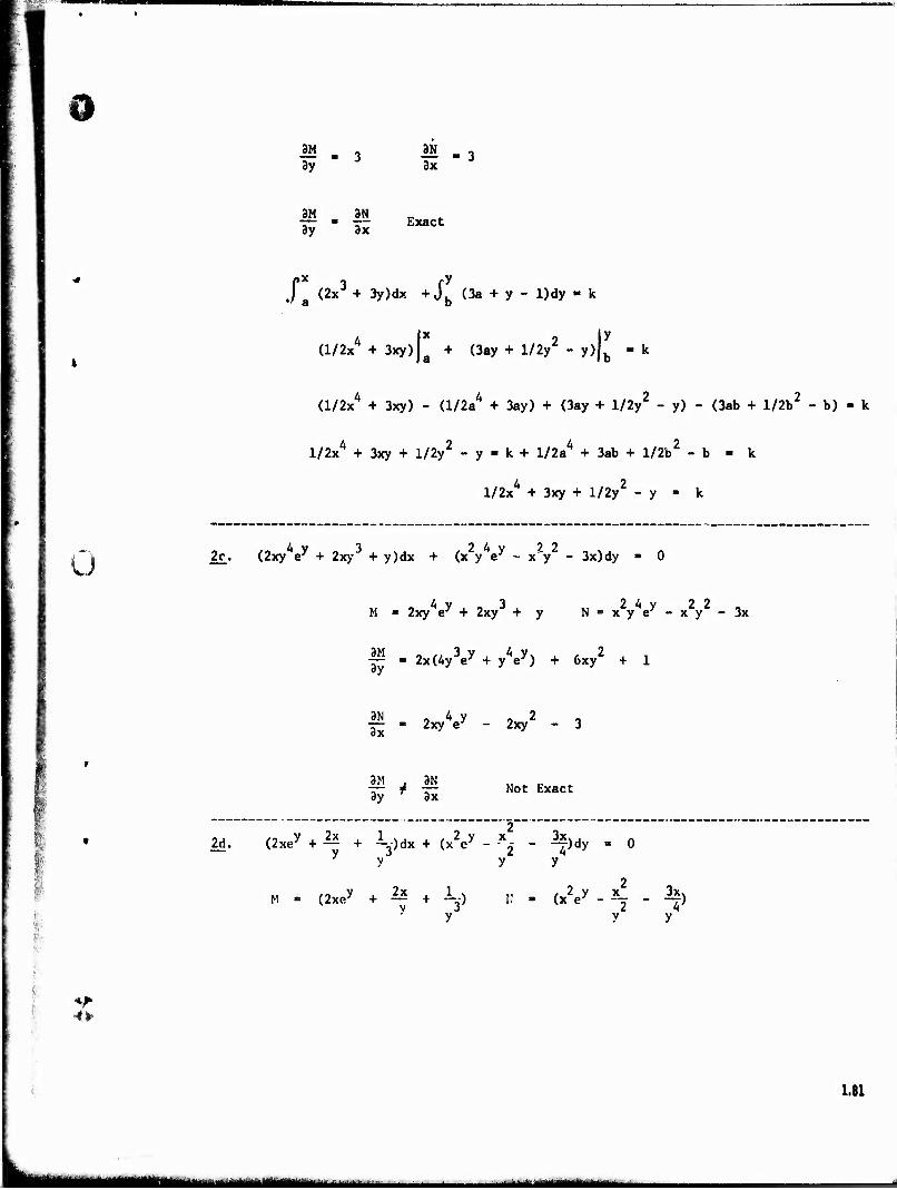
9 3y 3x

_3M 3y

.3N 3;ic

Exact

Ja (2x3 + 3y)dx +Jb (3a + y - l)dy - k

(l/2x" + 3xy)|a + (3ay + l/2y - y)Jb -k

(l/2x4 + 3xy) - (l/2aA + 3ay) + (3ay + l/2y2 - y) - (3ab + l/2b2 - b) - k

l/2xA + 3xy + l/2y2 - y - k + l/2a4 + 3ab + l/2b2 - b - k

l/2x4 + 3xy + l/2y2 - y - k

u 4 v 3 2 4 v 7 2 2c. (2xy V + 2xy + y)dx + (x y ey - x"y - 3x)dy -

o 4 y . -> 3 . x, 2*y 22 , M «■ 2xy e + 2xy + y N-xye'-xy -3x

— ■ 2x(4y e' + y e') + 6xy + 1

_3N 3x

2xyV - 2xy2 - 3

3M , 3N 3y f 3x

Not Exact

2d. (2xey + — + --3-)dx + (x2ey - *^ 7 y y

>y y

■4*

(2xey + — + K) (x2ey 3xN

1.81

kttU ■ mtai^mmmm

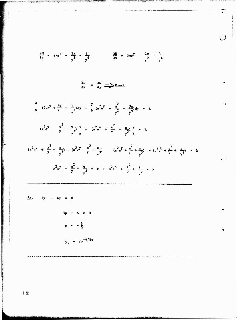
w^^wr1?^^^ . " ^'^y^^^^^Tr*** ^pfp^ag^w^fow,5^^;?^iB^«?75,^sr!'

iä . 2xey - 2x . i_ 2y zxe 2 4

y y

M K 2xey _ 2x _ 3_ 3x *xe 2 4

y y

3N 3N 3y - 3x ■ — ^ Exact

x y -, . .2 (2xey + 1* + l_)dx + ^ (a2ey _ al _ 3a)dy _ k

y y3'~ ' b y y

(XV + j!+ ^)X + (a2ey + I + a)V _ R

y a • yJ b

y 3' y

y - ¥ y

b 3' b^

«V + £+ *_ . k + a2eb + l+ *_ y y3 b b3

3a. 5y' + 6y = 0

5p + 6 = 0

Yt - Ce -6/5x

1.82

_____ ^M«IUÜ

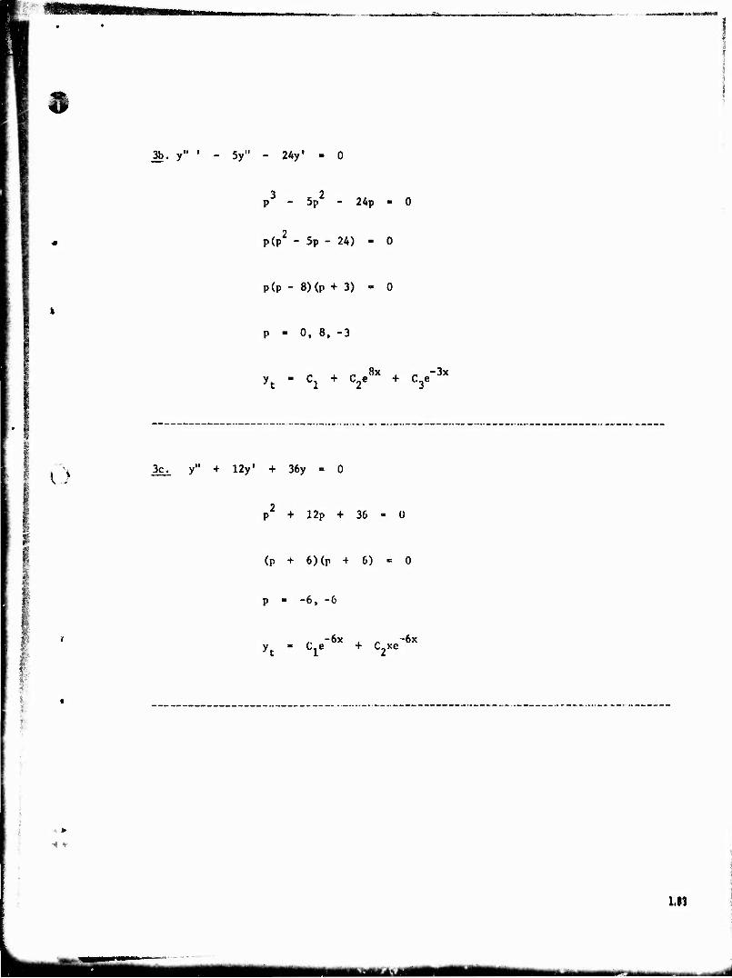
TL

3b. y" • - 5y" - 24y' - 0

p3 - 5p2 - 24p - 0

p(p - 5p - 24) - 0

P(p - 8)(p + 3) - 0

p - 0, 8, -3

yt " Cl + C2e8X + C3e"3X

o 3c. y" + 12y' + 36y = 0

1

p + 12p + 36 - 0

(p + 6)(p + 6) ■= 0

p - -6, -6

yt * Cle C2XC

I

1.(1

■— --■ --

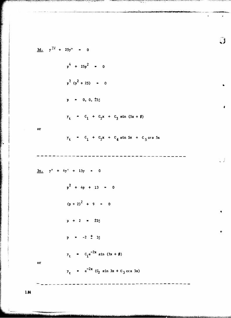
P^WyiJM^U,*^J«WWn^^^ ■ ss!!wsBPTi».!.rflwyr^*■ *«Ja™^^ . ■

■JMWJl«IIIW»»WWMWMW*iBMM^WWWWWl>BW^hwwa»

3d. yIV + 25y"

p4 + 25p2 - 0

p2 (p2 +25) - 0

p - 0, 0, +5j

yt " Cl + C2X + C3 sin *5x + ^

Q

or

y - C. + C.x + C. sin 5x + C5cfs 5x

v i

3e. y" + 4y' + 13y

p + Ap + 13

(p + 2)' + 9

p + 2 - +3j

-2 I 3j

yt - Cie"2x sin (3x + 0)

or

-2x y ■ e (C^ sin 3x + Cj ccs 3x)

1.84

tmm ^mmmtmmm

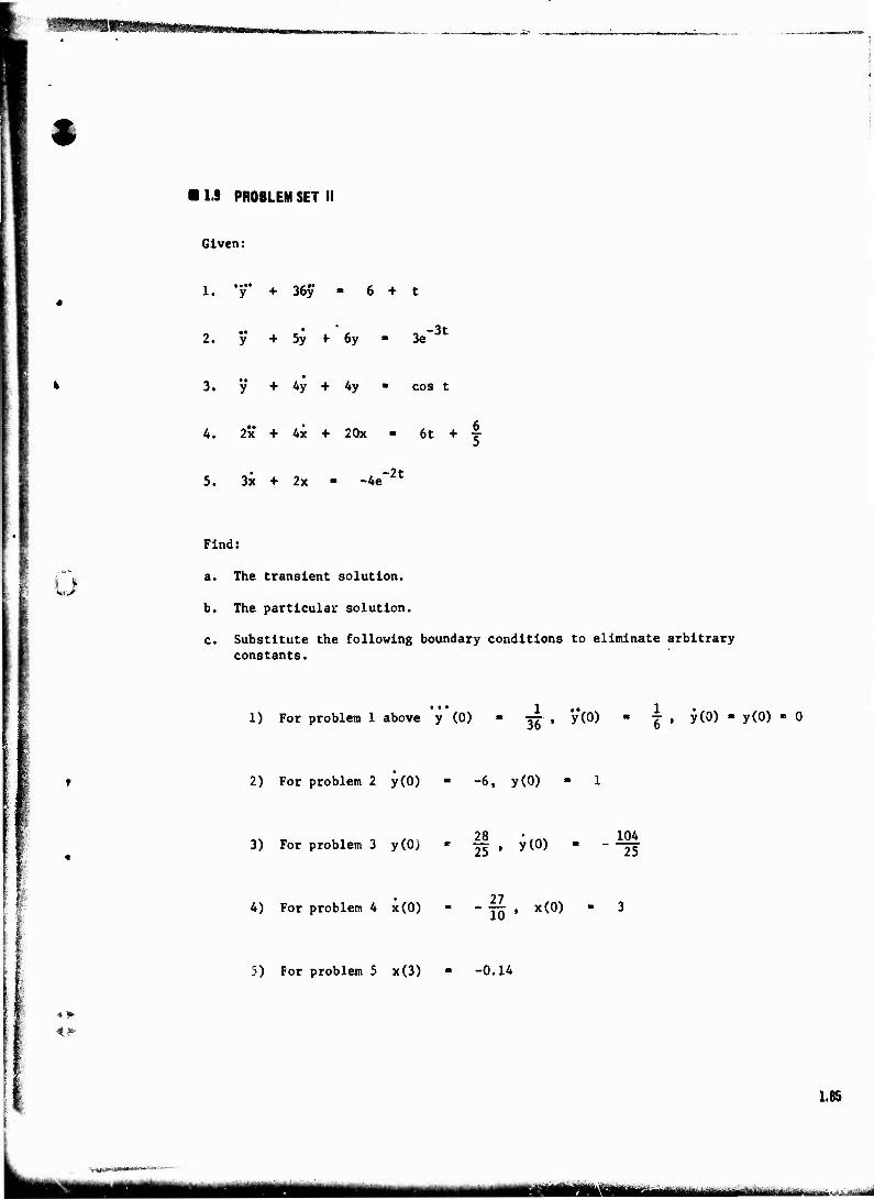
IS- ■iiiMwmumm.i.,1

•

1.9 PROBLEM SET II

Given:

1. *y" + 36y - 6 + t

2. y + 5y + 6y 3e -3t

3. y + Ay + Ay ■ cos t

A. 2x + Ax + 20x - 6t +

5. 3x + 2x -Ae ■2t

I §

Find:

a. The transient solution.

b. The particular solution.

c. Substitute the following boundary conditions to eliminate arbitrary constants.

1) For problem 1 above 'y'(O) - ■— , y(0) - | , y(0) - y(0) - 0

2) For problem 2 y(0) - -6, y(0) - 1

3) For problem 3 y(0) g, y(0) 10A 25

A) For problem A x(0) 22 10

, x(0)

5) For problem 5 x(3) - -0.1A

1.85

L. mmm KMMtaHMHIM i.^.^-..:LV*toätä

J

d. Find a , w. , c , T where applicable.

e. Describe the system damping where applicable (I.e. underdamped, overdamped, etc.).

£. SKETCH the total response (I.e. total solution).

1.86

m*mm^mmm*m^*^*mmmmum* Mi r i —- ■••- - - ._«.« Hfcifl

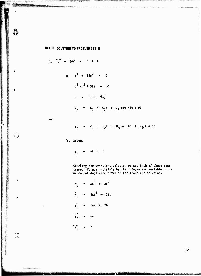
i iin'ii IIII ji iij i.»U4j;,iiiill5H.l? J1ÜJWSfJP,.?'. " " v*"»«<»^i:.-j"f7^S73H,

1.10 SOLUTION TO PROBLEM SET II

1^ y + 36y 6 + t

I u

or

h 2 a. p + 36p - 0

p2 (p2 +36) - 0

p - 0, 08 +6J

yt " Cl + V + C3 Sin (6t + *J

y - C, + C-t + C4 sin 6t + C& cos 6t

b. Assume

At + B

Checking the transient solution we see both of these same terms. We must multiply by the independent variable until we do not duplicate terms in the transient solution.

4*

<4m

3 2 At + Bt

3At + 2Bt

6At + 2B

6A

1.81

m-jm

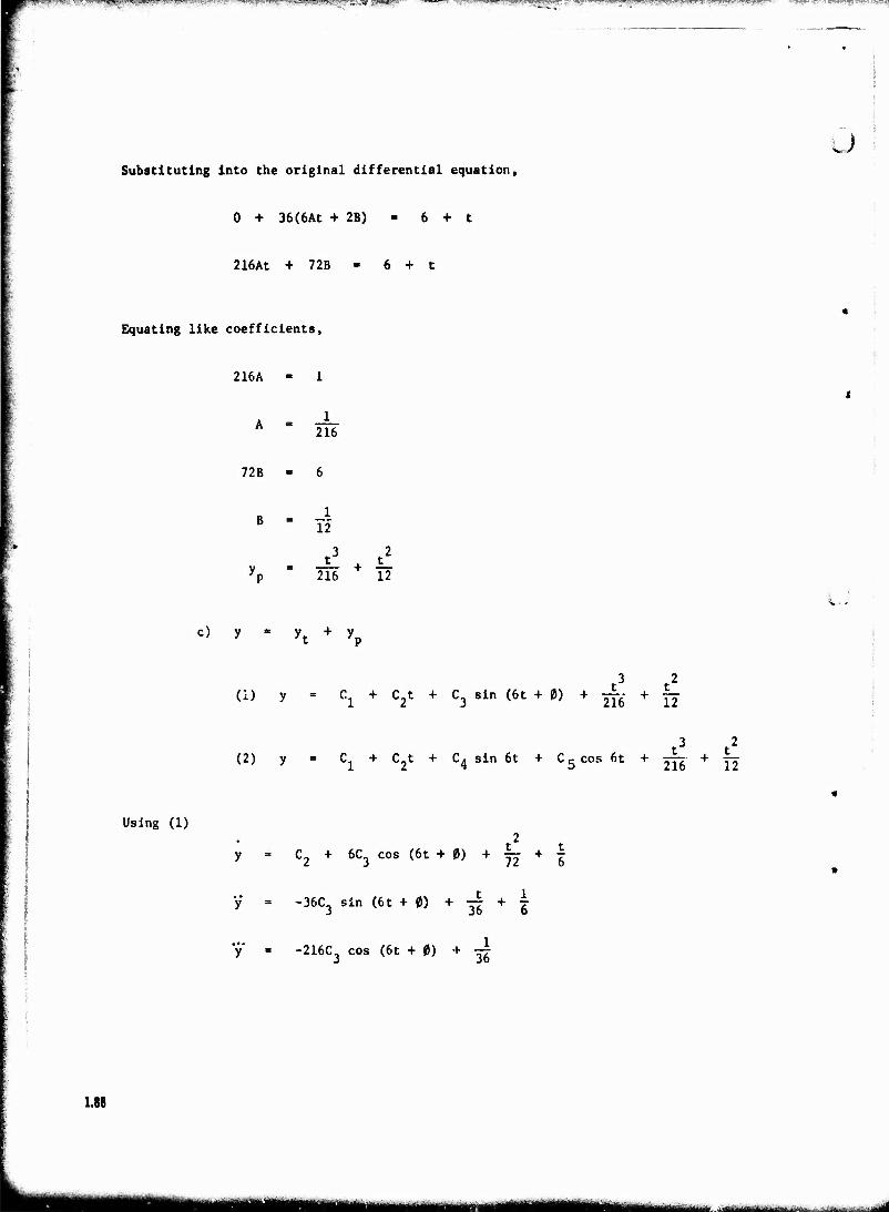
$V^UW#l*;!*!V<!?^l^WW^<f^ wv»? '.'^!Pt U'W1'.1, *,^!^?^?T --' ~^™^''^j'?^*?^?rr^?'f*T^-~*T**7*''w*t*°Fr'" ■ ^ws^ *f-* p^*^ ^^ :*?s^

Substituting into the original differential equation,

0 + 36(6At + 2B) - 6 + t

216At + 72B - 6 + t

Equating like coefficients,

216A

72B

1 216

_1 12

216 12

c) y = yt + y

t3 t2 (i) y - Cx + C2t + C3 sin (6t + 0) + 216 + 12

t3 t2 (2) y - C + C2t + C4 sin 6t + C 5 cos 6t + -~ + yj

Using (1)

C2 + 6C3 cos (6t + 0) + 72 + !

■36C3 sin (6t + 0) + — + -

-216C3 cos (6t + 0) + ■ ~

)

5 i

1.88

kMHaaaHilii|H

'■'•

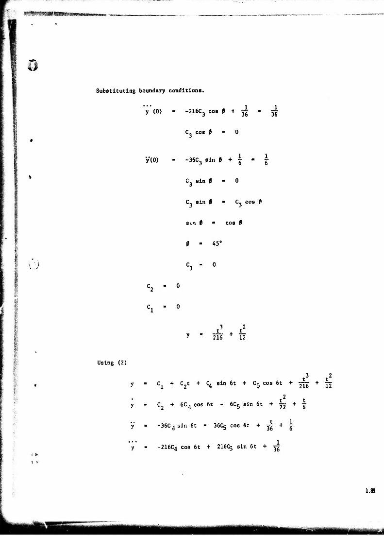
Substituting boundary conditions

y (0) - 216C3 cos 0 -f ^ _1 36

C cos 0

y(0) -36C3 sin 0 + | - ^

C sin 0 - 0

C. sin 0 - C- cos 0

sia 0 cos 0

I i I

Using (2)

45°

3 .2

216 T 12

t3 t2 C + C.t + C4 sin 6t + Cc cos 6t + jrr + TJ

C- + 6C4 cos 6t - 6C5 sin 6t + 72 + £

-36C4sin 6t - 36C5 cos 6t + 36 + 6

-2I6C4 cos 6t + 216(5 sin 61+-^

.)

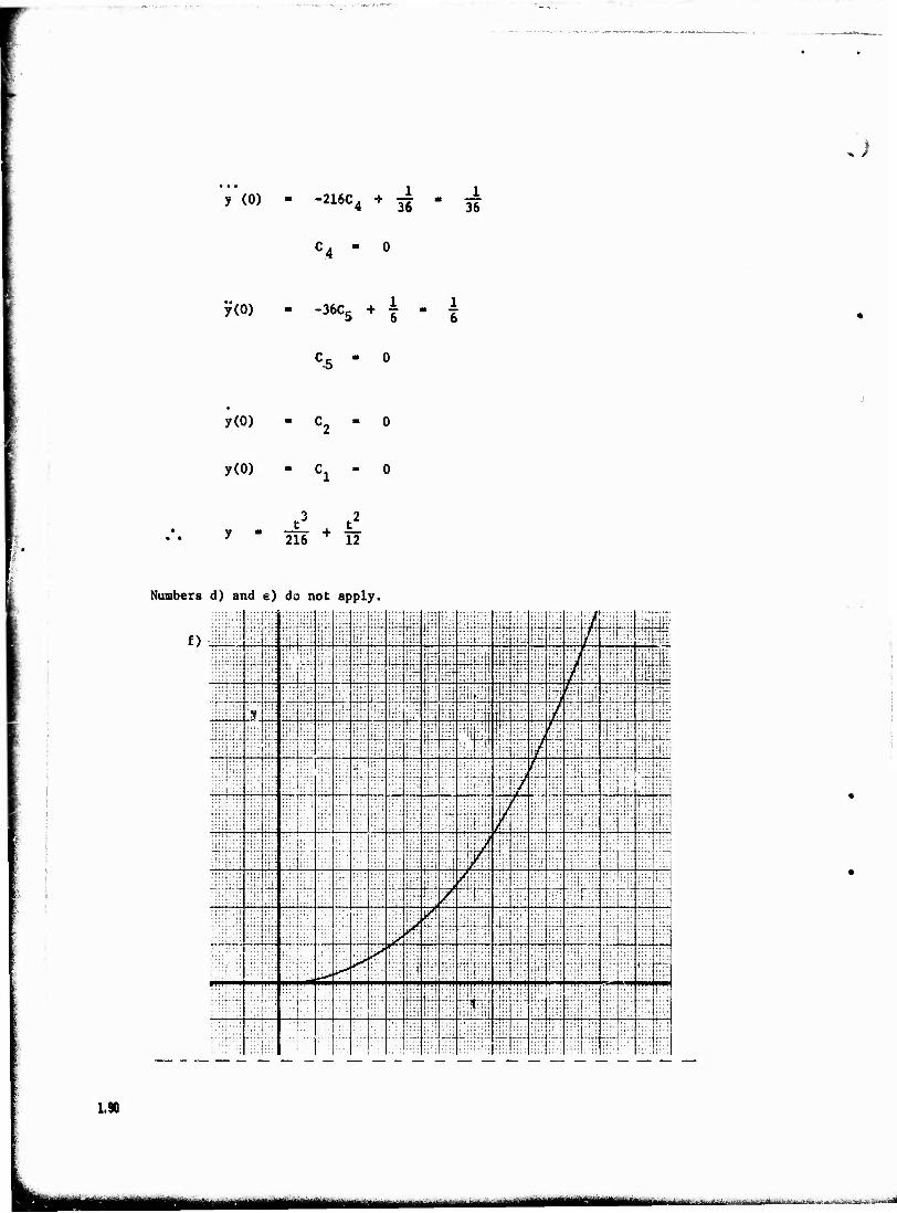
y (0) - -216C, + 4 T 36

_1 36

c4 - 0

y(0) -36C5 + i

y(0)

y(0) - c.

216 12

Numbers d) and e) do not apply.

• ::;: i :t:: # .... ." ::ii i :::: i .::: :::: i." !iH

~: ;«;' :::: ; ;;; :::: ;;:* Hir :H: :::; :::':' '.'.ti :::: in:

.... '.'■'. :::: '■'. Ir l-i-i :"■ :::L 7 tjj< tr.: .... :.*:

::!■

SIM :!i: :::: i ij ::•: Si iii! ;Y

;.*; ':■'.■ :j i ffi

• i ■■

jiJJ :::: ; fill

.:::■

'.','. i :::i :::• :::: ! ;=;; ::i^

t :/

'::': ::!: :ii; rjrl ■i.

'■'■ ■

:::: ;■■'■: ;.:;;

•1 .„. ..... .... .... - ::!: '.'.'.'. ilii ;ü'

::::

: "

-■:■; :: .:::;.:: :;!; "..'.

;:•; ftj ;ili|;ii; :.:. :;:: ::i: ?;'' '.'.'.'. :i;:

.... ... ! :' ...: :::; ■i/ - :.:: i '

.... .::: ;;?! {•*;

:;:: ■.

Till :.

:;; :;:: :::;

::~ — ■

:•:: :;; ■ :: ::i;

;. •: ::::

■■:! -: ::.: i":

-• tri

iill :!::

■ ■ ! ■ u

.. j..; .!- i'il ::: •41 III

' :1 nil

; ::•:

:::: iiij

:.:.' .::. :i;: :■"

.:-■

■ ::•: ....

1.90

ÜH «MMHKMMEM |1jjM|Mi|^1,J.^..-^^...,^-....-.v^..-^:,^.^.-.----.>v^-, .„ V-V^W-i:

> mmmmmim*mmmi»sms™eKm*m»m,~m. ~ . — ——.

i i

u 2. y + 5y + 6y 3e -3t

a) p + 5p + 6

(p + 3)(p + 2) - 0

p - -3, -2

-3t b) Assume y » Ae (forcing function and all its derivatives) P

Cross check with y . Since y appears in y multiply by t in

order to eliminate the duplication.

•'* v* Ate •3t

-3Ate-3t + Ae'3t

9Ate'3t - 3Ae"3t - 3Ae"3t

9Ate"3t - 6Ae"3t

Substituting into the original D.E.

e"3t [(9At - 6A) + 5(A - 3At) + 6At] . -3t . e

e~3t (-A) 3e ■3t

I § <> O

A - -3

-3t y - -3te P

1.91

i^MMMU "•■"—■-■■

c) y - cie_3t + C2e"2t ' 3te"3t

-3Cle-3t - 2C2e"

2t + 9te"3t - 3e"3t

Substituting the boundary conditions

.)

y(0) Cl + C2=->C2 1 - c.

y(0) -6 -3CX - 2C2 - 3

-3 -3C1 - 2 + 2C

Cl = l

(1 - 3t)e -3t

From the homogeneous equation

y + 5y + 6y

2 , u) =6 n

2?o

5 27T 1.02

u, ■ is undefined d

The system is overdamped and non-oscillatory.

1.92

mmmmmämalil mttamat iMMteiMHH« -.,. ,...,, i._^.L.., ,....,.. .jaa^_.3tj-1)lfayi;lt|...,ly.LÜMürtttaÜÜ-aiÄuÜ-" ■'---- ■'■■ - !■

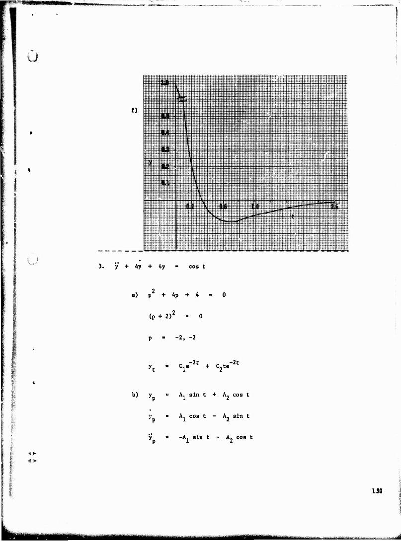
'«»MIBP immw-nww», «HM

u

i t v./

f)

3. y + 4y + 4y cos t

a) p + 4p +

(P + 2)'

-2, -2

Cle"2t + C2te"2t

b) y„ A1 sin t + A- cos t

■ •

y„

A. cos t - A« sin t

-A. sin t - A. cos t

1.93

MUM I MMMBÜÜ—ü iÜBttÜtfliiaitfilii tiifiiriliftrttiiiar I H'' -j^^>iA.ia&j^i***<ai»ä 111 ITI*M

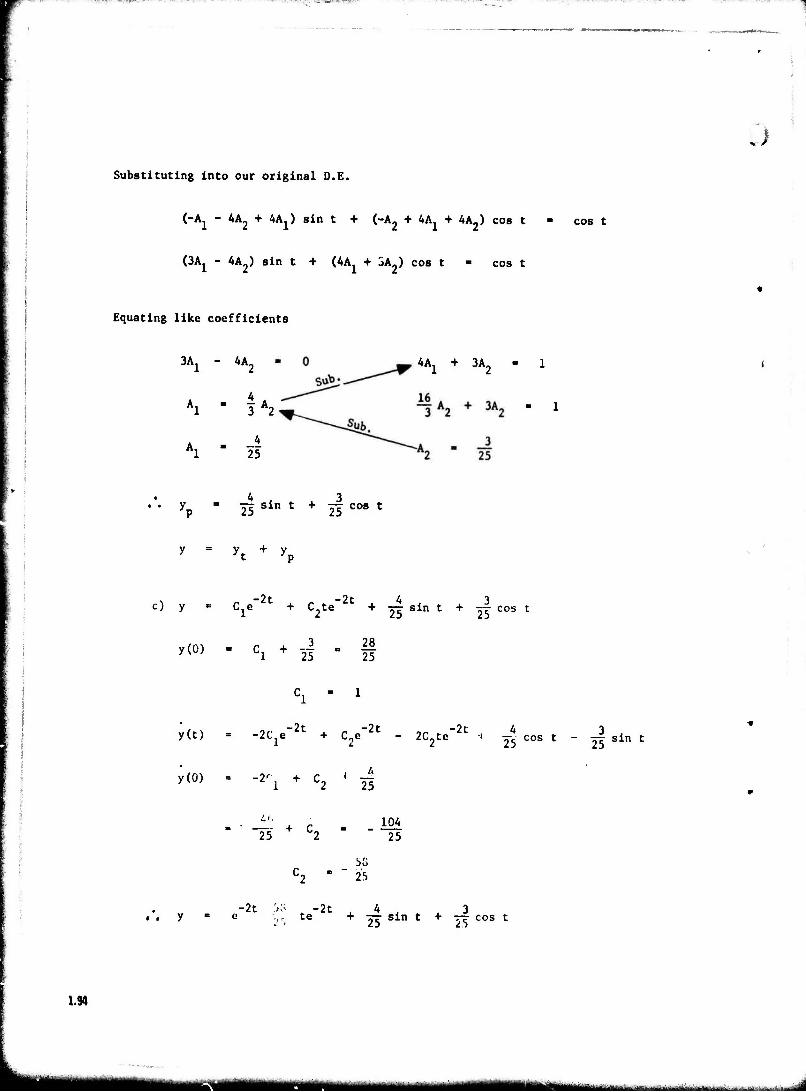
^^^>i'7Trm^V^Jrr-r^^^^^f^7f ■" *>•■' r**. '•"'■■.?•; ***?TWTZy?7F*r*& ■

Substituting into our original D.E.

;

(-Ax - 4A2 + 4AX) sin t + (-A,, + 4AX + 4A2> cos t COS t

I I (3AX - 4A2) sin t + (4Aj + 3A2> cos t - cos t

Equating like coefficients

3A1 - 4A2

Al " U Al

4 25

4AX + 3A-

4 3 TT sin t + jr cos t

y + y

c) y = Cie~2t + C2te"

2t + 2j sin t + y| cos t

y(0) . Cl + -J - ff

y(t)

y(0)

-2C1e + C2e

■If + C * — 1 1 C2 25

2C2te"2t -l y*- cos t

25 sin t

M + C2 104 25

1.94

58 25

-2t W -2t , 4 , ,3 • . y ■ e '-,r te + 25 sin c + 5? cos £

jiliiiifa-filMrtiaililtlfliaiiiaMiliiaKi^aMii Yin' ku "i i i II'I' hiliiM

;■--■ ...... ... ._

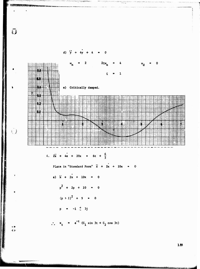
&%@»%£8!&mm^!wmi>mmmB*

■:- : -,-, ,,■»:■■■ ■-..-,,-■■—■.;*•.,-.- -:,-,.. -.. ,-...-,-.■ ■.■ ,--..-..,--

o

o

d) y + 4y + 4

4. 2x + 4x + 20x 6t + |

Place in "Standard Form" x + 2x + lOx - 0

a) x + 2x + lOx

p + 2p + 10

(P v iy + 9

-1 t 3j

4. *'

e-t (C, 6ln 3t + C, cos 3t)

1.95

■^-vüb. ■ '-■■■■ •■-a-^a

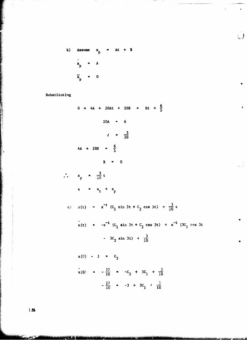
b) Assume x ■ At + B P

x - A P

Substituting

5.96

0 + 4A + 20At + 20B 6t + f

20A

/ - -TZ 3

10

4A + 20B - r

Xp " 10 C

X^ + X t p

c) x(t) e_t (C sin 3t + C, cos 3t) + r^ t

x(t) - -e-t (Cx sin 3t + C2 cos 3t) + e_t (3Cj cos 3t

- 3C2 sin 3t) -i j|

x(0)

x(0) 27 10

27 10

-C2 + 3C;l +

-3 + 3C,

10

10

»I I I |[ MMltllflllMII ,^.,......, ,._.._..,., .,^^„„. _.,..,.

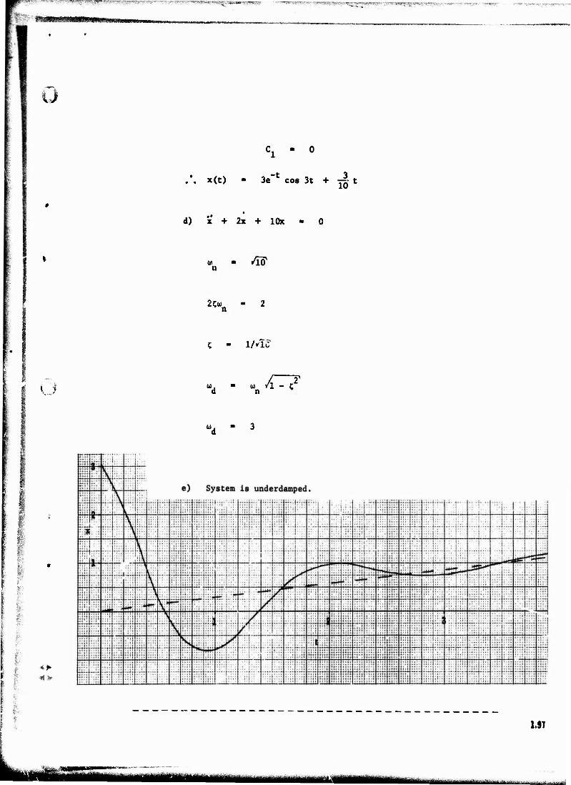
'. ■*» e^w1*,^ ^r.-'T^'r T "y,^^^^*i**'7F7? j^WSf' '■-}wjivrir." ■ V^"1BI .»j p. w i (,-r. wy^3p-»»i!"s :■"

u

.*. x(t) • 3e_t cos 3t + ■— t

d) x + 2x + lOx - 0

fid

2;u

1 o - XT7

:• 3? m

■■■;■■

4>

1 1.9T

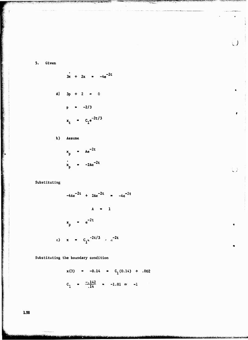
IVl'^'^Bl^MWiLv.'WJI^tfWJM "T ^UJjlllliyilJSp^llWJJ'llWJ^.JUJII^ ""ÜBWSpiirirai

5. Given

v

3x + 2x -4e -2t

a) 3p + 2

•2/3

xt - Cle -2t/3

b) Assume

x - Ae P

-2t

-2Ae ■2t

Substituting

-6Ae"2t + 2Ae"2t - -4e~2t

x ■ e P

_-2t

c) x - Clt"2t/3 , *"2t

Substituting the boundary condition

x(3) -0.14 - ^(0.14) + .002

-.142 .14

-1.01 » -1

1.98

^MM—iam———»«Jt. „,. . , , ___,

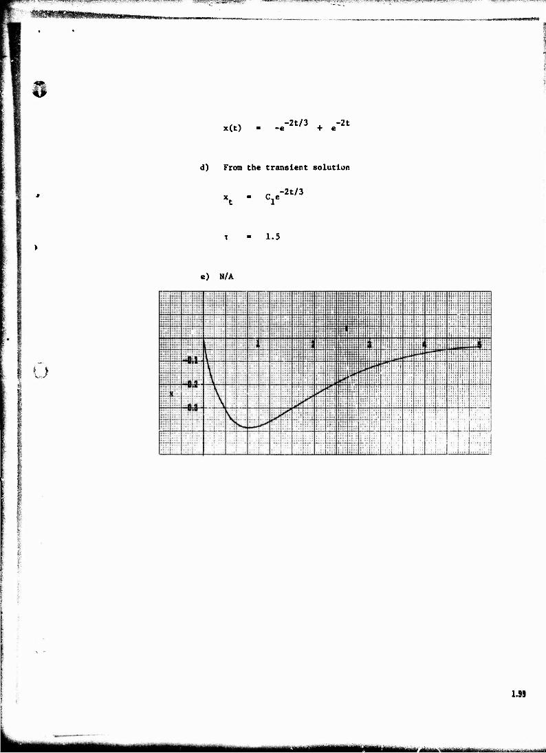
^^^f^-w^ji^»«^*«^^^ <**f*> ■■- •■?*^n^*i"W»

x(t) -2t/3 . -2t -e + e

d) From the transient solution

-2t/3 xt « Cle

1.5

e) N/A

u

1.99

IIIWÜMMMH M^ll ,...——... ,.,, ,. ... ..

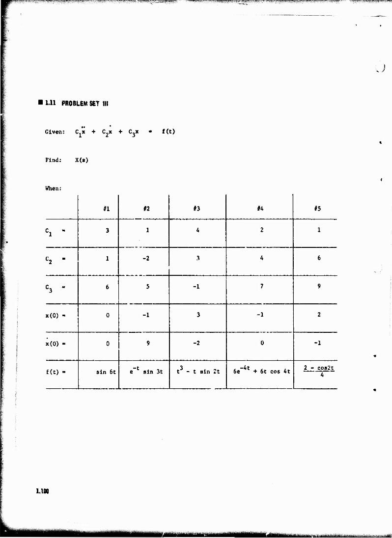
■ i iPiyitKMSwrjwraMWUiyp iu»»iiii'iwI""^^°*yv.w!...i;^gir..!iiwujpi,»>.4»j'.<iiwiff.'

1.U PROBLEM SET III

Given: C.x + C2x + C.x • f(t)

Find: X(s)

Ü

When:

n #2 #3 H #5

Cl " 3 1 A 2 1

C2 - 1 -2 3 A 6

C3 " 6 5 -1 7 9

x(0) - 0 -1 3 -1 2

x(0) - 0 9 -2 0 -1

f(t) - sin 6t e_t sin 3t t3 - t sin 2t -At 6e + 6t cos At

2 - cos2t A

1.100

^M"">^*>*"^ " ■-■-■ . -:

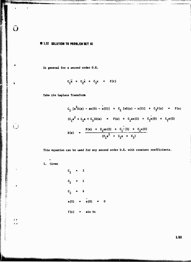
■-.■-TV-M..— ■ r-^.--rr.-r*?T-7a:»>wrv- '^■':3r':^cw^#4.:iifjiw^v«,.'5^!!^g^gj^^j|^p ■ HPSJB^p I •^r'K^^^TTPT^JTV^^^^'Wltf»*^/^^'. :■' :n" S ?car^wj^f^E!W,^^r " .^^SWT^7^^»»'»'TBj-v«i,»r-».T'

Ü

1.12 SOLUTION TO PROBLEM SET Hi

In general for a second order D.E.

Cj'x + C2x + CjX - f(t)

Take the Laplace Transform

u

Cx [s^X(s) - sx(0) - x(0)] + C2 [sX(s) - x(0)] + C3X(s) - F(s)

(C^2 + C2s + C3)X(s) - F(s) + CjSxCO) + 0^(0) + C2x(0)

F(s) + C^sx«» + C^(0) + C2x(0) X(s)

<C18 + C28 + C3)

This equation can be used for any second order D.E. with constant coefficients.

6

1. Given

C2 *

*

. 5:

"I *

x(0) - x(0)

f(t) - sin 6t

1.101

■HiMMMMI HBiMia mmimtimm

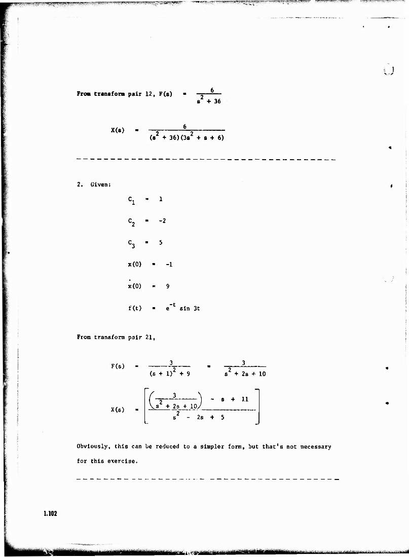
^^jinyv^www'swsww^^ •>'^/i!li«^«W»wvw5^!g5»*«|Mp m'isvmiQj^.e!*!**'

From transform pair 12, F(s) s + 36

X(s) (s2 + 36)(3s2 + s + 6)

2. Given:

"3

x(0)

x(0)

-t f(t) - e sin 3t

From transform pair 21,

F(s)

X(s)

(s + 1)' + 9

s + 2s + 10.

s + 2s ->• 10

s + 11

s - 2s + 5

1.102

Obviously, this can be reduced to a simpler form, but that's not necessary

for this exercise.

u

ikfeu:ä "- -: -■'■-■■" -■'■■'-1-- --■ •- ■"

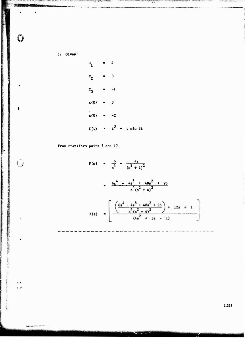
frf. v,"v vfT.-r* --vr -v- ■ ^■'jirv.-TTT, .^j*i59'WJiJt^SBtPir',3Sy6i5|^?ia,!*,i'ir .„p-u;. i^Ti"a5f^«T^p^C ~ -

3. Given:

C2 * 3

C3 ■1 -1

x(0) - 3

i(0) - -2

f(t) M t3 - t sin 2t

I From transform pairs 5 and 17,

u F(s) 4s 2 2 (s^ + ur

6s4 - As5 + 48s2 + 96

8 (s +4)

■4 P

1.103

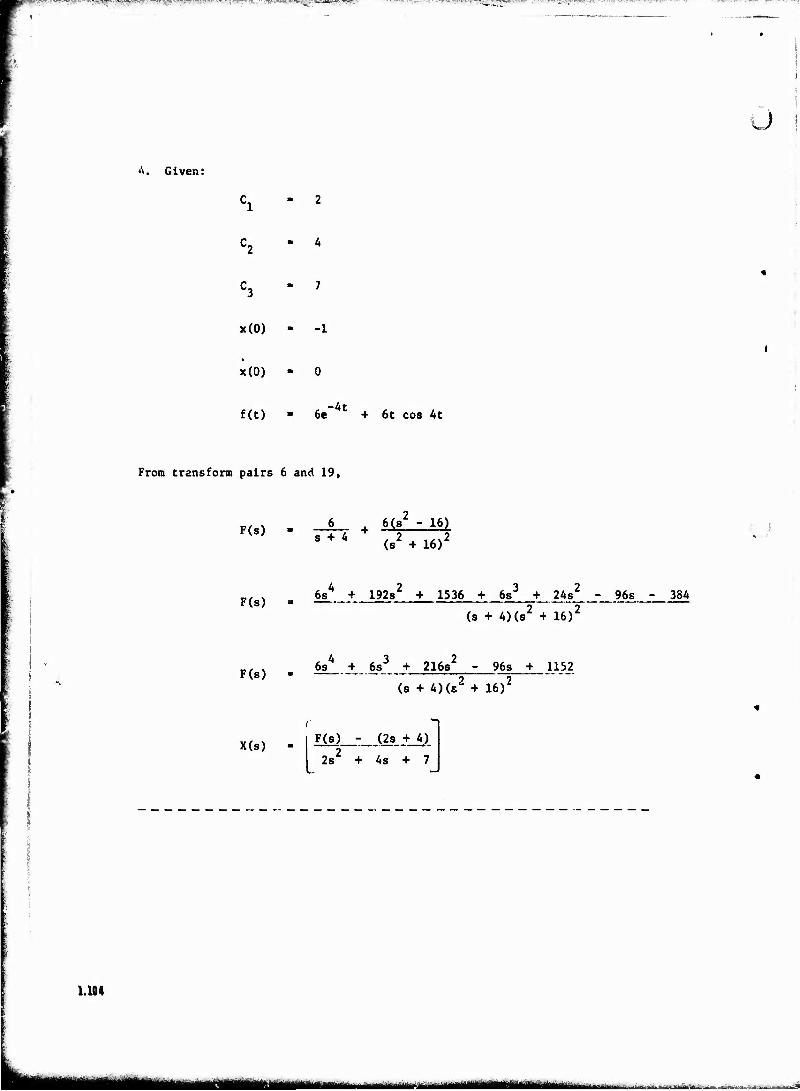
««■-Fr;. "t'iww *Sp«-T ^.7™"^.^^F«l^«TV'T-^^l^;^W;^TOT'Ty^n|^r^^fI-T^».-'S

1.104

4. Given:

3

x(0)

x(0)

u i

f(t) -4t 6e + 6t cos At

From transform pairs 6 and 19,

F(s) . _§_- + 6(8« - 16) s + 4 / 2 x iA\2

(s + 16)

F(s) 6s4 + 192s2 + 1536 + 6s3 + 24 s2 - 96s - 384

(s + 4)(s2 + 16)2

F(s) 6sA + 6s3 + 216s2 - 96s + 1152

(s + 4)(s2 + 16)2

X(s) F(s) - (2s + 4)

2s2 + 4s + 7

UMiVM nmü üüIüI ..-.- t.,lj-^,..^:h..-, ...^.. . _,,. ............. ; .-. *^J.£.-ta&k

■i-^.-îr^\^Y-'-- r^^'-' -~'T: - '>:TS~'^^r"»*^'"*V*^-'. .»yjiC"fY—?■••;■ ■ V"'^?'v~- ~-V'-***« ■ ir^**"sfr^s'^?'?: "s*™î™7 ':"'""'pr"*i"^'7^.':-''"''-'^K'^;'"^""

S. Given:

"3

x(0)

1

6

9

2

x(0)

f(t)

-1

2 - cos 2t i - J cos 2t

From transform pairs 3 and 13,

u F(s)

F(s)

X(s)

t G) * i (/+ J

2s + 8 - s

s(s2 + 4)

F(s) + (2s + 11)

s2 + 6s + 9

1 4

»2 + 8

s(s2 + 4)

•4 *

1.105

.îL-.J.,jfca^..~^.^.^w...,'^... ■

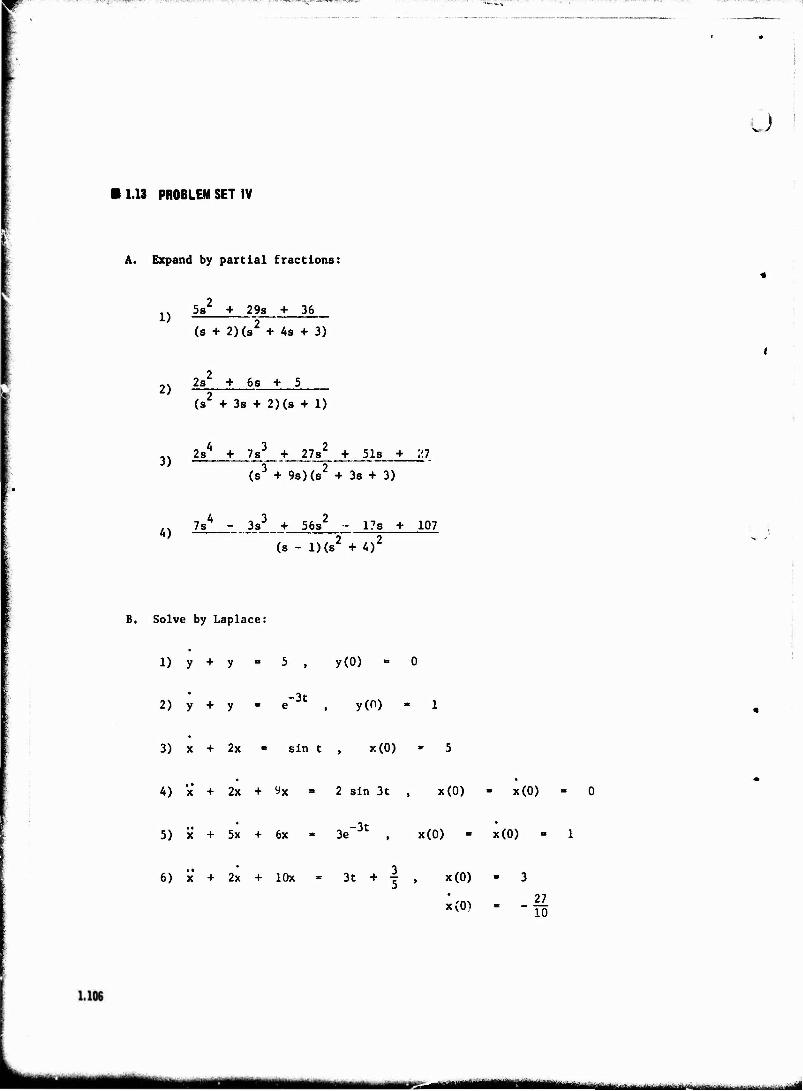
-.. ■', *. '■—--T!»??s*»«5y wiajöBj "'---.'~'""''"""1"

1.13 PROBLEM SET IV

A. Expand by partial fractions:

1) 5s + 29s + 36

(s + 2)(s2 + As + 3)

2) 2s + 6s + 5

(s2 + 3s + 2)(s + 1)

3) 2sA + 7s3 + 27s2 + 51s + :i7

(s3 + 9s)(s2 + 3s + 3)

4) 7sA - 3s3 + 56s2 - 17s + 107

(s - l)(s2 + A)2

B. Solve by Laplace:

1) y + y - 5 , y<0)

2) y + y - e"3t , y(0)

3) x + 2x sin t , x(0)

A) x + 2x + ^x » 2 sin 3t , x(0) x(0)

5) x + 5x + 6x 3e ■3t x(0) x(0)

6) x + 2x + lOx 3t + | , x(0)

x(0) 27 10

^^-Mt^m—a—w—»«^-

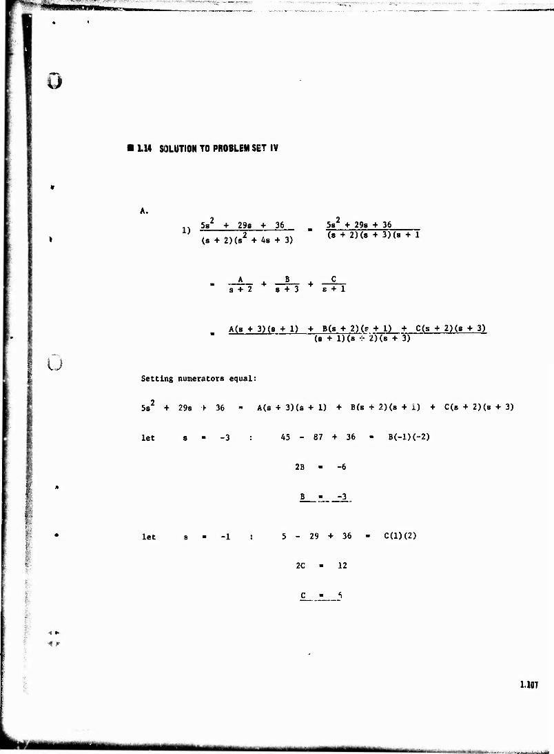
BWiBawuPTSP Ko<t-<yffT"HM»:> u|g«t;'yBwr<»ti.a^jjr, . . -

LM SOLUTION TO PROBLEM SET IV

A.

1) 5s* + 29s + 36

(s + 2)(s2 + 4s + 3)

5afc + 29s + 36 (s + 2)(s + 3)(s + 1

A + -^ + -5- s + 2 s + 3 " s + 1

u A(s + 3)(s + 1) + B(s 4- 2)(g + 1) + C(s + 2)(s + 3)

(| + I)(l+'2)(|+J5

Setting numerators equal:

58* + 29s * 36 A(s + 3)(s + 1) + B(s + 2)(s + 1) + C(s + 2)(s + 3)

let s 45-87+36 - B(-l)(-2)

2B

let s 29 + 36 C(l)(2)

4 *»

2C - 12

1.107

mm ^^^ IHHMWW

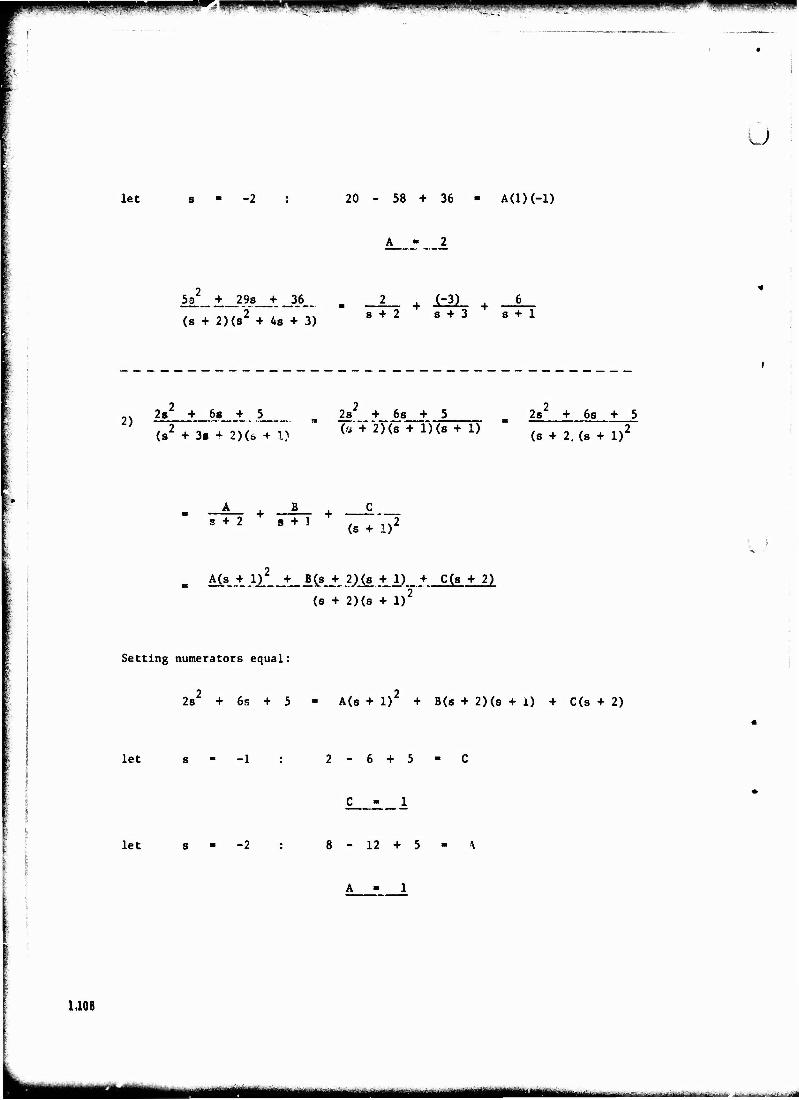
wpj-uiwiin^iijiii i II wtm ..,imu,mi,tu-u.jijijujMjiij ■*i'**•",''■' ■ '■ '::" "'■„■'*¥' ■ ■ ~.-..- '■'^■■", rt-L .-^-"-V;, VJ"' *-«*f** i «•«^«pnfinMVMmimppni,, JIHI-IW ppupip

O

let -2 20-58 + 36 - A(l)(-1)

5a +_J9s__+ 36_

(s + 2)(s2 + As + 3) 1=21

8 + 2 S + 3 8 + 1

2) 28 + 6s + 5

(s2 + 3s + 2)(s + l>

2s + 6s + 5 {n + 2)(s + l)(s + 1)

2s + 6s + 5

(s + 2, (s + l)2

_A_ + _!_ + ___C 8 + 2 9 + 1 (s + I)2

A(s + 1) + B(s + 2)(s + 1) + C(s + 2)

(s + 2)(s + l)2


2s + 6s + 5 A(s + 1) + B(s + 2)(s + i) + C(s + 2)

let s 2-6 + 5 - C

let s 8-12 + 5

1.108

■■»iMilrMiiEiii -if^ ■ - ■•■^■■-^^.■■i-.^-.--i-y--~^- -i-**.,**^-**..-»^-™**

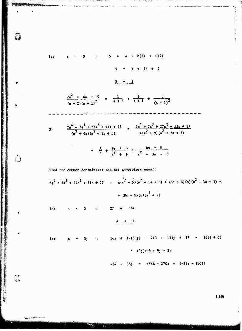
o

let s^O 5 - A + B(2) + C(2)

1 + 2B + 2

2s + 6s + 5

(s + 2)(s + l)2 8+28+1 <s+l)2

3) 2sA -f 7s3 + 27s2 + 51s + 27

(s1 + 9s)(s2 + 3s + 3)

2s4 + 7s3 + 27s2 + 51s + 27

P(S2 + 9)(s2 + 3s + 3)

i }

A ,, B« + C ■ — + —« + 8 s2 + 9

Ds + E

s + 3s + 3

Find the common denominator and set numerators equal:

2s4 + 7s3 + 27s2 + 51s + 27 « Al«2 + 9)(s2 + Is + 3) + (Bs + C)(s)(s2 + 3s + 3) +

+ (Ds + E)(s)(s2 + 9)

let s 27 - "7A

let 3J 162 + (-189j) - 243 + 153j + 27 - (3Bj + C)

4 *•

41>

(3j)(-9 + 9j + 3)

-54 - 36j - (54B - 27C) + (-81B - 18C)j

1.109

a

Since the real part on the left must equal the real part on the right,

(7) -54 - 5AB - 27C

and the imaginary parts must also be equal

(7) -36 ■= -81B - 18C

from (T) C - +2 + 2B

substituting into (Y)

-36 = -81B - 18(2 + 2B)

0 = -117B

B ^ 0

C - 2 + 2B

C = 2

let s 2 - 7j - 27 + 51j + 27 - A(8)(? + 3j) + (jB + C)

(j)(2 + 3j) + (jD + E)(j)(8)

2 + 44j 16 + 24j + 4j - 6 - 8D + 8jE

-8 + 16j * -8D + (8E)j

Setting real and imaginary parts equal,

-8D

1.110

mma mi MI miTir [fäfrg^"-" ■m^ „..., -•-:^rtTffm ■ ••< ; ..^....«■^■n.-j-^a,

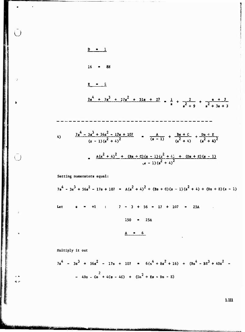
u D - 1

16 - 8E

2s4 + 7s3 + 27s2 + 51s + 27 L.*~2

8 + 2

8+9 8+38 + 3

4) 7s4 - 3s3 + 56s2 - 17s + 107

(s - l)(s2 + A)2 (s - 1) Bs + C Ds 4 E

2 2 2 (s + 4) (s' + 4)

( A(s2 + 4)2 + (Bs + C)(s - l)(a2 + 4*, + (Ds + E)(s - 1)

,* - 1)0? + 4)2


7s4 - 3s3 + 56s2 - 17s + 107 - A(s2 + 4)2 + (Bs + C)(s - l)(s2 + 4) + (Ds + E)(s - 1)

Let s - +1 7-3 + 56-17 + 107 - 25A

150 - 25A

Multiply it out

7s4 - 3s3 + 56s2 - 17s + 107 - 6(a4 + 8s2 + 16) + (Bs4 - BS3 + 4Bs2

4 ¥ 4Bs - Cs + 4Cs - 4C) + (DE + ES - Ds - E)

1.111

IHM ..--.. ii. „n- ■ ■ .., -..„ Ji^^..1f|j|||

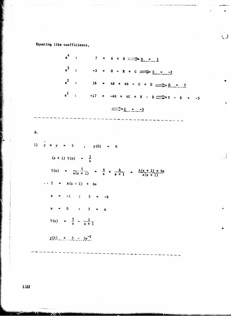
Equating like coefficients,

_4 6 + B r.-r>B - 1

\ ) v./

-3 0 - B + C -2

56 48 + 4B - C + D -^ D

-17 -4B + 4C + E - D

:>E

B.

1) y + y y(0)

(s + 1) Y(s)

Y(s) s(s + 1)

A(s + 1) + Bs

^ + -JL_- S 8 + 1

A(s_+_1)_+ jte s(s + 1)

Y(s) J. + 1

ZiO. 5 - 5e -t

1.112

Kbaää - ' B ~*—~— ■ ■....„■u^.^'-.,L.....c,.-!aB-:,^.,J,.,.^..^-

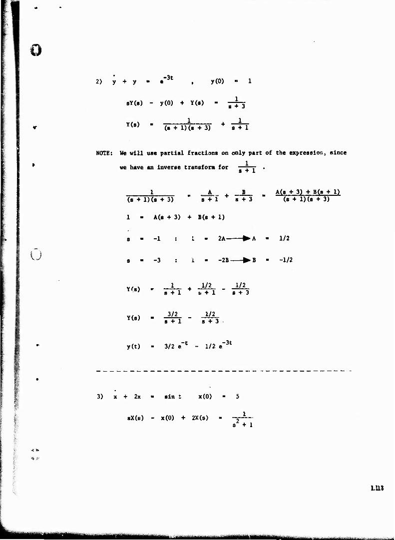
1 o

2) y + y

sY(s)

Y(s)

-3t

y(0) + Y(s)

1

y(0) - l

l " m i

(s + l)(s + 3) 8 + 1

NOTE: We will use partial fractions on only part of the expression, since

1 we have an inverse transform for s + 1

u

T + B

(s + l)(s + 3) s + 1 s + 3

1 - A(s + 3) + B(s + 1)

-1

-3

; JL 2A-

A(s + 3) + B(s + 1) <s + l)(s + 3)

1/2

-2B -1/2

Y(s) 1 + _J72_ i/2 S + l fe + 1 6 + 3

Y(8) 3/2 1/2 s + l s + 3

y(t) - 3/2 e-t - 1/2 e"3t

3) x + 2x - sin t x(0)

sX(s) - x(0) + 2X(s) - s2 + l

1.U3

IT iiTmiiiiiiiria^^aita^MliStti kUM> """ -w.it-.,». f...J.1^.....J— ......: .. :.■ ..

x(«) Transform available so do not

(a' + l)(s + 2) s + 2 include in partial fraction

expansion.

)

(8* + i)(s + 2)

As + B C „ (As + B)(s + 2) + C(s + 1)

s2 + 1 8+2 (s2+l)(s+2)

1 " (As + B)(s + 2) + C(s + 1)

5C 1/5

8-0 2B + C ;>B 2/5

3A + 3B + 2C _ >A -1/5

v,a^ . -1/5 s 2/5 5 1/5 X(8) T~7 + 2 7 . + s + 2 s + i. s + 1

x(t) « -1/5 cos t + 2/5 sin t + 5 1/5 e -2t

A) x + 2x + 9x 2 sin 3t x(0) - x(0) - 0

(s' + 2s + 9) X(s) s2 + 9

X(s) (s2 + 9)(s2 + 2s + 9)

As + B Cs + D

s2 + 9 s2 + 2s + 9

1.114

6 - (As + B)(s2 + 2s + 9) + (Cs + D)(s2 + 9)

6 • 9B ♦ 9D

■HMMMMIHMMlratllWl MB "— ■■--■' .-—a-- ■■-.-.■—»■-■. —.»...:

-v > W*e!m£fä@G&£t mmmamn

ö 3j (3Aj + B)(-9 + 6j + 9) - (3Aj + B)(6J)

s - 1

A

B

D

-18A + 6Bj

-1/3

0

2/3

12A + (C + D)10

12 (-1/3) + IOC + 10 (2/3)

1/3

x(8) . Z&L* + 1/3 « ± 2/3 s + 9 s + 2s + 9

u \i X(8)

-1/3 8 1/3 (s + 2)

s2 + 9 (s + l)2 + 8

-1/3 s + 1/3 (8 + 1) + 1/3

a2 + 9 (s + l)2 + 8 (s + l)2 ♦■ 8

x(t) -1/3 cos 3t + 1/3 e_t cos 2/2t + V(6,/2 $* sln 2/2 * •

5) x + 5x + 6x - 3e -3t x(0) - x(0)

s2 X(s) - »x(0) - x(0) + 5sX(s) - 5x(0) + 6X(s) - 3

s + 3

(s' + 5s + 6) X(s) s + 3 + 8 + 6 s + 9s + 21 s + 3

4 V

1.116

^^„gng^g^m,

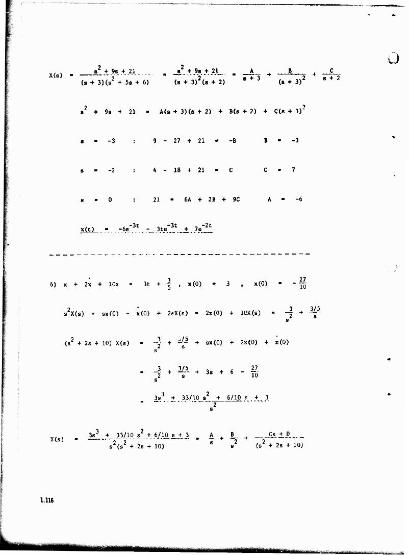
X(s) s* + 9s + 21 s' + 9s + 21

(s + 3)(s' + 5s + 6) (s + 3)'(s + 2) -A- + — » + _<L. 8 + 3 (s + 3)2 8 + 2

o

s2 + 9s + 21 - A(s+3)(s+2) + B(s + 2) 4 C(s + 3)~

s - -3 9 - 27 + 21 - -B B - -3

-18+21 C - 7

21 - 6A + 2B + 9C A - -6

-3t , -3t , , -2C x(t) - -6e *x -_ 3U..1 -±-7A

6) x + 2x + lOx 3t + | , x(O) 3 , x(O) 27 10

s2X(s) = sx(0) - x(0) + 2sX(s) - 2x(0) + lCX(s) 2 + IL? 2 s s

(s4 + 2s + 10) X(s) 3 + 'ill + 8X(0) + 2x(0) + x(0) 2 s

\ ♦ ^ ♦ * ♦ • - To

3s3 + 33/10 «2__+_A/W «"-.-+ _3

X(s) Cs + D 3s3 + 33/10 s2 + 6/10_s_+ 3 _ A + B_ +

" sVT IsTlO) S s2 (s2 ♦ 2s + 10)

1.116

"MJujUfchBiiiii imii^jg^im.., | ^attMaiäafa

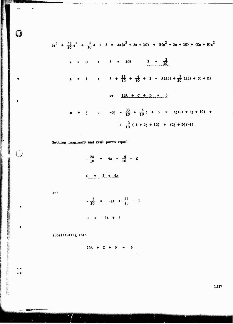
3s3 + ~ a2 + j| s + 3 - Aa(s2 + 2s + 10) + B<»2 + 2s + 10) + (Cs + D)s2

! I 4 *■

4P

3 - 10B B " 15

3 + |§ + Y§ + 3 - A(13) + jl (13) + (C + D)

or 13A + C + D

• + J -3j - |§ + j| j + 3 - Aj(-l + 2j+10) +

+ jfc (-1 + 2j + 10) + (CJ + D)(-l)

Setting Imaginary and real parts equal

U To • * + 15 - c

and

3 + 9A

3 „ , 27 n IS " "2A + To " D

-2A + 3

substituting into

13A + C + D - 6

1.117

13A - 3 + 9A - 2A + 3 - 6

A - 0

then

and

o

xc.) - ^+ -j^±± 3/10 + 3 8 + 1

s + 2s + 10 2 2

(s + 1) + 3* i I

1.118

3 -t x(t) - y^ t + 3e cos 3t

Mi aaü^:-:.-!,..v..-.i.,-.■:.■,„..:.,-■ ■-■ - „^^jt.nvj'j-iinrTilrvflu«!n'ii^if. ■■■finrfTf'n'

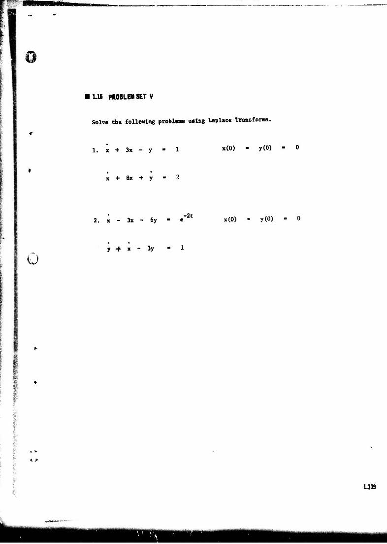
i E u

1.15 PROBLEM SET V

Solve the following problems using Laplace Transforms.

1. x + 3x - y - 1

x + 8x + y ■ 2

x(0) - y(0) - 0

2. x - 3x - 6y - e

y + x - 3y - 1

-2t x(0) ■ y(0)

' I;

1.119

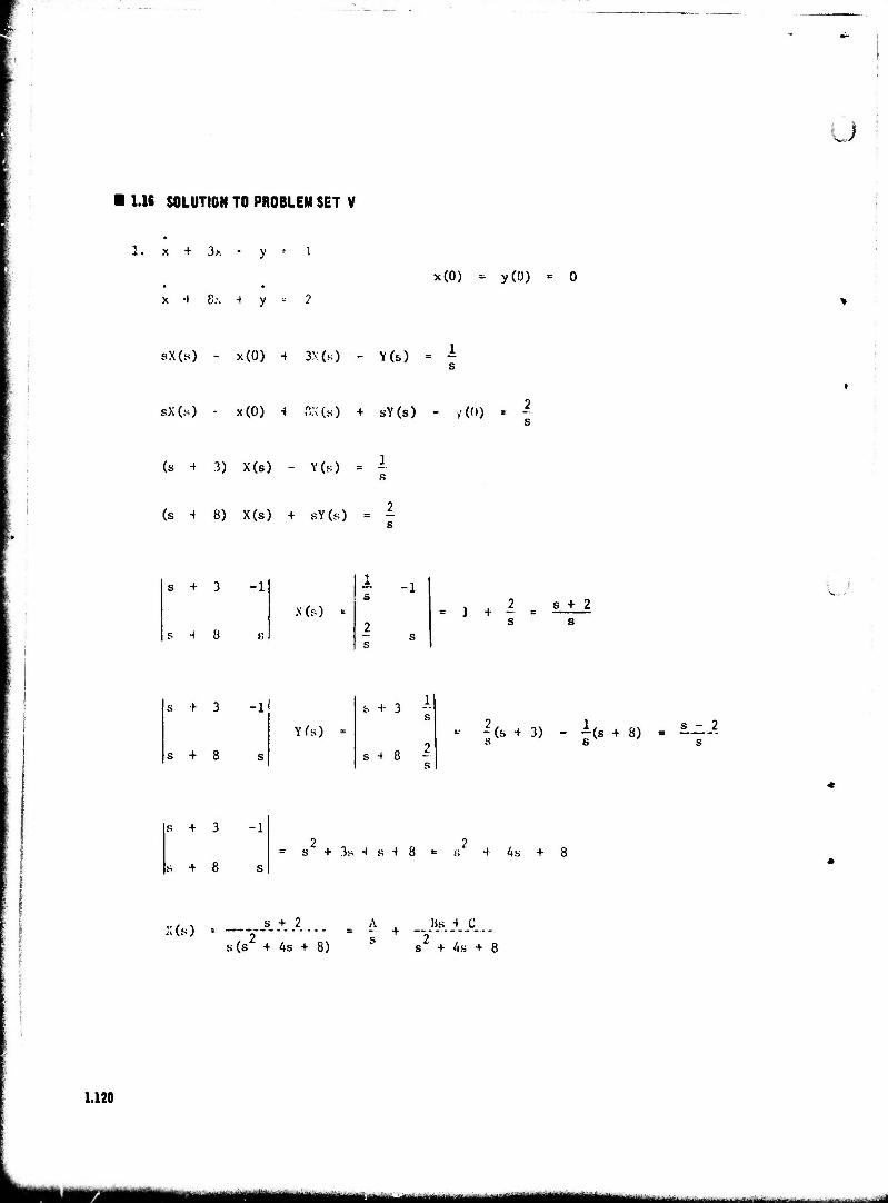
1.16 SOLUTION TO PROBLEM SET V

1. x + 3x - y ' 1

x 4 B,\ 4 y = 2

X(O) - y(O)

Ü I

SX(s) x(O) 4 3>(s) - Y(s) - i s

sX(s) - x(0) 4 ,«tt(s) + sY(s) - /(O)

(s 4 3) X(s) - Y(s) = J

(s 4 8) X(s) + sY(s) - 4

s 4 3

S 4 8

•V(s)

-1

! 4 2 S + 2 1 + — ■

s s

+ 3

+ 8

Yfs) =

s + 3

s 4 8

;(s + 3) J(. 4- 8) s - 2 s

I s 4- 3 -1

s 4- 8 s = s 4- 3s 4 s 4 4 4s 4- 8

1.120

y,K s. __ s_ +2 _ A „JI.S.+ _C.._.

s(s 4- As 4- 8) s s2 4- 4s + 8

mmmmmmmmmmäMmumimmmtmmtmmmm^mm ^---...^-»■„„„„„^i-i....^,.,,. unr-i'irtfniiuil

ü A(s' + 4s + 8) + s(bs + C) - s + 2

s = 0: 8A = 2 s*:A + B«0 s: 4A + C = 1

u

X(s)

A -..!/*

1/4 + _r.i/i_s.._,. s (s 4 2)2 + 4

B • - 1/4 C - 0

1/4 1/4 s + 2

(s + 2)' + 4 (s + 2)' + 4_

x(t) = 1/4 I 1 - e"2t (cos 2t - sin 2t)I

Us)

2

s - 2 A + Bs + C

s(s2 + 4s + 8) S s2 + 4s + 8

A(s' 4 Is + 8) + s(Bs + C) = s - 2

i t

s = 0: 8A = -2 s": A + B = 0 s: 4A + C = 1

A - -1/4 B =1/4 C = 2

Y(s) = 1/4 Cs + iy + 4j

1/4 -1 . __s_± A (s 4 2)' + 4 (s + 2)' + 4

[" -2t.

2. x - 3x - 6y - e

y + x - 3y - 1

y(t) = 1/4 1-1 + e '"'(cos 2t + 3 si

-2t

in ?t)J

x(0) = y(0) = 0

. 1 f. 1.121

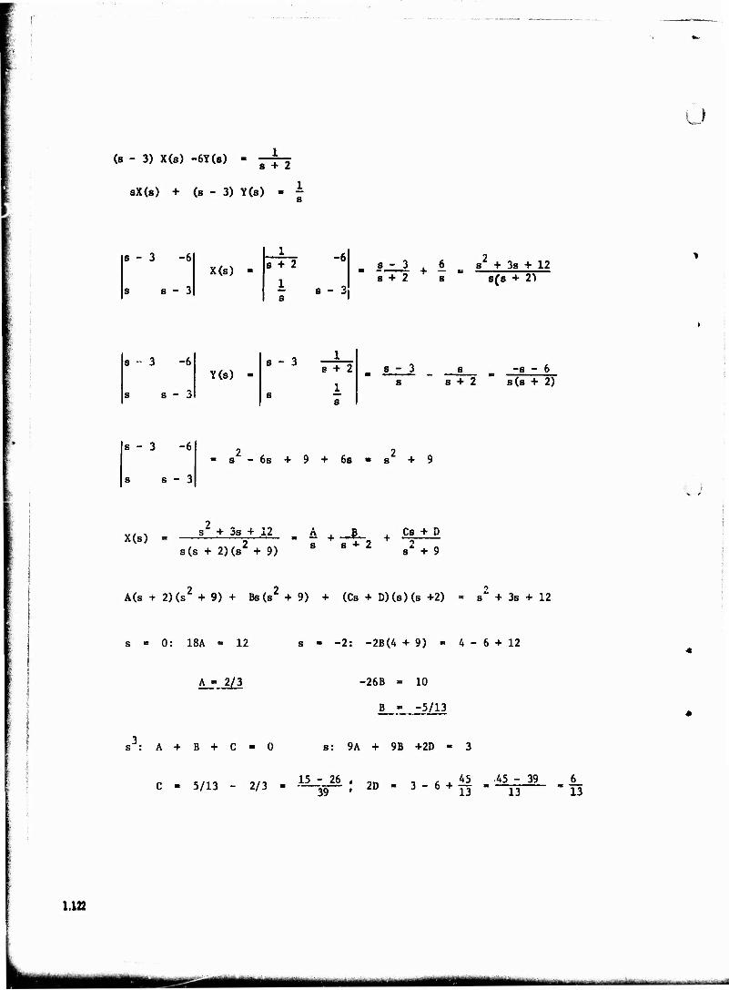
(s - 3) X(s) -6Y(s) 8 + 2

sX(s) + (s - 3) Y(s)

s-3 -6

s 8-3

X(s) s + 2

1 8

-6

_ o

s-3 „ 6 8 + 2 8

s + 3s + 12 8(8 + 2)

s-3 -6

S S - 3

Y(s) 8-3

8 + 2

1 s

8-3 _ 8 m -8-6 8 s + 2 " s(s + 2)

s-3 -6

s s-3

-s- 6s + 9 + 6s »a2 + 9

X(s) s(s + 2) (s* + 9)

ü + 6 8 8 + 2

Cs + D

s + 9

A(s + 2)(s2 + 9) + Bs(s2 + 9) + (Cs + D)(s) (s +2) s" + 3s + 12

s = 0: 18A - 12 - -2: -2B(4 +9) - 4-6+12

A = 2/3 •26B - 10

B_-1-5/13

A + B + C ■ 0 s: 9A + 9B +2D - 3

1.122

C = 5/13 - 2/3 - ^-^ ; 2D - 3 - 6 + |f - *Lz 39 - |j

— ■■-

u

* *■

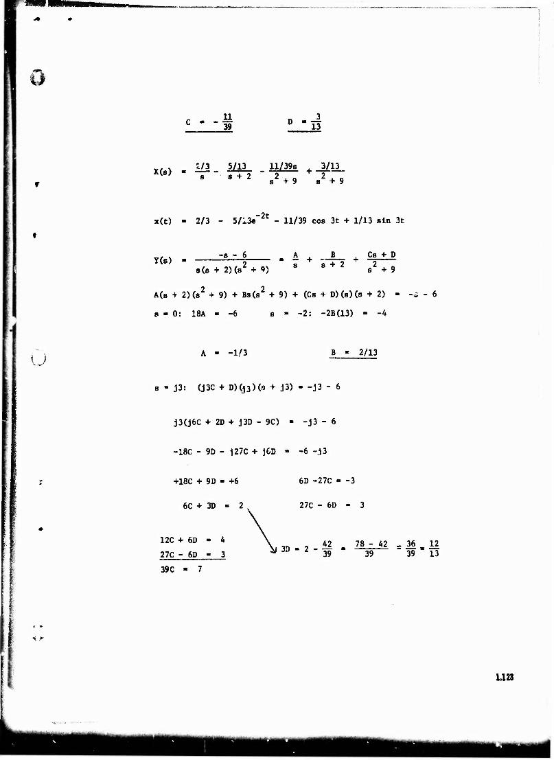
11 c - -w -if

x,s) . ±12- 5/13_ . 11/398 + ^/13_. *{s) s 8+2 2in2,„ 8+9 8+9

x(t) - 2/3 - 5/13e"2t - 11/39 cos 3t + 1/13 sin 3t

Y(s) -s-6

s(s + 2) (s* + 9) A + 8 8 + 2

B Cs + D

a2 + 9

A(s + 2)(s2 + 9) + Bs(s2 + 9) + (Cs + D) (s) (s + 2) -

s - 0: 18A s - ~2: -2B(13) - -4

' u A - -1/3 B * 2/13

s - j3: (J3C + D)(j3)(o + j3) - -j3 - 6

J3(j6C + 2D + J3D - 9C) - -j3 - 6

-18C - 9D - 127C + j6D - -6 -j3

+18C + 9D - +6 6D -27C - -3

6C + 3D 27C - 6D - 3

12C + 6D - 4

27C - 6D - 3

39C - 7

3D - 2 42 78 - 42 .36 12 39 " 39 " 39 * 13

1.123

\*.^

39 D - 13

1.124

Y(8) = ZUI ., _2/JL3 7j39e_ 4/13

y(t) = -1/3 + 2/13e"2t + 7/39 cos 3t + 4/39 sin 3t

- --- ■■ ■ fc;^l"'-»'-t-'-:—'-" ^-—■■-■ "nhir^^-i ni-.f f,lVtiiil.1,.li;'i-.:-i;Wii-ii

1*1

CHAPTER

EQUATIONS OF MOTION

l )

(Ravisad Novambar 1973)

2.1 INTRODUCTION

These notes are written as a general classroom text for the theoretical approach to Stability and Control in the course curriculum of the USAF Test Pilot School.

The theoretical discussion will, of necessity, incorporate certain simplifying assumptions. These simplifying assumptions are made in order to make the main elements of the subject more clear. The equations developed are by no means suitable for design of modern aircraft, but the basic method of attacking the problem is valid. Now that analog and digi- tal computers are available, the aircraft designers* more rigorous theoretical calculations, modified by data obtained from the wind tunnel, often give results which closely predict the flying qualities of new airplanes. However, neither the theoretical nor the wind tunnel results are infallible. Therefore, there is still a valid requirement for the test pilot .in the development cycle of new aircraft.

2.2 TERMS AND SYMBOLS

There will be many terms and symbols used during the stability and control phase. Some of these will be familiar, but many will be new. It will be a great asset to be able to recall at a glance the definitions represented by these symbols. Below is a condensed list of the terms and symbols used in this course:

2.2.1 Terms

Stability Derivatives

-m„ 3Cm m 3 a

Nondimensional quantities expressing the variation of the force or moment coefficient with a disturbance from steady flight.

(2.1)

3C n 3 t (2.2)

Stability Parameters - A quantity that expresses the variation of force ^ moment on aircraft caused by flight or by a disturbance from steady flight.

_ pUSc fc U 3Cm,

y (Change in pitching moment caused (2.3) by a change in velocity)

2.1

—---■■- -- ■-■ ■ ■■■ ■ -■ - ■

k •

o Sc L = j—— C (Change in lift caused by a (2.4) q J'L q change in pitch rate)

Static Stability - The initial tendency of an airplane to return to steady state flight; after a disturbance.

Dynamic Stability - The time history of the respc.ise of an airplane to a ~ ' disturbance, in which the aircraft ultimately returns

to a steady state flight.

Neutral Stability -

a) Static - The airplane would have no tendency to move from its disturbed condition.

b) Dynamic - The airplane would sustain a steady oscillation caused by a disturbance.

Static Instability - A characteristic of an aircraft such that when disturbed from steady flight, its tendency is to depart further or diverge from the original condition of steady flight.

Dynamic Instability - Time history of an aircraft response to a disturbance in which the aircraft ultimately diverges to departure or destruction.

Flight Control Sign Convention - Any control movement or deflection that ~ " ~~~ causes a positive movement or moment on

the airplane shall be considered a positive control movement. This sign convention does not conform to the convention used by NASA and some reference text books. This convention is the easiest to remember and is used at the Flight Test Center, therefore, it will be used in the School.

Degrees of Freedom - The number of paths that a physical system is free

2.2

uilu^^al_aumM^aiCM—MllMWttf<^fc«<ini' i --.~_

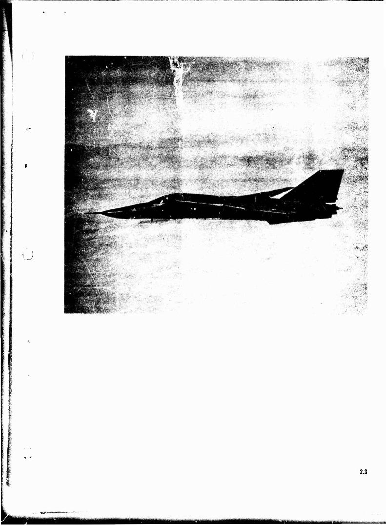
m ■MMH — ■• ■ ■ - ■ ■-

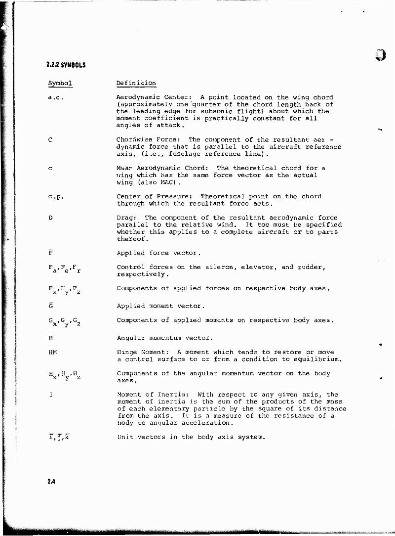
2.2.2 SYMBOLS

Symbol Definition

a.c. Aerodynamic Center: A point located on the wing chord (approximately one quarter of the chord length back of the leading edge for subsonic flight) about which the moment joefficient is practically constant for all angles of attack.

C Chorciwise Force: The component of the resultant aer - dynamic force that is parallel to the aircraft reference axis, (i.e., fuselage reference line).

c Mean Aerodynamic Chord: The theoretical chord for a wing which has the same force vector as the actual wing (also MAC).

c.p. Center of Pressure: Theoretical point on the chord through which the resultant force acts.

D Drag: The component of the resultant aerodynamic force parallel to the relative wind. It too must be specified whether this applies to a complete aircraft or to parts thereof.

F Applied force vector.

F ,F ,F Control forces on the aileron, elevator, and rudder, respectively.

F ,F ,F Components of applied forces on respective body axes.

G Applied moment vector.

Components of applied moments on respective body axes.

Angular momentum vector.

Hinge Moment: A moment which tends to restore or move a control surface to or from a condition to equilibrium.

Components of the angular momentum vector on the body axes.

Moment of Inertia: With respect to any given axis, the moment of inertia is the sum of the products of the mass of each elementary particle by the square of its distance from the axis. It is a measure of the resistance of a body to angular acceleration.

i, J,k Unit vectors in the body axis system.

G ' X G ,

Y G

z

H

HM

Hx' !

H Y

H z

i -

2.4

3

im»H—rmmii«i

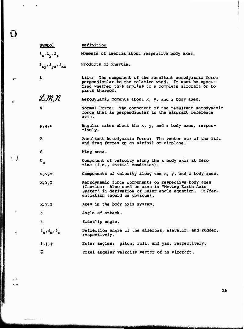
o

o

Symbol

xy' yz' xz

N

P,q,r

R

S

Uo

u,v,w

X,Y,Z

x,y,z

a

I

W6r

0)

Definition

Moments of inertia about respective body axes.

Products of inertia.

Lift: The component of the resultant aerodynamic force perpendicular to the relative wind. It must be specified whether this applies to a complete aircraft or to parts thereof.

Aerodynamic moments about x, y, and z body axes.

Normal Force: The component of the resultant aerodynamic force that is perpendicular to the aircraft reference axis.

Angular rates about the x, y, and z body axes, respectively.

Resultant Aerodynamic Force: The vector sum of the lift and drag forces on an airfoil or airplane.

Wing area.

Component of velocity along the x body axis at zero time (i.e., initial condition).

Components of velocity along the x, y, and z body axes.

Aerodynamic force components on respective body axes (Caution: Also used as axes in "Moving Earth Axis System" in derivation of Euler angle equation. Differ- entiation should be obvious),

Axes in the body axis system.

Angle of attack.

Sideslip angle.

Deflection angle of the ailerons, elevator, and rudder, respectively.

Euler angles: pitch, roll, and yaw, respectively.

Total angular velocity vector of an aircraft.

2.6

mmmm ■atouuttiui

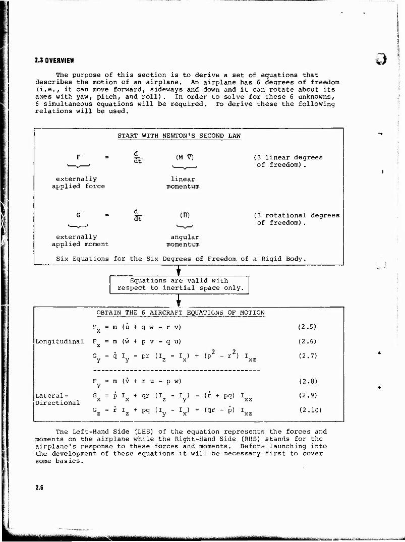
2.3 OVERVIEW

The purpose of this section is to derive a set of equations that describes the motion of an airplane. An airplane has 6 decrees of freedom (i.e., it can move forward, sideways and down and it can rotate about its axes with yaw, pitch, and roll). In order to solve for these 6 unknowns, 6 simultaneous equations will be required. To derive these the following relations will be used.

o

START WITH NEWTON'S SECOND LAW

F d dT (M V)

externally applied force

linear momentum

G d at (H)

externally applied moment

angular momentum

(3 linear degrees of freedom).

(3 rotational degrees of freedom).

Six Equations for the Six Degrees of Freedom of a Rigid Body,

I Equations are valid with

respect to inertial space only.

1 OBTAIN THE 6 AIRCRAFT EQUATIONS OF MOTION

(2.5) " X

= m (Ü + q w - r v)

Longitudinal F z = m (w + p V - q u) (2.6)

G y

= q I y

- pr (I - I ) r z X + / 2 2, T

(P " r > Xxz (2.7)

(2.8) F y

= m (V + r u - p w)

Lateral - Directional

G X

= P i X

+ qr (Iz - ly) - (r + Pq) Ixz (2.9)

G z = r I z

+ pq <Iy - V + (qr - P) ixz (2.10)

Tne Left-Hand Side (LHS) of the equation represent» the forces and moments on the airplane while the Right-Hand Side (RHS) stands for the airplane's response to these forces and moments. Before launching into the development of these equations it will be necessary first to cover some basics.

2.S

mmjmm tasmjmmm kaiM riik duaMMMHM« lliMiirdiHi i r n

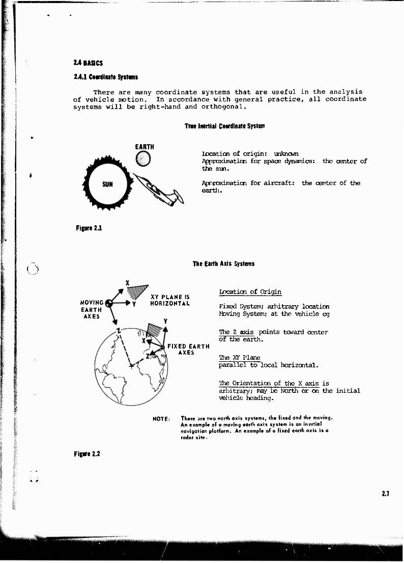
2.4 BASICS

24.1 Coordinate Systems

There are many coordinate systems that are useful in the analysis of vehicle motion. In accordance with general practice, all coordinate systems will be right-hand and orthogonal.

True Inertial Coordinate System

EARTH Location of origin: unknown Approximation for space dynamics: the center of the sun.

Approximation for aircraft: the center of the earth.

Figure 2.1

( 1 The Earth Axis Systems

MOVING EARTH AXES

XY PLANE IS HORIZONTAL

FIXED EARTH AXES

Location of Origin

Fixed System; arbitrary location MDving System; at the vehicle eg

The Z axis points toward center of the earth.

The xy Plane parallel to local horizontal.

rJhe Orientation of the X axis is arbitrary; may be North or on the initial vehicle heading.

Figure 2.2

NOTE: There Jre two *arth axis systems, the fixed and the moving. An example of a moving earth axis system is an inertial navigation platform. An example of a fixed earth axis is a radar site.

2.7

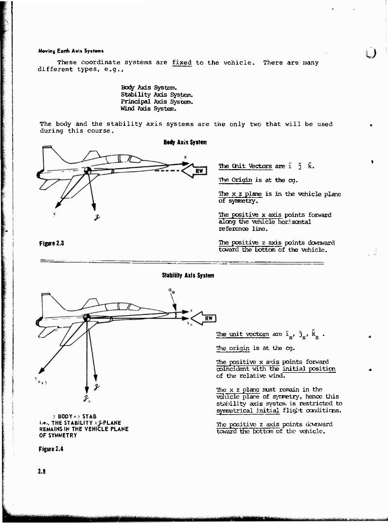
Moving Earth Axis System«

These coordinate systems are fixed to the vehicle, different types, e.g.,

There are many u

Body Axis System. Stability Axis System. Principal Axis System. Wind Axis System.

The body and the stability axis systems are the only two that will be used during this course.

Body Axis System

The Ihit Vectors are I j k.

The Origin is at the eg.

The x z plane is in the vehicle plane of symmetry.

The positive x axis points forward alcng the vehicle horizontal reference line.

Figure 2.3 The positive z axis points downward toward the bottom of the vehicle.

Stability Axis System

vBODY=vSTAB i.e., THE STABILITY *^PLANE REMAINS IN THE VEHICLE PLANE OF SYMMETRY

Figure 2.4

'Ihe unit vectors are I , i , k . s s s

The origin is at the eg.

The positive x axis points forward coincident with" the initial position of the relative wind.

The x z plane must remain in the vehicle plane of symmetry» hence this stability axis system is restricted to symmetrical initial flight conditions.

The positive z axis points downward toward the bottom of the vehicle.

2.8

mmmamMmm***— . ■■ MMI ■UMi I

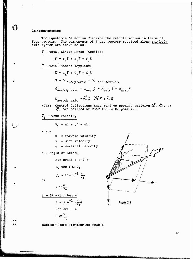
o 2.4.2 Vector Definitions

The Equations of Motion describe the vehicle motion in terms of four vectors. The components of these vectors resolved along the body axis system are shown below.

F - Total Linear Force (Applied)

F = Fr+Fj+FR" x yJ z

G - Total Moment (Applied)

G = Gr+GT+GR" x Y z

aerodynamic other sources

G , .=L r + M T+N k~ aerodynamic aero aeroJ aero

I

aerodynamic J

NOTE: Control deflections that tend to produce positive 6L,, 7)2, or 71, are defined at USAF TPS to be positive.

VT - True Velocity

u V = ui + vj + wk

where

u = forward velocity v = side velocity w = vertical velocity

a - Angle of Attack

For small a and ß

VT cos 3 ^ Vm

or

a ~ sin

w_ Vl

-1 w_ Vn

6 - Sideslip Angle

B = sin"1 <§->

For small 3

v VT

/

Figure 2.5

CAUTION - OTHER DEFINITIONS ARE POSSIBLE

2.9

■M*. mmämt tRjHtfcJUa fili■»„„,,„

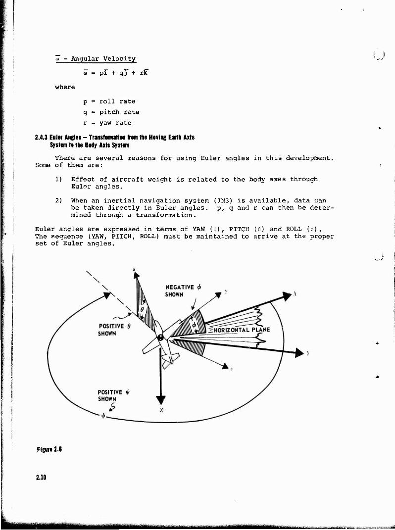
öT - Angular Velocity

öT = pr + qj" + rk~

where

p = roll rate

q = pitch rate

r = yaw rate

2.4.3 Euler Angles - Transfonnation from the Moving Earth Axis System to the Body Axis System

There are several reasons for using Euler angles in this development. Some of them are:

1) Effect of aircraft weight is related to the body axes through Euler angles.

2) When an inertial navigation system (INS) is available, data can be taken directly in Euler angles, p, q and r can then be determined through a transformation.

Euler angles are expressed in terms of YAW U), PITCH (9) and ROLL ($) . The sequence (YAW, PITCH, ROLL) must be maintained to arrive at the proper set of Euler angles.

u

Figure 2.S

2.10

m ■--■- .,-..--.-~~—^~.

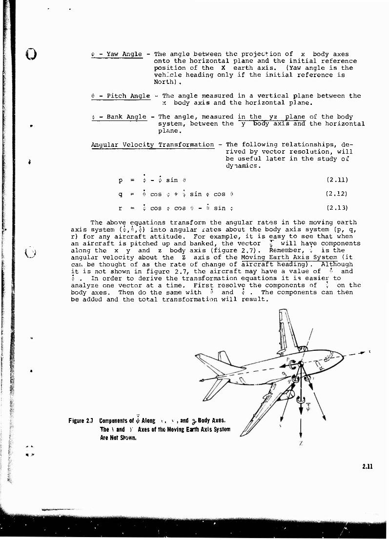
o j[ - Yaw Angle - The angle between the projection of x body axes onto the horizontal plane and the initial reference position of the X earth axis. (Yaw angle is the vehicle heading only if the initial reference is North).

0 - Pitch Angle - The angle measured in a vertical plane between the __ ^ body axis and the horizontal plane.

4> - Bank Angle - The angle, measured in the yz plane of the body — system, between the ~y body axis and the horizontal

pl«ne.

Angular Velocity Transformation - The following relationships, de- . . rived by vector resolution, will

be useful later in the study of dynamics.

p = $ - y\t sin e

q = 6 cos $ + 'p sin 9 cos 6

r — i cos $ cos 9 - 8 sin ;•

(2.11)

(2.12)

(2.13)

u

The above equations transform the angular rates in the moving earth axis system (^,e,4>) into angular rates about the body axis system (p, q, r) for any aircraft attitude. For example, it is easy to see that when an aircraft is pitched up and banked, the vector J" will have components along the x y and z body axis (figure 2.7). Remember, v is the angular velocity about the Z axis of the Moving Earth Axis System (it cau be thought of as the rate of change of aircraft heading) . Although it is not shown in figure 2.7, the aircraft may have a value of 8 and I . In order to derive the transformation equations it is easier to analyze one vector at a time. First resolve the components of I on the body axes. Then do the same with e and I . The components can then be added and the total transformation will result.

Figure 2.7 Components of «|» Along >, y , and 5. Body Axes. The \ and V Axes of the Moving Earth Axis System Are Not Shown.

* *. «>

2.11

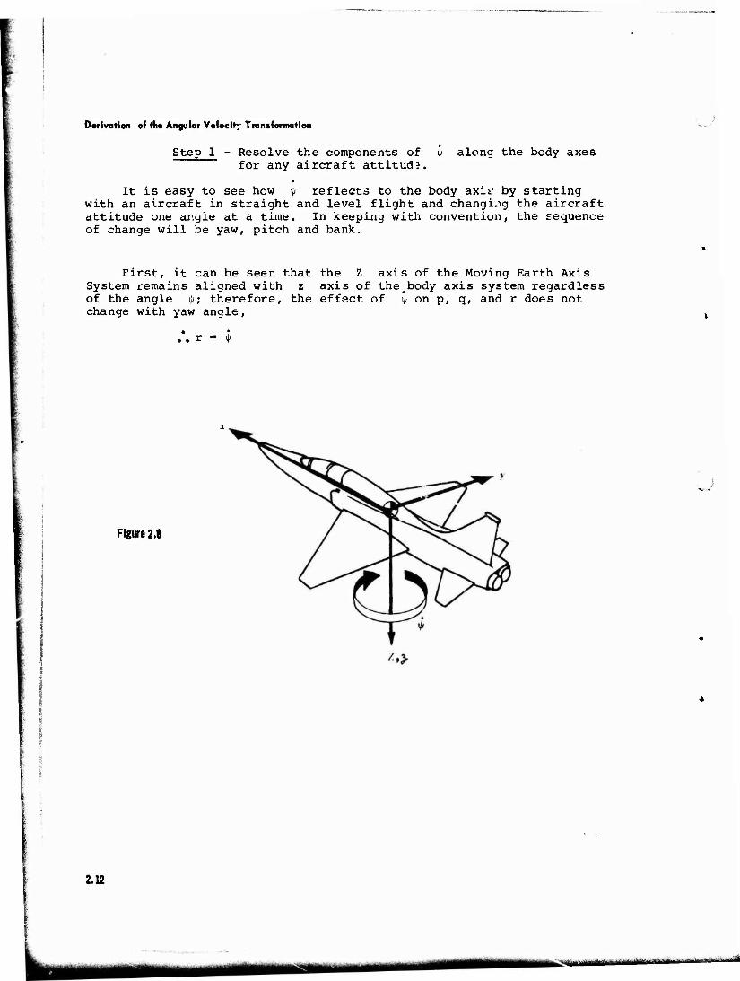
Derivation of fht Angular Voiocit-- Transformation

Step 1 - Resolve the components of for any aircraft attitude,

i> along the body axes

It is easy to see how i* reflects to the body axii- by starting with an aircraft in straight and level flight and changing the aircraft attitude one angle at a time. In keeping with convention, the sequence of change will be yaw, pitch and bank.

First, it can be seen that the Z axis of the Moving Earth Axis System remains aligned with z axis of the#body axis system regardless of the angle ip; therefore, the effect of ty on p, q, and r does not change with yaw angle,

Figure 2.8

2.12

^■«imiitruwari

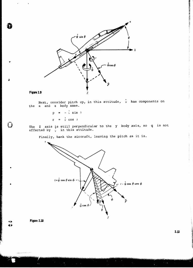
ö

V'\

^ X

Figure 2.9 z

0

4#

Next, consider pitch up, in this attitude, <j» has components on the x and z body axes.

p = - v sin e

r = -ii cos 6

The Z axis is still perpendicular to the y body axis, so q is not effected by ^ in this attitude.

Finally, bank the aircraft, leaving the pitch as it is.

r = i/i cos 0 cos </>

Figure 2.10

2.13

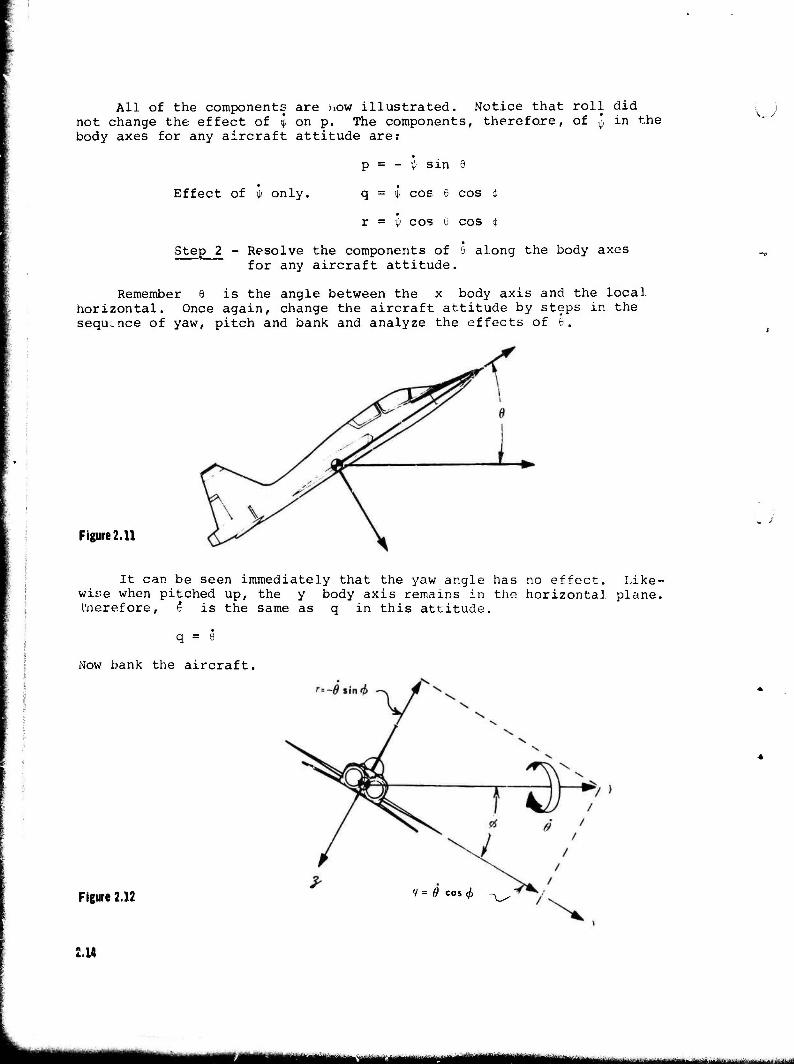
All of the components are now illustrated. Notice that roll did not change the effect of $ on p. The components, therefore, of ^ in the body axes for any aircraft attitude are:

p = - I sin e

Effect of * only. q = i> cos 6 cos $

r = ii cos 6 cos i

Step 2 - Resolve the components of 9 along the body axes for any aircraft attitude.

Remember 9 is the angle between the x body axis and the local horizontal. Once again, change the aircraft attitude by steps in the sequ.nce of yaw, pitch and bank and analyze the effects of 9.

*». /

Figure 2.11

It can be seen immediately that the yaw angle has no effect. Like- wise when pitched up, the y body axis remains in the horizontal plane, therefore, 9* is the same as q in this attitude.

q = 9

Now bank the aircraft,

Figure 2.12 '/ = 9 cos 4> ~x_^.-

2.14

.^—^ -M.M_.^...-.J....—

n It can be seen from figure 2.12 that the components of 9 on the body axes are

q = 6 cos $

r ■ - 8 sin <|»

Notice that p is not affected by 6 since by definition on an axis perpendicular to the x body axis.

is measured

Step 3 - Resolve the components of along the body axes.

This one is easy since by definition 4. is measured along the x body axis. Therefore, $ affects the value of p only, or

P = I

The components of ^,9, and I along the x, y, and z body axes for any aircraft attitude have been derived. These can now be summed to give the transformation equations.

p = { - i sin e

u

1;

q = 9 cos $ + <p sin $ cos 9

r = i> cos <J> cos e - 6 sin <J>

2.4.4 Assumptions

The following assumptions will be made to simplify the derivation of the equations of motion. The reasons for these assumptions will become obvious as the equations are derived.

Rigid Body - Aeroelastic effects must be considered separately.

Earth and Atmosphere are Assumed Fixed - Allows use of Moving Earth Axis ~ System as an "inertial reference".

Constant Mass - Most motion of interest in stability and control takes place in a relatively short time.

The x z Plane is a Plane of Symmetry - This restriction is made to simplify the RHS oF ^he equation. It allows the cancellation of certain terms containing products of inertia. The restriction can easily be removed oy including these terms.

2.5 RIGHT-HAND SIDE OF EQUATION

Tne RHS of the equation represents the aircraft response to any forces or moments that are applied to it. Through the application o Newton's Second Law, two vector relations can be used to derive the : required equations. These are the linear force and moment relations

2.15

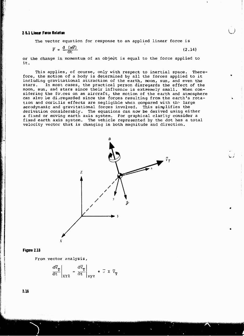
2 5.1 Line» Force Relation

The vector equation for response to an applied linear force is

f=d_(mV)_ (2#14)

V-

dt

or the change in momentum of an object is equal to the force applied to it.

This applies, of course, only with respect to inertial space. There- fore, the motion of a body is determined by all the forces applied to it including gravitational attraction of the earth, moon, sun, and even the stars. In most cases, the practical person disregards the effect of the moon, sun, and stars since their influence is extremely small. When considering the fo.ces on an aircraft, the motion of the earth and atmosphere can also be disregarded since the forces resulting from the earth's rotation and coriclis effects are negligible when compared with thr- large aerodynamic and gravitational forces involved. This simplifies the derivation considerably. The equations can now be derived using either a fixed or moving earth axis system. For graphical clarity consider a fixed earth axis system. The vehicle represented by the dot has a total velocity vector that is changing in both magnitude and direction.

a

-*>)

Figure 2.13

From vector analysis,

dV,

dt XYZ

dV,

dF T

X V„ xyz

2.16

u Substituting this into equation 2.14, and assuming mass is constant, the applied force is,

F = m 5 dt + a) X V„

xyz

which in component foim is

F = m üi + vj~ + wk +

i T k

P q r

u V w

i >

Expanding

F = m [üi + vj + wk + (qw - rv)i - (pw - ru)J + (pv - qu)k]

Rearranging

F = m [(ü + qw - rv)i + (v + ru - pw)j + (w + pv - qu)k]

Now since

F = Fi+FT+Fk x yJ z

These three component equations result:

Fx = m (ü + qw - rv)

Fy = m (v + ru - pw)

F = m (w + pv - qu)

(2.15)

(2.16)

(2.17)

HP

2.S.2 Moment Equations

Once again from Newton's Second Law,

G = d(H) dt

(2.18)

or the change in angular momentum is equal to the total applied moment.

Angular Momentum

Angular momentum should not be as difficult to understand as some people would like to make it. It can be thought of as linear momentum with a moment arm included.

2.17

lttWrtlifmrii tf r I — I I I' •- I i \ buw i

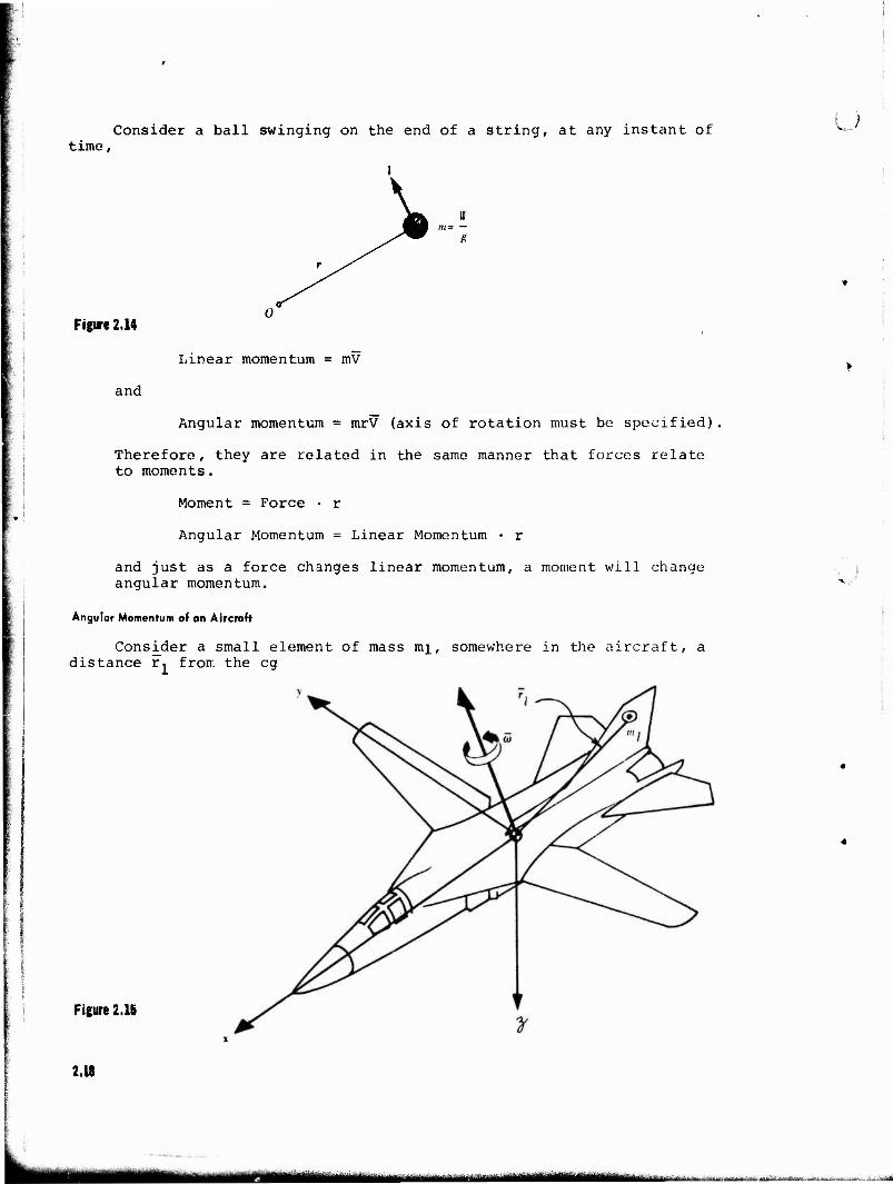
time, Consider a ball swinging on the end of a string, at any instant of V-V

Figure 2.14

and

Linear momentum = mV

Angular momentum = mrV (axis of rotation must be specified)

Therefore, they are related in the same manner that forces relate to moments.

Moment = Force • r

Angular Momentum = Linear Momentum • r

and just as a force changes linear momentum, a moment will change angular momentum.

Angular Momentum of an Aircraft

Consider a small element of mass mj_, somewhere in the aircraft, a distance r, from the eg

Figure 2. IS

2.18

■MMI

•:

The airplane is rotating about all three axes so that

u = pi + qj + rk

and

rx = XjT + yxJ + Zjk

The angular momentum of m^ is

Hmi = mx (r1 X Vx)

(2.19)

(2.20)

(2.21)

and

dr, Vl dt

(i.e., in the inertial frame) XYZ

From vector analysis

dr..

dt

ar,

XYZ dt + u) X r. xyz

(2.22)

i )

Since the airplane is a rigid body ri does not change. Therefore the first term can be excluded, and the inertial velocity of the element m^ is

V, = u, X r.

Substituting this into equation 2.21

ml m, (r, X oi X r, )

(2.23)

(2.24)

HP

This is the angular momentum of the small element of mass m^. In order to find the angular momentuu of the whole airplane, v.ake the sum of all the elements. Using notation in which the i subscript indicates any particular element and n is the total number of elements in the airplane,

where

then

H = l mi [r. X ui X r. ] i=l 1 X

m. - scalar l

r. = x.i + y.j + z.k l l J i l

i j k

P g r a. X r. = l

x. y. z 11 l

(2.25)

(2.26)

\2.21)

2.19

mmm

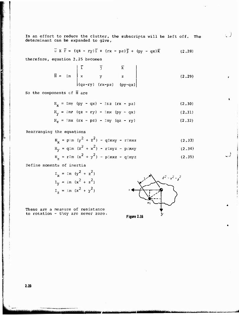
In an effort to reduce the clutter, the subscripts will be left off. The determinant can be expanded to give,

a to X r = (qz - ry)i + (rx - pz)J + (py - qx)k

therefore, equation 2.25 becomes

i J k

H = Im x y z

(qz-ry) (rx-pz) (py-qx)

So the components cf H are

(2.28)

(2.29)

Hx = Imy (py - qx) - lir.z (rx - pz)

H = Zmz (qz - ry) - Iisx (py - qx)

Hz = Imx (rx - pz) - Imy (qz - ry)

(2.30)

(2.31)

(2.32)

Rearranging the equations

Hx = pirn (y2 + Z2)

Hy = qlm (z + yf)

H = rrm (x2 + y2)

Define moments of inertia

Ix = Zm (y + z )

2 2 Iy = Im (x + z )

I, = Im (x2 + y2)

These are a measure of resistance to rotation - they are never zero

qlmxy - rlmxz

rlmyz - plmxy

plmxz - qlmyz

•*tS2l

(2.33)

(2.34)

(2.35)

Figure 2.16

2.20

1 MftflMb^k».auta.

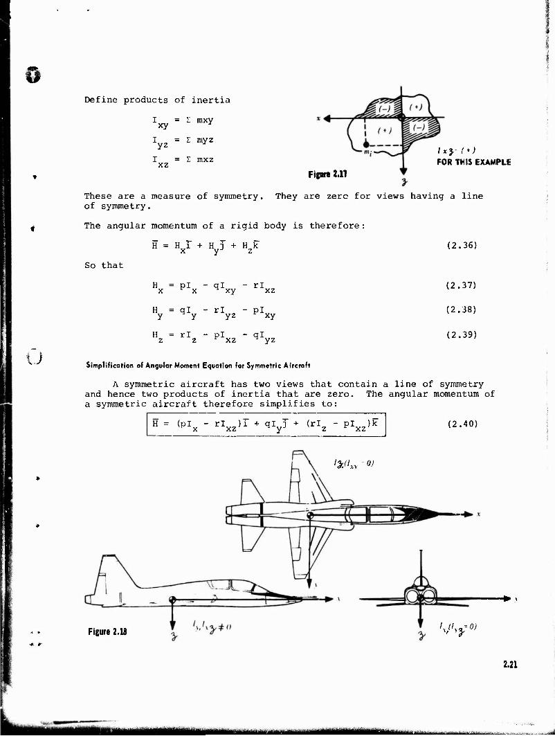
© Define products of inertia

xy mxy

I = I myz yz J

I = I mxz xz Figure 2.17

FOR THIS EXAMPLE

These are a measure of symmetry. They are zero for views having a line of symmetry.

The angular momentum of a rigid body is therefore:

H = Hi + Hj +Hk x yJ z (2.36)

So that

H = pi - ql x x xy rl xz

H = ql - rl - pi y y yz r xy

H = rl z z pi - ql c xz ^ yz

(2.37)

(2.38)

(2.39)

Simplification of Angular Moment Equation for Symmetric Aircraft

A symmetric aircraft has two views that contain a line of symmetry and hence two products of inertia that are zero. The angular momentum of a symmetric aircraft therefore simplifies to:

H = (pi - rl )i + ql ] + (rl - pi )k r x xz y z xz (2.40)

Wxv °>

Figure 2.18 'x/'yyO)

> V

2.21

!—^ae—■»»■■! Mi «.-^. ...„-»-. ma -^.,..

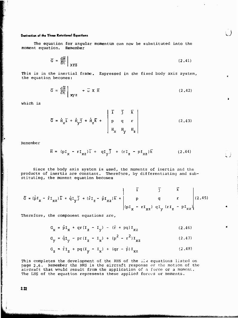
Derivation of the Three Rotational Equations U The equation for angular momentum can now be substituted into the

moment equation. Remember

r - dH G " dt (2.41) XYZ

This is in the inertial frame, the equation becomes:

Expressed in the fixed body axis system,

G = dH dt u X H

xyz (2.42)

which is

G = Ki + Hj+Hk + x yJ z

1 j k

p q r

H X

H y

H z

(2.43)

Remember

H = (pi - rl )i + ql j + (rl - pi )k v x xz y z xz' (2.44) u

Since the body axis system is used, the moments of inertia and the products of inertia are constant. Therefore, by differentiating and substituting, the moment equation becomes

G =(PTx- rIxzU +*V +<rIz" Plxz)k +

Therefore, the component equations are,

l

P

3

q

k

r

(pi - rl ) ql (rl - pi ) v x xz ^ y z xz

(2.45)

G = pi + qr(I - I ) - (r + pq)I x v x ^ z y ^ xz

G = ql - pr(I - I ) + (p2 - r2)I y ^ y * z x v xz

G = rl + pq(I - I ) + (qr - p)I z z ^ y x M c xz

(2.46)

(2.47)

(2.48)

This completes the development of the RHS of the ^lx equations listed on page 2.6. Remember the RHS is the aircraft response or the motion of the aircraft that would result from the application of a force or a moment. The LHS of the equation represents these applied forces or moments.

2.22

mmmmmm Ü^MHtt^

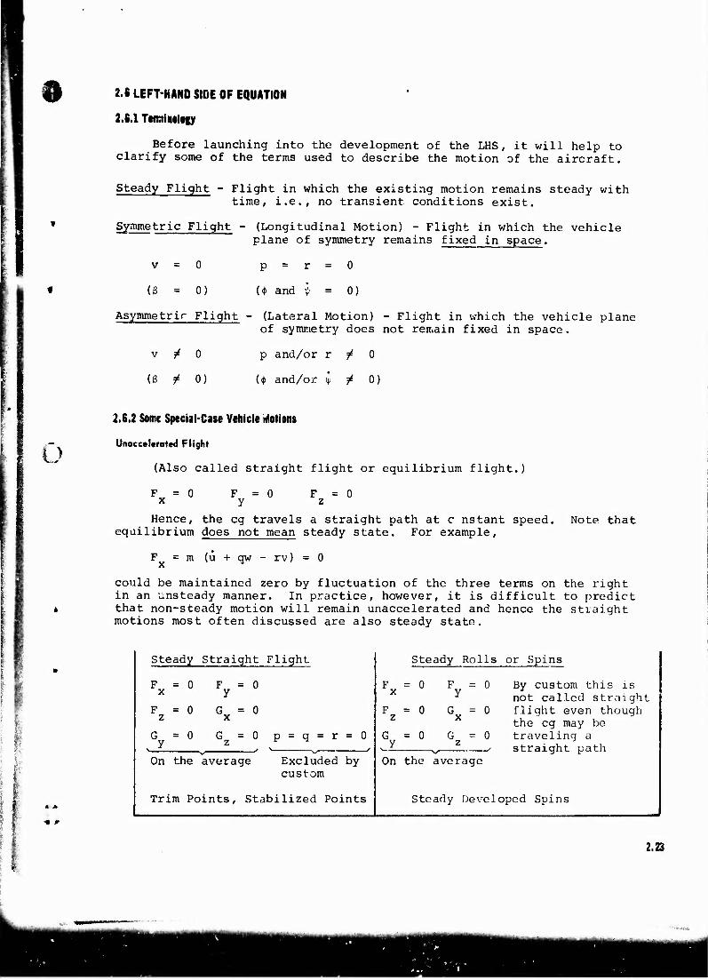
9 2.S LEFT-HAND SIDE OF EQUATION

2.6.1 Terminology

Before launching into the development of the LHS, it will help to clarify some of the terms used to describe the motion of the aircraft.

Steady Flight - Flight in which the existing motion remains steady with time, i.e., no transient conditions exist.

Symmetric Flight - (Longitudinal Motion) - Flight in which the vehicle plane of symmetry remains fixed in space.

v = 0

(ß = 0)

p = r = 0

(<t> and l = 0)

Asymmetric Flight - (Lateral Motion) - Flight in which the vehicle plane of symmetry does not remain fixed in space.

v fi 0

(ß * 0)

p and/or r / 0

(<|> and/or $ ^ 0)

o 2.6.2 Some Special-Case Vehicle Motions

Unaccelerated Flight

(Also called straight flight or equilibrium flight.)

Fx = ° F = 0 y

F = 0 z

Hence, the eg travels a straight path at c nstant speed, equilibrium does not mean steady state. For example,

Note that

F =m(u+qw-rv)=0

could be maintained zero by fluctuation of the three terms on the right in an unsteady manner. In practice, however, it is difficult to predict that non-steady motion will remain unaccelerated and hence the straight motions most often discussed are also steady state.

» *

Steady Straight Flight

F = 0 z

G = 0 y

F = 0 y

G = o x

Gz = 0 p = q ' > ,

Excluded by custom

On the average

Trim Points, Stabilized Points

Steady Rolls or Spins

F = 0 x

F = 0 z

G = 0 . y

G = 0 x

G = 0 z

On the average

By custom this is not called straight flight even though the eg may be traveling a straight path

Steady Developed Spins

2.23

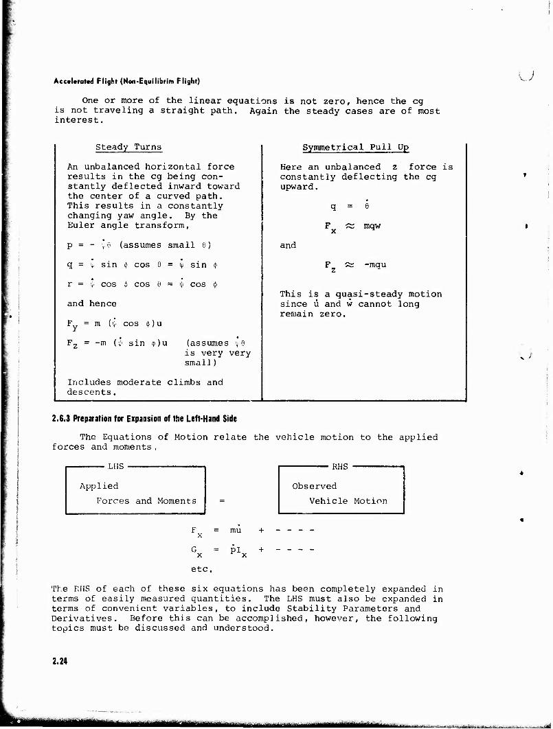
Accelerated Flight (Non-Equilibrim Flight)

One or more of the linear equations is not zero, hence the eg is not traveling a straight path. Again the steady cases are of most interest.

u

Steady Turns Symmetrical Pull Up

An unbalanced horizontal force Here an unbalanced z force is results in the eg being constantly deflected inward toward the center of a curved path.

constantly deflecting the eg upward.

This results in a constantly changing yaw angle. By the Euler angle transform,

q = e

F A; mqw

p = - ye (assumes small 6) and

q = l sin <p cos e = i> sin <J> F ä -mqu

r = v cos 0 cos 6 = i> cos $

and hence This is a quasi-steady motion since ü and w cannot long remain zero.

Fy = m (i/ cos <p) u

Fz = -m (y1 sin (j>) u (assumes j-9 is very very small)

Includes moderate climbs and descents.

2.6.3 Preparation for Expansion of the Left-Hand Side

The Equations of Motion relate the vehicle motion to the applied forces and moments ,

LHS

Applied

Forces and Moments

RHS

Observed

Vehicle Motion

= mu

G = pi x r x

+

+

etc.

The RHS of each of these six equations has been completely expanded in terms of easily measured quantities. The LHS must also be expanded in terms of convenient variables, to include Stability Parameters and Derivatives. Before this can be accomplished, however, the following topics must be discussed and understood.

2.24

UM ~ "- -*-"• ■—--■■■■■■■ ■--'-"

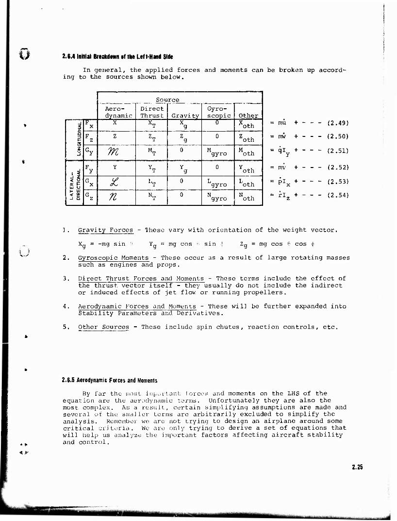
ü 2.6.4 Initial Breakdown of the Left-Hand Side

In general, the applied forces and moments can be broken up according to the sources shown below.

Source Aero- dynamic

Direct Thrust Gravity

Gyro- scopic Other

-1 < z

g o z w

F X

X Xm X g

0 *oth

F 2

Z ZT Z g

0 Zoth

GY ?n MT 0 M gyro oth

«i a P UJ U 1- W < S -1 Q

Fy Y YT Y

g 0 oth

G X £ Lm 0 L gyro loth

G z n NT 0 N gyro oth

= mu +

= mw +

= ql + y

= mv +

= Plx +

- (2.49)

- (2.50)

- (2.51)

- (2.52)

- (2.53)

- (2.54)

I > V

1. Gravity Forces - These vary with orientation of the weight vector.

<q = -mg sin 0 Y„ = mg cos u sin ! mg cos 6 cos *

2. Gyroscopic Moments - These occur as a result of large rotating masses such as engines and props.

3. Direct Thrust Forces and Moments - These terms include the effect of the thrust, vector itself - they usually do not include the indirect or induced effects of jet flow or running propellers.

4. Aerodynamic Forces and Moments - These will be further expanded into Stability Parameters and Derivatives.

5. Other Sources - These include spin chutes, reaction controls, etc.

2.6.5 Aerodynamic Forces and Moments

By far the most important forces and moments on the LHS of the equation are the aerodynamic terms. Unfortunately they are also the most complex. As a result, certain simplifying assumptions are made and several of the smaller terms are arbitrarily excluded to simplify the analysis. Remember we are not trying to design an airplane around some critical criteria. We are only trying to derive a set of equations that will help us analyze the important factors affecting aircraft stability and control.

2.25

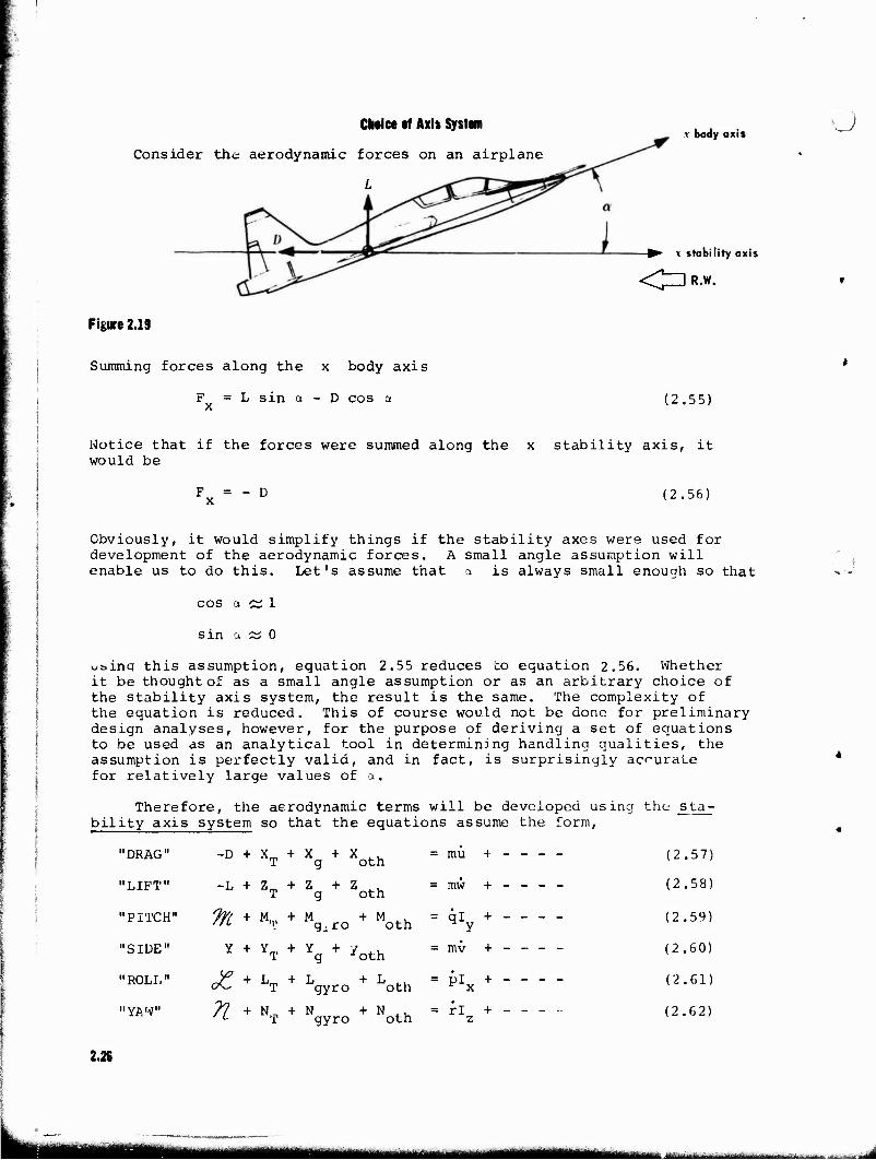
Choice »f Axi» System

Consider the aerodynamic forces on an airplane

L

x body axis

► v stability axis

<^ZlR.W.

u

Figure 2.19

Summing forces along the x body axis

F = L sin a - D cos a x (2.55)

Notice that if the forces were summed along the x would be

stability axis, it

F = - D x (2.56)

Obviously, it would simplify things if the stability axes were used for development of the aerodynamic forces. A small angle assumption will enable us to do this. Let's assume that a is always small enough so that

cos a c 1

sin a £2 0

ubinq this assumption, equation 2.55 reduces to equation 2.56. Whether it be thought of as a small angle assumption or as an arbitrary choice of the stability axis system, the result is the same. The complexity of the equation is reduced. This of course would not be done for preliminary design analyses, however, for the purpose of deriving a set of equations to be used as an analytical tool in determining handling qualities, the assumption is perfectly valid, and in fact, is surprisingly accurate for relatively large values of a.

Therefore, the aerodynamic terms will be developed using the stability axis system so that the equations assume the form,

"DRAG"

"LIFT"

"PITCH"

"SIDE"

"ROLL"

"YAW"

-D + X,,, + X + X . , T g oth

-L + Zm + Z + Z' . T g oth

A* + M- + Mg,ro + Moth

Y + YT + Yg + 'oth

Jf + K * L + CA^ T qyro

71 + N,., + N + ' L T qyro

oth

oth

= mu +

= mw +

= ql + H y = mv +

= pi + r x

= rl + z

(2.57)

(2.58)

(2.59)

(2.60)

(2.61)

(2.62)

2.26

-—■ ■-1 tmmm MM määmmäL *>*,.>...<. ,-.^ ■^^■„■■■„aii-A.-fj,■,>-, i„,--i-1,

Expansion of Aerodynamic Terms

A stability and control analysis is concerned he question of how a vehicle responds to certain perturbations or in^uus. For instance, up elevator should cause the nose to come up; or if the aircraft hits some turbulence that causes a small amount of sideslrp, the airplane should realign itself with the relative vvind. Intuitively, it can be seen that the aerodynamic terms are going to have the most effect on the resulting motion of the aircraft. Unfortunately, the equations that result from summing forces and moments are non-linear. As a result, exact solutions to these equations are impossible. Therefore, a technique to linearize the equations must be used so that solutions can be obtained. In order to do this the small perturbation theory is introduced.

Small Perturbation Theory

The small perturbation theory is based on a simple and very popular technique used for linearizing a set of differential equations. In a nutshell, it is simply the process of expanding the equations using a Taylor series expansion and excluding the higher order terms. To fully understand the derivation some assumptions and definitions must first be established.

The Small Disturbance Assumption

u The aerodynamic forces and moments are primarily a function of the

following variables:

Temperature and Altitude

Accounted for by p, M, R

2. Angular Velocities

Accounted for by p, q, r,

3. Control Deflections

Accounted for by 5 , 6 , 6 , 6 cl IT

4. Position and Magnitude of the Relative Wind

Accounted for by the components u, v, w of true velocity, or alternately, by:

w V~~ ' T

v v~

In general, the time derivatives of these variables could also L< significant. In other words:

2.27

>A mm t^mmmmm ^d

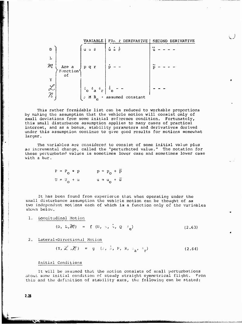
VARIABLE

D

L

m

Y

71

i Are a i / Function*

of

u a ß

p q r

6 6 6 ear

P M R ■•>

FJ.K i' DERIVATIVE

U a e

p -

SECOND DERIVATIVE u

u - - - -

assumed constant

This rather formidable list can be reduced to workable proportions by making the assumption that the vehicle motion will consist only of small deviations from some initial reference condition. Fortunately, this small disturbance assumption applies to many cases of practical interest, and as a bonus, stability parameters and derivatives derived under this assumption continue to give good results for motions somewhat larger.

The variables are considered to consist of some initial value plus an incremental change, called the "perturbated value." The notation for these perturbatec? values is sometimes lower case and sometimes lower case with a bar.

p = p + p o r p = P0 + p

U = Ü + u o

u = U + Ü" o

It has been found from experierce that when operating under the small disturbance assumption the vehicle motion can be thought of as two independent motions each of which is a function only of the variables shown below.

1. Longitudinal Motion

(D, L,7/i) = f (U, a, '., Q 6, (2.63)

Lateral-Directional Motion

(Y, Z ,71) = 3, 8, P, R, o , 5 ) (2.64)

Initial Conditions

It will be assumed that the motion consists of small perturbations about some initial condition of steady straight symmetrical flight. From this and the definition of stability axes, the following can be stated:

2.28

«MM

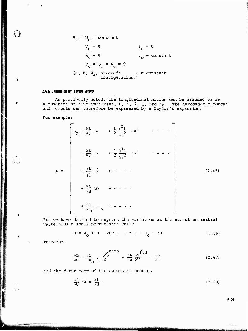
} Vm = U = constant T o

V = 0 o

ßo = 0

W = 0 o a = constant

o

P = Q = R = 0 o o o

, M, R , aircraft configuration.

= constant

2.6.6 Expansion by Taylor Series

As previously noted, the longitudinal motion can be assumed to be a function of five variables, U, a, a, Q, and <5e. The aerodynamic forces and moments can therefore be expressed by a Taylor's expansion.

For example:

L =

\ * w 4°

, 3L . 3 a

, 3 L , • + — A a

J. 1 ^L A,,2 + I 772" AU dU

J. 1 32L , 2 + 2 —Z na

d a

L

da

+ |S AQ + -

e

(2.65)

But we have decided to express the variables as the sum of an initial value plus a small perturbated value

U = U + u where u = U - U = AU o o (2.66)

Thare fore

a L _ d L dir ~ w~ • AU o

Zero ill 2V :<u /u

/.o dL 3u'

(2.67)

aid the first term of the expansion becomes

du U - MT u (2.63)

2.2a

«^■MMMHUEI - -

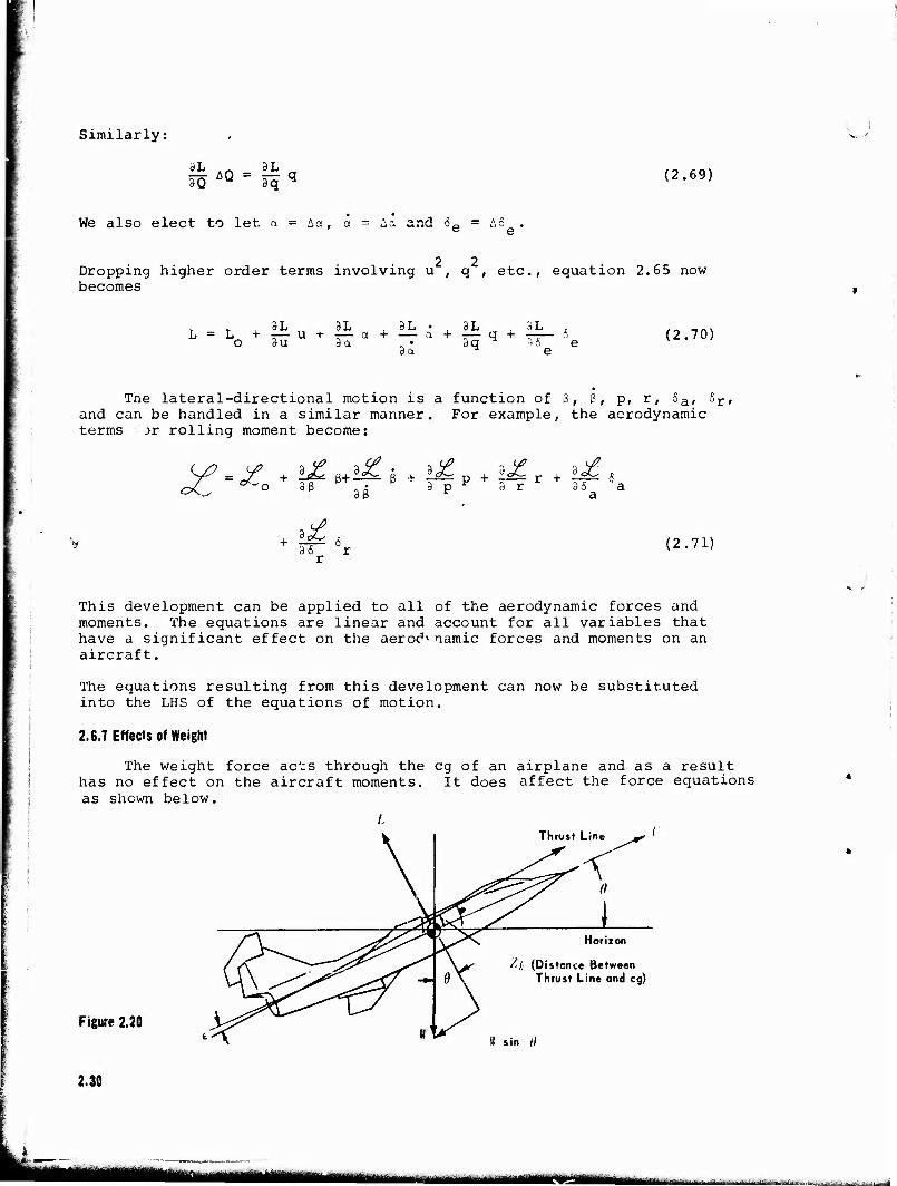
Similarly:

3Q AQ = 3q q (2.69)

We also elect to let n = Aa, a - Aa and Se = A6 .

2 2 Dropping higher order terms involving u , q , etc., equation 2.65 now becomes

, 3L SL SL • , 3L , 3L . L = L + ^- u + -— a + — a + 7— q+ 7-7— *

o 3 u 8a . • ^ q 3 6 e 3a ^ e (2.70)

The lateral-directional motion is a function of B, ß, p, r, 5a, 6r, and can be handled in a similar manner. For example, the aerodynamic terms jr rolling moment become:

oC ^-o 36 " • P 3 p P "■ - 3 r 35 a a

+ iK 6 36 r r

(2.71)

This development can be applied to all of the aerodynamic forces and moments. The equations are linear and account for all variables that have a significant effect on the aerodynamic forces and moments on an aircraft.

The equations resulting from this development can now be substituted into the LHS of the equations of motion.

2.6.7 Effects of Weight

The weight force acts through the eg of an airplane and as a result has no effect on the aircraft moments. It does affect the force equations as shown below.

Figure 2.20

L

\

\

Thrust Line j^ '

pr ;

t ^y

^

K'

i X. Horizon

' 7-k (Distance Between Thrust Line and eg)

\

II sin 0

2.30

-°~" —— - - - —■

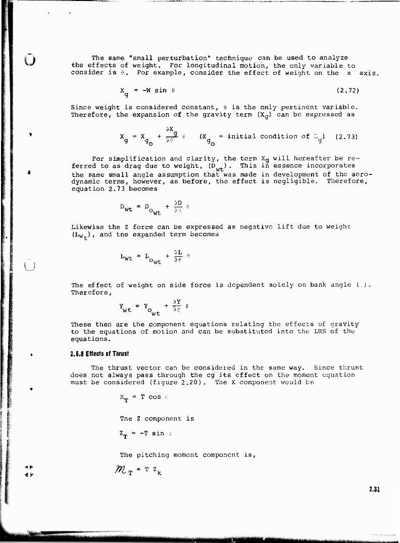
u The same "small perturbation" technique can be used to analyze the effects of weight. For longitudinal motion, the only variable to consider is G. For example, consider the effect of weight on the x axis,

'

X = -W sin 8 g

(2.72)

Since weight is considered constant, 6 is the only pertinent variable. Therefore, the expansion of the gravity term (Xg) can be expressed as

3X X = X + r-r^ (X = initial condition of :; ) (2.73)

For simplification and clarity, the term Xg will hereafter be referred to as drag due to weight, (D .). This in essence incorporates the same small angle assumption that was made in development of the aerodynamic terms, however, as before, the effect is negligible. Therefore, equation 2.73 becomes

Dwt = D + |° a wt owt 39

Likewise the Z force can be expressed as negative lift due to weight (Lw ), and the expanded term becomes

I u Jwt = L

>wt + w 9

The effect of weight on side force is dependent solely on bank angle (., Therefore,

Y = Y + — <f> Wt O . 3$ wt

These then are the component equations relating the effects of gravity to the equations of motion and can be substituted into the LHS of the equations.

2.6.8 Effects of Thrust

The thrust vector can be considered in the same way. Since thrust does not always pass through the eg its effect on the moment equation must be considered (figure 2.20). The X component would be

X = T cos L

Tne Z component is

Z = -T sin c

*+ *>

The pitching moment component is,

2.31

■jMfcM» ■ ■ ,., ..■■-,... ■ ... ■

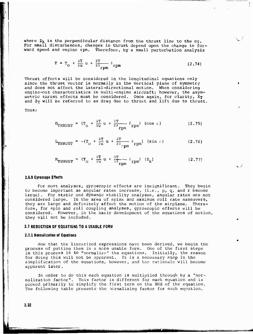
where Zfc is the perpendicular distance from the thrust line to the eg. For small disturbances, changes in thrust depend upon the change in forward speed and engine rpm. Therefore, by a small perturbation analysis

T + o 3T 3u U +

5T 35 rpm r.pm (2.74)

Thrust effects will be considered in the longitudinal equations only since the thrust vector is normally in the vertical plane of symmetry and does not affect the lateral-directional motion. When considering engine-out characteristics in multi-engine aircraft; however, the asymmetric thrust effects must be considered. Once again, for clarity, Xx and Z-r will be referred to as drag due to thrust and lift due to thrust.

Thus:

DTHRUST= (To + UU + W— «rpm) (cOS £> rpm r (2.75)

LTHRUST = -<To + ?£ U + T6 «rpm5 (sin e) rpm r (2.76)

MTHRUST = (To + f£ U + i 5rPm) (Zk> rpm r

(2.77)

.. J

2.6.9 Gyroscope Effects

For most analyses, gyroscopic effects are insignificant. They begin to become important as angular rates increase, (i.e., p, q, and r become large). For static and dynamic stability analyses, angular rates are not considered large. In the area of spins and maximum roll rate maneuvers, they are large and definitely affect the motion of the airplane. There- fore, for spin and roll coupling analyses, gyroscopic effects will be considered. However, in the basic development of the equations of motion, they will not be included.

2.7 REDUCTION OF EQUATIONS TO A USABLE FORM

2.7.1 Normalization of Equations

Now that the linearized expressions nave been derived, we begin the process of putting them in a more usable form. One of the first steps in this process is to "normalize" the equations. Initially, the reason for doing this will not be apparent. It is a necessary step in the simplification of the equations, however, and the rationale will become apparent later.

In order to do this each equation is multiplied through by a "normalization factor". This factor is different for each equation and is picked primarily to simplify the first term on the RHS of the equation. The following table presents the normalizing factor for each equation.

2.32

ÜM mm mmm

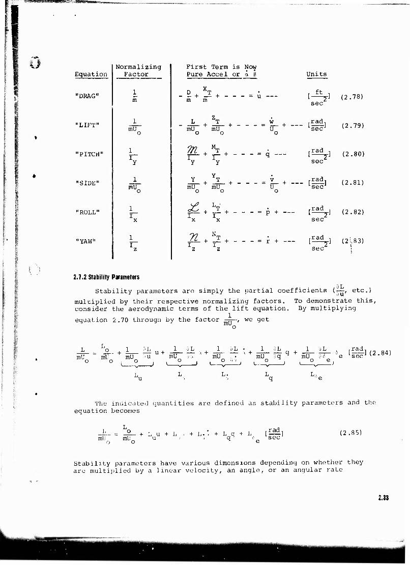
o 1

Equation

"DRAG"

"LIFT"

"PITCH"

"SIDE"

"ROLL"

"YAW"

Normalizing Factor

1 m

mU

mU

First Term is Now Pure Accel or a ß

D XT - + —- + - m m = u —

L -T mU mU + - w

Units

l-^yl (2.78) sec

+ — l~l (2.79)

p. + -1 + - - y y

Y T —-— + —— + mU mU o o

£♦:* —

q — 1^2"] (2.80) sec

+ — [££l] (2.81) sec

P + — [^jl (2.82) sec

71 T z z

= r + — [^_] (21.83) sec2 !

■ 'I

2.7.2 Stability Parameters ■ 3L

Stability parameters are simply the partial coefficients (—, etc.)

multiplied by their respective normalizing factors. To demonstrate this, consider the aerodynamic terms of the lift equation. By multiplying

equation 2.70 through by the factor =rr~i we get

L mU

JL- + L_ mU mU o , o

)L , 1 BL U + -rr— i u mU i a

1 oL • 1 9L 1 ciL , ,rad, mU , • mU Sq mU 3 6 "e sec'

, ° ''•'* , i ° J ^_° e; (2.84!

L. L^

The indicated quantities are defined as stability parameters and the equation becomes

_L_ = _2_ + L U + L < + L.<; + L q + Lx [^±] mU mU u < - qM ^ sec1

Q O fe=

(2.85)

Stability parameters have various dimensions depending on whether they are multiplied by a linear velocity, an angle, or an angular rate

2.33

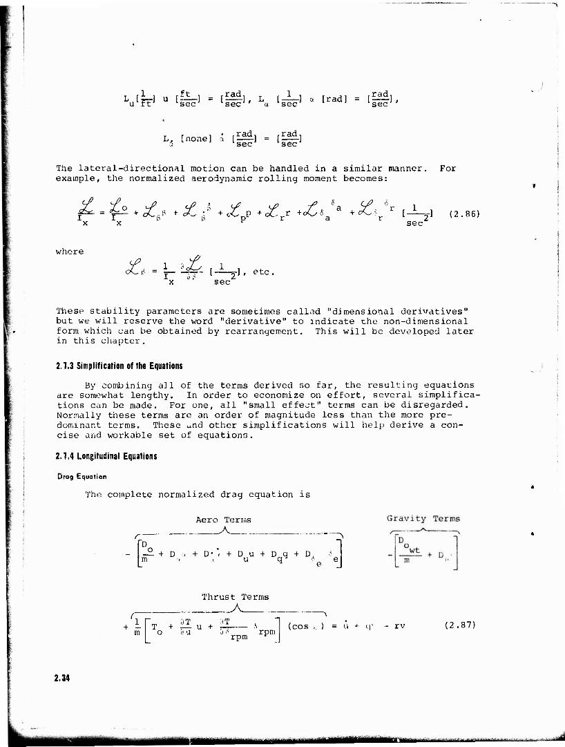
VrTJ U 4h] - 1^' L« Is-eT1 ° '"<" = ISifl'

L. [none] a [**i] = [Ä a sec sec

The lateral-directional motion can be handled in a similar manner. For example, the normalized aerodynamic rolling moment becomes:

£-£♦£. *Ä7-£pP-«£rr-eV- r r I-^-y] (2.86)

sec

whore

£l «U^- [-L_]f etc, I up X sec

These stability parameters are sometimes called "dimensional derivatives" but we will reserve the word "derivative" to indicate the non-dimensional form which can be obtained by rearrangement. This will be developed later in this chapter.

2.7.3 Simplification of the Equations

By combining all of the terms derived so far, the resulting equations are somewhat lengthy. In order to economize on effort, several simplifications can be made. For one, all "small effect" terms can be disregarded. Normally these terms are an order of magnitude less than the more predominant terms. These und other simplifications will help derive a concise and workable set of equations.

2.7.4 Longitudinal Equations

Drag Equation

The complete normalized drag equation is

m

Aero Terms A

+ Du + D*-i + Du + Dq + D. -> j u q 6 „1

♦V m

Thrust Terms A

T + il u + O 3 U

3T

rpm rpm (cos ,-; = U + (.]' rv (2.87)

2.34

Mm ^mmmmm B*M. ^ ■■»"■"»»-"""-

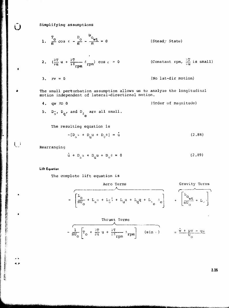
ü Simplifying assumptions

T D Üo ,

m mm (Steady State)

,3T ^ 3T (3U-U + TT rpm

& ) COS E rpm = 0 (Constant rpm, -— is small)

3. rv = 0 (No lat-dir motion)

The small perturbation assumption allows us to analyze the longitudinal motion independent of lateral-directional motion.

4. qw £S 0 (Order of magnitude)

5. D», D , and D„ are all small,

The resulting equation is

•[D a + D u + DQe] = u a u ö (2.88)

Rearranging

u + Da + Du + D,6 = 0 a u 6

(2.89)

w

Lift Equation

The complete lift equation is

Aero Terms

r

-fr- +La + L-a + Lu + Lq + LI & mU a a u q 6 e

o ^ e

Gravity Terms

r

wt mU

+ L

~\

m

i l

mU

Thrust Terms A

T + |i u + |?— * o 3u 3 6 rpm rpm (sin i ) w + pv - qu

Ü

» i . i.

2.35

mmm ■M^HM "^'^^^^TMiirtlüirrii ■^■■^i...l. ^:i.h-,v.|.i,-lt; ■ ,-, i- ■-„- j,-, !■■■--iiudJi

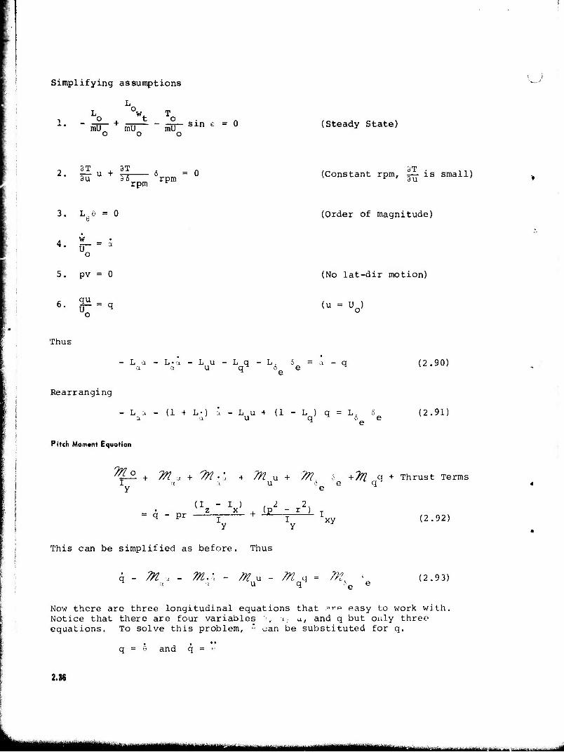
Simplifying assumptions

L Lo °w To

1- " SO- + fnU 5D- sin e = ° (Steady State) o o o

3 T BT 3T 2* 3u U + 3^ 6rpm = ° (Constant rpm, ,_ is small) rpm r

3. Löe = 0 (Order of magnitude)

A W 4. {r= a o

5. pv = 0 (No lat-dir motion)

6. g£=q (u-ü0)

Thus • •

- L a - L•a - L u - L q - L. 6 = a - q (2.90) " e

v I

Rearranging

L a - (1 + L«) a - L u + (1 - L ) q = L. 6 (2.91) a a u q o e ~ e

Pitch Moment Equation

%l2. + 7n a + 7n-'<x + TM. u + Tn, i + % q + Thrust Terms I a ) u 6 e q y e

(I - I ) , I 2, z X:' (p - r ) , = q _ pr + -*-- I 2)

y y J

This can be simplified as before. Thus

q - M ■, - m.i - m u - m q = n?k « (2.93) ^ a a u q *.e e

Now there are three longitudinal equations that r"-" easy to work with. Notice that there are four variables ■'■, i, a, and q but only three equations. To solve this problem, ° can be substituted for q.

q = 6 and q = >'

2.3S

, läÜÜ IIM^I.IHI—^M——■ II

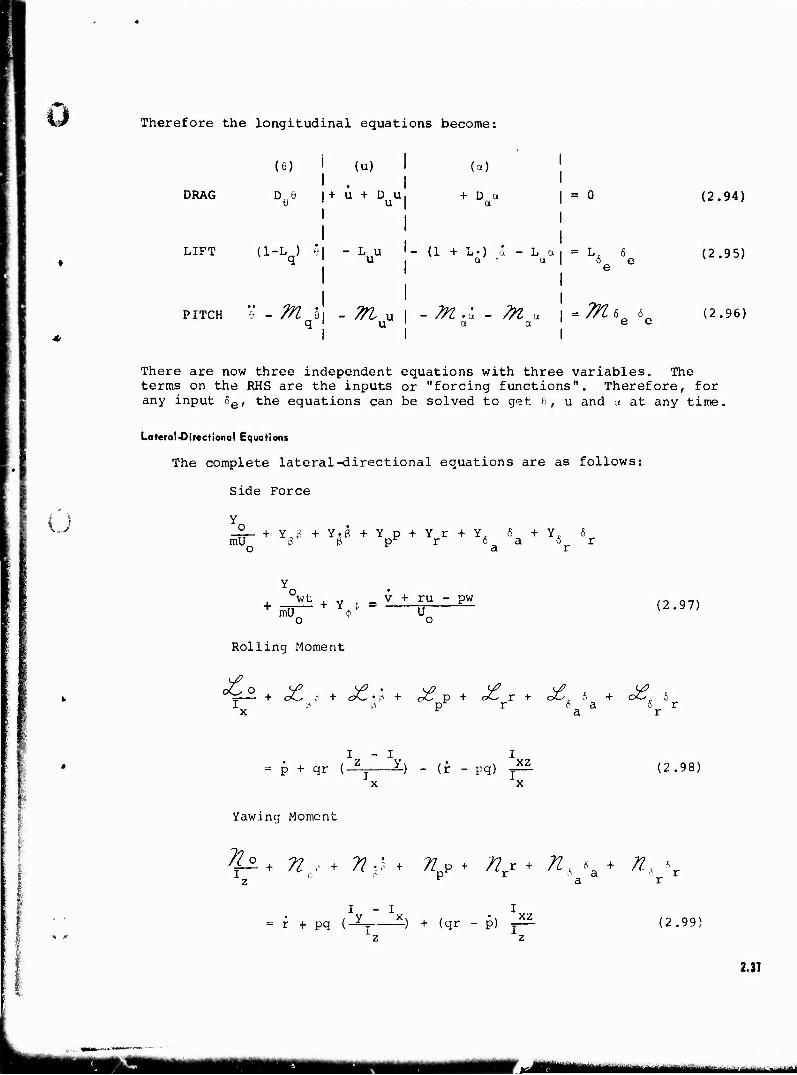
ö Therefore the longitudinal equations become:

u

DRAG

(6) I (U) I

I

(a)

+ D a a I = o

I

(2.94)

LIFT (1-L ) G| - Luu I- (1 + L.) a - \* t * L& 6g (2.95) I I ' , e

PITCH 0 - M ei . ?n u i - ^z.a - ?n u \ =Ms a ' u a a II I

6 e e (2.96)

There are now three independent equations with three variables. The terms on the RHS are the inputs or "forcing functions". Therefore, for any input 5e, the equations can be solved to get e, u and a at any time,

Lateral-Directional Equations

The complete lateral-directional equations are as follows:

Side Force

Y -£- + YJ + Y.J + Y p + Yr + Y. 6+YA 5^ mU 6 ß p^ r 6 a a 6 r o a r

x wt + v .» - v + ru - pw + m Y * * Ü o o (2.97)

Rolling Moment

I rf ü p^ r 6 a 6 r

I - I I p + qr (—j ±-) - (r - pq) j

x x (2.98)

Yawing Moment

^ + 7?.,- + 71 •• ♦ ftp + /?rr + /Z^a + ^ o

I - I I r + pq ( yT X) + (qr - p) ~ (2.99)

2.37

r^ mmm - M

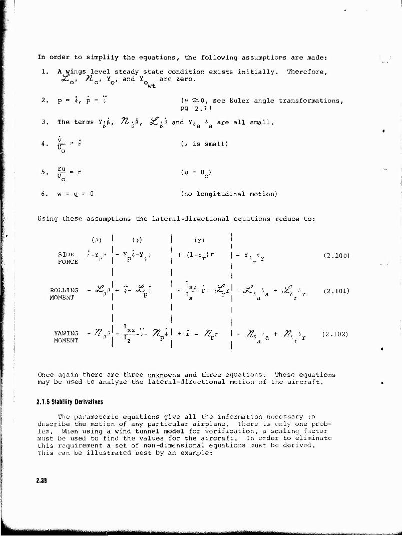
In order to simpliiy the equations, the following assumptions are made:

1. A wings level steady state condition exists initially. Therefore,

°^o' ^o' Yo' and Yo are zero- wt

2. p = <*>, p = (9 ~0, see Euler angle transformations, P9 2.7)

3. The terms Y-B, 7t-&, &£"al and Y5 6 are all small. p P P a a

4. g-. * G o

(a is small)

r ru 5. ,--r (U = Uo)

w = q = 0 (no longitudinal motion)

Using these assumptions the lateral-directional equations reduce to:

(S)

S IDE p -Y , |3 FORCE p VV

ROLLING - c£ft + V- o^ J MOMENT l I P

YAWING MOMENT *,«-!

xz •r- /^p*

(r)

+ (1-Y )r r YS 6r r

=— r- aO r' = e*Lc 6 + c£^ - I r 1 5 a 5 r x a r

+ r 7lf X* 5a + ^

(2.100)

(2.101)

(2.102)

Once again there are three unknowns and three equations. These equations may be used to analyze the lateral-directional motion of the aircraft.

2.7.5 Stability Derivatives

The parameteric equations give all the information necessary to describe the motion of any particular airplane. There is only one problem. When using a wind tunnel model for verification, a scaling factor must be used to find the values for the aircraft. In order to eliminate this requirement a set of non-dimensional equations must be derived. This can be illustrated best by an example:

2.3

«HI ■^ttHIW^MM - '-'-—■..J.--.^'.:.'.-

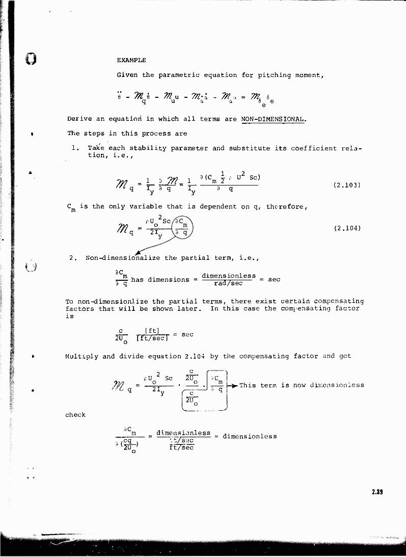
o EXAMPLE

Given the parametric equation for pitching moment,

q U a a 6 e ^ e

Derive an equation in which all terms are NON-DIMENSIONAL.

The steps in this process are

1. Take each stability parameter and substitute its coefficient relation, i.e. ,

u

"l q iy 5 q iy

a (c i p u2 sc) m 2 ä q

C is the only variable that is dependent on q, therefore,

2. Non-dimensionalize the partial term, i.e.,

3C m , ,. . dimensionless T has dimensions = -5-7 = sec 3 q rad/sec

(2.103)

(2.104)

To non-dimensionlize the partial terms, there exist certain compensating factors that will be shown later. In this case the compensating factor is

[ft] 2U [ft/sec] = sec

Multiply and divide equation 2.104 by the compensating factor and get

check

M pU 2 Sc

0

c 2U

0

( ^ 2U

0 V

3C m 3 q 21

y •This term is now dimensionless

oC m

3 (§3-) 20"

dimensionless ': t/sec~ ft/sec

dimensionless

2.39

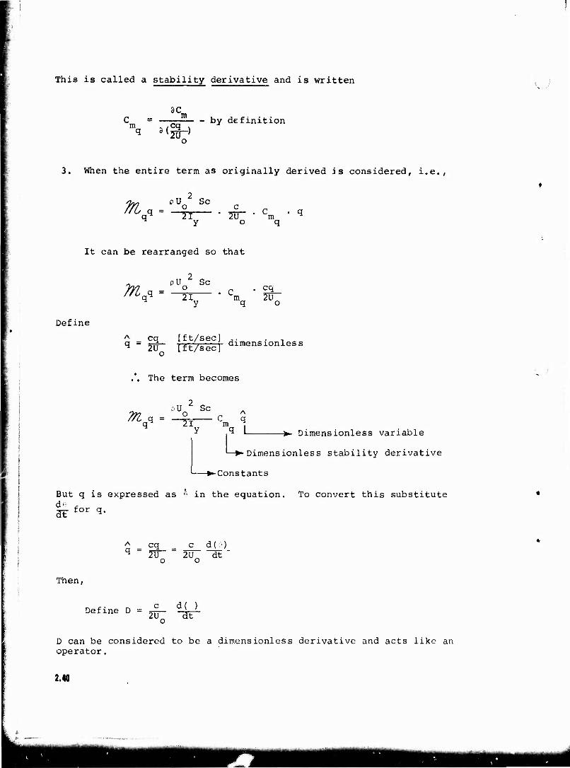
This is called a stability derivative and is written

3C_ m

* 3(2U > o

- by definition

3. When the entire term as originally derived is considered, i.e.,

7n pU Sc o c ,q - -^ w- . C • q

O q TT

It can be rearranged so that

„ p U Sc

"^ 21 ' Cm 2Ü" M y q o

Define A cq [ft/sec] ,. . , q = 2U^ [ft/sec) ^mensionless

.*. The term becomes

pu 2 Sc j% q = ° C q

q^1 21 m , y ,q L

L, ->- Dimensionless variable

Dimensionless stability derivative

•Constants

But q is expressed as 6 in the equation. To convert this substitute do , ar for *•

eg _ c d( ■:•) 2~Ü~ 2U dt " o o

Then,

Define D = -c d( }

2U ~~3F o

D can be considered to be a dimensionless derivative and acts like an operator.

2.40

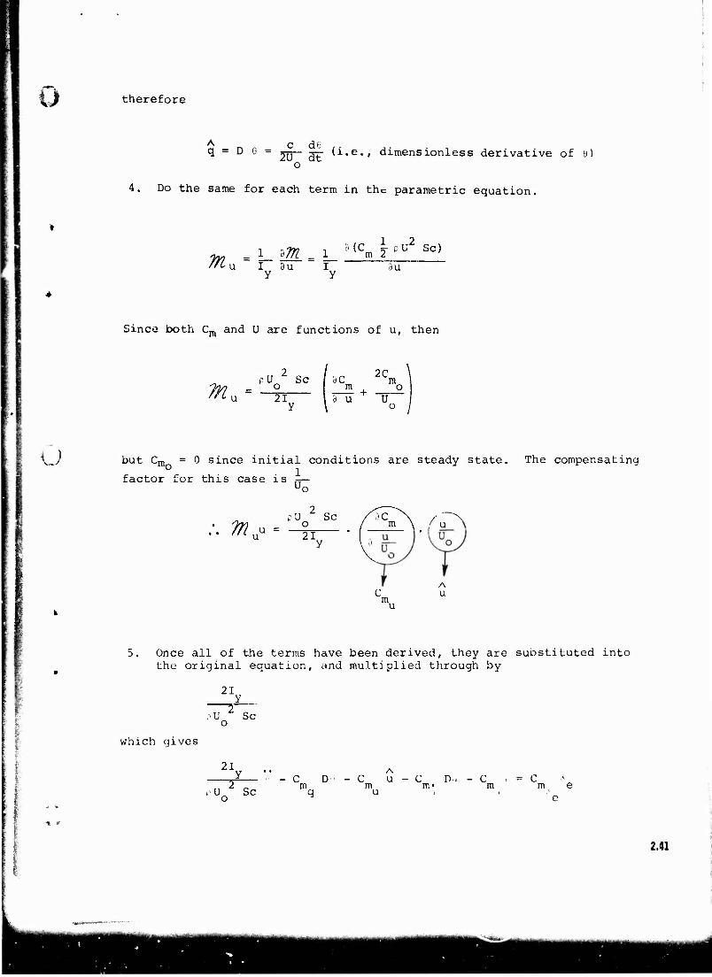
ö therefore

A c d 6 q = D e = 2TT~ 3t *i,e"' dimensionless derivative of e)

o

4. Do the same for each term in the parametric equation.

"£u I 3u I y y

3U

Since both Cm and U are functions of u, then

;

pU 2 Sc / äC 2Cm

21 3 u U

u but Cm = 0 since initial conditions are steady state. The compensating o ^ factor for this case is —-

PU Sc /.)C \ /'^\ :. in* = ° / m wu 21

A C u m u

I 8

5. Once all of the terms have been derived, they are substituted into the original equation, and multiplied through by

21

pU SC o

which gives

21 .. A —J-— ■ - c D■• - c u - c n. - c . = c >^ ,, 2 „ m m m • m me p U Sc q u

2.41

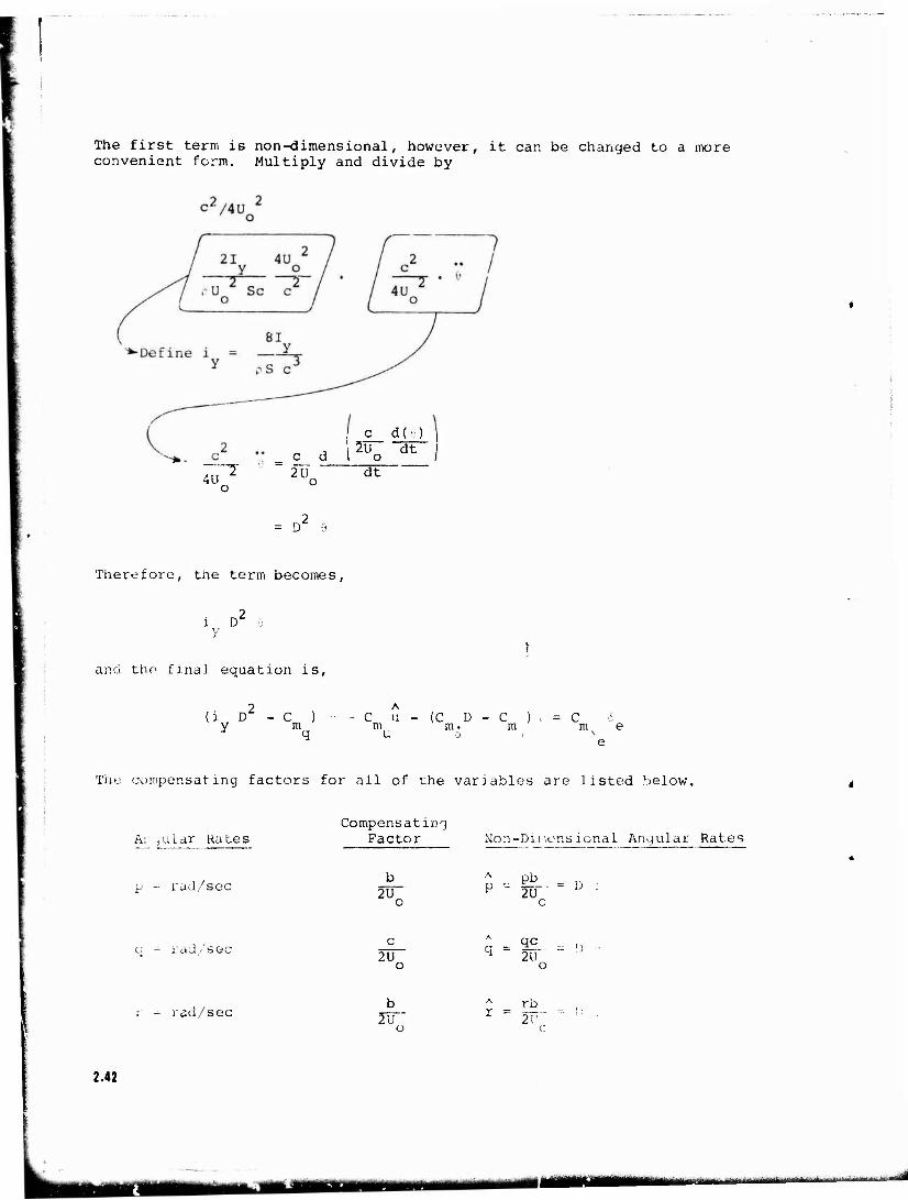
The first term is non-dimensional, however, it can be changed to a more convenient form. Multiply and divide by

4U rr c d

c d(e) 2u dt o

2U dt

= D

Therefore, the term becomes,

j D y

and the final equation is,

2 A

(l D - C ) - - C u - (C D - C y m m m- m J q u a = C m v e

e

The compensating factors for all of the variables are listed below.

A: ;ular Rates Compensating

Factor Non-Dinensional Angular Rates

p - rad/sec 2U pb 2Ü~

D :

c; - r ad/'sec 2U 1 2U o

rad/sec 2U rb

2.42

UMM a'tMiWti<iTTflir-i,'°-^-1'f-^h^""^-'^'^-^-^^ü^^

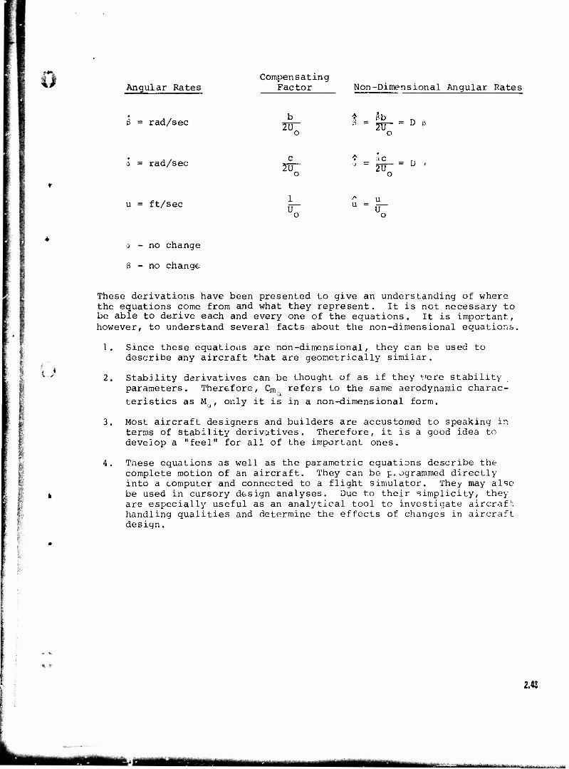
Angular Rates

ß = rad/sec

a = rad/sec

u = ft/sec

Compensating Factor Non-Dimensional Angular Rates

= D ß b ß .. fo 2U 2U o o

c A IC

2U -X 2U o o

1 A u u U U

= D

a - no change

ß - no change

l I

These derivations have been presented to give an understanding of where the equations come from and what they represent. It is not necessary to be able to derive each and every one of the equations. It is important, however, to understand several facts about the non-dimensional equations.

o 1.

2.

4.

Since these equations are non-dimensional, they can be describe any aircraft that are geometrically similar.

used to

Stability derivatives can be thought of as if they were stability parameters. Therefore, Cm refers to the same aerodynamic characteristics as M , only it is in a non-dimensional form.

Most aircraft designers and builders are accustomed to speaking in terms of stability derivatives. Therefore, it is a good idea to develop a "feel" for all of the important ones.

These equations as well as the parametric equations describe the complete motion of an aircraft. They can be programmed directly into a computer and connected to a flight simulator. They may also be used in cursory design analyses. Due to their simplicity, they are especially useful as an analytical tool to investigate aircraft handling qualities and determine the effects of changes in aircraft design.

2.42

«MMH ^^AWv.m.Mi.,*-.,«,: *■.... ,■,■■■„

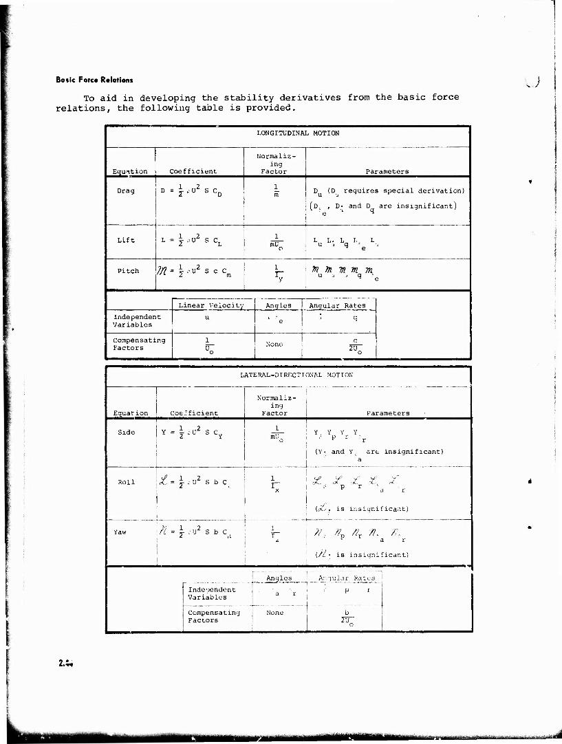
Bo tic Fere« Relations

To aid in developing the stability derivatives from the basic force relations, the following table is provided.

2.U

LONGITUDINAL MOTION

Equation Coefficient

Normaliz- ing

Factor Parameters

Drag 1 2

D = jpU S CD 1 m D (D requires special derivation)

(Dk , D- and D are insignificant) ' e J ^

Lift 1 2 L = ±-kV S CL

1 mU o

L L. L I. L u i q • M e

Pitch Jft = I c U2 S c C '"2 m 1 I y

in 7n m m m U •-< x q 5e

Linear Velocity Angles Angular Rates

Independent Variables

u e q

Compensating Factors

1 U 0

None

s c 2TT o

LATERAL-DIRECTIONAL MOTION

Equation Coefficient

Normaliz- ing

Factor Parameters

Side 1 2 Y - t c V S C 1

mU Y . Y Y Y

p r ^ r

(Y- and Y^ art insignificant) a

Roll X = i- : U2 S b C

Yaw yi l 2

j /2 = i- ■ u s b c 2 ii

£, f £ £< Z ■ p r

(uo , is insignificant)

77, ?L 7L 71. 7L 1 a r

(//: is insignificant)

Independent Variables

Compensating Factors

Angles _ Angular Kates

■> i i' p r

None

«MMEM ^jj^-jj-Hy rrtfiifiiiirii'ini-'ir-"-'-"'-1-- ■• 'M r fry r •"*■'■*

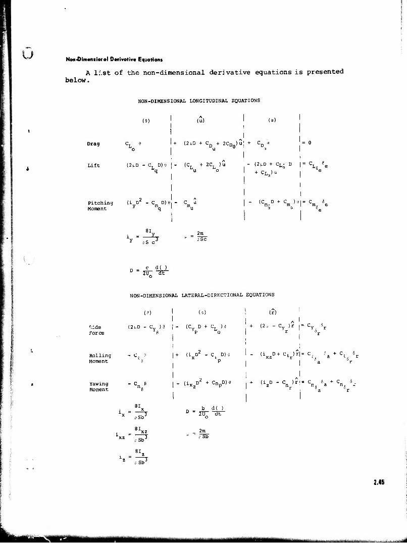
u Non-Dimemiorol Derivative Equations

A list of the non-dimensional derivative equations is presented below.

NON-DIMENSIONAL LONGITUDINAL EQUATIONS

(e) (u) (a)

Drag (2uD + CD + 2CD )u; + % a

Lift (2uD - C D) 6 | - (CL + 2CL ) u - (2uD + CL-a D | = C ^

q , I +CL)a |

Pitching Moment

i D - C D) 8, - C a y m m 1 q i u

(C D + C )o|= C_ &.

81 l = *T

2m oSc

D - ° d( 1 o

NON-DIMENSIONAL LATERAL-DIRECTIONAL EQUATIONS

I I

Rolling Moment

(3) (;)

r;ide (2uD - C )S | - (C D + CL ) 4 force 8 P o

Yawing " Cn 8

Moment 6

81

pSb

81

cSb

81

7T

xz

P Sb

I

+ (i D2 - C D)| X P

(iv D + Cn D»*

n - b d(. > o

2m FSS

(r)

+ (2. - C )r |= C 5r r , 6r

(i D + c, )r|= C, £ + C 5 i a c« r

a r

+ (i D - C )r*= C 6 + C « z n ' n. a n. r S 6 l a r

2.45

L— aa^Ha^taaaa^MMM -~-~- ■•■ *• ■ ■ - -- ~ '■- - ■ i ifciftlM

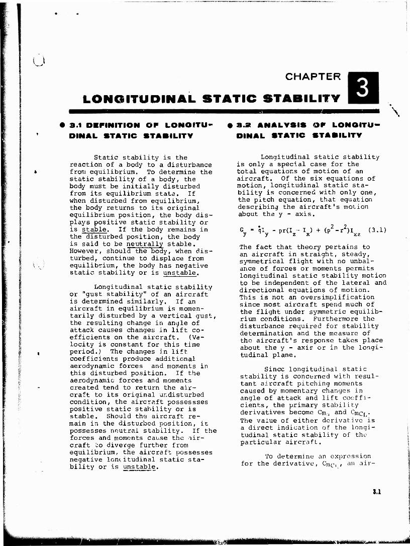
ü

V: 1

>

CHAPTER

LONGITUDINAL STATIC STABILITY

• 3.1 DEFINITION OF LONGITU- DINAL STATIC STABILITY

Static stability is the reaction of a body to a disturbance from equilibrium. To determine the static stability of a body, the body must be initially disturbed from its equilibrium state. If when disturbed from equilibrium, the body returns to its original equilibrium position, the body displays positive static stability or is stable. If the body remains in the disturbed position, the body is said to be neutrally stable. However, should the body, when disturbed, continue to displace from equilibrium, the body has negative static stability or is unstable.

Longitudinal static stability or "gust stability" of an aircraft is determined similarly. If an aircraft in equilibrium is momentarily disturbed by a vertical gust, the resulting change in angle of attack causes changes in lift coefficients on the aircraft. (Ve- locity is constant for this time period.) The changes in lift coefficients produce additional aerodynamic forces and moments in this disturbed position. If the aerodynamic forces and moments created tend to return the aircraft to its original undisturbed condition, the aircraft possessses positive static stability or is stable. Should the aircraft remain in the disturbed position, it possesses neutral stability. If the forces and moments cause the aircraft co diverge further from equilibrium, the aircraft possesses negative lone itudinal static stability or is unstable.

\

• 3.Ä ANALYSIS OF LONGITU- DINAL STATIC STABILITY

Longitudinal static stability is only a special case for the total equations of motion of an aircraft. Of the six equations of motion, longitudinal static stability is concerned with only one, the pitch equation, that equation describing the aircraft's motion about the y - axis.

<K Pr(Iz~ I ) + <p' r2)I xz (3.1)

The fact that theory pertains to an aircraft in straight, steady, symmetrical flight with no unbalance of forces or moments permits longitudinal static stability motion to be independent of the lateral and directional equations of motion. This is not an oversimplification since most aircraft spend much of the flight under symmetric equilibrium conditions. Furthermore the disturbance required for stability determination and the measure of the aircraft's response takes place about the y - axis or in the longitudinal plane.

Since longitudinal static stability is concerned with resultant aircraft pitching moments caused by momentary changes in angle of attack and lift coefficients, the primary stability derivatives become Cma and CmcL« The value of either derivative is a direct indication of the longitudinal static stability of the particular aircraft.

To determine an expression for the derivative, Cm^r , an air-

3.1

m±

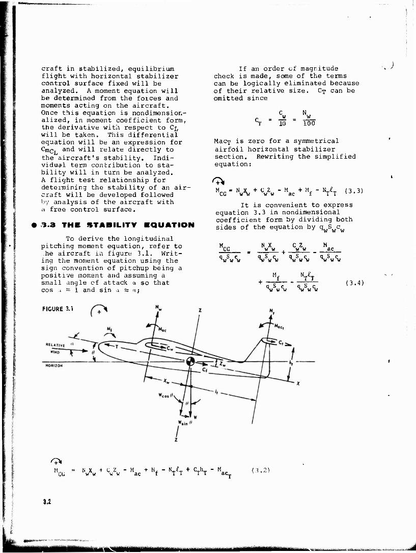
craft in stabilized, equilibrium flight with horizontal stabilizer control surface fixed will be analyzed. A moment equation will be determined from the foices and moments acting on the aircraft. Once this equation is nondimension- alized, in moment coefficient form, the derivative with respect to CL will be taken. This differential equation will be an expression for CmcL and will relate directly to the aircraft's stability. Indi- vidual term contribution to stability will in turn be analyzed. A flight test relationship for determining the stability of an aircraft will be developed followed by analysis of the aircraft with a free control surface.

• 13 THE STABILITY EQUATION

To derive the longitudinal pitching moment equation, refer to he aircraft in figure 3.1. Writ-

ing the moment equation using the sign convention of pitchup being a positive moment and assuming a small angle of attack a so that cos u ~ 1 and sin a s: a;

If an order of magnitude check is made, some of the terms can be logically eliminated because of their relative size. Op can be omitted since

T w 10

N w 100

Macip is zero for a symmetrical airfoil horizontal stabilizer section. Rewriting the simplified equation:

M CG \\ + c z w w M + M, ac f Vi (3.3)

It is convenient to express equation 3.3 in nondimensional coefficient form by dividing both sides of the equation by q S c www

■*CG q S c www

NX C Z w w w w ac

q. S c q S c www Trf W V

u

q S c nw w w

T T qS c TJ W W

(3.4)

FIGURE 3.1

M CG N X + w w

CZ - w w M f ac v-T + cThT ac,„ (3.2)

3.2

- .■<-.■'".■*«■■, .-."■:."».ift,- .

<mmmmmlmm ±^>- l-^,..... -.,..,

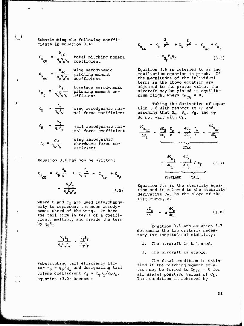
u Substituting the following coefficients in equation 3.4:

CG

CG % wcw coefficient

M ac

total pitching moment coefficient

wing aerodynamic

ac „ pitching moment

qSc ..... . T* w w coefficient

•£ fuselage aerodynamic s pitching moment co-

"""'"•• efficient

wing aerodynamic normal force coefficient

h www

N w

q S ^w w

w w c - cN — + cr ■— mCG N c c c

v^ c + c

ac f

(3.6)

Equation 3.6 is referred to as the equilibrium equation in pitch. If the magnitudes of the individual terms in the above equation are adjusted to the proper value, the aircraft may be placed in equilibrium flight wnere Cm_ = 0.

Taking the derivative of equation 3.6 with respect to CL and assuming that Xw, Zw, VJJ , and HT do not vary with CL,

qTST

Cw Cc " q S

W W

tail aerodynamic normal force coefficient

wing aerodynamic chordwise force coefficient

dC "CG

dC. 5i i + !fc 5t dCL c dCL c

WING

dC ac

dC.

Equation 3.4 may now be written:

X Z c - cv -- + c — - c + c m__ N c c c m m. CG ac f

VT q S c nw w w (3.5)

where C and cw are used interchange- ably to represent the mean aerodynamic chord of the wing. To have the tail term in ter; s of a coefficient, multiply and divide the term t>y qTsT

q S c Trf w w

q S ST T qTST

dC

dC.

dC.,

—- v n dC. H T L

FUSELAGE TAIL

(3.7)

Equation 3.7 is the stability equation and is related to the stability derivative Cm by the slope of the lift curve, a.

dC n da

dC n dC,

(3.8)

Equation 3.6 and equation 3.7 determine the two criteria necessary for longitudinal stability:

1. The aircraft is balanced.

2. The aircraft is stable.

Substituting tail efficiency factor n„ = qT/q and designating tail

volume coefficient V(1 = i ST/cwSw,

Equation (3.5) becomes:

The final condition is satisfied if the pitching moment equation may be forced to CmcG - 0 for all useful positive values of Cjjt This condition is achieved by

3.3

mamat matäthm

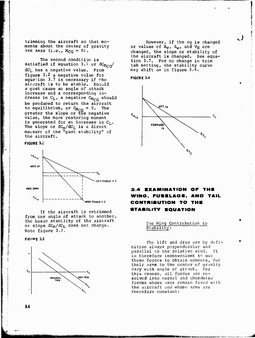
= trimming the aircraft so that moments about the center of gravity are zero (i.e., MQQ = 0) .

The second condition is satisfied if equation 3.7 or dCmcG/ dCL has a negative value. From figure 3.2 a negative value for equation 3.7 is necessary if the aircraft is to be stable. Should a gust cause an angle of attack increase and a corresponding increase in CL, a negative QnCG should be produced to return the aircraft to equilibrium, or CMc = 0. The greater the slope or the negative value, the more restoring moment is generated for an increase in CL. The slope or dCm/dC^ is a direct measure of the "gust stability" of the aircraft.

FIGURE 3.2

+c_

NOSE DOWN

LE2S STABLE A C

MORE STABLE AC

If the aircraft is retrimmed from one angle of attack to another, the basic stability of the aircraft or slope dCm/dCL does not change. Note figure 3.3.

FIGURE 3.3

However, if the eg is changed or values of Xw, Zw, and V"H are changed, the slope or stability of the aircraft is changed. See equation 3.7. For no change in trim tab setting, ehe stability curve may shift as in figure 3.4.

FIGURE 3.4

.;

<g

3.4 EXAMINATION OF THE WINO, FUSELAGE, AND TAIL CONTRIBUTION TO THE

STABILITY EQUATION

The Wing Contribution to Stability:

The lift and drag are by definition always perpendicular and parallel to the relative wind. It is therefore inconvenient to use these forces to obtain moments, for their arms to the center of gravity vary with angle of attack. For this reason, all forces are resolved into normal and chordwise forces whose axes remain fixed with the aircraft and whose arms are therefore constant:

3.«

MM

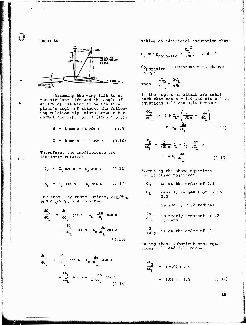
FIGURE 3.5

RESULTANT AERODYNAMIC FORCE

X BODY AXIS

Assuming the wing lift to be the airplane lift and the angle of attack of the wing to be the airplane's angle of attack, the following relationship exists between the normal and lift forces (figure 3.5) s

L cos a + D sin a (3.9)

Making an additional assumption that:

cL2

Cr = Cn .. + —=- and if 1 "parasite KJR e

Cn ..is constant with change "parasite in CL:

dC„ 2CT Then dCT IT® e

If the angles of attack are small such that cos a - 1.0 and sin o = a, equations 3.13 and 3.14 become:

5 dC,

N 1 + Cra da

L TT® e dC,

+ C, D d da

(3.15)

I 1

C - D cos a - L sin a (3.10)

Therefore, the coefficients are similarly related:

dC, 2 c-d4i0 dC. iBL e L D dC,

a-C da L dC, (3.16)

CN - CL cos a + CD sin a (3.11) Examining the above equations for relative magnitude,

Cr - C cos a - C sin a (3.12)

The stability contributions, dC^/dCL and dCc/dCjj, are obtained:

dCM dC, An,

L L Li

+ dc[ Sln a + CD dt[ C0S a

(3.13)

Cn is on the order of 0.3

CL usually ranges from .2 to 2.0

a is small, ~ .2 radians

3=- is nearly constant at .2 dC. ,. L radians

Ti^Re is on the order of .1

Making these substitutions, equations 3.15 and 3.16 become

dcc dcn r da . . __ cos a _ C — sin a L L Li

dC, . r da sin a-C, -r~r cos a

L at (3.14)

dC„ ^ dC. 1 -.04 + .06

- 1.02 » 1.0 (3.17)

3.5

a* Mflü ........... ... .

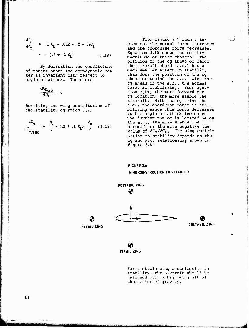
dC. .1 C. .012 - .2 - .2C,

- (.2 + .1 CJ (3.18)

By definition the coefficient of moment about the aerodynamic center is invariant with respect to angle of attack. Therefore,

dCm ac dCL

= 0

Rewriting the wing contribution of the stability equation 3.7,

dC X w dC,

WING

(.2 + .1 C.) — (3.19) L c

From figure 3.5 when a increases, the normal force increases and the chordwise force decreases. Equation 3.19 shows the relative magnitude of these changes. The position of the eg above or below the aircraft chord (a.c.) has a much smaller effect on stability than does the position of the eg ahead or behind the a.c. With the eg ahead of the a.c., the normal force is stabilizing. From equation 3.19, the more forward the eg location, the more stable the aircraft. With the eg below the a.c, the chordwise force is stabilizing since this force decreases as the angle of attack increases. The further the eg is located below the a.c, the more stable the aircraft or the more negative the value of dCjn/dCL. The wing contribution to stability depends on the eg and a.c relationship shown in figure 3.6.

FIGURE 3.6

WING CONSTRUCTION TO STABILITY

DESTABILIZING

STABILIZING DESTABILIZING

STABILIZING

II

For a stable wing contribution to stability, the aircraft should be designed with a high wing aft of the center of gravity.

—•--'— «■MlttMi

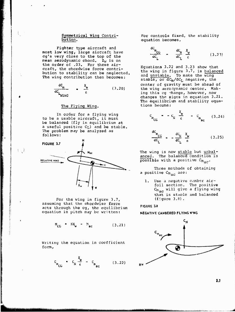
t )

Symmetrical Wing Contri- bution.

Fighter type aircraft and most low wing, large aircraft have cg's very close to the top of the mean aerodynamic chord. Zw is on the order of .03. For these aircraft, the chordwise force contribution to stability can be neglected. The wing contribution then becomes:

dC

dC, UNG

w c

(3.20)

The Flying Wing.

In order for a flying wing to be a usable aircraft, it must be balanced (fly in equilibrium at a useful positive CL) and be stable. The problem may be analyzed as follows:

FIGURE 3.7

For the wing in figure 3.7, assuming that the chordwise force acts through the eg, the equilibrium equation in pitch may be written:

MCG NX (3.21)

Writing the equation in coefficient form,

CG

w

c (3.22)

For controls fixed, the stability equation becomes,

dC CG

dC,

dC ft

dC, w c

(3.23)

Equations 3.22 and 3.2 3 show that the wing in figure 3.7, is balanced and unstable. To make the wing stabTe7_ör—d"Cm/dCL negative, the center of gravity must be ahead of the wing aerodynamic center. Mak- ing this eg change, however, now changes the signs in equation 3.21. The equilibrium and stability equations become:

mCG N w c ac

dC CG

dC.

dC, X N _w dC, c

(3.241

(3.25)

The wing is now stable but unbalanced. The balanced condition is possible with a positive Cm .

Three methods of obtaining a positive Qn _ are: ac

1. Use a negative camber airfoil section. The positive Cm will give a flying wing

ctC that is staole and balanced (figure 3.8).

FIGURE 3.8

NEGATIVE CAMBERED FLYING W'NG

Ck

ac RW

3.T

■MM

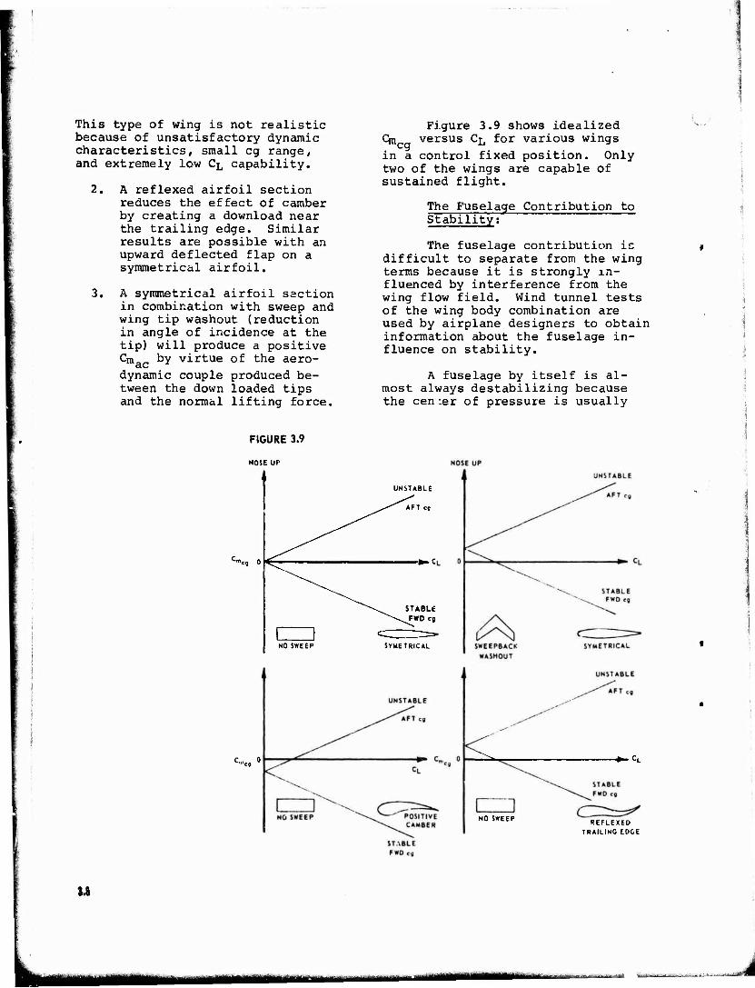
This type of wing is not realistic because of unsatisfactory dynamic characteristics, small eg range, and extremely low C^ capability.

2. A reflexed airfoil section reduces the effect of camber by creating a download near the trailing edge. Similar results are possible with an upward deflected flap on a symmetrical airfoil.

3. A symmetrical airfoil section in combination with sweep and wing tip washout (reduction in angle of incidence at the tip) will produce a positive On--, by virtue of the aerodynamic couple produced between the down loaded tips and the normal lifting force.

Figure 3.9 shows idealized Cm versus Cj_, for various wings in a control fixed position. Only two of the wings are capable of sustained flight.

The Fuselage Contribution to Stability;

The fuselage contribution ic difficult to separate from the wing terms because it is strongly influenced by interference from the wing flow field. Wind tunnel tests of the wing body combination are used by airplane designers to obtain information about the fuselage influence on stability.

A fuselage by itself is almost always destabilizing because the cen ;er of pressure is usually

3.8

FIGURE 3.9

NOSE UP

1

UNSTABLE

^^"AFT e?

^\. STABLE ^^^FWDeg

1 1 ■^ZZZT^» NO SWEEP SYMETRICAL

»-cL

NO SWEEP REFLEXED TRAILING COCE

HW MMMM

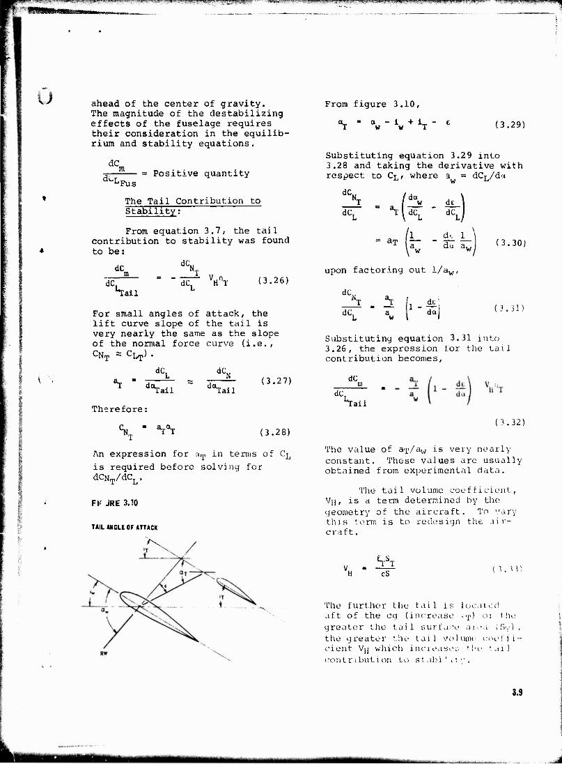
«^»juTr1-^^?^1-»»-^.^'^'»^'1'''1^'*^!^^ WPWPWBI'PBBIB JBPWWWjWlSggW ,'I)W«I..MIMI..|.JMJ»'' ww.wjWWP.il!«"-- "■ -'

a

ahead of the center of gravity. The magnitude of the destabilizing effects of the fuselage requires their consideration in the equilibrium and stability equations.

dC. m di_L

Positive quantity Fus

The Tail Contribution to Stability;

From equation 3.7, the tail contribution to stability was found to be:

dC dC

N„

dC 4

dC, Vl (3.26)

ail

For small angles of attack, the lift curve slope of the tail is very nearly the same as the slope of the normal force curve (i.e., CNT ~ CL ).

dC, dt\

*T

Therefore:

%

!*rail

VT

da, Tail (3.27)

(3.28)

An expression for otm in terms of CL

is required before solving for dCNT/dCL,

Fl' JRE 3.10

TAIL ANCLE OF ATTACK

From figure 3.10,

iw + 1T (3.29)

Substituting equation 3.29 into 3.28 and taking the derivative with respect to CL, where a = dCL/d<»

N~ /da \ T / w dc

dC. M dC,

— aip

w

dCl

ck 1 da a ITA (3.30) w

upon factoring out l/aw,

dCK N„

dC. w \

dc' ~T~ i dai (3.31)

Substituting equation 3.31 into 3.26, the expression tor the tail contribution becomes,

dC

dC 4 ail

3.32)

The value of aT/aw i-s very nearly constant. These values are usually obtained from experimental data.

The tail volume coefficient, VJI , is a term determined by the

geometry of the aircraft. To vary this term is to redesign the aircraft.

cS ( 3 . * 3)

The further the tail is located aft of the eg (increase .■]>) or the

greater the tail surface area (S>j ) .

the greater the tail volume coefficient V|[ which increases t be tail

contribution to stabi'it*'.

3.9

MM - -- -■- - - - MBM

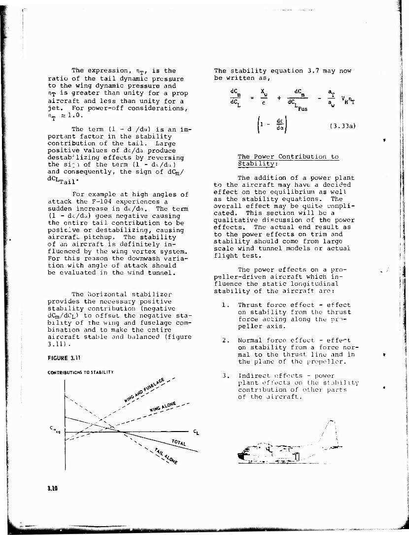
The expression, n-p, is the ratio of the tail dynamic pressure to the wing dynamic pressure and n-p is greater than unity for a prop aircraft and less than unity for a jet. For power-off considerations, nT = 1.0.

The term (1 - d /da) is an important factor in the stability contribution of the tail. Large positive values of dc/da produce destabilizing effects by reversing the si~i of the term (1 - dt/da) and consequently, the sign of dC^/ dCLTail*

For example at high angles of attack the F-104 experiences a sudden increase in dc/da. The term (1 - dt/da) goes negative causing the entire tail contribution to be posic_ve or destabilizing, causing aircraft pitchup. The stability of an aircraft is definitely influenced by the wing vortex system. For this reason the downwash variation with angle of attack should be evaluated in the wind tunnel.

The horizontal stabilizer provides the necessary positive stability contribution (negative dCnj/dCL) to offset the negative stability of the wing and fuselage combination and to make the entire aircraft stable and balanced (figure 3.11).

FIGURE 3.11

CONTRIBUTIONS TO STABILITY

The stability equation 3.7 may now be written as,

V,

V N

X N

X

X

*^V '

wy

-'-'- Vv ,"— "

dC n dC.

dC

dC, 'Fus

I" f da

w

(3.33a)

The Power Contribution to Stability:

The addition of a power plant to the aircraft may have a decided effect on the equilibrium as well as the stability equations. The overall effect may be quite complicated. This section will be a qualitative discussion of the power effects. Tne actual end result as to the power effects on trim and stability should come from large scale wind tunnel models or actual flight test.

The power effects on a propeller-driven aircraft which influence the static longitudinal stability of the aircraft are:

1. Thrust force effect - effect on stability from the thrust force acting along the propeller axis.

2. Normal force? effect - effect on stability from a force normal to the thrust line and in the plane of the propeller.

3. Indirect effects - power plant effects on the stability contribution of other parts of the aircraft.

^ v _ Dv —!■■"■ «. r 1 H. -~r*

3.10

i iiMiMm -

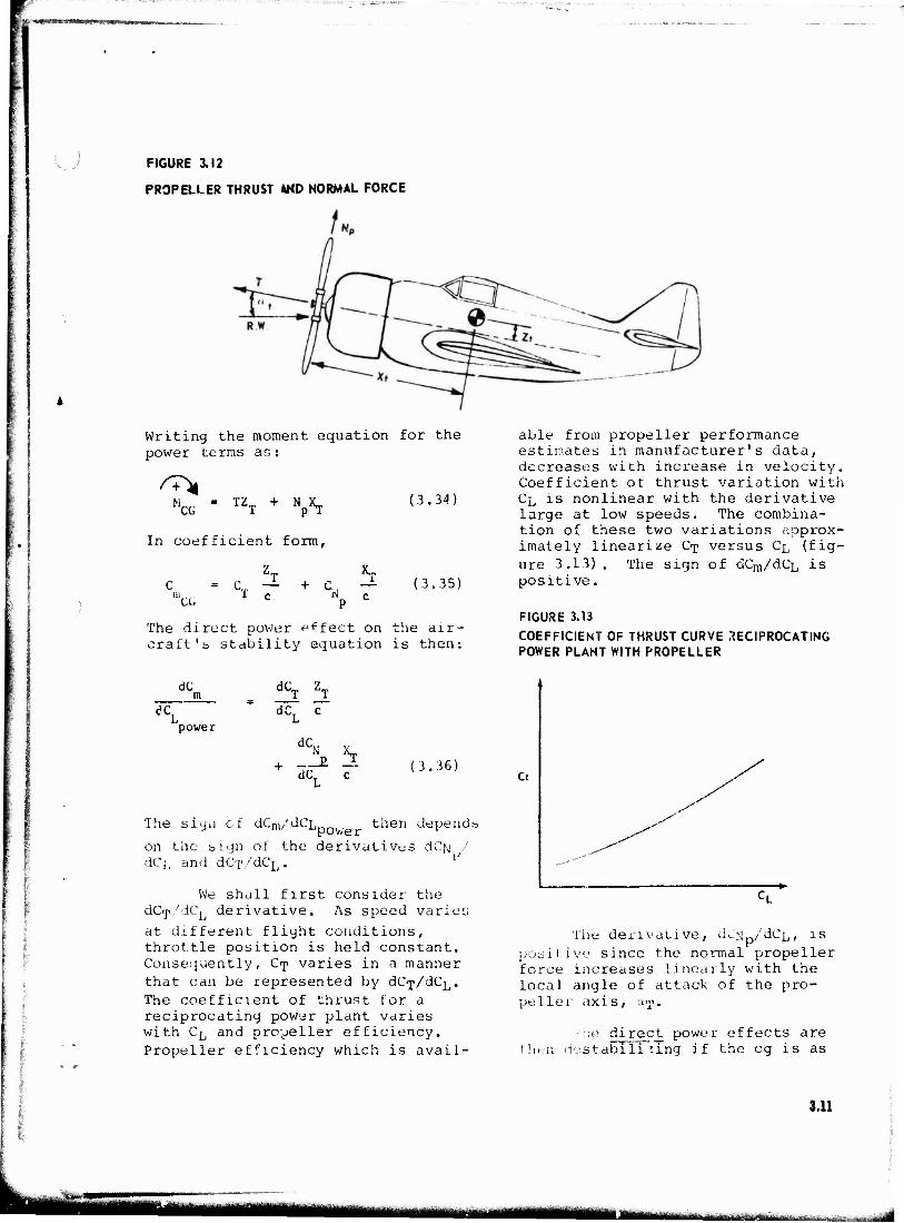
FIGURE 3.12

PROPELLER THRUST AND NORMAL FORCE

Writing the moment equation for the power terms as:

CG TZT + NpXT

In coefficient form,

zT x. c = cT — + c. — \c X c ^p c

(3.34:

(3.35)

The direct power effect on the aircraft's stability equation is then:

able from propeller estimates in manufac decreases with incre Coefficient of thrus CL is nonlinear with large at low speeds, tion of these two va imately linearize C-p ure 3.13). The sign positive.

performance turer's data, ase in velocity, t variation with the derivative The combina-

riations approx- versus CL (fig- of aCm/dCL is

FIGURE 3.13

COEFFICIENT OF THRUST CURVE RECIPROCATING POWER PLANT WITH PROPELLER

dC tn

dS zT

dCL power dCL c

dCN x + __E -2

aCL c

he sign c. f dCm/dCLnnwoT

(3.36)

then depends

on the sign of the derivatives dCw / dC;, and dOx>/dCL.

We shall first consider the dGp/dCL derivative. As speed varies at different flight conditions, throttle position is held constant. Consequently, Cy varies in a manner that can be represented by dCT/dCL. The coefficient of thrust for a reciprocating power plant varies with CL and proueller efficiency. Propeller efficiency which is avail-

Ct

The derivative, dCy /dCL/ is positive since the normal propeller force increases linearly with the local angle of attack of the propeller axis, j'p.

I h 'he direct power effects are stabilising if the eg is as

f

f 3.11

■HMI

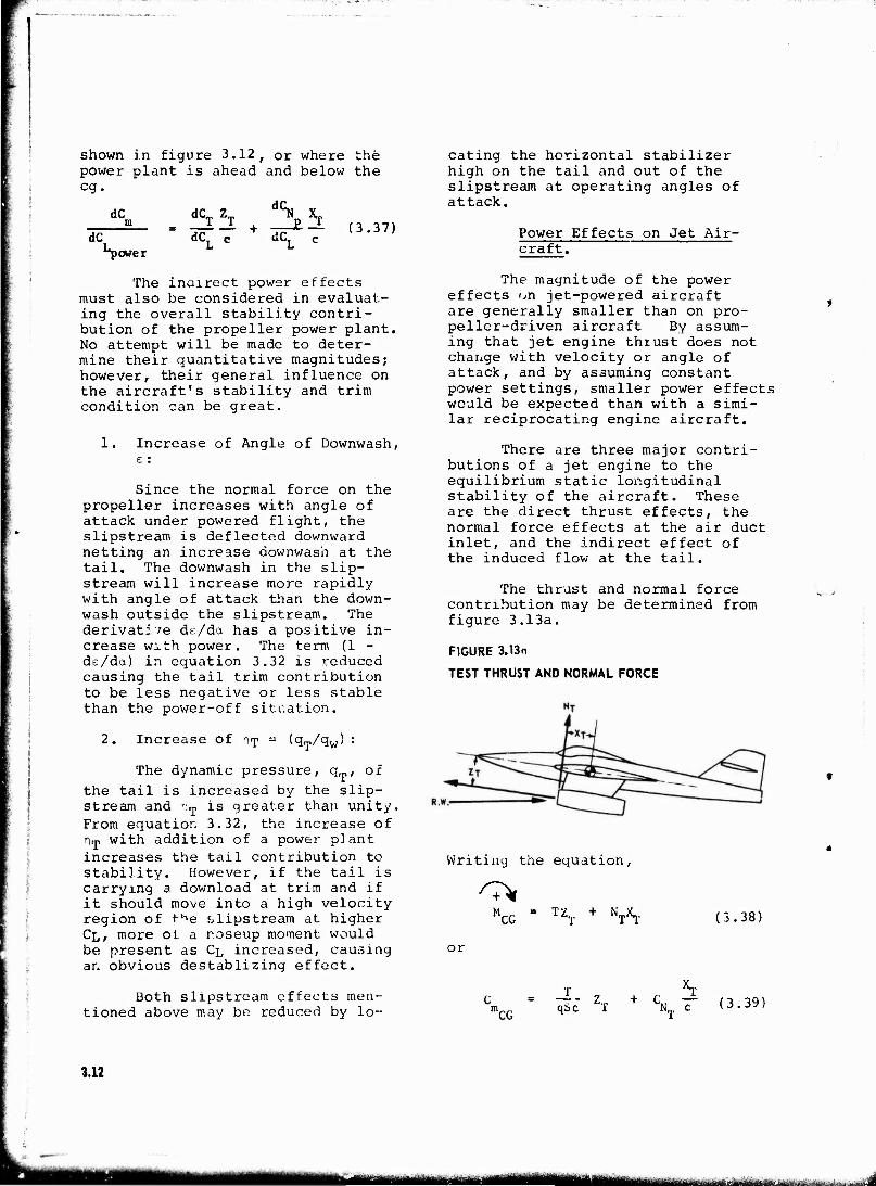
shown in figure 3.12, or where the power plant is ahead and below the eg.

dC dC. c dCT

dC dcTzT (3.37)

s ewer

The indirect power effects must also be considered in evaluating the overall stability contribution of the propeller power plant. No attempt will be made to determine their quantitative magnitudes; however, their general influence on the aircraft's stability and trim condition can be great.

1. Increase of Angle of Downwash, E :

Since the normal force on the propeller increases with angle of attack under powered flight, the slipstream is deflected downward netting an increase downwash at the tail. The downwash in the slipstream will increase more rapidly with angle of attack than the downwash outside the slipstream. The derivative de/da has a positive increase with power. The term (1 - de/da) in equation 3.32 is reduced causing the tail trim contribution to be less negative or less stable than the power-off situation.

2. Increase of HT = (qT/qw) :

The dynamic pressure, q_, of the tail is increased by the slipstream and "T is greater than unity. From equation 3.32, the increase of rim with addition of a power plant increases the tail contribution to stability. However, if the tail is carrying a download at trim and if it should move into a high velocity region of t-^e slipstream at higher CL, more ol a noseup moment would be present as CL increased, causing an obvious destablizing effect.

Both slipstream effects mentioned above may be reduced by lo-

cating the horizontal stabilizer high on the tail and out of the slipstream at operating angles of attack.

Power Effects on Jet Air- craft.

The magnitude of the power effects on jet-powered aircraft are generally smaller than on propeller-driven aircraft By assuming that jet engine thrust does not change with velocity or angle of attack, and by assuming constant power settings, smaller power effects would be expected than with a similar reciprocating engine aircraft.

There are three major contributions of a jet engine to the equilibrium static longitudinal stability of the aircraft. These are the direct thrust effects, the normal force effects at the air duct inlet, and the indirect effect of the induced flow at the tail.

The thrust and normal force contribution may be determined from figure 3.13a.

FIGURE 3.13n

TEST THRUST AND NORMAL FORCE

Writing the equation,

CG IZT + NTXj, (3.38)

or

c T *T mCG = tfc" ZT + \T (3.39)

3.12

MM«!

With the aircraft in unaccelerated flight, the dynamic pressure is a function of lift coefficient.

q = W

CLS (3.40)

Therefore,

"CG IT- CL + \ T (3'41)

Ir thrust is considered independent of speed,* then

dC B

dC. r Z

T dC,

T T

dC. -^ (3.42)

The thrust contribution to stability then depends on whether the thrust line is above or below the eg. Locating the engine below the eg causes a destablizing influence, and above the eg a stabilizing influence.

The normal force contribution depends on the sign of the derivative dCNip/dCL. The normal force Nrp is created at the air-duct inlet to the turbojet unit. This force is created as a result of the momentum change of the free stream which bends to flow along the duct axis. The magnitude of the force is a function of the mass airflow rate, Wa, and the angle aT between the local flow at the duct entrance and the duct axis.

M - Wa \r NT - — V aT (3.43)

With an increase in aT, NT will increase, causing dCftm/dCr, to be positive. The normal force contribution will be destabilizing if the inlet duct is ahead of the center of gravity. The magnitude of the destabilizing moment will depend on

For aircraft which hove large thrust variation with airspeed, the pitching moment coefficient n:ust be calculated for different values of the aircraft's lift coefficient.

the distance the inlet duct is ahead of the center of gravity.

For a jet engine to definitely contribute to positive longitudinal stability, (dC^/dCL negative), the jet engine would be located above and behind the center of gravity.

The indirect contribution of the jet unit to longitudinal stability is the effect of the jet induced downwash at the horizontal tail. This applies to the situation where the jet exhaust passes under or over the horizontal tail surface. The jet exhaust as it discharges from the tail pipe spreads outward. Turbulent mixing causes outer air to be drawn in towards the exhaust area. Downwash at the tail is directly affected. With the exhaust below the tail surface, the downwash is increased, causing the tail term to be less stabilizing.

From the above discussion it can be seen that several factors are important in deciding the power effect on stability. Each aircraft must be examined individually. This is the reason that aircraft are tested for stability in several configurations and at different power settings.

• 3.5 THE NEUTRAL POINT

The stick-fixed neutral point is defined as the center of gravity position at which the aircraft displays neutral stability or where dCm/dCL =0.

The symbol h is used for center of gravity position where,

CG

c (3.44)

\

3.13

m susjiiii in - nir>-ii ii - i

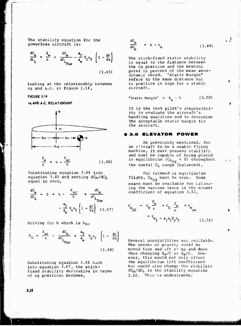
The stability equation for the powerless aircraft is:

dC jr dC,

1> - h n (3.49)

J

dC n dC,

dC

dCT

Fus

*T u li de

~ T Vl I1 ~ da w 1

(3.45)

Looking at the relationship between eg and a.c. in figure 3.14,

The stick-fixed static stability is equal to the distance between the eg position and the neutral point in percent of the mean aerodynamic chord. "Static Margin" refers to the same distance but is positive in sign for a stable aircraft..

FIGURE 3,14

eg AND A.C. RELATIONSHIP

X X w , ac — = h c c

(3.46)

"Static Margin" h (3.50)

It is the test pilot's responsibility to evaluate the aircraft's handling qualities and to determine the acceptable static margin for the aircraft.

• 3.6 ELEVATOR POWER

As previously mentioned, for an ö^rcraft to be a usable flying machine, it must possess stability and must be capable of being placed in equilibrium (Cm = 0) throughout

the useful CL range (balanced).

Substituting equation 3.46 into equation 3.4 5 and setting dCm/dCL equal to zero,

dC n dC,

0 - h ac c

dC

dC,

"* V n I 1 d£ - VHnT 11 - — w

Fus

dal (3.47)

Solving for h which is hn,

For trimmed or equilibrium flight, Cm must be zero. Some

means must be available for balancing the various terns in the moment coefficient of equation 3.51,

: = c., — + c„ zw + c CG c ac

+ C m£ - aTaTVHnT (3.51)

jac c

dC

dC. Fus

L 3l If l, dE + T VT j1 " dJ

(3.48)

Substituting equation 3.48 back into equation 3.47, the stick- fixed stability derivative in terms of eg positions becomes,

Several possioilities are available. The center of gravity could be moved fore and aft or up and down thus changing Xw/C or Zw/C. How- ever, this would not only affect the equilibrium lift coefficient but would also change the stability dCm/dCL in the stability equation 3.52. This is undesirable.

3.14

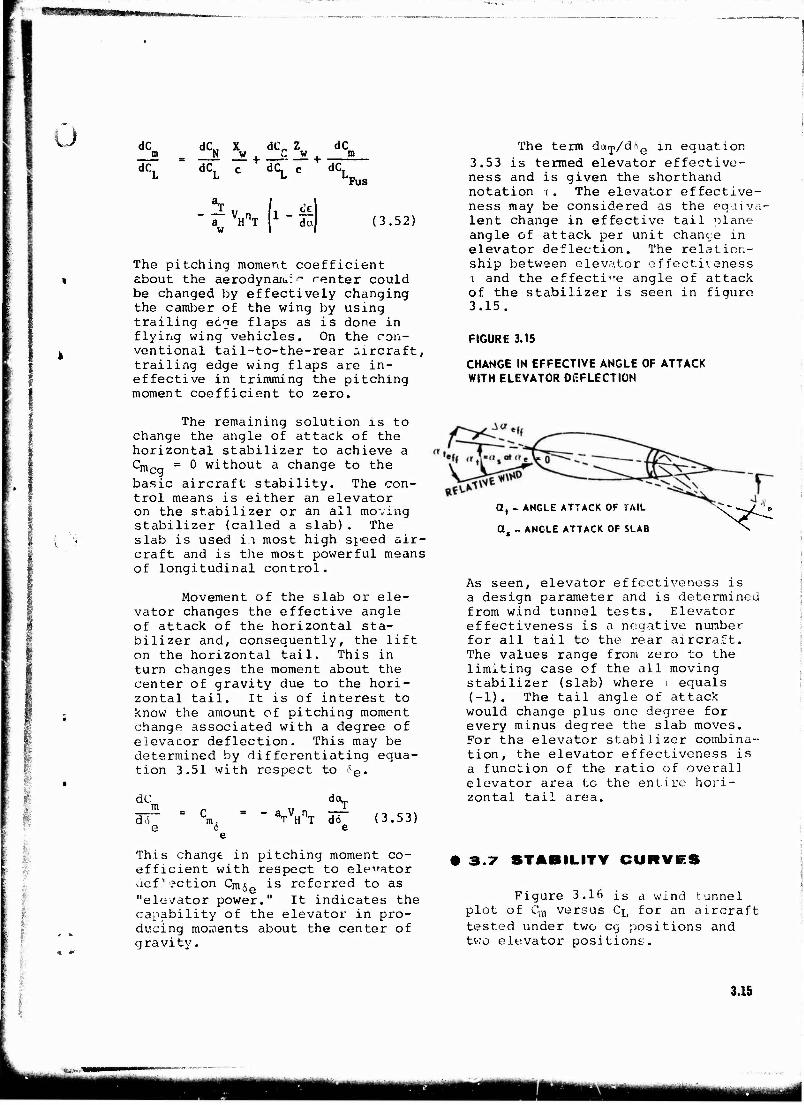
'R'HHHSWKSSIl^SW»*»«»»«»»

Ü dC n> dC,

dC„ X dC„ Z dC N _w , C _w » dC c dC. c d 1CL CL Fus

w du (3.52)

The pitching moment coefficient about the aerodynaiu:^ renter could be changed by effectively changing the camber of the wing by using trailing ecge flaps as is done in flying wing vehicles. On the conventional tail-to-the-rear aircraft, trailing edge wing flaps are ineffective in trimming the pitching moment coefficient to zero.

The term daT/d6e in equation 3.53 is termed elevator effectiveness and is given the shorthand notation r. The elevator effectiveness may be considered as the equivalent change in effective tail plane angle of attack per unit chance in elevator deflection. The relationship between elevator effectiveness T and the effective angle of attack of the stabilizer is seen in figure 3.15.

FIGURE 3.15

CHANGE IN EFFECTIVE ANGLE OF ATTACK WITH ELEVATOR DEFLECTION

i

i

The remaining solution is to change the angle of attack of the horizontal stabilizer to achieve a cm™ = 0 without a change to the basic aircraft stability. The control means is either an elevator on the stabilizer or an all moving stabilizer (called a slab). The slab is used i.i most high speed aircraft and is the most powerful means of longitudinal control.

Movement of the slab or elevator changes the effective angle of attack of the horizontal stabilizer and, consequently, the lift on the horizontal tail. This in turn changes the moment about the center of gravity due to the horizontal tail. It is of interest to know the amount of pitching moment change associated with a degree of elevator deflection. This may be determined by differentiating equation 3.51 with respect to 5e.

dC —- = C diS m, e 6 ■ -vv H T d6

a, - ANGLE ATTACK OF TAIL

a. - ANCLE ATTACK OF SLAB ^:

As seen, elevator effectiveness is a design parameter and is determined from wind tunnel tests. Elevator effectiveness is a negative number for all tail to the rear aircraft. The values range from zero to the limiting case of the all moving stabilizer (slab) where i equals (-1). The tail angle of attack would change plus one degree for every minus degree the slab moves. For the elevator stabilizer combination, the elevator effectiveness is a function of the ratio of overall elevator area to the entire horizontal tail area.

(3.53)

%■

4 «■'

This change in pitching moment coefficient with respect to elevator def1 action Cm<5e is referred to as "elevator power." It indicates the capability of the elevator in producing moments about the center of gravity.

• 3.7 STABILITY CURVES

Figure 3.16 is a wind tunnel plot of Cm versus Cj_, for an aircraft tested under two eg positions and two elevator positions.

3.15

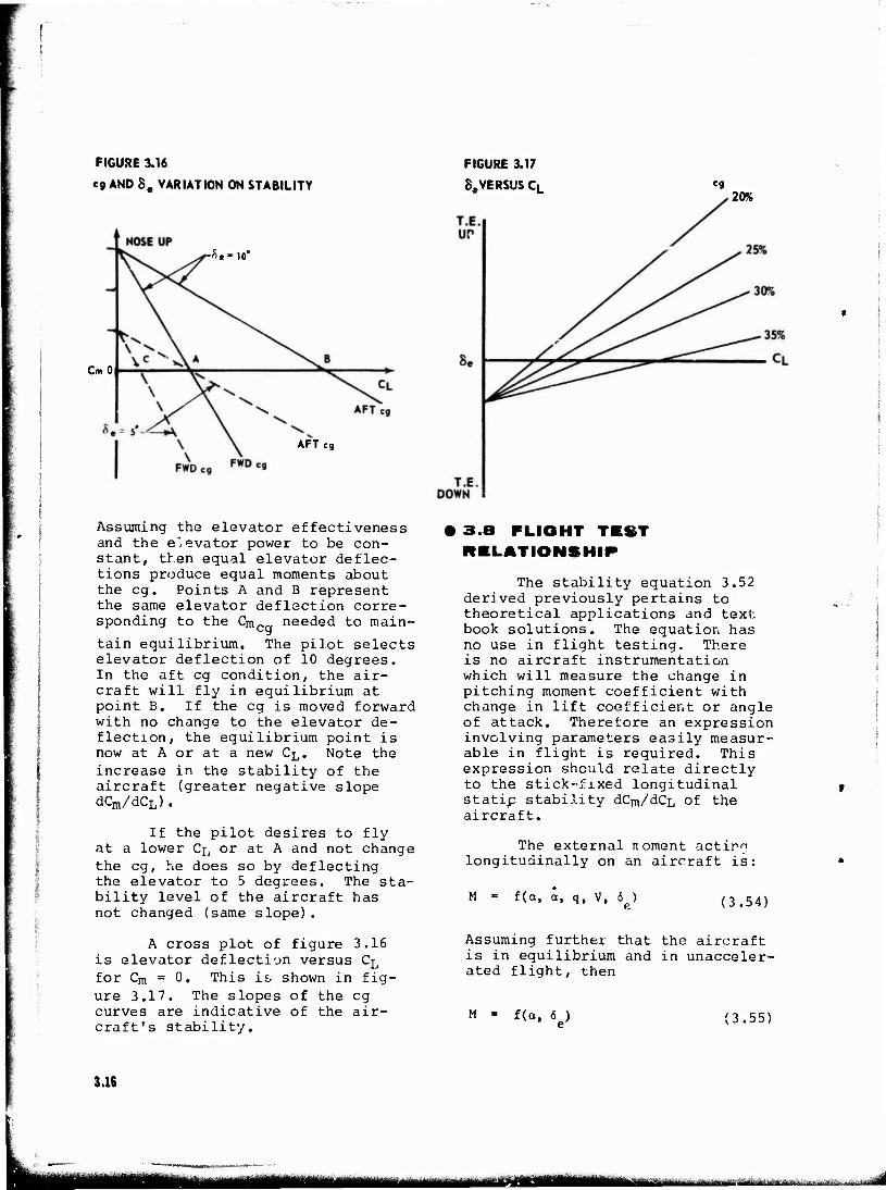
FIGURE 3.16

eg AND Se VARIATION ON STABILITY

-S.-io*

Cm 0

AFT eg

Assuming the elevator effectiveness and the e'evator power to be constant, then equal elevator deflections produce equal moments about the eg. Points A and B represent the same elevator deflection corresponding to the Cm needed to main-

tain equilibrium. The pilot selects elevator deflection of 10 degrees. In the aft eg condition, the aircraft will fly in equilibrium at point B. If the eg is moved forward with no change to the elevator deflection, the equilibrium point is now at A or at a new C^. Note the increase in the stability of the aircraft (greater negative slope dCm/dCL).

If the pilot desires to fly at a lower Cj, or at A and not change the eg, he does so by deflecting the elevator to 5 degrees. The stability level of the aircraft has not changed (same slope).

A cross plot of figure 3.16 is elevator deflection versus CL for Cm = 0. This is shown in figure 3.17. The slopes of the eg curves are indicative of the aircraft's stability.

FIGURE 3.17

8,VERSUS CL «9 20%

3.8 FLIGHT TEST RELATIONSHIP

The stability equation 3.52 derived previously pertains to theoretical applications and text book solutions. The equation has no use in flight testing. There is no aircraft instrumentation which will measure the change in pitching moment coefficient with change in lift coefficient or angle of attack. Therefore an expression involving parameters easily measurable in flight is required. This expression should relate directly to the stick-fixed longitudinal static stability dCm/dCL of the aircraft.

The external noment actir? longitudinally on an aircraft is:

M f(a, a, q, V, 6 ) (3.54)

Assuming further that the aircraft is in equilibrium and in unaccelerated flight, then

f(a, 6e) (3.55)

3.16

m ■Ml

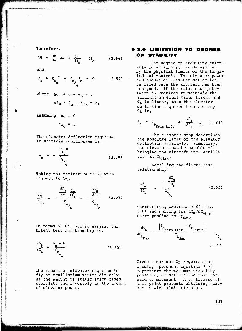
m.WMUWllli jWlLimiaiMUJ ■ n»u» - ,J.^|l'»l^^P!S|l^^pKgjp^P^'l-^S.*-l-'.Mi.l.'»!WIWIIWM ■JIUJ!PMI-«.I»1M"«LJJI"IIW-V«J'WJ.1" i- AWtl: w«nsqipv<«m

Therefore,

*M - f A« + f- A6 e

and

C-Ca+C 6 -0 m m me a o

where Ac. = a - a_ = a

(3.56)

(3.57)

A6e = 5„ _ 6p =6,

assuming oD = 0

6e^ = °

• 3.9 LIMITATION TO DIORII OF STABILITY

The degree of stability tolerable in an aircraft is determined by the physical limits of the longitudinal control. The elevator power and amount of elevator deflection is fixed once the aircraft has been designed. If the relationship between 6e required to maintain the aircraft in equilibrium flight and CL is linear, then the elevator deflection required to reach any CL is,

"Zero Lift

d6 e dC. L (3.61)

The elevator deflection required to maintain equilibrium is,

C a m a (3.58)

Taking the derivative of &B with respect to Cj,,

dC

dCT

■n da do" dCT

dC n dC,

(3.59)

In terms of the static margin, the flight test relationship is,

da e dC, (3.60]

The elevator stop determines the absolute limit of the elevator deflection available. Similarly, the elevator must be capable of bringing the aircraft into equilibrium at CL,.

Recalling the flight test relationship,

d6 e dC,

dC IT

dCT !3.62)

Max

Substituting equation 3.6? into 3.61 and solving for dCm/dCL corresponding to CL, Max

6 ero Lift "Limi J

dC Hi ax Max

o e

!3.63)

The amount of elevator required to fly at equilibrium varies directly as the amount of static stick-fixed stability and inversely as the amoun, of elevator power.

Given a maximum CL required for landing approach, equation J.6 3 represents the maximum stability possible, or defines the most forward eg movement. A eg forward of this point prevents obtaining maximum CL with limit elevator.

3.17

tamtmmm OWitt.

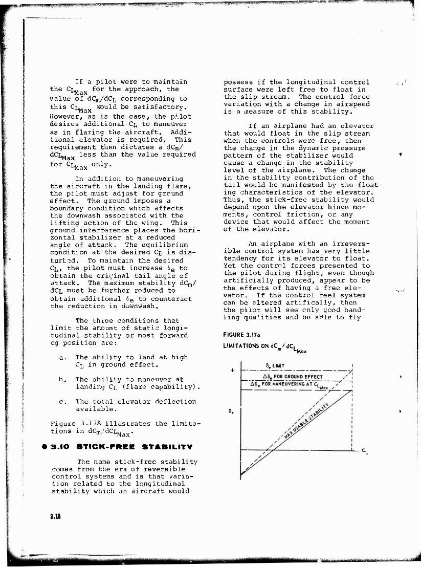
iipM111.»»n iiin,mBaim,i i- iym*,w.u!w -^wpBBWPiy re . ^MMWlWBWWMMI^pp^p^WgWPWWpB

If a pilot were to maintain the Ci». for the approach, the value of dQn/dCL corresponding to this CL would be satisfactory. However, as is the case, the p.!lot desires additional CL to maneuver as in flaring the aircraft. Addi- tional elevator is required. This requirement then dictates a dCm/ dCLM less than the value required

for %iax only'

In addition to maneuvering the aircraft in the landing flare, the pilot must adjust for ground effect. The ground imposes a boundary condition which affects the downwash associated with the lifting action of the wing. This ground interference places the horizontal stabilizer at a reduced angle of attack. The equilibrium condition at the desired CL is disturbed . To maintain the desired CL, the pilot must increase 5e to obtain the original tail angle of attack. The maximum stability dC^/ dCL must be further reduced to obtain additional 6e to counteract the reduction in downwash.

The three conditions that limit the amount of static longitudinal stability or most forward eg position are:

a. The ability to land at high CL in ground effect.

b. The ability to maneuver at landing CL (flare capability).

c. The total elevator deflection available.

Figure 3.17A illustrates the limitations in dCm/dCLMax.

3.10 STICK-FREE STABILITY

The name stick-free stability comes from the era of reversible control systems and is that variation related to the longitudinal stability which an aircraft would

possess if the longitudinal control surface were left free to float in the slip stream. The control force variation with a change in airspeed is a measure of this stability.

If an airplane had an elevator that would float in the slip stream when the controls were free, then the change in the dynamic pressure pattern of the stabilizer would cause a change in the stability level of the airplane. The change in the stability contribution of the tail would be manifested by the floating characteristics of the elevator. Thus, the stick-free stability would depend upon the elevator hinge moments, control friction, or any device that would affect the moment of the elevator.

An airplane with an irreversible control system has very little tendency for its elevator to float. Yet the control forces presented to the pilot during flight, even though artificially produced, appear to be the effects of having a free elevator, If the control feel system can be altered artifically, then the pilot will see enly good handling qualities and be aHle to fly

FIGURE 3.17a

LIMITATIONS ON dC /dC, uMax

8,

S. LIMIT

mtm HUM HjMiagm mmm <■ uftü^aa BM

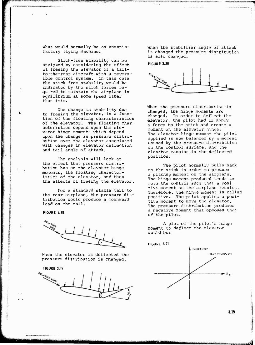
smpnünpnpffpn|wn,iQi m "T^I'WJ'S'WBWI ■J^''i^-^-:..:"we)',-it,M;'-^iipy^Mmi IIIIIIJJIIILI J„I_^.,«--

what would normally be an unsatisfactory flying machine.

Stick-free stability can be analyzed by considering the effect of freeing the elevator of a tail- to-the-rear aircraft with a reversible control system. In this case the stick free stability would be indicated by the stick forces required to maintain the. airplane in equilibrium at some speed other than trim.

The change in stability due to freeing the elevator, is a function of the floating characteristics of the elevator. The floating characteristics depend upon the elevator hinge moments which depend upon the change in pressure distribution over the elevator associated with changes in elevator deflection and tail angle of attack.

The analysis will look at the effect that pressure distribution has on the elevator hinge moments, the floating characteristics of the elevator, and then the effects of freeing the elevator.

For 3 standard stable tail to the rear airplane, the pressure distribution would produce a rownward load on the tail.

FIGURE 3.18

When the elevator is deflected the pressure distribution is changed.

FIGURE 3.19

When the stabilizer angle of attack is changed the pressure distribution is also changed.

FIGURE 3.20

When the pressure distribution is changed, the hinge moments are changed. In order to deflect the elevator, the pilot had to apply a force to the stick and create a moment on the elevator hinge. The elevator hinge rroment the pilot applied is now balanced by a moment caused by the pressure distribution on the control surface, and the elevator remains in the deflected position.

The pilot normally pulls back on the stick in order to produce a pitchup moment on the airplane. The hinge moment produced tends to move the control such that a positive moment on the airplane results. Therefore, the hinge moment is called positive. The pilot applies a positive moment to move the elevator. The pressure distribution produces a negative moment that opposes that of the pilot.

A plot of the pilot's hinge moment to deflect the elevator would be:

FIGURE 3.21

(,'ILOT PRODUCED!

3.19

MMM ■■■-'■■■-■■

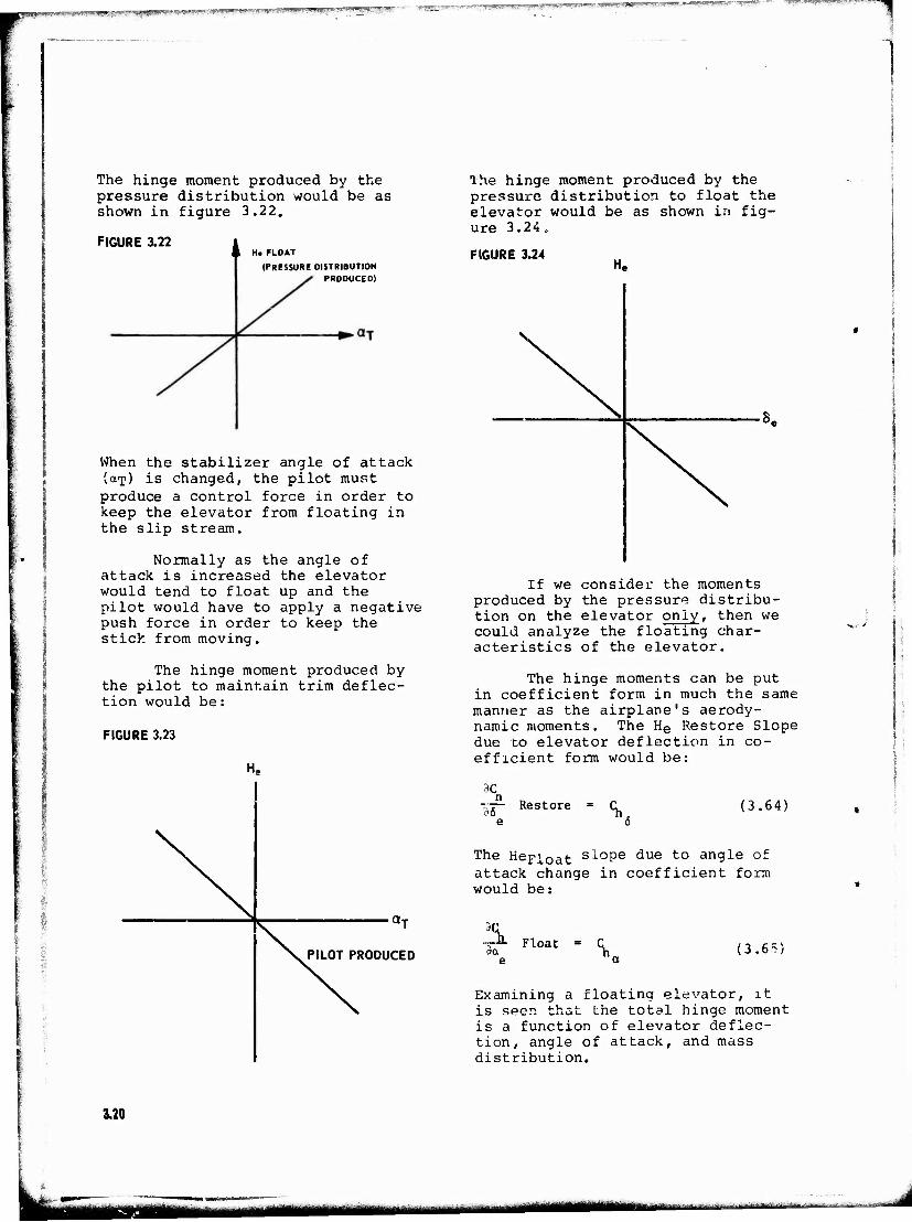
nMPfPBV^VP**) PUB f--'i'':""--^"'*''*'-:'>f'!,T' # r- «■-" -^S5Jf7*p^3,,T,-p'

The hinge moment produced by the pressure distribution would be as shown in figure 3.22.

FIGURE 3.22 A H. FLOAT

(PRESSURE DISTRIBUTION PRODUCED)

When the stabilizer angle of attack (CXT) is changed, the pilot must produce a control force in order to keep the elevator from floating in the slip stream.

Normally as the angle of attack is increased the elevator would tend to float up and the pilot would have to apply a negative push force in order to keep the stick from moving.

The hinge moment produced by the pilot to maintain trim deflection would be:

FIGURE 3.23

He

aT

PILOT PRODUCED

The hinge moment produced by the pressure distribution to float the elevator would be as shown in figure 3.24,

FIGURE 3.24 He

■8.

If we consider the moments produced by the pressure distribution on the elevator only, then we could analyze the floating characteristics of the elevator.

The hinge moments can be put in coefficient form in much the same manner as the airplane's aerodynamic moments. The He Restore Slope due to elevator deflection in coefficient form would be:

3C

3T Restore - Si e 6

(3.64)

The Hepioat slope due to angle of attack change in coefficient form would be:

Ja" Float = S, e a

(3.65)

Examining a floating elevator, it is seen that the total hinge moment is a function of elevator deflection, angle of attack, and mass distribution.

3.20

I I Ml MM umm ttrntittf'"-- '—min ■' *""'' ---'■"—*--*-■

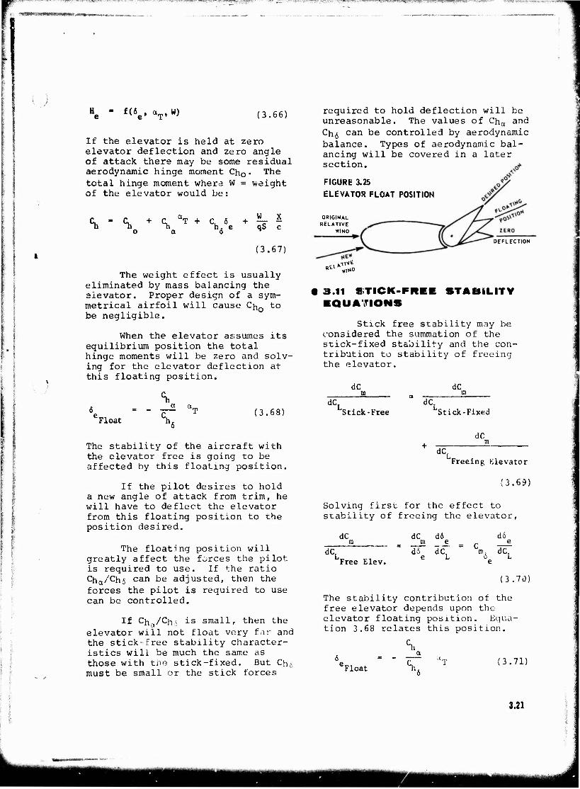
-.-; P"W«T^S2t""".!",V'-**_^''r'*'":.*l'.,^h',-,"','uyv"

f(6e, oT, w) (3.66)

If the elevator is held at zero elevator deflection and zero angle of attack there may be some residual aerodynamic hinge moment ChQ•

T^e total hinge moment where W = weight of the elevator would be:

°h o

aT + Cu 6 + \ - a h6 e qS c

(3.67)

The weight effect is usually eliminated by mass balancing the aievator. Proper design of a symmetrical airfoil will cause ChQ to be negligible.

When the elevator assumes its equilibrium position the total hinge moments will be zero and solving for the elevator deflection at this floating position.

°h « a„

'Float (3.68)

The stability of the aircraft with the elevator free is going to be affected by this floating position.

If the pilot desires to hold a new angle of attack from trim, he will have to deflect the elevator from this floating position to the position desired.

The floating position will greatly affect the forces the pilot is required to use. If the ratio Cha/Ch6

can be adjusted, then the forces the pilot is required to use can be controlled.

If Cha/Ch5 is small, then the

elevator will not float very far and the stick-free stability characteristics will be much the same as those with the stick-fixed. But Cn,s must be small or the stick forces

required to hold deflection will be unreasonable. The values of Cha and Chß can be controlled by aerodynamic balance. Types of aerodynamic balancing will be covered in a later section.

FIGURE 3.25 ELEVATOR FLOAT POSITION

ORIGINAL RELATIVE

WIND

■=1 ^,Vt

DEFLECTION

• 3.11 »TICK-FREE STABILITY EQUATIONS

Stick free stability may be considered the summation of the stick-fixed stability and the contribution to stability of freeing the elevator.

dC dC

dC, dC, JStick-Free "Stick-Fixed

dC

Freeing Elevator

(3.69)

Solving first for the effect to stability of freeing the elevator,

dC dC d6 m e

iCL d& dC

Free Elev.

d6 e dC,

(3.70)

The stability contribution of the free elevator depends upon the elevator floating position. Equa- tion 3.68 relates this position.

'Float

"h

°h. (3.71)

3.21

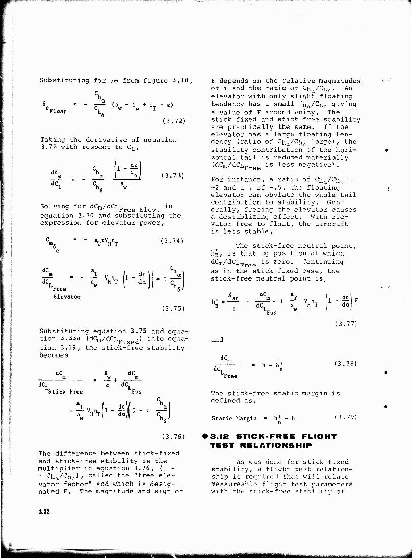
W:j% ."" " '"''" !mVI!"'-s~'*'■KST,«fit"iTT ■ ;.- ..--. .-...v—. ..■ " y9Hjf£i<K5«flV7 ■."

■■■ 5

Substituting for a>p from figure 3.10,

"Float h6 (3.72)

Taking the derivative of equation 3.72 with respect to CL,

d6 e dCL

I"- j a a

(3.73)

in Solving for dCm/dCL^ „1 ? m/ -"-"Free Elev. equation 3.70 and substituting the expression for elevator power,

VVi (3.74)

dC i

dC, - _

Free

*T T VT

w

, dell

Elevator

(3.75)

Substituting equation 3.75 and equation 3.33a (dCm/dCLF- J into equation 3.69, the stick-free stability becomes

dC m

X dC w m

dCL Stick Free

aT - r Vx

w

c dC

| da

Fus

F depends on the relative magnitudes of T and the ratio of Chu/CUl5 . An elevator with only slight floating tendency has a small '.'ha/Ch<5 giving a value of F around unity. The stick fixed and stick free stability are practically the same. If the elevator has a large floating tendency (ratio of Cha/Qi,5 large) , the stability contribution of the horizontal tail is reduced materially (dCm/dCLpree is less negative).

For instance, a ratio of Cha/Cftö = -2 and a T of -.5, the floating elevator can obviate the whole tail contribution to stability. Gen- erally, freeing the elevator causes a destablizing effect. With elevator free to float, the aircraft is less stable.

The stick-free neutral point, hr' dCm/dCLFree as in the stick-fixed case, the stick-free neutral point is,

»n, is that eg position at which is zero. Continuing

X h' --&

n c

and

dC

dC. "Fus

+ t Vi w

da

(3.77)

dC

dC. h - h' n

(3.78)

Free

The stick-free static margin is defined as,

Static Margin - h' - h n (3.79)

(3.76)

The difference between stick-fixed and stick-free stability is the multiplier in equation 3.76, (1 -

t Cha/Ch6)/ called the "free elevator factor" and which is designated F. The magnitude and sign of

3.12 STICK-FREE FLIGHT TEST RELATIONSHIP

As was done for stick-fixed stability, a flight test relationship is required that will relate measureablo flight test parameters with the stick-free stability of

1.22

MM mmmmm turn [■■■VlMlill-l ll M 'illII V i

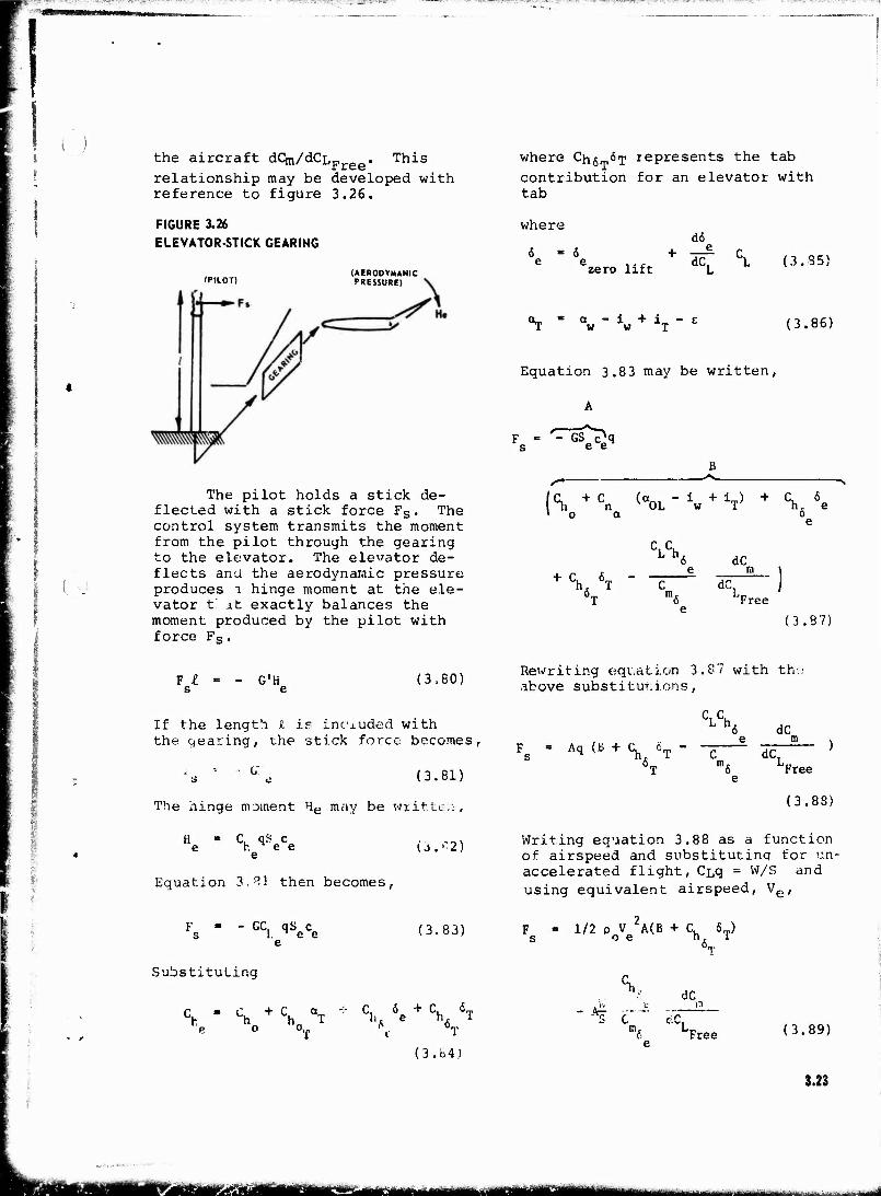
■ '--■;-T:^':-;-f"7.-v-.";T_:-:^:i ^^.-5--o-w; - ■

the aircraft dCm/dCL Free" This

relationship may be developed with reference to figure 3.26.

where Ch5_6T represents the tab

contribution for an elevator with tab

i

FIGURE 3.26 ELEVATOR-STICK GEARING

(PILOT)

where

(AERODYMANIC PRESSURE)

The pilot holds a stick deflected with a stick force Fs. The control system transmits the moment from the pilot through the gearing to the elevator. The elevator deflects ana the aerodynamic pressure produces i hinge moment at the elevator f. it exactly balances the moment produced by the pilot with force Fs.

d6

e e ... dCT L (3.35 zero lift L

a - i + i - e w w T

Equation 3.8 3 may be written,

A

B

(3.86)

h n OL w T ht e o a 6

CLCh 6 dC e m

+ V 6T " C dC 6 Free

(3.87)

F I " - G'H s e

(3.80) Rewriting equation 3.87 with thü above s ub s t i t utions,

} 1

If the length i is included with the gearing, the stick force becomes,

ra "■ G", (3.8D

The hinge moment He may be written.

e h e e e (j.*-2)

Equation 3.21 then becomes,

CLCh

Fs = Aq(B+Ch 6T

6T

6 dC e m dC. )

Free

(3.88)

Writing equation 3.88 as a function of airspeed and substituting for unaccelerated flight, CT/J = W/S and using equivalent airspeed, Ve,

F ■ - GC. qS c s Lee e

Substituting

* K \ T e o o

(3.83)

C. 6 + C, 6 h e \T

(3.64)

F = 1/2 p V "A(B + C, 6 ) s o e ti, i

6T

%, dC

cC, "Free (3.89)

3.23

jBBüüüai att**.t*~*L.~. ■.■■..^i,,.,..,..,^^^.t..-^, .,, . ...... ■ . . -■~.J.*Jl

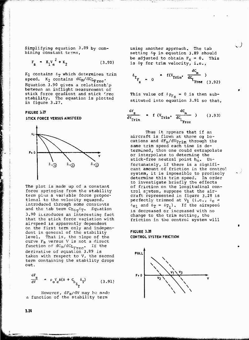
:-^.-v> . ... ... ■ .-; -■;■■_ • '-rrTvr.- i?:~-. •*-■: JiVagps ?">'-; Mf- - , \ ■»-:.--; '■' ■n

Simplifying equation 3.89 by combining constant terms,

KlVe +K2 (3.90)

Ki contains 6T which determines trim speed. K2 contains dCm/dCLFree.

Equation 3.90 gives a relationship between an inflight measurement of stick force gradient and stick 'ree stability. The equation is plotted in figure 3.27.

FIGURE 3.27

STICK FORCE VERSUS AIRSPEED

1 i

K2-

^ rs U

\ \ N. V

8,0 8,0 *•©

The plot is made up of a constant force springing from the stability term plus a variable force proportional to the velocity squared, introduced through some constants and the tab term Ch^m^T« Equation

3.90 introduces an interesting fact that the stick force variation with airspeed is apparently dependent on the first term only and independent in general of the stability level. That is, the slope of the curve Fs versus V is not a direct function of dCm/dCLr ,0. If the

derivative of equation 3.89 is taken with respect to V, the second term containing the stability drops out.

dF

TV" = poVeA(B + V V 6T

(3.91)

However, dFs/dV may be made a function of the stability term

using another approach. The tab setting <ST in equation 3.89 should be adjusted to obtain Fs = 0. This is 6T for trim velocity, i.e.,

U

dC f(V,

F = 0 s

Trim* dC, )

Tree (3.92)

This value of 5pF = 0 is then sub-

stituted into equation 3.91 so that,

dF dC

dV, f (V, Trim

Trim* dCT (3.93)

Free

Thus it appears that if an aircraft is flown at throe eg locations and dFs/dV>rrim through the same trim speed each time is determined, then one could extrapolate or interpolate to determine the stick-free neutral point hn. Un- fortunately, if there is a significant amount of friction in the control system, it is impossible to precisely determine this trim speed. In order to investigate briefly the effects of friction on the longitudinal control system, suppose that the aircraft represented in figure 3.28 is perfectly trimmed at V^ (i.e., 6e = 6ei and 6>p = ST-I ) . If the airspeed

is decreased or increased with no change to the trim setting, the friction in the control system will

FIGURE 3.28 CONTROL SYSTEM FRICTION

PULL

Ff 0

3.24

«MB ■"•'-—m- - majai fa fcgamg ^

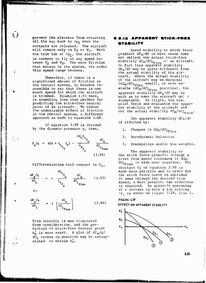
gg^TTllWHPIW "..-, - iW'iiPiiiiifPPu.' *m ■"»» '"«PH

\ t

I

prevent the elevator from returning all the way back to &e\ when the controls are released. The aircraft will return only to V2 or V3. With the trim tab at 6i>j_, the aircraft

is content to fly at any speed between V2 and V3. The more friction that exists in the system, the wider this speed range becomes.

Therefore, if there is a significant amount of friction in the control system, it becomes impossible to say that there is one exact speed for which the aircraft is trimmed. Equation 3.93 then, is something less than perfect for predicting the stick-free neutral point of an aircraft. To reduce the undesirable effect of friction in the control system, a different approach is made to equation 3.88.

If equation 3.88 is divided by the dynamic pressure q, then,

ACLCh dC F /q - A(B + C, 6 ) s hr T

6T dC.

tree

(3.94)

Differentiating with respect to CL,

AC, dyq

dC,

cr

dFs/q

6 dC e m - (3.95)

"i dC,

Free

dCT = f

dC

dC, (3.96)

"Free

Trim velocity is now eliminated from consideration, and the pre- diction of stick-free neutral point hn is more exact. A plot of dFs/q/ dCT versus eg position may be extrap- olated to obtain hn.

t.i; APPARENT STICK-FREE tILITY

Speed stability or stick force gradient dFs/dV in most cases does not reflect the actual stick-free stability dCm/dCL. an aircraft. -m/-^Free In fact this apparent stability dFs/dV may be quite different from the actual stability of the aircraft. Where the actual stability of the aircraft may be marginal (dCm/dCLFreo small), or even un-

stable (dCm/dCLF positive), the

apparent stability dFs/dV may be such as to make the aircraft qu: ~* acceptable. In flight, the tesl pilot feels and evaluates the apparent stability or the aircraft and not the actual stability dCm/dCL .

The apparent stability dFs/dV is affected by:

1. Changes in dCm/dCLpree

2. Aerodynamic balancing

3. Downsprings and/or bob weights.

The apparent stability or the stick force gradient through a given trim speed increases if dCm/ dCr,„ is made more negative. The uFree 3

constant K2 of equation 3.90 is made more positive and in order for the stick force curve to continue to pass through the desired trim speed, a more positive tab selection is required. An aircraft operating at a certain eg with a tab setting &1'-, is shown on figure 3.29, line 1.

FIGURE 3.29

EFFECT ON APPARENT STABILITY

*2

K2

Fs

3.25

IMMHHI ttwb

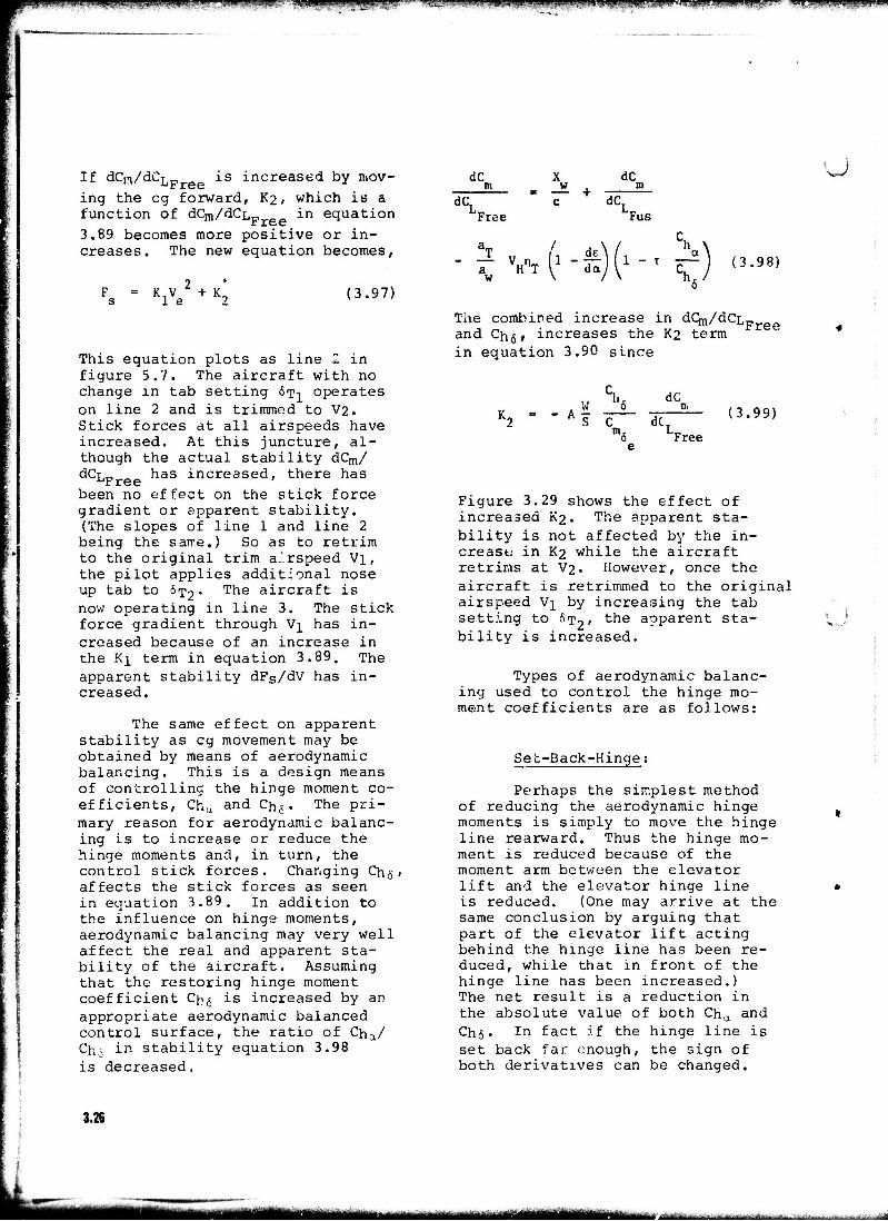
«psw«s»wm"WPe!ppB!^^ SpP5^J""~'*?iS*H»SWäWp^ wPW

i I

If dCn/dCLp is increased by moving the eg forward, K2, which is a function of dCm/dCLF in equation 3.89 becomes more positive or increases. The new equation becomes,

= K.V - + K. 1 e 2 (3.97)

This equation plots as line 2 in figure 5.7. The aircraft with no change in tab setting 6TI operates on line 2 and is trimmed to V"2. Stick forces at all airspeeds have increased. At this juncture, although the actual stability dCm/ dCijr, has increased, there has ^Free been no effect on the stick force gradient or apparent stability. (The slopes of line 1 and line 2 being the same.) So as to retrim to the original trim airspeed Vi, the pilot applies additional nose up tab to ST?- T'ie aircraft is now operating in line 3. The stick force gradient through V^ has increased because of an increase in the Ki term in equation 3.89. The apparent stability dFs/dV has increased.

The same effect on apparent stability as eg movement may be obtained by means of aerodynamic balancing. This is a design means of controlling the hinge moment coefficients, Chu and Chj. The primary reason for aerodynamic balancing is to increase or reduce the hinge moments and, in turn, the control stick forces. Changing Ch.5, affects the stick forces as seen in equation 3.89. in addition to the influence on hinge moments, aerodynamic balancing may very well affect the real and apparent stability of the aircraft. Assuming that the restoring hinge moment coefficient Cn<$ is increased by an appropriate aerodynamic balanced control surface, the ratio of Cha/ C'h.,5 in stability equation 3.98 is decreased,

dC dC u m

1CL dCT

Free Fus

J v. (*-£)(*-£) <3-981

The combined increase in dCra/dCLF ep and Chj, increases the K2 term in equation 3.90 since

U6 dC

s c dC, (3.99) JFree

Figure 3.29 shows the effect of increased K2. The apparent stability is not affected by the increase in K2 while the aircraft retrims at V2. However, once the aircraft is retrimmed to the original airspeed V]_ by increasing the tab setting to ^To» the apparent stability is increased.

Types of aerodynamic balancing used to control the hinge moment coefficients are as follows:

Set-Back-Hinge:

Perhaps the simplest method of reducing the aerodynamic hinge moments is simply to move the hinge line rearward. Thus the hinge moment is reduced because of the moment arm between the elevator lift and the elevator hinge line is reduced. (One may arrive at the same conclusion by arguing that part of the elevator lift acting behind the hinge line has been reduced, while that in front of the hinge line has been increased.) The net result is a reduction in the absolute value of both Cha and Ch6» *n fact if the hinge line is set back far enough, the sign of both derivatives can be changed.

-t 1 Vi;,'

3.26

^HJIge J..-^^.^^.. ■.-,.: -...■„.■ :.).,-... ^W,./.,:,.-^.,

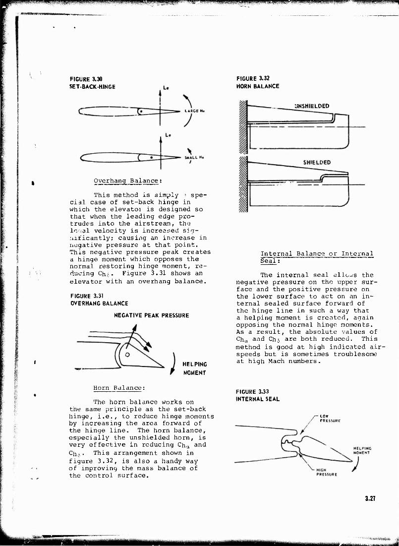
1 IJ" ' ■■ ^ . ■■*■'. ■J-U.ILI«....VI-.*«.U.,« .mm.wmwmmiMm^.-m^»- - ^T— ■ ■ W J l.u ■■ J III, . ..■■. H J^Jf^H, .■» * i. „ . [J .U. I i H »■ - ■ .. . JIP.. g.HJ.i. ' ^

JMMMMWMWWMMMMMMMww i ...„„.. ,

FIGURE 3.30 SET-BACK-HINGE

LARGE He

FIGURE 3.32 HORN BALANCE

Overhang Balance;

This method is simply -< special case of set-back hinge in which the elevatoi is designed so that when the leading edge pro- trudes into the airstream, the local velocity is increased significantly; causing an increase in negative pressure at that point. This negative pressure peak creates a hinge moment which opposes the normal restoring hinge moment, reducing Chi- Figure 3.31 shows an elevator with an overhang balance.

FIGURE 3.31 OVERHANG BALANCE

NEGATIVE PEAK PRESSURE

UNSHIELDED

HELPING MOMENT

Internal Balance or Internal Seal;

The internal seal allocs the negative pressure on the upper surface and the positive pressure on the lower surface to act on an internal sealed surface forward of the hinge line in such a way that a helping moment is created, again opposing the normal hinge moments. As a result, the absolute values of Chu and Chi are both reduced. This method is good at high indicated airspeeds but is sometimes troublesome at high Mach numbers.

Horn Balance;

The horn balance works on the same principle as the set-back hinge, i.e., to reduce hinge moments by increasing the area forward of the hinge line. The horn balance, especially the unshielded horn, is very effective in reducing Cha and ChL\. This arrangement shown in figure 3.32, is also a handy way of improving the mass balance of the control surface.

FIGURE 3.33 INTERNAL SEAL

/ - LOW

PRESSURE

3.27

«m tmmmm ■-"''"—-"'--—- -

\^mjimmvmi9m!^'^'i*m'^.mi '■ut"- PIPPMWWWWPBWP BUPpaappiP mwm*w.; pjpj PWIWWJWM WWJJMBWKM - - ■' *m.l""i-J WI>M,■.,».im

Elevator Modifications:

Bevel Angle on Top or on Bottom of the Stabilizer.

This device, which causes flow separation on one side but not on the other, reduced the absolute values of Cha and Chs.

Trailing Edge Strips.

This device, found on the B-57, increases both Cha

an^ c-h5 • In combination with a balance tab, trailing edge strips produce a very high positive Cha, but still a low Chfi« This results in what is called a favorable "Response Effect," i.e., it takes a lower control force to hold a deflection than was originally required to produce it.

Convex Trailing Edge.

This type surface produces a more negative Ch5, but tends as well to produce a dangerous short- period oscillation.

Tabs;

A tab is simply a small flap which has been placed en the trailing edge of a larger one. The tab greatly modifies the flap hinge moments but has only a small effect on the lift of the elevator or the entire airfoil. Tabs in general are designed to modify stick-forces and therefore Ch$ but will not affect Cha. A positive tab deflection is one which will tend to move the elevator in a positive direction.

Trim Tab.

factory trim tab should be able to accomplish this throughout the aircraft flight envelope. Ordinarily, a trim tab will not significantly vary Cha or Ch5. The functions of the spring and trim or balance and trim tabs may be combined in a single tab. Another method of trimming an aircraft is the use of an adjustable horizontal stabilizer. Normally the trim tab or horizontal stabilizer setting will have a small effect on stability.

Balance Tab.

A balance tab is a simple tab which is mechanically geared to the elevator so that a certain elevator deflection produces a given tab deflection. If the tab is geared to move in the same direction as the surface, it is called a leading tab. If it moves in the opposite direction, it is called a lagging tab. The purpose of the balance tab is usually to reduce the hinge moments and stick forces (lagging tab) at the price of a certain loss in control effectiveness. Sometimes, however, a leading tab is used to increase control effectiveness at the price of increase'! stick forces. The leading tab ma* also be used for the express mrpose of increasing control forces. Thus Chfi may be increased or decreased, while Cha remains unaffected. If the linkage shown in figure 3.34 is made so that the length may be varied ,by the pilot, then the tab may also serve as c- trimming device.

FIGUkE 3.34 BALANCE TAB

A tab which is controlled by a switch or control separate from the normal cockpit pi lot control is called a trim tab. The purpose of the trim tab is to reduce the elevator hinge moment and, therefore, the stick force to zero for a given flight condition. A satis-

LAGGING TAB

3.28

ÜÜÜ ^mmmmmmm L -^„ ■■-.._ ..,. :-^-. ■„»-„,.„,„.,

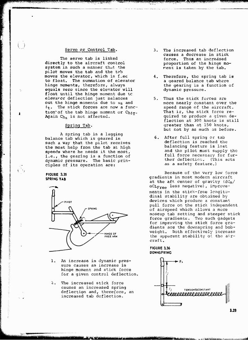
nMH^pgQ4^BPMPm^«i«MWM.«'IH««lllMl I ""W?^""PWIWPP U.MIP..I1HH. im

i >

I V'

■ i

Servo or Control Tab.

The servo tab is linked directly to the aircraft control system in such a manner that the pilot moves the tab and the tab moves the elevator, which is f^ee to float. The summation of elevator hinge moments, therefore, always equals zero since the elevator will float until the hinge moment due tc elevator deflection just balances out the hinge moments due to <xs and 6f The stick forces are now a function* of the tab hinge moment or ChöT. Again Cha is not affected.

Spring Tab.

A spring tab is a lagging balance tab which is geared in such a way that the pilot receives the most help from the tab at high speeds where he needs it the most, i.e., the gearing is a function of dynamic pressure. The basic principles of its operation are:

FIGURE 3.35 SPRING TAB

The increased tab def action

An increase in dynamic pressure causes an increase in hinge moment and stick force for a given control deflection,

The increased stick force causes an increased spring deflection and, therefore, an increased tab deflection.

causes a decrease in stick force. Thus an increased proportion of the hinge mo- rdent is taken by the tab.

4. Therefore, the spring tab is a geared balance tab where the gearing is a function of dynamic pressure.

5. Thus the stick forces are more nearly constant over the speed range of the aircraft. That is, the stick force required to produce a given deflection at 300 knots is still greater than at 150 knots, but not by as much as before.

6. After full spring or tab deflection is reached the balancing feature is lost and the pilot must supply the full force necessary for further deflection. (This acts as a safety feature.)

Because of the very low force gradients in most modern aircraft at the aft center of gravity (dCm/ aCLpree less negative), improvements in the stick-free longitudinal stability are obtained by devices which produce a constant pull force on the stick independent of airspeed which allows a more noseup tab setting and steeper stick force gradients. Two such gadgets for improving the stick force gradients are the downspring and bobweight. Both effectively increase the apparent stability of the aircraft.

FIGURE 3.36 DOWNSPRING

3.29

MAmm flfoj-flih ■■ -.. „_■:;, ji^ä^.^j.i.

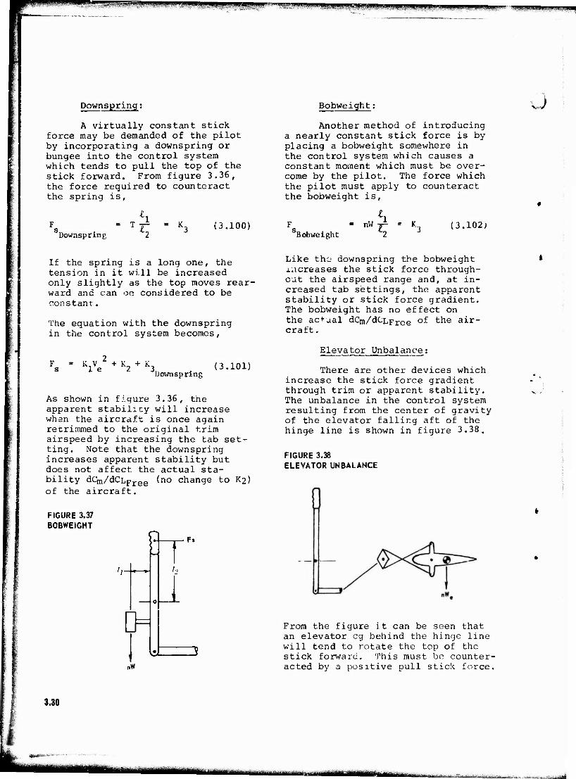
.iijjii.,„„,,„ iii ii4iini|BJ|ii -»■..». Wfm ??J - "■'■ "'^-"IWlSjgiMiWIWWaiMWttiWMl.--11 »"»W IMWP

Downspring;

A virtually constant stick force may be demanded of the pilot by incorporating a downspring or bungee into the control system which tends to pull the top of the stick forward. From figure 3.36, the force required to counteract the spring is,

Downspring (3.100)

Bobweight:

Another method of introducing a nearly constant stick force is by placing a bobweight somewhere in the control system which causes a constant moment which must be overcome by the pilot. The force which the pilot must apply to counteract the bobweight is,

= nW 'Bobweight r2

= K„ (3.102;

Ü

If the spring is a long one, the tension in it will be increased only slightly as the top moves rearward and can oe considered to be constant.

The equation with the downspring in the control system becomes,

K..V 1 e + K2 + K3 Downspring

(3.101)

As shown in figure 3.36, the apparent stability will increase whan the aircraft is once again retrimmed to the original trim airspeed by increasing the tab setting. Note that the downspring increases apparent stability but does not affect the actual stability dCm/dCLFree (no change to K2) of the aircraft.

FIGURE 3.37 BOBWEIGHT

Ft T

0=

l;

Like thcj downspring the bobweight increases the stick force throughout the airspeed range and, at increased tab settings, the apparent stability or stick force gradient. The bobweight has no effect on the actual dCm/dCLpree

or" the aircraft.

Elevator Unbalance:

There are other devices which increase the stick force gradient through trim or apparent stability. The unbalance in the control system resulting from the center of gravity of the elevator falling aft of the hinge line is shown in figure 3.38.

FIGURE 3.38 ELEVATOR UNBALANCE

nW

From the figure it can be seen that an elevator eg behind the hinge line will tend to rotate the top of the stick forward. This must be counter- acted by a positive pull stick force.

3.30

. . ...,,,..v-..^....,-,(r.n

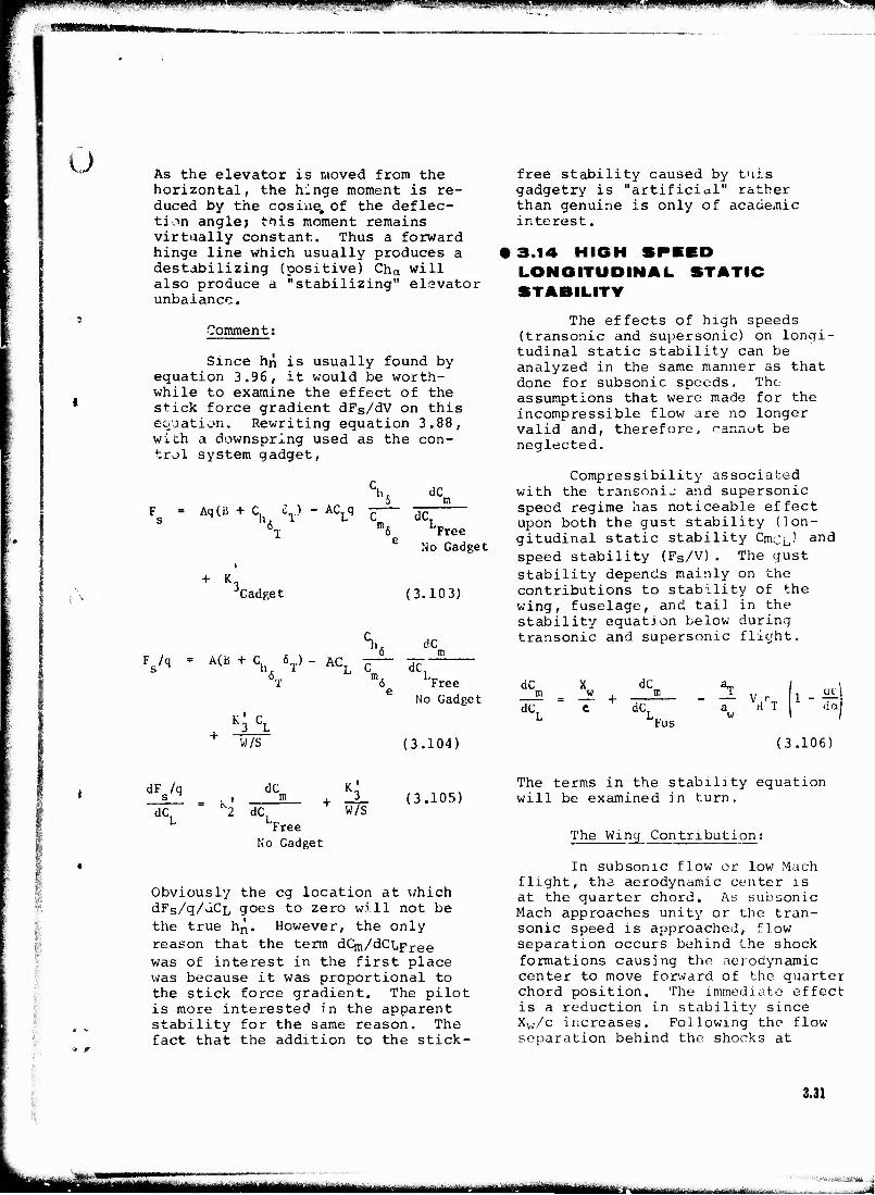
u^mm^smm^m^M^m»«m^pmM^mm^nmi^iu§m ..I^U^W-WE^ iwpipp i "p^wpaw^wwwiipiipw MM», ■

L) As the elevator is moved from the horizontal, the h:lnge moment is reduced by the cosine, of the deflection angle; this moment remains virtually constant. Thus a forward hinge line which usually produces a destabilizing (positive) Cha will also produce a "stabilizing" elavator unbalance.

Comment:

Since hn is usually found by equation 3.96, it would be worth- while to examine the effect of the stick force gradient dFs/dV on this equation. Rewriting equation 3.88, with a downspring used as the control system gadget,

S. dC 5 m F = Aq(B + C d ) - ACLq — -^

6T

m6 LFree e No Gadget

(3.103)

Chr dC

+ K„ JCadget

Fs/q A(B + C 6 > - ACL — 6T m6

K3CL

dC Free

W/S

No Gadget

(3.104)

free stability caused by Ulis gadgetry is "artificial" rather than genuine is only of academic interest.

3.14 HIGH LONGITUDINAL STABILITY

STATIC

The effects of high speeds (transonic and supersonic) on longitudinal static stability can be analyzed in the same manner as that done for subsonic speeds. The assumptions that were made for the incompressible flow are no longer valid and, therefore, cannot be neglected.

Compressibility associated with the transonic and supersonic speed regime has noticeable effect upon both the gust stability (longitudinal static stability CmCjJ and

speed stability (Fs/V). The gust stability depends mainly on the contributions to stability of the wing, fuselage, and tail in the stability equation below during transonic and supersonic flight.

dC

dCT dC, JFus

a n 1 w 1 - da

(3.106)

dC,

dC

2 dC, Free

No Gadget

_2_ (3.105) W/S

Obviously the eg location at which dFs/q/JCL goes to zero will not be the true hn. However, the only reason that the term dCm/dCLpj-gg was of interest in the first place was because it was proportional to the stick force gradient. The pilot is more interested in the apparent stability for the same reason. The fact that the addition to the stick-

The terms in the stability equation will be examined in turn.

The Wing Contribution;

In subsonic flow or low Mach flight, the aerodynamic center is at the quarter chord. As subsonic Mach approaches unity or the transonic speed is approached, flow separation occurs behind the shock formations causing the aerodynamic center to move forward of the quarter chord position. The immediate effect is a reduction in stability since Xw/c increases. Following the flow separation behind the shocks at

3.31

MM •'•i--^-m«f!Mm.

»JT<* ni'niafrriiiliin.iii.y i -r *tA

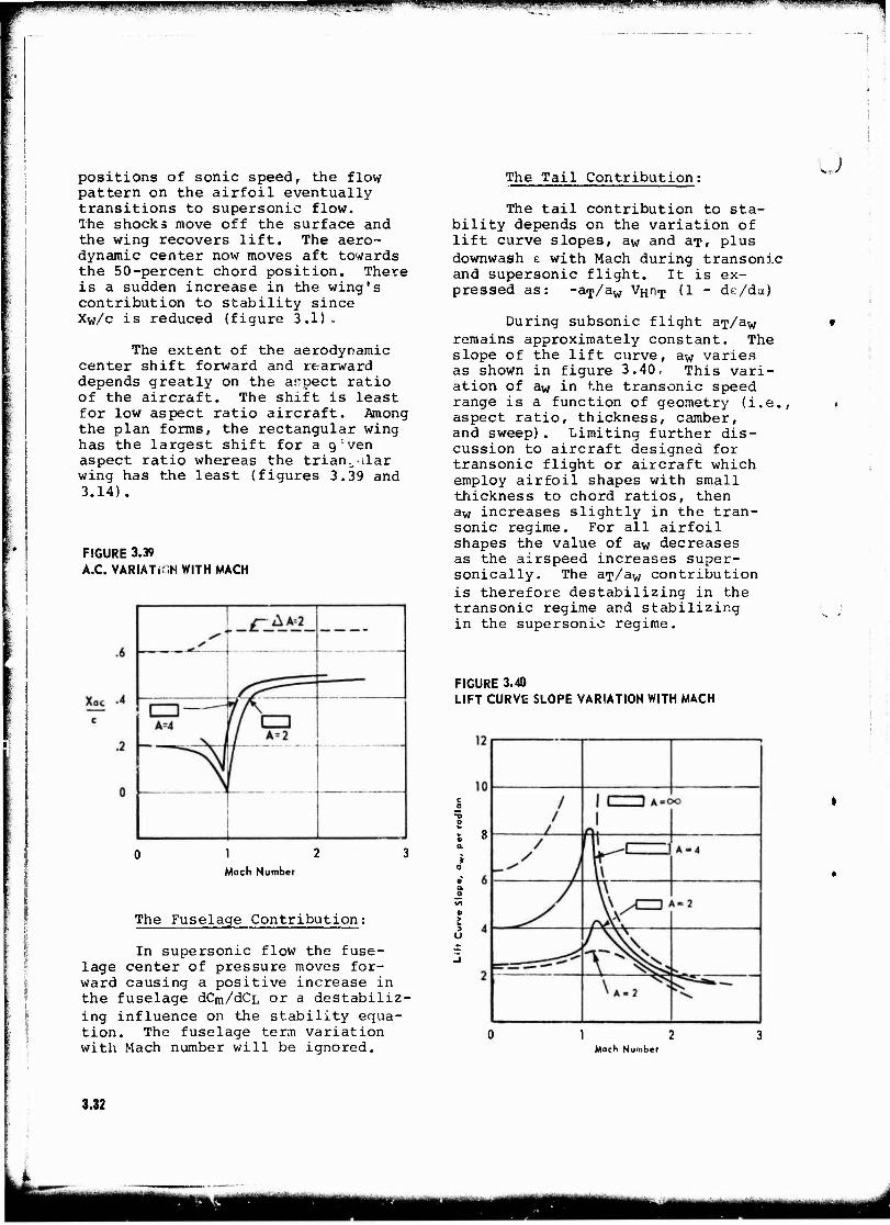
M-w*1 ■■■BW ukllJilliliiwiliBJl.ltLBJJM.^^111! ■^^^Vl-^^^-H.W^lW.JMtP^'-t'iW'trf.l'l,PL.|.'!.|-*-rP

positions of sonic speed, the flow pattern on the airfoil eventually transitions to supersonic flow. The shocks move off the surface and the wing recovers lift. The aerodynamic center now moves aft towards the 50-percent chord position. There is a sudden increase in the wing's contribution to stability since Xw/c is reduced (figure 3.1).

The extent of the aerodynamic center shift forward and rearward depends greatly on the aspect ratio of the aircraft. The shift is least for low aspect ratio aircraft. Among the plan forms, the rectangular wing has the largest shift for a g:ven aspect ratio whereas the trian^-dar wing has the least (figures 3.39 and 3.14).

FIGURE 3.39 A.C. VARIATION WITH MACH

1 2 Mach Number

The Fuselage Contribution;

In supersonic flow the fuselage center of pressure moves forward causing a positive increase in the fuselage dCm/dCL or a destabilizing influence on the stability equation. The fuselage term variation with Mach number will be ignored.

The Tail Contribution:

The tail contribution to stability depends on the variation of lift curve slopes, aw and aT, plus downwash e with Mach during transonic and supersonic flight. It is expressed as: -arp/aw VHHT (1 ~ de/da)

During subsonic flight aT/aw remains approximately constant. The slope of the lift curve, aw varies as shown in figure 3.40, This variation of aw in the transonic speed range is a function of geometry (i.e., aspect ratio, thickness, camber, and sweep). Limiting further discussion to aircraft designed for transonic flight or aircraft which employ airfoil shapes with small thickness to chord ratios, then aw increases slightly in the transonic regime. For all airfoil shapes the value of aw decreases as the airspeed increases supersonically. The aT/aw contribution is therefore destabilizing in the transonic regime and stabilizing in the supersonic regime.

FIGURE 3.40 LIFT CURVE SLOPE VARIATION WITH MACH

O

I 8

2 u

1 2 Mach Number

3.32

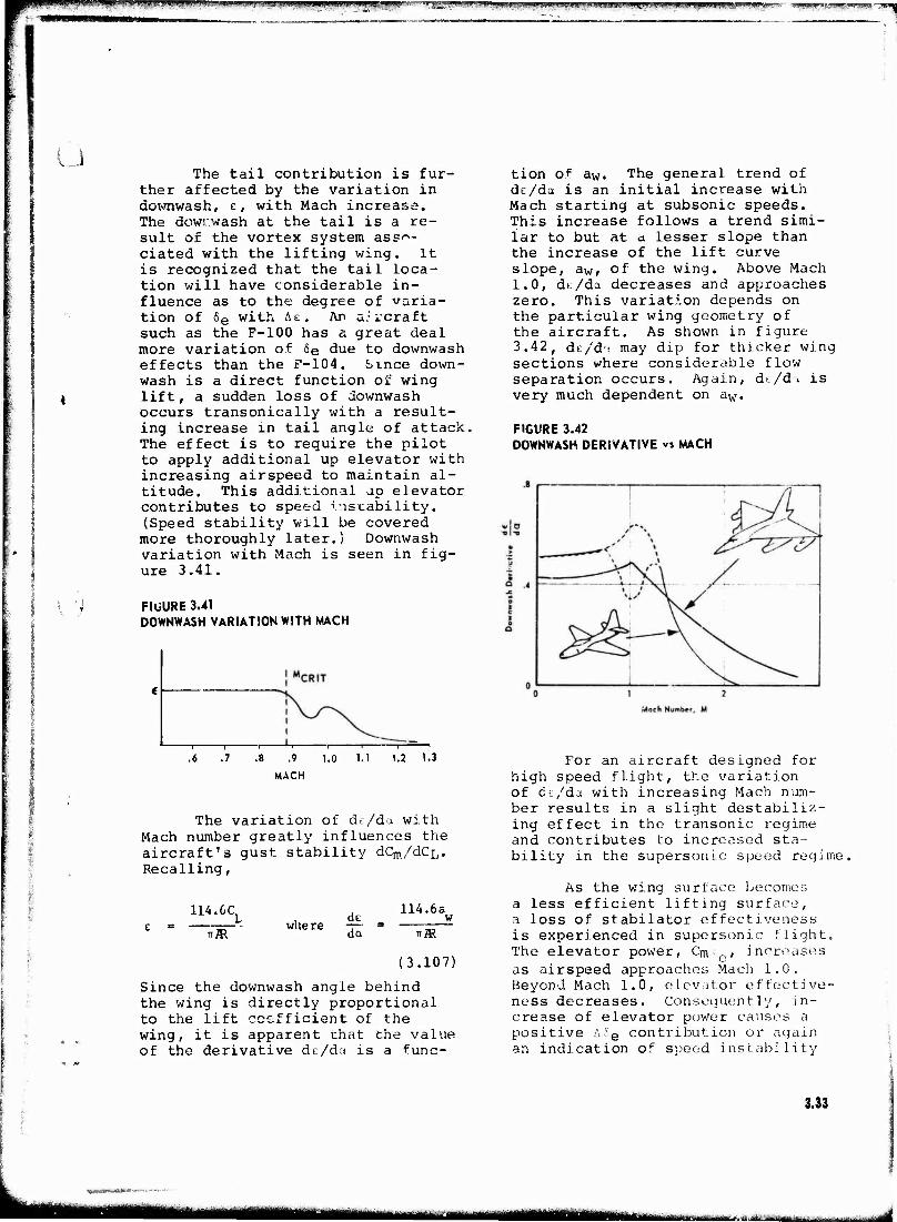
TJI^.-.V;....jw.."—; , Ji.lwnUMgrpWI II^WW^ ""^""iKqw'^^^ •*m

L

t ! I v

The tail contribution is further affected by the variation in downwash, e, with Mach increase?. The dowi. wash at the tail is a result of the vortex system associated with the lifting wing. It is recognized that the tail location will have considerable influence as to the degree of variation of &Q with Ae. An aircraft such as the F-100 has a great deal more variation of 6e due to downwash effects than the F-104. Since downwash is a direct function or" wing lift, a sudden loss of downwash occurs transonically with a resulting increase in tail angle of attack. The effect is to require the pilot to apply additional up elevator with increasing airspeed to maintain altitude. This additional ap elevator contributes to speed instability. (Speed stability will be covered more thoroughly later.) Downwash variation with Mach is seen in figure 3.41.

FIliURE 3.41 DOWNWASH VARIATION WITH MACH

.7 .9

MACH

1.0 1.1 1.2 1.3

The variation of de/da with Mach number greatly influences the aircraft's gust stability dCm/dCL. Recalling,

114.6^

itäf whe re da

114.6a w

(3.107)

Since the downwash angle behind the wing is directly proportional to the lift coefficient of the wing, it is apparent that the value of the derivative de/da is a func-

tion of aw. The general trend of de/da is an initial increase with Mach starting at subsonic speeds. This increase follows a trend similar to but at a lesser slope than the increase of the lift curve slope, aw, of the wing. Above Mach 1.0, de/da decreases and approaches zero. This variation depends on the particular wing geometry of the aircraft. As shown in figure 3.42, dt/d'i may dip for thicker wing sections where considerable flow separation occurs. Again, de/d-i is very much dependent on aw.

FIGURE 3.42 DOWNWASH DERIVATIVE vs MACH

For an aircraft designed for high speed flight, the variation of de/da with increasing Mach number results in a slight destabilizing effect in the transonic regime and contributes to increased stability in the supersonic speed regime,

As the wing surface becomes a less efficient lifting surface, a loss of stabilator effectiveness is experienced in supersonic flight. The elevator power, QT\.-C, increases as airspeed approaches Mach 1.0. Beyond Mach 1.0, elevator effectiveness decreases. Consequently, increase of elevator power causes a positive contribution or again an indication of speed instability

3.33

L. mrfi&miBm**?**-*^

^MttMW -•■•■• ■ .■»,*..-+ A

WÜPBPHPPÜP* «wpimm«1 ■ iipnfgptpi|||pn)|gMppMP|app»i^9i pmpjapi ppppippppn

I !

as Mach 1.0 is approached. With decrease in elevator power, a negative A6e contribution once again produces speed stability. For the F-10* the relative order of magnitude of these values cause an initial increase in gust stability in the transonic regime followed by a steatiily decreasing stability influence as Cm6e approaches zero.

dC

dC. \ ail

The sonic and stabil: ty figure 3.4 stability and then d The speed craft is a ing the pi equation,

a T w 1 - ||j (3.108)

overall effect of tran- supersonic flight on gust or dCm/dCL is shown in 3 . t'tatic longitudinal increases transonically ecreases supersonically. stability of the air- ffected as well. Recall- tching moment coefficient

AC - C + CAa + CA« + C A6 m m m m* a m, e

o a a 6 e

+ C AV + C Aq v q (3.109)

and since CmcL = § Qna ,then:

Assuming no change in speed or pitch rate, and since under compressibility CmQ is not zero, the

elevator required to maintain steady flight is:

A6 AC. (3.110)

Speed stability depends on the variations of 6e with transonic and supersonic speeds and according to equation 3.110, depends on how Cm0, Cm6e, and Cmc vary.

FIGURE 3.43 MACH VARIATIONS ON CM0.CmSe AND C„,CL

.04

.02

0

1 1 1 1 1 TYPICAL SWEPT.WIHC AIRPLANE

TAIL, CG • IS« MAC

(A) ZERO- OFT PITCHING MOMENT

+ CM

014

.012

.010

8 M

0* 40M-

»M U 0M

- " -

2=5 ■"'— **"*• *s /

EDGE ELEVATOR if PLACE OF ONE PIECE HORIZONTAL TAIL

\N*.

!■ )

V —- -J! «KM

I0M

c 1

CONTROL EFFECTIVENESS 0M

|

-CmCL

0 FT

40,000 FT 20,000 FT

> '~2

.1 / \ TAILCSS

DELTA WING

(Cl STATi : LON 1ITUD NAL S TA6IL TT

1.0 11 1.2 13

MACH NUMBER

IS 14 17

If equation 3.110 is analyzed using the plots in figure 3.43, speed instability during transonic flight becomes obvious. The value of - Cm0/

Cm6e increases from approx-

imately zero in the subsonic range to some positive value as the aircraft passes through Mach 1.0. The value of Cmc"i/Cm6e increases to a very large number in comparison to Cm0/Cm,5 through this same range.

The result is a positive A6e or a reversal of elevator deflection with increasing airspeed. This manifests itself as a relaxation of forward pressure or even a pull force to maintain attitude or prevent a nose down tendency. As the aircraft speed increases to supersonic speed, A6e again becomes nega-

3.34

•MMI^ MoMMMMHMM a^j,.L.-Jj.ftti-;iii

*!^.«Mm4-*^WWP'!»'l'»[« -THJCTWW'WBWW.ViH-", J ptpiBpp>y^wt^BfWpwi»»ipw'!WWI"w^

tive and the pilot regains speed stability or decreasing 6e with increasing airspeed. The actual results of some aircraft flown in this range are shown in figure 3.44,

FIGURE 3.44 Se vsMACH

10

8

O ° m g z 4 o

o a.

M

i-T~n

.7 .8

Whether th or reversal in e and stick forces depends on many magnitude of var time required to region of instab tern cli-iracterist of flight, It i the engineer to plots it the de-j is acceptable, only one capable ef fects.

.9 1.0 1.1 1.2 1.3 1.4 1.5 16 1.7 1.8 1.9 2.0

MACH NUMBER

e speed instability levator deflections are objectionable, factors such as iation, length of transverse the

ility, control sys- ics, and conditions s impossible for determine from data ree of instability The pilot is the of evaluating these

In the F-100C, a pull force of 1.4 pounds was required when accelerating from Mach 0.87 to Mach 1.0. The test pilot described this trim change as disconcerting while attempting to maneuver the aircraft in this region and recommended that a "q" or Mach sensing device be installed to eliminate

this characteristic. Consequently, a mechanism was incorporated to automatically change the artificial feel gradien : as the aircraft accel- erates through the transonic range. Also, the longitudinal trim, is automatically changed in uiis region by the use of a "flach Trimmer."

In the F-104, the test pilot stated that, transonic trim changes required an aft stick movement with increasing speed and a forward stick movement when decreasing speed, but described this speed instability as acceptable.

In the F-106 the pilot stated that the 1.0 to 1.1 Mich region is characterized by a moderate trim change necessita? ing pi lot technique to .'.void large variations in altitude <...img accelerations. Minor , ■ hai.qes are encountered up to

3.35

)liu,«i..y. jinyj I, u..mg""-;»UM TV,:- »»""»jyTA'.,, I'A^ARJW.';, J|B!-.!I IJ ■•I,«"!-JI-I»MI)MIJJ|;P- »'-'"'SKIT"" .."■-■l»>'""f A„ll ■fi.™»'!J"J™'^SWr?I^W Hfl»«? '"-■••—' ~;" - ~'T "—■*- ■ ^-7*T7^TP^P^^W«

Mach 1.35. His report concluded that the speed instabilities were not unsatisfactory.

In the T-38 which embodies the latest design concept, a departure is noted from the low tail configuration difficulties where the pilot described the transonic trim change as being hardly per- ceptible.

Aircraft design considerations are, of course, influenced by the stability aspects of high speed flight. It is desirable to design an aircraft where trim changes through transonic speeds are small. A flat wing without camber, twist, or incidence or a low aspect ratio wing and tail provide values of Xw/c, aw, afp, and clt/da which vary

minimally over the Mach number range. An all-moving tail (slab) for control gives negligible variation of T with Mach and maximum control effectiveness. A full power, irreversible control system is desirable to counteract the erratic changes in pressure distribution which affect Cha and Ch6e.

In the transonic speed regime the meaning or importance of "neutral point" is reduced. At transonic speeds the variation of control angle and trim force with speed, although important, is not affected by eg position. Instead of relating trim gradients to a eg margin, it is more useful to view variation of control for trim as a function of compressibility and ignore eg position.

3.3G

mM^Umm

■■

CHAPTER

MANEUVERABILITY

14.1 MANEUVERING FLIGHT

The method used to analyze maneuvering flight will be to determine stick-fixed maneuver points (hm) and stick-free maneuver points (hm). It will be seen that these are analogous to their counterparts in static stability, the stick- fixed and stick-free neutral points. The maneuver points will also be defined in terms of the neutral points and the theory will help to predict which of these points will be critical as regards the aft center of gravity location. It will also be shown how the forward center of gravity is affected by the parameters that define the maneuver points.

Maneuvering flight will be analyzed much in the same manner used in determining a flight te'=t relationship in longitudinal stability. For stick-fixed longitudinal stability, the flight, test relationship was determined to be

d5 e dCr

dC /dCT m L Cm&a

(4.1)

This equation gave the static longitudinal stability of the aircraft in terms that could easily be measured in flight test.

In maneuvering flight, a similar stick-fixed equation relating to easily measurable flight test quantities is desirable. Where in longitudinal stability, the elevator deflection was related to lift coefficient or angle of attack, one may surmise that in maneuvering flight elevator deflection will relate to load factor n.

REVISED I FEBRUARY 1974

To determine this expression, one must refer to the aircraft's basic equations of motion. As in longitudinal stability, the'six equations of motion are the basis for all analysis of aircraft stability and control. In maneuvering an aircraft the same equations will hold true, but one additiona derivative will have to be added to the analysis. Recalling the pitching moment equation

M = ql + pr (I n y r x V + <p r ) I xz

(4.2)

and the fact that in static stability analysis we have no roll rate, yaw rate, or pitch acceleration, equation 4.2 reduces to:

q I = 0 (4.3)

The variables that cause external pitching moments on an aircraft are infinite, i.e., speed brakes, canopy, elevator, etc. There are, however, fi 'e primary variables that we can consider.

M f(V, a, a, 6 , q) (4.4)

If any or all of these variables change, there will be a change of total pitching moment that will equal the sum of the partial changes of all the variables. This is written as

a M = —;— A of + -* a + ——— ^b + <J a <5> ' <> & e

(4.5)

4.1

mgmmm

Since in maneuvering flight, AV and A& are zero, equation 4.5 becomes:

da d& e </q

and since M = qSc Cm, then

= q Sc ^8.

q Sc C "fe

—;— = q Sc —r— ^q ^q

(4.6)

(4.7)

(4.8)

(4.9)

Substituting these values intr equation 4.6, and multiplying by 1/q Sc,

dz C Aa + C A 5 + -—

m& e ^q e

q = 0 (4.10)

The derivative 3Cm/3n is carried instead of Cmg since the compensating factor c/2V is not used at this time.

Solving for the change in elevator deflection A6e,

A & = - C A a - o»r Id„A q e m m q (4.11)

ferent load factors will define the stick-fixed maneuver point. The immediate goal then is to determine the change in angle of attack, Aa, and change in pitch rate, Aq, in terms of load factor n.

14.2 THE PULL UP MANEUVER

4-3 in the pull up maneuver, the change in angle of attack of the aircraft, Aa, may be related to the lift coeffici jnt of the aircraft. In the pull up with constant velocity, the angle of attack of the whole aircraft will be changed since the aircraft has to fly at a higher CL to obtain the load factor required. The change in CL required to maneuver at high load factors at a constant velocity comes from two sources: (1) load factor increase,- \l) elevator deflection. Although often ignored because of its small value when compared to total CL, the change in lift with elevator deflection CL,5eA6e will be carried along for

a more general analysis.

AFTER ELEVATOR

DEFLECTION

BEFORE ELEVATOR

DEFLECTION CLMAN

V..

V

The analysis of equation 4.11 may be continued by substituting in values for Aa and Aq. The final equation obtained should be in the form of some flight test relationship. Since maneuvering is related to load factor, the elevator deflection required to obtain dif-

CL&eX

Figure 4.1 Lift Coefficient Versus Angle of Attack

4.2

«MWUMMi t^mm^am^mmtm ---■ iaüifitetä■**» —-

I*/

Referring to figure 4.1, the aircraft is in equilibrum at some CL0 corresponding to some a0 before the elevator is deflected to initiate the pull up. If the elevator is considered as a flap, its deflection will affect the lift curve as follows. When the elevator is deflected upward, the left curve shifts downward and does not change slope. This says that a certain amount of lift is initially lost when the elevator is deflected upward. The loss in lift because of elevator deflection is designated CL$ A6e. The increase in down- loading on the tail or increase in negative lift on the horizontal stabilizer causes a moment on the aircraft which creates a nose up pitch rate. The aircraft continues to pitch upward and increase its angle of attack until it reaches a new CL and an equilibrium load factor. In other words a pitch rate is initiated and a increases until a maneuvering lift coefficient CLU,,, is reached for the deflected MAN elevator 6e. The change in angle of attack is Aa. The change in CL has come partially from the deflected elevator and mainly from the pitching maneuver. The change in CL due to the maneuver is from CLO to CL MAN* Since it did not change the slope of the lift curve, if the change in lift caused by elevator deflection is included the expression for Aa becomes:

To put equation 4.14 in terms of load factor, ACLMAN must be defined. This is the change in lift from the initial condition to the final maneuvering condition. This change can occur from one g flight to some other load factor or it can start at 2 or 3 g's and progress to some new load factor. If CL is at one g then

CT = -x w_ qs

(4.15)

n W = _?_

"hn qS n - initial load factor o n o

(4.16)

nW CT = —r Ti - final load factor

^ ^ (4.17)

A CL " S " CL MAN JMAN o

nW %W

qS IS = CL(n-no) (4.18)

aa (4.12)

Finally substituting ACLM2VM into equation 4.14,

Aa = i [cL (n-nQ) - CL6e A6e] (4.19)

Equation 4.19 is row ready for substitution into equation 4.11.

An expression for Aq in equation 4.11 will be derived using the pull up maneuver analysis.

AC,

* *

(4.12a)

ACL " AC^N-% A6e = a*«*4-") e

Aa = { [AC

LMAN " C\ ABe] <4'14>

4.3

^HM ■"•«yfiitwj«**

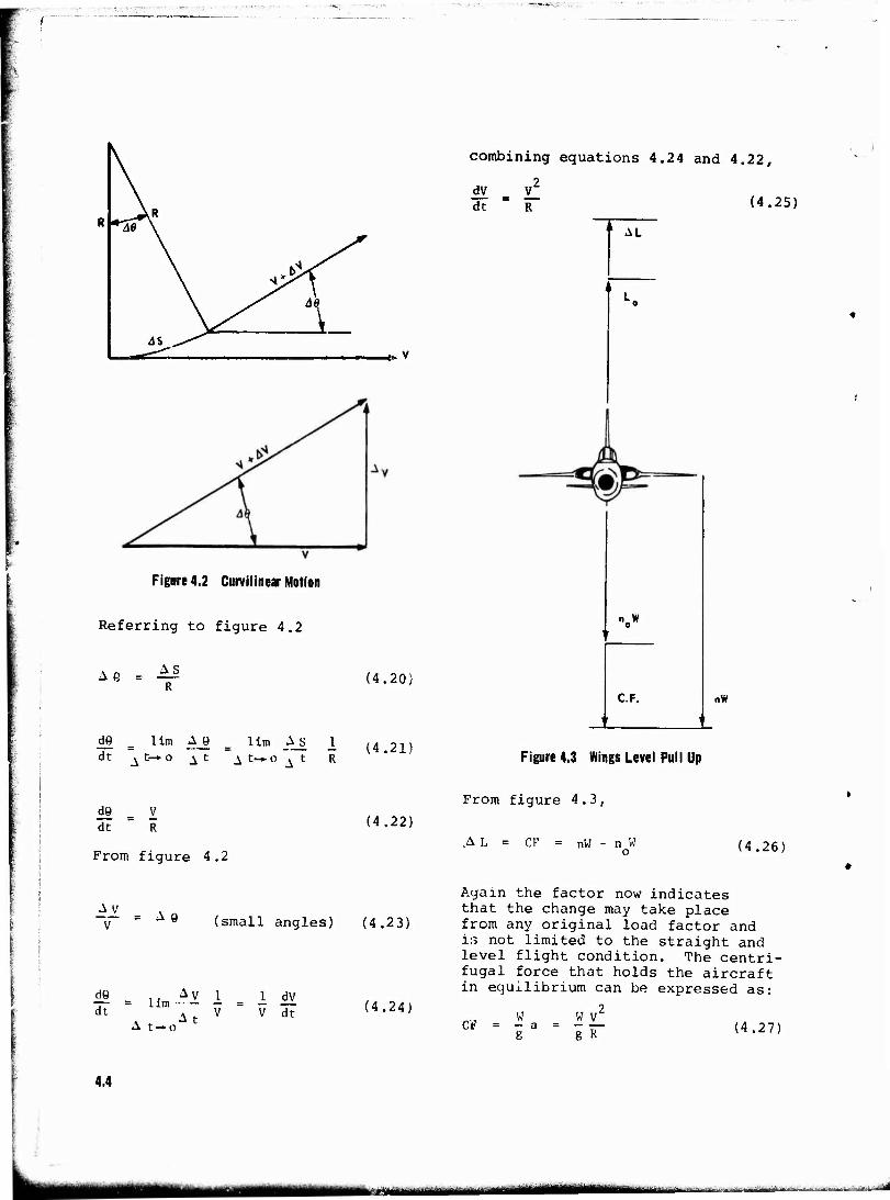
^AR *M\

AS ^"^

Figure 4.2 Curvilinear Motion

Referring to figure 4.2

A e AS

d0 _ lim _AJ) _ lim _A_S I dt ^ t— o A t itn-o^t R

(4.20)

(4.21)

combining equations 4.24 and 4.22,

dV V2

AL

"o*

C.F. nW

Figure 4.3 Wings Level Pull Up

do = V dt R

From figure 4 .2

(4.22)

From figure 4.3,

AL = CF = nW - n W o (4.26)

A V ~ " Ae (small angles) (4.23)

do = Ay I = 1 dV dt " lm "A . V ~ V dt

A t-0at

(4.24)

Ayam the factor now indicates that the change may take place from any original load factor and i:s not limited to the straight and level flight condition. The centrifugal force that holds the aircraft in equilibrium can be expressed as:

CF W — a g

w _yj g R (4.27)

4.4

^^^^JMaMMii iml ii

0 Therefore:

AL - W(n-no) = | f (4.28)

■8 (n - n ) = | V o' R

(4.29)

Substituting from equation 4.22,

Aq«|> = 1 . i (n-n) dt V

(4.30)

Now equations 4.30 and 3.19 may be substituted into equation 4.11.

""*.

ffl g , V -3— f* (n - n ) <Jq V o

Cm&„ (4.31)

Equation 4.35 is now in the fcrm that will define the stick- fix ;^d maneuver point for the pull up.. The definition of the maneuver point (hm) is the eg position at which the elevator deflection per g goes to zero. Taking the limit of equation 4.35, where An is defined as (n - nQ),

lim

An- o

,A5.

An *! dn (4.36)

or

d&e aCL [». h + pp- C n 4m tn

qJ (4.37)

dn C C. m L_

a 5 e

C a

e

Setting equation 4.37 equal to zero will give the eg position (h) as the maneuver point (hm).

P7C- c

4m m (4.38)

& KJ From longitudinal stability,

a (h - h ) n

(4.32)

Also to help further in reducing the equation to its simplest terms,

V 2 W

P3CT

(4.33:

Solving equation 4.38 for hn and substituting into equation 4.37,

aCL

dn C CT a 8

- C^ a o

(h h ) (4.39) m

where (hm - h) is defined as the stick-fixed maneuver margin.

4 »•

and

m ^q 2V Cmq

(4.34)

Substituting equations 4.34, 4.33 and 4.22 into equation 4.31 and turning the algebra crank, results in,

AS aC + -

L C C, m L

a 8 m&a

e

Sc h - h + P 7- C

n 4m m (4.35)

The significant points to be made about equation 4.39 are:

1. The derivative d6e/dn varies with the maneuver margin. The more forward the eg, the more elevator will be required to obtain the limit load factor. That is, as the eg moves forward, more elevator deflection is necessary to obtain a given load factor.

2. The higher the CL, the more elevator will be required to obtain the limit load factor. That is, at low speeds (high

4.5

^M£W

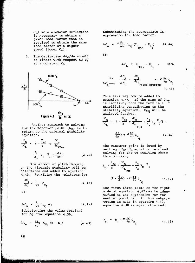
CL) more elevator deflection is necessary to obtain a given load factor than is required to obtain the same load factor at a higher speed (lower CL)•

The derivative d6e/dn should be linear with respect to eg at a constant CL-

Substituting the appropriate CL expression for load factor;

AC = ^^(C

if

4m ^ WLMAN " V

HlAN

(4.44)

then

<Me

HIGH C

Figure 4.4 -jjj- vs eg

Another approach to solving for the maneuver point (hm) is to return to the original stability equation.

dc n dCT

= h

H

dC + —2

LFus

v (1-1:1) T *• da ; (4.40)

1 xm m

Ac, —o AcT

dC 2 _ p Sc dC. Am m

Pitch Damping " (4.45)

This term may now be added to equation 4.45. If the sign of Cnw is negative, then the term is a stabilizing contribution to the stability equation analyzed further.

Cmq will be

dC _n dCT

X h - ac

dC

dC, Fus

-^V * (1 a H Tv w

T^ + 'Irc dot 4m m (4.46)

The maneuver point is found by setting dCm/dCL equal to zero and solving for the eg position where this occurs. i

The effect of pitch damping on the aircraft stability will be determined and added to equation 4.40. Recalling the relationship:

dc n dq

c 2V~ Cmn

(4.41)

or

AC =7,-7; Cm Aq m 2V "q (4.42)

Substituting the value obtained for Aq froiu equation 4.30,

Ac 2JL. 2V2

-mq ^ no> (4.43)

dC h - — m c dCT

Fus

«-£-> 4m m (4.47)

The first three terms on the right side of equation 4.47 may be identified as the expression for the neutral point hn. If this substitution is made in equation 4.47, equation 4.38 is again obtained.

4m m (4.48)

4.6

—-— — imzmm MM ...■■^.--...,■ .tl M-V^HUTI -

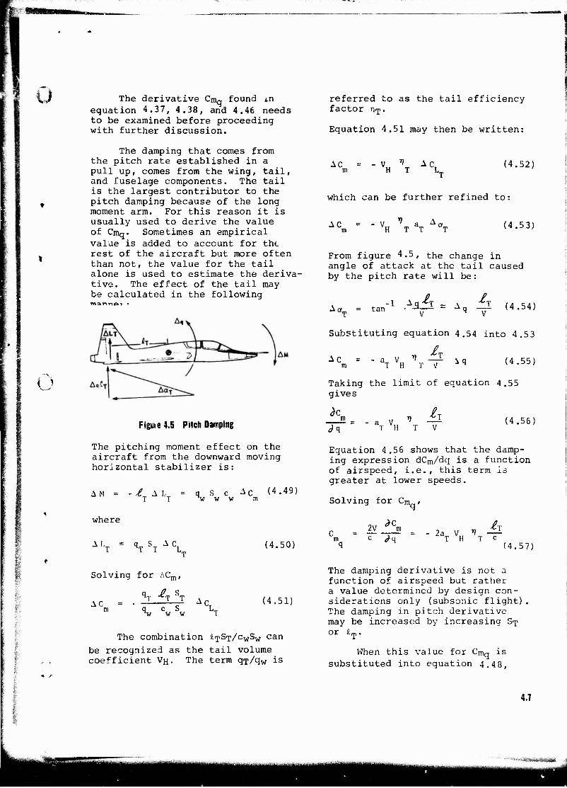
The derivative Cm^ found j.n equation 4.37, 4.38, and 4.46 needs to be examined before proceeding with further discussion.

referred to as the tail efficiency factor nx-

Equation 4.51 may then be written:

u

The damping that comes from the pitch rate established in a pull up, comes from the wing, tail, and fuselage components. The tail is the largest contributor to the pitch damping because of the long moment arm. For this reason it is usually used to derive the value of Cmq. Sometimes an empirical value is added to account for the rest of the aircraft but more often than not, the value for the tail alone is used to estimate the derivative. The effect of the tail may be calculated in the following manno* •

Figuie 4.5 Pitch Damping

AC V ^ Ac H T L„ (4.52)

which can be further refined to:

AC V a ^a H T T T (4.53)

From figure 4.5, the change in angle of attack at the tail caused by the pitch rate will be:

A aT = tan ■1 Aq A _ A _£l (4.54)

V n V

Substituting equation 4.54 into 4.53

Ac a V 1 A iq T H TV 4 (4.55)

Taking the limit of equation 4.55 gives

n a V T H £, (4.56)

I

V

The pitching moment effect on the aircraft from the downward moving horizontal stabilizer is:

AM = -4 AL = q S c AC (4.49] T T w w w m

where

AL = q S A c T 4T T L„

Solving for ACm,

(4.50)

AC q c S w w w

(4,51)

The combination £TST/

CWSW can

be recognized as the tail volume coefficient V"H. The term qxAlw is

Equation 4.56 shows that the damping expression dCm/dq is a function of airspeed, i.e., this term is greater at lower speeds.

Solving for Cm , 4

2V in c ^q

- 2a V V —- T H T c (4.57)

The damping derivative is not a function of airspeed but rather a value determined by design considerations only (subsonic flight) The damping in pitch derivative may be increased by increasing S^ or f>T.

When this value for Cmq is substituted into equation 4.48,

4.7

"v at*' mnm» auma

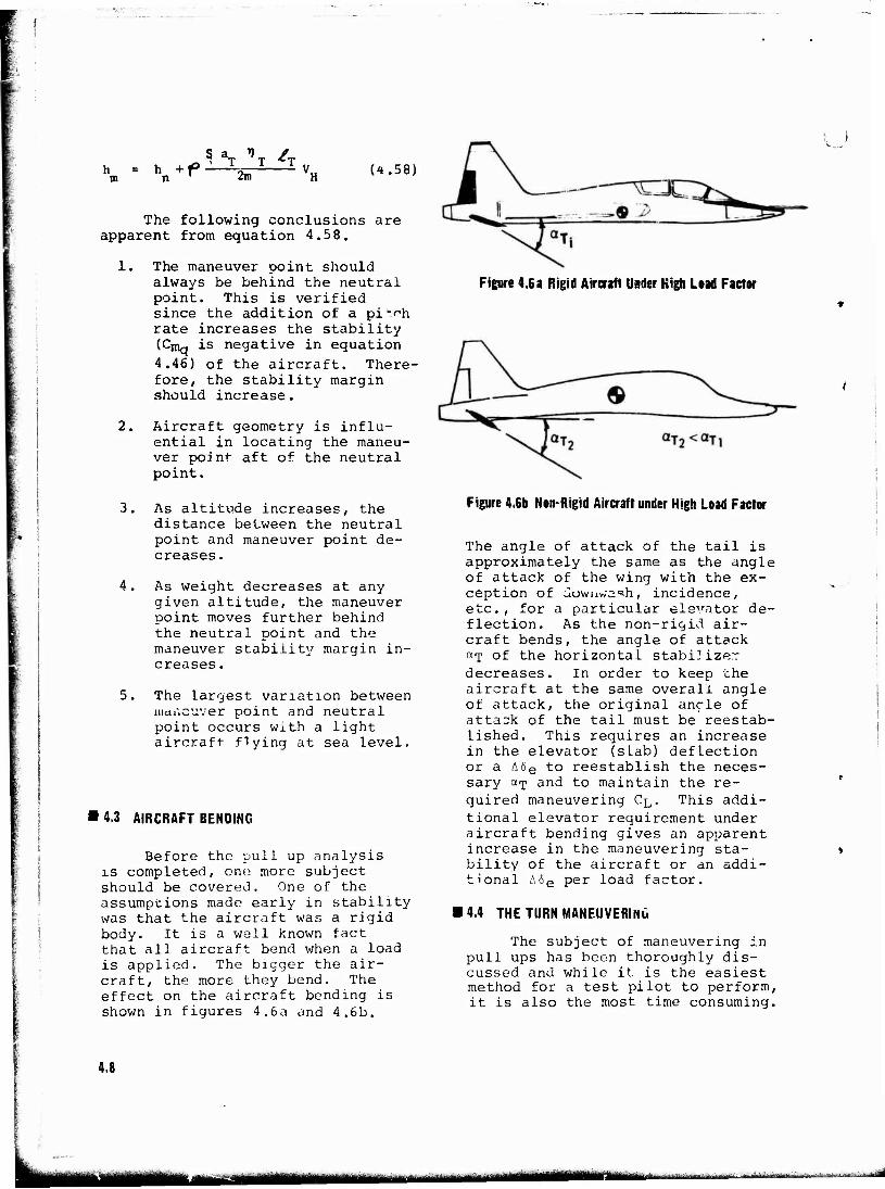
■ hn+<°

S aT VT

2m /^T

(4.58)

The following conclusions are apparent from equation 4.58.

1. The maneuver point should always be behind the neutral point. This is verified since the addition of a pi^h rate increases the stability (Cmq *s negative in equation 4.46) of the aircraft. There- fore, the stability margin should increase.

2. Aircraft geometry is influ- ential in locating the maneuver poinl- aft of the neutral point.

3. As altitude increases, the distance between the neutral point and maneuver point decreases .

4. As weight decreases at any given altitude, the maneuver point moves further behind the neutral point and the maneuver stability margin increases .

5. The largest variation between maneuver point and neutral point occurs with a light aircraft flying at sea level.

14,3 AIRCRAFT BENDING

Before the pull up analysis is completed, one more subject should be covered. One of the assumptions made early in stability was that the aircraft was a rigid body. It is a well known fact that al] aircraft bend when a load is applied. The bigger the aircraft, the more they bend. The effect on the aircraft bending is shown in figures 4.6a and 4.6b.

t )

Figure 4.6a Rigid Aircraft Under High Load Factor

Figure 4.6b Non-Rigid Aircraft under High Load Factor

The angle of attack of the tail is approximately the same as the angle of attack of the wing with the exception of üownwa^h, incidence, etc., for a particular elevator deflection. As the non-rigid aircraft bends, the angle of attack aT of the horizontal stabilizer decreases. In order to keep the aircraft at the same overall angle of attack, the original ancle of attack of the tail must be reestab- lished. This requires an increase in the elevator (slab) deflection or a A6e to reestablish the necessary aT and to maintain the required maneuvering C^. This additional elevator requirement under aircraft bending gives an apparent increase in the maneuvering stability of the aircraft or an additional A6e per load factor.

14.4 THE TURN MANEUVERING

The subject of maneuvering in pull ups has been thoroughly discussed and while it is the easiest method for a test pilot to perform, it is also the most time consuming.

4.8

nu. MM* i ■lMHMiHll«iiiii|-in ^.^..^■....^..■■■.^„...■a^M^.

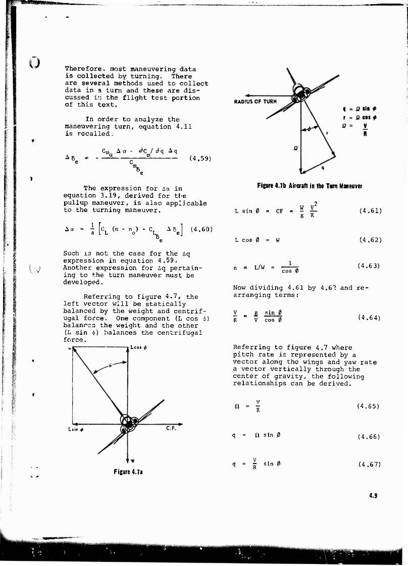
0 Therefore, most maneuvering data is collected by turning. There are several methods used to collect data in a turn and these are discussed in the flight test portion of this text.

In order to analyze the maneuvering turn, equation 4.11 is recalled;

Cra A a - JC I d q A q A 5 = - —2 2

e (4.59) n».

RADIUS OF TURN

8,

I-

The expression for Aa in equation 3.19, derived for the pullup maneuver, is also applicable to the turning maneuver.

.a = \ [ C (n n„> ■ CT i6e] (4.60)

Such is not the case for the Aq expression in equation 4.59. Another expression for Aq pertain- ing to the turn maneuver must be developed.

Referring to figure 4.7, the left vector will be statically balanced by the weight and centrifugal force. One component (L cos $) balances the weight and the other (L sin (ji) balances the centrifugal force.

Leos 0

Lsin <t>

Figure 4.7b Aircraft in the Turn Maneuver

L sin 0 CF = W V g R

Figure 4,7a

L cos d = W

L/W = 1

cos 0

(4.61)

(4.62)

(4.63)

Now dividing 4.61 by 4.6? and rearranging terms:

V _ £ sin 0 R " V cos 0 (4.64)

Referring to figure 4.7 where pitch rate is represented by a vector along the wings and yaw rate a vector vertically through the center of gravity, the following relationships can be derived.

a V

R

H sin 0

| sin 0

(4.65)

(4.661

!4.67)

4.9

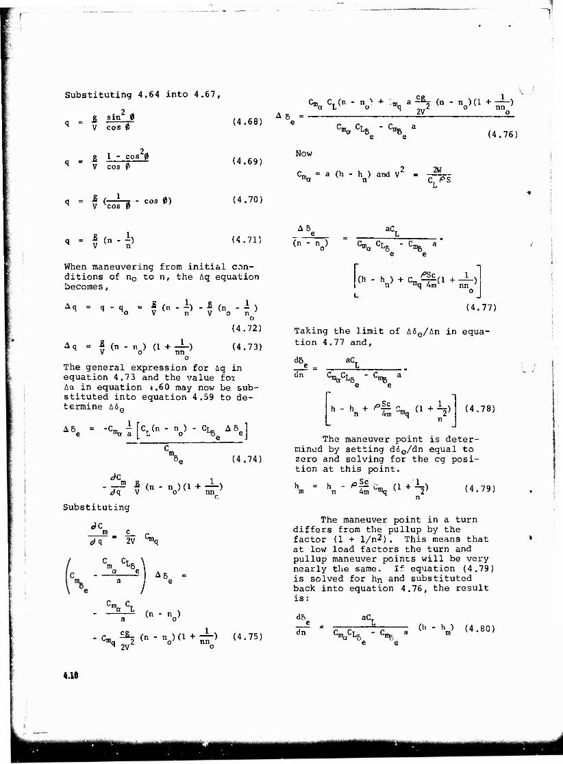
I r

Substituting 4.64 into 4.67,

2 A £ sin

V cos 0 (4.68)

A 6

Cm CT (n - n > + :m a ^ (n - n )(1 + —) '"a L o "'q „2 o' nn

2V o

v,, J

Cma CL8 " Cm& a (4.76)

j» 1 - cos 0 q V cos 0

4 V vcos 0

(4.69)

(4.70)

Now

cm„ = a (h " h ) a"d V2 = -~=-- % rr c, PS

- ! <» - r) (4.71)

When maneuvering from initial conditions of nQ to n, the Aq equation becomes,

Aq = q-qo = * <„ . I) . 1 (n . I ) o

(4.72)

(4.73) A q = Ä (n _ „o) (i + JL) nn

The general expression for Aq in equation 4.73 and the value for Aa in equation i.60 may now be substituted into equation 4.59 to determine A6Q

A 8. ■S» i [V» • V - °i«.A B.]

J~ I (n- n)(l+zi-) c/q V o nn

Substituting

Jc

^q 2V Cmq

c cLc m ^5 a e A 8.

SCL (n - n )

(4.74)

S C~h (n - no)(l + ^) (4.75) ^ 2V o

A8 aC,

(n - no) S* CH e

(h - h ) + cm ^T% + -L) n "q 4m nn '

o

(4.77)

Taking the limit of A6e/An in equation 4.77 and,

dB. aC.

"V^C

h - h + P^£ 1

4m mq 2 n (4.78)

The maneuver point is determined by setting d6e/dn equal to zero and solving for the eg position at this point.

h = h - Pp- Cm (1 + K) m n 4m ""q v 1' (4.79)

The maneuver point in a turn differs from the pullup by the factor (1 + 1/n2). This means that at low load factors the turn and pullup maneuver points will be very nearly the same. If equation (4.79; is solved for hn and substituted back into equation 4.76, the result is:

dS e dn

aC.

:maCL& - C

*& ~ (h - hj (4.80)

4.10

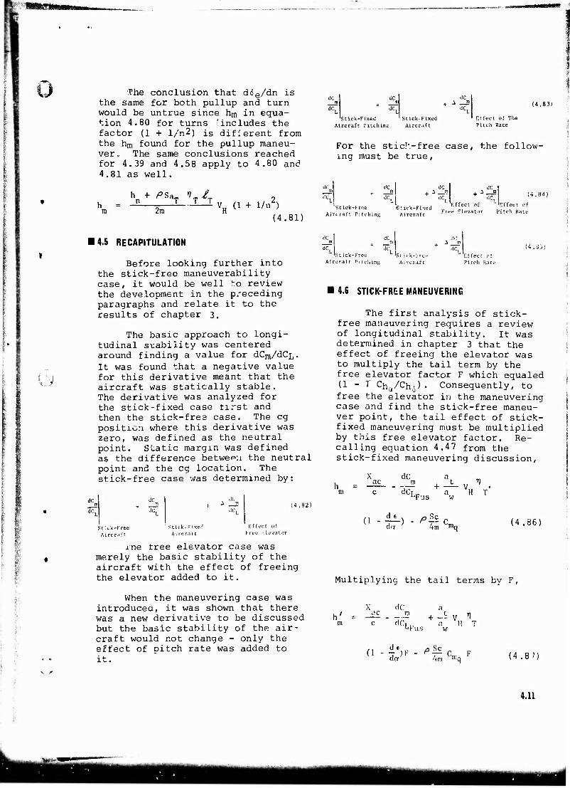
The conclusion that d6e/dn is the same for both pullup and turn would be untrue since hm in equation 4.80 for turns 'includes the factor (1 + l/n2) is difierent from the hm found for the pullup maneuver. The same conclusions reached for 4.39 and 4.58 apply to 4.80 and 4.81 as well.

hn+ ^SaT ygr 2m

VH (1 + 1/n ) (4.81)

dC n dC,

'Stick-Fixed Stick-Fixed

(4.83)

Aircraft Pitching Aircraft Ri feet of The Pitch Rate

For the stick-free case, the following must be true,

dC I —-

'stick-tree Aircraft Pitching

m

>St ick-Fixed

(4.84)

Free elevator Effect of

Pitch Rate

14.5 RECAPITULATION

Before looking further into the stick-free maneuverability case, it would be well to review the development in the preceding paragraphs and relate it to the results of chapter 3.

The basic approach to longitudinal stability was centered around finding a value for dCm/dCL. It was found that a negative value for this derivative meant that the aircraft was statically stable. The derivative was analyzed for the stick-fixed case first and then the stick-free case. The eg position where this derivative was zero, was defined as the neutral point. Static margin was defined as the difference betwepu the neutral point and the eg location. The stick-free case was determined by:

dC m dC.

dC n JC,

Stick-Free Aircraft

Stick-l:ixeJ Aircrnit

(4.82)

Effect of Free '"levator

ine tree elevator case was merely the basic stability of the aircraft with the effect of freeing the elevator added to it.

JC n dC,

Ms "''Stick-Free ~ 'Stick-Free Aircraft Pitching Ai'.craft

"Effect of Pitch Rate

I 4.6 STICK-FREE MANEUVERING

The first analysis of stick- free maneuvering requires a review of longitudinal stability. It was determined in chapter 3 that the effect of freeing the elevator was to multiply the tail term by the free elevator factor F which equaled (1 - T Ch /ChO . Consequently, to free the elevator in the maneuvering case and find the stick-free maneuver point, the tail effect of stick- fixed maneuvering must be multiplied by this free elevator factor. Re- calling equation 4.47 from the stick-fixed maneuvering discussion,

dc n

dCL F-JS

"H T

(1 d_e_ da (4.86)

Multiplying the tail terms by F,

When the maneuvering case was introduced, it was shown that there was a new derivative to be discussed but the basic stability of the aircraft would not change - only the effect of pitch rate was added to it.

C

dC _ n dC LFus

a ~c- v * a 11 T w

(l - -r-ir da

o Sc p — C F ■*m (4.8 7)

.11

The first three terms on the right are the expression for stick- free neutral point, hn.

h' = m

/°2£ c F 4m Lraq * (4.88)

This is the stick free maneuver point in terms of the stick-free neutral point for the pullup case. It may be extended to the turn case by using the term for the pitch rate of the tail in a turn.

h' m

= h' - /°|C- Cm F (1 + ~) n 4m q I

n (4.89)

These equations do not give any flight test relationship and so it is necessary to derive this from stick forces, as was done in longitudinal static stability. The method used will be to relate the stick force-per-g to the stick- free maneuver point since stick forces can be related to the freeing of the elevator. Starting with the relationship of stick force, gearing, and hinge moments that was derived in chapter 5,

= -GH

q S c C, n e e h

Gq S c C, e e h

(4.90)

(4.91)

(4.92;

The change in stick force for a change in load factor becomes,

Stick-Free Pullup Maneuver;

AChe must be written in terms of load factor and substituted back into equation 4.93. This will require defining Aa-p and A6e in terms of load factor. The change in angle of attack of the tail comes partly from the change in angle of attack of the wing due to downwash and partly from the pitch rate.

A«„ % (1 da -± (4.95)

where Aayj + Aq in the above equation are

AaW = i K 0-%> -\ ±\] (4.96)

= £ V (n - no>

ai

(4.97)

c cTc. m L8

a e

— (h - h )(n - n ) a v m o

(4.98)

If the equations abovp are substituted into 4.94, the results would be cumbersome at best. To simplify things CL,5e will be assumed small enough to ignore. (Reason- able assumption since total change in lift of the aircraft when the elevator is deflected is small.) The above equations simplify to:

(1 ->■

u

AF

A n Gq S c --—i

e e An (4.93)

(n - n ) +-S- X (n - n ) (4.99) o ,,l T o

where A & = - ~- (h - h ) (n - n ) (4 .100)

e L mo

AC,

aT e

(4.94) Substituting equations 4.99 and 4.100 into 4.94,

4.12

'^~J2^"'n-,"'~r*~ '"■"'—r—:■ * ■—^"y-Tg** WT_J-- ■■•-.•.■ ««.-ly,,.» ' " ""^IIIBW"^ "—

i.j

*Cfc

a a V

- C h6 V (h - h )

m (4.101)

Substituting V^ = W/pgC^ and Cm&

- -ae VH and isolating the maneuver margin (h - hm) by factoring out (- Chß CL/Cm6 ), the result is:

A C.

Cm&„

<L_ (1 . di_} a da e H

^■w

+ —2 ^V- s a Vu + h - h Ch„ 2m e H m o

(4.102)

h . h. = pi Is vu (1 -~) U.103)

From longitudinal stability,

Cb a

n n da

and if the second term in the parenthesis is multiplied by

-2ca„

•2caT and knowing that

v. -2a -»-A

T c (4.104)

Rewriting equation 4.102,

A.C.

h' - h + (1 - F)/3!^ Cm - h + h n n 4m mq n

but

h = h m n

/°S£ c 4m mq

(4.108)

(4.109)

Therefore:

A C, Ch, n - n "V

+ p 4a Cmq F

(4.110)

Substituting equation 4.110 back into 4.9 3 and taking the limit

dFs 2 % -r-5 = G 1/2 /^V S c —-b- CT • dn e e Cm L

|h - h' +/°^C„ F *q j Sc 4m Lm" (4.111)

Defining the stick-free maneuver point as the eg position where dFs/dn is equal to zero,

h' = h' -P m n

Sc 4m Cmq F

(4.112)

a /a e I

F = 1

(4.10b)

(4.106:

which is the same equation as 4.88 previously derived. Equation 4.111 may be written,

dFs 2 Cll5 —- = G 1/2 <°V S c —■ CT dn e e Gnlc L

The second term becomes

<P"1>'°!i S

hi - h* | (4.113)

Equation 4.113 may be rearranged (4.107) if the following substitutions are

made.

4.13

Cm6e

d** a V =

e H ax7FVH

e

= C LSe c S L w w

(4 114)

Substituting equations 4.118 and 4.119 into equation 4.94 and performing the same factoring and substitutions as in the pullup case ;

then,

'L " PV2

S (4.115)

AC, <VL

The stick-force-per-g equation becomes:

dF

dn" " - G (Se Ce W V t"sm C '

h - h'

e

(4.116)

Stick-Free Turn Maneuver.;

The procedure used for determining tne dFs/dn equation and an expression for the stick-free maneuver point for the turning maneuver is practically identical to the pullup case. For the turn condition Aq is now,

= f (n - n ) (1 + JL) nn (4.117)

The change in angle of attack of the tail, AaT and A6e become

A a - -i (n - n )(1 - J*-) + T a o da

&—% (n - n )(1 + —) (4.118) „i. o nn V o

A5 -c,

Li (h - h )(n - n ) + n o

P~ C„.(n-n )(1 + —) 4tn mq o nn o

(4.119)

Sc [h'hn+^SF <1+1/n>

(4.3.20)

Substituting 4.120 into 4.93

dF , ch_CT ~ = G 1/2 /°V S c --2-i . dn e e C„ "» '5.

[h-h; + ^c">aF(i + i2>

n J

(4.121)

And solving for the stick-free maneuver point,

SC Cm F (1 + 1/n2) (4.122) n 4m l"q

h' ./oil r\ AT

Further substitution puts equation 4.121 into the following form:

dF c -T-5 = - G (S c dn e e »V ^-sT—;

[" - K) (4.123)

Ayain, the turning stick- force-per-g equation 4.123 appears identical to the stick-free pullup equation. However, the expression for the maneuver point h^ is different.

The term in the first parenthesis represents the ninge moment of the elevator. The second term is the elevator power and the last term is the negative value of the

4.14

u stick-free maneuver margin. The following conclusions are drawn from th:.s equation.

1. The stick-fcrce-per-g appears to vary directly with the weight. However, weight also appears inversely in hm. Therefore, the full effect of weight cannot be truly analyzed since one effect could cancel the other.

2. Since airspeed does not appear in the equation, the stick-force-per-g will be the same at all airspeeds for a fixed eg.

I 4.7 EFFECT OF BOBWEIGHTS AND SPRINGS

The effect of bobweights and springs on the stick-free maneuver point and stick-force gradients is of interest. The result of adding a spring or a bobweight to the control system adds an incremental force to the system. The effect of the spring is different from the effect of the bobweight. The spring exerts a constant force on the stick no matter what load factor is applied. The bobweight exerts a force on the stick proportional to the load factor.

BOBWEIGHT DOWNSPRING

From equation 3.112, come the following conclusions.

1. The difference between the stick-fixed and stick-free maneuver point is a function of the free elevator factor,

The stick-free maneuver point, hm, varies directly with altitude, becoming closer to the stick-free neutral point, the higher the aircraft flies.

The location of one stick- free maneuver point is of academic interest only since it occurs at the point where dFs/dn = 0. It is difficult to fly an aircraft with this type gradient. Consequently, military specifications limit the minimum value of dFs/dn to three pounds per g.

The forward eg is limited by stick force per g. The maximum value is limited by the type aircraft (bomber, fighter, or trainer); i.e., heavier gradients in bomber type and lighter ones in fighters.

CONTROL COLUMN

1

nW

r-F,

r

AFs^AnWi

(a)

AFS=T5

b

m

Figure 4,8 Bobweight and Downspring

The force increment for the downspring and bobveight are:

AF s

Spring

G S c W Cv, c

(h Vhm)(n " no) + T b (4.124)

4.15

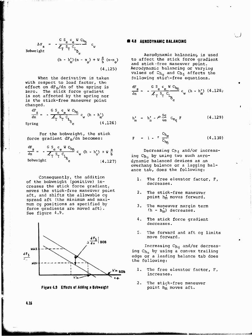
AF s Bobweight

G S c WCh. e e "5

A ST V

(h - h') (n - n ) + W £ (n-n ) m o b o

(4.125)

When the derivative is taken with respect to load factor, tho effect on dFs/dn of the spring is zero. The stick force gradient is not affected by the spring nor is the stick-free maneuver point changed.

dF s dn

Spring

G Sa c W Ch_ e e "5 TT sT C

c (h - h') w m (4.126)

4.8 AERODYNAMIC BALANCING

Aerodynamic balancing is used to affect the stick force gradient and stick-free maneuver point. Aerodynamic balancing or varying values of Cha and Chj affects the following stick-free equations.

dF s dn

h' = m

G S c W Ch. e e "g

^T ST V c (h - h') (4.128; w m

h' n Sc 4m

(4.129)

u

For the bobweight, the stick force gradient dFs/dn becomes:

dF G S c W Cho

~ = - 7 e. % 5 c (h - h') f w| dn £ a„ CT w rn b

T T L„ Bobweight 14.127)

Consequently, the addition of the bobweight (positive) increases the stick force gradient, moves the stick-free maneuver point aft, and shifts the allowable eg spread aft (the minimum and maximum eg positions as specified by force gradients are moved aft) . See figure 4.9.

MAX--

JF<

MIN

BOB

<•»•

= 1 (4.130)

Figure 4.9 Effects of Adding a Bobweight

Decreasing Ch5 and/or increasing Cha by using two such aerodynamic balanced devices as an overhang balance or a lagging balance tab, does the following:

1. The free elevator factor, F, decreases.

2. The stick-free maneuver point hm moves forward.

3. The maneuver margin term <h - hm) decreases.

4. The stick force gradient decreases.

5. The forward and aft eg limits move forward.

Increasing Ch^ and/or decreasing cha

by using a convex trailing edge or a leading balance tab does the following:

1. The free elevator factor, F, increases.

2. The stick-free maneuver point hm moves aft.

4.16

iw ■MMMMHMIH .■„'.,,-'—*-•*■*■■—■-'■ MMBÜtMiiäi

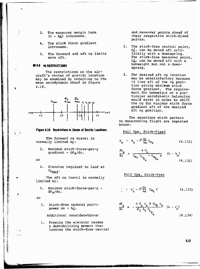
3. The maneuver margin term (h - hm) increases.

4. The stick force gradient increases.

5. The forward and aft eg limits move aft.

14.9 eg RESTRICTIONS

The restrictions on the aircraft's center of gravity location may be examined by referring to the mean aerodynamic chord in figure 4.10.

if, JF.

CLM., *■ M.. *>Mln h; hn £ hm

FWD-

Figure 4.10 Restrictions to Center of Gravity Locations

The forward eg travel is normally limited by:

1. Maximum stick-force-per-g gradient - dFs/dn.

or

and maneuver points ahead of their respective stick-fixed points.

2. The stick-free neutral point, hn, can be moved aft artifically with a downspring. The stick-free maneuver point, hm, can be moved aft with a bobweight but not a downspring.

3. The desired aft eg location may be unsatisfactory because it lies aft of the eg position giving minimum stick force gradient. The requirement for bobweight or a particular aerodynamic balancing would exist in order to shift the eg for minimum stick force gradient aft of the desired aft eg position.

The equations which pertain to maneuvering flight are repeated below:

Pull Ups, Stick-Fixed

P£l 4m mq (4.131)

dn

a CT

- C, (h - h )

% (4.132)

2. Elevator required to land at CL

MAX'

The aft eg travel is normally limited by:

1. Minimum stick-force-per-g - dFs/dn.

Pull Ups, Stick-Free

- h' - P^- C. F n 4m "'q (4.133)

or

Stick-free neutral point- power on - hn.

Additional considerations:

fs G Se Ce W CH Cw dn " - £T ST C

(h - n')

(4.134)

1. Freeing the elevator causes a destabilizing moment that locates the stick-free neutral

4.17

'"'•^■•r;*ttf*>s^t^i*''

llll ittiWrMWiiir-''1"--^"- ■---"-"■ MMl

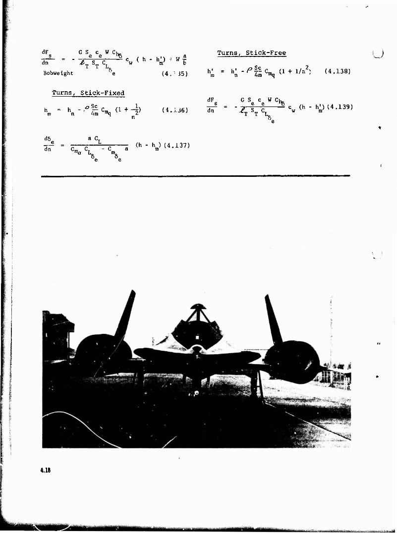
dF G S c W Ch_ __!_ = - ec

e„ a c (h.h') + »r dn £>„ S„ Cr w v m' b

T T L„ Bobweight (4.; 35)

Turns, Stick-Free

Sc h' = h' -Pj- C_ (1 + 1/n") (4.138)

in n 4m ™q

U

Turns, Stick-Fixed

h - h -<\- C- (1 +4) (4.1.16) m n 4a luq *■

dF s

dn

G S c WCh. e e "8

Z. sm c. 'T T L„ c (h - h') (4.139)

w m

i5j dn

a C

Cma CL, (h-hm) (4.137)

e e

4.18

I^MMMk MWMMM^ ...,.:.I: .-,,^■■■ -v. -.:■■- ■_■■-. .;i,.,.„,-,.A->cl, - ■!.,^».^;M

o CHAPTER

DIRECTIONAL STATIC STABILITY

(REVISED FEBRUARY 1974)

15.1 INTRODUCTION

An analysis of the equations of aircraft motion leads to the following mathematical description of aircraft lateral-directional motion:

F = mv + mru - pwm

G = pi + qrl x x ^ - I ) - (r + pq)I xz

(5.1)

(5.2)

W

G = rl + pq(I - I ) z z c^ y x + (qr - p)I xz (5.3)

The right side of the equation represents the response of an aircraft to applied forces and moments. The forces and moments are expressed on the left side of the equation in terms of stability derivatives and small perturbations. As in "Long-Stat", an analysis of the lateral-directional static stability need only concern itself with the values of these derivatives. Further analysis of the aircraft equations of motion reveals the left side of the foregoing equations to be composed primarily of contributions from aerodynamic forces and moments, direct thrust, gravity, and gyroscopic moments. Of these, only the aerodynamic forces and moments (Y, , ) will be analyzed because the other sources are usually eliminated through proper design.

It has been shown in Chapter 1 that when operating under a small disturbance assumption, aircraft lateral-directional motion can be considered independent of longitudinal motion and that it can be considered as a function of the following variables:

(YX ,V) = f(B, 6r> :s.4)

;.

The ensu:ng analysis is concerned with the question of lateral-directional static stability or the tendency of an airplane to return to stabilized flight after being perturbed in yaw or roll. This will be determined by the values of the yawing and roiling moments [71 & £ ) . Since the side force equation governs only the aircraft translatory response and has no effect on the angular motion, the side force equation will not be considered.

The two remaining aerodynamic functions can be expressed in terms of non-dimensional stability derivatives, angular rates and angular dis- placements :

C~ A /S n '"&' '"■&" ~'Lp^ ~'lr~ ~"Aa

a -™6T r

A. C 5 = C i B + Cf-3 + C{ p + C} r + C{. 6a +

• r

(5.5)

(5.6)

5.1

mttmm uauü+in^,..^... ■.. ■ :

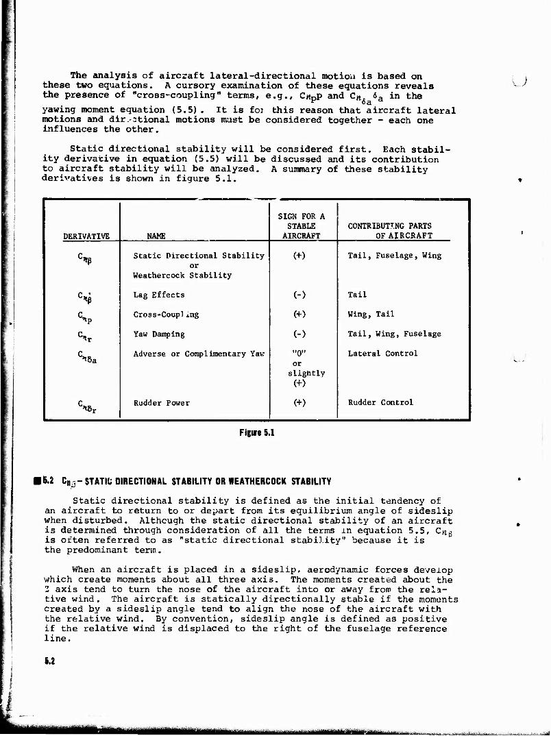
The analysis of aircraft lateral-directional motion is based on these two equations. A cursory examination of these equations reveals the presence of "cross-coupling" terms, e.g., CnDp and Cttr <5a in the

*? oa yawing moment equation (5.5) . It is foi this reason that aircraft lateral motions and dir.-stional motions must be considered together - each one influences the other.

u

Static directional stability will be considered first. Each stability derivative in equation (5.5) will be discussed and its contribution to aircraft stability will be analyzed. A summary of these stability derivatives is shown in figure 5.1.

DERIVATIVE NAME

SIGN FOR A STABLE

AIRCRAFT CONTRIBUTING PARTS

OF AIRCRAFT

% Static Directional Stability

or Weathercock Stability

(+) Tail, Fuselage, Wing

% Lag Effects (-) Tail

% Cross-Coupl i.ng (+) Wing, Tail

Ctr Yaw Damping (-) Tail, Wing, Fuselage

Ctoa Adverse or Complimentary Yaw "0"

or slightly

(+)

Lateral Control

C«*r Rudder Power (+) Rudder Control

Figure 5.1

6.2 Cn/r STATIC DIRECTIONAL STABILITY OR WEATHERCOCK STABILITY

Static directional stability is defined as the initial tendency of an aircraft to return to or depart from its equilibrium angle of sideslip when disturbed. Although the static directional stability of an aircraft is determined through consideration of all the terms in equation 5.5, C^o is often referred to as "static directional stability" because it is the predominant term.

When an aircraft is placed in a sideslip, aerodynamic forces develop which create moments about all three axis. The moments created about the - axis tend to turn the nose of the aircraft into or away from the relative wind. The aircraft is statically directionally stable if the moments created by a sideslip angle tend to align the nose of the aircraft with the relative wind. By convention, sideslip angle is defined as positive if the relative wind is displaced to the right of the fuselage reference line.

5.2

mm mmmm ■■

u

M

Figure 5.2

In figure 5.2 the aircraft is in a right sideslip. It is statically stable if it develops yawing moments that tend to align it with the relative wind, or, in this case, right (positive) yawing moments. Therefore, an aircraft is statically directionally stuble if it develops positive yawing moments with a positive increase in sideslip. Thus, the slope of a plot of yawing moment coefficient, Cn, versus sideslip, ß, is a quantitative measure of the static directional stability that an aircraft possesses. This plot would normally be determined from wind tunnel results.

5.3

k -■

Mi "•"wM*Mmm SB

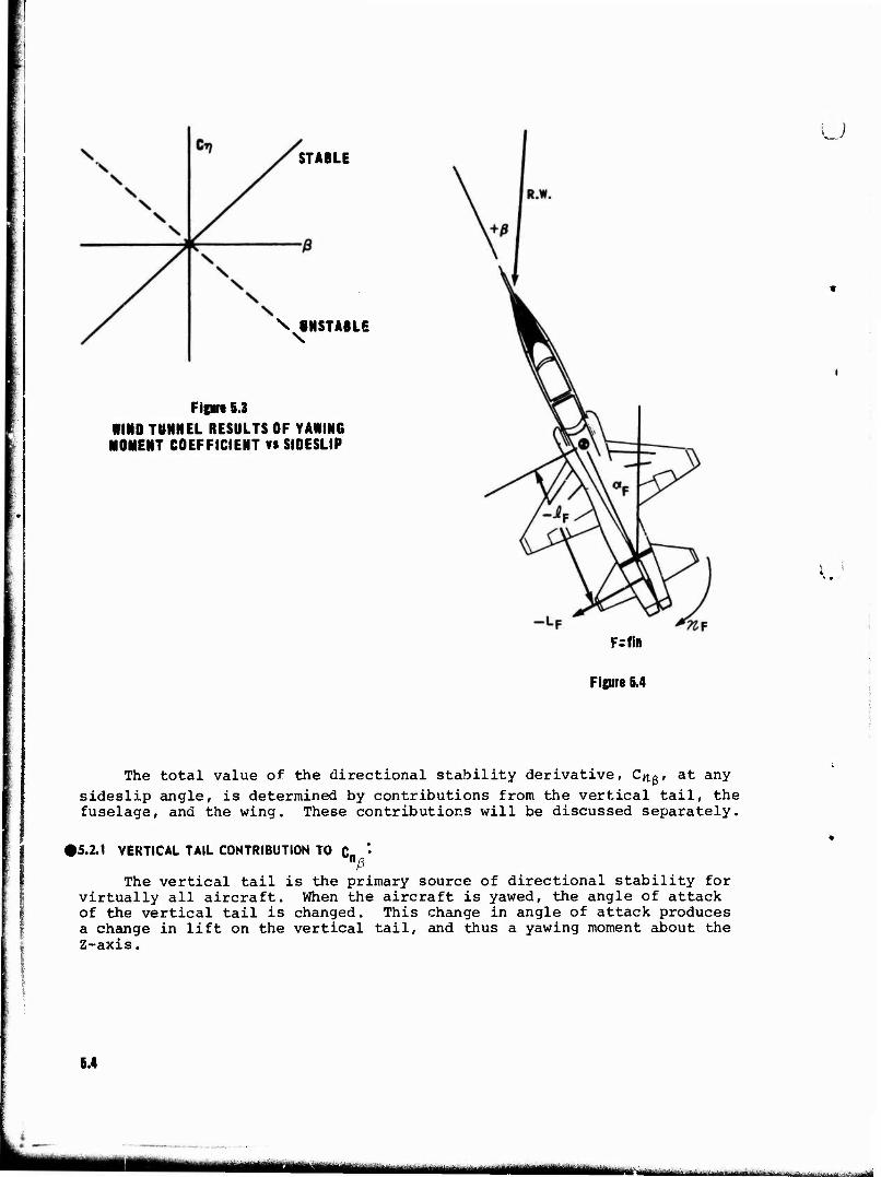
STABLE

\ UNSTABLE

Figure 5.3

WIND TUNNEL RESULTS OF YAWING MOMENT COEFFICIENT vs SIDESLIP

u

4>..'

Fsfln

Figure 5.4

The total value of the directional stability derivative, C^g/ at any sideslip angle, is determined by contributions from the vertical tail, the fuselage, and the wing. These contributions will be discussed separately.

>5.2.1 VERTICAL TAIL CONTRIBUTION TO C

! !

•ß The vertical tail is the primary source of directional stability for

virtually all aircraft. When the aircraft is yawed, the angle of attack of the vertical tail is changed. This change in angle of attack produces a change in lift on the vertical tail, and thus a yawing moment about the Z-axis.

5.4

— •"*'■-■ ■-■ :- - - ■■-■■)•

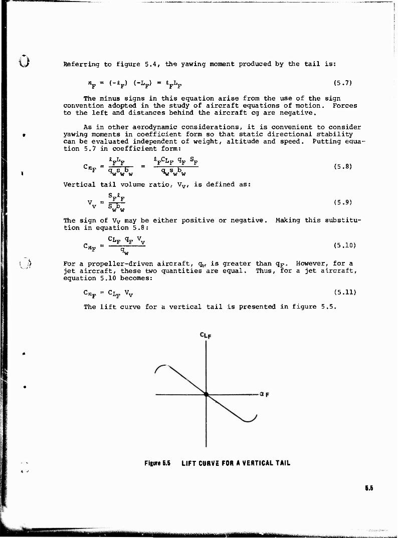
0 Referring to figure 5.4, the yawing moment produced by the tail is:

o

np = <-lp) (-Lp) = iFhF (5.7)

The minus signs in this equation arise from the use of the sign convention adopted in the study of aircraft equations of motion. Forces to the left and distances behind the aircraft eg are negative.

As in other aerodynamic considerations, it is convenient to consider yawing moments in coefficient form so that static directional stability can be evaluated independent of weight, altitude and speed. Putting equation 5.7 in coefficient form:

*FLF VCLF <*F SF q s b %* w " ^nF Q s b

Tf W W -V W W

Vertical tail volume ratio, Vv, is defined as:

V. = F F s~b~ w w

(5.8)

(5.9)

The sign of Vv may be either positive or negative. Making this substitution in equation 5.8:

-nF CLF

qF Vv (5.10)

For a propeller-driven aircraft, qw is greater than qF. However, for a jet aircraft, these two quantities are equal. Thus, for a jet aircraft, equation 5.10 becomes:

C„F = CLp Vv (5.11)

The lift curve for a vertical tail is presented in figure 5.5.

Figure 5.5 LIFT CURVE FOR A VERTICAL TAIL

5.5

MMMM-tMMMMi ttiüi "-■-^^initiiYniiirtirJiii v. i -iii-i i -iii ■ i

The negative slope of this curve is a result of the sign convention used. Reference figure 5.4. When the relative wind is displaced to the right of the fuselage reference line, the vertical tail is placed at a positive angle of attack. However, this results in a lift force to the left, or a negative lift. Thus, the sign of the lift curve slope of a vertical tail, aF, will always be negative below the stall.

CLF = ap ap

Making this substitution in equation 5.11

CtF = ap ap Vv

(5.12)

(5.13)

The angle of attack of the vertical tail, ap, is not merely fc. If the vertical tail were placed alone in an airstream, the ap would >e equal to e. However, when the tail is installed on an aircraft, changes in both magnitude and direction of the local flow at the tail take place.

These changes may be caused by a propeller slipstream, or by the wing and the fuselage when the airplane is yawed. The angular deflection is allowed for by introducing the sidewash angle, o, analogous to the downwash angle, e. The value of a is very difficult to predict, therefore suitable wind tunnel tests are required, causes aw to be less than |

The sign of Thus,

a =

is defined as positive if it

(5.14)

Substituting in equation 5.13:

F v (fi - a) (5.15)

The contribution of the vertical tail to weathercock stability is found by examining the change in Cn„ with a change in sideslip angle, t

ac, = VvaF (1 " ff* (5-16)

Fixed

•nF 36 (Tail)

The subscript "fixed" is added to emphasize that, thus far, the vertical tail has been considered as a surface with no movable parts, i.e., the rudder is "fixed."

Equation 5.16 reveals that the vertical tail contribution to directional stability can only be changed by varying the vertical tail volume ratio, Vv, or the vertical tail lift curve slope, ap. The vertical tail volume ratio can be changed by varying the size of the vertical tail, or its distance from the aircraft eg. The vertical tail lift curve slope can be changed by altering the basic airfoil section of the vertical tail, or by end piating the vertical fin. An end plate on the top of the vertical tail is a relatively minor modification and yet it increases the directional stability of the aircraft significantly. This fact has been utilized in the case of the T-38 (figure 5.6). As can be seen in figure 5.7, the entire stabilatcr on the F-104 acts as an end plate and, therefore, adds greatly to the directional stability of the aircraft.

5.6

mBgmn^ig|Biaifr .^

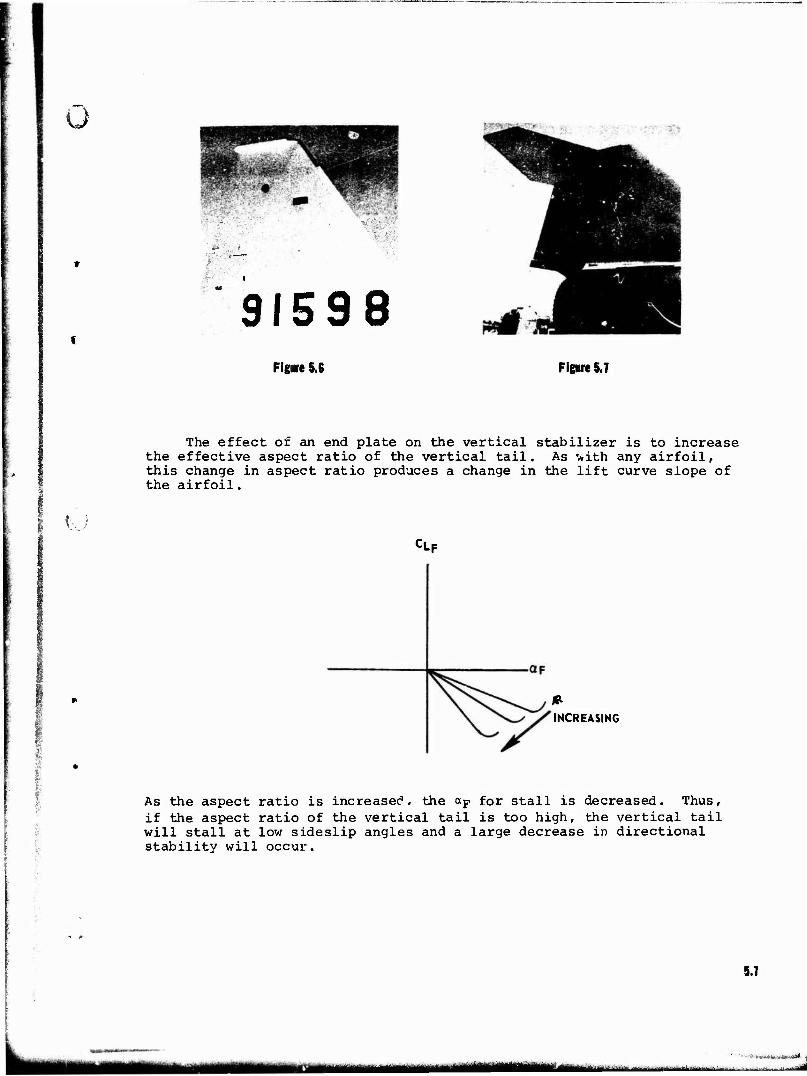
ö

91598 Figure 5.6 Figure 5.7

The effect of an end plate on the vertical stabilizer is to increase the effective aspect ratio of the vertical tail. As '*ith any airfoil, this change in aspect ratio produces a change in the lift curve slope of the airfoil.

I w

'

CLF

INCREASING

I- !

As the aspect ratio is increasec", the <*p for stall is decreased. Thus, if the aspect ratio of the vertical tail is too high, the vertical tail will stall at low sideslip angles and a large decrease in directional stability will occur.

5.7

MMMMi ■^-.-^. ,^..., -:-.,■-

I1 > i rfiiiiii Hhiifl f

■a

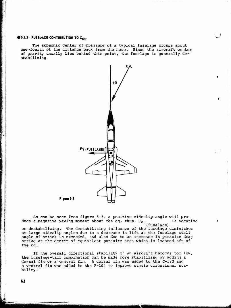
#5.2.2 FUSELAGE CONTRIBUTION TO Cn/3:

The subsonic center of pressure of a typical fuselage occurs about one-fourth of the distance back from the nose. Since the aircraft center of gravity usually lies behind this point, the fuselage is generally destabilizing .

\)

Figure 5.8

FY (FUSELAGE)

■

As can be seer from figure 5.8, a positive sideslip angle will produce a negative yawing moment about the eg, thus, Cn & is negative

(fuselage) or destabilizing. The destabilizing influence of the fuselage diminishes at large sideslip angles due to a decrease in lift as the fuselage stall angle of attack is exceeded, and also due to an increase in parasite drag acting at the center of equivalent parasite area which is located aft of the eg.

If the overall directional stability of an aircraft becomes too low, the fuselage-tail combination can be made more stabilizing by adding a dorsal fin or a ventral fin. A dorsal fin was added to the C-12 3 and a ventral fin was added to the F-104 to improve static directional stability.

5.8

.*.

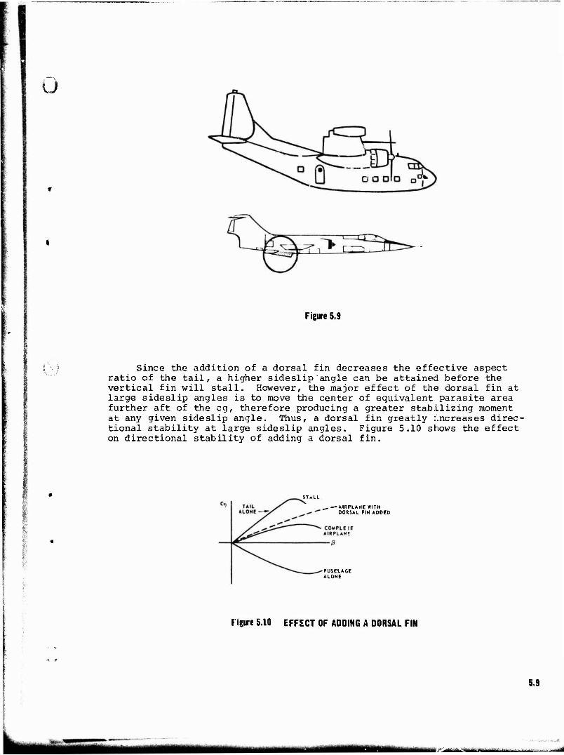
ü

Figure 5.9

Since the addition of a dorsal fin decreases the effective aspect ratio of the tail, a higher sideslip angle can be attained before the vertical fin will stall. However, the major effect of the dorsal fin at large sideslip angles is to move the center of equivalent parasite area further aft of the eg, therefore producing a greater stabilizing moment at any given sideslip angle. Thus, a dorsal fin greatly increases directional stability at large sideslip angles. Figure 5.10 shows the effect on directional stability of adding a dorsal fin.

„ —AIRPLANE WITH DORSAL FIN ADDED

FUSELAGE ALONE

Figure5.10 EFFECT OF ADDING A DORSAL FIN

5,9

^mtmmm ~* »■ ^..^ ,1—.«jlas,*..^,...... ... . . ■df

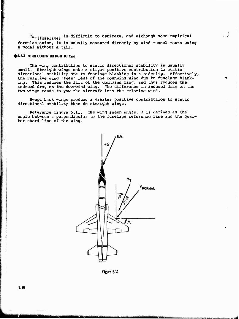
is difficult to estimate, and although some empirical

is u a model without a tail.

Cnß(fuselage) formulas exist, it is usually measured directly by wind tunnel tests using

•5.2.3 WING CONTRIBUTION TO Cn/3'

The wing contribution to static directional stability is usually small. Straight wings make a slight positive contribution to static directional stability due to fuselage blanking in a sideslip. Effectively, the relative wind "sees" less of the downwind wing due to fuselage blanking. This reduces the lift of the downwind wing, and thus reduces the induced drag on the downwind wing. The difference in induced drag on the two wings tends to yaw the aircraft into the relative wind.

Swept back wings produce a greater positive contribution to static directional stability than do straight wings.

Reference figure 5.1.1. The wing sweep angle, A is defined as the angle between a perpendicular to the fuselage reference line and the quarter chord line of the wing.

Figure 5.11

5.10

MMmtmmm 1 mi

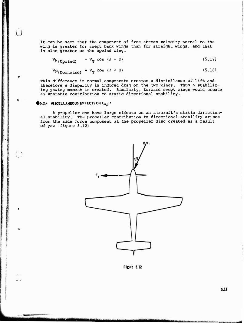
ü

. f.

It can be seen that the component of free stream velocity normal to the wing is greater for swept back wings than for straight wings, and that is also greater on the upwind wing.

VN(UPwind) - VT COS (A " ß)

VN(Downwind) = VT COS (A + S)

(5.17)

(5.18)

This difference in normal components creates a dissimilance oi: lift and therefore a disparity in induced drag on the two wings. Thus a stabilizing yawing moment is created. Similarly, forward swept wings would create an unstable contribution to static directional stability.

• 5.2.4 MISCELLANEOUS EFFECTS ON C, •ß

A propeller can have large effects on an aircraft's static diraction- al stability. The jropeller contribution to directional stability arises from the side force component at the propeller disc created as a result of yaw (figure 5.12)

Figure 5.12

5.11

unit

i

The propeller is destabilizing if a tractor and stabilizing if a pusher. '^.J Similarly, engine intakes have the same effects if they are located fore or aft of the aircraft eg.

Engine nacelles act like a small fuselage and can be stabilizing or destabilizing depending on whether their cp is located ahead or behind the eg.

Aircraft eg movement is-restricted by longitudinal static stability considerations. However, within the relatively narrow lin i.ts established r-y longitudinal considerations, eg movements have no significant effects * on static directional stability.

15.3 Cn^-RUDDER POWER

In most flight conditions, it is desired to maintain the sideslip , angle equal to zero. If the aircraft has positive directional stability and is symmetrical, then it will tend to fly in this condition. However, yawing moments may act on the aircraft as a result of asymmetric thrust (one engine inoperative), slip stream rotation, or the unsymmetric flow field associated with turning flight. Under these conditions, sideslip angle can be kept to zero only by the application of a control moment. The control that provides this moment is the rudder.

Recall that,

CHp = aF ap 7v (5.13)

3Cn„ 3C,. 3u F n ~ V —L (5.19) 3 & r 3 6 " F V 36 r r

Defining rudder effectiveness, T, as:

3 a T = rr— (5.20)

a o r

TT-C«6.- = aF Vv T (5'21) r

The derivative, C|1(sr> is called "rudder power" and by definition, its algebraid sign is always positive. This is because a positive rudder deflection, +-r is defined as one that produces a positive moment about the eg, +Cn. The magnitude of the rudder pow^r can be altered by varying the size of the vertical tail and its distance from the aircraft eg, or by using different airfoils for the tail and/or rudder, or by varying the size of the rudder.

I&.4 RUDDER FIXED STATIC DIRECTIONAL STABILITY

Having some knowledge of both C^,. and Cnö , it is now possible to work toward some relationship that can be used in flight to measure the

5.12

„mmtmum

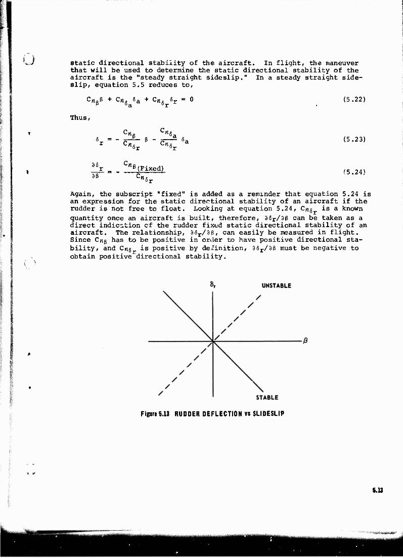
u static directional stability of the aircraft. In flight, the maneuver that will be used to determine the static directional stability of the aircraft is the "steady straight sideslip." In a steady straight sideslip, equation 5.5 reduces to,

A JL

(5.22)

Thus,

6 = - 'H,

(5.23)

36 ]

36 '"ß(Fixed)

(5.24)

Again, the subscript "fixed" is added as a reminder that equation 5.24 is an expression for the static directional stability of an aircraft if the rudder is not free to float. Looking at equation 5.24, Cn$ is a known

quantity once an aircraft is built, therefore, 3 6r/3ß can be taken as a direct indication cf the rudder fixed static directional stability of an aircraft. The relationship, 36r/3ß, can easily be measured in flight. Since C^g has to be positive in order to have positive directional stability, and Cn$ is positive by definition, 36r/3ß must be negative to obtain positive directional stability.

Figure 5.13 RUDDER DEFLECTION vs SLIDESLIP

5.13

■■^^■feft^j**-'

16.5 RUDDER FREE DIRECTIONAL STABILITY Ü

On aircraft with reversible control systems, the rudder is free to float in response to its hinge moments, and this floating can have large effects on the directional stability of the airplane. In fact, a plot of 36r/3ß may be stable while an examination of the rudder free static directional stability reveals the aircraft to be unstable. Thus, if the rudder is free to float, there will be a change in the tail contribution to static directional stability. To analyze the nature of this change, recall that hinge moments are produced by the pressure distribution caused by angle of attack and control surface deflection. In the case of the rudder,

o SH 3H

In coefficient form

(5.25)

ch = ch. + ch, (5.26)

It can be seen that when the vertical tail is placed at some angle of attack, aF, the rudder will start to "float." However, as soon as it deflects, restoring moments are set up, and an equilibrium floating angle will be reached where the floating tendency is just balanced by the restoring tendency and Ch = 0. At this point,

chr aF = ~ ch. >r(Float) (5.27)

Thus,

chn r(Float) Ch,

(5.28)

With this background, it is now possible to develop a relationship that expresses the static directional stability of an aircraft with the rudder free to float.

Recall that,

cnF = Vy ap ap (5.13)

3aF - a + r-ri- 6_ 3 r r(Float)

(5.29)

Therefore,

= V - a + 36r °r(Float)

(5.30)

5.14

Yartltoifcr^liäälrtrtm ,'m ■ ' "

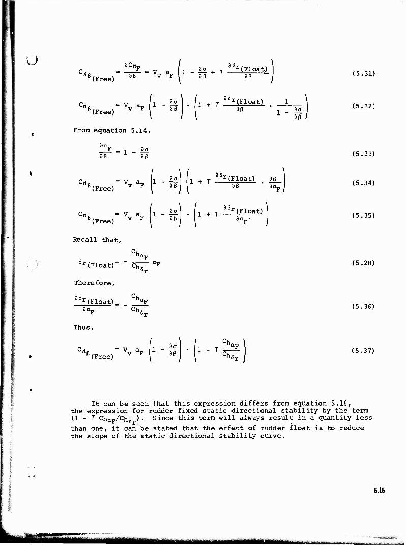
u CW -!f!±-v a 1 3g . T 36r(Float)

Wf5(Free) 3ß v F 9ß U (5.31)

Cn ^Free)'^^!1 " "

1 + T "*(Float) . _JL. 3ß 1 _ i£

3ß

(5.32)

From equation 5.14,

3ß 3ß (5.33)

96, Cnc = V a. 1 - & 1 + T r(Float) . 3ß

(Free) v F 3ß 3ß 3oT (5.34)

Cn, (Free) ̂

VvaF I1 "If 1 + T 85r (Float) (5.35)

s Recall that,

6r(Float)" '

ChaF Ch6r

Therefore,

36r (Float). 3aF

ChaF Ch6r

Thus,

(5.28)

(5.36)

"Vreef ^ ^ " ^ Ch

1 - T ap

Ch6l (5.37)

It can be seen that this expression differs from equation 5.16, the expression for rudder fixed static directional stability by the term (1 - T ChaF/Chg ) • Since this term will always result in a quantity less

than one, it can be stated that the effect of rudder float is to reduce the slope of the static directional stability curve.

5.15

ÜU mm I li I II ilMJl

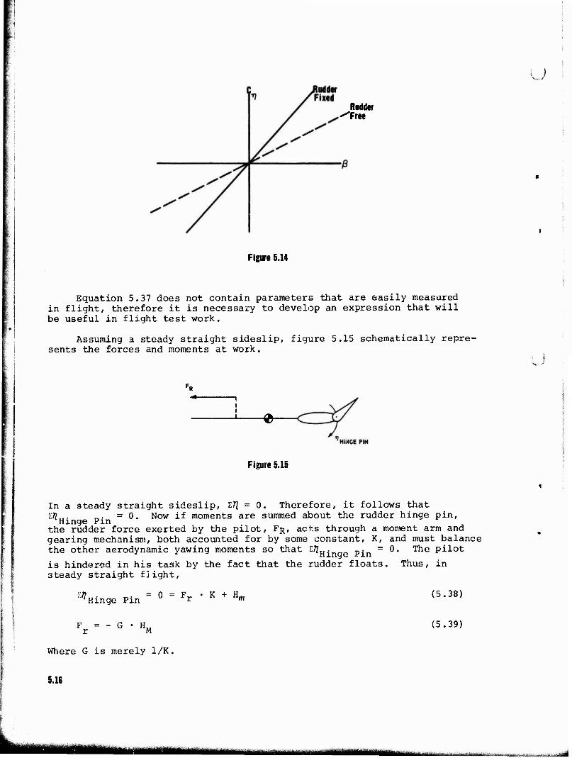
u Rudder

^Free

Figure 5.14

Equation 5.37 does not contain parameters that are easily measured in flight, therefore it is necessary to develop an expression that will be useful in flight test work.

Assuming a steady straight sideslip, figure 5.15 schematically represents the forces and moments at work. u

-fc-

Figure 5.15

In a steady straight sideslip, l7[ = 0. Therefore, it follows that E» . _. =0. Now if moments are summed about the rudder hinge pin, Hinge Pin

the rudder force exerted by the pilot, FR, acts through a moment arm and gearing mechanism, both accounted for by some constant, K, and must balance the other aerodynamic yawing moments so that ^Hinqe pj_n

=

is hindered in his task by the fact that the rudder floats steady straight fiight,

m

F

Hinge Pin - 0 - F,

H. r M

Where G is merely 1/K,

K + H, m

0. The pilot

Thus, in

(5.38)

(5.39)

5.16

L_ •MM ""titvntimhf-v ■ ■ - - ■ - ■■-■ ■■■ ■■****

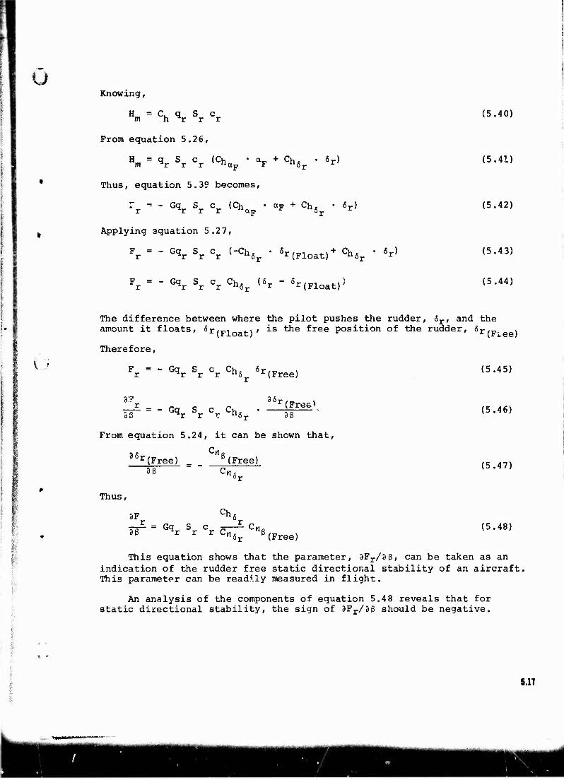
o Knowing,

Hm = Ch *r Sr Cr

From equation 5.26,

H = q S c (CK * oip + cht ' 6r)

Thus, equation 5.39 becomes,

r -- - Gq S c (Ch • »F + Cht ' 6r) r ^r r r "aF c "5r

r

Applying equation 5.2 7,

F = - Gq S c (-Ch* • «r/pi t-\ + Ch* r r r r 6r r (Float) ri6r

F = - Gq S C CK, (6r - <5r/oi «,4.\ ' r r r r "6r * r(Float)

6r)

(5.40)

(5.41)

(5.42)

(5.43)

(5.44)

\J

The difference between where the pilot pushes the rudder, 6r, and the amount it floats, 6r,_,n . . , is the free position of the rudder, 6r/T, . L (Float) r *■ (Fiee) Therefore,

F =-Gq S c Chc 6r,„ , r ^r r r n6 r(Free)

37.. 3(5 rrr~ = _ Gq S c Ch. 33 ^r r r n&r

r(Free^ 36

(5.45)

(5.46)

From equation 5.24, it can be shown that,

35r(Free) m _ %Free) 3ß Cut

(5.47)

Thus,

3F Ch,

JT = Gqr Sr Cr C^T CH *r (Free)

(5.48)

This equation shows that the parameter, 3Fr/3ß, can be taken as an indication of the rudder free static directional stability of an aircraft. This parameter can be readily measured in flight.

An analysis of the components of equation 5.48 reveals that for static directional stability, the sign of 3Fr/3ß should be negative.

5.17

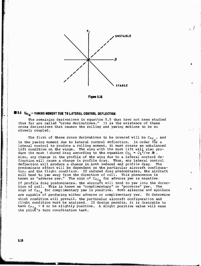
L.;

UNSTABLE

STABLE

Figure 5.16

1B-6 CBja - YAWING MOMENT DUE TO LATERAL CONTROL DEFLECTION

The remaining derivatives in equation 5.5 that have not been studied thus far are called "cross derivatives." It is the existence of these cross derivatives that causes the rolling and yawing motions to be so closely coupled.

'• i

The first of these cross derivatives to be covered will be C^j , and is the yawing moment due to lateral control deflection. In order for a lateral control to produce a rolling moment, it must create an unbalanced lift condition on the wings. The wing with the most lift will also produce the most i lduced drag according to the equation Cp^ = Ci^/ve ZR . Also, any change in the profile of the wing due to a lateral control deflection will cause a change in profile drag. Thus, any lateral control deflection will produce a change in both induced and profile drag. The predominate effect will be dependent on the particular aircraft configuration and the flight condition. If induced drag predominates, the aircraft will tend to yaw away from the direction of roll. This phenomenon is known as "adverse yaw." The sign of Cn$ for adverse yaw is negative. If profile drag predominates, the aircraft will tend to yaw into the direction of roll. This is known as "complimentary" or "proverse" yaw. The sign of C^ for complimentary yaw is positive. Both ailerons and spoilers are capable of producing either adverse or complimentary yaw. To determine which condition will prevail, the particular aircraft configuration and flight condition must be analyzed. If design permits, it is desirable to have C^ = 0 or be slightly positive. A slight positive value will ease the pilot's turn coordination task.

HMHMI laSUmlBlMmaL

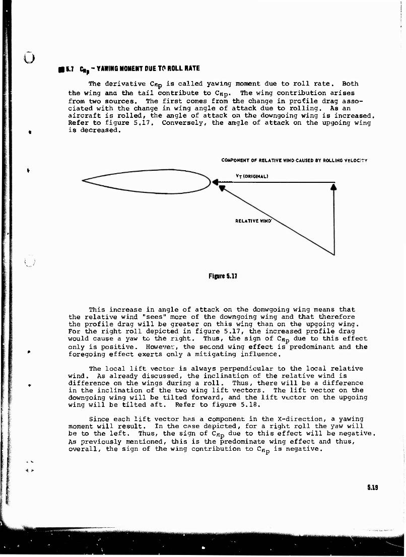
15.7 da - YAWING MOMENT CUE TP ROLL RATE

\ j

The derivative Cnp is called yawing moment due to roll rate. Both the wing and the tail contribute to dtp. The wing contribution arises from two sources. The first comes from the change in profile drag associated with the change in wing angle of attack due to rolling. As an aircraft is rolled, the angle of attack on the downgoing wing is increased, Refer to figure 5.17. Conversely, the angle of attack on the upgoing wing is decreased.

COMPONENT OF RELATIVE WIND CAUSED BY ROLLING VELQCTY

VT (ORIGINAL)

RELATIVE WIND

Figure 5.17

I I

This increase in angle of attack on the donwgoing wing means that the relative wind "sees" more of the downgoing wing and that therefore the profile drag will be greater on this wing than on the upgoing wing. For the right roll depicted in figure 5.17, the increased profile drag would cause a yaw to the right. Thus, the sign of Cnp due to this effect only is positive. However, the second wing effect is predominant and the foregoing effect exerts only a mitigating influence.

The local lift vector is always perpendicular to the local relative wind. As already discussed, the inclination of the relative wind is difference on the wings during a roll. Thus, there will be a difference in the inclination of the two wing lift vectors. The lift vector on the downgoing wing will be tilted forward, and the lift vector on the upgoing wing will be tilted aft. Refer to figure 5.18.

Since each lift vector has a component in the X-direction, a yawing moment will result. In the case depicted, for a right roll the yaw will be to the left. Thus, the sign of Cnp due to this effect will be negative, As previously mentioned, this is the predominate wing effect and thus, overall, the sign of the wing contribution to Crtp is negative.

5.19

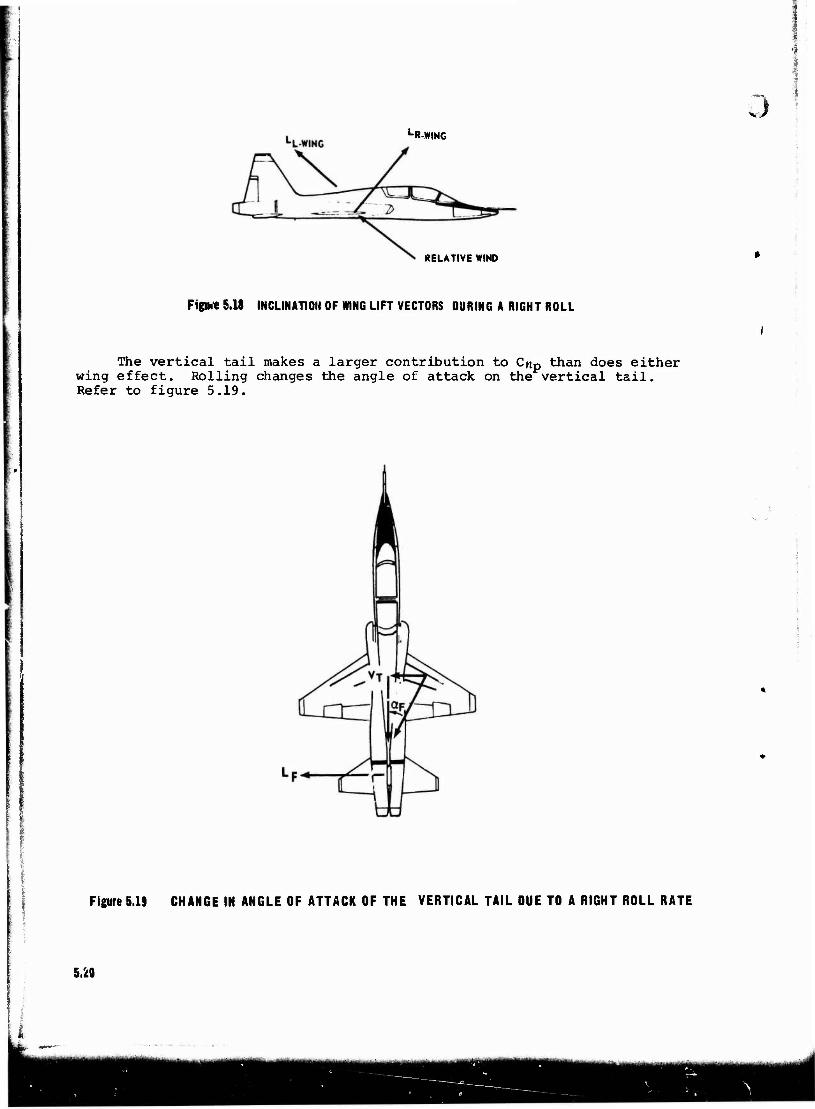
LR-J»INC

0 !

RELATIVE WIND

FiglM 5.18 INCLINATION OF WING LIFT VECTORS DURING A RIGHT ROLL

The vertical tail makes a larger contribution to Cnp than does either wing effect. Rolling changes the angle of attack on the vertical tail. Refer to figure 5.19.

Figure 5.19 CHANGE IN ANGLE OF ATTACK OF THE VERTICAL TAIL DUE TO A RIGHT ROLL RATE

5.20

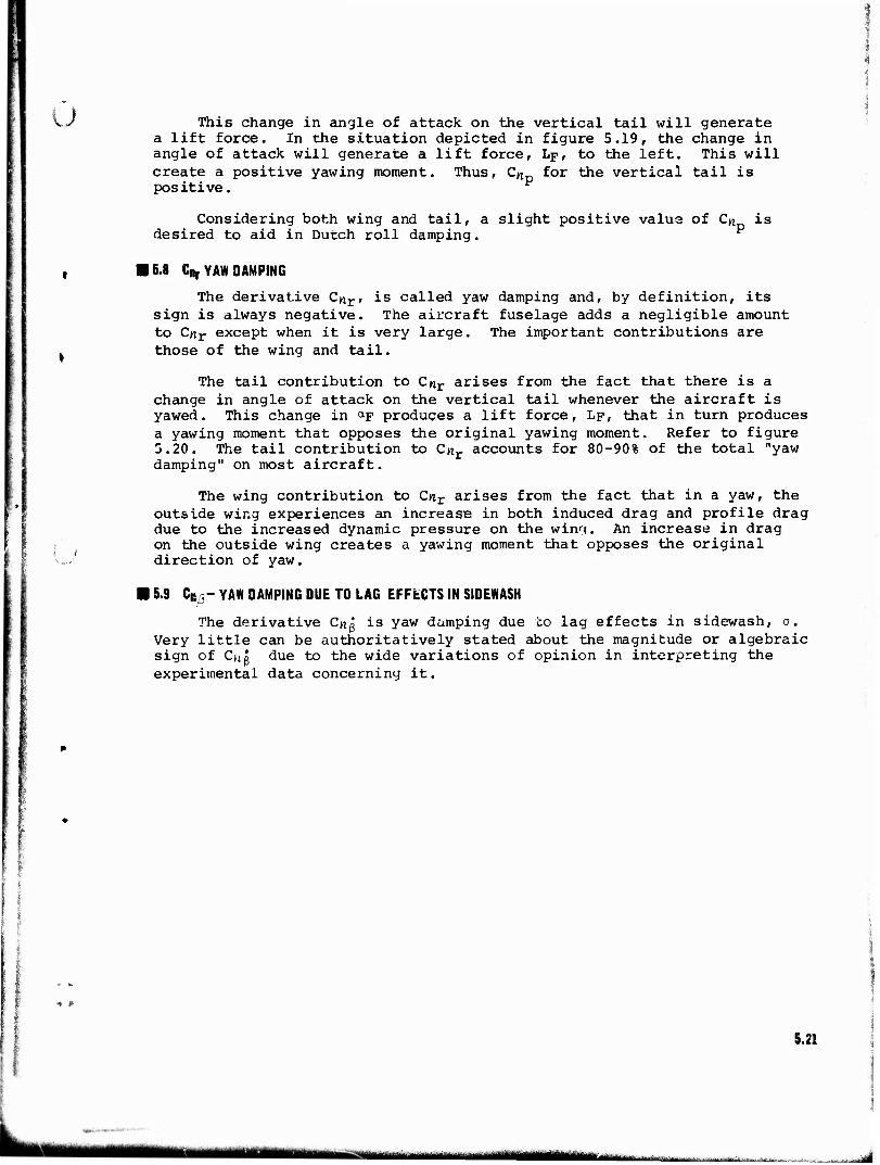
u This change in angle of attack on the vertical tail will generate a lift force. In the situation depicted in figure 5.19, the change in angle of attack will generate a lift force, Lp, to the left. This will create a positive yawing moment, positive.

Thus, Cn_. for the vertical tail is

I /

Considering both wing and tail, a slight positive value of Cn is desired to aid in Dutch roll damping.

16.8 Cnr YAW DAMPING

The derivative Cnr, is called yaw damping and, by definition, its sign is always negative. The aircraft fuselage adds a negligible amount to Cnr except when it is very large. The important contributions are those of the wing and tail.

The tail contribution to Cnr arises from the fact that there is a change in angle of attack on the vertical tail whenever the aircraft is yawed. This change in <*F produces a lift force, LF, that in turn produces a yawing moment that opposes the original yawing moment. Refer to figure 5.20. The tail contribution to Cnr accounts for 80-90% of the total "yaw damping" on most aircraft.

The wing contribution to Cnr arises from the fact that in a yaw, the outside wing experiences an increase in both induced drag and profile drag due to the increased dynamic pressure on the win'f. An increase in drag on the outside wing creates a yawing moment that opposes the original direction of yaw.

15.9 Cn - YAW DAMPING DUE TO LAG EFFfcCTS IN SIDEWASH

The derivative Cno is yaw damping due to lag effects in sidewash, a. Very little can be authoritatively stated about the magnitude or algebraic sign of Cn$ due to the wide variations of opinion in interpreting the experimental data concerniny it.

5.21

HMMMteMM flfcÜühiiitrhtiTi nr i m If

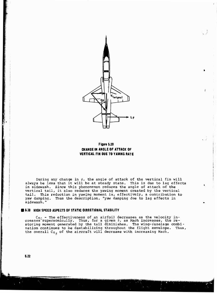
Figure 5.20

CHANGE IN ANGLE OF ATTACK OF VERTICAL FIN DUE TO YAWING RATE

During any change in ß, the angle of attack of the vertical fin will always be less than it will be at steady state. This is due to lag effects in sidewash. Since this phenomenon reduces the angle of attack of the vertical tail, it also reduces the yawing moment created by the vertical tail. This reduction in yawing moment is, effectively, a contribution to yaw damping. Thus the description, "yaw damping due to lag effects in sidewash."

i 6.10 HIGH SPEED ASPECTS OF STATIC DIRECTIONAL STABILITY

CyiQ - The effectiveness of an airfoil decreases as the velocity increases supersonically. Thus, for a given ß, as Mach increases, the restoring moment generated by the tail diminishes. The wing-fuselage combination continues to be destabilizing throughout the flight envelope. Thus, the overall CnQ of the aircraft will decrease with increasing Mach.

5.22

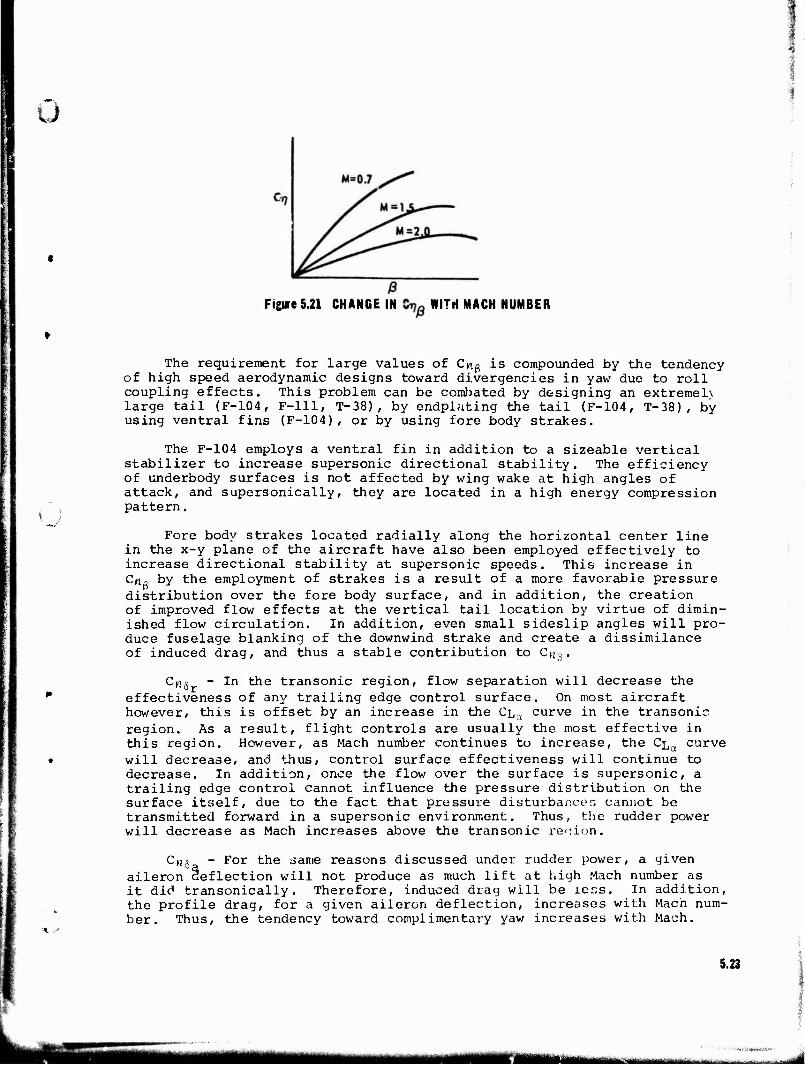
u

Figure 5.21 CHANGE IN WITH MACH NUMBER

\ i

The requirement for large values of Cnß is compounded by the tendency of high speed aerodynamic designs toward divergencies in yaw due to roll coupling effects. This problem can be combated by designing an extremel\ large tail (F-104, F-lll, T-38), by endplating the tail (F-104, T-38), by using ventral fins (F-104), or by using fore body strakes.

The F-104 employs a ventral fin in addition to a sizeable vertical stabilizer to increase supersonic directional stability. The efficiency of underbody surfaces is not affected by wing wake at high angles of attack, and supersonically, they are located in a high energy compression pattern.

Fore body strakes located radially along the horizontal center line in the x-y plane of the aircraft have also been employed effectively to increase directional stability at supersonic speeds. This increase in C-ria by the employment of strakes is a result of a more favorable pressure distribution over the fore body surface, and in addition, the creation of improved flow effects at the vertical tail location by virtue of diminished flow circulation. In addition, even small sideslip angles will produce fuselage blanking of the downwind strake and create a dissimilance of induced drag, and thus a stable contribution to CWa.

CM(5 - In the transonic region, flow separation will decrease the effectiveness of any trailing edge control surface. On most aircraft however, this is offset by an increase in the CLa curve in the transonic region. As a result, flight controls are usually the most effective in this region. However, as Mach number continues to increase, the CLa curve will decrease, and thus, control surface effectiveness will continue to decrease. In addition, once the flow over the surface is supersonic, a trailing edge control cannot influence the pressure distribution on the surface itself, due to the fact that pressure disturbances cannot be transmitted forward in a supersonic environment. Thus, the rudder power will decrease as Mach increases above the transonic region.

-»6; For the bailie reasons discussed under rudder power, a given aileron 3eflection will not produce as much lift at high Mach number as it did transonically. Therefore, induced drag will be ier.s. In addition, the profile drag, for a given aileron deflection, increases with Mach number. Thus, the tendency toward complimentary yaw increases with Mach.

5.23

m

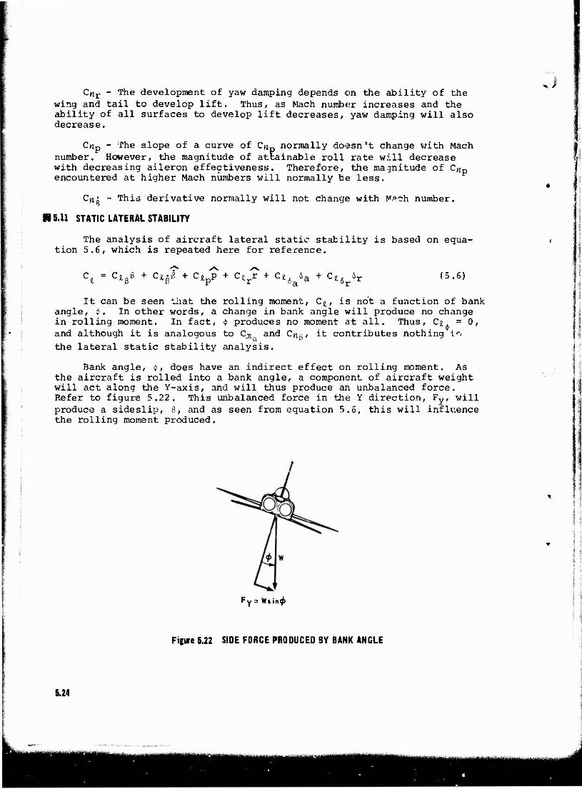
Cnr - The development of yaw damping depends on the ability of the wing and tail to develop lift. Thus, as Mach number increases and the ability of all surfaces to develop lift decreases, yaw damping will also decrease.

J

dtp - The slope of a curve of Cnp normally doesn't change with Mach number. However, the magnitude of attainable roll rate will decrease with decreasing aileron effectiveness. Therefore, the magnitude of Cn„ encountered at higher Mach numbers will normally be less.

Cnx - This derivative normally will not change with M?ch number.

15.11 STATIC LATERAL STABILITY

The analysis of aircraft lateral static stability is based on equation 5.6, which is repeated here for reference.

= c*«e C4gß s\

C*rr + C*6a6a + C lx ur °r

(5.6)

It can be seen that the rolling moment, C^, is not a function of bank angle, $, In other words, a change in bank angle will produce no change in rolling moment. In fact, $ produces no moment at all. Thus, Ci = 0, and although it is analogous to C^ and Cn^, it contributes nothing in the lateral static stability analysis.

Bank angle, <j>, does have an indirect effect on rolling moment. As the aircraft is rolled into a bank angle, a component of aircraft weight will act along the Y-axis, and will thus produce an unbalanced force. Refer to figure 5.22. This unbalanced force in the Y direction, Fy, will produce a sideslip, ß, and as seen from equation 5.6, this will influence the rolling moment produced.

Fy = Wsin^

Figure 5.22 SIDE FORCE PRODUCED BY BANK ANGLE

5.24

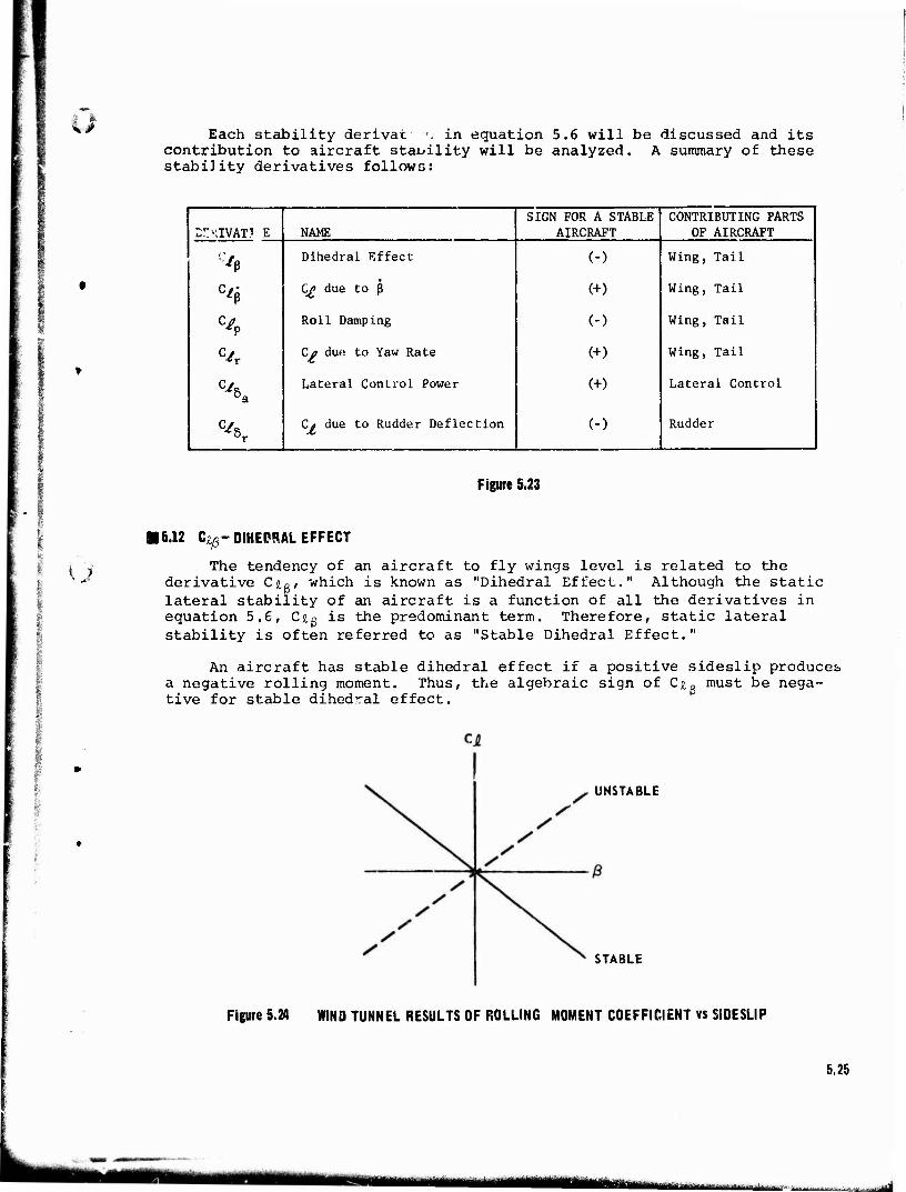
Each stability derivac J in equation 5.6 will be discussed and its contribution to aircraft stability will be analyzed. A summary of these stability derivatives follows:

SIGN FOR A STABLE CONTRIBUTING PARTS Zr.KVlkTl E NAME AIRCRAFT OF AIRCRAFT

% Dihedral Effect (-) Wing, Tail

% C£ due to ß (+) Wing, Tail

% Roll Damping (-) Wing, Tail

% Ca due to Yaw Rate (+) Wing, Tail

cx Lateral Control Power (+) Lateral Control

c\ C* due to Rudder Deflection (-) Rudder

Figure 5.23

l I

u 16.12 Ciß- DIHEDRAL EFFECT

The tendency of an aircraft to fly wings level is related to the derivative Cjtß, which is known as "Dihedral Effect." Although the static lateral stability of an aircraft is a function of all the derivatives in equation 5.6, Ci$ is the predominant term. Therefore, static lateral stability is often referred to as "Stable Dihedral Effect."

An aircraft has stable dihedral effect if a positive sideslip produces a negative rolling moment. Thus, the algebraic sign of CJU must be negative for stable dihedral effect.

UNSTABLE

STABLE

Figure 5.24 WIND TUNNEL RESULTS OF ROLLING MOMENT COEFFICIENT vs SIDESLIP

5.25

üüWkääir: .

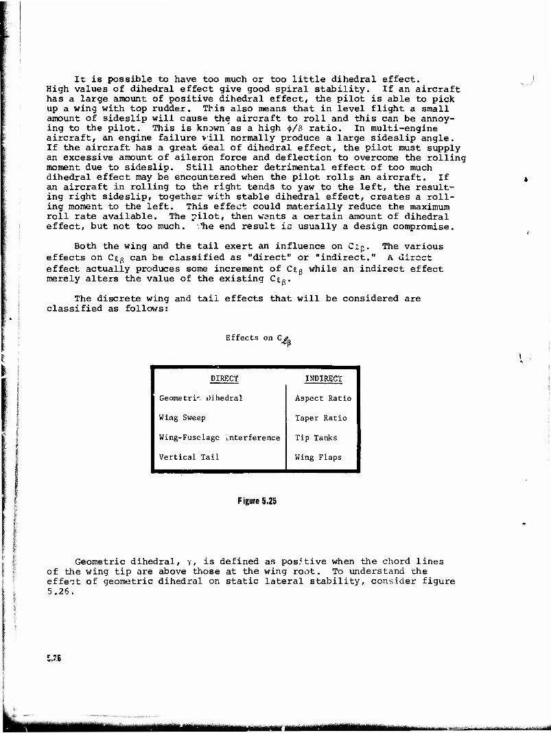
It is possible to have too much or too little dihedral effect. High values of dihedral effect give good spiral stability. If an aircraft has a large amount of positive dihedral effect, the pilot is able to pick up a wing with top rudder. This also means that in level flight a small amount of sideslip will cause the aircraft to roll and this can be annoying to the pilot. This is known'as a high <f>/0 ratio. In multi-engine aircraft, an engine failure will normally produce a large sideslip angle. If the aircraft has a great deal of dihedral effect, the pilot must supply an excessive amount of aileron force and deflection to overcome the rolling moment due to sideslip. Still another detrimental effect of too much dihedral effect may be encountered when the pilot rolls an aircraft. If an aircraft in rolling to the right tends to yaw to the left, the resulting right sideslip, together with stable dihedral effect, creates a rolling moment to the left. This effect could materially reduce the maximum roll rate available. The pilot, then wants a certain amount of dihedral effect, but not too much, '.''he end result is usually a design compromise.

.J

Both the wing and the tail exert an influence on Ci$. The various effects on Cj,g can be classified as "direct" or "indirect." A direct effect actually produces some increment of Cx,g while an indirect effect merely alters the value of the existing CJU.

The discrete wing and tail effects that will be considered are classified as follows:

Effects on C4>

DIRECT INDIRECT

Geometrie Dihedral Aspect Ratio

Wing Sweep Taper Ratio

Wing-Fuselage "interference Tip Tanks

Vertical Tail Wing Flaps

Figure 5.25

Geometric dihedral, y, is defined as positive when the chord lines of the wing tip are above those at the wing root. To understand the effect of geometric dihedral on static lateral stability, consider figure 5.25.

5.7.B

MMM MW ÜÜtfgttÜ n^^iawaiJ^^A-

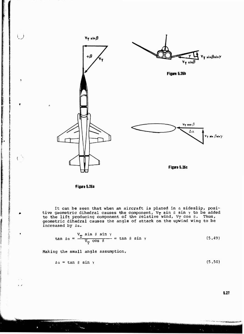
t ) VT «in/9

Figure 5.26c

rT»i nß%inY

VT sin ßtlny

Figure 5.26a

It can be seen that when an aircraft is planed in a sideslip, positive geometric dihedral causes the component, Vip sin 6 sin y to be added to the lift producing component of the relative wind, VT cos ß. Thus, geometric dihedral causes the angle of attack on the upwind wing to be increased by Aa.

tan A a = VT sin sin Y

VT cos = tan ß sin y (5.49)

Making the small angle assumption,

Aa = tan ß sin y (5.50)

5.21

*^^<*äfi3$&&&&>^

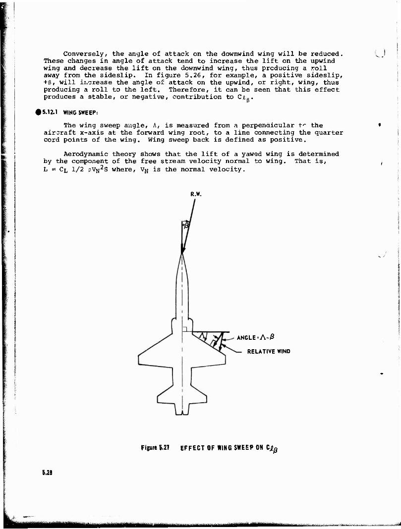
Conversely, the angle of attack on the downwind wing will be reduced. These changes in angle of attack tend to increase the lift on the upwind wing and decrease the lift on the downwind wing, thus producing a roll away from the sideslip. In figure 5.26, for example, a positive sideslip, +ß, will ii.crease the angle of attack on the upwind, or right, wing, thus producing a roll to the left. Therefore, it can be seen that this effect produces a stable, or negative, contribution to CJU.

15.12.1 WING SWEEP:

The wing sweep angle, A, is measured from a perpendicular t~ the aircraft x-axis at the forward wing root, to a line connecting the quarter cord points of the wing. Wing sweep back is defined as positive.

Aerodynamic theory shows that the lift of a yawed wing is determined by the component of the free stream velocity normal to wing. That is, L = CL 1/2 PV"N

2S where, VN is the normal velocity.

R.W.

! i

ANGLE =A-/3

RELATIVE WIND

5.28

Figure 5.27 EFFECT OF WING SWEEP ON Cj^

HMMI iiiinr — nhr"-'-' ,J-- ■•• ■ •-■

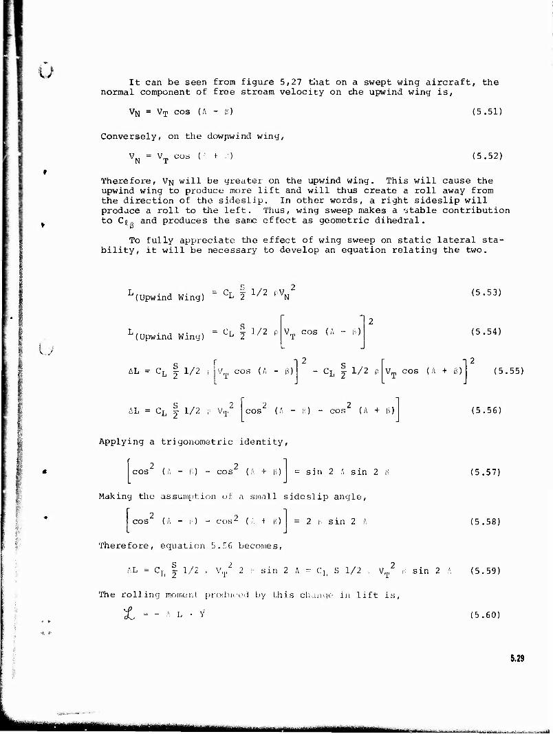
u It can be seen from figure 5,27 that on a swept wing aircraft, the

normal component of free stream velocity on xhe upwind wing is,

VN = VT cos (A ~ t) (5.51)

Conversely, on the downwind wing,

VN = VT cos (.'. f ,) (5.52)

Therefore, V"N will be greater on the upwind wing. This will cause the upwind wing to produce more lift and will thus create a roll away from the direction of the sideslip. In other words, a right sideslip will produce ä roll to the left. Thus, wing sweep makes a stable contribution to C#ft and produces the same effect as geometric dihedral.

To fully appreciate the effect of wing sweep on static lateral stability, it will be necessary to develop an equation relating the two.

L(Upwind Wing) CL 2 1/2 pVN (5.53)

u '(Upwind Winy)

= CL | 1/2 VT cos (A - i3)

AL = CL | 1/2 i V cos (A - 3) - CL § 1/2 p

(5.54)

12 VT cos (A + 6) (5.55)

AL = CL | 1/2 ; VT2 2 2

cos (A -8) - cos (A + ß) (5.56)

Applying a trigonometric identity,

2 2 cos (A - !';) - cos (A + 3) = sin 2 A sin 2 B

Making the assumption of: a small sideslip angle,

cos (A - |.) - cos' (A + a = 2 h sin 2 A

(5.57)

(5.58)

Therefore, equation 5.56 becomes,

AL = Cf| | 1/2 , Vr2 2 i- sin 2 A = cL S 1/2 , V,^ n sin 2 A (5.59)

The rolling moment produced by this change in lift is,

Z = - A L . Y (5.60)

5.29

-■ --- — .■—■■■■■-i.a.—M ■ ■ ...,-■..-.

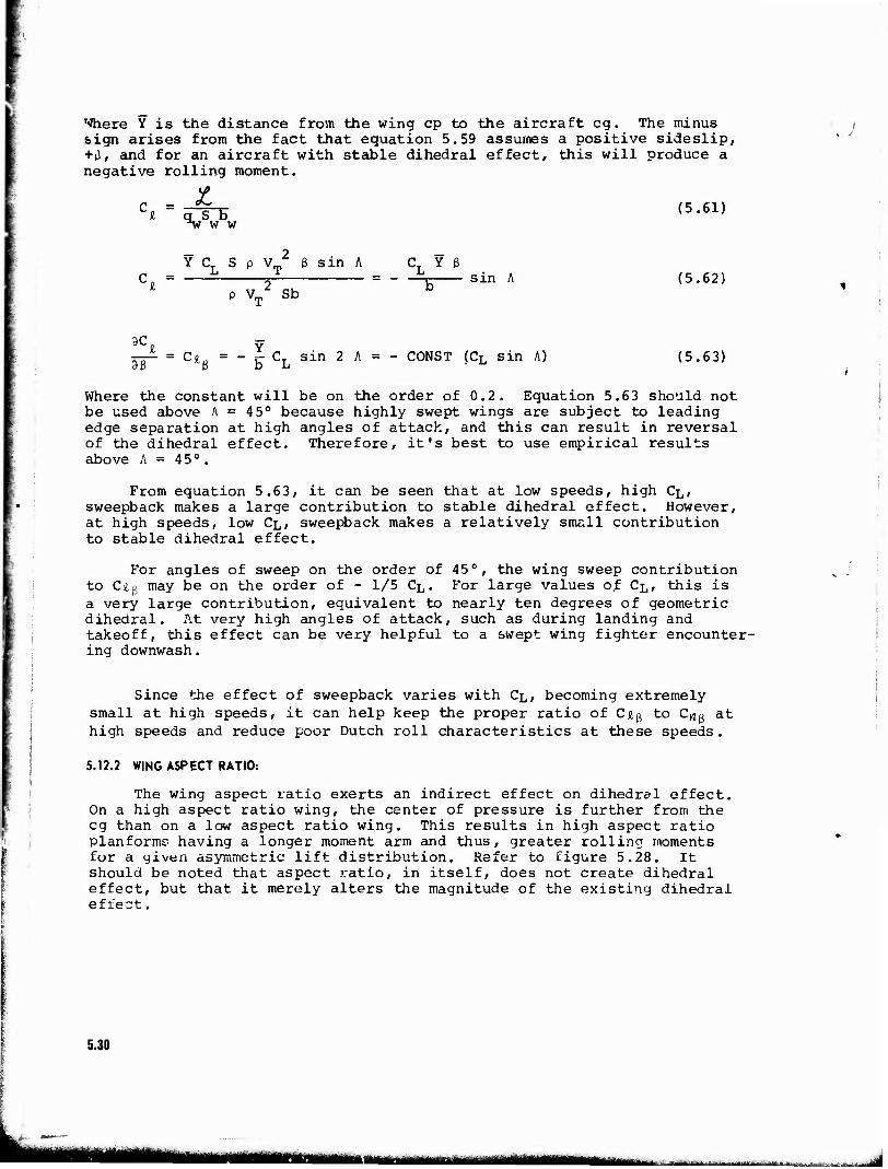
Where Y is the distance from the wing cp to the aircraft eg. The minus sign arises from the fact that equation 5.59 assumes a positive sideslip, +»J, and for an aircraft with stable dihedral effect, this will produce a negative rolling moment.

p = ^^ ^i a S b ^w w w

(5.61)

Ci = Y CL S p VT 6 sin A

p vT2 Sb

CL Y ß sin A (5.62)

5 = cio = - r- CT sin 2 b L A = - CONST (CL sin A) (5.63)

Where the constant will be on the order of 0.2. Equation 5.63 should not be used above A = 45° because highly swept wings are subject to leading edge separation at high angles of attack, and this can result in reversal of the dihedral effect. Therefore, it's best to use empirical results above A = 45°.

From equation 5.63, it can be seen that at low speeds, high CL, sweepback makes a large contribution to stable dihedral effect. However, at high speeds, low CL, sweepback makes a relatively small contribution to stable dihedral effect.

For angles of sweep on the order of 45°, the wing sweep contribution to CILQ may be on the order of - 1/5 CL . For large values of CL, this is a very large contribution, equivalent to nearly ten degrees of geometric dihedral. At very high angles of attack, such as during landing and takeoff, this effect can be very helpful to a swept wing fighter encounter- ing downwash.

Since the effect of sweepback varies with CL, becoming extremely small at high speeds, it can help keep the proper ratio of Cj,g to Crtg at high speeds and reduce poor Dutch roll characteristics at these speeds.

5.12.2 WING ASPECT RATIO:

The wing aspect ratio exerts an indirect effect on dihedral effect. On a high aspect ratio wing, the center of pressure is further from the eg than on a low aspect ratio wing. This results in high aspect ratio planformr. having a longer moment arm and thus, greater rolling moments for a yivttn asymmetric lift distribution. Refer to figure 5.28. It should be noted that aspect ratio, in itself, does not create dihedral effect, but that it merely alters the magnitude of the existing dihedral effect.

5.30

iaMtHHH^Ha MUTur TITMÜliM-iiM ■■■^-^»■-i't---

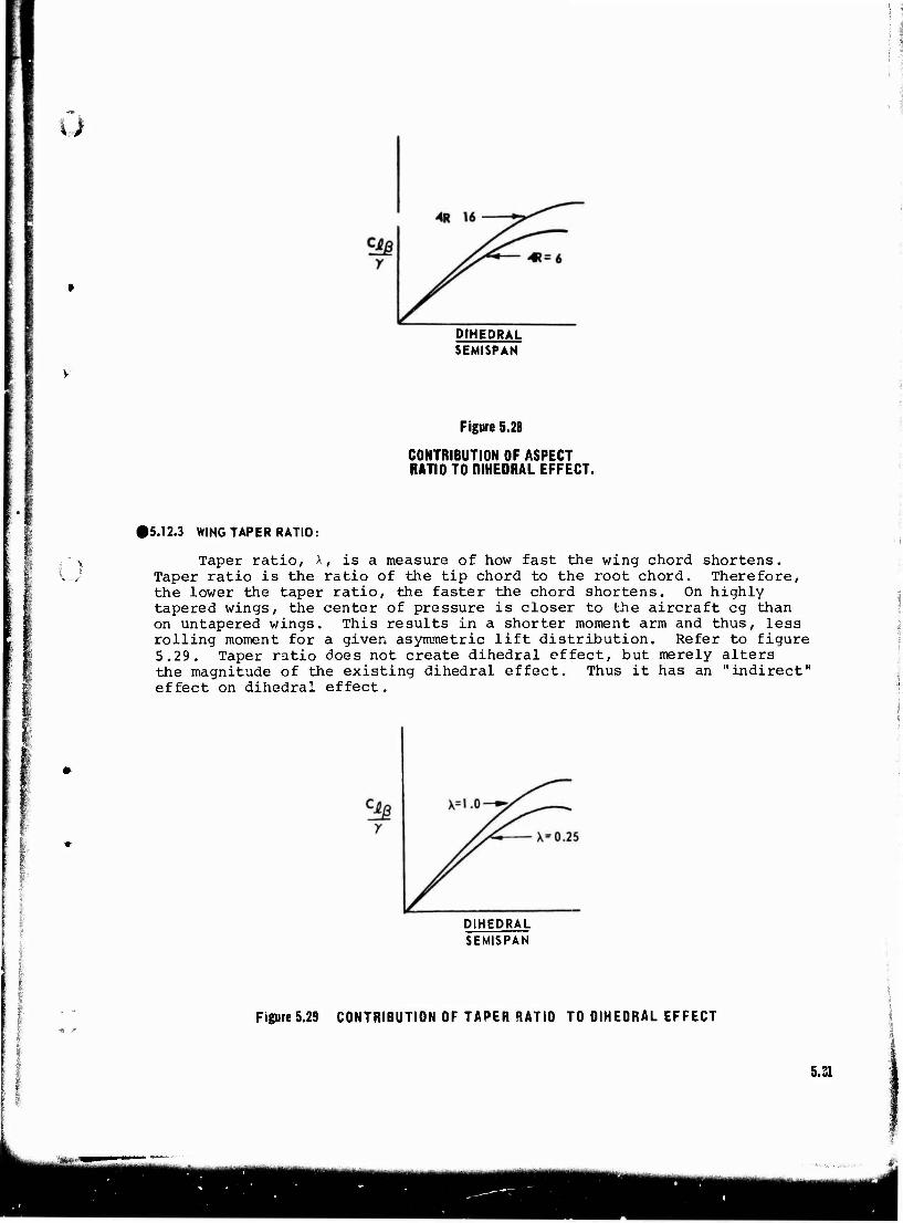
u

DIHEDRAL SEMISPAN

Figure 5.28

CONTRIBUTION OF ASPECT RATIO TO niHEDRAL EFFECT.

I

»5.12.3 WING TAPER RATIO:

Taper ratio, A, is a measure of how fast the wing chord shortens. Taper ratio is the ratio of the tip chord to the root chord. Therefore, the lower the taper ratio, the faster the chord shortens. On highly tapered wings, the center of pressure is closer to the aircraft eg than on untapered wings. This results in a shorter moment arm and thus, less rolling moment for a given asymmetric lift distribution. Refer to figure 5.29. Taper ratio does not create dihedral effect, but merely alters the magnitude of the existing dihedral effect. Thus it has an "indirect" effect on dihedral effect.

I f

DIHEDRAL SEMISPAN

Figure 5.29 CONTRIBUTION OF TAPER RATIO TO DIHEDRAL EFFECT

5.31

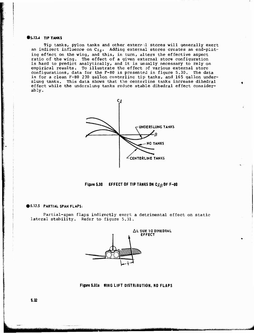
»5.12.4 TIP TANKS

Tip tanks, pylon tanks and other extern ;1 stores will generally exert an indirect influence on Cig. Adding external stores creates an end-plating effect on the wing, and this, in turn, alters the effective aspect ratio of the wing. The effect of a given external store configuration is hard to predict analytically, and it is usually necessary to rely on empirical results. To illustrate the effect of various external store configurations, data for the F-80 is presented in figure 5.30. The data is for a clean F-80 230 gallon centerline tip tanks, and 165 gallon underslung tanks. This data shows that the centerline tanks increase dihedral effect while the underslung tanks reduce stable dihedral effect considerably.

UNDERSLUNG TANKS

NO TANKS

CENTERLINE TANKS

Figure 5.30 EFFECT OF TIP TANKS ON Cjlß OF F-80

»5.12.5 PARTIAL SPAN FLAPS:

Partial-span flaps indirectly exert a detrimental effect on static lateral stability. Refer to figure 5.31.

AL DUE 10 DIHEDRAL EFFECT

Figure 5.31a WING LIFT DISTRIBUTION, NO FLAPS

5.32

«MM ii—mm- —- - ■ ^ -- .. ■■ ^t^nm

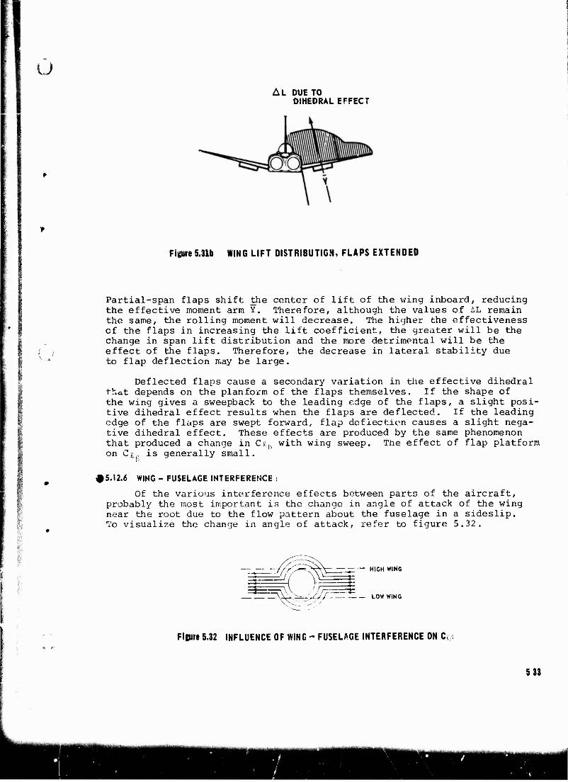
u AL DUE TO

DIHEDRAL EFFECT

Figure 5.31b WING LIFT DISTRIBUTION, FLAPS EXTENDED

Partial-span flaps shift the center of lift of the wing inboard, reducing the effective moment arm Y. Therefore, although the values of AL remain the same, the rolling moment will decrease. The higher the effectiveness of the flaps in increasing the lift coefficient, the greater will be the change in span lift distribution and the more detrimental will be the effect of the flaps. Therefore, the decrease in lateral stability due to flap deflection may be large.

Deflected flaps cause a secondary variation in the effective dihedral thdt depends on the planform of the flaps themselves. If the shape of the wing gives a sweepback to the leading edge of the flaps, a slight positive dihedral effect results when the flaps are deflected. If the leading edge of the flaps are swept forward, flap deflection causes a slight negative dihedral effect. These effects are produced by the same phenomenon that produced a change in Csh with wing sweep. The effect of flap platform on Cj, is generally small.

p

#5.12.6 WING - FUSELAGE INTERFERENCE :

Of the various interference effects between parts of the aircraft, probably the most important is the change in angle of attack of the wing near the root due to the flow pattern about the fuselage in a sideslip. To visualize the change in angle of attack, refer to figure 5.32.

U A If? ^UfZ

HIGH WING

. — LOW WING

Figure 5.32 INFLUENCE OF WING - FUSELAGE INTERFERENCE ON C

5 33

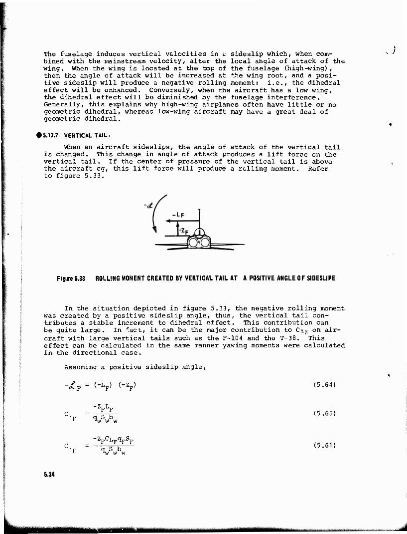
The fuselage induces vertical velocities in & sideslip which, when combined with the mainstream velocity, alter the local angle of attack of the wing. When the wing is located at the top of the fuselage (high-wing), then the angle of attack will be increased at the wing root, and a positive sideslip will produce a negative rolling moment: i.e., the dihedral effect will be enhanced. Conversely, when the aircraft has a low wing, the dihedral effect will be diminished by the fuselage interference. Generally, this explains why high-wing airplanes often have little or no geometric dihedral, whereas low-wing aircraft may have a great deal of geometric dihedral.

J

»5.12.7 VERTICAL TAIL:

When an aircraft sideslips, the angle of attack of the vertical tail is changed. This change in angle of attack produces a lift force on the vertical tail. If the center of pressure of the vertical tail is above the aircraft eg, this lift force will produce a rolling moment. Refer to figure 5.33.

Figure 5.33 ROLLING MOMENT CREATED BY VERTICAL TAIL AT A POSITIVE ANGLE OF SIDESLIPE

In the situation depicted in figure 5.33, the negative rolling moment was created by a positive sideslip angle, thus, the vertical tail contributes a stable increment to dihedral effect. This contribution can be quite large. In fact, it can be the major contribution to Cig on aircraft with large vertical tails such as the F-104 and the T-38. This effect can be calculated in the same manner yawing moments were calculated in the directional case.

Assuming a positive sideslip angle,

-*F " (' v <-v (5.64)

-ZFLF q S b ^w w w

(5.65)

■ZFCLFqFSF

~ q. s b V w w (5.66)

5.34

yM IMhjgMfciMI

Define Vp as,

SPZF

VF = /^- (5.67) w w

Assume that for a jet aircraft,

qF - % (5.68)

And equation 5.66 becomesf

% = - CLp VF = - aFaFVp (5.69)

Knowing

ap = (6 - a) (5.14)

CiF = - aFVp (ß - a) (5.70)

- arVr 1 - 42.I (5.71) pVertical tail

Equation 5.71 reveals that a vertical tail contributes a stable increment to Clo, whereas a ventral fin [Vp = (+)] would contribute an unstable increment to Cj, . Also, if the lift curve slope of the vertical tail is increased, by end plating for example, the stable dihedral effect would be greatly increased. For example, the F-104 has a high horizontal stabilizer that acts as an end plate on the vertical tail and this increases the stable dihedral effect. In fact, the increase is so large that it is necessary to add negative geometric dihedral to the wings and a ventral fin to maintain a reasonable value of stable dihedral effect.

15.13 C^a - LATERAL CONTROL POWER

Lateral control is achieved by altering the lift distribution so that the total lift on the two wings differ, thereby creatina a rolling moment. This may be done simply by destroying a certain amount of lift on one wing by means of a spoiler, or by altering the lift on both wings by means of ailerons. This discussion will be limited to the use of ailerons as the means of lateral control.

mmammmtmmm*mmmmm**m-~~~ mmmmmmmmm^mmm, , „J

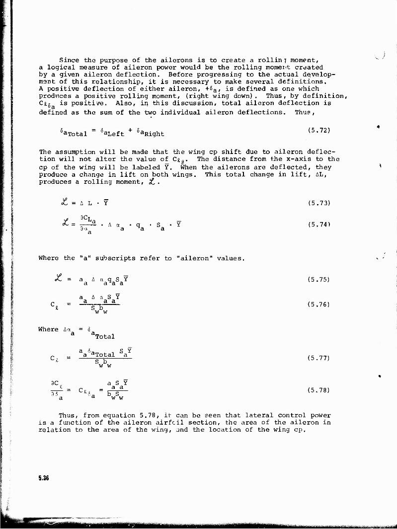
Since the purpose of the ailerons is to create a rolling moment, a logical measure of aileron power would be the rolling moniert created by a given aileron deflection. Before progressing to the actual development of this relationship, it is necessary to make several definitions. A positive deflection of either aileron, +Sa, is defined as one which produces a positive rolling moment, (right wing down) . Thus, by definition, CJU is positive. Also, in this discussion, total aileron deflection is defined as the sum of the two individual aileron deflections;. Thus*,

5aTotal = ä*Left + 6*Right (5,72)

The assumption will be made that the wing cp shift due to aileron deflection will not alter the value of CJU. The distance from the x-axis to the cp of the wing will be labeled Y. When the ailerons are deflected, they produce a change in lift on both wings. This total change in lift, AL, produces a rolling moment, £.

Z = A L • Y (5.73)

3CL

!

Z = - - • A a • q • S • Y (5.74) 3a a ^a a 5L

Where the "a" subscripts refer to "aileron" values,

£ = aa A aaqaSaY (5.75)

(5.76) C£ =

a A a S } a a a

S b w w

I

Where A<t a

= 6 Total

Cj = a aTotal S Y a

S b w w (5.77)

"w"w

f 3C a S Y

I TT = C^a = b¥- (5-78> a a w w

i: Thus, from equation 5.78, it can be seen that lateral control power

is a function of the aileron airfoil section, the area of the aileron in relation to the area of the wing, and the location of the wing cp.

5.36

tmmmmmmmmKmmmmmmtmmmimtmmimm, ,

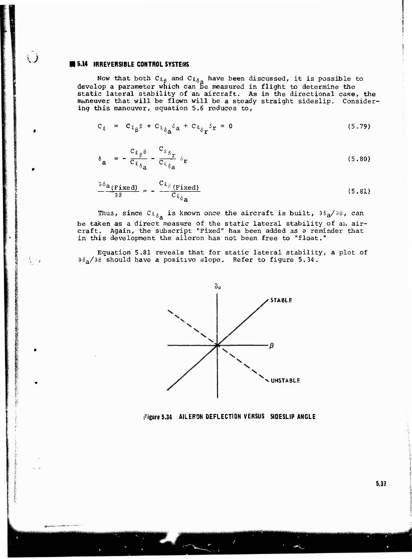
u 15.14 IRREVERSIBLE CONTROL SYSTEMS

Now that both Cjtg and Ci$ have been discussed, it is possible to develop a parameter which can Be measured in flight to determine the static lateral stability of an aircraft. As in the directional case, the maneuver that will be flown will be a steady straight sideslip. Consider- ing this maneuver, equation 5.6 reduces to,

= c» + C*6> + CJU 5r = 0 6r (5.79)

°r Cl— 6r (5.80)

i $

36 a(Fixed) 36

Ct 13 (Fixed) (5.81)

Thus, since CJU is known once the aircraft is built, 36a/3ß, can be taken as a direct measure of the static lateral stability of an aircraft. Again, the subscript "Fixed" has been added as o reminder that in this development the aileron has not been free to "float."

Equation 5.81 reveals that for static lateral stability, a plot of 9<5a/3ß should have a positive slope. Refer to figure 5.34.

Oa

STABLE

N UNSTABLE

Figure 5.34 AILERON DEFLECTION VERSUS SIDESLIP ANGLE

5.37

15.15 REVERSIBLE CONTROL SYSTEMS u It is now necessary to consider an aircraft with a reversible con-

trol system. On this type aircraft, the ailerons are free to float in response to their hinge moments. Using the same approach as in the directional case, it is possible to derive an expression that will relate the "Aileron Free" static lateral stability to parameters that can be easily measured in flight.

In a steady straight sideslip, 'Lit- 0. Therefore, it follows that £<£-., = 0. Now if moments are summed about the aileron hinge pin, Aileron Hinge Pin

the aileron force exerted by the pilot, Fa, acts through a moment arm and gearing mechanism, both accounted for by some constant, K, and must balance the other aerodynamic rolling moments so that Â;ieron

= 0- Thus, in steady straight flight, Hinge Pin

''"'Aileron Hinge Pin

— V — L • K + H, a a (5.82)

- G H (5.83)

Where 3 is merely 1/K,

Knowing.

H = C, q S c a h a a a (5.84)

From equation 5.26

H= = q, s, c, (chaa • aa + Ch5a ' «a> a a a (5.85)


F = - G q S C (Ch • a_ + Cn c • 6j a â a a "ota a "6a a (5.86)

From equation 5.27,

' S Ch,

Ch, &a> a(Float) (5.87)

equation 5.86 becomes,

G â Sa Ca ("Ch,. «a/?1^t) + Ch 1 a **) (5.88)

= - G q S c CK i* "a a a (Float) (5.89)

5.38

MttMli ■■'—- ■■—■'- -^--^^-^-^—■■* -*-■■

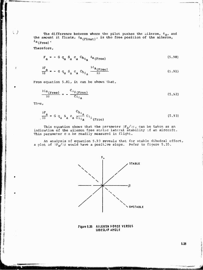
■$!9^?'!&!9*&mm§te&.i^.,_ %^..«.,

O The difference between where the pilot pushes the aileron, <5a, and the amount it floats, Öa/Fi t\t is the free position of the aileron, 6a(Free)*

Therefore,

F = - G q S c CK a a a a(Free) (5.90)

3Fa 36a(Free) —-a- = - G q S c Ch. ^^;- 33 ci a a n6a dß (5.91)

From equation 5.81, it can be shown that,

36a (Free) 3ß

^(Free) (5.92)

Th'is,

3F Ch, = G q S C

a a a CJU ^U (Frae)

(5.93)

This equation shows that the parameter 3Fa/3ü, can be taken as an indication of the aileron free static lateral stability of an aircraft. This parameter en be readily measured in flight.

An analysis of equation 5.9 3 reveals that for stable dihedral effect, a plot of 3Fa/3ß would have a positive slope. Pefer to figure 5.35.

STABLE

N UNSTABLE

Figure £.35 Al LERON FORCE VERSUS SIDESLIP ANGLE

5.39

-"-■-■ r*»**^™.-*™..:*,^»- *****

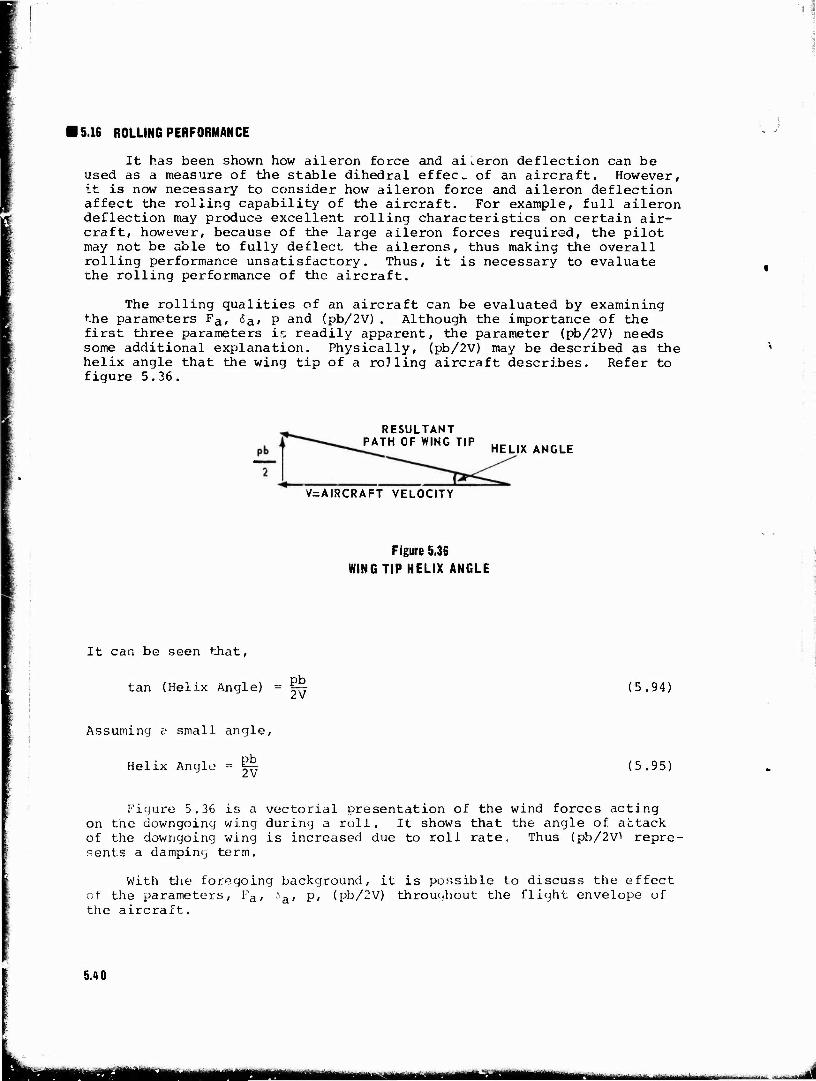
15.16 ROLLING PERFORMANCE

It has been shown how aileron force and ai i.eron deflection can be used as a measure of the stable dihedral effect of an aircraft. However, it is now necessary to consider how aileron force and aileron deflection affect the rolling capability of the aircraft. For example, full aileron deflection may produce excellent rolling characteristics on certain aircraft, however, because of the large aileron forces required, the pilot may not be able to fully deflect the ailerons, thus making the overall rolling performance unsatisfactory. Thus, it is necessary to evaluate the rolling performance of the aircraft.

The rolling qualities of an aircraft can be evaluated by examining the parameters Fa, Sa, p and (pb/2V). Although the importance of the first three parameters is readily apparent, the parameter (pb/2V) needs some additional explanation. Physically, (pb/2V) may be described as the helix angle that the wing tip of a rolling aircraft describes. Refer to figure 5.36.

RESULTANT PATH OF WING TIP

V=AIRCRAFT VELOCITY

HELIX ANGLE

Figure 5.36 WING TIP HELIX ANGLE

It can be seen that,

tan (Helix Angle) = - £b 2 V

(5.94)

Assuming v small angle,

Helix Angle = l^r (5.95)

Figure 5.36 is a vectorial presentation of the wind forces acting on the downgoing wing during a roll. It shows that the angle of attack of the downgoing wing is increased due to roll rate. Thus (pb/2V^ represents a damping term.

With the foregoing background, it is possible to discuss the effect of the parameters, Fa, 6a, p, (pb/2V) throughout the flight envelope of the aircraft.

5.40

hs^ «Mtai ^M liu ..»^ -,v. ...v,..,, „^.,W.„. .^.:,..:,..:..

u From equation 5.90, it can be seen that

Fa " (f) V 6a(Free)

6a(Free) " (f) Fa ^2

(5.96)

(5.97)

To derive a functional relationship for (pb/2V), it is necessary to start with,

/N ^ d = C£gß + Cjgß + Cnp p + Cnr r + Cn& 6a + Cn& &r (5.6)

and examine the effects of roll terms only, i.e., assume that the roll moment developed is due to the interaction of moments due to 6a and roll damping only. Therefore, equation 5.6 becomes,

S* Dh C* = C£p p + Ci&a&a = Clp (|^) + c^ 6

Va (5.98)

Below Mach or aerolastic effects, C# = constant, so if it is desired Max to evaluate an aircraft's maximum rolling performance, equation 5.98 becomes,

i i i % <^» + c I 6a = constant 15.99)

Constant - Cs &a

2V C*n (5.100)

<§> - <« 5a (5.101)

From equation 5.9 7,

(§> - (f) 6a = (f) Fa ^2 (5.102)

A function relationship for roll rate, p, can be derived from equation 5.100,

f Constant - Co 6a

P = !•' [5.103)

i

\ I P = (f) V h. (5.104)

5.41

hü ■tt

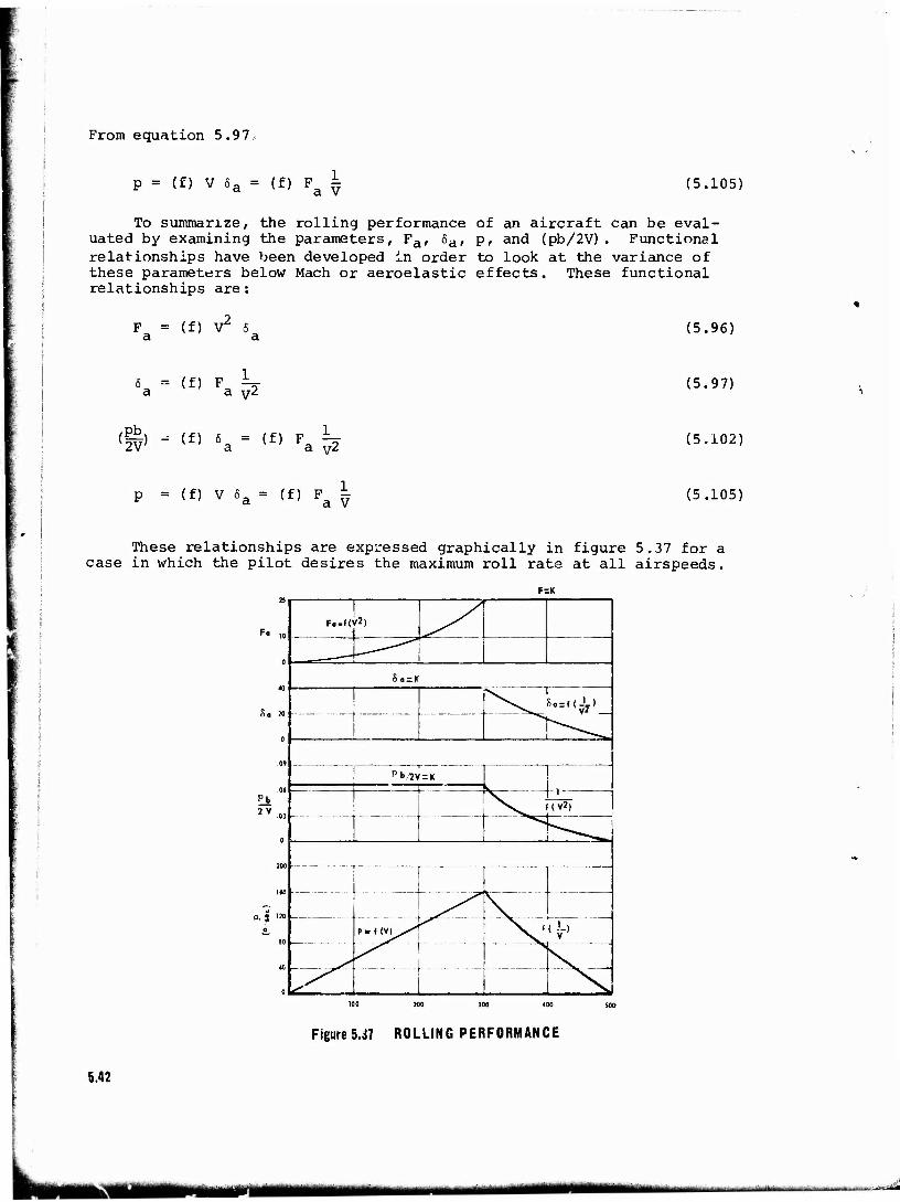
From equation 5.97

p = (f) V 6a = (f) Fa £ (5.105)

To summarize, the rolling performance of an aircraft can be evaluated by examining the parameters, Fa, 6a, p, and (pb/2V). Functional relationships have been developed in order to look at the variance of these parameters below Mach or aeroelastic effects. These functional relationships are:

(5.96)

(5.97)

(5.102)

(5.105)

These relationships are expressed graphically in figure 5.37 for a case in which the pilot desires the maximum roll rate at all airspeeds.

Fa = !

(f) V s a

t 6 = a

(f) F V a v2

(Pb) ^ V2V; (f) 6 a = (f) Fa ~2

P = (f) V 6a - (f) Fa i

25

Fo |0

F: :K

Fo.f< ,,

0

8<.=r

So »

0

•S. S. = ,(J7)

P b/jv = K

Pb 2V 03

\^ <V2)

»«^^ 1

— X 0. J 1»

o

*T

V^ 40

0

--V-—-

5.42

Figure 5.37 ROLLING PERFORMANCE

mm mm — a—Mi»Urinim .-^,-ti ,■„.-. —-..., -

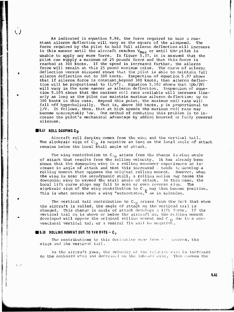
u As indicated in equation 5.9 6, the force required to hold a con-

stant aileron deflection will vary as the square of the airspeed. The force required by the pilot to hold full aileron deflection will increase in this manner until the aircraft reaches VMax or until the pilot is unable to apply any more force. In figure 5.37, it is assumed that the pilot can supply a maximum of 25 pounds force and that this force is reached at 300 knots. If the speed is increased further, the aileron force will remain at this 25 pound maximum value. The curve of aileron deflection versus airspeed shows that the pilot is able to maintain full aileron deflection out to 300 knots. Inspection of equaLion 5.97 shows that if aileron force is constant beyond 300 knots, then aileron deflection will be proportional to (1/V ). Equation 5.102 shows that (pb/2V) will vary in the same manner as aileron deflection. Inspection of equation 5.105 shows that the maximum roll rate available will increase linearly as long as the pilot can maintain maximum aileron deflection; up to 300 knots in this case. Beyond this point, the maximum roll rate will fall off hyperbolically. That is, above 300 knots, p is proportional to 1/V. It fellows, then, that at high speeds the maximum roll rate may become unacceptably low. One method of combating this problem is to increase the pilot's mechanical advantage by adding boosted or fully powered ailerons.

15.17 ROLL DAMPING Cap

Aircraft roll damping comes from the winy and the vertical tail. The algebraic sign of Cj is negative as long as the local angle of attack remains below the local stall angle of attack.

The wing contribution to C;D arises from the change in winy angle of attack that results from the rolling velocity. It has already been shown that the donwgoing wing in a rolling maneuver experiences an increase in angle of attack and that this increased .< tends to develop a rolling moment that opposes the original rolling moment. However, when the wing is near the aerodynamic stall, a rolling motion may cause the downgoiny wing to exceed the stall angle of attack. In this case, the local lift curve slope may fall to zero or even reverse sign. The algebraic sign of the wing contribution to C, may then become positive. This is what occurs when a wing "autorotates, as in spinning.

The vertical tail contribution to Cy.p arises from the fact that when the aircraft is rolled, the angle of attack on the vertical taxi is changed. This change in angle of attack develops a lift force. If the vertical tail eg is above or below the aircraft eg, the rolling moment developed will oppose the original rolling moment and C. f) due to a conventional vertical taix or a ventral fin will be negative.

| 015.18 ROLLING MOMENT DUE TO YAW RATE-Cr

The contributions to this derivative come from r sources, the | wings and the vertical tail.

As the aircraft yaws, the velocity of the relative wind is increased on the outboard wing and decreased on the inboard winy. This causes the

5.43

UMMHIBIIRIlMMmuwmsumamimmMmJKBMRMtnmwir ■ ■-*

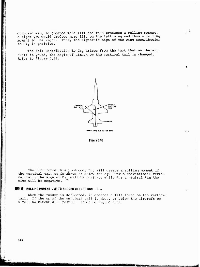
outboard wing to produce more lift and thus produces a rolling moment. A right yaw would produce more lift on the left wing and thus a rolling moment to the right. Thus, the algebraic sign of the wing contribution to Ci.r is positive.

The tail contribution to Cir arises from the fact that as the aircraft is yawed, the angle of attack on the vertical tail is changed. Refer to figure 5.38.

COMPONENT » — DUE TO TAW V'

RATF/X aF

CHANGE l»aF DUE TOY«! RATE

Figure 5.38

I

The lift force thus produced, Lp, will create a rolling moment if the vertical tail eg is above or below the eg. For a conventional vertical tail, the sign of Cfr will be positive while for a zentral fin the sign will be negative.

15.19 ROLLING MOMENT DUE TO RUDDER DEFLECTION - C r

When the rudder is deflected, it creates a lift force on the vertical tail. If the cp of the vertical tail is above or below the aircraft eg a rolling moment wil] result. Refer to figure 5.39.

5.44

IflgUgjifrlfcggll^Hg,^^ -..,^-jdÜ

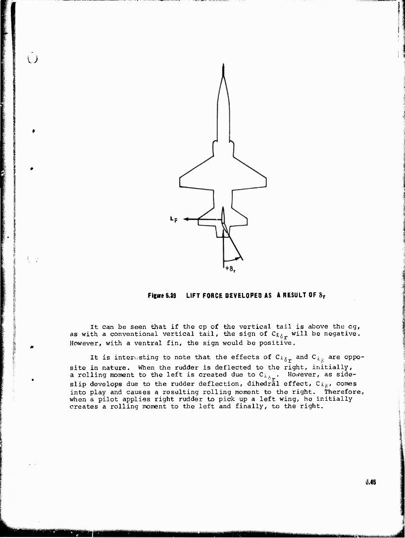
u ; I

:

Figure 5.39 LIFT FORCE DEVELOPED AS A RESULT OF 8,

It can be seen that if the cp of the vertical tail is above the eg, as with a conventional vertical tail, the sign of d& will be negative. However, with a ventral fin, the sign would be positive.

It is interesting to note that the effects of Cn6 and C^ are opposite in nature. When the rudder is deflected to the right, initially, a rolling moment to the left is created due to Cr . However, as side- ör slip develops due to the rudder deflection, dihedral effect, Cjg, comes into play and causes a resulting rolling moment to the right. Therefore, when a pilot applies right rudder to pick up a left wing, he initially creates a rolling moment to the left and finally, to the right.

Ü.45

UMMM ";—■---"

15.20 ROLLING MOMENT DUE TO LAG EFFECTS IN SIDEWASH -C > In the discussion of Cn«, it was pointed out that during an increase

in (3, the angle of attack of the vertical tail will be less than it will finally be in steady state conditions. If the cp of the vertical tail is displaced from the aircraft eg, this change in ap due to lag effects will alter the rolling moment created during the 3 build up period. Be- cause of lag effects, Cp will be less during the ß build up period than at steady state. Thus, for a conventional vertical tail, the algebraic sign of C,- is positive.

me Again, it should be pointed out that there is widespread disagree-

nt over the interpretation of data concerning lag effects in sidewash and that the foregoing is only one basic approach to a many faceted and complex problem.

B 5.21 HIGH SPEED CONSIDERATIONS OF STATIC LATERAL STABILITY

C, . - Generally, CJI„ is not greatly affected by Macn number. How- ever, in the transonic region the increase in the lift curve slope of the vertical tail increases this contribution to Cj,„ and usually results in an overall increase in Cz,: in the transonic region.

C, - Because of the decrease in the lift curve slope of all aerodynamic surfaces in supersonic flight, lateral control power decreases ds Mach number increases supersonically.

Aeroelasticity problems have been qu: ':e predominant in the lateral control system, since in flight at very high dynamic pressures the wing torsional deflections which occur with aileron usage are considerable and cause noticeable changes in aileron effectiveness. At some high dynamic pressures, dependent upon the given wing structural integrity, the twisting deformation might be gre«t enough to nullify the effect of aileron deflection and the aileron effectiveness will be reduced to zero. Since at speeds above the poinc where this phenomenon occurs, rolling moments are created which are opposite in direction to the control deflection, this speed is termed "aileron reversal speed." In order to alleviate this characteristic the wing must have a high torsional stiffness which presents a significant design problem in sweptwing aircraft. For an aircraft design of the B-47 type, it is easy to visualize how aeroelastic distortion might result in a considerable reduction in lateral control capability at high speeds. In addition, lateral control effectiveness at transonic Mach numbers may be reduced seriously by flow separation effects as ä result of shock formation. However, modern high speed fighter designs have been so successful in introducing sufficient rigidity into wing structures and employing such design modifications as split ailerons, inboard ailerons, spoiler systems, etc., that the resulting high control power, coupled with the low C,p of low aspect ratio planforms, has resulted in the lateral control becoming an accelerating dc'ite rather than a rate control. That is to say, a steady state rolling velocity is normally not reached prior to attaining the desired bank angle. Consequently, many high speed aircraft have a type of differential aileron system to pru'/ide the pilot with much more control surface during approach and Ian.turns and to restrict, his degree of control in other areas of flight.

5.46

lumutmmtmmmmmmimmmMi

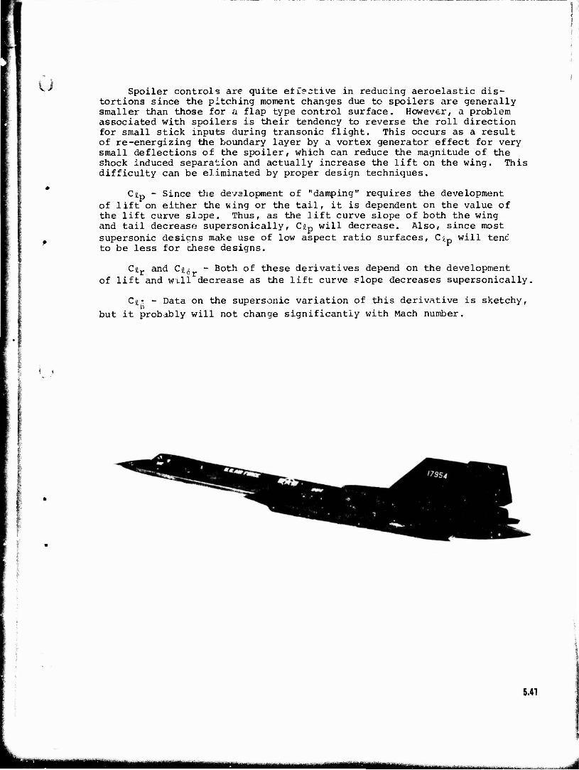
u Spoiler controls are quite effective in reducing aeroelastic dis- tortions since the pitching moment changes due to spoilers are generally smaller than those for a flap type control surface. However, a problem associated with spoilers is their tendency to reverse the roll direction for small stick inputs during transonic flight. This occurs as a result of re-energizing the boundary layer by a vortex generator effect for very small deflections of the spoiler, which can reduce the magnitude of the shock induced separation and actually increase the lift on the wing. This difficulty can be eliminated by proper design techniques.

< i

Cüp - Since the development of "damping" requires the development of lift on either the wing or the tail, it is dependent on the value of the lift curve slope. Thus, as the lift curve slope of both the wing and tail decrease supersonically, C£p will decrease. Also, since most supersonic designs make use of low aspect ratio surfaces, Cjtp will tend to be less for these designs.

Cjtr and Cj.,5 - Both of these derivatives depend on the development of lift and will decrease as the lift curve slope decreases supersonically,

cr< Data on the supersonic variation of this derivative is sketchy,

but it probably will not change significantly with Mach number.

5.47

■MMM mm .... MM

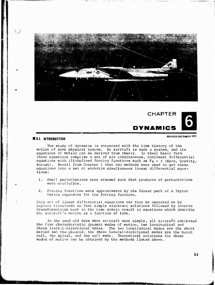
K )

CHAPTER

DYNAMICS m 6.1 INTRODUCTION

REVISED DECEMBER 1973

The study of dynamics is concerned with the time history of the motion of some physical system. An aircraft is such a system, and its equations of motion can be derived from theory. In their basic form these equations comprise a set of six simultaneous, nonlinear differential equations with ill-defined forcing functions such as Fx = f (Aero, Gravity, Thrust). Recall from Chapter 1 that two methods were used to get these equations into a set of workable simultaneous linear differential equations :

1. Small perturbations were assumed such that products of perturbations were negligible.

2. Forcinq functions were approximated by the linear part of a Taylor Series expansion for the forcing function.

This set of linear differential equations can then be operated on by Laplace transforms so that simple algebraic solutions followed by inverse transformations back to the time domain result in equations which describe the aircraft's motion as a function of time.

In the good old days when aircraft were simple, all aircraft exhibited the five characteristic dynamic modes of motion, two longitudinal and three lateral-directional modes. The two longitudinal modes are the short period and the phuyoid; the three lateral-directional modes are the Dutch roll, the spiral, and the roll mode. Theoretical solutions for these modes of motion can be obtained by the methods listed above.

6.1

mm aBMH MMMM

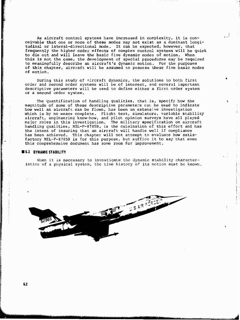
As aircraft control systems have increased in complexity, it is con- ceivable that one or more of these modes may not exist as a dominant longitudinal or lateral-directional mode. It can be expected, however, that frequently the higher order effects of complex control systems will be quick to die out and will leave the basic five dynamic modes of motion. When this is not the case, the development of special procedures may be required to meaningfully describe an aircraft's dynamic motion. For the purposes of this chapter, aircraft will be assumed to possess these five basic modes of motion.

During this study of aircraft dynamics, the solutions to both first order and second order systems will be of interest, and several important descriptive parameters will be used to define either a first order system or a second order system.

The quantification of handling qualities, that is, specify how the magnitude of some of these descriptive parameters can be used to indicate how well an aircraft can be flown, has been an extensive investigation which is by no means complete. Flight test, simulators, variable stability aircraft, engineering know-how, and pilot opinion surveys have all played major roles in this investigation. The military specification on aircraft handling qualities, MIL-F-8785B, is the culmination of this effort and has the intent of insuring that an aircraft will handle well if compliance has been achieved. This chapter will not attempt to evaluate how satisfactory MIL-F-8785B is for this purpose, but suffice it to say that even this comprehensive document has some room for improvement.

16.2 DYNAMIC STABILITY

When it is necessary to investigate the dynamic stability characteristics of a physical system, the time history of its motion must be known.

6.2

mum

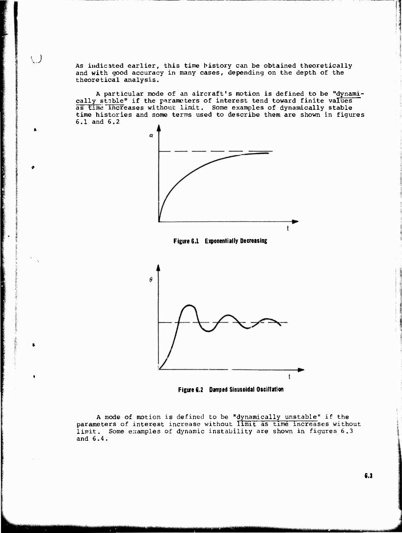
I'

ü As indicated earlier, this time history can be obtained theoretically and with good accuracy in many cases, depending on the depth of the theoretical analysis.

A particular mode of an aircraft's motion is defined to be "dynamically stable" if the parameters of interest tend toward finite values as time increases without limit. Some examples of dynamically stable time histories and some terms used to describe them are shown in figures 6.1 and 6.2

Figure 6.1 Exponentially Decreasing

( K

Figure 6.2 Damped Sinusoidal Oscillation

A mode of motion is defined to be "dynamically unstable" if the parameters of interest increase without limit as time increases without limit. Some examples of dynamic instability are shown in figures 6.3 and 6.4.

6.3

"^-■■"-"- i

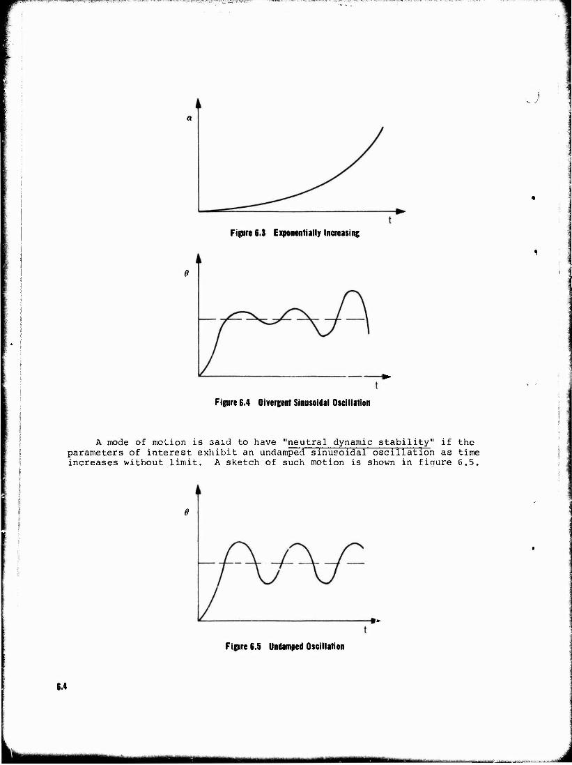
','(«.—.. ■ W'3*~~" " "■'.^'^.ÄW*^-^,,r^'l'v'i,^--<^^7yf5';"T[ ^■™irr~^-?-**yxzw-*>.'-t-,' ; .-3T-~T-.—r>.-^-=*-*i^-^,.,n*(.!iu,u» i.^^—^TT:-~f—"^.-r* 'M '■■i*'—^' ■■ ■'- T^-~.-' ^(T°.r-

i

Figure 6.3 Exponentially Increasing

Figure 6.4 Divergent Sinusoidal Oscillation

A mode of motion is said to have "neutral dynamic stability" if the parameters of interest exhibit an undamped sinusoidal oscillation as time increases without limit. A sketch of such motion is shown in figure 6.5.

Figure 6.5 Undamped Oscillation

6.4

MHM

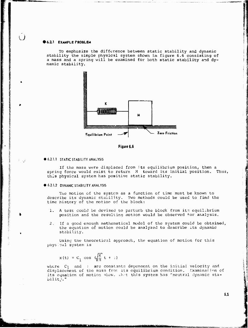
ü • 6.2.1 EXAMPLE PROBLEM

I

To emphasize the difference between static stability and dynamic stability the simple physical system shown in figure 6.6 consisting of a mass and a spring will be examined for both static stability and dynamic stability.

Zero Friction

Figure 6.6

• 6.2.1.1 STATIC STABILITY ANALYSIS

I

If the mass were displaced from 5ts equilibrium position, then a spring force would exist to return M toward its initial position. Thus, this physical system has positive static stability.

• 6.2.1.2 DYNAMIC STABILITY ANALYSIS

Tne motion of the system as a function of time must be known to describe its dynamic stability. Two methods could be used to find the time history of the motion of the block:

1. A test could be devised to perturb the block from its equilibrium position and the resulting motion would be observed for analysis.

2, If a good enough mathematical model of the system could be obtained, the equation of motion could be analyzed to describe its dynamic stability.

Using the theoretical approach, the equation of motion for this phys'.cal system is

x(t) ci cos {VM

t +

where C^ and : are constants dependent on the initial velocity and displacement of the mass fror, its equilibrium condition. Dxam.inat i on of its equation of motion shov. Ji't this system has "neutral dynamic sta- bilit/."

S.5

IMWH I mMM —,-,

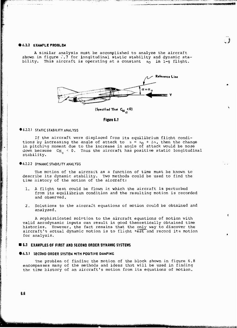
vy-7irv*r**7j^*F!^ ^=*Tv '«•;!-—■STT^^-'?'-,T7-TT^»V;T---<^^ ■■ ■--■'. -j—,■ >i7-;«-T*"."-"■ ' "fV;"1''

• 6.2.2 EXAMPLE PROBLEM

A similar analysis must be accomplished to analyze the aircraft shown in figure C,7 for longitudinal static stability and dynamic stability. This aircraft is operating at a constant aQ in 1-g flight.

3

Reference Line

(Specified That C. <0)

Figure 6.7

• 6.2.2.1 STATIC STABILITY ANALYSIS

If the aircraft were displaced from its equilibrium flight conditions by increasing the angle of attack to a = a. + Aa, then the change in pitching moment due to the increase in angle of attack would be nose down because stability.

CM < 0. Tnus the aircraft has positive static longitudinal

• 6.2.2.2 DYNAMIC STABILITY ANALYSIS

The motion of the aircrart as a function of time must be known to describe its dynamic stability. Two methods could be used to find the time history of the motion of the aircraft:

1. A flight test could be flown in which the aircraft is perturbed from its equilibrium condition and the resulting motion is recorded and observed.

2. Solutions to the aircraft equations of motion could be obtained and analyzed.

A sophisticated solution to the aircraft equations of motion with valid aerodynamic inputs can result in good theoretically obtained time histories. However, the fact remains that the only way to discover the aircraft's actual dynamic motion is to flight test and record its motion for analysis.

■ 6.3 EXAMPLES OF FIRST AND SECOND ORDER DYNAMIC SYSTEMS

• 6.3.1 SECOND ORDER SYSTEM WITH POSITIVE DAMPING

Tne problem of finding the motion of the block shown in figure 6.8 encompasses many of the methods and ideas that will be used in finding the time history of an aircraft's motion from its equations of motion.

6.6

mmmmmm

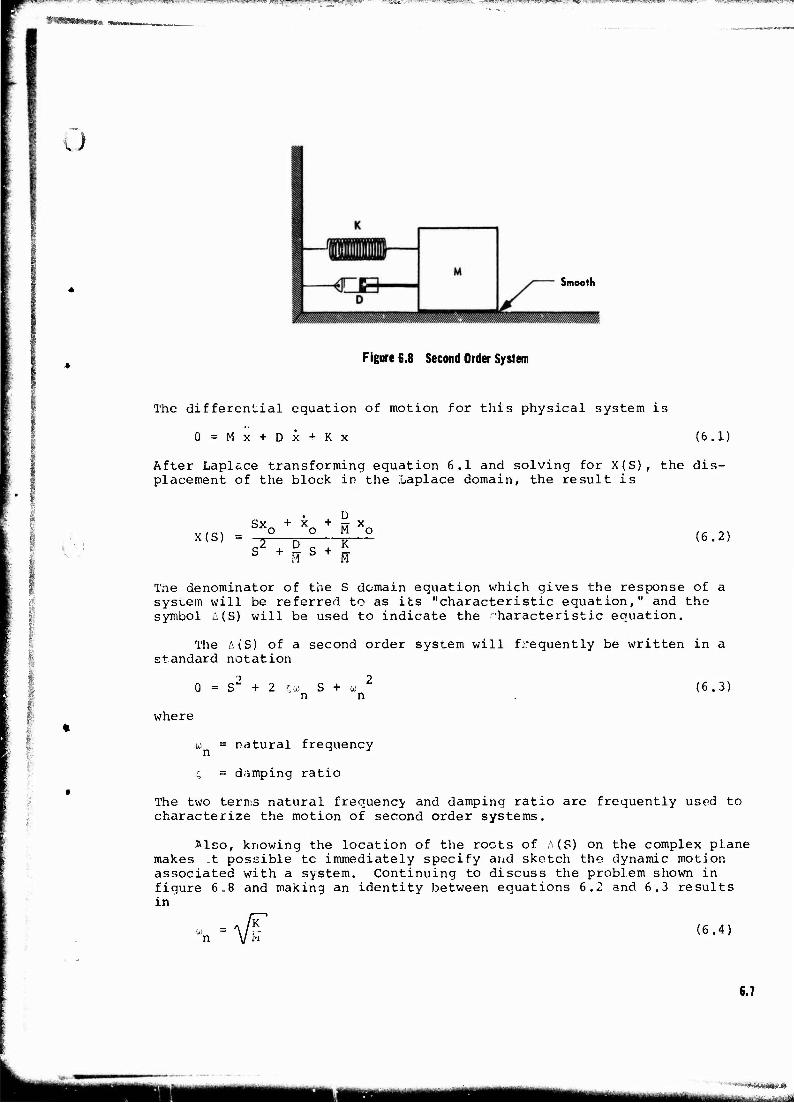
WMMMMftft Tw*»«,,»,,,,,,

_,i--,T^;»r^^,---^¥--.-.-^r---.^:J.,-.ir^-:--w3-^.,i.,- ■■:•■■•- :,-,- ._ ,—:„_ V_T ^„„.-„.^^

: u

Smooth

Figure 6.8 Second Order System

The differential equation of motion for this physical system is

0=Mx + Dx + Kx (6.1)

After Laplace transforming equation 6.1 and solving for X(S), the displacement of the block in the Laplace domain, the result is

I I

&;

\ I

X(S) =

D Sxo + Xo + M Xo

s21 § s; j M M

(6.2)

The denominator of the S domain equation which gives the response of a system will be referred to as its "characteristic equation," and the symbol MS) will be used to indicate the -haracteristic equation.

The A(S) of a second order system will frequently be written in a standard notation

2 2 0 = S + 2 ;u> S + u n n (6.3)

where

u = natural frequency

z, = damping ratio

The two terms natural frequency and damping ratio are frequently used to characterize the motion of second order systems.

Also, knowing the location of the roots of A(S) on the complex plane makes -t possible to immediately specify and sketch the dynamic motion associated with a system. Continuing to discuss the problem shown in figure 6„8 and making an identity between equations 6.2 and 6.3 results in

iii — n (6.4)

6.7

MüMlIIMIIIiÜMi w»

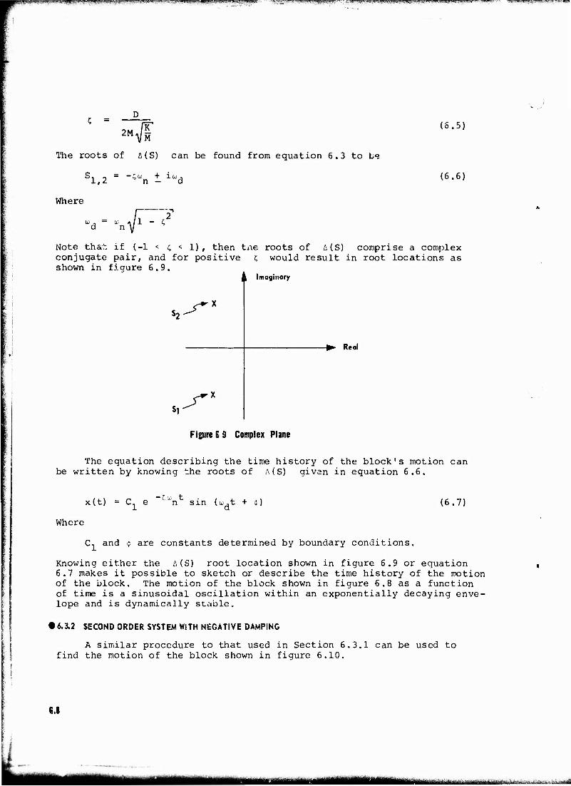
PMPWWPi.mWB^pBBpjWWpW—JpBII'pawnPB vmH!WWW-)IP ■" ■"■"- "■*,.. ».WJ ■ "">T" "•' • "'■' '.''^WW,"- -A»"»¥"-J!?-"-«vwi>«,>'."'»:,"iJ!».'>»'l.<"«,i|.,<.«i,p»|ii.i»»...i»p»

c = 2M VM

(6.5)

The roots of A{S) can be found from equation 6.3 to be

'1,2 o + i a) _, n — d

(6.6)

Where

0) . = w d »V Note that if (-1 < z, < 1) , then trie roots of A(S) comprise a complex conjugate pair, and for positive t, would result in root locations as shown in figure 6.9.

i i Imaginary

-► Real

Figure E 9 Complex Plane

The equation describing the time history of the block's motion can be written by knowing the roots of MS) given in equation 6.6.

x(t) = C, e ~ "u'n sin (w,t + t) 1 a (6.7)

Where

C, and $ are constants determined by boundary conditions.

Knowing either the A(S) root location shown in figure 6.9 or equation 6.7 makes it possible to sketch or describe the time history of the motion of the block. The motion of the block shown in figure 6.8 as a function of time is a sinusoidal oscillation within an exponentially decaying envelope and is dynamically stable.

• 6.3.2 SECOND ORDER SYSTEM WITH NEGATIVE DAMPING

A similar procedure to that used in Section 6.3.1 can be used to find the motion of the block shown in figure 6.10.

6.8

I i i nil MMmLL^t-.-^.i-L... ,<■■-.,

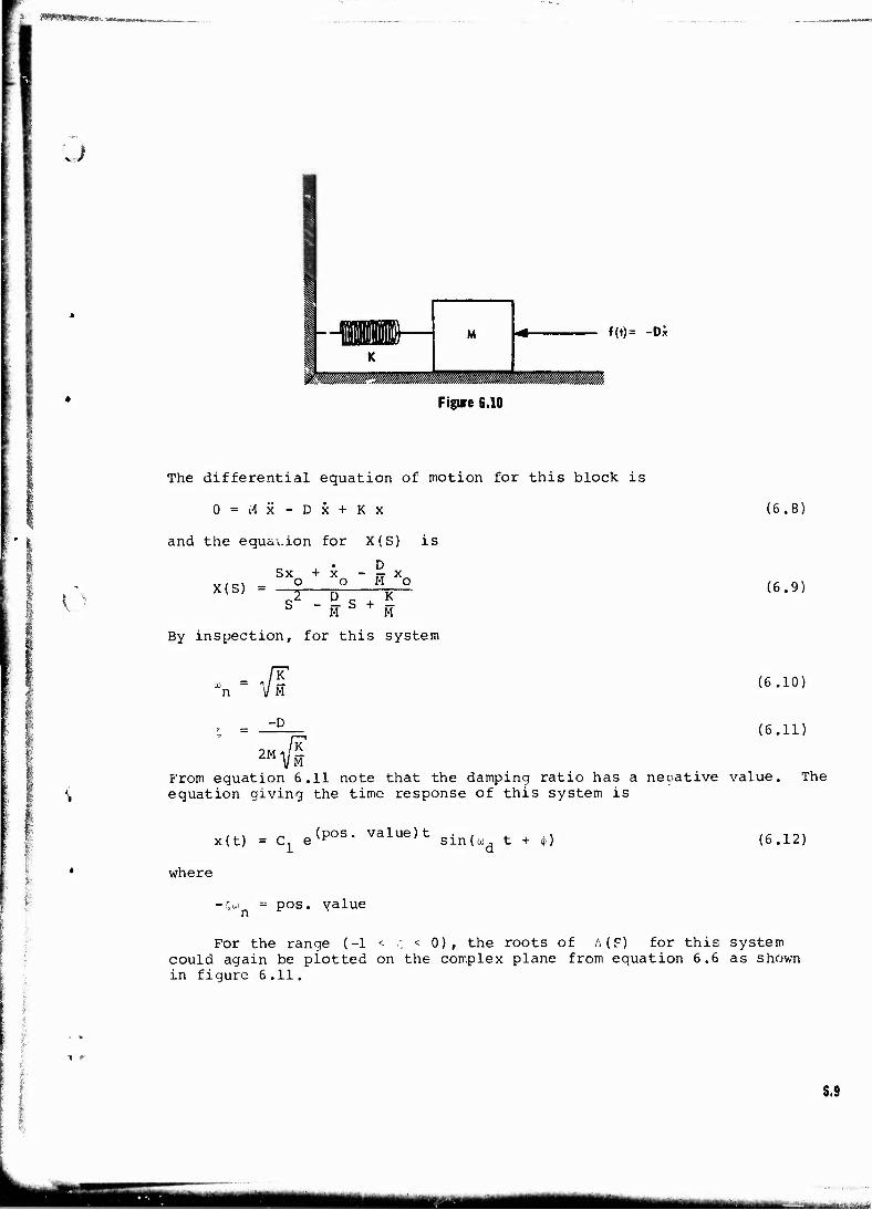
?■ tmrmmmam*\m

' I

1 1

4 UHU M

W/MWW/KfflWM

|j 1HIKI

wmmmmm.

f(t)= -D;

Figure 6.10

The differential equation of motion for this block is

0 = Mx-Dx+Kx

and the equation for X(S) is

X(S) Sx + X - rr X

o o M o

s2 - % S I g M M

(6.8)

(6.9)

By inspection, for this system

-D

2MV^

(6.10)

(6.11)

From equation 6.11 note that the damping ratio has a negative value. The equation giving the time response of this system is

,., „ (pos. value)t . , . . ,, x(t) = C, e r sin(üjj t + $) (6.12)

where

•c,u = pos. value

For the range (-1 < c, < 0), the roots of A(F) for this system could again be plotted on the complex plane from equation 6.6 as shown in figure 6.11.

5.9

HE ■BOH tmaim^mmmmmm mmmm*m,ui 11 in,!

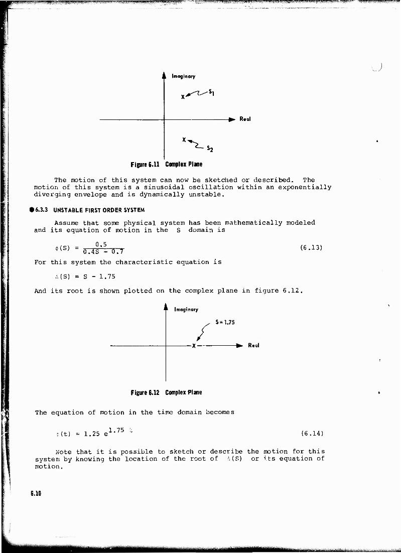
Jm,lll»i«J»|i i. "«»j.JHfliJ.i i.. i jj^ippjpwwwwpgpBrp-"''T%;.'" "wwgffWiw "■ **■'"" *"*''■''-• -w"-1" ■'■' T* WIJ»* -W**»»1 -^BW^W»WW

I L Imaginary

HP*. Real

"^

Figure 6.11 Complex Plane

The motion of this system can now be sketched or described. The motion of this system is a sinusoidal oscillation within an exponentially diverging envelope and is dynamically unstable.

• 6.3.3 UNSTABLE FIRST ORDER SYSTEM

Assume that some physical system has been mathematically modeled and its equation of motion in the S domain is

MS) = 0.5 0.4S - 0.7

(6.13)

For this system the characteristic equation is

MS) = S - 1.75

And its root is shown plotted on the complex plane in figure 6.12.

li I magmary

S=1.75

-► Real

Figure 6.12 Complex Plane

The equation of motion in the time domain becomes

1 75 - <(t) - 1.25 e1''3 " (6.14)

Note that it is possible to sketch or describe the motion for this system by knowing the location of the root of MS) or its equation of motion.

6.10

J

«MÜMMMÜ ammaUTm»'intmma«tXmmii, - ■ - - — — '■'■■■■■'

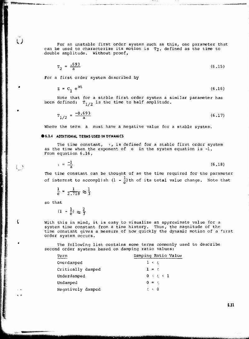
W &l&KWmt**lra*. j^m „ __.

W For an unstable first order system such as this, one parameter that can be used to characterize its motion is T2, defined as the time to double amplitude. Without proof,

i )

r

T = -693 l2 " a

For a first order system described by

Z = C± eat

(6.15)

(6.16)

Note that for a stable first order system a similar parameter has been defined: T, ,, is the time to half amplitude,

-0.693 1/2 (6.17)

Where the term a must have a negative value for a stable system.

• 6.3.4 ADDITIONAL TERMS USED IN DYNAMICS

The time constant, x, is defined for a stable first order system as the time when the exponent of e in the system equation is -1. From equation 6.16,

-1 a (6.18)

The time constant can be thought of as the time required for the parameter

of interest to accomplish (1 - —) th of its total value change. Note that

1 e 2.718

f

so that

(1 1. 2 e> * T

With this in mind, it is easy to visualize an approximate value for a system time constant from a time history. Thus, the magnitude of the time constant gives a measure of how quickly the dynamic motion of a first order system occurs.

The following list contains some terms commonly used to describe second order systems based on damping ratio values:

Term

Overdamped

Critically damped

Underdamped

Undamped

Negatively damped

Damping Ratio Value

1 < t.

1 = rp

0 < c < 1

0 = r,

r, < 0

6.11

teuMMMMMM ---■"■■'•■ BBJüiB)feafcaiai& ■

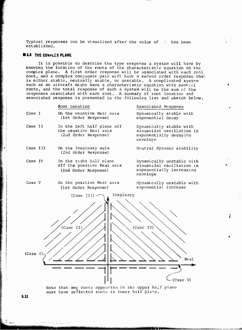
Typical responses can be visualized after the value of established.

has been

IM THE COMPLEX PLANE

It is possible to describe the type response a system will have by knowing the location of the roots of its characteristic equation on the complex plane. A first order response will be associated with each real root, and a complex conjugate pair will have a second order response tha'; is either stable, neutrally stable, or unstable. A complicated system such as an aircraft might have a characteristic equation with severed roots, and the total response of such a system will be the sum of the responses associated with each root. A summary of root location and associated response is presented in the following list and bketch below.

Case I

Root Location

On the negative Rea] axis (1st Order Response)

Associated Response

Dynamically stable with exponential decay

Case II In the left half plane off the negative Real axis (2nd Order Response)

Dynamically stable with sinusoidal oscillation in exponentially decaying envelope

Case III On the Imaginary axis (2nd Order Response)

Neutral dynamic stability

Case IV In the right half plane off the positive Real axis (2nd Order Response)

Dynamically unstable with sinusoidal oscillation in exponentially increasing envelope

Case V

S

(Case I)

On the positive Real axis (1st Order Response)

Dynamically unstable with exponential increase

Imaginary

(Case V)

Note that any roots appearing in the upper half plane must have reflected roots in lower half pla-.e.

S.12

'—

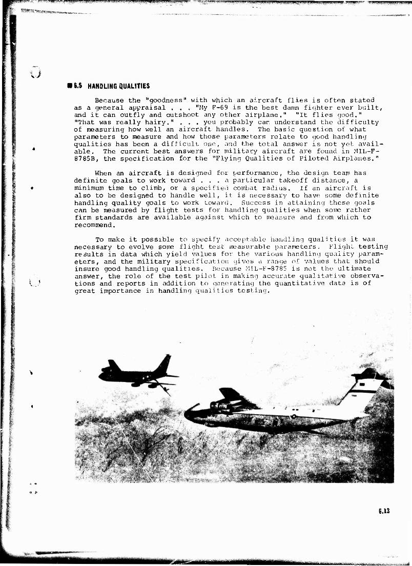
m,wmtm»">!",mi<im

^fH^y^itumiamm^^^...

JiWl!UWJ,l'j,".l-«ttw.B!'»ll>iJ« """-Tr^;;*""-JJ ] "* »Hi "L<'l»-l-'-0™^WT'!WPlwmqp»^!PliqmPiB!WW|i.ll )■ ..II.U '■■ ' "

U IS.5 HANDLING QUALITIES

Because the "goodness" with which an aircraft flies is often stated as a general appraisal . . . "My F-69 is the best damn fighter ever built, and it can outfly and outshoot any other airplane." "It flies good." "That was really hairy." . . . you probably car. understand the difficulty of measuring how well an aircraft handles. The basic question of what parameters to measure and how those parameters relate to qood handling qualities has been a difficult one, and the total answer is not yet available. The current best answers for military aircraft are found in MIL-F- 8785B, the specification for the "Flying Qualities of Piloted Airplanes."

When an aircraft is designed for performance, the design team has definite goals to work toward ... a particular takeoff distance, a minimum time to climb, or a specified combat radius. If an aircraft is also to be designed to handle well, it is necessary to have some definite handling quality goals to work toward. Success in attaining these goals can be measured by flight tests for handling qualities when some rather firm standards are available against v/hich to measure and from which to recommend.

To make it possible to specify acceptable handling qualities it was necessary to evolve some flight test measurable parameters. Flight testing results in data which yield values for the various handling quality parameters, and the military specification gives a range of values that should insure good handling qualities. Because MIL-F-8785 is not the ultimate answer, the role of the test pilot in making accurate qualitative observations and reports in addition to generating the quantitative data is of great importance in handling qualities testing.

i &f-

~^Wm>*'

6.13

*j#ma*mk tämilliiäi*ämim^"&^<^*^^*.- ~^d^&.-^.- .*.. ti. ■ .-■ ..

One method that has been extensively used in handling qualities quantification is the use of pilot opinion surveys and variable stability aircraft. For example, a best range of values for the short period damping ratio and natural frequency could be identified by flying a particular aircraft type to accomplish a specific task while allowing the x, and wn to vary. From the opinions of a large numoer of pilots, a valid best range of values for shown in figure 6,13.

and wn could thus be obtained, as

BEST TESTED BOUNDARY

■ UNSATISFACTORY BOUNDARY

RESPONSE ERRATIC OR STEP-LIKE. rORCES TOO NEAVT. MOT MANJUVERABLE. STICK MOTION TOO GREAT.

NOT VERY MANEUVERA8LE. STIFF AND SLUGGISH. FORCE TOO HEAVY. GOOD FLYING BUT MOT A FIGHTER

BOMBER OR HEAVY FIGHTER. NOT UANEUVERABLE. FORCES HEAVY AHD STICK MOTKN TOO GREAT. TRIMS WELL

.3 .4 .5 ,4 .7 .( .9 1.0

SHORT PERIOO DAMPING RA'HO {,

Figure 6.13

6.14

ttMtt ■■■r-fcfW

«ÜHMM .,^..■1 ,.-..±,,.*.^,....^.^-,!,^ „ ,-jtf rylT-ri,ry.i-,-:-

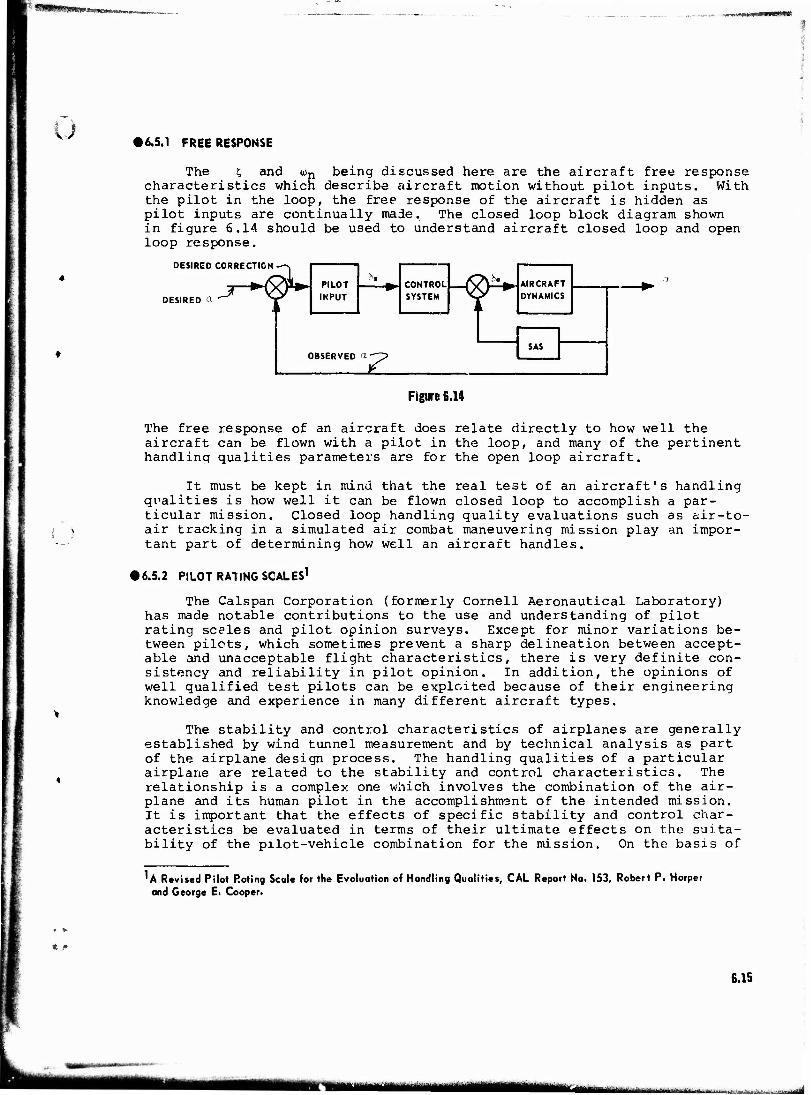
'WWW»-.UM..»»

u • 6.5.1 FREE RESPONSE

The and "n being discussed here are the aircraft free response characteristics which describe aircraft motion without pilot inputs. With the pilot in the loop, the free response of the aircraft is hidden as pilot inputs are continually made. The closed loop block diagram shown in figure 6.14 should be used to understand aircraft closed loop and open loop response.

DESIRED CORRECTION ■

DESIRED a &. PILOT

INPUT

J* ^ CONTROL SYSTEM t AIRCRAFT

F DYNAMICS

i 1 OBSERVED d' 5

1 SAS

K" Figure 6.14

The free response of an aircraft does relate directly to how well the aircraft can be flown with a pilot in the loop, and many of the pertinent handling qualities parameters are for the open loop aircraft.

It must be kept in mind that the real test of an aircraft's handling qualities is how well it can be flown closed loop to accomplish a particular mission. Closed loop handling quality evaluations such as air-to- air tracking in a simulated air combat maneuvering mission play an important part of determining how well an aircraft handles.

• 6.5.2 PILOT RATING SCALES1

The Calspan Corporation (formerly Cornell Aeronautical Laboratory) has made notable contributions to the use and understanding of pilot rating scales and pilot opinion surveys. Except for minor variations between pilots, which sometimes prevent a sharp delineation between acceptable and unacceptable flight characteristics, there is very definite con- sistency and reliability in pilot opinion. In addition, the opinions of well qualified test pilots can be exploited because of their engineering knowledge and experience in many different aircraft types.

The stability and control characteristics of airplanes are generally established by wind tunnel measurement and by technical analysis as part of the airplane design process. The handling qualities of a particular airplane are related to the stability and control characteristics. The relationship is a complex one which involves the combination of the airplane and its human pilot in the accomplishment of the intended mission. It is important that the effects of specific stability and control characteristics be evaluated in terms of their ultimate effects on the suitability of the pilot-vehicle combination for the mission. On the basis of

^A Revised Pilot Rating Scale for the Evaluation of Handling Qualities, CAL Report No. 153, Robert P. Harper

and George E. Cooper.

6.15

y

mmmmm

thir information, intelligent decisions can be made during the airplane design phase which will lead to the desired handling qualities of the final product.

There are three general ways in which the relationship between stability and control parameters and the degree of suitability of the airplane for the mission may be examined:

1. Theoretical analysis

2. Experimental performance measurement

3. Pilot evaluation

Each of the three approaches has an important rol^ in the complete evaluation. One might ask, however, why is the pilot assessment necessary? At present a mathematical representation of the human operator best lends itself to analysis of specific simple tasks. Since the intended use is made up of several tasks and several modes of pilot-vehicle behavior, difficulty is experienced first in accurately describing all modes analytically, and second In integrating the quality of the subordinate parts into a measure of overall quality for the intended use. In spite of these difficulties, theoretical analysis is fundamental to understanding pilot- vehicle difficulties, and pilot evaluation without it remains a purely

.| experimental process.

The attainment of satisfactory performance in fulfillment of a designated mission is, of course, a fundamental reason for our concern with handling qualities. Why cannot the experimental measurement of performance replace pilot evaluation? Uny not measure pilot-vehicle performance in the intended use - isn't: good performance consonant with good quality? A significant difficulty arises here in that the performance measurement tasks may not demand of the pilot all that the real mission demands. The pilot is an adaptive controller whose qoal (when so in- structed) is to achieve good performance. In a specific task, he is capable of attaining essentially the saim? performance for a wide range of vehicle characteristics, at the expense of significant reductions in his capacity to assume other duties and planning operations. Significant differences in task performance may not be measured where very real differences in mission suitability do exist.

The questions which arise: in using performance measurements may be : summarized as follows: (i) For what maneuvers and tasks should measure-

ments be made to define the mission suitability? (2) How do we integrate and weigh the performance in several tasks to give an overall measure of quality if measurable differences do exist? (3) Is it necessary to measure or evaluate pilot workload and attention factors for performance to be meaningful? If so, how are these factors weighed with those in (2)? (4) What disturbances and distractions are necessary to provide a realistic workload for the pilot during the ncasurement of his performance in the specified task?

Pilot evaluation still remains the only method of assessing the interactions between [ lot performance and workload in determining suitability of the airplane for tan:- mission. Tt is required in order to provide a basic measure of quality and to serve as a standard aqainst which

6.16

—

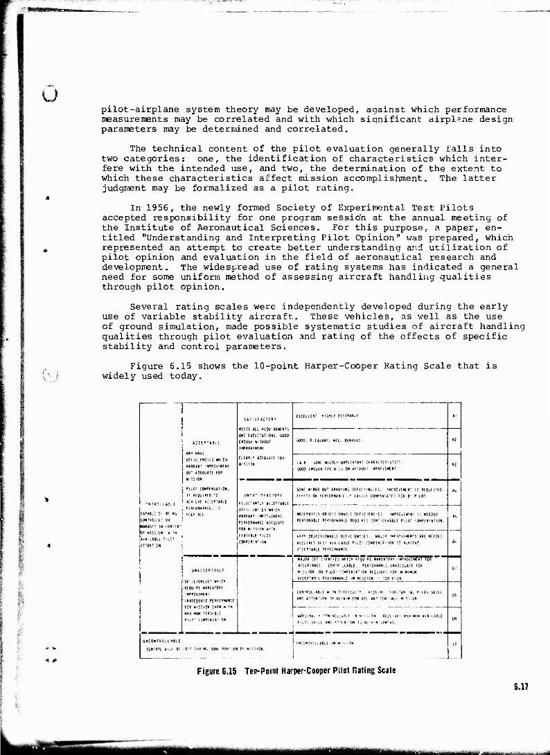
'.■t-r^v^v1-;*'■*

WMUmmwpäLa

U pilot-airplane system theory may be developed, against which performance measurements may be correlated and with which siqnificant airplane design parameters may be determined and correlated.

The technical content of the pilot evaluation generally falls into two categories: one, the identification of characteristics which inter- fere with the intended use, and two, the determination of the extent to which these characteristics affect mission accomplishment. The latter judgment may be formalized as a pilot rating.

In 1956, the newly formed Society of Experimental Test Pilots accepted responsibility for one program session at the annual meeting of the Institute of Aeronautical Sciences. For this purpose, a paper, en- titled "Understanding and Interpreting Pilot Opinion" was prepared, which represented an attempt to create better understanding and utilization of pilot opinion and evaluation in the field of aeronautical research and development. The widespread use of rating systems has indicated a general need for some uniform method of assessing aircraft handling qualities through pilot opinion.

Several rating scales were independently developed during the early- use of variable stability aircraft. These vehicles, as well as the use of ground simulation, made possible systematic studies of aircraft handling qualities through pilot evaluation and rating of the effects of specific stability and control parameters.

Figure 6.15 shows the 10-point Harper-Cooper Rating Scale that is widely used today.

.

»T W 01i

CAPABiL" C"

CONTROLLED i

MANAGFT IN •

OF Ml S3'ON

1V4IUBU ?

ATTENTION

AB.E

BEING

ACCEPTABLE

MAT HAVE

0£» iClCNCIES WHICH

WARRANT IMPROVEMENT.

BUT ADEQUATE F0«

MISSION.

Pi LOT COMPENSATION.

IE REQUIRED TO

ICn;E*f ACCEPTABLE

PERIQRMANCE. IS

F-EiSi'tlf.

0

UNACCEP!A9if

0EfICIEHCIES WHICH

REQUIRE MANDATORY

'MPROVEMENI.

INADEQUATE PEWMANCE

FOR MiSSiON EvfN *:Tn

MAIiMUM FEASIBLE

PiLO' COMffNSA'I ON.

SA1 ! SF ACTORY

MEETS ALL REQUIREMENTS

AND EXPECTATIONS. GOOD

ENOUGH WITHOUT

IMPROVEMENT

CLEARLY ADEQUATE »OR

HI SS'ON.

l!NSAT f AC0R«

RElKIANM ACCEPTABLE

DE> It:FNCIES WHICH

»ARRANT IMPLEMENT,

PERFORMANCE AOEQLlA'!

'OR MISSION WITH

FEASIBLE PILOT

COMP'ENSAT 'ON,

EUCfLLENT, HICHLY DESIRABLE

ooOD. PLEASANT, »tu BEHAVED

FAIR. SOME MILDLY UNPLEASANT CHAR ACHRI STiC?

MOD ENOUGH (OK MiSSlON WITHOUT iMPBC-VEMENT

SOML" MINOR BUI ANNOYING DEFICIENCIES. 'MPROvFMEN' IS REQUESTED.

EttfC! ON PERFORMANCE IS EASILY CONPINSA'T.') FOR B\ PILOT.

MODERATE!* 08IEC rtONABLf 0t f IC \ ENC i i S. iMPROvEM'NT IS NFEDED.

REASONABLE PERFORMANCE »EQUIRES C0*r IDEft*Bt£ PILOT COMPENSATION1.

VERY OBJFCTIONABLE DEFICIENCIES. MAJJR IMPROVEMENTS AfiE NEEDE['.

REQUIRES BEST AVAILABLE PILO' COMPENSATION TO ACHIEVE

j *rCEPTA8LE PERFORMANCE.

UNCONTROLLABLE

CONTROL »III BE LOST DUR'Nfj SOME PORTION 0' MISSION.

MAJOR DEFICIENCIES WHICH RfQljiRE MANDATORY IMPROVEMENT FOR

ACCEPTANCE. C0NTK' .LABlE. PERFORMANCE INADLQUATE FOR

MISSION, OR PILOT COMPENSATION REQUIRED 10» MINIMUM

ACCEPTABLE PERFORMANCE iN MISSION 'S TOO H:GH,

CONTROLLABLE WITH OIFMCLHTY. REQUiRf:- SU«ST AJil I Al »MOi SK 1LI

AND ATTfNMON TO RETAIN CON;R0L AND CONTINUE MiSS'QH.

MARGINAL.- rnt,i «OLL ABi F IN M'SS ON RE^U'lUS Mii'MUM Avi < L ABLE

PILO! S»'LI AMD -""TEmtiON TO RETAIN C0NT«O'..

ICONT-CILABLE IN t

Figure 6.15 Ten-Point Harper-Cooper Pilot Rating Scale

6.17

5

- — M&h .L,,,V—. ■ s A-»^ -- .■..^ .^j.: ,

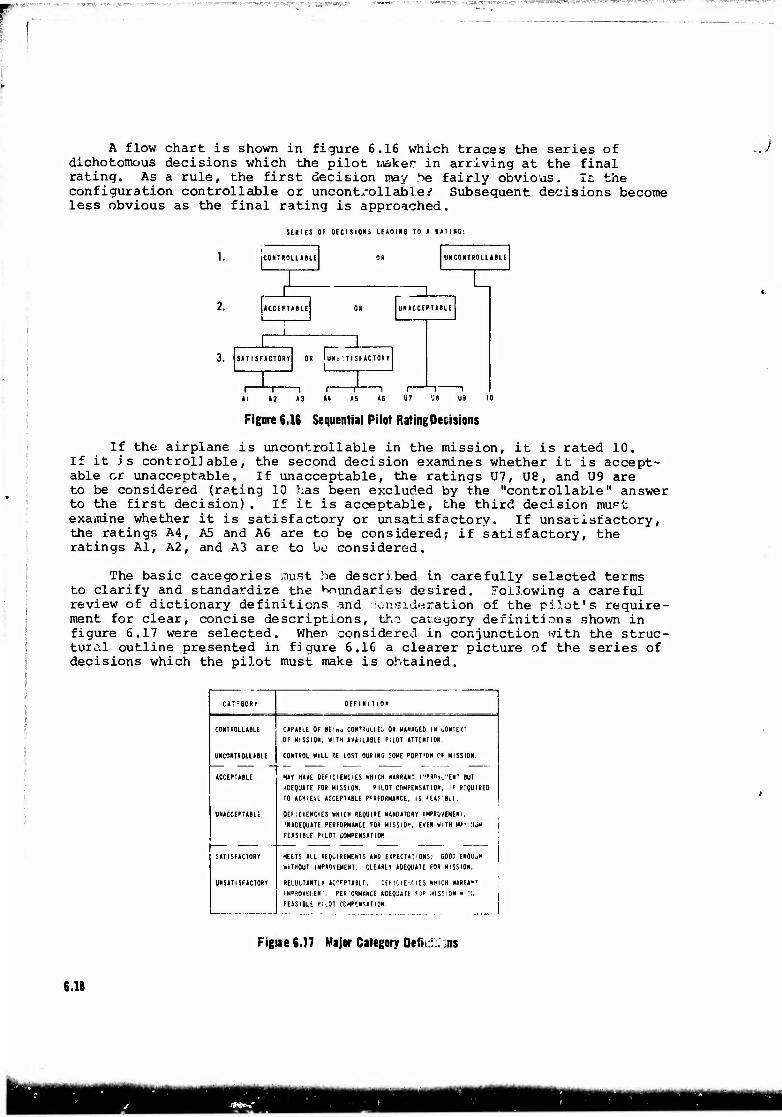
* ^^V"*'--'"1''"'^.^""^-''' ...... . —... -..,..—.^.-,-.-. -,

A flow chart is shown in figure 6.16 which traces the series of dichotomous decisions which the pilot maker in arriving at the final rating. As a rule, the first decision may he fairly obvious. l£. the configuration controllable or uncontrollable.'' Subsequent decisions become less obvious as the final rating is approached.

SERIES OF DECISION LEADING TO * RAT INC:

OR ICOKTPIOLLABLE UNCONTROLLABLE

umcc

3. S*TISF»CT0RY (UN;'TISFA

1 I r 1 r «I «2 13 >4 15 16 U7 ';< U9 10

Figure 6.16 Sequential Pilot Rating Decisions

If the airplane is uncontrollable in the mission, it is rated 10. If it is controllable, the second decision examines whether it is acceptable or unacceptable. If unacceptable, the ratings U7, U8, and U9 are to be considered (rating 10 has been excluded by the "controllable" answer to the first decision), If it is acceptable, the third decision mupt examine whether it is satisfactory or unsatisfactory. If unsatisfactory, the ratings A4, A5 and A6 are to be considered; if satisfactory, the ratings Al, A2, and A3 are to be considered.

The basic categories must be described in carefully selected terms to clarify and standardize the N-iundaries desired. Following a careful review of dictionary definitions and consideration of the pilot's requirement for clear, concise descriptions, tha category definitions shown in figure 6.17 were selected. When considered in conjunction with the structural outline presented in figure 6.16 a clearer picture of the series of decisions which the pilot must make is obtained.

CA7:GCRV ]

DEFINIT10*

CONTROLLABLE

UNC0NTR0LLA61E

ACCEPTABLE

UNACCEPTABLE

SATISFACTORY

UNSATISF1CT0RV

CAPABLE OF BEUo «WTMUI;, OR MANAGED IK I.0NTEXT OF MISSION, WITH AVAILABLE PILOT ATTENTION.

CONTROL »ILL BE LOST DURING SOUS PORTON CF MISSION.

MA» HAVE DEFICIENCIES WHICH «ARRANT 1 "»Rfl.t:'EMT BUT •DEQUATE FOR MISSION. PILOT COMPENSATION, IF «rjUIREO TO ACHIEVE ACCEPTABLE PFRFOKMANCE, IS FEAS'BU,

DEFICIENCIES WHICH REQUIRE MANDATORY IMPROVEMENT. 'NADEOUATE PERFORMANCE FOR MISSIOH. EVEN KITH MKItUri | FEASIBLE PILOT COMPENSATION 1

MEETS ALL RETIREMENTS AND EXPECTATIONS; GOOD EN01K.H j WITHOUT IMPROVEMENT. CLEARLY ADEQUATE FOR MISSION.

RELUCTANTLY AC'PTABLF. DEFICIENCIES WHICH WARR1»T IMPSOVEhENT. PERCRMAhCE ADEQUATE I0P MISSION »'Tl. 1 FEASIBLE PILOT COMPENSATION.

Figure 6.17 Major Category Defii:. ns

6.18

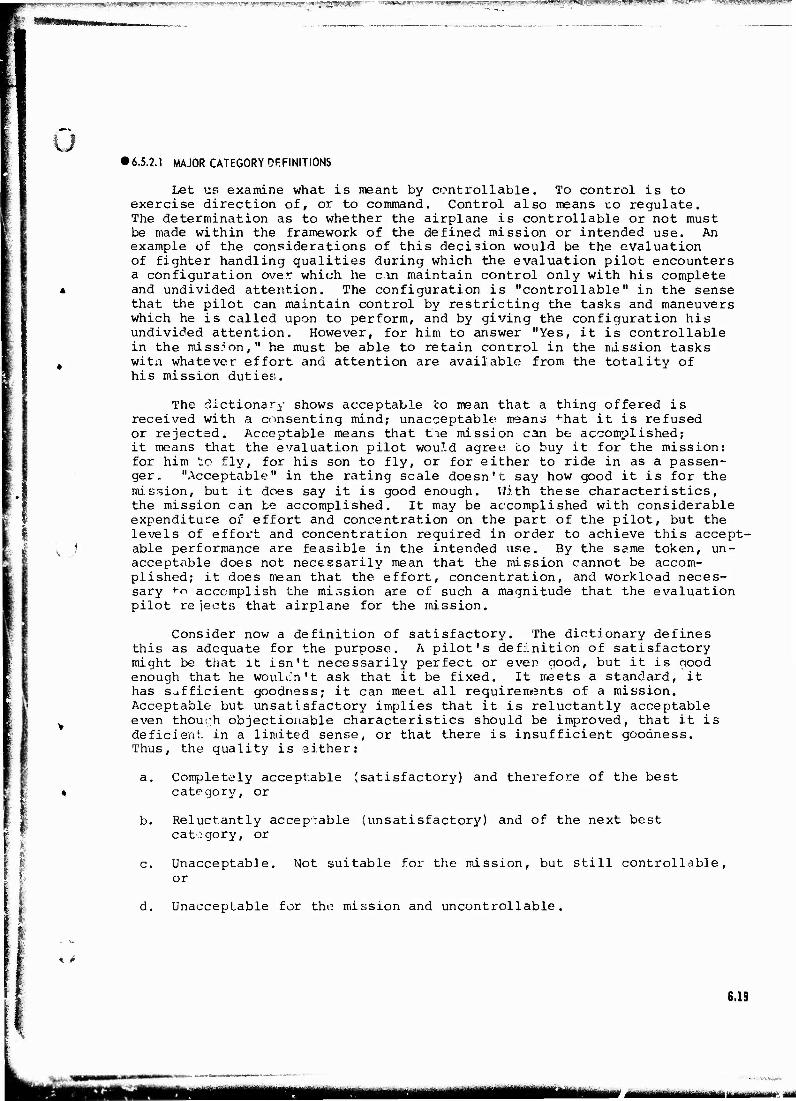
-s-iiwdj^w^'^SV" '. ■-' * P' ^-T'-r '."-■ '■ ■-;■—— -■ ■■-■^•7.."^r- :^? ■ !P?T ■ -.»^v.^--^--^-'---^-*^^ :*?^-^"*r''"

• 6.5.2.1 MAJOR CATEGORY DFFINITIONS

Let us examine what is meant by controllable. To control is to exercise direction of, or to command. Control also means v.o regulate. The determination as to whether the airplane is controllable or not must be made within the framework of the defined mission or intended use. An example of the considerations of this decision would be the evaluation of fighter handling qualities during which the evaluation pilot encounters a configuration over which he cm maintain control only with his complete and undivided attention. The configuration is "controllable" in the sense that the pilot can maintain control by restricting the tasks and maneuvers which he is called upon to perform, and by giving the configuration his undivided attention. However, for him to answer "Yes, it is controllable in the mission," he must be able to retain control in the mission tasks witn whatever effort and attention are available from the totality of his mission duties;.

The dictionary shows acceptable to mean that a thing offered is received with a consenting mind; unacceptable means +-hat it is refused or rejected. Acceptable means that tie mission can be accomplished; it means that the evaluation pilot would agree to buy it for the mission: for him to fly, for his son to fly, or for either to ride in as a passen- ger. "Acceptable" in the rating scale doesn't say how good it is for the mission, but it does say it is good enough. With these characteristics, the mission can be accomplished. It may be accomplished with considerable expenditure of effort and concentration on the part of the pilot, but the levels of effort and concentration required in order to achieve this acceptable performance are feasible in the intended use. By the same token, unacceptable does not necessarily mean that the mission cannot be accomplished; it does mean that the effort, concentration, and workload necessary t-n accomplish the mission are of such a magnitude that the evaluation pilot rejects that airplane for the mission.

;-

Consider now a definition of satisfactory. The dictionary defines this as adequate for the purpose. A pilot's definition of satisfactory might be that it isn't necessarily perfect or even good, but it is good enough that he wouldn't ask that it be fixed. It meets a standard, it has sufficient goodness; it can meet all requirements of a mission. Acceptable but unsatisfactory implies that it is reluctantly acceptable even thouch objectionable characteristics should be improved, that it is deficient in a limited sense, or that there is insufficient goodness. Thus, the quality is either:

a. Completely acceptable (satisfactory) and therefore of the best category, or

! k

b. Reluctantly acceptable (unsatisfactory) and of the next best category, or

c. Unacceptable. Not suitable for the mission, but still controllable, or

i I Unacceptable for the mission and uncontrollable.

6.19

mm mm ^^m . ......

*wr»l3gwm<l!r!pr,*±})pwilb-'l*'~" ■-^l^3iT-»CT'f'^..|;>'^1)fywi^^ ■ *JW«»!OT*t»'(J!WW4l

• 6.5.2.2 EXPERIMENTAL USE OF RATING OF HANDLING QUALITIES

The evaluation of handling qualities has a similarity to other scientific experiments in that the output data are only as good as the care taken in the design and execution of the experiment itself and in the analysis and reporting of the results. There are two basic categories of output data in a handling qualities evaluation: the pilot comment data and the pilot ratings. Both items are important output data. An experiment which ignores one of the two outputs is discarding a substan- tial part of the output information.

As one might expect, the output data which are -ost often neglected are the pilot comments, primarily because they are qaite difficult to deal with due to their qualitative form and, perhaps, their bulk. Ratings, however, without the attendant pilot objections, are only part of the story. Only if the deficient areas can be identified, can one expect to * devise improvements to eliminate or attenuate the shortcomings. The pilot comments are the means by which the identification can be made.

There are several factors which have a strong influence on the quality of pilot evaluation data and a brief discussion of them follows.

• 6.5.2.3 MISSIONDEFINITION

Explicit definition of the mission is probably the most important contributor to the objectivity of the pilot evaluation data. The mission is defined here as a use to which the pilot-airplane combination is to be put. The mission must be very carefully examined, and a clear definition and understanding must be reached between the engineer and the evalua- »■■■>' tion pilot as to their interpretation of this mission. This definition must include:

a. what the pilot is required to accomplish with the airplane, and

b. the conditions or circumstances under which he must perform the mission.

For example, the conditions or circumstances might include instrument or visual flight or both, type of displays in the cockpit, input information to assist the pilot in the accomplishment of the mission, etc. The environment in which the mission is to be accomplished must i also be defined and considered in the evaluation, and could include, for example, the presence or absence of turbulence, day versus night, the frequency with which the mission has to be repeated, the variability in the preparedness of the pilot for the mission, and his level of proficiency. '

; i

• 6.5.2.4 SIMULATION SITUATION

The pilot evaluation is seldom conducted under the circumstances of the r«.al mission. The evaluation almost inherently involves simulation to some degree because of the absence of the real situation. As an example, the evaluation of a day fighter is seldom carried out under the circumstances of a combat mission in which the pilot is not only shooting at real targets, but also beinq shot back at by real guns. Therefore, after the mission has been defined, the relationship of the simulation

6.20

—*———*

liîû.ii.'i^piPt'fpLiiBjpmw ' "^rsu^^^r^Twaii ppvppm sg: ■ "?'■:■• R • p pvf JV ■ i"w^KüBffl" ■ 1 îjaupii ■;nr"''1' "*tp«^Bp'!.T?^1Sr'

u situation to the real mission must be explicitly stated for both the engineer and the evaluation pilot so that' each may clearly understand the limitations of the simulation situation.

The pilot and engineer must both know what is left out o* the evaluation program, and also what is in that should not be in. The fact that the anxiety and tension of the real situation are missimj. and that the airplane is flying in the clear blue of calm daylight air, instead of in the icing, cloudy, turbulent, dark situation of the real mission, will affect results. Regardless of the evaluation tasks selected, the pilot must use his knowledge and experience to provide a rating which includes all considerations which are pertinent to the mission, whether provided in the tasks or not.

u

% 0

• 6.5.2.5 PILOT COMMENT DATA

One of the fallacies resulting from the use of a rating scale which is considered for universal handling qualities application is the assumption that the numerical pilot rating can represent the entire qualitative assessment. Extreme care must be taken against this oversimplification because it does not constitute the full data gathering process.

The pilot objections to the handling qualities are important, particularly co the airplane designer who is responsible for the improvement of the handling qualities. But, even more important, the pilot comment data are essential to the engineer who is attempting to understand and use the pilot rating data. If ratings are the only output data, one has no real way of assessing whether the objectives of the experiment were actually realized. Pilot comments supply a means of assessing whether the pilot objections (which lead to his summary rating) were related to the mission or resulted from some extraneous uncontrolled factor in the execution of the experiment, or from individual pilots focusing on and weighing differently various aspects of the mission. In order that the pilot comments be most useful, several details are important.

The comments must be given by the pilot in the simplest language. Engineering terms are generally to be avoided, unless they are carefully defined. The pilot should report what he sees and feels, and describe his difficulties in carrying out that which he is attempting. It is then important for the pilot to relate the difficulties which he is having in executing specific tasks to their effect on the accomplishment of the mission.

The pilot should be required to make specific comments in evaluating each configuration. These comments generally are in response to questions which have been developed in the discussions of the mission and simulation situation. The pilot must also be free to make comments regarding his difficulties over and above the answers to the specific questions asked of him. In this regard, the test pilot should strive for a balance between a continuous running commentary and occasional comment in the form of an explicit adjective. The former often requires so much editing to find the substance that it is often ignored, while the latter may add nothing to the numerical rating itself.

The pilot comments must be taken during or immediately after each evaluation. For in-flight evaluations, this means that the comments

6.21

mm -'-—- «MjH.I.Unli Ill ■ I ■• ■

■BWWBMWMBlMPlWWP^P!!Pg*llgWaWl|l|WBI*WB^W?S* wf^wiB8WWWlPlliPlffHB)l"ip'' PW PMIJWWM. WIMHP1' "-■^■■»'■"»■'W^'JN

should be recorded on a tape recorder. Experience has shovm that the best free comments are o.'ten given during the evaluation. If the comments are left until the conclusion of the evaluation, tiey are often forgotten. A useful procedure is to permit free comment during the evaluation itself and to require answers to specific questions in the summary comments at the end of the evaluation.

Questionnaires and supplementary pilot comments are most necessary to ensure that: (a) all important or suspected aspects are considered and not overlooked, (b) information is provided "-j.ati.ve to why a given rating has been given, (c) an understanding is provided of the tradeoffs with which pilots must continually contend, and (d) supplementary comment that might not be offered otherwise is stimulated. It is recommended that the pilots participate in the preparation of the questionnaires. The questionnaires should be modified if necessary as a result of the pilots' initial evaluations.

• 6.5.2.6 PILOT RATING DATA

The pilot rating is ar overall summation of the net effect of all of the objections which the pilot has observed during the evaluation as they relate to the mission. It is emphasized that the basic question that is asked of the pilot conditions the answei that he provides. For this reason, it is most important to ensure that the objectives of the program are clearly stated and understood by all concerned, and that all criteria, whether established or assumed, be clearly defined. In other words, it is extremely important that the basis upon which the evaluation is established te firmly understood by pilots and engineers. Unless a common basis is used, one cannot hope to achieve comparable pilot ratings, and confusing disagreement will often result. Care must also be taken that criteria established at the beginning of the program carry through to the end. If the pilot finds it necessary to modify his tasks, technique or mission definition during the program, he must make it clear just when this change occurred.

u

A discussion of the speci some disagreement among pilots numerical rating. There is ge is only a shorthand for the wo heavily on the specific adject which best fits their overall dichotomous decisions sequenti two or three ratings. The dec based upon the adjective descr is much to be preferred since cisions to the mission.

fie use of a rating scale tends to indicate as to how they actually arrive at a specific

neral agreement that the numerical rating rd definition. Some pilots, however, lean ive description and look for that description assessment. Other pilots prefer to make the ally, thereby arriving at a choice between ision among the two or three ratings is then lption. In concept, the latter technique it emphasizes the relatiwnship of all de-

It is suggested that the actual technique used is somewhere between the two techniques above and not so c cferent among pilots. In the past, the pilot's choice has probably been strongly influenced by the relative usefulness of the descriptions provided for the categories on one hand, and the numerical ratings on the other. The evaluation pilot is more or less continuously considering the rating decision process during his evaluation. He proceeds through the dichotomous decisions to the adjective descriptors enough times that his final decision is a blend of both techniques. It is therefore obvious that descriptors should not be contra- dictory to the mission-oriented framework.

6.22

Ik mwtmr^— I i MBüi - wmk

ijxkuiBjjn .mm*mm*,.t,wuiMWPmmw.wwppqwpaiiaww'i»w|ijgip *~1..»»^g;«i..i, ■.m■■put»im»ypyiu.<.■)iJ.II. t>wwwM ---WI-»mutmuwn

Half ratings are permitted (e.g., rating 4.5) and are generally used by the evaluation pilot to indicate a reluctance to assign either of the adjacent ratings to describe the configuration. Any finer breakdown than half ratings is prohibited since any number greater than or less than the half rating implies that it belongs ; the adjacent group. Any distinction between configurations assigned th .• same rating must be made in the pilot comments. Use of the 3.5, 6.5, nd 9.5 ratings is dis- couraged as they must be interpreted as evidence that the pilot is unable to make the fundamental decision with respect to category.

As noted previously, the pilot rating and comments must be given on the spot in order to be most meaningful. If the pilot should later want to change his rating, the engineer should record the reasons and the new rating for consideration in the analysis, and should attempt to repeat the configuration later in the evaluation program. If the configuration cannot be repeated, the larger weight (in most circumstances) should be given to the on-the-spot rating since it was given when all the characteristics were freshest in the pilot's mind.

• 6.5.2.7 EXECUTION OF HANDLING QUALITIES EXPERIMENTS

Probably the most important item is the admonition to execute the experiment as it was planned. This requires careful attention to the conduct of the experiment so that the plans are actually executed in the manne? intended. It is valuable for the engineer to monitor the pilot comment data as the experiment is conducted in order that he becoir.es aware of evaluation difficulties as soon as they occur. These difficulties may take a variety of forms. The pilot may use words which die engineer needs to have defined. The pilot's word descriptions may not convey a clear, understandable picture of the piloting difficulties. Direct communication between pilot and engineer is most important in clarifying such uncer- tainties. In fact, communication is probably the most important single element in the evaluation of handling qualities. Pilot and engineer must endeavor to understand one another, and cooperate to achieve and retain this understanding. The very nature of the experiment itself makes this somewhat difficult. The engineer is usually not present during the evaluation and, hence, he has only the pilot's word description of any piloting difficulty. Often, these described difficulties are contrary to the intuitive judgments of the engineer based on the characteristics of the airplane by itself. Mutual confidence is required. The engineer should be confident that the pilot will give him accurate, meaningful data; the pilot should be confident that the engineer is vitally interested in what he has to say and trusts the accuracy of his comments.

It is important that the pilot have no foreknowledge of the specific characteristics of the configuration being investigated. This does not exclude information which can bei provided to help shorten certain tests (e.g., the parameter variations are lateral-directional, only). But it does exclude foreknowledge of the specific parameters under evaluation. The pilot must be free to examine the configuration without prejudice, learn all he can about it from meeting it as an unknown for the first time, look clearly and accurately at his difficulties in performing the evaluation task, and freely associate these difficulties with their effects on the ultimate success of the mission. A considerable aid to the pilot in this assessment is to present the configuration in a random-appearing fashion.

6.23

rppwMWiiwjii^j,mmwi^wi«WM|lf.t ILi"''P^:.'lWll¥Wlwpilj!>'.!i'!;lali!gf■* m^«^L^»^pi!ii^Ml'^^Wwpp!«ffl"1, .MJpg— ■»» PUP ' lm,'m WMW

t

The amount of time which the pilot should use for the evaluation is difficult to specify a priori. He is normally at>ked to examine each configuration for as long as is necessary to feel confident that he can give a reliable and repeatable assessment. Sometimes, however, it is necessary to limit the evaluation time to a specific period of time because of circumstances beyond the control of the researcher. If the evaluation time per pilot is limited, a laiger sanpie of pilots or repeat evaluations will be required for similar accuracy, and the pilot comment data will be of poorer quality.

One final point is the state of mind of the evaluation pilot. He must be confident of the importance of the simulation program and join wholeheartedly into the production of data which will supply answers to the questions. Pilots as a group are strongly motivated toward the production of data to improve the handling qualities of the airplanes they fly. It isn't usually necessary to explicitly motivate the pilot, but it is very important to inspire in him confidence in the structure of the experiment and the usefulness of his rating and comment data. Pilot evaluations are probably one of the most difficult tasks that a pilot undertakes. To produce useful data involves a lot of hard work, tenacity, and careful thought. There is a strong tendency for the pilot to become discourage! in the course of his evaluations about their ultimate usefulness. He worries constantly about his assessments: their accuracy and repeatability. The pilot may feel that the engineer has the answers on a sheet of paper and he is merely testing the pilot as to his ability to search out the correct answers. Such feelings are added to by a lack of communication between the piloting and engineering organizations and are to be avoided. Probably the best approach is to explicitly state to the pilot that only he knows the answers to the questions which are being asked, and he can arrive at these correct answers by carrying out the evaluation program. He must be reassured in the course of the program that his assessments are good, so that he gains confidence in the manner in which he is carrying out the program.

■ 6.6 CONTROL INPUTS

There are several different control inputs that could be used to excite the dynamic modes of motion of an aircraft. To accomplish the task of obtaining the free response of an aircraft, the pilot makes an appropriate control input, removes himself from the loop, and observes the resulting aircraft motion. Three inputs that are frequently used in stability and control investigations will be discussed in this section: the step input, the pulse, and the doublet.

• 6.6.1 STEP INPUT

When a step input, is made, the applicable control is rapidly moved to a desired new position and F'.eadily held there. The aircraft motion resulting from this suddenly applied new control position can then be recorded for analysis. A mathematical representation of a step input assumes the deflection occurs in zero time and is contrasted to a typic-'l actual control position time history in figure 6.18. The "unit step" input is frequently used in theoretical analysis and has the magnitude of one radian, which is equivalent to 57.3 degrees. Specifying control inputs in dimensionless radians instead of degrees is convenient for use in the non-dimensional equations of motion.

6.24

|||y|[B3iiyt^1^-l.»,:W..^;-.:^

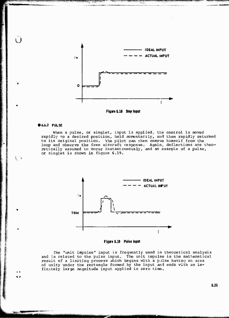
tl^^i^iKIIWai«»,W.i^',"W^—Wi:"i ■■»'■'■»»'■■;„' i_ ..wmmtT-mg-r'-r^gst . f.y». ,. ..jj,.y..j.. ■■ ..i in ...JI ,. .i.i.JW... i pj |.i, :|.,.I.I i.in.i ...n.|. u J m.Df^.1 I' -m*!f<':-r*1**W!~

IK*««*«

0 Ja

IDEAL INPUT

ACTUAL INPUT

T*-

Figure 6.18 Step Input

• 6.6.2 PULSE

When a pulse, or singlet, input is applied,, the rapidly to a desired position, held momentarily, and to its original position, 'i'he pilot can then remove loop and observe the free aircraft response. Again, retically assumed to occur instantaneously, and an or singlet is shown in figure 6.19.

control is moved then rapidly returned himself from the deflections are theo-

example of a pulse,

i 1

ACTUAL INPUT

ke r*

/

i \ V \

TRIM

t

Figure 6.19 Pulse Input

4 *.

«K P

The "unit impulse" input is frequently used in theoretical analysis and is related to the pulse input. The unit impulse is the mathematical result of a limiting process which begins with a pulse having an area of unity under the rectangle formed by the input and ends with an infinitely large magnitude input applied in zero time.

6.25

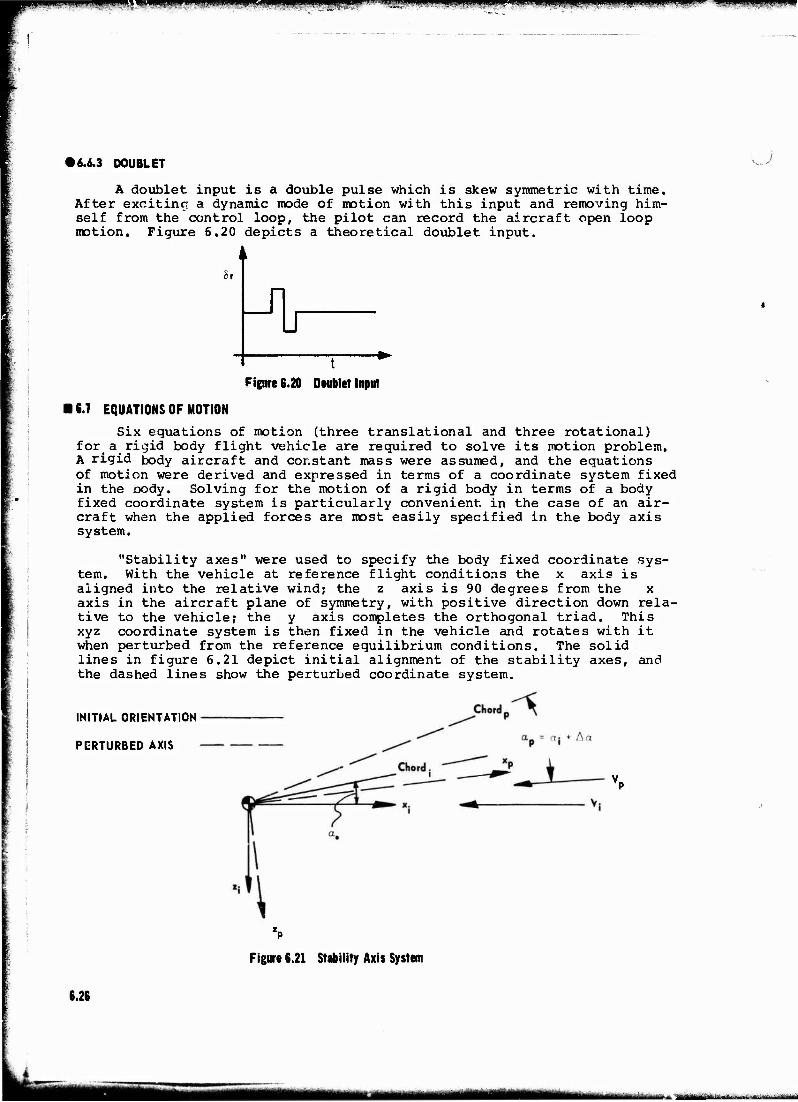
ppiPPPfliwpisiJip^^ ■ *■.'■■■■■ ■ »" " ■■»!!»■ ■'■■■ '■!" ' Hm'IWW »■IIJIWl fill JPUW U. I'

• 6.6.3 DOUBLET

A doublet input is a double pulse which is skew symmetric with time. After exciting a dynamic mode of motion with this input and removing himself from the control loop, the pilot can record the aircraft open loop motion. Figure 5.20 depicts a theoretical doublet input.

8r

_J1 u t

Figure 6.20 Doublet Input

16.7 EQUATIONS OF MOTION

Six equations of motion (three translational and three rotational) for a rigid body flight vehicle are required to solve its motion problem. A rigid body aircraft and constant mass were assumed, and the equations of motion were derived and expressed in terms of a coordinate system fixed in the oody. Solving for the motion of a rigid body in terms of a body fixed coordinate system is particularly convenient in the case of an aircraft when the applied forces are most easily specified in the body axis system.

"Stability axes" were used to specify the body fixed coordinate system. With the vehicle at reference flight conditions the x axis is aligned into the relative wind; the z axis is 90 degrees from the x axis in the aircraft plane of symmetry, with positive direction down relative to the vehicle; the y axis completes the orthogonal triad. This xyz coordinate system is then fixed in the vehicle and rotates with it when perturbed from the reference equilibrium conditions. The solid lines in figure 6.21 depict initial alignment of the stability axes, and the dashed lines show the perturbed coordinate system.

INITIAL ORIENTATION

PERTURBED AXIS

Figure 6.21 Stability Axis System

6.26

MUM amattattat

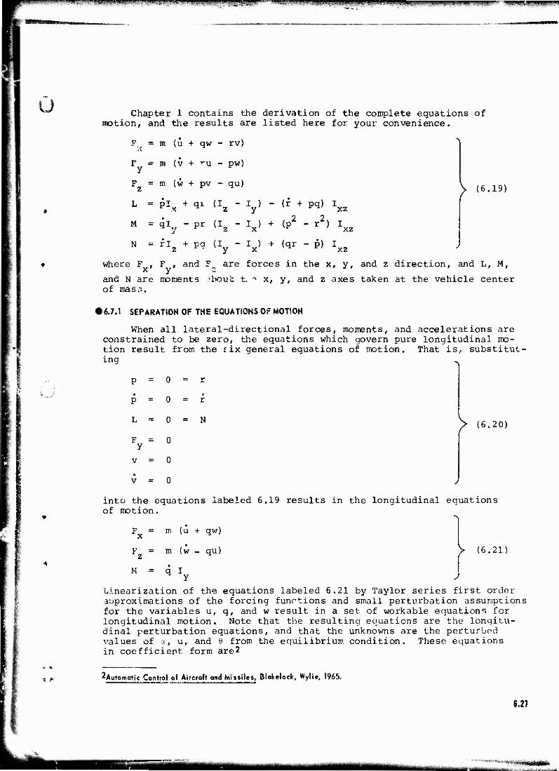
—— «■■,,., , . ___ ii.imnnii

Chapter 1 contains the derivation of the complete equations of motion, and the results are listed here for your convenience.

F, = m (u + qw - rv)

pw) F = m (v + ru y

F = m (w + pv - qu) >

(6.19)

L = plx + qi (Iz - Iy) - (r + pq) Ixz

M = qi - pr (I - I ) + (p2 - r2) I ^ y v 2 x r xz

N = rl + pa (I - I ) + (qr - p) I z r - y x xz

where F , F , and F^ are forces in the x, y, and z direction, and L, M,

and N are moments 'bout t. -> x, y, and z axes taken at the vehicle center of mas'3.

X

*w'

• 6.7.1 SEPARATION OF THE EQUATIONS Of MOTION

When all lateral-directional forces, moments, and accelerations are constrained to be zero, the equations which govern pure longitudinal motion result from the fix general equations of motion. That is, substituting

p = 0 = V

p = 0 = r

L ^ 0 = N

F = y

0

v = 0

> (6.20)

v = 0

into the equations labeled 6.19 results in the longitudinal equations of motion.

F = m (u + qw)

F = m (w - qu) z (6.21]

M q i y J

Linearization of the equations labeled 6.21 by Taylor series first order approximations of the forcing functions and small perturbation assumptions for the variables u, q, and w result in a set of workable equations for longitudinal motion. Note that the resulting equations are the longitudinal perturbation equations, and that the unknowns are the perturbed values of a, u, and 8 from the equilibrium condition. These equations in coefficient form are2

% f ^Automatic Control of Aircraft and Missiles, Slakelock, Wylie, 1965.

6.27

mmmm mumm --—- i 111 IllHlill

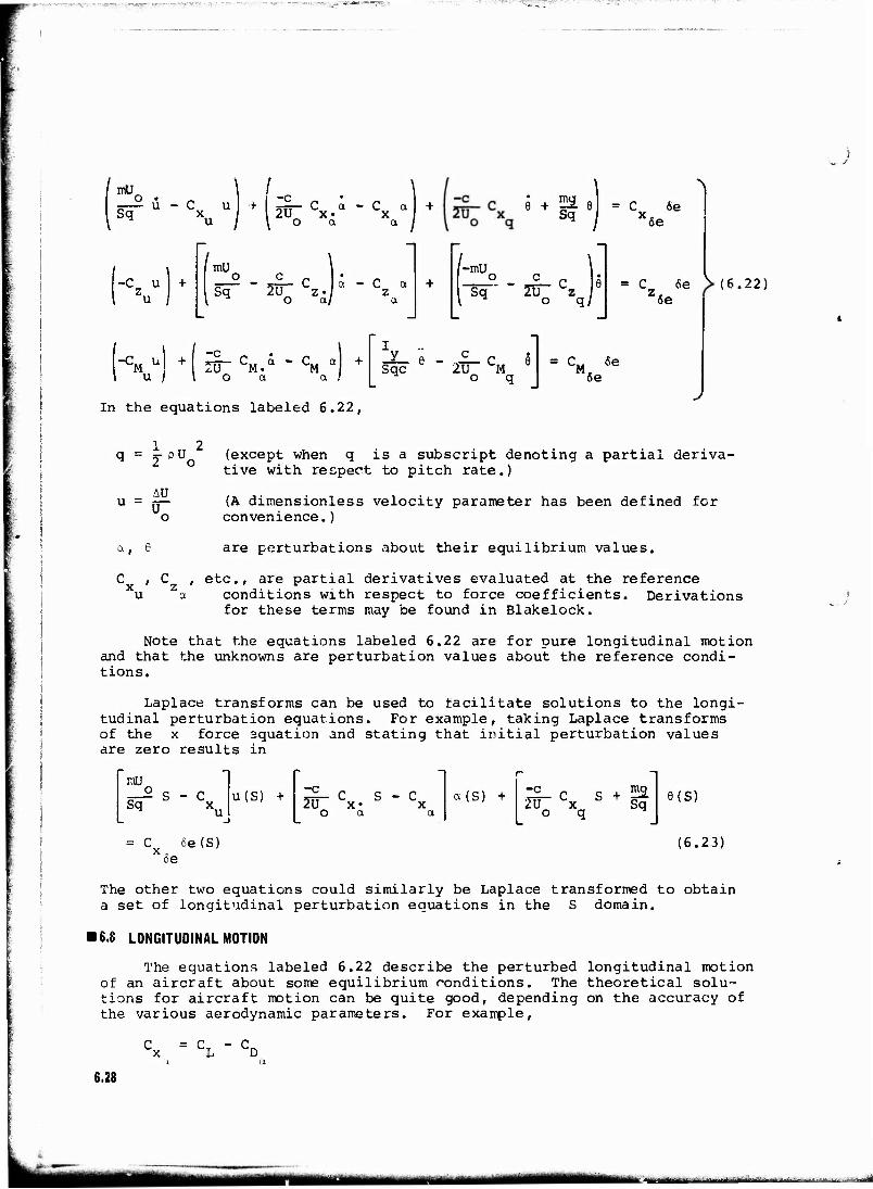
■- ■--.->.'' ■ >"W,f-|»^-"r"Tr'™ -' ">■'■■: —■"■ J-i; -->—■■ -^, '■;

mUc

Sq" u - C u

X u

-C u | + u

u

mU.

Sq

1 -c 2U C a x«

o a C a x a

° «£- C la - C a 2U 2'/ z

O a/ a

f-mU

"Sq"

mg

Sq

20" Cz o c

\

= C 6e x6e

= C 6e > (6.22) Z6e

-c „ CM a - Cu a UM» M O a a /

I y

Sqc — C 2U CM

o c = C 6e

5e

In the equations labeled 6.22, y

u

u =

1 „ 2 2-pUo

AU

(except when q is a subscript denoting a partial derivative with respect to pitch rate.)

(A dimensionless velocity parameter has been defined for convenience.)

a, 6 are perturbations about their equilibrium values.

C , C , etc., are partial derivatives evaluated at the reference u a conditions with respect to force coefficients. Derivations

for these terms may be found in Blakelock.

Note that the equations labeled 6.22 are for pure longitudinal motion and that the unknowns are perturbation values about the reference conditions.

Laplace transforms can be used to facilitate solutions to the longitudinal perturbation equations. For example, taking Laplace transforms of the x force aquation and stating that initial perturbation values are zero results in

mU o Sq

= C

S - C u(S) + -c !U

c s x»

o o. a (S) + :c c s + £a

2tT X Sq o q ^

6e (S)

e(s)

(6.23) 'fie

The other two equations could similarly be Laplace transformed to obtain a set of longitudinal perturbation equations in the S domain.

I6.S LONGITUDINAL MOTION

The equations labeled 6.22 describe the perturbed longitudinal motion of an aircraft about some equilibrium conditions. The theoretical solutions for aircraft motion can be quite good, depending on the accuracy of the various aerodynamic parameters. For example,

= c - c UL UD

6.28

aaaHa i-MteMMufc«a.^.:-'-i.-w ■■■■

__. t-«w-<?.-.jra

( 5

u

i )

is one parameter appearing in the x force equation, and the goodness of the solution will certainly depend on' how accurately the values of CL and CQ are known. Before an aircraft flies, such values result from theoretical predictions and wind tunnel data. After appropriate flight tests have been flown, values for the various stability derivatives can be extracted from flight tesc data.

• 6.8.1 EXAMPLE PROBLEM

Blakelock presents an example problem for a four-engine jet transport using the longitudinal equatxcns to solve for the perturbed aircraft motion. The reference flight conditions are straight and level at 40,000 feet with a velocity of 600 feet per second. Values for the various aerodynamic parameters are specified, and the set of longitudinal equations in the Laplace domain become

[13.78S + ,088]u(S) - .392a(S) + .746(S) = C 6e(S) X5e

M Se 6e

1.48u(S) + [13.78S + 4.46]a (Ü) - 13.78S6(S) = C 6e(E) Z6e

C + [.0552S + .619] a (S) + [.514S2 + .1923] 6(3) = C.

These equations are of the form

au + ba + c6~d

eu + fa + ge = h

iu + ja + ke = J.

(6.24)

(6.25)

and the set of equations can be readily solved for any of the variables. For example, from equation 6.25,

u(S)

a d c

e h g i l k Numerator(S)

a b c Denominator(S)

e f g i j k

Recall that the denominator of the above equation ir the S domain is the system characteristic equation and that the location of the roots of MS) will immediately indicate the type of dynamic response. From equation 6.24

MS) = 97.5S4 + 79S3 + 128.9S2 + .998S + .677 (6.26)

Factoring higher order equations such as 6.26 is not a simple thing, but some systematic approaches do exist. Blakelock refers to Lin's method and accomplishes the factoring of 6.26 into two quadratics.

MS) (S2 + .00466S + .005,^ (S + .806S + 1.211) (6.27)

6.29

•MMH

*gr ■^rcrr'''-^^:-'*;^'»^-'.''':r'"?"WT-";'■''■'■'-" ' "'"■"■. ■-'■ '-'■""V---,"-'-/^TT'^^ ^J'PiWHWfi WIM , 7.!«Erwg?5"WHg!: =-^-^TT^-"^.'.v-:-».^'j«r";v-1 ^^'T^T**^.^^?^f*"*-«F-:T^*''-:;^'I'w***'^7'?'ST|5*

Each of the quadratics listed in equation 6.27 will have a natural frequency and damping ratio associated with it, and the values can be rapidly computed by comparing the particular quadratic to the standard notation second order characteristic equation:

,J

t,1 = 0.352

u = 1.145 radians/sec nl

(6.28)

;x = 0.332

a = 0.07 3 radians/sec n2

(6.29)

• 6.8.2 LONGITUDINAL MOTION MODES

Experience has shown that aircraft exhibit two different types of longitudinal oscillations:

1. One of short period with relatively heavy damping that is called the "short period" mode.

2. Another of long period with very light damping that is called the "phugoid" mode.

The periods and damping of these oscillations vary from aircraft to aircraft and with flight conditions.

The shcrt period mode is characterized primarily by variations in angle of attack and pitch angle with very little change in forward speed. Relative to the phugoid, the short period has a high frequency and heavy damping.

Typical values" for its damped period are in the range of 2 to 5 seconds. Generally, the short period motion is the more important longitudinal mode for handling qualities since it is contributing to the motion being observed ard corrected by the pilot when the pilot is in the loop.

The phugoid mode is characterized mainly by variations in u and 0 with a nearly constant. This long period oscillation can be thought of as a constant total energy problem with exchanges between potential and kinetic energy. The aircraft nose drops and airspeed increases as the aircraft descends below its initial altitude. Then the nose rotates up, causing the aircraft to climb above its initial altitude with airspeed decreasing until the nose lazily drops belo- the horizon at the top of the maneuver.

Because of light damping, many cycles are requii -d for this motion to damp out. However, its long period combined with low damping results in an oscillation that is easily controlled by the pilot, even for a slightly divergent motion. When the pilot is in the loop, he is frequently not aware that the phugoid mode exists as he makes control inputs and ob- tains aircraft response before the phugoid can be seen. Typical values for its damped period range in the order of 45 to 90 seconds.

J

6.30

MM ■»"--'■--■ >■-■■■■•■-■ ■- ;

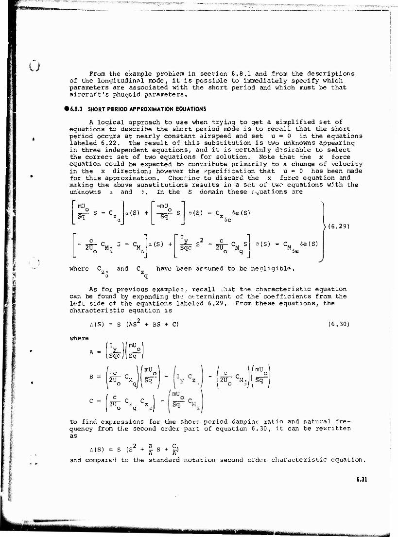
^'TO^iMMMPW|^ffi3SjBqyri, ■iJWK.wi. '"■TSsn^^iv'»--, - . ■■".- !~'!r-ir r\f- ■jj?r'r!\- «.ysn-

Ü From the example problem in section 6.8.1 and from the descriptions

of the longitudinal mode, it is possiole to immediately specify which parameters are associated with the short period and which must be that aircraft's phugoid parameters.

• 6.8.3 SHORT PERIOD APPROXIMATION EQUATIONS

A logical approach to use when trying to get a simplified set of equations to describe the short period mode is to recall that the short period occurs at nearly constant airspeed and set u = 0 in the equations labeled 6.22. The result of this substitution is two unknowns appearing in three independent equations, and it is certainly desirable to select the correct set of two equations for solution.. Note that the x force equation could be expected to contribute primarily to a change of velocity in the x direction; however the .-specification that u = 0 has been made for this approximation. Chooring to discard the x force equation and making the above substitutions results in a set of two equations with the unknowns a and 5. In the S domain these equations 3re

mU 5-2 S - C Sq z

-£- C 2U M«

O a

a(S) +

- C

-mU

"Sq 2. s

M a (S) +

6(S)

J

ri

Sqc

C: 6e(S) Z6e

fa 2lT LM b

}(6,29)

e(s) = c M 5e(S) 6e

where C and C have been arr.umed to be nealigible. 7. • 7. - 3

J

' 3 As for previous example.?,, recall ;hat toe characteristic equation

can be found by expanding the determinant of the coefficients from the ltift side of the equations labeled 6.29. From these equations, the characteristic equation is

A(S) = S (AS + BS + C) (6.30)

where

.Sqcj

mU c Sq

mU \ B = | 2TT CM I So^

C= 2Ü-S Cz O q a

,/mu \

2Uo \M.j| Sq

To find expressions for the short period dampinc ratio and natural frequency from the second order part of equation 6.30, it can be rewritten as

MS) = S (S2 + | S + S-)

and compared to the standard notation second order characteristic equation.

6.31

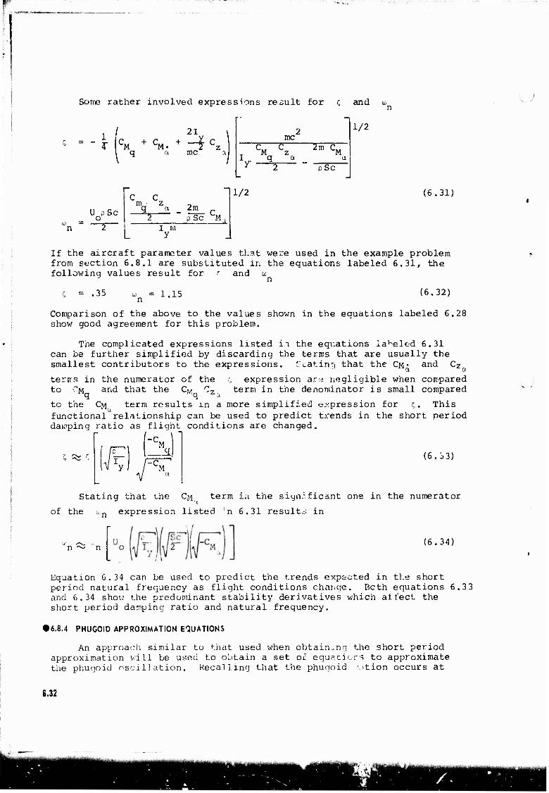
Some rather involved expressions result for Q and <u

1 4~

( 21 C„. + C,. + —2. 'M ~M< a mc

2 mc

m

w - n

U pSc o

L" 2m_ c

p Sc M I ia y

M z I q a y —^—

1/2

2m C 'M

pSc

1/2

(6.31)

If the aircraft parameter values that were used in the example problem from section 6.8.1 are substituted in the equations labeled 6.31, the followinq values result for r and ID

= .35 1.15 (6.32)

Comparison of the above to the values shown in the equations labeled 6.28 show good agreement for this problem.

The complicated expressions listed in the equations labeled 6.31 can be further simplified by discarding the terms that are usually the smallest contributors to the expressions. Grating that the CM« and Cz

terirs in the numerator of the ,; expression ara negligible when compared to CM and that the CM Cz term in the denominator is small compared

to the CM term results in a more simplified expression for r,. This functional relationship can be used to predict trends in the short period damping ratio as flight conditions are changed.

-C. M _q

'M (6.33)

Stating that the CM term in the sign;.ficant one in the numerator

of the tun expression listed :n 6.31 results in

(6.34)

Equation 6.34 can be used to predict the trends expscted in the short period natural frequency as flight conditions change. Beth equations 6.3 3 and 6.34 show the predominant stability derivatives which affect the short period damping ratio and natural frequency.

• 6.8.4 PHUGOID APPROXIMATION EQUATIONS

An approach similar to that used when obtaining the short period approximation will be used to obtain a set of equatiors to approximate the phugoid oscillation. Recalling that the phugoid otion occurs at

6.32

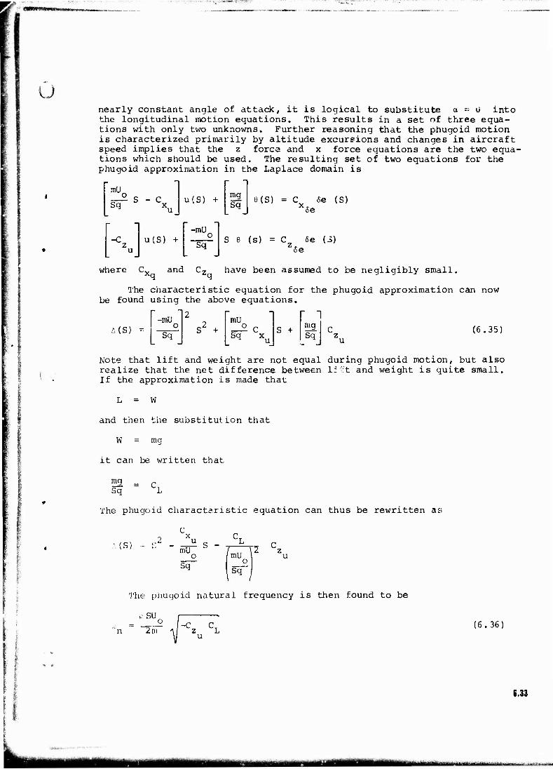
V J nearly constant angle of attack, it is logical to substitute a -- ü into the longitudinal motion equations. This results in a set of three equations with only two unknowns. Further reasoning that the phugoid motion is characterized primarily by altitude excursions and changes in aircraft speed implies that the z force and x force equations are the two equations which should be used. The resulting set of two equations for the phugoid approximation in the Laplace domain is

mV c Sq S - C u(S) +

-mU

mg Sq 6(S) = C 6e (S)

Se

u(S) + Sq S 6 (s) = C 6e (3) Z6e

where and Cz have been assumed to be negligibly small,

The characteristic equation for the phugoid approximation can now be found using the above equations.

A(S) =

r ™l 2

s2 +

P -* p -1

-mU o Sq

mU

Sq *u_ s + mg

Sq (6.35)

Note that lift and weight are not equal during phugoid motion, but also realize that the net difference between 1:':t and weight is quite small. If the approximation is made that

L = W

and then the substitution that

W = mg

it can be written that

mg = r Sq L

The phugoid characteristic equation can thus be rewritten as

C

mU c Sq

S - mU c Sq

The phugoid natural frequency is then found to be

p SU i .

2n. ^ zu L (6.36)

I 6.33

■MM

" fr -—i?<&-*i*?-y?-*r■.■~™tv?riv- ■««-» ;.r-s;,*a'f—-»^•■ ■ ,-.-^-.-,--.-,-:T".9PT» ■.■;—^,*;*-Tf-.-.■!■■»-* :i:r*:.T; '." -=■,-;;■;■■- ■.--- -.^.•«»5r^?'."T ■■■ -■ -- — ■■-■" T". — ;^- —--.»;vr. ■

In an effort to further simplify equation 6.36, the examined. Examining figure f,22

Cz terms should be

HORIZON

Figure 6.22

leadi! to

F = z

then,

3F

3U

L cos a - D sin a

3L , . . 3a 3D „ 3o -r— cos a + L Sin a — sin a - D cos a —— 3u 3u 3u 3u

which must be evaluated at the equilibrium conditions for use in the first order Taylor Series that was used in obtaining the linearized equations of motion

3F z

3U o

- 3L 3U

And,

3F z 3

C 3U DU CL S \ PV2

When the approximation that V = U is made in the above equation, the result is

3F 5 3u

?CL . 1 M2 3lTS 2 pu CT SpU

Li

In order to have a nondimensional expression, the correct factor must be used

U 3F _o z Lz Sq 3u u ^

6.34

UM -■•■'-■•- ■ ■' ^-' —— ■-■ ■ --.•■-■■■--■■•--...« tkiM

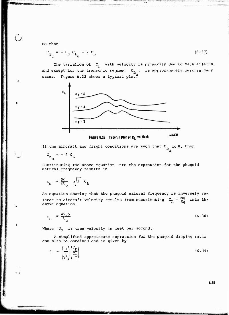
■ :-:■■■ -.-- ■---■■■ .■ ^T -;.-, ;: ;~--;y;' ;■■ ■i./ü-" ~~wc?~~\- --r.r.-!—--&•>- -v,--- r^-v^^----

u So that

C z u

U CT o L 2 CT (6.37)

The variation of CT with velocity is primarily due to Mach effects,

and except for the transonic regime, CT , is approximately zero in many

cases. Figure 6.23 shows a typical plot.

xT 2

Figure 6.23 Typical Plot of CL vs Mach MACH

If the aircraft and flight conditions are such that CL ~ 0, then u

C - 2 C,

Substituting the above equation into the expression for the phugoid natural frequency results in

«n =m~o <f An equation showing that the phugoid natural frequency is inversely re-

lated to aircraft velocity results from substituting C = ~£ into th» above equation.

45.5 (6.38)

Where UQ is true velocity in feet per second.

A simplified approixmate expression for the phugoid damping ratio can also be obtained and is given by

' l\/CDl

■F (6.39)

I 6.35

MH» i II ■■■■■■ in l in—I

F^,i^Tayji^f«i5gyy3^ ■*-STTJ< i,gy^f >.^*3^Jgw?f???w*'»'' -»T-fyy JFPn

Equations 6.38 and 6.39 can be used to understand some major contributors to the natural frequency and damping ratio of the phugoid motion.

u

16.8.5 EQUATION FOR n/a

Noting that the requirements of MIL-F-8785 for the short period natural frequency are stated as a function of n/a, it is desirable to develop a theoretical capability to predict n/a. Consider the z force equation for longitudinal motion.

EAF = m (w - U 6) 2 O '

and recall that Newton's Second Law is a directional relationship

F = m i~

Thus

a = w - U e z o (6.40)

where all the variables appearing in equation 6.40 are perturbations about the equilibrium condition. Rewriting the above equation and stating that

=uo <[T o 0)

n = U„ (, e) (6.41)

Of course expressions for a and e can be obtained from the short period solutions for a(t) and 8 (t), and an expression that gives n(t) can be written from equation 6.41. The ratio of the magnitudes of the n and u envelopes can then be used to determine n/a.

Using a theoretically obtained n/a along with the short period natural frequency and damping ratio obtained from the equations of motion makes it possible to accomplish a design problem to check whether or not the aircraft is being designed to comply with the MIL-F-8785.

■ 6.9 LATERAL-DIRECTIONAL MOTION MODES

There are three typical asymmetric modes of motion exhibited by aircraft. These modes are the roll, spiral, and Dutch roll.

• 6.9.1 kOLL MODE

The roll mode is considered to be a first order response which describes the aircraft roll rate response to an aileron input. Figure 6.24 depicts an idealized roll rate time history to a step aileron input. The roll mode time constant is normally small, with a MIL-F-8785 requirement to be less than three seconds.

6.3U

llgMBf fra—ÜMI

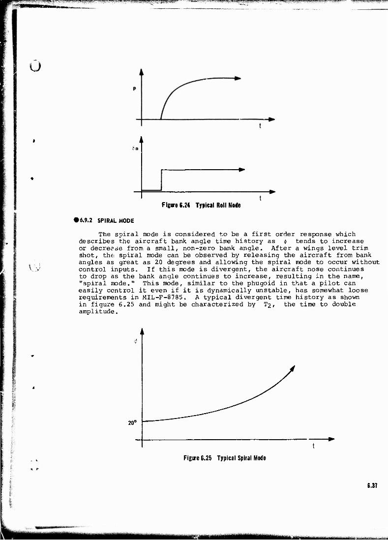
y»^-i«w»mB^ij»jTOir'j—M'»;T »»■ CW> ü '' =■',». ■■WW BBBPWP ,!l' ' >M'l"<mpiH.'jBag^^|BPW!WW ..»MWMlf—*™ vm*—«• >>vm»>'

u

>0

Figure 6.24 Typical Roll Kode

»6.9.2 SPIRAL MODE

i &

The spiral mode is considered to be a first order response which describes the aircraft bank angle time history as 4> tends to increase or decrease from a small, non-zero bank angle. After a wings level trim shot, the< spiral mode can be observed by releasing the aircraft from bank angles as great as 20 degrees and allowing the spiral mode to occur without control inputs. If this mode is divergent, the aircraft nose continues to drop as the bank angle continues to increase, resulting in the name, "spiral mode." This mode, similar to the phugoid in that a pilot can easily control it even if it is dynamically unstable, has somewhat loose requirements in MIL-F-8785. A typical divergent time history as shown in figure 6.25 and might be characterized by T2, the time to double amplitude.

i 6 M.

I t:'

20°

Figure 6.25 Typical Spiral Mode

6.37

MMMIMHMI ■ ---"-••

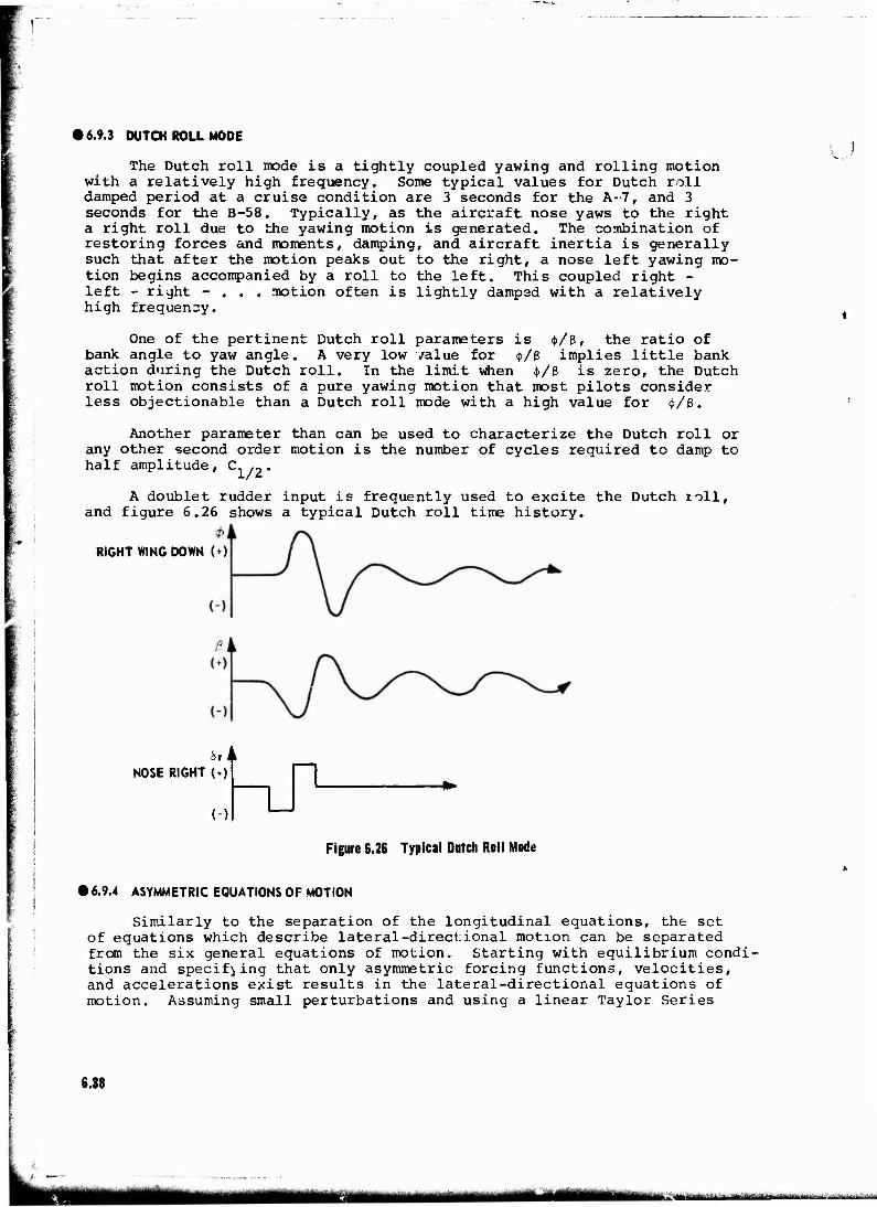
• 6.9.3 DUTCH ROLL MODE

The Dutch roll mode is a tightly coupled yawing and rolling motion with a relatively high frequency. Some typical values for Dutch roll damped period at a cruise condition are 3 seconds for the A-7, and 3 seconds for the B-58. Typically, as the aircraft nose yaws to the right a right roll due to the yawing motion is generated. The combination of restoring forces and moments, damping, and aircraft inertia is generally such that after the motion peaks out to the right, a nose left yawing motion begins accompanied by a roll to the left. This coupled right - left - right - . . . motion often is lightly damped with a relatively high frequency.

One of the pertinent Dutch roll parameters is <t>/ß, the ratio of bank, angle to yaw angle. A very low value for $/ß implies little bank action during the Dutch roll. In the limit when 4>/ß is zero, the Dutch roll motion consists of a pure yawing motion that most pilots consider less objectionable than a Dutch roll mode with a high value for 4>/ß.

Another parameter than can be used to characterize the Dutch roll or any other second order motion is the number of cycles required to damp to half amplitude, C./2.

A doublet rudder input is frequently used to excite the Dutch toll, and figure 6.26 shows a typical Dutch roll time history.

RIGHT WING DOWN ( + )

Sri L

RIGHT (*)

()

Figure S.26 Typical Dutch Roil Mode

• 6.9.4 ASYMMETRIC EQUATIONS OF MOTION

Similarly to the separation of the longitudinal equations, the set of equations which describe lateral-directional motion can be separated from the six general equations of motion. Starting with equilibrium conditions and specifying that only asymmetric forcing functions, velocities, and accelerations exist results in the lateral-directional equations of motion. Assuming small perturbations and using a linear Taylor Series

6.38

m — — ll^^f ^^w.^-.-;>.^,....

u approximation for the forcing functions result in the linear, lateral- directional perturbation equations of motion

±- C 2U y o Jp

Sqb

I xz Sqb

* -

- C +

2IT S

^- c o i

/mU ° - 2U C bq o y,

mu * - C V + —1

y si - C ß=C 6r+C

*ß *6r 1 5a

6a

bqo zuQ xr * ü6r v,fia M6.42)

+ S|B # - b C 2TT SJ o r

i|< - C. N. 6r + C

6r N 6a

6a

Note that the lateral-directional equations of motion have been non- dimensional zed by span, b, as opposed to chord. Also, recall that the stability derivative

but that the script

is not a lift-referenced stability derivative f refers to rolling moment.

It is appropriate to point out that if the products of perturbation are not small, then the lateral-directional motion will couple directly into longitudinal motion. This can be readily seen by examination of the pitching moment equation and makes the point that asymmetric motion can couple into symmetric motion. Our analysis will assume that conditions are such that coupling does not exist.

• 6.9.5 ROOTS OF A (S) FOR ASYMMETRIC MOTION

Laplace transforming the equations labeled 6.42 puts them into a form that readily yields the characteristic equation for asymmetric motion or that can be used to find the time response for some specified input.

The roots of the lateral directional characteristic equation typically are comprised of a relatively large negative real root, a small real root that is either positive or negative, and a complex conjugate pair of roots.

The large real root is the one associated with the roll mode of motion. Note that a large negative value for this root implies a fast time constant.

The small real root that might be either positive or negative is associated with the spiral mode. A slowly changing time response results from this small root, and the motion is either stable for a negative root or divergent for a positive root.

The complex conjugate pair of roots corresponds to the Dutch roll mode which frequently exhibits high frequency and light damping for SAS off conditions. This second order motion is of great interest in handling qualities investigations.

Figure fa.24 shows typical characteristic equation root locations for the asymmetric motion modes.

6.39

ma Tl in l

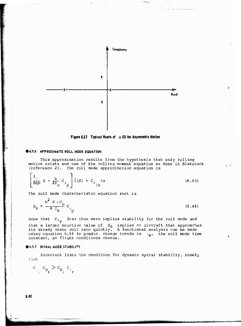
< l Imaginary

-X— Real

Figure 6.27 Typical Roots of A (S) for Asymmetric Motion

• 6.9.6 APPROXIMATE ROLL MODE EQUATION

This approximation results from the hypothesis that only rolling motion exists and use of the rolling moment equation as done in Blakelock (reference 2). The roll mode approximation equation is

Sqb b C XT C( o

*(S) 6 a (6.43)

The roll mode characteristic equation root is

b2 S pU

4 I (6.44)

Note that C£ less than zero implies stability for the roll mode and

that a larger negative value of SR implies an aircraft that approaches its steady state roll rate quickly. A functional analysis can be made using equation 6.44 to predic. change trends in iR, the roll mode time constant, as flight conditions change.

• 6.9.7 SPIRAL MODE STABILITY

Blakelock lists the condition for dynamic spiral stability, namely that

C c > c c N N, v r t-; r

6.40

ÜÜHtfalTMlnii' » * I '■•-■-;'-~---^-**—

ü

{ I

and points out that increasing C$ while decreasing Cj, is a reason-

able design method if increasing spiral stability is desired. Also he lists an equation to calculate the spiral mode A(S) root

= sa_ - „ c mU y, o * 4>

'N_ - C.

n Ci CN

P i

(6.45)

I 6.9.8 DUTCH ROLL MODE APPROXIMATE EQUATIONS

The approximate equations for Dutch roll motion can be obtained by using the equations labeled 6.42 and specifying that pure sideslip exists (8 = -*) and bank angle is zero. While this specification is generally not true, the result is a reasonable approximation for the Dutch roll damping ratio and natural frequency:

> (6.46)

of An approximate functional relationship can be found for the magnitude

(> to ß

(6.47)

Equation 6.47 is of value in predicting trends in $/e tions are changed.

• 6.9.9 COUPLED ROLL-SPIRAL MODE

as flight condi-

This by aircra this mode has two p conjugate the roll root beco to form a 6.28.

mode of lateral-directional motion has rarely been exhibited ft, but the possibility exists that it can indeed happen. If is present, the characteristic equation for asymmetric motion

airs of complex conjugate roots instead of the usual one complex pair along with two real roots. The phenomenon which occurs is

mode root decreases in absolute magnitude while the spiral mode me.5 more negative until they meet and split off the real axis second complex conjugate pair of roots, as depicted in figure

6.41

ma^ammmam^Mmm ten«».

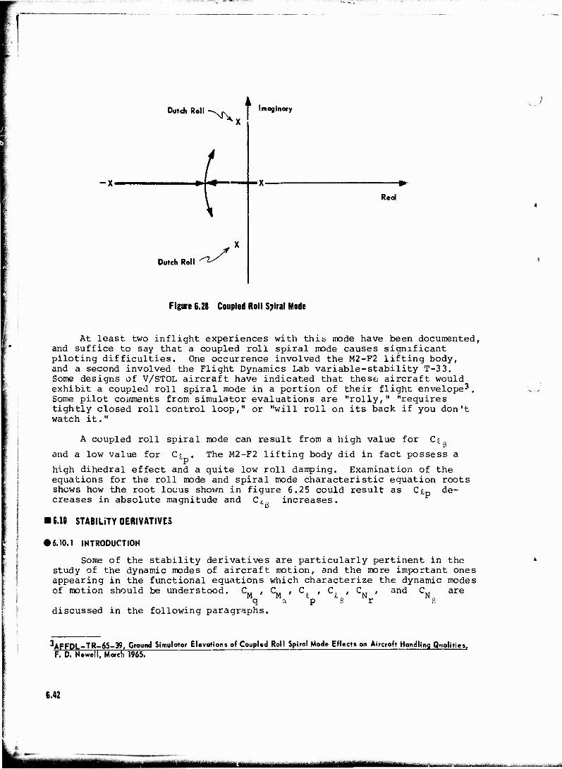
Dutch Roll ^V

-x-

Dutch Roll

Imaginary

Real

Figure 6.28 Coupled Roll Spiral Mode

At least two inflight experiences with this mode have been documented, and suffice to say that a coupled roll spiral mode causes significant piloting difficulties. One occurrence involved the M2-F2 lifting body, and a second involved the Flight Dynamics Lab variable-stability T-33. Some designs of V/STOL aircraft have indicated that these aircraft would exhibit a coupled roll spiral mode in a portion of their flight envelope^. Some pilot comments from simulator evaluations are "roily," "requires tightly closed roll control loop," or "will roll on its back if you don't watch it."

A coupled roll spiral mode can result from a high value for Ci P

and a low value for C< The M2-F2 lifting body did in fact possess a

high dihedral effect and a quite low roll damping. Examination of the equations for the roll mode and spiral mode characteristic equation roots shows how the root locus shown in figure 6.25 could result as Cj,p decreases in absolute magnitude and Cx increases. ;

16.10 STABILITY DERIVATIVES

• 6.10.1 INTRODUCTION

Some of the stability derivatives are particularly pertinent in the study of the dynamic modes of aircraft motion, and the more important ones appearing in the functional equations which characterize the dynamic modes of motion should be understood. C„ , (

M q

discussed in the following paragraphs.

"M P ß V and C are

ß

•^AFFDL-TR-65-39, Ground Simulotor Elevations of Coupled Roll Spiral Mode Effects on Aircraft Handling Qualities. F. D. Newell, Morel, 1965.

6.42

IÜB1 ItfÜ^

0 »6.10.2 PARTICULAR STABILITY DERIVATIVES

• 6.10.2.1 C, M,i

(\)

This stability derivative is the change in pitching moment coefficient with varying angle of attack and is commonly referred to as the longitudinal static stability derivative. When the angle of attack of the airframe increases from the equilibrium condition, the increased lift on the horizontal tail causes a negative pitching moment about the center of gravity of the airframe. Simultaneously, the increased lift of the wing causes a positive or negative pitching moment, depending on the fore and aft location of the lift vector with respect to the center of gravity. These contributions together with the pitching moment contribution of the fuselage are combined to establish the derivative CM .

The magnitude and sign of the total CM for a particular airframe con-

figuration are thus a function cf the center of gravity position, and this fact is very important in lognitudinal stability and control. If the center of gravity is ahead of the neutral point, the value of C^ is

negative, and the airframe is said to possess static longitudinal stability. Conversely, if the center of gravity is aft of the neutral point, the value of CM is positive, and the airframe is the) statically un-

stable. CM is perhaps the most important derivative as far as longi-

tudinal stability and control are concerned. It pr:marily establishes the natural frequency of the short period mode, and is a major factor in determining the response of the airframe to elevator motions and to gusts. In general, a large negative value of CM (i.e., large static stability)

is desirable for good flying qualities. However, if it is too ic ge, the required elevator effectiveness for satisfactory control may become unreasonably high. A compromise is thus necessary in selecting a design range for CM .

a not in terms of

the relation is:

Design values of static stability are usually expressed

CM but rather in terms of the derivative CMC, where

It should be pointed out that CMCT in CM0 = cMcL cLa the above expression is actually a partial derivative for which the forward speed remains constant.

• 6.10.2.2 C M„

%

The stability derivative CM is the change in pitching moment coefficient with varying pitch velocity and is commonly referred to as the pitch damping derivative. As the airframe pitches abo'jt its center of gravity pach, the angle of attack of the horizontal tail changes, and a lift force is developed on the horizontal tail producing a negative pitching moment on the airframe and hence a contribution to the derivative CM . There is also a contribution to CM because of various "deadweight" aeroelastic effects. Since the airframe is moving in a curved flight path due to its pitching, a centrifugal force is developed on all the components of the airframe. The force car. cause the wing to twist as a result of the dead weight moment of overhanging nacelles, and can cause the horizontal tail angle of attack to change as a result of faselaqe bending due to the weight of the tail section. In low speed flight, CM comes mostly from

6.43

MM Mta

the effect of the curved flight path on the horizontal tail and its sign is negative. In high speed flight the sign of CM can be oositive or negative, depending on the nature of the aeroelastrc effects. The derivative CM is very important in longitudinal dynamics because it contributes

a major portion of the damping of the short period mode for conventional aircraft. As pointed out, this damping effect comes mostly from the horizontal i-ail. For tailless aircraft, the magnitude of CM is consequently small; this is the main reason for the usually poor damping of this type of configuration. CM is also involved to a certain extent in the damp-

ing of the phugoid mode. In almost all cases, high negative values of CM are desired. In the light of the present design trend toward larger

radii of gyration in pitch and high altitude flight, it is believed that consideration of CM is necessary in the preliminary design stage

• 6.10.2.3 C£,

\w>

This stability derivative is the change in rolling moment coefficient with variation in sideslip angle and is usually referred to as the "effective dihedral derivative." When the airframe sideslips, a rolling moment is developed because of the dihedral effect of the winq and because of the usual high position of the vertical tail realtive to the equilibrium x-axis. No general statements can be made concerning the relative magnitudes of the contributions to CJJ from the vertical tail

p

and from the wing since these contributions vary considerably from airframe to airframe and for different angles of attack of the same airframe. Ca is nearly always negative in sign, signifying a negative rolling noment for a positive sideslip.

The derivative Co is very important in lateral stability and con-

trol, and it is therefore usually considered in the preliminary design of an airframe. It is involved in damping both the Dutch roll mode and the spiral mode. It is also involved in the maneuvering characteristics of an airframe, especially with regarci to lateral control with the rudder alone near stall.

• 6.10.2.4 C,

The stability derivative, Cj , is the change in rolling moment coefficient with change in rolling velocity and is usually known as the roll damping derivative. When the airframe rolls at an angular velocity p, a rolling moment is produced as a result of this velocity; this moment opposes the rotation. C; is composed of contributions, negative in sign,

from the wing and the horizontal and vertical tails. However, unless the size of the tail is unusually large in comparison with the size of the wing, the major portion of the total Cf comes from the wing.

The derivative C ,■ is quite important in lateral dynamics because

essentially C^ alone determines the damping in roll characteristics

of the aircraft. Normally, it appears that small negative values of C% are more desirable than large ones because the airframe will respond better to a given aileron input and will suffer fewer flight perturbations due to gust inputs.

6.44

M «MM mmm

u • 6.10.2.5 CNl

The stability derivative, Cfj , ^s ^e change In yawing moment coefficient with variation in sideslip angle. It is usually referred to as the static directional derivative or the "weathercock" derivative. When the airframe sideslips, the relative wind strikes the airframe obliquely, creating a yawing moment, N, about the center of gravity. The major portion of C^D comes from the vertical tail, which stabilizes the body of the airframe just as the tail feathers of an arrow stabilize the arrow shaft. The C^o contribution due to the vertical tail is positive, sig-

nifying static directional ptability, whereas the CN6 due to body is negative, signifying static directional instability. There is also a contribution to Cu« from the wing, the value of which is usually positive but very small compared to the body and vertical tail contributions.

The derivative CNO is very important in determining the dynamic lateral stability and control characteristics. Most of the references concerning full-scale flight tests and free-flight wind tunnel model tests agree that CNB should be as high as possible for good flying qualities. A high value of C\$„ aids the pilot in effecting coordinated turns and prevents excessive sideslip and yawing motions in extreme flight maneuvers and in rough air. CNS primarily determines the natural frequency of the Dutch rcll oscillatory mode or the airframe, and it is also a factor in determining the spiral stability characteristics.

i ; • 6.10.2.6 CN

The stability derivative C^j- ' i v_he change in yawing moment coefficient with change of yawing velocity. It is known as the yaw damping derivative. When the airframe is yawing at an angular velocity r, a yawing moment is produced which opposes the rotation. CNr is made up of contributions from the wing, the fuselage, and the vertical tail, all of which are negative in sign. The contribution from the vertical tail is by far the largest, usually amounting to about 80 or 90 percent of the total CNr of the airframe.

The derivative CNr is very important in lateral dynamics because it is the main contributor to the damping of the Dutch roll oscillatory mode. It also is important to the spiral mode. For each mode, large negative values of CN are desired.

■ 6.11 PILOT EXTINCTION OF SECOND ORDER MOTION

Pilot-observed data can be used to obt-iin approximate values for the damped frequency and damping ratio for second order motion such as the short period or Dutch roll.

• 6.11.1 ESTIMATION OF d

To obtain a value for u^, the pilot needs merely to observe the number of cycles that occur during a particular increment of time.

6.45

■"- - ■ ■■- ■

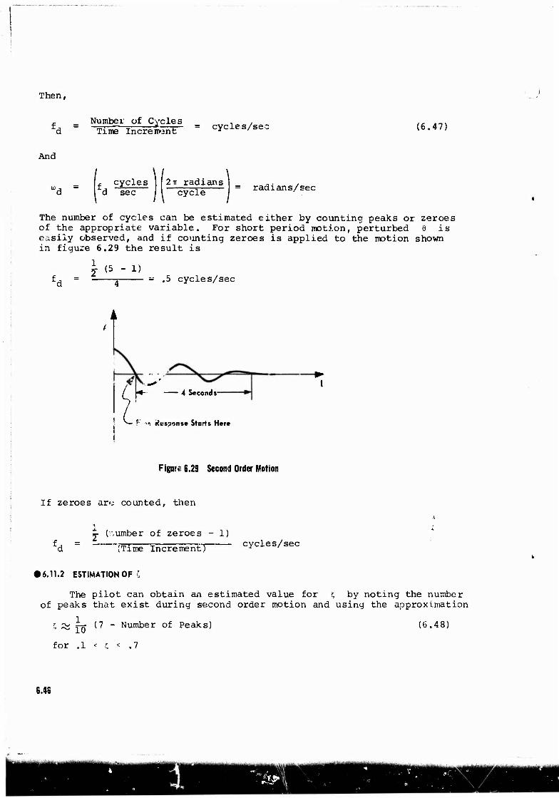
Then,

ff\, Number of Cycles Time Increment = cycles/sec (6.47)

And

cycles I 2TT radians d sec cycle = radians/sec

The number of cycles can be estimated either by counting peaks or zeroes of the appropriate variable. For short period motion, perturbed 6 is easily observed, and if counting zeroes is applied to the motion shown in figure 6.29 the result is

(5 - 1) .5 cycles/sec

4 Seconds

f- •'. Response Starts Here

Figure 6.29 Second Order Motion

If zeroes ar« counted, then

(number of zeroes - 1)

" (Time Increment! cycles/sec

• 6.11.2 ESTIMATION OF L

The pilot can obtain an estimated value for 5 by noting the number of peaks that exist during second order motion and using the approximation

; ~ Yf) (7 ~ Number of Peaks)

for .1 < c < .7

(6.48)

6.46

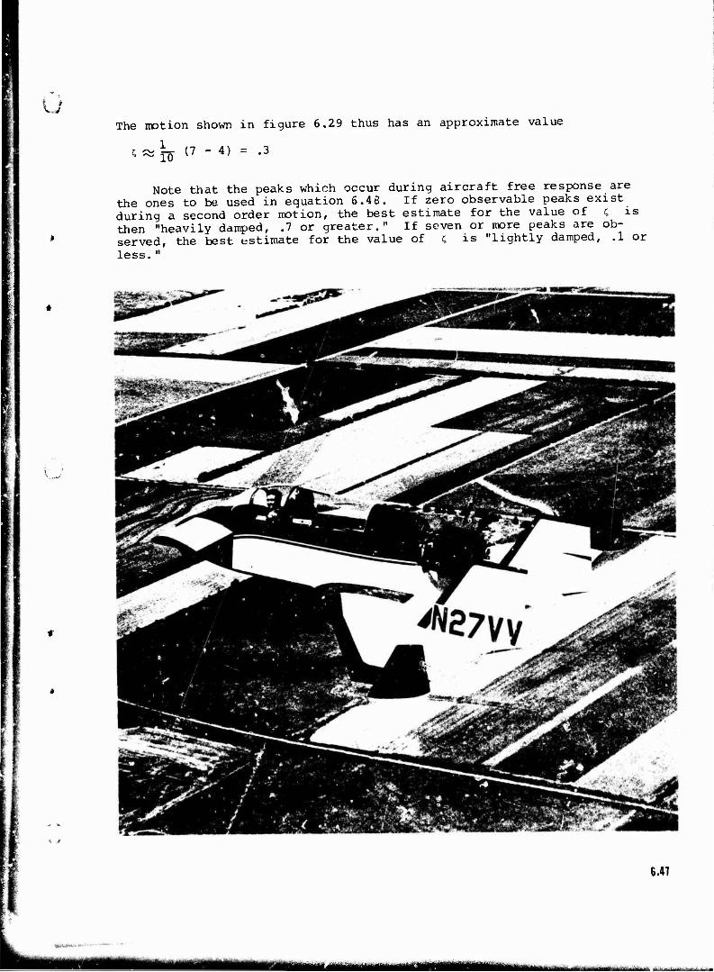
u The notion shown in figure 6.29 thus has an approximate value

C^JJ (7 "4) = .3

Note that the peaks which occur during aircraft free response are the ones to be used in equation 6.48. If zero observable peaks exist during a second order motion, the best estimate for the value of c, is then "heavily damped, .7 or greater." If seven or more peaks are observed, the best estimate for the value of ; is "lightly damped, .1 or less."

6.41

UM MM^tefciaMfcftlfc "-^—-*-

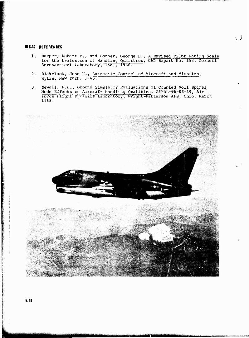
16.12 REFERENCES

1. Harper, Robert P., and Cooper, George E., A Revised Pilot Rating Scale for the Evaluation of Handling Qualities, CAL Report No. 153, Cornell Aeronautical Laboratory, Inc., 1966.

2. Blakelock, John H., Automatic Control of Aircraft and Missiles, Wylie, New York, 1965T

3. Newell, F.D., Ground Simulator Evaluations of Coupled Roll Spiral Mode Effects on Aircraft Handling Qualities, AFFDL-TR-6 5-39', Air Force Flight Dvnamics Laboratory, Wright-Patterson AFB, Ohio, March 1965.

•SSWi /'t'"v'^;

6.48

*MM MTMIM ■fa^gf/aLa»*.^.--..^.,-.- ■ .J;,^,t^-j;li,.i,aMiir^-.K.-v...i. ■■■<aJJri.v^M^a

\ )

VOLUME II

CHAPTER VII

•STALL GYRATIONS/SPINS Revised December 1973

I *

7-/

^tma —-—i 1 ... .

TABLE OF CONTENTS

Page No.

LIST OF ABBREVIATIONS AND SYMBOLS

REFERENCES

7.1 INTRODUCTION 7.1

7.1.1 Definitions 7.1

7.1.2 Susceptibility and Resistance to Departures and Spins 7.4

7.1.3 Spin Modes 7.5

7.1.4 Spin Phases 7.6

7.2 THE SPINNING MOTION 7.7

7.2.1 Description of Flightpath 7.8

7.2.2 Aerodynamic Factors 7.10

7.2.3 Aircraft Mass Distribution 7.14

7.3 EQUATIONS OF MOTION 7.17


7.3.2 Governing Equations 7.17

7.3.3 Aerodynamic Prerequisites 7.20

7.3.4 Estimation of Spin Characteristics 7.24

7.3.5 Gyroscopic Influences 7.27

7.3.6 Spin Characteristics of Fuselage-Loaded Aircraft 7.32

7.3.7 Sideslips . 7.34

7.4 INVERTED SPINS 7.35

7.4.1 Angle of Attack in Inverted Spin 7.35

7.4.2 Roll and Yaw Directions in an Inverted Spin .... 7.36

7.4.3 Applicability of Equations of Motion 7.37

7.5 RECOVERY 7.38

7.5.1 Terminology 7.38

7.5.2 Alteration of Aerodynamic Moments 7.39

7.5.3 Use of Inertial Moments 7.4J

7.5.4 Other Recovery Means 7.41

7.5.5 Recovery from Inverted Spins 7.42

7- //

i^^—laiai»tilfM*m«tt«r ■

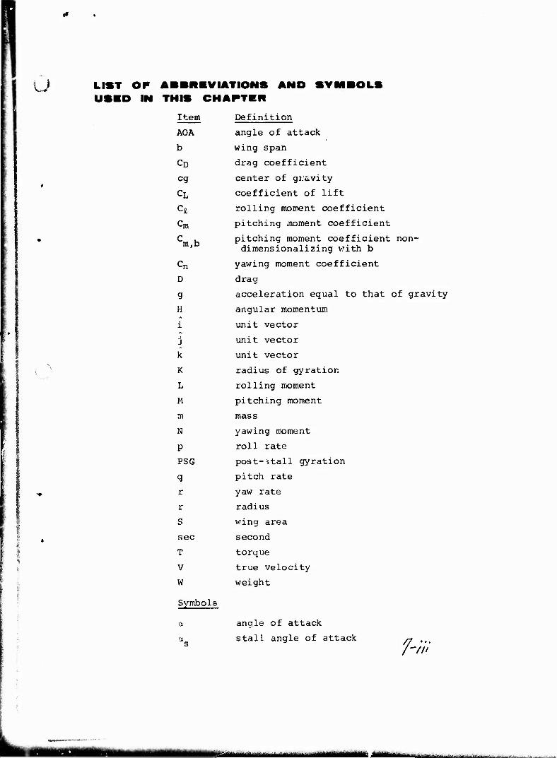
V j LIST OP ABBREVIATIONS AND SYMBOLS USID IN THIS CHAPTER

Item Definition

AOA angle of attack

b wing span

cD drag coefficient

eg center of gravity

cL coefficient of lift

c* rolling moment coefficient

Cm pitching moment coefficient

C U m,b pitching moment coefficient non- dimensionalizing v.'ith b

Cn yawing moment coefficient

D drag

g acceleration equal to that of gravity

H angular momentum

i unit vector

J unit vector

k unit vector

K radius of gyration

L rolling moment

M pitching moment

m mass

N yawing moment

P roll rate

PSG post-^tall gyration

q pitch rate

r yaw rate

r radius

S wing area

sec second

T torque

V true velocity

W weight

Symbols

a angle of attack

a stall angle of attack ^ ,.

H ///

mum - — ^^^^

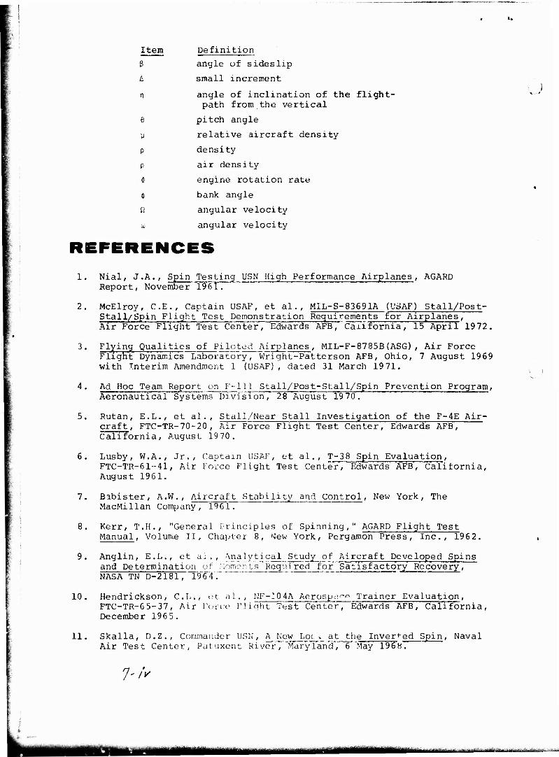
Item Definition

8 angle of sideslip

A small increment

n angle of inclination of t path from the vertical

e pitch angle

V relative aircraft density

P density

p air density

$ engine rotation rate

* bank angle

Q angular velocity

u angular velocity

1. Nial, J.A., Spin Testing USN High Performance Airplanes, AGARD Report, November 1961.

2. McElroy, C.E., Captain USAF, et al., MIL-S-836 91A (USAF) Stall/Post- Stall/Spin Flight Test Demonstration Requirements for Airplanes, Air Force Flight Test Center, Edwards AFB,"California, 15 April 1972.

3. Flying Qualities of Piloted Airplanes, MIL-F-8785B(ASG), Air Force Flight Dynamics Laboratory, Wright-Patterson AFB, Ohio, 7 August 1969 with Interim Amendment 1 (USAF), dated 31 March 19 71.

4. Ad Hoc Team Report on F-lll Stall/Post-Stall/Spin Prevention Program, Aeronautical Systems Division, 28 August 19 70.

5. Rutan, E.L., et al., Stall/Near Stall Investigation of the F-4E Air- craft, FTC-TR-70-20, Air Force Flight Test Center, Edwards AFB, California, August 19 70.

6. Lusby, W.A., Jr., Captain USAF, et al., T-38 Spin Evaluation, FTC-TR-61-41, Air Force Flight Test Center, Edwards AFB, California, August 1961.

7. Babister, A.W., Aircraft Stability and Control, New York, The MacMillan Company, 1961.

8. Kerr, T.H., "General Principles of Spinning," AGARD Flight Test Manual, Volume II, Chapter 8, ^Jew York, Pergamon Press, Inc., 1962.

9. Anglin, E.L., et ai ., Analytical Study of Aircraft Developed Spins and Determination of Moments Required for Satisfactory Recovery, NASA TN D-2181, 1964.

10. Hendrickson, C.L., et al., NF-3 0 4A Aerospci'-p Trainer Evaluation, FTC-TR-65-37, Air Forte Flight Test Center, Edwards AFB, California, December 196 5.

11. Skalla, D.Z., Commander USN, A New Loc >, at the Inverted Spin, Naval Air Test Center, Patuxent River, Maryland, 6 May 1968.

7-/V

müi ngmmami —m

u CHAPTER

POST-STALL GYRATIONS/SPINS VII •iiiiillliiiiiiiiiiiiiiiiiiiiiiiiiiiiiiiiiiikiiiiiiiMiiiiiiiiiMiiiiiiiiiniiiiiiiiiiiiigiiiiiiiiiiiiiiiiiiiiiiiiiiimiiiiiiiiMiiiiiiii

T.l INTRODUCTION

"Of the myriad of coupled an airplane can perform, t out as being unique. When is stalled and left to its perform some sort of rolli and pitching motion which, continue, may develop into tic motion called a spin, airplane descends rapidly earth in a helical movamen vertical axis at an angle tween the stall and 90°." page 2)

motions which he spin stands an airplane

elf, it will ng, yawing if allowed to a characteris-

in which the toward thf; t about the of attack be-

(Reference 1,

From this classical description it is clear that an aircraft spin is an extremely complex maneuver simultaneously involving pitch, roll, and yaw rates along with extreme angles of attack and large angles of sideslip. It is indeed more complex than the description. In the initial stages, the aircraft will still have some of its translational velocity, and the aircraft can spin at angles of attack greater than 9 0 degrees.

Recently a renewed interest in the high angle of attack (AOA) flight regime has generated considerable interest in designing to avoid the spin entirely in tactical aircraft. Clearly such design goals are worthy, and a wholj set of terms (not necessarily new) has been redefined to make more explr'cit the requirements which hopefully will make spin resistant tactical aircraft a reality. Words like "departure," stall," "post-stall gyration (PSG)," and "spin" itself have taken on different shades of meaning since the publication of reference 2. Given the complicated motions associated with a PSG or a spin and the explicit requirements now imposed by references 2 and 3, it is imperative that the test pilot clearly understand the precise terminology of the high AOA flight regime.

#7.1.1 DEFINITIONS

• 7.1.1.1 Stall Versus Out-of-Contro'!.

Stalls and associated aerodynamic phenomena have been described completely in chapter 2, but it is worth repeating the formal definition of a stall from page 67 of reference 3. In terms of angle of attack, the stall is defined as the lowest of the following:

a. Angle of attack for the highest steady load factor, normal to the flightpath, that can be attained at a given speed or Mach number.

7.1

b. Angle of attack, for a given speed or Mach number, at which abrupt or uncontrollable pitching, rolling, or yawing occurs. Angular limits of 20 degrees (Classes I, II, or III) or 30 degrees (Class IV) are specified in paragraph 3.4.2.1.2 of reference 3.

c. Angle of attack, for a given speed or Mach number, at which in- tolerable buffeting is encountered.

d. An arbitrary angle of attack, allowed by paragraph 3.1.9.2.1 of reference 3, which may be based on such considerations as ability to perform altitude corrections, excessive sinking speed, or ability to execute a go-around.

Reference 2 defines the stall angle of attack more simply: The angle of attack for maximum usable lift at a given flight condition. This latter definition is the one most useful in this course, but the student must understand that "maximum usable lift" is determined from one of the four conditions given above.

• 7.1.1.2 Departure.

u

Departure is defined as that event in the post-stall flight regime vvhich precipitates entry into a PSG, spin or deep stall condition (reference 2, paragraph 6.3.9). Notice two things about this definition. First, departure occurs in the post-stall flign: regime; that is, the stall always precedes departure. It can be inferred then that the angle of attack for maximum usable lift is always less than the angle of attack at which departure occurs. The second point is that only one of three motions may result after departure - the aircraft enters either a PSG, spin or deep stall (of course, a PSG can progress into a spin or deep stall). Implicit in this definition is the implication that an immediate recovery cannot be attained. For example, a light aircraft whose stall is defined by a g-break, may recover immediately if the longitudinal control pressure is relaxed. However, note that movement or position of controls is not mentioned in the definition. The same light aircraft that would not depart if control pressures were relaxed at the stall may depart and enter a spin if pro-spin controls are applied at the stall. Hence, in discussing, susceptibility or resistance to departure one must specify control positions as well as loading and configuration.

The departure event is usually a large amplitude, uncommanded, and divergent motion. Such descriptive terms as nose slice or pitch-up are commonly used to describe the event. Large amplitude excursions impiy changes in yaw, roll, or pitch greater than 20 degrees (class I, II, and III) or 30 degrees (class IV) (reference 3, paragraph 3.4.2.1.2). Un- commanded morions are motions not intended by the pilot, even though the control positions are legitimately causing the departure. The aircraft may not follow the pilot's commands for a number of reasons: the high angle of attack may render the control surface ineffective when moved to its desired position; or the pilot may be unable to position the stick to put the surface in the desired position due to lateral or transverse g loads. In either of these conditions the aircraft motion is "uncommanded." Finally, a divergent motion is one which either continuously or periodically increases in amplitude. The T-33 usually exhibits a "bucking" motion after the stall in which the nose periodically rises and falls. However, the motion is not divergent unless aggravated by full aft stick or some other pro-spin control. The T-38 will sometimes

7.2

iüü lateNJitftrtfiiMthi iiiiir-i - t ■■n-.|-[i'r^-^-;-"-'-"—^••■-■■■■'■'■■■■•■ :> ■---—■ ■——*

{^J exhibit a non-divergent lateral oscillation near the stall angle of attack. Neither of these motions are normally counted as departures, though their occurrence does serve as warning of impending departure if further misapplications of controls are made. With this sort of background it is easy to see why a departure is so hard to define, yet is relatively easy for a pilot to recognize. Next one must examine the terms "post-stall gyration", "spin" ani "deep stalls", used to define a departure.

• 7.1.1.3 Post-Stall Gyration. i

A post-stall gyration is an uncontrolled motion about one or more axes following departure (reference 2, paragraph 6.3.10). PSG is a very difficult term to define concisely because it can occur in so many different ways. Frequently, the motions are completely random about all axes and no more descriptive term than PSG can be applied. On the other hand a snap roll or a tumble are post-stall gyrations. The main difficulty lies in distinguiphing between a PSG and either the incipient phase of a spin or an oscillatory spin. The chief distinguishing characteristic is that a PSG may involve angles of attack that are intermittently below the airplane's stall angle of attack, whereas a spin always occurs at angles of attack greater than stall.

• 7.1.1.4 Spin.

A spin is a sustained yaw rotation at angles of attack above the aircraft's stall angle of attack (reference 2, paragraph 6.3.11). This definition bears a bit of explanation in that a spin is certainly not altogether a yaw rotation. Only the perfect flat spin (a = 90 degrees) could satisfy that constraint. The inference is, however, that the yaw rotation is dominant in characterizing a spin. Indeed, to a pilot, the recognition of a sustained (though not necessarily steady) yaw rate is probably the most important visual cue that a spin is occurring. Even though roll rate and yaw rate are often of nearly the same magnitude, the pilot still ordinarily recognizes the spin because of the yaw rate. In steep spins (with a relatively close to as) it is quite easy to con- fuse the roll rate and yaw rate and pilots sometimes have difficulty in recognizing this typr of motion and treating it as a spin. The steep inverted spin is pa.cicularly confusing since the roll and yaw rates are in opposite directions. Once again though, the yaw rate determines the direction of the spin and the required control manipulations to recover. All in all, it is well to remember that the spin is trvly a complicated maneuver involving simultaneous roll, pitch, and yaw ratios and high angles of attack. And, even though the overall rotary motion in a spin will probably have oscillations in pitch, roll, and yaw superimposed upon it, it is still most easily recognized by its sustained yawing component.

•7.1.1.5 Deep Stall.

A deep stall is an out-of-control flight condition in which the airplane is sustained at an angle of attack well beyond that for as while experiencing negligible rotational velocities (reference 2, paragraph 6.3.12). It may be distinguisned from a PSG by the lack of significant motions other than a high rate of descent. The deep stall may be a fairly stable maneuver such as a falling leaf, or it can be characterized by large amplitude angle of attack oscillations. For an aircraft to stay in a deep stalled condition, significant oscillations

7.3

mtm -*■'■'1V ••■**"■•?it-irh:-"Jiirir ii_ _in

must be limited to the longitudinal axis. Lateral and directional control surfaces are either stalled or blanked out. Depending on the pitching moment coefficient, recovery may or may not be possible.

• 7.1.2 SUSCEPTIBILITY AND RESISTANCE TO DEPARTURES AND SPINS:

Susceptibility/resistance to departures and spins has become an extremely important design goal for the generation of high performance aircraft presently in the design stage. Reference 4 offers convincing proof that such design emphasis is in fact overdue. But, for the designer to meet this requirement in an aircraft and for the test pilot to test against this requirement, it is essential that the words "susceptible" and "resistant" be understood alike by all concerned.

• 7.1.2.1 Extremely Susceptibie to Departure (Spins).

An aircraft is said to be extremely susceptible to departure (spins) if the uncontrolled motion occurs with the normal application of pitch control alone or with small roll and yaw control inputs. The only allowable roll and yaw control inputs are those normally associated with a given maneuver task. In short, an airplane that departs or enters a spin during Phase A of the flight test demonstration falls within this category (reference 2, paragraph 3.4.1.8).

• 7.1.2.2 Susceptible to Departure (Spins).

An aircraft is said to be susceptible to departure (spins) when the application or brief misapplication of pitch and roll and yaw controls that may be anticipated in normal operational use cause departure (spin). The amount of misapplied controls to be used will be approved by the procuring activity for Phase B of the flight test demonstration. In other words each aircraft will be stalled and aggravated control inputs will be briefly applied to determine departure (spin) susceptibility.

• 7 1.2.3 Resistant to Departure (Spins).

An aircraft is said to be departure (spin) resistant if only large and reasonably sustained misapplication of controls results in a departure (spin). "Reasonably sustained" means up to 3 seconds before recovery is initiated (reference 2, table I). This time delay may be increased for aircraft without positive indication of impending loss of control. This aircraft departs (spins) during Phase C of the flight test demonstration.

• 7.1.2.4 Extremely Resistant to Departure (Spins).

An aircraft is said to be extremely resistant to departure (spins) if these motions occur only after abrupt, inordinately sustained application of gross, abnormal, pro-departure controls. Aircraft in this category will only depart (spin) in Phase D of the flight test demonstration when the controls are applied and hold in the most critical manner to attain each possible mode of post-stall motion and held for various lengths of time up to 15 seconds or three spin turns, whichever is longer.

7.4

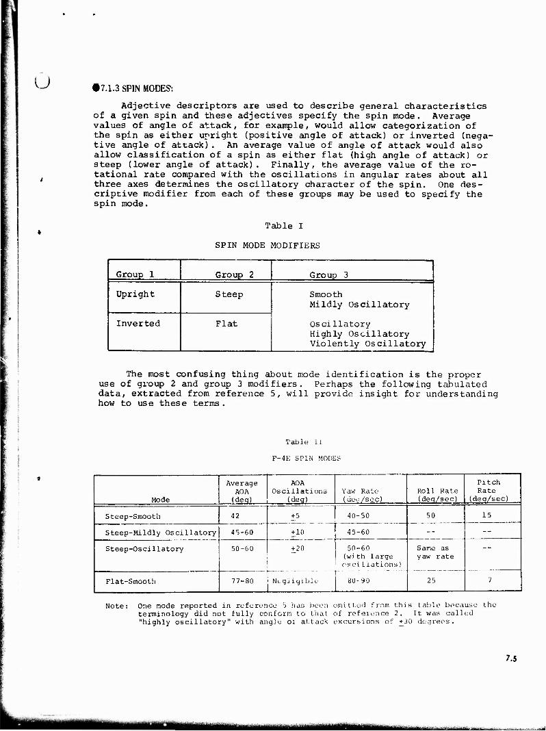
ü • 7.1.3 SPIN MODES':

Adjective descriptors are used to describe general characteristics of a given spin and these adjectives specify the spin mode. Average values of angle of attack, for example, would allow categorization of the spin as either upright (positive angle of attack) or inverted (negative angle of attack). An average value of angle of attack would also allow classification of a spin as either flat (high angle of attack) or steep (lower angle of attack). Finally, the average value of the rotational rate compared with the oscillations in angular rates about all three axes determines the oscillatory character of the spin. One des- cripcive modifier from each of these groups may be used to specify the spin mode.

Table I

SPIN MODE MODIFIERS

Group 1 Group 2 Group 3

Upright Steep Smooth Mildly Oscillatory

Oscillatory Highly Oscillatory Violently Oscillatory

Inverted Flat

The most confusing thing about mode identification is the proper use of group 2 and group 3 modifiers. Perhaps the following tabulated data, extracted from reference 5, will provide insight for understanding how to use these terms.

Table U

F-4E SPIN MODES

Mode

Average AOA

(deq)

AOA Oscillations

(deq) Y aw Ra te (dec/sec)

Roll Rate (deq/sec)

Pitch Rate

(deg/sec)

Steep-Smooth 42 + 5

+ 10

40-50 50 15

Steep-Mildly Oscillatory 45-60 45-60 -- --

Steep-Oscillatory 50-60 + 20

Neg] igible

50-60 (wi th large oscillations)

80- 90

Same as yaw rate

Flat-Smooth 77-80 25 7

Note: One mode reported in reference 5 has been omitted from this table because the terminology did not fully conform to that of reference 2. It was called "highly oscillatory" with angle ol attack excursions of +30 degrees.

7.5

■MHH ifMW iiiii i rum mtiM mi

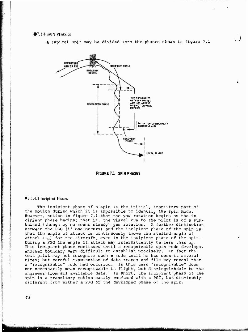
17.1.4 SPIN PHASES:

A typical spin may be divided into the phases shown in figure 7.1

INCIPIENT PHASE

THE BOUNDARIES BETWEEN PHASES ARE NOT ALWAYS DISTINCT OR WELL DEFINED

INITIATION OF RECOVERY CONTROLS AND

LEVEL FLIGHT

FIGURE 7.1 SPIN PHASES

• 7.1.4.1 Incipient Phase.

The incipient phase of a spin is the initial, transitory part of the motion during which it is impossible to identify the spin mode. However, notice in figure 7.1 that the yaw rotation begins as the incipient phase begins; that is, the visual cue to the pilot is of a sustained (though by no means steady) yaw rotation. A further distinction between the PSG (if one occurs) and the incipient phase of the spin is that the angle of attack is continuously above the stalled angle of attack (as) for the aircraft, even in the incipient phase of the spin. During a PSG the angle of attack may intermittently be less than os. This incipient phase continues until a recognizable spin mode develops, another boundary very difficult to establish precisely. In fact the test pilot may not recognize such a mode until he has seen it several times; but careful examination of data traces and film may reveal that a "recognizable" mode had occurred. In this case "recognizable" does not necessarily mean recognizable in flight, but distinguishable to the engineer from all available data. In short, the incipient phase of the spin is a transitory motion easily confused with a PSG, but distinctly different from either a PSG or the developed phase of ehe spin.

7.6

mat ""^■^* tiÜIMM ■■■VHMC ri mrMfedäiMl

• 7.1.4.2 Developed Phase.

I

The developed phase of a spin is that stage oi the motion in which it is possible to identify the spin mode. During this phase it is common for oscillations to be present, but the mean motion is still abundantly clear. The aerodynamic forces and moments are not usually completely balanced by the corresponding linear and angular accelerations, but at least equilibrium conditions are being approached. Generally it is evident in the cockpit that the developed phase is in progress, though the exact point at which it began may be quite fuzzy. Since the aircraft motion is approaching an equilibrium state, it is frequently advisable to initiate recovery before equilibrium is achieved. For example, during the T-38 test program warning lights were installed to signal a buildup in yaw rate. Test pilots initiated recovery attempts when these lights came on. Still, in the flat spin mode with recovery initiated at 85 degrees per second, a peak yaw rate of 165 degrees per second was achieved. The longitudinal acceleration at the pilot's station was approximately 3.5 g and the spin was terminated by deployment of the spin chute (reference 6, pages 10, 11). The developed spin, while it may be more comfortable due to less violent oscillations, can be de- ceptively dangerous, and the spin phase which follows can be disastrous.

• 7.1.4.3 Fully Developed Phase.

A fully developed spin is one in which the trajectory has become vertical and no significant change in the spin characteristics is noted from turn to turn. Many aircraft never reach this phase during a spin, but when they do, they are often very difficult to recover. The smooth, flat spin of the F-4 is a classic example in which this phase is attained and from which there is no known aerodynamic means of recovery. But a fully developed spin obviously requires time and altitude to be generated; how much time and how much attitude are strong fuctions of entry conditions. As a general rule, departures that occur at high airspeeds (high kinetic energy) require more time and altitude to reach the fully developed phase than departures which occur at low kinexiic energy. Finally, the spin characteristics which remain essentially unchanged in the fully developed phase include such parameters as time per turn, body axis angular velocities, altitude loss per turn, and similar quantities. How- ever, the definition does not prohibit a cyclic variation in any of these parameters. Hence, a fully developed spxn can be oscillatory.

! l

With this rather lengthy set of definitions in mind it is now appropriate to look more closely at spinning motions and at the aerodynamic and inertial factors which cause them and the PSG.

! ■7.2 THE SPINNING MOTION

Because the PSG is a random and usually a highly irregular motion, it is very difficult to study. On the other hand, the spin can approach an equilibrium condition and is therefore much more easily understood. Further, since the PSG is affected by the same aerodynamic and mass loading characteristics as the spin, an understanding of the spin and the factors affecting it are appropriate to the purposes of this course.

7.7

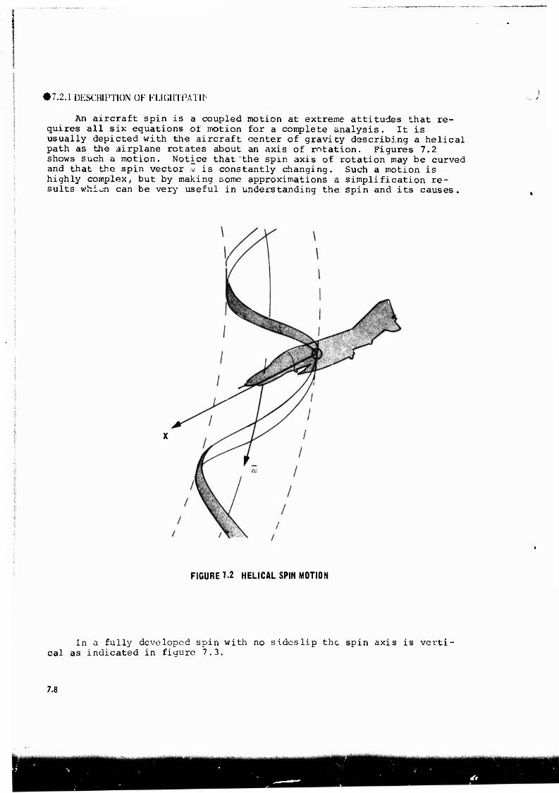
• 7.2.1 DESCRIPTION OF FTJGHTPATlf-

An aircraft spin is a coupled motion at extreme attitudes that requires all six equations of motion for a complete analysis. It is usually depicted with the aircraft center of gravity describing a helical path as the airplane rotates about an axis of rotation. Figures 7.2 shows such a motion. Notice that the spin axis of rotation may be curved and that the spin vector w is constantly changing. Such a motion is highly complex, but by making some approximations a simplification results whion can be very useful in understanding the spin and its causes.

FIGURE 7.2 HELICAL SPIN MOTION

In a fully developed spin with no sideslip the spin axis is vertical as indicated in figure 7.3.

7.8

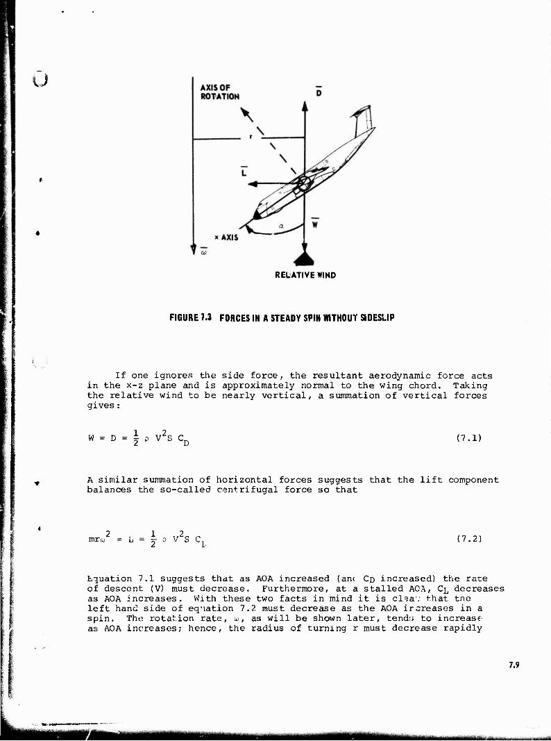
ü

RELATIVE WIND

FIGURE 7.3 FORCES IN A STEADY SPIN WITHOUT SIDESLIP

If one ignores the side force, the resultant aerodynamic force acts in the x-z plane and is approximately normal to the wing chord. Taking the relative wind to be nearly vertical, a summation of vertical forces gives:

W = D = \ p V2S CD (7.1)

A similar summation of horizontal forces suggests that the lift component balances the so-called centrifugal force so that

2 12 mroj = L = j P

v S C (7.2)

Equation 7.1 suggests that as AOA increased (an< CD increased) the rate of descent (V) must decrease. Furthermore, at a stalled AOA, CL decreases as AOA increases. With these two facts in mind it is cl^av that tne left hand side of equation 7.2 must decrease as the AOA ircreases in a spin. The rotation rate, w, as will be shown later, tend;; to increase as AOA increases; hence, the radius of turning r must decrease rapidly

7.9

mm mmmmm

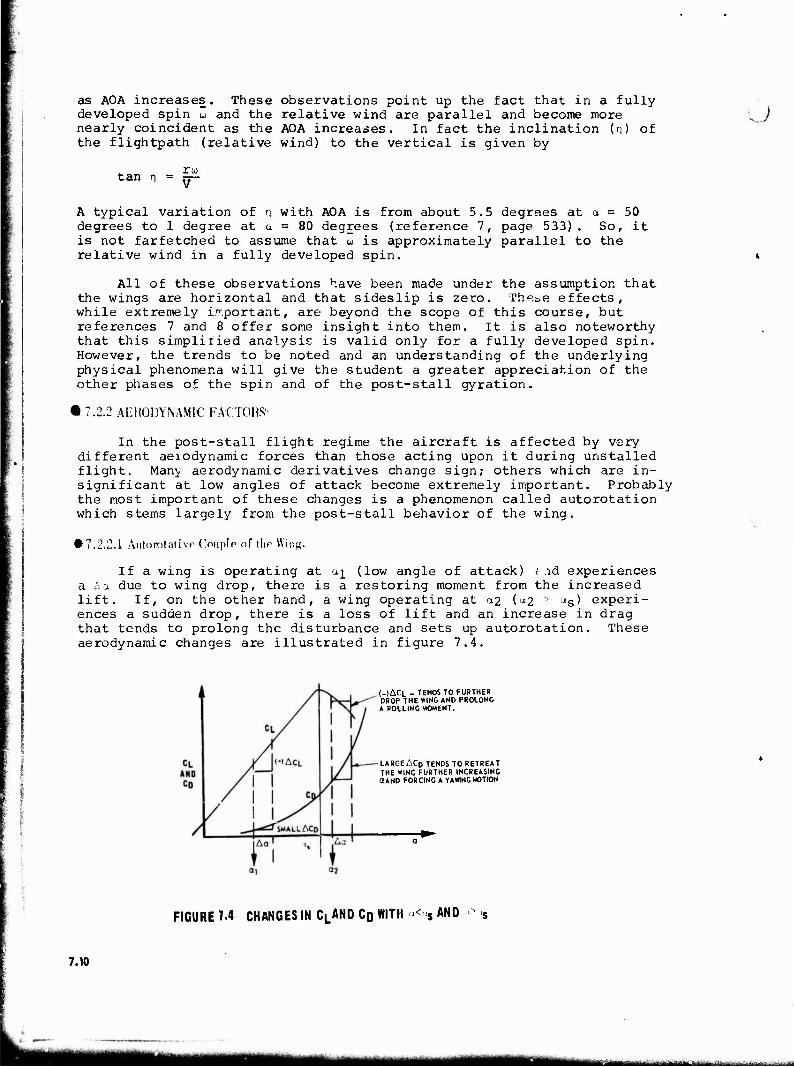
as AOA increases. These observations point up the fact that in a fully developed spin u and the relative wind are parallel and become more nearly coincident as the AOA increases. In fact the inclination (n) of the flightpath (relative wind) to the vertical is given by

tan n = 77— ru V

A typical variation of n with AOA is from about 5.5 degrees at a = 50 degrees to 1 degree at a = 80 degrees (reference 7, page 533). So, it is not farfetched to assume that w is approximately parallel to the relative wind in a fully developed spin.

All of these observations have been made under the assumption that the wings are horizontal and that sideslip is zero. These effects, while extremely important, are beyond the scope of this course, but references 7 and 8 offer some insight into them. It is also noteworthy that this simplified analysis is valid only for a fully developed spin. However, the trends to be noted and an understanding of the underlying physical phenomena will give the student a greater appreciation of the other phases of the spin and of the post-stall gyration.

• 7.2.2 AERODYNAMIC FACTORS'-

In the post-stall flight regime the aircraft is affected by vary different aerodynamic forces than those acting upon it during unstalled flight. Many aerodynamic derivatives change sign; others which are insignificant at low angles of attack become extremely important. Probably the most important of these changes is a phenomenon called autorotation which stems largely from the post-stall behavior of the wing.

• 7.2.2.1 Autorotativr Couple of tlir Wing.

If a wing is operating at ai_ (low angle of attack) i id experiences a A a due to wing drop, there is a restoring moment from the increased lift. If, on the other hand, a wing operating at 0.2 (^2 > as' experiences a sudden drop, there is a loss of lift and an increase in drag that tends to prolong the disturbance and sets up autorotation. These aerodynamic changes are illustrated in figure 7.4.

(-)ACL - TENDS TO FURTHER DROP THE WING AND PROLONG A ROLLING MOMENT.

LARGE ACD TENDS TO RETREAT THE WING FURTHER INCREASING OAND FORCING A YAWING MOTION

FIGURE 1.4 CHANGES IN CLAND CD WITH a<«, AND

7.10

i -

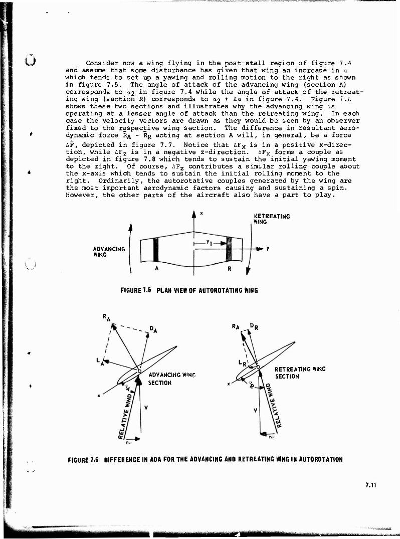
ü Consider now a wing flying in the post-stall region of figure 7.4 and assume that some disturbance has given that wing an increase in a which tends to set up a yawing and rolling motion to the right as shown in figure 7.5. The angle of attack of the advancing wing (section A) corresponds to c*2 in figure 7.4 while the angle of attack of the retreating wing (section R) corresponds to 02 + An in figure 7.4. Figure 7.C shows these two sections and illustrates why the advancing wing is operating at a lesser angle of attack than the retreating wing. In each case the velocity vectors are drawn as they would be seen by an observer fixed to the respective wing section. The difference in resultant aerodynamic force RA - RR acting at section A will, in general, be a force AF, depicted in figure 7.7. Notice that AFX is in a positive x-direction, while AFZ is in a negative z-direction. AFX forms a couple as depicted in figure 7.8 which tends to sustain the initial yawing moment to the right. Of course, AFZ contributes a similar rolling couple about the x-axis which tends to sustain the initial rolling moment to the right. Ordinarily, the autorotative couples generated by the wing are the most important aerodynamic factors causing and sustaining a spin. However, the other parts of the aircraft also have a part to play.

! I

f ADVANCING WING

RETREATING WING

FIGURE 7.5 PLAN VIEW OF AUTOROTATING WING

RA OR

ADVANCING WINC SECTION

RETREATING WING SECTION

FIGURE 7.6 DIFFERENCE IN AOA FOR THE ADVANCING AND RETREATING WING IN AUTOROTATION

7.11

wi att—

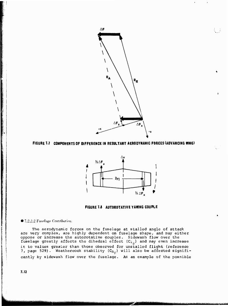
FIGURE 7.7 COMPOHENTS OF DIFFERENCE IN RESULTANT AERODYNAMIC FORCES (ADVANCING WING)

I

J4 AF„

FIGURE 7.8 AUTOROTATIVE YAWING COUPLE

• 7.2.2.2 Fuselage Contribution.

The aerodynamic forces on the fuselage at stalled angle of attack are very complex, are highly dependent on fuselage shape, and may either oppose or increase the autorotative couples. Sidewash flow over the fuselage greatly affects the dihedral effect (CJU) and may even increase it to values greater than those observed for unstalled flight (reference 7, page 529). Weathercock stability (CnR) will also be affected significantly by sidewash flow over the fuselage. As an example of the possible

7.12

flM

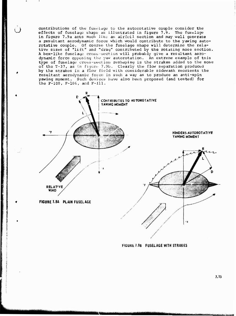
V. ) contributions of the fuselage to the autorotative couple consider the effects of fuselage shape as illustrated in figure 7.9. The fuselage in figure 7.9a acts much likt an airfoil section and may well generate a resultant aerodynamic force which would contribute to the yawing autorotative couple. Of course the fuselage shape will determine the relative sizes of "lift" and "drag" contributed by the rotating nose section. A box-like fuselage cross-section will probably give a resultant aerodynamic force opposing the yaw autorotation. An extreme example of tnis type of fuselage cross-section reshaping is the strakes added to the nose of the T-37, as in figure 7.9b. Clearly the flow separation produced by the strakes in a flow field with considerable sidewash reorients the resultant aerodynamic force in such a way as to produce an anti-spin yawing moment. Such devices have also been proposed (and tested) for the F-100, F-10G, and F-lll.

CONTRIBUTES TO AUTOROTATIVE YAWING MOMENT

HINDERS AUTOROTATIVE YAWING MOMENT

FIGURE T.9A PLAIN FUSELAGE

FIGURE J.9B FUSELAGE WITH STRAKES

7.13

iMgilaä&um

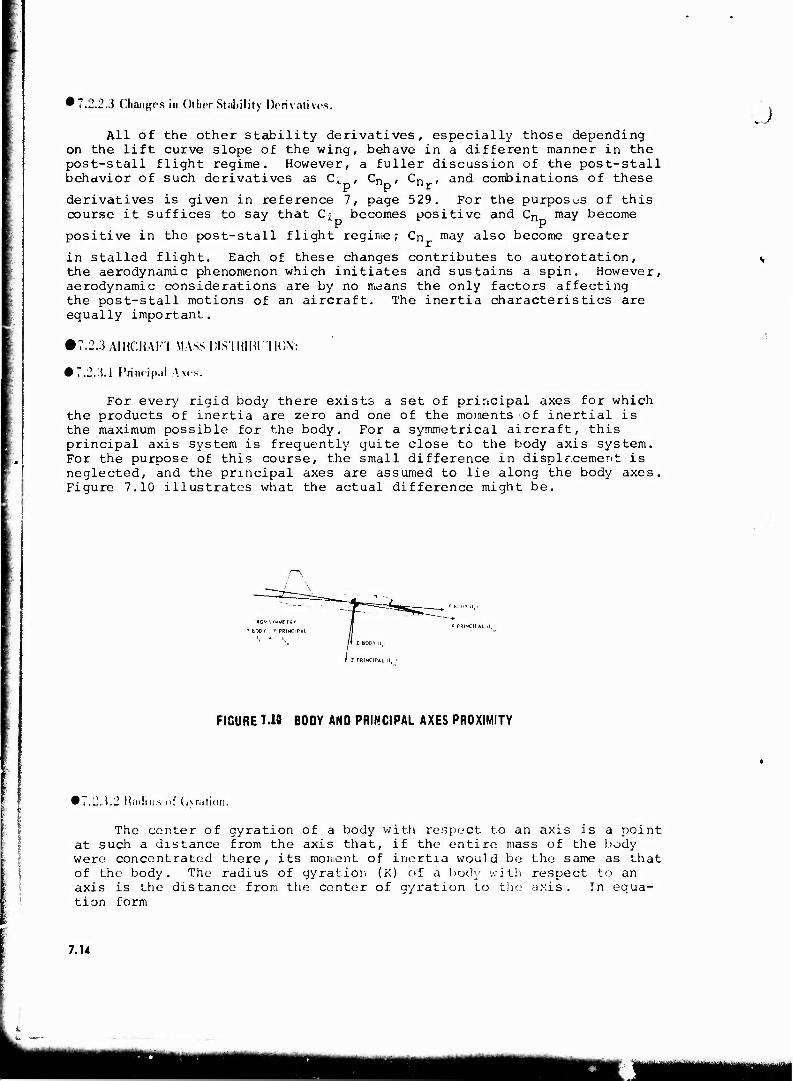
*7.2.2.3 Changes in Other Stability Derivatives.

All of the other stability derivatives, especially those depending on the lift curve slope of the wing, behave in a different manner in the post-stall flight regime. However, a fuller discussion of the post-stall behavior of such derivatives as Cj, , Cn , Cn , and combinations of these

hr r *■ derivatives is given in reference 7, page 529. For the purposes of this course it suffices to say that C« becomes positive and Cn may become positive in the post-stall flight regime; Cn may also become greater in stalled flight. Each of these changes contributes to autorotation, the aerodynamic phenomenon which initiates and sustains a spin. However, aerodynamic considerations are by no means the only factors affecting the post-stall motions of an aircraft. The inertia characteristics are equally important.

• 7.2.3 AIRCHAFI MASS DISTHIBl TION:

• 7.2..i.l Principal Axes.

For every rigid body there exists a set of principal axes for which the products of inertia are zero and one of the moments of inertial is the maximum possible for the body. For a symmetrical aircraft, this principal axis system is frequently quite close to the body axis system. For the purpose of this course, the small difference in displacement is neglected, and the principal axes are assumed to lie along the body axes. Figure 7.10 illustrates what the actual difference might be.

J

r\

"B0V\ 'WMF TRY

tx< . V PRINCIPAL

If I BODY |l,

t 1 PRINCIPAL

FIGURE 7.10 BODY AND PRINCIPAL AXES PROXIMITY

♦ 7.1..5.2 Hadiiis of (ivration.

The center of gyration of a body with respect to an axis is a point at such a distance from the axis that, if the entire mass of the body were concentrated there, its moment of inertia would be the same as that of the body. The radius of gyration (K) of a body with respect to an axis is the distance from the center of gyration to the axis. In equation form

u

or

/(y2 + z2) dm = I = K 2m 1 xx

/(x2 + z2) dm = I = K 2m

fix2 + y2) dm = I = K 2m z z

K. = I./m, i = x, y, or z l l 4 (7.3)

•7.2.3.3 Relative Aircraft Density. Y:

A nondimensional parameter called relative aircraft density (y) is frequently used to compare aircraft density to air density.

(7.4) m/Sb m u ~ o PSb

•7.2.3.4 Relative Magnitude of the Moments of Inertia.

The aircraft mass distribution is frequently used to classify the aircraft according to loading. Because aircraft are "flattened" into the XY plane, Iz is invariably the maximum moment of inertia. Ix is greater or less than Iy depending on the aircraft's mass distribution. The relative magnitudes of the moments of inertia are shown in figure 7.11. As will be seen in the next paragraph the relative magnitudes of Ix, Iy, and Iz are of utmost importance in interpreting the equations of motion.

7.15

mm ■'■v. ...^■V^.^v-^*'

iÜatoig^l^teiha^MMrilMinnlni ■ -iiF'iiri-i'ni Hill

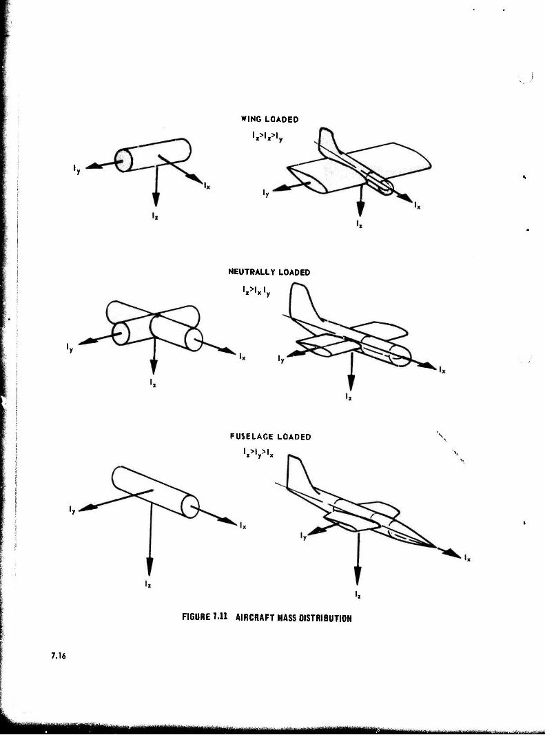
WING LOADED

NEUTRALLY LOADED

FUSELAGE LOADED

Wx

7.16

FIGURE 7.11 AIRCRAFT MASS DISTRIBUTION

L- -■■■--•■—•■ - ■'■•■■ IMS ;-■■ j.«

.J IT.3 EQUATIONS OF MOTION

'■ I

Maneuvers within the post-stall flight regime can be analyzed by using all six equations of motion and integrating them numerically on a computer. From such studies, predictions of rate of rotation, angle of attack, magnitude of the oscillations, optimum recovery techniques, and other parameters can be made. However, such studies must use rather in- accurate theory to predict stability derivatives or else depend on wind tunnel data or free flight model tests to provide the aerodynamic data. Hence, many researchers prefer to rely almost completely on model tests for predictions prior to flight tests. Correlation between model tests and aircraft flight tests is generally good. But model tests also have limitations. Spin tunnel tests primarily examine developed or fully developed spins; there is no good way to investigate PSG's or the incipient phase of the spin in the spin tunnel. Reynolds number effects on both spin tunnel and free flight models make it very difficult to accurately extrapolate to the full scale aircraft. Engine gyroscopic effects are not often simulated in model tests. Finally, model tests are always done for a specific aircraft configuration, which is a distinct advantage for a flight test program even though it does not suit tne purposes of this course. However, it would be foolish to ignore either computer analyses or model tests in preparing for a series of post-stall flight tests. For obvious reasons, this course will be restricted to a much simplified look at the equations of motion as applied to a fully developed spin.

• 7.3.1 ASSUMPTIONS':

The analytical treatment used in these notes is based on many simplifying assumptions, but even with these assumptions good qualitative information can be obtained. The most important assumption is that only a fully developed spin with the wings horizontal will be considered. The wings horizontal, fully developed spin involves ^ balance between applied and inertial forces and moments. Some of the ramifications of this assumption are:

a. The rate of descent (V) is virtually constant, as is altitude loss per turn.

b. V and u are parallel.

— • • c. The time per turn is constant, or u is constant. Hence, p = q =

r = 0.

d. With the wings horizontal iö lies entirely within the xz plane and q = 0 . (~=pi+rk).

Initially, it will also be assumed that tne applied moments consist entirely of aerodynamic ones, although other factors will be considered in later paragraphs.

• 7.3.2 GOVERNING EQUATIONS:

The reference frame for expressing moments, forces, accelerations, etc., is the xyz body axis frame which rotates at the same rate as the spin rotation rate ~. The origin of the xyz axes is centered at the

7.17

rinimMfcrriT 11 i ■■*«

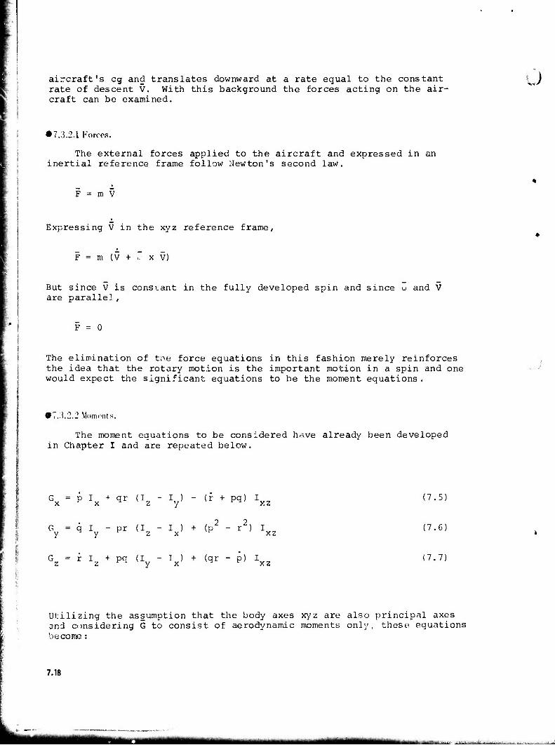
aircraft's eg and translates downward at a rate equal to the constant rate of descent V. With this background the forces acting on the aircraft can be examined.

Ü

• 7.3.2.1 Forces.

The external forces applied to the aircraft and expressed in an inertial reference frame follow Newton's second law.

F = m V

Expressing V in the xyz reference frame,

F = m (V + . x V)

But since V is constant in the fully developed spin and since tu and V are parallel ,

F = 0

The elimination of the force equations in this fashion merely reinforces the idea that the rotary motion is the important motion in a spin and one would expect the significant equations to be the moment equations.

• 7.3.2.2 Moments.

The moment equations to be considered have already been developed in Chapter I and are repeated below.

G = p I + qr (I - I ) - (r + pq) I x r x 1 z y l^ xz (7.5)

G = q I - pr (I - I ) + (p2 - r2) I Y y z x ^ xz !7.6)

G = r I + pq (I - I ) + (qr - p) I z z y x ^ c xz (7.7)

Utilizing the assumption that the body axes xyz are also principal axes and considering G to consist of aerodynamic moments only, these equations become:

7.18

■MMMMWI HUM^MM.

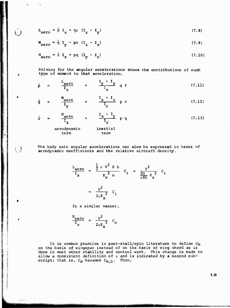
u L = p I + qr (I - I ) aero r x * z y

Maero = * Jy " ?r (Iz " V

N = r I + pq (I - I ) aero z ^M y x

(7.8)

(7.9)

(7.10)

Solving for the angular accelerations shows the contributions of each type of moment to that acceleration.

I - I aero + -Y. ?. q r I I y x x

(7.11)

M I - I aGro + _z * p r I I F

y y

N _... i„ - I. aero , x y Xz V *z

aerodynamic inertial term term

(7.12)

(7.13)

Ü The body axis angular accelerations can also be expressed in terirs of aerodynamic coefficients and the relative aircraft density.

aero 1 2 j p M S b

K m x

V 2m K pSb x

2 C*

V

2yK 2 ^

In a similar manner,

aero V

2pK 2 n

;. i

It is common practice in post-stall/spin literature to define Cm on the basis of wingspan instead of on the basis of wing chord as is done in most other stability and control work. This change is made to allow a consistent definition of u and is indicated by a second subscript; that is, Cm becames Cm j-,. Then,

7.19

UK |B|i|th^J.., t , ,._,. ....„._... _ .

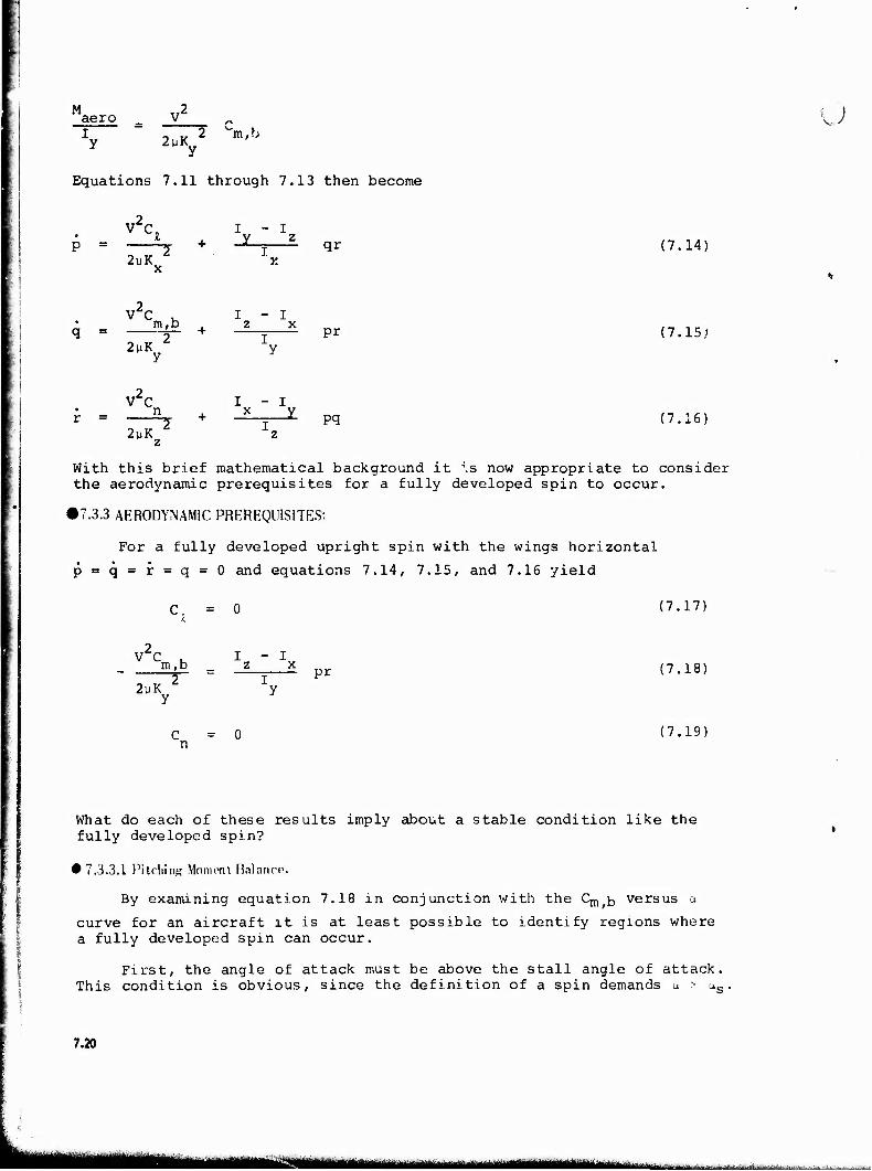
M aero

2pK 2 m,b o

Equations 7.11 through 7.13 then become

V2C P =

2uK

1 - I T + "I qr (7.14)

V2C . I - I q = __m_£ + z * pr (7.15)

r - V2C I - I

n J. x y + ^L pg

2pK Z 1z (7.16)

With this brief mathematical background it ^.s now appropriate to consider the aerodynamic prerequisites for a fully developed spin to occur.

• 7.3.3 AERODYNAMIC PREREQUISITES:

For a fully developed upright spin with the wings horizontal

p=q=r=q=0 and equations 7.14, 7.15, and 7.16 yield

Cl = 0 [7.17)

v2c m,b I - I z x pr 17.18) 2uK

C = 0 n 17.19)

What do each of these results imply about a stable condition like the fully developed spin?

• 7.3.3.1 Pitching Moment Balance.

By examining equation 7.18 in conjunction with the Cm ^ versus a

curve for an aircraft it is at least possible to identify regions where a fully developed spin can occur.

First, the angle of attack must be above the stall angle of attack. This condition is obvious, since the definition of a spin demands a > us

7.20

mm^^m^mmmttttmmmmmm

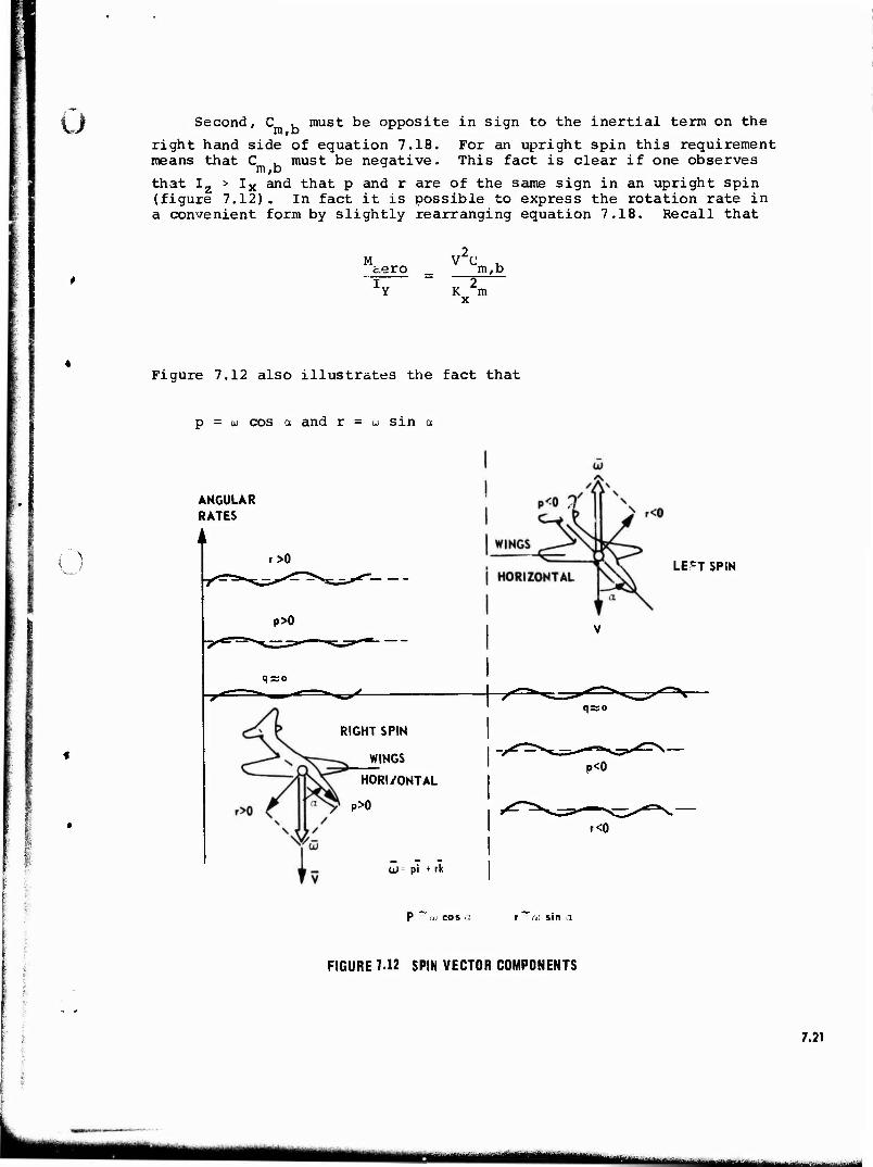
u Second, C . must be opposite in sign to the inertial term on the

right hand side of equation 7.18. For an upright spin this requirement means that C , must be negative. This fact is clear if one observes m,b that Iz > Ix and that p and r are of the same sign in an upright spin (figure 7.12) . In fact it is possible to express the rotation rate in a convenient form by slightly rearranging equation 7.18. Recall that

M aero V2C m,b

K 2m x

Figure 7.12 also illustrates the fact that

p= u cos a and r = w sin a

ANGULAR RATES

' I

i I

r>0

p>0

q=o

LEFT SPIN

RIGHT SPIN

WINGS

HORIZONTAL

p>0

Ol pi + rk

1=0

P<0

r<0

P *"aJ COS r a) sin a

FIGURE 7.12 SPIN VECTOR COMPONENTS

7.21

m )m

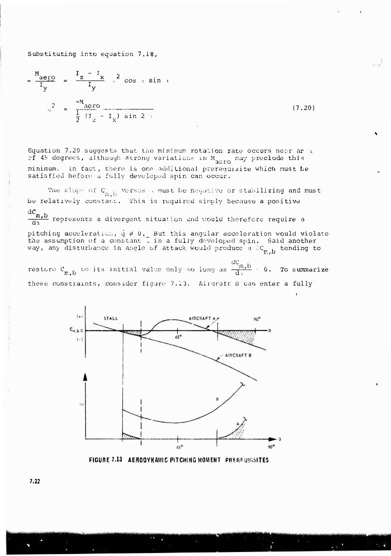
Substituting into equation 7.18,

aero I - I _ z x 2 cos a sin -i

-M aero (7.20)

i- (I - I ) sin 2 2 z x

Equation 7.20 suggests that the minimum rotation rate occurs ne:.r ar u cf 45 degrees, although strong variations in M may preclude this

ae i o minimum. in fact, there is one additional prerequisite which must be satisfied before a fully developed spin can occur.

The sloe'' of C , versus ■. must be neuative or stabilizing and must m,D

be relatively constant. This is required simply because a positive

dC ~m,b da represents a divergent situation and would therefore require a

pitching acceleration, q r 0._ But this angular acceleration would violate the assumption of a constant .. in a fully developed spin. Said another way, any disturbance in anale of attack would produce a .'.C , tendinq to 2 ' - - t rn,b *

dC restore C , to its initial value only so lone; as , m,b J J d

m,b 0. To summarize

these constraints, consider figure 7.13. Aircraft B can enter a fully

FIGURE 7.13 AERODYNAMIC PITCHING MOMENT PREREQUISITES

7.22

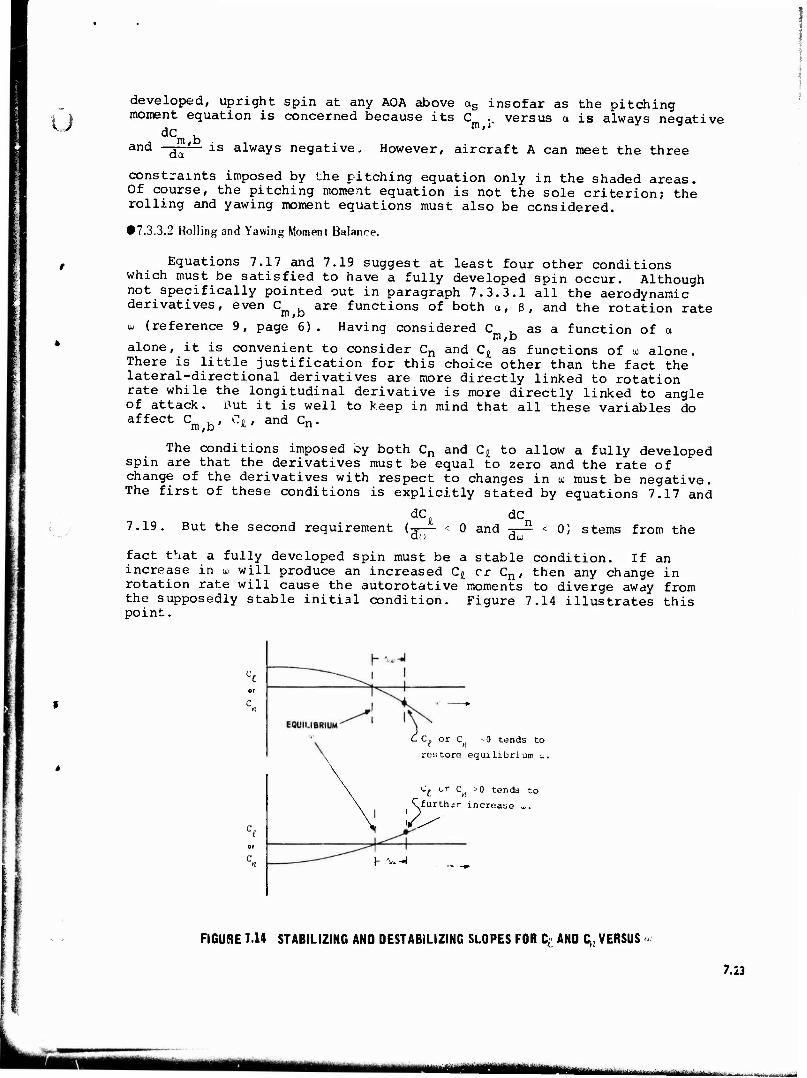
u developed, upright spin at any AOA above as insofar as the pitching moment equation is concerned because its C .. versus a is always negative

dc m'r

and ~m,b da is always negative- However, aircraft A can meet the three

constraints imposed by the pitching equation only in the shaded areas. Of course, the pitching moment equation is not the sole criterion; the rolling and yawing moment equations must also be considered.

• 7.3.3.2 Rolling and Yawing Moment Balance.

Equations 7.17 and 7.19 suggest at least four other conditions which must be satisfied to have a fully developed spin occur. Although not specifically pointed out in paragraph 7.3.3.1 all the aerodynamic derivatives, even Cm b are functions of both a, ß, and the rotation rate

w (reference 9, page 6). Having considered C . as a function of a m,b alone, it is convenient to consider Cn and C^ as functions of co alone. There is little justification for this choice other than the fact the lateral-directional derivatives are more directly linked to rotation rate while the longitudinal derivative is more directly linked to angle of attack. But it is well to keep in mind that all these variables do affect Cm b, C.lt and Cn.

The conditions imposed by both Cn and C£ to allow a fully developed spin are that the derivatives must be equal to zero and the rate of change of the derivatives with respect to changes in u must be negative. The first of these conditions is explicitly stated by equations 7.17 and

7.19. But the second requirement (- dC

0 and dC r dw 0) stems from the

fact that a fully developed spin must be a stable condition. If an increase in u will produce an increased C^ or Cn, then any change in rotation rate will cause the autorotative moments to diverge away from the supposedly stable initial condition. Figure 7.14 illustrates this point.

C C. or C - 0 tends to

restore equilibrium u.

t Cp or c„ >0 tends tc

icrease u,. <\furthär inc

I- .<W-I

FIGURE 7.14 STABILIZING AND DESTABILIZING SLOPES FOR C, AND C(1 VERSUS

7.23

Man '"-**■**•'--inn

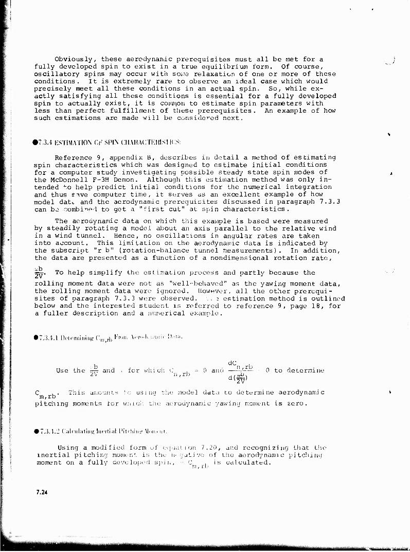
Obviously, these aerodynamic prerequisites must all be met for a fully developed spin to exist in a true equilibrium form. Of course, oscillatory spins may occur with some relaxation of one or more of these conditions. It is extremely rare to observe an ideal case which would precisely meet all these conditions in an actual spin. So, while exactly satisfying all these conditions is essential for a fully developed spin to actually exist, it is common to estimate spin parameters with less than perfect fulfillment of these prerequisites. An example of how such estimations are made will be considered next.

•7.3.4 ESTIMATION CF SPIN CHARACTKKISIICS':

Reference 9, appendix B, describes in detail a method of estimating spin characteristics which was designed to estimate initial conditions for a computer study investigating possible steady state spin modes of the McDonnell F-3H Demon. Although this estimation method was only intended to help predict initial conditions for the numerical integration and thus save computer time, it serves as an excellent example of how model date and the aerodynamic prerequisites discussed in paragraph 7.3.3 can bo combined to get a "first cut" at spin characteristics.

The aerodynamic data on which this example is based were measured by steadily rotating a model about an axis parallel to the relative wind in a wind tunnel. Hence, no oscillations in angular rates are taken into account. This limitation on the aerodynamic data is indicated by the subscript "r b" (rotation-balance tunnel measurements). In addition, the data are presented as a function of a nondimensional rotation rate,

~~. To help simplify the estimation process and partly because the

rolling moment data were not as "well-behaved" as the yawing moment data, the rolling moment data were ignored. However, all the other prerequisites of paragraph 7.3.3 were observed. . B estimation method is outlined below and the interested student is referred to reference 9, page 18, for a fuller description and a numerical example.

• 7.3.4.1 Ortr: Fmm Ai-i'^K iiaini r ! )ata.

Use the ~- and dC .

r ii. n n,rb for wh.i ch (-. , - 0 ana .-•—— n , rb , JJ . d(2V)

0 to determine

C , . This amounts to using the model data to determine aerodynamic m,rb

pitching moments ror whi oil the aerodynamic yawing moment is zero.

• 7.3.4.2 Calculating Incrtial Pitching \|<um nl.

Using a modified form of equation 7.20, and recognizing that the inertial pitching moment, is the negative of the aerodynamic pitching moment on a fully developed spin,

in, rl s calculated.

7.24

*•*■'--"— -- — ■■■--■ -■■■■ -

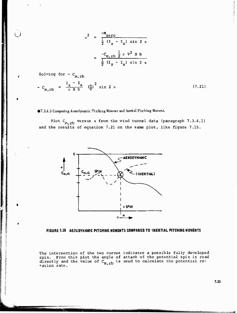
u

Solving for - C . m,rb

I - I. 'm,rb

-M aero

I (Iz " V sin 2 a

-Cm>rb I P V2 S b

I (I2 - V sin 2 a

p S b VV (—) sin 2 a (7.21)

#7.3.4.3 Comparing Aerodynamic Pitching Moment and l'nertial Pitching Moment.

Plot C , versus a from the wind tunnel data (paragraph 7.3.4

and the results of equation 7.21 on the same plot, like figure 7.15

•t Cm,rb

AERODYNAMIC

Si _?=v & ^-(-INERTIAL)

i a SPIN

FIGURE T.1S AERODYNAMIC PITCHING MOMENTS COMPARED TO -INERTIAL PITCHING MOMENTS

The intersection of the two curves indicates a possible fully developed spin. From this plot the angle of attack of the potential spin is read directly and the value of C , is used to calculate the potential ro-

j_ m, rb t-.ation rate.

7.25

mrnmrn ta.

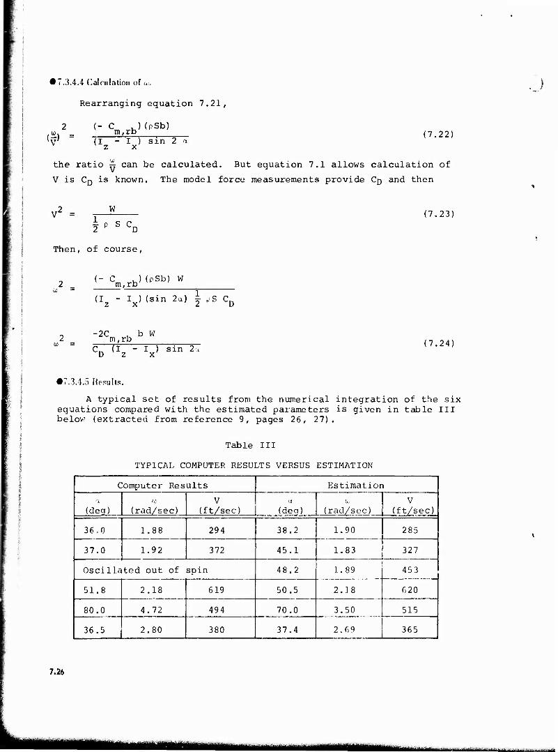
• 7.3.4.4 Calculation of a,.

Rearranging equation 7.21,

2 I" cm ,J (psb) .a». m, rt> lVJ " (I - I ) sin 2 a * z x

(7.22)

the ratio ~ can be calculated. But equation 7.1 allows calculation of

V is CD is known. The model force measurements provide Crj and then

V2 = w

2P S CD

(7.23)

Then, of course,

9 (- C , ) (oSb) W 2 m,rb u =

(I. Ix)(sin 2a) | ,S CD

-2C . b W m,rb

s71; I ) sin 2.» x

(7.24)

•7.3.4.5 Results.

A typical set of results from the numerical integration of the six equations compared with the estimated parameters is given in table III below (extracted from reference 9, pages 26, 27).

Table III

TYPICAL COMPUTER RESULTS VERSUS ESTIMATION

Computer Results Estimation

(deg) (0

(rad/sec) V

(ft/sec) u

(deq) tu

(rad/sec) V

(ft/sec)

36.0 1.88 294 38.2 1.90 285

37.0 1.92 372 45.1 1.83 327

Oscillated out of spin 48.2 1.89 453

51.8 2.18 619 50.5 2.18 6 20

80.0 4.72 494 70.0 3.50 515

36.5 2.80 380 37.4 2.69 365

7.26

■-• -

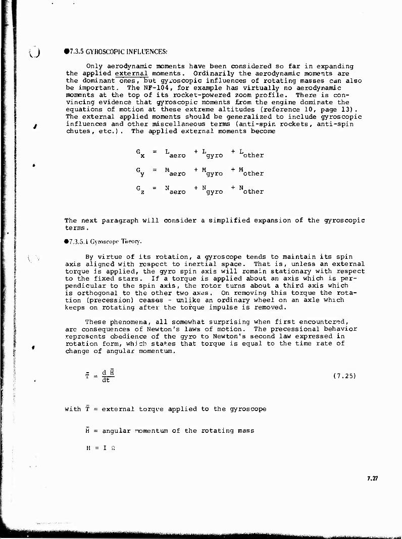
17.3.5 GYROSCOPIC INFLUENCES:

Only aerodynamic moments have been considered so far in expanding the applied external moments. Ordinarily the aerodynamic moments are the dominant ones, but gyroscopic influences of rotating masses can also be important. The NF-104, for example has virtually no aerodynamic moments at the top of its rocket-powered zoom profile. There is convincing evidence that gyroscopic moments from the engine dominate the equations of motion at these extreme altitudes (reference 10, page 13). The external applied moments should be generalized to include gyroscopic influences and other miscellaneous terms (anti-spin rockets, anti-spin chutes, etc.). The applied external moments become

G = L + L + L .. x aero gyro other

G=M +M + M .. y aero gyro other

G=N + N + N .. z aero gyro other

The next paragraph will consider a simplified expansion of the gyroscopic terms.

• 7.3.5.1 Gyroscope Theory.

By virtue of its rotation, a gyroscope tends to maintain its spin axis aligned with respect to inertial space. That is, unless an external torque is applied, the gyro spin axis will remain stationary with respect to the fixed stars. If a torque is applied about an axis which is perpendicular to the spin axis, the rotor turns about a third axis which is orthogonal to the other two axes. On removing this torque the rotation (precession) ceases - unlike an ordinary wheel on an axle which keeps on rotating after the torque impulse is removed.

These phenomena, all somewhat surprising when first encountered, are consequences of Newton's laws of motion. The precessional behavior represents obedience of the gyro to Newton's second law expressed in rotation form, which states that torque is equal to the time rate of change of angular momentum.

T = d H dt

(7.25)

with f = external torque applied to the gyroscope

H = angular nomentum of the rotating mass

H = I Q

7.27

— »aaiui

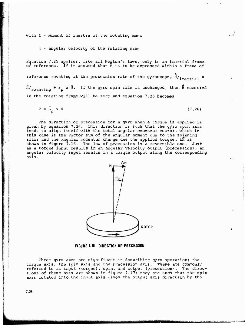
with I = moment of inertia of the rotating mass

il = angular velocity of the rotating mass

Equation 7.25 applies, like all Newton's laws, only in an inertial frame of reference. If it assumed that■H is to be expressed within a frame of

reference rotating at the precession rate of the gyroscope, HA ,_. , = r -si r i 'inertial • • H/ . + u) x H. If the gyro spin rate is unchanged, then H measured

in the rotating frame will be zero and equation 7.25 becomes

T = ui x H P

(7.26)

The direction of precession for a gyro when a torque is applied is given by equation 7.26. This direction is such that the gyro spin axis tends to align itself with the total angular momentum vector, which in this case is the vector sum of the angular moment due to the spinning rotor and the angular momentum change due the applied torque, AH as shown in figure 7.16. The law of precession is a reversible one. Just as a torque input results in an angular velocity output (precession), an angular velocity input results in a torque output along the corresponding axis .

ROTOR

FIGURE T.16 DIRECTION OF PRECESSION

Three gyro axes are significant in describing gyro operation; the torque axis, the spin axis and the precession axis. These are commonly referred to as input (torque), spin, and output (precession). The directions of these axes are shown in figure 7.17; they are such that the spin axis rotated into the input axis gives the output axis direction by the

7.28

in iiiiiiir1- ■i—«■- ■■

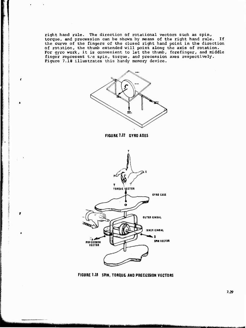
right hand rule. The direction of rotational vectors such as spin, torque, and precession can be shown by means of the right hand rule. If the curve of the fingers of the closed right hand point in the direction of rotation, the thumb extended will point along the axis of rotation. For gyro work, it is convenient to let the thumb, forefinger, and middle finger represent t»<e spin, torque, and precession axes respectively. Figure 7.18 illustrates this handy memory device.

FIGURE M7 GYRO AXES

GYRO CASE

OUTER GIMBM.

INNER CIMBAL

SMN VECTOR

FIGURE 7.18 SPIN, TORQUE- AND PRECESSION VECTORS

7.29

in ttHtittMM - ■-■■-■■■ ■'

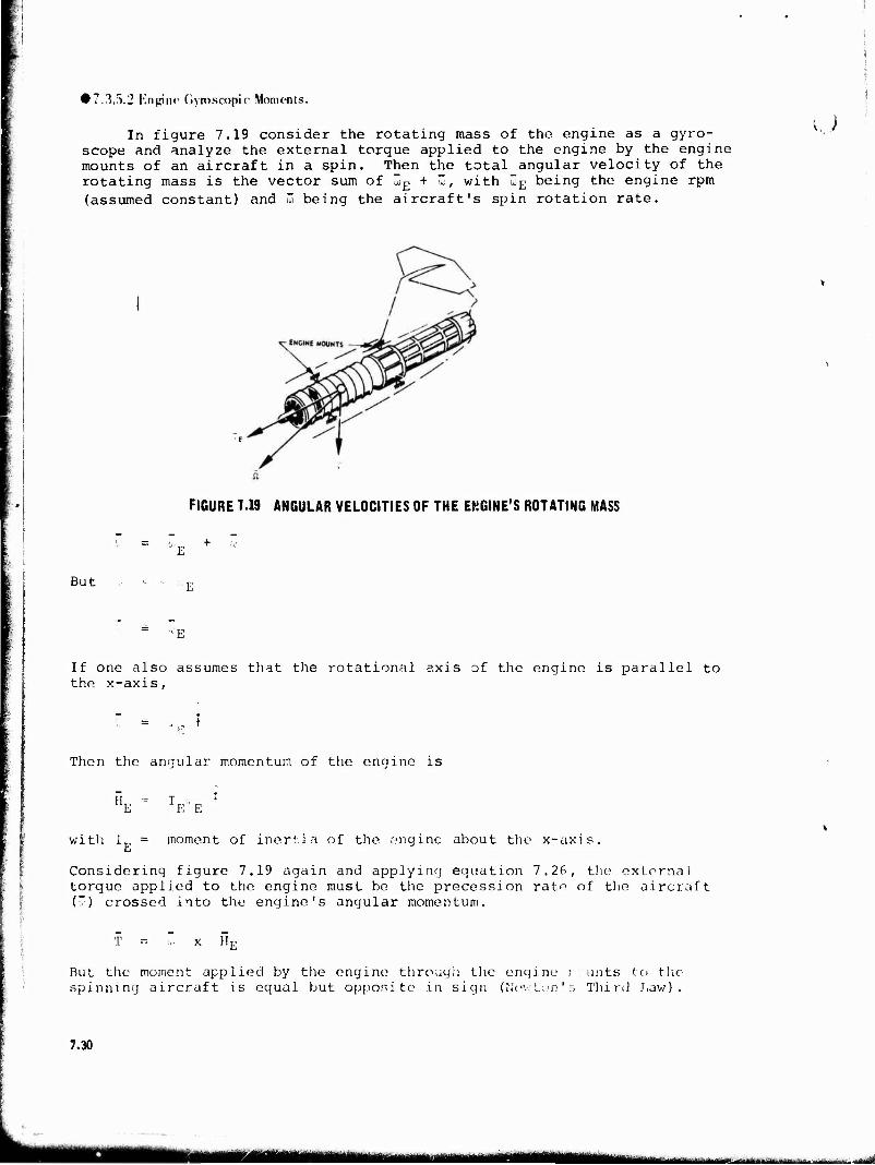
• 7.3.5.2 Kngine Gyroscopic Moments.

In figure 7.19 consider the rotating mass of the engine as a gyroscope and analyze the external torque applied to the engine by the engine mounts of an aircraft in a spin. Then the total angular velocity of the rotating mass is the vector sum of ü£ + ~, with ~E being the engine rpm (assumed constant) and 3 being the aircraft's spin rotation rate.

u

FIGURE 7.19 ANGULAR VELOCITIES OF THE ENGINE'S ROTATING MASS

+ w

But

" 'E

If one also assumes that the rotational axis of the engine is parallel to the x-axis,

"„ ♦

Then the angular momentum of the engine is

HE E E

with I_ = moment of inertia of the engine about the x-axis.

Considering figure 7.19 again and applying equation 7.26, the external torque applied to the engine must be the precession rate of the aircraft (~) crossed into the engine's angular momentum.

T = : x nE

Rut the moment applied by the engine through the engine r tints to the spinning aircraft is equal but opposite in sign (Newton's Third Law).

7.30

jtäiiaisJ^muMniamMnäiM\h-'-MYiikd-\ti-«\'m\-1 i- ■ i ~.*.lMä

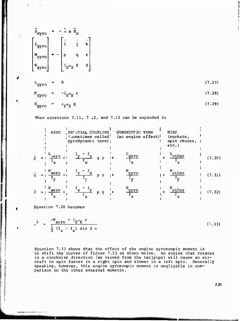
ayro

gyro

M gyro

N gyro

u x H_ E

p q

VE°

gyro

Mgyro = "VE r

Ngyro = VE q

(7.27)

(7.28)

(7.29)

Then equations 7.11, 7 i2, and 7.13 can be expanded to

AERO

aero

x

I M aero , q = i -_ +

aero , r = I — +

1 INITIAL COUPLING GYROSCOPIC TERM " MISC 1 «ometimes called' (an engine effect)! (rockets, ' gyrodynamic term)

I - I

I - I z x

I - I _x Y_

q r i +

p r | +

P q i +

_gyro

M gyr°

N 9Yro

spin chutes, | etc.)

I L

I +

other

M other

+ other l . I z i

(7.30)

I (7.31)

| (7.32)

Equation 7.20 becomes

-M + I„ü)_ r aero E E

hh I ) sin 2 a x

(7.33)

Equation 7.33 shows that the effect of the engine gyroscopic moment is to shift the curves of figure 7.13 as shown below. An engine that rotates in a clockwise direction (as viewed from the tailpipe) will cause an aircraft to spin faster in a right spin and slower in a left spin. Generally speaking, however, this engine gyroscopic moment is negligible in comparison to the other external moments.

7.31

«HMMM ■-''■"""-"— t -

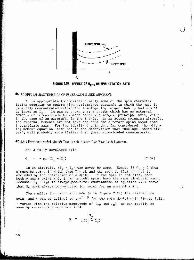
u

RIGHT SPIN

~---i.t EFT SPIN

FIGURE IM EFFECT OF Mgyro ON SPIN ROTATION RATE

•7.3.6 SPIN CHARACTERISTICS OF FUSELAGF-LOADFJ) AIRCRAFT:

It is appropriate to consider briefly some of the spin characteristics peculiar to modern high performance aircraft in which the mass is generally concentrated within the fuselage (Iy larger than Ix and almcst as large as Iz). It can be shown that a system which has no external moments or forces tends to rotate about its largest principal axis, which in the case of an aircraft, is the Z axis. In an actual spinning aircraft, the external moments are not zero and thus the aircraft spins about some intermediate axis. For the idealized spin thus far considered, the pitching moment equation leads one to the observation that fuselage-loaded aircraft will probably spin flatter than their wing-loaded counterparts.

• 7.3.6 1 Fuselage-Loaded Aircraft Tend to Spin Flatter Than Wing-Loaded Aircraft.

For a fully developed spin

Pr V 17.34)

In an aircraft, (Iz - Ix) can never be zero. Hence, if Gy = 0 then p must be zero, in which case ~ = rk and the spin is flat (ü = pi is excluded by the definition of a sj.in) . If the spin is not flat, then both p and r exist and, in an upright spin, have the same algebraic sign, Because (Iz - Ix) is always positive, examination of equation 7.34 shows that G„ mast always be negative (or zero) for an upright spin.

The smaller the pitch attitude (i1 in figure 7.21) the flatter the •1 p spin, and 0 can be defined as sin for the spin depicted in figure 7.21,

- varies with the relative magnitude of (Iz and Ix), as can readily be seen by rearranging equation 7.34.

r(I - I ) z x

7.32

MMMMM ■ndttkaHMUaUi ..._^.. ,,..,t. :.■-, ..

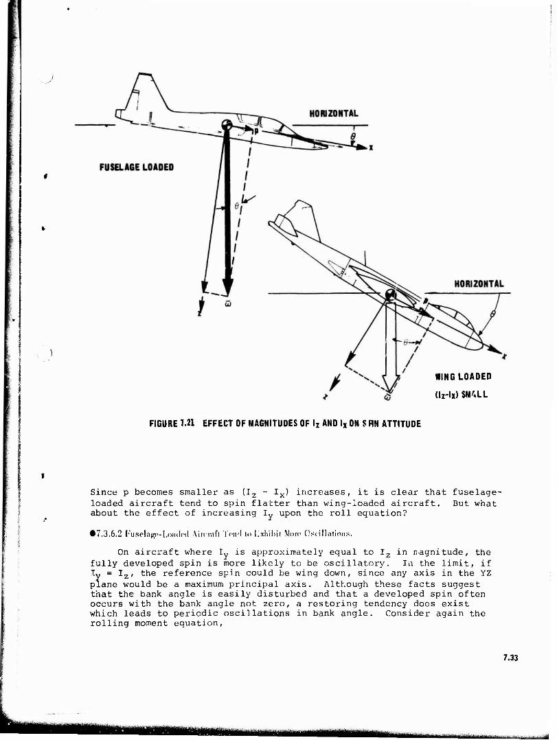
: WING LOADED

(lz-lx) SM^LL

FIGURE 7.21 EFFECT OF MAGNITUDES OF lz AND lx ON S FIN ATTITUDE

Since p becomes smaller as (I, Ix) increases, it is clear that fuselage- loaded aircraft tend to spin flatter than wing-loaded aircraft. But what about the effect of increasing Iy upon the roll equation?

• 7.3.6.2 Fuselagp-Loadod Aircraft Tend It) l.xliibit More Oscillations.

On aircraft where Iy is approximately equal to Iz in ragnitude, the fully developed spin is more likely to be oscillatory. In the limit, if ly = Iz, the reference spin could be wing down, since any axis in the YZ plane would be a maximum principal axis. Although these facts suggest that the bank angle is easily disturbed and that a developed spin often occurs with the bank angle not zero, a restoring tendency does exist which leads to periodic oscillations in bank angle. Consider again the rolling moment equation,

7.33

MM

G =pl+qr(l-l) x * x M z y

(7.35)

If an "o" subscript is used to represent the reference or steady-state conditions,

Gx„ = F> I + q„ * (I - I ) ox o o z

If instantaneous values are represented by equation 7.35, the change in external moments due to the perturbations of the angular acceleration and angular velocities is

(Gx ~ G ) - (p - po) Ix + (q r - qo rQ) C; I.)

Assuming perturbations in roll with not signiiicantly change r , r * rQ and

AG = Ap I + Aq (I - I ) r x x ^ 7. y o

Ap AG

Aq I - I

z T y r I o x

(7.36)

! I

The second term on the right side of equation 7.36 serves to damp oscillations in that it reduces the ability of perturbations in rolling moment (AGX) to produce perturbations in roll acceleration (Ap). For fuselage- loaded aircraft, in which (Iz - Iv) is small, the damping is much reduced. Thus, any perturbations in the motion tend to persist longer in fuselage- loaded aircraft than they do in wing-Joaded aircraft.

.3.7 SIDKSUP:

It is beyond the scope of this course to deal with the effects of sideslip in any detail. However, it is noteworthy that sideslip need not be zero in a developed spin; in fact it usually is not. Reference 7, page 535, shows that sideslip in a spin arises from two sources: wing tilt with respect to the horizontal (f) and the inclination of the flight path to the vertical (n).

= <j, - (7.37)

If then, one considers a spin with a helical flight path as opposed to a vertical flight path, the inclination of the flight path to the vertical is positive and equal to the helix angle. Then, in order to maintain zero sideslip, the retreating wing must be inclined downwards by an amount equal to the helix angle in order to have zero sideslip. However, it is quite common to have fully developed spins (with the spin axis vertical, not the flight path) with varying amounts of sideslip. Sideslip on a stalled wing will generally increase the lift on the wing toward which the sideslip occurs and reduce the lift on the opposite wing. It is eas^ to understand that a small amount of sideslip can produce a large rolling

7.34

I

moment and thereby significantly alter the balance of rolling moments. These qualitative comments are quite cursory and the inquisitive student may wish to pursue these effects further. Reference 7 offers an expanded discussion, but to adequately discuss sideslip effects in any detail one must consider all three moment equations and their coupling effects. The consideration of sideslip leads to the general conclusion that the rolling couple can be balanced over a wide range of angles of attack and spin rotation rates.

■ 1.4 INVERTED SPINS

Since PSG's are definitely uncontrolled aircraft motions, there is absolutely no guarantee that all spins will be of an upright variety, as has so far been assumed. The test pilot particularly (and operational pilots as well) will continue to experience inverted spins and PSG's which may be mainly inverted aircraft motions. As reference 11, page 1, points out,

"...inverted spins cannot be prevented by handbook entries that 'the airplane resists inverted spins'."

It is, therefore, essential that the test pilot have some appreciation of the nature of the inverted PSG/spin. As usual, the analytical emphasis will necessarily be restricted to the fully developed spin, but the qualitative comments which follow also apply in a general way to other types of post-stall motion.

The most common pilot reaction is, "I have no idea what happened! dirt, and confusion." Why? First, in and of itself, particularly when even experienced test pilots can be reduced in an anticipated inverted takes one of two forms: (1) inabil is inverted or upright or (2) inabi the spin. Each of these problems w

to an inverted post-stall maneuver The cockpit was full of surprise, negative g flight is disconcerting it is entered inadvertently. But upset and their powers of observation

spin. This disorientation usually ity to distinguish whether the motion lity to determine the direction of ill be considered separately.

.1 ANGI.K OK ATTACK IN AN INVKHTF.I) SPIN-

The angle of attack in 7.22). It might appear tha in an upright or inverted s it is an inverted spin. Su (the Hawker Hunter has an e this); however if the moti or a PSG, the pilot's tacti aircraft has an angle of at reliable means of determini Lacking an anyle of attack or his sensory cues, neithe about determining spin dire

an inverted sp t it would be e pin; if the pil rh an "analysis asily recognize on is highly os le senses are j tack indicator, ng whether the syste:,., _■ pil r of which are ction?

in is always negative (figure asy to determine the difference ot is "hanging in the straps,''

is accurate in some spin modes d smooth, fiat mode such as dilatory, not fully developed, ust not good enough. If the this is probably the most

maneuver is erect or inverted, ot must rely on the accelerometer easy to interpret. But what

7.35

MMHI mm

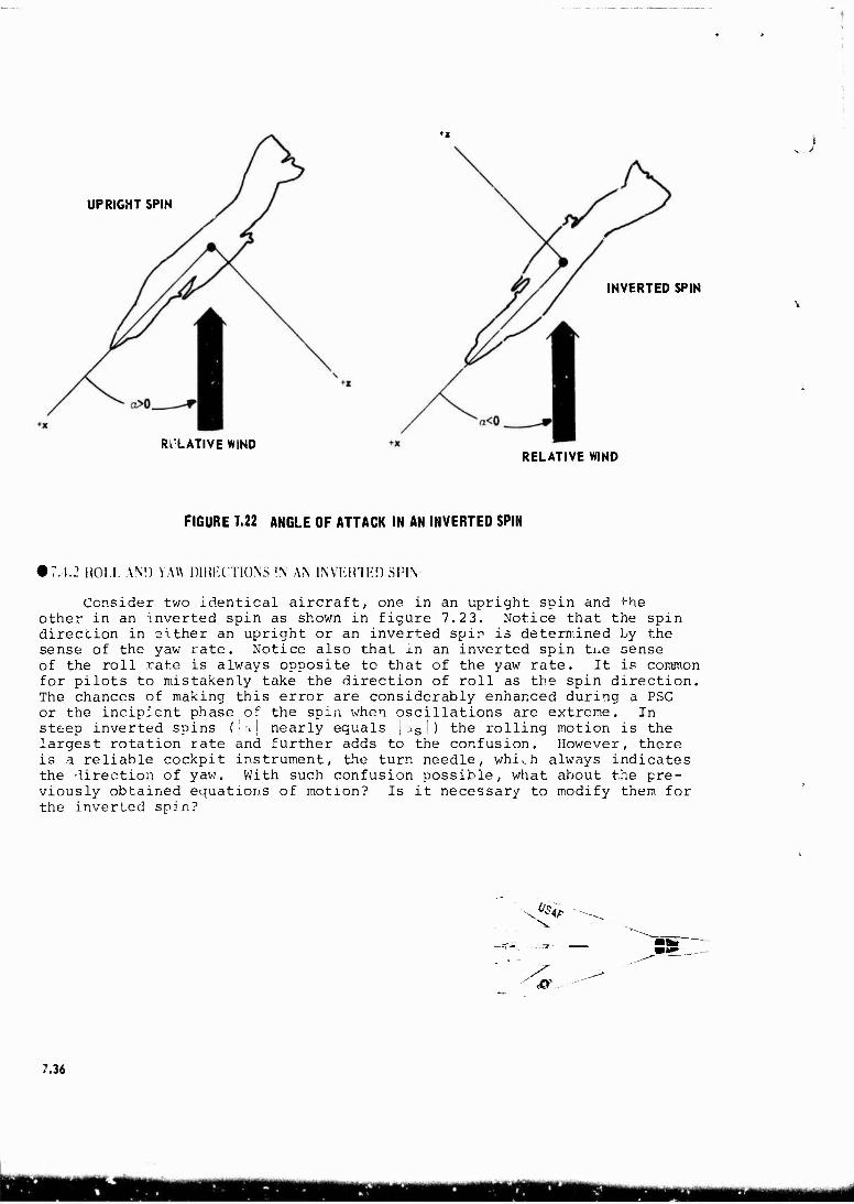
UPRIGHT SPIN

INVERTED SPIN

RELATIVE WIND

J

RELATIVE WIND

FIGURE 7.22 ANGLE OF ATTACK IN AN INVERTED SPIN

• 7.4.2 ROLL AND YAW DIRECTIONS !N AN INVERTED SPIV

Consider two identical aircraft, one in an upright spin and the other in an inverted spin as shown in figure 7.23. Notice that the spin direction in either an upright or an inverted spin is determined by the sense of the yaw rate. Notice also that in an inverted spin ti.e sense of the roll rate is always opposite to that of the yaw rate. It is common for pilots to mistakenly take the direction of roll as the spin direction. The chances of making this error are considerably enhanced during a PSG or the incipient phase of the spin when oscillations are extreme. In steep inverted spins (!aj nearly equals | as | ) the rolling motion is the largest rotation rate and further adds to the confusion. However, there is a reliable cockpit instrument, the turn needle, whivh always indicates the direction of yaw. With such confusion possible, what about the previously obtained equations of motion? Is it necessary to modify them for the inverted spin?

us 4P

7.36

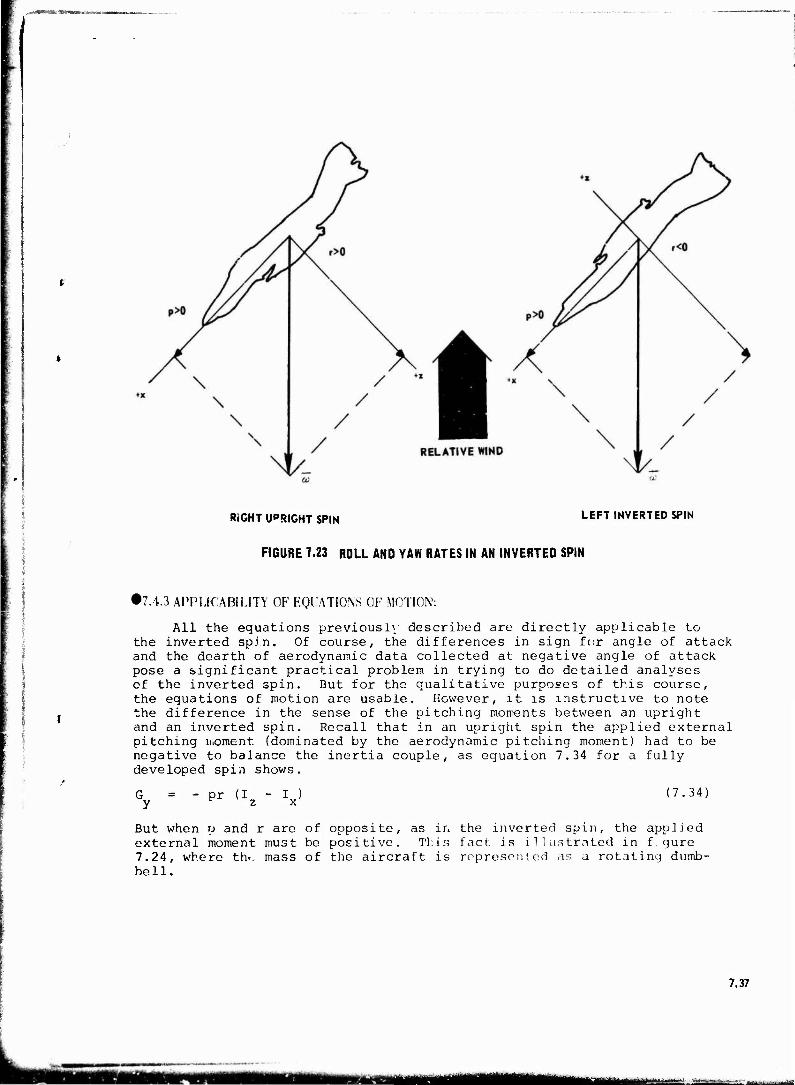
RIGHT UPRIGHT SPIN LEFT INVERTED SPIN

FIGURE T.23 ROLL AND YAW RATES IN AN INVERTED SPIN

•7.4.3 APPLICABILITY OF EQUATIONS OF MOTION':

All the equations previously described are dire the inverted spin. Of course, the differences in si and the dearth of aerodynamic data collected at nega pose a significant practical problem in trying to do of the inverted spin. But for the qualitative purpo the equations of motion are usable. However, it is the difference in the sense of the pitching moments and an inverted spin. Recall that in an upright spi pitching moment (dominated by the aerodynamic pitchi negative to balance the inertia couple, as equation developed spin shows.

pr (I. I ) x

ctly applicable to gn for angle of attack tive angle of attack detailed analyses

ses of this course, instructive to note between an upright n the applied external ng moment) had to be 7.34 for a fully

(7.34)

But when p and r are of opposite, as in the inverted spin, the applied external moment must be positive. This fact is illustrated in f.gure 7.24, where tht. mass of the aircraft is represented as a rotating dumb- bell.

7.37

JtaNMNtttifli

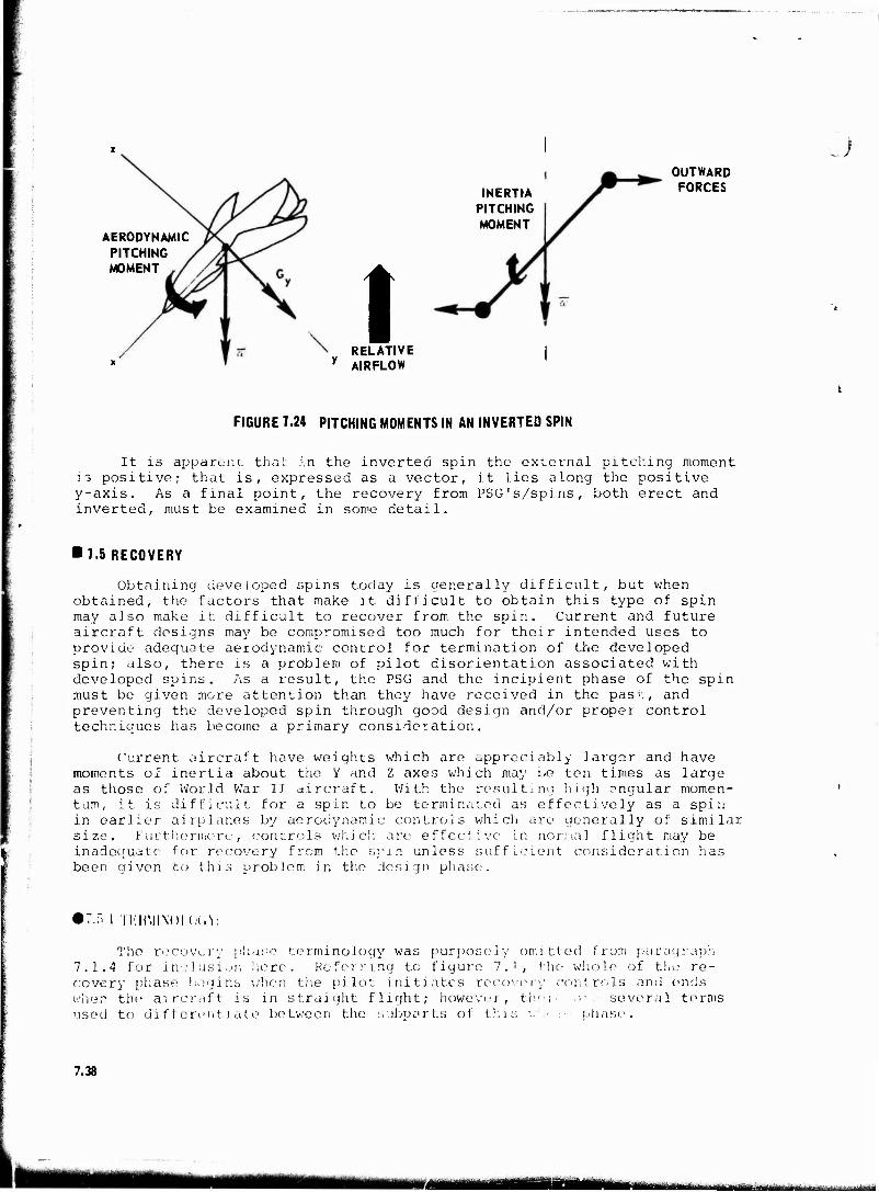
AERODYNAMIC PITCHING MOMENT

INERTIA PITCHING MOMENT

t RELATIVE

y AIRFLOW

OUTWARD FORCES

J

FIGURE 7.24 PITCHING MOMENTS IN AN INVERTED SPIN

It is apparent that in the inverted spin the external pitching moment J3 positive; that is, expressed as a vector, it lies along the positive y-axis. As a final point, the recovery from PSG's/spins, both erect and inverted, must be examined in some detail.

■ 7.5 RECOVERY

Obtaining obtained, the may also make aircraft desig provide adequa spin; also, th developed spin must be given preventing the techniques has

developed spins today is generally difficult, but when factors that make it difficult to obtain this type of spin it difficult to recover from the spin. Current and future ns may be compromised too much for their intended uses to te aerodynamic control for termination of the developed ere is a problem of pilot disorientation associated with s. As a result, the PSG and the incipient phase of the spin more attention than they have received in the pas1:, and developed spin through good design and/or proper control become a primary consideration.

Current aircraft have weights which are appreciably larger and have moments of inertia about the Y and Z axes which may be ten times as large as those of World War II aircraft. With the resulting high angular momentum, it is difficult for a spin to be terminated as effectively as a spin in earlier airplanes by aerodynamic controls which are generally of similar size. Furthermore, controls which, are effective in normal flight may be inadequate for recovery from the spin unless sufficient consideration has been given to this problem in the design phase.

riiHMiNoi.oi.t:

The recovery phase terminology was purposely omitted from paragraph 7.1.4 for inclusion here. Referring to figure 7.', the; whole of the recovery phase begins when the pilot initiates recover eher the aircraft is in straight flight; however, tlv used to differentiate between the subparts of this '..

>n t rols and ends a i ..• several terms phase .

7.38

'Til MM« iMBMta mm i

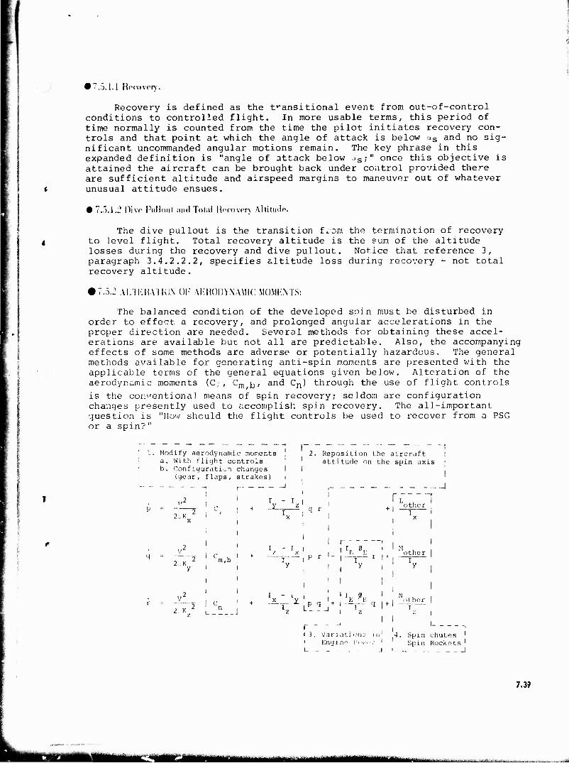
• 7.5.1.1 Recovery.

Recovery is defined as the transitional event from out-of-control conditions to controlled flight. In more usable terms, this period of time normally is counted from the time the pilot initiates recovery controls and that point at which the angle of attack is below as and no significant uncommanded angular motions remain. The key phrase in this expanded definition is "angle of attack below JS;" once this objective is attained the aircraft can be brought back under control provided there are sufficient altitude and airspeed margins to maneuver out of whatever unusual attitude ensues.

• 7.5.1.2 Dive Pulloiit and Total Recover\ Altitude.

The dive pullout is the transition from the termination of recovery to level flight. Total recovery altitude is the sum of the altitude losses during the recovery and dive pullout. Notice that reference 3, paragraph 3.4.2.2.2, specifies altitude loss during recovery - not total recovery altitude.

5.2 AUK RATION OF AERODYNAMIC MOMENTS:

i . :

| I

\ I

The balanced condition of the developed spin must be disturbed in order to effect a recovery, and prolonged angular accelerations in the proper direction are needed. Several methods for obtaining these accelerations are available but not all are predictable. Also, the accompanying effects of some methods are adverse or potentially hazardous. The general methods available for generating anti-spin moments are presented with the applicable terms of the general equations given below. Alteration of the aerodynamic moments (Cj, Cm j-,, and Cn) through the use of flight controls is the conventional means of spin recovery; seldom are configuration changes presently used to accomplish spin recovery. The all-important question is "How should the flight controls be used to recover from a PSG or a spin?"

! l. Modify aerodynamic moments ' I a. With flight controls I b. Configuration changes I I (gear, flaps, strakes) i

2;.K

2. Reposition the aircraft I attitude on the spin axis >

__i

I — q r

other 1

2..K i C m,b

I - I i z x

P r other I y

1 I

2. K I C

.- J I I

r L

I 3. Variations in' 4. Spin chutes ' i Engine )>i ■*,■.>:; ' ' Spin Rockets ' i- .- - - -J i.. _ -. _ I

7,3?

MMMUkMWMI MB ^^^^^.jt:.^

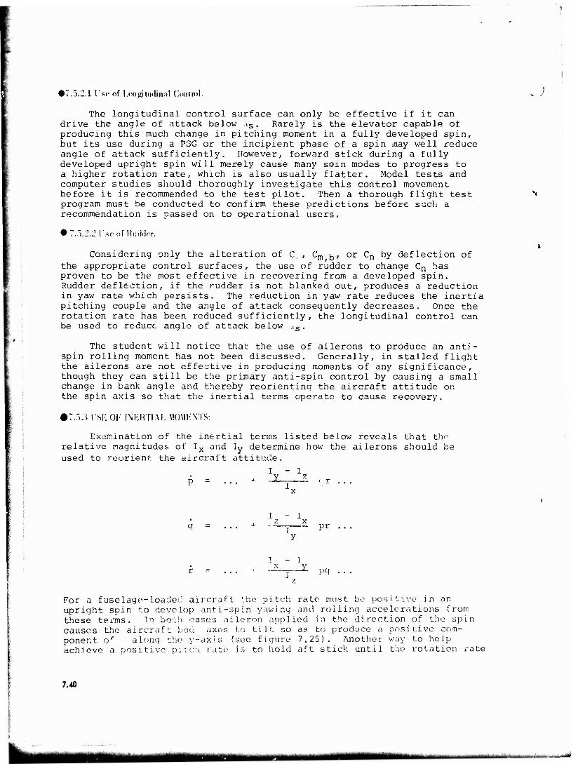
•7.5.2.1 l'sp of Longitudinal Control.

The longitudinal control surface can only be effective if it can drive the angle of attack below JS . Rarely is the elevator capable of producing this much change in pitching moment in a fully developed spin, but its use during a PGG or the incipient phase of a spin may well reduce angle of attack sufficiently. However, forward stick during a fully developed upright spin will merely cause many spin modes to progress to a higher rotation rate, which is also usually flatter. Model tests and computer studies should thoroughly investigate this control movement before it is recommended to the test pilot. Then a thorough flight test program must be conducted to confirm these predictions before such a recommendation is passed on to operational users.

I .so of Ri.diW.

Considering only the alteration of C, , Cm b, or Cn by deflection of the appropriate control surfaces, the use of rudder to change Cn has proven to be the most effective in recovering from a developed spin. Rudder deflection, if the rudder is not blanked out, produces a reduction in yaw rate which persists. The reduction in yaw rate reduces the inertia pitching couple and the angle of attack consequently decreases. Once the rotation rate has been reduced sufficiently, the longitudinal control can be used to reduce angle of attack below as.

The student will notice that the use of ailerons to produce an anti- spin rolling moment has not been discussed. Generally, in stalled flight the ailerons are not effective in producing moments of any significance, though they can still be the primary anti-spin control by causing a small change in bank angle and thereby reorienting the aircraft attitude on the spin axis so that the inertial terms operate to cause recovery.

#7.5.3 ! SH OK INERTIAL MOMKNTs-

Examination of the inertial terms listed below reveals that the relative magnitudes of Ix and Iv determine how the ailerons should be used to reorient the aircraft attitude.

I - I y z

q = pr

- 1 pq

For a f uselage-loade<" aircraft 'he pitch rate must be positive : n an upright spin to develop anti-spin yawing and rolling accelerations from these terms. In both cases aileron applied in the direction of the spin causes the aircraft bod axes to tilt so as to produce a positive component of along the y-axis (see figure 7.25). Another way to help achieve a positive pitch rate is to hold aft stick until the rotation rate

7.40

"■"-—'■"■-*- ■■■■-■-" —-—-

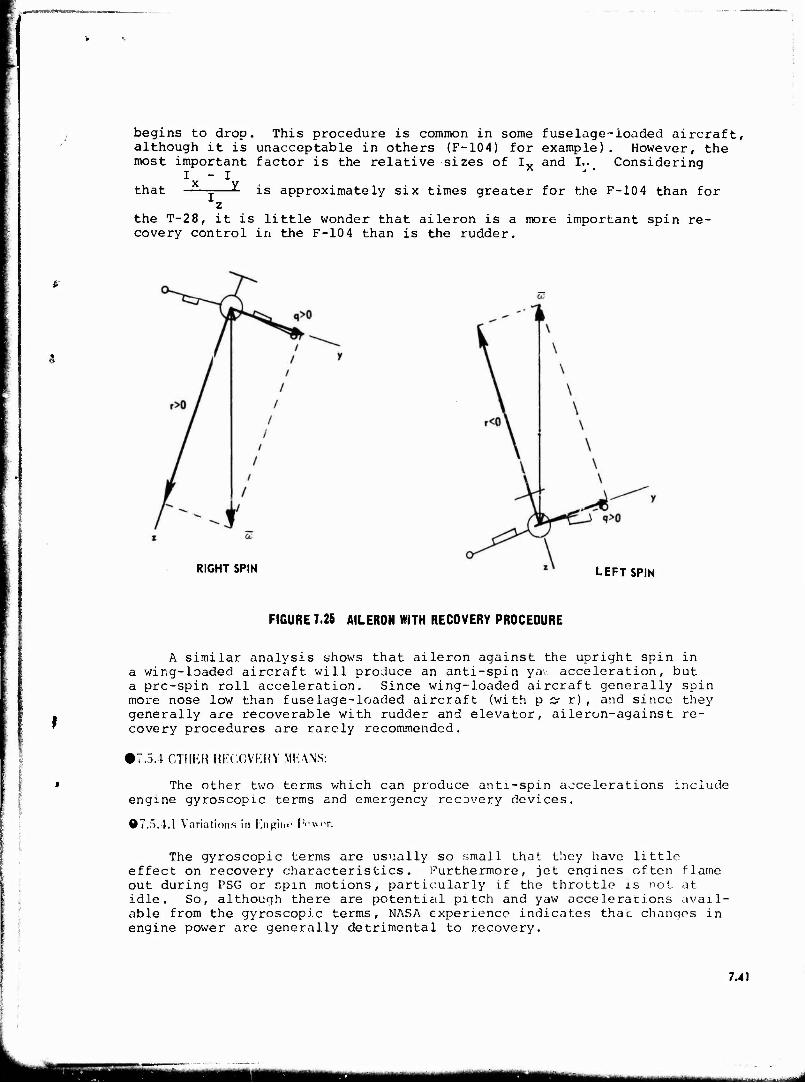
. ^*fljw-<l V>#***t* XV*- .*.

begins to drop. This procedure is common in some fuselage-loaded aircraft, although it is unacceptable in others (F-104) for example). However, the most important factor is the relative sizes of Iv and I,. Considering

I - I X

that =—E is approximately six times greater for the F-10 4 than for z

the T-28, it is little wonder that aileron is a more important spin recovery control in the F-10 4 than is the rudder.

RIGHT SPIN LEFT SPIN

FIGURE 7.25 AILERON WITH RECOVERY PROCEDURE

A similar analysis shows that aileron against the upright spin in a wing-loaded aircraft will produce an anti-spin yai. acceleration, but a prc-spin roll acceleration. Since wing-loaded aircraft generally spin more nose low than fuselage-loaded aircraft (with py r), and since they generally are recoverable with rudder and elevator, aileron-against recovery procedures are rarely recommended.

•7.5.4 CTHKR RECOVERY MEANS:

The other two terms which can produce anti-spin accelerations include engine gyroscopic terms and emergency recovery devices.

07.5.4.1 Variations in En ginP IV.WT.

The gyroscopic terms are usually so small that they have little effect on recovery characteristics. Furthermore, jet engines often flame out during PSG or spin motions, particularly if the throttle is not at idle. So, although there are potentiell pitch and yaw accelerations available from the gyroscopic terms, NASA experience indicates thai: changes in engine power are generally detrimental to recovery.

7.41

MHiHitt tMJMJ

ft?.5.4.2 Emergency Recovery Devices.

Emergency recovery devices may take many forms - anti-spin parachutes attached to the aft fuselage, anti-spin parachutes attached to the wing tip, anti-spin rockets, strakes, etc. The design of such devices is a complex subject worthy of careful engineering in its own right. Cer- tainly such design considerations are not the concern of test pilots; but the reliability of the device, its attachments, and its jettison mechanism are of vital concern to him. He is also likely to be concerned with tests to validate this reliability.

•7 5.5 RECOVERY FROM INVERTED SPINS':

Recovery from inverted spins is generally easier than recovery from upright spins, particularly if the rudder is in undisturbed airflow. In fact many aircraft will recover from an inverted spin as soon as the controls are neutralized. In any case rudder opposite to the turn needle may be recommended, often in conjunction with aft stick. Some fuselage- loaded T-tailed aircraft may require anti-spin aileron. An analysis similar to that in paragraph 7.5.3 shows that in an inverted spin aileron against the spin is the correct anti-spin control for a faselage-loaded aircraft.

7.42

mrä

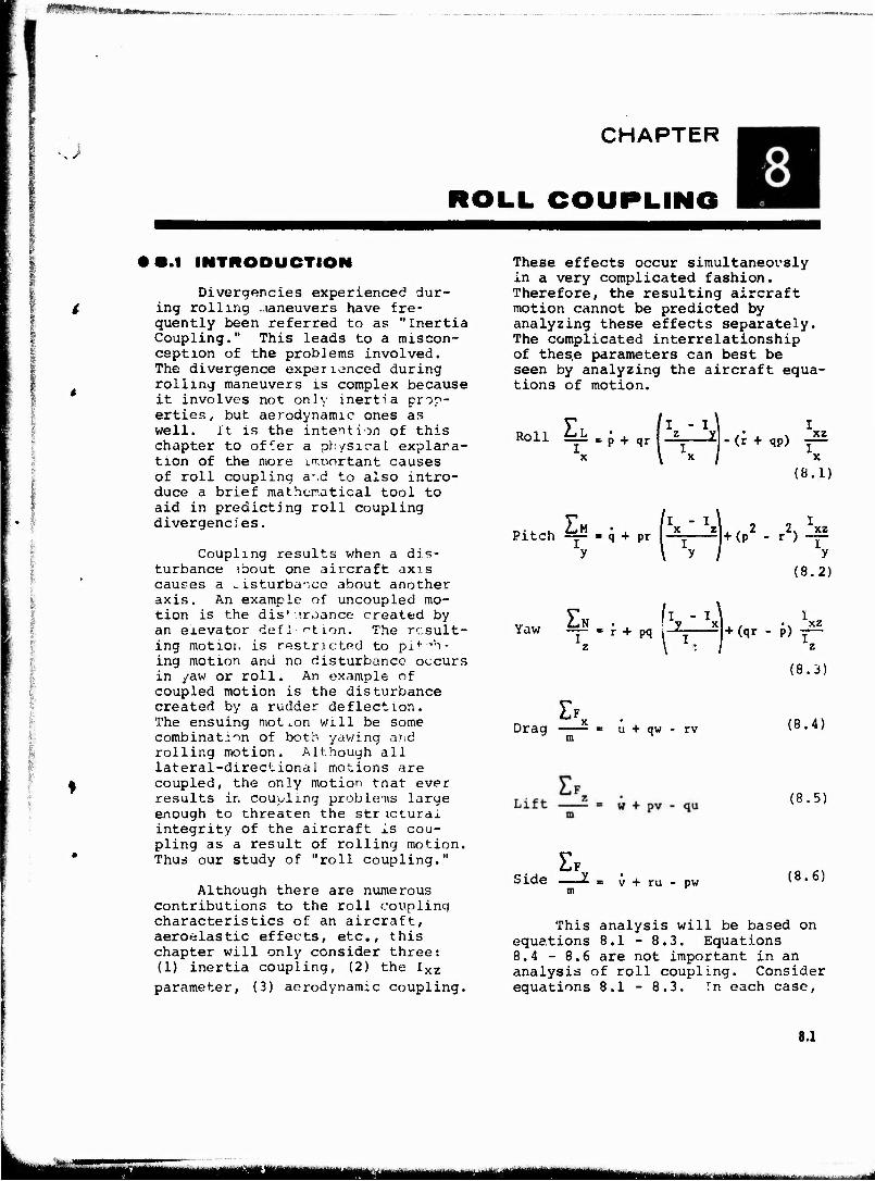
flBHHMHHu

) CHAPTER

ROLL COUPLING

• S.I INTRODUCTION

Divergencies experienced during rolling maneuvers have frequently been referred to as "Inertia Coupling." This leads to a miscon- ception of the problems involved. The divergence experienced during rolling maneuvers is complex because it involves not on]y inertia properties, but aerodynamic ones as well. It is the intention of this chapter to offer a physical explanation of the more imuortant causes of roll coupling a-.d to also intro- duce a brief mathematical tool to aid in predicting roll coupling divergencies.

Coupling results when a disturbance ?bout one aircraft axis causes a disturbance about another axis. An example of uncoupled motion is the dis*-'.roance created by an elevator defl-ction. The resulting motioi. is restricted to pish- ing motion and no disturbance occurs in yaw or roll. An example of coupled motion is the disturbance created by a rudder deflection. The ensuing motion will be some combination of both yawing arid rolling motion. Although all lateral-directional motions are coupled, the only motion that ever results in coupling problems large enough to threaten the str icturax integrity of the aircraft is coupling as a result of rolling motion. Thus our study of "roll coupling."

Although there are numerous contributions to the roll coupling characteristics of an aircraft, aeroelastic effects, etc., this chapter will only consider three: (1) inertia coupling, (2) the Ixz parameter, (3) aerodynamic coupling.

These effects occur simultaneously in a very complicated fashion. Therefore, the resulting aircraft motion cannot be predicted by analyzing these effects separately. The complicated interrelationship of thes.e parameters can best be seen by analyzing the aircraft equations of motion.

Rol i LL i ——- * p + qr (r + qp) xz

I X

(8.1)

Pitch Z,M J x z . .2 2. xz q pr 1 i ]+<P " r > T (8.2)

Yaw EN = r + pq

I - I , 1 *

~ + (qr - p) xz

Drag » u + qw - rv m

Side v + ru - pw

z

(8.3)

(8.4)

(8.5)

(8.6)

This analysis will be based on equations 8.1 - 8.3. Equations 8.4 - 8.6 are not important in an analysis of roll coupling. Consider equations 8.1-8.3. Tn each case,

8.1

mi tmmmmmMtmtmjtmmm ■am

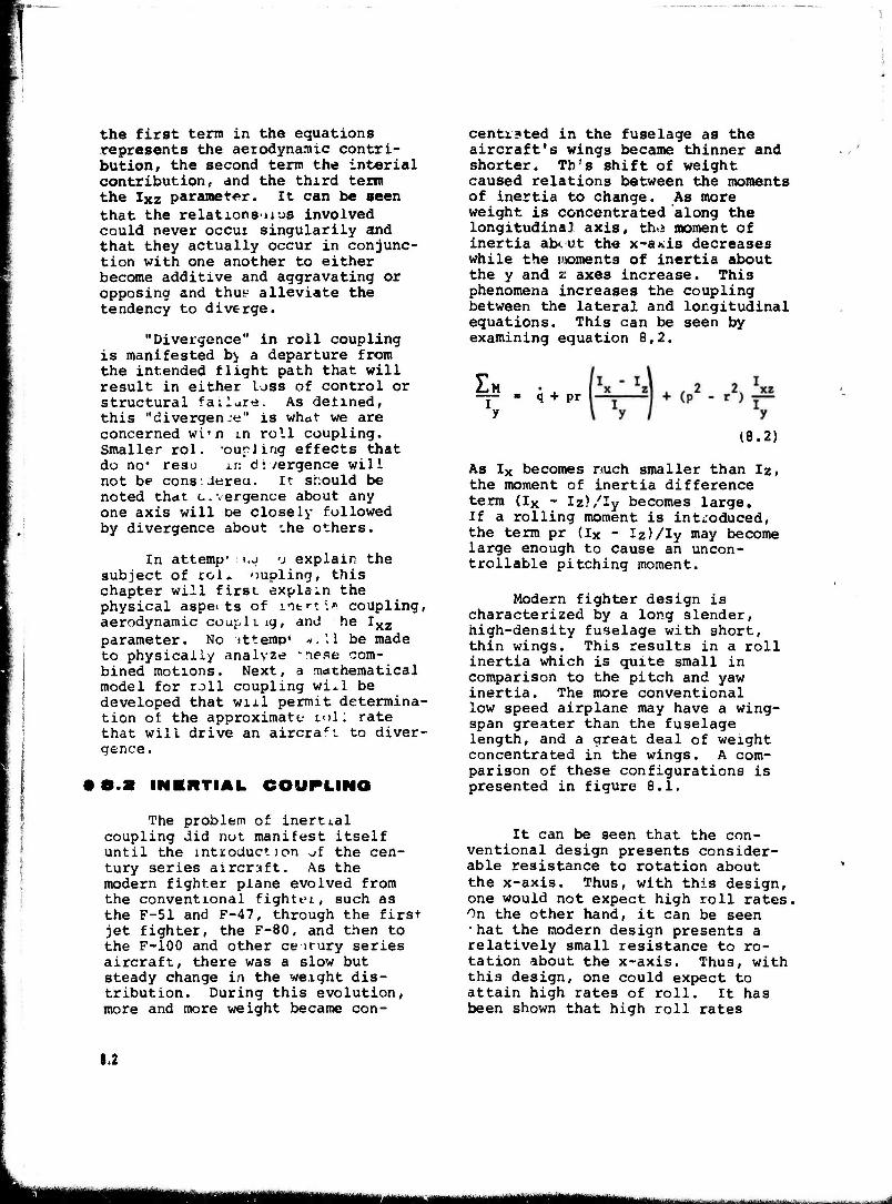
the first term in the equations represents the aerodynamic contribution, the second term the interial contribution, and the third term the Ixz parameter. It can be seen that the relations-uus involved could never occur singularily and that they actually occur in conjunction with one another to either become additive and aggravating or opposing and thus-- alleviate the tendency to diverge.

"Divergence" in roll coupling is manifested b> a departure from the intended flight path that will result in either IJSS of control or structural failure. As defined, this "divergent" is what we are concerned wi*n in roll coupling. Smaller rol. -oupJing effects that do no* resj. xr; divergence will not be cons:Jereu. It should be noted that c.. vergence about any one axis will t>e closely followed by divergence about ehe others.

In attemp* LJ <J explain the subject of rol» oupling, this chapter will first explain the physical aspei ts of inert'.* coupling, aerodynamic coupliig, and parameter. No ittemp* *;' to physically analyze -nes bined motions. Next, a ma model for roll coupling wi developed that wnl permit tion of the approximate to that will drive an aircra*" gence.

he *xz 1 be made e com- thematical .1 be determina-

1 1 rate t to diver-

centi?ted in the fuselage as the aircraft's wings became thinner and shorter. Trrs shift of weight caused relations between the moments of inertia to change. As more weight is concentrated along the longitudinal axis, the moment of inertia about the x-axis decreases while the moments of inertia about the y and z axes increase. This phenomena increases the coupling between the lateral and longitudinal equations. This can be seen by examining equation 8,2.

EM I

q + pr

(8.2)

• 0.« INKMTIAL COUPLING

As Ix becomes nuch smaller than Iz, the moment of inertia difference term (Ix - Iz)/Iy becomes large. If a rolling moment is introduced, the term pr (Ix - Iz)/Iy may become large enough to cause an uncontrollable pitching moment.

Modern fighter design is characterized by a long slender, high-density fuselage with short, thin wings. This results in a roll inertia which is quite small in comparison to the pitch and yaw inertia. The more conventional low speed airplane may have a wingspan greater than the fuselage length, and a great deal of weight concentrated in the wings. A comparison of these configurations is presented in figure 8.1.

The problem of inerti.al coupling did not manifest itself until the introduction of the cen- tury series aircraft. As the modern fighter plane evolved from the conventional fightet, such as the F-51 and F-47, through the first jet fighter, the F-80, and then to the F-100 and other ce irury series aircraft, there was a slow but steady change in the weight distribution. During this evolution, more and more weight became con-

It can be seen that the conventional design presents considerable resistance to rotation about the x-axis. Thus, with this design, one would not expect high roll rates. On the other hand, it can be seen • hat the modern design presents a relatively small resistance to rotation about the x-axis. Thus, with this design, one could expect to attain high rates of roll. It has been shown that high roll rates

8.2

IMMMMWI

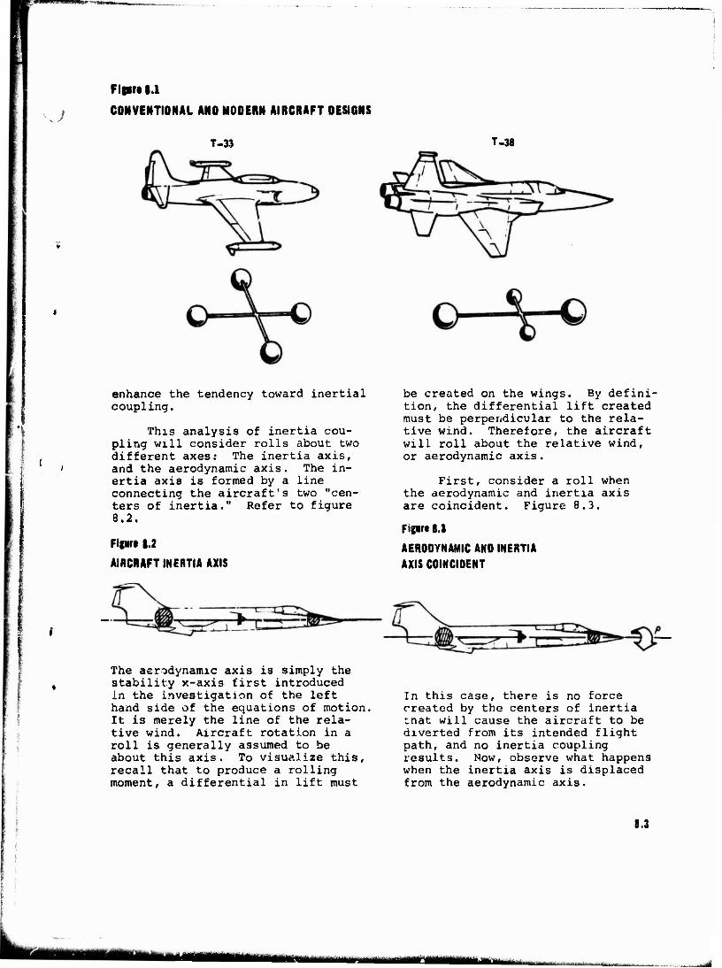
WUU .Will!»,». :vmu

\J Flprt 1.1

CONVENTIONAL AND MODERN AIRCRAFT DESIGNS

T-33 T-38

'1

enhance the tendency toward inertial coupling.

This analysis of inertia coupling will consider rolls about two different axes: The inertia axis, and the aerodynamic axis. The inertia axis is formed by a line connecting the aircraft's two "centers of inertia." Refer to figure 8.2.

Flfiirt 1.2

AIRCRAFT INERTIA AXIS

be created on the wings. By definition, the differential lift created must be perpendicular to the relative wind. Therefore, the aircraft will roll about the relative wind, or aerodynamic axis.

First, consider a roll when the aerodynamic and inertia axis are coincident. Figure 8.3.

Figin 8.1

AERODYNAMIC AND INERTIA

AXIS COINCIDENT

The aerodynamic axis is simply the stability x-axis first introduced in the investigation of the left hand side of the equations of motion. It is merely the line of the relative wind. Aircraft rotation in a roll is generally assumed to be about this axis. To visualize this, recall that to produce a rolling moment, a differential in lift must

In this case, there is no force created by the centers of inertia tnat will cause the aircraft to be diverted from its intended flight path, and no inertia coupling results. Now, observe what happens when the inertia axis is displaced from the aerodynamic axis.

j 8.3

itf an - - - —

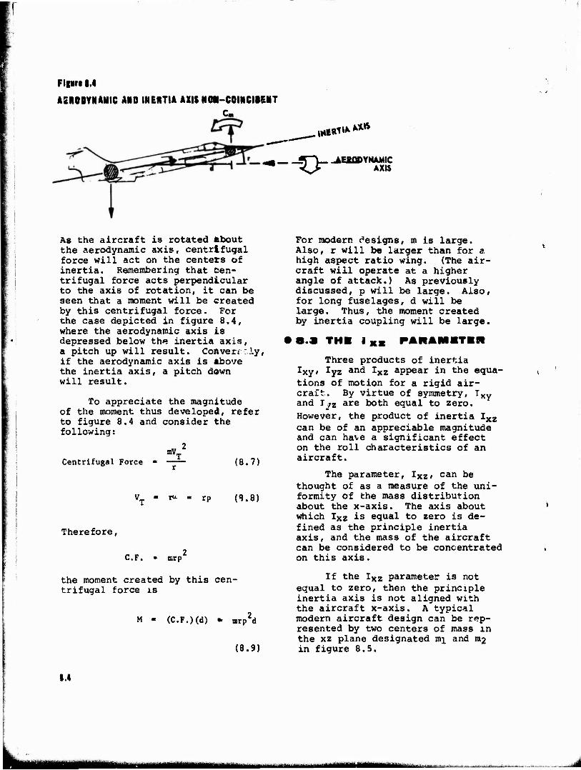
If

Figart 1.4

AERODYNAMIC AND INERTIA AXIS NCK-C0INCID5NT C

.|Hl«t* AX»

_fpv .AERODYNAMIC <,> AXIS

As the aircraft is rotated «bout the aerodynamic axis, centrifugal force will act on the centers of inertia. Remembering that Cen- trifugal force acts perpendicular to the axis of rotation, it can be seen that a moment will be created by this centrifugal force. For the case depicted in figure 8.4, where the aerodynamic axis is depressed below the inertia axis, a pitch up will result. Convert* :.ly, if the aerodynamic axis is above the inertia axis, a pitch down will result.

To appreciate the magnitude of the moment thus developed, refer to figure 8.4 and consider the following:

mV, Centrifugal Force (8.7)

VT - ** - rp («3.8]

Therefore,

C.F. » mrp

the moment created by this centrifugal force is

M - (C.F.)(d) * n>rp <1

For modern designs, m is large. Also, r will be larger than for a high aspect ratio wing. (The aircraft will operate at a higher angle of attack.) As previously discussed, p will be large. Also, for long fuselages, d will be large. Thus, the moment created by inertia coupling will be large.

Three products of inertia lxy' ■Lyz and Ixz appear in the equa-

tes)

tions of motion for a rigid aircraft. By virtue of symmetry, Txv and I/z are both equal to zero.

However, the product of inertia Ixz can be of an appreciable magnitude and can have a significant effect on the roll characteristics of an aircraft.

The parameter, lxz, can be thought of as a measure of the uni- formity of the mass distribution about the x-axis. The axis about which IXz is equal to zero is defined as the principle inertia axis, and the mass of the aircraft can be considered to be concentrated on this axis.

If the Ixz parameter is not equal to zero, then the principle inertia axis is not aligned with the aircraft x-axis. A typical modern aircraft design can be represented by two centers of mass in the xz plane designated mi and m2 in figure 8.5.

I.«

MHHM ■M

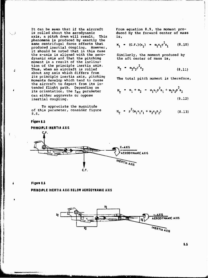
It can be seen that if the aircraft is rolled about the aerodynamic axis, a pitch down will result. This phenomena is produced by exactly the same centrifugal force effects that produced inertial coupling. However, it should be noted that in this case the x-axis is aligned with the aerodynamic axis and that the pitching moment is a result of the inclination of the principle inertia axis. Thus, when an aircraft is rolled about any axis which differs from its principle inertia axis, pitching moments develop which tend to cause the aircraft to depart from its intended flight path. Depending on its orientation, the Ix2 parameter can either aggravate or oppose inertial coupling.

To appreciate the magnitude of this parameter, consider figure 8.6.

From equation 8.9, the moment produced by the forward center of mass is,

Hx - (C.F.)(x1) - «W^l (8«10>

Similarly, the moment produced by the aft center of mass is,

M2 - m2x2P z2 (8>U)

The total pitch moment is therefore,

m1 + m2 - mixiP zi + m2X2P 22 2

z

(8.12)

Hj = P O»!*!2! + m2x2Z2) (8.13)

Figur* 8.5

PRINCIPLE INERTIA AXIS

C,F.

X-AXIS

AERODYNAMIC AXIS

C.F.

Figur« 8.8

PRINCIPLE INERTIA AXIS BELOW AERODYNAMIC AXIS

AERODYNAMIC AXIS

8.5

mtmmLa^m tmtmmmm Mai

But for a simplified system,

lxz " VlZl + m2x2Z2

Therefore,

P2I xz

(8.14)

(8.15)

Thus, it can be seen that the magnitude of the pitching moment thus developed depends on the roll rate and the magnitude of the Ix2 parameter relative to the roll axis.

The product of inertia, lxz» is not only of ^oncern because of its introduction of a pitching moment, but also because it plays an important role in determining the aircraft's cross over speed from adverse to complimentary yaw. Pri- marily, an aircraft's cross over speed is determined by the relationship of the induced and parasite drag generated by a wing during a rolling maneuver. However, this primary effect is mitigated somewhat by the effect of the Ixz parameter.

As previously shown, the IXz parameter can cause a pitching moment during a rolling maneuver. However, since the aircraft is rolling, gyroscopic effects come into play, and this moment results in a yawing motion. From figure 3.6, it can be seen that when the principle inertia axis is below the roll axis, a pitch down will result. For the right ..oil depicted, this pitching moment would result in a yaw left. Thus, in this case, the Ixz parameter would contribute to the adverse yaw tendency of the aircraft. In actual practice however, it will be found that the aerodynamic axis generally lies below the principle inertia axis throughout most of ehe flight envelope. Thus the Ixz parameter will generally cause the aircraft to transition from adverse to complimentary yaw at an earlier speed. For a relative comparison of values, the

F-102 nets an IXz of 3,500 slugs- feet2 and a crossover speed of 268 knots. The F-100 has an Ixz of 942 slugs-feet2 and experiences complimentary yaw in roll above 360 knots.

9 8.4 AIRODVNAMiC COUPLING

This analysis of roll coupling is not concerned with all aerodynamic coupling terms (Cnp, Cn6a, C^r, C£6j.,

etc.). Only the "kinematic coupling" aspects of aerodynamic coupling will be considered.

Kinematic coupling may be considered as an actual interchange of a and ß during a rolling maneuver. This interchange is an important means by which the longitudinal and lateral motions are capable of in- fluencing each other during a rapid roll.

To understand how this interchange of a for ß occurs, consider figure 8.7.

In this figure the aircraft is assumed to have either infinitely large inertia or negligible stability. Thus, it will roll about its principle inertia axis. In (I) the aircraft initiates a roll from a positive angle of attack. In (II) the initial angle of attack is converted to a positive sideslip angle of equal magnitude after 90° of roll. In (III) the aircraft has again exchanged 8 and a and after 180° of roll has an angle of attack equal in magnitude but opposite in sign to the original a. The interchange continues and in (IV) this -a is converted to -ß.

Next, consider an aircraft with infinitely large stability in {. tch and yaw or negligible inertia. Refer to figure 8.8.

8.S

tn^^^^mmumammilttm

*>SV*x®W^tm>miiL- vw»»«

Figiril.T KINEMATIC COUPLING. STABLE ROLLING OF AN AIRCRAFT NITH INFINITELY LARGE STABILITY IN PITCH AUD YAN OR NEGLIGIBLE INERTIA

Figur« «.a

KINEMATIC COUPLING. STABLE ROLLING OF AN AIRCRAFT NITH INFINITELY LARGE STABILITY IN PITCH AND YAW OR NEGLIGIBLE INERTIA

III

+a $

S.T

■■WHM

'-T7.^n-?^ji»j H'>u:' T'i-'PfipraWSi'WlWK"^-: B^TWTIT^fi-t|>™.«*■-»-"*-; „T'B-rwin'^TJ^fi^ 'r"Jü-i-S£frr ■ ^^^■-^..■-■-T55^.'j»,-^^:f-r^-=rr?:-4 *j,;5wij>g<j«e^--™i»»v™r?,»5-T-:~"T-' ' "■■"' '

wmnamiii»,«»*

In this case, the aircraft will roll about its aerodynamic axis, and no interchange of a or 6 will occur. However, in this situation it is possible for inertia coupling to occur.

that, It will be shown in dynamics

fnB= (f)CB, (8.18)

The situation depicted in figure 8.8 never actually occurs but can be fairly well approximated by an aircraft possessing large magnitudes of Cnß and Cma which is rolled at a relatively slow roll rate. However, in most cases, the actual aircraft motion will lie somewhere between the two extremes depicted.

Two empirical relationships can be stated:

m, (O C m (8.19)

-Kpr

ß = Xpcr

(8.16)

(8.17)

These relationships show that any roll rate will cause an interchange of a and 8, the exact amount depending on the relative vai"es of the moments of inertia and Cma and Cnß. It can also L>e seen that for a given aircraft, the rate of interchange of a and 8 depends on the roll rate.

It has been shown that whenever a and t exist, a rolling maneuver will generate inertia coupling. The relative value of Cma and Cnß will determine just what axis an aircraft will actually .roll about r

and thus how much interchange of a and ß will occur.

Subsequent to a disturbance in pitch or yaw from an aircraft's equilibrium condition, a finite period of time will be required for the natural aircraft stability to reduce the distarDance to zero. The frequency of this response is a function of the value of Cng and

Cmo-

Assume that an aircraft is rolled at a rate that creates a disturbance in 8 at a rate equal to the maximum rate that the natural aircraft stability can damp out the disturbance. Thus,

Kpor P (8.20)

In this case there would be no buildup of 8, and a condition of neutral stability in yaw would result. However, if the roll rate were increased slightly above this value then successively larger increases in 6 would occur and divergence would result. This analysis can also be followed through for an initial disturbance in a. It is not important which diverges first, a or 8, since any divergence about one axis will quickly drive the other divergent. As a matter of interest however, supersonically Cne decreases more rapidly than Cm<x

and therefore, most modern aircraft will diverge in yaw first.

It can be shown on an analog computer that when Cma = Cng a stable condition will exist at all roll rates. This is often referred to as a "tuned condition," and is a possible dodge for an aircraft designer to utilize in a critical flic'it area. However, it is difficult to capitalize on this ocvurisnce because of the wide variation of the stability derivatives - ;h Mach number.

It may be th»tc ci '.rcraft will possess stability parameters such that a roll coupling problem exists at a given roll rate. How-

8.8

watm tt^attmamu* im^M^il^,.^^ ,..:,,■ S&^JK;^

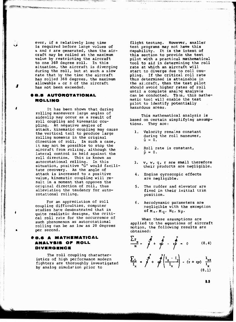
se*9e^5Ksgj3W^!^5|?W !-ff-^W-, W^ ^t^^ym^-^-.^^m^:^-z-

ever, if a relatively long time is required before large values of o and 6 are generated, then the aircraft may be rolled at the maximum value by restricting the aircraft to one 360 degree roll. In this situation, the aircraft is diverging during the roll, but at such a slow rate that by the time the aircraft has rolled 360 degrees, the maximum allowable a or ß of the aircraft has not been exceeded.

• a.B AUTOROTATION AL ROLLING

It has been shown that during rolling maneuvers large angles of sideslip may occur as a result of roll coupling and kinematic coupling. At negative angles of attack, kinematic coupling may cause the vertical tail to produce large rolling moments in the original direction of roll. In such a case, it may not be possible to stop the aircraft from rolling, although the lateral control is held against the roll direction. This is known as autorotational rolling. In this situation, positive "G" would facilitate recovery. As the angle of attack is increased to a positive value, kinematic coupling will result in a moment that opposes the original direction of roll, thus alleviating the tendency for autorotational rolling.

For an appreciation of roll coupling difficulties, computer studies have demonstrated that in quite realistic designs, the critical roll rate for the occurrence of such phenomenon as autorotational rolling can be as low as 20 degrees per second.

• e.S A MATHEMATICAL ANALYSIS OF ROLL DIVIROINCI

The roll coupling characteristics of high performance modern fighters are thoroughly investigated by analog simulation prior to

flight testing. However, smaller test programs may not have this capability. It is the intent of this section to provide the test pilot with a practical mathematical tool to aid in determining the roll rate at which an aircraft will start to diverge due to roll coupling. If the critical roll rate thus determined is attainable in the ai.craft, then the test pilot should avoid higher rates of roll until a complete analog analysis can be conducted. This, this mathe- matic tool will enable the test pilot to identify potentially hazardous areas.

This mathematical analysis is based on certain simplifying assumptions . They are:

1. Velocity remains constant during the roll maneuver, ü - 0.

2. Roll rate is constant, p = 0.

3. v, w, q, r are small therefore their products are negligible.

4. Engine gyroscopic effects are negligible.

5. The rudder and elevator are fixed in their initial trim position.

6. Aerodynamic parameters are negligible with the exception Of Mai Hq( Nß , Np-

When these assumptions are applied to the equations of aircraft motion, the following results are obtained: r^ o o o

_JS= /+ J . J _ o (8.4)

(8.1)

I.S

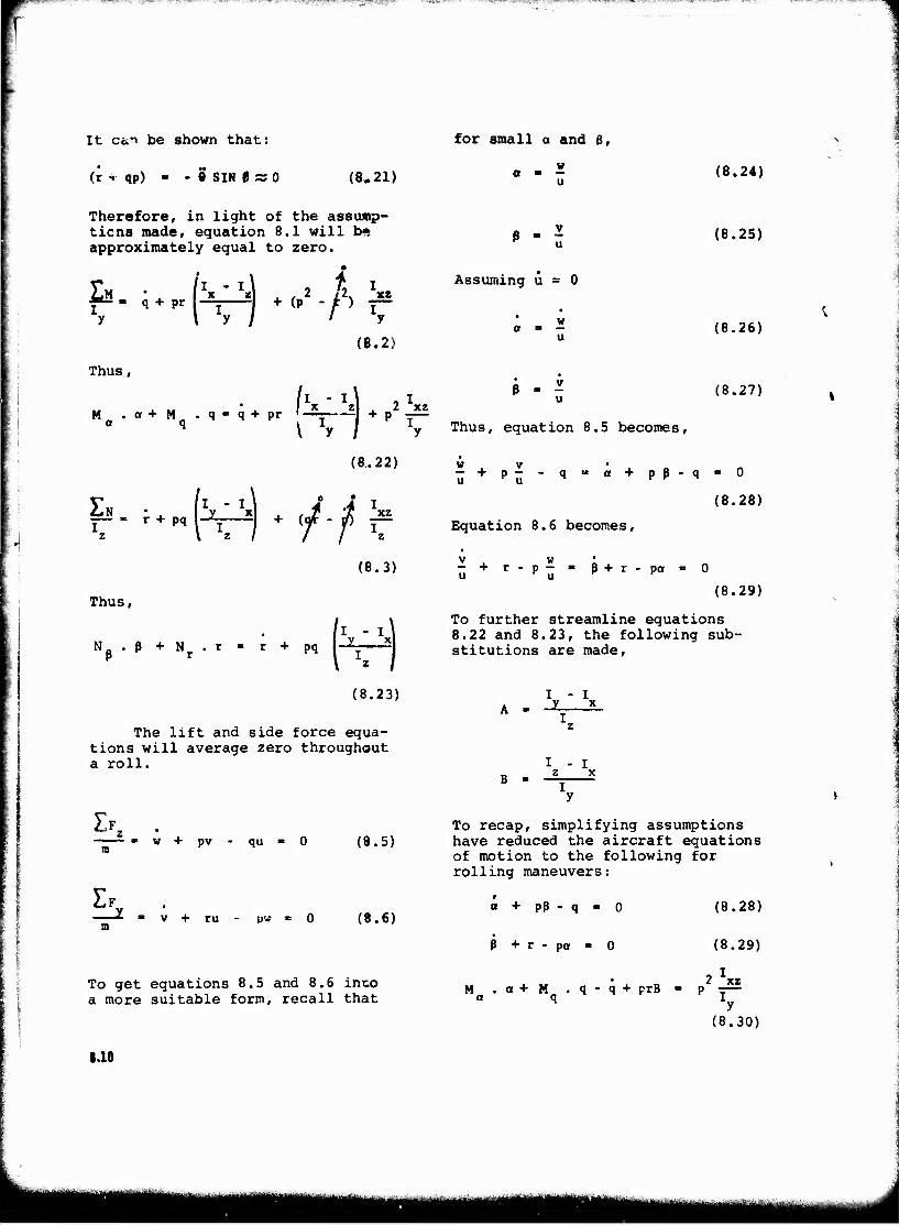
■flJgP!Was'™,!i™ * ' iii jflipUfM1*!)!* TjjpHffw »ts^augyp^ -^«^g^w- ■ ■ i-.s^-ar^v^- ™^A*-S' SWW

It Cc.-> be shown that:

(r ■*■ qp) - - 0 SIN 0 SJ 0 (8.21)

for small a and 0,

w u

(8.24)

Therefore, in light of the assumptions made, equation 8.1 will be approximately equal to zero.

•

£.;♦■.(*£) .^ xz

y

IB. 2)

Thus,

M .oi+M . q = q + pr + pr 1-5—-£] + p2 ^ \ y

(8.22)

EN 'I - I

i r + pql"V-^ + < 2 \ Z / / / Z /•/*■

Thus,

+ N . r = r + pq

(8.3)

1 " I . _y xi I

(8.23)

The lift and side force equations will average zero throughout a roll.

Assuming u = 0

(8.25)

(8.26)

0 - J (8.27)


w , v - + p - - q u u ^

a + p ß - q - 0

(8.28)

Equation 8.6 becomes,

v w • - + r-p- » B+r-pot u u r

(8.29)

To further streamline equations 8.22 and 8.23, the following substitutions are made,

I - I

B = I - I z x

w + pv - qu - 0 (8.5)

v + ru - pw « 0 (8.6)

To get equations 8.5 and 8.6 into a more suitable form, recall that

To recap, simplifying assumptions have reduced the aircraft equations of motion to the following for rolling maneuvers:

a + pß - q «. o

ß + r - pa ■ 0

M .a+M .q-q + prB a q

(8.28)

(8.29)

2*xz

y (8.30)

1.10

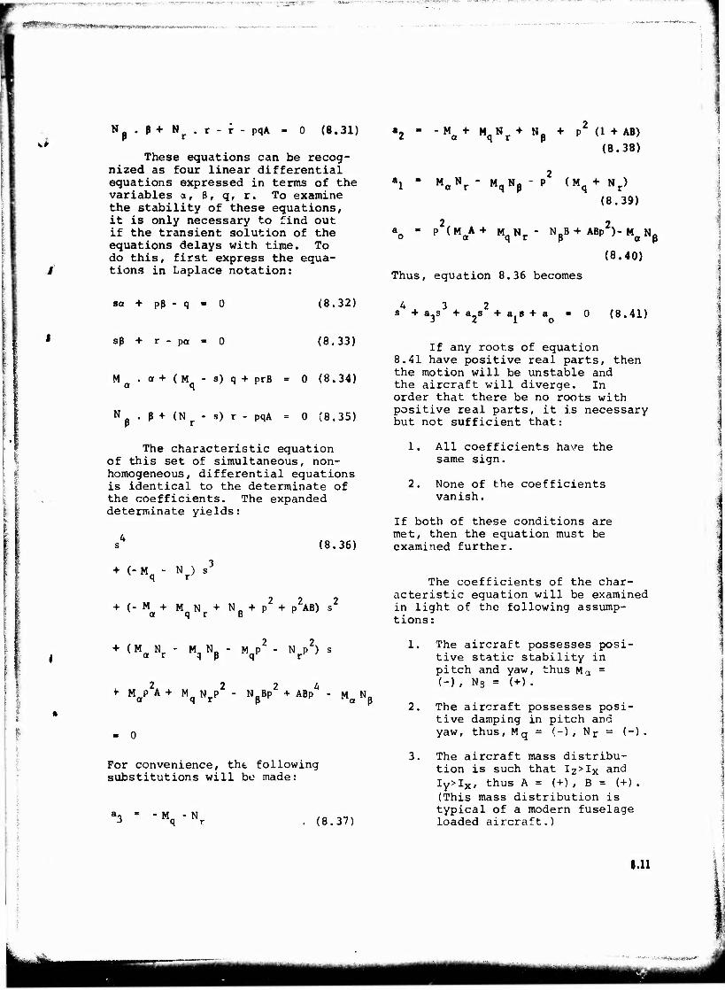
&&Q^fälfäQ&&&&eM&m<m&™m'**x»>a.,

*<■

N . ß + N . r - r - pqA - 0 (8.31)

These equations can be recognized as four linear differential equations expressed in terras of the variables o, ß, q, r. To examine the stability of these equations, it is only necessary to find out if the transient solution of the equations delays with time. To do this, first express the equations in Laplace notation:

Mcr + MqNr + Nß + p (l + AB)

M N a r MqNß - P

(8.38)

(Mq+ Nr)

(8.39)

P (M A + M N a 'q "r NpB+ ABp )-MaNß

(8.40)

Thus, equation 8.36 becomes

sa + pß (8.32) 4 3 2 s + a3s + as + a 8 + a * 0 (8.41)

sß + r - pa (8.33)

Ma " a + ( Mq " s) q + prB = ° (8,34)

N + (Nr - s) r - pqA = 0 (8.35)

If any roots of equation 8.41 have positive real parts, then the motion will be unstable and the aircraft will diverge. In order that there be no roots with positive real parts, it is necessary but not sufficient that:

The characteristic equation of this set of simultaneous, non- homogeneous, differential equations is identical to the determinate of the coefficients. The expanded determinate yields:

s4 (8.36)

1. All coefficients have the same sign.

2. None of the coefficients vanish.

If both of these conditions are met, then the equation must be examined further.

+ (-Mq - Nf) sJ

+ (-M+MN +N+p2+ p2AB) s2

a q r p

The coefficients of the characteristic equation will be examined in light of the following assumptions:

+ (M N - M, N. - M„P2 - N p2) s a i -) p q r

*■ Map2A + Mq Nrp2 - NßBp2 + ABp4 - Ma N

For convenience, the following substitutions will be made:

- M - N . (8.37)

1. The aircraft possesses positive static stability in pitch and yaw, thus Ma = (-), NB = ( + ).

2. The aircraft possesses positive damping in pitch and yaw, thus, Mq = (-) , Nr = (-)

3. The aircraft mass distribution is such that Iz>Ix ancä

Iy>Ix, thus A = (+), B = (+). (This mass distribution is typical of a modern fuselage loaded aircraft.)

8.11

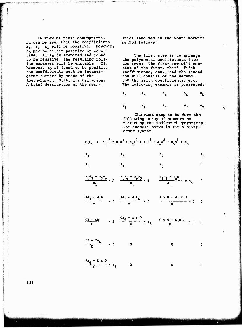
«.--r^-T^e-Ti^ "- .-j." ~j£?Zr>S¥r'ry '"TL-f7?^*7- -r*Yr-y?i^?i&w<^r^':'Z^^*f2'''*

In view of these assumptions, it can be seen that the coefficients a2» *2» al will be positive. However, aG may be either positive or negative. If a0 is examined and found to be negative, the resulting rolling maneuver will be unstable. If, however, a<> if found to be positive, the coefficients must be investigated further by means of the Routh-Hurwitz Stability Criterion. A brief description of the mech-

anics involved in the Routh-Horwitz method follows:

The first step is to arrange the polynomial coefficients into two rows: The first row will consist of the first, third, fifth coefficients, etc., and the second row will consist of the second, fourth, sixth coefficients, etc. The following example is presented:

8.12

The next step is to form the following array of numbers obtained by the indicated operations. The example 3hown is for a sixth- order system.

F(«) = as + a.8 + a„s + a.s + a.s + a.s + a, o 1 2 J *» 5 o

a.a - a_a a a - a a, a,a, - a x 12 3 o 14 o 5 n 1 6 o . m A ■ B = a, 0

a, a, a. 6 "1 'I

Aa. - a B Aa5 - aLa6 A x Ü - a. x 0

CB - AD Ca. - A x 0 o C x 0 - A x 0

ED - Ca,

Fa, - E x 0 -a6 0

V

The last step is to investigate the signs of the numbers in the first column in this array. If all of the elements in the first column are positive, the system is stable. If one or more of the elements is negative, the system is unstable.

When the Routh-Hurwitz Cri- terion is applied to equation 8.41, the following equations result. They must both be positive if the system is to be stable.

a3a2

ala2a3 a a, o 3

(8.42)

(8.43)

In summary, to determine if a given roll rate will result in a stable aircraft motion:

1. Determine the value of a0 (equation 8.40) . If it is negative the system is unstable.

2. Determine the values of ai, &2i 33 (equations 37 - 39).

3. Solve equation 8.42. If negative the system is unstable.

4. Solve equation 8.43. If negative the system is unstable.

5. If steps 1-4 yield no negative results, the system is stable for the roll rate investigated.

Although somewhat unwieldly, in the absence of adequate analog simulation, the foregoing system will yield fairly accurate results. It can serve to warn the test pilot of a perilous situation.

• 0.7 CONCLUSIONS

As an aircraft's inertias are disproportionately increased in relation to its aerodynamic sta- bilities in pitch and yaw, the aircraft will be liable to pitching and yawing motions during rolling maneuvers. The more typical case is a divergence in yaw by virtue of an inadequate value of 'no-

The peak loads resulting from roll coupling generally increase in proportion to the initial incidence of the principle inertial axis and progressively with the duration of the roll and the rapidity of aileron application at the beginning and the end of the maneuver. The most severe cases naturally should be expected in a flight regime of low Cnß and high dynamic pressures.

The rolling pull-out maneuver in a high performance aircraft is especially dangerous. It combines many unfavorable features: High speed hence high roll rate capability; high acceleration which favors poor coordination and in- advertent excitation of transients by the pilot; and high dynamic pressures which at large values of a and S may break the aircraft.

Most high performance aircraft incorporate roll rate limiters in addition to angular damping augmenters. In these aircraft a lateral control with enough power for low speed .s almost certain to be too powerful for high speeds. Fortunately, limiters of various kinds are not too difficult to incorporate in a fully powered control system.

It is obvious that flight testing in suspected regions of roll coupling warrant a cautious methodical approach and must be accompanied by thorough computer studies that stay current with the flight test data. The only way that the pilot can discover the

8.13

exact critical roll limit in flight is when he exceeds it, which is obviously not the approach to take. Because of this, flight tests are generally discontinued v/hen computer studies indicate that the next data point may be "over the line."

The following example is cited. The Bell X-2 rocket ship in 1956 was launched from its mother ship at Edwards. The pilot flew a perfect profile bat the rocket engine burned a few critical seconds longer than the engineers predicted, resulting in a greater speed (Mach 3.2) and greater altitude (119,300 feet) than planned. Unknown to the pilot, he was progressively running out of directional stability. When he was over the point at which he had preplanned to start his turn toward Roger's Dry Lake he actuated his controls. The X-2 went divergent with a resultant loss of control. The accident investigation revealed the cause to be a greater loss in directional stability than planned, resulting in divergent roll coupling.

A combination of reasonable piloting restrictions coupled with increased directional stability has provided the solution to roll coupling problems in the present generation of aircraft. The problem is one of understanding since a thinking pilot would no more exceed the roll limitations imposed on an aircraft than he would the structural "G" limitations.

Besides pilot education, some other schemes to eliminate roll coupling divergencies are:

1. Roll rate limiters.

2. Angular damping augmenters.

3. Placarded roll limits such as

a. "G" limits.

b. Total allowable roll at maximum rate.

c. Altitude limits.

d. Mach limits.

e. Flap position limits.

1.14

PUBBB immmimffmm/^gmgmßtmKgfKmfKi mqm&mo^qi i "pnn^wpip "* aggwammgi—3 ipwwy«»wwiyy8wwgsw»w "»!»a»i-;!.iwt,'>'.'.»-.-i-i»*

CHAPTER

CONTROL SYSTEMS

dF /dn s

db /dv e

d6r/dß

ABBREVIATIONS AND SYMBOLS

FOR THIS CHAPTER

hinge moment coefficient (restoring)

hinge moment coefficient (floating)

hinge moment coefficient (tab)

q "dynamic pressure"

qc compressible dynamic pressure

?■ elevator deflection

V airspeed

di 'dn elevator angle per g

normal acceleration

stick force per g

elevator angle to airspeed ratio

rudder angle per degree of sideslip

elevator deflection

lbs/ft

lbs/ft

degrees or radians

knots

2 tt/sec

degref.s or radians

Yaw damping derivative

Yav,ing moment coefficient with sideslip angle

Yawing moment coefficient with rolling velocity

9.1

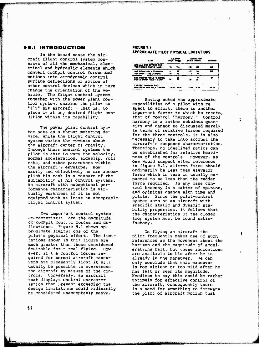
BMP '*'■•" ■"" '■'-*" "■'^w^.mMwg.w^t»»1 v» r;>w '»»J ,w.4iaww.* Pfirr',~T-*w^^frV.M*yy ■BMPMMI M| |' ■■»mpW »■«»!' ■-.-""•"' "irWSr^- "'if waaiMfPUWUllBW

• •.1 INTRODUCTION In the broad sense the air-

craft flight control system consists of all the mechanical, electrical and hydraulic elements which convert cockpit control forces and motions into aerodynamic control surface deflections or action of other control devices which in turn change the orientation of the vehicle. The flight control system together with the power plant control system, enables the pilot to "fly" his aircraft - that is, to place it at ai.y desired flight condition within its capability.

T:ie power plant control system acts as a thrust metering device, while the flight control system varies the moments about the aircraft center of gravity. Through tnest control systems the pilot is able to vary the velocity, normal acceleration, sideslip, roll rate, and other parameters within the aircraft's envelope. How easily and effectively he can accomplish his task is a measure of the suitability of his control systems. An aircraft with exceptional performance characteristics is virtually worthless if it is not equipped with at least an acceptable flight control system.

Two important control system characteristic are the magnitude of cockpit control forces and deflections. Figure 9.1 shows approximate limitat ons of the pilot's physical effort. The limitations shown in this figure are much greater than those considered desirable for n-.rmal flying. How- ever, if tie control forces required for normal aircraft maneuvers are pleasantly light it wiii usually be pussible to overstress the aircraft by misuse of the controls. Conversely, an aircraft that displays control characteristics that prevent exceeding the design limitat: >ns would ordinarily be considered unacceptably heavy.

FIGURE 9.1 APPROXIMATE PILOT PHYSICAL LIMITATIONS

C*M AN, MOM

»TIC« «Mil ILIVATM

ITICK «HML «UDO!«

MAX All OUT imiit re« »BY SHOUT TIM a HANOI! N !M IK IM 440

MA« raiauiM.« a HAND» re« IHMT TUt (1 HANOI SO

o> N

lit n

III »0

MO

HA« COMTMTAW.« '1 HAND!) re*C« MMT TIN« (| HAND! M s X

40 10

•

lARCItl HAHO m TOOT MOVIHtNT FOP »ULI TRAVIl -1« IN JO IH -»IN -»IN -JIN

Having noted the approximate capabilities of a pilot with respect to effort, there is another important factor to which he reacts, that of control 'harmony." Control harmony is a rather nebulous quantity and cannot be discussed merely in terms of relative forces required for the three controls, it is also necessary to take into account the aircraft's response characteristics. Therefore, no idealized ratios can be established for relative heavi- ness of the controls. However, as one would suspect after reference to figure 9.1, aileron force should ordinarily be less than elevator force which in turn is usually expected to be less than the rudder force required. In any case control harmony is a matter of opinion, and opinions change with time and pilots. Since the pilot-control system acts on an aircraft with specific static and dynamic stability properties, it follows that the characteristics of the closed loop system must be found satisfactory.

In flying an aircraft the pilot frequently makes use of such references as the movement about the horizon and the magnitude of accelerations felt, but these indications are available to him after he is already in the maneuver. He can only conclude that this maneuver is too violent or too mild after he has felt or seen its magnitude. Needless to say this could be rather untimely for effective control of the aircraft, consequently there is a need for something to forewarn the pilot of aircraft motion that

9.2

mmm ■NtffMMMI ■fniHrn r

- fttt-MJ--"f***js?,v-^M»,V ..T^, ,+mwwmw-v^,v«**xr'**!** ~ """ ^^^W^TT^*?«^^^i;n I.H-Jmmw\mwwxxmt*a™^<-'-H*r*->* P«WPW ■.•!'.!*-WT<|

/

will take place as a result of his use of the cockpit controls. Con- trol movement and force are two of the pilot's inputs to the stick, of which he is usually aware. In some flight regimes the stick movement can be considerable but at high speeds and aft eg conditions, the stick movements may be barely per- ceptible and for this reason it is generally conceded that control force is the most important indication of the magnitude of the maneuver. It follows that there should be no reversal of these forces in order that the pilot is never required to reverse his thinking. " would seem that stick deflections should never reverse either, but it may be possible to relax such a requirement in the portion of the aircraft envelope where stick movement is so small as -o be unnoticeable. If the stir movement is infinitesimal the piloi simply senses that be must pull to slow down and is probably unaware of the fact that the stick way have moved forward a fraction jf an inch.

To summarize the general requirements of the aerodynamic control system; two conditions must be met if the pilot is to be given suitable command over his airplane.

1. It must be capable of actuat- ing the control surface.

2. It must provide the pilot with a "feel" that bears a satisfactory relationshio to the aircraft's reaction.

There are numerous variations in the designs of aircraft control systems. However, these systems may be rather simply classified. The first classification in which the majority -f the modern aircraft control systems fall is that in whi:h the moments about the aircraft cc.ter of qi ivity are created by varyinq the camber or angle of attack ^f the aerodynamic lifting

or stabilizing surfaces. The most familiar example, is the use of trailing edge flaps on the wings, horizontal and vertical stabilizer, called ailerons, elevator and rudder, respectively. Another subclass of aerodynamic control is the spoiler which has come into rather wide use in recent years for lateral control. This device creates rolling moments by changing the energy of the airflow over one wing thereby resulting in a differential lift between the two wings. These aerodynamic systems can be further broken down into "reversible" and irreversible systems. These systems can be simple mechanical controls in which the pilot supplies all of the force required to move the control surface. "his type system is called "reversible" since all of the forces reqi. r°<? to overcome the hinge moments at trie control surface are transmitted to the cockpit controls. The system may have buil* into it a mechanical, hydraulic or some other type of boosting device, which supplies some specific proportion of the control force. Sys- tems of this nature are generally called "boosted control systems." However, they are still considered "reversible." Even though the force required of the pilot :.s less than the control surface hinge moments the force required is proportional to these moments. In other words the pilot furnishes a fraction of the force required to overcome the hinge moments throughout the aircraft's envelope. The ccatrol system is said to be irreversible if the pilot through his cockpit controls, actuates a hydraulic, elec- tronic, or some other '/De of device which in turn moves the control surface. In this system the aerodynamic hinge moments at the con* rol surface are no longer transmitted to the stick. Here, without artificial feel devices the pilct would feel only the force required to actuate the valves or sensing devices of his powered control system. Because of this, artificial ^eel. which approximates the feei that the pilot

9.3

'.T—»V" :-:iT . ..JLIIlJltp|!a^^LI .IJV4WI .-^^s- mpi«uij|i||LiiiLH| '' "5"TPi^,'h--^J^,«rf,lW'*,fl^?i-'!^"--"^!p i

senses with a must be added.

'reversible" system

A second category of control system is that of reaction controls. In this system small jets are usually located near the extremities of the aircraft where the length of the moment arm is greatest. These jets may be fired in order to create pitching, rolling, or yawing moments. Reaction controls are used extensively for control of vehicles in the very low speed or very high altitude flight regimes where aerodynamic controls are ineffective. Since this control system is used primarily in areas where aerodynamic damping is very light or in some cases almost non-existent, it becomes apparent that a different technique is required in the use of *-he cockpit controls. When an angular velocity about the eg is established by use of one of the reaction jets, this velocity tends to continue undiminished until an equal and opposite pulse is introduced. Therefore, it is obvious that a considerable change in ground rules is iequired for the pilot to intelligently evaluate such a control system.

Other control system categories might include the use of inertial or magnetic control devices not only to guide, but to control the orientation of a vehicle in space.

Since in the final analysis it is the pilot-control system - aircraft combination which must be satisfactory in order for the aircraft itself to be conridered acceptable, this chapter "ill concern itself with not only the various types of control systems mentioned above, but also with the pilot himself.

• 9.8 SIRVOMICHANISMS

From experitnce it has been shown that in simple tasks the difference in performance between

one pilot and another is generally snail, becoming negligible when such tasks are repetitive. As the complexity of the task is gradually increased his performance becomes more inconsistent. Then at each progressively more difficult stage the performance depends on the variance of adaptability of pilots, the degrees of predictability of the system they operate, their individual nervous and muscular characteristics and also their psychological and physiological condition at the time. In spite of all this the human pilot is popular with servo engineers for use as an adaptive servo. The human, however, has some limiting character .sties which are virtually constant. They are his reaction time (normally between 0.2 and 0.3 seconds) and his neuro-muscular lag (0.10 to 0.16 seconds). These virtually fixed characteristics represent some of his most serious liabilities as a servo element and restrict system performance. Therefore, the control system designer must design for the physical limitations of the pilot as well as for the airplane characteristics.

A servomechanism can be defined as an automatic control system which senses the output of a system, compares thjs output with the desired output, and if a difference exists - causes the output to be changed until it equals the desired value Familiar examples of servomechanisms are automatic tracking radar, and thermostatically controlled air conditioning units. Another example is the human uody when performing even the simplest of tasks. A boy catching a ball senses the direction of motion of the ball with his eyes and moves his body, arms and hands until the ball enters his glove. He is sub- consciously but continually comparing -he relative position and motion of the ball and glove and correcting the motion of the glove until the ball enters it. A pilot flying an aircraft, may be thought of as part

9.4

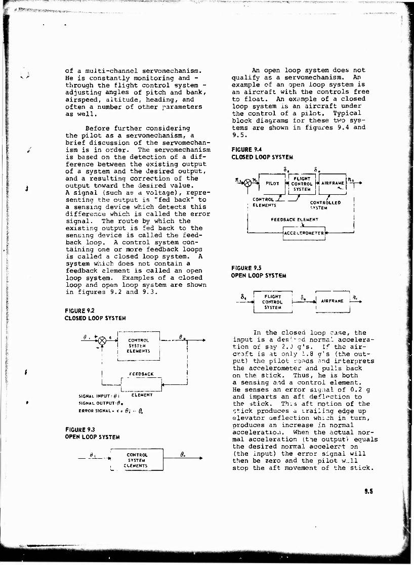
|f pj&mtommmmm—mem

of a multi-channel servomechanism. He is constantly monitoring and - through the flight control system - adjusting angles of pitch and bank, airspeed, altitude, heading, and often a number of other parameters as well.

Before further considering the pilot as a servomechanism, a brief discussion of the servomechanism is in order. The servomechanism is based on the detection of a difference between the existing output of a system and the desired output, and a resulting correction of the output toward the desired value. A signal (such as a voltage), representing the output is "fed back" to a sensing device which detects this difference which is called the error signal. The route by which the existing output is fed back to the sending device is called the feedback loop. A control system containing one or more feedback loops is called a closed loop system. A system which does not contain a feedback element is called an open loop system. Examples of a closed loop and open loop system are shown in figures 9.2 and 9.3.

FIGURE 9.2 CLOSED LOOP SYSTEM

An open loop system does not qualify as a servomechanism. An example of an open loop system is an aircraft with the controls free to float. An example of a closed loop system is an aircraft under the control of a pilot. Typical block diagrams for these two systems are shown in figures 9.4 and 9.5.

FIGURE 9.4 CLOSED LOOP SYSTEM

S. 8. Ki/CX*« ! FLIGHT -iH>p-i» PILOT «| CONTROL W AIRFRAME \

SYSTEM I

CONTROL J— ! ELEMENTS

"7— CONTROLLED 'iVSTEM

FEEDBACK ELEMENT

, _k

-UCCELEROMETERK- ! i

FIGURE 9.5 OPEN LOOP SYSTEM

8, FLIGHT CONTROL

SYSTEM

AIRFRAME X

Sty*- CONTROL SYSTbM

ELEMENTS

*i ►

L [" FEEDBACK

SIGNAL INPUT :0i ELEMENT

SIGNAL OUTPUT-0«

ERROR SIGNAL. ( = 0; ■■ 0.

FIGURE 9.3 OPEN LOOP SYSTEM

e, r

L

CONTROL SYSTEM

CLEMENTS

0,

In the closed loop case, the input is a des', -ad normal acceleration of say 2.J g's. If the aircraft is at only 1.8 g's (the output) the pilot reads and irterprets the accelerometer and pulls back on the stick. Thus, he is both a sensing and a control element. He senses an error signal of 0.2 g and imparts an aft deflection to the -stick. This aft notion of the <:tick produces a '-railing edge up elevator deflection whuh in turn, produces an increase in normal acceleration. When the actual normal acceleration (tie output'i equals the desired normal accelerrt on (the input) the error signal will then be zero and the pilot w..ll stop the aft movement of the stick.

9.5

m^.^^'*^y^rr^-^r^W^ Jr:^r^i•,'Ant<fW".»^-,'.^™^7^n-wr^ .-o . ■-.- .-r—-,,-..-,.^-»^,; -r - -!W> ■ ".-.;■.- ■ ;.:<w)Kr.r~un.:ir!T«s?f^s7^-

In the open loop system, the stick is deflected tc a position which is estimated to produce a normal acceleration of 2.0 g's. The elevator is moved to a corresponding angle by the flight control system, and the airplane is given a normal acceleration which may or may not be exactly 2.0 g's. Since there is no feedback, no further refinement is possible. The normal acceleration obtained with this stick deflection depends on many variables including altitude, airspeed, eg position, etc.

It is quite possible for an aircraft to exhibit satisfactory open loop characteristics and yet be unsatisfactory when the pilot is introduced into the system and the loop is closed. For example, suppose that the stick-fixed longitudinal dynamic characteristics oi an aircraft were such that an elevator pulse produced a pitch rate trace as shown in figure 9.6.

FIGURE 9.6 OPEN LOOP DYNAMIC TIME "«TORY

AIRFRAME OUTPUT

(PITCH RATE)

AIRFRAME ; INPUT

(ELEVATOR DEFLECTION)

-#• TIME

/I -♦TIME

This open loop dynamic time history indicates stable, moderately-damped longitudinal dynamics. If the pilot were required to control the aircraft quite closely, however, such as in low-level, high-speed formation flying, the closed loop dynamic time history might indicate an entirely different situation. The resulting pilot-induced oscillations might lead to normal accelerations which would produce structural damage to the aircraft. The results seen in figure 9.7 could well be caused by the designer failing to take into account that the normal pilot response time was similar to the short period in a portion of the aircraft's envelope.

Thus the job of matching airframe and pilot characteristics with suitable flight control system characteristics is not an easy one. But if the airplane designer does not bear in mind the basic characteristics and limitations of the pilot when he designs the aircraft and control system, the results might well prove disappointing.

• 9.3 BOOSTID CONTROL SYSTEMS

As the si*s and speed of aircraft increase, the hinge moments and thus the control forces increase accordingly. Neglecting Mach effects, if the dimensions and speed of a given aircraft are both doubled,

FIGURF 9.7

CLOSED LOOP DYNAMIC TIME HISTORY

AIRFRAME OUTPUT "

(PITCH RATE )

AIRFRAME „ INPUT

(ELEVATOR DEFLECTION)

¥ TIME

► TIME

9.6

s-,E AT" "jTOi-f «^'^T^pi^^«! ";-;- -*- —.'" ' Ti :v^7" g^ty WOT*w.^<!ifcy Wg'-f > papygWjWHW, ■^«^«^^^•^w^

u

[ I

i i

the cootrol forces will be multiplied by a factor of thirty-two. Although aerodynamic balancing couj-d alleviate the problem up to a point, the difficulty in the past of achieving the production toi- erAI\SSs necessary to produce a Ch5 OdPsJ?, tl.0002 per degree, and the «cratlc variations in hinge moment in the transonic regime led to the development of boosted control systems. In"this type of system the pilot is required to produce only a fraction of the force required to overcome the hinge moments. However, he does produce a specified portion of this force and the force required of the pilot is still approximately proportional to the hinge moments on the control surface. The control system then, is still a reversible one in that the hinge moments are fed back to the stick.

One method of control boosting is shown in figures 9.8 and 9.9. This system uses the hydraulic method of amplifying which requires the addition of <. hydraulic cylinder on a follower arm. Ls in the unboosted system the pilot moves the stick aft and the trailing edge of the elevator deflects up.

The process however causes a hydraulic pressure drop across the piston causing the cylinder to collapse and affecting additional elevator deflection. As the cylinder collapses a follow-up linkage reduces the pressure drop across the piston to zero and the follower arm contraction ceases. Starting from an initially trimmed condition with zero stick force the pilot pulls back on the stick and holds. There is an accompanying up elevator produced, identical to that which would be produced in an unboosted system. This up elevator moves the follow-up arm down but point (2) does not move as far as point (1) and thus the free crank "B" rotates clockwise relative to bell crank "A". This produces an upward motion at point (3) relative to the hor:zontal arm of the bell crank "A" and the valve slides toward the elevator, thereby unport- ing two orifices in the cylinder wall astraddle the piston head. High-pressure oil is fed to the orifice on the rod side and the oil pressure drop across the piston forces it to collapse and therefore shorten the follower arm achieving an additional up elevator deflection. As the elevator moves up, the follow-

1 I

I I

FIGURE 9.3

SCHEMATIC OF BOOSTED CONTROL SYSTEM

HYDRAULIC CYLINDER

ImTTW BELt CRANK "A"

-TV—^ WmTT

FOLLOW-UP ARM

HYDRAULIC VALVE

FRFE CRANK "B"

9.7

wmtA

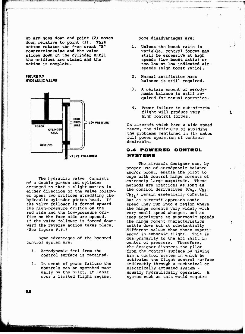
Mip^WPUUNL! W "UtymJltyWm?* S^Uß. #W$!9£.mi> ffl1-.': ■■■- ,^ WWWA'^H^-Ji^ltJ '™*1»W^wrTW5Fl'7?i!' «- ^TTT^^sr'. Ji'fjy-i ■

: !

up arm goes down and point (2) moves down relative to point (1). This action rotates the free crank "B" counterclockwise and the valve slides down on the cylinder until the orifices are closed and the action is complete.

FIGURE 9.9 HYDRAULIC VALVE

LOW PRESSURE

VALVE FOLLOWER

The hydraulic valve consists of a double piston and cylinder arranged so that a slight motion in either direction of the valve follower opens two orifices straddling the hydraulic cylinder piston head. If the valve follower is forced upward the high-pressure orifice on the rod side and the low-pressure orifice on the face side are opened. If the valve follower is forced downward the reverse action takes place. (See figure 9.9.)

Some advantages of the boosted control system aret

1. Aerodynamic feel from the control surface is retained.

2. In event of power failure the controls can be operated manually by the pilot, at least over a limited flight regime.

Some disadvantages are:

1. Unless the boost ratio is variable, control forces may still be excessive at high speeds (low boost ratio) or too low at low indicated airspeeds (high boost ratio).

2. Normal antiflutter mass balance is still required.

3. A certain amount of aerodynamic balance is still required for manual operation.

4. Power failure in out-of-trim flight will produce very high control forces.

On aircraft which have a wide speed range, the difficulty of avoiding the problems mentioned in (1) makes full power operation of controls desirable.

9.4 POWERED CONTROL SYSTEMS

The aircraft designer can, by proper use of aerodynamic balance and/or boost, enable the pilot to cope with control hinge moments of extremely large magnitude. These methods are practical as long as the control derivatives (Cha,

chs » Chst) remain essentially constant. But as aircraft approach sonic speed they run into a region where the hinge moments vary widely with very small speed changes, and as they accelerate to supersonic speeds the hinge moment characteristics settle down but at substantially different values than those experienced in subsonic flight. This is due primarily to the aft shift in center of pressure. Therefore, the designer divorces the pilot from the control surface by giving him a control system in which he activates the flight control surface indirectly through a mechanical or electrically actuated system - ucually hydraulically operated. A system such as this would require

1.1

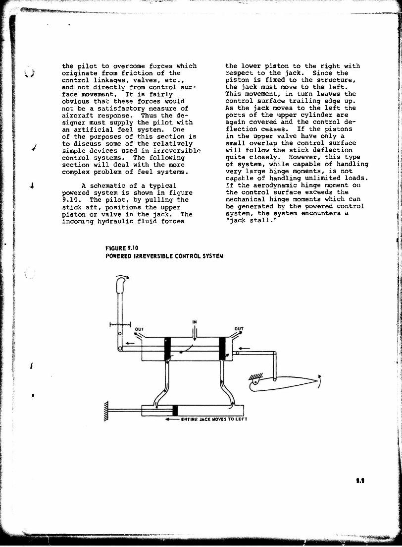
*""S?^<tTWi;:T*S?T<~, " ^"-. ■ ■ -.■*;■.■'■■ * ._ .■ — .

''"»RW^'te^'I'Wy a*-;*! iT;

the pilot to overcome forces which originate from friction of the control linkages, valves, etc., and not directly from control surface movement. It is fairly obvious that these forces would not be a satisfactory measure of aircraft response. Thus the designer must supply the pilot with an artificial feel system. One of the purposes of this section is to discuss some of the relatively simple devices used in irreversible control systems. The following section will deal with the more complex problem of feel systems.

A schematic of a typical powered system is shown in figure 9.10. The pilot, by pulling the stick aft, positions the upper piston or valve in the jack. The incoming hydraulic fluid forces

the lower piston to the right with respect to the jack. Since the piston is fixed to the structure, the jack must move to the left. This movement, in turn leaves the control surface trailing edge up. As the jack moves to the left the ports of the upper cylinder are again covered and the control deflection ceases. If the pistons in the upper valve have only a small overlap the control surface will follow the stick deflection quite closely. However, this type of system, while capable of handling very large hinge moments, is not capable of handling unlimited loads. If the aerodynamic hinge moment on the control surface exceeds the mechanical hinge moments which can be generated by the powered control system, the system encounters a "jack stall."

FIGURE 9.10

POWERED IRREVERSIBLE CONTROL SYSTEM

li

ENTIRE JACK MOVES TO LEFT

9.9

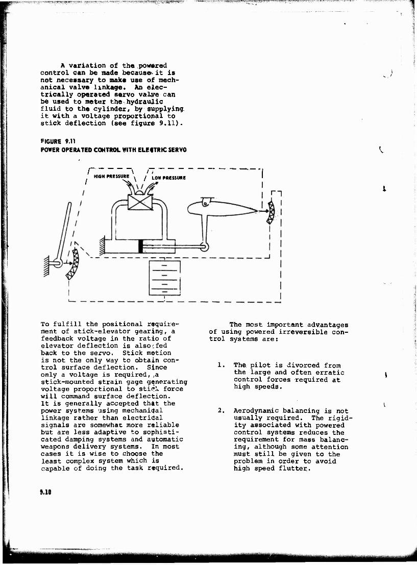
^^L^â^^g%j!liyift;^.|ii rr ^pfj?«j3jr?^JSHV■ M^kj?M»«^H*HJ»|flW4Sî2*S3KB a>pg?^ri:pTi.:, i"!wyaf.^."iu_'ii twg^îHf7yi*^-'7^3?^!^wi^^ '^'iyji;Bii; -jgM'yjJ—

A variation of the powered control can be made because- it is not necessary to make use of mechanical valve linkage. An electrically operated servo valve can be used to meter the hydraulic fluid to the cylinder, by supplying it with a voltage proportional to stick deflection (see figure 9.11).

FIGURE 9.11 POWER OPERATED CONTROL WITH ELECTRIC SERVO ',

/

I \ n HICH PRESSURE ^ / L0W PRESSURE

To fulfill the positional requirement of stick-elevator gearing, a feedback voltage in the ratio of elevator deflection is also.fed back to the servo. Stick motion is not the only way to obtain control surface deflection. Since only a voltage is required, ,a stick-mounted strain gage generating voltage proportional to stitfk force will command surface deflection. It is generally accepted that the power systems using mechanical linkage rather than electrical signals are somewhat more reliable but are less adaptive to sophisticated damping systems and automatic weapons delivery systems. In most cases it is wise to choose the least complex system which is capable of doing the task required.

The most important advantages of using powered irreversible control systems are:

1. The pilot is divorced from the large and often erratic control forces required at high speeds.

2. Aerodynamic balancing is not usually required. The rigidity associated with powered control systems reduces the requirement for mass balancing, although some attention must still be given to the problem in order to avoid high speed flutter.

9.10

i ,11111 ]iuwu.TOi.iiH»im .1 UWHtR-UJlHUUIJ. I.IJJIL Jlilll BUPP

J

The primary disadvantages are:

1. An artificial feel system must be incorporated into the aircraft control system.

2. The increased complexity of the control-feel system combination reduces system reliability.

3. It is often difficult or im- practical to build into the system a standby capable of reverting to manual revtrsible control.

B.a AIRCRAFT FEIL

SYSTEMS

Aircraft feel was discussed at some length in section 9.1, however, several additional comments will now be made before some of the artificial devices that affect feel are described.

The control system characteristics, together with the airframe stability characteristics, are determined Oy airframe design, the control-feel system is the place »/here the handling qualities may be patched up - or ruined.

The aircraft-feel system ordinarily includes stability augmentation devices, since they definitely affect aircraft handling qualities, but becai.se of their dual function and unique character they will be considered separately.

The feel characteristics of a reversible contici system may certainly be altered in order to improve handling qualities. In fact two devices for doing just that were discussed previously in this course, i.- ., the downspring and bobweight. In the following paragraphs, though, the control system will be assumed to be irreversible and feel systems artificial.

kC- TBRISTICS OP CONTROL

Mechanical characteristics of control systems which affect feel will now be discussed before going into artificial devices which are incorporated in order to improve feel.

Breakout Force:

This term defines the force necessary to be applied to the stick before it moves. The source lies in the cumulative affect of the following:

1. The mechanical friction of the control circuit, the feel unit, and the valve.

2. The force due to viscous flow past the valve in its neutral position and/or valve centering spring, and

3. The preload of the feel unit.

If the breakout force is high, it will tend to produce overshoot- ing in the desired small and rapid control pressures (e.g., during tracking or .instrument flight) because of the pilot's neuromuscular and reaction lag. As the pilot exerts pressure on the cockpit control to overcome this force he is likely to continue this pressure for a short period after the friction is overcome and this take the control past the desired value. These effects will be aggravated if the force level immediately following breakout force becomes noticeably lower because of lower running friction.

Backlash:

Mechanical play in the control system resulting from cable stretch, valve overlap, etc., is called by various names - backlash, lost motion, free play, mechanical hysteresis. If it reaches annoy-

9.11

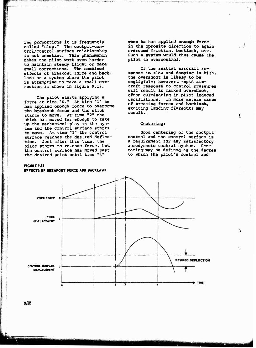
^■fp^'*^ ■*■■ ^v*.*i3.^^r,-^-^-i6a5w-wj»-r:^

j ,.

ing proportions it is frequently called "slop." The cockpit-control/control-surface relationship is not constant. This phenomenon makes the pilot work even harder to maintain steady flight or make small corrections. The combined effects of breakout force and backlash on a system where the pilot is attempting to make a small correction is shown in figure 9.12.

The pilot starts applying a force at time "0." At time "1" he has applied enough force to overcome the breakout force and the stick starts to move. At time "2" the stick has moved far enough to take up the mechanical play in the system and the control surface starts to move. At time "3" the control surface reaches the desired deflection. Just after this time, the pilot starts to release force, but the control surface has moved past the desired point until time "4"

when he has applied enough force in the opposite direction to again overcome friction, backlash, etc. Such a system would thus cause the pilot to overcontrol.

If the initial aircraft response is slow and damping is high, the overshoot is likely to be negligible; however, rapid aircraft response to control pressures will result in marked overshoot, often culminating in pilot induced oscillations. In more severe casas of breaking forces and backlash, exciting landing flareouts may result.

Centering:

Good centering of the cockpit control and the control surface is a requirement for any satisfactory aerodynamic control system. Cen- tering may be defined as the degree tc which the pilot's control and

FIGURE 9.12 EFFECTS OF BREAKOUT FORCE AND BACKLASH

STICK FORCE 0

STICK DISPLACEMENT

CONTROL SURFACE 9

DISPLACEMENT

S.12

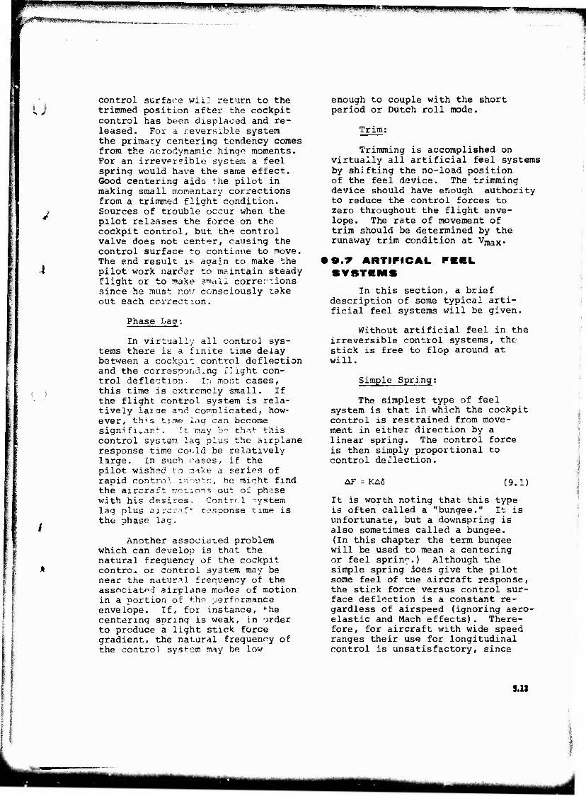
lllLlkl i y iUJllU, ll 1.[ JU|pj^y..i.j|»iij|j| pummmm " ■•"l!'w" *!»JlJ«IvlJLWU|ipMlH!

U control surface will return to the trimmed position after the cockpit control has been displaced and released. For a reversible system the primary centering tendency comes from the aerodynamic hinge moments. For an irreversible system a feel spring would have the same effect. Good centering aids the pilot in making small momentary corrections from a trimmed flight condition. Sources of trouble occur when the pilot releases the force on the cockpit control, but the control valve does not center, causing the control surface to continue to move. The end result is again to make the pilot work narder to maintain steady flight or to make 5«ali corrections since he must now consciously take out each correction.

Phase Lag:

In virtually all control systems there is a finite time delay between a cockpit control deflection and the corresponding flight control deflection In mor;t cases, this time is extremely small. If the flight control system is relatively laioe and complicated, however, this time lag can become signif i_ar:*-. It. may be that this control system lag plus the airplane response time could be relatively large. In such cases, if the pilot wished to make a series of rapid control imuts, he might find the aircraft motions out of phase with his desires. Control system lag plus aircraft response time is the phase lag.

Another associated problem which can develop is that the natural frequency of the cockpit contro* or control system may be near the natural frequency of the associated airplane modes of motion in a portion of the performance envelope. If, for instance, *he centering spring is weak, in order to produce a light stick force gradient, the natural frequency of the control system may be low

enough to couple with the short period or Dutch roll mode.

Trim:

Trimming is accomplished on virtually all artificial feel systems by shifting the no-load position of the feel device. The trimming device should have enough authority to reduce the control forces to zero throughout the flight envelope. The rate of movement of trim should be determined by the runaway trim condition at Vmax.

• 9.7 ARTIFICAL SYSTEMS

FEEL

In this section, a brief description of some typical artificial feel systems will be given.

Without artificial feel in the irreversible control systems, the stick is free to flop around at will.

Simple Spring:

The simplest type of feel system is that in which the cockpit control is restrained from movement in either direction by a linear spring. The control force is then simply proportional to control deflection.

AF = KA6 (9.1)

It is worth noting that this type is often called a "bungee." It is unfortunate, but a downspring is also sometimes called a bungee. (In this chapter the term bungee will be used to mean a centering or feel spring.) Although the simple spring ioes give the pilot some feel of rne aircraft response, the stick force versus control surface deflection is a constant regardless of airspeed (ignoring aeroelastic and Mach effects). There- fore, for aircraft with wide speed ranges their use for longitudinal control is unsatisfactory, since

S.1S

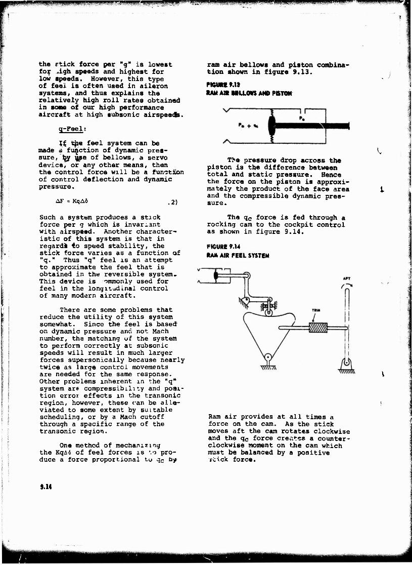
IWIPMIW^WfippPIW ^aWBPBgJiP^JSPWi ■' • ^a'J^^WMWiW 1

the etick force per "g" is lowest for .igh speeds and highest for low speeds. However, this type of feel is often used in aileron systems/ and thus explains the relatively high roll rates obtained in some of our high performance aircraft at high subsonic airspeeds.

q-Feel;

It the feel system can be made & function of dynamic pressure, by use of bellows, a servo device, or any other means, then the control force will be a function of control deflection and dynamic pressure.

AF = KqA6 .2)

Such a system produces a stick force per g which is invariant with airspeed. Another characteristic of this system is that in regards to speed stability, the stick force varies as a function of "q." Thus "q" feel is an attempt to approximate the feel that is obtained in the reversible system. This device is ommonly used for feel in the longitudinal control of many modern aircraft.

There are some problems that reduce the utility of this system somewhat. Since the feel is based on dynamic pressure and not Mach number, the matching of the system to perform correctly at subsonic speeds will result in much larger forces supersonically because nearly twice as large control movements are needed for the same response. Other problems inherent m the "q" system are compressibility and position error effects in the transonic region, however, these can be alLe- viated to some extent by suitable scheduling, or by a Mach cutoff through a specific range of the transonic region.

One method of mechanizing the Kqa6 of feel forces is :o produce a force proportional to qc tay

ram air bellows and piston combination shown in figure 9.13.

FIGURE 9.13 RAM AIR MLLOWS AMD PftTON

K The pressure drop across the

piston is the difference between total and static pressure. Hence the force on the piston is approximately the product of the face area and the compressible dynamic pressure.

The qc force is fed through a rocking cam to the cockpit control as shown in figure 9.14.

FIGURE 9.14 RAM AIR FEEL SYSTEM

Ram air provides at all times a force on the cam. As the stick moves aft the cam rotates clockwise and the qc force creates a counterclockwise moment on the cam which must be balanced by a positive itick force.

9.14

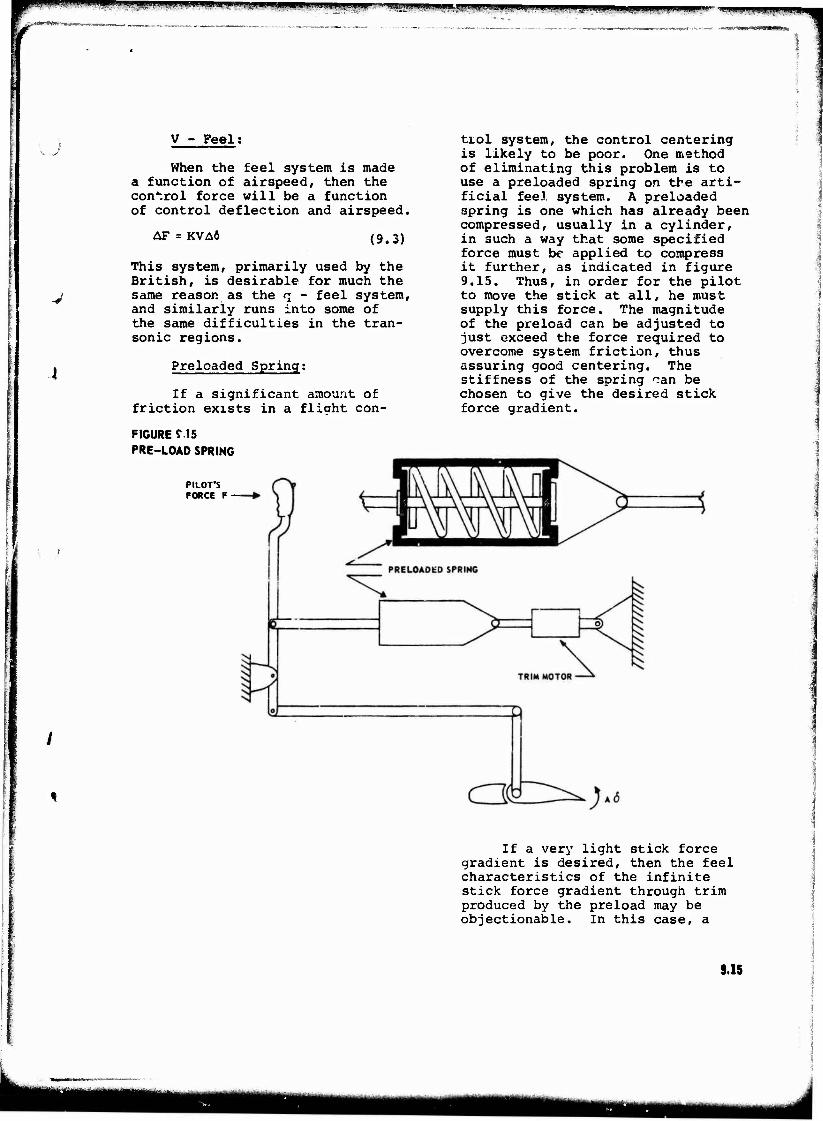
ji HI IL..UH ^spp^BwpppBffiiijiiBff mmtm^fufsammi^m ' msmmm^mf&am wwwmww •^* iw'ffflv «*w«wi-,.

1.»PM"1WH «1 M»

J V - Feel;

When the feel system is made a function of airspeed, then the control force will be a function of control deflection and airspeed.

AF = KVAÖ (9.3)

This system, primarily used by the British, is desirable for much the same reason as the q - feel system, and similarly runs into some of the same difficulties in the transonic regions.

Preloaded Spring;

If a significant amount of friction exists in a flight con-

FIGURE 915 PRE-LOAD SPRING

PILOT'S FORCE F

tiol system, the control centering is likely to be poor. One method of eliminating this problem is to use a preloaded spring on the artificial fee.! system. A preloaded spring is one which has already been compressed, usually in a cylinder, in such a way that some specified force must be applied to compress it further, as indicated in figure 9.15. Thus, in order for the pilot to move the stick at all, he must supply this force. The magnitude of the preload can be adjusted to just exceed the force required to overcome system friction, thus assuring good centering. The stiffness of the spring can be chosen to give the desired stick force gradient.

If a very light stick force gradient is desired, then the feel characteristics of the infinite stick force gradient through trim produced by the preload may be objectionable. In this case, a

9.15

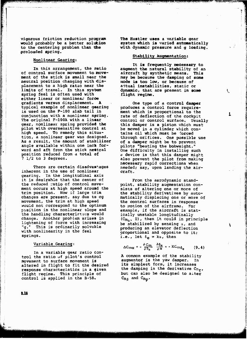
mm JUM.lUJUJiU.il U ] w WW w IIIU.IJUWMW .iHWWJWWPW»'#!W^^^^

vigorous friction reduction program Mould probably be a better solution to the centering problem than the preloaded spring.

Nonlinear Gearing;

In this arrangement, the ratio of control surface movement to movement of the stick is small near the neutral position changing with displacement to a high ratio near the limits of travel. In this system spring feel is often used with either linear or nonlinear force gradients versus displacement. A typical example of nonlinear gearing is used on the F-100 slab tail in conjunction with a nonlinear spring. The original F-100A with a linear gear, nonlinear spring provided the pilot with oversensitive control at high speed. To remedy this situation, a nonlinear gear was designed. As a result, the amount of stabilizer angle available within one inca forward and aft from the stick nettral position reduced from a total of 7 1/2 to 3 degrees.

There are certain disadvantages inherent in the use of nonlinear gearing. In the longitudinal axis it is desirable that the center of the reduced ratio of control movement occurs at high speed around the trim position. Now if large trim changes are present, say due to eg movement, the trim at high speed would not correspond to the optimum position in the nonlinear slope and the handling characteristics would change. Another problem arises in lightening of force with increasing "g." This is ordinarily solvable with nonlinearity in the feel springs.

Variable Gearing?

In a variable gear ratio control the ratio of pilot's control movement to surface movement is altered in flight to fit the desired response characteristics in a qfiven flight regime. This principle of control is applied in the B-58.

The Hustler uses a variable gear system which is varied automatically with dynamic pressure and g loading.

Stability Augmentation:

It is frequently necessary to augment the natural stability of an aircraft by synthetic means. This may be because the damping of some mode is too low, or because of actual instabilities, static or dynamic, that are present in some flight regime.

One type of a control damper produces a control force requirement which is proportional to the rate of deflection of the cockpit control or control surface. Usually this damper is a piston which must be moved in a cylinder which contains oil which must be forced through orifices. One possible use of a damper might be to prevent pilots "beating the bobweight." One difficulty in installing such ä device is that this damper might also prevent the pilot from making necessary rapid corrections when needed; say, upon landing the aircraft.

From the aerodynamic stand- paint, stability augmentation consists of altering one or more of the stability derivatives by automatically displacing one or more of the control surfaces in response to motion of the airframe. For example, if the aircraft is statically unstable longitudinally (Cma> 0), then it could in principle be stabilized by sensing a, and producing an elevator deflection proportional and opposite to it; i.e., let 6e = ka, then

AC ma <?Cm_ JOT - KCm6e (9.4)

A common example of the stability augmentor is the yaw damper. In its simplest form, it increases the damping in the derivative Cnr, but can also be designed to alter Cng and Cnp.

',

5.16

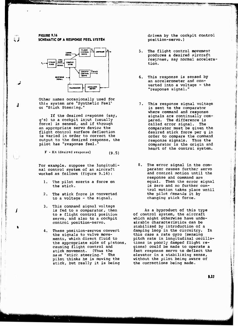
--»I.I. JIVI.M* II..,. -1«^,^^ TTr.^-r mmmmm WW I.^IJJi.Liii J*viU*Utmi np * ■«

u FIGURE 9.16 SCHEMATIC OF A RESPONSE FEEL SYSTEM

driven by the cockpit control position-servo.)

SMKMt »IGNAl V"

f LIGHT CCNTHOL 1IRVO

^ AlMRAMf

/ »•AW

COM- MAND COM*A«

ATM CAM SIGNAL

b STICK N coe«HT

»•vo

»WKAL

5. The flight control movement produces a desired aircraft response, say normal acceleration.

6. This response is sensed by an accelerometer and converted into a voltage - the "response signal."

Other names occasionally used for this system are "Synthetic Feel' or "Stick Steering."

If the desired response (say, g's) to a cockpit input (usually force) is sensed, and if through an appropriate servo device the flight control surface deflection is varied in order to correct the output to the desired response, the pilot has "response feel."

F - KX (desired response) (9.5)

For example, suppose the longitudinal control system of an aircraft worked as follows (figure 9.16):

1. The pilot exerts a force on the stick.

2. The stick force is converted to a voltage - the signal.

3. This command signal voltage is fed to a comparator, then to a flight control position servo, and also to a cockpit control position-servo.

4. These position-servos convert the signals to valve movements, which direct fluid to the appropriate side of pistons, causing flight control and stick movement. (Thus the naae "stick steering." The pilot thinks he is moving the stick, but really it is being

7. This response signal voltage is sent to the comparator where command and response signals are continually compared. The difference is called error signal. The comparator must be given the desired stick force per g in order to compare the command response signals. Thus the comparator is the origin and heart of the control system.

8. The error signal in the comparator causes further servo and control motion until the response and command are equal. Then the error signal is zero and no further control motion takes place until the pilot demands it by changing stick force.

As a byproduct of this type of control system, the aircraft which might otherwise have undesirable characteristics can be stabilized by introduction of a damping loop in the circuitry. In this case a rate gyro (sensing pitch rate in longitudinal oscillations in poorly damped flight regions) could be made to operate a fast response servo to deflect the elevator in a stabilizing sense, without the pilot being aware of the corrections being made.

S.1T

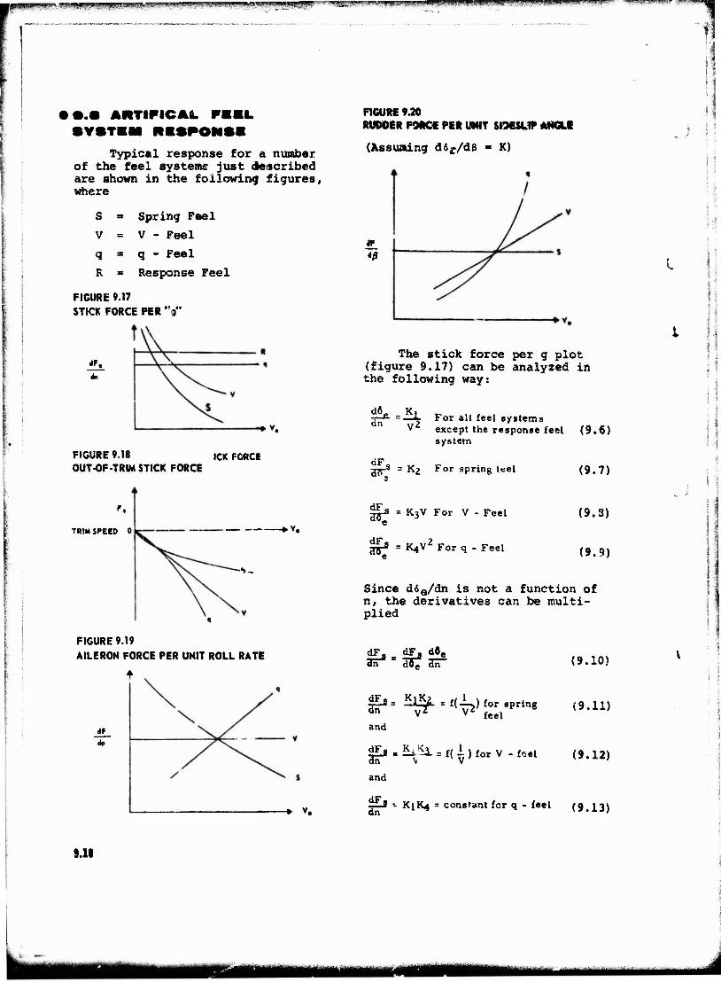
IpjppapaBliPPff^iW^g'ffWBPWll'^WigBWWBPPBP »"'•'iBWWP'wgflBPWIlPWW"!!^^

Typical response for a number of the feel systems just described are shown in the following figures, where

S = Spring Feel

V = V - Feel

q = q - Feel R = Response Feel

FIGURE 9.17 STICK FORCE PER "3"

<IF,

»V.

FIGURE 9.18 ,« FOR« OUT-OF-TRIM STICK FORCE

TRIM SPEED 0 » V,

S-

FIGURE 9.19 AILERON FORCE PER UNIT ROLL RATE

if

FIGURE 9.20 RUDDER FOUCi PER UNIT SKNESUP ANGLE

(Assuming dör/dß * K)

*ß

The stick force per g plot (figure 9.17) can be analyzed in the following way:

JJJJ*- =—^ For all feel systems V except the response feel (9.6)

system

dF -rjj-S = K^ For spring teel

$£a = K3V For V - Feel e

jjjj = K4V2 For q - Feel

(9.7)

(9.3)

(9.9)

Since d5Q/dn is not a function of n, the derivatives can be multiplied

on d0e dn (9.10)

§*= •^■^(•^) Jor spring (9.U)

j£f • &51 = f( i ) for V - feel (9.12)

* v.

and

dFa

dn

I

- K1K4 = consent for q - feel (9.13)

9.11

■■HmmMeHMHMi

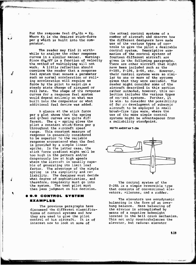
[■■HjPl^fBPUBBg •■\\i"" \>" •■' >,ym&'BWW HP PJl -■''-*■' »'""wppjppp fwpi ".^^^'»iBatiWS» ^."«lii.f'pjJjgj'ii ■',»■'■'■—"—-' y"-'-"?*■•nmcnrapomppi"

MPAmMMm»*«»

For the response feel dFg/dn » K5. iJ Where K5 is the desired stick-force

per g which is built into the comparator .

The reader may find it worth- while to analyze the other response curves in a similar manner. Warning: Since d6e/dV is a function of velocity the method of multiplying will not work. A little reflection should

. convince the reader that a response 4 feel system that senses a parameter

such as normal acceleration or rolling acceleration will require no force by the pilot to maint iin a steady state change of airspeed or

ji roll rate. The shape of the response curves for a response feel system would depend entirely on what was built into the comparator or what additional feel device was added.

A glance at the stick force per g plot shows that the spring and q-feel curves are quite different. The q - spring gives the pilot a constant stick-force per g throughout the aircraft speed range. This constant measure of response is generally considered to be superior to the variable response encountered when the feel is provided by a simple linear spring. In the latter case, the stick force gradient might well be too high in the pattern and/or dangerously low at high speeds where the aircraft is usually capable of generating its limit load factor. The advantage of the simple spring is its simplicity and reliability. The designer must decide

^ what degree of sophistication, and therefore, complexity must go into the system. The test pilot must then pass judgment on his decision.

• 9.9 CONTROL SVSTEM EXAMPLES

The previous paragraphs have discussed the different classifica- tions of control systems and how they are used to give the pilot control of his aircraft. It is of interest now to look at some of

the actual control systems of a number of aircraft and observe how the different designers have made use of the various types of controls to give the pilot a desirable control system. Descriptive sum- maries of the control systems of fourteen different aircraft are given in the following paragraphs. There are other aircraft that might have been included such as the F-100, F-106, B-66, etc. However, their control systems were so similar to one or more of the systems given that they were excluded. The reader might consider some of the aircraft described in this section rather outmoded, however, this selection includes the various types of cortrol systems. Further, it is wis- to consider the possibility of fur idä development of subsonic aircraft to be employed in small brush-fire type wars, where the use of the more simple control systems might be advantageous from a reliability standpoint.

NOPTH AMERICAN T-28A

The control system of the T-28A is a simple reversible type that consists of conventional elevators, ailerons, and a rudder.

The elevators use aerodynamic balancing in the form of an over- hung balance. Mass balancing of the elvator is accomplished by means of a negative bobweight located in the bell crank mechanism. This not only counterbalances the elevator, but reducet; elevator

9.19

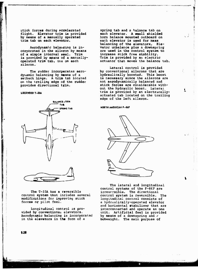
MHM—WmlWflumi ÜHM ilMfflUMW'ffW-'-^l^tF^w^ww?.^,^

f stick forces during accelerated flight. Elevator trim is provided by means of a manually operated trim tab on each elevator.

Aerodynamic balancing is incorporated in the aileron by means of a simple internal seal. Trim is provided by means of a manually- operated trim tab, one on each aileron.

The rudder incorporates aerodynamic balancing by means of a setback hinge. A trim tab located on the trailing edge of the rudder provides directional tiim.

LOCKHEED T-33A

BALANCE ~TKIM

i

' i

The T-33A has a reversible control system that includes several modifications for improving stick forces or pilot feel.

Longitudinal control is provided by conventional elevators. Aerodynamic balancing is incorporated in the elevators in the form of a

spring tab and a balance tab on each elevator. A small shielded horn balance mounted outboard on each elevator is used for mass balancing of the elevators.. Ele- vator unbalance plus a downspring are used in the control system to increase stick free stability. Trim is provided by an electric actuator that moves the balance tab.

Lateral control is provided by conventional ailerons that are hydraulically boosted. This boost is necessary since the ailerons are not aerodynamically balanced and stick forces are considerable without the hydraulic boost. Lateral trim is provided by an electrically- actuated tab located on the trailing edge of the left aileron.

NORTH AMERICAN F-86F

t

The lateral and longitudinal control systems of the F-86F are irreversible. The directional control system is reversible. The longitudinal control consists of a hydraulically-operated elevator and horizontal stabilizer that are interconnected and operate as one unit. Artificial feel is provided by means of a downspring and r bobweight. The main purpose of

8.21

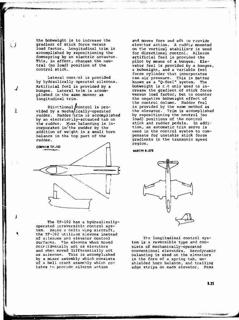
. r^„ ...

u

J

the bobweight is to increase the gradient of stick force versus load factor. Longitudinal trim is accomplished by repositioning the downspring by an electric actuator. This, in effect, changes the neutral (no load) position of the control stick.

Lateral control is provided by hydraulically operated ailerons. Artificial feel is provided by a bungee. Lateral trim is accomplished in the same manner as longitudinal trim.

Direbtional /control is provided by a mecha/.ically-operated rudder. Rudder/crim is accomplished by an electrice.ily-actuated tab on the rudder. M4SS balancing is incorporated in/the rudder by the addition of weight in a small horn balance in the top part of the rudder.

CONV/tIR TF-102

-<o

The TF-102 has a hydraulically- operated irreversible control system. Being a delta wing aircraft, the TF-102 utilises elevons instead of ailerons and elevator control surfaces. The elevons when moved coirjridentally act as elevators and when moved iifferentially act as ailerons. This is accomplished by a mixer assembly which consists of a bell crank assembly which rotates to provide aileron action

and moves fore and aft ^o provide elevator action. A rudder mounted on the vertical stabilizer is used for directional control. Aileron artificial feel is provided the pilot by means of a bungee. Ele- vator feel is provided by a bungee, a bobweight, and a variable feel force cylinder that incorporates ram air pressure. This is better known as a "Q-feel" system. The bobweight is r. >t only used to increase the gradient of stick force versus load factor, but to counter the negative bobweight effect of the control column. Rudder feel is provided by the same method as the elevator. Trim is accomplished by repositioning the neutral (no load) positions of the control stick and rudder pedals. In addition, an automatic trim servo is used in the control system to com- pensate for unstable stick force gradients in the transonic speed region.

MARTIN B-57E

^

v/1

The longitudinal control system is a reversible type and consists of mechanically-operated conventional elevators. Aerodynamic balancing is used on the elevators in the form of a spring tab, unshielded horn balance, and trailing edge strips on each elevator. Mass

9.21

tmam MM 1 '«Eifciijtlii^tbi'v '-..«**($■*"'*"'

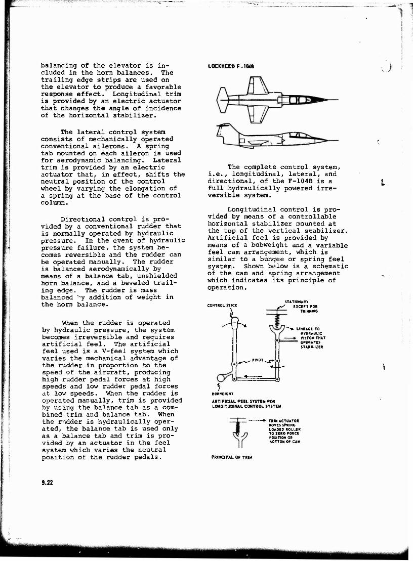
:;'.*--?•. ".^T7^;^'~T-7:V;*--7W>-; IJ-;_ •

'1

i ■

balancing of the elevator is included in the horn balances. The trailing edge strips are used on the elevator to produce a favorable response effect. Longitudinal trim is provided by an electric actuator that changes the angle of incidence of the horizontal stabilizer.

The lateral control system consists of mechanically operated conventional ailerons. A spring tab mounted on each aileron is used for aerodynamic balancing. Lateral trim is provided by an electric actuator that, in effect, shifts the neutral position of the control wheel by varying the elongation of a spring at the base of the control column.

Directional control is provided by a conventional rudder that is normally operated by hydraulic pressure. In the event of hydraulic pressure failure, the system becomes reversible and the rudder can be operated manually. The rudder is balanced aerodynamically by means of a balance tab, unshielded horn balance, and a beveled trailing edge. The rudder is mass balanced uy addition of weight in the horn balance.

When the rudder is operated by hydraulic pressure, the system becomes irreversible and requires artificial feel. The artificial feel used is a V-feei system which varies the mechanical advantage of the rudder in proportion to the speed of the aircraft, producing high rudder pedal forces at high speeds and low rudder pedal forces at low speeds. When the rudder is operated manually, trim is provided by using the balance tab as a combined trim and balance tab. When the rudder is hydraulically operated, the balance tab is used only as a balance tab and trim is provided by an actuator in the feel system which varies the neutral position of the rudder pedals.

LOCKHEED F-104B J

The complete control system, i.e., longitudinal, lateral, and directional, of the F-104B is a full hydraulically powered irreversible system.

Longitudinal control is provided by means of a controllable horizontal stabilizer mounted at the top of the vertical stabilizer. Artificial feel is provided by means of a bobweight and a variable feel cam arrangement, which is similar to a bungee or spring feel system. Shown below is a schematic of the cam and spring arrangement which indicates its principle of operation.

CONTROL STICK

'"w*

STATIONARY f/ EXCEPT FOR

LINKAGE TO HYDRAULIC PISTON THAT OPERATES STABILIZER

iS

ARTIFICIAL FEEL SYSTEM FOR LONGITUDINAL CONTROL SYSTEM

-* TRIM ACTUATOR MOVES SPRING LOADED ROLLER TO ZERO FORCE POSITION OR BOTTOM OF CAM

PRINCIPAL OF TRIM

9.22

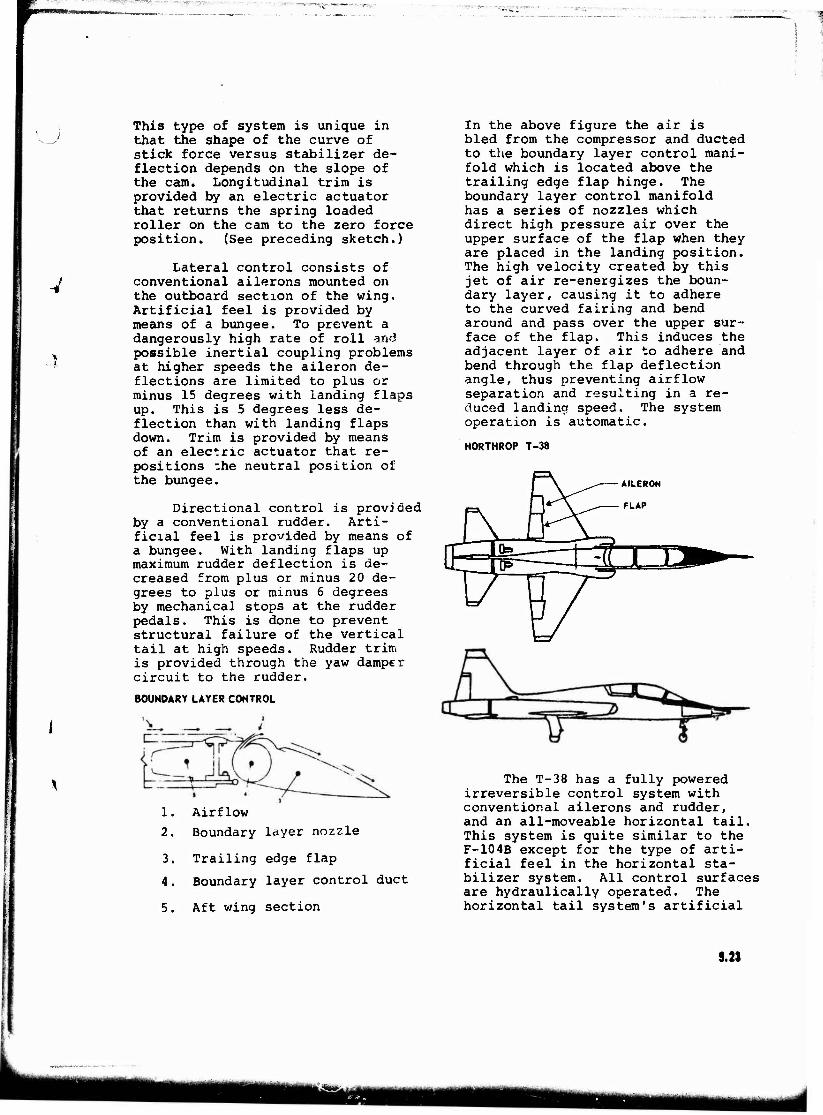
V

This type of system is unique in that the shape of the curve of stick force versus stabilizer deflection depends on the slope of the cam. Longitudinal trim is provided by an electric actuator that returns the spring loaded roller on the cam to the zero force position. (See preceding sketch.)

Lateral control consists of conventional ailerons mounted on the outboard section of the wing. Artificial feel is provided by means of a bungee. To prevent a dangerously high rate of roll ami possible inertial coupling problems at higher speeds the aileron deflections are limited to plus or minus 15 degrees with landing flaps up. This is 5 degrees less deflection than with landing flaps down. Trim is provided by means of an electric actuator that re- positions -he neutral position of the bungee.

Directional control is provided by a conventional rudder. Arti- ficial feel is provided by means of a bungee. With landing flaps up maximum rudder deflection is decreased from plus or minus 20 degrees to plus or minus 6 degrees by mechanical stops at the rudder pedals. This is done to prevent structural failure of the vertical tail at high speeds. Rudder trim is provided through the yaw damper circuit to the rudder.

BOUNDARY LAYER CONTROL

1. Airflow

2. Boundary layer nozzle

3. Trailing edge flap

4. Boundary layer control duct

5. Aft wing section

In the above figure the air is bled from the compressor and ducted to the boundary layer control manifold which is located above the trailing edge flap hinge. The boundary layer control manifold has a series of nozzles which direct high pressure air over the upper surface of the flap when they are placed in the landing position. The high velocity created by this jet of air re-energizes the boundary layer, causing it to adhere to the curved fairing and bend around and pass over the upper surface of the flap. This induces the adjacent layer of air to adhere and bend through the flap deflection angle, thus preventing airflow separation and resulting in a reduced landing speed. The system operation is automatic.

NORTHROP T-38

-AILERON

- FLAP

"JbJ M "" Ite'

The T-38 has a fully powered irreversible control system with conventional ailerons and rudder, and an all-moveable horizontal tail. This system is quite similar to the F-104B except for the type of artificial feel in the horizontal stabilizer system. All control surfaces are hydraulically operated. The horizontal tail system's artificial

9.21

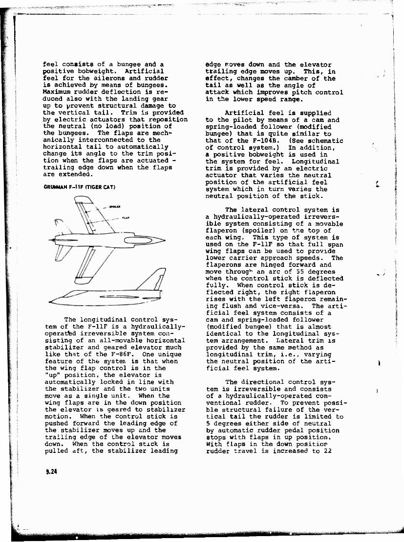
TiH^W^fi^Uffigg*1*^^ - JTfli ;'Ti7"^s^^FS"/;"»^*':ra"vtv!^

■ ~-~~;

feel consists of a bungee and a positive bobweight. Artificial feel for the ailerons and rudder is achieved by means of bungees. Maximum rudder deflection is reduced also with the landing gear up to prevent structural damage to the vertical tail. Trim is provided by electric actuators that reposition the neutral (no load) position of the bungees. The flaps are mechanically interconnected to the horizontal tail to automatically change its angle to the trim position when the flaps are actuated - trailing edge down when the flaps are extended.

GRUMMAN F-11F (TIGER CAT)

The longitudinal control system of the F-11F is a hydraulically- operatted irreversible system consisting of an all-movable horizontal stabilizer and geared elevator much like that of the F-86F. One unique feature of the systen is that when the wing flap control is in the "up" position, the elevator is automatically locked in line with the stabilizer and the two units move as a single unit. When the wing flaps are in the down position the elevator is geared to stabilizer motion. When the control stick is pushed forward the leading edge of the stabilizer moves up and the trailing edge of the elevator moves down. When the control stick is pulled dft, the stabilizer leading

edge roves down and the elevator trailing edge moves up. This, in effect, changes the camber of the tail as well as the angle of attack which improves pitch control in the lower speed range.

Artificial feel is supplied to the pilot by means of a cam and spring-loaded follower (modified bungee) that is quite similar to that of the F-104B. (See schematic of control system.) In addition, a positive bobweight is used in the system for feel. Longitudinal trim is provided by an electric actuator that varies the neutral position of the artificial feel system which in turn varies the neutral position of the stick.

The lateral control system is a hydraulically-operated irreversible system consisting of a movable flaperon (spoiler) on tne top of each wing. This type of system is used on the F-11F so that full span wing flaps can be used to provide lower carrier approach speeds. The flaperons are hinged forward and move through an arc of 55 degrees when the control stick is deflected fully. When control stick is deflected right, the right flaperon rises with the left flaperon remaining flush and vice-versa. The artificial feel system consists of a cam and spring-loaded follower (modified bungee) that is almost identical to the longitudinal system arrangement. Lateral trim is provided by the same method as longitudinal trim, i.e., varying the neutral position of the artificial feel system.

The directional control system is irreversible and consists of a hydraulically-operated conventional rudder. To prevent possible structural failure of the vertical tail the rudder is limited to 5 degrees either side of neutral by automatic rudder pedal position stops with flaps in up position. With flaps in the down positior rudder travel is increased to 22

t

**• *

9.24

i jtt-'""--'—

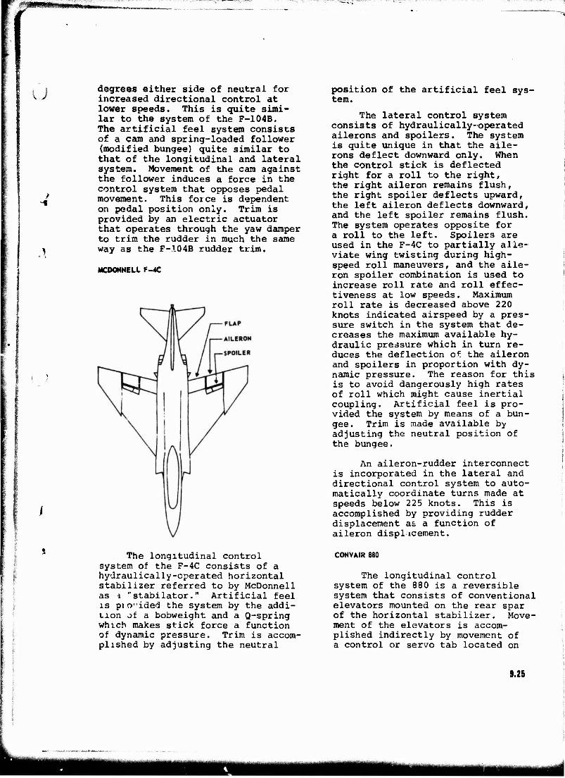
jMMNHNMNift

u degrees either side of neutral for increased directional control at lower speeds. This is quite similar to the system of the F-104B. The artificial feel system consists of a cam and spring-loaded follower (modified bungee) quite similar to that of the longitudinal and lateral system. Movement of the cam against the follower induces a force in the control system that opposes pedal movement. This force is dependent on pedal position only. Trim is provided by an electric actuator that operates through the yaw damper to trim the rudder in much the same way as the F-104B rudder trim.

MCDONNELL F-4C

position of the artificial feel system.

The lateral control system consists of hydraulically-operated ailerons and spoilers. The system is quite unique in that the ailerons deflect downward only. When the control stick is deflected right for a roll to the right, the right aileron remains flush, the right spoiler deflects upward, the left aileron deflects downward, and the left spoiler remains flush. The system operates opposite for a roll to the left. Spoilers are used in the F-4C to partially alleviate wing twisting during high- speed roll maneuvers, and the aileron spoiler combination is used to increase roll rate and roll effectiveness at low speeds. Maximum roll rate is decreased above 220 knots indicated airspeed by a pressure switch in the system that decreases the maximum available hydraulic pressure which in turn reduces the deflection of the aileron and spoilers in proportion with dynamic pressure. The reason for this is to avoid dangerously high rates of roll which might cause inertial coupling. Artificial feel is provided the system by means of a bungee. Trim is made available by adjusting the neutral position of the bungee.

An aileron-rudder interconnect is incorporated in the lateral and directional control system to automatically coordinate turns made at speeds below 225 knots. This is accomplished by providing rudder displacement as a function of aileron displacement.

i r

The longitudinal control system of the F-4C consists of a hydraulically-cperated horizontal stabilizer referred to by McDonnell as i "stabilator." Artificial feel is pio'ided the system by the addition of a bobweight and a Q-spring which makes stick force a function of dynamic pressure. Trim is accomplished by adjusting the neutral

CONVAIR 880

The longitudinal control system of the 880 is a reversible system that consists of conventional elevators mounted on the rear spar of the horizontal stabilizer. Move- ment of the elevators is accomplished indirectly by movement of a control or servo tab located on

9.2S

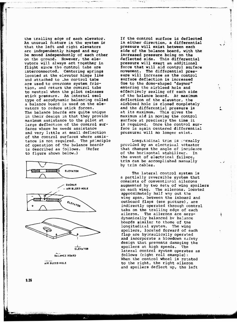
tammammnmm ,

the trailing edge of each elevator. An unusual feature in the system is that the left and right elevators are independently hinged and may be moved independently of each other on the ground. However, the elevators will always act together in flight since th« control tabs are interconnected. Centering springs located at the elevator hinge line and attached to .he control tabs are used to overcome system friction, and return the control tabs to neutral when the pilot releases stick pressure. An internal seal type of aerodynamic balancing called a balance board is used on the elevators to reduce stick forces. The balance boards are quite unique in their design in that they provide maximum assistance to the pilot at large deflection of the control surfaces where he needs assistance and very little at small deflection of the control surfaces where assistance is not required. The principle of operation of the balance boards? is described as follows. (Refer to figure shown below.)

DAGMAR

AIR BLEED HOLE

<^_

ELEVATOR

BALANCE BOARD

AIR BLEED HOLE

If the control surface is deflected in either direction, a differential pressure will exist between each side of the balance board, with the increased pressure being on the deflected side. This differential pressure will exert an additional force that will aid control surface movement. The differential pressure will increase as the control surface deflection is increased due to the dome-shaped "dagmar" entering the airbleed hole and effectively sealing off each side of the balance board. At maximum deflection of the elevator, the airbleed hole is closed completely and the differential pressure is at its maximum. This gives the maximum aid in moving the control surface at precisely the time it is required. Once the control surface is again centered differential pressures will no longer exist.

Longitudinal trim is ;:r'rmally provided by an electrical actuator that changes the angle of incidence of the horizontal stabilizer. In the event of electrical failure, trim can be accomplished manually by trim cables.

The lateral control system is a partially reversible system that consists of conventional ailerons augmented by two sets» of wing spoilers on each wing. The ailerons, located approximately half wiy out the wing span, between the inboard and outboard flaps (see picture), are indirectly operated through control tabs on the trailing edge of each aileron. The ailerons are aerodynamically balanced bv balance boards similar to those of the longitudinal system. The wing spoilers, located forward of each flap are hydraulically operated and incorporate a blowdown safety design that prevents damaging the spoilers at high speeds. The lateral control system operates as follows (right roll example): When the control wheel is rotated to the right, the right aileron and spoilers deflect up, the left

9.26

)

* *

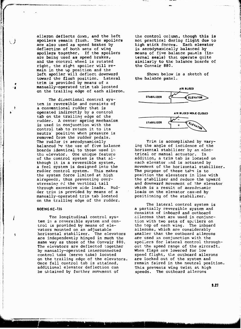
aileron deflects down, and the left spoilers remain flush. The spoilers are also used as speed brakes by deflection of both sets of wing spoilers together. If the spoilers are being used as speed brakes, and the control wheel is rotated right, the right spoiler will remain in the up position and the left spoiler will deflect downward toward the flush position. Lateral trim is provided by means of a manually-operated trim tab located on the trailing edge of each aileron.

The directional control system is reversible and consists of a conventional rudder that is operated indirectly by a control tab on the trailing edge of the rudder. A center spring mechanism is used in conjunction with the control tab to return it to its neutra" position when pressure is removed from the rudder pedals. The rudJsr is aerodynamically balanced hy the use of five balance boards identical to those used in the elevator. One unique feature of the control system is that although it is a reversible system, a feel system is designed into the rudder control system. This makes the system force limited at high airspeeds, thus preventing over- stressing ci the vertical tail through excessive side loads. Rud- der trim is provided by means of a manually-operated trim tab located on the trailing edge of the rudder.

BOEING KC-135

The longitudinal control system is; a reversible system and control Ls provided by means of elevators mounted on an adjustable horizontal stabilizer. The elevators are independently hinged in much the same way as those of the Convair 880. The elevators are deflected together by manually-operated interconnected control tabs (servo tabs) located on the trailing edge of the elevators. Once full control tab is attained, additional elevator deflection can be obtained by further movement of

the control column, though this is not practical during flight due to high stick forces. Each elevator is aerodynamically balanced by means of five balance pai.els (internal seals) that operate quite similarly to the balance boards of the Convair 880.

Shown below is a sketch of the balance panel.

AIR BLEED

AIR BLEED HOLE CLOSED

Trim is accomplished by varying the angle of incidence of the horizontal stabilizer by an electrical or manual actuator. In addition, a trim tab is located on each elevator and is actuated by movement of the horizontal stabilizer. The purpose of these tabs is to position the elevators in line with the stabilizer and reduce the upward and downward movement of the elevator which is a result of aerodvnamic loads on the elevator caused by positioning of the stabilizer.

The lateral control system is a partially reversible system and consists of inboard and outboard ailerons that are used in conjunction with two sets of spoilers on the top of each wing. The inboard ailerons, which are considerably smaller than the outboard ailerons are used in conjunction with the spoilers for lateral control throughout the speed range of the aircraft. When flaps are lowered for low speed flight, the outboard ailerons are locked out of the system and remain faired in the neutral position. This prevents wing twist at high speeds. The outboard ailerons

9.27

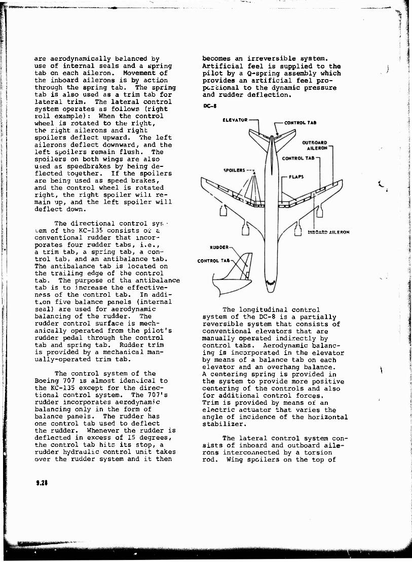
are aerodynamically balanced by use of internal seals and a spring tab on each aileron. Movement of the inboard ailerons is by action through the spring tab. The spring tab is also used as a trim tab for lateral trim. The lateral control system operates as follows (right roll example): When the control wheel is rotated to the right, the right ailerons and right spoilers deflect upward. The left ailerons deflect downward, and the left spoilers remain flush. The spoilers on both wings are also used as speedbrakes by being deflected together. If the spoilers are being used as speed brakes, and the control wheel is rotated right, the right spoiler will remain up, and the left spoiler will deflect down.

The directional control syf. • tern of the KC-135 consists oi a conventional rudder that incorporates four rudder tabs, i.e., a trim tab, a spring tab, a control tab, and an antibalance tab. The antibalance tab is located on the trailing edge of the control tab. The purpose of tha antibalance tab is to increase the effectiveness of the control tab. In addition five balance panels (internal seal) are used for aerodynamic balancing of the rudder. The rudder control surface is mechanically operated from the pilot's rudder pedal through the control tab and spring tab. Rudder trim is provided by a mechanical manually-operated trim tab.

The control system of the Boeing 707 is almost identical to the KC-135 except for the directional control system. The 707's rudder incorporates aerodynanu c balancing only in the form of balance panels. The rudder has one control tab used to deflect the rudder. Whenever the rudder is deflected in excess of 15 degrees, the control tab hits its stop, a rudder hydraulic control unit takes over the rudder system and it then

becomes an irreversible system. Artificial feel is supplied to the pilot by a Q-spring assembly which provides an artificial feel proper cional to the dynamic pressure and rudder deflection.

DC-8

ELEVATOR CONTROL TAB

JUDMBn All CDQfcl

RUDDER

CONTROL TAB

The longitudinal control system of the DC-8 is a partially reversible system that consists of conventional elevators that are manually operated indirectly by control tabs. Aerodynamic balancing is incorporated in the elevator by means of a balance tab on each elevator and an overhang balance. A centering spring is provided in the system to provide more positive centering of the controls and also for additional control forces. Trim is provided by means of an electric actuator that varies the angle of incidence of the horizontal stabilizer.

The lateral control system consists of inboard and outboard ailerons interconnected by a torsion rod. Wing spoilers on the top of

S.28

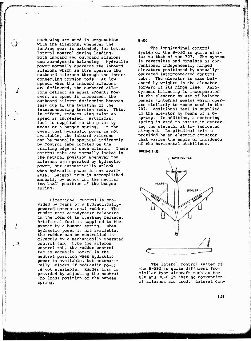
mwiMi SW»

each wing are used in conjunction with the ailerons, whenever the landing gear is extended, for better lateral control during landing. Both inboard and outboard ailerons use aerodynamic balancing. Hydraulic power normally operates the inboard ailerons which in turn operate the outboard ailerons through the interconnecting torsion rods. At .low speeds when the inboard ailerons are deflected, the outboard ailerons deflect an equal amount; however, as speed is increased, the outboard aileron del Lection becomes less due to the twisting of the interconnecting torsion rods. This, in effect, reduces wing twist as speed is increased. Artificial feel is supplied to the pilot oy means of a bungee spring. In the event that hydraulic power is not available, the inboard filerons can be manually operated indirectly by control tabs located on the trailing edge of each aileron. These control tabs are normally locked in the neutral position whenever the ailerons are operated by hydraulic power, but automatically unlock when hydraulic power is not available. Lateral trim is accomplished manually by adjusting the neuvral (no load) position of the bungee spring.

Directional control is provided by means of a hydraulically- powered conven* i.onal rudder. The rudder uses aerodynamic balancing in the form of an overhang balance. Artificial feel is supplied to the system by a bungee spring. When hydraulic power is not available, the rudder can be controlled indirectly by a mechanically-operated control tab. Like the aileron control tab, the rudder control tab is normally locked in the neutral position when hydraulic power is available, but automatically in locks if hydraulic po»^ iS not available. Rudder trim is provided by adjusting the neutral 'no load) position of the bungee spring.

B-52C

The longitudinal control system of the B-52G is quite similar to that of the 707. The system is reversible and consists of conventional independently hinged elevators positioned by manually- operated interconnected control tabs. The elevator is mass balanced by weights in the elevator forward of its hinge line. Aero- dynamic balancing is incorporated in the elevator by use of balance panels (internal seals) which operate similarly to those used in the 707. Additional feel is supplied to the elevator by means of a Q- spring. In addition, a centering spring is used to assist in centering the elevator at low indicated airspeed. Longitudinal trim is provided by an electric actuator that varies the angle of incidence of the horizontal stabilizer.

BOEING B-52

CONTROL TAB

The lateral control system of the B-52G is quite different from similar type aircraft such as the 880 and DC-8 in that no conventional ailerons are used. Lateral con-

9.29

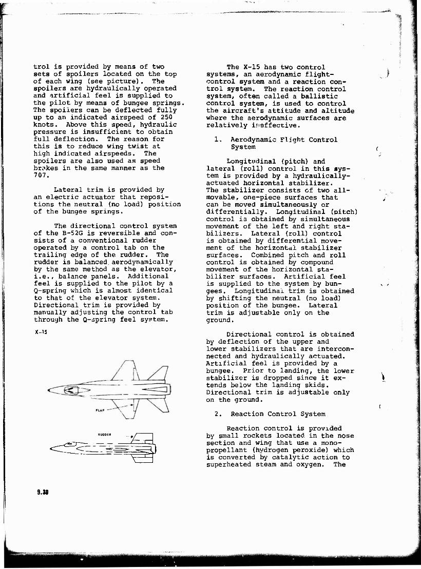
trol is provided by means of two sets of spoilers located on the top of each wing (see picture). The spoilers are hydraulically operated and artificial feel is supplied to the pilot by means of bungee springs. The spoilers can be deflected fully up to an indicated airspeed of 250 knots. Above this speed, hydraulic pressure is insufficient to obtain full deflection. The reason for this is to reduce wing twist at high indicated airspeeds. The spoilers are also used as speed brakes in the same manner as the 707.

Lateral trim is provided by an electric actuator that reposi- tions the neutral (no load) position of the bungee springs.

The directional control system of the B-52G is reversible and consists of a conventional rudder operated by a control tab on the trailing edge of the rudder. The rudder is balanced aerodynamically by the same method as the elevator, i.e., balance panels. Additional feel is supplied to the pilot by a Q-spring which is almost identical to that of the elevator system. Directional trim is provided by manually adjusting the control tab through the Q-spring feel system.

X-15

f

The X-15 has two control systems, an aerodynamic flight- control system and a reaction control system. The reaction control system, often called a ballistic control system, is used to control the aircraft's attitude and altitude where the aerodynamic surfaces are relatively ineffective.

1. Aerodynamic Flight Control System

Longitudinal (pitch) and lateral (roll) control in this system is provided by a hydraulically- actuated horizontal stabilizer. The stabilizer consists of two all- movable, one-piece surfaces that can be moved simultaneously or differentially. Longitudinal (pitch) control is obtained by simultaneous movement of the left and right stabilizers. Lateral (roll) control is obtained by differential movement of the horizontal stabilizer surfaces. Combined pitch and roll control is obtained by compound movement of the horizontal stabilizer surfaces. Artificial feel is supplied to the system by bungees. Longitudinal trim is obtained by shifting the neutral (no load) position of the bungee. Lateral trim is adjustable only on the ground.

Directional control is obtained by deflection of the upper and lower stabilizers that are interconnected and hydraulically actuated. Artificial feel is provided by a bungee. Prior to landing, the lower stabilizer is dropped since it ex- tends below the landing skids. Directional trim is adjustable only on the ground.

2. Reaction Control System

Reaction control is provided by small rockets located in the nose section and wing that use a mono- propellant (hydrogen peroxide) which is converted by catalytic action to superheated steam and oxygen. The

•3

9.10

X 0

* .1

reaction of the escaping gases causes the aircraft to move about the selected or combined axes. The control used by the pilot consists of a control stick handle located on the left console of the cockpit. Upward and downward movement of the control handle operates the rockets located on the top and bottom of the nose section, respectively, and gives the aircraft pitch control. Sideward movement of the control handle operates the rockets located on the sides of the nose section and provides the aircraft with directional control. Rotating the control handle operates the rockets located in the

wing section and provides lateral control.

Artificial feel is provided the pilot for all three axes of operation by spring bungees connected to the system. The angular acceleration and velocity of the aircraft vary with the amount and duration of the ballistic control handle application. The velocity tends to sustain itself after the stick is returned to the neutral position. A subsequent stick movement opposite to the initial one is required to cancel the original induced velocity.

J

9.31

tm^mmmttmmmmm^^^^- - DTIC

Documents

Transcript of tm^mmmttmmmmm^^^^- - DTIC