istanbul technical university graduate school of science - Polen

ISTANBUL TECHNICAL UNIVERSITY GRADUATE SCHOOL OF SCIENCE

ENGINEERING AND TECHNOLOGY

M.Sc. THESIS

AEROSPIKE NOZZLE DESIGN AND ANALYSIS

Sherif FARRAG

Department of Aeronautical and Astronautical Engineering

Aeronautical and Astronautical Engineering Graduate Programme

JUNE, 2020

Department of Aeronautical and Astronautical Engineering

Aeronautical and Astronautical Engineering Graduate Programme

JUNE, 2020

ISTANBUL TECHNICAL UNIVERSITY GRADUATE SCHOOL OF SCIENCE

ENGINEERING AND TECHNOLOGY


M.Sc. THESIS

Sherif FARRAG

511171132

Thesis Advisor: Prof. Dr. Fırat Oğuz EDİS

Uçak ve Uzay Mühendisliği Anabilim Dalı

Uçak ve Uzay Mühendisliği Yüksek Lisans Programı

HAZİRAN, 2020

AEROSPİKE NOZUL TASARIMI VE ANALİZİ

YÜKSEK LİSANS TEZİ

Sherif FARRAG

511171132

Tez Danışmanı: Prof. Dr. Fırat Oğuz EDİS

ISTANBUL TEKNİK ÜNİVERSİTESİ FEN BİLİMLERİ ENSTİTÜSÜ

v

Thesis Advisor: Prof. Dr. Fırat Oğuz Edis ..............................

İstanbul Technical University

Jury Members: Doç. Dr. Ayşe Gül Güngör .............................

Istanbul Technical University

Prof. Dr. Metin Muradoğlu ..............................

Koç University

Sherif Farrag, a M.Sc student of İTU Graduate School of Science Engineering and

Technology, student ID 511171132, successfully defended the thesis entitled

“AEROSPIKE NOZZLE DESIGN AND ANALYSIS”, which he prepared after

fulfilling the requirements specified in the associated legislations, before the jury

whose signatures are below.

Date of Submission : 14 June 2020

Date of Defense : 21 July 2020

vii

To my wife,

ix

FOREWORD

This thesis is considered to be as a development on the experience which I self-built

through the past few years. Especially, the highlight of my projects I built in 2015

which considered to be the most powerful student-built solid rocket engine in Turkey

that has been marked safe and launched by the ESRA and until the thesis written date.

I would like to thank the main reason that pushed me to overcome difficulties during

all phases of the project and without her I could not have reached this point. She is the

one who insisted to push me to choose the topic that I am interested in whatever other

considerations. However, designing and manufacturing rocket engine has put my life

in danger once in the past due to a serious rocket work accident, she has never let me

give up my passionate field! She is my wife Mrs. Hanaa Mostafa. I appreciate the

support, time and flexibility that my research advisor Prof. Dr. Fırat EDİS has offered

me during this master research and even my previous B.Cs. research. He has always

been a trustworthy mentor to me. Also, I appreciate the logistical support that Mr.

Ahmet Fathy has offered me during the analysis work of his research. Moreover, I

would like to thank Mr. Çağrı Eren Durkaya and Mr. Ibrahim Çiçek for the translation

effort they did.

June 2020

Sherif FARRAG

(R&D Engineer)

xi

TABLE OF CONTENTS

Page

FOREWORD ............................................................................................................. ix TABLE OF CONTENTS .......................................................................................... xi

ABBREVIATIONS .................................................................................................. xv

SYMBOLS .............................................................................................................. xvii LIST OF TABLES .................................................................................................. xix

LIST OF FIGURES ................................................................................................ xxi SUMMARY ........................................................................................................... xxix ÖZET……………………………………………………………………………xxxiii

1. INTRODUCTION .................................................................................................. 1 1.1 Nozzle Definition ............................................................................................... 1 1.2 Nozzle Types ...................................................................................................... 2

1.2.1 Conical nozzle ............................................................................................. 2

1.2.2 Bell nozzle ................................................................................................... 3 1.2.3 Aerospike nozzle ......................................................................................... 3

2. LITERATURE SURVEY ...................................................................................... 5 2.1 Working Principle .............................................................................................. 5

2.2 Governing Equation ........................................................................................... 9 2.3 Detailed Angelino Method Discussion [2] [12] ............................................... 14

2.4 Thrust Calculations .......................................................................................... 16 2.4.1 Conical nozzle [4] [14] ............................................................................. 16 2.4.2 Aerospike nozzle [15] [16] [17] ................................................................ 17

2.5 Specific Impulse ............................................................................................... 19

3. NOZZLE CFD ANALYSIS & OPTIMIZATION ............................................ 21 3.1 Full Spike Nozzle ............................................................................................. 21

3.1.1 Cad model ................................................................................................. 21 3.1.2 Cfd mesh tool ............................................................................................ 22

3.1.2.1 Mesh setup ......................................................................................... 22 3.1.2.2 Mesh output ........................................................................................ 23

3.1.3 Cfd fluent .................................................................................................. 24

3.1.4 Thrust calculations .................................................................................... 27

3.2 40% Truncated Aerospike Nozzle .................................................................... 28 3.2.1 Cad model ................................................................................................. 28 3.2.2 Cfd mesh tool ............................................................................................ 29

3.2.2.1 Mesh setup ......................................................................................... 29 3.2.2.2 Mesh output ........................................................................................ 29

3.2.3 Cfd fluent .................................................................................................. 30 3.2.4 Thrust calculations .................................................................................... 32

3.3 20% Truncated Aerospike Nozzle .................................................................... 32 3.3.1 Cad model ................................................................................................. 33 3.3.2 Cfd mesh tool ............................................................................................ 33

xii

3.3.2.1 Mesh setup .......................................................................................... 33

3.3.2.2 Mesh output ........................................................................................ 34 3.3.3 Cfd fluent................................................................................................... 35

3.3.4 Thrust calculations .................................................................................... 36 3.4 40%Truncated - Blind Central Hole ................................................................. 37


3.4.2.1 Mesh setup .......................................................................................... 38

3.4.2.2 Mesh output ........................................................................................ 38 3.4.3 Cfd fluent................................................................................................... 39 3.4.4 Thrust calculations .................................................................................... 40

3.5 40%Truncated – 0.98%Flux Central Straight Bleed ........................................ 41 3.5.1 Cad model, mesh tool & boundary conditions .......................................... 43

3.5.2 CFD fluent ................................................................................................. 44

4.5.3 Thrust calculations .................................................................................... 45 3.6 Hybrid Aerospike-Conical Nozzle-40%Truncated – 2.9%Flux Central Bleed.

................................................................................................................................ 46 3.6.1 Cad model ................................................................................................. 47 3.6.2 Cfd mesh tool ............................................................................................ 47

3.6.2.1 Mesh setup .......................................................................................... 47 3.6.2.2 Mesh output ........................................................................................ 49

3.6.3 Cfd fluent................................................................................................... 50

3.6.4 Thrust calculations .................................................................................... 51 3.7 Hybrid Aerospike Conical Nozzle-40%Truncated – 5.9%Flux Central Bleed.52



3.7.3 Cfd fluent................................................................................................... 56 4.7.4 Thrust calculations .................................................................................... 57

3.8 Nozzle Performance Summary ......................................................................... 59

4. STEERING CONTROL ...................................................................................... 61 4.1 90% Positioned Secondary Injection on 40% Truncated Aerospike Nozzle ... 65



4.1.3 Cfd fluent................................................................................................... 70 4.1.4 Side force calculations .............................................................................. 71

4.2 20% Positioned Secondary Injection on 40% Truncated Aerospike Nozzle

Design & Analysis .................................................................................................. 74

4.3 Secondary Jet Position Effect on Aerospike Nozzle Summary........................ 75

5. CONCLUSION .................................................................................................... 77 REFERENCES ......................................................................................................... 79

APPENDICES .......................................................................................................... 83 APPENDIX A ........................................................................................................ 83

APPENDIX B ......................................................................................................... 85 APPENDIX C ......................................................................................................... 92 APPENDIX D ........................................................................................................ 93 APPENDIX E ....................................................................................................... 100

xiii

APPENDIX F ....................................................................................................... 102

APPENDIX G ...................................................................................................... 108 APPENDIX H ...................................................................................................... 110

APPENDIX I ........................................................................................................ 117 APPENDIX J ........................................................................................................ 119 APPENDIX K ...................................................................................................... 122 APPENDIX L ....................................................................................................... 124 APPENDIX M ...................................................................................................... 131

APPENDIX N ...................................................................................................... 133 APPENDIX O ...................................................................................................... 140 APPENDIX P ....................................................................................................... 142 APPENDIX Q ...................................................................................................... 155 APPENDIX R ...................................................................................................... 158

CURRICULUM VITAE ........................................................................................ 161

xv

ABBREVIATIONS

CAD : Computer Aided Drafting

CFD : Computational Fluid Dynamics

ITU : Istanbul Technical University

MOC : Method of Characteristics

OQ : Orthogonal Quality

SW : Solid Works

xvii

SYMBOLS

A : Area

A* : Chocked Area

F : Force

Isp : Specific Impulse

K : Kelvin

L : Length

l : length of a characteristic segment

ℓ : Length of a characteristic segment

m : Mass Flow Rate (Mass Flux)

M : Mach Number

M : Moment

P : Pressure

a : Atmospheric Pressure

c : Combustion Pressure

r : Radial Coordinates

R : Universal Gas Constant

T : Temperature

T : Thrust

v : Velocity

: Mach Angle

: Prandtl-Meyer angle

: Geometric angle with the reference axis

: Expansion Ratio

: Heat Capacity Ratio

: Correction Factor

: Density

: Derivation Angle

xviii

: Angle between thrust axis and vertical

Subscripts:

0 : Stagnation

“Base” or b : Aerospike Nozzle Front Base Section (if there is truncation)

e : Exit

t : Throat

thruster : Case Without Nozzle Centerbody

x : X Axis Direction

y : Y axis Direction

z : Z Axis Direction

xix

LIST OF TABLES

Page

Table 2. 1 : Conical nozzle. Divergence half angle relation with correction factor

[4]. ...................................................................................................................... 17 Table 3.1: Full spike nozzle face mesh setting......................................................... 23

Table 3.2: Full spike nozzle node & element mesh number. ................................... 24 Table 3.3: Full spike nozzle thrust Matlab code inputs. .......................................... 27 Table 3.4: Full spike nozzle thrust Matlab code outputs. ........................................ 27 Table 3.5 : 40% Truncated aerospike nozzle face & edge mesh settings. ................ 29

Table 3.6 : 40% Truncated aerospike element & node mesh number....................... 30 Table 3.7 : 40% Truncated aerospike nozzle Matlab thrust code inputs. .................. 31 Table 3.8 : 40% Truncated aerospike nozzle Matlab thrust code outputs. ................ 32

Table 3.9 : 20% Truncated aerospike nozzle face & edge mesh settings ................. 34 Table 3.10 : 20% Truncated aerospike nozzle node & element number. .................. 34 Table 3.11 : 20% Truncated aerospike nozzle Matlab thrust code inputs. ................ 36

Table 3.12 : 20% Truncated aerospike nozzle Matlab thrust code outputs. .............. 36 Table 3.13 : 40% Truncated – blind central hole aerospike nozzle face & edge mesh

settings. .............................................................................................................. 38

Table 3.14 : 40% Truncated – blind central hole aerospike nozzle node & element

number................................................................................................................ 39 Table 3.15 : 40% Truncated – blind central hole aerospike nozzle-Matlab thrust code

inputs. ................................................................................................................. 40 Table 3.16 : 40% Truncated – blind central hole aerospike nozzle-Matlab thrust code

outputs. ............................................................................................................... 41 Table 3.17 : 40%truncated – 0.98%flux central straight bleed-Matlab thrust code

inputs. ................................................................................................................. 45 Table 3.18 : 40%truncated – 0.98%flux central straight bleed-Matlab thrust code

outputs. ............................................................................................................... 45 Table 3.19 : Hybrid aerospike conical nozzle- 40% truncated – 2.9% flux central

bleed- face & edge mesh setting. ....................................................................... 48

Table 3.20 : Hybrid aerospike conical nozzle- 40% truncated – 2.9% flux central

bleed- mesh element & node number................................................................. 49 Table 3.21 : Hybrid aerospike conical nozzle- 40% truncated – 2.9% flux central

bleed- Matlab thrust code inputs. ....................................................................... 51


bleed- Matlab thrust code outputs. ..................................................................... 51 Table 3.23 : Hybrid aerospike conical nozzle- 40% truncated – 5.9% flux central

bleed- mesh face & edge setting. ....................................................................... 54 Table 3.24 : Hybrid aerospike conical nozzle- 40% truncated – 5.9% flux central

bleed- element & node number. ......................................................................... 55 Table 3.25 : Hybrid aerospike conical nozzle-40%truncated – 5.9%flux central

bleed- Matlab thrust code inputs. ....................................................................... 57

xx


bleed- Matlab thrust code outputs. ..................................................................... 58 Table 3.27 : Nozzle Performance Summary. ............................................................ 60

Table 4.1 : 90% positioned Secondary Injection on 40% Truncated aerospike

Nozzle- body & face mesh setting. ............................................................................ 67 Table 4.2 : 40% Truncated aeropsike nozzle-90% secondary jet positioning- edge

mesh setting. ....................................................................................................... 69 Table 4. 3 : Mesh element & nodes number. ............................................................ 70

Table 4.4 : 20% secondary Jet position Performance outputs. ................................. 73 Table 4.5 : Secondary jet performance comparison for different configurations. .... 75

xxi

LIST OF FIGURES

Page

Figure 1.1 : Typical temperature (T), pressure (p), and velocity (v) profiles in a de

Laval Nozzle [3]. .................................................................................................. 2 Figure 1.2 : Simplified diagrams of several different nozzle configurations and their

flow effects [4]. .................................................................................................... 2 Figure 1. 3 : Size comparison of bell and plug nozzle [from Berman and Crimp,

1961]. ................................................................................................................... 4 Figure 2.1 : How specific impulse changes with altitude for the Aerospike nozzle

and the Bell nozzle [5]. ................................................................................................ 5

Figure 2.2 : XRS=2200 linear aerospike engine test (Retrieved from NASA

Marshall Space Flight Center database). .............................................................. 6 Figure 2.3 : Model of aerospike with flow field [2].................................................... 7

Figure 2.4 : Exhaust Flow along a Truncated Aerospike Nozzle [2]. ......................... 7 Figure 2.5 : The four expansion regimes of a de Laval nozzle [3]: • under-expanded

• perfectly expanded • over-expanded • grossly over-expanded .......................... 8

Figure 2.6 : Exhaust Flow from a Full and Truncated Spike [2]. ............................... 9 Figure 2. 7 : Sketch of full-length aerospike nozzle contour according to Wang &

Qin study [6]. ..................................................................................................... 10 Figure 2.8 : The B-Spline Method [8]....................................................................... 11

Figure 2.9 : Two-dimensional plug nozzle [12]. ....................................................... 12 Figure 2.10 : Comparison of approximate and exact solutions in plug nozzle design

[12] where is b = r/re. ........................................................................................ 13 Figure 2.11 : Annular plug nozzle [12]. .................................................................... 14 Figure 2. 12 : Conical nozzle flow sketch [14]. ........................................................ 16

Figure 2.13 : Flow field characteristics of an aerospike nozzle [from Ruf and

McConnaughey, 1997]. ...................................................................................... 17

Figure 3.1 : Full spike nozzle 2D sketch ................................................................... 22 Figure 3.2: Full spike nozzle mesh sectioning .......................................................... 23

Figure 3.3 : Full spike nozzle mesh map .................................................................. 23 Figure 3.4 : Full spike nozzle Mach contours using CFD ........................................ 25 Figure 3.5 : Full spike nozzle static pressure contours using CFD ........................... 26 Figure 3.6 : 40% truncated aeropsike nozzle 2D dimentional sketch ....................... 28

Figure 3.7 : 40% truncated aeropsike nozzle mesh sectioning ................................. 29 Figure 3.8 : 40% truncated aeropsike nozzle mesh map ........................................... 29 Figure 3.9 : 40% truncated aeropsike nozzle Mach contours ................................... 30

Figure 3.10: 40% truncated aeropsike nozzle static pressure contours..................... 31 Figure 3.11 : 20% truncated aeropsike nozzle 2D dimenstional sketch .................. 33 Figure 3.12 : 20% truncated aeropsike nozzle mesh sectioning ............................... 33 Figure 3.13 : 20% truncated aeropsike nozzle mesh map ......................................... 34 Figure 3. 14: 20% truncated aeropsike nozzle Mach contours ................................. 35

Figure 3.15 : 20% truncated aeropsike nozzle static pressure contours.................... 35 Figure 3.16 : 40% truncated-blind central hole aeropsike nozzle 2D dimenstional

sketch.................................................................................................................. 37

xxii

Figure 3.17 : 40% truncated-blind central hole aeropsike nozzle mesh sectioning .. 38

Figure 3.18 : 40% truncated-blind central hole aeropsike nozzle mesh map ............ 38 Figure 3.19 : 40% truncated-blind central hole aeropsike nozzle Mach contours .... 39

Figure 3.20 : 40% truncated-blind central hole aeropsike nozzle static pressure

contours .............................................................................................................. 40 Figure 3.21 : Turbine exhaust leaving the base for a truncated aerospike engine [18]

............................................................................................................................ 42 Figure 3.22 : Rocketdyne J-2T 250K Toroidal Aerospike [18] ................................ 42

Figure 3.23: 40%Truncated – 0.98%flux central straight bleed-Boundary conditions

definition ............................................................................................................ 43 Figure 3.24 : 40%Truncated – 0.98%flux central straight bleed-Mach contours ..... 44 Figure 3.25: 40%Truncated – 0.98%flux central straight bleed-static pressure

contours .............................................................................................................. 44

Figure 3.26 : Hybrid aeropsike conical nozzle-40%truncated – 2.9%flux central

bleed-2d dimensional sketch .............................................................................. 47 Figure 3.27 : Hybrid aeropsike conical nozzle-40%truncated – 2.9%flux central

bleed- boundary conditions definition ................................................................ 48 Figure 3.28 : Hybrid aeropsike conical nozzle-40%truncated – 2.9%flux central

bleed- face & edge mesh setting ........................................................................ 48


bleed- mesh map ................................................................................................. 49 Figure 3.30 : Hybrid aeropsike conical nozzle-40%truncated – 2.9%flux central

bleed- Mach contours Figure…………………………………………………..50

Figure 3.31 : Hybrid aerospike conical nozzle-40%truncated – 2.9%flux central

bleed…........................................................................................................................50


bleed- 2D dimensional drawing ......................................................................... 53 Figure 3.33 : Hybrid aeropsike conical nozzle-40%truncated – 5.9%flux central

bleed- boundary conditions definition ................................................................ 54 Figure 3.34 : Hybrid aeropsike conical nozzle-40%truncated – 5.9%flux central

bleed- mesh sectioning ....................................................................................... 54


bleed- mesh map ................................................................................................. 55 Figure 3.36 : Hybrid aeropsike conical nozzle-40%truncated – 5.9%flux central

bleed-Mach contours .......................................................................................... 56 Figure 3.37 : Hybrid aeropsike conical nozzle-40%truncated – 5.9%flux central

bleed-static pressure contours ............................................................................ 56

Figure 4.1: Movable nozzle [20] ............................................................................... 62 Figure 4.2: Jet tabs on a rocket developed by Lockheed for the U. S. Air Force [20].

............................................................................................................................ 62 Figure 4.3 : Secondary injection [20] ........................................................................ 63

Figure 4.4 : Auxiliary "Vernier" thrusters [19] ......................................................... 63 Figure 4.5 : Aerodynamic control. Nike missile with fin stabilizers and canard

steering [20]. ....................................................................................................... 64

Figure 4.6 : 90% positioned Secondary Injection on 40% Truncated aerospike

Nozzle-2D dimnsional drawing ......................................................................... 65


Nozzle- control volume 2D dimensional sketch ................................................ 66 Figure 4.8 : 90% positioned Secondary Injection on 40% Truncated aerospike

Nozzle- body & face mesh setting ..................................................................... 67

xxiii


Nozzle- detailed body & face mesh setting........................................................ 67 Figure 4.10 : 90% positioned Secondary Injection on 40% Truncated aerospike

Nozzle- edge mesh setting ................................................................................. 68 Figure 4.11: 90% positioned Secondary Injection on 40% Truncated aerospike

Nozzle-detailed edge mesh setting ..................................................................... 68 Figure 4. 12 : 90% positioned Secondary Injection on 40% Truncated aerospike

Nozzle- mesh map .............................................................................................. 69


Nozzle- Mach contours ...................................................................................... 70 Figure 4. 14 : 90% positioned Secondary Injection on 40% Truncated aerospike

Nozzle- sectional Mach contours ar secondary jet center .................................. 70 Figure 4.15 : 90% positioned Secondary Injection on 40% Truncated aerospike

Nozzle- pressure contours-ISO .......................................................................... 71


Nozzle- resultant side force map ........................................................................ 72

Figure 4.17 : 20% positioned secondary injection on 40% truncated aerospike

nozzle-2D dimensional sketch ........................................................................... 74 Figure 4.18 : 20% positioned secondary injection on 40% truncated aerospike

nozzle- static pressure contours-ISO .................................................................. 75 Figure B.1 : Full spike nozzle CAD model ............................................................... 85 Figure B 2 : Full spike plug CAD model .................................................................. 85

Figure B.3 : Full spike nozzle boundary conditions definition ................................. 85 Figure B.4: Full spike nozzle element quality contours ........................................... 86

Figure B.5 : Full spike nozzle element quality chart ................................................ 86 Figure B.6: Full spike nozzle skewness Chart .......................................................... 86

Figure B.7: Full spike nozzle orthogonal quality chart ............................................. 87 Figure B.8: Full spike nozzle fluent convergence graph .......................................... 87

Figure B.9: Full spike nozzle velocity contours ....................................................... 87 Figure B.10: Full spike nozzle unfilled Mach lines .................................................. 88 Figure B.11 : Full spike nozzle streamlines .............................................................. 88

Figure B.12: Full spike nozzle temperature contours ............................................... 89

Figure B.13 : Full spike nozzle wall temperature with y axis .................................. 89 Figure B.14: Full spike nozzle wall adjacent static pressure with y axis ................. 90 Figure B.15 : Full spike nozzle wall Adjacent flow density with y axis .................. 90 Figure B.16: Full spike nozzle wall adjacent shear force with x axis ....................... 91 Figure B.17 : Full spike nozzle throat exit velocity component in x direction ......... 91

Figure D.1: 40% Truncated aeropsike nozzle CAD model ...................................... 93 Figure D.2: 40% Truncated aeropsike plug CAD model .......................................... 93

Figure D.3: 40% Truncated aeropsike nozzle boundary condition definition .......... 94 Figure D.4: 40% Truncated aeropsike nozzle element quality contours .................. 94

Figure D.5: 40% Truncated aeropsike nozzle element quality chart ........................ 94 Figure D.6: 40% Truncated aeropsike nozzle skewness chart .................................. 95 Figure D.7: 40% Truncated aeropsike nozzle orthogonal quality chart ................... 95

Figure D.8: 40% Truncated aeropsike nozzle fluent convergence graph ................. 95 Figure D.9: 40% Truncated aeropsike nozzle velocity contours .............................. 96

Figure D.10: 40% Truncated aeropsike nozzle Mach lines ...................................... 96 Figure D.11: 40% Truncated aeropsike nozzle streamlines ...................................... 97 Figure D.12: 40% Truncated aeropsike nozzle temperature contours K .................. 97 Figure D.13: 40% Truncated aeropsike nozzle wall temperature with y axis .......... 98

xxiv

Figure D 14: 40% Truncated aeropsike nozzle wall adjacent static pressure with y

axis ..................................................................................................................... 98 Figure D.15: 40% truncated aeropsike nozzle wall shear stress with y position ...... 99

Figure F.1: 20% Truncated aeropsike nozzle CAD model ..................................... 102 Figure F. 2: 20% Truncated aeropsike plug CAD model ....................................... 102 Figure F. 3: 20% Truncated aeropsike nozzle boundary condition defenition ....... 102 Figure F.4: 20% Truncated aeropsike nozzle element quality contours ................. 103 Figure F.5: 20% Truncated aeropsike nozzle element quality chart ....................... 103

Figure F.6: 20% Truncated aeropsike nozzle skewness chart ................................ 103 Figure F.7: 20% Truncated aeropsike nozzle orthogonal quality chart .................. 104 Figure F.8: 20% Truncated aeropsike nozzle fluent convergence graph ................ 104 Figure F 9: 20% Truncated aeropsike nozzle velocity contours ............................. 104 Figure F.10: 20% Truncated aeropsike nozzle Mach lines ..................................... 105

Figure F.11: 20% Truncated aeropsike nozzle streamlines .................................... 105

Figure F.12: 20% Truncated aeropsike nozzle temperature contours ..................... 106 Figure F.13: 20% Truncated aeropsike nozzle wall temperature with y axis ......... 106

Figure F.14: 20% Truncated aeropsike nozzle wall adjacent static pressure with y

axis ................................................................................................................... 107 Figure F.15: 20% Truncated aeropsike nozzle wall shear stress with y position ... 107

Figure H.1: 40% Truncated aeropsike nozzle-blind central hole-nozzle CAD model

.............................................................................................................. 110 Figure H.2: 40% Truncated aeropsike nozzle-blind central hole-plug CAD model

.......................................................................................................................... 110 Figure H.3: 40% Truncated aeropsike nozzle-blind central hole-nozzle boundary

condition definition ......................................................................................... 111 Figure H.4: 40% Truncated aeropsike nozzle-blind central hole-nozzle element

quality contours ................................................................................................ 111 Figure H.5: 40% Truncated aeropsike nozzle-blind central hole-nozzle element

quality chart ...................................................................................................... 111 Figure H.6: 40% Truncated aeropsike nozzle-blind central hole-nozzle skewness

chart .................................................................................................................. 111

Figure H.7: 40% Truncated aeropsike nozzle-blind central hole-nozzle orthogonal

quality chart ...................................................................................................... 112 Figure H.8: 40% Truncated aeropsike nozzle-blind central hole-nozzle convergence

graph ................................................................................................................. 112 Figure H.9: 40% Truncated aeropsike nozzle-blind central hole-nozzle velocity

contours ............................................................................................................ 113

Figure H.10: 40% Truncated aeropsike nozzle-blind central hole-nozzle Mach lines

.......................................................................................................................... 113 Figure H.11: 40% Truncated aeropsike nozzle-blind central hole-nozzle streamlines

.......................................................................................................................... 114 Figure H.12: 40% Truncated aeropsike nozzle-blind central hole-nozzle temperature

contours ............................................................................................................ 114 Figure H.13: 40% Truncated aeropsike nozzle-blind central hole-nozzle wall

temperature with y axis .................................................................................... 115 Figure H.14: 40% Truncated aeropsike nozzle-blind central hole-nozzle wall

adjacent static pressure with y axis .................................................................. 115 Figure H.15: 40% Truncated aeropsike nozzle-blind central hole-nozzle wall shear

stress with x position ........................................................................................ 116 Figure J.1: 40%Truncated – 0.98%flux central straight bleed velocity contours ... 119

xxv

Figure J.2: 40%Truncated – 0.98%flux central straight bleed streamlines ............ 119

Figure J.3: 40%Truncated – 0.98%flux central straight bleed temperature contours

.......................................................................................................................... 120 Figure J.4: 40%Truncated – 0.98%flux central straight bleed ............................... 120 Figure J.5: 40%Truncated – 0.98%flux central straight bleed base exit density with

y axis ................................................................................................................ 121 Figure J.6: 40%Truncated – 0.98%flux central straight bleed bleed exit velocity

with y axis ........................................................................................................ 121

Figure L.1: Hybrid aeropsike conical nozzle-40%truncated – 2.9%flux central

bleed-nozzle CAD model..................................................................... 124 Figure L.2: Hybrid aeropsike conical nozzle-40%truncated – 2.9%flux central

bleed-plug CAD model .................................................................................... 124 Figure L.3: Hybrid aeropsike conical nozzle-40%truncated – 2.9%flux central

bleed- element quality contours ....................................................................... 125


bleed-element quality chart .............................................................................. 125


bleed-skewness chart ........................................................................................ 125 Figure L.6: Hybrid aeropsike conical nozzle-40%truncated – 2.9%flux central

bleed-orthogonal quality chart ......................................................................... 126 Figure L.7: Hybrid aeropsike conical nozzle-40%truncated – 2.9%flux central

bleed-convergence graph ................................................................................. 126


bleed-velocity contours .................................................................................... 126


bleed-Mach lines .............................................................................................. 127


bleed-streamlines.............................................................................................. 127

Figure L 11: Hybrid aeropsike conical nozzle-40%truncated – 2.9%flux central

bleed-static pressure of base with y axis .......................................................... 128 Figure L.12: Hybrid aeropsike conical nozzle-40%truncated – 2.9%flux central

bleed-Mach number of full exit section of the whole nozzle with y axis ........ 128


bleed-flow velocity component in x direction of full exit section of the whole

nozzle with y axis ............................................................................................. 129 Figure L.14: Hybrid aeropsike conical nozzle-40%truncated – 2.9%flux central

bleed-wall shear stress with y position ............................................................ 129

Figure N.1: Hybrid Aeropsike Conical Nozzle-40%Truncated – 5.9%Flux Central

Bleed-nozzle CAD model .................................................................... 133

Figure N.2: Hybrid Aeropsike Conical Nozzle-40%Truncated – 5.9%Flux Central

Bleed-plug CAD nozzle ................................................................................... 133

Figure N.3: Hybrid aeropsike conical nozzle-40%truncated – 5.9%flux central

bleed-element quality contours ........................................................................ 134 Figure N.4: Hybrid aeropsike conical nozzle-40%truncated – 5.9%flux central

bleed-element quality chart .............................................................................. 134 Figure N.5: Hybrid aeropsike conical nozzle-40%truncated – 5.9%flux central

bleed-skewness chart ........................................................................................ 134 Figure N.6: Hybrid aeropsike conical nozzle-40%truncated – 5.9%flux central

bleed-orthogonal quality chart ......................................................................... 135

xxvi


bleed-convergence graph .................................................................................. 135 Figure N.8: Hybrid Aeropsike Conical Nozzle-40%Truncated – 5.9%Flux Central

Bleed-velocity contours .................................................................................... 135 Figure N.9: Hybrid Aeropsike Conical Nozzle-40%Truncated – 5.9%Flux Central

Bleed-Mach lines .............................................................................................. 136 Figure N.10: Hybrid Aeropsike Conical Nozzle-40%Truncated – 5.9%Flux Central

Bleed-streamlines ............................................................................................. 136

Figure N.11: Hybrid Aeropsike conical nozzle-40%truncated – 5.9%flux central

bleed-temperature contours .............................................................................. 137 Figure N.12: Hybrid aeropsike conical nozzle-40%truncated – 5.9%flux central

bleed-static pressure of base with y axis .......................................................... 137 Figure N.13: Hybrid aeropsike conical nozzle-40%truncated – 5.9%flux central

bleed-Mach number of full exit section of the whole nozzle with y axis ........ 138


bleed-flow velocity component in x direction of full exit section of the whole

nozzle with y axis ............................................................................................. 138 Figure N.15: Hybrid aeropsike conical nozzle-40%truncated – 5.9%flux central

bleed-wall shear stress with y position ............................................................. 139

Figure P.1: 90% positioned secondary injection on 40% truncated aerospike nozzle

CAD model .......................................................................................... 142 Figure P.2: 90% positioned secondary injection on 40% truncated aerospike nozzle-

mesh body partitioning ..................................................................................... 142 Figure P.3: 90% positioned secondary injection on 40% truncated aerospike nozzle-

detailed body partitioning ................................................................................. 143 Figure P.4: 90% positioned secondary injection on 40% truncated aerospike nozzle-

detailed mesh elements1 ................................................................................... 143 Figure P.5: 90% positioned secondary injection on 40% truncated aerospike nozzle-

detailed mesh element2 .................................................................................... 144 Figure P.6: 90% positioned secondary injection on 40% truncated aerospike nozzle-

mesh quality contours ....................................................................................... 144

Figure P.7: 90% positioned secondary injection on 40% truncated aerospike nozzle-

detailed mesh quality contours1 ....................................................................... 145 Figure P.8: 90% positioned secondary injection on 40% truncated aerospike nozzle-

detailed mesh quality contours2 ....................................................................... 145 Figure P.9: 90% positioned secondary injection on 40% truncated aerospike nozzle-

detailed mesh quality contours3 ....................................................................... 146

Figure P.10: 90% positioned secondary injection on 40% truncated aerospike

nozzle- element quality chart ........................................................................... 146


nozzle- skewness chart ..................................................................................... 146


nozzle- orthogonal quality chart ....................................................................... 147 Figure P.13: 90% positioned secondary injection on 40% truncated aerospike

nozzle-convergence graph ................................................................................ 147 Figure P.14: 90% positioned secondary injection on 40% truncated aerospike

nozzle-wall Mach contours .............................................................................. 148 Figure P.15: 90% positioned secondary injection on 40% truncated aerospike

nozzle-Mach lines ............................................................................................ 148

xxvii


nozzle-velocity contours .................................................................................. 149 Figure P.17: 90% positioned secondary injection on 40% truncated aerospike

nozzle-detailed velocity contours ..................................................................... 149 Figure P.18: 90% positioned secondary injection on 40% truncated aerospike

nozzle-sectional velocity contours at secondary jet center .............................. 150 Figure P.19: 90% positioned secondary injection on 40% truncated aerospike

nozzle-secondary jet streamlines...................................................................... 150


nozzle-full streamlines ..................................................................................... 151 Figure P.21: 90% positioned secondary injection on 40% truncated aerospike

nozzle-full streamlines-ISO ............................................................................. 151 Figure P.22: 90% positioned secondary injection on 40% truncated aerospike

nozzle-pressure contours .................................................................................. 152


nozzle-detailed pressure contours .................................................................... 152


nozzle-sectional pressure contours at secondary jet center .............................. 153 Figure P.25: 90% positioned secondary injection on 40% truncated aerospike

nozzle-wall temperature contours .................................................................... 153 Figure P.26: 90% positioned secondary injection on 40% truncated aerospike

nozzle-temperature contours ............................................................................ 154


nozzle- sectional temperature contours at secondary jet center ....................... 154

Figure R.1: 20% positioned secondary injection on 40% truncated aerospike nozzle-

velocity contours. ................................................................................. 158


Mach lines ........................................................................................................ 158


detailed Mach lines. ......................................................................................... 159 Figure R.4: 20% positioned secondary injection on 40% truncated aerospike nozzle-

pressure contours. ............................................................................................. 159


sectional pressure contours at secondary jet center.......................................... 160

xxviii

xxix

SUMMARY

This research is done mainly to design and optimize an annular aerospike nozzle

operating at sea level through four sections; First, to develop the equation of the

contour points. Second, optimize the nozzle by comparing the performance under

different configurations. Third, design of thrust vector control using secondary jets.

Fourth, presenting a new introduced concept in this research that has shown

increasing the thrust of 4.7%.

Engineers have introduced various of approaches to design an aerospike nozzle

contour. For example; Wang and Qin Study, The B-Spline Method, Rao Method,

Zebbiche and Youbi method, Foelsch approach and Angelino approximate

method. All these approaches are discussed in a detailed manner and finally

Angelino method is decided to be used to continue the research with due to the

accuracy it offered and simplicity. The method is based mainly on geometric

equation, expansion fan Prandtl-Meyer function and the isentropic flow relations.

Assuming that the nozzle operates on the ground (sea level) inside a wind tunnel.

Also, according to Angelino method the contour points are then determined using

a written Matlab code. Contour points are determined to give optimum

performance and optimum expansion using the right expansion ratio according to

the isentropic relations at atmospheric pressure (101325 Pa). The combustion

pressure and temperature are set to ~700 PSI and ~1500C. Since the nozzle is

axisymmetric around the nozzle main axis, a 2D Ansys analysis is performed. A

structured mesh is used and Ansys fluent is set to double precision to get high

accuracy while density-based solver is chosen to calculate the properties.

Sutherland law is set to control the fluid viscosity, ideal gas is assumed, second

order upwind flow and turbulent model of K-epsilon (2eqn) realizable is used.

Also, since nozzle is assumed to operate on sea level in a wind tunnel test, side

boundaries are set to wall since they are the wind tunnel wall. Also, as the nozzle

has an axis of symmetry. So, a 2-D analysis is applied on a half sectional planes

then using an axisymmetric property a complete result is obtained. Using these


xxx

configurations aerospike nozzle is analyzed under various truncation percentages

(Full, 40%, 20%). It is found that truncation of 40% gives the optimum

performance since the expanded downstream flow has a very low pressure near or

little less than the atmosphere while truncation is creating a base area which adds

some thrust to the nozzle. Also, increasing the truncation to higher than 40%

decreases the performance since very important centerbody areas that have very

high flow pressure on have been removed. From thermal point of view 40%

truncation is better than full plug since the full spike tip has minimum wall mount

which will be affected dramatically from the exhaust high temperature. Also, using

a high truncation like 20% would result in high temperature zones in the base area

as observed from this research results.

For further optimizing on the 40% truncated nozzle, a blind hole is added at the

base center and then analyzed. Adding blind holes at the base center showed

increase in thrust and so the specific impulse since. Efforts have been done to

eliminate the vortices at the nozzle base zone. A used concept to reach that goal is

using some of the rocket exhaust itself. Most of liquid rocket engines have a turbine

to compress the fuel and oxidizer in a separate volume before injecting them into

the combustion chamber to meet the desired combustion pressure. In which is

called closed cycle rocket combustion or staged combustion cycle that has been

used in a considerable number of modern rockets, the turbine exhaust which uses

some of the fuel and oxidizer to run is injected in the combustion chamber to

increase to add to the thrust an amount. But here in our design the turbine exhaust

is injected through multi-mini nozzles located at the base to reduce the vortices

zone and add an amount to the thrust. The many small nozzles can be assumed as

a wide radial tube outlet with low pressure source (compared to the main

combustion chamber). Hence, a bleed is added to the central hole introduced

previously. A central bleed showed greater performance since the bleed gas

eliminate the vortices generation at the base. Also, it is noted that the base thrust

contribution to the whole thrust has increased. Till this point, 40% truncation with

central bleed has shown a great performance. It is fact that, injecting exhaust

through the base increases the thrust of the engine. However, the main

disadvantage is that the exhaust leaving the central bleed is not expanded any. So,

lots of energy would be lost as a thermal energy with the flow injected. This

research is proposing a new concept to solve that challenge in which called

xxxi

“Hybrid Aerospike-Conical Nozzle”. This new concept has been analyzed using

CFD and showed significant increase of thrust which is required and will result in

reduction in number of engines used in a particular rocket since a smaller number

of engines would produce the same amount of thrust. The idea of the Hybrid

Aerospike-Conical Nozzle is that it uses the unused nozzle central volume and

make a central bleed by opening the hole to the main combustion chamber and

reduces the loss by expanding the flow through convergent-divergent nozzle. This

concept can be summarized as a two merged nozzle inside each other. Aerospike

nozzle from outside and conical nozzle from inside. In this research a conical

nozzle with a 12° divergent angle is used to decrease loss of the unparalleled flow.

Also, the central flow is maximized by maximizing the throat area while keeping

the optimum expansion ratio to optimum between 700 PSI combustion pressure

and ambient pressure according to the isentropic relations. The Hybrid

Aerospike-Conical Nozzle is analyzed using CFD and the results showed a

significant thrust increase of 4.7%.

The last section of the research is discussing the thrust vector control of the

aerospike nozzle. In this research, a secondary injections method is used to thrust

vector control the nozzle due to the manufacturing simplicity since no moving

hydraulics, gimbals or moving actuator are required except for valves for each

injection nozzle. A ~1% mass flow rate of the primary flow flux is applied through

a 4.6mm inject nozzle placed on the contour and open to the main combustion

chamber pressure. It is found that the interaction between the side jet and primary

flow creates high pressure zone in front of the secondary jet and low-pressure zone

behind the secondary jet. Hence, Different inlet positions are applied on a 40%

truncated aerospike nozzle to optimize the best secondary nozzle position (20%

and 90% distances measured from the primary nozzle throat are applied and

compared). The 90% position showed clearly higher performance and side force

since the interaction between the primary flow and the secondary side jet creates a

stronger bow shock which increases the pressure in front of the secondary.

Moreover, positioning the nozzle near the tip minimized the low-pressure zone

since it is created between the secondary nozzle and the tip. Positioning the jet at

20% distance (measured from the throat) upstream increases the distance between

the secondary nozzle and the tip and so to the low-pressure zone. Hence, it is can

be concluded that positioning the secondary jet at 20% decreases the side force.

xxxiii

AEROSPİKE NOZUL TASARIMI VE ANALİZİ

ÖZET

Bu araştırma temel olarak dairesel bir Aerospike lüle tasarlamak ve optimize etmek

için yapılmıştır ve dört bölümde incelenmiştir; İlk bölüm, kontur noktalarının denklem

geliştirilmesi. İkinci olarak, performansı farklı konfigürasyonlar altında karşılaştırarak

nozul optimizasyonu. Üçüncü olarak, ikincil jetler kullanılarak itme vektörü

kontrolünün tasarımı. Dördüncüsü, bu araştırmada % 4,7'lik itki artışı gösteren yeni

bir konsept sunumu.

Mühendisler, bir aerospike konturu tasarlamak için çeşitli yaklaşımlar geliştirdiler.

Örneğin; Wang ve Qin Çalışması, B-Spline Yöntemi, Rao Yöntemi, Zebbiche ve

Youbi yöntemi, Foelsch yaklaşımı ve Angelino yaklaşık yöntemi. Tüm bu yaklaşımlar

detaylı bir şekilde tartışılmış ve son olarak, sunduğu doğruluk ve kolaylık nedeniyle

Angelino yönteminin araştırmaya devam etmek için kullanılmasına karar verilmiştir.

Yöntem temel olarak geometrik denklem, genişleme fanı Prandtl-Meyer fonksiyonu

ve izantropik akış ilişkilerine dayanmaktadır. Nozülün bir rüzgar tüneli içinde yerde

(deniz seviyesinde) çalıştığı varsayıldı. Ayrıca, Angelino yöntemine göre, kontur

noktaları yazılı bir Matlab kodu kullanılarak belirlendi. Kontur noktaları, atmosferik

basınçta (101325 Pa) izantropik bağıntılara göre doğru genişleme oranı kullanılarak

optimum performans ve optimum genişleme sağlayacak şekilde belirlendi. Yanma

basıncı ve sıcaklığı ~ 700 PSI ve ~ 1500C'ye ayarlanmıştır. Nozul, nozül ana ekseni

etrafında eksenel simetrik olduğundan, bir 2D Ansys analizi gerçekleştirildi. Yapısal

bir mesh kullanılarak ve Ansys Fluent, yoğunluk tabanlı çözücüsü çift duyarlıkla

kullanıldı. Sutherland kanunu, akışkan viskozitesini kontrol etmek için ayarlanmış,

ideal gaz varsayılmış, ikinci derece rüzgar üstü ayrıklaştırma ve K-epsilon (2eqn)

gerçekleştirilebilir türbülanslı modeli kullanılmıştır. Ayrıca bir rüzgar tüneli testinde

nozülün deniz seviyesinde çalıştığı varsayıldığından, yan sınırlar rüzgar tüneli duvarı

olduklarından duvara ayarlanmıştır. Ayrıca, nozül bir simetri eksenine sahip

xxxiv

olduğundan, yarım kesit düzlemlerine 2-D analiz uygulandıktan sonra eksenel simetrik

özellik kullanılarak tam bir sonuç elde edilir. Bunları kullanarak farklı nozul

konfigürasyonları, çeşitli kesme yüzdeleri altında analiz edilir (Tam, %40, %20).

Genişleyen akış atmosfere yakın ya da biraz daha düşük bir basınca sahipken, kesme,

nozüle biraz itme ekleyen bir taban alanı yarattığından %40'lık kesmenin optimum

performansı verdiği bulunmuştur. Ayrıca, kesme oranını %40'ın üzerine çıkarmak, çok

yüksek akış basıncına sahip çok önemli merkez alan alanları kaldırıldığı için

performansı düşürmektedir. Termal açıdan %40 kesme, tam tapadan daha iyidir, çünkü

tam spike uç, yüksek egzoz sıcaklığından önemli ölçüde etkilenecek olan minimum

duvar montajına sahiptir. Ayrıca, %20 gibi yüksek bir kesme kullanmak, bu araştırma

sonuçlarından gözlemlendiği gibi taban alanında yüksek sıcaklık bölgelerine neden

olur.

%40 kesilmiş nozulda daha fazla optimizasyon için, taban merkezine bir kör delik

eklendi ve ardından analiz yapıldı. Taban merkezine kör delikler eklemek, itme

kuvvetinde ve dolayısıyla özgül itkide artış göstemiştir. Nozul taban bölgesindeki

girdapları ortadan kaldırmak için efor sarfedildi. Bu hedefe ulaşmak için kullanılan bir

yöntem de roket egzozunun bir kısmını kullanmaktır. Sıvı roket motorlarının çoğu,

istenen yanma basıncını karşılamak için yanma odasına enjekte etmeden önce yakıtı

ve oksitleyiciyi ayrı bir hacimde sıkıştırmak için bir türbine sahiptir. Önemli sayıda

modern rokette kullanılan kapalı çevrimli roket yanması veya aşamalı yanma döngüsü

olarak adlandırılan, çalıştırmak için yakıt ve oksitleyicinin bir kısmını kullanan türbin

egzozu, itme kuvvetini artırmak için yanma odasına enjekte edilir. Ancak burada,

tasarımımızda türbin egzozu, girdap bölgesini azaltmak ve itme kuvvetini bir miktar

arttırmak için tabanda bulunan multi-mini nozullardan enjekte edilir. Birçok küçük

nozul, düşük basınç kaynaklı (ana yanma odasına kıyasla) geniş bir radyal boru çıkışı

olarak kabul edilebilir. Bu nedenle, daha önce girilen merkezi deliğe bir taşma payı

eklenir. Merkezi bir akış, tabandaki girdap oluşumunu ortadan kaldırdığından daha

yüksek performans gösterdi. Ayrıca, tüm itme kuvvetine taban katkısının arttığı da

belirtilmektedir. Bu noktaya kadar, merkezi akışla %40 kesinti kayda değer bir

performans gösterdi. Tabandan egzoz enjekte etmenin motorun itme gücünü artırdığı

bir gerçektir. Diğer yandan, ana dezavantaj, merkezi kanaldan çıkan egzozun herhangi

bir şekilde genişletilmemesidir. Dolayısıyla, enjekte edilen akışla termal enerji olarak

çok fazla enerji kaybedilecektir. Bu araştırma, "Hibrit Aerospike-Konik Nozul" adı

verilen bu sorunu çözmek için yeni bir konsept önermektedir. Bu yeni konsept, CFD

xxxv

kullanılarak analiz edildi ve gerekli olan itme kuvvetinde önemli bir artış olduğunu

gösterdi. Böylece daha az sayıda motor aynı miktarda itme gücü üreteceğinden, belirli

bir rokette kullanılan motorların sayısında azalmaya neden olacak sonucu oratay

koyuyor. Hibrit aerospike-Konik Nozul fikri, kullanılmayan nozul merkezi hacmini

kullanması ve ana yanma odasına deliği açarak merkezi bir sızdırma yapması ve

yakınsak-ıraksak nozul aracılığıyla akışı genişleterek kaybı azaltmasıdır. Bu kavram,

dıştan aerospike ve içeriden konik nozul birleşimiyle iç içe iki birleştirilmiş nozul diye

özetlenebilir. Bu araştırmada, akış kaybını azaltmak için 12 derecelik farklı açıya sahip

bir konik nozül kullanılmıştır. Ayrıca, izantropik bağıntılara göre 700 PSI yanma

basıncı ve ortam basıncı arasında optimum genleşme oranını korurken boğaz alanını

maksimize ederek merkezi akış artırılır. Hibrit aerospike -Konik Nozul, CFD

kullanılarak analiz edildi ve sonuçlar, %4,7'lik önemli bir itme artışı gösterdi.

Çalışmanın son bölümünde, nozulun itme vektörü kontrolü incelenmiştir. Bu

araştırmada, her bir enjeksiyon nozulu için valfler dışında hareketli hidrolik, yalpa

çemberi veya hareketli aktüatör gerekmediğinden, itme vektörü nozulu kontrol etmek

için üretim kolaylığı nedeniyle ikincil bir enjeksiyon yöntemi kullanılmıştır. Birincil

akış akısının ~ %1 kütle akış hızı, kontur üzerine yerleştirilmiş ve ana yanma odası

basıncına açık 4.6 mm'lik bir enjeksiyon memesi yoluyla uygulanır. Yan jet ile birincil

akış arasındaki etkileşimin, ikincil jetin önünde yüksek basınç bölgesi ve ikincil jetin

arkasında düşük basınç bölgesi oluşturduğu bulunmuştur. Bu nedenle, en iyi ikincil

nozül konumunu optimize etmek için %40 kesilmiş bir aerospikeuna farklı giriş

konumları uygulanır (birincil nozul boğazından ölçülen %20 ve %90 mesafeler

uygulanır ve karşılaştırılır). Birincil akış ile ikincil yan jet arasındaki etkileşim, ikincil

önündeki basıncı artıran daha güçlü bir yay şoku yarattığı için, %90 pozisyon gösterdi

ki daha yüksek performans ve yan kuvvet elde edilir. Ayrıca, nozülün ucun yakınına

konumlandırılması, ikincil nozül ile uç arasında oluşturulduğu için düşük basınç

bölgesini en aza indirmiştir. Jeti % 20 mesafede (boğazdan ölçüldüğünde) yukarı

yönde konumlandırmak, ikincil nozül ile uç arasındaki ve dolayısıyla düşük basınç

bölgesine olan mesafeyi artırır. Bu nedenle, ikincil jeti %20'de konumlandırmanın yan

kuvveti azalttığı sonucuna varılabilir.

1

1. INTRODUCTION

A rocket [1] is a flying vehicle that uses rocket engine to propel itself. The rocket

engine work by pushing exhaust formed from propellant carried on the rocket itself.

Rocket engines work by Newton’s third law which states that "every action has an

equal and opposite reaction" action and reaction and push rockets forward simply by

expelling their exhaust in the opposite direction at high speed, and can therefore work

in the vacuum of space. Various nozzle types are used direct a rocket exhaust flow.

The most used nozzles are Conical, Bell or Aerospike. Aerospike nozzles have been

introduced by the second half of the last century. However, it lakes to real test data and

deep design analysis at different conditions compared to the conventional conical and

bell shaped nozzle. Hence, this research aims to investigate the aerospike nozzle by

three ways. First, choosing the best approach to design an aerospike nuzzle contour by

comparing the result to the method of characteristics. Second, applying different

configurations to the nozzle and analyze it using CFD. Third, designing of thrust

control system using secondary jets and apply different configurations to optimize the

result. As aerospike nozzle is designed originally because it has features over the

conventional nozzles, this research is giving more investigation and optimization

configuration on aerospike nozzle to be used in design phases.

1.1 Nozzle Definition

A nozzle is a mechanical device [2] of varying cross section which controls the

direction and characteristics of the fluid flowing through it. They are used in rocket

engines to expand and accelerate the combustion gases, from burning propellants, so

that the exhaust gases exit the nozzle at supersonic or hypersonic velocities. The main

goal of a supersonic nozzle is to convert a maximum percentage of the thermal energy

of the flow to kinetic energy to achieve maximum performance. To do that most of

supersonic nozzles consists of two main sections; Convergent and divergent sections.

The flow sub sonically expands through the convergence section while increasing its

velocity till it reaches M=1 (Chocked condition) at the throat. Then it is continuing to

increase its velocity though the expansion divergent supersonic section till exhaust

leaves the nozzle with an ambient pressure in the best conditions. During this

convergent section thermodynamic parameters such as Pressure, Temperature and

Mach number vary as (Figure 1.1) shows.

https://en.wikipedia.org/wiki/Reaction_(physics)

https://en.wikipedia.org/wiki/Vacuum

2

Figure 1.1 : Typical temperature (T), pressure (p), and velocity (v) profiles in a de

Laval Nozzle [3].

1.2 Nozzle Types

Lots of nozzles types have been developed in history. They vary according to their

geometry but have the same working principle. Different nozzles have its own exhaust

treatment method and so its own performance and volume. For example, (Figure 1.2)

shows different Conical, Bell and aerospike nozzle having the same expansion ratio

but their volume occupied changes dramatically from one to another. In this section

three types of nozzles (conical, bell and aerospike) are being discussed due to its

relation to this research.

Figure 1.2 : Simplified diagrams of several different nozzle configurations and their

flow effects [4].

1.2.1 Conical nozzle

Conical nozzle is similar to all nozzle types. It has convergence-divergence sections.

The convergence angle usually is set to 45°. But, its divergent section differs from the

others that it diverges at a constant angle (usually 12°-15°) giving it a simple conical

shape. Due to that simplicity most early rocket engines used this type. On the other

hand, the flow leaves the conical nozzle with the same angle that the divergence section

has. So, it suffers from high losses since the flow is not parallel to the rocket axis.

3

Engineers minimized these losses by decreasing the divergent angle. But, again

decreasing the divergent angle resulted in a very long nozzle-specially at high

altitudes-which adds more weight to the overall nozzle mass which is not required.

Other disadvantages are the manufacturing difficulties and the over stress loads.

1.2.2 Bell nozzle

The de Laval nozzle (or Bell Nozzle) [3] was originally developed in the 19th century

by Gustaf de Laval for use in steam turbines. It was first used in an early rocket engine

developed by Robert Goddard, one of the fathers of modern rocketry. It has since been

used in almost all rocket engines, including Walter Thiel's implementation, which

made possible Germany's V-2 rocket. Since the Bell nozzle consists of external bell-

shaped contour, it can reach higher expansion ratios faster than the conical nozzle and

then achieve shorter length. As the combustion gas enters the rocket nozzle, it is

traveling at subsonic velocities. As the throat constricts, the gas is forced to accelerate

until at the nozzle throat, where the cross-sectional area is the least, the linear velocity

becomes sonic. From the throat the cross-sectional area then increases, the gas expands

and the linear velocity becomes progressively more supersonic. The linear velocity of

the exiting exhaust gases can be calculated using the following equation:

ve =√TR

𝑀

2ϒ

ϒ−1[1 − (

𝑃𝑒

𝑝)

ϒ−1

ϒ ] (1.1)

1.2.3 Aerospike nozzle

The aerospike (or plug) nozzle concept that has been under development since the

1950s [2] is yet to be utilized on a launch platform. The aerospike nozzle delivers

better performance compared to present day bell nozzle. The aerospike nozzle is a bell

nozzle with its nozzle profile turned inside out. Flow of combustion gases is directed

radially inward towards the nozzle axis. This concept is the opposite of a bell nozzle

which expands the flow away from the axis along diverging nozzle walls.

Unlike aerospike nozzle in a standard bell nozzle, flow expansion continues regardless

of what the ambient pressure is. and the flow can continue to over-expand until it

separates from the nozzle walls. But, aerospike nozzle has a compensation feature that

the flow always attached to the nozzle wall while expands till it reaches ambient

https://en.wikipedia.org/wiki/Gustaf_de_Laval

https://en.wikipedia.org/wiki/Steam_turbine

https://en.wikipedia.org/wiki/Robert_Goddard_(scientist)

https://en.wikipedia.org/wiki/Walter_Thiel

https://en.wikipedia.org/wiki/V-2

https://en.wikipedia.org/wiki/Speed_of_sound

https://en.wikipedia.org/wiki/Mach_number

https://en.wikipedia.org/wiki/Supersonic

4

pressure as there is no outside wall to control it. Another important advantage of an

aerospike nozzle that it is small compared to a bell and conical nozzle has the same

expansion ratio as shown in Figure 1.2 & Figure 1.3. Also, aerospike nozzle has higher

performance than a bell or conical nozzle having the same expansion ratio as shown

in Figure 2.1.

Figure 1. 3 : Size comparison of bell and plug nozzle [from Berman and Crimp,

1961].

Another advantage of the aerospike engine that it uses a simple gas generator cycle

with a lower chamber pressure than typical rocket engines reducing the risk of a

catastrophic explosion. Although low chamber pressures result in reduced

performance, the aerospike's high expansion ratio availability makes up for this

deficiency.

Aerospike nozzles also are like bell nozzles can be directed and controlled using

secondary jets as discussed lately in this research which replaces the huge mechanical

moving gambles to rotate the whole nozzle.

5

2. LITERATURE SURVEY

An aerospike nozzle has a spike in the center (And that how is gained its name) of the

nozzle. Aerospike nozzle can be described as an inverted bell nozzle where the flow

expands on the outside of the nozzle instead of being completely constrained by the

nozzle walls. Features of the aerospike nozzle has attracted the researchers to give

deeper studies about it since mid-1950s through the 1960s.

2.1 Working Principle

The term “aerospike” derives from the fact that the central spike need not be a real,

solid surface; the spike can be aerodynamically formed by injecting gases from the

engine base. The nozzle exhaust flow is free to expand through a series of expansion

fans centered at the lip (Figure 2.3) on the open sides and self-adjust to static pressure

changes with altitude. As shown in Figure 2.1, this automatic altitude compensation

of the exhaust gases allows the nozzle to run at more optimum conditions and higher

specific impulse than a conventional fixed-geometry, bell-type nozzle, which is

designed to be optimum for only one altitude.

Figure 2.1 : How specific impulse changes with altitude for the Aerospike nozzle

and the Bell nozzle [5].

Aerospike nozzle can be classified according to two important features, truncation and

geometric shape. It can be designed to have full spike(plug) which gives maximum

specific impulse for the given inputs. Or truncated with various truncations

percentages. Truncation usually produces vortices at the base area (Figure 2.4) which

is treated with central bleed to overcome that thrust loss. Also, they can be classified

according to geometry as it can be linear or annular. The linear aerospike nozzle has a

6

linear pattern of mini expansion nozzles that direct the flow perpendicular to the spike

surface on both sides equally. And thrust vectoring can be controlled through

controlling the amount of mass flow rate coming from each nozzle. The second

aerospike type which is chosen to be studied in this research is the annular aerospike

nozzle. An annular aerospike nozzle has higher efficiency and higher specific impulse

than linear aerospike nozzle since the nature of the linear nozzle produces turbulence

similar to wingtip vortices as shown in Figure 2.2.

Figure 2.2 : XRS=2200 linear aerospike engine test (Retrieved from NASA Marshall

Space Flight Center database).

On the other hand, a linear aerospike nozzle length can be lengthened in order to

produce more thrust and can be fitted easily in a space craft. Also, the fact that is

consists of mini thrusters causes less instabilities probabilities. Over all in this research

we chose to work with the annular aerospike nozzle as it has higher efficiency, impulse

and has a closer combustion features to a bell nozzle. The main advantage to the

annular aerospike nozzle design (both full length and truncated spike) is its altitude

compensation ability below or at its design altitude. More specifically, the aerospike

will not suffer from the same overexpansion losses a bell nozzle suffers and can

operate near optimally, giving the highest possible performance at every altitude up to

its design altitude.

https://en.wikipedia.org/wiki/Wingtip_vortices

7

Figure 2.3 : Model of aerospike with flow field [2].

Figure 2.4 : Exhaust Flow along a Truncated Aerospike Nozzle [2].

However, aerospike nozzle can suffer from over expansion or under expansion (Figure

2.6) like a conventional bell nozzle (Figure 2.5). In a bell nozzle an under expansion

happens when the nozzle operates at higher altitude than the design one. So, the flow

exits the nozzle at higher pressure than the atmosphere. On the other hand, it suffers

overexpansion when operates on lower altitudes than the designed one so the flow

exits at lower pressure than the altitude faces compression from the ambient medium.

8

Figure 2.5 : The four expansion regimes of a de Laval nozzle [3]:

• under-expanded

• perfectly expanded

• over-expanded

• grossly over-expanded

In an aerospike nozzle the flow compensates automatically to the ambient pressure

reduces the thrust losses however it still suffers from over expansion and under

expansion when operating on different altitude from the designed one. However, these

losses are minimal as the outer surface of the nozzle is virtual consists of the

atmosphere itself enabling the flow to expand comfortably. So, in another way the

expansion ratio of an aerospike nozzle is determined from the ambient pressure not the

nozzle geometry. In fact, to be able to compare an aerospike nozzle to a bell nozzle

overexpansion and under expansion should be judged separately. A CFD analysis

shows that an over expanded aerospike nozzle is a way better than an over expanded

bell nozzle having the same expansion ratio. On the other hand, an under expanded

bell nozzle is better than an under expanded aerospike nozzle having the same

expansion ratio and again working on the same altitude. That is because an over

expanded bell nozzle produces vortices at the nozzle tips which causes losses and an

under expanded aerospike nozzle produces reflected shock waves at the lip causes gain

losses. So, it is recommended to design the aerospike nozzle with a higher expansion

ratio as much as possible in order to gain maximum performance. Overall if we did

that, we got a better performance and lighter nozzle than a bell nozzle designed for the

same application and altitude. Taking in mind that the nature of the aerospike nozzle

enables us to make a very high expansion ratio nozzle it can saves 25%-35% more fuel

than conventional nozzles at lower altitudes and 5%-6% at higher altitude due to the

fact that it can achieve higher expansion ratios.

9

Figure 2.6 : Exhaust Flow from a Full and Truncated Spike [2].

2.2 Governing Equation

Determining the Contour of an aerospike nozzle plug plays a vital and most important

point of designing. Although it controlled by the same physics, various approaches

have been developed to determine the spike contour.

A. Wang and Qin Study [6]. which assumed the primary nozzle contour to

be approximated by two circular arcs and a parabola; the plug contour

is approximated by a parabola and a third-order polynomial (Figure

2.7). This method is mainly built on the assumption that the exhaust

deviation angle from primary nozzle axis after expansion wave ED is

half of that after expansion wave EF under design condition. Passing

EF, the exhaust pressure becomes equal to the ambient pressure at

design altitude. for mass conservation, the length L of EF can be

determined by the density r, velocity v and Mach number M of exhaust

behind the expansion wave EF with L = mM/ rvW, W is the width of

the plug. Then, combined with the inclination of EF, coordinates of F

can be obtained. As it is assumed that the turning angle of exhaust

passing expansion wave ED is /2 and flow parameters along ED are

achieved by Prandtl–Meyer function with the same way applied to EF,

thus, the position of point D is also determined. Not only three critical

points C, D and F are fixed but also tangent angles at points C and F

are known, combined with connecting condition at point D, coefficients

10

in parabola CD and the third-order curve DF are solved. After that the

Parabolas BC, CD and the Cubic polynomial curve DF equations

coefficients can be determined.

Figure 2. 7 : Sketch of full-length aerospike nozzle contour according to Wang &

Qin study [6].

This method is an approximated method and does not show a great

accuracy with respect to the flow characteristics at each point of the

contour.

B. The B-Spline Method [7] [8]

In this method B-Spline method is used to generate various random

curves using these equations then test each individually using CFD

analysis.

{𝑥(𝑢) = ∑ 𝑋𝑖𝑁𝑖,𝑘(𝑢)

𝑛+1

𝑖=1

𝑦(𝑢) = ∑ 𝑌𝑖𝑁𝑖,𝑘(𝑢)𝑛+1

𝑖=1

𝑛 ≥ 𝑘 − 1 (2.1)

𝑁𝑖,𝑘(𝑢) =𝑢−𝑢𝑖

𝑢𝑖+𝑘−1−𝑢𝑖𝑁𝑖,𝑘−1(𝑢) +

𝑢𝑖+𝑘−𝑢

𝑢𝑖+𝑘−𝑢𝑖+1𝑁𝑖+1,𝑘−1(𝑢) (2.2)

𝑁𝑖,1(𝑢) = {1, 𝑢𝑖 < 𝑢 < 𝑢𝑖+1

0, 𝑜𝑡ℎ𝑒𝑟𝑤𝑖𝑠𝑒 (2.3)

11

Figure 2.8 : The B-Spline Method [8].

C. Rao Method [9]

In this method, the maximum thrust is obtained by nozzle contour

according to fixed length of the nozzle and constant ambient pressure.

The assumptions of the study are non-viscous and isentropic flow

expansion. In this study, the variational integral is formulated along

with control surface in output of nozzle and the characteristic of flow

is determined in the control surface and the nozzle contour is

constructed by the method of characteristics to meet desired flow. The

major problem with this approach is assuming a constant length of the

nozzle, assuming a constant characteristic slope contour and the

complexity of the design process.

D. Zebbiche and Youbi [10], investigate a method based on the use of the

Prandtl-Meyer function of a perfect gas to design the contour of a plug

nozzle of arbitrary shape and specified exit flow conditions. Using this

method, the condition of designed nozzles in supersonic flow was

compared with common bell-shaped nozzle that the results indicate of

optimization of plug nozzle in term of thrust generation. This method

is very promising but suffer from complexity.

12

E. Another approach of designing an aerospike nozzle contour can be

found such as Foelsch method [11]. It is known that the equations for

the nozzle's contours are derived by integration of the characteristic

equations of the axially symmetric flow. Since it is not possible to

integrate these equations mathematically in an exact form, it was

necessary to find a way to approximate the calculations. In this method

the approximation offers itself by considering and comparing the

conditions of the flow in a cone with those in a nozzle, as a linearization

of the characteristic equations.

F. Angelino approximate method [12]

This method is used for axisymmetric plug nozzles derived from a

simple exact technique valid in the two-dimensional case. The method

mainly uses Prandtl-Meyer function and the isentropic relations applied

to a series of expansion fans start at the lip A (Figure 2.9). This method

is a way simpler than the exact method of characteristics method shown

in [13].

Figure 2.9 : Two-dimensional plug nozzle [12].

13

Figure 2.10 : Comparison of approximate and exact solutions in plug nozzle design

[12] where is b = r/re.

As seen from (Figure 2.10) the Angelino Approximate Method is almost identical to

the exact solution. Hence, Angelino is chosen due to is simplicity and accuracy relative

to the exact MOC exact solution.

14

2.3 Detailed Angelino Method Discussion [2] [12]

Figure 2.11 : Annular plug nozzle [12].

Assumptions and boundaries:

The derivation starts with assuming a chocked nozzle which means it reached the

maximum mass flow rate and the flow is sonic at the throat AB (Figure 2.11). So that,

Pe/Pt > 0.528 for Also flow is assumed to expand according to Prandtl-Meyer

function through a centered wave originating at the plug nozzle lip. The streamline

passing through point B is the required contour profile. And it is assumed that the line

between the lip A and any point on the contour is a characteristic line which has

constant properties. For maximum performance it is assumed the flow exits the nozzle

parallel to the nozzle axis to have the maximum thrust component in the rocket axis.

Also, the flow is assumed to be parallel to nozzle contour at any point adjacent to the

wall. Angelino method ideal inviscid flow and isentropic process so all isentropic

relations are applicable.

Contour Determination:

It is known from Prandtl-Meyer theory that:

sin-1(1

𝑀) (2.4)

√ϒ+1

ϒ−1tan−1(√(

ϒ−1

ϒ+1) (𝑀2 − 1)) − tan−1 √𝑀2 − 1 (2.5)

From the geometry of (Figure 2.11) it can be concluded equation (2.6), (2.7), (2.8) &

(2.9):

e - (2.6)

15

ℓ = 𝑟𝑒−[𝑟𝑒2−(AM sin α/π)]1/2

sin α , X = ℓ cos Y= ℓ sin (2.7)

Ae = π(𝑟𝑒2 − 𝑟𝑏

2) (2.8)

At = π(𝑟𝑒

2−𝑟𝑏2)

𝑐𝑜𝑠𝑣𝑒 (2.9)

It is known that:

Ae / At (2.10)

From Isentropic flow Mach number relations equation (2.11) & (2.12) are retrieved:

𝑃

𝑃𝑡= (1 +

ϒ−1

2𝑀2)

−ϒ

ϒ−1 (2.11)

ϒ+1

2

−ϒ+1

2(ϒ−1) (1+ϒ−1

2𝑀2)

ϒ+12(ϒ−1)

𝑀

Equations in (2.7) presents the required contour of the spike nozzle. Matlab code in

APPENDIX A determines this contour equations of a full spike nozzle with the

following inputs (rb = 0 as it is full nozzle, rt = 0.05mm, Pt = 700 PSI, Patm = 101325

Pascal, ϒ = 1.4.)

First, the exit Mach number Me for optimum condition as Pe=Patm is calculated from

equation (2.11). Prandtl-Meyer angle for the last expansion fan at exit is calculated

from equation (2.5). The optimum expansion ratio is calculated from equation (2.12).

Then by dividing equation (2.8) by equation (2.9) and by knowing the value of re is

determined. Ae & At now can be calculated from equation (2.8) & equation (2.9)

respectively. is determined for Me from equation (2.4). Now the position of the last

point of the contour can be calculated from equations (2.7) since all unknowns are

determined. In order to calculated the rest of the contour points a vector is created that

contains Mach numbers between M=1 at throat and M=Me at the exit with step of

0.001. for each Mach number A, ence, ℓ, X & Y are calculated like previously

described for Me. The resultant vectors X, Y present the contour curve (Figure 1.12).

16

Figure 2.12: Full spike plug contour generated using Angelino method using

APPENDIX A Matlab code.

2.4 Thrust Calculations

2.4.1 Conical nozzle [4] [14]

Figure 2. 12 : Conical nozzle flow sketch [14].

Momentum Equation applied to conical nozzle Figure (1.13):

∑ 𝐹𝑥 = 𝑇 + (𝑝𝑎 − 𝑝𝑒)𝐴𝑒 ∫ 𝜌(��. ��)𝑣𝑥𝑑𝐴𝐶𝑆

(2.13)

Ideal Nozzle Thrust:

𝑇𝑖𝑠𝑒𝑛𝑡𝑟,1−𝑑 = ��𝑣𝑒 + (𝑝𝑒 − 𝑝𝑎)𝐴𝑒 (2.14)

Real nozzle thrust due to convergent angle loss:

𝑇𝑐𝑜𝑛𝑖𝑐 =1+cos 𝛼

2[��𝑣𝑒 + (𝑝𝑒 − 𝑝𝑎)𝐴𝑠𝑝ℎ] (2.15)

17

1

2(1 + cos 𝛼)(2.16)

As discussed in section (1.2.1) the divergent angle is proportional to the losses and so

inversely proportional to the correction factor as shown in Table 2.2.

Table 2. 1 : Conical nozzle. Divergence half angle relation with correction factor

[4].

Nozzle Cone Divergence Half Angle, α (deg) Correction Factor,

0 1.0000

2 0.9997

4 0.9988

6 0.9972

8 0.9951

10 0.9924

12 0.9890

14 0.9851

15 0.9830

16 0.9806

18 0.9755

20 0.9698

22 0.9636

24 0.9567

2.4.2 Aerospike nozzle [15] [16] [17]

Figure 2.13 : Flow field characteristics of an aerospike nozzle [from Ruf and

McConnaughey, 1997].

T = Fthruster + FCenterbody + Fbase (2.17)

18

An aerospike nozzle produces three components of thrust equation (2.17):

1- Thrust generated from the exhaust momentum leaving the combustion chamber

throat (Thruster) at high pressure equation (2.18).

2- Thrust generated from exhaust pressure acting towards the center body contour

surface equation (2.19).

3- Extra Thrust generated due to high pressure region due to vortices shown in

(Figure 2.14) at the nozzle base (if exists) equation (2.20)

Fthruster = (mvexit + (pexit-p0)Aexit)cos θ (2.18)

Fthruster = thrust force acting on the thrust

�� = mass flow rate

vexit = exhaust gas velocity at the nozzle exit

pexit = pressure of the exhaust gases at the nozzle exit

Aexit = cross-sectional area of the nozzle exit

θ = angle between the thrust axis and the vertical

Fcenterbody = ∫ Acenterbody (pcenterbody − p∞)𝑑A (2.19)

Fcenterbody = thrust force acting on the centerbody

Acenterbody = cross-sectional area of the centerbody moving along the nozzle axis

Pcenterbody = pressure of the exhaust gases on the centerbody moving along the nozzle

axis

p∞ = ambient pressure of the atmosphere

Fbase = (pbase – p∞) Abase (2.20)

Fbase = thrust force acting on the base

Pbase = pressure of the re-circulating flow on the base

p∞ = ambient pressure of the atmosphere

Abase = cross-sectional area of the base

19

2.5 Specific Impulse

Specific impulse is the change in momentum per unit mass for rocket fuels, or rather

how much more push accumulates as you use that fuel. This number represents a key

value when designing a rocket engine and its nozzle.

Isp = Thrust

Rate of propellant usage (2.21)

21

3. NOZZLE CFD ANALYSIS & OPTIMIZATION

In this section Aerospike nozzle is analyzed, studied and compared according to

different configurations and fixed environmental conditions as following:

1- Full Spike Nozzle

2- 40% Truncated Aerospike Nozzle

3- 20% Truncated Aerospike Nozzle

4- 40%Truncated - Blind Central Bleed

5- 40%Truncated – 0.98%Flux Central Straight Bleed

Then a new concept is first introduced in this research through the

following:

6- Hybrid Aerospike-Conical Nozzel-40%Truncated – 2.9%Flux Central

Bleed

7- Hybrid Aerospike-Conical Nozzel-40%Truncated – 5.9% Max Flux

Central Bleed with full convergent divergent conical nozzle.

3.1 Full Spike Nozzle

In this section Full aerospike nozzle is designed and analyzed using CFD, Total thrust,

Specific impulse calculated using Matlab using CFD output data. Plug 3D Model is

generated using SolidWorks to calculate the nozzle mass.

3.1.1 Cad model

From Angelino method used in the Matlab code, the full aerospike nozzle is drawn

(Figure 3.1)

22

Figure 3.1 : Full spike nozzle 2D sketch.

Besides thrust as a key factor of design criteria, mass is important too as it affect

directly the thrust to weight ratio of a rocket. In order to keep tracking of the mass of

the nozzle and be able to compare their masses at different configurations, material is

chosen to be plain carbon steel due to its high strength and temperature withstanding

properties.

Using SolidWorks evaluation tool for just the plug part (Figure B.2) using steel density

of 0.01 g/mm3 results in mass of 1582.87 g for current volume of 202941.44 mm3.

3.1.2 Cfd mesh tool

3.1.2.1 Mesh setup

Table 3.1: General mesh settings.

Use Advanced Size Function On: Proximity and Curvature

Relevance Center, Span Angle Center Fine

Smoothing High

Max Face size, Max size 2mm

Growth rate 1.2

23

Figure 3.2: Full spike nozzle mesh sectioning.

As shown in (Figure 3.2) a control surface is prepared and divided into three regions

(A, B & C) in order to have the ability to decrease the element size in regions near the

contour and increase is in far regions to save processing time while maintaining

reasonable accuracy for the case to converge. As seen in (Table 3.1) this strategy is

applied while setting the behavior to hard as it will give priority to element mesh size

on the entity unlike the soft behavior as when is used the size control may be affected

by proximity, curvature and local re-meshing.

Table 3.1: Full spike nozzle face mesh setting.

Section Element size Behavior

Face A 1mm Hard

Face B 0.5mm Hard

Edges C (Contour, Lip, Combustion

Chamber)

0.1mm Hard

3.1.2.2 Mesh output

Figure 3.3 : Full spike nozzle mesh map.

24

As a result of the mesh strategy a control surface (Figure 3.3) is obtained with high

element density near the contour. It can be seen from (Figures B.4-7) most of the

elements shown in (Table 3.2) has quality and orthogonal quality near the one while

maintaining most of the elements’ skewness near zero which indicates a high mesh

overall quality as seen in (Figures B.4-7).

Table 3.2: Full spike nozzle node & element mesh number.

Nodes 100007

Elements 98369

3.1.3 Cfd fluent

The choose of fluent solver setting play a vital role in the final CFD solution. Hence,

solver settings have been chosen to meet the current axisymmetric compressible

supersonic flow as seen in (Table 3.2).

Table 3.2 : Fluent settings.

Property Setting

Precision Double Precision

Solver Type Density-Based (More accurate for compressible flow)

Time Steady

2D Space Axisymmetric

Energy On

Viscous Model k-epsilon (2eqn) Realizable

Material Air

Density Ideal Gas

Viscosity Sutherland

Boundary

Conditions

Pressure Input: 4800000 Pascal

Pressure Input Initialization 4700000 Pascal

Inlet Total Temperature: 1773k

Pressure Outlet: 101325 Pascal

Outlet Total Temperature: 300k

Far field: Is set to Wall as it is assumed to be tested in a wind tunnel

25

Table 3.3 (continued) : Fluent settings.

Solution Method Formulation:

Implicit

Flux Type:

Roe-FDS

Gradient:

Least squares Cell Based

Flow:

Second Order Upwind

Turbulent Kinetic Energy:

Second Order Upwind

Turbulent Dissipation rate:

Second Order Upwind

Solution Initialization From Pressure Input

Number of Iterations Depends on the nozzle but

generally >5000

Figure 3.4 : Full spike nozzle Mach contours using CFD.

26

Figure 3.5 : Full spike nozzle static pressure contours using CFD.

As seen from streamlines and Mach lines of Figures B.10,11 & Figure 3.4 the flow

leaves the lip of the nozzle almost straight parallel to the nozzle axis which indicates

an optimum flow expansion at the given ambient conditions and that was expected

since the Matlab code in APPENDIX A designed an aerospike contour at ambient

pressure. Also, another indication of high performance can be concluded by studying

(Figure 2.6); The Figure shows a three expansion cases of aerospike nozzle (optimum,

over expanded and under expanded). It can be concluded from the Figure an over

expanded aerospike nozzle creates a Mach diamonds due to the shock waves created

from the reflected Mach waves from the contour and from the wave on the other side

of the nozzle. Also, an under expanded aerospike nozzle shows a shock waves due to

the expanded flow interaction with the surrounding ambient air. So, since we cannot

see shockwaves (Mach diamonds or near the shear layer between the exhaust and the

ambient). Hence, the flow is optimum expanded as designed. It can be shown that in

(Figure 3.5) the flow starts to expand gradually from the lip to near ambient at the

contour tip as expected. Fluent numerical values are listed in (Table 3.3) to be used in

Matlab thrust code in the next section.

27

Table 3.3: Full spike nozzle thrust Matlab code inputs.

Throat average Exit Velocity component in X Direction 460m/s

Mass Flow Rate 7.89 kg/sec

Contour Wall Viscous Force -55.44152 N

Contour wall static pressure with Y Axis Exported from Fluent as Excel

sheet and prepared to be

imported to Matlab APPENDIX

C (YPContour.xlsx)

3.1.4 Thrust calculations

Using the aerospike thrust relations presented in previous section Matlab code is

written to calculate the total thrust force produced by full spike nozzle.

According to CFD fluent outputs introduced previously the static pressure output data

are imported to excel sheet then is integrated using Matlab code at APPENDIX C then

the rest of the thrust components are calculated and listed in (Table 3.4).

Table 3.4: Full spike nozzle thrust Matlab code outputs.

FThruster 8.4993e+03 N

FCenterbody 5.9048e+03 N

FViscous -55.44152 N

Total Thrust 1.4349e+04 N

Specific Impulse 185.3822 s

Result Discussion:

The Nozzle Produces a total pressure thrust force in the axial direction of about 1.464

tf. The Exit Mach number of the flow is 3.3 which deviates from the theoretical value

(3,17) about 4%. Also, as can be seen clearly the flow is optimum expanded as the

flow exits parallel to the horizontal axis. Moreover, From the pressure contours it can

be seen clearly that the aerospike nozzle has an outstanding feature of compensating

automatically to the outer pressure. Also, the deviation between the theoretical result

and CFD results are clearly due to the assumptions behind each solver. The CFD

solution uses density-based solver and (2eqn) K-epsilon viscous and uses the

geometric condition that the nozzle has an axis of symmetry to rotate the solution about

360° (axisymmetric), while Angelino method assumes 2D geometry. From previous

sections it is discussed that an aerospike nozzle should be designed with higher

28

expansion ratio as possible with little overexpansion to give an overall better

performance aver all the whole altitude. Since an over expanded aerospike nozzle is

away better than a bell nozzle having the same expansion ratio. And an under expanded

aerospike nozzle is not a lot better than an under expanded nozzle has the same

expansion ratio operating on the same altitude. Hence, this nozzle is accepted to

complete the rest of the research with as the flow is optimum expanded to the given

ambient pressure. From Figure B.7 it can be seen that it converged smoothly after 7155

iterations which indicates suitable mesh and boundary conditions.

3.2 40% Truncated Aerospike Nozzle

In this section a 40% Truncated version of the Full aerospike nozzle discussed in the

previous section is designed and analyzed using CFD, Total thrust, Specific impulse

calculated using Matlab using CFD output data. Plug 3D Model is generated using

Solid works to calculate the nozzle mass.

3.2.1 Cad model

From Angelino method used in the Matlab code in APPENDIX. A, the full aerospike

nozzle is drawn and 40% Truncated (Figure 3.6)

Figure 3.6 : 40% truncated aerospike nozzle 2D dimensional sketch.

Using SolidWorks evaluation tool for just the plug part (Figure D.2) using steel density


29

3.2.2 Cfd mesh tool

3.2.2.1 Mesh setup

General mash setting from (Table 3.1) is re applied to this configuration then followed

with local settings of (Table 3.5) then boundary naming is set as (Figure D.3).

Figure 3.7 : 40% truncated aerospike nozzle mesh sectioning.

Table 3.5 : 40% Truncated aerospike nozzle face & edge mesh settings.


Face A 1mm Hard

Face B 0.5mm Hard


Chamber)

0.1mm Hard

3.2.2.2 Mesh output

Figure 3.8 : 40% truncated aerospike nozzle mesh map.

30


element density near the contour and the base. It can be seen from (Figures D.4-7)

most of the elements shown in (Table 3.6) has quality and orthogonal quality near the

one while maintaining most of the elements’ skewness near zero which indicates a

high mesh overall quality.

Table 3.6 : 40% Truncated aerospike element & node mesh number.

Nodes 79037

Elements 77732

3.2.3 Cfd fluent

Figure 3.9: 40% truncated aerospike nozzle Mach contours.

31

Figure 3.10: 40% truncated aerospike nozzle static pressure contours.

As seen from streamlines and Mach lines of Figures D.10,11 & Figure 3.9 the flow

still leaves the lip of the nozzle almost straight parallel to the nozzle axis which

indicates an optimum flow expansion at the given ambient conditions. Also, it can be

noticed that the flow treats the side boundaries as a fixed barrier since the far side

boundaries are assumed to be walls as the engine is assumed to operate in a wind

tunnel. It can be shown that in Figure 3.10 the all high-pressure values that are marked

in red and more than 200000pascal are covered with the contour walls while contour

wall regions that have lower pressure values are truncated. It can be noticed that a

small high-pressure zone is generated at the base. Fluent numerical values are listed in

(Table 3.7) to be used in Matlab thrust code in the next section.

Table 3.7 : 40% Truncated aerospike nozzle Matlab thrust code inputs.

Throat average Exit Velocity component in X

Direction

460m/s



Contour wall static pressure with Y Axis Exported from Fluent as Excel sheet

and prepared to be imported to Matlab

(YPContour.xlsx)

Base wall static pressure with Y Axis Exported from Fluent as Excel sheet


(YPBase.xlsx)

32


Using the aerospike thrust relations presented in previous section Matlab code is

written to calculate the total thrust force produced by the 40% Truncated aerospike

nozzle.

According to CFD fluent outputs introduced previously the static pressure output data

are imported to excel sheet then is integrated using Matlab code at APPENDIX E then

the rest of the thrust components are calculated and listed in (Table 3.8).

Table 3.8 : 40% Truncated aerospike nozzle Matlab thrust code outputs.

Fthruster 8.4993e+03 N


FViscous -50.51 N

FBase 9.1162 N



Result Discussion:

When we compare the results to the previous Full aerospike nozzle, we find that

although we cut the center body to 40%, the centerbody thrust increased. That is

because by the end of the contour at the full nozzle the pressure reaches small values

that are slightly less than the ambient which generates negative thrust. By cutting 60%

of the centerbody we are minimize that negative thrust. Also, Base add a high-pressure

region which add thrust. It is also clear that the negative viscous force is reduced as

the wall was shortened. Moreover, as the volume of the plug is reduced the nozzle

overall mass is reduced too. Besides overall the total thrust and Specific impulse are

increased compared to the previous nozzle. Also, we notice that at the base area a very

high temperature region is formed and wakes are formed which decreases the base

thrust. From Figure D.8 it can be seen that the solution ended up oscillating around a

constant value which indicates enough accuracy to end the analysis after more than

18000 iterations.

3.3 20% Truncated Aerospike Nozzle

In this section a 20% Truncated version (Figure 3.11) of the Full aerospike nozzle

discussed in a previous section is designed and analyzed using CFD, Total thrust,

Specific impulse calculated using Matlab using CFD output data. Plug 3D Model is

generated using SolidWorks to calculate the nozzle mass. After that it is compared

with the 40% truncated nozzle.

33

3.3.1 Cad model

Figure 3.11 : 20% truncated aerospike nozzle 2D dimensional sketch.

Using SolidWorks evaluation tool for just the plug part (Figure D.2) using steel density


3.3.2 Cfd mesh tool

3.3.2.1 Mesh setup


with local settings of (Table 3.9) then boundary naming is set as (Figure F.3).

Figure 3.12 : 20% truncated aerospike nozzle mesh sectioning.

34

Table 3.9 : 20% Truncated aerospike nozzle face & edge mesh settings.


Face A 1mm Hard

Face B 0.5mm Hard


Chamber)

0.1mm Hard

3.3.2.2 Mesh output

Figure 3.13 : 20% truncated aerospike nozzle mesh map.

As a result of the mesh strategy. A control surface with mesh map (Figure 3.13) is

obtained with high element density near the contour and the base. It can be seen from

(Figures F.4-7) most of the elements shown in (Table 3.10) has quality and orthogonal

quality near the one while maintaining most of the elements’ skewness near zero which

indicates a high mesh overall quality.

Table 3.10 : 20% Truncated aerospike nozzle node & element number.

Nodes 73032

Elements 71811

35

3.3.3 Cfd fluent

Figure 3. 14: 20% truncated aerospike nozzle Mach contours.

Figure 3.15 : 20% truncated aerospike nozzle static pressure contours.

As seen from streamlines and Mach lines of Figures F.10,11 & Figure 3.15 the flow


indicates an optimum flow expansion at the given ambient conditions. It can be shown

36

that in Figure 3.10 that all high-pressure values that are marked in red and more than

200000pascal are not totally covered with the contour walls while contour wall regions

that have lower pressure values are truncated. It can be noticed that a wide very high-

pressure zone is generated at the base. Fluent numerical values are listed in Table 3.11

to be used in Matlab thrust code in the next section.

Table 3.11 : 20% Truncated aerospike nozzle Matlab thrust code inputs.

Throat average Exit Velocity component in X Direction 460m/s



Contour wall static pressure with Y Axis Exported from Fluent as Excel


imported to Matlab

(YPContour.xlsx)

Base wall static pressure with Y Axis Exported from Fluent as Excel


imported to Matlab

(YPBase.xlsx)


Using the aerospike thrust relations presented in previous section, Matlab code is

written to calculate the total thrust force produced by the nozzle. According to CFD

fluent outputs introduced previously the static pressure output data are imported to

excel sheet then is integrated using Matlab code at APPENDIX G then the rest of the

thrust components are calculated and listed in (Table 3.12).

Table 3.12 : 20% Truncated aerospike nozzle Matlab thrust code outputs.



FViscous -40.61 N

FBase 163.4938 N

Total Thrust 1.4312+04 N


Result Discussion:

When we compare the results to the previous Full aerospike nozzle, we find that

comparing to the 40% truncated nozzle when we increase the truncation to 20%, we

start to lose thrust from the center body as regions has positive values of (P - Patm) are

37

cut. Also, Base area increases. Hence, base thrust increases. However, stronger wakes

are formed which causes less efficiency. It is clear that the negative viscous force is

reduced as the wall was shortened. As the volume of the plug is reduced the nozzle

overall mass is reduced too. As a result, Overall, the total thrust and Specific impulse

are decreased compared to the previous nozzle. We notice that at the base area a very

high temperature region is formed. Hence, As the overall performance of the 40%

truncated nozzle gives higher thrust and impulse, we are continuing the research with

40% Truncated Nozzle. From Figure F.8 it can be seen that it converged smoothly

after more than 4500 iterations which indicates suitable mesh and boundary conditions.

3.4 40%Truncated - Blind Central Hole

As this research aims to optimize the aerospike nozzle and increasing thrust and

impulse, we need to monitor regions which lower the thrust and modify them. As we

decided to complete the research with the 40% Truncated Nozzle. We are making

further modifications on it. First, a source of low thrust is its base region. And the

major reason is the strong wakes formed. As an approach to reduce this effect a blind

hole is added to the center of the nozzle then analyzed and studied (Figure 3.16).

3.4.1 Cad model

Figure 3.16 : 40% truncated-blind central hole aerospike nozzle 2D dimensional

sketch.

Using SolidWorks evaluation tool for just the plug part (Figure H.2) using steel density


38

3.4.2 Cfd mesh tool

3.4.2.1 Mesh setup

General mash setting from Table 3.1 is re applied to this configuration then followed

with local settings of Table 3.13 then boundary naming is set as Figure H.3 shows.

Figure 3.17 : 40% truncated-blind central hole aerospike nozzle mesh sectioning.

Table 3.13 : 40% Truncated – blind central hole aerospike nozzle face & edge mesh

settings.


Face A 1mm Hard

Face B 0.5mm Hard

Edges C (Contour, Lip, Combustion Chamber,

Base)

0.1mm Hard

3.4.2.2 Mesh output

Figure 3.18 : 40% truncated-blind central hole aerospike nozzle mesh map.

39


element density near the contour, the base and bleed. It can be seen from Figures H.4-

7 most of the elements shown in (Table 3.14) has quality and orthogonal quality near

the one while maintaining most of the elements’ skewness near zero which indicates a

high mesh overall quality.

Table 3.14 : 40% Truncated – blind central hole aerospike nozzle node & element

number.

Nodes 82791

Elements 81365

3.4.3 Cfd fluent

Figure 3.19 : 40% truncated-blind central hole aerospike nozzle Mach contours.

40

Figure 3.20 : 40% truncated-blind central hole aerospike nozzle static pressure

contours.

As seen from streamlines and Mach lines of Figures H.10,11 & Figure 3.9 the flow



that in (Figure 3.20) the wakes generated at the base area is decreased as expected.

Hence the design achieved its main target. Fluent numerical values are listed in (Table

3.15) to be used in Matlab thrust code in the next section.

Table 3.15 : 40% Truncated – blind central hole aerospike nozzle-Matlab thrust code

inputs.


Direction

460m/s


Contour Wall Viscous Force -50.51N



(YPContour.xlsx)

Base wall static pressure with Y Axis

Note that Base here is Base1 + Base2 ass shown

in the boundary naming drawings

Exported from Fluent as Excel sheet


(YPBase.xlsx)


Using the aerospike thrust relations presented in previous section, Matlab code is

written to calculate the total thrust force produced by the nozzle. According to CFD

41

fluent outputs introduced previously the static pressure output data are imported to

excel sheet then is integrated using Matlab code at APPENDIX I then the rest of the

thrust components are calculated and listed in (Table 3.16).

Table 3.16 : 40% Truncated – blind central hole aerospike nozzle-Matlab thrust code

outputs.



FViscous -50.51 N

FBase 24.5517 N



Result Discussion:

When we compare the results to the 40% Truncated No-Hole nozzle we find that as

was expected, adding blind central hole increases the base thrust component as moving

the base far away from the wakes decreases the wakes affect. Also, it is noted that the

base which is mentioned here is the short wall Base1 + Base2. Wakes at Base 1 is

negligible as it is very short compared to the Base2. Hence, overall Thrust and Impulse

increase slightly compared to the 40% Truncated No-Hole Nozzle. From Figure H.8 it

can be seen that the solution suffered from high and low peaks at the beginning due to

the blind hole but it could converge smoothly after 5000 iterations which indicates

suitable mesh and boundary conditions.

3.5 40%Truncated – 0.98%Flux Central Straight Bleed

As it is discussed in the previous section adding a blind central hole decreases the base

wake effect and increases the thrust slightly. Here we are discussing adding a bleed

injection to this central hole (Figure 3.21). From a previous engineering work the

exhaust exits the fuel and oxidizer pump (Usually 1-2% of the main mass flow rate) is

being injected through a heat exchanger (Figure 3.22) through the base section. That

decreases the wake region and add amount of thrust.

42

Figure 3.21 : Turbine exhaust leaving the base for a truncated aerospike engine [18].

Figure 3.22 : Rocketdyne J-2T 250K Toroidal Aerospike [18].

For more analysis simplicity we assume that a full open central hole to the combustion

chamber with a pressure control valve to control the mass flow rate. However, this

assumption is the real case of small-scale rocket as there is no pumps, All the liquids

are kept pressurize in the tanks and a full hole to the main combustion chamber with

pressure reduction throat is applicable.

43

3.5.1 Cad model, mesh tool & boundary conditions

There are no changes from the previous nozzle (40% Truncated-Blind-Central Hole

Nozzle) as the only change is fluent boundary conditions (Figure 3.21). which are set

as following:

Boundary Condition:

Pressure Inlet: 4800000 Pascal

Pressure Inlet Total Temperature: 1773k




Base2: Mass Flow inlet of 0.97% (0.0767 kg/sec) of the main flux (7.89 Kg/sec)

Temperature of the bleed is same of combustion chamber.

Figure 3.23: 40%Truncated – 0.98%flux central straight bleed-Boundary conditions

definition.

44

3.5.2 CFD fluent

Figure 3.24 : 40%Truncated – 0.98%flux central straight bleed-Mach contours.

Figure 3.25: 40%Truncated – 0.98%flux central straight bleed-static pressure

contours.

As seen from streamlines and Mach lines of Figures J.2,4 & Figure 3.24 the flow still

leaves the lip of the nozzle almost straight parallel to the nozzle axis which indicates

an optimum flow expansion at the given ambient conditions. It can be shown that in

45

(Figure 3.25). It can be noticed that adding a bleed inject to the central hole has a great

effect on the wakes generated at the base zone as it is totally demolished and replaced

with high pressure region from the leaving exhaust. Fluent numerical values are listed

in (Table 3.17) to be used in Matlab thrust code in the next section.

Table 3.17 : 40%truncated – 0.98%flux central straight bleed-Matlab thrust code

inputs.


Direction

460m/s

Bleed average Exit Velocity component in X

Direction

285m/s

Main Mass Flow Rate 7.89 kg/s

Bleed Mass Flow Rate 0.0767 kg/s


Bleed Wall Viscous Force -0.897 N



('YPContourNoBleed.xlsx) as it is

same of no bleed


Note that Base here is Base1 + Bleed exit

section as shown in the boundary naming

drawings (Figure 3.23)



('YPBase.xlsx)


Using the aerospike thrust relations presented in a previous section Matlab code is

written APPENDIX K to calculate the total thrust force produced by the 40%

Truncated aerospike nozzle using CFD fluent outputs introduced previously in (Table

3.17). Then outputs are calculated and listed in (Table 3.18).

Table 3.18 : 40%truncated – 0.98%flux central straight bleed-Matlab thrust code

outputs.



FBleed_Momentum 21.8595 N

F Contour viscous -50.51 N

FBleed Viscous -0.8970 N

FBase 75.0693 N



Result Discussion:

When we compare the results to the 40% Truncated Blind central hole, we find that

as was expected, adding mass flow rate to the central hole decreases the wakes formed

at the base and increases the pressure at this region. Also, it is noted that the base which

46

is mentioned here is the short wall Base1 + Bleed Exit Section. We note that there are

a new two components added to the total thrust which are the bleed flow momentum

and the negative viscous force caused by the bleed passing the wall. As a result, Over

All Thrust increased and impulse decreased slightly because of the addition mass flow

rate.

3.6 Hybrid Aerospike-Conical Nozzle-40%Truncated – 2.9%Flux Central Bleed.

We see that through the previous design the exhaust of the fuel and oxidizer pump is

being injected through a central bleed. Also, this can be approached in small scale

rockets which do not have pumps by opening the bleed to the combustion chamber

with pressure suppression valve to control the mass flow rate. This method increased

total thrust slightly as it adds extra momentum and pressure components. But, it is

obvious that this method reduces the efficiency dramatically specially with increasing

the mass flow rate as the flow leaves the bleed with lots of energy that is not used

presented in high temperature as seen in the temperature contours (Figure J.3). This

section and the next section present a new concept that is first introduced in this

research. The aim of these concept is to maximize the nozzle thrust by increasing the

bleed mass flow rate while decreasing the energy loss of the bleed exhaust by passing

through Convergent-Divergent Nozzle. For simplicity a conical nozzle is chosen with

12 divergence degrees. The designed introduced in this section presents a 2.9% mass

flow rate of the primary nozzle flux. It should be noticed that in this concept the bleed

is fully open directly to the main combustion chamber without any pressure

suppression valves to reduce manufacturing complexity and to use the maximum

pressure of the combustion chamber to increase the mass flow rate and so thrust. So

mass flow rate is determined mainly by the Conical nozzle throat area as other

parameters are fixed. In this section we are analyzing this Hybrid Nozzle (Aerospike-

Conical) concept by passing 2.9% flux and with using expansion ration of 1.56

(Figure3.26).

47

3.6.1 Cad model

Figure 3.26 : Hybrid aerospikes conical nozzle-40%truncated – 2.9%flux central

bleed-2d dimensional sketch.

Using SolidWorks evaluation tool for just the plug part (Figure L.2) using steel density


3.6.2 Cfd mesh tool

3.6.2.1 Mesh setup


with local settings of Table 3.19 then boundary naming is set as Figure 3.27 with the

following setting:

Boundary Condition:






Base2: Pressure Inlet of 4800000 Pascal

48



bleed- boundary conditions definition.


bleed- face & edge mesh setting.


bleed- face & edge mesh setting.


Face A 1mm Hard

Face B 0.5mm Hard

Edges C (Contour, Lip, Combustion Chamber, Base,

Conical Nozzle Divergent section)

0.1mm Hard

49

3.6.2.2 Mesh output


bleed- mesh map.


element density near the contour, base and central conical nozzle. It can be seen from

(Figures L3-6) most of the elements shown in (Table 3.20) has quality and orthogonal




bleed- mesh element & node number.

Nodes 83821

Elements 82307

50

3.6.3 Cfd fluent


bleed- Mach contours.


bleed- static pressure contours.

As seen from streamlines and Mach lines of (Figures L.9,10) & (Figure 3.30) the flow


indicates an optimum flow expansion at the given ambient conditions. Also, we can

see very high Mach values that reaches 4.4 as a result of the interaction between the

51

central flow and primary flow at high velocities. It can be shown that conical nozzle

expanded the flow so it leaves with lower pressure but still higher than ambient which

indicates a low performance (Figure 3.31). Also, from temperature contours of Figure

L.15 it can be seen that the exhaust exits the nozzle with a relatively high temperature

which means losses are exits and a higher expansion ratio is needed to achieve more

optimum nozzle. Fluent numerical values are listed in (Table 3.21) to be used in Matlab

thrust code in the next section.


bleed- Matlab thrust code inputs.


Direction

460m/s


Direction

1200m/s (From fluent Chart)




Bleed Wall Viscous Force -1.45 N




same of no bleed


Note that Base here is Base1 + Conical Nozzle

exit section as shown in the boundary naming

drawings



('YPBase.xlsx)


Using the aerospike thrust relations and conical Nozzle thrust relation presented in

previous section, Matlab code is written APPENDIX M to calculate the total thrust

force produced by the nozzle

According to CFD fluent outputs introduced previously in (Table 3.21) the below

outputs are calculated (Table 3.22) using APPENDIX M.


bleed- Matlab thrust code outputs.



FBleed Momentum 276 N


FBleed Viscous -1.45 N

FBase 13.7153 N



52

Result Discussion:

When we compare the results this Nozzle (Hybrid Aerospike Conical Nozzle-

40%Truncated – 2.9%Flux Central Bleed) to the previous nozzle (40%Truncated –

0.98%Flux Central Straight Bleed) we find that as was expected, the Hybrid Aerospike

Conical nozzle increased the bleed thrust as it increased the momentum of the exhaust

by expanding the flow. So, the flow is faster more than four times than the previous

design. It is also noticed that the base thrust is reduced due to the expansion which

reduced the pressure but increased momentum. Over all momentum has covered the

pressure loss and add much extra thrust. Also, the conical nozzle exhaust is under

expanded which means there are still losses presented in heat exiting the conical

nozzle. That requires bigger expansion ration to be more optimum. Moreover, we see

the exit area of the conical nozzle a lot smaller than the plug base area which causes

wakes at the Base reducing again the base pressure thrust. From Figure L.7 it can be

seen that it converged smoothly after 2500 iterations which indicates suitable mesh

and boundary conditions. For the next design more optimum nozzle is presented that

solves these problems and decreases losses.

3.7 Hybrid Aerospike Conical Nozzle-40%Truncated – 5.9%Flux Central Bleed.

We see that through the previous design the flow was under expanded due to low

expansion ratio. Lots of losses presented in heat leaves the conical nozzle. Also, the

exit area was a lot smaller than the base which caused waked that reduces thrust. In

this design we are trying to push the nozzle to its limits and get maximum thrust by

solving the previous nozzle problems and maximize its mass flow rate. It is known that

the pressure is fixed since it is opened to the combustion chamber. So the way to

increase the mass flow rate is to maximize throat area. Using the Isentropic relations

between the combustion chamber pressure and the ambient pressure we get that the

expansion ratio of 6.758.

And by knowing that the maximum conical nozzle exit area due to geometry

limitations is 30mm so the throat dimeter is calculated to be 11.54mm (Figure 3.32).

53

3.7.1 Cad model


bleed- 2D dimensional drawing.

Using SolidWorks evaluation tool for just the plug part (Figure N.2) using steel density


3.7.2 Cfd mesh tool

3.7.2.1 Mesh setup


with local settings of (Table 3.23) applied to (Figure 3.34) then boundary naming is

set as (Figure 3.33) as following:






Base2: Pressure Inlet of 4800000 Pascal


54


bleed- boundary conditions definition.


bleed- mesh sectioning.


bleed- mesh face & edge setting.


Face A 1mm Hard

Face B 0.5mm Hard


Chamber, Base, Conical Nozzle Divergent

& Convergent section)

0.1mm Hard

55

3.7.2.2 Mesh output


bleed- mesh map.


element density near the contour, the base and the conical nozzle. It can be seen from

(Figures N.3-6) most of the elements shown in (Table 3.24) has quality and orthogonal




bleed- element & node number.

Nodes 89504

Elements 87825

56

3.7.3 Cfd fluent


bleed-Mach contours.


bleed-static pressure contours.

57

As seen from streamlines and Mach lines of Figures D.10,11 & Figure 3.9 the flow



that in Figure 3.37 the exhaust leaves the conical nozzle with almost ambient pressure

which indicates high performance and optimum expansion. Also, from Figure N.11 it

can be seen the flow exiting the conical flow with a lot lower temperature than the

previous design which indicates lower losses that most of the temperature is converted

to momentum through the expansion section. Fluent numerical values are listed in

(Table 3.25) to be used in Matlab thrust code in the next section.

Table 3.25 : Hybrid aerospike conical nozzle-40%truncated – 5.9%flux central

bleed- Matlab thrust code inputs.


Direction

460m/s


Direction

1575m/s (From fluent Chart)




Bleed Wall Viscous Force -9 N




same of no bleed


Note that Base here is Base1 + Conical Nozzle

exit section as shown in the boundary naming

drawings



('YPBase.xlsx)


Using the aerospike thrust relations and conical Nozzle thrust relation presented in a

previous section. Matlab code is written APPENDIX O to calculate the total thrust

force produced by the nozzle. According to CFD fluent outputs introduced previously

in (Table 3.25) the below outputs in (Table 3.26) are calculated.

58


bleed- Matlab thrust code outputs.



FBleed_Momentum 733.1625 N


FBleedViscous -9 N

FBase -22 N



Result Discussion:

From Figure N.7 it can be seen that it converged smoothly after 2500 iterations which

indicates suitable mesh and boundary conditions. We can notice that clearly this nozzle

increased the thrust dramatically. It is worth to say that the thrust increased by 4.7%

compared to the no-bleed 40%Truncated nozzle and by 4.8% compared to the full

aerospike Nozzle. When we are comparing the specific impulse, we find that it is 1%

less compared to the no-bleed 40%Truncated nozzle and 0.9% less compared to the

full aerospike Nozzle. After determining the expansion ratio using the isentropic

relations, we notice that according to CFD analysis the flow exits the conical nozzle at

pressure lower than the ambient about 4.4% which is almost optimum but caused a

very small negative base pressure about -9N which is negligible. Also, we can notice

that compared to the full nozzle design the thrust increased dramatically but the

impulse decreased slightly due to the nature of the conical nozzle that the flow exits

the nozzle with a 12° angle which is not parallel to the horizontal axis. That means

there is losses due to the exit angle. That can be solved by using Bell shaped conical

nozzle instead in future. Finally, it is clear that the Hybrid Aerospike-Conical Nozzle

has showed great potential by increasing the thrust dramatically which can help a lot

to decrease the number of engines used in rockets that requires high thrust and lots of

engines. Normally, if it is wanted to increase a rocket engine thrust, throat area (so

nozzle dimensions) increases or combustion pressure needs to increase instead which

cause problems to structure. Using the concept introduced in this research we achieve

higher thrust using the same combustion chamber without increasing the nozzle

dimensions or combustion pressure. As an example, if a rocket uses twenty Aerospike

engines to lift off, using the hybrid engine it can achieve the same performance using

nineteen engines and even less compared to bell nozzles.

59

3.8 Nozzle Performance Summary

As a brief of this section an aerospike nozzle is optimized through different

configurations applied while obtaining different thrust and impulse which indicates

main two keys of nozzle design (Table 3.27).

60

Table 3.27 : Nozzle Performance Summary.

Parameter

Full Spike

Nozzle

40%

Truncated

Aerospike

Nozzle

20%

Truncated

Aerospike

Nozzle

40%Truncated

- Blind

Central Hole

40%Truncated

– 0.98%Flux

Central

Straight Bleed

Hybrid Aerospike

Conical Nozzle-

40%Truncated –

2.9%Flux Central

Bleed.

Hybrid Aerospike

Conical Nozzle-

40%Truncated –

5.9%Flux Central

Bleed.

Fthruster (KN) 8.5 8.5 8.5 8.5 8.5 8.5 8.5

FCenterbody (KN) 5.90e 5.91 5.69 5.91e 5.91 5.91 5.91

FBleed Momentum (N) 0 0 0 0 21.86 276 733.16

FContour viscous (N) -55.44152 -50.51 -40.61 -50.51 -50.51 -50.51 -50.51

FBleed Viscous (N) 0 0 0 0 -0.8970 -1.45 -9

FBase (N) 0 9.1 163.5 24.5 75 13.7 -22

Total Thrust (KN) 14.34 14.37 14.31 14.38 14.45 14.65 15.05

Specific Impulse s 185.4 185.7 184.9 185.9 185 184 183.7

Nozzle Plug Mass (g) 1582 1398 1027

1041

1041

1186

1161

61

4. STEERING CONTROL

A missile or space vehicle requires a significant amount of steering control- as it flies

through atmospheric winds and performs the pitch, yaw, and roll maneuvers necessary

in the performance of its mission. Most liquid-propelled vehicles are steered by engine

gimbaling; that is, the entire chamber and nozzle assembly is moved relative to the rest

of the vehicle so that the direction of thrusting is changed. Moving a solid-rocket

chamber relative to the vehicle is a large task because the chamber is a major portion

of the vehicle and contains all of the rocket's propellant. The combustion chamber is

not separate from the propellant tankage. Solid rockets are therefore steered by moving

the nozzle alone, by moving the exit cone of the nozzle alone, or by changing the

direction of the exhaust jet coming from the nozzle. Any method of controlling the

direction of thrusting in relation to the engine or the vehicle is termed "thrust vector

control" or TVC .

Moving the entire nozzle or the exit cone has been done successfully in many missiles

(Minuteman, Skybolt, air-to-air missiles). Deflection of the exhaust-gas jet alone has

also been accomplished by placing obstacles such as vanes or tabs in the nozzle to

disturb the exhaust flow pattern, or by injecting a fluid (gas or liquid) through the

nozzle wall at right angles to the main gas stream. In this way, the jet and the thrust

direction are deflected a few degrees off the vehicle centerline. This method of steering

is used in such operational rocket vehicles as Minuteman n, Polaris, and the 120-inch

boosters for the TITAN III C. Another way to steer a rocket is achieved by using

A vernier thruster [19] (Figure 4.4) which is a rocket engine used on a spacecraft for

fine adjustments to the attitude or velocity of a spacecraft. On space vehicles with two

sizes of attitude control thrusters, the main ACS (Attitude Control System) thrusters

are used for larger movements, while the verniers are reserved for smaller adjustments.

Due to their weight and the extra plumbing required for their operation, vernier rockets

are seldom used in new designs. Instead, as modern rocket engines gained better

control, larger thrusters could also be fired for very short pulses, resulting in the same

change of momentum as a longer thrust from a smaller thruster.

Another method of steering for rocket vehicles involves the use of aerodynamic

surfaces (vanes, fins, or canards) which give steering-control forces through lift, like

an airplane wing. A vehicle with this kind of control needs no thrust vector control in

https://en.wikipedia.org/wiki/Rocket_engine

https://en.wikipedia.org/wiki/Spacecraft

https://en.wikipedia.org/wiki/Orientation_(geometry)

https://en.wikipedia.org/wiki/Velocity

https://en.wikipedia.org/wiki/Momentum

62

the propulsion system (e. g. most air-to-air and ground-to-air missiles). However,

aerodynamic control can occur only in the atmosphere and while the vehicle has

sufficient velocity through the air. Aerodynamic steering may be combined with TVC;

the TVC provides steering control near the ground before the vehicle has built up

velocity, and on the edge of the atmosphere or in space where a wing becomes useless

[20].

Figure 4.1: Movable nozzle [20].

Figure 4.2: Jet tabs on a rocket developed by Lockheed for the U. S. Air Force [20].

63

Figure 4.3 : Secondary injection [20].

Figure 4.4 : Auxiliary "Vernier" thrusters [19].

64

Figure 4.5 : Aerodynamic control. Nike missile with fin stabilizers and canard

steering [20].

To summaries, in order to Steer a rocket one of the following methods is used:

Gimbaled engine(s) or nozzle(s)

Reactive fluid injection

Auxiliary "Vernier" thrusters

Exhaust vanes or taps also known as jet vanes

fins, or canards.

As it is discussed Using Reactive fluid injection does not include any massive

moving actuators like gimbaled engines or nozzle method. Also, it does not have

any moving control surfaces like exhaust vanes, taps, fins or canards. Also, this

method presents the most cost-effective way to steer a rocket. Hence, the

secondary injection method is studied, analyzed and optimized on the previous

optimized aerospike nozzle.

https://en.wikipedia.org/wiki/Gimbaled_thrust

65


In this section a single 4.6mm circular injection is added to the previous optimized

40% truncated aerospike nozzle. The injector is placed at 90% of the plug length. The

injection pressure and temperature are set to be equal to the combustion chamber while

the mass flow rate in return is expected to be 1% of the main mass flow rate. It is noted

that since adding secondary injection will make the nozzle lose its axisymmetric

feature. 2D analysis is not possible. Instead a 3D CFD analysis is performed with XY

symmetry as a single injector is added (Figure 4.6). Also, a control volume is prepared

for fluent as shown in (Figure 4.7) and (Figure P.1).

4.1.1 Cad model


Nozzle-2D dimensional drawing.

66

4.1.2 Cfd mesh tool

4.1.2.1 Mesh setup


with local settings of Table 4.1 with Figures 4.8,9 and local settings of Table 4.2 with

Figures 4.10,11. Also the control volume is divided into six partitions as shown in

Figure P.2 and Figure P.3.


Nozzle- control volume 2D dimensional sketch.

67


Nozzle- body & face mesh setting.


Nozzle- detailed body & face mesh setting.

Table 4.1 : 90% positioned Secondary Injection on 40% Truncated aerospike

Nozzle- body & face mesh setting.

Face or Body Property

MultiZone A Hex

Face Sizing B Element Size = 0.5mm

Face Meshing C Mapped Face Meshing

Body Sizing D Element size = 2mm

Face Meshing E Mapped Face Meshing

Face Sizing F Element Size =0.5mm

MultiZone G Hex

Body Sizing H Element Size = 0.1mm

Face Meshing I Mapped Face Meshing

MultiZone J Hex

68


Nozzle- edge mesh setting.

Figure 4.11: 90% positioned Secondary Injection on 40% Truncated aerospike

Nozzle-detailed edge mesh setting.

69

Table 4.2 : 40% Truncated aerospike nozzle-90% secondary jet positioning- edge

mesh setting.

Edge Property

Edge Sizing A Element Sizing = 0.5mm

Edge Sizing B Division No = 45, Bias = 7

Edge Sizing C 2edge, Division No= 137

Edge Sizing D 2edge, Division No=100, Bias=5

Edge Sizing F Division No=25, Bias=8

Edge Sizing G 2edge, Division No=137

Edge Sizing H edge, Division No=274

Edge Sizing I Element size=0.5mm

4.1.2.2 Mesh output

As a result of the mesh strategy a control surface Figure 4.12 and Figures P.4,5 are

obtained with high element density near the contour, the base and the secondary inject.

It can be seen from Figures P.6-12 most of the elements shown in Table 4.3 have

quality and orthogonal quality near the one while maintaining most of the elements’

skewness near zero which indicates a high mesh overall quality.

Figure 4. 12 : 90% positioned Secondary Injection on 40% Truncated aerospike

Nozzle- mesh map.

70

Table 4. 3 : Mesh element & nodes number.

Nodes 14868992

Elements 3599402

4.1.3 Cfd fluent


Nozzle- Mach contours.

Figure 4. 14 : 90% positioned Secondary Injection on 40% Truncated aerospike

Nozzle- sectional Mach contours at secondary jet center.

71


Nozzle- pressure contours-ISO.

As seen from streamlines and Mach lines of Figures P.14,15 & Figures 4.13,14 an

aggressive bow shock wave is generated in front of the inject due to the interaction of

two supersonic flow. That bow shock produced a high-pressure zone in front of it

which increases the side force while generating a low-pressure zone downstream

which weaken the side force as seen in Figure 4.15. Numerical values and Matlab

thrust side force and thrust outputs are listed in Table 4.4 and explained in the next

section.

4.1.4 Side force calculations

Side force contents of three values (Injection momentum force + Injection exit pressure

+ The amplification amount produced by the upper and lower surface pressure

difference caused by the bow shock wave). A Matlab Code in APPENDIX Q is written

to calculate the side force using the CFD exported EXCEL data.

72


Nozzle- resultant side force map.

Result Discussion:

From Figure P.13 it can be seen that the solution ended up oscillating around a constant

value which indicates enough accuracy to end the analysis after more than 8000

iterations. In order to present the numerical outputs, the phenomena itself should be

explained; a side secondary jet is chosen to be perpendicular to the nozzle axis so the

exhaust momentum gives the maximum side force contribution. Secondary inject

causes Bow shock to the primary flow which cause high pressure zone around the

inject opening tends to diminish away from the leading edge of the hole. a low-pressure

region behind caused by over expansion of the primary inject, this region affects

directly the base area since the inject opening is very close to the end of the plug and

the base. Which causes force opposes the main thrust at the base itself. It should be

noticed that all these forces including the main thrust force are deviates from the

centroid which causes momentum should be taken in consideration. Hence, and from

Table 4.4 and Figure 4.16 to summarize. The forces acting on the nozzle in Y (side)

direction are:

1- Side Force in Y direction caused by the inject gas momentum (F1)

acting at Y distance of X1=0.05828m from the contour start.

73

2- Side Force in Y direction caused by pressure difference between the

upper and lower plug surfaces including the high pressure inject throat

opening + the bow shock amplification resultant. (F2) acting at Y

distance of X2=0.0528m from the contour start.

3- Primary thrust force (Fthruster) in X direction caused by the primary

exhaust momentum leaving the throat acting on the centroid.

4- Primary thrust force (FJet Pressure) in X direction caused by the primary

exhaust pressure leaving the throat acting on the centroid.

5- Primary thrust force (F4) in X direction caused by pressure around the

plug including the high pressure inject throat opening + the bow shock

effect and deviates from the centroid by Y1=6.0912e-05m

6- Base Pressure force (F3) caused by exhaust in the base area in X

direction and deviates from the centroid by Y2=4.1965e-04m

7- Viscous force acting on the centroid (Fviscous (N)).

Resultant Side Force:

The total side force (Total Fy = -125.2891 N) acting at (Xr=0.0551m) distance from

the plug start which is 85.0588% of the plug length. Also, amplification factor (which

is the ratio of the Total side force to the side force if there is no primary force effect)

of 1.395 is resulted and specific impulse of the side inject flow of 167.3862 s is

calculated.

Table 4.4 : 20% secondary Jet position Performance outputs.

Fthruster (N) -8.4993e+03

Fviscous (N) 50.5100

F1 -52.1892

FJet Pressure (N) -37.5975

F3 18.3868

Y2 4.1965e-04

F2 -73.0999

F4 -5.7687e+03

Y1 6.0912e-05

X2

X1

0.0528

58.28

Total Fy (N) -125.2891

Xr (m) 0.0551

Amplification Factor 1.395

Total Thrust (N) -1.4199e+04

Specific Impulse for Primary Flow (s) 183.4488

Specific Impulse for Secondary Flow (s) 167.3862

Secondary Jet Mass Flow Rate kg/s 0.0763

Ratio of Secondary Flow Rate to primary

One

0.967%

74


Design & Analysis

A modified design is being investigated to study the effect of the position of the

secondary inject on the resultant side force. In this section the secondary inject is being

positioned at 20% of the nozzle contour length (Figure 4.17) then analyzed using CFD.

Fluent pressure contours appear at Figure 4.18 which indicates again a bow shock in

front of the secondary jet but this time the bow shock is weaker since the primary flow

velocity lower at this position. Hence, the high-pressure region in front of the jet is

weaker. On the other hand, the low-pressure zone downstream the jet is very wide

which decreased the total side force a lot to 94.9366 N. and gave secondary jet specific

impulse of 126.94 s and Amplification Factor of 0.6386.


nozzle-2D dimensional sketch.

75


nozzle- static pressure contours-ISO.

4.3 Secondary Jet Position Effect on Aerospike Nozzle Summary

As a brief, the results of three configurations are being compared to see the

optimization results clearly in Table 4.5. 20% positioned jet, 90% positioned jet and a

third nozzle without any primary flow to see the side force of the side jet alone to be

able to calculate the amplification factor which is the ratio of the total side force to the

side force if there is no primary flow. The results show maximum side force when

positioning the side jet at 90% of the contour as was expected from the previous

analysis discussion and the pressure contours.

Table 4.5 : Secondary jet performance comparison for different configurations.

Jet Position Total Side

Force

Jet Specific

Impulse

Amplification

Factor

20% 94.9366 N 126.94s 1.0573

90% 125.2891N 167.3862 1.395

Jet Without Primary Flow 89.7867N 119.9 1

77

5. CONCLUSION

An Aerospike Nozzle plug contour is designed according to Angelino

approximation method. The contour point is determined using a written Matlab

code to get the optimum performance in the ambient atmosphere of 101325 Pa.

The combustion pressure and temperature is set to ~700 PSI and ~1500C. Nozzle

is imported to SolidWorks in order to draw the boundaries required for Ansys.

Since the nozzle is Axisymmetric around the nozzle main axis a 2D Ansys

Analysis is performed. Nozzle is analyzed under various truncation percentages

(Full, 40%, 20%) it is found that truncation of 40% gives the optimum performance

since the expanded downstream flow has a very low pressure near or little less than

the atmosphere while truncation creating a base area which add some thrust to the

nozzle. Also increasing the truncation to higher than 40% decreases the

performance since a high-pressure zone are delaminated and replaced by base low-

pressure zone. From thermal point of view 40% truncation is better than full plug

since the full spike tip has minimum wall mount which will be affected

dramatically from the exhaust high temperature.

A central hole is added and analyzed. It is found that adding a blind hole increases

the performance since the wall is moved far back from the base high vortices and

low-pressure zone. Also adding bleed gas to the central hole showed greater

performance since the bleed gas eliminate the vortices generation at the base.

Also, a new concept is new introduced in the research has been analyzed using

CFD and showed significant increase of thrust which is required and will result in

reduction in number of engines used in a particular rocket since a smaller number

of engines would produce the same amount of thrust. This nozzle is a “Hybrid

Aerospike-Conical Nozzle”. The Design goal is to use the unused bleed gas

thermal energy by expanding the gas through a conical nozzle while giving the

bleed maximum flux by opening the central hole to the main combustion chamber

and by increasing the throat diameter to maximum while keeping the expansion

ration of the conical nozzle to optimum to work between the 700 Psi combustion

chamber and the ambient. The CFD Results showed a dramatic thrust increase of

4.7%.

A secondary injections method is used to steer control the nozzle due to the

manufacturing simplicity since no moving hydraulics, gimbals or moving actuator

78

are required except for valves for each inject. A ~1% mass flow rate of the primary

flow is applied through a 4.6mm inject opening to the main combustion chamber

pressure. Different inlet positions are studied. 20% and 90% distances measured

from the start of the 40% truncated aerospike nozzle length is applied. The 90%

position showed clearly higher performance, side force and impulse since the

interaction between the primary exhaust and the jet create a bow shock which

increases the pressure in front of the jet opening while demolish back downstream

of the jet creating a very low-pressure zone that encounter the jet thruster function.

Positioning the jet at 20% upstream causes a long zone of this low-pressure area

which causes 1.0573 amplification factor. Since the amplification factor is very

close to one, it can be concluded that the low-pressure area has almost eliminated

the high pressure bow shock area effect. Hence, eliminating this downstream zone

to minimum increases the performance of the secondary jet. So, 90% position

showed the maximum performance and amplification factor. Another reason 90%

jet position is better that moving the jet to the end of the contour would maximize

the area projection parallel to the rocket axis which will maximize the side force

from geometry point of view. Another reason that moving downstream creating

stronger bow shock due to higher Mach number downstream. Hence, creating

higher pressure zone. It is also should be noted that secondary jets optimum

position of an aerospike nozzle totally differs from the conical and Bell nozzles. In

conical nozzle it is better to keep the secondary jet close to the throat since the low

downstream pressure zone are reinforcing the side force since the nozzle wall is

outside not inside the flow. Hence, for aerospike nozzles 90% position secondary

jet is better while for conical nozzles 20% position is better. For better performance

in future work, central Bell nozzle can be worked on instead of the conical central

bleed nozzle. It should improve the performance since the exhaust exits the nozzle

at very low or zero angle instead of 12 degrees in the conical nozzle. That will

direct the whole exhaust momentum to parallel to main axis of the nozzle which

will increase thrust. Also, secondary jets number around the nozzle can be studied.

Which is better, three inlets with 120 degrees between of four jets with 90 degrees

between. As the bow shocks created from each nozzle can affect the other bow

shock created from other nozzles. The question is, is it better to keep them far as

much as possible to eliminate interaction by the 120° angle. Or it is better to keep

them close and allow interaction by decreasing the angle to 90°.

79

REFERENCES

[1] Rocket. (n.d.). Wikipedia. Retrieved February, 2020, from

https://en.wikipedia.org/wiki/Rocket

[2] Kumar, K. N., Gopalsamy, M., Antony, D., Krishnaraj, R., and Viswanadh.

(2017). Design and Optimization of Aerospike nozzle using. IOP Conference

Series: Materials Science and Engineering, (Vol.247, p. 01200).

[3] Rocket engine. (n.d.). Wikipedia. Retrieved February, 2020, from

https://en.wikipedia.org/wiki/Rocket_engine_nozzle

[4] Sutton, G. P., and Biblarz, O. (2001). Rocket propulsion elements. Hoboken: John

Wiley & Sons.

[5] Corda, S., Neal, B., Moes, T., Cox, T., Monaghan, R., Voelker, L., Corpening,

G., Larson, R., Powers, B. (1998). Flight testing the Linear Aerospike SR-71

Experiment (LASRE) (Report No. NASA/TM-1998-206567). NASA Technical

Reports Server.

[6] Wang, C., Liu, Y., & Qin, Li. (2009). Aerospike nozzle contour design and its

performance validation. Acta Astronautica 64 (2009) 1264 – 1275. Retrieved

from ScienceDirect.

[7] Shahorkhi, A., & Noori, S. (2010). Favorable plug shape of an aerospike nozzle

in design, over an under expansion conditions. Journal of Computational and

Applied Research in Mechanical Engineering, (Vol. 8, No. 1, pp. 1-14).

[8] Shahorkhi, A., & Noori, S. (2010). Survey of the central plug shape of the

aerospike nozzle. 17th Australian Fluid Mechanics Conference. Retrieved

from https://www.researchgate.net/publication/290305532

[9] C. C. Lee. (1963). Computation of plug nozzle contours by the RAO optimum

thrust method. Scientific Research Laboratories Brown Engineering Company,

INC.

[10] Masdari, Tahani, M., & Fardi, M. (2017). Designing of axisymmetric aerospike

nozzle based on modified MOC. Scientia Iranica B (2019) 26(2), 834-842.

[11] Foelsch, K. (n.d). The analytical design of axially symmetric laval nozzle for a

parallel and uniform jet. AIAA Journal. doi:10.2514/8.11758

[12] G. Angelino. (1964). Approximate method for plug nozzle design, AIAA Journal

2 (10).

[13] UTAH State University. Mechanical & Aerospace Engineering. MAE 6530,

Propulsion systems II. (2009). Using method of characteristics for aerospike

nozzle contour design [PowerPoint slides]. Retrieved from

http://ma-enas.eng.usu.edu/MAE_5540_Web/propulsion_systems/section5

/section.5.4.ppt

https://en.wikipedia.org/wiki/Rocket

https://en.wikipedia.org/wiki/Rocket_engine_nozzle

https://www.researchgate.net/publication/290305532

http://ma-enas.eng.usu.edu/MAE_5540_Web/propulsion_systems/section5

80

[14] Purde university. School of Aeronautics & Astronautics. AAE439. (n.d.). Real

nozzle. Retrieved March, 2020, from

https://engineering.purdue.edu/AAECourses/aae439/2008/aae439_class_lectu

re/lecture_notes/chap4_71_95.pdf

[15] Propst, M., Sieder, J., Bach, C., & Tajmar, M. (2014). Numerical analysis on

an aerodynamically thrust-vectored aerospike nozzle. German Aerospace

Congress (DLRK), Augsburg. Retrieved from


[16] Johnson, P. (2019). CFD analysis of a linear aerospike engine with film-cooling.

(Master thesis). San Jose State University, California, USA.

[17] Aerospike aerodynamics. (n.d.). Aerospaceweb. Retrieved February, 2020,

from http://www.aerospaceweb.org/design/aerospike/aerodynamics.shtml

[18] Are aerospike engines better than traditional rocket engines. (2019).

Everydayastronaut. Retrieved March, 2020, from

https://everydayastronaut.com/aerospikes/

[19] Varnier thruster. (n.d.). Wikipedia. Retrieved February, 2020, from

https://en.wikipedia.org/wiki/Vernier_thruster

[20] Joseph, F. (1968). Exploring in aerospace rocketry, Solid-propellant rocket

systems. (Report No. NASA-TM-X-52393). NASA Technical Reports Server.

Retrieved from https://ntrs.nasa.gov/citations/19680010362

[21] Daussauge, J. (2010). High-performance rocket nozzle concept. Journal of

Propulsion and Power. doi:10.2514/1.48904

[22] Eilers, S., Wilson, M., Whitmore, S., & Peterson, Z. (2012). Analytical and

experimental evaluation of aerodynamic thrust vectoring on an aerospike

nozzle. 46th AIAA Journal. doi:10.2514/6.2010-6964

[23] Emi, N., F., & Frazier, C. (2011). Attitude control using aerodynamic vectoring

on an aerospike nozzle. Rock Mountain NASA Space Grant Symposium.

Retrieved from

https://digitalcommons.usu.edu/cgi/viewcontent.cgi?article=1060&context=s

pacegrant

[24] Bani, A. (2016). Design and analysis of an axisymmetric aerospike supersonic

micro-nozzle for a refrigerant cold-gas propulsion system for small satellites.

(Master thesis). Missouri S&T University, Missouri, USA.

[25] Denton, B. (2008). Design and analysis of rocket nozzle contours for launch pico-

satellite. (Master thesis). Rochester institute of technology, NY, USA.

[26] Levaka, V., & Reddy, S. (2014). Design and flow simulation of truncated

aeropsike nozzle. IJRET. eISSN: 2319-1163. pISSN: 23321-7308. Retrieved

from https://ijret.org/volumes/2014v03/i11/IJRET20140311019.pdf

https://engineering.purdue.edu/AAECourses/aae439/2008/aae439_class_lecture/lecture_notes/chap4_71_95.pdf

https://engineering.purdue.edu/AAECourses/aae439/2008/aae439_class_lecture/lecture_notes/chap4_71_95.pdf


http://www.aerospaceweb.org/design/aerospike/aerodynamics.shtml

http://www.aerospaceweb.org/design/aerospike/aerodynamics.shtml

https://everydayastronaut.com/aerospikes/

https://en.wikipedia.org/wiki/Vernier_thruster

https://ntrs.nasa.gov/citations/19680010362

https://doi.org/10.2514/6.2010-6964

https://digitalcommons.usu.edu/cgi/viewcontent.cgi?article=1060&context=spacegrant

https://digitalcommons.usu.edu/cgi/viewcontent.cgi?article=1060&context=spacegrant

https://ijret.org/volumes/2014v03/i11/IJRET20140311019.pdf

81

[27] Back, C., Schöngrath, S., Bust, B., Propst, M., Katzmann, J., & Tanjmar, M.

(2018). How to steer an aerospike. 69th International Astronautical Congress

(IAC), Bremen, Germany. October 1-5. IAC-18-C4.3.15.

[28] Academia. (2009). Mesh quality and advanced topics Ansys workbench 16.0

[PowerPoint slides]. Retrieved from https://www.academia.edu/16970000

[29] J.J.Korte, A.O.Salas, H.J.Dunn, N. M. Alexandrov, W. W. Follett, G. E.

Orient, & A. Hadid. (1997). Multidisciplinary Approach to Aerospike Nozzle

Design. (Report ID. 19970014941). NASA Technical Reports Server.

Retrieved from https://ntrs.nasa.gov/citations/19970014941

[30] Nazarinia, M., Lahouti, A., & Tolouei, E. (2005). Design and numerical

analysis of aerospike nozzle with different plug shapes to compare their

performance with conventional nozzle. 11th Australian International

Aerospace Congress. Retrieved from


[31] Swathi, G., Sandeep, C., Snigdha, M., Seavanthi, G., & Govardhan, D.

(2017). Three dimensional computational flow simulation of truncated

aerospike nozzle considering different plug lengths. Indian Journal of Science

and Technology (Vol 10(13):1-4). doi:10.17485/ijst/2017/v10i13/111909

[32] Chun-Guang, J., Yu, L., Chang-Hui, W., Wen-Bo, X., and Zhen, L. (2009).

A study for thrust vector control of aerospike nozzle based on second injection.

Journal of Propulsion Technology (Vol. 30-1, pp. 66_71). Retrieved from


[33] Anderson, J.D. (1990). Modern Compressible Flow, 3rd Edn., pp. 397-407,

McGraw-Hill, New York, USA

https://www.academia.edu/16970000

https://ntrs.nasa.gov/citations/19970014941



83

APPENDICES

APPENDIX A: Full spike contour design Matlab code

clc;

close all;

clear all;

%%INPUTS

alfa=1.4;

pe=101325;

pt=700*6894.7572932;

rt=0.05;

rb=0;

%% BOUNDRIES

Me=sqrt((((pe./pt).^((alfa-1)./(-alfa)))-1).*(2./(alfa-1)))

%Isentropic relations

thetat=(sqrt((alfa+1)./(alfa-1)).*atan(sqrt((alfa-1).*(Me.^2-

1)./(alfa+1)))-atan(sqrt(Me.^2-1)));%.*180./pi Expansion fan

ExpRatio=(((alfa+1)/2).^(-(alfa+1)/(2.*alfa-1))).*((1+(((alfa-

1).*Me.^2)./2)).^((alfa+1)./(2.*(alfa-1)))./Me) %Isentropic

relations

re=sqrt((((rt.^2).*(ExpRatio./cos(thetat))-

rb^2)./(ExpRatio./cos(thetat)-1)))%Angelino

At=pi.*(re.^2-rt.^2)./(cos(thetat))%Angelino

Ae=At.*(((alfa+1)/2).^(-(alfa+1)/(2.*alfa-1))).*((1+(((alfa-

1).*Me.^2)./2)).^((alfa+1)./(2.*(alfa-1)))./Me) %Isentropic

relations

%% CONTOUR CALCULATIONS

M = 1 : 0.001 : Me;

A=At.*(((alfa+1)/2).^(-(alfa+1)/(2.*alfa-1))).*((1+(((alfa-

1).*M.^2)./2)).^((alfa+1)./(2.*(alfa-1)))./M); %Isentropic relations

84

Meu=asin(1./M);

theta=(sqrt((alfa+1)./(alfa-1)).*atan(sqrt((alfa-1).*(M.^2-

1)./(alfa+1)))-atan(sqrt(M.^2-1)));

L=(re-sqrt(re.^2-(A.*M.*sin(Meu+thetat-

theta)./pi)))./(sin(Meu+thetat-theta));

x=L.*cos(Meu+thetat-theta);

y=L.*sin(Meu+thetat-theta);

%% PLOTTING

plot(x,y)

xlim([-0.1 0.2])

ylim([-0.1 0.2])

m= y(1)/x(1);

Xt= linspace(-0.01,0);

Yt= (-1./m).*Xt;

line(Xt,Yt)

Xs= linspace(0,1);

Re=re+Xs.*0;

line(Xs,Re)

--------------------------------------------------------------------------------

------------------

OUTPUTS:

Me = 3.1747

ExpRatio = 6.7751

re = 0.0524

At = 0.0013

Ae = 0.0086

85

APPENDIX B: Full spike nozzle Figures.

Figure B.1 : Full spike nozzle CAD model.

Figure B 2 : Full spike plug CAD model.

Figure B.3 : Full spike nozzle boundary conditions definition.

86

Figure B.4: Full spike nozzle element quality contours.

Figure B.5 : Full spike nozzle element quality chart.

Figure B.6: Full spike nozzle skewness Chart.

87

Figure B.7: Full spike nozzle orthogonal quality chart.

Figure B.8: Full spike nozzle fluent convergence graph.

Figure B.9: Full spike nozzle velocity contours.

88

Figure B.10: Full spike nozzle unfilled Mach lines.

Figure B.11 : Full spike nozzle streamlines.

89

Figure B.12: Full spike nozzle temperature contours.

Figure B.13 : Full spike nozzle wall temperature with y axis.

90

Figure B.14: Full spike nozzle wall adjacent static pressure with y axis.

Figure B.15 : Full spike nozzle wall Adjacent flow density with y axis.

91

Figure B.16: Full spike nozzle wall adjacent shear force with x axis.

Figure B.17 : Full spike nozzle throat exit velocity component in x direction.

92

APPENDIX C: Full aerospike nozzle thrust code.

clc

close all

clear all

Y= xlsread('YPContour.xlsx','A:A');

P= xlsread('YPContour.xlsx','B:B');

Po=4800000;

Patm=101325;

flux=7.89;

Aty= pi*(0.05234828201^2-0.04909613294^2); %throat area projection in Y

direction

Vx=460; % Throat average Exit Velocity component in X Direction

n = size(Y)

i = 1;

Fcenterbody=0;

Fthruster=0;

Fthruster = (flux*Vx)+(Po-Patm)*Aty

% CenterBody Thrust Calculation

while 1727 > i+1

dAy=pi.*(Y(i+1).^2-Y(i).^2);

dPavg=((P(i+1)+P(i))./2)-Patm;

Fcenterbody=dPavg.*dAy+Fcenterbody;

i = i+1;

end

Fcenterbody=Fcenterbody

% Thruster Thrust Calculation

Fviscous= -55.44152

Total_Thrust = Fthruster + Fcenterbody + Fviscous

Specific_Impulse = Total_Thrust/(flux*9.81)

93

APPENDIX D: 40% Truncated Aerospike Nozzle.

Figure D.1: 40% Truncated aerospike nozzle CAD model.

Figure D.2: 40% Truncated aerospike plug CAD model.

94

Figure D.3: 40% Truncated aerospike nozzle boundary condition definition.

Figure D.4: 40% Truncated aerospike nozzle element quality contours.

Figure D.5: 40% Truncated aerospike nozzle element quality chart.

95

Figure D.6: 40% Truncated aerospike nozzle skewness chart.

Figure D.7: 40% Truncated aerospike nozzle orthogonal quality chart.

Figure D.8: 40% Truncated aerospike nozzle fluent convergence graph.

96

Figure D.9: 40% Truncated aerospike nozzle velocity contours.

Figure D.10: 40% Truncated aerospike nozzle Mach lines.

97

Figure D.11: 40% Truncated aerospike nozzle streamlines.

Figure D.12: 40% Truncated aerospike nozzle temperature contours K.

98

Figure D.13: 40% Truncated aerospike nozzle wall temperature with y axis.

Figure D 14: 40% Truncated aerospike nozzle wall adjacent static pressure with y.

axis

99

Figure D.15: 40% truncated aerospike nozzle wall shear stress with y position.

100

APPENDIX E: 40%Truncated aerospike nozzle Matlab thrust code

clc

close all

clear all

Yc= xlsread('YPContourNoBleed.xlsx','A:A');

Pc= xlsread('YPContourNoBleed.xlsx','B:B');

Yb= xlsread('YPBase.xlsx','A:A');

Pb= xlsread('YPBase.xlsx','B:B');

Po=4800000;

Patm=101325;

flux=7.89; %FROM CFD

Aty= pi*(0.05234828201^2-0.04909613294^2); %Projection of throat area on Y axis

Vx=460; %Average throat exit velocity

n = size(Yc)

k = size(Yb)

i = 1;

Fcenterbody=0;

Fthruster=0;

Fbase=0;



while 740 > i+1

dAy=pi.*(Yc(i+1).^2-Yc(i).^2);

dPavg=((Pc(i+1)+Pc(i))./2)-Patm;


i = i+1;

end

Fcenterbody=-Fcenterbody


i=1;

while 49 > i+1

dAy=pi.*(Yb(i+1).^2-Yb(i).^2);

dPavg=((Pb(i+1)+Pb(i))./2)-Patm;

Fbase=dPavg.*dAy+Fbase;

101

i = i+1;

end

Fbase=Fbase

Fviscous= -50.51 %From CFD

Total_Thrust= Fthruster + Fcenterbody + Fbase + Fviscous

SPecific_Impulse= Total_Thrust/(flux*9.81)

102

APPENDIX F: 20% Truncated Aerospike Nozzle

Figure F.1: 20% Truncated aerospike nozzle CAD model.

Figure F. 2: 20% Truncated aerospike plug CAD model.

Figure F. 3: 20% Truncated aerospike nozzle boundary condition definition.

103

Figure F.4: 20% Truncated aerospike nozzle element quality contours.

Figure F.5: 20% Truncated aerospike nozzle element quality chart.

Figure F.6: 20% Truncated aerospike nozzle skewness chart.

104

Figure F.7: 20% Truncated aerospike nozzle orthogonal quality chart.

Figure F.8: 20% Truncated aerospike nozzle fluent convergence graph.

Figure F 9: 20% Truncated aerospike nozzle velocity contours.

105

Figure F.10: 20% Truncated aerospike nozzle Mach lines.

Figure F.11: 20% Truncated aerospike nozzle streamlines.

106

Figure F.12: 20% Truncated aerospike nozzle temperature contours.

Figure F.13: 20% Truncated aerospike nozzle wall temperature with y axis.

107

Figure F.14: 20% Truncated aerospike nozzle wall adjacent static pressure with y

axis.

Figure F.15: 20% Truncated aerospike nozzle wall shear stress with y position.

108

APPENDIX G: 20% Truncated aerospike nozzle Matlab thrust code

clc

close all

clear all

Yc= xlsread('YPContour.xlsx','A:A');

Pc= xlsread('YPContour.xlsx','B:B');



Po=4800000;

Patm=101325;



Vx=460; %Average throat exit velocity in X Direction

n = size(Yc)

k = size(Yb)

i = 1;

Fcenterbody=0;

Fthruster=0;

Fbase=0;



while 401 > i+1

dAy=pi.*(Yc(i+1).^2-Yc(i).^2);



i = i+1;

end



i=1;

while 270 > i+1

dAy=pi.*(Yb(i+1).^2-Yb(i).^2);



109

i = i+1;

end

Fbase=-Fbase




110

APPENDIX H: 40% Truncated aerospike nozzle-blind central hole

Figure H.1: 40% Truncated aerospike nozzle-blind central hole-nozzle CAD model.

Figure H.2: 40% Truncated aerospike nozzle-blind central hole-plug CAD model.

Figure H.3: 40% Truncated aerospike nozzle-blind central hole-nozzle boundary

condition definition

111

.

Figure H.4: 40% Truncated aerospike nozzle-blind central hole-nozzle element quality

contours.

Figure H.5: 40% Truncated aerospike nozzle-blind central hole-nozzle element quality

chart.

Figure H.6: 40% Truncated aerospike nozzle-blind central hole-nozzle skewness chart.

112

Figure H.7: 40% Truncated aerospike nozzle-blind central hole-nozzle orthogonal

quality chart.

Figure H.8: 40% Truncated aerospike nozzle-blind central hole-nozzle convergence

graph.

113

Figure H.9: 40% Truncated aerospike nozzle-blind central hole-nozzle velocity

contours.

Figure H.10: 40% Truncated aerospike nozzle-blind central hole-nozzle Mach lines.

114

Figure H.11: 40% Truncated aerospike nozzle-blind central hole-nozzle streamlines.

Figure H.12: 40% Truncated aerospike nozzle-blind central hole-nozzle temperature

contours.

115

Figure H.13: 40% Truncated aerospike nozzle-blind central hole-nozzle wall

temperature with y axis.

Figure H.14: 40% Truncated aerospike nozzle-blind central hole-nozzle wall adjacent

static pressure with y axis.

116

Figure H.15: 40% Truncated aerospike nozzle-blind central hole-nozzle wall shear

stress with x position.

117

APPENDIX I: 40% Truncated aerospike nozzle-blind central hole-Matlab thrust

code

clc

close all

clear all





Po=4800000;

Patm=101325;




n = size(Yc)

k = size(Yb)

i = 1;

Fcenterbody=0;

Fthruster=0;

Fbase=0;



while 740 > i+1

dAy=pi.*(Yc(i+1).^2-Yc(i).^2);



i = i+1;

end



i=1;

while 49 > i+1

dAy=pi.*(Yb(i+1).^2-Yb(i).^2);


118


i = i+1;

end

Fbase=Fbase




119

APPENDIX J: 40%Truncated – 0.98%flux central straight bleed

Figure J.1: 40%Truncated – 0.98%flux central straight bleed velocity contours.

Figure J.2: 40%Truncated – 0.98%flux central straight bleed streamlines.

120

Figure J.3: 40%Truncated – 0.98%flux central straight bleed temperature contours.

Figure J.4: 40%Truncated – 0.98%flux central straight bleed

base exit static pressure with y axis.

121

Figure J.5: 40%Truncated – 0.98%flux central straight bleed base exit density with

y axis.

Figure J.6: 40%Truncated – 0.98%flux central straight bleed bleed exit velocity with

y axis.

122

APPENDIX K: 40%Truncated – 0.98%flux central straight bleed -Matlab thrust code

clc

close all

clear all





Po=4800000;

Patm=101325;




Flux_bleed = 0.0767;

V_Bleed_Exit = 285;

n = size(Yc)

k = size(Yb)

i = 1;

Fcenterbody=0;

Fthruster=0;

Fbase=0;



while 740 > i+1

dAy=pi.*(Yc(i+1).^2-Yc(i).^2);



i = i+1;

end



i=1;

while 10 > i+1

dAy=pi.*(Yb(i+1).^2-Yb(i).^2);

123



i = i+1;

end

Fbase=-Fbase

F_Bleed_Momentum= Flux_bleed * V_Bleed_Exit;


F_Bleed_viscous= -0.897 %From CFD

Total_Thrust= Fthruster + Fcenterbody + Fbase + Fviscous + F_Bleed_viscous +

F_Bleed_Momentum + F_Bleed_viscous

SPecific_Impulse= Total_Thrust/((flux+Flux_bleed)*9.81)

124

APPENDIX L: Hybrid aerospike conical nozzle-40%truncated – 2.9%flux central

bleed

Figure L.1: Hybrid aerospike conical nozzle-40%truncated – 2.9%flux central bleed-

nozzle CAD model.


plug CAD model.

125


element quality contours.


element quality chart.


skewness chart.

126


orthogonal quality chart.


convergence graph.


velocity contours.

127


Mach lines.

Figure L.10: Hybrid aerospike conical nozzle-40%truncated – 2.9%flux central

bleed-streamlines.

128

Figure L 11: Hybrid aerospike conical nozzle-40%truncated – 2.9%flux central

bleed-static pressure of base with y axis.


bleed-Mach number of full exit section of the whole nozzle with y axis.

129


bleed-flow velocity component in x direction of full exit section of the whole nozzle

with y axis.


bleed-wall shear stress with y position.

130


Temperature Contours.

131

APPENDIX M: Hybrid aerospike conical nozzle-40%truncated – 2.9%flux central

bleed-thrust Matlab code

clc

close all

clear all





Po=4800000;

Patm=101325;




Flux_bleed = 0.23;

V_Bleed_Exit = 1200;

n = size(Yc)

k = size(Yb)

i = 1;

Fcenterbody=0;

Fthruster=0;

Fbase=0;



while 740 > i+1

dAy=pi.*(Yc(i+1).^2-Yc(i).^2);



i = i+1;

end



i=1;

while 10 > i+1

132

dAy=pi.*(Yb(i+1).^2-Yb(i).^2);



i = i+1;

end

Fbase=-Fbase

F_Bleed_Momentum= Flux_bleed * V_Bleed_Exit


F_Bleed_viscous= -1.45 %From CFD




133

APPENDIX N: Hybrid Aerospike Conical Nozzle-40%Truncated – 5.9%Flux

Central Bleed

Figure N.1: Hybrid Aerospike Conical Nozzle-40%Truncated – 5.9%Flux Central

Bleed-nozzle CAD model.


Bleed-plug CAD nozzle.

134

Figure N.3: Hybrid aerospike conical nozzle-40%truncated – 5.9%flux central

bleed-element quality contours.


bleed-element quality chart.


bleed-skewness chart.

135


bleed-orthogonal quality chart.


bleed-convergence graph.

Figure N.8: Hybrid aerospike Conical Nozzle-40%Truncated – 5.9%Flux Central

Bleed-velocity contours.

136


Bleed-Mach lines.


Bleed-streamlines.

137

Figure N.11: Hybrid Aerospike conical nozzle-40%truncated – 5.9%flux central

bleed-temperature contours.


bleed-static pressure of base with y axis.

138


bleed-Mach number of full exit section of the whole nozzle with y axis.


bleed-flow velocity component in x direction of full exit section of the whole nozzle

with y axis.

139


bleed-wall shear stress with y position.

140

APPENDIX O: Hybrid Aerospike Conical Nozzle-40%Truncated – 5.9%Flux

Central Bleed-Thrust Matlab Code

clc

close all

clear all





Po=4800000;

Patm=101325;




Flux_bleed = 0.4655;

V_Bleed_Exit = 1575;

n = size(Yc)

k = size(Yb)

i = 1;

Fcenterbody=0;

Fthruster=0;

Fbase=0;



while 740 > i+1

dAy=pi.*(Yc(i+1).^2-Yc(i).^2);



i = i+1;

end



i=1;

while 10 > i+1

141

dAy=pi.*(Yb(i+1).^2-Yb(i).^2);



i = i+1;

end

Fbase=-Fbase

F_Bleed_Momentum= Flux_bleed * V_Bleed_Exit


F_Bleed_viscous= -9 %From CFD




142

APPENDIX P: 90% positioned secondary injection on 40% truncated aerospike

nozzle

Figure P.1: 90% positioned secondary injection on 40% truncated aerospike nozzle

CAD model.


mesh body partitioning.

143


detailed body partitioning.


detailed mesh elements1.

144


detailed mesh element2.


mesh quality contours.

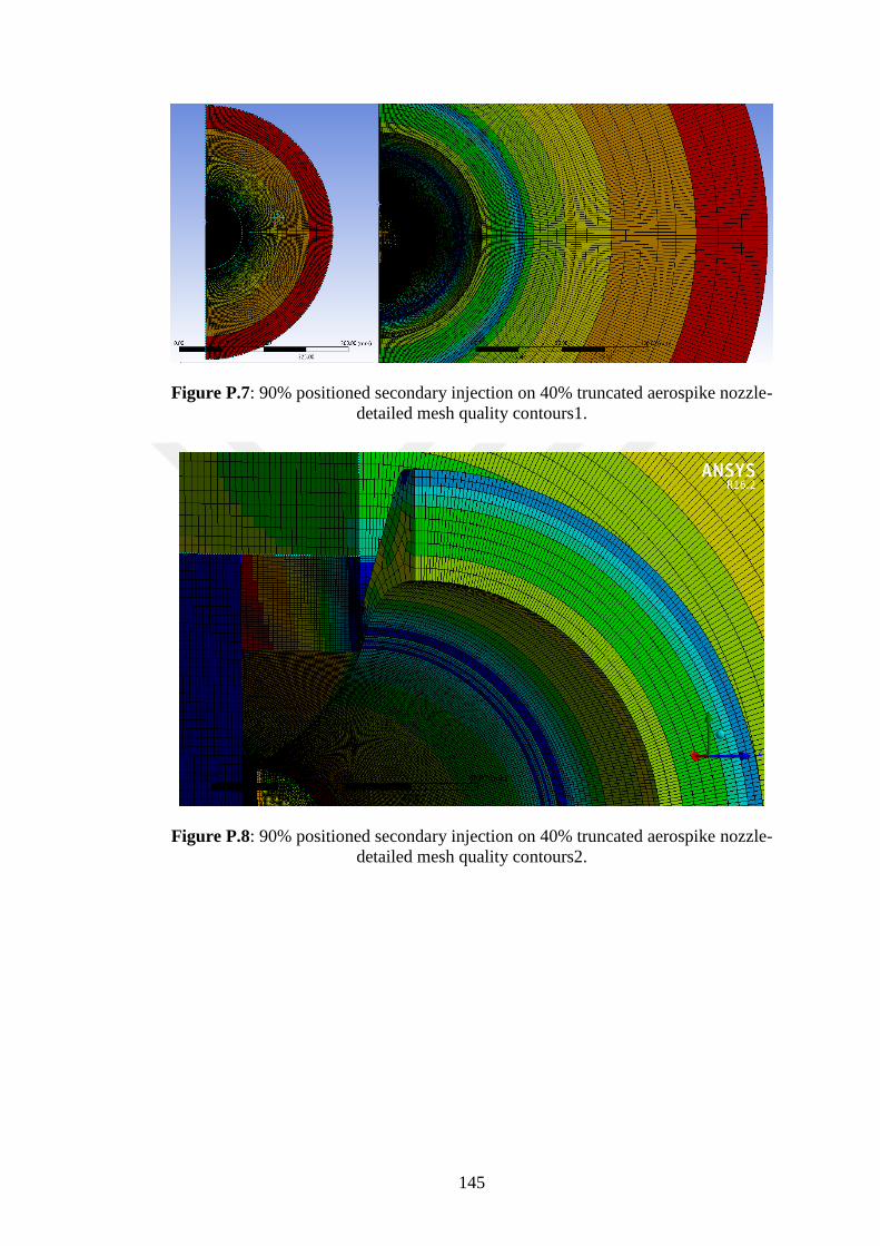
145


detailed mesh quality contours1.



146




nozzle- element quality chart.


nozzle- skewness chart.

147


nozzle- orthogonal quality chart.


nozzle-convergence graph.

148


nozzle-wall Mach contours.


nozzle-Mach lines.

149


nozzle-velocity contours.


nozzle-detailed velocity contours.

150


nozzle-sectional velocity contours at secondary jet center.


nozzle-secondary jet streamlines.

151


nozzle-full streamlines.


nozzle-full streamlines-ISO.

152


nozzle-pressure contours.


nozzle-detailed pressure contours.

153


nozzle-sectional pressure contours at secondary jet center.


nozzle-wall temperature contours.

154


nozzle-temperature contours.


nozzle- sectional temperature contours at secondary jet center.

155

APPENDIX Q: 90% positioned secondary injection on 40% truncated aerospike

nozzle-Matlab code

clc

close all

clear all

Xc= xlsread('YPContour.xlsx','A:A');

Yc= xlsread('YPContour.xlsx','B:B');

Axc= xlsread('YPContour.xlsx','C:C');

Ayc= xlsread('YPContour.xlsx','D:D');

Pc= xlsread('YPContour.xlsx','E:E');

X_Jet= xlsread('YPJet.xlsx','A:A');

Y_Jet= xlsread('YPJet.xlsx','B:B');

Ay_Jet=xlsread('YPJet.xlsx','C:C');

P_Jet= xlsread('YPJet.xlsx','D:D');

Y_Base= xlsread('YPBase.xlsx','A:A');

Ax_Base= xlsread('YPBase.xlsx','B:B');

P_Base=xlsread('YPBase.xlsx','C:C');

Po=4800000;

Patm=101325;




Fthruster = -((flux*Vx)+(Po-Patm)*Aty)

Fviscous= 50.51 %From CFD

%Jet Nozzle Momentum

Jet_flux=0.0763; %From CFD

Vy_Jet_Avg=684; %From CFD

F_Jet_Momentum =(Jet_flux*-Vy_Jet_Avg)

Mz_Jet_Momentum=F_Jet_Momentum*0.05828

156

% % Jet Nozzle Pressure Calculation

F_Jet_Pressure=0;

i = 1;

while 1016 > i

F_Jet_Pressure=P_Jet(i)*Ay_Jet(i)+F_Jet_Pressure;

i = i+1;

end

F_Jet_Pressure= -F_Jet_Pressure*2

% Base Pressure & Base Moment

i=1;

Fx_Base=0;

Mz_Base_Fx=0;

Ry_Base=0;

while 6049 > i

Fx_Base=(P_Base(i)-101325)*Ax_Base(i)+Fx_Base;

Mz_Base_Fx=((P_Base(i)-101325)*Ax_Base(i))*(Y_Base(i))+Mz_Base_Fx; %No

Axis Correction Required

i = i+1;

end

Fx_Base=Fx_Base*2

Mz_Base_Fx=-Mz_Base_Fx*2

Ry_Base=-Mz_Base_Fx/Fx_Base % Y Position of the Base Resultant

% Contour Pressure Difference & Contour Moment calculation

i=1;

Fy_Contour=0;

Fx_Contour=0;

Mz_Contour_Fy=0;

Mz_Contour_Fx=0;

Ry_Contour=0;

Rx_Contour=0;

while 41251 > i

Fy_Contour=Pc(i)*Ayc(i)+Fy_Contour;

157

Fx_Contour=(Pc(i)-101325)*Axc(i)+Fx_Contour;

Mz_Contour_Fy=(Pc(i)*Ayc(i))*(Xc(i)-0.032)+Mz_Contour_Fy; %axis Correction to

start from Contour start line

Mz_Contour_Fx=((Pc(i)-101325)*Axc(i))*(Yc(i))+Mz_Contour_Fx; %No Axis

Correction Required

i = i+1;

end

Fy_Contour=Fy_Contour*2

Fx_Contour=Fx_Contour*2

Mz_Contour_Fy=Mz_Contour_Fy*2

Mz_Contour_Fx=-Mz_Contour_Fx*2

Ry_Contour=-Mz_Contour_Fx/Fx_Contour

Rx_Contour=Mz_Contour_Fy/Fy_Contour

%Total Values Calculations

Total_Thrust= Fx_Base+Fx_Contour

Total_Fy= F_Jet_Momentum +Fy_Contour

Total_Fx= Fx_Base+Fx_Contour

Total_Moment_Fy= Mz_Jet_Momentum+Mz_Contour_Fy;

Total_Moment_Fx= Mz_Base_Fx+Mz_Contour_Fx;

Xr=Total_Moment_Fy/Total_Fy

Xr_Percentage=(Xr/0.064756)*100

Yr=-Total_Moment_Fx/Total_Fx

%Amplified value Gained From Bow Shock wave

F_Jet_Amplification=Fy_Contour-F_Jet_Pressure %Contour Pressure Difference

without the jet pressure effect

F_Jet_Amplification_Factor=( Total_Fy /(Total_Fy- F_Jet_Amplification))

Total_Thrust= Fthruster + Fx_Contour + Fx_Base + Fviscous

SPecific_Impulse_Primary= -Total_Thrust/(flux*9.81)

SPecific_Impulse_Secondary= -Total_Fy/(Jet_flux*9.81)

158

APPENDIX R: 20% positioned secondary injection on 40% truncated aerospike

nozzle


velocity contours.


Mach lines.

159


detailed Mach lines.


pressure contours.

160


sectional pressure contours at secondary jet center.

161

CURRICULUM VITAE

Name Surname : Sherif FARRAG

Place and Date of Birth : Egypt, 18.10.1992

E-Mail : [email protected]

EDUCATION:

B.Sc.: 2017, Istanbul Technical University, Aerospace faculty, Department of

Aeronautics and Astronautics Engineering.

M.Sc.: 2020, Istanbul Technical University, Aerospace faculty, Department of

Aeronautics and Astronautics Engineering

PROFESSIONAL EXPERIENCE AND REWARDS:

ESRA (Experimental Sounding Rocket Association) competition, USA, 2015.

Rocket propulsion team leader.

Built the most powerful student-built solid rocket engine in Turkey that has been

marked safe and launched at the ESRA.

T.V interviews about the project:

URL-1 < https://www.youtube.com/watch?v=AZOpT3utO80&t=2s>

URL-2 < https://www.youtube.com/watch?v=TnrBtNr8-mo>

URC (Universal Rover Challenge) world international competition, USA, 2014.

Ranked 9th.

Iranian CanSat international Competition, USA, 2014. Ranked 7th.

UNISEC-Egypt formal representative in Japan, 2014.

Designing, manufacturing and implementation of Seven-hole Probe (B.Sc.

graduation project).

https://www.youtube.com/watch?v=TnrBtNr8-mo

istanbul technical university graduate school of science - Polen

Documents

Transcript of istanbul technical university graduate school of science - Polen