istanbul technical university graduate school of science - Polen
Upload
khangminh22Category
view
0download
0
ISTANBUL TECHNICAL UNIVERSITY ENERGY INSTITUTE
Ph.D. THESIS
EXTENDED EXERGY ACCOUNTING (EEA) ANALYSIS OF TURKISH
SOCIETY- DETERMINATION OF ENVIRONMENTAL REMEDIATION
COSTS
Candeniz SEÇKİN
Department of Energy Science and Technology
Energy Science and Technology Programme
Anabilim Dalı : Herhangi Mühendislik, Bilim
Programı : Herhangi Program
FEBRUARY 2013

FEBRUARY 2013
ISTANBUL TECHNICAL UNIVERSITY ENERGY INSTITUTE
EXTENDED EXERGY ACCOUNTING (EEA) ANALYSIS OF TURKISH
SOCIETY- DETERMINATION OF ENVIRONMENTAL REMEDIATION
COSTS
Ph.D. THESIS
Candeniz SEÇKİN
(301052004)
Department of Energy Science and Technology
Energy Science and Technology Programme
Anabilim Dalı : Herhangi Mühendislik, Bilim
Programı : Herhangi Program
Thesis Advisor: Prof. Dr. Ahmet R. BAYÜLKEN
Co-Advisor: Prof. Dr. Enrico SCIUBBA

ŞUBAT 2013
İSTANBUL TEKNİK ÜNİVERSİTESİ ENERJİ ENSTİTÜSÜ
GENİŞLETİLMİŞ EKSERJİ ANALİZİ METODUNUN TURKİYE
UYGULAMASI – CEVRESEL ETKİ MALİYETLERİNİN BELİRLENMESİ
DOKTARA TEZİ
Candeniz SEÇKİN
(301052004)
Enerji Bilim ve Teknoloji Anabilim Dalı
Enerji Bilim ve Teknoloji Programı
Anabilim Dalı : Herhangi Mühendislik, Bilim
Programı : Herhangi Program
Tez Danışmanı: Prof. Dr. Ahmet R. BAYÜLKEN
Eş Danışman: Prof. Dr. Enrico SCIUBBA

v
Thesis Advisor : Prof. Dr. Ahmet R. BAYÜLKEN ..............................
İstanbul Technical University
Co-advisor : Prof.Dr. Enrico SCIUBBA ..............................
University of Rome 1 “La Sapienza”
Jury Members : Prof. Dr. Altuğ ŞİŞMAN
Istanbul Technical University .............................
Prof. Dr. Taner DERBENTLİ ..............................
Istanbul Technical University
Prof. Dr. Olcay KINCAY ..............................
Yıldız Technical University
Prof. Dr. Hasan HEPERKAN ..............................
Yıldız Technical University
Assoc. Prof. Dr. Şükrü BEKDEMİR ..............................
Yıldız Technical University
Prof. Dr. Olcay KINCAY ..............................
Yıldız Technical University
Candeniz Seçkin, a Ph.D. student of ITU Institute of Energy/ Graduate School of
Energy Science and Technology student ID 301052004, successfully defended the
thesis/dissertation entitled “Extended Exergy Accounting (EEA) Analysis of
Turkish Society- Determination of Environmental Remediation Cost”, which she
prepared after fulfilling the requirements specified in the associated legislations,
before the jury whose signatures are below.
Date of Submission : 14 November 2012
Date of Defense : 08 February 2013

vi
vii
To my beloved father İnal SEÇKİN,

viii
ix
FOREWORD
In the long period of time that passed between the beginning and the delivery of this
Ph.D. thesis, there have been many people who have strongly influenced the destiny
of this work. I have learnt a lot from all of them, both personally and professionally.
In this Foreword, I would like to mention some of these people and express my
gratitude for each and every of them.
I want to express my greatest thanks to my two supervisors, Prof. Dr. Ahmet
Bayülken (Istanbul Technical University) and Prof. Dr. Enrico Sciubba (University
of Roma 1 - La Sapienza). I really thank Prof. Bayülken for all his enthusiasm,
criticism, support, understanding and patience in every phase of this study. Prof.
Bayülken has unselfishly dealt with all of my problems during my doctoral studies
and I benefitted from his academic experience in all kind of problem solving.
I express my deep sense of gratitude and thanks to Prof. Sciubba for his constant and
valuable guidance, for the many discussions we had about the methodology to use in
this Ph.D., for his advice about the application of the method, for reading and
reviewing my articles and for his very generous academic help which was really
invaluable, reinforced the academic side of this present study and improved my
scientific view and approach. I have learned a lot from him, both in the easy and in
the hard way, while completing a substantial part of this study in my 18 months stay
at University of Roma. It has been a great pleasure to work with Prof. Sciubba and I
owe him my grateful thanks for all academic support I received from him.
It is impossible to forget Prof. Dr. Ali Toker who filled the big gap of an important
requirement for a Ph.D. student: MOTIVATION. When we met, I was exhausted,
thought it would be impossible to go further in my studies and had been struggling
with academic and personal problems for a long time. In this last year, Prof. Toker
has spent much of his time to motivate me and by virtue of his very precious advice,
I could complete the writing of this thesis. Sometimes there are things in life which
are vital and impossible to substitute with something different: motivation is one of
them, especially in the last part of a long and tiring study such as a Ph.D. That is why
his attention and moral support were priceless and his existence in my life is a gift
from God to me.
I owe my sincere thanks to the Tincel Foundation and to the Istanbul Technical
University (ITU) for the financial support of a part of my research at the University
of Roma. In addition, I wish to express my truthful thanks to the Executive
Committee of Istanbul Technical University Energy Institute for their continued
support of my research in abroad.
I would also like to thank my friends: Umut Kıvanç Şahin and Aslıhan Albostan for
all the psychological support, understanding and patience. At least one million times
x
I have had problems in this thesis and every time they dealt with my problems as if
they were their own. I am really lucky to have friends like them.
This Ph.D. thesis is dedicated to my beloved father, Prof. Dr. İnal Seçkin, who has
always believed in me, supported and encouraged me. I know that he had cultivated
different dreams for my life but I have finished this Ph.D. with his very generous
support. The truth will never change that he will always constitute an important part
of all my life. Baba, thank you very much for everything, first and foremost for
giving me the honour of being your daughter, showing me the real meaning of what a
father is and providing me the comfort of trusting someone endlessly, deeply and
undoubtedly.
To my mother I owe my thanks for always supporting me and trying to hold back the
bad things that may have been happening around to stop them from affecting my
motivation and my concentration, especially when I was living in Italy and she kept
me in connection with the part of the family I had temporarily left behind.
August 2012
Candeniz SEÇKİN
(Mechanical Engineer, M.Sc.)

xi
TABLE OF CONTENTS
Page
FOREWORD ............................................................................................................. ix
TABLE OF CONTENTS .......................................................................................... xi ABBREVIATIONS ................................................................................................. xiii LIST OF TABLES ................................................................................................... xv
LIST OF FIGURES ............................................................................................... xxv
LIST OF SYMBOLS ........................................................................................... xxvii SUMMARY ........................................................................................................... xxxi ÖZET .................................................................................................................... xxxiii
1. INTRODUCTION .................................................................................................. 1 1.1 Resource Use and Exergy Analysis ................................................................... 1 1.2 LCA Approach in Exergy Analysis and Extended Exergy Accounting (EEA) . 3
1.2.1 Cumulative exergy consumption (CExC) .................................................. .4
1.2.2 Exergetic life cycle analysis (ELCA) ........................................................4
1.2.3 Cumulative exergy extraction from the natural environment (CEENE) .... .5
1.2.4 Life cycle exergy analysis (LCEA) ............................................................5
1.2.5 Extended exergy accounting (EEA) ........................................................... .6
1.3 Scope and Structure of the Dissertation ............................................................. 7
1.4 Summary of Contributions ................................................................................. 8
1.5 Literature Review ............................................................................................... 9
2. EXERGY CONCEPT AND EEA METHODOLOGY ..................................... 11 2.1 Definition of Exergy ......................................................................................... 11 2.2 Reference Environment .................................................................................... 14
2.3 Computation of Exergy and Exergy Transfer .................................................. 15
2.3.1 Calculation of standard chemical exergy ................................................. .15
2.3.2 Exergy transferred via heat transfer...........................................................18
2.3.3 Exergy transfer with work interaction........................................................18
2.3.4 Exergy of electricity ....................................................................................18
2.4 Extended Exergy Accounting (EEA) ............................................................. .19
2.4.1 Exergetic equivalent of labour .................................................................. .19
2.4.2 Exergetic equivalent of capital .................................................................. .22
2.4.3 Environmental remediation cost (EEENV) ................................................. .23
2.5 Framework of Societal EEA Application (Choice of Control Volume and Division) .24
3. EXERGY TRANSFERS FROM ENVIRONMENT ......................................... 27 3.1 Exergy Fluxes from ENV to the Sectors via Energy Carriers and Materials ... 27
3.1.1 Exergy transfer from ENV to EX ............................................................. 27
3.1.2 Exergy transfer from ENV to CO ............................................................. 29 3.1.3 Exergy transfer from ENV to AG ............................................................. 31 3.1.4 Exergy transfer from ENV to IN ............................................................... 31
3.1.5 Exergy transfer from ENV to DO ............................................................. 31 3.2 Water Transfer between ENV and the Sectors ................................................. 32
xii
3.3 Summary of Fluxes Received from ENV ......................................................... 32
4. EXERGY CONTENT OF SECTORAL PRODUCTS ..................................... 35 4.1 Conversion Sector (CO) ................................................................................... 35 4.2 Agricultural Sector (AG) .................................................................................. 37
4.3 Industrial Sector (IN) ........................................................................................ 43 4.4 Transportation Sector (TR) ............................................................................... 55 4.5 Domestic Sector (DO) ...................................................................................... 58
4.6 Tertiary Sector (TE) ......................................................................................... 60
5. EXERGETIC EQUIVALENT OF THE EXTERNALITIES .......................... 63 5.1 Global Exergy Flux into the Control Volume (Ein) and Econometric Factors 63
5.1.1 Global exergy flux into the control volume (Ein) ...................................... 63
5.1.2 Econometric factors: , , eeC and eeL ..................................................... 66 5.2 Exergetic Equivalent of Sectoral Labour Input ................................................ 67
5.3 Exergetic Equivalent of Sectoral Capital Input and Output ............................. 67 5.4 Environmental Remediation Cost (EEENV) Determination and Sectoral EEENV Inputs ... 69
5.4.1 The concept of environmental remediation cost (EEENV) ......................... 70 5.4.2 Environmental remediation cost of solid waste (EEENV-s) ........................ 72
5.4.2.1 DO sector solid waste ......................................................................... 73
5.4.2.2 TE sector solid waste .......................................................................... 84
5.4.2.3 IN sector solid waste .......................................................................... 90 5.4.2.4 CO sector solid waste ......................................................................... 95 5.4.2.5 AG sector solid waste ....................................................................... 104
5.4.2.6 TR sector solid waste ....................................................................... 109
5.4.3 Environmental remediation cost of gas emissions (EEENV-g) .................. 116
5.4.3.1 Environmental remediation cost (EEENV-g) of CO2 .......................... 117 5.4.3.2 Environmental remediation cost (EEENV-g) of N2O .......................... 123
5.4.3.3 Environmental remediation cost (EEENV-g) of CH4 .......................... 126 5.4.3.4 Environmental remediation cost of greenhouse gases ..................... 129 5.4.3.5 Sectoral gas emissions and equivalent EEENV-g ................................ 130
5.4.4 Environmental remediation cost of liquid waste (EEENV-lq) .................... 132 5.4.4.1 DO sector liquid waste and treatment system ..................................... 134
5.4.4.2 Untreated wastewater ....................................................................... 136 5.4.4.3 Treated wastewater (sludge processing) .......................................... 141 5.4.4.4 EEENV-lq of the sectors ...................................................................... 145
5.4.5 Environmental remediation cost of discharged heat (EEENV-d) ............... 148 5.4.5.1 DO sector discharge heat .................................................................. 148 5.4.5.2 TE sector discharge heat .................................................................. 153
5.4.5.3 IN sector discharge heat ................................................................... 155 5.4.5.4 CO sector discharge heat .................................................................. 157 5.4.5.5 AG sector discharge heat .................................................................. 159 5.4.5.6 TR sector discharge heat .................................................................. 162
6. CONCLUSIONS AND RECOMMENDATIONS FOR FUTURE
RESEARCH ............................................................................................................ 165 6.1 Summary, Results and Discussion ................................................................. 165
6.1.1 Sensitivity analysis of the results ........................................................ 174 6.2 Conclusion and Further Research Tasks ........................................................ 176
REFERENCES ....................................................................................................... 179 APPENDICES ........................................................................................................ 201
CURRICULUM VITAE ........................................................................................ 297
xiii
ABBREVIATIONS
A : Abroad
AC : Annual cost
AD : Anaerobic digestion
AG : Agricultural Sector
BOI5 : Biochemical oxygen demand
C : Celsius degree
CAA : Canadian Automobile Association
CDP : Cumulative degree of perfection
CEENE : Cumulative exergy extraction from the natural environment
CExC : Cumulative exergy consumption
CExD : Cumulative exergy demand
CHP : Combined heat and power plant
CO : Conversion Sector
COD : Chemical oxygen demand
Dancee : The Danish Cooperation for Environment in Eastern Europe
DM : Dry matter
DO : Domestic Sector
ECN : Energy Research Center for Netherlands
EDANA : European Disposables and Nonwovens Association
EEA : Extended exergy accounting
EIA : U.S. Energy Information Administration
ELCA : Exergetic life cycle analysis
ELV : End of Life Vehicle
ENV : Environment
EPA : European Environment Agency
Eurostat : European Union Statistical Department
EX : Extraction Sector
FAO : Food and Agriculture Organization of United Nations
FCC : Fluid catalytic cracking
GJ : Giga Joule (109 J)
HHV : High heating value
IC : Investment cost
IEA : International Energy Agency
IGCC : Integrated gasification combined cycle
IN : Industrial Sector
Ind. : Industry
IUV : In use vehicles
J : Joule
K : Kelvin
KJ : Kilo Joule (103 J)
KW : Kilo-watt
kWh : Kilo-what-hour (3600 KJ)
xiv
l : liter
LASDER : Turkish Tire Industrialists Association
LCA : Life cycle assessment
LCEA : Life cycle exergy analysis
LHV : Low heating value
LPG : Liquefied petroleum gas
LULUCF : Land-use, land use change and forestry
MJ : Mega Joule (106 J)
MREC : Midwest Rural Energy Council
MRF : Materials Reprocessing Facility
MSW : Municipal solid waste
NACE :Statistical classification of economic activities in the European
Community
ODM : Organic dry matter
OM : Organic matter
OP : Fixed and varying operation costs
ORC : Organic Rankine Cycle
SWAP : Save Waste & Prosper
tDM : Ton dry matter
TE : Tertiary Sector
TEP : Tons equivalent of petroleum (41,868 GJ)
TJ : Tera Joule (1012
J)
TL : Turkish Lira
TN : Total nitrogen
TP : Total phosphorus
TR : Transportation Sector
TRP : Transportation line
TSS : Total suspended solids
TUGEM : Republic of Turkey, General Directorate of Agricultural Production
and Development
TUKDER : Union of Turkish Brick and Tile Producers
TUPRAS : Turkish Petroleum Refineries Corporation
Turkstat : Turkish Statistical Institute
Tusiad : Turkish Industry and Business Association
UNDP : United Nations Development Programme
UNEP : United Nations Environment Programme
W : Watt
YEM : Construction Industry Center of Turkey
xv
LIST OF TABLES
Page
Table 2.1 : Specific exergy equations. ...................................................................... 12
Table 2.1 : LHV equations for organic compounds .................................................. 17
Table 3.1 : Extracted fossil fuels and exergy content ............................................... 27
Table 3.2 : Extracted ores and exergy content .......................................................... 28
Table 3.3 : Extracted minerals and exergy content ................................................... 28
Table 3.4 : Exergy of utilized renewable energy sources ......................................... 29
Table 3.5 : Id, AAG, ζ and Esolar,AG .............................................................................. 31
Table 3.6 : Exergy of water received from ENV ...................................................... 32
Table 3.7 : Summary of fluxes received from ENV ................................................. 32
Table 3.8 : EX Sector products ................................................................................. 33
Table 4.1 : CO Sector Products – 1 ........................................................................... 35
Table 4.2 : CO Sector Products – 2 ........................................................................... 36
Table 4.3 : Refinery by products ............................................................................... 36
Table 4.4 : AG Sector products transfer to TE and DO ............................................ 38
Table 4.5 : Exergy of remaining AG products which is transferred to TE -1 ........... 40
Table 4.6 : Exergy of remaining AG products which is transferred to TE -2 ........... 40
Table 4.7 : HHV of biogas ........................................................................................ 42
Table 4.8 : Exergy of manure for biogas production ................................................ 42
Table 4.9 : Exergy of exported AG products ............................................................ 43
Table 4.10: Production of food processing industry and corresponding exergy ............. 46
Table 4.11: Fodder production .................................................................................. 48
Table 4.12: Seed production and corresponding exergy ........................................... 48
Table 4.13: Exergy content of textile industry products –1 ...................................... 49
Table 4.14: Exergy content of textile industry products –2 ...................................... 49
Table 4.15: Exergy of wood and paper products ...................................................... 50
Table 4.16: Exergy content of produced fertilizers and consumed plastic and rubber.... 51
Table 4.17: Exergetic equivalent of other chemical industry products ..................... 51
Table 4.18: Exergy content of sectorally consumed non-metallic mineral products 52
Table 4.19: Exergy content of sectorally consumed metal products......................... 53
Table 4.20: Products of the recycling processes ....................................................... 54
Table 4.21: Exergy of produced scrap ...................................................................... 54
Table 4.22: Produced blast furnace gas and exergy content ..................................... 55
Table 4.23: Exergy content of IN sector products .................................................... 55
Table 4.24: Efficiency of transportation modes ........................................................ 57
Table 4.25: Low heating value (LHV) of fuels ......................................................... 57
Table 4.26: Exergetic output of TR Sector and its distribution through the sectors (TJ) ... 58
Table 4.27: Exergy of incinerated MSW .................................................................. 59
Table 4.28: Exergy of consumed materials in material recycling and composting .. 59
Table 4.29: DO Sector products (output) .................................................................. 60
Table 4.30: Allocation of exergy fluxes from TE to the other sectors ...................... 61
xvi
Table 4.31: Exergy of import and export .................................................................. 61
Table 5.1 : Allocation of direct fluxes from surroundings ........................................ 64
Table 5.2 : Id, Atotal, ζ and Esolar,total ............................................................................ 65
Table 5.3 : Econometric factors and used country specific valuables ....................... 66
Table 5.4 : Sectoral number of workers, annual work hours and exergetic equivalent
of labour .................................................................................................. 67
Table 5.5 : Sectoral capital input and output, exergetic equivalent of capital .......... 68
Table 5.6 : Capital transfer between TE and A ......................................................... 68
Table 5.7 : Composition of DO sector waste ............................................................ 76
Table 5.8 : Number of trucks and their exergetic content ......................................... 76
Table 5.9 : Material exergy (EM-t) of systems and processes except transportation ...... 77
Table 5.10: Physical exergy (EPHYS-t) inflow of the environmental remediation system . 77
Table 5.11: Exergetic equivalent of the capital of processes .................................... 78
Table 5.12: Exergetic equivalent of the capital of trucks .......................................... 78
Table 5.13: Exergetic equivalent of diesel fuel capital ............................................ .79
Table 5.14: Labour consumption and its exergetic equivalent (EEL-t) .................... ..80
Table 5.15: Emissions from the TRP lines .............................................................. ..81
Table 5.16: Emissions from the processes ............................................................. ...81
Table 5.17: Environmental remediation cost of emission gases (EEENV-t) .............. ..81
Table 5.18: Energy content (LHV) of the non- recyclables .................................. ....82
Table 5.19: Properties of incineration process ......................................................... .82
Table 5.20: Properties of biogas utilization.............................................................. .82
Table 5.21: Energy balance of the system ................................................................ .83
Table 5.22: Amount and exergy of recycled materials ............................................ .83
Table 5.23: Amount and exergy of produced compost ............................................ .84
Table 5.24: Products of DO sector solid waste environmental remediation system....... .84
Table 5.25: EEENV-s for DO sector solid waste ......................................................... .84
Table 5.26: Composition of TE sector waste ........................................................... .85
Table 5.27: Number of trucks and their exergetic content ....................................... .85
Table 5.28: Material exergy (EM-t) of systems and processes except transportation lines ... .85
Table 5.29: Physical exergy (EPHYS-t) inflow of the environmental remediation system ..... .86
Table 5.30: Exergetic equivalent of the capital of processes ................................... .86
Table 5.31: Exergetic equivalent of the capital of trucks ......................................... .86
Table 5.32: Exergetic equivalent of diesel fuel capital ............................................ .87
Table 5.33: Labour consumption and its exergetic equivalent (EEL-t) ..................... .87
Table 5.34: Emissions from the TRP lines ............................................................... .87
Table 5.35: Emissions from the processes ............................................................... .87
Table 5.36: Environmental remediation cost of emission gases (EEENV-t) ............... .88
Table 5.37: Energy balance of the system ................................................................ .88
Table 5.38: Amount and exergy of recycled materials ............................................ .89
Table 5.39: Amount and exergy of produced compost ............................................ .89
Table 5.40: Products of TE sector solid waste environmental remediation system ....... .89
Table 5.41: EEENV-s for TE sector solid waste ......................................................... .89
Table 5.42: Composition of IN sector waste ............................................................ .90
Table 5.43: Number of trucks and their exergetic content ....................................... .91
Table 5.44: Material exergy (EM-t) of systems and processes except transportation lines ... .91
Table 5.45: Physical exergy (EPHYS-t) inflow of the environmental remediation system .. .91
Table 5.46: Exergetic equivalent of the capital of processes ................................... .92
Table 5.47: Exergetic equivalent of the capital of trucks ......................................... .92
Table 5.48: Exergetic equivalent of diesel fuel capital ............................................ .92
xvii
Table 5.49: Labour consumption and its exergetic equivalent (EEL-t) ..................... .92
Table 5.50: Emissions from the TRP lines ............................................................... .93
Table 5.51: Emissions from the processes ............................................................... .93
Table 5.52: Environmental remediation cost of emission gases (EEENV-t) .............. .93
Table 5.53: Energy balance of the system................................................................ .94
Table 5.54: Amount and exergy of recycled materials ............................................ .94
Table 5.55: Amount and exergy of produced compost ............................................ .94
Table 5.56: Products of IN sector solid waste environmental remediation system . .95
Table 5.57: EEENV-s for IN sector solid waste .......................................................... .95
Table 5.58: Composition of CO sector waste .......................................................... .95
Table 5.59: Composition of “Others” in Table 5.58 ................................................ .96
Table 5.60: Number of trucks and their exergetic content ....................................... .99
Table 5.61: Material exergy (EM-t) of systems and processes except transportation lines ... .99
Table 5.62: Physical exergy (EPHYS-t) inflow of the environmental remediation system ..... .99
Table 5.63: Exergetic equivalent of the capital of processes ................................. .100
Table 5.64: Exergetic equivalent of the capital of trucks ....................................... .100
Table 5.65: Exergetic equivalent of diesel fuel capital .......................................... .100
Table 5.66: Labour consumption and its exergetic equivalent (EEL-t) ................... .101
Table 5.67: Emissions from the TRP lines ............................................................. .101
Table 5.68: Emissions from the processes ............................................................. .101
Table 5.69: Environmental remediation cost of emission gases (EEENV-t) ............ .102
Table 5.70: Energy balance of the system.............................................................. .102
Table 5.71: Amount and exergy of recycled materials .......................................... .103
Table 5.72: Amount and exergy of produced compost .......................................... .103
Table 5.73: Products of CO sector solid waste environmental remediation system...... .103
Table 5.74: EEENV-s for CO sector solid waste ....................................................... .103
Table 5.75: Properties of agricultural waste .......................................................... .104
Table 5.76: Number of trucks and their exergetic content ..................................... .105
Table 5.77: Material exergy (EM-t) of systems and processes except transportation lines.105
Table 5.78: Physical exergy (EPHYS-t) inflow of the environmental remediation system ... .105
Table 5.79: Exergetic equivalent of the capital of processes ................................. .106
Table 5.80: Exergetic equivalent of the capital of trucks ....................................... .106
Table 5.81: Exergetic equivalent of diesel fuel consumption ................................ .106
Table 5.82: Labour consumption and its exergetic equivalent (EEL-t) ................... .106
Table 5.83: Emissions from transportation (TRP-1) and processes ....................... .107
Table 5.84: Environmental remediation cost of emission gases (EEENV-t) ............ .107
Table 5.85: Properties of biogas utilization ........................................................... .107
Table 5.86: Energy balance of the system.............................................................. .108
Table 5.87: Amount and exergy of produced compost .......................................... .108
Table 5.88: Products of AG sector solid waste environmental remediation system .... .108
Table 5.89: EEENV-s for AG sector solid waste ...................................................... .109
Table 5.90: Composition of ELVs, excluding tires ................................................ .110
Table 5.91: Number of trucks and their exergetic content ..................................... .111
Table 5.92: Material exergy (EM-t) of systems and processes except transportation lines . .111
Table 5.93: Physical exergy (EPHYS-t) inflow of the environmental remediation system ... .112
Table 5.94: Exergetic equivalent of the capital of processes ................................. .112
Table 5.95: Exergetic equivalent of the capital of trucks ....................................... .112
Table 5.96: Exergetic equivalent of diesel fuel capital .......................................... .112
Table 5.97: Labour consumption and its exergetic equivalent (EEL-t) ................... .113
Table 5.98: Emissions from the TRP lines ............................................................. .113
xviii
Table 5.99: Emissions from the processes ............................................................. .113
Table 5.100: Environmental remediation cost of emission gases (EEENV-t) ........... .114
Table 5.101: Amount and exergy of recycled materials ........................................ .114
Table 5.102: Properties of incineration process ..................................................... .114
Table 5.103: Energy balance of the system ............................................................ .115
Table 5.104: Products of TR sector solid waste environmental remediation system ... .115
Table 5.105: EEENV-s for TR sector solid waste ..................................................... .115
Table 5.106: Sectoral emissions of CO2, N2O and CH4 (Ari, 2010) ...................... .116
Table 5.107: Exergy of CaO ................................................................................... .120
Table 5.108: Material exergy (EM-t) of natural gas fuelled heater and electricity plant ... .120
Table 5.109: Physical exergy (EPHYS-t) inflow of the environmental remediation system . .120
Table 5.110: Exergetic equivalent of CaO and natural gas capital ........................ .121
Table 5.111: Exergetic equivalent of CO2 heating process and electricity plant ... .121
Table 5.112: Labour consumption and its exergetic equivalent (EEL-t) ................. .121
Table 5.113: Emissions from the system ................................................................ .122
Table 5.114: Net electricity production of the system ........................................... .122
Table 5.115: Products of the CO2 environmental remediation system .................. .122
Table 5.116: Input fluxes (except EEENV-t) to the CO2 environmental remediation system . .123
Table 5.117: Material exergy (EM-t) inputs of the environmental remediation system . .124
Table 5.118: Physical exergy (EPHYS-t) inflow of the environmental remediation system . .124
Table 5.119: Exergetic equivalent of natural gas capital ....................................... .124
Table 5.120: Exergetic equivalent of N2O heating process and electricity plant ... .125
Table 5.121: Labour consumption and its exergetic equivalent (EEL-t) ................. .125
Table 5.122: Emissions from the system ................................................................ .125
Table 5.123: Net electricity production of the system ........................................... .126
Table 5.124: Products of the N2O environmental remediation system .................. .126
Table 5.125: Input fluxes (except EEENV-t) to the N2O environmental remediation system . .126
Table 5.126: Material exergy (EM-t) input of the environmental remediation system .. .127
Table 5.127: Exergetic equivalent of CHP capital ................................................. .127
Table 5.128: Labour consumption and its exergetic equivalent (EEL-t) ................. .128
Table 5.129: Emissions from the system ................................................................ .128
Table 5.130: Energy production of the system ....................................................... .128
Table 5.131: Products of the CH4 treatment system .............................................. .128
Table 5.132: Input fluxes (except EEENV-t) to the CH4 environmental remediation system ... .129
Table 5.133: eeENV-g (X1, X2 and X3) for CO2, N2O and CH4 ................................ .130
Table 5.134: EEENV-g of the sectors ........................................................................ .131
Table 5.135: Properties of raw and treated wastewater and legal standards .......... .134
Table 5.136: DO sector wastewater generation ...................................................... .136
Table 5.137: Material exergy (EM-t) received by the system .................................. .137
Table 5.138: Physical exergy (EPHYS-t) received by the system ............................. .137
Table 5.139: Exergetic equivalent of the capital (EC-t) received by the system ..... .137
Table 5.140: Emissions from the processes ........................................................... .139
Table 5.141: Environmental remediation cost of emissions (EEENV-t) ........................ .139
Table 5.142: Properties of biogas utilization ............................................................. .139
Table 5.143: Energy balance of the system ............................................................ .140
Table 5.144: Amount and exergy of fertilizer ........................................................ .140
Table 5.145: EEENV-lq,w for untreated wastewater .................................................. .141
Table 5.146: Material exergy (EM-t) received by the system .................................. .142
Table 5.147: Exergetic equivalent of the capital (EC-t) received by the system ..... .142
Table 5.148: Emissions from the processes ........................................................... .142
xix
Table 5.149: Environmental remediation cost of emissions (EEENV-t) ........................ .143
Table 5.150: Properties of biogas utilization ............................................................. .143
Table 5.151: Energy balance of the system............................................................ .144
Table 5.152: Amount and exergy of produced fertilizer ......................................... .144
Table 5.153: EEENV-lq,sl for treated wastewater ...................................................... .144
Table 5.154: Wastewater produced in IN and CO Sector ...................................... .145
Table 5.155: EEENV-lq for IN and CO sector ............................................................ .146
Table 5.156: Produced wastewater and EEENV-lq for TE Sector ............................. .146
Table 5.157: EEENV-lq for AG sector ...................................................................... .147
Table 5.158: Weight and volume of CO2, N2O and CH4 ....................................... .149
Table 5.159: Composition of flue gas released from DO sector ............................ .149
Table 5.160: Weight of H2O, N2, O2, CO, SO2 ...................................................... .150
Table 5.161: Heat release from the gases ............................................................... .150
Table 5.162: Exergetic equivalent of ORC capital ................................................ .151
Table 5.163: Exergetic equivalent of the annualized ORC capital ........................ .152
Table 5.164: EEENV-d for DO sector heat discharge ............................................... .152
Table 5.165: Weight and volume of CO2, N2O and CH4 ....................................... .153
Table 5.166: Composition of flue gas released from TE sector ............................. .153
Table 5.167: Weight of H2O, N2, O2, CO, SO2 ...................................................... .153
Table 5.168: Heat release from the gases ............................................................... .154
Table 5.169: Exergetic equivalent of ORC capital ................................................ .154
Table 5.170: Exergetic equivalent of the annualized ORC capital ........................ .154
Table 5.171: EEENV-d for TE sector heat discharge ................................................ .155
Table 5.172: Weight and volume of CO2, N2O and CH4 ....................................... .155
Table 5.173: Composition of flue gas .................................................................... .155
Table 5.174: Weight of H2O, N2, O2, CO, SO2 ...................................................... .156
Table 5.175: Heat release from the gases ............................................................... .156
Table 5.176: Exergetic equivalent of ORC capital ................................................ .156
Table 5.177: Exergetic equivalent of the annualized ORC capital ........................ .156
Table 5.178: EEENV-d for IN sector heat discharge ................................................. .157
Table 5.179: Weight and volume of CO2, N2O and CH4 ....................................... .157
Table 5.180: Composition of flue gas .................................................................... .157
Table 5.181: Weight of H2O, N2, O2, CO, SO2 ...................................................... .158
Table 5.182: Heat release from the gases ............................................................... .158
Table 5.183: Exergetic equivalent of ORC capital ................................................ .158
Table 5.184: Exergetic equivalent of the annualized ORC capital ........................ .159
Table 5.185: EEENV-d for CO sector heat discharge ............................................... .159
Table 5.186: AG sector exhaust gas emissions (Emission factors are LHV based) ..... .160
Table 5.187: Weight and volume of CO2, N2O and CH4 ....................................... .161
Table 5.188: Composition of exhaust gas .............................................................. .161
Table 5.189: Weight of H2O, N2 and O2 ................................................................ .161
Table 5.190: Heat release from the gases ............................................................... .161
Table 5.191: Exergetic equivalent of ORC capital ................................................ .162
Table 5.192: Exergetic equivalent of the annualized ORC capital ........................ .162
Table 5.193: EEENV-d for AG sector heat discharge ............................................... .162
Table 5.194: Share of road transportation in total CO2, N2O and CH4 emissions . .163
Table 5.195: Composition of exhaust gas .............................................................. .163
Table 5.196: Weight of H2O, N2 and CO ............................................................... .163
Table 5.197: Heat release from the gases ............................................................... .164
Table 5.198: Exergetic equivalent of ORC capital ................................................ .164
xx
Table 5.199: Exergetic equivalent of the annualized ORC capital ........................ .164
Table 5.200: EEENV-d for TR sector heat discharge ................................................ .164
Table 6.1 : EEENV components and EEENV of the sectors (TJ) ................................ 165
Table 6.2 : Input and output fluxes and EEAeff for EX Sector ................................ 166
Table 6.3 : Input and output fluxes and EEAeff for CO Sector ................................ 167
Table 6.4 : Input and output fluxes and EEAeff for AG Sector ............................... 167
Table 6.5 : Input and output fluxes and EEAeff for IN Sector ................................. 167
Table 6.6 : Input and output fluxes and EEAeff for TR Sector ................................ 168
Table 6.7 : Input and output fluxes and EEAeff for TE Sector ................................ 168
Table 6.8 : Input and output fluxes and EEAeff for DO Sector ............................... 169
Table 6.9 : EEA analysis results of the present and earlier studies ......................... 172
Table A.1: Chemical formula and exergy of some minerals ................................... 202
Table A.2: Molar weight and chemical exergy of compounds ............................... 203
Table A.3: Chemical exergy of minerals ................................................................. 204
Table A.4: References of mineral compositions ..................................................... 207
Table A.5: Ore (domestic production) exergy calculation ...................................... 207
Table A.6: Gold and silver ore exergy calculation .................................................. 208
Table A.7: References of ore grades ....................................................................... 208
Table B.1: Specific exergy and HHV for fuels ........................................................ 209
Table B.2: Ultimate analysis of agricultural waste and wood (ar) .......................... 210
Table B.3: HHV, LHV, LHV, HHV and E of agricultural waste and wood ............ 211
Table B.4: Ultimate analysis of asphalt ................................................................... 212
Table B.5: Coefficients of Boie correlation for asphalt .......................................... 213
Table B.6: HHV, LHV, LHV, HHV and E of asphalt .............................................. 213
Table B.7: HHV, LHV, LHV, HHV and E of paraffine wax ................................... 214
Table C.1: Exergy of AG sector products ............................................................... 215
Table C.2: Exergy of IN sector products ................................................................ 216
Table C.3: Exergy of metal ..................................................................................... 217
Table C.4: Ultimate analysis of hide ....................................................................... 217
Table C.5: HHVar, LHVar, LHV, HHV and E of hide .............................................. 219
Table C.6: Ultimate analysis of organic solid waste ............................................... 219
Table C.7: HHVar, LHVar, LHV, HHV and E of organic waste ............................... 220
Table C.8: Ultimate analysis of compost ................................................................ 220
Table C.9: HHVar, LHVar, LHV, HHV and E of compost ....................................... 220
Table D.1: Energy carrier and exergy consumption in transportation modes ............... 221
Table D.2: Allocation of consumed energy between freight and passenger transportation 223
Table D.3: Freight traffic (ton-km) by sectors in railway transportation ................ 223
Table D.4: Share of sectoral employers .................................................................. 223
Table D.5: Allocation of consumed energy carriers through service receiving sectors
(rail transportation) ................................................................................ 224
Table D.6: Allocation of consumed energy carriers through service receiving sectors
(air transportation) ................................................................................. 224
Table D.7: Allocation of consumed energy carriers through service receiving sectors
(marine transportation) .......................................................................... 225
Table D.8: Allocation of consumed energy carriers through service receiving sectors
(road transportation) .............................................................................. 225
Table D.9: Allocation of consumed energy carriers through service receiving sectors
(pipeline transport) ................................................................................ 226
xxi
Table D.10: Allocation of consumed energy carriers through service receiving
sectors (non specified transportation) ................................................... 226
Table E.1 : Fixed capital investment and purchases of goods and services of the sectors .... 228
Table E.2 : AG sector products transferred from TE to IN and DO ....................... 229
Table E.3 : Imported energy carriers and exergy content ....................................... 230
Table E.4 : Exported energy carriers and exergy content ....................................... 230
Table E.5 : Exergy of energy carriers transferred to EX sector .............................. 230
Table E.6 : Exergy of energy carriers transferred to CO sector .............................. 231
Table E.7 : Exergy of energy carriers transferred to AG sector .............................. 231
Table E.8 : Exergy of energy carriers transferred to TE sector............................... 231
Table E.9 : Exergy of energy carriers transferred to IN sector ............................... 232
Table E.10 Exergy of energy carriers transferred to TR sector .............................. 232
Table E.11: Exergy of energy carriers transferred to DO sector ............................. 233
Table E.12: Products of IN Sector .......................................................................... 234
Table E.13: Distribution of “Other products” ......................................................... 234
Table E.14: EX Sector exergy consumption from societal products ...................... 235
Table E.15: CO Sector exergy consumption from societal products ...................... 235
Table E.16: AG Sector exergy consumption from societal products ...................... 235
Table E.17: IN Sector exergy consumption from societal products ....................... 235
Table E.18: TR Sector exergy consumption from societal products ...................... 235
Table E.19: TE Sector exergy consumption from societal products ....................... 236
Table E.20: DO Sector exergy consumption from societal products ...................... 236
Table E.21: Water supplied by mains ..................................................................... 236
Table E.22: Exergy of imported and exported commodities .................................. 237
Table E.23: Allocation of exergy of “products distributed through the sectors” .... 242
Table E.24: Exergetic equivalent of “other chemical products”, “other industrial
products” and “art works” ................................................................... 242
Table E.25: Distribution of “import-export” exergy through the sectors” .............. 242
Table F.1 : NACE classification ............................................................................. 243
Table F.2 : Number of workers ............................................................................... 244
Table F.3 : Average weekly work hours ................................................................. 244
Table G.1 : Ultimate composition of MSW (dry matter) ........................................ 247
Table G.2 : Amount of waste used in energy generation ........................................ 247
Table G.3 : Recycled waste materials ..................................................................... 248
Table G.4 : DO sector solid waste composition ...................................................... 248
Table G.5 : Transportation distance and energy consumption ................................ 249
Table G.6 : Exergy of fuel and fuel capital for TRP-1 ............................................ 250
Table G.7 : Exergy of trucks and labour for TRP-1 ................................................ 250
Table G.8 : Energy consumption of preliminary sorting stage ............................... 251
Table G.9 : Properties of recycling process ............................................................ 251
Table G.10: Energy consumption in pretreatment and recycling............................ 252
Table G.11: Exergy of recycled materials ............................................................... 252
Table G.12: Constituents of non-recycled mixed material ..................................... 253
Table G.13: Capital of MRF plant .......................................................................... 253
Table G.14: Exergy of fuel and fuel capital for TRP-2 ........................................... 254
Table G.15: Exergy of trucks and labour for TRP-2 ............................................... 254
Table G.16: Energy content of incinerated materials ................................................ 255
Table G.17: Energy generation and consumption of incineration process ............. 255
Table G.18: Exergy of fuel and fuel capital for TRP-3 ........................................... 255
Table G.19: Exergy of trucks and labour for TRP-3 ............................................... 256
xxii
Table G.20: Exergy of fuel and fuel capital for TRP-4 ........................................... 256
Table G.21: Exergy of trucks and labour for TRP-4 ............................................... 256
Table G.22: Exergy of fuel and fuel capital for TRP-5 ........................................... 257
Table G.23: Exergy of trucks and labour for TRP-5 ............................................... 257
Table G.24: Energy consumption in mixing and sterilization of organic waste ..... 258
Table G.25: Composition of organic waste (dry composition) ............................... 258
Table G.26: Produced gas from anaerobic digestion .............................................. 259
Table G.27: Energy consumption in AD ................................................................. 259
Table G.28: Capital of pretreatment and AD stages ............................................... 259
Table G.29: Energy consumption in upgrading ...................................................... 260
Table G.30: Gas composition after upgrading ........................................................ 260
Table G.31: Energy production in biorefinery ........................................................ 260
Table G.32: Capital of biorefinery .......................................................................... 261
Table G.33: Produced compost and exergy content ................................................ 261
Table G.34: Energy consumption and capital of composting ................................. 261
Table G.35: Emission factors .................................................................................. 262
Table G.36: Emission of gasses from AD and upgrading ....................................... 262
Table G.37: Emissions from TRP lines and processes ............................................ 263
Table G.38: Exergy of fuel and fuel capital for TRP-6 ........................................... 263
Table G.39: Exergy of trucks and labour for TRP-6 ............................................... 264
Table G.40: Properties of syngas and electricity production in IGCC .................... 264
Table G.41: Capital of IGCC plant ......................................................................... 265
Table G.42: Emission factors and emissions from IGCC plant .............................. 265
Table G.43: Manure generation............................................................................... 265
Table G.44: Composition of agricultural sector waste (%wt.) and ODM ............... 266
Table G.45: Gas composition from AD process (m3) ............................................. 266
Table G.46: Energy consumption in pre-treatment (mixing and sterilization) of AD
process ................................................................................................. 267
Table G.47: ELV composition (% wt.) including tires ........................................... 267
Table G.48: Weight and components of ELV (including tires) .............................. 268
Table G.49: Composition (% wt.) of tires ............................................................... 268
Table G.50: Weight of tires (from IUV+ELV) ....................................................... 268
Table G.51: Weight of constituting materials in ELV tires .................................... 269
Table G.52: Constituting materials in ELV (excluding tires) ................................. 269
Table G.53: Exergy of trucks .................................................................................. 269
Table G.54: Energy consumption of dismantling process ...................................... 270
Table G.55: Capital of dismantling ......................................................................... 270
Table G.56: Capital of ELV shredding ................................................................... 271
Table G.57: Energy consumption of ELV shredding process ................................. 271
Table G.58: Energy consumption of tire shredding process ................................... 271
Table G.59: Capital of tire shredding ...................................................................... 271
Table G.60: Properties of recycling of ELVs .......................................................... 272
Table G.61: Energy consumption in recycling ........................................................ 272
Table G.62: Energy generation and consumption of incineration process.............. 272
Table G.63: Capital of incineration ......................................................................... 273
Table G.64: Emissions of tire incineration .............................................................. 273
Table H.1 : Properties of natural gas fuelled heater ................................................ 275
Table H.2 : Heat release from CaO, CaCO3 and CO2 ............................................. 276
Table H.3 : Emissions of natural gas combustion ................................................... 277
Table H.4 : Exergy of produced CaO and CaCO3 ................................................... 278
xxiii
Table H.5 : Properties of natural gas fuelled heater ................................................ 279
Table H.6 : Heat release from N2 and O2 ................................................................ 279
Table H.7 : Emissions of natural gas combustion ................................................... 280
Table H.8 : Eph of produced N2 ............................................................................... 281
Table H.9 : Eph of produced O2 ............................................................................... 281
Table H.10: Chemical exergy of N2+O2 mixture .................................................... 282
Table I.1 : Per capita length of sewage system ....................................................... 283
Table I.2 : DM content of DO sector untreated wastewater.................................... 284
Table I.3 : Sludge generation .................................................................................. 284
Table I.4 : Capital of gravity belt thickening process ............................................. 285
Table I.5 : Capital of AD process ............................................................................ 286
Table I.6 : Properties of CH4 generation in AD process ......................................... 286
Table I.7 : Biogas composition from AD process ................................................... 287
Table I.8 : Energy consumption in upgrading ......................................................... 287
Table I.9 : Produced gas after upgrading ................................................................ 287
Table I.10: Energy production in biorefinery ......................................................... 288
Table I.11: DM of input & output sludges and DM destruction in AD .................. 288
Table I.12: Exergy and capital of FeCl3 and CaO ................................................... 289
Table I.13: Energy consumption of drying ............................................................. 289
Table I.14: Capital of drying ................................................................................... 289
Table I.15: Emission of gases from AD and upgrading .......................................... 290
Table I.16: Capital of supplied electricity from regional electricity network ......... 290
Table I.17: Sludge generation and properties of sludge .......................................... 290
Table I.18: Ultimate analysis of dried digestate ...................................................... 291
Table I.19: HHVar, LHVar, LHV, HHV and E of dried digestate ............................. 291

xxiv
xxv
LIST OF FIGURES
Page
Figure 2.1 : Constituent fluxes of EEA methodology. .............................................. 20
Figure 2.2 : Representation of system (S) and treatment system (St). ...................... 24
Figure 2.3 : Schematic outline of the sectors and surroundings. .............................. 25 Figure 5.1 : Representation of system (S) and treatment system (St) ....................... 71 Figure 5.2 : Illustration of DO sector solid waste treatment. .................................... 75
Figure 5.3 : Illustration of CO sector solid waste treatment ..................................... 98 Figure 5.4 : Illustration of AG sector solid waste treatment ................................... 104
Figure 5.5 : Illustration of TR sector solid waste treatment.................................... 110
Figure 5.6 : Schematic overview of CO2 environmental remediation system ........ 118
Figure 5.7 : Schematic overview of N2O environmental remediation system ........ 123
Figure 5.8 : Schematic overview of CH4 environmental remediation system ........ 127
Figure 5.9 : Schematic representation of wastewater environmental remediation system . 135
Figure J.1 : Sketch of the control volume configuration. ....................................... 293
Figure J.2 : A reversible device used to determine exergy.. ...................................... 294

xxvi
xxvii
LIST OF SYMBOLS
ar : As received
C : Capital
c : Chemical concentration
cP : Specific heat capacity at constant pressure
E : Exergy
e : Specific exergy
EE : Extended exergy
ee : Specific extended exergy
EEAeff : EEA efficiency
eeC : Exergetic equivalent of capital
eeL : Exergetic equivalent of labour
Ein : Global exergy input into the society
En : Energy
ENV : Environment
esurv : Minimum pro-capite exergy requirement for survival
Eused : Exergy consumed by the entire population
f : Exergy consumption amplification factor
G : Gibbs Free Energy
g : Gravity
h : Specific enthalpy
HDI : Human development index
HDI0 : Conventional reference HDI (HDI of a primitive society)
hfg : Enthalpy of the evaporation of water
I : Solar radiation
L : Labour, cumulative workhours
m : Mass
M2 : Total monetary circulation in the country
n : Mole number
NC : Number of carbon atoms
Nh : Population numerosity
Nwh : Total number of work-hours generated in the society
P : Pressure
P : Product
Q : Heat
r : Reaction
R : Universal gas constant
S : Global wages in a Country, system
s : Specific entropy
T : Temperature
u : Specific internal energy
V : Velocity
V : Volume
xxviii
W : Work
x : Number of molecule group
XH : Mass friction of hydrogen
y : Molar fraction
z : Element mass fraction
z : Height
ζ : Exergy coefficient of solar energy
ηI : First law efficiency
ηII : Second law efficiency
μ : Chemical potential
: Fraction of the primary exergy embodied into labour
: An amplification factor that accounts for the creation of wealth due
to exclusively financial activities HHV : Exergy coefficient in terms of HHV
LHV : Exergy coefficient in terms of LHV
$ : Dollar
€ : Euro
Subscripts
A : Area
a : Atomic ratio
ar : As received
C : Capital
ch : Chemical
d : Discharge heat
dry : Dry material
el : Electrical
ENV : Environmental remediation
f : Fuel
f : Formation
fu : Sample
g : Gas (emissions)
geo : Geothermal
h : Heat
h+el : heat and electric
i : Substance i
input : input
k : Kinetic
L : Labour
lq : Liquid (wastewater)
M : Material
output : Output
p : Potential
P : Product
ph : Physical
PHYS : Energy carrier
s : Solid waste
sector : Sector
shaft : Shaft
sl : sludge
xxix
solar : Solar
t : Treatment system (remediation system)
total : Total
w : Untreated wastewater
W : Waste
0 : Reference environment
Superscripts
0 : standard (at reference conditions)

xxx
xxxi
EXTENDED EXERGY ACCOUNTING (EEA) ANALYSIS OF TURKISH
SOCIETY- DETERMINATION OF ENVIRONMENTAL REMEDIATION
COSTS
SUMMARY
The fact that source of all activities on earth is the availability of energy and its
conversion into different forms is the motivation of the use of thermodynamic
methods in resource use and sustainability analysis. Exergy, by definition, does not
identify the ability of humankind to exploit a resource (it is the maximum limit of
utulization from the resource but impossible to realize), but is a path-independent
property, serving as a metric to measure the theoretically extractable work contained
in a resource. As a result, the most promising approach to adequately describe the
resource potential and consumption of this potential so far has been addressed as
exergy analysis in which exergy (available energy, maximum work generation limit
of the resource) is regarded as utility potential of the resource and resource depletion
is the lost of this potential in the course of material and energy transformations.
Application of an exergy based analysis to a society and determining the use of
resources in terms of exergy enable to gain a more comprehensive and deeper insight
from sustainability point of view, to identify areas where large improvements are
needed by applying more efficient technologies. In this thesis, a completely resource-
based method of analysis, the Extended Exergy Accounting (EEA) technique, has been
applied to the specific case of the Turkish society (on the basis of a 2006 database), to
disclose the present situation of the resource use efficiency within the society. EEA is an
exergy based method but clearly has some “extended” abilities: EEA enables to
convert the so-called “externalities”, i.e., the immaterial/non-energetic fluxes of
labour, capital and environmental remediation, into their exergetic equivalents.
Hence, EEA provides a more comprehensive and deeper insight of the resource
consumption and of the environmental impact. This present thesis is intended to
provide support for possible structural interventions aimed at the improvement of the
degree of resource consumption quality within the country. Following the routine of
EEA applications, the Turkish society has been modeled as an open thermodynamic
system, interacting with two “external” systems, namely “Environment” and
“Abroad”, and consisting itself of seven internal subsystems: Extraction-,
Conversion-, Transportation-, Agricultural-, Industrial-, Tertiary- and Domestic
sector. Furthermore in this thesis, the environmental remediation costs of sectoral
solid waste, liquid waste, gas emissions and discharge heat are obtained in
accordance with the original calculation procedure proposed by EEA, i.e., without
recurring the conversion of monetary equivalent of the environmental remediation
(treatment) processes into its exergetic equivalent as it has been applied so far in the
literature. As a result, this thesis provides the environmental remediation cost
equivalent of considered pollutants for the first time in the literature and the results
have the corresponding importance. In the analysis of gas emissions, considering the
wide variety of emission gases and due to lack of sufficiently disaggregated data for
all types of emissions, three types of greenhouse gases (CO2, CH4, N2O) are
xxxii
undertaken. Thereby, computed sectoral resource consumption efficiencies are more
realistic than those of societal EEA analysis applications which have been performed
and presented to date in the literature.
xxxiii
GENİŞLETİLMİŞ EKSERJİ ANALİZİ METODUNUN TURKİYE
UYGULAMASI – CEVRESEL ETKİ MALİYETLERİNİN BELİRLENMESİ
ÖZET
Bu tez çalışmasında, kaynak kullanım verimliliği yönünden incelenmek üzere
Turkiye örneği ele alınmış, motod olarak Extended Exergy Accounting (EEA,
Genişletilmiş Ekserji Analizi) metodu uygulanış ve ulaşılan sonuçlar sunulmuştur.
İlk olarak Dr. Enrico Sciubba tarafından geliştirilerek literatüre katılan ve ekserji
bazlı bir kaynak kullanım analizi metodu olan EEA metodu, bugüne kadar literatüre
katılmış hiçbir metodolojinin yapısında barındırmadığı bir yenilik sunularak, ele
alınan sistemin, enerji yada ağırlık birimleri ile ifade edilebilen girdilerin yanında
(enerji akışları ve materyal dışında), sisteme olan “diğer” girişlerin - kapital, iş gücü
ve çevresel etki - ekserji biriminde ifade edilmesi için yeni bir hesaplama metodu
sunulmuştur. Metodun arkasındaki zihniyet, sistemin tükettiği kapital, işgücü ve
çevresel etkinin giderilmesi için harcanan ekserjinin üretiminde kaynak kullanıldığı
ve adı geçen ekserji tüketimlerinin de sistemin toplam kaynak kullanımı içerisinde
ele alınması gerektiğidir. İş gücü ve kapitalin ekserji karşılıkları olarak, bunları
yaratmak için gerekli olan kaynak tüketiminin ekserji değeri belirlenmektedir.
Çevresel etki olarak ise, sistemden çıkan atığın temizlenmesi için gerekli kaynak
kullanımının ekserji karşılığı hesaplanır. Sonuç olarak EEA, sistemin hertürlü kaynak
tüketimini tek bir birimle (ekserji) ifade ederek birim bütünlüğünün sağlanmasının
yanında, bugüne kadar hiç ele alınmamış olan ek akışların da sistem ekserji dengesi
içerisine katılması ile “genişletilmiş ekserji dengesi (extended exergetic balance)”
kurulmasını sağlamakta ve adından da anlaşılır şekilde, şu anda literatürde olan en
“gelişmiş” ekserji bazlı kaynak kullanım analizi metodunu sunmaktadır. Özetle, EEA
metodu ile yapılan analizlerde, sistemin her safhasında kullanılan malzeme, enerji,
kapital, işçilik ve çevresel etki (ele alınan sisteminin atık ve emisyonlarının izin
verilen sınırlar dahilinde tutulması için yapılacak işlemler) gibi faktörlerin hepsi
analize katılarak ekserji biriminde ifade edilmiş ve sistemin kaynak kullanımı
değerlendirmesine katılmıştır.
Bu çalışmada, sistem olarak ele alınan Türkiye, EEA metodu ile incelenmiştir.
Çalışmanın amacı: eylem yapıcı birimlere, ülke içerisinde kaynak kullanım
kalitesinin değerlendirilmesi ve ülkenin daha kararlı ve sürdürülebilir çizgide
varlığını devam ettirmesi için en mantıklı ve faydalı müdehale noktalarının
bildirilmesidir. Çalışmada yapılan uygulama özetlenecek olursa: EEA ile yapılan
ülke analizlerinde mutat olduğu üzere, ele alınan ülke 7 sektörel bölüme ayrılmakta
ve birbiri arasındaki ekserji alışverişleri analiz edilmektedir. Bu sektörlerin kendi
içindeki ekserji akışlarının yanında çevre ile (Environment, ENV) ve diğer ülkeler
(Abroad, A) ile etkileşimi de hesaplamalara dahil edilmektedir. Söz konusu 7
sektörel bölüm ve kapsadığı faliyetler şunlardır:
xxxiv
EX (Madencilik Sektörü): Hammadde çıkarma ve işleme (Petrol ve doğal gaz çıkarma
ve rafineri işlemleri dahil)
CO (Dönüşüm Sektörü): Enerji üretim tesisleri (rafineriler, ısı ve elektrik üretimi)
AG (Tarım Sektörü): Tarım ve hayvancılık faliyetleri
IN (Endüstri Sektörü): Endüstriyel faliyet kolları (rafineriler hariç)
TR (Ulaştırma Sektörü): Ulaştırma faliyetleri
TE (Servis sektörü): Servis faliyetleri (otel, eğitim, danışmanlık vs. hizmetleri)
DO (Hanehalkı): Ev içi kullanım ve üretime dayalı faliyetler
Yukarıda özetlenen EEA metodolojisinin Türkiye uygulamasının tez içinde
sunulmasının yanısıra, bugüne kadar literatürde ilk defa görülür şekilde, sektörel katı,
sıvı ve gaz atıkların çevresel etki maliyetleri, EEA metodu içerinde sunulan orjinal
tanım ve teori doğrultusunda hesaplanmıştır. Diğer bir değişle, bugüne kadar
literatürde uygulanan: atık temizleme faliyetlerinin gerektirdiği parasal yatırımın
ekserji karşılığını “çevresel etki maliyeti” olarak kabul eden pratik fakat sentetik ve
metodun doğasını yansıtmayan yaklaşımın dışına çıkarak, çevresel etki maliyetleri,
gerçek sistemler ele alınarak, EEA içerisinde sunulan orjinal tanımına uygun olarak
hesaplanmıştır.
Çevresel etkinin ekserjetik maliyetinin hesaplanmasında ele alınan sistemlerin ticari
olarak aktif, teknik olarak bilinen ve yaygınlıkla kullanılan sistemler olmasına dikkat
edilmiştir. Bu amaçla,
1) günümüzde atık su ve katı atık islahı için sıklıkla kullanılan ve atıktan, yaklaşık
98% saflıkta metan oranına sahip olan -bir nevi doğal gaz alternatifi- bir tür yakıt
(biyogaz) ürtilmesini sağlayan anaerobik çürütme (anaerobic digestion) prosesi
2) dönüştürülebilir atıklar için geridönüşüm
tabanlı sistem seçimleri yapılmış ve bu çalışma dahilinde analiz edilmiştir.
Katı atık söz konusu olduğunda, atık türlerinin atık kompozisyonu içindeki oranları
değişmekle beraber, DO, IN ve TE Sektörlerin katı atık bileşiminin ayni
maddelerden oluştuğu göz önüne alınarak aynı proses zinciri içinde atık giderimi
incelenmiştir. Özetle: atığın organik kısmı anaerobik çürütme prosesine tabi tutularak
elde edilen biyogaz bir kojenerasyon tesisinde yakıt olarak kullanılmış ve elektrik ve
ısı üretilmiştir. Inorganik kısım ise olabilecek maksimum oranda geridönüşüme
uğradıktan sonra, geridönüşümsüz kısım yakma tesinde yakılarak ısı ve elektrik
üretilmiştir. Geridönüsüm işlemleri sırasında oluşan artık kısım, düzenli depolama
yapılmıştır. EX Sektör atığı, doğadan gelip tekrar depolama yolu ile doğaya terk
edildiğinden incelenmemiştir. CO Sektör atığı içerisinde de yukarıda sayılan
sektörlerin atık bileşiminde bulunan maddeler olduğundan yukarıda özetlenen atık
giderimi sistemlerine ek olarak, rafineri atıkları için IGCC (integrated gasification
combined cycle, entegre gazlaştırma kombine çevrim) sistemi ile enerji üretimi
yapılmıştır. AG Sectör katı atığı olarak ele alınan hayvan ve bitki artıkları, anaerobik
çürütme prosesinden geçirilmiş, oluşan biyogaz enerji üretiminde kullanılmıştır. TR
Sektör atığı, tamamen farklı bir bileşime sahip olduğundan, sektöre özel bir
yaklaşımla, taşıtların parçalanmasından sonra geri dönüşüm prosesi yapılmış, atık
lastikler ise yakılarak ısı ve elektrik üretiminde değerlendirilmiştir. Geri dönüşüm
işlemi artıkları ve yanmadan arta kalan kül, düzenli depolama ile yok edilmiştir. TR
Sektör atığı olarak, sadece kara yolu atıkları incelemeye alınmıştır. Türkiyedeki

xxxv
ulaştırma sisteminin ne derece kara yoluna dayandığı dikkate alınırsa atığın büyük
kısmının kara yolu taşıtlarından üretilmesini beklemek mantıklıdır. Ayrıca diğer
ulaştırma motlarının ürettiği atık üzerine veri yoktur.
Gaz emisyonlar için, güvenli ve düzenli bir veri analizinin ulaşılabilir olduğu CO2,
CH4 ve N2O gazları ve bunların giderilmesi ele alınmıştır. Zaten kendisi bir yakıt
olarak kullanılabilir olan CH4 enerji üretiminde değerlendirilerek, bu sistemin EEA
analizi sunulmuştur. CO2 giderimi için CO2’nun Ca ile reaksiyonu sonucu CaCO3
üretimine dayanan bir sistemden faydalanılmıştır. N2O için ise N2O’nun yüksek
sıcaklıkta dekompozisyonuna dayanan bir sistem incelenmiştir.
Sıvı atıklar için ise, Türkiye’nin DO Sektörü tarafından üretilen evsel sıvı atık ele
alınmıştır. Türkiye’ye özgü datalar incilendiğinde, atığın bir kısmının hiç işlem
görmediği, bir kısmının ise çeşitli kademelerde arıtma proseslerine uğradıktan sonra
“arıtma çamuru” oluştuğu ve bu çamurun düzenli depolama ile gömüldüğü
bilinmektedir. Bu çalışmada hem hiç proses görmemiş atık suyun hem de üretilen
çamurun anaerobik çürütülmesi yolu ile bertarafının çevresel etki maliyetleri
bulunmuştur. Diğer sektörel atıklar için de, çevresel etki maliyetinin evsel sıvı atık
ile aynı olduğu kabul edilerek diğer sektörler için işlem yapılmıştır. Bu yaklaşımın
gerekliliği, her sektörlerün atık su bileşimlerine ait bir veri kaynağının Türkiye için
olmaması ve bu derece ayrıntılı bir analizin zaman ve hacim olarak sınırlı böylesi bir
tez çalışması içinde mümkün olmadığı göz önüne alınarak açıklanabilir.
Diğer bir çevresel etki ekserji maliyeti araştırması, sektörlerden atmosfere deşarj
edilen ısının giderimi için yapılmıştır. Söz konusu ısı, en büyük oranda ve en yüksek
sıcaklıkda baca gazları yolu ile atmosfere verildiği için baca gazları ele alınmış ve
ortalama baca gazı bileşimlerinden yola çıkarak, atık gazların çevre ile aynı sıcaklığa
getirilmesi için kullanılan ORC (Organic Rankine Cycle) sisteminden elektrik
üretilminin EEA analizi sunulmuştur.
Yukarıda anlatılan çevresel etki ekserji maliyetleri ve sektörel verimler sonuç
bölümünde özetlenerek sunulmuştur. Bulunan sonuçların ayrıntılı incelemesi de
sonuç bölümünde görülmektedir. Sonuçlara göre EX, CO, AG, IN, TR, TE ve DO
Sektörlerin EEA analizi verimleri 91%, 43%, 0,13%, 57%, 48%, 87% ve 99% olarak
belirlenmiştir.

xxxvi

1
1. INTRODUCTION
1.1 Resource Use and Exergy Analysis
In the 1970’s, it became clear that the extensive use of natural resources would lead
to the depletion of these resources irreversibly. Later on, environmental problems-
especially resulting from industrial activities of developed and developing countries-
and also the increase in population of the world cause extensive use of natural
sources which is seen as one of the major problems of mankind. The concepts of
sustainability and sustainable development are proposed to define and to search the
possible solutions. Sustainable development is described by the United Nation
Committee as ““development that meets the needs of the present without
compromising the ability of future generations to meet their own needs””
(Brundtland et al., 1987, Chapter 2).
One of the main fields of research within sustainability/sustainable development/
ecology is the measurement of the metabolism of regions, societies, industrial
systems, production processes etc. Resource consumption is obviously an important
aspect of the human society’s metabolism, and low resource consumption is a
necessary concern for sustainable way of living. However, still, available
methodologies in the literature do not (or only inadequately) provide a way for
determination of resource use since the term “resource” is very broad and versatile in
meaning (Gößling-Reisemann, 2008, p. 13). A good definition of resource is:
““Resources are the flows and reservoirs of matter and energy that can sustain or
benefit living systems”” (Gößling-Reisemann, 2008, p. 15). Another definition which
is available on internet is: ““Any asset used in the production of products and/or
services”” (Url-2). According to Gößling (2001):
The term living system has to be understood in a broader sense, including our economic system
as a whole, since it is composed of humans and their technological extensions. This definition
also includes purely energetic components, like the radiation field of the sun, and distinguishes
between the living system and its environment. (p. 30)
2
As it is seen in the above definitions of the term “resource”, it includes natural and
manmade objects. Utility potential of resources is also implied in the definition. It
must be noticed that the answer of the question: “can a material (physical) object (for
example: raw material, fuels etc.) or immaterial object (labour etc.) be viewed as a
resource?” is dependent upon whether it can be utilized by a living system or not
(Gößling, 2001, p. 13; Gößling-Reisemann, 2008, p. 30). Although in some of the
studies in the literature, the difference between resource use, resource consumption
and resource depletion are highlighted and they are defined as related but different
concepts (Gößling-Reisemann, 2008), mostly they are used in the same meaning in
the literature and also in this thesis.
The fact that source of all activities on earth is the availability of energy and its
conversion into different forms is the motivation for the use of thermodynamic
methods in resource use and sustainability analysis. Odum and Barett (1971)
clarified that all progress is due to special power subsidies, and progress evaporates
whenever and wherever they are removed. Odum and Barett (1971) and Odum
(1996) states that the ultimate thing which supports and guarantees the survival of
societies is the availability of energy (exergy). Ayres (1994) and Szargut et al. (1988)
concluded that available energy or exergy is the only source of all planetary activities
on the earth. The first law of thermodynamics declares that energy is never
destroyed or created, but merely transformed. In any physical or chemical process, it
is possible to change the form (state) of energy or matter, but not the quantity.
Energy analysis does not give any idea about the maximum utilization potential of
resources (by definition, exergy) and loss of this potential in processes. Although
mass and energy are conserved properties, exergy is an extensive property, with the
same unit as energy but not conserved. In all transformations of matter or energy,
there is always exergy loss (Szargut et al., 1988). Exergy, by definition, does not
identify the ability of humankind to exploit a resource (it is the maximum limit of
utilization from the resource but impossible to realize), but is a path-independent
property, serving as a metric to measure the theoretically extractable work contained
in a resource. Therefore, exergy can be regarded as a useful tool for comparing the
magnitudes of resources regardless of current technical ability and experience (Wall,
1977). Hence, exergy based analysis of systems and/or processes addresses the most
resource consuming (exergy depleting) points and revealing how much it is possible
3
to design more efficient systems in terms of “resource consumption”, it is a key
component in obtaining sustainable development (Utlu and Hepbasli, 2007b, p. 5;
Hermann, 2006, p. 2). As a result, the most promising approach to adequately
describe the resource potential and consumption of this potential so far has been
exergy analysis (Gößling-Reisemann, 2008, p. 11) in which exergy (available
energy, maximum work generation limit of the resource) is regarded as utility
potential of the resource and resource depletion is the loss of this potential in the
course of material and energy transformations (in other words, exergy of natural
resources is regarded as a measure of the resource quality). Hence, exergy is capable
of functioning as a unified measure to quantify all types of resources and their utility
potential and also to map the resource consumption correctly. Together with energy
analysis, exergy analysis has been used to examine the ways of utilization from
resources not only on quantity base but also on quality base. Thereby, exergy
depletion, which occurs in all kind of processes, is regarded as a well defined
candidate for the sought measure of resource use. Application of a exergy based
analyses to a society and describing the use of resources in terms of exergy enables
to gain a more comprehensive and deeper insight from sustainability point of view,
to identify areas where large improvements (in the sense of resource depletion) are
needed by applying more efficient technologies (Dincer et al, 2004, p. 526) and
facilitates to determine the priority of these areas to tackle.
1.2 LCA Approach in Exergy Analysis and Extended Exergy Accounting (EEA)
Exergy analysis, originally used as a “one-dimensional‟ analysis focusing solely on
the use of energy carriers in a system, was later expanded into a “Life Cycle”
dimension. Life Cycle Assessment (LCA) is a “cradle to grave” method in which all
energy flows from extraction to end use (including final disposal of the product)
are accounted for (Davidsson, 2001, Chapter 2). LCA based methods analyze the
entire supply and demand chains of a product or process, and enables to evaluate the
impact of emissions (Azapagic, 1999; Burgess and Brennan, 2001). Inserting the
exergy concept into Life Cycle Assessment methodology has been discussed and
suggested by many different researchers since the late 1990s (Cornelissen, 1997;
Finnveden and Östlund, 1997; Gong and Wall, 1997; Ayres et al., 1998; Dewulf and
Van Langenhove, 2002). Authors concluded that the use of exergy in life cycle
4
analysis has many benefits. Ayres et al. (1998) elucidated some important and
beneficial concerns: using a single unit (exergy) makes it possible to compute the
consumption and wasting of nature’s utility capital over the physical life of a
product, using a single unit enables to compare environmental impacts of different
processes. However, Ayres et al. (1998) also pointed out that exergy counting is not
an appropriate way of environmental damage assessment since it does not provide a
measure of (for example) toxicity but it is the best possible available alternative.
Cornelissen and Hirs (2002) states that exergetic content of the considered waste stream
can not be viewed as an exact indicator for the potential of environmental damage.
Different methods that combine the concepts of exergy and LCA with many
similarities but also some important differences have been introduced and performed
in the literature. Brief descriptions of a few of the most known exergy analysis
methods with life cycle approach are presented below, based on Davidsson (2011)
and Rubio Rodríguez et al. (2011).
1.2.1 Cumulative exergy consumption (CExC)
The method is proposed by Szargut et al. (1988) in which the sum of exergy of
energy carriers and material flows, from the extraction of natural resources to the
final product, is accounted for. Unlike cumulative energy consumption method, non-
energetic raw materials exergy is taken into account.
Dewulf et al. (2010) proposed Cumulative Degree of Perfection (CDP) as an
indicator based on CExC which is defined as the ratio of the exergy of the final
product(s) to the cumulative exergy consumed to make the product(s) (Hau and
Bakshi, 2005).
Another notation, cumulative exergy demand (CExD) is introduced by Bösch et al.
(2007) but CExD is equivalent to the definition of CExC, both quantifying the total
exergy requirement in the course of fabrication and/or processing of a product
(Bösch et al., 2007; Rubio Rodríguez et al., 2011).
1.2.2 Exergetic life cycle analysis (ELCA)
ELCA is a method developed by Cornelissen (1997) which is determining the
depletion of natural resources by obtaining the life cycle irreversibility, i.e., the
exergy loss (De Meester, 2009; Cornelissen and Hirs, 2002). Zero- ELCA, which is
5
also a method by Cornelissen (1997), characterizes the “exergetic cost” of the
pollutants by determining the cumulative exergy need for treatment of the pollutants.
A zero environmental impact (zero exergy emission) is reached by bringing the
pollutants to complete equilibrium with the surroundings, which can be technically
achieved by application of different amendment techniques (Cornelissen, 1997;
Rubio Rodríguez et al., 2011). At first, ELCA did not separate renewable and non-
renewable natural sources. Cornelissen and Hirs (2002) later split the resources as
renewable and non renewable resources and underlined the depletion of exergy via
consumption of these different resource types.
1.2.3 Cumulative exergy extraction from the natural environment (CEENE)
CEENE is introduced by Dewulf et al. (2007) as an impact assessment method. The
method scientifically enables to quantify the consumed resources that are deprived
from the natural ecosystem based on consistent exergy data on fossil and nuclear
sources, metal ores, minerals, air, water, land occupation and renewable energy
sources. Cumulative amount of consumed exergy is called the “cumulative exergy
extraction from the natural environment (CEENE)”. In CExC and CExD (mentioned
above) is accounting for all kind of resource consumptions but not land use. In
CEENE, land use is also included.
1.2.4 Life cycle exergy analysis (LCEA)
The essence of LCEA is outlined fundamentally by Gong and Wall (1997, 2001). The
LCEA splits the life of a system into three stages: construction stage, operational stage and
clean up (destruction) stage. In the stage of construction, the input exergy accumulates in
the materials that compose the system (from the moment 0 to the moment of the start of
system operation). The second stage is the operating stage, from the moment of start to the
moment of closing of the plant, in which the exergy is provided to the system for the
maintenance and operation of the plant. The third stage is destruction of the plant. In the
case of exergy input from renewable energy sources, this exergy is not accounted for (free
resources). A plant or a system is accepted as “sustainable” if “exergy of output” from the
system is greater than the sum of exergy introduced to the system, directly and indirectly,
in the first, second and third stages (Wall, 2011; Rodio Rodríguez et al. 2011; Davidsson,
2011; Mengoli, 2010). Wall (1997, 2011) points out that utilizing from renewable energy
in operational phase does not make a system sustainable since in one of the
6
aforementioned three stages, exergy of non-renewable sources might be used more than
utilized renewable energy.
1.2.5 Extended exergy accounting (EEA)
Finally, another holistic method, Extended Exergy Accounting (EEA) methodology
was proposed by Sciubba (1999) in which exergetic equivalent of five different
production factors to obtain a commodity are accounted for. To do this, all materials
and energy flows’ exergy are taken into account (like CExC method). But, the
novelty of EEA is that non-energetic and immaterial fluxes (capital, labor and
environmental impact, totally called “externalities”) are quantified in exergy (in a
homogeneous unit - Joules) and internalized in the analysis by their exergetic
equivalent (in other words, “resource value equivalent”). Exergetic equivalent of
externalities are computed based on local econometric and social data. Therefore,
method has special solutions of geographical area and economic structure under
study (Sciubba et al., 2008) Labour and capital are quantified by the exergy
expenditures necessary to generate them. Environmental remediation cost is
quantified as cumulative exergy consumption of a treatment system for the pollutant
which is used to bring the pollutants to both thermal- and chemical equilibrium with
the surroundings (Sciubba et al., 2008; Corrado et al., 2006). Detailed explanation of
Extended Exergy Accounting (EEA) methodology and computing of exergetic
equivalent of labour, capital and environmental remediation are presented in relevant
sections of this present thesis.
EEA can be considered as a synthesis of above mentioned pre-existing theories. Like it is in
Life- Cycle Analysis (LCA), the time span in EEA covers the entire life of the plant, starting
from the extraction of primary sources and ending with the treatment of system effluents.
Exactly like CExC analysis, all inputs fluxes of the production chain are tracked and all of
the exergy inputs and outputs are accounted for. Like Zero-ELCA (i.e., in line with zero
exergy emission concept), assessment of environmental impact is characterized as the
cumulative exergy consumption of a treatment system which brings the effluents to
complete equilibrium with reference environment (Sciubba, 2003b)., EEA contains the
concept of attributing a resources-based cost to “external” production and this approach is
also available in Emergy Analysis (Sciubba et al., 2008). Thermoeconomic methods (which
are not mentioned above) are other exergy based methods in which economic factors have
7
been combined with exergy analysis. Theormoeconomics builds a single objective function
by using an “exergy to money” conversion factor. (Bejan et al., 1996; Moran and Sciubba,
1994). In thermoeconomics, efficiencies are calculated via an exergy analysis and monetary
costs are expressed as a function of technical and thermodynamic parameters of the process.
An optimization determining the design and the operative conditions that minimize the total
monetary cost is performed counting financial, environmental and technical constraints of
the considered process. EEA aims to go further than thermoeconomics, and introduces a
costing methodology purely in exergetic metric including conversion of capital into exergy
(Sciubba, 2003b). But, like Thermoeconomics, EEA builds “exergy cost balance” to
quantify the “resource based value” of every flow of matter and energy (Sciubba, 2003a).
Extended Exergy Accounting (EEA) includes the “extended exergy balance” of all
material, energy carriers and also immaterial/non-energetic production factors
(externalities) and provides a good measure of resource which are irreversibly
consumed in the life cycle of a material or immaterial commodity. Thus, the global
problem of resource depletion and environment damage can be monitored by EEA,
which is in essence a carefully and rigorously defined extension not of the concept of
exergy but of its application to measure different fluxes (Sciubba, 2004). Once the
numeraire of extended exergy (which is a strictly thermodynamic quantity that
expresses the amount of equivalent primary exergy “embodied” in a commodity) is
employed as the sole measure of resource consumption, it automatically follows with
minimization of exergy use and destruction which are essential for improving the
degree of sustainability. In spite of the limitations posed by many assumptions
required to close the model (which are documented in following chapters),
comparison of heterogeneous resource quantities and also comparison of different
socio-economic scenarios by referring them to a common base (extended exergy) are
possible by means of EEA Analysis. Hence, EEA offers more insight than other
exergy based methods in the literature (Sciubba et al., 2008).
1.3 Scope and Structure of the Dissertation
This thesis focuses on the analysis of the Turkish Society for the year 2006 by means
of the EEA methodology and showing the state of resource depletion due to 1)
human actions within the societal system and 2) interactions with environment
(biosphere as a whole) and other countries. It is intended to provide support for

8
possible structural interventions aimed at the improvement of the degree of
sustainability of the Country. To attain these goals, the following steps were
necessary:
Searching and gathering necessary data for the “System Turkey2006”
Accounting for the exergy rates transferred via material and energy carriers between
environment, other Societies and sectors of the Turkish economy in the year 2006.
Performing an EEA Assessment including the non-energetic and immaterial fluxes of
labour and capital which are transferred between abroad and Turkish sectors in the year 2006.
Computing environmental remediation cost for considered wastes and emissions.
The dissertation is organized in chapters: Chapter 2 contains the theoretical
background of exergy concept and description of EEA (Extended Exergy
Accounting) theory. In Chapter 3, exergy transfers via material and energy carrier
flows from Environment to the society are presented. Chapter 4 aims to determine
the exergy transfers via material and energy carrier flows between seven sectors of
Turkey, namely: Extraction, Conversion, Agricultural, Industrial, Transportation,
Tertiary and Domestic Sectors. Chapter 5 focuses on externalities: labour, capital and
environmental remediation cost. The chapter contains determination of exergetic
equivalent of labour and capital, exergy input and output of the sectors via labour and
capital transfers and introduction of some state-of-the-art technological systems to
determine “environmental remediation cost” of gas, liquid and solid effluents as well
as discharged heat from above listed Turkish sectors. As for sectoral gas emissions,
only CO2, CH4 and N2O are considered due to scarcity of data. Chapter 6 contains
the general conclusions, evaluation of results and future work.
1.4 Summary of Contributions
The main contributions of this dissertation to the literature are briefly listed as:
Extended Exergy Accounting (EEA) of the Turkish Society (system) and
determination of resource use efficiency of Turkish sectors.
Application of a structure of mass flow map which is different from earlier EEA
studies in the literature.
9
A comprehensive EEA analysis of environmental remediation (treatment) systems
and determination of real “environmental remediation cost” of pollutants in line with
original structure of EEA methodology.
1.5 Literature Review
The exergy concept has its roots in “Classical Thermodynamics”. The first
appearance of the exergy concept (but not under the name of “exergy”) emerged very
early in the history, first by Carnot in the year 1824. He stated that “the work that
can be extracted of a heat engine is proportional to the temperature difference
between the hot and the cold reservoir”. The term “exergy” was introduced at a
scientific meeting in 1953 by Zoran Rant and was defined as “technical working
capacity” (see Sciubba and Wall (2007) for an extensive review of the literature and
a historical perspective).
Assessment of systems by use of exergy analysis has been developed quite slowly.
The aim of performing an exergy analysis is to have a measure of the thermodynamic
perfection degree within the limit of nature. With this regard, to date, abundant
amount of studies have been performed on exergy analyses of different fields
(especially industrial plants) which are available in the literature. Exergy analysis has
been applied mostly to chemical processes and heat exchangers. Based on data
presented in Sciubba and Wall (2007), Rant (1947) performed the first “exergy
analysis” (under the name of “available energy”) to a chemical process: soda
production. Other initial studies which introduce the concept of “exergy analysis” to
the literature are: Glaser (1949) and Obert and Birnie (1949).
In recent years, “exergy” has started to be used for assessment of resource use and to
measure environmental impact of wastes and emissions. Wall (1977) states that
waste and emissions have effects on environment and advocates that the effects are
related to the exergy of produced waste. Since exergy indicates the thermodynamic
distance of the state of a subject from the reference environment, this distance is
assumed to be a measure of potential (of the subject) to cause change or impact on
nature (Gasparatos et al., 2009b; Gong and Wall, 2001). Researchers also agreed that
exergy is useful as a measure in environmental assessment of wastes and emissions
together with its advantage of characterizing resource depletion. (Szargut et al.,
2002; Szargut, 2005; Gong and Wall, 2001; Rosen, 2002a; Dincer, I., 2000; Sciubba,

10
2003a, Ayres et al., 1998). It must be noticed that, exergy is not a completely
acceptable indicator for environmental impact since it is not capable of providing
information about -for example- toxicity related chemical pollution phenomena
(Ayres et al., 1998; Cornelissen and Hirs, 2002; Sciubba, 2009).
As for resource consumption, exergy represents the useful energy (maximum limit of
utilization) in the resource. Then, the consumption of this useful energy identifies the
“resource consumption” (Sciubba, 2009). Hence, exergy is a well-defined concept
that offers a unitary and objective measure and a better understanding of resource use
as well as the waste emissions, with essential implications to sustainability (Szargut,
2005; Rosen et al., 2008). For those reasons, increasing number of scientists have
performed exergy based analyses in resource accounting studies (Reistad, 1975;
Wall, 1977; Szargut et al, 1988; Cornelissen, 1997; Ayres et al., 1998; Valero, 2008;
Cornelissen and Hirs, 2002; Rosen, 2002b; Rosen, 2002c; Szargut et al., 2002;
Sciubba, 2003a).
Studies on exergy analysis of Turkey started with Unlu et al. (1987), who examined
the Turkish textile industry by using energy and exergy methods. Applications of
societal (Ileri and Gurer, 1998; Rosen and Dincer, 1997; Unal, 1994; Utlu and
Hepbasli, 2004b, Utlu and Hepbasli, 2007b) and sectoral (Ozdogan and Arikol, 1995;
Utlu and Hepbasli,2003; Utlu and Hepbasli, 2004a; Utlu and Hepbasli, 2004c; Ertay,
1997; Camdali and Ediger, 2007; Utlu and Hepbasli, 2006a; Utlu and Hepbasli,
2006b; Utlu and Hepbasli, 2007a, Utlu and Hepbasli, 2009; Hepbasli, 2008) exergy
analysis to the “system Turkey” abundant in the literature but the present thesis is the
first EEA application to Turkish society.
EEA has been applied to different societies in the literature: Norway (Ertesvag,
2005), Italy (Milia and Sciubba,2006), Siena region of Italy (Sciubba et al., 2008),
UK (Gasparatos et al.,2009c), the Dutch energy sector (Ptasinski et al.,2006), China
(Chen and Chen, 2009; Dai et al., 2008) and Nova Scotia province of Canada (Bligh
and Ugursal, 2012). There are also applications of EEA for particular industrial
processes (Sciubba, 2003a; Talens Peiró et al., 2010; Tijani et al., 2007; Balocco et
al., 2004)
11
2. EXERGY CONCEPT AND EEA METHODOLOGY
2.1 Definition of Exergy
“Exergy” (available energy) defines the maximum work which can be obtained from
a system in the course of bringing it to a state of complete equilibrium with the
reference environment (synonym: dead state, which emphasizes the impossibility of
obtaining further work from a system which is in equilibrium with the reference
environment) by means of ideally reversible processes in which the system interacts
only with its reference environment. Conversely, the exergy of a substance at its
initial state represents the theoretical minimum amount of work required to bring the
substance from the dead state to its initial state. (Szargut et al.,1988; Szargut, 2005;
Wall, 1977, Sciubba et al.,2008; Kotas, 1995). Exergy content of resources
characterizes “the measure of potential usefulness”, i.e., ability to perform “useful
work” (Ayres and Ayres, 1999). This definition brings about the result of regarding
the exergy content of a resource as an indicator of “resource quality”. Szargut et al.
(1988) and Bejan et al. (1996) presented the properties of the aforementioned
processes between initial state of the substance and dead state (reference state,
reference environment state) which are:
reversible
take place in an open system with stationary flow
exchange heat only with the environment
the substance is in equilibrium with the dead state at the end of the processes.
When the nuclear, magnetic, electrical and surface tension effects are ignored,
exergy (E), has four components which are listed as: kinetic (Ek), potential (Ep),
physical (Eph), and chemical exergy (Ech) (Dunbar et al., 1992; Ayres et al., 2006;
Szargut et al., 1988; Bejan et al.,1996). The equation of E is seen in equation (2.1).
The unit of E is the same as that of energy (J).
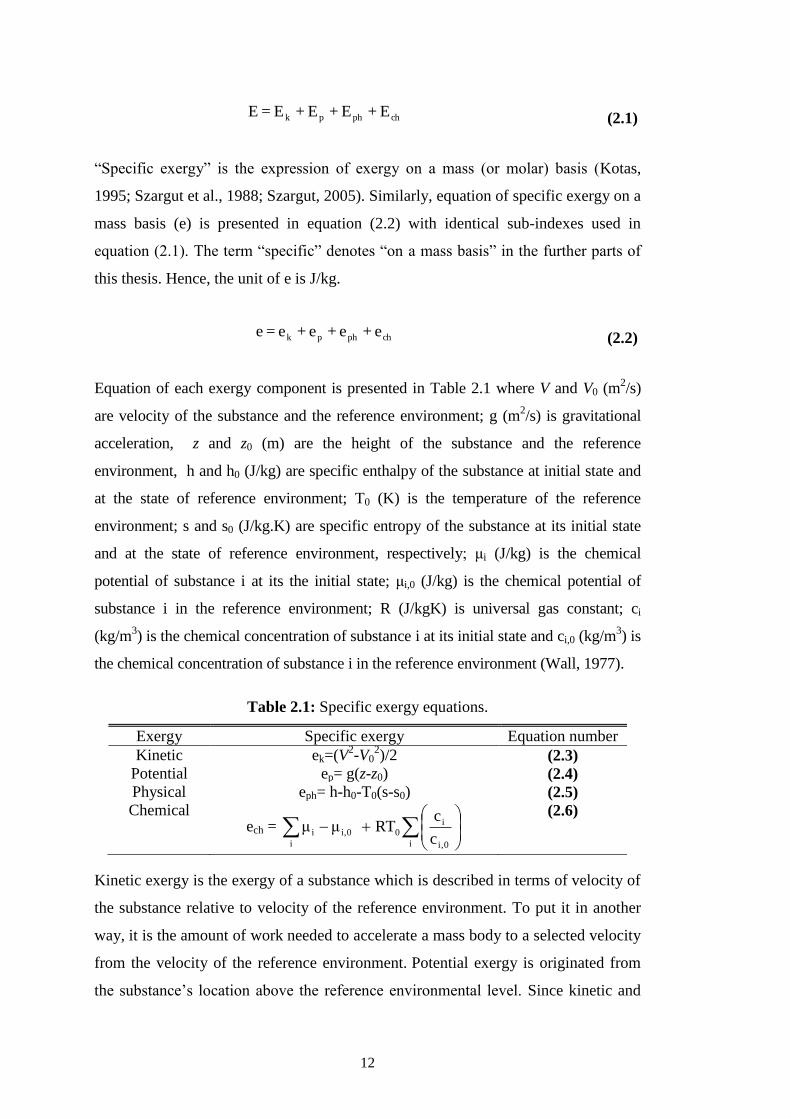
12
chphpk E + E + E +E = E (2.1)
“Specific exergy” is the expression of exergy on a mass (or molar) basis (Kotas,
1995; Szargut et al., 1988; Szargut, 2005). Similarly, equation of specific exergy on a
mass basis (e) is presented in equation (2.2) with identical sub-indexes used in
equation (2.1). The term “specific” denotes “on a mass basis” in the further parts of
this thesis. Hence, the unit of e is J/kg.
chphpk e + e + e +e = e (2.2)
Equation of each exergy component is presented in Table 2.1 where V and V0 (m2/s)
are velocity of the substance and the reference environment; g (m2/s) is gravitational
acceleration, z and z0 (m) are the height of the substance and the reference
environment, h and h0 (J/kg) are specific enthalpy of the substance at initial state and
at the state of reference environment; T0 (K) is the temperature of the reference
environment; s and s0 (J/kg.K) are specific entropy of the substance at its initial state
and at the state of reference environment, respectively; μi (J/kg) is the chemical
potential of substance i at its the initial state; μi,0 (J/kg) is the chemical potential of
substance i in the reference environment; R (J/kgK) is universal gas constant; ci
(kg/m3) is the chemical concentration of substance i at its initial state and ci,0 (kg/m
3) is
the chemical concentration of substance i in the reference environment (Wall, 1977).
Table 2.1: Specific exergy equations.
Exergy Specific exergy Equation number
Kinetic ek=(V2-V0
2)/2 (2.3)
Potential ep= g(z-z0) (2.4)
Physical eph= h-h0-T0(s-s0) (2.5)
Chemical ech =
i 0,i
i0
i
i,0ic
cRTμμ
(2.6)
Kinetic exergy is the exergy of a substance which is described in terms of velocity of
the substance relative to velocity of the reference environment. To put it in another
way, it is the amount of work needed to accelerate a mass body to a selected velocity
from the velocity of the reference environment. Potential exergy is originated from
the substance’s location above the reference environmental level. Since kinetic and

13
potential energy are entirely convertible to work, equations of kinetic and potential
energy and exergy are identical as it is seen in Table 2.1. Physical exergy is the
theoretical maximum limit of work which is obtained as a substance passes from its
initial state (temperature and pressure are T and P, respectively) to the state of
reference environment (temperature and pressure are T0 and P0, respectively)
(Szargut et al., 1988; Szargut, 2005). Equation (2.5) clearly expresses that the
amount of useful work which can be extracted from a certain system is not measured
by enthalpic content, because even in reversible processes, a portion of that energy is
devaluated by the unavoidable entropic degradation which is equal to [T0(s-s0)]
(Szargut et al., 1988; Wall, 1977; Sciubba et al., 2008). Derivation of physical exergy
is presented in Appendix J. The chemical exergy of a substance is the amount of
maximum work obtained from reversible processes to bring the substance to the
chemical equilibrium with the reference environment at constant temperature and
pressure (T0 and P0). Substance composition is converted into the composition of the
reference environment with the same concentration (Rivero and Garfias, 2006;
Szargut et al., 1988) As it is seen in equation (2.6), the chemical exergy has two
contributions: “reactional exergy” and “concentrational exergy”. Reactional exergy
part originated by the necessary chemical reactions to produce stable components
(species) existing in the reference environment (reaction products) from the initial
composition of the substance. Concentrational exergy is the exergy resulting from
the reversible processes to match the chemical concentration of the reaction products
with the chemical concentration of the consisting species of the reference
environment (Rivero and Garfias, 2006; Wall, 1977; Szargut et al., 1988).
In previous studies (Szargut et al.,1988; Szargut, 1989; Szargut, 2005; Kotas, 1995;
Morris and Szargut, 1986; Bejan et al., 1996) the concept of exergy and its
calculation have been extensively discussed. Szargut et al.(1988) proposed a route
for the calculation of standard chemical exergy which is chemical exergy of
substances under pressure and temperature associated with the reference environment
at global scale. In this thesis, Szargut’s exergy calculation route or (for some
substances) tabulated standard chemical exergy in Szargut et al. (1988) are used.
Defined standard exergies of substances facilitate the calculation of exergy under
different conditions (Chen and Qi, 2007). Details are presented in Section 2.3.
14
2.2 Reference Environment
In exergy analysis, all input or output fluxes (mechanical power, electrical energy,
heat, nuclear energy, any type of materials, etc.), are directly assigned to corresponding
exergy content. Exergy is always quantified with respect to a reference environment to
address the question: how much work potential does a resource contain?. For
consistency, exergy calculations must be with respect to the same set of reference
conditions. The reference environment has a stable equilibrium and acts as an infinite
system (sink, source) for heat and materials. Since the reference environment is stable,
intensive properties (i.e., temperature T0 , pressure P0, chemical potentials and
concentrations) remain constant (Szargut et al., 1988; Sciubba, 2003a).
There are two different approaches in the literature to address a reference
environment. The first one is “partial reference environment” and the second is
“comprehensive reference environments” approaches (Valero, 2008). In the first
approach, a specific reference environment is defined for the analyzed processes. The
rationale behind this approach is: exergy analysis is done to point out the possible
improvements for the system, but some of these improvements are not attainable due
to some limitations and restrictions of the system. With a specific reference
environment, only possibilities for practically applicable system evolutions are
analyzed. Bosjankovic (1963), Gaggioli and Petit (1976) and Sussman (1979)
applied this reference environment approach in their studies. As for the second
approach, reference environment consists of 3 sinks: gaseous components of the
atmospheric air, solid components of the earth’s crust external layer and ions and
molecular components of seawater (Szargut et al., 1988) However, there are
differences in reference environment proposal of different authors: Ahrendts (1980),
Kameyama et al. (1982), Ranz (1999), Szargut, et al. (1988), etc. One of the most
known and widely applied reference environment system is Szargut’s approach in
which criterion is abundance of species in the environment (Szargut, et al., 1988;
Szargut, 2005). Szargut’s reference environment is defined at reference temperature
(298,15 K) and pressure (1atm) and average composition of the Earth’s litho-,hydro-
and atmo- sphere. It is assumed that the reference environment is thermodynamically
dead. For a society exergy account study like this thesis, to select a global standard
environment which includes the atmosphere, the ocean and the top layer of the
earth’s crust (like Szargut’s approach) is reasonable. Following the procedure by
15
Szargut et al. (1988), the proper reference state for a substance is estimated by
selecting one of the above listed environmental platforms which the element is likely
to end up after undergoing a serious of reactions to reach the entire equilibrium with
the reference environment. The determination of appropriate environmental platform
is based on substance’s volatility (atmospheric sink), solubility (oceanic sink) and
non solubility (earth’s crust sink) (Szargut et al.1988; Szargut, 2005; Ayres and
Ayres, 1999)
Standard chemical exergy of some elements and compounds (the term “standard”
signifies “at reference temperature and pressure”) are determined by applying the
defined procedure in Szargut et al. (1988). Tabulated values for standard chemical
exergy of substances and reference environment model which are available in
Szargut et al. (1988) are used in the present thesis.
2.3 Computation of Exergy and Exergy Transfer
2.3.1 Calculation of standard chemical exergy
There are four ways of computing the standard chemical exergy of compounds
(Szargut et al., 1988):
1) If standard reference reactions (reactions which have inputs and outputs as species
exist in reference environment) are known for the compound under study, standard
chemical exergy of the compound is computed as (Szargut, 1988):
j
0
j,chj
k
0
k,chk
0
r
0
ch enenGe (2.7)
where 0
che (J/kg) is standard chemical exergy of the compound, 0
rG (J/kg) is
standard Gibbs free energy of the reference reaction, nk and nj are the mole numbers
of output and input reference species, 0
k,che and 0
j,che (J/kg) are standard chemical
exergies of the output and input reference species, respectively.
2) If the standard chemical exergies of consisting elements of the substance are
known, standard chemical exergy of the compound can be computed as (Szargut et
al., 1988):
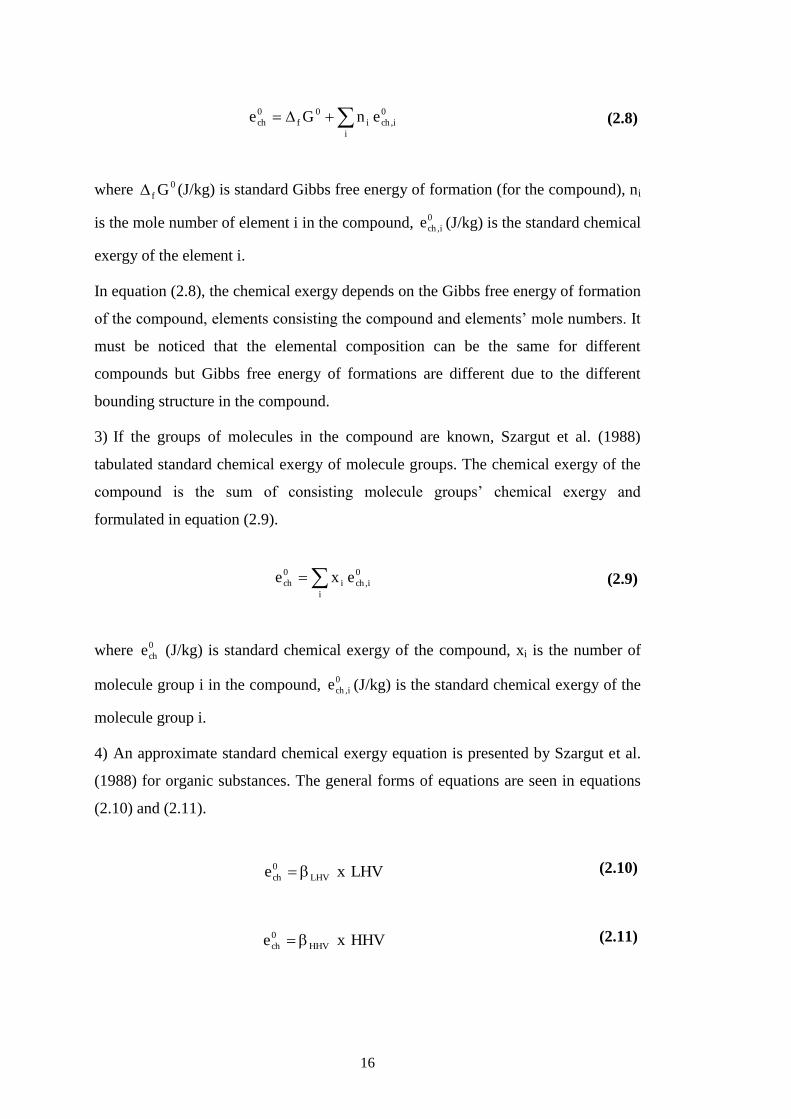
16
i
0
i,chi
0
f
0
ch enGe (2.8)
where 0
f G (J/kg) is standard Gibbs free energy of formation (for the compound), ni
is the mole number of element i in the compound, 0
i,che (J/kg) is the standard chemical
exergy of the element i.
In equation (2.8), the chemical exergy depends on the Gibbs free energy of formation
of the compound, elements consisting the compound and elements’ mole numbers. It
must be noticed that the elemental composition can be the same for different
compounds but Gibbs free energy of formations are different due to the different
bounding structure in the compound.
3) If the groups of molecules in the compound are known, Szargut et al. (1988)
tabulated standard chemical exergy of molecule groups. The chemical exergy of the
compound is the sum of consisting molecule groups’ chemical exergy and
formulated in equation (2.9).
i
0
i,chi
0
ch exe (2.9)
where 0
che (J/kg) is standard chemical exergy of the compound, xi is the number of
molecule group i in the compound, 0
i,che (J/kg) is the standard chemical exergy of the
molecule group i.
4) An approximate standard chemical exergy equation is presented by Szargut et al.
(1988) for organic substances. The general forms of equations are seen in equations
(2.10) and (2.11).
LHVxe LHV
0
ch (2.10)
HHVxe HHV
0
ch (2.11)
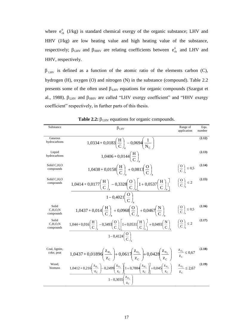
17
where 0
che (J/kg) is standard chemical exergy of the organic substance; LHV and
HHV (J/kg) are low heating value and high heating value of the substance,
respectively; LHV and HHV are relating coefficients between 0
che and LHV and
HHV, respectively.
LHV is defined as a function of the atomic ratio of the elements carbon (C),
hydrogen (H), oxygen (O) and nitrogen (N) in the substance (compound). Table 2.2
presents some of the often used LHV equations for organic compounds (Szargut et
al., 1988). LHV and HHV are called “LHV exergy coefficient” and “HHV exergy
coefficient” respectively, in further parts of this thesis.
Table 2.2:LHV equations for organic compounds.
Substance LHV Range of
application Equ.
number
Gaseous
hydrocarbons
Ca N
10694,0
C
H0,0183+1,0334
(2.12)
Liquid
hydrocarbons
aC
H0,0144+1,0406
(2.13)
Solid C,H,O compounds
aa C
O0813,0
C
H0,0158+1,0438
5,0
C
O
a
(2.14)
Solid C,H,O compounds
a
aaa
C
O4021,01
C
H0537,01
C
O3328,0
C
H0,0177+1,0414
2C
O
a
(2.15)
Solid
C,H,O,N compounds
aaa C
N0467,0
C
O0968,0
C
H0,014+1,0437
5,0
C
O
a
(2.16)
Solid
C,H,O,N compounds
a
aaaa
C
O4124,01
C
N0493,0
C
H0531,01
C
O3493,0
C
H0,016+1,044
2C
O
a
(2.17)
Coal, lignite,
coke, peat
C
N
C
O
C
H
z
z0428,0
z
z0617,0
z
z0,01896+1,0437 222
67,0z
z
C
O2
(2.18)
Wood,
biomass
C
O
C
N
C
H
C
O
C
H
z
z3035,01
z
z045,0
z
z7884,01
z
z2499,0
z
z0,216+1,0412
2
2222
67,2
z
z
C
O2
(2.19)

18
In Table 2.2, aC
H
, aC
O
, aC
N
are atomic ratio of the elements composing the
considered compound; NC is the number of carbon atoms in the molecule; zH2, zC,
zO2, zN2 are hydrogen, carbon, oxygen and nitrogen mass fractions in the compound,
respectively (Szargut et al., 1988).
2.3.2 Exergy transferred via heat transfer
Equation of transferred exergy via heat transfer is seen in equation (2.20) where .
E (W) is
the exergy transfer rate, A(m2) is the heat transfer area, A
.
Q (W/m2) is heat transfer flux
rate through A, T0 is the temperature of the reference environment, T is the temperature at
which the heat transfer takes place (Cornelissen, 1997, Wall, 1977; Szargut et al. 1988).
dAQT
TTE
A
A
.0
.
(2.20)
If the temperature is homogeneous through the heat transfer area,
dAQQA
A
..
(2.21)
Hence, .
E becomes:
.0
.
QT
TTE
(2.22)
2.3.3 Exergy transfer with work interaction
As stated above, exergy is defined as the maximum work potential. Hence,
transferred exergy via work interaction is totally equal to exergy transfer.
2.3.4 Exergy of electricity
By the definition of exergy, electricity is identical to the physical work (totally
exergy). It is formulated in equation (2.23).
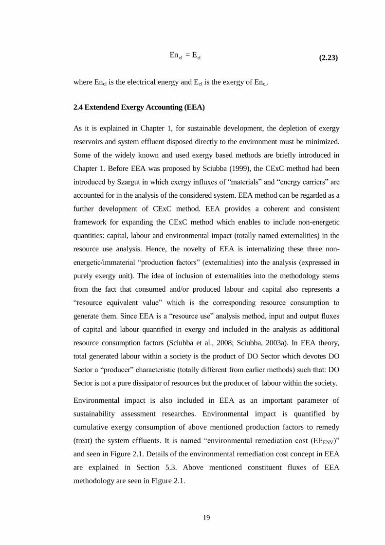
19
elel E=En (2.23)
where Enel is the electrical energy and Eel is the exergy of Enel.
2.4 Extendend Exergy Accounting (EEA)
As it is explained in Chapter 1, for sustainable development, the depletion of exergy
reservoirs and system effluent disposed directly to the environment must be minimized.
Some of the widely known and used exergy based methods are briefly introduced in
Chapter 1. Before EEA was proposed by Sciubba (1999), the CExC method had been
introduced by Szargut in which exergy influxes of “materials” and “energy carriers” are
accounted for in the analysis of the considered system. EEA method can be regarded as a
further development of CExC method. EEA provides a coherent and consistent
framework for expanding the CExC method which enables to include non-energetic
quantities: capital, labour and environmental impact (totally named externalities) in the
resource use analysis. Hence, the novelty of EEA is internalizing these three non-
energetic/immaterial “production factors” (externalities) into the analysis (expressed in
purely exergy unit). The idea of inclusion of externalities into the methodology stems
from the fact that consumed and/or produced labour and capital also represents a
“resource equivalent value” which is the corresponding resource consumption to
generate them. Since EEA is a “resource use” analysis method, input and output fluxes
of capital and labour quantified in exergy and included in the analysis as additional
resource consumption factors (Sciubba et al., 2008; Sciubba, 2003a). In EEA theory,
total generated labour within a society is the product of DO Sector which devotes DO
Sector a “producer” characteristic (totally different from earlier methods) such that: DO
Sector is not a pure dissipator of resources but the producer of labour within the society.
Environmental impact is also included in EEA as an important parameter of
sustainability assessment researches. Environmental impact is quantified by
cumulative exergy consumption of above mentioned production factors to remedy
(treat) the system effluents. It is named “environmental remediation cost (EEENV)”
and seen in Figure 2.1. Details of the environmental remediation cost concept in EEA
are explained in Section 5.3. Above mentioned constituent fluxes of EEA
methodology are seen in Figure 2.1.
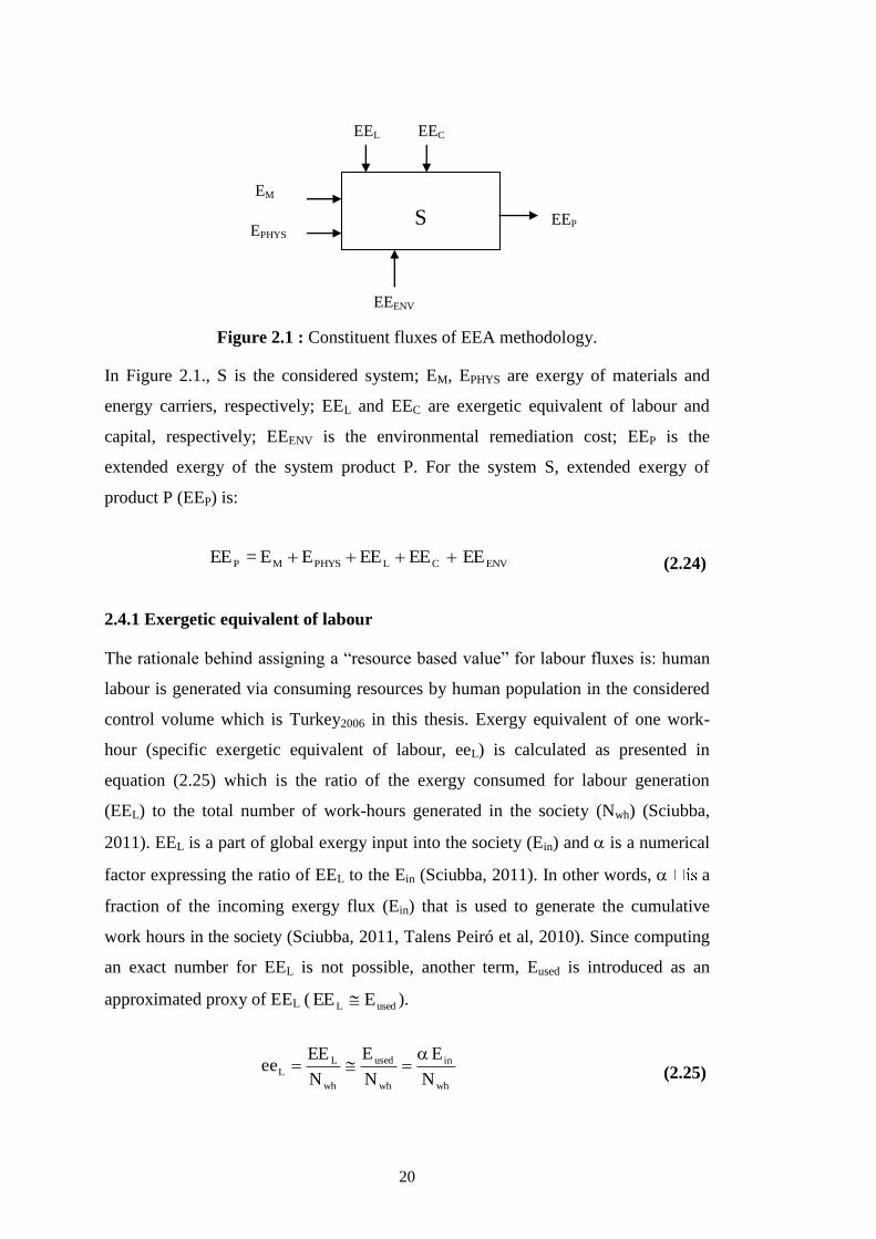
20
Figure 2.1 : Constituent fluxes of EEA methodology.
In Figure 2.1., S is the considered system; EM, EPHYS are exergy of materials and
energy carriers, respectively; EEL and EEC are exergetic equivalent of labour and
capital, respectively; EEENV is the environmental remediation cost; EEP is the
extended exergy of the system product P. For the system S, extended exergy of
product P (EEP) is:
ENVCLPHYSMP EEEE EE E E =EE (2.24)
2.4.1 Exergetic equivalent of labour
The rationale behind assigning a “resource based value” for labour fluxes is: human
labour is generated via consuming resources by human population in the considered
control volume which is Turkey2006 in this thesis. Exergy equivalent of one work-
hour (specific exergetic equivalent of labour, eeL) is calculated as presented in
equation (2.25) which is the ratio of the exergy consumed for labour generation
(EEL) to the total number of work-hours generated in the society (Nwh) (Sciubba,
2011). EEL is a part of global exergy input into the society (Ein) and is a numerical
factor expressing the ratio of EEL to the Ein (Sciubba, 2011). In other words, a
fraction of the incoming exergy flux (Ein) that is used to generate the cumulative
work hours in the society (Sciubba, 2011, Talens Peiró et al, 2010). Since computing
an exact number for EEL is not possible, another term, Eused is introduced as an
approximated proxy of EEL ( usedL EEE ).
wh
in
wh
used
wh
LL
N
E
N
E
N
EEee
(2.25)
S
EEENV
EM
EEP
EPHYS
EEL EEC
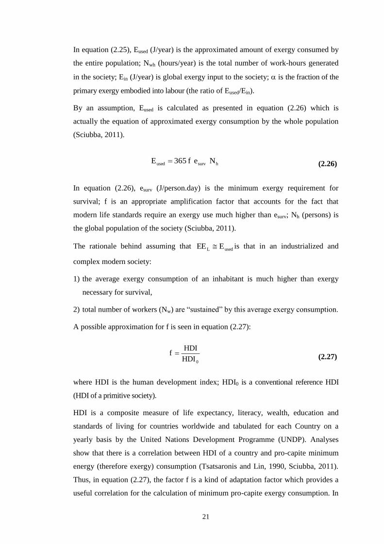
21
In equation (2.25), Eused (J/year) is the approximated amount of exergy consumed by
the entire population; Nwh (hours/year) is the total number of work-hours generated
in the society; Ein (J/year) is global exergy input to the society; is the fraction of the
primary exergy embodied into labour (the ratio of Eused/Ein).
By an assumption, Eused is calculated as presented in equation (2.26) which is
actually the equation of approximated exergy consumption by the whole population
(Sciubba, 2011).
hsurvused Nef365E (2.26)
In equation (2.26), esurv (J/person.day) is the minimum exergy requirement for
survival; f is an appropriate amplification factor that accounts for the fact that
modern life standards require an exergy use much higher than esurv; Nh (persons) is
the global population of the society (Sciubba, 2011).
The rationale behind assuming that usedL EEE is that in an industrialized and
complex modern society:
1) the average exergy consumption of an inhabitant is much higher than exergy
necessary for survival,
2) total number of workers (Nw) are “sustained” by this average exergy consumption.
A possible approximation for f is seen in equation (2.27):
0HDI
HDIf
(2.27)
where HDI is the human development index; HDI0 is a conventional reference HDI
(HDI of a primitive society).
HDI is a composite measure of life expectancy, literacy, wealth, education and
standards of living for countries worldwide and tabulated for each Country on a
yearly basis by the United Nations Development Programme (UNDP). Analyses
show that there is a correlation between HDI of a country and pro-capite minimum
energy (therefore exergy) consumption (Tsatsaronis and Lin, 1990, Sciubba, 2011).
Thus, in equation (2.27), the factor f is a kind of adaptation factor which provides a
useful correlation for the calculation of minimum pro-capite exergy consumption. In
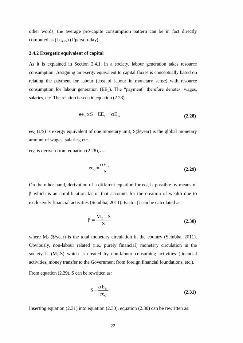
22
other words, the average pro-capite consumption pattern can be in fact directly
computed as (f esurv) (J/person-day).
2.4.2 Exergetic equivalent of capital
As it is explained in Section 2.4.1, in a society, labour generation takes resource
consumption. Assigning an exergy equivalent to capital fluxes is conceptually based on
relating the payment for labour (cost of labour in monetary sense) with resource
consumption for labour generation (EEL). The “payment” therefore denotes: wages,
salaries, etc. The relation is seen in equation (2.28).
inLC EEESxee (2.28)
eeC (J/$) is exergy equivalent of one monetary unit; S($/year) is the global monetary
amount of wages, salaries, etc.
eeC is deriven from equation (2.28), as:
S
Eee in
C
(2.29)
On the other hand, derivation of a different equation for eeC is possible by means of
which is an amplification factor that accounts for the creation of wealth due to
exclusively financial activities (Sciubba, 2011). Factor can be calculated as:
S
SM2 (2.30)
where M2 ($/year) is the total monetary circulation in the country (Sciubba, 2011).
Obviously, non-labour related (i.e., purely financial) monetary circulation in the
society is (M2-S) which is created by non-labour consuming activities (financial
activities, money transfer to the Government from foreign financial foundations, etc.).
From equation (2.29), S can be rewritten as:
C
in
ee
ES
(2.31)
Inserting equation (2.31) into equation (2.30), equation (2.30) can be rewritten as:

23
C
in2
ee
ES SM
(2.32)
As a result, the equation of eeC can be written as:
SM
Eee
2
inC
(2.33)
2.4.3 Environmental remediation cost (EEENV)
As for computing of “environmental remediation cost (EEENV)”, EEA follows a
similar route to Zero-Exergetic Life Cycle Analysis (Zero-ELCA) methodology
which is briefly explained in Chapter 1. The essence of this idea is: the potential
environmental impact of an effluent is represented by the cumulative amount of
exergetic resources that must be consumed by the whole treatment process to
attain an ideal, zero-impact disposal of the effluent. “Environmental
remediation cost (EEENV)” is computed by inserting a (real or virtual) effluent
treatment system (a set of processes and systems, totally named “environmental
remediation (treatment) system” which is system S t in Figure 2.2) for each type
of effluents. In each environmental remediation system, physical exergy of each
single effluent must be brought down to zero. In theoretical framework of EEA,
each discharge into the environment must be at reference conditions, in other
words, its environmental impact must be equal to zero. Since these
environmental treatment systems also consume material, energy, labour and
capital inputs, also they have environmental remediation costs (which are
represented as EM-t, EPHYS-t, EEL-t, EEC-t, EEENV-t in Figure 2.2) and resource
exergy use equivalent of all these fluxes must be completely and correctly
charged to embedded global primary exergy consumption of P. Representation
of the system St and above mentioned fluxes are seen in Figure 2.2, details of
EEENV computing and formulations are presented in Section 5.4.
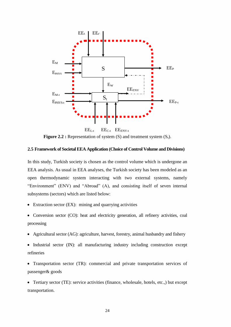
24
Figure 2.2 : Representation of system (S) and treatment system (St).
2.5 Framework of Societal EEA Application (Choice of Control Volume and Divisions)
In this study, Turkish society is chosen as the control volume which is undergone an
EEA analysis. As usual in EEA analyses, the Turkish society has been modeled as an
open thermodynamic system interacting with two external systems, namely
“Environment” (ENV) and “Abroad” (A), and consisting itself of seven internal
subsystems (sectors) which are listed below:
Extraction sector (EX): mining and quarrying activities
Conversion sector (CO): heat and electricity generation, all refinery activities, coal
processing
Agricultural sector (AG): agriculture, harvest, forestry, animal husbandry and fishery
Industrial sector (IN): all manufacturing industry including construction except
refineries
Transportation sector (TR): commercial and private transportation services of
passenger& goods
Tertiary sector (TE): service activities (finance, wholesale, hotels, etc.,) but except
transportation.
EW
EM
EEP
EPHYS
EEL EEC
EEC-t
EM-t
EPHYS-t EEP-t
EEENV-t EEL-t
EEENV
St
S
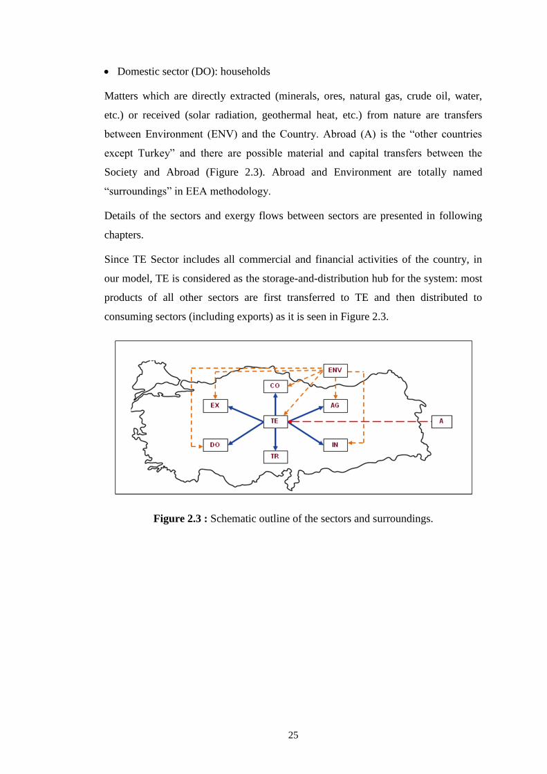
25
Domestic sector (DO): households
Matters which are directly extracted (minerals, ores, natural gas, crude oil, water,
etc.) or received (solar radiation, geothermal heat, etc.) from nature are transfers
between Environment (ENV) and the Country. Abroad (A) is the “other countries
except Turkey” and there are possible material and capital transfers between the
Society and Abroad (Figure 2.3). Abroad and Environment are totally named
“surroundings” in EEA methodology.
Details of the sectors and exergy flows between sectors are presented in following
chapters.
Since TE Sector includes all commercial and financial activities of the country, in
our model, TE is considered as the storage-and-distribution hub for the system: most
products of all other sectors are first transferred to TE and then distributed to
consuming sectors (including exports) as it is seen in Figure 2.3.
Figure 2.3 : Schematic outline of the sectors and surroundings.

26
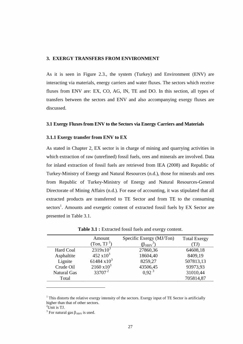
27
3. EXERGY TRANSFERS FROM ENVIRONMENT
As it is seen in Figure 2.3., the system (Turkey) and Environment (ENV) are
interacting via materials, energy carriers and water fluxes. The sectors which receive
fluxes from ENV are: EX, CO, AG, IN, TE and DO. In this section, all types of
transfers between the sectors and ENV and also accompanying exergy fluxes are
discussed.
3.1 Exergy Fluxes from ENV to the Sectors via Energy Carriers and Materials
3.1.1 Exergy transfer from ENV to EX
As stated in Chapter 2, EX sector is in charge of mining and quarrying activities in
which extraction of raw (unrefined) fossil fuels, ores and minerals are involved. Data
for inland extraction of fossil fuels are retrieved from IEA (2008) and Republic of
Turkey-Ministry of Energy and Natural Resources (n.d.), those for minerals and ores
from Republic of Turkey-Ministry of Energy and Natural Resources-General
Directorate of Mining Affairs (n.d.). For ease of accounting, it was stipulated that all
extracted products are transferred to TE Sector and from TE to the consuming
sectors1. Amounts and exergetic content of extracted fossil fuels by EX Sector are
presented in Table 3.1.
Table 3.1 : Extracted fossil fuels and exergy content.
Amount
(Ton, TJ 2)
Specific Exergy (MJ/Ton)
(HHV3)
Total Exergy
(TJ)
Hard Coal
2319x103
27860,36 64608,18
Asphaltite 452 x103 18604,40 8409,19
Lignite 61484 x103 8259,27 507813,13
Crude Oil 2160 x103 43506,45 93973,93
Natural Gas
33707 2 0,92
3 31010,44
Total
705814,87
1 This distorts the relative exergy intensity of the sectors. Exergy input of TE Sector is artificially
higher than that of other sectors. 2Unit is TJ.
3 For natural gas HHV
is used.
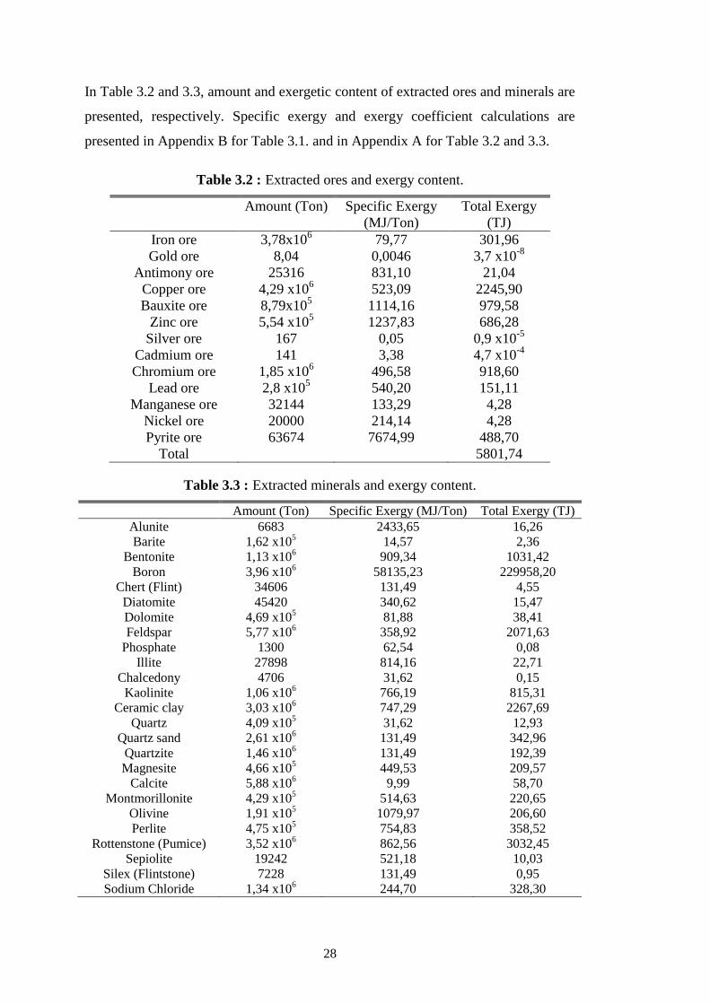
28
In Table 3.2 and 3.3, amount and exergetic content of extracted ores and minerals are
presented, respectively. Specific exergy and exergy coefficient calculations are
presented in Appendix B for Table 3.1. and in Appendix A for Table 3.2 and 3.3.
Table 3.2 : Extracted ores and exergy content.
Amount (Ton) Specific Exergy
(MJ/Ton)
Total Exergy
(TJ)
Iron ore 3,78x10⁶
79,77 301,96
Gold ore 8,04 0,0046 3,7 x10⁻⁸
Antimony ore 25316 831,10 21,04
Copper ore 4,29 x10⁶ 523,09 2245,90
Bauxite ore 8,79x10⁵
1114,16 979,58
Zinc ore 5,54 x10⁵ 1237,83 686,28
Silver ore 167 0,05 0,9 x10⁻⁵
Cadmium ore 141 3,38 4,7 x10⁻⁴
Chromium ore 1,85 x10⁶ 496,58 918,60
Lead ore 2,8 x10⁵ 540,20 151,11
Manganese ore 32144 133,29 4,28
Nickel ore 20000 214,14 4,28
Pyrite ore 63674 7674,99 488,70
Total 5801,74
Table 3.3 : Extracted minerals and exergy content.
Amount (Ton) Specific Exergy (MJ/Ton) Total Exergy (TJ)
Alunite 6683 2433,65 16,26
Barite 1,62 x10⁵ 14,57 2,36
Bentonite 1,13 x10⁶ 909,34 1031,42
Boron 3,96 x10⁶ 58135,23 229958,20
Chert (Flint) 34606 131,49 4,55
Diatomite 45420 340,62 15,47
Dolomite 4,69 x10⁵ 81,88 38,41
Feldspar 5,77 x10⁶ 358,92 2071,63
Phosphate 1300 62,54 0,08
Illite 27898 814,16 22,71
Chalcedony 4706 31,62 0,15
Kaolinite 1,06 x10⁶ 766,19 815,31
Ceramic clay 3,03 x10⁶ 747,29 2267,69
Quartz 4,09 x10⁵ 31,62 12,93
Quartz sand 2,61 x10⁶ 131,49 342,96
Quartzite 1,46 x10⁶ 131,49 192,39
Magnesite 4,66 x10⁵ 449,53 209,57
Calcite 5,88 x10⁶ 9,99 58,70
Montmorillonite 4,29 x10⁵ 514,63 220,65
Olivine 1,91 x10⁵ 1079,97 206,60
Perlite 4,75 x10⁵ 754,83 358,52
Rottenstone (Pumice) 3,52 x10⁶ 862,56 3032,45
Sepiolite 19242 521,18 10,03
Silex (Flintstone) 7228 131,49 0,95
Sodium Chloride 1,34 x10⁶
244,70 328,30
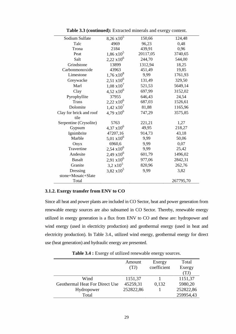
29
Table 3.3 (continued): Extracted minerals and exergy content.
Sodium Sulfate 8,26 x10⁵ 150,66 124,48
Talc 4969 96,23 0,48
Trona 2184 439,91 0,96
Peat 1,86 x10⁵ 20117,05 3740,65
Salt 2,22 x10⁶ 244,70 544,00
Grindstone 13899 1312,94 18,25
Carbonmonoxide 43963 451,49 19,85
Limestone 1,76 x10⁸ 9,99 1761,93
Greywacke 2,51 x10⁶ 131,49 329,50
Marl 1,08 x10⁷ 521,53 5649,14
Clay 4,52 x10⁶ 697,99 3152,02
Pyrophyllite 37955 646,43 24,54
Trass 2,22 x10⁶ 687,03 1526,61
Dolomite 1,42 x10⁷ 81,88 1165,96
Clay for brick and roof
tile 4,79 x10
6 747,29 3575,85
Serpentine (Crysolite) 5763 221,21 1,27
Gypsum 4,37 x10⁶ 49,95 218,27
Ignimbrite 47207,16 914,73 43,18
Marble 5,01 x10⁶ 9,99 50,06
Onyx 6960,6 9,99 0,07
Travertine 2,54 x10⁶ 9,99 25,42
Andesite 2,49 x10⁶ 601,79 1496,02
Basalt 2,91 x10⁶ 977,06 2842,31
Granite 3,2 x10⁵ 820,96 262,76
Dressing
stone+Mosaic+Slate 3,82 x10
5 9,99 3,82
Total 267795,70
3.1.2. Exergy transfer from ENV to CO
Since all heat and power plants are included in CO Sector, heat and power generation from
renewable energy sources are also subsumed in CO Sector. Thereby, renewable energy
utilized in energy generation is a flux from ENV to CO and these are: hydropower and
wind energy (used in electricity production) and geothermal energy (used in heat and
electricity production). In Table 3.4., utilized wind energy, geothermal energy for direct
use (heat generation) and hydraulic energy are presented.
Table 3.4 : Exergy of utilized renewable energy sources.
Amount
(TJ)
Exergy
coefficient
Total
Exergy
(TJ)
Wind 1151,37 1 1151,37
Geothermal Heat For Direct Use
45259,31 0,132 5980,20
Hydropower 252822,86 1 252822,86
Total 259954,43
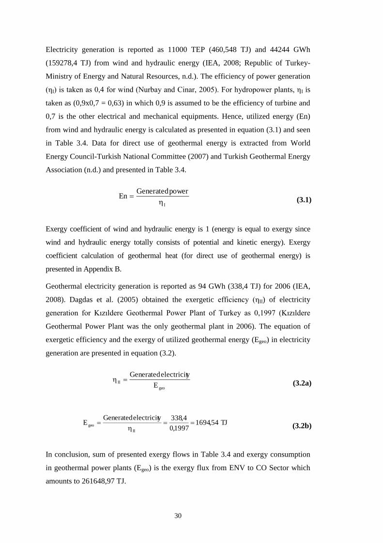
30
Electricity generation is reported as 11000 TEP (460,548 TJ) and 44244 GWh
(159278,4 TJ) from wind and hydraulic energy (IEA, 2008; Republic of Turkey-
Ministry of Energy and Natural Resources, n.d.). The efficiency of power generation
(ηI) is taken as 0,4 for wind (Nurbay and Cinar, 2005). For hydropower plants, ηI is
taken as (0,9x0,7 = 0,63) in which 0,9 is assumed to be the efficiency of turbine and
0,7 is the other electrical and mechanical equipments. Hence, utilized energy (En)
from wind and hydraulic energy is calculated as presented in equation (3.1) and seen
in Table 3.4. Data for direct use of geothermal energy is extracted from World
Energy Council-Turkish National Committee (2007) and Turkish Geothermal Energy
Association (n.d.) and presented in Table 3.4.
I
powerGeneratedEn
(3.1)
Exergy coefficient of wind and hydraulic energy is 1 (energy is equal to exergy since
wind and hydraulic energy totally consists of potential and kinetic energy). Exergy
coefficient calculation of geothermal heat (for direct use of geothermal energy) is
presented in Appendix B.
Geothermal electricity generation is reported as 94 GWh (338,4 TJ) for 2006 (IEA,
2008). Dagdas et al. (2005) obtained the exergetic efficiency (ηII) of electricity
generation for Kızıldere Geothermal Power Plant of Turkey as 0,1997 (Kızıldere
Geothermal Power Plant was the only geothermal plant in 2006). The equation of
exergetic efficiency and the exergy of utilized geothermal energy (Egeo) in electricity
generation are presented in equation (3.2).
geo
IIE
yelectricitGenerated
(3.2a)
TJ54,16941997,0
4,338yelectricitGeneratedE
II
geo
(3.2b)
In conclusion, sum of presented exergy flows in Table 3.4 and exergy consumption
in geothermal power plants (Egeo) is the exergy flux from ENV to CO Sector which
amounts to 261648,97 TJ.
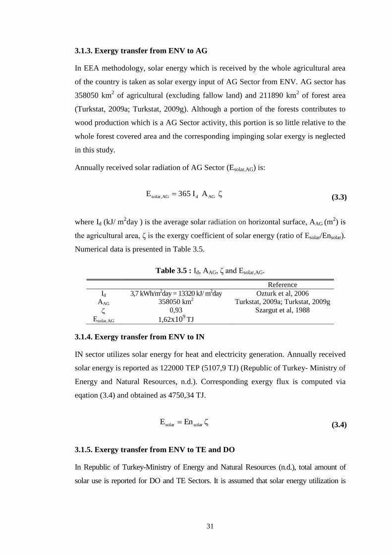
31
3.1.3. Exergy transfer from ENV to AG
In EEA methodology, solar energy which is received by the whole agricultural area
of the country is taken as solar exergy input of AG Sector from ENV. AG sector has
358050 km2 of agricultural (excluding fallow land) and 211890 km
2 of forest area
(Turkstat, 2009a; Turkstat, 2009g). Although a portion of the forests contributes to
wood production which is a AG Sector activity, this portion is so little relative to the
whole forest covered area and the corresponding impinging solar exergy is neglected
in this study.
Annually received solar radiation of AG Sector (Esolar,AG) is:
AGdAG,solar AI365E (3.3)
where Id (kJ/ m2day ) is the average solar radiation on horizontal surface, AAG (m
2) is
the agricultural area, ζ is the exergy coefficient of solar energy (ratio of Esolar/Ensolar).
Numerical data is presented in Table 3.5.
Table 3.5 : Id, AAG, ζ and Esolar,AG.
Reference
Id 3,7 kWh/m2day = 13320 kJ/ m
2day Ozturk et al, 2006
AAG 358050 km2 Turkstat, 2009a; Turkstat, 2009g
0,93 Szargut et al, 1988
Esolar,AG 1,62x10⁹
TJ
3.1.4. Exergy transfer from ENV to IN
IN sector utilizes solar energy for heat and electricity generation. Annually received
solar energy is reported as 122000 TEP (5107,9 TJ) (Republic of Turkey- Ministry of
Energy and Natural Resources, n.d.). Corresponding exergy flux is computed via
eqation (3.4) and obtained as 4750,34 TJ.
solarsolar EnE (3.4)
3.1.5. Exergy transfer from ENV to TE and DO
In Republic of Turkey-Ministry of Energy and Natural Resources (n.d.), total amount of
solar use is reported for DO and TE Sectors. It is assumed that solar energy utilization is
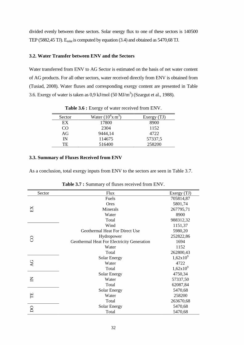
32
divided evenly between these sectors. Solar energy flux to one of these sectors is 140500
TEP (5882,45 TJ). Esolar is computed by equation (3.4) and obtained as 5470,68 TJ.
3.2. Water Transfer between ENV and the Sectors
Water transferred from ENV to AG Sector is estimated on the basis of net water content
of AG products. For all other sectors, water received directly from ENV is obtained from
(Tusiad, 2008). Water fluxes and corresponding exergy content are presented in Table
3.6. Exergy of water is taken as 0,9 kJ/mol (50 MJ/m3) (Szargut et al., 1988).
Table 3.6 : Exergy of water received from ENV.
Sector Water (104x m3) Exergy (TJ)
EX 17800 8900
CO 2304 1152
AG 9444,14 4722
IN 114675 57337,5
TE 516400 258200
3.3. Summary of Fluxes Received from ENV
As a conclusion, total exergy inputs from ENV to the sectors are seen in Table 3.7.
Table 3.7 : Summary of fluxes received from ENV.
Sector Flux Exergy (TJ)
EX
Fuels 705814,87
Ores 5801,74
Minerals 267795,71
Water 8900
Total 988312,32
CO
Wind 1151,37
Geothermal Heat For Direct Use 5980,20
Hydropower 252822,86
Geothermal Heat For Electricity Generation 1694
Water 1152
Total 262800,43
AG
Solar Energy 1,62x10⁹
Water 4722
Total 1,62x10⁹
IN Solar Energy 4750,34
Water 57337,50
Total 62087,84
TE
Solar Energy 5470,68
Water 258200
Total 263670,68
DO
Solar Energy 5470,68
Total 5470,68
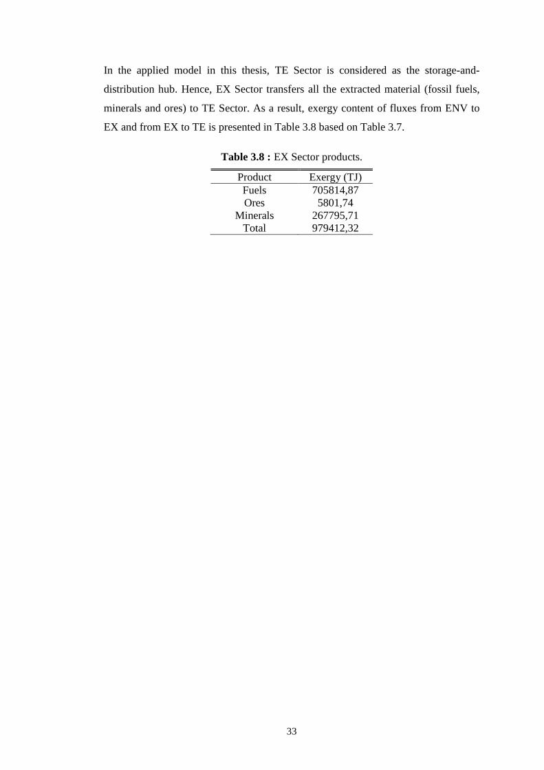
33
In the applied model in this thesis, TE Sector is considered as the storage-and-
distribution hub. Hence, EX Sector transfers all the extracted material (fossil fuels,
minerals and ores) to TE Sector. As a result, exergy content of fluxes from ENV to
EX and from EX to TE is presented in Table 3.8 based on Table 3.7.
Table 3.8 : EX Sector products.
Product Exergy (TJ)
Fuels 705814,87
Ores 5801,74
Minerals 267795,71
Total 979412,32

34
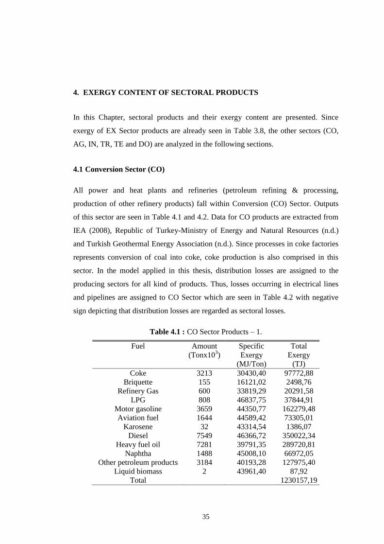
35
4. EXERGY CONTENT OF SECTORAL PRODUCTS
In this Chapter, sectoral products and their exergy content are presented. Since
exergy of EX Sector products are already seen in Table 3.8, the other sectors (CO,
AG, IN, TR, TE and DO) are analyzed in the following sections.
4.1 Conversion Sector (CO)
All power and heat plants and refineries (petroleum refining & processing,
production of other refinery products) fall within Conversion (CO) Sector. Outputs
of this sector are seen in Table 4.1 and 4.2. Data for CO products are extracted from
IEA (2008), Republic of Turkey-Ministry of Energy and Natural Resources (n.d.)
and Turkish Geothermal Energy Association (n.d.). Since processes in coke factories
represents conversion of coal into coke, coke production is also comprised in this
sector. In the model applied in this thesis, distribution losses are assigned to the
producing sectors for all kind of products. Thus, losses occurring in electrical lines
and pipelines are assigned to CO Sector which are seen in Table 4.2 with negative
sign depicting that distribution losses are regarded as sectoral losses.
Table 4.1 : CO Sector Products – 1.
Fuel Amount
(Tonx103)
Specific
Exergy
(MJ/Ton)
Total
Exergy
(TJ)
Coke 3213 30430,40 97772,88
Briquette 155 16121,02 2498,76
Refinery Gas 600 33819,29 20291,58
LPG 808 46837,75 37844,91
Motor gasoline 3659 44350,77 162279,48
Aviation fuel 1644 44589,42 73305,01
Karosene 32 43314,54 1386,07
Diesel 7549 46366,72 350022,34
Heavy fuel oil 7281 39791,35 289720,81
Naphtha 1488 45008,10 66972,05
Other petroleum products 3184 40193,28 127975,40
Liquid biomass 2 43961,40 87,92
Total
1230157,19
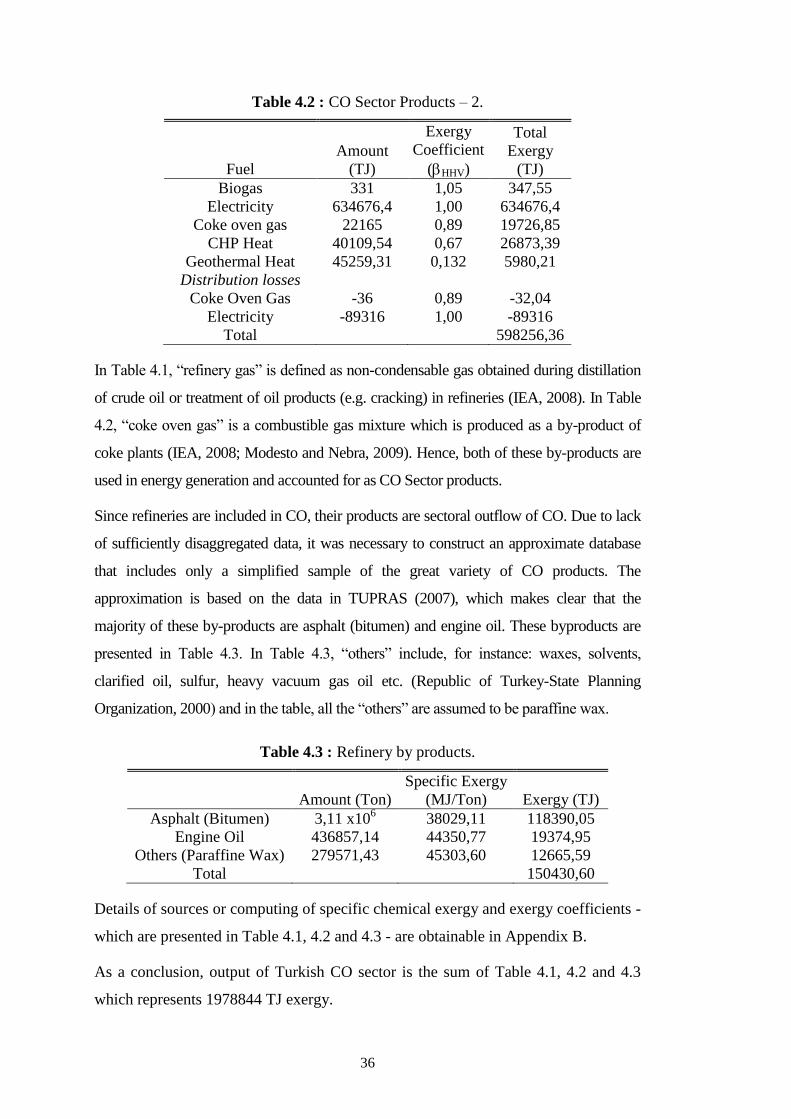
36
Table 4.2 : CO Sector Products – 2.
Fuel
Amount
(TJ)
Exergy
Coefficient
(HHV)
Total
Exergy
(TJ)
Biogas 331 1,05 347,55
Electricity 634676,4 1,00 634676,4
Coke oven gas 22165 0,89 19726,85
CHP Heat 40109,54 0,67 26873,39
Geothermal Heat 45259,31 0,132 5980,21
Distribution losses
Coke Oven Gas -36 0,89 -32,04
Electricity -89316 1,00 -89316
Total
598256,36
In Table 4.1, “refinery gas” is defined as non-condensable gas obtained during distillation
of crude oil or treatment of oil products (e.g. cracking) in refineries (IEA, 2008). In Table
4.2, “coke oven gas” is a combustible gas mixture which is produced as a by-product of
coke plants (IEA, 2008; Modesto and Nebra, 2009). Hence, both of these by-products are
used in energy generation and accounted for as CO Sector products.
Since refineries are included in CO, their products are sectoral outflow of CO. Due to lack
of sufficiently disaggregated data, it was necessary to construct an approximate database
that includes only a simplified sample of the great variety of CO products. The
approximation is based on the data in TUPRAS (2007), which makes clear that the
majority of these by-products are asphalt (bitumen) and engine oil. These byproducts are
presented in Table 4.3. In Table 4.3, “others” include, for instance: waxes, solvents,
clarified oil, sulfur, heavy vacuum gas oil etc. (Republic of Turkey-State Planning
Organization, 2000) and in the table, all the “others” are assumed to be paraffine wax.
Table 4.3 : Refinery by products.
Amount (Ton)
Specific Exergy
(MJ/Ton) Exergy (TJ)
Asphalt (Bitumen) 3,11 x10⁶ 38029,11 118390,05
Engine Oil 436857,14 44350,77 19374,95
Others (Paraffine Wax) 279571,43 45303,60 12665,59
Total
150430,60
Details of sources or computing of specific chemical exergy and exergy coefficients -
which are presented in Table 4.1, 4.2 and 4.3 - are obtainable in Appendix B.
As a conclusion, output of Turkish CO sector is the sum of Table 4.1, 4.2 and 4.3
which represents 1978844 TJ exergy.
37
4.2 Agricultural Sector (AG)
This sector comprises harvesting, forestry, animal husbandry, and fishery.
Natural resources made available by the environment are the main inputs to
the sector as it is seen in Table 3.7. Products of the AG sector are split into
three groups:
Group 1: AG products for industrial use, energy production and
consumption by DO Sector which are all transferred to TE.
Group 2: AG products which are transferred from AG directly to DO and
consumed by people in rural areas (in the model applied in this thesis, this is
the only direct transfer of materials between two sectors by-passing TE sector)
Group 3: exported AG Sector products
As for Group 1, AG sends products to TE for use in food processing industry,
chemical industry, textile industry, fodder industry, seed industry and other
industrial processes. In the available data for AG sector products (Turkstat,
2009f), total country own consumption of produced AG products is available
but there is no data for industrial consumption and DO sector consumption
share in total country consumption amount. An assumption was necessary such
as: 20% of total comestible AG sector products (vegetables, fruit, leguminous
seeds, honey, egg, olive, milk, soybean, tea and potato) consumption is
assumed to be consumed directly by people in rural area (Group 2) and the left
is transferred to TE sector to be sold to IN sector (industrial use) and DO
sector. All the country consumption of cereals, meat, poultry products, fishery
products, bee wax, tobacco, sunflower, rape, cotton, sugar beet is assumed to
be transferred to IN sector for further processing (no direct transfer to DO
sector). The allocation of AG sector products for comestible goods is
presented in Table 4.4. Details of the AG products exergy content are
presented in Appendix C.
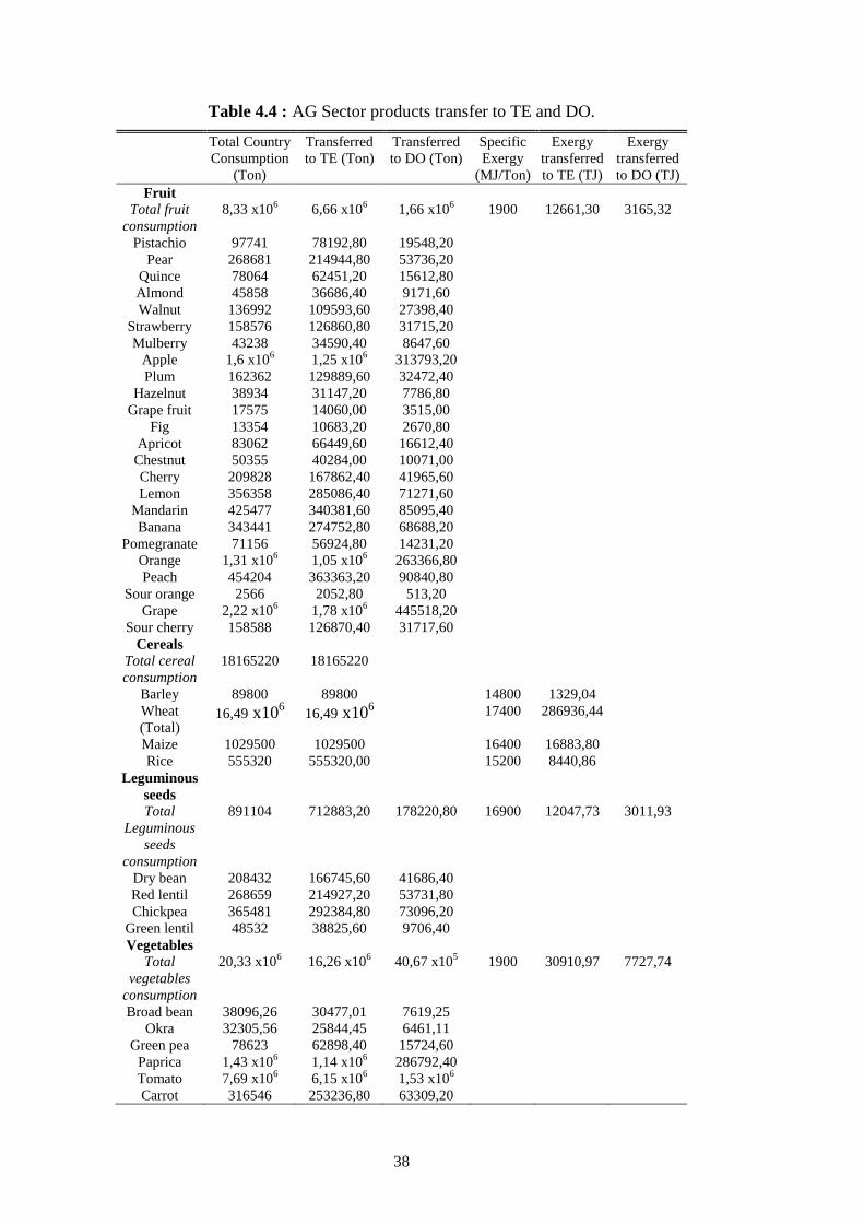
38
Table 4.4 : AG Sector products transfer to TE and DO.
Total Country
Consumption
(Ton)
Transferred
to TE (Ton)
Transferred
to DO (Ton)
Specific
Exergy
(MJ/Ton)
Exergy
transferred
to TE (TJ)
Exergy
transferred
to DO (TJ)
Fruit
Total fruit
consumption
8,33 x10⁶ 6,66 x10
6 1,66 x10
6 1900 12661,30 3165,32
Pistachio 97741 78192,80 19548,20
Pear 268681 214944,80 53736,20
Quince 78064 62451,20 15612,80
Almond 45858 36686,40 9171,60
Walnut 136992 109593,60 27398,40
Strawberry 158576 126860,80 31715,20
Mulberry 43238 34590,40 8647,60
Apple 1,6 x10⁶ 1,25 x10
6 313793,20
Plum 162362 129889,60 32472,40
Hazelnut 38934 31147,20 7786,80
Grape fruit 17575 14060,00 3515,00
Fig 13354 10683,20 2670,80
Apricot 83062 66449,60 16612,40
Chestnut 50355 40284,00 10071,00
Cherry 209828 167862,40 41965,60
Lemon 356358 285086,40 71271,60
Mandarin 425477 340381,60 85095,40
Banana 343441 274752,80 68688,20
Pomegranate 71156 56924,80 14231,20
Orange 1,31 x10⁶ 1,05 x10
6 263366,80
Peach 454204 363363,20 90840,80
Sour orange 2566 2052,80 513,20
Grape 2,22 x10⁶ 1,78 x10
6 445518,20
Sour cherry 158588 126870,40 31717,60
Cereals
Total cereal
consumption
18165220 18165220
Barley 89800 89800 14800 1329,04
Wheat
(Total) 16,49 x10
6 16,49 x10
6 17400 286936,44
Maize 1029500 1029500 16400 16883,80
Rice 555320 555320,00 15200 8440,86
Leguminous
seeds
Total
Leguminous
seeds
consumption
891104 712883,20 178220,80 16900 12047,73 3011,93
Dry bean 208432 166745,60 41686,40
Red lentil 268659 214927,20 53731,80
Chickpea 365481 292384,80 73096,20
Green lentil 48532 38825,60 9706,40
Vegetables
Total
vegetables
consumption
20,33 x10⁶ 16,26 x10
6 40,67 x10
5 1900 30910,97 7727,74
Broad bean 38096,26 30477,01 7619,25
Okra 32305,56 25844,45 6461,11
Green pea 78623 62898,40 15724,60
Paprica 1,43 x10⁶ 1,14 x10
6 286792,40
Tomato 7,69 x10⁶ 6,15 x10
6 1,53 x10
6
Carrot 316546 253236,80 63309,20
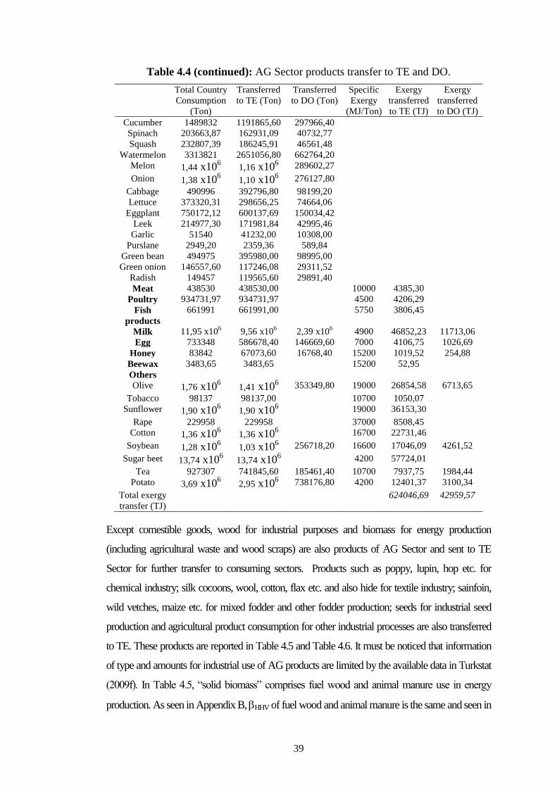
39
Table 4.4 (continued): AG Sector products transfer to TE and DO.
Total Country
Consumption
(Ton)
Transferred
to TE (Ton)
Transferred
to DO (Ton)
Specific
Exergy
(MJ/Ton)
Exergy
transferred
to TE (TJ)
Exergy
transferred
to DO (TJ)
Cucumber 1489832 1191865,60 297966,40
Spinach 203663,87 162931,09 40732,77
Squash 232807,39 186245,91 46561,48
Watermelon 3313821 2651056,80 662764,20
Melon 1,44 x10⁶ 1,16 x10
6 289602,27
Onion 1,38 x10⁶ 1,10 x10
6 276127,80
Cabbage 490996 392796,80 98199,20
Lettuce 373320,31 298656,25 74664,06
Eggplant 750172,12 600137,69 150034,42
Leek 214977,30 171981,84 42995,46
Garlic 51540 41232,00 10308,00
Purslane 2949,20 2359,36 589,84
Green bean 494975 395980,00 98995,00
Green onion 146557,60 117246,08 29311,52
Radish 149457 119565,60 29891,40
Meat 438530 438530,00 10000 4385,30
Poultry 934731,97 934731,97 4500 4206,29
Fish
products
661991 661991,00 5750 3806,45
Milk 11,95 x10⁶ 9,56 x10
6 2,39 x10
6 4900 46852,23 11713,06
Egg 733348 586678,40 146669,60 7000 4106,75 1026,69
Honey 83842 67073,60 16768,40 15200 1019,52 254,88
Beewax 3483,65 3483,65 15200 52,95
Others
Olive 1,76 x10⁶ 1,41 x10
6 353349,80 19000 26854,58 6713,65
Tobacco 98137 98137,00 10700 1050,07
Sunflower 1,90 x10⁶ 1,90 x10
6 19000 36153,30
Rape 229958 229958 37000 8508,45
Cotton 1,36 x10⁶ 1,36 x10
6 16700 22731,46
Soybean 1,28 x10⁶ 1,03 x10
6 256718,20 16600 17046,09 4261,52
Sugar beet 13,74 x10⁶ 13,74 x10
6 4200 57724,01
Tea 927307 741845,60 185461,40 10700 7937,75 1984,44
Potato 3,69 x10⁶ 2,95 x10
6 738176,80 4200 12401,37 3100,34
Total exergy
transfer (TJ)
624046,69 42959,57
Except comestible goods, wood for industrial purposes and biomass for energy production
(including agricultural waste and wood scraps) are also products of AG Sector and sent to TE
Sector for further transfer to consuming sectors. Products such as poppy, lupin, hop etc. for
chemical industry; silk cocoons, wool, cotton, flax etc. and also hide for textile industry; sainfoin,
wild vetches, maize etc. for mixed fodder and other fodder production; seeds for industrial seed
production and agricultural product consumption for other industrial processes are also transferred
to TE. These products are reported in Table 4.5 and Table 4.6. It must be noticed that information
of type and amounts for industrial use of AG products are limited by the available data in Turkstat
(2009f). In Table 4.5, “solid biomass” comprises fuel wood and animal manure use in energy
production. As seen in Appendix B, HHV of fuel wood and animal manure is the same and seen in
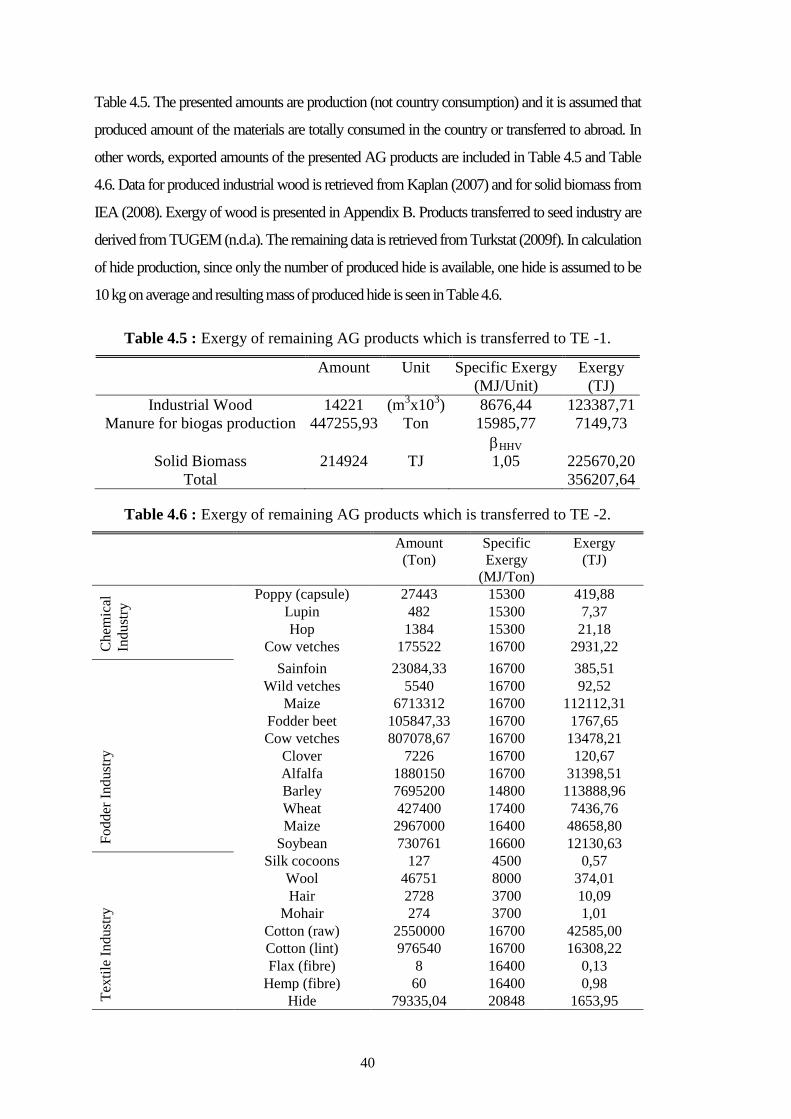
40
Table 4.5. The presented amounts are production (not country consumption) and it is assumed that
produced amount of the materials are totally consumed in the country or transferred to abroad. In
other words, exported amounts of the presented AG products are included in Table 4.5 and Table
4.6. Data for produced industrial wood is retrieved from Kaplan (2007) and for solid biomass from
IEA (2008). Exergy of wood is presented in Appendix B. Products transferred to seed industry are
derived from TUGEM (n.d.a). The remaining data is retrieved from Turkstat (2009f). In calculation
of hide production, since only the number of produced hide is available, one hide is assumed to be
10 kg on average and resulting mass of produced hide is seen in Table 4.6.
Table 4.5 : Exergy of remaining AG products which is transferred to TE -1.
Amount Unit Specific Exergy
(MJ/Unit)
Exergy
(TJ)
Industrial Wood 14221 (m3x10
3) 8676,44 123387,71
Manure for biogas production 447255,93 Ton 15985,77 7149,73
HHV
Solid Biomass 214924 TJ 1,05
225670,20
Total 356207,64
Table 4.6 : Exergy of remaining AG products which is transferred to TE -2.
Amount
(Ton)
Specific
Exergy
(MJ/Ton)
Exergy
(TJ)
Chem
ical
Indust
ry
Poppy (capsule) 27443 15300 419,88
Lupin 482 15300 7,37
Hop 1384 15300 21,18
Cow vetches 175522 16700 2931,22
Fo
dd
er I
nd
ust
ry
Sainfoin 23084,33 16700 385,51
Wild vetches 5540 16700 92,52
Maize 6713312 16700 112112,31
Fodder beet 105847,33 16700 1767,65
Cow vetches 807078,67 16700 13478,21
Clover 7226 16700 120,67
Alfalfa 1880150 16700 31398,51
Barley 7695200 14800 113888,96
Wheat 427400 17400 7436,76
Maize 2967000 16400 48658,80
Soybean 730761 16600 12130,63
Tex
tile
In
dust
ry
Silk cocoons 127 4500 0,57
Wool 46751 8000 374,01
Hair 2728 3700 10,09
Mohair 274 3700 1,01
Cotton (raw) 2550000 16700 42585,00
Cotton (lint) 976540 16700 16308,22
Flax (fibre) 8 16400 0,13
Hemp (fibre) 60 16400 0,98
Hide 79335,04 20848 1653,95
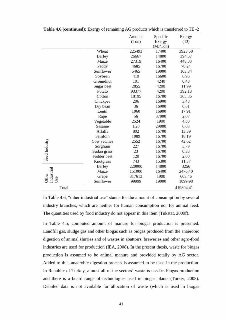
41
Table 4.6 (continued): Exergy of remaining AG products which is transferred to TE -2
Amount
(Ton)
Specific
Exergy
(MJ/Ton)
Exergy
(TJ) S
eed I
ndust
ry
Wheat 225493 17400 3923,58
Barley 26667 14800 394,67
Maize 27319 16400 448,03
Paddy 4685 16700 78,24
Sunflower 5465 19000 103,84
Soybean 419 16600 6,96
Groundnut 101 4240 0,43
Sugar beet 2855 4200 11,99
Potato 93377 4200 392,18
Cotton 18195 16700 303,86
Chickpea 206 16900 3,48
Dry bean 36 16900 0,61
Lentil 1060 16900 17,91
Rape 56 37000 2,07
Vegetable 2524 1900 4,80
Sesame 1,20 29000 0,03
Alfalfa 802 16700 13,39
Sainfoin 1089 16700 18,19
Cow vetches 2552 16700 42,62
Sorghum 227 16700 3,79
Sudan grass 23 16700 0,38
Fodder beet 120 16700 2,00
Knotgrass 743 15300 11,37
Oth
er
Indust
rial
Use
Barley 220000 14800 3256
Maize 151000 16400 2476,40
Grape 317613 1900 603,46
Sunflower 99999 19000 1899,98
Total 419804,41
In Table 4.6, “other industrial use” stands for the amount of consumption by several
industry branches, which are neither for human consumption nor for animal feed.
The quantities used by food industry do not appear in this item (Tukstat, 2009f).
In Table 4.5, computed amount of manure for biogas production is presented.
Landfill gas, sludge gas and other biogas such as biogas produced from the anaerobic
digestion of animal slurries and of wastes in abattoirs, breweries and other agro-food
industries are used for production (IEA, 2008). In the present thesis, waste for biogas
production is assumed to be animal manure and provided totally by AG sector.
Added to this, anaerobic digestion process is assumed to be used in the production.
In Republic of Turkey, almost all of the sectors’ waste is used in biogas production
and there is a board range of technologies used in biogas plants (Turker, 2008).
Detailed data is not available for allocation of waste (which is used in biogas
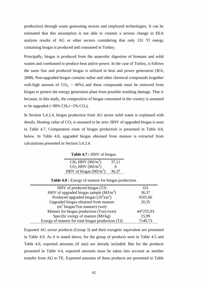
42
production) through waste generating sectors and employed technologies. It can be
estimated that this assumption is not able to commit a serious change in EEA
analysis results of AG or other sectors considering that only 331 TJ energy
containing biogas is produced and consumed in Turkey.
Principally, biogas is produced from the anaerobic digestion of biomass and solid
wastes and combusted to produce heat and/or power. In the case of Turkey, it follows
the same line and produced biogas is utilized in heat and power generation (IEA,
2008). Non-upgraded biogas contains sulfur and other chemical compounds (together
with high amount of CO2, ~ 40%) and these compounds must be removed from
biogas to protect the energy generation plant from possible resulting damage. That is
because, in this study, the composition of biogas consumed in the country is assumed
to be upgraded (~98% CH4+~2% CO2).
In Section 5.4.2.4, biogas production from AG sector solid waste is explained with
details. Heating value of CO2 is assumed to be zero. HHV of upgraded biogas is seen
in Table 4.7. Computation route of biogas production is presented in Table 4.8,
below. In Table 4.8, upgraded biogas obtained from manure is extracted from
calculations presented in Section 5.4.2.4.
Table 4.7 : HHV of biogas.
CH4 HHV (MJ/m3) 37,11
CO2 HHV (MJ/m3) 0
HHV of biogas (MJ/m3) 36,37
Table 4.8 : Exergy of manure for biogas production.
HHV of produced biogas (TJ) 331
HHV of upgraded biogas sample (MJ/m3) 36,37
Produced upgraded biogas (103xm
3) 9101,66
Upgraded biogas obtained from manure
(m3 biogas/Ton manure) (wet)
20,35
Manure for biogas production (Ton) (wet) 447255,93
Specific exergy of manure (MJ/kg) 15,99
Exergy of manure for total biogas production (TJ) 7149,73
Exported AG sector products (Group 3) and their exergetic equivalent are presented
in Table 4.9. As it is stated above, for the group of products seen in Table 4.5 and
Table 4.6, exported amounts (if any) are already included. But for the products
presented in Table 4.4, exported amounts must be taken into account as another
transfer from AG to TE. Exported amounts of these products are presented in Table
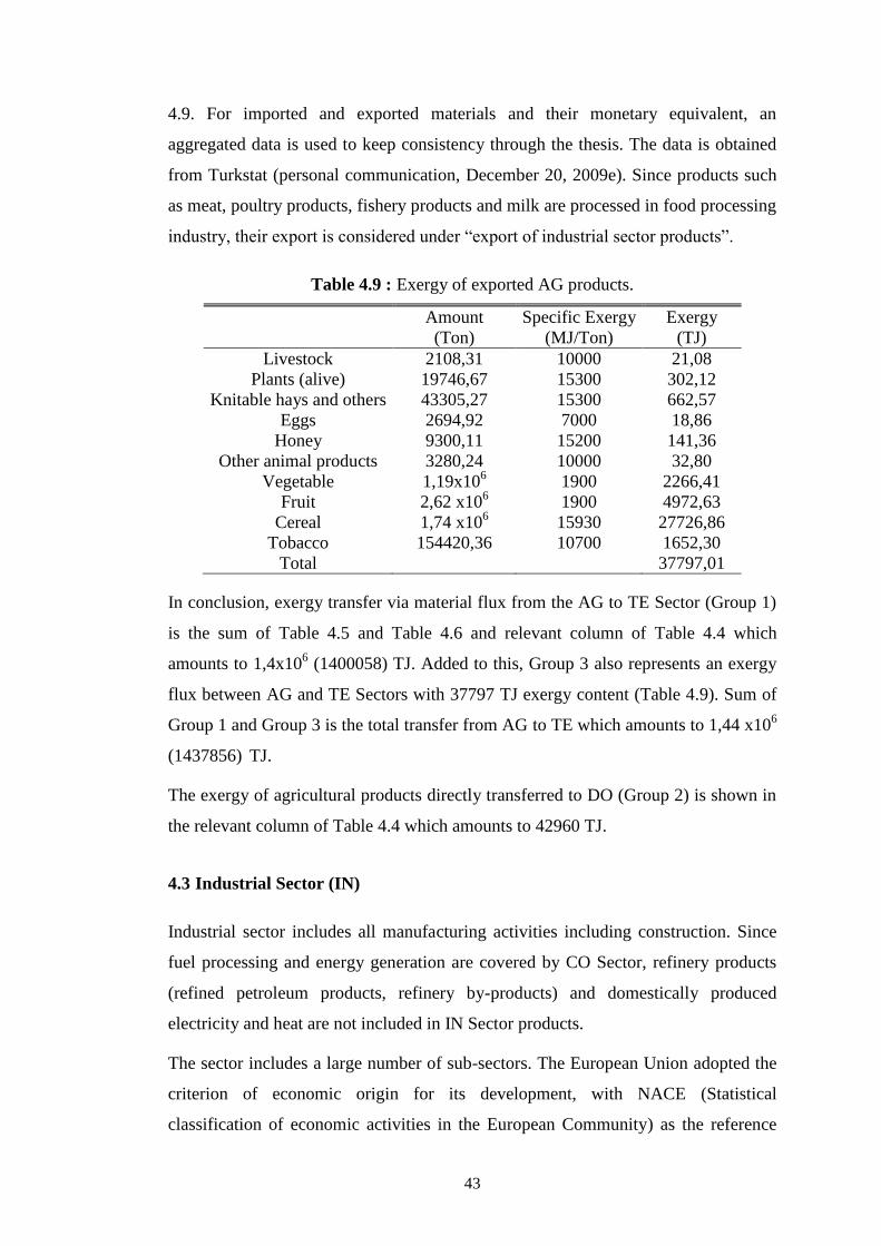
43
4.9. For imported and exported materials and their monetary equivalent, an
aggregated data is used to keep consistency through the thesis. The data is obtained
from Turkstat (personal communication, December 20, 2009e). Since products such
as meat, poultry products, fishery products and milk are processed in food processing
industry, their export is considered under “export of industrial sector products”.
Table 4.9 : Exergy of exported AG products.
Amount
(Ton)
Specific Exergy
(MJ/Ton)
Exergy
(TJ)
Livestock 2108,31 10000 21,08
Plants (alive) 19746,67 15300 302,12
Knitable hays and others 43305,27 15300 662,57
Eggs 2694,92 7000 18,86
Honey 9300,11 15200 141,36
Other animal products 3280,24 10000 32,80
Vegetable 1,19x10⁶
1900 2266,41
Fruit 2,62 x10⁶ 1900 4972,63
Cereal 1,74 x10⁶ 15930 27726,86
Tobacco 154420,36 10700 1652,30
Total 37797,01
In conclusion, exergy transfer via material flux from the AG to TE Sector (Group 1)
is the sum of Table 4.5 and Table 4.6 and relevant column of Table 4.4 which
amounts to 1,4x10⁶ (1400058) TJ. Added to this, Group 3 also represents an exergy
flux between AG and TE Sectors with 37797 TJ exergy content (Table 4.9). Sum of
Group 1 and Group 3 is the total transfer from AG to TE which amounts to 1,44 x10⁶
(1437856) TJ.
The exergy of agricultural products directly transferred to DO (Group 2) is shown in
the relevant column of Table 4.4 which amounts to 42960 TJ.
4.3 Industrial Sector (IN)
Industrial sector includes all manufacturing activities including construction. Since
fuel processing and energy generation are covered by CO Sector, refinery products
(refined petroleum products, refinery by-products) and domestically produced
electricity and heat are not included in IN Sector products.
The sector includes a large number of sub-sectors. The European Union adopted the
criterion of economic origin for its development, with NACE (Statistical
classification of economic activities in the European Community) as the reference
44
framework. Industrial sector is examined according to NACE Revision 2
classification of industrial sector divisions (sub-industries, sub-sectors) and the list of
the sectoral divisions is presented below (Eurostat, 2008). As it is reasoned above,
the division of “Manufacture of coke and refined petroleum products” is excluded
from the list of the industrial sector divisions.
Manufacture of food products
Manufacture of beverages
Manufacture of tobacco products
Manufacture of textiles
Manufacture of wearing apparel
Manufacture of leather and related products
Manufacture of wood and of products of wood and cork, except furniture;
manufacture of articles of straw and plaiting materials
Manufacture of paper and paper products
Printing and reproduction of recorded media
Manufacture of chemicals and chemical products
Manufacture of basic pharmaceutical products and pharmaceutical preparations
Manufacture of rubber and plastic products
Manufacture of other non-metallic mineral products
Manufacture of basic metals
Manufacture of fabricated metal products, except machinery and equipment
Manufacture of computer, electronic and optical products
Manufacture of electrical equipment
Manufacture of machinery and equipment
Manufacture of motor vehicles, trailers and semi-trailers
Manufacture of other transport equipment
Manufacture of furniture
45
Other manufacturing
Repair and installation of machinery and equipment
IN includes a large spectrum of manufacturing activities generating a broad range of
products. The largest industries are: food processing, textile, wood, paper, iron and steel,
nonferrous metal and chemical industries. To avoid double accounting, consumed raw
materials (which are further over and over processed and convert into products of IN
Sector) are regarded as the output of IN. In order to do this, within the limits of national
data, “domestic production+import-export” of the raw materials are computed or -if data
is available- directly published raw material consumption is used.
In this thesis, “food processing industry” (also named “food industry”) covers
manufacturing of food products, beverages and tobacco products, seed industry is also
comprised in food industry. According to NACE Revision 2, manufacture of prepared
animal feeds is also included in this division of industrial activity.
As for food industry and textile industry, because sufficiently disaggregated data
about the products of the sector were not available, the exergy input in a single
technological line is assumed to be equal to the exergy of the products of that
line. It is tantamount to taking into account only the mass-flow rate losses
(material waste) of the processes, and additionally assuming that the processes
employed in production lines urge no physical or chemical conversion which
substantially modifies chemical or physical exergy of the inputs (raw materials
entering the processes). As a special example to explain this approach, assume
that X ton/year of cotton is delivered to the textile industry: the total input exergy
will be [X.Ecotton] (J/year). If the cumulative mass flow rate of cotton apparel
(shirts, jeans, cloth, skirts, towels, etc.) is [X], [(1-X] is being the wasted
material, then the total exergy assigned to the output is [X.Ecotton]. In this study,
the factor for food processing and textile industries is estimated to be equal to
0,9 (Ertesvag, 2005). In other words, 10% of the input mass flow is assumed not
to be incorporated in the final form of the sub-sectoral products and included in
the IN sector solid waste.
As it is stated earlier, TE sector is the collection and distribution hub of the
model and transfers raw materials to IN sector to be used as the feedstock in
industrial production. Details are presented later in the Section dedicated to TE
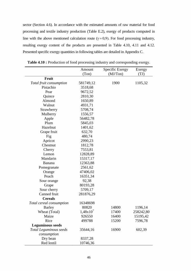
46
sector (Section 4.6). In accordance with the estimated amounts of raw material for food
processing and textile industry production (Table E.2), exergy of products computed in
line with the above mentioned calculation route (. For food processing industry,
resulting exergy content of the products are presented in Table 4.10, 4.11 and 4.12.
Presented specific exergy quantities in following tables are detailed in Appendix C.
Table 4.10 : Production of food processing industry and corresponding exergy.
Amount
(Ton)
Specific Exergy
(MJ/Ton)
Exergy
(TJ)
Fruit
Total fruit consumption 581749,12 1900 1105,32
Pistachio 3518,68
Pear 9672,52
Quince 2810,30
Almond 1650,89
Walnut 4931,71
Strawberry 5708,74
Mulberry 1556,57
Apple 56482,78
Plum 5845,03
Hazelnut 1401,62
Grape fruit 632,70
Fig 480,74
Apricot 2990,23
Chestnut 1812,78
Cherry 7553,81
Lemon 12828,89
Mandarin 15317,17
Banana 12363,88
Pomegranate 2561,62
Orange 47406,02
Peach 16351,34
Sour orange 92,38
Grape 80193,28
Sour cherry 5709,17
Canned fruit 281876,29
Cereals
Total cereal consumption 16348698
Barley 80820 14800 1196,14
Wheat (Total) 1,48x10⁷
17400 258242,80
Maize 926550 16400 15195,42
Rice 499788 15200 7596,78
Leguminous seeds
Total Leguminous seeds
consumption
35644,16 16900 602,39
Dry bean 8337,28
Red lentil 10746,36
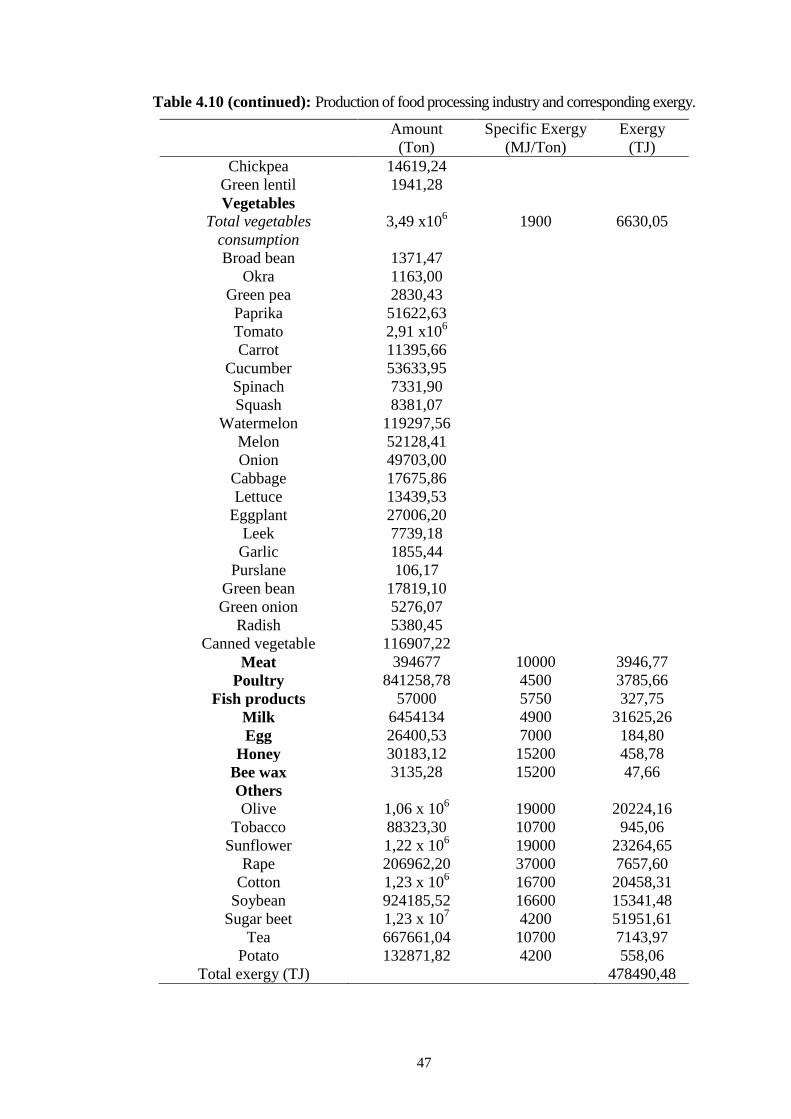
47
Table 4.10 (continued): Production of food processing industry and corresponding exergy.
Amount
(Ton)
Specific Exergy
(MJ/Ton)
Exergy
(TJ)
Chickpea 14619,24
Green lentil 1941,28
Vegetables
Total vegetables
consumption
3,49 x10⁶ 1900 6630,05
Broad bean 1371,47
Okra 1163,00
Green pea 2830,43
Paprika 51622,63
Tomato 2,91 x10⁶
Carrot 11395,66
Cucumber 53633,95
Spinach 7331,90
Squash 8381,07
Watermelon 119297,56
Melon 52128,41
Onion 49703,00
Cabbage 17675,86
Lettuce 13439,53
Eggplant 27006,20
Leek 7739,18
Garlic 1855,44
Purslane 106,17
Green bean 17819,10
Green onion 5276,07
Radish 5380,45
Canned vegetable 116907,22
Meat 394677 10000 3946,77
Poultry 841258,78 4500 3785,66
Fish products 57000 5750 327,75
Milk 6454134 4900 31625,26
Egg 26400,53 7000 184,80
Honey 30183,12 15200 458,78
Bee wax 3135,28 15200 47,66
Others
Olive 1,06 x 10⁶
19000 20224,16
Tobacco 88323,30 10700 945,06
Sunflower 1,22 x 10⁶ 19000 23264,65
Rape 206962,20 37000 7657,60
Cotton 1,23 x 10⁶ 16700 20458,31
Soybean 924185,52 16600 15341,48
Sugar beet 1,23 x 10⁷ 4200 51951,61
Tea 667661,04 10700 7143,97
Potato 132871,82 4200 558,06
Total exergy (TJ) 478490,48
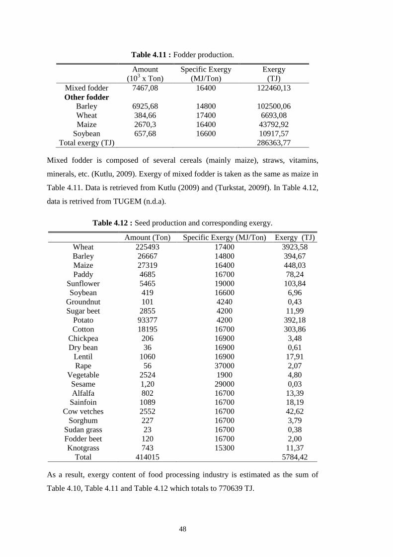
48
Table 4.11 : Fodder production.
Amount
(103 x Ton)
Specific Exergy
(MJ/Ton)
Exergy
(TJ)
Mixed fodder 7467,08 16400 122460,13
Other fodder
Barley 6925,68 14800 102500,06
Wheat 384,66 17400 6693,08
Maize 2670,3 16400 43792,92
Soybean 657,68 16600 10917,57
Total exergy (TJ) 286363,77
Mixed fodder is composed of several cereals (mainly maize), straws, vitamins,
minerals, etc. (Kutlu, 2009). Exergy of mixed fodder is taken as the same as maize in
Table 4.11. Data is retrieved from Kutlu (2009) and (Turkstat, 2009f). In Table 4.12,
data is retrived from TUGEM (n.d.a).
Table 4.12 : Seed production and corresponding exergy.
Amount (Ton) Specific Exergy (MJ/Ton) Exergy (TJ)
Wheat 225493 17400 3923,58
Barley 26667 14800 394,67
Maize 27319 16400 448,03
Paddy 4685 16700 78,24
Sunflower 5465 19000 103,84
Soybean 419 16600 6,96
Groundnut 101 4240 0,43
Sugar beet 2855 4200 11,99
Potato 93377 4200 392,18
Cotton 18195 16700 303,86
Chickpea 206 16900 3,48
Dry bean 36 16900 0,61
Lentil 1060 16900 17,91
Rape 56 37000 2,07
Vegetable 2524 1900 4,80
Sesame 1,20 29000 0,03
Alfalfa 802 16700 13,39
Sainfoin 1089 16700 18,19
Cow vetches 2552 16700 42,62
Sorghum 227 16700 3,79
Sudan grass 23 16700 0,38
Fodder beet 120 16700 2,00
Knotgrass 743 15300 11,37
Total 414015
5784,42
As a result, exergy content of food processing industry is estimated as the sum of
Table 4.10, Table 4.11 and Table 4.12 which totals to 770639 TJ.
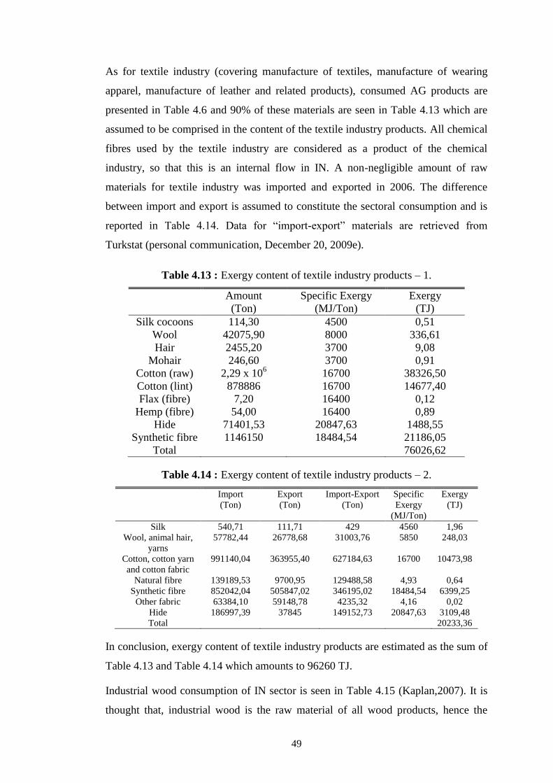
49
As for textile industry (covering manufacture of textiles, manufacture of wearing
apparel, manufacture of leather and related products), consumed AG products are
presented in Table 4.6 and 90% of these materials are seen in Table 4.13 which are
assumed to be comprised in the content of the textile industry products. All chemical
fibres used by the textile industry are considered as a product of the chemical
industry, so that this is an internal flow in IN. A non-negligible amount of raw
materials for textile industry was imported and exported in 2006. The difference
between import and export is assumed to constitute the sectoral consumption and is
reported in Table 4.14. Data for “import-export” materials are retrieved from
Turkstat (personal communication, December 20, 2009e).
Table 4.13 : Exergy content of textile industry products – 1.
Amount
(Ton)
Specific Exergy
(MJ/Ton)
Exergy
(TJ)
Silk cocoons 114,30 4500 0,51
Wool 42075,90 8000 336,61
Hair 2455,20 3700 9,08
Mohair 246,60 3700 0,91
Cotton (raw) 2,29 x 10⁶ 16700 38326,50
Cotton (lint) 878886 16700 14677,40
Flax (fibre) 7,20 16400 0,12
Hemp (fibre) 54,00 16400 0,89
Hide 71401,53 20847,63 1488,55
Synthetic fibre 1146150 18484,54 21186,05
Total 76026,62
Table 4.14 : Exergy content of textile industry products – 2.
Import
(Ton)
Export
(Ton)
Import-Export
(Ton)
Specific
Exergy
(MJ/Ton)
Exergy
(TJ)
Silk 540,71 111,71 429 4560 1,96
Wool, animal hair,
yarns
57782,44 26778,68 31003,76 5850 248,03
Cotton, cotton yarn
and cotton fabric
991140,04 363955,40 627184,63 16700 10473,98
Natural fibre 139189,53 9700,95 129488,58 4,93 0,64
Synthetic fibre 852042,04 505847,02 346195,02 18484,54 6399,25
Other fabric 63384,10 59148,78 4235,32 4,16 0,02
Hide 186997,39 37845 149152,73 20847,63 3109,48
Total 20233,36
In conclusion, exergy content of textile industry products are estimated as the sum of
Table 4.13 and Table 4.14 which amounts to 96260 TJ.
Industrial wood consumption of IN sector is seen in Table 4.15 (Kaplan,2007). It is
thought that, industrial wood is the raw material of all wood products, hence the
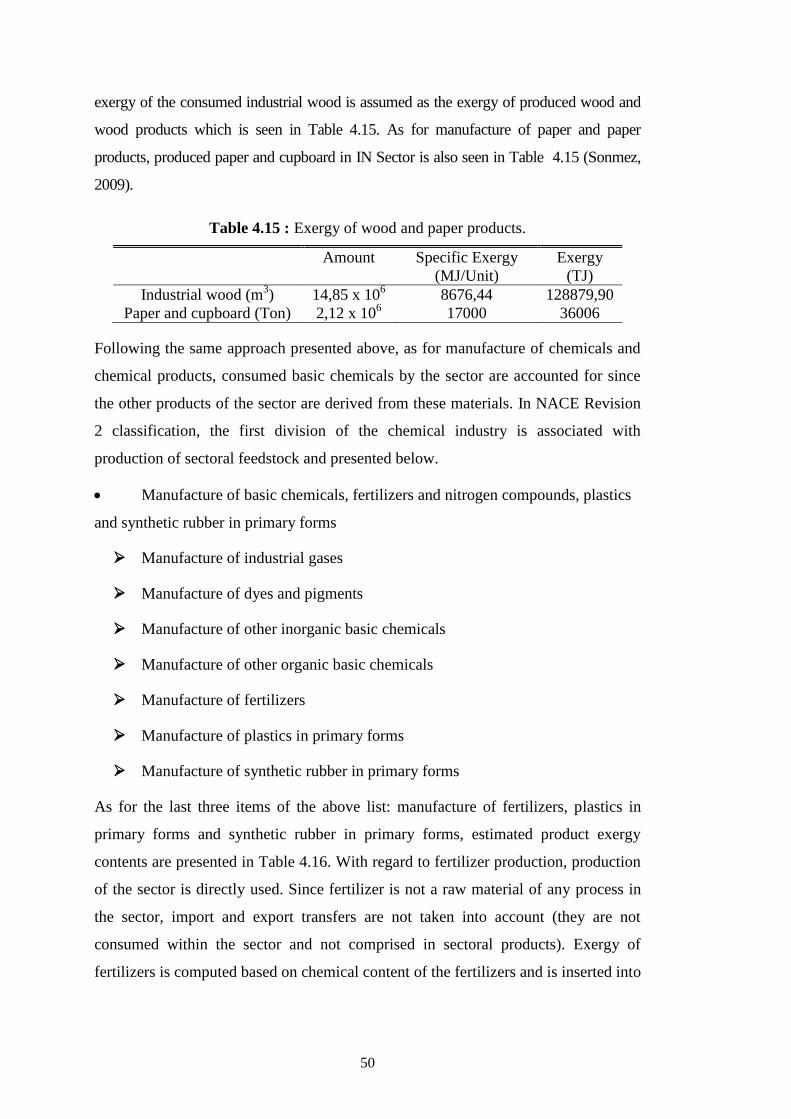
50
exergy of the consumed industrial wood is assumed as the exergy of produced wood and
wood products which is seen in Table 4.15. As for manufacture of paper and paper
products, produced paper and cupboard in IN Sector is also seen in Table 4.15 (Sonmez,
2009).
Table 4.15 : Exergy of wood and paper products.
Amount Specific Exergy
(MJ/Unit)
Exergy
(TJ)
Industrial wood (m3) 14,85 x 10
6 8676,44 128879,90
Paper and cupboard (Ton) 2,12 x 10⁶ 17000 36006
Following the same approach presented above, as for manufacture of chemicals and
chemical products, consumed basic chemicals by the sector are accounted for since
the other products of the sector are derived from these materials. In NACE Revision
2 classification, the first division of the chemical industry is associated with
production of sectoral feedstock and presented below.
Manufacture of basic chemicals, fertilizers and nitrogen compounds, plastics
and synthetic rubber in primary forms
Manufacture of industrial gases
Manufacture of dyes and pigments
Manufacture of other inorganic basic chemicals
Manufacture of other organic basic chemicals
Manufacture of fertilizers
Manufacture of plastics in primary forms
Manufacture of synthetic rubber in primary forms
As for the last three items of the above list: manufacture of fertilizers, plastics in
primary forms and synthetic rubber in primary forms, estimated product exergy
contents are presented in Table 4.16. With regard to fertilizer production, production
of the sector is directly used. Since fertilizer is not a raw material of any process in
the sector, import and export transfers are not taken into account (they are not
consumed within the sector and not comprised in sectoral products). Exergy of
fertilizers is computed based on chemical content of the fertilizers and is inserted into
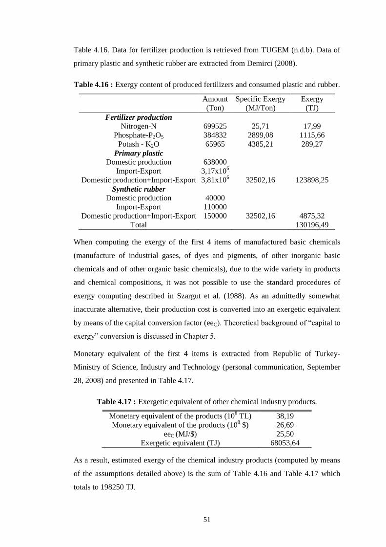
51
Table 4.16. Data for fertilizer production is retrieved from TUGEM (n.d.b). Data of
primary plastic and synthetic rubber are extracted from Demirci (2008).
Table 4.16 : Exergy content of produced fertilizers and consumed plastic and rubber.
Amount
(Ton)
Specific Exergy
(MJ/Ton)
Exergy
(TJ)
Fertilizer production
Nitrogen-N 699525 25,71 17,99
Phosphate-P2O5 384832 2899,08 1115,66
Potash - K2O 65965 4385,21 289,27
Primary plastic
Domestic production 638000
Import-Export 3,17x10⁶
Domestic production+Import-Export 3,81x10⁶ 32502,16 123898,25
Synthetic rubber
Domestic production 40000
Import-Export 110000
Domestic production+Import-Export 150000 32502,16 4875,32
Total 130196,49
When computing the exergy of the first 4 items of manufactured basic chemicals
(manufacture of industrial gases, of dyes and pigments, of other inorganic basic
chemicals and of other organic basic chemicals), due to the wide variety in products
and chemical compositions, it was not possible to use the standard procedures of
exergy computing described in Szargut et al. (1988). As an admittedly somewhat
inaccurate alternative, their production cost is converted into an exergetic equivalent
by means of the capital conversion factor (eeC). Theoretical background of “capital to
exergy” conversion is discussed in Chapter 5.
Monetary equivalent of the first 4 items is extracted from Republic of Turkey-
Ministry of Science, Industry and Technology (personal communication, September
28, 2008) and presented in Table 4.17.
Table 4.17 : Exergetic equivalent of other chemical industry products.
Monetary equivalent of the products (108 TL) 38,19
Monetary equivalent of the products (108 $) 26,69
eeC (MJ/$) 25,50
Exergetic equivalent (TJ) 68053,64
As a result, estimated exergy of the chemical industry products (computed by means
of the assumptions detailed above) is the sum of Table 4.16 and Table 4.17 which
totals to 198250 TJ.
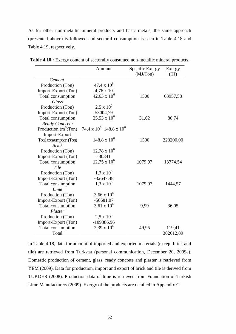
52
As for other non-metallic mineral products and basic metals, the same approach
(presented above) is followed and sectoral consumption is seen in Table 4.18 and
Table 4.19, respectively.
Table 4.18 : Exergy content of sectorally consumed non-metallic mineral products.
Amount Specific Exergy
(MJ/Ton)
Exergy
(TJ)
Cement
Production (Ton) 47,4 x 10⁶
Import-Export (Ton) -4,76 x 10⁶
Total consumption 42,63 x 10⁶ 1500 63957,58
Glass
Production (Ton) 2,5 x 10⁶
Import-Export (Ton) 53004,79
Total consumption 25,53 x 10⁶ 31,62 80,74
Ready Concrete
Production (m3;Ton) 74,4 x 10
6; 148,8 x 10
6
Import-Export
Total consumption (Ton) 148,8 x 10⁶ 1500 223200,00
Brick
Production (Ton) 12,78 x 10⁶
Import-Export (Ton) -30341
Total consumption 12,75 x 10⁶ 1079,97 13774,54
Tile
Production (Ton) 1,3 x 10⁶
Import-Export (Ton) -32647,48
Total consumption 1,3 x 10⁶ 1079,97 1444,57
Lime
Production (Ton) 3,66 x 10⁶
Import-Export (Ton) -56681,07
Total consumption 3,61 x 10⁶ 9,99 36,05
Plaster
Production (Ton) 2,5 x 10⁶
Import-Export (Ton) -109386,96
Total consumption 2,39 x 10⁶ 49,95 119,41
Total 302612,89
In Table 4.18, data for amount of imported and exported materials (except brick and
tile) are retrieved from Turkstat (personal communication, December 20, 2009e).
Domestic production of cement, glass, ready concrete and plaster is retrieved from
YEM (2009). Data for production, import and export of brick and tile is derived from
TUKDER (2008). Production data of lime is retrieved from Foundation of Turkish
Lime Manufacturers (2009). Exergy of the products are detailed in Appendix C.
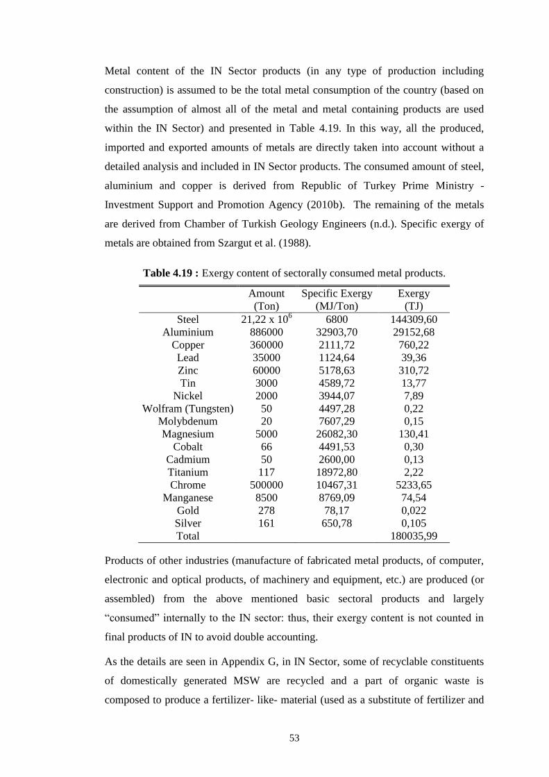
53
Metal content of the IN Sector products (in any type of production including
construction) is assumed to be the total metal consumption of the country (based on
the assumption of almost all of the metal and metal containing products are used
within the IN Sector) and presented in Table 4.19. In this way, all the produced,
imported and exported amounts of metals are directly taken into account without a
detailed analysis and included in IN Sector products. The consumed amount of steel,
aluminium and copper is derived from Republic of Turkey Prime Ministry -
Investment Support and Promotion Agency (2010b). The remaining of the metals
are derived from Chamber of Turkish Geology Engineers (n.d.). Specific exergy of
metals are obtained from Szargut et al. (1988).
Table 4.19 : Exergy content of sectorally consumed metal products.
Amount
(Ton)
Specific Exergy
(MJ/Ton)
Exergy
(TJ)
Steel 21,22 x 10⁶ 6800 144309,60
Aluminium 886000 32903,70 29152,68
Copper 360000 2111,72 760,22
Lead 35000 1124,64 39,36
Zinc 60000 5178,63 310,72
Tin 3000 4589,72 13,77
Nickel 2000 3944,07 7,89
Wolfram (Tungsten) 50 4497,28 0,22
Molybdenum 20 7607,29 0,15
Magnesium 5000 26082,30 130,41
Cobalt 66 4491,53 0,30
Cadmium 50 2600,00 0,13
Titanium 117 18972,80 2,22
Chrome 500000 10467,31 5233,65
Manganese 8500 8769,09 74,54
Gold 278 78,17 0,022
Silver 161 650,78 0,105
Total 180035,99
Products of other industries (manufacture of fabricated metal products, of computer,
electronic and optical products, of machinery and equipment, etc.) are produced (or
assembled) from the above mentioned basic sectoral products and largely
“consumed” internally to the IN sector: thus, their exergy content is not counted in
final products of IN to avoid double accounting.
As the details are seen in Appendix G, in IN Sector, some of recyclable constituents
of domestically generated MSW are recycled and a part of organic waste is
composed to produce a fertilizer- like- material (used as a substitute of fertilizer and
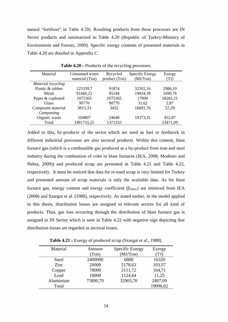
54
named “fertilizer” in Table 4.20). Resulting products from these processes are IN
Sector products and summarized in Table 4.20 (Republic of Turkey-Ministry of
Environment and Forests, 2009). Specific exergy contents of presented materials in
Table 4.20 are detailed in Appendix C.
Table 4.20 : Products of the recycling processes.
Material Consumed waste
material (Ton)
Recycled
product (Ton)
Specific Exergy
(MJ/Ton)
Exergy
(TJ)
Material recycling
Plastic & rubber 125339,7 91874 32502,16 2986,10
Metal 91660,22 85244 19834,39 1690,76
Paper & cupboard 1075365 1075365 17000 18281,21
Glass 90770 90770 31,62 2,87
Composite material 3813,33 3432 16691,76 57,29
Composting
Organic waste 104807 24648 18373,31 452,87
Total 1491755,25 1371333 23471,09
Added to this, by-products of the sector which are used as fuel or feedstock in
different industrial processes are also sectoral products. Within this content, blast
furnace gas (which is a combustible gas produced as a by-product from iron and steel
industry during the combustion of coke in blast furnaces (IEA, 2008; Modesto and
Nebra, 2009)) and produced scrap are presented in Table 4.21 and Table 4.22,
respectively. It must be noticed that data for re-used scrap is very limited for Turkey
and presented amount of scrap materials is only the available data. As for blast
furnace gas, energy content and exergy coefficient (HHV) are retrieved from IEA
(2008) and Szargut et al. (1988), respectively. As stated earlier, in the model applied
in this thesis, distribution losses are assigned to relevant sectors for all kind of
products. Thus, gas loss occurring through the distribution of blast furnace gas is
assigned to IN Sector which is seen in Table 4.22 with negative sign depicting that
distribution losses are regarded as sectoral losses.
Table 4.21 : Exergy of produced scrap (Szargut et al., 1988).
Material Amount
(Ton)
Specific Exergy
(MJ/Ton)
Exergy
(TJ)
Steel 2400000 6800 16320
Zinc 20000 5178,63 103,57
Copper 78000 2111,72 164,71
Lead 10000 1124,64 11,25
Aluminium 75890,70 32903,70 2497,09
Total 19096,62
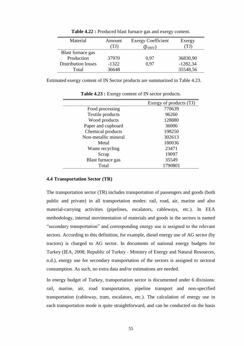
55
Table 4.22 : Produced blast furnace gas and exergy content.
Material Amount
(TJ)
Exergy Coefficient
(HHV)
Exergy
(TJ)
Blast furnace gas
Production 37970 0,97 36830,90
Distribution losses -1322 0,97 -1282,34
Total 36648 35548,56
Estimated exergy content of IN Sector products are summarized in Table 4.23.
Table 4.23 : Exergy content of IN sector products.
Exergy of products (TJ)
Food processing 770639
Textile products 96260
Wood products 128880
Paper and cupboard 36006
Chemical products 198250
Non-metallic mineral 302613
Metal 180036
Waste recycling 23471
Scrap 19097
Blast furnace gas 35549
Total 1790801
4.4 Transportation Sector (TR)
The transportation sector (TR) includes transportation of passengers and goods (both
public and private) in all transportation modes: rail, road, air, marine and also
material-carrying activities (pipelines, escalators, cableways, etc.). In EEA
methodology, internal movimentation of materials and goods in the sectors is named
“secondary transportation” and corresponding energy use is assigned to the relevant
sectors. According to this definition, for example, diesel energy use of AG sector (by
tractors) is charged to AG sector. In documents of national energy budgets for
Turkey (IEA, 2008; Republic of Turkey - Ministry of Energy and Natural Resources,
n.d.), energy use for secondary transportation of the sectors is assigned to sectoral
consumption. As such, no extra data and/or estimations are needed.
In energy budget of Turkey, transportation sector is documented under 6 divisions:
rail, marine, air, road transportation, pipeline transport and non-specified
transportation (cableway, tram, escalators, etc.). The calculation of energy use in
each transportation mode is quite straightforward, and can be conducted on the basis

56
of above referenced available national energy budgets. However, there is no
available data on allocation of fuel consumption in TR sector services (sectoral
output, sectoral product) to other sectors. Hence, some preliminary approximations
were necessary. Assumptions and resulting apportionment of fuel consumption
through transportation service receiving sectors are presented in Appendix D.
In Table D.1 (Appendix D), total transferred energy carriers consumed by TR sector
and total energy and exergy consumptions are reported. As it is seen in the Table
D.1, sum of exergy consumptions via energy carriers amounts to 663682,24 TJ
which also refers to EPHYS flow received by TR sector.
In transportation sector, the goal of electricity and fossil fuel consumption is
production of shaft work. Produced shaft power is work output of the transportation
system and by definition, equal to exergy. For electrically and fossil fuel propelled
vehicles, shaft work output is calculated by equations (4.1) and (4.2), respectively
(Saidur, 2007; Ediger and Camdali, 2007; Ji and Chen, 2006; Jaber et al., 2008).
For electrically propelled vehicles:
elIshaft Enx W (4.1)
For fossil fuel propelled vehicles:
ffIshaft mxEnx W (4.2)
where, Wshaft (J) is the shaft work;I is the first law efficiency of considered
transportation mode; Enel (J) is the electrical energy; Enf (J/Ton) is low heating value
(LHV) of fuel; mf (Ton/year) is fuel consumption.
The first law efficiency ( I) of road (Nakicenovic et al., 1996; CAA, 2009),
marine, air and rail (Nakicenovic et al., 1996) transportation modes are reported in
Table 4.24. For non-specified transportation, the prevailing energy carrier is
electricity and the efficiency is assumed to be 75% based on Nakicenovic et al.
(1996). Efficiency of pipeline transportation (operation of pipelines transporting of
gases, liquids and other commodities; pumping stations) is computed based on data
presented in Johnson (2010). Details are seen in equations (4.3) and (4.4).
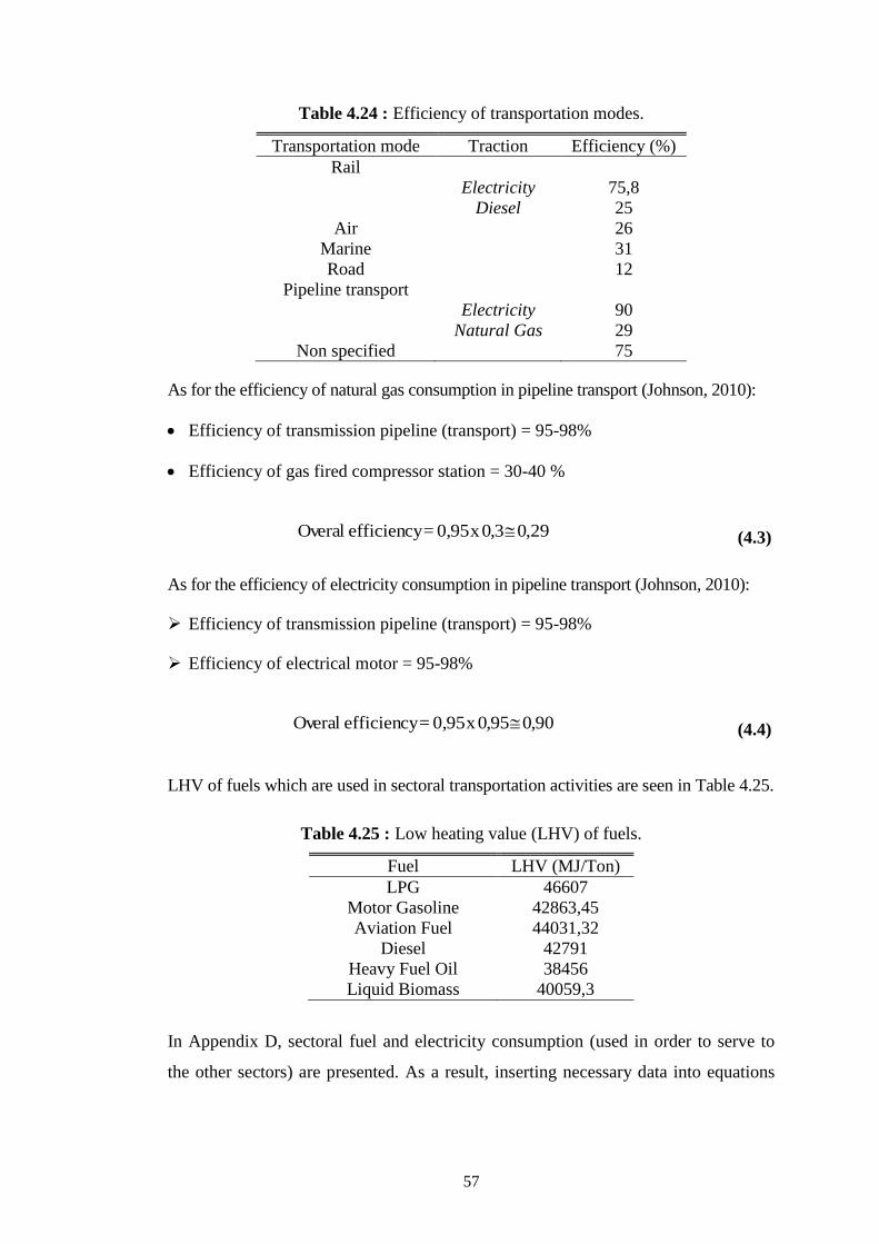
57
Table 4.24 : Efficiency of transportation modes.
Transportation mode Traction Efficiency (%)
Rail
Electricity 75,8
Diesel 25
Air
26
Marine
31
Road
12
Pipeline transport
Electricity 90
Natural Gas 29
Non specified
75
As for the efficiency of natural gas consumption in pipeline transport (Johnson, 2010):
Efficiency of transmission pipeline (transport) = 95-98%
Efficiency of gas fired compressor station = 30-40 %
29,03,0x0,95 =efficiency Overal (4.3)
As for the efficiency of electricity consumption in pipeline transport (Johnson, 2010):
Efficiency of transmission pipeline (transport) = 95-98%
Efficiency of electrical motor = 95-98%
90,095,0x0,95 =efficiency Overal (4.4)
LHV of fuels which are used in sectoral transportation activities are seen in Table 4.25.
Table 4.25 : Low heating value (LHV) of fuels.
Fuel LHV (MJ/Ton)
LPG 46607
Motor Gasoline 42863,45
Aviation Fuel 44031,32
Diesel 42791
Heavy Fuel Oil 38456
Liquid Biomass 40059,3
In Appendix D, sectoral fuel and electricity consumption (used in order to serve to
the other sectors) are presented. As a result, inserting necessary data into equations
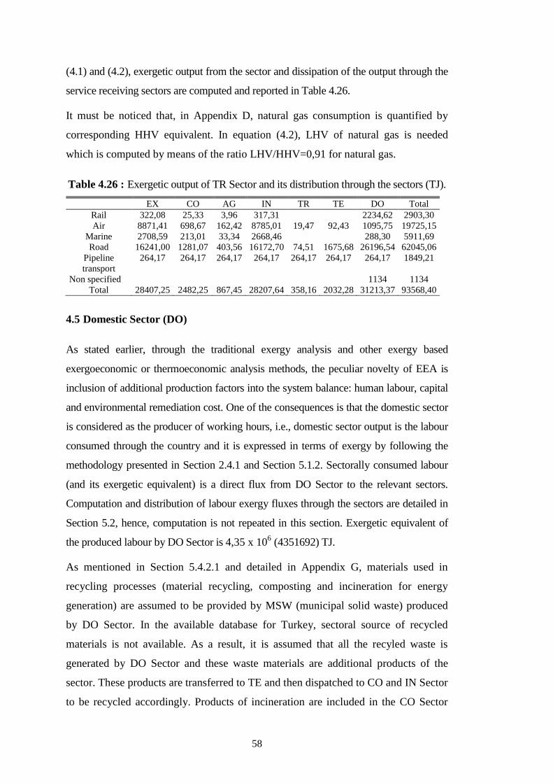
58
(4.1) and (4.2), exergetic output from the sector and dissipation of the output through the
service receiving sectors are computed and reported in Table 4.26.
It must be noticed that, in Appendix D, natural gas consumption is quantified by
corresponding HHV equivalent. In equation (4.2), LHV of natural gas is needed
which is computed by means of the ratio LHV/HHV=0,91 for natural gas.
Table 4.26 : Exergetic output of TR Sector and its distribution through the sectors (TJ).
EX CO AG IN TR TE DO Total
Rail 322,08 25,33 3,96 317,31 2234,62 2903,30
Air 8871,41 698,67 162,42 8785,01 19,47 92,43 1095,75 19725,15
Marine 2708,59 213,01 33,34 2668,46 288,30 5911,69
Road 16241,00 1281,07 403,56 16172,70 74,51 1675,68 26196,54 62045,06
Pipeline
transport
264,17 264,17 264,17 264,17 264,17 264,17 264,17 1849,21
Non specified 1134 1134
Total 28407,25 2482,25 867,45 28207,64 358,16 2032,28 31213,37 93568,40
4.5 Domestic Sector (DO)
As stated earlier, through the traditional exergy analysis and other exergy based
exergoeconomic or thermoeconomic analysis methods, the peculiar novelty of EEA is
inclusion of additional production factors into the system balance: human labour, capital
and environmental remediation cost. One of the consequences is that the domestic sector
is considered as the producer of working hours, i.e., domestic sector output is the labour
consumed through the country and it is expressed in terms of exergy by following the
methodology presented in Section 2.4.1 and Section 5.1.2. Sectorally consumed labour
(and its exergetic equivalent) is a direct flux from DO Sector to the relevant sectors.
Computation and distribution of labour exergy fluxes through the sectors are detailed in
Section 5.2, hence, computation is not repeated in this section. Exergetic equivalent of
the produced labour by DO Sector is 4,35 x 10⁶ (4351692) TJ.
As mentioned in Section 5.4.2.1 and detailed in Appendix G, materials used in
recycling processes (material recycling, composting and incineration for energy
generation) are assumed to be provided by MSW (municipal solid waste) produced
by DO Sector. In the available database for Turkey, sectoral source of recycled
materials is not available. As a result, it is assumed that all the recyled waste is
generated by DO Sector and these waste materials are additional products of the
sector. These products are transferred to TE and then dispatched to CO and IN Sector
to be recycled accordingly. Products of incineration are included in the CO Sector
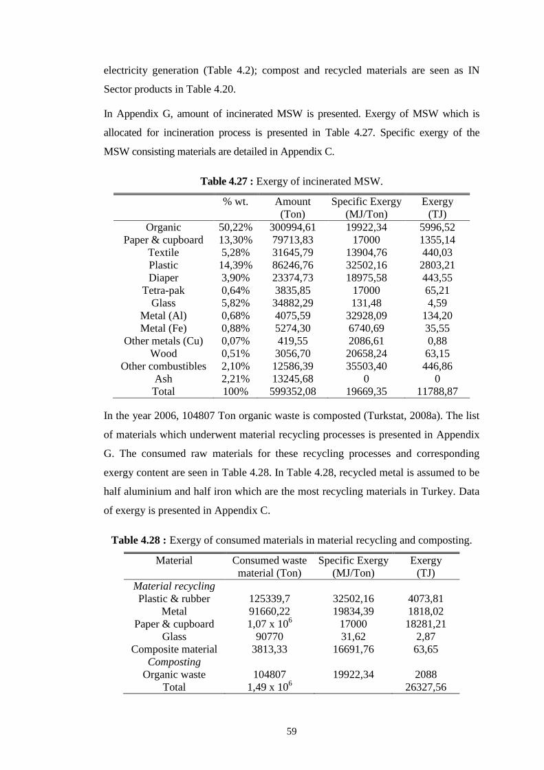
59
electricity generation (Table 4.2); compost and recycled materials are seen as IN
Sector products in Table 4.20.
In Appendix G, amount of incinerated MSW is presented. Exergy of MSW which is
allocated for incineration process is presented in Table 4.27. Specific exergy of the
MSW consisting materials are detailed in Appendix C.
Table 4.27 : Exergy of incinerated MSW.
% wt. Amount
(Ton)
Specific Exergy
(MJ/Ton)
Exergy
(TJ)
Organic 50,22% 300994,61 19922,34 5996,52
Paper & cupboard 13,30% 79713,83 17000 1355,14
Textile 5,28% 31645,79 13904,76 440,03
Plastic 14,39% 86246,76 32502,16 2803,21
Diaper 3,90% 23374,73 18975,58 443,55
Tetra-pak 0,64% 3835,85 17000 65,21
Glass 5,82% 34882,29 131,48 4,59
Metal (Al) 0,68% 4075,59 32928,09 134,20
Metal (Fe) 0,88% 5274,30 6740,69 35,55
Other metals (Cu) 0,07% 419,55 2086,61 0,88
Wood 0,51% 3056,70 20658,24 63,15
Other combustibles 2,10% 12586,39 35503,40 446,86
Ash 2,21% 13245,68 0 0
Total 100% 599352,08 19669,35 11788,87
In the year 2006, 104807 Ton organic waste is composted (Turkstat, 2008a). The list
of materials which underwent material recycling processes is presented in Appendix
G. The consumed raw materials for these recycling processes and corresponding
exergy content are seen in Table 4.28. In Table 4.28, recycled metal is assumed to be
half aluminium and half iron which are the most recycling materials in Turkey. Data
of exergy is presented in Appendix C.
Table 4.28 : Exergy of consumed materials in material recycling and composting.
Material Consumed waste
material (Ton)
Specific Exergy
(MJ/Ton)
Exergy
(TJ)
Material recycling
Plastic & rubber 125339,7 32502,16 4073,81
Metal 91660,22 19834,39 1818,02
Paper & cupboard 1,07 x 10⁶ 17000 18281,21
Glass 90770 31,62 2,87
Composite material 3813,33 16691,76 63,65
Composting
Organic waste 104807 19922,34 2088
Total 1,49 x 10⁶ 26327,56
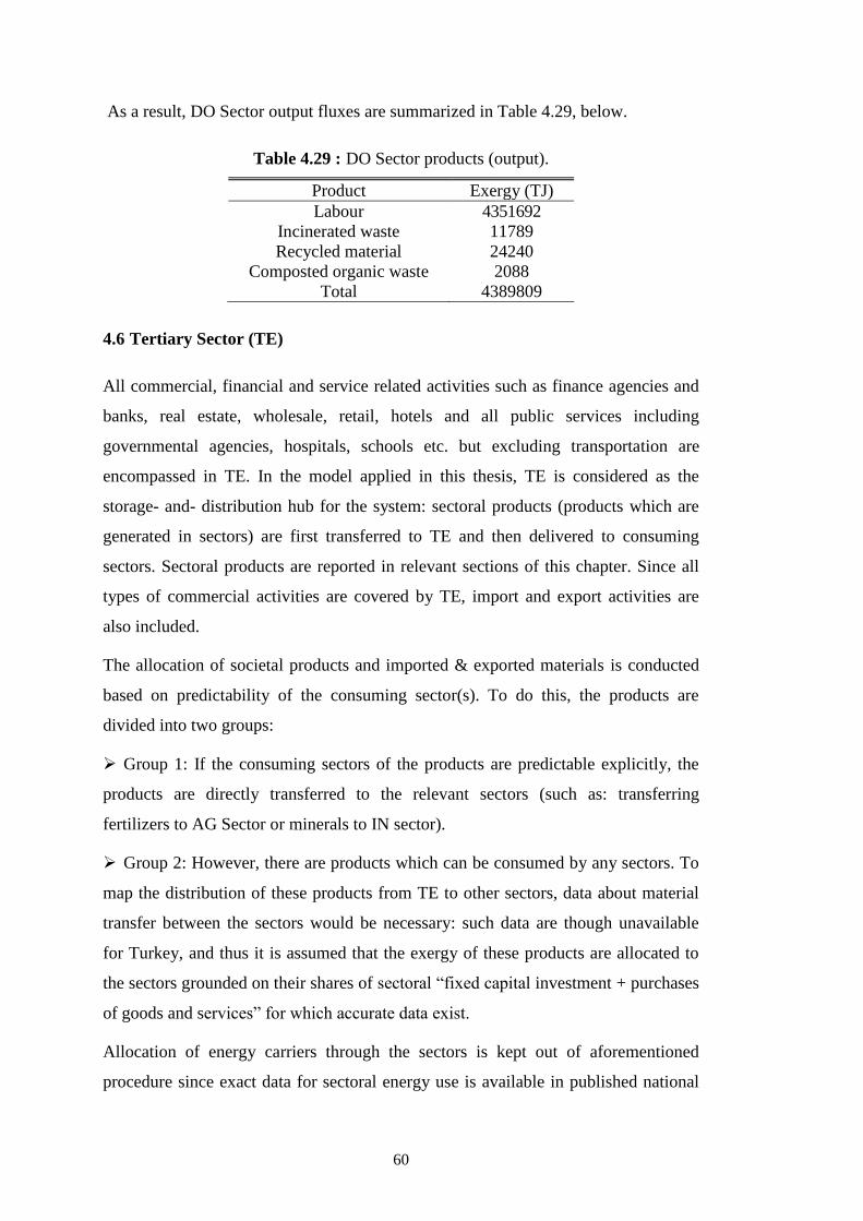
60
As a result, DO Sector output fluxes are summarized in Table 4.29, below.
Table 4.29 : DO Sector products (output).
Product Exergy (TJ)
Labour 4351692
Incinerated waste 11789
Recycled material 24240
Composted organic waste 2088
Total 4389809
4.6 Tertiary Sector (TE)
All commercial, financial and service related activities such as finance agencies and
banks, real estate, wholesale, retail, hotels and all public services including
governmental agencies, hospitals, schools etc. but excluding transportation are
encompassed in TE. In the model applied in this thesis, TE is considered as the
storage- and- distribution hub for the system: sectoral products (products which are
generated in sectors) are first transferred to TE and then delivered to consuming
sectors. Sectoral products are reported in relevant sections of this chapter. Since all
types of commercial activities are covered by TE, import and export activities are
also included.
The allocation of societal products and imported & exported materials is conducted
based on predictability of the consuming sector(s). To do this, the products are
divided into two groups:
Group 1: If the consuming sectors of the products are predictable explicitly, the
products are directly transferred to the relevant sectors (such as: transferring
fertilizers to AG Sector or minerals to IN sector).
Group 2: However, there are products which can be consumed by any sectors. To
map the distribution of these products from TE to other sectors, data about material
transfer between the sectors would be necessary: such data are though unavailable
for Turkey, and thus it is assumed that the exergy of these products are allocated to
the sectors grounded on their shares of sectoral “fixed capital investment + purchases
of goods and services” for which accurate data exist.
Allocation of energy carriers through the sectors is kept out of aforementioned
procedure since exact data for sectoral energy use is available in published national
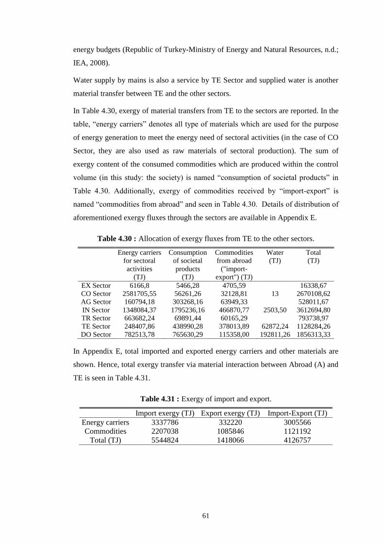
61
energy budgets (Republic of Turkey-Ministry of Energy and Natural Resources, n.d.;
IEA, 2008).
Water supply by mains is also a service by TE Sector and supplied water is another
material transfer between TE and the other sectors.
In Table 4.30, exergy of material transfers from TE to the sectors are reported. In the
table, “energy carriers” denotes all type of materials which are used for the purpose
of energy generation to meet the energy need of sectoral activities (in the case of CO
Sector, they are also used as raw materials of sectoral production). The sum of
exergy content of the consumed commodities which are produced within the control
volume (in this study: the society) is named “consumption of societal products” in
Table 4.30. Additionally, exergy of commodities received by “import-export” is
named “commodities from abroad” and seen in Table 4.30. Details of distribution of
aforementioned exergy fluxes through the sectors are available in Appendix E.
Table 4.30 : Allocation of exergy fluxes from TE to the other sectors.
Energy carriers
for sectoral
activities
(TJ)
Consumption
of societal
products
(TJ)
Commodities
from abroad
("import-
export") (TJ)
Water
(TJ)
Total
(TJ)
EX Sector 6166,8 5466,28 4705,59 16338,67
CO Sector 2581705,55 56261,26 32128,81 13 2670108,62
AG Sector 160794,18 303268,16 63949,33 528011,67
IN Sector 1348084,37 1795236,16 466870,77 2503,50 3612694,80
TR Sector 663682,24 69891,44 60165,29 793738,97
TE Sector 248407,86 438990,28 378013,89 62872,24 1128284,26
DO Sector 782513,78 765630,29 115358,00 192811,26 1856313,33
In Appendix E, total imported and exported energy carriers and other materials are
shown. Hence, total exergy transfer via material interaction between Abroad (A) and
TE is seen in Table 4.31.
Table 4.31 : Exergy of import and export.
Import exergy (TJ) Export exergy (TJ) Import-Export (TJ)
Energy carriers 3337786 332220 3005566
Commodities 2207038 1085846 1121192
Total (TJ) 5544824 1418066 4126757

62
63
5. EXERGETIC EQUIVALENT OF THE EXTERNALITIES
5.1 Global Exergy Flux into the Control Volume (Ein) and Econometric Factors
5.1.1 Global exergy flux into the control volume (Ein)
As stated in previous chapters of the present thesis, Ein (J/year) is global exergy input
of the society. In other words, Ein is net exergy input received through the interaction
of the system (the society) with the surroundings (environment and abroad, i.e., ENV
and A). Ein consisting input and output fluxes are listed below:
Input fluxes:
Extracted ores, minerals and raw (unrefined) fossil fuels
Renewable energy sources (hydropower, geothermal heat, wind energy, solar energy)
Import
Water
Output fluxes:
Export
This must be remarked that, EEA is a resource use evaluation method and resources
are quantified in terms of exergy. Ein does not represent total exergy consumption of
the society but the amount of resources received by the society. These resources are
consumed directly and/or consumed in production of domestic products, labour,
capital as well as a portion of Ein is wasted (not utilized within the society). EEA is a
method to evaluate the efficiency of resource use within the society. This is because,
not the total exergy consumption of the society but resource reception is accounted
for in Ein. All kind of productions within the society (domestic product, labour,
capital, etc.) is achieved via utilization of above listed resources (utilization is always
limited to an extent). In this thesis, computation of Ein is necessary to use in
determination of eeC and eeL (resource use equivalent of capital and labour for one
monetary unit and one work hour, respectively) and also that of econometric factors:
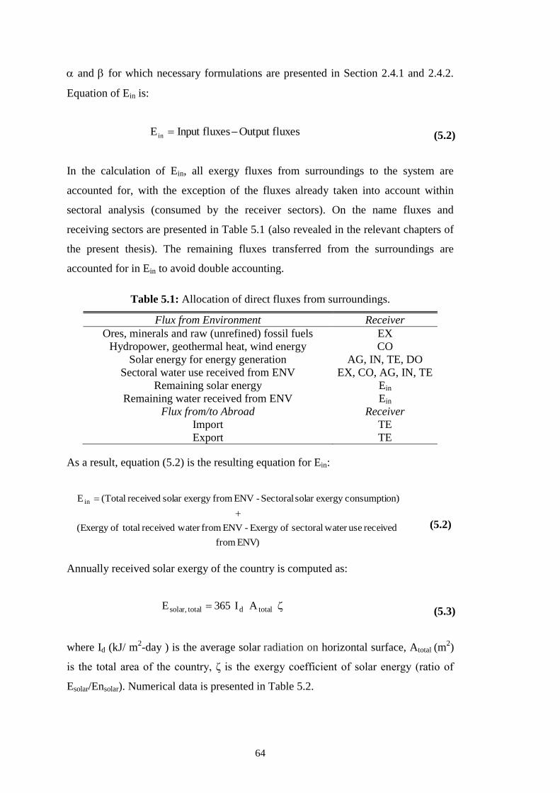
64
and for which necessary formulations are presented in Section 2.4.1 and 2.4.2.
Equation of Ein is:
fluxesOutputfluxesInputE in (5.2)
In the calculation of Ein, all exergy fluxes from surroundings to the system are
accounted for, with the exception of the fluxes already taken into account within
sectoral analysis (consumed by the receiver sectors). On the name fluxes and
receiving sectors are presented in Table 5.1 (also revealed in the relevant chapters of
the present thesis). The remaining fluxes transferred from the surroundings are
accounted for in Ein to avoid double accounting.
Table 5.1: Allocation of direct fluxes from surroundings.
Flux from Environment Receiver
Ores, minerals and raw (unrefined) fossil fuels EX
Hydropower, geothermal heat, wind energy CO
Solar energy for energy generation AG, IN, TE, DO
Sectoral water use received from ENV EX, CO, AG, IN, TE
Remaining solar energy Ein
Remaining water received from ENV Ein
Flux from/to Abroad Receiver
Import TE
Export TE
As a result, equation (5.2) is the resulting equation for Ein:
ENV) from
received use water sectoral ofExergy -ENV from water received totalof(Exergy
n)consumptioexergy solar Sectoral - ENV fromexergy solar received (Total E in
(5.2)
Annually received solar exergy of the country is computed as:
totaldtotal,solar AI365E (5.3)
where Id (kJ/ m2-day ) is the average solar radiation on horizontal surface, Atotal (m
2)
is the total area of the country, ζ is the exergy coefficient of solar energy (ratio of
Esolar/Ensolar). Numerical data is presented in Table 5.2.
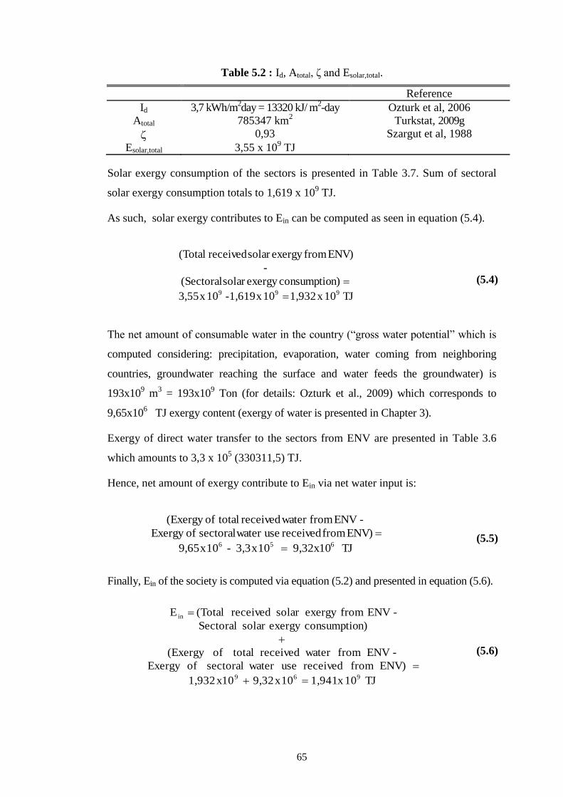
65
Table 5.2 : Id, Atotal, ζ and Esolar,total.
Reference
Id 3,7 kWh/m2day = 13320 kJ/ m
2-day Ozturk et al, 2006
Atotal 785347 km2 Turkstat, 2009g
0,93 Szargut et al, 1988
Esolar,total 3,55 x 10⁹ TJ
Solar exergy consumption of the sectors is presented in Table 3.7. Sum of sectoral
solar exergy consumption totals to 1,619 x 109 TJ.
As such, solar exergy contributes to Ein can be computed as seen in equation (5.4).
TJ 10 x 1,932 10x 1,619-10x 3,55
n)consumptioexergy solar (Sectoral
-
ENV) fromexergy solar received (Total
999
(5.4)
The net amount of consumable water in the country (“gross water potential” which is
computed considering: precipitation, evaporation, water coming from neighboring
countries, groundwater reaching the surface and water feeds the groundwater) is
193x109 m
3 = 193x10
9 Ton (for details: Ozturk et al., 2009) which corresponds to
9,65x10⁶ TJ exergy content (exergy of water is presented in Chapter 3).
Exergy of direct water transfer to the sectors from ENV are presented in Table 3.6
which amounts to 3,3 x 10⁵ (330311,5) TJ.
Hence, net amount of exergy contribute to Ein via net water input is:
TJ 9,32x10 10x3,3-10x9,65
ENV) from received use water sectoral ofExergy
-ENV from water received totalof(Exergy
656
(5.5)
Finally, Ein of the society is computed via equation (5.2) and presented in equation (5.6).
TJ10x 1,94110x9,32 x101,932
ENV) from received usewater sectoral ofExergy
-ENV from water received total of(Exergy
n)consumptio exergy solar Sectoral
- ENV fromexergy solar received (Total E
969
in
(5.6)
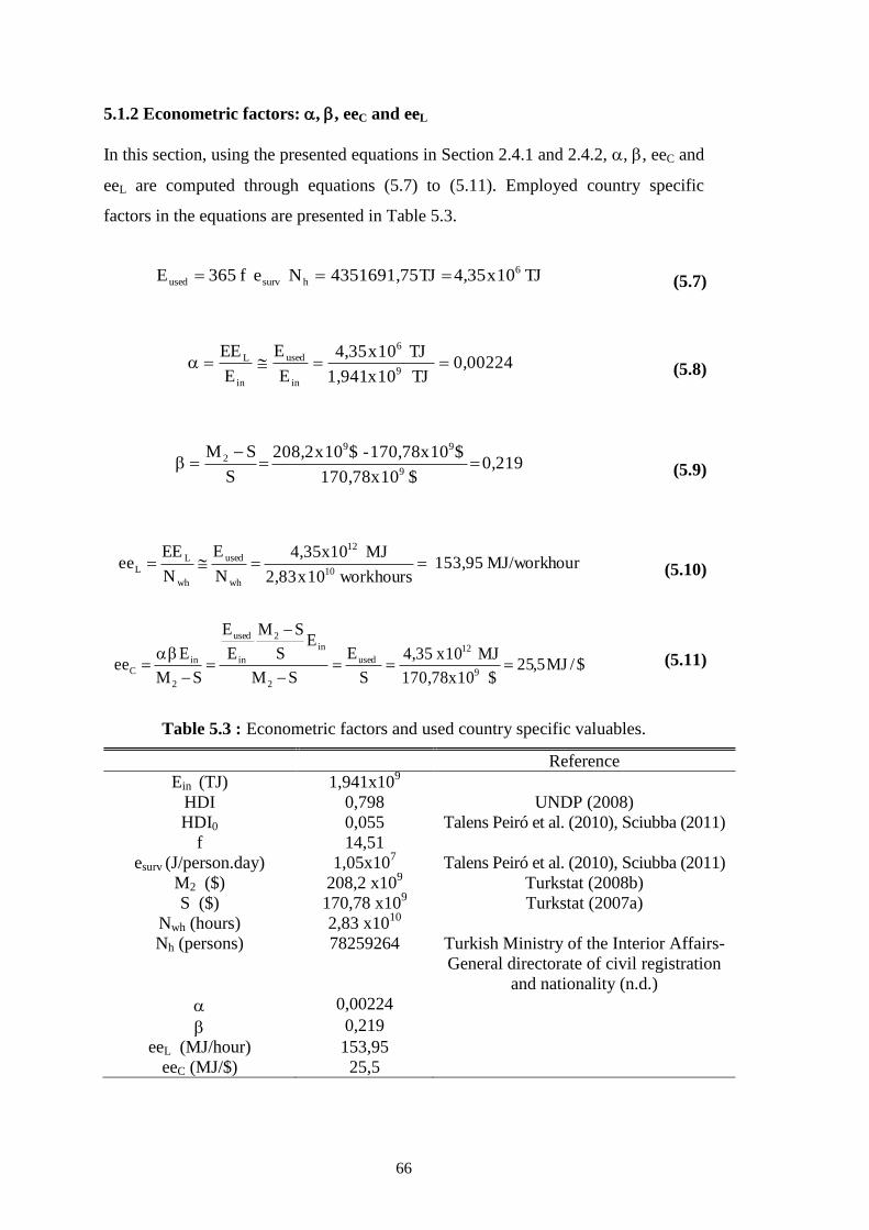
66
5.1.2 Econometric factors: , , eeC and eeL
In this section, using the presented equations in Section 2.4.1 and 2.4.2, , , eeC and
eeL are computed through equations (5.7) to (5.11). Employed country specific
factors in the equations are presented in Table 5.3.
TJ10x4,35TJ4351691,75Nef365E 6
hsurvused (5.7)
0,00224TJ10x1,941
TJ10x4,35
E
E
E
EE9
6
in
used
in
L (5.8)
0,219$10x170,78
$10x170,78 -$10x208,2
S
SM9
99
2
(5.9)
rMJ/workhou153,95hourswork10x2,83
MJ104,35x
N
E
N
EEee
10
12
wh
used
wh
L
L (5.10)
$/MJ5,25$10x170,78
MJ10x4,35
S
E
SM
ES
SM
E
E
SM
Eee
9
12
used
2
in2
in
used
2
inC
(5.11)
Table 5.3 : Econometric factors and used country specific valuables.
Reference
Ein (TJ) 1,941x109
HDI 0,798 UNDP (2008)
HDI0 0,055 Talens Peiró et al. (2010), Sciubba (2011)
f 14,51
esurv (J/person.day) 1,05x10⁷ Talens Peiró et al. (2010), Sciubba (2011)
M2 ($) 208,2 x10⁹ Turkstat (2008b)
S ($) 170,78 x10⁹ Turkstat (2007a)
Nwh (hours) 2,83 x10¹⁰
Nh (persons) 78259264 Turkish Ministry of the Interior Affairs-
General directorate of civil registration
and nationality (n.d.)
0,00224
0,219
eeL (MJ/hour) 153,95
eeC (MJ/$) 25,5
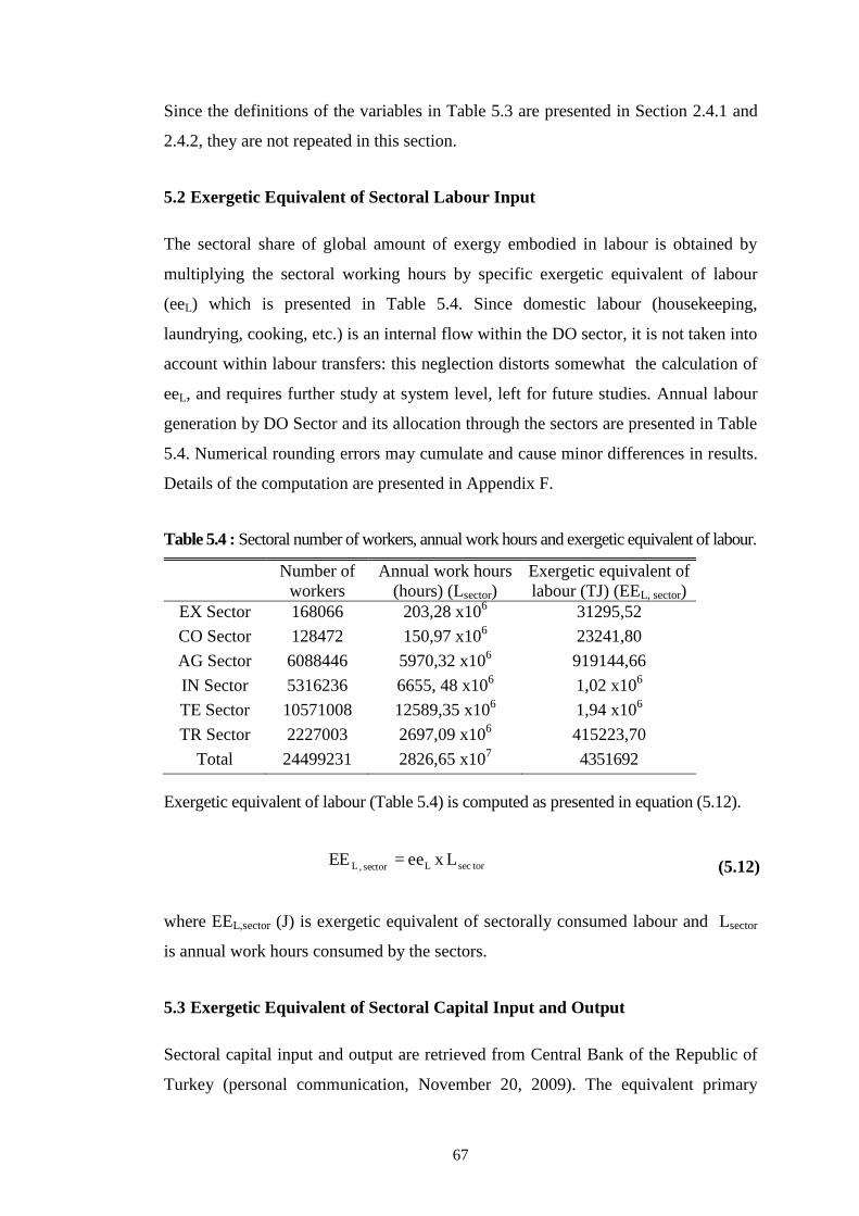
67
Since the definitions of the variables in Table 5.3 are presented in Section 2.4.1 and
2.4.2, they are not repeated in this section.
5.2 Exergetic Equivalent of Sectoral Labour Input
The sectoral share of global amount of exergy embodied in labour is obtained by
multiplying the sectoral working hours by specific exergetic equivalent of labour
(eeL) which is presented in Table 5.4. Since domestic labour (housekeeping,
laundrying, cooking, etc.) is an internal flow within the DO sector, it is not taken into
account within labour transfers: this neglection distorts somewhat the calculation of
eeL, and requires further study at system level, left for future studies. Annual labour
generation by DO Sector and its allocation through the sectors are presented in Table
5.4. Numerical rounding errors may cumulate and cause minor differences in results.
Details of the computation are presented in Appendix F.
Table 5.4 : Sectoral number of workers, annual work hours and exergetic equivalent of labour.
Number of
workers
Annual work hours
(hours) (Lsector)
Exergetic equivalent of
labour (TJ) (EEL, sector)
EX Sector 168066 203,28 x10⁶ 31295,52
CO Sector 128472 150,97 x10⁶ 23241,80
AG Sector 6088446 5970,32 x106 919144,66
IN Sector 5316236 6655, 48 x106 1,02 x10
6
TE Sector 10571008 12589,35 x106 1,94 x10
6
TR Sector 2227003 2697,09 x106 415223,70
Total 24499231 2826,65 x107 4351692
Exergetic equivalent of labour (Table 5.4) is computed as presented in equation (5.12).
torsecLsector ,L Lxee =EE (5.12)
where EEL,sector (J) is exergetic equivalent of sectorally consumed labour and Lsector
is annual work hours consumed by the sectors.
5.3 Exergetic Equivalent of Sectoral Capital Input and Output
Sectoral capital input and output are retrieved from Central Bank of the Republic of
Turkey (personal communication, November 20, 2009). The equivalent primary
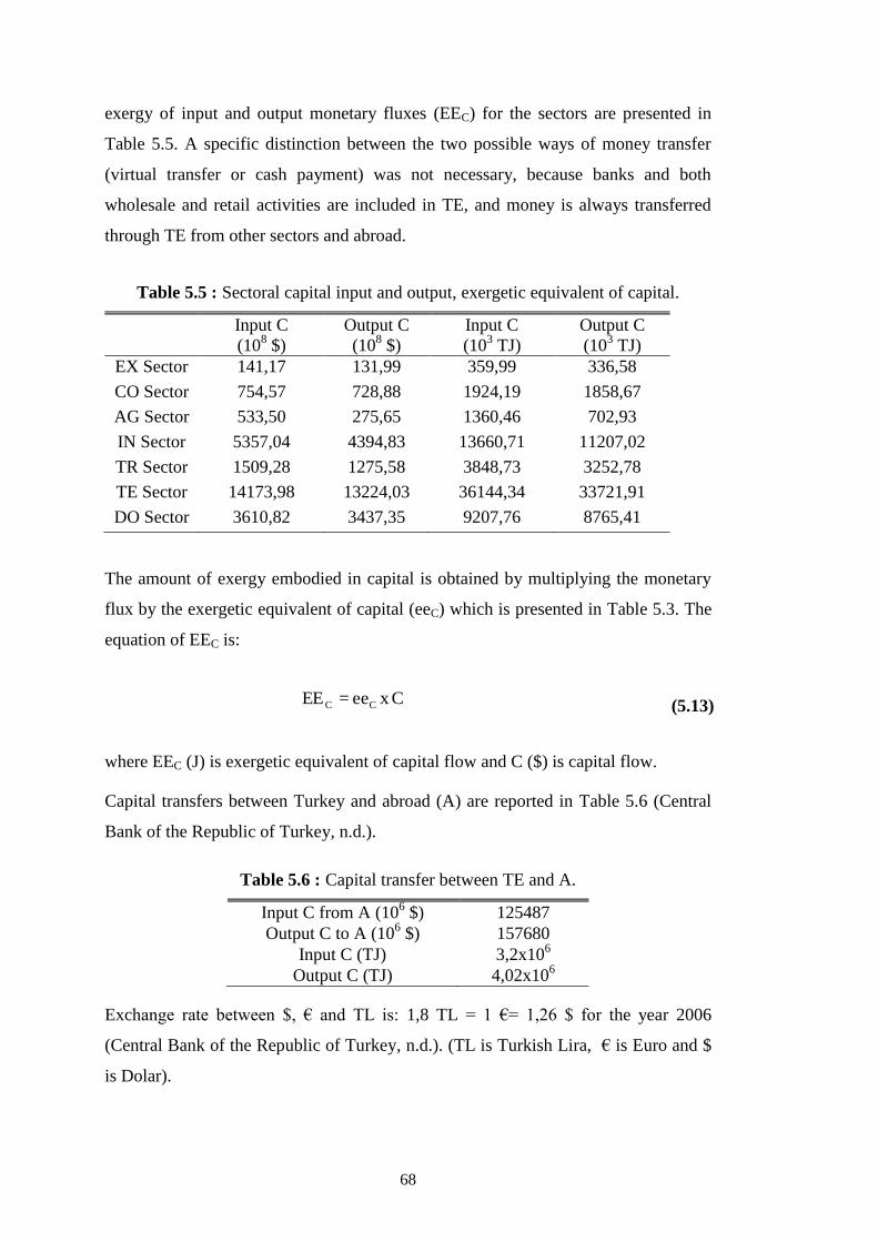
68
exergy of input and output monetary fluxes (EEC) for the sectors are presented in
Table 5.5. A specific distinction between the two possible ways of money transfer
(virtual transfer or cash payment) was not necessary, because banks and both
wholesale and retail activities are included in TE, and money is always transferred
through TE from other sectors and abroad.
Table 5.5 : Sectoral capital input and output, exergetic equivalent of capital.
Input C
(108 $)
Output C
(108 $)
Input C
(103 TJ)
Output C
(103 TJ)
EX Sector 141,17 131,99 359,99 336,58
CO Sector 754,57 728,88 1924,19 1858,67
AG Sector 533,50 275,65 1360,46 702,93
IN Sector 5357,04 4394,83 13660,71 11207,02
TR Sector 1509,28 1275,58 3848,73 3252,78
TE Sector 14173,98 13224,03 36144,34 33721,91
DO Sector 3610,82 3437,35 9207,76 8765,41
The amount of exergy embodied in capital is obtained by multiplying the monetary
flux by the exergetic equivalent of capital (eeC) which is presented in Table 5.3. The
equation of EEC is:
Cxee =EE CC (5.13)
where EEC (J) is exergetic equivalent of capital flow and C ($) is capital flow.
Capital transfers between Turkey and abroad (A) are reported in Table 5.6 (Central
Bank of the Republic of Turkey, n.d.).
Table 5.6 : Capital transfer between TE and A.
Input C from A (106 $) 125487
Output C to A (106 $) 157680
Input C (TJ) 3,2x10⁶
Output C (TJ) 4,02x10⁶
Exchange rate between $, € and TL is: 1,8 TL = 1 €= 1,26 $ for the year 2006
(Central Bank of the Republic of Turkey, n.d.). (TL is Turkish Lira, € is Euro and $
is Dolar).
69
5.4 Environmental Remediation Cost (EEENV) Determination and Sectoral
EEENV Inputs
The goal of the present section (Section 5.4) is determination of environmental
remediation cost (EEENV) of solid, liquid and gas waste and EEENV input of Turkish
sectors. In the present thesis, cooling of discharged heat to the environmental temperature
is also accounted for in the content of EEENV since heat has also effects on temperature
distribution of the surrounding atmosphere. In summary, the content of “waste” is
classified into four groups: solid waste, gas emissions, liquid waste and discharge heat.
Alternative treatment technologies can be chosen and formulated to clean-up the
pollutants and assess the environmental impact of aforementioned waste types. Solid &
liquid waste and emission gases are in fact collective denominations for a very broad
range of materials and it is almost impossible to deal with the environmental remediation
cost of all types of pollutants. Considered fraction of sectoral solid and liquid waste and
undertaken environmental remediation systems (treatment systems) are detailed in the
relevant subsections below. As for gas emissions, due to lack of sufficiently
disaggregated data and great variety of emission gases, only three types of greenhouse
gases (CO2, CH4, N2O) are analyzed in this thesis.
For Extraction Sector (EX Sector), environmental remediation cost of sectoral solid and
liquid wastes are assumed to be zero as a result of the fact that solid waste of the sector is
mostly soil with little amount of minerals etc. and they are buried into the land after the
mining activity (i.e. discharged to the nature in the original form): since no data are available
for the amount of exergy (mechanical, chemical and thermal) needed to complete this
“landfilling” task, this item is neglected in the present calculation. For liquid waste, the
discharge to the environment is 201 million m3 (for the year of 2004, no data exist for 2006)
(Turkstat, 2005c). As it is seen in Table 3.6, water use of the sector is 178 million m3which is
lower than sectoral discharge. During mining activities, extracted ground water is added to
the used water (totally received from nature) by the sector and totally discharged directly to
nature (Turkstat, 2005c). It is expected to exist particulate matter discharged by mining
activities but their relative amount is negligible with respect to that of the water. In
conclusion, solid and liquid discharge of the sector is coming from the environment and left
to the environment (almost) without changing the physical and chemical structure, therefore,
EEENV originated by solid and liquid discharges are assumed to be zero in this thesis.
70
5.4.1 The concept of environmental remediation cost (EEENV)
As a result of EEA’s being an exergy based “resource use assessment” methodology,
“environmental impact” is also quantified by exergy. In theoretical structure of EEA
methodology, the concept of “environmental remediation cost” relies on the “zero
impact” approach which can be described as: converting effluent streams of the
considered process into effluents which are at the state of complete equilibrium with
the reference environment before being discharged into the environment (i.e., the
discharged effluent has “zero impact” on the environment) (Sciubba, 2003b). The
essence of this idea is representing the environmental impact of the effluent by the
cumulative amount of resources (in terms of exergy) that must be consumed to attain
an ideal, zero-impact disposal of the effluent. The cumulative amount of consumed
resources is called “environmental remediation cost (EEENV)”. In brief, according to
EEA, exergetic cost which represents the environmental impact of the effluent
(EEENV) is not proportional to the exergetic content of the effluent, but it is equal to
the extended exergy (sum of the material exergy and physical exergy, plus exergetic
equivalent of externalities: i) labour and capital required by the installation and
operation of the process and ii) environmental remediation cost of “possible”
effluents from treatment (remediation) process which must be cleaned) ideally
required to cool the effluent to T0 and break it up into its constituents such that each
one of them is in equilibrium conditions with the surroundings (Sciubba, 2005). In
other words, environmental impact is quantified as the total exergy of resources
“used up” in the environmental remediation processes. But in reality, since there is
no totally “clean” technology (Sciubba, 2003b), because, in fact, the present
treatment technologies do not always produce effluents in equilibrium with the
surroundings, choosing the minimum environmentally hazardous technology and
establishing a "consciously accepted" level of pollution for each of the substances is
a reasonable approach, on the effluent side of the issue (Sciubba, 2001).
To attain this goal, a virtual or real environmental remediation (clean-up, treatment)
system is inserted to the considered system which is called “environmental
remediation system” and is represented as “St” in Figure 5.1. Since this effluent
treatment process (St) has inputs of material, energy, labour and capital, exergetic
equivalent of these production factors are accounted for in EEENV. Though a similar
“environmental impact” computation route is proposed in Zero-ELCA (see Section

71
1.2.2), “environmental remediation cost (EEENV) results are more comprehensive and
indicative since exergetic equivalent of externalities are included within the analysis
in EEA methodology.
Figure 5.1: Representation of system (S) and treatment system (St).
Schematic representation of aforementioned “environmental remediation cost”
concept is presented in Figure 5.1 where EW is the exergy of effluent from S; St is the
environmental remediation (treatment, clean up) system; EM-t, EPHYS-t are respectively
the exergy of material and energy carriers received by the treatment system St; EEL-t
and EEC-t are respectively the exergetic equivalent of labour and capital received by
the treatment system St; EEP-t is the extended exergy of the treatment system
“possible” product Pt. (While some treatment systems clean up the effluent of S, the
treatment system can produce additional products. In this case, additional products
are denoted by Pt). The treatment system St may produce possible “extra” effluents
(pollutants) which must be cleaned by “extra” treatment systems added to St. EEENV-t
denotes the environmental remediation cost of these “extra” effluents from St
(environmental remediation cost of St).
In Figure 5.1, extended exergetic balance of system St is:
EW
EM
EEP
EPHYS
EEL EEC
EEC-t
EM-t
EPHYS-t EEP-t
EEENV-t EEL-t
EEENV
St
S
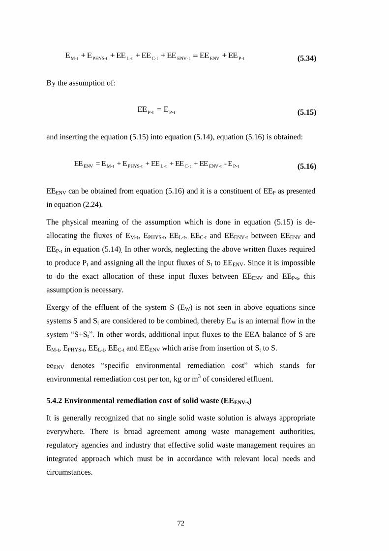
72
EE+ EEEE+EE+EE+E+E t-PENVt-ENVt-Ct-Lt-PHYSt-M (5.34)
By the assumption of:
t-Pt-P E=EE (5.15)
and inserting the equation (5.15) into equation (5.14), equation (5.16) is obtained:
t-Pt-ENVt-Ct-Lt-PHYSt-MENV E - EE+EE+EE+E+E =EE (5.16)
EEENV can be obtained from equation (5.16) and it is a constituent of EEP as presented
in equation (2.24).
The physical meaning of the assumption which is done in equation (5.15) is de-
allocating the fluxes of EM-t, EPHYS-t, EEL-t, EEC-t and EEENV-t between EEENV and
EEP-t in equation (5.14). In other words, neglecting the above written fluxes required
to produce Pt and assigning all the input fluxes of St to EEENV. Since it is impossible
to do the exact allocation of these input fluxes between EEENV and EEP-t, this
assumption is necessary.
Exergy of the effluent of the system S (EW) is not seen in above equations since
systems S and St are considered to be combined, thereby EW is an internal flow in the
system “S+St”. In other words, additional input fluxes to the EEA balance of S are
EM-t, EPHYS-t, EEL-t, EEC-t and EEENV which arise from insertion of St to S.
eeENV denotes “specific environmental remediation cost” which stands for
environmental remediation cost per ton, kg or m3 of considered effluent.
5.4.2 Environmental remediation cost of solid waste (EEENV-s)
It is generally recognized that no single solid waste solution is always appropriate
everywhere. There is broad agreement among waste management authorities,
regulatory agencies and industry that effective solid waste management requires an
integrated approach which must be in accordance with relevant local needs and
circumstances.
73
In below subsections, applied processes for sectoral solid waste treatment are
presented. Set of processes and systems employed in environmental remediation
(treatment) is totally named “environmental remediation system”. For the ease of
explanation and not to repeat the same information for sectoral environmental
remediation processes, the sectors which have a wider variety of constituting
materials in waste composition are presented earlier. Thereby, the order of the
sectors is different then commonly used order in earlier chapters of the thesis.
5.4.2.1 DO sector solid waste
Processing and utilizing from the energy potential of municipal wastes is technically
reasonable due to the facts of: 1) a sizeable fraction of the waste, depending on the
country, consists of combustible components, which can serve as a fuel in heat & energy
generation processes (UNEP, 2005) and 2) a part of municipal waste can be recycled and
reused in the country.
Most of the combustible components in municipal solid waste are also
biodegradable, thus, after undergoing a biological conversion process, a combustible
gas is obtained which is convenient to use in energy generation processes, or which
can be stored or transported for later use. This possibility of recovering energy via
biological conversion and producing a combustible gas, methane, serves a twofold
function: namely waste treatment and energy production (UNEP, 2005).
Anaerobic digestion (biogasification, methane fermentation or biomethanization,
denominated as AD in this thesis) is defined as the biological decomposition of
organic matter under anaerobic conditions (without the presence of oxygen). The
products are primarily methane (CH4) with an accompanying production of other
gases, chief of which is carbon dioxide (CO2) (UNEP, 2005; EPA, 2002b). The residue
of the AD process (digestate) can be composted further to produce “compost” (a kind
of fertilizer) which is another product of AD process (MREC, 2003; EPA, 2002a,
2002b).
In a greenhouse gas assessment report prepared for European Union countries (Smith
et.al., 2001), it has shown that source segregation of MSW (municipal solid waste)
followed by recycling (for paper, metals, textiles and plastics) and AD/compositing
(for putrescible waste) gives the lowest net flux of greenhouse gases, compared with
74
other options for the treatment of bulk MSW. As a result in this thesis, AD and
further composting is applied to organic fraction of considered waste compositions.
Environmental remediation system applied to DO, TE and IN sector (illustrated in
Figure 5.2) can be described as: collected waste is transferred to MRF (Materials
Reprocessing Facility) in which organic fraction of waste is separated from inorganic
fraction as well as the inorganic part is sorted, pre-treated and recycled. The organic
fraction is essentially made of kitchen garbage while mainly plastics, paper&cardboard,
wood, textiles and rubber constitute the inorganic fraction. Non-recyclable part of
considered inorganic materials are transferred to an incineration plant where electricity
and heat are produced by a CHP (combined heat and power plant). Ash produced from
recycling processes (in MRF) and from incineration of non-recyclables are landfilled
(Figure 5.2). As it is seen in the figure, the only discharge to the environment is
landfilled ash which has no green house gas emission capacity to the atmosphere after
landfilling (Chen and Cheng, 2008). “TRP” stands for transportation line in Figure 5.2.
The organic fraction is then delivered to another plant where undergoes anaerobic
digestion in order to produce biogas. Afterwards, biogas is upgraded by removing
CO2, H2S etc. and volumetric fraction of CH4 reaches 98% (in our system) which is
convenient to be used as a substitute of natural gas. The digestate, i.e., the residue of
the anaerobic digestion process, is composted and produced compost is taken out of
the system as a system product. A similar treatment route for organic waste is
elaborated and outlined also in Poschl et al. (2010) and EPA (2002a).
The composition of considered DO sector waste is seen in Table 5.7. In the available
database for Turkey, solid waste of all sectors is collected at one center and then
allocated to recycling, composting and incineration: the source of waste is not
known. Therefore in this thesis, all the recycled waste of Turkey (metal recycling,
composting, incineration, etc.) is assumed to be provided from the DO sector solid
waste and transferred to TE from DO and then from TE to the relevant sector. Under
these circumstances, calculation of the DO sector waste composition is presented in
Appendix G.
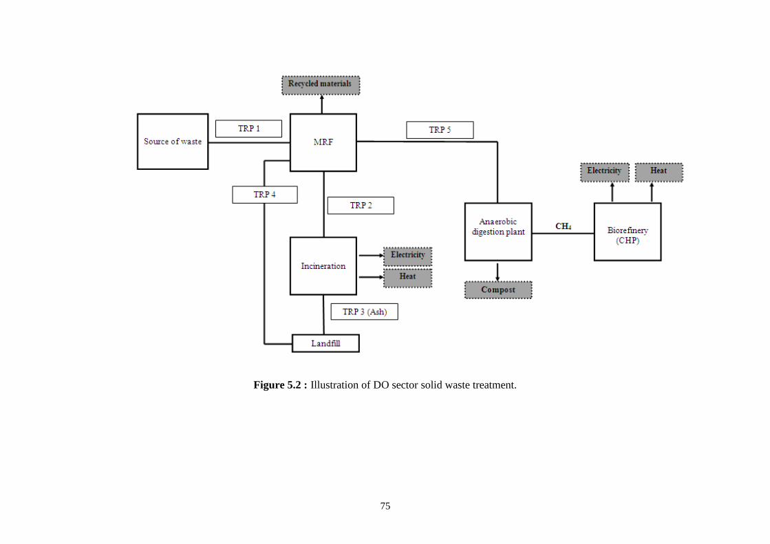
75
Figure 5.2 : Illustration of DO sector solid waste treatment.
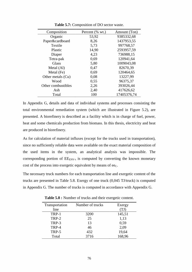
76
Table 5.7: Composition of DO sector waste.
Composition Percent (% wt.) Amount (Ton)
Organic 53,92 9385332,68
Paper&cardboard 8,26 1437953,55
Textile 5,73 997768,57
Plastic 14,90 2593957,59
Diaper 4,23 736988,15
Tetra-pak 0,69 120941,64
Glass 5,80 1009043,08
Metal (Al) 0,47 82670,39
Metal (Fe) 0,69 120464,65
Other metals (Cu) 0,08 13227,99
Wood 0,55 96375,37
Other combustibles 2,26 393026,44
Ash 2,40 417626,62
Total 100 17405376,74
In Appendix G, details and data of individual systems and processes consisting the
total environmental remediation system (which are illustrated in Figure 5.2), are
presented. A biorefinery is described as a facility which is in charge of fuel, power,
heat and some chemicals production from biomass. In this thesis, electricity and heat
are produced in biorefinery.
As for calculation of material influxes (except for the trucks used in transportation),
since no sufficiently reliable data were available on the exact material composition of
the used items in the system, an analytical analysis was impossible. The
corresponding portion of EEENV-t is computed by converting the known monetary
cost of the process into exergetic equivalent by means of eeC.
The necessary truck numbers for each transportation line and exergetic content of the
trucks are presented in Table 5.8. Exergy of one truck (0,045 TJ/truck) is computed
in Appendix G. The number of trucks is computed in accordance with Appendix G.
Table 5.8 : Number of trucks and their exergetic content.
Transportation
line
Number of trucks Exergy
(TJ)
TRP-1 3200 145,51
TRP-2 25 1,13
TRP-3 13 0,59
TRP-4 46 2,09
TRP-5 432 19,64
Total 3716 168,96
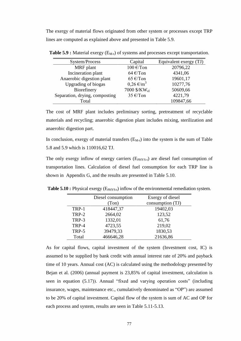
77
The exergy of material flows originated from other system or processes except TRP
lines are computed as explained above and presented in Table 5.9.
Table 5.9 : Material exergy (EM-t) of systems and processes except transportation.
System/Process Capital Equivalent exergy (TJ)
MRF plant 100 €/Ton 20796,22
Incineration plant 64 €/Ton 4341,06
Anaerobic digestion plant 65 €/Ton 19601,17
Upgrading of biogas 0,26 €/m3
10277,76
Biorefinery 7000 $/KWel 50609,66
Separation, drying, composting 35 €/Ton 4221,79
Total
109847,66
The cost of MRF plant includes preliminary sorting, pretreatment of recyclable
materials and recycling; anaerobic digestion plant includes mixing, sterilization and
anaerobic digestion part.
In conclusion, exergy of material transfers (EM-t) into the system is the sum of Table
5.8 and 5.9 which is 110016,62 TJ.
The only exergy inflow of energy carriers (EPHYS-t) are diesel fuel consumption of
transportation lines. Calculation of diesel fuel consumption for each TRP line is
shown in Appendix G, and the results are presented in Table 5.10.
Table 5.10 : Physical exergy (EPHYS-t) inflow of the environmental remediation system.
Diesel consumption
(Ton)
Exergy of diesel
consumption (TJ)
TRP-1 418447,37 19402,03
TRP-2 2664,02 123,52
TRP-3 1332,01 61,76
TRP-4 4723,55 219,02
TRP-5 39479,33 1830,53
Total 466646,28 21636,86
As for capital flows, capital investment of the system (Investment cost, IC) is
assumed to be supplied by bank credit with annual interest rate of 20% and payback
time of 10 years. Annual cost (AC) is calculated using the methodology presented by
Bejan et al. (2006) (annual payment is 23,85% of capital investment, calculation is
seen in equation (5.17)). Annual “fixed and varying operation costs” (including
insurance, wages, maintenance etc., cumulatively denominated as “OP”) are assumed
to be 20% of capital investment. Capital flow of the system is sum of AC and OP for
each process and system, results are seen in Table 5.11-5.13.
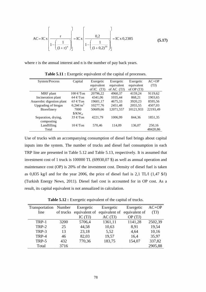
78
2385,0xIC
)2,01(
11
2,0xIC
)r1(
11
rxICAC
10n
(5.17)
where r is the annual interest and n is the number of pay back years.
Table 5.11 : Exergetic equivalent of the capital of processes.
System/Process Capital Exergetic
equivalent
of IC (TJ)
Exergetic
equivalent
of AC (TJ)
Exergetic
equivalent
of OP (TJ)
AC+OP
(TJ)
MRF plant 100 €/Ton 20796,22 4960,37 4159,24 9119,62
Incineration plant 64 €/Ton 4341,06 1035,44 868,21 1903,65
Anaerobic digestion plant 65 €/Ton 19601,17 4675,33 3920,23 8595,56
Upgrading of biogas 0,26€/m3 10277,76 2451,48 2055,55 4507,03
Biorefinery 7000
$/KWel
50609,66 12071,557 10121,933 22193,49
Separation, drying,
composting
35 €/Ton 4221,79 1006,99 844,36 1851,35
Landfilling 10 €/Ton 570,46 114,09 136,07 250,16
Total 48420,86
Use of trucks with an accompanying consumption of diesel fuel brings about capital
inputs into the system. The number of trucks and diesel fuel consumption in each
TRP line are presented in Table 5.12 and Table 5.13, respectively. It is assumed that
investment cost of 1 truck is 100000 TL (69930,07 $) as well as annual operation and
maintenance cost (OP) is 20% of the investment cost. Density of diesel fuel is taken
as 0,835 kg/l and for the year 2006, the price of diesel fuel is 2,1 TL/l (1,47 $/l)
(Turkish Energy News, 2011). Diesel fuel cost is accounted for in OP cost. As a
result, its capital equivalent is not annualized in calculation.
Table 5.12 : Exergetic equivalent of the capital of trucks.
Transportation
line
Number
of trucks
Exergetic
equivalent of
IC (TJ)
Exergetic
equivalent of
AC (TJ)
Exergetic
equivalent of
OP (TJ)
AC+OP
(TJ)
TRP-1 3200 5706,4 1361,11 1141,28 2502,39
TRP-2 25 44,58 10,63 8,91 19,54
TRP-3 13 23,18 5,52 4,64 10,16
TRP-4 46 82,03 19,57 16,4 35,97
TRP-5 432 770,36 183,75 154,07 337,82
Total 3716 2905,88
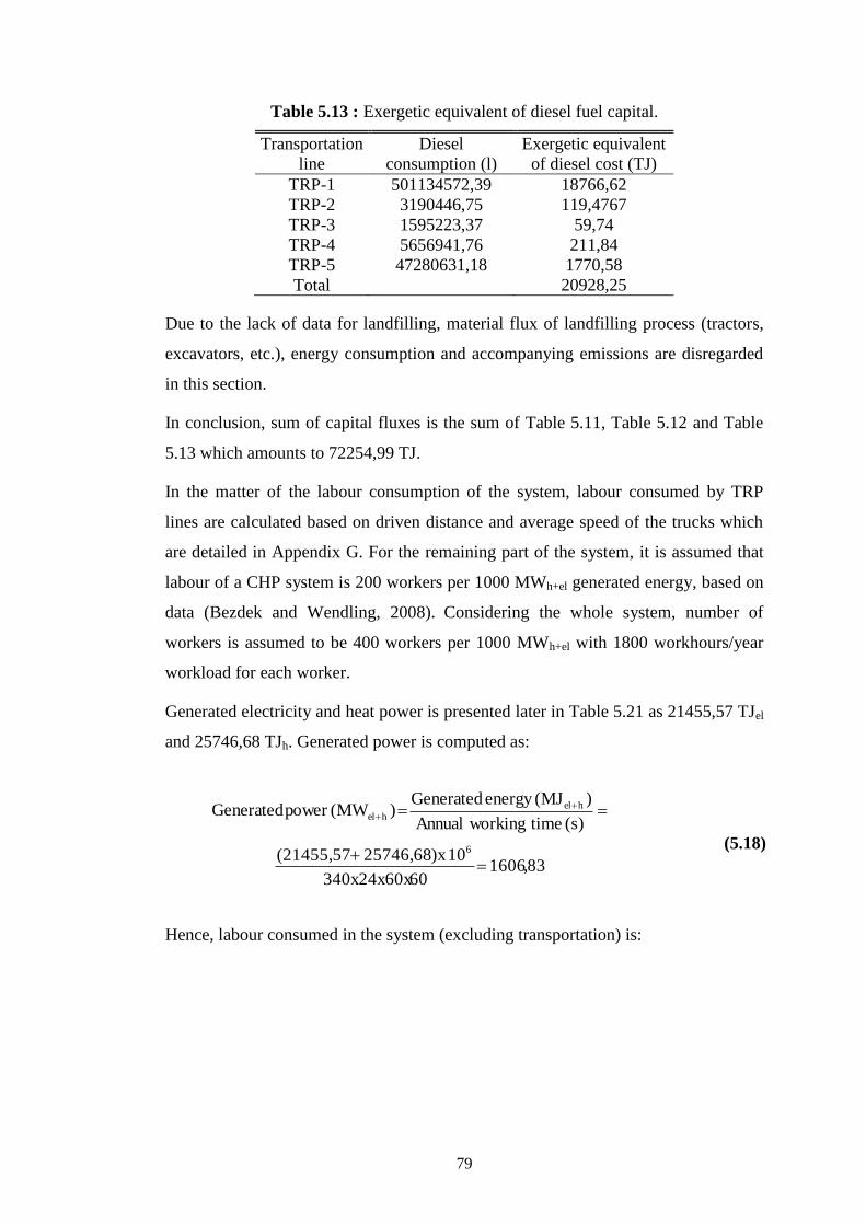
79
Table 5.13 : Exergetic equivalent of diesel fuel capital.
Transportation
line
Diesel
consumption (l)
Exergetic equivalent
of diesel cost (TJ)
TRP-1 501134572,39 18766,62
TRP-2 3190446,75 119,4767
TRP-3 1595223,37 59,74
TRP-4 5656941,76 211,84
TRP-5 47280631,18 1770,58
Total 20928,25
Due to the lack of data for landfilling, material flux of landfilling process (tractors,
excavators, etc.), energy consumption and accompanying emissions are disregarded
in this section.
In conclusion, sum of capital fluxes is the sum of Table 5.11, Table 5.12 and Table
5.13 which amounts to 72254,99 TJ.
In the matter of the labour consumption of the system, labour consumed by TRP
lines are calculated based on driven distance and average speed of the trucks which
are detailed in Appendix G. For the remaining part of the system, it is assumed that
labour of a CHP system is 200 workers per 1000 MWh+el generated energy, based on
data (Bezdek and Wendling, 2008). Considering the whole system, number of
workers is assumed to be 400 workers per 1000 MWh+el with 1800 workhours/year
workload for each worker.
Generated electricity and heat power is presented later in Table 5.21 as 21455,57 TJel
and 25746,68 TJh. Generated power is computed as:
83,160660340x24x60x
10)x 25746,68 (21455,57
(s) time workingAnnual
)(MJenergy Generated)MW(powerGenerated
6
helhel
(5.18)
Hence, labour consumed in the system (excluding transportation) is:
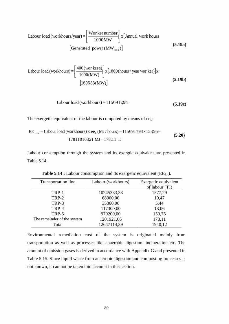
80
)MW(powerGenerated
xhoursworkAnnualxMW1000
numberkerWor = /year)(workhours loadLabour
hel
(5.19a)
)MW(83,1606
xker)woryear/hours(1800x)MW(1000
)skerwor(400 = )(workhours loadLabour
(5.19b)
94,1156917 = )(workhours loadLabour (5.19c)
The exergetic equivalent of the labour is computed by means of eeL:
TJ178,11MJ 51178110163,
95,153x94,1156917)hours/MJ(ee x )(workhours loadabour LEE LtL
(5.20)
Labour consumption through the system and its exergtic equivalent are presented in
Table 5.14.
Table 5.14 : Labour consumption and its exergetic equivalent (EEL-t).
Transportation line Labour (workhours) Exergetic equivalent
of labour (TJ)
TRP-1 10245333,33 1577,29
TRP-2 68000,00 10,47
TRP-3 35360,00 5,44
TRP-4 117300,00 18,06
TRP-5 979200,00 150,75 The remainder of the system 1201921,06 178,11
Total 12647114,39 1940,12
Environmental remediation cost of the system is originated mainly from
transportation as well as processes like anaerobic digestion, incineration etc. The
amount of emission gases is derived in accordance with Appendix G and presented in
Table 5.15. Since liquid waste from anaerobic digestion and composting processes is
not known, it can not be taken into account in this section.
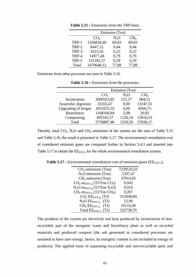
81
Table 5.15 : Emissions from the TRP lines.
Emission (Ton)
CO2 N2O CH4
TRP-1 1326818,40 69,83 69,83
TRP-2 8447,12 0,44 0,44
TRP-3 4223,56 0,22 0,22
TRP-4 14977,48 0,79 0,79
TRP-5 125181,57 6,59 6,59
Total 1479648,12 77,88 77,88
Emissions from other processes are seen in Table 5.16.
Table 5.16 : Emissions from the processes.
Emission (Ton) CO2 N2O CH4
Incineration 3009323,85 131,27 984,51
Anaerobic digestion 33355,67 0,00 13247,55
Upgrading of biogas 1053555,55 0,00 8566,75
Biorefinery 1168106,84 2,08 20,82
Composting 495545,57 1126,24 15016,53
Total 5759887,48 1259,59 37836,17
Thereby, total CO2, N2O and CH4 emissions of the system are the sum of Table 5.15
and Table 5.16, the result is presented in Table 5.17. The environmental remediation cost
of considered emission gases are computed further in Section 5.4.3 and inserted into
Table 5.17 to obtain the EEENV-t for the whole environmental remediation system.
Table 5.17 : Environmental remediation cost of emission gases (EEENV-t).
CO2 emissions (Ton) 7239535,61
N2O emission (Ton) 1337,47
CH4 emission (Ton) 37914,05
CO2 eeENV-g (TJ/Ton CO2) 0,043
N2O eeENV-g (TJ/Ton N2O) 0,010
CH4 eeENV-g (TJ/Ton CH4) 0,267
CO2 EEENV-g (TJ) 312608,84
N2O EEENV-g (TJ) 12,90
CH4 EEENV-g (TJ) 10116,96
Total EEENV-t (TJ) 322738,70
The products of the system are electricity and heat produced by incineration of non-
recyclable part of the inorganic waste and biorefinery plant as well as recycled
materials and produced compost (the ash generated in considered processes are
assumed to have zero exergy, hence, its exergetic content is not included in exergy of
products). The applied route of separating recyclable and non-recyclable parts and
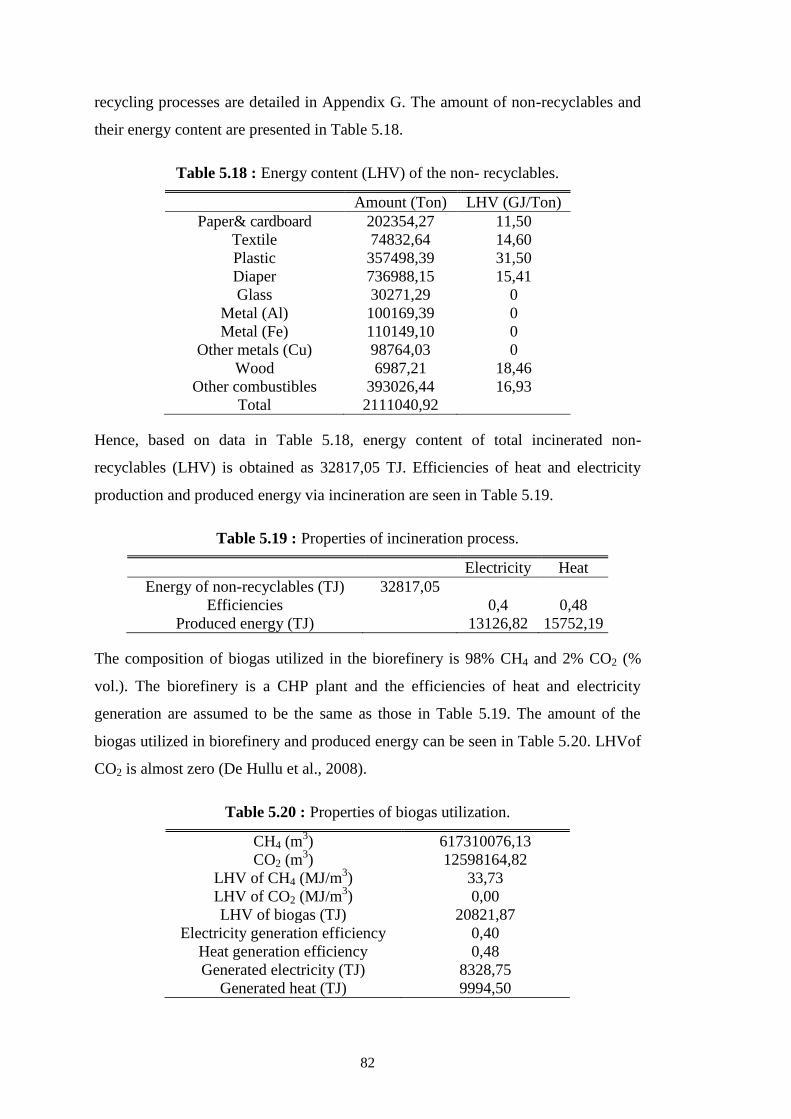
82
recycling processes are detailed in Appendix G. The amount of non-recyclables and
their energy content are presented in Table 5.18.
Table 5.18 : Energy content (LHV) of the non- recyclables.
Amount (Ton) LHV (GJ/Ton)
Paper& cardboard 202354,27 11,50
Textile 74832,64 14,60
Plastic 357498,39 31,50
Diaper 736988,15 15,41
Glass 30271,29 0
Metal (Al) 100169,39 0
Metal (Fe) 110149,10 0
Other metals (Cu) 98764,03 0
Wood 6987,21 18,46
Other combustibles 393026,44 16,93
Total 2111040,92
Hence, based on data in Table 5.18, energy content of total incinerated non-
recyclables (LHV) is obtained as 32817,05 TJ. Efficiencies of heat and electricity
production and produced energy via incineration are seen in Table 5.19.
Table 5.19 : Properties of incineration process.
Electricity Heat
Energy of non-recyclables (TJ) 32817,05
Efficiencies 0,4 0,48
Produced energy (TJ) 13126,82 15752,19
The composition of biogas utilized in the biorefinery is 98% CH4 and 2% CO2 (%
vol.). The biorefinery is a CHP plant and the efficiencies of heat and electricity
generation are assumed to be the same as those in Table 5.19. The amount of the
biogas utilized in biorefinery and produced energy can be seen in Table 5.20. LHVof
CO2 is almost zero (De Hullu et al., 2008).
Table 5.20 : Properties of biogas utilization.
CH4 (m3) 617310076,13
CO2 (m3) 12598164,82
LHV of CH4 (MJ/m3) 33,73
LHV of CO2 (MJ/m3) 0,00
LHV of biogas (TJ) 20821,87
Electricity generation efficiency 0,40
Heat generation efficiency 0,48
Generated electricity (TJ) 8328,75
Generated heat (TJ) 9994,50
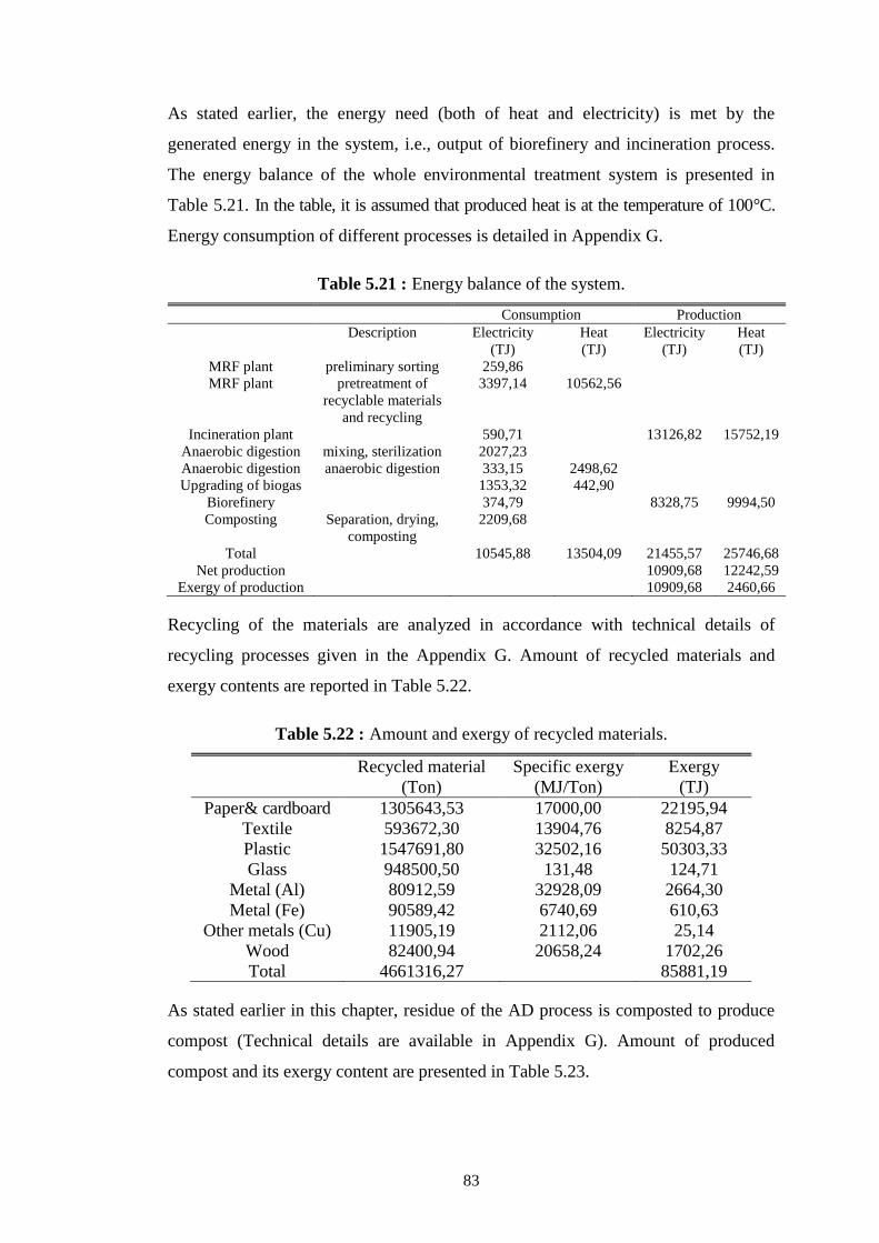
83
As stated earlier, the energy need (both of heat and electricity) is met by the
generated energy in the system, i.e., output of biorefinery and incineration process.
The energy balance of the whole environmental treatment system is presented in
Table 5.21. In the table, it is assumed that produced heat is at the temperature of 100°C.
Energy consumption of different processes is detailed in Appendix G.
Table 5.21 : Energy balance of the system.
Consumption Production
Description Electricity
(TJ)
Heat
(TJ)
Electricity
(TJ)
Heat
(TJ)
MRF plant preliminary sorting 259,86
MRF plant pretreatment of
recyclable materials
and recycling
3397,14 10562,56
Incineration plant 590,71 13126,82 15752,19
Anaerobic digestion mixing, sterilization 2027,23
Anaerobic digestion anaerobic digestion 333,15 2498,62
Upgrading of biogas 1353,32 442,90
Biorefinery 374,79 8328,75 9994,50
Composting Separation, drying,
composting
2209,68
Total 10545,88 13504,09 21455,57 25746,68
Net production 10909,68 12242,59
Exergy of production 10909,68 2460,66
Recycling of the materials are analyzed in accordance with technical details of
recycling processes given in the Appendix G. Amount of recycled materials and
exergy contents are reported in Table 5.22.
Table 5.22 : Amount and exergy of recycled materials.
Recycled material
(Ton)
Specific exergy
(MJ/Ton)
Exergy
(TJ)
Paper& cardboard 1305643,53 17000,00 22195,94
Textile 593672,30 13904,76 8254,87
Plastic 1547691,80 32502,16 50303,33
Glass 948500,50 131,48 124,71
Metal (Al) 80912,59 32928,09 2664,30
Metal (Fe) 90589,42 6740,69 610,63
Other metals (Cu) 11905,19 2112,06 25,14
Wood 82400,94 20658,24 1702,26
Total 4661316,27 85881,19
As stated earlier in this chapter, residue of the AD process is composted to produce
compost (Technical details are available in Appendix G). Amount of produced
compost and its exergy content are presented in Table 5.23.
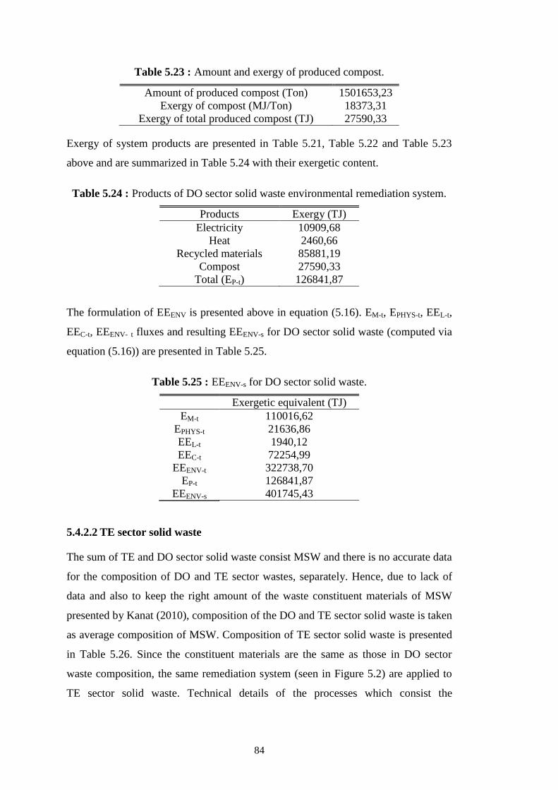
84
Table 5.23 : Amount and exergy of produced compost.
Amount of produced compost (Ton) 1501653,23
Exergy of compost (MJ/Ton) 18373,31
Exergy of total produced compost (TJ) 27590,33
Exergy of system products are presented in Table 5.21, Table 5.22 and Table 5.23
above and are summarized in Table 5.24 with their exergetic content.
Table 5.24 : Products of DO sector solid waste environmental remediation system.
Products Exergy (TJ)
Electricity 10909,68
Heat 2460,66
Recycled materials 85881,19
Compost 27590,33
Total (EP-t) 126841,87
The formulation of EEENV is presented above in equation (5.16). EM-t, EPHYS-t, EEL-t,
EEC-t, EEENV- t fluxes and resulting EEENV-s for DO sector solid waste (computed via
equation (5.16)) are presented in Table 5.25.
Table 5.25 : EEENV-s for DO sector solid waste.
Exergetic equivalent (TJ)
EM-t 110016,62
EPHYS-t 21636,86
EEL-t 1940,12
EEC-t 72254,99
EEENV-t 322738,70
EP-t 126841,87
EEENV-s 401745,43
5.4.2.2 TE sector solid waste
The sum of TE and DO sector solid waste consist MSW and there is no accurate data
for the composition of DO and TE sector wastes, separately. Hence, due to lack of
data and also to keep the right amount of the waste constituent materials of MSW
presented by Kanat (2010), composition of the DO and TE sector solid waste is taken
as average composition of MSW. Composition of TE sector solid waste is presented
in Table 5.26. Since the constituent materials are the same as those in DO sector
waste composition, the same remediation system (seen in Figure 5.2) are applied to
TE sector solid waste. Technical details of the processes which consist the
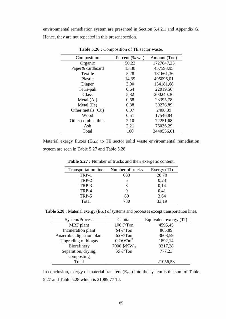
85
environmental remediation system are presented in Section 5.4.2.1 and Appendix G.
Hence, they are not repeated in this present section.
Table 5.26 : Composition of TE sector waste.
Composition Percent (% wt.) Amount (Ton)
Organic 50,22 1727847,23
Paper& cardboard 13,30 457593,95
Textile 5,28 181661,36
Plastic 14,39 495096,01
Diaper 3,90 134181,68
Tetra-pak 0,64 22019,56
Glass 5,82 200240,36
Metal (Al) 0,68 23395,78
Metal (Fe) 0,88 30276,89
Other metals (Cu) 0,07 2408,39
Wood 0,51 17546,84
Other combustibles 2,10 72251,68
Ash 2,21 76036,29
Total 100 3440556,01
Material exergy fluxes (EM-t) to TE sector solid waste environmental remediation
system are seen in Table 5.27 and Table 5.28.
Table 5.27 : Number of trucks and their exergetic content.
Transportation line Number of trucks Exergy (TJ)
TRP-1 633 28,78
TRP-2 5 0,23
TRP-3 3 0,14
TRP-4 9 0,41
TRP-5 80 3,64
Total 730 33,19
Table 5.28 : Material exergy (EM-t) of systems and processes except transportation lines.
System/Process Capital Equivalent exergy (TJ)
MRF plant 100 €/Ton 4595,45
Incineration plant 64 €/Ton 865,89
Anaerobic digestion plant 65 €/Ton 3608,59
Upgrading of biogas 0,26 €/m3 1892,14
Biorefinery 7000 $/KWel 9317,28
Separation, drying,
composting
35 €/Ton 777,23
Total 21056,58
In conclusion, exergy of material transfers (EM-t) into the system is the sum of Table
5.27 and Table 5.28 which is 21089,77 TJ.
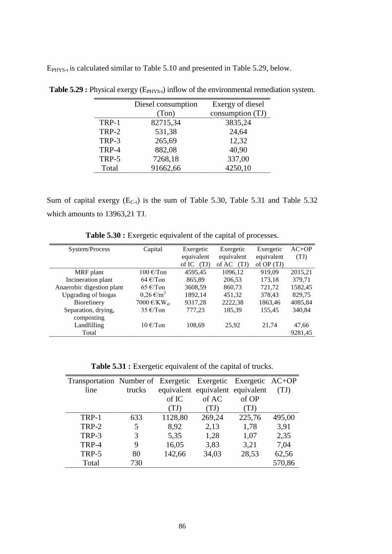
86
EPHYS-t is calculated similar to Table 5.10 and presented in Table 5.29, below.
Table 5.29 : Physical exergy (EPHYS-t) inflow of the environmental remediation system.
Diesel consumption
(Ton)
Exergy of diesel
consumption (TJ)
TRP-1 82715,34 3835,24
TRP-2 531,38 24,64
TRP-3 265,69 12,32
TRP-4 882,08 40,90
TRP-5 7268,18 337,00
Total 91662,66 4250,10
Sum of capital exergy (EC-t) is the sum of Table 5.30, Table 5.31 and Table 5.32
which amounts to 13963,21 TJ.
Table 5.30 : Exergetic equivalent of the capital of processes.
System/Process Capital Exergetic
equivalent
of IC (TJ)
Exergetic
equivalent
of AC (TJ)
Exergetic
equivalent
of OP (TJ)
AC+OP
(TJ)
MRF plant 100 €/Ton 4595,45 1096,12 919,09 2015,21
Incineration plant 64 €/Ton 865,89 206,53 173,18 379,71
Anaerobic digestion plant 65 €/Ton 3608,59 860,73 721,72 1582,45
Upgrading of biogas 0,26 €/m3 1892,14 451,32 378,43 829,75
Biorefinery 7000 €/KWel 9317,28 2222,38 1863,46 4085,84
Separation, drying,
composting
35 €/Ton 777,23 185,39 155,45 340,84
Landfilling 10 €/Ton 108,69 25,92 21,74 47,66
Total 9281,45
Table 5.31 : Exergetic equivalent of the capital of trucks.
Transportation
line
Number of
trucks
Exergetic
equivalent
of IC
(TJ)
Exergetic
equivalent
of AC
(TJ)
Exergetic
equivalent
of OP
(TJ)
AC+OP
(TJ)
TRP-1 633 1128,80 269,24 225,76 495,00
TRP-2 5 8,92 2,13 1,78 3,91
TRP-3 3 5,35 1,28 1,07 2,35
TRP-4 9 16,05 3,83 3,21 7,04
TRP-5 80 142,66 34,03 28,53 62,56
Total 730 570,86
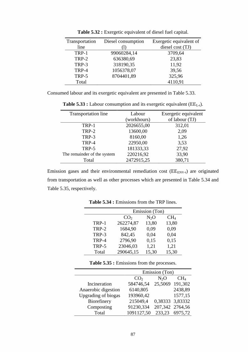
87
Table 5.32 : Exergetic equivalent of diesel fuel capital.
Transportation
line
Diesel consumption
(l)
Exergetic equivalent of
diesel cost (TJ)
TRP-1 99060284,14 3709,64
TRP-2 636380,69 23,83
TRP-3 318190,35 11,92
TRP-4 1056378,07 39,56
TRP-5 8704401,89 325,96
Total 4110,91
Consumed labour and its exergetic equivalent are presented in Table 5.33.
Table 5.33 : Labour consumption and its exergetic equivalent (EEL-t).
Transportation line Labour
(workhours)
Exergetic equivalent
of labour (TJ)
TRP-1 2026655,00 312,01
TRP-2 13600,00 2,09
TRP-3 8160,00 1,26
TRP-4 22950,00 3,53
TRP-5 181333,33 27,92 The remainder of the system 220216,92 33,90
Total 2472915,25 380,71
Emission gases and their environmental remediation cost (EEENV-t) are originated
from transportation as well as other processes which are presented in Table 5.34 and
Table 5.35, respectively.
Table 5.34 : Emissions from the TRP lines.
Emission (Ton)
CO2 N2O CH4
TRP-1 262274,87 13,80 13,80
TRP-2 1684,90 0,09 0,09
TRP-3 842,45 0,04 0,04
TRP-4 2796,90 0,15 0,15
TRP-5 23046,03 1,21 1,21
Total 290645,15 15,30 15,30
Table 5.35 : Emissions from the processes.
Emission (Ton)
CO2 N2O CH4
Incineration 584746,54 25,5069 191,302
Anaerobic digestion 6140,805
2438,89
Upgrading of biogas 193960,42
1577,15
Biorefinery 215049,4 0,38333 3,83332
Composting 91230,334 207,342 2764,56
Total 1091127,50 233,23 6975,72

88
Thereby, total CO2, N2O and CH4 emissions of the system are the sum of Table 5.34
and Table5.35 and the sum is presented in Table 5.36. The environmental
remediation cost of considered emission gases is computed further in Section 5.4.3
and inserted into Table 5.36 to obtain the EEENV-t for the TE sector solid waste
treatment system.
Table 5.36 : Environmental remediation cost of emission gases (EEENV-t).
CO2 emissions (Ton) 1381772,65
N2O emission (Ton) 248,53
CH4 emission (Ton) 6991,02
CO2 eeENV-g (TJ/Ton CO2) 0,043
N2O eeENV-g (TJ/Ton N2O) 0,010
CH4 eeENV-g (TJ/Ton CH4) 0,267
CO2 EEENV-g (TJ) 59666,03
N2O EEENV-g (TJ) 2,3969133
CH4 EEENV-g (TJ) 1865,4792
Total EEENV-t (TJ) 61533,91
Products of the system are the same as those of DO sector waste remediation system:
electricity, heat, recycled materials and compost. In Table 5.37, energy balance of the
system and net heat and electricity production are seen.
Table 5.37 : Energy balance of the system.
Consumption Production
Description Electricity
(TJ)
Heat
(TJ)
Electricity
(TJ)
Heat
(TJ)
MRF plant preliminary sorting 51,37
MRF plant pretreatment of
recyclable materials
and recycling
654,67 2093,42
Incineration plant 114,78 2550,69 3060,83
Anaerobic digestion mixing, sterilization 373,22
Anaerobic digestion anaerobic digestion 61,33 460,00
Upgrading of biogas 249,15 81,54
Biorefinery 69,00 1533,33 1839,99
Composting Separation, drying,
composting
406,80
Total 1980,31 2634,96 4084,02 4900,83
Net production 2103,71 2265,87
Exergy of
production
2103,71 455,42
Amount of recycled materials and exergy contents are seen in Table 5.38.
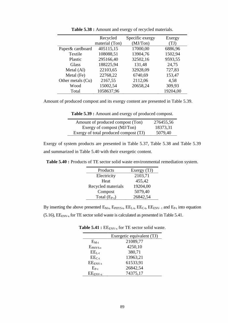
89
Table 5.38 : Amount and exergy of recycled materials.
Recycled
material (Ton)
Specific exergy
(MJ/Ton)
Exergy
(TJ)
Paper& cardboard 405115,15 17000,00 6886,96
Textile 108088,51 13904,76 1502,94
Plastic 295166,40 32502,16 9593,55
Glass 188225,94 131,48 24,75
Metal (Al) 22103,65 32928,09 727,83
Metal (Fe) 22768,22 6740,69 153,47
Other metals (Cu) 2167,55 2112,06 4,58
Wood 15002,54 20658,24 309,93
Total 1058637,96 19204,00
Amount of produced compost and its exergy content are presented in Table 5.39.
Table 5.39 : Amount and exergy of produced compost.
Amount of produced compost (Ton) 276455,56
Exergy of compost (MJ/Ton) 18373,31
Exergy of total produced compost (TJ) 5079,40
Exergy of system products are presented in Table 5.37, Table 5.38 and Table 5.39
and summarized in Table 5.40 with their exergetic content.
Table 5.40 : Products of TE sector solid waste environmental remediation system.
Products Exergy (TJ)
Electricity 2103,71
Heat 455,42
Recycled materials 19204,00
Compost 5079,40
Total (EP-t) 26842,54
By inserting the above presented EM-t, EPHYS-t, EEL-t, EEC-t, EEENV- t and EP-t into equation
(5.16), EEENV-s for TE sector solid waste is calculated as presented in Table 5.41.
Table 5.41 : EEENV-s for TE sector solid waste.
Exergetic equivalent (TJ)
EM-t 21089,77
EPHYS-t 4250,10
EEL-t 380,71
EEC-t 13963,21
EEENV-t 61533,91
EP-t 26842,54
EEENV-s 74375,17

90
5.4.2.3 IN sector solid waste
The considered composition of IN sector solid waste is presented in Table 5.42. The
composition is estimated based on data (SWAP, 2005) due to the fact that there is
neither official data nor study in the literature for average composition of Turkish IN
sector waste. Since the type of the constituent materials are similar to those of TE
and DO sector solid waste, the same treatment system (presented in Figure 5.2) are
applied to the waste and results are seen below. In Table 5.42, the part of “hazardous
waste” is seen as 4% of the industrial waste. Unfortunately in Turkey, hazardous
waste is mostly landfilled and although very limited amount is recycled and reused.
Uncontrolled production of hazardous waste and its illegally dumped or discharged
to receiving water bodies are one of the primary problems arising along with
industrial activities in Turkey (Salihoglu, 2010). As a result, treatment of hazardous
waste is a very important issue for the country, but, since it takes special
technologies and detailed analyses, it is taken out of the scope of this thesis. In other
words, since the hazardous waste has a little share in the total composition of IN
sector solid waste, environmental remediation cost of relevant part is neglected.
Table 5.42 : Composition of IN sector waste.
Composition Percent (% wt.) Amount (Ton)
Organic 18,21 3162955,78
Paper& cardboard 32,38 5625836,00
Textile 2,19 380048,51
Plastic 20,06 3484831,44
Glass 0,55 96144,71
Metal (Al) 0,23 40655,45
Metal (Fe) 10,31 1791825,71
Other metals (Cu) 0,12 20943,72
Wood 3,61 626703,61
Other combustibles 4,38 760097,01
Ash 3,97 689362,63
Hazardous waste 3,99 693859,43
Total 100 17373264,00
Material exergy fluxes (EM-t) to IN sector solid waste environmental remediation
system are seen in Table 5.43 and Table 5.44.
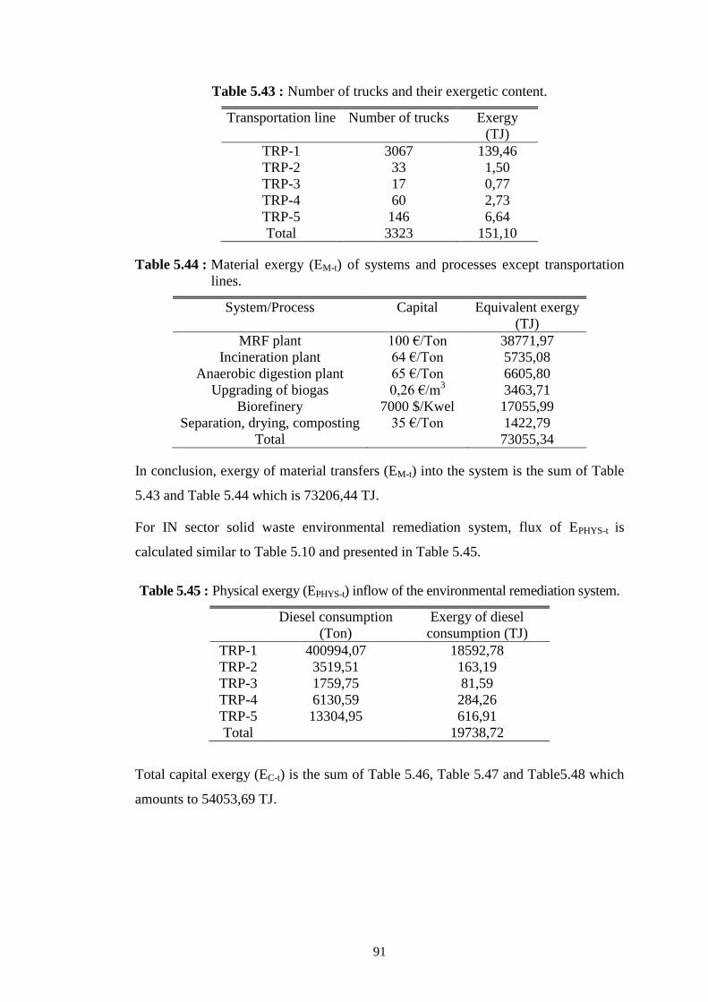
91
Table 5.43 : Number of trucks and their exergetic content.
Transportation line Number of trucks Exergy
(TJ)
TRP-1 3067 139,46
TRP-2 33 1,50
TRP-3 17 0,77
TRP-4 60 2,73
TRP-5 146 6,64
Total 3323 151,10
Table 5.44 : Material exergy (EM-t) of systems and processes except transportation
lines.
System/Process Capital Equivalent exergy
(TJ)
MRF plant 100 €/Ton 38771,97
Incineration plant 64 €/Ton 5735,08
Anaerobic digestion plant 65 €/Ton 6605,80
Upgrading of biogas 0,26 €/m3 3463,71
Biorefinery 7000 $/Kwel 17055,99
Separation, drying, composting 35 €/Ton 1422,79
Total 73055,34
In conclusion, exergy of material transfers (EM-t) into the system is the sum of Table
5.43 and Table 5.44 which is 73206,44 TJ.
For IN sector solid waste environmental remediation system, flux of EPHYS-t is
calculated similar to Table 5.10 and presented in Table 5.45.
Table 5.45 : Physical exergy (EPHYS-t) inflow of the environmental remediation system.
Diesel consumption
(Ton)
Exergy of diesel
consumption (TJ)
TRP-1 400994,07 18592,78
TRP-2 3519,51 163,19
TRP-3 1759,75 81,59
TRP-4 6130,59 284,26
TRP-5 13304,95 616,91
Total 19738,72
Total capital exergy (EC-t) is the sum of Table 5.46, Table 5.47 and Table5.48 which
amounts to 54053,69 TJ.
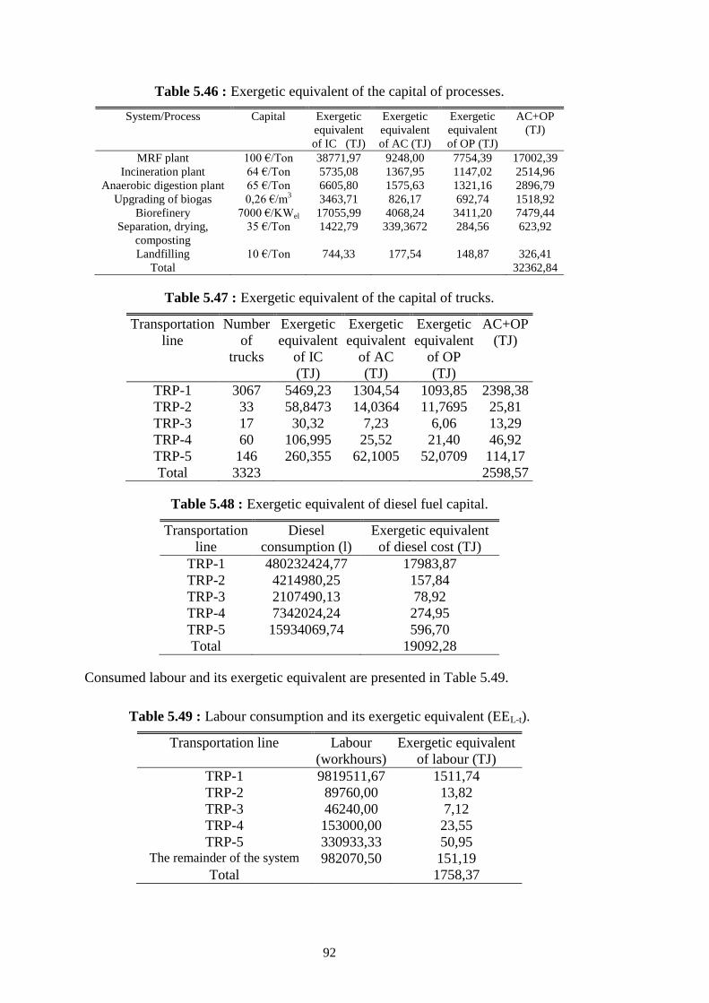
92
Table 5.46 : Exergetic equivalent of the capital of processes.
System/Process Capital Exergetic
equivalent
of IC (TJ)
Exergetic
equivalent
of AC (TJ)
Exergetic
equivalent
of OP (TJ)
AC+OP
(TJ)
MRF plant 100 €/Ton 38771,97 9248,00 7754,39 17002,39
Incineration plant 64 €/Ton 5735,08 1367,95 1147,02 2514,96
Anaerobic digestion plant 65 €/Ton 6605,80 1575,63 1321,16 2896,79
Upgrading of biogas 0,26 €/m3 3463,71 826,17 692,74 1518,92
Biorefinery 7000 €/KWel 17055,99 4068,24 3411,20 7479,44
Separation, drying,
composting
35 €/Ton 1422,79 339,3672 284,56 623,92
Landfilling 10 €/Ton 744,33 177,54 148,87 326,41
Total 32362,84
Table 5.47 : Exergetic equivalent of the capital of trucks.
Transportation
line
Number
of
trucks
Exergetic
equivalent
of IC
(TJ)
Exergetic
equivalent
of AC
(TJ)
Exergetic
equivalent
of OP
(TJ)
AC+OP
(TJ)
TRP-1 3067 5469,23 1304,54 1093,85 2398,38
TRP-2 33 58,8473 14,0364 11,7695 25,81
TRP-3 17 30,32 7,23 6,06 13,29
TRP-4 60 106,995 25,52 21,40 46,92
TRP-5 146 260,355 62,1005 52,0709 114,17
Total 3323 2598,57
Table 5.48 : Exergetic equivalent of diesel fuel capital.
Transportation
line
Diesel
consumption (l)
Exergetic equivalent
of diesel cost (TJ)
TRP-1 480232424,77 17983,87
TRP-2 4214980,25 157,84
TRP-3 2107490,13 78,92
TRP-4 7342024,24 274,95
TRP-5 15934069,74 596,70
Total 19092,28
Consumed labour and its exergetic equivalent are presented in Table 5.49.
Table 5.49 : Labour consumption and its exergetic equivalent (EEL-t).
Transportation line Labour
(workhours)
Exergetic equivalent
of labour (TJ)
TRP-1 9819511,67 1511,74
TRP-2 89760,00 13,82
TRP-3 46240,00 7,12
TRP-4 153000,00 23,55
TRP-5 330933,33 50,95 The remainder of the system 982070,50 151,19
Total 1758,37
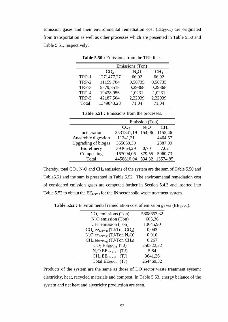
93
Emission gases and their environmental remediation cost (EEENV-t) are originated
from transportation as well as other processes which are presented in Table 5.50 and
Table 5.51, respectively.
Table 5.50 : Emissions from the TRP lines.
Emissions (Ton)
CO2 N2O CH4
TRP-1 1271477,27 66,92 66,92
TRP-2 11159,704 0,58735 0,58735
TRP-3 5579,8518 0,29368 0,29368
TRP-4 19438,956 1,0231 1,0231
TRP-5 42187,504 2,22039 2,22039
Total 1349843,28 71,04 71,04
Table 5.51 : Emissions from the processes.
Emission (Ton)
CO2 N2O CH4
Incineration 3531841,19 154,06 1155,46
Anaerobic digestion 11241,21 4464,57
Upgrading of biogas 355059,30 2887,09
Biorefinery 393664,29 0,70 7,02
Composting 167004,06 379,55 5060,73
Total 4458810,04 534,32 13574,85
Thereby, total CO2, N2O and CH4 emissions of the system are the sum of Table 5.50 and
Table5.51 and the sum is presented in Table 5.52. The environmental remediation cost
of considered emission gases are computed further in Section 5.4.3 and inserted into
Table 5.52 to obtain the EEENV-t for the IN sector solid waste treatment system.
Table 5.52 : Environmental remediation cost of emission gases (EEENV-t).
CO2 emissions (Ton) 5808653,32
N2O emission (Ton) 605,36
CH4 emission (Ton) 13645,90
CO2 eeENV-g (TJ/Ton CO2) 0,043
N2O eeENV-g (TJ/Ton N2O) 0,010
CH4 eeENV-g (TJ/Ton CH4) 0,267
CO2 EEENV-g (TJ) 250822,22
N2O EEENV-g (TJ) 5,84
CH4 EEENV-g (TJ) 3641,26
Total EEENV-t (TJ) 254469,32
Products of the system are the same as those of DO sector waste treatment system:
electricity, heat, recycled materials and compost. In Table 5.53, energy balance of the
system and net heat and electricity production are seen.
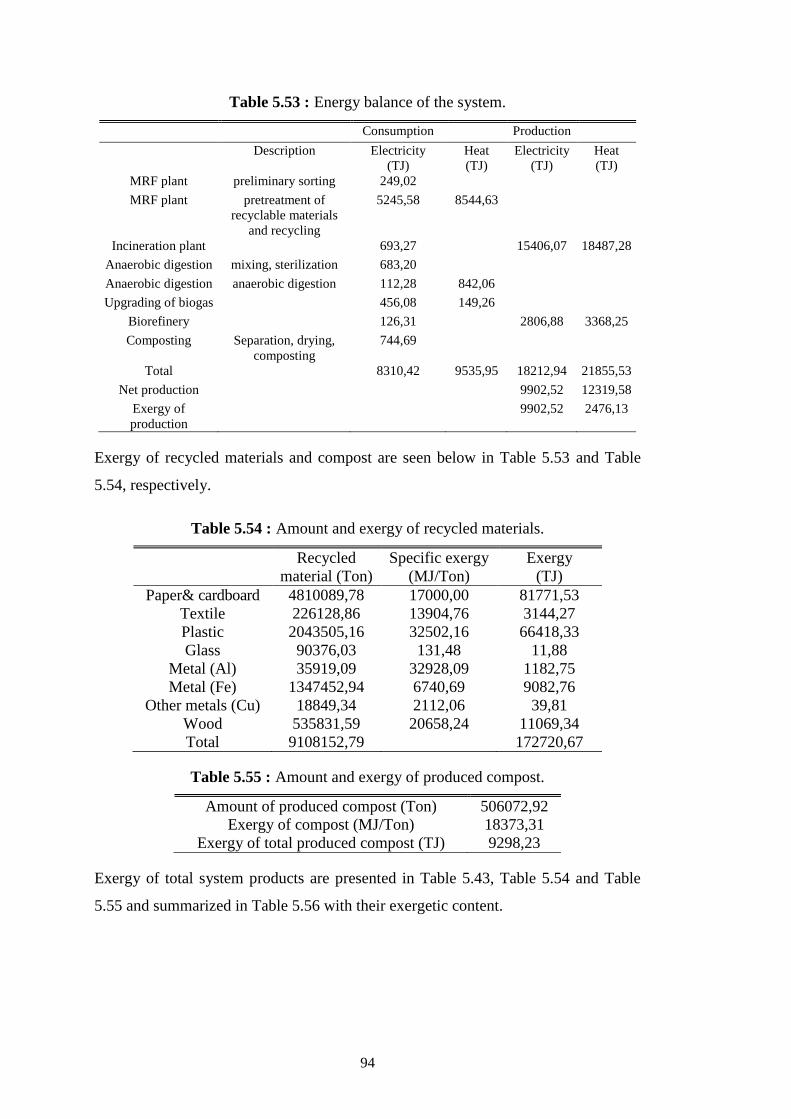
94
Table 5.53 : Energy balance of the system.
Consumption Production
Description Electricity
(TJ)
Heat
(TJ)
Electricity
(TJ)
Heat
(TJ)
MRF plant preliminary sorting 249,02
MRF plant pretreatment of
recyclable materials
and recycling
5245,58 8544,63
Incineration plant 693,27 15406,07 18487,28
Anaerobic digestion mixing, sterilization 683,20
Anaerobic digestion anaerobic digestion 112,28 842,06
Upgrading of biogas 456,08 149,26
Biorefinery 126,31 2806,88 3368,25
Composting Separation, drying,
composting
744,69
Total 8310,42 9535,95 18212,94 21855,53
Net production 9902,52 12319,58
Exergy of
production
9902,52 2476,13
Exergy of recycled materials and compost are seen below in Table 5.53 and Table
5.54, respectively.
Table 5.54 : Amount and exergy of recycled materials.
Recycled
material (Ton)
Specific exergy
(MJ/Ton)
Exergy
(TJ)
Paper& cardboard 4810089,78 17000,00 81771,53
Textile 226128,86 13904,76 3144,27
Plastic 2043505,16 32502,16 66418,33
Glass 90376,03 131,48 11,88
Metal (Al) 35919,09 32928,09 1182,75
Metal (Fe) 1347452,94 6740,69 9082,76
Other metals (Cu) 18849,34 2112,06 39,81
Wood 535831,59 20658,24 11069,34
Total 9108152,79 172720,67
Table 5.55 : Amount and exergy of produced compost.
Amount of produced compost (Ton) 506072,92
Exergy of compost (MJ/Ton) 18373,31
Exergy of total produced compost (TJ) 9298,23
Exergy of total system products are presented in Table 5.43, Table 5.54 and Table
5.55 and summarized in Table 5.56 with their exergetic content.
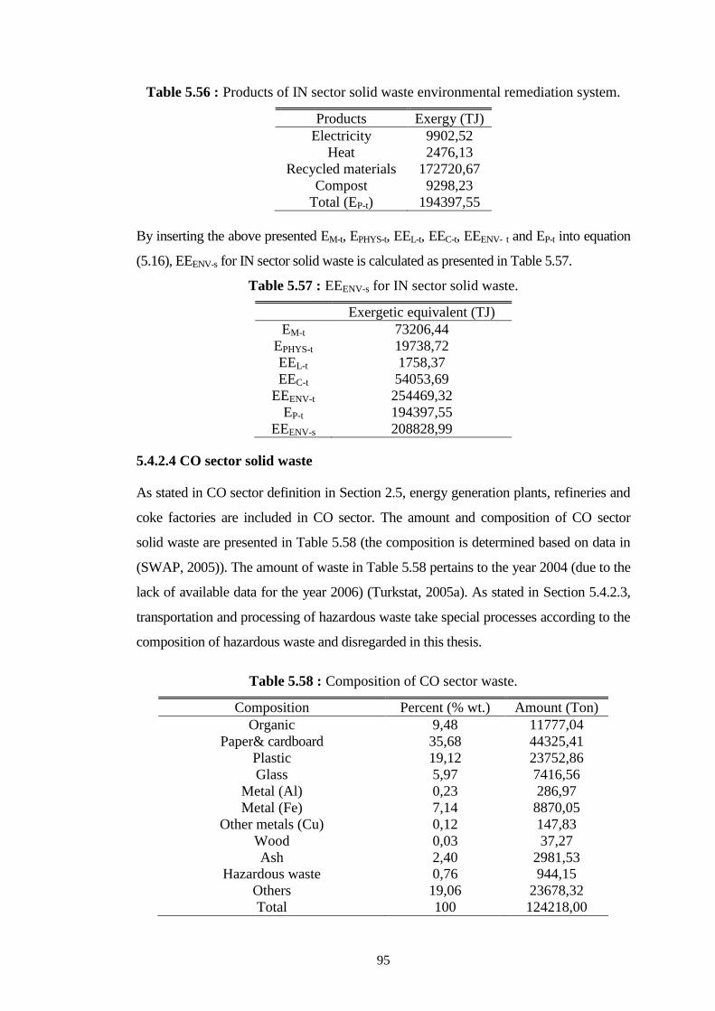
95
Table 5.56 : Products of IN sector solid waste environmental remediation system.
Products Exergy (TJ)
Electricity 9902,52
Heat 2476,13
Recycled materials 172720,67
Compost 9298,23
Total (EP-t) 194397,55
By inserting the above presented EM-t, EPHYS-t, EEL-t, EEC-t, EEENV- t and EP-t into equation
(5.16), EEENV-s for IN sector solid waste is calculated as presented in Table 5.57.
Table 5.57 : EEENV-s for IN sector solid waste.
Exergetic equivalent (TJ)
EM-t 73206,44
EPHYS-t 19738,72
EEL-t 1758,37
EEC-t 54053,69
EEENV-t 254469,32
EP-t 194397,55
EEENV-s 208828,99
5.4.2.4 CO sector solid waste
As stated in CO sector definition in Section 2.5, energy generation plants, refineries and
coke factories are included in CO sector. The amount and composition of CO sector
solid waste are presented in Table 5.58 (the composition is determined based on data in
(SWAP, 2005)). The amount of waste in Table 5.58 pertains to the year 2004 (due to the
lack of available data for the year 2006) (Turkstat, 2005a). As stated in Section 5.4.2.3,
transportation and processing of hazardous waste take special processes according to the
composition of hazardous waste and disregarded in this thesis.
Table 5.58 : Composition of CO sector waste.
Composition Percent (% wt.) Amount (Ton)
Organic 9,48 11777,04
Paper& cardboard 35,68 44325,41
Plastic 19,12 23752,86
Glass 5,97 7416,56
Metal (Al) 0,23 286,97
Metal (Fe) 7,14 8870,05
Other metals (Cu) 0,12 147,83
Wood 0,03 37,27
Ash 2,40 2981,53
Hazardous waste 0,76 944,15
Others 19,06 23678,32
Total 100 124218,00
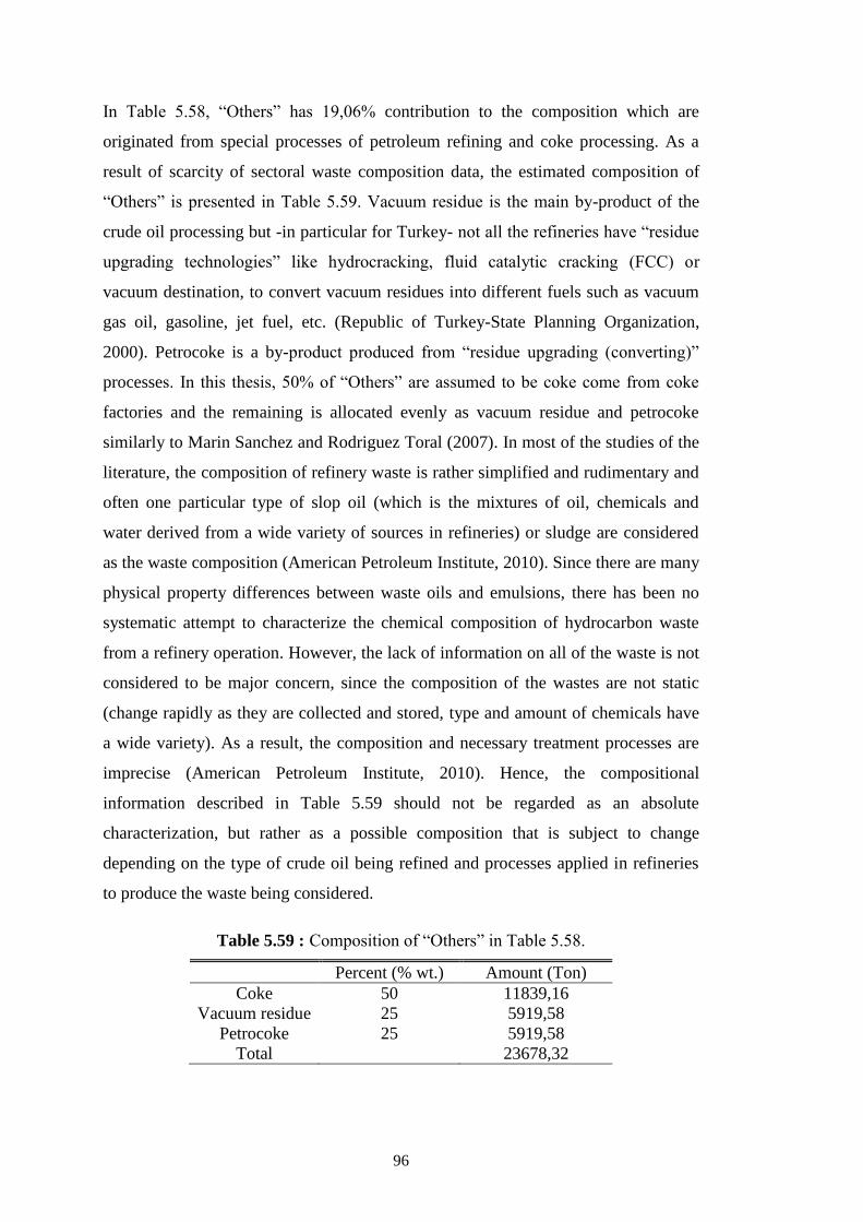
96
In Table 5.58, “Others” has 19,06% contribution to the composition which are
originated from special processes of petroleum refining and coke processing. As a
result of scarcity of sectoral waste composition data, the estimated composition of
“Others” is presented in Table 5.59. Vacuum residue is the main by-product of the
crude oil processing but -in particular for Turkey- not all the refineries have “residue
upgrading technologies” like hydrocracking, fluid catalytic cracking (FCC) or
vacuum destination, to convert vacuum residues into different fuels such as vacuum
gas oil, gasoline, jet fuel, etc. (Republic of Turkey-State Planning Organization,
2000). Petrocoke is a by-product produced from “residue upgrading (converting)”
processes. In this thesis, 50% of “Others” are assumed to be coke come from coke
factories and the remaining is allocated evenly as vacuum residue and petrocoke
similarly to Marin Sanchez and Rodriguez Toral (2007). In most of the studies of the
literature, the composition of refinery waste is rather simplified and rudimentary and
often one particular type of slop oil (which is the mixtures of oil, chemicals and
water derived from a wide variety of sources in refineries) or sludge are considered
as the waste composition (American Petroleum Institute, 2010). Since there are many
physical property differences between waste oils and emulsions, there has been no
systematic attempt to characterize the chemical composition of hydrocarbon waste
from a refinery operation. However, the lack of information on all of the waste is not
considered to be major concern, since the composition of the wastes are not static
(change rapidly as they are collected and stored, type and amount of chemicals have
a wide variety). As a result, the composition and necessary treatment processes are
imprecise (American Petroleum Institute, 2010). Hence, the compositional
information described in Table 5.59 should not be regarded as an absolute
characterization, but rather as a possible composition that is subject to change
depending on the type of crude oil being refined and processes applied in refineries
to produce the waste being considered.
Table 5.59 : Composition of “Others” in Table 5.58.
Percent (% wt.) Amount (Ton)
Coke 50 11839,16
Vacuum residue 25 5919,58
Petrocoke 25 5919,58
Total 23678,32
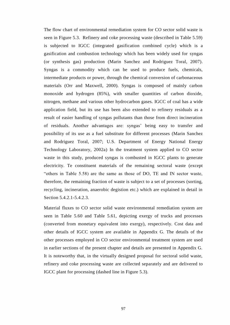
97
The flow chart of environmental remediation system for CO sector solid waste is
seen in Figure 5.3. Refinery and coke processing waste (described in Table 5.59)
is subjected to IGCC (integrated gasification combined cycle) which is a
gasification and combustion technology which has been widely used for syngas
(or synthesis gas) production (Marin Sanchez and Rodriguez Toral, 2007).
Syngas is a commodity which can be used to produce fuels, chemicals,
intermediate products or power, through the chemical conversion of carbonaceous
materials (Orr and Maxwell, 2000). Syngas is composed of mainly carbon
monoxide and hydrogen (85%), with smaller quantities of carbon dioxide,
nitrogen, methane and various other hydrocarbon gases. IGCC of coal has a wide
application field, but its use has been also extended to refinery residuals as a
result of easier handling of syngas pollutants than those from direct incineration
of residuals. Another advantages are: syngas’ being easy to transfer and
possibility of its use as a fuel substitute for different processes (Marin Sanchez
and Rodriguez Toral, 2007; U.S. Department of Energy National Energy
Technology Laboratory, 2002a) In the treatment system applied to CO sector
waste in this study, produced syngas is combusted in IGCC plants to generate
electricity. Te constituent materials of the remaining sectoral waste (except
“others in Table 5.58) are the same as those of DO, TE and IN sector waste,
therefore, the remaining fraction of waste is subject to a set of processes (sorting,
recycling, incineration, anaerobic degistion etc.) which are explained in detail in
Section 5.4.2.1-5.4.2.3.
Material fluxes to CO sector solid waste environmental remediation system are
seen in Table 5.60 and Table 5.61, depicting exergy of trucks and processes
(converted from monetary equivalent into exergy), respectively. Cost data and
other details of IGCC system are available in Appendix G. The details of the
other processes employed in CO sector environmental treatment system are used
in earlier sections of the present chapter and details are presented in Appendix G.
It is noteworthy that, in the virtually designed proposal for sectoral solid waste,
refinery and coke processing waste are collected separately and are delivered to
IGCC plant for processing (dashed line in Figure 5.3).
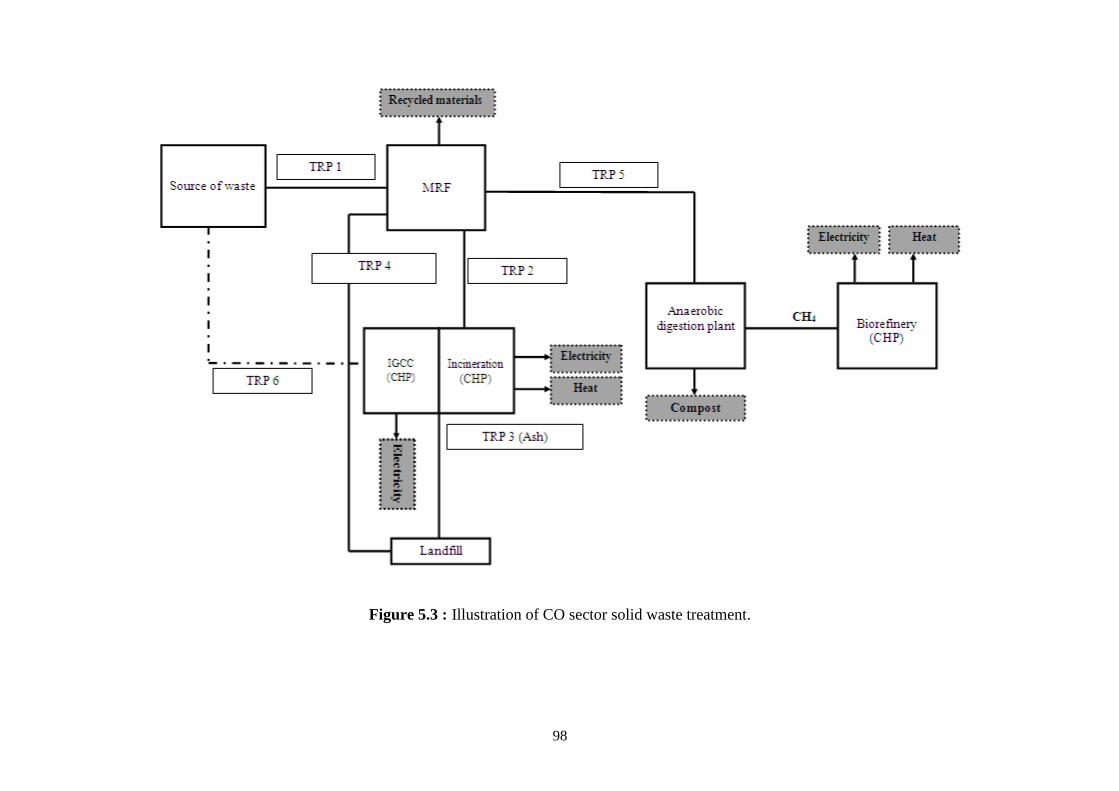
98
Figure 5.3 : Illustration of CO sector solid waste treatment.
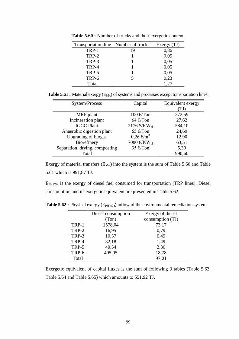
99
Table 5.60 : Number of trucks and their exergetic content.
Transportation line Number of trucks Exergy (TJ)
TRP-1 19 0,86
TRP-2 1 0,05
TRP-3 1 0,05
TRP-4 1 0,05
TRP-5 1 0,05
TRP-6 5 0,23
Total 1,27
Table 5.61 : Material exergy (EM-t) of systems and processes except transportation lines.
System/Process Capital Equivalent exergy
(TJ)
MRF plant 100 €/Ton 272,59
Incineration plant 64 €/Ton 27,62
IGCC Plant 2176 $/KWel 584,10
Anaerobic digestion plant 65 €/Ton 24,60
Upgrading of biogas 0,26 €/m3 12,90
Biorefinery 7000 €/KWel 63,51
Separation, drying, composting 35 €/Ton 5,30
Total 990,60
Exergy of material transfers (EM-t) into the system is the sum of Table 5.60 and Table
5.61 which is 991,87 TJ.
EPHYS-t is the exergy of diesel fuel consumed for transportation (TRP lines). Diesel
consumption and its exergetic equivalent are presented in Table 5.62.
Table 5.62 : Physical exergy (EPHYS-t) inflow of the environmental remediation system.
Diesel consumption
(Ton)
Exergy of diesel
consumption (TJ)
TRP-1 1578,04 73,17
TRP-2 16,95 0,79
TRP-3 10,57 0,49
TRP-4 32,18 1,49
TRP-5 49,54 2,30
TRP-6 405,05 18,78
Total
97,01
Exergetic equivalent of capital fluxes is the sum of following 3 tables (Table 5.63,
Table 5.64 and Table 5.65) which amounts to 551,92 TJ.
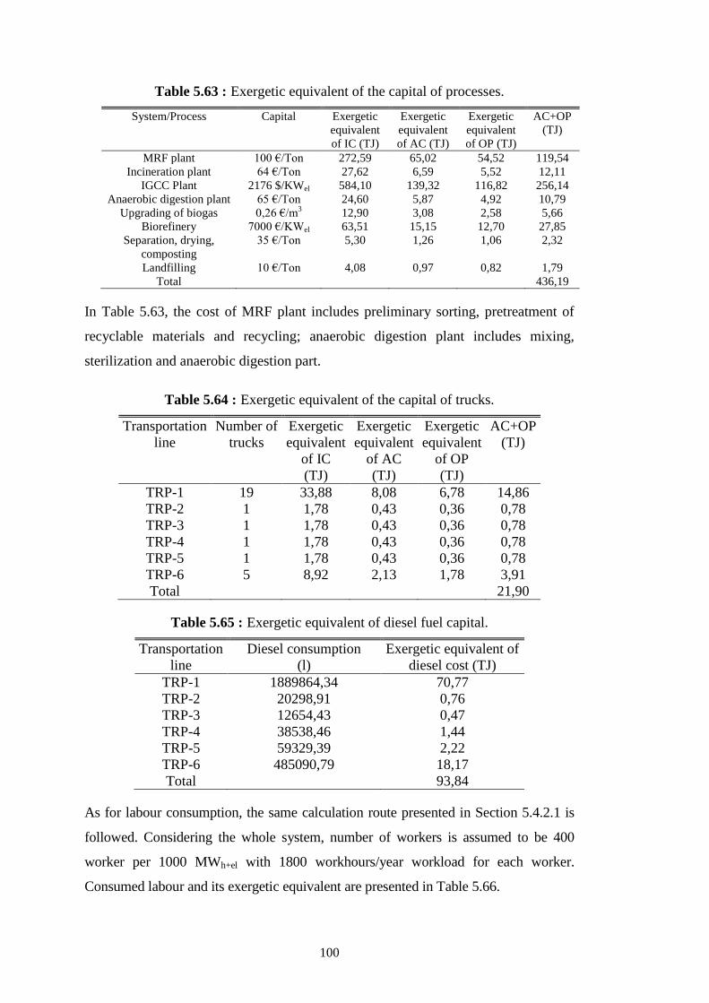
100
Table 5.63 : Exergetic equivalent of the capital of processes.
System/Process Capital Exergetic
equivalent
of IC (TJ)
Exergetic
equivalent
of AC (TJ)
Exergetic
equivalent
of OP (TJ)
AC+OP
(TJ)
MRF plant 100 €/Ton 272,59 65,02 54,52 119,54
Incineration plant 64 €/Ton 27,62 6,59 5,52 12,11
IGCC Plant 2176 $/KWel 584,10 139,32 116,82 256,14
Anaerobic digestion plant 65 €/Ton 24,60 5,87 4,92 10,79
Upgrading of biogas 0,26 €/m3 12,90 3,08 2,58 5,66
Biorefinery 7000 €/KWel 63,51 15,15 12,70 27,85
Separation, drying,
composting
35 €/Ton 5,30 1,26 1,06 2,32
Landfilling 10 €/Ton 4,08 0,97 0,82 1,79
Total 436,19
In Table 5.63, the cost of MRF plant includes preliminary sorting, pretreatment of
recyclable materials and recycling; anaerobic digestion plant includes mixing,
sterilization and anaerobic digestion part.
Table 5.64 : Exergetic equivalent of the capital of trucks.
Transportation
line
Number of
trucks
Exergetic
equivalent
of IC
(TJ)
Exergetic
equivalent
of AC
(TJ)
Exergetic
equivalent
of OP
(TJ)
AC+OP
(TJ)
TRP-1 19 33,88 8,08 6,78 14,86
TRP-2 1 1,78 0,43 0,36 0,78
TRP-3 1 1,78 0,43 0,36 0,78
TRP-4 1 1,78 0,43 0,36 0,78
TRP-5 1 1,78 0,43 0,36 0,78
TRP-6 5 8,92 2,13 1,78 3,91
Total 21,90
Table 5.65 : Exergetic equivalent of diesel fuel capital.
Transportation
line
Diesel consumption
(l)
Exergetic equivalent of
diesel cost (TJ)
TRP-1 1889864,34 70,77
TRP-2 20298,91 0,76
TRP-3 12654,43 0,47
TRP-4 38538,46 1,44
TRP-5 59329,39 2,22
TRP-6 485090,79 18,17
Total 93,84
As for labour consumption, the same calculation route presented in Section 5.4.2.1 is
followed. Considering the whole system, number of workers is assumed to be 400
worker per 1000 MWh+el with 1800 workhours/year workload for each worker.
Consumed labour and its exergetic equivalent are presented in Table 5.66.
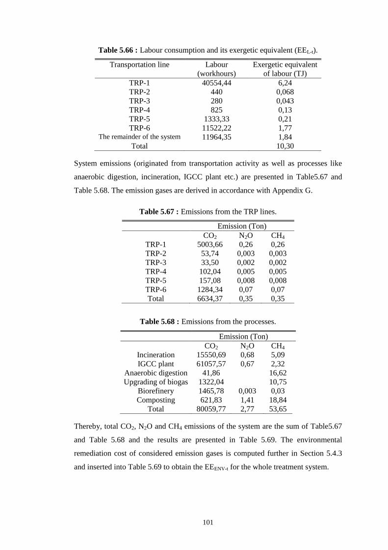
101
Table 5.66 : Labour consumption and its exergetic equivalent (EEL-t).
Transportation line Labour
(workhours)
Exergetic equivalent
of labour (TJ)
TRP-1 40554,44 6,24
TRP-2 440 0,068
TRP-3 280 0,043
TRP-4 825 0,13
TRP-5 1333,33 0,21
TRP-6 11522,22 1,77 The remainder of the system 11964,35 1,84
Total 10,30
System emissions (originated from transportation activity as well as processes like
anaerobic digestion, incineration, IGCC plant etc.) are presented in Table5.67 and
Table 5.68. The emission gases are derived in accordance with Appendix G.
Table 5.67 : Emissions from the TRP lines.
Emission (Ton)
CO2 N2O CH4
TRP-1 5003,66 0,26 0,26
TRP-2 53,74 0,003 0,003
TRP-3 33,50 0,002 0,002
TRP-4 102,04 0,005 0,005
TRP-5 157,08 0,008 0,008
TRP-6 1284,34 0,07 0,07
Total 6634,37 0,35 0,35
Table 5.68 : Emissions from the processes.
Emission (Ton)
CO2 N2O CH4
Incineration 15550,69 0,68 5,09
IGCC plant 61057,57 0,67 2,32
Anaerobic digestion 41,86
16,62
Upgrading of biogas 1322,04
10,75
Biorefinery 1465,78 0,003 0,03
Composting 621,83 1,41 18,84
Total 80059,77 2,77 53,65
Thereby, total CO2, N2O and CH4 emissions of the system are the sum of Table5.67
and Table 5.68 and the results are presented in Table 5.69. The environmental
remediation cost of considered emission gases is computed further in Section 5.4.3
and inserted into Table 5.69 to obtain the EEENV-t for the whole treatment system.

102
Table 5.69 : Environmental remediation cost of emission gases (EEENV-t).
CO2 emissions (Ton) 86694,13
N2O emission (Ton) 3,11
CH4 emission (Ton) 54
CO2 eeENV-g (TJ/Ton CO2) 0,043
N2O eeENV-g (TJ/Ton N2O) 0,010
CH4 eeENV-g (TJ/Ton CH4) 0,267
CO2 EEENV-g (TJ) 3743,52
N2O EEENV-g (TJ) 0,03
CH4 EEENV-g (TJ) 14,41
Total EEENV-t (TJ) 3757,96
Products of the remediation system are electricity and heat produced by incineration
of non-recyclable part of the inorganic waste, biorefinery plant and IGCC plant.
Recycled materials and produced compost (the ash generated in considered processes
are assumed to have zero exergy and its exergetic content is not included in exergy of
products). Principals of computing the produced and/or consumed energy by the
processes are presented in Appendix G. Energy balance of the system and net heat
and electricity production are presented in Table 5.70.
Table 5.70 : Energy balance of the system.
Consumption Production
Description Electricity
(TJ)
Heat
(TJ)
Electricity
(TJ)
Heat
(TJ)
MRF plant preliminary sorting 1,49
MRF plant pretreatment of
recyclable materials
and recycling
31,56 88,92
Incineration plant 3,05 67,83 81,40
IGCC plant 9,28 309,22
Anaerobic digestion mixing, sterilization 2,54
Anaerobic digestion anaerobic digestion 0,42 3,14
Upgrading of biogas 1,70 0,56
Biorefinery 0,47 10,45 12,54
Composting Separation, drying,
composting
2,77
Total 53,28 92,61 387,51 93,94
Net production 334,23 1,33
Exergy of production 334,23 0,27
Amount of recycled materials and exergy contents are seen in Table 5.71.
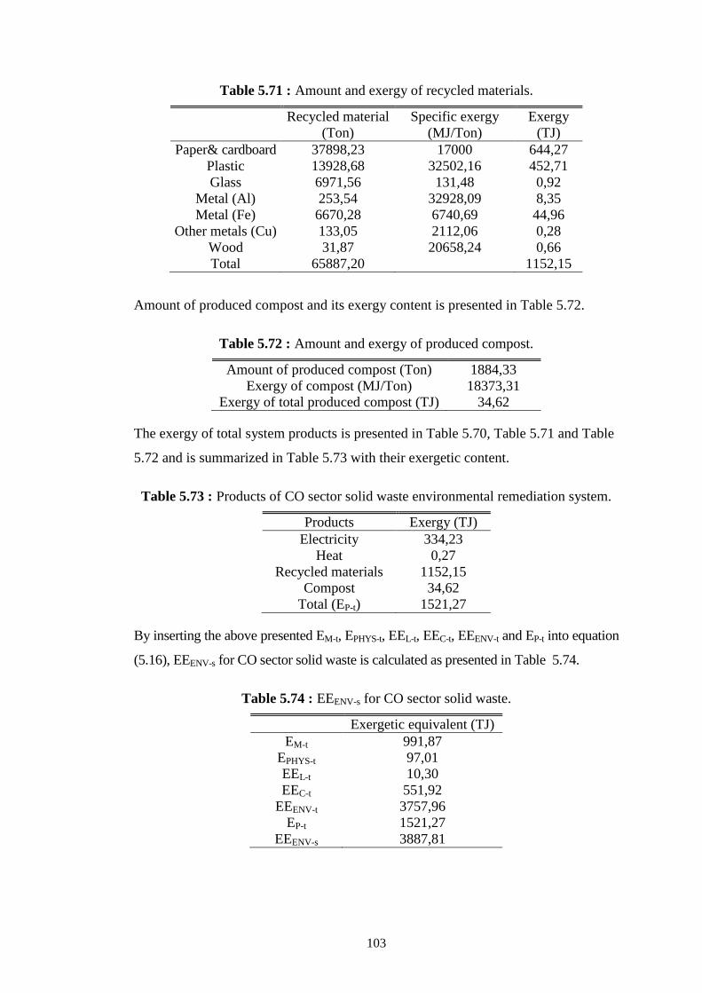
103
Table 5.71 : Amount and exergy of recycled materials.
Recycled material
(Ton)
Specific exergy
(MJ/Ton)
Exergy
(TJ)
Paper& cardboard 37898,23 17000 644,27
Plastic 13928,68 32502,16 452,71
Glass 6971,56 131,48 0,92
Metal (Al) 253,54 32928,09 8,35
Metal (Fe) 6670,28 6740,69 44,96
Other metals (Cu) 133,05 2112,06 0,28
Wood 31,87 20658,24 0,66
Total 65887,20 1152,15
Amount of produced compost and its exergy content is presented in Table 5.72.
Table 5.72 : Amount and exergy of produced compost.
Amount of produced compost (Ton) 1884,33
Exergy of compost (MJ/Ton) 18373,31
Exergy of total produced compost (TJ) 34,62
The exergy of total system products is presented in Table 5.70, Table 5.71 and Table
5.72 and is summarized in Table 5.73 with their exergetic content.
Table 5.73 : Products of CO sector solid waste environmental remediation system.
Products Exergy (TJ)
Electricity 334,23
Heat 0,27
Recycled materials 1152,15
Compost 34,62
Total (EP-t) 1521,27
By inserting the above presented EM-t, EPHYS-t, EEL-t, EEC-t, EEENV-t and EP-t into equation
(5.16), EEENV-s for CO sector solid waste is calculated as presented in Table 5.74.
Table 5.74 : EEENV-s for CO sector solid waste.
Exergetic equivalent (TJ)
EM-t 991,87
EPHYS-t 97,01
EEL-t 10,30
EEC-t 551,92
EEENV-t 3757,96
EP-t 1521,27
EEENV-s 3887,81
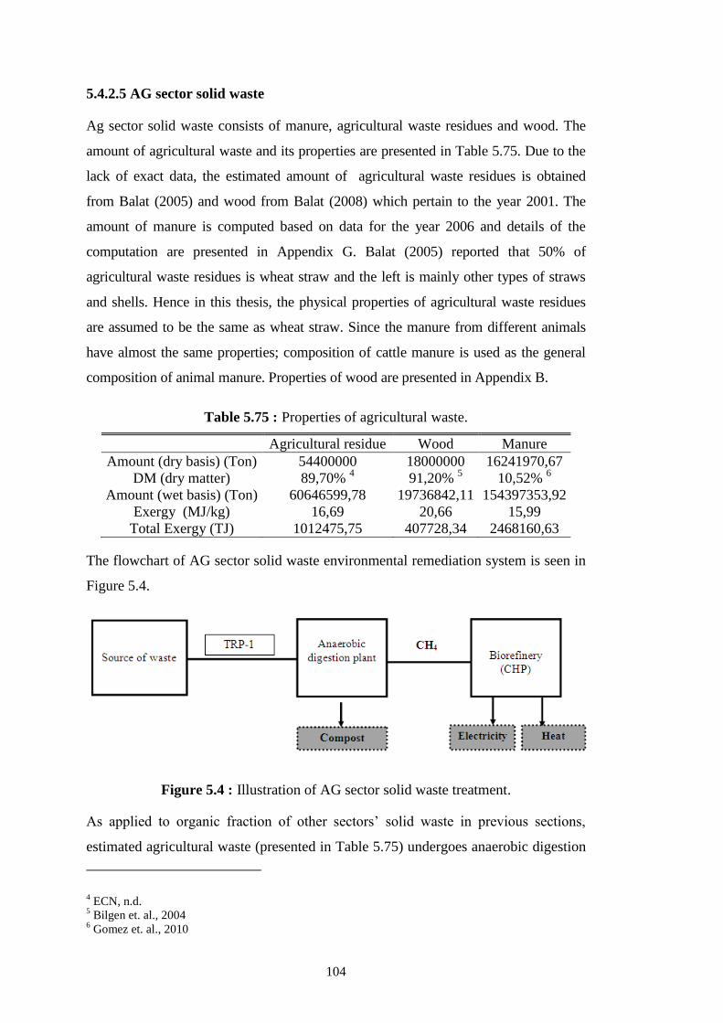
104
5.4.2.5 AG sector solid waste
Ag sector solid waste consists of manure, agricultural waste residues and wood. The
amount of agricultural waste and its properties are presented in Table 5.75. Due to the
lack of exact data, the estimated amount of agricultural waste residues is obtained
from Balat (2005) and wood from Balat (2008) which pertain to the year 2001. The
amount of manure is computed based on data for the year 2006 and details of the
computation are presented in Appendix G. Balat (2005) reported that 50% of
agricultural waste residues is wheat straw and the left is mainly other types of straws
and shells. Hence in this thesis, the physical properties of agricultural waste residues
are assumed to be the same as wheat straw. Since the manure from different animals
have almost the same properties; composition of cattle manure is used as the general
composition of animal manure. Properties of wood are presented in Appendix B.
Table 5.75 : Properties of agricultural waste.
Agricultural residue Wood Manure
Amount (dry basis) (Ton) 54400000 18000000 16241970,67
DM (dry matter) 89,70% 4
91,20% 5 10,52%
6
Amount (wet basis) (Ton) 60646599,78 19736842,11 154397353,92
Exergy (MJ/kg) 16,69 20,66 15,99
Total Exergy (TJ) 1012475,75 407728,34 2468160,63
The flowchart of AG sector solid waste environmental remediation system is seen in
Figure 5.4.
Figure 5.4 : Illustration of AG sector solid waste treatment.
As applied to organic fraction of other sectors’ solid waste in previous sections,
estimated agricultural waste (presented in Table 5.75) undergoes anaerobic digestion
4 ECN, n.d.
5 Bilgen et. al., 2004
6 Gomez et. al., 2010
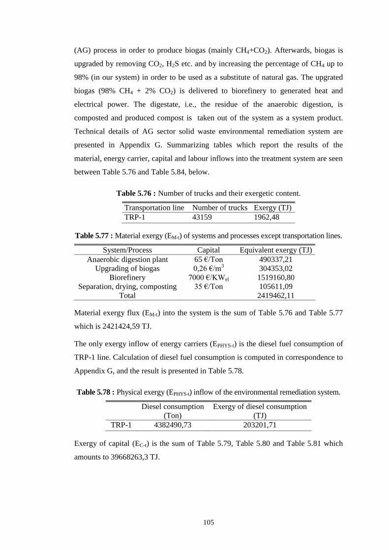
105
(AG) process in order to produce biogas (mainly CH4+CO2). Afterwards, biogas is
upgraded by removing CO2, H2S etc. and by increasing the percentage of CH4 up to
98% (in our system) in order to be used as a substitute of natural gas. The upgrated
biogas (98% CH4 + 2% CO2) is delivered to biorefinery to generated heat and
electrical power. The digestate, i.e., the residue of the anaerobic digestion, is
composted and produced compost is taken out of the system as a system product.
Technical details of AG sector solid waste environmental remediation system are
presented in Appendix G. Summarizing tables which report the results of the
material, energy carrier, capital and labour inflows into the treatment system are seen
between Table 5.76 and Table 5.84, below.
Table 5.76 : Number of trucks and their exergetic content.
Transportation line Number of trucks Exergy (TJ)
TRP-1 43159 1962,48
Table 5.77 : Material exergy (EM-t) of systems and processes except transportation lines.
System/Process Capital Equivalent exergy (TJ)
Anaerobic digestion plant 65 €/Ton 490337,21
Upgrading of biogas 0,26 €/m3 304353,02
Biorefinery 7000 €/KWel 1519160,80
Separation, drying, composting 35 €/Ton 105611,09
Total 2419462,11
Material exergy flux (EM-t) into the system is the sum of Table 5.76 and Table 5.77
which is 2421424,59 TJ.
The only exergy inflow of energy carriers (EPHYS-t) is the diesel fuel consumption of
TRP-1 line. Calculation of diesel fuel consumption is computed in correspondence to
Appendix G, and the result is presented in Table 5.78.
Table 5.78 : Physical exergy (EPHYS-t) inflow of the environmental remediation system.
Diesel consumption
(Ton)
Exergy of diesel consumption
(TJ)
TRP-1 4382490,73 203201,71
Exergy of capital (EC-t) is the sum of Table 5.79, Table 5.80 and Table 5.81 which
amounts to 39668263,3 TJ.
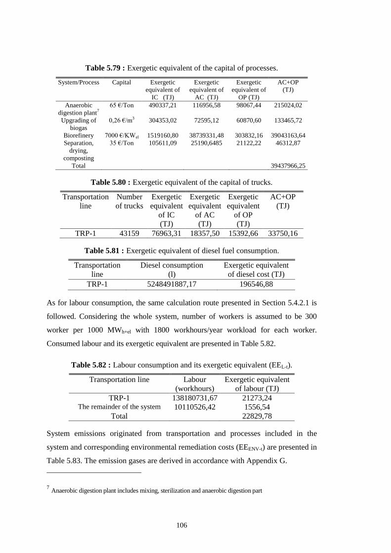
106
Table 5.79 : Exergetic equivalent of the capital of processes.
System/Process Capital Exergetic
equivalent of
IC (TJ)
Exergetic
equivalent of
AC (TJ)
Exergetic
equivalent of
OP (TJ)
AC+OP
(TJ)
Anaerobic
digestion plant7
65 €/Ton 490337,21 116956,58 98067,44 215024,02
Upgrading of
biogas
0,26 €/m3 304353,02 72595,12 60870,60 133465,72
Biorefinery 7000 €/KWel 1519160,80 38739331,48 303832,16 39043163,64
Separation,
drying,
composting
35 €/Ton 105611,09 25190,6485 21122,22 46312,87
Total 39437966,25
Table 5.80 : Exergetic equivalent of the capital of trucks.
Transportation
line
Number
of trucks
Exergetic
equivalent
of IC
(TJ)
Exergetic
equivalent
of AC
(TJ)
Exergetic
equivalent
of OP
(TJ)
AC+OP
(TJ)
TRP-1 43159 76963,31 18357,50 15392,66 33750,16
Table 5.81 : Exergetic equivalent of diesel fuel consumption.
Transportation
line
Diesel consumption
(l)
Exergetic equivalent
of diesel cost (TJ)
TRP-1 5248491887,17 196546,88
As for labour consumption, the same calculation route presented in Section 5.4.2.1 is
followed. Considering the whole system, number of workers is assumed to be 300
worker per 1000 MWh+el with 1800 workhours/year workload for each worker.
Consumed labour and its exergetic equivalent are presented in Table 5.82.
Table 5.82 : Labour consumption and its exergetic equivalent (EEL-t).
Transportation line Labour
(workhours)
Exergetic equivalent
of labour (TJ)
TRP-1 138180731,67 21273,24 The remainder of the system 10110526,42 1556,54
Total 22829,78
System emissions originated from transportation and processes included in the
system and corresponding environmental remediation costs (EEENV-t) are presented in
Table 5.83. The emission gases are derived in accordance with Appendix G.
7 Anaerobic digestion plant includes mixing, sterilization and anaerobic digestion part

107
Table 5.83 : Emissions from transportation (TRP-1) and processes.
Emission (Ton)
CO2 N2O CH4
TRP-1 13896059,00 731,37 731,37
Anaerobic digestion 1049035,98 397654,60
Upgrading of biogas 33170069,87 257149,98
Biorefinery 35063305,62 62,50 625,01
Composting 15600986,84 28173,70 375649,27
Total 98779457,31 28967,57 1031810,24
The environmental remediation cost of considered emission gases is computed
further in Section 5.4.3 and inserted into Table 5.84 to obtain the EEENV-t for the
whole environmental remediation system.
Table 5.84 : Environmental remediation cost of emission gases (EEENV-t).
CO2 emissions (Ton) 98779457,31
N2O emission (Ton) 28967,57
CH4 emission (Ton) 1031810,24
CO2 eeENV-g (TJ/Ton CO2) 0,043
N2O eeENV-g (TJ/Ton N2O) 0,010
CH4 eeENV-g (TJ/Ton CH4) 0,267
CO2 EEENV-g (TJ) 4265374,65
N2O EEENV-g (TJ) 279,374782
CH4 EEENV-g (TJ) 275327,588
Total EEENV-t (TJ) 4540981,61
The products of the environmental remediation system are produced energy
(electricity and heat) in biorefinery plant and compost produced in composting
process. The composition of biogas utilized in the biorefinery is the same as
presented in previous sections (98% CH4 and 2% CO2). The biorefinery is a CHP
plant and system biogas production, the efficiencies of heat and electricity generation
and produced energy can be seen in Table 5.85.
Table 5.85 : Properties of biogas utilization.
CH4 (m3) 18529924709,13
CO2 (m3) 378161728,76
LHV of CH4 (MJ/m3) 33,73
LHV of CO2 (MJ/m3) 0
LHV of biogas (TJ) 625014,3604
Electricity generation efficiency 0,40
Heat generation efficiency 0,48
Generated electricity (TJ) 250005,74
Generated heat (TJ) 300006,89
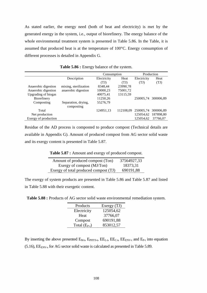
108
As stated earlier, the energy need (both of heat and electricity) is met by the
generated energy in the system, i.e., output of biorefinery. The energy balance of the
whole environmental treatment system is presented in Table 5.86. In the Table, it is
assumed that produced heat is at the temperature of 100°C. Energy consumption of
different processes is detailed in Appendix G.
Table 5.86 : Energy balance of the system.
Consumption Production
Description Electricity
(TJ)
Heat
(TJ)
Electricity
(TJ)
Heat
(TJ)
Anaerobic digestion mixing, sterilization 8348,44 23990,78
Anaerobic digestion anaerobic digestion 10000,23 75001,72
Upgrading of biogas 40075,41 13115,59
Biorefinery 11250,26 250005,74 300006,89
Composting Separation, drying,
composting
55276,79
Total 124951,13 112108,09 250005,74 300006,89
Net production 125054,62 187898,80
Exergy of production 125054,62 37766,07
Residue of the AD process is composted to produce compost (Technical details are
available in Appendix G). Amount of produced compost from AG sector solid waste
and its exergy content is presented in Table 5.87.
Table 5.87 : Amount and exergy of produced compost.
Amount of produced compost (Ton) 37564927,33
Exergy of compost (MJ/Ton) 18373,31
Exergy of total produced compost (TJ) 690191,88
The exergy of system products are presented in Table 5.86 and Table 5.87 and listed
in Table 5.88 with their exergetic content.
Table 5.88 : Products of AG sector solid waste environmental remediation system.
Products Exergy (TJ)
Electricity 125054,62
Heat 37766,07
Compost 690191,88
Total (EP-t) 853012,57
By inserting the above presented EM-t, EPHYS-t, EEL-t, EEC-t, EEENV-t and EP-t into equation
(5.16), EEENV-s for AG sector solid waste is calculated as presented in Table 5.89.
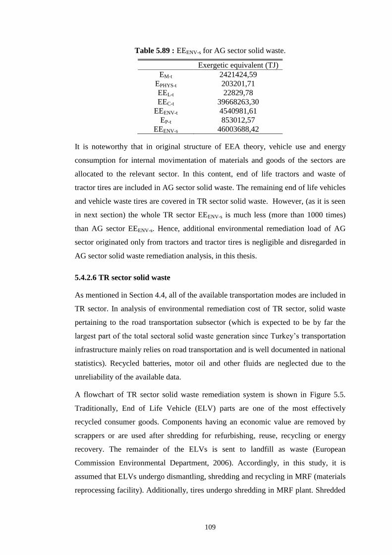
109
Table 5.89 : EEENV-s for AG sector solid waste.
Exergetic equivalent (TJ)
EM-t 2421424,59
EPHYS-t 203201,71
EEL-t 22829,78
EEC-t 39668263,30
EEENV-t 4540981,61
EP-t 853012,57
EEENV-s 46003688,42
It is noteworthy that in original structure of EEA theory, vehicle use and energy
consumption for internal movimentation of materials and goods of the sectors are
allocated to the relevant sector. In this content, end of life tractors and waste of
tractor tires are included in AG sector solid waste. The remaining end of life vehicles
and vehicle waste tires are covered in TR sector solid waste. However, (as it is seen
in next section) the whole TR sector EEENV-s is much less (more than 1000 times)
than AG sector EEENV-s. Hence, additional environmental remediation load of AG
sector originated only from tractors and tractor tires is negligible and disregarded in
AG sector solid waste remediation analysis, in this thesis.
5.4.2.6 TR sector solid waste
As mentioned in Section 4.4, all of the available transportation modes are included in
TR sector. In analysis of environmental remediation cost of TR sector, solid waste
pertaining to the road transportation subsector (which is expected to be by far the
largest part of the total sectoral solid waste generation since Turkey’s transportation
infrastructure mainly relies on road transportation and is well documented in national
statistics). Recycled batteries, motor oil and other fluids are neglected due to the
unreliability of the available data.
A flowchart of TR sector solid waste remediation system is shown in Figure 5.5.
Traditionally, End of Life Vehicle (ELV) parts are one of the most effectively
recycled consumer goods. Components having an economic value are removed by
scrappers or are used after shredding for refurbishing, reuse, recycling or energy
recovery. The remainder of the ELVs is sent to landfill as waste (European
Commission Environmental Department, 2006). Accordingly, in this study, it is
assumed that ELVs undergo dismantling, shredding and recycling in MRF (materials
reprocessing facility). Additionally, tires undergo shredding in MRF plant. Shredded
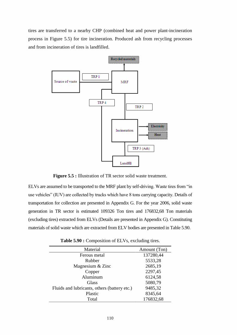
110
tires are transferred to a nearby CHP (combined heat and power plant-incineration
process in Figure 5.5) for tire incineration. Produced ash from recycling processes
and from incineration of tires is landfilled.
Figure 5.5 : Illustration of TR sector solid waste treatment.
ELVs are assumed to be transported to the MRF plant by self-driving. Waste tires from “in
use vehicles” (IUV) are collected by trucks which have 8 tons carrying capacity. Details of
transportation for collection are presented in Appendix G. For the year 2006, solid waste
generation in TR sector is estimated 109326 Ton tires and 176832,68 Ton materials
(excluding tires) extracted from ELVs (Details are presented in Appendix G). Constituting
materials of solid waste which are extracted from ELV bodies are presented in Table 5.90.
Table 5.90 : Composition of ELVs, excluding tires.
Material Amount (Ton)
Ferous metal 137280,44
Rubber 5533,28
Magnesium & Zinc 2685,19
Copper 2297,45
Aluminum 6124,58
Glass 5080,79
Fluids and lubricants, others (battery etc.) 9485,32
Plastic 8345,64
Total 176832,68
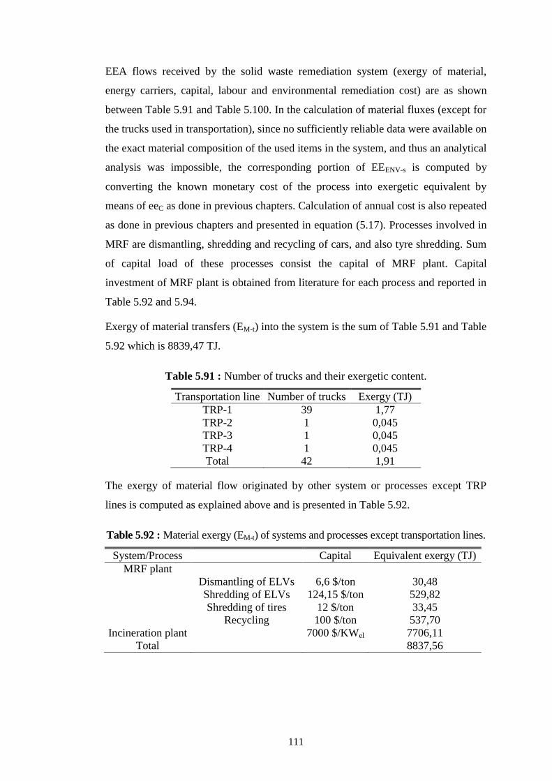
111
EEA flows received by the solid waste remediation system (exergy of material,
energy carriers, capital, labour and environmental remediation cost) are as shown
between Table 5.91 and Table 5.100. In the calculation of material fluxes (except for
the trucks used in transportation), since no sufficiently reliable data were available on
the exact material composition of the used items in the system, and thus an analytical
analysis was impossible, the corresponding portion of EEENV-s is computed by
converting the known monetary cost of the process into exergetic equivalent by
means of eeC as done in previous chapters. Calculation of annual cost is also repeated
as done in previous chapters and presented in equation (5.17). Processes involved in
MRF are dismantling, shredding and recycling of cars, and also tyre shredding. Sum
of capital load of these processes consist the capital of MRF plant. Capital
investment of MRF plant is obtained from literature for each process and reported in
Table 5.92 and 5.94.
Exergy of material transfers (EM-t) into the system is the sum of Table 5.91 and Table
5.92 which is 8839,47 TJ.
Table 5.91 : Number of trucks and their exergetic content.
Transportation line Number of trucks Exergy (TJ)
TRP-1 39 1,77
TRP-2 1 0,045
TRP-3 1 0,045
TRP-4 1 0,045
Total 42 1,91
The exergy of material flow originated by other system or processes except TRP
lines is computed as explained above and is presented in Table 5.92.
Table 5.92 : Material exergy (EM-t) of systems and processes except transportation lines.
System/Process Capital Equivalent exergy (TJ)
MRF plant
Dismantling of ELVs 6,6 $/ton 30,48
Shredding of ELVs 124,15 $/ton 529,82
Shredding of tires 12 $/ton 33,45
Recycling 100 $/ton 537,70
Incineration plant 7000 $/KWel 7706,11
Total 8837,56
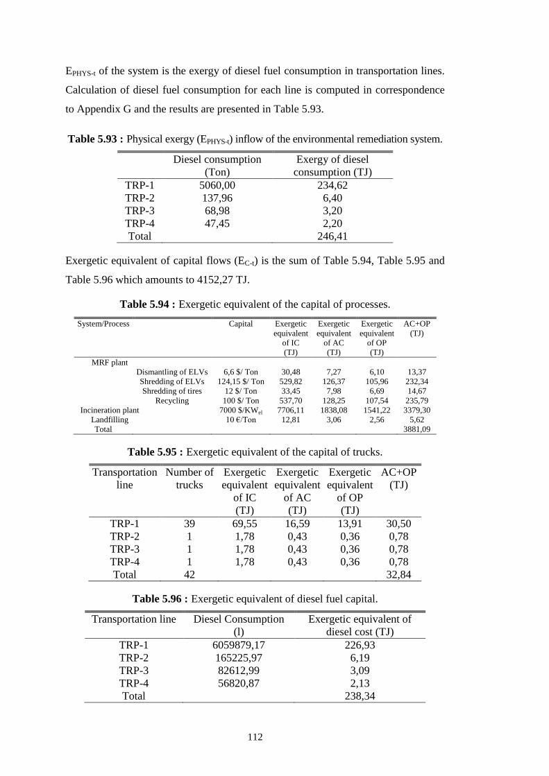
112
EPHYS-t of the system is the exergy of diesel fuel consumption in transportation lines.
Calculation of diesel fuel consumption for each line is computed in correspondence
to Appendix G and the results are presented in Table 5.93.
Table 5.93 : Physical exergy (EPHYS-t) inflow of the environmental remediation system.
Diesel consumption
(Ton)
Exergy of diesel
consumption (TJ)
TRP-1 5060,00 234,62
TRP-2 137,96 6,40
TRP-3 68,98 3,20
TRP-4 47,45 2,20
Total 246,41
Exergetic equivalent of capital flows (EC-t) is the sum of Table 5.94, Table 5.95 and
Table 5.96 which amounts to 4152,27 TJ.
Table 5.94 : Exergetic equivalent of the capital of processes.
System/Process Capital Exergetic
equivalent
of IC
(TJ)
Exergetic
equivalent
of AC
(TJ)
Exergetic
equivalent
of OP
(TJ)
AC+OP
(TJ)
MRF plant
Dismantling of ELVs 6,6 $/ Ton 30,48 7,27 6,10 13,37
Shredding of ELVs 124,15 $/ Ton 529,82 126,37 105,96 232,34
Shredding of tires 12 $/ Ton 33,45 7,98 6,69 14,67
Recycling 100 $/ Ton 537,70 128,25 107,54 235,79
Incineration plant 7000 $/KWel 7706,11 1838,08 1541,22 3379,30
Landfilling 10 €/Ton 12,81 3,06 2,56 5,62
Total 3881,09
Table 5.95 : Exergetic equivalent of the capital of trucks.
Transportation
line
Number of
trucks
Exergetic
equivalent
of IC
(TJ)
Exergetic
equivalent
of AC
(TJ)
Exergetic
equivalent
of OP
(TJ)
AC+OP
(TJ)
TRP-1 39 69,55 16,59 13,91 30,50
TRP-2 1 1,78 0,43 0,36 0,78
TRP-3 1 1,78 0,43 0,36 0,78
TRP-4 1 1,78 0,43 0,36 0,78
Total 42 32,84
Table 5.96 : Exergetic equivalent of diesel fuel capital.
Transportation line Diesel Consumption
(l)
Exergetic equivalent of
diesel cost (TJ)
TRP-1 6059879,17 226,93
TRP-2 165225,97 6,19
TRP-3 82612,99 3,09
TRP-4 56820,87 2,13
Total 238,34

113
As for labour consumption, the same calculation route presented in Section 5.4.2.1 is
followed. Considering the whole system, number of workers is assumed to be 300
workers per 1000 MWh+el with 1800 workhours/year workload for each worker.
Consumed labour and its exergetic equivalent are presented in Table 5.97.
Table 5.97 : Labour consumption and its exergetic equivalent (EEL-t).
Transportation line Labour
(workhours)
Exergetic equivalent
of labour (TJ)
TRP-1 124865 19,22
TRP-2 2720 0,42
TRP-3 1760 0,27
TRP-4 1200 0,18
The left of the system 50121,15 7,72
Total 27,81
System emissions originated from transportation as well as other processes which are
included in the system presented in Table 5.98 and Table 5.99, respectively. The
emission gases are derived in accordance with Appendix G.
Table 5.98 : Emissions from the TRP lines.
Emission (Ton)
CO2 N2O CH4
TRP-1 16044,31 0,84 0,84
TRP-2 437,46 0,02 0,02
TRP-3 218,729 0,01 0,01
TRP-4 150,44 0,008 0,008
Total 16850,94 0,89 0,89
Table 5.99 : Emissions from the processes.
Emission (Ton)
CO2 N2O CH4
Incineration plant 270449,89 1,80 9,01
Thereby, total CO2, N2O and CH4 emissions of the system are the sum of Table 5.98 and
Table 5.99 and the sum is presented in Table 5.100. The environmental remediation cost
of considered emission gases is computed further in Section 5.4.3 and inserted into Table
5.100 to obtain the EEENV-t for the TR sector solid waste remediation system.
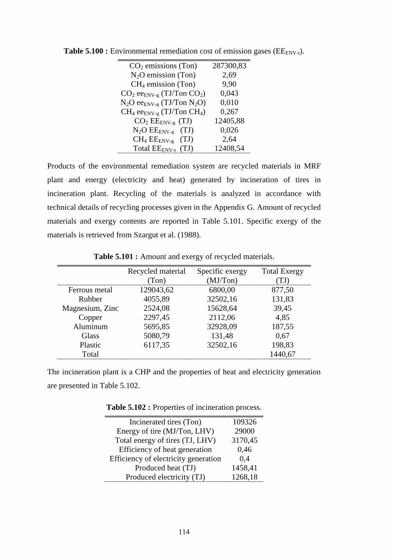
114
Table 5.100 : Environmental remediation cost of emission gases (EEENV-t).
CO2 emissions (Ton) 287300,83
N2O emission (Ton) 2,69
CH4 emission (Ton) 9,90
CO2 eeENV-g (TJ/Ton CO2) 0,043
N2O eeENV-g (TJ/Ton N2O) 0,010
CH4 eeENV-g (TJ/Ton CH4) 0,267
CO2 EEENV-g (TJ) 12405,88
N2O EEENV-g (TJ) 0,026
CH4 EEENV-g (TJ) 2,64
Total EEENV-t (TJ) 12408,54
Products of the environmental remediation system are recycled materials in MRF
plant and energy (electricity and heat) generated by incineration of tires in
incineration plant. Recycling of the materials is analyzed in accordance with
technical details of recycling processes given in the Appendix G. Amount of recycled
materials and exergy contents are reported in Table 5.101. Specific exergy of the
materials is retrieved from Szargut et al. (1988).
Table 5.101 : Amount and exergy of recycled materials.
Recycled material
(Ton)
Specific exergy
(MJ/Ton)
Total Exergy
(TJ)
Ferrous metal 129043,62 6800,00 877,50
Rubber 4055,89 32502,16
131,83
Magnesium, Zinc 2524,08 15628,64 39,45
Copper 2297,45 2112,06 4,85
Aluminum 5695,85 32928,09 187,55
Glass 5080,79 131,48 0,67
Plastic 6117,35 32502,16 198,83
Total 1440,67
The incineration plant is a CHP and the properties of heat and electricity generation
are presented in Table 5.102.
Table 5.102 : Properties of incineration process.
Incinerated tires (Ton) 109326
Energy of tire (MJ/Ton, LHV) 29000
Total energy of tires (TJ, LHV) 3170,45
Efficiency of heat generation 0,46
Efficiency of electricity generation 0,4
Produced heat (TJ) 1458,41
Produced electricity (TJ) 1268,18
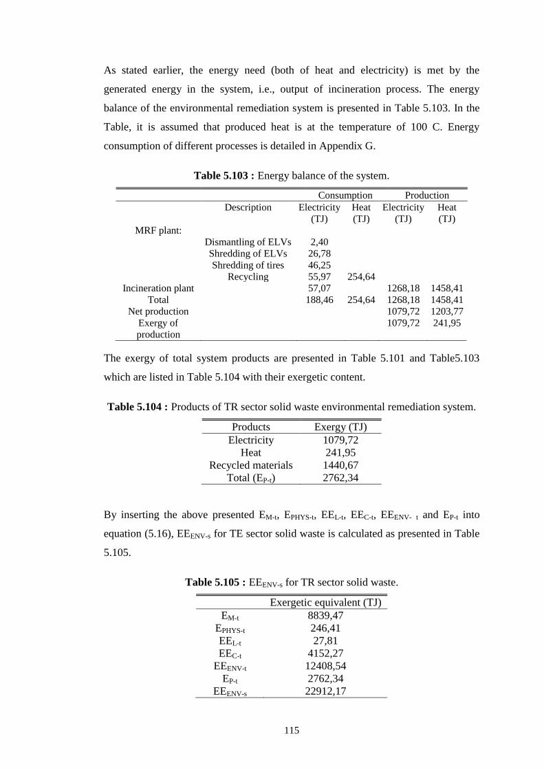
115
As stated earlier, the energy need (both of heat and electricity) is met by the
generated energy in the system, i.e., output of incineration process. The energy
balance of the environmental remediation system is presented in Table 5.103. In the
Table, it is assumed that produced heat is at the temperature of 100 C. Energy
consumption of different processes is detailed in Appendix G.
Table 5.103 : Energy balance of the system.
Consumption Production
Description Electricity
(TJ)
Heat
(TJ)
Electricity
(TJ)
Heat
(TJ)
MRF plant:
Dismantling of ELVs 2,40
Shredding of ELVs 26,78
Shredding of tires 46,25
Recycling 55,97 254,64
Incineration plant 57,07 1268,18 1458,41
Total 188,46 254,64 1268,18 1458,41
Net production 1079,72 1203,77
Exergy of
production
1079,72 241,95
The exergy of total system products are presented in Table 5.101 and Table5.103
which are listed in Table 5.104 with their exergetic content.
Table 5.104 : Products of TR sector solid waste environmental remediation system.
Products Exergy (TJ)
Electricity 1079,72
Heat 241,95
Recycled materials 1440,67
Total (EP-t) 2762,34
By inserting the above presented EM-t, EPHYS-t, EEL-t, EEC-t, EEENV- t and EP-t into
equation (5.16), EEENV-s for TE sector solid waste is calculated as presented in Table
5.105.
Table 5.105 : EEENV-s for TR sector solid waste.
Exergetic equivalent (TJ)
EM-t 8839,47
EPHYS-t 246,41
EEL-t 27,81
EEC-t 4152,27
EEENV-t 12408,54
EP-t 2762,34
EEENV-s 22912,17
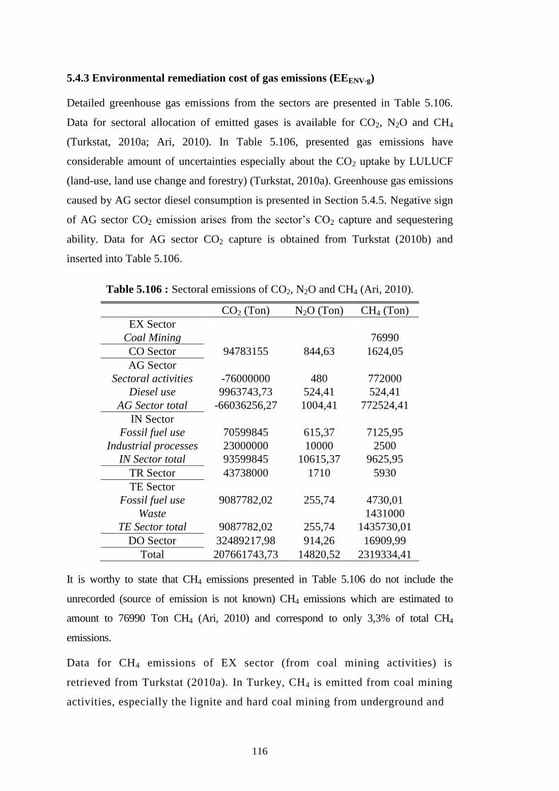
116
5.4.3 Environmental remediation cost of gas emissions (EEENV-g)
Detailed greenhouse gas emissions from the sectors are presented in Table 5.106.
Data for sectoral allocation of emitted gases is available for CO2, N2O and CH4
(Turkstat, 2010a; Ari, 2010). In Table 5.106, presented gas emissions have
considerable amount of uncertainties especially about the CO2 uptake by LULUCF
(land-use, land use change and forestry) (Turkstat, 2010a). Greenhouse gas emissions
caused by AG sector diesel consumption is presented in Section 5.4.5. Negative sign
of AG sector CO2 emission arises from the sector’s CO2 capture and sequestering
ability. Data for AG sector CO2 capture is obtained from Turkstat (2010b) and
inserted into Table 5.106.
Table 5.106 : Sectoral emissions of CO2, N2O and CH4 (Ari, 2010).
CO2 (Ton) N2O (Ton) CH4 (Ton)
EX Sector
Coal Mining
76990
CO Sector 94783155 844,63 1624,05
AG Sector
Sectoral activities -76000000 480 772000
Diesel use 9963743,73 524,41 524,41
AG Sector total -66036256,27 1004,41 772524,41
IN Sector
Fossil fuel use 70599845 615,37 7125,95
Industrial processes 23000000 10000 2500
IN Sector total 93599845 10615,37 9625,95
TR Sector 43738000 1710 5930
TE Sector
Fossil fuel use 9087782,02 255,74 4730,01
Waste
1431000
TE Sector total 9087782,02 255,74 1435730,01
DO Sector 32489217,98 914,26 16909,99
Total 207661743,73 14820,52 2319334,41
It is worthy to state that CH4 emissions presented in Table 5.106 do not include the
unrecorded (source of emission is not known) CH4 emissions which are estimated to
amount to 76990 Ton CH4 (Ari, 2010) and correspond to only 3,3% of total CH4
emissions.
Data for CH4 emissions of EX sector (from coal mining activities) is
retrieved from Turkstat (2010a). In Turkey, CH4 is emitted from coal mining
activities, especially the lignite and hard coal mining from underground and
117
surface mines (Turkstat, 2010a). Since in national energy consumption data
(IEA,2008; Republic of Turkey- Ministry of Energy and Natural Resources, n.d.), EX
sector consumes only electricity (no fossil fuel combustion emissions), the only
considerable emission from the sector is taken as aforementioned CH4 emissions.
As for IN sector, total sectoral emissions are retrieved from Ari (2010). Emissions which
are produced from industrial processes are derived from Turkstat (2010a). Thereby, the
remaining part of total sectoral emissions is considered as emissions from fossil fuel use.
Data for TR, TE and DO sector emissions are derived from Ari (2010).
The principal objective of this section is computing eeENV-g for CO2, N2O and CH4
emissions and total EEENV-g load of Turkish sectors. Due to the scarcity of publicated data
for detailed sectoral allocation of other emission gases (such as SO2 or HF), their treatment
technologies and corresponding eeENV-g values are not incorporated in the analysis.
5.4.3.1 Environmental remediation cost (EEENV-g) of CO2
CO2 capture and treatment receive noticeable attention as a “high potential
greenhouse gas” mitigation option. In this section of CO2 capturing, a lime (CaCO3)
based technology is adopted and a generalized modelling tool of the technology is
analyzed to estimate “environmental remediation cost of CO2” which is the amount
of irrevocable resource consumption (in terms of exergy) of CO2 environmental
remediation (treatment) system. This is a new and promising technology that may
help in mitigation of global warming and climate change caused by CO2 emissions
(Rubin et al., 2007; Manovic and Anthony; 2010). It is shown by some of the
economic analysis for CO2 treatment systems (Abanades et al., 2004; Abanades et
al., 2007; Mac Kenzie et al., 2007) that i) Ca-based CO2 capture systems are
economically attractive, ii) system is advantageous since CaO is relatively
inexpensive and abundant.
The schematic representation of the Ca-based CO2 capture system via CaO-
carbonation reaction (CO2 environmental remediation system) is shown in Figure
5.6. The system is designed based on the system available in Romeo et al. (2010).
During the carbonation step, particles of CaO are transformed to CaCO3. CaO acts as
a CO2 absorbent, capturing CO2 to form CaCO3 (Alonsol et al., 2011). The composed
CaCO3 is landfilled in the present system. The mass balance presented in Figure 5.6
is for annual 1 kg CO2 processing.

118
Figure 5.6 : Schematic overview of CO2 environmental remediation system.
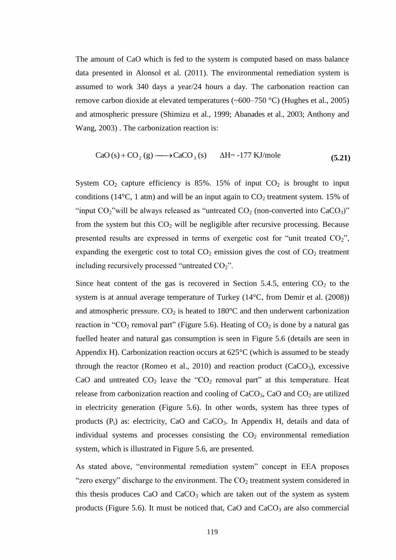
119
The amount of CaO which is fed to the system is computed based on mass balance
data presented in Alonsol et al. (2011). The environmental remediation system is
assumed to work 340 days a year/24 hours a day. The carbonation reaction can
remove carbon dioxide at elevated temperatures (~600–750 °C) (Hughes et al., 2005)
and atmospheric pressure (Shimizu et al., 1999; Abanades et al., 2003; Anthony and
Wang, 2003) . The carbonization reaction is:
)s(CaCO)g(CO)s(CaO 32 ΔH= -177 KJ/mole (5.21)
System CO2 capture efficiency is 85%. 15% of input CO2 is brought to input
conditions (14°C, 1 atm) and will be an input again to CO2 treatment system. 15% of
“input CO2”will be always released as “untreated CO2 (non-converted into CaCO3)”
from the system but this CO2 will be negligible after recursive processing. Because
presented results are expressed in terms of exergetic cost for “unit treated CO2”,
expanding the exergetic cost to total CO2 emission gives the cost of CO2 treatment
including recursively processed “untreated CO2”.
Since heat content of the gas is recovered in Section 5.4.5, entering CO2 to the
system is at annual average temperature of Turkey (14°C, from Demir et al. (2008))
and atmospheric pressure. CO2 is heated to 180°C and then underwent carbonization
reaction in “CO2 removal part” (Figure 5.6). Heating of CO2 is done by a natural gas
fuelled heater and natural gas consumption is seen in Figure 5.6 (details are seen in
Appendix H). Carbonization reaction occurs at 625°C (which is assumed to be steady
through the reactor (Romeo et al., 2010) and reaction product (CaCO3), excessive
CaO and untreated CO2 leave the “CO2 removal part” at this temperature. Heat
release from carbonization reaction and cooling of CaCO3, CaO and CO2 are utilized
in electricity generation (Figure 5.6). In other words, system has three types of
products (Pt) as: electricity, CaO and CaCO3. In Appendix H, details and data of
individual systems and processes consisting the CO2 environmental remediation
system, which is illustrated in Figure 5.6, are presented.
As stated above, “environmental remediation system” concept in EEA proposes
“zero exergy” discharge to the environment. The CO2 treatment system considered in
this thesis produces CaO and CaCO3 which are taken out of the system as system
products (Figure 5.6). It must be noticed that, CaO and CaCO3 are also commercial
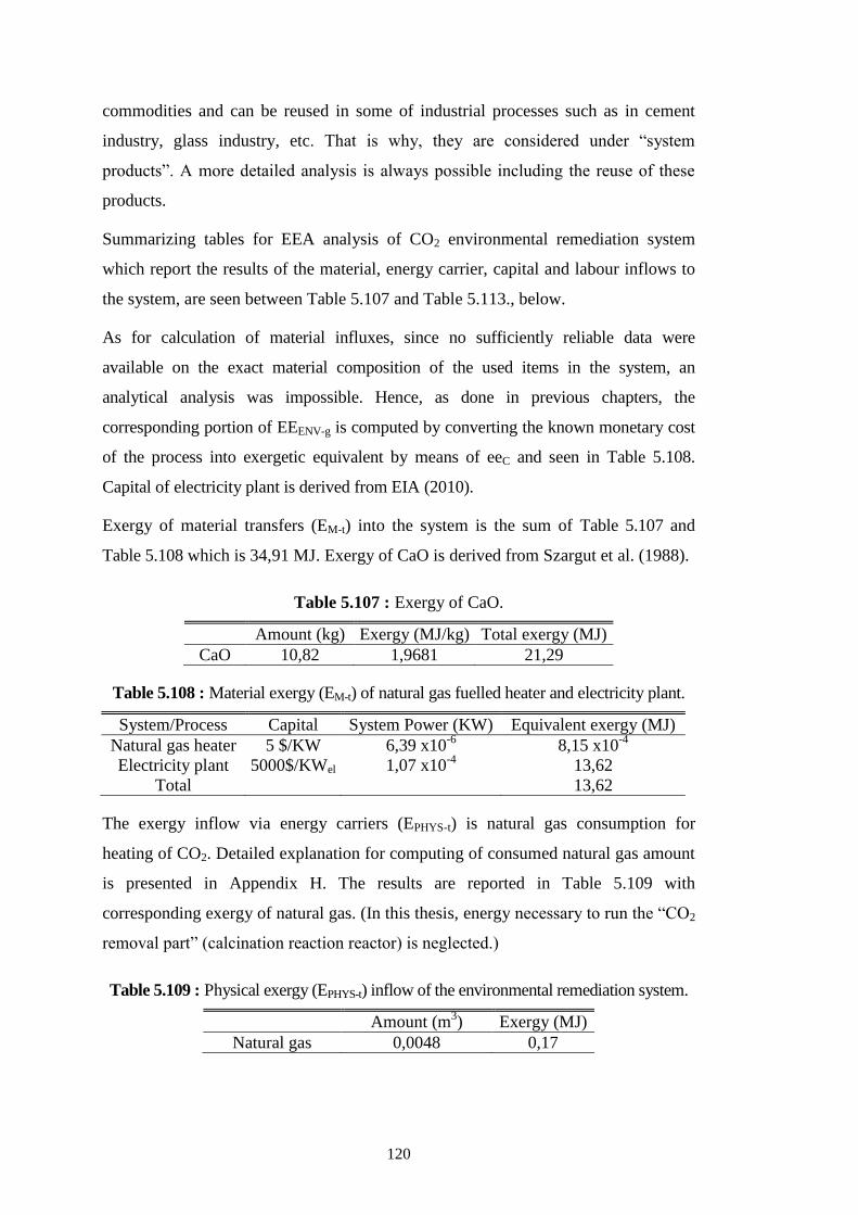
120
commodities and can be reused in some of industrial processes such as in cement
industry, glass industry, etc. That is why, they are considered under “system
products”. A more detailed analysis is always possible including the reuse of these
products.
Summarizing tables for EEA analysis of CO2 environmental remediation system
which report the results of the material, energy carrier, capital and labour inflows to
the system, are seen between Table 5.107 and Table 5.113., below.
As for calculation of material influxes, since no sufficiently reliable data were
available on the exact material composition of the used items in the system, an
analytical analysis was impossible. Hence, as done in previous chapters, the
corresponding portion of EEENV-g is computed by converting the known monetary cost
of the process into exergetic equivalent by means of eeC and seen in Table 5.108.
Capital of electricity plant is derived from EIA (2010).
Exergy of material transfers (EM-t) into the system is the sum of Table 5.107 and
Table 5.108 which is 34,91 MJ. Exergy of CaO is derived from Szargut et al. (1988).
Table 5.107 : Exergy of CaO.
Amount (kg) Exergy (MJ/kg) Total exergy (MJ)
CaO 10,82 1,9681 21,29
Table 5.108 : Material exergy (EM-t) of natural gas fuelled heater and electricity plant.
System/Process Capital System Power (KW) Equivalent exergy (MJ)
Natural gas heater 5 $/KW 6,39 x10⁻⁶
8,15 x10⁻⁴
Electricity plant 5000$/KWel 1,07 x10⁻⁴
13,62
Total 13,62
The exergy inflow via energy carriers (EPHYS-t) is natural gas consumption for
heating of CO2. Detailed explanation for computing of consumed natural gas amount
is presented in Appendix H. The results are reported in Table 5.109 with
corresponding exergy of natural gas. (In this thesis, energy necessary to run the “CO2
removal part” (calcination reaction reactor) is neglected.)
Table 5.109 : Physical exergy (EPHYS-t) inflow of the environmental remediation system.
Amount (m3) Exergy (MJ)
Natural gas 0,0048 0,17
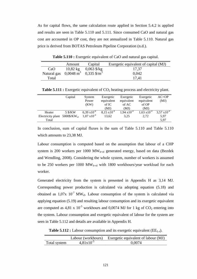
121
As for capital flows, the same calculation route applied in Section 5.4.2 is applied
and results are seen in Table 5.110 and 5.111. Since consumed CaO and natural gas
cost are accounted in OP cost, they are not annualized in Table 5.110. Natural gas
price is derived from BOTAS Petroleum Pipeline Corporation (n.d.).
Table 5.110 : Exergetic equivalent of CaO and natural gas capital.
Amount Capital Exergetic equivalent of capital (MJ)
CaO 10,82 kg 0,063 $/kg 17,37
Natural gas 0,0048 m3 0,335 $/m
3 0,042
Total 17,41
Table 5.111 : Exergetic equivalent of CO2 heating process and electricity plant.
Capital System
Power
(KW)
Exergetic
equivalent
of IC
(MJ)
Exergetic
equivalent
of AC
(MJ)
Exergetic
equivalent
of OP
(MJ)
AC+OP
(MJ)
Heater 5 $/KW 6,39 x10⁻⁶
8,15 x10⁻⁴
1,94 x10⁻⁴
1,63 x10⁻⁴
3,57 x10⁻⁴
Electricity plant 5000$/KWel 1,07 x10⁻⁴
13,62 3,25 2,72 5,97
Total 5,97
In conclusion, sum of capital fluxes is the sum of Table 5.110 and Table 5.110
which amounts to 23,38 MJ.
Labour consumption is computed based on the assumption that labour of a CHP
system is 200 workers per 1000 MWh+el generated energy, based on data (Bezdek
and Wendling, 2008). Considering the whole system, number of workers is assumed
to be 250 workers per 1000 MWh+el with 1800 workhours/year workload for each
worker.
Generated electricity from the system is presented in Appendix H as 3,14 MJ.
Corresponding power production is calculated via adopting equation (5.18) and
obtained as 1,07x 10⁻⁷
MWel. Labour consumption of the system is calculated via
applying equation (5.19) and resulting labour consumption and its exergetic equivalent
are computed as 4,81 x 10⁻⁵
workhours and 0,0074 MJ for 1 kg of CO2 entering into
the system. Labour consumption and exergetic equivalent of labour for the system are
seen in Table 5.112 and details are available in Appendix H.
Table 5.112 : Labour consumption and its exergetic equivalent (EEL-t).
Labour (workhours) Exergetic equivalent of labour (MJ)
Total system 4,81x10⁻⁵
0,0074
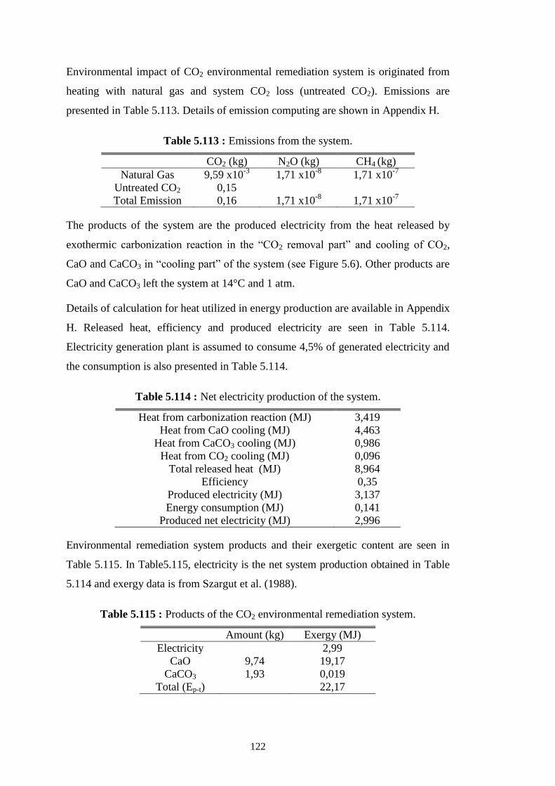
122
Environmental impact of CO2 environmental remediation system is originated from
heating with natural gas and system CO2 loss (untreated CO2). Emissions are
presented in Table 5.113. Details of emission computing are shown in Appendix H.
Table 5.113 : Emissions from the system.
CO2 (kg) N2O (kg) CH4 (kg)
Natural Gas 9,59 x10⁻³
1,71 x10⁻⁸
1,71 x10⁻⁷
Untreated CO2 0,15
Total Emission 0,16 1,71 x10⁻⁸
1,71 x10⁻⁷
The products of the system are the produced electricity from the heat released by
exothermic carbonization reaction in the “CO2 removal part” and cooling of CO2,
CaO and CaCO3 in “cooling part” of the system (see Figure 5.6). Other products are
CaO and CaCO3 left the system at 14°C and 1 atm.
Details of calculation for heat utilized in energy production are available in Appendix
H. Released heat, efficiency and produced electricity are seen in Table 5.114.
Electricity generation plant is assumed to consume 4,5% of generated electricity and
the consumption is also presented in Table 5.114.
Table 5.114 : Net electricity production of the system.
Heat from carbonization reaction (MJ) 3,419
Heat from CaO cooling (MJ) 4,463
Heat from CaCO3 cooling (MJ) 0,986
Heat from CO2 cooling (MJ) 0,096
Total released heat (MJ) 8,964
Efficiency 0,35
Produced electricity (MJ) 3,137
Energy consumption (MJ) 0,141
Produced net electricity (MJ) 2,996
Environmental remediation system products and their exergetic content are seen in
Table 5.115. In Table5.115, electricity is the net system production obtained in Table
5.114 and exergy data is from Szargut et al. (1988).
Table 5.115 : Products of the CO2 environmental remediation system.
Amount (kg) Exergy (MJ)
Electricity 2,99
CaO 9,74 19,17
CaCO3 1,93 0,019
Total (Ep-t) 22,17
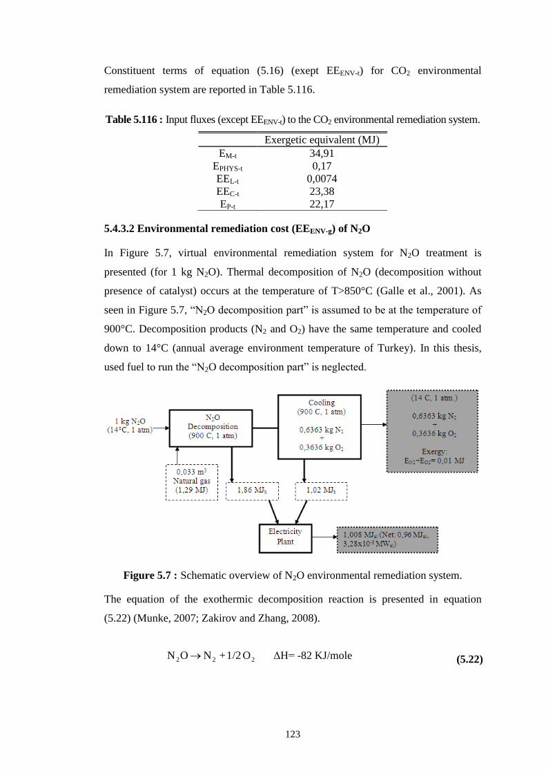
123
Constituent terms of equation (5.16) (exept EEENV-t) for CO2 environmental
remediation system are reported in Table 5.116.
Table 5.116 : Input fluxes (except EEENV-t) to the CO2 environmental remediation system.
Exergetic equivalent (MJ)
EM-t 34,91
EPHYS-t 0,17
EEL-t 0,0074
EEC-t 23,38
EP-t 22,17
5.4.3.2 Environmental remediation cost (EEENV-g) of N2O
In Figure 5.7, virtual environmental remediation system for N2O treatment is
presented (for 1 kg N2O). Thermal decomposition of N2O (decomposition without
presence of catalyst) occurs at the temperature of T>850°C (Galle et al., 2001). As
seen in Figure 5.7, “N2O decomposition part” is assumed to be at the temperature of
900°C. Decomposition products (N2 and O2) have the same temperature and cooled
down to 14°C (annual average environment temperature of Turkey). In this thesis,
used fuel to run the “N2O decomposition part” is neglected.
Figure 5.7 : Schematic overview of N2O environmental remediation system.
The equation of the exothermic decomposition reaction is presented in equation
(5.22) (Munke, 2007; Zakirov and Zhang, 2008).
222 O 1/2+ N ON ΔH= -82 KJ/mole (5.22)
124
N2O is heated up to 900°C by a natural gas fuelled heater. Natural gas consumption
is seen in Figure 5.7 and detailed calculation can be seen in Appendix H. Heat
release from decomposition reaction and cooling of N2 and O2 are utilized in
electricity generation (Figure 5.7). In other words, system has three types of products
(Pt) as: electricity, N2 and O2. In Appendix H, details and data of individual systems
and processes consisting the total environmental treatment system, which is
illustrated in Figure 5.7, are presented. Properties of system products are summarized
in Figure 5.7. The whole system is assumed to work 340 days a year/24 hours a day.
Summarizing tables for EEA analysis of N2O environmental remediation system
which report the results of the material, energy carrier, capital and labour inflows to
the system, are seen between Table 5.117 and Table 5.122, below.
As done in the previous chapters, material influxes are computed by converting the
known monetary cost of the process into exergetic equivalent by means of eeC and seen
in Table 5.117.
Table 5.117 : Material exergy (EM-t) inputs of the environmental remediation system.
System/Process Capital System Power
(KW)
Equivalent exergy
(MJ)
Natural gas heater 5 $/KW 4,38 x10⁻⁵
5,59 x10⁻³
Electricity plant 5000$/KWel 3,43 x10⁻⁵
4,38
Total 4,38
The exergy inflow of energy carriers (EPHYS-t) is the natural gas consumption for
heating of N2O and presented in Table 5.118 with corresponding exergy. Detailed
explanation for computing of consumed natural gas is presented in Appendix H.
Table 5.118 : Physical exergy (EPHYS-t) inflow of the environmental remediation system.
Amount (m3) Exergy (MJ)
Natural gas 0,033 1,18
As for capital flows, the same calculation route applied in Section 5.4.2.1 is applied
and results are seen in Table 5.119 and Table 5.120. Since consumed natural gas cost
is accounted in OP cost, they are not annualized in Table 5.119.
Table 5.119 : Exergetic equivalent of natural gas capital.
Amount
(m3)
Capital
($/m3)
Exergetic equivalent
of capital (MJ)
Natural gas 0,033 0,335 0,28
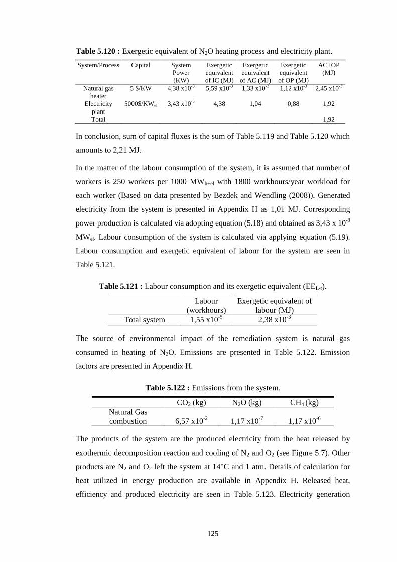
125
Table 5.120 : Exergetic equivalent of N2O heating process and electricity plant.
System/Process Capital System
Power
(KW)
Exergetic
equivalent
of IC (MJ)
Exergetic
equivalent
of AC (MJ)
Exergetic
equivalent
of OP (MJ)
AC+OP
(MJ)
Natural gas
heater
5 $/KW 4,38 x10⁻⁵
5,59 x10⁻³
1,33 x10⁻³
1,12 x10⁻³
2,45 x10⁻³
Electricity
plant
5000$/KWel 3,43 x10⁻⁵
4,38 1,04 0,88 1,92
Total 1,92
In conclusion, sum of capital fluxes is the sum of Table 5.119 and Table 5.120 which
amounts to 2,21 MJ.
In the matter of the labour consumption of the system, it is assumed that number of
workers is 250 workers per 1000 MWh+el with 1800 workhours/year workload for
each worker (Based on data presented by Bezdek and Wendling (2008)). Generated
electricity from the system is presented in Appendix H as 1,01 MJ. Corresponding
power production is calculated via adopting equation (5.18) and obtained as 3,43 x 10⁻⁸
MWel. Labour consumption of the system is calculated via applying equation (5.19).
Labour consumption and exergetic equivalent of labour for the system are seen in
Table 5.121.
Table 5.121 : Labour consumption and its exergetic equivalent (EEL-t).
Labour
(workhours)
Exergetic equivalent of
labour (MJ)
Total system 1,55 x10⁻⁵
2,38 x10⁻³
The source of environmental impact of the remediation system is natural gas
consumed in heating of N2O. Emissions are presented in Table 5.122. Emission
factors are presented in Appendix H.
Table 5.122 : Emissions from the system.
CO2 (kg) N2O (kg) CH4 (kg)
Natural Gas
combustion 6,57 x10⁻²
1,17 x10⁻⁷
1,17 x10⁻⁶
The products of the system are the produced electricity from the heat released by
exothermic decomposition reaction and cooling of N2 and O2 (see Figure 5.7). Other
products are N2 and O2 left the system at 14°C and 1 atm. Details of calculation for
heat utilized in energy production are available in Appendix H. Released heat,
efficiency and produced electricity are seen in Table 5.123. Electricity generation
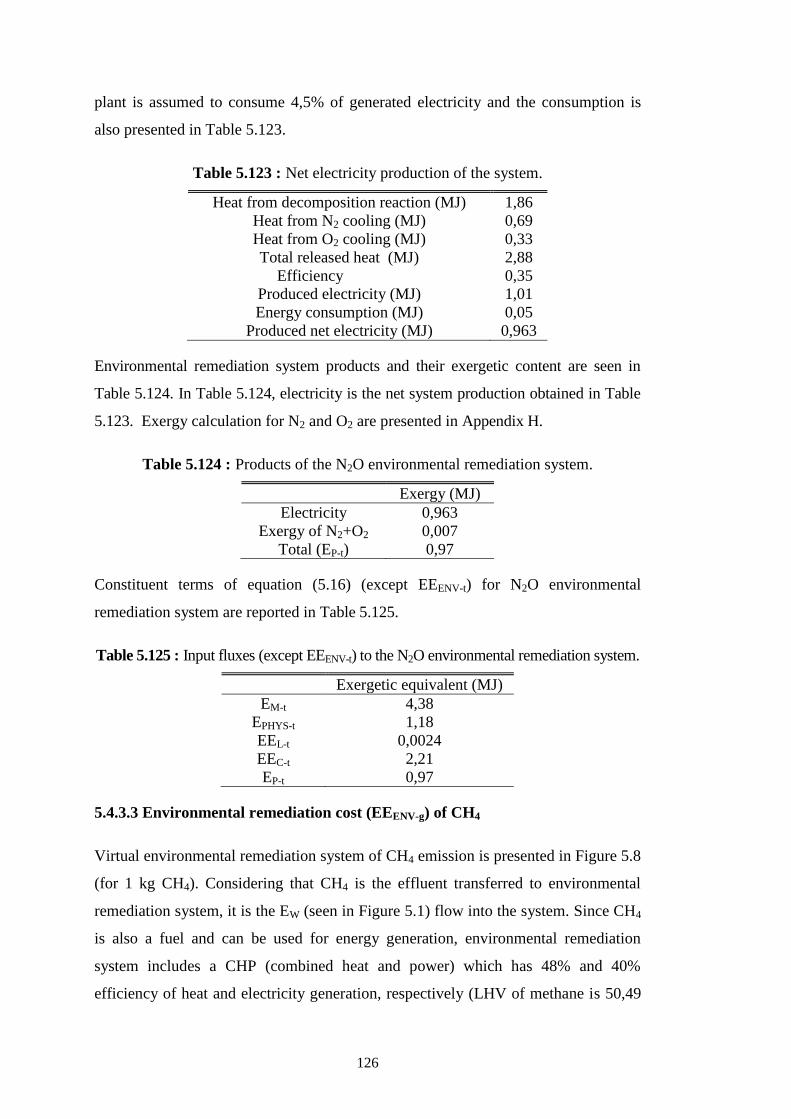
126
plant is assumed to consume 4,5% of generated electricity and the consumption is
also presented in Table 5.123.
Table 5.123 : Net electricity production of the system.
Heat from decomposition reaction (MJ) 1,86
Heat from N2 cooling (MJ) 0,69
Heat from O2 cooling (MJ) 0,33
Total released heat (MJ) 2,88
Efficiency
0,35
Produced electricity (MJ) 1,01
Energy consumption (MJ) 0,05
Produced net electricity (MJ) 0,963
Environmental remediation system products and their exergetic content are seen in
Table 5.124. In Table 5.124, electricity is the net system production obtained in Table
5.123. Exergy calculation for N2 and O2 are presented in Appendix H.
Table 5.124 : Products of the N2O environmental remediation system.
Exergy (MJ)
Electricity 0,963
Exergy of N2+O2 0,007
Total (EP-t) 0,97
Constituent terms of equation (5.16) (except EEENV-t) for N2O environmental
remediation system are reported in Table 5.125.
Table 5.125 : Input fluxes (except EEENV-t) to the N2O environmental remediation system.
Exergetic equivalent (MJ)
EM-t 4,38
EPHYS-t 1,18
EEL-t 0,0024
EEC-t 2,21
EP-t 0,97
5.4.3.3 Environmental remediation cost (EEENV-g) of CH4
Virtual environmental remediation system of CH4 emission is presented in Figure 5.8
(for 1 kg CH4). Considering that CH4 is the effluent transferred to environmental
remediation system, it is the EW (seen in Figure 5.1) flow into the system. Since CH4
is also a fuel and can be used for energy generation, environmental remediation
system includes a CHP (combined heat and power) which has 48% and 40%
efficiency of heat and electricity generation, respectively (LHV of methane is 50,49
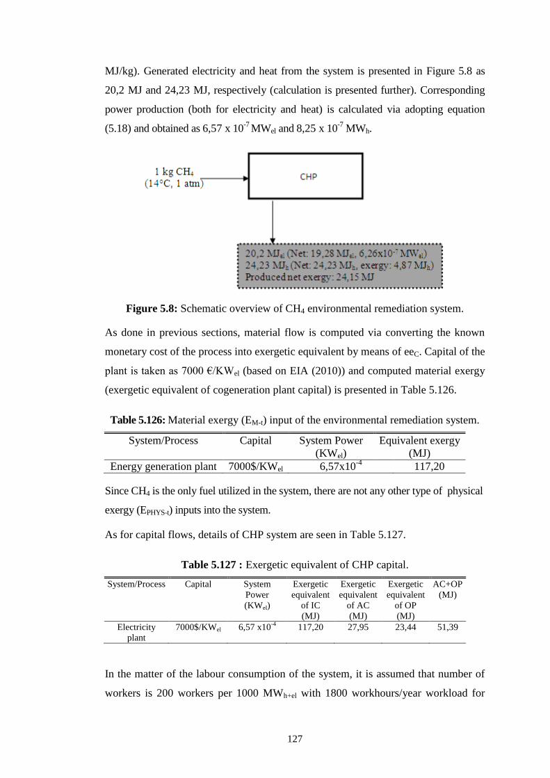
127
MJ/kg). Generated electricity and heat from the system is presented in Figure 5.8 as
20,2 MJ and 24,23 MJ, respectively (calculation is presented further). Corresponding
power production (both for electricity and heat) is calculated via adopting equation
(5.18) and obtained as 6,57 x 10⁻⁷
MWel and 8,25 x 10⁻⁷
MWh.
Figure 5.8: Schematic overview of CH4 environmental remediation system.
As done in previous sections, material flow is computed via converting the known
monetary cost of the process into exergetic equivalent by means of eeC. Capital of the
plant is taken as 7000 €/KWel (based on EIA (2010)) and computed material exergy
(exergetic equivalent of cogeneration plant capital) is presented in Table 5.126.
Table 5.126: Material exergy (EM-t) input of the environmental remediation system.
System/Process Capital System Power
(KWel)
Equivalent exergy
(MJ)
Energy generation plant 7000$/KWel 6,57x10⁻⁴
117,20
Since CH4 is the only fuel utilized in the system, there are not any other type of physical
exergy (EPHYS-t) inputs into the system.
As for capital flows, details of CHP system are seen in Table 5.127.
Table 5.127 : Exergetic equivalent of CHP capital.
System/Process Capital System
Power
(KWel)
Exergetic
equivalent
of IC
(MJ)
Exergetic
equivalent
of AC
(MJ)
Exergetic
equivalent
of OP
(MJ)
AC+OP
(MJ)
Electricity
plant
7000$/KWel 6,57 x10⁻⁴
117,20 27,95 23,44 51,39
In the matter of the labour consumption of the system, it is assumed that number of
workers is 200 workers per 1000 MWh+el with 1800 workhours/year workload for
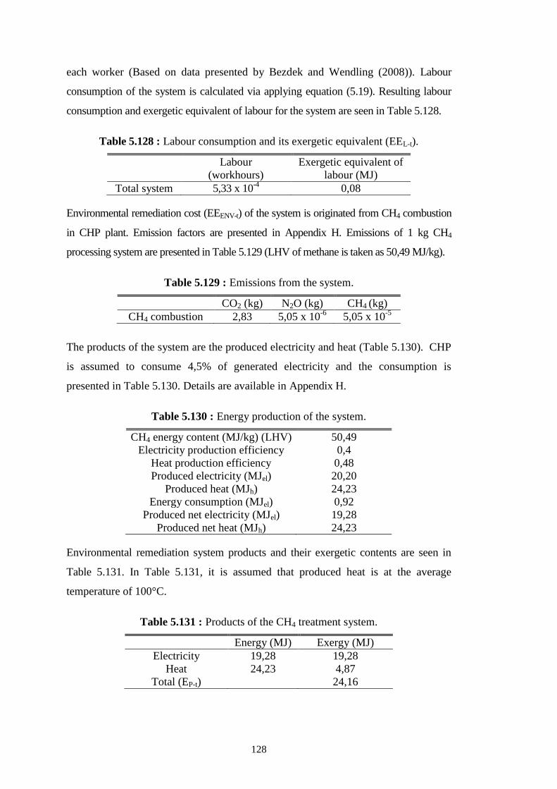
128
each worker (Based on data presented by Bezdek and Wendling (2008)). Labour
consumption of the system is calculated via applying equation (5.19). Resulting labour
consumption and exergetic equivalent of labour for the system are seen in Table 5.128.
Table 5.128 : Labour consumption and its exergetic equivalent (EEL-t).
Labour
(workhours)
Exergetic equivalent of
labour (MJ)
Total system 5,33 x 10⁻⁴
0,08
Environmental remediation cost (EEENV-t) of the system is originated from CH4 combustion
in CHP plant. Emission factors are presented in Appendix H. Emissions of 1 kg CH4
processing system are presented in Table 5.129 (LHV of methane is taken as 50,49 MJ/kg).
Table 5.129 : Emissions from the system.
CO2 (kg) N2O (kg) CH4 (kg)
CH4 combustion 2,83 5,05 x 10⁻⁶
5,05 x 10⁻⁵
The products of the system are the produced electricity and heat (Table 5.130). CHP
is assumed to consume 4,5% of generated electricity and the consumption is
presented in Table 5.130. Details are available in Appendix H.
Table 5.130 : Energy production of the system.
CH4 energy content (MJ/kg) (LHV) 50,49
Electricity production efficiency 0,4
Heat production efficiency 0,48
Produced electricity (MJel) 20,20
Produced heat (MJh) 24,23
Energy consumption (MJel) 0,92
Produced net electricity (MJel) 19,28
Produced net heat (MJh) 24,23
Environmental remediation system products and their exergetic contents are seen in
Table 5.131. In Table 5.131, it is assumed that produced heat is at the average
temperature of 100°C.
Table 5.131 : Products of the CH4 treatment system.
Energy (MJ) Exergy (MJ)
Electricity 19,28 19,28
Heat 24,23 4,87
Total (EP-t) 24,16
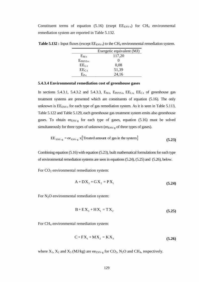
129
Constituent terms of equation (5.16) (exept EEENV-t) for CH4 environmental
remediation system are reported in Table 5.132.
Table 5.132 : Input fluxes (except EEENV-t) to the CH4 environmental remediation system.
Exergetic equivalent (MJ)
EM-t 117,20
EPHYS-t 0
EEL-t 0,08
EEC-t 51,39
EP-t 24,16
5.4.3.4 Environmental remediation cost of greenhouse gases
In sections 5.4.3.1, 5.4.3.2 and 5.4.3.3, EM-t, EPHYS-t, EEL-t, EEC-t of greenhouse gas
treatment systems are presented which are constituents of equation (5.16). The only
unknown is EEENV-t for each type of gas remediation system. As it is seen in Table 5.113,
Table 5.122 and Table 5.129, each greenhouse gas treatment system emits also greenhouse
gases. To obtain eeENV-g for each type of gases, equation (5.16) must be solved
simultaneously for three types of unknown (eeENV-g of three types of gases).
systemtheingasofamountTreatedxee =EE g-ENVg-ENV (5.23)
Combining equation (5.16) with equation (5.23), built mathematical formulations for each type
of environmental remediation systems are seen in equations (5.24), (5.25) and (5.26), below.
For CO2 environmental remediation system:
123 XP=XG+XD+A (5.24)
For N2O environmental remediation system:
213 XT=XH+XE+B (5.25)
For CH4 environmental remediation system:
321 XK=XM+XF+C (5.26)
where X1, X2 and X3 (MJ/kg) are eeENV-g for CO2, N2O and CH4, respectively.
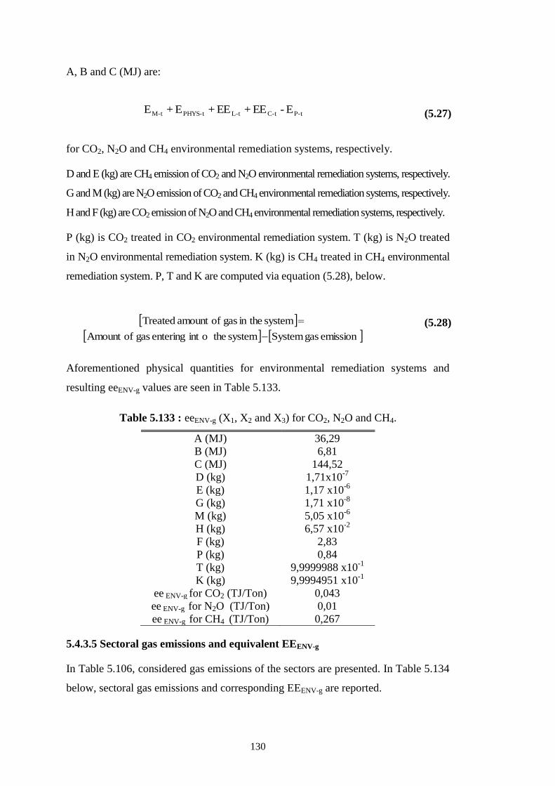
130
A, B and C (MJ) are:
t-Pt-Ct-Lt-PHYSt-M E - EE+EE+E+E (5.27)
for CO2, N2O and CH4 environmental remediation systems, respectively.
D and E (kg) are CH4 emission of CO2 and N2O environmental remediation systems, respectively.
G and M (kg) are N2O emission of CO2 and CH4 environmental remediation systems, respectively.
H and F (kg) are CO2 emission of N2O and CH4 environmental remediation systems, respectively.
P (kg) is CO2 treated in CO2 environmental remediation system. T (kg) is N2O treated
in N2O environmental remediation system. K (kg) is CH4 treated in CH4 environmental
remediation system. P, T and K are computed via equation (5.28), below.
emissiongasSystemsystemtheointenteringgasofAmount
systemtheingasofamountTreated
(5.28)
Aforementioned physical quantities for environmental remediation systems and
resulting eeENV-g values are seen in Table 5.133.
Table 5.133 : eeENV-g (X1, X2 and X3) for CO2, N2O and CH4.
A (MJ) 36,29
B (MJ) 6,81
C (MJ) 144,52
D (kg) 1,71x10⁻⁷
E (kg) 1,17 x10⁻⁶
G (kg) 1,71 x10⁻⁸
M (kg) 5,05 x10⁻⁶
H (kg) 6,57 x10⁻²
F (kg) 2,83
P (kg) 0,84
T (kg) 9,9999988 x10⁻¹
K (kg) 9,9994951 x10⁻¹
ee ENV-g for CO2 (TJ/Ton) 0,043
ee ENV-g for N2O (TJ/Ton) 0,01
ee ENV-g for CH4 (TJ/Ton) 0,267
5.4.3.5 Sectoral gas emissions and equivalent EEENV-g
In Table 5.106, considered gas emissions of the sectors are presented. In Table 5.134
below, sectoral gas emissions and corresponding EEENV-g are reported.
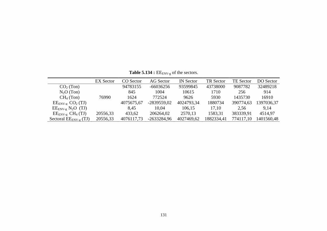
131
Table 5.134 : EEENV-g of the sectors.
EX Sector CO Sector AG Sector IN Sector TR Sector TE Sector DO Sector
CO2 (Ton) 94783155 -66036256 93599845 43738000 9087782 32489218
N2O (Ton) 845 1004 10615 1710 256 914
CH4 (Ton) 76990 1624 772524 9626 5930 1435730 16910
EEENV-g CO2 (TJ) 4075675,67 -2839559,02 4024793,34 1880734 390774,63 1397036,37
EEENV-g N2O (TJ) 8,45 10,04 106,15 17,10 2,56 9,14
EEENV-g CH4 (TJ) 20556,33 433,62 206264,02 2570,13 1583,31 383339,91 4514,97
Sectoral EEENV-g (TJ) 20556,33 4076117,73 -2633284,96 4027469,62 1882334,41 774117,10 1401560,48

132
5.4.4 Environmental remediation cost of liquid waste (EEENV-lq)
This section focuses on determining the environmental remediation cost of
wastewater (EEENV-lq) emitted from the sectors. In spite of high energy consumption
of wastewater treatment plants, they are essential in community service. It is also
expected to see a rising line in energy consumption of waste water treatment
processes due to population growth, increasingly restrictive environmental
regulations, and demand for wastewater reuse (due to the degradation of clean water
sources of the world) (European Commission, 2001a). Municipal wastewater
treatment plants generate sludge as a by-product of the physical, chemical and
biological processes. Many reasons such as: rapidly shrinking landfill space,
increased environmental awareness and more stringent environmental standards on
sludge disposal management make governing the disposal of sludge a worldwide
problem (Xu and Lancaster, 2009). In wastewater treatment, the goal is twofold: to
remove the pollutants from wastewater and to reduce the amount of sludge that needs
to be disposed (Xu and Lancaster, 2009). In general, sludge must be subject to a
treatment (remediation) process in order to change its characteristic. This treatment
has many objectives such as: reduction of excess volume by eliminating the liquid
portion of the sludge, decomposition of highly putrescible organic matter into
relatively stable or inert organic and inorganic compounds, etc. A typical wastewater
treatment plant consists of a set of processes including primary treatment, secondary
treatment, tertiary treatment and sludge processing. In primary treatment, physical
barriers remove larger solids from the wastewater. Secondary treatment covers
biological processes that promote biodegradation by microorganisms. Some of
secondary treatment methods: aerobic and anaerobic stabilization ponds, trickling
filters and activated sludge process (European Commission, 2001b; Eggleston et
al.,2006c). The activated sludge process is by far the most frequently used biological
treatment (secondary treatment) process (Kim et al., 2002; M/J Industrial Solutions,
2003). Tertiary treatment is further treatment of wastewater and disinfection is one of
the techniques of tertiary treatment (Eggleston et al., 2006c). Sludge is produced in
all of the primary, secondary and tertiary treatment processes and this sludge must be
processed before it is safely disposed of. Anaerobic digestion (AD) is a sludge
stabilization method which furnishes a considerable power supply and as a result, the
overall cost of sewage treatment is reduced (Qasim, 1999). Among widely used
133
sludge stabilization techniques, anaerobic digestion is unique since it enables to
produce energy gain by biogas utilization, providing cost effectiveness and
minimizing the mass and volume of disposed final sludge (Tchobanoglous et al.,
2002). As stated in Section 5.4.1, in AD process, after breaking down a large fraction
of the organic matter (biodegradable part) into carbon dioxide (CO2) and methane
(CH4), the remaining part (digestate) is dried and becomes a residual soil-like
material. This material partially replaces the use of conventional fertilizer, since it
contains compounds of agricultural value: it is rich in nitrates and performs well as a
fertilizer. It contains also organic matter but it is under the level of having a
significant positive impact on soil physical properties (European Commission,
2001b). This fertilizer like material (named “fertilizer” in this thesis) is another
product of the wastewater remediation system. For these reasons, anaerobic sludge
digestion is mostly preferred to reduce the cost of wastewater remediation and
considered as a major and essential part of modern wastewater treatment plants
(Appels et al., 2008).
In this section, anaerobic digestion of sludge which is produced through the
wastewater treatment processes, and energy generation via biogas utilization are
overviewed within the content of wastewater treatment. Due to the wide variety of
wastewater composition emitted from refineries, different sub-industries, energy
generation plants etc., wastewater treatment takes a particularly designed system for
each type of sub-industry and also of type of processes encompassed in the sub-
industries. Since the scope and volume of this thesis is limited and also analysis of
wastewater composition for all sub-industries, refineries, coke factories and
agricultural activities etc. are not available for Turkey, properly designing and
detailed examination of wastewater remediation systems (which can bring the
untreated wastewater of the sectors to the legal water discharge limits) were
impossible. As an alternative, a virtual remediation system for municipal wastewater
is analyzed under several assumptions. Specific wastewater environmental
remediation cost (eeENV-lq, TJ/m3) is calculated for municipal wastewater and the
other sectors are assumed to have the same specific wastewater environmental
remediation cost.
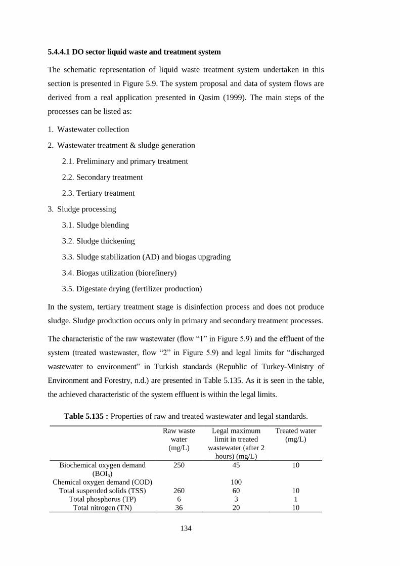
134
5.4.4.1 DO sector liquid waste and treatment system
The schematic representation of liquid waste treatment system undertaken in this
section is presented in Figure 5.9. The system proposal and data of system flows are
derived from a real application presented in Qasim (1999). The main steps of the
processes can be listed as:
1. Wastewater collection
2. Wastewater treatment & sludge generation
2.1. Preliminary and primary treatment
2.2. Secondary treatment
2.3. Tertiary treatment
3. Sludge processing
3.1. Sludge blending
3.2. Sludge thickening
3.3. Sludge stabilization (AD) and biogas upgrading
3.4. Biogas utilization (biorefinery)
3.5. Digestate drying (fertilizer production)
In the system, tertiary treatment stage is disinfection process and does not produce
sludge. Sludge production occurs only in primary and secondary treatment processes.
The characteristic of the raw wastewater (flow “1” in Figure 5.9) and the effluent of the
system (treated wastewaster, flow “2” in Figure 5.9) and legal limits for “discharged
wastewater to environment” in Turkish standards (Republic of Turkey-Ministry of
Environment and Forestry, n.d.) are presented in Table 5.135. As it is seen in the table,
the achieved characteristic of the system effluent is within the legal limits.
Table 5.135 : Properties of raw and treated wastewater and legal standards.
Raw waste
water
(mg/L)
Legal maximum
limit in treated
wastewater (after 2
hours) (mg/L)
Treated water
(mg/L)
Biochemical oxygen demand
(BOI5)
250 45 10
Chemical oxygen demand (COD) 100
Total suspended solids (TSS) 260 60 10
Total phosphorus (TP) 6 3 1
Total nitrogen (TN) 36 20 10
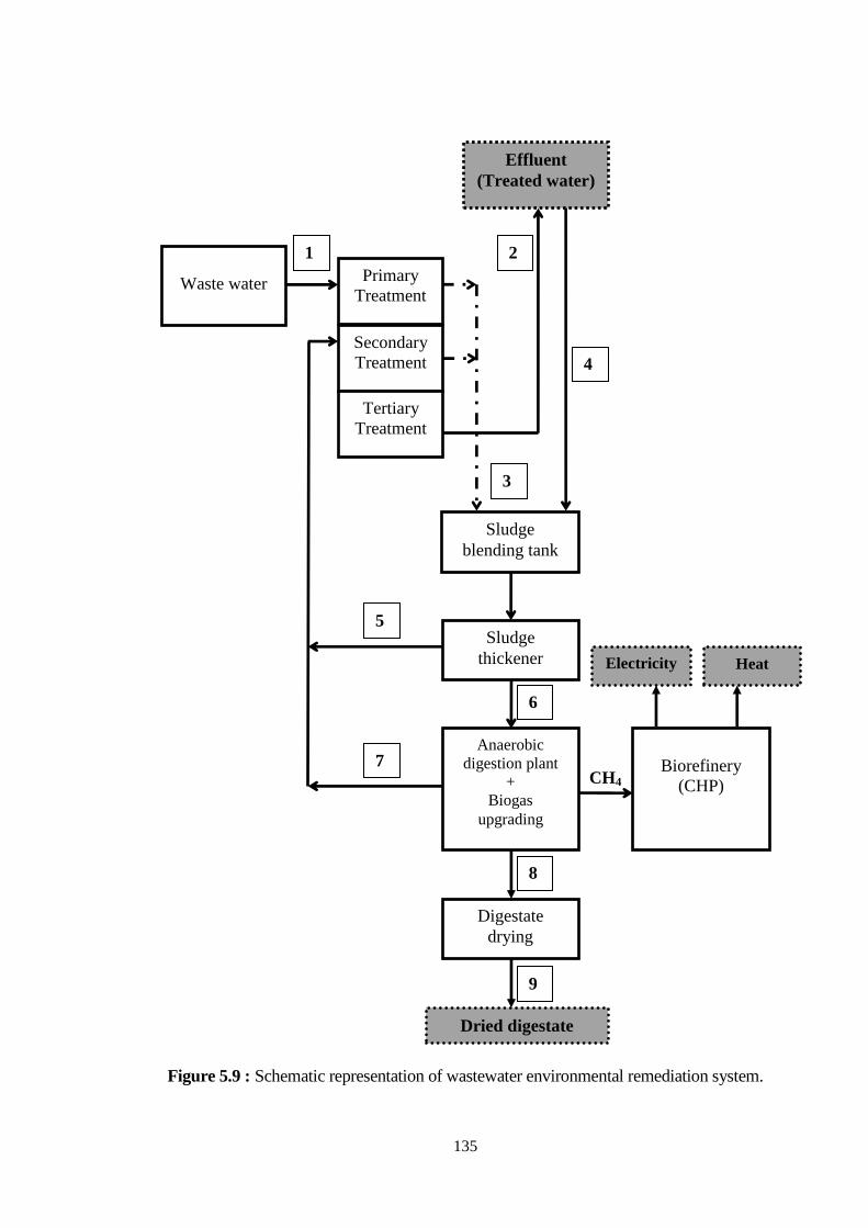
135
Figure 5.9 : Schematic representation of wastewater environmental remediation system.
5
7
1 2
3
4
6
8
9
Waste water Primary
Treatment
Secondary
Treatment
Tertiary
Treatment
Effluent
(Treated water)
Sludge
blending tank
Sludge
thickener
Digestate
drying
Anaerobic
digestion plant
+
Biogas
upgrading
CH4
Electricity
y Heat
Biorefinery
(CHP)
Dried digestate
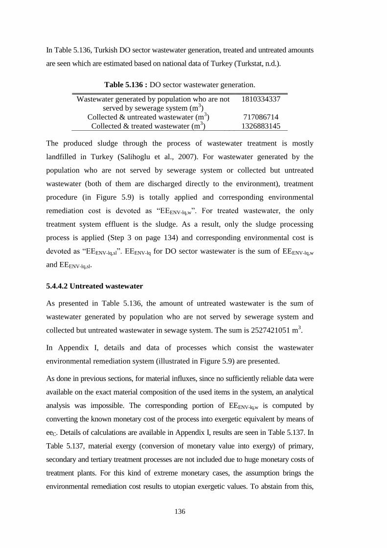
136
In Table 5.136, Turkish DO sector wastewater generation, treated and untreated amounts
are seen which are estimated based on national data of Turkey (Turkstat, n.d.).
Table 5.136 : DO sector wastewater generation.
Wastewater generated by population who are not
served by sewerage system (m3)
1810334337
Collected & untreated wastewater (m3) 717086714
Collected & treated wastewater (m3) 1326883145
The produced sludge through the process of wastewater treatment is mostly
landfilled in Turkey (Salihoglu et al., 2007). For wastewater generated by the
population who are not served by sewerage system or collected but untreated
wastewater (both of them are discharged directly to the environment), treatment
procedure (in Figure 5.9) is totally applied and corresponding environmental
remediation cost is devoted as “EEENV-lq,w”. For treated wastewater, the only
treatment system effluent is the sludge. As a result, only the sludge processing
process is applied (Step 3 on page 134) and corresponding environmental cost is
devoted as “EEENV-lq,sl”. EEENV-lq for DO sector wastewater is the sum of EEENV-lq,w
and EEENV-lq,sl.
5.4.4.2 Untreated wastewater
As presented in Table 5.136, the amount of untreated wastewater is the sum of
wastewater generated by population who are not served by sewerage system and
collected but untreated wastewater in sewage system. The sum is 2527421051 m3.
In Appendix I, details and data of processes which consist the wastewater
environmental remediation system (illustrated in Figure 5.9) are presented.
As done in previous sections, for material influxes, since no sufficiently reliable data were
available on the exact material composition of the used items in the system, an analytical
analysis was impossible. The corresponding portion of EEENV-lq,w is computed by
converting the known monetary cost of the process into exergetic equivalent by means of
eeC. Details of calculations are available in Appendix I, results are seen in Table 5.137. In
Table 5.137, material exergy (conversion of monetary value into exergy) of primary,
secondary and tertiary treatment processes are not included due to huge monetary costs of
treatment plants. For this kind of extreme monetary cases, the assumption brings the
environmental remediation cost results to utopian exergetic values. To abstain from this,
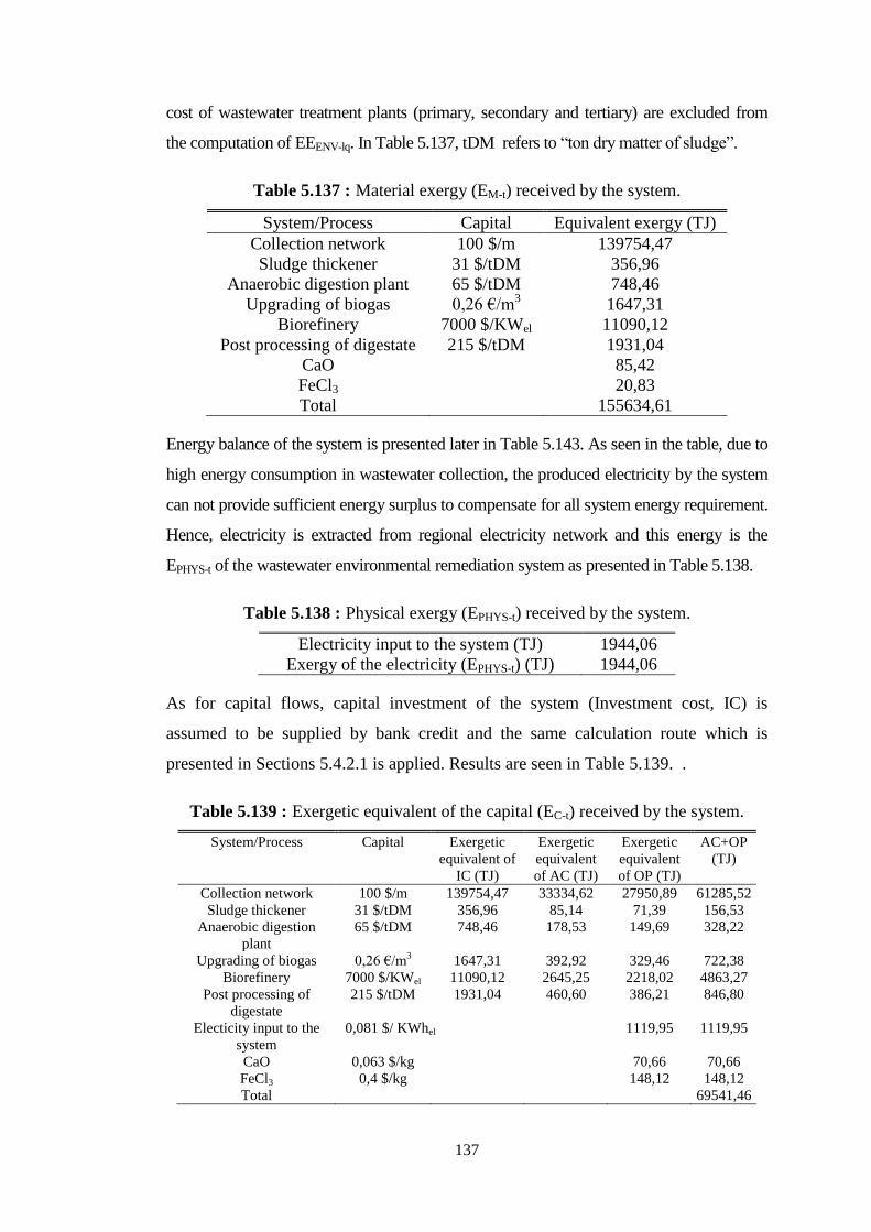
137
cost of wastewater treatment plants (primary, secondary and tertiary) are excluded from
the computation of EEENV-lq. In Table 5.137, tDM refers to “ton dry matter of sludge”.
Table 5.137 : Material exergy (EM-t) received by the system.
System/Process Capital Equivalent exergy (TJ)
Collection network 100 $/m 139754,47
Sludge thickener 31 $/tDM 356,96
Anaerobic digestion plant 65 $/tDM 748,46
Upgrading of biogas 0,26 €/m3 1647,31
Biorefinery 7000 $/KWel 11090,12
Post processing of digestate 215 $/tDM 1931,04
CaO 85,42
FeCl3 20,83
Total 155634,61
Energy balance of the system is presented later in Table 5.143. As seen in the table, due to
high energy consumption in wastewater collection, the produced electricity by the system
can not provide sufficient energy surplus to compensate for all system energy requirement.
Hence, electricity is extracted from regional electricity network and this energy is the
EPHYS-t of the wastewater environmental remediation system as presented in Table 5.138.
Table 5.138 : Physical exergy (EPHYS-t) received by the system.
Electricity input to the system (TJ) 1944,06
Exergy of the electricity (EPHYS-t) (TJ) 1944,06
As for capital flows, capital investment of the system (Investment cost, IC) is
assumed to be supplied by bank credit and the same calculation route which is
presented in Sections 5.4.2.1 is applied. Results are seen in Table 5.139. .
Table 5.139 : Exergetic equivalent of the capital (EC-t) received by the system.
System/Process Capital Exergetic
equivalent of
IC (TJ)
Exergetic
equivalent
of AC (TJ)
Exergetic
equivalent
of OP (TJ)
AC+OP
(TJ)
Collection network 100 $/m 139754,47 33334,62 27950,89 61285,52
Sludge thickener 31 $/tDM 356,96 85,14 71,39 156,53
Anaerobic digestion
plant
65 $/tDM 748,46 178,53 149,69 328,22
Upgrading of biogas 0,26 €/m3 1647,31 392,92 329,46 722,38
Biorefinery 7000 $/KWel 11090,12 2645,25 2218,02 4863,27
Post processing of
digestate
215 $/tDM 1931,04 460,60 386,21 846,80
Electicity input to the
system
0,081 $/ KWhel 1119,95 1119,95
CaO 0,063 $/kg 70,66 70,66
FeCl3 0,4 $/kg 148,12 148,12
Total 69541,46

138
Since capital of annual electricity input from regional electricity network and
consumed CaO and FeCl3 for digestate stabilization are considered under OP cost,
they are not annualized as seen in Table 5.139. Details are presented in Appendix I.
As for labour consumption of the system, it is assumed that labour of the system is
200 workers per 1000 MWh+el generated energy, based on data (Bezdek and
Wendling, 2008). Considering the whole system, number of workers is assumed to be
400 workers per 1000 MWh+el with 1800 workhours/year workload for each worker.
Generated electricity and heat is presented later in Table 5.143 as 1825,08 TJel and
2190,10 TJh. To compute the exergetic equivalent of labour, equations (5.18), (5.19)
and (5.20) are adapted and the results are seen in equations (5.29), (5.30) and (5.31).
Exergetic equivalent of labour is calculated via equations presented below.
68,13660340x24x60x
10 x 2190,10) (1825,08
(s) time workingAnnual
)(MJenergy Generated)MW(powerGenerated
6
hel
hel
(5.29)
Hence, labour consumed in the system is:
98411,34)MW(68,136xker)woryear/hours(1800x)MW(1000
)skerwor(400
= )(workhours loadLabour
(5.30)
The exergetic equivalent of the labour is computed by means of eeL:
TJ15,15MJ15150651,7 95,153x34,98411
)hours/MJ(ee x )(workhours loadabour LEE Lt-L
(5.31)
Environmental remediation cost of the system is originated from greenhouse gas emissions
from AD, biogas upgrading and biogas incineration (in biorefinery). Details of emissions
are presented in Appendix I. Total CO2, N2O and CH4 emissions of the system are seen in
Table 5.140. The environmental remediation cost of emission gases are computed in
Section 5.4.3 and inserted into Table 5.141 to obtain the EEENV-t for the whole wastewater
treatment system.
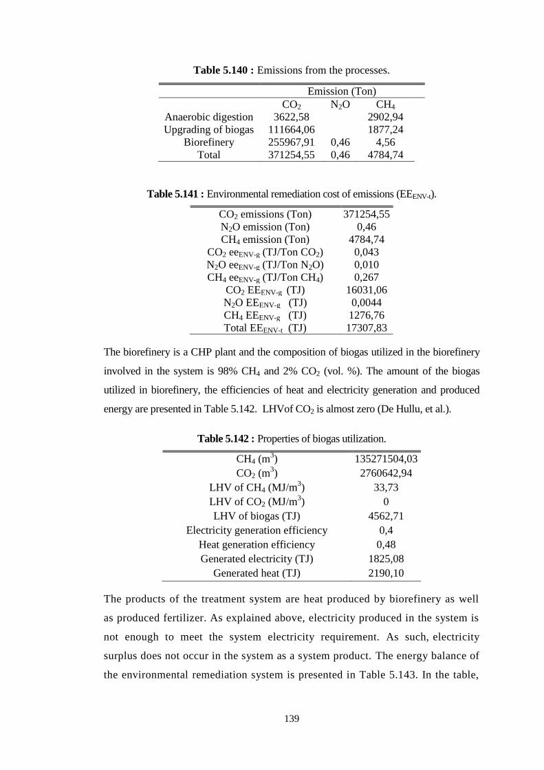
139
Table 5.140 : Emissions from the processes.
Table 5.141 : Environmental remediation cost of emissions (EEENV-t).
CO2 emissions (Ton) 371254,55
N2O emission (Ton) 0,46
CH4 emission (Ton) 4784,74
CO2 eeENV-g (TJ/Ton CO2) 0,043
N2O eeENV-g (TJ/Ton N2O) 0,010
CH4 eeENV-g (TJ/Ton CH4) 0,267
CO2 EEENV-g (TJ) 16031,06
N2O EEENV-g (TJ) 0,0044
CH4 EEENV-g (TJ) 1276,76
Total EEENV-t (TJ) 17307,83
The biorefinery is a CHP plant and the composition of biogas utilized in the biorefinery
involved in the system is 98% CH4 and 2% CO2 (vol. %). The amount of the biogas
utilized in biorefinery, the efficiencies of heat and electricity generation and produced
energy are presented in Table 5.142. LHVof CO2 is almost zero (De Hullu, et al.).
Table 5.142 : Properties of biogas utilization.
CH4 (m3) 135271504,03
CO2 (m3) 2760642,94
LHV of CH4 (MJ/m3) 33,73
LHV of CO2 (MJ/m3) 0
LHV of biogas (TJ) 4562,71
Electricity generation efficiency 0,4
Heat generation efficiency 0,48
Generated electricity (TJ) 1825,08
Generated heat (TJ) 2190,10
The products of the treatment system are heat produced by biorefinery as well
as produced fertilizer. As explained above, electricity produced in the system is
not enough to meet the system electricity requirement. As such, electricity
surplus does not occur in the system as a system product. The energy balance of
the environmental remediation system is presented in Table 5.143. In the table,
Emission (Ton)
CO2 N2O CH4
Anaerobic digestion 3622,58 2902,94
Upgrading of biogas 111664,06 1877,24
Biorefinery 255967,91 0,46 4,56
Total 371254,55 0,46 4784,74
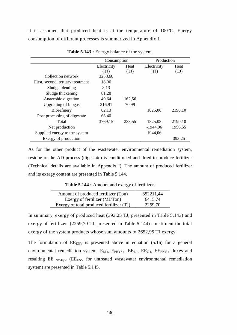
140
it is assumed that produced heat is at the temperature of 100°C. Energy
consumption of different processes is summarized in Appendix I.
Table 5.143 : Energy balance of the system.
Consumption Production
Electricity
(TJ)
Heat
(TJ)
Electricity
(TJ)
Heat
(TJ)
Collection network 3258,60
First, second, tertiary treatment 18,06
Sludge blending 8,13
Sludge thickening 81,28
Anaerobic digestion 40,64 162,56
Upgrading of biogas 216,91 70,99
Biorefinery 82,13 1825,08 2190,10
Post processing of digestate 63,40
Total 3769,15 233,55 1825,08 2190,10
Net production -1944,06 1956,55
Supplied energy to the system 1944,06
Exergy of production 393,25
As for the other product of the wastewater environmental remediation system,
residue of the AD process (digestate) is conditioned and dried to produce fertilizer
(Technical details are available in Appendix I). The amount of produced fertilizer
and its exergy content are presented in Table 5.144.
Table 5.144 : Amount and exergy of fertilizer.
Amount of produced fertilizer (Ton) 352211,44
Exergy of fertilizer (MJ/Ton) 6415,74
Exergy of total produced fertilizer (TJ) 2259,70
In summary, exergy of produced heat (393,25 TJ, presented in Table 5.143) and
exergy of fertilizer (2259,70 TJ, presented in Table 5.144) constituent the total
exergy of the system products whose sum amounts to 2652,95 TJ exergy.
The formulation of EEENV is presented above in equation (5.16) for a general
environmental remediation system. EM-t, EPHYS-t, EEL-t, EEC-t, EEENV-t fluxes and
resulting EEENV-lq,w (EEENV for untreated wastewater environmental remediation
system) are presented in Table 5.145.
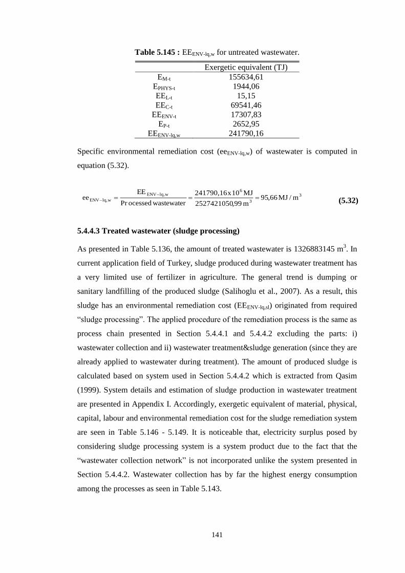
141
Table 5.145 : EEENV-lq,w for untreated wastewater.
Exergetic equivalent (TJ)
EM-t 155634,61
EPHYS-t 1944,06
EEL-t 15,15
EEC-t 69541,46
EEENV-t 17307,83
EP-t 2652,95
EEENV-lq,w 241790,16
Specific environmental remediation cost (eeENV-lq,w) of wastewater is computed in
equation (5.32).
3
3
6w,lqENV
w,lqENV m/MJ66,95m ,992527421050
MJ10x241790,16
wastewaterocessedPr
EEee
(5.32)
5.4.4.3 Treated wastewater (sludge processing)
As presented in Table 5.136, the amount of treated wastewater is 1326883145 m3. In
current application field of Turkey, sludge produced during wastewater treatment has
a very limited use of fertilizer in agriculture. The general trend is dumping or
sanitary landfilling of the produced sludge (Salihoglu et al., 2007). As a result, this
sludge has an environmental remediation cost (EEENV-lq,sl) originated from required
“sludge processing”. The applied procedure of the remediation process is the same as
process chain presented in Section 5.4.4.1 and 5.4.4.2 excluding the parts: i)
wastewater collection and ii) wastewater treatment&sludge generation (since they are
already applied to wastewater during treatment). The amount of produced sludge is
calculated based on system used in Section 5.4.4.2 which is extracted from Qasim
(1999). System details and estimation of sludge production in wastewater treatment
are presented in Appendix I. Accordingly, exergetic equivalent of material, physical,
capital, labour and environmental remediation cost for the sludge remediation system
are seen in Table 5.146 - 5.149. It is noticeable that, electricity surplus posed by
considering sludge processing system is a system product due to the fact that the
“wastewater collection network” is not incorporated unlike the system presented in
Section 5.4.4.2. Wastewater collection has by far the highest energy consumption
among the processes as seen in Table 5.143.
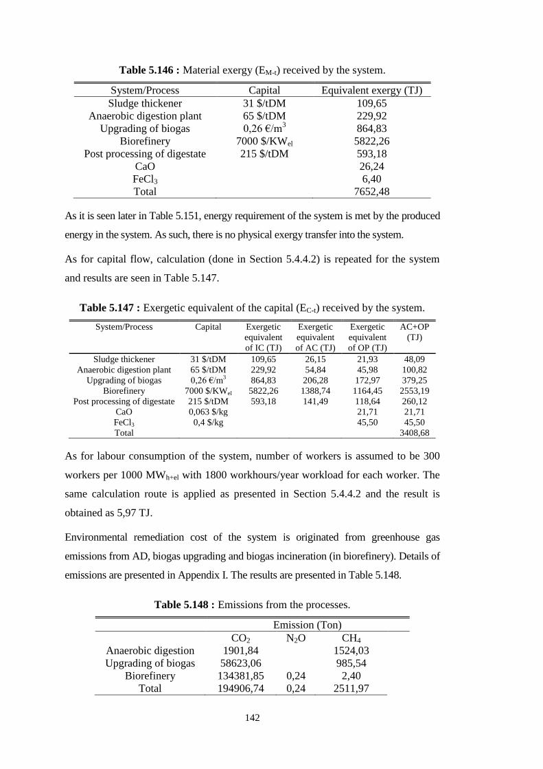
142
Table 5.146 : Material exergy (EM-t) received by the system.
System/Process Capital Equivalent exergy (TJ)
Sludge thickener 31 $/tDM 109,65
Anaerobic digestion plant 65 $/tDM 229,92
Upgrading of biogas 0,26 €/m3 864,83
Biorefinery 7000 $/KWel 5822,26
Post processing of digestate 215 $/tDM 593,18
CaO 26,24
FeCl3 6,40
Total 7652,48
As it is seen later in Table 5.151, energy requirement of the system is met by the produced
energy in the system. As such, there is no physical exergy transfer into the system.
As for capital flow, calculation (done in Section 5.4.4.2) is repeated for the system
and results are seen in Table 5.147.
Table 5.147 : Exergetic equivalent of the capital (EC-t) received by the system.
System/Process Capital Exergetic
equivalent
of IC (TJ)
Exergetic
equivalent
of AC (TJ)
Exergetic
equivalent
of OP (TJ)
AC+OP
(TJ)
Sludge thickener 31 $/tDM 109,65 26,15 21,93 48,09
Anaerobic digestion plant 65 $/tDM 229,92 54,84 45,98 100,82
Upgrading of biogas 0,26 €/m3 864,83 206,28 172,97 379,25
Biorefinery 7000 $/KWel 5822,26 1388,74 1164,45 2553,19
Post processing of digestate 215 $/tDM 593,18 141,49 118,64 260,12
CaO 0,063 $/kg 21,71 21,71
FeCl3 0,4 $/kg 45,50 45,50
Total 3408,68
As for labour consumption of the system, number of workers is assumed to be 300
workers per 1000 MWh+el with 1800 workhours/year workload for each worker. The
same calculation route is applied as presented in Section 5.4.4.2 and the result is
obtained as 5,97 TJ.
Environmental remediation cost of the system is originated from greenhouse gas
emissions from AD, biogas upgrading and biogas incineration (in biorefinery). Details of
emissions are presented in Appendix I. The results are presented in Table 5.148.
Table 5.148 : Emissions from the processes.
Emission (Ton)
CO2 N2O CH4
Anaerobic digestion 1901,84 1524,03
Upgrading of biogas 58623,06 985,54
Biorefinery 134381,85 0,24 2,40
Total 194906,74 0,24 2511,97
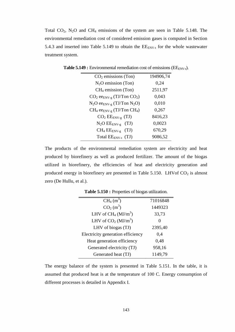
143
Total CO2, N2O and CH4 emissions of the system are seen in Table 5.148. The
environmental remediation cost of considered emission gases is computed in Section
5.4.3 and inserted into Table 5.149 to obtain the EEENV-t for the whole wastewater
treatment system.
Table 5.149 : Environmental remediation cost of emissions (EEENV-t).
CO2 emissions (Ton) 194906,74
N2O emission (Ton) 0,24
CH4 emission (Ton) 2511,97
CO2 eeENV-g (TJ/Ton CO2) 0,043
N2O eeENV-g (TJ/Ton N2O) 0,010
CH4 eeENV-g (TJ/Ton CH4) 0,267
CO2 EEENV-g (TJ) 8416,23
N2O EEENV-g (TJ) 0,0023
CH4 EEENV-g (TJ) 670,29
Total EEENV-t (TJ) 9086,52
The products of the environmental remediation system are electricity and heat
produced by biorefinery as well as produced fertilizer. The amount of the biogas
utilized in biorefinery, the efficiencies of heat and electricity generation and
produced energy in biorefinery are presented in Table 5.150. LHVof CO2 is almost
zero (De Hullu, et al.).
Table 5.150 : Properties of biogas utilization.
CH4 (m3) 71016848
CO2 (m3) 1449323
LHV of CH4 (MJ/m3) 33,73
LHV of CO2 (MJ/m3) 0
LHV of biogas (TJ) 2395,40
Electricity generation efficiency 0,4
Heat generation efficiency 0,48
Generated electricity (TJ) 958,16
Generated heat (TJ) 1149,79
The energy balance of the system is presented in Table 5.151. In the table, it is
assumed that produced heat is at the temperature of 100 C. Energy consumption of
different processes is detailed in Appendix I.
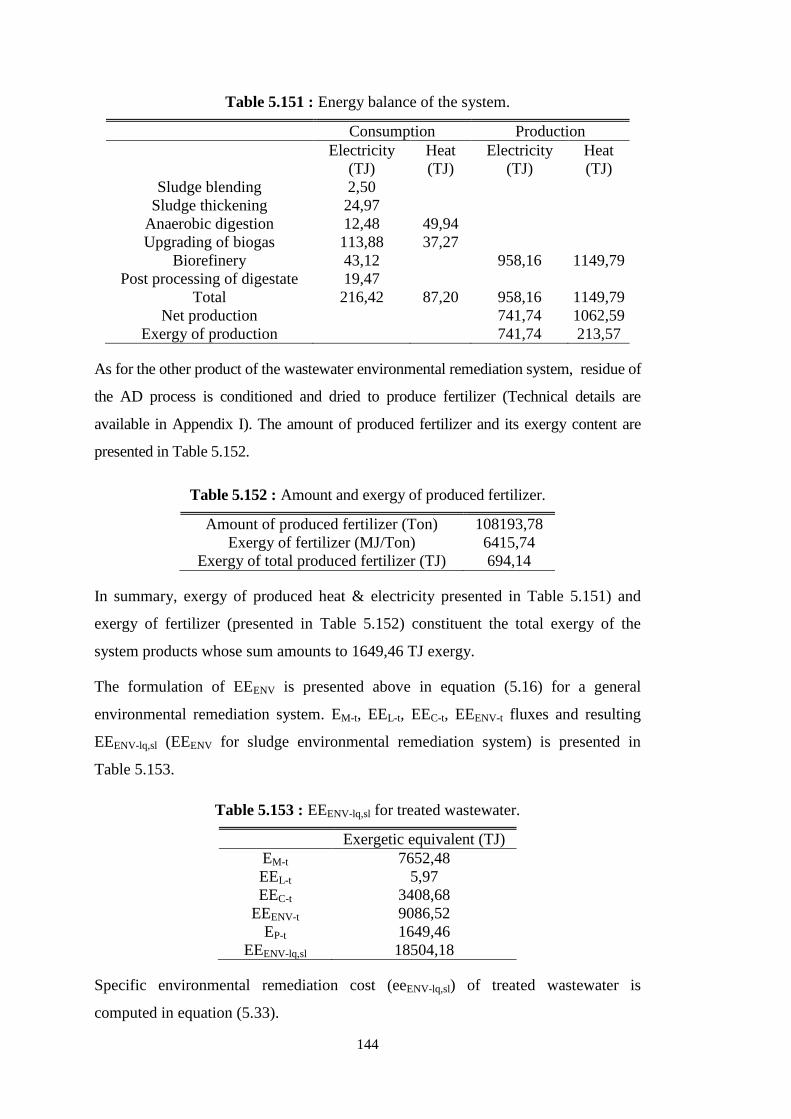
144
Table 5.151 : Energy balance of the system.
Consumption Production
Electricity
(TJ)
Heat
(TJ)
Electricity
(TJ)
Heat
(TJ)
Sludge blending 2,50
Sludge thickening 24,97
Anaerobic digestion 12,48 49,94
Upgrading of biogas 113,88 37,27
Biorefinery 43,12 958,16 1149,79
Post processing of digestate 19,47
Total 216,42 87,20 958,16 1149,79
Net production 741,74 1062,59
Exergy of production 741,74 213,57
As for the other product of the wastewater environmental remediation system, residue of
the AD process is conditioned and dried to produce fertilizer (Technical details are
available in Appendix I). The amount of produced fertilizer and its exergy content are
presented in Table 5.152.
Table 5.152 : Amount and exergy of produced fertilizer.
Amount of produced fertilizer (Ton) 108193,78
Exergy of fertilizer (MJ/Ton) 6415,74
Exergy of total produced fertilizer (TJ) 694,14
In summary, exergy of produced heat & electricity presented in Table 5.151) and
exergy of fertilizer (presented in Table 5.152) constituent the total exergy of the
system products whose sum amounts to 1649,46 TJ exergy.
The formulation of EEENV is presented above in equation (5.16) for a general
environmental remediation system. EM-t, EEL-t, EEC-t, EEENV-t fluxes and resulting
EEENV-lq,sl (EEENV for sludge environmental remediation system) is presented in
Table 5.153.
Table 5.153 : EEENV-lq,sl for treated wastewater.
Exergetic equivalent (TJ)
EM-t 7652,48
EEL-t 5,97
EEC-t 3408,68
EEENV-t 9086,52
EP-t 1649,46
EEENV-lq,sl 18504,18
Specific environmental remediation cost (eeENV-lq,sl) of treated wastewater is
computed in equation (5.33).
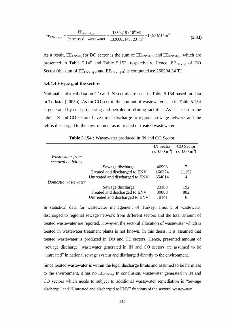
145
3
3
6sl,lqENV
sl,lqENV m/MJ95,13m 23,1326883145
MJ10x18,18504
wastewaterocessedPr
EEee
(5.33)
As a result, EEENV-lq for DO sector is the sum of EEENV-lq,w and EEENV-lq,sl which are
presented in Table 5.145 and Table 5.153, respectively. Hence, EEENV-lq of DO
Sector (the sum of EEENV-lq,w and EEENV-lq,sl) is computed as: 260294,34 TJ.
5.4.4.4 EEENV-lq of the sectors
National statistical data on CO and IN sectors are seen in Table 5.154 based on data
in Turkstat (2005b). As for CO sector, the amount of wastewater seen in Table 5.154
is generated by coal processing and petroleum refining facilities. As it is seen in the
table, IN and CO sectors have direct discharge to regional sewage network and the
left is discharged to the environment as untreated or treated wastewater.
Table 5.154 : Wastewater produced in IN and CO Sector.
IN Sector
(x1000 m3)
CO Sector
(x1000 m3)
Wastewater from
sectoral activities
Sewage discharge 46993 7
Treated and discharged to ENV 160374 11152
Untreated and discharged to ENV 354014 4
Domestic wastewater
Sewage discharge 23183 192
Treated and discharged to ENV 30888 802
Untreated and discharged to ENV 10141 6
In statistical data for wastewater management of Turkey, amount of wastewater
discharged to regional sewage network from different sectors and the total amount of
treated wastewater are reported. However, the sectoral allocation of wastewater which is
treated in wastewater treatment plants is not known. In this thesis, it is assumed that
treated wastewater is produced in DO and TE sectors. Hence, presented amount of
“sewage discharge” wastewater generated in IN and CO sectors are assumed to be
“untreated” in national sewage system and discharged directly to the environment.
Since treated wastewater is within the legal discharge limits and assumed to be harmless
to the environment, it has no EEENV-lq. In conclusion, wastewater generated in IN and
CO sectors which needs to subject to additional wastewater remediation is “Sewage
discharge” and “Untreated and discharged to ENV” fractions of the sectoral wastewater.
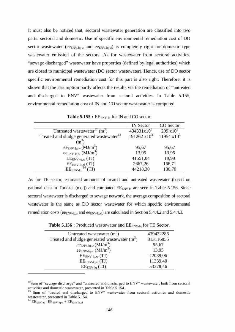
146
It must also be noticed that, sectoral wastewater generation are classified into two
parts: sectoral and domestic. Use of specific environmental remediation cost of DO
sector wastewater (eeENV,lq-w and eeENV,lq-sl) is completely right for domestic type
wastewater emission of the sectors. As for wastewater from sectoral activities,
“sewage discharged” wastewater have properties (defined by legal authorities) which
are closed to municipal wastewater (DO sector wastewater). Hence, use of DO sector
specific environmental remediation cost for this part is also right. Therefore, it is
shown that the assumption partly affects the results via the remediation of “untreated
and discharged to ENV” wastewater from sectoral activities. In Table 5.155,
environmental remediation cost of IN and CO sector wastewater is computed.
Table 5.155 : EEENV-lq for IN and CO sector.
IN Sector CO Sector
Untreated wastewater12
(m3) 434331x10
3 209 x10
3
Treated and sludge generated wastewater13
(m3)
191262 x103 11954 x10
3
eeENV-lq,w (MJ/m3) 95,67 95,67
eeENV-lq,sl (MJ/m3) 13,95 13,95
EEENV-lq,w (TJ) 41551,04 19,99
EEENV-lq,sl (TJ) 2667,26 166,71
EEENV-lq 14
(TJ) 44218,30 186,70
As for TE sector, estimated amounts of treated and untreated wastewater (based on
national data in Turkstat (n.d.)) and computed EEENV-lq are seen in Table 5.156. Since
sectoral wastewater is discharged to sewage network, the average composition of sectoral
wastewater is the same as DO sector wastewater for which specific environmental
remediation costs (eeENV-lq,w and eeENV-lq,sl) are calculated in Section 5.4.4.2 and 5.4.4.3.
Table 5.156 : Produced wastewater and EEENV-lq for TE Sector.
Untreated wastewater (m3) 439432286
Treated and sludge generated wastewater (m3) 813116855
eeENV-lq,w (MJ/m3) 95,67
eeENV-lq,sl (MJ/m3) 13,95
EEENV-lq,w (TJ) 42039,06
EEENV-lq,sl (TJ) 11339,40
EEENV-lq (TJ) 53378,46
12
Sum of “sewage discharge” and “untreated and discharged to ENV” wastewater, both from sectoral
activities and domestic wastewater, presented in Table 5.154. 13
Sum of “treated and discharged to ENV” wastewater from sectoral activities and domestic
wastewater, presented in Table 5.154. 14
EEENV-lq= EEENV-lq,w + EEENV-lq,sl
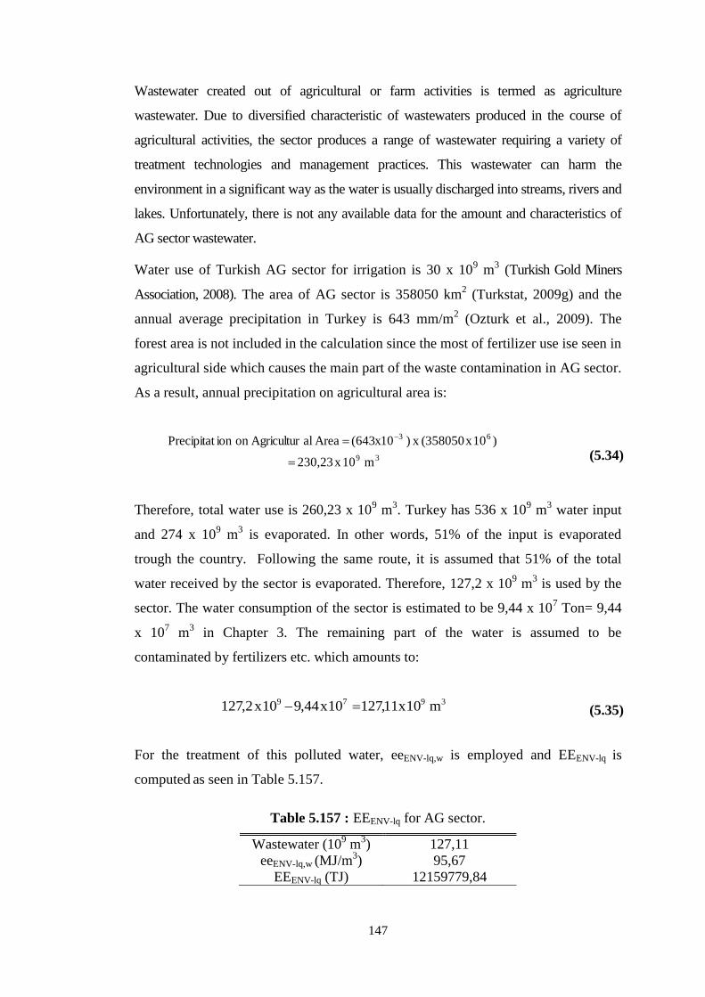
147
Wastewater created out of agricultural or farm activities is termed as agriculture
wastewater. Due to diversified characteristic of wastewaters produced in the course of
agricultural activities, the sector produces a range of wastewater requiring a variety of
treatment technologies and management practices. This wastewater can harm the
environment in a significant way as the water is usually discharged into streams, rivers and
lakes. Unfortunately, there is not any available data for the amount and characteristics of
AG sector wastewater.
Water use of Turkish AG sector for irrigation is 30 x 109 m
3 (Turkish Gold Miners
Association, 2008). The area of AG sector is 358050 km2 (Turkstat, 2009g) and the
annual average precipitation in Turkey is 643 mm/m2 (Ozturk et al., 2009). The
forest area is not included in the calculation since the most of fertilizer use ise seen in
agricultural side which causes the main part of the waste contamination in AG sector.
As a result, annual precipitation on agricultural area is:
39
63
m 10 x 230,23
)10x358050(x)10x643(Area alAgriculturon ion Precipitat
(5.34)
Therefore, total water use is 260,23 x 10⁹ m
3. Turkey has 536 x 10
9 m
3 water input
and 274 x 109 m
3 is evaporated. In other words, 51% of the input is evaporated
trough the country. Following the same route, it is assumed that 51% of the total
water received by the sector is evaporated. Therefore, 127,2 x 10⁹ m
3 is used by the
sector. The water consumption of the sector is estimated to be 9,44 x 10⁷ Ton= 9,44
x 107 m
3 in Chapter 3. The remaining part of the water is assumed to be
contaminated by fertilizers etc. which amounts to:
3979 m 10x11,12710x44,910x2,127 (5.35)
For the treatment of this polluted water, eeENV-lq,w is employed and EEENV-lq is
computed as seen in Table 5.157.
Table 5.157 : EEENV-lq for AG sector.
Wastewater (109 m
3) 127,11
eeENV-lq,w (MJ/m3) 95,67
EEENV-lq (TJ) 12159779,84
148
5.4.5 Environmental remediation cost of discharged heat (EEENV-d)
Human induced anthropogenic heat discharge and its spatial pattern are key issues in
global environmental change and critical to improve the understanding of human
impacts on the environment. The costs of increasing atmospheric temperature are
considerable in terms of environment, economics and thermal discomfort (Dhakal
and Hanaki, 2002). One of the substantial and major factors of worsening the heat
environment is heat discharge from buildings and transportation vehicles, especially
in densely built urban cities (Dhakal and Hanaki, 2002; Ichinose et al., 1999; Urano
et al., 1999). If it is impossible to mitigate the anthropogenic heat, managing the heat
discharge may have the prospect of improving thermal environment. The objective of
this section is the analysis of anthropogenic heat discharged from the sectors and
determination of its environmental remediation cost (EEENV-d) within the frame of
some specific assumptions.
Discharged heat is originated from different sources in each sector. In this study, EEENV-d
is obtained by means of designing a waste heat utilization process for each case. Low
temperature heat sources (such as heat loss from building walls, fertilizers, animal
manure, etc.) don’t have a high utilization capacity and disregarded in this section.
For EX sector, sectoral energy consumption is reported as electricity (IEA, 2008).
The only considerable sectoral gas emission is the CH4 originated from coal mining
activities. The temperature of released gas is not high enough to be utilized in energy
production. As a result, EX sector discharge heat is taken as 0 (zero) in this thesis.
5.4.5.1 DO sector discharge heat
Buildings act as heat sinks in urban environmental system. The incoming solar
radiation from the sun is stored in the buildings and released to the atmosphere. Also,
to meet the energy need of human activities (such as lighting, electrical appliances,
heating and cooling) a considerable amount of energy is consumed every day in
buildings (Dhakal et al., 2003). Discharged heat from buildings is assumed to be
equal to building energy consumption in many of past studies (Dhakal et al., 2004).
Such an approach ignores the temperature of discharged heat and its utilization
capacity. As a result, heat transmitted from outside surface of walls, roofs, windows,
doors and underground are disregarded in this thesis, since the temperature of
released heat is not high enough to be utilized in energy generation (its exergy is very
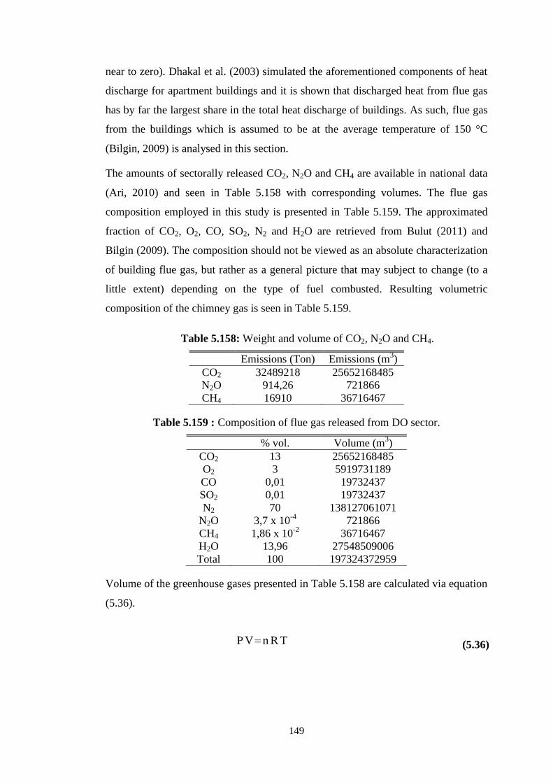
149
near to zero). Dhakal et al. (2003) simulated the aforementioned components of heat
discharge for apartment buildings and it is shown that discharged heat from flue gas
has by far the largest share in the total heat discharge of buildings. As such, flue gas
from the buildings which is assumed to be at the average temperature of 150 °C
(Bilgin, 2009) is analysed in this section.
The amounts of sectorally released CO2, N2O and CH4 are available in national data
(Ari, 2010) and seen in Table 5.158 with corresponding volumes. The flue gas
composition employed in this study is presented in Table 5.159. The approximated
fraction of CO2, O2, CO, SO2, N2 and H2O are retrieved from Bulut (2011) and
Bilgin (2009). The composition should not be viewed as an absolute characterization
of building flue gas, but rather as a general picture that may subject to change (to a
little extent) depending on the type of fuel combusted. Resulting volumetric
composition of the chimney gas is seen in Table 5.159.
Table 5.158: Weight and volume of CO2, N2O and CH4.
Emissions (Ton) Emissions (m3)
CO2 32489218 25652168485
N2O 914,26 721866
CH4 16910 36716467
Table 5.159 : Composition of flue gas released from DO sector.
% vol. Volume (m3)
CO2 13 25652168485
O2 3 5919731189
CO 0,01 19732437
SO2 0,01 19732437
N2 70 138127061071
N2O 3,7 x 10⁻⁴
721866
CH4 1,86 x 10⁻²
36716467
H2O 13,96 27548509006
Total 100 197324372959
Volume of the greenhouse gases presented in Table 5.158 are calculated via equation
(5.36).
TRnVP (5.36)

150
where P is pressure (atm), V is volume (m3), n is mole number, R is universal gas
constant (8,314 J K-1
mol-1
; 0,08314 bar l K-1
mol-1
; 0,0821 atm l K-1
mol-1
) and T is
temperature (K). For the case undertaken in this section, T =150°C, P=1 atm.
Since the volume of CO2 and its volumetric fraction are known (seen in Table 5.158
and Table 5.159, respectively), volumes of other gases are computed proportional to
their volumetric fraction in Table 5.159.
It is assumed that emitted gas is cooled down to annual average ambient temperature
of Turkey (14 °C) (Demir et al., 2008) from 150°C (temperature of emission).
Computed weight of H2O, N2, O2, CO, SO2 emissions are seen in Table 5.160. In
Table 5.160, densities are presented for 150 °C, 1 atm conditions and retrieved from
Incropera and De Witt (1996) and Cengel and Boles (1994).
Table 5.160 : Weight of H2O, N2, O2, CO, SO2.
Emissions (m3) Density (kg/m
3) Emissions (Ton)
H2O 27548509006 0,5163 14224459
N2 138127061071 0,8021 110785259
O2 5919731189 0,9126 5402347
CO 19732437 0,7987 15760
SO2 19732437 1,8207 35926
The discharged heat (Qd) is calculated via:
2
1
T
T
pd dT)T(cmQ (5.37)
where Qd (J) is discharged heat, m (kg) is mass, cp(T) (J/kgK) is
specific heat capacity and T (K) is the temperature. T1 (K) and T2 (K) are initial and
final temperature of considered gas. Variation of cP with temperature is extracted
from Cengel and Boles (1994) and results are presented in Table 5.161.
Table 5.161 : Heat release from the gases.
Emission (Ton) Heat release (MJ/kg) Total heat release (TJ)
CO2 32489218 0,126 4099
N2O 914,26 0,131 0,12
CH4 16910 0,342 5,79
H2O 14224459 0,267 3800
N2 110785259 0,149 16462
O2 5402347 0,132 714,71
CO 15760 0,148 2,33
SO2 35926 0,091 3,25
Total 25088
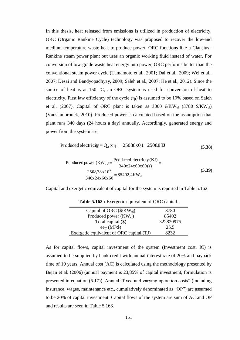
151
In this thesis, heat released from emissions is utilized in production of electricity.
ORC (Organic Rankine Cycle) technology was proposed to recover the low-and
medium temperature waste heat to produce power. ORC functions like a Clausius–
Rankine steam power plant but uses an organic working fluid instead of water. For
conversion of low-grade waste heat energy into power, ORC performs better than the
conventional steam power cycle (Tamamoto et al., 2001; Dai et al., 2009; Wei et al.,
2007; Desai and Bandyopadhyay, 2009; Saleh et al., 2007; He et al., 2012). Since the
source of heat is at 150 °C, an ORC system is used for conversion of heat to
electricity. First law efficiency of the cycle (ηI) is assumed to be 10% based on Saleh
et al. (2007). Capital of ORC plant is taken as 3000 €/KWel (3780 $/KWel)
(Vanslambrouck, 2010). Produced power is calculated based on the assumption that
plant runs 340 days (24 hours a day) annually. Accordingly, generated energy and
power from the system are:
TJ8,25081,0x25088xQ =y electricit Produced Id (5.38)
el
9
el
KW85402,460x60x24x340
10x78,2508
)s(60x60x24x340
)KJ(electrictyoducedPr)KW(poweroducedPr
(5.39)
Capital and exergetic equivalent of capital for the system is reported in Table 5.162.
Table 5.162 : Exergetic equivalent of ORC capital.
Capital of ORC ($/KWel) 3780
Produced power (KWel) 85402
Total capital ($) 322820975
eeC (MJ/$) 25,5
Exergetic equivalent of ORC capital (TJ) 8232
As for capital flows, capital investment of the system (Investment cost, IC) is
assumed to be supplied by bank credit with annual interest rate of 20% and payback
time of 10 years. Annual cost (AC) is calculated using the methodology presented by
Bejan et al. (2006) (annual payment is 23,85% of capital investment, formulation is
presented in equation (5.17)). Annual “fixed and varying operation costs” (including
insurance, wages, maintenance etc., cumulatively denominated as “OP”) are assumed
to be 20% of capital investment. Capital flows of the system are sum of AC and OP
and results are seen in Table 5.163.
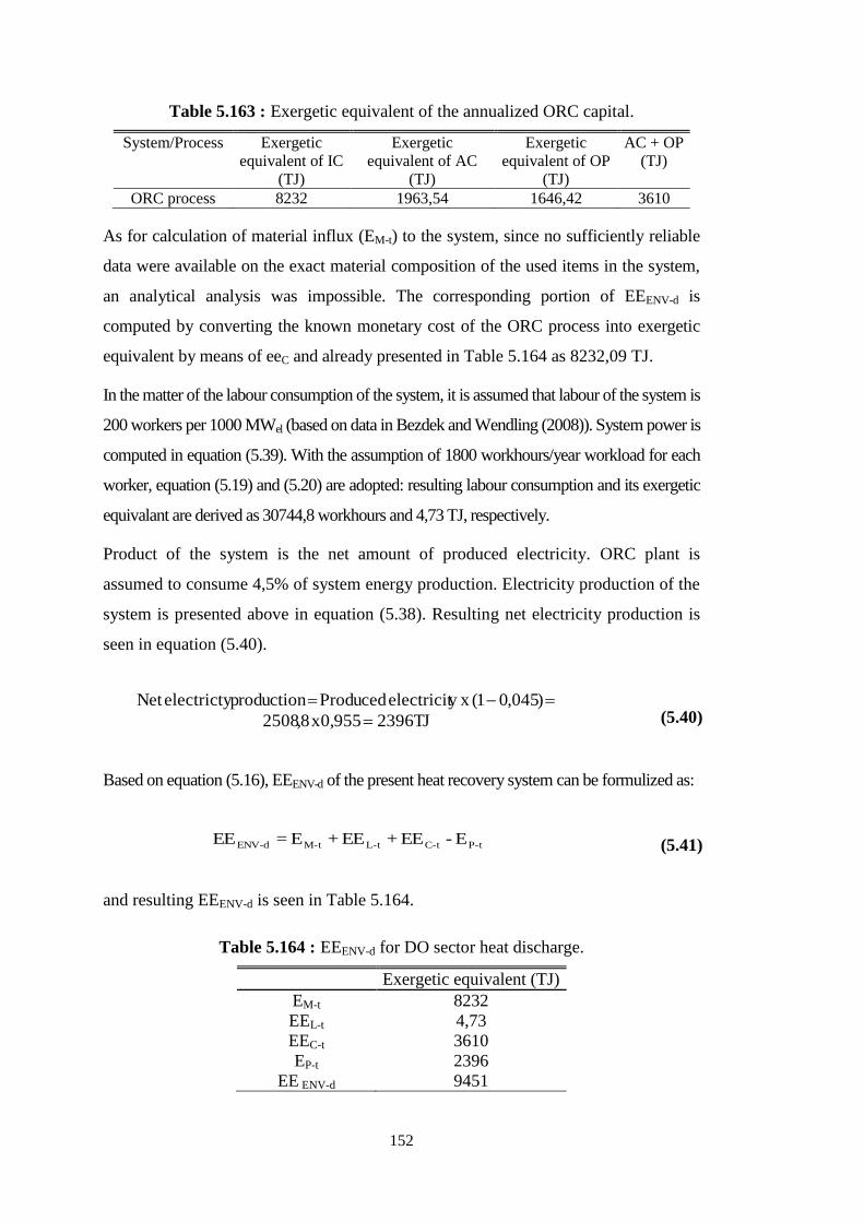
152
Table 5.163 : Exergetic equivalent of the annualized ORC capital.
System/Process Exergetic
equivalent of IC
(TJ)
Exergetic
equivalent of AC
(TJ)
Exergetic
equivalent of OP
(TJ)
AC + OP
(TJ)
ORC process 8232 1963,54 1646,42 3610
As for calculation of material influx (EM-t) to the system, since no sufficiently reliable
data were available on the exact material composition of the used items in the system,
an analytical analysis was impossible. The corresponding portion of EEENV-d is
computed by converting the known monetary cost of the ORC process into exergetic
equivalent by means of eeC and already presented in Table 5.164 as 8232,09 TJ.
In the matter of the labour consumption of the system, it is assumed that labour of the system is
200 workers per 1000 MWel (based on data in Bezdek and Wendling (2008)). System power is
computed in equation (5.39). With the assumption of 1800 workhours/year workload for each
worker, equation (5.19) and (5.20) are adopted: resulting labour consumption and its exergetic
equivalant are derived as 30744,8 workhours and 4,73 TJ, respectively.
Product of the system is the net amount of produced electricity. ORC plant is
assumed to consume 4,5% of system energy production. Electricity production of the
system is presented above in equation (5.38). Resulting net electricity production is
seen in equation (5.40).
TJ23960,955x8,2508
)045,01(y xelectricit ProducedproductionelectrictyNet
(5.40)
Based on equation (5.16), EEENV-d of the present heat recovery system can be formulized as:
t-Pt-Ct-Lt-Md-ENV E -EE+EE+E =EE (5.41)
and resulting EEENV-d is seen in Table 5.164.
Table 5.164 : EEENV-d for DO sector heat discharge.
Exergetic equivalent (TJ)
EM-t 8232
EEL-t 4,73
EEC-t 3610
EP-t 2396
EE ENV-d 9451
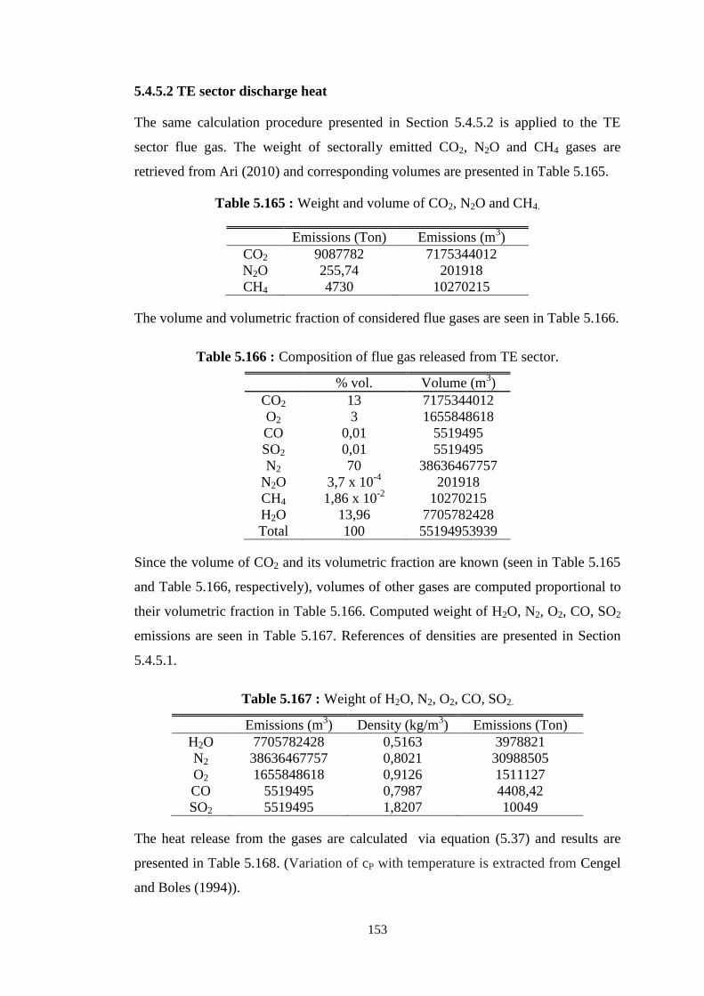
153
5.4.5.2 TE sector discharge heat
The same calculation procedure presented in Section 5.4.5.2 is applied to the TE
sector flue gas. The weight of sectorally emitted CO2, N2O and CH4 gases are
retrieved from Ari (2010) and corresponding volumes are presented in Table 5.165.
Table 5.165 : Weight and volume of CO2, N2O and CH4.
Emissions (Ton) Emissions (m3)
CO2 9087782 7175344012
N2O 255,74 201918
CH4 4730 10270215
The volume and volumetric fraction of considered flue gases are seen in Table 5.166.
Table 5.166 : Composition of flue gas released from TE sector.
% vol. Volume (m3)
CO2 13 7175344012
O2 3 1655848618
CO 0,01 5519495
SO2 0,01 5519495
N2 70 38636467757
N2O 3,7 x 10⁻⁴
201918
CH4 1,86 x 10⁻²
10270215
H2O 13,96 7705782428
Total 100 55194953939
Since the volume of CO2 and its volumetric fraction are known (seen in Table 5.165
and Table 5.166, respectively), volumes of other gases are computed proportional to
their volumetric fraction in Table 5.166. Computed weight of H2O, N2, O2, CO, SO2
emissions are seen in Table 5.167. References of densities are presented in Section
5.4.5.1.
Table 5.167 : Weight of H2O, N2, O2, CO, SO2.
Emissions (m3) Density (kg/m
3) Emissions (Ton)
H2O 7705782428 0,5163 3978821
N2 38636467757 0,8021 30988505
O2 1655848618 0,9126 1511127
CO 5519495 0,7987 4408,42
SO2 5519495 1,8207 10049
The heat release from the gases are calculated via equation (5.37) and results are
presented in Table 5.168. (Variation of cP with temperature is extracted from Cengel
and Boles (1994)).
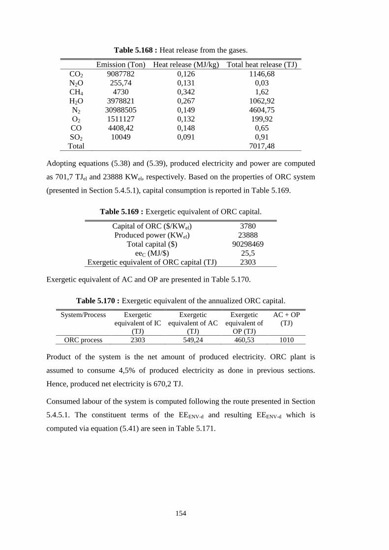
154
Table 5.168 : Heat release from the gases.
Emission (Ton) Heat release (MJ/kg) Total heat release (TJ)
CO2 9087782 0,126 1146,68
N2O 255,74 0,131 0,03
CH4 4730 0,342 1,62
H2O 3978821 0,267 1062,92
N2 30988505 0,149 4604,75
O2 1511127 0,132 199,92
CO 4408,42 0,148 0,65
SO2 10049 0,091 0,91
Total 7017,48
Adopting equations (5.38) and (5.39), produced electricity and power are computed
as 701,7 TJel and 23888 KWel, respectively. Based on the properties of ORC system
(presented in Section 5.4.5.1), capital consumption is reported in Table 5.169.
Table 5.169 : Exergetic equivalent of ORC capital.
Capital of ORC ($/KWel) 3780
Produced power (KWel) 23888
Total capital ($) 90298469
eeC (MJ/$) 25,5
Exergetic equivalent of ORC capital (TJ) 2303
Exergetic equivalent of AC and OP are presented in Table 5.170.
Table 5.170 : Exergetic equivalent of the annualized ORC capital.
System/Process Exergetic
equivalent of IC
(TJ)
Exergetic
equivalent of AC
(TJ)
Exergetic
equivalent of
OP (TJ)
AC + OP
(TJ)
ORC process 2303 549,24 460,53 1010
Product of the system is the net amount of produced electricity. ORC plant is
assumed to consume 4,5% of produced electricity as done in previous sections.
Hence, produced net electricity is 670,2 TJ.
Consumed labour of the system is computed following the route presented in Section
5.4.5.1. The constituent terms of the EEENV-d and resulting EEENV-d which is
computed via equation (5.41) are seen in Table 5.171.
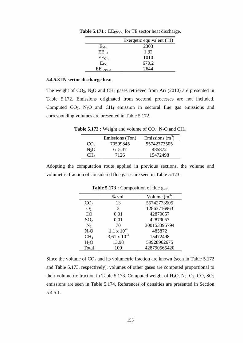
155
Table 5.171 : EEENV-d for TE sector heat discharge.
Exergetic equivalent (TJ)
EM-t 2303
EEL-t 1,32
EEC-t 1010
EP-t 670,2
EEENV-d 2644
5.4.5.3 IN sector discharge heat
The weight of CO2, N2O and CH4 gases retrieved from Ari (2010) are presented in
Table 5.172. Emissions originated from sectoral processes are not included.
Computed CO2, N2O and CH4 emission in sectoral flue gas emissions and
corresponding volumes are presented in Table 5.172.
Table 5.172 : Weight and volume of CO2, N2O and CH4.
Emissions (Ton) Emissions (m3)
CO2 70599845 55742773505
N2O 615,37 485872
CH4 7126 15472498
Adopting the computation route applied in previous sections, the volume and
volumetric fraction of considered flue gases are seen in Table 5.173.
Table 5.173 : Composition of flue gas.
% vol. Volume (m3)
CO2 13 55742773505
O2 3 12863716963
CO 0,01 42879057
SO2 0,01 42879057
N2 70 300153395794
N2O 1,1 x 10⁻⁴
485872
CH4 3,61 x 10⁻³
15472498
H2O 13,98 59928962675
Total 100 428790565420
Since the volume of CO2 and its volumetric fraction are known (seen in Table 5.172
and Table 5.173, respectively), volumes of other gases are computed proportional to
their volumetric fraction in Table 5.173. Computed weight of H2O, N2, O2, CO, SO2
emissions are seen in Table 5.174. References of densities are presented in Section
5.4.5.1.
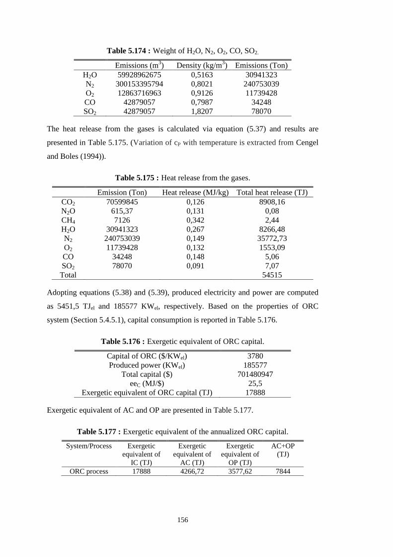
156
Table 5.174 : Weight of H2O, N2, O2, CO, SO2.
Emissions (m3) Density (kg/m
3) Emissions (Ton)
H2O 59928962675 0,5163 30941323
N2 300153395794 0,8021 240753039
O2 12863716963 0,9126 11739428
CO 42879057 0,7987 34248
SO2 42879057 1,8207 78070
The heat release from the gases is calculated via equation (5.37) and results are
presented in Table 5.175. (Variation of cP with temperature is extracted from Cengel
and Boles (1994)).
Table 5.175 : Heat release from the gases.
Emission (Ton) Heat release (MJ/kg) Total heat release (TJ)
CO2 70599845 0,126 8908,16
N2O 615,37 0,131 0,08
CH4 7126 0,342 2,44
H2O 30941323 0,267 8266,48
N2 240753039 0,149 35772,73
O2 11739428 0,132 1553,09
CO 34248 0,148 5,06
SO2 78070 0,091 7,07
Total 54515
Adopting equations (5.38) and (5.39), produced electricity and power are computed
as 5451,5 TJel and 185577 KWel, respectively. Based on the properties of ORC
system (Section 5.4.5.1), capital consumption is reported in Table 5.176.
Table 5.176 : Exergetic equivalent of ORC capital.
Capital of ORC ($/KWel) 3780
Produced power (KWel) 185577
Total capital ($) 701480947
eeC (MJ/$) 25,5
Exergetic equivalent of ORC capital (TJ) 17888
Exergetic equivalent of AC and OP are presented in Table 5.177.
Table 5.177 : Exergetic equivalent of the annualized ORC capital.
System/Process Exergetic
equivalent of
IC (TJ)
Exergetic
equivalent of
AC (TJ)
Exergetic
equivalent of
OP (TJ)
AC+OP
(TJ)
ORC process 17888 4266,72 3577,62 7844
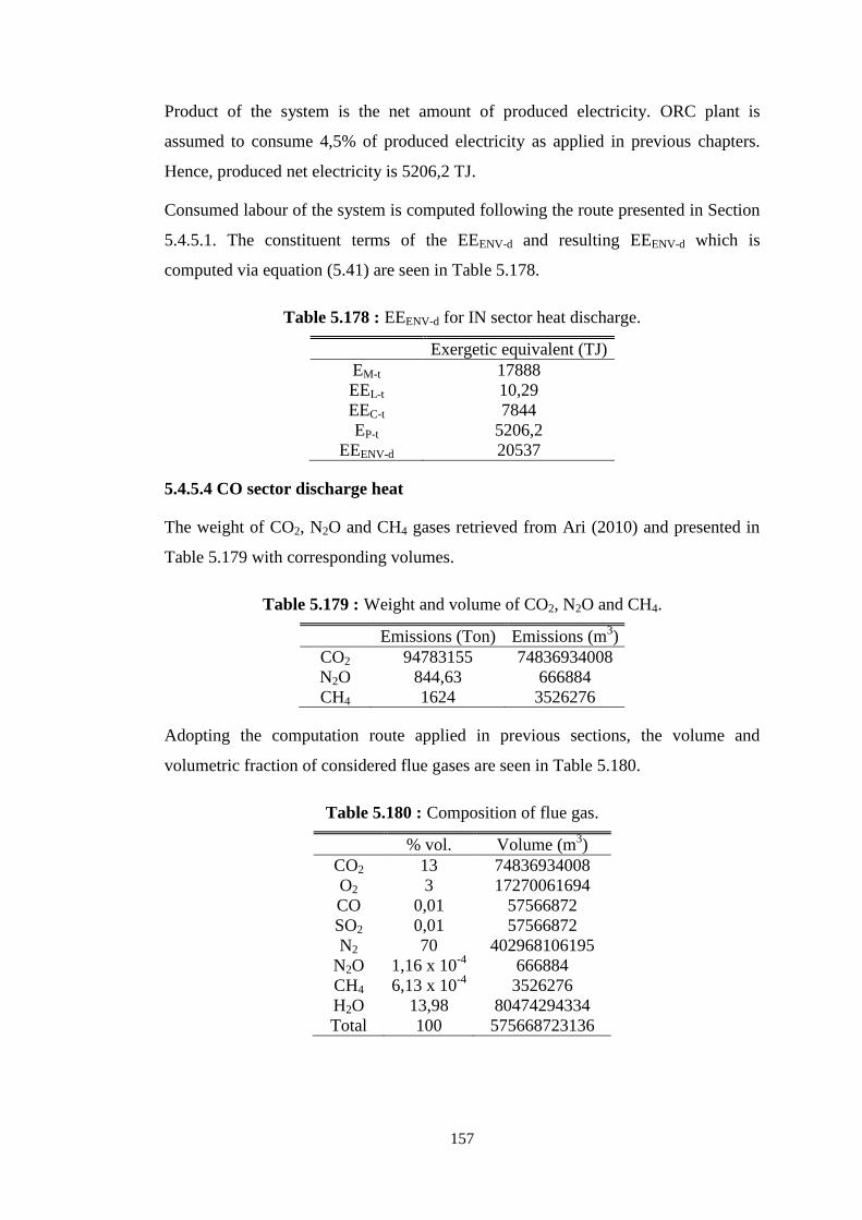
157
Product of the system is the net amount of produced electricity. ORC plant is
assumed to consume 4,5% of produced electricity as applied in previous chapters.
Hence, produced net electricity is 5206,2 TJ.
Consumed labour of the system is computed following the route presented in Section
5.4.5.1. The constituent terms of the EEENV-d and resulting EEENV-d which is
computed via equation (5.41) are seen in Table 5.178.
Table 5.178 : EEENV-d for IN sector heat discharge.
Exergetic equivalent (TJ)
EM-t 17888
EEL-t 10,29
EEC-t 7844
EP-t 5206,2
EEENV-d 20537
5.4.5.4 CO sector discharge heat
The weight of CO2, N2O and CH4 gases retrieved from Ari (2010) and presented in
Table 5.179 with corresponding volumes.
Table 5.179 : Weight and volume of CO2, N2O and CH4.
Emissions (Ton) Emissions (m3)
CO2 94783155 74836934008
N2O 844,63 666884
CH4 1624 3526276
Adopting the computation route applied in previous sections, the volume and
volumetric fraction of considered flue gases are seen in Table 5.180.
Table 5.180 : Composition of flue gas.
% vol. Volume (m3)
CO2 13 74836934008
O2 3 17270061694
CO 0,01 57566872
SO2 0,01 57566872
N2 70 402968106195
N2O 1,16 x 10⁻⁴
666884
CH4 6,13 x 10⁻⁴
3526276
H2O 13,98 80474294334
Total 100 575668723136
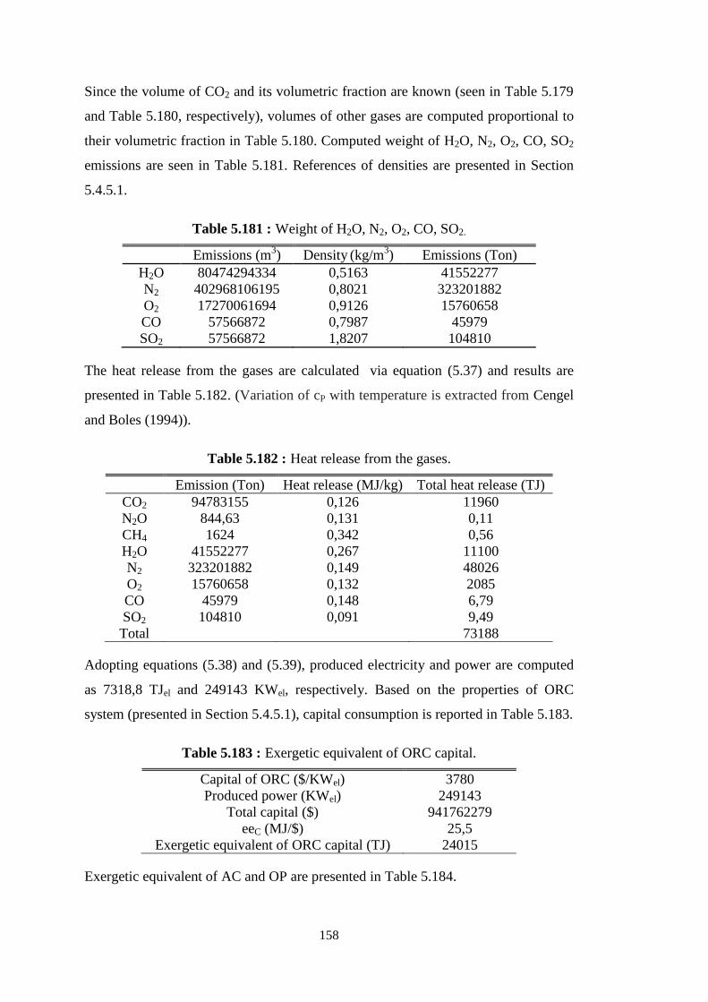
158
Since the volume of CO2 and its volumetric fraction are known (seen in Table 5.179
and Table 5.180, respectively), volumes of other gases are computed proportional to
their volumetric fraction in Table 5.180. Computed weight of H2O, N2, O2, CO, SO2
emissions are seen in Table 5.181. References of densities are presented in Section
5.4.5.1.
Table 5.181 : Weight of H2O, N2, O2, CO, SO2.
Emissions (m3) Density
(kg/m
3) Emissions (Ton)
H2O 80474294334 0,5163 41552277
N2 402968106195 0,8021 323201882
O2 17270061694 0,9126 15760658
CO 57566872 0,7987 45979
SO2 57566872 1,8207 104810
The heat release from the gases are calculated via equation (5.37) and results are
presented in Table 5.182. (Variation of cP with temperature is extracted from Cengel
and Boles (1994)).
Table 5.182 : Heat release from the gases.
Emission (Ton) Heat release (MJ/kg) Total heat release (TJ)
CO2 94783155 0,126 11960
N2O 844,63 0,131 0,11
CH4 1624 0,342 0,56
H2O 41552277 0,267 11100
N2 323201882 0,149 48026
O2 15760658 0,132 2085
CO 45979 0,148 6,79
SO2 104810 0,091 9,49
Total 73188
Adopting equations (5.38) and (5.39), produced electricity and power are computed
as 7318,8 TJel and 249143 KWel, respectively. Based on the properties of ORC
system (presented in Section 5.4.5.1), capital consumption is reported in Table 5.183.
Table 5.183 : Exergetic equivalent of ORC capital.
Capital of ORC ($/KWel) 3780
Produced power (KWel) 249143
Total capital ($) 941762279
eeC (MJ/$) 25,5
Exergetic equivalent of ORC capital (TJ) 24015
Exergetic equivalent of AC and OP are presented in Table 5.184.
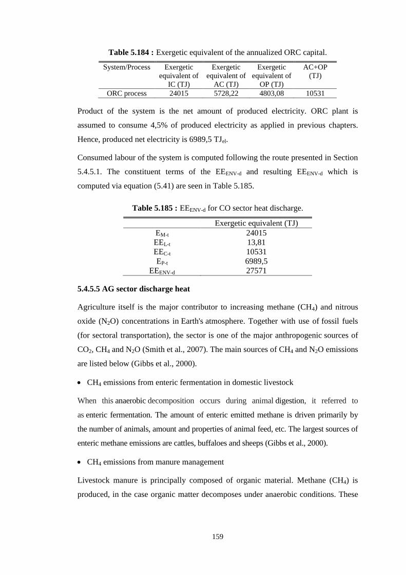
159
Table 5.184 : Exergetic equivalent of the annualized ORC capital.
System/Process Exergetic
equivalent of
IC (TJ)
Exergetic
equivalent of
AC (TJ)
Exergetic
equivalent of
OP (TJ)
AC+OP
(TJ)
ORC process 24015 5728,22 4803,08 10531
Product of the system is the net amount of produced electricity. ORC plant is
assumed to consume 4,5% of produced electricity as applied in previous chapters.
Hence, produced net electricity is 6989,5 TJel.
Consumed labour of the system is computed following the route presented in Section
5.4.5.1. The constituent terms of the EEENV-d and resulting EEENV-d which is
computed via equation (5.41) are seen in Table 5.185.
Table 5.185 : EEENV-d for CO sector heat discharge.
Exergetic equivalent (TJ)
EM-t 24015
EEL-t 13,81
EEC-t 10531
EP-t 6989,5
EEENV-d 27571
5.4.5.5 AG sector discharge heat
Agriculture itself is the major contributor to increasing methane (CH4) and nitrous
oxide (N2O) concentrations in Earth's atmosphere. Together with use of fossil fuels
(for sectoral transportation), the sector is one of the major anthropogenic sources of
CO2, CH4 and N2O (Smith et al., 2007). The main sources of CH4 and N2O emissions
are listed below (Gibbs et al., 2000).
CH4 emissions from enteric fermentation in domestic livestock
When this anaerobic decomposition occurs during animal digestion, it referred to
as enteric fermentation. The amount of enteric emitted methane is driven primarily by
the number of animals, amount and properties of animal feed, etc. The largest sources of
enteric methane emissions are cattles, buffaloes and sheeps (Gibbs et al., 2000).
CH4 emissions from manure management
Livestock manure is principally composed of organic material. Methane (CH4) is
produced, in the case organic matter decomposes under anaerobic conditions. These
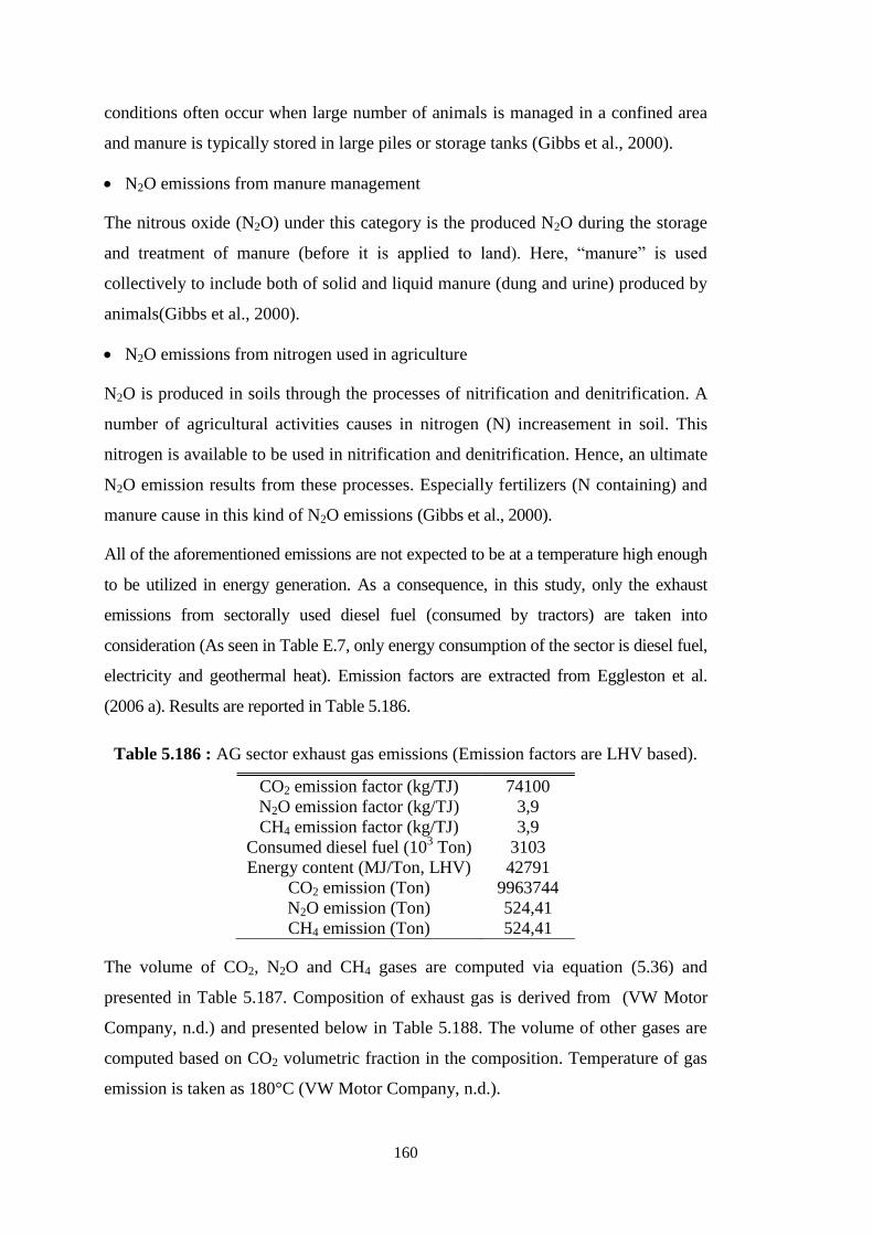
160
conditions often occur when large number of animals is managed in a confined area
and manure is typically stored in large piles or storage tanks (Gibbs et al., 2000).
N2O emissions from manure management
The nitrous oxide (N2O) under this category is the produced N2O during the storage
and treatment of manure (before it is applied to land). Here, “manure” is used
collectively to include both of solid and liquid manure (dung and urine) produced by
animals(Gibbs et al., 2000).
N2O emissions from nitrogen used in agriculture
N2O is produced in soils through the processes of nitrification and denitrification. A
number of agricultural activities causes in nitrogen (N) increasement in soil. This
nitrogen is available to be used in nitrification and denitrification. Hence, an ultimate
N2O emission results from these processes. Especially fertilizers (N containing) and
manure cause in this kind of N2O emissions (Gibbs et al., 2000).
All of the aforementioned emissions are not expected to be at a temperature high enough
to be utilized in energy generation. As a consequence, in this study, only the exhaust
emissions from sectorally used diesel fuel (consumed by tractors) are taken into
consideration (As seen in Table E.7, only energy consumption of the sector is diesel fuel,
electricity and geothermal heat). Emission factors are extracted from Eggleston et al.
(2006 a). Results are reported in Table 5.186.
Table 5.186 : AG sector exhaust gas emissions (Emission factors are LHV based).
CO2 emission factor (kg/TJ) 74100
N2O emission factor (kg/TJ) 3,9
CH4 emission factor (kg/TJ) 3,9
Consumed diesel fuel (103 Ton) 3103
Energy content (MJ/Ton, LHV) 42791
CO2 emission (Ton) 9963744
N2O emission (Ton) 524,41
CH4 emission (Ton) 524,41
The volume of CO2, N2O and CH4 gases are computed via equation (5.36) and
presented in Table 5.187. Composition of exhaust gas is derived from (VW Motor
Company, n.d.) and presented below in Table 5.188. The volume of other gases are
computed based on CO2 volumetric fraction in the composition. Temperature of gas
emission is taken as 180°C (VW Motor Company, n.d.).
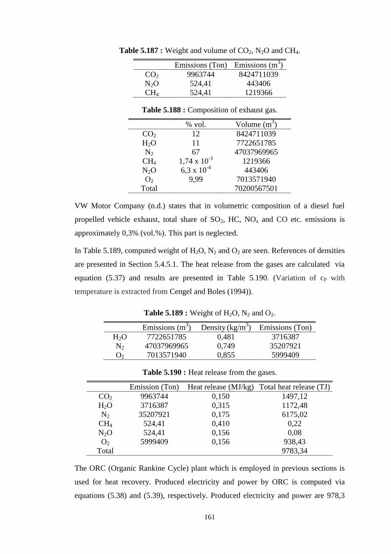
161
Table 5.187 : Weight and volume of CO2, N2O and CH4.
Emissions (Ton) Emissions (m3)
CO2 9963744 8424711039
N2O 524,41 443406
CH4 524,41 1219366
Table 5.188 : Composition of exhaust gas.
% vol. Volume (m3)
CO2 12 8424711039
H2O 11 7722651785
N2 67 47037969965
CH4 1,74 x 10⁻³
1219366
N2O 6,3 x 10⁻⁴
443406
O2 9,99 7013571940
Total 70200567501
VW Motor Company (n.d.) states that in volumetric composition of a diesel fuel
propelled vehicle exhaust, total share of SO2, HC, NOx and CO etc. emissions is
approximately 0,3% (vol.%). This part is neglected.
In Table 5.189, computed weight of H2O, N2 and O2 are seen. References of densities
are presented in Section 5.4.5.1. The heat release from the gases are calculated via
equation (5.37) and results are presented in Table 5.190. (Variation of cP with
temperature is extracted from Cengel and Boles (1994)).
Table 5.189 : Weight of H2O, N2 and O2.
Emissions (m3) Density
(kg/m
3) Emissions (Ton)
H2O 7722651785 0,481 3716387
N2 47037969965 0,749 35207921
O2 7013571940 0,855 5999409
Table 5.190 : Heat release from the gases.
Emission (Ton) Heat release (MJ/kg) Total heat release (TJ)
CO2 9963744 0,150 1497,12
H2O 3716387 0,315 1172,48
N2 35207921 0,175 6175,02
CH4 524,41 0,410 0,22
N2O 524,41 0,156 0,08
O2 5999409 0,156 938,43
Total 9783,34
The ORC (Organic Rankine Cycle) plant which is employed in previous sections is
used for heat recovery. Produced electricity and power by ORC is computed via
equations (5.38) and (5.39), respectively. Produced electricity and power are 978,3
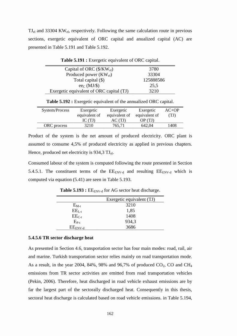
162
TJel and 33304 KWel, respectively. Following the same calculation route in previous
sections, exergetic equivalent of ORC capital and anualized capital (AC) are
presented in Table 5.191 and Table 5.192.
Table 5.191 : Exergetic equivalent of ORC capital.
Capital of ORC ($/KWel) 3780
Produced power (KWel) 33304
Total capital ($) 125888586
eeC (MJ/$) 25,5
Exergetic equivalent of ORC capital (TJ) 3210
Table 5.192 : Exergetic equivalent of the annualized ORC capital.
System/Process Exergetic
equivalent of
IC (TJ)
Exergetic
equivalent of
AC (TJ)
Exergetic
equivalent of
OP (TJ)
AC+OP
(TJ)
ORC process 3210 765,71 642,04 1408
Product of the system is the net amount of produced electricity. ORC plant is
assumed to consume 4,5% of produced electricity as applied in previous chapters.
Hence, produced net electricity is 934,3 TJel.
Consumed labour of the system is computed following the route presented in Section
5.4.5.1. The constituent terms of the EEENV-d and resulting EEENV-d which is
computed via equation (5.41) are seen in Table 5.193.
Table 5.193 : EEENV-d for AG sector heat discharge.
Exergetic equivalent (TJ)
EM-t 3210
EEL-t 1,85
EEC-t 1408
EP-t 934,3
EEENV-d 3686
5.4.5.6 TR sector discharge heat
As presented in Section 4.6, transportation sector has four main modes: road, rail, air
and marine. Turkish transportation sector relies mainly on road transportation mode.
As a result, in the year 2004, 84%, 98% and 96,7% of produced CO2, CO and CH4
emissions from TR sector activities are emitted from road transportation vehicles
(Pekin, 2006). Therefore, heat discharged in road vehicle exhaust emissions are by
far the largest part of the sectorally discharged heat. Consequently in this thesis,
sectoral heat discharge is calculated based on road vehicle emissions. in Table 5.194,
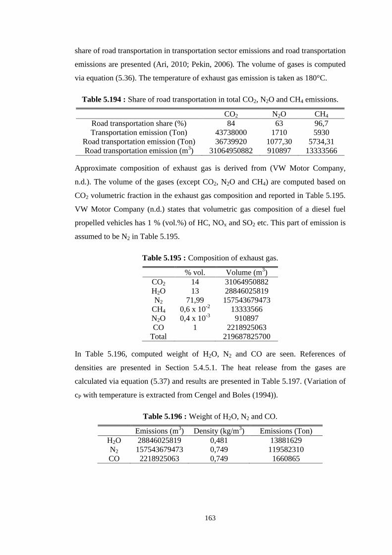
163
share of road transportation in transportation sector emissions and road transportation
emissions are presented (Ari, 2010; Pekin, 2006). The volume of gases is computed
via equation (5.36). The temperature of exhaust gas emission is taken as 180°C.
Table 5.194 : Share of road transportation in total CO2, N2O and CH4 emissions.
CO2 N2O CH4
Road transportation share (%) 84 63 96,7
Transportation emission (Ton) 43738000 1710 5930
Road transportation emission (Ton) 36739920 1077,30 5734,31
Road transportation emission (m3) 31064950882 910897 13333566
Approximate composition of exhaust gas is derived from (VW Motor Company,
n.d.). The volume of the gases (except CO2, N2O and CH4) are computed based on
CO2 volumetric fraction in the exhaust gas composition and reported in Table 5.195.
VW Motor Company (n.d.) states that volumetric gas composition of a diesel fuel
propelled vehicles has 1 % (vol.%) of HC, NOx and SO2 etc. This part of emission is
assumed to be N2 in Table 5.195.
Table 5.195 : Composition of exhaust gas.
% vol. Volume (m3)
CO2 14 31064950882
H2O 13 28846025819
N2 71,99 157543679473
CH4 0,6 x 10⁻²
13333566
N2O 0,4 x 10⁻³
910897
CO 1 2218925063
Total 219687825700
In Table 5.196, computed weight of H2O, N2 and CO are seen. References of
densities are presented in Section 5.4.5.1. The heat release from the gases are
calculated via equation (5.37) and results are presented in Table 5.197. (Variation of
cP with temperature is extracted from Cengel and Boles (1994)).
Table 5.196 : Weight of H2O, N2 and CO.
Emissions (m3) Density (kg/m
3) Emissions (Ton)
H2O 28846025819 0,481 13881629
N2 157543679473 0,749 119582310
CO 2218925063 0,749 1660865
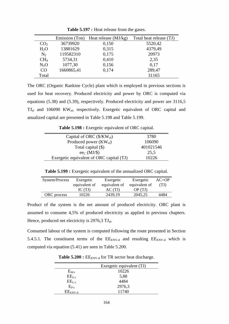
164
Table 5.197 : Heat release from the gases.
Emission (Ton) Heat release (MJ/kg) Total heat release (TJ)
CO2 36739920 0,150 5520,42
H2O 13881629 0,315 4379,49
N2 119582310 0,175 20973
CH4 5734,31 0,410 2,35
N2O 1077,30 0,156 0,17
CO 1660865,41 0,174 289,47
Total 31165
The ORC (Organic Rankine Cycle) plant which is employed in previous sections is
used for heat recovery. Produced electricity and power by ORC is computed via
equations (5.38) and (5.39), respectively. Produced electricity and power are 3116,5
TJel and 106090 KWel, respectively. Exergetic equivalent of ORC capital and
anualized capital are presented in Table 5.198 and Table 5.199.
Table 5.198 : Exergetic equivalent of ORC capital.
Capital of ORC ($/KWel) 3780
Produced power (KWel) 106090
Total capital ($) 401021546
eeC (MJ/$) 25,5
Exergetic equivalent of ORC capital (TJ) 10226
Table 5.199 : Exergetic equivalent of the annualized ORC capital.
System/Process Exergetic
equivalent of
IC (TJ)
Exergetic
equivalent of
AC (TJ)
Exergetic
equivalent of
OP (TJ)
AC+OP
(TJ)
ORC process 10226 2439,19 2045,25 4484
Product of the system is the net amount of produced electricity. ORC plant is
assumed to consume 4,5% of produced electricity as applied in previous chapters.
Hence, produced net electricity is 2976,3 TJel.
Consumed labour of the system is computed following the route presented in Section
5.4.5.1. The constituent terms of the EEENV-d and resulting EEENV-d which is
computed via equation (5.41) are seen in Table 5.200.
Table 5.200 : EEENV-d for TR sector heat discharge.
Exergetic equivalent (TJ)
EM-t 10226
EEL-t 5,88
EEC-t 4484
EP-t 2976,3
EEENV-d 11740
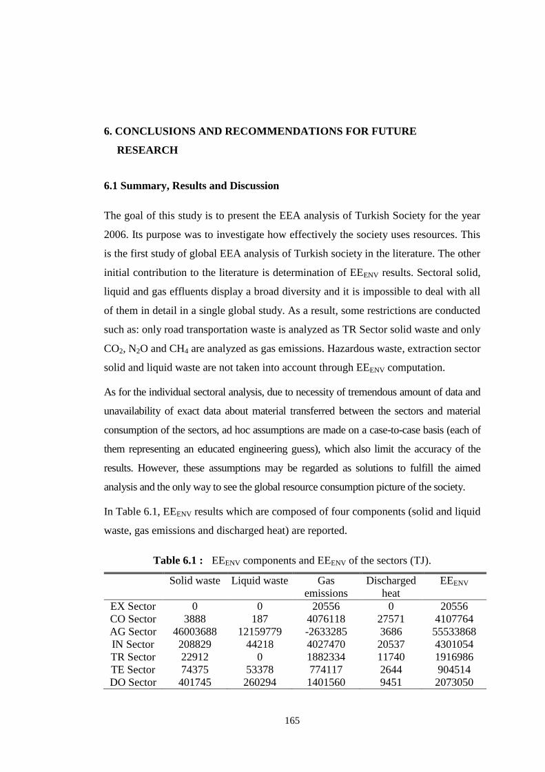
165
6. CONCLUSIONS AND RECOMMENDATIONS FOR FUTURE
RESEARCH
6.1 Summary, Results and Discussion
The goal of this study is to present the EEA analysis of Turkish Society for the year
2006. Its purpose was to investigate how effectively the society uses resources. This
is the first study of global EEA analysis of Turkish society in the literature. The other
initial contribution to the literature is determination of EEENV results. Sectoral solid,
liquid and gas effluents display a broad diversity and it is impossible to deal with all
of them in detail in a single global study. As a result, some restrictions are conducted
such as: only road transportation waste is analyzed as TR Sector solid waste and only
CO2, N2O and CH4 are analyzed as gas emissions. Hazardous waste, extraction sector
solid and liquid waste are not taken into account through EEENV computation.
As for the individual sectoral analysis, due to necessity of tremendous amount of data and
unavailability of exact data about material transferred between the sectors and material
consumption of the sectors, ad hoc assumptions are made on a case-to-case basis (each of
them representing an educated engineering guess), which also limit the accuracy of the
results. However, these assumptions may be regarded as solutions to fulfill the aimed
analysis and the only way to see the global resource consumption picture of the society.
In Table 6.1, EEENV results which are composed of four components (solid and liquid
waste, gas emissions and discharged heat) are reported.
Table 6.1 : EEENV components and EEENV of the sectors (TJ).
Solid waste Liquid waste Gas
emissions
Discharged
heat
EEENV
EX Sector 0 0 20556 0 20556
CO Sector 3888 187 4076118 27571 4107764
AG Sector 46003688 12159779 -2633285 3686 55533868
IN Sector 208829 44218 4027470 20537 4301054
TR Sector 22912 0 1882334 11740 1916986
TE Sector 74375 53378 774117 2644 904514
DO Sector 401745 260294 1401560 9451 2073050
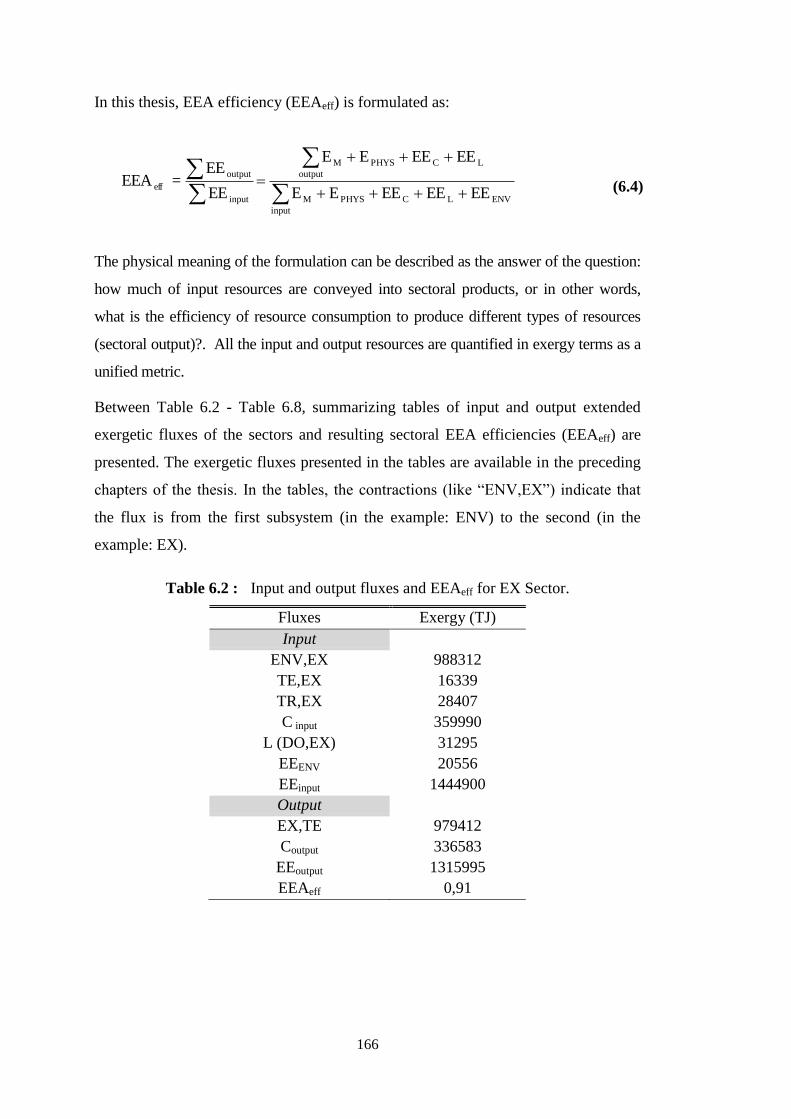
166
In this thesis, EEA efficiency (EEAeff) is formulated as:
input
ENVLCPHYSM
output
LCPHYSM
input
output
effEEEEEEEE
EEEEEE
EE
EE=EEA (6.4)
The physical meaning of the formulation can be described as the answer of the question:
how much of input resources are conveyed into sectoral products, or in other words,
what is the efficiency of resource consumption to produce different types of resources
(sectoral output)?. All the input and output resources are quantified in exergy terms as a
unified metric.
Between Table 6.2 - Table 6.8, summarizing tables of input and output extended
exergetic fluxes of the sectors and resulting sectoral EEA efficiencies (EEAeff) are
presented. The exergetic fluxes presented in the tables are available in the preceding
chapters of the thesis. In the tables, the contractions (like “ENV,EX”) indicate that
the flux is from the first subsystem (in the example: ENV) to the second (in the
example: EX).
Table 6.2 : Input and output fluxes and EEAeff for EX Sector.
Fluxes Exergy (TJ)
Input
ENV,EX 988312
TE,EX 16339
TR,EX 28407
C input 359990
L (DO,EX) 31295
EEENV 20556
EEinput 1444900
Output
EX,TE 979412
Coutput 336583
EEoutput 1315995
EEAeff 0,91
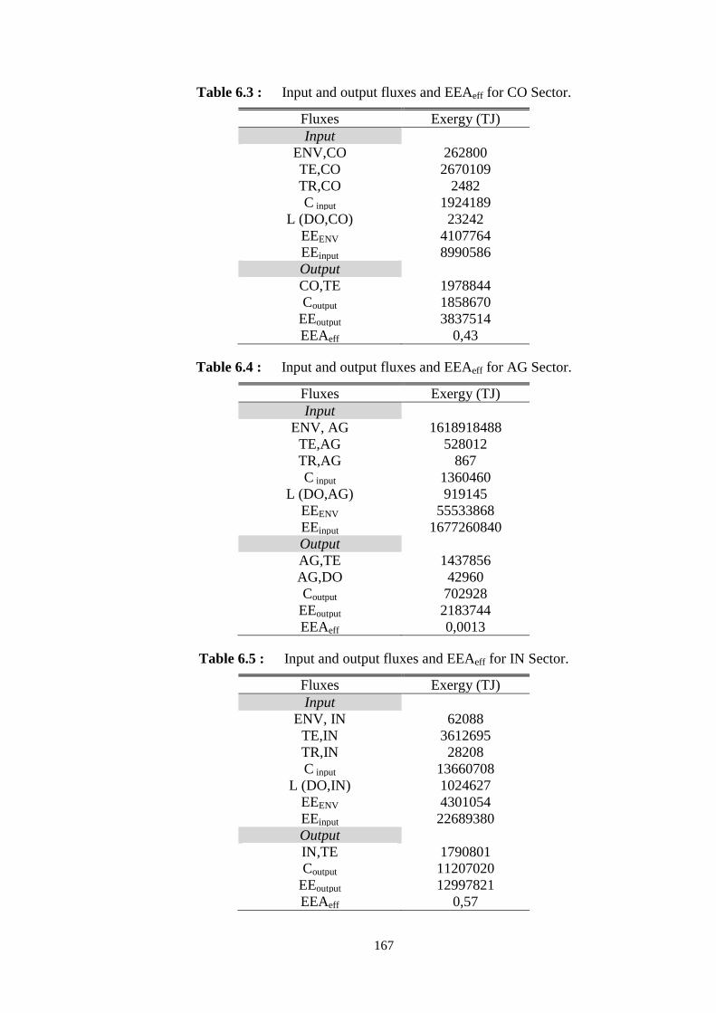
167
Table 6.3 : Input and output fluxes and EEAeff for CO Sector.
Fluxes Exergy (TJ)
Input
ENV,CO 262800
TE,CO 2670109
TR,CO 2482
C input 1924189
L (DO,CO) 23242
EEENV 4107764
EEinput 8990586
Output
CO,TE 1978844
Coutput 1858670
EEoutput 3837514
EEAeff 0,43
Table 6.4 : Input and output fluxes and EEAeff for AG Sector.
Fluxes Exergy (TJ)
Input
ENV, AG 1618918488
TE,AG 528012
TR,AG 867
C input 1360460
L (DO,AG) 919145
EEENV 55533868
EEinput 1677260840
Output
AG,TE 1437856
AG,DO 42960
Coutput 702928
EEoutput 2183744
EEAeff 0,0013
Table 6.5 : Input and output fluxes and EEAeff for IN Sector.
Fluxes Exergy (TJ)
Input
ENV, IN 62088
TE,IN 3612695
TR,IN 28208
C input 13660708
L (DO,IN) 1024627
EEENV 4301054
EEinput 22689380
Output
IN,TE 1790801
Coutput 11207020
EEoutput 12997821
EEAeff 0,57
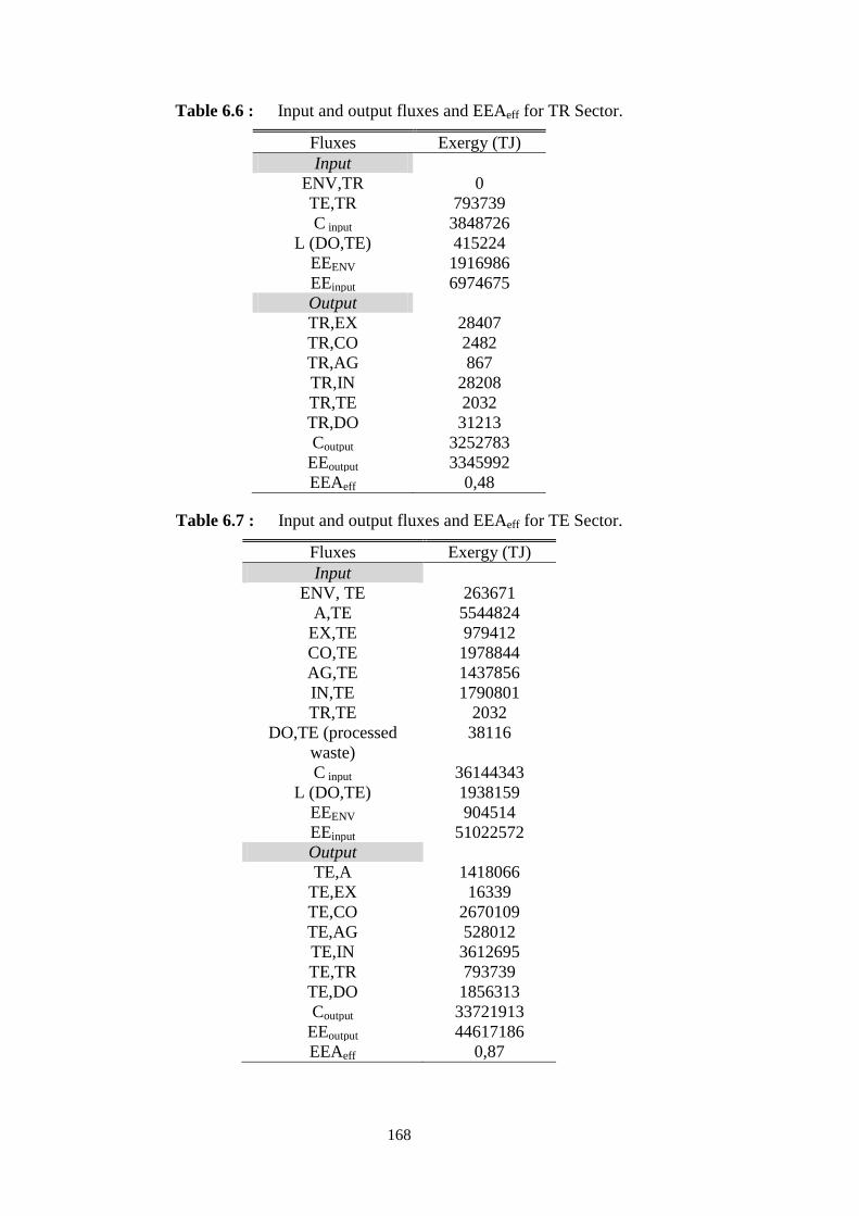
168
Table 6.6 : Input and output fluxes and EEAeff for TR Sector.
Fluxes Exergy (TJ)
Input
ENV,TR 0
TE,TR 793739
C input 3848726
L (DO,TE) 415224
EEENV 1916986
EEinput 6974675
Output
TR,EX 28407
TR,CO 2482
TR,AG 867
TR,IN 28208
TR,TE 2032
TR,DO 31213
Coutput 3252783
EEoutput 3345992
EEAeff 0,48
Table 6.7 : Input and output fluxes and EEAeff for TE Sector.
Fluxes Exergy (TJ)
Input
ENV, TE 263671
A,TE 5544824
EX,TE 979412
CO,TE 1978844
AG,TE 1437856
IN,TE 1790801
TR,TE 2032
DO,TE (processed
waste)
38116
C input 36144343
L (DO,TE) 1938159
EEENV 904514
EEinput 51022572
Output
TE,A 1418066
TE,EX 16339
TE,CO 2670109
TE,AG 528012
TE,IN 3612695
TE,TR 793739
TE,DO 1856313
Coutput 33721913
EEoutput 44617186
EEAeff 0,87
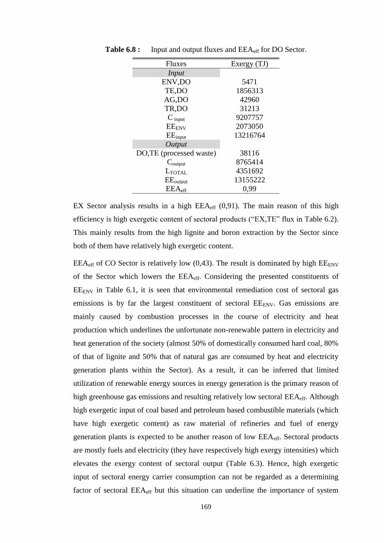
169
Table 6.8 : Input and output fluxes and EEAeff for DO Sector.
Fluxes Exergy (TJ)
Input
ENV,DO 5471
TE,DO 1856313
AG,DO 42960
TR,DO 31213
C input 9207757
EEENV 2073050
EEinput 13216764
Output
DO,TE (processed waste) 38116
Coutput 8765414
LTOTAL 4351692
EEoutput 13155222
EEAeff 0,99
EX Sector analysis results in a high EEAeff (0,91). The main reason of this high
efficiency is high exergetic content of sectoral products (“EX,TE” flux in Table 6.2).
This mainly results from the high lignite and boron extraction by the Sector since
both of them have relatively high exergetic content.
EEAeff of CO Sector is relatively low (0,43). The result is dominated by high EEENV
of the Sector which lowers the EEAeff. Considering the presented constituents of
EEENV in Table 6.1, it is seen that environmental remediation cost of sectoral gas
emissions is by far the largest constituent of sectoral EEENV. Gas emissions are
mainly caused by combustion processes in the course of electricity and heat
production which underlines the unfortunate non-renewable pattern in electricity and
heat generation of the society (almost 50% of domestically consumed hard coal, 80%
of that of lignite and 50% that of natural gas are consumed by heat and electricity
generation plants within the Sector). As a result, it can be inferred that limited
utilization of renewable energy sources in energy generation is the primary reason of
high greenhouse gas emissions and resulting relatively low sectoral EEAeff. Although
high exergetic input of coal based and petroleum based combustible materials (which
have high exergetic content) as raw material of refineries and fuel of energy
generation plants is expected to be another reason of low EEAeff. Sectoral products
are mostly fuels and electricity (they have respectively high exergy intensities) which
elevates the exergy content of sectoral output (Table 6.3). Hence, high exergetic
input of sectoral energy carrier consumption can not be regarded as a determining
factor of sectoral EEAeff but this situation can underline the importance of system
170
efficiency in the course of energy generation and also in refineries. Employing more
efficient plants and changing or upgrading the current technologies in refineries arise
as remedial approaches to heighten the amount of sectoral products with
accompanying high exergy content and to raise the current EEAeff of the Sector (for
example, as stated in Section 5.4.2.4, all Turkish refineries do not have “residue
upgrading technologies” which functions as converting vacuum residues into
different types of fuels). This approach also causes in reduction of solid waste
generation and lower EEENV in the Sector. As presented in Appendix G, use of waste
in CO Sector for electricity production is quite limited but this issue should be
concerned by policy makers to lower the EEENV load of CO Sector.
AG has a remarkably low EEAeff (0,0013) which results from two concurring factors:
1) the very large input from the ENV (inputs from ENV to AG includes solar energy
received by the agricultural area. Since agricultural area is almost %45,5 of the total
land of the country, proportional amount of solar energy is transferred to AG Sector as
a sectoral influx) and 2) the very low exergy content of the agricultural products. A
rather high amount of labour input (21% of the total workforce) is another factor which
contributes to the low EEA efficiency. As seen in Table 6.1, the sector has the
advantage of negative environmental cost of gas emissions (as a result of sectors
capture and sequestering ability) but sectoral EEENV is 80% of total EEENV of the
society due to the tremendous amount of sectoral solid waste and corresponding
EEENV-s which plays not dominant but a non-negligible role as a reason of low EEAeff.
The IN Sector has the relatively low efficiency of 0,57. The largest input fluxes to
the sector are: EEENV (19%) and material influx from TE Sector (TE,IN) (16%). The
Sector is capital intensive (60% of sectoral EEinput), but also generates a large output
of capital. Hence, capital input (Cinput) is somehow balanced with sectoral capital
output (Coutput). The material flux from TE to IN Sector (“TE,IN”) is high but this can
be viewed “normal” for a sector like IN Sector. In contrast, output flux (“IN,TE”) is
not high enough to compensate the EEAeff lowering effect of “TE,IN” flux (“IN,TE”
is 50% of “TE,IN”). As a result, it looks like energy generation and manufacturing
processes within the sector do not operate very effectively. Indeed, since
computation of “IN,TE” and also “TE,IN” relies on some fundamental assumptions,
they should not be regarded as exact numbers and this makes is difficult to mention
about these fluxes. A cleaner reality of the sector is predominant effect of
171
environmental remediation cost (as an input flux) on EEAeff. As it is seen in Table
6.1 that environmental cost of sectoral gas emissions predominantly contribute to the
high EEENV. As a result, attempting to lower the use of fossil fuels (which cause high
amount of gas emission) can be considered as an urgent approach to remedy the
current resource dissipating situation of IN Sector.
EEAeff of TR sector is 0,48. As a result of the unfortunate non-renewable pattern of
Turkish transportation, the most active transportation mode is road transportation
(82% of sectoral energy consumption) which completely dominate the use of energy
carriers and lowering EEAeff such as: 1) extensive use of fossil fuels (exergetically
very ”expensive”) in road transportation causes in exergetically high influx to the
sector 2) low efficiency of road transportation vehicles brings about exergetically
low sectoral output 3) high greenhouse gas emissions resulting from combustion of
fossil fuels. The only advantage of TR sector which raises the sectoral efficiency is
its no liquid waste production and relatively low environmental remediation cost of
solid waste (Table 6.1) which reduce its EEENV but these advantages are not
sufficient to raise the efficiency because of the prevailing effects of the above listed
efficiency lowering factors. The pursuit of more efficient and less polluting
transportation may include the collective effort of vehicular improvements (for
example: plug-in electric or hybrid cars), redesign of cities, more sucessful traffic
management and development of efficient public transit infrastructure.
The TE Sector has a quite high EEAeff (0,87). In spite of high labour input to the
sector (44% of total produced labour within the society), the sectoral output has very
high exergetic content (since in the model adopted in this study, the sector supplies
the overwhelming majority of the material fluxes to the other sectors) which results
in a high EEA efficiency. The sectoral efficiency strictly depends on imported and
exported commodities (without taking into account the material interaction of the
Sector with abroad, the sectoral EEAeff is 94%). This shows that, being a net
importer rather than exporter is the predominant reason of extended exergetic losses
of TE Sector.
DO sector displays a high EEAeff (0,99). Sector looks like quite “balanced” in terms
of extended exergy. Indeed, the accuracy of the computed efficiency is limited by the
assumptions made in this specific application and also by assumptions proposed by
EEA methodology. The well balanced profile of the sector emerges from the fact that
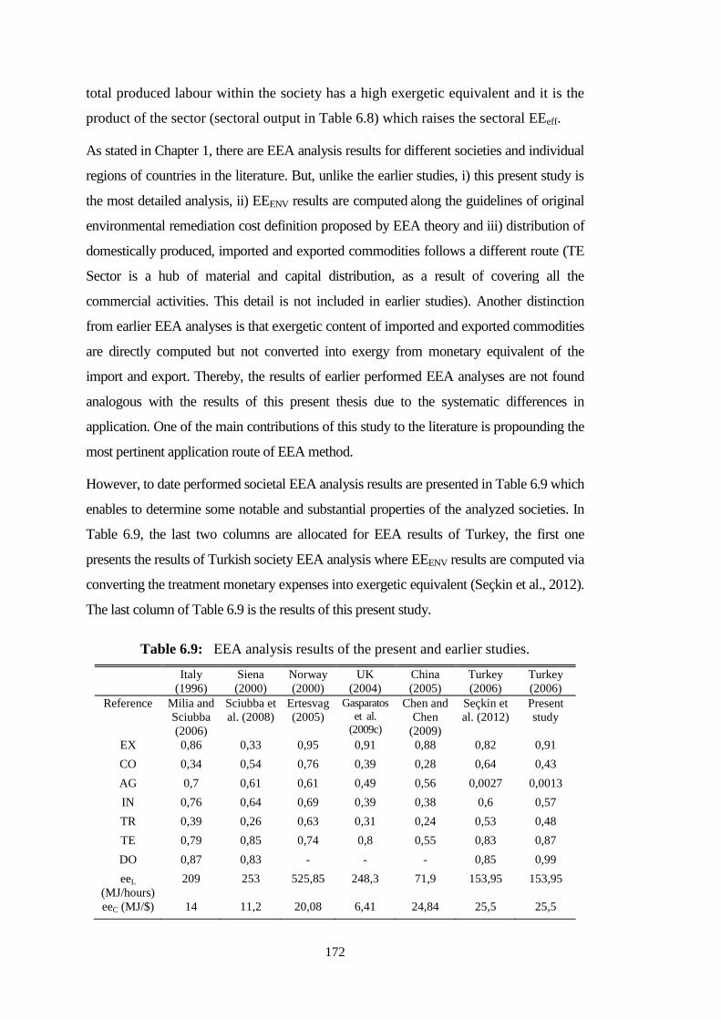
172
total produced labour within the society has a high exergetic equivalent and it is the
product of the sector (sectoral output in Table 6.8) which raises the sectoral EEeff.
As stated in Chapter 1, there are EEA analysis results for different societies and individual
regions of countries in the literature. But, unlike the earlier studies, i) this present study is
the most detailed analysis, ii) EEENV results are computed along the guidelines of original
environmental remediation cost definition proposed by EEA theory and iii) distribution of
domestically produced, imported and exported commodities follows a different route (TE
Sector is a hub of material and capital distribution, as a result of covering all the
commercial activities. This detail is not included in earlier studies). Another distinction
from earlier EEA analyses is that exergetic content of imported and exported commodities
are directly computed but not converted into exergy from monetary equivalent of the
import and export. Thereby, the results of earlier performed EEA analyses are not found
analogous with the results of this present thesis due to the systematic differences in
application. One of the main contributions of this study to the literature is propounding the
most pertinent application route of EEA method.
However, to date performed societal EEA analysis results are presented in Table 6.9 which
enables to determine some notable and substantial properties of the analyzed societies. In
Table 6.9, the last two columns are allocated for EEA results of Turkey, the first one
presents the results of Turkish society EEA analysis where EEENV results are computed via
converting the treatment monetary expenses into exergetic equivalent (Seçkin et al., 2012).
The last column of Table 6.9 is the results of this present study.
Table 6.9: EEA analysis results of the present and earlier studies.
Italy
(1996)
Siena
(2000)
Norway
(2000)
UK
(2004)
China
(2005)
Turkey
(2006)
Turkey
(2006)
Reference Milia and
Sciubba
(2006)
Sciubba et
al. (2008)
Ertesvag
(2005)
Gasparatos
et al.
(2009c)
Chen and
Chen
(2009)
Seçkin et
al. (2012)
Present
study
EX 0,86 0,33 0,95 0,91 0,88 0,82 0,91
CO 0,34 0,54 0,76 0,39 0,28 0,64 0,43
AG 0,7 0,61 0,61 0,49 0,56 0,0027 0,0013
IN 0,76 0,64 0,69 0,39 0,38 0,6 0,57
TR 0,39 0,26 0,63 0,31 0,24 0,53 0,48
TE 0,79 0,85 0,74 0,8 0,55 0,83 0,87
DO 0,87 0,83 - - - 0,85 0,99
eeL
(MJ/hours)
209 253 525,85 248,3 71,9 153,95 153,95
eeC (MJ/$) 14 11,2 20,08 6,41 24,84 25,5 25,5
173
As it is seen in Table 6.9, the results of the present study are different from the study
presented by Seçkin et al. (2012) which indicates the predominant role of accurate
EEENV numbers in obtaining cleaner and deeper EEAeff results. The most remarkable
difference between Turkish results and other countries is seen in EEAeff of AG
Sector which emerges from accounting for the sectoral solar exergy reception as a
sectoral input in Turkish society EEA analyses (the last two columns of Table 6.9).
These results can be inferred by evaluating the results of each societal EEA analysis
(presented in Table 6.9): it is seen that eeL is much lower for China and much higher
for Norway than other countries. Although eeL depends on several econometric
factors, it is estimated that these results arise from the high population of Chinese
society and low population of Norwegian society. High population results in
generation of high workhours which lowers eeL. eeC of analyzed countries are closed,
with an exception of UK. Sectoral EEAeff of above mentioned societies have a great
variation. As for EX sector, Siena province of Italy has a considerably low efficiency
among the other societies, due to high capital input into the sector. For Italy, UK,
China and Turkey, EEAeff of CO sector is relatively low which results from the low
efficiency of power & heat generation processes and high greenhouse gas emissions
occurred in the course of energy generation. The EEA efficiency of Turkish AG
sector is remarkably low due to high input of solar exergy to the sector (discussed
above). China and UK have the lowest IN Sector EEAeff through the sectors. As for
Turkish IN sector, EEA efficiency is relatively lower than Italy, Siena and Norway.
Considering that IN sector is an intensive energy and material consumer, the sector is
significant from resource use point of view and a little higher efficiency may results
in noticeably lower global extended exergy consumption (cumulative extended
exergy consumption of a country). Within this frame, IN sector result of countries is
worthy to notice, on the resource consumption side of the issue. As for TR sector,
Italy, Siena, UK and China have relatively low EEAeff. Results of Norway and
Turkey are relatively higher but, in general, TR sector EEAeff figures are lower than
those of other sectors for all the societies presented in Table 6.9. The main reason is
unavoidably high consumption of fossil fuels in the sector which is extensively
discussed above for the case of Turkey. As for DO sector, efficiencies of different
societies (including Turkey) are high and quite similar as a result of total labour
production within the country is a DO Sector product which raises the sectoral
174
EEAeff of DO Sector. As for TE sector, it is not scientifically meaningful to compare
the results of Turkey with other countries due to the fact that TE sector is in charge
of material and energy carrier distribution through the country which changes the
intensity of the sectoral input and output flows in this study and Seçkin et al. (2012).
One remarkable consequence from Table 6.9 is: TE Sector of China has a
particularly low efficiency which shows that commercial and financial activities are
not very strong in the society. The major part of above evaluation of Table 6.9 is
published in Seçkin et al. (2012).
6.1.1 Sensitivity analysis of the results
Sensitivity analysis is one of the most effective methods in the analysis of the
systems under investigation. In the method of sensitivity analysis, all parameters are
assumed constant except one of them and that parameter is varied in a logical
interval. Hence, a sensitivity analysis is carried out here by varying the quantity of
some major input fluxes of the sectors to determine the effect of the uncertainties
(emerges from assumptions done through the study) on the results. The sensitivity
analysis was only performed for the fluxes which predominantly prevail the EEAeff
of the sectors.
As seen between Table 6.2 - Table 6.8, exergetic resource use equivalent of capital is
the highest or one of the highest inputs to the sectors (25% for EX, 21% for CO, 60%
for IN, 55% for TR, 71% for TE and 70% for DO) but capital inputs are published by
the national data and has a definite characteristics. As a result, it is assumed that
capital data is accurate and is not subjected to sensitivity analysis.
As for EX Sector (EEAeff is 91%), the largest input into the sector is from ENV to EX
(the flux of ENV,EX in Table 6.2 which corresponds to 68,4% of total input). Indeed,
the exergy of fluxes from ENV is computed based on national data and assumptions on
grade of ores are conducted basis on average grade of Turkish ores. As a result, a
considerable amount of divergence (from the real exergetic content of inputs from the
ENV) is not very expected. The most uncertain fluxes (due to the assumptions which
are detailed in Appendix E and Appendix D) are TE,EX and TR,EX fluxes (Table 6.2)
which constitute 1,1% and 2% of the total input flux. Hence, EEAeff of EX sector is not
expected to be strongly influenced by uncertainties (emerge from the assumptions) in
175
the analysis. The only source of uncertainty which can affect the results may be the
uncertainty of national data which is used in computation.
As for CO Sector (EEAeff is 43%), the highest input fluxes are TE,CO and EEENV
fluxes which constitute the share of 30% and 46% of total input, respectively. As
explained in Section 4.6 and detailed in Appendix E, there are substantial assumption
in computation of material distribution from TE. Hence, the quantity of TE,CO flux
contains uncertainty. If the flux is reduced to -10% of its computed current exergy
content (90% of the presented TE,CO flux), the EEAeff of the sector is 44%. The
sectoral efficiency is not affected strongly by the uncertainty of the assumptions
performed in TE sector material distribution (detailed in Appendix E). EEENV results
depends on the accuracy of the national waste and emission data, -10% reduction in
EEENV results in the EEAeff of 44,7%, It can be inferred that accuracy of data is
moderately significant for CO Sector results.
As for IN Sector (EEAeff is 57%), the sector is capital intensive and 60% of input
flux is exergetic equivalent of capital input. Capital data of the country is definite and
does not need a sensitivity analysis. Additionally, 19% of total input flux is
constituted by EEENV of the sector. The accuracy of sectoral EEENV depends on the
accuracy of the national waste and emission data which is computed based on some
assumptions (Turkstat, 2010a, 2010b). But, reducing the EEENV to 90% and 80% of
the present sectoral EEENV results in the EEAeff of 57,5% and 58,5%, respectively. It
can be inferred that accuracy of data is moderately significant for IN Sector results.
TR Sector (EEAeff is 48%) is also a capital intensive sector which receives the 55%
of the total influx as exergetic equivalent of capital input. Furthermore, 27% of the
input flux is EEENV which is mainly constituted by sectoral gas emissions (Table
6.1). Reducing the quantity of EEENV to -10% of its presented exergetic resource use
equivalent (90% of the presented EEENV in Table 6.5) causes in 49,3% EEAeff (i.e.,
causes an considerable difference).
The highest input to the TE sector (EEAeff is 87%) is capital input (71%of total
input) but as it is stated above, capital fluxes are not subject to a sensitivity analysis.
The second largest input is the exergy of imported materials (11%) and its effect on
the sectoral EEAeff is analyzed in Section 6.1.
176
As for DO sector (EEAeff is 99%), the highest input fluxes are: capital (70%), EEENV
(16%) and exergy of material consumption received from TE (TE,DO 14%). 10%
increase in both of EEENV and TE,DO fluxes (separately) results in 98% EEAeff which
indicates that the effect of the fluxes except capital is not very dominant on the results.
6.2 Conclusion and Further Research Tasks
Since the system (Turkey) is a large and complex system and due to scarcity of
necessary data, some assumptions which are made in computation of sectoral products
and their transfers within the country were strictly necessary. It must be remarked that
the accuracy of the results depends on some fundamental assumptions made in the
specific applications and a sensitivity study for each of these assumptions ought to be
carried out. This though exceeds the limits and the goals of the present thesis.
One of the main contributions of this thesis to the literature is the exact numbers of the
environmental remediation cost (EEENV) for the solid and liquid waste and also gas
emissions as well as discharged heat from the sectors obtained in line with the original
calculation procedure of EEENV which is defined in EEA theory. To date in the
literature, EEENV is computed by converting the monetary cost of effluent treatment
process into exergetic equivalent (by means of eeC). This is the first time in the
scientific literature that numerical equivalents of environmental remediation costs are
presented for a board range of effluent types. This must be also noticed that, in
computation of environmental remediation costs, heat discharge and wastewater of the
analyzed treatment systems are not taken into computation due to scarcity of data.
Effluent control & abatement techniques which are employed in this thesis are
analyzed hypothetically but the analysis is conducted based on real data presented in
the literature. Environmental remediation systems (treatment systems) are preferred
primarily to be on “anaerobic digestion” and “recycling” based, to avoid from
“incineration process” which is expected (on the basis of an educated guess) to have
higher EEENV values originated by high incineration emissions and produced ash (25-
30% wt. of the incinerated material) which must be discharged to the environment by
trucks which is tantamount to consumption of fuel and having extra gas emissions due
to transportation. But, it must be stated that, environmental remediation costs (EEENV)
are computed on a defined disposal process chain for respective effluents. However, it
is well known that different effluent remediation technologies carry different extended
177
exergetic costs, and their EEENV values may differ. Hence, one of the welcome
consequences of this thesis is the necessity of further examination of different effluent
handling and treatment routes to determine the lowest extended exergetic cost of
EEENV. But, present thesis presents the analysis of state-of-the-art, well-established and
commercially mature industrial treatment technologies and the obtained EEENV results
have the corresponding importance. The numerical results can in turn be used in the
future EEA analyses.
It is worthy to state that computation route for the exergetic equivalent of labour and
capital relies also on realistic assumptions which are proposed by EEA methodology.
Hence, these values must be viewed as “approximate econometric indicators” rather
than exact exergetic equivalents. However, they are very beneficial and instructive to
compare the countries on the same basis.
On the basis of the study presented in this thesis, future work ought to be focused on
the development and comparative assessment of alternative strategies to improve the
societal resource consumption quality. It must be also highlighted that always there are
possible remediation/improvement strategies which aim at raising the EEAeff of the
Sectors. But, not only the EEAeff but also the total extended exergy (EE) consumption
of each sector should be taken into account, since it is more reasonable to attack to the
problem by striving for a little improvement in a high consumption sector: it is to be
expected that such a strategy may require more immediate and less expensive (in an
extended exergy sense) investments than making a global attack to other sectors with a
lower extended exergy throughput. In other words, the answer of the question: “at
global scale (i.e., for the whole society) and in terms of resource use, is a net
efficiency increase in a sector which covers a low percentage of the Country EE
more beneficial or profitable than a smaller efficiency increase in a larger sector or
not?” must have been very well analyzed in planning and applying the improvements.
A cornerstone of sustainable development is the establishment of affordable, effective
and truly sustainable resource management. The listed results of this thesis and
presented remarks in Section 6.1 ought to be viewed as indicators of: quality of
resource conversion in sectoral processes at the national level and resource
consumption intensity in intrinsic societal resource utilization structure. However, a
resource use analysis is necessary but not sufficient in order to conduct a strategy at
national level and suggesting solutions for the diagnosed problems. Determination of
178
resource use equivalent for different environmental remediation paths and choosing the
less exergetically expensive solution of pollutant remediation, sustainability analysis of
possible solutions are required further steps of this study. For instance, utilization of
geothermal energy may be preferable from resource use consumption point of view in
order to avoid from use of exergetically intensive fossil fuels and accompanying gas
emissions but the use of geothermal energy is restricted by the renewability rate of
geothermal resources. Hence, collective evaluation of the results from this and
afformentioned further studies is necessary to gain a better understanding and deeper
insight of the problems and thier solutions.
As it is seen in Section 5.4, EEENV of EX Sector solid and liquid waste is assumed to
be zero. It is granted that this is a shortcoming of the presented study from the EEA
application point of view but considering that no published data of solid and liquid
waste composition of the sector and necessity of employing different techniques and
technologies for the treatment, it was impossible to involve the treatment systems
into this present thesis. This shortcoming of the study must be augmented by future
reserches which include the technical details of the special systems of mining solid
and liquid waste treatment.
In this study, buffering and capturing capacity of the environment (such as:
photosynthesis, chemical buffering in the atmosphere and in the oceans, thermal
evaporation and convection in the atmosphere and in the water reservoirs) is
disregarded based on the fact that the analysis is performed for a very limited time
scale (1 year). This poses another shortcoming of the present analysis and the effect
of buffering by the environment must be internalized into the model.

179
REFERENCES
Abanades, J. C., Alvarez, D., Anthony, E. J. and Lu, D. (2003). In-situ capture of
CO2 in a fluidized bed combustor, The 17th FBC Conference of
ASME, Jacksonville, Florida, USA, April 19-23.
Abanades, J. C., Grasa, G., Alonso, M., Rodriguez, N., Anthony, E. J. and
Romeo, L. M. (2007). Cost structure of a postcombustion CO2 capture
system using CaO, Environ. Sci. Technol., 41, 5523-5527.
Abanades, J. C., Rubin, E. S. and Anthony, E. J. (2004). Sorbent cost and performance
in CO2 capture system, Ind. Eng. Chem. Res., 43, 3462-3466.
Ahrendts, J. (1980). Reference states, Energy ,5, 667–677.
Alonsol, M., Rodriguez, N., Gonzalez, B., Arias, B. and Abanades, J. C. (2011).
Capture of CO2 during low temperature biomass combustion in a
fluidized bed using CaO. Process description, experimental results and
economics, Energy Procedia, 4, 795-802.
Angelis-Dimakis, A., Biberacher, M., Dominguez, J., Fiorese, G., Gadocha,
S., Gnansounou, E., Guariso, G., Kartalidis, A., Panichelli,
L., Pinedo, I. and Robba, M. (2011). Methods and tools to
evaluate the availability of renewable energy sources, Renewable
& Sustainable Energy Reviews, 15, 1182-1200.
Anthony, E. J. and Wang, J. (2003). Capturing CO2 in coal-fired combustors using
CaO based sorbents, The 5th
International Symposium on Coal
Combustion, Nanjing, China, September 19-23.
Appels, L., Baeyens, J., Degreve, J. and Dewil, R. (2008). Principles and potential
of the anaerobic digestion of waste-activated sludge, Progress in
Energy and Combustion Science, 34, 755–781.
Ayres, R. U. (1994). Information, Entropy and Progress: A New Evolutionary
Paradigm. AIP Press, Woodbury, NY, USA.
Ayres, R. U. and Ayres L. W. (1999). Accounting for resources 2: The life cycle of
materials. Edward Elgar, Cheltenham, UK.
Ayres, R. U., Ayres, L. W. and Martinas, K. (1998). Exergy, waste accounting and
Life Cycle Analysis, Energy, 23, 355-363.
Ayres, R., Ayres, L. W. and Masini, A. (2006). Sustainable Metals Management,
Securing our Future- Step Towards a closed loop economy. In A. Von
Gleich, R. U. Ayres and S. Gößling-Reisemann (Ed.), Chapter 6: An
application of exergy accounting to five basic metal industries. (pp.
141-195) Dordrecht, The Netherlands: Springer Press.
Azapagic, A. (1999). Life Cycle Assessment and Its Application to Process Selection,
Design and Optimization, Chemical Engineering Journal, 73, 1-21.
180
Balat, H. (2008). Contribution of green energy sources to electrical power
production of Turkey: A review, Renewable & Sustainable Energy
Reviews, 12, 1652-1666.
Balat, M. (2005). Use of biomass sources for energy in Turkey and a view to
biomass potential. Biomass and Bioenergy, 29, 32–41.
Balocco, C., Papeschi, S., Grazzini, G. and Basosi, R. (2004). Using exergy to analyze
the sustainability of an urban area, Ecological Economics, 48, 231– 244.
Batzias, F. A., Sidiras, D. K. and Spyrou, E. K. (2005). Evaluating livestock manures
for biogas production: a GIS based method, Renewable Energy, 30,
1161–1176.
Bejan, A., Tsatsaronis G. and Moran, M. (1996). Thermal Design and
Optimization. John Wiley & Sons, New York, USA.
Berglund, M. and Borjesson, P. (2006). Assessment of energy performance in the
life-cycle of biogas production, Biomass and Bioenergy, 30, 254-266.
Bilgen, S., Kaygusuz, K. and Sari, A. (2004). Second Law Analysis of Various Types
of Coal and Woody Biomass in Turkey, Energy Sources, 26, 1083–1094.
Bilgin, A. (2009). Energy Efficiency in Boilers and Emissions, The IX. National
HVAC and Sanitary Convention and Exhibition (TESKON), Izmir,
Turkey, April 13-16
Bligh, D. C. and Ugursal, V. I. (2012). Extended exergy analysis of the economy of
Nova Scotia, Canada, Energy, 44, 878-890.
Bösch, M. E., Hellweg, S., Huijbregts, M. A. J. and Frischknecht, R. (2007).
Applying Cumulative Exergy Demand (CExD) Indicators to the
ecoinvent database, International Journal of Life Cycle Assessment,
12, 181-190.
Bosjankovic, F. (1963). Reference level of exergy of chemically reacting systems,
Forschung im Ingenieurwesen, 21, 151–152.
Burgess, A. A. and Brennan, D. J. (2001). Application of Life Cycle Assessment to
Chemical Processes, Chemical Engineering Science, 56, 2589-2604.
Camdali, U. and Ediger, V. (2007). Optimization of Fossil Fuel Sources: An
Exergy Approach, Energy Sources, Part A, 29, 251–259.
Celik, O. and Yurter, G. (2004). The Effect of Different Puzzolanic Additives On
Mechanical Properties of Cement Mortars, Dogus University
Periodical, 5, 147-154.
Cengel, Y. A. and Boles, M. A. (1994). Thermodynamics: an engineering approach.
McGraw Hill, London, Britain.
Central Bank of the Republic of Turkey (2009). Personal communication.
Chen G. Q., Qi Z. H. (2007). Systems account of societal exergy utilization: China
2003, Ecological Modelling, 208, 102–118.
Chen, B. and Chen, G. Q. (2006). Exergy analysis for resource conversion of the Chinese
Society 1993 under the material product system, Energy, 31, 1115-1150.
181
Chen, G. Q. and Chen, B. (2009). Extended-exergy analysis of the Chinese society.
Energy, 34,1127–1144.
Chen, G. Q. and Qi, Z. H. (2007). Systems account of societal exergy utilization:
China 2003, Ecological Modelling, 208, 102–118.
Chen, T. C. and Cheng, F. L. (2008). Greenhouse gases emissions from waste
management practices using Life Cycle Inventory model, Journal of
Hazardous Materials, 155, 23–31.
Cherubini F., Bargigli S. and Ulgiati S. (2009). Life cycle assessment (LCA) of
waste management strategies: Landfilling, sorting plant and
incineration, Energy, 34, 2116–2123.
Cornelissen, R. L. (1997). Thermodynamics and sustainable development ‐ The use
of exergy analysis and the reduction of irreversibility, PhD Thesis,
University of Twente, Nederlands.
Cornelissen, R. L. and Hirs, G. G. (2002). The value of the exergetic life cycle
assessment besides the LCA, Energy Conversion and Management ,
43, 1417–1424.
Corrado, A., Fiorini, P. and Sciubba, E. (2006). Environmental assessment and
extended exergy analysis of a “zero CO2 emission”, high-efficiency
steam power plant, Energy,31, 3186–3198.
Craighilla, A. L. and Powell, J. C. (1996). Lifecycle assessment and economic
evaluation of recycling: a case study. Resources, Conservation and
Recycling, 17, 75-96.
Dagdas, A., Ozturk, R. and Bekdemir, S. (2005). Thermodynamic evaluation of
Denizli Kızıldere geothermal power plant and its performance
improvement, Energy Conversion and Management, 46, 245–256.
Dai, Y. P., Wang, J. F. and Lin, G. (2009). Parametric optimization and comparative
study of organic Rankine cycle (ORC) for low grade waste heat recovery.
Energy Conversion and Management, 50, 576-82.
Davidsson, S. (2011). Life Cycle Exergy Analysis of Wind Energy Systems,
Assessing and improving life cycle analysis methodology. PhD
Thesis, Uppsala University, Sweeden.
De Meester, B., Dewulf, J., Verbeke, S., Janssens, A. and Van Langenhove, H.
(2009). Exergetic life-cycle assessment (ELCA) for resource
consumption evaluation in the built environment, Building and
Environment, 44, 11–17.
Deb Mondol, J., Mcllveen-Wright, D., Rezvani, S., Huang, Y. and Hewitt N. (2009). Techno-economic evaluation of advanced IGCC lignite coal
fuelled power plants with CO2 capture, Fuel, 88, 2495–2506.
Desai, N. B. and Bandyopadhyay, S. (2009). Process integration of organic
Rankine cycle. Energy, 34, 1674-86.
Dewulf, J. and Van Langenhove, H. (2002). Assessment of the sustainability of
technology by means of a Thermodynamically Based Life Cycle
Analysis, Environmental Science and Pollution Research, 9, 267-273.
182
Dewulf, J., Bösch, M. E., De Meester, B., Van Der Vors, G., Van Langenhove,
H., Hellweg, S. and Huijbregts M. A. J. (2007). Cumulative Exergy
Extraction from the Natural Environment (CEENE): a comprehensive
Life Cycle Impact Assessment method for resource accounting,
Environmental Science & Technology, 41, 8477-8483.
Dewulf, J., Van der Vorst, G., Kang, W. and Van Langenhove, H. (2010). The
efficiency of the manufacturing of chemical products through the
overall industrial metabolism. In ECOS 2010. Proceedings of The
23th International Conference on Efficiency, Cost, Optimization,
Simulation and Environmental Impact of Energy Systems,
Laussanne, Switzerland, 14–17 June.
Dhakal, S. and Hanaki, K. (2002). Improvement of urban thermal environment by
managing heat discharge sources and surface modification in Tokyo,
Energy Buildings, 34, 13–23.
Dhakal, S., Hanaki, K., Hiramatsu A. (2003). Estimation of heat discharges by
residential buildings in Tokyo, Energy Conversion and Management,
44, 1487–1499.
Dhakal, S., Hanaki, K., Hiramatsu A. (2004). Heat discharges from an office
building in Tokyo using DOE-2, Energy Conversion and
Management, 45, 1107–1118.
Dincer, I. (2000). Thermodynamics, exergy and environmental impact, Energy
Sources, 22, 723–732.
Dincer, I., Hussain M. M. and Al-Zaharnah I. (2005). Energy and exergy
utilization in agricultural sector of Saudi Arabia, Energy Policy, 33,
1461-1467.
Dincer, I., Hussain, M. M. and Al-Zaharnah, I. (2004). Energy and exergy
utilization in transportation sector of Saudi Arabia, Applied Thermal
Engineering, 24, 525–538.
Dunbar, W. R., Lior, N. and Gaggioli, R. A. (1992). The component equations of
energy and exergy, ASME J. Energy Resources Technology, 114, 75-83.
Ediger, V. S. and Camdali, U. (2007). Energy and exergy efficiencies in Turkish
transportation sector, 1988–2004, Energy Policy, 35, 1238–1244.
Ertay, S. (1997). Energy and exergy utilization in Turkish residential and
commercial sector. M.Sc. Thesis, University of Middle East Technical
University, Ankara, Turkey.
Ertesvag, I. S. (2005). Energy, exergy, and extended-exergy analysis of the
Norwegian society 2000, Energy, 30, 649–75.
Ertesvag, I. S. and Mielnik M. (2000). Exergy analysis of the Norwegian society.
Energy, 25, 957-973.
European Commission (2001a). Disposal and Recycling Routes for Sewage Sludge,
Part 1—Regulatory Report. Office for Official Publications of the
European Communities Luxembourg, Luxembourg.
European Commission (2001b). Disposal and Recycling Routes for Sewage Sludge,
Part 3 – scientific and technical report. Office for Official
183
Publications of the European Communities Luxembourg,
Luxembourg.
Ferrao, P. and Amaral, J. (2006). Assessing the economics of auto recycling
activities in relation to European Union Directive on end of life
vehicles, Technological Forecasting & Social Change, 73, 277–289.
Ferrao, P., Ribeiro, P. and Silva, P. (2008). A management system for end-of-life
tyres: A Portuguese case study, Waste Management, 28, 604–614.
Finnveden, G. and Östlund, P. (1997). Exergies of natural resources in life‐ cycle
assessment and other applications, Energy, 22, 923-931.
Fruergaard, T. and Astrup, T. (2011). Optimal utilization of waste-to-energy in an
LCA perspective, Waste Management, 31, 572–582.
Gaggioli, R. and Petit, P. (1976). Second law analysis for pinpointing the true
inefficiencies in final conversion systems, A.C.S. Division of Fuel
Chemistry, 21, 56-75.
Galle, M., Agar, D. W. and Watzenberger, O. (2001). Thermal N2O
decomposition in regenerative heat exchanger reactors, Chem. Eng.
Sci., 56, 1587-1595.
Garcia, G. O., Douglas, P., Croiset, E. and Zheng, L. (2006). Technoeconomic
evaluation of IGCC power plants for CO2 avoidance, Energy
Conversion and Management, 47, 2250–2259.
Gasparatos, A., Ei-Haram, M. and Horner, M. (2009a). Assessing the
sustainability of the UK society using thermodynamic concepts: Part
2, Renewable and Sustainable Energy Reviews, 13, 956–970.
Gasparatos, A., Ei-Haram, M. and Horner, M. (2009b). A longitudinal analysis of
the UK transport sector, 1970-2010, Energy Policy, 37, 623–32.
Gasparatos, A., El-Haram, M. and Horner, M. (2009c). Assessing the
sustainability of the UK society using thermodynamic concepts: Part
2, Renew Sust Energ Rev, 13,1074-81.
Gerardi, M. H. (2003). The Microbiology of Anaerobic Digesters. A John Wiley &
Sons, Inc., Publication Hoboken, New Jersey, USA.
Giannouli, M., De Haan, P., Keller, M. and Samaras Z. (2007).Waste from road
transport: development of a model to predict waste from end-of-life
and operation phases of road vehicles in Europe, Journal of Cleaner
Production, 15, 1169-1182.
Glaser, H. (1949). Der Gutegrad von Waermeaustauschern, Chem. Ing. Techn, 21, 95-96.
Gomez, A., Zubizarreta, J., Rodrigues, M., Dopazo, C. and Fueyo, N. (2010).
Potential and cost of electricity generation from human and animal
waste in Spain, Renewable Energy, 35, 498-505.
Gong, M. and Wall, G. (1997). On Exergetics, Economics, and Optimization of
Technical Processes to Meet Environmental Conditions, International
Conference on Thermodynamic Analysis and Improvement of Energy
Systems (TAIES), Beijing, China, June 10-13.
184
Gong, M. and Wall G. (2001). On exergy and sustainable development-Part 2:
Indicators and methods, Exergy Int J, 1, 217–33.
Gößling, S. (2001). Entropy production as a measure for resource use, PhD Thesis,
University of Hamburg, Hamburg, Germany.
Gößling-Reisemann, S. (2008). What Is Resource Consumption and How Can It Be
Measured?, Journal of Industrial Ecology, 12, 10-25.
Gunerhan, G. G., Kocar, G. and Hepbasli, A. (2001). Geothermal energy
utilization in Turkey, Int. J. Energy Res.,25, 769-784.
Hansan, J. A. (1996). Management of Urban Biodegradable Waste: Collection,
Occupational Health, Biological Treatment, Product Quality Criteria
and End-User Demand. James & James Science
Publishers, London, UK.
He, C., Liu, C., Gao, H., Xie, H., Li, Y., Wu, S. and Xu, J. (2012). The optimal
evaporation temperature and working fluids for subcritical organic
Rankine cycle, Energy, 38, 136-43.
Hepbasli, A. (2008). A study on estimating the energetic and exergetic prices of various
residential energy sources, Energy and Buildings, 40, 308–315.
Hermann, W. A. (2006). Quantifying global exergy resources, Energy, 31, 1685–1702.
Hughes, R. W., Lu, D. Y., Anthony, E. J. and Macchi, A. (2005). Design, process
simulation and construction of an atmospheric dual fluidized bed
combustion system for in situ CO2 capture using high-temperature
sorbents, Fuel Proc. Technol., 86, 1523-1531.
Ichinose, T., Shimidozono, K. and Hanaki, K. (1999). Impact of anthropogenic heat on
urban climate in Tokyo, Atmospheric Environment, 33, 3919–30.
IEA (International Energy Agency) (2008). Energy Statistics of OECD Countries.
IEA, Paris, France.
Ileri, A. and Gurer, T. (1998). Energy and exergy utilization in Turkey during
1995, Energy, 23, 1099–106.
Incropera, F. P. and De Witt, D. P. (1996). Fundamentals of Heat and Mass
Transfer. John Wiley & Sons Inc., New York, USA.
Jaber, J. O, Al-Ghandoor, A. and Sawalha, S .A. (2008). Energy analysis and
exergy utilization in the transportation sector of Jordan, Energy
Policy, 36, 2995-3000.
Ji, X. and Chen, G. Q. (2006). Exergy analysis of energy utilization in the
transportation sector in China, Energy Policy, 34, 1709-19.
Jury, C., Benetto, E., Koster, D., Schmitt, B. and Welfring, J. (2010). Life Cycle
Assessment of biogas production by monofermentation of energy crops
and injection into the natural gas grid, Biomass and bioenergy, 34, 54 – 66.
Kameyama, H., Yoshida, K., Yamauchi, S. and Fueki, K. (1982). Evaluation of
reference exergy for the elements, Applied Energy, 11, 69–83.
Kanat, G. (2010). Municipal solid-waste management in Istanbul. Waste
Management, 30, 1737–1745.
185
Kaplan, E. (2007). Türkiye’de Orman Ürünleri Talebi ile Arz Kaynaklarının
Değerlendirilmesi ve Endüstriyel Plantasyonların Yeri, International
Symposium on Bottlenecks, Solutions, and Priorities in the Context of
Functions of Forest Resources, Istanbul, Turkey, October 17-19.
Khizanishvili I. G. and Gaprindashvili G. G. (2006). Andesite Glaze For High
Voltage Porcelain Insulators, Glass And Ceramics, 23, 202-203.
Kim, Y., Kwak, M., Lee, S., Lee, W. and Choi, J. (2002). Effects of Pretreatment on
thermophilic, aerobic digestion, Journal of Environmental Engineering, 128,
755-763.
Korkmaz, A., Yanik, J., Brebu, M. and Vasile C. (2009). Pyrolysis of the tetra
pak, Waste Management, 29, 2836–2841.
Kotas, T. J. (1995). The exergy method of thermal plant analysis. Krieger Publishing
Company, Florida, USA.
Kratzeisen M., Starcevic N., Martinov M., Maurer C., Muller J. (2010).
Applicability of biogas digestate as solid fuel, Fuel, 89, 2179-2650.
LASDER (Turkish Tire Industrialists Association) (2009). Personal
communication.
Lloyd W. G. and Davenport D. A. (1980). Applying thermodynamics to fossil fuel,
Journal of Chemical Education, 57, 56–60.
Mac Kenzie, A., Granatstein, D. L., Anthony, E. J. and Abanades, J. C. (2007).
Economics of CO2 capture using the calcium cycle with a pressurized
fluidized bed combustor, Energy Fuels, 21, 920-926.
Manovic, V. and Anthony, E. J. (2010). Lime-Based Sorbents for High-
Temperature CO2 Capture—A Review of Sorbent Modification
Methods, Int. J. Environ. Res. Public Health, 7, 3129-3140.
Marin Sanchez, J. E. and Rodriguez Toral M. A. (2007). An estimation of
cogeneration potential by using refinery residuals in Mexico, Energy
Policy, 35, 5876–5891.
Milia, D. and Sciubba, E. (2006). Exergy-based lumped simulation of complex
systems: An interactive analysis tool, Energy, 31, 100–11.
Milne, T. A., Brennan, A. H. and Glenn, B. H. (1990). Sourcebook of Methods of
Analysis for Biomass Conversion and Biomass Conversion Processes.
Elsevier Science Publishers & Solar Energy Research Institute,
Golden, Colorado, USA.
Modesto, M. and Nebra, S. A. (2009). Exergoeconomic analysis of the power
generation system using blast furnace and coke oven gas in a brazilian
steel mill, Applied Thermal Engineering, 29, 2127–2136.
Moran, M. J. and Sciubba, E. (1994). Exergy analysis: principles and practice, J
Eng for GT and Power, 116, 285-290.
Morris, D. R. and Szargut, J. T. (1986). Standard chemical exergy of some
elements and compounds on the planet earth, Energy, 11, 733–55.
Nakicenovic, N., Gilli, P. V. and Kurz, R. (1996). Regional and global exergy and
energy efficiencies, Energy, 21, 323–37.
186
Obert, E. F. and Birnie, C. (1949). Evaluation and location of losses in a 60 MW
power station, Exergy and Power, 11,187-193.
Odum, E.P. and Barett G.W. (1971). Fundamentals of Ecology. Saunders,
Philadelphia, USA.
Odum, H.T. (1996). Environmental Accounting: Emergy and Environmental
Decision Making. John Wiley & Sons, New York, USA.
Oladiran, M. T. and Meyer, J. P. (2007). Energy and exergy analyses of energy
consumptions in the industrial sector in South Africa, Applied Energy,
84, 1056–1067.
Ozdogan, S. and Arikol, M. (1995). Energy and exergy analyses of selected Turkish
industries, Energy,20,73–80.
Ozturk, H. H., Hepbasli, A., Akdeniz, C., Bulut, H., Duran, A. S. and Kacira,
M. (2006). Investigation of the exergy of solar radiaition for the
southest Anatolian Region of Turkey. The 5th
GAP Engineering
Congress, Urfa, Turkey, April 26-28.
Ozturk, I. (1999). Anaerobik Biyoteknoloji ve Atık Arıtımındaki Uygulamaları. Su
Vakfı Yayınları, Istanbul, Turkey.
Ozturk, I. (2009). Kentsel Katı Atık Yönetimi ve AB Uyumlu Uygulamaları. Istac
Press, Istanbul, Turkey.
Ozturk, M., Bezir, N. C. and Ozek N. (2009). Hydropower–water and renewable
energy in Turkey: Sources and policy, Renewable and Sustainable
Energy Reviews, 13, 605–615.
Pekin, M. A. (2006). Greenhouse Gas Emissions Produced by Transportation Sector
(Ulaştırma Sektöründen Kaynaklanan Sera Gazı Emisyonları), M.Sc
Thesis, Istanbul Technical University, Institute of Science and
Technology, Istanbul, Turkey.
Poschl, M., Ward, S. and Owende, P. (2010). Evaluation of energy efficiency of
various biogas production and utilization pathways, Applied Energy,
87, 3305–3321.
Přemyslovská, E., Šlezingerová, J. and Rybníček M. (2007). Basic density of
wood in different forest type, International Scientific Conference
Bioclimatology and Natural Hazards, Zvolen, Slovakia, September
17 – 20.
Ptasinski, K. J., Koymans, M. N. and Verspagen, H. H. G. (2006). Performance of
the Dutch energy sector based on energy, exergy and extended exergy
accounting, Energy, 31, 3135–44.
Qasim (1999). Wastewater Treatment Plants: Planning, Design, and Operation.
CLC press, Florida, USA.
Rant, Z. (1947). Energetska ocenitev postopka fabrikacije sode Na2CO3, Ljublijana,
PhD Thesis, University of Ljublijana, Slovakia.
Ranz, L. (1999). The exergy cost analysis of the terrestrial mineral resources. Its
application for the sustainable management, PhD thesis, University of
Zaragoza, Zaragoza, Spain.
187
Reistad, G.M. (1975). Available energy conversion and utilization in the United
States, Journal of Engineering for Power, 97, 429-434.
Republic of Turkey-Ministry of Science, Industry and Technology (2008).
Kimya Sektörü Stratejik Plan Raporu. Personal communication.
Republic of Turkey-State Planning Organization (2000). Petrol Urunleri Ozel
Ihtisas Komisyonu Raporu, Ankara, Turkey.
Republic of Turkey-State Planning Organization (2001a). Madencilik Özel İhtisas
Komisyonu Raporu- Endüstriyel Hammaddeler Alt Komisyonu: Genel
Endüstri Mineralleri IV (Bentonit-Barit-Diatomit-Aşındırıcılar)
Çalışma Grubu Raporu, Ankara, Turkey.
Republic of Turkey-State Planning Organization (2001b). Madencilik Özel
İhtisas Komisyonu Raporu- Endüstriyel Hammaddeler Alt
Komisyonu: Toprak Sanayii Hammaddeleri II (Refrakter Killer Ve
Şiferton-Manyezit-Dolomit-Olivin-Zirkondisten, Sillimanit,
Andaluzit) Çalışma Grubu Raporu, Ankara, Turkey.
Republic of Turkey-State Planning Organization (2001c). Madencilik Özel İhtisas
Komisyonu Raporu- Endüstriyel Hammaddeler Alt Komisyonu:
Toprak Sanayii Hammaddeleri IV (Çimento Hammaddeleri) Çalışma
Grubu Raporu, Ankara, Turkey.
Republic of Turkey-State Planning Organization (2001d). Madencilik Özel
İhtisas Komisyonu Raporu- Endüstriyel Hammaddeler Alt
Komisyonu: Yapı Malzemeleri III (Pomza-Perlit-Vermikülit-Flogopit-
Genleşen Killer) Çalışma Grubu Raporu, Ankara, Turkey.
Republic of Turkey-State Planning Organization (2001e). Madencilik Özel İhtisas
Komisyonu Raporu Metal Madenler Alt Komisyonu Bakır-Pirit
Çalışma Grubu Raporu, Ankara, Turkey.
Republic of Turkey-State Planning Organization (2001f). Madencilik Özel İhtisas
Komisyonu Raporu Metal Madenler Alt Komisyonu Boksit Çalışma
Grubu Raporu, Ankara, Turkey.
Republic of Turkey-State Planning Organization (2001g). Madencilik Özel
İhtisas Komisyonu Raporu Metal Madenler Alt Komisyonu Değerli
Metaller Çalişma Grubu Raporu, Ankara, Turkey.
Republic of Turkey-State Planning Organization (2001h). Madencilik Özel
İhtisas Komisyonu Raporu Metal Madenler Alt Komisyonu Demir
Çalışma Grubu Raporu, Ankara, Turkey.
Republic of Turkey-State Planning Organization (2001i). Madencilik Özel İhtisas
Komisyonu Raporu Metal Madenler Alt Komisyonu Diğer Metal
Madenler Çalışma Grubu Raporu, Ankara, Turkey.
Republic of Turkey-State Planning Organization (2001j). Madencilik Özel İhtisas
Komisyonu Raporu Metal Madenler Alt Komisyonu Krom Çalışma
Grubu Raporu, Ankara, Turkey.
Republic of Turkey-State Planning Organization (2001k). Madencilik Özel
İhtisas Komisyonu Raporu Metal Madenler Alt Komisyonu Kurşun-
Çinko-Kadmiyum Çalışma Grubu Raporu, Ankara, Turkey.
188
Rigamonti, L., Grosso, M., Giugliano, M. (2009). Life cycle assessment for
optimising the level of separated collection in integrated MSW
management systems, Waste Management, 29, 934–944.
Ringen, S., Lanum, J. and Miknis, F. P. (1979). Calculating heating values from
elemental composition of fossil fuels, Fuel, 58, 69-71.
Rivero, R. and Garfias, M. (2006). Standard chemical exergy of elements updated,
Energy,31, 3310–3326.
Romeo, L. M., Uson, S., Valero, A. and Escosa, J. M. (2010). Exergy analysis as a
tool for the integration of very complex energy systems: The case of
carbonation/calcination CO2 systems in existing coal power plants, Int
J Greenh Gas Con, 4, 647–54.
Rosa R.N. and Rosa D. R. N. (2008). Exergy cost of mineral resources, Int. J.
Exergy, 5, 532- 555.
Rosen, M. A. (2002a). Can exergy help us understand and address environmental
concerns?, International Journal of Exergy, 2, 214–217.
Rosen, M. A. (2002b). Energy crisis or exergy crisis?, International Journal of
Exergy, 2, 125-123.
Rosen, M. A. (2002c). Exergy and government policy: Is there a link?, International
Journal of Exergy, 2, 224-226.
Rosen, M. A. and Dincer, I. (1997). Sectoral energy and exergy modeling of
Turkey, Transaction ASME, 119, 200–204.
Rosen, M. A., Dincer, I. and Kanoglu, M. (2008). Role of exergy in increasing
efficiency and sustainability and reducing environmental impact,
Energ Policy, 36, 128–137.
Rubin, E. S., Chen, C. and Rao, A. B. (2007). Cost and performance of fossil fuel
power plants with CO2 capture and storage, Energy Policy, 35, 4444–
4454.
Rubio Rodríguez, M. A., De Ruyck J., Roque Díaz P., Verma V. K. and Bram S.
(2011). An LCA based indicator for evaluation of alternative energy
routes, Applied Energy, 88, 630-635.
Saidur, R., Sattar, M. A., Masjuki, H. H., Ahmed, S. and Hashim, U. (2007). An
estimation of the energy and exergy efficiencies for the energy
resources consumption in the transportation sector in Malaysia,
Energy Policy, 35, 4018–26.
Saleh, B., Koglbauer, G., Wendland, M. and Fischer, J. (2007). Working fluids
for low-temperature organic Rankine cycles, Energy, 32, 1210–1221.
Salihoglu, G. (2010). Industrial hazardous waste management in Turkey: Current
state of the field and primary challenges, Journal of Hazardous
Materials, 177, 42–56.
Salihoglu, N. K., Pinarli, V. and Salihoglu, G. (2007). Solar drying in sludge
management in Turkey, Renewable Energy, 32, 1661–1675.
Schievano, A., D’Imporzano, G., Malagutti, L., Fragali, E., Ruboni, G. and
Adani F. (2010). Evaluating inhibition conditions in high-solids

189
anaerobic digestion of organic fraction of municipal solid waste,
Bioresource Technology, 101, 5728–5732.
Sciubba, E. (1999). Extended exergy accounting: towards an exergetic theory of
value. In ECOS’99. Proceedings of the International Conference on
Efficiency, Costs, Optimization, Simulation and Environmental Impact
of Energy Systems, Tokyo, Japan, 08-10 June.
Sciubba, E. (2001). Using exergy to evaluate environmental externalities. The 4th NTVA
Seminar of Industrial Ecology, Trondheim, Norway, June 14-16.
Sciubba, E. (2003a). Cost analysis of energy conversion systems via a novel
resource-based quantifier, Energy, 28, 457–477.
Sciubba, E. (2003b). Extended exergy accounting applied to energy recovery from
waste: The concept of total recycling, Energy, 28, 1315–1334.
Sciubba, E. (2004). From Engineering Economics to Extended Exergy Accounting:
A Possible Path from Monetary to Resource-Based Costing, Journal
of Industrial Ecology, 8, 19–40.
Sciubba, E. (2005). Exergo-economics: thermodynamic foundation for a more
rational resource use, Int. J. Energy Res., 29, 613–636.
Sciubba, E. (2009). Exergy-based Ecological Indicators: a necessary tool for
Resource Use assessment studies, The 4th
International Exergy,
Energy and Environment Symposium, Sharjah, UAE, April 19-23.
Sciubba, E. (2011). A revised calculation of the econometric factors - and for
the Extended Exergy Accounting method, Ecological modeling, 222,
1060-1066.
Sciubba, E. and Wall, G. (2007). A brief Commented History of Exergy From the
Beginnings to 2004, Int. J. of Thermodynamics, 10, 1-26.
Sciubba, E., Bastianoni, S. and Tiezzi, E. (2008). Exergy and extended exergy accounting
of very large complex systems with an application to the province of Siena,
Italy, Journal of Environmental Management, 86, 372–382.
Seçkin, C., Sciubba, E. and Bayulken, A.R. (2012). An application of the extended
exergy accounting method to the Turkish society, year 2006, Energy,
40, 151-163.
Shimizu, T., Hirama, T., Hosoda, H., Kitano, K., Inagaki, M. and Tejima, K. (1999). A twin fluid-bed reactor for removal of CO2 from combustion
processes, Trans. IChemE, 77, 62-66.
Simsek, O. and Erdal, M. (2004). Investigation of Some Mechanical and Physical
Properties of the Ahlat Stone (Ignimbrite), Gazi University Journal of
Science, 17, 71-78.
Sloan D. S., Pelletier R. A. and Modell M. (2009). Supercritical Water Oxidation in
the City of Orlando, Biosolids Technical Bulletin, 14, 1-18.
Suh Y. J. and Rousseaux P. (2002). An LCA of alternative wastewater sludge treatment
scenarios, Resources, Conservation and Recycling, 35, 191–200.
Sussman, M. (1979). Choosing a reference environment-state for available-energy
computations, The 72nd
Annual Meeting of American Institute of
Chemical Engineers, San Francisco, USA, November 25-29.
190
Szargut, J. (1989). Chemical exergies of the elements, Appl Energy, 32, 269–286.
Szargut, J. (2005). Exergy method: technical and ecological applications. WIT
Press, Southampton, USA.
Szargut, J., Morris, D. R. and Steward, F. R. (1988). Exergy Analysis of Thermal, Chemical
and Metallurgical Processes. Hemisphere Pubs., New York, USA.
Szargut, J., Ziebik, A. and Stanek, W. (2002). Depletion of the non-renewable
natural exergy resources as a measure of the ecological cost, Energy
Conversion and Management, 43, 1149-1163.
Talens Peiró, L., Villalba Méndez, G., Sciubba, E. and Gabarrell i Durany, X.
(2010). Extended exergy accounting applied to biodiesel production,
Energy, 35, 2861-2869.
Tamamoto, T., Furuhata, T., Arai, N. and Mori, K. (2001). Design and testing of
the organic Rankine cycle, Energy, 26, 239-51.
Tchobanoglous, G., Burton, F. L. and Stensel, H. D. (2002). Wastewater
Engineering - Treatment Disposal Reuse, 4th Edition. McGraw-Hill
and Metcalf & Eddy Inc., Boston, USA.
Tijani A. S., Witt, W. and Dietzsch, L. (2007). Process and plant improvement
using extended exergy analysis, a case study. In ESCAPE 17.
Proceedings of 17th European Symposium on Computer Aided
Process Engineering, Bucharest, Romania, May 27-30.
Torgovnikov, G. and Vinden, P. (2009). High-intensity microwave wood
modification for increasing permeability, Forest Prod. J., 59, 84–92.
Tsatsaronis, G. and Lin, L. (1990). On Exergy Costing in Exergoeconomics. 1990
Winter Annual Meeting of the American Society of Mechanical
Engineers. Dallas, Texas, USA, November 25–30.
Turker, M. (2008). Anaerobik Biyoteknoloji ve Biyogaz Üretimi Dünya’da ve
Türkiye’de Eğilimler, The 7th
National Clean Energy Symposium
(UTES), Istanbul, Turkey, December 17-19.
Turkstat (2007a). Annual industry and service statistics 2006. Turkish Statistical
Institute , Ankara, Turkey.
Turkstat (2007b). Household Labour Force Statistics 2006. Turkish Statistical
Institute, Ankara, Turkey.
Turkstat (2008b). Statistical Indicators 1923-2007. Turkish Statistical Institute,
Ankara, Turkey.
Turkstat (2009a). Agricultural Structure-Production, Price, Value, 2007. Turkish
Statistical Institute , Ankara, Turkey.
Turkstat (2009b). Labour cost survey 2004-2008. Turkish Statistical Institute , Ankara, Turkey.
Turkstat (2009e). Personal communication
Turkstat (2009f). The Summary of Agricultural Statistics 1989-2008. Turkish
Statistical Institute , Ankara, Turkey.
Turkstat (2009g). Turkey’s Statistical Yearbook 2008. Turkish Statistical Institute,
Ankara, Turkey.
191
Turkstat (2010a). Turkey Greenhouse Gas Inventory,1990 to 2008. Annual Report
for submission under the Framework Convention on Climate Change.
National Inventory Report. Turkish Statistical Institute , Ankara,
Turkey.
Turkstat (2010b). Turkey Greenhouse Gas Inventory,1990 to 2008. Annual Report
for submission under the Framework Convention on Climate Change.
National Inventory Report: Land Use Land Use Change and Forestry.
Turkish Statistical Institute , Ankara, Turkey.
Unal, A. (1994). Energy and exergy balance for Turkey in 1991, M.Sc. Thesis,
University of Middle East Technical University, Ankara, Turkey.
Unlu, G., Arıkol, M. and Kaptanoglu, D. (1987). Survey of industrial energy requirements:
Findings for the Turkish textile industry, Energy, 11, 721–725.
Urano A, Ichinose T, Hanaki K. (1999). Thermal environment simulation for three
dimensional replacement of urban activity, J Wind Eng Ind Aerodyn,
81, 197–210.
Utlu, Z. and Hepbasli, A. (2003). A study on the evaluation of energy utilization
efficiency in the Turkish residential–commercial sector using energy and
exergy analyses, Energy and Buildings, 35,1145–53.
Utlu, Z. and Hepbasli, A. (2004a). Comparison of Turkey’s sectoral energy
utilization efficiencies between 1990 and 2000: part 1.Utility and
industrial sectors, Energy Sources, 26, 1345-1355.
Utlu, Z. and Hepbasli, A. (2004b). Evaluating the energy utilization efficiency of
Turkey’s renewable energy sources during 2001, Renewable and
Sustainable Energy Reviews, 8, 237–255.
Utlu, Z. and Hepbasli, A. (2004c). Turkey’s sectoral energy and exergy analysis
between 1999 and 2000, Int J Energ Res.,28, 1176-1191.
Utlu, Z. and Hepbasli, A. (2006a). Assessment of the energy and exergy utilization
efficiencies in the Turkish agricultural sector, Int. J. Energy Res., 30, 659–670.
Utlu, Z. and Hepbasli, A. (2006b). Assessment of the energy utilization efficiency
in the Turkish transportation sector between 2000 and 2020 using
energy and exergy analysis method, Energy Policy, 34, 1611–1618.
Utlu, Z. and Hepbasli, A. (2006c). Estimating the energy and exergy utilization
efficiencies for the residential–commercial sector: an application,
Energy Policy, 34, 1097–1105.
Utlu, Z. and Hepbasli, A. (2007a). A review and assessment of the energy utilization
efficiency in the Turkish industrial sector using energy and exergy analysis
method, Renewable and Sustainable Energy Reviews, 11, 1438–1459.
Utlu, Z. and Hepbasli, A. (2007b). A review on analyzing and evaluating the energy
utilization efficiency of countries, Renewable and Sustainable Energy
Reviews, 11, 1–29.
Utlu, Z. and Hepbasli, A. (2009). Exergoeconomic aspects of sectoral energy
utilization for Turkish industrial sector and their impact on energy
policies, Energy Policy, 37, 577–587.
192
Valero, A. (2008). Exergy evolution of the mineral capital on earth. Ph.D. Thesis.
University of Zaragoza, Zaragoza, Spain.
Wall, G. (2011). Life Cycle Exergy Analysis of Renewable Energy Systems, The
Open Renewable Energy Journal, 4, 72-77.
Wall, G., Sciubba, E. and Naso, V. (1994). Exergy use in Italian Society, Energy,
19, 1267-1274.
Wei, D. H., Lu, X. S., Lu, Z. and Gu, J. M. (2007). Performance analysis and
optimization of organic Rankine cycle (ORC) for waste heat recovery,
Energy Conversion and Management, 48, 1113-1119.
Xu, C. C. and Lancaster, J. (2009). Treatment of Secondary Sludge for Energy
Recovery, in Energy Recovery, p. 187-209, Eds. Du Bois, E. and
Mercier, A., Nova Science Publishers Inc., New York, USA.
YEM (Construction Industry Center) (2009). Türk Yapı Sektörü Raporu, 2008. Ali
Rıza Baskan Güzel Sanatlar Press, Istanbul, Turkey.
Zakirov, V. and Zhang, H. (2008). A model for the operation of nitrous oxide
monopropellant, Aerospace Science and Technology, 12, 318–323.
Zhang B. and Chen G. Q. (2010). Physical sustainability assessment for the China
society: Exergy-based systems account for resources use and
environmental emissions, Renewable & Sustainable Energy Reviews,
14, 6, 1527-1545.
American Petroleum Institute (2010). Reclaimed Petroleum Hydrocarbons:
Residual Hydrocarbon Wastes from Petroleum Refining. Date
retrieved: 01.04.2011, address:
http://www.petroleumhpv.org/docs/rec_subs/Residual%20hydrocarbo
n%20wastes%20-%20CAD%20final%208_30_10.pdf.
Ari, I. (2010). Emission Trading for Combating with the Climate Change and its
Implementation in Turkey. Planning Expertise Thesis in Republic of
Turkey-State Planning Organization, Ankara, Turkey. Date retrieved:
01.04.2011, address:
http://www.dpt.gov.tr/DocObjects/View/9840/tez-iari.pdf accessed
March 2011.
Banks, C. (2009). Optimising Anaerobic Digestion. Date retrieved: 21.15.2011, address:
http://www.kingdombio.com/Optimising%20anaerobic%20digestion.pdf.
Bezdek, R. H and Wendling, R. M. (2008). Establishing benchmarks for
environmental comparison. Date retrieved: 01.04.2011, address:
http://www.misi-net.com/publications/ModernPowerSystems-1206.pdf.
BOTAS Petroleum Pipeline Corporation (n.d.). Date retrieved: 01.04.2011,
address: http://www.botas.gov.tr.
Brundtland G. H. (1987). Our Common Future, Report of the World Commission on
Environment and Development, Oxford University Press, Oxford. Date
retrieved: 13.07.2011, address: http://www.un-documents.net/wced-ocf.htm.
Bulut, H. (2011). Course Notes on Steam Boilers. Date retrieved: 15.05.2011,
address: http://eng.harran.edu.tr/~hbulut/buhar.pdf.
193
CAA (Canadian Automobile Association) (2009). Primer on Automobile Fuel
Efficiency and Emissions. Date retrieved: 21.11.2010, address:
http://www.caa.ca/primer/documents/primer-eng.pdf.
California Environmental Protection Agency- Air Resources Board (2008).
Mandatory Reporting of Greenhouse Gas Emissions: Instructional
Guidance for Operators. Chapter 13: Common Calculation Methods. Date
retrieved: 01.04.2012, address: http://www.arb.ca.gov/cc/reporting/ghg-
rep/ghg-rep-guid/13_CommonMeths.pdf.
Central Bank of the Republic of Turkey (n.d.). Statistical data. Date retrieved:
01.10.2010, address: http://evds.tcmb.gov.tr/cbt.html.
Chamber of Turkish Geology Engineers (n.d.). Date retrieved: 07.06.2010,
address: http://www.jmo.org.tr.
Dai, J., Chen, B. and Lin, H. (2008). Extended exergy-based ecological accounting of China
during 2000-2007. Date retrieved: 13.07.2011, address:
http://www.iemss.org/iemss2010/papers/W17/W.17.13.Extended%20exergy-
based%20ecological%20accounting%20of%20China%20during%202000-
2007%20-%20JING%20DAI.pdf.
Dancee (The Danish Cooperation for Environment in Eastern Europe) (2004).
The FEASIBLE Model, Version 2-User Manual and Documentation,
Appendix 3: Documentation of Expenditure Functions - Wastewater.
Date retrieved: 01.09.2011, address:
http://www.oecd.org/document/56/0,3746,en_2649_34291_33719928
_1_1_1_1,00.html.
De Hullu, J., Maassen, J. I. W., Van Meel, P. A., Shazad, S. and Vaesse, J. M. P.
(2008). Comparing different biogas upgrading techniques: Final
report. Date retrieved: 01.04.2011, address:
http://students.chem.tue.nl/ifp24/BiogasPublic.pdf.
Demir, I., Kilic, G., Coskun, M. and Sumer, U. M. (2008). Türkiye’de Maksimum,
Minimum ve Ortalama Hava Sıcaklıkları ile Yagıs Dizilerinde
Gözlenen Degisiklikler ve Egilimler, Turkish Mechanical Engineers
Chamber- Climate Change Symposium, Ankara, Turkey, 13-14
March. Date retrieved: 01.06.2011, address:
http://www.mgm.gov.tr/FILES/iklim/gozlemdegisiklik.pdf.
Demirci, B. (2008). Plastik Sektörü 2007 Yılı Değerlendirmesi ve İleriye Dönük
Beklentiler. Date retrieved: 10.07.2010, address:
http://www.yapiveri.com/VImages/2008/Arastirmalar/02.08_pagev.pdf.
ECN (Energy research Center for Netherlands) (n.d.). Date retrieved: 13.07.2011,
address: http://www.ecn.nl/phyllis/DataTable.asp.
EDANA (European Disposables and Nonwovens Association) (2001). Diapers: Health
Benefits and Environmental Aspects. Date retrieved: 01.04.2011, address:
http://www.hapco.edana.org/documents_sections/hapco_publications/diap
ers.pdf.
Eggleston, S., Buendia, L., Miwa, K., Ngara, T. and Tanabe, K. (2006a). IPCC
Guidelines for National Greenhouse Gas Inventories. Vol 2: Energy.
IPCC National Greenhouse Gas Inventories Programme, Institute for
194
Global Environmental Strategies,. Hayama, Kanagawa, Japan. Date
retrieved: 01.04.2011, address: http://www.ipcc-
nggip.iges.or.jp/public/2006gl/index.html.
Eggleston, S., Buendia, L., Miwa, K., Ngara, T., Tanabe, K. (2006b). IPCC
Guidelines for National Greenhouse Gas Inventories. Vol 5: Waste.
IPCC National Greenhouse Gas Inventories Programme, Institute for
Global Environmental Strategies, Hayama, Kanagawa, Japan.
http://www.ipcc-nggip.iges.or.jp/public/2006gl/index.html.
Eggleston, S., Buendia, L., Miwa, K., Ngara, T., Tanabe, K., 2006c. IPCC
Guidelines for National Greenhouse Gas Inventories. Vol 6:
Wastewater Treatment and Discharge. IPCC National Greenhouse
Gas Inventories Programme-Institute for Global Environmental
Strategies, Hayama, Kanagawa, Japan. Date retrieved: 15.03.2010,
address: http://www.ipcc-nggip.iges.or.jp/public/2006gl/index.html.
EIA (U.S. Energy Information Administration) (2010). Updated Capital Cost Estimates
for Electricity Generation Plants. Date retrieved: 01.04.2011, address:
http://www.mit.edu/~jparsons/current%20downloads/EIA%202010%20up
dated%20capital%20costs.pdf.
EPA (European Environment Agency) (2002a). Biodegradable municipal waste
management in Europe Part 1: Strategies and instruments. Date
retrieved: 01.04.2011, address:
http://www.eea.europa.eu/publications/topic_report_2001_15_Part1.
EPA (European Environment Agency) (2002b). Biodegradable municipal waste
management in Europe, Part 3: Technology and market issues. Date
retrieved: 01.04.2011, address:
http://scp.eionet.europa.eu/publications/topic15_2001.
Ertesvag, I. S. (2000). Energy and exergy in moist fuels. Date retrieved: 13.02.2011,
address: http://folk.ntnu.no/ivarse/energi/moistfuel.pdf.
Esen, S. E. (2002). Türkiye’nin Kentsel Çevre Altyapısı (Atıksu Bertarafı) Yatırım
İhtiyacı, Fayda-Maliyet Analizleri ve Strateji Önerisi (2002-2023).
Planning Expertise Thesis in Republic of Turkey-State Planning
Organization, Ankara, Turkey. Date retrieved: 01.09.2011, address:
www.dpt.gov.tr/DocObjects/Download/3230/atiksu.pdf.
European Commission Environmental Department (2006). A study to examine
the benefits of the End of Life Vehicles Directive and the costs and
benefits of a revision of the 2015 targets for recycling, re-use and
recovery under the ELV Directive 2006. Date retrieved: 13.07.2011,
address: http://ec.europa.eu/environment/waste/elv_index.htm accessed
June 2011.
Eurostat (2008). NACE Rev. 2- Statistical classification of economic activites in the
European Community. Date retrieved: 08.06.2010, address:
http://epp.eurostat.ec.europa.eu/cache/ITY_OFFPUB/KS-RA-07-
015/EN/KS-RA-07-015-EN.PDF.
EVD (2008). Market survey Turkey – Environment. Date retrieved: 01.04.2012,
address: www.tulipconsultancy.com/?download/1.
195
FAO (Food and Agriculture Organization of United Nations) (n.d.). FAO
Corporate Document Repository Appendix 1 - List of wood densities
for tree species from tropical America, Africa, and Asia. Date
retrieved: 08.09.2012, address:
http://www.fao.org/docrep/w4095e/w4095e0c.htm.
Foundation of Turkish Lime Manufacturers (2009). Statistics 2006. Date
retrieved: 10.07.2011, address:
http://www.kirec.org/index.php?page=icerikgoster&menuID=59.
Gibbs, M., Johnson, D., Lassey, K., Ulyatt, M., Jun, P., Gaffney K. and
Conneely D. (2000). Agriculture. In: IPCC Good Practice Guidance
and Uncertainty Management in National Greenhouse Gas
Inventories. Date retrieved: 01.04.2011, address: http://www.ipcc-
nggip.iges.or.jp/public/gp/english/4_Agriculture.pdf.
Hau, J. L. and Bakshi, B. R. (2005). A Multiscale and Multiobjective Approach for
Environmentally Conscious Process Retrofitting, Date retrieved: 13.07.2011,
address: http://www.nt.ntnu.no/users/skoge/prost/proceedings/aiche-
2004/pdffiles/papers/393e.pdf.
Johnson, A. (2010). A Discussion of Natural Gas Pipeline System Efficiency. Date retrieved:
21.11.2010, address:
http://www.gaselectricpartnership.com/BBPipeline%20Efficiency%20ATJ.pdf.
Kutlu, H. R. (2009). Karma Yem Sanayi ve Genetiği Değiştirilmiş Organizmalar
(GDO). Date retrieved: 08.05.2010, address:
http://www.zootekni.org.tr/upload/File/GDO-HRKutlu1.pdf.
M/J Industrial Solutions (2003). Municipal Wastewater Treatment Plant Energy
Baseline Study. Date retrieved: 13.07.2011, address:
http://www.cee1.org/ind/mot-sys/ww/pge1.pdf.
Mengoli, A. (2010). Life Cycle Exergy Analysis (LCEA) in a residential heating
process. Date retrieved: 13.07.2011, address:
http://www.exergy.se/courses/exergyanalysis/reports/Alessandro%20
Mengoli.pdf.
MREC (Midwest Rural Energy Council) (2003). Anaerobic digestion of farm and
food processing residues, Good Practice Guidelines. Date retrieved:
01.04.2011, address: http://www.mrec.org/biogas/adgpg.pdf.
Munke, K., Curri, J., Laru, J. P., Sempere R., Puyp, H., Pos, F., Köss, F.,
Morett, U. and Ceustermans, J. (2007). Code of Practice Nitrous
Oxide, European Industrial Gases Association (AISBL), Brussels,
Belgium. Date retrieved: 01.04.2011, address:
http://www.eiga.org/fileadmin/docs_pubs/Doc_116_07_E.pdf.
Nurbay, N. and Cinar, A. (2005). Rüzgar Türbinlerinin Çeşitleri ve Birbirleriyle
Karşılaştırılması, The 3th National Renewable Energy Sources Symposium,
Mersin, Turkey, October18-21. Date retrieved: 07.01.2010, address:
http://www.emo.org.tr/etkinlikler/yeksem/etkinlik_bildiriler.php?etkinlikkod=5.
Orr, D. and Maxwell, D. (2000). A Comparison of Gasification and Incineration of
Hazardous Wastes. Date retrieved: 01.04.2011, address:
http://www.netl.doe.gov/publications/others/techrpts/igcc_wp.pdf.
196
Ozkan, S. G. and Tuncer, G. (2001). Pomza Madenciliğine Genel Bir Bakış, The
4th
National Raw Material Symposium, Izmir, Turkey, October18-19.
Date retrieved: 10.02.2010, address:
http://www.maden.org.tr/resimler/ekler/ecd070e606afbf0_ek.pdf.
Pehlken, A. and Essadiqi, E. (2005). Scrap tire recyling in Canada. Date retrieved:
15.04.2012, address: http://www.nrcan.gc.ca/mms-smm/busi-indu/rad-
rad/pdf/scr-tir-rec-peh-eng.pdf.
Recycling Council of Ontario (2010). Measuring energy savings and greenhouse
gas (GHG) emission reductions benefits resulting from recycling in
Canada. Date retrieved: 21.15.2011, address:
https://www.rco.on.ca/uploads/File/projects/completed/GreenhouseGa
sAndRecycling/RC_Projects-GHG-Fact_Sheet.pdf.
Republic of Turkey - Energy Market Regulatory Authority (2010). Electricity
Market Report. Date retrieved: 01.04.2012, address:
http://www.enkoenerji.com.tr/en/legislation/other/files/electricity-
market-report-2010.pdf.
Republic of Turkey Prime Ministry-Investment Support And Promotion Agency of
Turkey (2010a). Transportation & Logistics Industry Report. Date
retrieved: 28.05.2010, address: http://www.invest.gov.tr/en-
US/infocenter/publications/Documents/TRANSPORTATION.LOGISTICS
.INDUSTRY.pdf.
Republic of Turkey Prime Ministry-Investment Support and Promotion Agency
(2010b). Turkiye Metal Sektörü Raporu. Date retrieved: 18.07.2010,
address: http://www.invest.gov.tr/tr-
R/infocenter/publications/Documents/METAL.SEKTORU.pdf.
Republic of Turkey Prime Ministry-State Personnel Presidency (2008). Statistics
of workers distribution in government. Date retrieved: 01.10.2010,
address: http://www.dpb.gov.tr/spp_statics.html.
Republic of Turkey-Ministry of Energy and Natural Resources (n.d.). Energy
balance table of Turkey 2006- both of energy flows and material flows
are available. Date retrieved: 07.01.2010, address:
http://www.enerji.gov.tr/index.php?dil=tr&sf=webpages&b=y_istatistik&bn
=244&hn=244&id=398.
Republic of Turkey-Ministry of Energy and Natural Resources-General
Directorate of Mining Affairs (n.d.). Mining Products of Turkey
2006-2009. Date retrieved: 07.06.2010, address:
http://www.migem.gov.tr.
Republic of Turkey-Ministry of Environment and Forestry, (n.d.). Atık su Deşarj
Standartları. Date retrieved: 13.07.2011, address:
http://suyonetimi.ormansu.gov.tr/su/Files/Projeler/Ulusal/DESARJ%20
STANDARTLARI.pdf.
Republic of Turkey-Ministry of Environment and Forests (2009). Waste
recycling report 2006. Date retrieved: 07.06.2010, address:
http://atik.cevreorman.gov.tr/atikyonetimi/AnaSayfa/solmenu/atikistat
istikleri.aspx?sflang=tr.
197
Republic of Turkey-State Planning Organization (2007). Genel Ekonomik Hedefler
ve Yatırımlar. Date retrieved: 15.11.2010, address:
http://ekutup.dpt.gov.tr/program/2008/hedef.pdf.
Shulman, V. L. (2009). Tyre Recycling in European Union. Date retrieved:
21.15.2011, address: http://www.eng-
forum.com/RecShow/Abstracts/tyre_recycling.htm.
Smith, A., Brown, K., Ogilvie, S., Rushton, K. and Bates, J. (2001). Waste
Management Options and Climate Change Final report to the
European Commission. Date retrieved: 01.04.2011, address:
http://ec.europa.eu/environment/waste/studies/pdf/climate_change.pdf
Smith, P., Martino, D., Cai, Z., Gwary, D., Janzen, H., Kumar, P., Mc Carl, B., Ogle,
S., O’Mara, F., Rice, C., Scholes, B. and Sirotenko, O., (2007).
Agriculture. In: Climate Change 2007: Mitigation. Contribution of Working
Group III to the Fourth Assessment Report of the Intergovernmental Panel
on Climate Change (IPCC), Eds. Metz B., Davidson O. R., Bosch P. R.,
Dave R. and Meyer L.A., Cambridge University Press, Cambridge, United
Kingdom and New York, USA. Date retrieved: 01.04.2011, address:
http://www.ipcc.ch/pdf/assessment-report/ar4/wg3/ar4-wg3-chapter8.pdf.
Sonmez, A. E. (2009). Kağıt ürünleri sanayi. Date retrieved: 08.05.2010, address:
http://www.ceidam.com/FileUpload/bs238314/File/kagit_ve_karton_u
runleri.pdf.
Stegmann, K. R. (2007). Solid Waste Management in Asia. Date retrieved:
01.04.2012, address: http://www.tu-harburg.de/aws/asia-
link/TETRAWAMABOOK06112006S.pdf.
Sturz, A., Itoh, M. and Smith S. (1998). Mineralogy And Chemical Composition
Of Clay Minerals, Tag Hydrothermal Mound. Date retrieved:
10.02.2010, address: http://www-
odp.tamu.edu/publications/158_SR/VOLUME/CHAP_20.PDF.
SWAP (Save Waste & Prosper) (2005). Commercial and industrial waste in the
Yorkshire and Humber Region. Date retrieved: 01.04.2011, address:
http://www.lgyh.gov.uk/dnlds/CI%20Final%20Report%20V5.pdf.
Tian, H., Chen, D., Cai, J. and Yan, X. (2009). Effect of Operation Parameters on High
Temperature Air Gasification. Date retrieved: 01.04.2011, address:
http://www.cslforum.org/publications/documents/COHYGEN_Project.pdf.
TUGEM (Republic of Turkey, General Directorate of Agricultural Production and
Development) (n.d.a). Data of Seed for the year 2006. Date retrieved:
08.03.2010, address:
http://www.tugem.gov.tr/UploadDocument/D20091012160803.38837.html.
TUGEM (Republic of Turkey, General Directorate of Agricultural Production
and Development) (n.d.b) Kimyevi gübre üretim, tüketim, ithalat ve
ihracat istatistikleri. Date retrieved: 10.07.2010, address:
http://www.tugem.gov.tr/ContentViewer.aspx?ContentId=24.
TUKDER (Union of Turkish Brick and Tile Producers) (2008). Türkiye Tuğla ve
Kiremit Sanayi Bilgileri. Date retrieved: 10.07.2010, address:
http://www.yapiveri.com/VImages/2008/Arastirmalar/tukder-2008.pdf.
198
TUPRAS (Turkish Petroleum Refineries Corporation) (2007). Annual Report
2007, TUPRAS, Ankara, Turkey. Date retrieved: 08.03.2010, address:
http://www.tupras.com.tr/detailpage.tr.php?lPageID=12.
Turkish Energy News (2011). Which fuel is more economical?. Date retrieved:
01.04.2011, address: http://www.turkishenergynews.com/haber/hangi-
yakit-daha-ekonomik-103.htm.
Turkish Geothermal Energy Association (n.d.). Date retrieved: 07.06.2010,
address: http://www.jeotermaldernegi.org.tr.
Turkish Gold Miners Associaition (2008). Gold mining in Turkey. Date retrieved: 13.07.2011,
address: http://www.altinmadencileri.org.tr/userfiles/file/maden%20web-24-10-
08.pdf.
Turkish Ministry of the Interior Affairs-General directorate of civil registration
and nationality (n.d.). Statistic of population in Turkey. Date
retrieved: 01.10.2010, address: http://www.nvi.gov.tr.
Turkish Republic-General Directorate of Mineral Research and Exploration (n.d.). Import and export of mining products. Date retrieved:
15.11.2010, address: http://www.mta.gov.tr/v2.0/index.php.
Turkish State Railways (2010). Turkish State Railways Annual Statistics 2005 –
2009. Date retrieved: 28.05.2010, address:
http://www.tcdd.gov.tr/tcdding/20052009ist.pdf.
Turkstat (2005a). Amount of industrial waste by industry group, 2004. Date
retrieved: 01.04.2011, address: http://www.tuik.gov.tr.
Turkstat (2005b). Amount of wastewater discharged to the receiving bodies by the
status of treatment and industry group. Date retrieved: 01.04.2011,
address: www.tuik.gov.tr.
Turkstat (2005c). Maden Isletmeleri Atik Envanteri 2004. Date retrieved:
16.09.2012, address: http://www.tuik.gov.tr/PreTablo.do?alt_id=10.
Turkstat (2008a). Amount of waste brought to composting facilities by type of
waste and disposal or recovery method, 2006 (Kompost tesislerine
getirilen atık miktarının atık tipine, bertaraf ve geri kazanım
yöntemine göre dağılımı, 2006). Date retrieved: 21.11.2010, address:
http://www.tuik.gov.tr.
Turkstat (2009c). Main Drinking Water Indicators of Municipalities. Date retrieved:
28.10.2010, address: www.tuik.gov.tr .
Turkstat (2009d). Number and population of municipalities served by sewerage
systems and wastewater treatment plants. Date retrieved: 21.11.2010,
address: http://www.tuik.gov.tr.
Turkstat (n.d.). Fundamental indicators of municipal waste water. Turkish Statistical
Institute, Ankara, Turkey. Date retrieved: 01.04.2011, address:
www.tuik.gov.tr.
Tusiad (2008). Water Management in Turkey: Problems and Suggestions Report.
Date retrieved: 07.03.2010, address:
http://www.tusiad.org/__rsc/shared/file/su-yonetimi.pdf.
199
U.S. Department of Energy National Energy Technology Laboratory (2002a). Gasification
Plant Cost and Performance Optimization Task 1 Topical Report IGCC Plant
Cost Optimization. Date retrieved: 01.04.2011, address: http://www.fischer-
tropsch.org/DOE/DOE_reports/40342/40342,%20Vol.%201/40342.%
20Vol.%201.pdf.
U.S. Department of Energy National Energy Technology Laboratory (2002b).
Wabash River Coal Gasification Repowering Project: A DOE
Assessment. Date retrieved: 01.04.2011,
address:http://www.netl.doe.gov/technologies/coalpower/cctc/resources/p
dfs/wabsh/netl1164.pdf.
UNDP (United Nations Development Programme) (2008). Human development
indices. Date retrieved: 13.07.2011, address:
http://hdr.undp.org/en/reports.
UNEP (United Nations Environment Programme) (2005). Solid Waste
Management. Date retrieved: 01.04.2011,
address:http://www.unep.or.jp/ietc/publications/spc/solid_waste_mana
gement/index.asp.
Union of Chambers of Turkish Engineers and Architects- Chamber of
Mechanical Engineers (2010). Reality of Railway Transportation –
Chamber Report (Ulaşımda Demiryolu Gerçeği Oda Raporu). Date
retrieved: 28.05.2010, address:
http://www.mmo.org.tr/resimler/dosya_ekler/6a9e2da28c80651_ek.pd
f?tipi=3&turu=X&sube=0,.
Url-1 <http://www.inchem.org/documents/cicads/cicads/cicad59.htm#3.1>, date
retrieved 01.03.2010.
Url-2 <http://www.investorwords.com/4217/resource.html>, date retrieved 01.06.2011.
Url-3 <http://www.marbleport.com/maden-kaolen-44.html>, date retrieved 21.02. 2010.
Url-4 <http://www.tedpella.com/vacuum_html/MicaGradeV1properties.htm>, date
retrieved 21.02. 2010.
Url-5 < http://www.webmineral.com>, date retrieved 21.02.2010.
Uz, B. (1999). Evaluation of Bazalts as a Broken Rock -Example of Trakya-Tekirdag
Region Bazalts, The 2nd
National Crushed Stone Symposium, Istanbul,
Turkey. Date retrieved: 10.02.2010, address:
http://www.maden.org.tr/resimler/ekler/33f1dd0f3f537bc_ek.pdf.
Valero, A., Ranz, L. and Botero, E. (2002). Exergetic evaluation of natural mineral capital (1)
Reference environment methodology. Date retrieved: 10.02.2010, address:
http://teide.cps.unizar.es:8080/pub/publicir.nsf/codigospub/0275/$FILE/cp0275.pdf.
Vanslambrouck, B. (2010). CHP: Technology Update The Organic Rankine Cycle
(ORC). Date retrieved: 15.05.2011, address:
http://www.leefmilieubrussel.be/uploadedFiles/Contenu_du_site/Profe
ssionnels/Formations_et_s%C3%A9minaires/S%C3%A9minaire_UR
E_(Energie)_2010_(Actes)/02-ORC_VANSLAMBROUCK.pdf.
Vest, H. (2000). Recycling of Used Car Tyres. Date retrieved: 01.04.2012, address:
http://sleekfreak.ath.cx:81/3wdev/GATE_DL/ENV/W13E_00.PDF.
200
VW Motor Company (n.d.). Motor Vehicle Exhaust Emissions. Date retrieved: 01.04.2011,
address: http://www.volkspage.net/technik/ssp/ssp/SSP_230.pdf.
Wall, G. (1977). Exergy – a useful concept within resource accounting. Date
retrieved: 07.06.2011, address: http://www.exergy.se/ftp/paper1.pdf.
Weinstein, P. E. (2006). Waste-to-Energy as a Key Component of Integrated Solid Waste
Management For Santiago, Chile: A Cost- Benefıt Analysis, M.Sc. Thesis,
Columbia University, Columbia, USA. Date retrieved: 01.04.2011, address:
http://www.seas.columbia.edu/earth/wtert/sofos/Estevez_thesis.pdf.
World Energy Council-Turkish National Committee (2007). 2005-2006 Türkiye Enerji
Raporu, DEK-TMK, Ankara, Turkey. Date retrieved: 07.06.2010, address:
http://www.dektmk.org.tr/pdf/Enerji_Raporu_2005-2006.pdf.
201
APPENDICES
APPENDIX A: Exergy of Minerals
APPENDIX B: Exergy of Fuels and Some Organic Materials
APPENDIX C: Exergy of Agricultural and Industrial Products
APPENDIX D: Energy and Exergy Consumption of Transportation Modes
APPENDIX E: Details of Material Transfer from TE to the Other Sectors
APPENDIX F: Sectoral Labour Consumption
APPENDIX G: Details of the Solid Waste Treatment Processes
APPENDIX H: Details of the Gas Emission Treatment Processes
APPENDIX I : Details of the Wastewater Treatment Process
APPENDIX J: Physical Exergy
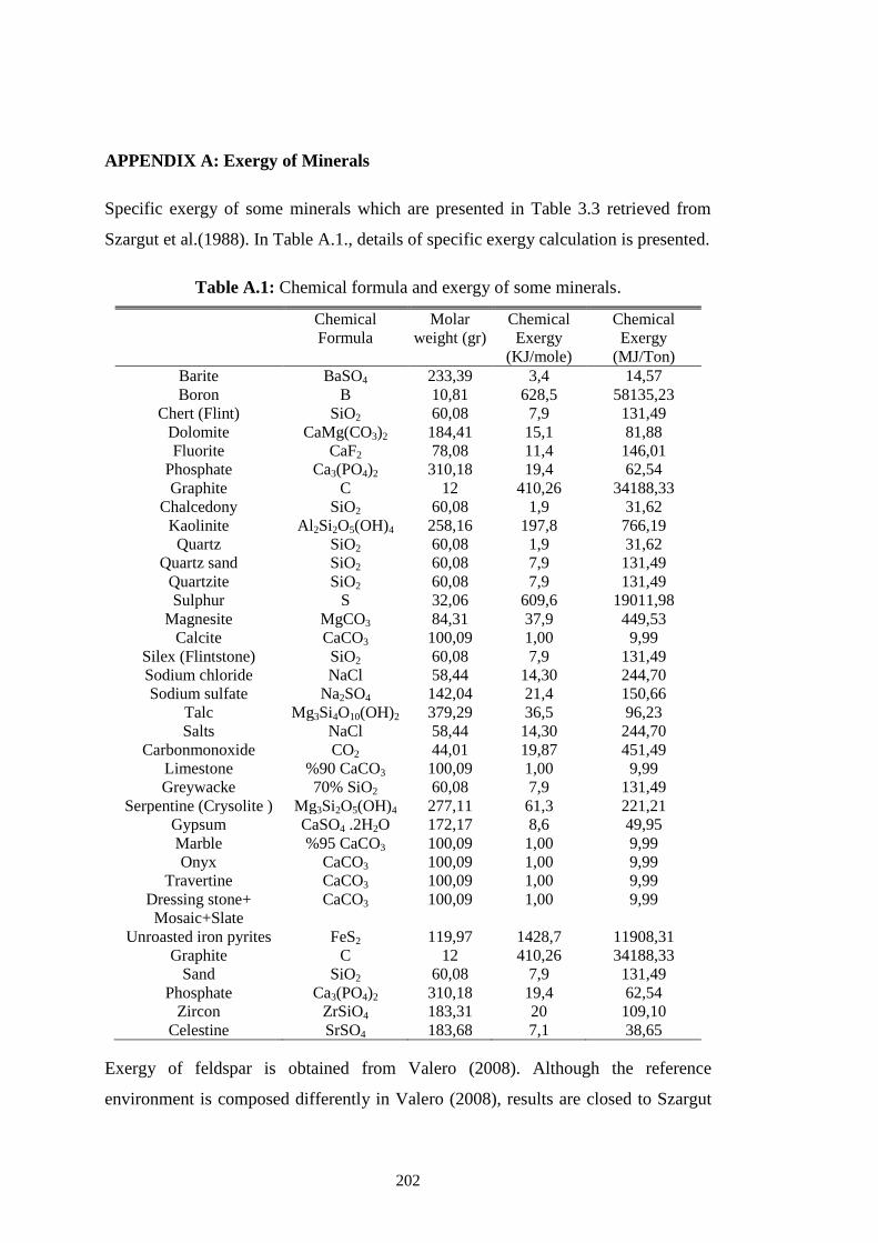
202
APPENDIX A: Exergy of Minerals
Specific exergy of some minerals which are presented in Table 3.3 retrieved from
Szargut et al.(1988). In Table A.1., details of specific exergy calculation is presented.
Table A.1: Chemical formula and exergy of some minerals.
Chemical
Formula
Molar
weight (gr)
Chemical
Exergy
(KJ/mole)
Chemical
Exergy
(MJ/Ton)
Barite BaSO4 233,39 3,4 14,57
Boron B 10,81 628,5 58135,23
Chert (Flint) SiO2 60,08 7,9 131,49
Dolomite CaMg(CO3)2 184,41 15,1 81,88
Fluorite CaF2 78,08 11,4 146,01
Phosphate Ca3(PO4)2 310,18 19,4 62,54
Graphite C 12 410,26 34188,33
Chalcedony SiO2 60,08 1,9 31,62
Kaolinite Al2Si2O5(OH)4 258,16 197,8 766,19
Quartz SiO2 60,08 1,9 31,62
Quartz sand SiO2 60,08 7,9 131,49
Quartzite SiO2 60,08 7,9 131,49
Sulphur S 32,06 609,6 19011,98
Magnesite MgCO3 84,31 37,9 449,53
Calcite CaCO3 100,09 1,00 9,99
Silex (Flintstone) SiO2 60,08 7,9 131,49
Sodium chloride NaCl 58,44 14,30 244,70
Sodium sulfate Na2SO4 142,04 21,4 150,66
Talc Mg3Si4O10(OH)2 379,29 36,5 96,23
Salts NaCl 58,44 14,30 244,70
Carbonmonoxide CO2 44,01 19,87 451,49
Limestone %90 CaCO3 100,09 1,00 9,99
Greywacke 70% SiO2 60,08 7,9 131,49
Serpentine (Crysolite ) Mg3Si2O5(OH)4 277,11 61,3 221,21
Gypsum CaSO4 .2H2O 172,17 8,6 49,95
Marble %95 CaCO3 100,09 1,00 9,99
Onyx CaCO3 100,09 1,00 9,99
Travertine CaCO3 100,09 1,00 9,99
Dressing stone+
Mosaic+Slate
CaCO3 100,09 1,00 9,99
Unroasted iron pyrites FeS2 119,97 1428,7 11908,31
Graphite C 12 410,26 34188,33
Sand SiO2 60,08 7,9 131,49
Phosphate Ca3(PO4)2 310,18 19,4 62,54
Zircon ZrSiO4 183,31 20 109,10
Celestine SrSO4 183,68 7,1 38,65
Exergy of feldspar is obtained from Valero (2008). Although the reference
environment is composed differently in Valero (2008), results are closed to Szargut
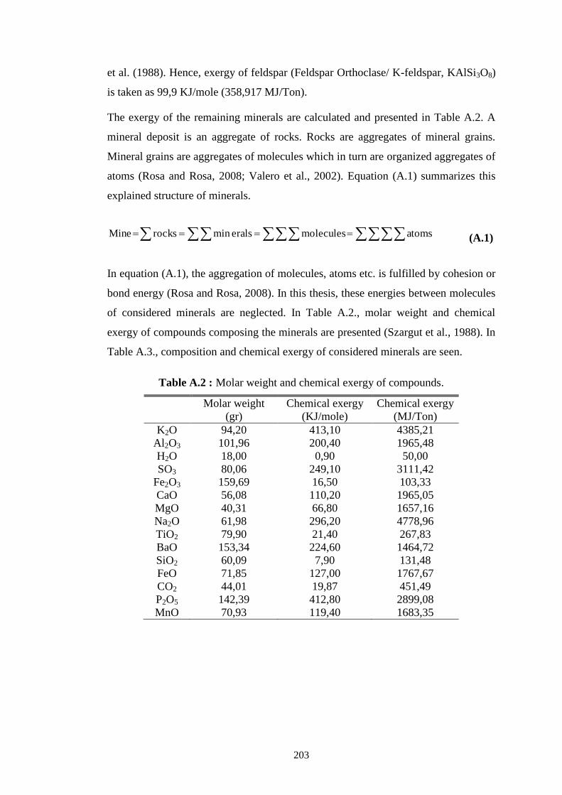
203
et al. (1988). Hence, exergy of feldspar (Feldspar Orthoclase/ K-feldspar, KAlSi3O8)
is taken as 99,9 KJ/mole (358,917 MJ/Ton).
The exergy of the remaining minerals are calculated and presented in Table A.2. A
mineral deposit is an aggregate of rocks. Rocks are aggregates of mineral grains.
Mineral grains are aggregates of molecules which in turn are organized aggregates of
atoms (Rosa and Rosa, 2008; Valero et al., 2002). Equation (A.1) summarizes this
explained structure of minerals.
atomsmoleculeseralsminrocksMine (A.1)
In equation (A.1), the aggregation of molecules, atoms etc. is fulfilled by cohesion or
bond energy (Rosa and Rosa, 2008). In this thesis, these energies between molecules
of considered minerals are neglected. In Table A.2., molar weight and chemical
exergy of compounds composing the minerals are presented (Szargut et al., 1988). In
Table A.3., composition and chemical exergy of considered minerals are seen.
Table A.2 : Molar weight and chemical exergy of compounds.
Molar weight
(gr)
Chemical exergy
(KJ/mole)
Chemical exergy
(MJ/Ton)
K2O 94,20 413,10 4385,21
Al2O3 101,96 200,40 1965,48
H2O 18,00 0,90 50,00
SO3 80,06 249,10 3111,42
Fe2O3 159,69 16,50 103,33
CaO 56,08 110,20 1965,05
MgO 40,31 66,80 1657,16
Na2O 61,98 296,20 4778,96
TiO2 79,90 21,40 267,83
BaO 153,34 224,60 1464,72
SiO2 60,09 7,90 131,48
FeO 71,85 127,00 1767,67
CO2 44,01 19,87 451,49
P2O5 142,39 412,80 2899,08
MnO 70,93 119,40 1683,35
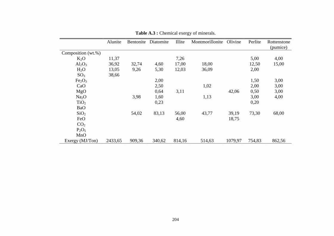
204
Table A.3 : Chemical exergy of minerals.
Alunite
Bentonite Diatomite
Illite Montmorillonite
Olivine
Perlite Rottenstone
(pumice)
Composition (wt.%)
K2O 11,37 7,26 5,00 4,00
Al2O3 36,92 32,74 4,60 17,00 18,00 12,50 15,00
H2O 13,05 9,26 5,30 12,03 36,09 2,00
SO3 38,66
Fe2O3 2,00 1,50 3,00
CaO 2,50 1,02 2,00 3,00
MgO 0,64 3,11 42,06 0,50 3,00
Na2O 3,98 1,60 1,13 3,00 4,00
TiO2 0,23 0,20
BaO
SiO2 54,02 83,13 56,00 43,77 39,19 73,30 68,00
FeO 4,60 18,75
CO2
P2O5
MnO
Exergy (MJ/Ton) 2433,65 909,36 340,62 814,16 514,63 1079,97 754,83 862,56

205
Table A.3 (continued) : Chemical exergy of minerals.
Sepiolite
Trona Grindstone
Clay
Pyrophyllite
Trass
Diabase
Ignimbrite
Andesite
Composition (wt.%)
K2O 0,08 2,44 4,81
Al2O3 65,00 2,50 28,30 12,35 15,20 15,33 18,10
H2O 17,00 19,93 2,00 5,00
SO3
Fe2O3 32,00 31,60 1,40 4,90 7,10
CaO 2,42 11,50 2,00 11,60
MgO 26,27 27,20 0,45 0,53 4,00
Na2O 41,13 2,14 4,13 1,70 5,46
TiO2 1,00 0,42 0,70
BaO
SiO2 56,73 1,00 35,50 66,70 76,82 71,60 66,55 58,50
FeO
CO2 38,94
P2O5
MnO
Exergy (MJ/Ton) 521,19 439,90 1312,94 697,99 646,43 687,03 674,21 914,73 601,79
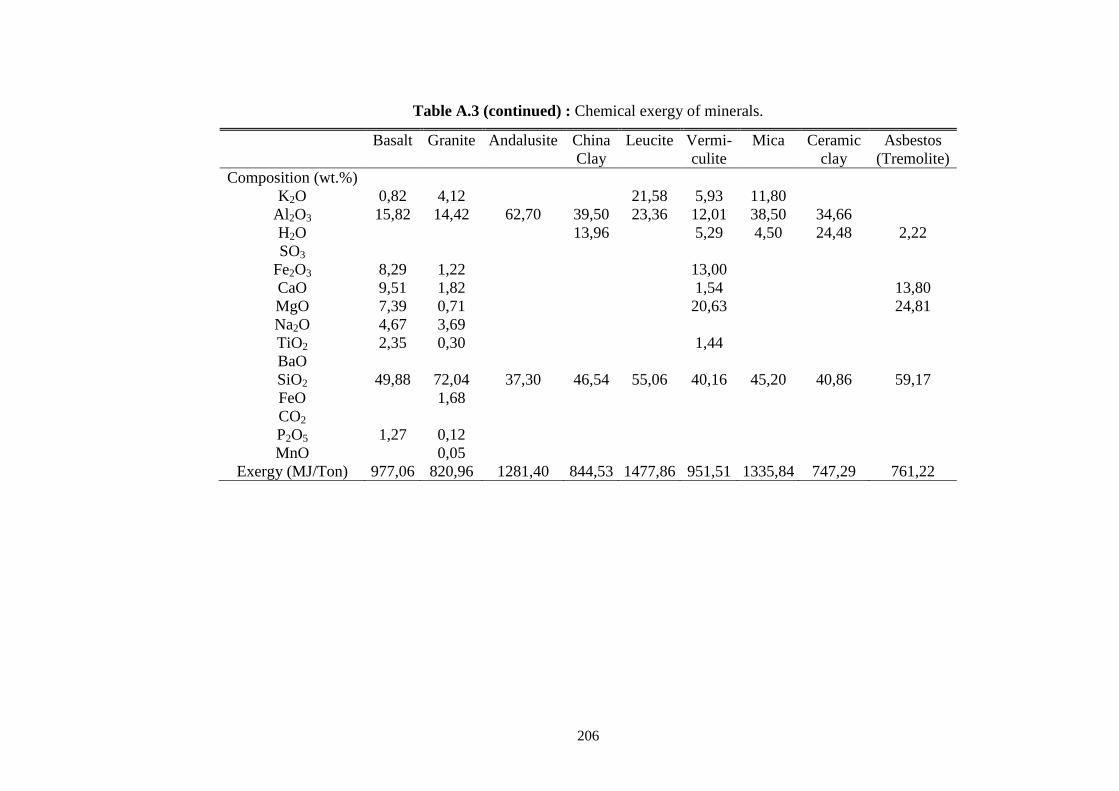
206
Table A.3 (continued) : Chemical exergy of minerals.
Basalt
Granite
Andalusite
China
Clay
Leucite Vermi-
culite
Mica
Ceramic
clay
Asbestos
(Tremolite)
Composition (wt.%)
K2O 0,82 4,12 21,58 5,93 11,80
Al2O3 15,82 14,42 62,70 39,50 23,36 12,01 38,50 34,66
H2O 13,96 5,29 4,50 24,48 2,22
SO3
Fe2O3 8,29 1,22 13,00
CaO 9,51 1,82 1,54 13,80
MgO 7,39 0,71 20,63 24,81
Na2O 4,67 3,69
TiO2 2,35 0,30 1,44
BaO
SiO2 49,88 72,04 37,30 46,54 55,06 40,16 45,20 40,86 59,17
FeO 1,68
CO2
P2O5 1,27 0,12
MnO 0,05
Exergy (MJ/Ton) 977,06 820,96 1281,40 844,53 1477,86 951,51 1335,84 747,29 761,22
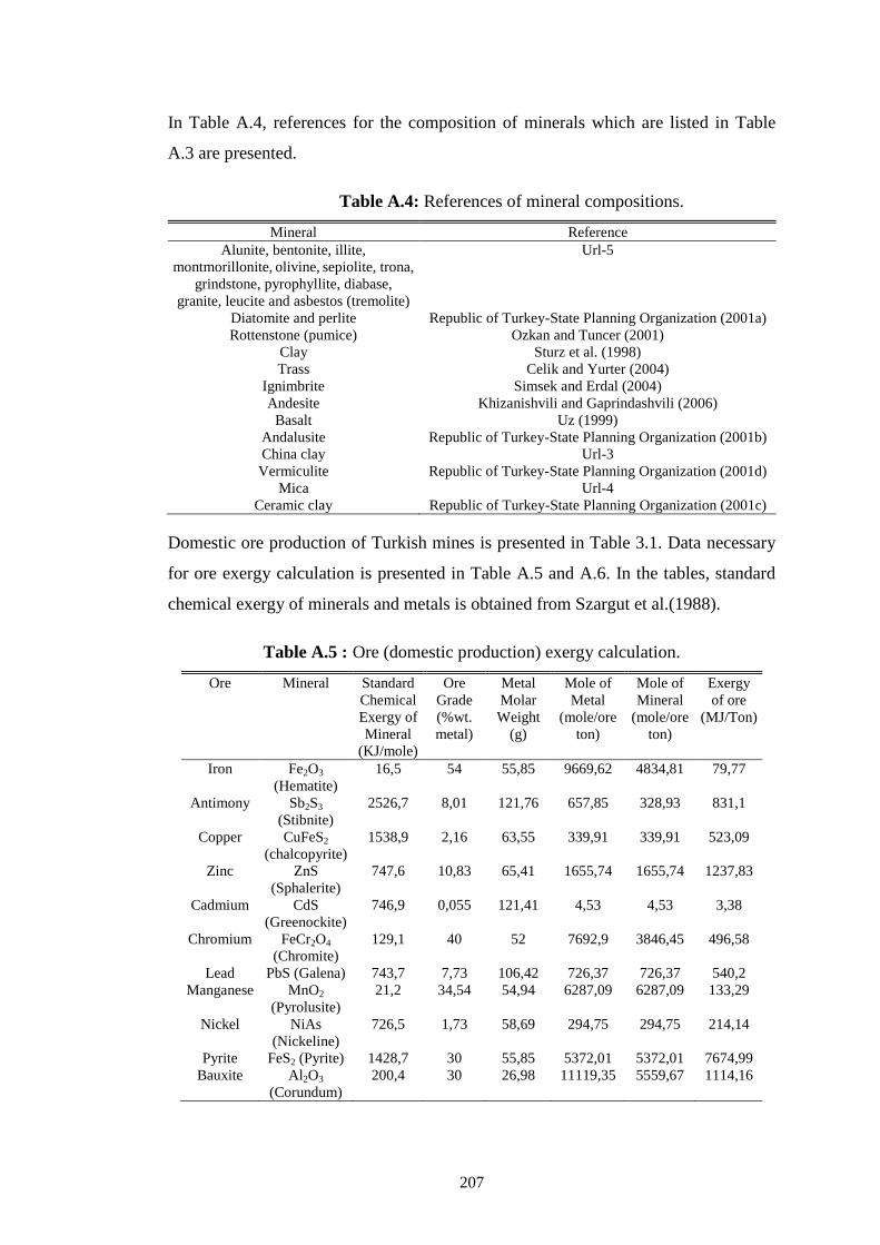
207
In Table A.4, references for the composition of minerals which are listed in Table
A.3 are presented.
Table A.4: References of mineral compositions.
Mineral Reference
Alunite, bentonite, illite,
montmorillonite, olivine,
sepiolite, trona,
grindstone, pyrophyllite, diabase,
granite, leucite and asbestos (tremolite)
Url-5
Diatomite and perlite Republic of Turkey-State Planning Organization (2001a)
Rottenstone (pumice) Ozkan and Tuncer (2001)
Clay Sturz et al. (1998)
Trass Celik and Yurter (2004)
Ignimbrite Simsek and Erdal (2004)
Andesite Khizanishvili and Gaprindashvili (2006)
Basalt Uz (1999)
Andalusite Republic of Turkey-State Planning Organization (2001b)
China clay Url-3
Vermiculite Republic of Turkey-State Planning Organization (2001d)
Mica Url-4
Ceramic clay Republic of Turkey-State Planning Organization (2001c)
Domestic ore production of Turkish mines is presented in Table 3.1. Data necessary
for ore exergy calculation is presented in Table A.5 and A.6. In the tables, standard
chemical exergy of minerals and metals is obtained from Szargut et al.(1988).
Table A.5 : Ore (domestic production) exergy calculation.
Ore Mineral Standard
Chemical
Exergy of
Mineral
(KJ/mole)
Ore
Grade
(%wt.
metal)
Metal
Molar
Weight
(g)
Mole of
Metal
(mole/ore
ton)
Mole of
Mineral
(mole/ore
ton)
Exergy
of ore
(MJ/Ton)
Iron Fe2O3
(Hematite)
16,5 54 55,85 9669,62 4834,81 79,77
Antimony Sb2S3
(Stibnite)
2526,7 8,01 121,76 657,85 328,93 831,1
Copper CuFeS2
(chalcopyrite)
1538,9 2,16 63,55 339,91 339,91 523,09
Zinc ZnS
(Sphalerite)
747,6 10,83 65,41 1655,74 1655,74 1237,83
Cadmium CdS
(Greenockite)
746,9 0,055 121,41 4,53 4,53 3,38
Chromium FeCr2O4
(Chromite)
129,1 40 52 7692,9 3846,45 496,58
Lead PbS (Galena) 743,7 7,73 106,42 726,37 726,37 540,2
Manganese MnO2
(Pyrolusite)
21,2 34,54 54,94 6287,09 6287,09 133,29
Nickel NiAs
(Nickeline)
726,5 1,73 58,69 294,75 294,75 214,14
Pyrite FeS2 (Pyrite) 1428,7 30 55,85 5372,01 5372,01 7674,99
Bauxite Al2O3
(Corundum)
200,4 30 26,98 11119,35 5559,67 1114,16
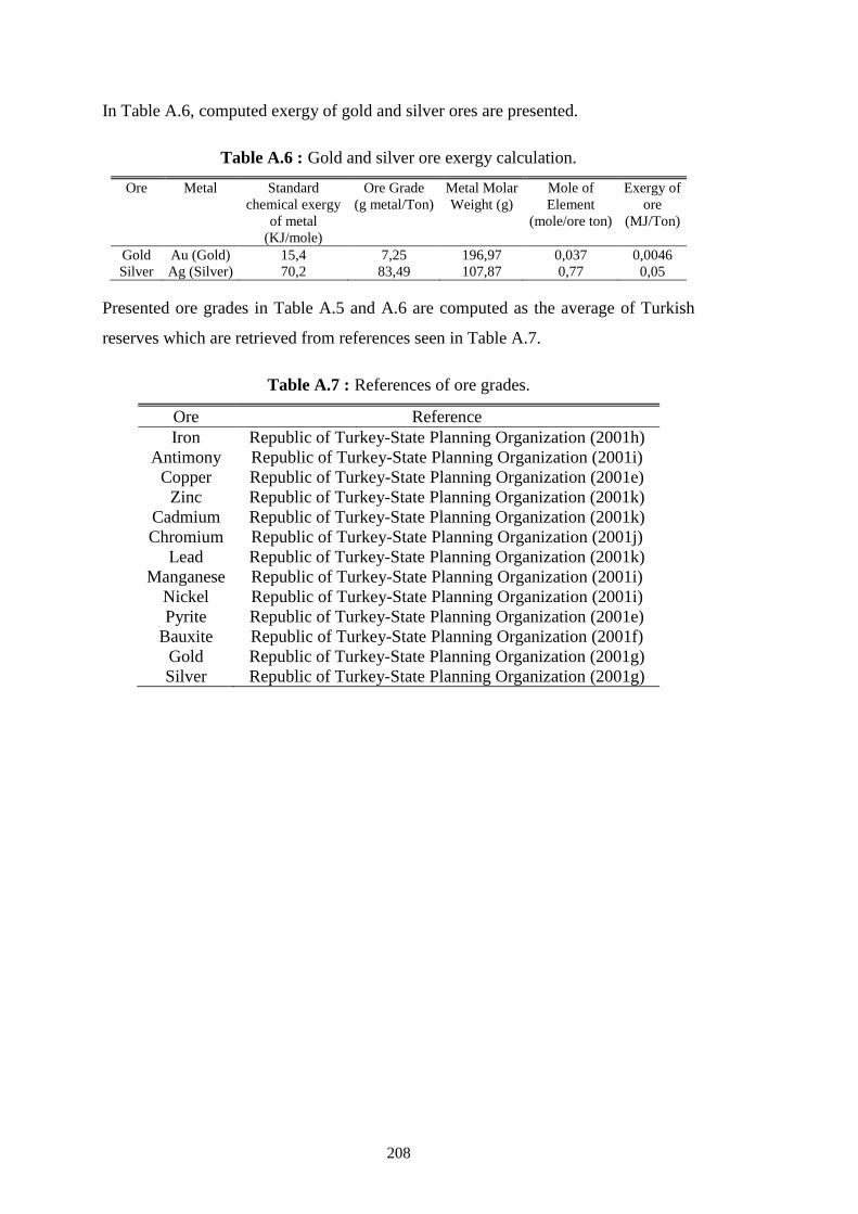
208
In Table A.6, computed exergy of gold and silver ores are presented.
Table A.6 : Gold and silver ore exergy calculation.
Ore Metal Standard
chemical exergy
of metal
(KJ/mole)
Ore Grade
(g metal/Ton)
Metal Molar
Weight (g)
Mole of
Element
(mole/ore ton)
Exergy of
ore
(MJ/Ton)
Gold Au (Gold) 15,4 7,25 196,97 0,037 0,0046
Silver Ag (Silver) 70,2 83,49 107,87 0,77 0,05
Presented ore grades in Table A.5 and A.6 are computed as the average of Turkish
reserves which are retrieved from references seen in Table A.7.
Table A.7 : References of ore grades.
Ore Reference
Iron Republic of Turkey-State Planning Organization (2001h)
Antimony Republic of Turkey-State Planning Organization (2001i)
Copper Republic of Turkey-State Planning Organization (2001e)
Zinc Republic of Turkey-State Planning Organization (2001k)
Cadmium Republic of Turkey-State Planning Organization (2001k)
Chromium Republic of Turkey-State Planning Organization (2001j)
Lead Republic of Turkey-State Planning Organization (2001k)
Manganese Republic of Turkey-State Planning Organization (2001i)
Nickel Republic of Turkey-State Planning Organization (2001i)
Pyrite Republic of Turkey-State Planning Organization (2001e)
Bauxite Republic of Turkey-State Planning Organization (2001f)
Gold Republic of Turkey-State Planning Organization (2001g)
Silver Republic of Turkey-State Planning Organization (2001g)
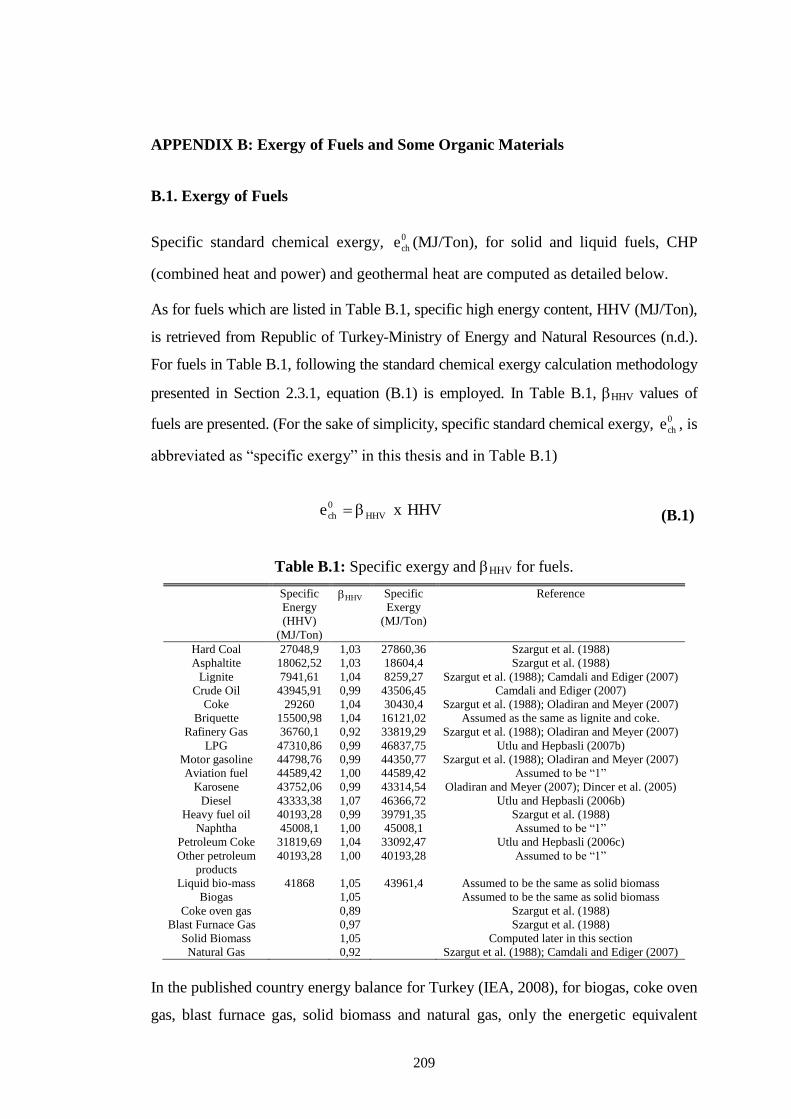
209
APPENDIX B: Exergy of Fuels and Some Organic Materials
B.1. Exergy of Fuels
Specific standard chemical exergy, 0
che (MJ/Ton), for solid and liquid fuels, CHP
(combined heat and power) and geothermal heat are computed as detailed below.
As for fuels which are listed in Table B.1, specific high energy content, HHV (MJ/Ton),
is retrieved from Republic of Turkey-Ministry of Energy and Natural Resources (n.d.).
For fuels in Table B.1, following the standard chemical exergy calculation methodology
presented in Section 2.3.1, equation (B.1) is employed. In Table B.1, HHV values of
fuels are presented. (For the sake of simplicity, specific standard chemical exergy, 0
che , is
abbreviated as “specific exergy” in this thesis and in Table B.1)
HHVxe HHV
0
ch (B.1)
Table B.1: Specific exergy and HHV for fuels.
Specific
Energy
(HHV)
(MJ/Ton)
HHV Specific
Exergy
(MJ/Ton)
Reference
Hard Coal 27048,9 1,03 27860,36 Szargut et al. (1988)
Asphaltite 18062,52 1,03 18604,4 Szargut et al. (1988)
Lignite 7941,61 1,04 8259,27 Szargut et al. (1988); Camdali and Ediger (2007)
Crude Oil 43945,91 0,99 43506,45 Camdali and Ediger (2007)
Coke 29260 1,04 30430,4 Szargut et al. (1988); Oladiran and Meyer (2007)
Briquette 15500,98 1,04 16121,02 Assumed as the same as lignite and coke.
Rafinery Gas 36760,1 0,92 33819,29 Szargut et al. (1988); Oladiran and Meyer (2007)
LPG 47310,86 0,99 46837,75 Utlu and Hepbasli (2007b)
Motor gasoline 44798,76 0,99 44350,77 Szargut et al. (1988); Oladiran and Meyer (2007)
Aviation fuel 44589,42 1,00 44589,42 Assumed to be “1”
Karosene 43752,06 0,99 43314,54 Oladiran and Meyer (2007); Dincer et al. (2005)
Diesel 43333,38 1,07 46366,72 Utlu and Hepbasli (2006b)
Heavy fuel oil 40193,28 0,99 39791,35 Szargut et al. (1988)
Naphtha 45008,1 1,00 45008,1 Assumed to be “1”
Petroleum Coke 31819,69 1,04 33092,47 Utlu and Hepbasli (2006c)
Other petroleum
products
40193,28 1,00 40193,28 Assumed to be “1”
Liquid bio-mass 41868 1,05 43961,4 Assumed to be the same as solid biomass
Biogas 1,05 Assumed to be the same as solid biomass
Coke oven gas 0,89 Szargut et al. (1988)
Blast Furnace Gas 0,97 Szargut et al. (1988)
Solid Biomass 1,05 Computed later in this section
Natural Gas 0,92 Szargut et al. (1988); Camdali and Ediger (2007)
In the published country energy balance for Turkey (IEA, 2008), for biogas, coke oven
gas, blast furnace gas, solid biomass and natural gas, only the energetic equivalent

210
(HHV) of production and consumption is available. Hence, HHV is used to obtain the
exergetic equivalent. This is because, only HHV is presented in Table B.1.
B.2. Exergy of Agricultural Waste
Exergy of agricultural waste and wood (together consisting of solid biomass) is
calculated on the basis of equation (2.10) and (2.11), respectively.
For agricultural waste, an approximate composition (as received) is obtained form
Bilgen et al. (2004) and presented in Table B.2.
Table B.2 : Ultimate analysis of agricultural waste and wood (ar).
Agricultural waste (wt.% ar) Wood (wt.% ar)
C 48,3 52,1
H 5,7 6,1
O 45,3 41
N 0,7 0,2
HHV of the waste is calculated by the empiric equation proposed by Bilgen et al.
(2004) for biomass samples (equation (B.2)).
2
ar 10x)N(5,14)O(4,15)H(3,142)C(5,33)kg/MJ(HHV (B.2)
where HHVar is HHV of as received (wet basis) sample, C is weight percent of
carbon, H is weight percent of hydrogen, O is weight percent of oxygen, N is weight
percent of nitrogen in the considered sample.
fgHfg
fu
O2Harar hX94,8HHVh
m
mHHVLHV (B.3)
where LHVar is LHV of as received (wet basis) sample, mH2O(kg) is the mass of H2O
produced by combustion of the sample, mfu(kg) is the mass of the sample, XH is the
mass friction of hydrogen in the sample, hfg (MJ/kg).is the enthalpy of the
evaporation of water (at standard environmental conditions); the numerical value
(8,94 XH) is equal to the ratio of fu
O2H
m
m. At the standard environmental conditions
(25°C and 1 atm) hfg is the 2,4423 MJ/kg (Ertesvag, 2000).
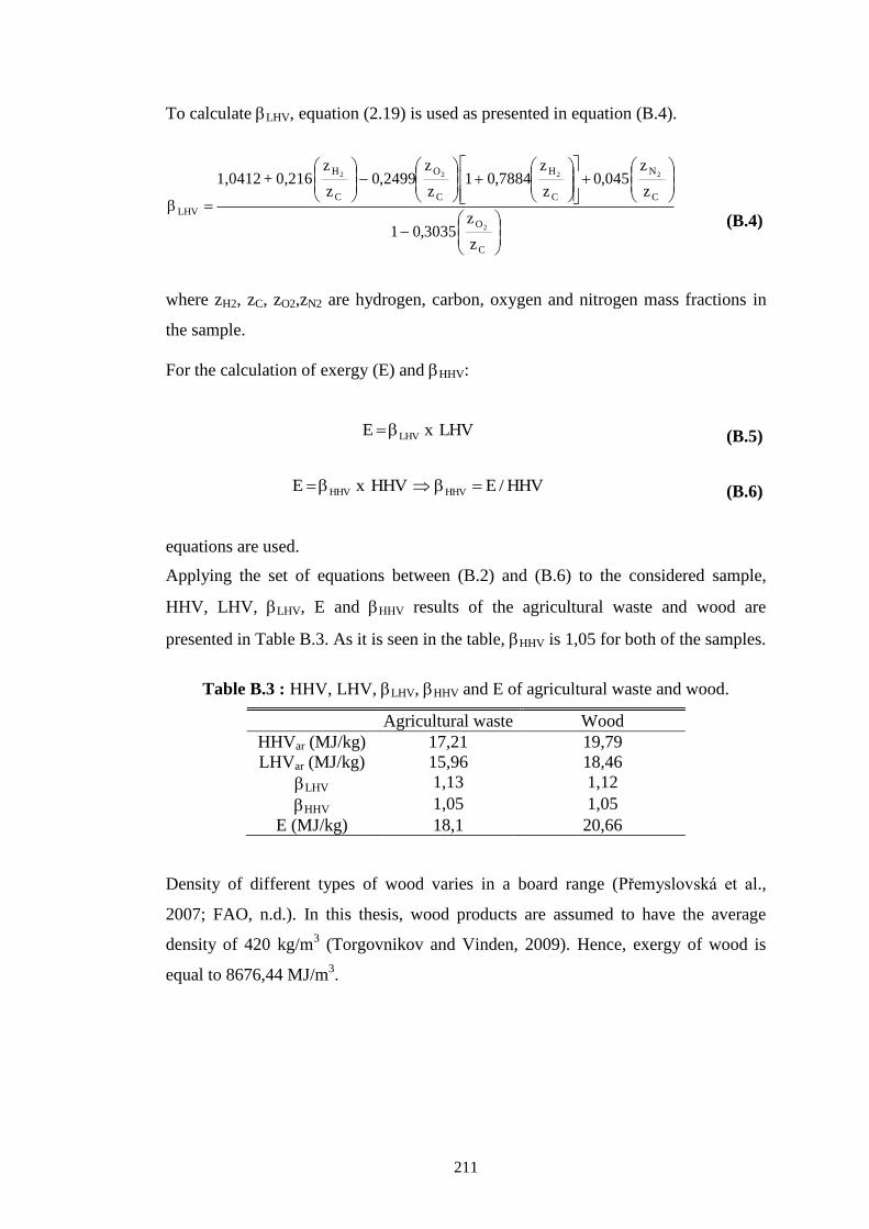
211
To calculate LHV, equation (2.19) is used as presented in equation (B.4).
C
O
C
N
C
H
C
O
C
H
LHV
z
z3035,01
z
z045,0
z
z7884,01
z
z2499,0
z
z0,216+1,0412
2
2222
(B.4)
where zH2, zC, zO2,zN2 are hydrogen, carbon, oxygen and nitrogen mass fractions in
the sample.
For the calculation of exergy (E) and HHV:
LHVxE LHV (B.5)
HHV/EHHVxE HHVHHV (B.6)
equations are used.
Applying the set of equations between (B.2) and (B.6) to the considered sample,
HHV, LHV, LHV, E and HHV results of the agricultural waste and wood are
presented in Table B.3. As it is seen in the table, HHV is 1,05 for both of the samples.
Table B.3 : HHV, LHV, LHV, HHV and E of agricultural waste and wood.
Agricultural waste Wood
HHVar (MJ/kg) 17,21 19,79
LHVar (MJ/kg) 15,96 18,46
LHV 1,13 1,12
HHV 1,05 1,05
E (MJ/kg) 18,1 20,66
Density of different types of wood varies in a board range (Přemyslovská et al.,
2007; FAO, n.d.). In this thesis, wood products are assumed to have the average
density of 420 kg/m3 (Torgovnikov and Vinden, 2009). Hence, exergy of wood is
equal to 8676,44 MJ/m3.
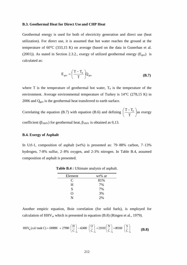
212
B.3. Geothermal Heat for Direct Use and CHP Heat
Geothermal energy is used for both of electricity generation and direct use (heat
utilization). For direct use, it is assumed that hot water reaches the ground at the
temperature of 60°C (333,15 K) on average (based on the data in Gunerhan et al.
(2001)). As stated in Section 2.3.2., exergy of utilized geothermal energy (Egeo) is
calculated as:
geo0
geo QT
TTE
(B.7)
where T is the temperature of geothermal hot water, T0 is the temperature of the
environment. Average environmental temperature of Turkey is 14°C (278,15 K) in
2006 and Qgeo is the geothermal heat transferred to earth surface.
Correlating the equation (B.7) with equation (B.6) and defining
T
TT 0 as exergy
coefficient (HHV) for geothermal heat, HHVis obtained as 0,13.
B.4. Exergy of Asphalt
In Url-1, composition of asphalt (wt%) is presented as: 79–88% carbon, 7–13%
hydrogen, 7-8% sulfur, 2–8% oxygen, and 2-3% nitrogen. In Table B.4, assumed
composition of asphalt is presented.
Table B.4 : Ultimate analysis of asphalt.
Another empiric equation, Boie correlation (for solid fuels), is employed for
calculation of HHVar which is presented in equation (B.8) (Ringen et al., 1979).
aaaa
arC
S80160
C
N21010
C
O42400
C
H27990100890)Cmole/cal(HHV
(B.8)
Element wt% ar
C 81%
H 7%
S 7%
O 3%
N 2%
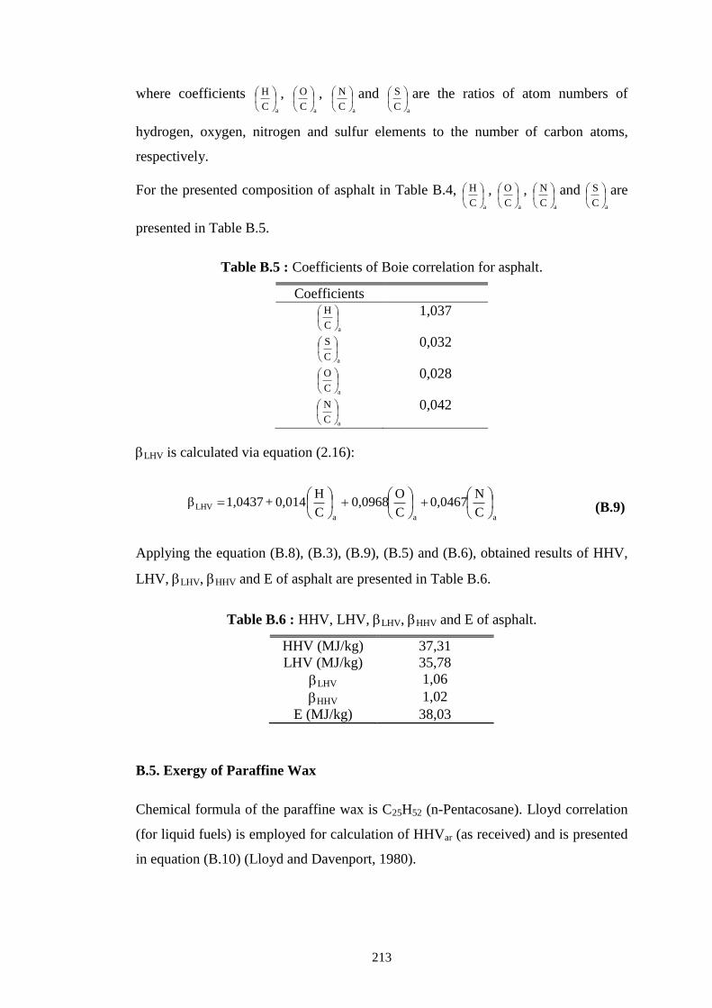
213
where coefficients aC
H
, aC
O
, aC
N
and
aC
S
are the ratios of atom numbers of
hydrogen, oxygen, nitrogen and sulfur elements to the number of carbon atoms,
respectively.
For the presented composition of asphalt in Table B.4, aC
H
, aC
O
, aC
N
and
aC
S
are
presented in Table B.5.
Table B.5 : Coefficients of Boie correlation for asphalt.
Coefficients
aC
H
1,037
aC
S
0,032
aC
O
0,028
aC
N
0,042
LHV is calculated via equation (2.16):
aaa
LHVC
N0,0467
C
O0,0968
C
H0,014+1,0437β
(B.9)
Applying the equation (B.8), (B.3), (B.9), (B.5) and (B.6), obtained results of HHV,
LHV, LHV, HHV and E of asphalt are presented in Table B.6.
Table B.6 : HHV, LHV, LHV, HHV and E of asphalt.
HHV (MJ/kg) 37,31
LHV (MJ/kg) 35,78
LHV 1,06
HHV 1,02
E (MJ/kg) 38,03
B.5. Exergy of Paraffine Wax
Chemical formula of the paraffine wax is C25H52 (n-Pentacosane). Lloyd correlation
(for liquid fuels) is employed for calculation of HHVar (as received) and is presented
in equation (B.10) (Lloyd and Davenport, 1980).
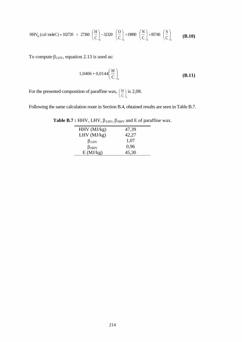
214
aaaa
arC
S85740
C
N19890
C
O32320
C
H27360102720)moleC/cal(HHV
(B.10)
To compute LHV, equation 2.13 is used as:
aC
H0,0144+1,0406
(B.11)
For the presented composition of paraffine wax, aC
H
is 2,08.
Following the same calculation route in Section B.4, obtained results are seen in Table B.7.
Table B.7 : HHV, LHV, LHV, HHV and E of paraffine wax.
HHV (MJ/kg) 47,39
LHV (MJ/kg) 42,27
LHV 1,07
HHV 0,96
E (MJ/kg) 45,30

215
APPENDIX C: Exergy of Agricultural and Industrial Products
C.1. Exergy of Agricultural Products
Exergetic content of the agricultural products are inserted into Table 4.4, Table 4.10
and Table 4.12 by means of exergy data available in the literature. Exergy of the
products and the respective source of data are presented in Table C.1.
Table C.1: Exergy of AG sector products.
Specific
Exergy
(MJ/Ton)
Reference
Fruit 1900 Chen and Chen,2009; Chen and Chen,2006; Ertesvag
and Mielnik,2000
Cereals
Barley 14800 Ertesvag and Mielnik,2000
Wheat 17400 Wall et al.,1994
Maize 16400 Wall et al.,1994
Rice 15200 Chen and Chen,2009; Chen and Chen,2006; Wall et
al.,1994
Leguminous seeds 16900 Wall et al.,1994
Vegetables 1900 Chen and Chen,2009; Chen and Chen,2006; Ertesvag
and Mielnik,2000; Wall et al., 1994
Meat 10000 Chen and Chen,2009; Chen and Chen,2006; Wall et
al.,1994
Poultry 4500 Chen and Chen,2009; Chen and Chen,2006
Fish products 5750 Chen and Chen,2009; Chen and Chen,2006; Ertesvag
and Mielnik,2000
Milk 4900 Chen and Chen,2009; Chen and Chen,2006; Ertesvag
and Mielnik,2000
Egg 7000 Ertesvag and Mielnik,2000; Wall et al.,1994
Honey 15200 Ertesvag and Mielnik,2000
Bee wax 15200 Ertesvag and Mielnik,2000
Others
Olive 19000 Wall et al.,1994
Tobacco 10700 Chen and Chen,2009; Chen and Chen,2006
Sunflower 19000 Wall et al.,1994
Rape 37000 Chen and Chen,2009; Chen and Chen,2006
Cotton 16700 Chen and Chen,2009; Chen and Chen,2006
Soybean 16600 Wall et al.,1994
Sugar beet 4200 Chen and Chen,2009; Chen and Chen,2006; Wall et
al.,1994
Tea 10700 Ertesvag and Mielnik,2000
Potato 4200 Chen and Chen,2009; Chen and Chen,2006; Wall et
al.,1994
As for AG sector products seen in Table 4.6, exergy of puppy, lupin and hop is
assumed to be equal to the exergy of hay (15300 MJ/Ton) which is available in the
studies of Ertesvag and Mielnik (2000) and Wall et al. (1994). Products which are
used for fodder industry (cow vetches, sainfoin, wild vetches, fodder beet, clover,
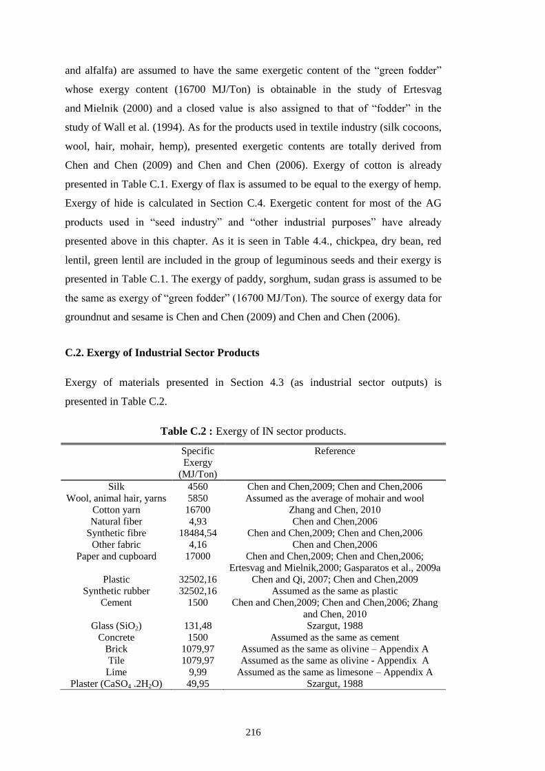
216
and alfalfa) are assumed to have the same exergetic content of the “green fodder”
whose exergy content (16700 MJ/Ton) is obtainable in the study of Ertesvag
and Mielnik (2000) and a closed value is also assigned to that of “fodder” in the
study of Wall et al. (1994). As for the products used in textile industry (silk cocoons,
wool, hair, mohair, hemp), presented exergetic contents are totally derived from
Chen and Chen (2009) and Chen and Chen (2006). Exergy of cotton is already
presented in Table C.1. Exergy of flax is assumed to be equal to the exergy of hemp.
Exergy of hide is calculated in Section C.4. Exergetic content for most of the AG
products used in “seed industry” and “other industrial purposes” have already
presented above in this chapter. As it is seen in Table 4.4., chickpea, dry bean, red
lentil, green lentil are included in the group of leguminous seeds and their exergy is
presented in Table C.1. The exergy of paddy, sorghum, sudan grass is assumed to be
the same as exergy of “green fodder” (16700 MJ/Ton). The source of exergy data for
groundnut and sesame is Chen and Chen (2009) and Chen and Chen (2006).
C.2. Exergy of Industrial Sector Products
Exergy of materials presented in Section 4.3 (as industrial sector outputs) is
presented in Table C.2.
Table C.2 : Exergy of IN sector products.
Specific
Exergy
(MJ/Ton)
Reference
Silk 4560 Chen and Chen,2009; Chen and Chen,2006
Wool, animal hair, yarns 5850 Assumed as the average of mohair and wool
Cotton yarn 16700 Zhang and Chen, 2010
Natural fiber 4,93 Chen and Chen,2006
Synthetic fibre 18484,54 Chen and Chen,2009; Chen and Chen,2006
Other fabric 4,16 Chen and Chen,2006
Paper and cupboard 17000 Chen and Chen,2009; Chen and Chen,2006;
Ertesvag and Mielnik,2000; Gasparatos et al., 2009a
Plastic 32502,16 Chen and Qi, 2007; Chen and Chen,2009
Synthetic rubber 32502,16 Assumed as the same as plastic
Cement 1500 Chen and Chen,2009; Chen and Chen,2006; Zhang
and Chen, 2010
Glass (SiO2) 131,48 Szargut, 1988
Concrete 1500 Assumed as the same as cement
Brick 1079,97 Assumed as the same as olivine – Appendix A
Tile 1079,97 Assumed as the same as olivine - Appendix A
Lime 9,99 Assumed as the same as limesone – Appendix A
Plaster (CaSO4 .2H2O) 49,95 Szargut, 1988
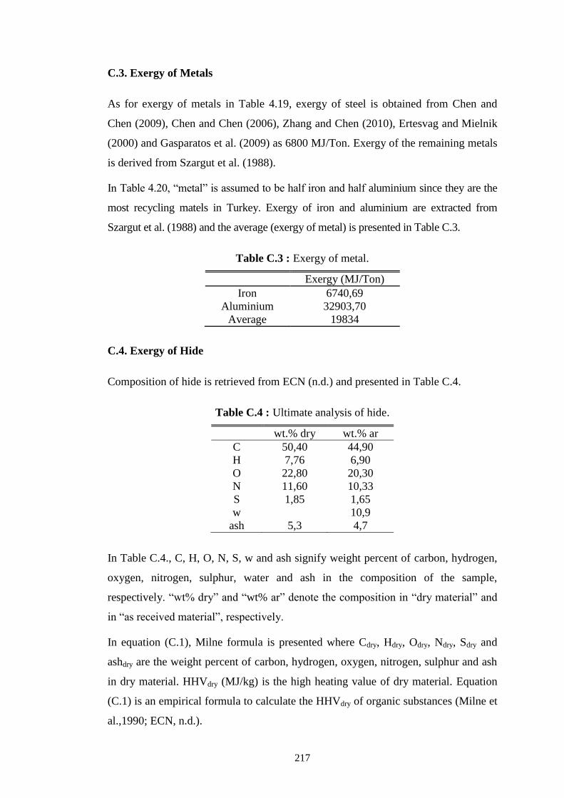
217
C.3. Exergy of Metals
As for exergy of metals in Table 4.19, exergy of steel is obtained from Chen and
Chen (2009), Chen and Chen (2006), Zhang and Chen (2010), Ertesvag and Mielnik
(2000) and Gasparatos et al. (2009) as 6800 MJ/Ton. Exergy of the remaining metals
is derived from Szargut et al. (1988).
In Table 4.20, “metal” is assumed to be half iron and half aluminium since they are the
most recycling matels in Turkey. Exergy of iron and aluminium are extracted from
Szargut et al. (1988) and the average (exergy of metal) is presented in Table C.3.
Table C.3 : Exergy of metal.
Exergy (MJ/Ton)
Iron 6740,69
Aluminium 32903,70
Average 19834
C.4. Exergy of Hide
Composition of hide is retrieved from ECN (n.d.) and presented in Table C.4.
Table C.4 : Ultimate analysis of hide.
wt.% dry wt.% ar
C 50,40 44,90
H 7,76 6,90
O 22,80 20,30
N 11,60 10,33
S 1,85 1,65
w 10,9
ash 5,3 4,7
In Table C.4., C, H, O, N, S, w and ash signify weight percent of carbon, hydrogen,
oxygen, nitrogen, sulphur, water and ash in the composition of the sample,
respectively. “wt% dry” and “wt% ar” denote the composition in “dry material” and
in “as received material”, respectively.
In equation (C.1), Milne formula is presented where Cdry, Hdry, Odry, Ndry, Sdry and
ashdry are the weight percent of carbon, hydrogen, oxygen, nitrogen, sulphur and ash
in dry material. HHVdry (MJ/kg) is the high heating value of dry material. Equation
(C.1) is an empirical formula to calculate the HHVdry of organic substances (Milne et
al.,1990; ECN, n.d.).
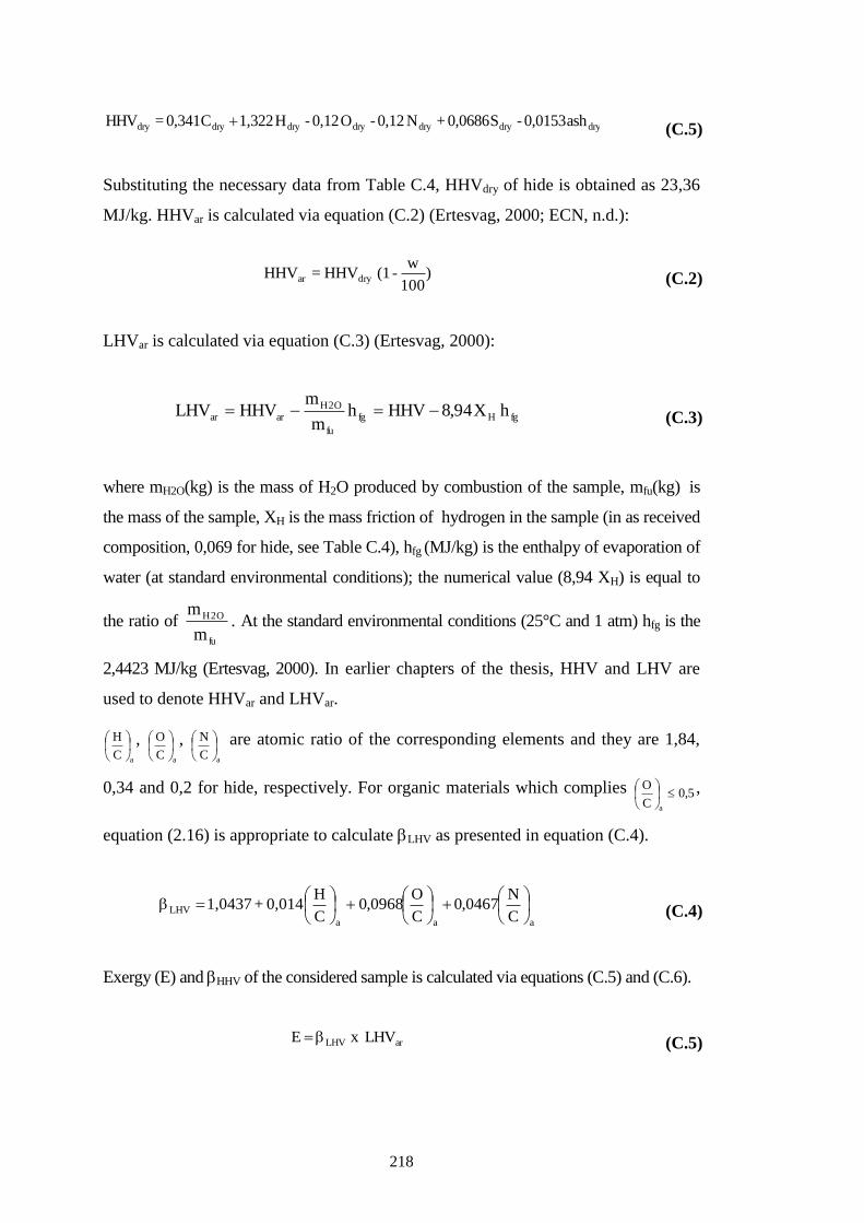
218
drydrydrydrydrydrydry ash 0,0153 - S 0,0686 + N 0,12 - O 0,12 - H 1,322 C 0,341 = HHV
(C.5)
Substituting the necessary data from Table C.4, HHVdry of hide is obtained as 23,36
MJ/kg. HHVar is calculated via equation (C.2) (Ertesvag, 2000; ECN, n.d.):
)100
w-(1 HHV = HHV dryar (C.2)
LHVar is calculated via equation (C.3) (Ertesvag, 2000):
fgHfg
fu
O2Harar hX94,8HHVh
m
mHHVLHV (C.3)
where mH2O(kg) is the mass of H2O produced by combustion of the sample, mfu(kg) is
the mass of the sample, XH is the mass friction of hydrogen in the sample (in as received
composition, 0,069 for hide, see Table C.4), hfg (MJ/kg) is the enthalpy of evaporation of
water (at standard environmental conditions); the numerical value (8,94 XH) is equal to
the ratio of fu
O2H
m
m. At the standard environmental conditions (25°C and 1 atm) hfg is the
2,4423 MJ/kg (Ertesvag, 2000). In earlier chapters of the thesis, HHV and LHV are
used to denote HHVar and LHVar.
aC
H
, aC
O
, aC
N
are atomic ratio of the corresponding elements and they are 1,84,
0,34 and 0,2 for hide, respectively. For organic materials which complies 5,0C
O
a
,
equation (2.16) is appropriate to calculate LHV as presented in equation (C.4).
aaa
LHVC
N0467,0
C
O0968,0
C
H0,014+1,0437
(C.4)
Exergy (E) and HHV of the considered sample is calculated via equations (C.5) and (C.6).
arLHV LHVxE (C.5)
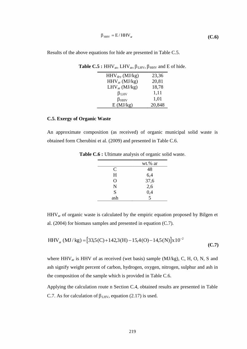
219
arHHV HHV/E (C.6)
Results of the above equations for hide are presented in Table C.5.
Table C.5 : HHVar, LHVar, LHV, HHV and E of hide.
HHVdry (MJ/kg) 23,36
HHVar (MJ/kg) 20,81
LHVar (MJ/kg) 18,78
LHV 1,11
HHV 1,01
E (MJ/kg) 20,848
C.5. Exergy of Organic Waste
An approximate composition (as received) of organic municipal solid waste is
obtained form Cherubini et al. (2009) and presented in Table C.6.
Table C.6 : Ultimate analysis of organic solid waste.
wt.% ar
C 48
H 6,4
O 37,6
N 2,6
S 0,4
ash 5
HHVar of organic waste is calculated by the empiric equation proposed by Bilgen et
al. (2004) for biomass samples and presented in equation (C.7).
2
ar 10x)N(5,14)O(4,15)H(3,142)C(5,33)kg/MJ(HHV
(C.7)
where HHVar is HHV of as received (wet basis) sample (MJ/kg), C, H, O, N, S and
ash signify weight percent of carbon, hydrogen, oxygen, nitrogen, sulphur and ash in
the composition of the sample which is provided in Table C.6.
Applying the calculation route n Section C.4, obtained results are presented in Table
C.7. As for calculation of LHV, equation (2.17) is used.
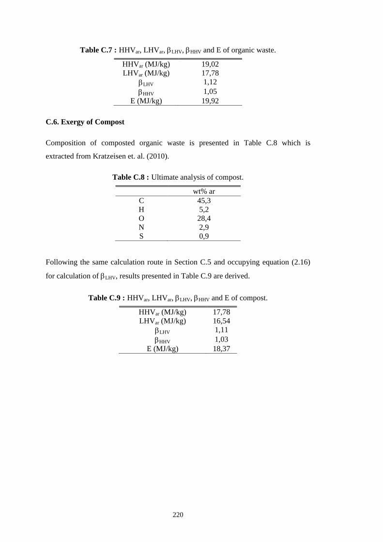
220
Table C.7 : HHVar, LHVar, LHV, HHV and E of organic waste.
HHVar (MJ/kg) 19,02
LHVar (MJ/kg) 17,78
LHV 1,12
HHV 1,05
E (MJ/kg) 19,92
C.6. Exergy of Compost
Composition of composted organic waste is presented in Table C.8 which is
extracted from Kratzeisen et. al. (2010).
Table C.8 : Ultimate analysis of compost.
wt% ar
C 45,3
H 5,2
O 28,4
N 2,9
S 0,9
Following the same calculation route in Section C.5 and occupying equation (2.16)
for calculation of LHV, results presented in Table C.9 are derived.
Table C.9 : HHVar, LHVar, LHV, HHV and E of compost.
HHVar (MJ/kg) 17,78
LHVar (MJ/kg) 16,54
LHV 1,11
HHV 1,03
E (MJ/kg) 18,37
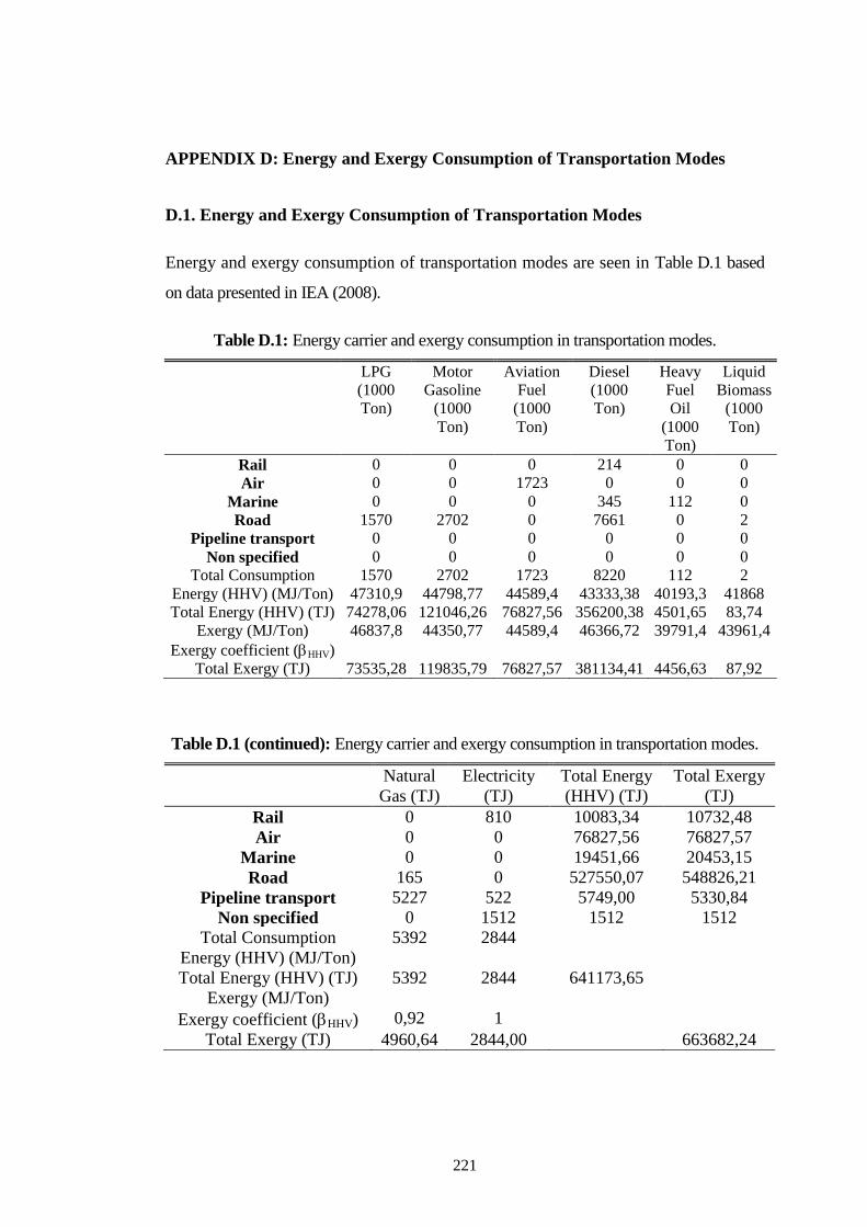
221
APPENDIX D: Energy and Exergy Consumption of Transportation Modes
D.1. Energy and Exergy Consumption of Transportation Modes
Energy and exergy consumption of transportation modes are seen in Table D.1 based
on data presented in IEA (2008).
Table D.1: Energy carrier and exergy consumption in transportation modes.
LPG
(1000
Ton)
Motor
Gasoline
(1000
Ton)
Aviation
Fuel
(1000
Ton)
Diesel
(1000
Ton)
Heavy
Fuel
Oil
(1000
Ton)
Liquid
Biomass
(1000
Ton)
Rail 0 0 0 214 0 0
Air 0 0 1723 0 0 0
Marine 0 0 0 345 112 0
Road 1570 2702 0 7661 0 2
Pipeline transport 0 0 0 0 0 0
Non specified 0 0 0 0 0 0
Total Consumption 1570 2702 1723 8220 112 2
Energy (HHV) (MJ/Ton) 47310,9 44798,77 44589,4 43333,38 40193,3 41868
Total Energy (HHV) (TJ) 74278,06 121046,26 76827,56 356200,38 4501,65 83,74
Exergy (MJ/Ton) 46837,8 44350,77 44589,4 46366,72 39791,4 43961,4
Exergy coefficient (HHV)
Total Exergy (TJ) 73535,28 119835,79 76827,57 381134,41 4456,63 87,92
Table D.1 (continued): Energy carrier and exergy consumption in transportation modes.
Natural
Gas (TJ)
Electricity
(TJ)
Total Energy
(HHV) (TJ)
Total Exergy
(TJ)
Rail 0 810 10083,34 10732,48
Air 0 0 76827,56 76827,57
Marine 0 0 19451,66 20453,15
Road 165 0 527550,07 548826,21
Pipeline transport 5227 522 5749,00 5330,84
Non specified 0 1512 1512 1512
Total Consumption 5392 2844
Energy (HHV) (MJ/Ton)
Total Energy (HHV) (TJ) 5392 2844 641173,65
Exergy (MJ/Ton)
Exergy coefficient (HHV) 0,92 1
Total Exergy (TJ) 4960,64 2844,00 663682,24
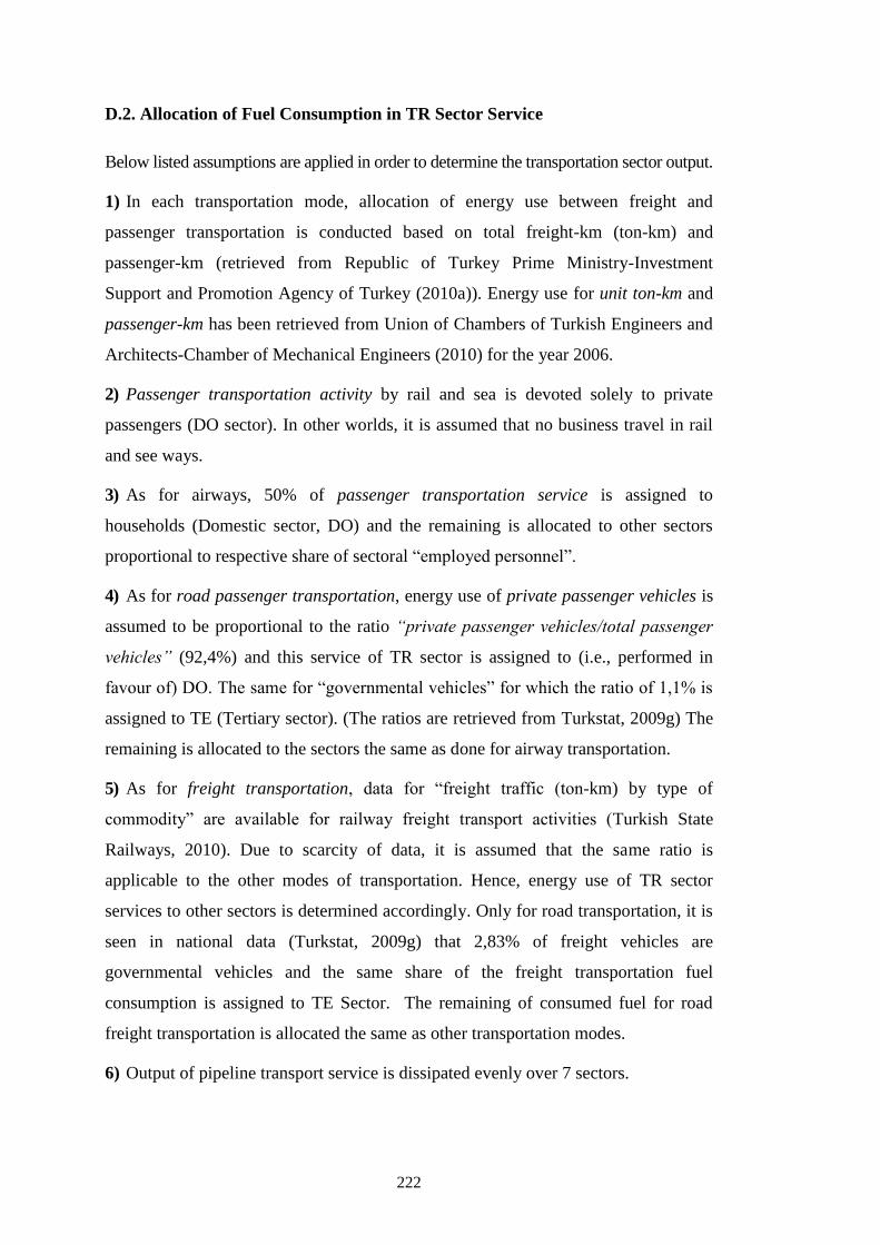
222
D.2. Allocation of Fuel Consumption in TR Sector Service
Below listed assumptions are applied in order to determine the transportation sector output.
1) In each transportation mode, allocation of energy use between freight and
passenger transportation is conducted based on total freight-km (ton-km) and
passenger-km (retrieved from Republic of Turkey Prime Ministry-Investment
Support and Promotion Agency of Turkey (2010a)). Energy use for unit ton-km and
passenger-km has been retrieved from Union of Chambers of Turkish Engineers and
Architects-Chamber of Mechanical Engineers (2010) for the year 2006.
2) Passenger transportation activity by rail and sea is devoted solely to private
passengers (DO sector). In other worlds, it is assumed that no business travel in rail
and see ways.
3) As for airways, 50% of passenger transportation service is assigned to
households (Domestic sector, DO) and the remaining is allocated to other sectors
proportional to respective share of sectoral “employed personnel”.
4) As for road passenger transportation, energy use of private passenger vehicles is
assumed to be proportional to the ratio “private passenger vehicles/total passenger
vehicles” (92,4%) and this service of TR sector is assigned to (i.e., performed in
favour of) DO. The same for “governmental vehicles” for which the ratio of 1,1% is
assigned to TE (Tertiary sector). (The ratios are retrieved from Turkstat, 2009g) The
remaining is allocated to the sectors the same as done for airway transportation.
5) As for freight transportation, data for “freight traffic (ton-km) by type of
commodity” are available for railway freight transport activities (Turkish State
Railways, 2010). Due to scarcity of data, it is assumed that the same ratio is
applicable to the other modes of transportation. Hence, energy use of TR sector
services to other sectors is determined accordingly. Only for road transportation, it is
seen in national data (Turkstat, 2009g) that 2,83% of freight vehicles are
governmental vehicles and the same share of the freight transportation fuel
consumption is assigned to TE Sector. The remaining of consumed fuel for road
freight transportation is allocated the same as other transportation modes.
6) Output of pipeline transport service is dissipated evenly over 7 sectors.
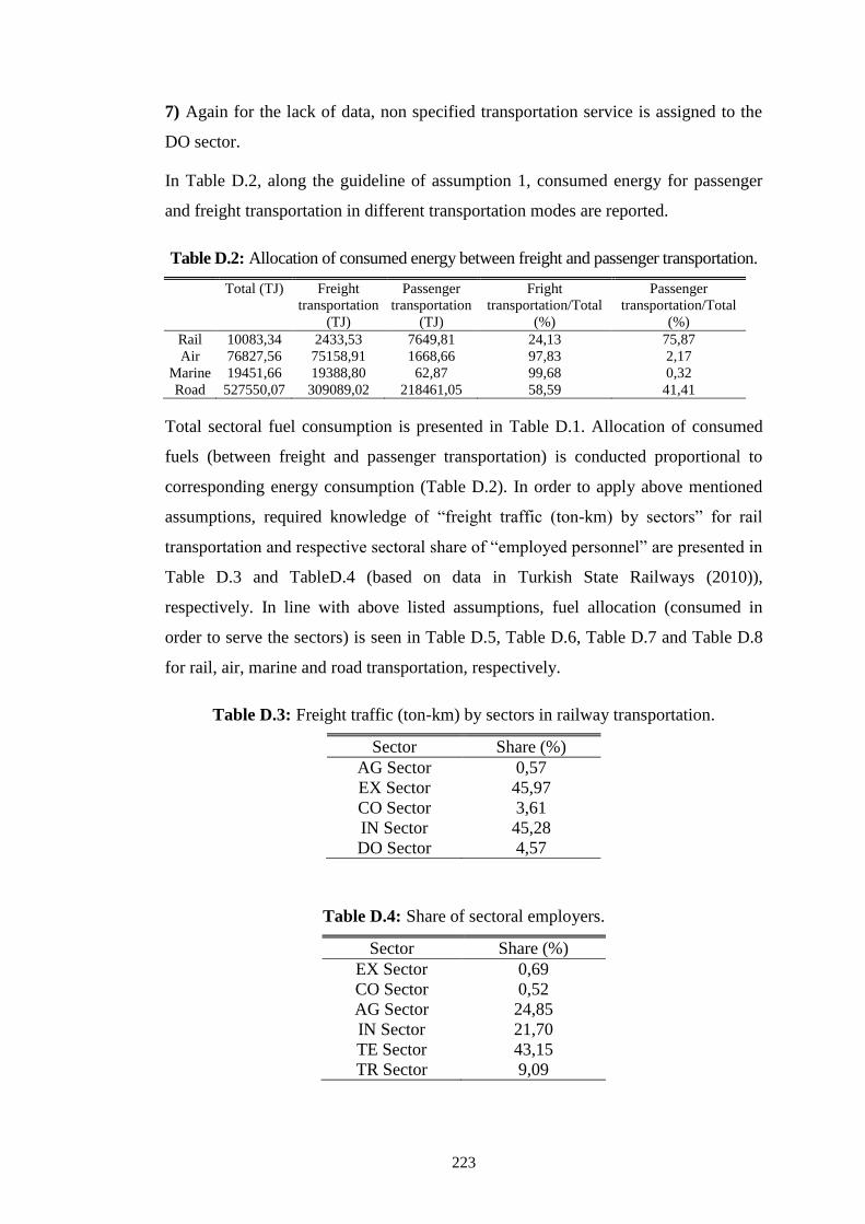
223
7) Again for the lack of data, non specified transportation service is assigned to the
DO sector.
In Table D.2, along the guideline of assumption 1, consumed energy for passenger
and freight transportation in different transportation modes are reported.
Table D.2: Allocation of consumed energy between freight and passenger transportation.
Total (TJ) Freight
transportation
(TJ)
Passenger
transportation
(TJ)
Fright
transportation/Total
(%)
Passenger
transportation/Total
(%)
Rail 10083,34 2433,53 7649,81 24,13 75,87
Air 76827,56 75158,91 1668,66 97,83 2,17
Marine 19451,66 19388,80 62,87 99,68 0,32
Road 527550,07 309089,02 218461,05 58,59 41,41
Total sectoral fuel consumption is presented in Table D.1. Allocation of consumed
fuels (between freight and passenger transportation) is conducted proportional to
corresponding energy consumption (Table D.2). In order to apply above mentioned
assumptions, required knowledge of “freight traffic (ton-km) by sectors” for rail
transportation and respective sectoral share of “employed personnel” are presented in
Table D.3 and TableD.4 (based on data in Turkish State Railways (2010)),
respectively. In line with above listed assumptions, fuel allocation (consumed in
order to serve the sectors) is seen in Table D.5, Table D.6, Table D.7 and Table D.8
for rail, air, marine and road transportation, respectively.
Table D.3: Freight traffic (ton-km) by sectors in railway transportation.
Sector Share (%)
AG Sector 0,57
EX Sector 45,97
CO Sector 3,61
IN Sector 45,28
DO Sector 4,57
Table D.4: Share of sectoral employers.
Sector Share (%)
EX Sector 0,69
CO Sector 0,52
AG Sector 24,85
IN Sector 21,70
TE Sector 43,15
TR Sector 9,09

224
Table D.5: Allocation of consumed energy carriers through service receiving sectors
(rail transportation).
Diesel (1000 Ton) Electricity (TJ)
Total energy carrier
consumption
214 810
Passenger transportation total 162,35 614,51
Sectors
DO 162,35 614,51
Freight transportation total 51,65 195,49
Sectors
AG 0,29 1,11
EX 23,74 89,86
CO 1,87 7,07
IN 23,39 88,53
DO 2,36 8,93
Table D.6: Allocation of consumed energy carriers through service receiving sectors
(air transportation).
Aviation Fuel (1000 Ton)
Total energy carrier consumption 1723
Passenger transportation total 37,42
Sectors
DO 18,71
EX 0,13
CO 0,10
AG 4,65
IN 4,06
TE 8,07
TR 1,70
Freight transportation total 1685,58
Sectors
AG 9,54
EX 774,79
CO 60,93
IN 763,31
DO 77,00
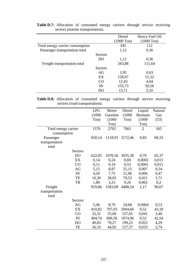
225
Table D.7: Allocation of consumed energy carriers through service receiving
sectors (marine transportation).
Diesel
(1000 Ton)
Heavy Fuel Oil
(1000 Ton)
Total energy carrier consumption 345 112
Passenger transportation total 1,12 0,36
Sectors
DO 1,12 0,36
Freight transportation total 343,88 111,64
Sectors
AG 1,95 0,63
EX 158,07 51,32
CO 12,43 4,04
IN 155,73 50,56
DO 15,71 5,10
Table D.8: Allocation of consumed energy carriers through service receiving
sectors (road transportation).
LPG
(1000
Ton)
Motor
Gasoline
(1000
Ton)
Diesel
(1000
Ton)
Liquid
Biomass
(1000
Ton)
Natural
Gas
(TJ)
Total energy carrier
consumption
1570 2702 7661 2 165
Passenger
transportation
total
650,14 1118,91 3172,46 0,83 68,33
Sectors
DO 622,05 1070,56 3035,38 0,79 65,37
EX 0,14 0,24 0,69 0,0002 0,015
CO 0,11 0,19 0,53 0,0001 0,011
AG 5,15 8,87 25,15 0,007 0,54
IN 4,50 7,75 21,96 0,006 0,47
TE 16,30 28,05 79,53 0,021 1,71
TR 1,89 3,25 9,20 0,002 0,2
Freight
transportation
total
919,86 1583,09 4488,54 1,17 96,67
Sectors
AG 5,06 8,70 24,68 0,0064 0,53
EX 410,82 707,03 2004,66 0,52 43,18
CO 32,31 55,60 157,65 0,041 3,40
IN 404,74 696,56 1974,96 0,52 42,54
DO 40,83 70,27 199,23 0,052 4,29
TE 26,10 44,92 127,37 0,033 2,74
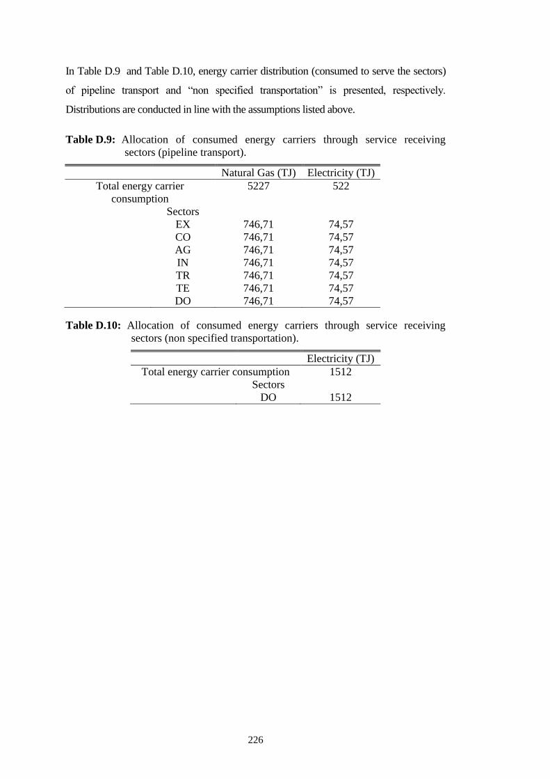
226
In Table D.9 and Table D.10, energy carrier distribution (consumed to serve the sectors)
of pipeline transport and “non specified transportation” is presented, respectively.
Distributions are conducted in line with the assumptions listed above.
Table D.9: Allocation of consumed energy carriers through service receiving
sectors (pipeline transport).
Natural Gas (TJ) Electricity (TJ)
Total energy carrier
consumption
5227 522
Sectors
EX 746,71 74,57
CO 746,71 74,57
AG 746,71 74,57
IN 746,71 74,57
TR 746,71 74,57
TE 746,71 74,57
DO 746,71 74,57
Table D.10: Allocation of consumed energy carriers through service receiving
sectors (non specified transportation).
Electricity (TJ)
Total energy carrier consumption 1512
Sectors
DO 1512
227
APPENDIX E: Details of Material Transfer from TE to the Other Sectors
E.1. Methodology for Material Distribution from TE to the Sectors
Any type of material (commodity) consumption within the society is computed as:
Export-ImportProduction =nconsumptio Societal (E.6)
The rationale behind computing the exergy of commodities which are transferred
from TE to the other sectors is based on the same idea in equation (E.1), namely,
exergy of commodities (transferred from TE and sectorally consumed) is computed
according to equation (E.2) and is assigned to sectoral consumption of the
commodity consuming sector(s).
Export)-Importn(Productio ofExergy =nconsumptioexergy Sectoral (E.2)
If the consuming sectors of the commodities are predictable explicitly, exergy of
consumption (via equation (E.2)) is directly assigned to the exergy consumption of
commodity consuming sector (such as: transferring fertilizers to AG Sector or
minerals to IN sector). However, there are commodities which can be consumed by
any sectors. To map the distribution of these commodities from TE to other sectors,
data about material transfer between the sectors would be necessary: such data are
though unavailable for Turkey, and thus it is assumed that the exergy of these
commodities are allocated to the sectors proportionally to the sectoral “fixed capital
investment + purchases of goods and services” for which accurate data exist and
presented in Table E.1. In Table E.1, data of sectoral “fixed capital investment” is
retrieved from Republic of Turkey-State Planning Organization (2007), that of
“purchases of goods and services” is retrieved from Turkstat (2007a).
Allocation of fuels through the sectors is kept out of aforementioned procedure since
exact data for sectoral fuel consumption is available in published national energy
budgets (IEA, 2008; Republic of Turkey-Ministry of Energy and Natural Resources,
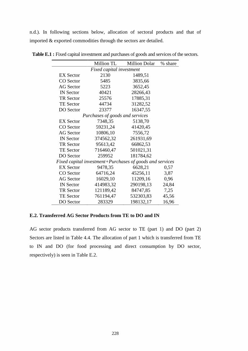
228
n.d.). In following sections below, allocation of sectoral products and that of
imported & exported commodities through the sectors are detailed.
Table E.1 : Fixed capital investment and purchases of goods and services of the sectors.
Million TL Million Dolar % share
Fixed capital investment
EX Sector 2130 1489,51
CO Sector 5485 3835,66
AG Sector 5223 3652,45
IN Sector 40421 28266,43
TR Sector 25576 17885,31
TE Sector 44734 31282,52
DO Sector 23377 16347,55
Purchases of goods and services
EX Sector 7348,35 5138,70
CO Sector 59231,24 41420,45
AG Sector 10806,10 7556,72
IN Sector 374562,32 261931,69
TR Sector 95613,42 66862,53
TE Sector 716460,47 501021,31
DO Sector 259952 181784,62
Fixed capital investment+Purchases of goods and services
EX Sector 9478,35 6628,21 0,57
CO Sector 64716,24 45256,11 3,87
AG Sector 16029,10 11209,16 0,96
IN Sector 414983,32 290198,13 24,84
TR Sector 121189,42 84747,85 7,25
TE Sector 761194,47 532303,83 45,56
DO Sector 283329 198132,17 16,96
E.2. Transferred AG Sector Products from TE to DO and IN
AG sector products transferred from AG sector to TE (part 1) and DO (part 2)
Sectors are listed in Table 4.4. The allocation of part 1 which is transferred from TE
to IN and DO (for food processing and direct consumption by DO sector,
respectively) is seen in Table E.2.
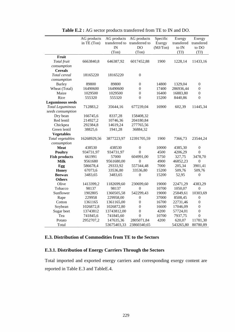
229
Table E.2 : AG sector products transferred from TE to IN and DO.
AG products
in TE (Ton)
AG products
transferred to
IN
(Ton)
AG products
transferred to
DO
(Ton)
Specific
Exergy
(MJ/Ton)
Exergy
transfered
to IN
(TJ)
Exergy
transfered
to DO
(TJ)
Fruit
Total fruit
consumption
6663840,8 646387,92 6017452,88 1900 1228,14 11433,16
Cereals
Total cereal
consumption
18165220 18165220 0
Barley 89800 89800 0 14800 1329,04 0
Wheat (Total) 16490600 16490600 0 17400 286936,44 0
Maize 1029500 1029500 0 16400 16883,80 0
Rice 555320 555320 0 15200 8440,86 0
Leguminous seeds
Total Leguminous
seeds consumption
712883,2 35644,16 677239,04 16900 602,39 11445,34
Dry bean 166745,6 8337,28 158408,32
Red lentil 214927,2 10746,36 204180,84
Chickpea 292384,8 14619,24 277765,56
Green lentil 38825,6 1941,28 36884,32
Vegetables
Total vegetables
consumption
16268929,56 3877223,97 12391705,59 1900 7366,73 23544,24
Meat 438530 438530 0 10000 4385,30 0
Poultry 934731,97 934731,97 0 4500 4206,29 0
Fish products 661991 57000 604991,00 5750 327,75 3478,70
Milk 9561680 9561680,00 0 4900 46852,23 0
Egg 586678,4 29333,92 557344,48 7000 205,34 3901,41
Honey 67073,6 33536,80 33536,80 15200 509,76 509,76
Beewax 3483,65 3483,65 0 15200 52,95 0
Others
Olive 1413399,2 1182699,60 230699,60 19000 22471,29 4383,29
Tobacco 98137 98137 0 10700 1050,07 0
Sunflower 1902805 1360505,58 542299,43 19000 25849,61 10303,69
Rape 229958 229958,00 0 37000 8508,45 0
Cotton 1361165 1361165,00 0 16700 22731,46 0
Soybean 1026872,8 1026872,80 0 16600 17046,09 0
Sugar beet 13743812 13743812,00 0 4200 57724,01 0
Tea 741845,6 741845,60 0 10700 7937,75 0
Potato 2952707,2 147635,36 2805071,84 4200 620,07 11781,30
Total 53675403,33 23860340,65 543265,80 80780,89
E.3. Distribution of Commodities from TE to the Sectors
E.3.1. Distribution of Energy Carriers Through the Sectors
Total imported and exported energy carriers and corresponding exergy content are
reported in Table E.3 and TableE.4.
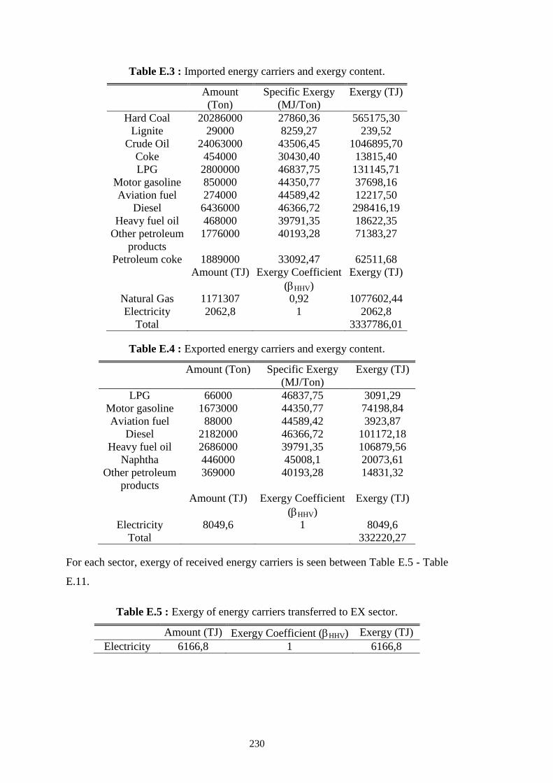
230
Table E.3 : Imported energy carriers and exergy content.
Amount
(Ton)
Specific Exergy
(MJ/Ton)
Exergy (TJ)
Hard Coal 20286000 27860,36 565175,30
Lignite 29000 8259,27 239,52
Crude Oil 24063000 43506,45 1046895,70
Coke 454000 30430,40 13815,40
LPG 2800000 46837,75 131145,71
Motor gasoline 850000 44350,77 37698,16
Aviation fuel 274000 44589,42 12217,50
Diesel 6436000 46366,72 298416,19
Heavy fuel oil 468000 39791,35 18622,35
Other petroleum
products
1776000 40193,28 71383,27
Petroleum coke 1889000 33092,47 62511,68
Amount (TJ) Exergy Coefficient
(HHV)
Exergy (TJ)
Natural Gas 1171307 0,92 1077602,44
Electricity 2062,8 1 2062,8
Total 3337786,01
Table E.4 : Exported energy carriers and exergy content.
Amount (Ton) Specific Exergy
(MJ/Ton)
Exergy (TJ)
LPG 66000 46837,75 3091,29
Motor gasoline 1673000 44350,77 74198,84
Aviation fuel 88000 44589,42 3923,87
Diesel 2182000 46366,72 101172,18
Heavy fuel oil 2686000 39791,35 106879,56
Naphtha 446000 45008,1 20073,61
Other petroleum
products
369000 40193,28 14831,32
Amount (TJ) Exergy Coefficient
(HHV)
Exergy (TJ)
Electricity 8049,6 1 8049,6
Total 332220,27
For each sector, exergy of received energy carriers is seen between Table E.5 - Table
E.11.
Table E.5 : Exergy of energy carriers transferred to EX sector.
Amount (TJ) Exergy Coefficient (HHV) Exergy (TJ)
Electricity 6166,8 1 6166,8
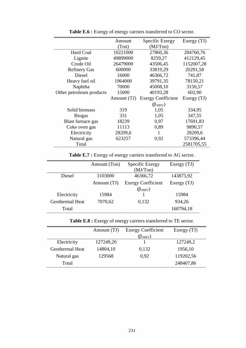
231
Table E.6 : Exergy of energy carriers transferred to CO sector.
Amount
(Ton)
Specific Exergy
(MJ/Ton)
Exergy (TJ)
Hard Coal 10221000 27860,36 284760,76
Lignite 49899000 8259,27 412129,45
Crude Oil 26479000 43506,45 1152007,28
Refinery Gas 600000 33819,29 20291,58
Diesel 16000 46366,72 741,87
Heavy fuel oil 1964000 39791,35 78150,21
Naphtha 70000 45008,10 3150,57
Other petroleum products 15000 40193,28 602,90
Amount (TJ) Exergy Coefficient
(HHV)
Exergy (TJ)
Solid biomass 319 1,05 334,95
Biogas 331 1,05 347,55
Blast furnace gas 18239 0,97 17691,83
Coke oven gas 11113 0,89 9890,57
Electricity 28209,6 1 28209,6
Natural gas 623257 0,92 573396,44
Total 2581705,55
Table E.7 : Exergy of energy carriers transferred to AG sector.
Amount (Ton) Specific Exergy
(MJ/Ton)
Exergy (TJ)
Diesel 3103000 46366,72 143875,92
Amount (TJ) Exergy Coefficient
(HHV)
Exergy (TJ)
Electricity 15984 1 15984
Geothermal Heat 7070,62 0,132 934,26
Total 160794,18
Table E.8 : Exergy of energy carriers transferred to TE sector.
Amount (TJ) Exergy Coefficient
(HHV)
Exergy (TJ)
Electricity 127249,20 1 127249,2
Geothermal Heat 14804,10 0,132 1956,10
Natural gas 129568 0,92 119202,56
Total 248407,86

232
Table E.9 : Exergy of energy carriers transferred to IN sector.
Amount (Ton) Specific Exergy
(MJ/Ton)
Exergy (TJ)
Hard Coal 11672000 27860,36 325186,14
Asphaltit 120000 18604,40 2232,53
Lignite 4897000 8259,27 40445,66
Coke 3612000 30430,40 109914,60
LPG 392000 46837,75 18360,40
Motor gasoline 21000 44350,77 931,37
Diesel 298000 46366,72 13817,28
Heavy fuel oil 2754000 39791,35 109585,37
Naphtha 941000 45008,10 42352,62
Other petroleum
products
4523000 40193,28 181794,21
Petroleum coke 1981000 33092,47 65556,18
Amount (TJ) Exergy Coefficient
(HHV)
Exergy (TJ)
Natural Gas 161447 0,92 148531,24
Electricity 234842,4 1 234842,40
Coke oven gas 11016 0,89 9804,24
CHP heat 40109,54 0,67 26873,39
Blast furnace gas 18409 0,97 17856,73
Total 1348084,37
Table E.10 : Exergy of energy carriers transferred to TR sector.
Amount (Ton) Specific Exergy
(MJ/Ton)
Exergy (TJ)
LPG 1570000 46837,75 73535,28
Motor gasoline 2702000 44350,77 119835,79
Aviation fuel 1723000 44589,42 76827,57
Diesel 8220000 46366,72 381134,41
Heavy fuel oil 112000 39791,35 4456,63
Liquid biomass 2000 43961,4 87,92
Amount (TJ) Exergy Coefficient
(HHV)
Exergy (TJ)
Natural Gas 5392 0,92 4960,64
Electricity 2844 1 2844
Total 663682,24
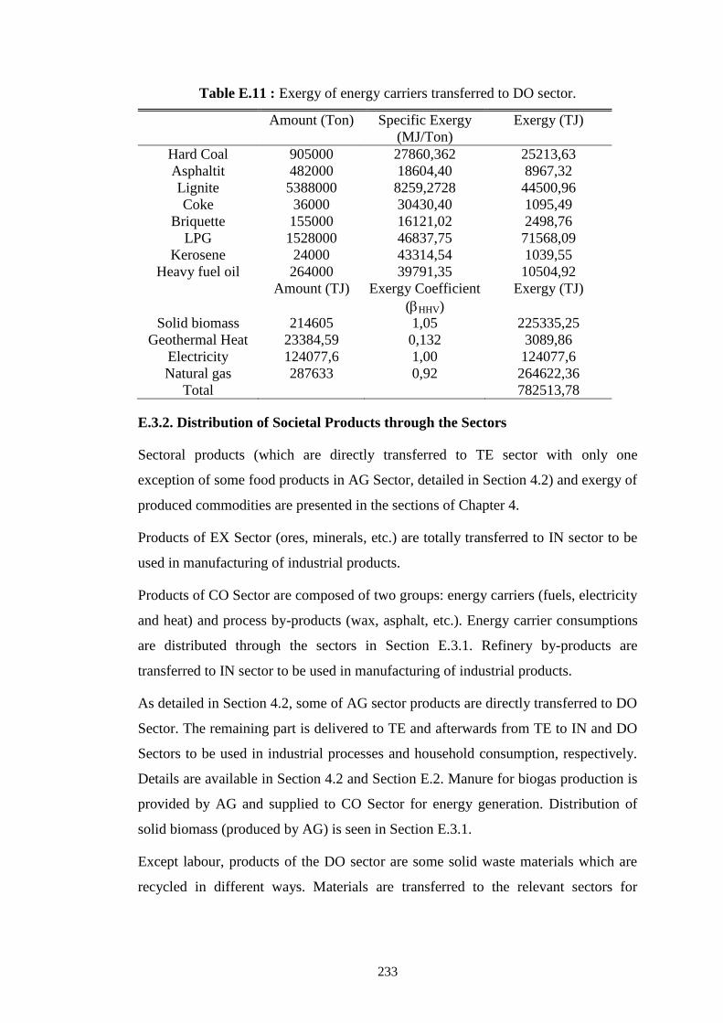
233
Table E.11 : Exergy of energy carriers transferred to DO sector.
Amount (Ton) Specific Exergy
(MJ/Ton)
Exergy (TJ)
Hard Coal 905000 27860,362 25213,63
Asphaltit 482000 18604,40 8967,32
Lignite 5388000 8259,2728 44500,96
Coke 36000 30430,40 1095,49
Briquette 155000 16121,02 2498,76
LPG 1528000 46837,75 71568,09
Kerosene 24000 43314,54 1039,55
Heavy fuel oil 264000 39791,35 10504,92
Amount (TJ) Exergy Coefficient
(HHV)
Exergy (TJ)
Solid biomass 214605 1,05 225335,25
Geothermal Heat 23384,59 0,132 3089,86
Electricity 124077,6 1,00 124077,6
Natural gas 287633 0,92 264622,36
Total 782513,78
E.3.2. Distribution of Societal Products through the Sectors
Sectoral products (which are directly transferred to TE sector with only one
exception of some food products in AG Sector, detailed in Section 4.2) and exergy of
produced commodities are presented in the sections of Chapter 4.
Products of EX Sector (ores, minerals, etc.) are totally transferred to IN sector to be
used in manufacturing of industrial products.
Products of CO Sector are composed of two groups: energy carriers (fuels, electricity
and heat) and process by-products (wax, asphalt, etc.). Energy carrier consumptions
are distributed through the sectors in Section E.3.1. Refinery by-products are
transferred to IN sector to be used in manufacturing of industrial products.
As detailed in Section 4.2, some of AG sector products are directly transferred to DO
Sector. The remaining part is delivered to TE and afterwards from TE to IN and DO
Sectors to be used in industrial processes and household consumption, respectively.
Details are available in Section 4.2 and Section E.2. Manure for biogas production is
provided by AG and supplied to CO Sector for energy generation. Distribution of
solid biomass (produced by AG) is seen in Section E.3.1.
Except labour, products of the DO sector are some solid waste materials which are
recycled in different ways. Materials are transferred to the relevant sectors for
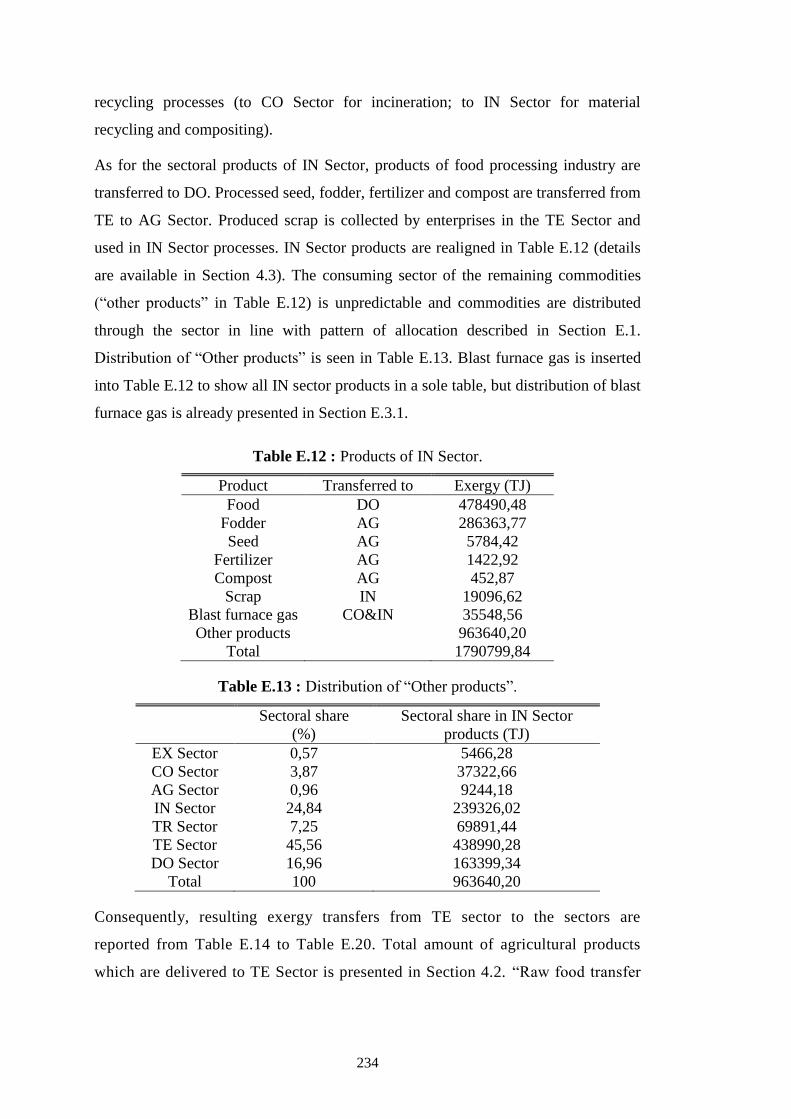
234
recycling processes (to CO Sector for incineration; to IN Sector for material
recycling and compositing).
As for the sectoral products of IN Sector, products of food processing industry are
transferred to DO. Processed seed, fodder, fertilizer and compost are transferred from
TE to AG Sector. Produced scrap is collected by enterprises in the TE Sector and
used in IN Sector processes. IN Sector products are realigned in Table E.12 (details
are available in Section 4.3). The consuming sector of the remaining commodities
(“other products” in Table E.12) is unpredictable and commodities are distributed
through the sector in line with pattern of allocation described in Section E.1.
Distribution of “Other products” is seen in Table E.13. Blast furnace gas is inserted
into Table E.12 to show all IN sector products in a sole table, but distribution of blast
furnace gas is already presented in Section E.3.1.
Table E.12 : Products of IN Sector.
Product Transferred to Exergy (TJ)
Food DO 478490,48
Fodder AG 286363,77
Seed AG 5784,42
Fertilizer AG 1422,92
Compost AG 452,87
Scrap IN 19096,62
Blast furnace gas CO&IN 35548,56
Other products 963640,20
Total 1790799,84
Table E.13 : Distribution of “Other products”.
Sectoral share
(%)
Sectoral share in IN Sector
products (TJ)
EX Sector 0,57 5466,28
CO Sector 3,87 37322,66
AG Sector 0,96 9244,18
IN Sector 24,84 239326,02
TR Sector 7,25 69891,44
TE Sector 45,56 438990,28
DO Sector 16,96 163399,34
Total 100 963640,20
Consequently, resulting exergy transfers from TE sector to the sectors are
reported from Table E.14 to Table E.20. Total amount of agricultural products
which are delivered to TE Sector is presented in Section 4.2. “Raw food transfer
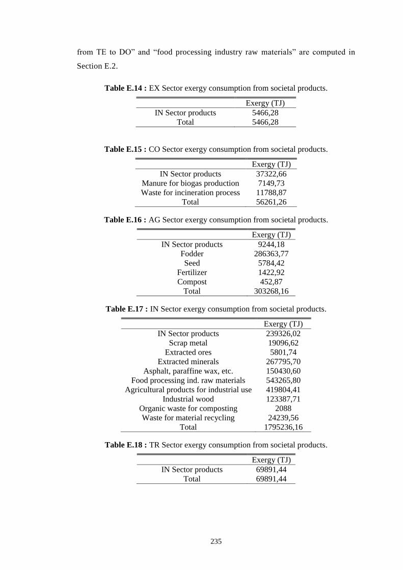
235
from TE to DO” and “food processing industry raw materials” are computed in
Section E.2.
Table E.14 : EX Sector exergy consumption from societal products.
Exergy (TJ)
IN Sector products 5466,28
Total 5466,28
Table E.15 : CO Sector exergy consumption from societal products.
Exergy (TJ)
IN Sector products 37322,66
Manure for biogas production 7149,73
Waste for incineration process 11788,87
Total 56261,26
Table E.16 : AG Sector exergy consumption from societal products.
Exergy (TJ)
IN Sector products 9244,18
Fodder 286363,77
Seed 5784,42
Fertilizer 1422,92
Compost 452,87
Total 303268,16
Table E.17 : IN Sector exergy consumption from societal products.
Exergy (TJ)
IN Sector products 239326,02
Scrap metal 19096,62
Extracted ores 5801,74
Extracted minerals 267795,70
Asphalt, paraffine wax, etc. 150430,60
Food processing ind. raw materials 543265,80
Agricultural products for industrial use 419804,41
Industrial wood 123387,71
Organic waste for composting 2088
Waste for material recycling 24239,56
Total 1795236,16
Table E.18 : TR Sector exergy consumption from societal products.
Exergy (TJ)
IN Sector products 69891,44
Total 69891,44
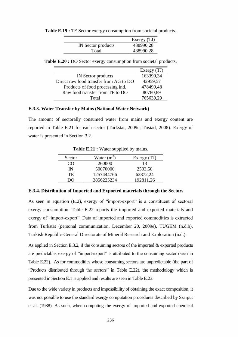
236
Table E.19 : TE Sector exergy consumption from societal products.
Exergy (TJ)
IN Sector products 438990,28
Total 438990,28
Table E.20 : DO Sector exergy consumption from societal products.
Exergy (TJ)
IN Sector products 163399,34
Direct raw food transfer from AG to DO 42959,57
Products of food processing ind. 478490,48
Raw food transfer from TE to DO 80780,89
Total 765630,29
E.3.3. Water Transfer by Mains (National Water Network)
The amount of sectorally consumed water from mains and exergy content are
reported in Table E.21 for each sector (Turkstat, 2009c; Tusiad, 2008). Exergy of
water is presented in Section 3.2.
Table E.21 : Water supplied by mains.
Sector Water (m3) Exergy (TJ)
CO 260000 13
IN 50070000 2503,50
TE 1257444766 62872,24
DO 3856225234 192811,26
E.3.4. Distribution of Imported and Exported materials through the Sectors
As seen in equation (E.2), exergy of “import-export” is a constituent of sectoral
exergy consumption. Table E.22 reports the imported and exported materials and
exergy of “import-export”. Data of imported and exported commodities is extracted
from Turkstat (personal communication, December 20, 2009e), TUGEM (n.d.b),
Turkish Republic-General Directorate of Mineral Research and Exploration (n.d.).
As applied in Section E.3.2, if the consuming sectors of the imported & exported products
are predictable, exergy of “import-export” is attributed to the consuming sector (seen in
Table E.22). As for commodities whose consuming sectors are unpredictable (the part of
“Products distributed through the sectors” in Table E.22), the methodology which is
presented in Section E.1 is applied and results are seen in Table E.23.
Due to the wide variety in products and impossibility of obtaining the exact composition, it
was not possible to use the standard exergy computation procedures described by Szargut
et al. (1988). As such, when computing the exergy of imported and exported chemical
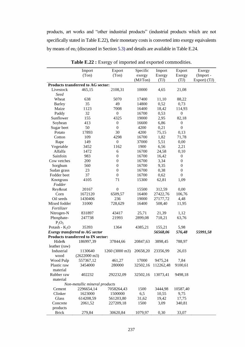
237
products, art works and “other industrial products” (industrial products which are not
specifically stated in Table E.22), their monetary costs is converted into exergy equivalents
by means of eeC (discussed in Section 5.3) and details are available in Table E.24.
Table E.22 : Exergy of imported and exported commodities.
Import
(Ton)
Export
(Ton)
Specific
exergy
(MJ/Ton)
Import
Exergy
(TJ)
Export
Exergy
(TJ)
Exergy
(Import -
Export) (TJ)
Products transferred to AG sector:
Livestock 465,15 2108,31 10000 4,65 21,08
Seed
Wheat 638 5070 17400 11,10 88,22
Barley 35 49 14800 0,52 0,73
Maize 1123 7008 16400 18,42 114,93
Paddy 32 0 16700 0,53 0
Sunflower 155 4325 19000 2,95 82,18
Soybean 413 0 16600 6,86 0
Sugar beet 50 0 4200 0,21 0
Potato 17893 30 4200 75,15 0,13
Cotton 109 4298 16700 1,82 71,78
Rape 149 0 37000 5,51 0,00
Vegetable 3452 1162 1900 6,56 2,21
Alfalfa 1472 6 16700 24,58 0,10
Sainfoin 983 0 16700 16,42 0
Cow vetches 200 0 16700 3,34 0
Sorghum 560 0 16700 9,35 0
Sudan grass 23 0 16700 0,38 0
Fodder beet 37 0 16700 0,62 0
Knotgrass 4105 71 15300 62,81 1,09
Fodder
Rey&oat 20167 0 15500 312,59 0,00
Corn 1672120 6509,57 16400 27422,76 106,76
Oil seeds 1430406 236 19000 27177,72 4,48
Mixed fodder 31000 728,629 16400 508,40 11,95
Fertilizer
Nitrogen-N 831897 43417 25,71 21,39 1,12
Phosphate-
P2O5
247738 21993 2899,08 718,21 63,76
Potash - K2O 35393 1364 4385,21 155,21 5,98
Exergy transferred to AG sector 56568,06 576,48 55991,58
Products transferred to IN sector:
Hide&
leather (raw)
186997,39 37844,66 20847,63 3898,45 788,97
Industrial
wood
1130640
(2622000 m3)
1260 (3000 m3) 20658,20 23356,99 26,03
Wood Pulp 557367,12 461,27 17000 9475,24 7,84
Plastic raw
material
3454000 280000 32502,16 112262,48 9100,61
Rubber raw
material
402232 292232,09 32502,16 13073,41 9498,18
Non-metallic mineral products
Cement 2296654,14 7058264,43 1500 3444,98 10587,40
Clinker 1623000 1500000 6,5 10,55 9,75
Glass 614208,59 561203,80 31,62 19,42 17,75
Concrete
products
2061,52 227209,18 1500 3,09 340,81
Brick 279,84 30620,84 1079,97 0,30 33,07
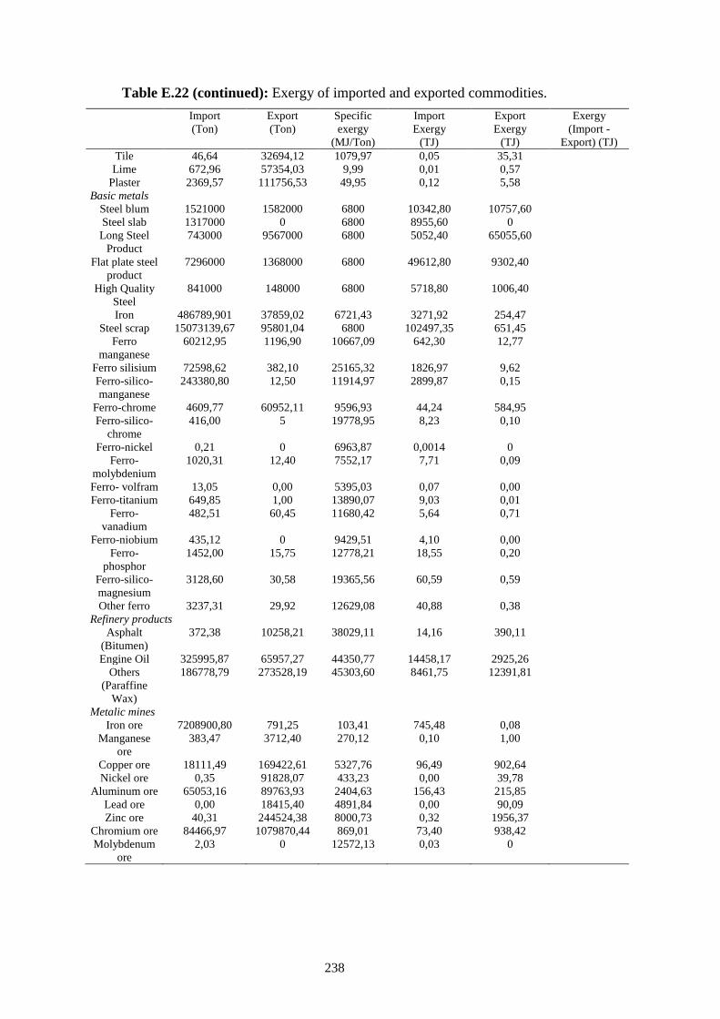
238
Table E.22 (continued): Exergy of imported and exported commodities.
Import
(Ton)
Export
(Ton)
Specific
exergy
(MJ/Ton)
Import
Exergy
(TJ)
Export
Exergy
(TJ)
Exergy
(Import -
Export) (TJ)
Tile 46,64 32694,12 1079,97 0,05 35,31
Lime 672,96 57354,03 9,99 0,01 0,57
Plaster 2369,57 111756,53 49,95 0,12 5,58
Basic metals
Steel blum 1521000 1582000 6800 10342,80 10757,60
Steel slab 1317000 0 6800 8955,60 0
Long Steel
Product
743000 9567000 6800 5052,40 65055,60
Flat plate steel
product
7296000 1368000 6800 49612,80 9302,40
High Quality
Steel
841000 148000 6800 5718,80 1006,40
Iron 486789,901 37859,02 6721,43 3271,92 254,47
Steel scrap 15073139,67 95801,04 6800 102497,35 651,45
Ferro
manganese
60212,95 1196,90 10667,09 642,30 12,77
Ferro silisium 72598,62 382,10 25165,32 1826,97 9,62
Ferro-silico-
manganese
243380,80 12,50 11914,97 2899,87 0,15
Ferro-chrome 4609,77 60952,11 9596,93 44,24 584,95
Ferro-silico-
chrome
416,00 5 19778,95 8,23 0,10
Ferro-nickel 0,21 0 6963,87 0,0014 0
Ferro-
molybdenium
1020,31 12,40 7552,17 7,71 0,09
Ferro- volfram 13,05 0,00 5395,03 0,07 0,00
Ferro-titanium 649,85 1,00 13890,07 9,03 0,01
Ferro-
vanadium
482,51 60,45 11680,42 5,64 0,71
Ferro-niobium 435,12 0 9429,51 4,10 0,00
Ferro-
phosphor
1452,00 15,75 12778,21 18,55 0,20
Ferro-silico-
magnesium
3128,60 30,58 19365,56 60,59 0,59
Other ferro 3237,31 29,92 12629,08 40,88 0,38
Refinery products
Asphalt
(Bitumen)
372,38 10258,21 38029,11 14,16 390,11
Engine Oil 325995,87 65957,27 44350,77 14458,17 2925,26
Others
(Paraffine
Wax)
186778,79 273528,19 45303,60 8461,75 12391,81
Metalic mines
Iron ore 7208900,80 791,25 103,41 745,48 0,08
Manganese
ore
383,47 3712,40 270,12 0,10 1,00
Copper ore 18111,49 169422,61 5327,76 96,49 902,64
Nickel ore 0,35 91828,07 433,23 0,00 39,78
Aluminum ore 65053,16 89763,93 2404,63 156,43 215,85
Lead ore 0,00 18415,40 4891,84 0,00 90,09
Zinc ore 40,31 244524,38 8000,73 0,32 1956,37
Chromium ore 84466,97 1079870,44 869,01 73,40 938,42
Molybdenum
ore
2,03 0 12572,13 0,03 0
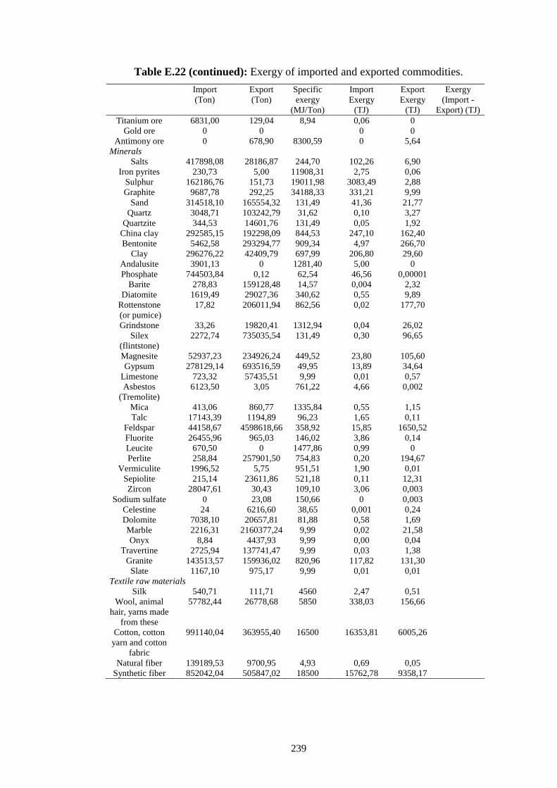
239
Table E.22 (continued): Exergy of imported and exported commodities.
Import
(Ton)
Export
(Ton)
Specific
exergy
(MJ/Ton)
Import
Exergy
(TJ)
Export
Exergy
(TJ)
Exergy
(Import -
Export) (TJ)
Titanium ore 6831,00 129,04 8,94 0,06 0
Gold ore 0 0 0 0
Antimony ore 0 678,90 8300,59 0 5,64
Minerals
Salts 417898,08 28186,87 244,70 102,26 6,90
Iron pyrites 230,73 5,00 11908,31 2,75 0,06
Sulphur 162186,76 151,73 19011,98 3083,49 2,88
Graphite 9687,78 292,25 34188,33 331,21 9,99
Sand 314518,10 165554,32 131,49 41,36 21,77
Quartz 3048,71 103242,79 31,62 0,10 3,27
Quartzite 344,53 14601,76 131,49 0,05 1,92
China clay 292585,15 192298,09 844,53 247,10 162,40
Bentonite 5462,58 293294,77 909,34 4,97 266,70
Clay 296276,22 42409,79 697,99 206,80 29,60
Andalusite 3901,13 0 1281,40 5,00 0
Phosphate 744503,84 0,12 62,54 46,56 0,00001
Barite 278,83 159128,48 14,57 0,004 2,32
Diatomite 1619,49 29027,36 340,62 0,55 9,89
Rottenstone
(or pumice)
17,82 206011,94 862,56 0,02 177,70
Grindstone 33,26 19820,41 1312,94 0,04 26,02
Silex
(flintstone)
2272,74 735035,54 131,49 0,30 96,65
Magnesite 52937,23 234926,24 449,52 23,80 105,60
Gypsum 278129,14 693516,59 49,95 13,89 34,64
Limestone 723,32 57435,51 9,99 0,01 0,57
Asbestos
(Tremolite)
6123,50 3,05 761,22 4,66 0,002
Mica 413,06 860,77 1335,84 0,55 1,15
Talc 17143,39 1194,89 96,23 1,65 0,11
Feldspar 44158,67 4598618,66 358,92 15,85 1650,52
Fluorite 26455,96 965,03 146,02 3,86 0,14
Leucite 670,50 0 1477,86 0,99 0
Perlite 258,84 257901,50 754,83 0,20 194,67
Vermiculite 1996,52 5,75 951,51 1,90 0,01
Sepiolite 215,14 23611,86 521,18 0,11 12,31
Zircon 28047,61 30,43 109,10 3,06 0,003
Sodium sulfate 0 23,08 150,66 0 0,003
Celestine 24 6216,60 38,65 0,001 0,24
Dolomite 7038,10 20657,81 81,88 0,58 1,69
Marble 2216,31 2160377,24 9,99 0,02 21,58
Onyx 8,84 4437,93 9,99 0,00 0,04
Travertine 2725,94 137741,47 9,99 0,03 1,38
Granite 143513,57 159936,02 820,96 117,82 131,30
Slate 1167,10 975,17 9,99 0,01 0,01
Textile raw materials
Silk 540,71 111,71 4560 2,47 0,51
Wool, animal
hair, yarns made
from these
57782,44 26778,68 5850 338,03 156,66
Cotton, cotton
yarn and cotton
fabric
991140,04 363955,40 16500 16353,81 6005,26
Natural fiber 139189,53 9700,95 4,93 0,69 0,05
Synthetic fiber 852042,04 505847,02 18500 15762,78 9358,17
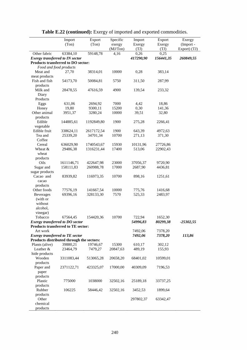
240
Table E.22 (continued): Exergy of imported and exported commodities.
Import
(Ton)
Export
(Ton)
Specific
exergy
(MJ/Ton)
Import
Exergy
(TJ)
Export
Exergy
(TJ)
Exergy
(Import -
Export) (TJ)
Other fabric 63384,10 59148,78 4,16 0,26 0,25
Exergy transferred to IN sector 417290,90 156441,35 260849,55
Products transferred to DO sector:
Food and food products
Meat and
meat products
27,70 38314,01 10000 0,28 383,14
Fish and fish
products
54173,70 50084,81 5750 311,50 287,99
Milk and
Diary
Products
28478,55 47616,59 4900 139,54 233,32
Eggs 631,06 2694,92 7000 4,42 18,86
Honey 19,80 9300,11 15200 0,30 141,36
Other animal
products
3951,37 3280,24 10000 39,51 32,80
Edible
vegetable
144885,61 1192849,80 1900 275,28 2266,41
Edible fruit 338624,11 2617172,54 1900 643,39 4972,63
Tea and
Coffee
25339,20 34701,34 10700 271,13 371,30
Cereal 636029,90 1740543,67 15930 10131,96 27726,86
Wheat &
wheat
products
29486,38 1316231,44 17400 513,06 22902,43
Oils 1611146,71 422647,98 23000 37056,37 9720,90
Sugar and
sugar products
158111,83 260988,78 17000 2687,90 4436,81
Cacao and
cacao
products
83939,82 116973,35 10700 898,16 1251,61
Other foods 77576,19 141667,54 10000 775,76 1416,68
Beverages
(with or
without
alcohol,
vinegar)
69396,16 328133,30 7570 525,33 2483,97
Tobacco 67564,45 154420,36 10700 722,94 1652,30
Exergy transferred to DO sector 54996,83 80299,38 -25302,55
Products transferred to TE sector:
Art work 7492,06 7378,20
Exergy transferred to TE sector 7492,06 7378,20 113,86
Products distributed through the sectors:
Plants (alive) 39880,21 19746,67 15300 610,17 302,12
Leather &
hide products
23464,79 7479,27 20847,63 489,19 155,93
Wooden
products
3311083,44 513065,28 20658,20 68401,02 10599,01
Paper and
paper
products
2371122,71 423325,07 17000,00 40309,09 7196,53
Plastic
products
775000 1038000 32502,16 25189,18 33737,25
Rubber
products
106225 58446,42 32502,16 3452,53 1899,64
Other
chemical
products
297802,37 63342,47
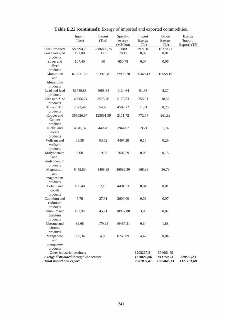
241
Table E.22 (continued): Exergy of imported and exported commodities.
Import
(Ton)
Export
(Ton)
Specific
exergy
(MJ/Ton)
Import
Exergy
(TJ)
Export
Exergy
(TJ)
Exergy
(Import -
Export) (TJ)
Steel Products 583994,28 2686869,75 6800 3971,16 18270,71
Gold and gold
products
192,00 111 78,17 0,02 0,01
Silver and
silver
products
107,40 90 650,78 0,07 0,06
Aluminium
and
Aluminium
products
619031,58 323920,81 32903,70 20368,43 10658,19
Lead and lead
products
81739,88 4688,84 1124,64 91,93 5,27
Zinc and Zinc
products
145966,74 3575,76 5178,63 755,91 18,52
Tin and Tin
products
2573,44 54,46 4589,72 11,81 0,25
Copper and
Copper
products
365926,97 123891,39 2111,72 772,74 261,62
Nickel and
nickel
products
4870,14 440,46 3944,07 19,21 1,74
Volfram and
volfram
products
33,58 63,62 4497,28 0,15 0,29
Molybdenum
and
molybdenum
products
6,08 19,33 7607,29 0,05 0,15
Magnesium
and
magnesium
products
6455,53 1408,35 26082,30 168,38 36,73
Cobalt and
cobalt
products
186,40 2,18 4491,53 0,84 0,01
Cadmium and
cadmium
products
8,78 27,31 2600,00 0,02 0,07
Titanium and
titanium
products
162,92 45,71 18972,80 3,09 0,87
Chrome and
chrome
products
32,65 179,23 10467,31 0,34 1,88
Manganese
and
manganese
products
509,34 4,05 8769,09 4,47 0,04
Other industrial products 1208267,81 694661,39
Exergy distributed through the sectors 1670689,96 841150,73 829539,23
Total import and export 2207037,81 1085846,13 1121191,68
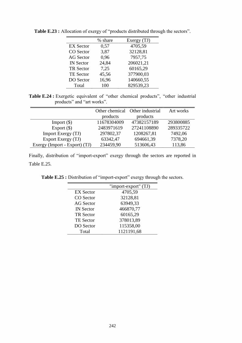
242
Table E.23 : Allocation of exergy of “products distributed through the sectors”.
% share Exergy (TJ)
EX Sector 0,57 4705,59
CO Sector 3,87 32128,81
AG Sector 0,96 7957,75
IN Sector 24,84 206021,21
TR Sector 7,25 60165,29
TE Sector 45,56 377900,03
DO Sector 16,96 140660,55
Total 100 829539,23
Table E.24 : Exergetic equivalent of “other chemical products”, “other industrial
products” and “art works”.
Other chemical
products
Other industrial
products
Art works
Import ($) 11678304009 47382157189 293800885
Export ($) 2483971619 27241108890 289335722
Import Exergy (TJ) 297802,37 1208267,81 7492,06
Export Exergy (TJ) 63342,47 694661,39 7378,20
Exergy (Import - Export) (TJ) 234459,90 513606,43 113,86
Finally, distribution of “import-export” exergy through the sectors are reported in
Table E.25.
Table E.25 : Distribution of “import-export” exergy through the sectors.
"import-export" (TJ)
EX Sector 4705,59
CO Sector 32128,81
AG Sector 63949,33
IN Sector 466870,77
TR Sector 60165,29
TE Sector 378013,89
DO Sector 115358,00
Total 1121191,68
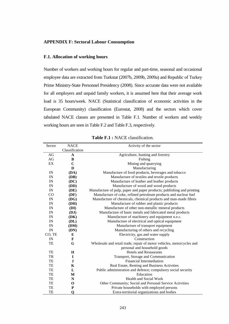
243
APPENDIX F: Sectoral Labour Consumption
F.1. Allocation of working hours
Number of workers and working hours for regular and part-time, seasonal and occasional
employee data are extracted from Turkstat (2007b, 2009b, 2009a) and Republic of Turkey
Prime Ministry-State Personnel Presidency (2008). Since accurate data were not available
for all employers and unpaid family workers, it is assumed here that their average work
load is 35 hours/week. NACE (Statistical classification of economic activities in the
European Community) classification (Eurostat, 2008) and the sectors which cover
tabulated NACE classes are presented in Table F.1. Number of workers and weekly
working hours are seen in Table F.2 and Table F.3, respectively.
Table F.1 : NACE classification.
Sector NACE
Classification
Activity of the sector
AG A Agriculture, hunting and forestry
AG B Fishing
EX C Mining and quarrying
D Manufacturing
IN (DA) Manufacture of food products, beverages and tobacco
IN (DB) Manufacture of textiles and textile products
IN (DC) Manufacture of leather and leather products
IN (DD) Manufacture of wood and wood products
IN (DE) Manufacture of pulp, paper and paper products; publishing and printing
CO (DF) Manufacture of coke, refined petroleum products and nuclear fuel
IN (DG) Manufacture of chemicals, chemical products and man-made fibres
IN (DH) Manufacture of rubber and plastic products
IN (DI) Manufacture of other non-metallic mineral products
IN (DJ) Manufacture of basic metals and fabricated metal products
IN (DK) Manufacture of machinery and equipment n.e.c.
IN (DL) Manufacture of electrical and optical equipment
IN (DM) Manufacture of transport equipment
IN (DN) Manufacturing of others and recycling
CO, TE E Electricity, gas and water supply
IN F Construction
TE G Wholesale and retail trade; repair of motor vehicles, motorcycles and
personal and household goods
TE H Hotels and Restaurants
TR I Transport, Storage and Communication
TE J Financial Intermediation
TE K Real Estate, Renting and Business Activities
TE L Public administration and defence; compulsory social security
TE M Education
TE N Health and Social Work
TE O Other Community; Social and Personal Service Activities
TE P Private households with employed persons
TE Q Extra-territorial organizations and bodies
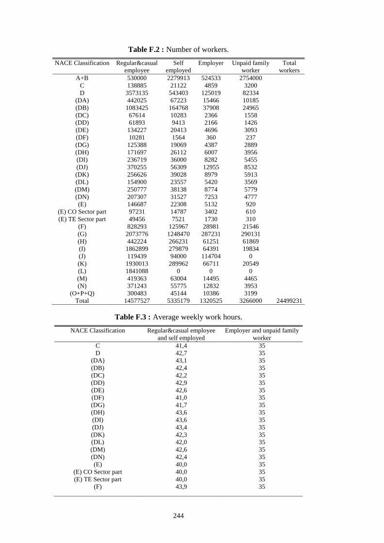
244
Table F.2 : Number of workers.
NACE Classification Regular&casual
employee
Self
employed
Employer Unpaid family
worker
Total
workers
A+B 530000 2279913 524533 2754000
C 138885 21122 4859 3200
D 3573135 543403 125019 82334
(DA) 442025 67223 15466 10185
(DB) 1083425 164768 37908 24965
(DC) 67614 10283 2366 1558
(DD) 61893 9413 2166 1426
(DE) 134227 20413 4696 3093
(DF) 10281 1564 360 237
(DG) 125388 19069 4387 2889
(DH) 171697 26112 6007 3956
(DI) 236719 36000 8282 5455
(DJ) 370255 56309 12955 8532
(DK) 256626 39028 8979 5913
(DL) 154900 23557 5420 3569
(DM) 250777 38138 8774 5779
(DN) 207307 31527 7253 4777
(E) 146687 22308 5132 920
(E) CO Sector part 97231 14787 3402 610
(E) TE Sector part 49456 7521 1730 310
(F) 828293 125967 28981 21546
(G) 2073776 1248470 287231 290131
(H) 442224 266231 61251 61869
(I) 1862899 279879 64391 19834
(J) 119439 94000 114704 0
(K) 1930013 289962 66711 20549
(L) 1841088 0 0 0
(M) 419363 63004 14495 4465
(N) 371243 55775 12832 3953
(O+P+Q) 300483 45144 10386 3199
Total 14577527 5335179 1320525 3266000 24499231
Table F.3 : Average weekly work hours.
NACE Classification Regular&casual employee
and self employed
Employer and unpaid family
worker
C 41,4 35
D 42,7 35
(DA) 43,1 35
(DB) 42,4 35
(DC) 42,2 35
(DD) 42,9 35
(DE) 42,6 35
(DF) 41,0 35
(DG) 41,7 35
(DH) 43,6 35
(DI) 43,6 35
(DJ) 43,4 35
(DK) 42,3 35
(DL) 42,0 35
(DM) 42,6 35
(DN) 42,4 35
(E) 40,0 35
(E) CO Sector part 40,0 35
(E) TE Sector part 40,0 35
(F) 43,9 35
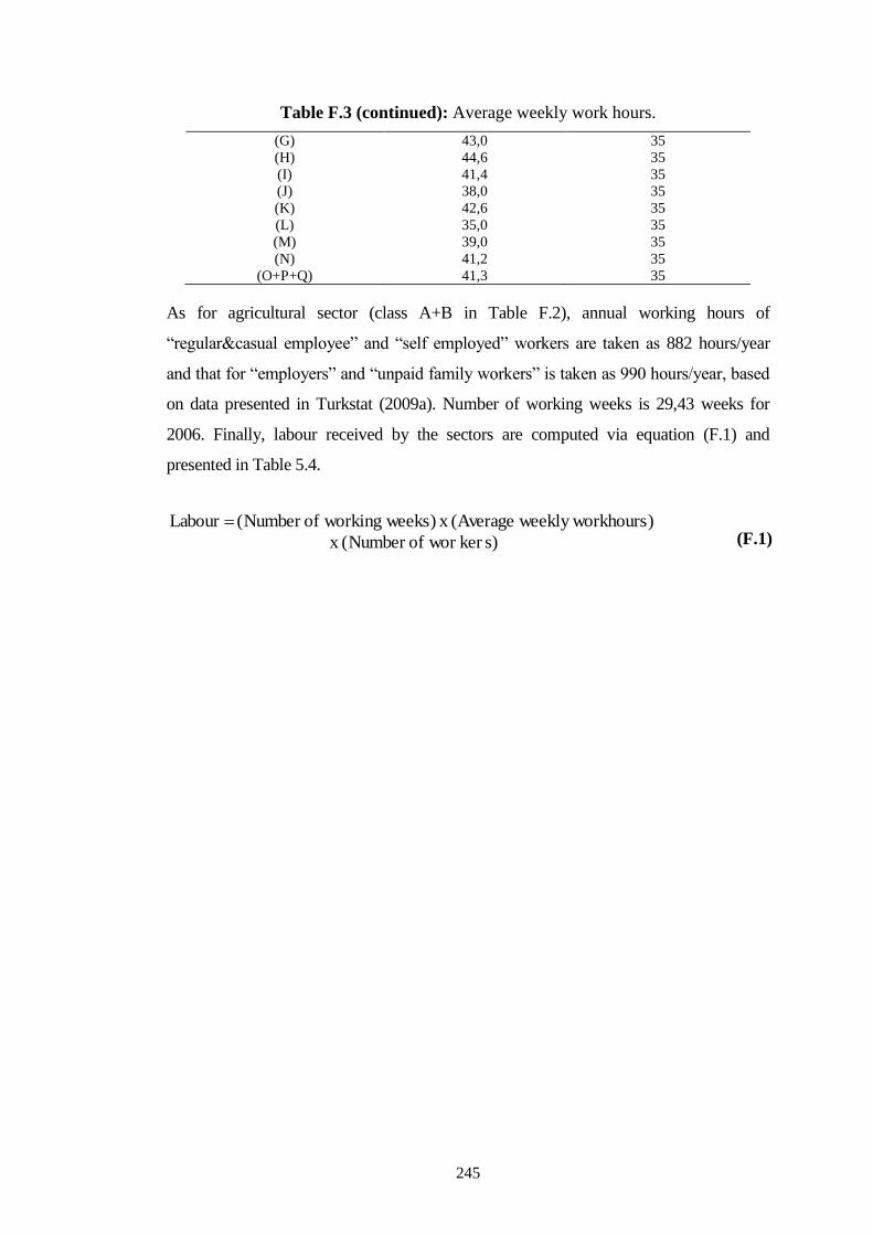
245
Table F.3 (continued): Average weekly work hours.
(G) 43,0 35
(H) 44,6 35
(I) 41,4 35
(J) 38,0 35
(K) 42,6 35
(L) 35,0 35
(M) 39,0 35
(N) 41,2 35
(O+P+Q) 41,3 35
As for agricultural sector (class A+B in Table F.2), annual working hours of
“regular&casual employee” and “self employed” workers are taken as 882 hours/year
and that for “employers” and “unpaid family workers” is taken as 990 hours/year, based
on data presented in Turkstat (2009a). Number of working weeks is 29,43 weeks for
2006. Finally, labour received by the sectors are computed via equation (F.1) and
presented in Table 5.4.
)skerworofNumber(x
)workhoursweeklyAverage(x)weeksworkingofNumber(Labour (F.1)

246
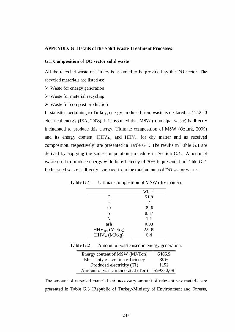
247
APPENDIX G: Details of the Solid Waste Treatment Processes
G.1 Composition of DO sector solid waste
All the recycled waste of Turkey is assumed to be provided by the DO sector. The
recycled materials are listed as:
Waste for energy generation
Waste for material recycling
Waste for compost production
In statistics pertaining to Turkey, energy produced from waste is declared as 1152 TJ
electrical energy (IEA, 2008). It is assumed that MSW (municipal waste) is directly
incinerated to produce this energy. Ultimate composition of MSW (Ozturk, 2009)
and its energy content (HHVdry and HHVar for dry matter and as received
composition, respectively) are presented in Table G.1. The results in Table G.1 are
derived by applying the same computation procedure in Section C.4. Amount of
waste used to produce energy with the efficiency of 30% is presented in Table G.2.
Incinerated waste is directly extracted from the total amount of DO sector waste.
Table G.1 : Ultimate composition of MSW (dry matter).
wt. %
C 51,9
H 7
O 39,6
S 0,37
N 1,1
ash 0,03
HHVdry (MJ/kg) 22,09
HHVar (MJ/kg) 6,4
Table G.2 : Amount of waste used in energy generation.
Energy content of MSW (MJ/Ton) 6406,9
Electricity generation efficiency 30%
Produced electricity (TJ) 1152
Amount of waste incinerated (Ton) 599352,08
The amount of recycled material and necessary amount of relevant raw material are
presented in Table G.3 (Republic of Turkey-Ministry of Environment and Forests,
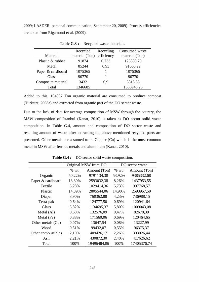
248
2009; LASDER, personal communication, September 20, 2009). Process efficiencies
are taken from Rigamonti et al. (2009).
Table G.3 : Recycled waste materials.
Material
Recycled
material (Ton)
Recycling
efficiency
Consumed waste
material (Ton)
Plastic & rubber 91874 0,733 125339,70
Metal 85244 0,93 91660,22
Paper & cardboard 1075365 1 1075365
Glass 90770 1 90770
Composite material 3432 0,9 3813,33
Total 1346685
1386948,25
Added to this, 104807 Ton organic material are consumed to produce compost
(Turkstat, 2008a) and extracted from organic part of the DO sector waste.
Due to the lack of data for average composition of MSW through the country, the
MSW composition of Istanbul (Kanat, 2010) is taken as DO sector solid waste
composition. In Table G.4, amount and composition of DO sector waste and
resulting amount of waste after extracting the above mentioned recycled parts are
presented. Other metals are assumed to be Copper (Cu) which is the most common
metal in MSW after ferrous metals and aluminium (Kanat, 2010).
Table G.4 : DO sector solid waste composition.
Original MSW from DO DO sector waste
% wt. Amount (Ton) % wt. Amount (Ton)
Organic 50,22% 9791134,30 53,92% 9385332,68
Paper & cardboard 13,30% 2593032,38 8,26% 1437953,55
Textile 5,28% 1029414,36 5,73% 997768,57
Plastic 14,39% 2805544,06 14,90% 2593957,59
Diaper 3,90% 760362,88 4,23% 736988,15
Tetra-pak 0,64% 124777,50 0,69% 120941,64
Glass 5,82% 1134695,37 5,80% 1009043,08
Metal (Al) 0,68% 132576,09 0,47% 82670,39
Metal (Fe) 0,88% 171569,06 0,69% 120464,65
Other metals (Cu) 0,07% 13647,54 0,08% 13227,99
Wood 0,51% 99432,07 0,55% 96375,37
Other combustibles 2,10% 409426,17 2,26% 393026,44
Ash 2,21% 430872,30 2,40% 417626,62
Total 100% 19496484,06 100% 17405376,74
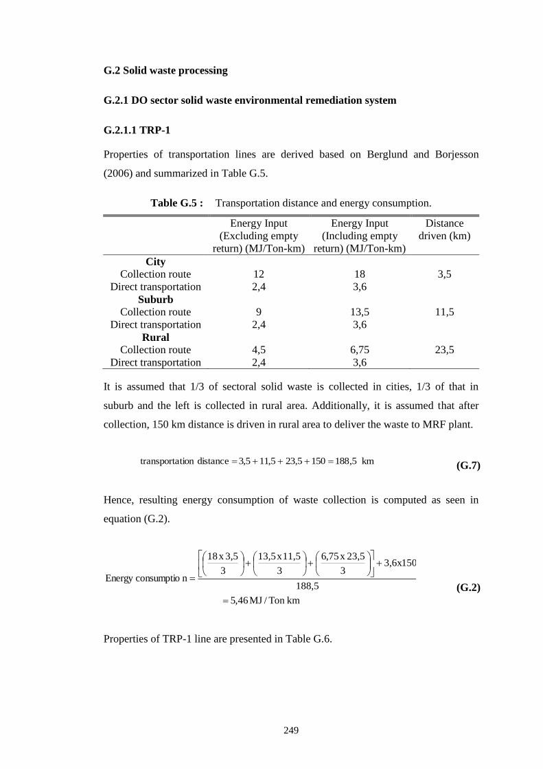
249
G.2 Solid waste processing
G.2.1 DO sector solid waste environmental remediation system
G.2.1.1 TRP-1
Properties of transportation lines are derived based on Berglund and Borjesson
(2006) and summarized in Table G.5.
Table G.5 : Transportation distance and energy consumption.
Energy Input
(Excluding empty
return) (MJ/Ton-km)
Energy Input
(Including empty
return) (MJ/Ton-km)
Distance
driven (km)
City
Collection route 12 18 3,5
Direct transportation 2,4 3,6
Suburb
Collection route 9 13,5 11,5
Direct transportation 2,4 3,6
Rural
Collection route 4,5 6,75 23,5
Direct transportation 2,4 3,6
It is assumed that 1/3 of sectoral solid waste is collected in cities, 1/3 of that in
suburb and the left is collected in rural area. Additionally, it is assumed that after
collection, 150 km distance is driven in rural area to deliver the waste to MRF plant.
km5,1881505,235,115,3distancetion transporta (G.7)
Hence, resulting energy consumption of waste collection is computed as seen in
equation (G.2).
kmTon/MJ46,5
188,5
3,6x1503
23,5x75,6
3
11,5x13,5
3
3,5x18
nconsumptionergyE
(G.2)
Properties of TRP-1 line are presented in Table G.6.

250
Table G.6 : Exergy of fuel and fuel capital for TRP-1.
Average transportation distance (km) 188,5
Total distance travelled (including return) (km) 377
Average energy consumption (MJ/Ton-km) 5,46
Transported waste (Ton) 17405376,74
Total energy consumption (TJ) 17905,78
Diesel fuel energy content (MJ/Ton) 42791,00
Diesel fuel consumption (Ton) 418447,37
Diesel fuel exergy content (MJ/Ton) 46366,72
Total diesel exergy consumption (TJ) 19402,03
Density of diesel fuel (kg/l) 0,835
Volume of consumed diesel fuel (l) 501134572,39
Price of diesel fuel ($/l) 1,47
Exergetic equivalent of capital (TJ) 18766,61
Employed number of trucks and consumed labour through TRP-1 line are
summarized in Table G.7.
Table G.7 : Exergy of trucks and labour for TRP-1.
Load capacity (Ton/truck) 16
Waste (Ton) 17405376,74
Average speed of truck (km/h) 40
Average distance of transportation (km) 188,5
Total distance travelled (including return) (km) 377
Travel time (including return) (hours) 9,42
Daily ring number 1
Annual working days (days) 340
1 truck annual load capacity (Ton/truck) 5440
Truck number (trucks) 3200
1 truck exergy (TJ/truck) 0,045
Total exergy of trucks (TJ) 145,51
Annual working hours (Labour) (hours) 10245333,33
Exergetic equivalent of labour (TJ) 1577,29
Since collection activity decreases the average speed through the transportation,
average speed of trucks is assumed to be 40 km/h. (The speed is assumed to be 60
km/h for other TRP lines. Mathematical formulations for some of the items seen in
Table G.7 are presented in equation (G.3), (G.4) and (G.5).
number ringDaily capacity x Load x days workingAnnual
year) (Ton/truckcapacity load annual truck 1 (G.3)
)Truck/Ton(capacityloadannualtruck1
)Ton(wastedTransporte(trucks)number truck Necessary
(G.4)
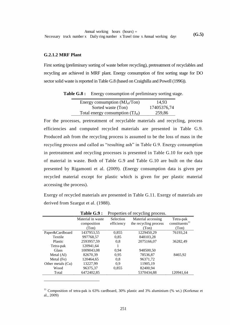
251
days workingAnnualx timeTravelx number ringDaily number x truck Necessary
(hours) hours workingAnnual
(G.5)
G.2.1.2 MRF Plant
First sorting (preliminary sorting of waste before recycling), pretreatment of recyclables and
recycling are achieved in MRF plant. Energy consumption of first sorting stage for DO
sector solid waste is reported in Table G.8 (based on Craighilla and Powell (1996)).
Table G.8 : Energy consumption of preliminary sorting stage.
Energy consumption (MJel/Ton) 14,93
Sorted waste (Ton) 17405376,74
Total energy consumption (TJel) 259,86
For the processes, pretreatment of recyclable materials and recycling, process
efficiencies and computed recycled materials are presented in Table G.9.
Produced ash from the recycling process is assumed to be the loss of mass in the
recycling process and called as “resulting ash” in Table G.9. Energy consumption
in pretreatment and recycling processes is presented in Table G.10 for each type
of material in waste. Both of Table G.9 and Table G.10 are built on the data
presented by Rigamonti et al. (2009). (Energy consumption data is given per
recycled material except for plastic which is given for per plastic material
accessing the process).
Exergy of recycled materials are presented in Table G.11. Exergy of materials are
derived from Szargut et al. (1988).
Table G.9 : Properties of recycling process.
Material in waste
composition
(Ton)
Selection
efficiency
Material accessing
the recycling process
(Ton)
Tetra-pak
constituents11
(Ton)
Paper&Cardboard 1437953,55 0,855 1229450,29 76193,24
Textile 997768,57 0,85 848103,28
Plastic 2593957,59 0,8 2075166,07 36282,49
Tetra-pak 120941,64 1
Glass 1009043,08 0,94 948500,50
Metal (Al) 82670,39 0,95 78536,87 8465,92
Metal (Fe) 120464,65 0,8 96371,72
Other metals (Cu) 13227,99 0,9 11905,19
Wood 96375,37 0,855 82400,94
Total 6472402,85 5370434,88 120941,64
11
Composition of tetra-pak is 63% cardboard, 30% plastic and 3% aluminium (% wt.) (Korkmaz et
al., 2009)
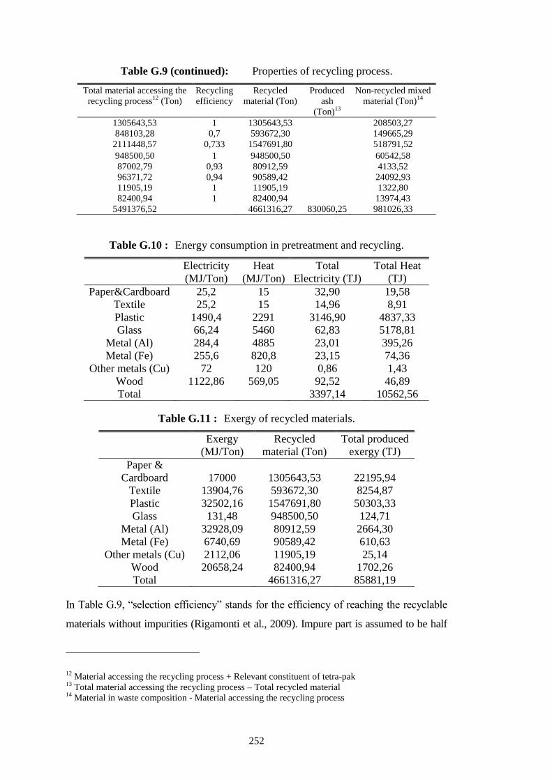
252
Table G.9 (continued): Properties of recycling process.
Total material accessing the
recycling process12
(Ton)
Recycling
efficiency
Recycled
material (Ton)
Produced
ash
(Ton)13
Non-recycled mixed
material (Ton)14
1305643,53 1 1305643,53 208503,27
848103,28 0,7 593672,30 149665,29
2111448,57 0,733 1547691,80 518791,52
948500,50 1 948500,50 60542,58
87002,79 0,93 80912,59 4133,52
96371,72 0,94 90589,42 24092,93
11905,19 1 11905,19 1322,80
82400,94 1 82400,94 13974,43
5491376,52 4661316,27 830060,25 981026,33
Table G.10 : Energy consumption in pretreatment and recycling.
Electricity
(MJ/Ton)
Heat
(MJ/Ton)
Total
Electricity (TJ)
Total Heat
(TJ)
Paper&Cardboard 25,2 15 32,90 19,58
Textile 25,2 15 14,96 8,91
Plastic 1490,4 2291 3146,90 4837,33
Glass 66,24 5460 62,83 5178,81
Metal (Al) 284,4 4885 23,01 395,26
Metal (Fe) 255,6 820,8 23,15 74,36
Other metals (Cu) 72 120 0,86 1,43
Wood 1122,86 569,05 92,52 46,89
Total 3397,14 10562,56
Table G.11 : Exergy of recycled materials.
Exergy
(MJ/Ton)
Recycled
material (Ton)
Total produced
exergy (TJ)
Paper &
Cardboard 17000 1305643,53 22195,94
Textile 13904,76 593672,30 8254,87
Plastic 32502,16 1547691,80 50303,33
Glass 131,48 948500,50 124,71
Metal (Al) 32928,09 80912,59 2664,30
Metal (Fe) 6740,69 90589,42 610,63
Other metals (Cu) 2112,06 11905,19 25,14
Wood 20658,24 82400,94 1702,26
Total
4661316,27 85881,19
In Table G.9, “selection efficiency” stands for the efficiency of reaching the recyclable
materials without impurities (Rigamonti et al., 2009). Impure part is assumed to be half
12
Material accessing the recycling process + Relevant constituent of tetra-pak 13
Total material accessing the recycling process – Total recycled material 14
Material in waste composition - Material accessing the recycling process
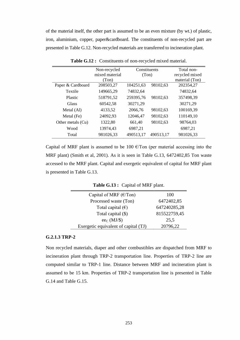
253
of the material itself, the other part is assumed to be an even mixture (by wt.) of plastic,
iron, aluminium, copper, paper&cardboard. The constituents of non-recycled part are
presented in Table G.12. Non-recycled materials are transferred to incineration plant.
Table G.12 : Constituents of non-recycled mixed material.
Non-recycled
mixed material
(Ton)
Constituents
(Ton)
Total non-
recycled mixed
material (Ton)
Paper & Cardboard 208503,27 104251,63 98102,63 202354,27
Textile 149665,29 74832,64 74832,64
Plastic 518791,52 259395,76 98102,63 357498,39
Glass 60542,58 30271,29 30271,29
Metal (Al) 4133,52 2066,76 98102,63 100169,39
Metal (Fe) 24092,93 12046,47 98102,63 110149,10
Other metals (Cu) 1322,80 661,40 98102,63 98764,03
Wood 13974,43 6987,21 6987,21
Total 981026,33 490513,17 490513,17 981026,33
Capital of MRF plant is assumed to be 100 €/Ton (per material accessing into the
MRF plant) (Smith et al, 2001). As it is seen in Table G.13, 6472402,85 Ton waste
accessed to the MRF plant. Capital and exergetic equivalent of capital for MRF plant
is presented in Table G.13.
Table G.13 : Capital of MRF plant.
Capital of MRF (€/Ton) 100
Processed waste (Ton) 6472402,85
Total capital (€) 647240285,28
Total capital ($) 815522759,45
eeC (MJ/$) 25,5
Exergetic equivalent of capital (TJ) 20796,22
G.2.1.3 TRP-2
Non recycled materials, diaper and other combustibles are dispatched from MRF to
incineration plant through TRP-2 transportation line. Properties of TRP-2 line are
computed similar to TRP-1 line. Distance between MRF and incineration plant is
assumed to be 15 km. Properties of TRP-2 transportation line is presented in Table
G.14 and Table G.15.
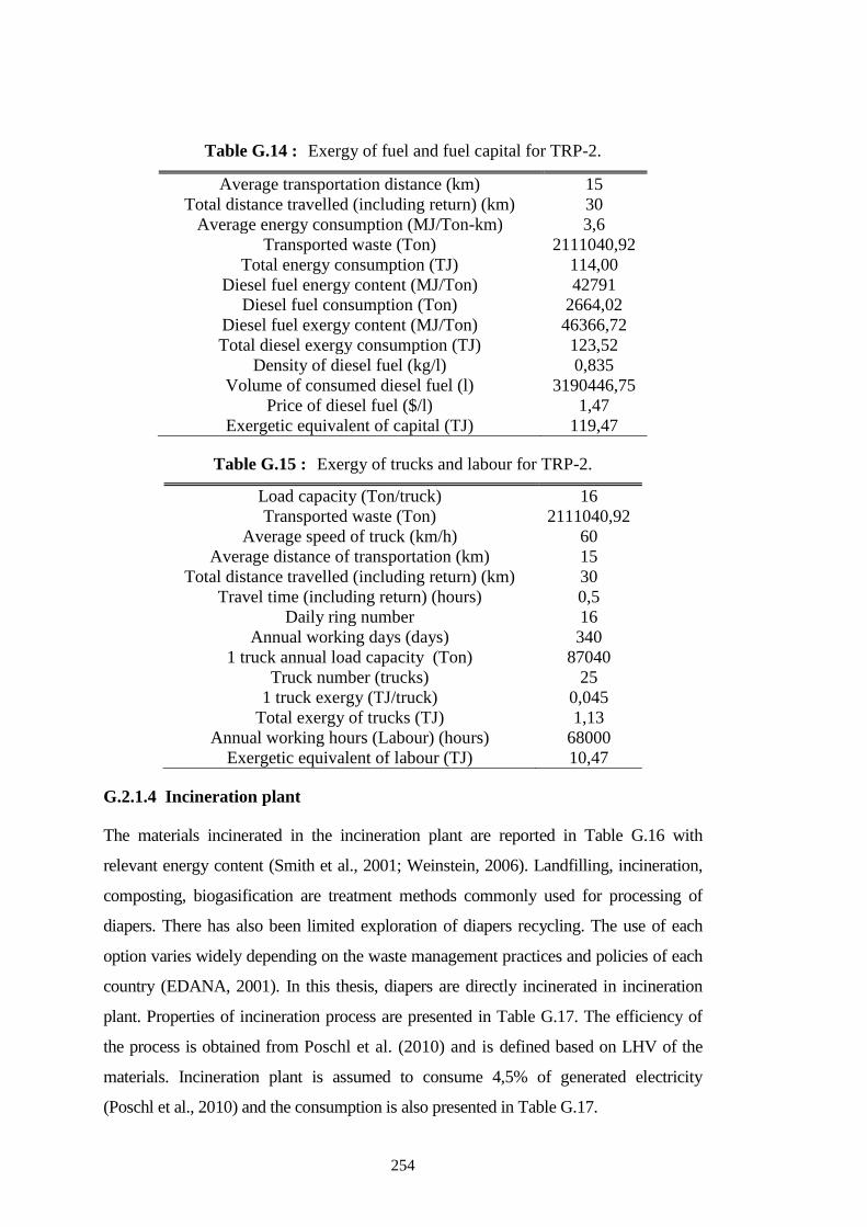
254
Table G.14 : Exergy of fuel and fuel capital for TRP-2.
Average transportation distance (km) 15
Total distance travelled (including return) (km) 30
Average energy consumption (MJ/Ton-km) 3,6
Transported waste (Ton) 2111040,92
Total energy consumption (TJ) 114,00
Diesel fuel energy content (MJ/Ton) 42791
Diesel fuel consumption (Ton) 2664,02
Diesel fuel exergy content (MJ/Ton) 46366,72
Total diesel exergy consumption (TJ) 123,52
Density of diesel fuel (kg/l) 0,835
Volume of consumed diesel fuel (l) 3190446,75
Price of diesel fuel ($/l) 1,47
Exergetic equivalent of capital (TJ) 119,47
Table G.15 : Exergy of trucks and labour for TRP-2.
Load capacity (Ton/truck) 16
Transported waste (Ton) 2111040,92
Average speed of truck (km/h) 60
Average distance of transportation (km) 15
Total distance travelled (including return) (km) 30
Travel time (including return) (hours) 0,5
Daily ring number 16
Annual working days (days) 340
1 truck annual load capacity (Ton) 87040
Truck number (trucks) 25
1 truck exergy (TJ/truck) 0,045
Total exergy of trucks (TJ) 1,13
Annual working hours (Labour) (hours) 68000
Exergetic equivalent of labour (TJ) 10,47
G.2.1.4 Incineration plant
The materials incinerated in the incineration plant are reported in Table G.16 with
relevant energy content (Smith et al., 2001; Weinstein, 2006). Landfilling, incineration,
composting, biogasification are treatment methods commonly used for processing of
diapers. There has also been limited exploration of diapers recycling. The use of each
option varies widely depending on the waste management practices and policies of each
country (EDANA, 2001). In this thesis, diapers are directly incinerated in incineration
plant. Properties of incineration process are presented in Table G.17. The efficiency of
the process is obtained from Poschl et al. (2010) and is defined based on LHV of the
materials. Incineration plant is assumed to consume 4,5% of generated electricity
(Poschl et al., 2010) and the consumption is also presented in Table G.17.
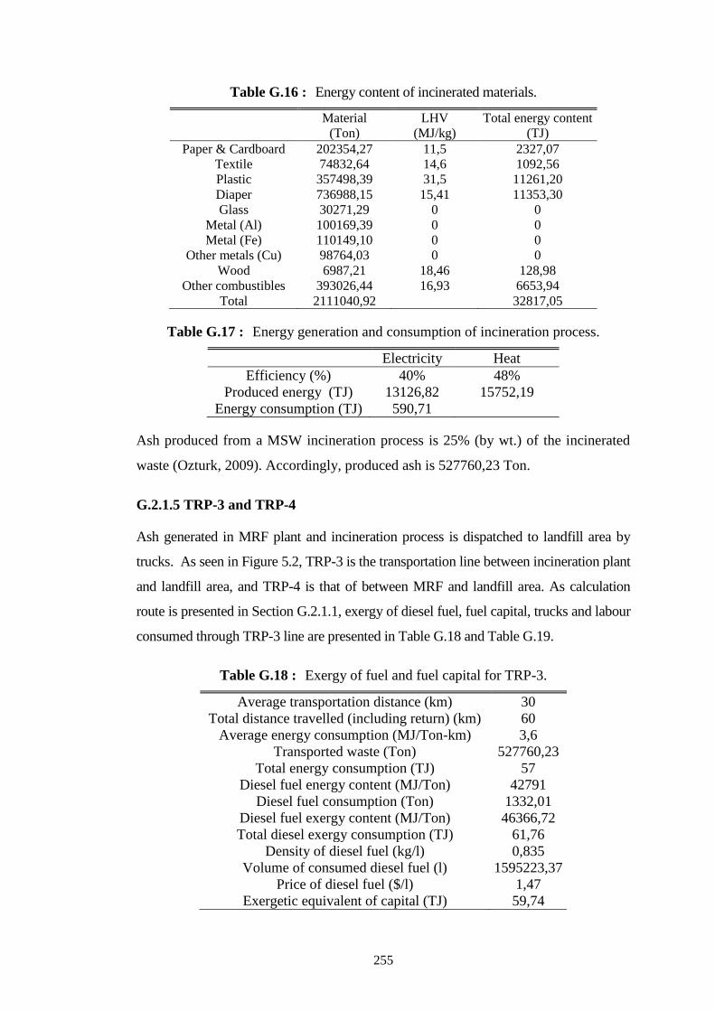
255
Table G.16 : Energy content of incinerated materials.
Material
(Ton)
LHV
(MJ/kg)
Total energy content
(TJ)
Paper & Cardboard 202354,27 11,5 2327,07
Textile 74832,64 14,6 1092,56
Plastic 357498,39 31,5 11261,20
Diaper 736988,15 15,41 11353,30
Glass 30271,29 0 0
Metal (Al) 100169,39 0 0
Metal (Fe) 110149,10 0 0
Other metals (Cu) 98764,03 0 0
Wood 6987,21 18,46 128,98
Other combustibles 393026,44 16,93 6653,94
Total 2111040,92 32817,05
Table G.17 : Energy generation and consumption of incineration process.
Electricity Heat
Efficiency (%) 40% 48%
Produced energy (TJ) 13126,82 15752,19
Energy consumption (TJ) 590,71
Ash produced from a MSW incineration process is 25% (by wt.) of the incinerated
waste (Ozturk, 2009). Accordingly, produced ash is 527760,23 Ton.
G.2.1.5 TRP-3 and TRP-4
Ash generated in MRF plant and incineration process is dispatched to landfill area by
trucks. As seen in Figure 5.2, TRP-3 is the transportation line between incineration plant
and landfill area, and TRP-4 is that of between MRF and landfill area. As calculation
route is presented in Section G.2.1.1, exergy of diesel fuel, fuel capital, trucks and labour
consumed through TRP-3 line are presented in Table G.18 and Table G.19.
Table G.18 : Exergy of fuel and fuel capital for TRP-3.
Average transportation distance (km) 30
Total distance travelled (including return) (km) 60
Average energy consumption (MJ/Ton-km) 3,6
Transported waste (Ton) 527760,23
Total energy consumption (TJ) 57
Diesel fuel energy content (MJ/Ton) 42791
Diesel fuel consumption (Ton) 1332,01
Diesel fuel exergy content (MJ/Ton) 46366,72
Total diesel exergy consumption (TJ) 61,76
Density of diesel fuel (kg/l) 0,835
Volume of consumed diesel fuel (l) 1595223,37
Price of diesel fuel ($/l) 1,47
Exergetic equivalent of capital (TJ) 59,74
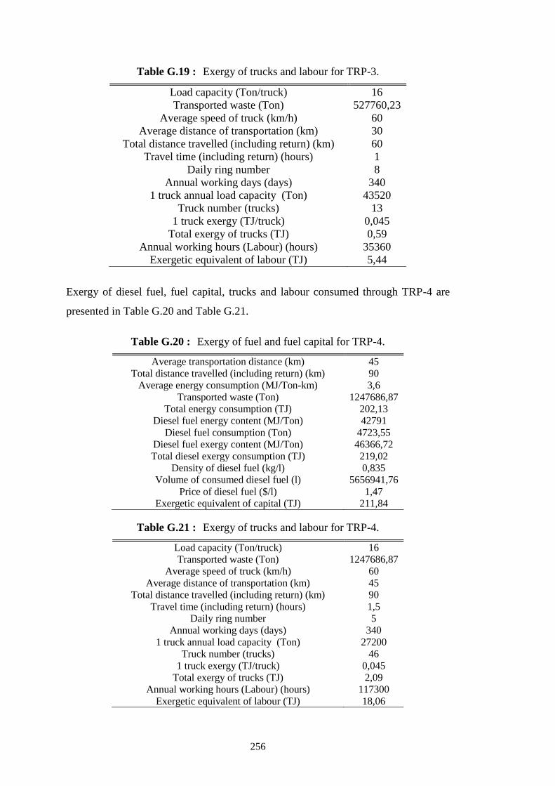
256
Table G.19 : Exergy of trucks and labour for TRP-3.
Load capacity (Ton/truck) 16
Transported waste (Ton) 527760,23
Average speed of truck (km/h) 60
Average distance of transportation (km) 30
Total distance travelled (including return) (km) 60
Travel time (including return) (hours) 1
Daily ring number 8
Annual working days (days) 340
1 truck annual load capacity (Ton) 43520
Truck number (trucks) 13
1 truck exergy (TJ/truck) 0,045
Total exergy of trucks (TJ) 0,59
Annual working hours (Labour) (hours) 35360
Exergetic equivalent of labour (TJ) 5,44
Exergy of diesel fuel, fuel capital, trucks and labour consumed through TRP-4 are
presented in Table G.20 and Table G.21.
Table G.20 : Exergy of fuel and fuel capital for TRP-4.
Average transportation distance (km) 45
Total distance travelled (including return) (km) 90
Average energy consumption (MJ/Ton-km) 3,6
Transported waste (Ton) 1247686,87
Total energy consumption (TJ) 202,13
Diesel fuel energy content (MJ/Ton) 42791
Diesel fuel consumption (Ton) 4723,55
Diesel fuel exergy content (MJ/Ton) 46366,72
Total diesel exergy consumption (TJ) 219,02
Density of diesel fuel (kg/l) 0,835
Volume of consumed diesel fuel (l) 5656941,76
Price of diesel fuel ($/l) 1,47
Exergetic equivalent of capital (TJ) 211,84
Table G.21 : Exergy of trucks and labour for TRP-4.
Load capacity (Ton/truck) 16
Transported waste (Ton) 1247686,87
Average speed of truck (km/h) 60
Average distance of transportation (km) 45
Total distance travelled (including return) (km) 90
Travel time (including return) (hours) 1,5
Daily ring number 5
Annual working days (days) 340
1 truck annual load capacity (Ton) 27200
Truck number (trucks) 46
1 truck exergy (TJ/truck) 0,045
Total exergy of trucks (TJ) 2,09
Annual working hours (Labour) (hours) 117300
Exergetic equivalent of labour (TJ) 18,06
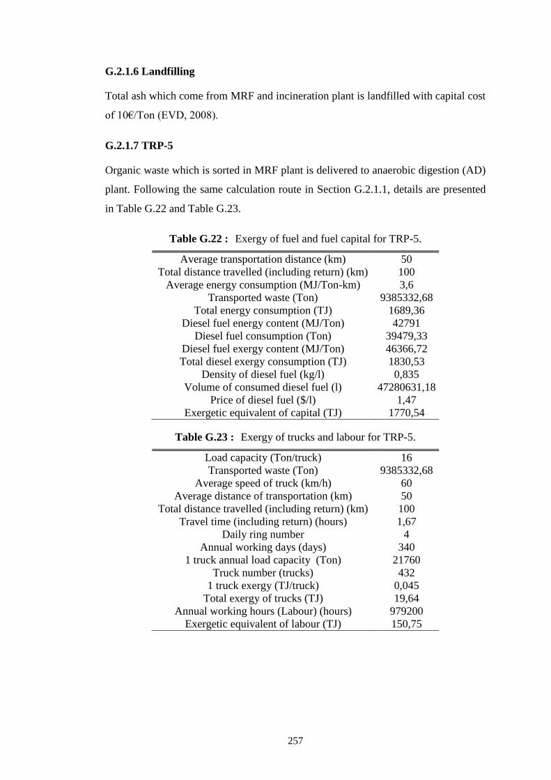
257
G.2.1.6 Landfilling
Total ash which come from MRF and incineration plant is landfilled with capital cost
of 10€/Ton (EVD, 2008).
G.2.1.7 TRP-5
Organic waste which is sorted in MRF plant is delivered to anaerobic digestion (AD)
plant. Following the same calculation route in Section G.2.1.1, details are presented
in Table G.22 and Table G.23.
Table G.22 : Exergy of fuel and fuel capital for TRP-5.
Average transportation distance (km) 50
Total distance travelled (including return) (km) 100
Average energy consumption (MJ/Ton-km) 3,6
Transported waste (Ton) 9385332,68
Total energy consumption (TJ) 1689,36
Diesel fuel energy content (MJ/Ton) 42791
Diesel fuel consumption (Ton) 39479,33
Diesel fuel exergy content (MJ/Ton) 46366,72
Total diesel exergy consumption (TJ) 1830,53
Density of diesel fuel (kg/l) 0,835
Volume of consumed diesel fuel (l) 47280631,18
Price of diesel fuel ($/l) 1,47
Exergetic equivalent of capital (TJ) 1770,54
Table G.23 : Exergy of trucks and labour for TRP-5.
Load capacity (Ton/truck) 16
Transported waste (Ton) 9385332,68
Average speed of truck (km/h) 60
Average distance of transportation (km) 50
Total distance travelled (including return) (km) 100
Travel time (including return) (hours) 1,67
Daily ring number 4
Annual working days (days) 340
1 truck annual load capacity (Ton) 21760
Truck number (trucks) 432
1 truck exergy (TJ/truck) 0,045
Total exergy of trucks (TJ) 19,64
Annual working hours (Labour) (hours) 979200
Exergetic equivalent of labour (TJ) 150,75
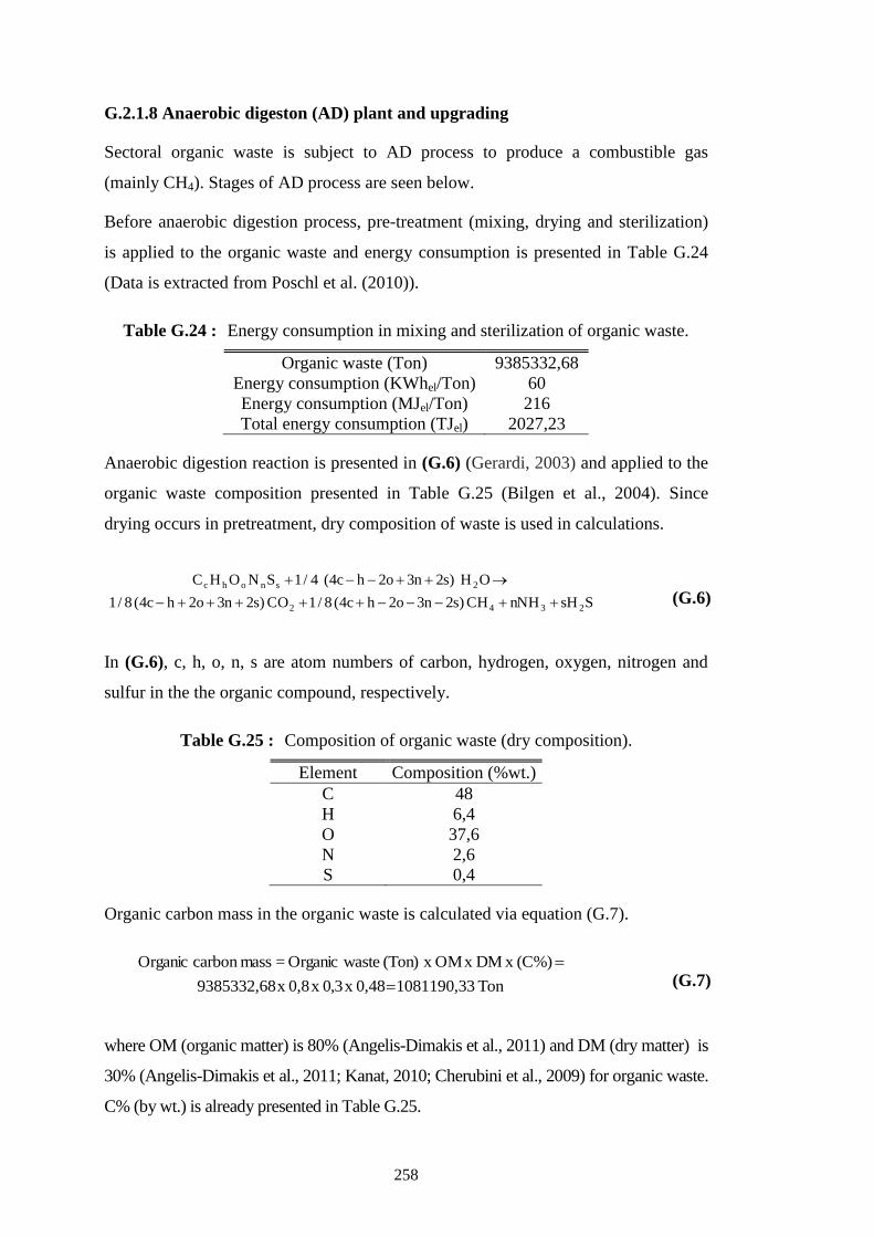
258
G.2.1.8 Anaerobic digeston (AD) plant and upgrading
Sectoral organic waste is subject to AD process to produce a combustible gas
(mainly CH4). Stages of AD process are seen below.
Before anaerobic digestion process, pre-treatment (mixing, drying and sterilization)
is applied to the organic waste and energy consumption is presented in Table G.24
(Data is extracted from Poschl et al. (2010)).
Table G.24 : Energy consumption in mixing and sterilization of organic waste.
Organic waste (Ton) 9385332,68
Energy consumption (KWhel/Ton) 60
Energy consumption (MJel/Ton) 216
Total energy consumption (TJel) 2027,23
Anaerobic digestion reaction is presented in (G.6) (Gerardi, 2003) and applied to the
organic waste composition presented in Table G.25 (Bilgen et al., 2004). Since
drying occurs in pretreatment, dry composition of waste is used in calculations.
SsHnNHCH)s2n3o2hc4(8/1CO)s2n3o2hc4(8/1
OH)s2n3o2hc4(4/1SNOHC
2342
2snohc
(G.6)
In (G.6), c, h, o, n, s are atom numbers of carbon, hydrogen, oxygen, nitrogen and
sulfur in the the organic compound, respectively.
Table G.25 : Composition of organic waste (dry composition).
Element Composition (%wt.)
C 48
H 6,4
O 37,6
N 2,6
S 0,4
Organic carbon mass in the organic waste is calculated via equation (G.7).
Ton1081190,330,48x 3,0x 0,8 x 9385332,68
(C%)x DMx OM x (Ton) wasteOrganic = masscarbon Organic
(G.7)
where OM (organic matter) is 80% (Angelis-Dimakis et al., 2011) and DM (dry matter) is
30% (Angelis-Dimakis et al., 2011; Kanat, 2010; Cherubini et al., 2009) for organic waste.
C% (by wt.) is already presented in Table G.25.
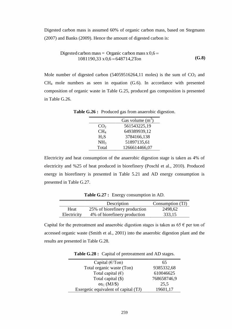
259
Digested carbon mass is assumed 60% of organic carbon mass, based on Stegmann
(2007) and Banks (2009). Hence the amount of digested carbon is:
Ton 648714,26,0x1081190,33
0,6xmasscarbon Organic = masscarbon Digested
(G.8)
Mole number of digested carbon (54059516264,11 moles) is the sum of CO2 and
CH4 mole numbers as seen in equation (G.6). In accordance with presented
composition of organic waste in Table G.25, produced gas composition is presented
in Table G.26.
Table G.26 : Produced gas from anaerobic digestion.
Gas volume (m3)
CO2 561543225,19
CH4 649389939,12
H2S 3784166,138
NH3 51897135,61
Total 1266614466,07
Electricity and heat consumption of the anaerobic digestion stage is taken as 4% of
electricity and %25 of heat produced in biorefinery (Poschl et al., 2010). Produced
energy in biorefinery is presented in Table 5.21 and AD energy consumption is
presented in Table G.27.
Table G.27 : Energy consumption in AD.
Description Consumption (TJ)
Heat 25% of biorefinery production 2498,62
Electricity 4% of biorefinery production 333,15
Capital for the pretreatment and anaerobic digestion stages is taken as 65 € per ton of
accessed organic waste (Smith et al., 2001) into the anaerobic digestion plant and the
results are presented in Table G.28.
Table G.28 : Capital of pretreatment and AD stages.
Capital (€/Ton) 65
Total organic waste (Ton) 9385332,68
Total capital (€) 610046625
Total capital ($) 768658746,9
eeC (MJ/$) 25,5
Exergetic equivalent of capital (TJ) 19601,17
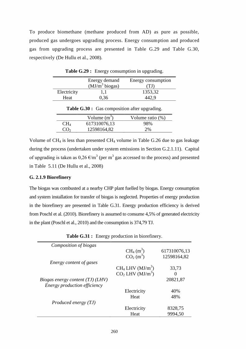
260
To produce biomethane (methane produced from AD) as pure as possible,
produced gas undergoes upgrading process. Energy consumption and produced
gas from upgrading process are presented in Table G.29 and Table G.30,
respectively (De Hullu et al., 2008).
Table G.29 : Energy consumption in upgrading.
Energy demand
(MJ/m3 biogas)
Energy consumption
(TJ)
Electricity 1,1 1353,32
Heat 0,36 442,9
Table G.30 : Gas composition after upgrading.
Volume (m3) Volume ratio (%)
CH4 617310076,13 98%
CO2 12598164,82 2%
Volume of CH4 is less than presented CH4 volume in Table G.26 due to gas leakage
during the process (undertaken under system emissions in Section G.2.1.11). Capital
of upgrading is taken as 0,26 €/m3 (per m
3 gas accessed to the process) and presented
in Table 5.11 (De Hullu et al., 2008)
G. 2.1.9 Biorefinery
The biogas was combusted at a nearby CHP plant fuelled by biogas. Energy consumption
and system installation for transfer of biogas is neglected. Properties of energy production
in the biorefinery are presented in Table G.31. Energy production efficiency is derived
from Poschl et al. (2010). Biorefinery is assumed to consume 4,5% of generated electricity
in the plant (Poschl et al., 2010) and the consumption is 374,79 TJ.
Table G.31 : Energy production in biorefinery.
Composition of biogas
CH4 (m3) 617310076,13
CO2 (m3) 12598164,82
Energy content of gases
CH4 LHV (MJ/m3) 33,73
CO2 LHV (MJ/m3) 0
Biogas energy content (TJ) (LHV) 20821,87
Energy production efficiency
Electricity 40%
Heat 48%
Produced energy (TJ)
Electricity 8328,75
Heat 9994,50
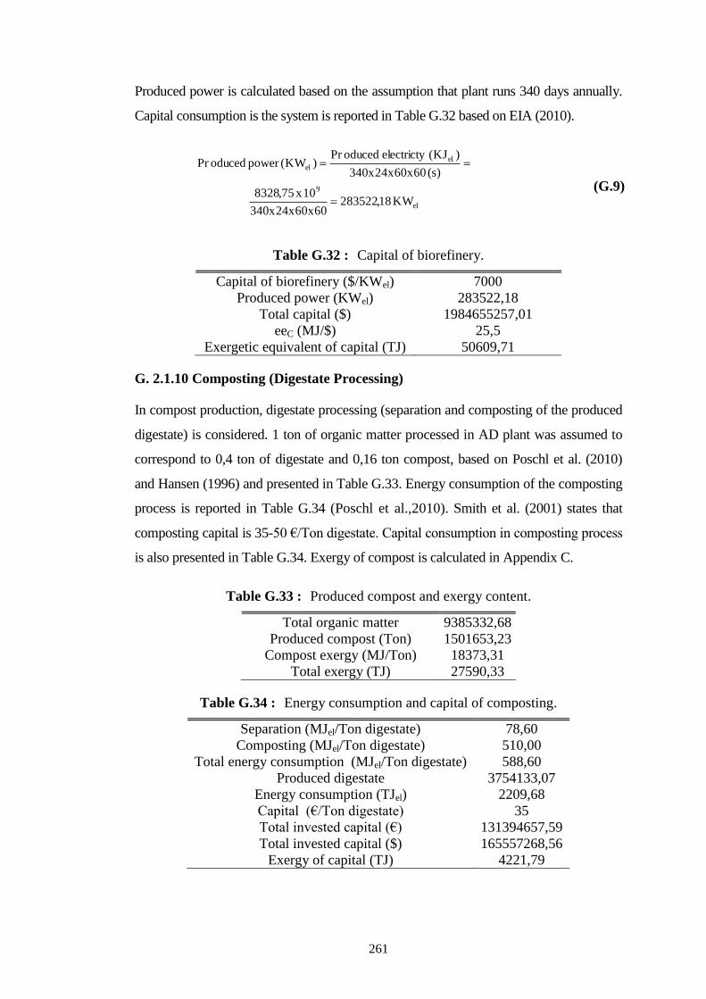
261
Produced power is calculated based on the assumption that plant runs 340 days annually.
Capital consumption is the system is reported in Table G.32 based on EIA (2010).
el
9
elel
KW18,28352260x60x24x340
10x75,8328
)s(60x60x24x340
)KJ(electrictyoducedPr)KW(poweroducedPr
(G.9)
Table G.32 : Capital of biorefinery.
Capital of biorefinery ($/KWel)
7000
Produced power (KWel) 283522,18
Total capital ($) 1984655257,01
eeC (MJ/$) 25,5
Exergetic equivalent of capital (TJ) 50609,71
G. 2.1.10 Composting (Digestate Processing)
In compost production, digestate processing (separation and composting of the produced
digestate) is considered. 1 ton of organic matter processed in AD plant was assumed to
correspond to 0,4 ton of digestate and 0,16 ton compost, based on Poschl et al. (2010)
and Hansen (1996) and presented in Table G.33. Energy consumption of the composting
process is reported in Table G.34 (Poschl et al.,2010). Smith et al. (2001) states that
composting capital is 35-50 €/Ton digestate. Capital consumption in composting process
is also presented in Table G.34. Exergy of compost is calculated in Appendix C.
Table G.33 : Produced compost and exergy content.
Total organic matter 9385332,68
Produced compost (Ton) 1501653,23
Compost exergy (MJ/Ton) 18373,31
Total exergy (TJ) 27590,33
Table G.34 : Energy consumption and capital of composting.
Separation (MJel/Ton digestate) 78,60
Composting (MJel/Ton digestate) 510,00
Total energy consumption (MJel/Ton digestate) 588,60
Produced digestate 3754133,07
Energy consumption (TJel) 2209,68
Capital (€/Ton digestate) 35
Total invested capital (€) 131394657,59
Total invested capital ($) 165557268,56
Exergy of capital (TJ) 4221,79
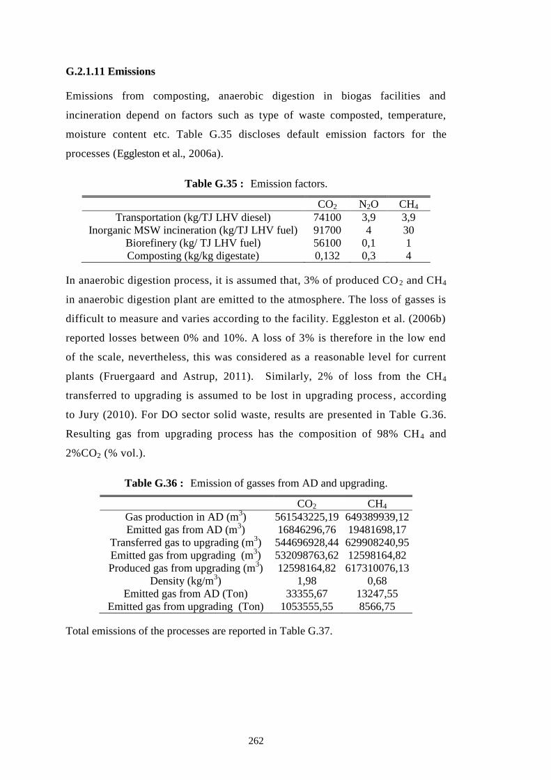
262
G.2.1.11 Emissions
Emissions from composting, anaerobic digestion in biogas facilities and
incineration depend on factors such as type of waste composted, temperature,
moisture content etc. Table G.35 discloses default emission factors for the
processes (Eggleston et al., 2006a).
Table G.35 : Emission factors.
CO2 N2O CH4
Transportation (kg/TJ LHV diesel) 74100 3,9 3,9
Inorganic MSW incineration (kg/TJ LHV fuel) 91700 4 30
Biorefinery (kg/ TJ LHV fuel) 56100 0,1 1
Composting (kg/kg digestate) 0,132 0,3 4
In anaerobic digestion process, it is assumed that, 3% of produced CO 2 and CH4
in anaerobic digestion plant are emitted to the atmosphere. The loss of gasses is
difficult to measure and varies according to the facility. Eggleston et al. (2006b)
reported losses between 0% and 10%. A loss of 3% is therefore in the low end
of the scale, nevertheless, this was considered as a reasonable level for current
plants (Fruergaard and Astrup, 2011). Similarly, 2% of loss from the CH4
transferred to upgrading is assumed to be lost in upgrading process , according
to Jury (2010). For DO sector solid waste, results are presented in Table G.36.
Resulting gas from upgrading process has the composition of 98% CH4 and
2%CO2 (% vol.).
Table G.36 : Emission of gasses from AD and upgrading.
CO2 CH4
Gas production in AD (m3) 561543225,19 649389939,12
Emitted gas from AD (m3) 16846296,76 19481698,17
Transferred gas to upgrading (m3) 544696928,44 629908240,95
Emitted gas from upgrading (m3) 532098763,62 12598164,82
Produced gas from upgrading (m3) 12598164,82 617310076,13
Density (kg/m3) 1,98 0,68
Emitted gas from AD (Ton) 33355,67 13247,55
Emitted gas from upgrading (Ton) 1053555,55 8566,75
Total emissions of the processes are reported in Table G.37.

263
Table G.37 : Emissions from TRP lines and processes.
CO2 (Ton) N2O (Ton) CH4 (Ton)
TRP-1 1326818,40 69,83 69,83
TRP-2 8447,12 0,44 0,44
TRP-3 4223,56 0,22 0,22
TRP-4 14977,48 0,79 0,79
TRP-5 125181,57 6,59 6,59
Incineration 3009323,85 131,27 984,51
AD 33355,67 0,00 13247,55
Upgrading of biogas 1053555,55 0,00 8566,75
Biorefinery 1168106,84 2,08 20,82
Composting 495545,57 1126,24 15016,53
Total 7239535,61 1337,47 37914,05
The same calculation route (presented above) is applied to TE and IN sector solid
waste and corresponding results are presented in Section 5.4.2.2 and 5.4.2.3.
G.2.2 CO sector solid waste environmental remediation system
The fraction of CO sector solid waste matching with DO sector solid waste
composition (Table 5.58) undergoes the same treatment procedure explained in
Section G.2.1. As for the part of “others” which consists of refinery and coke
factories waste, below detailed procedure is applied.
G.2.2.1 TRP-6
Transportation distance of TRP-6 (Figure 5.3) is assumed to be equal to sum of that of TRP-
1 and TRP2. Distances of TRP-1 and TRP-2 are presented in Table G.6 and Table G.14 as
188,33 and 15 km, respectively. As a result, TRP-6 transportation distance is 203,33 km.
Properties of TRP-6 transportation line is presented in Table G.38 and Table G.39.
Table G.38 : Exergy of fuel and fuel capital for TRP-6.
Average transportation distance (km) 203,33
Total distance travelled (including return) (km) 406,67
Average energy consumption (MJ/Ton-km) 3,6
Transported waste (Ton) 23678,32
Total energy consumption (TJ) 17,33
Diesel fuel energy content (MJ/Ton) 42791
Diesel fuel consumption (Ton) 405,05
Diesel fuel exergy content (MJ/Ton) 46366,72
Total diesel exergy consumption (TJ) 18,78
Density of diesel fuel (kg/l) 0,835
Volume of consumed diesel fuel (l) 485090,79
Price of diesel fuel ($/l) 1,47
Exergetic equivalent of capital (TJ) 18,17

264
Table G.39 : Exergy of trucks and labour for TRP-6.
Load capacity (Ton/truck) 16
Transported waste (Ton) 23678,32
Average speed of truck (km/h) 60
Average distance of transportation (km) 203,33
Total distance travelled (including return) (km) 406,67
Travel time (including return) (hours) 6,78
Daily ring number 1
Annual working days (days) 340
1 truck annual load capacity (Ton) 5440
Truck number (trucks) 5
1 truck exergy (TJ/truck) 0,045
Total exergy of trucks (TJ) 0,23
Annual working hours (Labour) (hours) 11522
Exergetic equivalent of labour (TJ) 1,77
G.2.2.2 IGCC plant
The composition of petroleum refining and coke processing waste which is
considered in this thesis, is presented in Table G.40. Produced syngas from raw
materials (coke, vacuum residue and petrocoke) are assumed to be 2,85 m3/kg-raw-
material (Tian et al., 2009). Energy need of the system is assumed to be 3% of the
system energy production (Marin Sanchez and Rodriguez Toral, 2007). Properties of
produced syngas and generated electricity with efficiecy of 40% (based on LHV) are
presented in Table G.40. In Table G.40, LHV and HHV of produced syngas is
retrieved from Marin Sanchez and Rodriguez Toral (2007) and U.S. Department of
Energy National Energy Technology Laboratory (2002b).
Table G.40 : Properties of syngas and electricity production in IGCC.
Coke Vacuum
residue
Petrocoke Total
Raw material (Ton) 11839,16 5919,58 5919,58 23678,32
Produced syngas (m3) 33741606 16870803 16870803 67483212
Syngas LHV (MJ/m3) 10,69 14,09 10,35
Syngas HHV (MJ/m3) 10,92 14,4 10,57
Energy (LHV) of syngas (TJ) 360,75 237,76 174,55 773,06
Energy (HHV) of syngas (TJ) 368,58 242,92 178,3 789,80
Produced energy (TJel) 309,22
IGCC energy consumption (TJel) 9,28
Net energy production (TJel) 299,94
Cost of IGCC plant is computed based on data retrieved from Garcia et al. (2006)
and exergetic equivalent of capital is computed in Table G.41. Power is computed by
the equation (5.18).
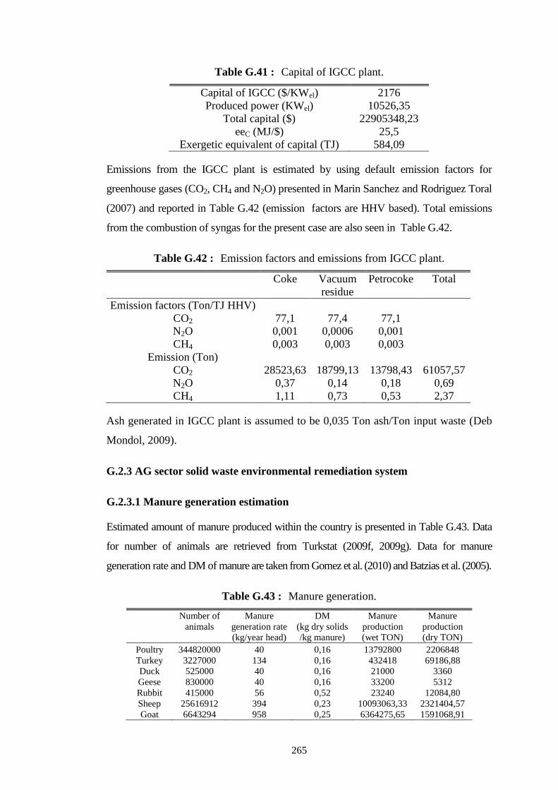
265
Table G.41 : Capital of IGCC plant.
Capital of IGCC ($/KWel) 2176
Produced power (KWel) 10526,35
Total capital ($) 22905348,23
eeC (MJ/$) 25,5
Exergetic equivalent of capital (TJ) 584,09
Emissions from the IGCC plant is estimated by using default emission factors for
greenhouse gases (CO2, CH4 and N2O) presented in Marin Sanchez and Rodriguez Toral
(2007) and reported in Table G.42 (emission factors are HHV based). Total emissions
from the combustion of syngas for the present case are also seen in Table G.42.
Table G.42 : Emission factors and emissions from IGCC plant.
Coke Vacuum
residue
Petrocoke Total
Emission factors (Ton/TJ HHV)
CO2 77,1 77,4 77,1
N2O 0,001 0,0006 0,001
CH4 0,003 0,003 0,003
Emission (Ton)
CO2 28523,63 18799,13 13798,43 61057,57
N2O 0,37 0,14 0,18 0,69
CH4 1,11 0,73 0,53 2,37
Ash generated in IGCC plant is assumed to be 0,035 Ton ash/Ton input waste (Deb
Mondol, 2009).
G.2.3 AG sector solid waste environmental remediation system
G.2.3.1 Manure generation estimation
Estimated amount of manure produced within the country is presented in Table G.43. Data
for number of animals are retrieved from Turkstat (2009f, 2009g). Data for manure
generation rate and DM of manure are taken from Gomez et al. (2010) and Batzias et al. (2005).
Table G.43 : Manure generation.
Number of
animals
Manure
generation rate
(kg/year head)
DM
(kg dry solids
/kg manure)
Manure
production
(wet TON)
Manure
production
(dry TON)
Poultry 344820000 40 0,16 13792800 2206848
Turkey 3227000 134 0,16 432418 69186,88
Duck 525000 40 0,16 21000 3360
Geese 830000 40 0,16 33200 5312
Rubbit 415000 56 0,52 23240 12084,80
Sheep 25616912 394 0,23 10093063,33 2321404,57
Goat 6643294 958 0,25 6364275,65 1591068,91
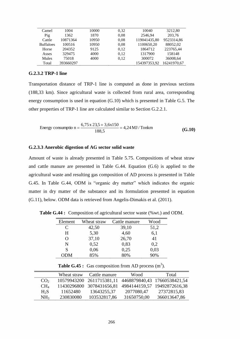
266
Camel 1004 10000 0,32 10040 3212,80
Pig 1362 1870 0,08 2546,94 203,76
Cattle 10871364 10950 0,08 119041435,80 9523314,86
Buffaloes 100516 10950 0,08 1100650,20 88052,02
Horse 204352 9125 0,12 1864712 223765,44
Asses 329475 4000 0,12 1317900 158148
Mules 75018 4000 0,12 300072 36008,64
Total 393660297 154397353,92 16241970,67
G.2.3.2 TRP-1 line
Transportation distance of TRP-1 line is computed as done in previous sections
(188,33 km). Since agricultural waste is collected from rural area, corresponding
energy consumption is used in equation (G.10) which is presented in Table G.5. The
other properties of TRP-1 line are calculated similar to Section G.2.2.1.
Tonkm/MJ24,4188,5
3,6x1505,23x6,75nconsumptionergyE
(G.10)
G.2.3.3 Anerobic digestion of AG sector solid waste
Amount of waste is already presented in Table 5.75. Compositions of wheat straw
and cattle manure are presented in Table G.44. Equation (G.6) is applied to the
agricultural waste and resulting gas composition of AD process is presented in Table
G.45. In Table G.44, ODM is “organic dry matter” which indicates the organic
matter in dry matter of the substance and its formulation presented in equation
(G.11), below. ODM data is retrieved from Angelis-Dimakis et al. (2011).
Table G.44 : Composition of agricultural sector waste (%wt.) and ODM.
Element Wheat straw Cattle manure Wood
C 42,50 39,10 51,2
H 5,30 4,60 6,1
O 37,10 26,70 41
N 0,52 0,83 0,2
S 0,06 0,25 0,03
ODM 85% 80% 90%
Table G.45 : Gas composition from AD process (m3).
Wheat straw Cattle manure Wood Total
CO2 10579943200 2611715381,11 4468879840,43 17660538421,54
CH4 11430296800 3078431656,81 4984144159,57 19492872616,38
H2S 11652480 13643255,37 2077080,47 27372815,83
NH3 230830080 103532817,86 31650750,00 366013647,86
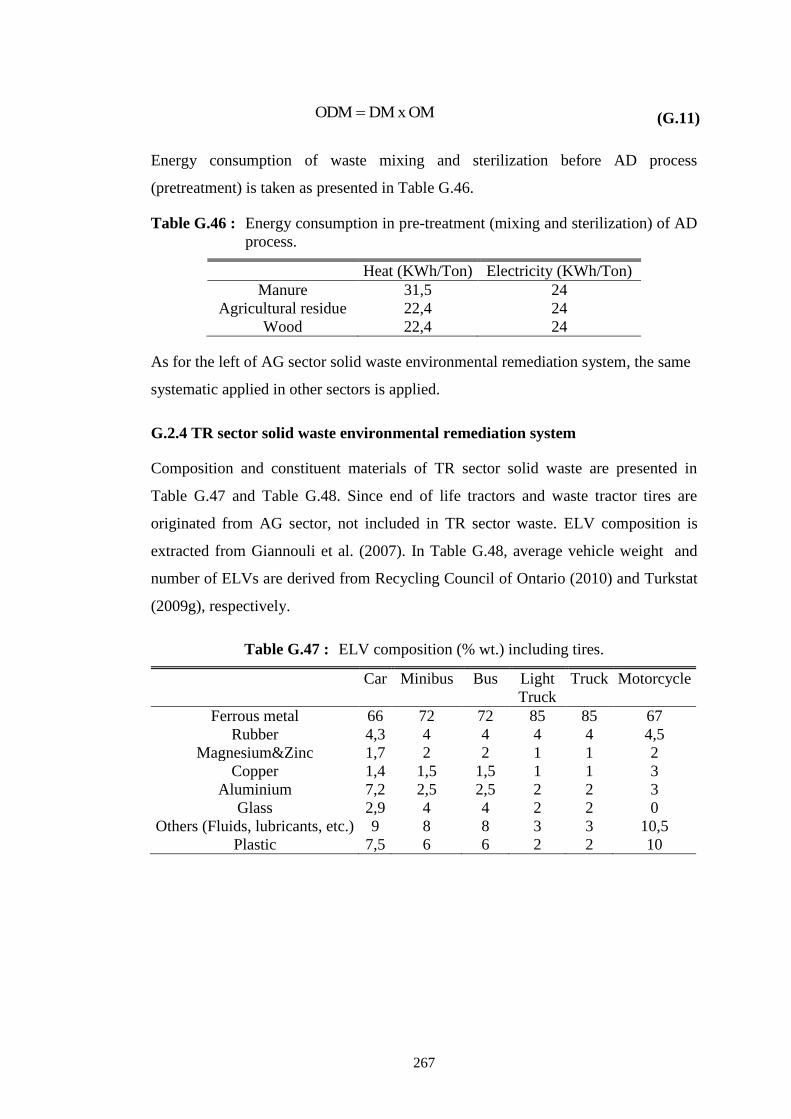
267
OMxDMODM (G.11)
Energy consumption of waste mixing and sterilization before AD process
(pretreatment) is taken as presented in Table G.46.
Table G.46 : Energy consumption in pre-treatment (mixing and sterilization) of AD
process.
Heat (KWh/Ton) Electricity (KWh/Ton)
Manure 31,5 24
Agricultural residue 22,4 24
Wood 22,4 24
As for the left of AG sector solid waste environmental remediation system, the same
systematic applied in other sectors is applied.
G.2.4 TR sector solid waste environmental remediation system
Composition and constituent materials of TR sector solid waste are presented in
Table G.47 and Table G.48. Since end of life tractors and waste tractor tires are
originated from AG sector, not included in TR sector waste. ELV composition is
extracted from Giannouli et al. (2007). In Table G.48, average vehicle weight and
number of ELVs are derived from Recycling Council of Ontario (2010) and Turkstat
(2009g), respectively.
Table G.47 : ELV composition (% wt.) including tires.
Car Minibus Bus Light
Truck
Truck Motorcycle
Ferrous metal 66 72 72 85 85 67
Rubber 4,3 4 4 4 4 4,5
Magnesium&Zinc 1,7 2 2 1 1 2
Copper 1,4 1,5 1,5 1 1 3
Aluminium 7,2 2,5 2,5 2 2 3
Glass 2,9 4 4 2 2 0
Others (Fluids, lubricants, etc.) 9 8 8 3 3 10,5
Plastic 7,5 6 6 2 2 10
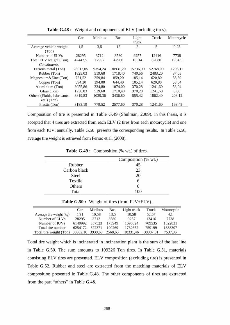
268
Table G.48 : Weight and components of ELV (including tires).
Car Minibus Bus Light
truck
Truck Motorcycle
Average vehicle weight
(Ton)
1,5 3,5 12 2 5 0,25
Number of ELVs
28295 3712 3580 9257 12416 7738
Total ELV weight (Ton) 42442,5 12992 42960 18514 62080 1934,5
Constituents:
Ferrous metal (Ton) 28012,05 9354,24 30931,20 15736,90 52768,00 1296,12
Rubber (Ton) 1825,03 519,68 1718,40 740,56 2483,20 87,05
Magnesium&Zinc (Ton) 721,52 259,84 859,20 185,14 620,80 38,69
Copper (Ton) 594,20 194,88 644,40 185,14 620,80 58,04
Aluminium (Ton) 3055,86 324,80 1074,00 370,28 1241,60 58,04
Glass (Ton) 1230,83 519,68 1718,40 370,28 1241,60 0,00
Others (Fluids, lubricants,
etc.) (Ton)
3819,83 1039,36 3436,80 555,42 1862,40 203,12
Plastic (Ton) 3183,19 779,52 2577,60 370,28 1241,60 193,45
Composition of tire is presented in Table G.49 (Shulman, 2009). In this thesis, it is
accepted that 4 tires are extracted from each ELV (2 tires from each motorcycle) and one
from each IUV, annually. Table G.50 presents the corresponding results. In Table G.50,
average tire weight is retrieved from Ferrao et al. (2008).
Table G.49 : Composition (% wt.) of tires.
Composition (% wt.)
Rubber 45
Carbon black 23
Steel 20
Textile 6
Others 6
Total 100
Table G.50 : Weight of tires (from IUV+ELV).
Car Minibus Bus Light truck Truck Motorcycle
Average tire weight (kg) 5,91 10,58 13,5 10,58 52,67 4,1
Number of ELVs
28295 3712 3580 9257 12416 7738
Number of IUVs
6140992 357523 175949 1695624 709535 1822831
Total tire number 6254172 372371 190269 1732652 759199 1838307
Total tire weight (Ton) 36962,16 3939,69 2568,63 18331,46 39987,01 7537,06
Total tire weight which is incinerated in incineration plant is the sum of the last line
in Table G.50. The sum amounts to 109326 Ton tires. In Table G.51, materials
consisting ELV tires are presented. ELV composition (excluding tire) is presented in
Table G.52. Rubber and steel are extracted from the matching materials of ELV
composition presented in Table G.48. The other components of tires are extracted
from the part “others” in Table G.48.
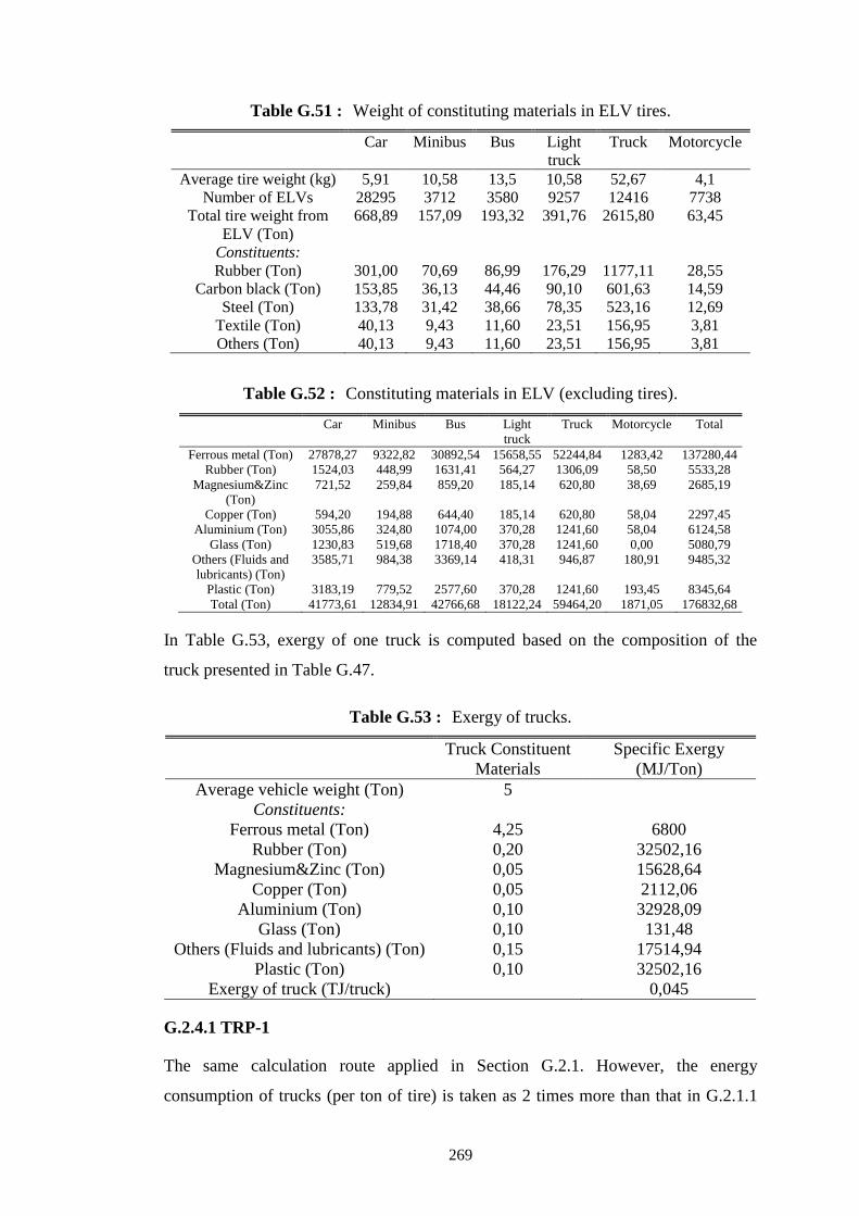
269
Table G.51 : Weight of constituting materials in ELV tires.
Car Minibus Bus Light
truck
Truck Motorcycle
Average tire weight (kg) 5,91 10,58 13,5 10,58 52,67 4,1
Number of ELVs 28295 3712 3580 9257 12416 7738
Total tire weight from
ELV (Ton)
668,89 157,09 193,32 391,76 2615,80 63,45
Constituents:
Rubber (Ton) 301,00 70,69 86,99 176,29 1177,11 28,55
Carbon black (Ton) 153,85 36,13 44,46 90,10 601,63 14,59
Steel (Ton) 133,78 31,42 38,66 78,35 523,16 12,69
Textile (Ton) 40,13 9,43 11,60 23,51 156,95 3,81
Others (Ton) 40,13 9,43 11,60 23,51 156,95 3,81
Table G.52 : Constituting materials in ELV (excluding tires).
Car Minibus Bus Light
truck
Truck Motorcycle Total
Ferrous metal (Ton) 27878,27 9322,82 30892,54 15658,55 52244,84 1283,42 137280,44
Rubber (Ton) 1524,03 448,99 1631,41 564,27 1306,09 58,50 5533,28
Magnesium&Zinc
(Ton)
721,52 259,84 859,20 185,14 620,80 38,69 2685,19
Copper (Ton) 594,20 194,88 644,40 185,14 620,80 58,04 2297,45
Aluminium (Ton) 3055,86 324,80 1074,00 370,28 1241,60 58,04 6124,58
Glass (Ton) 1230,83 519,68 1718,40 370,28 1241,60 0,00 5080,79
Others (Fluids and
lubricants) (Ton)
3585,71 984,38 3369,14 418,31 946,87 180,91 9485,32
Plastic (Ton) 3183,19 779,52 2577,60 370,28 1241,60 193,45 8345,64
Total (Ton) 41773,61 12834,91 42766,68 18122,24 59464,20 1871,05 176832,68
In Table G.53, exergy of one truck is computed based on the composition of the
truck presented in Table G.47.
Table G.53 : Exergy of trucks.
Truck Constituent
Materials
Specific Exergy
(MJ/Ton)
Average vehicle weight (Ton) 5
Constituents:
Ferrous metal (Ton) 4,25 6800
Rubber (Ton) 0,20 32502,16
Magnesium&Zinc (Ton) 0,05 15628,64
Copper (Ton) 0,05 2112,06
Aluminium (Ton) 0,10 32928,09
Glass (Ton) 0,10 131,48
Others (Fluids and lubricants) (Ton) 0,15 17514,94
Plastic (Ton) 0,10 32502,16
Exergy of truck (TJ/truck) 0,045
G.2.4.1 TRP-1
The same calculation route applied in Section G.2.1. However, the energy
consumption of trucks (per ton of tire) is taken as 2 times more than that in G.2.1.1

270
since tires have holes in their centers and it is assumed that 1 truck tire carrying
capacity is 8 Ton in collection phase. Hence average energy consumption of waste
collection is:
Tonkm/MJ92,102x46,5nconsumptionergyE (G.12)
The properties of the TRP line are computed in line with the Section G.2.1.1. The
computation route applied in other TRP lines of TR sector is identical to that of
presented TRP lines in Section G.2.1.1.
G.2.4.2 MRF Plant
Processes involved in MRF are dismantling, shredding and recycling and also tyre
shredding. Capital and energy consumption of MRF plant are sum of capital and sum
of energy consumption of these processes. Results are presented below.
Dismantling of ELVs
Energy consumption and capital of the dismantler are presented in Table G.54 and
Table G.55, respectively. Data is obtained based on Ferrao and Amaral (2006).
Table G.54 : Energy consumption of dismantling process.
Energy consumption 3,68 KWh/ton (13,25 MJ/ton)
Total weight of vehicles (Ton) 180923
Total energy consumption (TJ) 2,40
Table G.55 : Capital of dismantling.
Capital of dismantler (€/Ton) 5,24
Capital of dismantler ($/Ton) 6,6
Total weight of vehicles (Ton) 180923
Total capital (€) 948657,87
Total capital ($) 1195308,92
eeC (MJ/$) 25,5
Exergetic equivalent of capital (TJ) 30,48
Shredding of ELVs
The part of vehicles which are subject to shredding is total weight of vehicles
excluding tires except the part “others” in Table G.52. Energy consumption and
capital of the process are presented in Table G.56 and Table G.57, respectively. Data
is obtained based on Ferrao and Amaral (2006).
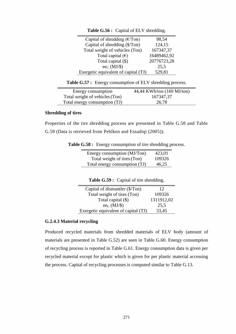
271
Table G.56 : Capital of ELV shredding.
Capital of shredding (€/Ton) 98,54
Capital of shredding ($/Ton) 124,15
Total weight of vehicles (Ton) 167347,37
Total capital (€) 16489462,92
Total capital ($) 20776723,28
eeC (MJ/$) 25,5
Exergetic equivalent of capital (TJ) 529,81
Table G.57 : Energy consumption of ELV shredding process.
Energy consumption 44,44 KWh/ton (160 MJ/ton)
Total weight of vehicles (Ton) 167347,37
Total energy consumption (TJ) 26,78
Shredding of tires
Properties of the tire shredding process are presented in Table G.58 and Table
G.59 (Data is retrieved from Pehlken and Essadiqi (2005)).
Table G.58 : Energy consumption of tire shredding process.
Energy consumption (MJ/Ton) 423,01
Total weight of tires (Ton) 109326
Total energy consumption (TJ) 46,25
Table G.59 : Capital of tire shredding.
Capital of dismantler ($/Ton) 12
Total weight of tires (Ton) 109326
Total capital ($) 1311912,02
eeC (MJ/$) 25,5
Exergetic equivalent of capital (TJ) 33,45
G.2.4.3 Material recycling
Produced recycled materials from shredded materials of ELV body (amount of
materials are presented in Table G.52) are seen in Table G.60. Energy consumption
of recycling process is reported in Table G.61. Energy consumption data is given per
recycled material except for plastic which is given for per plastic material accessing
the process. Capital of recycling processes is computed similar to Table G.13.

272
Table G.60 : Properties of recycling of ELVs.
Material in waste
composition
(Ton)
Recycling
efficiency
Recycled
material
(Ton)
Produced
ash
(Ton)
Ferrous metal (Ton) 137280,44 0,94 129043,61
Rubber (Ton) 5533,28 0,733 4055,89
Magnesium&Zinc (Ton) 2685,19 0,94 2524,08
Copper (Ton) 2297,45 1 2297,45
Aluminium (Ton) 6124,58 0,93 5695,86
Glass (Ton) 5080,79 1 5080,79
Plastic (Ton) 8345,64 0,733 6117,35
Total (Ton) 167347,37 154815,04 12532,33
Table G.61 : Energy consumption in recycling.
Electricity
(MJ/Ton)
Heat
(MJ/Ton)
Total
Electricity (TJ)
Total
Heat (TJ)
Ferrous metal 255,6 820,8 32,98 105,92
Rubber 1490,4 2291 8,25 12,68
Magnesium 72 11400 0,09 14,39
Zinc 72 37000 0,09 46,70
Copper 72 120 0,17 0,28
Aluminium 284,4 4885 1,62 27,82
Glass 66,24 5460 0,34 27,74
Plastic 1490,4 2291 12,44 19,12
Total 55,97 254,64
G.2.4.4 Incineration of tires
Energy generation and energy need of tire incineration process is presented in Table
G.62. Incineration plant is assumed to consume 4,5% of generated electricity by the
CHP plant (Poschl et al., 2010) and the consumption is also presented in Table G.62.
In Table G.62, tire energy content is obtained from Vest (2000).
Table G.62 : Energy generation and consumption of incineration process.
Electricity Heat
Tire weight (Ton) 109326
Tire energy content (MJ/Ton) 29000
Efficiency (%) 40% 46%
Produced energy (TJ) 1268,18 1458,41
Energy consumption (TJ) 57,07
Ash produced from tire incineration process is taken as 25% (by wt.) of the
incinerated tires based on Ozturk (2009). Accordingly, produced as from the process
is 27331,50 Ton which is landfilled.
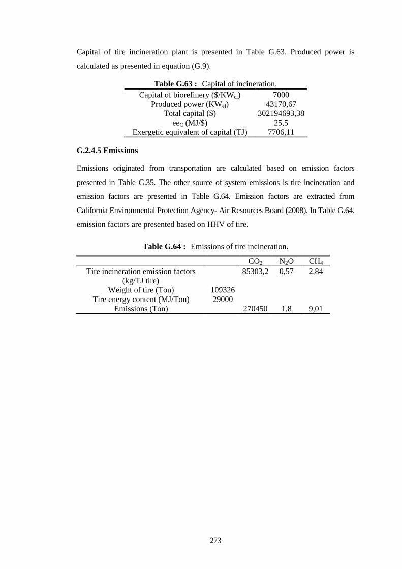
273
Capital of tire incineration plant is presented in Table G.63. Produced power is
calculated as presented in equation (G.9).
Table G.63 : Capital of incineration.
Capital of biorefinery ($/KWel) 7000
Produced power (KWel) 43170,67
Total capital ($) 302194693,38
eeC (MJ/$) 25,5
Exergetic equivalent of capital (TJ) 7706,11
G.2.4.5 Emissions
Emissions originated from transportation are calculated based on emission factors
presented in Table G.35. The other source of system emissions is tire incineration and
emission factors are presented in Table G.64. Emission factors are extracted from
California Environmental Protection Agency- Air Resources Board (2008). In Table G.64,
emission factors are presented based on HHV of tire.
Table G.64 : Emissions of tire incineration.
CO2 N2O CH4
Tire incineration emission factors
(kg/TJ tire)
85303,2 0,57 2,84
Weight of tire (Ton) 109326
Tire energy content (MJ/Ton) 29000
Emissions (Ton) 270450 1,8 9,01

274
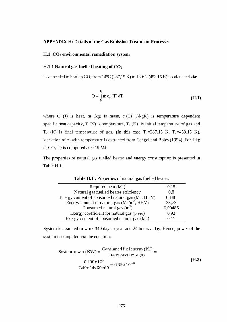
275
APPENDIX H: Details of the Gas Emission Treatment Processes
H.1. CO2 environmental remediation system
H.1.1 Natural gas fuelled heating of CO2
Heat needed to heat up CO2 from 14°C (287,15 K) to 180°C (453,15 K) is calculated via:
2
1
T
T
p dT)T(cmQ (H.1)
where Q (J) is heat, m (kg) is mass, cp(T) (J/kgK) is temperature dependent
specific heat capacity, T (K) is temperature, T1 (K) is initial temperature of gas and
T2 (K) is final temperature of gas. (In this case T1=287,15 K, T2=453,15 K).
Variation of cP with temperature is extracted from Cengel and Boles (1994). For 1 kg
of CO2, Q is computed as 0,15 MJ.
The properties of natural gas fuelled heater and energy consumption is presented in
Table H.1.
Table H.1 : Properties of natural gas fuelled heater.
Required heat (MJ) 0,15
Natural gas fuelled heater efficiency 0,8
Energy content of consumed natural gas (MJ, HHV) 0,188
Energy content of natural gas (MJ/m3, HHV) 38,73
Consumed natural gas (m3) 0,00485
Exergy coefficient for natural gas (βHHV) 0,92
Exergy content of consumed natural gas (MJ) 0,17
System is assumed to work 340 days a year and 24 hours a day. Hence, power of the
system is computed via the equation:
63
10x39,660x60x24x340
10x188,0
)s(60x60x24x340
)KJ(energyfuelConsumed)KW(powerSystem
(H.2)
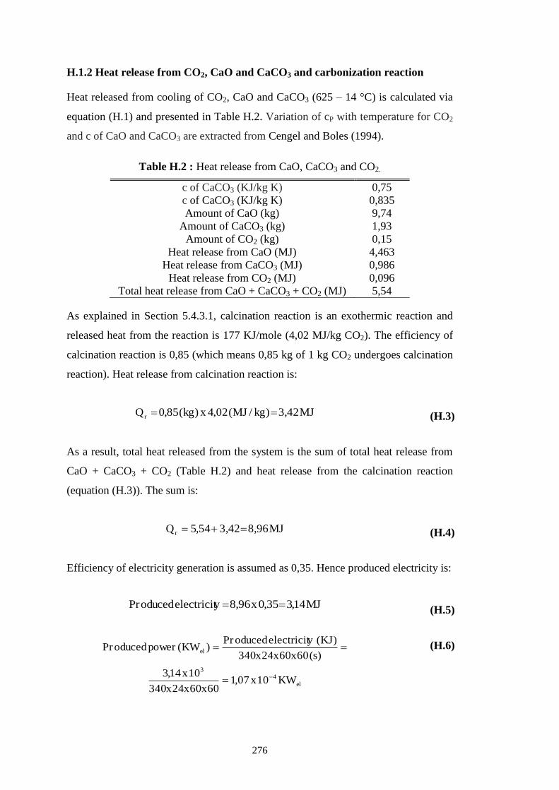
276
H.1.2 Heat release from CO2, CaO and CaCO3 and carbonization reaction
Heat released from cooling of CO2, CaO and CaCO3 (625 – 14 °C) is calculated via
equation (H.1) and presented in Table H.2. Variation of cP with temperature for CO2
and c of CaO and CaCO3 are extracted from Cengel and Boles (1994).
Table H.2 : Heat release from CaO, CaCO3 and CO2.
c of CaCO3 (KJ/kg K) 0,75
c of CaCO3 (KJ/kg K) 0,835
Amount of CaO (kg) 9,74
Amount of CaCO3 (kg) 1,93
Amount of CO2 (kg) 0,15
Heat release from CaO (MJ) 4,463
Heat release from CaCO3 (MJ) 0,986
Heat release from CO2 (MJ) 0,096
Total heat release from CaO + CaCO3 + CO2 (MJ) 5,54
As explained in Section 5.4.3.1, calcination reaction is an exothermic reaction and
released heat from the reaction is 177 KJ/mole (4,02 MJ/kg CO2). The efficiency of
calcination reaction is 0,85 (which means 0,85 kg of 1 kg CO2 undergoes calcination
reaction). Heat release from calcination reaction is:
MJ3,42)kg/MJ(02,4x)kg(85,0Q r (H.3)
As a result, total heat released from the system is the sum of total heat release from
CaO + CaCO3 + CO2 (Table H.2) and heat release from the calcination reaction
(equation (H.3)). The sum is:
MJ8,963,4254,5Q r (H.4)
Efficiency of electricity generation is assumed as 0,35. Hence produced electricity is:
MJ14,335,0x8,96yelectricitoducedPr (H.5)
el
43
el
KW10x07,160x60x24x340
10x14,3
)s(60x60x24x340
)KJ(yelectricitoducedPr)KW(poweroducedPr
(H.6)
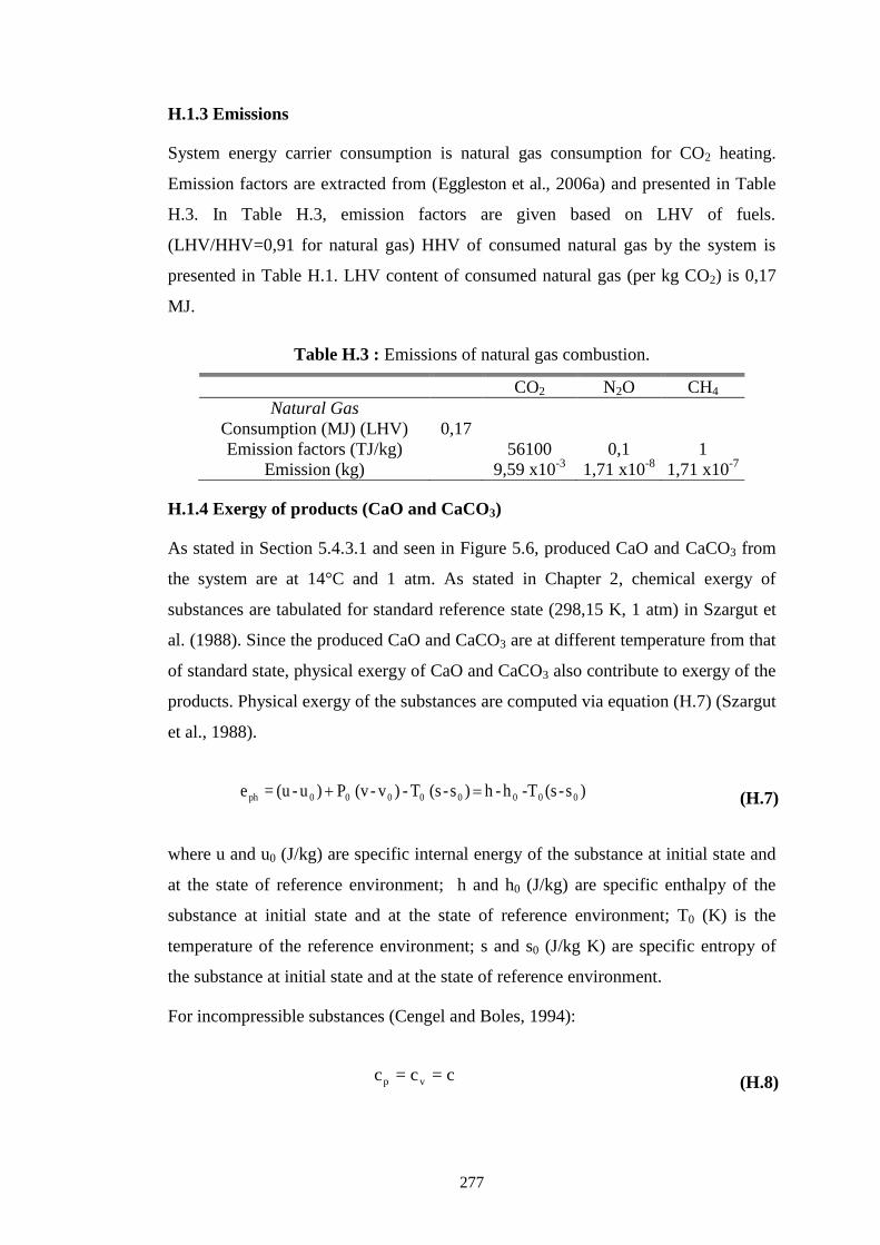
277
H.1.3 Emissions
System energy carrier consumption is natural gas consumption for CO2 heating.
Emission factors are extracted from (Eggleston et al., 2006a) and presented in Table
H.3. In Table H.3, emission factors are given based on LHV of fuels.
(LHV/HHV=0,91 for natural gas) HHV of consumed natural gas by the system is
presented in Table H.1. LHV content of consumed natural gas (per kg CO2) is 0,17
MJ.
Table H.3 : Emissions of natural gas combustion.
CO2 N2O CH4
Natural Gas
Consumption (MJ) (LHV) 0,17
Emission factors (TJ/kg) 56100 0,1 1
Emission (kg) 9,59 x10⁻³
1,71 x10⁻⁸
1,71 x10⁻⁷
H.1.4 Exergy of products (CaO and CaCO3)
As stated in Section 5.4.3.1 and seen in Figure 5.6, produced CaO and CaCO3 from
the system are at 14°C and 1 atm. As stated in Chapter 2, chemical exergy of
substances are tabulated for standard reference state (298,15 K, 1 atm) in Szargut et
al. (1988). Since the produced CaO and CaCO3 are at different temperature from that
of standard state, physical exergy of CaO and CaCO3 also contribute to exergy of the
products. Physical exergy of the substances are computed via equation (H.7) (Szargut
et al., 1988).
)s-(s-Th-h )s-(s T - )v-(v P )u-(u =e 00000000ph (H.7)
where u and u0 (J/kg) are specific internal energy of the substance at initial state and
at the state of reference environment; h and h0 (J/kg) are specific enthalpy of the
substance at initial state and at the state of reference environment; T0 (K) is the
temperature of the reference environment; s and s0 (J/kg K) are specific entropy of
the substance at initial state and at the state of reference environment.
For incompressible substances (Cengel and Boles, 1994):
c=c=c vp (H.8)
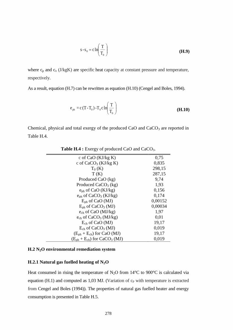
278
0
0T
Tlnc s-s (H.9)
where cp and cv (J/kgK) are specific heat capacity at constant pressure and temperature,
respectively.
As a result, equation (H.7) can be rewritten as equation (H.10) (Cengel and Boles, 1994).
T
Tlnc-T )T-(T c =e
0
00ph
(H.10)
Chemical, physical and total exergy of the produced CaO and CaCO3 are reported in
Table H.4.
Table H.4 : Exergy of produced CaO and CaCO3.
c of CaO (KJ/kg K) 0,75
c of CaCO3 (KJ/kg K) 0,835
T0 (K) 298,15
T (K) 287,15
Produced CaO (kg) 9,74
Produced CaCO3 (kg) 1,93
eph of CaO (KJ/kg) 0,156
eph of CaCO3 (KJ/kg) 0,174
Eph of CaO (MJ) 0,00152
Eph of CaCO3 (MJ) 0,00034
ech of CaO (MJ/kg) 1,97
ech of CaCO3 (MJ/kg) 0,01
Ech of CaO (MJ) 19,17
Ech of CaCO3 (MJ) 0,019
(Eph + Ech) for CaO (MJ) 19,17
(Eph + Ech) for CaCO3 (MJ) 0,019
H.2 N2O environmental remediation system
H.2.1 Natural gas fuelled heating of N2O
Heat consumed in rising the temperature of N2O from 14°C to 900°C is calculated via
equation (H.1) and computed as 1,03 MJ. (Variation of cP with temperature is extracted
from Cengel and Boles (1994)). The properties of natural gas fuelled heater and energy
consumption is presented in Table H.5.

279
Table H.5 : Properties of natural gas fuelled heater.
Required heat (MJ) 1,03
Natural gas fuelled heater efficiency 0,8
Energy content of consumed natural gas (MJ, HHV) 1,29
Energy content of natural gas (MJ/m3, HHV) 38,73
Consumed natural gas (m3) 0,033
Exergy coefficient for natural gas (βHHV) 0,92
Exergy content of consumed natural gas (MJ) 1,18
Power of the system is computed via the equation (H.2) and obtained as 4,38 x 10⁻⁵
KW.
H.2.2 Heat release from decomposition reaction, N2 and O2
The released from cooling of N2 and O2 (900 – 14 °C) is calculated via equation
(H.1) and presented in Table H.6. Variation of cP with temperature for N2 and O2 are
extracted from Cengel and Boles (1994).
Table H.6 : Heat release from N2 and O2.
Amount of N2 (kg) 0,64
Amount of O2 (kg) 0,36
Temperature gradient (K) 886
Heat release from N2 (MJ) 0,69
Heat release from O2 (MJ) 0,33
Total heat release from N2+O2 (MJ) 1,02
As explained in Section 5.4.3.2 decomposition reaction is an exothermic reaction and
released heat from the reaction is 82 KJ/mole (1,86 MJ/kg N2O). Hence, heat release
from decomposition of 1 kg N2O is 1,86 MJ. As a result, total heat released from the
system is:
MJ2,881,8602,1Q (H.11)
Efficiency of electricity generation is 0,35. Thereby, produced electricity is:
MJ01,135,0x88,2yelectricitoducedPr (H.12)
Power of electricity plant is:
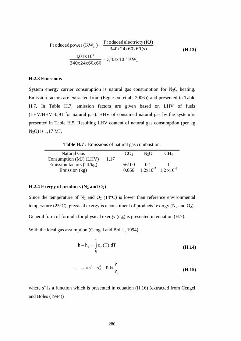
280
el
53
el
KW10x43,360x60x24x340
10x01,1
)s(60x60x24x340
)KJ(electrictyoducedPr)KW(poweroducedPr
(H.13)
H.2.3 Emissions
System energy carrier consumption is natural gas consumption for N2O heating.
Emission factors are extracted from (Eggleston et al., 2006a) and presented in Table
H.7. In Table H.7, emission factors are given based on LHV of fuels
(LHV/HHV=0,91 for natural gas). HHV of consumed natural gas by the system is
presented in Table H.5. Resulting LHV content of natural gas consumption (per kg
N2O) is 1,17 MJ.
Table H.7 : Emissions of natural gas combustion.
Natural Gas CO2 N2O CH4
Consumption (MJ) (LHV) 1,17
Emission factors (TJ/kg) 56100 0,1 1
Emission (kg) 0,066 1,2x10⁻⁷
1,2 x10⁻⁶
H.2.4 Exergy of products (N2 and O2)
Since the temperature of N2 and O2 (14°C) is lower than reference environmental
temperature (25°C), physical exergy is a constituent of products’ exergy (N2 and O2).
General form of formula for physical exergy (eph) is presented in equation (H.7).
With the ideal gas assumption (Cengel and Boles, 1994):
dT)T(chh
T
T
P0
0
(H.14)
0
00
00
P
PlnRssss (H.15)
where so is a function which is presented in equation (H.16) (extracted from Cengel
and Boles (1994))
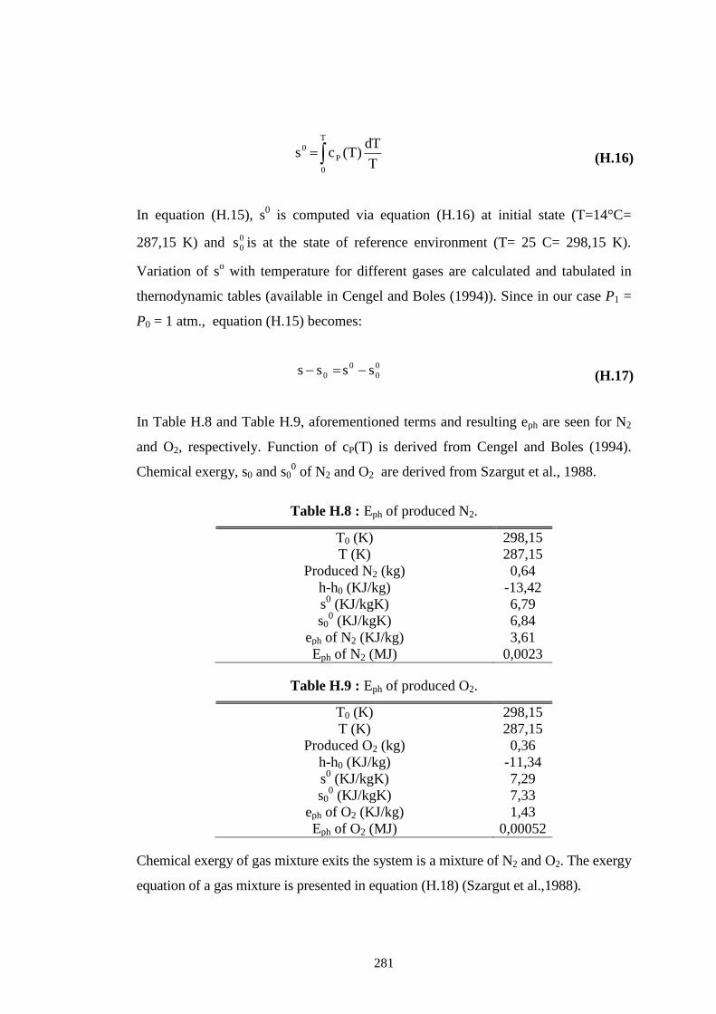
281
T
0
P
0
T
dT)T(cs (H.16)
In equation (H.15), s0 is computed via equation (H.16) at initial state (T=14°C=
287,15 K) and 0
0s is at the state of reference environment (T= 25 C= 298,15 K).
Variation of so with temperature for different gases are calculated and tabulated in
thernodynamic tables (available in Cengel and Boles (1994)). Since in our case P1 =
P0 = 1 atm., equation (H.15) becomes:
0
0
0
0 ssss (H.17)
In Table H.8 and Table H.9, aforementioned terms and resulting eph are seen for N2
and O2, respectively. Function of cP(T) is derived from Cengel and Boles (1994).
Chemical exergy, s0 and s00 of N2 and O2 are derived from Szargut et al., 1988.
Table H.8 : Eph of produced N2.
T0 (K) 298,15
T (K) 287,15
Produced N2 (kg) 0,64
h-h0 (KJ/kg) -13,42
s0 (KJ/kgK)
6,79
s00 (KJ/kgK)
6,84
eph of N2 (KJ/kg) 3,61
Eph of N2 (MJ) 0,0023
Table H.9 : Eph of produced O2.
T0 (K) 298,15
T (K) 287,15
Produced O2 (kg) 0,36
h-h0 (KJ/kg) -11,34
s0 (KJ/kgK)
7,29
s00 (KJ/kgK)
7,33
eph of O2 (KJ/kg) 1,43
Eph of O2 (MJ) 0,00052
Chemical exergy of gas mixture exits the system is a mixture of N2 and O2. The exergy
equation of a gas mixture is presented in equation (H.18) (Szargut et al.,1988).
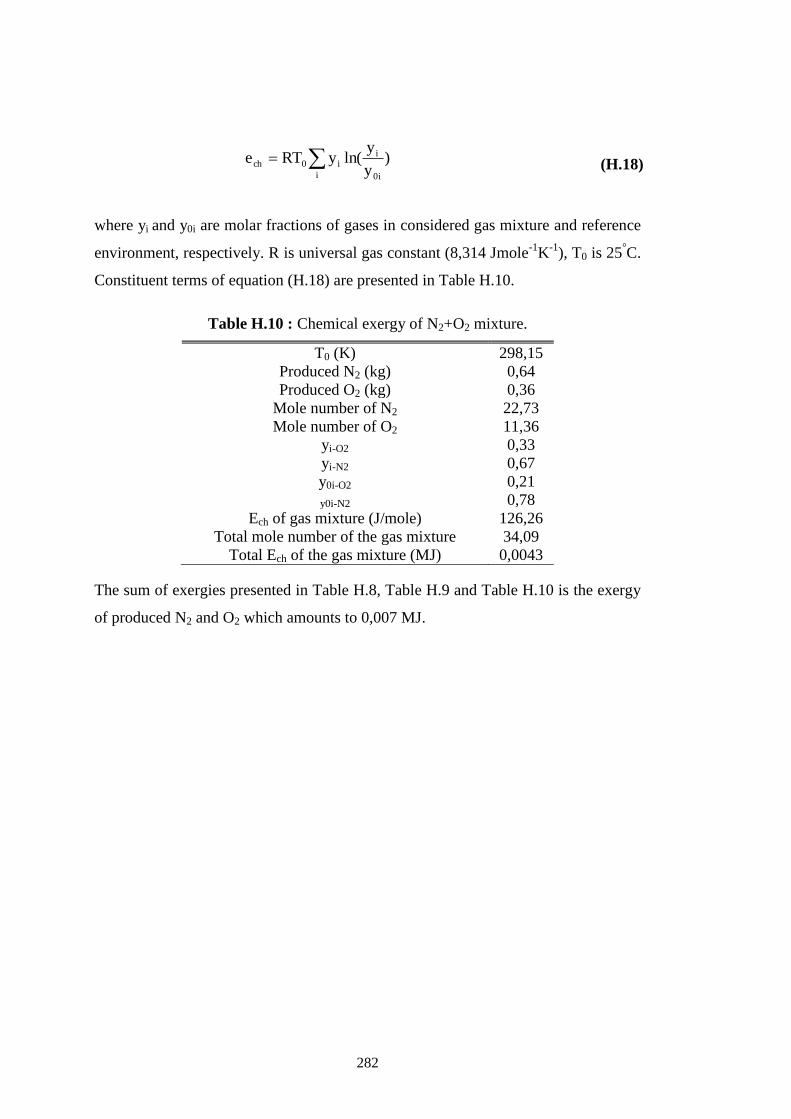
282
i i0
ii0ch )
y
yln(yRTe (H.18)
where yi and y0i are molar fractions of gases in considered gas mixture and reference
environment, respectively. R is universal gas constant (8,314 Jmole-1
K-1
), T0 is 25°C.
Constituent terms of equation (H.18) are presented in Table H.10.
Table H.10 : Chemical exergy of N2+O2 mixture.
T0 (K) 298,15
Produced N2 (kg) 0,64
Produced O2 (kg) 0,36
Mole number of N2 22,73
Mole number of O2 11,36
yi-O2 0,33
yi-N2 0,67
y0i-O2 0,21
y0i-N2 0,78
Ech of gas mixture (J/mole) 126,26
Total mole number of the gas mixture 34,09
Total Ech of the gas mixture (MJ) 0,0043
The sum of exergies presented in Table H.8, Table H.9 and Table H.10 is the exergy
of produced N2 and O2 which amounts to 0,007 MJ.
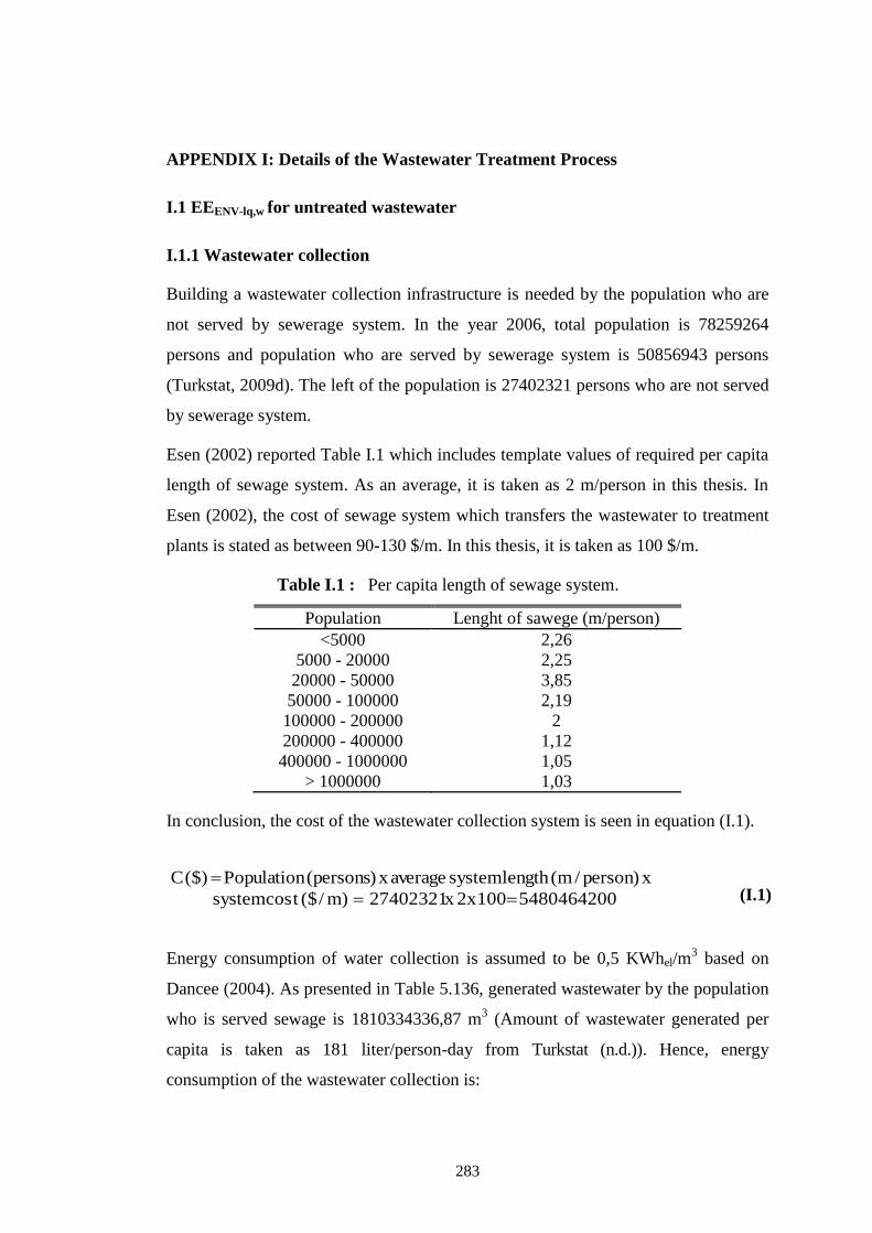
283
APPENDIX I: Details of the Wastewater Treatment Process
I.1 EEENV-lq,w for untreated wastewater
I.1.1 Wastewater collection
Building a wastewater collection infrastructure is needed by the population who are
not served by sewerage system. In the year 2006, total population is 78259264
persons and population who are served by sewerage system is 50856943 persons
(Turkstat, 2009d). The left of the population is 27402321 persons who are not served
by sewerage system.
Esen (2002) reported Table I.1 which includes template values of required per capita
length of sewage system. As an average, it is taken as 2 m/person in this thesis. In
Esen (2002), the cost of sewage system which transfers the wastewater to treatment
plants is stated as between 90-130 $/m. In this thesis, it is taken as 100 $/m.
Table I.1 : Per capita length of sewage system.
Population Lenght of sawege (m/person)
<5000 2,26
5000 - 20000 2,25
20000 - 50000 3,85
50000 - 100000 2,19
100000 - 200000 2
200000 - 400000 1,12
400000 - 1000000 1,05
> 1000000 1,03
In conclusion, the cost of the wastewater collection system is seen in equation (I.1).
5480464200100x2x27402321)m/($tcossystem
x)person/m(lengthsystemaveragex)persons(Population($)C
(I.1)
Energy consumption of water collection is assumed to be 0,5 KWhel/m3 based on
Dancee (2004). As presented in Table 5.136, generated wastewater by the population
who is served sewage is 1810334336,87 m3 (Amount of wastewater generated per
capita is taken as 181 liter/person-day from Turkstat (n.d.)). Hence, energy
consumption of the wastewater collection is:
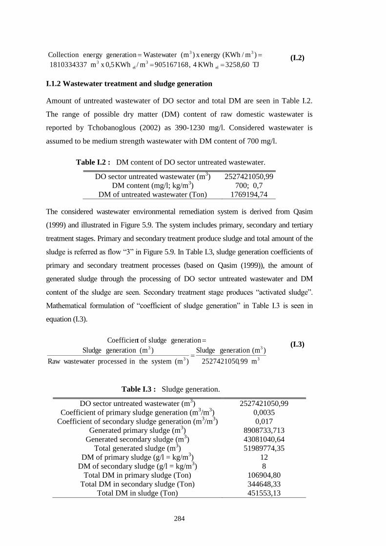
284
TJ 3258,60KWh 4,905167168m/KWh5,0xm1810334337
)m/KWh(energyx)m(WastewatergenerationenergyCollection
el
3
el
3
33
(I.2)
I.1.2 Wastewater treatment and sludge generation
Amount of untreated wastewater of DO sector and total DM are seen in Table I.2.
The range of possible dry matter (DM) content of raw domestic wastewater is
reported by Tchobanoglous (2002) as 390-1230 mg/l. Considered wastewater is
assumed to be medium strength wastewater with DM content of 700 mg/l.
Table I.2 : DM content of DO sector untreated wastewater.
DO sector untreated wastewater (m3) 2527421050,99
DM content (mg/l; kg/m3) 700; 0,7
DM of untreated wastewater (Ton) 1769194,74
The considered wastewater environmental remediation system is derived from Qasim
(1999) and illustrated in Figure 5.9. The system includes primary, secondary and tertiary
treatment stages. Primary and secondary treatment produce sludge and total amount of the
sludge is referred as flow “3” in Figure 5.9. In Table I.3, sludge generation coefficients of
primary and secondary treatment processes (based on Qasim (1999)), the amount of
generated sludge through the processing of DO sector untreated wastewater and DM
content of the sludge are seen. Secondary treatment stage produces “activated sludge”.
Mathematical formulation of “coefficient of sludge generation” in Table I.3 is seen in
equation (I.3).
3
3
3
3
m99,2527421050
)(mgeneration Sludge
)m(systemtheinprocessedwastewaterRaw
)m(generationSludge
generation sludge oft Coefficien
(I.3)
Table I.3 : Sludge generation.
DO sector untreated wastewater (m3) 2527421050,99
Coefficient of primary sludge generation (m3/m
3) 0,0035
Coefficient of secondary sludge generation (m3/m
3) 0,017
Generated primary sludge (m3) 8908733,713
Generated secondary sludge (m3) 43081040,64
Total generated sludge (m3) 51989774,35
DM of primary sludge (g/l = kg/m3) 12
DM of secondary sludge (g/l = kg/m3) 8
Total DM in primary sludge (Ton) 106904,80
Total DM in secondary sludge (Ton) 344648,33
Total DM in sludge (Ton) 451553,13

285
I.1.3 Sludge blending
Energy consumption of sludge blending is reported as 5 KWh/tDM (18000 KJ/tDM) of
electricity (1 tDM = 1 ton of the mixed sludge in dry basis) which incorporates the
energy consumption of pumping and blending of the sludge (Suh and Rousseaux, 2002).
TJ13,8)tDM(13,451553x)tDM/TJ(18000x10
nconsumptioenergy blending Sludge
9-
(I.4)
Due to the absence of data, capital cost of the blending tank is not included in the
calculation.
I.1.4 Sludge thickening
Gravity belt thickening is applied in the considered system obtained from Qasim
(1999). The energy consumption of the thickening process is retrieved from (Suh and
Rousseaux, 2002) as 50 KWh/tDM (180000 KJ/tDM) of electricity. Energy
consumption in gravity belt thicking stage is:
TJ28,81)tDM(13,451553x)tDM/TJ(180000x10
nconsumptioenergy Thickening
9-
(I.5)
Cost of gravity belt thickening process is computed based on data retrieved from
Sloan et al. (2009) and exergetic equivalent of capital is computed in Table I.4.
Table I.4 : Capital of gravity belt thickening process.
Capital of thickening ($/tDM) 31
DM of thickened sludge (Ton) 451553,13
Total capital ($) 13998147,03
eeC (MJ/$) 25,5
Exergetic equivalent of capital (TJ) 356,96
In the course of gravity belt thickening process, 4 kg of polymer consumption per tDM
sludge is reported in Suh and Rousseaux (2002). Due to the lack of exact chemical
composition of polymers, it is not counted in material flows of the system. The excessive
liquid from the thickening process, in the form of supernatant, is sent back to secondary
treatment stage for further treatment as seen in Figure 5.9 (flow “5”).
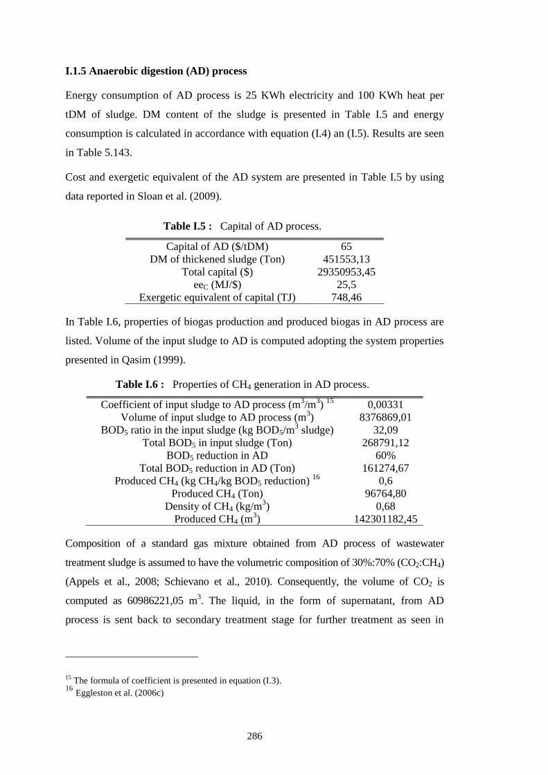
286
I.1.5 Anaerobic digestion (AD) process
Energy consumption of AD process is 25 KWh electricity and 100 KWh heat per
tDM of sludge. DM content of the sludge is presented in Table I.5 and energy
consumption is calculated in accordance with equation (I.4) an (I.5). Results are seen
in Table 5.143.
Cost and exergetic equivalent of the AD system are presented in Table I.5 by using
data reported in Sloan et al. (2009).
Table I.5 : Capital of AD process.
Capital of AD ($/tDM) 65
DM of thickened sludge (Ton) 451553,13
Total capital ($) 29350953,45
eeC (MJ/$) 25,5
Exergetic equivalent of capital (TJ) 748,46
In Table I.6, properties of biogas production and produced biogas in AD process are
listed. Volume of the input sludge to AD is computed adopting the system properties
presented in Qasim (1999).
Table I.6 : Properties of CH4 generation in AD process.
Coefficient of input sludge to AD process (m3/m
3)
15 0,00331
Volume of input sludge to AD process (m3) 8376869,01
BOD5 ratio in the input sludge (kg BOD5/m3 sludge) 32,09
Total BOD5 in input sludge (Ton) 268791,12
BOD5 reduction in AD 60%
Total BOD5 reduction in AD (Ton) 161274,67
Produced CH4 (kg CH4/kg BOD5 reduction) 16
0,6
Produced CH4 (Ton) 96764,80
Density of CH4 (kg/m3) 0,68
Produced CH4 (m3) 142301182,45
Composition of a standard gas mixture obtained from AD process of wastewater
treatment sludge is assumed to have the volumetric composition of 30%:70% (CO2:CH4)
(Appels et al., 2008; Schievano et al., 2010). Consequently, the volume of CO2 is
computed as 60986221,05 m3. The liquid, in the form of supernatant, from AD
process is sent back to secondary treatment stage for further treatment as seen in
15
The formula of coefficient is presented in equation (I.3). 16
Eggleston et al. (2006c)
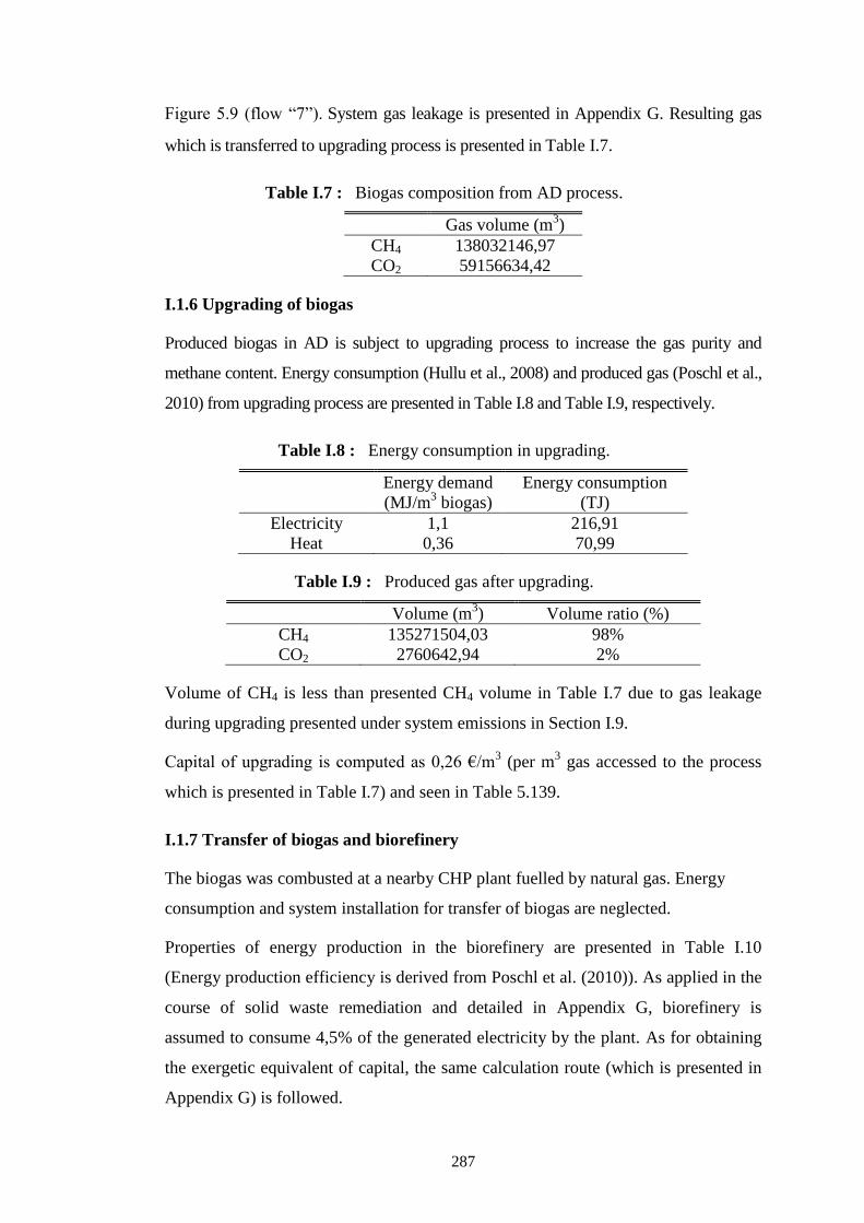
287
Figure 5.9 (flow “7”). System gas leakage is presented in Appendix G. Resulting gas
which is transferred to upgrading process is presented in Table I.7.
Table I.7 : Biogas composition from AD process.
Gas volume (m3)
CH4 138032146,97
CO2 59156634,42
I.1.6 Upgrading of biogas
Produced biogas in AD is subject to upgrading process to increase the gas purity and
methane content. Energy consumption (Hullu et al., 2008) and produced gas (Poschl et al.,
2010) from upgrading process are presented in Table I.8 and Table I.9, respectively.
Table I.8 : Energy consumption in upgrading.
Energy demand
(MJ/m3 biogas)
Energy consumption
(TJ)
Electricity 1,1 216,91
Heat 0,36 70,99
Table I.9 : Produced gas after upgrading.
Volume (m3) Volume ratio (%)
CH4 135271504,03 98%
CO2 2760642,94 2%
Volume of CH4 is less than presented CH4 volume in Table I.7 due to gas leakage
during upgrading presented under system emissions in Section I.9.
Capital of upgrading is computed as 0,26 €/m3 (per m
3 gas accessed to the process
which is presented in Table I.7) and seen in Table 5.139.
I.1.7 Transfer of biogas and biorefinery
The biogas was combusted at a nearby CHP plant fuelled by natural gas. Energy
consumption and system installation for transfer of biogas are neglected.
Properties of energy production in the biorefinery are presented in Table I.10
(Energy production efficiency is derived from Poschl et al. (2010)). As applied in the
course of solid waste remediation and detailed in Appendix G, biorefinery is
assumed to consume 4,5% of the generated electricity by the plant. As for obtaining
the exergetic equivalent of capital, the same calculation route (which is presented in
Appendix G) is followed.
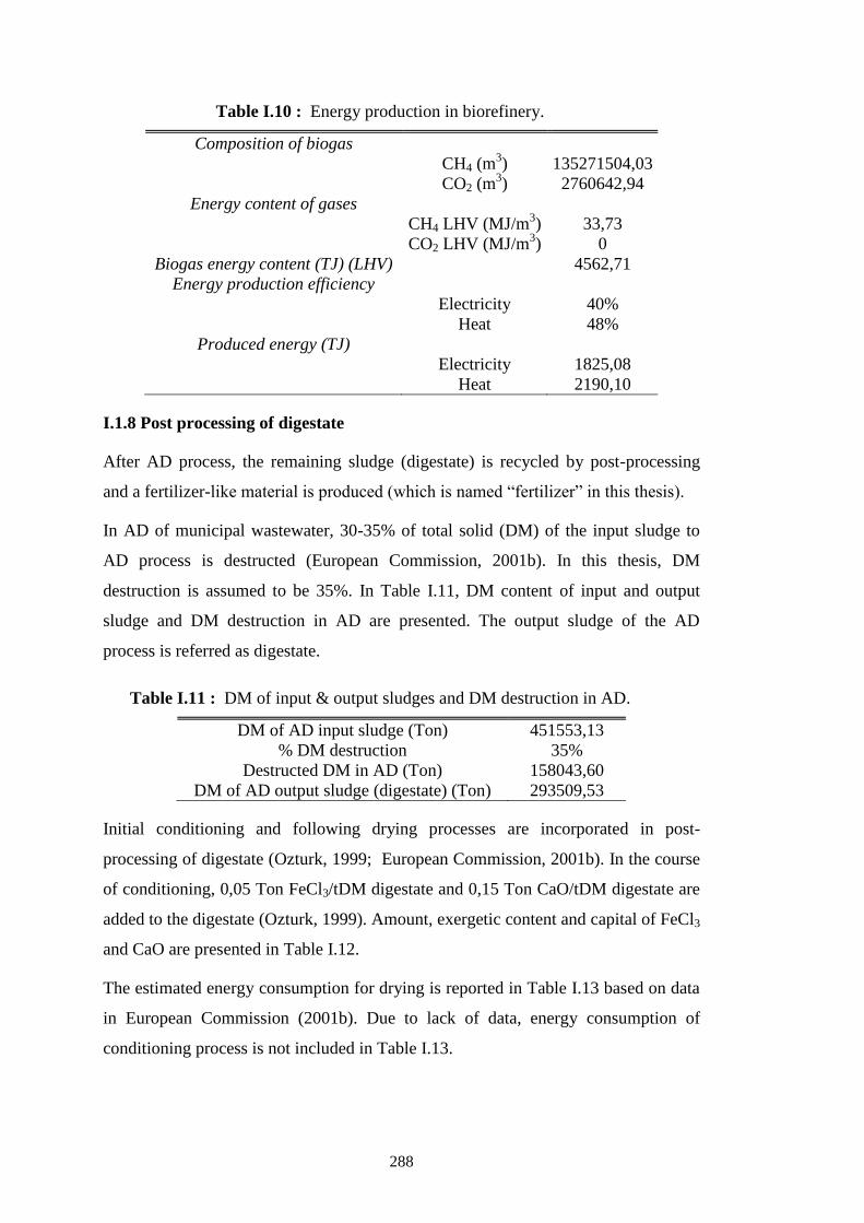
288
Table I.10 : Energy production in biorefinery.
Composition of biogas
CH4 (m3) 135271504,03
CO2 (m3) 2760642,94
Energy content of gases
CH4 LHV (MJ/m3) 33,73
CO2 LHV (MJ/m3) 0
Biogas energy content (TJ) (LHV) 4562,71
Energy production efficiency
Electricity 40%
Heat 48%
Produced energy (TJ)
Electricity 1825,08
Heat 2190,10
I.1.8 Post processing of digestate
After AD process, the remaining sludge (digestate) is recycled by post-processing
and a fertilizer-like material is produced (which is named “fertilizer” in this thesis).
In AD of municipal wastewater, 30-35% of total solid (DM) of the input sludge to
AD process is destructed (European Commission, 2001b). In this thesis, DM
destruction is assumed to be 35%. In Table I.11, DM content of input and output
sludge and DM destruction in AD are presented. The output sludge of the AD
process is referred as digestate.
Table I.11 : DM of input & output sludges and DM destruction in AD.
DM of AD input sludge (Ton) 451553,13
% DM destruction 35%
Destructed DM in AD (Ton) 158043,60
DM of AD output sludge (digestate) (Ton) 293509,53
Initial conditioning and following drying processes are incorporated in post-
processing of digestate (Ozturk, 1999; European Commission, 2001b). In the course
of conditioning, 0,05 Ton FeCl3/tDM digestate and 0,15 Ton CaO/tDM digestate are
added to the digestate (Ozturk, 1999). Amount, exergetic content and capital of FeCl3
and CaO are presented in Table I.12.
The estimated energy consumption for drying is reported in Table I.13 based on data
in European Commission (2001b). Due to lack of data, energy consumption of
conditioning process is not included in Table I.13.
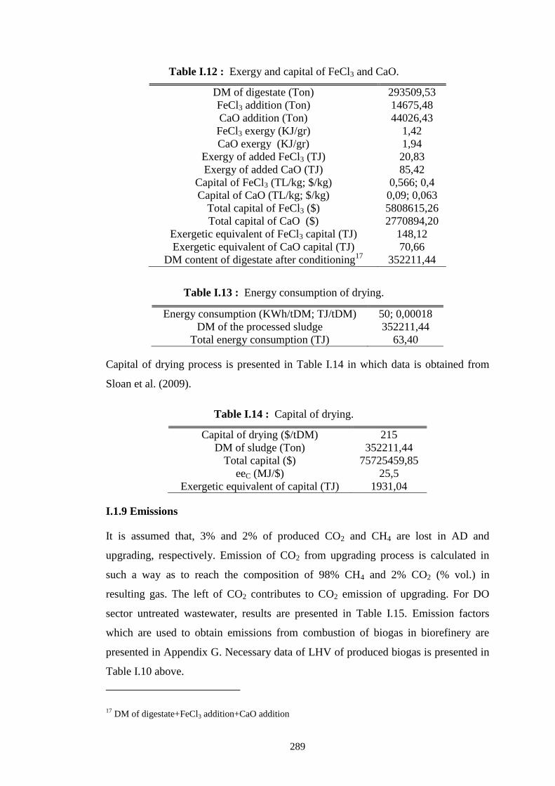
289
Table I.12 : Exergy and capital of FeCl3 and CaO.
DM of digestate (Ton) 293509,53
FeCl3 addition (Ton) 14675,48
CaO addition (Ton) 44026,43
FeCl3 exergy (KJ/gr) 1,42
CaO exergy (KJ/gr) 1,94
Exergy of added FeCl3 (TJ) 20,83
Exergy of added CaO (TJ) 85,42
Capital of FeCl3 (TL/kg; $/kg) 0,566; 0,4
Capital of CaO (TL/kg; $/kg) 0,09; 0,063
Total capital of FeCl3 ($) 5808615,26
Total capital of CaO ($) 2770894,20
Exergetic equivalent of FeCl3 capital (TJ) 148,12
Exergetic equivalent of CaO capital (TJ) 70,66
DM content of digestate after conditioning17
352211,44
Table I.13 : Energy consumption of drying.
Energy consumption (KWh/tDM; TJ/tDM) 50; 0,00018
DM of the processed sludge 352211,44
Total energy consumption (TJ) 63,40
Capital of drying process is presented in Table I.14 in which data is obtained from
Sloan et al. (2009).
Table I.14 : Capital of drying.
Capital of drying ($/tDM) 215
DM of sludge (Ton) 352211,44
Total capital ($) 75725459,85
eeC (MJ/$) 25,5
Exergetic equivalent of capital (TJ) 1931,04
I.1.9 Emissions
It is assumed that, 3% and 2% of produced CO2 and CH4 are lost in AD and
upgrading, respectively. Emission of CO2 from upgrading process is calculated in
such a way as to reach the composition of 98% CH4 and 2% CO2 (% vol.) in
resulting gas. The left of CO2 contributes to CO2 emission of upgrading. For DO
sector untreated wastewater, results are presented in Table I.15. Emission factors
which are used to obtain emissions from combustion of biogas in biorefinery are
presented in Appendix G. Necessary data of LHV of produced biogas is presented in
Table I.10 above.
17
DM of digestate+FeCl3 addition+CaO addition
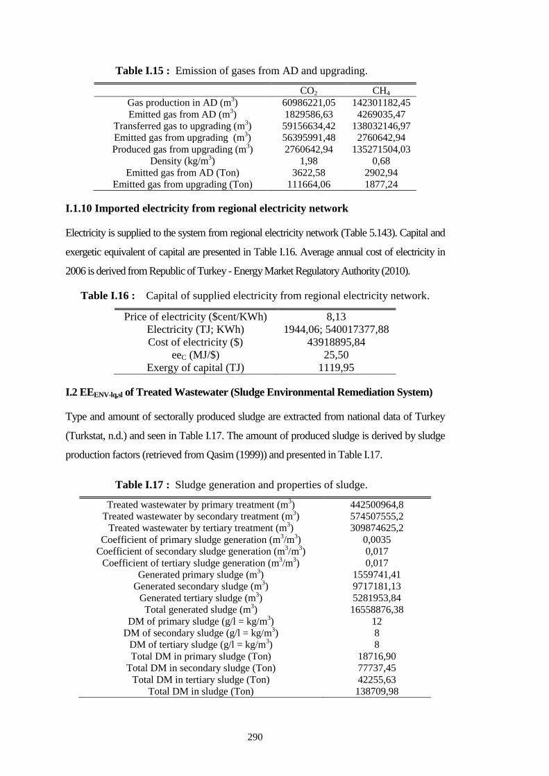
290
Table I.15 : Emission of gases from AD and upgrading.
CO2 CH4
Gas production in AD (m3) 60986221,05 142301182,45
Emitted gas from AD (m3) 1829586,63 4269035,47
Transferred gas to upgrading (m3) 59156634,42 138032146,97
Emitted gas from upgrading (m3) 56395991,48 2760642,94
Produced gas from upgrading (m3) 2760642,94 135271504,03
Density (kg/m3) 1,98 0,68
Emitted gas from AD (Ton) 3622,58 2902,94
Emitted gas from upgrading (Ton) 111664,06 1877,24
I.1.10 Imported electricity from regional electricity network
Electricity is supplied to the system from regional electricity network (Table 5.143). Capital and
exergetic equivalent of capital are presented in Table I.16. Average annual cost of electricity in
2006 is derived from Republic of Turkey - Energy Market Regulatory Authority (2010).
Table I.16 : Capital of supplied electricity from regional electricity network.
Price of electricity ($cent/KWh) 8,13
Electricity (TJ; KWh) 1944,06; 540017377,88
Cost of electricity ($) 43918895,84
eeC (MJ/$) 25,50
Exergy of capital (TJ) 1119,95
I.2 EEENV-lq,sl of Treated Wastewater (Sludge Environmental Remediation System)
Type and amount of sectorally produced sludge are extracted from national data of Turkey
(Turkstat, n.d.) and seen in Table I.17. The amount of produced sludge is derived by sludge
production factors (retrieved from Qasim (1999)) and presented in Table I.17.
Table I.17 : Sludge generation and properties of sludge.
Treated wastewater by primary treatment (m3) 442500964,8
Treated wastewater by secondary treatment (m3) 574507555,2
Treated wastewater by tertiary treatment (m3) 309874625,2
Coefficient of primary sludge generation (m3/m
3) 0,0035
Coefficient of secondary sludge generation (m3/m
3) 0,017
Coefficient of tertiary sludge generation (m3/m
3) 0,017
Generated primary sludge (m3) 1559741,41
Generated secondary sludge (m3) 9717181,13
Generated tertiary sludge (m3) 5281953,84
Total generated sludge (m3) 16558876,38
DM of primary sludge (g/l = kg/m3) 12
DM of secondary sludge (g/l = kg/m3) 8
DM of tertiary sludge (g/l = kg/m3) 8
Total DM in primary sludge (Ton) 18716,90
Total DM in secondary sludge (Ton) 77737,45
Total DM in tertiary sludge (Ton) 42255,63
Total DM in sludge (Ton) 138709,98
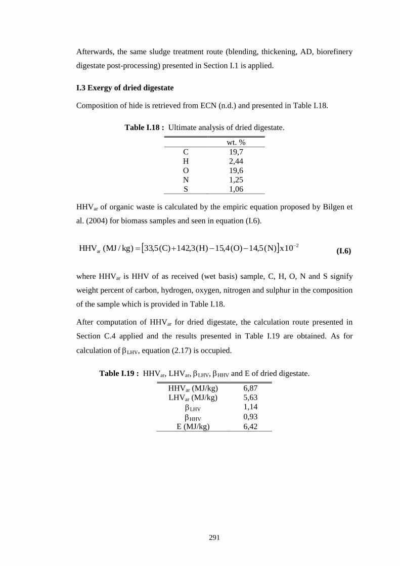
291
Afterwards, the same sludge treatment route (blending, thickening, AD, biorefinery
digestate post-processing) presented in Section I.1 is applied.
I.3 Exergy of dried digestate
Composition of hide is retrieved from ECN (n.d.) and presented in Table I.18.
Table I.18 : Ultimate analysis of dried digestate.
wt. %
C 19,7
H 2,44
O 19,6
N 1,25
S 1,06
HHVar of organic waste is calculated by the empiric equation proposed by Bilgen et
al. (2004) for biomass samples and seen in equation (I.6).
2
ar 10x)N(5,14)O(4,15)H(3,142)C(5,33)kg/MJ(HHV (I.6)
where HHVar is HHV of as received (wet basis) sample, C, H, O, N and S signify
weight percent of carbon, hydrogen, oxygen, nitrogen and sulphur in the composition
of the sample which is provided in Table I.18.
After computation of HHVar for dried digestate, the calculation route presented in
Section C.4 applied and the results presented in Table I.19 are obtained. As for
calculation of LHV, equation (2.17) is occupied.
Table I.19 : HHVar, LHVar, LHV, HHV and E of dried digestate.
HHVar (MJ/kg) 6,87
LHVar (MJ/kg) 5,63
LHV 1,14
HHV 0,93
E (MJ/kg) 6,42

292
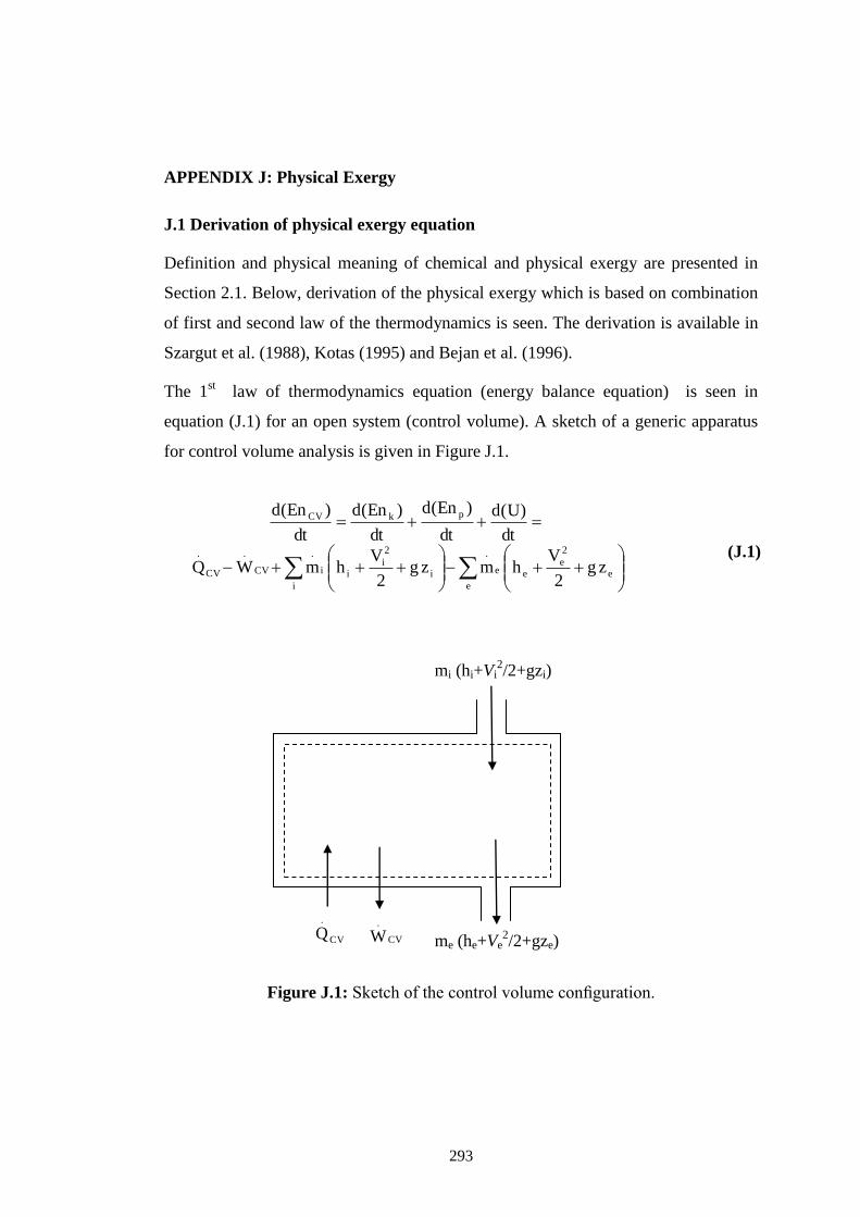
293
APPENDIX J: Physical Exergy
J.1 Derivation of physical exergy equation
Definition and physical meaning of chemical and physical exergy are presented in
Section 2.1. Below, derivation of the physical exergy which is based on combination
of first and second law of the thermodynamics is seen. The derivation is available in
Szargut et al. (1988), Kotas (1995) and Bejan et al. (1996).
The 1st law of thermodynamics equation (energy balance equation) is seen in
equation (J.1) for an open system (control volume). A sketch of a generic apparatus
for control volume analysis is given in Figure J.1.
e
e
2
eee
.
i
i
2
iii
.
CV
.
CV
.
pkCV
zg2
Vhmzg
2
VhmWQ
dt
)U(d
dt
)En(d
dt
)En(d
dt
)En(d
(J.1)
Figure J.1: Sketch of the control volume configuration.
CV
.
Q
CV
.
W
mi (hi+Vi2/2+gzi)
me (he+Ve2/2+gze)
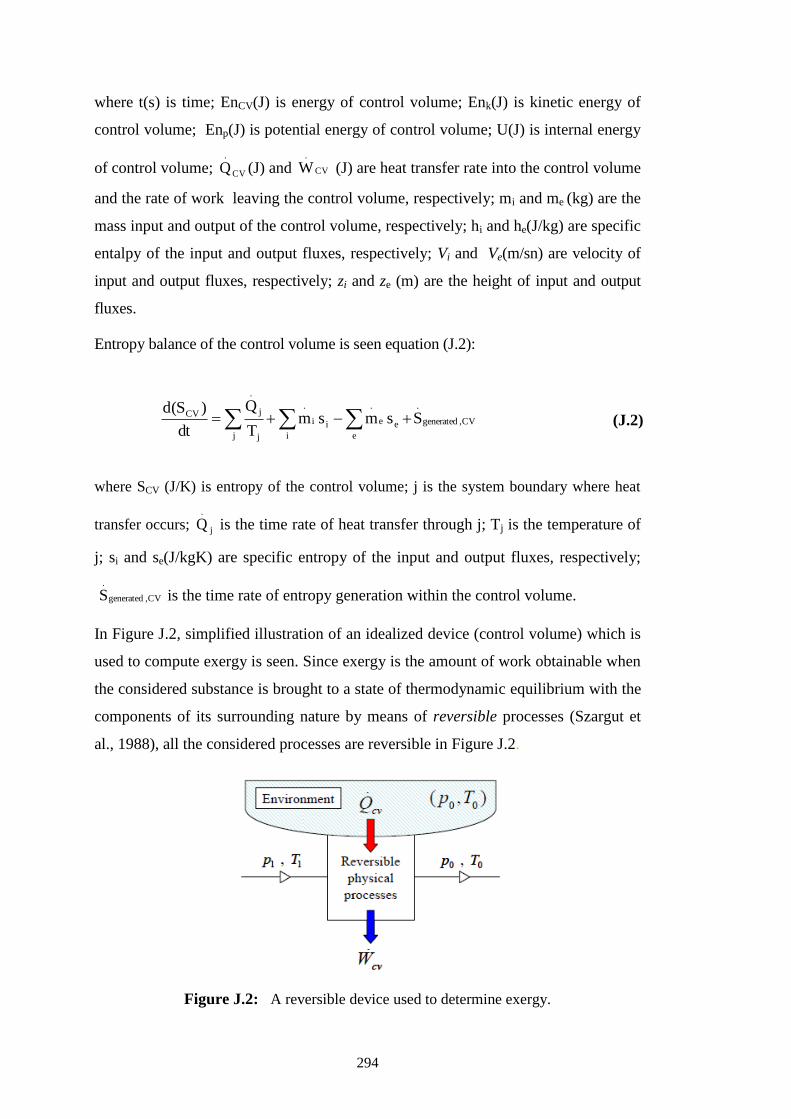
294
where t(s) is time; EnCV(J) is energy of control volume; Enk(J) is kinetic energy of
control volume; Enp(J) is potential energy of control volume; U(J) is internal energy
of control volume; CV
.
Q (J) and CV
.
W (J) are heat transfer rate into the control volume
and the rate of work leaving the control volume, respectively; mi and me (kg) are the
mass input and output of the control volume, respectively; hi and he(J/kg) are specific
entalpy of the input and output fluxes, respectively; Vi and Ve(m/sn) are velocity of
input and output fluxes, respectively; zi and ze (m) are the height of input and output
fluxes.
Entropy balance of the control volume is seen equation (J.2):
CV,generated
.
e
ee
.
i
ii
.
j j
j
.
CV SsmsmT
Q
dt
)S(d (J.2)
where SCV (J/K) is entropy of the control volume; j is the system boundary where heat
transfer occurs; j
.
Q is the time rate of heat transfer through j; Tj is the temperature of
j; si and se(J/kgK) are specific entropy of the input and output fluxes, respectively;
CV,generated
.
S is the time rate of entropy generation within the control volume.
In Figure J.2, simplified illustration of an idealized device (control volume) which is
used to compute exergy is seen. Since exergy is the amount of work obtainable when
the considered substance is brought to a state of thermodynamic equilibrium with the
components of its surrounding nature by means of reversible processes (Szargut et
al., 1988), all the considered processes are reversible in Figure J.2.
Figure J.2: A reversible device used to determine exergy.
295
The temperature and pressure conditions of the environment are P0 and T0,
respectively and those of the initial state of the process fluid are P1,T1 (Figure J.2).
The heat transfers to/from the ideal reversible module in Figure J.2 take place
between the environment and the system at the temperature of T0, the produced work
( CV
.
W ) is the maximum possible amount of work (since the processes are reversible)
when the process fluid is brought to equilibrium with its natural surroundings (here
referred as the environment).
The energy balance equation of the reversible device is seen in equation (J.3) (based
on equation (J.1)), assuming steady state conditions and neglecting the changes in
kinetic and potential energy of the process fluid. Equation (J.3) includes the change
of state for the fluid passing through the ideal device in Figure J.2, as well as the
exchange of heat and work.
01
.
CV
.
CV
.CV hhmWQ0
dt
)En(d (J.3)
Similarly, the entropy balance of the control volume (assuming no irreversibilities) is
obtained from equation (J.2) and seen in equation (J.4).
01
.
0
CV
.
CV ssmT
Q0
dt
)S(d (J.4)
Equation (J.4) can be rewriten as equation (J.5).
100
.
CV
.
ssTmQ (J.5)
Substituting equation (J.5) into equation (J.3), the formulation of reversible work
which can be obtained from the process in Figure J.2 can be written as equation (J.6).
10100
.
CV
.
hhssTmW (J.6)
296
By definition, physical exergy is equal to CV
.
W and physical exery (Eph) of the fluid
working in the system in Figure J.2 is seen in equation (J.7).
01001
.
10100CV
.
ph ssThhmhhssTmWE (J.7)
A extensive explanation of chemical exergy computation is presented in detail in
Szargut et al. (1988).
297
CURRICULUM VITAE
Name Surname: Candeniz SEÇKİN
Place and Date of Birth: Istanbul, 08.09.1980
E-Mail: [email protected], [email protected]
B.Sc.: Istanbul Technical University/Mechanical Engineering Department (2002)
M.Sc.: Istanbul Technical University/Energy Institute (2006)
PUBLICATIONS/PRESENTATIONS ON THE THESIS
Seckin, C., Sciubba, E. and Bayulken, A. R. (2012). Extended exergy analysis of
Turkish transportation sector. Journal of Cleaner Production (accepted manuscript,
available on sciencedirect.com).
Seckin, C., Sciubba, E. and Bayulken, A. R. (2012). An application of the extended
exergy accounting method to the Turkish society, year 2006. Energy, 40, 151-163.
Seckin, C. and Bayulken, A. R. (2012). Environmental Remediation Cost of Solid
Waste in EEA Methodology – An Application to Turkish Tertiary Sector Solid
Waste. GCGW 2012 - Global Conference on Global Warming 2012, Istanbul,
Turkey, July 8–12.
Seckin, C., Sciubba, E. and Bayulken, A. R. (2012). Resource Use Evaluation of
Turkish transportation Sector via Extended Exergy Accounting Method. The 25th
International Conference on Efficiency, Cost, Optimization, Simulation and
Environmental Impact of Energy Systems (ECOS 2012), Perugia, Italy, June 26–29.
Seckin, C., Sciubba, E. and Bayulken, A. R. (2012). Determination of environmental
remediation cost of municipal waste in terms of extended exergy. The 25th
International Conference on Efficiency, Cost, Optimization, Simulation and
Environmental Impact of Energy Systems (ECOS 2012), Perugia, Italy, June 26–29.
Seckin, C. and Bayulken, A. R. (2011). Assessment of Resource Use in Turkish
Household Sector and Labour Generation. The 10th
International Conference on
Sustainable Energy Technologies (SET 2011), Istanbul, Turkey, September 4–17.
Seckin, C., Sciubba, E. and Bayulken, A. R. (2011). Extended Exergy Accounting
applied to the Turkish society 2006. The 24th
International Conference on Efficiency,
Cost, Optimization, Simulation and Environmental Impact of Energy Systems (ECOS
2011), Novi Sad, Serbia, July 4–7.

298
Copyright © 2022 FDOKUMEN