J. Fluid Mech. (1993). vol. 251, pp. 219-238 Copyright Q 1993 Cambridge University Press

219

Isotropy of the small scales of turbulence at low Reynolds number

By J. KIM’ AND R. A. ANTONIA’ * Center for Turbulence Research, NASA-Ames Research Center, Moffett Field, CA 94035, USA

%Department of Mechanical Engineering, University of Newcastle, New South Wales, 2308, Australia

(Received 4 November 1991 and in revised form 2 December 1992)

Spectral local isotropy tests are applied to direct numerical simulation data, mainly at the centreline of a fully developed turbulent channel flow. Despite the small Reynolds number of the simulation, the high-wavenumber behaviour of velocity and vorticity spectra is consistent with local isotropy. This consistency is verified by the relationship between streamwise wavenumber spectra and spanwise wavenumber spectra. The high-wavenumber behaviour of the pressure spectrum is also consistent with local isotropy and compares favourably with the calculation of Batchelor (1951), which assumes isotropy and joint normality of the velocity field at two points in space. The latter assumption is validated by the shape but not the magnitude of the quadruple correlation of the streamwise velocity fluctuation at small separations. There is only partial support for local spectral isotropy away from the centreline as the magnitude of the mean strain rate increases.

1. Introduction Several tests can be applied for checking local isotropy in turbulent flows (e.g. Monin

& Yaglom 1975). Antonia, Anselmet & Chambers (1986) underlined however that different tests may have different levels of sensitivity and therefore provide different measures of the departure from local isotropy. In particular, it was noted that mean square values of derivatives (of either velocity or temperature) weighted all of the spectrum so that deviations of these values from isotropy do not necessary indicate a breakdown in isotropy of the small scales of motion. Derivatives do show departures from local isotropy, when ‘local’ is interpreted to mean ‘in physical space’, as originally proposed by Kolmogorov (1941) and as used in most applications of the concept.

Indeed, the high-wavenumber regions of measured spectra of velocity fluctuations and of their derivatives appear to be consistent with local isotropy (e.g. Champagne 1981; Antonia et al. 1986; Antonia, Shah & Browne 1987). The wake data presented by Antonia, Shah & B r - e (1987, 1988) were obtained for small turbulence Reyngds-bers (RA1 = uFA, /u , where u1 is the longitudinal velocity fluctuation and A, = u ~ / u ~ ~ ~ is the longitudinal Taylor microscale, was in the range 40-80). At such Reynolds numbers, the spectral separation between the energy-containing part of the spectrum and the dissipation part of the spectrum is insufficient for an inertial subrange to exist. Nonetheless, the high-wavenumber regions of the velocity derivative spectra seemed to satisfy the isotropic spectral relations, allowing for the experimental uncertainty. The result implies that spectral local isotropy can be attained, independently of the Reynolds number. This implication is of some importance and, in the present paper, is tested against numerical data.

.I n

220 J. Kim and R . A . Antonia

Direct numerical simulations (DNS) of turbulent flows (Kim, Moin & Moser 1987; Spalart 1988) have provided data that can permit a useful check of spectral isotropy, albeit at small Reynolds numbers. In this context, the simulations offer several advantages over hot-wire measurements. The use of Taylor’s hypothesis -which is required in experiments for converting time derivatives to x1 derivatives and for transforming the frequency n into a one-dimensional wavenumber k, (= 2nn/U, where B is the local mean velocity) - is avoided in the simulations. The general difficulties (e.g. Mestayer & Chambaud 1979) in inferring velocity derivatives from hot-wire signals at two points in space are absent in the simulations. Also, the x, resolution, especially in the wall region, is better for the simulations than for hot-wire measurements.

In a previous paper (Antonia, Kim & Browne 1991), the DNS data in a turbulent channel flow were used to examine the behaviour of the mean squared values of the velocity derivatives across the channel. It was concluded that the assumption of axisymmetry (or invariance of the derivative statistics with respect to rotation about a particular axis) generally provided a better approximation to these values than local isotropy. However, as noted above, mean squared values of velocity derivatives provide a different test for local isotropy from the behaviour of the high-wavenumber part of the derivative spectra. In view of the simplicity and theoretical importance of the concept of local isotropy, the present paper uses the same DNS data to examine in some detail the extent to which spectral local isotropy is satisfied. ‘Spectral local isotropy’ is used here - as in Van Atta (1977) - to signify the degree to which spectra of various quantities satisfy the appropriate isotropic relations when the wavenumber is sufficiently large. The particular quantities considered include the three velocity fluctuations, three vorticity fluctuations and the pressure fluctuation. To our knowledge, no previous attempt has been made to compare the high-wavenumber region of the pressure spectrum with the isotropic calculation of Batchelor (1951) or Heisenberg (1948) although several two-point pressure correlation calculations have been reported for isotropic turbulence (Batchelor 1951 ; Uberoi 1953; Hunt, Buell & Wray 1987) and measurements and calculations of the pressure spectrum have been made by Jones et al. (1979) and George, Beuther & Arnott (1984) up to wavenumbers extending slightly beyond the inertial subrange. Fung et al.3 (1992) recent calculation of the pressure spectrum using a kinematic simulation of homogeneous isotropic turbulence reproduced the -$ inertial range behaviour, in agreement with the results of George et al. (1984). Unlike experimental data, the DNS data provide spectral data in terms of wavenumbers in both the streamwise and spanwise directions. The comparison between streamwise wavenumber spectra and spanwise wavenumber spectra provides a further check of spectral isotropy.

A brief description of the database used in this study is given in $2. The isotropic form of various spectra is presented in $3, and this relationship is examined in $4 by comparing with the computed results. Further local isotropy tests using one- dimensional spectra and two-point correlations are given in & 5 and 6. The effect of Reynolds number on the high-wavenumber part of the spectra is considered in $7.

2. DNS database The present study uses a database obtained from a direct numerical simulation of a

fully developed turbulent channel flow at Re = U, h l v = 7900, where Re is a Reynolds number based on the centreline velocity (U,) and the channel half-width (h). This Reynolds number corresponds to h+ = hUJv = 395 or Re, = 17, Blv = 700, where

Isotropy of the small scales of turbulence 22 1

U, = ( T J ~ ) ; , 8, and v denote the friction velocity, the momentum thickness, and the kinematic viscosity, respectively. At the centreline, RA1 is equal to 53. In the computation, 256 x 193 x 192 spectral modes - in the streamwise (x , ) , normal to the wall (x2) , and spanwise (x,) directions, respectively - were used. The spacings between collocation points were Ax: x 7, Ax,+ x 0.05 (near the wall) to 5.5 (at the centreline), and Ax: x 4, where the superscript + denotes the normalization by the friction velocity and the kinematic viscosity.

Turbulence statistics associated with this simulation are given in Kim (1989) and Antonia et al. (1991, 1992), and the reader may refer to these papers for the numerical algorithm and other details associated with the computation. With the spectral method used in the computation, the velocity field is advanced in the wavenumber space, and one-dimensional spectra are computed by summing over the other wavenumbers and time (in our case over several fields).

3. Isotropic spectra of velocity, vorticity and pressure fluctuations For isotropic turbulence, the one-dimensional spectra of the three velocity

components are well known and given in several texts (e.g. Batchelor 1953; Hinze 1959; Panchev 1971). The isotropic forms of the u,, u2 and ug spectra are written as

where $,t(kl) (i = 1,2,3) is the spectral density function of us, as a function of the one- dimensional wavenumber k, (in the x , direction). E(k) is the three-dimensional spectrum which depends on the magnitude k of the wavenumber vector k. The integrals Jrm$,t(k,)dk, and jomE(k)dk equal - - - the velocity variance $ (no summation on i ) and the kinetic energy per unit mass gu; + ui + u:) respectively.

The isotropic relations for spectra of the velocity derivatives ut,, (i = 1,2,3 and j = 1,2,3) were derived by Antonia et al. (1987). The spectrum of ut, is given by

] = k; $u* (i = 1,2,3). (3)

The spectra of and us,, are given by

(4)

with

222 J. Kim and R. A. Antonia

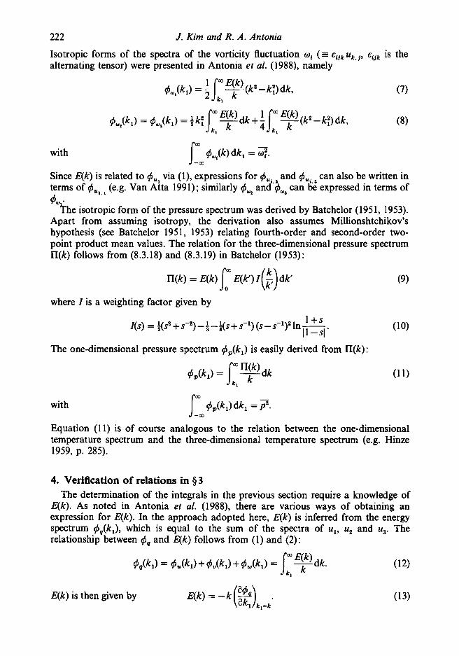
Isotropic forms of the spectra of the vorticity fluctuation wi (= 6 i j k U k , , , c i j k is the alternating tensor) were presented in Antonia et al. (1988), namely

with

Since E(k) is related to #,, via (l), expressions for #,. and #,,,, can also be written in terms of #u,, l (e.g. Van Atta 1991); similarly and’h,. can be expressed in terms of

yhe isotropic form of the pressure spectrum was derived by Batchelor (1951, 1953). Apart from assuming isotropy, the derivation also assumes Millionshtchikov’s hypothesis (see Batchelor 1951, 1953) relating fourth-order and second-order two- point product mean values. The relation for the three-dimensional pressure spectrum n(k) follows from (8.3.18) and (8.3.19) in Batchelor (1953):

6, *

n(k) = E(k) lom E(k’) Z(k) dk’ (9)

where Z is a weighting factor given by

(10) 1 +s I(s) = xs2 + s - ~ ) - $ - g(s + s-’) (s - s-1)2 In -

11 -sI *

The one-dimensional pressure spectrum #&) is easily derived from n(k) :

with

Equation (1 1) is of course analogous to the relation between the one-dimensional temperature spectrum and the three-dimensional temperature spectrum (e.g. Hinze 1959, p. 285).

4. Verification of relations in $ 3 The determination of the integrals in the previous section require a knowledge of

E(k). As noted in Antonia et al. (1988), there are various ways of obtaining an expression for E(k). In the approach adopted here, E(k) is inferred from the energy spectrum #&), which is equal to the sum of the spectra of ul, up and u3. The relationship between #, and E(k) follows from (1) and (2):

E(k) is then given by

Isotropy of the small scales of turbulence 223

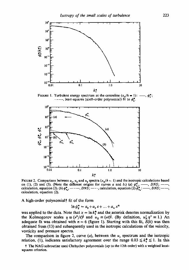
k: FIGURE 1. Turbulent energy spectrum at the centreline ( x J h = 1): -, q5:;

-__- , least-squares (sixth-order polynomial) fit to 4:.

10'

10'

*; 10'

3 10'

a

r." a lo-'

10-

lo-' 0.01 0.1 1 .o 10

k: FIGURE 2. Comparison between ul, uz and u3 spectra (x , /h = 1) and the isotropic calculations based on (l), (2) and (3). (Note the different origins for curves a and b.) (a) q5:, - , DNS; --, calculation, equation (2). (b) +:*, ---, DNS; --, calculation, equation (2) &s: - , DNS; --, calculation, equation (2).

A high-order polynomialt fit of the form In#,* = a,+a,x+ ...+ a,xn

was applied to the data. Note that x = Ink: and the asterisk denotes normalization by the Kolmogorov scales 71 E (v3/$ and uK = (v$. (By definition, u&q+ = 1.) An adequate fit was obtained with n = 6 (figure 1). Starting with this fit, E(k) was then obtained from (13) and subsequently used in the isotropic calculations of the velocity, vorticity and pressure spectra.

The comparison in figure 2, curve (a), between the u1 spectrum and the isotropic relation, ( I ) , indicates satisfactory agreement over the range 0.03 5 k: 5 1. In this

t The NAG subroutine used Chebychev polynomials (up to the 12th order) with a weighted least- squares criterion.

224 J. Kim and R. A . Antonia

range, there is also good agreement (curve b) between $u2 or gU3 and the values obtained with (2). Note that the approximate equality between $,, and $,, is consistent with isotropy (and with the less stringent requirement of axisymmetry). f h e departure in curves (a) and (b) between the calculation and the data for k: 5 0.03 is not unexpected. The departure at the largest wavenumbers (k: > 1) partly reflects small errors (as illustrated by the slight upturn) in the distributions of $,,, $u and $u3 and also likely inaccuracies in E(k). Distributions of $uz (or $u3) were also cafculated using

and a polynomial fit to $,,, similar to that used for $*. For 0.03 < k: < 1, the resulting calculation (not shown here) follows the DNS distributions of q5u2 (or $uJ as well as that in figure 2 (curve (6)). For k: > 1, the agreement is better than in curve (b), due to the direct use of $,, as input to the calculation.

Reasonable agreement can be observed in figure 3(a)(i) between the w1 spectrum and the calculation based on (7). There is somewhat better agreement, figure 3(a)(ii) and (iii), between the DNS distributions of $,2 or and the calculation based on (8). For clarity, the distributions of $,o, and $,, are displaced in figure 3. These distributions are essentially identical, as can be inferred from the comparison with the calculated distribution, which is the same for $,z as for $, . The near equality between $, and $,,, like that between $uz and $u3, represents good support for axisymmetry. It should be noted that $,, and $,, can also be calculated by starting with $ul instead of E(k). Since

By substituting this expression in (7) and (8), it is easy to show that

and

Equations (16) and (17) yield distributions, figure 3(b), which are in as good an agreement with the DNS distributions of $(dl and (or $,,,) as the calculations shown in figure 3(a), up to k: x 1. For larger wavenumbers, ( 16) and (17) are in better agreement with the DNS distributions since the DNS distribution of 4u is used as input for the calculations based on (1 6) and (17).

The vorticity spectrum can be obtained from the sum of the spectra of the individual vorticity components, namely

I . I

The reasonable agreement between $,(k1) and isotropy (i.e. (7) and (8) or (16), (17)), as shown in figure 3(a, b), follows from that between the individual components of 4, and the isotropic calculations. Note that $,(kl) should represent the energy dissipation spectrum for homogeneous turbulence. Antonia et al. (1988) observed a close correspondence between approximations to the energy dissipation spectrum and the vorticity spectrum, measured in the self-preserving region of a cylinder wake. The

Isotropy of the small scales of turbulence 225

I I , I I I 1 I I I ,

0.01 0.1 1 .o 10 I

k: FIGURE 3. Comparison between w,:.yz, w3 and w spectra and isotropic calculations (x , /h = 1). (Note the different origins for curves i, ii, 111 and iv.) -, DNS; --, calculation. For (a) the calculations are based on (7), (8) and (13). For (b), the calculations are based on (16), (17) using the DNS distribution of as input.

present data closely satisfy the homogeneous relation 8 = vz everywhere across the channel (Antonia et al. 1991) and the behaviour of $&) in figure 3 should therefore reflect closely that of $c(kl).

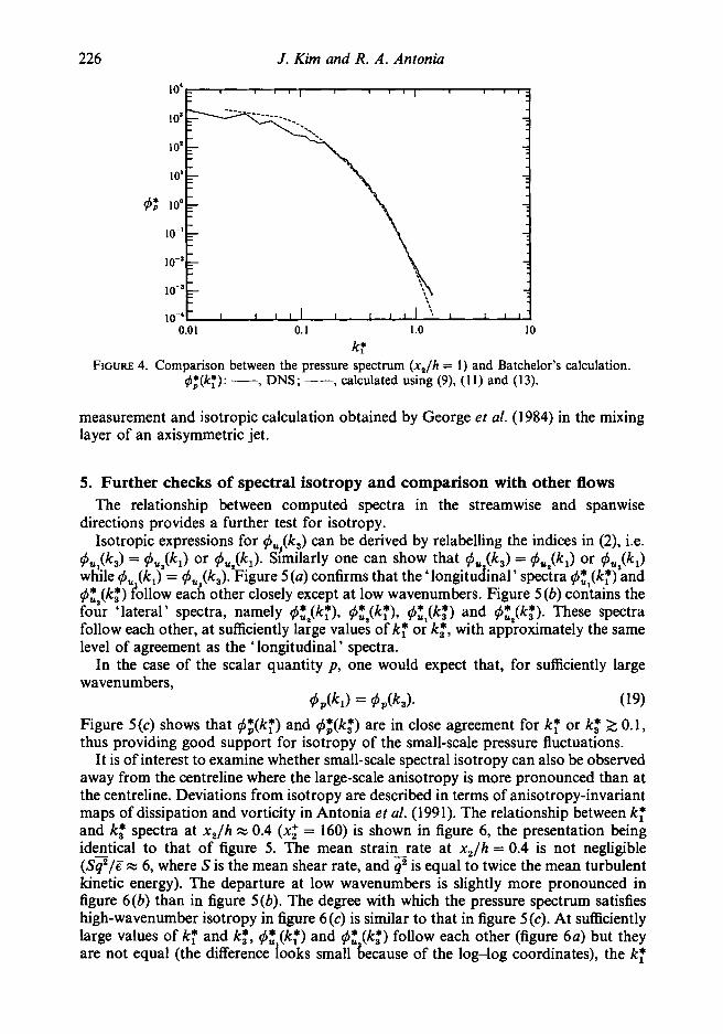
The pressure spectrum q5: is shown in figure 4 together with the isotropic calculation based on (9), (10) and (11). There is quite satisfactory agreement between the two distributions over more than a half decade in wavenumber extending up to nearly the Kolmogorov wavenumber (kf = 1). For kf > 1, the DNS distribution curls up a little (this may be a numerical effect but should not be of serious concern here as it is relatively small) while the calculation may become unreliable due to inaccuracies in fitting to E(k) in this region. The agreement between the two distributions in figure 4 implies support for the two assumptions made in Batchelor’s (195 1) calculation. Further evidence for local isotropy of the pressure spectrum is given in $ 5 while the normality assumption is considered in $6. The agreement at relatively large k: in figure 4 complements the agreement - primarily over the inertial subrange - between

226 J . Kim and R. A . Antonia

10‘ I I

FIGURE

..

0.01 0.1 1 .o 10

k: 4. Comparison between the pressure spectrum (x , /h = 1) and Batchelor’s

$X(k:): -, DNS; --, calculated using (S), (11) and (13). calculation.

measurement and isotropic calculation obtained by George et al. (1984) in the mixing layer of an axisymmetric jet.

5. Further checks of spectral isotropy and comparison with other flows The relationship between computed spectra in the streamwise and spanwise

directions provides a further test for isotropy. Isotropic expressions for $u.,(k3) can be derived by relabelling the indices in (2), i.e.

$ul(k3) = $,Jk,) or $&). Similarly one can show that 9, (k,) = $,P(kl) or $&,) while $, (k,) = $u (k,). Figure 5 (a) confirms that the ‘longitudinal ’ spectra $:l(kt) and $:3(k:) follow each other closely except at low wavenumbers. Figure 5 (b) contains the four ‘lateral’ spectra, namely $;Jk;), $:Jk:), $:,(k:) and $:,(k:). These spectra follow each other, at sufficiently large values of k: or k:, with approximately the same level of agreement as the ‘longitudinal ’ spectra.

In the case of the scalar quantity p, one would expect that, for sufficiently large wavenumbers,

Figure 5(c) shows that $:(k;) and $,*(k:) are in close agreement for k: or k: 2 0.1, thus providing good support for isotropy of the small-scale pressure fluctuations.

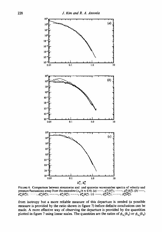
It is of interest to examine whether small-scale spectral isotropy can also be observed away from the centreline where the large-scale anisotropy is more pronounced than at the centreline. Deviations from isotropy are described in terms of anisotropy-invariant maps of dissipation and vorticity in Antonia et al. (1991). The relationship between k: and k: spectra at x 2 / h x 0.4 (x: = 160) is shown in figure 6, the presentation being identical to that of figure 5. The mean strain rate at x, /h = 0.4 is not negligible ( S z / B x 6, where S is the mean shear rate, and is equal to twice the mean turbulent kinetic energy). The departure at low wavenumbers is slightly more pronounced in figure 6(b) than in figure 5(b). The degree with which the pressure spectrum satisfies high-wavenumber isotropy in figure 6(c) is similar to that in figure S(c). At sufficiently large values of k: and k:, 9: (k:) and $: (k:) follow each other (figure 6a) but they are not equal (the difference iooks small because of the log-log coordinates), the k:

$ p ( k J = $ p ( k 3 ) . (19)

Isotropy of the small scales of turbulence 227

0.01 0.1 1 .o 10

1 o a

10'

101

100

10-1

I 0-9

10-3

10-4

10-6 0.01 0. I 1 .o 10

- 101 r

0.01 0.1 1 .o 10

k:, k: FIGURE 5. Comparison between velocity spectra in the streamwise and spanwise wavenumber spectra of velocity and pressure fluctuations at the centreline (x , /h = 1). (a) -, 6: (k:); ----, #: (k:). (b) -9 #:,(k:); . . . . - 9 #:,(k:); ---, #:,(k:); ----, #:,(k:). (c) -, #f(k:); ----, #f&:).

spectrum falling below the k: spectra. In figure 6(b) , for sufficiently large wavenumbers, qbZl(kj) x qb:z(kj) while qb:?(k:) x $2 (k:). These four magnitudes should however be the same (to satisfy local isotropy). As in figure 6 ( 4 , the k: spectra lie below the k: spectra. It is possible that these differences reflect a 'small' departure of the small scales

228 J . Kim and R. A . Antonia

10-4

lo-' 0.01

L 0.1 llll

1 .o _i 10

10'

10'

10'

1 oo 10-1

10-8

10-3

lo-'

lo-' 0.01 0.1 1 .o 10

1 (4 ;

- - - 1

T1

10-3 - lo-' I 1 1 1 I I I 1 I 1 1 1

0.01 0.1 1 .o 10

k:, k: FIGURE 6. Comparison between streamwise and and spanwise wavenumber spectra of velocity and pressure fluctuations away from the centreline (x, /h x 0.4). (a) -, #: (kf); ----, 4; (k:). (6) -, #:pf); . ' ' ' ., #lfJ(kf); ---, #:,(k:); - - - - 9 #:p:). (c) -1 #;(if); ----2 #;(R:).

from isotropy but a more reliable measure of this departure is needed (a possible measure is provided by the ratio shown in figure 7) before definite conclusions can be made. A more effective way of observing the departure is provided by the quantities plotted in figure 7 using linear scales. The quantities are the ratios of q5&J or $,&)

Isotropy of the small scales of turbulence 229

0 0.2 0.4 0.6 0.8 1 .o 1.2

2.0 * I I I I I ~

(b)

-

1 I I I 1 0 0.2 0.4 0.6 0.8 1 .o I .2

k: FIGURE 7. Ratio of $: (k:) or $:ik,+) and its isotropic value, calculated from (2). (4 $:,(k3/[#:,(k:)1iw9 (6) $:Jk3/[$:,(k3Iiw; -, X; = 40; ---, 160; ----. 395.

and the corresponding isotropic spectra. The distributions support previous con- clusions inferred from the log-log plots. In particular, isotropy is closely satisfied for g5ul(k3) and k: R. 0.2 at x i = 160 and 395. There is more scatter in the case of &,(k3) but the conclusion is unaltered. The departure from isotropy at low wavenumbers (kj 5 0.2) is indeed more emphasized in figure 7 than in figure 6.

The isotropy of small scales when S ~ / B is sufficiently small and the possible departures from isotropy at larger values of @ / B are not a peculiarity of this flow. Spalart’s (1988) DNS boundary-layer distributions of g5:l(kj), $:P<kj) and $:l(kj) at y+ = 200 (figure 21 a of this paper) show that and $,*,(kj) are in close agreement with isotropy (equation (2)) when kj 2 0.1 (the madmum value of k: was only 0.7). Results at y+ = 40 (figure 21 b of his paper) show that g5:Jkj) was in reasonable agreement with (2) for k: 2 0.1 but g5: (kj) was significantly underestimated by (2). The present spectra for g5:l(k:) and g5:,(k:) at x l = 40 ( S ~ / B = 7.6) show very similar trends to those of Spalart. The degree to which g5:,(k3/[g5:&3]is0 approximates 1 at x l = 40 is comparable to that at x, /h = 1 (xi = 395). At x i = 40, the ratio g5:,(k,*)/[g5:,(k:)],, is however consistently greater than 1, the departure increasing as kj+ 1.

230 J. Kim and R. A . Antonia

There is somewhat mixed experimental support for small-scale isotropy, in the context of (1) and (2). For example, most of the distributions of $,e(k,) and $&) obtained by Comte-Bellot (1963) in a fully developed turbulent channel flow indicate varying degrees of departure from (2) when k, is sufficiently large? (these departures are certainly smaller than those at small k,). The data show evidence of an increased departure from local isotropy as the wall is approached. There is however no evidence, at least when the strain rate is small, to support that the departure increases as the Reynolds number decreases. (For Comte-Bellot’s data, h+ is in the range 2300-8200, easily one order of magnitude larger than for the present simulations.) Klebanoff s (1955) measured u spectra in a turbulent boundary layer (x , /6 = 0.05 and 0.58) showed an asymptotic trend towards the isotropic calculation at large wavenumbers. Mestayer (1982) observed quite good agreement with (2) at x , / 6 = 0.33 in a relatively high Reynolds number turbulent boundary layer. Champagne, Harris & Corrsin (1970) reported reasonable agreement between (2) and their measurements of $u,(kl) and $,S(k,) in a nearly homogeneous turbulent shear flow (@/F = 5.9) when 0.04 5 0.5. The deviation from (2) when k: > 0.5 was attributed to spatial resolution limitations (both wire lengths and separation between the wires of the X-probe).

6. Pressure and velocity correlations at small separations The correlation between the pressure fluctuations at two points is given by

(Batchelor 1951, 1953)

P(r) = 222Jr(y-f)(92dy, Y aY

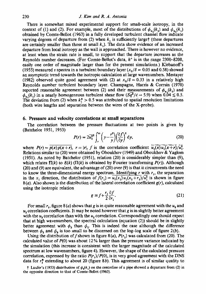
where P(r) = p(x)p(x + r), r = Irl, f is the correlation coefficient u,(x) ul(x + r)/z. Relations similar to (20) were obtained by Oboukhov (1949) and Oboukhov & Yaglom (1951). As noted by Batchelor (1951), relation (20) is considerably simpler than (9), which relates n(k) to E(k) (ll(k) is obtained by Fourier transforming P(r)). Although (20) and (9) are equivalent, the advantage of (20) over (9) is that it circumvents the need to know the three-dimensional energy spectrum. Identifying r with r,, the separation in the x , direction, the distribution of f ( r l ) = u ~ ( x , ) u l ( x l + r l ) / ~ is shown in figure 8(a). Also shown is the distribution of the lateral correlation coefficient g(r), calculated using the isotropic relation

g = f+-- rl af 2 ar,

For small r,, figure 8 (a) shows that g is in quite reasonable agreement with the u, and u3 correlation coefficients. It may be noted however that g is in slightly better agreement with the u3 correlation than with the u, correlation. Correspondingly one should expect that at high wavenumbers, the spectral calculation (equation (2)) should be in slightly better agreement with $3 than $,. This is indeed the case although the difference between $, and $3 is too small to be discerned on the log-log scale of figure 2(b).

Using the distribution offshown in figure 8 (a), P(r,) was calculated from (20). The calculated value of P(0) was about 12 YO larger than the pressure variance indicated by the simulation (this increase is consistent with the larger magnitude of the calculated spectrum at low wavenumbers, figure 4). However, the shape of the calculated pressure correlation, expressed by the ratio P(r,)/P(O), is in very good agreement with the DNS data for r: extending to about 20 (figure 8b). This agreement is of similar quality to

t Laufer’s (1953) distribution of $*(kl) on the centreline of a pipe showed a departure from (2) in the opposite direction to that of Comte-Bellot (1963).

Isotropy of the small scales of turbulence 23 1

0 20 80 loo

0 20 40 60 80 loo

FIGURE 8. Velocity and pressure correlations at small longitudinal separations (x,/h = 1). (a) Longitudinal and lateral-velocity correlation coefficients--, f = ul(xl) uI(xI + rl)/q, DNS. g: ----. up(x,) u2(x1 +rl)/u:, DNS; --- , us(x!) us(xl + rl)/ut, DNS ; --, calculated from (23). (6) Pressure correlation coefficients. (The longitudinal velocity correlation coefficient f is also shown (-).) P(rl) /P(0): ---, DNS; --, calculated from (20).

r:

that shown in figure 4 at high wavenumbers. Comparison of figure 8(a and b) indicates that the shape of P(r,) is much more similar to that of g(r,) thanf(r,). This similarity has been noted by Hunt et al. (1987) who carried out a direct spectral simulation of nearly isotropic turbulence. These authors commented that for a distribution of Townsend-type large-scale eddies, the pressure variation across an eddy should be similar to that using u2. The value of P(0) calculated by Hunt et al. using (20) was about 7% lower than the pressure variance obtained in their simulation.

In Batchelor’s (195 1) calculation, fourth-order moments of velocity fluctuations were assumed to be related to second-order moments by

- -- -- ui uj u; u; = W U U ; u:, + u* u; u p ; + u* u:, u, u;,

where the unprimed and primed quantities refer to points x and x’ (= x + r ) respectively. When all the indices are equal to 1, the above relation reduces to

The validity of (22) was checked for the present data at the centreline with r -= rl and

232 J. Kim and R. A. Antonia

4

3

O

I I I I I 0 20 40 60 80 100

1 .o

0.8

0.6

0.4

0 20 40 60 80 100 0.2

r* = r: or r:

FIGURE 9. Comparison between fourth-order and second-or$r correlations of u1 ( x , / h = 1). (a) Left- (-) and right-hand sides (---) of (22), normalized by uf . (b) Left- (-) and right-hand sides

(---) of (22), normalized by their respective values at r, = 0 or r3 = 0.

r ZE r3. The resulting distributions are shown in figure 9(a), where the normalization is by q, and in figure 9(b), where each side of (22) is normalized by its own value at r = 0. At sufficiently large values of r, u1 ul(r) should become negligible and u: u ! ( r ) / q should approach 1. This is indeed what figure 9(a) indicates, consistent with Batchelor's expectation that (22) is more ~- likely to apply in the energy-containing range of r than at small separations. As r -+ 0, u: u:(r)/u: should approach 3 for a Gaussian distribution. Figure 9(a) shows that this is not the case, the flatness factor $/zz being equal to about 3.68 (it is reasonable to attribute this departure from Gaussianity to the small scales; one would also expect the departure to increase with Reynolds number). When the normalization of each side of (22) is by its own value at rl = 0 (or r3 = 0), the two sides of the equation are practically identical for values of rr (or r:) extending up to about 40. This agreement reflects that between P(r)/P(O) and Batchelor's calculation. This seems reasonable since only derivatives of the fourth-order velocity product enter the calculation.

7. Dependence on Reynolds number The present data have been obtained at small values of the Reynolds number. Low

Reynolds number effects are therefore expected to influence the statistics of the velocity and scalar fields everywhere in the flow. The effect of Reynolds number on the

Isotropy of the small scales of turbulence

0.005 I I I

n

0 0.4 0.8 1.2

k:

233

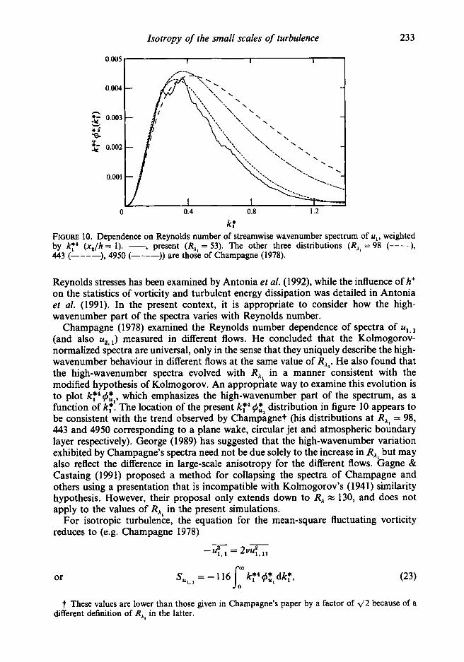
FIGURE 10. Dependence on Reynolds number of streamwise wavenumber spectrum of uI, weighted by k:4 (x , /h = 1). - , present (R,, = 53). The other three distributions (R,, = 98 (----). 443 (----), 4950 (---)) are those of Champagne (1978).

Reynolds stresses has been examined by Antonia et al. (1992), while the influence of hf on the statistics of vorticity and turbulent energy dissipation was detailed in Antonia et al. (1991). In the present context, it is appropriate to consider how the high- wavenumber part of the spectra varies with Reynolds number.

Champagne (1978) examined the Reynolds number dependence of spectra of ul,l (and also u ~ , ~ ) measured in different flows. He concluded that the Kolmogorov- normalized spectra are universal, only in the sense that they uniquely describe the high- wavenumber behaviour in different flows at the same value of R,,. He also found that the high-wavenumber spectra evolved with R,, in a manner consistent with the modified hypothesis of Kolmogorov. An appropnate way to examine this evolution is to plot k:4$:1, which emphasizes the high-wavenumber part of the spectrum, as a function of k:. The location of the present k:4 distribution in figure 10 appears to be consistent with the trend observed by champagne? (his distributions at R,, = 98, 443 and 4950 corresponding to a plane wake, circular jet and atmospheric boundary layer respectively). George (1989) has suggested that the high-wavenumber variation exhibited by Champagne’s spectra need not be due solely to the increase in R,, but may also reflect the difference in large-scale anisotropy for the different flows. Gagne & Castaing (1991) proposed a method for collapsing the spectra of Champagne and others using a presentation that is incompatible with Kolmogorov’s (1941) similarity hypothesis. However, their proposal only extends down to R, x 130, and does not apply to the values of RA1 in the present simulations.

For isotropic turbulence, the equation for the mean-square fluctuating vorticity reduces to (e.g. Champagne 1978)

or r m

t These values are lower than those given in Champagne’s paper by a factor of .\/2 because of a different definition of R,, in the latter.

234 J. Kim and R. A . Antonia

h +A

Y, 3 SL"

0 0.5 1 .o 1.5 2.0

n ~0.0050 +-

*; 8.

0.0025 2

Y,

c

0

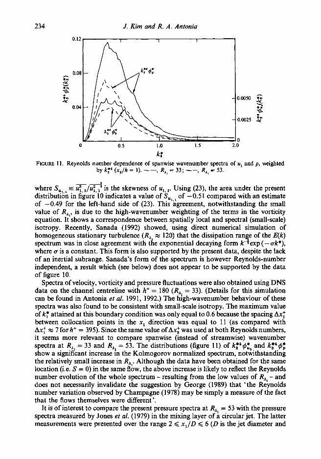
k; FIGURE 1 1 . Reynolds number dependence of spanwise wavenumber spectra of u1 and p , weighted

by kj4 (x,/h = 1). --, R,, = 33; -, R,, = 53.

- -a where Su,,, = u:, Ju;, is the skewness of u,, Using (23), the area under the present distribution in figure 10 indicates a value of S,, of -0.51 compared with an estimate of -0.49 for the left-hand side of (23). This'igreement, notwithstanding the small value of R,,, is due to the high-wavenumber weighting of the terms in the vorticity equation. It shows a correspondence between spatially local and spectral (small-scale) isotropy. Recently, Sanada (1992) showed, using direct numerical simulation of homogeneous stationary turbulence (R, x 120) that the dissipation ran e of the E(k)

where v is a constant. This form is also supported by the present data, despite the lack of an inertial subrange. Sanada's form of the spectrum is however Reynolds-number independent, a result which (see below) does not appear to be supported by the data of figure 10.

Spectra of velocity, vorticity and pressure fluctuations were also obtained using DNS data on the channel centreline with h+ = 180 (R,, = 33). (Details for this simulation can be found in Antonia et al. 1991, 1992.) The high-wavenumber behaviour of these spectra was also found to be consistent with small-scale isotropy. The maximum value of k: attained at this boundary condition was only equal to 0.6 because the spacing Ax: between collocation points in the x , direction was equal to 1 1 (as compared with Ax: x 7 for h+ = 395). Since the same value of Ax: was used at both Reynolds numbers, it seems more relevant to compare spanwise (instead of streamwise) wavenumber spectra at RA1 = 33 and RA1 = 53. The distributions (figure 11) of kt49:, and k t 4 9 ; show a significant increase in the Kolmogorov normalized spectrum, notwithstanding the relatively small increase in R,'. Although the data have been obtained for the same location (i.e. S = 0) in the same flow, the above increase is likely to reflect the Reynolds number evolution of the whole spectrum - resulting from the low values of R,, - and does not necessarily invalidate the suggestion by George (1989) that 'the Reynolds number variation observed by Champagne (1 978) may be simply a measure of the fact that the flows themselves were different '.

It is of interest to compare the present pressure spectra at R,, = 53 with the pressure spectra measured by Jones et al. (1979) in the mixing layer of a circular jet. The latter measurements were presented over the range 2 < x , / D < 6 ( D is the jet diameter and

spectrum was in close agreement with the exponential decaying form k- f exp (- ak*),

Isotropy of the small scales of turbulence 235

, . I . , , , , , I , , ,

(4

10-6 lo-* 10-1 10

k: FIGURE 12. Comparison between the centreline pressure and velocity spectra with those of Jones etaf. (1979). (a) 4;; (4) (c) 4:. Jones et al. ----, RAI = 466; --- --- , RAI = 841 ; ----, present (RAI = 53); -, k:-s for (a) or R:-s for (b) and (c).

x1 is measured from the jet exit plane). The values of RAl, inferred from the data of Jones et al. increase from about 466 at x J D = 2 to 841 at x , / D = 6. The measured pressure spectra shown in figure 12 (a) extend to values of k: near the start of the k:-i inertial subrange. The location of the present spectrum suggests that the inertial subrange for the Jones et al. experiments should extend up to k: x 0.1. For k: > 0.1, the present pressure spectrum provides a plausible extension of the Jones et al.

236 J . Kim and R. A. Antonia

spectrum to high wavenumbers; the extension seems justified given that the roll-off in the measured pressure spectra may be attributed to probe roll-off due to spatial averaging (George et al. 1984). The present distributions of $2, and $2, (figure 126, c) are also plausible extensions (to the dissipation range) of the k:-t inertial subrange exhibited by the Jones et al. (1979) velocity spectra.

8. Conclusions and discussion Low Reynolds number DNS data on the centreline of a fully developed turbulent

channel flow are generally in good agreement with spectral local isotropy. The behaviour of high-wavenumber spectra of velocity, vorticity and pressure fluctuations is adequately described by the appropriate isotropic relations.

The high-wavenumber pressure spectrum compares favourably with Batchelor’s (195 1, 1953) analysis which provides an expression for the three-dimensional pressure spectrum in terms of the three-dimensional energy spectrum. Equivalently, the shape of the two-point pressure correlation is in good agreement with Batchelor’s calculation for small longitudinal separations. For such separations, the shape of the two-point quadruple velocity correlation is also in good agreement with that implied by the joint normality assumption in Batchelor’s theory.

The high-wavenumber isotropy exhibited by the results of @4 and 5 supports the idea that small scales are close to being isotropic, in spite of the absence of an inertial subrange. This absence implies that a large separation between the energy-containing lengthscales and the dissipative lengthscales is apparently not needed before the latter become isotropic. This issue as well as the need to better define conditions under which small scales may tend to a universal form are clearly of interest (e.g. Phillips 1991 ; Hunt & Vasilicos 1991 ; Sreenivasan 1991). For example, in the context of decaying oceanic turbulence, Phillips (199 1) observed that the Kolmogorov scaling of the high- wavenumber part of the spectrum need not imply a Kolmogorov-type energy cascade. The apparent insensitivity of the small scales to the large-scale anisotropy, as reflected by the present data, appears to be somewhat inconsistent with that of Domaradzky & Rogallo (1991) and Brasseur (1991), which point to strong non-local interactions between small and large wavenumbers. Such interactions would suggest that the small scales feel the straining motions by large scales and could therefore be anisotropic. It is possible, however, that although individual triad interactions are highly non-local (in wavenumber space), they may average out so that the net effect on the anisotropy of the small-scale motion is negligible (R. S. Rogallo, private communication).

The analysis by Durbin & Speziale (1 991) has shown that the dissipation rate tensor cannot be isotropic if the mean strain rate is not zero. At x z / h = 0.4, the mean strain rate is not negligible and the computed dissipation rate tensor is anisotropic. Yet figure 6 ( c ) suggests that the small-scale pressure fluctuations satisfy isotropy as well as on the centreline (figure 5c) . The strain at x z / h = 0.4 produces an anisotropy which seems to shift the high-wavenumber velocity spectrum, but, in log-log coordinates, does not greatly alter its shape from that predicted by small-scale isotropy. As noted in $ 5 , a better measure of the departure from isotropy is required before the effect of parameters such as SF/6 on small scales of the turbulence can be assessed unambiguously. Such an investigation is currently underway by the present authors.

As is well known, the assumption of local isotropy allows a considerable simplification when estimates of quantities such as care required through measurement. The present centreline spectra show that the departure from isotropy is negligible at high wavenumbers and relatively small at low wavenumbers. Accordingly, the

Isotropy of the small scales of turbulence 237

assumption of isotropy yields a sufficiently accurate estimate of F at this location (see Antonia et al. 1991). As the distance from the centreline (and therefore the magnitude of S) increases, the assumption becomes less adequate. It was shown in Antonia et al. that the assumption of local axisymmetry is more accurate (though less easy to implement) than local isotropy. Near the wall, both assumptions are tenuous; in this region, the experimenter may derive some comfort from the fact that the major contributions to F reside in only a few terms (see figure 4 of Antonia et al. 1991) and that the most important of these, viz. c, appears to be amenable to measurement (Zhu, Antonia & Kim 1993).

We are very grateful to Dr P. A. Durbin, Dr R. S. Rogallo and Professor A. M. Yaglom for their comments on the manuscript. R. A. A. acknowledges the support by the Australian Research Council.

R E F E R E N C E S

ANTONIA, R. A., ANSELMET, F. & CHAMBERS, A. J. 1986 Assessment of local isotropy using measurements in a turbulent plane jet. J. Fluid Mech. 163, 365-391.

ANTONIA, R. A., BROWNE, L. W. B. & SHAH, D. A. 1988 Characteristics of vorticity fluctuations in a turbulent wake. J. Fluid Mech. 189, 349-365.

ANTONIA, R. A., KIM, J. & BROWNE, L. W. B. 1991 Some characteristics of small-scale turbulence in a turbulent duct flow. J. Fluid Mech. 233, 369-388.

ANTONIA, R. A., SHAH, D. A. & BROWNE, L. W. B. 1987 Spectra of velocity derivatives in a turbulent wake. Phys. Fluids 30, 3455-3462.

ANTONIA, R. A., SHAH, D. A. & BROWNE, L. W. B. 1988 Dissipation and vorticity spectra in a turbulent wake. Phys. Fluids 31, 1805-1807.

ANTONIA, R. A,, TEITEL, M., KIM, J. & BROWNE, L. W. B. 1992 Low Reynolds number effects in a fully developed turbulent channel flow. J. Fluid Mech. 236, 579-605.

BATCHELOR, G. K. 1951 Pressure fluctuations in isotropic turbulence. Proc. Camb. Phil. SOC. 47, 359-374.

BATCHELOR, G. K. 1953 The Theory of Homogeneous Turbulence. Cambridge University Press. BRASSEUR, J. G. 1991 Comments on the Kolmogorov hypothesis of isotropy in the small scales.

CHAMPAGNE, F. H. 1978 The fine-scale structure of the turbulent velocity field. J . Fluid Mech. 86,

CHAMPAGNE, F. H., HARRIS, V. G. & CORRSIN, S. 1970 Experiments on nearly homogeneous turbulent shear flow. J. Fluid Mech. 41, 81-139.

COMTE-BELLOT, G. 1963 Turbulent flow between two parallel walls. Universite de Grenoble (translated by P. Bradshaw, Rep. ARC 31609 FM4/02, 1969).

DOMARADZKY, J. A. & ROGALLO, R. S. 1991 Local energy transfer and nonlocal interactions in homogeneous, isotropic turbulence. Phys. Fluids A 2, 41 3-426.

DURBIN, P. A. & SPEZIALE, C. G. 1991 Local anisotropy in strained turbulence at high Reynolds numbers. Trans. ASME I: J. Fluids Engng. 113, 707-709.

FUNG, J. C. H., HUNT, J. C. R., MALIK, N. A. & PERKINS, R. A. 1992 Kinematic simulation of homogeneous turbulence by unsteady random Fourier modes. J. Fluid Mech. 236, 28 1-3 18.

GAGNE, Y. & CASTAING, B. 1991 Une representation universelle sans invariance globale d’ichelle des spectres d’energie en turbulence diveloppie. C. R. Acad. Sci. Paris 312 (11), 441-445.

GEORGE, W. K. 1989 The self-preservation of turbulent flows and its relation to initial conditions and coherent structures. In New Horizons in Turbulence (ed. W . K. George & R. Arndt), pp. 39-674. Hemisphere.

GEORGE, W. K., BEUTCHER, P. D. & ARNDT, R. E. A. 1984 Pressure spectra in turbulent free shear flows. J. Fluid Mech. 148, 155-191.

HEISENBERG, W. 1948 Zur Statischen Theorie der Turbulenz. Z. Phys. 124, 628-657.

AIAA-91-0230, 29th Aerospace Sciences Meeting, January 7-10, 1991, Reno, Nevada.

67-108.

238

HINZE, J. 0. 1975 Turbulence. McGraw-Hill. HUNT, J. C. R., BUELL, J. C. & WRAY, A. A. 1987 Big whorls carry little whorls. In Proc. First

Summer Program of the Center for Turbulence Research, Rep. CTR-S87, pp. 79-94 NASA Ames/Stanford University.

HUNT, J. C. R. & VASILICOS, J. C. 1991 Kolmogorov’s contributions to the physical and geometrical understanding of small-scale turbulence and recent developments. Proc. R. SOC. Lond. A 434,

JON=, B. G., ADRIAN, R. J., NITHIANANDAN, C. K. & PLANCHON, H. P. 1979 Spectra of turbulent

KIM, J. 1989 On the structure of pressure fluctuations in simulated turbulent channel flow. J. Fluid

KIM, J., MOIN, P. & MOSER, R. 1987 Turbulence statistics in fully developed channel flow at low

KLEBANOFF, P. S. 1955 Characteristics of turbulence in a boundary layer with zero pressure gradient.

KOLMOGOROV, A. N. 1941 The local structure of turbulence in an incompressible fluid with very

LAUFER, J. 1953 The structure of turbulence in fully developed pipe flow. NACA Rep. 1174. MESTAYER, P. 1982 Local isotropy and anisotropy in a high-Reynolds-number turbulent boundary

MESTAYER, P. & CHAMBAUD, P. 1979 Some limitation to measurements of turbulence micro-

MONIN, A. S. & YAGLOM, A. M. 1975 Statistical fluid mechanics. In Mechanics of Turbulence (ed.

OBOUKHOV, A. M. 1949 Pressure fluctuations in a turbulent flow. Dokl. Akad. Nauk SSSR 66,

OBOUKHOV, A. M. & YAGLOM, A. M. 1951 Microstructure of a turbulent flow. Prikl. Math. Mekh.

PANCHEV, S . 1971 Random Functions and Turbulence. Pergamon. PHILLIPS, 0. M. 1991 The Kolmogorov spectrum and its oceanic cousins: a review. Proc. R. SOC.

Lond. A434, 125-138. SANADA, T. 1992 Comment on the dissipation-range spectrum in turbulent flows. Phys. Fluids A 4,

1086-1087. SPALART, P. R. 1988 Direct simulation of a turbulent boundary layer up to R, = 1410. J . Fluid

Mech. 187, 61-98. SREENIVASAN, K. R. 1991 On local isotropy of passive scalars in turbulent shear flows. Proc. R. SOC.

Lond. A 434, 165- 182. UBEROI, M. S. 1953 Quadruple velocity correlations and pressure fluctuations in isotropic

turbulence. J. Aero. Sci. 20, 197-204. VAN ATTA, C. W. 1977 Second-order spectral local isotropy in turbulent scalar fields. J. Fluid Mech.

80, 609-615. VAN AITA, C. W. 1991 Local isotropy of the smallest scales of turbulent scalar and velocity fields.

Proc. R. SOC. Lond. A434, 139-141. ZHU, Y., ANTONIA, R. A. & KIM, J. 1993 Velocity and temperature derivative measurements in the

near-wall region of a turbulent duct flow. To be presented at Int. Con$ on Near- Wall Turbulent Flows, Tempe, Arizona.

J . Kim and R. A . Antonia

183-2 10.

static pressure fluctuations in jet mixing layers. AIAA J. 17, 449457.

Mech. 205, 421-451.

Reynolds number. J. Fluid Mech. 177, 133-166.

NACA Rep. 1247.

large Reynolds numbers. Dokl. Akad. Nauk. SSSR 30, 301-305.

layer. J. Fluid Mech. 125, 475-503.

structure with hot and cold-wires. Boundary-Layer Met. 16, 31 1-329.

J. L. Lumley), vol. 2. MIT Press.

17-20.

15, 3-26 (translated as NACA Rep. TM 1350, June 1953).