Ironless transducer for measuring the mechanical properties of porous materials

Olivier Doutres, Nicolas Dauchez,a) Jean-Michel Genevaux, Guy Lemarquand, and

Sylvain Mezil

Laboratoire d’Acoustique de l’Universite du Maine, UMR CNRS 6613,

Avenue Olivier Messiaen, 72085 Le Mans Cedex 9, France

(Dated: 18 January 2010)

This paper presents a measurement set-up for determining the mechanical properties

of porous materials at low and medium frequencies, by extending towards higher

frequencies the quasistatic method based on a compression test. Indeed, classical

quasi-static methods generally neglect the inertia effect of the porous sample and the

coupling between the surrounding fluid and the frame: they are restricted to low fre-

quency range (< 100 Hz) or specific sample shape. In the present method, the porous

sample is placed in a cavity to avoid a lateral airflow. Then a specific electrodynamic

ironless transducer is used to compress the sample. This highly linear transducer

is used as actuator and sensor: the mechanical impedance of the porous sample is

deduced from the measurement of the electrical impedance of the transducer. The

loss factor and the Young’s modulus of the porous material are estimated by inverse

method based on the Biot’s model. Experimental results obtained with a polymer

foam show the validity of the method in comparison with quasistatic method. The

frequency limit has been extended from 100 Hz to 500 Hz. Sensitivity of each input

parameter is estimated in order to point out the limitations of the method.

PACS numbers: 43.20.Ye, 43.20.Jr, 43.38.Dv

a)Institut Superieur de Mecanique de Paris - SUPMECA Paris, LISMMA, 3 rue Fernand Hainault, 93407

Saint Ouen Cedex, France

1

hal-0

0449

742,

ver

sion

1 -

22 J

an 2

010

Author manuscript, published in "Journal of Applied Physics (2010) 1"

shaker

fixed plate

A

force sensor

shaker

moving plate

accelerometerssample sample

(a) (b)

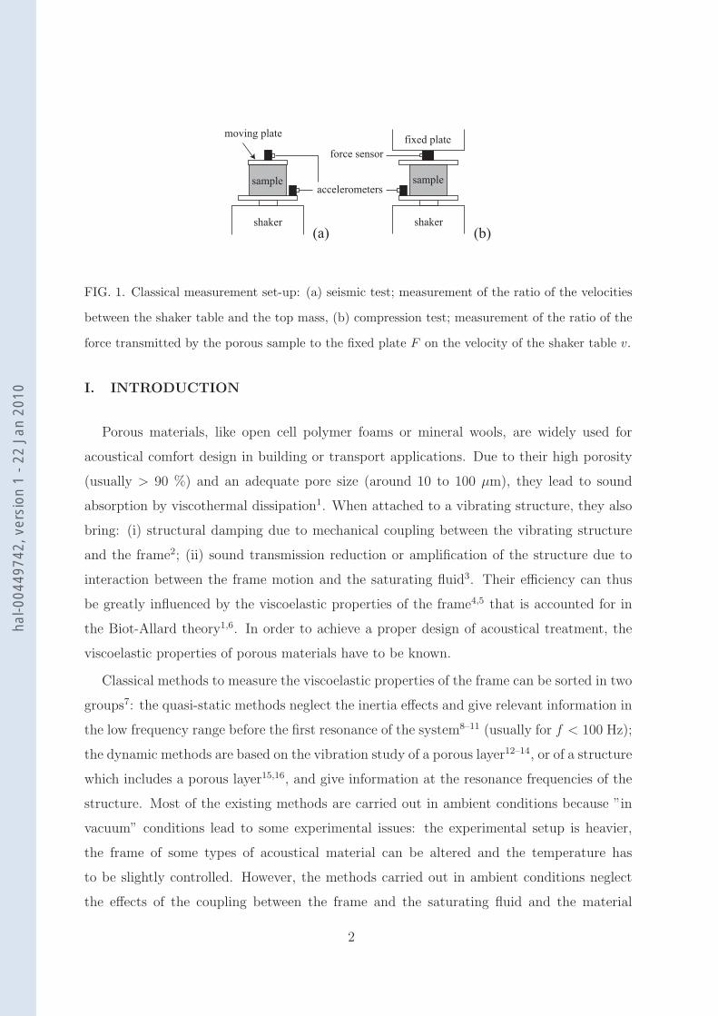
FIG. 1. Classical measurement set-up: (a) seismic test; measurement of the ratio of the velocities

between the shaker table and the top mass, (b) compression test; measurement of the ratio of the

force transmitted by the porous sample to the fixed plate F on the velocity of the shaker table v.

I. INTRODUCTION

Porous materials, like open cell polymer foams or mineral wools, are widely used for

acoustical comfort design in building or transport applications. Due to their high porosity

(usually > 90 %) and an adequate pore size (around 10 to 100 µm), they lead to sound

absorption by viscothermal dissipation1. When attached to a vibrating structure, they also

bring: (i) structural damping due to mechanical coupling between the vibrating structure

and the frame2; (ii) sound transmission reduction or amplification of the structure due to

interaction between the frame motion and the saturating fluid3. Their efficiency can thus

be greatly influenced by the viscoelastic properties of the frame4,5 that is accounted for in

the Biot-Allard theory1,6. In order to achieve a proper design of acoustical treatment, the

viscoelastic properties of porous materials have to be known.

Classical methods to measure the viscoelastic properties of the frame can be sorted in two

groups7: the quasi-static methods neglect the inertia effects and give relevant information in

the low frequency range before the first resonance of the system8–11 (usually for f < 100 Hz);

the dynamic methods are based on the vibration study of a porous layer12–14, or of a structure

which includes a porous layer15,16, and give information at the resonance frequencies of the

structure. Most of the existing methods are carried out in ambient conditions because ”in

vacuum” conditions lead to some experimental issues: the experimental setup is heavier,

the frame of some types of acoustical material can be altered and the temperature has

to be slightly controlled. However, the methods carried out in ambient conditions neglect

the effects of the coupling between the frame and the saturating fluid and the material

2

hal-0

0449

742,

ver

sion

1 -

22 J

an 2

010

is considered as ”in vacuum”. Pritz15,16, Ingard17, Rice and Goransson18 carried out frame

compressibility measurements in air and ”in vacuum” using the resonant method of Fig. 1(a).

In this configuration, the porous sample is placed between a vibrating base and an additional

mass: the structure is supposed to behave as a spring-mass system. It is shown that the

frequency response of the mass with respect to the shaker table motion is considerably

damped when air is present. This difference is due to the presence of a lateral airflow

(perpendicular to the imposed displacement) pumped in and out of the material during

sinusoidal compression. The evaluation of the Young’s modulus is hardly affected by the

presence of the air but the apparent loss factor of the material is greatly overestimated.

Effect of air on a quasi-static measurement, such as proposed by Mariez8 (fig. 1(b)), has

also been studied numerically by Etchessahar14 and Danilov et al.19. In this configuration,

the porous sample is placed between a vibrating base and a impervious rigid wall and the

mechanical impedance is measured. It is shown that both real and imaginary part of this

impedance can be greatly influenced by the presence of air for thin samples or materials

having a large airflow resistivity. Tarnow10 proposes an analytical correction which accounts

for this influence on the measurement of the force transmitted by the porous sample to

the rigid wall for cylindrical samples. In a previous paper20, the authors investigated the

feasibility to extend the quasistatic compression method toward higher frequencies by mean

of:

• a cavity where the sample is set-up n order to reduce the air pumping effects,

• an electrodynamic loudspeaker as actuator and sensor to simplify the measurement

set-up.

This method is in good agreement with the quasistatic one but the frequency range was

limited below the first frequency resonance of the loudspeaker by non linearities of the

transducer.

In the present paper, the method is extended towards medium frequencies by using a

specific electrodynamic transducer devoid of major non linearities. In a first part, the

transducer design is described and the measurement procedure is detailed. Then results are

given for one polymer foam. Sensitivity of each input parameter is estimated in order to

point out the limitations of the method.

3

hal-0

0449

742,

ver

sion

1 -

22 J

an 2

010

sample

carbon foam piston

magnets

top cavity

ferrofluid seals

voice-coilbottom cavity

position probe

J

(revolution axis)

x

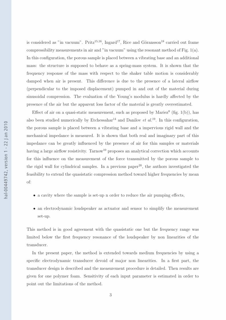
FIG. 2. Measurement set-up for the electrodynamic method. x axis is oriented in the direction

opposite to the gravity field.

II. MEASUREMENT SET-UP

The electro-mechanical setup to measure the porous mechanical properties is shown in

Fig. 2. The electrodynamic transducer used to compress the sample is mounted between two

cavities. It is made of a voice-coil motor such as those used in traditional electrodynamic

loudspeakers. However, this motor is ironless21,22 and the viscoelastic suspension is replaced

by ferrofluid seals23 in order to vanish the major electrical and mechanical nonlinearities24,25

respectively. Furthermore, the motor is constituted by a stack of three permanent magnet

rings 20 mm high with a inner diameter of 49.7 mm. Each ring is an assembly of 16 single tiles

(Fig. 3) of Nd2Fe14B with a magnetization of J = 1.4 T. The rings are radially magnetized

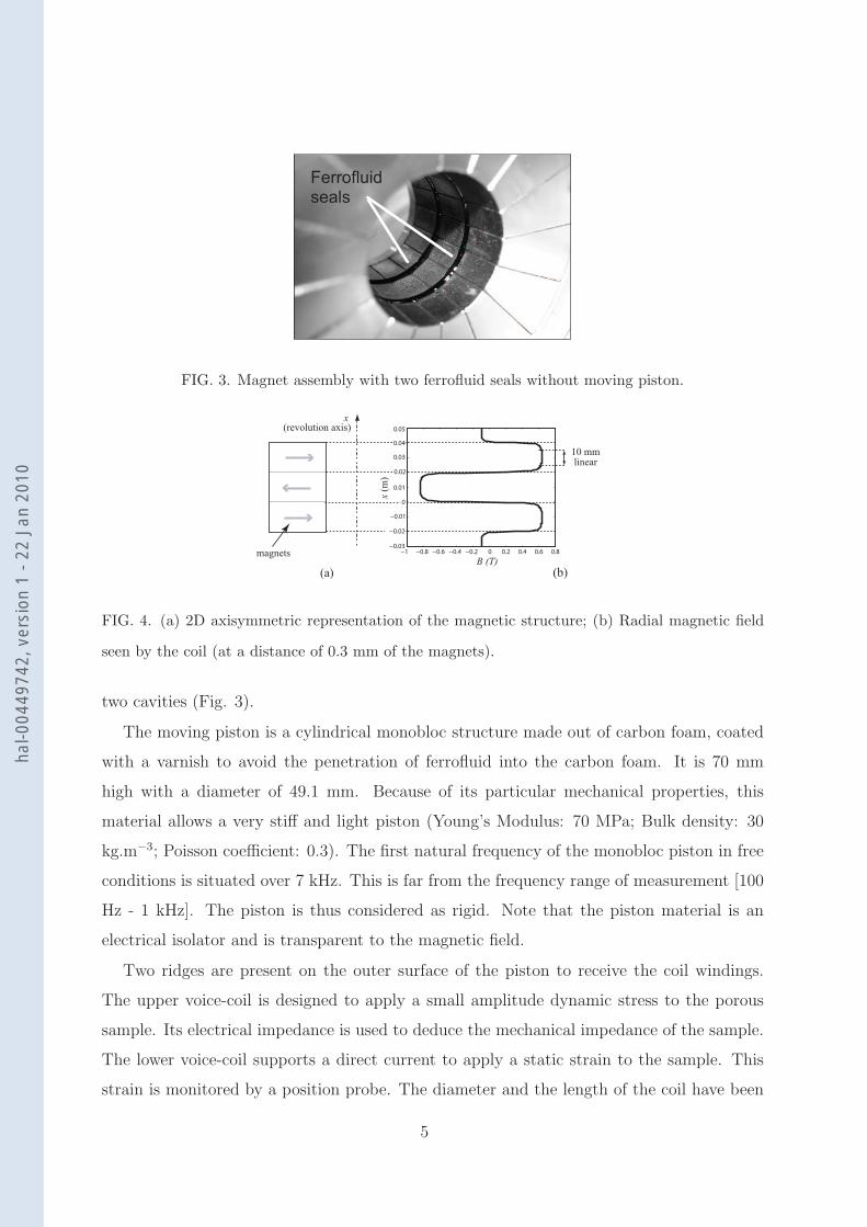
with successive opposite directions (Fig. 2) to avoid a magnetic field leakage26. Fig. 4 shows

an analytical simulation27 of the radial magnetic field seen by the coils, i.e. at a distance

of 0.3 mm of the magnets. It is shown that the magnetic structure allows a high magnetic

field (around 0.7 T) which is constant over 10 mm on the height of each ring. Thus, the

electrodynamic motor can be used to apply a static compression of 10 mm and preserve the

same properties. The inner face of the motor presents also a strong gradient of the magnetic

field where the magnetic field reverses, i.e. at the interface between two rings. These regions,

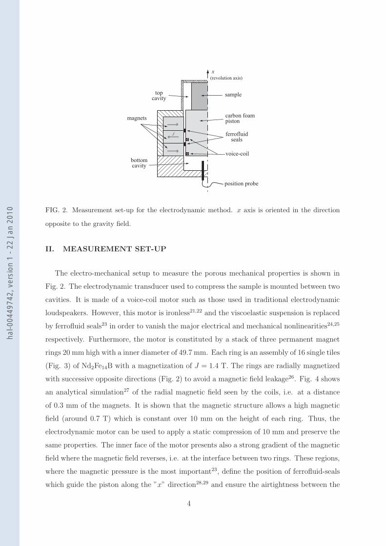
where the magnetic pressure is the most important23, define the position of ferrofluid-seals

which guide the piston along the ”x” direction28,29 and ensure the airtightness between the

4

hal-0

0449

742,

ver

sion

1 -

22 J

an 2

010

Ferrofluidseals

FIG. 3. Magnet assembly with two ferrofluid seals without moving piston.

(b)(a)

−1 −0.8 −0.6 −0.4 −0.2 0 0.2 0.4 0.6 0.8−0.03

−0.02

−0.01

0

0.01

0.02

0.03

0.04

0.05

x (m

)

B (T)

x (revolution axis)

magnets

10 mm linear

FIG. 4. (a) 2D axisymmetric representation of the magnetic structure; (b) Radial magnetic field

seen by the coil (at a distance of 0.3 mm of the magnets).

two cavities (Fig. 3).

The moving piston is a cylindrical monobloc structure made out of carbon foam, coated

with a varnish to avoid the penetration of ferrofluid into the carbon foam. It is 70 mm

high with a diameter of 49.1 mm. Because of its particular mechanical properties, this

material allows a very stiff and light piston (Young’s Modulus: 70 MPa; Bulk density: 30

kg.m−3; Poisson coefficient: 0.3). The first natural frequency of the monobloc piston in free

conditions is situated over 7 kHz. This is far from the frequency range of measurement [100

Hz - 1 kHz]. The piston is thus considered as rigid. Note that the piston material is an

electrical isolator and is transparent to the magnetic field.

Two ridges are present on the outer surface of the piston to receive the coil windings.

The upper voice-coil is designed to apply a small amplitude dynamic stress to the porous

sample. Its electrical impedance is used to deduce the mechanical impedance of the sample.

The lower voice-coil supports a direct current to apply a static strain to the sample. This

strain is monitored by a position probe. The diameter and the length of the coil have been

5

hal-0

0449

742,

ver

sion

1 -

22 J

an 2

010

determined so that a porous materials with Young’s modulus of 400 kPa can be compressed

with a static strain of 2 %. For softer materials such as glass wool, the dimensions of the

voice-coil motor allow a maximum static compression of 10 mm.

Note that since the ferrofluid seals have no stiffness in the axial direction, unlike rubber

suspension and spider in traditional loudspeakers, the axial stiffness is only due to the

sample and to the air cavities loading the piston. Finally, the diameter of the sample has to

be smaller than the diameter of the top cavity to avoid lateral friction.

III. PRINCIPLE OF MEASUREMENT

The electrodynamic transducer is used to apply static and dynamic stresses to the porous

sample. From the measurement of the electrical impedance Zvc of the upper voice-coil, and

a linear model of the transducer behavior, the mechanical impedance Zp = F/v at the

porous/piston interface is determined. F is the force applied to the porous sample and v

is the velocity of the piston. The mechanical properties of the porous material, Young’s

modulus E and loss factor η, are then determined from the mechanical impedance of the

sample by reversing a poroelastic model based on the Biot-Allard theory1.

A. Transducer modeling

The transducer modeling is identical to the one used in a previous paper20. However,

since the motor is ironless and the viscoelastic suspension is replaced by ferrofluid seals, both

the compliance of the loudspeaker suspensions Cms and the shunting parallel resistance rf

are considered equal to zero. This model is now briefly presented.

The electrodynamic transducer is described by an equivalent electrical circuit. The de-

velopment of this model is described in detail by Thiele and Small30–32. This low frequency

model is valid under the first resonance frequency of the piston (here 7 kHz in free condi-

tions). The moving piston is thus considered as rigid and having only one degree of freedom

in the axial direction.

Fig. 5 is the analogous circuit for the setup of Fig. 2, with

U input voltage of the dynamic voice-coil,

i current passing through the dynamic voice-coil,

6

hal-0

0449

742,

ver

sion

1 -

22 J

an 2

010

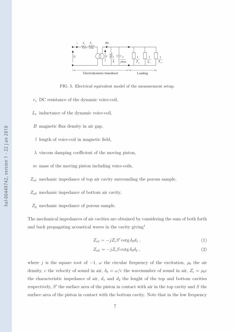
FIG. 5. Electrical equivalent model of the measurement setup.

re DC resistance of the dynamic voice-coil,

Le inductance of the dynamic voice-coil,

B magnetic flux density in air gap,

l length of voice-coil in magnetic field,

λ viscous damping coefficient of the moving piston,

m mass of the moving piston including voice-coils,

Za1 mechanic impedance of top air cavity surrounding the porous sample,

Za2 mechanic impedance of bottom air cavity,

Zp mechanic impedance of porous sample.

The mechanical impedances of air cavities are obtained by considering the sum of both forth

and back propagating acoustical waves in the cavity giving1

Za1 = −jZcS′ cotg δ0d1 , (1)

Za2 = −jZcS cotg δ0d2 , (2)

where j is the square root of −1, ω the circular frequency of the excitation, ρ0 the air

density, c the velocity of sound in air, δ0 = ω/c the wavenumber of sound in air, Zc = ρ0c

the characteristic impedance of air, d1 and d2 the lenght of the top and bottom cavities

respectively, S ′ the surface area of the piston in contact with air in the top cavity and S the

surface area of the piston in contact with the bottom cavity. Note that in the low frequency

7

hal-0

0449

742,

ver

sion

1 -

22 J

an 2

010

range, the two air cavities can be considered as simple compliances and equations (1-2) may

be symplified as

Z lfa1 =

γP0S′

jωd1, (3)

Z lfa2 = γP0S

jωd2, (4)

where γP0 is the adiabatic bulk modulus of the fluid with γ the ratio specific heats and P0

the atmospheric pressure.

From circuit analysis of Fig. 5, the electrical impedance is given by

Zvc =U

i= Ze +

(Bl)2

Zm + [Zp + Za1 + Za2](5)

with

Ze = re + jωLe , (6)

Zm = λ+ jωm . (7)

Hence, the mechanical impedance of the sample can be derived from the measurement of

Zvc, the properties of the transducer and of the two air cavities as

Zp =(Bl)2

Zvc − Ze

− (Zm + Za1 + Za2) . (8)

B. Determination of the transducer properties

The properties of the transducer are determined from the measurement of the electri-

cal impedance Zvc0 without porous sample in the top cavity. In that case, the equivalent

electrical circuit model gives

Zvc0 = Ze +(Bl)2

Zm + [Za10 + Za2]. (9)

with Za10 = −jZcS cotg δ0d1 (Eq.(1) with S ′ = S). The model is fitted on the measurement

to get re, Le, λ, m and Bl.

C. Calculation of the material mechanical properties

The mechanical properties of the porous sample are determined by fitting a poroelastic

model based on the Biot-Allard theory on the impedance Zp, determined from the measure-

ment of Zvc (Eq. (5)).

8

hal-0

0449

742,

ver

sion

1 -

22 J

an 2

010

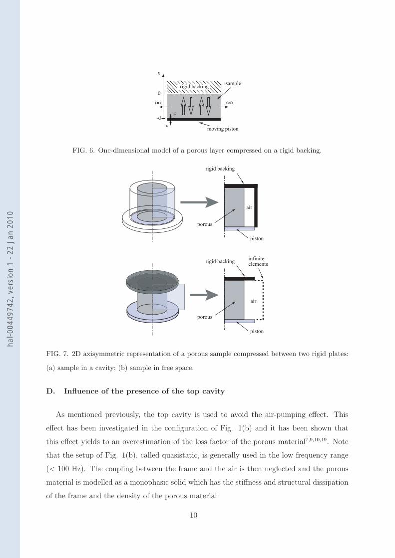
In the considered model, the material is isotropic and the displacements of the frame

and air are one-dimensional (Fig. 6): the porous material is considered as infinite in the

lateral directions and the effects of the boundary conditions are neglected. This assumption

is discussed in the next section.

The mechanical impedance can be derived analytically from the calculation of the total

stress σtxx applied by the porous sample to the vibrating piston (Fig. 6):

Zthp (ω) =

F

v=

Spσtxx(−d)

ωuw

, (10)

with Sp the surface area of the porous sample in contact with the vibrating piston (Sp =

S − S ′), uw the amplitude of the displacement imposed by the piston and d the sample

thickness. Note that the porous material is considered as infinite in the lateral directions in

the poroelastic model but the lateral dimensions are taken into account through the area of

the sample. According to the Biot-Allard theory1,6, three waves may propagate in a porous

media: two compressional waves and a shear wave. In this work, the shear wave is not excited

and only the two compressional waves are considered. These waves are characterized by a

complex wave number δi (i = 1, 2) and a displacement ratio µi. This ratio indicates in which

medium the waves mainly propagate. The total stress is thus the sum of the stress exerted

by the fluid and solid phases characterized by these two waves as

σtxx(−d) = σs

xx(−d) + σfxx(−d) (11)

=[

(P + Q) + µ1(R + Q)]

δ1 cos(δ1d)D1 +[

(P + Q) + µ2(R + Q)]

δ2 cos(δ2d)D2 .

In these equations, R is the bulk modulus of the fluid phase and Q quantifies the potential

coupling between the solid and fluid phases. Expression of these two last coefficients can

be found in reference1. D1 and D2 are the amplitude coefficients of the two compressional

waves and can be determined from the boundary conditions applied to the sample. Here,

the displacement is nul at x = 0 and is equal to the one of the piston at x = −d which gives

D1 =uw(µ2 − 1)

sin(δ1d)(µ1 − µ2), (12)

D2 =uw(1− µ1)

sin(δ2d)(µ1 − µ2). (13)

9

hal-0

0449

742,

ver

sion

1 -

22 J

an 2

010

v

rigid backing

F

0

-d

x

∞ ∞

sample

moving piston

FIG. 6. One-dimensional model of a porous layer compressed on a rigid backing.

porous

air

piston

rigid backing

porous

air

piston

rigid backinginfinite elements

FIG. 7. 2D axisymmetric representation of a porous sample compressed between two rigid plates:

(a) sample in a cavity; (b) sample in free space.

D. Influence of the presence of the top cavity

As mentioned previously, the top cavity is used to avoid the air-pumping effect. This

effect has been investigated in the configuration of Fig. 1(b) and it has been shown that

this effect yields to an overestimation of the loss factor of the porous material7,9,10,19. Note

that the setup of Fig. 1(b), called quasistatic, is generally used in the low frequency range

(< 100 Hz). The coupling between the frame and the air is then neglected and the porous

material is modelled as a monophasic solid which has the stiffness and structural dissipation

of the frame and the density of the porous material.

10

hal-0

0449

742,

ver

sion

1 -

22 J

an 2

010

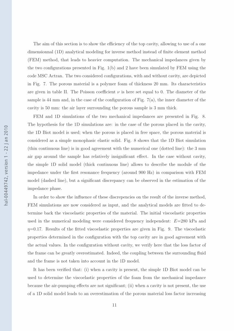
The aim of this section is to show the efficiency of the top cavity, allowing to use of a one

dimensionnal (1D) analytical modeling for inverse method instead of finite element method

(FEM) method, that leads to heavier computation. The mechanical impedances given by

the two configurations presented in Fig. 1(b) and 2 have been simulated by FEM using the

code MSC Actran. The two considered configurations, with and without cavity, are depicted

in Fig. 7. The porous material is a polymer foam of thickness 20 mm. Its characteristics

are given in table II. The Poisson coefficient ν is here set equal to 0. The diameter of the

sample is 44 mm and, in the case of the configuration of Fig. 7(a), the inner diameter of the

cavity is 50 mm: the air layer surrounding the porous sample is 3 mm thick.

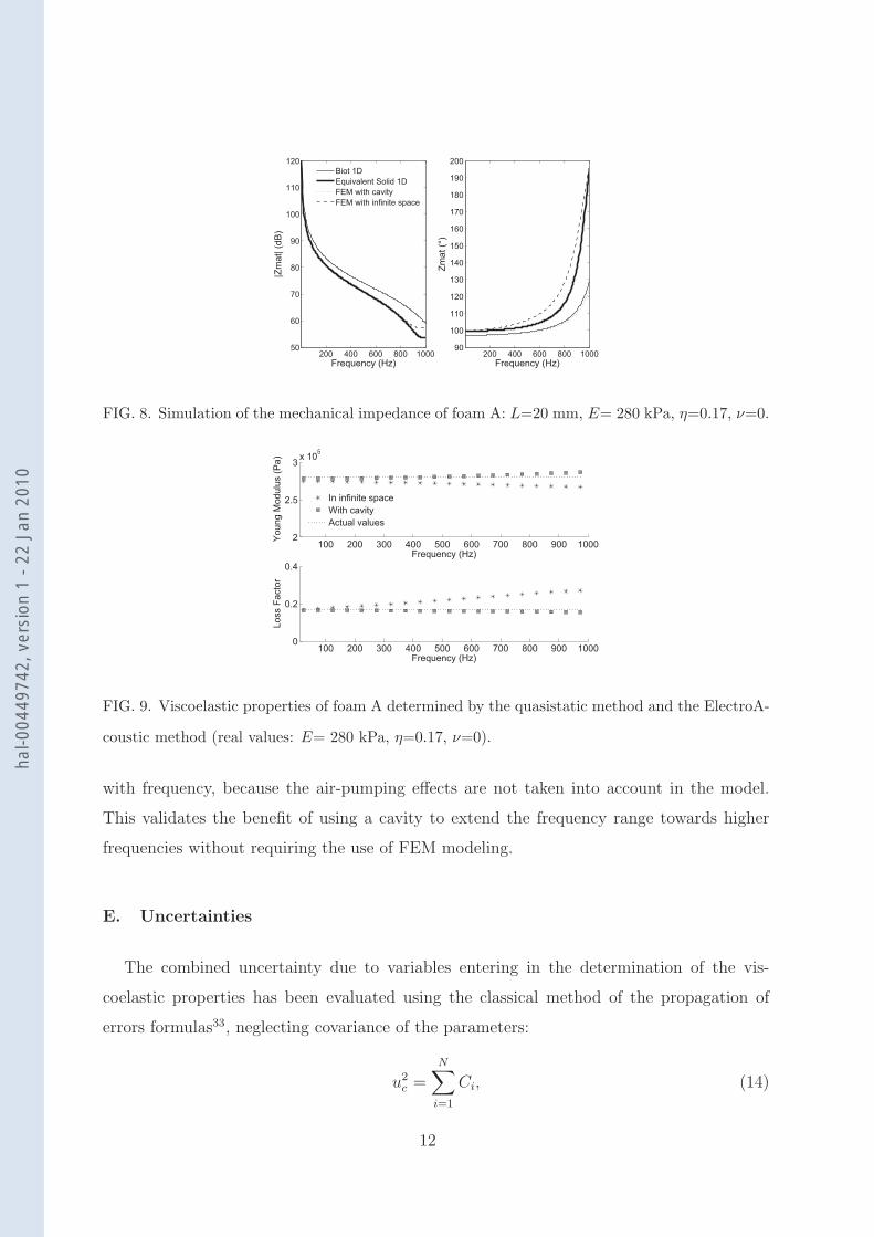
FEM and 1D simulations of the two mechanical impedances are presented in Fig. 8.

The hypothesis for the 1D simulations are: in the case of the porous placed in the cavity,

the 1D Biot model is used; when the porous is placed in free space, the porous material is

considered as a simple monophasic elastic solid. Fig. 8 shows that the 1D Biot simulation

(thin continuous line) is in good agreement with the numerical one (dotted line): the 3 mm

air gap around the sample has relatively insignificant effect. In the case without cavity,

the simple 1D solid model (thick continuous line) allows to describe the module of the

impedance under the first resonance frequency (around 900 Hz) in comparison with FEM

model (dashed line), but a significant discrepancy can be observed in the estimation of the

impedance phase.

In order to show the influence of these discrepencies on the result of the inverse method,

FEM simulations are now considered as input, and the analytical models are fitted to de-

termine back the viscoelastic properties of the material. The initial viscoelastic properties

used in the numerical modeling were considered frequency independent: E=280 kPa and

η=0.17. Results of the fitted viscoelastic properties are given in Fig. 9. The viscoelastic

properties determined in the configuration with the top cavity are in good agreement with

the actual values. In the configuration without cavity, we verify here that the loss factor of

the frame can be greatly overestimated. Indeed, the coupling between the surrounding fluid

and the frame is not taken into account in the 1D model.

It has been verified that: (i) when a cavity is present, the simple 1D Biot model can be

used to determine the viscoelastic properties of the foam from the mechanical impedance

because the air-pumping effects are not significant; (ii) when a cavity is not present, the use

of a 1D solid model leads to an overestimation of the porous material loss factor increasing

11

hal-0

0449

742,

ver

sion

1 -

22 J

an 2

010

200 400 600 800 100050

60

70

80

90

100

110

120

Frequency (Hz)

|Zm

at| (

dB

)

200 400 600 800 100090

100

110

120

130

140

150

160

170

180

190

200

Frequency (Hz)

Zm

at (°

)

Biot 1D

Equivalent Solid 1D

FEM with cavity

FEM with infinite space

FIG. 8. Simulation of the mechanical impedance of foam A: L=20 mm, E= 280 kPa, η=0.17, ν=0.

100 200 300 400 500 600 700 800 900 10002

2.5

3x 10

5

Frequency (Hz)

Yo

un

g M

od

ulu

s (

Pa

)

100 200 300 400 500 600 700 800 900 10000

0.2

0.4

Frequency (Hz)

Lo

ss F

acto

r

In infinite space

With cavity

Actual values

FIG. 9. Viscoelastic properties of foam A determined by the quasistatic method and the ElectroA-

coustic method (real values: E= 280 kPa, η=0.17, ν=0).

with frequency, because the air-pumping effects are not taken into account in the model.

This validates the benefit of using a cavity to extend the frequency range towards higher

frequencies without requiring the use of FEM modeling.

E. Uncertainties

The combined uncertainty due to variables entering in the determination of the vis-

coelastic properties has been evaluated using the classical method of the propagation of

errors formulas33, neglecting covariance of the parameters:

u2c =

N∑

i=1

Ci, (14)

12

hal-0

0449

742,

ver

sion

1 -

22 J

an 2

010

with Ci the contribution of each parameter to the combined uncertainty defined by

Ci =

(

∂f

∂xi

)2

u2(xi), (15)

where u(xi) is the standard uncertainty related to the variable xi and f the function relying

xi to the parameter either E or η. The N variables considered are the electrical impedance

Zvc and Zvc0 with and without sample respectively, those of the transducer (re, Le, m, λ,

Bl) and those of the porous material which are used for the inverse identification (σ, φ, α∞,

Λ, Λ′, ρ1). The partial derivatives are estimated numerically. Uncertainties are defined by

the variance si determined from repetability tests qi for a type A of n evaluations:

s2i =1

n− 1

n∑

j=1

(qj − q)2 (16)

where q is the average value ot the qi. The uncertainty on Zvc is 10−3 Ohms. The uncertainty

of the others variables are given in table I and II. The expanded uncertainties U = k uc is

obtained considering the coverage factor k = 2.

IV. RESULTS

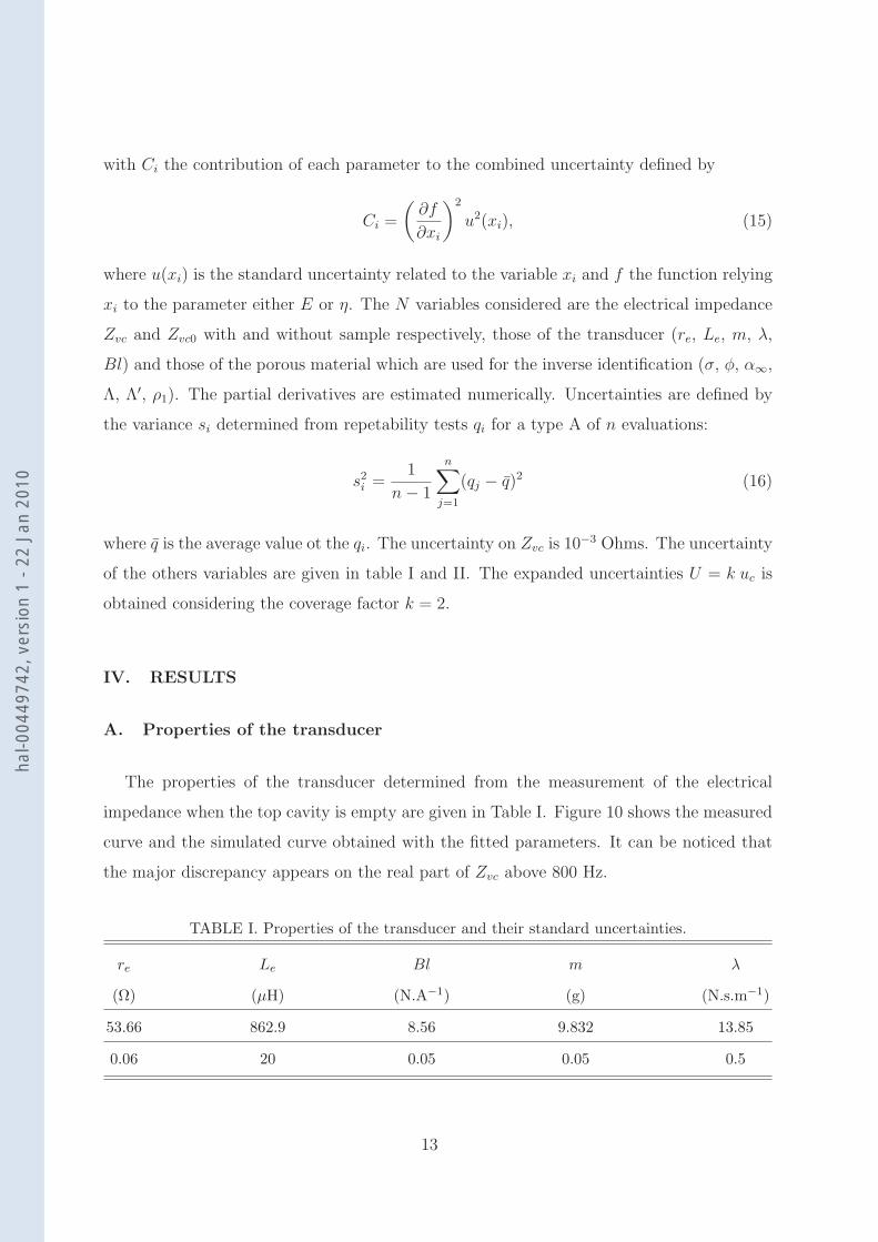
A. Properties of the transducer

The properties of the transducer determined from the measurement of the electrical

impedance when the top cavity is empty are given in Table I. Figure 10 shows the measured

curve and the simulated curve obtained with the fitted parameters. It can be noticed that

the major discrepancy appears on the real part of Zvc above 800 Hz.

TABLE I. Properties of the transducer and their standard uncertainties.

re Le Bl m λ

(Ω) (µH) (N.A−1) (g) (N.s.m−1)

53.66 862.9 8.56 9.832 13.85

0.06 20 0.05 0.05 0.5

13

hal-0

0449

742,

ver

sion

1 -

22 J

an 2

010

100 200 300 400 500 600 700 800 900 100053

54

55

56

57

58

59

60

Re(

Zvc)

Frequency (Hz)

Measurement: empty cavity

Simulation: empty cavity

Measurement: cavity with porous

100 200 300 400 500 600 700 800 900 1000−1

0

1

2

3

4

5

Im

(Zvc)

Frequency (Hz)

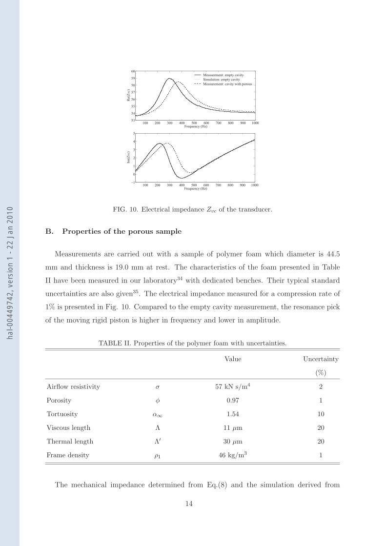
FIG. 10. Electrical impedance Zvc of the transducer.

B. Properties of the porous sample

Measurements are carried out with a sample of polymer foam which diameter is 44.5

mm and thickness is 19.0 mm at rest. The characteristics of the foam presented in Table

II have been measured in our laboratory34 with dedicated benches. Their typical standard

uncertainties are also given35. The electrical impedance measured for a compression rate of

1% is presented in Fig. 10. Compared to the empty cavity measurement, the resonance pick

of the moving rigid piston is higher in frequency and lower in amplitude.

TABLE II. Properties of the polymer foam with uncertainties.

Value Uncertainty

(%)

Airflow resistivity σ 57 kN s/m4 2

Porosity φ 0.97 1

Tortuosity α∞ 1.54 10

Viscous length Λ 11 µm 20

Thermal length Λ′ 30 µm 20

Frame density ρ1 46 kg/m3 1

The mechanical impedance determined from Eq.(8) and the simulation derived from

14

hal-0

0449

742,

ver

sion

1 -

22 J

an 2

010

100 300 600 1000−10

0

10

20

30

40

Frequency (Hz)

Mag

(Z)

100 300 600 1000−100

−80

−60

−40

−20

0

Frequency (Hz)

Arg

(Z)

(deg

)

Za10

th

Zp

Zp

th

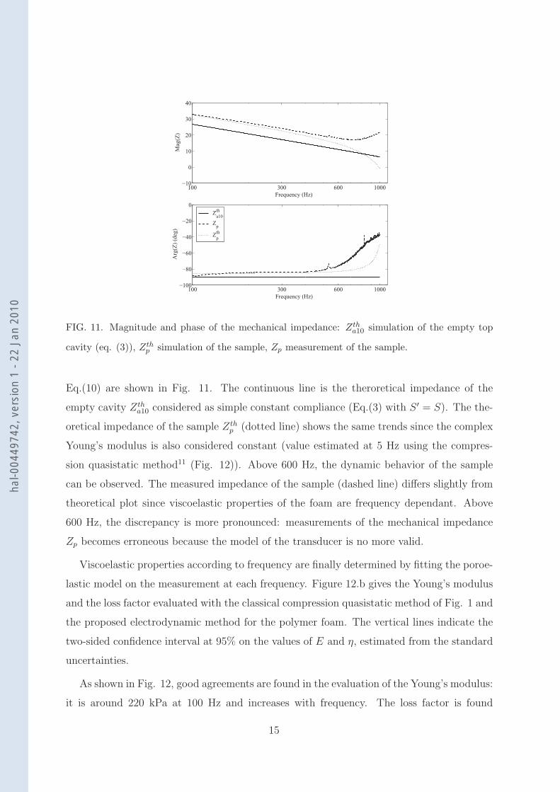
FIG. 11. Magnitude and phase of the mechanical impedance: Ztha10 simulation of the empty top

cavity (eq. (3)), Zthp simulation of the sample, Zp measurement of the sample.

Eq.(10) are shown in Fig. 11. The continuous line is the theroretical impedance of the

empty cavity Ztha10 considered as simple constant compliance (Eq.(3) with S ′ = S). The the-

oretical impedance of the sample Zthp (dotted line) shows the same trends since the complex

Young’s modulus is also considered constant (value estimated at 5 Hz using the compres-

sion quasistatic method11 (Fig. 12)). Above 600 Hz, the dynamic behavior of the sample

can be observed. The measured impedance of the sample (dashed line) differs slightly from

theoretical plot since viscoelastic properties of the foam are frequency dependant. Above

600 Hz, the discrepancy is more pronounced: measurements of the mechanical impedance

Zp becomes erroneous because the model of the transducer is no more valid.

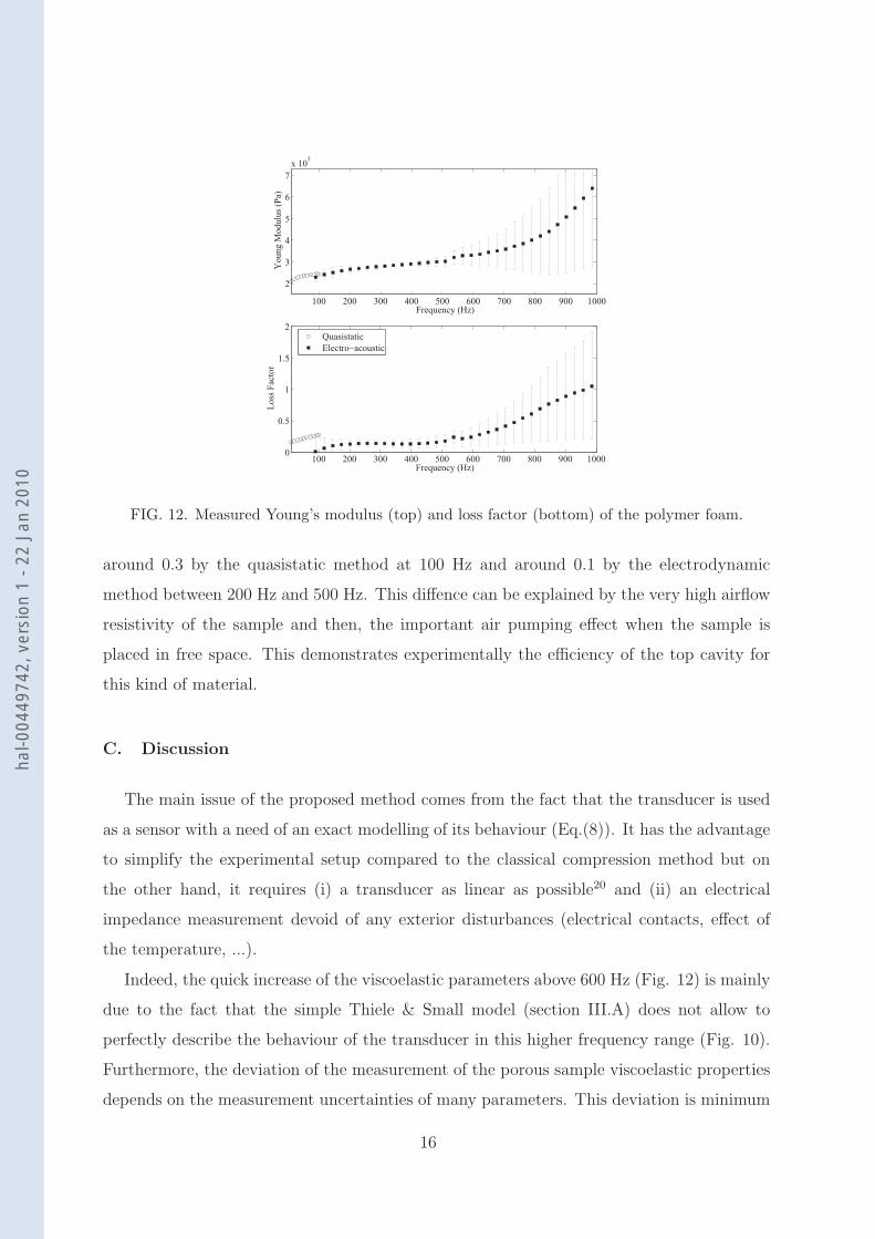
Viscoelastic properties according to frequency are finally determined by fitting the poroe-

lastic model on the measurement at each frequency. Figure 12.b gives the Young’s modulus

and the loss factor evaluated with the classical compression quasistatic method of Fig. 1 and

the proposed electrodynamic method for the polymer foam. The vertical lines indicate the

two-sided confidence interval at 95% on the values of E and η, estimated from the standard

uncertainties.

As shown in Fig. 12, good agreements are found in the evaluation of the Young’s modulus:

it is around 220 kPa at 100 Hz and increases with frequency. The loss factor is found

15

hal-0

0449

742,

ver

sion

1 -

22 J

an 2

010

100 200 300 400 500 600 700 800 900 1000

2

3

4

5

6

7

x 105

Frequency (Hz)

Young M

odulu

s (P

a)

100 200 300 400 500 600 700 800 900 10000

0.5

1

1.5

2

Frequency (Hz)

Loss

Fac

tor

Quasistatic

Electro−acoustic

FIG. 12. Measured Young’s modulus (top) and loss factor (bottom) of the polymer foam.

around 0.3 by the quasistatic method at 100 Hz and around 0.1 by the electrodynamic

method between 200 Hz and 500 Hz. This diffence can be explained by the very high airflow

resistivity of the sample and then, the important air pumping effect when the sample is

placed in free space. This demonstrates experimentally the efficiency of the top cavity for

this kind of material.

C. Discussion

The main issue of the proposed method comes from the fact that the transducer is used

as a sensor with a need of an exact modelling of its behaviour (Eq.(8)). It has the advantage

to simplify the experimental setup compared to the classical compression method but on

the other hand, it requires (i) a transducer as linear as possible20 and (ii) an electrical

impedance measurement devoid of any exterior disturbances (electrical contacts, effect of

the temperature, ...).

Indeed, the quick increase of the viscoelastic parameters above 600 Hz (Fig. 12) is mainly

due to the fact that the simple Thiele & Small model (section III.A) does not allow to

perfectly describe the behaviour of the transducer in this higher frequency range (Fig. 10).

Furthermore, the deviation of the measurement of the porous sample viscoelastic properties

depends on the measurement uncertainties of many parameters. This deviation is minimum

16

hal-0

0449

742,

ver

sion

1 -

22 J

an 2

010

200 400 600 800 100010

−15

10−10

10−5

100

Frequency (Hz)

Ci r

elat

ed t

o η

(a)

re

Le

Bl

200 400 600 800 1000 Frequency (Hz)

(b)

λ

m

200 400 600 800 100010

−15

10−10

10−5

100

Frequency (Hz)

Ci r

elat

ed t

o η

(c)

φ

Λ’

ρ1

200 400 600 800 1000 Frequency (Hz)

(d)

σ

Λ

α∞

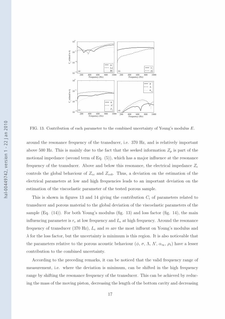
FIG. 13. Contribution of each parameter to the combined uncertainty of Young’s modulus E.

around the resonance frequency of the transducer, i.e. 370 Hz, and is relatively important

above 500 Hz. This is mainly due to the fact that the seeked information Zp is part of the

motional impedance (second term of Eq. (5)), which has a major influence at the resonance

frequency of the transducer. Above and below this resonance, the electrical impedance Ze

controls the global behaviour of Zvc and Zvc0. Thus, a deviation on the estimation of the

electrical parameters at low and high frequencies leads to an important deviation on the

estimation of the viscoelastic parameter of the tested porous sample.

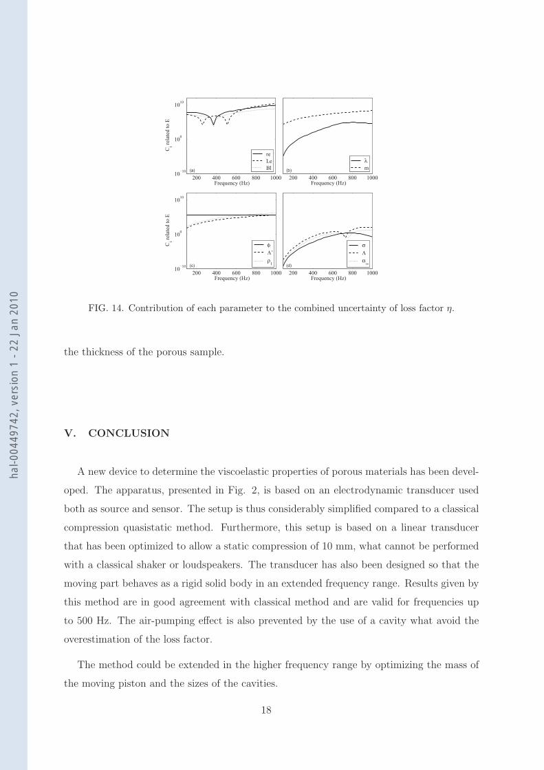
This is shown in figures 13 and 14 giving the contribution Ci of parameters related to

transducer and porous material to the global deviation of the viscoelastic parameters of the

sample (Eq. (14)). For both Young’s modulus (fig. 13) and loss factor (fig. 14), the main

influencing parameter is re at low frequency and Le at high frequency. Around the resonance

frequency of transducer (370 Hz), Le and m are the most influent on Young’s modulus and

λ for the loss factor, but the uncertainty is minimum is this region. It is also noticeable that

the parameters relative to the porous acoustic behaviour (φ, σ, Λ, Λ′, α∞, ρ1) have a lesser

contribution to the combined uncertainty.

According to the preceding remarks, it can be noticed that the valid frequency range of

measurement, i.e. where the deviation is minimum, can be shifted in the high frequency

range by shifting the resonance frequency of the transducer. This can be achieved by reduc-

ing the mass of the moving piston, decreasing the length of the bottom cavity and decreasing

17

hal-0

0449

742,

ver

sion

1 -

22 J

an 2

010

200 400 600 800 100010

−10

100

1010

Frequency (Hz)

Ci r

elat

ed t

o E

(a)

re

Le

Bl

200 400 600 800 1000 Frequency (Hz)

(b)

λ

m

200 400 600 800 100010

−10

100

1010

Frequency (Hz)

Ci r

elat

ed t

o E

(c)

φ

Λ’

ρ1

200 400 600 800 1000 Frequency (Hz)

(d)

σ

Λ

α∞

FIG. 14. Contribution of each parameter to the combined uncertainty of loss factor η.

the thickness of the porous sample.

V. CONCLUSION

A new device to determine the viscoelastic properties of porous materials has been devel-

oped. The apparatus, presented in Fig. 2, is based on an electrodynamic transducer used

both as source and sensor. The setup is thus considerably simplified compared to a classical

compression quasistatic method. Furthermore, this setup is based on a linear transducer

that has been optimized to allow a static compression of 10 mm, what cannot be performed

with a classical shaker or loudspeakers. The transducer has also been designed so that the

moving part behaves as a rigid solid body in an extended frequency range. Results given by

this method are in good agreement with classical method and are valid for frequencies up

to 500 Hz. The air-pumping effect is also prevented by the use of a cavity what avoid the

overestimation of the loss factor.

The method could be extended in the higher frequency range by optimizing the mass of

the moving piston and the sizes of the cavities.

18

hal-0

0449

742,

ver

sion

1 -

22 J

an 2

010

VI. ACKNOWLEDGEMENTS

The authors are grateful to the C.N.R.S., Region Pays de la Loire and the European

Commission (CREDO project - Contract no.: 030814) for their financial support, and to

Benoıt Merit for its contribution to design the magnetic part of the transducer.

REFERENCES

1J. F. Allard and N. Atalla, Propagation of Sound in Porous Media: Modelling Sound

Absorbing Materials, (2nd edition, Wiley, 2009).

2N. Dauchez, S. Sahraoui and N. Atalla, J. Sound Vib. 265, 437 (2003).

3O. Doutres, N. Dauchez and J.M. Genevaux, J. Acoust. Soc. Am. 121, 206 (2007).

4O. Doutres, N. Dauchez, J.M Genevaux and O. Dazel, J. Acoust. Soc. Am. 122, 2038

(2007).

5O. Doutres, N. Dauchez, J.M Genevaux and O. Dazel, Acta Acustica united with Acustica

95, 178 (2009).

6M. A. Biot, J. Appl. Phys. 33, 1482 (1962).

7Jaouen L., Renault A. and Deverge M., Appl. Acoust. 69, 1129 (2008).

8E. Mariez and S. Sahraoui, Internoise Congress Proceedings, Liverpool, 951 (1996).

9N. Dauchez, M. Etchessahar and S. Sahraoui, 2nd Biot conference on Poromechanics,

(2002).

10V. Tarnow, J. Acoust. Soc. Am. 118, 3672 (2005).

11M. Etchessahar, S. Sahraoui, L. Benyahia J.F. and Tassin, J. Acoust. Soc. Am. 117, 1114

(2005).

12L. Boeckx, P. Leclaire, P. Khurana, C. Glorieux, W. Lauriks and J.F. Allard, J. Acoust.

Soc. Am. 117, 545 (2005).

13J.F. Allard, O. Dazel, J. Descheemaeker, N. Geebelen, L. Boeckx, W. Lauriks J. Appl.

Phys. 106, 014906 (2009).

14M. Etchessahar, ”Caracterisation mecanique en basses frequences des materiaux acous-

tiques, Ph.D. dissertation (Universite du Maine, Le Mans, France, 2002).

15T. Pritz, J. Sound . Vib. 72, 317 (1980).

16T. Pritz, J. Sound . Vib. 106, 161 (1986).

19

hal-0

0449

742,

ver

sion

1 -

22 J

an 2

010

17U. Ingard, Notes on sound absorption technology, (Noise Control Foundation, 1994).

18H.J. Rice and P. Goransson, Int. J. Mech. Sc. 41, 561 (1999).

19O. Danilov, F. Sgard and X. Olny, J. Sound . Vib. 276, 729 (2004).

20O. Doutres, N. Dauchez N., J.-M. Genevaux and G. Lemarquand, 124, EL335 (2008).

21G. Lemarquand, IEEE Transactions on Magnetics 43, 3371 (2007).

22M. Berkouk, V. Lemarquand and G. Lemarquand, IEEE Transactions on Magnetics 37,

1011 (2001).

23R. Ravaud, G. Lemarquand and V. Lemarquand, J. Appl. Phys. 106, 34911 (2009).

24W. Klippel, J. Audio Eng. Soc. 54, 907 (2006).

25B. Merit, G. Lemarquand and V. Lemarquand, IEEE Transactions on Magnetics 45, 2867

(2009).

26M. Remy, G. Lemarquand, B. Castagnede and G. Guyader., IEEE Transactions on Mag-

netics 44, 4289 (2008).

27R. Ravaud and G. Lemarquand, Progress In Electromagnetics Research 91, 53 (2009).

28R. Ravaud, M. Pinho, G. Lemarquand, N. Dauchez, J.M. Genevaux, B. Brouard and V.

Lemarquand, IEEE Transactions on Magnetics 45, (2009).

29M. Pinho, N. Dauchez, J.M. Genevaux, B. Brouard and G. Lemarquand, COBEM, Inter-

national Congress of Mechanical Engineering, Gramados-RS, Brazil, (2009).

30A.N. Thiele, J. Audio Eng. Soc. 19, 382 (1971).

31R.H. Small, J. Audio Eng. Soc. 20, 798 (1972).

32R.H. Small, J. Audio Eng. Soc. 21, (1973).

33Guide to the expression of uncertainty in measurement (GUM), International Organization

for Standardization (ISO), (1995).

34B. Castagnede, A. Aknine, M. Melon and C. Depollier, Ultrasonics 36, 323 (1998)

35N. Dauchez, Ph. D. dissertation, (Universite du Maine, France, 1999).

20

hal-0

0449

742,

ver

sion

1 -

22 J

an 2

010