Herding Kittens: Advanced BIM Coordination Techniques in ...
Upload
khangminh22Category
view
1download
0
ISSN 1440-771X
Department of Econometrics and Business Statistics
http://business.monash.edu/econometrics-and-business-statistics/research/publications
March 2020
Working Paper 09/20
Investor-herding and risk-profiles: A State-Space model-based
assessment
Harminder B. Nath and Robert D. Brooks
Page 1 of 41
Investor-herding and risk-profiles: A State-Space model-based assessment
Harmindar B. Nath*, Robert D. Brooks
Department of Econometrics and Business Statistics,
Monash University, Caulfield East 3145, Australia
Abstract
This paper, using the Australian stock market data, examines the investor-herding and risk-
profiles link that has implications for asset pricing, portfolio diversification and foreign
investments. As investors may herd towards a specific factor, sector or style to combat
market conditions for optimizing investment returns, examining such herding can reveal
investors’ risk profiles. We employ State-Space models for extracting time series of herd
dynamics and the proportion of signal explained by herding (PoSEH). Market volatility has a
significant negative effect on PoSEH, with the most/least effect on high/low performance
days of stock returns. Using quantile regression, we observe that herding and adverse-
herding can emerge during the worst and best performance days of stock returns, and that
extreme volatility can bring herding to a near halt. The study reveals the presence of a
regulated stock market environment and risk-aversion tendencies among investors.
JEL-classification: C31, C32, G12, G14
Key words: Herd behaviour, Risk aversion, State-Space models, Quantile regression.
_____________________________________________________________________
*Corresponding author: Tel: +61 3 9903 4345; Fax: +61 3 9903 2007 Email addresses: [email protected] (H.B. Nath), [email protected] (R.D. Brooks)

Page 2 of 41
1. Introduction
Social psychology experiments on the behaviour of individuals in group situations reveal
that individuals conform to group opinion, even when they do not agree with the group or
believe that the group is wrong – a phenomenon known as herd behaviour (Asch, 1952). In
stock markets situations investors may adapt to herd behaviour due to lack of confidence in
their own judgement, or due to social coherence – ‘others are doing, so they must do’, or
lured by successes of others and want to take advantage of opportunities availed by others
or getting excited as a gambler to the thought of making quick easy money. Others may
herd because they find it easier to dive into a risky venture in the company of others.
Prechter (2001) asserts that ‘it is a lesser-known fact that the vast majority of professionals
herd just like the naïve majority’. Based on a survey, Shiller & Pound (1989) find herding to
be common among institutional investors as they place a significant weight on the advice of
other professionals in making their buy and sell decisions in volatile markets.
The existence of herd behaviour in a market challenges the validity of the efficient
market hypothesis (EMH)1 that portrays that all investors are rational and possess the same
full set of information for assessing the expected stock prices (Fama, 1970). The lack of full
use of available information by market participants due to herding can intensify the
inefficiency of the market leading to a disequilibrium relation between risk and return. Thus,
herding can be viewed as a signal of an inefficient market, and an inefficient market may be
interpreted as riskier than an efficient market. Discussing the economic implications of
herding in the Taiwanese market, Demirer et al. (2010) point to its likely knock-on effect on
portfolio management and the need to design policies like banning the short sales to deal
with its negative effect on asset pricing.
Previous research (e.g., Chang, Cheng and Khorana (CCK), 2000; Demirer et al., 2010;
Lao and Singh, 2011; Yao et al., 2014) indicates that emerging markets that lack regulation,
transparency and information efficiency are prone to herd behaviour, and that developed
markets show no evidence of herding (Christie and Huang, 1995; CCK, 2000; Henker et al.,
2006). In these studies, US as the developed market and China, Taiwan and South Korea as
1 See Lao and Singh (2011) and references therein for more details.
Page 3 of 41
the emerging markets are the most common markets being investigated. This paper focuses
on the Australian market, a developed market in the Asia and Pacific region and the only
developed market to survive a recession following the Global Financial Crisis (GFC) in 2008
(Davis, 2011). This makes the Australian stock market an interesting market for examining
the investor-herding and risk-profiles link. Moreover, while most of the markets around the
globe recovered and surpassed their pre-GFC stock market indices well before 2017, the
Australian stock market in 2017 was still struggling to break the ceiling of its pre-GFC index
that grew from 3133 in March 2000 to 6873 by October 2007. The few studies (Henker et
al., 2006; Chiang and Zheng, 2010; Bohl et al., 2013) that have examined herding in the
Australian market either use very small sample periods or a very small sample of stocks and
present conflicting evidence. This is also the first study to combine the strengths of quantile
regression and State Space modelling for understanding the investor herd behaviour.
While the concept of regular herd behaviour is easily understood and much explored via
the use of the Christie and Huang (1995) and CCK (2000) models and their extensions (e.g.,
Chiang and Zheng, 2010; Chaing, Li and Tan, 2010; Lao and Singh, 2011; Yao, Ma and He,
2014), the concept of adverse herding is relatively unexplored in the stock market settings.
Effinger and Polborn (2001) explain the presence of adverse herding phenomenon via a
model of competing agents facing incentives where doing things differently to the mob
establishes smartness. Huang and Salmon (2004) discuss the concept of adverse herding in
the context of stock markets. They argue that adverse herd behaviour is likely to emerge
due to a high level of uncertainty and divergence of opinion among market participants with
no clear indication of the future direction of the market. It makes a defensive stock beta
(beta <1) appear more defensive and an aggressive stock beta (beta > 1) more aggressive,
inflating the cross-sectional dispersion of betas.
This paper examines the investor herding and risk-profiles link using data that covers
the pre−, post−, and the GFC periods, and also the short-sales ban period. We employ the
Hwang and Salmon (2004) model for examining herding as well as adverse herding
behaviour. Our benchmark results are based on applying the ordinary least squares (OLS)
method for estimating betas as in Hwang and Salmon (2004) but employ quantile regression
for capturing the heterogeneous responses of stock returns to market movements and
Page 4 of 41
other factors. This eliminates the need for using subjective judgement in defining the
extreme market conditions while evaluating the changing relationship between the stock
returns and market returns, and/ or other factors in response to the perceived risk and
profit opportunities during periods of extreme market expansions and contractions. If
investors’ investment strategies change due to market conditions and other factors, it
would be reflected in the quantile regression estimates of betas at the extreme quantiles
and would be different from the OLS based estimates. If different, it would mean that the
stocks’ risk exposure to market conditions and other factors are not homogenous and that
investors price their assets differently in response to the market risk situations. Thus, the
time series dynamics of herding extracted using the State Space models from such varied
factor sensitivities and viewed along with the market conditions would reveal investors’ risk
tendencies. Many studies (e.g., Lakoniskok et al., 1992, Grinblatt et al., 1995) report that
herding is stronger among small size stocks; our study focuses only on large size stocks. It
also does not segregate institutional investors from the individual investors.
As investors may herd towards a specific factor, sector or style to combat market
conditions and to optimize their investment returns, we investigate herding towards the
market portfolio as well as herding towards book-to-market (BM) ratio2, 3and trading
volume (TR) factors. Since over and under valuations of stocks as reflected in the BM ratios
are indicators of investors’ risk aversion tendencies (Arnott et al., 2005), viewing the level of
herding towards BM factor together with the prevalence of the market conditions would
reflect investors’ risk tendency at a given point in time. There is much evidence that trading
volume sustains stock price movements. Stickel and Verrecchia (1994) assert that “a
conventional wisdom on Wall Street is that volume is the fuel for stock prices”. Low trading
volume is likely to reverse price changes more than the high trading volume. As herding can
lead to significant mispricing, it would be of interest to examine herding towards the trading
volume to find out what information on investor risk profile is conveyed by such herding.
Our study of herding towards the BM and TR factors is different from the previous studies
2 Viewing the algebraic development of the BM ratio, Peterkort and Nielsen (2005) explain that the BM ratio is the product of ‘financial risk’ (debt divided by market equity) and ‘asset risk’ (the inverse of debt divided by book equity).
3 In seeking to assign the BM ratio a ‘risk-based’ or a ‘mispricing’ connotation, Dempsey (2010) using Australian data concludes that ‘BM effect cannot be divorced from underlying leverage as a risk factor’. He adds, ‘the BM variable absorbs market movements as a proxy for financial risk and is seen as the price adjustment mechanism of convergence to norm from more extreme values whatever triggers such movement’.
Page 5 of 41
that explore the existence of herding towards the market portfolio by controlling the effect
of volume via dummy variables, or by forming quintile portfolios on BM ratios.
We observe herding levels vary across the quantiles of the return distribution. The
existence of herding and adverse herding at the extreme quantiles suggests that such
behaviour can emerge during the worst and the best performance days of stock returns. The
proportion of signal explained by herding (PoSEH) based on the cross-sectional standard
deviations of average and extreme quantiles’ betas of the return distribution is not the
same; investors seem to value their assets differently on the low and the high-performance
days of stock returns compared to an average day. Like Hwang and Salmon (2004), our
findings do not support the common belief reflected in past studies (e.g., Demirer et al.,
2010; Chiang and Zheng, 2010; Yao et al., 2014) via the Christie and Huang (1995) and CCK
(2000) methodologies that herding occurs during market stress. We find that market
volatility has a significant negative influence in reducing PoSEH; it has the most (least) effect
on high (low) performance days of the stock returns. While herding towards trading volume
is stronger during the low performance days of stock returns, its movement towards the
market portfolio and BM factors is stronger during the high-performance days. As the size of
the signal explained by the BM factor herding is consistently high across all levels of the
return distribution and experiences minimal effect of market volatility, it can be inferred
that for risk-minimising investors herd towards BM frequently, a risk leverage factor.
Moreover, since herding (adverse herding) takes place during calmer (turbulent) periods
when the investor confidence is high (low) in the market performance, it not only suggests a
link between the investor herding and their risk-profiles but also endorses risk-aversion
among investors. Absence of herding during the short-selling ban period (Nov 2008 – May
2009) suggests the effectiveness of the regulatory system.
The structure of the paper is as follows. Section 2 outlines some literature on herding
and the scope of the problem. Section 3 details the data and the sampling design. While
Section 4 provides the methodology, Section 5 presents results and their discussion. Section
6 concludes the paper.

Page 6 of 41
2. Related empirical studies on herding
The literature on empirical studies of herd behaviour documents extensive use of the return
dispersion-based models of Christie and Huang (1995) and CCK (2000) and their extensions
(e.g., Chiang et al., 2010; Lao & Singh, 2011; Bohl et al., 2013; Yao et al., 2014). These
models are basically cross sectional in nature and are based on the notion that herding is
likely to occur during extreme market stress. The methodologies explore the idiosyncratic
risk behaviour of stock returns during different market conditions (Demirer et al., 2010), and
as such there is no direct comparison between results from this strand of models and the
Hwang and Salmon (2004) models applying dispersions in the systematic risk. Although, the
Hwang and Salmon (2004) method also uses the cross-sectional relationships, it includes a
time dimension to the methodology that allows tracking finer evolutionary movements in
herd behaviour. This section briefly outlines research that relates to and sets up background
for the current study.
Hwang and Salmon (2004) argue that as the Christie and Huang (1995) methodology
does not control for movements in fundamentals; it is not possible to separate investor
moves being due to adjustments based on fundamentals or to herding, and therefore,
whether the market is moving towards a relatively efficient or an inefficient outcome. They
build their model upon the CAPM betas − the systematic risk measure of equities, which as
per the literature (e.g., Fama and MacBeth, 1973; Ferson and Harvey, 1991, 1993) change
over time. They argue that a time-variation effect in CAPM betas is unlikely due to
fundamental shifts as capital restructuring events of firms are infrequent and are not likely
to occur over short time horizons. Thus, the empirical evidence of the time effect in these
betas is more likely to emerge out of behavioural anomalies like investor sentiment or
herding. The method allows measuring herd movements, which may follow a different path
from the market itself, separating them from asset returns movements caused by shifts in
fundamentals, and thus encapsulating investors’ herding as well as adverse herding
tendencies. The application of their method to the US and the South Korean stock markets
reveals the presence of herding towards the market portfolio during up as well as down
market conditions. Contrary to the common belief put forward by earlier researchers, they
observe investors exhibiting herd behaviour during calmer periods of the market and reduce

Page 7 of 41
their herding activity or move away from it during periods of crisis. It reappears in quieter
times when investors are confident of the direction of the market.
Based on the Christie and Huang (1995) and CCK (2000) models and a partial use of the
Hwang and Salmon (2004) model in the Taiwanese stock market, Demirer et al. (2010)
report strong evidence of herding in all sectors and that the herding effect is more
noticeable during periods of market downturns. However, this study does not provide
information on the proportion of signal explained by herding or the presence of adverse
herding. It is not clear if the inclusion of control variables such as market volatility and
market returns enhance or reduce the degree of herding. A significant negative coefficient
on market volatility simply suggests reduction in the cross-sectional dispersion of betas due
to increase in market volatility, and as such there is no direct comparison between the
outcomes of their study derived from the Christie and Huang (1995), CCK (2000) and Huang
and Salmon (2004) methodologies. Therefore, the conclusion that “herding is more likely to
occur during periods of market stress, i.e., highly volatile periods” is not supported.
Applying the Christie and Huang (1995) and CCK (2000) models of herding, Henker et al.
(2006) investigate intraday investor herding behaviour in the Australian Stock market for the
period 2001 - 2002 and find no evidence of herding. Chiang and Zheng (2010) use a modified
version of the CCK (2000) model to study herding in the industrial sector stocks in 18
international markets including Australia for the period May 1988 – April 2009. For
Australia, their study (Tables 2 and 3) exhibits the market index herding in the absence as
well as in the presence of US market variables, and displays such herding (c.f., Table 5, Panel
A4) during the Global Financial Crisis (GFC) period in the presence of US market variables. A
positive and significant coefficient of CSADUS, t in this study simply implies a co-varying risk
associated with industry sectors; a shock in a similar industry sector in US tends to get
transmitted to Australia. However, their Table 4, Panel A, does not show such herding in
rising or declining market conditions in the presence of US market variables4.
4 Using 23 countries and forming 4 regions (North America, Europe, Japan and Asia), Fama & French (2012) test whether asset prices are integrated across markets, but do not find strong support for such integration.
Page 8 of 41
Using the CCK (2000) model, Bohl et al. (2013) examine the effect of short-selling bans
imposed following the GFC on institutional investors’ herding behaviour in six stock markets
(US, UK, Germany, France, South Korea and Australia). They observe Australia5 to be the
only market to show a weak tendency (results significant at the 10% level) for herding. Bohl
et al. (2013) document many studies that point to overvaluation of stock prices from short-
selling restrictions. However, Bai et al. (2006) show that if investors are risk averse, short-
selling bans may cause over or under valuations of stock prices depending on the degree of
asymmetric information in a given stock. Bohl et al. (2013) explain that “restricting short-
sellers causes uncertainty about stock prices, which may reduce investor’s trust in the
market consensus resulting in adverse herding”. Thus, while the over and under valuations
of stocks as reflected in the BM ratios (Arnott et al., 2005) are indicators of investor risk
aversion tendencies, the presence of adverse herding in a market is also a sign of risk
aversion as investors resort to fundamentals.
We follow the Huang and Salmon (2004) methodology of herding as it allows one to
identify periods of herding, adverse herding or neither of the two, and the turning points in
these movements. Such tendencies cannot be observed with the Christie and Huang (1995)
and CCK (2000) models. The use of the Hwang and Salmon linear factor model provides
additional insights into other dimensions towards which the investors may herd in addition
to the market factor. It facilitates examining herding during calmer, crisis and short-selling
ban periods, and thus helps infer behavioural implications of such herding in stock markets.
If investors are risk averse, they are likely to stick to fundamentals during the major
downturns of the market and an adverse herd behaviour should emerge.
3. Data Description
Our sample consists of all constituent stocks in the S&P/ASX200 for the period 1st October
2000 to 31st May 2017. The S&P/ASX200 index represents approximately 89 percent of the
total market capitalisation in the Australian market. It is most widely used as ‘today’s
portfolio benchmark index’. The S&P/ASX200 was established in April 2000, but seemed to
5 A study based on 44 stocks comprising all financial stocks on the ASX200 and five other stocks that were part of the Australian Prudential Regulation Authority-regulated business. The naked short-sale ban on all stocks was imposed between 22 Sep 2008 and 18th Nov 2008, and the short-sale ban for the period 19th November 2008 and 24th May 2009.

Page 9 of 41
have teething problems at the start, so we start our sample from October 2000. The
constituents of the index are reviewed every quarter by the regulatory authority making
some stocks leave and new ones enter the index. However, in our sampling design we use
200 stocks in a year that were part of the ASX200 on 31st December of the previous year;
the only exception is the start period where 200 stocks from the September quarter of year
2000 are included in our sample. Daily end of the day stock prices, market capitalization,
trading volume, market-to-book values, as well as the S&P/ASX200 index values are
downloaded from DataStream. We use the 30-day Cash rate as set by Reserve Bank of
Australia Board at monthly meetings as a proxy for the daily risk-free rate of return and is
also downloaded from DataStream. Excluding the non-trading days due to weekends and
public holidays, our sample ends with 4216 daily observations on each variable for each
stock covering a period of 200 months and approximately 200 stocks in each month.
Initially, we used the Hwang and Salmon (2004) sampling design for selecting our sample,
but our sample lost too many stocks as we followed them back in time. The number of
stocks per month over 17 years’ period varied from 200 in 2017 to 106 in 2000. This
sampling design would have exposed our findings to survivorship and sample selection bias
discussed in Hwang and Salmon (2004). Moreover, we could not be sure of the robustness
of our findings based on sample comprising vast variation in its size. Nevertheless, the
pattern of herding was observed to be similar based on Hwang and Salmon (2004) and our
current sample design.
4. Research design and Modelling Framework
We follow the Hwang and Salmon (2004) methodology and set up models within the
following framework. The Capital Asset Pricing Model (CAPM) in equilibrium links the
expected excess returns on a risky security i and the contemporaneous expected excess
returns on a market portfolio in period t as
𝐸𝑡(𝑟𝑖𝑡) = 𝛽𝑖𝑚𝑡 𝐸𝑡(𝑟𝑚𝑡), 𝑖 = 1, 2, , 𝑁 (1)
where 𝑟𝑖𝑡 and 𝑟𝑚𝑡 are the excess returns on security i and the market portfolio at time t,
respectively, 𝛽𝑖𝑚𝑡 is the systematic risk parameter, and 𝐸𝑡(∙) represents the conditional
expectation at time t. The systematic risk varies over time. The existence of herding is likely

Page 10 of 41
to bias relationship (1) and affect 𝐸𝑡(𝑟𝑖𝑡) and 𝛽𝑖𝑚𝑡. Let 𝛽𝑖𝑚𝑡𝑏 denote the biased systematic
risk parameter. Hwang and Salmon (2004) introduce herding towards the market portfolio
parameter ℎ𝑚𝑡 at time t as
𝛽𝑖𝑚𝑡𝑏 = 𝛽𝑖𝑚𝑡 − ℎ𝑚𝑡(𝛽𝑖𝑚𝑡 − 1) (2)
Relation (2) implies that when ℎ𝑚𝑡 = 0, there is no herding towards the market and the
equilibrium CAPM applies; when ℎ𝑚𝑡 = 1, there is perfect herding towards the market
portfolio, making 𝛽𝑖𝑚𝑡𝑏 = 1, and, therefore, 0 < ℎ𝑚𝑡 < 1 indicates some degree of herding
depending on the magnitude of ℎ𝑚𝑡. The Hwang and Salmon (2004) measure of herding at
time t is based on the cross-sectional standard deviations (CSSD) of 𝛽𝑖𝑚𝑡𝑏 and 𝛽𝑖𝑚𝑡, and is
defined by relation
𝐶𝑆𝑆𝐷(𝛽𝑖𝑚𝑡𝑏 ) = 𝐶𝑆𝑆𝐷(𝛽𝑖𝑚𝑡)(1 − ℎ𝑚𝑡) (3)
As 𝐶𝑆𝑆𝐷(𝛽𝑖𝑚𝑡) and ℎ𝑚𝑡 are both non-observable, Hwang and Salmon suggest building a
State-Space model and use a Kalman filter for estimating ℎ𝑚𝑡. Taking natural logarithm of
relation (3) and allowing 𝐶𝑆𝑆𝐷(𝛽𝑖𝑚𝑡) to be stochastic, one can express the relation as
log[𝐶𝑆𝑆𝐷(𝛽𝑖𝑚𝑡𝑏 )] = 𝜇𝑚 + 𝜈𝑚𝑡 + 𝐻𝑚𝑡 (4)
where 𝜇𝑚 = 𝐸[log[𝐶𝑆𝑆𝐷(𝛽𝑖𝑚𝑡)]] , 𝜈𝑚𝑡~ 𝑖𝑖𝑑(0, 𝜎𝑚𝜈2 ), 𝐻𝑚𝑡 = log(1 − ℎ𝑚𝑡).
Now assuming 𝐻𝑚𝑡 follows a dynamic AR(1) process with mean zero, we can express 𝐻𝑚𝑡 as
𝐻𝑚𝑡 = 𝜙𝑚 𝐻𝑚 𝑡−1 + 𝜂𝑚𝑡 (5)
where 𝜂𝑚𝑡 ~ 𝑖𝑖𝑑(0, 𝜎𝑚𝜂2 ).
Equations (4) and (5) represent a standard State-Space model, which can be estimated using
a Kalman filter, with Eq (4) being the measurement equation and Eq (5) the state equation.
The primary interest here is on the dynamic movements in the state variable 𝐻𝑚𝑡 captured
by Eq (5). When 𝜎𝑚𝜂2 is zero, Hmt, and therefore, hmt is also zero for all t. Thus, a significant
value of 𝜎𝑚𝜂2 would imply the existence of herding and a significant φ value would support
the autoregressive structure assumed in this model. For herding process 𝐻𝑚𝑡 to be
stationary, |φ| 1. However, in an empirical study a sample estimate of 𝛽𝑖𝑚𝑡𝑏 will be
required which will involve a sampling error and will affect the CSSD (𝛽𝑖𝑚𝑡𝑏 ). We let 𝑏𝑖𝑚𝑡

Page 11 of 41
denote a sample estimate of 𝛽𝑖𝑚𝑡𝑏 and 𝛿𝑖𝑚𝑡 the sampling error in using this estimate, which
is assumed to have mean and variance as (0, 𝜎𝑚𝛿2 ). Using 𝑏𝑖𝑚𝑡 as a sample estimate of 𝛽𝑖𝑚𝑡
𝑏 ,
the state space model in equations (4) and (5) can be re-specified as
log[𝐶𝑆𝑆𝐷(𝑏𝑖𝑚𝑡)] = 𝜇𝑚𝑠 + 𝐻𝑚𝑡 + 𝜈𝑚𝑡
𝑠 (6)
𝐻𝑚𝑡 = 𝜙𝑚𝐻𝑚𝑡−1 + 𝜂𝑚𝑡 (7)
In Eq (6), 𝜇𝑚𝑠 = 𝐸[log[𝐶𝑆𝑆𝐷(𝛽𝑖𝑚𝑡)]] + 𝜇𝛿, where 𝜇𝛿 is an unknown mean factor due to
sampling error, and 𝜈𝑚𝑡𝑠 ~ 𝑖𝑖𝑑(0, 𝜎𝑚𝜈
2 + 𝜎𝑚𝛿2 ). Clearly, 𝜇𝑚
𝑠 ≠ 𝜇𝑚 𝑎𝑛𝑑 𝑉𝑎𝑟𝑖𝑎𝑛𝑐𝑒(𝜈𝑚𝑡𝑠 ) >
𝑉𝑎𝑟𝑖𝑎𝑛𝑐𝑒(𝜈𝑚𝑡), and the true mean 𝜇𝑚 cannot be identified, but the herding state variable
𝐻𝑚𝑡 in equations (6) and (7) is not impacted by the estimation error. However, due to
sampling error it would be harder for estimates of 𝜙 to be significant. The estimation error
impact could be minimised using a longer estimation time interval to compute beta
estimates, but it would make it difficult to track rapid changes in herding. It is documented
in the literature (e.g., Henker et al. 2006) that herding does not show up in very small
estimation time intervals as well as in larger than one-month time frame.
Hwang and Salmon (2004) test the robustness of their herding measure by
comparing its performance in models that employ CSSD of betas estimated from the market
and the Fama and French (1993) three factor (FF-3) models. They extract herding
movements towards the market portfolio from the CSSD of betas obtained from these
models in the absence and presence of market volatility, market returns, SMB (Small minus
Big), HML (High minus Low) and some microeconomic variables as controls. It follows that
the performance of herding variable Hm is comparable, with PoSEH approximately 40% in
each model (Table 3, Panel A). While market volatility and market returns play important
roles in these models, SMB, HML and microeconomic factors have no effect. Based on FF-3
betas, herding towards SMB (Table 3, Panel B) is not very persistent or smooth, and herding
towards HML (Table 3, Panel C) is not explained well with PoSEH about 22%. It seems that
the use of FF-3 betas on SMB and HML are not able to capture the finer influence of size and
BM factors. In relation to using CAPM or the FF-3 model for risk adjustment, Duan et al.
(2019) remark that size and value factors in FF-3 model may also be exposed to other
mispricing factors. As our sample consists of large stocks only and the interest is to capture
Page 12 of 41
the risk adjustment effect of BM factor, we do not use FF-3 model for measuring herding
movements towards the BM factor.
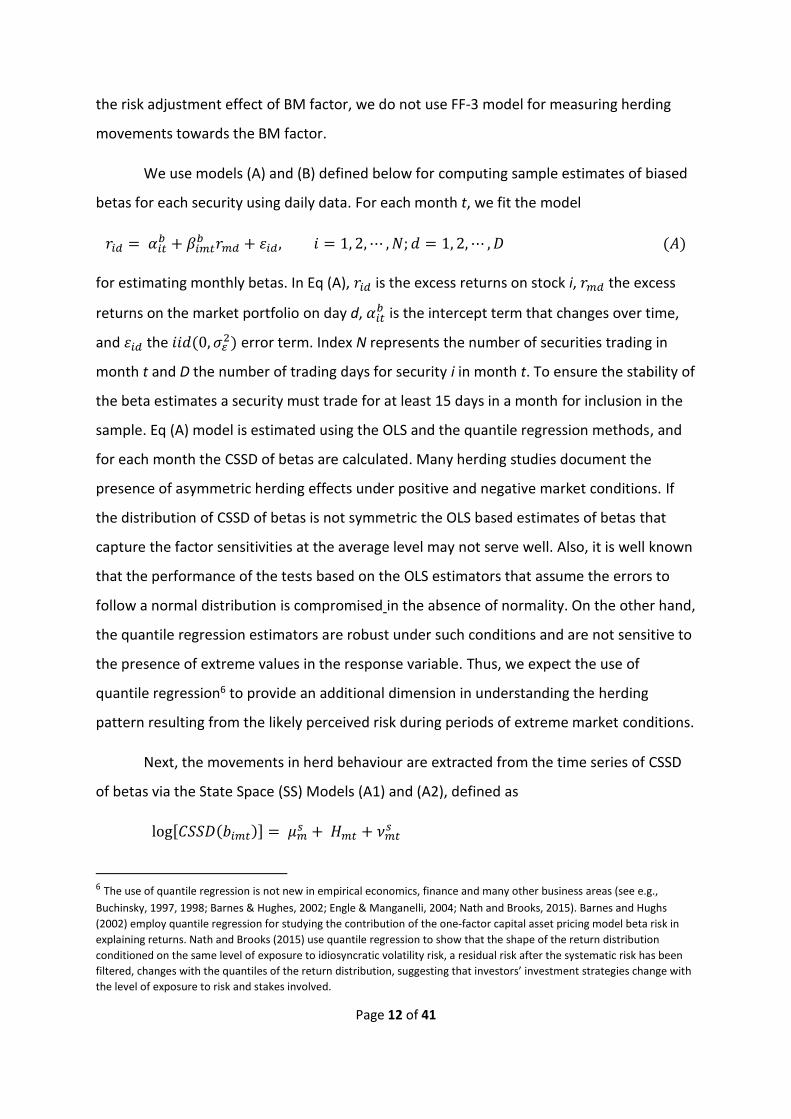
We use models (A) and (B) defined below for computing sample estimates of biased
betas for each security using daily data. For each month t, we fit the model
𝑟𝑖𝑑 = 𝛼𝑖𝑡𝑏 + 𝛽𝑖𝑚𝑡
𝑏 𝑟𝑚𝑑 + 휀𝑖𝑑, 𝑖 = 1, 2, ⋯ , 𝑁; 𝑑 = 1, 2, ⋯ , 𝐷 (𝐴)
for estimating monthly betas. In Eq (A), 𝑟𝑖𝑑 is the excess returns on stock i, 𝑟𝑚𝑑 the excess
returns on the market portfolio on day d, 𝛼𝑖𝑡𝑏 is the intercept term that changes over time,
and 휀𝑖𝑑 the 𝑖𝑖𝑑(0, 𝜎2) error term. Index N represents the number of securities trading in
month t and D the number of trading days for security i in month t. To ensure the stability of
the beta estimates a security must trade for at least 15 days in a month for inclusion in the
sample. Eq (A) model is estimated using the OLS and the quantile regression methods, and
for each month the CSSD of betas are calculated. Many herding studies document the
presence of asymmetric herding effects under positive and negative market conditions. If
the distribution of CSSD of betas is not symmetric the OLS based estimates of betas that
capture the factor sensitivities at the average level may not serve well. Also, it is well known
that the performance of the tests based on the OLS estimators that assume the errors to
follow a normal distribution is compromised in the absence of normality. On the other hand,
the quantile regression estimators are robust under such conditions and are not sensitive to
the presence of extreme values in the response variable. Thus, we expect the use of
quantile regression6 to provide an additional dimension in understanding the herding
pattern resulting from the likely perceived risk during periods of extreme market conditions.
Next, the movements in herd behaviour are extracted from the time series of CSSD
of betas via the State Space (SS) Models (A1) and (A2), defined as
log[𝐶𝑆𝑆𝐷(𝑏𝑖𝑚𝑡)] = 𝜇𝑚𝑠 + 𝐻𝑚𝑡 + 𝜈𝑚𝑡
𝑠
6 The use of quantile regression is not new in empirical economics, finance and many other business areas (see e.g.,
Buchinsky, 1997, 1998; Barnes & Hughes, 2002; Engle & Manganelli, 2004; Nath and Brooks, 2015). Barnes and Hughs
(2002) employ quantile regression for studying the contribution of the one-factor capital asset pricing model beta risk in
explaining returns. Nath and Brooks (2015) use quantile regression to show that the shape of the return distribution
conditioned on the same level of exposure to idiosyncratic volatility risk, a residual risk after the systematic risk has been
filtered, changes with the quantiles of the return distribution, suggesting that investors’ investment strategies change with
the level of exposure to risk and stakes involved.
Page 13 of 41
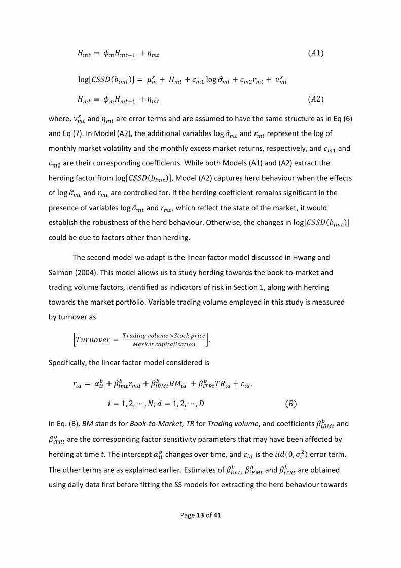
𝐻𝑚𝑡 = 𝜙𝑚𝐻𝑚𝑡−1 + 𝜂𝑚𝑡 (𝐴1)
log[𝐶𝑆𝑆𝐷(𝑏𝑖𝑚𝑡)] = 𝜇𝑚𝑠 + 𝐻𝑚𝑡 + 𝑐𝑚1 log �̂�𝑚𝑡 + 𝑐𝑚2𝑟𝑚𝑡 + 𝜈𝑚𝑡
𝑠
𝐻𝑚𝑡 = 𝜙𝑚𝐻𝑚𝑡−1 + 𝜂𝑚𝑡 (𝐴2)
where, 𝜈𝑚𝑡𝑠 and 𝜂𝑚𝑡 are error terms and are assumed to have the same structure as in Eq (6)
and Eq (7). In Model (A2), the additional variables log �̂�𝑚𝑡 and 𝑟𝑚𝑡 represent the log of
monthly market volatility and the monthly excess market returns, respectively, and 𝑐𝑚1 and
𝑐𝑚2 are their corresponding coefficients. While both Models (A1) and (A2) extract the
herding factor from log[𝐶𝑆𝑆𝐷(𝑏𝑖𝑚𝑡)], Model (A2) captures herd behaviour when the effects
of log �̂�𝑚𝑡 and 𝑟𝑚𝑡 are controlled for. If the herding coefficient remains significant in the
presence of variables log �̂�𝑚𝑡 and 𝑟𝑚𝑡, which reflect the state of the market, it would
establish the robustness of the herd behaviour. Otherwise, the changes in log[𝐶𝑆𝑆𝐷(𝑏𝑖𝑚𝑡)]
could be due to factors other than herding.
The second model we adapt is the linear factor model discussed in Hwang and
Salmon (2004). This model allows us to study herding towards the book-to-market and
trading volume factors, identified as indicators of risk in Section 1, along with herding
towards the market portfolio. Variable trading volume employed in this study is measured
by turnover as
[𝑇𝑢𝑟𝑛𝑜𝑣𝑒𝑟 = 𝑇𝑟𝑎𝑑𝑖𝑛𝑔 𝑣𝑜𝑙𝑢𝑚𝑒 ×𝑆𝑡𝑜𝑐𝑘 𝑝𝑟𝑖𝑐𝑒
𝑀𝑎𝑟𝑘𝑒𝑡 𝑐𝑎𝑝𝑖𝑡𝑎𝑙𝑖𝑧𝑎𝑡𝑖𝑜𝑛].
Specifically, the linear factor model considered is
𝑟𝑖𝑑 = 𝛼𝑖𝑡𝑏 + 𝛽𝑖𝑚𝑡
𝑏 𝑟𝑚𝑑 + 𝛽𝑖𝐵𝑀𝑡𝑏 𝐵𝑀𝑖𝑑 + 𝛽𝑖𝑇𝑅𝑡
𝑏 𝑇𝑅𝑖𝑑 + 휀𝑖𝑑,
𝑖 = 1, 2, ⋯ , 𝑁; 𝑑 = 1, 2, ⋯ , 𝐷 (𝐵)
In Eq. (B), BM stands for Book-to-Market, TR for Trading volume, and coefficients 𝛽𝑖𝐵𝑀𝑡𝑏 and
𝛽𝑖𝑇𝑅𝑡𝑏 are the corresponding factor sensitivity parameters that may have been affected by
herding at time t. The intercept 𝛼𝑖𝑡𝑏 changes over time, and 휀𝑖𝑑 is the 𝑖𝑖𝑑(0, 𝜎2) error term.
The other terms are as explained earlier. Estimates of 𝛽𝑖𝑚𝑡𝑏 , 𝛽𝑖𝐵𝑀𝑡
𝑏 and 𝛽𝑖𝑇𝑅𝑡𝑏 are obtained
using daily data first before fitting the SS models for extracting the herd behaviour towards
Page 14 of 41
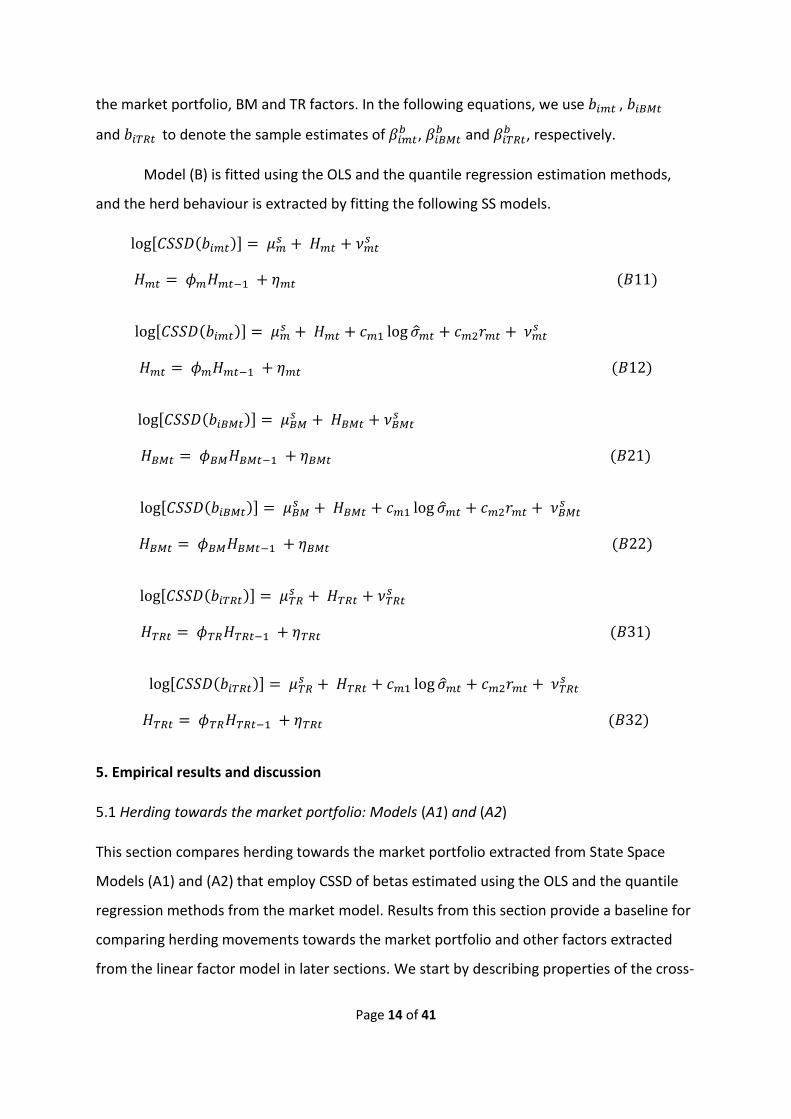
the market portfolio, BM and TR factors. In the following equations, we use 𝑏𝑖𝑚𝑡 , 𝑏𝑖𝐵𝑀𝑡
and 𝑏𝑖𝑇𝑅𝑡 to denote the sample estimates of 𝛽𝑖𝑚𝑡𝑏 , 𝛽𝑖𝐵𝑀𝑡
𝑏 and 𝛽𝑖𝑇𝑅𝑡𝑏 , respectively.
Model (B) is fitted using the OLS and the quantile regression estimation methods,
and the herd behaviour is extracted by fitting the following SS models.
log[𝐶𝑆𝑆𝐷(𝑏𝑖𝑚𝑡)] = 𝜇𝑚𝑠 + 𝐻𝑚𝑡 + 𝜈𝑚𝑡
𝑠
𝐻𝑚𝑡 = 𝜙𝑚𝐻𝑚𝑡−1 + 𝜂𝑚𝑡 (𝐵11)
log[𝐶𝑆𝑆𝐷(𝑏𝑖𝑚𝑡)] = 𝜇𝑚𝑠 + 𝐻𝑚𝑡 + 𝑐𝑚1 log �̂�𝑚𝑡 + 𝑐𝑚2𝑟𝑚𝑡 + 𝜈𝑚𝑡
𝑠
𝐻𝑚𝑡 = 𝜙𝑚𝐻𝑚𝑡−1 + 𝜂𝑚𝑡 (𝐵12)
log[𝐶𝑆𝑆𝐷(𝑏𝑖𝐵𝑀𝑡)] = 𝜇𝐵𝑀𝑠 + 𝐻𝐵𝑀𝑡 + 𝜈𝐵𝑀𝑡
𝑠
𝐻𝐵𝑀𝑡 = 𝜙𝐵𝑀𝐻𝐵𝑀𝑡−1 + 𝜂𝐵𝑀𝑡 (𝐵21)
log[𝐶𝑆𝑆𝐷(𝑏𝑖𝐵𝑀𝑡)] = 𝜇𝐵𝑀𝑠 + 𝐻𝐵𝑀𝑡 + 𝑐𝑚1 log �̂�𝑚𝑡 + 𝑐𝑚2𝑟𝑚𝑡 + 𝜈𝐵𝑀𝑡
𝑠
𝐻𝐵𝑀𝑡 = 𝜙𝐵𝑀𝐻𝐵𝑀𝑡−1 + 𝜂𝐵𝑀𝑡 (𝐵22)
log[𝐶𝑆𝑆𝐷(𝑏𝑖𝑇𝑅𝑡)] = 𝜇𝑇𝑅𝑠 + 𝐻𝑇𝑅𝑡 + 𝜈𝑇𝑅𝑡
𝑠
𝐻𝑇𝑅𝑡 = 𝜙𝑇𝑅𝐻𝑇𝑅𝑡−1 + 𝜂𝑇𝑅𝑡 (𝐵31)
log[𝐶𝑆𝑆𝐷(𝑏𝑖𝑇𝑅𝑡)] = 𝜇𝑇𝑅𝑠 + 𝐻𝑇𝑅𝑡 + 𝑐𝑚1 log �̂�𝑚𝑡 + 𝑐𝑚2𝑟𝑚𝑡 + 𝜈𝑇𝑅𝑡
𝑠
𝐻𝑇𝑅𝑡 = 𝜙𝑇𝑅𝐻𝑇𝑅𝑡−1 + 𝜂𝑇𝑅𝑡 (𝐵32)
5. Empirical results and discussion
5.1 Herding towards the market portfolio: Models (A1) and (A2)
This section compares herding towards the market portfolio extracted from State Space
Models (A1) and (A2) that employ CSSD of betas estimated using the OLS and the quantile
regression methods from the market model. Results from this section provide a baseline for
comparing herding movements towards the market portfolio and other factors extracted
from the linear factor model in later sections. We start by describing properties of the cross-

Page 15 of 41
sectional standard deviations of the betas and the explanatory variables used in fitting SS
Models (A1) and (A2).
5.1.1 Characteristics of Market Excess Returns, Market volatility and Cross-Sectional
Standard Deviations of betas
Figure 1 displays time graph of monthly excess returns on the ASX200 index, and Columns 2
and 3 in Table 1, Panel A, report summary statistics of daily and monthly excess returns on
the ASX200 index for the period 1st October 2000 to 31st May 2017. The daily excess returns
for the index range between −8.7% and 5.6%, while the monthly excess returns vary
between −13.9% and 6.9%. The daily and monthly mean excess returns are very close to
zero, but there is considerable variation in them and both distributions are negatively
skewed and leptokurtic, implying more positive returns than negative. The Jarque-Bera
statistic for normality shows that daily as well as the monthly excess returns on the market
index are non-Gaussian. The monthly excess returns dip sharply between August 2007 and
September 2009, surrounding the GFC and the short-selling ban periods.
Figure 2 graphs monthly volatility in the ASX200 series. The volatility peaks during
the GFC period of mid-2007 to 2008. Column 4 in Table 1, Panel A, reports properties of
monthly volatility in the ASX200 series for the sample period. The volatility series is
positively skewed and leptokurtic, suggesting that extreme volatility is less common. This
series is non-Gaussian.
Fig. 1. Time Series of Monthly Excess returns on ASX200 Index (variable MXRet_Mkt).
-0.15
-0.1
-0.05
0
0.05
0.1
01
-Oct
-00
01
-Ju
n-0
1
01
-Fe
b-0
2
01
-Oct
-02
01
-Ju
n-0
3
01
-Fe
b-0
4
01
-Oct
-04
01
-Ju
n-0
5
01
-Fe
b-0
6
01
-Oct
-06
01
-Ju
n-0
7
01
-Fe
b-0
8
01
-Oct
-08
01
-Ju
n-0
9
01
-Fe
b-1
0
01
-Oct
-10
01
-Ju
n-1
1
01
-Fe
b-1
2
01
-Oct
-12
01
-Ju
n-1
3
01
-Fe
b-1
4
01
-Oct
-14
01
-Ju
n-1
5
01
-Fe
b-1
6
01
-Oct
-16
MXRet_Mkt

Page 16 of 41
Fig. 2. Time Series of Volatility in Monthly ASX200 returns Index (variable MMktVol).
Fig. 3. Monthly Cross-Sectional Standard Deviations (CSSD) of betas based on Model (A). This figure graphs the
CSSDs of betas obtained from fitting Model (A) via the Ordinary Least Squares (OLS) and the quantile regression estimation methods; Q05_CSSD and Q95_CSSD represent series at the 5th and 95th quantiles.
Table 1, Panel B, contains summary statistics of CSSD(bimt) on ASX200 returns
estimated using the OLS and the quantile regression methods, and the log (natural
logarithm) of these CSSDs, the log-CSSD(bimt). While all CSSD(bimt) series are non-Gaussian
and positively skewed, their logged values are Gaussian. As the means and standard
deviations of CSSD(bimt) and log-CSSD(bimt) series at the extreme quantiles are much larger
than the values based on the OLS method, we expect to find variation in herding patterns
emerging from these series. Figure 3 displays monthly CSSD(bimt) estimated from Model (A)
and employed in fitting Models (A1) and (A2), and Table 2 shows estimation output for
Models (A1) and (A2). Figure 3 shows very little variation in OLS based CSSD(bimt) series
compared to the ones based on the 5th and 95th quantiles. It suggests more uncertainty
0
0.05
0.1
0.15
0.20
1-O
ct-0
0
01
-Ju
n-0
1
01
-Fe
b-0
2
01
-Oct
-02
01
-Ju
n-0
3
01
-Fe
b-0
4
01
-Oct
-04
01
-Ju
n-0
5
01
-Fe
b-0
6
01
-Oct
-06
01
-Ju
n-0
7
01
-Fe
b-0
8
01
-Oct
-08
01
-Ju
n-0
9
01
-Fe
b-1
0
01
-Oct
-10
01
-Ju
n-1
1
01
-Fe
b-1
2
01
-Oct
-12
01
-Ju
n-1
3
01
-Fe
b-1
4
01
-Oct
-14
01
-Ju
n-1
5
01
-Fe
b-1
6
01
-Oct
-16
MMktVol
0
1
2
3
4
5
6
7
Oct
-00
Jun
-01
Feb
-02
Oct
-02
Jun
-03
Feb
-04
Oct
-04
Jun
-05
Feb
-06
Oct
-06
Jun
-07
Feb
-08
Oct
-08
Jun
-09
Feb
-10
Oct
-10
Jun
-11
Feb
-12
Oct
-12
Jun
-13
Feb
-14
Oct
-14
Jun
-15
Feb
-16
Oct
-16
Monthly Cross-Sctional Standard deviations of betas: Model (A)
Q05_CSSD Q95_CSSD OLS_CSSD
Page 17 of 41
among betas from the extreme tail regions of the return distribution, and that excess
market returns affect extreme returns differently to the returns on the average level.
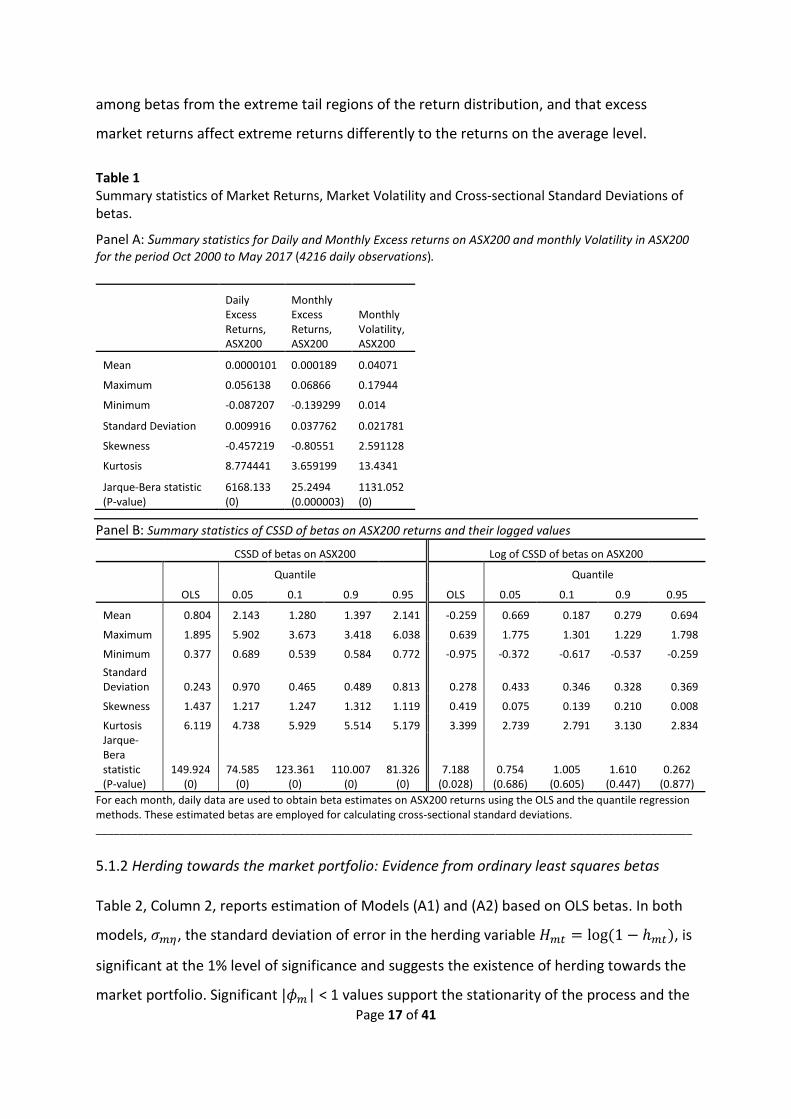
Table 1 Summary statistics of Market Returns, Market Volatility and Cross-sectional Standard Deviations of betas.
Panel A: Summary statistics for Daily and Monthly Excess returns on ASX200 and monthly Volatility in ASX200
for the period Oct 2000 to May 2017 (4216 daily observations).
Daily Excess Returns, ASX200
Monthly Excess Returns, ASX200
Monthly Volatility, ASX200
Mean 0.0000101 0.000189 0.04071
Maximum 0.056138 0.06866 0.17944
Minimum -0.087207 -0.139299 0.014
Standard Deviation 0.009916 0.037762 0.021781
Skewness -0.457219 -0.80551 2.591128
Kurtosis 8.774441 3.659199 13.4341
Jarque-Bera statistic (P-value)
6168.133 (0)
25.2494 (0.000003)
1131.052 (0)
Panel B: Summary statistics of CSSD of betas on ASX200 returns and their logged values
CSSD of betas on ASX200 Log of CSSD of betas on ASX200
Quantile Quantile
OLS 0.05 0.1 0.9 0.95 OLS 0.05 0.1 0.9 0.95
Mean 0.804 2.143 1.280 1.397 2.141 -0.259 0.669 0.187 0.279 0.694
Maximum 1.895 5.902 3.673 3.418 6.038 0.639 1.775 1.301 1.229 1.798
Minimum 0.377 0.689 0.539 0.584 0.772 -0.975 -0.372 -0.617 -0.537 -0.259
Standard Deviation 0.243 0.970 0.465 0.489 0.813 0.278 0.433 0.346 0.328 0.369
Skewness 1.437 1.217 1.247 1.312 1.119 0.419 0.075 0.139 0.210 0.008
Kurtosis 6.119 4.738 5.929 5.514 5.179 3.399 2.739 2.791 3.130 2.834 Jarque-Bera statistic (P-value)
149.924 (0)
74.585 (0)
123.361 (0)
110.007 (0)
81.326 (0)
7.188 (0.028)
0.754 (0.686)
1.005 (0.605)
1.610 (0.447)
0.262 (0.877)
For each month, daily data are used to obtain beta estimates on ASX200 returns using the OLS and the quantile regression methods. These estimated betas are employed for calculating cross-sectional standard deviations. ____________________________________________________________________________________________________
5.1.2 Herding towards the market portfolio: Evidence from ordinary least squares betas
Table 2, Column 2, reports estimation of Models (A1) and (A2) based on OLS betas. In both
models, 𝜎𝑚𝜂, the standard deviation of error in the herding variable 𝐻𝑚𝑡 = log (1 − ℎ𝑚𝑡), is
significant at the 1% level of significance and suggests the existence of herding towards the
market portfolio. Significant |𝜙𝑚| < 1 values support the stationarity of the process and the

Page 18 of 41
autoregressive structure used in modelling. Sizable positive values of 𝜙𝑚 show persistence
in the herding process. The autocorrelation function of residuals (not provided in this paper)
after fitting both models showed no unexplained pattern. A PoSEH value of 34.1% for Model
(A1) shows the amount of variation in log-CSSD(𝑏𝑖𝑚𝑡) due to herding and that the value
reduces to 25.9% for Model (A2), when the effect of monthly market volatility and returns
are controlled for. The likelihood and Schwarz Information Criterion (SIC) values suggest
that Model (A2) fits better than Model (A1) and imply that part of the variation in log-
CSSD(𝑏𝑖𝑚𝑡) is explained by market volatility, log-Vm. The market return 𝑟𝑚 does not have a
significant effect on log-CSSD(𝑏𝑖𝑚𝑡). A significant negative relationship of log-Vm with log-
CSSD(𝑏𝑖𝑚𝑡) at all quantiles and on the average level means that market volatility reduces
the CSSD(𝑏𝑖𝑚𝑡). The effect of rm on CSSD(𝑏𝑖𝑚𝑡) is variable; it is not significant at the 95th
quantile and at the average level.
Table 2 Herding towards the market portfolio: State-Space Models (A1) and (A2) (standard errors are reported in parentheses).
______________________________________________________________________________ Table 2 displays estimation of State-Space Models
(A1): log[𝐶𝑆𝑆𝐷(𝑏𝑖𝑚𝑡)] = 𝜇𝑚𝑠 + 𝐻𝑚𝑡 + 𝜈𝑚𝑡
𝑠 𝑎𝑛𝑑 𝐻𝑚𝑡 = 𝜙𝑚𝐻𝑚𝑡−1 + 𝜂𝑚𝑡, (A2): log[𝐶𝑆𝑆𝐷(𝑏𝑖𝑚𝑡)] = 𝜇𝑚
𝑠 + 𝐻𝑚𝑡 + 𝑐𝑚1 log �̂�𝑚𝑡 + 𝑐𝑚2𝑟𝑚𝑡 + 𝜈𝑚𝑡𝑠 𝑎𝑛𝑑 𝐻𝑚𝑡 = 𝜙𝑚𝐻𝑚𝑡−1 + 𝜂𝑚𝑡,
and the proportion of signal explained by herding based on each model, when the Cross-Sectional Standard Deviations are obtained from betas calculated using the OLS and the quantile regression estimation methods. In column 1, σmν and σmη represent standard deviations of 𝜈𝑚𝑡
𝑠 and 𝜂𝑚𝑡, respectively.
______________________________________________________________________________
Page 19 of 41
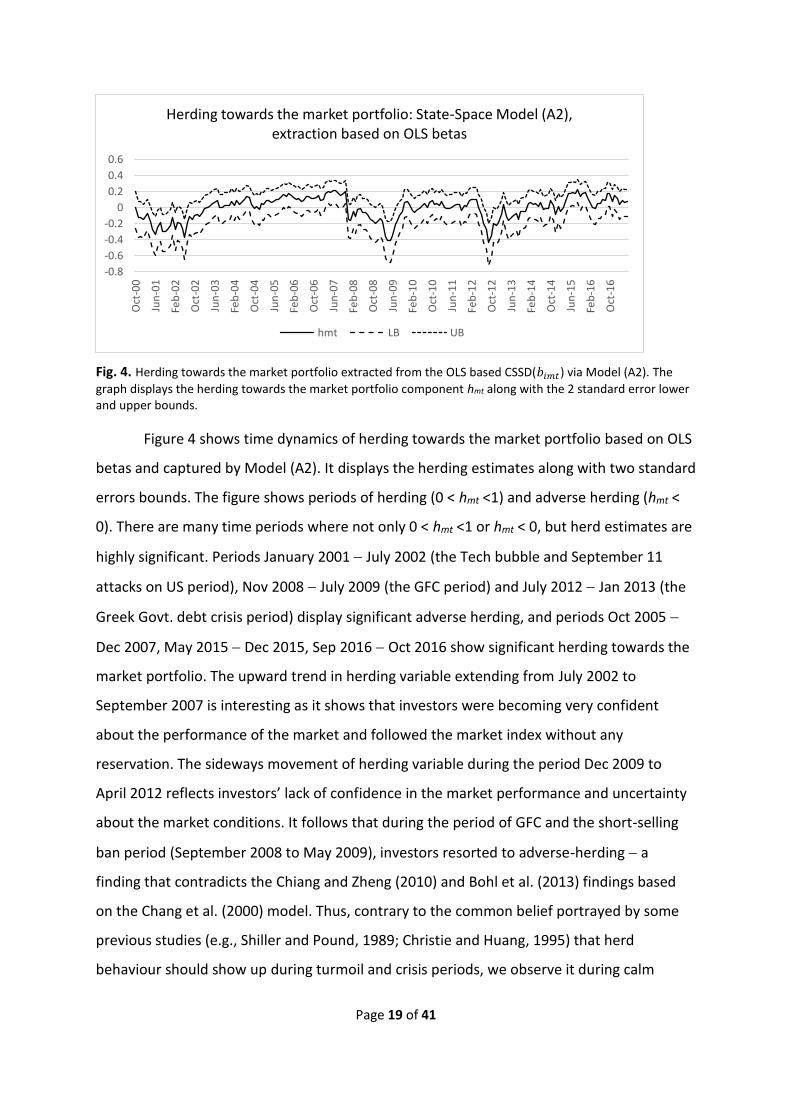
Fig. 4. Herding towards the market portfolio extracted from the OLS based CSSD(𝑏𝑖𝑚𝑡) via Model (A2). The
graph displays the herding towards the market portfolio component hmt along with the 2 standard error lower and upper bounds.
Figure 4 shows time dynamics of herding towards the market portfolio based on OLS
betas and captured by Model (A2). It displays the herding estimates along with two standard
errors bounds. The figure shows periods of herding (0 < hmt <1) and adverse herding (hmt <
0). There are many time periods where not only 0 < hmt <1 or hmt < 0, but herd estimates are
highly significant. Periods January 2001 − July 2002 (the Tech bubble and September 11
attacks on US period), Nov 2008 − July 2009 (the GFC period) and July 2012 − Jan 2013 (the
Greek Govt. debt crisis period) display significant adverse herding, and periods Oct 2005 −
Dec 2007, May 2015 − Dec 2015, Sep 2016 − Oct 2016 show significant herding towards the
market portfolio. The upward trend in herding variable extending from July 2002 to
September 2007 is interesting as it shows that investors were becoming very confident
about the performance of the market and followed the market index without any
reservation. The sideways movement of herding variable during the period Dec 2009 to
April 2012 reflects investors’ lack of confidence in the market performance and uncertainty
about the market conditions. It follows that during the period of GFC and the short-selling
ban period (September 2008 to May 2009), investors resorted to adverse-herding − a
finding that contradicts the Chiang and Zheng (2010) and Bohl et al. (2013) findings based
on the Chang et al. (2000) model. Thus, contrary to the common belief portrayed by some
previous studies (e.g., Shiller and Pound, 1989; Christie and Huang, 1995) that herd
behaviour should show up during turmoil and crisis periods, we observe it during calm
-0.8
-0.6
-0.4
-0.2
0
0.2
0.4
0.6
Oct
-00
Jun
-01
Feb
-02
Oct
-02
Jun
-03
Feb
-04
Oct
-04
Jun
-05
Feb
-06
Oct
-06
Jun
-07
Feb
-08
Oct
-08
Jun
-09
Feb
-10
Oct
-10
Jun
-11
Feb
-12
Oct
-12
Jun
-13
Feb
-14
Oct
-14
Jun
-15
Feb
-16
Oct
-16
Herding towards the market portfolio: State-Space Model (A2), extraction based on OLS betas
hmt LB UB
Page 20 of 41
periods when investors are able to easily predict the market moves and become fearless in
following the market. The build-up of longish increasing trend towards a statistically
significant herding pattern seen prior to GFC does not persist after the GFC and the
presence of adverse herding during the GFC and the short selling ban periods suggests
investors became more cautious and risk-averse during these periods. Thus, it follows that
Christie and Huang (1995) and CCK (2000) models are geared towards capturing very
different patterns compared to the Hwang and Salmon (2004) model.
5.1.3 Herding towards the market portfolio: Evidence from Quantile regression betas
The comments made in the preceding section on herding extracted from the SS Models (A1)
and (A2) employing the OLS based log-CSSD(𝑏𝑖𝑚𝑡) can be extended to all model fittings
based on quantile regression estimated betas. It is clear that Model (A2) is a better fitting
model. While the PoSEH using CSSD of the 90th and 95th quantile betas in Model (A1) are
much higher (31.4% and 43.1%, respectively) than using CSSD of the 5th and 10th quantile
betas (22.4% and 22.9%, respectively), this is not true for Model (A2). We observe that the
PoSEH with Model (A2) drops considerably at the upper quantiles, indicating that some of
the variation in log[CSSD(bimt)] is explained by log-Vm and market returns. The negative
coefficients of log-Vm at all quantiles are significant at the 1% level and the coefficients of
market returns rm are also highly significant at these quantiles with the exception of the 95th
quantile. While the presence of log-Vm and 𝑟𝑚 has caused reduction in the PoSEH at all
quantile levels and the average level (34.1% to 25.9%), the impact is maximum at the 95th
quantile (43% to 25.8%) and virtually none at the 5th quantile (22.4% to 22.4%). This
suggests that market volatility has a substantial impact on betas on high performance days.
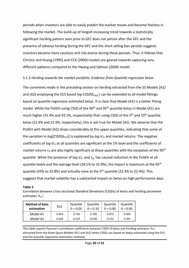
Table 3 Correlation between Cross-Sectional Standard Deviations (CSSDs) of betas and herding parameter
estimates ‘hmt’.
Method of beta estimation
OLS Quantile
= 0.05
Quantile
= 0.10
Quantile
= 0.90
Quantile
= 0.95
Model A1 -0.859 -0.766 -0.780 -0.873 -0.906
Model A2 -0.634 -0.529 -0.448 -0.532 -0.381
This table reports Pearson’s correlation coefficients between CSSD of betas and herding estimates ‘hmt’
extracted from the State-Space Models (A1) and (A2) when CSSDs are based on betas estimated using the OLS
and the quantile regression estimation methods.

Page 21 of 41
Table 3 exhibits correlation between CSSD(bimt) and hmt estimates extracted from
Models (A1) and (A2) employing the OLS and quantile regression estimated betas. As per
the literature (e.g., Hwang and Salmon, 2004), herding towards the market portfolio should
reduce cross-sectional variance of betas; the stronger the herding the higher the reduction
in the cross-sectional variance of betas. On the surface, the presence of negative
correlations in Table 3 supports this argument. For Model (A1), the correlation coefficient
for the 95th quantile is -0.906 and herding explains 43% of the variation in log-CSSD(𝑏𝑖𝑚𝑡)
and 𝜎𝑚𝜂 is 15.87% (Table 2, Panel A) compared to the correlation coefficient of -0.859, the
PoSEH as 34.1%, and 𝜎𝑚𝜂 equal to 9.48% for the OLS estimated values. However, Model
(A2) yields the correlation and 𝜎𝑚𝜂 values as -0.381 and 9.5%, respectively, for the 95th
quantile, and -0.634 and 7.2% for the OLS based estimates, while the PoSEH values of
25.83% and 25.93% in these two situations are virtually the same. This suggests that some
of the variation in CSSD of betas and, therefore, in the measurement equation is due to
market volatility in returns, i.e., log-Vm. Controlling for log-Vm in Model (A2) reduces 𝜎𝑚𝜈 as
well as 𝜎𝑚𝜂. The reduction in 𝜎𝑚𝜈 is about 6% at all levels of the return distribution, and the
PoSEH settles to about 22% to 26%, implying that some of the variation in the cross-
sectional variance of betas at the extreme quantiles may be due to factors other than
herding. A significant negative relationship of log-Vm with log-CSSD(𝑏𝑖𝑚𝑡) (Table 2, Model
(A2)) at all quantiles and on the average level means that market volatility reduces the
CSSD(𝑏𝑖𝑚𝑡); it impacts the entire distribution of CSSD(𝑏𝑖𝑚𝑡). It could be that an increase in
market volatility creates uncertainty among the market participants and they start to herd
back to fundamentals, a sign of risk-aversion, and this causes reduction in the cross-
sectional variance of betas.
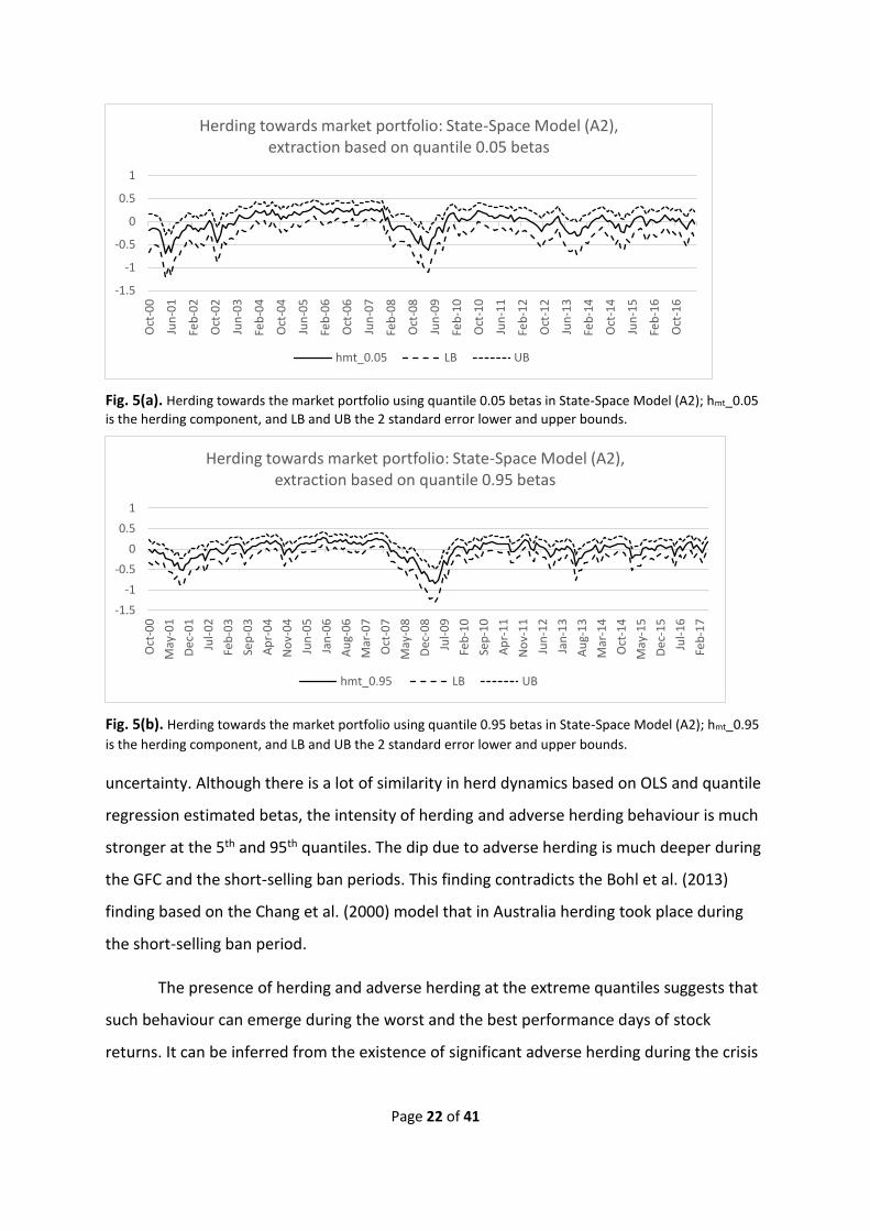
We now discuss herd dynamics based on the better fitting Model (A2). Figures 5(a)
and 5(b) display herd dynamics extracted from Model (A2) employing CSSDs of betas
estimated at the 5% and 95% quantiles, respectively. These graphs show many periods of
herding and adverse herding. There is an increasing trend in herding movement leading up
to the warning signs of the GFC and then results in adverse herding. Herding takes place
during calmer periods and adverse herding during turmoil periods. After the GFC, the herd
movement is mostly sideways and horizontal in nature and not significant, implying
Page 22 of 41
Fig. 5(a). Herding towards the market portfolio using quantile 0.05 betas in State-Space Model (A2); hmt_0.05
is the herding component, and LB and UB the 2 standard error lower and upper bounds.
Fig. 5(b). Herding towards the market portfolio using quantile 0.95 betas in State-Space Model (A2); hmt_0.95
is the herding component, and LB and UB the 2 standard error lower and upper bounds.
uncertainty. Although there is a lot of similarity in herd dynamics based on OLS and quantile
regression estimated betas, the intensity of herding and adverse herding behaviour is much
stronger at the 5th and 95th quantiles. The dip due to adverse herding is much deeper during
the GFC and the short-selling ban periods. This finding contradicts the Bohl et al. (2013)
finding based on the Chang et al. (2000) model that in Australia herding took place during
the short-selling ban period.
The presence of herding and adverse herding at the extreme quantiles suggests that
such behaviour can emerge during the worst and the best performance days of stock
returns. It can be inferred from the existence of significant adverse herding during the crisis
-1.5
-1
-0.5
0
0.5
1
Oct
-00
Jun
-01
Feb
-02
Oct
-02
Jun
-03
Feb
-04
Oct
-04
Jun
-05
Feb
-06
Oct
-06
Jun
-07
Feb
-08
Oct
-08
Jun
-09
Feb
-10
Oct
-10
Jun
-11
Feb
-12
Oct
-12
Jun
-13
Feb
-14
Oct
-14
Jun
-15
Feb
-16
Oct
-16
Herding towards market portfolio: State-Space Model (A2), extraction based on quantile 0.05 betas
hmt_0.05 LB UB
-1.5
-1
-0.5
0
0.5
1
Oct
-00
May
-01
Dec
-01
Jul-
02
Feb
-03
Sep
-03
Ap
r-0
4
No
v-0
4
Jun
-05
Jan
-06
Au
g-0
6
Mar
-07
Oct
-07
May
-08
Dec
-08
Jul-
09
Feb
-10
Sep
-10
Ap
r-1
1
No
v-1
1
Jun
-12
Jan
-13
Au
g-1
3
Mar
-14
Oct
-14
May
-15
Dec
-15
Jul-
16
Feb
-17
Herding towards market portfolio: State-Space Model (A2), extraction based on quantile 0.95 betas
hmt_0.95 LB UB

Page 23 of 41
periods that investors move away from herding, a sign of risk-aversion, to cope with the
unpredictable market movements.
5.2 Herding towards the Market portfolio, Book-to-Market and Trading Volume factors:
The Linear Factor Model
We now examine investor herd behaviour and risk profiles link using the linear factor model
described by Model (B), and factor sensitivities other than the systematic risk. We start by
describing the characteristics of CSSDs of betas − the factor loadings of excess market
returns, Book-to-market (BM) ratios and Trading volume (TR), obtained by fitting Model (B).
Table 4 displays summary statistics of CSSDs of betas obtained by using the OLS and the
quantile regression methods.
5.2.1 Characteristics of Cross-Sectional Standard Deviations of betas from the Linear Factor
Model
We start by comparing the CSSDs of OLS betas for excess market returns, obtained by fitting
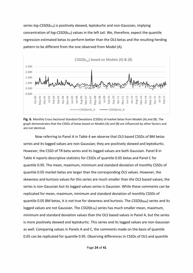
Models (A) and (B). Figure 6 graphs the time series of CSSDs of market betas (CSSD(bmt)) for
Models (A) and (B). It shows that starting from about January 2006 the two series start to
separate from each other; the CSSD(bmt) values from Model (B) are generally larger than
Model (A) on a monthly basis. The summary statistics of CSSD(bmt) series for Model (A)
(Table 1, Panel B, Column 2) and Model (B) (Table 4, Column 2), reveals that Model (B)
based mean, maximum and minimum values of CSSD(bmt), when the effects of BM and TR
are controlled for, are larger than the corresponding Model (A) values, but the standard
deviation value of CSSD(bmt) is lower. Larger mean, maximum and minimum values of
CSSD(bmt) imply that there is more variation in market beta estimates for individual stocks
on a monthly basis. This could be due to the presence of other sources of information like
BM and TR that investors resort to for their decision making in response to the varying
market conditions on a daily basis, and, therefore, adding variations in individual monthly
betas. Smaller standard deviation of CSSD(bmt) values indicates similarity and stability in
market betas resulting from Model (B). The usage of such betas should, therefore, extract
more stable herding movement estimates from the SS models. The positive skew and
kurtosis in CSSD(bmt) series is also much larger for Model (B) compared to Model (A); the
Page 24 of 41
series log-CSSD(bmt) is positively skewed, leptokurtic and non-Gaussian, implying
concentration of log-CSSD(bmt) values in the left tail. We, therefore, expect the quantile
regression estimated betas to perform better than the OLS betas and the resulting herding
pattern to be different from the one observed from Model (A).
Fig. 6. Monthly Cross-Sectional Standard Deviations (CSSDs) of market betas from Models (A) and (B). The
graph demonstrates that the CSSDs of betas based on Models (A) and (B) are influenced by other factors and
are not identical.
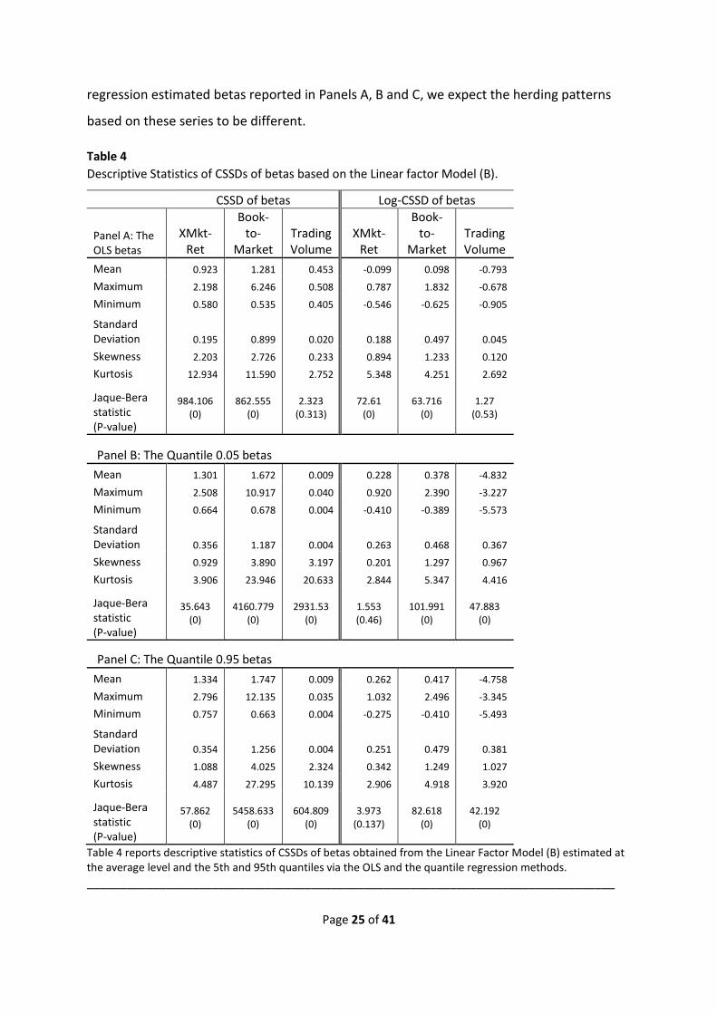
Now referring to Panel A in Table 4 we observe that OLS based CSSDs of BM betas
series and its logged values are non-Gaussian; they are positively skewed and leptokurtic.
However, the CSSD of TR beta series and its logged values are both Gaussian. Panel B in
Table 4 reports descriptive statistics for CSSDs of quantile 0.05 betas and Panel C for
quantile 0.95. The mean, maximum, minimum and standard deviation of monthly CSSDs of
quantile 0.05 market betas are larger than the corresponding OLS values. However, the
skewness and kurtosis values for this series are much smaller than the OLS based values; the
series is non-Gaussian but its logged values series is Gaussian. While these comments can be
replicated for mean, maximum, minimum and standard deviation of monthly CSSDs of
quantile 0.05 BM betas, it is not true for skewness and kurtosis. The CSSD(bBMt) series and its
logged values are not Gaussian. The CSSD(bTRt) series has much smaller mean, maximum,
minimum and standard deviation values than the OLS based values in Panel A, but the series
is more positively skewed and leptokurtic. This series and its logged values are non-Gaussian
as well. Comparing values in Panels A and C, the comments made on the basis of quantile
0.05 can be replicated for quantile 0.95. Observing differences in CSSDs of OLS and quantile
0.000
0.500
1.000
1.500
2.000
2.500
Oct
-00
May
-01
Dec
-01
Jul-
02
Feb
-03
Sep
-03
Ap
r-0
4
No
v-0
4
Jun
-05
Jan
-06
Au
g-0
6
Mar
-07
Oct
-07
May
-08
Dec
-08
Jul-
09
Feb
-10
Sep
-10
Ap
r-1
1
No
v-1
1
Jun
-12
Jan
-13
Au
g-1
3
Mar
-14
Oct
-14
May
-15
Dec
-15
Jul-
16
Feb
-17
CSSD(bmt) based on Models (A) & (B)
CSSD(bmt)_A CSSD(bmt)_B
Page 25 of 41
regression estimated betas reported in Panels A, B and C, we expect the herding patterns
based on these series to be different.
Table 4
Descriptive Statistics of CSSDs of betas based on the Linear factor Model (B).
CSSD of betas Log-CSSD of betas
Panel A: The OLS betas
XMkt-Ret
Book-to-
Market Trading Volume
XMkt-Ret
Book-to-
Market Trading Volume
Mean 0.923 1.281 0.453 -0.099 0.098 -0.793
Maximum 2.198 6.246 0.508 0.787 1.832 -0.678
Minimum 0.580 0.535 0.405 -0.546 -0.625 -0.905
Standard Deviation 0.195 0.899 0.020 0.188 0.497 0.045
Skewness 2.203 2.726 0.233 0.894 1.233 0.120
Kurtosis 12.934 11.590 2.752 5.348 4.251 2.692
Jaque-Bera statistic (P-value)
984.106 (0)
862.555 (0)
2.323 (0.313)
72.61 (0)
63.716 (0)
1.27 (0.53)
Panel B: The Quantile 0.05 betas
Mean 1.301 1.672 0.009 0.228 0.378 -4.832
Maximum 2.508 10.917 0.040 0.920 2.390 -3.227
Minimum 0.664 0.678 0.004 -0.410 -0.389 -5.573
Standard Deviation 0.356 1.187 0.004 0.263 0.468 0.367
Skewness 0.929 3.890 3.197 0.201 1.297 0.967
Kurtosis 3.906 23.946 20.633 2.844 5.347 4.416
Jaque-Bera statistic (P-value)
35.643 (0)
4160.779 (0)
2931.53 (0)
1.553 (0.46)
101.991 (0)
47.883 (0)
Panel C: The Quantile 0.95 betas
Mean 1.334 1.747 0.009 0.262 0.417 -4.758
Maximum 2.796 12.135 0.035 1.032 2.496 -3.345
Minimum 0.757 0.663 0.004 -0.275 -0.410 -5.493
Standard Deviation 0.354 1.256 0.004 0.251 0.479 0.381
Skewness 1.088 4.025 2.324 0.342 1.249 1.027
Kurtosis 4.487 27.295 10.139 2.906 4.918 3.920
Jaque-Bera statistic (P-value)
57.862 (0)
5458.633 (0)
604.809 (0)
3.973 (0.137)
82.618 (0)
42.192 (0)
Table 4 reports descriptive statistics of CSSDs of betas obtained from the Linear Factor Model (B) estimated at the average level and the 5th and 95th quantiles via the OLS and the quantile regression methods.
________________________________________________________________________________

Page 26 of 41
5.2.2 Herding towards Market portfolio, Book-to-Market and Trading Volume factors:
Evidence from the OLS estimated betas
Figure 7 displays the time series graphs of CSSDs of market, BM and TR betas obtained by
OLS estimation of the linear factor Model (B). As the three series show vast variations in
intensity and do not always peak in the same time period, we expect variations in the level
of herding towards each factor. These variations should reveal investors’ risk tendencies
during calmer and turbulent periods.
Fig. 7. Comparison of monthly Cross-Sectional Standard Deviations of betas − the Model (B) factor
sensitivities. The graph shows CSSDs of betas − the sensitivities of stock returns to market portfolio, Book-to-Market and Trading volume within the linear factor model estimated using the OLS method. The three series behave quite differently and should yield differences in herding behaviour.
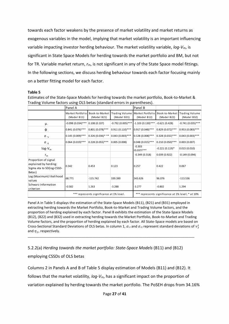
Table 5 reports the estimation of State-Space models employed for extracting herd
behaviour towards the market portfolio, BM, and TR factors from the log-CSSD of OLS
estimated betas. Panel A in Table 5 reports the estimation of SS Models (B11), (B21) and
(B31) and Panel B the estimation of Models (B12), (B22) and (B32). It follows from Panels A
and B that the herding parameter φ is highly significant for all factors. However, the
variance 𝜎 . 𝜂 2 of the herding variable is significant in all models and for all factors but for
trading volume, suggesting a weak tendency of herding towards the TR factor. Viewing the
Log (Maximum likelihood) and the Schwarz Information Criterion values in Table 5 for
models in Panels A and B for all factors, it follows that models representing herding towards
the market portfolio and BM factors perform better when the market volatility and market
returns are incorporated in the model. However, this is not true for TR-herding. The PoSEH
0
1
2
3
4
5
6
7
Oct
-00
Jun
-01
Feb
-02
Oct
-02
Jun
-03
Feb
-04
Oct
-04
Jun
-05
Feb
-06
Oct
-06
Jun
-07
Feb
-08
Oct
-08
Jun
-09
Feb
-10
Oct
-10
Jun
-11
Feb
-12
Oct
-12
Jun
-13
Feb
-14
Oct
-14
Jun
-15
Feb
-16
Oct
-16
OLS based Monthly CSSD of betas from Model (B)
CSSD(bmt) CSSD(bBMt) CSSD(bTRt)
Page 27 of 41
towards each factor weakens by the presence of market volatility and market returns as
exogenous variables in the model, implying that market volatility is an important influencing
variable impacting investor herding behaviour. The market volatility variable, log-Vm, is
significant in State Space Models for herding towards the market portfolio and BM, but not
for TR. Variable market return, rm, is not significant in any of the State Space model fittings.
In the following sections, we discuss herding behaviour towards each factor focusing mainly
on a better fitting model for each factor.
Table 5 Estimates of the State-Space Models for herding towards the market portfolio, Book-to-Market & Trading Volume factors using OLS betas (standard errors in parentheses).
Panel A in Table 5 displays the estimation of the State-Space Models (B11), (B21) and (B31) employed in extracting herding towards the Market Portfolio, Book-to-Market and Trading Volume factors, and the proportion of herding explained by each factor. Panel B exhibits the estimation of the State-Space Models (B12), (B22) and (B32) used in extracting herding towards the Market Portfolio, Book-to-Market and Trading Volume factors, and the proportion of herding explained by each factor. All State-Space models are based on Cross-Sectional Standard Deviations of OLS betas. In column 1, σ.ν and σ.η represent standard deviations of 𝜈.𝑡
𝑠 and 𝜂.𝑡, respectively. _______________________________________________________________________________________
5.2.2(a) Herding towards the market portfolio: State-Space Models (B11) and (B12)
employing CSSDs of OLS betas
Columns 2 in Panels A and B of Table 5 display estimation of Models (B11) and (B12). It
follows that the market volatility, log-Vm, has a significant impact on the proportion of
variation explained by herding towards the market portfolio. The PoSEH drops from 34.16%
Panel A Panel B
Market Portfol io
(Model B11)
Book-to-Market
(Model B21)
Trading Volume
(Model B31)
Market Portfol io
(Model B12)
Book-to-Market
(Model B22)
Trading Volume
(Model B32)
µ ∙ -0.098 (0.034)*** 0.108 (0.107) -0.792 (0.005)*** -1.103 (0.130)*** -0.621 (0.428) -0.741 (0.035)***
φ . 0.841 (0.076)*** 0.801 (0.078)*** 0.911 (0.110)*** 0.917 (0.048)*** 0.829 (0.072)*** 0.953 (0.083)***
σ .ν 0.145 (0.009)*** 0.326 (0.036)* ** 0.043 (0.003)*** 0.128 (0.008)*** 0.328 (0.032)*** 0.043 (0.003)***
σ .η 0.064 (0.019)*** 0.228 (0.055)*** 0.005 (0.008) 0.048 (0.015)*** 0.210 (0.050)*** 0.003 (0.007)
log-Vm -0.303
(0.037)***-0.221 (0.119)* 0.015 (0.010)
rm -0.349 (0.318) 0.039 (0.922) -0.149 (0.094)
Proportion of signal
explained by herding:
Sigma eta to SD(log-CSSD-
Betas)
0.342 0.453 0.123 0.257 0.422 0.067
Log (Maximum) likelihood
values68.771 -115.742 339.390 343.626 96.076 -113.536
Schwarz information
criterion-0.582 1.263 -3.288 -3.277 -0.802 1.294
*** represents s igni ficance at 1% level ; * at 10%*** represents s igni ficance at 1% level .
Page 28 of 41
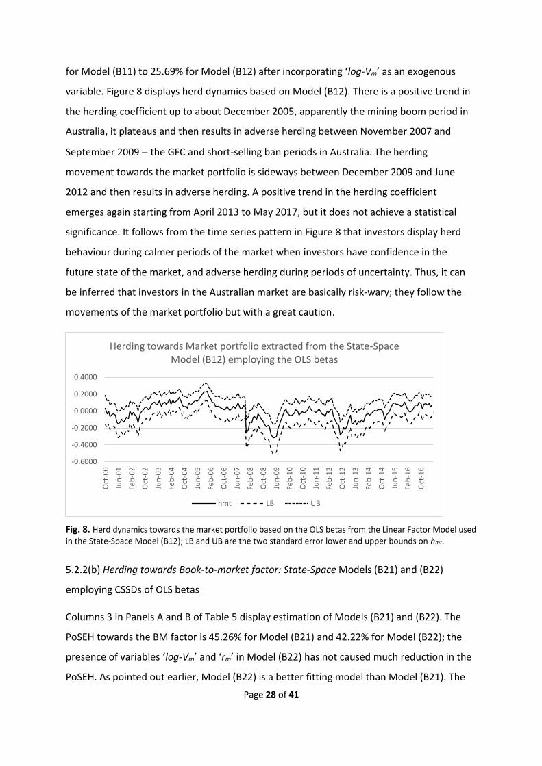
for Model (B11) to 25.69% for Model (B12) after incorporating ‘log-Vm’ as an exogenous
variable. Figure 8 displays herd dynamics based on Model (B12). There is a positive trend in
the herding coefficient up to about December 2005, apparently the mining boom period in
Australia, it plateaus and then results in adverse herding between November 2007 and
September 2009 − the GFC and short-selling ban periods in Australia. The herding
movement towards the market portfolio is sideways between December 2009 and June
2012 and then results in adverse herding. A positive trend in the herding coefficient
emerges again starting from April 2013 to May 2017, but it does not achieve a statistical
significance. It follows from the time series pattern in Figure 8 that investors display herd
behaviour during calmer periods of the market when investors have confidence in the
future state of the market, and adverse herding during periods of uncertainty. Thus, it can
be inferred that investors in the Australian market are basically risk-wary; they follow the
movements of the market portfolio but with a great caution.
Fig. 8. Herd dynamics towards the market portfolio based on the OLS betas from the Linear Factor Model used
in the State-Space Model (B12); LB and UB are the two standard error lower and upper bounds on hmt.
5.2.2(b) Herding towards Book-to-market factor: State-Space Models (B21) and (B22)
employing CSSDs of OLS betas
Columns 3 in Panels A and B of Table 5 display estimation of Models (B21) and (B22). The
PoSEH towards the BM factor is 45.26% for Model (B21) and 42.22% for Model (B22); the
presence of variables ‘log-Vm’ and ‘rm’ in Model (B22) has not caused much reduction in the
PoSEH. As pointed out earlier, Model (B22) is a better fitting model than Model (B21). The
-0.6000
-0.4000
-0.2000
0.0000
0.2000
0.4000
Oct
-00
Jun
-01
Feb
-02
Oct
-02
Jun
-03
Feb
-04
Oct
-04
Jun
-05
Feb
-06
Oct
-06
Jun
-07
Feb
-08
Oct
-08
Jun
-09
Feb
-10
Oct
-10
Jun
-11
Feb
-12
Oct
-12
Jun
-13
Feb
-14
Oct
-14
Jun
-15
Feb
-16
Oct
-16
Herding towards Market portfolio extracted from the State-Space Model (B12) employing the OLS betas
hmt LB UB

Page 29 of 41
explanatory variable ‘log-Vm’ has a negative but a mild effect on log-CSSD(biBMt), and
accounts for only a small amount of variation in log-CSSD(biBMt).
Figure 9 displays time series dynamics of herding towards the BM factor. There are
many time periods showing incidents of herding and adverse-herding. However, the number
of adverse-herding episodes are more frequent than observed for herding towards the
market portfolio, suggesting investors’ efforts to adjust to the changing market conditions
or perceived upcoming turbulent periods and/ or bad news. Upward trending pattern in
herding coefficients is less persistent and short lived compared to the case of herding
towards the market portfolio; the movements are either sideways or in adverse-herding
mode that suggests the presence of a risk-aversion attitude among investors.
Fig. 9. Herd dynamics towards Book-to-Market factor based on the OLS betas from the Linear Factor Model
used in the State-Space Model (B22); LB and UB are the two standard error lower and upper bounds on h_BMt.
5.2.2(c) Herding towards trading volume: State-Space Models (B31) and (B32) employing
CSSDs of OLS betas
We observed in Figure 7 that the time series movements in CSSD(bmt), CSSD(bBMt) and
CSSD(bTRt) are quite different and we expect variation in herding behaviour towards each
factor. Columns 4 in Panels A and B of Table 5 show estimation of Models (B31) and (B32).
The standard deviation 𝜎. 𝜂 of herding variable towards the trading volume factor is very
close to zero, indicating that there is weak to no herding towards the trading volume factor.
The proportion of signal explained by herding is just 12.26% based on Model (B31) that
drops to 6.73% for Model (B32), when the effect of market volatility has been controlled for.
-4.0000
-3.0000
-2.0000
-1.0000
0.0000
1.0000
Oct
-00
Jun
-01
Feb
-02
Oct
-02
Jun
-03
Feb
-04
Oct
-04
Jun
-05
Feb
-06
Oct
-06
Jun
-07
Feb
-08
Oct
-08
Jun
-09
Feb
-10
Oct
-10
Jun
-11
Feb
-12
Oct
-12
Jun
-13
Feb
-14
Oct
-14
Jun
-15
Feb
-16
Oct
-16
Herding towards Book-to-Market extrcated from the State-Space Model (B22) employing the OLS betas
h_BMt LB UB
Page 30 of 41
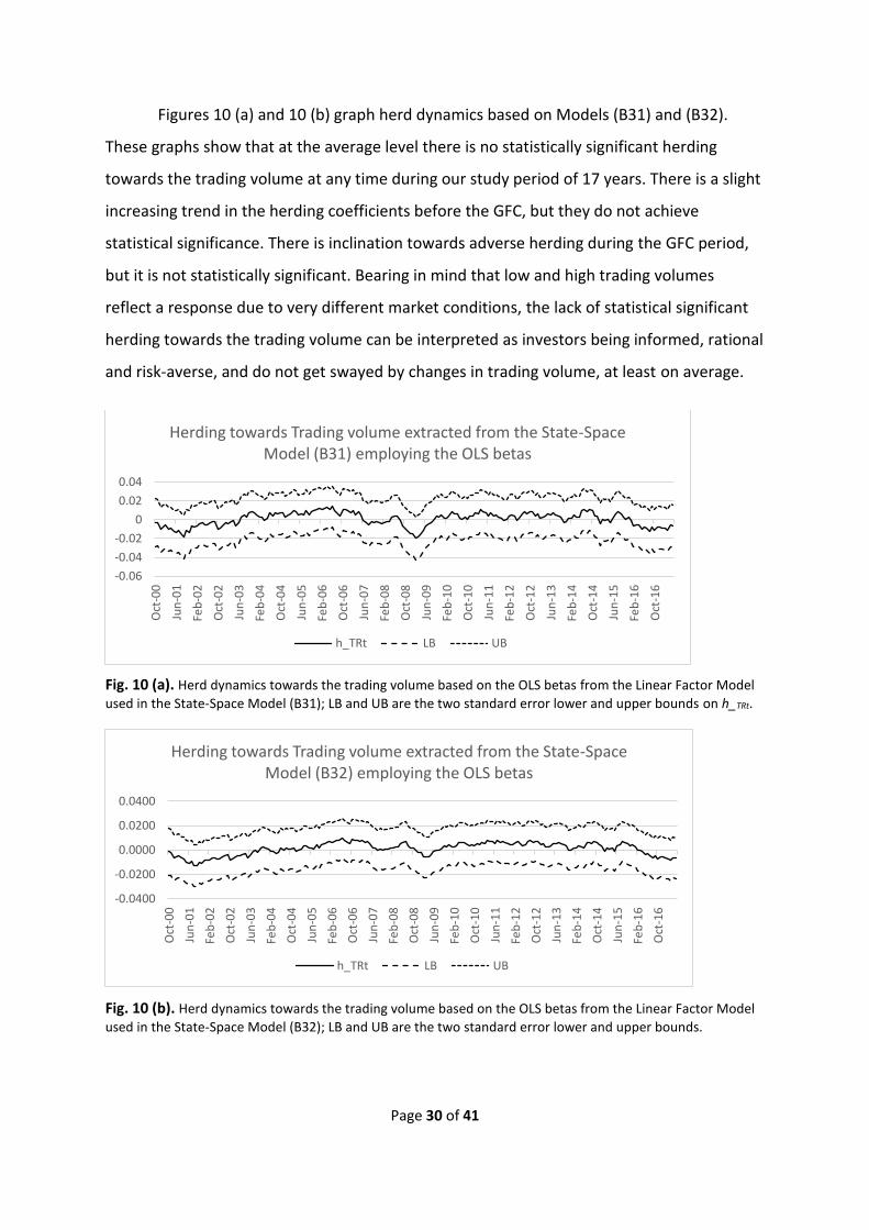
Figures 10 (a) and 10 (b) graph herd dynamics based on Models (B31) and (B32).
These graphs show that at the average level there is no statistically significant herding
towards the trading volume at any time during our study period of 17 years. There is a slight
increasing trend in the herding coefficients before the GFC, but they do not achieve
statistical significance. There is inclination towards adverse herding during the GFC period,
but it is not statistically significant. Bearing in mind that low and high trading volumes
reflect a response due to very different market conditions, the lack of statistical significant
herding towards the trading volume can be interpreted as investors being informed, rational
and risk-averse, and do not get swayed by changes in trading volume, at least on average.
Fig. 10 (a). Herd dynamics towards the trading volume based on the OLS betas from the Linear Factor Model
used in the State-Space Model (B31); LB and UB are the two standard error lower and upper bounds on h_TRt.
Fig. 10 (b). Herd dynamics towards the trading volume based on the OLS betas from the Linear Factor Model
used in the State-Space Model (B32); LB and UB are the two standard error lower and upper bounds.
-0.06
-0.04
-0.02
0
0.02
0.04
Oct
-00
Jun
-01
Feb
-02
Oct
-02
Jun
-03
Feb
-04
Oct
-04
Jun
-05
Feb
-06
Oct
-06
Jun
-07
Feb
-08
Oct
-08
Jun
-09
Feb
-10
Oct
-10
Jun
-11
Feb
-12
Oct
-12
Jun
-13
Feb
-14
Oct
-14
Jun
-15
Feb
-16
Oct
-16
Herding towards Trading volume extracted from the State-Space Model (B31) employing the OLS betas
h_TRt LB UB
-0.0400
-0.0200
0.0000
0.0200
0.0400
Oct
-00
Jun
-01
Feb
-02
Oct
-02
Jun
-03
Feb
-04
Oct
-04
Jun
-05
Feb
-06
Oct
-06
Jun
-07
Feb
-08
Oct
-08
Jun
-09
Feb
-10
Oct
-10
Jun
-11
Feb
-12
Oct
-12
Jun
-13
Feb
-14
Oct
-14
Jun
-15
Feb
-16
Oct
-16
Herding towards Trading volume extracted from the State-Space Model (B32) employing the OLS betas
h_TRt LB UB
Page 31 of 41
5.2.3 Herding towards Market portfolio, Book-to-Market and Trading Volume factors:
Evidence from the quantile-regression estimated betas
This section discusses herd behaviour based on the linear factor Model (B) when estimated
using the quantile regression method focusing on quantiles 0.05 and 0.95. Panel A in Table 6
reports the estimation of SS Models (B11), (B21) and (B31) and Panel B details SS Models
(B12), (B22) and (B32) employed in extracting herd behaviour towards the Market portfolio,
Book-to-Market and Trading volume factors. Figures 11(a) – 13(b) show herd dynamics over
time based on the better fitting models for each factor at quantiles 0.05 and 0.95. We now
discuss the herding pattern for each factor.
An inspection of the models in Panels A and B reveals that the herding parameter φ
is highly significant in each model. However, the log (maximum) likelihood and the Schwarz
information criterion show that State-Space Models (B11), (B21) and (B31) in Panel A are
better performing than Models (B12), (B22) and (B32) in Panel B. This observation is further
supported by the fact that standard deviations ‘𝜎 .𝜂’ for all Panel B models are near zero
implying virtually no herding towards each factor based on these models; the explanatory
variables ‘log-Vm’ and ‘rm’ have a negative and highly significant relationship with log-
CSSD(b. t), and are able to explain most of the variation in log-CSSD(b. t) in the presence of
each factor, and not much explaining left for herding. It seems that while small levels of
market volatility are perceived as investment opportunities by investors and herding
continues, the extreme volatility is seen as a danger sign making investors lose confidence in
the market and herd behaviour comes to a near halt. However, such pattern was not
observed when OLS based betas were employed in the linear factor model. Table 7 lists the
PoSEH towards each factor based on a better fitting State-Space model employing the linear
factor model betas. We now discuss herding towards each factor separately.
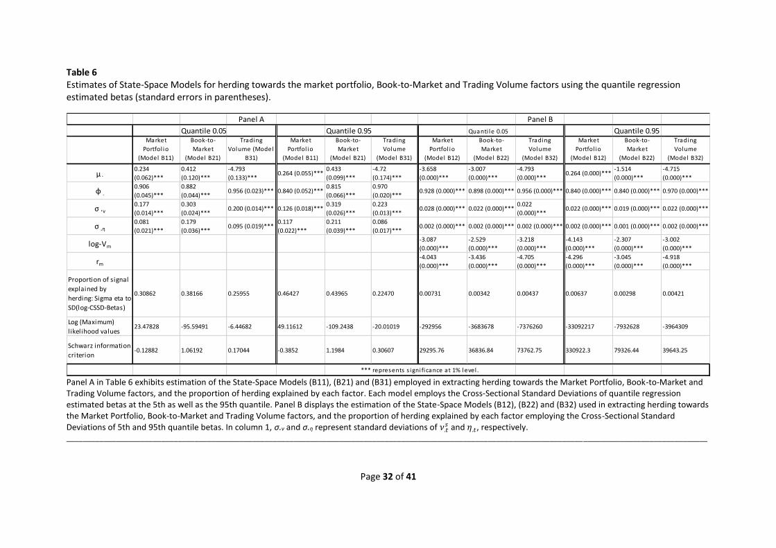
Page 32 of 41
Table 6 Estimates of State-Space Models for herding towards the market portfolio, Book-to-Market and Trading Volume factors using the quantile regression estimated betas (standard errors in parentheses).
Panel A in Table 6 exhibits estimation of the State-Space Models (B11), (B21) and (B31) employed in extracting herding towards the Market Portfolio, Book-to-Market and Trading Volume factors, and the proportion of herding explained by each factor. Each model employs the Cross-Sectional Standard Deviations of quantile regression estimated betas at the 5th as well as the 95th quantile. Panel B displays the estimation of the State-Space Models (B12), (B22) and (B32) used in extracting herding towards the Market Portfolio, Book-to-Market and Trading Volume factors, and the proportion of herding explained by each factor employing the Cross-Sectional Standard Deviations of 5th and 95th quantile betas. In column 1, σ.ν and σ.η represent standard deviations of 𝜈.𝑡
𝑠 and 𝜂.𝑡, respectively. ___________________________________________________________________________________________________________________________________________________________
Panel A Panel B
Quantile 0.05 Quantile 0.95 Quanti le 0.05 Quantile 0.95Market
Portfol io
(Model B11)
Book-to-
Market
(Model B21)
Trading
Volume (Model
B31)
Market
Portfol io
(Model B11)
Book-to-
Market
(Model B21)
Trading
Volume
(Model B31)
Market
Portfol io
(Model B12)
Book-to-
Market
(Model B22)
Trading
Volume
(Model B32)
Market
Portfol io
(Model B12)
Book-to-
Market
(Model B22)
Trading
Volume
(Model B32)
µ ∙0.234
(0.062)***
0.412
(0.120)***
-4.793
(0.133)***0.264 (0.055)***
0.433
(0.099)***
-4.72
(0.174)***
-3.658
(0.000)***
-3.007
(0.000)***
-4.793
(0.000)***0.264 (0.000)***
-1.514
(0.000)***
-4.715
(0.000)***
φ .0.906
(0.045)***
0.882
(0.044)***0.956 (0.023)*** 0.840 (0.052)***
0.815
(0.066)***
0.970
(0.020)***0.928 (0.000)*** 0.898 (0.000)*** 0.956 (0.000)*** 0.840 (0.000)*** 0.840 (0.000)*** 0.970 (0.000)***
σ .ν0.177
(0.014)***
0.303
(0.024)***0.200 (0.014)*** 0.126 (0.018)***
0.319
(0.026)***
0.223
(0.013)***0.028 (0.000)*** 0.022 (0.000)***
0.022
(0.000)***0.022 (0.000)*** 0.019 (0.000)*** 0.022 (0.000)***
σ .η0.081
(0.021)***
0.179
(0.036)***0.095 (0.019)***
0.117
(0.022)***
0.211
(0.039)***
0.086
(0.017)***0.002 (0.000)*** 0.002 (0.000)*** 0.002 (0.000)*** 0.002 (0.000)*** 0.001 (0.000)*** 0.002 (0.000)***
log-Vm-3.087
(0.000)***
-2.529
(0.000)***
-3.218
(0.000)***
-4.143
(0.000)***
-2.307
(0.000)***
-3.002
(0.000)***
rm-4.043
(0.000)***
-3.436
(0.000)***
-4.705
(0.000)***
-4.296
(0.000)***
-3.045
(0.000)***
-4.918
(0.000)***
Proportion of signal
explained by
herding: Sigma eta to
SD(log-CSSD-Betas)
0.30862 0.38166 0.25955 0.46427 0.43965 0.22470 0.00731 0.00342 0.00437 0.00637 0.00298 0.00421
Log (Maximum)
likelihood values23.47828 -95.59491 -6.44682 49.11612 -109.2438 -20.01019 -292956 -3683678 -7376260 -33092217 -7932628 -3964309
Schwarz information
criterion-0.12882 1.06192 0.17044 -0.3852 1.1984 0.30607 29295.76 36836.84 73762.75 330922.3 79326.44 39643.25
*** represents s igni ficance at 1% level .
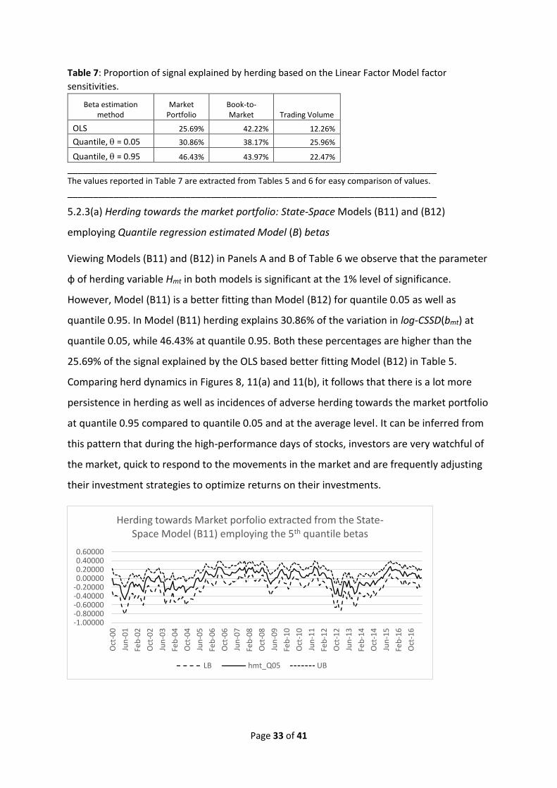
Page 33 of 41
Table 7: Proportion of signal explained by herding based on the Linear Factor Model factor
sensitivities.
Beta estimation method
Market Portfolio
Book-to-Market Trading Volume
OLS 25.69% 42.22% 12.26%
Quantile, = 0.05 30.86% 38.17% 25.96%
Quantile, = 0.95 46.43% 43.97% 22.47%
________________________________________________________________________ The values reported in Table 7 are extracted from Tables 5 and 6 for easy comparison of values.
________________________________________________________________________
5.2.3(a) Herding towards the market portfolio: State-Space Models (B11) and (B12)
employing Quantile regression estimated Model (B) betas
Viewing Models (B11) and (B12) in Panels A and B of Table 6 we observe that the parameter
φ of herding variable Hmt in both models is significant at the 1% level of significance.
However, Model (B11) is a better fitting than Model (B12) for quantile 0.05 as well as
quantile 0.95. In Model (B11) herding explains 30.86% of the variation in log-CSSD(bmt) at
quantile 0.05, while 46.43% at quantile 0.95. Both these percentages are higher than the
25.69% of the signal explained by the OLS based better fitting Model (B12) in Table 5.
Comparing herd dynamics in Figures 8, 11(a) and 11(b), it follows that there is a lot more
persistence in herding as well as incidences of adverse herding towards the market portfolio
at quantile 0.95 compared to quantile 0.05 and at the average level. It can be inferred from
this pattern that during the high-performance days of stocks, investors are very watchful of
the market, quick to respond to the movements in the market and are frequently adjusting
their investment strategies to optimize returns on their investments.
-1.00000-0.80000-0.60000-0.40000-0.200000.000000.200000.400000.60000
Oct
-00
Jun
-01
Feb
-02
Oct
-02
Jun
-03
Feb
-04
Oct
-04
Jun
-05
Feb
-06
Oct
-06
Jun
-07
Feb
-08
Oct
-08
Jun
-09
Feb
-10
Oct
-10
Jun
-11
Feb
-12
Oct
-12
Jun
-13
Feb
-14
Oct
-14
Jun
-15
Feb
-16
Oct
-16
Herding towards Market porfolio extracted from the State-Space Model (B11) employing the 5th quantile betas
LB hmt_Q05 UB
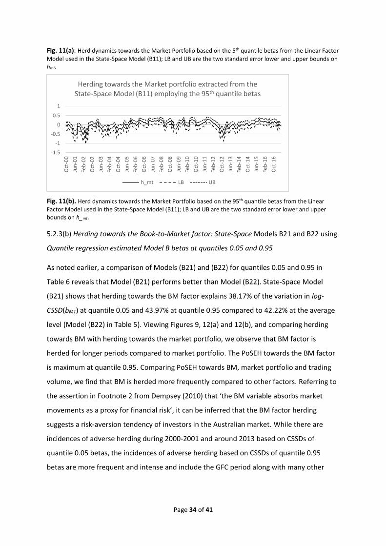
Page 34 of 41
Fig. 11(a): Herd dynamics towards the Market Portfolio based on the 5th quantile betas from the Linear Factor
Model used in the State-Space Model (B11); LB and UB are the two standard error lower and upper bounds on hmt.
Fig. 11(b). Herd dynamics towards the Market Portfolio based on the 95th quantile betas from the Linear
Factor Model used in the State-Space Model (B11); LB and UB are the two standard error lower and upper bounds on h_mt.
5.2.3(b) Herding towards the Book-to-Market factor: State-Space Models B21 and B22 using
Quantile regression estimated Model B betas at quantiles 0.05 and 0.95
As noted earlier, a comparison of Models (B21) and (B22) for quantiles 0.05 and 0.95 in
Table 6 reveals that Model (B21) performs better than Model (B22). State-Space Model
(B21) shows that herding towards the BM factor explains 38.17% of the variation in log-
CSSD(bMT) at quantile 0.05 and 43.97% at quantile 0.95 compared to 42.22% at the average
level (Model (B22) in Table 5). Viewing Figures 9, 12(a) and 12(b), and comparing herding
towards BM with herding towards the market portfolio, we observe that BM factor is
herded for longer periods compared to market portfolio. The PoSEH towards the BM factor
is maximum at quantile 0.95. Comparing PoSEH towards BM, market portfolio and trading
volume, we find that BM is herded more frequently compared to other factors. Referring to
the assertion in Footnote 2 from Dempsey (2010) that ‘the BM variable absorbs market
movements as a proxy for financial risk’, it can be inferred that the BM factor herding
suggests a risk-aversion tendency of investors in the Australian market. While there are
incidences of adverse herding during 2000-2001 and around 2013 based on CSSDs of
quantile 0.05 betas, the incidences of adverse herding based on CSSDs of quantile 0.95
betas are more frequent and intense and include the GFC period along with many other
-1.5
-1
-0.5
0
0.5
1
Oct
-00
Jun
-01
Feb
-02
Oct
-02
Jun
-03
Feb
-04
Oct
-04
Jun
-05
Feb
-06
Oct
-06
Jun
-07
Feb
-08
Oct
-08
Jun
-09
Feb
-10
Oct
-10
Jun
-11
Feb
-12
Oct
-12
Jun
-13
Feb
-14
Oct
-14
Jun
-15
Feb
-16
Oct
-16
Herding towards the Market portfolio extracted from the State-Space Model (B11) employing the 95th quantile betas
h_mt LB UB
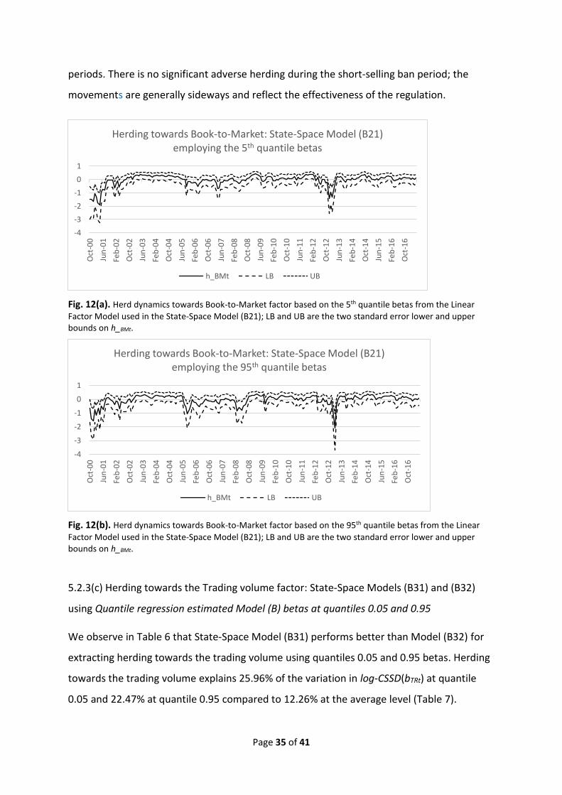
Page 35 of 41
periods. There is no significant adverse herding during the short-selling ban period; the
movements are generally sideways and reflect the effectiveness of the regulation.
Fig. 12(a). Herd dynamics towards Book-to-Market factor based on the 5th quantile betas from the Linear
Factor Model used in the State-Space Model (B21); LB and UB are the two standard error lower and upper bounds on h_BMt.
Fig. 12(b). Herd dynamics towards Book-to-Market factor based on the 95th quantile betas from the Linear
Factor Model used in the State-Space Model (B21); LB and UB are the two standard error lower and upper bounds on h_BMt.
5.2.3(c) Herding towards the Trading volume factor: State-Space Models (B31) and (B32)
using Quantile regression estimated Model (B) betas at quantiles 0.05 and 0.95
We observe in Table 6 that State-Space Model (B31) performs better than Model (B32) for
extracting herding towards the trading volume using quantiles 0.05 and 0.95 betas. Herding
towards the trading volume explains 25.96% of the variation in log-CSSD(bTRt) at quantile
0.05 and 22.47% at quantile 0.95 compared to 12.26% at the average level (Table 7).
-4
-3
-2
-1
0
1
Oct
-00
Jun
-01
Feb
-02
Oct
-02
Jun
-03
Feb
-04
Oct
-04
Jun
-05
Feb
-06
Oct
-06
Jun
-07
Feb
-08
Oct
-08
Jun
-09
Feb
-10
Oct
-10
Jun
-11
Feb
-12
Oct
-12
Jun
-13
Feb
-14
Oct
-14
Jun
-15
Feb
-16
Oct
-16
Herding towards Book-to-Market: State-Space Model (B21) employing the 5th quantile betas
h_BMt LB UB
-4
-3
-2
-1
0
1
Oct
-00
Jun
-01
Feb
-02
Oct
-02
Jun
-03
Feb
-04
Oct
-04
Jun
-05
Feb
-06
Oct
-06
Jun
-07
Feb
-08
Oct
-08
Jun
-09
Feb
-10
Oct
-10
Jun
-11
Feb
-12
Oct
-12
Jun
-13
Feb
-14
Oct
-14
Jun
-15
Feb
-16
Oct
-16
Herding towards Book-to-Market: State-Space Model (B21) employing the 95th quantile betas
h_BMt LB UB
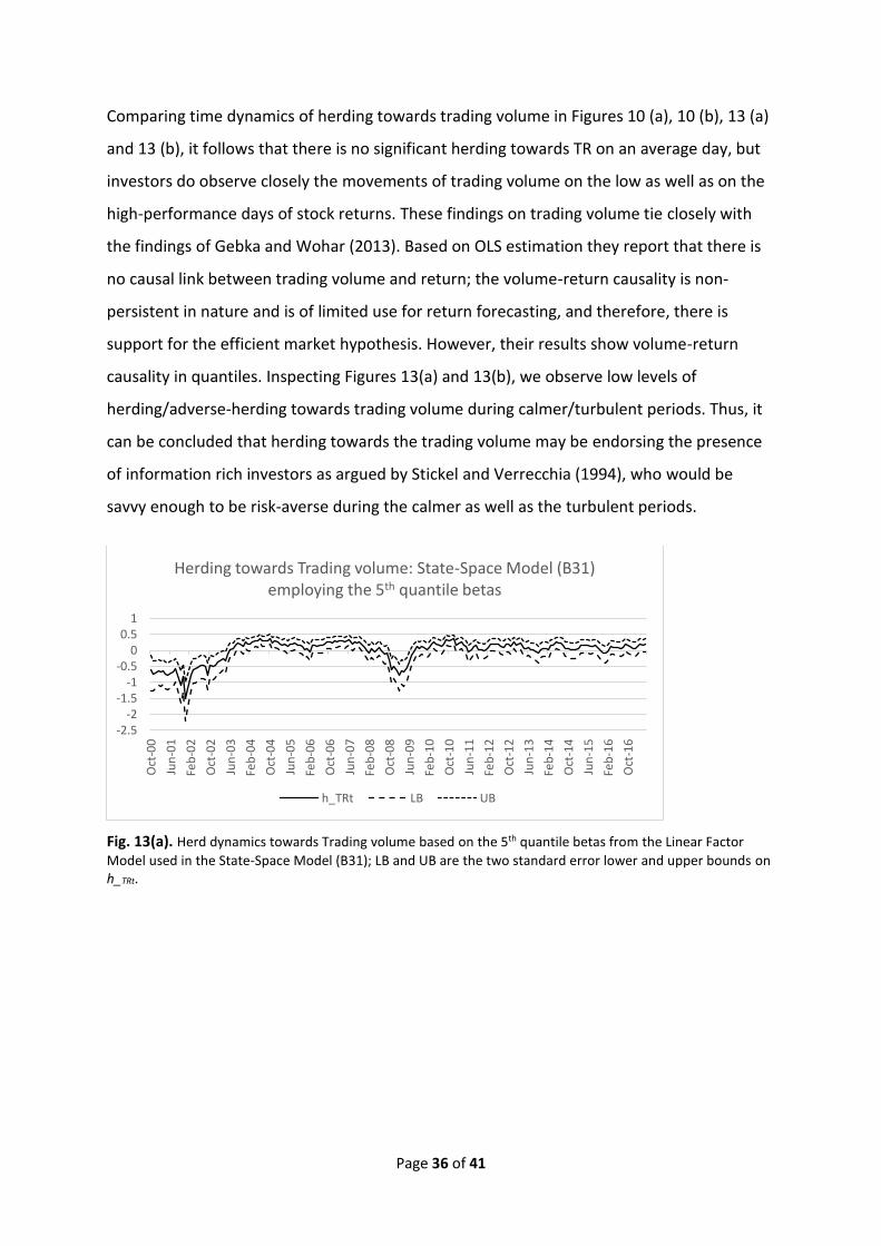
Page 36 of 41
Comparing time dynamics of herding towards trading volume in Figures 10 (a), 10 (b), 13 (a)
and 13 (b), it follows that there is no significant herding towards TR on an average day, but
investors do observe closely the movements of trading volume on the low as well as on the
high-performance days of stock returns. These findings on trading volume tie closely with
the findings of Gebka and Wohar (2013). Based on OLS estimation they report that there is
no causal link between trading volume and return; the volume-return causality is non-
persistent in nature and is of limited use for return forecasting, and therefore, there is
support for the efficient market hypothesis. However, their results show volume-return
causality in quantiles. Inspecting Figures 13(a) and 13(b), we observe low levels of
herding/adverse-herding towards trading volume during calmer/turbulent periods. Thus, it
can be concluded that herding towards the trading volume may be endorsing the presence
of information rich investors as argued by Stickel and Verrecchia (1994), who would be
savvy enough to be risk-averse during the calmer as well as the turbulent periods.
Fig. 13(a). Herd dynamics towards Trading volume based on the 5th quantile betas from the Linear Factor
Model used in the State-Space Model (B31); LB and UB are the two standard error lower and upper bounds on h_TRt.
-2.5-2
-1.5-1
-0.50
0.51
Oct
-00
Jun
-01
Feb
-02
Oct
-02
Jun
-03
Feb
-04
Oct
-04
Jun
-05
Feb
-06
Oct
-06
Jun
-07
Feb
-08
Oct
-08
Jun
-09
Feb
-10
Oct
-10
Jun
-11
Feb
-12
Oct
-12
Jun
-13
Feb
-14
Oct
-14
Jun
-15
Feb
-16
Oct
-16
Herding towards Trading volume: State-Space Model (B31) employing the 5th quantile betas
h_TRt LB UB

Page 37 of 41
Fig. 13(b). Herd dynamics towards Trading volume based on the 95th quantile betas from the Linear Factor
Model used in the State-Space Model (B31); LB and UB are the two standard error lower and upper bounds on h_TRt.
6. Conclusion
This paper examines investor-herding and risk-profiles link for understanding the implied
risk in a stock market that carries implications for portfolio diversification and asset pricing.
Employing Australian data, we use an in-depth time series approach to evaluate herd
dynamics towards the market portfolio, Book-to-Market ratio and trading volume factors
and to find the proportion of signal explained by herding (PoSEH) in each case. Specifically,
State-Space models are used for extracting the latent herding component from the cross-
sectional standard deviations (CSSD) of factor sensitivities estimated using the quantile
regression and the OLS methods that allow capturing the effect of various factors at the
extreme quantiles and at the average level of the return distribution.
We observe many periods of herding and adverse herding towards the market
portfolio; the intensity of both events is much greater when extreme quantile betas are
employed compared to the use of average betas. The PoSEH using the OLS and the 5th and
95th quantile betas are 34.08%, 22.43% and 43.05% (Table 2), respectively, suggesting that
the level of herding is not homogenous across the return distribution; investors value their
assets differently on the low- and the high-performance days of stock returns compared to
an average day. We observe investors herd during calmer periods and show adverse herding
behaviour − a sign of risk aversion, during turbulent periods. The existence of herding and
adverse herding at the extreme quantiles suggests that such behaviour can emerge during
-2.5-2
-1.5-1
-0.50
0.51
Oct
-00
Jun
-01
Feb
-02
Oct
-02
Jun
-03
Feb
-04
Oct
-04
Jun
-05
Feb
-06
Oct
-06
Jun
-07
Feb
-08
Oct
-08
Jun
-09
Feb
-10
Oct
-10
Jun
-11
Feb
-12
Oct
-12
Jun
-13
Feb
-14
Oct
-14
Jun
-15
Feb
-16
Oct
-16
Herding towards Trading volume: State-Space Model (B31) employing the 95th quantile betas
h_TRt LB UB
Page 38 of 41
the worst and the best performance days of stock returns and that risk aversion plays an
important part in herd behaviour.
Market volatility has a significant negative relationship with CSSD of market betas of
securities at all levels of the return distribution and a strong negative effect on herding. The
PoSEH drops when market volatility is used as an explanatory variable in the State Space
models. It has the most effect on high-performance days of stock returns, has a moderate
effect on an average day and virtually no effect on low-performance days (Table 2).
The PoSEH based on the linear factor model shows that herding towards the market
portfolio (trading volume) is stronger during the best (the worst) performance days of stock
returns. However, PoSEH towards the BM factor is high at all levels of the return distribution
suggesting BM as the most desired herding factor. Keeping in view the assertion ‘the BM
variable absorbs market movements as a proxy for financial risk’ from Dempsey (2010), it
can be inferred that the BM factor herding in the Australian market endorses investors’ risk-
aversion tendencies. There are incidences of adverse herding towards this factor during
2000-2001, GFC and around 2012-2013 (the Greek Govt. debt crisis period), but no such
effect during the short-selling ban period (Nov 2008-May 2009). The non-significant
sideways herding movements during the short-selling ban period imply the presence of a
regulated stock market environment. The dominance of BM factor herding among others,
and the occurrence of herding/adverse-herding during calmer/turbulent periods when the
investor confidence is high/low supports the risk-aversion tendencies of investors.
References
Arnott, R.D., Hsu, J., Moore, P., 2005. Fundamental indexation. Financial Analysts Journal.
61, 83-99.
Asch, E., 1952. Social Psychology, Englewood Cliffs, N. J., Prentice Hall.
Bai, Y., Chang, E.C., Wang, J., 2006. Asset prices under short-sale constraints. Working paper,
‘web.mit.edu/wangj/www/pap/BCW_061112.pdf’.
Barnes, M., Hughes, A., 2002. A quantile regression analysis of the cross section of stock
market returns. Federal Reserve Bank of Boston working paper. 02-2002, 1-34.
Page 39 of 41
Bohl, M.T., Klein, A.C., Siklos, P.L., 2013. Short-selling bans and institutional investor’s
herding behaviour: Evidence from the Global Financial Crisis, CIGI Papers, No. 18,
https://www.cigionline.org.
Buchinsky, M., 1997. The dynamics of changes in the female wage distribution in the USA: A
quantile regression approach. Journal of Applied Econometrics. 13, 1-30.
Buchinsky, M., 1998. Recent advances in quantile regression models: A practical guideline
for empirical research. Journal of Human Resources. 33, 88-126.
Chang, E.C., Cheng, J.W., Khorana, A., 2000. An examination of herd behaviour in equity
markets: An international perspective. Journal of Banking and Finance. 24, 1651-1679.
Chiang, T.C., Li J., Tan, L., 2010. Empirical investigation of herding behaviour in Chinese stock
markets: Evidence from quantile regression analysis. Global Finance Journal. 21, 111-124.
Chiang, T.C., Zheng, D., 2010. An empirical analysis of herd behaviour in global stock
markets. Journal of Banking & Finance. 34, 1911-1921.
Christie, W.G., Huang, R.D., 1995. Following the Pied Piper: Do individual Returns Herd
around the Market? Financial Analyst Journal. 51, 31-37.
Demirer, R., Kutan, A., Chen, C., 2010. Do investors herd in emerging markets? Evidence
from the Taiwanese market. Journal of Economic Behaviour & Organization. 76, 283-295.
Dempsey, M., 2010. The book-to-market equity ratio as a proxy for risk: evidence from
Australian market. Australian Journal of Management. 35, 7-21.
Duan, X., Guo, L., Li, F. W., Tu, J., 2019. Sentiment, Limited Attention and Mispricing.
European Financial Management Association Conference-2019, University of Azores, S.
Maguel, Portugal.
Economou, F., Kostakis, A., Philippas, N., 2011. Cross-country effects in herding behaviour:
Evidence from four South European markets. Journal of International Financial Markets,
Institutions & Money. 21, 443-460.
Effinger, M.R., Polborn, M.K., 2001. Herding and anti-herding: A model of reputational
differentiation. European Economic Review. 45, 3, 385-403.

Page 40 of 41
Engle, R. F., Manganelli, S., 2004. CAViaR: Conditional Value at Risk by Regression Quantile.
Journal of Business, Economics and Statistics. 22, 367-381.
Fama, E. F., French, K. R., 1992. The cross-section of expected stock returns. Journal of Finance.
47, 427-465.
Fama, E. F., French, K. R., 2012. Size, value and momentum in international stock returns.
Journal of Financial Economics. 105, 457-472.
Fama, E., MacBeth, J., 1973. Risk, return and equilibrium: Empirical tests. Journal of Political
Economy. 81, 607-636.
Ferson, W.E., Harvey, C.R., 1991. The variation of economic risk premiums. Journal of
Political Economy. 99, 285-315.
Ferson, W.E., Harvey, C.R., 1993. The risk and predictability of international equity returns.
Review of Financial Studies. 6, 527-566.
Gebka, B., Wohar, M.E., 2013. Causality between trading volume and returns: Evidence from
quantile regressions. International Review of Economics and Finance. 27, 144-159.
Grinblatt, M., Titman, S., Wermers, R., 1995. Momentum investment strategies, portfolio
performance, and herding: A study of mutual fund behaviour. American Economics Review.
85(5), 1088-1105.
Hwang, S., Salmon, M., 2004. Market stress and herding. Journal of Empirical Finance. 11,
585-616.
Henker, J., Henker, T., Mitsios, A., 2006. Do Investors herd intraday in Australian equities?
International Journal of Managerial Finance. 2 (3), 196-219.
Koenker, R., Bassett, G., 1978. Regression quantiles. Econometrica. 46, 33-50.
Koenker, R., Hallock, K., 2001. Quantile regression. Journal of Economics Perspectives. 15,
143-56.
Lao, P., H. Singh, 2011. Herding behaviour in the Chinese and Indian stocks market. Journal
of Asian Economics. 22, 495-506.
Lakonishok, J., Shleifer, A., Vishny, R.W., 1992. The impact of Institutional Trading on stock
prices. Journal of Financila Economics. 32, 23-44.

Page 41 of 41
Nath, H.B., Brooks, R.D., 2015. Assessing the idiosyncratic risk and stock returns relation in
heteroskedasticity corrected predictive models using quantile regression. International
Review of Economics and Finance. 38, 94-111.
Peterkort, R.F., Nielson, J.F., 2005. Is the book-to-market ratio a measure of risk? Journal of
Financial Research. 28, 487-502.
Prechter, R.R. Jr., 2001. Unconscious herding behaviour as the Psychological Basis of
Financial market trends and patterns. The Journal of Psychology and Financial Markets. 2(3),
120-125.
Scharfstein, D.S., Stein, J. C., 1990. Herd behaviour and investment. The American Economic
Review, Nashville. 80, 465 – 479.
Stickel, S.E., Verrecchia, R.E., 1994. Evidence that trading volume sustains stock price
changes. Financial Analysts Journal. 50, 57-67.
Yao, J., Ma, C., He, W.P., 2014. Investor herding behaviour of Chinese stock market.
International Review of Economics and Finance. 29, pp12-29.
______________________________
Copyright © 2022 FDOKUMEN