ANY OPINIONS EXPRESSED ARE THOSE OF THE AUTHOR(S) AND NOT NECESSARILY THOSE OF THE SCHOOL OF ECONOMICS & SOCIAL SCIENCES, SMU

SSSMMUUU EEECCCOOONNNOOOMMMIIICCCSSS &&& SSSTTAM TAATTTIIISSSTTTIIICCCSSS WWWOOORRRKKKIIINNNGGG PPPAAAPPPEEERRR SSSEEERRRIIIEEESSS

Investing in Real Estate: Mortgage Financing Practices and Optimal Holding Period

Winston T.H. Koh Edward H.K. Ng

February 2005

Paper No. 03-2005

Investing in Real Estate: Mortgage Financing

Practices and Optimal Holding Period*

Winston T.H. Koh a and Edward H.K. Ng b

February 2005

Forthcoming in International Real Estate Review

ABSTRACT

Real estate investments are typically characterized by high degrees of leverage and

long loan tenures. In perfect capital markets, leverage has no impact on the

investment decision apart from tax considerations. However, the mortgage financing

market is imperfect in many countries. In the presence of market imperfections, an

optimal holding period exists for real property investments. We provide a simple

rule to calculate the optimal holding period is to compare the required rate of return

with the leveraged rate of return on equity.

JEL Classification number: G11

Keywords: mortgage financing, real estate, financial leverage, optimal holding period

* We would like an anonymous referee for helpful comments on the paper. Winston Koh gratefully acknowledges research support from the Wharton-SMU Research Centre, Singapore Management University. a Corresponding author. School of Economics and Social Sciences, Singapore Management University. 469 Bukit Timah Road, Singapore 259756. Tel: +65-68220853; Email: winstonkoh@smu.edu.sg. b Department of Finance and Banking, NUS Business School, National University of Singapore, 10 Kent Ridge Crescent, Singapore 117592. Tel: +65-68748434; Email: edwardng@nus.edu.sg.

1

1. Introduction

Real estate investment has proven to be a very profitable asset class in many countries.

Ibbotson and Siegel (1984) reported that from 1947 to 1982, real estate values in the United

States had risen approximately seventeen fold. This represents a compound annual rate of

return of 8.3%, for unleveraged real estate investments. The returns for leveraged real estate

investments are significantly higher (see also Goetzmann and Ibbotson, 1990). In Asian

economies, the real estate boom during the 1980s and 1990s had also produced spectacular

rates of returns. Like other types of leveraged investments, a key determinant of the realized

returns is the choice of the holding period and the optimal time to exit the investment.

Real estate investments are typically characterized by high degrees of leverage and

long loan tenures. Moreover, mortgage loans are typically structured with regular payments of

both interest and principal over the tenure of the loan. In the case of residential properties,

mortgage loan quantum of as high as 90 percent are available in most countries. Also, tenures

of residential mortgage loans average about 15 to 20 years, and can be as long as 35 years in

some countries such as Singapore and Sweden. In perfect capital markets, leverage has no

impact on the investment decision aside from tax considerations. However, the mortgage

financing market is quite far from perfect in many countries. In the presence of such market

imperfections, we show in this paper that an optimal holding period exists for real estate

investments.

Specifically, we present a simple model to calculate the optimal holding period and the

maximized value of the real estate investment. This facilitates a comparison of the relative

attractiveness of the various investment opportunities. Our modeling approach is motivated by

several institutional features of real estate markets, which we shall discuss briefly here. Firstly,

the mortgage interest rate – which is usually either a fixed rate or a floating rate with a fixed

spread over the prime lending rate – is generally fixed throughout the tenure of a mortgage

loan, even though given the amortization schedule of the mortgage loan, the degree of financial

leverage and the risk of financial distress of the mortgagee declines over time. Unless the

2

homeowner takes the initiative to refinance the outstanding mortgage loan, the same interest

rate is applied throughout the loan tenure even though the credit risk of the outstanding loan is

reduced progressively over time.

Secondly, a related observation is that in some real estate markets (e.g. in Asian

economies such as Singapore and Hong Kong), the difference in the mortgage loan rate of a

5-year housing loan and a 30-year housing loan are quite small. A possible explanation is that

the presence of a relatively flat term structure of mortgage interest rates may reflect an

oligopolistic market for real estate financing where financial institutions find it optimal to offer

a ‘pooled’ mortgage loan rate with minimum credit differentiation. Whatever the reason

behind this minimal differentiation in mortgage loan rates, the net result of this institutional

feature of a real estate market is that investors will likely choose to refinance as often as is

practicable to increase the financial leverage on the existing real estate property (and the

leveraged return on equity), and perhaps use the cashflow released from the refinancing to

invest in another real estate property or in other assets. Moreover, investors would likely opt

for the longer repayment period since the flat mortgage yield curve implies that borrowers with

the longest loan tenure are being subsidized, from a credit risk perspective.

These institutional features, when they are present, differentiate real estate investments

from the class of project investment problems in corporate finance, where the choice of the

optimal capital structure (i.e. degree of financial leverage) is a separate decision from the

investment decision. Moreover, if the capital market is competitive and operates efficiently,

then by the well-known Proposition II of Modigliani and Miller (1958), the required rate of

return on the asset is invariant to the source of funds. As the level of financial leverage is

reduced, the required rate of return on equity is reduced correspondingly in line with the

lowering of the risk of financial distress. In some real estate markets, however, the investment

decision is often not separate from the capital structure decision. In fact, the optimal structure

for a real estate investment is to obtain the highest possible degree of financial leverage.

3

With these institutional setting in mind, we present a simple partial equilibrium

continuous-time formulation of the real estate investment problem, focusing on the impact of

financial leverage on the optimal holding period decision and the resultant maximized net

returns. We show that a minimum quantum of mortgage loan (i.e. a minimum level of financial

leverage) is necessary if a real estate investment is to produce a rate of return greater than the

required rate. If refinancing of outstanding loans is not available or not practicable (due to

transaction costs, for instance), we demonstrate that a simple method to determine if the real

estate property should continue to be held or should be liquidated is to compare the leveraged

rate of return against the required rate of return at each point in time. As the mortgage loan is

amortized, the leveraged rate of return on equity declines in line with the fall in the debt-to-

equity ratio. The optimal time to exit the real estate investment, or to refinance with a fresh

mortgage loan, is when the leveraged rate of return falls below the required rate of return. If

refinancing of outstanding loan is available, an alternative to selling the property is to refinance

it and obtain higher degree of leverage and extend the loan tenure.

Our study is related to a line of research in the real estate literature on tenure choice.

The research includes Brueggeman, Fisher and Stern (1981), Alberts and Castanias (1982),

Hendershott and Ling (1984), Ling and Whinihan (1985), Follain and Ling (1988), Linneman

and Wachter (1989), Hendershott and Haurin (1990), and Gau and Wang (1990, 1994), and

more recently, Goodman (2003). A key focus of this literature is on the impact changes in tax

structures, inflation trends and relocation costs on the holding period decision. Goodman

(2003) found that due to transactions costs, most housing buyers do not routinely move in

response to small changes in income or housing price. He modeled tenure choice decisions as

multi-period optimization in the presence of transactions costs. In the earlier literature, Ling

and Whinihan (1986) developed a model in which both the holding period and the rate of

capital appreciation are determined endogenously. Gau and Wang (1990, 1994) also examined

the issue of optimal holding period, focusing on the issue of the refinancing decision and

impact of tax changes on the investor’s decision.

4

The contribution of the present paper to this literature is to highlight the role that

financial leverage plays in determining the profitability of a real estate investment and the

associated optimal holding period, in the presence of market imperfections. The related

research that studies the issue of real estate investment holding period include Genesove and

Mayer (1997) which examined the phenomenon of financially constrained homeowners setting

higher reservation sale prices and taking a longer time to sell their properties, and Glower,

Haurin and Hendershott (1998), which explored the impact of seller preferences and motivation

on the selling time, asking price and eventual sale price. Grenadier (1995) has applied the real

options framework to analyze a variety of real assets, including real estate contracts.

The rest of the paper is structured as follows. In Section 2, we introduce the model, and

discuss the motivation behind the key assumptions. The main result on the optimal holding

period is presented in Proposition 1. In Section 3, we discuss the intuition behind Proposition 1

by using the Dupont decomposition formula to calculate the leveraged rate of return on equity.

The comparative statics results and a numerical analysis are discussed in Section 4. Section 5

discusses the extension of the results as the assumptions are relaxed. Section 6 considers the

case of stochastic capital appreciation. We derive an optimal rule for continuing to hold the real

estate property or to liquidate investment. Section 7 concludes the paper.

2. The Model

Consider a potential investment in a real estate property with a normalized value of 1.

Mortgage loans for new real estate investments are available at a fixed interest rate of r. The

loan quantum available to the investor is D and the loan period is T. In the following analysis,

we shall abstract from tax issues.1 To establish the basic point on the linkage between financial

1 Tax issues are clearly important, but the treatment varies across countries. In some countries, a capital

gains tax may be levied on a real estate investment if it is liquidated within a specified period from the

date of purchase. The impact of a capital gains tax and other tax allowances (e.g. for property

depreciation or equity loss) can be incorporated into an extended version of the model. See DiPasquale

and Wheaton (1996) or Shilling (2002) for a discussion of these issues in the U.S. market.

5

leverage and optimal holding period, suppose for the moment that the refinancing of existing

mortgage loans is not an available option. In this case, we show that the optimal holding period

for the real estate investment is endogenously determined. If this assumption is relaxed, as we

shall discuss later, the optimal strategy is to refinance the property at the first practicable

opportunity to increase both financial leverage and extend the tenure of the loan. We denote

the constant stream of mortgage repayment by M and the outstanding mortgage loan at time t

by ( )D t . Assuming continuous time to ease the analysis, we obtain

1 rTrDMe−≡

−,

( )1( ) Max , 01

r T t

rTeD t D

e

− −

−

⎧ ⎫⎡ ⎤−⎪ ⎪≡ ⎨ ⎬⎢ ⎥−⎪ ⎪⎣ ⎦⎩ ⎭ (1)

Suppose the investor expects the value of the real estate to change over time at an

expected constant rate of c (which may be negative in the case of capital depreciation).2 For

simplicity, let the net rental return be a constant percentage δ of the real estate property value.

At time t, the real estate property has a value of cte , and fetches a rental return of δ cte . We

make two additional assumptions in the following analysis: a constant mortgage rate of r and a

constant required rate of return k. As we shall discuss later in Section 5, the qualitative aspects

of our results carry over to the case where k and r may vary over time.

While the assumptions of a constant mortgage interest rate and a constant required rate

of return are simplifying assumptions for our analysis, they also reflect the institutional

environment in some real estate markets. First, a constant mortgage loan rate is clearly not

consistent with an efficient debt market with zero transaction costs. As the mortgage loan is

amortized, the mortgage interest rate on the outstanding loan should be lowered to reflect the

lower financial risk of the remaining mortgage loan. However, this assumption is not

unrealistic as financial institutions in many real estate markets (e.g. in Singapore and Hong

Kong) offer mortgage loan packages where the contractual mortgage rates are constant over a

larger part of the tenure of the mortgage loan and there is minimal differentiation in mortgage

loan rates across different loan tenures. The homeowner has to refinance the outstanding 2 In Section 6, we consider the case where the rate of capital appreciation is stochastic.

6

mortgage loan in order to enjoy a slightly lower interest rate. However, given the transaction

costs involved, a more common reason for refinancing the mortgage loans is to free some of the

locked-in equity for other investments and establish a higher loan-to-value ratio for the real

estate investment.

Next, there are situations where the required rate of return for a real estate investment

may vary little over time. In the case of investments that are atomistic and diversifiable, such

as stocks and bonds, the required rate of return on equity will generally vary positively with the

degree of financial leverage, due to the increased risk of a larger dispersion of returns.

However, if the investment is not atomistic, as in the case of real estate investments, the

positive relationship between required rate of return on equity and the degree of financial

leverage may not hold. In this case, as the degree of financial leverage falls, the equity to asset

ratio rises, so that a larger portion of the investment risk now falls on the investor’s own

money. The investment risk in a real estate is also not easily diversifiable given its lumpy

nature. As a result, it is a-priori unclear if the investor would require a lower rate of return on

each marginal dollar invested in the real estate property to replace bank debt. If the mortgage

loan is with recourse, as is the norm, the liability on the investor is unlimited. Since the

investor’s private funds are liable for any claim by the creditors, it is reasonable that the

required rate of return on equity may not vary with the degree of financial leverage.

In fact, if the mortgage loan is without recourse (which is a very uncommon practice in

many Asian countries), so that the investor has limited liability on the outstanding loan, the

required rate of return on the real estate investment may in fact rise as the mortgage loan is

amortized. Empirically, the probable positive relationship between the required rate of return

on real estate investments and the outstanding amount of a mortgage loan without recourse has

some support in the findings of Newsome and Hill (1987). They surveyed over 200 real estate

professionals from the United States of America and Canada, regarding the relationship

between financial leverage and the required rate of return on equity in real estate investments.

They found that 71% of the respondents stated that they would either hold constant or lower

7

their required rate of return on equity. In light of these considerations, our initial analysis for

the case of a constant required rate of return is relevant to situations where the required rate of

return is not sensitive to changes in the outstanding mortgage loan exposure. As we shall

discuss in Section 5, if the required rate of return is decreasing (increasing) over time, the

optimal holding period will be longer (shorter) compared with the case when it is constant.

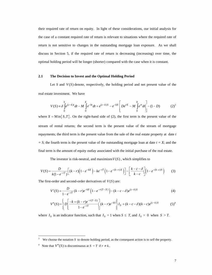
2.1 The Decision to Invest and the Optimal Holding Period

Let S and ( )V S denote, respectively, the holding period and net present value of the

real estate investment. We have

( ) ( )

0 0 0

( ) (1 )S X X

c k t kt c k S kX rX rtV S e dt M e dt e e De M e dt Dδ − − − −⎡ ⎤

≡ − + − − − −⎢ ⎥⎢ ⎥⎣ ⎦

∫ ∫ ∫ (2)3

where { }Min ,X S T= . On the right-hand side of (2), the first term is the present value of the

stream of rental returns; the second term is the present value of the stream of mortgage

repayments; the third term is the present value from the sale of the real estate property at date t

= S; the fourth term is the present value of the outstanding mortgage loan at date t = X; and the

final term is the amount of equity outlay associated with the initial purchase of the real estate.

The investor is risk-neutral, and maximizes ( )V S , which simplifies to

( ) ( ) ( )( ) ( )( ) ( ) 1 1 1(1 )

kX rT k r X k c SrT

D k cV S k r e ke e ek ck e

δ− − − − − −−

− −⎡ ⎤⎡ ⎤= − − − − − −⎢ ⎥⎣ ⎦ −− ⎣ ⎦ (3)

The first-order and second-order derivatives of ( )V S are:

( )( ) ( )( ) ( ) 1 ( )1

kX r T X c k SrT

DV S k r e e k c ee

δ− − − −−

′ = − − − − −−

(4)

( )( )( )( ) ( ) ( )( )

1

r T SkS c k S

SrTk k r eV S D k r e I k c k c e

eδ

− −− −

−

⎧ ⎫⎡ ⎤− + −⎪ ⎪′′ = − + − − −⎢ ⎥⎨ ⎬−⎢ ⎥⎪ ⎪⎣ ⎦⎩ ⎭

(5)4

where SI is an indicator function, such that SI = 1 when S ≤ T, and SI = 0 when S > T.

3 We choose the notation S to denote holding period, as the consequent action is to sell the property. 4 Note that ( )V S′′ is discontinuous at S = T if r ≠ k..

8

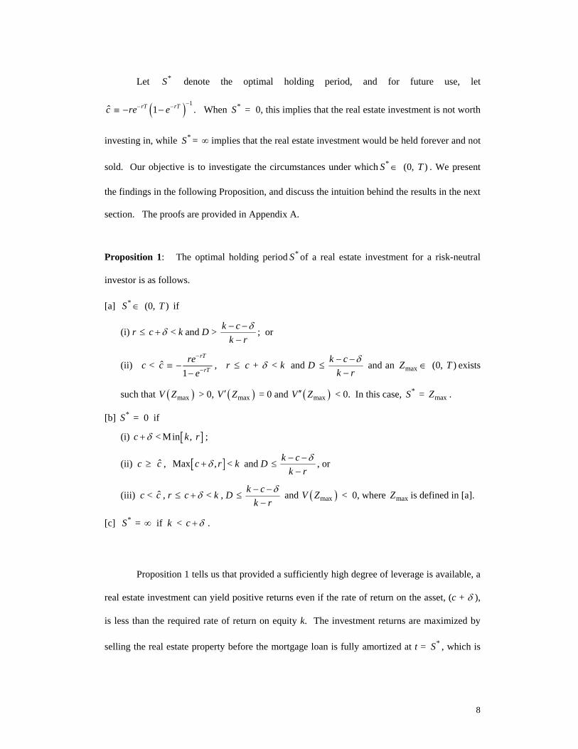
Let *S denote the optimal holding period, and for future use, let

c ≡ ( ) 11rT rTre e

−− −− − . When *S = 0, this implies that the real estate investment is not worth

investing in, while *S = ∞ implies that the real estate investment would be held forever and not

sold. Our objective is to investigate the circumstances under which *S ∈ (0, )T . We present

the findings in the following Proposition, and discuss the intuition behind the results in the next

section. The proofs are provided in Appendix A.

Proposition 1: The optimal holding period *S of a real estate investment for a risk-neutral

investor is as follows.

[a] *S ∈ (0, )T if

(i) r ≤ c δ+ < k and D > k ck r

δ− −−

; or

(ii) c < c ≡1

rT

rTre

e

−

−−−

, r ≤ c + δ < k and D ≤k c

k rδ− −

− and an maxZ ∈ (0, )T exists

such that ( )maxV Z > 0, ( )maxV Z′ = 0 and ( )maxV Z′′ < 0. In this case, *S = maxZ .

[b] *S = 0 if

(i) c δ+ < [ ]Min , k r ;

(ii) c ≥ c , [ ]Max ,c rδ+ < k and D ≤k c

k rδ− −

−, or

(iii) c < c , r ≤ c δ+ < k , D ≤k c

k rδ− −

− and ( )maxV Z < 0, where maxZ is defined in [a].

[c] *S = ∞ if k < c δ+ .

Proposition 1 tells us that provided a sufficiently high degree of leverage is available, a

real estate investment can yield positive returns even if the rate of return on the asset, (c + δ ),

is less than the required rate of return on equity k. The investment returns are maximized by

selling the real estate property before the mortgage loan is fully amortized at t = *S , which is

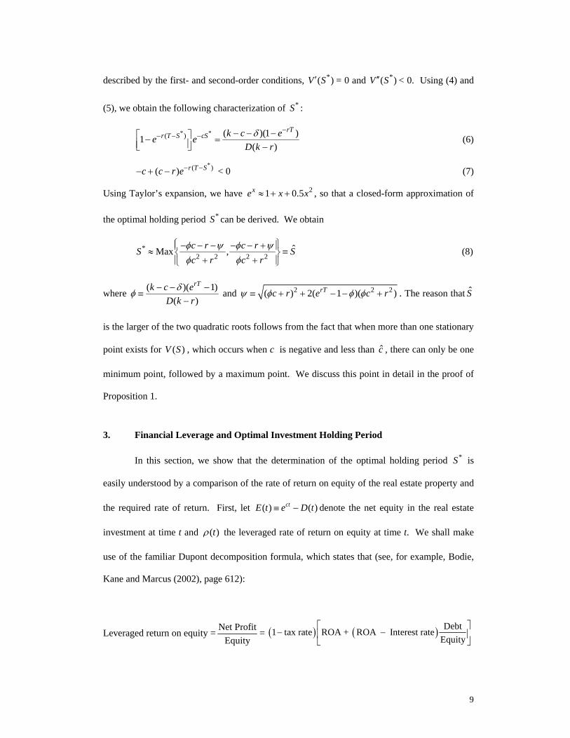
9

described by the first- and second-order conditions, *( )V S′ = 0 and *( )V S′′ < 0. Using (4) and

(5), we obtain the following characterization of *S :

* *( ) ( )(1 )1( )δ −

− − − − − −⎡ ⎤− =⎢ ⎥⎣ ⎦ −

rTr T S cS k c ee e

D k r (6)

*( )( ) r T Sc c r e− −− + − < 0 (7)

Using Taylor’s expansion, we have 21 0.5xe x x≈ + + , so that a closed-form approximation of

the optimal holding period *S can be derived. We obtain

*2 2 2 2

ˆMax ,φ ψ φ ψφ φ

⎧ ⎫− − − − − +⎪ ⎪≈ ≡⎨ ⎬+ +⎪ ⎪⎩ ⎭

c r c rS Sc r c r

(8)

where ( )( 1)( )

rTk c eD k r

δφ − − −≡

− and 2 2 2( ) 2( 1 )( )rTc r e c rψ φ φ φ≡ + + − − + . The reason that S

is the larger of the two quadratic roots follows from the fact that when more than one stationary

point exists for ( )V S , which occurs when c is negative and less than c , there can only be one

minimum point, followed by a maximum point. We discuss this point in detail in the proof of

Proposition 1.

3. Financial Leverage and Optimal Investment Holding Period

In this section, we show that the determination of the optimal holding period *S is

easily understood by a comparison of the rate of return on equity of the real estate property and

the required rate of return. First, let ( ) ( )ctE t e D t≡ − denote the net equity in the real estate

investment at time t and ( )tρ the leveraged rate of return on equity at time t. We shall make

use of the familiar Dupont decomposition formula, which states that (see, for example, Bodie,

Kane and Marcus (2002), page 612):

Leveraged return on equity = Net ProfitEquity

= ( ) ( ) Debt1 tax rate ROA + ROA Interest rateEquity

⎡ ⎤− −⎢ ⎥

⎣ ⎦

10

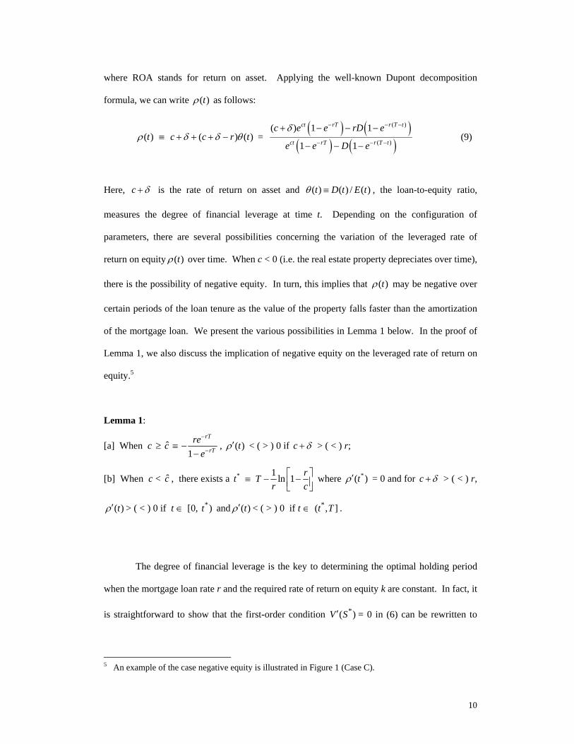
where ROA stands for return on asset. Applying the well-known Dupont decomposition

formula, we can write ( )tρ as follows:

( )tρ ≡ ( ) ( )δ δ θ+ + + −c c r t = ( ) ( )

( ) ( )( )

( )

( ) 1 1

1 1

ct rT r T t

ct rT r T t

c e e rD e

e e D e

δ − − −

− − −

+ − − −

− − − (9)

Here, c δ+ is the rate of return on asset and ( ) ( ) / ( )t D t E tθ ≡ , the loan-to-equity ratio,

measures the degree of financial leverage at time t. Depending on the configuration of

parameters, there are several possibilities concerning the variation of the leveraged rate of

return on equity ( )tρ over time. When c < 0 (i.e. the real estate property depreciates over time),

there is the possibility of negative equity. In turn, this implies that ( )tρ may be negative over

certain periods of the loan tenure as the value of the property falls faster than the amortization

of the mortgage loan. We present the various possibilities in Lemma 1 below. In the proof of

Lemma 1, we also discuss the implication of negative equity on the leveraged rate of return on

equity.5

Lemma 1:

[a] When c ≥ c ≡1

rT

rTre

e

−

−−−

, ( )tρ′ < ( > ) 0 if c δ+ > ( < ) r;

[b] When c < c , there exists a *t 1 ln 1 rTr c

⎡ ⎤≡ − −⎢ ⎥⎣ ⎦ where *( )tρ′ = 0 and for c δ+ > ( < ) r,

( )tρ′ > ( < ) 0 if t ∈ *[0, )t and ( )tρ′ < ( > ) 0 if t ∈ *( , ]t T .

The degree of financial leverage is the key to determining the optimal holding period

when the mortgage loan rate r and the required rate of return on equity k are constant. In fact, it

is straightforward to show that the first-order condition *( )V S′ = 0 in (6) can be rewritten to

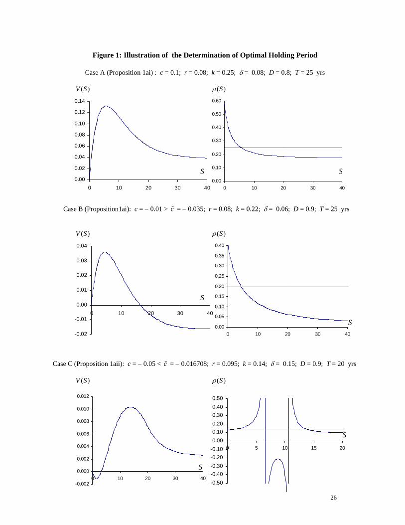
5 An example of the case negative equity is illustrated in Figure 1 (Case C).

11

yield *( )Sρ = k. This equivalence implies that optimal holding period is determined simply by

equating the leveraged rate of return on equity at time t to the required rate of return.

There are several cases to consider. We begin with the situation when t ≥ T. In this

case, the mortgage loan is fully repaid and ( )tρ is constant at c δ+ . Obviously, if c δ+ > k,

it is optimal to continue to hold on to the property (as in Proposition 1c) irrespective of the

capital structure. For the case where c δ+ < k, there are a number of scenarios. If c δ+ < k <

r, then ( )tρ may be strictly increasing in t or initially decreasing in t, depending on the

magnitude of c. Whichever the case, ( )tρ is always less than k. Therefore, it is not optimal to

invest in the real estate property at all (as stated in Proposition 1bi).

Next, if r ≤ c δ+ < k, it is clearly not advisable to hold on to the real estate property

beyond t = T as the rate of return on equity would be less than the required rate of return.

However, in this case, if c ≥ c , then by Lemma 1a, ( )tρ is highest at t = 0, and decreases over

time to c δ+ . If (0)ρ > k, it is optimal to invest in the property, and hold on to it as long

as ( )tρ exceeds k. It is also easy to verify that corresponding to the condition that (0)ρ > k is

the equivalent condition that D > ( ) /( )k c k rδ− − − , as in Proposition 1ai. This condition

says that when c ≥ c , the degree of financial leverage must be at least ( ) /( )k c k rδ− − − at t

= 0, in order that it is potentially worthwhile to invest in the property.

Next, suppose [ ]Max ,c rδ+ < k and D ≤ ( ) /( )k c k rδ− − − . If c ≥ c , both (0)ρ <

k and ( )Tρ < k. By Lemma 1a, we have ( )tρ < k for all t ∈ [0, ]T since ( )tρ is strictly

decreasing in t (when c δ+ > r) or strictly increasing in t (when c δ+ < r). Again, it is not

optimal to invest (Proposition 1bii).

To complete the analysis, we consider the remaining case when [ ]Max ,c rδ+ < k and

D ≤ ( ) /( )k c k rδ− − − and c < c . In this case, it is routine to show that both (0)ρ < k and

( )Tρ < k. There are several possibilities to consider. If c δ+ < r < k, ( )tρ will be initially

12

decreasing in t, by Lemma 1b. Hence, ( )tρ < k, for all t ∈ [0, ]T . It is therefore not optimal to

invest in the property. (Proposition 1biii).

On the other hand, if r < c δ+ < k, ( )tρ will be initially increasing in t (by Lemma 1b).

In this case, it is possible for ( )tρ to exceed k for some t . Suppose there exists a *1t and *

2t

where 0 < *1t < *

2t < T, such that ( )tρ = k at t = *1t and *

2t , ( )tρ > k for t ∈ ( )* *1 2, t t , and

( )tρ < k, otherwise. In this case, it is optimal to invest in the property and liquidate at t = *2t ,

where *2( )tρ′ < 0. This situation corresponds to the situation in Proposition 1aii, so that *

2t is

equivalent to maxZ , so that *S = *2t . However, if *

1t and *2t do not exist, then it is not optimal to

invest in the property so that *S = 0 (Proposition 1biii). In Figure I below, we illustrate the

various possibilities.

---------------------------------------------------

INSERT FIGURE 1 HERE

---------------------------------------------------

4. Comparative Statics and Numerical Analysis

In this section, we analyze the comparative statics of *S and *( )V S , and present a set

of numerical results on the variations of *S and *( )V S . We begin first with the comparative

statics results, which are summarized in Table 1. The detailed derivation is presented in

Appendix B.

13

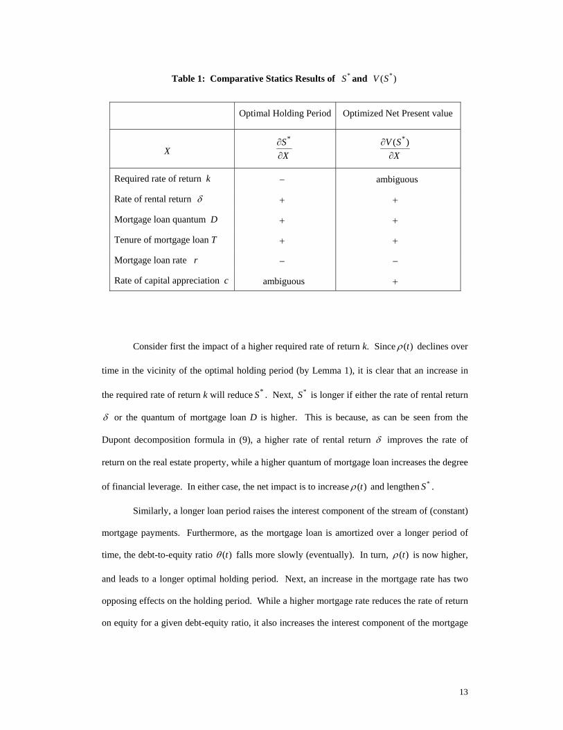
Table 1: Comparative Statics Results of *S and *( )V S

Optimal Holding Period Optimized Net Present value

X *S

X∂∂

*( )V S

X∂

∂

Required rate of return k − ambiguous

Rate of rental return δ + +

Mortgage loan quantum D + +

Tenure of mortgage loan T + +

Mortgage loan rate r − −

Rate of capital appreciation c ambiguous +

Consider first the impact of a higher required rate of return k. Since ( )tρ declines over

time in the vicinity of the optimal holding period (by Lemma 1), it is clear that an increase in

the required rate of return k will reduce *S . Next, *S is longer if either the rate of rental return

δ or the quantum of mortgage loan D is higher. This is because, as can be seen from the

Dupont decomposition formula in (9), a higher rate of rental return δ improves the rate of

return on the real estate property, while a higher quantum of mortgage loan increases the degree

of financial leverage. In either case, the net impact is to increase ( )tρ and lengthen *S .

Similarly, a longer loan period raises the interest component of the stream of (constant)

mortgage payments. Furthermore, as the mortgage loan is amortized over a longer period of

time, the debt-to-equity ratio ( )tθ falls more slowly (eventually). In turn, ( )tρ is now higher,

and leads to a longer optimal holding period. Next, an increase in the mortgage rate has two

opposing effects on the holding period. While a higher mortgage rate reduces the rate of return

on equity for a given debt-equity ratio, it also increases the interest component of the mortgage

14

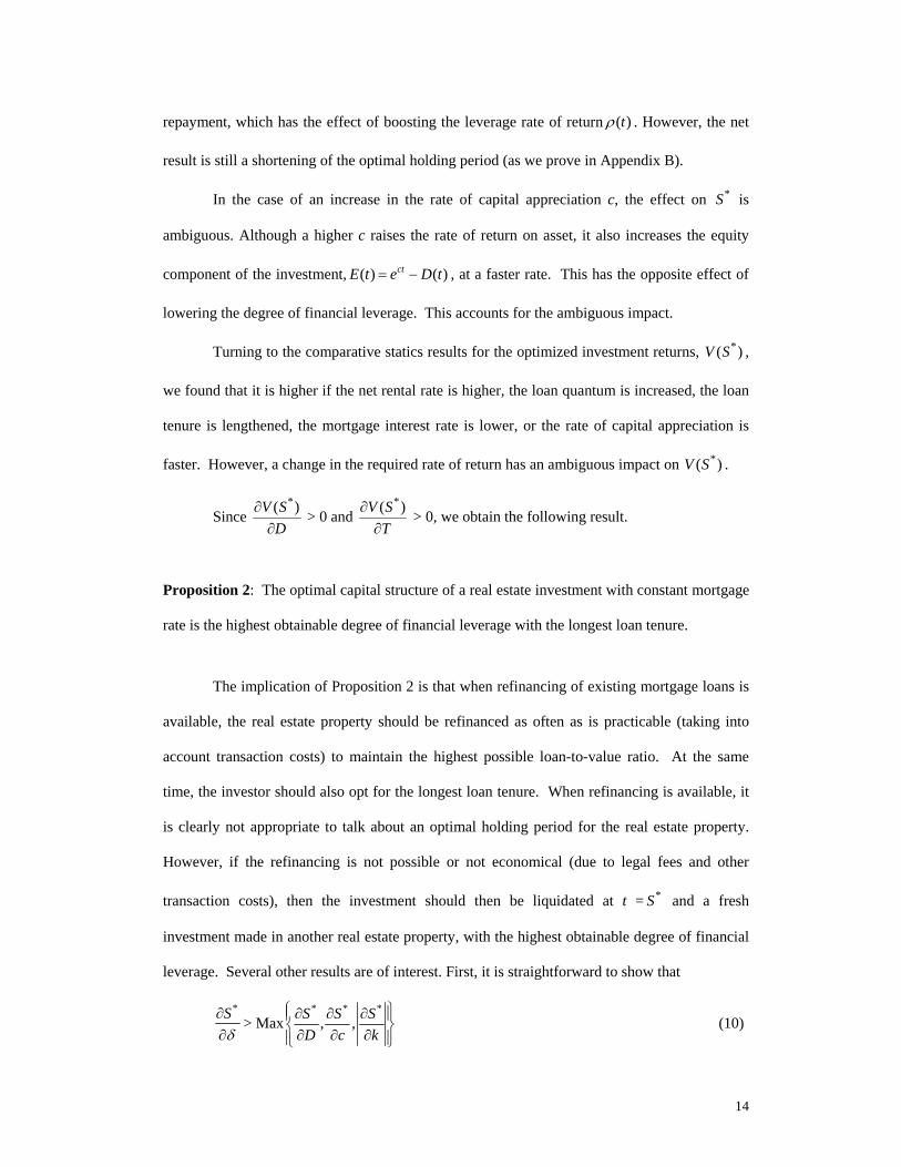
repayment, which has the effect of boosting the leverage rate of return ( )tρ . However, the net

result is still a shortening of the optimal holding period (as we prove in Appendix B).

In the case of an increase in the rate of capital appreciation c, the effect on *S is

ambiguous. Although a higher c raises the rate of return on asset, it also increases the equity

component of the investment, ( ) ( )ctE t e D t= − , at a faster rate. This has the opposite effect of

lowering the degree of financial leverage. This accounts for the ambiguous impact.

Turning to the comparative statics results for the optimized investment returns, *( )V S ,

we found that it is higher if the net rental rate is higher, the loan quantum is increased, the loan

tenure is lengthened, the mortgage interest rate is lower, or the rate of capital appreciation is

faster. However, a change in the required rate of return has an ambiguous impact on *( )V S .

Since *( )V S

D∂

∂ > 0 and

*( )V ST

∂∂

> 0, we obtain the following result.

Proposition 2: The optimal capital structure of a real estate investment with constant mortgage

rate is the highest obtainable degree of financial leverage with the longest loan tenure.

The implication of Proposition 2 is that when refinancing of existing mortgage loans is

available, the real estate property should be refinanced as often as is practicable (taking into

account transaction costs) to maintain the highest possible loan-to-value ratio. At the same

time, the investor should also opt for the longest loan tenure. When refinancing is available, it

is clearly not appropriate to talk about an optimal holding period for the real estate property.

However, if the refinancing is not possible or not economical (due to legal fees and other

transaction costs), then the investment should then be liquidated at t = *S and a fresh

investment made in another real estate property, with the highest obtainable degree of financial

leverage. Several other results are of interest. First, it is straightforward to show that

*Sδ

∂∂

> Max* * *

, ,S S SD c k

⎧ ⎫∂ ∂ ∂⎪ ⎪⎨ ⎬

∂ ∂ ∂⎪ ⎪⎩ ⎭ (10)

15

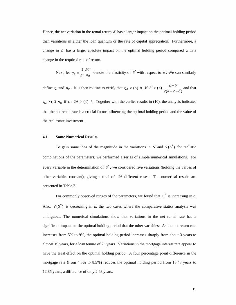
Hence, the net variation in the rental return δ has a larger impact on the optimal holding period

than variations in either the loan quantum or the rate of capital appreciation. Furthermore, a

change in δ has a larger absolute impact on the optimal holding period compared with a

change in the required rate of return.

Next, let *

*S

Sδδη

δ∂

≡∂

denote the elasticity of *S with respect to δ . We can similarly

define cη and Dη . It is then routine to verify that δη > (<)

cη

if *S > (<)

( )c

c k c−

− −δ

δand that

δη > (<)

Dη if 2c δ+ > (<) k. Together with the earlier results in (10), the analysis indicates

that the net rental rate is a crucial factor influencing the optimal holding period and the value of

the real estate investment.

4.1 Some Numerical Results

To gain some idea of the magnitude in the variations in *S and *( )V S for realistic

combinations of the parameters, we performed a series of simple numerical simulations. For

every variable in the determination of *S , we considered five variations (holding the values of

other variables constant), giving a total of 26 different cases. The numerical results are

presented in Table 2.

For commonly observed ranges of the parameters, we found that *S is increasing in c.

Also, *( )V S is decreasing in k, the two cases where the comparative statics analysis was

ambiguous. The numerical simulations show that variations in the net rental rate has a

significant impact on the optimal holding period that the other variables. As the net return rate

increases from 5% to 9%, the optimal holding period increases sharply from about 3 years to

almost 19 years, for a loan tenure of 25 years. Variations in the mortgage interest rate appear to

have the least effect on the optimal holding period. A four percentage point difference in the

mortgage rate (from 4.5% to 8.5%) reduces the optimal holding period from 15.48 years to

12.85 years, a difference of only 2.63 years.

16

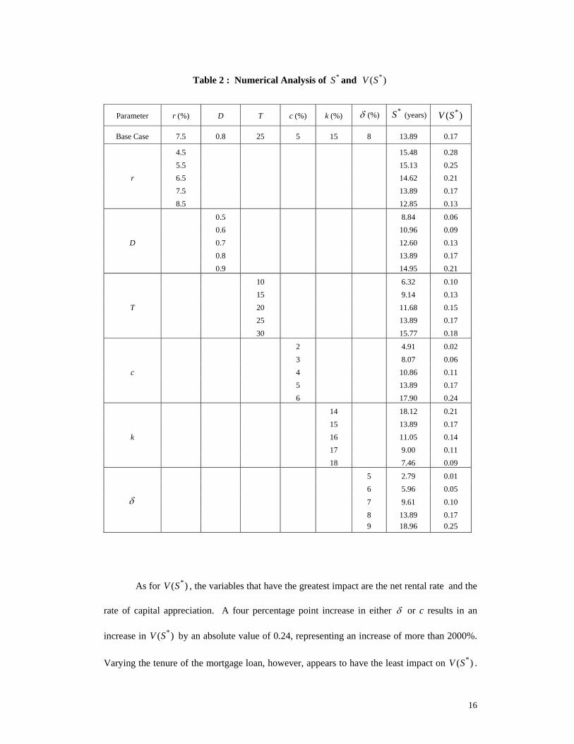
Table 2 : Numerical Analysis of *S and *( )V S

Parameter r (%) D T c (%) k (%) δ (%) *S (years) *( )V S

Base Case 7.5 0.8 25 5 15 8 13.89 0.17

4.5 15.48 0.28 5.5 15.13 0.25 r 6.5 14.62 0.21 7.5 13.89 0.17 8.5 12.85 0.13

0.5 8.84 0.06 0.6 10.96 0.09

D 0.7 12.60 0.13 0.8 13.89 0.17 0.9 14.95 0.21

10 6.32 0.10 15 9.14 0.13

T 20 11.68 0.15 25 13.89 0.17 30 15.77 0.18

2 4.91 0.02 3 8.07 0.06 c 4 10.86 0.11 5 13.89 0.17 6 17.90 0.24

14 18.12 0.21 15 13.89 0.17 k 16 11.05 0.14 17 9.00 0.11 18 7.46 0.09

5 2.79 0.01 6 5.96 0.05

δ 7 9.61 0.10 8 13.89 0.17 9 18.96 0.25

As for *( )V S , the variables that have the greatest impact are the net rental rate and the

rate of capital appreciation. A four percentage point increase in either δ or c results in an

increase in *( )V S by an absolute value of 0.24, representing an increase of more than 2000%.

Varying the tenure of the mortgage loan, however, appears to have the least impact on *( )V S .

17

For instance, as the loan tenure T increases from 10 years to 30 years, representing a 200%

increase, *( )V S only registered a 80% increase, from a value of 0.10 to 0.18.

5. Extensions of the Model

In this section, we discuss a number of related issues and consider the extension of our

analysis when some of the assumptions in the preceding analysis are relaxed. First, we had

assumed a continuous amortization of the mortgage loan throughout the loan tenure. If,

instead, the principal is only repaid at the end of the loan period, then the mortgage loan is

essentially a bond with a stream of constant interest payments. In this case, the loan-to-value

ratio at any point in time is simply ( ) ctDt

e D=

−θ . Applying the optimality condition of *( )Sρ

= k, the optimal holding period *S can be shown to be 1 ( )ln D k rc k c

−⎡ ⎤⎢ ⎥− −⎣ ⎦δ

, for the case where the

rate of capital appreciation c is constant.

It is also straightforward to extend basic model consider situations where the mortgage

interest r varies over the loan tenure or where the stream of loan payments may incorporate

features such as a balloon payment scheme, or other more complicated structures. If the

schedule of the applicable mortgage interest rates and the repayments are fixed upfront, we can

similarly solve for the optimal holding period and calculate the value of the optimized real

estate investment. Also, while our results are obtained in the setting of a real estate market, the

analysis is applicable to other types of investment where there is substantial degree of financial

leverage and the principal is amortized over the loan tenure.

We turn now to discuss the relaxation of the assumption of a constant required rate of

return k. Suppose the required rate of return varies over the loan period, given by the function

( )k t . In this case, we can show that the first-order condition that characterizes *S can be

written as:

18

( ) ( )( ) ( )

* *

* *

( )

( )

( ) 1 1

1 1

cS rT r T S

cS rT r T S

c e e rD e

e e D e

δ − − −

− − −

+ − − −

− − − = * * *( ) ( )k S S k S′+

(11)

which reduces to *( )Sρ = * * *( ) ( )k S S k S′+ . Hence, allowing the required rate of return to vary

over time introduces an additional term * *( )S k S′ in the determination of the optimal holding

period, compared with the case when the required rate of return is constant. If ( )k t′ < ( > ) 0

for all t, then it is straightforward to show that the optimal holding will be longer (shorter).

The comparative statics result we obtain in Section 4 carry over to the general case.

6. Stochastic Rate of Capital Appreciation

In this section, we further extend the model in another direction; namely, to consider

the case where the rate of capital appreciation is stochastic. In this case, instead of an optimal

holding period, the investor chooses an optimal stopping rule to decide if he should hold on to

the property or liquidate the investment as the mortgage is amortized. This analysis is related

to the real options literature focusing on the optimal timing of investments under certainty

(McDonald and Siegel, 1985; Dixit and Pindyck, 1994).

Let the price of a real estate property at time t be ( )P t where ( )P t follows a

continuous-time stochastic process, specifically a geometric Brownian motion:

P PdP dt dzP

µ σ= + (12)

where µ is the expected rate of capital appreciation; Pσ is the per-unit time variance of the rate

of capital appreciation, and Pdz is the random increment to the Wiener process Pz . As is well

known, this stochastic process implies that ( )P t is log-normally distributed and that

[ ]( ) ( ) StE P t S P t S eµ+ = + (13)

where (0)P = 1. For simplicity, suppose rental returns grow at a constant rate of µ . Since the

investor is risk neutral, the decision at time t, whether to hold on to the real estate property or

19

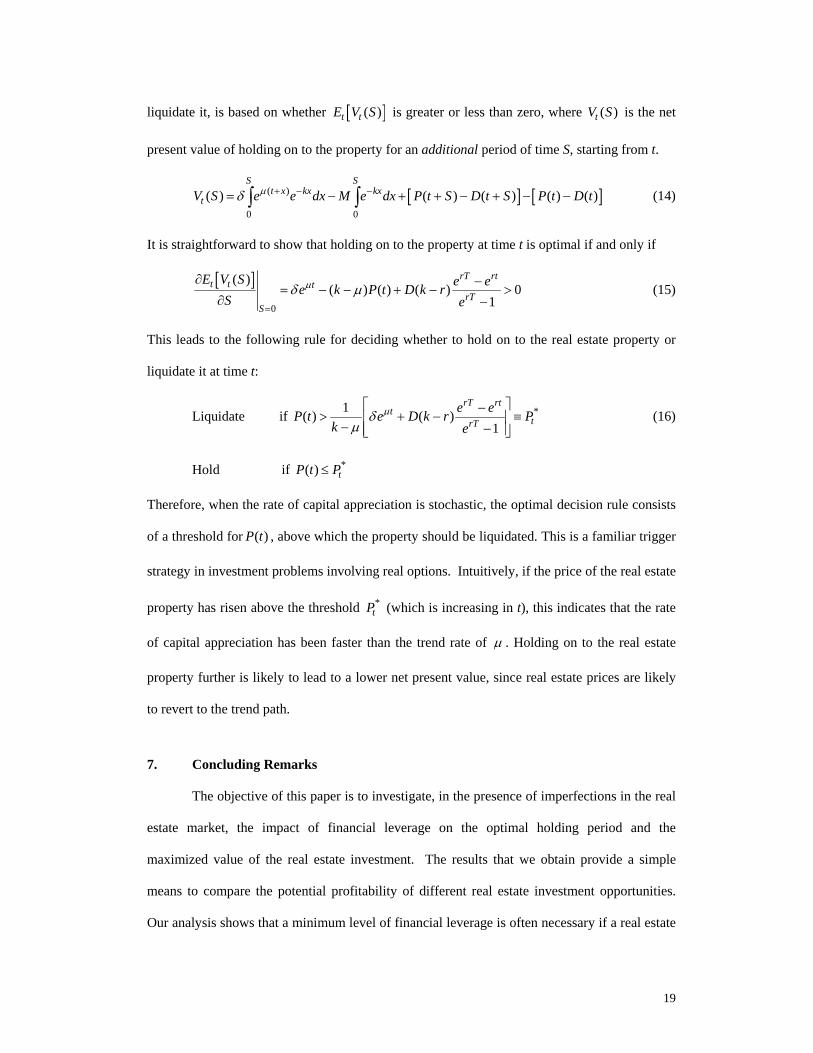
liquidate it, is based on whether [ ]( )t tE V S is greater or less than zero, where ( )tV S is the net

present value of holding on to the property for an additional period of time S, starting from t.

[ ] [ ]( )

0 0

( ) ( ) ( ) ( ) ( )S S

t x kx kxtV S e e dx M e dx P t S D t S P t D tµδ + − −= − + + − + − −∫ ∫ (14)

It is straightforward to show that holding on to the property at time t is optimal if and only if

[ ]

0

( )( ) ( ) ( ) 0

1

rT rtt t t

rTS

E V S e ee k P t D k rS e

µδ µ=

∂ −= − − + − >

∂ − (15)

This leads to the following rule for deciding whether to hold on to the real estate property or

liquidate it at time t:

Liquidate if *1( ) ( )1

rT rtt

trTe eP t e D k r P

k eµδ

µ⎡ ⎤−

> + − ≡⎢ ⎥− −⎢ ⎥⎣ ⎦

(16)

Hold if *( ) tP t P≤

Therefore, when the rate of capital appreciation is stochastic, the optimal decision rule consists

of a threshold for ( )P t , above which the property should be liquidated. This is a familiar trigger

strategy in investment problems involving real options. Intuitively, if the price of the real estate

property has risen above the threshold *tP (which is increasing in t), this indicates that the rate

of capital appreciation has been faster than the trend rate of µ . Holding on to the real estate

property further is likely to lead to a lower net present value, since real estate prices are likely

to revert to the trend path.

7. Concluding Remarks

The objective of this paper is to investigate, in the presence of imperfections in the real

estate market, the impact of financial leverage on the optimal holding period and the

maximized value of the real estate investment. The results that we obtain provide a simple

means to compare the potential profitability of different real estate investment opportunities.

Our analysis shows that a minimum level of financial leverage is often necessary if a real estate

20

investment is to produce a rate of return greater than the required rate. As the mortgage loan is

amortized, the leveraged rate of return on equity falls, so that the optimal time to exit the real

estate investment is when the leveraged rate of return falls below the required rate of return. If

refinancing of outstanding loan is available, an alternative to selling the property is to refinance

it and obtain higher degree of leverage and extend the loan tenure. Our results provide a simple

way to re-evaluate the desirability to continue to hold onto the real estate investment, to

liquidate it or to refinance it, as the investment environment changes.

Our model can also be extended to consider cases where the mortgage interest rate and

the required rate of return vary over time. As we have shown in Section 6, uncertainty can be

introduced into the model by considering a stochastic process in the evolution of real estate

prices. The analysis can similarly be extended to include stochastic movements in the rental

returns to derive an optimal holding rule. Using a similar approach, Chen and Ling (1989) has

considered the case of stochastic mortgage rates and derived a similar rule for deciding on the

optimal time to refinance the real estate property. A further extension of this approach is to

consider joint stochastic processes in mortgage interest rate, the rental rate and the rate of real

estate price appreciation, to derive optimal holding rules that take account of the option value

of holding on to a real estate property (if the investment is made) or waiting before making an

investment.

21

Appendix A

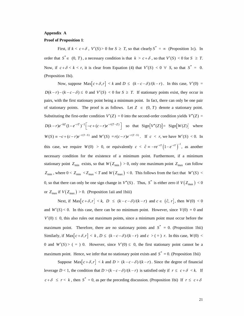
Proof of Proposition 1:

First, if k < c δ+ , ( )V S′ > 0 for S ≥ T, so that clearly *S = ∞ (Proposition 1c). In

order that *S ∈ (0, )T , a necessary condition is that k > c δ+ , so that ( )V S′ < 0 for S ≥ T.

Now, if c δ+ < k < r, it is clear from Equation (4) that ( )V S′ < 0 ∀ S, so that *S = 0.

(Proposition 1bi).

Now, suppose [ ]Max ,c rδ+ < k and D ≤ ( ) /( )k c k rδ− − − . In this case, (0)V ′ =

( ) ( )D k r k c δ− − − − ≤ 0 and ( )V S′ < 0 for S ≥ T. If stationary points exist, they occur in

pairs, with the first stationary point being a minimum point. In fact, there can only be one pair

of stationary points. The proof is as follows. Let Z ∈ (0, )T denote a stationary point.

Substituting the first-order condition ( )V Z′ = 0 into the second-order condition yields ( )V Z′′ =

1 ( )( ) (1 ) ( )− − − − −⎡ ⎤− − − + −⎣ ⎦kZ rT r T ZD k r e e c c r e so that Sign [ ]( )V Z′′ = Sign [ ]( )W Z where

( )W S ≡ ( )( ) r T Sc c r e− −− + − and ( )W S′ = ( )( ) r T Sr c r e− −− . If c < r, we have ( )W S′ < 0. In

this case, we require (0)W > 0, or equivalently c < c ≡ ( ) 11rT rTre e

−− −− − , as another

necessary condition for the existence of a minimum point. Furthermore, if a minimum

stationary point minZ exists, so that ( )minW Z > 0, only one maximum point maxZ can follow

minZ , where 0 < minZ < maxZ < T and ( )maxW Z < 0. This follows from the fact that ( )W S′ <

0, so that there can only be one sign change in ( )V S′′ . Thus, *S is either zero if ( )maxV Z < 0

or maxZ if ( )maxV Z > 0. (Proposition 1aii and 1biii)

Next, if [ ]Max ,c rδ+ < k, D ≤ ( ) /( )k c k rδ− − − and c ∈ ( ]ˆ, c r , then (0)W < 0

and ( )W S′ < 0. In this case, there can be no minimum point. However, since (0)V = 0 and

(0)V ′ ≤ 0, this also rules out maximum points, since a minimum point must occur before the

maximum point. Therefore, there are no stationary points and *S = 0. (Proposition 1bii)

Similarly, if [ ]Max ,c rδ+ < k , D ≤ ( ) /( )k c k rδ− − − and c > ( = ) r. In this case, (0)W <

0 and ( )W S′ > ( = ) 0. However, since (0)V ′ ≤ 0, the first stationary point cannot be a

maximum point. Hence, we infer that no stationary point exists and *S = 0. (Proposition 1bii)

Suppose [ ]Max ,c rδ+ < k and D > ( ) /( )k c k rδ− − − . Since the degree of financial

leverage D < 1, the condition that D > ( ) /( )k c k rδ− − − is satisfied only if r ≤ c δ+ < k. If

c δ+ ≤ r < k , then *S = 0, as per the preceding discussion. (Proposition 1bi) If r ≤ c δ+

22

< k, (0)V ′ > 0 and ( )V S′ < 0 for S ≥ T. In this case, ( )V S has an interior maximum point at

*S ∈ (0, )T . (Proposition 1ai.) No minimum point can exist. Suppose, to the contrary, a

minimum point exists. Then, it must be flanked by two maximum points. This is not possible.

Since Sign [ ]( )V Z′′ = Sign [ ]( )W Z , and ( )W S′ = ( )( ) r T Sr c r e− −− , there can only be one

change in sign for ( )V Z′′ . Q.E.D.

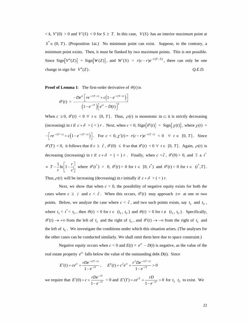
Proof of Lemma 1: The first-order derivative of ( )tθ is

( )tθ ′ = ( )

( )

( ) ( )

2

1

1 ( )

ct r T t r T t

rT ct

De re c e

e e D t

− − − −

−

⎡ ⎤− + −⎣ ⎦⎡ ⎤− −⎣ ⎦

When c ≥ 0, ( )tθ ′ < 0 ∀ t ∈ [0, ]T . Thus, ( )tρ is monotonic in c; it is strictly decreasing

(increasing) in t if c δ+ > ( < ) r . Next, when c < 0, Sign [ ]( )tθ ′ = Sign [ ]( )tχ , where ( )tχ =

( )( ) ( )1r T t r T tre c e− − − −⎡ ⎤− + −⎣ ⎦ . For c < 0, ( )tχ′ = ( )( ) r T tr c r e− −− < 0 ∀ t ∈ [0, ]T . Since

( )Tθ ′ < 0, it follows that if c ≥ c , (0)θ ′ ≤ 0 so that ( )tθ ′ < 0 ∀ t ∈ [0, ]T . Again, ( )tρ is

decreasing (increasing) in t if c δ+ > ( < ) r . Finally, when c < c , (0)θ ′ > 0, and ∃ a *t

1 ln 1 rTr c

⎡ ⎤≡ − −⎢ ⎥⎣ ⎦ where *( )tθ ′ = 0, ( )tθ ′ > 0 for t ∈ *[0, )t and ( )tθ ′ < 0 for t ∈ *( , ]t T .

Thus, ( )tρ will be increasing (decreasing) in t initially if c δ+ > ( < ) r.

Next, we show that when c < 0, the possibility of negative equity exists for both the

cases where c ≥ c and c < c . When this occurs, ( )tθ ′ may approach ±∞ at one or two

points. Below, we analyze the case where c < c , and two such points exists, say Lt and Ut ,

where Lt < *t < Ut , then ( )tθ < 0 for t ∈ ( , )L Ut t and ( )tθ > 0 for t ∉ ( , )L Ut t . Specifically,

( )tθ ′ → +∞ from the left of Lt and the right of Ut , and ( )tθ ′ → −∞ from the right of Lt and

the left of Ut . We investigate the conditions under which this situation arises. (The analyses for

the other cases can be conducted similarly. We shall omit them here due to space constraint.)

Negative equity occurs when c < 0 and E(t) = cte − D(t) is negative, as the value of the

real estate property cte falls below the value of the outstanding debt D(t). Since ( )

( )1

r T tct

rTrDeE t ce

e

− −

−′ = +

−,

2 ( )2( ) 0

1

r T tct

rTr DeE t c e

e

− −

−′′ = + >

−

we require that (0)1

rT

rTrDeE c

e

−

−′ = +

− < 0 and ( ) 0

1cT

rTrDE T cee−

′ = + >−

for Lt Ut to exist. We

23

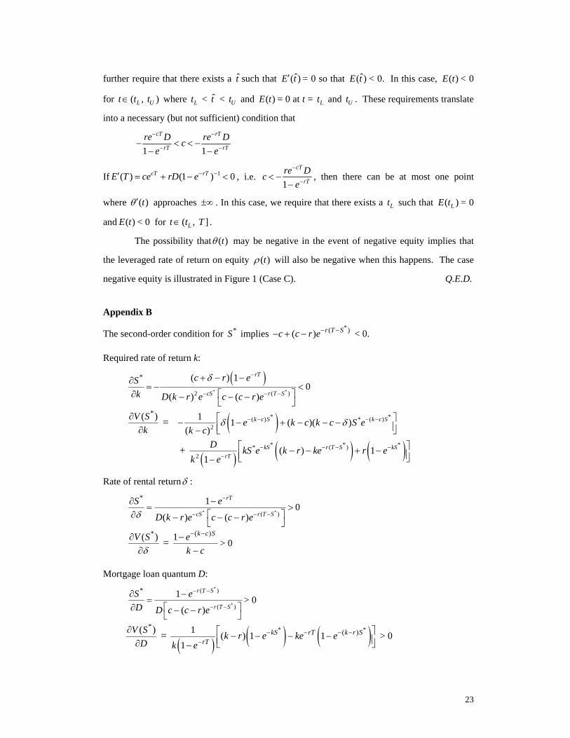
further require that there exists a t such that ˆ( )E t′ = 0 so that ˆ( )E t < 0. In this case, ( )E t < 0

for ( , )L Ut t t∈ where Lt < t < Ut and ( )E t = 0 at t = Lt and Ut . These requirements translate

into a necessary (but not sufficient) condition that

1 1

cT rT

rT rTre D re Dc

e e

− −

− −− < < −− −

If 1( ) (1 ) 0cT rTE T ce rD e− −′ = + − < , i.e. 1

cT

rTre Dc

e

−

−< −−

, then there can be at most one point

where ( )tθ ′ approaches ±∞ . In this case, we require that there exists a Lt such that ( )LE t = 0

and ( )E t < 0 for ( , ]Lt t T∈ .

The possibility that ( )tθ may be negative in the event of negative equity implies that

the leveraged rate of return on equity ( )tρ will also be negative when this happens. The case

negative equity is illustrated in Figure 1 (Case C). Q.E.D.

Appendix B

The second-order condition for *S implies *( )( ) r T Sc c r e− −− + − < 0.

Required rate of return k:

( )* *2 ( )

* ( ) 10

( ) ( )

rT

cS r T S

c r eSk D k r e c c r e

δ −

− − −

+ − −∂= − <

∂ ⎡ ⎤− − −⎣ ⎦

*( )V Sk

∂∂

= ( )* *( ) * ( )2

1 1 ( )( )( )

k c S k c Se k c k c S ek c

δ δ− − − −⎡ ⎤− − + − − −⎢ ⎥⎣ ⎦−

+ ( ) ( ) ( )* * ** ( )

2( ) 1

1kS r T S kS

rT

D kS e k r ke r ek e

− − − −−

⎡ ⎤− − + −⎢ ⎥⎣ ⎦−

Rate of rental returnδ :

* *( )

* 1 0( ) ( )

rT

cS r T S

S e

D k r e c c r eδ

−

− − −

∂ −= >

∂ ⎡ ⎤− − −⎣ ⎦

*( )V Sδ

∂∂

= ( )1 k c Se

k c

− −−−

> 0

Mortgage loan quantum D:

*

*

( )

( )

* 1

( )

r T S

r T S

S eD D c c r e

− −

− −

∂ −=

∂ ⎡ ⎤− −⎣ ⎦

> 0

*( )V S

D∂

∂ =

( ) ( ) ( )* *( )1 ( ) 1 11

− − − −−

⎡ ⎤− − − −⎢ ⎥⎣ ⎦−kS rT k r S

rTk r e ke e

k e > 0

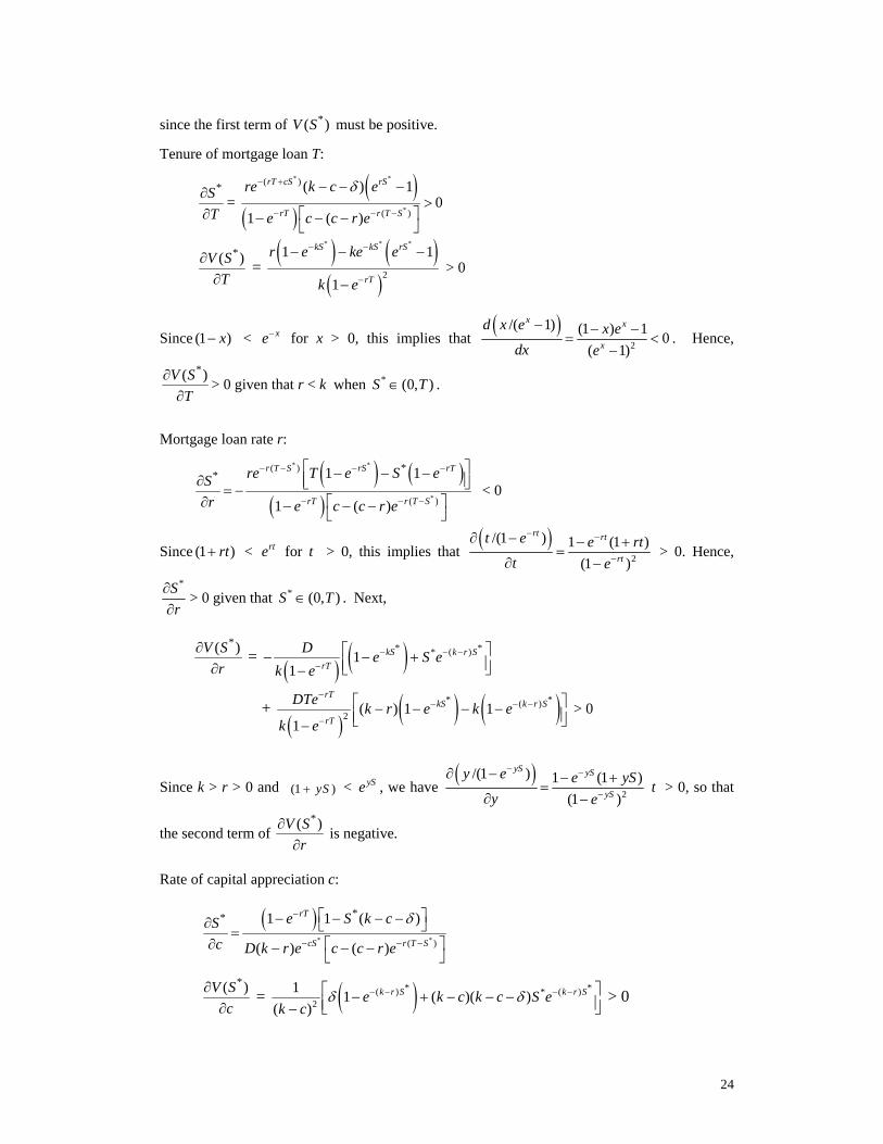
24

since the first term of *( )V S must be positive.

Tenure of mortgage loan T:

*∂∂ST

= ( )

( )

* *

*

( )

( )

( ) 10

1 ( )

δ− +

− − −

− − −>

⎡ ⎤− − −⎣ ⎦

rT cS rS

rT r T S

re k c e

e c c r e

*( )V ST

∂∂

= ( ) ( )

( )

* * *

2

1 1

1

− −

−

− − −

−

kS kS rS

rT

r e ke e

k e > 0

Since (1 )x− < xe− for x > 0, this implies that ( )

2

/( 1) (1 ) 1 0( 1)

x x

x

d x e x edx e

− − −= <

−. Hence,

*( )V ST

∂∂

> 0 given that r < k when *S (0, )T∈ .

Mortgage loan rate r:

( ) ( )( )

* *

*

( )

( )

** 1 1

1 ( )

r T S rS rT

rT r T S

re T e S eSr e c c r e

− − − −

− − −

⎡ ⎤− − −∂ ⎢ ⎥⎣ ⎦= −∂ ⎡ ⎤− − −⎣ ⎦

< 0

Since (1 )rt+ < rte for t > 0, this implies that ( )

2

/(1 ) 1 (1 )(1 )

rt rt

rt

t e e rtt e

− −

−

∂ − − +=

∂ − > 0. Hence,

*Sr

∂∂

> 0 given that *S (0, )T∈ . Next,

*( )V Sr

∂∂

= ( ) ( )* ** ( )11

kS k r SrT

D e S ek e

− − −−

⎡ ⎤− − +⎢ ⎥⎣ ⎦−

+ ( ) ( ) ( )* *( )

2 ( ) 1 11

−− − −

−

⎡ ⎤− − − −⎢ ⎥⎣ ⎦−

rTkS k r S

rT

DTe k r e k ek e

> 0

Since k > r > 0 and

(1 )yS+ < ySe , we have ( )

2

/(1 ) 1 (1 )(1 )

yS yS

yS

y e e ySy e

− −

−

∂ − − +=

∂ − t > 0, so that

the second term of *( )V S

r∂

∂ is negative.

Rate of capital appreciation c:

( )

* *( )

** 1 1 ( )

( ) ( )

δ−

− − −

⎡ ⎤− − − −∂ ⎣ ⎦=∂ ⎡ ⎤− − −⎣ ⎦

rT

cS r T S

e S k cSc D k r e c c r e

*( )V S

c∂

∂ = ( )* *( ) * ( )

21 1 ( )( )

( )k r S k r Se k c k c S e

k cδ δ− − − −⎡ ⎤− + − − −⎢ ⎥⎣ ⎦−

> 0

25

References

Alberts, W., Castanias, R.P., 1982. The Impact of Changes in Tax Depreciation Rates on Holding Periods for Real Estate Investments. National Tax Journal 35, 43-54.

Bodie, Z., Kane, A., Marcus, A.J., 2002. Investments. McGraw Hill, New York, USA. Brueggeman, W.B., Fisher, J.D. Stern, J.J., 1981. Federal Income Taxes, Inflation and Holding

Periods for Income-Producing Property. AREUEA Journal 9, 148-164. Chen, A., Ling, D.C., 1989. Optimal Mortgage Refinancing with Stochastic Interest Rates.

Journal of the American Real Estate and Urban Economics Association 17, 278-299. DiPasquale, D., Wheaton, W., 1996. Urban Economics and Real Estate Markets. Prentice Hall,

New Jersey, USA. Dixit, A., Pindyck, R.S.,1994. Investment Under Uncertainty. Princeton University Press, New

Jersey, USA. Follain, J.R., Ling, D.C., 1988. Another Look at Tenure Choice, Inflation, and Taxes.

AREUEA Journal 16, 207-229. Gau, G.K., Wang, K., 1990. Capital Structure Decisions in Real Estate Investment. AREUEA

Journal 18, 501-521. Gau, G.K., Wang, K., 1994. Tax-Induced Holding Periods of Real Estate Investors: Theory

and Empirical Evidence. Journal of Real Estate Finance and Economics 8, 71-85. Genesove, D., Mayer, C.J., 1997. Equity and Time to Sale in the Real Estate Market. American

Economic Review 87, 255-269. Goodman, A.C., 2003. Following a Panel of Stayers: Length of Stay, Tenure Choice, and

Housing Demand. Journal of Housing Economics 12, 106-133. Glower, M., Haurin, D.R., Hendershott, P.H., 1998. Selling Time and Selling Price: The

Influence of Seller Motivation. Real Estate Economics 26, 719-740. Goetzmann, Q.N., Ibbotson, R.G., 1990. The Performance of Real Estate as an Investment

Class. Journal of Applied Corporate Finance 3, 65-76. Grenadier, S., 1995. Valuing Lease Contracts: A Real Options Approach. Journal of Financial

Economics 38, 297-331. Hendershott, P.H., Haurin, D.R., 1990. Research on Real Estate Investment. AREUEA

Journal 18, 369 - 375. Hendershott, P.H., Ling, D.C., 1984. Trading and the Tax Shelter Value of Depreciable Real

Estate. National Tax Journal 37, 213-23. Newsome, B., Hill, K., 1987. The Influence of Debt Financing on Real Estate Value and

Required Return: Theory and Practice. Real Estate Appraiser and Analyst, 38-53. Ibbotson, R.G., Siegel, L.B., 1984. Real Estate Returns: A Comparison with Other

Investments. AREUEA Journal 12, 219-242. Ling, D.C., Whinihan, M.J., 1985. Valuing Depreciable Real Estate: A New Methodology.

AREUEA Journal 13, 181-194. Linneman, P., Wachter, S., 1989. The Impacts of Borrowing Constraints on Homeownership.

AREUEA Journal 17, 389-402. McDonald, R.L., Siegel, D., 1985. Investment and The Valuation of Firms Where There is an

Option to Shut Down. International Economic Review 26, 331-349. Modigliani, F., Miller, M., 1958. The Cost of Capital, Corporation Finance and The Theory of

Investment. American Economic Review, 267-297. Shilling, J.D., 2002. Real Estate – Thirteen Edition. South-Western, Thomson Learning. USA.

26

Figure 1: Illustration of the Determination of Optimal Holding Period

Case A (Proposition 1ai) : c = 0.1; r = 0.08; k = 0.25; δ = 0.08; D = 0.8; T = 25 yrs ( )V S ( )Sρ

S S

Case B (Proposition1ai): c = − 0.01 > c = − 0.035; r = 0.08; k = 0.22; δ = 0.06; D = 0.9; T = 25 yrs ( )V S ( )Sρ

S

S

Case C (Proposition 1aii): c = − 0.05 < c = − 0.016708; r = 0.095; k = 0.14; δ = 0.15; D = 0.9; T = 20 yrs ( )V S ( )Sρ

S

S

-0.02

-0.01

0.00

0.01

0.02

0.03

0.04

0 10 20 30 40

0.00

0.05

0.10

0.15

0.20

0.25

0.30

0.35

0.40

0 10 20 30 40

0.00

0.02

0.04

0.06

0.08

0.10

0.12

0.14

0 10 20 30 400.00

0.10

0.20

0.30

0.40

0.50

0.60

0 10 20 30 40

-0.002

0.000

0.002

0.004

0.006

0.008

0.010

0.012

0 10 20 30 40-0.50-0.40-0.30-0.20-0.100.000.100.200.300.400.50

0 5 10 15 20

27

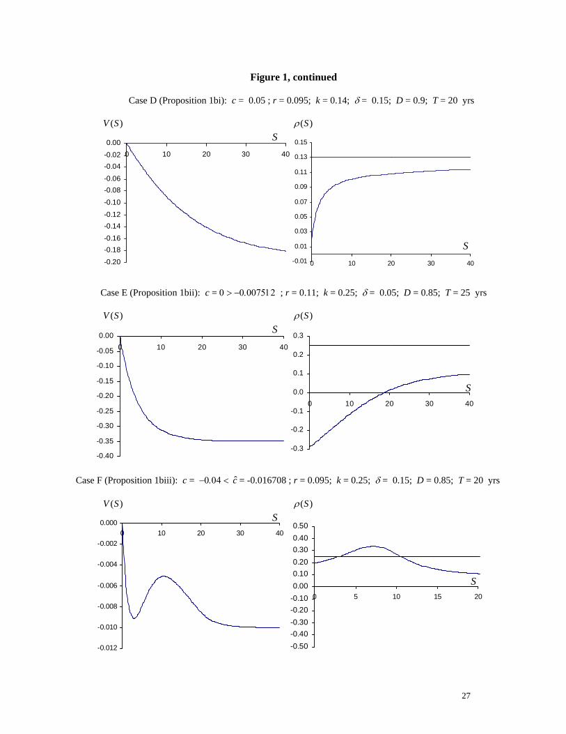
Figure 1, continued

Case D (Proposition 1bi): c = 0.05 ; r = 0.095; k = 0.14; δ = 0.15; D = 0.9; T = 20 yrs

( )V S ( )Sρ S

S

Case E (Proposition 1bii): c = 0 > −0.007512 ; r = 0.11; k = 0.25; δ = 0.05; D = 0.85; T = 25 yrs

( )V S ( )Sρ S

S

Case F (Proposition 1biii): c = −0.04 < c = -0.016708 ; r = 0.095; k = 0.25; δ = 0.15; D = 0.85; T = 20 yrs

( )V S ( )Sρ S

S

-0.40

-0.35

-0.30

-0.25

-0.20

-0.15

-0.10

-0.05

0.000 10 20 30 40

-0.3

-0.2

-0.1

0.0

0.1

0.2

0.3

0 10 20 30 40

-0.20-0.18-0.16

-0.14-0.12

-0.10

-0.08-0.06

-0.04-0.02

0.000 10 20 30 40

-0.01

0.01

0.03

0.05

0.07

0.09

0.11

0.13

0.15

0 10 20 30 40

-0.012

-0.010

-0.008

-0.006

-0.004

-0.002

0.0000 10 20 30 40

-0.50-0.40-0.30-0.20-0.100.000.100.200.300.400.50

0 5 10 15 20